Amazon Redshift Database Developer Guide
User Manual:
Open the PDF directly: View PDF ![]() .
.
Page Count: 1006 [warning: Documents this large are best viewed by clicking the View PDF Link!]
- Amazon Redshift
- Table of Contents
- Welcome
- Amazon Redshift System Overview
- Getting Started Using Databases
- Building a Proof of Concept for Amazon Redshift
- Amazon Redshift Best Practices
- Amazon Redshift Best Practices for Designing Tables
- Amazon Redshift Best Practices for Loading Data
- Take the Loading Data Tutorial
- Take the Tuning Table Design Tutorial
- Use a COPY Command to Load Data
- Use a Single COPY Command to Load from Multiple Files
- Split Your Load Data into Multiple Files
- Compress Your Data Files
- Use a Manifest File
- Verify Data Files Before and After a Load
- Use a Multi-Row Insert
- Use a Bulk Insert
- Load Data in Sort Key Order
- Load Data in Sequential Blocks
- Use Time-Series Tables
- Use a Staging Table to Perform a Merge (Upsert)
- Schedule Around Maintenance Windows
- Amazon Redshift Best Practices for Designing Queries
- Working with Recommendations from Amazon Redshift Advisor
- Viewing Amazon Redshift Advisor Recommendations in the Console
- Amazon Redshift Advisor Recommendations
- Compress Table Data
- Compress Amazon S3 File Objects Loaded by COPY
- Isolate Multiple Active Databases
- Reallocate Workload Management (WLM) Memory
- Skip Compression Analysis During COPY
- Split Amazon S3 Objects Loaded by COPY
- Update Table Statistics
- Enable Short Query Acceleration
- Replace Single-Column Interleaved Sort Keys
- Tutorial: Tuning Table Design
- Prerequisites
- Steps
- Step 1: Create a Test Data Set
- Step 2: Test System Performance to Establish a Baseline
- Step 3: Select Sort Keys
- Step 4: Select Distribution Styles
- Step 5: Review Compression Encodings
- Step 6: Recreate the Test Data Set
- Step 7: Retest System Performance After Tuning
- Step 8: Evaluate the Results
- Step 9: Clean Up Your Resources
- Summary
- Tutorial: Loading Data from Amazon S3
- Tutorial: Configuring Workload Management (WLM) Queues to Improve Query Processing
- Overview
- Section 1: Understanding the Default Queue Processing Behavior
- Section 2: Modifying the WLM Query Queue Configuration
- Section 3: Routing Queries to Queues Based on User Groups and Query Groups
- Section 4: Using wlm_query_slot_count to Temporarily Override Concurrency Level in a Queue
- Section 5: Cleaning Up Your Resources
- Tutorial: Querying Nested Data with Amazon Redshift Spectrum
- Managing Database Security
- Designing Tables
- Using Amazon Redshift Spectrum to Query External Data
- Amazon Redshift Spectrum Overview
- Getting Started with Amazon Redshift Spectrum
- IAM Policies for Amazon Redshift Spectrum
- Creating Data Files for Queries in Amazon Redshift Spectrum
- Creating External Schemas for Amazon Redshift Spectrum
- Creating External Tables for Amazon Redshift Spectrum
- Improving Amazon Redshift Spectrum Query Performance
- Monitoring Metrics in Amazon Redshift Spectrum
- Troubleshooting Queries in Amazon Redshift Spectrum
- Loading Data
- Using a COPY Command to Load Data
- Credentials and Access Permissions
- Preparing Your Input Data
- Loading Data from Amazon S3
- Loading Data from Amazon EMR
- Loading Data From Amazon EMR Process
- Step 1: Configure IAM Permissions
- Step 2: Create an Amazon EMR Cluster
- Step 3: Retrieve the Amazon Redshift Cluster Public Key and Cluster Node IP Addresses
- Step 4: Add the Amazon Redshift Cluster Public Key to Each Amazon EC2 Host's Authorized Keys File
- Step 5: Configure the Hosts to Accept All of the Amazon Redshift Cluster's IP Addresses
- Step 6: Run the COPY Command to Load the Data
- Loading Data from Remote Hosts
- Before You Begin
- Loading Data Process
- Step 1: Retrieve the Cluster Public Key and Cluster Node IP Addresses
- Step 2: Add the Amazon Redshift Cluster Public Key to the Host's Authorized Keys File
- Step 3: Configure the Host to Accept All of the Amazon Redshift Cluster's IP Addresses
- Step 4: Get the Public Key for the Host
- Step 5: Create a Manifest File
- Step 6: Upload the Manifest File to an Amazon S3 Bucket
- Step 7: Run the COPY Command to Load the Data
- Loading Data from an Amazon DynamoDB Table
- Verifying That the Data Was Loaded Correctly
- Validating Input Data
- Loading Tables with Automatic Compression
- Optimizing Storage for Narrow Tables
- Loading Default Column Values
- Troubleshooting Data Loads
- Updating Tables with DML Commands
- Updating and Inserting New Data
- Performing a Deep Copy
- Analyzing Tables
- Vacuuming Tables
- Managing Concurrent Write Operations
- Using a COPY Command to Load Data
- Unloading Data
- Creating User-Defined Functions
- Tuning Query Performance
- Query Processing
- Analyzing and Improving Queries
- Troubleshooting Queries
- Implementing Workload Management
- SQL Reference
- Amazon Redshift SQL
- Using SQL
- SQL Reference Conventions
- Basic Elements
- Names and Identifiers
- Literals
- Nulls
- Data Types
- Multibyte Characters
- Numeric Types
- Character Types
- Datetime Types
- Boolean Type
- Type Compatibility and Conversion
- Collation Sequences
- Expressions
- Conditions
- SQL Commands
- ABORT
- ALTER DATABASE
- ALTER DEFAULT PRIVILEGES
- ALTER GROUP
- ALTER SCHEMA
- ALTER TABLE
- ALTER TABLE APPEND
- ALTER USER
- ANALYZE
- ANALYZE COMPRESSION
- BEGIN
- CANCEL
- CLOSE
- COMMENT
- COMMIT
- COPY
- COPY Syntax
- COPY Syntax Overview
- COPY Parameter Reference
- Usage Notes
- COPY Examples
- Load FAVORITEMOVIES from an DynamoDB Table
- Load LISTING from an Amazon S3 Bucket
- Load LISTING from an Amazon EMR Cluster
- Using a Manifest to Specify Data Files
- Load LISTING from a Pipe-Delimited File (Default Delimiter)
- Load LISTING Using Columnar Data in Parquet Format
- Load LISTING Using Temporary Credentials
- Load EVENT with Options
- Load VENUE from a Fixed-Width Data File
- Load CATEGORY from a CSV File
- Load VENUE with Explicit Values for an IDENTITY Column
- Load TIME from a Pipe-Delimited GZIP File
- Load a Timestamp or Datestamp
- Load Data from a File with Default Values
- COPY Data with the ESCAPE Option
- Copy from JSON Examples
- Copy from Avro Examples
- Preparing Files for COPY with the ESCAPE Option
- CREATE DATABASE
- CREATE EXTERNAL SCHEMA
- CREATE EXTERNAL TABLE
- CREATE FUNCTION
- CREATE GROUP
- CREATE LIBRARY
- CREATE SCHEMA
- CREATE TABLE
- Syntax
- Parameters
- Usage Notes
- Examples
- Create a Table with a Distribution Key, a Compound Sort Key, and Compression
- Create a Table Using an Interleaved Sort Key
- Create a Table Using IF NOT EXISTS
- Create a Table with ALL Distribution
- Create a Table with Default EVEN Distribution
- Create a Temporary Table That Is LIKE Another Table
- Create a Table with an IDENTITY Column
- Create a Table with DEFAULT Column Values
- DISTSTYLE, DISTKEY, and SORTKEY Options
- CREATE TABLE AS
- CREATE USER
- CREATE VIEW
- DEALLOCATE
- DECLARE
- DELETE
- DROP DATABASE
- DROP FUNCTION
- DROP GROUP
- DROP LIBRARY
- DROP SCHEMA
- DROP TABLE
- DROP USER
- DROP VIEW
- END
- EXECUTE
- EXPLAIN
- FETCH
- GRANT
- INSERT
- LOCK
- PREPARE
- RESET
- REVOKE
- ROLLBACK
- SELECT
- SELECT INTO
- SET
- SET SESSION AUTHORIZATION
- SET SESSION CHARACTERISTICS
- SHOW
- START TRANSACTION
- TRUNCATE
- UNLOAD
- Syntax
- Parameters
- Usage Notes
- UNLOAD Examples
- Unload VENUE to a Pipe-Delimited File (Default Delimiter)
- Unload VENUE with a Manifest File
- Unload VENUE with MANIFEST VERBOSE
- Unload VENUE with a Header
- Unload VENUE to Smaller Files
- Unload VENUE Serially
- Load VENUE from Unload Files
- Unload VENUE to Encrypted Files
- Load VENUE from Encrypted Files
- Unload VENUE Data to a Tab-Delimited File
- Unload VENUE Using Temporary Credentials
- Unload VENUE to a Fixed-Width Data File
- Unload VENUE to a Set of Tab-Delimited GZIP-Compressed Files
- Unload Data That Contains a Delimiter
- Unload the Results of a Join Query
- Unload Using NULL AS
- ALLOWOVERWRITE Example
- UPDATE
- VACUUM
- SQL Functions Reference
- Leader Node–Only Functions
- Compute Node–Only Functions
- Aggregate Functions
- Bit-Wise Aggregate Functions
- Window Functions
- Window Function Syntax Summary
- AVG Window Function
- COUNT Window Function
- CUME_DIST Window Function
- DENSE_RANK Window Function
- FIRST_VALUE and LAST_VALUE Window Functions
- LAG Window Function
- LEAD Window Function
- LISTAGG Window Function
- MAX Window Function
- MEDIAN Window Function
- MIN Window Function
- NTH_VALUE Window Function
- NTILE Window Function
- PERCENT_RANK Window Function
- PERCENTILE_CONT Window Function
- PERCENTILE_DISC Window Function
- RANK Window Function
- RATIO_TO_REPORT Window Function
- ROW_NUMBER Window Function
- STDDEV_SAMP and STDDEV_POP Window Functions
- SUM Window Function
- VAR_SAMP and VAR_POP Window Functions
- Window Function Examples
- AVG Window Function Examples
- COUNT Window Function Examples
- CUME_DIST Window Function Examples
- DENSE_RANK Window Function Examples
- FIRST_VALUE and LAST_VALUE Window Function Examples
- LAG Window Function Examples
- LEAD Window Function Examples
- LISTAGG Window Function Examples
- MAX Window Function Examples
- MEDIAN Window Function Examples
- MIN Window Function Examples
- NTH_VALUE Window Function Examples
- NTILE Window Function Examples
- PERCENT_RANK Window Function Examples
- PERCENTILE_CONT Window Function Examples
- PERCENTILE_DISC Window Function Examples
- RANK Window Function Examples
- RATIO_TO_REPORT Window Function Examples
- ROW_NUMBER Window Function Example
- STDDEV_POP and VAR_POP Window Function Examples
- SUM Window Function Examples
- Unique Ordering of Data for Window Functions
- Conditional Expressions
- Date and Time Functions
- Summary of Date and Time Functions
- Summary of Date and Time Functions
- Date and Time Functions in Transactions
- Deprecated Leader Node-Only Functions
- ADD_MONTHS Function
- AT TIME ZONE Function
- CONVERT_TIMEZONE Function
- CURRENT_DATE Function
- DATE_CMP Function
- DATE_CMP_TIMESTAMP Function
- DATE_CMP_TIMESTAMPTZ Function
- DATE_PART_YEAR Function
- DATEADD Function
- DATEDIFF Function
- DATE_PART Function
- DATE_TRUNC Function
- EXTRACT Function
- GETDATE Function
- INTERVAL_CMP Function
- LAST_DAY Function
- MONTHS_BETWEEN Function
- NEXT_DAY Function
- SYSDATE Function
- TIMEOFDAY Function
- TIMESTAMP_CMP Function
- TIMESTAMP_CMP_DATE Function
- TIMESTAMP_CMP_TIMESTAMPTZ Function
- TIMESTAMPTZ_CMP Function
- TIMESTAMPTZ_CMP_DATE Function
- TIMESTAMPTZ_CMP_TIMESTAMP Function
- TIMEZONE Function
- TO_TIMESTAMP Function
- TRUNC Date Function
- Dateparts for Date or Time Stamp Functions
- Math Functions
- Mathematical Operator Symbols
- ABS Function
- ACOS Function
- ASIN Function
- ATAN Function
- ATAN2 Function
- CBRT Function
- CEILING (or CEIL) Function
- CHECKSUM Function
- COS Function
- COT Function
- DEGREES Function
- DEXP Function
- DLOG1 Function
- DLOG10 Function
- EXP Function
- FLOOR Function
- LN Function
- LOG Function
- MOD Function
- PI Function
- POWER Function
- RADIANS Function
- RANDOM Function
- ROUND Function
- SIN Function
- SIGN Function
- SQRT Function
- TAN Function
- TO_HEX Function
- TRUNC Function
- String Functions
- || (Concatenation) Operator
- BPCHARCMP Function
- BTRIM Function
- BTTEXT_PATTERN_CMP Function
- CHAR_LENGTH Function
- CHARACTER_LENGTH Function
- CHARINDEX Function
- CHR Function
- CONCAT (Oracle Compatibility Function)
- CRC32 Function
- FUNC_SHA1 Function
- INITCAP Function
- LEFT and RIGHT Functions
- LEN Function
- LENGTH Function
- LOWER Function
- LPAD and RPAD Functions
- LTRIM Function
- MD5 Function
- OCTET_LENGTH Function
- POSITION Function
- QUOTE_IDENT Function
- QUOTE_LITERAL Function
- REGEXP_COUNT Function
- REGEXP_INSTR Function
- REGEXP_REPLACE Function
- REGEXP_SUBSTR Function
- REPEAT Function
- REPLACE Function
- REPLICATE Function
- REVERSE Function
- RTRIM Function
- SPLIT_PART Function
- STRPOS Function
- STRTOL Function
- SUBSTRING Function
- TEXTLEN Function
- TRANSLATE Function
- TRIM Function
- UPPER Function
- JSON Functions
- Data Type Formatting Functions
- System Administration Functions
- System Information Functions
- CURRENT_DATABASE
- CURRENT_SCHEMA
- CURRENT_SCHEMAS
- CURRENT_USER
- CURRENT_USER_ID
- HAS_DATABASE_PRIVILEGE
- HAS_SCHEMA_PRIVILEGE
- HAS_TABLE_PRIVILEGE
- PG_BACKEND_PID
- PG_GET_COLS
- PG_GET_LATE_BINDING_VIEW_COLS
- PG_LAST_COPY_COUNT
- PG_LAST_COPY_ID
- PG_LAST_UNLOAD_ID
- PG_LAST_QUERY_ID
- PG_LAST_UNLOAD_COUNT
- SESSION_USER
- SLICE_NUM Function
- USER
- VERSION
- Reserved Words
- System Tables Reference
- System Tables and Views
- Types of System Tables and Views
- Visibility of Data in System Tables and Views
- STL Tables for Logging
- STL_AGGR
- STL_ALERT_EVENT_LOG
- STL_ANALYZE
- STL_BCAST
- STL_COMMIT_STATS
- STL_CONNECTION_LOG
- STL_DDLTEXT
- STL_DELETE
- STL_DISK_FULL_DIAG
- STL_DIST
- STL_ERROR
- STL_EXPLAIN
- STL_FILE_SCAN
- STL_HASH
- STL_HASHJOIN
- STL_INSERT
- STL_LIMIT
- STL_LOAD_COMMITS
- STL_LOAD_ERRORS
- STL_LOADERROR_DETAIL
- STL_MERGE
- STL_MERGEJOIN
- STL_NESTLOOP
- STL_PARSE
- STL_PLAN_INFO
- STL_PROJECT
- STL_QUERY
- STL_QUERY_METRICS
- STL_QUERYTEXT
- STL_REPLACEMENTS
- STL_RESTARTED_SESSIONS
- STL_RETURN
- STL_S3CLIENT
- STL_S3CLIENT_ERROR
- STL_SAVE
- STL_SCAN
- STL_SESSIONS
- STL_SORT
- STL_SSHCLIENT_ERROR
- STL_STREAM_SEGS
- STL_TR_CONFLICT
- STL_UNDONE
- STL_UNIQUE
- STL_UNLOAD_LOG
- STL_USERLOG
- STL_UTILITYTEXT
- STL_VACUUM
- STL_WINDOW
- STL_WLM_ERROR
- STL_WLM_RULE_ACTION
- STL_WLM_QUERY
- STV Tables for Snapshot Data
- STV_ACTIVE_CURSORS
- STV_BLOCKLIST
- STV_CURSOR_CONFIGURATION
- STV_EXEC_STATE
- STV_INFLIGHT
- STV_LOAD_STATE
- STV_LOCKS
- STV_PARTITIONS
- STV_QUERY_METRICS
- STV_RECENTS
- STV_SESSIONS
- STV_SLICES
- STV_STARTUP_RECOVERY_STATE
- STV_TBL_PERM
- STV_TBL_TRANS
- STV_WLM_QMR_CONFIG
- STV_WLM_CLASSIFICATION_CONFIG
- STV_WLM_QUERY_QUEUE_STATE
- STV_WLM_QUERY_STATE
- STV_WLM_QUERY_TASK_STATE
- STV_WLM_SERVICE_CLASS_CONFIG
- STV_WLM_SERVICE_CLASS_STATE
- System Views
- SVV_COLUMNS
- SVL_COMPILE
- SVV_DISKUSAGE
- SVV_EXTERNAL_COLUMNS
- SVV_EXTERNAL_DATABASES
- SVV_EXTERNAL_PARTITIONS
- SVV_EXTERNAL_SCHEMAS
- SVV_EXTERNAL_TABLES
- SVV_INTERLEAVED_COLUMNS
- SVL_QERROR
- SVL_QLOG
- SVV_QUERY_INFLIGHT
- SVL_QUERY_QUEUE_INFO
- SVL_QUERY_METRICS
- SVL_QUERY_METRICS_SUMMARY
- SVL_QUERY_REPORT
- SVV_QUERY_STATE
- SVL_QUERY_SUMMARY
- SVL_S3LOG
- SVL_S3PARTITION
- SVL_S3QUERY
- SVL_S3QUERY_SUMMARY
- SVL_S3RETRIES
- SVL_STATEMENTTEXT
- SVV_TABLES
- SVV_TABLE_INFO
- SVV_TRANSACTIONS
- SVL_USER_INFO
- SVL_UDF_LOG
- SVV_VACUUM_PROGRESS
- SVV_VACUUM_SUMMARY
- SVL_VACUUM_PERCENTAGE
- System Catalog Tables
- Configuration Reference
- Sample Database
- Appendix: Time Zone Names and Abbreviations
- Document History

Amazon Redshift
Database Developer Guide
API Version 2012-12-01

Amazon Redshift Database Developer Guide
Amazon Redshift: Database Developer Guide
Copyright © 2018 Amazon Web Services, Inc. and/or its affiliates. All rights reserved.
Amazon's trademarks and trade dress may not be used in connection with any product or service that is not Amazon's, in any manner
that is likely to cause confusion among customers, or in any manner that disparages or discredits Amazon. All other trademarks not
owned by Amazon are the property of their respective owners, who may or may not be affiliated with, connected to, or sponsored by
Amazon.

Amazon Redshift Database Developer Guide
Table of Contents
Welcome ........................................................................................................................................... 1
Are You a First-Time Amazon Redshift User? ................................................................................. 1
Are You a Database Developer? ................................................................................................... 2
Prerequisites .............................................................................................................................. 3
Amazon Redshift System Overview ...................................................................................................... 4
Data Warehouse System Architecture ........................................................................................... 4
Performance .............................................................................................................................. 6
Massively Parallel Processing .............................................................................................. 6
Columnar Data Storage ..................................................................................................... 7
Data Compression ............................................................................................................. 7
Query Optimizer ................................................................................................................ 7
Result Caching .................................................................................................................. 7
Compiled Code .................................................................................................................. 8
Columnar Storage ...................................................................................................................... 8
Internal Architecture and System Operation ................................................................................ 10
Workload Management ............................................................................................................. 11
Using Amazon Redshift with Other Services ................................................................................ 11
Moving Data Between Amazon Redshift and Amazon S3 ....................................................... 11
Using Amazon Redshift with Amazon DynamoDB ................................................................. 11
Importing Data from Remote Hosts over SSH ...................................................................... 11
Automating Data Loads Using AWS Data Pipeline ................................................................. 12
Migrating Data Using AWS Database Migration Service (AWS DMS) ......................................... 12
Getting Started Using Databases ........................................................................................................ 13
Step 1: Create a Database ......................................................................................................... 13
Step 2: Create a Database User .................................................................................................. 14
Delete a Database User ..................................................................................................... 14
Step 3: Create a Database Table ................................................................................................. 14
Insert Data Rows into a Table ............................................................................................ 15
Select Data from a Table ................................................................................................... 15
Step 4: Load Sample Data ......................................................................................................... 15
Step 5: Query the System Tables ............................................................................................... 16
View a List of Table Names ............................................................................................... 16
View Database Users ........................................................................................................ 17
View Recent Queries ......................................................................................................... 17
Determine the Process ID of a Running Query ..................................................................... 18
Step 6: Cancel a Query ............................................................................................................. 18
Cancel a Query from Another Session ................................................................................. 19
Cancel a Query Using the Superuser Queue ......................................................................... 19
Step 7: Clean Up Your Resources ................................................................................................ 20
Proof of Concept Playbook ................................................................................................................ 21
Identifying the Goals of the Proof of Concept .............................................................................. 21
Setting Up Your Proof of Concept .............................................................................................. 21
Designing and Setting Up Your Cluster ............................................................................... 22
Converting Your Schema and Setting Up the Datasets ........................................................... 22
Cluster Design Considerations .................................................................................................... 22
Amazon Redshift Evaluation Checklist ......................................................................................... 23
Benchmarking Your Amazon Redshift Evaluation .......................................................................... 24
Additional Resources ................................................................................................................. 25
Amazon Redshift Best Practices ......................................................................................................... 26
Best Practices for Designing Tables ............................................................................................. 26
Take the Tuning Table Design Tutorial ................................................................................ 27
Choose the Best Sort Key .................................................................................................. 27
Choose the Best Distribution Style ..................................................................................... 27
Use Automatic Compression .............................................................................................. 28
API Version 2012-12-01
iii

Amazon Redshift Database Developer Guide
Define Constraints ............................................................................................................ 28
Use the Smallest Possible Column Size ............................................................................... 28
Using Date/Time Data Types for Date Columns .................................................................... 29
Best Practices for Loading Data ................................................................................................. 29
Take the Loading Data Tutorial .......................................................................................... 29
Take the Tuning Table Design Tutorial ................................................................................ 29
Use a COPY Command to Load Data .................................................................................. 30
Use a Single COPY Command ............................................................................................ 30
Split Your Load Data into Multiple Files .............................................................................. 30
Compress Your Data Files .................................................................................................. 30
Use a Manifest File ........................................................................................................... 30
Verify Data Files Before and After a Load ............................................................................ 31
Use a Multi-Row Insert ..................................................................................................... 31
Use a Bulk Insert .............................................................................................................. 31
Load Data in Sort Key Order .............................................................................................. 31
Load Data in Sequential Blocks .......................................................................................... 32
Use Time-Series Tables ..................................................................................................... 32
Use a Staging Table to Perform a Merge ............................................................................. 32
Schedule Around Maintenance Windows ............................................................................. 32
Best Practices for Designing Queries ........................................................................................... 32
Working with Advisor ................................................................................................................ 34
Access Advisor ................................................................................................................. 34
Advisor Recommendations ................................................................................................. 35
Tutorial: Tuning Table Design ............................................................................................................. 45
Prerequisites ............................................................................................................................ 45
Steps ...................................................................................................................................... 45
Step 1: Create a Test Data Set ................................................................................................... 45
To Create a Test Data Set .................................................................................................. 46
Next Step ........................................................................................................................ 49
Step 2: Establish a Baseline ....................................................................................................... 49
To Test System Performance to Establish a Baseline ............................................................. 50
Next Step ........................................................................................................................ 52
Step 3: Select Sort Keys ............................................................................................................ 52
To Select Sort Keys .......................................................................................................... 53
Next Step ........................................................................................................................ 53
Step 4: Select Distribution Styles ............................................................................................... 53
Distribution Styles ............................................................................................................ 54
To Select Distribution Styles .............................................................................................. 54
Next Step ........................................................................................................................ 57
Step 5: Review Compression Encodings ....................................................................................... 57
To Review Compression Encodings ..................................................................................... 57
Next Step ........................................................................................................................ 59
Step 6: Recreate the Test Data Set ............................................................................................. 59
To Recreate the Test Data Set ............................................................................................ 60
Next Step ........................................................................................................................ 62
Step 7: Retest System Performance After Tuning ......................................................................... 62
To Retest System Performance After Tuning ........................................................................ 62
Next Step ........................................................................................................................ 66
Step 8: Evaluate the Results ...................................................................................................... 66
Next Step ........................................................................................................................ 68
Step 9: Clean Up Your Resources ................................................................................................ 68
Next Step ........................................................................................................................ 68
Summary ................................................................................................................................ 68
Next Step ........................................................................................................................ 69
Tutorial: Loading Data from Amazon S3 .............................................................................................. 70
Prerequisites ............................................................................................................................ 70
Overview ................................................................................................................................. 70
API Version 2012-12-01
iv

Amazon Redshift Database Developer Guide
Steps ...................................................................................................................................... 71
Step 1: Launch a Cluster ........................................................................................................... 71
Next Step ........................................................................................................................ 72
Step 2: Download the Data Files ................................................................................................ 72
Next Step ........................................................................................................................ 72
Step 3: Upload the Files to an Amazon S3 Bucket ........................................................................ 72
...................................................................................................................................... 73
Next Step ........................................................................................................................ 73
Step 4: Create the Sample Tables ............................................................................................... 74
Next Step ........................................................................................................................ 76
Step 5: Run the COPY Commands .............................................................................................. 76
COPY Command Syntax .................................................................................................... 76
Loading the SSB Tables ..................................................................................................... 77
Step 6: Vacuum and Analyze the Database .................................................................................. 87
Next Step ........................................................................................................................ 88
Step 7: Clean Up Your Resources ................................................................................................ 88
Next ............................................................................................................................... 88
Summary ................................................................................................................................ 88
Next Step ........................................................................................................................ 89
Tutorial: Configuring WLM Queues to Improve Query Processing ............................................................ 90
Overview ................................................................................................................................. 90
Prerequisites .................................................................................................................... 90
Sections .......................................................................................................................... 90
Section 1: Understanding the Default Queue Processing Behavior ................................................... 90
Step 1: Create the WLM_QUEUE_STATE_VW View ................................................................ 91
Step 2: Create the WLM_QUERY_STATE_VW View ................................................................. 92
Step 3: Run Test Queries ................................................................................................... 93
Section 2: Modifying the WLM Query Queue Configuration ............................................................ 94
Step 1: Create a Parameter Group ...................................................................................... 94
Step 2: Configure WLM ..................................................................................................... 95
Step 3: Associate the Parameter Group with Your Cluster ...................................................... 96
Section 3: Routing Queries to Queues Based on User Groups and Query Groups ................................ 98
Step 1: View Query Queue Configuration in the Database ...................................................... 98
Step 2: Run a Query Using the Query Group Queue .............................................................. 99
Step 3: Create a Database User and Group ........................................................................ 100
Step 4: Run a Query Using the User Group Queue .............................................................. 100
Section 4: Using wlm_query_slot_count to Temporarily Override Concurrency Level in a Queue ......... 101
Step 1: Override the Concurrency Level Using wlm_query_slot_count .................................... 102
Step 2: Run Queries from Different Sessions ...................................................................... 103
Section 5: Cleaning Up Your Resources ...................................................................................... 103
Tutorial: Querying Nested Data with Amazon Redshift Spectrum .......................................................... 104
Overview ............................................................................................................................... 104
Prerequisites .................................................................................................................. 104
Step 1: Create an External Table That Contains Nested Data ........................................................ 105
Step 2: Query Your Nested Data in Amazon S3 with SQL Extensions .............................................. 105
Extension 1: Access to Columns of Structs ......................................................................... 105
Extension 2: Ranging Over Arrays in a FROM Clause ............................................................ 106
Extension 3: Accessing an Array of Scalars Directly Using an Alias ......................................... 108
Extension 4: Accessing Elements of Maps .......................................................................... 108
Nested Data Use Cases ............................................................................................................ 109
Ingesting Nested Data ..................................................................................................... 109
Aggregating Nested Data with Subqueries ........................................................................ 109
Joining Amazon Redshift and Nested Data ........................................................................ 110
Nested Data Limitations .......................................................................................................... 111
Managing Database Security ............................................................................................................ 112
Amazon Redshift Security Overview .......................................................................................... 112
Default Database User Privileges .............................................................................................. 113
API Version 2012-12-01
v

Amazon Redshift Database Developer Guide
Superusers ............................................................................................................................. 113
Users ..................................................................................................................................... 114
Creating, Altering, and Deleting Users ............................................................................... 114
Groups .................................................................................................................................. 114
Creating, Altering, and Deleting Groups ............................................................................. 115
Schemas ................................................................................................................................ 115
Creating, Altering, and Deleting Schemas .......................................................................... 115
Search Path ................................................................................................................... 116
Schema-Based Privileges ................................................................................................. 116
Example for Controlling User and Group Access ......................................................................... 116
Designing Tables ............................................................................................................................ 118
Choosing a Column Compression Type ...................................................................................... 118
Compression Encodings ................................................................................................... 119
Testing Compression Encodings ........................................................................................ 125
Example: Choosing Compression Encodings for the CUSTOMER Table .................................... 127
Choosing a Data Distribution Style ........................................................................................... 129
Data Distribution Concepts .............................................................................................. 129
Distribution Styles .......................................................................................................... 130
Viewing Distribution Styles .............................................................................................. 131
Evaluating Query Patterns ............................................................................................... 132
Designating Distribution Styles ......................................................................................... 132
Evaluating the Query Plan ............................................................................................... 133
Query Plan Example ....................................................................................................... 134
Distribution Examples ..................................................................................................... 138
Choosing Sort Keys ................................................................................................................. 140
Compound Sort Key ........................................................................................................ 141
Interleaved Sort Key ....................................................................................................... 141
Comparing Sort Styles .................................................................................................... 142
Defining Constraints ............................................................................................................... 145
Analyzing Table Design ........................................................................................................... 146
Using Amazon Redshift Spectrum to Query External Data ................................................................... 148
Amazon Redshift Spectrum Overview ....................................................................................... 148
Amazon Redshift Spectrum Regions .................................................................................. 149
Amazon Redshift Spectrum Considerations ........................................................................ 149
Getting Started With Amazon Redshift Spectrum ....................................................................... 150
Prerequisites .................................................................................................................. 150
Steps ............................................................................................................................ 150
Step 1. Create an IAM Role .............................................................................................. 150
Step 2: Associate the IAM Role with Your Cluster ................................................................ 151
Step 3: Create an External Schema and an External Table .................................................... 152
Step 4: Query Your Data in Amazon S3 ............................................................................. 152
IAM Policies for Amazon Redshift Spectrum ............................................................................... 154
Amazon S3 Permissions ................................................................................................... 155
Cross-Account Amazon S3 Permissions .............................................................................. 156
Grant or Restrict Access Using Redshift Spectrum ............................................................... 156
Minimum Permissions ..................................................................................................... 157
Chaining IAM Roles ......................................................................................................... 158
Access AWS Glue Data .................................................................................................... 158
Creating Data Files for Queries in Amazon Redshift Spectrum ...................................................... 164
Creating External Schemas ...................................................................................................... 165
Working with External Catalogs ........................................................................................ 167
Creating External Tables .......................................................................................................... 171
Pseudocolumns .............................................................................................................. 172
Partitioning Redshift Spectrum External Tables .................................................................. 173
Mapping to ORC Columns ............................................................................................... 177
Improving Amazon Redshift Spectrum Query Performance .......................................................... 179
Monitoring Metrics .................................................................................................................. 181
API Version 2012-12-01
vi

Amazon Redshift Database Developer Guide
Troubleshooting Queries .......................................................................................................... 181
Retries Exceeded ............................................................................................................ 182
No Rows Returned for a Partitioned Table ......................................................................... 182
Not Authorized Error ....................................................................................................... 182
Incompatible Data Formats .............................................................................................. 182
Syntax Error When Using Hive DDL in Amazon Redshift ....................................................... 183
Permission to Create Temporary Tables ............................................................................. 183
Loading Data ................................................................................................................................. 184
Using COPY to Load Data ........................................................................................................ 184
Credentials and Access Permissions ................................................................................... 185
Preparing Your Input Data ............................................................................................... 186
Loading Data from Amazon S3 ........................................................................................ 187
Loading Data from Amazon EMR ...................................................................................... 196
Loading Data from Remote Hosts ..................................................................................... 200
Loading from Amazon DynamoDB .................................................................................... 206
Verifying That the Data Was Loaded Correctly ................................................................... 208
Validating Input Data ...................................................................................................... 208
Automatic Compression ................................................................................................... 209
Optimizing for Narrow Tables .......................................................................................... 211
Default Values ................................................................................................................ 211
Troubleshooting ............................................................................................................. 211
Updating with DML ................................................................................................................ 216
Updating and Inserting ........................................................................................................... 216
Merge Method 1: Replacing Existing Rows ......................................................................... 216
Merge Method 2: Specifying a Column List ........................................................................ 217
Creating a Temporary Staging Table ................................................................................. 217
Performing a Merge Operation by Replacing Existing Rows .................................................. 217
Performing a Merge Operation by Specifying a Column List ................................................. 218
Merge Examples ............................................................................................................. 219
Performing a Deep Copy ......................................................................................................... 221
Analyzing Tables .................................................................................................................... 223
Analyzing Tables ............................................................................................................ 223
Analysis of New Table Data ............................................................................................. 224
ANALYZE Command History ............................................................................................. 227
Vacuuming Tables ................................................................................................................... 228
VACUUM Frequency ........................................................................................................ 228
Sort Stage and Merge Stage ............................................................................................ 229
Vacuum Threshold .......................................................................................................... 229
Vacuum Types ................................................................................................................ 229
Managing Vacuum Times ................................................................................................. 230
Vacuum Column Limit Exceeded Error ............................................................................... 236
Managing Concurrent Write Operations ..................................................................................... 238
Serializable Isolation ....................................................................................................... 238
Write and Read-Write Operations ..................................................................................... 239
Concurrent Write Examples .............................................................................................. 240
Unloading Data .............................................................................................................................. 242
Unloading Data to Amazon S3 ................................................................................................. 242
Unloading Encrypted Data Files ................................................................................................ 245
Unloading Data in Delimited or Fixed-Width Format ................................................................... 246
Reloading Unloaded Data ........................................................................................................ 247
Creating User-Defined Functions ...................................................................................................... 248
UDF Security and Privileges ..................................................................................................... 248
Creating a Scalar SQL UDF ...................................................................................................... 248
Scalar SQL Function Example ........................................................................................... 249
Creating a Scalar Python UDF .................................................................................................. 249
Scalar Python UDF Example ............................................................................................. 250
Python UDF Data Types .................................................................................................. 250
API Version 2012-12-01
vii

Amazon Redshift Database Developer Guide
ANYELEMENT Data Type ................................................................................................. 251
Python Language Support ............................................................................................... 251
UDF Constraints ............................................................................................................. 254
Naming UDFs ......................................................................................................................... 254
Overloading Function Names ........................................................................................... 255
Preventing UDF Naming Conflicts ..................................................................................... 255
Logging Errors and Warnings ................................................................................................... 255
Tuning Query Performance .............................................................................................................. 257
Query Processing .................................................................................................................... 257
Query Planning And Execution Workflow ........................................................................... 257
Reviewing Query Plan Steps ............................................................................................ 259
Query Plan .................................................................................................................... 260
Factors Affecting Query Performance ................................................................................ 266
Analyzing and Improving Queries ............................................................................................. 267
Query Analysis Workflow ................................................................................................. 267
Reviewing Query Alerts ................................................................................................... 268
Analyzing the Query Plan ................................................................................................ 269
Analyzing the Query Summary ......................................................................................... 270
Improving Query Performance ......................................................................................... 275
Diagnostic Queries for Query Tuning ................................................................................. 277
Troubleshooting Queries .......................................................................................................... 280
Connection Fails ............................................................................................................. 281
Query Hangs .................................................................................................................. 281
Query Takes Too Long .................................................................................................... 282
Load Fails ...................................................................................................................... 283
Load Takes Too Long ...................................................................................................... 283
Load Data Is Incorrect ..................................................................................................... 283
Setting the JDBC Fetch Size Parameter ............................................................................. 284
Implementing Workload Management ............................................................................................... 285
Defining Query Queues ........................................................................................................... 285
Concurrency Level .......................................................................................................... 286
User Groups ................................................................................................................... 287
Query Groups ................................................................................................................ 287
Wildcards ....................................................................................................................... 287
WLM Memory Percent to Use ........................................................................................... 288
WLM Timeout ................................................................................................................ 288
Query Monitoring Rules .................................................................................................. 288
WLM Query Queue Hopping .................................................................................................... 288
WLM Timeout Queue Hopping ......................................................................................... 289
WLM Timeout Reassigned and Restarted Queries ................................................................ 289
QMR Hop Action Queue Hopping ..................................................................................... 289
QMR Hop Action Reassigned and Restarted Queries ............................................................ 290
WLM Query Queue Hopping Summary .............................................................................. 290
Short Query Acceleration ........................................................................................................ 291
Maximum SQA Run Time ................................................................................................. 292
Monitoring SQA .............................................................................................................. 292
Modifying the WLM Configuration ............................................................................................ 293
WLM Queue Assignment Rules ................................................................................................. 293
Queue Assignments Example ........................................................................................... 295
Assigning Queries to Queues ................................................................................................... 296
Assigning Queries to Queues Based on User Groups ............................................................ 296
Assigning a Query to a Query Group ................................................................................. 296
Assigning Queries to the Superuser Queue ........................................................................ 297
Dynamic and Static Properties ................................................................................................. 297
WLM Dynamic Memory Allocation .................................................................................... 298
Dynamic WLM Example ................................................................................................... 298
Query Monitoring Rules .......................................................................................................... 299
API Version 2012-12-01
viii

Amazon Redshift Database Developer Guide
Defining a Query Monitor Rule ......................................................................................... 300
Query Monitoring Metrics ................................................................................................ 301
Query Monitoring Rules Templates ................................................................................... 302
System Tables and Views for Query Monitoring Rules ......................................................... 303
WLM System Tables and Views ................................................................................................ 304
SQL Reference ............................................................................................................................... 306
Amazon Redshift SQL ............................................................................................................. 306
SQL Functions Supported on the Leader Node ................................................................... 306
Amazon Redshift and PostgreSQL .................................................................................... 307
Using SQL ............................................................................................................................. 312
SQL Reference Conventions ............................................................................................. 312
Basic Elements ............................................................................................................... 313
Expressions .................................................................................................................... 337
Conditions ..................................................................................................................... 340
SQL Commands ...................................................................................................................... 357
ABORT .......................................................................................................................... 359
ALTER DATABASE ........................................................................................................... 360
ALTER DEFAULT PRIVILEGES ............................................................................................ 361
ALTER GROUP ................................................................................................................ 363
ALTER SCHEMA .............................................................................................................. 364
ALTER TABLE ................................................................................................................. 365
ALTER TABLE APPEND ..................................................................................................... 374
ALTER USER ................................................................................................................... 377
ANALYZE ....................................................................................................................... 380
ANALYZE COMPRESSION ................................................................................................. 382
BEGIN ........................................................................................................................... 384
CANCEL ......................................................................................................................... 385
CLOSE ........................................................................................................................... 387
COMMENT ..................................................................................................................... 388
COMMIT ........................................................................................................................ 389
COPY ............................................................................................................................ 390
CREATE DATABASE .......................................................................................................... 448
CREATE EXTERNAL SCHEMA ............................................................................................ 449
CREATE EXTERNAL TABLE ................................................................................................ 452
CREATE FUNCTION ......................................................................................................... 463
CREATE GROUP .............................................................................................................. 467
CREATE LIBRARY ............................................................................................................ 468
CREATE SCHEMA ............................................................................................................ 470
CREATE TABLE ............................................................................................................... 471
CREATE TABLE AS ........................................................................................................... 483
CREATE USER ................................................................................................................. 490
CREATE VIEW ................................................................................................................. 493
DEALLOCATE .................................................................................................................. 496
DECLARE ....................................................................................................................... 496
DELETE ......................................................................................................................... 499
DROP DATABASE ............................................................................................................ 500
DROP FUNCTION ............................................................................................................ 501
DROP GROUP ................................................................................................................ 502
DROP LIBRARY ............................................................................................................... 502
DROP SCHEMA ............................................................................................................... 503
DROP TABLE .................................................................................................................. 504
DROP USER ................................................................................................................... 507
DROP VIEW ................................................................................................................... 508
END .............................................................................................................................. 509
EXECUTE ....................................................................................................................... 510
EXPLAIN ........................................................................................................................ 511
FETCH ........................................................................................................................... 515
API Version 2012-12-01
ix

Amazon Redshift Database Developer Guide
GRANT .......................................................................................................................... 516
INSERT .......................................................................................................................... 520
LOCK ............................................................................................................................ 524
PREPARE ....................................................................................................................... 525
RESET ........................................................................................................................... 527
REVOKE ......................................................................................................................... 527
ROLLBACK ..................................................................................................................... 531
SELECT .......................................................................................................................... 532
SELECT INTO .................................................................................................................. 560
SET ............................................................................................................................... 560
SET SESSION AUTHORIZATION ........................................................................................ 563
SET SESSION CHARACTERISTICS ....................................................................................... 564
SHOW ........................................................................................................................... 564
START TRANSACTION ...................................................................................................... 565
TRUNCATE ..................................................................................................................... 565
UNLOAD ........................................................................................................................ 566
UPDATE ......................................................................................................................... 580
VACUUM ........................................................................................................................ 584
SQL Functions Reference ......................................................................................................... 588
Leader Node–Only Functions ........................................................................................... 588
Compute Node–Only Functions ........................................................................................ 589
Aggregate Functions ....................................................................................................... 590
Bit-Wise Aggregate Functions .......................................................................................... 605
Window Functions .......................................................................................................... 610
Conditional Expressions ................................................................................................... 654
Date and Time Functions ................................................................................................. 663
Math Functions .............................................................................................................. 700
String Functions ............................................................................................................. 724
JSON Functions .............................................................................................................. 761
Data Type Formatting Functions ....................................................................................... 767
System Administration Functions ...................................................................................... 777
System Information Functions .......................................................................................... 780
Reserved Words ...................................................................................................................... 794
System Tables Reference ................................................................................................................. 797
System Tables and Views ......................................................................................................... 797
Types of System Tables and Views ............................................................................................ 797
Visibility of Data in System Tables and Views ............................................................................. 798
Filtering System-Generated Queries .................................................................................. 798
STL Tables for Logging ........................................................................................................... 798
STL_AGGR ..................................................................................................................... 800
STL_ALERT_EVENT_LOG .................................................................................................. 801
STL_ANALYZE ................................................................................................................. 803
STL_BCAST .................................................................................................................... 805
STL_COMMIT_STATS ....................................................................................................... 806
STL_CONNECTION_LOG ................................................................................................... 807
STL_DDLTEXT ................................................................................................................. 808
STL_DELETE ................................................................................................................... 810
STL_DISK_FULL_DIAG ...................................................................................................... 812
STL_DIST ....................................................................................................................... 812
STL_ERROR .................................................................................................................... 813
STL_EXPLAIN ................................................................................................................. 814
STL_FILE_SCAN .............................................................................................................. 816
STL_HASH ..................................................................................................................... 817
STL_HASHJOIN ............................................................................................................... 819
STL_INSERT ................................................................................................................... 820
STL_LIMIT ...................................................................................................................... 821
STL_LOAD_COMMITS ...................................................................................................... 823
API Version 2012-12-01
x

Amazon Redshift Database Developer Guide
STL_LOAD_ERRORS ......................................................................................................... 825
STL_LOADERROR_DETAIL ................................................................................................ 827
STL_MERGE ................................................................................................................... 829
STL_MERGEJOIN ............................................................................................................. 830
STL_NESTLOOP .............................................................................................................. 831
STL_PARSE .................................................................................................................... 832
STL_PLAN_INFO ............................................................................................................. 833
STL_PROJECT ................................................................................................................. 835
STL_QUERY .................................................................................................................... 837
STL_QUERY_METRICS ...................................................................................................... 838
STL_QUERYTEXT ............................................................................................................ 841
STL_REPLACEMENTS ....................................................................................................... 842
STL_RESTARTED_SESSIONS ............................................................................................. 843
STL_RETURN .................................................................................................................. 844
STL_S3CLIENT ................................................................................................................ 845
STL_S3CLIENT_ERROR ..................................................................................................... 847
STL_SAVE ...................................................................................................................... 848
STL_SCAN ...................................................................................................................... 849
STL_SESSIONS ............................................................................................................... 851
STL_SORT ...................................................................................................................... 852
STL_SSHCLIENT_ERROR ................................................................................................... 853
STL_STREAM_SEGS ......................................................................................................... 854
STL_TR_CONFLICT .......................................................................................................... 855
STL_UNDONE ................................................................................................................. 856
STL_UNIQUE .................................................................................................................. 856
STL_UNLOAD_LOG .......................................................................................................... 858
STL_USERLOG ................................................................................................................ 859
STL_UTILITYTEXT ........................................................................................................... 860
STL_VACUUM ................................................................................................................. 862
STL_WINDOW ................................................................................................................ 864
STL_WLM_ERROR ........................................................................................................... 865
STL_WLM_RULE_ACTION ................................................................................................. 866
STL_WLM_QUERY ........................................................................................................... 866
STV Tables for Snapshot Data .................................................................................................. 868
STV_ACTIVE_CURSORS .................................................................................................... 869
STV_BLOCKLIST ............................................................................................................. 869
STV_CURSOR_CONFIGURATION ........................................................................................ 872
STV_EXEC_STATE ............................................................................................................ 873
STV_INFLIGHT ................................................................................................................ 874
STV_LOAD_STATE ........................................................................................................... 875
STV_LOCKS .................................................................................................................... 876
STV_PARTITIONS ............................................................................................................ 877
STV_QUERY_METRICS ..................................................................................................... 879
STV_RECENTS ................................................................................................................ 882
STV_SESSIONS ............................................................................................................... 883
STV_SLICES ................................................................................................................... 884
STV_STARTUP_RECOVERY_STATE ..................................................................................... 885
STV_TBL_PERM .............................................................................................................. 886
STV_TBL_TRANS ............................................................................................................. 888
STV_WLM_QMR_CONFIG ................................................................................................. 889
STV_WLM_CLASSIFICATION_CONFIG ................................................................................. 890
STV_WLM_QUERY_QUEUE_STATE ..................................................................................... 891
STV_WLM_QUERY_STATE ................................................................................................ 892
STV_WLM_QUERY_TASK_STATE ........................................................................................ 893
STV_WLM_SERVICE_CLASS_CONFIG .................................................................................. 894
STV_WLM_SERVICE_CLASS_STATE .................................................................................... 896
System Views ......................................................................................................................... 896
API Version 2012-12-01
xi

Amazon Redshift Database Developer Guide
SVV_COLUMNS .............................................................................................................. 897
SVL_COMPILE ................................................................................................................. 899
SVV_DISKUSAGE ............................................................................................................. 900
SVV_EXTERNAL_COLUMNS .............................................................................................. 902
SVV_EXTERNAL_DATABASES ............................................................................................ 902
SVV_EXTERNAL_PARTITIONS ............................................................................................ 903
SVV_EXTERNAL_SCHEMAS ............................................................................................... 903
SVV_EXTERNAL_TABLES .................................................................................................. 904
SVV_INTERLEAVED_COLUMNS .......................................................................................... 905
SVL_QERROR ................................................................................................................. 906
SVL_QLOG ..................................................................................................................... 906
SVV_QUERY_INFLIGHT .................................................................................................... 907
SVL_QUERY_QUEUE_INFO ............................................................................................... 908
SVL_QUERY_METRICS ..................................................................................................... 909
SVL_QUERY_METRICS_SUMMARY ..................................................................................... 911
SVL_QUERY_REPORT ...................................................................................................... 912
SVV_QUERY_STATE ......................................................................................................... 914
SVL_QUERY_SUMMARY ................................................................................................... 916
SVL_S3LOG .................................................................................................................... 918
SVL_S3PARTITION .......................................................................................................... 919
SVL_S3QUERY ................................................................................................................ 920
SVL_S3QUERY_SUMMARY ................................................................................................ 921
SVL_S3RETRIES .............................................................................................................. 924
SVL_STATEMENTTEXT ..................................................................................................... 925
SVV_TABLES .................................................................................................................. 926
SVV_TABLE_INFO ............................................................................................................ 926
SVV_TRANSACTIONS ....................................................................................................... 928
SVL_USER_INFO ............................................................................................................. 929
SVL_UDF_LOG ................................................................................................................ 930
SVV_VACUUM_PROGRESS ................................................................................................ 932
SVV_VACUUM_SUMMARY ................................................................................................ 933
SVL_VACUUM_PERCENTAGE ............................................................................................. 934
System Catalog Tables ............................................................................................................ 935
PG_CLASS_INFO ............................................................................................................. 935
PG_DEFAULT_ACL ........................................................................................................... 936
PG_EXTERNAL_SCHEMA .................................................................................................. 938
PG_LIBRARY ................................................................................................................... 939
PG_STATISTIC_INDICATOR ............................................................................................... 939
PG_TABLE_DEF ............................................................................................................... 940
Querying the Catalog Tables ............................................................................................ 942
Configuration Reference .................................................................................................................. 947
Modifying the Server Configuration .......................................................................................... 947
analyze_threshold_percent ....................................................................................................... 948
Values (Default in Bold) ................................................................................................... 948
Description .................................................................................................................... 948
Examples ....................................................................................................................... 948
datestyle ............................................................................................................................... 948
Values (Default in Bold) ................................................................................................... 948
Description .................................................................................................................... 948
Example ........................................................................................................................ 948
describe_field_name_in_uppercase ............................................................................................ 949
Values (Default in Bold) ................................................................................................... 949
Description .................................................................................................................... 948
Example ........................................................................................................................ 948
enable_result_cache_for_session ............................................................................................... 949
Values (Default in Bold) ................................................................................................... 949
Description .................................................................................................................... 948
API Version 2012-12-01
xii

Amazon Redshift Database Developer Guide
extra_float_digits .................................................................................................................... 949
Values (Default in Bold) ................................................................................................... 949
Description .................................................................................................................... 950
max_cursor_result_set_size ...................................................................................................... 950
Values (Default in Bold) ................................................................................................... 950
Description .................................................................................................................... 950
query_group .......................................................................................................................... 950
Values (Default in Bold) ................................................................................................... 950
Description .................................................................................................................... 950
search_path ........................................................................................................................... 951
Values (Default in Bold) ................................................................................................... 951
Description .................................................................................................................... 951
Example ........................................................................................................................ 951
statement_timeout ................................................................................................................. 952
Values (Default in Bold) ................................................................................................... 952
Description .................................................................................................................... 952
Example ........................................................................................................................ 952
timezone ............................................................................................................................... 952
Values (Default in Bold) ................................................................................................... 952
Syntax ........................................................................................................................... 953
Description .................................................................................................................... 953
Time Zone Formats ......................................................................................................... 953
Examples ....................................................................................................................... 954
wlm_query_slot_count ............................................................................................................ 955
Values (Default in Bold) ................................................................................................... 955
Description .................................................................................................................... 955
Examples ....................................................................................................................... 955
Sample Database ............................................................................................................................ 957
CATEGORY Table .................................................................................................................... 958
DATE Table ............................................................................................................................ 958
EVENT Table .......................................................................................................................... 959
VENUE Table .......................................................................................................................... 959
USERS Table .......................................................................................................................... 960
LISTING Table ........................................................................................................................ 960
SALES Table ........................................................................................................................... 961
Time Zone Names and Abbreviations ................................................................................................ 962
Time Zone Names .................................................................................................................. 962
Time Zone Abbreviations ......................................................................................................... 971
Document History .......................................................................................................................... 975
Earlier Updates ....................................................................................................................... 977
API Version 2012-12-01
xiii

Amazon Redshift Database Developer Guide
Are You a First-Time Amazon Redshift User?
Welcome
Topics
•Are You a First-Time Amazon Redshift User? (p. 1)
•Are You a Database Developer? (p. 2)
•Prerequisites (p. 3)
This is the Amazon Redshift Database Developer Guide.
Amazon Redshift is an enterprise-level, petabyte scale, fully managed data warehousing service.
This guide focuses on using Amazon Redshift to create and manage a data warehouse. If you work with
databases as a designer, software developer, or administrator, it gives you the information you need to
design, build, query, and maintain your data warehouse.
Are You a First-Time Amazon Redshift User?
If you are a first-time user of Amazon Redshift, we recommend that you begin by reading the following
sections.
• Service Highlights and Pricing – The product detail page provides the Amazon Redshift value
proposition, service highlights, and pricing.
• Getting Started – Amazon Redshift Getting Started includes an example that walks you through the
process of creating an Amazon Redshift data warehouse cluster, creating database tables, uploading
data, and testing queries.
After you complete the Getting Started guide, we recommend that you explore one of the following
guides:
•Amazon Redshift Cluster Management Guide – The Cluster Management guide shows you how to
create and manage Amazon Redshift clusters.
If you are an application developer, you can use the Amazon Redshift Query API to manage clusters
programmatically. Additionally, the AWS SDK libraries that wrap the underlying Amazon Redshift
API can help simplify your programming tasks. If you prefer a more interactive way of managing
clusters, you can use the Amazon Redshift console and the AWS command line interface (AWS CLI). For
information about the API and CLI, go to the following manuals:
•API Reference
•CLI Reference
• Amazon Redshift Database Developer Guide (this document) – If you are a database developer, the
Database Developer Guide explains how to design, build, query, and maintain the databases that make
up your data warehouse.
If you are transitioning to Amazon Redshift from another relational database system or data warehouse
application, you should be aware of important differences in how Amazon Redshift is implemented. For
a summary of the most important considerations for designing tables and loading data, see Amazon
Redshift Best Practices for Designing Tables (p. 26) and Amazon Redshift Best Practices for Loading
Data (p. 29). Amazon Redshift is based on PostgreSQL 8.0.2. For a detailed list of the differences
between Amazon Redshift and PostgreSQL, see Amazon Redshift and PostgreSQL (p. 307).
API Version 2012-12-01
1
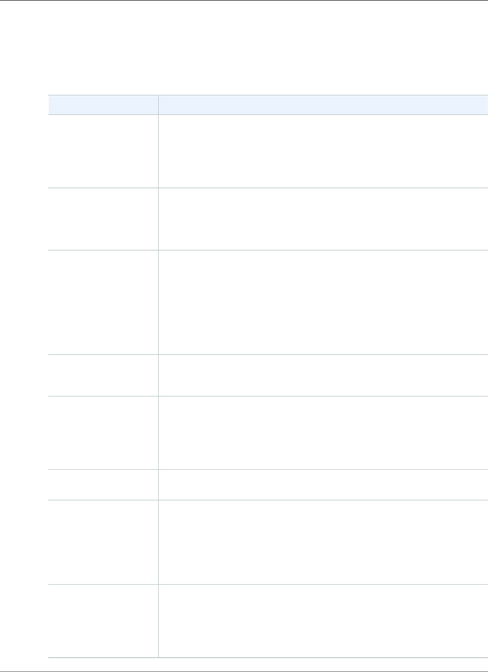
Amazon Redshift Database Developer Guide
Are You a Database Developer?
Are You a Database Developer?
If you are a database user, database designer, database developer, or database administrator, the
following table will help you find what you’re looking for.
If you want to ... We recommend
Quickly start using
Amazon Redshift
Begin by following the steps in Amazon Redshift Getting Started to quickly
deploy a cluster, connect to a database, and try out some queries.
When you are ready to build your database, load data into tables, and
write queries to manipulate data in the data warehouse, return here to the
Database Developer Guide.
Learn about the
internal architecture of
the Amazon Redshift
data warehouse.
The Amazon Redshift System Overview (p. 4) gives a high-level overview
of Amazon Redshift's internal architecture.
If you want a broader overview of the Amazon Redshift web service, go to
the Amazon Redshift product detail page.
Create databases,
tables, users, and other
database objects.
Getting Started Using Databases (p. 13) is a quick introduction to the
basics of SQL development.
The Amazon Redshift SQL (p. 306) has the syntax and examples for
Amazon Redshift SQL commands and functions and other SQL elements.
Amazon Redshift Best Practices for Designing Tables (p. 26) provides a
summary of our recommendations for choosing sort keys, distribution keys,
and compression encodings.
Learn how to design
tables for optimum
performance.
Designing Tables (p. 118) details considerations for applying compression
to the data in table columns and choosing distribution and sort keys.
Load data. Loading Data (p. 184) explains the procedures for loading large datasets
from Amazon DynamoDB tables or from flat files stored in Amazon S3
buckets.
Amazon Redshift Best Practices for Loading Data (p. 29) provides for tips
for loading your data quickly and effectively.
Manage users, groups,
and database security.
Managing Database Security (p. 112) covers database security topics.
Monitor and optimize
system performance.
The System Tables Reference (p. 797) details system tables and views
that you can query for the status of the database and monitor queries and
processes.
You should also consult the Amazon Redshift Cluster Management Guide to
learn how to use the AWS Management Console to check the system health,
monitor metrics, and back up and restore clusters.
Analyze and report
information from very
large datasets.
Many popular software vendors are certifying Amazon Redshift with their
offerings to enable you to continue to use the tools you use today. For more
information, see the Amazon Redshift partner page.
The SQL Reference (p. 306) has all the details for the SQL expressions,
commands, and functions Amazon Redshift supports.
API Version 2012-12-01
2

Amazon Redshift Database Developer Guide
Prerequisites
Prerequisites
Before you use this guide, you should complete these tasks.
• Install a SQL client.
• Launch an Amazon Redshift cluster.
• Connect your SQL client to the cluster master database.
For step-by-step instructions, see Amazon Redshift Getting Started.
You should also know how to use your SQL client and should have a fundamental understanding of the
SQL language.
API Version 2012-12-01
3
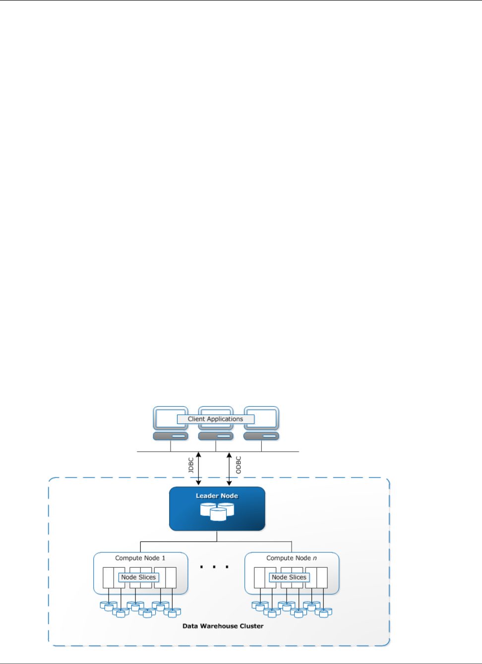
Amazon Redshift Database Developer Guide
Data Warehouse System Architecture
Amazon Redshift System Overview
Topics
•Data Warehouse System Architecture (p. 4)
•Performance (p. 6)
•Columnar Storage (p. 8)
•Internal Architecture and System Operation (p. 10)
•Workload Management (p. 11)
•Using Amazon Redshift with Other Services (p. 11)
An Amazon Redshift data warehouse is an enterprise-class relational database query and management
system.
Amazon Redshift supports client connections with many types of applications, including business
intelligence (BI), reporting, data, and analytics tools.
When you execute analytic queries, you are retrieving, comparing, and evaluating large amounts of data
in multiple-stage operations to produce a final result.
Amazon Redshift achieves efficient storage and optimum query performance through a combination
of massively parallel processing, columnar data storage, and very efficient, targeted data compression
encoding schemes. This section presents an introduction to the Amazon Redshift system architecture.
Data Warehouse System Architecture
This section introduces the elements of the Amazon Redshift data warehouse architecture as shown in
the following figure.
API Version 2012-12-01
4

Amazon Redshift Database Developer Guide
Data Warehouse System Architecture
Client applications
Amazon Redshift integrates with various data loading and ETL (extract, transform, and load) tools
and business intelligence (BI) reporting, data mining, and analytics tools. Amazon Redshift is based on
industry-standard PostgreSQL, so most existing SQL client applications will work with only minimal
changes. For information about important differences between Amazon Redshift SQL and PostgreSQL,
see Amazon Redshift and PostgreSQL (p. 307).
Connections
Amazon Redshift communicates with client applications by using industry-standard JDBC and ODBC
drivers for PostgreSQL. For more information, see Amazon Redshift and PostgreSQL JDBC and
ODBC (p. 308).
Clusters
The core infrastructure component of an Amazon Redshift data warehouse is a cluster.
A cluster is composed of one or more compute nodes. If a cluster is provisioned with two or more
compute nodes, an additional leader node coordinates the compute nodes and handles external
communication. Your client application interacts directly only with the leader node. The compute nodes
are transparent to external applications.
Leader node
The leader node manages communications with client programs and all communication with compute
nodes. It parses and develops execution plans to carry out database operations, in particular, the series
of steps necessary to obtain results for complex queries. Based on the execution plan, the leader node
compiles code, distributes the compiled code to the compute nodes, and assigns a portion of the data to
each compute node.
The leader node distributes SQL statements to the compute nodes only when a query references tables
that are stored on the compute nodes. All other queries run exclusively on the leader node. Amazon
Redshift is designed to implement certain SQL functions only on the leader node. A query that uses any
of these functions will return an error if it references tables that reside on the compute nodes. For more
information, see SQL Functions Supported on the Leader Node (p. 306).
Compute nodes
The leader node compiles code for individual elements of the execution plan and assigns the code to
individual compute nodes. The compute nodes execute the compiled code and send intermediate results
back to the leader node for final aggregation.
Each compute node has its own dedicated CPU, memory, and attached disk storage, which are
determined by the node type. As your workload grows, you can increase the compute capacity and
storage capacity of a cluster by increasing the number of nodes, upgrading the node type, or both.
Amazon Redshift provides two node types; dense storage nodes and dense compute nodes. Each node
provides two storage choices. You can start with a single 160 GB node and scale up to multiple 16 TB
nodes to support a petabyte of data or more.
For a more detailed explanation of data warehouse clusters and nodes, see Internal Architecture and
System Operation (p. 10).
Node slices
A compute node is partitioned into slices. Each slice is allocated a portion of the node's memory and
disk space, where it processes a portion of the workload assigned to the node. The leader node manages
distributing data to the slices and apportions the workload for any queries or other database operations
to the slices. The slices then work in parallel to complete the operation.
API Version 2012-12-01
5

Amazon Redshift Database Developer Guide
Performance
The number of slices per node is determined by the node size of the cluster. For more information about
the number of slices for each node size, go to About Clusters and Nodes in the Amazon Redshift Cluster
Management Guide.
When you create a table, you can optionally specify one column as the distribution key. When the table
is loaded with data, the rows are distributed to the node slices according to the distribution key that is
defined for a table. Choosing a good distribution key enables Amazon Redshift to use parallel processing
to load data and execute queries efficiently. For information about choosing a distribution key, see
Choose the Best Distribution Style (p. 27).
Internal network
Amazon Redshift takes advantage of high-bandwidth connections, close proximity, and custom
communication protocols to provide private, very high-speed network communication between the
leader node and compute nodes. The compute nodes run on a separate, isolated network that client
applications never access directly.
Databases
A cluster contains one or more databases. User data is stored on the compute nodes. Your SQL client
communicates with the leader node, which in turn coordinates query execution with the compute nodes.
Amazon Redshift is a relational database management system (RDBMS), so it is compatible with
other RDBMS applications. Although it provides the same functionality as a typical RDBMS, including
online transaction processing (OLTP) functions such as inserting and deleting data, Amazon Redshift is
optimized for high-performance analysis and reporting of very large datasets.
Amazon Redshift is based on PostgreSQL 8.0.2. Amazon Redshift and PostgreSQL have a number of
very important differences that you need to take into account as you design and develop your data
warehouse applications. For information about how Amazon Redshift SQL differs from PostgreSQL, see
Amazon Redshift and PostgreSQL (p. 307).
Performance
Amazon Redshift achieves extremely fast query execution by employing these performance features.
Topics
•Massively Parallel Processing (p. 6)
•Columnar Data Storage (p. 7)
•Data Compression (p. 7)
•Query Optimizer (p. 7)
•Result Caching (p. 7)
•Compiled Code (p. 8)
Massively Parallel Processing
Massively parallel processing (MPP) enables fast execution of the most complex queries operating on
large amounts of data. Multiple compute nodes handle all query processing leading up to final result
aggregation, with each core of each node executing the same compiled query segments on portions of
the entire data.
Amazon Redshift distributes the rows of a table to the compute nodes so that the data can be processed
in parallel. By selecting an appropriate distribution key for each table, you can optimize the distribution
API Version 2012-12-01
6

Amazon Redshift Database Developer Guide
Columnar Data Storage
of data to balance the workload and minimize movement of data from node to node. For more
information, see Choose the Best Distribution Style (p. 27).
Loading data from flat files takes advantage of parallel processing by spreading the workload across
multiple nodes while simultaneously reading from multiple files. For more information about how to
load data into tables, see Amazon Redshift Best Practices for Loading Data (p. 29).
Columnar Data Storage
Columnar storage for database tables drastically reduces the overall disk I/O requirements and is an
important factor in optimizing analytic query performance. Storing database table information in a
columnar fashion reduces the number of disk I/O requests and reduces the amount of data you need to
load from disk. Loading less data into memory enables Amazon Redshift to perform more in-memory
processing when executing queries. See Columnar Storage (p. 8) for a more detailed explanation.
When columns are sorted appropriately, the query processor is able to rapidly filter out a large subset of
data blocks. For more information, see Choose the Best Sort Key (p. 27).
Data Compression
Data compression reduces storage requirements, thereby reducing disk I/O, which improves query
performance. When you execute a query, the compressed data is read into memory, then uncompressed
during query execution. Loading less data into memory enables Amazon Redshift to allocate more
memory to analyzing the data. Because columnar storage stores similar data sequentially, Amazon
Redshift is able to apply adaptive compression encodings specifically tied to columnar data types. The
best way to enable data compression on table columns is by allowing Amazon Redshift to apply optimal
compression encodings when you load the table with data. To learn more about using automatic data
compression, see Loading Tables with Automatic Compression (p. 209).
Query Optimizer
The Amazon Redshift query execution engine incorporates a query optimizer that is MPP-aware and
also takes advantage of the columnar-oriented data storage. The Amazon Redshift query optimizer
implements significant enhancements and extensions for processing complex analytic queries that often
include multi-table joins, subqueries, and aggregation. To learn more about optimizing queries, see
Tuning Query Performance (p. 257).
Result Caching
To reduce query execution time and improve system performance, Amazon Redshift caches the results
of certain types of queries in memory on the leader node. When a user submits a query, Amazon
Redshift checks the results cache for a valid, cached copy of the query results. If a match is found in the
result cache, Amazon Redshift uses the cached results and doesn’t execute the query. Result caching is
transparent to the user.
Result caching is enabled by default. To disable result caching for the current session, set the
enable_result_cache_for_session (p. 949) parameter to off.
Amazon Redshift uses cached results for a new query when all of the following are true:
• The user submitting the query has access privilege to the objects used in the query.
• The table or views in the query haven't been modified.
• The query doesn't use a function that must be evaluated each time it's run, such as GETDATE.
• The query doesn't reference Amazon Redshift Spectrum external tables.
API Version 2012-12-01
7

Amazon Redshift Database Developer Guide
Compiled Code
• Configuration parameters that might affect query results are unchanged.
• The query syntactically matches the cached query.
To maximize cache effectiveness and efficient use of resources, Amazon Redshift doesn't cache some
large query result sets. Amazon Redshift determines whether to cache query results based on a number
of factors. These factors include the number of entries in the cache and the instance type of your
Amazon Redshift cluster.
To determine whether a query used the result cache, query the SVL_QLOG (p. 906) system view. If a
query used the result cache, the source_query column returns the query ID of the source query. If result
caching wasn't used, the source_query column value is NULL.
The following example shows that queries submitted by userid 104 and userid 102 use the result cache
from queries run by userid 100.
select userid, query, elapsed, source_query from svl_qlog
where userid > 1
order by query desc;
userid | query | elapsed | source_query
-------+--------+----------+-------------
104 | 629035 | 27 | 628919
104 | 629034 | 60 | 628900
104 | 629033 | 23 | 628891
102 | 629017 | 1229393 |
102 | 628942 | 28 | 628919
102 | 628941 | 57 | 628900
102 | 628940 | 26 | 628891
100 | 628919 | 84295686 |
100 | 628900 | 87015637 |
100 | 628891 | 58808694 |
For details about the queries used to create the results shown in the previous example, see Step 2: Test
System Performance to Establish a Baseline (p. 49) in the Tuning Table Design (p. 45) tutorial.
Compiled Code
The leader node distributes fully optimized compiled code across all of the nodes of a cluster. Compiling
the query eliminates the overhead associated with an interpreter and therefore increases the execution
speed, especially for complex queries. The compiled code is cached and shared across sessions on the
same cluster, so subsequent executions of the same query will be faster, often even with different
parameters.
The execution engine compiles different code for the JDBC connection protocol and for ODBC and psql
(libq) connection protocols, so two clients using different protocols will each incur the first-time cost
of compiling the code. Other clients that use the same protocol, however, will benefit from sharing the
cached code.
Columnar Storage
Columnar storage for database tables is an important factor in optimizing analytic query performance
because it drastically reduces the overall disk I/O requirements and reduces the amount of data you need
to load from disk.
The following series of illustrations describe how columnar data storage implements efficiencies and
how that translates into efficiencies when retrieving data into memory.
API Version 2012-12-01
8
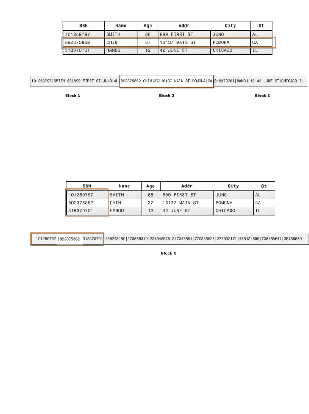
Amazon Redshift Database Developer Guide
Columnar Storage
This first illustration shows how records from database tables are typically stored into disk blocks by row.
In a typical relational database table, each row contains field values for a single record. In row-wise
database storage, data blocks store values sequentially for each consecutive column making up the
entire row. If block size is smaller than the size of a record, storage for an entire record may take more
than one block. If block size is larger than the size of a record, storage for an entire record may take
less than one block, resulting in an inefficient use of disk space. In online transaction processing (OLTP)
applications, most transactions involve frequently reading and writing all of the values for entire records,
typically one record or a small number of records at a time. As a result, row-wise storage is optimal for
OLTP databases.
The next illustration shows how with columnar storage, the values for each column are stored
sequentially into disk blocks.
Using columnar storage, each data block stores values of a single column for multiple rows. As records
enter the system, Amazon Redshift transparently converts the data to columnar storage for each of the
columns.
In this simplified example, using columnar storage, each data block holds column field values for as
many as three times as many records as row-based storage. This means that reading the same number
of column field values for the same number of records requires a third of the I/O operations compared
to row-wise storage. In practice, using tables with very large numbers of columns and very large row
counts, storage efficiency is even greater.
An added advantage is that, since each block holds the same type of data, block data can use a
compression scheme selected specifically for the column data type, further reducing disk space and
I/O. For more information about compression encodings based on data types, see Compression
Encodings (p. 119).
The savings in space for storing data on disk also carries over to retrieving and then storing that data in
memory. Since many database operations only need to access or operate on one or a small number of
columns at a time, you can save memory space by only retrieving blocks for columns you actually need
for a query. Where OLTP transactions typically involve most or all of the columns in a row for a small
number of records, data warehouse queries commonly read only a few columns for a very large number
of rows. This means that reading the same number of column field values for the same number of rows
API Version 2012-12-01
9
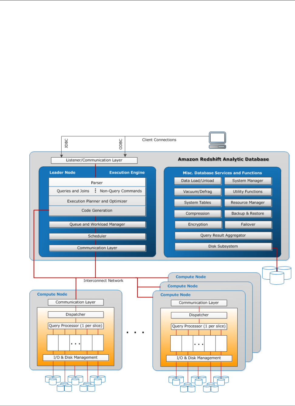
Amazon Redshift Database Developer Guide
Internal Architecture and System Operation
requires a fraction of the I/O operations and uses a fraction of the memory that would be required for
processing row-wise blocks. In practice, using tables with very large numbers of columns and very large
row counts, the efficiency gains are proportionally greater. For example, suppose a table contains 100
columns. A query that uses five columns will only need to read about five percent of the data contained
in the table. This savings is repeated for possibly billions or even trillions of records for large databases.
In contrast, a row-wise database would read the blocks that contain the 95 unneeded columns as well.
Typical database block sizes range from 2 KB to 32 KB. Amazon Redshift uses a block size of 1 MB,
which is more efficient and further reduces the number of I/O requests needed to perform any database
loading or other operations that are part of query execution.
Internal Architecture and System Operation
The following diagram shows a high level view of internal components and functionality of the Amazon
Redshift data warehouse.
API Version 2012-12-01
10

Amazon Redshift Database Developer Guide
Workload Management
Workload Management
Amazon Redshift workload management (WLM) enables users to flexibly manage priorities within
workloads so that short, fast-running queries won't get stuck in queues behind long-running queries.
Amazon Redshift WLM creates query queues at runtime according to service classes, which define the
configuration parameters for various types of queues, including internal system queues and user-
accessible queues. From a user perspective, a user-accessible service class and a queue are functionally
equivalent. For consistency, this documentation uses the term queue to mean a user-accessible service
class as well as a runtime queue.
When you run a query, WLM assigns the query to a queue according to the user's user group or by
matching a query group that is listed in the queue configuration with a query group label that the user
sets at runtime.
By default, Amazon Redshift configures one queue with a concurrency level of five, which enables up to
five queries to run concurrently, plus one predefined Superuser queue, with a concurrency level of one.
You can define up to eight queues. Each queue can be configured with a maximum concurrency level
of 50. The maximum total concurrency level for all user-defined queues (not including the Superuser
queue) is 50.
The easiest way to modify the WLM configuration is by using the Amazon Redshift Management Console.
You can also use the Amazon Redshift command line interface (CLI) or the Amazon Redshift API.
For more information about implementing and using workload management, see Implementing
Workload Management (p. 285).
Using Amazon Redshift with Other Services
Amazon Redshift integrates with other AWS services to enable you to move, transform, and load your
data quickly and reliably, using data security features.
Moving Data Between Amazon Redshift and Amazon
S3
Amazon Simple Storage Service (Amazon S3) is a web service that stores data in the cloud. Amazon
Redshift leverages parallel processing to read and load data from multiple data files stored in Amazon S3
buckets. For more information, see Loading Data from Amazon S3 (p. 187).
You can also use parallel processing to export data from your Amazon Redshift data warehouse to
multiple data files on Amazon S3. For more information, see Unloading Data (p. 242).
Using Amazon Redshift with Amazon DynamoDB
Amazon DynamoDB is a fully managed NoSQL database service. You can use the COPY command to load
an Amazon Redshift table with data from a single Amazon DynamoDB table. For more information, see
Loading Data from an Amazon DynamoDB Table (p. 206).
Importing Data from Remote Hosts over SSH
You can use the COPY command in Amazon Redshift to load data from one or more remote hosts, such
as Amazon EMR clusters, Amazon EC2 instances, or other computers. COPY connects to the remote hosts
API Version 2012-12-01
11

Amazon Redshift Database Developer Guide
Automating Data Loads Using AWS Data Pipeline
using SSH and executes commands on the remote hosts to generate data. Amazon Redshift supports
multiple simultaneous connections. The COPY command reads and loads the output from multiple host
sources in parallel. For more information, see Loading Data from Remote Hosts (p. 200).
Automating Data Loads Using AWS Data Pipeline
You can use AWS Data Pipeline to automate data movement and transformation into and out of Amazon
Redshift. By using the built-in scheduling capabilities of AWS Data Pipeline, you can schedule and
execute recurring jobs without having to write your own complex data transfer or transformation
logic. For example, you can set up a recurring job to automatically copy data from Amazon DynamoDB
into Amazon Redshift. For a tutorial that walks you through the process of creating a pipeline that
periodically moves data from Amazon S3 to Amazon Redshift, see Copy Data to Amazon Redshift Using
AWS Data Pipeline in the AWS Data Pipeline Developer Guide.
Migrating Data Using AWS Database Migration
Service (AWS DMS)
You can migrate data to Amazon Redshift using AWS Database Migration Service. AWS DMS can
migrate your data to and from most widely used commercial and open-source databases such as Oracle,
PostgreSQL, Microsoft SQL Server, Amazon Redshift, Aurora, DynamoDB, Amazon S3, MariaDB, and
MySQL. For more information, see Using an Amazon Redshift Database as a Target for AWS Database
Migration Service.
API Version 2012-12-01
12

Amazon Redshift Database Developer Guide
Step 1: Create a Database
Getting Started Using Databases
Topics
•Step 1: Create a Database (p. 13)
•Step 2: Create a Database User (p. 14)
•Step 3: Create a Database Table (p. 14)
•Step 4: Load Sample Data (p. 15)
•Step 5: Query the System Tables (p. 16)
•Step 6: Cancel a Query (p. 18)
•Step 7: Clean Up Your Resources (p. 20)
This section describes the basic steps to begin using the Amazon Redshift database.
The examples in this section assume you have signed up for the Amazon Redshift data warehouse
service, created a cluster, and established a connection to the cluster from your SQL query tool. For
information about these tasks, see Amazon Redshift Getting Started.
Important
The cluster that you deployed for this exercise will be running in a live environment. As long as
it is running, it will accrue charges to your AWS account. For more pricing information, go to the
Amazon Redshift pricing page.
To avoid unnecessary charges, you should delete your cluster when you are done with it. The
final step of the exercise explains how to do so.
Step 1: Create a Database
After you have verified that your cluster is up and running, you can create your first database. This
database is where you will actually create tables, load data, and run queries. A single cluster can host
multiple databases. For example, you can have a TICKIT database and an ORDERS database on the same
cluster.
After you connect to the initial cluster database, the database you created when you launched the
cluster, you use the initial database as the base for creating a new database.
For example, to create a database named tickit, issue the following command:
create database tickit;
For this exercise, we'll accept the defaults. For information about more command options, see CREATE
DATABASE (p. 448) in the SQL Command Reference.
After you have created the TICKIT database, you can connect to the new database from your SQL client.
Use the same connection parameters as you used for your current connection, but change the database
name to tickit.
You do not need to change the database to complete the remainder of this tutorial. If you prefer not to
connect to the TICKIT database, you can try the rest of the examples in this section using the default
database.
API Version 2012-12-01
13
Amazon Redshift Database Developer Guide
Step 2: Create a Database User
Step 2: Create a Database User
By default, only the master user that you created when you launched the cluster has access to the
initial database in the cluster. To grant other users access, you must create one or more user accounts.
Database user accounts are global across all the databases in a cluster; they do not belong to individual
databases.
Use the CREATE USER command to create a new database user. When you create a new user, you specify
the name of the new user and a password. A password is required. It must have between 8 and 64
characters, and it must include at least one uppercase letter, one lowercase letter, and one numeral.
For example, to create a user named GUEST with password ABCd4321, issue the following command:
create user guest password 'ABCd4321';
For information about other command options, see CREATE USER (p. 490) in the SQL Command
Reference.
Delete a Database User
You won't need the GUEST user account for this tutorial, so you can delete it. If you delete a database
user account, the user will no longer be able to access any of the cluster databases.
Issue the following command to drop the GUEST user:
drop user guest;
The master user you created when you launched your cluster continues to have access to the database.
Important
Amazon Redshift strongly recommends that you do not delete the master user.
For information about command options, see DROP USER (p. 507) in the SQL Reference.
Step 3: Create a Database Table
After you create your new database, you create tables to hold your database data. You specify any
column information for the table when you create the table.
For example, to create a table named testtable with a single column named testcol for an integer
data type, issue the following command:
create table testtable (testcol int);
The PG_TABLE_DEF system table contains information about all the tables in the cluster. To verify the
result, issue the following SELECT command to query the PG_TABLE_DEF system table.
select * from pg_table_def where tablename = 'testtable';
The query result should look something like this:
schemaname|tablename|column | type |encoding|distkey|sortkey | notnull
API Version 2012-12-01
14
Amazon Redshift Database Developer Guide
Insert Data Rows into a Table
----------+---------+-------+-------+--------+-------+--------+---------
public |testtable|testcol|integer|none |f | 0 | f
(1 row)
By default, new database objects, such as tables, are created in a schema named "public". For more
information about schemas, see Schemas (p. 115) in the Managing Database Security section.
The encoding, distkey, and sortkey columns are used by Amazon Redshift for parallel processing.
For more information about designing tables that incorporate these elements, see Amazon Redshift Best
Practices for Designing Tables (p. 26).
Insert Data Rows into a Table
After you create a table, you can insert rows of data into that table.
Note
The INSERT (p. 520) command inserts individual rows into a database table. For standard bulk
loads, use the COPY (p. 390) command. For more information, see Use a COPY Command to
Load Data (p. 30).
For example, to insert a value of 100 into the testtable table (which contains a single column), issue
the following command:
insert into testtable values (100);
Select Data from a Table
After you create a table and populate it with data, use a SELECT statement to display the data contained
in the table. The SELECT * statement returns all the column names and row values for all of the data in a
table and is a good way to verify that recently added data was correctly inserted into the table.
To view the data that you entered in the testtable table, issue the following command:
select * from testtable;
The result will look like this:
testcol
---------
100
(1 row)
For more information about using the SELECT statement to query tables, see SELECT (p. 532) in the
SQL Command Reference.
Step 4: Load Sample Data
Most of the examples in this guide use the TICKIT sample database. If you want to follow the examples
using your SQL query tool, you will need to load the sample data for the TICKIT database.
The sample data for this tutorial is provided in Amazon S3 buckets that give read access to all
authenticated AWS users, so any valid AWS credentials that permit access to Amazon S3 will work.
API Version 2012-12-01
15

Amazon Redshift Database Developer Guide
Step 5: Query the System Tables
To load the sample data for the TICKIT database, you will first create the tables, then use the COPY
command to load the tables with sample data that is stored in an Amazon S3 bucket. For steps to create
tables and load sample data, see Amazon Redshift Getting Started Guide.
Step 5: Query the System Tables
In addition to the tables that you create, your database contains a number of system tables. These
system tables contain information about your installation and about the various queries and processes
that are running on the system. You can query these system tables to collect information about your
database.
Note
The description for each table in the System Tables Reference indicates whether a table is visible
to all users or visible only to superusers. You must be logged in as a superuser to query tables
that are visible only to superusers.
Amazon Redshift provides access to the following types of system tables:
•STL Tables for Logging (p. 798)
These system tables are generated from Amazon Redshift log files to provide a history of the system.
Logging tables have an STL prefix.
•STV Tables for Snapshot Data (p. 868)
These tables are virtual system tables that contain snapshots of the current system data. Snapshot
tables have an STV prefix.
•System Views (p. 896)
System views contain a subset of data found in several of the STL and STV system tables. Systems
views have an SVV or SVL prefix.
•System Catalog Tables (p. 935)
The system catalog tables store schema metadata, such as information about tables and columns.
System catalog tables have a PG prefix.
You may need to specify the process ID associated with a query to retrieve system table information
about that query. For information, see Determine the Process ID of a Running Query (p. 18).
View a List of Table Names
For example, to view a list of all tables in the public schema, you can query the PG_TABLE_DEF system
catalog table.
select distinct(tablename) from pg_table_def where schemaname = 'public';
The result will look something like this:
tablename
---------
category
date
event
listing
sales
testtable
API Version 2012-12-01
16
Amazon Redshift Database Developer Guide
View Database Users
users
venue
View Database Users
You can query the PG_USER catalog to view a list of all database users, along with the user ID
(USESYSID) and user privileges.
select * from pg_user;
usename | usesysid | usecreatedb | usesuper | usecatupd | passwd | valuntil |
useconfig
------------+----------+-------------+----------+-----------+----------+----------
+-----------
rdsdb | 1 | t | t | t | ******** | |
masteruser | 100 | t | t | f | ******** | |
dwuser | 101 | f | f | f | ******** | |
simpleuser | 102 | f | f | f | ******** | |
poweruser | 103 | f | t | f | ******** | |
dbuser | 104 | t | f | f | ******** | |
(6 rows)
The user name rdsdb is used internally by Amazon Redshift to perform routine administrative and
maintenance tasks. You can filter your query to show only user-defined user names by adding where
usesysid > 1 to your select statement.
select * from pg_user
where usesysid > 1;
usename | usesysid | usecreatedb | usesuper | usecatupd | passwd | valuntil |
useconfig
------------+----------+-------------+----------+-----------+----------+----------
+-----------
masteruser | 100 | t | t | f | ******** | |
dwuser | 101 | f | f | f | ******** | |
simpleuser | 102 | f | f | f | ******** | |
poweruser | 103 | f | t | f | ******** | |
dbuser | 104 | t | f | f | ******** | |
(5 rows)
View Recent Queries
In the previous example, you found that the user ID (USESYSID) for masteruser is 100. To list the five
most recent queries executed by masteruser, you can query the SVL_QLOG view. The SVL_QLOG view
is a friendlier subset of information from the STL_QUERY table. You can use this view to find the query
ID (QUERY) or process ID (PID) for a recently run query or to see how long it took a query to complete.
SVL_QLOG includes the first 60 characters of the query string (SUBSTRING) to help you locate a specific
query. Use the LIMIT clause with your SELECT statement to limit the results to five rows.
select query, pid, elapsed, substring from svl_qlog
where userid = 100
order by starttime desc
limit 5;
The result will look something like this:
query | pid | elapsed | substring
API Version 2012-12-01
17
Amazon Redshift Database Developer Guide
Determine the Process ID of a Running Query
--------+-------+----------+--------------------------------------------------------------
187752 | 18921 | 18465685 | select query, elapsed, substring from svl_qlog order by query
204168 | 5117 | 59603 | insert into testtable values (100);
187561 | 17046 | 1003052 | select * from pg_table_def where tablename = 'testtable';
187549 | 17046 | 1108584 | select * from STV_WLM_SERVICE_CLASS_CONFIG
187468 | 17046 | 5670661 | select * from pg_table_def where schemaname = 'public';
(5 rows)
Determine the Process ID of a Running Query
In the previous example you learned how to obtain the query ID and process ID (PID) for a completed
query from the SVL_QLOG view.
You might need to find the PID for a query that is still running. For example, you will need the PID if you
need to cancel a query that is taking too long to run. You can query the STV_RECENTS system table to
obtain a list of process IDs for running queries, along with the corresponding query string. If your query
returns multiple PIDs, you can look at the query text to determine which PID you need.
To determine the PID of a running query, issue the following SELECT statement:
select pid, user_name, starttime, query
from stv_recents
where status='Running';
Step 6: Cancel a Query
If a user issues a query that is taking too long or is consuming excessive cluster resources, you might
need to cancel the query. For example, a user might want to create a list of ticket sellers that includes the
seller's name and quantity of tickets sold. The following query selects data from the SALES table USERS
table and joins the two tables by matching SELLERID and USERID in the WHERE clause.
select sellerid, firstname, lastname, sum(qtysold)
from sales, users
where sales.sellerid = users.userid
group by sellerid, firstname, lastname
order by 4 desc;
Note
This is a complex query. For this tutorial, you don't need to worry about how this query is
constructed.
The previous query runs in seconds and returns 2,102 rows.
Suppose the user forgets to put in the WHERE clause.
select sellerid, firstname, lastname, sum(qtysold)
from sales, users
group by sellerid, firstname, lastname
order by 4 desc;
The result set will include all of the rows in the SALES table multiplied by all the rows in the USERS table
(49989*3766). This is called a Cartesian join, and it is not recommended. The result is over 188 million
rows and takes a long time to run.
To cancel a running query, use the CANCEL command with the query's PID.
API Version 2012-12-01
18
Amazon Redshift Database Developer Guide
Cancel a Query from Another Session
To find the process ID, query the STV_RECENTS table, as shown in the previous step. The following
example shows how you can make the results more readable by using the TRIM function to trim trailing
spaces and by showing only the first 20 characters of the query string.
select pid, trim(user_name), starttime, substring(query,1,20)
from stv_recents
where status='Running';
The result looks something like this:
pid | btrim | starttime | substring
-------+------------+----------------------------+----------------------
18764 | masteruser | 2013-03-28 18:39:49.355918 | select sellerid, fir
(1 row)
To cancel the query with PID 18764, issue the following command:
cancel 18764;
Note
The CANCEL command will not abort a transaction. To abort or roll back a transaction, you must
use the ABORT or ROLLBACK command. To cancel a query associated with a transaction, first
cancel the query then abort the transaction.
If the query that you canceled is associated with a transaction, use the ABORT or ROLLBACK. command
to cancel the transaction and discard any changes made to the data:
abort;
Unless you are signed on as a superuser, you can cancel only your own queries. A superuser can cancel all
queries.
Cancel a Query from Another Session
If your query tool does not support running queries concurrently, you will need to start another session
to cancel the query. For example, SQLWorkbench, which is the query tool we use in the Amazon
Redshift Getting Started, does not support multiple concurrent queries. To start another session using
SQLWorkbench, select File, New Window and connect using the same connection parameters. Then you
can find the PID and cancel the query.
Cancel a Query Using the Superuser Queue
If your current session has too many queries running concurrently, you might not be able to run the
CANCEL command until another query finishes. In that case, you will need to issue the CANCEL command
using a different workload management query queue.
Workload management enables you to execute queries in different query queues so that you don't
need to wait for another query to complete. The workload manager creates a separate queue, called
the Superuser queue, that you can use for troubleshooting. To use the Superuser queue, you must be
logged on a superuser and set the query group to 'superuser' using the SET command. After running
your commands, reset the query group using the RESET command.
To cancel a query using the Superuser queue, issue these commands:
set query_group to 'superuser';
API Version 2012-12-01
19
Amazon Redshift Database Developer Guide
Step 7: Clean Up Your Resources
cancel 18764;
reset query_group;
For information about managing query queues, see Implementing Workload Management (p. 285).
Step 7: Clean Up Your Resources
If you deployed a cluster in order to complete this exercise, when you are finished with the exercise, you
should delete the cluster so that it will stop accruing charges to your AWS account.
To delete the cluster, follow the steps in Deleting a Cluster in the Amazon Redshift Cluster Management
Guide.
If you want to keep the cluster, you might want to keep the sample data for reference. Most of the
examples in this guide use the tables you created in this exercise. The size of the data will not have any
significant effect on your available storage.
If you want to keep the cluster, but want to clean up the sample data, you can run the following
command to drop the TICKIT database:
drop database tickit;
If you didn't create a TICKIT database, or if you don't want to drop the database, run the following
commands to drop just the tables:
drop table testtable;
drop table users;
drop table venue;
drop table category;
drop table date;
drop table event;
drop table listing;
drop table sales;
API Version 2012-12-01
20

Amazon Redshift Database Developer Guide
Identifying the Goals of the Proof of Concept
Building a Proof of Concept for
Amazon Redshift
Amazon Redshift is a fast, scalable data warehouse that makes it simple and cost-effective to analyze
all your data using standard SQL and your existing business intelligence tools. Amazon Redshift delivers
10 times faster performance than other data warehouses. It does so by using sophisticated query
optimization, columnar storage on high-performance local disks, machine learning, and massively
parallel query execution.
In the following sections, you can find a framework for building a proof of concept with Amazon
Redshift. The framework gives you architectural best practices for designing and operating a secure,
high-performing, and cost-effective Amazon Redshift data warehouse. This guidance is based on
reviewing designs of thousands of customers’ architectures across a wide variety of business types and
use cases. We compiled customer experiences to develop this set of best practices to help you identify
criteria for evaluating your data warehouse workload.
If you are a first-time user of Amazon Redshift, we recommend that you read Getting Started with
Amazon Redshift. This guide provides a tutorial for using Amazon Redshift to create a sample cluster and
work with sample data. To get insights into the benefits of using Amazon Redshift and into pricing, see
Service Highlights and Pricing Information on the marketing webpage.
Identifying the Goals of the Proof of Concept
Identifying the goals of the proof of concept plays a critical role in determining what you want to
measure as part of the evaluation process. The evaluation criteria should include the current challenges,
enhancements you want to make to improve customer experience, and methods of addressing your
current operational pain points. You can use the following questions to identify the goals of the proof of
concept:
• Do you have specific service level agreements whose terms you want to improve?
• What are your goals for scaling your Amazon Redshift data warehouse?
• What new datasets do you or your customers need to include in your data warehouse?
• What are the business-critical SQL queries you need to benchmark? Make sure to include the full range
of SQL complexities, such as the different types of queries (for example, ingest, update, and delete).
• What are the general types of workloads you plan to test? Examples might be extract transform load
(ETL) workloads, reporting queries, and batch extracts.
After you have answered these questions, you should be able to establish a SMART goal for building your
proof of concept.
Setting Up Your Proof of Concept
You set up your Amazon Redshift proof of concept environment in two steps. First, you set up the AWS
resources. Second, you convert the schema and datasets for evaluation.
API Version 2012-12-01
21

Amazon Redshift Database Developer Guide
Designing and Setting Up Your Cluster
Designing and Setting Up Your Cluster
You can set up your cluster with either of the following two node types:
•Dense Storage, which enables you to create very large data warehouses using hard disk drives (HDDs)
for a very low price.
•Dense Compute, which enables you to create high-performance data warehouses using fast CPUs,
large amounts of RAM, and solid-state disks (SSDs).
The goals of your workload and your overall budget should help you determine which type of node to
select. Resizing your cluster or switching to a different type of node is simply a button click in the AWS
Management Console. The following additional considerations can help guide you in setting up your
cluster:
• Select a cluster size that is large enough to handle your production workload. Generally, you need at
least two compute nodes (a multinode cluster). The leader node is included at no additional cost.
• Create your cluster in a virtual private cloud (VPC), which provides better performance than an EC2-
Classic installation.
• Plan to maintain at least 20 percent free space, or three times as much memory as needed by your
largest table. This extra space is needed to provide these:
• Scratch space for usage and rewriting tables
• Free space required for vacuum operations and for re-sorting tables
• Temporary tables used for storing intermediate query results
Converting Your Schema and Setting Up the Datasets
You can convert your schema, code, and data with either the AWS Schema Conversion Tool (AWS SCT) or
the AWS Database Migration Service (AWS DMS). Your best choice of tool depends on the source of your
data.
The following can help you set up your data in Amazon Redshift:
•Migrate from Oracle to Amazon Redshift – This project uses an AWS CloudFormation template, AWS
DMS, and AWS SCT to migrate your data with only a few clicks.
•Migrate Your Data Warehouse to Amazon Redshift Using the AWS SCT – This blog provides an
overview of how you can use the AWS SCT data extractors to migrate your data warehouse to Amazon
Redshift.
Cluster Design Considerations
Keep the following five attributes in mind when designing your cluster. The SET DW acronym is an easy
way to remember them:
•S – The S is for sort key. Query filters access sort key columns frequently. Follow these best practices to
select sort keys:
• Choose up to three columns to be the sort key columns
• Order the sort keys in increasing degree of specificity, but balance this with the frequency of use
For more guidance on selecting sort keys, see Choose the Best Sort Key and the AWS Big Data Blog
post The Advanced Table Design Playbook.
API Version 2012-12-01
22

Amazon Redshift Database Developer Guide
Amazon Redshift Evaluation Checklist
•E – The E is for encoding. Encoding sets the compression algorithm used for each column in each table.
You can either set encoding yourself, or have Amazon Redshift set this for you. For more information
on how to let Amazon Redshift choose the best compression algorithm, see Loading tables with
Automatic compression.
•T – The T is for table maintenance. The Amazon Redshift query optimizer creates more efficient
execution plans when query statistics are up-to-date. Use the ANALYZE command to gather statistics
after loading, updating or deleting data from tables. Similarly, you can minimize the number of blocks
scanned with the VACUUM command. VACUUM improves performance by doing the following:
• Removing the rows that have been logically deleted from the block, resulting in fewer blocks to scan
• Keeping the data in sort key order, which helps target the specific blocks for scanning.
•D – The D is for table distribution. You have three options for table distribution:
•KEY – You designate a column for distribution.
•EVEN – Amazon Redshift assigns the compute nodes with a round-robin pattern.
•ALL – Amazon Redshift puts a complete copy of the table in the database slice of each compute
node.
• The following guidelines can help you select the best distribution pattern:
• If users frequently join a Customers table using the customer id value and doing so distributes
the rows evenly across the database slices, then customer id is a good choice for a distribution
key.
• If a table is approximately 5 million rows and contains dimension data, then choose the ALL
distribution style.
•EVEN is a safe choice for a distribution pattern, but always results in data distribution across all
compute nodes.
•W – The W is for Amazon Redshift Workload Management (WLM). If you use WLM, you control the flow
of SQL statements through the compute clusters and how much system memory to allocate. For more
information on setting up WLM, see Implementing Workload Management (p. 285).
Amazon Redshift Evaluation Checklist
For best evaluation results, check the following list of items to determine if they apply to your Amazon
Redshift evaluation:
•Data load time – Using the COPY command is a common way to test how long it takes to load data.
For more information, see Best Practices for Loading Data.
•Throughput of the cluster – Measuring queries per hour is a common way to determine throughput.
To do so, set up a test to run typical queries for your workload.
•Data security – You can easily encrypt data at rest and in transit with Amazon Redshift. You also have
a number of options for managing keys, and Amazon Redshift also supports Single sign-on (SSO)
integration.
•Third-party tools integration – You can use either a JDBC or ODBC connection to integrate with
business intelligence and other external tools.
•Interoperability with other AWS services – Amazon Redshift integrates with other AWS services, such
as Amazon EMR, Amazon QuickSight, AWS Glue, Amazon S3 and Kinesis. You can use this integration
in setting up and managing your data warehouse.
•Backing up and making snapshots – Amazon Redshift automatically backs up your cluster at every 5
GB of changed data, or 8 hours (whichever occurs first). You can also create a snapshot at any time.
•Using snapshots – Try using a snapshot and creating a second cluster as part of your evaluation.
Evaluate if your development and testing organizations can use the cluster.
•Resizing – Your evaluation should include increasing the number or types of Amazon Redshift nodes.
Your cluster remains fully accessible during the resize, although it is in a read-only mode. Evaluate if
your users can detect that the resize is under way.
API Version 2012-12-01
23
Amazon Redshift Database Developer Guide
Benchmarking Your Amazon Redshift Evaluation
•Support – We strongly recommend that you evaluate AWS Support as part of your evaluation.
•Offloading queries and accessing infrequently used data – You can offload your queries to a separate
compute layer with Amazon Redshift Spectrum. You can also easily access infrequently used data
directly from S3 without ingesting it into your Amazon Redshift cluster.
•Operating costs – Compare the overall cost of operating your data warehouse with other options.
Amazon Redshift is fully managed, and you can perform unlimited analysis of a terabyte of your data
for approximately $1000 per year.
Benchmarking Your Amazon Redshift Evaluation
The following list of possible benchmarks might apply to your Amazon Redshift evaluation:
• Assemble a list of queries for each runtime category. Having a sufficient number (for example, 30 per
category) helps assure that your evaluation reflects a real-world data warehouse implementation.
• Add a unique identifier to associate each query that you include in your evaluation with one of the
categories you establish for your evaluation. You can then use these unique identifiers to determine
throughput for the system tables. You can also create a query_group to organize your evaluation
queries.
For example, if you have established a "Reporting" category for your evaluation, you might create a
coding system to tag your evaluation queries with the word "Report." You can then identify individual
queries within reporting as R1, R2, and so on. The following example demonstrates this approach.
[SELECT "Reporting" as query_category, "R1" as query_id,
* FROM customers]
When you have associated a query with an evaluation category, you can then use a unique identifier to
determine throughput from the system tables for each category. The following example demonstrates
how to do this.
select query, datediff(seconds, starttime, endtime)
from stl_query
where
querytxt like “%Reporting%”
and starttime >= '2018-04-15 00:00'
and endtime <'2018-04-15 23:59'
• Test throughput with historical user or ETL queries that have a variety of run times in your existing
data warehouse. Keep the following items in mind when testing throughput:
• If you are using a load testing utility (for example an open-source utility like JMeter, or a custom
utility), make sure that the tool can take the network transmission time into account.
• Make sure that the load testing utility is evaluating execution time based on throughput of the
internal system tables in Amazon Redshift.
• Identify all the various permutations that you plan to test during your evaluation. The following list
provides some common variables:
• Cluster size
• Instance type
• Load testing duration
• Concurrency settings
• WLM configuration
API Version 2012-12-01
24

Amazon Redshift Database Developer Guide
Additional Resources
Need more help? See, Request Support for your Amazon Redshift Proof-of-Concept.
Additional Resources
To help your Amazon Redshift evaluation, see the following:
•Top 10 Performance Tuning Techniques for Amazon Redshift on the Big Data Blog
•Top 8 Best Practices for High-Performance ETL Processing Using Amazon Redshift on the Big Data
Blog
•Amazon Redshift Management Overview in the Amazon Redshift Cluster Management Guide
•Amazon Redshift Spectrum Getting Started
API Version 2012-12-01
25

Amazon Redshift Database Developer Guide
Best Practices for Designing Tables
Amazon Redshift Best Practices
Following, you can find best practices for designing tables, loading data into tables, and writing queries
for Amazon Redshift, and also a discussion of working with Amazon Redshift Advisor.
Amazon Redshift is not the same as other SQL database systems. To fully realize the benefits of the
Amazon Redshift architecture, you must specifically design, build, and load your tables to use massively
parallel processing, columnar data storage, and columnar data compression. If your data loading and
query execution times are longer than you expect, or longer than you want, you might be overlooking
key information.
If you are an experienced SQL database developer, we strongly recommend that you review this topic
before you begin developing your Amazon Redshift data warehouse.
If you are new to developing SQL databases, this topic is not the best place to start. We recommend that
you begin by reading Getting Started Using Databases (p. 13) and trying the examples yourself.
In this topic, you can find an overview of the most important development principles, along with
specific tips, examples, and best practices for implementing those principles. No single practice
can apply to every application. You should evaluate all of your options before finalizing a database
design. For more information, see Designing Tables (p. 118), Loading Data (p. 184), Tuning Query
Performance (p. 257), and the reference chapters.
Topics
•Amazon Redshift Best Practices for Designing Tables (p. 26)
•Amazon Redshift Best Practices for Loading Data (p. 29)
•Amazon Redshift Best Practices for Designing Queries (p. 32)
•Working with Recommendations from Amazon Redshift Advisor (p. 34)
Amazon Redshift Best Practices for Designing
Tables
As you plan your database, certain key table design decisions heavily influence overall query
performance. These design choices also have a significant effect on storage requirements, which in
turn affects query performance by reducing the number of I/O operations and minimizing the memory
required to process queries.
In this section, you can find a summary of the most important design decisions and presents best
practices for optimizing query performance. Designing Tables (p. 118) provides more detailed
explanations and examples of table design options.
Topics
•Take the Tuning Table Design Tutorial (p. 27)
•Choose the Best Sort Key (p. 27)
•Choose the Best Distribution Style (p. 27)
•Let COPY Choose Compression Encodings (p. 28)
API Version 2012-12-01
26

Amazon Redshift Database Developer Guide
Take the Tuning Table Design Tutorial
•Define Primary Key and Foreign Key Constraints (p. 28)
•Use the Smallest Possible Column Size (p. 28)
•Use Date/Time Data Types for Date Columns (p. 29)
Take the Tuning Table Design Tutorial
Tutorial: Tuning Table Design (p. 45) walks you step by step through the process of choosing sort keys,
distribution styles, and compression encodings, and shows you how to compare system performance
before and after tuning.
Choose the Best Sort Key
Amazon Redshift stores your data on disk in sorted order according to the sort key. The Amazon Redshift
query optimizer uses sort order when it determines optimal query plans.
•If recent data is queried most frequently, specify the timestamp column as the leading column for
the sort key.
Queries are more efficient because they can skip entire blocks that fall outside the time range.
•If you do frequent range filtering or equality filtering on one column, specify that column as the
sort key.
Amazon Redshift can skip reading entire blocks of data for that column. It can do so because it tracks
the minimum and maximum column values stored on each block and can skip blocks that don't apply
to the predicate range.
•If you frequently join a table, specify the join column as both the sort key and the distribution key.
Doing this enables the query optimizer to choose a sort merge join instead of a slower hash join.
Because the data is already sorted on the join key, the query optimizer can bypass the sort phase of
the sort merge join.
For more information about choosing and specifying sort keys, see Tutorial: Tuning Table
Design (p. 45) and Choosing Sort Keys (p. 140).
Choose the Best Distribution Style
When you execute a query, the query optimizer redistributes the rows to the compute nodes as needed
to perform any joins and aggregations. The goal in selecting a table distribution style is to minimize the
impact of the redistribution step by locating the data where it needs to be before the query is executed.
1. Distribute the fact table and one dimension table on their common columns.
Your fact table can have only one distribution key. Any tables that join on another key aren't
collocated with the fact table. Choose one dimension to collocate based on how frequently it is joined
and the size of the joining rows. Designate both the dimension table's primary key and the fact table's
corresponding foreign key as the DISTKEY.
2. Choose the largest dimension based on the size of the filtered dataset.
Only the rows that are used in the join need to be distributed, so consider the size of the dataset after
filtering, not the size of the table.
3. Choose a column with high cardinality in the filtered result set.
If you distribute a sales table on a date column, for example, you should probably get fairly even data
distribution, unless most of your sales are seasonal. However, if you commonly use a range-restricted
API Version 2012-12-01
27

Amazon Redshift Database Developer Guide
Use Automatic Compression
predicate to filter for a narrow date period, most of the filtered rows occur on a limited set of slices
and the query workload is skewed.
4. Change some dimension tables to use ALL distribution.
If a dimension table cannot be collocated with the fact table or other important joining tables, you
can improve query performance significantly by distributing the entire table to all of the nodes. Using
ALL distribution multiplies storage space requirements and increases load times and maintenance
operations, so you should weigh all factors before choosing ALL distribution.
To let Amazon Redshift choose the appropriate distribution style, don't specify DISTSTYLE.
For more information about choosing distribution styles, see Tutorial: Tuning Table Design (p. 45) and
Choosing a Data Distribution Style (p. 129).
Let COPY Choose Compression Encodings
You can specify compression encodings when you create a table, but in most cases, automatic
compression produces the best results.
The COPY command analyzes your data and applies compression encodings to an empty table
automatically as part of the load operation.
Automatic compression balances overall performance when choosing compression encodings. Range-
restricted scans might perform poorly if sort key columns are compressed much more highly than other
columns in the same query. As a result, automatic compression chooses a less efficient compression
encoding to keep the sort key columns balanced with other columns.
Suppose that your table's sort key is a date or timestamp and the table uses many large varchar columns.
In this case, you might get better performance by not compressing the sort key column at all. Run
theANALYZE COMPRESSION (p. 382) command on the table, then use the encodings to create a new
table, but leave out the compression encoding for the sort key.
There is a performance cost for automatic compression encoding, but only if the table is empty
and does not already have compression encoding. For short-lived tables and tables that you create
frequently, such as staging tables, load the table once with automatic compression or run theANALYZE
COMPRESSIONcommand. Then use those encodings to create new tables. You can add the encodings to
the CREATE TABLE statement, or use CREATE TABLE LIKE to create a new table with the same encoding.
For more information, see Tutorial: Tuning Table Design (p. 45) and Loading Tables with Automatic
Compression (p. 209).
Define Primary Key and Foreign Key Constraints
Define primary key and foreign key constraints between tables wherever appropriate. Even though they
are informational only, the query optimizer uses those constraints to generate more efficient query
plans.
Do not define primary key and foreign key constraints unless your application enforces the constraints.
Amazon Redshift does not enforce unique, primary-key, and foreign-key constraints.
See Defining Constraints (p. 145) for additional information about how Amazon Redshift uses
constraints.
Use the Smallest Possible Column Size
Don’t make it a practice to use the maximum column size for convenience.
API Version 2012-12-01
28

Amazon Redshift Database Developer Guide
Using Date/Time Data Types for Date Columns
Instead, consider the largest values you are likely to store in a VARCHAR column, for example, and size
your columns accordingly. Because Amazon Redshift compresses column data very effectively, creating
columns much larger than necessary has minimal impact on the size of data tables. During processing
for complex queries, however, intermediate query results might need to be stored in temporary tables.
Because temporary tables are not compressed, unnecessarily large columns consume excessive memory
and temporary disk space, which can affect query performance.
Use Date/Time Data Types for Date Columns
Amazon Redshift stores DATE and TIMESTAMP data more efficiently than CHAR or VARCHAR, which
results in better query performance. Use the DATE or TIMESTAMP data type, depending on the resolution
you need, rather than a character type when storing date/time information. For more information, see
Datetime Types (p. 326).
Amazon Redshift Best Practices for Loading Data
Topics
•Take the Loading Data Tutorial (p. 29)
•Take the Tuning Table Design Tutorial (p. 29)
•Use a COPY Command to Load Data (p. 30)
•Use a Single COPY Command to Load from Multiple Files (p. 30)
•Split Your Load Data into Multiple Files (p. 30)
•Compress Your Data Files (p. 30)
•Use a Manifest File (p. 30)
•Verify Data Files Before and After a Load (p. 31)
•Use a Multi-Row Insert (p. 31)
•Use a Bulk Insert (p. 31)
•Load Data in Sort Key Order (p. 31)
•Load Data in Sequential Blocks (p. 32)
•Use Time-Series Tables (p. 32)
•Use a Staging Table to Perform a Merge (Upsert) (p. 32)
•Schedule Around Maintenance Windows (p. 32)
Loading very large datasets can take a long time and consume a lot of computing resources. How your
data is loaded can also affect query performance. This section presents best practices for loading data
efficiently using COPY commands, bulk inserts, and staging tables.
Take the Loading Data Tutorial
Tutorial: Loading Data from Amazon S3 (p. 70) walks you beginning to end through the steps to
upload data to an Amazon S3 bucket and then use the COPY command to load the data into your tables.
The tutorial includes help with troubleshooting load errors and compares the performance difference
between loading from a single file and loading from multiple files.
Take the Tuning Table Design Tutorial
Data loads are heavily influenced by table design, especially compression encodings and distribution
styles. Tutorial: Tuning Table Design (p. 45) walks you step-by-step through the process of choosing
API Version 2012-12-01
29

Amazon Redshift Database Developer Guide
Use a COPY Command to Load Data
sort keys, distribution styles, and compression encodings, and shows you how to compare system
performance before and after tuning.
Use a COPY Command to Load Data
The COPY command loads data in parallel from Amazon S3, Amazon EMR, Amazon DynamoDB, or
multiple data sources on remote hosts. COPY loads large amounts of data much more efficiently than
using INSERT statements, and stores the data more effectively as well.
For more information about using the COPY command, see Loading Data from Amazon S3 (p. 187) and
Loading Data from an Amazon DynamoDB Table (p. 206).
Use a Single COPY Command to Load from Multiple
Files
Amazon Redshift automatically loads in parallel from multiple data files.
If you use multiple concurrent COPY commands to load one table from multiple files, Amazon Redshift
is forced to perform a serialized load. This type of load is much slower and requires a VACUUM process
at the end if the table has a sort column defined. For more information about using COPY to load data in
parallel, see Loading Data from Amazon S3 (p. 187).
Split Your Load Data into Multiple Files
The COPY command loads the data in parallel from multiple files, dividing the workload among the
nodes in your cluster. When you load all the data from a single large file, Amazon Redshift is forced to
perform a serialized load, which is much slower. Split your load data files so that the files are about equal
size, between 1 MB and 1 GB after compression. For optimum parallelism, the ideal size is between 1 MB
and 125 MB after compression. The number of files should be a multiple of the number of slices in your
cluster. For more information about how to split your data into files and examples of using COPY to load
data, see Loading Data from Amazon S3 (p. 187).
Compress Your Data Files
We strongly recommend that you individually compress your load files using gzip, lzop, or bzip2 when
you have large datasets.
Specify the GZIP, LZOP, or BZIP2 option with the COPY command. This example loads the TIME table
from a pipe-delimited lzop file.
copy time
from 's3://mybucket/data/timerows.lzo'
iam_role 'arn:aws:iam::0123456789012:role/MyRedshiftRole'
lzop
delimiter '|';
Use a Manifest File
Amazon S3 provides eventual consistency for some operations. Thus, it's possible that new data won't
be available immediately after the upload, which can result in an incomplete data load or loading stale
data. You can manage data consistency by using a manifest file to load data. For more information, see
Managing Data Consistency (p. 189).
API Version 2012-12-01
30
Amazon Redshift Database Developer Guide
Verify Data Files Before and After a Load
Verify Data Files Before and After a Load
When you load data from Amazon S3, first upload your files to your Amazon S3 bucket, then verify that
the bucket contains all the correct files, and only those files. For more information, see Verifying That the
Correct Files Are Present in Your Bucket (p. 191).
After the load operation is complete, query the STL_LOAD_COMMITS (p. 823) system table to verify
that the expected files were loaded. For more information, see Verifying That the Data Was Loaded
Correctly (p. 208).
Use a Multi-Row Insert
If a COPY command is not an option and you require SQL inserts, use a multi-row insert whenever
possible. Data compression is inefficient when you add data only one row or a few rows at a time.
Multi-row inserts improve performance by batching up a series of inserts. The following example inserts
three rows into a four-column table using a single INSERT statement. This is still a small insert, shown
simply to illustrate the syntax of a multi-row insert.
insert into category_stage values
(default, default, default, default),
(20, default, 'Country', default),
(21, 'Concerts', 'Rock', default);
See INSERT (p. 520) for more details and examples.
Use a Bulk Insert
Use a bulk insert operation with a SELECT clause for high-performance data insertion.
Use the INSERT (p. 520) and CREATE TABLE AS (p. 483) commands when you need to move data or a
subset of data from one table into another.
For example, the following INSERT statement selects all of the rows from the CATEGORY table and
inserts them into the CATEGORY_STAGE table.
insert into category_stage
(select * from category);
The following example creates CATEGORY_STAGE as a copy of CATEGORY and inserts all of the rows in
CATEGORY into CATEGORY_STAGE.
create table category_stage as
select * from category;
Load Data in Sort Key Order
Load your data in sort key order to avoid needing to vacuum.
If each batch of new data follows the existing rows in your table, your data is properly stored in sort
order, and you don't need to run a vacuum. You don't need to presort the rows in each load because
COPY sorts each batch of incoming data as it loads.
For example, suppose that you load data every day based on the current day's activity. If your sort key is
a timestamp column, your data is stored in sort order. This order occurs because the current day's data is
always appended at the end of the previous day's data. For more information, see Loading Your Data in
Sort Key Order (p. 235).
API Version 2012-12-01
31

Amazon Redshift Database Developer Guide
Load Data in Sequential Blocks
Load Data in Sequential Blocks
If you need to add a large quantity of data, load the data in sequential blocks according to sort order to
eliminate the need to vacuum.
For example, suppose that you need to load a table with events from January 2017 to December
2017. Load the rows for January, then February, and so on. Your table is completely sorted when
your load completes, and you don't need to run a vacuum. For more information, see Use Time-Series
Tables (p. 32).
When loading very large datasets, the space required to sort might exceed the total available space. By
loading data in smaller blocks, you use much less intermediate sort space during each load. In addition,
loading smaller blocks make it easier to restart if the COPY fails and is rolled back.
Use Time-Series Tables
If your data has a fixed retention period, we strongly recommend that you organize your data as a
sequence of time-series tables. In this sequence, each table should be identical but contain data for
different time ranges.
You can easily remove old data simply by executing a DROP TABLE on the corresponding tables.
This approach is much faster than running a large-scale DELETE and saves you from having to run a
subsequent VACUUM process to reclaim space. You can create a UNION ALL view to hide the fact that
the data is stored in different tables. When you delete old data, simply refine your UNION ALL view to
remove the dropped tables. Similarly, as you load new time periods into new tables, add the new tables
to the view.
If you use time-series tables with a timestamp column for the sort key, you effectively load your data in
sort key order. Doing this eliminates the need to vacuum to resort the data. For more information, see
Load Data in Sort Key Order (p. 31).
Use a Staging Table to Perform a Merge (Upsert)
You can efficiently update and insert new data by loading your data into a staging table first.
Amazon Redshift doesn't support a single merge statement (update or insert, also known as an upsert)
to insert and update data from a single data source. However, you can effectively perform a merge
operation. To do so, load your data into a staging table and then join the staging table with your target
table for an UPDATE statement and an INSERT statement. For instructions, see Updating and Inserting
New Data (p. 216).
Schedule Around Maintenance Windows
If a scheduled maintenance occurs while a query is running, the query is terminated and rolled back
and you need to restart it. Schedule long-running operations, such as large data loads or VACUUM
operation, to avoid maintenance windows. You can also minimize the risk, and make restarts easier
when they are needed, by performing data loads in smaller increments and managing the size of your
VACUUM operations. For more information, see Load Data in Sequential Blocks (p. 32) and Vacuuming
Tables (p. 228).
Amazon Redshift Best Practices for Designing
Queries
To maximize query performance, follow these recommendations when creating queries.
API Version 2012-12-01
32
Amazon Redshift Database Developer Guide
Best Practices for Designing Queries
• Design tables according to best practices to provide a solid foundation for query performance. For
more information, see Amazon Redshift Best Practices for Designing Tables (p. 26).
• Avoid using select *. Include only the columns you specifically need.
• Use a CASE Expression (p. 655) to perform complex aggregations instead of selecting from the same
table multiple times.
• Don’t use cross-joins unless absolutely necessary. These joins without a join condition result in the
Cartesian product of two tables. Cross-joins are typically executed as nested-loop joins, which are the
slowest of the possible join types.
• Use subqueries in cases where one table in the query is used only for predicate conditions and
the subquery returns a small number of rows (less than about 200). The following example uses a
subquery to avoid joining the LISTING table.
select sum(sales.qtysold)
from sales
where salesid in (select listid from listing where listtime > '2008-12-26');
• Use predicates to restrict the dataset as much as possible.
• In the predicate, use the least expensive operators that you can. Comparison Condition (p. 341)
operators are preferable to LIKE (p. 346) operators. LIKE operators are still preferable to SIMILAR
TO (p. 348) or POSIX Operators (p. 351).
• Avoid using functions in query predicates. Using them can drive up the cost of the query by requiring
large numbers of rows to resolve the intermediate steps of the query.
• If possible, use a WHERE clause to restrict the dataset. The query planner can then use row order to
help determine which records match the criteria, so it can skip scanning large numbers of disk blocks.
Without this, the query execution engine must scan participating columns entirely.
• Add predicates to filter tables that participate in joins, even if the predicates apply the same filters.
The query returns the same result set, but Amazon Redshift is able to filter the join tables before the
scan step and can then efficiently skip scanning blocks from those tables. Redundant filters aren't
needed if you filter on a column that's used in the join condition.
For example, suppose that you want to join SALES and LISTING to find ticket sales for tickets listed
after December, grouped by seller. Both tables are sorted by date. The following query joins the tables
on their common key and filters for listing.listtime values greater than December 1.
select listing.sellerid, sum(sales.qtysold)
from sales, listing
where sales.salesid = listing.listid
and listing.listtime > '2008-12-01'
group by 1 order by 1;
The WHERE clause doesn't include a predicate for sales.saletime, so the execution engine is forced
to scan the entire SALES table. If you know the filter would result in fewer rows participating in the
join, then add that filter as well. The following example cuts execution time significantly.
select listing.sellerid, sum(sales.qtysold)
from sales, listing
where sales.salesid = listing.listid
and listing.listtime > '2008-12-01'
and sales.saletime > '2008-12-01'
group by 1 order by 1;
• Use sort keys in the GROUP BY clause so the query planner can use more efficient aggregation. A
query might qualify for one-phase aggregation when its GROUP BY list contains only sort key columns,
one of which is also the distribution key. The sort key columns in the GROUP BY list must include the
first sort key, then other sort keys that you want to use in sort key order. For example, it is valid to use
API Version 2012-12-01
33
Amazon Redshift Database Developer Guide
Working with Advisor
the first sort key, the first and second sort keys, the first, second, and third sort keys, and so on. It is
not valid to use the first and third sort keys.
You can confirm the use of one-phase aggregation by running the EXPLAIN (p. 511) command and
looking for XN GroupAggregate in the aggregation step of the query.
• If you use both GROUP BY and ORDER BY clauses, make sure that you put the columns in the same
order in both. That is, use the approach just following.
group by a, b, c
order by a, b, c
Don't use the following approach.
group by b, c, a
order by a, b, c
Working with Recommendations from Amazon
Redshift Advisor
To help you improve the performance and decrease the operating costs for your Amazon Redshift
cluster, Amazon Redshift Advisor offers you specific recommendations about changes to make. Advisor
develops its customized recommendations by analyzing performance and usage metrics for your cluster.
These tailored recommendations relate to operations and cluster settings. To help you prioritize your
optimizations, Advisor ranks recommendations by order of impact.
Advisor bases its recommendations on observations regarding performance statistics or operations data.
Advisor develops observations by running tests on your clusters to determine if a test value is within
a specified range. If the test result is outside of that range, Advisor generates an observation for your
cluster. At the same time, Advisor creates a recommendation about how to bring the observed value
back into the best-practice range. Advisor only displays recommendations that should have a significant
impact on performance and operations. When Advisor determines that a recommendation has been
addressed, it removes it from your recommendation list.
For example, suppose that your data warehouse contains a large number of uncompressed table
columns. In this case, you can save on cluster storage costs by rebuilding tables using the ENCODE
parameter to specify column compression. In another example, suppose that Advisor observes that your
cluster contains a significant amount of data in uncompressed table data. In this case, it provides you
with the SQL code block to find the table columns that are candidates for compression and resources
that describe how to compress those columns.
Topics
•Viewing Amazon Redshift Advisor Recommendations in the Console (p. 34)
•Amazon Redshift Advisor Recommendations (p. 35)
Viewing Amazon Redshift Advisor Recommendations
in the Console
You can view Amazon Redshift Advisor analysis results and recommendations in the AWS Management
Console.
API Version 2012-12-01
34
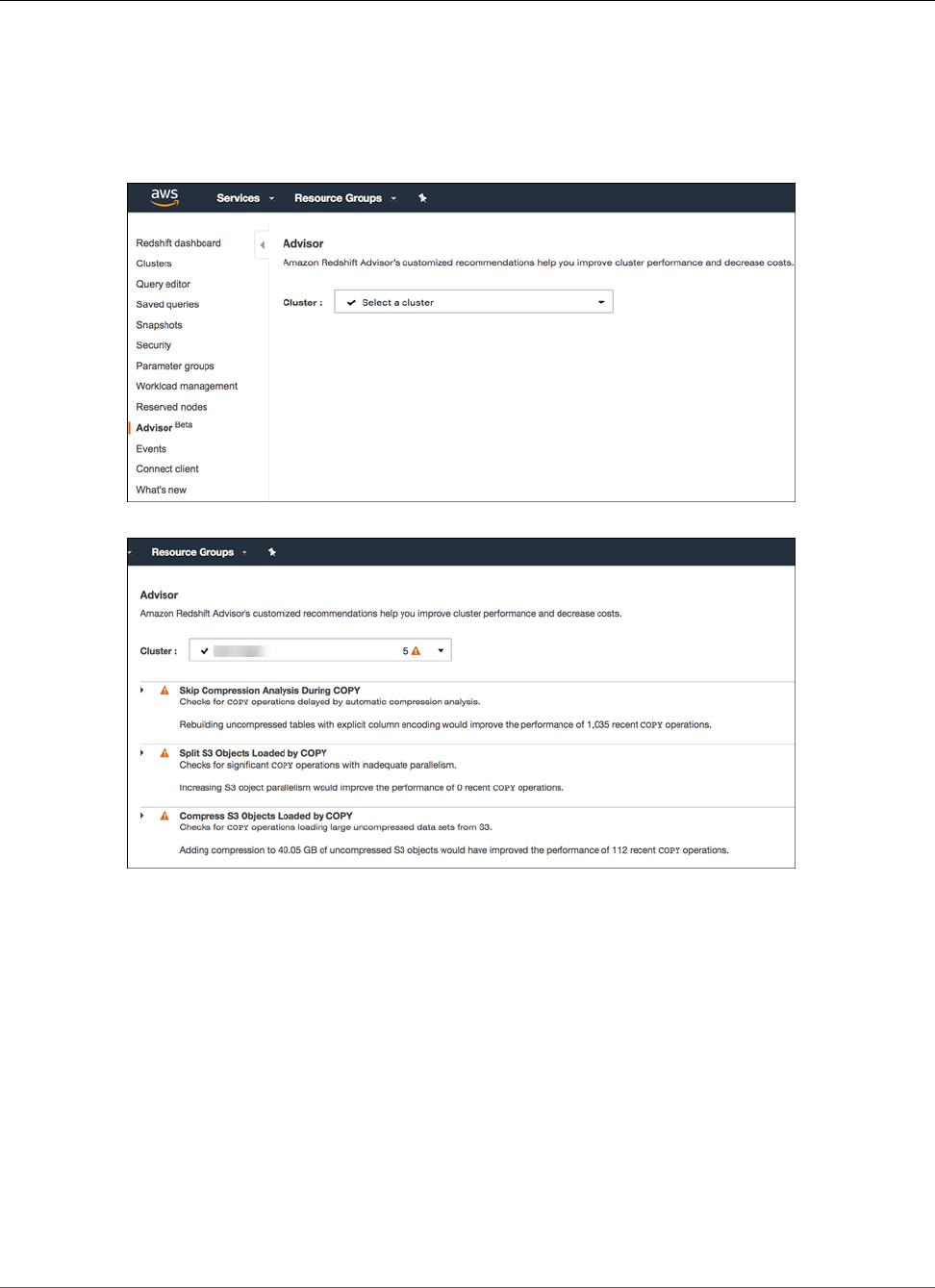
Amazon Redshift Database Developer Guide
Advisor Recommendations
To view Amazon Redshift Advisor recommendations in the console
1. Sign in to the AWS Management Console and open the Amazon Redshift console at https://
console.aws.amazon.com/redshift/.
2. In the navigation pane, choose Advisor.
3. Choose the cluster that you want to get recommendations for.
4. Expand each recommendation to see more details.
Amazon Redshift Advisor Recommendations
Amazon Redshift Advisor offers recommendations about how to optimize your Amazon Redshift
cluster to increase performance and save on operating costs. You can find explanations for each
recommendation in the console, as described preceding. You can find further details on these
recommendations in the following sections.
Topics
•Compress Table Data (p. 36)
•Compress Amazon S3 File Objects Loaded by COPY (p. 37)
•Isolate Multiple Active Databases (p. 38)
•Reallocate Workload Management (WLM) Memory (p. 38)
•Skip Compression Analysis During COPY (p. 40)
•Split Amazon S3 Objects Loaded by COPY (p. 41)
API Version 2012-12-01
35
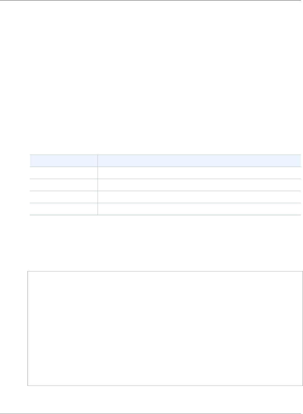
Amazon Redshift Database Developer Guide
Advisor Recommendations
•Update Table Statistics (p. 42)
•Enable Short Query Acceleration (p. 43)
•Replace Single-Column Interleaved Sort Keys (p. 44)
Compress Table Data
Amazon Redshift is optimized to reduce your storage footprint and improve query performance by using
compression encodings. When you don't use compression, data consumes additional space and requires
additional disk I/O. Applying compression to large uncompressed columns can have a big impact on your
cluster.
Analysis
The compression analysis in Advisor tracks uncompressed storage allocated to permanent user tables.
It reviews storage metadata associated with large uncompressed columns that aren't sort key columns.
Advisor offers a recommendation to rebuild tables with uncompressed columns when the total amount
of uncompressed storage exceeds 15 percent of total storage space, or at the following node-specific
thresholds.
Cluster Size Threshold
DC2.LARGE 480 GB
DC2.8XLARGE 2.56 TB
DS2.XLARGE 4 TB
DS2.8XLAGE 16 TB
Recommendation
Addressing uncompressed storage for a single table is a one-time optimization that requires the table to
be rebuilt. We recommend that you rebuild any tables that contain uncompressed columns that are both
large and frequently accessed. To identify which tables contain the most uncompressed storage, run the
following SQL command as a superuser.
SELECT
ti.schema||'.'||ti."table" tablename,
raw_size.size uncompressed_mb,
ti.size total_mb
FROM svv_table_info ti
LEFT JOIN (
SELECT tbl table_id, COUNT(*) size
FROM stv_blocklist
WHERE (tbl,col) IN (
SELECT attrelid, attnum-1
FROM pg_attribute
WHERE attencodingtype IN (0,128)
AND attnum>0 AND attsortkeyord != 1)
GROUP BY tbl) raw_size USING (table_id)
WHERE raw_size.size IS NOT NULL
ORDER BY raw_size.size DESC;
The data returned in the uncompressed_mb column represents the total number of uncompressed 1-
MB blocks for all columns in the table.
API Version 2012-12-01
36

Amazon Redshift Database Developer Guide
Advisor Recommendations
When you rebuild the tables, use the ENCODE parameter to explicitly set column compression.
Implementation Tips
• Leave any columns that are the first column in a compound sort key uncompressed. The Advisor
analysis doesn't count the storage consumed by those columns.
• Compressing large columns has a higher impact on performance and storage than compressing small
columns.
• If you are unsure which compression is best, use the ANALYZE COMPRESSION (p. 382) command to
suggest a compression.
• To generate the data definition language (DDL) statements for existing tables, you can use the AWS
Generate Table DDL utility, found on GitHub.
• To simplify the compression suggestions and the process of rebuilding tables, you can use the Amazon
Redshift Column Encoding Utility, found on GitHub.
Compress Amazon S3 File Objects Loaded by COPY
The COPY command takes advantage of the massively parallel processing (MPP) architecture in Amazon
Redshift to read and load data in parallel. It can read files from Amazon S3, DynamoDB tables, and text
output from one or more remote hosts.
When loading large amounts of data, we strongly recommend using the COPY command to load
compressed data files from S3. Compressing large datasets saves time uploading the files to S3. COPY
can also speed up the load process by uncompressing the files as they are read.
Analysis
Long-running COPY commands that load large uncompressed datasets often have an opportunity for
considerable performance improvement. The Advisor analysis identifies COPY commands that load large
uncompressed datasets. In such a case, Advisor generates a recommendation to implement compression
on the source files in S3.
Recommendation
Ensure that each COPY that loads a significant amount of data, or runs for a significant duration, ingests
compressed data objects from S3. You can identify the COPY commands that load large uncompressed
datasets from S3 by running the following SQL command as a superuser.
SELECT
wq.userid, query, exec_start_time AS starttime, COUNT(*) num_files,
ROUND(MAX(wq.total_exec_time/1000000.0),2) execution_secs,
ROUND(SUM(transfer_size)/(1024.0*1024.0),2) total_mb,
SUBSTRING(querytxt,1,60) copy_sql
FROM stl_s3client s
JOIN stl_query q USING (query)
JOIN stl_wlm_query wq USING (query)
WHERE s.userid>1 AND http_method = 'GET'
AND POSITION('COPY ANALYZE' IN querytxt) = 0
AND aborted = 0 AND final_state='Completed'
GROUP BY 1, 2, 3, 7
HAVING SUM(transfer_size) = SUM(data_size)
AND SUM(transfer_size)/(1024*1024) >= 5
ORDER BY 6 DESC, 5 DESC;
If the staged data remains in S3 after you load it, which is common in data lake architectures, storing this
data in a compressed form can reduce your storage costs.
API Version 2012-12-01
37
Amazon Redshift Database Developer Guide
Advisor Recommendations
Implementation Tips
• The ideal object size is 1–128 MB after compression.
• You can compress files with gzip, lzop, or bzip2 format.
Isolate Multiple Active Databases
As a best practice, we recommend isolating databases in Amazon Redshift from one another. Queries
run in a specific database and can't access data from any other database on the cluster. However, the
queries that you run in all databases of a cluster share the same underlying cluster storage space and
compute resources. When a single cluster contains multiple active databases, their workloads are usually
unrelated.
Analysis
The Advisor analysis reviews all databases on the cluster for active workloads running at the same time.
If there are active workloads running at the same time, Advisor generates a recommendation to consider
migrating databases to separate Amazon Redshift clusters.
Recommendation
Consider moving each actively queried database to a separate dedicated cluster. Using a separate cluster
can reduce resource contention and improve query performance. It can do so because it enables you
to set the size for each cluster for the storage, cost, and performance needs of each workload. Also,
unrelated workloads often benefit from different workload management configurations.
To identify which databases are actively used, you can run this SQL command as a superuser.
SELECT database,
COUNT(*) as num_queries,
AVG(DATEDIFF(sec,starttime,endtime)) avg_duration,
MIN(starttime) as oldest_ts,
MAX(endtime) as latest_ts
FROM stl_query
WHERE userid > 1
GROUP BY database;
Implementation Tips
• Because a user must connect to each database specifically, and queries can only access a single
database, moving databases to separate clusters has minimal impact for users.
• One option to move a database is to take the following steps:
1. Temporarily restore a snapshot of the current cluster to a cluster of the same size.
2. Delete all databases from the new cluster except the target database to be moved.
3. Resize the cluster to an appropriate node type and count for the database's workload.
Reallocate Workload Management (WLM) Memory
Amazon Redshift routes user queries to Defining Query Queues (p. 285) for processing. Workload
management (WLM) defines how those queries are routed to the queues. Amazon Redshift allocates each
queue a portion of the cluster's available memory. A queue's memory is divided among the queue's query
slots.
API Version 2012-12-01
38

Amazon Redshift Database Developer Guide
Advisor Recommendations
When a queue is configured with more slots than the workload requires, the memory allocated to these
unused slots goes underutilized. Reducing the configured slots to match the peak workload requirements
redistributes the underutilized memory to active slots, and can result in improved query performance.
Analysis
The Advisor analysis reviews workload concurrency requirements to identify query queues with unused
slots. Advisor generates a recommendation to reduce the number of slots in a queue when it finds the
following:
• A queue with slots that are completely inactive throughout the analysis
• A queue with more than four slots that had at least two inactive slots throughout the analysis
Recommendation
Reducing the configured slots to match peak workload requirements redistributes underutilized memory
to active slots. Consider reducing the configured slot count for queues where the slots have never been
fully utilized. To identify these queues, you can compare the peak hourly slot requirements for each
queue by running the following SQL command as a superuser.
WITH
generate_dt_series AS (select sysdate - (n * interval '5 second') as dt from (select
row_number() over () as n from stl_scan limit 17280)),
apex AS (
SELECT iq.dt, iq.service_class, iq.num_query_tasks, count(iq.slot_count) as
service_class_queries, sum(iq.slot_count) as service_class_slots
FROM
(select gds.dt, wq.service_class, wscc.num_query_tasks, wq.slot_count
FROM stl_wlm_query wq
JOIN stv_wlm_service_class_config wscc ON (wscc.service_class = wq.service_class
AND wscc.service_class > 5)
JOIN generate_dt_series gds ON (wq.service_class_start_time <= gds.dt AND
wq.service_class_end_time > gds.dt)
WHERE wq.userid > 1 AND wq.service_class > 5) iq
GROUP BY iq.dt, iq.service_class, iq.num_query_tasks),
maxes as (SELECT apex.service_class, trunc(apex.dt) as d, date_part(h,apex.dt) as
dt_h, max(service_class_slots) max_service_class_slots
from apex group by apex.service_class, apex.dt, date_part(h,apex.dt))
SELECT apex.service_class - 5 AS queue, apex.service_class, apex.num_query_tasks AS
max_wlm_concurrency, maxes.d AS day, maxes.dt_h || ':00 - ' || maxes.dt_h || ':59' as
hour, MAX(apex.service_class_slots) as max_service_class_slots
FROM apex
JOIN maxes ON (apex.service_class = maxes.service_class AND apex.service_class_slots =
maxes.max_service_class_slots)
GROUP BY apex.service_class, apex.num_query_tasks, maxes.d, maxes.dt_h
ORDER BY apex.service_class, maxes.d, maxes.dt_h;
The max_service_class_slots column represents the maximum number of WLM query slots in the
query queue for that hour. If underutilized queues exist, implement the slot reduction optimization by
modifying a parameter group, as described in the Amazon Redshift Cluster Management Guide.
Implementation Tips
• If your workload is highly variable in volume, make sure that the analysis captured a peak utilization
period. If it didn't, run the preceding SQL repeatedly to monitor peak concurrency requirements.
• For more details on interpreting the query results from the preceding SQL code, see the
wlm_apex_hourly.sql script on GitHub.
API Version 2012-12-01
39

Amazon Redshift Database Developer Guide
Advisor Recommendations
Skip Compression Analysis During COPY
When you load data into an empty table with compression encoding declared with the COPY command,
Amazon Redshift applies storage compression. This optimization ensures that data in your cluster is
stored efficiently even when loaded by end users. The analysis required to apply compression can require
significant time.
Analysis
The Advisor analysis checks for COPY operations that were delayed by automatic compression analysis.
The analysis determines the compression encodings by sampling the data while it's being loaded. This
sampling is similar to that performed by the ANALYZE COMPRESSION (p. 382) command.
When you load data as part of a structured process, such as in an overnight extract, transform, load
(ETL) batch, you can define the compression beforehand. You can also optimize your table definitions to
permanently skip this phase without any negative impacts.
Recommendation
To improve COPY responsiveness by skipping the compression analysis phase, implement either of the
following two options:
• Use the column ENCODE parameter when creating any tables that you load using the COPY command.
• Disable compression altogether by supplying the COMPUPDATE OFF parameter in the COPY command.
The best solution is generally to use column encoding during table creation, because this approach also
maintains the benefit of storing compressed data on disk. You can use the ANALYZE COMPRESSION
command to suggest compression encodings, but you must recreate the table to apply these encodings.
To automate this process, you can use the AWS ColumnEncodingUtility, found on GitHub.
To identify recent COPY operations that triggered automatic compression analysis, run the following SQL
command.
WITH xids AS (
SELECT xid FROM stl_query WHERE userid>1 AND aborted=0
AND querytxt = 'analyze compression phase 1' GROUP BY xid
INTERSECT SELECT xid FROM stl_commit_stats WHERE node=-1)
SELECT a.userid, a.query, a.xid, a.starttime, b.complyze_sec,
a.copy_sec, a.copy_sql
FROM (SELECT q.userid, q.query, q.xid, date_trunc('s',q.starttime)
starttime, substring(querytxt,1,100) as copy_sql,
ROUND(datediff(ms,starttime,endtime)::numeric / 1000.0, 2) copy_sec
FROM stl_query q JOIN xids USING (xid)
WHERE (querytxt ilike 'copy %from%' OR querytxt ilike '% copy %from%')
AND querytxt not like 'COPY ANALYZE %') a
LEFT JOIN (SELECT xid,
ROUND(sum(datediff(ms,starttime,endtime))::numeric / 1000.0,2) complyze_sec
FROM stl_query q JOIN xids USING (xid)
WHERE (querytxt like 'COPY ANALYZE %'
OR querytxt like 'analyze compression phase %')
GROUP BY xid ) b ON a.xid = b.xid
WHERE b.complyze_sec IS NOT NULL ORDER BY a.copy_sql, a.starttime;
Implementation Tips
• Ensure that all tables of significant size created during your ETL processes (for example, staging tables
and temporary tables) declare a compression encoding for all columns except the first sort key.
API Version 2012-12-01
40

Amazon Redshift Database Developer Guide
Advisor Recommendations
• Estimate the expected lifetime size of the table being loaded for each of the COPY commands
identified by the SQL command preceding. If you are confident that the table will remain extremely
small, disable compression altogether with the COMPUPDATE OFF parameter. Otherwise, create the
table with explicit compression before loading it with the COPY command.
Split Amazon S3 Objects Loaded by COPY
The COPY command takes advantage of the massively parallel processing (MPP) architecture in
Amazon Redshift to read and load data from files on Amazon S3. The COPY command loads the data in
parallel from multiple files, dividing the workload among the nodes in your cluster. To achieve optimal
throughput, we strongly recommend that you divide your data into multiple files to take advantage of
parallel processing.
Analysis
The Advisor analysis identifies COPY commands that load large datasets contained in a small number of
files staged in S3. Long-running COPY commands that load large datasets from a few files often have
an opportunity for considerable performance improvement. When Advisor identifies that these COPY
commands are taking a significant amount of time, it creates a recommendation to increase parallelism
by splitting the data into additional files in S3.
Recommendation
In this case, we recommend the following actions, listed in priority order:
1. Optimize COPY commands that load fewer files than the number of cluster nodes.
2. Optimize COPY commands that load fewer files than the number of cluster slices.
3. Optimize COPY commands where the number of files is not a multiple of the number of cluster slices.
Certain COPY commands load a significant amount of data or run for a significant duration. For these
commands, we recommend that you load a number of data objects from S3 that is equivalent to a
multiple of the number of slices in the cluster. To identify how many S3 objects each COPY command has
loaded, run the following SQL code as a superuser.
SELECT
query, COUNT(*) num_files,
ROUND(MAX(wq.total_exec_time/1000000.0),2) execution_secs,
ROUND(SUM(transfer_size)/(1024.0*1024.0),2) total_mb,
SUBSTRING(querytxt,1,60) copy_sql
FROM stl_s3client s
JOIN stl_query q USING (query)
JOIN stl_wlm_query wq USING (query)
WHERE s.userid>1 AND http_method = 'GET'
AND POSITION('COPY ANALYZE' IN querytxt) = 0
AND aborted = 0 AND final_state='Completed'
GROUP BY query, querytxt
HAVING (SUM(transfer_size)/(1024*1024))/COUNT(*) >= 2
ORDER BY CASE
WHEN COUNT(*) < (SELECT max(node)+1 FROM stv_slices) THEN 1
WHEN COUNT(*) < (SELECT COUNT(*) FROM stv_slices WHERE node=0) THEN 2
ELSE 2+((COUNT(*) % (SELECT COUNT(*) FROM stv_slices))/(SELECT COUNT(*)::DECIMAL FROM
stv_slices))
END, (SUM(transfer_size)/(1024.0*1024.0))/COUNT(*) DESC;
Implementation Tips
API Version 2012-12-01
41

Amazon Redshift Database Developer Guide
Advisor Recommendations
• The number of slices in a node depends on the node size of the cluster. For more information about
the number of slices in the various node types, see Clusters and Nodes in Amazon Redshift in the
Amazon Redshift Cluster Management Guide.
• You can load multiple files by specifying a common prefix, or prefix key, for the set, or by explicitly
listing the files in a manifest file. For more information about loading files, see Splitting Your Data into
Multiple Files (p. 187).
• Amazon Redshift doesn't take file size into account when dividing the workload. Split your load data
files so that the files are about equal size, between 1 MB and 1 GB after compression. For optimum
parallelism, the ideal size is between 1 MB and 125 MB after compression.
Update Table Statistics
Amazon Redshift uses a cost-based query optimizer to choose the optimum execution plan for queries.
The cost estimates are based on table statistics gathered using the ANALYZE command. When statistics
are out of date or missing, the database might choose a less efficient plan for query execution, especially
for complex queries. Maintaining current statistics helps complex queries run in the shortest possible
time.
Analysis
The Advisor analysis tracks tables whose statistics are out-of-date or missing. It reviews table access
metadata associated with complex queries. If tables that are frequently accessed with complex patterns
are missing statistics, Advisor creates a critical recommendation to run ANALYZE. If tables that are
frequently accessed with complex patterns have out-of-date statistics, Advisor creates a suggested
recommendation to run ANALYZE.
Recommendation
Whenever table content changes significantly, update statistics with ANALYZE. We recommend running
ANALYZE whenever a significant number of new data rows are loaded into an existing table with COPY
or INSERT commands. We also recommend running ANALYZE whenever a significant number of rows are
modified using UPDATE or DELETE commands. To identify tables with missing or out-of-date statistics,
run the following SQL command as a superuser. The results are ordered from largest to smallest table.
To identify tables with missing or out-of-date statistics, run the following SQL command as a superuser.
The results are ordered from largest to smallest table.
SELECT
ti.schema||'.'||ti."table" tablename,
ti.size table_size_mb,
ti.stats_off statistics_accuracy
FROM svv_table_info ti
WHERE ti.stats_off > 5.00
ORDER BY ti.size DESC;
Implementation Tips
The default ANALYZE threshold is 10 percent. This default means that the ANALYZE command skips a
given table if fewer than 10 percent of the table's rows have changed since the last ANALYZE. As a result,
you might choose to issue ANALYZE commands at the end of each ETL process. Taking this approach
means that ANALYZE is often skipped but also ensures that ANALYZE runs when needed.
ANALYZE statistics have the most impact for columns that are used in joins (for example, JOIN tbl_a
ON col_b) or as predicates (for example, WHERE col_b = 'xyz'). By default, ANALYZE collects
statistics for all columns in the table specified. If needed, you can reduce the time required to run
API Version 2012-12-01
42

Amazon Redshift Database Developer Guide
Advisor Recommendations
ANALYZE by running ANALYZE only for the columns where it has the most impact. You can run the
following SQL command to identify columns used as predicates. You can also let Amazon Redshift
choose which columns to analyze by specifying ANALYZE PREDICATE COLUMNS.
WITH predicate_column_info as (
SELECT ns.nspname AS schema_name, c.relname AS table_name, a.attnum as col_num, a.attname
as col_name,
CASE
WHEN 10002 = s.stakind1 THEN array_to_string(stavalues1, '||')
WHEN 10002 = s.stakind2 THEN array_to_string(stavalues2, '||')
WHEN 10002 = s.stakind3 THEN array_to_string(stavalues3, '||')
WHEN 10002 = s.stakind4 THEN array_to_string(stavalues4, '||')
ELSE NULL::varchar
END AS pred_ts
FROM pg_statistic s
JOIN pg_class c ON c.oid = s.starelid
JOIN pg_namespace ns ON c.relnamespace = ns.oid
JOIN pg_attribute a ON c.oid = a.attrelid AND a.attnum = s.staattnum)
SELECT schema_name, table_name, col_num, col_name,
pred_ts NOT LIKE '2000-01-01%' AS is_predicate,
CASE WHEN pred_ts NOT LIKE '2000-01-01%' THEN (split_part(pred_ts,
'||',1))::timestamp ELSE NULL::timestamp END as first_predicate_use,
CASE WHEN pred_ts NOT LIKE '%||2000-01-01%' THEN (split_part(pred_ts,
'||',2))::timestamp ELSE NULL::timestamp END as last_analyze
FROM predicate_column_info;
For more information, see Analyzing Tables (p. 223).
Enable Short Query Acceleration
Short query acceleration (SQA) prioritizes selected short-running queries ahead of longer-running
queries. SQA executes short-running queries in a dedicated space, so that SQA queries aren't forced to
wait in queues behind longer queries. SQA only prioritizes queries that are short-running and are in a
user-defined queue. With SQA, short-running queries begin running more quickly and users see results
sooner.
If you enable SQA, you can reduce or eliminate workload management (WLM) queues that are dedicated
to running short queries. In addition, long-running queries don't need to contend with short queries
for slots in a queue, so you can configure your WLM queues to use fewer query slots. When you use
lower concurrency, query throughput is increased and overall system performance is improved for most
workloads. For more information, see Short Query Acceleration (p. 291).
Analysis
Advisor checks for workload patterns and reports the number of recent queries where SQA would reduce
latency and the daily queue time for SQA-eligible queries.
Recommendation
Modify the WLM configuration to enable SQA. Amazon Redshift uses a machine learning algorithm
to analyze each eligible query. Predictions improve as SQA learns from your query patterns. For more
information, see Configuring Workload Management.
When you enable SQA, WLM sets the maximum run time for short queries to dynamic by default. We
recommend keeping the dynamic setting for SQA maximum run time.
Implementation Tips
To check whether SQA is enabled, run the following query. If the query returns a row, then SQA is
enabled.
API Version 2012-12-01
43

Amazon Redshift Database Developer Guide
Advisor Recommendations
select * from stv_wlm_service_class_config
where service_class = 14;
For more information, see Monitoring SQA (p. 292).
Replace Single-Column Interleaved Sort Keys
Some tables use an interleaved sort key on a single column. In general, such a table is less efficient and
consumes more resources than a table that uses a compound sort key on a single column.
Interleaved sorting improves performance in certain cases where multiple columns are used by different
queries for filtering. Using an interleaved sort key on a single column is effective only in a particular case.
That case is when queries often filter on CHAR or VARCHAR column values that have a long common
prefix in the first 8 bytes. For example, URL strings are often prefixed with "https://". For single-
column keys, a compound sort is better than an interleaved sort for any other filtering operations. A
compound sort speeds up joins, GROUP BY and ORDER BY operations, and window functions that use
PARTITION BY and ORDER BY on the sorted column. An interleaved sort doesn't benefit any of those
operations. For more information, see Choosing Sort Keys (p. 140).
Using compound sort significantly reduces maintenance overhead. Tables with compound sort keys don't
need the expensive VACUUM REINDEX operations that are necessary for interleaved sorts. In practice,
compound sort keys are more effective than interleaved sort keys for the vast majority of Amazon
Redshift workloads.
Analysis
Advisor tracks tables that use an interleaved sort key on a single column.
Recommendation
If a table uses interleaved sorting on a single column, recreate the table to use a compound sort key.
When you create new tables, use a compound sort key for single-column sorts. To find interleaved tables
that use a single-column sort key, run the following command.
SELECT schema AS schemaname, "table" AS tablename
FROM svv_table_info
WHERE table_id IN (
SELECT attrelid
FROM pg_attribute
WHERE attrelid IN (
SELECT attrelid
FROM pg_attribute
WHERE attsortkeyord <> 0
GROUP BY attrelid
HAVING MAX(attsortkeyord) = -1
)
AND NOT (atttypid IN (1042, 1043) AND atttypmod > 12)
AND attsortkeyord = -1);
For additional information about choosing the best sort style, see the AWS Big Data Blog post Amazon
Redshift Engineering's Advanced Table Design Playbook: Compound and Interleaved Sort Keys.
API Version 2012-12-01
44

Amazon Redshift Database Developer Guide
Prerequisites
Tutorial: Tuning Table Design
In this tutorial, you will learn how to optimize the design of your tables. You will start by creating
tables based on the Star Schema Benchmark (SSB) schema without sort keys, distribution styles, and
compression encodings. You will load the tables with test data and test system performance. Next, you
will apply best practices to recreate the tables using sort keys and distribution styles. You will load the
tables with test data using automatic compression and then you will test performance again so that you
can compare the performance benefits of well-designed tables.
Estimated time: 60 minutes
Estimated cost: $1.00 per hour for the cluster
Prerequisites
You will need your AWS credentials (access key ID and secret access key) to load test data from Amazon
S3. If you need to create new access keys, go to Administering Access Keys for IAM Users.
Steps
•Step 1: Create a Test Data Set (p. 45)
•Step 2: Test System Performance to Establish a Baseline (p. 49)
•Step 3: Select Sort Keys (p. 52)
•Step 4: Select Distribution Styles (p. 53)
•Step 5: Review Compression Encodings (p. 57)
•Step 6: Recreate the Test Data Set (p. 59)
•Step 7: Retest System Performance After Tuning (p. 62)
•Step 8: Evaluate the Results (p. 66)
•Step 9: Clean Up Your Resources (p. 68)
•Summary (p. 68)
Step 1: Create a Test Data Set
Data warehouse databases commonly use a star schema design, in which a central fact table contains
the core data for the database and several dimension tables provide descriptive attribute information for
the fact table. The fact table joins each dimension table on a foreign key that matches the dimension's
primary key.
Star Schema Benchmark (SSB)
For this tutorial, you will use a set of five tables based on the Star Schema Benchmark (SSB) schema. The
following diagram shows the SSB data model.
API Version 2012-12-01
45
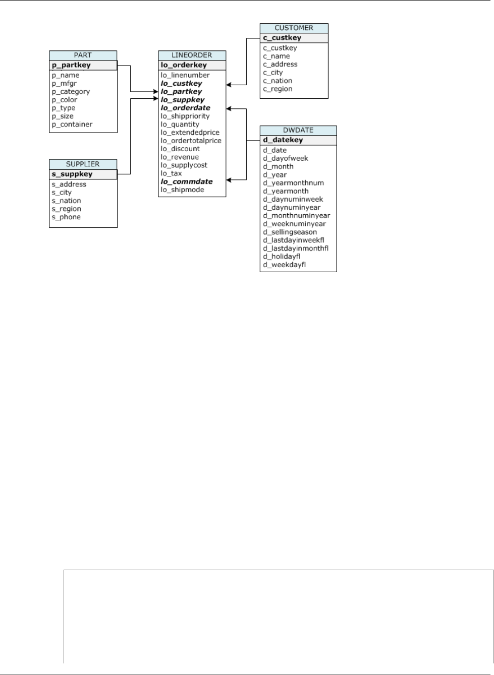
Amazon Redshift Database Developer Guide
To Create a Test Data Set
To Create a Test Data Set
You will create a set of tables without sort keys, distribution styles, or compression encodings. Then you
will load the tables with data from the SSB data set.
1. (Optional) Launch a cluster.
If you already have a cluster that you want to use, you can skip this step. Your cluster should have at
least two nodes. For the exercises in this tutorial, you will use a four-node cluster.
To launch a dc1.large cluster with four nodes, follow the steps in Amazon Redshift Getting Started,
but select Multi Node for Cluster Type and set Number of Compute Nodes to 4.
Follow the steps to connect to your cluster from a SQL client and test a connection. You do not need
to complete the remaining steps to create tables, upload data, and try example queries.
2. Create the SSB test tables using minimum attributes.
Note
If the SSB tables already exist in the current database, you will need to drop the tables first.
See Step 6: Recreate the Test Data Set (p. 59) for the DROP TABLE commands.
For the purposes of this tutorial, the first time you create the tables, they will not have sort keys,
distribution styles, or compression encodings.
Execute the following CREATE TABLE commands.
CREATE TABLE part
(
p_partkey INTEGER NOT NULL,
p_name VARCHAR(22) NOT NULL,
p_mfgr VARCHAR(6) NOT NULL,
p_category VARCHAR(7) NOT NULL,
p_brand1 VARCHAR(9) NOT NULL,
p_color VARCHAR(11) NOT NULL,
p_type VARCHAR(25) NOT NULL,
API Version 2012-12-01
46

Amazon Redshift Database Developer Guide
To Create a Test Data Set
p_size INTEGER NOT NULL,
p_container VARCHAR(10) NOT NULL
);
CREATE TABLE supplier
(
s_suppkey INTEGER NOT NULL,
s_name VARCHAR(25) NOT NULL,
s_address VARCHAR(25) NOT NULL,
s_city VARCHAR(10) NOT NULL,
s_nation VARCHAR(15) NOT NULL,
s_region VARCHAR(12) NOT NULL,
s_phone VARCHAR(15) NOT NULL
);
CREATE TABLE customer
(
c_custkey INTEGER NOT NULL,
c_name VARCHAR(25) NOT NULL,
c_address VARCHAR(25) NOT NULL,
c_city VARCHAR(10) NOT NULL,
c_nation VARCHAR(15) NOT NULL,
c_region VARCHAR(12) NOT NULL,
c_phone VARCHAR(15) NOT NULL,
c_mktsegment VARCHAR(10) NOT NULL
);
CREATE TABLE dwdate
(
d_datekey INTEGER NOT NULL,
d_date VARCHAR(19) NOT NULL,
d_dayofweek VARCHAR(10) NOT NULL,
d_month VARCHAR(10) NOT NULL,
d_year INTEGER NOT NULL,
d_yearmonthnum INTEGER NOT NULL,
d_yearmonth VARCHAR(8) NOT NULL,
d_daynuminweek INTEGER NOT NULL,
d_daynuminmonth INTEGER NOT NULL,
d_daynuminyear INTEGER NOT NULL,
d_monthnuminyear INTEGER NOT NULL,
d_weeknuminyear INTEGER NOT NULL,
d_sellingseason VARCHAR(13) NOT NULL,
d_lastdayinweekfl VARCHAR(1) NOT NULL,
d_lastdayinmonthfl VARCHAR(1) NOT NULL,
d_holidayfl VARCHAR(1) NOT NULL,
d_weekdayfl VARCHAR(1) NOT NULL
);
CREATE TABLE lineorder
(
lo_orderkey INTEGER NOT NULL,
lo_linenumber INTEGER NOT NULL,
lo_custkey INTEGER NOT NULL,
lo_partkey INTEGER NOT NULL,
lo_suppkey INTEGER NOT NULL,
lo_orderdate INTEGER NOT NULL,
lo_orderpriority VARCHAR(15) NOT NULL,
lo_shippriority VARCHAR(1) NOT NULL,
lo_quantity INTEGER NOT NULL,
lo_extendedprice INTEGER NOT NULL,
lo_ordertotalprice INTEGER NOT NULL,
lo_discount INTEGER NOT NULL,
lo_revenue INTEGER NOT NULL,
lo_supplycost INTEGER NOT NULL,
lo_tax INTEGER NOT NULL,
lo_commitdate INTEGER NOT NULL,
lo_shipmode VARCHAR(10) NOT NULL
API Version 2012-12-01
47

Amazon Redshift Database Developer Guide
To Create a Test Data Set
);
3. Load the tables using SSB sample data.
The sample data for this tutorial is provided in an Amazon S3 buckets that give read access to all
authenticated AWS users, so any valid AWS credentials that permit access to Amazon S3 will work.
a. Create a new text file named loadssb.sql containing the following SQL.
copy customer from 's3://awssampledbuswest2/ssbgz/customer'
credentials 'aws_access_key_id=<Your-Access-Key-ID>;aws_secret_access_key=<Your-
Secret-Access-Key>'
gzip compupdate off region 'us-west-2';
copy dwdate from 's3://awssampledbuswest2/ssbgz/dwdate'
credentials 'aws_access_key_id=<Your-Access-Key-ID>;aws_secret_access_key=<Your-
Secret-Access-Key>'
gzip compupdate off region 'us-west-2';
copy lineorder from 's3://awssampledbuswest2/ssbgz/lineorder'
credentials 'aws_access_key_id=<Your-Access-Key-ID>;aws_secret_access_key=<Your-
Secret-Access-Key>'
gzip compupdate off region 'us-west-2';
copy part from 's3://awssampledbuswest2/ssbgz/part'
credentials 'aws_access_key_id=<Your-Access-Key-ID>;aws_secret_access_key=<Your-
Secret-Access-Key>'
gzip compupdate off region 'us-west-2';
copy supplier from 's3://awssampledbuswest2/ssbgz/supplier'
credentials 'aws_access_key_id=<Your-Access-Key-ID>;aws_secret_access_key=<Your-
Secret-Access-Key>'
gzip compupdate off region 'us-west-2';
b. Replace <Your-Access-Key-ID> and <Your-Secret-Access-Key> with your own AWS
account credentials. The segment of the credentials string that is enclosed in single quotes must
not contain any spaces or line breaks.
c. Execute the COPY commands either by running the SQL script or by copying and pasting the
commands into your SQL client.
Note
The load operation will take about 10 to 15 minutes for all five tables.
Your results should look similar to the following.
Load into table 'customer' completed, 3000000 record(s) loaded successfully.
0 row(s) affected.
copy executed successfully
Execution time: 10.28s
(Statement 1 of 5 finished)
...
...
Script execution finished
Total script execution time: 9m 51s
4. Sum the execution time for all five tables, or else note the total script execution time. You’ll record
that number as the load time in the benchmarks table in Step 2, following.
5. To verify that each table loaded correctly, execute the following commands.
select count(*) from LINEORDER;
API Version 2012-12-01
48
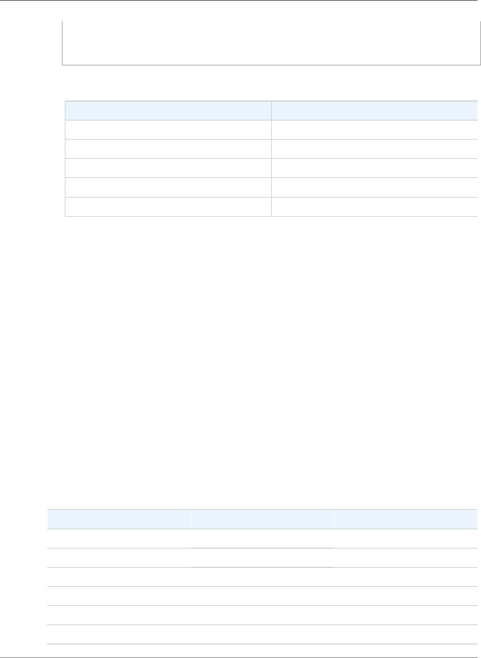
Amazon Redshift Database Developer Guide
Next Step
select count(*) from PART;
select count(*) from CUSTOMER;
select count(*) from SUPPLIER;
select count(*) from DWDATE;
The following results table shows the number of rows for each SSB table.
Table Name Rows
LINEORDER 600,037,902
PART 1,400,000
CUSTOMER 3,000,000
SUPPLIER 1,000,000
DWDATE 2,556
Next Step
Step 2: Test System Performance to Establish a Baseline (p. 49)
Step 2: Test System Performance to Establish a
Baseline
As you test system performance before and after tuning your tables, you will record the following
details:
• Load time
• Storage use
• Query performance
The examples in this tutorial are based on using a four-node dw2.large cluster. Your results will be
different, even if you use the same cluster configuration. System performance is influenced by many
factors, and no two systems will perform exactly the same.
You will record your results using the following benchmarks table.
Benchmark Before After
Load time (five tables)
Storage Use
LINEORDER
PART
CUSTOMER
DWDATE
API Version 2012-12-01
49
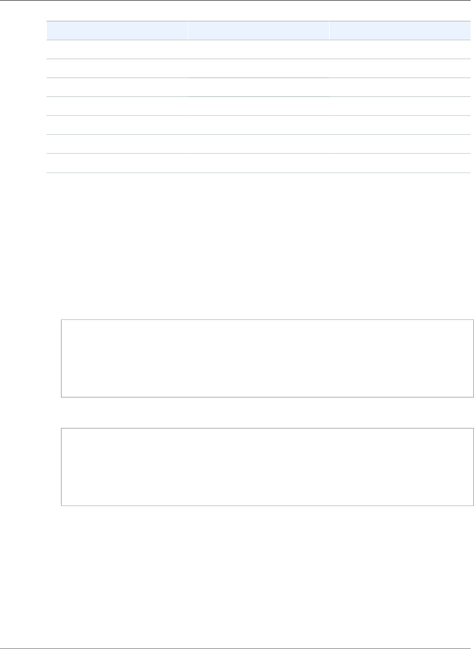
Amazon Redshift Database Developer Guide
To Test System Performance to Establish a Baseline
Benchmark Before After
SUPPLIER
Total storage
Query execution time
Query 1
Query 2
Query 3
Total execution time
To Test System Performance to Establish a Baseline
1. Note the cumulative load time for all five tables and enter it in the benchmarks table in the Before
column.
This is the value you noted in the previous step.
2. Record storage use.
Determine how many 1 MB blocks of disk space are used for each table by querying the
STV_BLOCKLIST table and record the results in your benchmarks table.
select stv_tbl_perm.name as table, count(*) as mb
from stv_blocklist, stv_tbl_perm
where stv_blocklist.tbl = stv_tbl_perm.id
and stv_blocklist.slice = stv_tbl_perm.slice
and stv_tbl_perm.name in ('lineorder','part','customer','dwdate','supplier')
group by stv_tbl_perm.name
order by 1 asc;
Your results should look similar to this:
table | mb
----------+------
customer | 384
dwdate | 160
lineorder | 51024
part | 200
supplier | 152
3. Test query performance.
The first time you run a query, Amazon Redshift compiles the code, and then sends compiled code
to the compute nodes. When you compare the execution times for queries, you should not use the
results for the first time you execute the query. Instead, compare the times for the second execution
of each query. For more information, see Factors Affecting Query Performance (p. 266).
Note
To reduce query execution time and improve system performance, Amazon Redshift caches
the results of certain types of queries in memory on the leader node. When result caching is
enabled, subsequent queries run much faster, which invalidates performance comparisons.
API Version 2012-12-01
50

Amazon Redshift Database Developer Guide
To Test System Performance to Establish a Baseline
To disable result caching for the current session, set the enable_result_cache_for_session (p. 949)
parameter to off, as shown following.
set enable_result_cache_for_session to off;
Run the following queries twice to eliminate compile time. Record the second time for each query in
the benchmarks table.
-- Query 1
-- Restrictions on only one dimension.
select sum(lo_extendedprice*lo_discount) as revenue
from lineorder, dwdate
where lo_orderdate = d_datekey
and d_year = 1997
and lo_discount between 1 and 3
and lo_quantity < 24;
-- Query 2
-- Restrictions on two dimensions
select sum(lo_revenue), d_year, p_brand1
from lineorder, dwdate, part, supplier
where lo_orderdate = d_datekey
and lo_partkey = p_partkey
and lo_suppkey = s_suppkey
and p_category = 'MFGR#12'
and s_region = 'AMERICA'
group by d_year, p_brand1
order by d_year, p_brand1;
-- Query 3
-- Drill down in time to just one month
select c_city, s_city, d_year, sum(lo_revenue) as revenue
from customer, lineorder, supplier, dwdate
where lo_custkey = c_custkey
and lo_suppkey = s_suppkey
and lo_orderdate = d_datekey
and (c_city='UNITED KI1' or
c_city='UNITED KI5')
and (s_city='UNITED KI1' or
s_city='UNITED KI5')
and d_yearmonth = 'Dec1997'
group by c_city, s_city, d_year
order by d_year asc, revenue desc;
Your results for the second time will look something like this:
SELECT executed successfully
Execution time: 6.97s
(Statement 1 of 3 finished)
SELECT executed successfully
Execution time: 12.81s
(Statement 2 of 3 finished)
SELECT executed successfully
Execution time: 13.39s
API Version 2012-12-01
51
Amazon Redshift Database Developer Guide
Next Step
(Statement 3 of 3 finished)
Script execution finished
Total script execution time: 33.17s
The following benchmarks table shows the example results for the cluster used in this tutorial.
Benchmark Before After
Load time (five tables) 10m 23s
Storage Use
LINEORDER 51024
PART 200
CUSTOMER 384
DWDATE 160
SUPPLIER 152
Total storage 51920
Query execution time
Query 1 6.97
Query 2 12.81
Query 3 13.39
Total execution time 33.17
Next Step
Step 3: Select Sort Keys (p. 52)
Step 3: Select Sort Keys
When you create a table, you can specify one or more columns as the sort key. Amazon Redshift stores
your data on disk in sorted order according to the sort key. How your data is sorted has an important
effect on disk I/O, columnar compression, and query performance.
In this step, you choose sort keys for the SSB tables based on these best practices:
• If recent data is queried most frequently, specify the timestamp column as the leading column for the
sort key.
• If you do frequent range filtering or equality filtering on one column, specify that column as the sort
key.
• If you frequently join a (dimension) table, specify the join column as the sort key.
API Version 2012-12-01
52
Amazon Redshift Database Developer Guide
To Select Sort Keys
To Select Sort Keys
1. Evaluate your queries to find timestamp columns that are used to filter the results.
For example, LINEORDER frequently uses equality filters using lo_orderdate.
where lo_orderdate = d_datekey and d_year = 1997
2. Look for columns that are used in range filters and equality filters. For example, LINEORDER also
uses lo_orderdate for range filtering.
where lo_orderdate = d_datekey and d_year >= 1992 and d_year <= 1997
3. Based on the first two best practices, lo_orderdate is a good choice for sort key.
In the tuning table, specify lo_orderdate as the sort key for LINEORDER.
4. The remaining tables are dimensions, so, based on the third best practice, specify their primary keys
as sort keys.
The following tuning table shows the chosen sort keys. You fill in the Distribution Style column in Step 4:
Select Distribution Styles (p. 53).
Table name Sort Key Distribution Style
LINEORDER lo_orderdate
PART p_partkey
CUSTOMER c_custkey
SUPPLIER s_suppkey
DWDATE d_datekey
Next Step
Step 4: Select Distribution Styles (p. 53)
Step 4: Select Distribution Styles
When you load data into a table, Amazon Redshift distributes the rows of the table to each of the node
slices according to the table's distribution style. The number of slices per node depends on the node
size of the cluster. For example, the dc1.large cluster that you are using in this tutorial has four nodes
with two slices each, so the cluster has a total of eight slices. The nodes all participate in parallel query
execution, working on data that is distributed across the slices.
When you execute a query, the query optimizer redistributes the rows to the compute nodes as needed
to perform any joins and aggregations. Redistribution might involve either sending specific rows to
nodes for joining or broadcasting an entire table to all of the nodes.
You should assign distribution styles to achieve these goals.
API Version 2012-12-01
53

Amazon Redshift Database Developer Guide
Distribution Styles
• Collocate the rows from joining tables
When the rows for joining columns are on the same slices, less data needs to be moved during query
execution.
• Distribute data evenly among the slices in a cluster.
If data is distributed evenly, workload can be allocated evenly to all the slices.
These goals may conflict in some cases, and you will need to evaluate which strategy is the best choice
for overall system performance. For example, even distribution might place all matching values for a
column on the same slice. If a query uses an equality filter on that column, the slice with those values
will carry a disproportionate share of the workload. If tables are collocated based on a distribution key,
the rows might be distributed unevenly to the slices because the keys are distributed unevenly through
the table.
In this step, you evaluate the distribution of the SSB tables with respect to the goals of data distribution,
and then select the optimum distribution styles for the tables.
Distribution Styles
When you create a table, you designate one of three distribution styles: KEY, ALL, or EVEN.
KEY distribution
The rows are distributed according to the values in one column. The leader node will attempt to place
matching values on the same node slice. If you distribute a pair of tables on the joining keys, the leader
node collocates the rows on the slices according to the values in the joining columns so that matching
values from the common columns are physically stored together.
ALL distribution
A copy of the entire table is distributed to every node. Where EVEN distribution or KEY distribution place
only a portion of a table's rows on each node, ALL distribution ensures that every row is collocated for
every join that the table participates in.
EVEN distribution
The rows are distributed across the slices in a round-robin fashion, regardless of the values in any
particular column. EVEN distribution is appropriate when a table does not participate in joins or when
there is not a clear choice between KEY distribution and ALL distribution. EVEN distribution is the default
distribution style.
For more information, see Distribution Styles (p. 130).
To Select Distribution Styles
When you execute a query, the query optimizer redistributes the rows to the compute nodes as needed
to perform any joins and aggregations. By locating the data where it needs to be before the query is
executed, you can minimize the impact of the redistribution step.
The first goal is to distribute the data so that the matching rows from joining tables are collocated, which
means that the matching rows from joining tables are located on the same node slice.
1. To look for redistribution steps in the query plan, execute an EXPLAIN command followed by the
query. This example uses Query 2 from our set of test queries.
API Version 2012-12-01
54

Amazon Redshift Database Developer Guide
To Select Distribution Styles
explain
select sum(lo_revenue), d_year, p_brand1
from lineorder, dwdate, part, supplier
where lo_orderdate = d_datekey
and lo_partkey = p_partkey
and lo_suppkey = s_suppkey
and p_category = 'MFGR#12'
and s_region = 'AMERICA'
group by d_year, p_brand1
order by d_year, p_brand1;
The following shows a portion of the query plan. Look for labels that begin with DS_BCAST or
DS_DIST labels
QUERY PLAN
XN Merge (cost=1038007224737.84..1038007224738.54 rows=280 width=20)
Merge Key: dwdate.d_year, part.p_brand1
-> XN Network (cost=1038007224737.84..1038007224738.54 rows=280 width=20)
Send to leader
-> XN Sort (cost=1038007224737.84..1038007224738.54 rows=280 width=20)
Sort Key: dwdate.d_year, part.p_brand1
-> XN HashAggregate (cost=38007224725.76..38007224726.46 rows=280
-> XN Hash Join DS_BCAST_INNER (cost=30674.95..38007188507.46
Hash Cond: ("outer".lo_orderdate = "inner".d_datekey)
-> XN Hash Join DS_BCAST_INNER
(cost=30643.00..37598119820.65
Hash Cond: ("outer".lo_suppkey = "inner".s_suppkey)
-> XN Hash Join DS_BCAST_INNER
Hash Cond: ("outer".lo_partkey =
"inner".p_partkey)
-> XN Seq Scan on lineorder
-> XN Hash (cost=17500.00..17500.00 rows=56000
-> XN Seq Scan on part
(cost=0.00..17500.00
Filter: ((p_category)::text =
-> XN Hash (cost=12500.00..12500.00 rows=201200
-> XN Seq Scan on supplier
(cost=0.00..12500.00
Filter: ((s_region)::text =
'AMERICA'::text)
-> XN Hash (cost=25.56..25.56 rows=2556 width=8)
-> XN Seq Scan on dwdate (cost=0.00..25.56 rows=2556
DS_BCAST_INNER indicates that the inner join table was broadcast to every slice. A DS_DIST_BOTH
label, if present, would indicate that both the outer join table and the inner join table were
redistributed across the slices. Broadcasting and redistribution can be expensive steps in terms of
query performance. You want to select distribution strategies that reduce or eliminate broadcast
and distribution steps. For more information about evaluating the EXPLAIN plan, see Evaluating
Query Patterns (p. 132).
2. Distribute the fact table and one dimension table on their common columns.
The following diagram shows the relationships between the fact table, LINEORDER, and the
dimension tables in the SSB schema.
API Version 2012-12-01
55

Amazon Redshift Database Developer Guide
To Select Distribution Styles
Each table can have only one distribution key, which means that only one pair of tables in the
schema can be collocated on their common columns. The central fact table is the clear first choice.
For the second table in the pair, choose the largest dimension that commonly joins the fact table. In
this design, LINEORDER is the fact table, and PART is the largest dimension. PART joins LINEORDER
on its primary key, p_partkey.
Designate lo_partkey as the distribution key for LINEORDER and p_partkey as the distribution
key for PART so that the matching values for the joining keys will be collocated on the same slices
when the data is loaded.
3. Change some dimension tables to use ALL distribution.
If a dimension table cannot be collocated with the fact table or other important joining tables,
you can often improve query performance significantly by distributing the entire table to all of the
nodes. ALL distribution guarantees that the joining rows will be collocated on every slice. You should
weigh all factors before choosing ALL distribution. Using ALL distribution multiplies storage space
requirements and increases load times and maintenance operations.
CUSTOMER, SUPPLIER, and DWDATE also join the LINEORDER table on their primary keys; however,
LINEORDER will be collocated with PART, so you will set the remaining tables to use DISTSTYLE ALL.
Because the tables are relatively small and are not updated frequently, using ALL distribution will
have minimal impact on storage and load times.
4. Use EVEN distribution for the remaining tables.
All of the tables have been assigned with DISTKEY or ALL distribution styles, so you won't assign
EVEN to any tables. After evaluating your performance results, you might decide to change some
tables from ALL to EVEN distribution.
The following tuning table shows the chosen distribution styles.
Table name Sort Key Distribution Style
LINEORDER lo_orderdate lo_partkey
PART p_partkey p_partkey
CUSTOMER c_custkey ALL
SUPPLIER s_suppkey ALL
DWDATE d_datekey ALL
You can find the steps for setting the distribution style in Step 6: Recreate the Test Data Set (p. 59).
API Version 2012-12-01
56

Amazon Redshift Database Developer Guide
Next Step
For more information, see Choose the Best Distribution Style (p. 27).
Next Step
Step 5: Review Compression Encodings (p. 57)
Step 5: Review Compression Encodings
Compression is a column-level operation that reduces the size of data when it is stored. Compression
conserves storage space and reduces the size of data that is read from storage, which reduces the
amount of disk I/O and therefore improves query performance.
By default, Amazon Redshift stores data in its raw, uncompressed format. When you create tables in an
Amazon Redshift database, you can define a compression type, or encoding, for the columns. For more
information, see Compression Encodings (p. 119).
You can apply compression encodings to columns in tables manually when you create the tables, or you
can use the COPY command to analyze the load data and apply compression encodings automatically.
To Review Compression Encodings
1. Find how much space each column uses.
Query the STV_BLOCKLIST system view to find the number of 1 MB blocks each column uses. The
MAX aggregate function returns the highest block number for each column. This example uses col
< 17 in the WHERE clause to exclude system-generated columns.
Execute the following command.
select col, max(blocknum)
from stv_blocklist b, stv_tbl_perm p
where (b.tbl=p.id) and name ='lineorder'
and col < 17
group by name, col
order by col;
Your results will look similar to the following.
col | max
----+-----
0 | 572
1 | 572
2 | 572
3 | 572
4 | 572
5 | 572
6 | 1659
7 | 715
8 | 572
9 | 572
10 | 572
11 | 572
12 | 572
13 | 572
14 | 572
15 | 572
API Version 2012-12-01
57
Amazon Redshift Database Developer Guide
To Review Compression Encodings
16 | 1185
(17 rows)
2. Experiment with the different encoding methods.
In this step, you create a table with identical columns, except that each column uses a different
compression encoding. Then you insert a large number of rows, using data from the p_name column
in the PART table, so that every column has the same data. Finally, you will examine the table to
compare the effects of the different encodings on column sizes.
a. Create a table with the encodings that you want to compare.
create table encodingshipmode (
moderaw varchar(22) encode raw,
modebytedict varchar(22) encode bytedict,
modelzo varchar(22) encode lzo,
moderunlength varchar(22) encode runlength,
modetext255 varchar(22) encode text255,
modetext32k varchar(22) encode text32k);
b. Insert the same data into all of the columns using an INSERT statement with a SELECT clause.
The command will take a couple minutes to execute.
insert into encodingshipmode
select lo_shipmode as moderaw, lo_shipmode as modebytedict, lo_shipmode as modelzo,
lo_shipmode as moderunlength, lo_shipmode as modetext255,
lo_shipmode as modetext32k
from lineorder where lo_orderkey < 200000000;
c. Query the STV_BLOCKLIST system table to compare the number of 1 MB disk blocks used by
each column.
select col, max(blocknum)
from stv_blocklist b, stv_tbl_perm p
where (b.tbl=p.id) and name = 'encodingshipmode'
and col < 6
group by name, col
order by col;
The query returns results similar to the following. Depending on how your cluster is configured,
your results will be different, but the relative sizes should be similar.
col | max
–------+-----
0 | 221
1 | 26
2 | 61
3 | 192
4 | 54
5 | 105
(6 rows)
The columns show the results for the following encodings:
• Raw
• Bytedict
• LZO
• Runlength
• Text255
API Version 2012-12-01
58

Amazon Redshift Database Developer Guide
Next Step
• Text32K
You can see that Bytedict encoding on the second column produced the best results for this
data set, with a compression ratio of better than 8:1. Different data sets will produce different
results, of course.
3. Use the ANALYZE COMPRESSION command to view the suggested encodings for an existing table.
Execute the following command.
analyze compression lineorder;
Your results should look similar to the following.
Table | Column | Encoding
-----------+------------------+-------------------
lineorder lo_orderkey delta
lineorder lo_linenumber delta
lineorder lo_custkey raw
lineorder lo_partkey raw
lineorder lo_suppkey raw
lineorder lo_orderdate delta32k
lineorder lo_orderpriority bytedict
lineorder lo_shippriority runlength
lineorder lo_quantity delta
lineorder lo_extendedprice lzo
lineorder lo_ordertotalprice lzo
lineorder lo_discount delta
lineorder lo_revenue lzo
lineorder lo_supplycost delta32k
lineorder lo_tax delta
lineorder lo_commitdate delta32k
lineorder lo_shipmode bytedict
Notice that ANALYZE COMPRESSION chose BYTEDICT encoding for the lo_shipmode column.
For an example that walks through choosing manually applied compression encodings, see Example:
Choosing Compression Encodings for the CUSTOMER Table (p. 127).
4. Apply automatic compression to the SSB tables.
By default, the COPY command automatically applies compression encodings when you load data
into an empty table that has no compression encodings other than RAW encoding. For this tutorial,
you will let the COPY command automatically select and apply optimal encodings for the tables as
part of the next step, Recreate the test data set.
For more information, see Loading Tables with Automatic Compression (p. 209).
Next Step
Step 6: Recreate the Test Data Set (p. 59)
Step 6: Recreate the Test Data Set
Now that you have chosen the sort keys and distribution styles for each of the tables, you can create the
tables using those attributes and reload the data. You will allow the COPY command to analyze the load
data and apply compression encodings automatically.
API Version 2012-12-01
59

Amazon Redshift Database Developer Guide
To Recreate the Test Data Set
To Recreate the Test Data Set
1. You need to drop the SSB tables before you run the CREATE TABLE commands.
Execute the following commands.
drop table part cascade;
drop table supplier cascade;
drop table customer cascade;
drop table dwdate cascade;
drop table lineorder cascade;
2. Create the tables with sort keys and distribution styles.
Execute the following set of SQL CREATE TABLE commands.
CREATE TABLE part (
p_partkey integer not null sortkey distkey,
p_name varchar(22) not null,
p_mfgr varchar(6) not null,
p_category varchar(7) not null,
p_brand1 varchar(9) not null,
p_color varchar(11) not null,
p_type varchar(25) not null,
p_size integer not null,
p_container varchar(10) not null
);
CREATE TABLE supplier (
s_suppkey integer not null sortkey,
s_name varchar(25) not null,
s_address varchar(25) not null,
s_city varchar(10) not null,
s_nation varchar(15) not null,
s_region varchar(12) not null,
s_phone varchar(15) not null)
diststyle all;
CREATE TABLE customer (
c_custkey integer not null sortkey,
c_name varchar(25) not null,
c_address varchar(25) not null,
c_city varchar(10) not null,
c_nation varchar(15) not null,
c_region varchar(12) not null,
c_phone varchar(15) not null,
c_mktsegment varchar(10) not null)
diststyle all;
CREATE TABLE dwdate (
d_datekey integer not null sortkey,
d_date varchar(19) not null,
d_dayofweek varchar(10) not null,
d_month varchar(10) not null,
d_year integer not null,
d_yearmonthnum integer not null,
d_yearmonth varchar(8) not null,
d_daynuminweek integer not null,
d_daynuminmonth integer not null,
d_daynuminyear integer not null,
d_monthnuminyear integer not null,
d_weeknuminyear integer not null,
d_sellingseason varchar(13) not null,
API Version 2012-12-01
60

Amazon Redshift Database Developer Guide
To Recreate the Test Data Set
d_lastdayinweekfl varchar(1) not null,
d_lastdayinmonthfl varchar(1) not null,
d_holidayfl varchar(1) not null,
d_weekdayfl varchar(1) not null)
diststyle all;
CREATE TABLE lineorder (
lo_orderkey integer not null,
lo_linenumber integer not null,
lo_custkey integer not null,
lo_partkey integer not null distkey,
lo_suppkey integer not null,
lo_orderdate integer not null sortkey,
lo_orderpriority varchar(15) not null,
lo_shippriority varchar(1) not null,
lo_quantity integer not null,
lo_extendedprice integer not null,
lo_ordertotalprice integer not null,
lo_discount integer not null,
lo_revenue integer not null,
lo_supplycost integer not null,
lo_tax integer not null,
lo_commitdate integer not null,
lo_shipmode varchar(10) not null
);
3. Load the tables using the same sample data.
a. Open the loadssb.sql script that you created in the first step.
b. Delete compupdate off from each COPY statement. This time, you will allow COPY to apply
compression encodings.
For reference, the edited script should look like the following:
copy customer from 's3://awssampledbuswest2/ssbgz/customer'
credentials 'aws_access_key_id=<Your-Access-Key-ID>;aws_secret_access_key=<Your-
Secret-Access-Key>'
gzip region 'us-west-2';
copy dwdate from 's3://awssampledbuswest2/ssbgz/dwdate'
credentials 'aws_access_key_id=<Your-Access-Key-ID>;aws_secret_access_key=<Your-
Secret-Access-Key>'
gzip region 'us-west-2';
copy lineorder from 's3://awssampledbuswest2/ssbgz/lineorder'
credentials 'aws_access_key_id=<Your-Access-Key-ID>;aws_secret_access_key=<Your-
Secret-Access-Key>'
gzip region 'us-west-2';
copy part from 's3://awssampledbuswest2/ssbgz/part'
credentials 'aws_access_key_id=<Your-Access-Key-ID>;aws_secret_access_key=<Your-
Secret-Access-Key>'
gzip region 'us-west-2';
copy supplier from 's3://awssampledbuswest2/ssbgz/supplier'
credentials 'aws_access_key_id=<Your-Access-Key-ID>;aws_secret_access_key=<Your-
Secret-Access-Key>'
gzip region 'us-west-2';
c. Save the file.
d. Execute the COPY commands either by running the SQL script or by copying and pasting the
commands into your SQL client.
API Version 2012-12-01
61
Amazon Redshift Database Developer Guide
Next Step
Note
The load operation will take about 10 to 15 minutes. This might be a good time to get
another cup of tea or feed the fish.
Your results should look similar to the following.
Warnings:
Load into table 'customer' completed, 3000000 record(s) loaded successfully.
...
...
Script execution finished
Total script execution time: 12m 15s
e. Record the load time in the benchmarks table.
Benchmark Before After
Load time (five tables) 10m 23s 12m 15s
Storage Use
LINEORDER 51024
PART 384
CUSTOMER 200
DWDATE 160
SUPPLIER 152
Total storage 51920
Query execution time
Query 1 6.97
Query 2 12.81
Query 3 13.39
Total execution time 33.17
Next Step
Step 7: Retest System Performance After Tuning (p. 62)
Step 7: Retest System Performance After Tuning
After recreating the test data set with the selected sort keys, distribution styles, and compressions
encodings, you will retest the system performance.
To Retest System Performance After Tuning
1. Record storage use.
API Version 2012-12-01
62

Amazon Redshift Database Developer Guide
To Retest System Performance After Tuning
Determine how many 1 MB blocks of disk space are used for each table by querying the
STV_BLOCKLIST table and record the results in your benchmarks table.
select stv_tbl_perm.name as "table", count(*) as "blocks (mb)"
from stv_blocklist, stv_tbl_perm
where stv_blocklist.tbl = stv_tbl_perm.id
and stv_blocklist.slice = stv_tbl_perm.slice
and stv_tbl_perm.name in ('customer', 'part', 'supplier', 'dwdate', 'lineorder')
group by stv_tbl_perm.name
order by 1 asc;
Your results will look similar to this:
table | blocks (mb)
-----------+-----------------
customer 604
dwdate 160
lineorder 27152
part 200
supplier 236
2. Check for distribution skew.
Uneven distribution, or data distribution skew, forces some nodes to do more work than others,
which limits query performance.
To check for distribution skew, query the SVV_DISKUSAGE system view. Each row in SVV_DISKUSAGE
records the statistics for one disk block. The num_values column gives the number of rows in that
disk block, so sum(num_values) returns the number of rows on each slice.
Execute the following query to see the distribution for all of the tables in the SSB database.
select trim(name) as table, slice, sum(num_values) as rows, min(minvalue),
max(maxvalue)
from svv_diskusage
where name in ('customer', 'part', 'supplier', 'dwdate', 'lineorder')
and col =0
group by name, slice
order by name, slice;
Your results will look something like this:
table | slice | rows | min | max
-----------+-------+----------+----------+-----------
customer | 0 | 3000000 | 1 | 3000000
customer | 2 | 3000000 | 1 | 3000000
customer | 4 | 3000000 | 1 | 3000000
customer | 6 | 3000000 | 1 | 3000000
dwdate | 0 | 2556 | 19920101 | 19981230
dwdate | 2 | 2556 | 19920101 | 19981230
dwdate | 4 | 2556 | 19920101 | 19981230
dwdate | 6 | 2556 | 19920101 | 19981230
lineorder | 0 | 75029991 | 3 | 599999975
lineorder | 1 | 75059242 | 7 | 600000000
lineorder | 2 | 75238172 | 1 | 599999975
lineorder | 3 | 75065416 | 1 | 599999973
lineorder | 4 | 74801845 | 3 | 599999975
lineorder | 5 | 75177053 | 1 | 599999975
lineorder | 6 | 74631775 | 1 | 600000000
lineorder | 7 | 75034408 | 1 | 599999974
API Version 2012-12-01
63
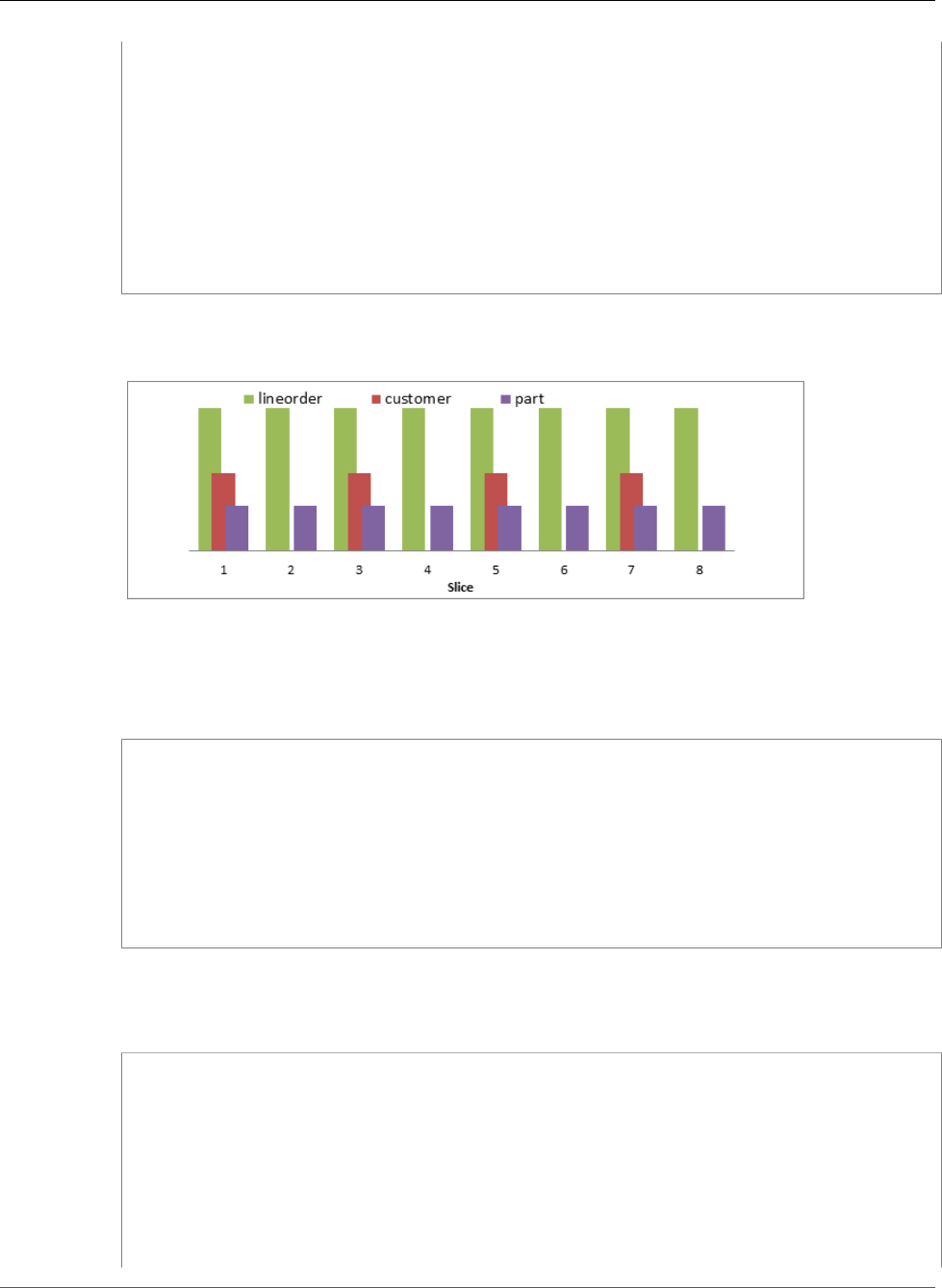
Amazon Redshift Database Developer Guide
To Retest System Performance After Tuning
part | 0 | 175006 | 15 | 1399997
part | 1 | 175199 | 1 | 1399999
part | 2 | 175441 | 4 | 1399989
part | 3 | 175000 | 3 | 1399995
part | 4 | 175018 | 5 | 1399979
part | 5 | 175091 | 11 | 1400000
part | 6 | 174253 | 2 | 1399969
part | 7 | 174992 | 13 | 1399996
supplier | 0 | 1000000 | 1 | 1000000
supplier | 2 | 1000000 | 1 | 1000000
supplier | 4 | 1000000 | 1 | 1000000
supplier | 6 | 1000000 | 1 | 1000000
(28 rows)
The following chart illustrates the distribution of the three largest tables. (The columns are not to
scale.) Notice that because CUSTOMER uses ALL distribution, it was distributed to only one slice per
node.
The distribution is relatively even, so you don't need to adjust for distribution skew.
3. Run an EXPLAIN command with each query to view the query plans.
The following example shows the EXPLAIN command with Query 2.
explain
select sum(lo_revenue), d_year, p_brand1
from lineorder, dwdate, part, supplier
where lo_orderdate = d_datekey
and lo_partkey = p_partkey
and lo_suppkey = s_suppkey
and p_category = 'MFGR#12'
and s_region = 'AMERICA'
group by d_year, p_brand1
order by d_year, p_brand1;
In the EXPLAIN plan for Query 2, notice that the DS_BCAST_INNER labels have been replaced by
DS_DIST_ALL_NONE and DS_DIST_NONE, which means that no redistribution was required for those
steps, and the query should run much more quickly.
QUERY PLAN
XN Merge (cost=1000014243538.45..1000014243539.15 rows=280 width=20)
Merge Key: dwdate.d_year, part.p_brand1
-> XN Network (cost=1000014243538.45..1000014243539.15 rows=280 width=20)
Send to leader
-> XN Sort (cost=1000014243538.45..1000014243539.15 rows=280 width=20)
Sort Key: dwdate.d_year, part.p_brand1
-> XN HashAggregate (cost=14243526.37..14243527.07 rows=280 width=20)
-> XN Hash Join DS_DIST_ALL_NONE (cost=30643.30..14211277.03
rows=4299912
Hash Cond: ("outer".lo_orderdate = "inner".d_datekey)
API Version 2012-12-01
64

Amazon Redshift Database Developer Guide
To Retest System Performance After Tuning
-> XN Hash Join DS_DIST_ALL_NONE
(cost=30611.35..14114497.06
Hash Cond: ("outer".lo_suppkey = "inner".s_suppkey)
-> XN Hash Join DS_DIST_NONE
(cost=17640.00..13758507.64
Hash Cond: ("outer".lo_partkey =
"inner".p_partkey)
-> XN Seq Scan on lineorder
(cost=0.00..6000378.88
-> XN Hash (cost=17500.00..17500.00 rows=56000
width=16)
-> XN Seq Scan on part
(cost=0.00..17500.00
Filter: ((p_category)::text =
'MFGR#12'::text)
-> XN Hash (cost=12500.00..12500.00 rows=188541
width=4)
-> XN Seq Scan on supplier
(cost=0.00..12500.00
Filter: ((s_region)::text =
'AMERICA'::text)
-> XN Hash (cost=25.56..25.56 rows=2556 width=8)
-> XN Seq Scan on dwdate (cost=0.00..25.56 rows=2556
width=8)
4. Run the same test queries again.
If you reconnected to the database since your first set of tests, disable result caching for this session.
To disable result caching for the current session, set the enable_result_cache_for_session (p. 949)
parameter to off, as shown following.
set enable_result_cache_for_session to off;
As you did earlier, run the following queries twice to eliminate compile time. Record the second time
for each query in the benchmarks table.
-- Query 1
-- Restrictions on only one dimension.
select sum(lo_extendedprice*lo_discount) as revenue
from lineorder, dwdate
where lo_orderdate = d_datekey
and d_year = 1997
and lo_discount between 1 and 3
and lo_quantity < 24;
-- Query 2
-- Restrictions on two dimensions
select sum(lo_revenue), d_year, p_brand1
from lineorder, dwdate, part, supplier
where lo_orderdate = d_datekey
and lo_partkey = p_partkey
and lo_suppkey = s_suppkey
and p_category = 'MFGR#12'
and s_region = 'AMERICA'
group by d_year, p_brand1
order by d_year, p_brand1;
-- Query 3
-- Drill down in time to just one month
select c_city, s_city, d_year, sum(lo_revenue) as revenue
from customer, lineorder, supplier, dwdate
API Version 2012-12-01
65

Amazon Redshift Database Developer Guide
Next Step
where lo_custkey = c_custkey
and lo_suppkey = s_suppkey
and lo_orderdate = d_datekey
and (c_city='UNITED KI1' or
c_city='UNITED KI5')
and (s_city='UNITED KI1' or
s_city='UNITED KI5')
and d_yearmonth = 'Dec1997'
group by c_city, s_city, d_year
order by d_year asc, revenue desc;
The following benchmarks table shows the results based on the cluster used in this example. Your results
will vary based on a number of factors, but the relative results should be similar.
Benchmark Before After
Load time (five tables) 10m 23s 12m 15s
Storage Use
LINEORDER 51024 27152
PART 200 200
CUSTOMER 384 604
DWDATE 160 160
SUPPLIER 152 236
Total storage 51920 28352
Query execution time
Query 1 6.97 3.19
Query 2 12.81 9.02
Query 3 13.39 10.54
Total execution time 33.17 22.75
Next Step
Step 8: Evaluate the Results (p. 66)
Step 8: Evaluate the Results
You tested load times, storage requirements, and query execution times before and after tuning the
tables, and recorded the results.
The following table shows the example results for the cluster that was used for this tutorial. Your results
will be different, but should show similar improvements.
API Version 2012-12-01
66
Amazon Redshift Database Developer Guide
Step 8: Evaluate the Results
Benchmark Before After Change %
Load time (five
tables)
623 732 109 17.5%
Storage Use
LINEORDER 51024 27152 -23872 -46.8%
PART 200 200 0 0%
CUSTOMER 384 604 220 57.3%
DWDATE 160 160 0 0%
SUPPLIER 152 236 84 55.3%
Total storage 51920 28352 -23568 -45.4%
Query execution time
Query 1 6.97 3.19 -3.78 -54.2%
Query 2 12.81 9.02 -3.79 -29.6%
Query 3 13.39 10.54 -2.85 -21.3%
Total execution
time
33.17 22.75 -10.42 -31.4%
Load time
Load time increased by 17.5%.
Sorting, compression, and distribution increase load time. In particular, in this case, you used automatic
compression, which increases the load time for empty tables that don't already have compression
encodings. Subsequent loads to the same tables would be faster. You also increased load time by using
ALL distribution. You could reduce load time by using EVEN or DISTKEY distribution instead for some of
the tables, but that decision needs to be weighed against query performance.
Storage requirements
Storage requirements were reduced by 45.4%.
Some of the storage improvement from using columnar compression was offset by using ALL
distribution on some of the tables. Again, you could improve storage use by using EVEN or DISTKEY
distribution instead for some of the tables, but that decision needs to be weighed against query
performance.
Distribution
You verified that there is no distribution skew as a result of your distribution choices.
By checking the EXPLAIN plan, you saw that data redistribution was eliminated for the test queries.
Query execution time
Total query execution time was reduced by 31.4%.
The improvement in query performance was due to a combination of optimizing sort keys, distribution
styles, and compression. Often, query performance can be improved even further by rewriting
API Version 2012-12-01
67

Amazon Redshift Database Developer Guide
Next Step
queries and configuring workload management (WLM). For more information, see Tuning Query
Performance (p. 257).
Next Step
Step 9: Clean Up Your Resources (p. 68)
Step 9: Clean Up Your Resources
Your cluster continues to accrue charges as long as it is running. When you have completed this tutorial,
you should return your environment to the previous state by following the steps in Step 5: Revoke Access
and Delete Your Sample Cluster in the Amazon Redshift Getting Started.
If you want to keep the cluster, but recover the storage used by the SSB tables, execute the following
commands.
drop table part cascade;
drop table supplier cascade;
drop table customer cascade;
drop table dwdate cascade;
drop table lineorder cascade;
Next Step
Summary (p. 68)
Summary
In this tutorial, you learned how to optimize the design of your tables by applying table design best
practices.
You chose sort keys for the SSB tables based on these best practices:
• If recent data is queried most frequently, specify the timestamp column as the leading column for the
sort key.
• If you do frequent range filtering or equality filtering on one column, specify that column as the sort
key.
• If you frequently join a (dimension) table, specify the join column as the sort key.
You applied the following best practices to improve the distribution of the tables.
• Distribute the fact table and one dimension table on their common columns
• Change some dimension tables to use ALL distribution
You evaluated the effects of compression on a table and determined that using automatic compression
usually produces the best results.
For more information, see the following links:
•Amazon Redshift Best Practices for Designing Tables (p. 26)
•Choose the Best Sort Key (p. 27)
API Version 2012-12-01
68

Amazon Redshift Database Developer Guide
Next Step
•Choosing a Data Distribution Style (p. 129)
•Choosing a Column Compression Type (p. 118)
•Analyzing Table Design (p. 146)
Next Step
For your next step, if you haven't done so already, we recommend taking Tutorial: Loading Data from
Amazon S3 (p. 70).
API Version 2012-12-01
69

Amazon Redshift Database Developer Guide
Prerequisites
Tutorial: Loading Data from Amazon
S3
In this tutorial, you will walk through the process of loading data into your Amazon Redshift database
tables from data files in an Amazon Simple Storage Service (Amazon S3) bucket from beginning to end.
In this tutorial, you will:
• Download data files that use CSV, character-delimited, and fixed width formats.
• Create an Amazon S3 bucket and then upload the data files to the bucket.
• Launch an Amazon Redshift cluster and create database tables.
• Use COPY commands to load the tables from the data files on Amazon S3.
• Troubleshoot load errors and modify your COPY commands to correct the errors.
Estimated time: 60 minutes
Estimated cost: $1.00 per hour for the cluster
Prerequisites
You will need the following prerequisites:
• An AWS account to launch an Amazon Redshift cluster and to create a bucket in Amazon S3.
• Your AWS credentials (an access key ID and secret access key) to load test data from Amazon S3. If you
need to create new access keys, go to Administering Access Keys for IAM Users.
This tutorial is designed so that it can be taken by itself. In addition to this tutorial, we recommend
completing the following tutorials to gain a more complete understanding of how to design and use
Amazon Redshift databases:
•Amazon Redshift Getting Started walks you through the process of creating an Amazon Redshift
cluster and loading sample data.
•Tutorial: Tuning Table Design (p. 45) walks you step by step through the process of designing and
tuning tables, including choosing sort keys, distribution styles, and compression encodings, and
evaluating system performance before and after tuning.
Overview
You can add data to your Amazon Redshift tables either by using an INSERT command or by using a
COPY command. At the scale and speed of an Amazon Redshift data warehouse, the COPY command is
many times faster and more efficient than INSERT commands.
The COPY command uses the Amazon Redshift massively parallel processing (MPP) architecture to
read and load data in parallel from multiple data sources. You can load from data files on Amazon S3,
Amazon EMR, or any remote host accessible through a Secure Shell (SSH) connection, or you can load
directly from an Amazon DynamoDB table.
In this tutorial, you will use the COPY command to load data from Amazon S3. Many of the principles
presented here apply to loading from other data sources as well.
API Version 2012-12-01
70
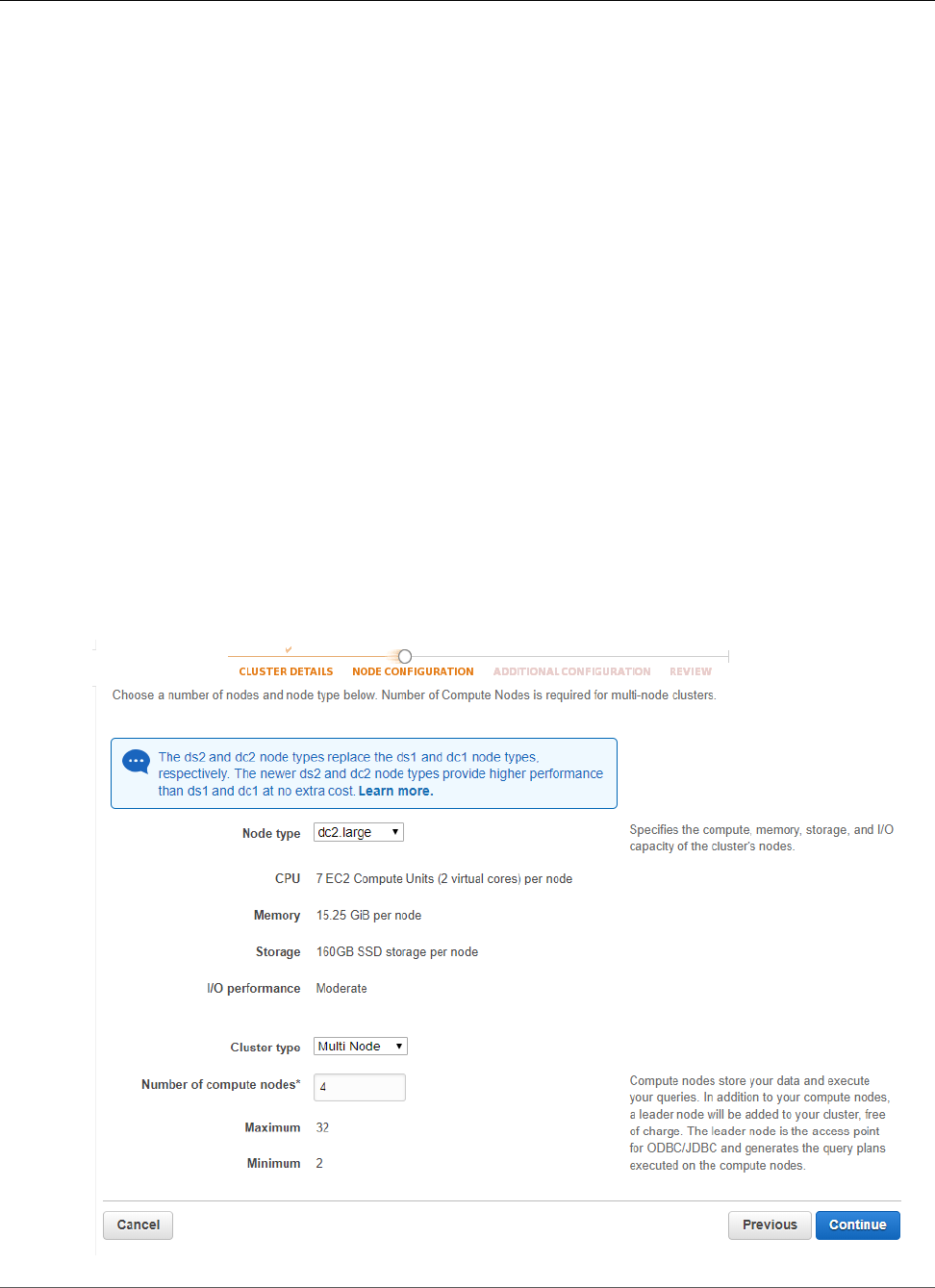
Amazon Redshift Database Developer Guide
Steps
To learn more about using the COPY command, see these resources:
•Amazon Redshift Best Practices for Loading Data (p. 29)
•Loading Data from Amazon EMR (p. 196)
•Loading Data from Remote Hosts (p. 200)
•Loading Data from an Amazon DynamoDB Table (p. 206)
Steps
•Step 1: Launch a Cluster (p. 71)
•Step 2: Download the Data Files (p. 72)
•Step 3: Upload the Files to an Amazon S3 Bucket (p. 72)
•Step 4: Create the Sample Tables (p. 74)
•Step 5: Run the COPY Commands (p. 76)
•Step 6: Vacuum and Analyze the Database (p. 87)
•Step 7: Clean Up Your Resources (p. 88)
Step 1: Launch a Cluster
If you already have a cluster that you want to use, you can skip this step.
For the exercises in this tutorial, you will use a four-node cluster. Follow the steps in Amazon Redshift
Getting Started, but select Multi Node for Cluster Type and set Number of Compute Nodes to 4.
API Version 2012-12-01
71

Amazon Redshift Database Developer Guide
Next Step
Follow the Getting Started steps to connect to your cluster from a SQL client and test a connection.
You do not need to complete the remaining Getting Started steps to create tables, upload data, and try
example queries.
Next Step
Step 2: Download the Data Files (p. 72)
Step 2: Download the Data Files
In this step, you will download a set of sample data files to your computer. In the next step, you will
upload the files to an Amazon S3 bucket.
To download the data files
1. Download the zipped file from the following link: LoadingDataSampleFiles.zip
2. Extract the files to a folder on your computer.
3. Verify that your folder contains the following files.
customer-fw-manifest
customer-fw.tbl-000
customer-fw.tbl-000.bak
customer-fw.tbl-001
customer-fw.tbl-002
customer-fw.tbl-003
customer-fw.tbl-004
customer-fw.tbl-005
customer-fw.tbl-006
customer-fw.tbl-007
customer-fw.tbl.log
dwdate-tab.tbl-000
dwdate-tab.tbl-001
dwdate-tab.tbl-002
dwdate-tab.tbl-003
dwdate-tab.tbl-004
dwdate-tab.tbl-005
dwdate-tab.tbl-006
dwdate-tab.tbl-007
part-csv.tbl-000
part-csv.tbl-001
part-csv.tbl-002
part-csv.tbl-003
part-csv.tbl-004
part-csv.tbl-005
part-csv.tbl-006
part-csv.tbl-007
Next Step
Step 3: Upload the Files to an Amazon S3 Bucket (p. 72)
Step 3: Upload the Files to an Amazon S3 Bucket
In this step, you create an Amazon S3 bucket and upload the data files to the bucket.
API Version 2012-12-01
72

Amazon Redshift Database Developer Guide
To upload the files to an Amazon S3 bucket
1. Create a bucket in Amazon S3.
a. Sign in to the AWS Management Console and open the Amazon S3 console at https://
console.aws.amazon.com/s3/.
b. Click Create Bucket.
c. In the Bucket Name box of the Create a Bucket dialog box, type a bucket name.
The bucket name you choose must be unique among all existing bucket names in Amazon
S3. One way to help ensure uniqueness is to prefix your bucket names with the name of your
organization. Bucket names must comply with certain rules. For more information, go to Bucket
Restrictions and Limitations in the Amazon Simple Storage Service Developer Guide.
d. Select a region.
Create the bucket in the same region as your cluster. If your cluster is in the Oregon region, click
Oregon.
e. Click Create.
When Amazon S3 successfully creates your bucket, the console displays your empty bucket in
the Buckets panel.
2. Create a folder.
a. Click the name of the new bucket.
b. Click the Actions button, and click Create Folder in the drop-down list.
c. Name the new folder load.
Note
The bucket that you created is not in a sandbox. In this exercise, you will add objects
to a real bucket, and you will be charged a nominal amount for the time that you store
the objects in the bucket. For more information about Amazon S3 pricing, go to the
Amazon S3 Pricing page.
3. Upload the data files to the new Amazon S3 bucket.
a. Click the name of the data folder.
b. In the Upload - Select Files wizard, click Add Files.
A file selection dialog box opens.
c. Select all of the files you downloaded and extracted, and then click Open.
d. Click Start Upload.
User Credentials
The Amazon Redshift COPY command must have access to read the file objects in the Amazon S3 bucket.
If you use the same user credentials to create the Amazon S3 bucket and to run the Amazon Redshift
COPY command, the COPY command will have all necessary permissions. If you want to use different
user credentials, you can grant access by using the Amazon S3 access controls. The Amazon Redshift
COPY command requires at least ListBucket and GetObject permissions to access the file objects in
the Amazon S3 bucket. For more information about controlling access to Amazon S3 resources, go to
Managing Access Permissions to Your Amazon S3 Resources.
Next Step
Step 4: Create the Sample Tables (p. 74)
API Version 2012-12-01
73
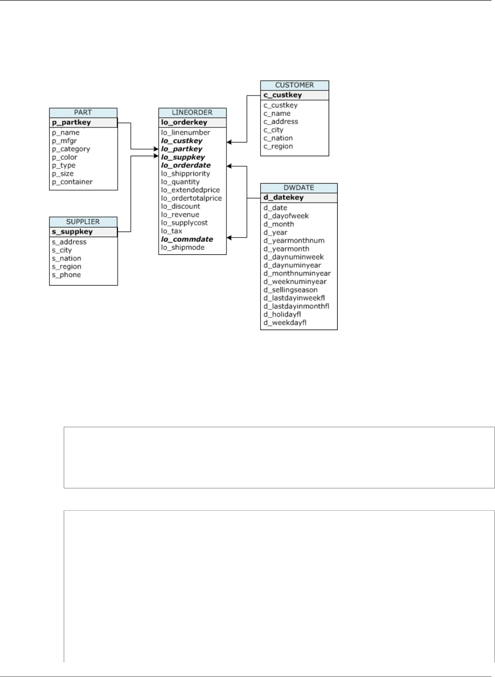
Amazon Redshift Database Developer Guide
Step 4: Create the Sample Tables
Step 4: Create the Sample Tables
For this tutorial, you will use a set of five tables based on the Star Schema Benchmark (SSB) schema. The
following diagram shows the SSB data model.
If the SSB tables already exist in the current database, you will need to drop the tables to remove them
from the database before you create them using the CREATE TABLE commands in the next step. The
tables used in this tutorial might have different attributes than the existing tables.
To create the sample tables
1. To drop the SSB tables, execute the following commands.
drop table part cascade;
drop table supplier;
drop table customer;
drop table dwdate;
drop table lineorder;
2. Execute the following CREATE TABLE commands.
CREATE TABLE part
(
p_partkey INTEGER NOT NULL,
p_name VARCHAR(22) NOT NULL,
p_mfgr VARCHAR(6),
p_category VARCHAR(7) NOT NULL,
p_brand1 VARCHAR(9) NOT NULL,
p_color VARCHAR(11) NOT NULL,
p_type VARCHAR(25) NOT NULL,
p_size INTEGER NOT NULL,
p_container VARCHAR(10) NOT NULL
);
CREATE TABLE supplier
(
API Version 2012-12-01
74

Amazon Redshift Database Developer Guide
Step 4: Create the Sample Tables
s_suppkey INTEGER NOT NULL,
s_name VARCHAR(25) NOT NULL,
s_address VARCHAR(25) NOT NULL,
s_city VARCHAR(10) NOT NULL,
s_nation VARCHAR(15) NOT NULL,
s_region VARCHAR(12) NOT NULL,
s_phone VARCHAR(15) NOT NULL
);
CREATE TABLE customer
(
c_custkey INTEGER NOT NULL,
c_name VARCHAR(25) NOT NULL,
c_address VARCHAR(25) NOT NULL,
c_city VARCHAR(10) NOT NULL,
c_nation VARCHAR(15) NOT NULL,
c_region VARCHAR(12) NOT NULL,
c_phone VARCHAR(15) NOT NULL,
c_mktsegment VARCHAR(10) NOT NULL
);
CREATE TABLE dwdate
(
d_datekey INTEGER NOT NULL,
d_date VARCHAR(19) NOT NULL,
d_dayofweek VARCHAR(10) NOT NULL,
d_month VARCHAR(10) NOT NULL,
d_year INTEGER NOT NULL,
d_yearmonthnum INTEGER NOT NULL,
d_yearmonth VARCHAR(8) NOT NULL,
d_daynuminweek INTEGER NOT NULL,
d_daynuminmonth INTEGER NOT NULL,
d_daynuminyear INTEGER NOT NULL,
d_monthnuminyear INTEGER NOT NULL,
d_weeknuminyear INTEGER NOT NULL,
d_sellingseason VARCHAR(13) NOT NULL,
d_lastdayinweekfl VARCHAR(1) NOT NULL,
d_lastdayinmonthfl VARCHAR(1) NOT NULL,
d_holidayfl VARCHAR(1) NOT NULL,
d_weekdayfl VARCHAR(1) NOT NULL
);
CREATE TABLE lineorder
(
lo_orderkey INTEGER NOT NULL,
lo_linenumber INTEGER NOT NULL,
lo_custkey INTEGER NOT NULL,
lo_partkey INTEGER NOT NULL,
lo_suppkey INTEGER NOT NULL,
lo_orderdate INTEGER NOT NULL,
lo_orderpriority VARCHAR(15) NOT NULL,
lo_shippriority VARCHAR(1) NOT NULL,
lo_quantity INTEGER NOT NULL,
lo_extendedprice INTEGER NOT NULL,
lo_ordertotalprice INTEGER NOT NULL,
lo_discount INTEGER NOT NULL,
lo_revenue INTEGER NOT NULL,
lo_supplycost INTEGER NOT NULL,
lo_tax INTEGER NOT NULL,
lo_commitdate INTEGER NOT NULL,
lo_shipmode VARCHAR(10) NOT NULL
);
API Version 2012-12-01
75

Amazon Redshift Database Developer Guide
Next Step
Next Step
Step 5: Run the COPY Commands (p. 76)
Step 5: Run the COPY Commands
You will run COPY commands to load each of the tables in the SSB schema. The COPY command
examples demonstrate loading from different file formats, using several COPY command options, and
troubleshooting load errors.
Topics
•COPY Command Syntax (p. 76)
•Loading the SSB Tables (p. 77)
COPY Command Syntax
The basic COPY (p. 390) command syntax is as follows.
COPY table_name [ column_list ] FROM data_source CREDENTIALS access_credentials [options]
To execute a COPY command, you provide the following values.
Table name
The target table for the COPY command. The table must already exist in the database. The table can be
temporary or persistent. The COPY command appends the new input data to any existing rows in the
table.
Column list
By default, COPY loads fields from the source data to the table columns in order. You can optionally
specify a column list, that is a comma-separated list of column names, to map data fields to specific
columns. You will not use column lists in this tutorial. For more information, see Column List (p. 407) in
the COPY command reference.
Data source
You can use the COPY command to load data from an Amazon S3 bucket, an Amazon EMR cluster, a
remote host using an SSH connection, or an Amazon DynamoDB table. For this tutorial, you will load
from data files in an Amazon S3 bucket. When loading from Amazon S3, you must provide the name of
the bucket and the location of the data files, by providing either an object path for the data files or the
location of a manifest file that explicitly lists each data file and its location.
• Key prefix
An object stored in Amazon S3 is uniquely identified by an object key, which includes the bucket name,
folder names, if any, and the object name. A key prefix refers to a set of objects with the same prefix.
The object path is a key prefix that the COPY command uses to load all objects that share the key
prefix. For example, the key prefix custdata.txt can refer to a single file or to a set of files, including
custdata.txt.001, custdata.txt.002, and so on.
• Manifest file
If you need to load files with different prefixes, for example, from multiple buckets or folders, or if
you need to exclude files that share a prefix, you can use a manifest file. A manifest file explicitly lists
API Version 2012-12-01
76

Amazon Redshift Database Developer Guide
Loading the SSB Tables
each load file and its unique object key. You will use a manifest file to load the PART table later in this
tutorial.
Credentials
To access the AWS resources that contain the data to load, you must provide AWS access credentials (that
is, an access key ID and a secret access key) for an AWS user or an IAM user with sufficient privileges.
To load data from Amazon S3, the credentials must include ListBucket and GetObject permissions.
Additional credentials are required if your data is encrypted or if you are using temporary access
credentials. For more information, see Authorization Parameters (p. 404) in the COPY command
reference. For more information about managing access, go to Managing Access Permissions to Your
Amazon S3 Resources. If you do not have an access key ID and secret access key, you will need to get
them. For more information, go to Administering Access Keys for IAM Users.
Options
You can specify a number of parameters with the COPY command to specify file formats, manage data
formats, manage errors, and control other features. In this tutorial, you will use the following COPY
command options and features:
•Key Prefix (p. 78)
•CSV Format (p. 78)
•NULL AS (p. 79)
•REGION (p. 80)
•Fixed-Width Format (p. 81)
•MAXERROR (p. 82)
•ACCEPTINVCHARS (p. 83)
•MANIFEST (p. 84)
•DATEFORMAT (p. 85)
•GZIP, LZOP and BZIP2 (p. 85)
•COMPUPDATE (p. 85)
•Multiple Files (p. 86)
Loading the SSB Tables
You will use the following COPY commands to load each of the tables in the SSB schema. The command
to each table demonstrates different COPY options and troubleshooting techniques.
To load the SSB tables, follow these steps:
1. Replace the Bucket Name and AWS Credentials (p. 77)
2. Load the PART Table Using NULL AS (p. 78)
3. Load the SUPPLIER table Using REGION (p. 80)
4. Load the CUSTOMER Table Using MANIFEST (p. 81)
5. Load the DWDATE Table Using DATEFORMAT (p. 85)
6. Load the LINEORDER Table Using Multiple Files (p. 85)
Replace the Bucket Name and AWS Credentials
The COPY commands in this tutorial are presented in the following format.
API Version 2012-12-01
77
Amazon Redshift Database Developer Guide
Loading the SSB Tables
copy table from 's3://<your-bucket-name>/load/key_prefix'
credentials 'aws_access_key_id=<Your-Access-Key-ID>;aws_secret_access_key=<Your-Secret-
Access-Key>'
options;
For each COPY command, do the following:
1. Replace <your-bucket-name> with the name of a bucket in the same region as your cluster.
This step assumes the bucket and the cluster are in the same region. Alternatively, you can specify the
region using the REGION (p. 397) option with the COPY command.
2. Replace <Your-Access-Key-ID> and <Your-Secret-Access-Key> with your own AWS IAM
account credentials. The segment of the credentials string that is enclosed in single quotation marks
must not contain any spaces or line breaks.
Load the PART Table Using NULL AS
In this step, you will use the CSV and NULL AS options to load the PART table.
The COPY command can load data from multiple files in parallel, which is much faster than loading
from a single file. To demonstrate this principle, the data for each table in this tutorial is split into eight
files, even though the files are very small. In a later step, you will compare the time difference between
loading from a single file and loading from multiple files. For more information, see Split Your Load Data
into Multiple Files (p. 30).
Key Prefix
You can load from multiple files by specifying a key prefix for the file set, or by explicitly listing the files
in a manifest file. In this step, you will use a key prefix. In a later step, you will use a manifest file. The key
prefix 's3://mybucket/load/part-csv.tbl' loads the following set of the files in the load folder.
part-csv.tbl-000
part-csv.tbl-001
part-csv.tbl-002
part-csv.tbl-003
part-csv.tbl-004
part-csv.tbl-005
part-csv.tbl-006
part-csv.tbl-007
CSV Format
CSV, which stands for comma separated values, is a common format used for importing and exporting
spreadsheet data. CSV is more flexible than comma-delimited format because it enables you to
include quoted strings within fields. The default quote character for COPY from CSV format is a double
quotation mark ( " ), but you can specify another quote character by using the QUOTE AS option. When
you use the quote character within the field, escape the character with an additional quote character.
The following excerpt from a CSV-formatted data file for the PART table shows strings enclosed in
double quotation marks ("LARGE ANODIZED BRASS") and a string enclosed in two double quotation
marks within a quoted string ("MEDIUM ""BURNISHED"" TIN").
15,dark sky,MFGR#3,MFGR#47,MFGR#3438,indigo,"LARGE ANODIZED BRASS",45,LG CASE
22,floral beige,MFGR#4,MFGR#44,MFGR#4421,medium,"PROMO, POLISHED BRASS",19,LG DRUM
23,bisque slate,MFGR#4,MFGR#41,MFGR#4137,firebrick,"MEDIUM ""BURNISHED"" TIN",42,JUMBO JAR
The data for the PART table contains characters that will cause COPY to fail. In this exercise, you will
troubleshoot the errors and correct them.
API Version 2012-12-01
78
Amazon Redshift Database Developer Guide
Loading the SSB Tables
To load data that is in CSV format, add csv to your COPY command. Execute the following command to
load the PART table.
copy part from 's3://<your-bucket-name>/load/part-csv.tbl'
credentials 'aws_access_key_id=<Your-Access-Key-ID>;aws_secret_access_key=<Your-Secret-
Access-Key>'
csv;
You should get an error message similar to the following.
An error occurred when executing the SQL command:
copy part from 's3://mybucket/load/part-csv.tbl'
credentials' ...
ERROR: Load into table 'part' failed. Check 'stl_load_errors' system table for details.
[SQL State=XX000]
Execution time: 1.46s
1 statement(s) failed.
1 statement(s) failed.
To get more information about the error, query the STL_LOAD_ERRORS table. The following query uses
the SUBSTRING function to shorten columns for readability and uses LIMIT 10 to reduce the number of
rows returned. You can adjust the values in substring(filename,22,25) to allow for the length of
your bucket name.
select query, substring(filename,22,25) as filename,line_number as line,
substring(colname,0,12) as column, type, position as pos, substring(raw_line,0,30) as
line_text,
substring(raw_field_value,0,15) as field_text,
substring(err_reason,0,45) as reason
from stl_load_errors
order by query desc
limit 10;
query | filename | line | column | type | pos |
--------+-------------------------+-----------+------------+------------+-----+----
333765 | part-csv.tbl-000 | 1 | | | 0 |
line_text | field_text | reason
------------------+------------+----------------------------------------------
15,NUL next, | | Missing newline: Unexpected character 0x2c f
NULL AS
The part-csv.tbl data files use the NUL terminator character (\x000 or \x0) to indicate NULL values.
Note
Despite very similar spelling, NUL and NULL are not the same. NUL is a UTF-8 character with
codepoint x000 that is often used to indicate end of record (EOR). NULL is a SQL value that
represents an absence of data.
By default, COPY treats a NUL terminator character as an EOR character and terminates the record,
which often results in unexpected results or an error. Because there is no single standard method of
indicating NULL in text data, the NULL AS COPY command option enables you to specify which character
to substitute with NULL when loading the table. In this example, you want COPY to treat the NUL
terminator character as a NULL value.
API Version 2012-12-01
79
Amazon Redshift Database Developer Guide
Loading the SSB Tables
Note
The table column that receives the NULL value must be configured as nullable. That is, it must
not include the NOT NULL constraint in the CREATE TABLE specification.
To load PART using the NULL AS option, execute the following COPY command.
copy part from 's3://<your-bucket-name>/load/part-csv.tbl'
credentials 'aws_access_key_id=<Your-Access-Key-ID>;aws_secret_access_key=<Your-Secret-
Access-Key>'
csv
null as '\000';
To verify that COPY loaded NULL values, execute the following command to select only the rows that
contain NULL.
select p_partkey, p_name, p_mfgr, p_category from part where p_mfgr is null;
p_partkey | p_name | p_mfgr | p_category
-----------+----------+--------+------------
15 | NUL next | | MFGR#47
81 | NUL next | | MFGR#23
133 | NUL next | | MFGR#44
(2 rows)
Load the SUPPLIER table Using REGION
In this step you will use the DELIMITER and REGION options to load the SUPPLIER table.
Note
The files for loading the SUPPLIER table are provided in an AWS sample bucket. You don't need
to upload files for this step.
Character-Delimited Format
The fields in a character-delimited file are separated by a specific character, such as a pipe character ( | ),
a comma ( , ) or a tab ( \t ). Character-delimited files can use any single ASCII character, including one
of the nonprinting ASCII characters, as the delimiter. You specify the delimiter character by using the
DELIMITER option. The default delimiter is a pipe character ( | ).
The following excerpt from the data for the SUPPLIER table uses pipe-delimited format.
1|1|257368|465569|41365|19950218|2-HIGH|0|17|2608718|9783671|4|2504369|92072|2|19950331|
TRUCK
1|2|257368|201928|8146|19950218|2-HIGH|0|36|6587676|9783671|9|5994785|109794|6|19950416|
MAIL
REGION
Whenever possible, you should locate your load data in the same AWS region as your Amazon Redshift
cluster. If your data and your cluster are in the same region, you reduce latency, minimize eventual
consistency issues, and avoid cross-region data transfer costs. For more information, see Amazon
Redshift Best Practices for Loading Data (p. 29)
If you must load data from a different AWS region, use the REGION option to specify the AWS region in
which the load data is located. If you specify a region, all of the load data, including manifest files, must
be in the named region. For more information, see REGION (p. 397).
API Version 2012-12-01
80
Amazon Redshift Database Developer Guide
Loading the SSB Tables
If your cluster is in the US East (N. Virginia) region, execute the following command to load the SUPPLIER
table from pipe-delimited data in an Amazon S3 bucket located in the US West (Oregon) region. For this
example, do not change the bucket name.
copy supplier from 's3://awssampledbuswest2/ssbgz/supplier.tbl'
credentials 'aws_access_key_id=<Your-Access-Key-ID>;aws_secret_access_key=<Your-Secret-
Access-Key>'
delimiter '|'
gzip
region 'us-west-2';
If your cluster is not in the US East (N. Virginia) region, execute the following command to load the
SUPPLIER table from pipe-delimited data in an Amazon S3 bucket located in the US East (N. Virginia)
region. For this example, do not change the bucket name.
copy supplier from 's3://awssampledb/ssbgz/supplier.tbl'
credentials 'aws_access_key_id=<Your-Access-Key-ID>;aws_secret_access_key=<Your-Secret-
Access-Key>'
delimiter '|'
gzip
region 'us-east-1';
Load the CUSTOMER Table Using MANIFEST
In this step, you will use the FIXEDWIDTH, MAXERROR, ACCEPTINVCHARS, and MANIFEST options to load
the CUSTOMER table.
The sample data for this exercise contains characters that will cause errors when COPY attempts to load
them. You will use the MAXERRORS option and the STL_LOAD_ERRORS system table to troubleshoot the
load errors and then use the ACCEPTINVCHARS and MANIFEST options to eliminate the errors.
Fixed-Width Format
Fixed-width format defines each field as a fixed number of characters, rather than separating fields with
a delimiter. The following excerpt from the data for the CUSTOMER table uses fixed-width format.
1 Customer#000000001 IVhzIApeRb MOROCCO 0MOROCCO AFRICA 25-705
2 Customer#000000002 XSTf4,NCwDVaWNe6tE JORDAN 6JORDAN MIDDLE EAST 23-453
3 Customer#000000003 MG9kdTD ARGENTINA5ARGENTINAAMERICA 11-783
The order of the label/width pairs must match the order of the table columns exactly. For more
information, see FIXEDWIDTH (p. 408).
The fixed-width specification string for the CUSTOMER table data is as follows.
fixedwidth 'c_custkey:10, c_name:25, c_address:25, c_city:10, c_nation:15,
c_region :12, c_phone:15,c_mktsegment:10'
To load the CUSTOMER table from fixed-width data, execute the following command.
copy customer
from 's3://<your-bucket-name>/load/customer-fw.tbl'
credentials 'aws_access_key_id=<Your-Access-Key-ID>;aws_secret_access_key=<Your-Secret-
Access-Key>'
fixedwidth 'c_custkey:10, c_name:25, c_address:25, c_city:10, c_nation:15, c_region :12,
c_phone:15,c_mktsegment:10';
API Version 2012-12-01
81
Amazon Redshift Database Developer Guide
Loading the SSB Tables
You should get an error message, similar to the following.
An error occurred when executing the SQL command:
copy customer
from 's3://mybucket/load/customer-fw.tbl'
credentials'aws_access_key_id=...
ERROR: Load into table 'customer' failed. Check 'stl_load_errors' system table for
details. [SQL State=XX000]
Execution time: 2.95s
1 statement(s) failed.
MAXERROR
By default, the first time COPY encounters an error, the command fails and returns an error message. To
save time during testing, you can use the MAXERROR option to instruct COPY to skip a specified number
of errors before it fails. Because we expect errors the first time we test loading the CUSTOMER table
data, add maxerror 10 to the COPY command.
To test using the FIXEDWIDTH and MAXERROR options, execute the following command.
copy customer
from 's3://<your-bucket-name>/load/customer-fw.tbl'
credentials 'aws_access_key_id=<Your-Access-Key-ID>;aws_secret_access_key=<Your-Secret-
Access-Key>'
fixedwidth 'c_custkey:10, c_name:25, c_address:25, c_city:10, c_nation:15, c_region :12,
c_phone:15,c_mktsegment:10'
maxerror 10;
This time, instead of an error message, you get a warning message similar to the following.
Warnings:
Load into table 'customer' completed, 112497 record(s) loaded successfully.
Load into table 'customer' completed, 7 record(s) could not be loaded. Check
'stl_load_errors' system table for details.
The warning indicates that COPY encountered seven errors. To check the errors, query the
STL_LOAD_ERRORS table, as shown in the following example.
select query, substring(filename,22,25) as filename,line_number as line,
substring(colname,0,12) as column, type, position as pos, substring(raw_line,0,30) as
line_text,
substring(raw_field_value,0,15) as field_text,
substring(err_reason,0,45) as error_reason
from stl_load_errors
order by query desc, filename
limit 7;
The results of the STL_LOAD_ERRORS query should look similar to the following.
query | filename | line | column | type | pos |
line_text | field_text | error_reason
--------+---------------------------+------+-----------
+------------+-----+-------------------------------+------------
+----------------------------------------------
334489 | customer-fw.tbl.log | 2 | c_custkey | int4 | -1 | customer-fw.tbl
| customer-f | Invalid digit, Value 'c', Pos 0, Type: Integ
API Version 2012-12-01
82
Amazon Redshift Database Developer Guide
Loading the SSB Tables
334489 | customer-fw.tbl.log | 6 | c_custkey | int4 | -1 | Complete
| Complete | Invalid digit, Value 'C', Pos 0, Type: Integ
334489 | customer-fw.tbl.log | 3 | c_custkey | int4 | -1 | #Total rows
| #Total row | Invalid digit, Value '#', Pos 0, Type: Integ
334489 | customer-fw.tbl.log | 5 | c_custkey | int4 | -1 | #Status
| #Status | Invalid digit, Value '#', Pos 0, Type: Integ
334489 | customer-fw.tbl.log | 1 | c_custkey | int4 | -1 | #Load file
| #Load file | Invalid digit, Value '#', Pos 0, Type: Integ
334489 | customer-fw.tbl000 | 1 | c_address | varchar | 34 | 1
Customer#000000001 | .Mayag.ezR | String contains invalid or unsupported UTF8
334489 | customer-fw.tbl000 | 1 | c_address | varchar | 34 | 1
Customer#000000001 | .Mayag.ezR | String contains invalid or unsupported UTF8
(7 rows)
By examining the results, you can see that there are two messages in the error_reasons column:
•Invalid digit, Value '#', Pos 0, Type: Integ
These errors are caused by the customer-fw.tbl.log file. The problem is that it is a log file, not a
data file, and should not be loaded. You can use a manifest file to avoid loading the wrong file.
•String contains invalid or unsupported UTF8
The VARCHAR data type supports multibyte UTF-8 characters up to three bytes. If the load data
contains unsupported or invalid characters, you can use the ACCEPTINVCHARS option to replace each
invalid character with a specified alternative character.
Another problem with the load is more difficult to detect—the load produced unexpected results. To
investigate this problem, execute the following command to query the CUSTOMER table.
select c_custkey, c_name, c_address
from customer
order by c_custkey
limit 10;
c_custkey | c_name | c_address
-----------+---------------------------+---------------------------
2 | Customer#000000002 | XSTf4,NCwDVaWNe6tE
2 | Customer#000000002 | XSTf4,NCwDVaWNe6tE
3 | Customer#000000003 | MG9kdTD
3 | Customer#000000003 | MG9kdTD
4 | Customer#000000004 | XxVSJsL
4 | Customer#000000004 | XxVSJsL
5 | Customer#000000005 | KvpyuHCplrB84WgAi
5 | Customer#000000005 | KvpyuHCplrB84WgAi
6 | Customer#000000006 | sKZz0CsnMD7mp4Xd0YrBvx
6 | Customer#000000006 | sKZz0CsnMD7mp4Xd0YrBvx
(10 rows)
The rows should be unique, but there are duplicates.
Another way to check for unexpected results is to verify the number of rows that were loaded. In our
case, 100000 rows should have been loaded, but the load message reported loading 112497 records.
The extra rows were loaded because the COPY loaded an extraneous file, customer-fw.tbl0000.bak.
In this exercise, you will use a manifest file to avoid loading the wrong files.
ACCEPTINVCHARS
API Version 2012-12-01
83

Amazon Redshift Database Developer Guide
Loading the SSB Tables
By default, when COPY encounters a character that is not supported by the column's data type, it skips
the row and returns an error. For information about invalid UTF-8 characters, see Multibyte Character
Load Errors (p. 214).
You could use the MAXERRORS option to ignore errors and continue loading, then query
STL_LOAD_ERRORS to locate the invalid characters, and then fix the data files. However, MAXERRORS
is best used for troubleshooting load problems and should generally not be used in a production
environment.
The ACCEPTINVCHARS option is usually a better choice for managing invalid characters.
ACCEPTINVCHARS instructs COPY to replace each invalid character with a specified valid character
and continue with the load operation. You can specify any valid ASCII character, except NULL, as the
replacement character. The default replacement character is a question mark ( ? ). COPY replaces
multibyte characters with a replacement string of equal length. For example, a 4-byte character would
be replaced with '????'.
COPY returns the number of rows that contained invalid UTF-8 characters, and it adds an entry to the
STL_REPLACEMENTS system table for each affected row, up to a maximum of 100 rows per node slice.
Additional invalid UTF-8 characters are also replaced, but those replacement events are not recorded.
ACCEPTINVCHARS is valid only for VARCHAR columns.
For this step, you will add the ACCEPTINVCHARS with the replacement character '^'.
MANIFEST
When you COPY from Amazon S3 using a key prefix, there is a risk that you will load unwanted tables.
For example, the 's3://mybucket/load/ folder contains eight data files that share the key prefix
customer-fw.tbl: customer-fw.tbl0000, customer-fw.tbl0001, and so on. However, the same
folder also contains the extraneous files customer-fw.tbl.log and customer-fw.tbl-0001.bak.
To ensure that you load all of the correct files, and only the correct files, use a manifest file. The manifest
is a text file in JSON format that explicitly lists the unique object key for each source file to be loaded.
The file objects can be in different folders or different buckets, but they must be in the same region. For
more information, see MANIFEST (p. 396).
The following shows the customer-fw-manifest text.
{
"entries": [
{"url":"s3://<your-bucket-name>/load/customer-fw.tbl-000"},
{"url":"s3://<your-bucket-name>/load/customer-fw.tbl-001"},
{"url":"s3://<your-bucket-name>/load/customer-fw.tbl-002"},
{"url":"s3://<your-bucket-name>/load/customer-fw.tbl-003"},
{"url":"s3://<your-bucket-name>/load/customer-fw.tbl-004"},
{"url":"s3://<your-bucket-name>/load/customer-fw.tbl-005"},
{"url":"s3://<your-bucket-name>/load/customer-fw.tbl-006"},
{"url":"s3://<your-bucket-name>/load/customer-fw.tbl-007"}
]
}
To load the data for the CUSTOMER table using the manifest file
1. Open the file customer-fw-manifest in a text editor.
2. Replace <your-bucket-name> with the name of your bucket.
3. Save the file.
4. Upload the file to the load folder on your bucket.
5. Execute the following COPY command.
copy customer from 's3://<your-bucket-name>/load/customer-fw-manifest'
API Version 2012-12-01
84
Amazon Redshift Database Developer Guide
Loading the SSB Tables
credentials 'aws_access_key_id=<Your-Access-Key-ID>;aws_secret_access_key=<Your-Secret-
Access-Key>'
fixedwidth 'c_custkey:10, c_name:25, c_address:25, c_city:10, c_nation:15,
c_region :12, c_phone:15,c_mktsegment:10'
maxerror 10
acceptinvchars as '^'
manifest;
Load the DWDATE Table Using DATEFORMAT
In this step, you will use the DELIMITER and DATEFORMAT options to load the DWDATE table.
When loading DATE and TIMESTAMP columns, COPY expects the default format, which is YYYY-MM-DD
for dates and YYYY-MM-DD HH:MI:SS for time stamps. If the load data does not use a default format,
you can use DATEFORMAT and TIMEFORMAT to specify the format.
The following excerpt shows date formats in the DWDATE table. Notice that the date formats in column
two are inconsistent.
19920104 1992-01-04 Sunday January 1992 199201 Jan1992 1 4 4 1...
19920112 January 12, 1992 Monday January 1992 199201 Jan1992 2 12 12 1...
19920120 January 20, 1992 Tuesday January 1992 199201 Jan1992 3 20 20 1...
DATEFORMAT
You can specify only one date format. If the load data contains inconsistent formats, possibly in different
columns, or if the format is not known at load time, you use DATEFORMAT with the 'auto' argument.
When 'auto' is specified, COPY will recognize any valid date or time format and convert it to the
default format. The 'auto' option recognizes several formats that are not supported when using a
DATEFORMAT and TIMEFORMAT string. For more information, see Using Automatic Recognition with
DATEFORMAT and TIMEFORMAT (p. 433).
To load the DWDATE table, execute the following COPY command.
copy dwdate from 's3://<your-bucket-name>/load/dwdate-tab.tbl'
credentials 'aws_access_key_id=<Your-Access-Key-ID>;aws_secret_access_key=<Your-Secret-
Access-Key>'
delimiter '\t'
dateformat 'auto';
Load the LINEORDER Table Using Multiple Files
This step uses the GZIP and COMPUPDATE options to load the LINEORDER table.
In this exercise, you will load the LINEORDER table from a single data file, and then load it again from
multiple files in order to compare the load times for the two methods.
Note
The files for loading the LINEORDER table are provided in an AWS sample bucket. You don't
need to upload files for this step.
GZIP, LZOP and BZIP2
You can compress your files using either gzip, lzop, or bzip2 compression formats. When loading from
compressed files, COPY uncompresses the files during the load process. Compressing your files saves
storage space and shortens upload times.
COMPUPDATE
API Version 2012-12-01
85
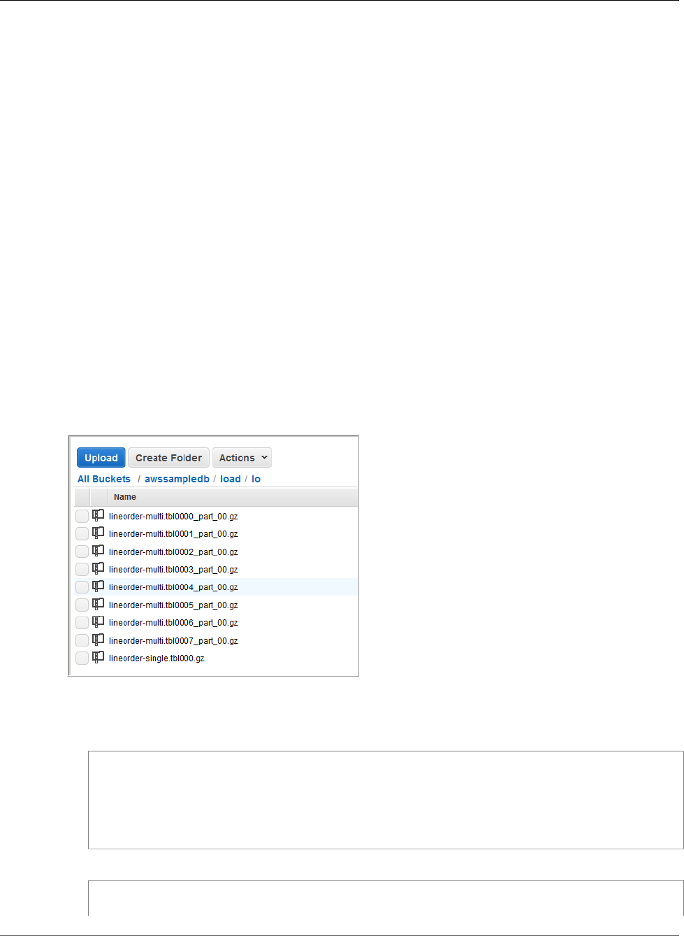
Amazon Redshift Database Developer Guide
Loading the SSB Tables
When COPY loads an empty table with no compression encodings, it analyzes the load data to determine
the optimal encodings. It then alters the table to use those encodings before beginning the load. This
analysis process takes time, but it occurs, at most, once per table. To save time, you can skip this step by
turning COMPUPDATE off. To enable an accurate evaluation of COPY times, you will turn COMPUPDATE
off for this step.
Multiple Files
The COPY command can load data very efficiently when it loads from multiple files in parallel instead
of loading from a single file. If you split your data into files so that the number of files is a multiple of
the number of slices in your cluster, Amazon Redshift divides the workload and distributes the data
evenly among the slices. The number of slices per node depends on the node size of the cluster. For more
information about the number of slices that each node size has, go to About Clusters and Nodes in the
Amazon Redshift Cluster Management Guide.
For example, the dc1.large compute nodes used in this tutorial have two slices each, so the four-node
cluster has eight slices. In previous steps, the load data was contained in eight files, even though the files
are very small. In this step, you will compare the time difference between loading from a single large file
and loading from multiple files.
The files you will use for this tutorial contain about 15 million records and occupy about 1.2 GB. These
files are very small in Amazon Redshift scale, but sufficient to demonstrate the performance advantage
of loading from multiple files. The files are large enough that the time required to download them and
then upload them to Amazon S3 is excessive for this tutorial, so you will load the files directly from an
AWS sample bucket.
The following screenshot shows the data files for LINEORDER.
To evaluate the performance of COPY with multiple files
1. Execute the following command to COPY from a single file. Do not change the bucket name.
copy lineorder from 's3://awssampledb/load/lo/lineorder-single.tbl'
credentials 'aws_access_key_id=<Your-Access-Key-ID>;aws_secret_access_key=<Your-Secret-
Access-Key>'
gzip
compupdate off
region 'us-east-1';
2. Your results should be similar to the following. Note the execution time.
Warnings:
Load into table 'lineorder' completed, 14996734 record(s) loaded successfully.
API Version 2012-12-01
86
Amazon Redshift Database Developer Guide
Step 6: Vacuum and Analyze the Database
0 row(s) affected.
copy executed successfully
Execution time: 51.56s
3. Execute the following command to COPY from multiple files. Do not change the bucket name.
copy lineorder from 's3://awssampledb/load/lo/lineorder-multi.tbl'
credentials 'aws_access_key_id=<Your-Access-Key-ID>;aws_secret_access_key=<Your-Secret-
Access-Key>'
gzip
compupdate off
region 'us-east-1';
4. Your results should be similar to the following. Note the execution time.
Warnings:
Load into table 'lineorder' completed, 14996734 record(s) loaded successfully.
0 row(s) affected.
copy executed successfully
Execution time: 17.7s
5. Compare execution times.
In our example, the time to load 15 million records decreased from 51.56 seconds to 17.7 seconds, a
reduction of 65.7 percent.
These results are based on using a four-node cluster. If your cluster has more nodes, the time savings
is multiplied. For typical Amazon Redshift clusters, with tens to hundreds of nodes, the difference
is even more dramatic. If you have a single node cluster, there is little difference between the
execution times.
Next Step
Step 6: Vacuum and Analyze the Database (p. 87)
Step 6: Vacuum and Analyze the Database
Whenever you add, delete, or modify a significant number of rows, you should run a VACUUM command
and then an ANALYZE command. A vacuum recovers the space from deleted rows and restores the sort
order. The ANALYZE command updates the statistics metadata, which enables the query optimizer to
generate more accurate query plans. For more information, see Vacuuming Tables (p. 228).
If you load the data in sort key order, a vacuum is fast. In this tutorial, you added a significant number of
rows, but you added them to empty tables. That being the case, there is no need to resort, and you didn't
delete any rows. COPY automatically updates statistics after loading an empty table, so your statistics
should be up-to-date. However, as a matter of good housekeeping, you will complete this tutorial by
vacuuming and analyzing your database.
To vacuum and analyze the database, execute the following commands.
vacuum;
analyze;
API Version 2012-12-01
87

Amazon Redshift Database Developer Guide
Next Step
Next Step
Step 7: Clean Up Your Resources (p. 88)
Step 7: Clean Up Your Resources
Your cluster continues to accrue charges as long as it is running. When you have completed this tutorial,
you should return your environment to the previous state by following the steps in Step 5: Revoke Access
and Delete Your Sample Cluster in the Amazon Redshift Getting Started.
If you want to keep the cluster, but recover the storage used by the SSB tables, execute the following
commands.
drop table part;
drop table supplier;
drop table customer;
drop table dwdate;
drop table lineorder;
Next
Summary (p. 88)
Summary
In this tutorial, you uploaded data files to Amazon S3 and then used COPY commands to load the data
from the files into Amazon Redshift tables.
You loaded data using the following formats:
• Character-delimited
• CSV
• Fixed-width
You used the STL_LOAD_ERRORS system table to troubleshoot load errors, and then used the REGION,
MANIFEST, MAXERROR, ACCEPTINVCHARS, DATEFORMAT, and NULL AS options to resolve the errors.
You applied the following best practices for loading data:
•Use a COPY Command to Load Data (p. 30)
•Split Your Load Data into Multiple Files (p. 30)
•Use a Single COPY Command to Load from Multiple Files (p. 30)
•Compress Your Data Files (p. 30)
•Use a Manifest File (p. 30)
•Verify Data Files Before and After a Load (p. 31)
For more information about Amazon Redshift best practices, see the following links:
•Amazon Redshift Best Practices for Loading Data (p. 29)
API Version 2012-12-01
88

Amazon Redshift Database Developer Guide
Next Step
•Amazon Redshift Best Practices for Designing Tables (p. 26)
•Amazon Redshift Best Practices for Designing Queries (p. 32)
Next Step
For your next step, if you haven't done so already, we recommend taking Tutorial: Tuning Table
Design (p. 45).
API Version 2012-12-01
89

Amazon Redshift Database Developer Guide
Overview
Tutorial: Configuring Workload
Management (WLM) Queues to
Improve Query Processing
Overview
This tutorial walks you through the process of configuring workload management (WLM) in Amazon
Redshift. By configuring WLM, you can improve query performance and resource allocation in your
cluster.
Amazon Redshift routes user queries to queues for processing. WLM defines how those queries are
routed to the queues. By default, Amazon Redshift has two queues available for queries: one for
superusers, and one for users. The superuser queue cannot be configured and can only process one query
at a time. You should reserve this queue for troubleshooting purposes only. The user queue can process
up to five queries at a time, but you can configure this by changing the concurrency level of the queue if
needed.
When you have several users running queries against the database, you might find another configuration
to be more efficient. For example, if some users run resource-intensive operations, such as VACUUM,
these might have a negative impact on less-intensive queries, such as reports. You might consider adding
additional queues and configuring them for different workloads.
Estimated time: 75 minutes
Estimated cost: 50 cents
Prerequisites
You will need an Amazon Redshift cluster, the sample TICKIT database, and the psql client tool. If you do
not already have these set up, go to Amazon Redshift Getting Started and Connect to Your Cluster by
Using the psql Tool.
Sections
•Section 1: Understanding the Default Queue Processing Behavior (p. 90)
•Section 2: Modifying the WLM Query Queue Configuration (p. 94)
•Section 3: Routing Queries to Queues Based on User Groups and Query Groups (p. 98)
•Section 4: Using wlm_query_slot_count to Temporarily Override Concurrency Level in a
Queue (p. 101)
•Section 5: Cleaning Up Your Resources (p. 103)
Section 1: Understanding the Default Queue
Processing Behavior
Before you start to configure WLM, it’s useful to understand the default behavior of queue processing in
Amazon Redshift. In this section, you’ll create two database views that return information from several
API Version 2012-12-01
90

Amazon Redshift Database Developer Guide
Step 1: Create the WLM_QUEUE_STATE_VW View
system tables. Then you’ll run some test queries to see how queries are routed by default. For more
information about system tables, see System Tables Reference (p. 797).
Step 1: Create the WLM_QUEUE_STATE_VW View
In this step, you’ll create a view called WLM_QUEUE_STATE_VW. This view returns information from the
following system tables.
•STV_WLM_CLASSIFICATION_CONFIG (p. 890)
•STV_WLM_SERVICE_CLASS_CONFIG (p. 894)
•STV_WLM_SERVICE_CLASS_STATE (p. 896)
You’ll use this view throughout the tutorial to monitor what happens to queues after you change the
WLM configuration. The following table describes the data that the WLM_QUEUE_STATE_VW view
returns.
Column Description
queue The number associated with the row that represents a queue. Queue number
determines the order of the queues in the database.
description A value that describes whether the queue is available only to certain user
groups, to certain query groups, or all types of queries.
slots The number of slots allocated to the queue.
mem The amount of memory, in MB per slot, allocated to the queue.
max_execution_time The amount of time a query is allowed to run before it is terminated.
user_* A value that indicates whether wildcard characters are allowed in the WLM
configuration to match user groups.
query_* A value that indicates whether wildcard characters are allowed in the WLM
configuration to match query groups.
queued The number of queries that are waiting in the queue to be processed.
executing The number of queries that are currently executing.
executed The number of queries that have executed.
To Create the WLM_QUEUE_STATE_VW View
1. Open psql and connect to your TICKIT sample database. If you do not have this database, see
Prerequisites (p. 90).
2. Run the following query to create the WLM_QUEUE_STATE_VW view.
create view WLM_QUEUE_STATE_VW as
select (config.service_class-5) as queue
, trim (class.condition) as description
, config.num_query_tasks as slots
, config.query_working_mem as mem
, config.max_execution_time as max_time
, config.user_group_wild_card as "user_*"
API Version 2012-12-01
91
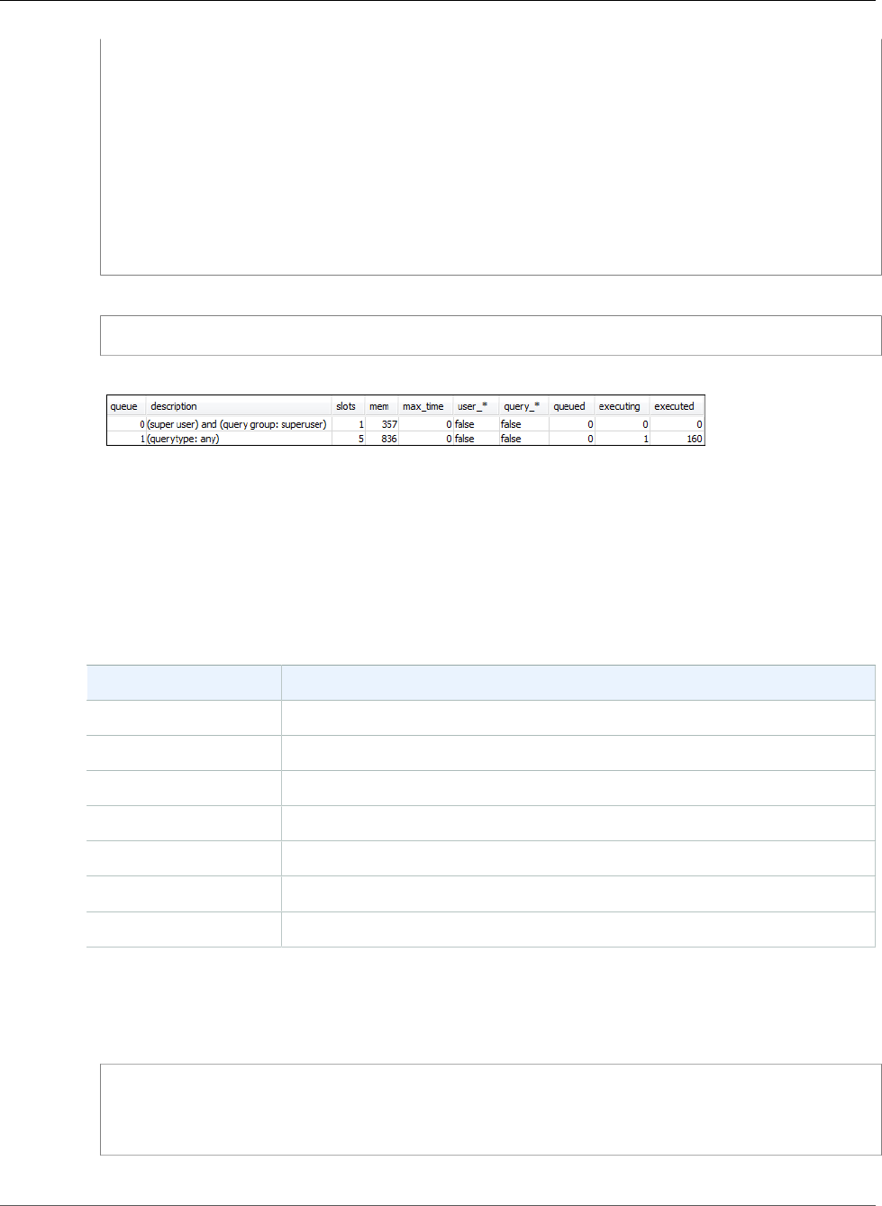
Amazon Redshift Database Developer Guide
Step 2: Create the WLM_QUERY_STATE_VW View
, config.query_group_wild_card as "query_*"
, state.num_queued_queries queued
, state.num_executing_queries executing
, state.num_executed_queries executed
from
STV_WLM_CLASSIFICATION_CONFIG class,
STV_WLM_SERVICE_CLASS_CONFIG config,
STV_WLM_SERVICE_CLASS_STATE state
where
class.action_service_class = config.service_class
and class.action_service_class = state.service_class
and config.service_class > 4
order by config.service_class;
3. Run the following query to see the information that the view contains.
select * from wlm_queue_state_vw;
The following is an example result.
Step 2: Create the WLM_QUERY_STATE_VW View
In this step, you’ll create a view called WLM_QUERY_STATE_VW. This view returns information from the
STV_WLM_QUERY_STATE (p. 892) system table.
You’ll use this view throughout the tutorial to monitor the queries that are running. The following table
describes the data that the WLM_QUERY_STATE_VW view returns.
Column Description
query The query ID.
queue The queue number.
slot_count The number of slots allocated to the query.
start_time The time that the query started.
state The state of the query, such as executing.
queue_time The number of microseconds that the query has spent in the queue.
exec_time The number of microseconds that the query has been executing.
To Create the WLM_QUERY_STATE_VW View
1. In psql, run the following query to create the WLM_QUERY_STATE_VW view.
create view WLM_QUERY_STATE_VW as
select query, (service_class-5) as queue, slot_count, trim(wlm_start_time) as start_time,
trim(state) as state, trim(queue_time) as queue_time, trim(exec_time) as exec_time
from stv_wlm_query_state;
2. Run the following query to see the information that the view contains.
API Version 2012-12-01
92
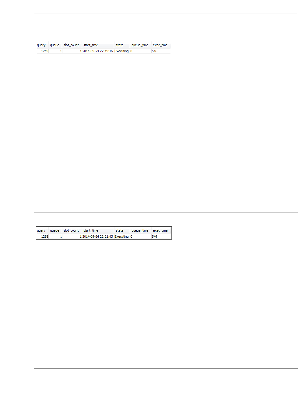
Amazon Redshift Database Developer Guide
Step 3: Run Test Queries
select * from wlm_query_state_vw;
The following is an example result.
Step 3: Run Test Queries
In this step, you’ll run queries from multiple connections in psql and review the system tables to
determine how the queries were routed for processing.
For this step, you will need two psql windows open:
• In psql window 1, you’ll run queries that monitor the state of the queues and queries using the views
you already created in this tutorial.
• In psql window 2, you’ll run long-running queries to change the results you find in psql window 1.
To Run the Test Queries
1. Open two psql windows. If you already have one window open, you only need to open a second
window. You can use the same user account for both of these connections.
2. In psql window 1, run the following query.
select * from wlm_query_state_vw;
The following is an example result.
This query returns a self-referential result. The query that is currently executing is the SELECT
statement from this view. A query on this view will always return at least one result. You’ll compare
this result with the result that occurs after starting the long-running query in the next step.
3. In psql window 2, you'll run a query from the TICKIT sample database. This query should run for
approximately a minute so that you have time to explore the results of the WLM_QUEUE_STATE_VW
view and the WLM_QUERY_STATE_VW view that you created earlier. If you find that the query
does not run long enough for you to query both views, you can increase the value of the filter on
l.listid to make it run longer.
Note
To reduce query execution time and improve system performance, Amazon Redshift caches
the results of certain types of queries in memory on the leader node. When result caching is
enabled, subsequent queries run much faster. To prevent the query from running to quickly,
disable result caching for the current session.
To disable result caching for the current session, set the enable_result_cache_for_session (p. 949)
parameter to off, as shown following.
set enable_result_cache_for_session to off;
In psql window 2, run the following query.
API Version 2012-12-01
93
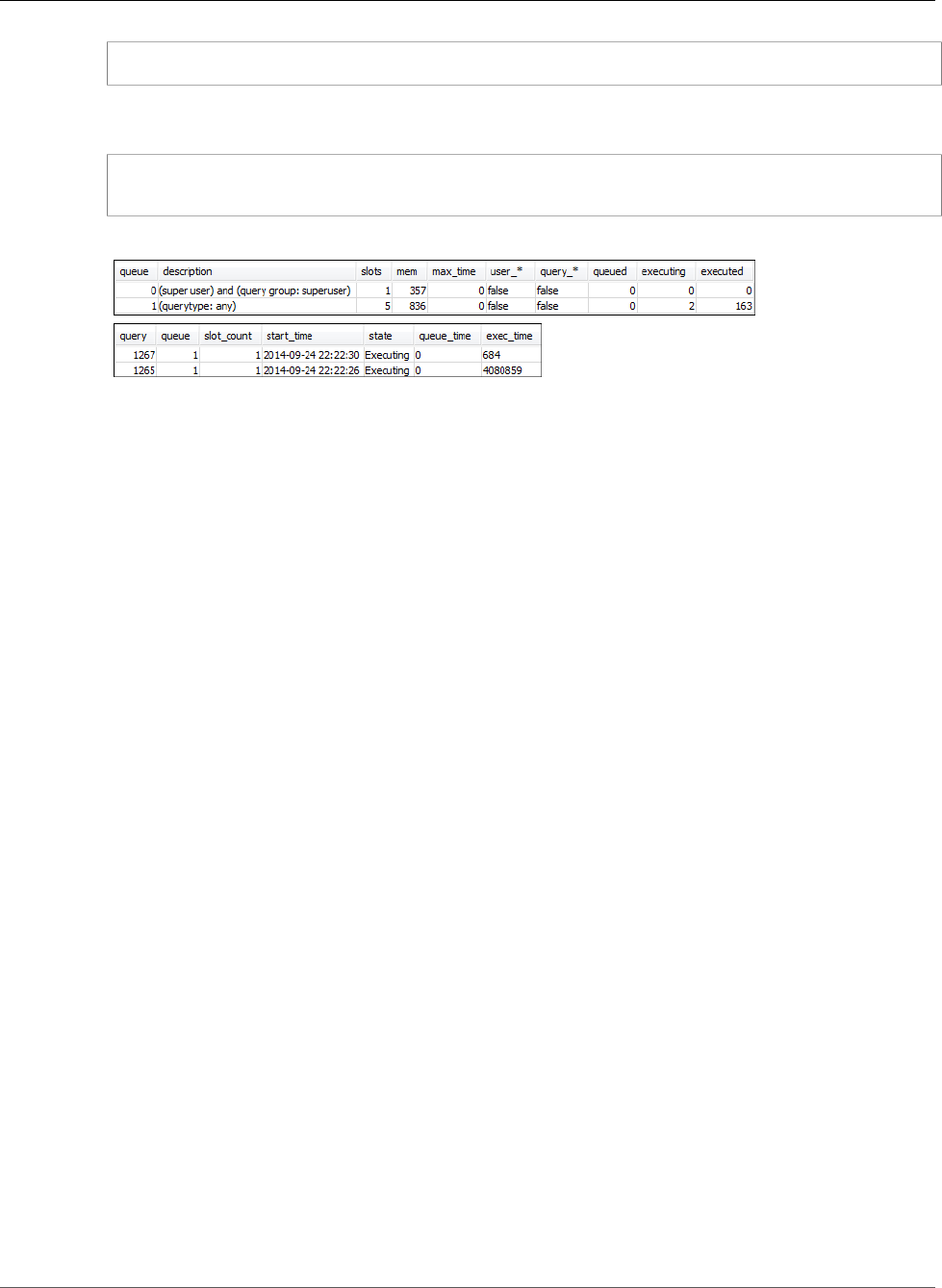
Amazon Redshift Database Developer Guide
Section 2: Modifying the WLM Query Queue Configuration
select avg(l.priceperticket*s.qtysold) from listing l, sales s where l.listid < 100000;
4. In psql window 1, query WLM_QUEUE_STATE_VW and WLM_QUERY_STATE_VW and compare the
results to your earlier results.
select * from wlm_queue_state_vw;
select * from wlm_query_state_vw;
The following are example results.
Note the following differences between your previous queries and the results in this step:
• There are two rows now in WLM_QUERY_STATE_VW. One result is the self-referential query for
running a SELECT operation on this view. The second result is the long-running query from the
previous step.
• The executing column in WLM_QUEUE_STATE_VW has increased from 1 to 2. This column entry means
that there are two queries running in the queue.
• The executed column is incremented each time you run a query in the queue.
The WLM_QUEUE_STATE_VW view is useful for getting an overall view of the queues and how many
queries are being processed in each queue. The WLM_QUERY_STATE_VW view is useful for getting a
more detailed view of the individual queries that are currently running.
Section 2: Modifying the WLM Query Queue
Configuration
Now that you understand how queues work by default, you'll learn how to configure query queues in
WLM. In this section, you’ll create and configure a new parameter group for your cluster. You’ll create
two additional user queues and configure them to accept queries based on the queries’ user group or
query group labels. Any queries that do not get routed to one of these two queues will be routed to the
default queue at run time.
Step 1: Create a Parameter Group
In this step, you’ll create a new parameter group to use to configure WLM for this tutorial.
To Create a Parameter Group
1. Sign in to the AWS Management Console and open the Amazon Redshift console at https://
console.aws.amazon.com/redshift/.
2. In the navigation pane, choose Parameter Groups.
3. Choose Create Cluster Parameter Group.
API Version 2012-12-01
94
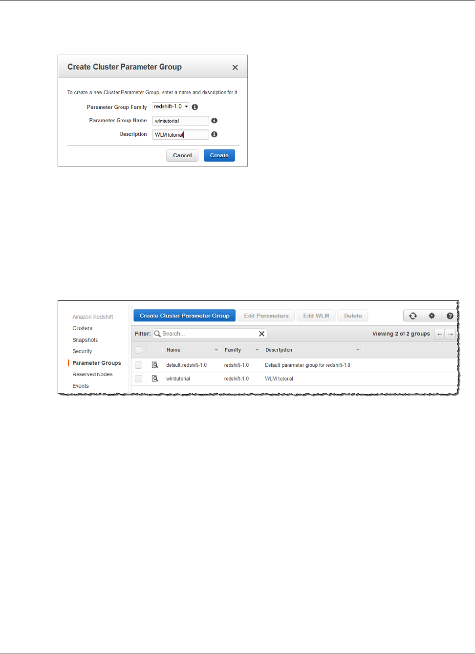
Amazon Redshift Database Developer Guide
Step 2: Configure WLM
4. In the Create Cluster Parameter Group dialog box, type wlmtutorial in the Parameter Group
Name field and type WLM tutorial in the Description field. You can leave the Parameter Group
Family setting as is. Then choose Create.
Step 2: Configure WLM
In this step, you’ll modify the default settings of your new parameter group. You’ll add two new query
queues to the WLM configuration and specify different settings for each queue.
To Modify Parameter Group Settings
1. On the Parameter Groups page of the Amazon Redshift console, click the magnifying glass icon next
to wlmtutorial. Doing this opens up the Parameters page for wlmtutorial.
2. Choose the WLM tab. Click Add New Queue twice to add two new queues to this WLM configuration.
Configure the queues with the following values.
• For queue 1, type 2 in the Concurrency file, test in the Query Groups box, and 30 in the %
Memory box. Leave the other boxes empty.
• For queue 2, type 3 in the Concurrency box, admin in the User Groups box, and 40 in the %
Memory box. Leave the other boxes empty.
• Don't make any changes to the default queue. WLM automatically assigns unallocated memory to
the default queue.
API Version 2012-12-01
95
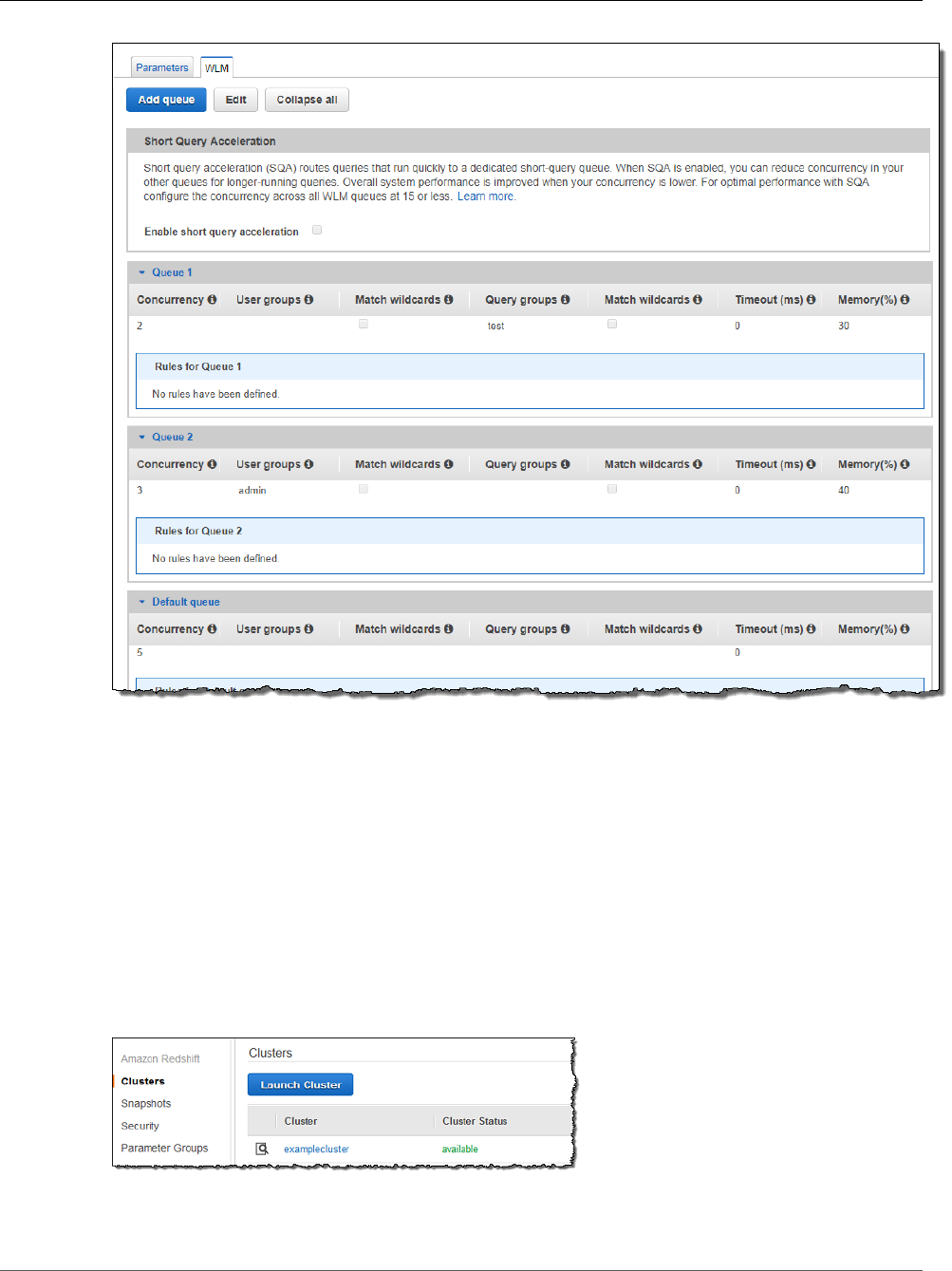
Amazon Redshift Database Developer Guide
Step 3: Associate the Parameter Group with Your Cluster
3. Click Save Changes.
Step 3: Associate the Parameter Group with Your
Cluster
In this step, you’ll open your sample cluster and associate it with the new parameter group. After you do
this, you’ll reboot the cluster so that Amazon Redshift can apply the new settings to the database.
To Associate the Parameter Group with Your Cluster
1. In the navigation pane, click Clusters, and then click your cluster to open it. If you are using the same
cluster from Amazon Redshift Getting Started, your cluster will be named examplecluster.
2. On the Configuration tab, click Modify in the Cluster menu.
API Version 2012-12-01
96
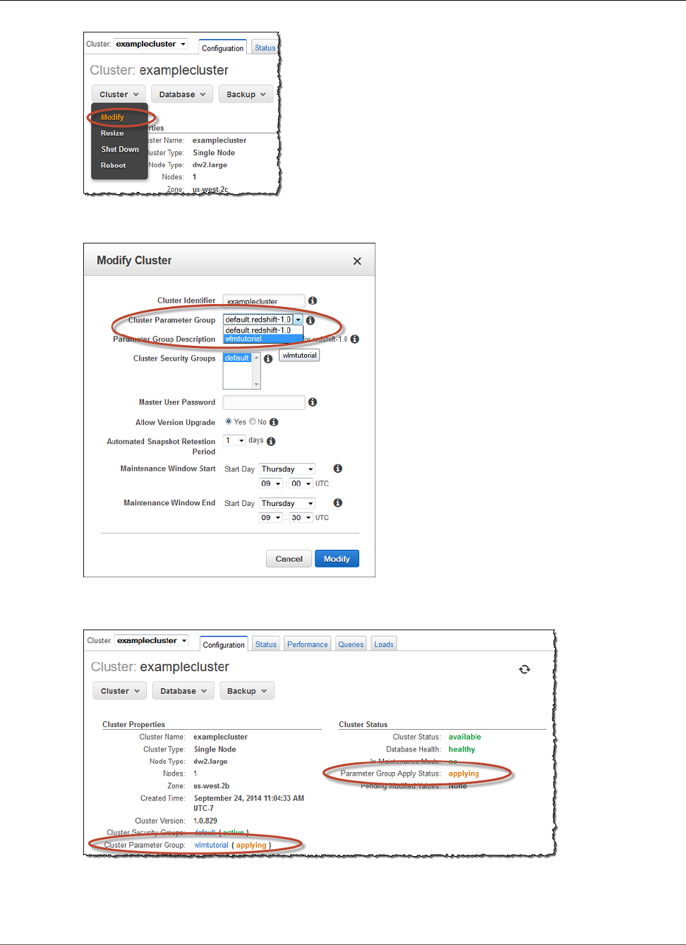
Amazon Redshift Database Developer Guide
Step 3: Associate the Parameter Group with Your Cluster
3. In the Modify Cluster dialog box, select wlmtutorial from the Cluster Parameter Group menu, and
then click Modify.
The statuses shown in the Cluster Parameter Group and Parameter Group Apply Status will change
from in-sync to applying as shown in the following.
After the new parameter group is applied to the cluster, the Cluster Properties and Cluster Status
show the new parameter group that you associated with the cluster. You need to reboot the cluster so
that these settings can be applied to the database also.
API Version 2012-12-01
97
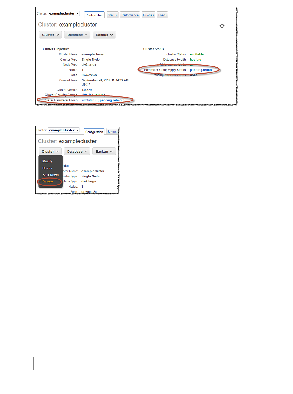
Amazon Redshift Database Developer Guide
Section 3: Routing Queries to Queues
Based on User Groups and Query Groups
4. In the Cluster menu, click Reboot. The status shown in Cluster Status will change from available to
rebooting. After the cluster is rebooted, the status will return to available.
Section 3: Routing Queries to Queues Based on
User Groups and Query Groups
Now that you have your cluster associated with a new parameter group, and you have configured WLM,
you’ll run some queries to see how Amazon Redshift routes queries into queues for processing.
Step 1: View Query Queue Configuration in the
Database
First, verify that the database has the WLM configuration that you expect.
To View the Query Queue Configuration
1. Open psql and run the following query. The query uses the WLM_QUEUE_STATE_VW view you created
in Step 1: Create the WLM_QUEUE_STATE_VW View (p. 91). If you already had a session connected
to the database prior to the cluster reboot, you’ll need to reconnect.
select * from wlm_queue_state_vw;
The following is an example result.
API Version 2012-12-01
98
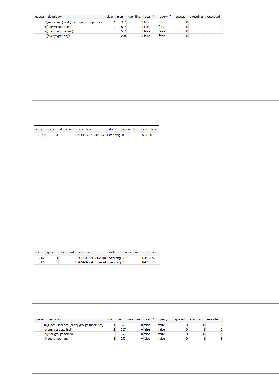
Amazon Redshift Database Developer Guide
Step 2: Run a Query Using the Query Group Queue
Compare these results to the results you received in Step 1: Create the WLM_QUEUE_STATE_VW
View (p. 91). Notice that there are now two additional queues. Queue 1 is now the queue for the
test query group, and queue 2 is the queue for the admin user group.
Queue 3 is now the default queue. The last queue in the list is always the default queue, and that
is the queue to which queries are routed by default if no user group or query group is specified in a
query.
2. Run the following query to confirm that your query now runs in queue 3.
select * from wlm_query_state_vw;
The following is an example result.
Step 2: Run a Query Using the Query Group Queue
To Run a Query Using the Query Group Queue
1. Run the following query to route it to the test query group.
set query_group to test;
select avg(l.priceperticket*s.qtysold) from listing l, sales s where l.listid <40000;
2. From the other psql window, run the following query.
select * from wlm_query_state_vw;
The following is an example result.
The query was routed to the test query group, which is queue 1 now.
3. Select all from the queue state view.
select * from wlm_queue_state_vw;
You'll see a result similar to the following.
4. Now, reset the query group and run the long query again:
reset query_group;
select avg(l.priceperticket*s.qtysold) from listing l, sales s where l.listid <40000;
API Version 2012-12-01
99

Amazon Redshift Database Developer Guide
Step 3: Create a Database User and Group
5. Run the queries against the views to see the results.
select * from wlm_queue_state_vw;
select * from wlm_query_state_vw;
The following are example results.
The result should be that the query is now running in queue 3 again.
Step 3: Create a Database User and Group
In Step 1: Create a Parameter Group (p. 94), you configured one of your query queues with a user
group named admin. Before you can run any queries in this queue, you need to create the user group in
the database and add a user to the group. Then you’ll log on with psql using the new user’s credentials
and run queries. You need to run queries as a superuser, such as the masteruser, to create database users.
To Create a New Database User and User Group
1. In the database, create a new database user named adminwlm by running the following command in a
psql window.
create user adminwlm createuser password '123Admin';
2. Then, run the following commands to create the new user group and add your new adminwlm user to
it.
create group admin;
alter group admin add user adminwlm;
Step 4: Run a Query Using the User Group Queue
Next you’ll run a query and route it to the user group queue. You do this when you want to route your
query to a queue that is configured to handle the type of query you want to run.
To Run a Query Using the User Group Queue
1. In psql window 2, run the following queries to switch to the adminwlm account and run a query as
that user.
set session authorization 'adminwlm';
select avg(l.priceperticket*s.qtysold) from listing l, sales s where l.listid <40000;
2. In psql window 1, run the following query to see the query queue that the queries are routed to.
select * from wlm_query_state_vw;
API Version 2012-12-01
100
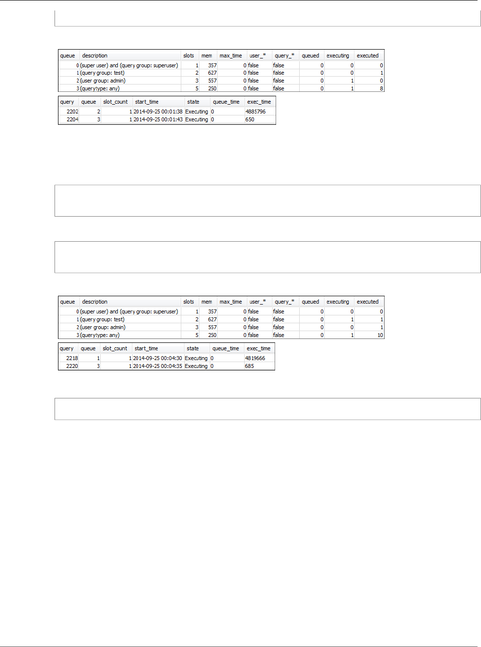
Amazon Redshift Database Developer Guide
Section 4: Using wlm_query_slot_count to
Temporarily Override Concurrency Level in a Queue
select * from wlm_queue_state_vw;
The following are example results.
Note that the queue this query ran in is queue 2, the admin user queue. Any time you run queries
logged in as this user, they will run in queue 2 unless you specify a different query group to use.
3. Now run the following query from psql window 2.
set query_group to test;
select avg(l.priceperticket*s.qtysold) from listing l, sales s where l.listid <40000;
4. In psql window 1, run the following query to see the query queue that the queries are routed to.
select * from wlm_queue_state_vw;
select * from wlm_query_state_vw;
The following are example results.
5. When you’re done, reset the query group.
reset query_group;
Section 4: Using wlm_query_slot_count to
Temporarily Override Concurrency Level in a
Queue
Sometimes, users might temporarily need more resources for a particular query. If so, they can use the
wlm_query_slot_count configuration setting to temporarily override the way slots are allocated in a
query queue. Slots are units of memory and CPU that are used to process queries. You might override the
slot count when you have occasional queries that take a lot of resources in the cluster, such as when you
perform a VACUUM operation in the database.
If you find that users often need to set wlm_query_slot_count for certain types of queries, you should
consider adjusting the WLM configuration and giving users a queue that better suits the needs of their
queries. For more information about temporarily overriding the concurrency level by using slot count,
see wlm_query_slot_count (p. 955).
API Version 2012-12-01
101
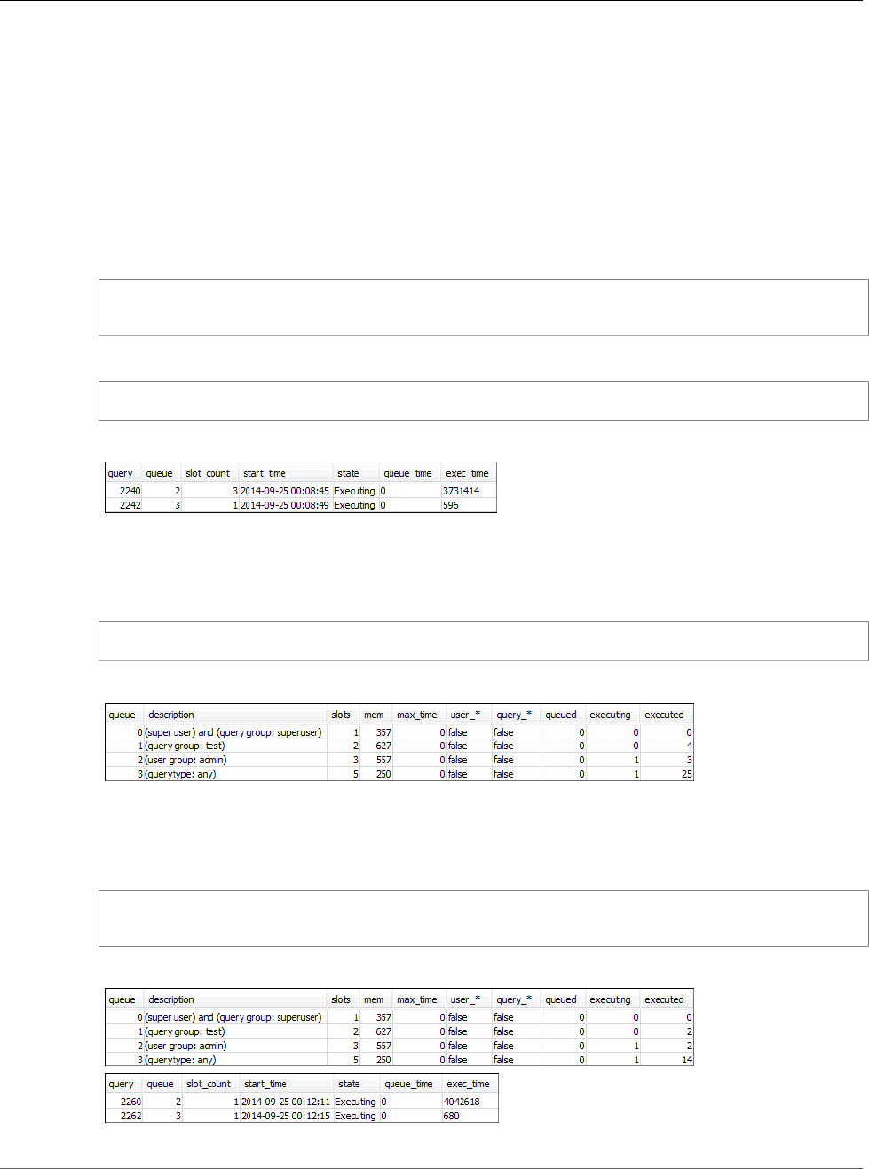
Amazon Redshift Database Developer Guide
Step 1: Override the Concurrency
Level Using wlm_query_slot_count
Step 1: Override the Concurrency Level Using
wlm_query_slot_count
For the purposes of this tutorial, we’ll run the same long-running SELECT query. We’ll run it as the
adminwlm user using wlm_query_slot_count to increase the number of slots available for the query.
To Override the Concurrency Level Using wlm_query_slot_count
1. Increase the limit on the query to make sure that you have enough time to query the
WLM_QUERY_STATE_VW view and see a result.
set wlm_query_slot_count to 3;
select avg(l.priceperticket*s.qtysold) from listing l, sales s where l.listid <40000;
2. Now, query WLM_QUERY_STATE_VW use the masteruser account to see how the query is running.
select * from wlm_query_state_vw;
The following is an example result.
Notice that the slot count for the query is 3. This count means that the query is using all three slots to
process the query, allocating all of the resources in the queue to that query.
3. Now, run the following query.
select * from WLM_QUEUE_STATE_VW;
The following is an example result.
The wlm_query_slot_count configuration setting is valid for the current session only. If that session
expires, or another user runs a query, the WLM configuration is used.
4. Reset the slot count and rerun the test.
reset wlm_query_slot_count;
select avg(l.priceperticket*s.qtysold) from listing l, sales s where l.listid <40000;
The following are example results.
API Version 2012-12-01
102
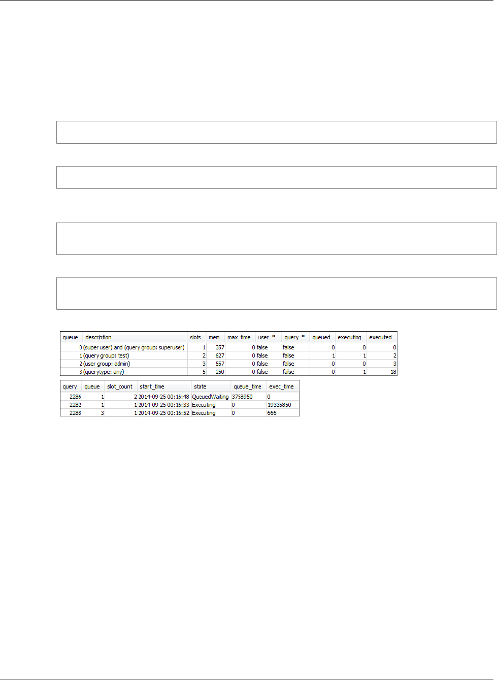
Amazon Redshift Database Developer Guide
Step 2: Run Queries from Different Sessions
Step 2: Run Queries from Different Sessions
Next, run queries from different sessions.
To Run Queries from Different Sessions
1. In psql window 1 and 2, run the following to use the test query group.
set query_group to test;
2. In psql window 1, run the following long-running query.
select avg(l.priceperticket*s.qtysold) from listing l, sales s where l.listid <40000;
3. As the long-running query is still going in psql window 1, run the following to increase the slot count
to use all the slots for the queue and then start running the long-running query.
set wlm_query_slot_count to 2;
select avg(l.priceperticket*s.qtysold) from listing l, sales s where l.listid <40000;
4. Open a third psql window and query the views to see the results.
select * from wlm_queue_state_vw;
select * from wlm_query_state_vw;
The following are example results.
Notice that the first query is using one of the slots allocated to queue 1 to run the query, and that
there is one query that is waiting in the queue (where queued is 1 and state is QueuedWaiting).
Once the first query completes, the second one will begin executing. This execution happens because
both queries are routed to the test query group, and the second query must wait for enough slots to
begin processing.
Section 5: Cleaning Up Your Resources
Your cluster continues to accrue charges as long as it is running. When you have completed this tutorial,
you should return your environment to the previous state by following the steps in Step 6: Find
Additional Resources and Reset Your Environment in Amazon Redshift Getting Started.
For more information about WLM, see Implementing Workload Management (p. 285).
API Version 2012-12-01
103

Amazon Redshift Database Developer Guide
Overview
Tutorial: Querying Nested Data with
Amazon Redshift Spectrum
Overview
Amazon Redshift Spectrum supports querying nested data in Parquet, ORC, JSON, and Ion file formats.
Redshift Spectrum accesses the data using external tables. You can create external tables that use the
complex data types struct, array, and map.
For example, suppose that your data file contains the following data in Amazon S3 in a folder named
customers.
{ Id: 1,
Name: {Given:"John", Family:"Smith"},
Phones: ["123-457789"],
Orders: [ {Date: "Mar 1,2018 11:59:59", Price: 100.50}
{Date: "Mar 1,2018 09:10:00", Price: 99.12} ]
}
{ Id: 2,
Name: {Given:"Jenny", Family:"Doe"},
Phones: ["858-8675309", "415-9876543"],
Orders: [ ]
}
{ Id: 3,
Name: {Given:"Andy", Family:"Jones"},
Phones: [ ]
Orders: [ {Date: "Mar 2,2018 08:02:15", Price: 13.50} ]
}
You can use Redshift Spectrum to query this data. The following tutorial shows you how to do so.
For tutorial prerequisites, steps, and nested data use cases, see the following topics:
•Prerequisites (p. 104)
•Step 1: Create an External Table That Contains Nested Data (p. 105)
•Step 2: Query Your Nested Data in Amazon S3 with SQL Extensions (p. 105)
•Nested Data Use Cases (p. 109)
•Nested Data Limitations (p. 111)
Prerequisites
If you are not using Redshift Spectrum yet, follow the steps in the Getting Started with Amazon Redshift
Spectrum (p. 150) tutorial before continuing.
API Version 2012-12-01
104
Amazon Redshift Database Developer Guide
Step 1: Create an External Table That Contains Nested Data
Step 1: Create an External Table That Contains
Nested Data
To create the external table for this tutorial, run the following command.
CREATE EXTERNAL TABLE spectrum.customers (
id int,
name struct<given:varchar(20), family:varchar(20)>,
phones array<varchar(20)>,
orders array<struct<shipdate:timestamp, price:double precision>>
)
STORED AS PARQUET
LOCATION 's3://awssampledbuswest2/nested_example/customers/';
In the example preceding, the external table spectrum.customers uses the struct and array data
types to define columns with nested data. Amazon Redshift Spectrum supports querying nested data in
Parquet, ORC, JSON, and Ion file formats. The LOCATION parameter has to refer to the Amazon S3 folder
that contains the nested data or files.
Note
Amazon Redshift doesn't support complex data types in an Amazon Redshift database table.
You can use complex data types only with Redshift Spectrum external tables.
You can nest array and struct types at any level. For example, you can define a column named
toparray as shown in the following example.
toparray array<struct<nestedarray:
array<struct<morenestedarray:
array<string>>>>>
You can also nest struct types as shown for column x in the following example.
x struct<a: string,
b: struct<c: integer,
d: struct<e: string>
>
>
Step 2: Query Your Nested Data in Amazon S3 with
SQL Extensions
Redshift Spectrum supports querying array, map, and struct complex types through extensions to the
Amazon Redshift SQL syntax.
Extension 1: Access to Columns of Structs
You can extract data from struct columns using a dot notation that concatenates field names into
paths. For example, the following query returns given and family names for customers. The given
API Version 2012-12-01
105
Amazon Redshift Database Developer Guide
Extension 2: Ranging Over Arrays in a FROM Clause
name is accessed by the long path c.name.given. The family name is accessed by the long path
c.name.family.
SELECT c.id, c.name.given, c.name.family
FROM spectrum.customers c;
The preceding query returns the following data.
id | given | family
---|-------|-------
1 | John | Smith
2 | Jenny | Doe
3 | Andy | Jones
(3 rows)
A struct can be a column of another struct, which can be a column of another struct, at any level.
The paths that access columns in such deeply nested structs can be arbitrarily long. For example, see
the definition for the column x in the following example.
x struct<a: string,
b: struct<c: integer,
d: struct<e: string>
>
>
You can access the data in e as x.b.d.e.
Note
You use structs only to describe the path to the fields that they contain. You can't access them
directly in a query or return them from a query.
Extension 2: Ranging Over Arrays in a FROM Clause
You can extract data from array columns (and, by extension, map columns) by specifying the array
columns in a FROM clause in place of table names. The extension applies to the FROM clause of the main
query, and also the FROM clauses of subqueries. You can't reference array elements by position, such as
c.orders[0].
By combining ranging over arrays with joins, you can achieve various kinds of unnesting, as explained
in the following use cases.
Unnesting Using Inner Joins
The following query selects customer IDs and order ship dates for customers that have orders. The SQL
extension in the FROM clause c.orders o depends on the alias c.
SELECT c.id, o.shipdate
FROM spectrum.customers c, c.orders o
API Version 2012-12-01
106

Amazon Redshift Database Developer Guide
Extension 2: Ranging Over Arrays in a FROM Clause
For each customer c that has orders, the FROM clause returns one row for each order o of the customer
c. That row combines the customer row c and the order row o. Then the SELECT clause keeps only the
c.id and o.shipdate. The result is the following.
id| shipdate
--|----------------------
1 |2018-03-01 11:59:59
1 |2018-03-01 09:10:00
3 |2018-03-02 08:02:15
(3 rows)
The alias c provides access to the customer fields, and the alias o provides access to the order fields.
The semantics are similar to standard SQL. You can think of the FROM clause as executing the following
nested loop, which is followed by SELECT choosing the fields to output.
for each customer c in spectrum.customers
for each order o in c.orders
output c.id and o.shipdate
Therefore, if a customer doesn't have an order, the customer doesn't appear in the result.
You can also think of this as the FROM clause performing a JOIN with the customers table and the
orders array. In fact, you can also write the query as shown in the following example.
SELECT c.id, o.shipdate
FROM spectrum.customers c INNER JOIN c.orders o ON true
Note
If a schema named c exists with a table named orders, then c.orders refers to the table
orders, and not the array column of customers.
Unnesting Using Left Joins
The following query outputs all customer names and their orders. If a customer hasn't placed an order,
the customer's name is still returned. However, in this case the order columns are NULL, as shown in the
following example for Jenny Doe.
SELECT c.id, c.name.given, c.name.family, o.shipdate, o.price
FROM spectrum.customers c LEFT JOIN c.orders o ON true
The preceding query returns the following data.
id | given | family | shipdate | price
----|---------|---------|----------------------|--------
1 | John | Smith | 2018-03-01 11:59:59 | 100.5
2 | John | Smith | 2018-03-01 09:10:00 | 99.12
2 | Jenny | Doe | |
API Version 2012-12-01
107
Amazon Redshift Database Developer Guide
Extension 3: Accessing an Array
of Scalars Directly Using an Alias
3 | Andy | Jones | 2018-03-02 08:02:15 | 13.5
(4 rows)
Extension 3: Accessing an Array of Scalars Directly
Using an Alias
When an alias p in a FROM clause ranges over an array of scalars, the query refers to the values of p
simply as p. For example, the following query produces pairs of customer names and phone numbers.
SELECT c.name.given, c.name.family, p AS phone
FROM spectrum.customers c LEFT JOIN c.phones p ON true
The preceding query returns the following data.
given | family | phone
-------|----------|-----------
John | Smith | 123-4577891
Jenny | Doe | 858-8675309
Jenny | Doe | 415-9876543
Andy | Jones |
(4 rows)
Extension 4: Accessing Elements of Maps
Redshift Spectrum treats the map data type as an array type that contains struct types with a key
column and a value column. The key must be a scalar; the value can be any data type.
For example, the following code creates an external table with a map for storing phone numbers.
CREATE EXTERNAL TABLE spectrum.customers (
id int,
name struct<given:varchar(20), family:varchar(20)>,
phones map<varchar(20), varchar(20)>,
orders array<struct<shipdate:timestamp, price:double precision>>
)
Because a map type behaves like an array type with columns key and value, you can think of the
preceding schemas as if they were the following.
CREATE EXTERNAL TABLE spectrum.customers (
id int,
name struct<given:varchar(20), family:varchar(20)>,
phones array<struct<key:varchar(20), value:varchar(20)>>,
orders array<struct<shipdate:timestamp, price:double precision>>
)
API Version 2012-12-01
108
Amazon Redshift Database Developer Guide
Nested Data Use Cases
The following query returns the names of customers with a mobile phone number and returns the
number for each name. The map query is treated as the equivalent of querying a nested array of
struct types. The following query only returns data if you have created the external table as described
previously.
SELECT c.name.given, c.name.family, p.value
FROM spectrum.customers c, c.phones p
WHERE p.key = 'mobile'
Note
The key for a map is a string for Ion and JSON file types.
Nested Data Use Cases
You can combine the extensions described previously with the usual SQL features. The following use
cases illustrate some common combinations. These examples help demonstrate how you can use nested
data. They aren't part of the tutorial.
Topics
•Ingesting Nested Data (p. 109)
•Aggregating Nested Data with Subqueries (p. 109)
•Joining Amazon Redshift and Nested Data (p. 110)
Ingesting Nested Data
You can use a CREATE TABLE AS statement to ingest data from an external table that contains complex
data types. The following query extracts all customers and their phone numbers from the external table,
using LEFT JOIN, and stores them in the Amazon Redshift table CustomerPhones.
CREATE TABLE CustomerPhones AS
SELECT c.name.given, c.name.family, p AS phone
FROM spectrum.customers c LEFT JOIN c.phones p ON true
Aggregating Nested Data with Subqueries
You can use a subquery to aggregate nested data. The following example illustrates this approach.
SELECT c.name.given, c.name.family, (SELECT COUNT(*) FROM c.orders o) AS ordercount
FROM spectrum.customers c
The following data is returned.
given | family | ordercount
API Version 2012-12-01
109
Amazon Redshift Database Developer Guide
Joining Amazon Redshift and Nested Data
--------|----------|--------------
Jenny | Doe | 0
John | Smith | 2
Andy | Jones | 1
(3 rows)
Note
When you aggregate nested data by grouping by the parent row, the most efficient way is the
one shown in the previous example. In that example, the nested rows of c.orders are grouped
by their parent row c. Alternatively, if you know that id is unique for each customer and
o.shipdate is never null, you can aggregate as shown in the following example. However, this
approach generally isn't as efficient as the previous example.
SELECT c.name.given, c.name.family, COUNT(o.shipdate) AS ordercount
FROM spectrum.customers c LEFT JOIN c.orders o ON true
GROUP BY c.id, c.name.given, c.name.family
You can also write the query by using a subquery in the FROM clause that refers to an alias (c) of the
ancestor query and extracts array data. The following example demonstrates this approach.
SELECT c.name.given, c.name.family, s.count AS ordercount
FROM spectrum.customers c, (SELECT count(*) AS count FROM c.orders o) s
Joining Amazon Redshift and Nested Data
You can also join Amazon Redshift data with nested data in an external table. For example, suppose that
you have the following nested data in Amazon S3.
CREATE EXTERNAL TABLE spectrum.customers2 (
id int,
name struct<given:varchar(20), family:varchar(20)>,
phones array<varchar(20)>,
orders array<struct<shipdate:timestamp, item:int>>
)
Suppose also that you have the following table in Amazon Redshift.
CREATE TABLE prices (
id int,
price double precision
)
The following query finds the total number and amount of each customer's purchases based on the
preceding. The following example is only an illustration. It only returns data if you have created the
tables described previously.
API Version 2012-12-01
110
Amazon Redshift Database Developer Guide
Nested Data Limitations
SELECT c.name.given, c.name.family, COUNT(o.date) AS ordercount, SUM(p.price) AS
ordersum
FROM spectrum.customers2 c, c.orders o, prices p ON o.item = p.id
GROUP BY c.id, c.name.given, c.name.family
Nested Data Limitations
The following limitations apply to nested data:
• An array can only contain scalars or struct types. Array types can't contain array or map types.
• Redshift Spectrum supports complex data types only as external tables.
• Query and subquery result columns must be scalar.
• If an OUTER JOIN expression refers to a nested table, it can refer only to that table and its nested
arrays (and maps). If an OUTER JOIN expression doesn't refer to a nested table, it can refer to any
number of non-nested tables.
• If a FROM clause in a subquery refers to a nested table, it can't refer to any other table.
• If a subquery depends on a nested table that refers to a parent, you can use the parent only in the
FROM clause. You can't use the query in any other clauses, such as a SELECT or WHERE clause. For
example, the following query isn't executed.
SELECT c.name.given
FROM spectrum.customers c
WHERE (SELECT COUNT(c.id) FROM c.phones p WHERE p LIKE '858%') > 1
The following query works because the parent c is used only in the FROM clause of the subquery.
SELECT c.name.given
FROM spectrum.customers c
WHERE (SELECT COUNT(*) FROM c.phones p WHERE p LIKE '858%') > 1
• A subquery that accesses nested data anywhere other than the FROM clause must return a single value.
The only exceptions are (NOT) EXISTS operators in a WHERE clause.
•(NOT) IN is not supported.
• The maximum nesting depth for all nested types is 100. This restriction applies to all file formats
(Parquet, ORC, Ion, and JSON).
• Aggregation subqueries that access nested data can only refer to arrays and maps in their FROM
clause, not to an external table.
API Version 2012-12-01
111

Amazon Redshift Database Developer Guide
Amazon Redshift Security Overview
Managing Database Security
Topics
•Amazon Redshift Security Overview (p. 112)
•Default Database User Privileges (p. 113)
•Superusers (p. 113)
•Users (p. 114)
•Groups (p. 114)
•Schemas (p. 115)
•Example for Controlling User and Group Access (p. 116)
You manage database security by controlling which users have access to which database objects.
Access to database objects depends on the privileges that you grant to user accounts or groups. The
following guidelines summarize how database security works:
• By default, privileges are granted only to the object owner.
• Amazon Redshift database users are named user accounts that can connect to a database. A user
account is granted privileges explicitly, by having those privileges assigned directly to the account, or
implicitly, by being a member of a group that is granted privileges.
• Groups are collections of users that can be collectively assigned privileges for easier security
maintenance.
• Schemas are collections of database tables and other database objects. Schemas are similar to
operating system directories, except that schemas cannot be nested. Users can be granted access to a
single schema or to multiple schemas.
For examples of security implementation, see Example for Controlling User and Group Access (p. 116).
Amazon Redshift Security Overview
Amazon Redshift database security is distinct from other types of Amazon Redshift security. In addition
to database security, which is described in this section, Amazon Redshift provides these features to
manage security:
•Sign-in credentials — Access to your Amazon Redshift Management Console is controlled by your
AWS account privileges. For more information, see Sign-In Credentials.
•Access management — To control access to specific Amazon Redshift resources, you define AWS
Identity and Access Management (IAM) accounts. For more information, see Controlling Access to
Amazon Redshift Resources.
•Cluster security groups — To grant other users inbound access to an Amazon Redshift cluster, you
define a cluster security group and associate it with a cluster. For more information, see Amazon
Redshift Cluster Security Groups.
•VPC — To protect access to your cluster by using a virtual networking environment, you can launch
your cluster in an Amazon Virtual Private Cloud (VPC). For more information, see Managing Clusters in
Virtual Private Cloud (VPC).
•Cluster encryption — To encrypt the data in all your user-created tables, you can enable cluster
encryption when you launch the cluster. For more information, see Amazon Redshift Clusters.
API Version 2012-12-01
112

Amazon Redshift Database Developer Guide
Default Database User Privileges
•SSL connections — To encrypt the connection between your SQL client and your cluster, you can use
secure sockets layer (SSL) encryption. For more information, see Connect to Your Cluster Using SSL.
•Load data encryption — To encrypt your table load data files when you upload them to Amazon
S3, you can use either server-side encryption or client-side encryption. When you load from server-
side encrypted data, Amazon S3 handles decryption transparently. When you load from client-side
encrypted data, the Amazon Redshift COPY command decrypts the data as it loads the table. For more
information, see Uploading Encrypted Data to Amazon S3 (p. 189).
•Data in transit — To protect your data in transit within the AWS cloud, Amazon Redshift uses
hardware accelerated SSL to communicate with Amazon S3 or Amazon DynamoDB for COPY, UNLOAD,
backup, and restore operations.
Default Database User Privileges
When you create a database object, you are its owner. By default, only a superuser or the owner of an
object can query, modify, or grant privileges on the object. For users to use an object, you must grant the
necessary privileges to the user or the group that contains the user. Database superusers have the same
privileges as database owners.
Amazon Redshift supports the following privileges: SELECT, INSERT, UPDATE, DELETE, REFERENCES,
CREATE, TEMPORARY, and USAGE. Different privileges are associated with different object types. For
information on database object privileges supported by Amazon Redshift, see the GRANT (p. 516)
command.
The right to modify or destroy an object is always the privilege of the owner only.
To revoke a privilege that was previously granted, use the REVOKE (p. 527) command. The privileges
of the object owner, such as DROP, GRANT, and REVOKE privileges, are implicit and cannot be granted
or revoked. Object owners can revoke their own ordinary privileges, for example, to make a table read-
only for themselves as well as others. Superusers retain all privileges regardless of GRANT and REVOKE
commands.
Superusers
Database superusers have the same privileges as database owners for all databases.
The masteruser, which is the user you created when you launched the cluster, is a superuser.
You must be a superuser to create a superuser.
Amazon Redshift system tables and system views are either visible only to superusers or visible to
all users. Only superusers can query system tables and system views that are designated "visible to
superusers." For information, see System Tables and Views (p. 797).
Superusers can view all PostgreSQL catalog tables. For information, see System Catalog Tables (p. 935).
A database superuser bypasses all permission checks. Be very careful when using a superuser role.
We recommend that you do most of your work as a role that is not a superuser. Superusers retain all
privileges regardless of GRANT and REVOKE commands.
To create a new database superuser, log on to the database as a superuser and issue a CREATE USER
command or an ALTER USER command with the CREATEUSER privilege.
create user adminuser createuser password '1234Admin';
alter user adminuser createuser;
API Version 2012-12-01
113

Amazon Redshift Database Developer Guide
Users
Users
You can create and manage database users using the Amazon Redshift SQL commands CREATE USER
and ALTER USER, or you can configure your SQL client with custom Amazon Redshift JDBC or ODBC
drivers that manage the process of creating database users and temporary passwords as part of the
database logon process.
The drivers authenticate database users based on AWS Identity and Access Management (IAM)
authentication. If you already manage user identities outside of AWS, you can use a SAML 2.0-compliant
identity provider (IdP) to manage access to Amazon Redshift resources. You use an IAM role to configure
your IdP and AWS to permit your federated users to generate temporary database credentials and log
on to Amazon Redshift databases. For more information, see Using IAM Authentication to Generate
Database User Credentials.
Amazon Redshift user accounts can only be created and dropped by a database superuser. Users are
authenticated when they login to Amazon Redshift. They can own databases and database objects (for
example, tables) and can grant privileges on those objects to users, groups, and schemas to control
who has access to which object. Users with CREATE DATABASE rights can create databases and grant
privileges to those databases. Superusers have database ownership privileges for all databases.
Creating, Altering, and Deleting Users
Database users accounts are global across a data warehouse cluster (and not per individual database).
• To create a user use the CREATE USER (p. 490) command.
• To create a superuser use the CREATE USER (p. 490) command with the CREATEUSER option.
• To remove an existing user, use the DROP USER (p. 507) command.
• To make changes to a user account, such as changing a password, use the ALTER USER (p. 377)
command.
• To view a list of users, query the PG_USER catalog table:
select * from pg_user;
usename | usesysid | usecreatedb | usesuper | usecatupd | passwd | valuntil |
useconfig
------------+----------+-------------+----------+-----------+----------+----------
+-----------
rdsdb | 1 | t | t | t | ******** | |
masteruser | 100 | t | t | f | ******** | |
dwuser | 101 | f | f | f | ******** | |
simpleuser | 102 | f | f | f | ******** | |
poweruser | 103 | f | t | f | ******** | |
dbuser | 104 | t | f | f | ******** | |
(6 rows)
Groups
Groups are collections of users who are all granted whatever privileges are associated with the group.
You can use groups to assign privileges by role. For example, you can create different groups for sales,
administration, and support and give the users in each group the appropriate access to the data they
require for their work. You can grant or revoke privileges at the group level, and those changes will apply
to all members of the group, except for superusers.
To view all user groups, query the PG_GROUP system catalog table:
API Version 2012-12-01
114

Amazon Redshift Database Developer Guide
Creating, Altering, and Deleting Groups
select * from pg_group;
Creating, Altering, and Deleting Groups
Only a superuser can create, alter, or drop groups.
You can perform the following actions:
• To create a group, use the CREATE GROUP (p. 467) command.
• To add users to or remove users from an existing group, use the ALTER GROUP (p. 363) command.
• To delete a group, use the DROP GROUP (p. 502) command. This command only drops the group, not
its member users.
Schemas
A database contains one or more named schemas. Each schema in a database contains tables and other
kinds of named objects. By default, a database has a single schema, which is named PUBLIC. You can use
schemas to group database objects under a common name. Schemas are similar to operating system
directories, except that schemas cannot be nested.
Identical database object names can be used in different schemas in the same database without conflict.
For example, both MY_SCHEMA and YOUR_SCHEMA can contain a table named MYTABLE. Users with the
necessary privileges can access objects across multiple schemas in a database.
By default, an object is created within the first schema in the search path of the database. For
information, see Search Path (p. 116) later in this section.
Schemas can help with organization and concurrency issues in a multi-user environment in the following
ways:
• To allow many developers to work in the same database without interfering with each other.
• To organize database objects into logical groups to make them more manageable.
• To give applications the ability to put their objects into separate schemas so that their names will not
collide with the names of objects used by other applications.
Creating, Altering, and Deleting Schemas
Any user can create schemas and alter or drop schemas they own.
You can perform the following actions:
• To create a schema, use the CREATE SCHEMA (p. 470) command.
• To change the owner of a schema, use the ALTER SCHEMA (p. 364) command.
• To delete a schema and its objects, use the DROP SCHEMA (p. 503) command.
• To create a table within a schema, create the table with the format schema_name.table_name.
To view a list of all schemas, query the PG_NAMESPACE system catalog table:
select * from pg_namespace;
API Version 2012-12-01
115
Amazon Redshift Database Developer Guide
Search Path
To view a list of tables that belong to a schema, query the PG_TABLE_DEF system catalog table. For
example, the following query returns a list of tables in the PG_CATALOG schema.
select distinct(tablename) from pg_table_def
where schemaname = 'pg_catalog';
Search Path
The search path is defined in the search_path parameter with a comma-separated list of schema names.
The search path specifies the order in which schemas are searched when an object, such as a table or
function, is referenced by a simple name that does not include a schema qualifier.
If an object is created without specifying a target schema, the object is added to the first schema that is
listed in search path. When objects with identical names exist in different schemas, an object name that
does not specify a schema will refer to the first schema in the search path that contains an object with
that name.
To change the default schema for the current session, use the SET (p. 560) command.
For more information, see the search_path (p. 951) description in the Configuration Reference.
Schema-Based Privileges
Schema-based privileges are determined by the owner of the schema:
• By default, all users have CREATE and USAGE privileges on the PUBLIC schema of a database. To
disallow users from creating objects in the PUBLIC schema of a database, use the REVOKE (p. 527)
command to remove that privilege.
• Unless they are granted the USAGE privilege by the object owner, users cannot access any objects in
schemas they do not own.
• If users have been granted the CREATE privilege to a schema that was created by another user, those
users can create objects in that schema.
Example for Controlling User and Group Access
This example creates user groups and user accounts and then grants them various privileges for an
Amazon Redshift database that connects to a web application client. This example assumes three groups
of users: regular users of a web application, power users of a web application, and web developers.
1. Create the groups where the user accounts will be assigned. The following set of commands creates
three different user groups:
create group webappusers;
create group webpowerusers;
create group webdevusers;
2. Create several database user accounts with different privileges and add them to the groups.
a. Create two users and add them to the WEBAPPUSERS group:
create user webappuser1 password 'webAppuser1pass'
in group webappusers;
API Version 2012-12-01
116
Amazon Redshift Database Developer Guide
Example for Controlling User and Group Access
create user webappuser2 password 'webAppuser2pass'
in group webappusers;
b. Create an account for a web developer and adds it to the WEBDEVUSERS group:
create user webdevuser1 password 'webDevuser2pass'
in group webdevusers;
c. Create a superuser account. This user will have administrative rights to create other users:
create user webappadmin password 'webAppadminpass1'
createuser;
3. Create a schema to be associated with the database tables used by the web application, and grant the
various user groups access to this schema:
a. Create the WEBAPP schema:
create schema webapp;
b. Grant USAGE privileges to the WEBAPPUSERS group:
grant usage on schema webapp to group webappusers;
c. Grant USAGE privileges to the WEBPOWERUSERS group:
grant usage on schema webapp to group webpowerusers;
d. Grant ALL privileges to the WEBDEVUSERS group:
grant all on schema webapp to group webdevusers;
The basic users and groups are now set up. You can now make changes to alter the users and groups.
4. For example, the following command alters the search_path parameter for the WEBAPPUSER1.
alter user webappuser1 set search_path to webapp, public;
The SEARCH_PATH specifies the schema search order for database objects, such as tables and
functions, when the object is referenced by a simple name with no schema specified.
5. You can also add users to a group after creating the group, such as adding WEBAPPUSER2 to the
WEBPOWERUSERS group:
alter group webpowerusers add user webappuser2;
API Version 2012-12-01
117

Amazon Redshift Database Developer Guide
Choosing a Column Compression Type
Designing Tables
Topics
•Choosing a Column Compression Type (p. 118)
•Choosing a Data Distribution Style (p. 129)
•Choosing Sort Keys (p. 140)
•Defining Constraints (p. 145)
•Analyzing Table Design (p. 146)
A data warehouse system has very different design goals as compared to a typical transaction-oriented
relational database system. An online transaction processing (OLTP) application is focused primarily on
single row transactions, inserts, and updates. Amazon Redshift is optimized for very fast execution of
complex analytic queries against very large data sets. Because of the massive amount of data involved in
data warehousing, you must specifically design your database to take full advantage of every available
performance optimization.
This section explains how to choose and implement compression encodings, data distribution keys, sort
keys, and table constraints, and it presents best practices for making these design decisions.
Choosing a Column Compression Type
Topics
•Compression Encodings (p. 119)
•Testing Compression Encodings (p. 125)
•Example: Choosing Compression Encodings for the CUSTOMER Table (p. 127)
Compression is a column-level operation that reduces the size of data when it is stored. Compression
conserves storage space and reduces the size of data that is read from storage, which reduces the
amount of disk I/O and therefore improves query performance.
You can apply a compression type, or encoding, to the columns in a table manually when you create the
table, or you can use the COPY command to analyze and apply compression automatically. For details
about applying automatic compression, see Loading Tables with Automatic Compression (p. 209).
Note
We strongly recommend using the COPY command to apply automatic compression.
You might choose to apply compression encodings manually if the new table shares the same data
characteristics as another table, or if in testing you discover that the compression encodings that
are applied during automatic compression are not the best fit for your data. If you choose to apply
compression encodings manually, you can run the ANALYZE COMPRESSION (p. 382) command against
an already populated table and use the results to choose compression encodings.
To apply compression manually, you specify compression encodings for individual columns as part of the
CREATE TABLE statement. The syntax is as follows:
CREATE TABLE table_name (column_name
data_type ENCODE encoding-type)[, ...]
Where encoding-type is taken from the keyword table in the following section.
API Version 2012-12-01
118
Amazon Redshift Database Developer Guide
Compression Encodings
For example, the following statement creates a two-column table, PRODUCT. When data is loaded into
the table, the PRODUCT_ID column is not compressed, but the PRODUCT_NAME column is compressed,
using the byte dictionary encoding (BYTEDICT).
create table product(
product_id int encode raw,
product_name char(20) encode bytedict);
You cannot change the compression encoding for a column after the table is created. You can specify the
encoding for a column when it is added to a table using the ALTER TABLE command.
ALTER TABLE table-name ADD [ COLUMN ] column_name column_type ENCODE encoding-type
Compression Encodings
Topics
•Raw Encoding (p. 120)
•Byte-Dictionary Encoding (p. 120)
•Delta Encoding (p. 121)
•LZO Encoding (p. 122)
•Mostly Encoding (p. 122)
•Runlength Encoding (p. 124)
•Text255 and Text32k Encodings (p. 124)
•Zstandard Encoding (p. 125)
A compression encoding specifies the type of compression that is applied to a column of data values as
rows are added to a table.
If no compression is specified in a CREATE TABLE or ALTER TABLE statement, Amazon Redshift
automatically assigns compression encoding as follows:
• Columns that are defined as sort keys are assigned RAW compression.
• Columns that are defined as BOOLEAN, REAL, or DOUBLE PRECISION data types are assigned RAW
compression.
• All other columns are assigned LZO compression.
The following table identifies the supported compression encodings and the data types that support the
encoding.
Encoding type Keyword in CREATE TABLE
and ALTER TABLE
Data types
Raw (no compression) RAW All
Byte dictionary BYTEDICT All except BOOLEAN
Delta DELTA
DELTA32K
SMALLINT, INT, BIGINT, DATE,
TIMESTAMP, DECIMAL
INT, BIGINT, DATE, TIMESTAMP,
DECIMAL
API Version 2012-12-01
119
Amazon Redshift Database Developer Guide
Compression Encodings
Encoding type Keyword in CREATE TABLE
and ALTER TABLE
Data types
LZO LZO All except BOOLEAN, REAL, and
DOUBLE PRECISION
MostlynMOSTLY8
MOSTLY16
MOSTLY32
SMALLINT, INT, BIGINT, DECIMAL
INT, BIGINT, DECIMAL
BIGINT, DECIMAL
Run-length RUNLENGTH All
Text TEXT255
TEXT32K
VARCHAR only
VARCHAR only
Zstandard ZSTD All
Raw Encoding
Raw encoding is the default encoding for columns that are designated as sort keys and columns that are
defined as BOOLEAN, REAL, or DOUBLE PRECISION data types. With raw encoding, data is stored in raw,
uncompressed form.
Byte-Dictionary Encoding
In byte dictionary encoding, a separate dictionary of unique values is created for each block of column
values on disk. (An Amazon Redshift disk block occupies 1 MB.) The dictionary contains up to 256 one-
byte values that are stored as indexes to the original data values. If more than 256 values are stored in a
single block, the extra values are written into the block in raw, uncompressed form. The process repeats
for each disk block.
This encoding is very effective when a column contains a limited number of unique values. This encoding
is optimal when the data domain of a column is fewer than 256 unique values. Byte-dictionary encoding
is especially space-efficient if a CHAR column holds long character strings.
Note
Byte-dictionary encoding is not always effective when used with VARCHAR columns. Using
BYTEDICT with large VARCHAR columns might cause excessive disk usage. We strongly
recommend using a different encoding, such as LZO, for VARCHAR columns.
Suppose a table has a COUNTRY column with a CHAR(30) data type. As data is loaded, Amazon Redshift
creates the dictionary and populates the COUNTRY column with the index value. The dictionary
contains the indexed unique values, and the table itself contains only the one-byte subscripts of the
corresponding values.
Note
Trailing blanks are stored for fixed-length character columns. Therefore, in a CHAR(30) column,
every compressed value saves 29 bytes of storage when you use the byte-dictionary encoding.
The following table represents the dictionary for the COUNTRY column:
Unique data value Dictionary index Size (fixed length, 30 bytes per
value)
England 0 30
API Version 2012-12-01
120
Amazon Redshift Database Developer Guide
Compression Encodings
Unique data value Dictionary index Size (fixed length, 30 bytes per
value)
United States of America 1 30
Venezuela 2 30
Sri Lanka 3 30
Argentina 4 30
Japan 5 30
Total 180
The following table represents the values in the COUNTRY column:
Original data value Original size (fixed
length, 30 bytes per
value)
Compressed value
(index)
New size (bytes)
England 30 0 1
England 30 0 1
United States of
America
30 1 1
United States of
America
30 1 1
Venezuela 30 2 1
Sri Lanka 30 3 1
Argentina 30 4 1
Japan 30 5 1
Sri Lanka 30 3 1
Argentina 30 4 1
Totals 300 10
The total compressed size in this example is calculated as follows: 6 different entries are stored in the
dictionary (6 * 30 = 180), and the table contains 10 1-byte compressed values, for a total of 190 bytes.
Delta Encoding
Delta encodings are very useful for datetime columns.
Delta encoding compresses data by recording the difference between values that follow each other in the
column. This difference is recorded in a separate dictionary for each block of column values on disk. (An
Amazon Redshift disk block occupies 1 MB.) For example, if the column contains 10 integers in sequence
from 1 to 10, the first will be stored as a 4-byte integer (plus a 1-byte flag), and the next 9 will each be
stored as a byte with the value 1, indicating that it is one greater than the previous value.
Delta encoding comes in two variations:
API Version 2012-12-01
121
Amazon Redshift Database Developer Guide
Compression Encodings
• DELTA records the differences as 1-byte values (8-bit integers)
• DELTA32K records differences as 2-byte values (16-bit integers)
If most of the values in the column could be compressed by using a single byte, the 1-byte variation
is very effective; however, if the deltas are larger, this encoding, in the worst case, is somewhat less
effective than storing the uncompressed data. Similar logic applies to the 16-bit version.
If the difference between two values exceeds the 1-byte range (DELTA) or 2-byte range (DELTA32K), the
full original value is stored, with a leading 1-byte flag. The 1-byte range is from -127 to 127, and the 2-
byte range is from -32K to 32K.
The following table shows how a delta encoding works for a numeric column:
Original data
value
Original size
(bytes)
Difference (delta) Compressed value Compressed size
(bytes)
1 4 1 1+4 (flag + actual
value)
54441
50 4 45 45 1
200 4 150 150 1+4 (flag + actual
value)
185 4 -15 -15 1
220 4 35 35 1
221 4 1 1 1
Totals 28 15
LZO Encoding
LZO encoding provides a very high compression ratio with good performance. LZO encoding works
especially well for CHAR and VARCHAR columns that store very long character strings, especially free
form text, such as product descriptions, user comments, or JSON strings. LZO is the default encoding
except for columns that are designated as sort keys and columns that are defined as BOOLEAN, REAL, or
DOUBLE PRECISION data types.
Mostly Encoding
Mostly encodings are useful when the data type for a column is larger than most of the stored values
require. By specifying a mostly encoding for this type of column, you can compress the majority of the
values in the column to a smaller standard storage size. The remaining values that cannot be compressed
are stored in their raw form. For example, you can compress a 16-bit column, such as an INT2 column, to
8-bit storage.
In general, the mostly encodings work with the following data types:
• SMALLINT/INT2 (16-bit)
• INTEGER/INT (32-bit)
• BIGINT/INT8 (64-bit)
• DECIMAL/NUMERIC (64-bit)
API Version 2012-12-01
122
Amazon Redshift Database Developer Guide
Compression Encodings
Choose the appropriate variation of the mostly encoding to suit the size of the data type for the
column. For example, apply MOSTLY8 to a column that is defined as a 16-bit integer column. Applying
MOSTLY16 to a column with a 16-bit data type or MOSTLY32 to a column with a 32-bit data type is
disallowed.
Mostly encodings might be less effective than no compression when a relatively high number of the
values in the column cannot be compressed. Before applying one of these encodings to a column, check
that most of the values that you are going to load now (and are likely to load in the future) fit into the
ranges shown in the following table.
Encoding Compressed Storage Size Range of values that can be compressed
(values outside the range are stored raw)
MOSTLY8 1 byte (8 bits) -128 to 127
MOSTLY16 2 bytes (16 bits) -32768 to 32767
MOSTLY32 4 bytes (32 bits) -2147483648 to +2147483647
Note
For decimal values, ignore the decimal point to determine whether the value fits into the range.
For example, 1,234.56 is treated as 123,456 and can be compressed in a MOSTLY32 column.
For example, the VENUEID column in the VENUE table is defined as a raw integer column, which means
that its values consume 4 bytes of storage. However, the current range of values in the column is 0 to
309. Therefore, re-creating and reloading this table with MOSTLY16 encoding for VENUEID would reduce
the storage of every value in that column to 2 bytes.
If the VENUEID values referenced in another table were mostly in the range of 0 to 127, it might make
sense to encode that foreign-key column as MOSTLY8. Before making the choice, you would have to run
some queries against the referencing table data to find out whether the values mostly fall into the 8-bit,
16-bit, or 32-bit range.
The following table shows compressed sizes for specific numeric values when the MOSTLY8, MOSTLY16,
and MOSTLY32 encodings are used:
Original value Original INT
or BIGINT size
(bytes)
MOSTLY8
compressed
size (bytes)
MOSTLY16
compressed size
(bytes)
MOSTLY32
compressed size
(bytes)
1412 4
10 4 1 2 4
100 4 1 2 4
1000 4 2 4
10000 4 2 4
20000 4 2 4
40000 8 4
100000 8 4
2000000000 8
Same as raw
data size
Same as raw data size
4
API Version 2012-12-01
123
Amazon Redshift Database Developer Guide
Compression Encodings
Runlength Encoding
Runlength encoding replaces a value that is repeated consecutively with a token that consists of
the value and a count of the number of consecutive occurrences (the length of the run). A separate
dictionary of unique values is created for each block of column values on disk. (An Amazon Redshift disk
block occupies 1 MB.) This encoding is best suited to a table in which data values are often repeated
consecutively, for example, when the table is sorted by those values.
For example, if a column in a large dimension table has a predictably small domain, such as a COLOR
column with fewer than 10 possible values, these values are likely to fall in long sequences throughout
the table, even if the data is not sorted.
We do not recommend applying runlength encoding on any column that is designated as a sort key.
Range-restricted scans perform better when blocks contain similar numbers of rows. If sort key columns
are compressed much more highly than other columns in the same query, range-restricted scans might
perform poorly.
The following table uses the COLOR column example to show how the runlength encoding works:
Original data value Original size (bytes) Compressed value
(token)
Compressed size
(bytes)
Blue 4 5
Blue 4
{2,Blue}
0
Green 5 6
Green 5 0
Green 5
{3,Green}
0
Blue 4 {1,Blue} 5
Yellow 6 7
Yellow 6 0
Yellow 6 0
Yellow 6
{4,Yellow}
0
Totals 51 23
Text255 and Text32k Encodings
Text255 and text32k encodings are useful for compressing VARCHAR columns in which the same words
recur often. A separate dictionary of unique words is created for each block of column values on disk.
(An Amazon Redshift disk block occupies 1 MB.) The dictionary contains the first 245 unique words in the
column. Those words are replaced on disk by a one-byte index value representing one of the 245 values,
and any words that are not represented in the dictionary are stored uncompressed. The process repeats
for each 1 MB disk block. If the indexed words occur frequently in the column, the column will yield a
high compression ratio.
For the text32k encoding, the principle is the same, but the dictionary for each block does not capture a
specific number of words. Instead, the dictionary indexes each unique word it finds until the combined
entries reach a length of 32K, minus some overhead. The index values are stored in two bytes.
API Version 2012-12-01
124

Amazon Redshift Database Developer Guide
Testing Compression Encodings
For example, consider the VENUENAME column in the VENUE table. Words such as Arena, Center, and
Theatre recur in this column and are likely to be among the first 245 words encountered in each block
if text255 compression is applied. If so, this column will benefit from compression because every time
those words appear, they will occupy only 1 byte of storage (instead of 5, 6, or 7 bytes, respectively).
Zstandard Encoding
Zstandard (ZSTD) encoding provides a high compression ratio with very good performance across diverse
data sets. ZSTD works especially well with CHAR and VARCHAR columns that store a wide range of long
and short strings, such as product descriptions, user comments, logs, and JSON strings. Where some
algorithms, such as Delta (p. 121) encoding or Mostly (p. 122) encoding, can potentially use more
storage space than no compression, ZSTD is very unlikely to increase disk usage. ZSTD supports all
Amazon Redshift data types.
Testing Compression Encodings
If you decide to manually specify column encodings, you might want to test different encodings with
your data.
Note
We recommend that you use the COPY command to load data whenever possible, and allow the
COPY command to choose the optimal encodings based on your data. Alternatively, you can use
the ANALYZE COMPRESSION (p. 382) command to view the suggested encodings for existing
data. For details about applying automatic compression, see Loading Tables with Automatic
Compression (p. 209).
To perform a meaningful test of data compression, you need a large number of rows. For this example,
we will create a table and insert rows by using a statement that selects from two tables; VENUE and
LISTING. We will leave out the WHERE clause that would normally join the two tables; the result is that
each row in the VENUE table is joined to all of the rows in the LISTING table, for a total of over 32 million
rows. This is known as a Cartesian join and normally is not recommended, but for this purpose, it is a
convenient method of creating a lot of rows. If you have an existing table with data that you want to
test, you can skip this step.
After we have a table with sample data, we create a table with seven columns, each with a different
compression encoding: raw, bytedict, lzo, runlength, text255, text32k, and zstd. We populate each
column with exactly the same data by executing an INSERT command that selects the data from the first
table.
To test compression encodings:
1. (Optional) First, we'll use a Cartesian join to create a table with a large number of rows. Skip this step
if you want to test an existing table.
create table cartesian_venue(
venueid smallint not null distkey sortkey,
venuename varchar(100),
venuecity varchar(30),
venuestate char(2),
venueseats integer);
insert into cartesian_venue
select venueid, venuename, venuecity, venuestate, venueseats
from venue, listing;
2. Next, create a table with the encodings that you want to compare.
create table encodingvenue (
venueraw varchar(100) encode raw,
venuebytedict varchar(100) encode bytedict,
API Version 2012-12-01
125
Amazon Redshift Database Developer Guide
Testing Compression Encodings
venuelzo varchar(100) encode lzo,
venuerunlength varchar(100) encode runlength,
venuetext255 varchar(100) encode text255,
venuetext32k varchar(100) encode text32k,
venuezstd varchar(100) encode zstd);
3. Insert the same data into all of the columns using an INSERT statement with a SELECT clause.
insert into encodingvenue
select venuename as venueraw, venuename as venuebytedict, venuename as venuelzo,
venuename as venuerunlength, venuename as venuetext32k, venuename as venuetext255,
venuename as venuezstd
from cartesian_venue;
4. Verify the number of rows in the new table.
select count(*) from encodingvenue
count
----------
38884394
(1 row)
5. Query the STV_BLOCKLIST (p. 869) system table to compare the number of 1 MB disk blocks used
by each column.
The MAX aggregate function returns the highest block number for each column. The STV_BLOCKLIST
table includes details for three system-generated columns. This example uses col < 6 in the WHERE
clause to exclude the system-generated columns.
select col, max(blocknum)
from stv_blocklist b, stv_tbl_perm p
where (b.tbl=p.id) and name ='encodingvenue'
and col < 7
group by name, col
order by col;
The query returns the following results. The columns are numbered beginning with zero. Depending
on how your cluster is configured, your result might have different numbers, but the relative sizes
should be similar. You can see that BYTEDICT encoding on the second column produced the best
results for this data set, with a compression ratio of better than 20:1. LZO and ZSTD encoding also
produced excellent results. Different data sets will produce different results, of course. When a column
contains longer text strings, LZO often produces the best compression results.
col | max
-----+-----
0 | 203
1 | 10
2 | 22
3 | 204
4 | 56
5 | 72
6 | 20
(7 rows)
If you have data in an existing table, you can use the ANALYZE COMPRESSION (p. 382) command
to view the suggested encodings for the table. For example, the following example shows the
recommended encoding for a copy of the VENUE table, CARTESIAN_VENUE, that contains 38 million
rows. Notice that ANALYZE COMPRESSION recommends LZO encoding for the VENUENAME column.
API Version 2012-12-01
126
Amazon Redshift Database Developer Guide
Example: Choosing Compression
Encodings for the CUSTOMER Table
ANALYZE COMPRESSION chooses optimal compression based on multiple factors, which include percent
of reduction. In this specific case, BYTEDICT provides better compression, but LZO also produces greater
than 90 percent compression.
analyze compression cartesian_venue;
Table | Column | Encoding | Est_reduction_pct
---------------+------------+----------+------------------
reallybigvenue | venueid | lzo | 97.54
reallybigvenue | venuename | lzo | 91.71
reallybigvenue | venuecity | lzo | 96.01
reallybigvenue | venuestate | lzo | 97.68
reallybigvenue | venueseats | lzo | 98.21
Example: Choosing Compression Encodings for the
CUSTOMER Table
The following statement creates a CUSTOMER table that has columns with various data types. This
CREATE TABLE statement shows one of many possible combinations of compression encodings for these
columns.
create table customer(
custkey int encode delta,
custname varchar(30) encode raw,
gender varchar(7) encode text255,
address varchar(200) encode text255,
city varchar(30) encode text255,
state char(2) encode raw,
zipcode char(5) encode bytedict,
start_date date encode delta32k);
The following table shows the column encodings that were chosen for the CUSTOMER table and gives an
explanation for the choices:
Column Data Type Encoding Explanation
CUSTKEY int delta CUSTKEY consists of
unique, consecutive
integer values. Since
the differences will be
one byte, DELTA is a
good choice.
CUSTNAME varchar(30) raw CUSTNAME has a
large domain with few
repeated values. Any
compression encoding
would probably be
ineffective.
GENDER varchar(7) text255 GENDER is very small
domain with many
repeated values.
Text255 works well
with VARCHAR columns
in which the same
words recur.
API Version 2012-12-01
127
Amazon Redshift Database Developer Guide
Example: Choosing Compression
Encodings for the CUSTOMER Table
Column Data Type Encoding Explanation
ADDRESS varchar(200) text255 ADDRESS is a large
domain, but contains
many repeated words,
such as Street Avenue,
North, South, and
so on. Text 255 and
text 32k are useful for
compressing VARCHAR
columns in which the
same words recur. The
column length is short,
so text255 is a good
choice.
CITY varchar(30) text255 CITY is a large domain,
with some repeated
values. Certain city
names are used much
more commonly than
others. Text255 is
a good choice for
the same reasons as
ADDRESS.
STATE char(2) raw In the United States,
STATE is a precise
domain of 50 two-
character values.
Bytedict encoding
would yield some
compression, but
because the column
size is only two
characters, compression
might not be worth
the overhead of
uncompressing the
data.
ZIPCODE char(5) bytedict ZIPCODE is a known
domain of fewer than
50,000 unique values.
Certain zip codes
occur much more
commonly than others.
Bytedict encoding is
very effective when
a column contains
a limited number of
unique values.
API Version 2012-12-01
128
Amazon Redshift Database Developer Guide
Choosing a Data Distribution Style
Column Data Type Encoding Explanation
START_DATE date delta32k Delta encodings are
very useful for datetime
columns, especially if
the rows are loaded in
date order.
Choosing a Data Distribution Style
Topics
•Data Distribution Concepts (p. 129)
•Distribution Styles (p. 130)
•Viewing Distribution Styles (p. 131)
•Evaluating Query Patterns (p. 132)
•Designating Distribution Styles (p. 132)
•Evaluating the Query Plan (p. 133)
•Query Plan Example (p. 134)
•Distribution Examples (p. 138)
When you load data into a table, Amazon Redshift distributes the rows of the table to each of the
compute nodes according to the table's distribution style. When you run a query, the query optimizer
redistributes the rows to the compute nodes as needed to perform any joins and aggregations. The goal
in selecting a table distribution style is to minimize the impact of the redistribution step by locating the
data where it needs to be before the query is executed.
This section will introduce you to the principles of data distribution in an Amazon Redshift database and
give you a methodology to choose the best distribution style for each of your tables.
Data Distribution Concepts
Nodes and slices
An Amazon Redshift cluster is a set of nodes. Each node in the cluster has its own operating system,
dedicated memory, and dedicated disk storage. One node is the leader node, which manages the
distribution of data and query processing tasks to the compute nodes.
The disk storage for a compute node is divided into a number of slices. The number of slices per node
depends on the node size of the cluster. For example, each DS1.XL compute node has two slices, and
each DS1.8XL compute node has 16 slices. The nodes all participate in parallel query execution, working
on data that is distributed as evenly as possible across the slices. For more information about the
number of slices that each node size has, go to About Clusters and Nodes in the Amazon Redshift Cluster
Management Guide.
Data redistribution
When you load data into a table, Amazon Redshift distributes the rows of the table to each of the node
slices according to the table's distribution style. As part of a query plan, the optimizer determines where
blocks of data need to be located to best execute the query. The data is then physically moved, or
redistributed, during execution. Redistribution might involve either sending specific rows to nodes for
joining or broadcasting an entire table to all of the nodes.
Data redistribution can account for a substantial portion of the cost of a query plan, and the network
traffic it generates can affect other database operations and slow overall system performance. To the
API Version 2012-12-01
129

Amazon Redshift Database Developer Guide
Distribution Styles
extent that you anticipate where best to locate data initially, you can minimize the impact of data
redistribution.
Data distribution goals
When you load data into a table, Amazon Redshift distributes the table's rows to the compute nodes and
slices according to the distribution style that you chose when you created the table. Data distribution has
two primary goals:
• To distribute the workload uniformly among the nodes in the cluster. Uneven distribution, or data
distribution skew, forces some nodes to do more work than others, which impairs query performance.
• To minimize data movement during query execution. If the rows that participate in joins or aggregates
are already collocated on the nodes with their joining rows in other tables, the optimizer does not
need to redistribute as much data during query execution.
The distribution strategy that you choose for your database has important consequences for query
performance, storage requirements, data loading, and maintenance. By choosing the best distribution
style for each table, you can balance your data distribution and significantly improve overall system
performance.
Distribution Styles
When you create a table, you can designate one of three distribution styles; EVEN, KEY, or ALL.
If you don't specify a distribution style, Amazon Redshift uses automatic distribution.
Automatic distribution
If you don't specify a distribution style with the CREATE TABLE statement, Amazon Redshift applies
automatic distribution.
With automatic distribution, Amazon Redshift assigns an optimal distribution style based on the size
of the table data. For example, Amazon Redshift initially assigns ALL distribution to a small table,
then changes to EVEN distribution when the table grows larger. When a table is changed from ALL to
EVEN distribution, storage utilization might change slightly. The change in distribution occurs in the
background, in a few seconds. Amazon Redshift never changes the distribution style from EVEN to ALL.
To view the distribution style applied to a table, query the PG_CLASS_INFO system catalog view. For
more information, see Viewing Distribution Styles (p. 131).
Even distribution
The leader node distributes the rows across the slices in a round-robin fashion, regardless of the values
in any particular column. EVEN distribution is appropriate when a table does not participate in joins or
when there is not a clear choice between KEY distribution and ALL distribution.
Key distribution
The rows are distributed according to the values in one column. The leader node places matching values
on the same node slice. If you distribute a pair of tables on the joining keys, the leader node collocates
the rows on the slices according to the values in the joining columns so that matching values from the
common columns are physically stored together.
ALL distribution
A copy of the entire table is distributed to every node. Where EVEN distribution or KEY distribution place
only a portion of a table's rows on each node, ALL distribution ensures that every row is collocated for
every join that the table participates in.
ALL distribution multiplies the storage required by the number of nodes in the cluster, and so it takes
much longer to load, update, or insert data into multiple tables. ALL distribution is appropriate only
API Version 2012-12-01
130
Amazon Redshift Database Developer Guide
Viewing Distribution Styles
for relatively slow moving tables; that is, tables that are not updated frequently or extensively. Small
dimension tables do not benefit significantly from ALL distribution, because the cost of redistribution is
low.
Note
After you have specified a distribution style for a column, Amazon Redshift handles data
distribution at the cluster level. Amazon Redshift does not require or support the concept of
partitioning data within database objects. You do not need to create table spaces or define
partitioning schemes for tables.
You can't change the distribution style of a table after it's created. To use a different distribution style,
you can recreate the table and populate the new table with a deep copy. For more information, see
Performing a Deep Copy (p. 221)
Viewing Distribution Styles
To view the distribution style of a table, query the PG_CLASS_INFO view or the SVV_TABLE_INFO view.
The RELEFFECTIVEDISTSTYLE column in PG_CLASS_INFO indicates the current distribution style for
the table. If the table uses automatic distribution, RELEFFECTIVEDISTSTYLE is 10 or 11, which indicates
whether the effective distribution style is AUTO (ALL) or AUTO (EVEN). If the table uses automatic
distribution, the distribution style might initially show AUTO (ALL), then change to AUTO (EVEN) when
the table grows.
The following table gives the distribution style for each value in RELEFFECTIVEDISTSTYLE column:
RELEFFECTIVEDISTSTYLE Current Distribution style
0 EVEN
1 KEY
8 ALL
10 AUTO (ALL)
11 AUTO (EVEN)
The DISTSTYLE column in SVV_TABLE_INFO indicates the current distribution style for the table. If the
table uses automatic distribution, DISTSTYLE is AUTO (ALL) or AUTO (EVEN).
The following example creates four tables using the three distribution styles and automatic distribution,
then queries SVV_TABLE_INFO to view the distribution styles.
create table dist_key (col1 int)
diststyle key distkey (col1);
create table dist_even (col1 int)
diststyle even;
create table dist_all (col1 int)
diststyle all;
create table dist_auto (col1 int);
select "schema", "table", diststyle from SVV_TABLE_INFO
where "table" like 'dist%';
schema | table | diststyle
------------+-----------------+------------
API Version 2012-12-01
131

Amazon Redshift Database Developer Guide
Evaluating Query Patterns
public | dist_key | KEY(col1)
public | dist_even | EVEN
public | dist_all | ALL
public | dist_auto | AUTO(ALL)
Evaluating Query Patterns
Choosing distribution styles is just one aspect of database design. You should consider distribution styles
only within the context of the entire system, balancing distribution with other important factors such as
cluster size, compression encoding methods, sort keys, and table constraints.
Test your system with data that is as close to real data as possible.
In order to make good choices for distribution styles, you need to understand the query patterns for
your Amazon Redshift application. Identify the most costly queries in your system and base your initial
database design on the demands of those queries. Factors that determine the total cost of a query
are how long the query takes to execute, how much computing resources it consumes, how often it is
executed, and how disruptive it is to other queries and database operations.
Identify the tables that are used by the most costly queries, and evaluate their role in query execution.
Consider how the tables are joined and aggregated.
Use the guidelines in this section to choose a distribution style for each table. When you have done so,
create the tables, load them with data that is as close as possible to real data, and then test the tables
for the types of queries that you expect to use. You can evaluate the query explain plans to identify
tuning opportunities. Compare load times, storage space, and query execution times in order to balance
your system's overall requirements.
Designating Distribution Styles
The considerations and recommendations for designating distribution styles in this section use a star
schema as an example. Your database design might be based on a star schema, some variant of a star
schema, or an entirely different schema. Amazon Redshift is designed to work effectively with whatever
schema design you choose. The principles in this section can be applied to any design schema.
1. Specify the primary key and foreign keys for all your tables.
Amazon Redshift does not enforce primary key and foreign key constraints, but the query optimizer
uses them when it generates query plans. If you set primary keys and foreign keys, your application
must maintain the validity of the keys.
2. Distribute the fact table and its largest dimension table on their common columns.
Choose the largest dimension based on the size of data set that participates in the most common join,
not just the size of the table. If a table is commonly filtered, using a WHERE clause, only a portion
of its rows participate in the join. Such a table has less impact on redistribution than a smaller table
that contributes more data. Designate both the dimension table's primary key and the fact table's
corresponding foreign key as DISTKEY. If multiple tables use the same distribution key, they will also
be collocated with the fact table. Your fact table can have only one distribution key. Any tables that
join on another key will not be collocated with the fact table.
3. Designate distribution keys for the other dimension tables.
Distribute the tables on their primary keys or their foreign keys, depending on how they most
commonly join with other tables.
4. Evaluate whether to change some of the dimension tables to use ALL distribution.
If a dimension table cannot be collocated with the fact table or other important joining tables, you
can improve query performance significantly by distributing the entire table to all of the nodes. Using
ALL distribution multiplies storage space requirements and increases load times and maintenance
API Version 2012-12-01
132

Amazon Redshift Database Developer Guide
Evaluating the Query Plan
operations, so you should weigh all factors before choosing ALL distribution. The following section
explains how to identify candidates for ALL distribution by evaluating the EXPLAIN plan.
5. Use EVEN distribution for the remaining tables.
If a table is largely denormalized and does not participate in joins, or if you don't have a clear choice
for another distribution style, use EVEN distribution (the default).
To let Amazon Redshift choose the appropriate distribution style, don't explicitly specify a distribution
style.
You cannot change the distribution style of a table after it is created. To use a different distribution
style, you can recreate the table and populate the new table with a deep copy. For more information, see
Performing a Deep Copy (p. 221).
Evaluating the Query Plan
You can use query plans to identify candidates for optimizing the distribution style.
After making your initial design decisions, create your tables, load them with data, and test them. Use
a test data set that is as close as possible to the real data. Measure load times to use as a baseline for
comparisons.
Evaluate queries that are representative of the most costly queries you expect to execute; specifically,
queries that use joins and aggregations. Compare execution times for various design options. When you
compare execution times, do not count the first time the query is executed, because the first run time
includes the compilation time.
DS_DIST_NONE
No redistribution is required, because corresponding slices are collocated on the compute nodes. You
will typically have only one DS_DIST_NONE step, the join between the fact table and one dimension
table.
DS_DIST_ALL_NONE
No redistribution is required, because the inner join table used DISTSTYLE ALL. The entire table is
located on every node.
DS_DIST_INNER
The inner table is redistributed.
DS_DIST_OUTER
The outer table is redistributed.
DS_BCAST_INNER
A copy of the entire inner table is broadcast to all the compute nodes.
DS_DIST_ALL_INNER
The entire inner table is redistributed to a single slice because the outer table uses DISTSTYLE ALL.
DS_DIST_BOTH
Both tables are redistributed.
DS_DIST_NONE and DS_DIST_ALL_NONE are good. They indicate that no distribution was required for
that step because all of the joins are collocated.
DS_DIST_INNER means that the step will probably have a relatively high cost because the inner table
is being redistributed to the nodes. DS_DIST_INNER indicates that the outer table is already properly
API Version 2012-12-01
133

Amazon Redshift Database Developer Guide
Query Plan Example
distributed on the join key. Set the inner table's distribution key to the join key to convert this to
DS_DIST_NONE. If distributing the inner table on the join key is not possible because the outer table is
not distributed on the join key, evaluate whether to use ALL distribution for the inner table. If the table is
relatively slow moving, that is, it is not updated frequently or extensively, and it is large enough to carry
a high redistribution cost, change the distribution style to ALL and test again. ALL distribution causes
increased load times, so when you retest, include the load time in your evaluation factors.
DS_DIST_ALL_INNER is not good. It means the entire inner table is redistributed to a single slice because
the outer table uses DISTSTYLE ALL, so that a copy of the entire outer table is located on each node. This
results in inefficient serial execution of the join on a single node instead taking advantage of parallel
execution using all of the nodes. DISTSTYLE ALL is meant to be used only for the inner join table.
Instead, specify a distribution key or use even distribution for the outer table.
DS_BCAST_INNER and DS_DIST_BOTH are not good. Usually these redistributions occur because the
tables are not joined on their distribution keys. If the fact table does not already have a distribution
key, specify the joining column as the distribution key for both tables. If the fact table already has a
distribution key on another column, you should evaluate whether changing the distribution key to
collocate this join will improve overall performance. If changing the distribution key of the outer table is
not an optimal choice, you can achieve collocation by specifying DISTSTYLE ALL for the inner table.
The following example shows a portion of a query plan with DS_BCAST_INNER and DS_DIST_NONE
labels.
-> XN Hash Join DS_BCAST_INNER (cost=112.50..3272334142.59 rows=170771 width=84)
Hash Cond: ("outer".venueid = "inner".venueid)
-> XN Hash Join DS_BCAST_INNER (cost=109.98..3167290276.71 rows=172456 width=47)
Hash Cond: ("outer".eventid = "inner".eventid)
-> XN Merge Join DS_DIST_NONE (cost=0.00..6286.47 rows=172456 width=30)
Merge Cond: ("outer".listid = "inner".listid)
-> XN Seq Scan on listing (cost=0.00..1924.97 rows=192497 width=14)
-> XN Seq Scan on sales (cost=0.00..1724.56 rows=172456 width=24)
After changing the dimension tables to use DISTSTYLE ALL, the query plan for the same query shows
DS_DIST_ALL_NONE in place of DS_BCAST_INNER. Also, there is a dramatic change in the relative cost
for the join steps.
-> XN Hash Join DS_DIST_ALL_NONE (cost=112.50..14142.59 rows=170771 width=84)
Hash Cond: ("outer".venueid = "inner".venueid)
-> XN Hash Join DS_DIST_ALL_NONE (cost=109.98..10276.71 rows=172456 width=47)
Hash Cond: ("outer".eventid = "inner".eventid)
-> XN Merge Join DS_DIST_NONE (cost=0.00..6286.47 rows=172456 width=30)
Merge Cond: ("outer".listid = "inner".listid)
-> XN Seq Scan on listing (cost=0.00..1924.97 rows=192497 width=14)
-> XN Seq Scan on sales (cost=0.00..1724.56 rows=172456 width=24)
Query Plan Example
This example shows how to evaluate a query plan to find opportunities to optimize the distribution.
Run the following query with an EXPLAIN command to produce a query plan.
explain
select lastname, catname, venuename, venuecity, venuestate, eventname,
month, sum(pricepaid) as buyercost, max(totalprice) as maxtotalprice
from category join event on category.catid = event.catid
join venue on venue.venueid = event.venueid
join sales on sales.eventid = event.eventid
join listing on sales.listid = listing.listid
join date on sales.dateid = date.dateid
API Version 2012-12-01
134

Amazon Redshift Database Developer Guide
Query Plan Example
join users on users.userid = sales.buyerid
group by lastname, catname, venuename, venuecity, venuestate, eventname, month
having sum(pricepaid)>9999
order by catname, buyercost desc;
In the TICKIT database, SALES is a fact table and LISTING is its largest dimension. In order to collocate
the tables, SALES is distributed on the LISTID, which is the foreign key for LISTING, and LISTING is
distributed on its primary key, LISTID. The following example shows the CREATE TABLE commands for
SALES and LISTID.
create table sales(
salesid integer not null,
listid integer not null distkey,
sellerid integer not null,
buyerid integer not null,
eventid integer not null encode mostly16,
dateid smallint not null,
qtysold smallint not null encode mostly8,
pricepaid decimal(8,2) encode delta32k,
commission decimal(8,2) encode delta32k,
saletime timestamp,
primary key(salesid),
foreign key(listid) references listing(listid),
foreign key(sellerid) references users(userid),
foreign key(buyerid) references users(userid),
foreign key(dateid) references date(dateid))
sortkey(listid,sellerid);
create table listing(
listid integer not null distkey sortkey,
sellerid integer not null,
eventid integer not null encode mostly16,
dateid smallint not null,
numtickets smallint not null encode mostly8,
priceperticket decimal(8,2) encode bytedict,
totalprice decimal(8,2) encode mostly32,
listtime timestamp,
primary key(listid),
foreign key(sellerid) references users(userid),
foreign key(eventid) references event(eventid),
foreign key(dateid) references date(dateid));
In the following query plan, the Merge Join step for the join on SALES and LISTING shows
DS_DIST_NONE, which indicates that no redistribution is required for the step. However, moving up
the query plan, the other inner joins show DS_BCAST_INNER, which indicates that the inner table is
broadcast as part of the query execution. Because only one pair of tables can be collocated using key
distribution, five tables need to be rebroadcast.
QUERY PLAN
XN Merge (cost=1015345167117.54..1015345167544.46 rows=1000 width=103)
Merge Key: category.catname, sum(sales.pricepaid)
-> XN Network (cost=1015345167117.54..1015345167544.46 rows=170771 width=103)
Send to leader
-> XN Sort (cost=1015345167117.54..1015345167544.46 rows=170771 width=103)
Sort Key: category.catname, sum(sales.pricepaid)
-> XN HashAggregate (cost=15345150568.37..15345152276.08 rows=170771
width=103)
Filter: (sum(pricepaid) > 9999.00)
-> XN Hash Join DS_BCAST_INNER (cost=742.08..15345146299.10
rows=170771 width=103)
Hash Cond: ("outer".catid = "inner".catid)
-> XN Hash Join DS_BCAST_INNER (cost=741.94..15342942456.61
rows=170771 width=97)
API Version 2012-12-01
135

Amazon Redshift Database Developer Guide
Query Plan Example
Hash Cond: ("outer".dateid = "inner".dateid)
-> XN Hash Join DS_BCAST_INNER
(cost=737.38..15269938609.81 rows=170766 width=90)
Hash Cond: ("outer".buyerid = "inner".userid)
-> XN Hash Join DS_BCAST_INNER
(cost=112.50..3272334142.59 rows=170771 width=84)
Hash Cond: ("outer".venueid = "inner".venueid)
-> XN Hash Join DS_BCAST_INNER
(cost=109.98..3167290276.71 rows=172456 width=47)
Hash Cond: ("outer".eventid =
"inner".eventid)
-> XN Merge Join DS_DIST_NONE
(cost=0.00..6286.47 rows=172456 width=30)
Merge Cond: ("outer".listid =
"inner".listid)
-> XN Seq Scan on listing
(cost=0.00..1924.97 rows=192497 width=14)
-> XN Seq Scan on sales
(cost=0.00..1724.56 rows=172456 width=24)
-> XN Hash (cost=87.98..87.98
rows=8798 width=25)
-> XN Seq Scan on event
(cost=0.00..87.98 rows=8798 width=25)
-> XN Hash (cost=2.02..2.02 rows=202
width=41)
-> XN Seq Scan on venue
(cost=0.00..2.02 rows=202 width=41)
-> XN Hash (cost=499.90..499.90 rows=49990
width=14)
-> XN Seq Scan on users (cost=0.00..499.90
rows=49990 width=14)
-> XN Hash (cost=3.65..3.65 rows=365 width=11)
-> XN Seq Scan on date (cost=0.00..3.65 rows=365
width=11)
-> XN Hash (cost=0.11..0.11 rows=11 width=10)
-> XN Seq Scan on category (cost=0.00..0.11 rows=11
width=10)
One solution is to recreate the tables with DISTSTYLE ALL. You cannot change a table's distribution style
after it is created. To recreate tables with a different distribution style, use a deep copy.
First, rename the tables.
alter table users rename to userscopy;
alter table venue rename to venuecopy;
alter table category rename to categorycopy;
alter table date rename to datecopy;
alter table event rename to eventcopy;
Run the following script to recreate USERS, VENUE, CATEGORY, DATE, EVENT. Don't make any changes to
SALES and LISTING.
create table users(
userid integer not null sortkey,
username char(8),
firstname varchar(30),
lastname varchar(30),
city varchar(30),
state char(2),
email varchar(100),
phone char(14),
likesports boolean,
liketheatre boolean,
API Version 2012-12-01
136

Amazon Redshift Database Developer Guide
Query Plan Example
likeconcerts boolean,
likejazz boolean,
likeclassical boolean,
likeopera boolean,
likerock boolean,
likevegas boolean,
likebroadway boolean,
likemusicals boolean,
primary key(userid)) diststyle all;
create table venue(
venueid smallint not null sortkey,
venuename varchar(100),
venuecity varchar(30),
venuestate char(2),
venueseats integer,
primary key(venueid)) diststyle all;
create table category(
catid smallint not null,
catgroup varchar(10),
catname varchar(10),
catdesc varchar(50),
primary key(catid)) diststyle all;
create table date(
dateid smallint not null sortkey,
caldate date not null,
day character(3) not null,
week smallint not null,
month character(5) not null,
qtr character(5) not null,
year smallint not null,
holiday boolean default('N'),
primary key (dateid)) diststyle all;
create table event(
eventid integer not null sortkey,
venueid smallint not null,
catid smallint not null,
dateid smallint not null,
eventname varchar(200),
starttime timestamp,
primary key(eventid),
foreign key(venueid) references venue(venueid),
foreign key(catid) references category(catid),
foreign key(dateid) references date(dateid)) diststyle all;
Insert the data back into the tables and run an ANALYZE command to update the statistics.
insert into users select * from userscopy;
insert into venue select * from venuecopy;
insert into category select * from categorycopy;
insert into date select * from datecopy;
insert into event select * from eventcopy;
analyze;
Finally, drop the copies.
drop table userscopy;
drop table venuecopy;
drop table categorycopy;
API Version 2012-12-01
137

Amazon Redshift Database Developer Guide
Distribution Examples
drop table datecopy;
drop table eventcopy;
Run the same query with EXPLAIN again, and examine the new query plan. The joins now show
DS_DIST_ALL_NONE, indicating that no redistribution is required because the data was distributed to
every node using DISTSTYLE ALL.
QUERY PLAN
XN Merge (cost=1000000047117.54..1000000047544.46 rows=1000 width=103)
Merge Key: category.catname, sum(sales.pricepaid)
-> XN Network (cost=1000000047117.54..1000000047544.46 rows=170771 width=103)
Send to leader
-> XN Sort (cost=1000000047117.54..1000000047544.46 rows=170771 width=103)
Sort Key: category.catname, sum(sales.pricepaid)
-> XN HashAggregate (cost=30568.37..32276.08 rows=170771 width=103)
Filter: (sum(pricepaid) > 9999.00)
-> XN Hash Join DS_DIST_ALL_NONE (cost=742.08..26299.10 rows=170771
width=103)
Hash Cond: ("outer".buyerid = "inner".userid)
-> XN Hash Join DS_DIST_ALL_NONE (cost=117.20..21831.99
rows=170766 width=97)
Hash Cond: ("outer".dateid = "inner".dateid)
-> XN Hash Join DS_DIST_ALL_NONE (cost=112.64..17985.08
rows=170771 width=90)
Hash Cond: ("outer".catid = "inner".catid)
-> XN Hash Join DS_DIST_ALL_NONE
(cost=112.50..14142.59 rows=170771 width=84)
Hash Cond: ("outer".venueid = "inner".venueid)
-> XN Hash Join DS_DIST_ALL_NONE
(cost=109.98..10276.71 rows=172456 width=47)
Hash Cond: ("outer".eventid =
"inner".eventid)
-> XN Merge Join DS_DIST_NONE
(cost=0.00..6286.47 rows=172456 width=30)
Merge Cond: ("outer".listid =
"inner".listid)
-> XN Seq Scan on listing
(cost=0.00..1924.97 rows=192497 width=14)
-> XN Seq Scan on sales
(cost=0.00..1724.56 rows=172456 width=24)
-> XN Hash (cost=87.98..87.98 rows=8798
width=25)
-> XN Seq Scan on event
(cost=0.00..87.98 rows=8798 width=25)
-> XN Hash (cost=2.02..2.02 rows=202
width=41)
-> XN Seq Scan on venue
(cost=0.00..2.02 rows=202 width=41)
-> XN Hash (cost=0.11..0.11 rows=11 width=10)
-> XN Seq Scan on category (cost=0.00..0.11
rows=11 width=10)
-> XN Hash (cost=3.65..3.65 rows=365 width=11)
-> XN Seq Scan on date (cost=0.00..3.65 rows=365
width=11)
-> XN Hash (cost=499.90..499.90 rows=49990 width=14)
-> XN Seq Scan on users (cost=0.00..499.90 rows=49990
width=14)
Distribution Examples
The following examples show how data is distributed according to the options that you define in the
CREATE TABLE statement.
API Version 2012-12-01
138

Amazon Redshift Database Developer Guide
Distribution Examples
DISTKEY Examples
Look at the schema of the USERS table in the TICKIT database. USERID is defined as the SORTKEY
column and the DISTKEY column:
select "column", type, encoding, distkey, sortkey
from pg_table_def where tablename = 'users';
column | type | encoding | distkey | sortkey
---------------+------------------------+----------+---------+---------
userid | integer | none | t | 1
username | character(8) | none | f | 0
firstname | character varying(30) | text32k | f | 0
...
USERID is a good choice for the distribution column on this table. If you query the SVV_DISKUSAGE
system view, you can see that the table is very evenly distributed. Column numbers are zero-based, so
USERID is column 0.
select slice, col, num_values as rows, minvalue, maxvalue
from svv_diskusage
where name='users' and col=0 and rows>0
order by slice, col;
slice| col | rows | minvalue | maxvalue
-----+-----+-------+----------+----------
0 | 0 | 12496 | 4 | 49987
1 | 0 | 12498 | 1 | 49988
2 | 0 | 12497 | 2 | 49989
3 | 0 | 12499 | 3 | 49990
(4 rows)
The table contains 49,990 rows. The rows (num_values) column shows that each slice contains about the
same number of rows. The minvalue and maxvalue columns show the range of values on each slice. Each
slice includes nearly the entire range of values, so there's a good chance that every slice will participate
in executing a query that filters for a range of user IDs.
This example demonstrates distribution on a small test system. The total number of slices is typically
much higher.
If you commonly join or group using the STATE column, you might choose to distribute on the STATE
column. The following examples shows that if you create a new table with the same data as the USERS
table, but you set the DISTKEY to the STATE column, the distribution will not be as even. Slice 0 (13,587
rows) holds approximately 30% more rows than slice 3 (10,150 rows). In a much larger table, this
amount of distribution skew could have an adverse impact on query processing.
create table userskey distkey(state) as select * from users;
select slice, col, num_values as rows, minvalue, maxvalue from svv_diskusage
where name = 'userskey' and col=0 and rows>0
order by slice, col;
slice | col | rows | minvalue | maxvalue
------+-----+-------+----------+----------
0 | 0 | 13587 | 5 | 49989
1 | 0 | 11245 | 2 | 49990
2 | 0 | 15008 | 1 | 49976
3 | 0 | 10150 | 4 | 49986
API Version 2012-12-01
139

Amazon Redshift Database Developer Guide
Choosing Sort Keys
(4 rows)
DISTSTYLE EVEN Example
If you create a new table with the same data as the USERS table but set the DISTSTYLE to EVEN, rows
are always evenly distributed across slices.
create table userseven diststyle even as
select * from users;
select slice, col, num_values as rows, minvalue, maxvalue from svv_diskusage
where name = 'userseven' and col=0 and rows>0
order by slice, col;
slice | col | rows | minvalue | maxvalue
------+-----+-------+----------+----------
0 | 0 | 12497 | 4 | 49990
1 | 0 | 12498 | 8 | 49984
2 | 0 | 12498 | 2 | 49988
3 | 0 | 12497 | 1 | 49989
(4 rows)
However, because distribution is not based on a specific column, query processing can be degraded,
especially if the table is joined to other tables. The lack of distribution on a joining column often
influences the type of join operation that can be performed efficiently. Joins, aggregations, and grouping
operations are optimized when both tables are distributed and sorted on their respective joining
columns.
DISTSTYLE ALL Example
If you create a new table with the same data as the USERS table but set the DISTSTYLE to ALL, all the
rows are distributed to the first slice of each node.
select slice, col, num_values as rows, minvalue, maxvalue from svv_diskusage
where name = 'usersall' and col=0 and rows > 0
order by slice, col;
slice | col | rows | minvalue | maxvalue
------+-----+-------+----------+----------
0 | 0 | 49990 | 4 | 49990
2 | 0 | 49990 | 2 | 49990
(4 rows)
Choosing Sort Keys
When you create a table, you can define one or more of its columns as sort keys. When data is initially
loaded into the empty table, the rows are stored on disk in sorted order. Information about sort key
columns is passed to the query planner, and the planner uses this information to construct plans that
exploit the way that the data is sorted.
Sorting enables efficient handling of range-restricted predicates. Amazon Redshift stores columnar data
in 1 MB disk blocks. The min and max values for each block are stored as part of the metadata. If query
uses a range-restricted predicate, the query processor can use the min and max values to rapidly skip
over large numbers of blocks during table scans. For example, if a table stores five years of data sorted
API Version 2012-12-01
140

Amazon Redshift Database Developer Guide
Compound Sort Key
by date and a query specifies a date range of one month, up to 98 percent of the disk blocks can be
eliminated from the scan. If the data is not sorted, more of the disk blocks (possibly all of them) have to
be scanned.
You can specify either a compound or interleaved sort key. A compound sort key is more efficient when
query predicates use a prefix, which is a subset of the sort key columns in order. An interleaved sort key
gives equal weight to each column in the sort key, so query predicates can use any subset of the columns
that make up the sort key, in any order. For examples of using compound sort keys and interleaved sort
keys, see Comparing Sort Styles (p. 142).
To understand the impact of the chosen sort key on query performance, use the EXPLAIN (p. 511)
command. For more information, see Query Planning And Execution Workflow (p. 257)
To define a sort type, use either the INTERLEAVED or COMPOUND keyword with your CREATE TABLE or
CREATE TABLE AS statement. The default is COMPOUND. An INTERLEAVED sort key can use a maximum
of eight columns.
To view the sort keys for a table, query the SVV_TABLE_INFO (p. 926) system view.
Topics
•Compound Sort Key (p. 141)
•Interleaved Sort Key (p. 141)
•Comparing Sort Styles (p. 142)
Compound Sort Key
A compound key is made up of all of the columns listed in the sort key definition, in the order they are
listed. A compound sort key is most useful when a query's filter applies conditions, such as filters and
joins, that use a prefix of the sort keys. The performance benefits of compound sorting decrease when
queries depend only on secondary sort columns, without referencing the primary columns. COMPOUND
is the default sort type.
Compound sort keys might speed up joins, GROUP BY and ORDER BY operations, and window functions
that use PARTITION BY and ORDER BY. For example, a merge join, which is often faster than a hash join,
is feasible when the data is distributed and presorted on the joining columns. Compound sort keys also
help improve compression.
As you add rows to a sorted table that already contains data, the unsorted region grows, which has
a significant effect on performance. The effect is greater when the table uses interleaved sorting,
especially when the sort columns include data that increases monotonically, such as date or timestamp
columns. You should run a VACUUM operation regularly, especially after large data loads, to re-sort and
re-analyze the data. For more information, see Managing the Size of the Unsorted Region (p. 231).
After vacuuming to resort the data, it's a good practice to run an ANALYZE command to update the
statistical metadata for the query planner. For more information, see Analyzing Tables (p. 223).
Interleaved Sort Key
An interleaved sort gives equal weight to each column, or subset of columns, in the sort key. If multiple
queries use different columns for filters, then you can often improve performance for those queries by
using an interleaved sort style. When a query uses restrictive predicates on secondary sort columns,
interleaved sorting significantly improves query performance as compared to compound sorting.
Important
Don’t use an interleaved sort key on columns with monotonically increasing attributes, such as
identity columns, dates, or timestamps.
API Version 2012-12-01
141

Amazon Redshift Database Developer Guide
Comparing Sort Styles
The performance improvements you gain by implementing an interleaved sort key should be weighed
against increased load and vacuum times.
Interleaved sorts are most effective with highly selective queries that filter on one or more of the sort
key columns in the WHERE clause, for example select c_name from customer where c_region
= 'ASIA'. The benefits of interleaved sorting increase with the number of sorted columns that are
restricted.
An interleaved sort is more effective with large tables. Sorting is applied on each slice, so an interleaved
sort is most effective when a table is large enough to require multiple 1 MB blocks per slice and the
query processor is able to skip a significant proportion of the blocks using restrictive predicates. To view
the number of blocks a table uses, query the STV_BLOCKLIST (p. 869) system view.
When sorting on a single column, an interleaved sort might give better performance than a compound
sort if the column values have a long common prefix. For example, URLs commonly begin with "http://
www". Compound sort keys use a limited number of characters from the prefix, which results in a lot
of duplication of keys. Interleaved sorts use an internal compression scheme for zone map values that
enables them to better discriminate among column values that have a long common prefix.
VACUUM REINDEX
As you add rows to a sorted table that already contains data, performance might deteriorate over
time. This deterioration occurs for both compound and interleaved sorts, but it has a greater effect on
interleaved tables. A VACUUM restores the sort order, but the operation can take longer for interleaved
tables because merging new interleaved data might involve modifying every data block.
When tables are initially loaded, Amazon Redshift analyzes the distribution of the values in the sort
key columns and uses that information for optimal interleaving of the sort key columns. As a table
grows, the distribution of the values in the sort key columns can change, or skew, especially with date or
timestamp columns. If the skew becomes too large, performance might be affected. To re-analyze the
sort keys and restore performance, run the VACUUM command with the REINDEX key word. Because it
needs to take an extra analysis pass over the data, VACUUM REINDEX can take longer than a standard
VACUUM for interleaved tables. To view information about key distribution skew and last reindex time,
query the SVV_INTERLEAVED_COLUMNS (p. 905) system view.
For more information about how to determine how often to run VACUUM and when to run a VACUUM
REINDEX, see Deciding Whether to Reindex (p. 230).
Comparing Sort Styles
This section compares the performance differences when using a single-column sort key, a compound
sort key, and an interleaved sort key for different types of queries.
For this example, you'll create a denormalized table named CUST_SALES, using data from the
CUSTOMER and LINEORDER tables. CUSTOMER and LINEORDER are part of the SSB data set, which is
used in the Tutorial: Tuning Table Design (p. 45).
The new CUST_SALES table has 480 million rows, which is not large by Amazon Redshift standards, but it
is large enough to show the performance differences. Larger tables will tend to show greater differences,
especially for interleaved sorting.
To compare the three sort methods, perform the following steps:
1. Create the SSB data set.
2. Create the CUST_SALES_DATE table.
3. Create three tables to compare sort styles.
4. Execute queries and compare the results.
API Version 2012-12-01
142
Amazon Redshift Database Developer Guide
Comparing Sort Styles
Create the SSB Data Set
If you haven't already done so, follow the steps in Step 1: Create a Test Data Set (p. 45) in the Tuning
Table Design tutorial to create the tables in the SSB data set and load them with data. The data load will
take about 10 to 15 minutes.
The example in the Tuning Table Design tutorial uses a four-node cluster. The comparisons in this
example use a two-node cluster. Your results will vary with different cluster configurations.
Create the CUST_SALES_DATE Table
The CUST_SALES_DATE table is a denormalized table that contains data about customers and revenues.
To create the CUST_SALES_DATE table, execute the following statement.
create table cust_sales_date as
(select c_custkey, c_nation, c_region, c_mktsegment, d_date::date, lo_revenue
from customer, lineorder, dwdate
where lo_custkey = c_custkey
and lo_orderdate = dwdate.d_datekey
and lo_revenue > 0);
The following query shows the row count for CUST_SALES.
select count(*) from cust_sales_date;
count
-----------
480027069
(1 row)
Execute the following query to view the first row of the CUST_SALES table.
select * from cust_sales_date limit 1;
c_custkey | c_nation | c_region | c_mktsegment | d_date | lo_revenue
----------+----------+----------+--------------+------------+-----------
1 | MOROCCO | AFRICA | BUILDING | 1994-10-28 | 1924330
Create Tables for Comparing Sort Styles
To compare the sort styles, create three tables. The first will use a single-column sort key; the second
will use a compound sort key; the third will use an interleaved sort key. The single-column sort will use
the c_custkey column. The compound sort and the interleaved sort will both use the c_custkey,
c_region, c_mktsegment, and d_date columns.
To create the tables for comparison, execute the following CREATE TABLE statements.
create table cust_sales_date_single
sortkey (c_custkey)
as select * from cust_sales_date;
create table cust_sales_date_compound
compound sortkey (c_custkey, c_region, c_mktsegment, d_date)
as select * from cust_sales_date;
create table cust_sales_date_interleaved
interleaved sortkey (c_custkey, c_region, c_mktsegment, d_date)
API Version 2012-12-01
143

Amazon Redshift Database Developer Guide
Comparing Sort Styles
as select * from cust_sales_date;
Execute Queries and Compare the Results
Execute the same queries against each of the tables to compare execution times for each table. To
eliminate differences due to compile time, run each of the queries twice, and record the second time.
1. Test a query that restricts on the c_custkey column, which is the first column in the sort key for
each table. Execute the following queries.
-- Query 1
select max(lo_revenue), min(lo_revenue)
from cust_sales_date_single
where c_custkey < 100000;
select max(lo_revenue), min(lo_revenue)
from cust_sales_date_compound
where c_custkey < 100000;
select max(lo_revenue), min(lo_revenue)
from cust_sales_date_interleaved
where c_custkey < 100000;
2. Test a query that restricts on the c_region column, which is the second column in the sort key for
the compound and interleaved keys. Execute the following queries.
-- Query 2
select max(lo_revenue), min(lo_revenue)
from cust_sales_date_single
where c_region = 'ASIA'
and c_mktsegment = 'FURNITURE';
select max(lo_revenue), min(lo_revenue)
from cust_sales_date_compound
where c_region = 'ASIA'
and c_mktsegment = 'FURNITURE';
select max(lo_revenue), min(lo_revenue)
from cust_sales_date_interleaved
where c_region = 'ASIA'
and c_mktsegment = 'FURNITURE';
3. Test a query that restricts on both the c_region column and the c_mktsegment column. Execute
the following queries.
-- Query 3
select max(lo_revenue), min(lo_revenue)
from cust_sales_date_single
where d_date between '01/01/1996' and '01/14/1996'
and c_mktsegment = 'FURNITURE'
and c_region = 'ASIA';
select max(lo_revenue), min(lo_revenue)
from cust_sales_date_compound
where d_date between '01/01/1996' and '01/14/1996'
and c_mktsegment = 'FURNITURE'
and c_region = 'ASIA';
select max(lo_revenue), min(lo_revenue)
API Version 2012-12-01
144
Amazon Redshift Database Developer Guide
Defining Constraints
from cust_sales_date_interleaved
where d_date between '01/01/1996' and '01/14/1996'
and c_mktsegment = 'FURNITURE'
and c_region = 'ASIA';
4. Evaluate the results.
The following table summarizes the performance of the three sort styles.
Important
These results show relative performance for the two-node cluster that was used for these
examples. Your results will vary, depending on multiple factors, such as your node type,
number of nodes, and other concurrent operations contending for resources.
Sort Style Query 1 Query 2 Query 3
Single 0.25 s 18.37 s 30.04 s
Compound 0.27 s 18.24 s 30.14 s
Interleaved 0.94 s 1.46 s 0.80 s
In Query 1, the results for all three sort styles are very similar, because the WHERE clause restricts
only on the first column. There is a small overhead cost for accessing an interleaved table.
In Query 2, there is no benefit to the single-column sort key because that column is not used in
the WHERE clause. There is no performance improvement for the compound sort key, because the
query was restricted using the second and third columns in the sort key. The query against the
interleaved table shows the best performance because interleaved sorting is able to efficiently filter
on secondary columns in the sort key.
In Query 3, the interleaved sort is much faster than the other styles because it is able to filter on the
combination of the d_date, c_mktsegment, and c_region columns.
This example uses a relatively small table, by Amazon Redshift standards, with 480 million rows. With
larger tables, containing billions of rows and more, interleaved sorting can improve performance by an
order of magnitude or more for certain types of queries.
Defining Constraints
Uniqueness, primary key, and foreign key constraints are informational only; they are not enforced by
Amazon Redshift. Nonetheless, primary keys and foreign keys are used as planning hints and they should
be declared if your ETL process or some other process in your application enforces their integrity.
For example, the query planner uses primary and foreign keys in certain statistical computations, to infer
uniqueness and referential relationships that affect subquery decorrelation techniques, to order large
numbers of joins, and to eliminate redundant joins.
The planner leverages these key relationships, but it assumes that all keys in Amazon Redshift tables are
valid as loaded. If your application allows invalid foreign keys or primary keys, some queries could return
incorrect results. For example, a SELECT DISTINCT query might return duplicate rows if the primary key
is not unique. Do not define key constraints for your tables if you doubt their validity. On the other hand,
you should always declare primary and foreign keys and uniqueness constraints when you know that
they are valid.
Amazon Redshift does enforce NOT NULL column constraints.
API Version 2012-12-01
145

Amazon Redshift Database Developer Guide
Analyzing Table Design
Analyzing Table Design
As you have seen in the previous sections, specifying sort keys, distribution keys, and column encodings
can significantly improve storage, I/O, and query performance. This section provides a SQL script that
you can run to help you identify tables where these options are missing or performing poorly.
Copy and paste the following code to create a SQL script named table_inspector.sql, then execute
the script in your SQL client application as superuser.
SELECT SCHEMA schemaname,
"table" tablename,
table_id tableid,
size size_in_mb,
CASE
WHEN diststyle NOT IN ('EVEN','ALL') THEN 1
ELSE 0
END has_dist_key,
CASE
WHEN sortkey1 IS NOT NULL THEN 1
ELSE 0
END has_sort_key,
CASE
WHEN encoded = 'Y' THEN 1
ELSE 0
END has_col_encoding,
CAST(max_blocks_per_slice - min_blocks_per_slice AS FLOAT) / GREATEST(NVL
(min_blocks_per_slice,0)::int,1) ratio_skew_across_slices,
CAST(100*dist_slice AS FLOAT) /(SELECT COUNT(DISTINCT slice) FROM stv_slices)
pct_slices_populated
FROM svv_table_info ti
JOIN (SELECT tbl,
MIN(c) min_blocks_per_slice,
MAX(c) max_blocks_per_slice,
COUNT(DISTINCT slice) dist_slice
FROM (SELECT b.tbl,
b.slice,
COUNT(*) AS c
FROM STV_BLOCKLIST b
GROUP BY b.tbl,
b.slice)
WHERE tbl IN (SELECT table_id FROM svv_table_info)
GROUP BY tbl) iq ON iq.tbl = ti.table_id;
The following sample shows the results of running the script with two sample tables, SKEW1 and
SKEW2, that demonstrate the effects of data skew.
| | | |has_ |has_ |has_ |ratio_skew|pct_
| | |size_|dist_ |sort_|col_ |_across_ |slices_
schemaname|tablename|tableid|in_mb|key |key |encoding|slices |populated
----------+---------+-------+-----+------+-----+--------+----------+---------
public |category |100553 | 28 | 1 | 1 | 0 | 0 | 100
public |date |100555 | 44 | 1 | 1 | 0 | 0 | 100
public |event |100558 | 36 | 1 | 1 | 1 | 0 | 100
public |listing |100560 | 44 | 1 | 1 | 1 | 0 | 100
public |nation |100563 | 175 | 0 | 0 | 0 | 0 | 39.06
public |region |100566 | 30 | 0 | 0 | 0 | 0 | 7.81
public |sales |100562 | 52 | 1 | 1 | 0 | 0 | 100
public |skew1 |100547 |18978| 0 | 0 | 0 | .15 | 50
public |skew2 |100548 | 353 | 1 | 0 | 0 | 0 | 1.56
public |venue |100551 | 32 | 1 | 1 | 0 | 0 | 100
public |users |100549 | 82 | 1 | 1 | 1 | 0 | 100
API Version 2012-12-01
146

Amazon Redshift Database Developer Guide
Analyzing Table Design
public |venue |100551 | 32 | 1 | 1 | 0 | 0 | 100
The following list describes the columns in the result:
has_dist_key
Indicates whether the table has distribution key. 1 indicates a key exists; 0 indicates there is no key.
For example, nation does not have a distribution key .
has_sort_key
Indicates whether the table has a sort key. 1 indicates a key exists; 0 indicates there is no key. For
example, nation does not have a sort key.
has_column_encoding
Indicates whether the table has any compression encodings defined for any of the columns. 1
indicates at least one column has an encoding. 0 indicates there is no encoding. For example,
region has no compression encoding.
ratio_skew_across_slices
An indication of the data distribution skew. A smaller value is good.
pct_slices_populated
The percentage of slices populated. A larger value is good.
Tables for which there is significant data distribution skew will have either a large value in the
ratio_skew_across_slices column or a small value in the pct_slices_populated column. This indicates that
you have not chosen an appropriate distribution key column. In the example above, the SKEW1 table has
a .15 skew ratio across slices, but that's not necessarily a problem. What's more significant is the 1.56%
value for the slices populated for the SKEW2 table. The small value is an indication that the SKEW2 table
has the wrong distribution key.
Run the table_inspector.sql script whenever you add new tables to your database or whenever you
have significantly modified your tables.
API Version 2012-12-01
147

Amazon Redshift Database Developer Guide
Amazon Redshift Spectrum Overview
Using Amazon Redshift Spectrum to
Query External Data
Using Amazon Redshift Spectrum, you can efficiently query and retrieve structured and semistructured
data from files in Amazon S3 without having to load the data into Amazon Redshift tables. Redshift
Spectrum queries employ massive parallelism to execute very fast against large datasets. Much of the
processing occurs in the Redshift Spectrum layer, and most of the data remains in Amazon S3. Multiple
clusters can concurrently query the same dataset in Amazon S3 without the need to make copies of the
data for each cluster.
Topics
•Amazon Redshift Spectrum Overview (p. 148)
•Getting Started with Amazon Redshift Spectrum (p. 150)
•IAM Policies for Amazon Redshift Spectrum (p. 154)
•Creating Data Files for Queries in Amazon Redshift Spectrum (p. 164)
•Creating External Schemas for Amazon Redshift Spectrum (p. 165)
•Creating External Tables for Amazon Redshift Spectrum (p. 171)
•Improving Amazon Redshift Spectrum Query Performance (p. 179)
•Monitoring Metrics in Amazon Redshift Spectrum (p. 181)
•Troubleshooting Queries in Amazon Redshift Spectrum (p. 181)
Amazon Redshift Spectrum Overview
Amazon Redshift Spectrum resides on dedicated Amazon Redshift servers that are independent of
your cluster. Redshift Spectrum pushes many compute-intensive tasks, such as predicate filtering and
aggregation, down to the Redshift Spectrum layer. Thus, Redshift Spectrum queries use much less of
your cluster's processing capacity than other queries. Redshift Spectrum also scales intelligently. Based
on the demands of your queries, Redshift Spectrum can potentially use thousands of instances to take
advantage of massively parallel processing.
You create Redshift Spectrum tables by defining the structure for your files and registering them as
tables in an external data catalog. The external data catalog can be AWS Glue, the data catalog that
comes with Amazon Athena, or your own Apache Hive metastore. You can create and manage external
tables either from Amazon Redshift using data definition language (DDL) commands or using any other
tool that connects to the external data catalog. Changes to the external data catalog are immediately
available to any of your Amazon Redshift clusters.
Optionally, you can partition the external tables on one or more columns. Defining partitions as part
of the external table can improve performance. The improvement occurs because the Amazon Redshift
query optimizer eliminates partitions that don’t contain data for the query.
After your Redshift Spectrum tables have been defined, you can query and join the tables just as you
do any other Amazon Redshift table. Amazon Redshift doesn't support update operations on external
tables. You can add Redshift Spectrum tables to multiple Amazon Redshift clusters and query the same
data on Amazon S3 from any cluster in the same AWS Region. When you update Amazon S3 data files,
the data is immediately available for query from any of your Amazon Redshift clusters.
The AWS Glue Data Catalog that you access might be encrypted to increase security. If the AWS Glue
catalog is encrypted, you need the AWS Key Management Service (AWS KMS) key for AWS Glue to access
the AWS Glue catalog. AWS Glue catalog encryption is not available in all AWS Regions. For a list of
API Version 2012-12-01
148

Amazon Redshift Database Developer Guide
Amazon Redshift Spectrum Regions
supported AWS Regions, see Encryption and Secure Access for AWS Glue in the AWS Glue Developer
Guide. For more information about AWS Glue Data Catalog encryption, see Encrypting Your AWS Glue
Data Catalog in the AWS Glue Developer Guide.
Note
You can't view details for Redshift Spectrum tables using the same resources that you use for
standard Amazon Redshift tables, such as PG_TABLE_DEF (p. 940), STV_TBL_PERM (p. 886),
PG_CLASS, or information_schema. If your business intelligence or analytics tool doesn't
recognize Redshift Spectrum external tables, configure your application to query
SVV_EXTERNAL_TABLES (p. 904) and SVV_EXTERNAL_COLUMNS (p. 902).
Amazon Redshift Spectrum Regions
Redshift Spectrum is available only in the following AWS Regions:
• US East (N. Virginia) Region (us-east-1)
• US East (Ohio) Region (us-east-2)
• US West (N. California) Region (us-west-1)
• US West (Oregon) Region (us-west-2)
• Asia Pacific (Mumbai) Region (ap-south-1)
• Asia Pacific (Seoul) Region (ap-northeast-2)
• Asia Pacific (Singapore) Region (ap-southeast-1)
• Asia Pacific (Sydney) Region (ap-southeast-2)
• Asia Pacific (Tokyo) Region (ap-northeast-1)
• Canada (Central) Region (ca-central-1)
• EU (Frankfurt) Region (eu-central-1)
• EU (Ireland) Region (eu-west-1)
• EU (London) Region (eu-west-2)
• South America (São Paulo) Region (sa-east-1)
Amazon Redshift Spectrum Considerations
Note the following considerations when you use Amazon Redshift Spectrum:
• The Amazon Redshift cluster and the Amazon S3 bucket must be in the same AWS Region.
• If your cluster uses Enhanced VPC Routing, you might need to perform additional configuration steps.
For more information, see Using Amazon Redshift Spectrum with Enhanced VPC Routing.
• External tables are read-only. You can't perform insert, update, or delete operations on external tables.
• You can't control user permissions on an external table. Instead, you can grant and revoke permissions
on the external schema.
• To run Redshift Spectrum queries, the database user must have permission to create temporary tables
in the database. The following example grants temporary permission on the database spectrumdb to
the spectrumusers user group.
grant temp on database spectrumdb to group spectrumusers;
For more information, see GRANT (p. 516).
• When using the Athena data catalog or AWS Glue Data Catalog, the following limits apply:
• A maximum of 10,000 databases per account.
• A maximum of 100,000 tables per database.
API Version 2012-12-01
149

Amazon Redshift Database Developer Guide
Getting Started With Amazon Redshift Spectrum
• A maximum of 1,000,000 partitions per table.
• A maximum of 10,000,000 partitions per account.
You can request a limit increase by contacting AWS Support.
These limits don’t apply to an Apache Hive metastore.
For more information, see Creating External Schemas for Amazon Redshift Spectrum (p. 165).
Getting Started with Amazon Redshift Spectrum
In this tutorial, you learn how to use Amazon Redshift Spectrum to query data directly from files on
Amazon S3. If you already have a cluster and a SQL client, you can complete this tutorial in ten minutes
or less.
Note
Redshift Spectrum queries incur additional charges. The cost of running the sample queries in
this tutorial is nominal. For more information about pricing, see Redshift Spectrum Pricing.
Prerequisites
To use Redshift Spectrum, you need an Amazon Redshift cluster and a SQL client that's connected to
your cluster so that you can execute SQL commands. The cluster and the data files in Amazon S3 must
be in the same AWS Region. For this example, the sample data is in the US West (Oregon) Region (us-
west-2), so you need a cluster that is also in us-west-2. If you don't have an Amazon Redshift cluster, you
can create a new cluster in us-west-2 and install a SQL client by following the steps in Getting Started
with Amazon Redshift.
If you already have a cluster, your cluster needs to be version 1.0.1294 or later to use Amazon Redshift
Spectrum. To find the version number for your cluster, run the following command.
select version();
To force your cluster to update to the latest cluster version, adjust your maintenance window.
Steps to Get Started
To get started using Amazon Redshift Spectrum, follow these steps:
•Step 1. Create an IAM Role for Amazon Redshift (p. 150)
•Step 2: Associate the IAM Role with Your Cluster (p. 151)
•Step 3: Create an External Schema and an External Table (p. 152)
•Step 4: Query Your Data in Amazon S3 (p. 152)
Step 1. Create an IAM Role for Amazon Redshift
Your cluster needs authorization to access your external data catalog in AWS Glue or Amazon Athena and
your data files in Amazon S3. You provide that authorization by referencing an AWS Identity and Access
Management (IAM) role that is attached to your cluster. For more information about using roles with
Amazon Redshift, see Authorizing COPY and UNLOAD Operations Using IAM Roles.
Note
If your cluster is in an AWS Region where AWS Glue is supported and you have Redshift
Spectrum external tables in the Athena data catalog, you can migrate your Athena data catalog
API Version 2012-12-01
150

Amazon Redshift Database Developer Guide
Step 2: Associate the IAM Role with Your Cluster
to an AWS Glue Data Catalog. To use the AWS Glue Data Catalog with Redshift Spectrum, you
might need to change your IAM policies. For more information, see Upgrading to the AWS Glue
Data Catalog in the Athena User Guide.
To create an IAM role for Amazon Redshift
1. Open the IAM console.
2. In the navigation pane, choose Roles.
3. Choose Create role.
4. Choose AWS service, and then choose Redshift.
5. Under Select your use case, choose Redshift - Customizable and then choose Next: Permissions.
6. The Attach permissions policy page appears. Choose AmazonS3ReadOnlyAccess
and AWSGlueConsoleFullAccess, if you're using the AWS Glue Data Catalog, or
AmazonAthenaFullAccess if you're using the Athena data catalog. Choose Next: Review.
Note
The AmazonS3ReadOnlyAccess policy gives your cluster read-only access to all Amazon
S3 buckets. To grant access to only the AWS sample data bucket, create a new policy and
add the following permissions.
{
"Version": "2012-10-17",
"Statement": [
{
"Effect": "Allow",
"Action": [
"s3:Get*",
"s3:List*"
],
"Resource": "arn:aws:s3:::awssampledbuswest2/*"
}
]
}
7. For Role name, type a name for your role, for example mySpectrumRole.
8. Review the information, and then choose Create role.
9. In the navigation pane, choose Roles. Choose the name of your new role to view the summary, and
then copy the Role ARN to your clipboard. This value is the Amazon Resource Name (ARN) for the
role that you just created. You use that value when you create external tables to reference your data
files on Amazon S3.
Step 2: Associate the IAM Role with Your Cluster
After you have created an IAM role that authorizes Amazon Redshift to access the external data catalog
and Amazon S3 on your behalf, you must associate that role with your Amazon Redshift cluster.
To associate the IAM role with your cluster
1. Sign in to the AWS Management Console and open the Amazon Redshift console at https://
console.aws.amazon.com/redshift/.
2. In the navigation pane, choose Clusters.
3. In the list, choose the cluster that you want to manage IAM role associations for.
4. Choose Manage IAM Roles.
5. Select your IAM role from the Available roles list.
API Version 2012-12-01
151

Amazon Redshift Database Developer Guide
Step 3: Create an External Schema and an External Table
6. Choose Apply Changes to update the IAM roles that are associated with the cluster.
Step 3: Create an External Schema and an External
Table
External tables must be created in an external schema. The external schema references a database in
the external data catalog and provides the IAM role ARN that authorizes your cluster to access Amazon
S3 on your behalf. You can create an external database in an Amazon Athena data catalog or an Apache
Hive metastore, such as Amazon EMR. For this example, you create the external database in an Amazon
Athena data catalog when you create the external schema Amazon Redshift. For more information, see
Creating External Schemas for Amazon Redshift Spectrum (p. 165).
To create an external schema and an external table
1. To create an external schema, replace the IAM role ARN in the following command with the role ARN
you created in step 1 (p. 150), and then execute the command in your SQL client.
create external schema spectrum
from data catalog
database 'spectrumdb'
iam_role 'arn:aws:iam::123456789012:role/mySpectrumRole'
create external database if not exists;
2. To create an external table, run the following CREATE EXTERNAL TABLE command.
Note
The Amazon S3 bucket with the sample data for this example is located in the us-west-2
region. Your cluster and the Redshift Spectrum files must be in the same AWS Region, so,
for this example, your cluster must also be located in us-west-2.
create external table spectrum.sales(
salesid integer,
listid integer,
sellerid integer,
buyerid integer,
eventid integer,
dateid smallint,
qtysold smallint,
pricepaid decimal(8,2),
commission decimal(8,2),
saletime timestamp)
row format delimited
fields terminated by '\t'
stored as textfile
location 's3://awssampledbuswest2/tickit/spectrum/sales/'
table properties ('numRows'='172000');
Step 4: Query Your Data in Amazon S3
After your external tables are created, you can query them using the same SELECT statements that you
use to query other Amazon Redshift tables. These SELECT statement queries include joining tables,
aggregating data, and filtering on predicates.
To query your data in Amazon S3
1. Get the number of rows in the SPECTRUM.SALES table.
API Version 2012-12-01
152
Amazon Redshift Database Developer Guide
Step 4: Query Your Data in Amazon S3
select count(*) from spectrum.sales;
count
------
172462
2. Keep your larger fact tables in Amazon S3 and your smaller dimension tables in Amazon Redshift,
as a best practice. If you loaded the sample data in Getting Started with Amazon Redshift, you
have a table named EVENT in your database. If not, create the EVENT table by using the following
command.
create table event(
eventid integer not null distkey,
venueid smallint not null,
catid smallint not null,
dateid smallint not null sortkey,
eventname varchar(200),
starttime timestamp);
3. Load the EVENT table by replacing the IAM role ARN in the following COPY command with the role
ARN you created in Step 1. Create an IAM Role for Amazon Redshift (p. 150).
copy event from 's3://awssampledbuswest2/tickit/allevents_pipe.txt'
iam_role 'arn:aws:iam::123456789012:role/mySpectrumRole'
delimiter '|' timeformat 'YYYY-MM-DD HH:MI:SS' region 'us-west-2';
The following example joins the external table SPECTRUM.SALES with the local table EVENT to find
the total sales for the top 10 events.
select top 10 spectrum.sales.eventid, sum(spectrum.sales.pricepaid) from
spectrum.sales, event
where spectrum.sales.eventid = event.eventid
and spectrum.sales.pricepaid > 30
group by spectrum.sales.eventid
order by 2 desc;
eventid | sum
--------+---------
289 | 51846.00
7895 | 51049.00
1602 | 50301.00
851 | 49956.00
7315 | 49823.00
6471 | 47997.00
2118 | 47863.00
984 | 46780.00
7851 | 46661.00
5638 | 46280.00
4. View the query plan for the previous query. Note the S3 Seq Scan, S3 HashAggregate, and S3
Query Scan steps that were executed against the data on Amazon S3.
explain
select top 10 spectrum.sales.eventid, sum(spectrum.sales.pricepaid)
from spectrum.sales, event
where spectrum.sales.eventid = event.eventid
and spectrum.sales.pricepaid > 30
group by spectrum.sales.eventid
API Version 2012-12-01
153

Amazon Redshift Database Developer Guide
IAM Policies for Amazon Redshift Spectrum
order by 2 desc;
QUERY PLAN
-----------------------------------------------------------------------------
XN Limit (cost=1001055770628.63..1001055770628.65 rows=10 width=31)
-> XN Merge (cost=1001055770628.63..1001055770629.13 rows=200 width=31)
Merge Key: sum(sales.derived_col2)
-> XN Network (cost=1001055770628.63..1001055770629.13 rows=200 width=31)
Send to leader
-> XN Sort (cost=1001055770628.63..1001055770629.13 rows=200 width=31)
Sort Key: sum(sales.derived_col2)
-> XN HashAggregate (cost=1055770620.49..1055770620.99 rows=200
width=31)
-> XN Hash Join DS_BCAST_INNER (cost=3119.97..1055769620.49
rows=200000 width=31)
Hash Cond: ("outer".derived_col1 = "inner".eventid)
-> XN S3 Query Scan sales (cost=3010.00..5010.50
rows=200000 width=31)
-> S3 HashAggregate (cost=3010.00..3010.50
rows=200000 width=16)
-> S3 Seq Scan spectrum.sales
location:"s3://awssampledbuswest2/tickit/spectrum/sales" format:TEXT
(cost=0.00..2150.00 rows=172000 width=16)
Filter: (pricepaid > 30.00)
-> XN Hash (cost=87.98..87.98 rows=8798 width=4)
-> XN Seq Scan on event (cost=0.00..87.98
rows=8798 width=4)
IAM Policies for Amazon Redshift Spectrum
By default, Amazon Redshift Spectrum uses the AWS Glue Data Catalog in AWS Regions that support
AWS Glue. In other AWS Regions, Redshift Spectrum uses the Athena data catalog. Your cluster needs
authorization to access your external data catalog in AWS Glue or Athena and your data files in Amazon
S3. You provide that authorization by referencing an AWS Identity and Access Management (IAM) role
API Version 2012-12-01
154

Amazon Redshift Database Developer Guide
Amazon S3 Permissions
that is attached to your cluster. If you use an Apache Hive metastore to manage your data catalog, you
don't need to provide access to Athena.
You can chain roles so that your cluster can assume other roles not attached to the cluster. For more
information, see Chaining IAM Roles in Amazon Redshift Spectrum (p. 158).
The AWS Glue catalog that you access might be encrypted to increase security. If the AWS Glue catalog
is encrypted, you need the AWS KMS key for AWS Glue to access the AWS Glue catalog. For more
information, see Encrypting Your AWS Glue Data Catalog in the AWS Glue Developer Guide.
Topics
•Amazon S3 Permissions (p. 155)
•Cross-Account Amazon S3 Permissions (p. 156)
•Policies to Grant or Restrict Redshift Spectrum Access (p. 156)
•Policies to Grant Minimum Permissions (p. 157)
•Chaining IAM Roles in Amazon Redshift Spectrum (p. 158)
•Controlling Access to the AWS Glue Data Catalog (p. 158)
Note
If you currently have Redshift Spectrum external tables in the Athena data catalog, you can
migrate your Athena data catalog to an AWS Glue Data Catalog. To use the AWS Glue Data
Catalog with Redshift Spectrum, you might need to change your IAM policies. For more
information, see Upgrading to the AWS Glue Data Catalog in the Athena User Guide.
Amazon S3 Permissions
At a minimum, your cluster needs GET and LIST access to your Amazon S3 bucket. If your bucket is not in
the same AWS account as your cluster, your bucket must also authorize your cluster to access the data.
For more information, see Authorizing Amazon Redshift to Access Other AWS Services on Your Behalf.
Note
The Amazon S3 bucket can't use a bucket policy that restricts access only from specific VPC
endpoints.
The following policy grants GET and LIST access to any Amazon S3 bucket. The policy allows access to
Amazon S3 buckets for Redshift Spectrum as well as COPY and UNLOAD operations.
{
"Version": "2012-10-17",
"Statement": [{
"Effect": "Allow",
"Action": ["s3:Get*", "s3:List*"],
"Resource": "*"
}]
}
The following policy grants GET and LIST access to your Amazon S3 bucket named myBucket.
{
"Version": "2012-10-17",
"Statement": [{
"Effect": "Allow",
"Action": ["s3:Get*", "s3:List*"],
"Resource": "arn:aws:s3:::myBucket/*"
}]
}
API Version 2012-12-01
155

Amazon Redshift Database Developer Guide
Cross-Account Amazon S3 Permissions
Cross-Account Amazon S3 Permissions
To grant Redshift Spectrum permission to access data in an Amazon S3 bucket that belongs to another
AWS account, add the following policy to the Amazon S3 bucket. For more information, see Granting
Cross-Account Bucket Permissions.
{
"Version": "2012-10-17",
"Statement": [
{
"Sid": "Example permissions",
"Effect": "Allow",
"Principal": {
"AWS": "arn:aws:iam::redshift-account:role/spectrumrole"
},
"Action": [
"s3:GetBucketLocation",
"s3:GetObject",
"s3:ListMultipartUploadParts",
"s3:ListBucket",
"s3:ListBucketMultipartUploads"
],
"Resource": [
"arn:aws:s3:::bucketname",
"arn:aws:s3:::bucketname/*"
]
}
]
}
Policies to Grant or Restrict Redshift Spectrum Access
To grant access to an Amazon S3 bucket only using Redshift Spectrum, include a condition that allows
access for the user agent AWS Redshift/Spectrum. The following policy allows access to Amazon S3
buckets only for Redshift Spectrum. It excludes other access, such as COPY and UNLOAD operations.
{
"Version": "2012-10-17",
"Statement": [{
"Effect": "Allow",
"Action": ["s3:Get*", "s3:List*"],
"Resource": "arn:aws:s3:::myBucket/*",
"Condition": {"StringEquals": {"aws:UserAgent": "AWS Redshift/Spectrum"}}
}]
}
Similarly, you might want to create an IAM role that allows access for COPY and UNLOAD operations, but
excludes Redshift Spectrum access. To do so, include a condition that denies access for the user agent
"AWS Redshift/Spectrum". The following policy allows access to an Amazon S3 bucket with the exception
of Redshift Spectrum.
{
"Version": "2012-10-17",
"Statement": [{
"Effect": "Allow",
"Action": ["s3:Get*", "s3:List*"],
"Resource": "arn:aws:s3:::myBucket/*",
"Condition": {"StringNotEquals": {"aws:UserAgent": "AWS Redshift/
Spectrum"}}
API Version 2012-12-01
156

Amazon Redshift Database Developer Guide
Minimum Permissions
}]
}
Policies to Grant Minimum Permissions
The following policy grants the minimum permissions required to use Redshift Spectrum with Amazon
S3, AWS Glue, and Athena.
{
"Version": "2012-10-17",
"Statement": [
{
"Effect": "Allow",
"Action": [
"s3:GetBucketLocation",
"s3:GetObject",
"s3:ListMultipartUploadParts",
"s3:ListBucket",
"s3:ListBucketMultipartUploads"
],
"Resource": [
"arn:aws:s3:::bucketname",
"arn:aws:s3:::bucketname/folder1/folder2/*"
]
},
{
"Effect": "Allow",
"Action": [
"glue:CreateDatabase",
"glue:DeleteDatabase",
"glue:GetDatabase",
"glue:GetDatabases",
"glue:UpdateDatabase",
"glue:CreateTable",
"glue:DeleteTable",
"glue:BatchDeleteTable",
"glue:UpdateTable",
"glue:GetTable",
"glue:GetTables",
"glue:BatchCreatePartition",
"glue:CreatePartition",
"glue:DeletePartition",
"glue:BatchDeletePartition",
"glue:UpdatePartition",
"glue:GetPartition",
"glue:GetPartitions",
"glue:BatchGetPartition"
],
"Resource": [
"*"
]
}
]
If you use Athena for your data catalog instead of AWS Glue, the policy requires full Athena access. The
following policy grants access to Athena resources. If your external database is in a Hive metastore, you
don't need Athena access.
{
"Version": "2012-10-17",
"Statement": [{
"Effect": "Allow",
API Version 2012-12-01
157

Amazon Redshift Database Developer Guide
Chaining IAM Roles
"Action": ["athena:*"],
"Resource": ["*"]
}]
}
Chaining IAM Roles in Amazon Redshift Spectrum
When you attach a role to your cluster, your cluster can assume that role to access Amazon S3, Athena,
and AWS Glue on your behalf. If a role attached to your cluster doesn't have access to the necessary
resources, you can chain another role, possibly belonging to another account. Your cluster then
temporarily assumes the chained role to access the data. You can also grant cross-account access by
chaining roles. You can chain a maximum of 10 roles. Each role in the chain assumes the next role in the
chain, until the cluster assumes the role at the end of chain.
To chain roles, you establish a trust relationship between the roles. A role that assumes another role
must have a permissions policy that allows it to assume the specified role. In turn, the role that passes
permissions must have a trust policy that allows it to pass its permissions to another role. For more
information, see Chaining IAM Roles in Amazon Redshift.
When you run the CREATE EXTERNAL SCHEMA command, you can chain roles by including a comma-
separated list of role ARNs.
Note
The list of chained roles must not include spaces.
In the following example, MyRedshiftRole is attached to the cluster. MyRedshiftRole assumes the
role AcmeData, which belongs to account 111122223333.
create external schema acme from data catalog
database 'acmedb' region 'us-west-2'
iam_role 'arn:aws:iam::123456789012:role/MyRedshiftRole,arn:aws:iam::111122223333:role/
AcmeData';
Controlling Access to the AWS Glue Data Catalog
If you use AWS Glue for your data catalog, you can apply fine-grained access control to the data catalog
with your IAM policy. For example, you might want to expose only a few databases and tables to a
specific IAM role.
The following sections describe the IAM policies for various levels of access to data stored in the AWS
Glue Data Catalog.
Topics
•Policy for Database Operations (p. 158)
•Policy for Table Operations (p. 159)
•Policy for Partition Operations (p. 162)
Policy for Database Operations
If you want to give users permissions to view and create a database, they need access rights to both the
database and the AWS Glue Data Catalog.
The following example query creates a database.
CREATE EXTERNAL SCHEMA example_db
API Version 2012-12-01
158

Amazon Redshift Database Developer Guide
Access AWS Glue Data
FROM DATA CATALOG DATABASE 'example_db' region 'us-west-2'
IAM_ROLE 'arn:aws:iam::redshift-account:role/spectrumrole'
CREATE EXTERNAL DATABASE IF NOT EXISTS
The following IAM policy gives the minimum permissions required for creating a database.
{
"Version": "2012-10-17",
"Statement": [
{
"Effect": "Allow",
"Action": [
"glue:GetDatabase",
"glue:CreateDatabase"
],
"Resource": [
"arn:aws:glue:us-west-2:redshift-account:database/example_db",
"arn:aws:glue:us-west-2:redshift-account:catalog"
]
}
]
}
The following example query lists the current databases.
SELECT * FROM SVV_EXTERNAL_DATABASES WHERE
databasename = 'example_db1' or databasename = 'example_db2';
The following IAM policy gives the minimum permissions required to list the current databases.
{
"Version": "2012-10-17",
"Statement": [
{
"Effect": "Allow",
"Action": [
"glue:GetDatabases",
],
"Resource": [
"arn:aws:glue:us-west-2:redshift-account:database/example_db1",
"arn:aws:glue:us-west-2:redshift-account:database/example_db2",
"arn:aws:glue:us-west-2:redshift-account:catalog"
]
}
]
}
Policy for Table Operations
If you want to give users permissions to view, create, drop, alter, or take other actions on tables, they
need access to the tables, the databases they belong to, and the catalog.
The following example query creates an external table.
API Version 2012-12-01
159
Amazon Redshift Database Developer Guide
Access AWS Glue Data
CREATE EXTERNAL TABLE example_db.example_tbl0(
col0 INT,
col1 VARCHAR(255)
) PARTITIONED BY (part INT) STORED AS TEXTFILE
LOCATION 's3://test/s3/location/';
The following IAM policy gives the minimum permissions required to create an external table.
{
"Version": "2012-10-17",
"Statement": [
{
"Effect": "Allow",
"Action": [
"glue:CreateTable"
],
"Resource": [
"arn:aws:glue:us-west-2:redshift-account:catalog",
"arn:aws:glue:us-west-2:redshift-account:database/example_db",
"arn:aws:glue:us-west-2:redshift-account:table/example_db/example_tbl0"
]
}
]
}
The following example queries each list the current external tables.
SELECT * FROM svv_external_tables
WHERE tablename = 'example_tbl0' OR
tablename = 'example_tbl1';
SELECT * FROM svv_external_columns
WHERE tablename = 'example_tbl0' OR
tablename = 'example_tbl1';
SELECT parameters FROM svv_external_tables
WHERE tablename = 'example_tbl0' OR
tablename = 'example_tbl1';
The following IAM policy gives the minimum permissions required to list the current external tables.
{
"Version": "2012-10-17",
"Statement": [
{
"Effect": "Allow",
"Action": [
"glue:GetTables"
],
API Version 2012-12-01
160
Amazon Redshift Database Developer Guide
Access AWS Glue Data
"Resource": [
"arn:aws:glue:us-west-2:redshift-account:catalog",
"arn:aws:glue:us-west-2:redshift-account:database/example_db",
"arn:aws:glue:us-west-2:redshift-account:table/example_db/example_tbl0",
"arn:aws:glue:us-west-2:redshift-account:table/example_db/example_tbl1"
]
}
]
}
The following example query alters an existing table.
ALTER TABLE example_db.example_tbl0
SET TABLE PROPERTIES ('numRows' = '100');
The following IAM policy gives the minimum permissions required to alter an existing table.
{
"Version": "2012-10-17",
"Statement": [
{
"Effect": "Allow",
"Action": [
"glue:GetTable",
"glue:UpdateTable"
],
"Resource": [
"arn:aws:glue:us-west-2:redshift-account:catalog",
"arn:aws:glue:us-west-2:redshift-account:database/example_db"
"arn:aws:glue:us-west-2:redshift-account:table/example_db/example_tbl0"
]
}
]
}
The following example query drops an existing table.
DROP TABLE example_db.example_tbl0;
The following IAM policy gives the minimum permissions required to drop an existing table.
{
"Version": "2012-10-17",
"Statement": [
{
"Effect": "Allow",
"Action": [
"glue:DeleteTable"
],
"Resource": [
"arn:aws:glue:us-west-2:redshift-account:catalog",
API Version 2012-12-01
161
Amazon Redshift Database Developer Guide
Access AWS Glue Data
"arn:aws:glue:us-west-2:redshift-account:database/example_db"
"arn:aws:glue:us-west-2:redshift-account:table/example_db/example_tbl0"
]
}
]
}
Policy for Partition Operations
If you want to give users permissions to perform partition-level operations (view, create, drop, alter, and
so on), they need permissions to the tables that the partitions belong to. They also need permissions to
the related databases and the AWS Glue Data Catalog.
The following example query creates a partition.
ALTER TABLE example_db.example_tbl0
ADD PARTITION (part=0) LOCATION 's3://test/s3/location/part=0/';
ALTER TABLE example_db.example_t
ADD PARTITION (part=1) LOCATION 's3://test/s3/location/part=1/';
The following IAM policy gives the minimum permissions required to create a partition.
{
"Version": "2012-10-17",
"Statement": [
{
"Effect": "Allow",
"Action": [
"glue:GetTable",
"glue:BatchCreatePartition"
],
"Resource": [
"arn:aws:glue:us-west-2:redshift-account:catalog",
"arn:aws:glue:us-west-2:redshift-account:database/example_db"
"arn:aws:glue:us-west-2:redshift-account:table/example_db/example_tbl0"
]
}
]
}
The following example query lists the current partitions.
SELECT * FROM svv_external_partitions
WHERE schemname = 'example_db' AND
tablename = 'example_tbl0'
The following IAM policy gives the minimum permissions required to list the current partitions.
{
"Version": "2012-10-17",
API Version 2012-12-01
162
Amazon Redshift Database Developer Guide
Access AWS Glue Data
"Statement": [
{
"Effect": "Allow",
"Action": [
"glue:GetPartitions",
"glue:GetTables",
"glue:GetTable"
],
"Resource": [
"arn:aws:glue:us-west-2:redshift-account:catalog",
"arn:aws:glue:us-west-2:redshift-account:database/example_db",
"arn:aws:glue:us-west-2:redshift-account:table/example_db/example_tbl0"
]
}
]
}
The following example query alters an existing partition.
ALTER TABLE example_db.example_tbl0 PARTITION(part='0')
SET LOCATION 's3://test/s3/new/location/part=0/';
The following IAM policy gives the minimum permissions required to alter an existing partition.
{
"Version": "2012-10-17",
"Statement": [
{
"Effect": "Allow",
"Action": [
"glue:GetPartition",
"glue:UpdatePartition"
],
"Resource": [
"arn:aws:glue:us-west-2:redshift-account:catalog",
"arn:aws:glue:us-west-2:redshift-account:database/example_db",
"arn:aws:glue:us-west-2:redshift-account:table/example_db/example_tbl0"
]
}
]
}
The following example query drops an existing partition.
ALTER TABLE example_db.example_tbl0 DROP PARTITION(part='0');
The following IAM policy gives the minimum permissions required to drop an existing partition.
{
"Version": "2012-10-17",
"Statement": [
API Version 2012-12-01
163

Amazon Redshift Database Developer Guide
Creating Data Files for Queries
in Amazon Redshift Spectrum
{
"Effect": "Allow",
"Action": [
"glue:DeletePartition"
],
"Resource": [
"arn:aws:glue:us-west-2:redshift-account:catalog",
"arn:aws:glue:us-west-2:redshift-account:database/example_db",
"arn:aws:glue:us-west-2:redshift-account:table/example_db/example_tbl0"
]
}
]
}
Creating Data Files for Queries in Amazon Redshift
Spectrum
The data files that you use for queries in Amazon Redshift Spectrum are commonly the same types of
files that you use for other applications such as Amazon Athena, Amazon EMR, and Amazon QuickSight.
If the files are formatted in a format that Redshift Spectrum supports and located in an Amazon S3
bucket that your cluster can access, you can query the data in its original format directly from Amazon
S3.
The Amazon S3 bucket with the data files and the Amazon Redshift cluster must be in the same
AWS Region. For information about supported AWS Regions, see Amazon Redshift Spectrum
Regions (p. 149).
Redshift Spectrum supports the following structured and semistructured data formats:
• AVRO
• PARQUET
• TEXTFILE
• SEQUENCEFILE
• RCFILE
• RegexSerDe
• Optimized row columnar (ORC)
• Grok
• OpenCSV
• Ion
• JSON
Note
Timestamp values in text files must be in the format yyyy-MM-dd HH:mm:ss.SSSSSS, as the
following timestamp value shows: 2017-05-01 11:30:59.000000.
We recommend using a columnar storage file format, such as Parquet. With a columnar storage file
format, you can minimize data transfer out of Amazon S3 by selecting only the columns you need.
Compression
To reduce storage space, improve performance, and minimize costs, we strongly recommend
compressing your data files. Redshift Spectrum recognizes file compression types based on the file
extension.
API Version 2012-12-01
164

Amazon Redshift Database Developer Guide
Creating External Schemas
Redshift Spectrum supports the following compression types and extensions:
• gzip – .gz
• Snappy – .snappy
• bzip2 – .bz2
Redshift Spectrum transparently decrypts data files that are encrypted using the following encryption
options:
• Server-side encryption (SSE-S3) using an AES-256 encryption key managed by Amazon S3.
• Server-side encryption with keys managed by AWS Key Management Service (SSE-KMS).
Redshift Spectrum doesn't support Amazon S3 client-side encryption. For more information, see
Protecting Data Using Server-Side Encryption.
Amazon Redshift uses massively parallel processing (MPP) to achieve fast execution of complex queries
operating on large amounts of data. Redshift Spectrum extends the same principle to query external
data, using multiple Redshift Spectrum instances as needed to scan files. Place the files in a separate
folder for each table.
You can optimize your data for parallel processing by the following practices:
• Break large files into many smaller files. We recommend using file sizes of 64 MB or larger. Store files
for a table in the same folder.
• Keep all the files about the same size. If some files are much larger than others, Redshift Spectrum
can't distribute the workload evenly.
Creating External Schemas for Amazon Redshift
Spectrum
All external tables must be created in an external schema, which you create using a CREATE EXTERNAL
SCHEMA (p. 449) statement.
Note
Some applications use the term database and schema interchangeably. In Amazon Redshift, we
use the term schema.
An Amazon Redshift external schema references an external database in an external data catalog. You
can create the external database in Amazon Redshift, in Amazon Athena, or in an Apache Hive metastore,
such as Amazon EMR. If you create an external database in Amazon Redshift, the database resides in the
Athena data catalog. To create a database in a Hive metastore, you need to create the database in your
Hive application.
Amazon Redshift needs authorization to access the data catalog in Athena and the data files in
Amazon S3 on your behalf. To provide that authorization, you first create an AWS Identity and Access
Management (IAM) role. Then you attach the role to your cluster and provide Amazon Resource Name
(ARN) for the role in the Amazon Redshift CREATE EXTERNAL SCHEMA statement. For more information
about authorization, see IAM Policies for Amazon Redshift Spectrum (p. 154).
Note
If you currently have Redshift Spectrum external tables in the Athena data catalog, you can
migrate your Athena data catalog to an AWS Glue Data Catalog. To use an AWS Glue Data
Catalog with Redshift Spectrum, you might need to change your IAM policies. For more
information, see Upgrading to the AWS Glue Data Catalog in the Athena User Guide.
API Version 2012-12-01
165
Amazon Redshift Database Developer Guide
Creating External Schemas
To create an external database at the same time you create an external schema, specify FROM DATA
CATALOG and include the CREATE EXTERNAL DATABASE clause in your CREATE EXTERNAL SCHEMA
statement.
The following example creates an external schema named spectrum_schema using the external
database spectrum_db.
create external schema spectrum_schema from data catalog
database 'spectrum_db'
iam_role 'arn:aws:iam::123456789012:role/MySpectrumRole'
create external database if not exists;
If you manage your data catalog using Athena, specify the Athena database name and the AWS Region in
which the Athena data catalog is located.
The following example creates an external schema using the default sampledb database in the Athena
data catalog.
create external schema athena_schema from data catalog
database 'sampledb'
iam_role 'arn:aws:iam::123456789012:role/MySpectrumRole'
region 'us-east-2';
Note
The region parameter references the AWS Region in which the Athena data catalog is located,
not the location of the data files in Amazon S3.
When using the Athena data catalog, the following limits apply:
• A maximum of 100 databases per account.
• A maximum of 100 tables per database.
• A maximum of 20,000 partitions per table.
You can request a limit increase by contacting AWS Support.
To avoid the limits, use a Hive metastore instead of an Athena data catalog.
If you manage your data catalog using a Hive metastore, such as Amazon EMR, your security groups must
be configured to allow traffic between the clusters.
In the CREATE EXTERNAL SCHEMA statement, specify FROM HIVE METASTORE and include the
metastore's URI and port number. The following example creates an external schema using a Hive
metastore database named hive_db.
create external schema hive_schema
from hive metastore
database 'hive_db'
uri '172.10.10.10' port 99
iam_role 'arn:aws:iam::123456789012:role/MySpectrumRole'
To view external schemas for your cluster, query the PG_EXTERNAL_SCHEMA catalog table or the
SVV_EXTERNAL_SCHEMAS view. The following example queries SVV_EXTERNAL_SCHEMAS, which joins
PG_EXTERNAL_SCHEMA and PG_NAMESPACE.
select * from svv_external_schemas
API Version 2012-12-01
166
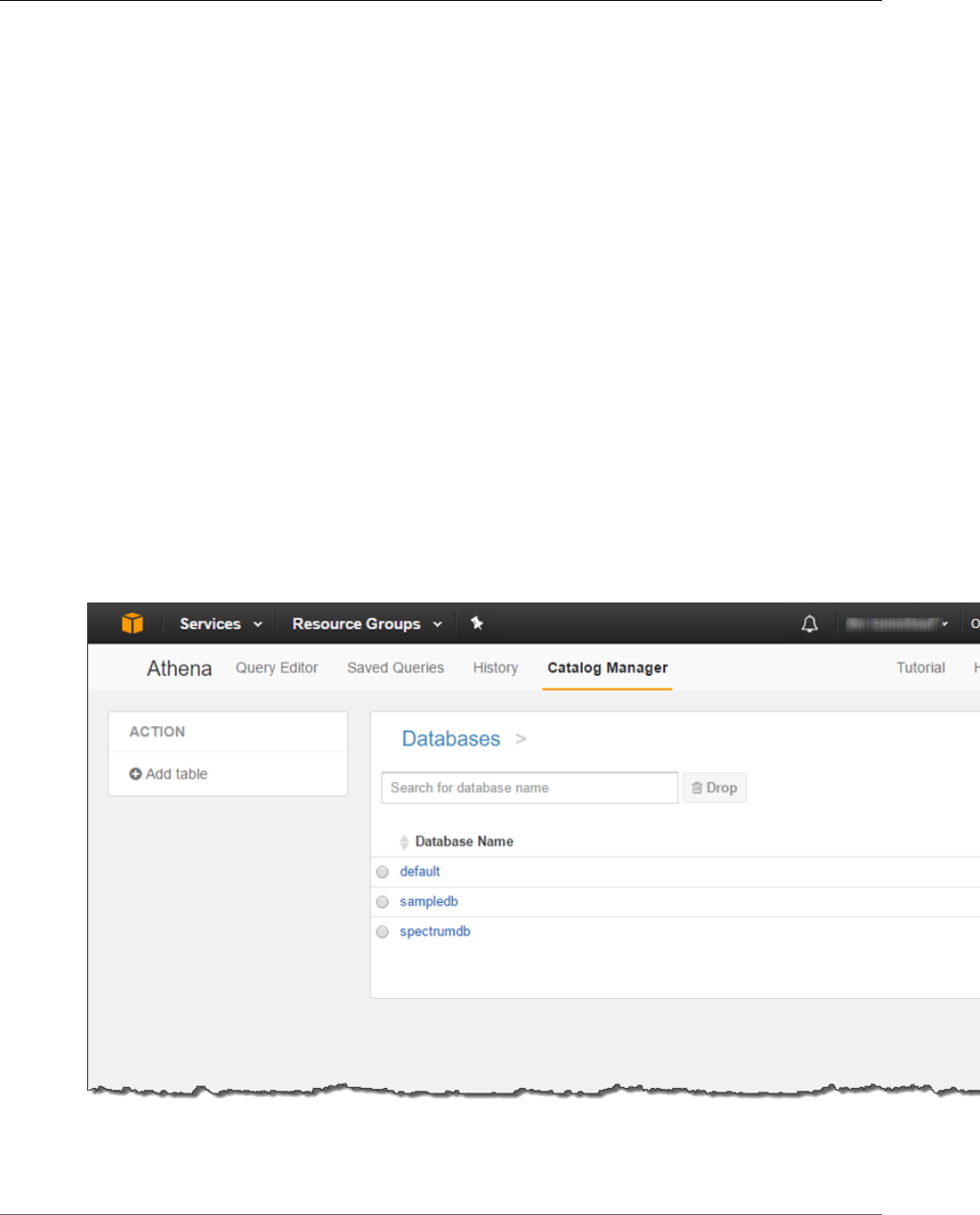
Amazon Redshift Database Developer Guide
Working with External Catalogs
For the full command syntax and examples, see CREATE EXTERNAL SCHEMA (p. 449).
Working with Amazon Redshift Spectrum External
Catalogs
The metadata for Amazon Redshift Spectrum external databases and external tables is stored in an
external data catalog. By default, Redshift Spectrum metadata is stored in an Athena data catalog. You
can view and manage Redshift Spectrum databases and tables in your Athena console.
You can also create and manage external databases and external tables using Hive data definition
language (DDL) using Athena or a Hive metastore, such as Amazon EMR.
Note
We recommend using Amazon Redshift to create and manage external databases and external
tables in Redshift Spectrum.
Viewing Redshift Spectrum Databases in Athena
If you created an external database by including the CREATE EXTERNAL DATABASE IF NOT EXISTS clause
as part of your CREATE EXTERNAL SCHEMA statement, the external database metadata is stored in your
Athena data catalog. The metadata for external tables that you create qualified by the external schema is
also stored in your Athena data catalog.
Athena maintains a data catalog for each supported AWS Region. To view table metadata, log on to
the Athena console and choose Catalog Manager. The following example shows the Athena Catalog
Manager for the US West (Oregon) Region.
If you create and manage your external tables using Athena, register the database using CREATE
EXTERNAL SCHEMA. For example, the following command registers the Athena database named
sampledb.
API Version 2012-12-01
167
Amazon Redshift Database Developer Guide
Working with External Catalogs
create external schema athena_sample
from data catalog
database 'sampledb'
iam_role 'arn:aws:iam::123456789012:role/mySpectrumRole'
region 'us-east-1';
When you query the SVV_EXTERNAL_TABLES system view, you see tables in the Athena sampledb
database and also tables that you created in Amazon Redshift.
select * from svv_external_tables;
schemaname | tablename | location
--------------+------------------+--------------------------------------------------------
athena_sample | elb_logs | s3://athena-examples/elb/plaintext
athena_sample | lineitem_1t_csv | s3://myspectrum/tpch/1000/lineitem_csv
athena_sample | lineitem_1t_part | s3://myspectrum/tpch/1000/lineitem_partition
spectrum | sales | s3://awssampledbuswest2/tickit/spectrum/sales
spectrum | sales_part | s3://awssampledbuswest2/tickit/spectrum/sales_part
Registering an Apache Hive Metastore Database
If you create external tables in an Apache Hive metastore, you can use CREATE EXTERNAL SCHEMA to
register those tables in Redshift Spectrum.
In the CREATE EXTERNAL SCHEMA statement, specify the FROM HIVE METASTORE clause and provide
the Hive metastore URI and port number. The IAM role must include permission to access Amazon S3 but
doesn't need any Athena permissions. The following example registers a Hive metastore.
create external schema if not exists hive_schema
from hive metastore
database 'hive_database'
uri 'ip-10-0-111-111.us-west-2.compute.internal' port 9083
iam_role 'arn:aws:iam::123456789012:role/mySpectrumRole';
Enabling Your Amazon Redshift Cluster to Access Your Amazon
EMR Cluster
If your Hive metastore is in Amazon EMR, you must give your Amazon Redshift cluster access to your
Amazon EMR cluster. To do so, you create an Amazon EC2 security group and allow all inbound traffic
to the EC2 security group from your Amazon Redshift cluster's security group and your Amazon EMR
cluster's security group. Then you add the EC2 security to both your Amazon Redshift cluster and your
Amazon EMR cluster.
To enable your Amazon Redshift cluster to access your Amazon EMR cluster
1. In Amazon Redshift, make a note of your cluster's security group name. In the Amazon Redshift
dashboard, choose your cluster. Find your cluster security groups in the Cluster Properties group.
API Version 2012-12-01
168
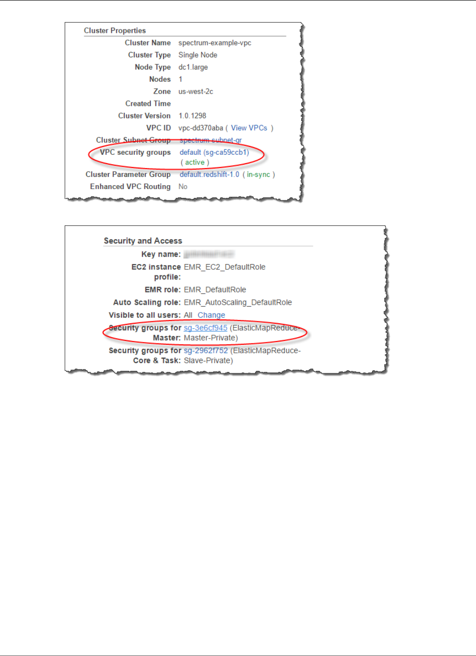
Amazon Redshift Database Developer Guide
Working with External Catalogs
2. In Amazon EMR, make a note of the EMR master node security group name.
3. Create or modify an Amazon EC2 security group to allow connection between Amazon Redshift and
Amazon EMR:
1. In the Amazon EC2 dashboard, choose Security Groups.
2. Choose Create Security Group.
3. If using VPC, choose the VPC that both your Amazon Redshift and Amazon EMR clusters are in.
4. Add an inbound rule.
5. For Type, choose TCP.
6. For Source, choose Custom.
7. Type the name of your Amazon Redshift security group.
8. Add another inbound rule.
9. For Type, choose TCP.
10.For Port Range, type 9083.
Note
The default port for an EMR HMS is 9083. If your HMS uses a different port, specify that
port in the inbound rule and in the external schema definition.
11.For Source, choose Custom.
12.Type the name of your Amazon EMR security group.
13.Choose Create.
API Version 2012-12-01
169

Amazon Redshift Database Developer Guide
Working with External Catalogs
4. Add the Amazon EC2 security group you created in the previous step to your Amazon Redshift
cluster and to your Amazon EMR cluster:
1. In Amazon Redshift, choose your cluster.
2. Choose Cluster, Modify.
3. In VPC Security Groups, add the new security group by pressing CRTL and choosing the new
security group name.
4. In Amazon EMR, choose your cluster.
5. Under Hardware, choose the link for the Master node.
6. Choose the link in the EC2 Instance ID column.
7. Choose Actions, Networking, Change Security Groups.
API Version 2012-12-01
170

Amazon Redshift Database Developer Guide
Creating External Tables
8. Choose the new security group.
9. Choose Assign Security Groups.
Creating External Tables for Amazon Redshift
Spectrum
Amazon Redshift Spectrum uses external tables to query data that is stored in Amazon S3. You can query
an external table using the same SELECT syntax you use with other Amazon Redshift tables. External
tables are read-only. You can't write to an external table.
You create an external table in an external schema. To create external tables, you must be the
owner of the external schema or a superuser. To transfer ownership of an external schema, use
ALTER SCHEMA (p. 364) to change the owner. The following example changes the owner of the
spectrum_schema schema to newowner.
alter schema spectrum_schema owner to newowner;
To run a Redshift Spectrum query, you need the following permissions:
• Usage permission on the schema
• Permission to create temporary tables in the current database
The following example grants usage permission on the schema spectrum_schema to the
spectrumusers user group.
API Version 2012-12-01
171
Amazon Redshift Database Developer Guide
Pseudocolumns
grant usage on schema spectrum_schema to group spectrumusers;
The following example grants temporary permission on the database spectrumdb to the
spectrumusers user group.
grant temp on database spectrumdb to group spectrumusers;
You can create an external table in Amazon Redshift, AWS Glue, Amazon Athena, or an Apache Hive
metastore. For more information, see Getting Started Using AWS Glue in the AWS Glue Developer Guide,
Getting Started in the Amazon Athena User Guide, or Apache Hive in the Amazon EMR Developer Guide.
If your external table is defined in AWS Glue, Athena, or a Hive metastore, you first create an external
schema that references the external database. Then you can reference the external table in your
SELECT statement by prefixing the table name with the schema name, without needing to create the
table in Amazon Redshift. For more information, see Creating External Schemas for Amazon Redshift
Spectrum (p. 165).
For example, suppose that you have an external table named lineitem_athena defined in an Athena
external catalog. In this case, you can define an external schema named athena_schema, then query
the table using the following SELECT statement.
select count(*) from athena_schema.lineitem_athena;
To define an external table in Amazon Redshift, use the CREATE EXTERNAL TABLE (p. 452) command.
The external table statement defines the table columns, the format of your data files, and the location
of your data in Amazon S3. Redshift Spectrum scans the files in the specified folder and any subfolders.
Redshift Spectrum ignores hidden files and files that begin with a period, underscore, or hash mark ( . , _,
or #) or end with a tilde (~).
The following example creates a table named SALES in the Amazon Redshift external schema named
spectrum. The data is in tab-delimited text files.
create external table spectrum.sales(
salesid integer,
listid integer,
sellerid integer,
buyerid integer,
eventid integer,
dateid smallint,
qtysold smallint,
pricepaid decimal(8,2),
commission decimal(8,2),
saletime timestamp)
row format delimited
fields terminated by '\t'
stored as textfile
location 's3://awssampledbuswest2/tickit/spectrum/sales/'
table properties ('numRows'='172000');
To view external tables, query the SVV_EXTERNAL_TABLES (p. 904) system view.
Pseudocolumns
By default, Amazon Redshift creates external tables with the pseudocolumns $path and $size. Select
these columns to view the path to the data files on Amazon S3 and the size of the data files for each
row returned by a query. The $path and $size column names must be delimited with double quotation
API Version 2012-12-01
172
Amazon Redshift Database Developer Guide
Partitioning Redshift Spectrum External Tables
marks. A SELECT * clause doesn't return the pseudocolumns. You must explicitly include the $path and
$size column names in your query, as the following example shows.
select "$path", "$size"
from spectrum.sales_part
where saledate = '2008-12-01';
You can disable creation of pseudocolumns for a session by setting the
spectrum_enable_pseudo_columns configuration parameter to false.
Important
Selecting $size or $path incurs charges because Redshift Spectrum scans the data files on
Amazon S3 to determine the size of the result set. For more information, see Amazon Redshift
Pricing.
Pseudocolumns Example
The following example returns the total size of related data files for an external table.
select distinct "$path", "$size"
from spectrum.sales_part;
$path | $size
---------------------------------------+-------
s3://awssampledbuswest2/tickit/spectrum/sales_partition/saledate=2008-01/ | 1616
s3://awssampledbuswest2/tickit/spectrum/sales_partition/saledate=2008-02/ | 1444
s3://awssampledbuswest2/tickit/spectrum/sales_partition/saledate=2008-03/ | 1644
Partitioning Redshift Spectrum External Tables
When you partition your data, you can restrict the amount of data that Redshift Spectrum scans by
filtering on the partition key. You can partition your data by any key.
A common practice is to partition the data based on time. For example, you might choose to partition
by year, month, date, and hour. If you have data coming from multiple sources, you might partition by a
data source identifier and date.
The following procedure describes how to partition your data.
To partition your data
1. Store your data in folders in Amazon S3 according to your partition key.
Create one folder for each partition value and name the folder with the partition key and value.
For example, if you partition by date, you might have folders named saledate=2017-04-31,
saledate=2017-04-30, and so on. Redshift Spectrum scans the files in the partition folder
and any subfolders. Redshift Spectrum ignores hidden files and files that begin with a period,
underscore, or hash mark ( . , _, or #) or end with a tilde (~).
2. Create an external table and specify the partition key in the PARTITIONED BY clause.
The partition key can't be the name of a table column. The data type can be any standard Amazon
Redshift data type except TIMESTAMPTZ.
3. Add the partitions.
Using ALTER TABLE (p. 365) … ADD PARTITION, add each partition, specifying the partition
column and key value, and the location of the partition folder in Amazon S3. You can add multiple
partitions in a single ALTER TABLE … ADD statement. The following example adds partitions for
'2008-01-01' and '2008-02-01'.
API Version 2012-12-01
173
Amazon Redshift Database Developer Guide
Partitioning Redshift Spectrum External Tables
alter table spectrum.sales_part add
partition(saledate='2008-01-01')
location 's3://awssampledbuswest2/tickit/spectrum/sales_partition/saledate=2008-01/';
partition(saledate='2008-02-01')
location 's3://awssampledbuswest2/tickit/spectrum/sales_partition/saledate=2008-02/';
Note
If you use the AWS Glue catalog, you can add up to 100 partitions using a single ALTER
TABLE statement.
Partitioning Data Examples
In this example, you create an external table that is partitioned by a single partition key and an external
table that is partitioned by two partition keys.
The sample data for this example is located in an Amazon S3 bucket that gives read access to all
authenticated AWS users. Your cluster and your external data files must be in the same AWS Region.
The sample data bucket is in the US West (Oregon) Region (us-west-2). To access the data using Redshift
Spectrum, your cluster must also be in us-west-2. To list the folders in Amazon S3, run the following
command.
aws s3 ls s3://awssampledbuswest2/tickit/spectrum/sales_partition/
PRE saledate=2008-01/
PRE saledate=2008-02/
PRE saledate=2008-03/
If you don't already have an external schema, run the following command. Substitute the Amazon
Resource Name (ARN) for your AWS Identity and Access Management (IAM) role.
create external schema spectrum
from data catalog
database 'spectrumdb'
iam_role 'arn:aws:iam::123456789012:role/myspectrumrole'
create external database if not exists;
Example 1: Partitioning with a Single Partition Key
In the following example, you create an external table that is partitioned by month.
To create an external table partitioned by month, run the following command.
create external table spectrum.sales_part(
salesid integer,
listid integer,
sellerid integer,
buyerid integer,
eventid integer,
dateid smallint,
qtysold smallint,
pricepaid decimal(8,2),
commission decimal(8,2),
saletime timestamp)
partitioned by (saledate char(10))
row format delimited
fields terminated by '|'
API Version 2012-12-01
174
Amazon Redshift Database Developer Guide
Partitioning Redshift Spectrum External Tables
stored as textfile
location 's3://awssampledbuswest2/tickit/spectrum/sales_partition/'
table properties ('numRows'='172000');
To add the partitions, run the following ALTER TABLE commands.
alter table spectrum.sales_part add
partition(saledate='2008-01')
location 's3://awssampledbuswest2/tickit/spectrum/sales_partition/saledate=2008-01/'
partition(saledate='2008-02')
location 's3://awssampledbuswest2/tickit/spectrum/sales_partition/saledate=2008-02/'
partition(saledate='2008-03')
location 's3://awssampledbuswest2/tickit/spectrum/sales_partition/saledate=2008-03/';
Run the following query to select data from the partitioned table.
select top 5 spectrum.sales_part.eventid, sum(spectrum.sales_part.pricepaid)
from spectrum.sales_part, event
where spectrum.sales_part.eventid = event.eventid
and spectrum.sales_part.pricepaid > 30
and saledate = '2008-01'
group by spectrum.sales_part.eventid
order by 2 desc;
eventid | sum
--------+---------
4124 | 21179.00
1924 | 20569.00
2294 | 18830.00
2260 | 17669.00
6032 | 17265.00
To view external table partitions, query the SVV_EXTERNAL_PARTITIONS (p. 903) system view.
select schemaname, tablename, values, location from svv_external_partitions
where tablename = 'sales_part';
schemaname | tablename | values | location
-----------+------------+-------------
+-------------------------------------------------------------------------
spectrum | sales_part | ["2008-01"] | s3://awssampledbuswest2/tickit/spectrum/
sales_partition/saledate=2008-01
spectrum | sales_part | ["2008-02"] | s3://awssampledbuswest2/tickit/spectrum/
sales_partition/saledate=2008-02
spectrum | sales_part | ["2008-03"] | s3://awssampledbuswest2/tickit/spectrum/
sales_partition/saledate=2008-03
Example 2: Partitioning with a Multiple Partition Key
To create an external table partitioned by date and eventid, run the following command.
create external table spectrum.sales_event(
salesid integer,
listid integer,
sellerid integer,
buyerid integer,
API Version 2012-12-01
175

Amazon Redshift Database Developer Guide
Partitioning Redshift Spectrum External Tables
eventid integer,
dateid smallint,
qtysold smallint,
pricepaid decimal(8,2),
commission decimal(8,2),
saletime timestamp)
partitioned by (salesmonth char(10), event integer)
row format delimited
fields terminated by '|'
stored as textfile
location 's3://awssampledbuswest2/tickit/spectrum/salesevent/'
table properties ('numRows'='172000');
To add the partitions, run the following ALTER TABLE commands.
alter table spectrum.sales_event add
partition(salesmonth='2008-01', event='101')
location 's3://awssampledbuswest2/tickit/spectrum/salesevent/salesmonth=2008-01/
event=101/';
partition(salesmonth='2008-01', event='102')
location 's3://awssampledbuswest2/tickit/spectrum/salesevent/salesmonth=2008-01/event=102/'
partition(salesmonth='2008-01', event='103')
location 's3://awssampledbuswest2/tickit/spectrum/salesevent/salesmonth=2008-01/event=103/'
partition(salesmonth='2008-02', event='101')
location 's3://awssampledbuswest2/tickit/spectrum/salesevent/salesmonth=2008-02/event=101/'
partition(salesmonth='2008-02', event='102')
location 's3://awssampledbuswest2/tickit/spectrum/salesevent/salesmonth=2008-02/event=102/'
partition(salesmonth='2008-02', event='103')
location 's3://awssampledbuswest2/tickit/spectrum/salesevent/salesmonth=2008-02/event=103/'
partition(salesmonth='2008-03', event='101')
location 's3://awssampledbuswest2/tickit/spectrum/salesevent/salesmonth=2008-03/event=101/'
partition(salesmonth='2008-03', event='102')
location 's3://awssampledbuswest2/tickit/spectrum/salesevent/salesmonth=2008-03/
event=102/';
partition(salesmonth='2008-03', event='103')
location 's3://awssampledbuswest2/tickit/spectrum/salesevent/salesmonth=2008-03/
event=103/';
Run the following query to select data from the partitioned table.
select spectrum.sales_event.salesmonth, event.eventname,
sum(spectrum.sales_event.pricepaid)
from spectrum.sales_event, event
where spectrum.sales_event.eventid = event.eventid
and salesmonth = '2008-02'
and (event = '101'
or event = '102'
or event = '103')
group by event.eventname, spectrum.sales_event.salesmonth
order by 3 desc;
salesmonth | eventname | sum
-----------+-----------------+--------
2008-02 | The Magic Flute | 5062.00
API Version 2012-12-01
176
Amazon Redshift Database Developer Guide
Mapping to ORC Columns
2008-02 | La Sonnambula | 3498.00
2008-02 | Die Walkure | 534.00
Mapping External Table Columns to ORC Columns
You use Amazon Redshift Spectrum external tables to query data from files in ORC format. Optimized
row columnar (ORC) format is a columnar storage file format that supports nested data structures.
For more information about querying nested data, see Querying Nested Data with Amazon Redshift
Spectrum (p. 104).
When you create an external table that references data in an ORC file, you map each column in the
external table to a column in the ORC data. To do so, you use one of the following methods:
•Mapping by position (p. 177)
•Mapping by column name (p. 178)
Mapping by column name is the default.
Mapping by Position
With position mapping, the first column defined in the external table maps to the first column in the
ORC data file, the second to the second, and so on. Mapping by position requires that the order of
columns in the external table and in the ORC file match. If the order of the columns doesn't match, then
you can map the columns by name.
Important
In earlier releases, Redshift Spectrum used position mapping by default. If you need to continue
using position mapping for existing tables, set the table property orc.schema.resolution to
position, as the following example shows.
alter table spectrum.orc_example
set table properties('orc.schema.resolution'='position');
For example, the table SPECTRUM.ORC_EXAMPLE is defined as follows.
create external table spectrum.orc_example(
int_col int,
float_col float,
nested_col struct<
"int_col" : int,
"map_col" : map<int, array<float >>
>
) stored as orc
location 's3://example/orc/files/';
The table structure can be abstracted as follows.
• 'int_col' : int
• 'float_col' : float
• 'nested_col' : struct
o 'int_col' : int
o 'map_col' : map
- key : int
- value : array
- value : float
The underlying ORC file has the following file structure.
API Version 2012-12-01
177
Amazon Redshift Database Developer Guide
Mapping to ORC Columns
• ORC file root(id = 0)
o 'int_col' : int (id = 1)
o 'float_col' : float (id = 2)
o 'nested_col' : struct (id = 3)
- 'int_col' : int (id = 4)
- 'map_col' : map (id = 5)
- key : int (id = 6)
- value : array (id = 7)
- value : float (id = 8)
In this example, you can map each column in the external table to a column in ORC file strictly by
position. The following shows the mapping.
External Table Column Name ORC Column ID ORC Column Name
int_col 1 int_col
float_col 2 float_col
nested_col 3 nested_col
nested_col.int_col 4 int_col
nested_col.map_col 5 map_col
nested_col.map_col.key 6 NA
nested_col.map_col.value 7 NA
nested_col.map_col.value.item 8 NA
Mapping by Column Name
Using name mapping, you map columns in an external table to named columns in ORC files on the same
level, with the same name.
For example, suppose that you want to map the table from the previous example,
SPECTRUM.ORC_EXAMPLE, with an ORC file that uses the following file structure.
• ORC file root(id = 0)
o 'nested_col' : struct (id = 1)
- 'map_col' : map (id = 2)
- key : int (id = 3)
- value : array (id = 4)
- value : float (id = 5)
- 'int_col' : int (id = 6)
o 'int_col' : int (id = 7)
o 'float_col' : float (id = 8)
Using position mapping, Redshift Spectrum attempts the following mapping.
External Table Column Name ORC Column ID ORC Column Name
int_col 1 struct
float_col 7 int_col
nested_col 8 float_col
API Version 2012-12-01
178

Amazon Redshift Database Developer Guide
Improving Amazon Redshift Spectrum Query Performance
When you query a table with the preceding position mapping, the SELECT command fails on type
validation because the structures are different.
You can map the same external table to both file structures shown in the previous examples by using
column name mapping. The table columns int_col, float_col, and nested_col map by column
name to columns with the same names in the ORC file. The column named nested_col in the external
table is a struct column with subcolumns named map_col and int_col. The subcolumns also map
correctly to the corresponding columns in the ORC file by column name.
Improving Amazon Redshift Spectrum Query
Performance
Look at the query plan to find what steps have been pushed to the Amazon Redshift Spectrum layer.
The following steps are related to the Redshift Spectrum query:
• S3 Seq Scan
• S3 HashAggregate
• S3 Query Scan
• Seq Scan PartitionInfo
• Partition Loop
The following example shows the query plan for a query that joins an external table with a local table.
Note the S3 Seq Scan and S3 HashAggregate steps that were executed against the data on Amazon S3.
explain
select top 10 spectrum.sales.eventid, sum(spectrum.sales.pricepaid)
from spectrum.sales, event
where spectrum.sales.eventid = event.eventid
and spectrum.sales.pricepaid > 30
group by spectrum.sales.eventid
order by 2 desc;
QUERY PLAN
-----------------------------------------------------------------------------
XN Limit (cost=1001055770628.63..1001055770628.65 rows=10 width=31)
-> XN Merge (cost=1001055770628.63..1001055770629.13 rows=200 width=31)
Merge Key: sum(sales.derived_col2)
-> XN Network (cost=1001055770628.63..1001055770629.13 rows=200 width=31)
Send to leader
-> XN Sort (cost=1001055770628.63..1001055770629.13 rows=200 width=31)
API Version 2012-12-01
179

Amazon Redshift Database Developer Guide
Improving Amazon Redshift Spectrum Query Performance
Sort Key: sum(sales.derived_col2)
-> XN HashAggregate (cost=1055770620.49..1055770620.99 rows=200
width=31)
-> XN Hash Join DS_BCAST_INNER (cost=3119.97..1055769620.49
rows=200000 width=31)
Hash Cond: ("outer".derived_col1 = "inner".eventid)
-> XN S3 Query Scan sales (cost=3010.00..5010.50
rows=200000 width=31)
-> S3 HashAggregate (cost=3010.00..3010.50
rows=200000 width=16)
-> S3 Seq Scan spectrum.sales location:"s3://
awssampledbuswest2/tickit/spectrum/sales" format:TEXT (cost=0.00..2150.00 rows=172000
width=16)
Filter: (pricepaid > 30.00)
-> XN Hash (cost=87.98..87.98 rows=8798 width=4)
-> XN Seq Scan on event (cost=0.00..87.98 rows=8798
width=4)
Note the following elements in the query plan:
• The S3 Seq Scan node shows the filter pricepaid > 30.00 was processed in the Redshift
Spectrum layer.
A filter node under the XN S3 Query Scan node indicates predicate processing in Amazon Redshift
on top of the data returned from the Redshift Spectrum layer.
• The S3 HashAggregate node indicates aggregation in the Redshift Spectrum layer for the group by
clause (group by spectrum.sales.eventid).
Following are ways to improve Redshift Spectrum performance:
• Use Parquet formatted data files. Parquet stores data in a columnar format, so Redshift Spectrum can
eliminate unneeded columns from the scan. When data is in text-file format, Redshift Spectrum needs
to scan the entire file.
• Use the fewest columns possible in your queries.
• Use multiple files to optimize for parallel processing. Keep your file sizes larger than 64 MB. Avoid data
size skew by keeping files about the same size.
• Put your large fact tables in Amazon S3 and keep your frequently used, smaller dimension tables in
your local Amazon Redshift database.
• Update external table statistics by setting the TABLE PROPERTIES numRows parameter. Use CREATE
EXTERNAL TABLE (p. 452) or ALTER TABLE (p. 365) to set the TABLE PROPERTIES numRows
parameter to reflect the number of rows in the table. Amazon Redshift doesn't analyze external
tables to generate the table statistics that the query optimizer uses to generate a query plan. If table
statistics aren't set for an external table, Amazon Redshift generates a query execution plan based on
an assumption that external tables are the larger tables and local tables are the smaller tables.
• The Amazon Redshift query planner pushes predicates and aggregations to the Redshift Spectrum
query layer whenever possible. When large amounts of data are returned from Amazon S3, the
processing is limited by your cluster's resources. Redshift Spectrum scales automatically to process
API Version 2012-12-01
180

Amazon Redshift Database Developer Guide
Monitoring Metrics
large requests. Thus, your overall performance improves whenever you can push processing to the
Redshift Spectrum layer.
• Write your queries to use filters and aggregations that are eligible to be pushed to the Redshift
Spectrum layer.
The following are examples of some operations that can be pushed to the Redshift Spectrum layer:
• GROUP BY clauses
• Comparison conditions and pattern-matching conditions, such as LIKE.
• Aggregate functions, such as COUNT, SUM, AVG, MIN, and MAX.
• String functions.
Operations that can't be pushed to the Redshift Spectrum layer include DISTINCT and ORDER BY.
• Use partitions to limit the data that is scanned. Partition your data based on your most common
query predicates, then prune partitions by filtering on partition columns. For more information, see
Partitioning Redshift Spectrum External Tables (p. 173).
Query SVL_S3PARTITION (p. 919) to view total partitions and qualified partitions.
Monitoring Metrics in Amazon Redshift Spectrum
You can monitor Amazon Redshift Spectrum queries using the following system views:
•SVL_S3QUERY (p. 920)
Use the SVL_S3QUERY view to get details about Redshift Spectrum queries (S3 queries) at the
segment and node slice level.
•SVL_S3QUERY_SUMMARY (p. 921)
Use the SVL_S3QUERY_SUMMARY view to get a summary of all Amazon Redshift Spectrum queries
(S3 queries) that have been run on the system.
The following are some things to look for in SVL_S3QUERY_SUMMARY:
• The number of files that were processed by the Redshift Spectrum query.
• The number of bytes scanned from Amazon S3. The cost of a Redshift Spectrum query is reflected in
the amount of data scanned from Amazon S3.
• The number of bytes returned from the Redshift Spectrum layer to the cluster. A large amount of data
returned might affect system performance.
• The maximum duration and average duration of Redshift Spectrum requests. Long-running requests
might indicate a bottleneck.
Troubleshooting Queries in Amazon Redshift
Spectrum
Following, you can find a quick reference for identifying and addressing some of the most common and
most serious issues you are likely to encounter with Amazon Redshift Spectrum queries. To view errors
generated by Redshift Spectrum queries, query the SVL_S3LOG (p. 918) system table.
Topics
•Retries Exceeded (p. 182)
API Version 2012-12-01
181
Amazon Redshift Database Developer Guide
Retries Exceeded
•No Rows Returned for a Partitioned Table (p. 182)
•Not Authorized Error (p. 182)
•Incompatible Data Formats (p. 182)
•Syntax Error When Using Hive DDL in Amazon Redshift (p. 183)
•Permission to Create Temporary Tables (p. 183)
Retries Exceeded
If an Amazon Redshift Spectrum request times out, the request is canceled and resubmitted. After five
failed retries, the query fails with the following error.
error: S3Query Exception (Fetch), retries exceeded
Possible causes include the following:
• Large file sizes (greater than 1 GB). Check your file sizes in Amazon S3 and look for large files and file
size skew. Break up large files into smaller files, between 100 MB and 1 GB. Try to make files about the
same size.
• Slow network throughput. Try your query later.
No Rows Returned for a Partitioned Table
If your query returns zero rows from a partitioned external table, check whether a partition
has been added for this external table. Redshift Spectrum only scans files in an Amazon S3
location that has been explicitly added using ALTER TABLE … ADD PARTITION. Query the
SVV_EXTERNAL_PARTITIONS (p. 903) view to find existing partitions. Run ALTER TABLE ADD …
PARTITION for each missing partition.
Not Authorized Error
Verify that the IAM role for the cluster allows access to the Amazon S3 file objects. If your external
database is on Amazon Athena, verify that the AWS Identity and Access Management (IAM) role
allows access to Athena resources. For more information, see IAM Policies for Amazon Redshift
Spectrum (p. 154).
Incompatible Data Formats
For a columnar file format, such as Parquet, the column type is embedded with the data. The column
type in the CREATE EXTERNAL TABLE definition must match the column type of the data file. If there is a
mismatch, you receive an error similar to the following:
Task failed due to an internal error.
File 'https://s3bucket/location/file has an incompatible Parquet schema
for column ‘s3://s3bucket/location.col1'. Column type: VARCHAR, Par
The error message might be truncated due to the limit on message length. To retrieve the complete error
message, including column name and column type, query the SVL_S3LOG (p. 918) system view.
The following example queries SVL_S3LOG for the last query executed.
select message
API Version 2012-12-01
182
Amazon Redshift Database Developer Guide
Syntax Error When Using Hive DDL in Amazon Redshift
from svl_s3log
where query = pg_last_query_id()
order by query,segment,slice;
The following is an example of a result that shows the full error message.
message
–––––––––––––––––––––––––––––––––––––––––––––––––––––––––––––––––––––––––––––––––––––––––-
S3 Query Exception (Fetch). Task failed due to an internal error.
File 'https://s3bucket/location/file has an incompatible
Parquet schema for column ' s3bucket/location.col1'.
Column type: VARCHAR, Parquet schema:\noptional int64 l_orderkey [i:0 d:1 r:0]\n
To correct the error, alter the external table to match the column type of the Parquet file.
Syntax Error When Using Hive DDL in Amazon
Redshift
Amazon Redshift supports data definition language (DDL) for CREATE EXTERNAL TABLE that is similar to
Hive DDL. However, the two types of DDL aren't always exactly the same. If you copy Hive DDL to create
or alter Amazon Redshift external tables, you might encounter syntax errors. The following are examples
of differences between Amazon Redshift and Hive DDL:
• Amazon Redshift requires single quotation marks (') where Hive DDL supports double quotation marks
(").
• Amazon Redshift doesn't support the STRING data type. Use VARCHAR instead.
Permission to Create Temporary Tables
To run Redshift Spectrum queries, the database user must have permission to create temporary tables in
the database. The following example grants temporary permission on the database spectrumdb to the
spectrumusers user group.
grant temp on database spectrumdb to group spectrumusers;
For more information, see GRANT (p. 516).
API Version 2012-12-01
183

Amazon Redshift Database Developer Guide
Using COPY to Load Data
Loading Data
Topics
•Using a COPY Command to Load Data (p. 184)
•Updating Tables with DML Commands (p. 216)
•Updating and Inserting New Data (p. 216)
•Performing a Deep Copy (p. 221)
•Analyzing Tables (p. 223)
•Vacuuming Tables (p. 228)
•Managing Concurrent Write Operations (p. 238)
A COPY command is the most efficient way to load a table. You can also add data to your tables using
INSERT commands, though it is much less efficient than using COPY. The COPY command is able to
read from multiple data files or multiple data streams simultaneously. Amazon Redshift allocates the
workload to the cluster nodes and performs the load operations in parallel, including sorting the rows
and distributing data across node slices.
Note
Amazon Redshift Spectrum external tables are read-only. You can't COPY or INSERT to an
external table.
To access data on other AWS resources, your cluster must have permission to access those resources and
to perform the necessary actions to access the data. You can use Identity and Access Management (IAM)
to limit the access users have to your cluster resources and data.
After your initial data load, if you add, modify, or delete a significant amount of data, you should follow
up by running a VACUUM command to reorganize your data and reclaim space after deletes. You should
also run an ANALYZE command to update table statistics.
This section explains how to load data and troubleshoot data loads and presents best practices for
loading data.
Using a COPY Command to Load Data
Topics
•Credentials and Access Permissions (p. 185)
•Preparing Your Input Data (p. 186)
•Loading Data from Amazon S3 (p. 187)
•Loading Data from Amazon EMR (p. 196)
•Loading Data from Remote Hosts (p. 200)
•Loading Data from an Amazon DynamoDB Table (p. 206)
•Verifying That the Data Was Loaded Correctly (p. 208)
•Validating Input Data (p. 208)
•Loading Tables with Automatic Compression (p. 209)
•Optimizing Storage for Narrow Tables (p. 211)
•Loading Default Column Values (p. 211)
•Troubleshooting Data Loads (p. 211)
API Version 2012-12-01
184

Amazon Redshift Database Developer Guide
Credentials and Access Permissions
The COPY command leverages the Amazon Redshift massively parallel processing (MPP) architecture
to read and load data in parallel from files on Amazon S3, from a DynamoDB table, or from text output
from one or more remote hosts.
Note
We strongly recommend using the COPY command to load large amounts of data. Using
individual INSERT statements to populate a table might be prohibitively slow. Alternatively, if
your data already exists in other Amazon Redshift database tables, use INSERT INTO ... SELECT
or CREATE TABLE AS to improve performance. For information, see INSERT (p. 520) or CREATE
TABLE AS (p. 483).
To load data from another AWS resource, your cluster must have permission to access the resource and
perform the necessary actions.
To grant or revoke privilege to load data into a table using a COPY command, grant or revoke the INSERT
privilege.
Your data needs to be in the proper format for loading into your Amazon Redshift table. This section
presents guidelines for preparing and verifying your data before the load and for validating a COPY
statement before you execute it.
To protect the information in your files, you can encrypt the data files before you upload them to your
Amazon S3 bucket; COPY will decrypt the data as it performs the load. You can also limit access to your
load data by providing temporary security credentials to users. Temporary security credentials provide
enhanced security because they have short life spans and cannot be reused after they expire.
You can compress the files using gzip, lzop, or bzip2 to save time uploading the files. COPY can then
speed up the load process by uncompressing the files as they are read.
To help keep your data secure in transit within the AWS cloud, Amazon Redshift uses hardware
accelerated SSL to communicate with Amazon S3 or Amazon DynamoDB for COPY, UNLOAD, backup,
and restore operations.
When you load your table directly from an Amazon DynamoDB table, you have the option to control the
amount of Amazon DynamoDB provisioned throughput you consume.
You can optionally let COPY analyze your input data and automatically apply optimal compression
encodings to your table as part of the load process.
Credentials and Access Permissions
To load or unload data using another AWS resource, such as Amazon S3, Amazon DynamoDB, Amazon
EMR, or Amazon EC2, your cluster must have permission to access the resource and perform the
necessary actions to access the data. For example, to load data from Amazon S3, COPY must have LIST
access to the bucket and GET access for the bucket objects.
To obtain authorization to access a resource, your cluster must be authenticated. You can choose either
role-based access control or key-based access control. This section presents an overview of the two
methods. For complete details and examples, see Permissions to Access Other AWS Resources (p. 424).
Role-Based Access Control
With role-based access control, your cluster temporarily assumes an AWS Identity and Access
Management (IAM) role on your behalf. Then, based on the authorizations granted to the role, your
cluster can access the required AWS resources.
We recommend using role-based access control because it is provides more secure, fine-grained control
of access to AWS resources and sensitive user data, in addition to safeguarding your AWS credentials.
API Version 2012-12-01
185
Amazon Redshift Database Developer Guide
Preparing Your Input Data
To use role-based access control, you must first create an IAM role using the Amazon Redshift service
role type, and then attach the role to your cluster. The role must have, at a minimum, the permissions
listed in IAM Permissions for COPY, UNLOAD, and CREATE LIBRARY (p. 427). For steps to create an IAM
role and attach it to your cluster, see Creating an IAM Role to Allow Your Amazon Redshift Cluster to
Access AWS Services in the Amazon Redshift Cluster Management Guide.
You can add a role to a cluster or view the roles associated with a cluster by using the Amazon Redshift
Management Console, CLI, or API. For more information, see Authorizing COPY and UNLOAD Operations
Using IAM Roles in the Amazon Redshift Cluster Management Guide.
When you create an IAM role, IAM returns an Amazon Resource Name (ARN) for the role. To execute
a COPY command using an IAM role, provide the role ARN using the IAM_ROLE parameter or the
CREDENTIALS parameter.
The following COPY command example uses IAM_ROLE parameter with the role MyRedshiftRole for
authentication.
copy customer from 's3://mybucket/mydata'
iam_role 'arn:aws:iam::12345678901:role/MyRedshiftRole';
Key-Based Access Control
With key-based access control, you provide the access key ID and secret access key for anIAM user that is
authorized to access the AWS resources that contain the data.
Note
We strongly recommend using an IAM role for authentication instead of supplying a plain-text
access key ID and secret access key. If you choose key-based access control, never use your AWS
account (root) credentials. Always create an IAM user and provide that user's access key ID and
secret access key. For steps to create an IAM user, see Creating an IAM User in Your AWS Account.
To authenticate using IAM user credentials, replace <access-key-id> and <secret-access-
key with an authorized user's access key ID and full secret access key for the ACCESS_KEY_ID and
SECRET_ACCESS_KEY parameters as shown following.
ACCESS_KEY_ID '<access-key-id>'
SECRET_ACCESS_KEY '<secret-access-key>';
The AWS IAM user must have, at a minimum, the permissions listed in IAM Permissions for COPY,
UNLOAD, and CREATE LIBRARY (p. 427).
Preparing Your Input Data
If your input data is not compatible with the table columns that will receive it, the COPY command will
fail.
Use the following guidelines to help ensure that your input data is valid:
• Your data can only contain UTF-8 characters up to four bytes long.
• Verify that CHAR and VARCHAR strings are no longer than the lengths of the corresponding columns.
VARCHAR strings are measured in bytes, not characters, so, for example, a four-character string of
Chinese characters that occupy four bytes each requires a VARCHAR(16) column.
• Multibyte characters can only be used with VARCHAR columns. Verify that multibyte characters are no
more than four bytes long.
• Verify that data for CHAR columns only contains single-byte characters.
API Version 2012-12-01
186

Amazon Redshift Database Developer Guide
Loading Data from Amazon S3
• Do not include any special characters or syntax to indicate the last field in a record. This field can be a
delimiter.
• If your data includes null terminators, also referred to as NUL (UTF-8 0000) or binary zero (0x000),
you can load these characters as NULLS into CHAR or VARCHAR columns by using the NULL AS
option in the COPY command: null as '\0' or null as '\000' . If you do not use NULL AS, null
terminators will cause your COPY to fail.
• If your strings contain special characters, such as delimiters and embedded newlines, use the ESCAPE
option with the COPY (p. 390) command.
• Verify that all single and double quotes are appropriately matched.
• Verify that floating-point strings are in either standard floating-point format, such as 12.123, or an
exponential format, such as 1.0E4.
• Verify that all timestamp and date strings follow the specifications for DATEFORMAT and
TIMEFORMAT Strings (p. 432). The default timestamp format is YYYY-MM-DD hh:mm:ss, and the
default date format is YYYY-MM-DD.
• For more information about boundaries and limitations on individual data types, see Data
Types (p. 315). For information about multibyte character errors, see Multibyte Character Load
Errors (p. 214)
Loading Data from Amazon S3
Topics
•Splitting Your Data into Multiple Files (p. 187)
•Uploading Files to Amazon S3 (p. 188)
•Using the COPY Command to Load from Amazon S3 (p. 191)
The COPY command leverages the Amazon Redshift massively parallel processing (MPP) architecture
to read and load data in parallel from files in an Amazon S3 bucket. You can take maximum advantage
of parallel processing by splitting your data into multiple files and by setting distribution keys on your
tables. For more information about distribution keys, see Choosing a Data Distribution Style (p. 129).
Data from the files is loaded into the target table, one line per row. The fields in the data file are
matched to table columns in order, left to right. Fields in the data files can be fixed-width or character
delimited; the default delimiter is a pipe (|). By default, all the table columns are loaded, but you can
optionally define a comma-separated list of columns. If a table column is not included in the column
list specified in the COPY command, it is loaded with a default value. For more information, see Loading
Default Column Values (p. 211).
Follow this general process to load data from Amazon S3:
1. Split your data into multiple files.
2. Upload your files to Amazon S3.
3. Run a COPY command to load the table.
4. Verify that the data was loaded correctly.
The rest of this section explains these steps in detail.
Splitting Your Data into Multiple Files
You can load table data from a single file, or you can split the data for each table into multiple files. The
COPY command can load data from multiple files in parallel. You can load multiple files by specifying a
common prefix, or prefix key, for the set, or by explicitly listing the files in a manifest file.
API Version 2012-12-01
187
Amazon Redshift Database Developer Guide
Loading Data from Amazon S3
Note
We strongly recommend that you divide your data into multiple files to take advantage of
parallel processing.
Split your data into files so that the number of files is a multiple of the number of slices in your cluster.
That way Amazon Redshift can divide the data evenly among the slices. The number of slices per node
depends on the node size of the cluster. For example, each DS1.XL compute node has two slices, and
each DS1.8XL compute node has 32 slices. For more information about the number of slices that each
node size has, go to About Clusters and Nodes in the Amazon Redshift Cluster Management Guide.
The nodes all participate in parallel query execution, working on data that is distributed as evenly as
possible across the slices. If you have a cluster with two DS1.XL nodes, you might split your data into four
files or some multiple of four. Amazon Redshift does not take file size into account when dividing the
workload, so you need to ensure that the files are roughly the same size, between 1 MB and 1 GB after
compression.
If you intend to use object prefixes to identify the load files, name each file with a common prefix. For
example, the venue.txt file might be split into four files, as follows:
venue.txt.1
venue.txt.2
venue.txt.3
venue.txt.4
If you put multiple files in a folder in your bucket, you can specify the folder name as the prefix and
COPY will load all of the files in the folder. If you explicitly list the files to be loaded by using a manifest
file, the files can reside in different buckets or folders.
For more information about manifest files, see Example: COPY from Amazon S3 using a
manifest (p. 435).
Uploading Files to Amazon S3
Topics
•Managing Data Consistency (p. 189)
•Uploading Encrypted Data to Amazon S3 (p. 189)
•Verifying That the Correct Files Are Present in Your Bucket (p. 191)
After splitting your files, you can upload them to your bucket. You can optionally compress or encrypt
the files before you load them.
Create an Amazon S3 bucket to hold your data files, and then upload the data files to the bucket. For
information about creating buckets and uploading files, see Working with Amazon S3 Buckets in the
Amazon Simple Storage Service Developer Guide.
Amazon S3 provides eventual consistency for some operations, so it is possible that new data will not be
available immediately after the upload. For more information see, Managing Data Consistency (p. 189)
Important
The Amazon S3 bucket that holds the data files must be created in the same region as your
cluster unless you use the REGION (p. 397) option to specify the region in which the Amazon
S3 bucket is located.
You can create an Amazon S3 bucket in a specific region either by selecting the region when you create
the bucket by using the Amazon S3 console, or by specifying an endpoint when you create the bucket
using the Amazon S3 API or CLI.
API Version 2012-12-01
188

Amazon Redshift Database Developer Guide
Loading Data from Amazon S3
Following the data load, verify that the correct files are present on Amazon S3.
Managing Data Consistency
Amazon S3 provides eventual consistency for some operations, so it is possible that new data will not
be available immediately after the upload, which could result in an incomplete data load or loading
stale data. COPY operations where the cluster and the bucket are in different regions are eventually
consistent. All regions provide read-after-write consistency for uploads of new objects with unique
object keys. For more information about data consistency, see Amazon S3 Data Consistency Model in the
Amazon Simple Storage Service Developer Guide.
To ensure that your application loads the correct data, we recommend the following practices:
• Create new object keys.
Amazon S3 provides eventual consistency in all regions for overwrite operations. Creating new file
names, or object keys, in Amazon S3 for each data load operation provides strong consistency in all
regions.
• Use a manifest file with your COPY operation.
The manifest explicitly names the files to be loaded. Using a manifest file enforces strong consistency.
The rest of this section explains these steps in detail.
Creating New Object Keys
Because of potential data consistency issues, we strongly recommend creating new files with unique
Amazon S3 object keys for each data load operation. If you overwrite existing files with new data, and
then issue a COPY command immediately following the upload, it is possible for the COPY operation
to begin loading from the old files before all of the new data is available. For more information about
eventual consistency, see Amazon S3 Data Consistency Model in the Amazon S3 Developer Guide.
Using a Manifest File
You can explicitly specify which files to load by using a manifest file. When you use a manifest file, COPY
enforces strong consistency by searching secondary servers if it does not find a listed file on the primary
server. The manifest file can be configured with an optional mandatory flag. If mandatory is true and
the file is not found, COPY returns an error.
For more information about using a manifest file, see the copy_from_s3_manifest_file (p. 395) option
for the COPY command and Example: COPY from Amazon S3 using a manifest (p. 435) in the COPY
examples.
Because Amazon S3 provides eventual consistency for overwrites in all regions, it is possible to load stale
data if you overwrite existing objects with new data. As a best practice, never overwrite existing files with
new data.
Uploading Encrypted Data to Amazon S3
Amazon S3 supports both server-side encryption and client-side encryption. This topic discusses the
differences between the server-side and client-side encryption and describes the steps to use client-side
encryption with Amazon Redshift. Server-side encryption is transparent to Amazon Redshift.
Server-Side Encryption
Server-side encryption is data encryption at rest—that is, Amazon S3 encrypts your data as it uploads
it and decrypts it for you when you access it. When you load tables using a COPY command, there is no
difference in the way you load from server-side encrypted or unencrypted objects on Amazon S3. For
API Version 2012-12-01
189

Amazon Redshift Database Developer Guide
Loading Data from Amazon S3
more information about server-side encryption, see Using Server-Side Encryption in the Amazon Simple
Storage Service Developer Guide.
Client-Side Encryption
In client-side encryption, your client application manages encryption of your data, the encryption keys,
and related tools. You can upload data to an Amazon S3 bucket using client-side encryption, and then
load the data using the COPY command with the ENCRYPTED option and a private encryption key to
provide greater security.
You encrypt your data using envelope encryption. With envelope encryption, your application handles all
encryption exclusively. Your private encryption keys and your unencrypted data are never sent to AWS,
so it's very important that you safely manage your encryption keys. If you lose your encryption keys, you
won't be able to unencrypt your data, and you can't recover your encryption keys from AWS. Envelope
encryption combines the performance of fast symmetric encryption while maintaining the greater
security that key management with asymmetric keys provides. A one-time-use symmetric key (the
envelope symmetric key) is generated by your Amazon S3 encryption client to encrypt your data, then
that key is encrypted by your master key and stored alongside your data in Amazon S3. When Amazon
Redshift accesses your data during a load, the encrypted symmetric key is retrieved and decrypted with
your real key, then the data is decrypted.
To work with Amazon S3 client-side encrypted data in Amazon Redshift, follow the steps outlined in
Protecting Data Using Client-Side Encryption in the Amazon Simple Storage Service Developer Guide, with
the additional requirements that you use:
•Symmetric encryption – The AWS SDK for Java AmazonS3EncryptionClient class uses envelope
encryption, described preceding, which is based on symmetric key encryption. Use this class to create
an Amazon S3 client to upload client-side encrypted data.
•A 256-bit AES master symmetric key – A master key encrypts the envelope key. You pass the master
key to your instance of the AmazonS3EncryptionClient class. Save this key, because you will need
it to copy data into Amazon Redshift.
•Object metadata to store encrypted envelope key – By default, Amazon S3 stores the envelope key
as object metadata for the AmazonS3EncryptionClient class. The encrypted envelope key that is
stored as object metadata is used during the decryption process.
Note
If you get a cipher encryption error message when you use the encryption API for the first time,
your version of the JDK may have a Java Cryptography Extension (JCE) jurisdiction policy file
that limits the maximum key length for encryption and decryption transformations to 128 bits.
For information about addressing this issue, go to Specifying Client-Side Encryption Using the
AWS SDK for Java in the Amazon Simple Storage Service Developer Guide.
For information about loading client-side encrypted files into your Amazon Redshift tables using the
COPY command, see Loading Encrypted Data Files from Amazon S3 (p. 195).
Example: Uploading Client-Side Encrypted Data
For an example of how to use the AWS SDK for Java to upload client-side encrypted data, go to Example
1: Encrypt and Upload a File Using a Client-Side Symmetric Master Key in the Amazon Simple Storage
Service Developer Guide.
The example shows the choices you must make during client-side encryption so that the data can
be loaded in Amazon Redshift. Specifically, the example shows using object metadata to store the
encrypted envelope key and the use of a 256-bit AES master symmetric key.
This example provides example code using the AWS SDK for Java to create a 256-bit AES symmetric
master key and save it to a file. Then the example upload an object to Amazon S3 using an S3 encryption
API Version 2012-12-01
190
Amazon Redshift Database Developer Guide
Loading Data from Amazon S3
client that first encrypts sample data on the client-side. The example also downloads the object and
verifies that the data is the same.
Verifying That the Correct Files Are Present in Your Bucket
After you upload your files to your Amazon S3 bucket, we recommend listing the contents of the
bucket to verify that all of the correct files are present and that no unwanted files are present. For
example, if the bucket mybucket holds a file named venue.txt.back, that file will be loaded, perhaps
unintentionally, by the following command:
copy venue from 's3://mybucket/venue' … ;
If you want to control specifically which files are loaded, you can use a manifest file to
explicitly list the data files. For more information about using a manifest file, see the
copy_from_s3_manifest_file (p. 395) option for the COPY command and Example: COPY from Amazon
S3 using a manifest (p. 435) in the COPY examples.
For more information about listing the contents of the bucket, see Listing Object Keys in the Amazon S3
Developer Guide.
Using the COPY Command to Load from Amazon S3
Topics
•Using a Manifest to Specify Data Files (p. 193)
•Loading Compressed Data Files from Amazon S3 (p. 193)
•Loading Fixed-Width Data from Amazon S3 (p. 194)
•Loading Multibyte Data from Amazon S3 (p. 195)
•Loading Encrypted Data Files from Amazon S3 (p. 195)
Use the COPY (p. 390) command to load a table in parallel from data files on Amazon S3. You can
specify the files to be loaded by using an Amazon S3 object prefix or by using a manifest file.
The syntax to specify the files to be loaded by using a prefix is as follows:
copy <table_name> from 's3://<bucket_name>/<object_prefix>'
authorization;
The manifest file is a JSON-formatted file that lists the data files to be loaded. The syntax to specify the
files to be loaded by using a manifest file is as follows:
copy <table_name> from 's3://<bucket_name>/<manifest_file>'
authorization
manifest;
The table to be loaded must already exist in the database. For information about creating a table, see
CREATE TABLE (p. 471) in the SQL Reference.
The values for authorization provide the AWS authorization your cluster needs to access the Amazon
S3 objects. For information about required permissions, see IAM Permissions for COPY, UNLOAD,
and CREATE LIBRARY (p. 427). The preferred method for authentication is to specify the IAM_ROLE
parameter and provide the Amazon Resource Name (ARN) for an IAM role with the necessary
permissions. Alternatively, you can specify the ACCESS_KEY_ID and SECRET_ACCESS_KEY parameters
and provide the access key ID and secret access key for an authorized IAM user as plain text. For more
information, see Role-Based Access Control (p. 424) or Key-Based Access Control (p. 425).
API Version 2012-12-01
191
Amazon Redshift Database Developer Guide
Loading Data from Amazon S3
To authenticate using the IAM_ROLE parameter, replace <aws-account-id> and <role-name> as
shown in the following syntax.
IAM_ROLE 'arn:aws:iam::<aws-account-id>:role/<role-name>'
The following example shows authentication using an IAM role.
copy customer
from 's3://mybucket/mydata'
iam_role 'arn:aws:iam::0123456789012:role/MyRedshiftRole';
To authenticate using IAM user credentials, replace <access-key-id> and <secret-access-
key with an authorized user's access key ID and full secret access key for the ACCESS_KEY_ID and
SECRET_ACCESS_KEY parameters as shown following.
ACCESS_KEY_ID '<access-key-id>'
SECRET_ACCESS_KEY '<secret-access-key>';
The following example shows authentication using IAM user credentials.
copy customer
from 's3://mybucket/mydata'
access_key_id '<access-key-id>'
secret_access_key '<secret-access-key';
For more information about other authorization options, see Authorization Parameters (p. 404)
If you want to validate your data without actually loading the table, use the NOLOAD option with the
COPY (p. 390) command.
The following example shows the first few rows of a pipe-delimited data in a file named venue.txt.
1|Toyota Park|Bridgeview|IL|0
2|Columbus Crew Stadium|Columbus|OH|0
3|RFK Stadium|Washington|DC|0
Before uploading the file to Amazon S3, split the file into multiple files so that the COPY command can
load it using parallel processing. The number of files should be a multiple of the number of slices in your
cluster. Split your load data files so that the files are about equal size, between 1 MB and 1 GB after
compression. For more information, see Splitting Your Data into Multiple Files (p. 187).
For example, the venue.txt file might be split into four files, as follows:
venue.txt.1
venue.txt.2
venue.txt.3
venue.txt.4
The following COPY command loads the VENUE table using the pipe-delimited data in the data files with
the prefix 'venue' in the Amazon S3 bucket mybucket.
Note
The Amazon S3 bucket mybucket in the following examples does not exist. For sample COPY
commands that use real data in an existing Amazon S3 bucket, see Step 4: Load Sample
Data (p. 15).
copy venue from 's3://mybucket/venue'
API Version 2012-12-01
192
Amazon Redshift Database Developer Guide
Loading Data from Amazon S3
iam_role 'arn:aws:iam::0123456789012:role/MyRedshiftRole'
delimiter '|';
If no Amazon S3 objects with the key prefix 'venue' exist, the load fails.
Using a Manifest to Specify Data Files
You can use a manifest to ensure that the COPY command loads all of the required files, and only the
required files, for a data load. Instead of supplying an object path for the COPY command, you supply
the name of a JSON-formatted text file that explicitly lists the files to be loaded. The URL in the manifest
must specify the bucket name and full object path for the file, not just a prefix. You can use a manifest to
load files from different buckets or files that do not share the same prefix. The following example shows
the JSON to load files from different buckets and with file names that begin with date stamps.
{
"entries": [
{"url":"s3://mybucket-alpha/2013-10-04-custdata", "mandatory":true},
{"url":"s3://mybucket-alpha/2013-10-05-custdata", "mandatory":true},
{"url":"s3://mybucket-beta/2013-10-04-custdata", "mandatory":true},
{"url":"s3://mybucket-beta/2013-10-05-custdata", "mandatory":true}
]
}
The optional mandatory flag specifies whether COPY should return an error if the file is not found. The
default of mandatory is false. Regardless of any mandatory settings, COPY will terminate if no files
are found.
The following example runs the COPY command with the manifest in the previous example, which is
named cust.manifest.
copy customer
from 's3://mybucket/cust.manifest'
iam_role 'arn:aws:iam::0123456789012:role/MyRedshiftRole'
manifest;
For more information, see Example: COPY from Amazon S3 using a manifest (p. 435).
Using a Manifest Created by UNLOAD
A manifest created by a UNLOAD (p. 566) operation using the MANIFEST parameter might have keys
that are not required for the COPY operation. For example, the following UNLOAD manifest includes a
meta key that is required for an Amazon Redshift Spectrum external table and for loading datafiles in an
ORC or Parquet file format. The COPY operation requires only the url key and an optional mandatory
key.
{
"entries": [
{"url":"s3://mybucket/unload/manifest_0000_part_00", "meta": { "content_length":
5956875 }},
{"url":"s3://mybucket/unload/unload/manifest_0001_part_00", "meta": { "content_length":
5997091 }}
]
}
Loading Compressed Data Files from Amazon S3
To load data files that are compressed using gzip, lzop, or bzip2, include the corresponding option: GZIP,
LZOP, or BZIP2.
API Version 2012-12-01
193
Amazon Redshift Database Developer Guide
Loading Data from Amazon S3
COPY does not support files compressed using the lzop --filter option.
For example, the following command loads from files that were compressing using lzop.
copy customer from 's3://mybucket/customer.lzo'
iam_role 'arn:aws:iam::0123456789012:role/MyRedshiftRole'
delimiter '|' lzop;
Loading Fixed-Width Data from Amazon S3
Fixed-width data files have uniform lengths for each column of data. Each field in a fixed-width data file
has exactly the same length and position. For character data (CHAR and VARCHAR) in a fixed-width data
file, you must include leading or trailing spaces as placeholders in order to keep the width uniform. For
integers, you must use leading zeros as placeholders. A fixed-width data file has no delimiter to separate
columns.
To load a fixed-width data file into an existing table, USE the FIXEDWIDTH parameter in the COPY
command. Your table specifications must match the value of fixedwidth_spec in order for the data to
load correctly.
To load fixed-width data from a file to a table, issue the following command:
copy table_name from 's3://mybucket/prefix'
iam_role 'arn:aws:iam::0123456789012:role/MyRedshiftRole'
fixedwidth 'fixedwidth_spec';
The fixedwidth_spec parameter is a string that contains an identifier for each column and the width of
each column, separated by a colon. The column:width pairs are delimited by commas. The identifier
can be anything that you choose: numbers, letters, or a combination of the two. The identifier has no
relation to the table itself, so the specification must contain the columns in the same order as the table.
The following two examples show the same specification, with the first using numeric identifiers and the
second using string identifiers:
'0:3,1:25,2:12,3:2,4:6'
'venueid:3,venuename:25,venuecity:12,venuestate:2,venueseats:6'
The following example shows fixed-width sample data that could be loaded into the VENUE table using
the above specifications:
1 Toyota Park Bridgeview IL0
2 Columbus Crew Stadium Columbus OH0
3 RFK Stadium Washington DC0
4 CommunityAmerica Ballpark Kansas City KS0
5 Gillette Stadium Foxborough MA68756
The following COPY command loads this data set into the VENUE table:
copy venue
from 's3://mybucket/data/venue_fw.txt'
iam_role 'arn:aws:iam::0123456789012:role/MyRedshiftRole'
fixedwidth 'venueid:3,venuename:25,venuecity:12,venuestate:2,venueseats:6';
API Version 2012-12-01
194
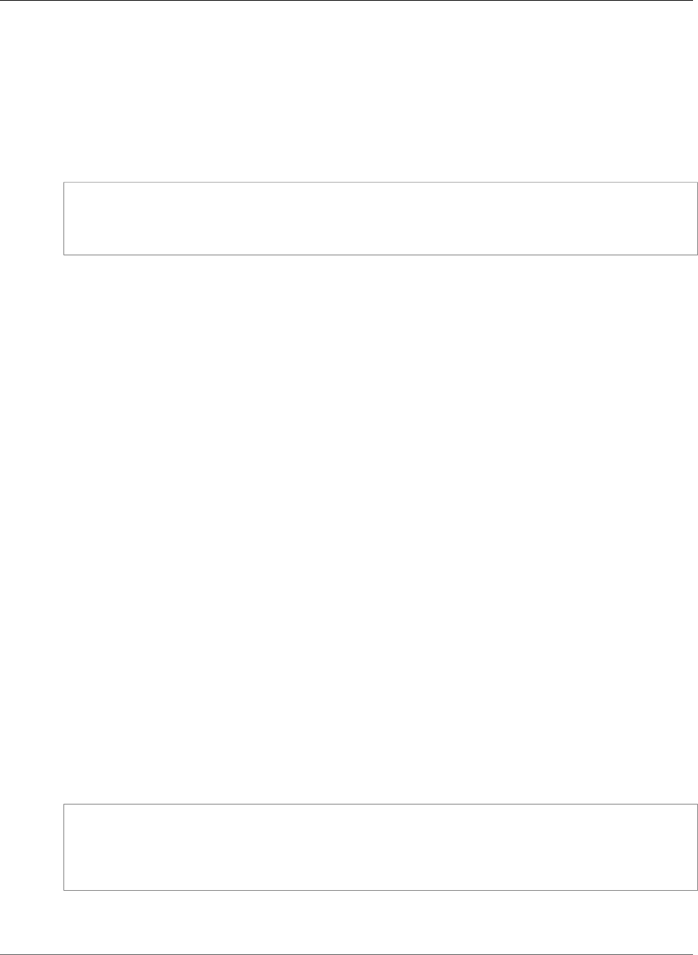
Amazon Redshift Database Developer Guide
Loading Data from Amazon S3
Loading Multibyte Data from Amazon S3
If your data includes non-ASCII multibyte characters (such as Chinese or Cyrillic characters), you must
load the data to VARCHAR columns. The VARCHAR data type supports four-byte UTF-8 characters,
but the CHAR data type only accepts single-byte ASCII characters. You cannot load five-byte or longer
characters into Amazon Redshift tables. For more information about CHAR and VARCHAR, see Data
Types (p. 315).
To check which encoding an input file uses, use the Linux file command:
$ file ordersdata.txt
ordersdata.txt: ASCII English text
$ file uni_ordersdata.dat
uni_ordersdata.dat: UTF-8 Unicode text
Loading Encrypted Data Files from Amazon S3
You can use the COPY command to load data files that were uploaded to Amazon S3 using server-side
encryption, client-side encryption, or both.
The COPY command supports the following types of Amazon S3 encryption:
• Server-side encryption with Amazon S3-managed keys (SSE-S3)
• Server-side encryption with AWS KMS-managed keys (SSE-KMS)
• Client-side encryption using a client-side symmetric master key
The COPY command doesn't support the following types of Amazon S3 encryption:
• Server-side encryption with customer-provided keys (SSE-C)
• Client-side encryption using an AWS KMS-managed customer master key
• Client-side encryption using a customer-provided asymmetric master key
For more information about Amazon S3 encryption, see Protecting Data Using Server-Side Encryption
and Protecting Data Using Client-Side Encryption in the Amazon Simple Storage Service Developer
Guide.
The UNLOAD (p. 566) command automatically encrypts files using SSE-S3. You can also unload using
SSE-KMS or client-side encryption with a customer-managed symmetric key. For more information, see
Unloading Encrypted Data Files (p. 245)
The COPY command automatically recognizes and loads files encrypted using SSE-S3 and SSE-KMS.
You can load files encrypted using a client-side symmetric master key by specifying the ENCRYPTED
option and providing the key value. For more information, see Uploading Encrypted Data to Amazon
S3 (p. 189).
To load client-side encrypted data files, provide the master key value using the
MASTER_SYMMETRIC_KEY parameter and include the ENCRYPTED option.
copy customer from 's3://mybucket/encrypted/customer'
iam_role 'arn:aws:iam::0123456789012:role/MyRedshiftRole'
master_symmetric_key '<master_key>'
encrypted
delimiter '|';
To load encrypted data files that are gzip, lzop, or bzip2 compressed, include the GZIP, LZOP, or BZIP2
option along with the master key value and the ENCRYPTED option.
API Version 2012-12-01
195

Amazon Redshift Database Developer Guide
Loading Data from Amazon EMR
copy customer from 's3://mybucket/encrypted/customer'
iam_role 'arn:aws:iam::0123456789012:role/MyRedshiftRole'
master_symmetric_key '<master_key>'
encrypted
delimiter '|'
gzip;
Loading Data from Amazon EMR
You can use the COPY command to load data in parallel from an Amazon EMR cluster configured to
write text files to the cluster's Hadoop Distributed File System (HDFS) in the form of fixed-width files,
character-delimited files, CSV files, or JSON-formatted files.
Loading Data From Amazon EMR Process
This section walks you through the process of loading data from an Amazon EMR cluster. The following
sections provide the details you need to accomplish each step.
•Step 1: Configure IAM Permissions (p. 196)
The users that create the Amazon EMR cluster and run the Amazon Redshift COPY command must
have the necessary permissions.
•Step 2: Create an Amazon EMR Cluster (p. 197)
Configure the cluster to output text files to the Hadoop Distributed File System (HDFS). You will need
the Amazon EMR cluster ID and the cluster's master public DNS (the endpoint for the Amazon EC2
instance that hosts the cluster).
•Step 3: Retrieve the Amazon Redshift Cluster Public Key and Cluster Node IP Addresses (p. 197)
The public key enables the Amazon Redshift cluster nodes to establish SSH connections to the hosts.
You will use the IP address for each cluster node to configure the host security groups to permit access
from your Amazon Redshift cluster using these IP addresses.
•Step 4: Add the Amazon Redshift Cluster Public Key to Each Amazon EC2 Host's Authorized Keys
File (p. 199)
You add the Amazon Redshift cluster public key to the host's authorized keys file so that the host will
recognize the Amazon Redshift cluster and accept the SSH connection.
•Step 5: Configure the Hosts to Accept All of the Amazon Redshift Cluster's IP Addresses (p. 199)
Modify the Amazon EMR instance's security groups to add ingress rules to accept the Amazon Redshift
IP addresses.
•Step 6: Run the COPY Command to Load the Data (p. 199)
From an Amazon Redshift database, run the COPY command to load the data into an Amazon Redshift
table.
Step 1: Configure IAM Permissions
The users that create the Amazon EMR cluster and run the Amazon Redshift COPY command must have
the necessary permissions.
To configure IAM permissions
1. Add the following permissions for the IAM user that will create the Amazon EMR cluster.
API Version 2012-12-01
196

Amazon Redshift Database Developer Guide
Loading Data from Amazon EMR
ec2:DescribeSecurityGroups
ec2:RevokeSecurityGroupIngress
ec2:AuthorizeSecurityGroupIngress
redshift:DescribeClusters
2. Add the following permission for the IAM role or IAM user that will execute the COPY command.
elasticmapreduce:ListInstances
3. Add the following permission to the Amazon EMR cluster's IAM role.
redshift:DescribeClusters
Step 2: Create an Amazon EMR Cluster
The COPY command loads data from files on the Amazon EMR Hadoop Distributed File System (HDFS).
When you create the Amazon EMR cluster, configure the cluster to output data files to the cluster's
HDFS.
To create an Amazon EMR cluster
1. Create an Amazon EMR cluster in the same AWS region as the Amazon Redshift cluster.
If the Amazon Redshift cluster is in a VPC, the Amazon EMR cluster must be in the same VPC group.
If the Amazon Redshift cluster uses EC2-Classic mode (that is, it is not in a VPC), the Amazon EMR
cluster must also use EC2-Classic mode. For more information, see Managing Clusters in Virtual
Private Cloud (VPC) in the Amazon Redshift Cluster Management Guide.
2. Configure the cluster to output data files to the cluster's HDFS. The HDFS file names must not
include asterisks (*) or question marks (?).
Important
The file names must not include asterisks ( * ) or question marks ( ? ).
3. Specify No for the Auto-terminate option in the Amazon EMR cluster configuration so that the
cluster remains available while the COPY command executes.
Important
If any of the data files are changed or deleted before the COPY completes, you might have
unexpected results, or the COPY operation might fail.
4. Note the cluster ID and the master public DNS (the endpoint for the Amazon EC2 instance that hosts
the cluster). You will use that information in later steps.
Step 3: Retrieve the Amazon Redshift Cluster Public Key and
Cluster Node IP Addresses
To retrieve the Amazon Redshift cluster public key and cluster node IP addresses for your
cluster using the console
1. Access the Amazon Redshift Management Console.
2. Click the Clusters link in the left navigation pane.
3. Select your cluster from the list.
4. Locate the SSH Ingestion Settings group.
Note the Cluster Public Key and Node IP addresses. You will use them in later steps.
API Version 2012-12-01
197
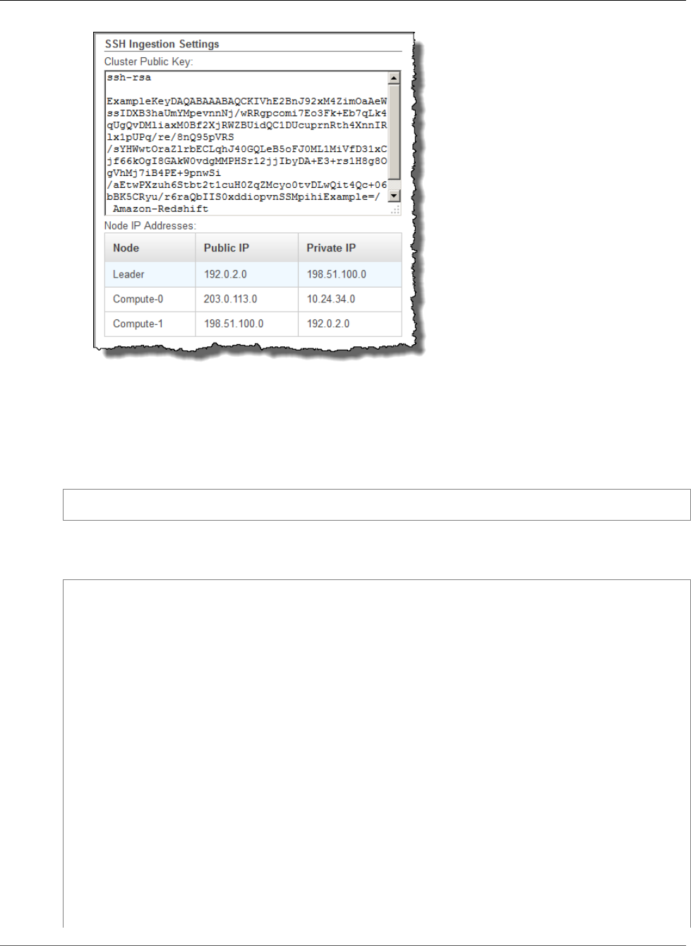
Amazon Redshift Database Developer Guide
Loading Data from Amazon EMR
You will use the Private IP addresses in Step 3 to configure the Amazon EC2 host to accept the
connection from Amazon Redshift.
To retrieve the cluster public key and cluster node IP addresses for your cluster using the Amazon
Redshift CLI, execute the describe-clusters command. For example:
aws redshift describe-clusters --cluster-identifier <cluster-identifier>
The response will include a ClusterPublicKey value and the list of private and public IP addresses, similar
to the following:
{
"Clusters": [
{
"VpcSecurityGroups": [],
"ClusterStatus": "available",
"ClusterNodes": [
{
"PrivateIPAddress": "10.nnn.nnn.nnn",
"NodeRole": "LEADER",
"PublicIPAddress": "10.nnn.nnn.nnn"
},
{
"PrivateIPAddress": "10.nnn.nnn.nnn",
"NodeRole": "COMPUTE-0",
"PublicIPAddress": "10.nnn.nnn.nnn"
},
{
"PrivateIPAddress": "10.nnn.nnn.nnn",
"NodeRole": "COMPUTE-1",
"PublicIPAddress": "10.nnn.nnn.nnn"
}
],
"AutomatedSnapshotRetentionPeriod": 1,
"PreferredMaintenanceWindow": "wed:05:30-wed:06:00",
"AvailabilityZone": "us-east-1a",
API Version 2012-12-01
198

Amazon Redshift Database Developer Guide
Loading Data from Amazon EMR
"NodeType": "ds1.xlarge",
"ClusterPublicKey": "ssh-rsa AAAABexamplepublickey...Y3TAl Amazon-Redshift",
...
...
}
To retrieve the cluster public key and cluster node IP addresses for your cluster using the Amazon
Redshift API, use the DescribeClusters action. For more information, see describe-clusters in the
Amazon Redshift CLI Guide or DescribeClusters in the Amazon Redshift API Guide.
Step 4: Add the Amazon Redshift Cluster Public Key to Each
Amazon EC2 Host's Authorized Keys File
You add the cluster public key to each host's authorized keys file for all of the Amazon EMR cluster nodes
so that the hosts will recognize Amazon Redshift and accept the SSH connection.
To add the Amazon Redshift cluster public key to the host's authorized keys file
1. Access the host using an SSH connection.
For information about connecting to an instance using SSH, see Connect to Your Instance in the
Amazon EC2 User Guide.
2. Copy the Amazon Redshift public key from the console or from the CLI response text.
3. Copy and paste the contents of the public key into the /home/<ssh_username>/.ssh/
authorized_keys file on the host. Include the complete string, including the prefix "ssh-rsa "
and suffix "Amazon-Redshift". For example:
ssh-rsa AAAACTP3isxgGzVWoIWpbVvRCOzYdVifMrh… uA70BnMHCaMiRdmvsDOedZDOedZ Amazon-
Redshift
Step 5: Configure the Hosts to Accept All of the Amazon
Redshift Cluster's IP Addresses
To allow inbound traffic to the host instances, edit the security group and add one Inbound rule for each
Amazon Redshift cluster node. For Type, select SSH with TCP protocol on Port 22. For Source, enter the
Amazon Redshift cluster node Private IP addresses you retrieved in Step 3: Retrieve the Amazon Redshift
Cluster Public Key and Cluster Node IP Addresses (p. 197). For information about adding rules to an
Amazon EC2 security group, see Authorizing Inbound Traffic for Your Instances in the Amazon EC2 User
Guide.
Step 6: Run the COPY Command to Load the Data
Run a COPY (p. 390) command to connect to the Amazon EMR cluster and load the data into an
Amazon Redshift table. The Amazon EMR cluster must continue running until the COPY command
completes. For example, do not configure the cluster to auto-terminate.
Important
If any of the data files are changed or deleted before the COPY completes, you might have
unexpected results, or the COPY operation might fail.
In the COPY command, specify the Amazon EMR cluster ID and the HDFS file path and file name.
copy sales
from 'emr://myemrclusterid/myoutput/part*' credentials
API Version 2012-12-01
199

Amazon Redshift Database Developer Guide
Loading Data from Remote Hosts
iam_role 'arn:aws:iam::0123456789012:role/MyRedshiftRole';
You can use the wildcard characters asterisk ( * ) and question mark ( ? ) as part of the file name
argument. For example, part* loads the files part-0000, part-0001, and so on. If you specify only a
folder name, COPY attempts to load all files in the folder.
Important
If you use wildcard characters or use only the folder name, verify that no unwanted files will be
loaded or the COPY command will fail. For example, some processes might write a log file to the
output folder.
Loading Data from Remote Hosts
You can use the COPY command to load data in parallel from one or more remote hosts, such Amazon
EC2 instances or other computers. COPY connects to the remote hosts using SSH and executes
commands on the remote hosts to generate text output.
The remote host can be an Amazon EC2 Linux instance or another Unix or Linux computer configured
to accept SSH connections. This guide assumes your remote host is an Amazon EC2 instance. Where the
procedure is different for another computer, the guide will point out the difference.
Amazon Redshift can connect to multiple hosts, and can open multiple SSH connections to each host.
Amazon Redshifts sends a unique command through each connection to generate text output to the
host's standard output, which Amazon Redshift then reads as it would a text file.
Before You Begin
Before you begin, you should have the following in place:
• One or more host machines, such as Amazon EC2 instances, that you can connect to using SSH.
• Data sources on the hosts.
You will provide commands that the Amazon Redshift cluster will run on the hosts to generate the text
output. After the cluster connects to a host, the COPY command runs the commands, reads the text
from the hosts' standard output, and loads the data in parallel into an Amazon Redshift table. The text
output must be in a form that the COPY command can ingest. For more information, see Preparing
Your Input Data (p. 186)
• Access to the hosts from your computer.
For an Amazon EC2 instance, you will use an SSH connection to access the host. You will need to access
the host to add the Amazon Redshift cluster's public key to the host's authorized keys file.
• A running Amazon Redshift cluster.
For information about how to launch a cluster, see Amazon Redshift Getting Started.
Loading Data Process
This section walks you through the process of loading data from remote hosts. The following sections
provide the details you need to accomplish each step.
•Step 1: Retrieve the Cluster Public Key and Cluster Node IP Addresses (p. 201)
The public key enables the Amazon Redshift cluster nodes to establish SSH connections to the remote
hosts. You will use the IP address for each cluster node to configure the host security groups or firewall
to permit access from your Amazon Redshift cluster using these IP addresses.
API Version 2012-12-01
200

Amazon Redshift Database Developer Guide
Loading Data from Remote Hosts
•Step 2: Add the Amazon Redshift Cluster Public Key to the Host's Authorized Keys File (p. 203)
You add the Amazon Redshift cluster public key to the host's authorized keys file so that the host will
recognize the Amazon Redshift cluster and accept the SSH connection.
•Step 3: Configure the Host to Accept All of the Amazon Redshift Cluster's IP Addresses (p. 203)
For Amazon EC2 , modify the instance's security groups to add ingress rules to accept the Amazon
Redshift IP addresses. For other hosts, modify the firewall so that your Amazon Redshift nodes are
able to establish SSH connections to the remote host.
•Step 4: Get the Public Key for the Host (p. 204)
You can optionally specify that Amazon Redshift should use the public key to identify the host. You
will need to locate the public key and copy the text into your manifest file.
•Step 5: Create a Manifest File (p. 204)
The manifest is a JSON-formatted text file with the details Amazon Redshift needs to connect to the
hosts and fetch the data.
•Step 6: Upload the Manifest File to an Amazon S3 Bucket (p. 205)
Amazon Redshift reads the manifest and uses that information to connect to the remote host. If the
Amazon S3 bucket does not reside in the same region as your Amazon Redshift cluster, you must use
the REGION (p. 397) option to specify the region in which the data is located.
•Step 7: Run the COPY Command to Load the Data (p. 205)
From an Amazon Redshift database, run the COPY command to load the data into an Amazon Redshift
table.
Step 1: Retrieve the Cluster Public Key and Cluster Node IP
Addresses
To retrieve the cluster public key and cluster node IP addresses for your cluster using the
console
1. Access the Amazon Redshift Management Console.
2. Click the Clusters link in the left navigation pane.
3. Select your cluster from the list.
4. Locate the SSH Ingestion Settings group.
Note the Cluster Public Key and Node IP addresses. You will use them in later steps.
API Version 2012-12-01
201
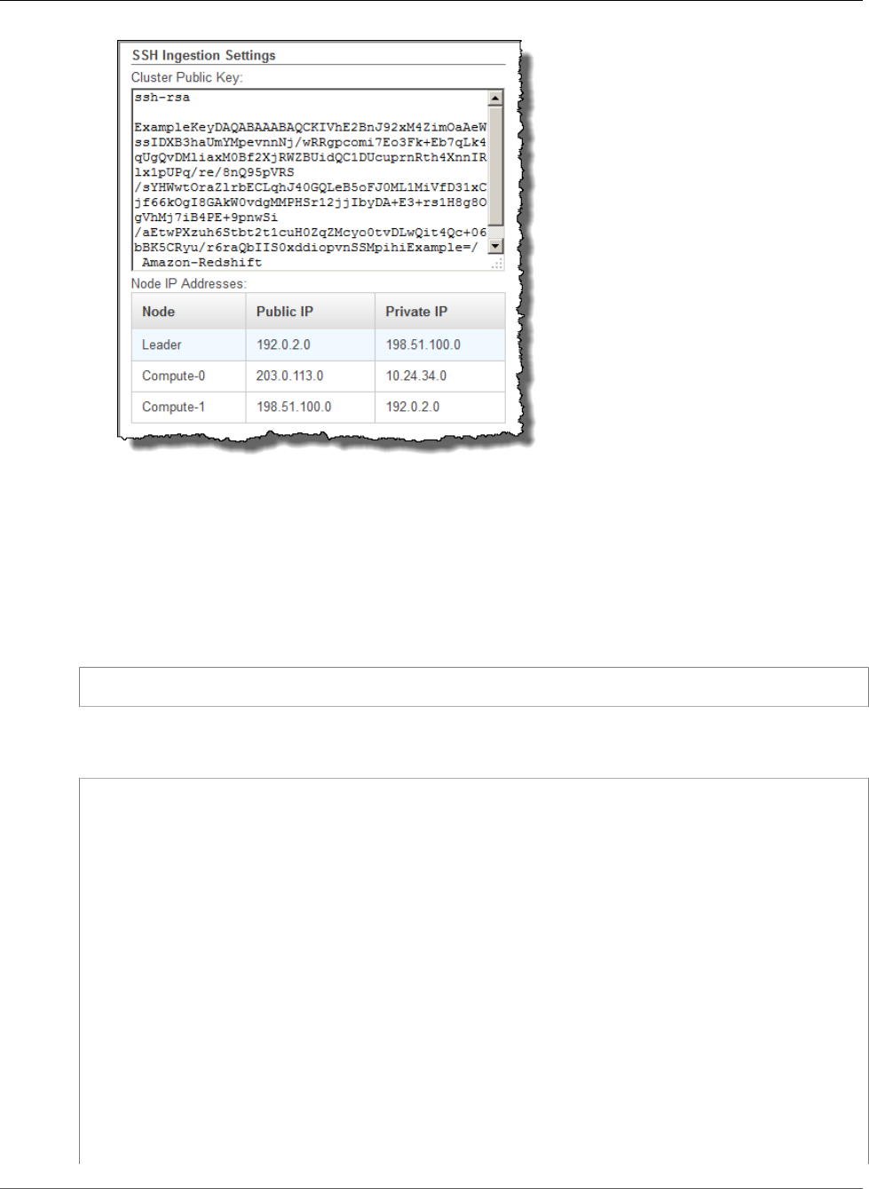
Amazon Redshift Database Developer Guide
Loading Data from Remote Hosts
You will use the IP addresses in Step 3 to configure the host to accept the connection from Amazon
Redshift. Depending on what type of host you connect to and whether it is in a VPC, you will use
either the public IP addresses or the private IP addresses.
To retrieve the cluster public key and cluster node IP addresses for your cluster using the Amazon
Redshift CLI, execute the describe-clusters command.
For example:
aws redshift describe-clusters --cluster-identifier <cluster-identifier>
The response will include the ClusterPublicKey and the list of Private and Public IP addresses, similar to
the following:
{
"Clusters": [
{
"VpcSecurityGroups": [],
"ClusterStatus": "available",
"ClusterNodes": [
{
"PrivateIPAddress": "10.nnn.nnn.nnn",
"NodeRole": "LEADER",
"PublicIPAddress": "10.nnn.nnn.nnn"
},
{
"PrivateIPAddress": "10.nnn.nnn.nnn",
"NodeRole": "COMPUTE-0",
"PublicIPAddress": "10.nnn.nnn.nnn"
},
{
"PrivateIPAddress": "10.nnn.nnn.nnn",
"NodeRole": "COMPUTE-1",
"PublicIPAddress": "10.nnn.nnn.nnn"
}
],
API Version 2012-12-01
202

Amazon Redshift Database Developer Guide
Loading Data from Remote Hosts
"AutomatedSnapshotRetentionPeriod": 1,
"PreferredMaintenanceWindow": "wed:05:30-wed:06:00",
"AvailabilityZone": "us-east-1a",
"NodeType": "ds1.xlarge",
"ClusterPublicKey": "ssh-rsa AAAABexamplepublickey...Y3TAl Amazon-Redshift",
...
...
}
To retrieve the cluster public key and cluster node IP addresses for your cluster using the Amazon
Redshift API, use the DescribeClusters action. For more information, see describe-clusters in the Amazon
Redshift CLI Guide or DescribeClusters in the Amazon Redshift API Guide.
Step 2: Add the Amazon Redshift Cluster Public Key to the
Host's Authorized Keys File
You add the cluster public key to each host's authorized keys file so that the host will recognize Amazon
Redshift and accept the SSH connection.
To add the Amazon Redshift cluster public key to the host's authorized keys file
1. Access the host using an SSH connection.
For information about connecting to an instance using SSH, see Connect to Your Instance in the
Amazon EC2 User Guide.
2. Copy the Amazon Redshift public key from the console or from the CLI response text.
3. Copy and paste the contents of the public key into the /home/<ssh_username>/.ssh/
authorized_keys file on the remote host. The <ssh_username> must match the value for the
"username" field in the manifest file. Include the complete string, including the prefix "ssh-rsa "
and suffix "Amazon-Redshift". For example:
ssh-rsa AAAACTP3isxgGzVWoIWpbVvRCOzYdVifMrh… uA70BnMHCaMiRdmvsDOedZDOedZ Amazon-
Redshift
Step 3: Configure the Host to Accept All of the Amazon Redshift
Cluster's IP Addresses
If you are working with an Amazon EC2 instance or an Amazon EMR cluster, add Inbound rules to the
host's security group to allow traffic from each Amazon Redshift cluster node. For Type, select SSH with
TCP protocol on Port 22. For Source, enter the Amazon Redshift cluster node IP addresses you retrieved
in Step 1: Retrieve the Cluster Public Key and Cluster Node IP Addresses (p. 201). For information about
adding rules to an Amazon EC2 security group, see Authorizing Inbound Traffic for Your Instances in the
Amazon EC2 User Guide.
Use the Private IP addresses when:
• You have an Amazon Redshift cluster that is not in a Virtual Private Cloud (VPC), and an Amazon EC2 -
Classic instance, both of which are in the same AWS region.
• You have an Amazon Redshift cluster that is in a VPC, and an Amazon EC2 -VPC instance, both of
which are in the same AWS region and in the same VPC.
Otherwise, use the Public IP addresses.
For more information about using Amazon Redshift in a VPC, see Managing Clusters in Virtual Private
Cloud (VPC) in the Amazon Redshift Cluster Management Guide.
API Version 2012-12-01
203

Amazon Redshift Database Developer Guide
Loading Data from Remote Hosts
Step 4: Get the Public Key for the Host
You can optionally provide the host's public key in the manifest file so that Amazon Redshift can identify
the host. The COPY command does not require the host public key but, for security reasons, we strongly
recommend using a public key to help prevent 'man-in-the-middle' attacks.
You can find the host's public key in the following location, where <ssh_host_rsa_key_name> is the
unique name for the host's public key:
: /etc/ssh/<ssh_host_rsa_key_name>.pub
Note
Amazon Redshift only supports RSA keys. We do not support DSA keys.
When you create your manifest file in Step 5, you will paste the text of the public key into the "Public
Key" field in the manifest file entry.
Step 5: Create a Manifest File
The COPY command can connect to multiple hosts using SSH, and can create multiple SSH connections
to each host. COPY executes a command through each host connection, and then loads the output
from the commands in parallel into the table. The manifest file is a text file in JSON format that
Amazon Redshift uses to connect to the host. The manifest file specifies the SSH host endpoints and the
commands that will be executed on the hosts to return data to Amazon Redshift. Optionally, you can
include the host public key, the login user name, and a mandatory flag for each entry.
The manifest file is in the following format:
{
"entries": [
{"endpoint":"<ssh_endpoint_or_IP>",
"command": "<remote_command>",
"mandatory":true,
“publickey”: “<public_key>”,
"username": “<host_user_name>”},
{"endpoint":"<ssh_endpoint_or_IP>",
"command": "<remote_command>",
"mandatory":true,
“publickey”: “<public_key>”,
"username": “host_user_name”}
]
}
The manifest file contains one "entries" construct for each SSH connection. Each entry represents a single
SSH connection. You can have multiple connections to a single host or multiple connections to multiple
hosts. The double quotes are required as shown, both for the field names and the values. The only value
that does not need double quotes is the Boolean value true or false for the mandatory field.
The following table describes the fields in the manifest file.
endpoint
The URL address or IP address of the host. For example,
"ec2-111-222-333.compute-1.amazonaws.com" or "22.33.44.56"
command
The command that will be executed by the host to generate text or binary (gzip, lzop, or bzip2)
output. The command can be any command that the user "host_user_name" has permission to run.
The command can be as simple as printing a file, or it could query a database or launch a script. The
API Version 2012-12-01
204

Amazon Redshift Database Developer Guide
Loading Data from Remote Hosts
output (text file, gzip binary file, lzop binary file, or bzip2 binary file) must be in a form the Amazon
Redshift COPY command can ingest. For more information, see Preparing Your Input Data (p. 186).
publickey
(Optional) The public key of the host. If provided, Amazon Redshift will use the public key to identify
the host. If the public key is not provided, Amazon Redshift will not attempt host identification. For
example, if the remote host's public key is: ssh-rsa AbcCbaxxx…xxxDHKJ root@amazon.com
enter the following text in the publickey field: AbcCbaxxx…xxxDHKJ.
mandatory
(Optional) Indicates whether the COPY command should fail if the connection fails. The default is
false. If Amazon Redshift does not successfully make at least one connection, the COPY command
fails.
username
(Optional) The username that will be used to log on to the host system and execute the remote
command. The user login name must be the same as the login that was used to add the public key to
the host's authorized keys file in Step 2. The default username is "redshift".
The following example shows a completed manifest to open four connections to the same host and
execute a different command through each connection:
{
"entries": [
{"endpoint":"ec2-184-72-204-112.compute-1.amazonaws.com",
"command": "cat loaddata1.txt",
"mandatory":true,
"publickey": "ec2publickeyportionoftheec2keypair",
"username": "ec2-user"},
{"endpoint":"ec2-184-72-204-112.compute-1.amazonaws.com",
"command": "cat loaddata2.txt",
"mandatory":true,
"publickey": "ec2publickeyportionoftheec2keypair",
"username": "ec2-user"},
{"endpoint":"ec2-184-72-204-112.compute-1.amazonaws.com",
"command": "cat loaddata3.txt",
"mandatory":true,
"publickey": "ec2publickeyportionoftheec2keypair",
"username": "ec2-user"},
{"endpoint":"ec2-184-72-204-112.compute-1.amazonaws.com",
"command": "cat loaddata4.txt",
"mandatory":true,
"publickey": "ec2publickeyportionoftheec2keypair",
"username": "ec2-user"}
]
}
Step 6: Upload the Manifest File to an Amazon S3 Bucket
Upload the manifest file to an Amazon S3 bucket. If the Amazon S3 bucket does not reside in the same
region as your Amazon Redshift cluster, you must use the REGION (p. 397) option to specify the region
in which the manifest is located. For information about creating an Amazon S3 bucket and uploading a
file, see Amazon Simple Storage Service Getting Started Guide.
Step 7: Run the COPY Command to Load the Data
Run a COPY (p. 390) command to connect to the host and load the data into an Amazon Redshift table.
In the COPY command, specify the explicit Amazon S3 object path for the manifest file and include the
SSH option. For example,
API Version 2012-12-01
205

Amazon Redshift Database Developer Guide
Loading from Amazon DynamoDB
copy sales
from 's3://mybucket/ssh_manifest' credentials
iam_role 'arn:aws:iam::0123456789012:role/MyRedshiftRole'
delimiter '|'
ssh;
Note
If you use automatic compression, the COPY command performs two data reads, which
means it will execute the remote command twice. The first read is to provide a sample for
compression analysis, then the second read actually loads the data. If executing the remote
command twice might cause a problem because of potential side effects, you should disable
automatic compression. To disable automatic compression, run the COPY command with the
COMPUPDATE option set to OFF. For more information, see Loading Tables with Automatic
Compression (p. 209).
Loading Data from an Amazon DynamoDB Table
You can use the COPY command to load a table with data from a single Amazon DynamoDB table.
Important
The Amazon DynamoDB table that provides the data must be created in the same region as your
cluster unless you use the REGION (p. 397) option to specify the region in which the Amazon
DynamoDB table is located.
The COPY command leverages the Amazon Redshift massively parallel processing (MPP) architecture to
read and load data in parallel from an Amazon DynamoDB table. You can take maximum advantage of
parallel processing by setting distribution styles on your Amazon Redshift tables. For more information,
see Choosing a Data Distribution Style (p. 129).
Important
When the COPY command reads data from the Amazon DynamoDB table, the resulting data
transfer is part of that table's provisioned throughput.
To avoid consuming excessive amounts of provisioned read throughput, we recommend that you not
load data from Amazon DynamoDB tables that are in production environments. If you do load data from
production tables, we recommend that you set the READRATIO option much lower than the average
percentage of unused provisioned throughput. A low READRATIO setting will help minimize throttling
issues. To use the entire provisioned throughput of an Amazon DynamoDB table, set READRATIO to 100.
The COPY command matches attribute names in the items retrieved from the DynamoDB table to
column names in an existing Amazon Redshift table by using the following rules:
• Amazon Redshift table columns are case-insensitively matched to Amazon DynamoDB item attributes.
If an item in the DynamoDB table contains multiple attributes that differ only in case, such as Price and
PRICE, the COPY command will fail.
• Amazon Redshift table columns that do not match an attribute in the Amazon DynamoDB table are
loaded as either NULL or empty, depending on the value specified with the EMPTYASNULL option in
the COPY (p. 390) command.
• Amazon DynamoDB attributes that do not match a column in the Amazon Redshift table are
discarded. Attributes are read before they are matched, and so even discarded attributes consume part
of that table's provisioned throughput.
• Only Amazon DynamoDB attributes with scalar STRING and NUMBER data types are supported. The
Amazon DynamoDB BINARY and SET data types are not supported. If a COPY command tries to load
an attribute with an unsupported data type, the command will fail. If the attribute does not match an
Amazon Redshift table column, COPY does not attempt to load it, and it does not raise an error.
The COPY command uses the following syntax to load data from an Amazon DynamoDB table:
API Version 2012-12-01
206

Amazon Redshift Database Developer Guide
Loading from Amazon DynamoDB
copy <redshift_tablename> from 'dynamodb://<dynamodb_table_name>'
authorization
readratio '<integer>';
The values for authorization are the AWS credentials needed to access the Amazon DynamoDB table. If
these credentials correspond to an IAM user, that IAM user must have permission to SCAN and DESCRIBE
the Amazon DynamoDB table that is being loaded.
The values for authorization provide the AWS authorization your cluster needs to access the Amazon
DynamoDB table. The permission must include SCAN and DESCRIBE for the Amazon DynamoDB table
that is being loaded. For more information about required permissions, see IAM Permissions for COPY,
UNLOAD, and CREATE LIBRARY (p. 427). The preferred method for authentication is to specify the
IAM_ROLE parameter and provide the Amazon Resource Name (ARN) for an IAM role with the necessary
permissions. Alternatively, you can specify the ACCESS_KEY_ID and SECRET_ACCESS_KEY parameters
and provide the access key ID and secret access key for an authorized IAM user as plain text. For more
information, see Role-Based Access Control (p. 424) or Key-Based Access Control (p. 425).
To authenticate using the IAM_ROLE parameter, <aws-account-id> and <role-name> as shown in
the following syntax.
IAM_ROLE 'arn:aws:iam::<aws-account-id>:role/<role-name>'
The following example shows authentication using an IAM role.
copy favoritemovies
from 'dynamodb://ProductCatalog'
iam_role 'arn:aws:iam::0123456789012:role/MyRedshiftRole';
To authenticate using IAM user credentials, replace <access-key-id> and <secret-access-
key with an authorized user's access key ID and full secret access key for the ACCESS_KEY_ID and
SECRET_ACCESS_KEY parameters as shown following.
ACCESS_KEY_ID '<access-key-id>'
SECRET_ACCESS_KEY '<secret-access-key>';
The following example shows authentication using IAM user credentials.
copy favoritemovies
from 'dynamodb://ProductCatalog'
access_key_id '<access-key-id>'
secret_access_key '<secret-access-key';
For more information about other authorization options, see Authorization Parameters (p. 404)
If you want to validate your data without actually loading the table, use the NOLOAD option with the
COPY (p. 390) command.
The following example loads the FAVORITEMOVIES table with data from the DynamoDB table my-
favorite-movies-table. The read activity can consume up to 50% of the provisioned throughput.
copy favoritemovies from 'dynamodb://my-favorite-movies-table'
iam_role 'arn:aws:iam::0123456789012:role/MyRedshiftRole'
readratio 50;
To maximize throughput, the COPY command loads data from an Amazon DynamoDB table in parallel
across the compute nodes in the cluster.
API Version 2012-12-01
207

Amazon Redshift Database Developer Guide
Verifying That the Data Was Loaded Correctly
Provisioned Throughput with Automatic Compression
By default, the COPY command applies automatic compression whenever you specify an empty target
table with no compression encoding. The automatic compression analysis initially samples a large
number of rows from the Amazon DynamoDB table. The sample size is based on the value of the
COMPROWS parameter. The default is 100,000 rows per slice.
After sampling, the sample rows are discarded and the entire table is loaded. As a result, many rows are
read twice. For more information about how automatic compression works, see Loading Tables with
Automatic Compression (p. 209).
Important
When the COPY command reads data from the Amazon DynamoDB table, including the rows
used for sampling, the resulting data transfer is part of that table's provisioned throughput.
Loading Multibyte Data from Amazon DynamoDB
If your data includes non-ASCII multibyte characters (such as Chinese or Cyrillic characters), you must
load the data to VARCHAR columns. The VARCHAR data type supports four-byte UTF-8 characters,
but the CHAR data type only accepts single-byte ASCII characters. You cannot load five-byte or longer
characters into Amazon Redshift tables. For more information about CHAR and VARCHAR, see Data
Types (p. 315).
Verifying That the Data Was Loaded Correctly
After the load operation is complete, query the STL_LOAD_COMMITS (p. 823) system table to verify
that the expected files were loaded. You should execute the COPY command and load verification within
the same transaction so that if there is problem with the load you can roll back the entire transaction.
The following query returns entries for loading the tables in the TICKIT database:
select query, trim(filename) as filename, curtime, status
from stl_load_commits
where filename like '%tickit%' order by query;
query | btrim | curtime | status
-------+---------------------------+----------------------------+--------
22475 | tickit/allusers_pipe.txt | 2013-02-08 20:58:23.274186 | 1
22478 | tickit/venue_pipe.txt | 2013-02-08 20:58:25.070604 | 1
22480 | tickit/category_pipe.txt | 2013-02-08 20:58:27.333472 | 1
22482 | tickit/date2008_pipe.txt | 2013-02-08 20:58:28.608305 | 1
22485 | tickit/allevents_pipe.txt | 2013-02-08 20:58:29.99489 | 1
22487 | tickit/listings_pipe.txt | 2013-02-08 20:58:37.632939 | 1
22489 | tickit/sales_tab.txt | 2013-02-08 20:58:37.632939 | 1
(6 rows)
Validating Input Data
To validate the data in the Amazon S3 input files or Amazon DynamoDB table before you actually load
the data, use the NOLOAD option with the COPY (p. 390) command. Use NOLOAD with the same COPY
commands and options you would use to actually load the data. NOLOAD checks the integrity of all of
the data without loading it into the database. The NOLOAD option displays any errors that would occur if
you had attempted to load the data.
For example, if you specified the incorrect Amazon S3 path for the input file, Amazon Redshift would
display the following error:
ERROR: No such file or directory
API Version 2012-12-01
208

Amazon Redshift Database Developer Guide
Automatic Compression
DETAIL:
-----------------------------------------------
Amazon Redshift error: The specified key does not exist
code: 2
context: S3 key being read :
location: step_scan.cpp:1883
process: xenmaster [pid=22199]
-----------------------------------------------
To troubleshoot error messages, see the Load Error Reference (p. 215).
Loading Tables with Automatic Compression
Topics
•How Automatic Compression Works (p. 209)
•Automatic Compression Example (p. 210)
You can apply compression encodings to columns in tables manually, based on your own evaluation
of the data, or you can use the COPY command to analyze and apply compression automatically. We
strongly recommend using the COPY command to apply automatic compression.
You can use automatic compression when you create and load a brand new table. The COPY command
will perform a compression analysis. You can also perform a compression analysis without loading data
or changing the compression on a table by running the ANALYZE COMPRESSION (p. 382) command
against an already populated table. For example, you can run the ANALYZE COMPRESSION command
when you want to analyze compression on a table for future use, while preserving the existing DDL.
Automatic compression balances overall performance when choosing compression encodings. Range-
restricted scans might perform poorly if sort key columns are compressed much more highly than other
columns in the same query. As a result, automatic compression will choose a less efficient compression
encoding to keep the sort key columns balanced with other columns. However, ANALYZE COMPRESSION
does not take sort keys into account, so it might recommend a different encoding for the sort key than
what automatic compression would choose. If you use ANALYZE COMPRESSION, consider changing the
encoding to RAW for sort keys.
How Automatic Compression Works
By default, the COPY command applies automatic compression whenever you run the COPY command
with an empty target table and all of the table columns either have RAW encoding or no encoding.
To apply automatic compression to an empty table, regardless of its current compression encodings, run
the COPY command with the COMPUPDATE option set to ON. To disable automatic compression, run the
COPY command with the COMPUPDATE option set to OFF.
You cannot apply automatic compression to a table that already contains data.
Note
Automatic compression analysis requires enough rows in the load data (at least 100,000 rows
per slice) to generate a meaningful sample.
Automatic compression performs these operations in the background as part of the load transaction:
1. An initial sample of rows is loaded from the input file. Sample size is based on the value of the
COMPROWS parameter. The default is 100,000.
2. Compression options are chosen for each column.
3. The sample rows are removed from the table.
4. The table is recreated with the chosen compression encodings.
API Version 2012-12-01
209
Amazon Redshift Database Developer Guide
Automatic Compression
5. The entire input file is loaded and compressed using the new encodings.
After you run the COPY command, the table is fully loaded, compressed, and ready for use. If you load
more data later, appended rows are compressed according to the existing encoding.
If you only want to perform a compression analysis, run ANALYZE COMPRESSION, which is more
efficient than running a full COPY. Then you can evaluate the results to decide whether to use automatic
compression or recreate the table manually.
Automatic compression is supported only for the COPY command. Alternatively, you can manually apply
compression encoding when you create the table. For information about manual compression encoding,
see Choosing a Column Compression Type (p. 118).
Automatic Compression Example
In this example, assume that the TICKIT database contains a copy of the LISTING table called BIGLIST,
and you want to apply automatic compression to this table when it is loaded with approximately 3
million rows.
To load and automatically compress the table
1. Ensure that the table is empty. You can apply automatic compression only to an empty table:
truncate biglist;
2. Load the table with a single COPY command. Although the table is empty, some earlier encoding
might have been specified. To ensure that Amazon Redshift performs a compression analysis, set the
COMPUPDATE parameter to ON.
copy biglist from 's3://mybucket/biglist.txt'
iam_role 'arn:aws:iam::0123456789012:role/MyRedshiftRole'
delimiter '|' COMPUPDATE ON;
Because no COMPROWS option is specified, the default and recommended sample size of 100,000
rows per slice is used.
3. Look at the new schema for the BIGLIST table in order to review the automatically chosen encoding
schemes.
select "column", type, encoding
from pg_table_def where tablename = 'biglist';
Column | Type | Encoding
---------------+-----------------------------+----------
listid | integer | delta
sellerid | integer | delta32k
eventid | integer | delta32k
dateid | smallint | delta
+numtickets | smallint | delta
priceperticket | numeric(8,2) | delta32k
totalprice | numeric(8,2) | mostly32
listtime | timestamp without time zone | none
4. Verify that the expected number of rows were loaded:
select count(*) from biglist;
count
---------
API Version 2012-12-01
210

Amazon Redshift Database Developer Guide
Optimizing for Narrow Tables
3079952
(1 row)
When rows are later appended to this table using COPY or INSERT statements, the same compression
encodings will be applied.
Optimizing Storage for Narrow Tables
If you have a table with very few columns but a very large number of rows, the three hidden metadata
identity columns (INSERT_XID, DELETE_XID, ROW_ID) will consume a disproportionate amount of the
disk space for the table.
In order to optimize compression of the hidden columns, load the table in a single COPY transaction
where possible. If you load the table with multiple separate COPY commands, the INSERT_XID column
will not compress well. You will need to perform a vacuum operation if you use multiple COPY
commands, but it will not improve compression of INSERT_XID.
Loading Default Column Values
You can optionally define a column list in your COPY command. If a column in the table is omitted from
the column list, COPY will load the column with either the value supplied by the DEFAULT option that
was specified in the CREATE TABLE command, or with NULL if the DEFAULT option was not specified.
If COPY attempts to assign NULL to a column that is defined as NOT NULL, the COPY command fails. For
information about assigning the DEFAULT option, see CREATE TABLE (p. 471).
When loading from data files on Amazon S3, the columns in the column list must be in the same order as
the fields in the data file. If a field in the data file does not have a corresponding column in the column
list, the COPY command fails.
When loading from Amazon DynamoDB table, order does not matter. Any fields in the Amazon
DynamoDB attributes that do not match a column in the Amazon Redshift table are discarded.
The following restrictions apply when using the COPY command to load DEFAULT values into a table:
• If an IDENTITY (p. 474) column is included in the column list, the EXPLICIT_IDS option must also be
specified in the COPY (p. 390) command, or the COPY command will fail. Similarly, if an IDENTITY
column is omitted from the column list, and the EXPLICIT_IDS option is specified, the COPY operation
will fail.
• Because the evaluated DEFAULT expression for a given column is the same for all loaded rows, a
DEFAULT expression that uses a RANDOM() function will assign to same value to all the rows.
• DEFAULT expressions that contain CURRENT_DATE or SYSDATE are set to the timestamp of the current
transaction.
For an example, see "Load data from a file with default values" in COPY Examples (p. 434).
Troubleshooting Data Loads
Topics
•S3ServiceException Errors (p. 212)
•System Tables for Troubleshooting Data Loads (p. 213)
•Multibyte Character Load Errors (p. 214)
•Load Error Reference (p. 215)
API Version 2012-12-01
211
Amazon Redshift Database Developer Guide
Troubleshooting
This section provides information about identifying and resolving data loading errors.
S3ServiceException Errors
The most common s3ServiceException errors are caused by an improperly formatted or incorrect
credentials string, having your cluster and your bucket in different regions, and insufficient Amazon S3
privileges.
The section provides troubleshooting information for each type of error.
Invalid Credentials String
If your credentials string was improperly formatted, you will receive the following error message:
ERROR: Invalid credentials. Must be of the format: credentials
'aws_access_key_id=<access-key-id>;aws_secret_access_key=<secret-access-key>
[;token=<temporary-session-token>]'
Verify that the credentials string does not contain any spaces or line breaks, and is enclosed in single
quotes.
Invalid Access Key ID
If your access key id does not exist, you will receive the following error message:
[Amazon](500310) Invalid operation: S3ServiceException:The AWS Access Key Id you provided
does not exist in our records.
This is often a copy and paste error. Verify that the access key ID was entered correctly.
Invalid Secret Access Key
If your secret access key is incorrect, you will receive the following error message:
[Amazon](500310) Invalid operation: S3ServiceException:The request signature we calculated
does not match the signature you provided.
Check your key and signing method.,Status 403,Error SignatureDoesNotMatch
This is often a copy and paste error. Verify that the secret access key was entered correctly and that it is
the correct key for the access key ID.
Bucket is in a Different Region
The Amazon S3 bucket specified in the COPY command must be in the same region as the cluster. If
your Amazon S3 bucket and your cluster are in different regions, you will receive an error similar to the
following:
ERROR: S3ServiceException:The bucket you are attempting to access must be addressed using
the specified endpoint.
You can create an Amazon S3 bucket in a specific region either by selecting the region when you create
the bucket by using the Amazon S3 Management Console, or by specifying an endpoint when you
create the bucket using the Amazon S3 API or CLI. For more information, see Uploading Files to Amazon
S3 (p. 188).
For more information about Amazon S3 regions, see Accessing a Bucket in the Amazon Simple Storage
Service Developer Guide.
API Version 2012-12-01
212
Amazon Redshift Database Developer Guide
Troubleshooting
Alternatively, you can specify the region using the REGION (p. 397) option with the COPY command.
Access Denied
The user account identified by the credentials must have LIST and GET access to the Amazon S3 bucket.
If the user does not have sufficient privileges, you will receive the following error message:
ERROR: S3ServiceException:Access Denied,Status 403,Error AccessDenied
For information about managing user access to buckets, see Access Control in the Amazon S3 Developer
Guide.
System Tables for Troubleshooting Data Loads
The following Amazon Redshift system tables can be helpful in troubleshooting data load issues:
• Query STL_LOAD_ERRORS (p. 825) to discover the errors that occurred during specific loads.
• Query STL_FILE_SCAN (p. 816) to view load times for specific files or to see if a specific file was even
read.
• Query STL_S3CLIENT_ERROR (p. 847) to find details for errors encountered while transferring data
from Amazon S3.
To find and diagnose load errors
1. Create a view or define a query that returns details about load errors. The following example joins
the STL_LOAD_ERRORS table to the STV_TBL_PERM table to match table IDs with actual table
names.
create view loadview as
(select distinct tbl, trim(name) as table_name, query, starttime,
trim(filename) as input, line_number, colname, err_code,
trim(err_reason) as reason
from stl_load_errors sl, stv_tbl_perm sp
where sl.tbl = sp.id);
2. Set the MAXERRORS option in your COPY command to a large enough value to enable COPY to
return useful information about your data. If the COPY encounters errors, an error message directs
you to consult the STL_LOAD_ERRORS table for details.
3. Query the LOADVIEW view to see error details. For example:
select * from loadview where table_name='venue';
tbl | table_name | query | starttime
--------+------------+-------+----------------------------
100551 | venue | 20974 | 2013-01-29 19:05:58.365391
| input | line_number | colname | err_code | reason
+----------------+-------------+-------+----------+---------------------
| venue_pipe.txt | 1 | 0 | 1214 | Delimiter not found
4. Fix the problem in the input file or the load script, based on the information that the view returns.
Some typical load errors to watch for include:
• Mismatch between data types in table and values in input data fields.
• Mismatch between number of columns in table and number of fields in input data.
API Version 2012-12-01
213
Amazon Redshift Database Developer Guide
Troubleshooting
• Mismatched quotes. Amazon Redshift supports both single and double quotes; however, these
quotes must be balanced appropriately.
• Incorrect format for date/time data in input files.
• Out-of-range values in input files (for numeric columns).
• Number of distinct values for a column exceeds the limitation for its compression encoding.
Multibyte Character Load Errors
Columns with a CHAR data type only accept single-byte UTF-8 characters, up to byte value 127, or 7F
hex, which is also the ASCII character set. VARCHAR columns accept multibyte UTF-8 characters, to a
maximum of four bytes. For more information, see Character Types (p. 323).
If a line in your load data contains a character that is invalid for the column data type, COPY returns
an error and logs a row in the STL_LOAD_ERRORS system log table with error number 1220. The
ERR_REASON field includes the byte sequence, in hex, for the invalid character.
An alternative to fixing invalid characters in your load data is to replace the invalid characters during the
load process. To replace invalid UTF-8 characters, specify the ACCEPTINVCHARS option with the COPY
command. For more information, see ACCEPTINVCHARS (p. 417).
The following example shows the error reason when COPY attempts to load UTF-8 character e0 a1 c7a4
into a CHAR column:
Multibyte character not supported for CHAR
(Hint: Try using VARCHAR). Invalid char: e0 a1 c7a4
If the error is related to a VARCHAR datatype, the error reason includes an error code as well as the
invalid UTF-8 hex sequence. The following example shows the error reason when COPY attempts to load
UTF-8 a4 into a VARCHAR field:
String contains invalid or unsupported UTF-8 codepoints.
Bad UTF-8 hex sequence: a4 (error 3)
The following table lists the descriptions and suggested workarounds for VARCHAR load errors. If one of
these errors occurs, replace the character with a valid UTF-8 code sequence or remove the character.
Error code Description
1 The UTF-8 byte sequence exceeds the four-byte maximum supported by VARCHAR.
2 The UTF-8 byte sequence is incomplete. COPY did not find the expected number of
continuation bytes for a multibyte character before the end of the string.
3 The UTF-8 single-byte character is out of range. The starting byte must not be 254,
255 or any character between 128 and 191 (inclusive).
4 The value of the trailing byte in the byte sequence is out of range. The continuation
byte must be between 128 and 191 (inclusive).
5 The UTF-8 character is reserved as a surrogate. Surrogate code points (U+D800
through U+DFFF) are invalid.
6 The character is not a valid UTF-8 character (code points 0xFDD0 to 0xFDEF).
7 The character is not a valid UTF-8 character (code points 0xFFFE and 0xFFFF).
API Version 2012-12-01
214
Amazon Redshift Database Developer Guide
Troubleshooting
Error code Description
8 The byte sequence exceeds the maximum UTF-8 code point.
9 The UTF-8 byte sequence does not have a matching code point.
Load Error Reference
If any errors occur while loading data from a file, query the STL_LOAD_ERRORS (p. 825) table to
identify the error and determine the possible explanation. The following table lists all error codes that
might occur during data loads:
Load Error Codes
Error code Description
1200 Unknown parse error. Contact support.
1201 Field delimiter was not found in the input file.
1202 Input data had more columns than were defined in the DDL.
1203 Input data had fewer columns than were defined in the DDL.
1204 Input data exceeded the acceptable range for the data type.
1205 Date format is invalid. See DATEFORMAT and TIMEFORMAT Strings (p. 432) for valid
formats.
1206 Timestamp format is invalid. See DATEFORMAT and TIMEFORMAT Strings (p. 432)
for valid formats.
1207 Data contained a value outside of the expected range of 0-9.
1208 FLOAT data type format error.
1209 DECIMAL data type format error.
1210 BOOLEAN data type format error.
1211 Input line contained no data.
1212 Load file was not found.
1213 A field specified as NOT NULL contained no data.
1214 Delimiter not found.
1215 CHAR field error.
1216 Invalid input line.
1217 Invalid identity column value.
1218 When using NULL AS '\0', a field containing a null terminator (NUL, or UTF-8 0000)
contained more than one byte.
1219 UTF-8 hexadecimal contains an invalid digit.
1220 String contains invalid or unsupported UTF-8 codepoints.
API Version 2012-12-01
215
Amazon Redshift Database Developer Guide
Updating with DML
Error code Description
1221 Encoding of the file is not the same as that specified in the COPY command.
Updating Tables with DML Commands
Amazon Redshift supports standard Data Manipulation Language (DML) commands (INSERT, UPDATE,
and DELETE) that you can use to modify rows in tables. You can also use the TRUNCATE command to do
fast bulk deletes.
Note
We strongly encourage you to use the COPY (p. 390) command to load large amounts of
data. Using individual INSERT statements to populate a table might be prohibitively slow.
Alternatively, if your data already exists in other Amazon Redshift database tables, use INSERT
INTO ... SELECT FROM or CREATE TABLE AS to improve performance. For information, see
INSERT (p. 520) or CREATE TABLE AS (p. 483).
If you insert, update, or delete a significant number of rows in a table, relative to the number of rows
before the changes, run the ANALYZE and VACUUM commands against the table when you are done.
If a number of small changes accumulate over time in your application, you might want to schedule
the ANALYZE and VACUUM commands to run at regular intervals. For more information, see Analyzing
Tables (p. 223) and Vacuuming Tables (p. 228).
Updating and Inserting New Data
You can efficiently add new data to an existing table by using a combination of updates and inserts from
a staging table. While Amazon Redshift does not support a single merge, or upsert, command to update a
table from a single data source, you can perform a merge operation by creating a staging table and then
using one of the methods described in this section to update the target table from the staging table.
Topics
•Merge Method 1: Replacing Existing Rows (p. 216)
•Merge Method 2: Specifying a Column List (p. 217)
•Creating a Temporary Staging Table (p. 217)
•Performing a Merge Operation by Replacing Existing Rows (p. 217)
•Performing a Merge Operation by Specifying a Column List (p. 218)
•Merge Examples (p. 219)
Note
You should run the entire merge operation, except for creating and dropping the temporary
staging table, in a single transaction so that the transaction will roll back if any step fails. Using
a single transaction also reduces the number of commits, which saves time and resources.
Merge Method 1: Replacing Existing Rows
If you are overwriting all of the columns in the target table, the fastest method for performing a merge
is by replacing the existing rows because it scans the target table only once, by using an inner join to
delete rows that will be updated. After the rows are deleted, they are replaced along with new rows by a
single insert operation from the staging table.
API Version 2012-12-01
216

Amazon Redshift Database Developer Guide
Merge Method 2: Specifying a Column List
Use this method if all of the following are true:
• Your target table and your staging table contain the same columns.
• You intend to replace all of the data in the target table columns with all of the staging table columns.
• You will use all of the rows in the staging table in the merge.
If any of these criteria do not apply, use Merge Method 2: Specifying a column list, described in the
following section.
If you will not use all of the rows in the staging table, you can filter the DELETE and INSERT statements
by using a WHERE clause to leave out rows that are not actually changing. However, if most of the rows
in the staging table will not participate in the merge, we recommend performing an UPDATE and an
INSERT in separate steps, as described later in this section.
Merge Method 2: Specifying a Column List
Use this method to update specific columns in the target table instead of overwriting entire rows.
This method takes longer than the previous method because it requires an extra update step. Use this
method if any of the following are true:
• Not all of the columns in the target table are to be updated.
• Most rows in the staging table will not be used in the updates.
Creating a Temporary Staging Table
The staging table is a temporary table that holds all of the data that will be used to make changes to the
target table, including both updates and inserts.
A merge operation requires a join between the staging table and the target table. To collocate the
joining rows, set the staging table's distribution key to the same column as the target table's distribution
key. For example, if the target table uses a foreign key column as its distribution key, use the same
column for the staging table's distribution key. If you create the staging table by using a CREATE TABLE
LIKE (p. 475) statement, the staging table will inherit the distribution key from the parent table. If
you use a CREATE TABLE AS statement, the new table does not inherit the distribution key. For more
information, see Choosing a Data Distribution Style (p. 129)
If the distribution key is not the same as the primary key and the distribution key is not updated as part
of the merge operation, add a redundant join predicate on the distribution key columns to enable a
collocated join. For example:
where target.primarykey = stage.primarykey
and target.distkey = stage.distkey
To verify that the query will use a collocated join, run the query with EXPLAIN (p. 511) and check for
DS_DIST_NONE on all of the joins. For more information, see Evaluating the Query Plan (p. 133)
Performing a Merge Operation by Replacing Existing
Rows
To perform a merge operation by replacing existing rows
1. Create a staging table, and then populate it with data to be merged, as shown in the following
pseudocode.
API Version 2012-12-01
217
Amazon Redshift Database Developer Guide
Performing a Merge Operation by Specifying a Column List
create temp table stage (like target);
insert into stage
select * from source
where source.filter = 'filter_expression';
2. Use an inner join with the staging table to delete the rows from the target table that are being
updated.
Put the delete and insert operations in a single transaction block so that if there is a problem,
everything will be rolled back.
begin transaction;
delete from target
using stage
where target.primarykey = stage.primarykey;
3. Insert all of the rows from the staging table.
insert into target
select * from stage;
end transaction;
4. Drop the staging table.
drop table stage;
Performing a Merge Operation by Specifying a
Column List
To perform a merge operation by specifying a column list
1. Put the entire operation in a single transaction block so that if there is a problem, everything will be
rolled back.
begin transaction;
…
end transaction;
2. Create a staging table, and then populate it with data to be merged, as shown in the following
pseudocode.
create temp table stage (like target);
insert into stage
select * from source
where source.filter = 'filter_expression';
3. Update the target table by using an inner join with the staging table.
• In the UPDATE clause, explicitly list the columns to be updated.
• Perform an inner join with the staging table.
• If the distribution key is different from the primary key and the distribution key is not being
updated, add a redundant join on the distribution key. To verify that the query will use a
API Version 2012-12-01
218
Amazon Redshift Database Developer Guide
Merge Examples
collocated join, run the query with EXPLAIN (p. 511) and check for DS_DIST_NONE on all of the
joins. For more information, see Evaluating the Query Plan (p. 133)
• If your target table is sorted by time stamp, add a predicate to take advantage of range-restricted
scans on the target table. For more information, see Amazon Redshift Best Practices for Designing
Queries (p. 32).
• If you will not use all of the rows in the merge, add a clause to filter the rows that need to be
changed. For example, add an inequality filter on one or more columns to exclude rows that have
not changed.
• Put the update, delete, and insert operations in a single transaction block so that if there is a
problem, everything will be rolled back.
For example:
begin transaction;
update target
set col1 = stage.col1,
col2 = stage.col2,
col3 = 'expression'
from stage
where target.primarykey = stage.primarykey
and target.distkey = stage.distkey
and target.col3 > 'last_update_time'
and (target.col1 != stage.col1
or target.col2 != stage.col2
or target.col3 = 'filter_expression');
4. Delete unneeded rows from the staging table by using an inner join with the target table. Some
rows in the target table already match the corresponding rows in the staging table, and others were
updated in the previous step. In either case, they are not needed for the insert.
delete from stage
using target
where stage.primarykey = target.primarykey;
5. Insert the remaining rows from the staging table. Use the same column list in the VALUES clause
that you used in the UPDATE statement in step two.
insert into target
(select col1, col2, 'expression')
from stage;
end transaction;
6. Drop the staging table.
drop table stage;
Merge Examples
The following examples perform a merge to update the SALES table. The first example uses the simpler
method of deleting from the target table and then inserting all of the rows from the staging table. The
second example requires updating on select columns in the target table, so it includes an extra update
step.
Sample merge data source
API Version 2012-12-01
219

Amazon Redshift Database Developer Guide
Merge Examples
The examples in this section need a sample data source that includes both updates and inserts. For the
examples, we will create a sample table named SALES_UPDATE that uses data from the SALES table.
We’ll populate the new table with random data that represents new sales activity for December. We will
use the SALES_UPDATE sample table to create the staging table in the examples that follow.
-- Create a sample table as a copy of the SALES table
create table sales_update as
select * from sales;
-- Change every fifth row so we have updates
update sales_update
set qtysold = qtysold*2,
pricepaid = pricepaid*0.8,
commission = commission*1.1
where saletime > '2008-11-30'
and mod(sellerid, 5) = 0;
-- Add some new rows so we have insert examples
-- This example creates a duplicate of every fourth row
insert into sales_update
select (salesid + 172456) as salesid, listid, sellerid, buyerid, eventid, dateid, qtysold,
pricepaid, commission, getdate() as saletime
from sales_update
where saletime > '2008-11-30'
and mod(sellerid, 4) = 0;
Example of a merge that replaces existing rows
The following script uses the SALES_UPDATE table to perform a merge operation on the SALES table
with new data for December sales activity. This example deletes rows in the SALES table that have
updates so they can be replaced with the updated rows in the staging table. The staging table should
contain only rows that will participate in the merge, so the CREATE TABLE statement includes a filter to
exclude rows that have not changed.
-- Create a staging table and populate it with updated rows from SALES_UPDATE
create temp table stagesales as
select * from sales_update
where sales_update.saletime > '2008-11-30'
and sales_update.salesid = (select sales.salesid from sales
where sales.salesid = sales_update.salesid
and sales.listid = sales_update.listid
and (sales_update.qtysold != sales.qtysold
or sales_update.pricepaid != sales.pricepaid));
-- Start a new transaction
begin transaction;
-- Delete any rows from SALES that exist in STAGESALES, because they are updates
-- The join includes a redundant predicate to collocate on the distribution key
–- A filter on saletime enables a range-restricted scan on SALES
delete from sales
using stagesales
where sales.salesid = stagesales.salesid
and sales.listid = stagesales.listid
and sales.saletime > '2008-11-30';
-- Insert all the rows from the staging table into the target table
insert into sales
select * from stagesales;
API Version 2012-12-01
220

Amazon Redshift Database Developer Guide
Performing a Deep Copy
-- End transaction and commit
end transaction;
-- Drop the staging table
drop table stagesales;
Example of a merge that specifies a column list
The following example performs a merge operation to update SALES with new data for December
sales activity. We need sample data that includes both updates and inserts, along with rows that have
not changed. For this example, we want to update the QTYSOLD and PRICEPAID columns but leave
COMMISSION and SALETIME unchanged. The following script uses the SALES_UPDATE table to perform
a merge operation on the SALES table.
-- Create a staging table and populate it with rows from SALES_UPDATE for Dec
create temp table stagesales as select * from sales_update
where saletime > '2008-11-30';
-- Start a new transaction
begin transaction;
-- Update the target table using an inner join with the staging table
-- The join includes a redundant predicate to collocate on the distribution key –- A filter
on saletime enables a range-restricted scan on SALES
update sales
set qtysold = stagesales.qtysold,
pricepaid = stagesales.pricepaid
from stagesales
where sales.salesid = stagesales.salesid
and sales.listid = stagesales.listid
and stagesales.saletime > '2008-11-30'
and (sales.qtysold != stagesales.qtysold
or sales.pricepaid != stagesales.pricepaid);
-- Delete matching rows from the staging table
-- using an inner join with the target table
delete from stagesales
using sales
where sales.salesid = stagesales.salesid
and sales.listid = stagesales.listid;
-- Insert the remaining rows from the staging table into the target table
insert into sales
select * from stagesales;
-- End transaction and commit
end transaction;
-- Drop the staging table
drop table stagesales;
Performing a Deep Copy
A deep copy recreates and repopulates a table by using a bulk insert, which automatically sorts the table.
If a table has a large unsorted region, a deep copy is much faster than a vacuum. The trade off is that
you should not make concurrent updates during a deep copy operation unless you can track it and move
API Version 2012-12-01
221

Amazon Redshift Database Developer Guide
Performing a Deep Copy
the delta updates into the new table after the process has completed. A VACUUM operation supports
concurrent updates automatically.
You can choose one of the following methods to create a copy of the original table:
• Use the original table DDL.
If the CREATE TABLE DDL is available, this is the fastest and preferred method. If you create a new
table, you can specify all table and column attributes, including primary key and foreign keys.
Note
If the original DDL is not available, you might be able to recreate the DDL by running a script
called v_generate_tbl_ddl. You can download the script from amazon-redshift-utils,
which is part of the Amazon Web Services - Labs git hub repository.
• Use CREATE TABLE LIKE.
If the original DDL is not available, you can use CREATE TABLE LIKE to recreate the original table. The
new table inherits the encoding, distkey, sortkey, and notnull attributes of the parent table. The new
table doesn't inherit the primary key and foreign key attributes of the parent table, but you can add
them using ALTER TABLE (p. 365).
• Create a temporary table and truncate the original table.
If you need to retain the primary key and foreign key attributes of the parent table, or if the parent
table has dependencies, you can use CREATE TABLE ... AS (CTAS) to create a temporary table, then
truncate the original table and populate it from the temporary table.
Using a temporary table improves performance significantly compared to using a permanent table,
but there is a risk of losing data. A temporary table is automatically dropped at the end of the session
in which it is created. TRUNCATE commits immediately, even if it is inside a transaction block. If the
TRUNCATE succeeds but the session terminates before the subsequent INSERT completes, the data is
lost. If data loss is unacceptable, use a permanent table.
To perform a deep copy using the original table DDL
1. (Optional) Recreate the table DDL by running a script called v_generate_tbl_ddl.
2. Create a copy of the table using the original CREATE TABLE DDL.
3. Use an INSERT INTO … SELECT statement to populate the copy with data from the original table.
4. Drop the original table.
5. Use an ALTER TABLE statement to rename the copy to the original table name.
The following example performs a deep copy on the SALES table using a duplicate of SALES named
SALESCOPY.
create table salescopy ( … );
insert into salescopy (select * from sales);
drop table sales;
alter table salescopy rename to sales;
To perform a deep copy using CREATE TABLE LIKE
1. Create a new table using CREATE TABLE LIKE.
2. Use an INSERT INTO … SELECT statement to copy the rows from the current table to the new table.
3. Drop the current table.
4. Use an ALTER TABLE statement to rename the new table to the original table name.
API Version 2012-12-01
222
Amazon Redshift Database Developer Guide
Analyzing Tables
The following example performs a deep copy on the SALES table using CREATE TABLE LIKE.
create table likesales (like sales);
insert into likesales (select * from sales);
drop table sales;
alter table likesales rename to sales;
To perform a deep copy by creating a temporary table and truncating the original table
1. Use CREATE TABLE AS to create a temporary table with the rows from the original table.
2. Truncate the current table.
3. Use an INSERT INTO … SELECT statement to copy the rows from the temporary table to the original
table.
4. Drop the temporary table.
The following example performs a deep copy on the SALES table by creating a temporary table and
truncating the original table:
create temp table salestemp as select * from sales;
truncate sales;
insert into sales (select * from salestemp);
drop table salestemp;
Analyzing Tables
The ANALYZE operation updates the statistical metadata that the query planner uses to choose optimal
plans.
In most cases, you don't need to explicitly run the ANALYZE command. Amazon Redshift monitors
changes to your workload and automatically updates statistics in the background. In addition, the COPY
command performs an analysis automatically when it loads data into an empty table.
To explicitly analyze a table or the entire database, run the ANALYZE (p. 380) command.
Topics
•Automatic Analyze (p. 223)
•Analysis of New Table Data (p. 224)
•ANALYZE Command History (p. 227)
Automatic Analyze
Amazon Redshift continuously monitors your database and automatically performs analyze operations in
the background. To minimize impact to your system performance, automatic analyze runs during periods
when workloads are light.
Automatic analyze is enabled by default. To disable automatic analyze, set the auto_analyze
parameter to false by modifying your cluster's parameter group.
To reduce processing time and improve overall system performance, Amazon Redshift skips automatic
analyze for any table where the extent of modifications is small.
An analyze operation skips tables that have up-to-date statistics. If you run ANALYZE as part of your
extract, transform, and load (ETL) workflow, automatic analyze skips tables that have current statistics.
Similarly, an explicit ANALYZE skips tables when automatic analyze has updated the table's statistics.
API Version 2012-12-01
223

Amazon Redshift Database Developer Guide
Analysis of New Table Data
Analysis of New Table Data
By default, the COPY command performs an ANALYZE after it loads data into an empty table. You can
force an ANALYZE regardless of whether a table is empty by setting STATUPDATE ON. If you specify
STATUPDATE OFF, an ANALYZE is not performed. Only the table owner or a superuser can run the
ANALYZE command or run the COPY command with STATUPDATE set to ON.
Amazon Redshift also analyzes new tables that you create with the following commands:
• CREATE TABLE AS (CTAS)
• CREATE TEMP TABLE AS
• SELECT INTO
Amazon Redshift returns a warning message when you run a query against a new table that was not
analyzed after its data was initially loaded. No warning occurs when you query a table after a subsequent
update or load. The same warning message is returned when you run the EXPLAIN command on a query
that references tables that have not been analyzed.
Whenever adding data to a nonempty table significantly changes the size of the table, you can explicitly
update statistics. You do so either by running an ANALYZE command or by using the STATUPDATE ON
option with the COPY command. To view details about the number of rows that have been inserted or
deleted since the last ANALYZE, query the PG_STATISTIC_INDICATOR (p. 939) system catalog table.
You can specify the scope of the ANALYZE (p. 380) command to one of the following:
• The entire current database
• A single table
• One or more specific columns in a single table
• Columns that are likely to be used as predicates in queries
The ANALYZE command gets a sample of rows from the table, does some calculations, and saves
resulting column statistics. By default, Amazon Redshift runs a sample pass for the DISTKEY column
and another sample pass for all of the other columns in the table. If you want to generate statistics for
a subset of columns, you can specify a comma-separated column list. You can run ANALYZE with the
PREDICATE COLUMNS clause to skip columns that aren’t used as predicates.
ANALYZE operations are resource intensive, so run them only on tables and columns that actually require
statistics updates. You don't need to analyze all columns in all tables regularly or on the same schedule.
If the data changes substantially, analyze the columns that are frequently used in the following:
• Sorting and grouping operations
• Joins
• Query predicates
To reduce processing time and improve overall system performance, Amazon Redshift skips
ANALYZE for any table that has a low percentage of changed rows, as determined by the
analyze_threshold_percent (p. 948) parameter. By default, the analyze threshold is set to 10 percent.
You can change the analyze threshold for the current session by running a SET (p. 560) command.
Columns that are less likely to require frequent analysis are those that represent facts and measures and
any related attributes that are never actually queried, such as large VARCHAR columns. For example,
consider the LISTING table in the TICKIT database.
select "column", type, encoding, distkey, sortkey
API Version 2012-12-01
224

Amazon Redshift Database Developer Guide
Analysis of New Table Data
from pg_table_def where tablename = 'listing';
column | type | encoding | distkey | sortkey
---------------+--------------------+----------+---------+---------
listid | integer | none | t | 1
sellerid | integer | none | f | 0
eventid | integer | mostly16 | f | 0
dateid | smallint | none | f | 0
numtickets | smallint | mostly8 | f | 0
priceperticket | numeric(8,2) | bytedict | f | 0
totalprice | numeric(8,2) | mostly32 | f | 0
listtime | timestamp with... | none | f | 0
If this table is loaded every day with a large number of new records, the LISTID column, which is
frequently used in queries as a join key, needs to be analyzed regularly. If TOTALPRICE and LISTTIME are
the frequently used constraints in queries, you can analyze those columns and the distribution key on
every weekday.
analyze listing(listid, totalprice, listtime);
Suppose that the sellers and events in the application are much more static, and the date IDs refer to a
fixed set of days covering only two or three years. In this case,the unique values for these columns don't
change significantly. However, the number of instances of each unique value will increase steadily.
In addition, consider the case where the NUMTICKETS and PRICEPERTICKET measures are queried
infrequently compared to the TOTALPRICE column. In this case, you can run the ANALYZE command on
the whole table once every weekend to update statistics for the five columns that are not analyzed daily:
Predicate Columns
As a convenient alternative to specifying a column list, you can choose to analyze only the columns
that are likely to be used as predicates. When you run a query, any columns that are used in a join, filter
condition, or group by clause are marked as predicate columns in the system catalog. When you run
ANALYZE with the PREDICATE COLUMNS clause, the analyze operation includes only columns that meet
the following criteria:
• The column is marked as a predicate column.
• The column is a distribution key.
• The column is part of a sort key.
If none of a table's columns are marked as predicates, ANALYZE includes all of the columns, even when
PREDICATE COLUMNS is specified. If no columns are marked as predicate columns, it might be because
the table has not yet been queried.
You might choose to use PREDICATE COLUMNS when your workload's query pattern is relatively stable.
When the query pattern is variable, with different columns frequently being used as predicates, using
PREDICATE COLUMNS might temporarily result in stale statistics. Stale statistics can lead to suboptimal
query execution plans and long execution times. However, the next time you run ANALYZE using
PREDICATE COLUMNS, the new predicate columns are included.
To view details for predicate columns, use the following SQL to create a view named
PREDICATE_COLUMNS.
CREATE VIEW predicate_columns AS
WITH predicate_column_info as (
SELECT ns.nspname AS schema_name, c.relname AS table_name, a.attnum as col_num, a.attname
as col_name,
CASE
WHEN 10002 = s.stakind1 THEN array_to_string(stavalues1, '||')
API Version 2012-12-01
225
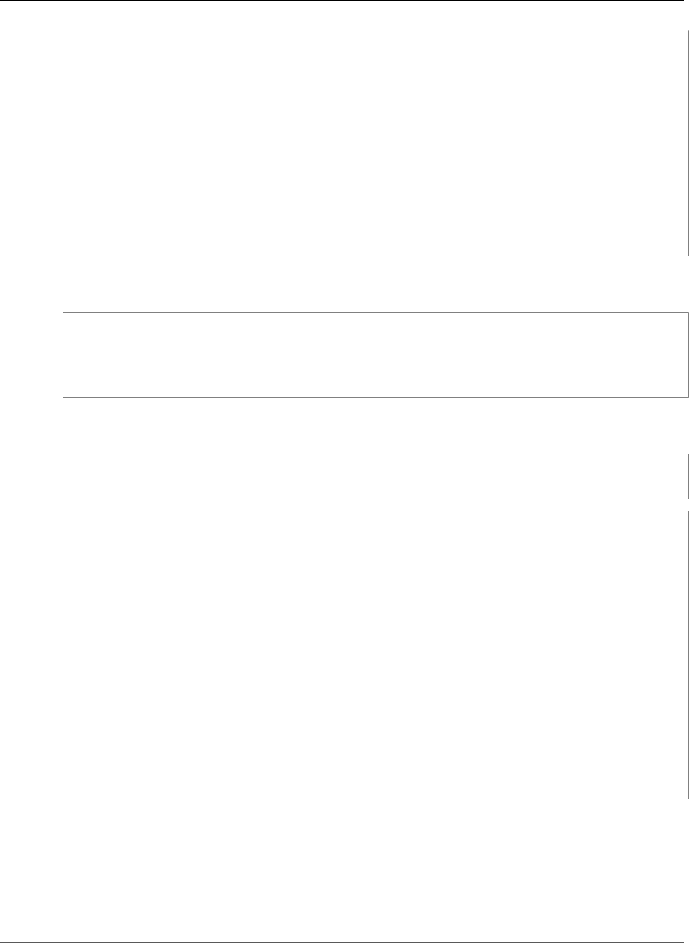
Amazon Redshift Database Developer Guide
Analysis of New Table Data
WHEN 10002 = s.stakind2 THEN array_to_string(stavalues2, '||')
WHEN 10002 = s.stakind3 THEN array_to_string(stavalues3, '||')
WHEN 10002 = s.stakind4 THEN array_to_string(stavalues4, '||')
ELSE NULL::varchar
END AS pred_ts
FROM pg_statistic s
JOIN pg_class c ON c.oid = s.starelid
JOIN pg_namespace ns ON c.relnamespace = ns.oid
JOIN pg_attribute a ON c.oid = a.attrelid AND a.attnum = s.staattnum)
SELECT schema_name, table_name, col_num, col_name,
pred_ts NOT LIKE '2000-01-01%' AS is_predicate,
CASE WHEN pred_ts NOT LIKE '2000-01-01%' THEN (split_part(pred_ts,
'||',1))::timestamp ELSE NULL::timestamp END as first_predicate_use,
CASE WHEN pred_ts NOT LIKE '%||2000-01-01%' THEN (split_part(pred_ts,
'||',2))::timestamp ELSE NULL::timestamp END as last_analyze
FROM predicate_column_info;
Suppose you run the following query against the LISTING table. Note that LISTID, LISTTIME, and
EVENTID are used in the join, filter, and group by clauses.
select s.buyerid,l.eventid, sum(l.totalprice)
from listing l
join sales s on l.listid = s.listid
where l.listtime > '2008-12-01'
group by l.eventid, s.buyerid;
When you query the PREDICATE_COLUMNS view, as shown in the following example, you see that
LISTID, EVENTID, and LISTTIME are marked as predicate columns.
select * from predicate_columns
where table_name = 'listing';
schema_name | table_name | col_num | col_name | is_predicate | first_predicate_use |
last_analyze
------------+------------+---------+----------------+--------------+---------------------
+--------------------
public | listing | 1 | listid | true | 2017-05-05 19:27:59 |
2017-05-03 18:27:41
public | listing | 2 | sellerid | false | |
2017-05-03 18:27:41
public | listing | 3 | eventid | true | 2017-05-16 20:54:32 |
2017-05-03 18:27:41
public | listing | 4 | dateid | false | |
2017-05-03 18:27:41
public | listing | 5 | numtickets | false | |
2017-05-03 18:27:41
public | listing | 6 | priceperticket | false | |
2017-05-03 18:27:41
public | listing | 7 | totalprice | false | |
2017-05-03 18:27:41
public | listing | 8 | listtime | true | 2017-05-16 20:54:32 |
2017-05-03 18:27:41
Keeping statistics current improves query performance by enabling the query planner to choose optimal
plans. Amazon Redshift refreshes statistics automatically in the background, and you can also explicitly
run the ANALYZE command. If you choose to explicitly run ANALYZE, do the following:
• Run the ANALYZE command before running queries.
• Run the ANALYZE command on the database routinely at the end of every regular load or update
cycle.
API Version 2012-12-01
226

Amazon Redshift Database Developer Guide
ANALYZE Command History
• Run the ANALYZE command on any new tables that you create and any existing tables or columns that
undergo significant change.
• Consider running ANALYZE operations on different schedules for different types of tables and
columns, depending on their use in queries and their propensity to change.
• To save time and cluster resources, use the PREDICATE COLUMNS clause when you run ANALYZE.
An analyze operation skips tables that have up-to-date statistics. If you run ANALYZE as part of your
extract, transform, and load (ETL) workflow, automatic analyze skips tables that have current statistics.
Similarly, an explicit ANALYZE skips tables when automatic analyze has updated the table's statistics.
ANALYZE Command History
It's useful to know when the last ANALYZE command was run on a table or database. When an ANALYZE
command is run, Amazon Redshift executes multiple queries that look like this:
padb_fetch_sample: select * from table_name
Query STL_ANALYZE to view the history of analyze operations. If Amazon Redshift analyzes a table using
automatic analyze, the is_background column is set to t (true). Otherwise, it is set to f (false). The
following example joins STV_TBL_PERM to show the table name and execution details.
select distinct a.xid, trim(t.name) as name, a.status, a.rows, a.modified_rows,
a.starttime, a.endtime
from stl_analyze a
join stv_tbl_perm t on t.id=a.table_id
where name = 'users'
order by starttime;
xid | name | status | rows | modified_rows | starttime | endtime
-------+-------+-----------------+-------+---------------+---------------------
+--------------------
1582 | users | Full | 49990 | 49990 | 2016-09-22 22:02:23 | 2016-09-22
22:02:28
244287 | users | Full | 24992 | 74988 | 2016-10-04 22:50:58 | 2016-10-04
22:51:01
244712 | users | Full | 49984 | 24992 | 2016-10-04 22:56:07 | 2016-10-04
22:56:07
245071 | users | Skipped | 49984 | 0 | 2016-10-04 22:58:17 | 2016-10-04
22:58:17
245439 | users | Skipped | 49984 | 1982 | 2016-10-04 23:00:13 | 2016-10-04
23:00:13
(5 rows)
Alternatively, you can run a more complex query that returns all the statements that ran in every
completed transaction that included an ANALYZE command:
select xid, to_char(starttime, 'HH24:MM:SS.MS') as starttime,
date_diff('sec',starttime,endtime ) as secs, substring(text, 1, 40)
from svl_statementtext
where sequence = 0
and xid in (select xid from svl_statementtext s where s.text like 'padb_fetch_sample%' )
order by xid desc, starttime;
xid | starttime | secs | substring
-----+--------------+------+------------------------------------------
1338 | 12:04:28.511 | 4 | Analyze date
1338 | 12:04:28.511 | 1 | padb_fetch_sample: select count(*) from
API Version 2012-12-01
227

Amazon Redshift Database Developer Guide
Vacuuming Tables
1338 | 12:04:29.443 | 2 | padb_fetch_sample: select * from date
1338 | 12:04:31.456 | 1 | padb_fetch_sample: select * from date
1337 | 12:04:24.388 | 1 | padb_fetch_sample: select count(*) from
1337 | 12:04:24.388 | 4 | Analyze sales
1337 | 12:04:25.322 | 2 | padb_fetch_sample: select * from sales
1337 | 12:04:27.363 | 1 | padb_fetch_sample: select * from sales
...
Vacuuming Tables
To clean up tables after a load or a series of incremental updates, you need to run the VACUUM (p. 584)
command, either against the entire database or against individual tables.
Note
Only the table owner or a superuser can effectively vacuum a table. If you do not have owner
or superuser privileges for a table, a VACUUM that specifies a single table will fail. If you run
a VACUUM of the entire database, without specifying a table name, the operation completes
successfully but has no effect on tables for which you do not have owner or superuser privileges.
For this reason, and because vacuuming the entire database is potentially an expensive
operation, we recommend vacuuming individual tables as needed.
When you perform a delete, the rows are marked for deletion, but not removed. Amazon Redshift
automatically runs a VACUUM DELETE operation in the background based on the number of deleted
rows in database tables. Amazon Redshift schedules the VACUUM DELETE to run during periods of
reduced load and pauses the operation during periods of high load. Automatic VACUUM DELETE is not
active in all AWS Regions.
For tables with a sort key, the VACUUM command ensures that new data in tables is fully sorted on
disk. When data is initially loaded into a table that has a sort key, the data is sorted according to the
SORTKEY specification in the CREATE TABLE (p. 471) statement. However, when you update the table,
using COPY, INSERT, or UPDATE statements, new rows are stored in a separate unsorted region on disk,
then sorted on demand for queries as required. If large numbers of rows remain unsorted on disk, query
performance might be degraded for operations that rely on sorted data, such as range-restricted scans
or merge joins. The VACUUM command merges new rows with existing sorted rows, so range-restricted
scans are more efficient and the execution engine doesn't need to sort rows on demand during query
execution.
When a table is sorted using an interleaved sort key, Amazon Redshift analyzes the distribution of values
in the sort key columns to determine the optimal sort strategy. Over time, that distribution can change,
or skew, which might degrade performance. Run a VACUUM REINDEX (p. 586) to re-analyze the sort key
distribution and restore performance. For more information, see Interleaved Sort Key (p. 141).
Topics
•VACUUM Frequency (p. 228)
•Sort Stage and Merge Stage (p. 229)
•Vacuum Threshold (p. 229)
•Vacuum Types (p. 229)
•Managing Vacuum Times (p. 230)
•Vacuum Column Limit Exceeded Error (p. 236)
VACUUM Frequency
You should vacuum as often as you need to in order to maintain consistent query performance. Consider
these factors when determining how often to run your VACUUM command.
API Version 2012-12-01
228

Amazon Redshift Database Developer Guide
Sort Stage and Merge Stage
• Run VACUUM during time periods when you expect minimal activity on the cluster, such as evenings or
during designated database administration windows.
• A large unsorted region results in longer vacuum times. If you delay vacuuming, the vacuum will take
longer because more data has to be reorganized.
• VACUUM is an I/O intensive operation, so the longer it takes for your vacuum to complete, the more
impact it will have on concurrent queries and other database operations running on your cluster.
• VACUUM takes longer for tables that use interleaved sorting. To evaluate whether interleaved tables
need to be resorted, query the SVV_INTERLEAVED_COLUMNS (p. 905) view.
Sort Stage and Merge Stage
Amazon Redshift performs a vacuum operation in two stages: first, it sorts the rows in the unsorted
region, then, if necessary, it merges the newly sorted rows at the end of the table with the existing
rows. When vacuuming a large table, the vacuum operation proceeds in a series of steps consisting
of incremental sorts followed by merges. If the operation fails or if Amazon Redshift goes off line
during the vacuum, the partially vacuumed table or database will be in a consistent state, but you will
need to manually restart the vacuum operation. Incremental sorts are lost, but merged rows that were
committed before the failure do not need to be vacuumed again. If the unsorted region is large, the lost
time might be significant. For more information about the sort and merge stages, see Managing the
Volume of Merged Rows (p. 231).
Users can access tables while they are being vacuumed. You can perform queries and write operations
while a table is being vacuumed, but when DML and a vacuum run concurrently, both might take longer.
If you execute UPDATE and DELETE statements during a vacuum, system performance might be reduced.
Incremental merges temporarily block concurrent UPDATE and DELETE operations, and UPDATE and
DELETE operations in turn temporarily block incremental merge steps on the affected tables. DDL
operations, such as ALTER TABLE, are blocked until the vacuum operation finishes with the table.
Vacuum Threshold
By default, VACUUM skips the sort phase for any table where more than 95 percent of the table's rows
are already sorted. Skipping the sort phase can significantly improve VACUUM performance. To change
the default sort threshold for a single table, include the table name and the TO threshold PERCENT
parameter when you run the VACUUM command.
Vacuum Types
You can run a full vacuum, a delete only vacuum, a sort only vacuum, or a reindex with full vacuum.
•VACUUM FULL
VACUUM FULL resorts rows and reclaims space from deleted rows. Amazon Redshift automatically
performs VACUUM DELETE ONLY operations in the background, so for most applications, VACUUM
FULL and VACUUM SORT ONLY are equivalent. VACUUM FULL is the same as VACUUM. Full vacuum is
the default vacuum operation.
•VACUUM DELETE ONLY
A DELETE ONLY vacuum is the same as a full vacuum except that it skips the sort. Amazon Redshift
automatically performs a DELETE ONLY vacuum in the background, so you rarely, if ever, need to run a
DELETE ONLY vacuum.
•VACUUM SORT ONLY
A SORT ONLY doesn't reclaim disk space. In most cases there is little benefit compared to a full
vacuum.
API Version 2012-12-01
229

Amazon Redshift Database Developer Guide
Managing Vacuum Times
•VACUUM REINDEX
Use VACUUM REINDEX for tables that use interleaved sort keys.
When you initially load an empty interleaved table using COPY or CREATE TABLE AS, Amazon Redshift
automatically builds the interleaved index. If you initially load an interleaved table using INSERT, you
need to run VACUUM REINDEX afterwards to initialize the interleaved index.
REINDEX reanalyzes the distribution of the values in the table's sort key columns, then performs a full
VACUUM operation. VACUUM REINDEX takes significantly longer than VACUUM FULL because it needs
to take an extra analysis pass over the data, and because merging in new interleaved data can involve
touching all the data blocks.
If a VACUUM REINDEX operation terminates before it completes, the next VACUUM resumes the
reindex operation before performing the vacuum.
Managing Vacuum Times
Depending on the nature of your data, we recommend following the practices in this section to minimize
vacuum times.
Topics
•Deciding Whether to Reindex (p. 230)
•Managing the Size of the Unsorted Region (p. 231)
•Managing the Volume of Merged Rows (p. 231)
•Loading Your Data in Sort Key Order (p. 235)
•Using Time Series Tables (p. 235)
Deciding Whether to Reindex
You can often significantly improve query performance by using an interleaved sort style, but over time
performance might degrade if the distribution of the values in the sort key columns changes.
When you initially load an empty interleaved table using COPY or CREATE TABLE AS, Amazon Redshift
automatically builds the interleaved index. If you initially load an interleaved table using INSERT, you
need to run VACUUM REINDEX afterwards to initialize the interleaved index.
Over time, as you add rows with new sort key values, performance might degrade if the distribution of
the values in the sort key columns changes. If your new rows fall primarily within the range of existing
sort key values, you don’t need to reindex. Run VACUUM SORT ONLY or VACUUM FULL to restore the
sort order.
The query engine is able to use sort order to efficiently select which data blocks need to be scanned
to process a query. For an interleaved sort, Amazon Redshift analyzes the sort key column values
to determine the optimal sort order. If the distribution of key values changes, or skews, as rows
are added, the sort strategy will no longer be optimal, and the performance benefit of sorting
will degrade. To reanalyze the sort key distribution you can run a VACUUM REINDEX. The reindex
operation is time consuming, so to decide whether a table will benefit from a reindex, query the
SVV_INTERLEAVED_COLUMNS (p. 905) view.
For example, the following query shows details for tables that use interleaved sort keys.
select tbl as tbl_id, stv_tbl_perm.name as table_name,
col, interleaved_skew, last_reindex
from svv_interleaved_columns, stv_tbl_perm
API Version 2012-12-01
230

Amazon Redshift Database Developer Guide
Managing Vacuum Times
where svv_interleaved_columns.tbl = stv_tbl_perm.id
and interleaved_skew is not null;
tbl_id | table_name | col | interleaved_skew | last_reindex
--------+------------+-----+------------------+--------------------
100048 | customer | 0 | 3.65 | 2015-04-22 22:05:45
100068 | lineorder | 1 | 2.65 | 2015-04-22 22:05:45
100072 | part | 0 | 1.65 | 2015-04-22 22:05:45
100077 | supplier | 1 | 1.00 | 2015-04-22 22:05:45
(4 rows)
The value for interleaved_skew is a ratio that indicates the amount of skew. A value of 1 means there
is no skew. If the skew is greater than 1.4, a VACUUM REINDEX will usually improve performance unless
the skew is inherent in the underlying set.
You can use the date value in last_reindex to determine how long it has been since the last reindex.
Managing the Size of the Unsorted Region
The unsorted region grows when you load large amounts of new data into tables that already contain
data or when you do not vacuum tables as part of your routine maintenance operations. To avoid long-
running vacuum operations, use the following practices:
• Run vacuum operations on a regular schedule.
If you load your tables in small increments (such as daily updates that represent a small percentage
of the total number of rows in the table), running VACUUM regularly will help ensure that individual
vacuum operations go quickly.
• Run the largest load first.
If you need to load a new table with multiple COPY operations, run the largest load first. When you
run an initial load into a new or truncated table, all of the data is loaded directly into the sorted
region, so no vacuum is required.
• Truncate a table instead of deleting all of the rows.
Deleting rows from a table does not reclaim the space that the rows occupied until you perform a
vacuum operation; however, truncating a table empties the table and reclaims the disk space, so no
vacuum is required. Alternatively, drop the table and re-create it.
• Truncate or drop test tables.
If you are loading a small number of rows into a table for test purposes, don't delete the rows when
you are done. Instead, truncate the table and reload those rows as part of the subsequent production
load operation.
• Perform a deep copy.
If a table that uses a compound sort key table has a large unsorted region, a deep copy is much
faster than a vacuum. A deep copy recreates and repopulates a table by using a bulk insert, which
automatically resorts the table. If a table has a large unsorted region, a deep copy is much faster than
a vacuum. The trade off is that you cannot make concurrent updates during a deep copy operation,
which you can do during a vacuum. For more information, see Amazon Redshift Best Practices for
Designing Queries (p. 32).
Managing the Volume of Merged Rows
If a vacuum operation needs to merge new rows into a table's sorted region, the time required for a
vacuum will increase as the table grows larger. You can improve vacuum performance by reducing the
number of rows that must be merged.
API Version 2012-12-01
231
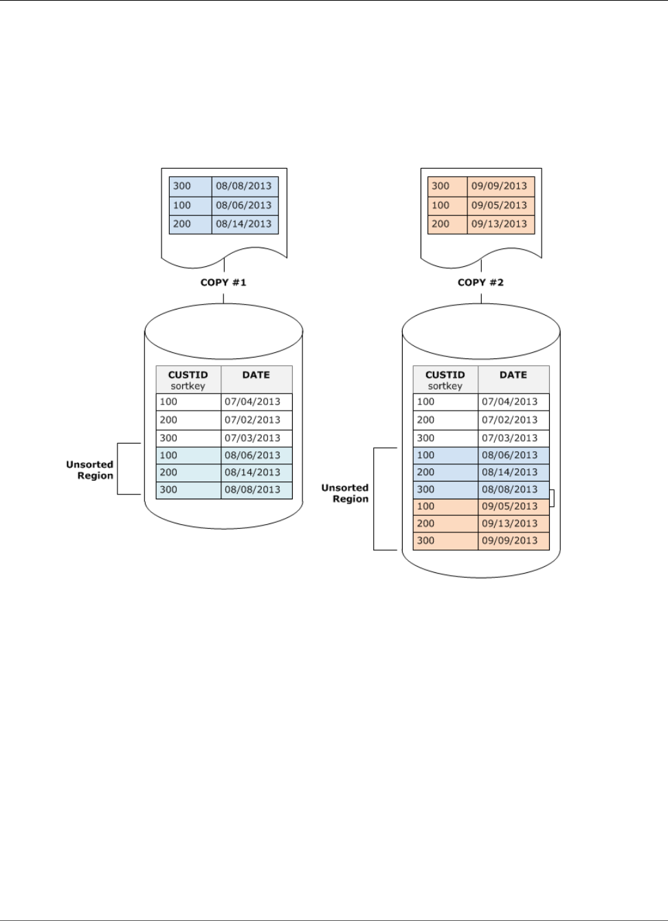
Amazon Redshift Database Developer Guide
Managing Vacuum Times
Prior to a vacuum, a table consists of a sorted region at the head of the table, followed by an unsorted
region, which grows whenever rows are added or updated. When a set of rows is added by a COPY
operation, the new set of rows is sorted on the sort key as it is added to the unsorted region at the end
of the table. The new rows are ordered within their own set, but not within the unsorted region.
The following diagram illustrates the unsorted region after two successive COPY operations, where the
sort key is CUSTID. For simplicity, this example shows a compound sort key, but the same principles
apply to interleaved sort keys, except that the impact of the unsorted region is greater for interleaved
tables.
A vacuum restores the table's sort order in two stages:
1. Sort the unsorted region into a newly-sorted region.
The first stage is relatively cheap, because only the unsorted region is rewritten. If the range of sort
key values of the newly-sorted region is higher than the existing range, only the new rows need to be
rewritten, and the vacuum is complete. For example, if the sorted region contains ID values 1 to 500
and subsequent copy operations add key values greater than 500, then only the unsorted region only
needs to be rewritten.
2. Merge the newly-sorted region with the previously-sorted region.
If the keys in the newly sorted region overlap the keys in the sorted region, then VACUUM needs to
merge the rows. Starting at the beginning of the newly-sorted region (at the lowest sort key), the
vacuum writes the merged rows from the previously sorted region and the newly sorted region into a
new set of blocks.
The extent to which the new sort key range overlaps the existing sort keys determines the extent
to which the previously-sorted region will need to be rewritten. If the unsorted keys are scattered
throughout the existing sort range, a vacuum might need to rewrite existing portions of the table.
API Version 2012-12-01
232
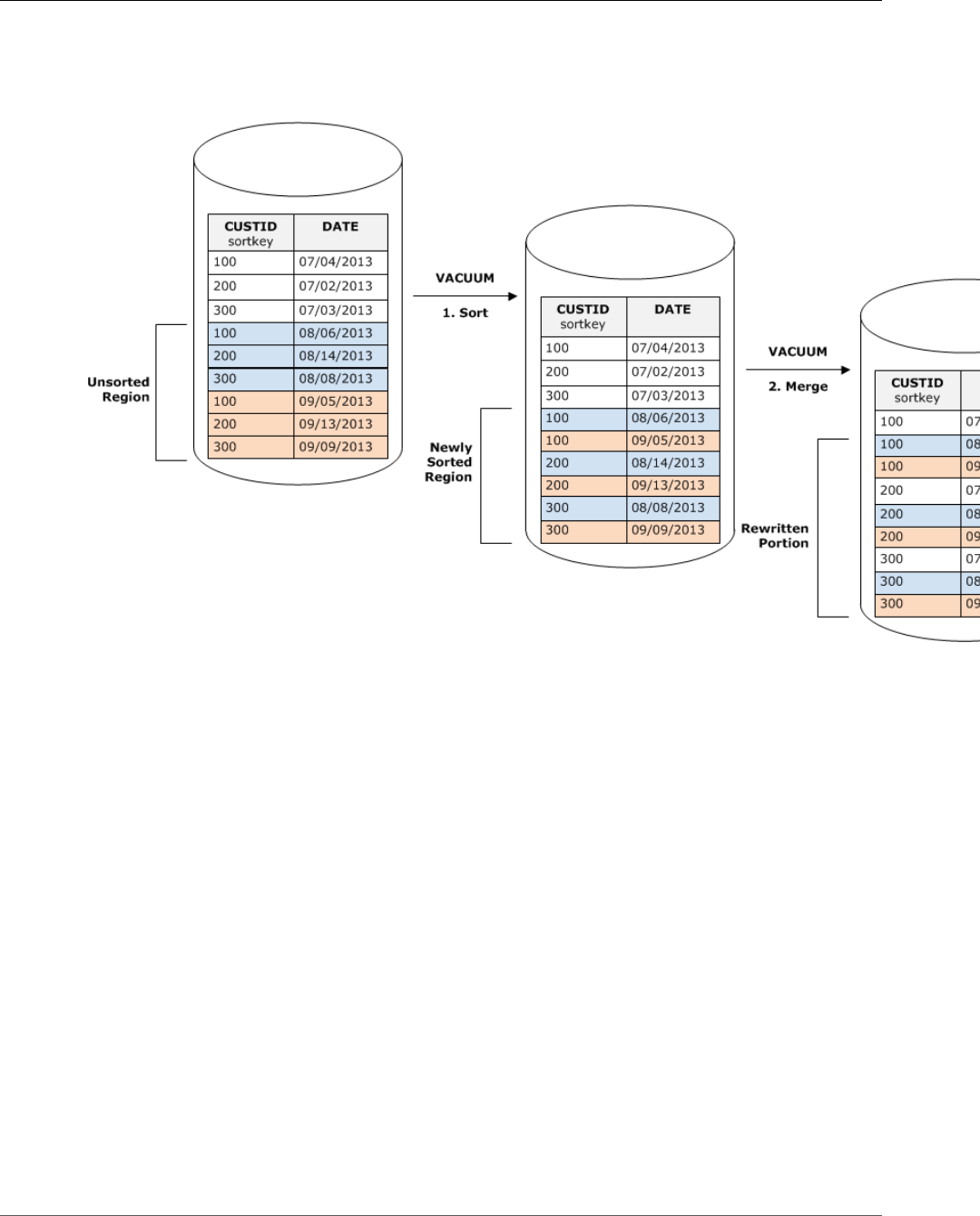
Amazon Redshift Database Developer Guide
Managing Vacuum Times
The following diagram shows how a vacuum would sort and merge rows that are added to a table where
CUSTID is the sort key. Because each copy operation adds a new set of rows with key values that overlap
the existing keys, almost the entire table needs to be rewritten. The diagram shows single sort and
merge, but in practice, a large vacuum consists of a series of incremental sort and merge steps.
If the range of sort keys in a set of new rows overlaps the range of existing keys, the cost of the merge
stage continues to grow in proportion to the table size as the table grows while the cost of the sort
stage remains proportional to the size of the unsorted region. In such a case, the cost of the merge stage
overshadows the cost of the sort stage, as the following diagram shows.
API Version 2012-12-01
233
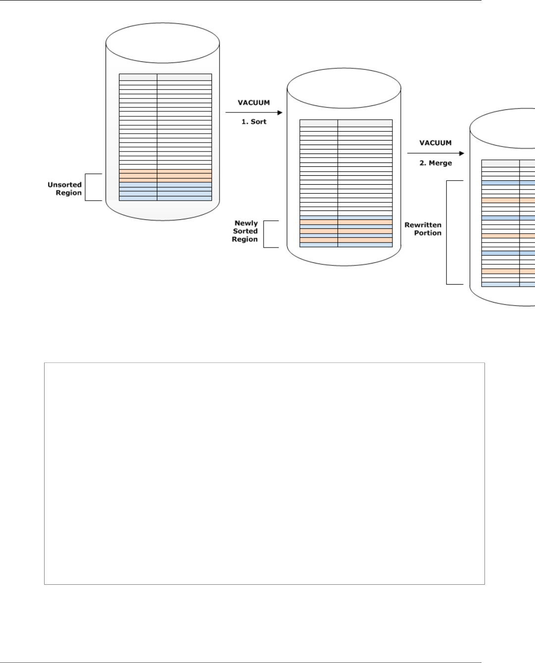
Amazon Redshift Database Developer Guide
Managing Vacuum Times
To determine what proportion of a table was remerged, query SVV_VACUUM_SUMMARY after the
vacuum operation completes. The following query shows the effect of six successive vacuums as
CUSTSALES grew larger over time.
select * from svv_vacuum_summary
where table_name = 'custsales';
table_name | xid | sort_ | merge_ | elapsed_ | row_ | sortedrow_ | block_ |
max_merge_
| | partitions | increments | time | delta | delta | delta |
partitions
-----------+------+------------+------------+------------+-------+------------+---------
+---------------
custsales | 7072 | 3 | 2 | 143918314 | 0 | 88297472 | 1524 |
47
custsales | 7122 | 3 | 3 | 164157882 | 0 | 88297472 | 772 |
47
custsales | 7212 | 3 | 4 | 187433171 | 0 | 88297472 | 767 |
47
custsales | 7289 | 3 | 4 | 255482945 | 0 | 88297472 | 770 |
47
custsales | 7420 | 3 | 5 | 316583833 | 0 | 88297472 | 769 |
47
custsales | 9007 | 3 | 6 | 306685472 | 0 | 88297472 | 772 |
47
(6 rows)
The merge_increments column gives an indication of the amount of data that was merged for each
vacuum operation. If the number of merge increments over consecutive vacuums increases in proportion
to the growth in table size, that is an indication that each vacuum operation is remerging an increasing
number of rows in the table because the existing and newly sorted regions overlap.
API Version 2012-12-01
234
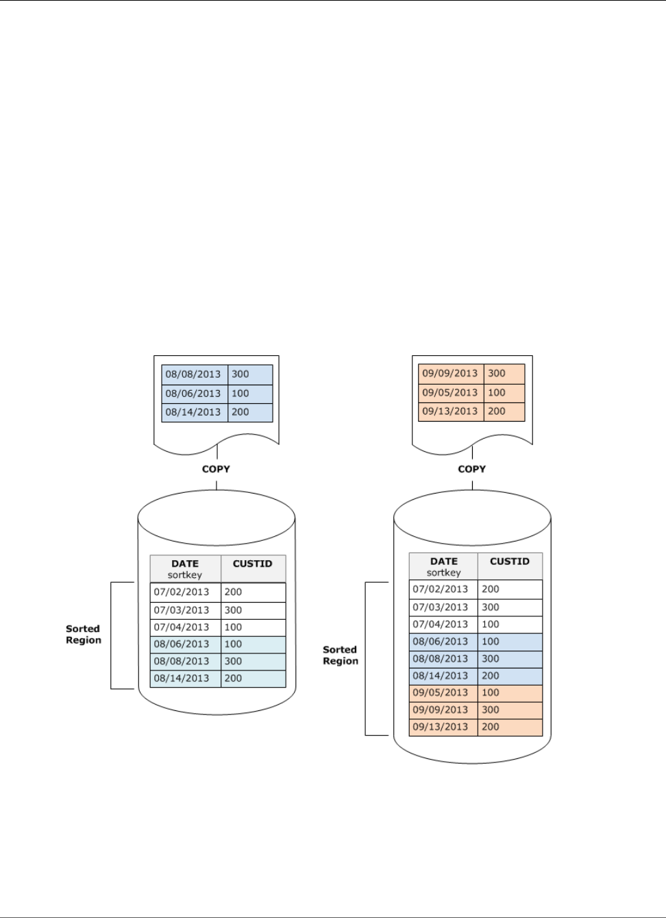
Amazon Redshift Database Developer Guide
Managing Vacuum Times
Loading Your Data in Sort Key Order
If you load your data in sort key order using a COPY command, you might reduce or even eliminate the
need to vacuum.
COPY automatically adds new rows to the table's sorted region when all of the following are true:
• The table uses a compound sort key with only one sort column.
• The sort column is NOT NULL.
• The table is 100 percent sorted or empty.
• All the new rows are higher in sort order than the existing rows, including rows marked for deletion. In
this instance, Amazon Redshift uses the first eight bytes of the sort key to determine sort order.
For example, suppose you have a table that records customer events using a customer ID and time. If
you sort on customer ID, it’s likely that the sort key range of new rows added by incremental loads will
overlap the existing range, as shown in the previous example, leading to an expensive vacuum operation.
If you set your sort key to a timestamp column, your new rows will be appended in sort order at the end
of the table, as the following diagram shows, reducing or even eliminating the need to vacuum.
Using Time Series Tables
If you maintain data for a rolling time period, use a series of tables, as the following diagram illustrates.
API Version 2012-12-01
235

Amazon Redshift Database Developer Guide
Vacuum Column Limit Exceeded Error
Create a new table each time you add a set of data, then delete the oldest table in the series. You gain a
double benefit:
• You avoid the added cost of deleting rows, because a DROP TABLE operation is much more efficient
than a mass DELETE.
• If the tables are sorted by timestamp, no vacuum is needed. If each table contains data for one month,
a vacuum will at most have to rewrite one month’s worth of data, even if the tables are not sorted by
timestamp.
You can create a UNION ALL view for use by reporting queries that hides the fact that the data is stored
in multiple tables. If a query filters on the sort key, the query planner can efficiently skip all the tables
that aren't used. A UNION ALL can be less efficient for other types of queries, so you should evaluate
query performance in the context of all queries that use the tables.
Vacuum Column Limit Exceeded Error
If your vacuum fails with the message ERROR: 1036 DETAIL: Vacuum column limit exceeded
or ERROR: 1036: Detail: vacuum_max_buffer is too small to vacuum, your table has more
columns than VACUUM can process with the available memory. The vacuum column limit is less than
the column limit for CREATE TABLE, which is 1600. The actual column limit for a vacuum depends on
the type of vacuum operation and your cluster's configuration. The column limit includes three hidden
system columns in addition to the user-defined columns.
If a vacuum operation that requires resorting (VACUUM FULL, VACUUM REINDEX, and VACUUM SORT on
tables with sort keys) exceeds the column limit, the vacuum fails with the following error.
ERROR: 1036 DETAIL: Vacuum column limit exceeded
The following table shows the approximate column limits for each node type when vacuuming requires
resorting.
Node type Column limit
dc1.large 250
dc1.8xlarge 312
dc2.large 375
dc2.8xlarge 468
API Version 2012-12-01
236
Amazon Redshift Database Developer Guide
Vacuum Column Limit Exceeded Error
Node type Column limit
ds2.xlarge 375
ds2.8xlarge 468
If the column limit is exceeded for a delete-only vacuum operation, the vacuum fails with the following
error.
ERROR: 1036: Detail: vacuum_max_buffer is too small to vacuum
The following table shows the approximate column limits for each node type for a delete-only vacuum
operation.
Node type Column limit
dc1.large 500
dc1.8xlarge 500
dc2.large 750
dc2.8xlarge 1250
ds2.xlarge 750
ds2.8xlarge 1250
You can increase the vacuum column limit by increasing the value of wlm_query_slot_count (p. 955),
which increases the amount of memory available for the query. The maximum value for
wlm_query_slot_count is limited to the concurrency value for the queue. For more information, see
Amazon Redshift Best Practices for Designing Queries (p. 32).
If increasing the value of wlm_query_slot_count is not an option, or if it doesn't solve the problem, you
can avoid needing to vacuum by performing a deep copy. To perform a deep copy, you create a copy of
the table, insert the rows from the original table into the copy, drop the original table, and then rename
the copy. A deep copy is often much faster than a vacuum. For more information, see Performing a Deep
Copy (p. 221).
For example, suppose the table calendardays has 365 columns. After a load operation, you perform a
vacuum and the vacuum fails, as the following example shows.
vacuum calendardays;
An error occurred when executing the SQL command:
vacuum calendardays;
ERROR: 1036
DETAIL: Vacuum column limit exceeded for table calendardays
HINT: Increase the value of wlm_query_slot_count or perform a deep copy instead of a
vacuum.
The following example sets wlm_query_slot_count to 10, performs a vacuum, and then resets
wlm_query_slot_count to 1. With the higher slot count, the vacuum succeeds.
set wlm_query_slot_count to 10;
API Version 2012-12-01
237

Amazon Redshift Database Developer Guide
Managing Concurrent Write Operations
vacuum calendardays;
set wlm_query_slot_count to 1;
vacuum executed successfully
You can perform a deep copy instead of a vacuum. The following example uses CREATE TABLE LIKE to
perform a deep copy.
create table likecalendardays (like calendardays);
insert into likecalendardays (select * from calendardays);
drop table calendardays;
alter table likecalendardays rename to calendardays;
Performing a deep copy using CREATE TABLE AS (CTAS) is faster than using CREATE TABLE LIKE, but
CTAS does not preserve the sort key, encoding, distkey, and notnull attributes of the parent table. For a
comparison of different deep copy methods, see Performing a Deep Copy (p. 221).
Managing Concurrent Write Operations
Topics
•Serializable Isolation (p. 238)
•Write and Read-Write Operations (p. 239)
•Concurrent Write Examples (p. 240)
Amazon Redshift allows tables to be read while they are being incrementally loaded or modified.
In some traditional data warehousing and business intelligence applications, the database is available
to users only when the nightly load is complete. In such cases, no updates are allowed during regular
work hours, when analytic queries are run and reports are generated; however, an increasing number of
applications remain live for long periods of the day or even all day, making the notion of a load window
obsolete.
Amazon Redshift supports these types of applications by allowing tables to be read while they are being
incrementally loaded or modified. Queries simply see the latest committed version, or snapshot, of the
data, rather than waiting for the next version to be committed. If you want a particular query to wait for
a commit from another write operation, you have to schedule it accordingly.
The following topics describe some of the key concepts and use cases that involve transactions, database
snapshots, updates, and concurrent behavior.
Serializable Isolation
Some applications require not only concurrent querying and loading, but also the ability to write to
multiple tables or the same table concurrently. In this context, concurrently means overlapping, not
scheduled to run at precisely the same time. Two transactions are considered to be concurrent if the
second one starts before the first commits. Concurrent operations can originate from different sessions
that are controlled either by the same user or by different users.
Note
Amazon Redshift supports a default automatic commit behavior in which each separately-
executed SQL command commits individually. If you enclose a set of commands in a transaction
block (defined by BEGIN (p. 384) and END (p. 509) statements), the block commits as
one transaction, so you can roll it back if necessary. An exception to this behavior is the
API Version 2012-12-01
238

Amazon Redshift Database Developer Guide
Write and Read-Write Operations
TRUNCATE command, which automatically commits all outstanding changes made in the
current transaction without requiring an END statement.
Concurrent write operations are supported in Amazon Redshift in a protective way, using write locks
on tables and the principle of serializable isolation. Serializable isolation preserves the illusion that
a transaction running against a table is the only transaction that is running against that table. For
example, two concurrently running transactions, T1 and T2, must produce the same results as at least
one of the following:
• T1 and T2 run serially in that order
• T2 and T1 run serially in that order
Concurrent transactions are invisible to each other; they cannot detect each other's changes. Each
concurrent transaction will create a snapshot of the database at the beginning of the transaction. A
database snapshot is created within a transaction on the first occurrence of most SELECT statements,
DML commands such as COPY, DELETE, INSERT, UPDATE, and TRUNCATE, and the following DDL
commands :
• ALTER TABLE (to add or drop columns)
• CREATE TABLE
• DROP TABLE
• TRUNCATE TABLE
If any serial execution of the concurrent transactions would produce the same results as their concurrent
execution, those transactions are deemed "serializable" and can be run safely. If no serial execution of
those transactions would produce the same results, the transaction that executes a statement that would
break serializability is aborted and rolled back.
System catalog tables (PG) and other Amazon Redshift system tables (STL and STV) are not locked in a
transaction; therefore, changes to database objects that arise from DDL and TRUNCATE operations are
visible on commit to any concurrent transactions.
For example, suppose that table A exists in the database when two concurrent transactions, T1 and T2,
start. If T2 returns a list of tables by selecting from the PG_TABLES catalog table, and then T1 drops
table A and commits, and then T2 lists the tables again, table A is no longer listed. If T2 tries to query
the dropped table, Amazon Redshift returns a "relation does not exist" error. The catalog query that
returns the list of tables to T2 or checks that table A exists is not subject to the same isolation rules as
operations against user tables.
Transactions for updates to these tables run in a read committed isolation mode. PG-prefix catalog tables
do not support snapshot isolation.
Serializable Isolation for System Tables and Catalog Tables
A database snapshot is also created in a transaction for any SELECT query that references a user-created
table or Amazon Redshift system table (STL or STV). SELECT queries that do not reference any table will
not create a new transaction database snapshot, nor will any INSERT, DELETE, or UPDATE statements
that operate solely on system catalog tables (PG).
Write and Read-Write Operations
You can manage the specific behavior of concurrent write operations by deciding when and how to run
different types of commands. The following commands are relevant to this discussion:
• COPY commands, which perform loads (initial or incremental)
API Version 2012-12-01
239

Amazon Redshift Database Developer Guide
Concurrent Write Examples
• INSERT commands that append one or more rows at a time
• UPDATE commands, which modify existing rows
• DELETE commands, which remove rows
COPY and INSERT operations are pure write operations, but DELETE and UPDATE operations are read-
write operations. (In order for rows to be deleted or updated, they have to be read first.) The results of
concurrent write operations depend on the specific commands that are being run concurrently. COPY
and INSERT operations against the same table are held in a wait state until the lock is released, then they
proceed as normal.
UPDATE and DELETE operations behave differently because they rely on an initial table read before they
do any writes. Given that concurrent transactions are invisible to each other, both UPDATEs and DELETEs
have to read a snapshot of the data from the last commit. When the first UPDATE or DELETE releases its
lock, the second UPDATE or DELETE needs to determine whether the data that it is going to work with is
potentially stale. It will not be stale, because the second transaction does not obtain its snapshot of data
until after the first transaction has released its lock.
Potential Deadlock Situation for Concurrent Write Transactions
Whenever transactions involve updates of more than one table, there is always the possibility of
concurrently running transactions becoming deadlocked when they both try to write to the same set of
tables. A transaction releases all of its table locks at once when it either commits or rolls back; it does not
relinquish locks one at a time.
For example, suppose that transactions T1 and T2 start at roughly the same time. If T1 starts writing to
table A and T2 starts writing to table B, both transactions can proceed without conflict; however, if T1
finishes writing to table A and needs to start writing to table B, it will not be able to proceed because T2
still holds the lock on B. Conversely, if T2 finishes writing to table B and needs to start writing to table A,
it will not be able to proceed either because T1 still holds the lock on A. Because neither transaction can
release its locks until all its write operations are committed, neither transaction can proceed.
In order to avoid this kind of deadlock, you need to schedule concurrent write operations carefully. For
example, you should always update tables in the same order in transactions and, if specifying locks, lock
tables in the same order before you perform any DML operations.
Concurrent Write Examples
The following pseudo-code examples demonstrate how transactions either proceed or wait when they
are run concurrently.
Concurrent COPY Operations into the Same Table
Transaction 1 copies rows into the LISTING table:
begin;
copy listing from ...;
end;
Transaction 2 starts concurrently in a separate session and attempts to copy more rows into the LISTING
table. Transaction 2 must wait until transaction 1 releases the write lock on the LISTING table, then it can
proceed.
begin;
[waits]
copy listing from ;
API Version 2012-12-01
240
Amazon Redshift Database Developer Guide
Concurrent Write Examples
end;
The same behavior would occur if one or both transactions contained an INSERT command instead of a
COPY command.
Concurrent DELETE Operations from the Same Table
Transaction 1 deletes rows from a table:
begin;
delete from listing where ...;
end;
Transaction 2 starts concurrently and attempts to delete rows from the same table. It will succeed
because it waits for transaction 1 to complete before attempting to delete rows.
begin
[waits]
delete from listing where ;
end;
The same behavior would occur if one or both transactions contained an UPDATE command to the same
table instead of a DELETE command.
Concurrent Transactions with a Mixture of Read and Write
Operations
In this example, transaction 1 deletes rows from the USERS table, reloads the table, runs a COUNT(*)
query, and then ANALYZE, before committing:
begin;
delete one row from USERS table;
copy ;
select count(*) from users;
analyze ;
end;
Meanwhile, transaction 2 starts. This transaction attempts to copy additional rows into the USERS table,
analyze the table, and then run the same COUNT(*) query as the first transaction:
begin;
[waits]
copy users from ...;
select count(*) from users;
analyze;
end;
The second transaction will succeed because it must wait for the first to complete. Its COUNT query will
return the count based on the load it has completed.
API Version 2012-12-01
241

Amazon Redshift Database Developer Guide
Unloading Data to Amazon S3
Unloading Data
Topics
•Unloading Data to Amazon S3 (p. 242)
•Unloading Encrypted Data Files (p. 245)
•Unloading Data in Delimited or Fixed-Width Format (p. 246)
•Reloading Unloaded Data (p. 247)
To unload data from database tables to a set of files in an Amazon S3 bucket, you can use the
UNLOAD (p. 566) command with a SELECT statement. You can unload text data in either delimited
format or fixed-width format, regardless of the data format that was used to load it. You can also specify
whether to create compressed GZIP files.
You can limit the access users have to your Amazon S3 bucket by using temporary security credentials.
Unloading Data to Amazon S3
Amazon Redshift splits the results of a select statement across a set of files, one or more files per node
slice, to simplify parallel reloading of the data. Alternatively, you can specify that UNLOAD (p. 566)
should write the results serially to one or more files by adding the PARALLEL OFF option. You can limit
the size of the files in Amazon S3 by specifying the MAXFILESIZE parameter. UNLOAD automatically
encrypts data files using Amazon S3 server-side encryption (SSE-S3).
You can use any select statement in the UNLOAD command that Amazon Redshift supports, except
for a select that uses a LIMIT clause in the outer select. For example, you can use a select statement
that includes specific columns or that uses a where clause to join multiple tables. If your query contains
quotes (enclosing literal values, for example), you need to escape them in the query text (\'). For more
information, see the SELECT (p. 532) command reference. For more information about using a LIMIT
clause, see the Usage Notes (p. 570) for the UNLOAD command.
For example, the following UNLOAD command sends the contents of the VENUE table to the Amazon S3
bucket s3://mybucket/tickit/unload/.
unload ('select * from venue')
to 's3://mybucket/tickit/unload/venue_'
iam_role 'arn:aws:iam::0123456789012:role/MyRedshiftRole';
The file names created by the previous example include the prefix 'venue_'.
venue_0000_part_00
venue_0001_part_00
venue_0002_part_00
venue_0003_part_00
By default, UNLOAD writes data in parallel to multiple files, according to the number of slices in the
cluster. To write data to a single file, specify PARALLEL OFF. UNLOAD writes the data serially, sorted
absolutely according to the ORDER BY clause, if one is used. The maximum size for a data file is 6.2 GB. If
the data size is greater than the maximum, UNLOAD creates additional files, up to 6.2 GB each.
The following example writes the contents VENUE to a single file. Only one file is required because the
file size is less than 6.2 GB.
API Version 2012-12-01
242
Amazon Redshift Database Developer Guide
Unloading Data to Amazon S3
unload ('select * from venue')
to 's3://mybucket/tickit/unload/venue_'
iam_role 'arn:aws:iam::0123456789012:role/MyRedshiftRole'
parallel off;
Note
The UNLOAD command is designed to use parallel processing. We recommend leaving
PARALLEL enabled for most cases, especially if the files will be used to load tables using a COPY
command.
Assuming the total data size for VENUE is 5 GB, the following example writes the contents of VENUE to
50 files, each 100 MB in size.
unload ('select * from venue')
to 's3://mybucket/tickit/unload/venue_'
iam_role 'arn:aws:iam::0123456789012:role/MyRedshiftRole'
parallel off
maxfilesize 100 mb;
If you include a prefix in the Amazon S3 path string, UNLOAD will use that prefix for the file names.
unload ('select * from venue')
to 's3://mybucket/tickit/unload/venue_'
iam_role 'arn:aws:iam::0123456789012:role/MyRedshiftRole';
You can limit the access users have to your data by using temporary security credentials. Temporary
security credentials provide enhanced security because they have short life spans and cannot be reused
after they expire. A user who has these temporary security credentials can access your resources only
until the credentials expire. For more information, see Temporary Security Credentials (p. 426). To
unload data using temporary access credentials, use the following syntax:
unload ('select * from venue')
to 's3://mybucket/tickit/venue_'
access_key_id '<access-key-id>'
secret_access_key '<secret-access-key>'
session_token '<temporary-token>';
Important
The temporary security credentials must be valid for the entire duration of the UNLOAD
statement. If the temporary security credentials expire during the load process, the UNLOAD will
fail and the transaction will be rolled back. For example, if temporary security credentials expire
after 15 minutes and the UNLOAD requires one hour, the UNLOAD will fail before it completes.
You can create a manifest file that lists the unload files by specifying the MANIFEST option in the
UNLOAD command. The manifest is a text file in JSON format that explicitly lists the URL of each file
that was written to Amazon S3.
The following example includes the manifest option.
unload ('select * from venue')
to 's3://mybucket/tickit/venue_'
iam_role 'arn:aws:iam::0123456789012:role/MyRedshiftRole'
manifest;
The following example shows a manifest for four unload files.
{
API Version 2012-12-01
243
Amazon Redshift Database Developer Guide
Unloading Data to Amazon S3
"entries": [
{"url":"s3://mybucket/tickit/venue_0000_part_00"},
{"url":"s3://mybucket/tickit/venue_0001_part_00"},
{"url":"s3://mybucket/tickit/venue_0002_part_00"},
{"url":"s3://mybucket/tickit/venue_0003_part_00"}
]
}
The manifest file can be used to load the same files by using a COPY with the MANIFEST option. For
more information, see Using a Manifest to Specify Data Files (p. 193).
After you complete an UNLOAD operation, confirm that the data was unloaded correctly by navigating to
the Amazon S3 bucket where UNLOAD wrote the files. You will see one or more numbered files per slice,
starting with the number zero. If you specified the MANIFEST option, you will also see a file ending with
'manifest'. For example:
mybucket/tickit/venue_0000_part_00
mybucket/tickit/venue_0001_part_00
mybucket/tickit/venue_0002_part_00
mybucket/tickit/venue_0003_part_00
mybucket/tickit/venue_manifest
You can programmatically get a list of the files that were written to Amazon S3 by calling an Amazon
S3 list operation after the UNLOAD completes; however, depending on how quickly you issue the call,
the list might be incomplete because an Amazon S3 list operation is eventually consistent. To get a
complete, authoritative list immediately, query STL_UNLOAD_LOG.
The following query returns the pathname for files that were created by an UNLOAD. The
PG_LAST_QUERY_ID (p. 791) function returns the most recent query.
select query, substring(path,0,40) as path
from stl_unload_log
where query=2320
order by path;
query | path
-------+--------------------------------------
2320 | s3://my-bucket/venue0000_part_00
2320 | s3://my-bucket/venue0001_part_00
2320 | s3://my-bucket/venue0002_part_00
2320 | s3://my-bucket/venue0003_part_00
(4 rows)
If the amount of data is very large, Amazon Redshift might split the files into multiple parts per slice. For
example:
venue_0000_part_00
venue_0000_part_01
venue_0000_part_02
venue_0001_part_00
venue_0001_part_01
venue_0001_part_02
...
The following UNLOAD command includes a quoted string in the select statement, so the quotes are
escaped (=\'OH\' ').
unload ('select venuename, venuecity from venue where venuestate=\'OH\' ')
to 's3://mybucket/tickit/venue/ '
API Version 2012-12-01
244

Amazon Redshift Database Developer Guide
Unloading Encrypted Data Files
iam_role 'arn:aws:iam::0123456789012:role/MyRedshiftRole';
By default, UNLOAD will fail rather than overwrite existing files in the destination bucket. To overwrite
the existing files, including the manifest file, specify the ALLOWOVERWRITE option.
unload ('select * from venue')
to 's3://mybucket/venue_pipe_'
iam_role 'arn:aws:iam::0123456789012:role/MyRedshiftRole'
manifest
allowoverwrite;
Unloading Encrypted Data Files
UNLOAD automatically creates files using Amazon S3 server-side encryption with AWS-managed
encryption keys (SSE-S3). You can also specify server-side encryption with an AWS Key Management
Service key (SSE-KMS) or client-side encryption with a customer-managed key (CSE-CMK). UNLOAD
doesn't support Amazon S3 server-side encryption using a customer-supplied key (SSE-C). For more
information, see Protecting Data Using Server-Side Encryption.
To unload to Amazon S3 using server-side encryption with an AWS KMS key, use the KMS_KEY_ID
parameter to provide the key ID as shown in the following example.
unload ('select venuename, venuecity from venue')
to 's3://mybucket/encrypted/venue_'
iam_role 'arn:aws:iam::0123456789012:role/MyRedshiftRole'
KMS_KEY_ID '1234abcd-12ab-34cd-56ef-1234567890ab'
encrypted;
If you want to provide your own encryption key, you can create client-side encrypted data files in
Amazon S3 by using the UNLOAD command with the ENCRYPTED option. UNLOAD uses the same
envelope encryption process that Amazon S3 client-side encryption uses. You can then use the COPY
command with the ENCRYPTED option to load the encrypted files.
The process works like this:
1. You create a base64 encoded 256-bit AES key that you will use as your private encryption key, or
master symmetric key.
2. You issue an UNLOAD command that includes your master symmetric key and the ENCRYPTED option.
3. UNLOAD generates a one-time-use symmetric key (called the envelope symmetric key) and an
initialization vector (IV), which it uses to encrypt your data.
4. UNLOAD encrypts the envelope symmetric key using your master symmetric key.
5. UNLOAD then stores the encrypted data files in Amazon S3 and stores the encrypted envelope key
and IV as object metadata with each file. The encrypted envelope key is stored as object metadata x-
amz-meta-x-amz-key and the IV is stored as object metadata x-amz-meta-x-amz-iv.
For more information about the envelope encryption process, see the Client-Side Data Encryption with
the AWS SDK for Java and Amazon S3 article.
To unload encrypted data files, add the master key value to the credentials string and include the
ENCRYPTED option. If you use the MANIFEST option, the manifest file is also encrypted.
unload ('select venuename, venuecity from venue')
to 's3://mybucket/encrypted/venue_'
iam_role 'arn:aws:iam::0123456789012:role/MyRedshiftRole'
API Version 2012-12-01
245
Amazon Redshift Database Developer Guide
Unloading Data in Delimited or Fixed-Width Format
master_symmetric_key '<master_key>'
manifest
encrypted;
To unload encrypted data files that are GZIP compressed, include the GZIP option along with the master
key value and the ENCRYPTED option.
unload ('select venuename, venuecity from venue')
to 's3://mybucket/encrypted/venue_'
iam_role 'arn:aws:iam::0123456789012:role/MyRedshiftRole'
master_symmetric_key '<master_key>'
encrypted gzip;
To load the encrypted data files, add the MASTER_SYMMETRIC_KEY parameter with the same master key
value and include the ENCRYPTED option.
copy venue from 's3://mybucket/encrypted/venue_'
iam_role 'arn:aws:iam::0123456789012:role/MyRedshiftRole'
master_symmetric_key '<master_key>'
encrypted;
Unloading Data in Delimited or Fixed-Width
Format
You can unload data in delimited format or fixed-width format. The default output is pipe-delimited
(using the '|' character).
The following example specifies a comma as the delimiter:
unload ('select * from venue')
to 's3://mybucket/tickit/venue/comma'
iam_role 'arn:aws:iam::0123456789012:role/MyRedshiftRole'
delimiter ',';
The resulting output files look like this:
20,Air Canada Centre,Toronto,ON,0
60,Rexall Place,Edmonton,AB,0
100,U.S. Cellular Field,Chicago,IL,40615
200,Al Hirschfeld Theatre,New York City,NY,0
240,San Jose Repertory Theatre,San Jose,CA,0
300,Kennedy Center Opera House,Washington,DC,0
...
To unload the same result set to a tab-delimited file, issue the following command:
unload ('select * from venue')
to 's3://mybucket/tickit/venue/tab'
iam_role 'arn:aws:iam::0123456789012:role/MyRedshiftRole'
delimiter as '\t';
Alternatively, you can use a FIXEDWIDTH specification. This specification consists of an identifier for
each table column and the width of the column (number of characters). The UNLOAD command will fail
rather than truncate data, so specify a width that is at least as long as the longest entry for that column.
API Version 2012-12-01
246
Amazon Redshift Database Developer Guide
Reloading Unloaded Data
Unloading fixed-width data works similarly to unloading delimited data, except that the resulting output
contains no delimiting characters. For example:
unload ('select * from venue')
to 's3://mybucket/tickit/venue/fw'
iam_role 'arn:aws:iam::0123456789012:role/MyRedshiftRole'
fixedwidth '0:3,1:100,2:30,3:2,4:6';
The fixed-width output looks like this:
20 Air Canada Centre Toronto ON0
60 Rexall Place Edmonton AB0
100U.S. Cellular Field Chicago IL40615
200Al Hirschfeld Theatre New York CityNY0
240San Jose Repertory TheatreSan Jose CA0
300Kennedy Center Opera HouseWashington DC0
For more details about FIXEDWIDTH specifications, see the COPY (p. 390) command.
Reloading Unloaded Data
To reload the results of an unload operation, you can use a COPY command.
The following example shows a simple case in which the VENUE table is unloaded using a manifest file,
truncated, and reloaded.
unload ('select * from venue order by venueid')
to 's3://mybucket/tickit/venue/reload_'
iam_role 'arn:aws:iam::0123456789012:role/MyRedshiftRole'
manifest
delimiter '|';
truncate venue;
copy venue
from 's3://mybucket/tickit/venue/reload_manifest'
iam_role 'arn:aws:iam::0123456789012:role/MyRedshiftRole'
manifest
delimiter '|';
After it is reloaded, the VENUE table looks like this:
select * from venue order by venueid limit 5;
venueid | venuename | venuecity | venuestate | venueseats
---------+---------------------------+-------------+------------+-----------
1 | Toyota Park | Bridgeview | IL | 0
2 | Columbus Crew Stadium | Columbus | OH | 0
3 | RFK Stadium | Washington | DC | 0
4 | CommunityAmerica Ballpark | Kansas City | KS | 0
5 | Gillette Stadium | Foxborough | MA | 68756
(5 rows)
API Version 2012-12-01
247
Amazon Redshift Database Developer Guide
UDF Security and Privileges
Creating User-Defined Functions
You can create a custom user-defined scalar function (UDF) using either a SQL SELECT clause or a
Python program. The new function is stored in the database and is available for any user with sufficient
privileges to run, in much the same way as you run existing Amazon Redshift functions.
For Python UDFs, in addition to using the standard Python functionality, you can import your own
custom Python modules. For more information, see Python Language Support for UDFs (p. 251).
By default, all users can execute UDFs. For more information about privileges, see UDF Security and
Privileges (p. 248).
Topics
•UDF Security and Privileges (p. 248)
•Creating a Scalar SQL UDF (p. 248)
•Creating a Scalar Python UDF (p. 249)
•Naming UDFs (p. 254)
•Logging Errors and Warnings in UDFs (p. 255)
UDF Security and Privileges
To create a UDF, you must have permission for usage on language for SQL or plpythonu (Python). By
default, USAGE ON LANGUAGE SQL is granted to PUBLIC, but you must explicitly grant USAGE ON
LANGUAGE PLPYTHONU to specific users or groups.
To revoke usage for SQL, first revoke usage from PUBLIC. Then grant usage on SQL only to the specific
users or groups permitted to create SQL UDFs. The following example revokes usage on SQL from
PUBLIC. Then it grants usage to the user group udf_devs.
revoke usage on language sql from PUBLIC;
grant usage on language sql to group udf_devs;
To execute a UDF, you must have execute permission for each function. By default, execute permission
for new UDFs is granted to PUBLIC. To restrict usage, revoke execute from PUBLIC for the function. Then
grant the privilege to specific individuals or groups.
The following example revokes execution on function f_py_greater from PUBLIC. Then it grants usage
to the user group udf_devs.
revoke execute on function f_py_greater(a float, b float) from PUBLIC;
grant execute on function f_py_greater(a float, b float) to group udf_devs;
Superusers have all privileges by default.
For more information, see GRANT (p. 516) and REVOKE (p. 527).
Creating a Scalar SQL UDF
A scalar SQL UDF incorporates a SQL SELECT clause that executes when the function is called and returns
a single value. The CREATE FUNCTION (p. 463) command defines the following parameters:
API Version 2012-12-01
248
Amazon Redshift Database Developer Guide
Scalar SQL Function Example
• (Optional) Input arguments. Each argument must have a data type.
• One return data type.
• One SQL SELECT clause. In the SELECT clause, refer to the input arguments using $1, $2, and so on,
according to the order of the arguments in the function definition.
The input and return data types can be any standard Amazon Redshift data type.
Don't include a FROM clause in your SELECT clause. Instead, include the FROM clause in the SQL
statement that calls the SQL UDF.
The SELECT clause can't include any of the following types of clauses:
• FROM
• INTO
• WHERE
• GROUP BY
• ORDER BY
• LIMIT
Scalar SQL Function Example
The following example creates a function that compares two numbers and returns the larger value. For
more information, see CREATE FUNCTION (p. 463).
create function f_sql_greater (float, float)
returns float
stable
as $$
select case when $1 > $2 then $1
else $2
end
$$ language sql;
The following query calls the new f_sql_greater function to query the SALES table and return either
COMMISSION or 20 percent of PRICEPAID, whichever is greater.
select f_sql_greater(commission, pricepaid*0.20) from sales;
Creating a Scalar Python UDF
A scalar Python UDF incorporates a Python program that executes when the function is called and
returns a single value. The CREATE FUNCTION (p. 463) command defines the following parameters:
• (Optional) Input arguments. Each argument must have a name and a data type.
• One return data type.
• One executable Python program.
The input and return data types can be any standard Amazon Redshift data type except TIMESTAMP
WITH TIME ZONE (TIMESTAMPTZ). In addition, Python UDFs can use the data type ANYELEMENT, which
API Version 2012-12-01
249
Amazon Redshift Database Developer Guide
Scalar Python UDF Example
Amazon Redshift automatically converts to a standard data type based on the arguments supplied at run
time. For more information, see ANYELEMENT Data Type (p. 251)
When an Amazon Redshift query calls a scalar UDF, the following steps occur at run time.
1. The function converts the input arguments to Python data types.
For a mapping of Amazon Redshift data types to Python data types, see Python UDF Data
Types (p. 250).
2. The function executes the Python program, passing the converted input arguments.
3. The Python code returns a single value. The data type of the return value must correspond to the
RETURNS data type specified by the function definition.
4. The function converts the Python return value to the specified Amazon Redshift data type, then
returns that value to the query.
Scalar Python UDF Example
The following example creates a function that compares two numbers and returns the larger value. Note
that the indentation of the code between the double dollar signs ($$) is a Python requirement. For more
information, see CREATE FUNCTION (p. 463).
create function f_py_greater (a float, b float)
returns float
stable
as $$
if a > b:
return a
return b
$$ language plpythonu;
The following query calls the new f_greater function to query the SALES table and return either
COMMISSION or 20 percent of PRICEPAID, whichever is greater.
select f_py_greater (commission, pricepaid*0.20) from sales;
Python UDF Data Types
Python UDFs can use any standard Amazon Redshift data type for the input arguments and the
function's return value. In addition to the standard data types, UDFs support the data type ANYELEMENT,
which Amazon Redshift automatically converts to a standard data type based on the arguments
supplied at run time. Scalar UDFs can return a data type of ANYELEMENT. For more information, see
ANYELEMENT Data Type (p. 251).
During execution, Amazon Redshift converts the arguments from Amazon Redshift data types to
Python data types for processing, and then converts the return value from the Python data type to the
corresponding Amazon Redshift data type. For more information about Amazon Redshift data types, see
Data Types (p. 315).
The following table maps Amazon Redshift data types to Python data types.
Amazon Redshift Data Type Python Data Type
smallint
integer
int
API Version 2012-12-01
250

Amazon Redshift Database Developer Guide
ANYELEMENT Data Type
Amazon Redshift Data Type Python Data Type
bigint
short
long
decimal or numeric decimal
double
real
float
boolean bool
char
varchar
string
timestamp datetime
ANYELEMENT Data Type
ANYELEMENT is a polymorphic data type, which means that if a function is declared using ANYELEMENT
for an argument's data type, the function can accept any standard Amazon Redshift data type as input
for that argument when the function is called. The ANYELEMENT argument is set to the data type
actually passed to it when the function is called.
If a function uses multiple ANYELEMENT data types, they must all resolve to the same actual data type
when the function is called. All ANYELEMENT argument data types are set to the actual data type of the
first argument passed to an ANYELEMENT. For example, a function declared as f_equal(anyelement,
anyelement) will take any two input values, so long as they are of the same data type.
If the return value of a function is declared as ANYELEMENT, at least one input argument must be
ANYELEMENT. The actual data type for the return value will be the same as the actual data type supplied
for the ANYELEMENT input argument.
Python Language Support for UDFs
You can create a custom UDF based on the Python programming language. The Python 2.7 Standard
Library is available for use in UDFs, with the exception of the following modules:
• ScrolledText
• Tix
• Tkinter
• tk
• turtle
• smtpd
In addition to the Python Standard Library, the following modules are part of the Amazon Redshift
implementation:
•numpy 1.8.2
•pandas 0.14.1
API Version 2012-12-01
251

Amazon Redshift Database Developer Guide
Python Language Support
•python-dateutil 2.2
•pytz 2014.7
•scipy 0.12.1
•six 1.3.0
•wsgiref 0.1.2
You can also import your own custom Python modules and make them available for use in UDFs by
executing a CREATE LIBRARY (p. 468) command. For more information, see Importing Custom Python
Library Modules (p. 252).
Important
Amazon Redshift blocks all network access and write access to the file system through UDFs.
Importing Custom Python Library Modules
You define scalar functions using Python language syntax. In addition to the native Python Standard
Library modules and Amazon Redshift preinstalled modules, you can create your own custom Python
library modules and import the libraries into your clusters, or use existing libraries provided by Python or
third parties.
You cannot create a library that contains a module with the same name as a Python Standard Library
module or an Amazon Redshift preinstalled Python module. If an existing user-installed library uses the
same Python package as a library you create, you must drop the existing library before installing the new
library.
You must be a superuser or have USAGE ON LANGUAGE plpythonu privilege to install custom libraries;
however, any user with sufficient privileges to create functions can use the installed libraries. You can
query the PG_LIBRARY (p. 939) system catalog to view information about the libraries installed on your
cluster.
To Import a Custom Python Module into Your Cluster
This section provides an example of importing a custom Python module into your cluster. To perform the
steps in this section, you must have an Amazon S3 bucket, where you upload the library package. You
then install the package in your cluster. For more information about creating buckets, go to Creating a
Bucket in the Amazon Simple Storage Service Console User Guide.
In this example, let's suppose that you create UDFs to work with positions and distances in your data.
Connect to your Amazon Redshift cluster from a SQL client tool, and run the following commands to
create the functions.
CREATE FUNCTION f_distance (x1 float, y1 float, x2 float, y2 float) RETURNS float IMMUTABLE
as $$
def distance(x1, y1, x2, y2):
import math
return math.sqrt((y2 - y1) ** 2 + (x2 - x1) ** 2)
return distance(x1, y1, x2, y2)
$$ LANGUAGE plpythonu;
CREATE FUNCTION f_within_range (x1 float, y1 float, x2 float, y2 float) RETURNS bool
IMMUTABLE as $$
def distance(x1, y1, x2, y2):
import math
return math.sqrt((y2 - y1) ** 2 + (x2 - x1) ** 2)
return distance(x1, y1, x2, y2) < 20
API Version 2012-12-01
252

Amazon Redshift Database Developer Guide
Python Language Support
$$ LANGUAGE plpythonu;
Note that a few lines of code are duplicated in the previous functions. This duplication is necessary
because a UDF cannot reference the contents of another UDF, and both functions require the same
functionality. However, instead of duplicating code in multiple functions, you can create a custom library
and configure your functions to use it.
To do so, first create the library package by following these steps:
1. Create a folder named geometry. This folder is the top level package of the library.
2. In the geometry folder, create a file named __init__.py. Note that the file name contains two
double underscore characters. This file indicates to Python that the package can be initialized.
3. Also in the geometry folder, create a folder named trig. This folder is the subpackage of the library.
4. In the trig folder, create another file named __init__.py and a file named line.py. In this folder,
__init__.py indicates to Python that the subpackage can be initialized and that line.py is the file
that contains library code.
Your folder and file structure should be the same as the following:
geometry/
__init__.py
trig/
__init__.py
line.py
For more information about package structure, go to Modules in the Python tutorial on the Python
website.
5. The following code contains a class and member functions for the library. Copy and paste it into
line.py.
class LineSegment:
def __init__(self, x1, y1, x2, y2):
self.x1 = x1
self.y1 = y1
self.x2 = x2
self.y2 = y2
def angle(self):
import math
return math.atan2(self.y2 - self.y1, self.x2 - self.x1)
def distance(self):
import math
return math.sqrt((self.y2 - self.y1) ** 2 + (self.x2 - self.x1) ** 2)
After you have created the package, do the following to prepare the package and upload it to Amazon
S3.
1. Compress the contents of the geometry folder into a .zip file named geometry.zip. Do not include the
geometry folder itself; only include the contents of the folder as shown following:
geometry.zip
__init__.py
trig/
__init__.py
line.py
2. Upload geometry.zip to your Amazon S3 bucket.
API Version 2012-12-01
253

Amazon Redshift Database Developer Guide
UDF Constraints
Important
If the Amazon S3 bucket does not reside in the same region as your Amazon Redshift cluster,
you must use the REGION option to specify the region in which the data is located. For more
information, see CREATE LIBRARY (p. 468).
3. From your SQL client tool, run the following command to install the library. Replace <bucket_name>
with the name of your bucket, and replace <access key id> and <secret key> with an access key
and secret access key from your AWS Identity and Access Management (IAM) user credentials.
CREATE LIBRARY geometry LANGUAGE plpythonu FROM 's3://<bucket_name>/geometry.zip'
CREDENTIALS 'aws_access_key_id=<access key id>;aws_secret_access_key=<secret key>';
After you install the library in your cluster, you need to configure your functions to use the library. To do
this, run the following commands.
CREATE OR REPLACE FUNCTION f_distance (x1 float, y1 float, x2 float, y2 float) RETURNS
float IMMUTABLE as $$
from trig.line import LineSegment
return LineSegment(x1, y1, x2, y2).distance()
$$ LANGUAGE plpythonu;
CREATE OR REPLACE FUNCTION f_within_range (x1 float, y1 float, x2 float, y2 float) RETURNS
bool IMMUTABLE as $$
from trig.line import LineSegment
return LineSegment(x1, y1, x2, y2).distance() < 20
$$ LANGUAGE plpythonu;
In the preceding commands, import trig/line eliminates the duplicated code from the original
functions in this section. You can reuse the functionality provided by this library in multiple UDFs. Note
that to import the module, you only need to specify the path to the subpackage and module name
(trig/line).
UDF Constraints
Within the constraints listed in this topic, you can use UDFs anywhere you use the Amazon Redshift built-
in scalar functions. For more information, see SQL Functions Reference (p. 588).
Amazon Redshift Python UDFs have the following constraints:
• Python UDFs cannot access the network or read or write to the file system.
• The total size of user-installed Python libraries cannot exceed 100 MB.
• The number of Python UDFs that can run concurrently per cluster is limited to one-fourth of the
total concurrency level for the cluster. For example, if the cluster is configured with a concurrency of
15, a maximum of three UDFs can run concurrently. After the limit is reached, UDFs are queued for
execution within workload management queues. SQL UDFs don't have a concurrency limit. For more
information, see Implementing Workload Management (p. 285).
Naming UDFs
You can avoid potential conflicts and unexpected results considering your UDF naming conventions
before implementation. Because function names can be overloaded, they can collide with existing and
future Amazon Redshift function names. This topic discusses overloading and presents a strategy for
avoiding conflict.
API Version 2012-12-01
254

Amazon Redshift Database Developer Guide
Overloading Function Names
Overloading Function Names
A function is identified by its name and signature, which is the number of input arguments and the
data types of the arguments. Two functions in the same schema can have the same name if they have
different signatures. In other words, the function names can be overloaded.
When you execute a query, the query engine determines which function to call based on the
number of arguments you provide and the data types of the arguments. You can use overloading
to simulate functions with a variable number of arguments, up to the limit allowed by the CREATE
FUNCTION (p. 463) command.
Preventing UDF Naming Conflicts
We recommend that you name all UDFs using the prefix f_. Amazon Redshift reserves the f_ prefix
exclusively for UDFs and by prefixing your UDF names with f_, you ensure that your UDF name won't
conflict with any existing or future Amazon Redshift built-in SQL function names. For example, by
naming a new UDF f_sum, you avoid conflict with the Amazon Redshift SUM function. Similarly, if you
name a new function f_fibonacci, you avoid conflict if Amazon Redshift adds a function named
FIBONACCI in a future release.
You can create a UDF with the same name and signature as an existing Amazon Redshift built-in SQL
function without the function name being overloaded if the UDF and the built-in function exist in
different schemas. Because built-in functions exist in the system catalog schema, pg_catalog, you can
create a UDF with the same name in another schema, such as public or a user-defined schema. When
you call a function that is not explicitly qualified with a schema name, Amazon Redshift searches the
pg_catalog schema first by default, so a built-in function will run before a new UDF with the same name.
You can change this behavior by setting the search path to place pg_catalog at the end so that your
UDFs take precedence over built-in functions, but the practice can cause unexpected results. Adopting
a unique naming strategy, such as using the reserved prefix f_, is a more reliable practice. For more
information, see SET (p. 560) and search_path (p. 951).
Logging Errors and Warnings in UDFs
You can use the Python logging module to create user-defined error and warning messages in your UDFs.
Following query execution, you can query the SVL_UDF_LOG (p. 930) system view to retrieve logged
messages.
Note
UDF logging consumes cluster resources and might affect system performance. We recommend
implementing logging only for development and troubleshooting.
During query execution, the log handler writes messages to the SVL_UDF_LOG system view, along with
the corresponding function name, node, and slice. The log handler writes one row to the SVL_UDF_LOG
per message, per slice. Messages are truncated to 4096 bytes. The UDF log is limited to 500 rows per
slice. When the log is full, the log handler discards older messages and adds a warning message to
SVL_UDF_LOG.
Note
The Amazon Redshift UDF log handler escapes newlines ( \n ), pipe ( | ) characters, and
backslash ( \ ) characters with a backslash ( \ ) character.
By default, the UDF log level is set to WARNING. Messages with a log level of WARNING, ERROR, and
CRITICAL are logged. Messages with lower severity INFO, DEBUG, and NOTSET are ignored. To set the
UDF log level, use the Python logger method. For example, the following sets the log level to INFO.
API Version 2012-12-01
255
Amazon Redshift Database Developer Guide
Logging Errors and Warnings
logger.setLevel(logging.INFO)
For more information about using the Python logging module, see Logging facility for Python in the
Python documentation.
The following example creates a function named f_pyerror that imports the Python logging module,
instantiates the logger, and logs an error.
CREATE OR REPLACE FUNCTION f_pyerror()
RETURNS INTEGER
VOLATILE AS
$$
import logging
logger = logging.getLogger()
logger.setLevel(logging.INFO)
logger.info('Your info message here')
return 0
$$ language plpythonu;
The following example queries SVL_UDF_LOG to view the message logged in the previous example.
select funcname, node, slice, trim(message) as message
from svl_udf_log;
funcname | query | node | slice | message
------------+-------+------+-------+------------------
f_pyerror | 12345 | 1| 1 | Your info message here
API Version 2012-12-01
256

Amazon Redshift Database Developer Guide
Query Processing
Tuning Query Performance
Amazon Redshift uses queries based on structured query language (SQL) to interact with data and
objects in the system. Data manipulation language (DML) is the subset of SQL that you use to view,
add, change, and delete data. Data definition language (DDL) is the subset of SQL that you use to add,
change, and delete database objects such as tables and views.
Once your system is set up, you will typically work with DML the most, especially the SELECT (p. 532)
command for retrieving and viewing data. To write effective data retrieval queries in Amazon Redshift,
become familiar with SELECT and apply the tips outlined in Amazon Redshift Best Practices for
Designing Tables (p. 26) to maximize query efficiency.
To understand how Amazon Redshift processes queries, use the Query Processing (p. 257) and
Analyzing and Improving Queries (p. 267) sections. Then you can apply this information in combination
with diagnostic tools to identify and eliminate issues in query performance.
To identify and address some of the most common and most serious issues you are likely to encounter
with Amazon Redshift queries, use the Troubleshooting Queries (p. 280) section.
Topics
•Query Processing (p. 257)
•Analyzing and Improving Queries (p. 267)
•Troubleshooting Queries (p. 280)
Query Processing
Amazon Redshift routes a submitted SQL query through the parser and optimizer to develop a query
plan. The execution engine then translates the query plan into code and sends that code to the compute
nodes for execution.
Topics
•Query Planning And Execution Workflow (p. 257)
•Reviewing Query Plan Steps (p. 259)
•Query Plan (p. 260)
•Factors Affecting Query Performance (p. 266)
Query Planning And Execution Workflow
The following illustration provides a high-level view of the query planning and execution workflow.
API Version 2012-12-01
257
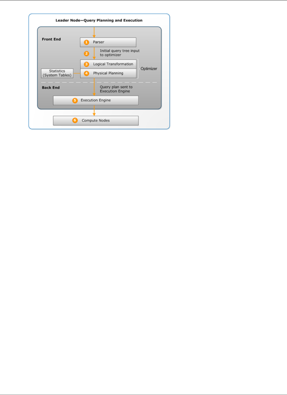
Amazon Redshift Database Developer Guide
Query Planning And Execution Workflow
The query planning and execution workflow follows these steps:
1. The leader node receives the query and parses the SQL.
2. The parser produces an initial query tree that is a logical representation of the original query. Amazon
Redshift then inputs this query tree into the query optimizer.
3. The optimizer evaluates and if necessary rewrites the query to maximize its efficiency. This process
sometimes results in creating multiple related queries to replace a single one.
4. The optimizer generates a query plan (or several, if the previous step resulted in multiple queries)
for the execution with the best performance. The query plan specifies execution options such as join
types, join order, aggregation options, and data distribution requirements.
You can use the EXPLAIN (p. 511) command to view the query plan. The query plan is a fundamental
tool for analyzing and tuning complex queries. For more information, see Query Plan (p. 260).
5. The execution engine translates the query plan into steps, segments and streams:
Step
Each step is an individual operation needed during query execution. Steps can be combined to
allow compute nodes to perform a query, join, or other database operation.
Segment
A combination of several steps that can be done by a single process, also the smallest compilation
unit executable by a compute node slice. A slice is the unit of parallel processing in Amazon
Redshift. The segments in a stream run in parallel.
Stream
A collection of segments to be parceled out over the available compute node slices.
The execution engine generates compiled C++ code based on steps, segments, and streams. Compiled
code executes faster than interpreted code and uses less compute capacity. This compiled code is then
broadcast to the compute nodes.
Note
When benchmarking your queries, you should always compare the times for the second
execution of a query, because the first execution time includes the overhead of compiling the
code. For more information, see Factors Affecting Query Performance (p. 266).
6. The compute node slices execute the query segments in parallel. As part of this process, Amazon
Redshift takes advantage of optimized network communication, memory, and disk management
API Version 2012-12-01
258

Amazon Redshift Database Developer Guide
Reviewing Query Plan Steps
to pass intermediate results from one query plan step to the next, which also helps to speed query
execution.
Steps 5 and 6 happen once for each stream. The engine creates the executable segments for one stream
and sends them to the compute nodes. When the segments of that stream are complete, the engine
generates the segments for the next stream. In this way, the engine can analyze what happened in the
prior stream (for example, whether operations were disk-based) to influence the generation of segments
in the next stream.
When the compute nodes are done, they return the query results to the leader node for final processing.
The leader node merges the data into a single result set and addresses any needed sorting or
aggregation. The leader node then returns the results to the client.
Note
The compute nodes might return some data to the leader node during query execution if
necessary. For example, if you have a subquery with a LIMIT clause, the limit is applied on the
leader node before data is redistributed across the cluster for further processing.
Reviewing Query Plan Steps
You can see the steps in a query plan by running the EXPLAIN command. The following example shows
a SQL query and the query plan that the EXPLAIN command produces for it. Reading the query plan
from the bottom up, you can see each of the logical operations needed to perform the query. For more
information, see Query Plan (p. 260).
explain
select eventname, sum(pricepaid) from sales, event
where sales.eventid = event.eventid
group by eventname
order by 2 desc;
XN Merge (cost=1002815366604.92..1002815366606.36 rows=576 width=27)
Merge Key: sum(sales.pricepaid)
-> XN Network (cost=1002815366604.92..1002815366606.36 rows=576 width=27)
Send to leader
-> XN Sort (cost=1002815366604.92..1002815366606.36 rows=576 width=27)
Sort Key: sum(sales.pricepaid)
-> XN HashAggregate (cost=2815366577.07..2815366578.51 rows=576 width=27)
-> XN Hash Join DS_BCAST_INNER (cost=109.98..2815365714.80
rows=172456 width=27)
Hash Cond: ("outer".eventid = "inner".eventid)
-> XN Seq Scan on sales (cost=0.00..1724.56 rows=172456
width=14)
-> XN Hash (cost=87.98..87.98 rows=8798 width=21)
-> XN Seq Scan on event (cost=0.00..87.98 rows=8798
width=21)
The following illustration uses the preceding query and associated query plan to show how those query
operations are mapped to steps, segments, and streams. Each query plan operation maps to multiple
steps within the segments, and sometimes to multiple segments within the streams.
API Version 2012-12-01
259
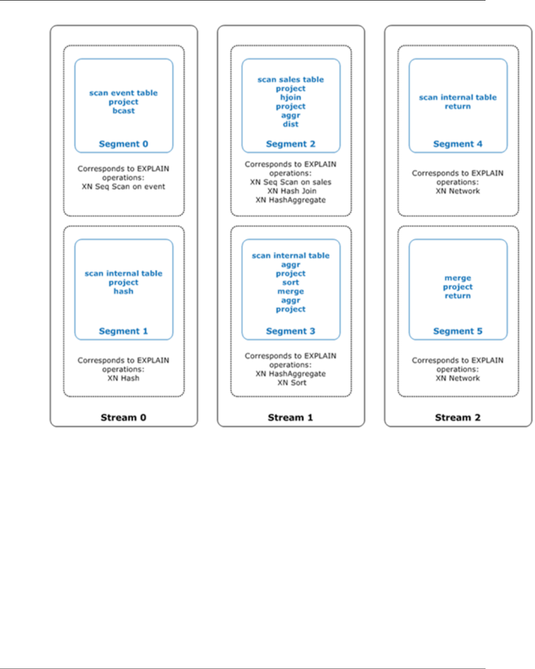
Amazon Redshift Database Developer Guide
Query Plan
Query Plan
You can use the query plan to get information on the individual operations required to execute a query.
Before you work with a query plan, we recommend you first understand how Amazon Redshift handles
processing queries and creating query plans. For more information, see Query Planning And Execution
Workflow (p. 257).
To create a query plan, run the EXPLAIN (p. 511) command followed by the actual query text. The
query plan gives you the following information:
• What operations the execution engine will perform, reading the results from bottom to top.
• What type of step each operation performs.
• Which tables and columns are used in each operation.
• How much data is processed in each operation, in terms of number of rows and data width in bytes.
• The relative cost of the operation. Cost is a measure that compares the relative execution times of the
steps within a plan. Cost does not provide any precise information about actual execution times or
memory consumption, nor does it provide a meaningful comparison between execution plans. It does
give you an indication of which operations in a query are consuming the most resources.
API Version 2012-12-01
260

Amazon Redshift Database Developer Guide
Query Plan
The EXPLAIN command doesn't actually run the query. It only shows the plan that Amazon Redshift
will execute if the query is run under current operating conditions. If you change the schema or data for
a table and run ANALYZE (p. 380) again to update the statistical metadata, the query plan might be
different.
The query plan output by EXPLAIN is a simplified, high-level view of query execution. It doesn't illustrate
the details of parallel query processing. To see detailed information, you need to run the query itself, and
then get query summary information from the SVL_QUERY_SUMMARY or SVL_QUERY_REPORT view. For
more information about using these views, see Analyzing the Query Summary (p. 270).
The following example shows the EXPLAIN output for a simple GROUP BY query on the EVENT table:
explain select eventname, count(*) from event group by eventname;
QUERY PLAN
-------------------------------------------------------------------
XN HashAggregate (cost=131.97..133.41 rows=576 width=17)
-> XN Seq Scan on event (cost=0.00..87.98 rows=8798 width=17)
EXPLAIN returns the following metrics for each operation:
Cost
A relative value that is useful for comparing operations within a plan. Cost consists of two decimal
values separated by two periods, for example cost=131.97..133.41. The first value, in this case
131.97, provides the relative cost of returning the first row for this operation. The second value, in
this case 133.41, provides the relative cost of completing the operation. The costs in the query plan
are cumulative as you read up the plan, so the HashAggregate cost in this example (131.97..133.41)
includes the cost of the Seq Scan below it (0.00..87.98).
Rows
The estimated number of rows to return. In this example, the scan is expected to return 8798 rows.
The HashAggregate operator on its own is expected to return 576 rows (after duplicate event names
are discarded from the result set).
Note
The rows estimate is based on the available statistics generated by the ANALYZE command.
If ANALYZE has not been run recently, the estimate will be less reliable.
Width
The estimated width of the average row, in bytes. In this example, the average row is expected to be
17 bytes wide.
EXPLAIN Operators
This section briefly describes the operators that you see most often in the EXPLAIN output. For a
complete list of operators, see EXPLAIN (p. 511) in the SQL Commands section.
Sequential Scan Operator
The sequential scan operator (Seq Scan) indicates a table scan. Seq Scan scans each column in the table
sequentially from beginning to end and evaluates query constraints (in the WHERE clause) for every row.
Join Operators
Amazon Redshift selects join operators based on the physical design of the tables being joined, the
location of the data required for the join, and the specific requirements of the query itself.
API Version 2012-12-01
261

Amazon Redshift Database Developer Guide
Query Plan
•Nested Loop
The least optimal join, a nested loop is used mainly for cross-joins (Cartesian products) and some
inequality joins.
•Hash Join and Hash
Typically faster than a nested loop join, a hash join and hash are used for inner joins and left and
right outer joins. These operators are used when joining tables where the join columns are not both
distribution keys and sort keys. The hash operator creates the hash table for the inner table in the join;
the hash join operator reads the outer table, hashes the joining column, and finds matches in the inner
hash table.
•Merge Join
Typically the fastest join, a merge join is used for inner joins and outer joins. The merge join is not used
for full joins. This operator is used when joining tables where the join columns are both distribution
keys and sort keys, and when less than 20 percent of the joining tables are unsorted. It reads two
sorted tables in order and finds the matching rows. To view the percent of unsorted rows, query the
SVV_TABLE_INFO (p. 926) system table.
Aggregate Operators
The query plan uses the following operators in queries that involve aggregate functions and GROUP BY
operations.
•Aggregate
Operator for scalar aggregate functions such as AVG and SUM.
•HashAggregate
Operator for unsorted grouped aggregate functions.
•GroupAggregate
Operator for sorted grouped aggregate functions.
Sort Operators
The query plan uses the following operators when queries have to sort or merge result sets.
•Sort
Evaluates the ORDER BY clause and other sort operations, such as sorts required by UNION queries
and joins, SELECT DISTINCT queries, and window functions.
•Merge
Produces final sorted results according to intermediate sorted results that derive from parallel
operations.
UNION, INTERSECT, and EXCEPT Operators
The query plan uses the following operators for queries that involve set operations with UNION,
INTERSECT, and EXCEPT.
•Subquery
Used to run UNION queries.
API Version 2012-12-01
262

Amazon Redshift Database Developer Guide
Query Plan
•Hash Intersect Distinct and Hash Intersect All
Used to run INTERSECT and INTERSECT ALL queries.
•SetOp Except
Used to run EXCEPT (or MINUS) queries.
Other Operators
The following operators also appear frequently in EXPLAIN output for routine queries.
•Unique
Eliminates duplicates for SELECT DISTINCT queries and UNION queries.
•Limit
Processes the LIMIT clause.
•Window
Runs window functions.
•Result
Runs scalar functions that do not involve any table access.
•Subplan
Used for certain subqueries.
•Network
Sends intermediate results to the leader node for further processing.
•Materialize
Saves rows for input to nested loop joins and some merge joins.
Joins in EXPLAIN
The query optimizer uses different join types to retrieve table data, depending on the structure of the
query and the underlying tables. The EXPLAIN output references the join type, the tables used, and the
way the table data is distributed across the cluster to describe how the query is processed.
Join Type Examples
The following examples show the different join types that the query optimizer can use. The join type
used in the query plan depends on the physical design of the tables involved.
Example: Hash Join Two Tables
The following query joins EVENT and CATEGORY on the CATID column. CATID is the distribution and
sort key for CATEGORY but not for EVENT. A hash join is performed with EVENT as the outer table and
CATEGORY as the inner table. Because CATEGORY is the smaller table, the planner broadcasts a copy
of it to the compute nodes during query processing by using DS_BCAST_INNER. The join cost in this
example accounts for most of the cumulative cost of the plan.
explain select * from category, event where category.catid=event.catid;
API Version 2012-12-01
263

Amazon Redshift Database Developer Guide
Query Plan
QUERY PLAN
-------------------------------------------------------------------------
XN Hash Join DS_BCAST_INNER (cost=0.14..6600286.07 rows=8798 width=84)
Hash Cond: ("outer".catid = "inner".catid)
-> XN Seq Scan on event (cost=0.00..87.98 rows=8798 width=35)
-> XN Hash (cost=0.11..0.11 rows=11 width=49)
-> XN Seq Scan on category (cost=0.00..0.11 rows=11 width=49)
Note
Aligned indents for operators in the EXPLAIN output sometimes indicate that those operations
do not depend on each other and can start in parallel. In the preceding example, although the
scan on the EVENT table and the hash operation are aligned, the EVENT scan must wait until the
hash operation has fully completed.
Example: Merge Join Two Tables
The following query also uses SELECT *, but it joins SALES and LISTING on the LISTID column, where
LISTID has been set as both the distribution and sort key for both tables. A merge join is chosen, and no
redistribution of data is required for the join (DS_DIST_NONE).
explain select * from sales, listing where sales.listid = listing.listid;
QUERY PLAN
-----------------------------------------------------------------------------
XN Merge Join DS_DIST_NONE (cost=0.00..6285.93 rows=172456 width=97)
Merge Cond: ("outer".listid = "inner".listid)
-> XN Seq Scan on listing (cost=0.00..1924.97 rows=192497 width=44)
-> XN Seq Scan on sales (cost=0.00..1724.56 rows=172456 width=53)
The following example demonstrates the different types of joins within the same query. As in the
previous example, SALES and LISTING are merge joined, but the third table, EVENT, must be hash joined
with the results of the merge join. Again, the hash join incurs a broadcast cost.
explain select * from sales, listing, event
where sales.listid = listing.listid and sales.eventid = event.eventid;
QUERY PLAN
----------------------------------------------------------------------------
XN Hash Join DS_BCAST_INNER (cost=109.98..3871130276.17 rows=172456 width=132)
Hash Cond: ("outer".eventid = "inner".eventid)
-> XN Merge Join DS_DIST_NONE (cost=0.00..6285.93 rows=172456 width=97)
Merge Cond: ("outer".listid = "inner".listid)
-> XN Seq Scan on listing (cost=0.00..1924.97 rows=192497 width=44)
-> XN Seq Scan on sales (cost=0.00..1724.56 rows=172456 width=53)
-> XN Hash (cost=87.98..87.98 rows=8798 width=35)
-> XN Seq Scan on event (cost=0.00..87.98 rows=8798 width=35)
Example: Join, Aggregate, and Sort
The following query executes a hash join of the SALES and EVENT tables, followed by aggregation and
sort operations to account for the grouped SUM function and the ORDER BY clause. The initial Sort
operator runs in parallel on the compute nodes. Then the Network operator sends the results to the
leader node, where the Merge operator produces the final sorted results.
explain select eventname, sum(pricepaid) from sales, event
where sales.eventid=event.eventid group by eventname
order by 2 desc;
QUERY PLAN
---------------------------------------------------------------------------------
XN Merge (cost=1002815366604.92..1002815366606.36 rows=576 width=27)
Merge Key: sum(sales.pricepaid)
API Version 2012-12-01
264

Amazon Redshift Database Developer Guide
Query Plan
-> XN Network (cost=1002815366604.92..1002815366606.36 rows=576 width=27)
Send to leader
-> XN Sort (cost=1002815366604.92..1002815366606.36 rows=576 width=27)
Sort Key: sum(sales.pricepaid)
-> XN HashAggregate (cost=2815366577.07..2815366578.51 rows=576 width=27)
-> XN Hash Join DS_BCAST_INNER (cost=109.98..2815365714.80
rows=172456 width=27)
Hash Cond: ("outer".eventid = "inner".eventid)
-> XN Seq Scan on sales (cost=0.00..1724.56 rows=172456
width=14)
-> XN Hash (cost=87.98..87.98 rows=8798 width=21)
-> XN Seq Scan on event (cost=0.00..87.98 rows=8798
width=21)
Data Redistribution
The EXPLAIN output for joins also specifies a method for how data will be moved around a cluster to
facilitate the join. This data movement can be either a broadcast or a redistribution. In a broadcast, the
data values from one side of a join are copied from each compute node to every other compute node,
so that every compute node ends up with a complete copy of the data. In a redistribution, participating
data values are sent from their current slice to a new slice (possibly on a different node). Data is typically
redistributed to match the distribution key of the other table participating in the join if that distribution
key is one of the joining columns. If neither of the tables has distribution keys on one of the joining
columns, either both tables are distributed or the inner table is broadcast to every node.
The EXPLAIN output also references inner and outer tables. The inner table is scanned first, and appears
nearer the bottom of the query plan. The inner table is the table that is probed for matches. It is usually
held in memory, is usually the source table for hashing, and if possible, is the smaller table of the two
being joined. The outer table is the source of rows to match against the inner table. It is usually read
from disk. The query optimizer chooses the inner and outer table based on database statistics from
the latest run of the ANALYZE command. The order of tables in the FROM clause of a query doesn't
determine which table is inner and which is outer.
Use the following attributes in query plans to identify how data will be moved to facilitate a query:
•DS_BCAST_INNER
A copy of the entire inner table is broadcast to all compute nodes.
•DS_DIST_ALL_NONE
No redistribution is required, because the inner table has already been distributed to every node using
DISTSTYLE ALL.
•DS_DIST_NONE
No tables are redistributed. Collocated joins are possible because corresponding slices are joined
without moving data between nodes.
•DS_DIST_INNER
The inner table is redistributed.
•DS_DIST_OUTER
The outer table is redistributed.
•DS_DIST_ALL_INNER
The entire inner table is redistributed to a single slice because the outer table uses DISTSTYLE ALL.
•DS_DIST_BOTH
Both tables are redistributed.
API Version 2012-12-01
265

Amazon Redshift Database Developer Guide
Factors Affecting Query Performance
Factors Affecting Query Performance
A number of factors can affect query performance. The following aspects of your data, cluster, and
database operations all play a part in how quickly your queries process.
•Number of nodes, processors, or slices – A compute node is partitioned into slices. More nodes means
more processors and more slices, which enables your queries to process faster by running portions
of the query concurrently across the slices. However, more nodes also means greater expense, so you
will need to find the balance of cost and performance that is appropriate for your system. For more
information on Amazon Redshift cluster architecture, see Data Warehouse System Architecture (p. 4).
•Node types – An Amazon Redshift cluster can use either dense storage or dense compute nodes. The
dense storage node types are recommended for substantial data storage needs, while dense compute
node types are optimized for performance-intensive workloads. Each node type offers different sizes
and limits to help you scale your cluster appropriately. The node size determines the storage capacity,
memory, CPU, and price of each node in the cluster. For more information on node types, see Amazon
Redshift Pricing.
•Data distribution – Amazon Redshift stores table data on the compute nodes according to a table's
distribution style. When you execute a query, the query optimizer redistributes the data to the
compute nodes as needed to perform any joins and aggregations. Choosing the right distribution
style for a table helps minimize the impact of the redistribution step by locating the data where it
needs to be before the joins are performed. For more information, see Choosing a Data Distribution
Style (p. 129).
•Data sort order – Amazon Redshift stores table data on disk in sorted order according to a table’s
sort keys. The query optimizer and the query processor use the information about where the data is
located to reduce the number of blocks that need to be scanned and thereby improve query speed. For
more information, see Choosing Sort Keys (p. 140).
•Dataset size – A higher volume of data in the cluster can slow query performance for queries, because
more rows need to be scanned and redistributed. You can mitigate this effect by regular vacuuming
and archiving of data, and by using a predicate to restrict the query dataset.
•Concurrent operations – Running multiple operations at once can affect query performance. Each
operation takes one or more slots in an available query queue and uses the memory associated with
those slots. If other operations are running, enough query queue slots might not be available. In this
case, the query will have to wait for slots to open before it can begin processing. For more information
about creating and configuring query queues, see Implementing Workload Management (p. 285).
•Query structure – How your query is written will affect its performance. As much as possible, write
queries to process and return as little data as will meet your needs. For more information, see Amazon
Redshift Best Practices for Designing Queries (p. 32).
•Code compilation – Amazon Redshift generates and compiles code for each query execution plan. The
compiled code segments are stored in a least recently used (LRU) cache and shared across sessions in a
cluster. Thus, subsequent executions of the same query, even in different sessions and often even with
different query parameters, will run faster because they can skip the initial generation and compilation
steps. The LRU cache persists through cluster reboots, but is wiped by maintenance upgrades.
The compiled code executes faster because it eliminates the overhead of using an interpreter. You
always have some overhead cost the first time code is generated and compiled. As a result, the
performance of a query the first time you run it can be misleading. The overhead cost might be
especially noticeable when you run one-off (ad hoc) queries. You should always run a query a second
time to determine its typical performance.
Similarly, be careful about comparing the performance of the same query sent from different clients.
The execution engine generates different code for the JDBC connection protocols and ODBC and psql
(libpq) connection protocols. If two clients use different protocols, each client will incur the first-time
cost of generating compiled code, even for the same query. Other clients that use the same protocol,
however, will benefit from sharing the cached code. A client that uses ODBC and a client running psql
with libpq can share the same compiled code.
API Version 2012-12-01
266

Amazon Redshift Database Developer Guide
Analyzing and Improving Queries
Analyzing and Improving Queries
Retrieving information from an Amazon Redshift data warehouse involves executing complex queries
on extremely large amounts of data, which can take a long time to process. To ensure queries process as
quickly as possible, there are a number of tools you can use to identify potential performance issues.
Topics
•Query Analysis Workflow (p. 267)
•Reviewing Query Alerts (p. 268)
•Analyzing the Query Plan (p. 269)
•Analyzing the Query Summary (p. 270)
•Improving Query Performance (p. 275)
•Diagnostic Queries for Query Tuning (p. 277)
Query Analysis Workflow
If a query is taking longer than expected, use the following steps to identify and correct issues that
might be negatively affecting the query’s performance. If you aren’t sure what queries in your system
might benefit from performance tuning, start by running the diagnostic query in Identifying Queries
That Are Top Candidates for Tuning (p. 278).
1. Make sure your tables are designed according to best practices. For more information, see Amazon
Redshift Best Practices for Designing Tables (p. 26).
2. See if you can delete or archive any unneeded data in your tables. For example, suppose your queries
always target the last 6 months’ worth of data but you have the last 18 months’ worth in your tables.
In this case, you can delete or archive the older data to reduce the number of records that need to be
scanned and distributed.
3. Run the VACUUM (p. 584) command on the tables in the query to reclaim space and re-sort rows.
Running VACUUM helps if the unsorted region is large and the query uses the sort key in a join or in
the predicate.
4. Run the ANALYZE (p. 380) command on the tables in the query to make sure statistics are up to date.
Running ANALYZE helps if any of the tables in the query have recently changed a lot in size. If running
a full ANALYZE command will take too long, run ANALYZE on a single column to reduce processing
time. This approach will still update the table size statistics; table size is a significant factor in query
planning.
5. Make sure your query has been run once for each type of client (based on what type of
connection protocol the client uses) so that the query is compiled and cached. This approach
will speed up subsequent runs of the query. For more information, see Factors Affecting Query
Performance (p. 266).
6. Check the STL_ALERT_EVENT_LOG (p. 801) table to identify and correct possible issues with your
query. For more information, see Reviewing Query Alerts (p. 268).
7. Run the EXPLAIN (p. 511) command to get the query plan and use it to optimize the query. For more
information, see Analyzing the Query Plan (p. 269).
8. Use the SVL_QUERY_SUMMARY (p. 916) and SVL_QUERY_REPORT (p. 912) views to get summary
information and use it to optimize the query. For more information, see Analyzing the Query
Summary (p. 270).
Sometimes a query that should execute quickly is forced to wait until another, longer-running query
finishes. In that case, you might have nothing to improve in the query itself, but you can improve overall
system performance by creating and using query queues for different types of queries. To get an idea
API Version 2012-12-01
267

Amazon Redshift Database Developer Guide
Reviewing Query Alerts
of queue wait time for your queries, see Reviewing Queue Wait Times for Queries (p. 279). For more
information about configuring query queues, see Implementing Workload Management (p. 285).
Reviewing Query Alerts
To use the STL_ALERT_EVENT_LOG (p. 801) system table to identify and correct potential performance
issues with your query, follow these steps:
1. Run the following to determine your query ID:
select query, elapsed, substring
from svl_qlog
order by query
desc limit 5;
Examine the truncated query text in the substring field to determine which query value to select.
If you have run the query more than once, use the query value from the row with the lower elapsed
value. That is the row for the compiled version. If you have been running many queries, you can raise
the value used by the LIMIT clause used to make sure your query is included.
2. Select rows from STL_ALERT_EVENT_LOG for your query:
Select * from stl_alert_event_log where query = MyQueryID;
3. Evaluate the results for your query. Use the following table to locate potential solutions for any issues
that you have identified.
Note
Not all queries will have rows in STL_ALERT_EVENT_LOG, only those with identified issues.
Issue Event Value Solution Value Recommended
Solution
Statistics for the tables in the query
are missing or out of date.
Missing query
planner statistics
Run the ANALYZE
command
See Table
Statistics Missing
or Out of
Date (p. 275).
There is a nested loop join (the least
optimal join) in the query plan.
Nested Loop Join
in the query plan
Review the join
predicates to
avoid Cartesian
products
See Nested
Loop (p. 275).
The scan skipped a relatively large
number of rows that are marked as
deleted but not vacuumed, or rows
that have been inserted but not
committed.
Scanned a large
number of
deleted rows
Run the VACUUM
command to
reclaim deleted
space
See Ghost Rows
or Uncommitted
Rows (p. 276).
API Version 2012-12-01
268

Amazon Redshift Database Developer Guide
Analyzing the Query Plan
Issue Event Value Solution Value Recommended
Solution
More than 1,000,000 rows were
redistributed for a hash join or
aggregation.
Distributed a
large number of
rows across the
network:RowCount
rows were
distributed in
order to process
the aggregation
Review the choice
of distribution
key to collocate
the join or
aggregation
See Suboptimal
Data
Distribution (p. 276).
More than 1,000,000 rows were
broadcast for a hash join.
Broadcasted a
large number of
rows across the
network
Review the choice
of distribution key
to collocate the
join and consider
using distributed
tables
See Suboptimal
Data
Distribution (p. 276).
A DS_DIST_ALL_INNER redistribution
style was indicated in the query
plan, which forces serial execution
because the entire inner table was
redistributed to a single node.
DS_DIST_ALL_INNER
for Hash Join in
the query plan
Review the choice
of distribution
strategy to
distribute the
inner, rather than
outer, table
See Suboptimal
Data
Distribution (p. 276).
Analyzing the Query Plan
Before analyzing the query plan, you should be familiar with how to read it. If you are unfamiliar with
reading a query plan, we recommend that you read Query Plan (p. 260) before proceeding.
Run the EXPLAIN (p. 511) command to get a query plan. To analyze the data provided by the query
plan, follow these steps:
1. Identify the steps with the highest cost. Concentrate on optimizing those when proceeding through
the remaining steps.
2. Look at the join types:
•Nested Loop: Such joins usually occur because a join condition was omitted. For recommended
solutions, see Nested Loop (p. 275).
•Hash and Hash Join: Hash joins are used when joining tables where the join columns are not
distribution keys and also not sort keys. For recommended solutions, see Hash Join (p. 275).
•Merge Join: No change is needed.
3. Notice which table is used for the inner join, and which for the outer join. The query engine generally
chooses the smaller table for the inner join, and the larger table for the outer join. If such a choice
doesn't occur, your statistics are likely out of date. For recommended solutions, see Table Statistics
Missing or Out of Date (p. 275).
4. See if there are any high-cost sort operations. If there are, see Unsorted or Missorted Rows (p. 276)
for recommended solutions.
5. Look for the following broadcast operators where there are high-cost operations:
•DS_BCAST_INNER: Indicates the table is broadcast to all the compute nodes, which is fine for a
small table but not ideal for a larger table.
•DS_DIST_ALL_INNER: Indicates that all of the workload is on a single slice.
•DS_DIST_BOTH: Indicates heavy redistribution.
API Version 2012-12-01
269
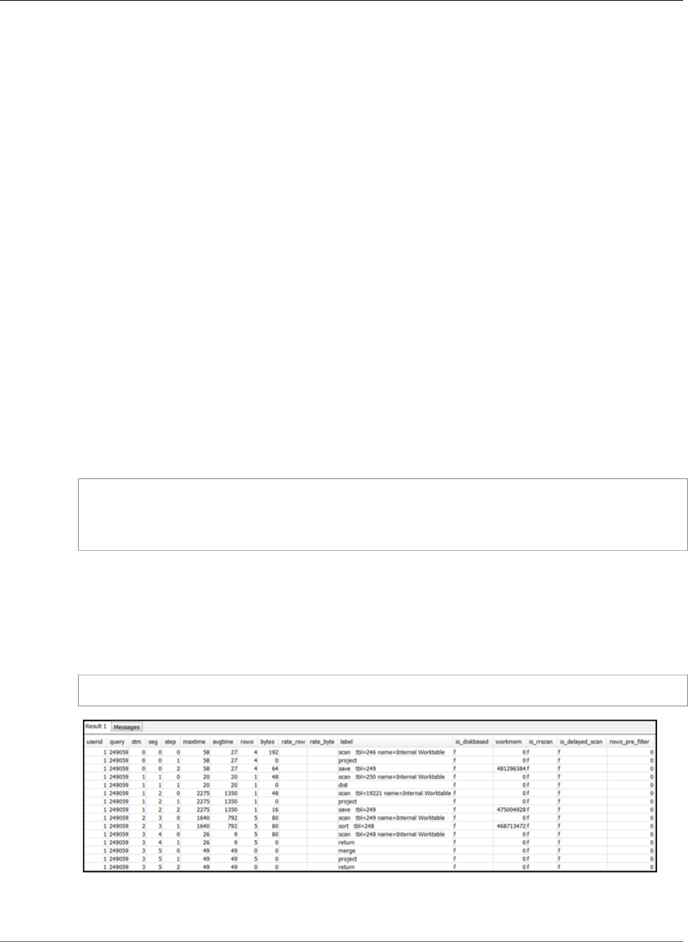
Amazon Redshift Database Developer Guide
Analyzing the Query Summary
For recommended solutions for these situations, see Suboptimal Data Distribution (p. 276).
Analyzing the Query Summary
To get execution steps and statistics in more detail than in the query plan than EXPLAIN (p. 511)
produces, use the SVL_QUERY_SUMMARY (p. 916) and SVL_QUERY_REPORT (p. 912) system views.
SVL_QUERY_SUMMARY provides query statistics by stream. You can use the information it provides to
identify issues with expensive steps, long-running steps, and steps that write to disk.
The SVL_QUERY_REPORT system view allows you to see information similar to that for
SVL_QUERY_SUMMARY, only by compute node slice rather than by stream. You can use the slice-level
information for detecting uneven data distribution across the cluster (also known as data distribution
skew), which forces some nodes to do more work than others and impairs query performance.
Topics
•Using the SVL_QUERY_SUMMARY View (p. 270)
•Using the SVL_QUERY_REPORT View (p. 272)
•Mapping the Query Plan to the Query Summary (p. 273)
Using the SVL_QUERY_SUMMARY View
To analyze query summary information by stream, do the following:
1. Run the following query to determine your query ID:
select query, elapsed, substring
from svl_qlog
order by query
desc limit 5;
Examine the truncated query text in the substring field to determine which query value represents
your query. If you have run the query more than once, use the query value from the row with the
lower elapsed value. That is the row for the compiled version. If you have been running many
queries, you can raise the value used by the LIMIT clause used to make sure your query is included.
2. Select rows from SVL_QUERY_SUMMARY for your query. Order the results by stream, segment, and
step:
select * from svl_query_summary where query = MyQueryID order by stm, seg, step;
3. Map the steps to the operations in the query plan using the information in Mapping the Query Plan to
the Query Summary (p. 273). They should have approximately the same values for rows and bytes
API Version 2012-12-01
270

Amazon Redshift Database Developer Guide
Analyzing the Query Summary
(rows * width from the query plan). If they don’t, see Table Statistics Missing or Out of Date (p. 275)
for recommended solutions.
4. See if the is_diskbased field has a value of t (true) for any step. Hashes, aggregates, and sorts are
the operators that are likely to write data to disk if the system doesn't have enough memory allocated
for query processing.
If is_diskbased is true, see Insufficient Memory Allocated to the Query (p. 277) for recommended
solutions.
5. Review the label field values and see if there is an AGG-DIST-AGG sequence anywhere in the steps.
Its presence indicates two-step aggregation, which is expensive. To fix this, change the GROUP BY
clause to use the distribution key (the first key, if there are multiple ones).
6. Review the maxtime value for each segment (it is the same across all steps in the segment). Identify
the segment with the highest maxtime value and review the steps in this segment for the following
operators.
Note
A high maxtime value doesn't necessarily indicate a problem with the segment. Despite
a high value, the segment might not have taken a long time to process. All segments in a
stream start getting timed in unison. However, some downstream segments might not be
able to run until they get data from upstream ones. This effect might make them seem to
have taken a long time because their maxtime value will include both their waiting time and
their processing time.
•BCAST or DIST: In these cases, the high maxtime value might be the result of redistributing a large
number of rows. For recommended solutions, see Suboptimal Data Distribution (p. 276).
•HJOIN (hash join): If the step in question has a very high value in the rows field compared to
the rows value in the final RETURN step in the query, see Hash Join (p. 275) for recommended
solutions.
•SCAN/SORT: Look for a SCAN, SORT, SCAN, MERGE sequence of steps just prior to a join step. This
pattern indicates that unsorted data is being scanned, sorted, and then merged with the sorted area
of the table.
See if the rows value for the SCAN step has a very high value compared to the rows value in
the final RETURN step in the query. This pattern indicates that the execution engine is scanning
rows that are later discarded, which is inefficient. For recommended solutions, see Insufficiently
Restrictive Predicate (p. 277).
If the maxtime value for the SCAN step is high, see Suboptimal WHERE Clause (p. 277) for
recommended solutions.
If the rows value for the SORT step is not zero, see Unsorted or Missorted Rows (p. 276) for
recommended solutions.
7. Review the rows and bytes values for the 5–10 steps that precede the final RETURN step to get an
idea of the amount of data that is being returned to the client. This process can be a bit of an art.
For example, in the following query summary, you can see that the third PROJECT step provides a
rows value but not a bytes value. By looking through the preceding steps for one with the same
rows value, you find the SCAN step that provides both rows and bytes information:
API Version 2012-12-01
271

Amazon Redshift Database Developer Guide
Analyzing the Query Summary
If you are returning an unusually large volume of data, see Very Large Result Set (p. 277) for
recommended solutions.
8. See if the bytes value is high relative to the rows value for any step, in comparison to other steps.
This pattern can indicate that you are selecting a lot of columns. For recommended solutions, see
Large SELECT List (p. 277).
Using the SVL_QUERY_REPORT View
To analyze query summary information by slice, do the following:
1. Run the following to determine your query ID:
select query, elapsed, substring
from svl_qlog
order by query
desc limit 5;
Examine the truncated query text in the substring field to determine which query value represents
your query. If you have run the query more than once, use the query value from the row with the
lower elapsed value. That is the row for the compiled version. If you have been running many
queries, you can raise the value used by the LIMIT clause used to make sure your query is included.
2. Select rows from SVL_QUERY_REPORT for your query. Order the results by segment, step,
elapsed_time, and rows:
select * from svl_query_report where query = MyQueryID order by segment, step,
elapsed_time, rows;
3. For each step, check to see that all slices are processing approximately the same number of rows:
API Version 2012-12-01
272
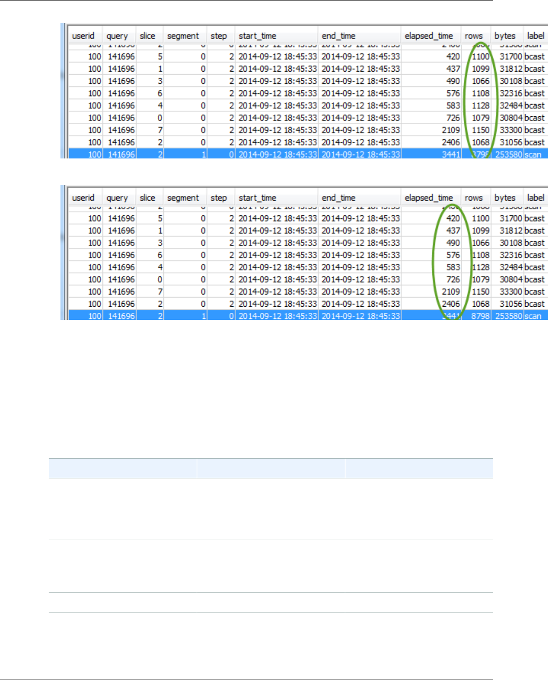
Amazon Redshift Database Developer Guide
Analyzing the Query Summary
Also check to see that all slices are taking approximately the same amount of time:
Large discrepancies in these values can indicate data distribution skew due to a suboptimal
distribution style for this particular query. For recommended solutions, see Suboptimal Data
Distribution (p. 276).
Mapping the Query Plan to the Query Summary
It helps to map the operations from the query plan to the steps (identified by the label field values) in
the query summary to get further details on them:
Query Plan Operation Label Field Value Description
Aggregate
HashAggregate
GroupAggregate
AGGR Evaluates aggregate functions
and GROUP BY conditions.
DS_BCAST_INNER BCAST (broadcast) Broadcasts an entire table or
some set of rows (such as a
filtered set of rows from a table)
to all nodes.
Doesn’t appear in query plan DELETE Deletes rows from tables.
DS_DIST_NONE
DS_DIST_ALL_NONE
DS_DIST_INNER
DIST (distribute) Distributes rows to nodes for
parallel joining purposes or
other parallel processing.
API Version 2012-12-01
273
Amazon Redshift Database Developer Guide
Analyzing the Query Summary
Query Plan Operation Label Field Value Description
DS_DIST_ALL_INNER
DS_DIST_ALL_BOTH
HASH HASH Builds hash table for use in hash
joins.
Hash Join HJOIN (hash join) Executes a hash join of two
tables or intermediate result
sets.
Doesn’t appear in query plan INSERT Inserts rows into tables.
Limit LIMIT Applies a LIMIT clause to result
sets.
Merge MERGE Merges rows derived from
parallel sort or join operations.
Merge Join MJOIN (merge join) Executes a merge join of two
tables or intermediate result
sets.
Nested Loop NLOOP (nested loop) Executes a nested loop join of
two tables or intermediate result
sets.
Doesn’t appear in query plan PARSE Parses strings into binary values
for loading.
Project PROJECT Evaluates expressions.
Network RETURN Returns rows to the leader or the
client.
Doesn’t appear in query plan SAVE Materializes rows for use in the
next processing step.
Seq Scan SCAN Scans tables or intermediate
result sets.
Sort SORT Sorts rows or intermediate
result sets as required by other
subsequent operations (such
as joins or aggregations) or to
satisfy an ORDER BY clause.
Unique UNIQUE Applies a SELECT DISTINCT
clause or removes duplicates as
required by other operations.
Window WINDOW Computes aggregate and
ranking window functions.
API Version 2012-12-01
274

Amazon Redshift Database Developer Guide
Improving Query Performance
Improving Query Performance
Following are some common issues that affect query performance, with instructions on ways to diagnose
and resolve them.
Topics
•Table Statistics Missing or Out of Date (p. 275)
•Nested Loop (p. 275)
•Hash Join (p. 275)
•Ghost Rows or Uncommitted Rows (p. 276)
•Unsorted or Missorted Rows (p. 276)
•Suboptimal Data Distribution (p. 276)
•Insufficient Memory Allocated to the Query (p. 277)
•Suboptimal WHERE Clause (p. 277)
•Insufficiently Restrictive Predicate (p. 277)
•Very Large Result Set (p. 277)
•Large SELECT List (p. 277)
Table Statistics Missing or Out of Date
If table statistics are missing or out of date, you might see the following:
• A warning message in EXPLAIN command results.
• A missing statistics alert event in STL_ALERT_EVENT_LOG. For more information, see Reviewing Query
Alerts (p. 268).
To fix this issue, run ANALYZE (p. 380).
Nested Loop
If a nested loop is present, you might see a nested loop alert event in STL_ALERT_EVENT_LOG. You can
also identify this type of event by running the query at Identifying Queries with Nested Loops (p. 279).
For more information, see Reviewing Query Alerts (p. 268).
To fix this, review your query for cross-joins and remove them if possible. Cross-joins are joins without
a join condition that result in the Cartesian product of two tables. They are typically executed as nested
loop joins, which are the slowest of the possible join types.
Hash Join
If a hash join is present, you might see the following:
• Hash and hash join operations in the query plan. For more information, see Analyzing the Query
Plan (p. 269).
• An HJOIN step in the segment with the highest maxtime value in SVL_QUERY_SUMMARY. For more
information, see Using the SVL_QUERY_SUMMARY View (p. 270).
To fix this issue, you can take a couple of approaches:
API Version 2012-12-01
275

Amazon Redshift Database Developer Guide
Improving Query Performance
• Rewrite the query to use a merge join if possible. You can do this by specifying join columns that are
both distribution keys and sort keys.
• If the HJOIN step in SVL_QUERY_SUMMARY has a very high value in the rows field compared to the
rows value in the final RETURN step in the query, check whether you can rewrite the query to join on a
unique column. When a query does not join on a unique column, such as a primary key, that increases
the number of rows involved in the join.
Ghost Rows or Uncommitted Rows
If ghost rows or uncommitted rows are present, you might see an alert event in STL_ALERT_EVENT_LOG
that indicates excessive ghost rows. For more information, see Reviewing Query Alerts (p. 268).
To fix this issue, you can take a couple of approaches:
• Check the Loads tab of your Amazon Redshift console for active load operations on any of the query
tables. If you see active load operations, wait for those to complete before taking action.
• If there are no active load operations, run VACUUM (p. 584) on the query tables to remove deleted
rows.
Unsorted or Missorted Rows
If unsorted or missorted rows are present, you might see a very selective filter alert event in
STL_ALERT_EVENT_LOG. For more information, see Reviewing Query Alerts (p. 268).
You can also check to see if any of the tables in your query have large unsorted areas by running the
query in Identifying Tables with Data Skew or Unsorted Rows (p. 278).
To fix this issue, you can take a couple of approaches:
• Run VACUUM (p. 584) on the query tables to re-sort the rows.
• Review the sort keys on the query tables to see if any improvements can be made. Remember to weigh
the performance of this query against the performance of other important queries and the system
overall before making any changes. For more information, see Choosing Sort Keys (p. 140).
Suboptimal Data Distribution
If data distribution is suboptimal, you might see the following:
• A serial execution, large broadcast, or large distribution alert event appears in
STL_ALERT_EVENT_LOG. For more information, see Reviewing Query Alerts (p. 268).
• Slices are not processing approximately the same number of rows for a given step. For more
information, see Using the SVL_QUERY_REPORT View (p. 272).
• Slices are not taking approximately the same amount of time for a given step. For more information,
see Using the SVL_QUERY_REPORT View (p. 272).
If none of the preceding is true, you can also see if any of the tables in your query have data skew by
running the query in Identifying Tables with Data Skew or Unsorted Rows (p. 278).
To fix this issue, take another look at the distribution styles for the tables in the query and see if any
improvements can be made. Remember to weigh the performance of this query against the performance
of other important queries and the system overall before making any changes. For more information, see
Choosing a Data Distribution Style (p. 129).
API Version 2012-12-01
276

Amazon Redshift Database Developer Guide
Diagnostic Queries for Query Tuning
Insufficient Memory Allocated to the Query
If insufficient memory is allocated to your query, you might see a step in SVL_QUERY_SUMMARY that
has an is_diskbased value of true. For more information, see Using the SVL_QUERY_SUMMARY
View (p. 270).
To fix this issue, allocate more memory to the query by temporarily increasing the number of query slots
it uses. Workload Management (WLM) reserves slots in a query queue equivalent to the concurrency level
set for the queue. For example, a queue with a concurrency level of 5 has 5 slots. Memory assigned to
the queue is allocated equally to each slot. Assigning several slots to one query gives that query access
to the memory for all of those slots. For more information on how to temporarily increase the slots for a
query, see wlm_query_slot_count (p. 955).
Suboptimal WHERE Clause
If your WHERE clause causes excessive table scans, you might see a SCAN step in the segment
with the highest maxtime value in SVL_QUERY_SUMMARY. For more information, see Using the
SVL_QUERY_SUMMARY View (p. 270).
To fix this issue, add a WHERE clause to the query based on the primary sort column of the largest
table. This approach will help minimize scanning time. For more information, see Amazon Redshift Best
Practices for Designing Tables (p. 26).
Insufficiently Restrictive Predicate
If your query has an insufficiently restrictive predicate, you might see a SCAN step in the segment
with the highest maxtime value in SVL_QUERY_SUMMARY that has a very high rows value compared
to the rows value in the final RETURN step in the query. For more information, see Using the
SVL_QUERY_SUMMARY View (p. 270).
To fix this issue, try adding a predicate to the query or making the existing predicate more restrictive to
narrow the output.
Very Large Result Set
If your query returns a very large result set, consider rewriting the query to use UNLOAD (p. 566) to
write the results to Amazon S3. This approach will improve the performance of the RETURN step by
taking advantage of parallel processing. For more information on checking for a very large result set, see
Using the SVL_QUERY_SUMMARY View (p. 270).
Large SELECT List
If your query has an unusually large SELECT list, you might see a bytes value that is high relative to
the rows value for any step (in comparison to other steps) in SVL_QUERY_SUMMARY. This high bytes
value can be an indicator that you are selecting a lot of columns. For more information, see Using the
SVL_QUERY_SUMMARY View (p. 270).
To fix this issue, review the columns you are selecting and see if any can be removed.
Diagnostic Queries for Query Tuning
Use the following queries to identify issues with queries or underlying tables that can affect query
performance. We recommend using these queries in conjunction with the query tuning processes
discussed in Analyzing and Improving Queries (p. 267).
Topics
API Version 2012-12-01
277

Amazon Redshift Database Developer Guide
Diagnostic Queries for Query Tuning
•Identifying Queries That Are Top Candidates for Tuning (p. 278)
•Identifying Tables with Data Skew or Unsorted Rows (p. 278)
•Identifying Queries with Nested Loops (p. 279)
•Reviewing Queue Wait Times for Queries (p. 279)
•Reviewing Query Alerts by Table (p. 280)
•Identifying Tables with Missing Statistics (p. 280)
Identifying Queries That Are Top Candidates for Tuning
The following query identifies the top 50 most time-consuming statements that have been executed
in the last 7 days. You can use the results to identify queries that are taking unusually long, and also
to identify queries that are run frequently (those that appear more than once in the result set). These
queries are frequently good candidates for tuning to improve system performance.
This query also provides a count of the alert events associated with each query identified. These
alerts provide details that you can use to improve the query’s performance. For more information, see
Reviewing Query Alerts (p. 268).
select trim(database) as db, count(query) as n_qry,
max(substring (qrytext,1,80)) as qrytext,
min(run_minutes) as "min" ,
max(run_minutes) as "max",
avg(run_minutes) as "avg", sum(run_minutes) as total,
max(query) as max_query_id,
max(starttime)::date as last_run,
sum(alerts) as alerts, aborted
from (select userid, label, stl_query.query,
trim(database) as database,
trim(querytxt) as qrytext,
md5(trim(querytxt)) as qry_md5,
starttime, endtime,
(datediff(seconds, starttime,endtime)::numeric(12,2))/60 as run_minutes,
alrt.num_events as alerts, aborted
from stl_query
left outer join
(select query, 1 as num_events from stl_alert_event_log group by query ) as alrt
on alrt.query = stl_query.query
where userid <> 1 and starttime >= dateadd(day, -7, current_date))
group by database, label, qry_md5, aborted
order by total desc limit 50;
Identifying Tables with Data Skew or Unsorted Rows
The following query identifies tables that have uneven data distribution (data skew) or a high percentage
of unsorted rows.
A low skew value indicates that table data is properly distributed. If a table has a skew value of 4.00
or higher, consider modifying its data distribution style. For more information, see Suboptimal Data
Distribution (p. 276).
If a table has a pct_unsorted value greater than 20 percent, consider running the VACUUM (p. 584)
command. For more information, see Unsorted or Missorted Rows (p. 276).
You should also review the mbytes and pct_of_total values for each table. These columns identify
the size of the table and what percentage of raw disk space the table consumes. The raw disk space
includes space that is reserved by Amazon Redshift for internal use, so it is larger than the nominal disk
capacity, which is the amount of disk space available to the user. Use this information to ensure that you
API Version 2012-12-01
278
Amazon Redshift Database Developer Guide
Diagnostic Queries for Query Tuning
have free disk space equal to at least 2.5 times the size of your largest table. Having this space available
enables the system to write intermediate results to disk when processing complex queries.
select trim(pgn.nspname) as schema,
trim(a.name) as table, id as tableid,
decode(pgc.reldiststyle,0, 'even',1,det.distkey ,8,'all') as distkey,
dist_ratio.ratio::decimal(10,4) as skew,
det.head_sort as "sortkey",
det.n_sortkeys as "#sks", b.mbytes,
decode(b.mbytes,0,0,((b.mbytes/part.total::decimal)*100)::decimal(5,2)) as pct_of_total,
decode(det.max_enc,0,'n','y') as enc, a.rows,
decode( det.n_sortkeys, 0, null, a.unsorted_rows ) as unsorted_rows ,
decode( det.n_sortkeys, 0, null, decode( a.rows,0,0, (a.unsorted_rows::decimal(32)/
a.rows)*100) )::decimal(5,2) as pct_unsorted
from (select db_id, id, name, sum(rows) as rows,
sum(rows)-sum(sorted_rows) as unsorted_rows
from stv_tbl_perm a
group by db_id, id, name) as a
join pg_class as pgc on pgc.oid = a.id
join pg_namespace as pgn on pgn.oid = pgc.relnamespace
left outer join (select tbl, count(*) as mbytes
from stv_blocklist group by tbl) b on a.id=b.tbl
inner join (select attrelid,
min(case attisdistkey when 't' then attname else null end) as "distkey",
min(case attsortkeyord when 1 then attname else null end ) as head_sort ,
max(attsortkeyord) as n_sortkeys,
max(attencodingtype) as max_enc
from pg_attribute group by 1) as det
on det.attrelid = a.id
inner join ( select tbl, max(mbytes)::decimal(32)/min(mbytes) as ratio
from (select tbl, trim(name) as name, slice, count(*) as mbytes
from svv_diskusage group by tbl, name, slice )
group by tbl, name ) as dist_ratio on a.id = dist_ratio.tbl
join ( select sum(capacity) as total
from stv_partitions where part_begin=0 ) as part on 1=1
where mbytes is not null
order by mbytes desc;
Identifying Queries with Nested Loops
The following query identifies queries that have had alert events logged for nested loops. For
information on how to fix the nested loop condition, see Nested Loop (p. 275).
select query, trim(querytxt) as SQL, starttime
from stl_query
where query in (
select distinct query
from stl_alert_event_log
where event like 'Nested Loop Join in the query plan%')
order by starttime desc;
Reviewing Queue Wait Times for Queries
The following query shows how long recent queries waited for an open slot in a query queue before
being executed. If you see a trend of high wait times, you might want to modify your query queue
configuration for better throughput. For more information, see Defining Query Queues (p. 285).
select trim(database) as DB , w.query,
substring(q.querytxt, 1, 100) as querytxt, w.queue_start_time,
w.service_class as class, w.slot_count as slots,
API Version 2012-12-01
279

Amazon Redshift Database Developer Guide
Troubleshooting Queries
w.total_queue_time/1000000 as queue_seconds,
w.total_exec_time/1000000 exec_seconds, (w.total_queue_time+w.total_Exec_time)/1000000 as
total_seconds
from stl_wlm_query w
left join stl_query q on q.query = w.query and q.userid = w.userid
where w.queue_start_Time >= dateadd(day, -7, current_Date)
and w.total_queue_Time > 0 and w.userid >1
and q.starttime >= dateadd(day, -7, current_Date)
order by w.total_queue_time desc, w.queue_start_time desc limit 35;
Reviewing Query Alerts by Table
The following query identifies tables that have had alert events logged for them, and also identifies what
type of alerts are most frequently raised.
If the minutes value for a row with an identified table is high, check that table to see if it needs routine
maintenance such as having ANALYZE (p. 380) or VACUUM (p. 584) run against it.
If the count value is high for a row but the table value is null, run a query against
STL_ALERT_EVENT_LOG for the associated event value to investigate why that alert is getting raised so
often.
select trim(s.perm_table_name) as table,
(sum(abs(datediff(seconds, s.starttime, s.endtime)))/60)::numeric(24,0) as minutes,
trim(split_part(l.event,':',1)) as event, trim(l.solution) as solution,
max(l.query) as sample_query, count(*)
from stl_alert_event_log as l
left join stl_scan as s on s.query = l.query and s.slice = l.slice
and s.segment = l.segment and s.step = l.step
where l.event_time >= dateadd(day, -7, current_Date)
group by 1,3,4
order by 2 desc,6 desc;
Identifying Tables with Missing Statistics
The following query provides a count of the queries that you are running against tables that are missing
statistics. If this query returns any rows, look at the plannode value to determine the affected table, and
then run ANALYZE (p. 380) on it.
select substring(trim(plannode),1,100) as plannode, count(*)
from stl_explain
where plannode like '%missing statistics%'
group by plannode
order by 2 desc;
Troubleshooting Queries
This section provides a quick reference for identifying and addressing some of the most common and
most serious issues you are likely to encounter with Amazon Redshift queries.
Topics
•Connection Fails (p. 281)
•Query Hangs (p. 281)
•Query Takes Too Long (p. 282)
•Load Fails (p. 283)
API Version 2012-12-01
280

Amazon Redshift Database Developer Guide
Connection Fails
•Load Takes Too Long (p. 283)
•Load Data Is Incorrect (p. 283)
•Setting the JDBC Fetch Size Parameter (p. 284)
These suggestions give you a starting point for troubleshooting. You can also refer to the following
resources for more detailed information.
•Accessing Amazon Redshift Clusters and Databases
•Designing Tables (p. 118)
•Loading Data (p. 184)
•Tutorial: Tuning Table Design (p. 45)
•Tutorial: Loading Data from Amazon S3 (p. 70)
Connection Fails
Your query connection can fail for the following reasons; we suggest the following troubleshooting
approaches.
Client Cannot Connect to Server
If you are using SSL or server certificates, first remove this complexity while you troubleshoot the
connection issue. Then add SSL or server certificates back when you have found a solution. For
more information, go to Configure Security Options for Connections in the Amazon Redshift Cluster
Management Guide.
Connection Is Refused
Generally, when you receive an error message indicating that there is a failure to establish a connection,
it means that there is an issue with the permission to access the cluster. For more information, go to The
connection is refused or fails in the Amazon Redshift Cluster Management Guide.
Query Hangs
Your query can hang, or stop responding, for the following reasons; we suggest the following
troubleshooting approaches.
Connection to the Database Is Dropped
Reduce the size of maximum transmission unit (MTU). The MTU size determines the maximum size,
in bytes, of a packet that can be transferred in one Ethernet frame over your network connection. For
more information, go to The connection to the database is dropped in the Amazon Redshift Cluster
Management Guide.
Connection to the Database Times Out
Your client connection to the database appears to hang or timeout when running long queries, such as
a COPY command. In this case, you might observe that the Amazon Redshift console displays that the
query has completed, but the client tool itself still appears to be running the query. The results of the
query might be missing or incomplete depending on when the connection stopped. This effect happens
API Version 2012-12-01
281

Amazon Redshift Database Developer Guide
Query Takes Too Long
when idle connections are terminated by an intermediate network component. For more information, go
to Firewall Timeout Issue in the Amazon Redshift Cluster Management Guide.
Client-Side Out-of-Memory Error Occurs with ODBC
If your client application uses an ODBC connection and your query creates a result set that is too large
to fit in memory, you can stream the result set to your client application by using a cursor. For more
information, see DECLARE (p. 496) and Performance Considerations When Using Cursors (p. 498).
Client-Side Out-of-Memory Error Occurs with JDBC
When you attempt to retrieve large result sets over a JDBC connection, you might encounter client-side
out-of-memory errors. For more information, see Setting the JDBC Fetch Size Parameter (p. 284).
There Is a Potential Deadlock
If there is a potential deadlock, try the following:
• View the STV_LOCKS (p. 876) and STL_TR_CONFLICT (p. 855) system tables to find conflicts
involving updates to more than one table.
• Use the PG_CANCEL_BACKEND (p. 778) function to cancel one or more conflicting queries.
• Use the PG_TERMINATE_BACKEND (p. 779) function to terminate a session, which forces any
currently running transactions in the terminated session to release all locks and roll back the
transaction.
• Schedule concurrent write operations carefully. For more information, see Managing Concurrent Write
Operations (p. 238).
Query Takes Too Long
Your query can take too long for the following reasons; we suggest the following troubleshooting
approaches.
Tables Are Not Optimized
Set the sort key, distribution style, and compression encoding of the tables to take full advantage of
parallel processing. For more information, see Designing Tables (p. 118) and Tutorial: Tuning Table
Design (p. 45).
Query Is Writing to Disk
Your queries might be writing to disk for at least part of the query execution. For more information, see
Improving Query Performance (p. 275).
Query Must Wait for Other Queries to Finish
You might be able to improve overall system performance by creating query queues and assigning
different types of queries to the appropriate queues. For more information, see Implementing Workload
Management (p. 285).
Queries Are Not Optimized
Analyze the explain plan to find opportunities for rewriting queries or optimizing the database. For more
information, see Query Plan (p. 260).
Query Needs More Memory to Run
If a specific query needs more memory, you can increase the available memory by increasing the
wlm_query_slot_count (p. 955).
API Version 2012-12-01
282

Amazon Redshift Database Developer Guide
Load Fails
Database Requires a VACUUM Command to Be Run
Run the VACUUM command whenever you add, delete, or modify a large number of rows, unless you
load your data in sort key order. The VACUUM command reorganizes your data to maintain the sort order
and restore performance. For more information, see Vacuuming Tables (p. 228).
Load Fails
Your data load can fail for the following reasons; we suggest the following troubleshooting approaches.
Data Source Is in a Different Region
By default, the Amazon S3 bucket or Amazon DynamoDB table specified in the COPY command must be
in the same region as the cluster. If your data and your cluster are in different regions, you will receive an
error similar to the following:
The bucket you are attempting to access must be addressed using the specified endpoint.
If at all possible, make sure your cluster and your data source are the same region. You can specify a
different region by using the REGION (p. 397) option with the COPY command.
Note
If your cluster and your data source are in different AWS regions, you will incur data transfer
costs. You will also have higher latency and more issues with eventual consistency.
COPY Command Fails
Query STL_LOAD_ERRORS to discover the errors that occurred during specific loads. For more
information, see STL_LOAD_ERRORS (p. 825).
Load Takes Too Long
Your load operation can take too long for the following reasons; we suggest the following
troubleshooting approaches.
COPY Loads Data from a Single File
Split your load data into multiple files. When you load all the data from a single large file, Amazon
Redshift is forced to perform a serialized load, which is much slower. The number of files should be a
multiple of the number of slices in your cluster, and the files should be about equal size, between 1 MB
and 1 GB after compression. For more information, see Amazon Redshift Best Practices for Designing
Queries (p. 32).
Load Operation Uses Multiple COPY Commands
If you use multiple concurrent COPY commands to load one table from multiple files, Amazon Redshift is
forced to perform a serialized load, which is much slower. In this case, use a single COPY command.
Load Data Is Incorrect
Your COPY operation can load incorrect data in the following ways; we suggest the following
troubleshooting approaches.
Not All Files Are Loaded
Eventual consistency can cause a discrepancy in some cases between the files listed using an Amazon
S3 ListBuckets action and the files available to the COPY command. For more information, see Verifying
That the Data Was Loaded Correctly (p. 208).
API Version 2012-12-01
283

Amazon Redshift Database Developer Guide
Setting the JDBC Fetch Size Parameter
Wrong Files Are Loaded
Using an object prefix to specify data files can cause unwanted files to be read. Instead,
use a manifest file to specify exactly which files to load. For more information, see the
copy_from_s3_manifest_file (p. 395) option for the COPY command and Example: COPY from Amazon
S3 using a manifest (p. 435) in the COPY examples.
Setting the JDBC Fetch Size Parameter
By default, the JDBC driver collects all the results for a query at one time. As a result, when you attempt
to retrieve a large result set over a JDBC connection, you might encounter a client-side out-of-memory
error. To enable your client to retrieve result sets in batches instead of in a single all-or-nothing fetch, set
the JDBC fetch size parameter in your client application.
Note
Fetch size is not supported for ODBC.
For the best performance, set the fetch size to the highest value that does not lead to out of memory
errors. A lower fetch size value results in more server trips, which prolongs execution times. The server
reserves resources, including the WLM query slot and associated memory, until the client retrieves the
entire result set or the query is canceled. When you tune the fetch size appropriately, those resources are
released more quickly, making them available to other queries.
Note
If you need to extract large datasets, we recommend using an UNLOAD (p. 566) statement to
transfer the data to Amazon S3. When you use UNLOAD, the compute nodes work in parallel to
speed up the transfer of data.
For more information about setting the JDBC fetch size parameter, go to Getting results based on a
cursor in the PostgreSQL documentation.
API Version 2012-12-01
284

Amazon Redshift Database Developer Guide
Defining Query Queues
Implementing Workload
Management
You can use workload management (WLM) to define multiple query queues and to route queries to the
appropriate queues at runtime.
When you have multiple sessions or users running queries at the same time, some queries might
consume cluster resources for long periods of time and affect the performance of other queries. For
example, suppose one group of users submits occasional complex, long-running queries that select and
sort rows from several large tables. Another group frequently submits short queries that select only a
few rows from one or two tables and run in a few seconds. In this situation, the short-running queries
might have to wait in a queue for a long-running query to complete.
You can improve system performance and your users’ experience by modifying your WLM configuration
to create separate queues for the long-running queries and the short-running queries. At run time, you
can route queries to these queues according to user groups or query groups.
You can configure up to eight query queues and set the number of queries that can run in each of those
queues concurrently. You can set up rules to route queries to particular queues based on the user running
the query or labels that you specify. You can also configure the amount of memory allocated to each
queue, so that large queries run in queues with more memory than other queues. You can also configure
the WLM timeout property to limit long-running queries.
Note
We recommend configuring your WLM query queues with a total of 15 or fewer query slots. For
more information, see Concurrency Level (p. 286)
Topics
•Defining Query Queues (p. 285)
•WLM Query Queue Hopping (p. 288)
•Short Query Acceleration (p. 291)
•Modifying the WLM Configuration (p. 293)
•WLM Queue Assignment Rules (p. 293)
•Assigning Queries to Queues (p. 296)
•WLM Dynamic and Static Configuration Properties (p. 297)
•WLM Query Monitoring Rules (p. 299)
•WLM System Tables and Views (p. 304)
Defining Query Queues
When users run queries in Amazon Redshift, the queries are routed to query queues. Each query
queue contains a number of query slots. Each queue is allocated a portion of the cluster's available
memory. A queue's memory is divided among the queue's query slots. You can configure WLM properties
for each query queue to specify the way that memory is allocated among slots, how queries can be
routed to specific queues at run time, and when to cancel long-running queries. You can also use the
wlm_query_slot_count parameter, which is separate from the WLM properties, to temporarily enable
queries to use more memory by allocating multiple slots.
API Version 2012-12-01
285

Amazon Redshift Database Developer Guide
Concurrency Level
By default, Amazon Redshift configures the following query queues:
•One superuser queue.
The superuser queue is reserved for superusers only and it can't be configured. You should only use
this queue when you need to run queries that affect the system or for troubleshooting purposes.
For example, use this queue when you need to cancel a user's long-running query or to add users
to the database. You should not use it to perform routine queries. The queue doesn't appear in the
console, but it does appear in the system tables in the database as the fifth queue. To run a query
in the superuser queue, a user must be logged in as a superuser, and must run the query using the
predefined superuserquery group.
•One default user queue.
The default queue is initially configured to run five queries concurrently. You can change the
concurrency, timeout, and memory allocation properties for the default queue, but you cannot specify
user groups or query groups. The default queue must be the last queue in the WLM configuration. Any
queries that are not routed to other queues run in the default queue.
Query queues are defined in the WLM configuration. The WLM configuration is an editable parameter
(wlm_json_configuration) in a parameter group, which can be associated with one or more clusters.
For more information, see Modifying the WLM Configuration (p. 293).
You can add additional query queues to the default WLM configuration, up to a total of eight user
queues. You can configure the following for each query queue:
• Concurrency level
• User groups
• Query groups
• WLM memory percent to use
• WLM timeout
• WLM query queue hopping
• Query monitoring rules
Concurrency Level
Queries in a queue run concurrently until they reach theWLM query slot count, or concurrency
level,defined for that queue. Subsequent queries then wait in the queue.
Note
WLM concurrency level is different from the number of concurrent user connections that can
be made to a cluster. The maximum number of concurrent user connections is 500. For more
information, see Connecting to a Cluster in the Amazon Redshift Cluster Management Guide.
Each queue can be configured with up to 50 query slots. The maximum WLM query slot count for
all user-defined queues is 50. The limit includes the default queue, but doesn't include the reserved
Superuser queue. Amazon Redshift allocates, by default, an equal, fixed share of available memory
to each queue, and an equal, fixed share of a queue's memory to each query slot in the queue.
The proportion of memory allocated to each queue is defined in the WLM configuration using
thememory_percent_to_useproperty. At run time, you can temporarily override the amount of
memory assigned to a query by setting thewlm_query_slot_count parameter to specify the number
of slots allocated to the query.
By default, WLM queues have a concurrency level of 5. Your workload might benefit from a higher
concurrency level in certain cases, such as the following:
API Version 2012-12-01
286
Amazon Redshift Database Developer Guide
User Groups
• If many small queries are forced to wait for long-running queries, create a separate queue with a
higher slot count and assign the smaller queries to that queue. A queue with a higher concurrency
level has less memory allocated to each query slot, but the smaller queries require less memory.
Note
If you enable short-query acceleration (SQA), WLM automatically prioritizes short queries
over longer-running queries, so you don't need a separate queue for short queries for most
workflows. For more information, see Short Query Acceleration (p. 291)
• If you have multiple queries that each access data on a single slice, set up a separate WLM queue to
execute those queries concurrently. Amazon Redshift will assign concurrent queries to separate slices,
which allows multiple queries to execute in parallel on multiple slices. For example, if a query is a
simple aggregate with a predicate on the distribution key, the data for the query will be located on a
single slice.
As a best practice, we recommend using a total query slot count of 15 or lower. All of the compute
nodes in a cluster, and all of the slices on the nodes, participate in parallel query execution. By increasing
concurrency, you increase the contention for system resources and limit the overall throughput.
The memory that is allocated to each queue is divided among the query slots in that queue. The amount
of memory available to a query is the memory allocated to the query slot in which the query is running,
regardless of the number of queries that are actually running concurrently. A query that can run entirely
in memory when the slot count is 5 might need to write intermediate results to disk if the slot count is
increased to 20. The additional disk I/O could degrade performance.
If a specific query needs more memory than is allocated to a single query slot, you can increase the
available memory by increasing the wlm_query_slot_count (p. 955) parameter. The following example
sets wlm_query_slot_count to 10, performs a vacuum, and then resets wlm_query_slot_count to
1.
set wlm_query_slot_count to 10;
vacuum;
set wlm_query_slot_count to 1;
For more information, see Improving Query Performance (p. 275).
User Groups
You can assign a set of user groups to a queue by specifying each user group name or by using wildcards.
When a member of a listed user group runs a query, that query runs in the corresponding queue. There
is no set limit on the number of user groups that can be assigned to a queue. For more information, see
Wildcards (p. 287)
Query Groups
You can assign a set of query groups to a queue by specifying each query group name or by using
wildcards. A query group is simply a label. At run time, you can assign the query group label to a series of
queries. Any queries that are assigned to a listed query group will run in the corresponding queue. There
is no set limit to the number of query groups that can be assigned to a queue. For more information, see
Wildcards (p. 287)
Wildcards
If wildcards are enabled in the WLM queue configuration, you can assign user groups and query
groups to a queue either individually or by using Unix shell-style wildcards. The pattern matching is
case insensitive. For example, the '*' wildcard character matches any number of characters, so if you
adddba_*to the list of user groups for a queue, then any query that is run by a user that belongs to
API Version 2012-12-01
287

Amazon Redshift Database Developer Guide
WLM Memory Percent to Use
a group with a name that begins with dba_, such as dba_admin or DBA_primary,is assigned to that
queue. The '?' wildcard character matches any single character, so if the queue includes user-group dba?
1, then user groups named dba11 and dba21 would match, but dba12 would not match. Wildcards are
disabled by default.
WLM Memory Percent to Use
To specify the amount of available memory that is allocated to a query, you can set the WLM Memory
Percent to Use parameter. By default, each user-defined queue is allocated an equal portion of the
memory that is available for user-defined queries. For example, if you have four user-defined queues,
each queue is allocated 25 percent of the available memory. The superuser queue has its own allocated
memory and cannot be modified. To change the allocation, you assign an integer percentage of memory
to each queue, up to a total of 100 percent. Any unallocated memory is managed by Amazon Redshift
and can be temporarily given to a queue if the queue requests additional memory for processing.
For example, if you configure four queues, you can allocate memory as follows: 20 percent, 30 percent,
15 percent, 15 percent. The remaining 20 percent is unallocated and managed by the service.
WLM Timeout
To limit the amount of time that queries in a given WLM queue are permitted to use, you can set the
WLM timeout value for each queue. The timeout parameter specifies the amount of time, in milliseconds,
that Amazon Redshift waits for a query to execute before either canceling or hopping the query. The
timeout is based on query execution time and doesn't include time spent waiting in a queue.
WLM attempts to hop CREATE TABLE AS (p. 483) (CTAS) statements and read-only queries, such as
SELECT statements. Queries that can't be hopped are canceled. For more information, see WLM Query
Queue Hopping (p. 288).
WLM timeout doesn’t apply to a query that has reached the returning state. To view the state of a query,
see the STV_WLM_QUERY_STATE (p. 892) system table. COPY statements and maintenance operations,
such as ANALYZE and VACUUM, are not subject to WLM timeout.
The function of WLM timeout is similar to the statement_timeout (p. 952) configuration parameter,
except that, where the statement_timeout configuration parameter applies to the entire cluster, WLM
timeout is specific to a single queue in the WLM configuration.
If statement_timeout (p. 952) is also specified, the lower of statement_timeout and WLM timeout
(max_execution_time) is used.
Query Monitoring Rules
Query monitoring rules define metrics-based performance boundaries for WLM queues and specify what
action to take when a query goes beyond those boundaries. For example, for a queue dedicated to short
running queries, you might create a rule that aborts queries that run for more than 60 seconds. To track
poorly designed queries, you might have another rule that logs queries that contain nested loops. For
more information, see WLM Query Monitoring Rules (p. 299).
WLM Query Queue Hopping
A query can be hopped due to a WLM timeout (p. 288) or a query monitoring rule (QMR) hop
action (p. 300).
When a query is hopped, WLM attempts to route the query to the next matching queue based on the
WLM queue assignment rules (p. 293). If the query doesn't match any other queue definition, the query
is canceled. It’s not assigned to the default queue.
API Version 2012-12-01
288

Amazon Redshift Database Developer Guide
WLM Timeout Queue Hopping
WLM Timeout Queue Hopping
WLM hops the following types of queries when they time out:
• Read-only queries, such as SELECT statements, that are in a WLM state of running. To find the WLM
state of a query, view the STATE column on the STV_WLM_QUERY_STATE (p. 892) system table.
• CREATE TABLE AS (CTAS) statements. WLM queue hopping supports both user-defined and system-
generated CTAS statements.
• SELECT INTO statements.
Queries that aren't subject to WLM timeout continue running in the original queue until completion. The
following types of queries aren’t subject to WLM timeout:
• COPY statements
• Maintenance operations, such as ANALYZE and VACUUM
• Read-only queries, such as SELECT statements, that have reached a WLM state of returning. To find
the WLM state of a query, view the STATE column on the STV_WLM_QUERY_STATE (p. 892) system
table.
Queries that aren’t eligible for hopping by WLM timeout are canceled when they time out. The following
types of queries are not eligible for hopping by a WLM timeout:
• INSERT, UPDATE, and DELETE statements
• UNLOAD statements
• User-defined functions (UDFs)
WLM Timeout Reassigned and Restarted Queries
When a query is hopped and no matching queue is found, the query is canceled.
When a query is hopped and a matching queue is found, WLM attempts to reassign the query to the new
queue. If a query can't be reassigned, it’s restarted in the new queue, as described following.
A query is reassigned only if all of the following are true:
• A matching queue is found.
• The new queue has enough free slots to run the query. A query might require multiple slots if the
wlm_query_slot_count (p. 955) parameter was set to a value greater than 1.
• The new queue has at least as much memory available as the query currently uses.
If the query is reassigned, the query continues executing in the new queue. Intermediate results are
preserved, so there is minimal effect on total execution time.
If the query can't be reassigned, the query is canceled and restarted in the new queue. Intermediate
results are deleted. The query waits in the queue, then begins running when enough slots are available.
QMR Hop Action Queue Hopping
A QMR hop action hops the following types of queries:
• INSERT, UPDATE, and DELETE statements.
• Read-only queries, such as SELECT statements.
API Version 2012-12-01
289

Amazon Redshift Database Developer Guide
QMR Hop Action Reassigned and Restarted Queries
• CREATE TABLE AS (CTAS) statements. WLM queue hopping supports both user-defined and system-
generated CTAS statements.
• SELECT INTO statements.
Queries that are not subject to a QMR hop action continue running in the original queue until
completion. The following types of queries aren’t subject to a QMR hop action:
• COPY statements.
• UNLOAD statements.
• User-defined functions (UDFs).
• Maintenance operations, such as ANALYZE and VACUUM.
QMR Hop Action Reassigned and Restarted Queries
When a query is hopped and no matching queue is found, the query is canceled.
When a query is hopped and a matching queue is found, WLM attempts to reassign the query to the
new queue. If a query can't be reassigned, it’s restarted in the new queue or continues execution in the
original queue, as described following.
A query is reassigned only if all of the following are true:
• A matching queue is found.
• The new queue has enough free slots to run the query. A query might require multiple slots if the
wlm_query_slot_count (p. 955) parameter was set to a value greater than 1.
• The new queue has at least as much memory available as the query currently uses.
If the query is reassigned, the query continues executing in the new queue. Intermediate results are
preserved, so there is minimal effect on total execution time.
If a query can't be reassigned, the query is either restarted or continues execution in the original queue.
If the query is restarted, the query is canceled and restarted in the new queue. Intermediate results are
deleted. The query waits in the queue, then begins execution when enough slots are available.
The following types of queries are restarted if they can't be reassigned:
• Read-only queries, such as SELECT statements that are in the WLM state of running
• CREATE TABLE AS (CTAS) statements
• SELECT INTO statements
The following types of queries continue execution in the original queue if they can't be reassigned:
• INSERT, UPDATE, and DELETE statements
• Read-only queries that have reached a WLM state of returning
To find whether a query that was hopped by QMR was reassigned, restarted, or canceled, query the
STL_WLM_RULE_ACTION (p. 866) system log table.
WLM Query Queue Hopping Summary
The following table summarizes the behavior of different types of queries with a WLM timeout.
API Version 2012-12-01
290
Amazon Redshift Database Developer Guide
Short Query Acceleration
Query Type Action
INSERT, UPDATE, and DELETE Cancel
User-defined functions (UDFs) Cancel
UNLOAD Cancel
COPY Continue execution
Maintenance operations Continue execution
Read-only queries in a returning state Continue execution
Read-only queries in a running state Reassign or restart
CREATE TABLE AS (CTAS), SELECT INTO Reassign or restart
The following table summarizes the behavior of different types of queries with a QMR hop action.
Query Type Action
COPY Continue execution
Maintenance operations Continue execution
User-defined functions (UDFs) Continue execution
UNLOAD Continue execution
INSERT, UPDATE, and DELETE Reassign or continue execution
Read-only queries in a returning state Reassign or continue execution
Read-only queries in a running state Reassign or restart
CREATE TABLE AS (CTAS), SELECT INTO Reassign or restart
Short Query Acceleration
Short query acceleration (SQA) prioritizes selected short-running queries ahead of longer-running
queries. SQA executes short-running queries in a dedicated space, so that SQA queries aren't forced to
wait in queues behind longer queries. SQA only prioritizes queries that are short-running and are in a
user-defined queue. With SQA, short-running queries begin running more quickly and users see results
sooner.
If you enable SQA, you can reduce or eliminate workload management (WLM) queues that are dedicated
to running short queries. In addition, long-running queries don't need to contend with short queries
for slots in a queue, so you can configure your WLM queues to use fewer query slots. When you use
lower concurrency, query throughput is increased and overall system performance is improved for most
workloads.
CREATE TABLE AS (p. 483) (CTAS) statements and read-only queries, such as SELECT (p. 532)
statements, are eligible for SQA.
Amazon Redshift uses a machine learning algorithm to analyze each eligible query and predict the
query's execution time. By default, WLM dynamically assigns a value for the SQA maximum run time
API Version 2012-12-01
291
Amazon Redshift Database Developer Guide
Maximum SQA Run Time
based on analysis of your cluster's workload. Alternatively, you can specify a fixed value of 1–20 seconds.
In some cases, the query's predicted run time might be less than the defined SQA maximum run time
and the query would thus need to wait in a queue. In these cases, SQA separates the query from the
WLM queues and schedules it for priority execution. If a query runs longer than the SQA maximum run
time, WLM moves the query to the first matching WLM queue based on the WLM queue assignment
rules (p. 293). Over time, predictions improve as SQA learns from your query patterns.
SQA is enabled by default in the default parameter group and for all new parameter groups. To
disable SQA in the Amazon Redshift console, edit the WLM configuration for a parameter group and
deselect Enable short query acceleration. When you enable SQA, your total WLM query slot count, or
concurrency, across all user-defined queues must be 15 or fewer. If you enable SQA using the AWS CLI
or the Amazon Redshift API, the slot count limitation is not enforced. As a best practice, we recommend
using a WLM query slot count of 15 or fewer to maintain optimum overall system performance. For
information about modifying WLM configurations, see Configuring Workload Management in the
Amazon Redshift Cluster Management Guide.
Maximum Run Time for Short Queries
When you enable SQA, WLM sets the maximum run time for short queries to dynamic by default. We
recommend keeping the dynamic setting for SQA maximum run time. You can override the default
setting by specifying a fixed value of 1–20 seconds.
In some cases, you might consider using different values for the SQA maximum run time values to
improve your system performance. In such cases, analyze your workload to find the maximum execution
time for most of your short-running queries. The following query returns the maximum run time for
queries at about the 70th percentile.
select least(greatest(percentile_cont(0.7)
within group (order by total_exec_time / 1000000) + 2, 2), 20)
from stl_wlm_query
where userid >= 100
and final_state = 'Completed';
After you identify a maximum run time value that works well for your workload, you don't need to
change it unless your workload changes significantly.
Monitoring SQA
To check whether SQA is enabled, run the following query. If the query returns a row, then SQA is
enabled.
select * from stv_wlm_service_class_config
where service_class = 14;
The following query shows the number of queries that went through each query queue (service class). It
also shows the average execution time, the number of queries with wait time at the 90th percentile, and
the average wait time. SQA queries use in service class 14.
select final_state, service_class, count(*), avg(total_exec_time),
percentile_cont(0.9) within group (order by total_queue_time), avg(total_queue_time)
from stl_wlm_query where userid >= 100 group by 1,2 order by 2,1;
To find which queries were picked up by SQA and completed successfully, run the following query.
select a.queue_start_time, a.total_exec_time, label, trim(querytxt)
API Version 2012-12-01
292

Amazon Redshift Database Developer Guide
Modifying the WLM Configuration
from stl_wlm_query a, stl_query b
where a.query = b.query and a.service_class = 14 and a.final_state = 'Completed'
order by b.query desc limit 5;
To find queries that SQA picked up but that timed out, run the following query.
select a.queue_start_time, a.total_exec_time, label, trim(querytxt)
from stl_wlm_query a, stl_query b
where a.query = b.query and a.service_class = 14 and a.final_state = 'Evicted'
order by b.query desc limit 5;
Modifying the WLM Configuration
The easiest way to modify the WLM configuration is by using the Amazon Redshift management console.
You can also use the Amazon Redshift command line interface (CLI) or the Amazon Redshift API.
For information about modifying WLM configurations, see Configuring Workload Management in the
Amazon Redshift Cluster Management Guide
Important
You might need to reboot the cluster after changing the WLM configuration. For more
information, see WLM Dynamic and Static Configuration Properties (p. 297).
WLM Queue Assignment Rules
When a user runs a query, WLM assigns the query to the first matching queue, based on these rules.
API Version 2012-12-01
293
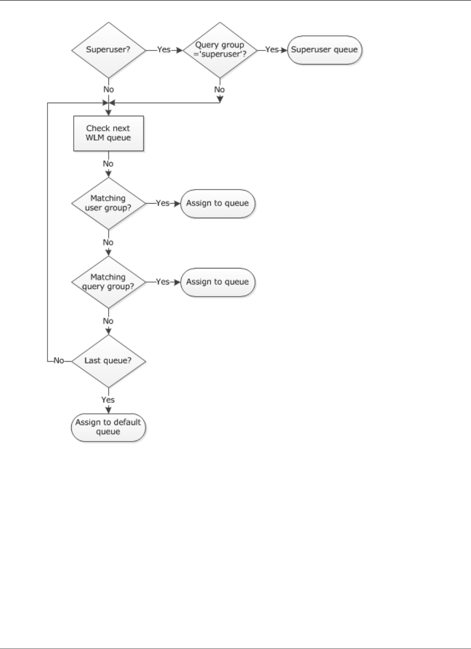
Amazon Redshift Database Developer Guide
WLM Queue Assignment Rules
1. If a user is logged in as a superuser and runs a query in the query group labeled superuser, the query is
assigned to the Superuser queue.
2. If a user belongs to a listed user group or if a user runs a query within a listed query group, the query
is assigned to the first matching queue.
3. If a query doesn't meet any criteria, the query is assigned to the default queue, which is the last queue
defined in the WLM configuration.
The following table shows a WLM configuration with the Superuser queue and four user-defined queues.
API Version 2012-12-01
294
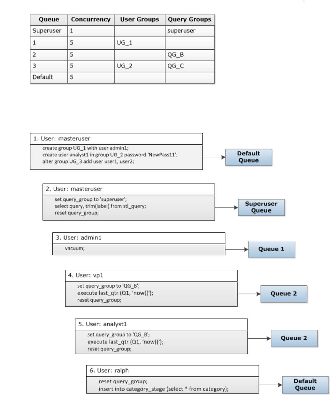
Amazon Redshift Database Developer Guide
Queue Assignments Example
Queue Assignments Example
The following example shows how queries are assigned to the queues in the previous example according
to user groups and query groups. For information about how to assign queries to user groups and query
groups at run time, see Assigning Queries to Queues (p. 296) later in this section.
In this example, WLM makes the following assignments:
API Version 2012-12-01
295
Amazon Redshift Database Developer Guide
Assigning Queries to Queues
1. The first set of statements shows three ways to assign users to user groups. The statements are
executed by the user masteruser, which is not a member of a user group listed in any WLM queue.
No query group is set, so the statements are routed to the default queue.
2. The user masteruser is a superuser and the query group is set to 'superuser', so the query is
assigned to the superuser queue.
3. The user admin1 is a member of the user group listed in queue 1, so the query is assigned to queue 1.
4. The user vp1 is not a member of any listed user group. The query group is set to 'QG_B', so the query
is assigned to queue 2.
5. The user analyst1 is a member of the user group listed in queue 3, but 'QG_B' matches queue 2, so
the query is assigned to queue 2.
6. The user ralph is not a member of any listed user group and the query group was reset, so there is no
matching queue. The query is assigned to the default queue.
Assigning Queries to Queues
The following examples assign queries to queues according to user groups and query groups.
Assigning Queries to Queues Based on User Groups
If a user group name is listed in a queue definition, queries run by members of that user group will be
assigned to the corresponding queue. The following example creates user groups and adds users to
groups by using the SQL commands CREATE USER (p. 490), CREATE GROUP (p. 467), and ALTER
GROUP (p. 363).
create group admin_group with user admin246, admin135, sec555;
create user vp1234 in group ad_hoc_group password 'vpPass1234';
alter group admin_group add user analyst44, analyst45, analyst46;
Assigning a Query to a Query Group
You can assign a query to a queue at run time by assigning your query to the appropriate query group.
Use the SET command to begin a query group.
SET query_group TO group_label
Here, group_label is a query group label that is listed in the WLM configuration.
All queries that you run after the SET query_group command will run as members of the specified
query group until you either reset the query group or end your current login session. For information
about setting and resetting Amazon Redshift objects, see SET (p. 560) and RESET (p. 527) in the SQL
Command Reference.
The query group labels that you specify must be included in the current WLM configuration; otherwise,
the SET query_group command has no effect on query queues.
The label defined in the TO clause is captured in the query logs so that you can use the label
for troubleshooting. For information about the query_group configuration parameter, see
query_group (p. 950) in the Configuration Reference.
The following example runs two queries as part of the query group 'priority' and then resets the query
group.
set query_group to 'priority';
API Version 2012-12-01
296
Amazon Redshift Database Developer Guide
Assigning Queries to the Superuser Queue
select count(*)from stv_blocklist;
select query, elapsed, substring from svl_qlog order by query desc limit 5;
reset query_group;
Assigning Queries to the Superuser Queue
To assign a query to the Superuser queue, log on to Amazon Redshift as a superuser and then run the
query in the superuser group. When you are done, reset the query group so that subsequent queries do
not run in the Superuser queue.
The following example assigns two commands to run in the Superuser queue.
set query_group to 'superuser';
analyze;
vacuum;
reset query_group;
To view a list of superusers, query the PG_USER system catalog table.
select * from pg_user where usesuper = 'true';
WLM Dynamic and Static Configuration Properties
The WLM configuration properties are either dynamic or static. If you change any of the dynamic
properties, you don’t need to reboot your cluster for the changes to take effect. While dynamic changes
are being applied, your cluster status is modifying. If you add or remove query queues or change any
of the static properties, you must restart your cluster before any WLM parameter changes, including
changes to dynamic properties, take effect.
The following WLM properties are static:
• User groups
• User group wildcard
• Query groups
• Query group wildcard
The following WLM properties are dynamic:
• Concurrency
• Percent of memory to use
• Timeout
If the timeout value is changed, the new value is applied to any query that begins execution after
the value is changed. If the concurrency or percent of memory to use are changed, Amazon Redshift
transitions to the new configuration dynamically so that currently running queries are not affected by
the change. For more information, see WLM Dynamic Memory Allocation (p. 298).
Topics
•WLM Dynamic Memory Allocation (p. 298)
•Dynamic WLM Example (p. 298)
API Version 2012-12-01
297
Amazon Redshift Database Developer Guide
WLM Dynamic Memory Allocation
WLM Dynamic Memory Allocation
In each queue, WLM creates a number of query slots equal to the queue's concurrency level. The amount
of memory allocated to a query slot equals the percentage of memory allocated to the queue divided
by the slot count. If you change the memory allocation or concurrency, Amazon Redshift dynamically
manages the transition to the new WLM configuration so that active queries can run to completion using
the currently allocated amount of memory, at the same time ensuring that total memory usage never
exceeds 100 percent of available memory.
The workload manager uses the following process to manage the transition.
1. WLM recalculates the memory allocation for each new query slot.
2. If a query slot is not actively being used by a running query, WLM removes the slot, which makes that
memory available for new slots.
3. If a query slot is actively in use, WLM waits for the query to finish.
4. As active queries complete, the empty slots are removed and the associated memory is freed.
5. As enough memory becomes available to add one or more slots, new slots are added.
6. When all queries that were running at the time of the change finish, the slot count equals the new
concurrency level, and the transition to the new WLM configuration is complete.
In effect, queries that are running when the change takes place continue to use the original memory
allocation, and queries that are queued when the change takes place are routed to new slots as they
become available.
If the WLM dynamic properties are changed during the transition process, WLM immediately begins to
transition to the new configuration, starting from the current state. To view the status of the transition,
query the STV_WLM_SERVICE_CLASS_CONFIG (p. 894) system table.
Dynamic WLM Example
Suppose your cluster WLM is configured with two queues, using the following dynamic properties.
Queue Concurrency % Memory to Use
1 4 50%
2 4 50%
Now suppose your cluster has 200 GB of memory available for query processing. (This number is
arbitrary and used for illustration only.) As the following equation shows, each slot is allocated 25 GB.
(200 GB * 50% ) / 4 slots = 25 GB
Next, you change your WLM to use the following dynamic properties.
Queue Concurrency % Memory to Use
1 3 75%
2 4 25%
As the following equation shows, the new memory allocation for each slot in queue 1 is 50 GB.
API Version 2012-12-01
298
Amazon Redshift Database Developer Guide
Query Monitoring Rules
(200 GB * 75% ) / 3 slots = 50 GB
Suppose queries A1, A2, A3, and A4 are running when the new configuration is applied, and queries B1,
B2, B3, and B4 are queued. WLM dynamically reconfigures the query slots as follows.
Step Queries
Running
Current Slot
Count
Target Slot
Count
Allocated
Memory
Available
Memory
1 A1, A2, A3, A4 4 0 100 GB 50 GB
2 A2, A3, A4 3 0 75 GB 75 GB
3 A3, A4 2 0 50 GB 100 GB
4 A3, A4, B1 2 1 100 GB 50 GB
5 A4, B1 1 1 75 GB 75 GB
6 A4, B1, B2 1 2 125 GB 25 GB
7 B1, B2 0 2 100 GB 50 GB
8 B1, B2, B3 0 3 150 GB 0 GB
1. WLM recalculates the memory allocation for each query slot. Originally, queue 1 was allocated
100 GB. The new queue has a total allocation of 150 GB, so the new queue immediately has 50 GB
available. Queue 1 is now using four slots, and the new concurrency level is three slots, so no new
slots are added.
2. When one query finishes, the slot is removed and 25 GB is freed. Queue 1 now has three slots and
75 GB of available memory. The new configuration needs 50 GB for each new slot, but the new
concurrency level is three slots, so no new slots are added.
3. When a second query finishes, the slot is removed, and 25 GB is freed. Queue 1 now has two slots and
100 GB of free memory.
4. A new slot is added using 50 GB of the free memory. Queue 1 now has three slots, and 50 GB free
memory. Queued queries can now be routed to the new slot.
5. When a third query finishes, the slot is removed, and 25 GB is freed. Queue 1 now has two slots, and
75 GB of free memory.
6. A new slot is added using 50 GB of the free memory. Queue 1 now has three slots, and 25 GB free
memory. Queued queries can now be routed to the new slot.
7. When the fourth query finishes, the slot is removed, and 25 GB is freed. Queue 1 now has two slots
and 50 GB of free memory.
8. A new slot is added using the 50 GB of free memory. Queue 1 now has three slots with 50 GB each
and all available memory has been allocated.
The transition is complete and all query slots are available to queued queries.
WLM Query Monitoring Rules
In Amazon Redshift workload management (WLM), query monitoring rules define metrics-based
performance boundaries for WLM queues and specify what action to take when a query goes beyond
those boundaries. For example, for a queue dedicated to short running queries, you might create a rule
API Version 2012-12-01
299

Amazon Redshift Database Developer Guide
Defining a Query Monitor Rule
that aborts queries that run for more than 60 seconds. To track poorly designed queries, you might have
another rule that logs queries that contain nested loops.
You define query monitoring rules as part of your workload management (WLM) configuration. You
can define up to twenty-five rules for each queue, with a limit of twenty-five rules for all queues. Each
rule includes up to three conditions, or predicates, and one action. A predicate consists of a metric, a
comparison condition (=, <, or > ), and a value. If all of the predicates for any rule are met, that rule's
action is triggered. Possible rule actions are log, hop, and abort, as discussed following.
The rules in a given queue apply only to queries running in that queue. A rule is independent of other
rules.
WLM evaluates metrics every 10 seconds. If more than one rule is triggered during the same period, WLM
initiates the most severe action—abort, then hop, then log. If the action is hop or abort, the action is
logged and the query is evicted from the queue. If the action is log, the query continues to run in the
queue. WLM initiates only one log action per query per rule. If the queue contains other rules, those
rules remain in effect. If the action is hop and the query is routed to another queue, the rules for the new
queue apply.
When all of a rule's predicates are met, WLM writes a row to the STL_WLM_RULE_ACTION (p. 866)
system table. In addition, Amazon Redshift records query metrics for currently running
queries to STV_QUERY_METRICS (p. 879). Metrics for completed queries are stored in
STL_QUERY_METRICS (p. 838).
Defining a Query Monitoring Rule
You create query monitoring rules as part of your WLM configuration, which you define as part of your
cluster's parameter group definition.
You can create rules using the AWS Management Console or programmatically using JSON.
Note
If you choose to create rules programmatically, we strongly recommend using the console to
generate the JSON that you include in the parameter group definition. For more information,
see Creating or Modifying a Query Monitoring Rule Using the Console and Configuring
Parameter Values Using the AWS CLI in the Amazon Redshift Cluster Management Guide.
To define a query monitoring rule, you specify the following elements:
• A rule name – Rule names must be unique within the WLM configuration. Rule names can be up to 32
alphanumeric characters or underscores, and can't contain spaces or quotation marks. You can have up
to twenty-five rules per queue, and the total limit for all queues is twenty-five rules.
• One or more predicates – You can have up to three predicates per rule. If all the predicates for any rule
are met, the associated action is triggered. A predicate is defined by a metric name, an operator ( =, <,
or > ), and a value. An example is query_cpu_time > 100000. For a list of metrics and examples of
values for different metrics, see Query Monitoring Metrics (p. 301) following in this section.
• An action – If more than one rule is triggered, WLM chooses the rule with the most severe action.
Possible actions, in ascending order of severity, are:
• Log – Record information about the query in the STL_WLM_RULE_ACTION system table. Use the Log
action when you want to only write a log record. WLM creates at most one log per query, per rule.
Following a log action, other rules remain in force and WLM continues to monitor the query.
• Hop – Log the action and hop the query to the next matching queue. If there isn't another
matching queue, the query is canceled. QMR hops only CREATE TABLE AS (CTAS) statements and
read-only queries, such as SELECT statements. For more information, see WLM Query Queue
Hopping (p. 288).
• Abort – Log the action and terminate the query. QMR doesn't abort COPY statements and
maintenance operations, such as ANALYZE and VACUUM.
API Version 2012-12-01
300
Amazon Redshift Database Developer Guide
Query Monitoring Metrics
For steps to create or modify a query monitoring rule, see Creating or Modifying a Query Monitoring
Rule Using the Console and Properties in the wlm_json_configuration Parameter in the Amazon Redshift
Cluster Management Guide.
You can find more information about query monitoring rules in the following topics:
•Query Monitoring Metrics (p. 301)
•Query Monitoring Rules Templates (p. 302)
•Creating a Rule Using the Console
•Configuring Workload Management
•System Tables and Views for Query Monitoring Rules (p. 303)
Query Monitoring Metrics
The following table describes the metrics used in query monitoring rules. (These metrics are distinct
from the metrics stored in the STV_QUERY_METRICS (p. 879) and STL_QUERY_METRICS (p. 838)
system tables.)
For a given metric, the performance threshold is tracked either at the query level or the segment level.
For more information about segments and steps, see Query Planning And Execution Workflow (p. 257).
Note
The WLM Timeout (p. 288) parameter is distinct from query monitoring rules.
Metric Name Description
Query CPU time query_cpu_time CPU time used by the query, in seconds. CPU
time is distinct from Query execution time.
Valid values are 0 to 10^6.
Blocks read query_blocks_read Number of 1 MB data blocks read by the query.
Valid values are 0 to 1024^2.
Scan row count scan_row_count The number of rows in a scan step. The row
count is the total number of rows emitted before
filtering rows marked for deletion (ghost rows)
and before applying user-defined query filters.
Valid values are 0 to 1024^4.
Query execution time query_execution_timeElapsed execution time for a query, in seconds.
Execution time doesn't include time spent waiting
in a queue.
Valid values are 0 to 86399.
CPU usage query_cpu_usage_percentPercent of CPU capacity used by the query.
Valid values are 0 to 6399.
Memory to disk query_temp_blocks_to_diskTemporary disk space used to write intermediate
results, in 1 MB blocks.
Valid values are 0 to 31981567.
API Version 2012-12-01
301
Amazon Redshift Database Developer Guide
Query Monitoring Rules Templates
Metric Name Description
CPU skew cpu_skew The ratio of maximum CPU usage for any slice
to average CPU usage for all slices. This metric is
defined at the segment level.
Valid values are 0 to 99.
I/O skew io_skew The ratio of maximum blocks read (I/O) for any
slice to average blocks read for all slices. This
metric is defined at the segment level.
Valid values are 0 to 99.
Rows joined join_row_count The number of rows processed in a join step.
Valid values are 0 to 10^15 .
Nested loop join row
count
nested_loop_join_row_countThe number or rows in a nested loop join.
Valid values are 0 to 10^15.
Return row count return_row_count The number of rows returned by the query.
Valid values are 0 to 10^15.
Segment execution
time
segment_execution_timeElapsed execution time for a single segment,
in seconds. To avoid or reduce sampling errors,
include segment_execution_time > 10 in
your rules.
Valid values are 0 to 86388
Spectrum scan row
count
spectrum_scan_row_countThe number of rows of data in Amazon S3
scanned by an Amazon Redshift Spectrum query.
Valid values are 0 to 10^15
Spectrum scan size spectrum_scan_size_mbThe size of data in Amazon S3, in MB, scanned by
an Amazon Redshift Spectrum query.
Valid values are 0 to 10^15
Note
Short segment execution times can result in sampling errors with some metrics, such as
io_skew and query_cpu_percent. To avoid or reduce sampling errors, include segment
execution time in your rules. A good starting point is segment_execution_time > 10.
The SVL_QUERY_METRICS (p. 909) view shows the metrics for completed queries. The
SVL_QUERY_METRICS_SUMMARY (p. 911) view shows the maximum values of metrics for completed
queries. Use the values in these views as an aid to determine threshold values for defining query
monitoring rules.
Query Monitoring Rules Templates
When you add a rule using the Amazon Redshift console, you can choose to create a rule from a
predefined template. Amazon Redshift creates a new rule with a set of predicates and populates the
predicates with default values. The default action is log. You can modify the predicates and action to
meet your use case.
API Version 2012-12-01
302
Amazon Redshift Database Developer Guide
System Tables and Views for Query Monitoring Rules
The following table lists available templates.
Template Name Predicates Description
Nested loop join nested_loop_join_row_count
> 100
A nested loop join might indicate an incomplete
join predicate, which often results in a very large
return set (a Cartesian product). Use a low row
count to find a potentially runaway query early.
Query returns a high
number of rows
return_row_count >
1000000
If you dedicate a queue to simple, short running
queries, you might include a rule that finds
queries returning a high row count. The template
uses a default of 1 million rows. For some
systems, you might consider one million rows to
be high, or in a larger system, a billion or more
rows might be high.
Join with a high
number of rows
join_row_count >
1000000000
A join step that involves an unusually high
number of rows might indicate a need for more
restrictive filters. The template uses a default of 1
billion rows. For an ad hoc queue that's intended
for quick, simple queries, you might use a lower
number.
High disk usage when
writing intermediate
results
query_temp_blocks_to_disk
> 100000
When currently executing queries use more than
the available system RAM, the query execution
engine writes intermediate results to disk (spilled
memory). Typically, this condition is the result
of a rogue query, which usually is also the query
that uses the most disk space. The acceptable
threshold for disk usage varies based on the
cluster node type and number of nodes. The
template uses a default of 100,000 blocks, or
100 GB. For a small cluster, you might use a lower
number.
Long running query
with high I/O skew
segment_execution_time
> 120 and io_skew >
1.30
I/O skew occurs when one node slice has a much
higher I/O rate than the other slices. As a starting
point, a skew of 1.30 (1.3 times average) is
considered high. High I/O skew is not always a
problem, but when combined with a long running
query time, it might indicate a problem with the
distribution style or sort key.
System Tables and Views for Query Monitoring Rules
When all of a rule's predicates are met, WLM writes a row to the STL_WLM_RULE_ACTION (p. 866)
system table with details for the query that triggered the rule and the resulting action.
In addition, Amazon Redshift records query metrics to two system tables.
•STV_QUERY_METRICS (p. 879) displays the metrics for currently running queries.
•STL_QUERY_METRICS (p. 838) records the metrics for completed queries.
• The SVL_QUERY_METRICS (p. 909) view shows the metrics for completed queries.
• The SVL_QUERY_METRICS_SUMMARY (p. 911) view shows the maximum values of metrics for
completed queries.
API Version 2012-12-01
303
Amazon Redshift Database Developer Guide
WLM System Tables and Views
WLM System Tables and Views
WLM configures query queues according to internally-defined WLM service classes. Amazon Redshift
creates several internal queues according to these service classes along with the queues defined in the
WLM configuration. The terms queue and service class are often used interchangeably in the system
tables. The superuser queue uses service class 5. User-defined queues use service class 6 and greater.
You can view the status of queries, queues, and service classes by using WLM-specific system tables.
Query the following system tables to do the following:
• View which queries are being tracked and what resources are allocated by the workload manager.
• See which queue a query has been assigned to.
• View the status of a query that is currently being tracked by the workload manager.
Table Name Description
STL_WLM_ERROR (p. 865) Contains a log of WLM-related error events.
STL_WLM_QUERY (p. 866) Lists queries that are being tracked by WLM.
STV_WLM_CLASSIFICATION_CONFIG (p. 890)Shows the current classification rules for WLM.
STV_WLM_QUERY_QUEUE_STATE (p. 891)Records the current state of the query queues.
STV_WLM_QUERY_STATE (p. 892) Provides a snapshot of the current state of queries that are
being tracked by WLM.
STV_WLM_QUERY_TASK_STATE (p. 893)Contains the current state of query tasks.
STV_WLM_SERVICE_CLASS_CONFIG (p. 894)Records the service class configurations for WLM.
STV_WLM_SERVICE_CLASS_STATE (p. 896)Contains the current state of the service classes.
You use the task ID to track a query in the system tables. The following example shows how to obtain
the task ID of the most recently submitted user query:
select task from stl_wlm_query where exec_start_time =(select max(exec_start_time) from
stl_wlm_query);
task
------
137
(1 row)
The following example displays queries that are currently executing or waiting in various service classes
(queues). This query is useful in tracking the overall concurrent workload for Amazon Redshift:
select * from stv_wlm_query_state order by query;
xid |task|query|service_| wlm_start_ | state |queue_ | exec_
| | |class | time | |time | time
----+----+-----+--------+-------------+---------+-------+--------
2645| 84 | 98 | 3 | 2010-10-... |Returning| 0 | 3438369
2650| 85 | 100 | 3 | 2010-10-... |Waiting | 0 | 1645879
API Version 2012-12-01
304

Amazon Redshift Database Developer Guide
WLM System Tables and Views
2660| 87 | 101 | 2 | 2010-10-... |Executing| 0 | 916046
2661| 88 | 102 | 1 | 2010-10-... |Executing| 0 | 13291
(4 rows)
API Version 2012-12-01
305

Amazon Redshift Database Developer Guide
Amazon Redshift SQL
SQL Reference
Topics
•Amazon Redshift SQL (p. 306)
•Using SQL (p. 312)
•SQL Commands (p. 357)
•SQL Functions Reference (p. 588)
•Reserved Words (p. 794)
Amazon Redshift SQL
Topics
•SQL Functions Supported on the Leader Node (p. 306)
•Amazon Redshift and PostgreSQL (p. 307)
Amazon Redshift is built around industry-standard SQL, with added functionality to manage very large
datasets and support high-performance analysis and reporting of those data.
Note
The maximum size for a single Amazon Redshift SQL statement is 16 MB.
SQL Functions Supported on the Leader Node
Some Amazon Redshift queries are distributed and executed on the compute nodes, and other queries
execute exclusively on the leader node.
The leader node distributes SQL to the compute nodes whenever a query references user-created tables
or system tables (tables with an STL or STV prefix and system views with an SVL or SVV prefix). A query
that references only catalog tables (tables with a PG prefix, such as PG_TABLE_DEF, which reside on the
leader node) or that does not reference any tables, runs exclusively on the leader node.
Some Amazon Redshift SQL functions are supported only on the leader node and are not supported on
the compute nodes. A query that uses a leader-node function must execute exclusively on the leader
node, not on the compute nodes, or it will return an error.
The documentation for each function that must run exclusively on the leader node includes a note
stating that the function will return an error if it references user-defined tables or Amazon Redshift
system tables. See Leader Node–Only Functions (p. 588) for a list of functions that run exclusively on
the leader node.
Examples
The CURRENT_SCHEMA function is a leader-node only function. In this example, the query does not
reference a table, so it runs exclusively on the leader node.
select current_schema();
The result is as follows.
API Version 2012-12-01
306
Amazon Redshift Database Developer Guide
Amazon Redshift and PostgreSQL
current_schema
---------------
public
(1 row)
In the next example, the query references a system catalog table, so it runs exclusively on the leader
node.
select * from pg_table_def
where schemaname = current_schema() limit 1;
schemaname | tablename | column | type | encoding | distkey | sortkey | notnull
------------+-----------+--------+----------+----------+---------+---------+---------
public | category | catid | smallint | none | t | 1 | t
(1 row)
In the next example, the query references an Amazon Redshift system table that resides on the compute
nodes, so it returns an error.
select current_schema(), userid from users;
INFO: Function "current_schema()" not supported.
ERROR: Specified types or functions (one per INFO message) not supported on Amazon
Redshift tables.
Amazon Redshift and PostgreSQL
Topics
•Amazon Redshift and PostgreSQL JDBC and ODBC (p. 308)
•Features That Are Implemented Differently (p. 308)
•Unsupported PostgreSQL Features (p. 309)
•Unsupported PostgreSQL Data Types (p. 310)
•Unsupported PostgreSQL Functions (p. 310)
Amazon Redshift is based on PostgreSQL 8.0.2. Amazon Redshift and PostgreSQL have a number of
very important differences that you must be aware of as you design and develop your data warehouse
applications.
Amazon Redshift is specifically designed for online analytic processing (OLAP) and business intelligence
(BI) applications, which require complex queries against large datasets. Because it addresses very
different requirements, the specialized data storage schema and query execution engine that Amazon
Redshift uses are completely different from the PostgreSQL implementation. For example, where online
transaction processing (OLTP) applications typically store data in rows, Amazon Redshift stores data in
columns, using specialized data compression encodings for optimum memory usage and disk I/O. Some
PostgreSQL features that are suited to smaller-scale OLTP processing, such as secondary indexes and
efficient single-row data manipulation operations, have been omitted to improve performance.
See Amazon Redshift System Overview (p. 4) for a detailed explanation of the Amazon Redshift data
warehouse system architecture.
PostgreSQL 9.x includes some features that are not supported in Amazon Redshift. In addition, there
are important differences between Amazon Redshift SQL and PostgreSQL 8.0.2 that you must be aware
of. This section highlights the differences between Amazon Redshift and PostgreSQL 8.0.2 and provides
guidance for developing a data warehouse that takes full advantage of the Amazon Redshift SQL
implementation.
API Version 2012-12-01
307

Amazon Redshift Database Developer Guide
Amazon Redshift and PostgreSQL
Amazon Redshift and PostgreSQL JDBC and ODBC
Because Amazon Redshift is based on PostgreSQL, we previously recommended using JDBC4 Postgresql
driver version 8.4.703 and psqlODBC version 9.x drivers; if you are currently using those drivers, we
recommend moving to the new Amazon Redshift–specific drivers going forward. For more information
about drivers and configuring connections, see JDBC and ODBC Drivers for Amazon Redshift in the
Amazon Redshift Cluster Management Guide.
To avoid client-side out-of-memory errors when retrieving large data sets using JDBC, you can enable
your client to fetch data in batches by setting the JDBC fetch size parameter. For more information, see
Setting the JDBC Fetch Size Parameter (p. 284).
Amazon Redshift does not recognize the JDBC maxRows parameter. Instead, specify a LIMIT (p. 555)
clause to restrict the result set. You can also use an OFFSET (p. 555) clause to skip to a specific starting
point in the result set.
Features That Are Implemented Differently
Many Amazon Redshift SQL language elements have different performance characteristics and use
syntax and semantics and that are quite different from the equivalent PostgreSQL implementation.
Important
Do not assume that the semantics of elements that Amazon Redshift and PostgreSQL have
in common are identical. Make sure to consult the Amazon Redshift Developer Guide SQL
Commands (p. 357) to understand the often subtle differences.
One example in particular is the VACUUM (p. 584) command, which is used to clean up and reorganize
tables. VACUUM functions differently and uses a different set of parameters than the PostgreSQL
version. See Vacuuming Tables (p. 228) for more about information about using VACUUM in Amazon
Redshift.
Often, database management and administration features and tools are different as well. For example,
Amazon Redshift maintains a set of system tables and views that provide information about how the
system is functioning. See System Tables and Views (p. 797) for more information.
The following list includes some examples of SQL features that are implemented differently in Amazon
Redshift.
•CREATE TABLE (p. 471)
Amazon Redshift does not support tablespaces, table partitioning, inheritance, and certain constraints.
The Amazon Redshift implementation of CREATE TABLE enables you to define the sort and
distribution algorithms for tables to optimize parallel processing.
Amazon Redshift Spectrum supports table partitioning using the CREATE EXTERNAL TABLE (p. 452)
command.
•ALTER TABLE (p. 365)
ALTER COLUMN actions are not supported.
ADD COLUMN supports adding only one column in each ALTER TABLE statement.
•COPY (p. 390)
The Amazon Redshift COPY command is highly specialized to enable the loading of data from Amazon
S3 buckets and Amazon DynamoDB tables and to facilitate automatic compression. See the Loading
Data (p. 184) section and the COPY command reference for details.
•INSERT (p. 520), UPDATE (p. 580), and DELETE (p. 499)
WITH is not supported.
API Version 2012-12-01
308

Amazon Redshift Database Developer Guide
Amazon Redshift and PostgreSQL
•VACUUM (p. 584)
The parameters for VACUUM are entirely different. For example, the default VACUUM operation in
PostgreSQL simply reclaims space and makes it available for re-use; however, the default VACUUM
operation in Amazon Redshift is VACUUM FULL, which reclaims disk space and resorts all rows.
• Trailing spaces in VARCHAR values are ignored when string values are compared. For more
information, see Significance of Trailing Blanks (p. 325).
Unsupported PostgreSQL Features
These PostgreSQL features are not supported in Amazon Redshift.
Important
Do not assume that the semantics of elements that Amazon Redshift and PostgreSQL have
in common are identical. Make sure to consult the Amazon Redshift Developer Guide SQL
Commands (p. 357) to understand the often subtle differences.
• Only the 8.x version of the PostgreSQL query tool psql is supported.
• Table partitioning (range and list partitioning)
• Tablespaces
• Constraints
• Unique
• Foreign key
• Primary key
• Check constraints
• Exclusion constraints
Unique, primary key, and foreign key constraints are permitted, but they are informational only. They
are not enforced by the system, but they are used by the query planner.
• Database roles
• Inheritance
• Postgres system columns
Amazon Redshift SQL does not implicitly define system columns. However, the PostgreSQL system
column names cannot be used as names of user-defined columns. See https://www.postgresql.org/
docs/8.0/static/ddl-system-columns.html
• Indexes
• NULLS clause in Window functions
• Collations
Amazon Redshift does not support locale-specific or user-defined collation sequences. See Collation
Sequences (p. 337).
• Value expressions
• Subscripted expressions
• Array constructors
• Row constructors
• Stored procedures
• Triggers
• Management of External Data (SQL/MED)
• Table functions
• VALUES list used as constant tables
API Version 2012-12-01
309

Amazon Redshift Database Developer Guide
Amazon Redshift and PostgreSQL
• Recursive common table expressions
• Sequences
• Full text search
Unsupported PostgreSQL Data Types
Generally, if a query attempts to use an unsupported data type, including explicit or implicit casts, it will
return an error. However, some queries that use unsupported data types will run on the leader node but
not on the compute nodes. See SQL Functions Supported on the Leader Node (p. 306).
For a list of the supported data types, see Data Types (p. 315).
These PostgreSQL data types are not supported in Amazon Redshift.
• Arrays
• BIT, BIT VARYING
• BYTEA
• Composite Types
• Date/Time Types
• INTERVAL
• TIME
• Enumerated Types
• Geometric Types
• JSON
• Network Address Types
• Numeric Types
• SERIAL, BIGSERIAL, SMALLSERIAL
• MONEY
• Object Identifier Types
• Pseudo-Types
• Range Types
• Text Search Types
• TXID_SNAPSHOT
• UUID
• XML
Unsupported PostgreSQL Functions
Many functions that are not excluded have different semantics or usage. For example, some supported
functions will run only on the leader node. Also, some unsupported functions will not return an error
when run on the leader node. The fact that these functions do not return an error in some cases should
not be taken to indicate that the function is supported by Amazon Redshift.
Important
Do not assume that the semantics of elements that Amazon Redshift and PostgreSQL have in
common are identical. Make sure to consult the Amazon Redshift Database Developer Guide SQL
Commands (p. 357) to understand the often subtle differences.
For more information, see SQL Functions Supported on the Leader Node (p. 306).
API Version 2012-12-01
310

Amazon Redshift Database Developer Guide
Amazon Redshift and PostgreSQL
These PostgreSQL functions are not supported in Amazon Redshift.
• Access privilege inquiry functions
• Advisory lock functions
• Aggregate functions
• STRING_AGG()
• ARRAY_AGG()
• EVERY()
• XML_AGG()
• CORR()
• COVAR_POP()
• COVAR_SAMP()
• REGR_AVGX(), REGR_AVGY()
• REGR_COUNT()
• REGR_INTERCEPT()
• REGR_R2()
• REGR_SLOPE()
• REGR_SXX(), REGR_SXY(), REGR_SYY()
• Array functions and operators
• Backup control functions
• Comment information functions
• Database object location functions
• Database object size functions
• Date/Time functions and operators
• CLOCK_TIMESTAMP()
• JUSTIFY_DAYS(), JUSTIFY_HOURS(), JUSTIFY_INTERVAL()
• PG_SLEEP()
• TRANSACTION_TIMESTAMP()
• ENUM support functions
• Geometric functions and operators
• Generic file access functions
• IS DISTINCT FROM
• Network address functions and operators
• Mathematical functions
• DIV()
• SETSEED()
• WIDTH_BUCKET()
• Set returning functions
• GENERATE_SERIES()
• GENERATE_SUBSCRIPTS()
• Range functions and operators
• Recovery control functions
• Recovery information functions
• ROLLBACK TO SAVEPOINT function
• Schema visibility inquiry functions
• Server signaling functions
API Version 2012-12-01
311

Amazon Redshift Database Developer Guide
Using SQL
• Snapshot synchronization functions
• Sequence manipulation functions
• String functions
• BIT_LENGTH()
• OVERLAY()
• CONVERT(), CONVERT_FROM(), CONVERT_TO()
• ENCODE()
• FORMAT()
• QUOTE_NULLABLE()
• REGEXP_MATCHES()
• REGEXP_SPLIT_TO_ARRAY()
• REGEXP_SPLIT_TO_TABLE()
• System catalog information functions
• System information functions
• CURRENT_CATALOG CURRENT_QUERY()
• INET_CLIENT_ADDR()
• INET_CLIENT_PORT()
• INET_SERVER_ADDR() INET_SERVER_PORT()
• PG_CONF_LOAD_TIME()
• PG_IS_OTHER_TEMP_SCHEMA()
• PG_LISTENING_CHANNELS()
• PG_MY_TEMP_SCHEMA()
• PG_POSTMASTER_START_TIME()
• PG_TRIGGER_DEPTH()
• SHOW VERSION()
• Text search functions and operators
• Transaction IDs and snapshots functions
• Trigger functions
• XML functions
Using SQL
Topics
•SQL Reference Conventions (p. 312)
•Basic Elements (p. 313)
•Expressions (p. 337)
•Conditions (p. 340)
The SQL language consists of commands and functions that you use to work with databases and
database objects. The language also enforces rules regarding the use of data types, expressions, and
literals.
SQL Reference Conventions
This section explains the conventions that are used to write the syntax for the SQL expressions,
commands, and functions described in the SQL reference section.
API Version 2012-12-01
312

Amazon Redshift Database Developer Guide
Basic Elements
Character Description
CAPS Words in capital letters are key words.
[ ] Square brackets denote optional arguments. Multiple arguments in square
brackets indicate that you can choose any number of the arguments. In addition,
arguments in brackets on separate lines indicate that the Amazon Redshift parser
expects the arguments to be in the order that they are listed in the syntax. For an
example, see SELECT (p. 532).
{ } Braces indicate that you are required to choose one of the arguments inside the
braces.
| Pipes indicate that you can choose between the arguments.
italics Words in italics indicate placeholders. You must insert the appropriate value in
place of the word in italics.
. . . An ellipsis indicates that you can repeat the preceding element.
' Words in single quotes indicate that you must type the quotes.
Basic Elements
Topics
•Names and Identifiers (p. 313)
•Literals (p. 315)
•Nulls (p. 315)
•Data Types (p. 315)
•Collation Sequences (p. 337)
This section covers the rules for working with database object names, literals, nulls, and data types.
Names and Identifiers
Names identify database objects, including tables and columns, as well as users and passwords. The
terms name and identifier can be used interchangeably. There are two types of identifiers, standard
identifiers and quoted or delimited identifiers. Identifiers must consist of only UTF-8 printable
characters. ASCII letters in standard and delimited identifiers are case-insensitive and are folded to
lowercase in the database. In query results, column names are returned as lowercase by default. To
return column names in uppercase, set the describe_field_name_in_uppercase (p. 949) configuration
parameter to true.
Standard Identifiers
Standard SQL identifiers adhere to a set of rules and must:
• Begin with an an ASCII single-byte alphabetic character or underscore character, or a UTF-8 multibyte
character two to four bytes long.
• Subsequent characters can be ASCII single-byte alphanumeric characters, underscores, or dollar signs,
or UTF-8 multibyte characters two to four bytes long.
• Be between 1 and 127 bytes in length, not including quotes for delimited identifiers.
• Contain no quotation marks and no spaces.
• Not be a reserved SQL key word.
API Version 2012-12-01
313

Amazon Redshift Database Developer Guide
Basic Elements
Delimited Identifiers
Delimited identifiers (also known as quoted identifiers) begin and end with double quotation marks (").
If you use a delimited identifier, you must use the double quotation marks for every reference to that
object. The identifier can contain any standard UTF-8 printable characters other than the double quote
itself. Therefore, you can create column or table names that include otherwise illegal characters, such as
spaces or the percent symbol.
ASCII letters in delimited identifiers are case-insensitive and are folded to lowercase. To use a double
quote in a string, you must precede it with another double quote character.
Examples
This table shows examples of delimited identifiers, the resulting output, and a discussion:
Syntax Result Discussion
"group" group GROUP is a reserved word, so usage of it within an identifier
requires double quotes.
"""WHERE""" "where" WHERE is also a reserved word. To include quotation marks
in the string, escape each double quote character with
additional double quote characters.
"This name" this name Double quotes are required in order to preserve the space.
"This ""IS IT""" this "is it" The quotes surrounding IS IT must each be preceded by an
extra quote in order to become part of the name.
To create a table named group with a column named this "is it":
create table "group" (
"This ""IS IT""" char(10));
The following queries return the same result:
select "This ""IS IT"""
from "group";
this "is it"
--------------
(0 rows)
select "this ""is it"""
from "group";
this "is it"
--------------
(0 rows)
The following fully qualified table.column syntax also returns the same result:
select "group"."this ""is it"""
from "group";
this "is it"
--------------
API Version 2012-12-01
314

Amazon Redshift Database Developer Guide
Basic Elements
(0 rows)
Literals
A literal or constant is a fixed data value, composed of a sequence of characters or a numeric constant.
Amazon Redshift supports several types of literals, including:
• Numeric literals for integer, decimal, and floating-point numbers. For more information, see Integer
and Floating-Point Literals (p. 321).
• Character literals, also referred to as strings, character strings, or character constants
• Datetime and interval literals, used with datetime data types. For more information, see Date and
Timestamp Literals (p. 328) and Interval Literals (p. 330).
Nulls
If a column in a row is missing, unknown, or not applicable, it is a null value or is said to contain
null. Nulls can appear in fields of any data type that are not restricted by primary key or NOT NULL
constraints. A null is not equivalent to the value zero or to an empty string.
Any arithmetic expression containing a null always evaluates to a null. All operators except
concatenation return a null when given a null argument or operand.
To test for nulls, use the comparison conditions IS NULL and IS NOT NULL. Because null represents a lack
of data, a null is not equal or unequal to any value or to another null.
Data Types
Topics
•Multibyte Characters (p. 316)
•Numeric Types (p. 316)
•Character Types (p. 323)
•Datetime Types (p. 326)
•Boolean Type (p. 331)
•Type Compatibility and Conversion (p. 333)
Each value that Amazon Redshift stores or retrieves has a data type with a fixed set of associated
properties. Data types are declared when tables are created. A data type constrains the set of values that
a column or argument can contain.
The following table lists the data types that you can use in Amazon Redshift tables.
Data Type Aliases Description
SMALLINT INT2 Signed two-byte integer
INTEGER INT, INT4 Signed four-byte integer
BIGINT INT8 Signed eight-byte integer
DECIMAL NUMERIC Exact numeric of selectable
precision
REAL FLOAT4 Single precision floating-point
number
API Version 2012-12-01
315
Amazon Redshift Database Developer Guide
Basic Elements
Data Type Aliases Description
DOUBLE PRECISION FLOAT8, FLOAT Double precision floating-point
number
BOOLEAN BOOL Logical Boolean (true/false)
CHAR CHARACTER, NCHAR, BPCHAR Fixed-length character string
VARCHAR CHARACTER VARYING,
NVARCHAR, TEXT
Variable-length character string
with a user-defined limit
DATE Calendar date (year, month, day)
TIMESTAMP TIMESTAMP WITHOUT TIME
ZONE
Date and time (without time
zone)
TIMESTAMPTZ TIMESTAMP WITH TIME ZONE Date and time (with time zone)
Multibyte Characters
The VARCHAR data type supports UTF-8 multibyte characters up to a maximum of four bytes. Five-
byte or longer characters are not supported. To calculate the size of a VARCHAR column that contains
multibyte characters, multiply the number of characters by the number of bytes per character. For
example, if a string has four Chinese characters, and each character is three bytes long, then you will
need a VARCHAR(12) column to store the string.
VARCHAR does not support the following invalid UTF-8 codepoints:
• 0xD800 - 0xDFFF
(Byte sequences: ED A0 80 - ED BF BF)
• 0xFDD0 - 0xFDEF, 0xFFFE, and 0xFFFF
(Byte sequences: EF B7 90 - EF B7 AF, EF BF BE, and EF BF BF)
The CHAR data type does not support multibyte characters.
Numeric Types
Topics
•Integer Types (p. 316)
•DECIMAL or NUMERIC Type (p. 317)
•Notes About Using 128-bit DECIMAL or NUMERIC Columns (p. 318)
•Floating-Point Types (p. 318)
•Computations with Numeric Values (p. 318)
•Integer and Floating-Point Literals (p. 321)
•Examples with Numeric Types (p. 322)
Numeric data types include integers, decimals, and floating-point numbers.
Integer Types
Use the SMALLINT, INTEGER, and BIGINT data types to store whole numbers of various ranges. You
cannot store values outside of the allowed range for each type.
API Version 2012-12-01
316
Amazon Redshift Database Developer Guide
Basic Elements
Name Storage Range
SMALLINT or INT2 2 bytes -32768 to +32767
INTEGER, INT, or INT4 4 bytes -2147483648 to
+2147483647
BIGINT or INT8 8 bytes -9223372036854775808
to
9223372036854775807
DECIMAL or NUMERIC Type
Use the DECIMAL or NUMERIC data type to store values with a user-defined precision. The DECIMAL and
NUMERIC keywords are interchangeable. In this document, decimal is the preferred term for this data
type. The term numeric is used generically to refer to integer, decimal, and floating-point data types.
Storage Range
Variable, up to 128 bits for uncompressed
DECIMAL types.
128-bit signed integers with up to 38 digits of
precision.
Define a DECIMAL column in a table by specifying a precision and scale:
decimal(precision, scale)
precision
The total number of significant digits in the whole value: the number of digits on both sides of the
decimal point. For example, the number 48.2891 has a precision of 6 and a scale of 4. The default
precision, if not specified, is 18. The maximum precision is 38.
If the number of digits to the left of the decimal point in an input value exceeds the precision of
the column minus its scale, the value cannot be copied into the column (or inserted or updated).
This rule applies to any value that falls outside the range of the column definition. For example, the
allowed range of values for a numeric(5,2) column is -999.99 to 999.99.
scale
The number of decimal digits in the fractional part of the value, to the right of the decimal point.
Integers have a scale of zero. In a column specification, the scale value must be less than or equal to
the precision value. The default scale, if not specified, is 0. The maximum scale is 37.
If the scale of an input value that is loaded into a table is greater than the scale of the column, the
value is rounded to the specified scale. For example, the PRICEPAID column in the SALES table is a
DECIMAL(8,2) column. If a DECIMAL(8,4) value is inserted into the PRICEPAID column, the value is
rounded to a scale of 2.
insert into sales
values (0, 8, 1, 1, 2000, 14, 5, 4323.8951, 11.00, null);
select pricepaid, salesid from sales where salesid=0;
pricepaid | salesid
-----------+---------
4323.90 | 0
API Version 2012-12-01
317
Amazon Redshift Database Developer Guide
Basic Elements
(1 row)
However, results of explicit casts of values selected from tables are not rounded.
Note
The maximum positive value that you can insert into a DECIMAL(19,0) column is
9223372036854775807 (263 -1). The maximum negative value is -9223372036854775807.
For example, an attempt to insert the value 9999999999999999999 (19 nines) will cause an
overflow error. Regardless of the placement of the decimal point, the largest string that Amazon
Redshift can represent as a DECIMAL number is 9223372036854775807. For example, the
largest value that you can load into a DECIMAL(19,18) column is 9.223372036854775807.
These rules derive from the internal storage of DECIMAL values as 8-byte integers. Amazon
Redshift recommends that you do not define DECIMAL values with 19 digits of precision unless
that precision is necessary.
Notes About Using 128-bit DECIMAL or NUMERIC Columns
Do not arbitrarily assign maximum precision to DECIMAL columns unless you are certain that your
application requires that precision. 128-bit values use twice as much disk space as 64-bit values and can
slow down query execution time.
Floating-Point Types
Use the REAL and DOUBLE PRECISION data types to store numeric values with variable precision. These
types are inexact types, meaning that some values are stored as approximations, such that storing and
returning a specific value may result in slight discrepancies. If you require exact storage and calculations
(such as for monetary amounts), use the DECIMAL data type.
Name Storage Range
REAL or FLOAT4 4 bytes 6 significant digits of
precision
DOUBLE PRECISION, FLOAT8, or FLOAT 8 bytes 15 significant digits of
precision
For example, note the results of the following inserts into a REAL column:
create table real1(realcol real);
insert into real1 values(12345.12345);
insert into real1 values(123456.12345);
select * from real1;
realcol
---------
123456
12345.1
(2 rows)
These inserted values are truncated to meet the limitation of 6 significant digits of precision for REAL
columns.
Computations with Numeric Values
In this context, computation refers to binary mathematical operations: addition, subtraction,
multiplication, and division. This section describes the expected return types for these operations, as well
API Version 2012-12-01
318
Amazon Redshift Database Developer Guide
Basic Elements
as the specific formula that is applied to determine precision and scale when DECIMAL data types are
involved.
When numeric values are computed during query processing, you might encounter cases where the
computation is impossible and the query returns a numeric overflow error. You might also encounter
cases where the scale of computed values varies or is unexpected. For some operations, you can use
explicit casting (type promotion) or Amazon Redshift configuration parameters to work around these
problems.
For information about the results of similar computations with SQL functions, see Aggregate
Functions (p. 590).
Return Types for Computations
Given the set of numeric data types supported in Amazon Redshift, the following table shows the
expected return types for addition, subtraction, multiplication, and division operations. The first column
on the left side of the table represents the first operand in the calculation, and the top row represents
the second operand.
INT2 INT4 INT8 DECIMAL FLOAT4 FLOAT8
INT2 INT2 INT4 INT8 DECIMAL FLOAT8 FLOAT8
INT4 INT4 INT4 INT8 DECIMAL FLOAT8 FLOAT8
INT8 INT8 INT8 INT8 DECIMAL FLOAT8 FLOAT8
DECIMAL DECIMAL DECIMAL DECIMAL DECIMAL FLOAT8 FLOAT8
FLOAT4 FLOAT8 FLOAT8 FLOAT8 FLOAT8 FLOAT4 FLOAT8
FLOAT8 FLOAT8 FLOAT8 FLOAT8 FLOAT8 FLOAT8 FLOAT8
Precision and Scale of Computed DECIMAL Results
The following table summarizes the rules for computing resulting precision and scale when
mathematical operations return DECIMAL results. In this table, p1 and s1 represent the precision and
scale of the first operand in a calculation and p2 and s2 represent the precision and scale of the second
operand. (Regardless of these calculations, the maximum result precision is 38, and the maximum result
scale is 38.)
Operation Result Precision and Scale
+ or - Scale = max(s1,s2)
Precision = max(p1-s1,p2-s2)+1+scale
* Scale = s1+s2
Precision = p1+p2+1
/ Scale = max(4,s1+p2-s2+1)
Precision = p1-s1+ s2+scale
For example, the PRICEPAID and COMMISSION columns in the SALES table are both DECIMAL(8,2)
columns. If you divide PRICEPAID by COMMISSION (or vice versa), the formula is applied as follows:
API Version 2012-12-01
319
Amazon Redshift Database Developer Guide
Basic Elements
Precision = 8-2 + 2 + max(4,2+8-2+1)
= 6 + 2 + 9 = 17
Scale = max(4,2+8-2+1) = 9
Result = DECIMAL(17,9)
The following calculation is the general rule for computing the resulting precision and scale for
operations performed on DECIMAL values with set operators such as UNION, INTERSECT, and EXCEPT or
functions such as COALESCE and DECODE:
Scale = max(s1,s2)
Precision = min(max(p1-s1,p2-s2)+scale,19)
For example, a DEC1 table with one DECIMAL(7,2) column is joined with a DEC2 table with one
DECIMAL(15,3) column to create a DEC3 table. The schema of DEC3 shows that the column becomes a
NUMERIC(15,3) column.
create table dec3 as select * from dec1 union select * from dec2;
Result
select "column", type, encoding, distkey, sortkey
from pg_table_def where tablename = 'dec3';
column | type | encoding | distkey | sortkey
-------+---------------+----------+---------+---------
c1 | numeric(15,3) | none | f | 0
In the above example, the formula is applied as follows:
Precision = min(max(7-2,15-3) + max(2,3), 19)
= 12 + 3 = 15
Scale = max(2,3) = 3
Result = DECIMAL(15,3)
Notes on Division Operations
For division operations, divide-by-zero conditions return errors.
The scale limit of 100 is applied after the precision and scale are calculated. If the calculated result scale
is greater than 100, division results are scaled as follows:
• Precision = precision - (scale - max_scale)
• Scale = max_scale
If the calculated precision is greater than the maximum precision (38), the precision is reduced to 38, and
the scale becomes the result of: max(38 + scale - precision), min(4, 100))
Overflow Conditions
Overflow is checked for all numeric computations. DECIMAL data with a precision of 19 or less is stored
as 64-bit integers. DECIMAL data with a precision that is greater than 19 is stored as 128-bit integers.
API Version 2012-12-01
320

Amazon Redshift Database Developer Guide
Basic Elements
The maximum precision for all DECIMAL values is 38, and the maximum scale is 37. Overflow errors occur
when a value exceeds these limits, which apply to both intermediate and final result sets:
• Explicit casting results in run-time overflow errors when specific data values do not fit the requested
precision or scale specified by the cast function. For example, you cannot cast all values from the
PRICEPAID column in the SALES table (a DECIMAL(8,2) column) and return a DECIMAL(7,3) result:
select pricepaid::decimal(7,3) from sales;
ERROR: Numeric data overflow (result precision)
This error occurs because some of the larger values in the PRICEPAID column cannot be cast.
• Multiplication operations produce results in which the result scale is the sum of the scale of each
operand. If both operands have a scale of 4, for example, the result scale is 8, leaving only 10 digits for
the left side of the decimal point. Therefore, it is relatively easy to run into overflow conditions when
multiplying two large numbers that both have significant scale.
Numeric Calculations with INTEGER and DECIMAL Types
When one of the operands in a calculation has an INTEGER data type and the other operand is DECIMAL,
the INTEGER operand is implicitly cast as a DECIMAL:
• INT2 (SMALLINT) is cast as DECIMAL(5,0)
• INT4 (INTEGER) is cast as DECIMAL(10,0)
• INT8 (BIGINT) is cast as DECIMAL(19,0)
For example, if you multiply SALES.COMMISSION, a DECIMAL(8,2) column, and SALES.QTYSOLD, a
SMALLINT column, this calculation is cast as:
DECIMAL(8,2) * DECIMAL(5,0)
Integer and Floating-Point Literals
Literals or constants that represent numbers can be integer or floating-point.
Integer Literals
An integer constant is a sequence of the digits 0-9, with an optional positive (+) or negative (-) sign
preceding the digits.
Syntax
[ + | - ] digit ...
Examples
Valid integers include the following:
23
-555
+17
Floating-Point Literals
Floating-point literals (also referred to as decimal, numeric, or fractional literals) are sequences of digits
that can include a decimal point, and optionally the exponent marker (e).
API Version 2012-12-01
321
Amazon Redshift Database Developer Guide
Basic Elements
Syntax
[ + | - ] digit ... [ . ] [ digit ...]
[ e | E [ + | - ] digit ... ]
Arguments
e | E
e or E indicates that the number is specified in scientific notation.
Examples
Valid floating-point literals include the following:
3.14159
-37.
2.0e19
-2E-19
Examples with Numeric Types
CREATE TABLE Statement
The following CREATE TABLE statement demonstrates the declaration of different numeric data types:
create table film (
film_id integer,
language_id smallint,
original_language_id smallint,
rental_duration smallint default 3,
rental_rate numeric(4,2) default 4.99,
length smallint,
replacement_cost real default 25.00);
Attempt to Insert an Integer That is Out of Range
The following example attempts to insert the value 33000 into a SMALLINT column.
insert into film(language_id) values(33000);
The range for SMALLINT is -32768 to +32767, so Amazon Redshift returns an error.
An error occurred when executing the SQL command:
insert into film(language_id) values(33000)
ERROR: smallint out of range [SQL State=22003]
Insert a Decimal Value into an Integer Column
The following example inserts the a decimal value into an INT column.
insert into film(language_id) values(1.5);
This value is inserted but rounded up to the integer value 2.
API Version 2012-12-01
322
Amazon Redshift Database Developer Guide
Basic Elements
Insert a Decimal That Succeeds Because Its Scale Is Rounded
The following example inserts a decimal value that has higher precision that the column.
insert into film(rental_rate) values(35.512);
In this case, the value 35.51 is inserted into the column.
Attempt to Insert a Decimal Value That Is Out of Range
In this case, the value 350.10 is out of range. The number of digits for values in DECIMAL columns is
equal to the column's precision minus its scale (4 minus 2 for the RENTAL_RATE column). In other words,
the allowed range for a DECIMAL(4,2) column is -99.99 through 99.99.
insert into film(rental_rate) values (350.10);
ERROR: numeric field overflow
DETAIL: The absolute value is greater than or equal to 10^2 for field with precision 4,
scale 2.
Insert Variable-Precision Values into a REAL Column
The following example inserts variable-precision values into a REAL column.
insert into film(replacement_cost) values(1999.99);
insert into film(replacement_cost) values(19999.99);
select replacement_cost from film;
replacement_cost
------------------
20000
1999.99
...
The value 19999.99 is converted to 20000 to meet the 6-digit precision requirement for the column.
The value 1999.99 is loaded as is.
Character Types
Topics
•Storage and Ranges (p. 323)
•CHAR or CHARACTER (p. 324)
•VARCHAR or CHARACTER VARYING (p. 324)
•NCHAR and NVARCHAR Types (p. 324)
•TEXT and BPCHAR Types (p. 325)
•Significance of Trailing Blanks (p. 325)
•Examples with Character Types (p. 325)
Character data types include CHAR (character) and VARCHAR (character varying).
Storage and Ranges
CHAR and VARCHAR data types are defined in terms of bytes, not characters. A CHAR column can only
contain single-byte characters, so a CHAR(10) column can contain a string with a maximum length of 10
bytes. A VARCHAR can contain multibyte characters, up to a maximum of four bytes per character. For
API Version 2012-12-01
323
Amazon Redshift Database Developer Guide
Basic Elements
example, a VARCHAR(12) column can contain 12 single-byte characters, 6 two-byte characters, 4 three-
byte characters, or 3 four-byte characters.
Name Storage Range (Width of Column)
CHAR, CHARACTER or NCHAR Length of string,
including trailing
blanks (if any)
4096 bytes
VARCHAR, CHARACTER VARYING, or
NVARCHAR
4 bytes +
total bytes for
characters, where
each character can
be 1 to 4 bytes.
65535 bytes (64K -1)
BPCHAR Converted to
fixed-length
CHAR(256).
256 bytes
TEXT Converted to
VARCHAR(256).
260 bytes
Note
The CREATE TABLE syntax supports the MAX keyword for character data types. For example:
create table test(col1 varchar(max));
The MAX setting defines the width of the column as 4096 bytes for CHAR or 65535 bytes for
VARCHAR.
CHAR or CHARACTER
Use a CHAR or CHARACTER column to store fixed-length strings. These strings are padded with blanks,
so a CHAR(10) column always occupies 10 bytes of storage.
char(10)
A CHAR column without a length specification results in a CHAR(1) column.
VARCHAR or CHARACTER VARYING
Use a VARCHAR or CHARACTER VARYING column to store variable-length strings with a fixed limit. These
strings are not padded with blanks, so a VARCHAR(120) column consists of a maximum of 120 single-
byte characters, 60 two-byte characters, 40 three-byte characters, or 30 four-byte characters.
varchar(120)
If you use the VARCHAR data type without a length specifier, the default length is 256.
NCHAR and NVARCHAR Types
You can create columns with the NCHAR and NVARCHAR types (also known as NATIONAL CHARACTER
and NATIONAL CHARACTER VARYING types). These types are converted to CHAR and VARCHAR types,
respectively, and are stored in the specified number of bytes.
An NCHAR column without a length specification is converted to a CHAR(1) column.
API Version 2012-12-01
324

Amazon Redshift Database Developer Guide
Basic Elements
An NVARCHAR column without a length specification is converted to a VARCHAR(256) column.
TEXT and BPCHAR Types
You can create an Amazon Redshift table with a TEXT column, but it is converted to a VARCHAR(256)
column that accepts variable-length values with a maximum of 256 characters.
You can create an Amazon Redshift column with a BPCHAR (blank-padded character) type, which
Amazon Redshift converts to a fixed-length CHAR(256) column.
Significance of Trailing Blanks
Both CHAR and VARCHAR data types store strings up to n bytes in length. An attempt to store a longer
string into a column of these types results in an error, unless the extra characters are all spaces (blanks),
in which case the string is truncated to the maximum length. If the string is shorter than the maximum
length, CHAR values are padded with blanks, but VARCHAR values store the string without blanks.
Trailing blanks in CHAR values are always semantically insignificant. They are disregarded when you
compare two CHAR values, not included in LENGTH calculations, and removed when you convert a CHAR
value to another string type.
Trailing spaces in VARCHAR and CHAR values are treated as semantically insignificant when values are
compared.
Length calculations return the length of VARCHAR character strings with trailing spaces included in the
length. Trailing blanks are not counted in the length for fixed-length character strings.
Examples with Character Types
CREATE TABLE Statement
The following CREATE TABLE statement demonstrates the use of VARCHAR and CHAR data types:
create table address(
address_id integer,
address1 varchar(100),
address2 varchar(50),
district varchar(20),
city_name char(20),
state char(2),
postal_code char(5)
);
The following examples use this table.
Trailing Blanks in Variable-Length Character Strings
Because ADDRESS1 is a VARCHAR column, the trailing blanks in the second inserted address are
semantically insignificant. In other words, these two inserted addresses match.
insert into address(address1) values('9516 Magnolia Boulevard');
insert into address(address1) values('9516 Magnolia Boulevard ');
select count(*) from address
where address1='9516 Magnolia Boulevard';
count
-------
2
API Version 2012-12-01
325
Amazon Redshift Database Developer Guide
Basic Elements
(1 row)
If the ADDRESS1 column were a CHAR column and the same values were inserted, the COUNT(*) query
would recognize the character strings as the same and return 2.
Results of the LENGTH Function
The LENGTH function recognizes trailing blanks in VARCHAR columns:
select length(address1) from address;
length
--------
23
25
(2 rows)
A value of Augusta in the CITY_NAME column, which is a CHAR column, would always return a length of
7 characters, regardless of any trailing blanks in the input string.
Values That Exceed the Length of the Column
Character strings are not truncated to fit the declared width of the column:
insert into address(city_name) values('City of South San Francisco');
ERROR: value too long for type character(20)
A workaround for this problem is to cast the value to the size of the column:
insert into address(city_name)
values('City of South San Francisco'::char(20));
In this case, the first 20 characters of the string (City of South San Fr) would be loaded into the
column.
Datetime Types
Topics
•Storage and Ranges (p. 326)
•DATE (p. 327)
•TIMESTAMP (p. 327)
•TIMESTAMPTZ (p. 327)
•Examples with Datetime Types (p. 328)
•Date and Timestamp Literals (p. 328)
•Interval Literals (p. 330)
Datetime data types include DATE, TIMESTAMP, and TIMESTAMPTZ.
Storage and Ranges
Name Storage Range Resolution
DATE 4 bytes 4713 BC to 294276 AD 1 day
TIMESTAMP 8 bytes 4713 BC to 294276 AD 1 microsecond
API Version 2012-12-01
326
Amazon Redshift Database Developer Guide
Basic Elements
Name Storage Range Resolution
TIMESTAMPTZ 8 bytes 4713 BC to 294276 AD 1 microsecond
DATE
Use the DATE data type to store simple calendar dates without time stamps.
TIMESTAMP
TIMESTAMP is an alias of TIMESTAMP WITHOUT TIME ZONE.
Use the TIMESTAMP data type to store complete time stamp values that include the date and the time of
day.
TIMESTAMP columns store values with up to a maximum of 6 digits of precision for fractional seconds.
If you insert a date into a TIMESTAMP column, or a date with a partial time stamp value, the value is
implicitly converted into a full time stamp value with default values (00) for missing hours, minutes, and
seconds. Time zone values in input strings are ignored.
By default, TIMESTAMP values are Coordinated Universal Time (UTC) in both user tables and Amazon
Redshift system tables.
TIMESTAMPTZ
TIMESTAMPTZ is an alias of TIMESTAMP WITH TIME ZONE.
Use the TIMESTAMPTZ data type to input complete time stamp values that include the date, the time of
day, and a time zone. When an input value includes a time zone, Amazon Redshift uses the time zone to
convert the value to Coordinated Universal Time (UTC) and stores the UTC value.
To view a list of supported time zone names, execute the following command.
select pg_timezone_names();
To view a list of supported time zone abbreviations, execute the following command.
select pg_timezone_abbrevs();
You can also find current information about time zones in the IANA Time Zone Database.
The following table has examples of time zone formats.
Format Example
day mon hh:mi:ss yyyy tz 17 Dec 07:37:16 1997 PST
mm/dd/yyyy hh:mi:ss.ss tz 12/17/1997 07:37:16.00 PST
mm/dd/yyyy hh:mi:ss.ss tz 12/17/1997 07:37:16.00 US/Pacific
yyyy-mm-dd hh:mi:ss+/-tz 1997-12-17 07:37:16-08
dd.mm.yyyy hh:mi:ss tz 17.12.1997 07:37:16.00 PST
TIMESTAMPTZ columns store values with up to a maximum of 6 digits of precision for fractional seconds.
API Version 2012-12-01
327

Amazon Redshift Database Developer Guide
Basic Elements
If you insert a date into a TIMESTAMPTZ column, or a date with a partial time stamp, the value is
implicitly converted into a full time stamp value with default values (00) for missing hours, minutes, and
seconds.
TIMESTAMPTZ values are UTC in user tables.
Examples with Datetime Types
Date Examples
Insert dates that have different formats and display the output:
create table datetable (start_date date, end_date date);
insert into datetable values ('2008-06-01','2008-12-31');
insert into datetable values ('Jun 1,2008','20081231');
select * from datetable order by 1;
start_date | end_date
------------------------
2008-06-01 | 2008-12-31
2008-06-01 | 2008-12-31
If you insert a time stamp value into a DATE column, the time portion is ignored and only the date
loaded.
Time Stamp Examples
If you insert a date into a TIMESTAMP or TIMESTAMPTZ column, the time defaults to midnight. For
example, if you insert the literal 20081231, the stored value is 2008-12-31 00:00:00.
To change the time zone for the current session, use the SET (p. 560) command to set the
timezone (p. 952) configuration parameter.
Insert timestamps that have different formats and display the output:
create table tstamp(timeofday timestamp, timeofdaytz timestamptz);
insert into tstamp values('Jun 1,2008 09:59:59', 'Jun 1,2008 09:59:59 EST' );
insert into tstamp values('Dec 31,2008 18:20','Dec 31,2008 18:20');
insert into tstamp values('Jun 1,2008 09:59:59 EST', 'Jun 1,2008 09:59:59');
timeofday
---------------------
2008-06-01 09:59:59
2008-12-31 18:20:00
(2 rows)
Date and Timestamp Literals
Dates
The following input dates are all valid examples of literal date values that you can load into Amazon
Redshift tables. The default MDY DateStyle mode is assumed to be in effect, which means that the
month value precedes the day value in strings such as 1999-01-08 and 01/02/00.
Note
A date or time stamp literal must be enclosed in quotes when you load it into a table.
API Version 2012-12-01
328
Amazon Redshift Database Developer Guide
Basic Elements
Input date Full Date
January 8, 1999 January 8, 1999
1999-01-08 January 8, 1999
1/8/1999 January 8, 1999
01/02/00 January 2, 2000
2000-Jan-31 January 31, 2000
Jan-31-2000 January 31, 2000
31-Jan-2000 January 31, 2000
20080215 February 15, 2008
080215 February 15, 2008
2008.366 December 31, 2008 (3-digit part of date must be
between 001 and 366)
Timestamps
The following input timestamps are all valid examples of literal time values that you can load into
Amazon Redshift tables. All of the valid date literals can be combined with the following time literals.
Input Timestamps (Concatenated Dates and
Times)
Description (of Time Part)
20080215 04:05:06.789 4:05 am and 6.789 seconds
20080215 04:05:06 4:05 am and 6 seconds
20080215 04:05 4:05 am exactly
20080215 040506 4:05 am and 6 seconds
20080215 04:05 AM 4:05 am exactly; AM is optional
20080215 04:05 PM 4:05 pm exactly; hour value must be < 12.
20080215 16:05 4:05 05 pm exactly
20080215 Midnight (by default)
Special Datetime Values
The following special values can be used as datetime literals and as arguments to date functions. They
require single quotes and are converted to regular timestamp values during query processing.
Description
now Evaluates to the start time of the current
transaction and returns a timestamp with
microsecond precision.
API Version 2012-12-01
329
Amazon Redshift Database Developer Guide
Basic Elements
Description
today Evaluates to the appropriate date and returns a
timestamp with zeroes for the timeparts.
tomorrow
yesterday
The following examples show how now and today work in conjunction with the DATEADD function:
select dateadd(day,1,'today');
date_add
---------------------
2009-11-17 00:00:00
(1 row)
select dateadd(day,1,'now');
date_add
----------------------------
2009-11-17 10:45:32.021394
(1 row)
Interval Literals
Use an interval literal to identify specific periods of time, such as 12 hours or 6 weeks. You can use
these interval literals in conditions and calculations that involve datetime expressions.
Note
You cannot use the INTERVAL data type for columns in Amazon Redshift tables.
An interval is expressed as a combination of the INTERVAL keyword with a numeric quantity and
a supported datepart; for example: INTERVAL '7 days' or INTERVAL '59 minutes'. Several
quantities and units can be connected to form a more precise interval; for example: INTERVAL '7
days, 3 hours, 59 minutes'. Abbreviations and plurals of each unit are also supported; for
example: 5 s, 5 second, and 5 seconds are equivalent intervals.
If you do not specify a datepart, the interval value represents seconds. You can specify the quantity value
as a fraction (for example: 0.5 days).
Examples
The following examples show a series of calculations with different interval values.
Add 1 second to the specified date:
select caldate + interval '1 second' as dateplus from date
where caldate='12-31-2008';
dateplus
---------------------
2008-12-31 00:00:01
(1 row)
Add 1 minute to the specified date:
select caldate + interval '1 minute' as dateplus from date
where caldate='12-31-2008';
API Version 2012-12-01
330
Amazon Redshift Database Developer Guide
Basic Elements
dateplus
---------------------
2008-12-31 00:01:00
(1 row)
Add 3 hours and 35 minutes to the specified date:
select caldate + interval '3 hours, 35 minutes' as dateplus from date
where caldate='12-31-2008';
dateplus
---------------------
2008-12-31 03:35:00
(1 row)
Add 52 weeks to the specified date:
select caldate + interval '52 weeks' as dateplus from date
where caldate='12-31-2008';
dateplus
---------------------
2009-12-30 00:00:00
(1 row)
Add 1 week, 1 hour, 1 minute, and 1 second to the specified date:
select caldate + interval '1w, 1h, 1m, 1s' as dateplus from date
where caldate='12-31-2008';
dateplus
---------------------
2009-01-07 01:01:01
(1 row)
Add 12 hours (half a day) to the specified date:
select caldate + interval '0.5 days' as dateplus from date
where caldate='12-31-2008';
dateplus
---------------------
2008-12-31 12:00:00
(1 row)
Boolean Type
Use the BOOLEAN data type to store true and false values in a single-byte column. The following table
describes the three possible states for a Boolean value and the literal values that result in that state.
Regardless of the input string, a Boolean column stores and outputs "t" for true and "f" for false.
State Valid Literal
Values
Storage
True TRUE 't'
'true' 'y'
'yes' '1'
1 byte
False FALSE 'f'
'false' 'n'
'no' '0'
1 byte
API Version 2012-12-01
331
Amazon Redshift Database Developer Guide
Basic Elements
State Valid Literal
Values
Storage
Unknown NULL 1 byte
You can use an IS comparison to check a Boolean value only as a predicate in the WHERE clause. You
can't use the IS comparison with a Boolean value in the SELECT list.
Note
We recommend always checking Boolean values explicitly, as shown in the examples following.
Implicit comparisons, such as WHERE flag or WHERE NOT flag might return unexpected
results.
Examples
You could use a BOOLEAN column to store an "Active/Inactive" state for each customer in a CUSTOMER
table.
create table customer(
custid int,
active_flag boolean default true);
insert into customer values(100, default);
select * from customer;
custid | active_flag
-------+--------------
100 | t
If no default value (true or false) is specified in the CREATE TABLE statement, inserting a default value
means inserting a null.
In this example, the query selects users from the USERS table who like sports but do not like theatre:
select firstname, lastname, likesports, liketheatre
from users
where likesports is true and liketheatre is false
order by userid limit 10;
firstname | lastname | likesports | liketheatre
----------+------------+------------+-------------
Lars | Ratliff | t | f
Mufutau | Watkins | t | f
Scarlett | Mayer | t | f
Shafira | Glenn | t | f
Winifred | Cherry | t | f
Chase | Lamb | t | f
Liberty | Ellison | t | f
Aladdin | Haney | t | f
Tashya | Michael | t | f
Lucian | Montgomery | t | f
(10 rows)
The following example selects users from the USERS table for whom is it unknown whether they like
rock music.
select firstname, lastname, likerock
from users
where likerock is unknown
API Version 2012-12-01
332

Amazon Redshift Database Developer Guide
Basic Elements
order by userid limit 10;
firstname | lastname | likerock
----------+----------+----------
Rafael | Taylor |
Vladimir | Humphrey |
Barry | Roy |
Tamekah | Juarez |
Mufutau | Watkins |
Naida | Calderon |
Anika | Huff |
Bruce | Beck |
Mallory | Farrell |
Scarlett | Mayer |
(10 rows)
The following example returns an error because it uses an IS comparison in the SELECT list.
select firstname, lastname, likerock is true as "check"
from users
order by userid limit 10;
[Amazon](500310) Invalid operation: Not implemented
The following example succeeds because it uses an equal comparison ( = ) in the SELECT list instead of
the IS comparison.
select firstname, lastname, likerock = true as "check"
from users
order by userid limit 10;
firstname | lastname | check
----------+-----------+------
Rafael | Taylor |
Vladimir | Humphrey |
Lars | Ratliff | true
Barry | Roy |
Reagan | Hodge | true
Victor | Hernandez | true
Tamekah | Juarez |
Colton | Roy | false
Mufutau | Watkins |
Naida | Calderon |
Type Compatibility and Conversion
Following, you can find a discussion about how type conversion rules and data type compatibility work in
Amazon Redshift.
Compatibility
Data type matching and matching of literal values and constants to data types occurs during various
database operations, including the following:
• Data manipulation language (DML) operations on tables
• UNION, INTERSECT, and EXCEPT queries
• CASE expressions
• Evaluation of predicates, such as LIKE and IN
• Evaluation of SQL functions that do comparisons or extractions of data
• Comparisons with mathematical operators
API Version 2012-12-01
333

Amazon Redshift Database Developer Guide
Basic Elements
The results of these operations depend on type conversion rules and data type compatibility.
Compatibility implies that a one-to-one matching of a certain value and a certain data type is not always
required. Because some data types are compatible, an implicit conversion, or coercion, is possible (for
more information, see Implicit Conversion Types (p. 334)). When data types are incompatible, you can
sometimes convert a value from one data type to another by using an explicit conversion function.
General Compatibility and Conversion Rules
Note the following compatibility and conversion rules:
• In general, data types that fall into the same type category (such as different numeric data types) are
compatible and can be implicitly converted.
For example, with implicit conversion you can insert a decimal value into an integer column. The
decimal is rounded to produce a whole number. Or you can extract a numeric value, such as 2008,
from a date and insert that value into an integer column.
• Numeric data types enforce overflow conditions that occur when you attempt to insert out-of-range
values. For example, a decimal value with a precision of 5 does not fit into a decimal column that was
defined with a precision of 4. An integer or the whole part of a decimal is never truncated; however,
the fractional part of a decimal can be rounded up or down, as appropriate. However, results of explicit
casts of values selected from tables are not rounded.
• Different types of character strings are compatible; VARCHAR column strings containing single-
byte data and CHAR column strings are comparable and implicitly convertible. VARCHAR strings
that contain multibyte data are not comparable. Also, you can convert a character string to a date,
timestamp, or numeric value if the string is an appropriate literal value; any leading or trailing spaces
are ignored. Conversely, you can convert a date, timestamp, or numeric value to a fixed-length or
variable-length character string.
Note
A character string that you want to cast to a numeric type must contain a character
representation of a number. For example, you can cast the strings '1.0' or '5.9' to decimal
values, but you cannot cast the string 'ABC' to any numeric type.
• If you compare numeric values with character strings, the numeric values are converted to character
strings. To enforce the opposite conversion (converting character strings to numeric values), use an
explicit function, such as CAST and CONVERT (p. 768).
• To convert 64-bit DECIMAL or NUMERIC values to a higher precision, you must use an explicit
conversion function such as the CAST or CONVERT functions.
• When converting DATE or TIMESTAMP to TIMESTAMPTZ, DATE or TIMESTAMP are assumed to use the
current session time zone. The session time zone is UTC by default. For more information about setting
the session time zone, see timezone (p. 952).
• Similarly, TIMESTAMPTZ is converted to DATE or TIMESTAMP based on the current session time zone.
The session time zone is UTC by default. After the conversion, time zone information is dropped.
• Character strings that represent a time stamp with time zone specified are converted to TIMESTAMPTZ
using the specified time zone. If the time zone is omitted, the current session time zone is used, which
is UTC by default.
Implicit Conversion Types
There are two types of implicit conversions:
• Implicit conversions in assignments, such as setting values in INSERT or UPDATE commands.
• Implicit conversions in expressions, such as performing comparisons in the WHERE clause.
The table following lists the data types that can be converted implicitly in assignments or expressions.
You can also use an explicit conversion function to perform these conversions.
API Version 2012-12-01
334

Amazon Redshift Database Developer Guide
Basic Elements
From Type To Type
BOOLEAN
CHAR
DECIMAL (NUMERIC)
DOUBLE PRECISION (FLOAT8)
INTEGER (INT, INT4)
REAL (FLOAT4)
SMALLINT (INT2)
BIGINT (INT8)
VARCHAR
CHAR VARCHAR
CHAR
VARCHAR
TIMESTAMP
DATE
TIMESTAMPTZ
BIGINT (INT8)
CHAR
DOUBLE PRECISION (FLOAT8)
INTEGER (INT, INT4)
REAL (FLOAT4)
SMALLINT (INT2)
DECIMAL (NUMERIC)
VARCHAR
BIGINT (INT8)
CHAR
DECIMAL (NUMERIC)
INTEGER (INT, INT4)
REAL (FLOAT4)
SMALLINT (INT2)
DOUBLE PRECISION (FLOAT8)
VARCHAR
BIGINT (INT8)
BOOLEAN
CHAR
INTEGER (INT, INT4)
DECIMAL (NUMERIC)
API Version 2012-12-01
335
Amazon Redshift Database Developer Guide
Basic Elements
From Type To Type
DOUBLE PRECISION (FLOAT8)
REAL (FLOAT4)
SMALLINT (INT2)
VARCHAR
BIGINT (INT8)
CHAR
DECIMAL (NUMERIC)
INTEGER (INT, INT4)
SMALLINT (INT2)
REAL (FLOAT4)
VARCHAR
BIGINT (INT8)
BOOLEAN
CHAR
DECIMAL (NUMERIC)
DOUBLE PRECISION (FLOAT8)
INTEGER (INT, INT4)
REAL (FLOAT4)
SMALLINT (INT2)
VARCHAR
CHAR
DATE
VARCHAR
TIMESTAMP
TIMESTAMPTZ
CHAR
DATE
VARCHAR
TIMESTAMPTZ
TIMESTAMP
Note
Implicit conversions between TIMESTAMPTZ, TIMESTAMP, DATE, or character strings use
the current session time zone. For information about setting the current time zone, see
timezone (p. 952).
API Version 2012-12-01
336

Amazon Redshift Database Developer Guide
Expressions
Collation Sequences
Amazon Redshift does not support locale-specific or user-defined collation sequences. In general, the
results of any predicate in any context could be affected by the lack of locale-specific rules for sorting
and comparing data values. For example, ORDER BY expressions and functions such as MIN, MAX,
and RANK return results based on binary UTF8 ordering of the data that does not take locale-specific
characters into account.
Expressions
Topics
•Simple Expressions (p. 337)
•Compound Expressions (p. 337)
•Expression Lists (p. 338)
•Scalar Subqueries (p. 339)
•Function Expressions (p. 340)
An expression is a combination of one or more values, operators, or functions that evaluate to a value.
The data type of an expression is generally that of its components.
Simple Expressions
A simple expression is one of the following:
• A constant or literal value
• A column name or column reference
• A scalar function
• An aggregate (set) function
• A window function
• A scalar subquery
Examples of simple expressions include:
5+12
dateid
sales.qtysold * 100
sqrt (4)
max (qtysold)
(select max (qtysold) from sales)
Compound Expressions
A compound expression is a series of simple expressions joined by arithmetic operators. A simple
expression used in a compound expression must return a numeric value.
Syntax
expression
operator
expression | (compound_expression)
API Version 2012-12-01
337

Amazon Redshift Database Developer Guide
Expressions
Arguments
expression
A simple expression that evaluates to a value.
operator
A compound arithmetic expression can be constructed using the following operators, in this order of
precedence:
• ( ) : parentheses to control the order of evaluation
• + , - : positive and negative sign/operator
• ^ , |/ , ||/ : exponentiation, square root, cube root
• * , / , % : multiplication, division, and modulo operators
• @ : absolute value
• + , - : addition and subtraction
• & , |, #, ~, <<, >> : AND, OR, NOT, shift left, shift right bitwise operators
• ||: concatenation
(compound_expression)
Compound expressions may be nested using parentheses.
Examples
Examples of compound expressions include:
('SMITH' || 'JONES')
sum(x) / y
sqrt(256) * avg(column)
rank() over (order by qtysold) / 100
(select (pricepaid - commission) from sales where dateid = 1882) * (qtysold)
Some functions can also be nested within other functions. For example, any scalar function can nest
within another scalar function. The following example returns the sum of the absolute values of a set of
numbers:
sum(abs(qtysold))
Window functions cannot be used as arguments for aggregate functions or other window functions. The
following expression would return an error:
avg(rank() over (order by qtysold))
Window functions can have a nested aggregate function. The following expression sums sets of values
and then ranks them:
rank() over (order by sum(qtysold))
Expression Lists
An expression list is a combination of expressions, and can appear in membership and comparison
conditions (WHERE clauses) and in GROUP BY clauses.
API Version 2012-12-01
338

Amazon Redshift Database Developer Guide
Expressions
Syntax
expression , expression , ... | (expression, expression, ...)
Arguments
expression
A simple expression that evaluates to a value. An expression list can contain one or more comma-
separated expressions or one or more sets of comma-separated expressions. When there are
multiple sets of expressions, each set must contain the same number of expressions, and be
separated by parentheses. The number of expressions in each set must match the number of
expressions before the operator in the condition.
Examples
The following are examples of expression lists in conditions:
(1, 5, 10)
('THESE', 'ARE', 'STRINGS')
(('one', 'two', 'three'), ('blue', 'yellow', 'green'))
The number of expressions in each set must match the number in the first part of the statement:
select * from venue
where (venuecity, venuestate) in (('Miami', 'FL'), ('Tampa', 'FL'))
order by venueid;
venueid | venuename | venuecity | venuestate | venueseats
---------+-------------------------+-----------+------------+------------
28 | American Airlines Arena | Miami | FL | 0
54 | St. Pete Times Forum | Tampa | FL | 0
91 | Raymond James Stadium | Tampa | FL | 65647
(3 rows)
Scalar Subqueries
A scalar subquery is a regular SELECT query in parentheses that returns exactly one value: one row with
one column. The query is executed and the returned value is used in the outer query. If the subquery
returns zero rows, the value of the subquery expression is null. If it returns more than one row, Amazon
Redshift returns an error. The subquery can refer to variables from the parent query, which will act as
constants during any one invocation of the subquery.
You can use scalar subqueries in most statements that call for an expression. Scalar subqueries are not
valid expressions in the following cases:
• As default values for expressions
• In GROUP BY and HAVING clauses
Example
The following subquery computes the average price paid per sale across the entire year of 2008, then the
outer query uses that value in the output to compare against the average price per sale per quarter:
API Version 2012-12-01
339
Amazon Redshift Database Developer Guide
Conditions
select qtr, avg(pricepaid) as avg_saleprice_per_qtr,
(select avg(pricepaid)
from sales join date on sales.dateid=date.dateid
where year = 2008) as avg_saleprice_yearly
from sales join date on sales.dateid=date.dateid
where year = 2008
group by qtr
order by qtr;
qtr | avg_saleprice_per_qtr | avg_saleprice_yearly
-------+-----------------------+----------------------
1 | 647.64 | 642.28
2 | 646.86 | 642.28
3 | 636.79 | 642.28
4 | 638.26 | 642.28
(4 rows)
Function Expressions
Syntax
Any built-in can be used as an expression. The syntax for a function call is the name of a function
followed by its argument list in parentheses.
function ( [expression [, expression...]] )
Arguments
function
Any built-in function.
expression
Any expression(s) matching the data type and parameter count expected by the function.
Examples
abs (variable)
select avg (qtysold + 3) from sales;
select dateadd (day,30,caldate) as plus30days from date;
Conditions
Topics
•Syntax (p. 341)
•Comparison Condition (p. 341)
•Logical Conditions (p. 343)
•Pattern-Matching Conditions (p. 345)
•BETWEEN Range Condition (p. 354)
•Null Condition (p. 355)
•EXISTS Condition (p. 356)
•IN Condition (p. 356)
API Version 2012-12-01
340

Amazon Redshift Database Developer Guide
Conditions
A condition is a statement of one or more expressions and logical operators that evaluates to true, false,
or unknown. Conditions are also sometimes referred to as predicates.
Note
All string comparisons and LIKE pattern matches are case-sensitive. For example, 'A' and 'a' do
not match. However, you can do a case-insensitive pattern match by using the ILIKE predicate.
Syntax
comparison_condition
| logical_condition
| range_condition
| pattern_matching_condition
| null_condition
| EXISTS_condition
| IN_condition
Comparison Condition
Comparison conditions state logical relationships between two values. All comparison conditions are
binary operators with a Boolean return type. Amazon Redshift supports the comparison operators
described in the following table:
Operator Syntax Description
<a < b Value a is less than value b.
>a > b Value a is greater than value b.
<= a <= b Value a is less than or equal to value b.
>= a >= b Value a is greater than or equal to value b.
=a = b Value a is equal to value b.
<> or != a <> b or a != b Value a is not equal to value b.
ANY | SOME a = ANY(subquery) Value a is equal to any value returned by the
subquery.
ALL a <> ALL or != ALL
(subquery))
Value a is not equal to any value returned by the
subquery.
IS TRUE
| FALSE |
UNKNOWN
a IS TRUE Value a is Boolean TRUE.
Usage Notes
= ANY | SOME
The ANY and SOME keywords are synonymous with the IN condition, and return true if the
comparison is true for at least one value returned by a subquery that returns one or more values.
Amazon Redshift supports only the = (equals) condition for ANY and SOME. Inequality conditions are
not supported.
Note
The ALL predicate is not supported.
API Version 2012-12-01
341

Amazon Redshift Database Developer Guide
Conditions
<> ALL
The ALL keyword is synonymous with NOT IN (see IN Condition (p. 356) condition) and returns true
if the expression is not included in the results of the subquery. Amazon Redshift supports only the
<> or != (not equals) condition for ALL. Other comparison conditions are not supported.
IS TRUE/FALSE/UNKNOWN
Non-zero values equate to TRUE, 0 equates to FALSE, and null equates to UNKNOWN. See the
Boolean Type (p. 331) data type.
Examples
Here are some simple examples of comparison conditions:
a = 5
a < b
min(x) >= 5
qtysold = any (select qtysold from sales where dateid = 1882
The following query returns venues with more than 10000 seats from the VENUE table:
select venueid, venuename, venueseats from venue
where venueseats > 10000
order by venueseats desc;
venueid | venuename | venueseats
---------+--------------------------------+------------
83 | FedExField | 91704
6 | New York Giants Stadium | 80242
79 | Arrowhead Stadium | 79451
78 | INVESCO Field | 76125
69 | Dolphin Stadium | 74916
67 | Ralph Wilson Stadium | 73967
76 | Jacksonville Municipal Stadium | 73800
89 | Bank of America Stadium | 73298
72 | Cleveland Browns Stadium | 73200
86 | Lambeau Field | 72922
...
(57 rows)
This example selects the users (USERID) from the USERS table who like rock music:
select userid from users where likerock = 't' order by 1 limit 5;
userid
--------
3
5
6
13
16
(5 rows)
This example selects the users (USERID) from the USERS table where it is unknown whether they like
rock music:
select firstname, lastname, likerock
from users
where likerock is unknown
API Version 2012-12-01
342
Amazon Redshift Database Developer Guide
Conditions
order by userid limit 10;
firstname | lastname | likerock
----------+----------+----------
Rafael | Taylor |
Vladimir | Humphrey |
Barry | Roy |
Tamekah | Juarez |
Mufutau | Watkins |
Naida | Calderon |
Anika | Huff |
Bruce | Beck |
Mallory | Farrell |
Scarlett | Mayer |
(10 rows
Logical Conditions
Logical conditions combine the result of two conditions to produce a single result. All logical conditions
are binary operators with a Boolean return type.
Syntax
expression
{ AND | OR }
expression
NOT expression
Logical conditions use a three-valued Boolean logic where the null value represents an unknown
relationship. The following table describes the results for logical conditions, where E1 and E2 represent
expressions:
E1 E2 E1 AND E2 E1 OR E2 NOT E2
TRUE TRUE TRUE TRUE FALSE
TRUE FALSE FALSE TRUE TRUE
TRUE UNKNOWN UNKNOWN TRUE UNKNOWN
FALSE TRUE FALSE TRUE
FALSE FALSE FALSE FALSE
FALSE UNKNOWN FALSE UNKNOWN
UNKNOWN TRUE UNKNOWN TRUE
UNKNOWN FALSE FALSE UNKNOWN
UNKNOWN UNKNOWN UNKNOWN UNKNOWN
The NOT operator is evaluated before AND, and the AND operator is evaluated before the OR operator.
Any parentheses used may override this default order of evaluation.
Examples
The following example returns USERID and USERNAME from the USERS table where the user likes both
Las Vegas and sports:
API Version 2012-12-01
343

Amazon Redshift Database Developer Guide
Conditions
select userid, username from users
where likevegas = 1 and likesports = 1
order by userid;
userid | username
--------+----------
1 | JSG99FHE
67 | TWU10MZT
87 | DUF19VXU
92 | HYP36WEQ
109 | FPL38HZK
120 | DMJ24GUZ
123 | QZR22XGQ
130 | ZQC82ALK
133 | LBN45WCH
144 | UCX04JKN
165 | TEY68OEB
169 | AYQ83HGO
184 | TVX65AZX
...
(2128 rows)
The next example returns the USERID and USERNAME from the USERS table where the user likes Las
Vegas, or sports, or both. This query returns all of the output from the previous example plus the users
who like only Las Vegas or sports.
select userid, username from users
where likevegas = 1 or likesports = 1
order by userid;
userid | username
--------+----------
1 | JSG99FHE
2 | PGL08LJI
3 | IFT66TXU
5 | AEB55QTM
6 | NDQ15VBM
9 | MSD36KVR
10 | WKW41AIW
13 | QTF33MCG
15 | OWU78MTR
16 | ZMG93CDD
22 | RHT62AGI
27 | KOY02CVE
29 | HUH27PKK
...
(18968 rows)
The following query uses parentheses around the OR condition to find venues in New York or California
where Macbeth was performed:
select distinct venuename, venuecity
from venue join event on venue.venueid=event.venueid
where (venuestate = 'NY' or venuestate = 'CA') and eventname='Macbeth'
order by 2,1;
venuename | venuecity
----------------------------------------+---------------
Geffen Playhouse | Los Angeles
Greek Theatre | Los Angeles
Royce Hall | Los Angeles
American Airlines Theatre | New York City
API Version 2012-12-01
344
Amazon Redshift Database Developer Guide
Conditions
August Wilson Theatre | New York City
Belasco Theatre | New York City
Bernard B. Jacobs Theatre | New York City
...
Removing the parentheses in this example changes the logic and results of the query.
The following example uses the NOT operator:
select * from category
where not catid=1
order by 1;
catid | catgroup | catname | catdesc
-------+----------+-----------+--------------------------------------------
2 | Sports | NHL | National Hockey League
3 | Sports | NFL | National Football League
4 | Sports | NBA | National Basketball Association
5 | Sports | MLS | Major League Soccer
...
The following example uses a NOT condition followed by an AND condition:
select * from category
where (not catid=1) and catgroup='Sports'
order by catid;
catid | catgroup | catname | catdesc
-------+----------+---------+---------------------------------
2 | Sports | NHL | National Hockey League
3 | Sports | NFL | National Football League
4 | Sports | NBA | National Basketball Association
5 | Sports | MLS | Major League Soccer
(4 rows)
Pattern-Matching Conditions
Topics
•LIKE (p. 346)
•SIMILAR TO (p. 348)
•POSIX Operators (p. 351)
A pattern-matching operator searches a string for a pattern specified in the conditional expression
and returns true or false depend on whether it finds a match. Amazon Redshift uses three methods for
pattern matching:
• LIKE expressions
The LIKE operator compares a string expression, such as a column name, with a pattern that uses the
wildcard characters % (percent) and _ (underscore). LIKE pattern matching always covers the entire
string. LIKE performs a case-sensitive match and ILIKE performs a case-insensitive match.
• SIMILAR TO regular expressions
The SIMILAR TO operator matches a string expression with a SQL standard regular expression pattern,
which can include a set of pattern-matching metacharacters that includes the two supported by the
LIKE operator. SIMILAR TO matches the entire string and performs a case-sensitive match.
• POSIX-style regular expressions
API Version 2012-12-01
345

Amazon Redshift Database Developer Guide
Conditions
POSIX regular expressions provide a more powerful means for pattern matching than the LIKE and
SIMILAR TO operators. POSIX regular expression patterns can match any portion of the string and
performs a case-sensitive match.
Regular expression matching, using SIMILAR TO or POSIX operators, is computationally expensive. We
recommend using LIKE whenever possible, especially when processing a very large number of rows. For
example, the following queries are functionally identical, but the query that uses LIKE executes several
times faster than the query that uses a regular expression:
select count(*) from event where eventname SIMILAR TO '%(Ring|Die)%';
select count(*) from event where eventname LIKE '%Ring%' OR eventname LIKE '%Die%';
LIKE
The LIKE operator compares a string expression, such as a column name, with a pattern that uses the
wildcard characters % (percent) and _ (underscore). LIKE pattern matching always covers the entire
string. To match a sequence anywhere within a string, the pattern must start and end with a percent
sign.
LIKE is case-sensitive; ILIKE is case-insensitive.
Syntax
expression [ NOT ] LIKE | ILIKE pattern [ ESCAPE 'escape_char' ]
Arguments
expression
A valid UTF-8 character expression, such as a column name.
LIKE | ILIKE
LIKE performs a case-sensitive pattern match. ILIKE performs a case-insensitive pattern match for
single-byte UTF-8 (ASCII) characters. To perform a case-insensitive pattern match for multibyte
characters, use the LOWER (p. 737) function on expression and pattern with a LIKE condition.
In contrast to comparison predicates, such as = and <>, LIKE and ILIKE predicates do not implicitly
ignore trailing spaces. To ignore trailing spaces, use RTRIM or explicitly cast a CHAR column to
VARCHAR.
pattern
A valid UTF-8 character expression with the pattern to be matched.
escape_char
A character expression that will escape metacharacters characters in the pattern. The default is two
backslashes ('\\').
If pattern does not contain metacharacters, then the pattern only represents the string itself; in that case
LIKE acts the same as the equals operator.
Either of the character expressions can be CHAR or VARCHAR data types. If they differ, Amazon Redshift
converts pattern to the data type of expression.
LIKE supports the following pattern-matching metacharacters:
API Version 2012-12-01
346
Amazon Redshift Database Developer Guide
Conditions
Operator Description
%Matches any sequence of zero or more characters.
_Matches any single character.
Examples
The following table shows examples of pattern matching using LIKE:
Expression Returns
'abc' LIKE 'abc' True
'abc' LIKE 'a%' True
'abc' LIKE '_B_' False
'abc' ILIKE '_B_' True
'abc' LIKE 'c%' False
The following example finds all cities whose names start with "E":
select distinct city from users
where city like 'E%' order by city;
city
---------------
East Hartford
East Lansing
East Rutherford
East St. Louis
Easthampton
Easton
Eatontown
Eau Claire
...
The following example finds users whose last name contains "ten" :
select distinct lastname from users
where lastname like '%ten%' order by lastname;
lastname
-------------
Christensen
Wooten
...
The following example finds cities whose third and fourth characters are "ea". The command uses ILIKE
to demonstrate case insensitivity:
select distinct city from users where city ilike '__EA%' order by city;
city
-------------
Brea
Clearwater
Great Falls
Ocean City
API Version 2012-12-01
347
Amazon Redshift Database Developer Guide
Conditions
Olean
Wheaton
(6 rows)
The following example uses the default escape string (\\) to search for strings that include "_":
select tablename, "column" from pg_table_def
where "column" like '%start\\_%'
limit 5;
tablename | column
-------------------+---------------
stl_s3client | start_time
stl_tr_conflict | xact_start_ts
stl_undone | undo_start_ts
stl_unload_log | start_time
stl_vacuum_detail | start_row
(5 rows)
The following example specifies '^' as the escape character, then uses the escape character to search for
strings that include "_":
select tablename, "column" from pg_table_def
where "column" like '%start^_%' escape '^'
limit 5;
tablename | column
-------------------+---------------
stl_s3client | start_time
stl_tr_conflict | xact_start_ts
stl_undone | undo_start_ts
stl_unload_log | start_time
stl_vacuum_detail | start_row
(5 rows)
SIMILAR TO
The SIMILAR TO operator matches a string expression, such as a column name, with a SQL standard
regular expression pattern. A SQL regular expression pattern can include a set of pattern-matching
metacharacters, including the two supported by the LIKE (p. 346) operator.
The SIMILAR TO operator returns true only if its pattern matches the entire string, unlike POSIX regular
expression behavior, where the pattern can match any portion of the string.
SIMILAR TO performs a case-sensitive match.
Note
Regular expression matching using SIMILAR TO is computationally expensive. We recommend
using LIKE whenever possible, especially when processing a very large number of rows. For
example, the following queries are functionally identical, but the query that uses LIKE executes
several times faster than the query that uses a regular expression:
select count(*) from event where eventname SIMILAR TO '%(Ring|Die)%';
select count(*) from event where eventname LIKE '%Ring%' OR eventname LIKE '%Die
%';
Syntax
expression [ NOT ] SIMILAR TO pattern [ ESCAPE 'escape_char' ]
API Version 2012-12-01
348

Amazon Redshift Database Developer Guide
Conditions
Arguments
expression
A valid UTF-8 character expression, such as a column name.
SIMILAR TO
SIMILAR TO performs a case-sensitive pattern match for the entire string in expression.
pattern
A valid UTF-8 character expression representing a SQL standard regular expression pattern.
escape_char
A character expression that will escape metacharacters in the pattern. The default is two backslashes
('\\').
If pattern does not contain metacharacters, then the pattern only represents the string itself.
Either of the character expressions can be CHAR or VARCHAR data types. If they differ, Amazon Redshift
converts pattern to the data type of expression.
SIMILAR TO supports the following pattern-matching metacharacters:
Operator Description
%Matches any sequence of zero or more characters.
_Matches any single character.
|Denotes alternation (either of two alternatives).
*Repeat the previous item zero or more times.
+Repeat the previous item one or more times.
?Repeat the previous item zero or one time.
{m} Repeat the previous item exactly m times.
{m,} Repeat the previous item m or more times.
{m,n} Repeat the previous item at least m and not more than n times.
() Parentheses group items into a single logical item.
[...] A bracket expression specifies a character class, just as in POSIX regular
expressions.
Examples
The following table shows examples of pattern matching using SIMILAR TO:
Expression Returns
'abc' SIMILAR TO 'abc' True
'abc' SIMILAR TO '_b_' True
API Version 2012-12-01
349
Amazon Redshift Database Developer Guide
Conditions
Expression Returns
'abc' SIMILAR TO '_A_' False
'abc' SIMILAR TO '%(b|d)%' True
'abc' SIMILAR TO '(b|c)%' False
'AbcAbcdefgefg12efgefg12' SIMILAR TO
'((Ab)?c)+d((efg)+(12))+'
True
'aaaaaab11111xy' SIMILAR TO 'a{6}_
[0-9]{5}(x|y){2}'
True
'$0.87' SIMILAR TO '$[0-9]+(.[0-9]
[0-9])?'
True
The following example finds all cities whose names contain "E" or "H":
select distinct city from users
where city similar to '%E%|%H%' order by city;
city
-----------------------
Agoura Hills
Auburn Hills
Benton Harbor
Beverly Hills
Chicago Heights
Chino Hills
Citrus Heights
East Hartford
The following example uses the default escape string ('\\') to search for strings that include "_":
select tablename, "column" from pg_table_def
where "column" similar to '%start\\_%'
limit 5;
tablename | column
-------------------+---------------
stl_s3client | start_time
stl_tr_conflict | xact_start_ts
stl_undone | undo_start_ts
stl_unload_log | start_time
stl_vacuum_detail | start_row
(5 rows)
The following example specifies '^' as the escape string, then uses the escape string to search for strings
that include "_":
select tablename, "column" from pg_table_def
where "column" similar to '%start^_%' escape '^'
limit 5;
tablename | column
-------------------+---------------
stl_s3client | start_time
stl_tr_conflict | xact_start_ts
stl_undone | undo_start_ts
stl_unload_log | start_time
stl_vacuum_detail | start_row
(5 rows)
API Version 2012-12-01
350
Amazon Redshift Database Developer Guide
Conditions
POSIX Operators
POSIX regular expressions provide a more powerful means for pattern matching than the LIKE (p. 346)
and SIMILAR TO (p. 348) operators. POSIX regular expression patterns can match any portion of a
string, unlike the SIMILAR TO operator, which returns true only if its pattern matches the entire string.
Note
Regular expression matching using POSIX operators is computationally expensive. We
recommend using LIKE whenever possible, especially when processing a very large number of
rows. For example, the following queries are functionally identical, but the query that uses LIKE
executes several times faster than the query that uses a regular expression:
select count(*) from event where eventname ~ '.*(Ring|Die).* ';
select count(*) from event where eventname LIKE '%Ring%' OR eventname LIKE '%Die%';
Syntax
expression [ ! ] ~ pattern
Arguments
expression
A valid UTF-8 character expression, such as a column name.
!
Negation operator.
~
Perform a case-sensitive match for any substring of expression.
pattern
A string literal that represents a SQL standard regular expression pattern.
If pattern does not contain wildcard characters, then the pattern only represents the string itself.
To search for strings that include metacharacters, such as ‘. * | ? ‘, and so on, escape the character
using two backslashes (' \\ '). Unlike SIMILAR TO and LIKE, POSIX regular expression syntax does not
support a user-defined escape character.
Either of the character expressions can be CHAR or VARCHAR data types. If they differ, Amazon Redshift
converts pattern to the data type of expression.
All of the character expressions can be CHAR or VARCHAR data types. If the expressions differ in data
type, Amazon Redshift converts them to the data type of expression.
POSIX pattern matching supports the following metacharacters:
POSIX Description
. Matches any single character.
*Matches zero or more occurrences.
+Matches one or more occurrences.
API Version 2012-12-01
351
Amazon Redshift Database Developer Guide
Conditions
POSIX Description
?Matches zero or one occurrence.
|Specifies alternative matches; for example, E | H means E or H.
^Matches the beginning-of-line character.
$Matches the end-of-line character.
$Matches the end of the string.
[ ] Brackets specify a matching list, that should match one expression in the list. A
caret (^) precedes a nonmatching list, which matches any character except for
the expressions represented in the list.
( ) Parentheses group items into a single logical item.
{m} Repeat the previous item exactly m times.
{m,} Repeat the previous item m or more times.
{m,n} Repeat the previous item at least m and not more than n times.
[: :] Matches any character within a POSIX character class. In the following
character classes, Amazon Redshift supports only ASCII characters:
[:alnum:], [:alpha:], [:lower:], [:upper:]
Amazon Redshift supports the following POSIX character classes.
Character Class Description
[[:alnum:]] All ASCII alphanumeric characters
[[:alpha:]] All ASCII alphabetic characters
[[:blank:]] All blank space characters
[[:cntrl:]] All control characters (nonprinting)
[[:digit:]] All numeric digits
[[:lower:]] All lowercase ASCII alphabetic characters
[[:punct:]] All punctuation characters
[[:space:]] All space characters (nonprinting)
[[:upper:]] All uppercase ASCII alphabetic characters
[[:xdigit:]] All valid hexadecimal characters
Amazon Redshift supports the following Perl-influenced operators in regular expressions. Escape the
operator using two backslashes (‘\\’).
Operator Description Equivalent character class expression
\\d A digit character [[:digit:]]
API Version 2012-12-01
352
Amazon Redshift Database Developer Guide
Conditions
Operator Description Equivalent character class expression
\\D A nondigit character [^[:digit:]]
\\w A word character [[:word:]]
\\W A nonword character [^[:word:]]
\\s A white space character [[:space:]]
\\S A non–white space character [^[:space:]]
Examples
The following table shows examples of pattern matching using POSIX operators:
Expression Returns
'abc' ~ 'abc' True
'abc' ~ 'a' True
'abc' ~ 'A' False
'abc' ~ '.*(b|d).*' True
'abc' ~ '(b|c).*' True
'AbcAbcdefgefg12efgefg12' ~ '((Ab)?
c)+d((efg)+(12))+'
True
'aaaaaab11111xy' ~ 'a{6}.[1]{5}(x|y)
{2}'
True
'$0.87' ~ '\\$[0-9]+(\\.[0-9][0-9])?' True
'ab c' ~ '[[:space:]]' True
'ab c' ~ '\\s' True
' ' ~ '\\S' False
The following example finds all cities whose names contain E or H:
select distinct city from users
where city ~ '.*E.*|.*H.*' order by city;
city
-----------------------
Agoura Hills
Auburn Hills
Benton Harbor
Beverly Hills
Chicago Heights
Chino Hills
Citrus Heights
East Hartford
The following example uses the escape string ('\\') to search for strings that include a period.
API Version 2012-12-01
353
Amazon Redshift Database Developer Guide
Conditions
select venuename from venue
where venuename ~ '.*\\..*';
venuename
-----------------------------
Bernard B. Jacobs Theatre
E.J. Nutter Center
Hubert H. Humphrey Metrodome
Jobing.com Arena
St. James Theatre
St. Pete Times Forum
Superpages.com Center
U.S. Cellular Field
BETWEEN Range Condition
A BETWEEN condition tests expressions for inclusion in a range of values, using the keywords BETWEEN
and AND.
Syntax
expression [ NOT ] BETWEEN expression AND expression
Expressions can be numeric, character, or datetime data types, but they must be compatible. The range is
inclusive.
Examples
The first example counts how many transactions registered sales of either 2, 3, or 4 tickets:
select count(*) from sales
where qtysold between 2 and 4;
count
--------
104021
(1 row)
The range condition includes the begin and end values.
select min(dateid), max(dateid) from sales
where dateid between 1900 and 1910;
min | max
-----+-----
1900 | 1910
The first expression in a range condition must be the lesser value and the second expression the greater
value. The following example will always return zero rows due to the values of the expressions:
select count(*) from sales
where qtysold between 4 and 2;
count
-------
0
API Version 2012-12-01
354
Amazon Redshift Database Developer Guide
Conditions
(1 row)
However, applying the NOT modifier will invert the logic and produce a count of all rows:
select count(*) from sales
where qtysold not between 4 and 2;
count
--------
172456
(1 row)
The following query returns a list of venues with 20000 to 50000 seats:
select venueid, venuename, venueseats from venue
where venueseats between 20000 and 50000
order by venueseats desc;
venueid | venuename | venueseats
---------+-------------------------------+------------
116 | Busch Stadium | 49660
106 | Rangers BallPark in Arlington | 49115
96 | Oriole Park at Camden Yards | 48876
...
(22 rows)
Null Condition
The null condition tests for nulls, when a value is missing or unknown.
Syntax
expression IS [ NOT ] NULL
Arguments
expression
Any expression such as a column.
IS NULL
Is true when the expression's value is null and false when it has a value.
IS NOT NULL
Is false when the expression's value is null and true when it has a value.
Example
This example indicates how many times the SALES table contains null in the QTYSOLD field:
select count(*) from sales
where qtysold is null;
count
-------
0
API Version 2012-12-01
355

Amazon Redshift Database Developer Guide
Conditions
(1 row)
EXISTS Condition
EXISTS conditions test for the existence of rows in a subquery, and return true if a subquery returns at
least one row. If NOT is specified, the condition returns true if a subquery returns no rows.
Syntax
[ NOT ] EXISTS (table_subquery)
Arguments
EXISTS
Is true when the table_subquery returns at least one row.
NOT EXISTS
Is true when the table_subquery returns no rows.
table_subquery
A subquery that evaluates to a table with one or more columns and one or more rows.
Example
This example returns all date identifiers, one time each, for each date that had a sale of any kind:
select dateid from date
where exists (
select 1 from sales
where date.dateid = sales.dateid
)
order by dateid;
dateid
--------
1827
1828
1829
...
IN Condition
An IN condition tests a value for membership in a set of values or in a subquery.
Syntax
expression [ NOT ] IN (expr_list | table_subquery)
Arguments
expression
A numeric, character, or datetime expression that is evaluated against the expr_list or table_subquery
and must be compatible with the data type of that list or subquery.
API Version 2012-12-01
356
Amazon Redshift Database Developer Guide
SQL Commands
expr_list
One or more comma-delimited expressions, or one or more sets of comma-delimited expressions
bounded by parentheses.
table_subquery
A subquery that evaluates to a table with one or more rows, but is limited to only one column in its
select list.
IN | NOT IN
IN returns true if the expression is a member of the expression list or query. NOT IN returns true
if the expression is not a member. IN and NOT IN return NULL and no rows are returned in the
following cases: If expression yields null; or if there are no matching expr_list or table_subquery
values and at least one of these comparison rows yields null.
Examples
The following conditions are true only for those values listed:
qtysold in (2, 4, 5)
date.day in ('Mon', 'Tues')
date.month not in ('Oct', 'Nov', 'Dec')
Optimization for Large IN Lists
To optimize query performance, an IN list that includes more than 10 values is internally evaluated
as a scalar array. IN lists with fewer than 10 values are evaluated as a series of OR predicates. This
optimization is supported for all data types except DECIMAL.
Look at the EXPLAIN output for the query to see the effect of this optimization. For example:
explain select * from sales
QUERY PLAN
--------------------------------------------------------------------
XN Seq Scan on sales (cost=0.00..6035.96 rows=86228 width=53)
Filter: (salesid = ANY ('{1,2,3,4,5,6,7,8,9,10,11}'::integer[]))
(2 rows)
SQL Commands
Topics
•ABORT (p. 359)
•ALTER DATABASE (p. 360)
•ALTER DEFAULT PRIVILEGES (p. 361)
•ALTER GROUP (p. 363)
•ALTER SCHEMA (p. 364)
•ALTER TABLE (p. 365)
•ALTER TABLE APPEND (p. 374)
•ALTER USER (p. 377)
•ANALYZE (p. 380)
•ANALYZE COMPRESSION (p. 382)
API Version 2012-12-01
357

Amazon Redshift Database Developer Guide
SQL Commands
•BEGIN (p. 384)
•CANCEL (p. 385)
•CLOSE (p. 387)
•COMMENT (p. 388)
•COMMIT (p. 389)
•COPY (p. 390)
•CREATE DATABASE (p. 448)
•CREATE EXTERNAL SCHEMA (p. 449)
•CREATE EXTERNAL TABLE (p. 452)
•CREATE FUNCTION (p. 463)
•CREATE GROUP (p. 467)
•CREATE LIBRARY (p. 468)
•CREATE SCHEMA (p. 470)
•CREATE TABLE (p. 471)
•CREATE TABLE AS (p. 483)
•CREATE USER (p. 490)
•CREATE VIEW (p. 493)
•DEALLOCATE (p. 496)
•DECLARE (p. 496)
•DELETE (p. 499)
•DROP DATABASE (p. 500)
•DROP FUNCTION (p. 501)
•DROP GROUP (p. 502)
•DROP LIBRARY (p. 502)
•DROP SCHEMA (p. 503)
•DROP TABLE (p. 504)
•DROP USER (p. 507)
•DROP VIEW (p. 508)
•END (p. 509)
•EXECUTE (p. 510)
•EXPLAIN (p. 511)
•FETCH (p. 515)
•GRANT (p. 516)
•INSERT (p. 520)
•LOCK (p. 524)
•PREPARE (p. 525)
•RESET (p. 527)
•REVOKE (p. 527)
•ROLLBACK (p. 531)
•SELECT (p. 532)
•SELECT INTO (p. 560)
•SET (p. 560)
•SET SESSION AUTHORIZATION (p. 563)
•SET SESSION CHARACTERISTICS (p. 564)
•SHOW (p. 564)
•START TRANSACTION (p. 565)
API Version 2012-12-01
358
Amazon Redshift Database Developer Guide
ABORT
•TRUNCATE (p. 565)
•UNLOAD (p. 566)
•UPDATE (p. 580)
•VACUUM (p. 584)
The SQL language consists of commands that you use to create and manipulate database objects, run
queries, load tables, and modify the data in tables.
Note
Amazon Redshift is based on PostgreSQL 8.0.2. Amazon Redshift and PostgreSQL have a
number of very important differences that you must be aware of as you design and develop
your data warehouse applications. For more information about how Amazon Redshift SQL
differs from PostgreSQL, see Amazon Redshift and PostgreSQL (p. 307).
Note
The maximum size for a single SQL statement is 16 MB.
ABORT
Aborts the currently running transaction and discards all updates made by that transaction. ABORT has
no effect on already completed transactions.
This command performs the same function as the ROLLBACK command. See ROLLBACK (p. 531) for
more detailed documentation.
Syntax
ABORT [ WORK | TRANSACTION ]
Parameters
WORK
Optional keyword.
TRANSACTION
Optional keyword; WORK and TRANSACTION are synonyms.
Example
The following example creates a table then starts a transaction where data is inserted into the table. The
ABORT command then rolls back the data insertion to leave the table empty.
The following command creates an example table called MOVIE_GROSS:
create table movie_gross( name varchar(30), gross bigint );
The next set of commands starts a transaction that inserts two data rows into the table:
begin;
insert into movie_gross values ( 'Raiders of the Lost Ark', 23400000);
API Version 2012-12-01
359
Amazon Redshift Database Developer Guide
ALTER DATABASE
insert into movie_gross values ( 'Star Wars', 10000000 );
Next, the following command selects the data from the table to show that it was successfully inserted:
select * from movie_gross;
The command output shows that both rows are successfully inserted:
name | gross
------------------------+----------
Raiders of the Lost Ark | 23400000
Star Wars | 10000000
(2 rows)
This command now rolls back the data changes to where the transaction began:
abort;
Selecting data from the table now shows an empty table:
select * from movie_gross;
name | gross
------+-------
(0 rows)
ALTER DATABASE
Changes the attributes of a database.
Syntax
ALTER DATABASE database_name
| RENAME TO new_name
| OWNER TO new_owner
| CONNECTION LIMIT { limit | UNLIMITED } ]
Parameters
database_name
Name of the database to alter. Typically, you alter a database that you are not currently connected
to; in any case, the changes take effect only in subsequent sessions. You can change the owner of the
current database, but you can't rename it:
alter database tickit rename to newtickit;
ERROR: current database may not be renamed
RENAME TO
Renames the specified database. For more information about valid names, see Names and
Identifiers (p. 313). You can't rename the dev, padb_harvest, template0, or template1 databases,
and you can't rename the current database. Only the database owner or a superuser (p. 113) can
rename a database; non-superuser owners must also have the CREATEDB privilege.
API Version 2012-12-01
360
Amazon Redshift Database Developer Guide
ALTER DEFAULT PRIVILEGES
new_name
New database name.
OWNER TO
Changes the owner of the specified database. You can change the owner of the current database or
some other database. Only a superuser can change the owner.
new_owner
New database owner. The new owner must be an existing database user with write privileges. See
GRANT (p. 516) for more information about user privileges.
CONNECTION LIMIT { limit | UNLIMITED }
The maximum number of database connections users are permitted to have open concurrently.
The limit is not enforced for super users. Use the UNLIMITED keyword to permit the maximum
number of concurrent connections. The limit of concurrent connections for each cluster is 500.
A limit on the number of connections for each user might also apply. For more information,
see CREATE USER (p. 490). The default is UNLIMITED. To view current connections, query the
STV_SESSIONS (p. 883) system view.
Note
If both user and database connection limits apply, an unused connection slot must be
available that is within both limits when a user attempts to connect.
Usage Notes
ALTER DATABASE commands apply to subsequent sessions not current sessions. You need to reconnect
to the altered database to see the effect of the change.
Examples
The following example renames a database named TICKIT_SANDBOX to TICKIT_TEST:
alter database tickit_sandbox rename to tickit_test;
The following example changes the owner of the TICKIT database (the current database) to DWUSER:
alter database tickit owner to dwuser;
ALTER DEFAULT PRIVILEGES
Defines the default set of access privileges to be applied to objects that are created in the future by the
specified user. By default, users can change only their own default access privileges. Only a superuser can
specify default privileges for other users.
You can apply default privileges to users or user groups. You can set default privileges globally for all
objects created in the current database, or for objects created only in the specified schemas.
Default privileges apply only to new objects. Running ALTER DEFAULT PRIVILEGES doesn’t change
privileges on existing objects.
For more information about privileges, see GRANT (p. 516).
To view information about the default privileges for database users, query the
PG_DEFAULT_ACL (p. 936) system catalog table.
API Version 2012-12-01
361

Amazon Redshift Database Developer Guide
ALTER DEFAULT PRIVILEGES
Syntax
ALTER DEFAULT PRIVILEGES
[ FOR USER target_user [, ...] ]
[ IN SCHEMA schema_name [, ...] ]
grant_or_revoke_clause
where grant_or_revoke_clause is one of:
GRANT { { SELECT | INSERT | UPDATE | DELETE | REFERENCES } [,...] | ALL [ PRIVILEGES ] }
ON TABLES
TO { user_name [ WITH GRANT OPTION ]| GROUP group_name | PUBLIC } [, ...]
GRANT { EXECUTE | ALL [ PRIVILEGES ] }
ON FUNCTIONS
TO { user_name [ WITH GRANT OPTION ] | GROUP group_name | PUBLIC } [, ...]
REVOKE [ GRANT OPTION FOR ] { { SELECT | INSERT | UPDATE | DELETE | REFERENCES } [,...] |
ALL [ PRIVILEGES ] }
ON TABLES
FROM user_name [, ...] [ CASCADE | RESTRICT ]
REVOKE { { SELECT | INSERT | UPDATE | DELETE | REFERENCES } [,...] | ALL [ PRIVILEGES ] }
ON TABLES
FROM { GROUP group_name | PUBLIC } [, ...] [ CASCADE | RESTRICT ]
REVOKE [ GRANT OPTION FOR ] { EXECUTE | ALL [ PRIVILEGES ] }
ON FUNCTIONS
FROM user_name [, ...] [ CASCADE | RESTRICT ]
REVOKE { EXECUTE | ALL [ PRIVILEGES ] }
ON FUNCTIONS
FROM { GROUP group_name | PUBLIC } [, ...] [ CASCADE | RESTRICT ]
Parameters
FOR USER target_user
Optional. The name of the user for which default privileges are defined. Only a superuser can specify
default privileges for other users. The default value is the current user.
IN SCHEMA schema_name
Optional. If an IN SCHEMA clause appears, the specified default privileges are applied to new objects
created in the specified schema_name. In this case, the user or user group that is the target of ALTER
DEFAULT PRIVILEGES must have CREATE privilege for the specified schema. Default privileges that
are specific to a schema are added to existing global default privileges. By default, default privileges
are applied globally to the entire database.
GRANT
The set of privileges to grant to the specified users or groups for all new tables or functions created
by the specified user. You can set the same privileges and options with the GRANT clause that you
can with the GRANT (p. 516) command.
WITH GRANT OPTION
A clause that indicates that the user receiving the privileges can in turn grant the same privileges to
others. You can't grant WITH GRANT OPTION to a group or to PUBLIC.
TO user_name | GROUP group_name
The name of the user or user group to which the specified default privileges will be applied.
API Version 2012-12-01
362
Amazon Redshift Database Developer Guide
ALTER GROUP
REVOKE
The set of privileges to revoke from the specified users or groups for all new tables or functions
created by the specified user. You can set the same privileges and options with the REVOKE clause
that you can with the REVOKE (p. 527) command.
GRANT OPTION FOR
A clause that revokes only the option to grant a specified privilege to other users and doesn't revoke
the privilege itself. You can't revoke GRANT OPTION from a group or from PUBLIC.
FROM user_name | GROUP group_name
The name of the user or user group from which the specified privileges will be revoked by default.
Examples
Suppose that you want to allow any user in the user group report_readers to view all tables created
by the user report_admin. In this case, execute the following command as a superuser.
alter default privileges for user report_admin grant select on tables to group
report_readers;
In the following example, the first command grants SELECT privileges on all new tables you create.
alter default privileges grant select on tables to public;
The following example grants INSERT privilege to the sales_admin user group for all new tables and
views that you create in the sales schema.
alter default privileges in schema sales grant insert on tables to group sales_admin;
The following example reverses the ALTER DEFAULT PRIVILEGES command in the preceding example.
alter default privileges in schema sales revoke insert on tables from group sales_admin;
By default, the PUBLIC user group has EXECUTE permission for all new user-defined functions. To revoke
public EXECUTE permissions for your new functions and then grant EXECUTE permission only to the
dev_test user group, execute the following commands.
alter default privileges revoke execute on functions from public;
alter default privileges grant execute on functions to group dev_test;
ALTER GROUP
Changes a user group. Use this command to add users to the group, drop users from the group, or
rename the group.
Syntax
ALTER GROUP group_name
{
ADD USER username [, ... ] |
DROP USER username [, ... ] |
API Version 2012-12-01
363
Amazon Redshift Database Developer Guide
ALTER SCHEMA
RENAME TO new_name
}
Parameters
group_name
Name of the user group to modify.
ADD
Adds a user to a user group.
DROP
Removes a user from a user group.
username
Name of the user to add to the group or drop from the group.
RENAME TO
Renames the user group. Group names beginning with two underscores are reserved for Amazon
Redshift internal use. For more information about valid names, see Names and Identifiers (p. 313).
new_name
New name of the user group.
Examples
The following example adds a user named DWUSER to the ADMIN_GROUP group:
alter group admin_group
add user dwuser;
The following example renames the group ADMIN_GROUP to ADMINISTRATORS:
alter group admin_group
rename to administrators;
ALTER SCHEMA
Changes the definition of an existing schema. Use this command to rename a schema or change the
owner of a schema.
For example, rename an existing schema to preserve a backup copy of that schema when you
plan to create a new version of that schema. For more information about schemas, see CREATE
SCHEMA (p. 470).
Syntax
ALTER SCHEMA schema_name
{
RENAME TO new_name |
OWNER TO new_owner
}
API Version 2012-12-01
364
Amazon Redshift Database Developer Guide
ALTER TABLE
Parameters
schema_name
The name of the database schema to be altered.
RENAME TO
A clause that renames the schema.
new_name
The new name of the schema. For more information about valid names, see Names and
Identifiers (p. 313).
OWNER TO
A clause that changes the owner of the schema.
new_owner
The new owner of the schema.
Examples
The following example renames the SALES schema to US_SALES.
alter schema sales
rename to us_sales;
The following example gives ownership of the US_SALES schema to the user DWUSER.
alter schema us_sales
owner to dwuser;
ALTER TABLE
Topics
•Syntax (p. 365)
•Parameters (p. 366)
•ALTER TABLE Examples (p. 370)
•Alter External Table Examples (p. 371)
•ALTER TABLE ADD and DROP COLUMN Examples (p. 372)
Changes the definition of a database table or Amazon Redshift Spectrum external table. This command
updates the values and properties set by CREATE TABLE or CREATE EXTERNAL TABLE.
Note
ALTER TABLE locks the table for read and write operations until the ALTER TABLE operation
completes.
Syntax
ALTER TABLE table_name
{
ADD table_constraint
API Version 2012-12-01
365

Amazon Redshift Database Developer Guide
ALTER TABLE
| DROP CONSTRAINT constraint_name [ RESTRICT | CASCADE ]
| OWNER TO new_owner
| RENAME TO new_name
| RENAME COLUMN column_name TO new_name
| ADD [ COLUMN ] column_name column_type
[ DEFAULT default_expr ]
[ ENCODE encoding ]
[ NOT NULL | NULL ] |
| DROP [ COLUMN ] column_name [ RESTRICT | CASCADE ] }
where table_constraint is:
[ CONSTRAINT constraint_name ]
{ UNIQUE ( column_name [, ... ] )
| PRIMARY KEY ( column_name [, ... ] )
| FOREIGN KEY (column_name [, ... ] )
REFERENCES reftable [ ( refcolumn ) ]}
The following options apply only to external tables:
SET LOCATION { 's3://bucket/folder/' | 's3://bucket/manifest_file' }
| SET FILE FORMAT format |
| SET TABLE PROPERTIES ('property_name'='property_value')
| PARTITION ( partition_column=partition_value [, ...] )
SET LOCATION { 's3://bucket/folder' |'s3://bucket/manifest_file' }
| ADD [IF NOT EXISTS]
PARTITION ( partition_column=partition_value [, ...] ) LOCATION { 's3://bucket/folder'
|'s3://bucket/manifest_file' }
[, ... ]
| DROP PARTITION ( partition_column=partition_value [, ...] )
Parameters
table_name
The name of the table to alter. Either specify just the name of the table, or use the format
schema_name.table_name to use a specific schema. External tables must be qualified by an external
schema name. You can also specify a view name if you are using the ALTER TABLE statement to
rename a view or change its owner. The maximum length for the table name is 127 bytes; longer
names are truncated to 127 bytes. You can use UTF-8 multibyte characters up to a maximum of four
bytes. For more information about valid names, see Names and Identifiers (p. 313).
ADD table_constraint
A clause that adds the specified constraint to the table. For descriptions of valid table_constraint
values, see CREATE TABLE (p. 471).
Note
You can't add a primary-key constraint to a nullable column. If the column was originally
created with the NOT NULL constraint, you can add the primary-key constraint.
DROP CONSTRAINT constraint_name
A clause that drops the named constraint from the table. To drop a constraint, specify the constraint
name, not the constraint type. To view table constraint names, run the following query.
select constraint_name, constraint_type
from information_schema.table_constraints;
RESTRICT
A clause that removes only the specified constraint. RESTRICT is an option for DROP CONSTRAINT.
RESTRICT can't be used with CASCADE.
API Version 2012-12-01
366

Amazon Redshift Database Developer Guide
ALTER TABLE
CASCADE
A clause that removes the specified constraint and anything dependent on that constraint. CASCADE
is an option for DROP CONSTRAINT. CASCADE can't be used with RESTRICT.
OWNER TO new_owner
A clause that changes the owner of the table (or view) to the new_owner value.
RENAME TO new_name
A clause that renames a table (or view) to the value specified in new_name. The maximum table
name length is 127 bytes; longer names are truncated to 127 bytes.
You can't rename a permanent table to a name that begins with '#'. A table name beginning with '#'
indicates a temporary table.
You can't rename an external table.
RENAME COLUMN column_name TO new_name
A clause that renames a column to the value specified in new_name. The maximum column name
length is 127 bytes; longer names are truncated to 127 bytes. For more information about valid
names, see Names and Identifiers (p. 313).
ADD [ COLUMN ] column_name
A clause that adds a column with the specified name to the table. You can add only one column in
each ALTER TABLE statement.
You can't add a column that is the distribution key (DISTKEY) or a sort key (SORTKEY) of the table.
You can't use an ALTER TABLE ADD COLUMN command to modify the following table and column
attributes:
• UNIQUE
• PRIMARY KEY
• REFERENCES (foreign key)
• IDENTITY
The maximum column name length is 127 bytes; longer names are truncated to 127 bytes. The
maximum number of columns you can define in a single table is 1,600.
The following restrictions apply when adding a column to an external table:
• You can't add a column to an external table with the column constraints DEFAULT, ENCODE, NOT
NULL, or NULL.
• You can't add columns to an external table that's defined using the AVRO file format.
• If pseudocolumns are enabled, the maximum number of columns that you can define in a single
external table is 1,598. If pseudocolumns aren't enabled, the maximum number of columns that
you can define in a single table is 1,600.
For more information, see CREATE EXTERNAL TABLE (p. 452).
column_type
The data type of the column being added. For CHAR and VARCHAR columns, you can use the MAX
keyword instead of declaring a maximum length. MAX sets the maximum length to 4,096 bytes for
CHAR or 65,535 bytes for VARCHAR. Amazon Redshift supports the following data types (p. 315):
• SMALLINT (INT2)
• INTEGER (INT, INT4)
• BIGINT (INT8)
API Version 2012-12-01
367

Amazon Redshift Database Developer Guide
ALTER TABLE
• DECIMAL (NUMERIC)
• REAL (FLOAT4)
• DOUBLE PRECISION (FLOAT8)
• BOOLEAN (BOOL)
• CHAR (CHARACTER)
• VARCHAR (CHARACTER VARYING)
• DATE
• TIMESTAMP
DEFAULT default_expr
A clause that assigns a default data value for the column. The data type of default_expr must match
the data type of the column. The DEFAULT value must be a variable-free expression. Subqueries,
cross-references to other columns in the current table, and user-defined functions are not allowed.
The default_expr is used in any INSERT operation that doesn't specify a value for the column. If no
default value is specified, the default value for the column is null.
If a COPY operation encounters a null field on a column that has a DEFAULT value and a NOT NULL
constraint, the COPY command inserts the value of the default_expr.
DEFAULT isn't supported for external tables.
ENCODE encoding
The compression encoding for a column. If no compression is selected, Amazon Redshift
automatically assigns compression encoding as follows:
• All columns in temporary tables are assigned RAW compression by default.
• Columns that are defined as sort keys are assigned RAW compression.
• Columns that are defined as BOOLEAN, REAL, or DOUBLE PRECISION data types are assigned RAW
compression.
• All other columns are assigned LZO compression.
Note
If you don't want a column to be compressed, explicitly specify RAW encoding.
The following compression encodings (p. 119) are supported:
• BYTEDICT
• DELTA
• DELTA32K
• LZO
• MOSTLY8
• MOSTLY16
• MOSTLY32
• RAW (no compression)
• RUNLENGTH
• TEXT255
• TEXT32K
• ZSTD
ENCODE isn't supported for external tables.
NOT NULL | NULL
NOT NULL specifies that the column is not allowed to contain null values. NULL, the default,
specifies that the column accepts null values.
API Version 2012-12-01
368

Amazon Redshift Database Developer Guide
ALTER TABLE
NOT NULL and NULL aren't supported for external tables.
DROP [ COLUMN ] column_name
The name of the column to delete from the table.
You can't drop the last column in a table. A table must have at least one column.
You can't drop a column that is the distribution key (DISTKEY) or a sort key (SORTKEY) of the table.
The default behavior for DROP COLUMN is RESTRICT if the column has any dependent objects, such
as a view, primary key, foreign key, or UNIQUE restriction.
The following restrictions apply when dropping a column from an external table:
• You can't drop a column from an external table if the column is used as a partition.
• You can't drop a column from an external table that is defined using the AVRO file format.
• RESTRICT and CASCADE are ignored for external tables.
For more information, see CREATE EXTERNAL TABLE (p. 452).
RESTRICT
When used with DROP COLUMN, RESTRICT means that column to be dropped isn't dropped, in these
cases:
• If a defined view references the column that is being dropped
• If a foreign key references the column
• If the column takes part in a multipart key
RESTRICT can't be used with CASCADE.
RESTRICT and CASCADE are ignored for external tables.
CASCADE
When used with DROP COLUMN, removes the specified column and anything dependent on that
column. CASCADE can't be used with RESTRICT.
RESTRICT and CASCADE are ignored for external tables.
The following options apply only to external tables.
SET LOCATION { 's3://bucket/folder/' | 's3://bucket/manifest_file' }
The path to the Amazon S3 folder that contains the data files or a manifest file that contains a list
of Amazon S3 object paths. The buckets must be in the same AWS Region as the Amazon Redshift
cluster. For a list of supported AWS Regions, see Amazon Redshift Spectrum Considerations (p. 149).
For more information about using a manifest file, see LOCATION in the CREATE EXTERNAL TABLE
Parameters (p. 453) reference.
SET FILE FORMAT format
The file format for external data files.
Valid formats are as follows:
• AVRO
• PARQUET
• RCFILE
• SEQUENCEFILE
• TEXTFILE
API Version 2012-12-01
369

Amazon Redshift Database Developer Guide
ALTER TABLE
SET TABLE PROPERTIES ( 'property_name'='property_value')
A clause that sets the table definition for table properties for an external table.
Note
Table properties are case-sensitive.
'numRows'='row_count'
A property that sets the numRows value for the table definition. To explicitly update an external
table's statistics, set the numRows property to indicate the size of the table. Amazon Redshift
doesn't analyze external tables to generate the table statistics that the query optimizer uses
to generate a query plan. If table statistics are not set for an external table, Amazon Redshift
generates a query execution plan. This plan is based on an assumption that external tables are
the larger tables and local tables are the smaller tables.
'skip.header.line.count'='line_count'
A property that sets number of rows to skip at the beginning of each source file.
PARTITION ( partition_column=partition_value [, ...] SET LOCATION { 's3://bucket/folder' |
's3://bucket/manifest_file' }
A clause that sets a new location for one or more partition columns.
ADD [ IF NOT EXISTS ] PARTITION ( partition_column=partition_value [, ...] ) LOCATION
{ 's3://bucket/folder' | 's3://bucket/manifest_file' } [, ... ]
A clause that adds one or more partitions. You can specify multiple PARTITION clauses using a single
ALTER TABLE … ADD statement.
Note
If you use the AWS Glue catalog, you can add up to 100 partitions using a single ALTER
TABLE statement.
The IF NOT EXISTS clause indicates that if the specified partition already exists, the command should
make no changes. It also indicates that the command should return a message that the partition
exists, rather than terminating with an error. This clause is useful when scripting, so the script
doesn’t fail if ALTER TABLE tries to add a partition that already exists.
DROP PARTITION (partition_column=partition_value [, ...] )
A clause that drops the specified partition. Dropping a partition alters only the external table
metadata. The data on Amazon S3 is not affected.
ALTER TABLE Examples
The following examples demonstrate basic usage of the ALTER TABLE command.
Rename a Table
The following command renames the USERS table to USERS_BKUP:
alter table users
rename to users_bkup;
You can also use this type of command to rename a view.
Change the Owner of a Table or View
The following command changes the VENUE table owner to the user DWUSER:
API Version 2012-12-01
370
Amazon Redshift Database Developer Guide
ALTER TABLE
alter table venue
owner to dwuser;
The following commands create a view, then change its owner:
create view vdate as select * from date;
alter table vdate owner to vuser;
Rename a Column
The following command renames the VENUESEATS column in the VENUE table to VENUESIZE:
alter table venue
rename column venueseats to venuesize;
Drop a Table Constraint
To drop a table constraint, such as a primary key, foreign key, or unique constraint, first find the internal
name of the constraint. Then specify the constraint name in the ALTER TABLE command. The following
example finds the constraints for the CATEGORY table, then drops the primary key with the name
category_pkey.
select constraint_name, constraint_type
from information_schema.table_constraints
where constraint_schema ='public'
and table_name = 'category';
constraint_name | constraint_type
----------------+----------------
category_pkey | PRIMARY KEY
alter table category
drop constraint category_pkey;
Alter External Table Examples
The following example sets the numRows table property for the SPECTRUM.SALES external table to
170,000 rows.
alter table spectrum.sales
set table properties ('numRows'='170000');
The following example changes the location for the SPECTRUM.SALES external table.
alter table spectrum.sales
set location 's3://awssampledbuswest2/tickit/spectrum/sales/';
The following example changes the format for the SPECTRUM.SALES external table to Parquet.
alter table spectrum.sales
set file format parquet;
The following example adds one partition for the table SPECTRUM.SALES_PART.
alter table spectrum.sales_part
API Version 2012-12-01
371
Amazon Redshift Database Developer Guide
ALTER TABLE
add if not exists partition(saledate='2008-01-01')
location 's3://awssampledbuswest2/tickit/spectrum/sales_partition/saledate=2008-01/';
The following example adds three partitions for the table SPECTRUM.SALES_PART.
alter table spectrum.sales_part add if not exists
partition(saledate='2008-01-01')
location 's3://awssampledbuswest2/tickit/spectrum/sales_partition/saledate=2008-01/'
partition(saledate='2008-02-01')
location 's3://awssampledbuswest2/tickit/spectrum/sales_partition/saledate=2008-02/'
partition(saledate='2008-03-01')
location 's3://awssampledbuswest2/tickit/spectrum/sales_partition/saledate=2008-03/';
The following example alters SPECTRUM.SALES_PART to drop the partition with
saledate='2008-01-01''.
alter table spectrum.sales_part
drop partition(saledate='2008-01-01');
The following example sets a new Amazon S3 path for the partition with saledate='2008-01-01'.
alter table spectrum.sales_part
partition(saledate='2008-01-01')
set location 's3://awssampledbuswest2/tickit/spectrum/sales_partition/
saledate=2008-01-01/';
The following example changes the name of sales_date to transaction_date.
alter table spectrum.sales rename column sales_date to transaction_date;
The following example sets the column mapping to position mapping for an external table that uses
optimized row columnar (ORC) format.
alter table spectrum.orc_example
set table properties('orc.schema.resolution'='position');
The following example sets the column mapping to name mapping for an external table that uses ORC
format.
alter table spectrum.orc_example
set table properties('orc.schema.resolution'='name');
ALTER TABLE ADD and DROP COLUMN Examples
The following examples demonstrate how to use ALTER TABLE to add and then drop a basic table
column and also how to drop a column with a dependent object.
ADD Then DROP a Basic Column
The following example adds a standalone FEEDBACK_SCORE column to the USERS table. This column
simply contains an integer, and the default value for this column is NULL (no feedback score).
First, query the PG_TABLE_DEF catalog table to view the USERS table:
column | type | encoding | distkey | sortkey
--------------+------------------------+----------+---------+--------
API Version 2012-12-01
372
Amazon Redshift Database Developer Guide
ALTER TABLE
userid | integer | delta | true | 1
username | character(8) | lzo | false | 0
firstname | character varying(30) | text32k | false | 0
lastname | character varying(30) | text32k | false | 0
city | character varying(30) | text32k | false | 0
state | character(2) | bytedict | false | 0
email | character varying(100) | lzo | false | 0
phone | character(14) | lzo | false | 0
likesports | boolean | none | false | 0
liketheatre | boolean | none | false | 0
likeconcerts | boolean | none | false | 0
likejazz | boolean | none | false | 0
likeclassical | boolean | none | false | 0
likeopera | boolean | none | false | 0
likerock | boolean | none | false | 0
likevegas | boolean | none | false | 0
likebroadway | boolean | none | false | 0
likemusicals | boolean | none | false | 0
Now add the feedback_score column:
alter table users
add column feedback_score int
default NULL;
Select the FEEDBACK_SCORE column from USERS to verify that it was added:
select feedback_score from users limit 5;
feedback_score
----------------
(5 rows)
Drop the column to reinstate the original DDL:
alter table users drop column feedback_score;
DROPPING a Column with a Dependent Object
This example drops a column that has a dependent object. As a result, the dependent object is also
dropped.
To start, add the FEEDBACK_SCORE column to the USERS table again:
alter table users
add column feedback_score int
default NULL;
Next, create a view from the USERS table called USERS_VIEW:
create view users_view as select * from users;
Now, try to drop the FEEDBACK_SCORE column from the USERS table. This DROP statement uses the
default behavior (RESTRICT):
alter table users drop column feedback_score;
API Version 2012-12-01
373
Amazon Redshift Database Developer Guide
ALTER TABLE APPEND
Amazon Redshift displays an error message that the column can't be dropped because another object
depends on it.
Try dropping the FEEDBACK_SCORE column again, this time specifying CASCADE to drop all dependent
objects:
alter table users
drop column feedback_score cascade;
ALTER TABLE APPEND
Appends rows to a target table by moving data from an existing source table. Data in the source table is
moved to matching columns in the target table. Column order doesn't matter. After data is successfully
appended to the target table, the source table is empty. ALTER TABLE APPEND is usually much faster
than a similar CREATE TABLE AS (p. 483) or INSERT (p. 520) INTO operation because data is moved,
not duplicated.
Note
ALTER TABLE APPEND moves data blocks between the source table and the target table.
To improve performance, ALTER TABLE APPEND doesn't compact storage as part of the
append operation. As a result, storage usage increases temporarily. To reclaim the space, run a
VACUUM (p. 584) operation.
Columns with the same names must also have identical column attributes. If either the source table
or the target table contains columns that don't exist in the other table, use the IGNOREEXTRA or
FILLTARGET parameters to specify how extra columns should be managed.
You can't append an identity column. If both tables include an identity column, the command fails. If
only one table has an identity column, include the FILLTARGET or IGNOREXTRA parameter. For more
information, see ALTER TABLE APPEND Usage Notes (p. 375).
Both the source table and the target table must be permanent tables. Both tables must use the same
distribution style and distribution key, if one was defined. If the tables are sorted, both tables must use
the same sort style and define the same columns as sort keys.
An ALTER TABLE APPEND command automatically commits immediately upon completion of the
operation. It can't be rolled back. You can't run ALTER TABLE APPEND within a transaction block
(BEGIN ... END).
Syntax
ALTER TABLE target_table_name APPEND FROM source_table_name
[ IGNOREEXTRA | FILLTARGET ]
Parameters
target_table_name
The name of the table to which rows will be appended. Either specify just the name of the table
or use the format schema_name.table_name to use a specific schema. The target table must be an
existing permanent table.
FROM source_table_name
The name of the table that provides the rows to be appended. Either specify just the name of the
table or use the format schema_name.table_name to use a specific schema. The source table must be
an existing permanent table.
API Version 2012-12-01
374

Amazon Redshift Database Developer Guide
ALTER TABLE APPEND
IGNOREEXTRA
A keyword that specifies that if the source table includes columns that are not present in the target
table, data in the extra columns should be discarded. You can't use IGNOREEXTRA with FILLTARGET.
FILLTARGET
A keyword that specifies that if the target table includes columns that are not present in the source
table, the columns should be filled with the DEFAULT (p. 474) column value, if one was defined, or
NULL. You can't use IGNOREEXTRA with FILLTARGET.
ALTER TABLE APPEND Usage Notes
ALTER TABLE APPEND moves only identical columns from the source table to the target table. Column
order doesn't matter.
If either the source table or the target tables contains extra columns, use either FILLTARGET or
IGNOREEXTRA according to the following rules:
• If the source table contains columns that don't exist in the target table, include IGNOREEXTRA. The
command ignores the extra columns in the source table.
• If the target table contains columns that don't exist in the source table, include FILLTARGET. The
command fills the extra columns in the target table with either the default column value or IDENTITY
value, if one was defined, or NULL.
• If both the source table and the target table contain extra columns, the command fails. You can't use
both FILLTARGET and IGNOREEXTRA.
If a column with the same name but different attributes exists in both tables, the command fails. Like-
named columns must have the following attributes in common:
• Data type
• Column size
• Compression encoding
• Not null
• Sort style
• Sort key columns
• Distribution style
• Distribution key columns
You can't append an identity column. If both the source table and the target table have identity columns,
the command fails. If only the source table has an identity column, include the IGNOREEXTRA parameter
so that the identity column is ignored. If only the target table has an identity column, include the
FILLTARGET parameter so that the identity column is populated according to the IDENTITY clause
defined for the table. For more information, see DEFAULT (p. 474).
ALTER TABLE APPEND Examples
Suppose your organization maintains a table, SALES_MONTHLY, to capture current sales transactions.
You want to move data from the transaction table to the SALES table, every month.
You can use the following INSERT INTO and TRUNCATE commands to accomplish the task.
insert into sales (select * from sales_monthly);
API Version 2012-12-01
375

Amazon Redshift Database Developer Guide
ALTER TABLE APPEND
truncate sales_monthly;
However, you can perform the same operation much more efficiently by using an ALTER TABLE APPEND
command.
First, query the PG_TABLE_DEF (p. 940) system catalog table to verify that both tables have the same
columns with identical column attributes.
select trim(tablename) as table, "column", trim(type) as type,
encoding, distkey, sortkey, "notnull"
from pg_table_def where tablename like 'sales%';
table | column | type | encoding | distkey | sortkey |
notnull
-----------+------------+-----------------------------+----------+---------+---------
+--------
sales | salesid | integer | lzo | false | 0 | true
sales | listid | integer | none | true | 1 | true
sales | sellerid | integer | none | false | 2 | true
sales | buyerid | integer | lzo | false | 0 | true
sales | eventid | integer | mostly16 | false | 0 | true
sales | dateid | smallint | lzo | false | 0 | true
sales | qtysold | smallint | mostly8 | false | 0 | true
sales | pricepaid | numeric(8,2) | delta32k | false | 0 |
false
sales | commission | numeric(8,2) | delta32k | false | 0 |
false
sales | saletime | timestamp without time zone | lzo | false | 0 |
false
salesmonth | salesid | integer | lzo | false | 0 | true
salesmonth | listid | integer | none | true | 1 | true
salesmonth | sellerid | integer | none | false | 2 | true
salesmonth | buyerid | integer | lzo | false | 0 | true
salesmonth | eventid | integer | mostly16 | false | 0 | true
salesmonth | dateid | smallint | lzo | false | 0 | true
salesmonth | qtysold | smallint | mostly8 | false | 0 | true
salesmonth | pricepaid | numeric(8,2) | delta32k | false | 0 |
false
salesmonth | commission | numeric(8,2) | delta32k | false | 0 |
false
salesmonth | saletime | timestamp without time zone | lzo | false | 0 |
false
Next, look at the size of each table.
select count(*) from sales_monthly;
count
-------
2000
API Version 2012-12-01
376
Amazon Redshift Database Developer Guide
ALTER USER
(1 row)
select count(*) from sales;
count
-------
412,214
(1 row)
Now execute the following ALTER TABLE APPEND command.
alter table sales append from sales_monthly;
Look at the size of each table again. The SALES_MONTHLY table now has 0 rows, and the SALES table
has grown by 2000 rows.
select count(*) from sales_monthly;
count
-------
0
(1 row)
select count(*) from sales;
count
-------
414214
(1 row)
If the source table has more columns than the target table, specify the IGNOREEXTRA parameter. The
following example uses the IGNOREEXTRA parameter to ignore extra columns in the SALES_LISTING
table when appending to the SALES table.
alter table sales append from sales_listing ignoreextra;
If the target table has more columns than the source table, specify the FILLTARGET parameter. The
following example uses the FILLTARGET parameter to populate columns in the SALES_REPORT table that
don't exist in the SALES_MONTH table.
alter table sales_report append from sales_month filltarget;
ALTER USER
Changes a database user account. If you are the current user, you can change your own password. For all
other options, you must be a database superuser to execute this command.
Syntax
ALTER USER username [ WITH ] option [, ... ]
where option is
CREATEDB | NOCREATEDB
| CREATEUSER | NOCREATEUSER
| SYSLOG ACCESS { RESTRICTED | UNRESTRICTED }
| PASSWORD { 'password' | 'md5hash' | DISABLE }
[ VALID UNTIL 'expiration_date' ]
| RENAME TO new_name |
| CONNECTION LIMIT { limit | UNLIMITED }
API Version 2012-12-01
377

Amazon Redshift Database Developer Guide
ALTER USER
| SET parameter { TO | = } { value | DEFAULT }
| RESET parameter
Parameters
username
Name of the user account.
WITH
Optional keyword.
CREATEDB | NOCREATEDB
The CREATEDB option allows the user to create new databases. NOCREATEDB is the default.
CREATEUSER | NOCREATEUSER
The CREATEUSER option creates a superuser with all database privileges, including CREATE USER.
The default is NOCREATEUSER. For more information, see superuser (p. 113).
SYSLOG ACCESS { RESTRICTED | UNRESTRICTED }
A clause that specifies the level of access that the user has to the Amazon Redshift system tables
and views.
If RESTRICTED is specified, the user can see only the rows generated by that user in user-visible
system tables and views. The default is RESTRICTED.
If UNRESTRICTED is specified, the user can see all rows in user-visible system tables and views,
including rows generated by another user. UNRESTRICTED doesn't give a regular user access to
superuser-visible tables. Only superusers can see superuser-visible tables.
Note
Giving a user unrestricted access to system tables gives the user visibility to data generated
by other users. For example, STL_QUERY and STL_QUERYTEXT contain the full text of
INSERT, UPDATE, and DELETE statements, which might contain sensitive user-generated
data.
All rows in STV_RECENTS and SVV_TRANSACTIONS are visible to all users.
For more information, see Visibility of Data in System Tables and Views (p. 798).
PASSWORD { 'password' | 'md5hash' | DISABLE }
Sets the user's password.
By default, users can change their own passwords, unless the password is disabled. To disable a
user's password, specify DISABLE. When a user's password is disabled, the password is deleted
from the system and the user can log on only using temporary IAM user credentials. For more
information, see Using IAM Authentication to Generate Database User Credentials. Only a superuser
can enable or disable passwords. You can't disable a superuser's password. To enable a password, run
ALTER USER and specify a password.
You can specify the password in clear text or as an MD5 hash string.
For clear text, the password must meet the following constraints:
• It must be 8 to 64 characters in length.
• It must contain at least one uppercase letter, one lowercase letter, and one number.
• It can use any printable ASCII characters (ASCII code 33 to 126) except ' (single quote), " (double
quote), :, \, /, @, or space.
API Version 2012-12-01
378
Amazon Redshift Database Developer Guide
ALTER USER
As a more secure alternative to passing the CREATE USER password parameter as clear text, you can
specify an MD5 hash of a string that includes the password and user name.
Note
When you specify an MD5 hash string, the ALTER USER command checks for a valid MD5
hash string, but it doesn't validate the password portion of the string. It is possible in this
case to create a password, such as an empty string, that you can't use to log on to the
database.
To specify an MD5 password, follow these steps:
1. Concatenate the password and user name.
For example, for password ez and user user1, the concatenated string is ezuser1.
2. Convert the concatenated string into a 32-character MD5 hash string. You can use any MD5
utility to create the hash string. The following example uses the Amazon Redshift MD5
Function (p. 740) and the concatenation operator ( || ) to return a 32-character MD5-hash
string.
select md5('ez' || 'user1');
md5
--------------------------------
153c434b4b77c89e6b94f12c5393af5b
3. Concatenate 'md5' in front of the MD5 hash string and provide the concatenated string as the
md5hash argument.
create user user1 password 'md5153c434b4b77c89e6b94f12c5393af5b';
4. Log on to the database using the user name and password.
For this example, log on as user1 with password ez.
VALID UNTIL 'expiration_date'
Specifies that the password has an expiration date. Use the value 'infinity' to avoid having an
expiration date. The valid data type for this parameter is timestamp.
RENAME TO
Renames the user account.
new_name
New name of the user. For more information about valid names, see Names and
Identifiers (p. 313).
Important
When you rename a user, you must also change the user’s password. The user name is used
as part of the password encryption, so when a user is renamed, the password is cleared. The
user will not be able to log on until the password is reset. For example:
alter user newuser password 'EXAMPLENewPassword11';
CONNECTION LIMIT { limit | UNLIMITED }
The maximum number of database connections the user is permitted to have open concurrently.
The limit is not enforced for super users. Use the UNLIMITED keyword to permit the maximum
number of concurrent connections. The limit of concurrent connections for each cluster is 500. A
limit on the number of connections for each database might also apply. For more information, see
API Version 2012-12-01
379
Amazon Redshift Database Developer Guide
ANALYZE
CREATE DATABASE (p. 448). The default is UNLIMITED. To view current connections, query the
STV_SESSIONS (p. 883) system view.
Note
If both user and database connection limits apply, an unused connection slot must be
available that is within both limits when a user attempts to connect.
SET
Sets a configuration parameter to a new default value for all sessions run by the specified user.
RESET
Resets a configuration parameter to the original default value for the specified user.
parameter
Name of the parameter to set or reset.
value
New value of the parameter.
DEFAULT
Sets the configuration parameter to the default value for all sessions run by the specified user.
Usage Notes
When using IAM authentication to create database user credentials, you might want to create a
superuser that is able to log on only using temporary credentials. You can't disable a superuser's
password, but you can create an unknown password using a randomly generated MD5 hash string.
alter user iam_superuser password 'mdA51234567890123456780123456789012';
When you set the search_path (p. 951) parameter with the ALTER USER command, the modification
takes effect on the specified user's next login. If you want to change the search_path for the current user
and session, use a SET command.
Examples
The following example gives the user ADMIN the privilege to create databases:
alter user admin createdb;
The following example sets the password of the user ADMIN to adminPass9 and sets an expiration date
and time for the password:
alter user admin password 'adminPass9'
valid until '2017-12-31 23:59';
The following example renames the user ADMIN to SYSADMIN:
alter user admin rename to sysadmin;
ANALYZE
Updates table statistics for use by the query planner.
API Version 2012-12-01
380

Amazon Redshift Database Developer Guide
ANALYZE
Syntax
ANALYZE [ VERBOSE ]
[ [ table_name [ ( column_name [, ...] ) ] ]
[ PREDICATE COLUMNS | ALL COLUMNS ]
Parameters
VERBOSE
A clause that returns progress information messages about the ANALYZE operation. This option is
useful when you don't specify a table.
table_name
You can analyze specific tables, including temporary tables. You can qualify the table with its
schema name. You can optionally specify a table_name to analyze a single table. You can't specify
more than one table_name with a single ANALYZE table_name statement. If you don't specify a
table_name value, all of the tables in the currently connected database are analyzed, including the
persistent tables in the system catalog. Amazon Redshift skips analyzing a table if the percentage
of rows that have changed since the last ANALYZE is lower than the analyze threshold. For more
information, see Analyze Threshold (p. 382).
You don't need to analyze Amazon Redshift system tables (STL and STV tables).
column_name
If you specify a table_name, you can also specify one or more columns in the table (as a column-
separated list within parentheses). If a column list is specified, only the listed columns are analyzed.
PREDICATE COLUMNS | ALL COLUMNS
Clauses that indicates whether ANALYZE should include only predicate columns. Specify PREDICATE
COLUMNS to analyze only columns that have been used as predicates in previous queries or are
likely candidates to be used as predicates. Specify ALL COLUMNS to analyze all columns. The default
is ALL COLUMNS.
A column is included in the set of predicate columns if any of the following is true:
• The column has been used in a query as a part of a filter, join condition, or group by clause.
• The column is a distribution key.
• The column is part of a sort key.
If no columns are marked as predicate columns, for example because the table has not yet been
queried, all of the columns are analyzed even when PREDICATE COLUMNS is specified. For more
information about predicate columns, see Analyzing Tables (p. 223).
Usage Notes
Amazon Redshift automatically runs ANALYZE on tables that you create with the following commands:
• CREATE TABLE AS
• CREATE TEMP TABLE AS
• SELECT INTO
You can't analyze an external table.
API Version 2012-12-01
381
Amazon Redshift Database Developer Guide
ANALYZE COMPRESSION
You do not need to run the ANALYZE command on these tables when they are first created. If you modify
them, you should analyze them in the same way as other tables.
Analyze Threshold
To reduce processing time and improve overall system performance, Amazon Redshift skips ANALYZE
for a table if the percentage of rows that have changed since the last ANALYZE command run is
lower than the analyze threshold specified by the analyze_threshold_percent (p. 948) parameter.
By default, analyze_threshold_percent is 10. To change analyze_threshold_percent
for the current session, execute the SET (p. 560) command. The following example changes
analyze_threshold_percent to 20 percent.
set analyze_threshold_percent to 20;
To analyze tables when only a small number of rows have changed, set analyze_threshold_percent
to an arbitrarily small number. For example, if you set analyze_threshold_percent to 0.01, then a
table with 100,000,000 rows will not be skipped if at least 10,000 rows have changed.
set analyze_threshold_percent to 0.01;
If ANALYZE skips a table because it doesn't meet the analyze threshold, Amazon Redshift returns the
following message.
ANALYZE SKIP
To analyze all tables even if no rows have changed, set analyze_threshold_percent to 0.
To view the results of ANALYZE operations, query the STL_ANALYZE (p. 803) system table.
For more information about analyzing tables, see Analyzing Tables (p. 223).
Examples
Analyze all of the tables in the TICKIT database and return progress information.
analyze verbose;
Analyze the LISTING table only.
analyze listing;
Analyze the VENUEID and VENUENAME columns in the VENUE table.
analyze venue(venueid, venuename);
Analyze only predicate columns in the VENUE table.
analyze venue predicate columns;
ANALYZE COMPRESSION
Performs compression analysis and produces a report with the suggested compression encoding for the
tables analyzed. For each column, the report includes an estimate of the potential reduction in disk space
compared to the current encoding.
API Version 2012-12-01
382

Amazon Redshift Database Developer Guide
ANALYZE COMPRESSION
Syntax
ANALYZE COMPRESSION
[ [ table_name ]
[ ( column_name [, ...] ) ] ]
[COMPROWS numrows]
Parameters
table_name
You can analyze compression for specific tables, including temporary tables. You can qualify the
table with its schema name. You can optionally specify a table_name to analyze a single table. If you
do not specify a table_name, all of the tables in the currently connected database are analyzed. You
can't specify more than one table_name with a single ANALYZE COMPRESSION statement.
column_name
If you specify a table_name, you can also specify one or more columns in the table (as a column-
separated list within parentheses).
COMPROWS
Number of rows to be used as the sample size for compression analysis. The analysis is run on rows
from each data slice. For example, if you specify COMPROWS 1000000 (1,000,000) and the system
contains 4 total slices, no more than 250,000 rows per slice are read and analyzed. If COMPROWS
is not specified, the sample size defaults to 100,000 per slice. Values of COMPROWS lower than
the default of 100,000 rows per slice are automatically upgraded to the default value. However,
compression analysis will not produce recommendations if the amount of data in the table is
insufficient to produce a meaningful sample. If the COMPROWS number is greater than the number
of rows in the table, the ANALYZE COMPRESSION command still proceeds and runs the compression
analysis against all of the available rows.
numrows
Number of rows to be used as the sample size for compression analysis. The accepted range for
numrows is a number between 1000 and 1000000000 (1,000,000,000).
Usage Notes
Run ANALYZE COMPRESSION to get recommendations for column encoding schemes, based on a sample
of the table's contents. ANALYZE COMPRESSION is an advisory tool and doesn't modify the column
encodings of the table. The suggested encoding can be applied by recreating the table, or creating a new
table with the same schema. Recreating an uncompressed table with appropriate encoding schemes can
significantly reduce its on-disk footprint, saving disk space and improving query performance for IO-
bound workloads.
ANALYZE COMPRESSION doesn't consider Runlength Encoding (p. 124) encoding on any column that is
designated as a SORTKEY because range-restricted scans might perform poorly when SORTKEY columns
are compressed much more highly than other columns.
ANALYZE COMPRESSION acquires an exclusive table lock, which prevents concurrent reads and writes
against the table. Only run the ANALYZE COMPRESSION command when the table is idle.
Examples
The following example shows the encoding and estimated percent reduction for the columns in the
LISTING table only:
API Version 2012-12-01
383

Amazon Redshift Database Developer Guide
BEGIN
analyze compression listing;
Table | Column | Encoding | Est_reduction_pct
--------+----------------+----------+------------------
listing | listid | delta | 75.00
listing | sellerid | delta32k | 38.14
listing | eventid | delta32k | 5.88
listing | dateid | zstd | 31.73
listing | numtickets | zstd | 38.41
listing | priceperticket | zstd | 59.48
listing | totalprice | zstd | 37.90
listing | listtime | zstd | 13.39
The following example analyzes the QTYSOLD, COMMISSION, and SALETIME columns in the SALES table.
analyze compression sales(qtysold, commission, saletime);
Table | Column | Encoding | Est_reduction_pct
------+------------+----------+------------------
sales | salesid | N/A | 0.00
sales | listid | N/A | 0.00
sales | sellerid | N/A | 0.00
sales | buyerid | N/A | 0.00
sales | eventid | N/A | 0.00
sales | dateid | N/A | 0.00
sales | qtysold | zstd | 67.14
sales | pricepaid | N/A | 0.00
sales | commission | zstd | 13.94
sales | saletime | zstd | 13.38
BEGIN
Starts a transaction. Synonymous with START TRANSACTION.
A transaction is a single, logical unit of work, whether it consists of one command or multiple commands.
In general, all commands in a transaction execute on a snapshot of the database whose starting time is
determined by the value set for the transaction_snapshot_begin system configuration parameter.
By default, individual Amazon Redshift operations (queries, DDL statements, loads) are automatically
committed to the database. If you want to suspend the commit for an operation until subsequent work is
completed, you need to open a transaction with the BEGIN statement, then run the required commands,
then close the transaction with a COMMIT (p. 389) or END (p. 509) statement. If necessary, you can
use a ROLLBACK (p. 531) statement to abort a transaction that is in progress. An exception to this
behavior is the TRUNCATE (p. 565) command, which commits the transaction in which it is run and
can't be rolled back.
Syntax
BEGIN [ WORK | TRANSACTION ] [ ISOLATION LEVEL option ] [ READ WRITE | READ ONLY ]
START TRANSACTION [ ISOLATION LEVEL option ] [ READ WRITE | READ ONLY ]
Where option is
SERIALIZABLE
| READ UNCOMMITTED
| READ COMMITTED
API Version 2012-12-01
384
Amazon Redshift Database Developer Guide
CANCEL
| REPEATABLE READ
Note: READ UNCOMMITTED, READ COMMITTED, and REPEATABLE READ have no
operational impact and map to SERIALIZABLE in Amazon Redshift.
Parameters
WORK
Optional keyword.
TRANSACTION
Optional keyword; WORK and TRANSACTION are synonyms.
ISOLATION LEVEL SERIALIZABLE
Serializable isolation is supported by default, so the behavior of the transaction is the same whether
or not this syntax is included in the statement. See Managing Concurrent Write Operations (p. 238).
No other isolation levels are supported.
Note
The SQL standard defines four levels of transaction isolation to prevent dirty reads (where
a transaction reads data written by a concurrent uncommitted transaction), nonrepeatable
reads (where a transaction re-reads data it read previously and finds that data was changed
by another transaction that committed since the initial read), and phantom reads (where
a transaction re-executes a query, returns a set of rows that satisfy a search condition,
and then finds that the set of rows has changed because of another recently-committed
transaction):
• Read uncommitted: Dirty reads, nonrepeatable reads, and phantom reads are possible.
• Read committed: Nonrepeatable reads and phantom reads are possible.
• Repeatable read: Phantom reads are possible.
• Serializable: Prevents dirty reads, nonrepeatable reads, and phantom reads.
Though you can use any of the four transaction isolation levels, Amazon Redshift processes
all isolation levels as serializable.
READ WRITE
Gives the transaction read and write permissions.
READ ONLY
Gives the transaction read-only permissions.
Examples
The following example starts a serializable transaction block:
begin;
The following example starts the transaction block with a serializable isolation level and read and write
permissions:
begin read write;
CANCEL
Cancels a database query that is currently running.
API Version 2012-12-01
385
Amazon Redshift Database Developer Guide
CANCEL
The CANCEL command requires the process ID of the running query and displays a confirmation message
to verify that the query was cancelled.
Syntax
CANCEL process_id [ 'message' ]
Parameters
process_id
Process ID corresponding to the query that you want to cancel.
'message'
An optional confirmation message that displays when the query cancellation completes. If you do
not specify a message, Amazon Redshift displays the default message as verification. You must
enclose the message in single quotes.
Usage Notes
You can't cancel a query by specifying a query ID; you must specify the query's process ID (PID). You can
only cancel queries currently being run by your user. Superusers can cancel all queries.
If queries in multiple sessions hold locks on the same table, you can use the
PG_TERMINATE_BACKEND (p. 779) function to terminate one of the sessions, which forces any
currently running transactions in the terminated session to release all locks and roll back the transaction.
Query the STV_LOCKS (p. 876) system table to view currently held locks.
Following certain internal events, Amazon Redshift might restart an active session and assign a new PID.
If the PID has changed, you might receive the following error message:
Session <PID> does not exist. The session PID might have changed. Check the
stl_restarted_sessions system table for details.
To find the new PID, query the STL_RESTARTED_SESSIONS (p. 843) system table and filter on the
oldpid column.
select oldpid, newpid from stl_restarted_sessions where oldpid = 1234;
Examples
To cancel a currently running query, first retrieve the process ID for the query that you want to cancel. To
determine the process IDs for all currently running queries, type the following command:
select pid, starttime, duration,
trim(user_name) as user,
trim (query) as querytxt
from stv_recents
where status = 'Running';
pid | starttime | duration | user | querytxt
-----+----------------------------+----------+----------+-----------------
802 | 2008-10-14 09:19:03.550885 | 132 | dwuser | select
venuename from venue where venuestate='FL', where venuecity not in
API Version 2012-12-01
386

Amazon Redshift Database Developer Guide
CLOSE
('Miami' , 'Orlando');
834 | 2008-10-14 08:33:49.473585 | 1250414 | dwuser | select *
from listing;
964 | 2008-10-14 08:30:43.290527 | 326179 | dwuser | select
sellerid from sales where qtysold in (8, 10);
Check the query text to determine which process id (PID) corresponds to the query that you want to
cancel.
Type the following command to use PID 802 to cancel that query:
cancel 802;
The session where the query was running displays the following message:
ERROR: Query (168) cancelled on user's request
where 168 is the query ID (not the process ID used to cancel the query).
Alternatively, you can specify a custom confirmation message to display instead of the default message.
To specify a custom message, include your message in quotes at the end of the CANCEL command:
cancel 802 'Long-running query';
The session where the query was running displays the following message:
ERROR: Long-running query
CLOSE
(Optional) Closes all of the free resources that are associated with an open cursor. COMMIT (p. 389),
END (p. 509), and ROLLBACK (p. 531) automatically close the cursor, so it is not necessary to use the
CLOSE command to explicitly close the cursor.
For more information, see DECLARE (p. 496), FETCH (p. 515).
Syntax
CLOSE cursor
Parameters
cursor
Name of the cursor to close.
CLOSE Example
The following commands close the cursor and perform a commit, which ends the transaction:
close movie_cursor;
API Version 2012-12-01
387

Amazon Redshift Database Developer Guide
COMMENT
commit;
COMMENT
Creates or changes a comment about a database object.
Syntax
COMMENT ON
{
TABLE object_name |
COLUMN object_name.column_name |
CONSTRAINT constraint_name ON table_name |
DATABASE object_name |
VIEW object_name
}
IS 'text'
Parameters
object_name
Name of the database object being commented on. You can add a comment to the following
objects:
• TABLE
• COLUMN (also takes a column_name).
• CONSTRAINT (also takes a constraint_name and table_name).
• DATABASE
• VIEW
IS 'text''
The text of the comment that you want to apply to the specified object. Enclose the comment in
single quotation marks.
column_name
Name of the column being commented on. Parameter of COLUMN. Follows a table specified in
object_name.
constraint_name
Name of the constraint that is being commented on. Parameter of CONSTRAINT.
table_name
Name of a table containing the constraint. Parameter of CONSTRAINT.
arg1_type, arg2_type, ...
Data types of the arguments for a function. Parameter of FUNCTION.
Usage Notes
Comments on databases may only be applied to the current database. A warning message is displayed
if you attempt to comment on a different database. The same warning is displayed for comments on
databases that do not exist.
API Version 2012-12-01
388
Amazon Redshift Database Developer Guide
COMMIT
Example
The following example adds a descriptive comment to the EVENT table:
comment on table
event is 'Contains listings of individual events.';
To view comments, query the PG_DESCRIPTION system catalog. The following example returns the
description for the EVENT table.
select * from pg_catalog.pg_description
where objoid =
(select oid from pg_class where relname = 'event'
and relnamespace =
(select oid from pg_catalog.pg_namespace where nspname = 'public') );
objoid | classoid | objsubid | description
-------+----------+----------+----------------------------------------
116658 | 1259 | 0 | Contains listings of individual events.
The following example uses the psql \dd command to view the comments. Amazon Redshift does not
support psql directly. You must execute psql commands from the PostgreSQL psql client.
Note
The \dd command returns comments only with the psql 8.x versions.
\dd event
Object descriptions
schema | name | object | description
--------+-------+--------+-----------------------------------------
public | event | table | Contains listings of individual events.
(1 row)
COMMIT
Commits the current transaction to the database. This command makes the database updates from the
transaction permanent.
Syntax
COMMIT [ WORK | TRANSACTION ]
Parameters
WORK
Optional keyword.
TRANSACTION
Optional keyword; WORK and TRANSACTION are synonyms.
Examples
Each of the following examples commits the current transaction to the database:
API Version 2012-12-01
389
Amazon Redshift Database Developer Guide
COPY
commit;
commit work;
commit transaction;
COPY
Loads data into a table from data files or from an Amazon DynamoDB table. The files can be located in
an Amazon Simple Storage Service (Amazon S3) bucket, an Amazon EMR cluster, or a remote host that is
accessed using a Secure Shell (SSH) connection.
Note
Amazon Redshift Spectrum external tables are read-only. You can't COPY to an external table.
The COPY command appends the new input data to any existing rows in the table.
The maximum size of a single input row from any source is 4 MB.
Note
To use the COPY command, you must have INSERT (p. 517) privilege for the Amazon Redshift
table.
Topics
•COPY Syntax (p. 390)
•COPY Syntax Overview (p. 390)
•COPY Parameter Reference (p. 394)
•Usage Notes (p. 423)
•COPY Examples (p. 434)
COPY Syntax
COPY table-name
[ column-list ]
FROM data_source
authorization
[ [ FORMAT ] [ AS ] data_format ]
[ parameter [ argument ] [, ... ] ]
COPY Syntax Overview
You can perform a COPY operation with as few as three parameters: a table name, a data source, and
authorization to access the data.
Amazon Redshift extends the functionality of the COPY command to enable you to load data in several
data formats from multiple data sources, control access to load data, manage data transformations, and
manage the load operation.
This section presents the required COPY command parameters and groups the optional parameters by
function. Subsequent topics describe each parameter and explain how various options work together.
You can also go directly to a parameter description by using the alphabetical parameter list.
Topics
API Version 2012-12-01
390
Amazon Redshift Database Developer Guide
COPY
•Required Parameters (p. 391)
•Optional Parameters (p. 392)
•Using the COPY Command (p. 393)
Required Parameters
The COPY command requires three elements:
•Table Name (p. 391)
•Data Source (p. 391)
•Authorization (p. 392)
The simplest COPY command uses the following format.
COPY table-name
FROM data-source
authorization;
The following example creates a table named CATDEMO, and then loads the table with sample data from
a data file in Amazon S3 named category_pipe.txt.
create table catdemo(catid smallint, catgroup varchar(10), catname varchar(10), catdesc
varchar(50));
In the following example, the data source for the COPY command is a data file named
category_pipe.txt in the tickit folder of an Amazon S3 bucket named awssampledbuswest2.
The COPY command is authorized to access the Amazon S3 bucket through an AWS Identity and Access
Management (IAM) role. If your cluster has an existing IAM role with permission to access Amazon S3
attached, you can substitute your role's Amazon Resource Name (ARN) in the following COPY command
and execute it.
copy catdemo
from 's3://awssampledbuswest2/tickit/category_pipe.txt'
iam_role 'arn:aws:iam::<aws-account-id>:role/<role-name>'
region 'us-west-2';
For steps to create an IAM role, see Step 2: Create an IAM Role in the Amazon Redshift Getting Started.
For complete instructions on how to use COPY commands to load sample data, including instructions
for loading data from other AWS regions, see Step 6: Load Sample Data from Amazon S3 in the Amazon
Redshift Getting Started..
table-name
The name of the target table for the COPY command. The table must already exist in the database.
The table can be temporary or persistent. The COPY command appends the new input data to any
existing rows in the table.
FROM data-source
The location of the source data to be loaded into the target table.
The most commonly used data repository is an Amazon S3 bucket. You can also load from data files
located in an Amazon EMR cluster, an Amazon EC2 instance, or a remote host that your cluster can
access using an SSH connection, or you can load directly from a DynamoDB table.
•COPY from Amazon S3 (p. 394)
API Version 2012-12-01
391

Amazon Redshift Database Developer Guide
COPY
•COPY from Amazon EMR (p. 398)
•COPY from Remote Host (SSH) (p. 399)
•COPY from Amazon DynamoDB (p. 402)
Authorization
A clause that indicates the method that your cluster will use for authentication and authorization
to access other AWS resources. The COPY command needs authorization to access data in another
AWS resource, including in Amazon S3, Amazon EMR, Amazon DynamoDB, and Amazon EC2. You can
provide that authorization by referencing an IAM role that is attached to your cluster or by providing
the access key ID and secret access key for an IAM user.
•Authorization Parameters (p. 404)
•Role-Based Access Control (p. 424)
•Key-Based Access Control (p. 425)
Optional Parameters
You can optionally specify how COPY will map field data to columns in the target table, define source
data attributes to enable the COPY command to correctly read and parse the source data, and manage
which operations the COPY command performs during the load process.
•Column Mapping Options (p. 406)
•Data Format Parameters (p. 392)
•Data Conversion Parameters (p. 393)
•Data Load Operations (p. 393)
Column Mapping
By default, COPY inserts field values into the target table's columns in the same order as the fields occur
in the data files. If the default column order will not work, you can specify a column list or use JSONPath
expressions to map source data fields to the target columns.
•Column List (p. 407)
•JSONPaths File (p. 407)
Data Format Parameters
You can load data from text files in fixed-width, character-delimited, comma-separated values (CSV), or
JSON format, or from Avro files.
By default, the COPY command expects the source data to be in character-delimited UTF-8 text files.
The default delimiter is a pipe character ( | ). If the source data is in another format, use the following
parameters to specify the data format.
•FORMAT (p. 408)
•CSV (p. 408)
•DELIMITER (p. 408)
•FIXEDWIDTH (p. 408)
•AVRO (p. 409)
•JSON (p. 410)
•ENCRYPTED (p. 397)
•BZIP2 (p. 416)
API Version 2012-12-01
392

Amazon Redshift Database Developer Guide
COPY
•GZIP (p. 416)
•LZOP (p. 416)
•PARQUET (p. 416)
•ORC (p. 416)
Data Conversion Parameters
As it loads the table, COPY attempts to implicitly convert the strings in the source data to the data type
of the target column. If you need to specify a conversion that is different from the default behavior, or
if the default conversion results in errors, you can manage data conversions by specifying the following
parameters.
•ACCEPTANYDATE (p. 417)
•ACCEPTINVCHARS (p. 417)
•BLANKSASNULL (p. 417)
•DATEFORMAT (p. 417)
•EMPTYASNULL (p. 417)
•ENCODING (p. 418)
•ESCAPE (p. 418)
•EXPLICIT_IDS (p. 419)
•FILLRECORD (p. 419)
•IGNOREBLANKLINES (p. 420)
•IGNOREHEADER (p. 420)
•NULL AS (p. 420)
•REMOVEQUOTES (p. 420)
•ROUNDEC (p. 420)
•TIMEFORMAT (p. 420)
•TRIMBLANKS (p. 421)
•TRUNCATECOLUMNS (p. 421)
Data Load Operations
Manage the default behavior of the load operation for troubleshooting or to reduce load times by
specifying the following parameters.
•COMPROWS (p. 421)
•COMPUPDATE (p. 422)
•MAXERROR (p. 422)
•NOLOAD (p. 422)
•STATUPDATE (p. 422)
Using the COPY Command
For more information about how to use the COPY command, see the following topics:
•COPY Examples (p. 434)
•Usage Notes (p. 423)
•Tutorial: Loading Data from Amazon S3 (p. 70)
API Version 2012-12-01
393

Amazon Redshift Database Developer Guide
COPY
•Amazon Redshift Best Practices for Loading Data (p. 29)
•Using a COPY Command to Load Data (p. 184)
•Loading Data from Amazon S3 (p. 187)
•Loading Data from Amazon EMR (p. 196)
•Loading Data from Remote Hosts (p. 200)
•Loading Data from an Amazon DynamoDB Table (p. 206)
•Troubleshooting Data Loads (p. 211)
COPY Parameter Reference
Topics
•Data Sources (p. 394)
•Authorization Parameters (p. 404)
•Column Mapping Options (p. 406)
•Data Format Parameters (p. 407)
•Data Load Operations (p. 421)
•Alphabetical Parameter List (p. 422)
Data Sources
You can load data from text files in an Amazon S3 bucket, in an Amazon EMR cluster, or on a remote host
that your cluster can access using an SSH connection. You can also load data directly from a DynamoDB
table.
The maximum size of a single input row from any source is 4 MB.
To export data from a table to a set of files in an Amazon S3, use the UNLOAD (p. 566) command.
Topics
•COPY from Amazon S3 (p. 394)
•COPY from Amazon EMR (p. 398)
•COPY from Remote Host (SSH) (p. 399)
•COPY from Amazon DynamoDB (p. 402)
COPY from Amazon S3
To load data from files located in one or more S3 buckets, use the FROM clause to indicate how COPY
will locate the files in Amazon S3. You can provide the object path to the data files as part of the FROM
clause, or you can provide the location of a manifest file that contains a list of Amazon S3 object paths.
COPY from Amazon S3 uses an HTTPS connection.
Important
If the Amazon S3 buckets that hold the data files do not reside in the same region as your
cluster, you must use the REGION (p. 397) parameter to specify the region in which the data is
located.
Topics
•Syntax (p. 395)
•Examples (p. 395)
•Optional Parameters (p. 397)
•Unsupported Parameters (p. 397)
API Version 2012-12-01
394
Amazon Redshift Database Developer Guide
COPY
Syntax
FROM { 's3://objectpath' | 's3://manifest_file' }
authorization
| MANIFEST
| ENCRYPTED
| REGION [AS] 'aws-region'
| optional-parameters
Examples
The following example uses an object path to load data from Amazon S3.
copy customer
from 's3://mybucket/customer'
iam_role 'arn:aws:iam::0123456789012:role/MyRedshiftRole';
The following example uses a manifest file to load data from Amazon S3.
copy customer
from 's3://mybucket/cust.manifest'
iam_role 'arn:aws:iam::0123456789012:role/MyRedshiftRole'
manifest;
Parameters
FROM
The source of the data to be loaded.
's3://copy_from_s3_objectpath'
Specifies the path to the Amazon S3 objects that contain the data—for example,
's3://mybucket/custdata.txt'. The s3://copy_from_s3_objectpath parameter can
reference a single file or a set of objects or folders that have the same key prefix. For
example, the name custdata.txt is a key prefix that refers to a number of physical files:
custdata.txt,custdata.txt.1, custdata.txt.2, custdata.txt.bak,and so on. The key
prefix can also reference a number of folders. For example, 's3://mybucket/custfolder' refers
to the folders custfolder, custfolder_1, custfolder_2, and so on. If a key prefix references
multiple folders, all of the files in the folders will be loaded. If a key prefix matches a file as well
as a folder, such as custfolder.log, COPY attempts to load the file also. If a key prefix might
result in COPY attempting to load unwanted files, use a manifest file. For more information, see
copy_from_s3_manifest_file (p. 395), following.
Important
If the S3 bucket that holds the data files does not reside in the same region as your cluster,
you must use the REGION (p. 397) parameter to specify the region in which the data is
located.
For more information, see Loading Data from Amazon S3 (p. 187).
's3://copy_from_s3_manifest_file'
Specifies the Amazon S3 object key for a manifest file that lists the data files to be loaded. The
's3://copy_from_s3_manifest_file' argument must explicitly reference a single file—for example,
's3://mybucket/manifest.txt'. It cannot reference a key prefix.
The manifest is a text file in JSON format that lists the URL of each file that is to be loaded from
Amazon S3. The URL includes the bucket name and full object path for the file. The files that are
specified in the manifest can be in different buckets, but all the buckets must be in the same region
API Version 2012-12-01
395

Amazon Redshift Database Developer Guide
COPY
as the Amazon Redshift cluster. If a file is listed twice, the file is loaded twice. The following example
shows the JSON for a manifest that loads three files.
{
"entries": [
{"url":"s3://mybucket-alpha/custdata.1","mandatory":true},
{"url":"s3://mybucket-alpha/custdata.2","mandatory":true},
{"url":"s3://mybucket-beta/custdata.1","mandatory":false}
]
}
The double quote characters are required, and must be simple quotation marks (0x22), not
slanted or "smart" quotes. Each entry in the manifest can optionally include a mandatory flag. If
mandatory is set to true, COPY terminates if it does not find the file for that entry; otherwise,
COPY will continue. The default value for mandatory is false.
When loading from data files in ORC or Parquet format, a meta field is required, as shown in the
following example.
{
"entries":[
{
"url":"s3://mybucket-alpha/orc/2013-10-04-custdata",
"mandatory":true,
"meta":{
"content_length":99
}
},
{
"url":"s3://mybucket-beta/orc/2013-10-05-custdata",
"mandatory":true,
"meta":{
"content_length":99
}
}
]
}
The manifest file must not be encrypted or compressed, even if the ENCRYPTED, GZIP, LZOP, or
BZIP2 options are specified. COPY returns an error if the specified manifest file is not found or the
manifest file is not properly formed.
If a manifest file is used, the MANIFEST parameter must be specified with the COPY command. If the
MANIFEST parameter is not specified, COPY assumes that the file specified with FROM is a data file.
For more information, see Loading Data from Amazon S3 (p. 187).
authorization
The COPY command needs authorization to access data in another AWS resource, including in
Amazon S3, Amazon EMR, Amazon DynamoDB, and Amazon EC2. You can provide that authorization
by referencing an AWS Identity and Access Management (IAM) role that is attached to your cluster
(role-based access control) or by providing the access credentials for an IAM user (key-based access
control). For increased security and flexibility, we recommend using IAM role-based access control.
For more information, see Authorization Parameters (p. 404).
MANIFEST
Specifies that a manifest is used to identify the data files to be loaded from Amazon S3. If the
MANIFEST parameter is used, COPY loads data from the files listed in the manifest referenced by
's3://copy_from_s3_manifest_file'. If the manifest file is not found, or is not properly formed, COPY
fails. For more information, see Using a Manifest to Specify Data Files (p. 193).
API Version 2012-12-01
396

Amazon Redshift Database Developer Guide
COPY
ENCRYPTED
A clause that specifies that the input files on Amazon S3 are encrypted using client-side encryption
with customer-managed symmetric keys (CSE-CMK). For more information, see Loading Encrypted
Data Files from Amazon S3 (p. 195). Don't specify ENCRYPTED if the input files are encrypted using
Amazon S3 server-side encryption (SSE-KMS or SSE-S3). COPY reads server-side encrypted files
automatically.
If you specify the ENCRYPTED parameter, you must also specify the
MASTER_SYMMETRIC_KEY (p. 397) parameter or include the master_symmetric_key value in
the CREDENTIALS (p. 405) string.
If the encrypted files are in compressed format, add the GZIP, LZOP, or BZIP2 parameter.
Manifest files and JSONPaths files must not be encrypted, even if the ENCRYPTED option is
specified.
MASTER_SYMMETRIC_KEY 'master_key'
The master symmetric key that was used to encrypt data files on Amazon S3. If
MASTER_SYMMETRIC_KEY is specified, the ENCRYPTED (p. 397) parameter must also be specified.
MASTER_SYMMETRIC_KEY can't be used with the CREDENTIALS parameter. For more information,
see Loading Encrypted Data Files from Amazon S3 (p. 195).
If the encrypted files are in compressed format, add the GZIP, LZOP, or BZIP2 parameter.
REGION [AS] 'aws-region'
Specifies the AWS region where the source data is located. REGION is required for COPY from an
Amazon S3 bucket or an DynamoDB table when the AWS resource that contains the data is not in
the same region as the Amazon Redshift cluster.
The value for aws_region must match a region listed in the Amazon Redshift regions and endpoints
table.
If the REGION parameter is specified, all resources, including a manifest file or multiple Amazon S3
buckets, must be located in the specified region.
Note
Transferring data across regions incurs additional charges against the Amazon S3 bucket or
the DynamoDB table that contains the data. For more information about pricing, see Data
Transfer OUT From Amazon S3 To Another AWS Region on the Amazon S3 Pricing page
and Data Transfer OUT on the Amazon DynamoDB Pricing page.
By default, COPY assumes that the data is located in the same region as the Amazon Redshift
cluster.
Optional Parameters
You can optionally specify the following parameters with COPY from Amazon S3:
•Column Mapping Options (p. 406)
•Data Format Parameters (p. 408)
•Data Conversion Parameters (p. 416)
•Data Load Operations (p. 421)
Unsupported Parameters
You cannot use the following parameters with COPY from Amazon S3:
API Version 2012-12-01
397
Amazon Redshift Database Developer Guide
COPY
• SSH
• READRATIO
COPY from Amazon EMR
You can use the COPY command to load data in parallel from an Amazon EMR cluster configured to
write text files to the cluster's Hadoop Distributed File System (HDFS) in the form of fixed-width files,
character-delimited files, CSV files, JSON-formatted files, or Avro files.
Topics
•Syntax (p. 398)
•Example (p. 398)
•Parameters (p. 398)
•Supported Parameters (p. 399)
•Unsupported Parameters (p. 399)
Syntax
FROM 'emr://emr_cluster_id/hdfs_filepath'
authorization
[ optional_parameters ]
Example
The following example loads data from as Amazon EMR cluster.
copy sales
from 'emr://j-SAMPLE2B500FC/myoutput/part-*'
iam_role 'arn:aws:iam::0123456789012:role/MyRedshiftRole';
Parameters
FROM
The source of the data to be loaded.
'emr://emr_cluster_id/hdfs_file_path'
The unique identifier for the Amazon EMR cluster and the HDFS file path that references the data
files for the COPY command. The HDFS data file names must not contain the wildcard characters
asterisk (*) and question mark (?).
Note
The Amazon EMR cluster must continue running until the COPY operation completes. If any
of the HDFS data files are changed or deleted before the COPY operation completes, you
might have unexpected results, or the COPY operation might fail.
You can use the wildcard characters asterisk (*) and question mark (?) as part of the hdfs_file_path
argument to specify multiple files to be loaded. For example, 'emr://j-SAMPLE2B500FC/
myoutput/part*' identifies the files part-0000, part-0001, and so on. If the file path does not
contain wildcard characters, it is treated as a string literal. If you specify only a folder name, COPY
attempts to load all files in the folder.
Important
If you use wildcard characters or use only the folder name, verify that no unwanted files will
be loaded. For example, some processes might write a log file to the output folder.
API Version 2012-12-01
398

Amazon Redshift Database Developer Guide
COPY
For more information, see Loading Data from Amazon EMR (p. 196).
authorization
The COPY command needs authorization to access data in another AWS resource, including in
Amazon S3, Amazon EMR, Amazon DynamoDB, and Amazon EC2. You can provide that authorization
by referencing an AWS Identity and Access Management (IAM) role that is attached to your cluster
(role-based access control) or by providing the access credentials for an IAM user (key-based access
control). For increased security and flexibility, we recommend using IAM role-based access control.
For more information, see Authorization Parameters (p. 404).
Supported Parameters
You can optionally specify the following parameters with COPY from Amazon EMR:
•Column Mapping Options (p. 406)
•Data Format Parameters (p. 408)
•Data Conversion Parameters (p. 416)
•Data Load Operations (p. 421)
Unsupported Parameters
You cannot use the following parameters with COPY from Amazon EMR:
• ENCRYPTED
• MANIFEST
• REGION
• READRATIO
• SSH
COPY from Remote Host (SSH)
You can use the COPY command to load data in parallel from one or more remote hosts, such Amazon
Elastic Compute Cloud (Amazon EC2) instances or other computers. COPY connects to the remote hosts
using Secure Shell (SSH) and executes commands on the remote hosts to generate text output. The
remote host can be an EC2 Linux instance or another Unix or Linux computer configured to accept SSH
connections. Amazon Redshift can connect to multiple hosts, and can open multiple SSH connections to
each host. Amazon Redshift sends a unique command through each connection to generate text output
to the host's standard output, which Amazon Redshift then reads as it does a text file.
Use the FROM clause to specify the Amazon S3 object key for the manifest file that provides the
information COPY will use to open SSH connections and execute the remote commands.
Topics
•Syntax (p. 400)
•Examples (p. 400)
•Parameters (p. 400)
•Optional Parameters (p. 402)
•Unsupported Parameters (p. 402)
Important
If the S3 bucket that holds the manifest file does not reside in the same region as your cluster,
you must use the REGION parameter to specify the region in which the bucket is located.
API Version 2012-12-01
399
Amazon Redshift Database Developer Guide
COPY
Syntax
FROM 's3://'ssh_manifest_file' }
authorization
SSH
| optional-parameters
Examples
The following example uses a manifest file to load data from a remote host using SSH.
copy sales
from 's3://mybucket/ssh_manifest'
iam_role 'arn:aws:iam::0123456789012:role/MyRedshiftRole'
ssh;
Parameters
FROM
The source of the data to be loaded.
's3://copy_from_ssh_manifest_file'
The COPY command can connect to multiple hosts using SSH, and can create multiple SSH
connections to each host. COPY executes a command through each host connection, and then loads
the output from the commands in parallel into the table. The s3://copy_from_ssh_manifest_file
argument specifies the Amazon S3 object key for the manifest file that provides the information
COPY will use to open SSH connections and execute the remote commands.
The s3://copy_from_ssh_manifest_file argument must explicitly reference a single file; it cannot be a
key prefix. The following shows an example:
's3://mybucket/ssh_manifest.txt'
The manifest file is a text file in JSON format that Amazon Redshift uses to connect to the host.
The manifest file specifies the SSH host endpoints and the commands that will be executed on the
hosts to return data to Amazon Redshift. Optionally, you can include the host public key, the login
user name, and a mandatory flag for each entry. The following example shows a manifest file that
creates two SSH connections:
{
"entries": [
{"endpoint":"<ssh_endpoint_or_IP>",
"command": "<remote_command>",
"mandatory":true,
"publickey": “<public_key>”,
"username": “<host_user_name>”},
{"endpoint":"<ssh_endpoint_or_IP>",
"command": "<remote_command>",
"mandatory":true,
"publickey": “<public_key>”,
"username": “<host_user_name>”}
]
}
The manifest file contains one "entries" construct for each SSH connection. You can have multiple
connections to a single host or multiple connections to multiple hosts. The double quote characters
API Version 2012-12-01
400

Amazon Redshift Database Developer Guide
COPY
are required as shown, both for the field names and the values.The quote characters must be simple
quotation marks (0x22), not slanted or "smart" quotation marks. The only value that does not need
double quote characters is the Boolean value true or false for the "mandatory" field.
The following list describes the fields in the manifest file.
endpoint
The URL address or IP address of the host—for example,
"ec2-111-222-333.compute-1.amazonaws.com", or "198.51.100.0".
command
The command to be executed by the host to generate text output or binary output in gzip,
lzop, or bzip2 format. The command can be any command that the user "host_user_name" has
permission to run. The command can be as simple as printing a file, or it can query a database or
launch a script. The output (text file, gzip binary file, lzop binary file, or bzip2 binary file) must
be in a form that the Amazon Redshift COPY command can ingest. For more information, see
Preparing Your Input Data (p. 186).
publickey
(Optional) The public key of the host. If provided, Amazon Redshift will use the public key
to identify the host. If the public key is not provided, Amazon Redshift will not attempt host
identification. For example, if the remote host's public key is ssh-rsa AbcCbaxxx…Example
root@amazon.com, type the following text in the public key field: "AbcCbaxxx…Example"
mandatory
(Optional) A clause that indicates whether the COPY command should fail if the connection
attempt fails. The default is false. If Amazon Redshift doesn't successfully make at least one
connection, the COPY command fails.
username
(Optional) The user name that will be used to log on to the host system and execute the
remote command. The user login name must be the same as the login that was used to add the
Amazon Redshift cluster's public key to the host's authorized keys file. The default username is
redshift.
For more information about creating a manifest file, see Loading Data Process (p. 200).
To COPY from a remote host, the SSH parameter must be specified with the COPY command. If the
SSH parameter is not specified, COPY assumes that the file specified with FROM is a data file and
will fail.
If you use automatic compression, the COPY command performs two data read operations,
which means it will execute the remote command twice. The first read operation is to provide
a data sample for compression analysis, then the second read operation actually loads the
data. If executing the remote command twice might cause a problem, you should disable
automatic compression. To disable automatic compression, run the COPY command with the
COMPUPDATE parameter set to OFF. For more information, see Loading Tables with Automatic
Compression (p. 209).
For detailed procedures for using COPY from SSH, see Loading Data from Remote Hosts (p. 200).
authorization
The COPY command needs authorization to access data in another AWS resource, including in
Amazon S3, Amazon EMR, Amazon DynamoDB, and Amazon EC2. You can provide that authorization
by referencing an AWS Identity and Access Management (IAM) role that is attached to your cluster
(role-based access control) or by providing the access credentials for an IAM user (key-based access
API Version 2012-12-01
401

Amazon Redshift Database Developer Guide
COPY
control). For increased security and flexibility, we recommend using IAM role-based access control.
For more information, see Authorization Parameters (p. 404).
SSH
A clause that specifies that data is to be loaded from a remote host using the SSH
protocol. If you specify SSH, you must also provide a manifest file using the s3://
copy_from_ssh_manifest_file (p. 400) argument.
Note
If you are using SSH to copy from a host using a private IP address in a remote VPC, the
VPC must have enhanced VPC routing enabled. For more information about Enhanced VPC
routing, see Amazon Redshift Enhanced VPC Routing.
Optional Parameters
You can optionally specify the following parameters with COPY from SSH:
•Column Mapping Options (p. 406)
•Data Format Parameters (p. 408)
•Data Conversion Parameters (p. 416)
•Data Load Operations (p. 421)
Unsupported Parameters
You cannot use the following parameters with COPY from SSH:
• ENCRYPTED
• MANIFEST
• READRATIO
COPY from Amazon DynamoDB
To load data from an existing DynamoDB table, use the FROM clause to specify the DynamoDB table
name.
Topics
•Syntax (p. 402)
•Examples (p. 403)
•Optional Parameters (p. 403)
•Unsupported Parameters (p. 404)
Important
If the DynamoDB table does not reside in the same region as your Amazon Redshift cluster, you
must use the REGION parameter to specify the region in which the data is located.
Syntax
FROM 'dynamodb://table-name'
authorization
READRATIO ratio
| REGION [AS] 'aws_region'
| optional-parameters
API Version 2012-12-01
402

Amazon Redshift Database Developer Guide
COPY
Examples
The following example loads data from a DynamoDB table.
copy favoritemovies from 'dynamodb://ProductCatalog'
iam_role 'arn:aws:iam::0123456789012:role/MyRedshiftRole'
readratio 50;
Parameters
FROM
The source of the data to be loaded.
'dynamodb://table-name'
The name of the DynamoDB table that contains the data, for example 'dynamodb://
ProductCatalog'. For details about how DynamoDB attributes are mapped to Amazon Redshift
columns, see Loading Data from an Amazon DynamoDB Table (p. 206).
A DynamoDB table name is unique to an AWS account, which is identified by the AWS access
credentials.
authorization
The COPY command needs authorization to access data in another AWS resource, including in
Amazon S3, Amazon EMR, Amazon DynamoDB, and Amazon EC2. You can provide that authorization
by referencing an AWS Identity and Access Management (IAM) role that is attached to your cluster
(role-based access control) or by providing the access credentials for an IAM user (key-based access
control). For increased security and flexibility, we recommend using IAM role-based access control.
For more information, see Authorization Parameters (p. 404).
READRATIO [AS] ratio
The percentage of the DynamoDB table's provisioned throughput to use for the data load.
READRATIO is required for COPY from DynamoDB. It cannot be used with COPY from Amazon
S3. We highly recommend setting the ratio to a value less than the average unused provisioned
throughput. Valid values are integers 1–200.
Important
Setting READRATIO to 100 or higher will enable Amazon Redshift to consume the entirety
of the DynamoDB table's provisioned throughput, which will seriously degrade the
performance of concurrent read operations against the same table during the COPY
session. Write traffic will be unaffected. Values higher than 100 are allowed to troubleshoot
rare scenarios when Amazon Redshift fails to fulfill the provisioned throughput of the
table. If you load data from DynamoDB to Amazon Redshift on an ongoing basis, consider
organizing your DynamoDB tables as a time series to separate live traffic from the COPY
operation.
Optional Parameters
You can optionally specify the following parameters with COPY from Amazon DynamoDB:
•Column Mapping Options (p. 406)
• The following data conversion parameters are supported:
•ACCEPTANYDATE (p. 417)
•BLANKSASNULL (p. 417)
•DATEFORMAT (p. 417)
•EMPTYASNULL (p. 417)
API Version 2012-12-01
403

Amazon Redshift Database Developer Guide
COPY
•ROUNDEC (p. 420)
•TIMEFORMAT (p. 420)
•TRIMBLANKS (p. 421)
•TRUNCATECOLUMNS (p. 421)
•Data Load Operations (p. 421)
Unsupported Parameters
You cannot use the following parameters with COPY from DynamoDB:
• All data format parameters
• ESCAPE
• FILLRECORD
• IGNOREBLANKLINES
• IGNOREHEADER
• NULL
• REMOVEQUOTES
• ACCEPTINVCHARS
• MANIFEST
• ENCRYPTED
Authorization Parameters
The COPY command needs authorization to access data in another AWS resource, including in Amazon
S3, Amazon EMR, Amazon DynamoDB, and Amazon EC2. You can provide that authorization by
referencing an AWS Identity and Access Management (IAM) role that is attached to your cluster (role-
based access control) or by providing the access credentials for an IAM user (key-based access control). For
increased security and flexibility, we recommend using IAM role-based access control. COPY can also use
temporary credentials to limit access to your load data, and you can encrypt your load data on Amazon
S3.
The following topics provide more details and examples of authentication options:
•IAM Permissions for COPY, UNLOAD, and CREATE LIBRARY (p. 427)
•Role-Based Access Control (p. 424)
•Key-Based Access Control (p. 425)
Use one of the following to provide authorization for the COPY command:
•IAM_ROLE (p. 404) parameter
•ACCESS_KEY_ID and SECRET_ACCESS_KEY (p. 405) parameters
•CREDENTIALS (p. 405) clause
IAM_ROLE 'iam-role-arn'
The Amazon Resource Name (ARN) for an IAM role that your cluster uses for authentication and
authorization. If you specify IAM_ROLE, you can't use ACCESS_KEY_ID and SECRET_ACCESS_KEY,
SESSION_TOKEN, or CREDENTIALS.
The following shows the syntax for the IAM_ROLE parameter.
API Version 2012-12-01
404
Amazon Redshift Database Developer Guide
COPY
IAM_ROLE 'arn:aws:iam::<aws-account-id>:role/<role-name>'
For more information, see Role-Based Access Control (p. 424).
ACCESS_KEY_ID 'access-key-id ' SECRET_ACCESS_KEY 'secret-access-key'
The access key ID and secret access key for an IAM user that is authorized to access the AWS
resources that contain the data. ACCESS_KEY_ID and SECRET_ACCESS_KEY must be used
together. Optionally, you can provide temporary access credentials and also specify the
SESSION_TOKEN (p. 405) parameter.
The following shows the syntax for the ACCESS_KEY_ID and SECRET_ACCESS_KEY parameters.
ACCESS_KEY_ID '<access-key-id>'
SECRET_ACCESS_KEY '<secret-access-key>';
For more information, see Key-Based Access Control (p. 425).
If you specify ACCESS_KEY_ID and SECRET_ACCESS_KEY, you can't use IAM_ROLE or CREDENTIALS.
Note
Instead of providing access credentials as plain text, we strongly recommend using role-
based authentication by specifying the IAM_ROLE parameter. For more information, see
Role-Based Access Control (p. 424).
SESSION_TOKEN 'temporary-token'
The session token for use with temporary access credentials. When SESSION_TOKEN is specified,
you must also use ACCESS_KEY_ID and SECRET_ACCESS_KEY to provide temporary access key
credentials. If you specify SESSION_TOKEN you can't use IAM_ROLE or CREDENTIALS. For more
information, see Temporary Security Credentials (p. 426) in the IAM User Guide.
Note
Instead of creating temporary security credentials, we strongly recommend using
role-based authentication. When you authorize using an IAM role, Amazon Redshift
automatically creates temporary user credentials for each session. For more information,
see Role-Based Access Control (p. 424).
The following shows the syntax for the SESSION_TOKEN parameter with the ACCESS_KEY_ID and
SECRET_ACCESS_KEY parameters.
ACCESS_KEY_ID '<access-key-id>'
SECRET_ACCESS_KEY '<secret-access-key>'
SESSION_TOKEN '<temporary-token>';
If you specify SESSION_TOKEN you can't use CREDENTIALS or IAM_ROLE.
[WITH] CREDENTIALS [AS] 'credentials-args'
A clause that indicates the method your cluster will use when accessing other AWS resources that
contain data files or manifest files. You can't use the CREDENTIALS parameter with IAM_ROLE or
ACCESS_KEY_ID and SECRET_ACCESS_KEY.
Note
For increased flexibility, we recommend using the IAM_ROLE (p. 404) or ACCESS_KEY_ID
and SECRET_ACCESS_KEY (p. 405) parameters instead of the CREDENTIALS parameter.
Optionally, if the ENCRYPTED (p. 397) parameter is used, the credentials-args string also provides
the encryption key.
API Version 2012-12-01
405
Amazon Redshift Database Developer Guide
COPY
The credentials-args string is case-sensitive and must not contain spaces.
The keywords WITH and AS are optional and are ignored.
You can specify either role-based access control (p. 424) or key-based access control (p. 425).
In either case, the IAM role or IAM user must have the permissions required to access the specified
AWS resources. For more information, see IAM Permissions for COPY, UNLOAD, and CREATE
LIBRARY (p. 427).
Note
To safeguard your AWS credentials and protect sensitive data, we strongly recommend
using role-based access control.
To specify role-based access control, provide the credentials-args string in the following format.
'aws_iam_role=arn:aws:iam::<aws-account-id>:role/<role-name>'
To specify key-based access control, provide the credentials-args in the following format.
'aws_access_key_id=<access-key-id>;aws_secret_access_key=<secret-access-key>'
To use temporary token credentials, you must provide the temporary access key ID, the temporary
secret access key, and the temporary token. The credentials-args string is in the following format.
CREDENTIALS
'aws_access_key_id=<temporary-access-key-id>;aws_secret_access_key=<temporary-secret-
access-key>;token=<temporary-token>'
For more information, see Temporary Security Credentials (p. 426).
If the ENCRYPTED (p. 397) parameter is used, the credentials-args string is in the following format,
where <master-key> is the value of the master key that was used to encrypt the files.
CREDENTIALS
'<credentials-args>;master_symmetric_key=<master-key>'
For example, the following COPY command uses role-based access control with an encryption key.
copy customer from 's3://mybucket/mydata'
credentials
'aws_iam_role=arn:aws:iam::<account-id>:role/<role-name>;master_symmetric_key=<master-
key>'
The following COPY command shows key-based access control with an encryption key.
copy customer from 's3://mybucket/mydata'
credentials
'aws_access_key_id=<access-key-id>;aws_secret_access_key=<secret-access-
key>;master_symmetric_key=<master-key>'
Column Mapping Options
By default, COPY inserts values into the target table's columns in the same order as fields occur in the
data files. If the default column order will not work, you can specify a column list or use JSONPath
expressions to map source data fields to the target columns.
API Version 2012-12-01
406

Amazon Redshift Database Developer Guide
COPY
•Column List (p. 407)
•JSONPaths File (p. 407)
Column List
You can specify a comma-separated list of column names to load source data fields into specific target
columns. The columns can be in any order in the COPY statement, but when loading from flat files, such
as in an Amazon S3 bucket, their order must match the order of the source data.
When loading from an Amazon DynamoDB table, order does not matter. The COPY command matches
attribute names in the items retrieved from the DynamoDB table to column names in the Amazon
Redshift table. For more information, see Loading Data from an Amazon DynamoDB Table (p. 206)
The format for a column list is as follows.
COPY tablename (column1 [,column2, ...])
If a column in the target table is omitted from the column list, then COPY loads the target column's
DEFAULT (p. 474) expression.
If the target column does not have a default, then COPY attempts to load NULL.
If COPY attempts to assign NULL to a column that is defined as NOT NULL, the COPY command fails.
If an IDENTITY (p. 474) column is included in the column list, then EXPLICIT_IDS (p. 419) must also
be specified; if an IDENTITY column is omitted, then EXPLICIT_IDS cannot be specified. If no column list
is specified, the command behaves as if a complete, in-order column list was specified, with IDENTITY
columns omitted if EXPLICIT_IDS was also not specified.
JSONPaths File
When loading from data files in JSON or Avro format, COPY automatically maps the data elements in the
JSON or Avro source data to the columns in the target table by matching field names in the Avro schema
to column names in the target table or column list.
If your column names and field names don't match, or to map to deeper levels in the data hierarchy, you
can use a JSONPaths file to explicitly map JSON or Avro data elements to columns.
For more information, see JSONPaths file (p. 412).
Data Format Parameters
By default, the COPY command expects the source data to be character-delimited UTF-8 text. The
default delimiter is a pipe character ( | ). If the source data is in another format, use the following
parameters to specify the data format:
•FORMAT (p. 408)
•CSV (p. 408)
•DELIMITER (p. 408)
•FIXEDWIDTH (p. 408)
•AVRO (p. 409)
•JSON (p. 410)
•PARQUET (p. 416)
•ORC (p. 416)
API Version 2012-12-01
407

Amazon Redshift Database Developer Guide
COPY
In addition to the standard data formats, COPY supports the following columnar data formats for COPY
from Amazon S3:
•ORC (p. 416)
•PARQUET (p. 416)
COPY from columnar format is supported with certain restriction. For more information, see COPY from
Columnar Data Formats (p. 431).
Data Format Parameters
FORMAT [AS]
(Optional) Identifies data format keywords. The FORMAT arguments are described following.
CSV [ QUOTE [AS] 'quote_character' ]
Enables use of CSV format in the input data. To automatically escape delimiters, newline characters,
and carriage returns, enclose the field in the character specified by the QUOTE parameter. The
default quote character is a double quotation mark ( " ). When the quote character is used within a
field, escape the character with an additional quote character. For example, if the quote character is
a double quotation mark, to insert the string A "quoted" word the input file should include the
string "A ""quoted"" word". When the CSV parameter is used, the default delimiter is a comma
( , ). You can specify a different delimiter by using the DELIMITER parameter.
When a field is enclosed in quotes, white space between the delimiters and the quote characters is
ignored. If the delimiter is a white space character, such as a tab, the delimiter is not treated as white
space.
CSV cannot be used with FIXEDWIDTH, REMOVEQUOTES, or ESCAPE.
QUOTE [AS] 'quote_character'
Optional. Specifies the character to be used as the quote character when using the CSV
parameter. The default is a double quotation mark ( " ). If you use the QUOTE parameter
to define a quote character other than double quotation mark, you don’t need to escape
double quotation marks within the field. The QUOTE parameter can be used only with the CSV
parameter. The AS keyword is optional.
DELIMITER [AS] ['delimiter_char']
Specifies the single ASCII character that is used to separate fields in the input file, such as a pipe
character ( | ), a comma ( , ), or a tab ( \t ). Non-printing ASCII characters are supported. ASCII
characters can also be represented in octal, using the format '\ddd', where 'd' is an octal digit (0–
7). The default delimiter is a pipe character ( | ), unless the CSV parameter is used, in which case
the default delimiter is a comma ( , ). The AS keyword is optional. DELIMITER cannot be used with
FIXEDWIDTH.
FIXEDWIDTH 'fixedwidth_spec'
Loads the data from a file where each column width is a fixed length, rather than columns being
separated by a delimiter. The fixedwidth_spec is a string that specifies a user-defined column label
and column width. The column label can be either a text string or an integer, depending on what
the user chooses. The column label has no relation to the column name. The order of the label/
width pairs must match the order of the table columns exactly. FIXEDWIDTH cannot be used with
CSV or DELIMITER. In Amazon Redshift, the length of CHAR and VARCHAR columns is expressed
in bytes, so be sure that the column width that you specify accommodates the binary length of
multibyte characters when preparing the file to be loaded. For more information, see Character
Types (p. 323).
The format for fixedwidth_spec is shown following:
API Version 2012-12-01
408

Amazon Redshift Database Developer Guide
COPY
'colLabel1:colWidth1,colLabel:colWidth2, ...'
AVRO [AS] 'avro_option'
Specifies that the source data is in Avro format.
Avro format is supported for COPY from these services and protocols:
• Amazon S3
• Amazon EMR
• Remote hosts (SSH)
Avro is not supported for COPY from DynamoDB.
Avro is a data serialization protocol. An Avro source file includes a schema that defines the structure
of the data. The Avro schema type must be record. COPY accepts Avro files creating using the
default uncompressed codec as well as the deflate and snappy compression codecs. For more
information about Avro, go to Apache Avro.
Valid values for avro_option are as follows:
• 'auto'
• 's3://jsonpaths_file'
The default is 'auto'.
'auto'
COPY automatically maps the data elements in the Avro source data to the columns in the
target table by matching field names in the Avro schema to column names in the target table.
The matching is case-sensitive. Column names in Amazon Redshift tables are always lowercase,
so when you use the ‘auto’ option, matching field names must also be lowercase. If the field
names are not all lowercase, you can use a JSONPaths file (p. 412) to explicitly map column
names to Avro field names.With the default 'auto' argument, COPY recognizes only the first
level of fields, or outer fields, in the structure.
By default, COPY attempts to match all columns in the target table to Avro field names. To load
a subset of the columns, you can optionally specify a column list.
If a column in the target table is omitted from the column list, then COPY loads the target
column's DEFAULT (p. 474) expression. If the target column does not have a default, then
COPY attempts to load NULL.
If a column is included in the column list and COPY does not find a matching field in the Avro
data, then COPY attempts to load NULL to the column.
If COPY attempts to assign NULL to a column that is defined as NOT NULL, the COPY command
fails.
's3://jsonpaths_file'
To explicitly map Avro data elements to columns, you can use an JSONPaths file. For more
information about using a JSONPaths file to map Avro data, see JSONPaths file (p. 412).
Avro Schema
An Avro source data file includes a schema that defines the structure of the data. COPY reads the
schema that is part of the Avro source data file to map data elements to target table columns. The
following example shows an Avro schema.
API Version 2012-12-01
409

Amazon Redshift Database Developer Guide
COPY
{
"name": "person",
"type": "record",
"fields": [
{"name": "id", "type": "int"},
{"name": "guid", "type": "string"},
{"name": "name", "type": "string"},
{"name": "address", "type": "string"}]
}
The Avro schema is defined using JSON format. The top-level JSON object contains three name/
value pairs with the names, or keys, "name", "type", and "fields".
The "fields" key pairs with an array of objects that define the name and data type of each
field in the data structure. By default, COPY automatically matches the field names to column
names. Column names are always lowercase, so matching field names must also be lowercase. Any
field names that don't match a column name are ignored. Order does not matter. In the previous
example, COPY maps to the column names id, guid, name, and address.
With the default 'auto' argument, COPY matches only the first-level objects to columns. To map to
deeper levels in the schema, or if field names and column names don't match, use a JSONPaths file
to define the mapping. For more information, see JSONPaths file (p. 412).
If the value associated with a key is a complex Avro data type such as byte, array, record, map, or
link, COPY loads the value as a string, where the string is the JSON representation of the data. COPY
loads Avro enum data types as strings, where the content is the name of the type. For an example,
see COPY from JSON Format (p. 428).
The maximum size of the Avro file header, which includes the schema and file metadata, is 1 MB.
The maximum size of a single Avro data block is 4 MB. This is distinct from the maximum row size. If
the maximum size of a single Avro data block is exceeded, even if the resulting row size is less than
the 4 MB row-size limit, the COPY command fails.
In calculating row size, Amazon Redshift internally counts pipe characters ( | ) twice. If your input
data contains a very large number of pipe characters, it is possible for row size to exceed 4 MB even
if the data block is less than 4 MB.
JSON [AS] 'json_option'
The source data is in JSON format.
JSON format is supported for COPY from these services and protocols:
• Amazon S3
• COPY from Amazon EMR
• COPY from SSH
JSON is not supported for COPY from DynamoDB.
Valid values for json_option are as follows :
• 'auto'
• 's3://jsonpaths_file'
The default is 'auto'.
'auto'
COPY maps the data elements in the JSON source data to the columns in the target table by
matching object keys, or names, in the source name/value pairs to the names of columns in
API Version 2012-12-01
410

Amazon Redshift Database Developer Guide
COPY
the target table. The matching is case-sensitive. Column names in Amazon Redshift tables
are always lowercase, so when you use the ‘auto’ option, matching JSON field names must
also be lowercase. If the JSON field name keys are not all lowercase, you can use a JSONPaths
file (p. 412) to explicitly map column names to JSON field name keys.
By default, COPY attempts to match all columns in the target table to JSON field name keys. To
load a subset of the columns, you can optionally specify a column list.
If a column in the target table is omitted from the column list, then COPY loads the target
column's DEFAULT (p. 474) expression. If the target column does not have a default, then
COPY attempts to load NULL.
If a column is included in the column list and COPY does not find a matching field in the JSON
data, then COPY attempts to load NULL to the column.
If COPY attempts to assign NULL to a column that is defined as NOT NULL, the COPY command
fails.
's3://jsonpaths_file'
COPY uses the named JSONPaths file to map the data elements in the JSON source data to the
columns in the target table. The s3://jsonpaths_file argument must be an Amazon S3
object key that explicitly references a single file, such as 's3://mybucket/jsonpaths.txt'; it
can't be a key prefix. For more information about using a JSONPaths file, see the section called
“JSONPaths file” (p. 412).
Note
If the file specified by jsonpaths_file has the same prefix as the path specified by
copy_from_s3_objectpath for the data files, COPY reads the JSONPaths file as a data file
and returns errors. For example, if your data files use the object path s3://mybucket/
my_data.json and your JSONPaths file is s3://mybucket/my_data.jsonpaths, COPY
attempts to load my_data.jsonpaths as a data file.
JSON Data File
The JSON data file contains a set of either objects or arrays. COPY loads each JSON object or array into
one row in the target table. Each object or array corresponding to a row must be a stand-alone, root-
level structure; that is, it must not be a member of another JSON structure.
A JSON object begins and ends with braces ( { } ) and contains an unordered collection of name/value
pairs. Each paired name and value are separated by a colon, and the pairs are separated by commas. By
default, the object key, or name, in the name/value pairs must match the name of the corresponding
column in the table. Column names in Amazon Redshift tables are always lowercase, so matching JSON
field name keys must also be lowercase. If your column names and JSON keys don't match, use a the
section called “JSONPaths file” (p. 412) to explicitly map columns to keys.
Order in a JSON object does not matter. Any names that don't match a column name are ignored. The
following shows the structure of a simple JSON object.
{
"column1": "value1",
"column2": value2,
"notacolumn" : "ignore this value"
}
A JSON array begins and ends with brackets ( [ ] ), and contains an ordered collection of values
separated by commas. If your data files use arrays, you must specify a JSONPaths file to match the
values to columns. The following shows the structure of a simple JSON array.
API Version 2012-12-01
411

Amazon Redshift Database Developer Guide
COPY
["value1", value2]
The JSON must be well-formed. For example, the objects or arrays cannot be separated by commas or
any other characters except white space. Strings must be enclosed in double quote characters. Quote
characters must be simple quotation marks (0x22), not slanted or "smart" quotation marks.
The maximum size of a single JSON object or array, including braces or brackets, is 4 MB. This is distinct
from the maximum row size. If the maximum size of a single JSON object or array is exceeded, even if the
resulting row size is less than the 4 MB row-size limit, the COPY command fails.
In calculating row size, Amazon Redshift internally counts pipe characters ( | ) twice. If your input data
contains a very large number of pipe characters, it is possible for row size to exceed 4 MB even if the
object size is less than 4 MB.
COPY loads \n as a newline character and loads \t as a tab character. To load a backslash, escape it with
a backslash ( \\ ).
COPY searches the specified JSON source for a well-formed, valid JSON object or array. If COPY
encounters any non–white space characters before locating a usable JSON structure, or between
valid JSON objects or arrays, COPY returns an error for each instance. These errors count toward the
MAXERROR error count. When the error count equals or exceeds MAXERROR, COPY fails.
For each error, Amazon Redshift records a row in the STL_LOAD_ERRORS system table. The
LINE_NUMBER column records the last line of the JSON object that caused the error.
If IGNOREHEADER is specified, COPY ignores the specified number of lines in the JSON data. Newline
characters in the JSON data are always counted for IGNOREHEADER calculations.
COPY loads empty strings as empty fields by default. If EMPTYASNULL is specified, COPY loads empty
strings for CHAR and VARCHAR fields as NULL. Empty strings for other data types, such as INT, are
always loaded with NULL.
The following options are not supported with JSON:
• CSV
• DELIMITER
• ESCAPE
• FILLRECORD
• FIXEDWIDTH
• IGNOREBLANKLINES
• NULL AS
• READRATIO
• REMOVEQUOTES
For more information, see COPY from JSON Format (p. 428). For more information about JSON data
structures, go to www.json.org.
JSONPaths file
If you are loading from JSON-formatted or Avro source data, by default COPY maps the first-level data
elements in the source data to the columns in the target table by matching each name, or object key, in a
name/value pair to the name of a column in the target table.
If your column names and object keys don't match, or to map to deeper levels in the data hierarchy, you
can use a JSONPaths file to explicitly map JSON or Avro data elements to columns. The JSONPaths file
maps JSON data elements to columns by matching the column order in the target table or column list.
API Version 2012-12-01
412

Amazon Redshift Database Developer Guide
COPY
The JSONPaths file must contain only a single JSON object (not an array). The JSON object is a name/
value pair. The object key, which is the name in the name/value pair, must be "jsonpaths". The value
in the name/value pair is an array of JSONPath expressions. Each JSONPath expression references a
single element in the JSON data hierarchy or Avro schema, similarly to how an XPath expression refers to
elements in an XML document. For more information, see JSONPath Expressions (p. 413).
To use a JSONPaths file, add the JSON or AVRO keyword to the COPY command and specify the S3
bucket name and object path of the JSONPaths file, using the following format.
COPY tablename
FROM 'data_source'
CREDENTIALS 'credentials-args'
FORMAT AS { AVRO | JSON } 's3://jsonpaths_file';
The s3://jsonpaths_file argument must be an Amazon S3 object key that explicitly references a
single file, such as 's3://mybucket/jsonpaths.txt'; it cannot be a key prefix.
Note
If you are loading from Amazon S3 and the file specified by jsonpaths_file has the same
prefix as the path specified by copy_from_s3_objectpath for the data files, COPY reads the
JSONPaths file as a data file and returns errors. For example, if your data files use the object
path s3://mybucket/my_data.json and your JSONPaths file is s3://mybucket/
my_data.jsonpaths, COPY attempts to load my_data.jsonpaths as a data file.
Note
If the key name is any string other than "jsonpaths", the COPY command does not return an
error, but it ignores jsonpaths_file and uses the 'auto' argument instead.
If any of the following occurs, the COPY command fails:
• The JSON is malformed.
• There is more than one JSON object.
• Any characters except white space exist outside the object.
• An array element is an empty string or is not a string.
MAXERROR does not apply to the JSONPaths file.
The JSONPaths file must not be encrypted, even if the ENCRYPTED (p. 397) option is specified.
For more information, see COPY from JSON Format (p. 428).
JSONPath Expressions
The JSONPaths file uses JSONPath expressions to map data fields to target columns. Each JSONPath
expression corresponds to one column in the Amazon Redshift target table. The order of the JSONPath
array elements must match the order of the columns in the target table or the column list, if a column
list is used.
The double quote characters are required as shown, both for the field names and the values.The quote
characters must be simple quotation marks (0x22), not slanted or "smart" quotation marks.
If an object element referenced by a JSONPath expression is not found in the JSON data, COPY attempts
to load a NULL value. If the referenced object is malformed, COPY returns a load error.
If an array element referenced by a JSONPath expression is not found in the JSON or Avro data, COPY
fails with the following error: Invalid JSONPath format: Not an array or index out of
range. Remove any array elements from the JSONPaths that don't exist in the source data and verify
that the arrays in the source data are well formed.
API Version 2012-12-01
413

Amazon Redshift Database Developer Guide
COPY
The JSONPath expressions can use either bracket notation or dot notation, but you cannot mix notations.
The following example shows JSONPath expressions using bracket notation.
{
"jsonpaths": [
"$['venuename']",
"$['venuecity']",
"$['venuestate']",
"$['venueseats']"
]
}
The following example shows JSONPath expressions using dot notation.
{
"jsonpaths": [
"$.venuename",
"$.venuecity",
"$.venuestate",
"$.venueseats"
]
}
In the context of Amazon Redshift COPY syntax, a JSONPath expression must specify the explicit path to
a single name element in a JSON or Avro hierarchical data structure. Amazon Redshift does not support
any JSONPath elements, such as wildcard characters or filter expressions, that might resolve to an
ambiguous path or multiple name elements.
For more information, see COPY from JSON Format (p. 428).
Using JSONPaths with Avro Data
The following example shows an Avro schema with multiple levels.
{
"name": "person",
"type": "record",
"fields": [
{"name": "id", "type": "int"},
{"name": "guid", "type": "string"},
{"name": "isActive", "type": "boolean"},
{"name": "age", "type": "int"},
{"name": "name", "type": "string"},
{"name": "address", "type": "string"},
{"name": "latitude", "type": "double"},
{"name": "longitude", "type": "double"},
{
"name": "tags",
"type": {
"type" : "array",
"name" : "inner_tags",
"items" : "string"
}
},
{
"name": "friends",
"type": {
"type" : "array",
"name" : "inner_friends",
"items" : {
"name" : "friends_record",
"type" : "record",
API Version 2012-12-01
414

Amazon Redshift Database Developer Guide
COPY
"fields" : [
{"name" : "id", "type" : "int"},
{"name" : "name", "type" : "string"}
]
}
}
},
{"name": "randomArrayItem", "type": "string"}
]
}
The following example shows a JSONPaths file that uses AvroPath expressions to reference the previous
schema.
{
"jsonpaths": [
"$.id",
"$.guid",
"$.address",
"$.friends[0].id"
]
}
The JSONPaths example includes the following elements:
jsonpaths
The name of the JSON object that contains the AvroPath expressions.
[ … ]
Brackets enclose the JSON array that contains the path elements.
$
The dollar sign refers to the root element in the Avro schema, which is the "fields" array.
"$.id",
The target of the AvroPath expression. In this instance, the target is the element in the "fields"
array with the name "id". The expressions are separated by commas.
"$.friends[0].id"
Brackets indicate an array index. JSONPath expressions use zero-based indexing, so this expression
references the first element in the "friends" array with the name "id".
The Avro schema syntax requires using inner fields to define the structure of record and array data types.
The inner fields are ignored by the AvroPath expressions. For example, the field "friends" defines
an array named "inner_friends", which in turn defines a record named "friends_record". The
AvroPath expression to reference the field "id" can ignore the extra fields to reference the target field
directly. The following AvroPath expressions reference the two fields that belong to the "friends"
array.
"$.friends[0].id"
"$.friends[0].name"
Columnar Data Format Parameters
In addition to the standard data formats, COPY supports the following columnar data formats for
COPY from Amazon S3. COPY from columnar format is supported with certain restrictions. For more
information, see COPY from Columnar Data Formats (p. 431).
API Version 2012-12-01
415

Amazon Redshift Database Developer Guide
COPY
ORC
Loads the data from a file that uses Optimized Row Columnar (ORC) file format.
PARQUET
Loads the data from a file that uses Parquet file format. For COPY from Parquet, the target table
can't use a SMALLINT data type. Instead, use INT.
File Compression Parameters
You can load from compressed data files by specifying the following parameters.
File Compression Parameters
BZIP2
A value that specifies that the input file or files are in compressed bzip2 format (.bz2 files). The
COPY operation reads each compressed file and uncompresses the data as it loads.
GZIP
A value that specifies that the input file or files are in compressed gzip format (.gz files). The COPY
operation reads each compressed file and uncompresses the data as it loads.
LZOP
A value that specifies that the input file or files are in compressed lzop format (.lzo files). The COPY
operation reads each compressed file and uncompresses the data as it loads.
Note
COPY does not support files that are compressed using the lzop --filter option.
Data Conversion Parameters
As it loads the table, COPY attempts to implicitly convert the strings in the source data to the data type
of the target column. If you need to specify a conversion that is different from the default behavior, or
if the default conversion results in errors, you can manage data conversions by specifying the following
parameters.
•ACCEPTANYDATE (p. 417)
•ACCEPTINVCHARS (p. 417)
•BLANKSASNULL (p. 417)
•DATEFORMAT (p. 417)
•EMPTYASNULL (p. 417)
•ENCODING (p. 418)
•ESCAPE (p. 418)
•EXPLICIT_IDS (p. 419)
•FILLRECORD (p. 419)
•IGNOREBLANKLINES (p. 420)
•IGNOREHEADER (p. 420)
•NULL AS (p. 420)
•REMOVEQUOTES (p. 420)
•ROUNDEC (p. 420)
•TIMEFORMAT (p. 420)
API Version 2012-12-01
416

Amazon Redshift Database Developer Guide
COPY
•TRIMBLANKS (p. 421)
•TRUNCATECOLUMNS (p. 421)
Data Conversion Parameters
ACCEPTANYDATE
Allows any date format, including invalid formats such as 00/00/00 00:00:00, to be loaded
without generating an error. This parameter applies only to TIMESTAMP and DATE columns. Always
use ACCEPTANYDATE with the DATEFORMAT parameter. If the date format for the data does not
match the DATEFORMAT specification, Amazon Redshift inserts a NULL value into that field.
ACCEPTINVCHARS [AS] ['replacement_char']
Enables loading of data into VARCHAR columns even if the data contains invalid UTF-8 characters.
When ACCEPTINVCHARS is specified, COPY replaces each invalid UTF-8 character with a string
of equal length consisting of the character specified by replacement_char. For example, if the
replacement character is '^', an invalid three-byte character will be replaced with '^^^'.
The replacement character can be any ASCII character except NULL. The default is a question mark
( ? ). For information about invalid UTF-8 characters, see Multibyte Character Load Errors (p. 214).
COPY returns the number of rows that contained invalid UTF-8 characters, and it adds an entry
to the STL_REPLACEMENTS (p. 842) system table for each affected row, up to a maximum of
100 rows for each node slice. Additional invalid UTF-8 characters are also replaced, but those
replacement events are not recorded.
If ACCEPTINVCHARS is not specified, COPY returns an error whenever it encounters an invalid UTF-8
character.
ACCEPTINVCHARS is valid only for VARCHAR columns.
BLANKSASNULL
Loads blank fields, which consist of only white space characters, as NULL. This option applies only
to CHAR and VARCHAR columns. Blank fields for other data types, such as INT, are always loaded
with NULL. For example, a string that contains three space characters in succession (and no other
characters) is loaded as a NULL. The default behavior, without this option, is to load the space
characters as is.
DATEFORMAT [AS] {'dateformat_string' | 'auto' }
If no DATEFORMAT is specified, the default format is 'YYYY-MM-DD'. For example, an alternative
valid format is 'MM-DD-YYYY'.
If the COPY command does not recognize the format of your date or time values, or if your date or
time values use different formats, use the 'auto' argument with the DATEFORMAT or TIMEFORMAT
parameter. The 'auto' argument recognizes several formats that are not supported when
using a DATEFORMAT and TIMEFORMAT string. The 'auto'' keyword is case-sensitive. For more
information, see Using Automatic Recognition with DATEFORMAT and TIMEFORMAT (p. 433).
The date format can include time information (hour, minutes, seconds), but this information is
ignored. The AS keyword is optional. For more information, see DATEFORMAT and TIMEFORMAT
Strings (p. 432).
EMPTYASNULL
Indicates that Amazon Redshift should load empty CHAR and VARCHAR fields as NULL. Empty
fields for other data types, such as INT, are always loaded with NULL. Empty fields occur when data
contains two delimiters in succession with no characters between the delimiters. EMPTYASNULL and
NULL AS '' (empty string) produce the same behavior.
API Version 2012-12-01
417

Amazon Redshift Database Developer Guide
COPY
ENCODING [AS] file_encoding
Specifies the encoding type of the load data. The COPY command converts the data from the
specified encoding into UTF-8 during loading.
Valid values for file_encoding are as follows:
•UTF8
•UTF16
•UTF16LE
•UTF16BE
The default is UTF8.
Source file names must use UTF-8 encoding.
The following files must use UTF-8 encoding, even if a different encoding is specified for the load
data:
• Manifest files
• JSONPaths files
The argument strings provided with the following parameters must use UTF-8:
• FIXEDWIDTH 'fixedwidth_spec'
• ACCEPTINVCHARS 'replacement_char'
• DATEFORMAT 'dateformat_string'
• TIMEFORMAT 'timeformat_string'
• NULL AS 'null_string'
Fixed-width data files must use UTF-8 encoding. The field widths are based on the number of
characters, not the number of bytes.
All load data must use the specified encoding. If COPY encounters a different encoding, it skips the
file and returns an error.
If you specify UTF16, then your data must have a byte order mark (BOM). If you know whether your
UTF-16 data is little-endian (LE) or big-endian (BE), you can use UTF16LE or UTF16BE, regardless of
the presence of a BOM.
ESCAPE
When this parameter is specified, the backslash character (\) in input data is treated as an escape
character. The character that immediately follows the backslash character is loaded into the table
as part of the current column value, even if it is a character that normally serves a special purpose.
For example, you can use this parameter to escape the delimiter character, a quotation mark,
an embedded newline character, or the escape character itself when any of these characters is a
legitimate part of a column value.
If you specify the ESCAPE parameter in combination with the REMOVEQUOTES parameter, you can
escape and retain quotation marks (' or ") that might otherwise be removed. The default null string,
\N, works as is, but it can also be escaped in the input data as \\N. As long as you don't specify an
alternative null string with the NULL AS parameter, \N and \\N produce the same results.
Note
The control character 0x00 (NUL) cannot be escaped and should be removed from the input
data or converted. This character is treated as an end of record (EOR) marker, causing the
remainder of the record to be truncated.
API Version 2012-12-01
418
Amazon Redshift Database Developer Guide
COPY
You cannot use the ESCAPE parameter for FIXEDWIDTH loads, and you cannot specify the escape
character itself; the escape character is always the backslash character. Also, you must ensure that
the input data contains the escape character in the appropriate places.
Here are some examples of input data and the resulting loaded data when the ESCAPE parameter
is specified. The result for row 4 assumes that the REMOVEQUOTES parameter is also specified. The
input data consists of two pipe-delimited fields:
1|The quick brown fox\[newline]
jumped over the lazy dog.
2| A\\B\\C
3| A \| B \| C
4| 'A Midsummer Night\'s Dream'
The data loaded into column 2 looks like this:
The quick brown fox
jumped over the lazy dog.
A\B\C
A|B|C
A Midsummer Night's Dream
Note
Applying the escape character to the input data for a load is the responsibility of the user.
One exception to this requirement is when you reload data that was previously unloaded
with the ESCAPE parameter. In this case, the data will already contain the necessary escape
characters.
The ESCAPE parameter does not interpret octal, hex, Unicode, or other escape sequence notation.
For example, if your source data contains the octal line feed value (\012) and you try to load this
data with the ESCAPE parameter, Amazon Redshift loads the value 012 into the table and does not
interpret this value as a line feed that is being escaped.
In order to escape newline characters in data that originates from Microsoft Windows platforms,
you might need to use two escape characters: one for the carriage return and one for the line feed.
Alternatively, you can remove the carriage returns before loading the file (for example, by using the
dos2unix utility).
EXPLICIT_IDS
Use EXPLICIT_IDS with tables that have IDENTITY columns if you want to override the
autogenerated values with explicit values from the source data files for the tables. If the command
includes a column list, that list must include the IDENTITY columns to use this parameter. The data
format for EXPLICIT_IDS values must match the IDENTITY format specified by the CREATE TABLE
definition.
FILLRECORD
Allows data files to be loaded when contiguous columns are missing at the end of some of the
records. The missing columns are filled with either zero-length strings or NULLs, as appropriate for
the data types of the columns in question. If the EMPTYASNULL parameter is present in the COPY
command and the missing column is a VARCHAR column, NULLs are loaded; if EMPTYASNULL is not
present and the column is a VARCHAR, zero-length strings are loaded. NULL substitution only works
if the column definition allows NULLs.
For example, if the table definition contains four nullable CHAR columns, and a record contains
the values apple, orange, banana, mango, the COPY command could load and fill in a record
that contains only the values apple, orange. The missing CHAR values would be loaded as NULL
values.
API Version 2012-12-01
419
Amazon Redshift Database Developer Guide
COPY
IGNOREBLANKLINES
Ignores blank lines that only contain a line feed in a data file and does not try to load them.
IGNOREHEADER [ AS ] number_rows
Treats the specified number_rows as a file header and does not load them. Use IGNOREHEADER to
skip file headers in all files in a parallel load.
NULL AS 'null_string'
Loads fields that match null_string as NULL, where null_string can be any string. If your data includes
a null terminator, also referred to as NUL (UTF-8 0000) or binary zero (0x000), COPY treats it as an
end of record (EOR) and terminates the record. If a field contains only NUL, you can use NULL AS to
replace the null terminator with NULL by specifying '\0' or '\000'—for example, NULL AS '\0'
or NULL AS '\000'. If a field contains a string that ends with NUL and NULL AS is specified, the
string is inserted with NUL at the end. Do not use '\n' (newline) for the null_string value. Amazon
Redshift reserves '\n' for use as a line delimiter. The default null_string is '\N'.
Note
If you attempt to load nulls into a column defined as NOT NULL, the COPY command will
fail.
REMOVEQUOTES
Removes surrounding quotation marks from strings in the incoming data. All characters within the
quotation marks, including delimiters, are retained. If a string has a beginning single or double
quotation mark but no corresponding ending mark, the COPY command fails to load that row and
returns an error. The following table shows some simple examples of strings that contain quotes and
the resulting loaded values.
Input String Loaded Value with REMOVEQUOTES Option
"The delimiter is a pipe (|) character" The delimiter is a pipe (|) character
'Black' Black
"White" White
Blue' Blue'
'Blue Value not loaded: error condition
"Blue Value not loaded: error condition
' ' 'Black' ' ' ' 'Black' '
' ' <white space>
ROUNDEC
Rounds up numeric values when the scale of the input value is greater than the scale of the column.
By default, COPY truncates values when necessary to fit the scale of the column. For example, if
a value of 20.259 is loaded into a DECIMAL(8,2) column, COPY truncates the value to 20.25 by
default. If ROUNDEC is specified, COPY rounds the value to 20.26. The INSERT command always
rounds values when necessary to match the column's scale, so a COPY command with the ROUNDEC
parameter behaves the same as an INSERT command.
TIMEFORMAT [AS] {'timeformat_string' | 'auto' | 'epochsecs' | 'epochmillisecs' }
Specifies the time format. If no TIMEFORMAT is specified, the default format is YYYY-MM-DD
HH:MI:SS for TIMESTAMP columns or YYYY-MM-DD HH:MI:SSOF for TIMESTAMPTZ columns,
API Version 2012-12-01
420

Amazon Redshift Database Developer Guide
COPY
where OF is the offset from Coordinated Universal Time (UTC). You can't include a time zone
specifier in the timeformat_string. To load TIMESTAMPTZ data that is in a format different from
the default format, specify 'auto'; for more information, see Using Automatic Recognition with
DATEFORMAT and TIMEFORMAT (p. 433). For more information about timeformat_string, see
DATEFORMAT and TIMEFORMAT Strings (p. 432).
The 'auto' argument recognizes several formats that are not supported when using a
DATEFORMAT and TIMEFORMAT string. If the COPY command does not recognize the format of your
date or time values, or if your date and time values use formats different from each other, use the
'auto' argument with the DATEFORMAT or TIMEFORMAT parameter. For more information, see
Using Automatic Recognition with DATEFORMAT and TIMEFORMAT (p. 433).
If your source data is represented as epoch time, that is the number of seconds or milliseconds since
January 1, 1970, 00:00:00 UTC, specify 'epochsecs' or 'epochmillisecs'.
The 'auto', 'epochsecs', and 'epochmillisecs' keywords are case-sensitive.
The AS keyword is optional.
TRIMBLANKS
Removes the trailing white space characters from a VARCHAR string. This parameter applies only to
columns with a VARCHAR data type.
TRUNCATECOLUMNS
Truncates data in columns to the appropriate number of characters so that it fits the column
specification. Applies only to columns with a VARCHAR or CHAR data type, and rows 4 MB or less in
size.
Data Load Operations
Manage the default behavior of the load operation for troubleshooting or to reduce load times by
specifying the following parameters.
•COMPROWS (p. 421)
•COMPUPDATE (p. 422)
•MAXERROR (p. 422)
•NOLOAD (p. 422)
•STATUPDATE (p. 422)
Parameters
COMPROWS numrows
Specifies the number of rows to be used as the sample size for compression analysis. The analysis
is run on rows from each data slice. For example, if you specify COMPROWS 1000000 (1,000,000)
and the system contains four total slices, no more than 250,000 rows for each slice are read and
analyzed.
If COMPROWS is not specified, the sample size defaults to 100,000 for each slice. Values of
COMPROWS lower than the default of 100,000 rows for each slice are automatically upgraded to
the default value. However, automatic compression will not take place if the amount of data being
loaded is insufficient to produce a meaningful sample.
If the COMPROWS number is greater than the number of rows in the input file, the COPY command
still proceeds and runs the compression analysis on all of the available rows. The accepted range for
this argument is a number between 1000 and 2147483647 (2,147,483,647).
API Version 2012-12-01
421

Amazon Redshift Database Developer Guide
COPY
COMPUPDATE [ { ON | TRUE } | { OFF | FALSE } ]
Controls whether compression encodings are automatically applied during a COPY.
The COPY command will automatically choose the optimal compression encodings for each column
in the target table based on a sample of the input data. For more information, see Loading Tables
with Automatic Compression (p. 209).
If COMPUPDATE is omitted, COPY applies automatic compression only if the target table is empty
and all the table columns either have RAW encoding or no encoding. This behavior is the default.
With COMPUPDATE ON (or TRUE), COPY applies automatic compression if the table is empty, even
if the table columns already have encodings other than RAW. Existing encodings are replaced. If
COMPUPDATE is specified, this behavior is the default.
With COMPUPDATE OFF (or FALSE), automatic compression is disabled.
MAXERROR [AS] error_count
If the load returns the error_count number of errors or greater, the load fails. If the load returns
fewer errors, it continues and returns an INFO message that states the number of rows that could
not be loaded. Use this parameter to allow loads to continue when certain rows fail to load into the
table because of formatting errors or other inconsistencies in the data.
Set this value to 0 or 1 if you want the load to fail as soon as the first error occurs. The AS keyword is
optional. The MAXERROR default value is 0 and the limit is 100000.
The actual number of errors reported might be greater than the specified MAXERROR because of
the parallel nature of Amazon Redshift. If any node in the Amazon Redshift cluster detects that
MAXERROR has been exceeded, each node reports all of the errors it has encountered.
NOLOAD
Checks the validity of the data file without actually loading the data. Use the NOLOAD parameter
to make sure that your data file will load without any errors before running the actual data load.
Running COPY with the NOLOAD parameter is much faster than loading the data because it only
parses the files.
STATUPDATE [ { ON | TRUE } | { OFF | FALSE } ]
Governs automatic computation and refresh of optimizer statistics at the end of a successful COPY
command. By default, if the STATUPDATE parameter is not used, statistics are updated automatically
if the table is initially empty.
Whenever ingesting data into a nonempty table significantly changes the size of the table, we
recommend updating statistics either by running an ANALYZE (p. 380) command or by using the
STATUPDATE ON argument.
With STATUPDATE ON (or TRUE), statistics are updated automatically regardless of whether the
table is initially empty. If STATUPDATE is used, the current user must be either the table owner or a
superuser. If STATUPDATE is not specified, only INSERT permission is required.
With STATUPDATE OFF (or FALSE), statistics are never updated.
For additional information, see Analyzing Tables (p. 223).
Alphabetical Parameter List
The following list provides links to each COPY command parameter description, sorted alphabetically.
•ACCEPTANYDATE (p. 417)
API Version 2012-12-01
422

Amazon Redshift Database Developer Guide
COPY
•ACCEPTINVCHARS (p. 417)
•ACCESS_KEY_ID and SECRET_ACCESS_KEY (p. 405)
•AVRO (p. 409)
•BLANKSASNULL (p. 417)
•BZIP2 (p. 416)
•COMPROWS (p. 421)
•COMPUPDATE (p. 422)
•CREDENTIALS (p. 405)
•CSV (p. 408)
•DATEFORMAT (p. 417)
•DELIMITER (p. 408)
•EMPTYASNULL (p. 417)
•ENCODING (p. 418)
•ENCRYPTED (p. 397)
•ESCAPE (p. 418)
•EXPLICIT_IDS (p. 419)
•FILLRECORD (p. 419)
•FIXEDWIDTH (p. 408)
•FORMAT (p. 408)
•IAM_ROLE (p. 404)
•FROM (p. 395)
•GZIP (p. 416)
•IGNOREBLANKLINES (p. 420)
•IGNOREHEADER (p. 420)
•JSON (p. 410)
•LZOP (p. 416)
•MANIFEST (p. 396)
•MASTER_SYMMETRIC_KEY (p. 397)
•MAXERROR (p. 422)
•NOLOAD (p. 422)
•NULL AS (p. 420)
•READRATIO (p. 403)
•REGION (p. 397)
•REMOVEQUOTES (p. 420)
•ROUNDEC (p. 420)
•SSH (p. 402)
•STATUPDATE (p. 422)
•TIMEFORMAT (p. 420)
•SESSION_TOKEN (p. 405)
•TRIMBLANKS (p. 421)
•TRUNCATECOLUMNS (p. 421)
Usage Notes
Topics
API Version 2012-12-01
423

Amazon Redshift Database Developer Guide
COPY
•Permissions to Access Other AWS Resources (p. 424)
•Loading Multibyte Data from Amazon S3 (p. 427)
•Errors When Reading Multiple Files (p. 428)
•COPY from JSON Format (p. 428)
•COPY from Columnar Data Formats (p. 431)
•DATEFORMAT and TIMEFORMAT Strings (p. 432)
•Using Automatic Recognition with DATEFORMAT and TIMEFORMAT (p. 433)
Permissions to Access Other AWS Resources
To move data between your cluster and another AWS resource, such as Amazon S3, Amazon DynamoDB,
Amazon EMR, or Amazon EC2, your cluster must have permission to access the resource and perform the
necessary actions. For example, to load data from Amazon S3, COPY must have LIST access to the bucket
and GET access for the bucket objects. For information about minimum permissions, see IAM Permissions
for COPY, UNLOAD, and CREATE LIBRARY (p. 427).
To get authorization to access the resource, your cluster must be authenticated. You can choose either of
the following authentication methods:
•Role-Based Access Control (p. 424) – For role-based access control, you specify an AWS Identity
and Access Management (IAM) role that your cluster uses for authentication and authorization.
To safeguard your AWS credentials and sensitive data, we strongly recommend using role-based
authentication.
•Key-Based Access Control (p. 425) – For key-based access control, you provide the AWS access
credentials (access key ID and secret access key) for an IAM user as plain text.
Role-Based Access Control
With role-based access control, your cluster temporarily assumes an IAM role on your behalf. Then, based
on the authorizations granted to the role, your cluster can access the required AWS resources.
An IAM role is similar to an IAM user, in that it is an AWS identity with permission policies that determine
what the identity can and cannot do in AWS. However, instead of being uniquely associated with one
user, a role can be assumed by any entity that needs it. Also, a role doesn’t have any credentials (a
password or access keys) associated with it. Instead, if a role is associated with a cluster, access keys are
created dynamically and provided to the cluster.
We recommend using role-based access control because it provides more secure, fine-grained control of
access to AWS resources and sensitive user data, in addition to safeguarding your AWS credentials.
Role-based authentication delivers the following benefits:
• You can use AWS standard IAM tools to define an IAM role and associate the role with multiple
clusters. When you modify the access policy for a role, the changes are applied automatically to all
clusters that use the role.
• You can define fine-grained IAM policies that grant permissions for specific clusters and database users
to access specific AWS resources and actions.
• Your cluster obtains temporary session credentials at run time and refreshes the credentials as needed
until the operation completes. If you use key-based temporary credentials, the operation fails if the
temporary credentials expire before it completes.
• Your access key ID and secret access key ID are not stored or transmitted in your SQL code.
To use role-based access control, you must first create an IAM role using the Amazon Redshift service
role type, and then attach the role to your cluster. The role must have, at a minimum, the permissions
API Version 2012-12-01
424
Amazon Redshift Database Developer Guide
COPY
listed in IAM Permissions for COPY, UNLOAD, and CREATE LIBRARY (p. 427). For steps to create an IAM
role and attach it to your cluster, see Authorizing Amazon Redshift to Access Other AWS Services On
Your Behalf in the Amazon Redshift Cluster Management Guide.
You can add a role to a cluster or view the roles associated with a cluster by using the Amazon Redshift
Management Console, CLI, or API. For more information, see Associating an IAM Role With a Cluster in
the Amazon Redshift Cluster Management Guide.
When you create an IAM role, IAM returns an Amazon Resource Name (ARN) for the role. To
specify an IAM role, provide the role ARN with either the IAM_ROLE (p. 404) parameter or the
CREDENTIALS (p. 405) parameter.
For example, suppose the following role is attached to the cluster.
"IamRoleArn": "arn:aws:iam::0123456789012:role/MyRedshiftRole"
The following COPY command example uses the IAM_ROLE parameter with the ARN in the previous
example for authentication and access to Amazon S3.
copy customer from 's3://mybucket/mydata'
iam_role 'arn:aws:iam::0123456789012:role/MyRedshiftRole';
The following COPY command example uses the CREDENTIALS parameter to specify the IAM role.
copy customer from 's3://mybucket/mydata'
credentials
'aws_iam_role=arn:aws:iam::0123456789012:role/MyRedshiftRole';
Key-Based Access Control
With key-based access control, you provide the access key ID and secret access key for anIAM user that
is authorized to access the AWS resources that contain the data. You can user either the ACCESS_KEY_ID
and SECRET_ACCESS_KEY (p. 405) parameters together or the CREDENTIALS (p. 405) parameter.
To authenticate using ACCESS_KEY_ID and SECRET_ACCESS_KEY, replace <access-key-id> and
<secret-access-key> with an authorized user's access key ID and full secret access key as shown
following.
ACCESS_KEY_ID '<access-key-id>'
SECRET_ACCESS_KEY '<secret-access-key>';
To authenticate using the CREDENTIALS parameter, replace <access-key-id> and <secret-access-
key> with an authorized user's access key ID and full secret access key as shown following.
CREDENTIALS
'aws_access_key_id=<access-key-id>;aws_secret_access_key=<secret-access-key>';
Note
We strongly recommend using an IAM role for authentication instead of supplying a plain-text
access key ID and secret access key. If you choose key-based access control, never use your AWS
account (root) credentials. Always create an IAM user and provide that user's access key ID and
secret access key. For steps to create an IAM user, see Creating an IAM User in Your AWS Account.
The IAM user must have, at a minimum, the permissions listed in IAM Permissions for COPY, UNLOAD,
and CREATE LIBRARY (p. 427).
API Version 2012-12-01
425
Amazon Redshift Database Developer Guide
COPY
Temporary Security Credentials
If you are using key-based access control, you can further limit the access users have to your data
by using temporary security credentials. Role-based authentication automatically uses temporary
credentials.
Note
We strongly recommend using role-based access control (p. 424) instead of creating
temporary credentials and providing access key ID and secret access key as plain text. Role-
based access controlautomatically uses temporary credentials.
Temporary security credentials provide enhanced security because they have short lifespans and cannot
be reused after they expire. The access key ID and secret access key generated with the token cannot
be used without the token, and a user who has these temporary security credentials can access your
resources only until the credentials expire.
To grant users temporary access to your resources, you call AWS Security Token Service (AWS STS) API
operations. The AWS STS API operations return temporary security credentials consisting of a security
token, an access key ID, and a secret access key. You issue the temporary security credentials to the users
who need temporary access to your resources. These users can be existing IAM users, or they can be non-
AWS users. For more information about creating temporary security credentials, see Using Temporary
Security Credentials in the IAM User Guide.
You can user either the ACCESS_KEY_ID and SECRET_ACCESS_KEY (p. 405) parameters together with
the SESSION_TOKEN (p. 405) parameter or the CREDENTIALS (p. 405) parameter. You must also
supply the access key ID and secret access key that were provided with the token.
To authenticate using ACCESS_KEY_ID, SECRET_ACCESS_KEY, and SESSION_TOKEN, replace
<temporary-access-key-id>, <temporary-secret-access-key>, and <temporary-token> as
shown following.
ACCESS_KEY_ID '<temporary-access-key-id>'
SECRET_ACCESS_KEY '<temporary-secret-access-key>'
SESSION_TOKEN '<temporary-token>';
To authenticate using CREDENTIALS, include token=<temporary-token> in the credentials string as
shown following.
CREDENTIALS
'aws_access_key_id=<temporary-access-key-id>;aws_secret_access_key=<temporary-secret-
access-key>;token=<temporary-token>';
The following example shows a COPY command with temporary security credentials.
copy table-name
from 's3://objectpath'
access_key_id '<temporary-access-key-id>'
secret_access_key '<temporary-secret-access-key>
token '<temporary-token>';
The following example loads the LISTING table with temporary credentials and file encryption.
copy listing
from 's3://mybucket/data/listings_pipe.txt'
access_key_id '<temporary-access-key-id>'
secret_access_key '<temporary-secret-access-key>
token '<temporary-token>'
API Version 2012-12-01
426

Amazon Redshift Database Developer Guide
COPY
master_symmetric_key '<master-key>'
encrypted;
The following example loads the LISTING table using the CREDENTIALS parameter with temporary
credentials and file encryption.
copy listing
from 's3://mybucket/data/listings_pipe.txt'
credentials
'aws_access_key_id=<temporary-access-key-id>;<aws_secret_access_key=<temporary-secret-
access-key>;token=<temporary-token>;master_symmetric_key=<master-key>'
encrypted;
Important
The temporary security credentials must be valid for the entire duration of the COPY or
UNLOAD operation. If the temporary security credentials expire during the operation, the
command fails and the transaction is rolled back. For example, if temporary security credentials
expire after 15 minutes and the COPY operation requires one hour, the COPY operation fails
before it completes. If you use role-based access, the temporary security credentials are
automatically refreshed until the operation completes.
IAM Permissions for COPY, UNLOAD, and CREATE LIBRARY
The IAM role or IAM user referenced by the CREDENTIALS parameter must have, at a minimum, the
following permissions:
• For COPY from Amazon S3, permission to LIST the Amazon S3 bucket and GET the Amazon S3 objects
that are being loaded, and the manifest file, if one is used.
• For COPY from Amazon S3, Amazon EMR, and remote hosts (SSH) with JSON-formatted data,
permission to LIST and GET the JSONPaths file on Amazon S3, if one is used.
• For COPY from DynamoDB, permission to SCAN and DESCRIBE the DynamoDB table that is being
loaded.
• For COPY from an Amazon EMR cluster, permission for the ListInstances action on the Amazon
EMR cluster.
• For UNLOAD to Amazon S3, GET, LIST and PUT permissions for the Amazon S3 bucket to which the
data files are being unloaded.
• For CREATE LIBRARY from Amazon S3, permission to LIST the Amazon S3 bucket and GET the Amazon
S3 objects being imported.
Note
If you receive the error message S3ServiceException: Access Denied, when running
a COPY, UNLOAD, or CREATE LIBRARY command, your cluster doesn’t have proper access
permissions for Amazon S3.
You can manage IAM permissions by attaching an IAM policy to an IAM role that is attached to
your cluster, to your IAM user, or to the group to which your IAM user belongs. For example, the
AmazonS3ReadOnlyAccess managed policy grants LIST and GET permissions to Amazon S3 resources.
For more information about IAM policies, see Managing IAM Policies in the IAM User Guide.
Loading Multibyte Data from Amazon S3
If your data includes non-ASCII multibyte characters (such as Chinese or Cyrillic characters), you must
load the data to VARCHAR columns. The VARCHAR data type supports four-byte UTF-8 characters,
but the CHAR data type only accepts single-byte ASCII characters. You cannot load five-byte or longer
characters into Amazon Redshift tables. For more information, see Multibyte Characters (p. 316).
API Version 2012-12-01
427
Amazon Redshift Database Developer Guide
COPY
Errors When Reading Multiple Files
The COPY command is atomic and transactional. In other words, even when the COPY command reads
data from multiple files, the entire process is treated as a single transaction. If COPY encounters an error
reading a file, it automatically retries until the process times out (see statement_timeout (p. 952)) or if
data cannot be download from Amazon S3 for a prolonged period of time (between 15 and 30 minutes),
ensuring that each file is loaded only once. If the COPY command fails, the entire transaction is aborted
and all changes are rolled back. For more information about handling load errors, see Troubleshooting
Data Loads (p. 211).
After a COPY command is successfully initiated, it does not fail if the session terminates, for example
when the client disconnects. However, if the COPY command is within a BEGIN … END transaction block
that does not complete because the session terminates, the entire transaction, including the COPY, is
rolled back. For more information about transactions, see BEGIN (p. 384).
COPY from JSON Format
The JSON data structure is made up of a set of objects or arrays. A JSON object begins and ends with
braces, and contains an unordered collection of name/value pairs. Each name and value are separated
by a colon, and the pairs are separated by commas. The name is a string in double quotation marks. The
quote characters must be simple quotation marks (0x22), not slanted or "smart" quotes.
A JSON array begins and ends with brackets, and contains an ordered collection of values separated by
commas. A value can be a string in double quotation marks, a number, a Boolean true or false, null, a
JSON object, or an array.
JSON objects and arrays can be nested, enabling a hierarchical data structure. The following example
shows a JSON data structure with two valid objects.
{
"id": 1006410,
"title": "Amazon Redshift Database Developer Guide"
}
{
"id": 100540,
"name": "Amazon Simple Storage Service Developer Guide"
}
The following shows the same data as two JSON arrays.
[
1006410,
"Amazon Redshift Database Developer Guide"
]
[
100540,
"Amazon Simple Storage Service Developer Guide"
]
You can let COPY automatically load fields from the JSON file by specifying the 'auto' option, or you can
specifiy a JSONPaths file that COPY will use to parse the JSON source data. A JSONPaths file is a text
file that contains a single JSON object with the name "jsonpaths" paired with an array of JSONPath
expressions. If the name is any string other than "jsonpaths", COPY uses the 'auto' argument
instead of using the JSONPaths file.
In the Amazon Redshift COPY syntax, a JSONPath expression specifies the explicit path to a single name
element in a JSON hierarchical data structure, using either bracket notation or dot notation. Amazon
Redshift does not support any JSONPath elements, such as wildcard characters or filter expressions, that
API Version 2012-12-01
428

Amazon Redshift Database Developer Guide
COPY
might resolve to an ambiguous path or multiple name elements. As a result, Amazon Redshift can't parse
complex, multi-level data structures.
The following is an example of a JSONPaths file with JSONPath expressions using bracket notation. The
dollar sign ($) represents the root-level structure.
{
"jsonpaths": [
"$['id']",
"$['store']['book']['title']",
"$['location'][0]"
]
}
In the previous example, $['location'][0] references the first element in an array. JSON uses zero-
based array indexing. Array indices must be positive integers (greater than or equal to zero).
The following example shows the previous JSONPaths file using dot notation.
{
"jsonpaths": [
"$.id",
"$.store.book.title",
"$.location[0]"
]
}
You cannot mix bracket notation and dot notation in the jsonpaths array. Brackets can be used in both
bracket notation and dot notation to reference an array element.
When using dot notation, the JSONPath expressions must not contain the following characters:
• Single straight quotation mark ( ' )
• Period, or dot ( . )
• Brackets ( [ ] ) unless used to reference an array element
If the value in the name/value pair referenced by a JSONPath expression is an object or an array, the
entire object or array is loaded as a string, including the braces or brackets. For example, suppose your
JSON data contains the following object.
{
"id": 0,
"guid": "84512477-fa49-456b-b407-581d0d851c3c",
"isActive": true,
"tags": [
"nisi",
"culpa",
"ad",
"amet",
"voluptate",
"reprehenderit",
"veniam"
],
"friends": [
{
"id": 0,
"name": "Carmella Gonzales"
},
{
"id": 1,
API Version 2012-12-01
429
Amazon Redshift Database Developer Guide
COPY
"name": "Renaldo"
}
]
}
The JSONPath expression $['tags'] then returns the following value.
"["nisi","culpa","ad","amet","voluptate","reprehenderit","veniam"]"
The JSONPath expression $['friends'][1] then returns the following value.
"{"id": 1,"name": "Renaldo"}"
Each JSONPath expression in the jsonpaths array corresponds to one column in the Amazon Redshift
target table. The order of the jsonpaths array elements must match the order of the columns in the
target table or the column list, if a column list is used.
For examples that show how to load data using either the 'auto' argument or a JSONPaths file, and
using either JSON objects or arrays, see Copy from JSON Examples (p. 442).
Escape Characters in JSON
COPY loads \n as a newline character and loads \t as a tab character. To load a backslash, escape it with
a backslash ( \\ ).
For example, suppose you have the following JSON in a file named escape.json in the bucket s3://
mybucket/json/.
{
"backslash": "This is a backslash: \\",
"newline": "This sentence\n is on two lines.",
"tab": "This sentence \t contains a tab."
}
Execute the following commands to create the ESCAPES table and load the JSON.
create table escapes (backslash varchar(25), newline varchar(35), tab varchar(35));
copy escapes from 's3://mybucket/json/escape.json'
iam_role 'arn:aws:iam::0123456789012:role/MyRedshiftRole'
format as json 'auto';
Query the ESCAPES table to view the results.
select * from escapes;
backslash | newline | tab
------------------------+-------------------+----------------------------------
This is a backslash: \ | This sentence | This sentence contains a tab.
: is on two lines.
(1 row)
Loss of numeric precision
You might lose precision when loading numbers from data files in JSON format to a column that is
defined as a numeric data type. Some floating point values are not represented exactly in computer
systems. As a result, data you copy from a JSON file might not be rounded as you expect. To avoid a loss
of precision, we recommend using one of the following alternatives:
API Version 2012-12-01
430

Amazon Redshift Database Developer Guide
COPY
• Represent the number as a string by enclosing the value in double quotation characters.
• Use ROUNDEC (p. 420) to round the number instead of truncating.
• Instead of using JSON or Avro files, use CSV, character-delimited, or fixed-width text files.
COPY from Columnar Data Formats
COPY can load data from Amazon S3 in the following columnar formats:
• ORC
• Parquet
COPY supports columnar formatted data with the following restrictions:
• The cluster must be in one of the following AWS Regions:
• US East (N. Virginia) Region (us-east-1)
• US East (Ohio) Region (us-east-2)
• US West (N. California) Region (us-west-1)
• US West (Oregon) Region (us-west-2)
• Asia Pacific (Mumbai) Region (ap-south-1)
• Asia Pacific (Seoul) Region (ap-northeast-2)
• Asia Pacific (Singapore) Region (ap-southeast-1)
• Asia Pacific (Sydney) Region (ap-southeast-2)
• Asia Pacific (Tokyo) Region (ap-northeast-1)
• Canada (Central) Region (ca-central-1)
• EU (Frankfurt) Region (eu-central-1)
• EU (Ireland) Region (eu-west-1)
• EU (London) Region (eu-west-2)
• South America (São Paulo) Region (sa-east-1)
• The Amazon S3 bucket must be in the same region as the Amazon Redshift cluster.
• COPY command credentials must be supplied using an AWS Identity and Access Management (IAM)
role as an argument for the IAM_ROLE (p. 404) parameter or the CREDENTIALS (p. 405) parameter.
• COPY doesn't automatically apply compression encodings.
• Only the following COPY parameters are supported:
•FROM (p. 395)
•IAM_ROLE (p. 404)
•CREDENTIALS (p. 405)
•STATUPDATE (p. 422)
•MANIFEST (p. 396)
• If COPY encounters an error while loading, the command fails. ACCEPTANYDATE, ACCEPTINVCHARS,
and MAXERROR aren't supported for columnar data types.
• Error messages are sent only to the SQL client. Errors are not logged in STL_LOAD_ERRORS.
• COPY inserts values into the target table's columns in the same order as the columns occur in the
columnar data files. The number of columns in the target table and the number of columns in the data
file must match.
• For COPY from Parquet, the target table can't use a SMALLINT data type. Instead, use INT.
• If the file you specify for the COPY operation includes one of the following extensions we will
decompress the data without the need for adding any parameters:
•.gz
API Version 2012-12-01
431

Amazon Redshift Database Developer Guide
COPY
•.snappy
•.bz2
DATEFORMAT and TIMEFORMAT Strings
The DATEFORMAT and TIMEFORMAT options in the COPY command take format strings. These strings
can contain datetime separators (such as '-', '/', or ':') and the following "dateparts" and "timeparts".
Note
If the COPY command does not recognize the format of your date or time values, or if your
date and time values use formats different from each other, use the 'auto' argument with
the TIMEFORMAT parameter. The 'auto' argument recognizes several formats that are not
supported when using a DATEFORMAT and TIMEFORMAT string.
Datepart or Timepart Meaning
YY Year without century
YYYY Year with century
MM Month as a number
MON Month as a name (abbreviated name or full name)
DD Day of month as a number
HH or HH24 Hour (24-hour clock)
Note
In DATETIME format strings for
SQL functions, HH is the same as
HH12. However, in DATEFORMAT and
TIMEFORMAT strings for COPY, HH is the
same as HH24.
HH12 Hour (12-hour clock)
MI Minutes
SS Seconds
AM or PM Meridian indicator (for 12-hour clock)
The default date format is YYYY-MM-DD. The default time stamp without time zone (TIMESTAMP)
format is YYYY-MM-DD HH:MI:SS. The default time stamp with time zone (TIMESTAMPTZ) format is
YYYY-MM-DD HH:MI:SSOF, where OF is the offset from UTC (for example, -8:00. You can't include a time
zone specifier (TZ, tz, or OF) in the timeformat_string. The seconds (SS) field also supports fractional
seconds up to a microsecond level of detail. To load TIMESTAMPTZ data that is in a format different
from the default format, specify 'auto'. For more information, see Using Automatic Recognition with
DATEFORMAT and TIMEFORMAT (p. 433).
For example, the following DATEFORMAT and TIMEFORMAT strings are valid.
COPY Syntax Example of Valid Input String
DATEFORMAT AS 'MM/DD/
YYYY'
03/31/2003
API Version 2012-12-01
432
Amazon Redshift Database Developer Guide
COPY
COPY Syntax Example of Valid Input String
DATEFORMAT AS 'MON DD,
YYYY'
March 31, 2003
TIMEFORMAT AS 'MM.DD.YYYY
HH:MI:SS'
03.31.2003 18:45:05
03.31.2003 18:45:05.123456
Using Automatic Recognition with DATEFORMAT and TIMEFORMAT
If you specify 'auto' as the argument for the DATEFORMAT or TIMEFORMAT parameter, Amazon
Redshift will automatically recognize and convert the date format or time format in your source data.
The following shows an example.
copy favoritemovies from 'dynamodb://ProductCatalog'
iam_role 'arn:aws:iam::0123456789012:role/MyRedshiftRole'
dateformat 'auto';
When used with the 'auto' argument for DATEFORMAT and TIMEFORMAT, COPY recognizes
and converts the date and time formats listed in the table in DATEFORMAT and TIMEFORMAT
Strings (p. 432). In addition, the 'auto' argument recognizes the following formats that are not
supported when using a DATEFORMAT and TIMEFORMAT string.
Format Example of Valid Input String
Julian J2451187
BC Jan-08-95 BC
YYYYMMDD HHMISS 19960108 040809
YYMMDD HHMISS 960108 040809
YYYY.DDD 1996.008
YYYY-MM-DD HH:MI:SS.SSS 1996-01-08 04:05:06.789
DD Mon HH:MI:SS YYYY TZ 17 Dec 07:37:16 1997 PST
MM/DD/YYYY HH:MI:SS.SS
TZ
12/17/1997 07:37:16.00 PST
YYYY-MM-DD HH:MI:SS+/-TZ 1997-12-17 07:37:16-08
DD.MM.YYYY HH:MI:SS TZ 12.17.1997 07:37:16.00 PST
Automatic recognition does not support epochsecs and epochmillisecs.
To test whether a date or timestamp value will be automatically converted, use a CAST function to
attempt to convert the string to a date or timestamp value. For example, the following commands test
the timestamp value 'J2345678 04:05:06.789':
create table formattest (test char(16));
insert into formattest values('J2345678 04:05:06.789');
select test, cast(test as timestamp) as timestamp, cast(test as date) as date from
formattest;
API Version 2012-12-01
433
Amazon Redshift Database Developer Guide
COPY
test | timestamp | date
----------------------+---------------------+------------
J2345678 04:05:06.789 1710-02-23 04:05:06 1710-02-23
If the source data for a DATE column includes time information, the time component is truncated. If the
source data for a TIMESTAMP column omits time information, 00:00:00 is used for the time component.
COPY Examples
Note
These examples contain line breaks for readability. Do not include line breaks or spaces in your
credentials-args string.
Topics
•Load FAVORITEMOVIES from an DynamoDB Table (p. 434)
•Load LISTING from an Amazon S3 Bucket (p. 434)
•Load LISTING from an Amazon EMR Cluster (p. 435)
•Using a Manifest to Specify Data Files (p. 435)
•Load LISTING from a Pipe-Delimited File (Default Delimiter) (p. 437)
•Load LISTING Using Columnar Data in Parquet Format (p. 437)
•Load LISTING Using Temporary Credentials (p. 437)
•Load EVENT with Options (p. 437)
•Load VENUE from a Fixed-Width Data File (p. 437)
•Load CATEGORY from a CSV File (p. 438)
•Load VENUE with Explicit Values for an IDENTITY Column (p. 439)
•Load TIME from a Pipe-Delimited GZIP File (p. 439)
•Load a Timestamp or Datestamp (p. 439)
•Load Data from a File with Default Values (p. 440)
•COPY Data with the ESCAPE Option (p. 441)
•Copy from JSON Examples (p. 442)
•Copy from Avro Examples (p. 444)
•Preparing Files for COPY with the ESCAPE Option (p. 446)
Load FAVORITEMOVIES from an DynamoDB Table
The AWS SDKs include a simple example of creating a DynamoDB table called Movies. (For this example,
see Getting Started with DynamoDB.) The following example loads the Amazon Redshift MOVIES table
with data from the DynamoDB table. The Amazon Redshift table must already exist in the database.
copy favoritemovies from 'dynamodb://Movies'
iam_role 'arn:aws:iam::0123456789012:role/MyRedshiftRole'
readratio 50;
Load LISTING from an Amazon S3 Bucket
The following example loads LISTING from an Amazon S3 bucket. The COPY command loads all of the
files in the /data/listing/ folder.
copy listing
from 's3://mybucket/data/listing/'
API Version 2012-12-01
434
Amazon Redshift Database Developer Guide
COPY
iam_role 'arn:aws:iam::0123456789012:role/MyRedshiftRole';
Load LISTING from an Amazon EMR Cluster
The following example loads the SALES table with tab-delimited data from lzop-compressed files in an
Amazon EMR cluster. COPY will load every file in the myoutput/ folder that begins with part-.
copy sales
from 'emr://j-SAMPLE2B500FC/myoutput/part-*'
iam_role 'arn:aws:iam::0123456789012:role/MyRedshiftRole'
delimiter '\t' lzop;
The following example loads the SALES table with JSON formatted data in an Amazon EMR cluster.
COPY will load every file in the myoutput/json/ folder.
copy sales
from 'emr://j-SAMPLE2B500FC/myoutput/json/'
iam_role 'arn:aws:iam::0123456789012:role/MyRedshiftRole'
JSON 's3://mybucket/jsonpaths.txt';
Using a Manifest to Specify Data Files
You can use a manifest to ensure that your COPY command loads all of the required files, and only the
required files, from Amazon S3. You can also use a manifest when you need to load multiple files from
different buckets or files that do not share the same prefix.
For example, suppose you need to load the following three files: custdata1.txt, custdata2.txt, and
custdata3.txt. You could use the following command to load all of the files in mybucket that begin
with custdata by specifying a prefix:
copy category
from 's3://mybucket/custdata'
iam_role 'arn:aws:iam::0123456789012:role/MyRedshiftRole';
If only two of the files exist because of an error, COPY will load only those two files and finish
successfully, resulting in an incomplete data load. If the bucket also contains an unwanted file that
happens to use the same prefix, such as a file named custdata.backup for example, COPY will load
that file as well, resulting in unwanted data being loaded.
To ensure that all of the required files are loaded and to prevent unwanted files from being loaded, you
can use a manifest file. The manifest is a JSON-formatted text file that lists the files to be processed by
the COPY command. For example, the following manifest loads the three files in the previous example.
{
"entries":[
{
"url":"s3://mybucket/custdata.1",
"mandatory":true
},
{
"url":"s3://mybucket/custdata.2",
"mandatory":true
},
{
"url":"s3://mybucket/custdata.3",
"mandatory":true
}
]
API Version 2012-12-01
435
Amazon Redshift Database Developer Guide
COPY
}
The optional mandatory flag indicates whether COPY should terminate if the file does not exist. The
default is false. Regardless of any mandatory settings, COPY will terminate if no files are found. In this
example, COPY will return an error if any of the files is not found. Unwanted files that might have been
picked up if you specified only a key prefix, such as custdata.backup, are ignored, because they are
not on the manifest.
When loading from data files in ORC or Parquet format, a meta field is required, as shown in the
following example.
{
"entries":[
{
"url":"s3://mybucket-alpha/orc/2013-10-04-custdata",
"mandatory":true,
"meta":{
"content_length":99
}
},
{
"url":"s3://mybucket-beta/orc/2013-10-05-custdata",
"mandatory":true,
"meta":{
"content_length":99
}
}
]
}
The following example uses a manifest named cust.manifest.
copy customer
from 's3://mybucket/cust.manifest'
iam_role 'arn:aws:iam::0123456789012:role/MyRedshiftRole'
manifest;
You can use a manifest to load files from different buckets or files that do not share the same prefix. The
following example shows the JSON to load data with files whose names begin with a date stamp.
{
"entries": [
{"url":”s3://mybucket/2013-10-04-custdata.txt","mandatory":true},
{"url":”s3://mybucket/2013-10-05-custdata.txt”,"mandatory":true},
{"url":”s3://mybucket/2013-10-06-custdata.txt”,"mandatory":true},
{"url":”s3://mybucket/2013-10-07-custdata.txt”,"mandatory":true}
]
}
The manifest can list files that are in different buckets, as long as the buckets are in the same region as
the cluster.
{
"entries": [
{"url":"s3://mybucket-alpha/custdata1.txt","mandatory":false},
{"url":"s3://mybucket-beta/custdata1.txt","mandatory":false},
{"url":"s3://mybucket-beta/custdata2.txt","mandatory":false}
]
}
API Version 2012-12-01
436
Amazon Redshift Database Developer Guide
COPY
Load LISTING from a Pipe-Delimited File (Default Delimiter)
The following example is a very simple case in which no options are specified and the input file contains
the default delimiter, a pipe character ('|').
copy listing
from 's3://mybucket/data/listings_pipe.txt'
iam_role 'arn:aws:iam::0123456789012:role/MyRedshiftRole';
Load LISTING Using Columnar Data in Parquet Format
The following example loads data from a folder on Amazon S3 named parquet.
copy listing
from 's3://mybucket/data/listings/parquet/'
iam_role 'arn:aws:iam::0123456789012:role/MyRedshiftRole'
format as parquet;
Load LISTING Using Temporary Credentials
The following example uses the SESSION_TOKEN parameter to specify temporary session credentials:
copy listing
from 's3://mybucket/data/listings_pipe.txt'
access_key_id '<access-key-id>'
secret_access_key '<secret-access-key'
session_token '<temporary-token>';
Load EVENT with Options
The following example loads pipe-delimited data into the EVENT table and applies the following rules:
• If pairs of quotation marks are used to surround any character strings, they are removed.
• Both empty strings and strings that contain blanks are loaded as NULL values.
• The load will fail if more than 5 errors are returned.
• Timestamp values must comply with the specified format; for example, a valid timestamp is
2008-09-26 05:43:12.
copy event
from 's3://mybucket/data/allevents_pipe.txt'
iam_role 'arn:aws:iam::0123456789012:role/MyRedshiftRole'
removequotes
emptyasnull
blanksasnull
maxerror 5
delimiter '|'
timeformat 'YYYY-MM-DD HH:MI:SS';
Load VENUE from a Fixed-Width Data File
copy venue
from 's3://mybucket/data/venue_fw.txt'
iam_role 'arn:aws:iam::0123456789012:role/MyRedshiftRole'
fixedwidth 'venueid:3,venuename:25,venuecity:12,venuestate:2,venueseats:6';
API Version 2012-12-01
437
Amazon Redshift Database Developer Guide
COPY
The preceding example assumes a data file formatted in the same way as the sample data shown. In the
sample following, spaces act as placeholders so that all of the columns are the same width as noted in
the specification:
1 Toyota Park Bridgeview IL0
2 Columbus Crew Stadium Columbus OH0
3 RFK Stadium Washington DC0
4 CommunityAmerica BallparkKansas City KS0
5 Gillette Stadium Foxborough MA68756
Load CATEGORY from a CSV File
Suppose you want to load the CATEGORY with the values shown in the following table.
catid catgroup catname catdesc
12 Shows Musicals Musical theatre
13 Shows Plays All "non-musical" theatre
14 Shows Opera All opera, light, and "rock" opera
15 Concerts Classical All symphony, concerto, and choir
concerts
The following example shows the contents of a text file with the field values separated by commas.
12,Shows,Musicals,Musical theatre
13,Shows,Plays,All "non-musical" theatre
14,Shows,Opera,All opera, light, and "rock" opera
15,Concerts,Classical,All symphony, concerto, and choir concerts
If you load the file using the DELIMITER parameter to specify comma-delimited input, the COPY
command will fail because some input fields contain commas. You can avoid that problem by using the
CSV parameter and enclosing the fields that contain commas in quote characters. If the quote character
appears within a quoted string, you need to escape it by doubling the quote character. The default quote
character is a double quotation mark, so you will need to escape each double quotation mark with an
additional double quotation mark. Your new input file will look something like this.
12,Shows,Musicals,Musical theatre
13,Shows,Plays,"All ""non-musical"" theatre"
14,Shows,Opera,"All opera, light, and ""rock"" opera"
15,Concerts,Classical,"All symphony, concerto, and choir concerts"
Assuming the file name is category_csv.txt, you can load the file by using the following COPY
command:
copy category
from 's3://mybucket/data/category_csv.txt'
iam_role 'arn:aws:iam::0123456789012:role/MyRedshiftRole'
csv;
Alternatively, to avoid the need to escape the double quotation marks in your input, you can specify
a different quote character by using the QUOTE AS parameter. For example, the following version of
category_csv.txt uses '%' as the quote character:
API Version 2012-12-01
438
Amazon Redshift Database Developer Guide
COPY
12,Shows,Musicals,Musical theatre
13,Shows,Plays,%All "non-musical" theatre%
14,Shows,Opera,%All opera, light, and "rock" opera%
15,Concerts,Classical,%All symphony, concerto, and choir concerts%
The following COPY command uses QUOTE AS to load category_csv.txt:
copy category
from 's3://mybucket/data/category_csv.txt'
iam_role 'arn:aws:iam::0123456789012:role/MyRedshiftRole'
csv quote as '%';
Load VENUE with Explicit Values for an IDENTITY Column
The following example assumes that when the VENUE table was created that at least one column (such
as the venueid column) was specified to be an IDENTITY column. This command overrides the default
IDENTITY behavior of auto-generating values for an IDENTITY column and instead loads the explicit
values from the venue.txt file.
copy venue
from 's3://mybucket/data/venue.txt'
iam_role 'arn:aws:iam::0123456789012:role/MyRedshiftRole'
explicit_ids;
Load TIME from a Pipe-Delimited GZIP File
The following example loads the TIME table from a pipe-delimited GZIP file:
copy time
from 's3://mybucket/data/timerows.gz'
iam_role 'arn:aws:iam::0123456789012:role/MyRedshiftRole'
gzip
delimiter '|';
Load a Timestamp or Datestamp
The following example loads data with a formatted timestamp.
Note
The TIMEFORMAT of HH:MI:SS can also support fractional seconds beyond the SS to a
microsecond level of detail. The file time.txt used in this example contains one row,
2009-01-12 14:15:57.119568.
copy timestamp1
from 's3://mybucket/data/time.txt'
iam_role 'arn:aws:iam::0123456789012:role/MyRedshiftRole'
timeformat 'YYYY-MM-DD HH:MI:SS';
The result of this copy is as follows:
select * from timestamp1;
c1
----------------------------
2009-01-12 14:15:57.119568
(1 row)
API Version 2012-12-01
439
Amazon Redshift Database Developer Guide
COPY
Load Data from a File with Default Values
The following example uses a variation of the VENUE table in the TICKIT database. Consider a
VENUE_NEW table defined with the following statement:
create table venue_new(
venueid smallint not null,
venuename varchar(100) not null,
venuecity varchar(30),
venuestate char(2),
venueseats integer not null default '1000');
Consider a venue_noseats.txt data file that contains no values for the VENUESEATS column, as shown in
the following example:
1|Toyota Park|Bridgeview|IL|
2|Columbus Crew Stadium|Columbus|OH|
3|RFK Stadium|Washington|DC|
4|CommunityAmerica Ballpark|Kansas City|KS|
5|Gillette Stadium|Foxborough|MA|
6|New York Giants Stadium|East Rutherford|NJ|
7|BMO Field|Toronto|ON|
8|The Home Depot Center|Carson|CA|
9|Dick's Sporting Goods Park|Commerce City|CO|
10|Pizza Hut Park|Frisco|TX|
The following COPY statement will successfully load the table from the file and apply the DEFAULT value
('1000') to the omitted column:
copy venue_new(venueid, venuename, venuecity, venuestate)
from 's3://mybucket/data/venue_noseats.txt'
iam_role 'arn:aws:iam::0123456789012:role/MyRedshiftRole'
delimiter '|';
Now view the loaded table:
select * from venue_new order by venueid;
venueid | venuename | venuecity | venuestate | venueseats
---------+----------------------------+-----------------+------------+------------
1 | Toyota Park | Bridgeview | IL | 1000
2 | Columbus Crew Stadium | Columbus | OH | 1000
3 | RFK Stadium | Washington | DC | 1000
4 | CommunityAmerica Ballpark | Kansas City | KS | 1000
5 | Gillette Stadium | Foxborough | MA | 1000
6 | New York Giants Stadium | East Rutherford | NJ | 1000
7 | BMO Field | Toronto | ON | 1000
8 | The Home Depot Center | Carson | CA | 1000
9 | Dick's Sporting Goods Park | Commerce City | CO | 1000
10 | Pizza Hut Park | Frisco | TX | 1000
(10 rows)
For the following example, in addition to assuming that no VENUESEATS data is included in the file, also
assume that no VENUENAME data is included:
1||Bridgeview|IL|
2||Columbus|OH|
3||Washington|DC|
4||Kansas City|KS|
5||Foxborough|MA|
API Version 2012-12-01
440
Amazon Redshift Database Developer Guide
COPY
6||East Rutherford|NJ|
7||Toronto|ON|
8||Carson|CA|
9||Commerce City|CO|
10||Frisco|TX|
Using the same table definition, the following COPY statement will fail because no DEFAULT value was
specified for VENUENAME, and VENUENAME is a NOT NULL column:
copy venue(venueid, venuecity, venuestate)
from 's3://mybucket/data/venue_pipe.txt'
iam_role 'arn:aws:iam::0123456789012:role/MyRedshiftRole'
delimiter '|';
Now consider a variation of the VENUE table that uses an IDENTITY column:
create table venue_identity(
venueid int identity(1,1),
venuename varchar(100) not null,
venuecity varchar(30),
venuestate char(2),
venueseats integer not null default '1000');
As with the previous example, assume that the VENUESEATS column has no corresponding values in
the source file. The following COPY statement will successfully load the table, including the predefined
IDENTITY data values instead of autogenerating those values:
copy venue(venueid, venuename, venuecity, venuestate)
from 's3://mybucket/data/venue_pipe.txt'
iam_role 'arn:aws:iam::0123456789012:role/MyRedshiftRole'
delimiter '|' explicit_ids;
This statement fails because it does not include the IDENTITY column (VENUEID is missing from the
column list) yet includes an EXPLICIT_IDS parameter:
copy venue(venuename, venuecity, venuestate)
from 's3://mybucket/data/venue_pipe.txt'
iam_role 'arn:aws:iam::0123456789012:role/MyRedshiftRole'
delimiter '|' explicit_ids;
This statement fails because it does not include an EXPLICIT_IDS parameter:
copy venue(venueid, venuename, venuecity, venuestate)
from 's3://mybucket/data/venue_pipe.txt'
iam_role 'arn:aws:iam::0123456789012:role/MyRedshiftRole'
delimiter '|';
COPY Data with the ESCAPE Option
The following example shows how to load characters that match the delimiter character (in this case, the
pipe character). In the input file, make sure that all of the pipe characters (|) that you want to load are
escaped with the backslash character (\). Then load the file with the ESCAPE parameter.
$ more redshiftinfo.txt
1|public\|event\|dwuser
2|public\|sales\|dwuser
API Version 2012-12-01
441
Amazon Redshift Database Developer Guide
COPY
create table redshiftinfo(infoid int,tableinfo varchar(50));
copy redshiftinfo from 's3://mybucket/data/redshiftinfo.txt'
iam_role 'arn:aws:iam::0123456789012:role/MyRedshiftRole'
delimiter '|' escape;
select * from redshiftinfo order by 1;
infoid | tableinfo
-------+--------------------
1 | public|event|dwuser
2 | public|sales|dwuser
(2 rows)
Without the ESCAPE parameter, this COPY command fails with an Extra column(s) found error.
Important
If you load your data using a COPY with the ESCAPE parameter, you must also specify the
ESCAPE parameter with your UNLOAD command to generate the reciprocal output file.
Similarly, if you UNLOAD using the ESCAPE parameter, you will need to use ESCAPE when you
COPY the same data.
Copy from JSON Examples
In the following examples, you will load the CATEGORY table with the following data.
CATID CATGROUP CATNAME CATDESC
1 Sports MLB Major League Baseball
2 Sports NHL National Hockey League
3 Sports NFL National Football League
4 Sports NBA National Basketball Association
5 Concerts Classical All symphony, concerto, and choir
concerts
Topics
•Load from JSON Data Using the 'auto' Option (p. 442)
•Load from JSON Data Using a JSONPaths file (p. 443)
•Load from JSON Arrays Using a JSONPaths file (p. 444)
Load from JSON Data Using the 'auto' Option
To load from JSON data using the 'auto' argument, the JSON data must consist of a set of objects. The
key names must match the column names, but in this case, order does not matter. The following shows
the contents of a file named category_object_auto.json.
{
"catdesc": "Major League Baseball",
"catid": 1,
"catgroup": "Sports",
"catname": "MLB"
}
{
"catgroup": "Sports",
API Version 2012-12-01
442
Amazon Redshift Database Developer Guide
COPY
"catid": 2,
"catname": "NHL",
"catdesc": "National Hockey League"
}{
"catid": 3,
"catname": "NFL",
"catgroup": "Sports",
"catdesc": "National Football League"
}
{
"bogus": "Bogus Sports LLC",
"catid": 4,
"catgroup": "Sports",
"catname": "NBA",
"catdesc": "National Basketball Association"
}
{
"catid": 5,
"catgroup": "Shows",
"catname": "Musicals",
"catdesc": "All symphony, concerto, and choir concerts"
}
To load from the JSON data file in the previous example, execute the following COPY command.
copy category
from 's3://mybucket/category_object_auto.json'
iam_role 'arn:aws:iam::0123456789012:role/MyRedshiftRole'
json 'auto';
Load from JSON Data Using a JSONPaths file
If the JSON data objects don't correspond directly to column names, you can use a JSONPaths file to
map the JSON elements to columns. Again, the order does not matter in the JSON source data, but the
order of the JSONPaths file expressions must match the column order. Suppose you have the following
data file, named category_object_paths.json.
{
"one": 1,
"two": "Sports",
"three": "MLB",
"four": "Major League Baseball"
}
{
"three": "NHL",
"four": "National Hockey League",
"one": 2,
"two": "Sports"
}
{
"two": "Sports",
"three": "NFL",
"one": 3,
"four": "National Football League"
}
{
"one": 4,
"two": "Sports",
"three": "NBA",
"four": "National Basketball Association"
}
{
"one": 6,
API Version 2012-12-01
443
Amazon Redshift Database Developer Guide
COPY
"two": "Shows",
"three": "Musicals",
"four": "All symphony, concerto, and choir concerts"
}
The following JSONPaths file, named category_jsonpath.json, maps the source data to the table
columns.
{
"jsonpaths": [
"$['one']",
"$['two']",
"$['three']",
"$['four']"
]
}
To load from the JSON data file in the previous example, execute the following COPY command.
copy category
from 's3://mybucket/category_object_paths.json'
iam_role 'arn:aws:iam::0123456789012:role/MyRedshiftRole'
json 's3://mybucket/category_jsonpath.json';
Load from JSON Arrays Using a JSONPaths file
To load from JSON data that consists of a set of arrays, you must use a JSONPaths file to map the array
elements to columns. Suppose you have the following data file, named category_array_data.json.
[1,"Sports","MLB","Major League Baseball"]
[2,"Sports","NHL","National Hockey League"]
[3,"Sports","NFL","National Football League"]
[4,"Sports","NBA","National Basketball Association"]
[5,"Concerts","Classical","All symphony, concerto, and choir concerts"]
The following JSONPaths file, named category_array_jsonpath.json, maps the source data to the
table columns.
{
"jsonpaths": [
"$[0]",
"$[1]",
"$[2]",
"$[3]"
]
}
To load from the JSON data file in the previous example, execute the following COPY command.
copy category
from 's3://mybucket/category_array_data.json'
iam_role 'arn:aws:iam::0123456789012:role/MyRedshiftRole'
json 's3://mybucket/category_array_jsonpath.json';
Copy from Avro Examples
In the following examples, you will load the CATEGORY table with the following data.
API Version 2012-12-01
444

Amazon Redshift Database Developer Guide
COPY
CATID CATGROUP CATNAME CATDESC
1 Sports MLB Major League Baseball
2 Sports NHL National Hockey League
3 Sports NFL National Football League
4 Sports NBA National Basketball Association
5 Concerts Classical All symphony, concerto, and choir
concerts
Topics
•Load from Avro Data Using the 'auto' Option (p. 445)
•Load from Avro Data Using a JSONPaths File (p. 446)
Load from Avro Data Using the 'auto' Option
To load from Avro data using the 'auto' argument, field names in the Avro schema must match the
column names. However, when using the 'auto' argument, order does not matter. The following shows
the schema for a file named category_auto.avro.
{
"name": "category",
"type": "record",
"fields": [
{"name": "catid", "type": "int"},
{"name": "catdesc", "type": "string"},
{"name": "catname", "type": "string"},
{"name": "catgroup", "type": "string"},
}
The data in an Avro file is in binary format, so it is not human-readable. The following shows a JSON
representation of the data in the category_auto.avro file.
{
"catid": 1,
"catdesc": "Major League Baseball",
"catname": "MLB",
"catgroup": "Sports"
}
{
"catid": 2,
"catdesc": "National Hockey League",
"catname": "NHL",
"catgroup": "Sports"
}
{
"catid": 3,
"catdesc": "National Basketball Association",
"catname": "NBA",
"catgroup": "Sports"
}
{
"catid": 4,
"catdesc": "All symphony, concerto, and choir concerts",
"catname": "Classical",
API Version 2012-12-01
445
Amazon Redshift Database Developer Guide
COPY
"catgroup": "Concerts"
}
To load from the Avro data file in the previous example, execute the following COPY command.
copy category
from 's3://mybucket/category_auto.avro'
iam_role 'arn:aws:iam::0123456789012:role/MyRedshiftRole'
format as avro 'auto';
Load from Avro Data Using a JSONPaths File
If the field names in the Avro schema don't correspond directly to column names, you can use a
JSONPaths file to map the schema elements to columns. The order of the JSONPaths file expressions
must match the column order.
Suppose you have a data file named category_paths.avro that contains the same data as in the
previous example, but with the following schema.
{
"name": "category",
"type": "record",
"fields": [
{"name": "id", "type": "int"},
{"name": "desc", "type": "string"},
{"name": "name", "type": "string"},
{"name": "group", "type": "string"},
{"name": "region", "type": "string"}
]
}
The following JSONPaths file, named category_path.avropath, maps the source data to the table
columns.
{
"jsonpaths": [
"$['id']",
"$['group']",
"$['name']",
"$['desc']"
]
}
To load from the Avro data file in the previous example, execute the following COPY command.
copy category
from 's3://mybucket/category_object_paths.avro'
iam_role 'arn:aws:iam::0123456789012:role/MyRedshiftRole'
format avro 's3://mybucket/category_path.avropath ';
Preparing Files for COPY with the ESCAPE Option
The following example describes how you might prepare data to "escape" newline characters before
importing the data into an Amazon Redshift table using the COPY command with the ESCAPE
parameter. Without preparing the data to delimit the newline characters, Amazon Redshift will return
load errors when you run the COPY command, because the newline character is normally used as a
record separator.
API Version 2012-12-01
446
Amazon Redshift Database Developer Guide
COPY
For example, consider a file or a column in an external table that you want to copy into an Amazon
Redshift table. If the file or column contains XML-formatted content or similar data, you will need
to make sure that all of the newline characters (\n) that are part of the content are escaped with the
backslash character (\).
A good thing about a file or table containing embedded newlines characters is that it provides a
relatively easy pattern to match. Each embedded newline character most likely always follows a >
character with potentially some white space characters (' ' or tab) in between, as you can see in the
following example of a text file named nlTest1.txt.
$ cat nlTest1.txt
<xml start>
<newline characters provide>
<line breaks at the end of each>
<line in content>
</xml>|1000
<xml>
</xml>|2000
With the following example, you can run a text-processing utility to pre-process the source file and insert
escape characters where needed. (The | character is intended to be used as delimiter to separate column
data when copied into an Amazon Redshift table.)
$ sed -e ':a;N;$!ba;s/>[[:space:]]*\n/>\\\n/g' nlTest1.txt > nlTest2.txt
Similarly, you can use Perl to perform a similar operation:
cat nlTest1.txt | perl -p -e 's/>\s*\n/>\\\n/g' > nlTest2.txt
To accommodate loading the data from the nlTest2.txt file into Amazon Redshift, we created a
two-column table in Amazon Redshift. The first column c1, is a character column that will hold XML-
formatted content from the nlTest2.txt file. The second column c2 holds integer values loaded from
the same file.
After running the sed command, you can correctly load data from the nlTest2.txt file into an
Amazon Redshift table using the ESCAPE parameter.
Note
When you include the ESCAPE parameter with the COPY command, it escapes a number of
special characters that include the backslash character (including newline).
copy t2 from 's3://mybucket/data/nlTest2.txt'
iam_role 'arn:aws:iam::0123456789012:role/MyRedshiftRole'
escape
delimiter as '|';
select * from t2 order by 2;
c1 | c2
-------------+------
<xml start>
<newline characters provide>
<line breaks at the end of each>
<line in content>
</xml>
| 1000
<xml>
</xml> | 2000
(2 rows)
API Version 2012-12-01
447
Amazon Redshift Database Developer Guide
CREATE DATABASE
You can prepare data files exported from external databases in a similar way. For example, with an
Oracle database, you can use the REPLACE function on each affected column in a table that you want to
copy into Amazon Redshift.
SELECT c1, REPLACE(c2, \n',\\n' ) as c2 from my_table_with_xml
In addition, many database export and extract, transform, load (ETL) tools that routinely process large
amounts of data provide options to specify escape and delimiter characters.
CREATE DATABASE
Creates a new database.
Syntax
CREATE DATABASE database_name [ WITH ]
[ OWNER [=] db_owner ]
[ CONNECTION LIMIT { limit | UNLIMITED } ]
Parameters
database_name
Name of the new database. For more information about valid names, see Names and
Identifiers (p. 313).
WITH
Optional keyword.
OWNER
Specifies a database owner.
=
Optional character.
db_owner
Username for the database owner.
CONNECTION LIMIT { limit | UNLIMITED }
The maximum number of database connections users are permitted to have open concurrently.
The limit is not enforced for super users. Use the UNLIMITED keyword to permit the maximum
number of concurrent connections. The limit of concurrent connections for each cluster is 500.
A limit on the number of connections for each user might also apply. For more information,
see CREATE USER (p. 490). The default is UNLIMITED. To view current connections, query the
STV_SESSIONS (p. 883) system view.
Note
If both user and database connection limits apply, an unused connection slot must be
available that is within both limits when a user attempts to connect.
CREATE DATABASE Limits
Amazon Redshift enforces these limits for databases.
API Version 2012-12-01
448
Amazon Redshift Database Developer Guide
CREATE EXTERNAL SCHEMA
• Maximum of 60 user-defined databases per cluster.
• Maximum of 127 bytes for a database name.
• Cannot be a reserved word.
Examples
The following example creates a database named TICKIT and gives ownership to the user DWUSER:
create database tickit
with owner dwuser;
Query the PG_DATABASE_INFO catalog table to view details about databases.
select datname, datdba, datconnlimit
from pg_database_info
where datdba > 1;
datname | datdba | datconnlimit
-------------+--------+-------------
admin | 100 | UNLIMITED
reports | 100 | 100
tickit | 100 | 100
CREATE EXTERNAL SCHEMA
Creates a new external schema in the current database. The owner of this schema is the issuer of
the CREATE EXTERNAL SCHEMA command. To transfer ownership of an external schema, use ALTER
SCHEMA (p. 364) to change the owner. Use the GRANT (p. 516) command to grant access to the
schema to other users or groups.
You can't use the GRANT or REVOKE commands for permissions on an external table. Instead, grant or
revoke the permissions on the external schema.
An Amazon Redshift external schema references a database in an external data catalog in AWS Glue or in
Amazon Athena or a database in an Apache Hive metastore, such as Amazon EMR.
Note
If you currently have Redshift Spectrum external tables in the Athena data catalog, you can
migrate your Athena data catalog to an AWS Glue Data Catalog. To use the AWS Glue Data
Catalog with Redshift Spectrum, you might need to change your IAM policies. For more
information, see Upgrading to the AWS Glue Data Catalog in the Athena User Guide.
All external tables must be created in an external schema. You can't create local tables in external
schemas. For more information, see CREATE EXTERNAL TABLE (p. 452).
External schemas do not support search paths.
To view details for external schemas, query the SVV_EXTERNAL_SCHEMAS (p. 903) system view.
Syntax
CREATE EXTERNAL SCHEMA [IF NOT EXISTS] schema_name
FROM { [ DATA CATALOG ] | HIVE METASTORE }
DATABASE 'database_name'
[ REGION 'aws-region' ]
API Version 2012-12-01
449
Amazon Redshift Database Developer Guide
CREATE EXTERNAL SCHEMA
[ URI 'hive_metastore_uri' [ PORT port_number ] ]
IAM_ROLE 'iam-role-arn-string' ]
[ CATALOG_ROLE 'catalog-role-arn-string' ]
[ CREATE EXTERNAL DATABASE IF NOT EXISTS ]
Parameters
IF NOT EXISTS
A clause that indicates that if the specified schema already exists, the command should make no
changes and return a message that the schema exists, rather than terminating with an error. This
clause is useful when scripting, so the script doesn’t fail if CREATE EXTERNAL SCHEMA tries to create
a schema that already exists.
schema_name
The name of the new external schema. For more information about valid names, see Names and
Identifiers (p. 313).
FROM [ DATA CATALOG ] | HIVE METASTORE
A keyword that indicates where the external database is located.
DATA CATALOG indicates that the external database is defined in the Athena data catalog.
If the external database is defined in an Athena data catalog in a different AWS Region, the REGION
parameter is required. DATA CATALOG is the default.
HIVE METASTORE indicates that the external database is defined in a Hive metastore. If HIVE
METASTORE, is specified, URI is required.
REGION 'aws-region'
If the external database is defined in an Athena data catalog, the AWS Region in which the database
is located. This parameter is required if the database is defined in an Athena data catalog.
URI 'hive_metastore_uri' [ PORT port_number ]
If the database is in a Hive metastore, specify the URI and optionally the port number for the
metastore. The default port number is 9083.
IAM_ROLE 'iam-role-arn-string'
The Amazon Resource Name (ARN) for an IAM role that your cluster uses for authentication and
authorization. As a minimum, the IAM role must have permission to perform a LIST operation on
the Amazon S3 bucket to be accessed and a GET operation on the Amazon S3 objects the bucket
contains. If the external database is defined in an Amazon Athena data catalog, the IAM role must
have permission to access Athena unless CATALOG_ROLE is specified. For more information, see IAM
Policies for Amazon Redshift Spectrum (p. 154). The following shows the syntax for the IAM_ROLE
parameter string for a single ARN.
IAM_ROLE 'arn:aws:iam::<aws-account-id>:role/<role-name>'
You can chain roles so that your cluster can assume another IAM role, possibly belonging to another
account. You can chain up to 10 roles. For more information, see Chaining IAM Roles in Amazon
Redshift Spectrum (p. 158).
Note
The list of chained roles must not include spaces.
The following shows the syntax for chaining three roles.
API Version 2012-12-01
450
Amazon Redshift Database Developer Guide
CREATE EXTERNAL SCHEMA
IAM_ROLE 'arn:aws:iam::<aws-account-id>:role/<role-1-name>,arn:aws:iam::<aws-account-
id>:role/<role-2-name>,arn:aws:iam::<aws-account-id>:role/<role-3-name>'
CATALOG_ROLE 'catalog-role-arn-string'
The Amazon Resource Name (ARN) for an IAM role that your cluster uses for authentication and
authorization for the data catalog. If CATALOG_ROLE isn't specified, Amazon Redshift uses the
specified IAM_ROLE. The catalog role must have permission to access the data catalog in AWS Glue
or Athena. For more information, see IAM Policies for Amazon Redshift Spectrum (p. 154). The
following shows the syntax for the CATALOG_ROLE parameter string for a single ARN.
CATALOG_ROLE 'arn:aws:iam::<aws-account-id>:role/<catalog-role>'
You can chain roles so that your cluster can assume another IAM role, possibly belonging to another
account. You can chain up to 10 roles. For more information, see Chaining IAM Roles in Amazon
Redshift Spectrum (p. 158).
Note
The list of chained roles must not include spaces.
The following shows the syntax for chaining three roles.
CATALOG_ROLE 'arn:aws:iam::<aws-account-id>:role/<catalog-role-1-
name>,arn:aws:iam::<aws-account-id>:role/<catalog-role-2-name>,arn:aws:iam::<aws-
account-id>:role/<catalog-role-3-name>'
CREATE EXTERNAL DATABASE IF NOT EXISTS
A clause that creates an external database with the name specified by the DATABASE argument, if
the specified external database doesn't exist. If the specified external database exists, the command
makes no changes. In this case, the command returns a message that the external database exists,
rather than terminating with an error.
Note
CREATE EXTERNAL DATABASE IF NOT EXISTS can't be used with HIVE METASTORE.
Usage Notes
When using the Athena data catalog, the following limits apply:
• A maximum of 100 databases per account.
• A maximum of 100 tables per database.
• A maximum of 20,000 partitions per table.
You can request a limit increase by contacting AWS Support.
These limits don’t apply to a Hive metastore.
Examples
The following example creates an external schema using a database in an Athena data catalog named
sampledb in the US West (Oregon) Region.
create external schema spectrum_schema
from data catalog
API Version 2012-12-01
451
Amazon Redshift Database Developer Guide
CREATE EXTERNAL TABLE
database 'sampledb'
region 'us-west-2'
iam_role 'arn:aws:iam::123456789012:role/MySpectrumRole';
The following example creates an external schema and creates a new external database named
spectrum_db.
create external schema spectrum_schema
from data catalog
database 'spectrum_db'
iam_role 'arn:aws:iam::123456789012:role/MySpectrumRole'
create external database if not exists;
The following example creates an external schema using a Hive metastore database named hive_db.
create external schema hive_schema
from hive metastore
database 'hive_db'
uri '172.10.10.10' port 99
iam_role 'arn:aws:iam::123456789012:role/MySpectrumRole';
The following example chains roles to use the role myS3Role for accessing Amazon S3 and uses
myAthenaRole for data catalog access. For more information, see Chaining IAM Roles in Amazon
Redshift Spectrum (p. 158).
create external schema spectrum_schema
from data catalog
database 'spectrum_db'
iam_role 'arn:aws:iam::123456789012:role/myRedshiftRole,arn:aws:iam::123456789012:role/
myS3Role'
catalog_role 'arn:aws:iam::123456789012:role/myAthenaRole'
create external database if not exists;
CREATE EXTERNAL TABLE
Creates a new external table in the specified schema. All external tables must be created in an external
schema. Search path is not supported for external schemas and external tables. For more information,
see CREATE EXTERNAL SCHEMA (p. 449).
To create external tables, you must be the owner of the external schema or a superuser. To transfer
ownership of an external schema, use ALTER SCHEMA to change the owner. Access to external tables
is controlled by access to the external schema. You can't GRANT (p. 516) or REVOKE (p. 527)
permissions on an external table. Instead, grant or revoke USAGE on the external schema.
In addition to external tables created using the CREATE EXTERNAL TABLE command, Amazon Redshift
can reference external tables defined in an AWS Glue or Amazon Athena data catalog or a Hive
metastore. Use the CREATE EXTERNAL SCHEMA (p. 449) command to register an external database
defined in an AWS Glue or Athena data catalog or Hive metastore and make the external tables available
for use in Amazon Redshift. If the external table exists in an AWS Glue or Athena data catalog or Hive
metastore, you don't need to create the table using CREATE EXTERNAL TABLE. To view external tables,
query the SVV_EXTERNAL_TABLES (p. 904) system view.
You can query an external table using the same SELECT syntax you use with other Amazon Redshift
tables. External tables are read-only. You can't write to an external table.
To create a view with an external table, include the WITH NO SCHEMA BINDING clause in the CREATE
VIEW (p. 493) statement.
API Version 2012-12-01
452
Amazon Redshift Database Developer Guide
CREATE EXTERNAL TABLE
You can't execute CREATE EXTERNAL TABLE inside a transaction (BEGIN … END).
Syntax
CREATE EXTERNAL TABLE
external_schema.table_name
(column_name data_type [, …] )
[ PARTITIONED BY (col_name data_type [, … ] )]
[ { ROW FORMAT DELIMITED row_format |
ROW FORMAT SERDE 'serde_name'
[ WITH SERDEPROPERTIES ( 'property_name' = 'property_value' [, ...] ) ] } ]
STORED AS file_format
LOCATION { 's3://bucket/folder/' | 's3://bucket/manifest_file' }
[ TABLE PROPERTIES ( 'property_name'='property_value' [, ...] ) ]
Parameters
external_schema.table_name
The name of the table to be created, qualified by an external schema name. External tables must be
created in an external schema. For more information, see CREATE EXTERNAL SCHEMA (p. 449).
The maximum length for the table name is 127 bytes; longer names are truncated to 127 bytes.
You can use UTF-8 multibyte characters up to a maximum of four bytes. Amazon Redshift enforces
a limit of 9,900 tables per cluster, including user-defined temporary tables and temporary tables
created by Amazon Redshift during query processing or system maintenance. Optionally, you can
qualify the table name with the database name. In the following example, the database name is
spectrum_db , the external schema name is spectrum_schema, and the table name is test.
create external table spectrum_db.spectrum_schema.test (c1 int)
stored as textfile
location 's3://mybucket/myfolder/';
If the database or schema specified doesn't exist, the table is not created, and the statement returns
an error. You can't create tables or views in the system databases template0, template1, and
padb_harvest.
The table name must be a unique name for the specified schema.
For more information about valid names, see Names and Identifiers (p. 313).
( column_name data_type )
The name and data type of each column being created.
The maximum length for the column name is 127 bytes; longer names are truncated to 127
bytes. You can use UTF-8 multibyte characters up to a maximum of four bytes. You can't specify
column names "$path" or "$size". For more information about valid names, see Names and
Identifiers (p. 313).
By default, Amazon Redshift creates external tables with the pseudocolumns $path
and $size. You can disable creation of pseudocolumns for a session by setting the
spectrum_enable_pseudo_columns configuration parameter to false. For more information,
see Pseudocolumns (p. 458).
If pseudocolumns are enabled, the maximum number of columns you can define in a single table
is 1,598. If pseudocolumns are not enabled, the maximum number of columns you can define in a
single table is 1,600.
API Version 2012-12-01
453
Amazon Redshift Database Developer Guide
CREATE EXTERNAL TABLE
Note
If you are creating a "wide table," make sure that your list of columns doesn't exceed row-
width boundaries for intermediate results during loads and query processing. For more
information, see Usage Notes (p. 477).
data_type
The following data types (p. 315) are supported:
• SMALLINT (INT2)
• INTEGER (INT, INT4)
• BIGINT (INT8)
• DECIMAL (NUMERIC)
• REAL (FLOAT4)
• DOUBLE PRECISION (FLOAT8)
• BOOLEAN (BOOL)
• CHAR (CHARACTER)
• VARCHAR (CHARACTER VARYING)
• DATE (DATE data type can be used only with text, Parquet, or ORC data files, or as a partition
column)
• TIMESTAMP
Timestamp values in text files must be in the format yyyy-MM-dd HH:mm:ss.SSSSSS, as the
following timestamp value shows: 2017-05-01 11:30:59.000000 .
The length of a VARCHAR column is defined in bytes, not characters. For example, a VARCHAR(12)
column can contain 12 single-byte characters or 6 two-byte characters. When you query an external
table, results are truncated to fit the defined column size without returning an error. For more
information, see Storage and Ranges (p. 323)
For best performance, we recommend specifying the smallest column size that fits your data. To find
the maximum size in bytes for values in a column, use the OCTET_LENGTH function. The following
example returns the maximum size of values in the email column.
select max(octet_length(email)) from users;
max
---
62
PARTITIONED BY (col_name data_type [, … ] )
A clause that defines a partitioned table with one or more partition columns. A separate data
directory is used for each specified combination, which can improve query performance in some
circumstances. Partitioned columns don't exist within the table data itself. If you use a value for
col_name that is the same as a table column, you get an error.
After creating a partitioned table, alter the table using an ALTER TABLE (p. 365) … ADD PARTITION
statement to add partitions. When you add a partition, you define the location of the subfolder on
Amazon S3 that contains the partition data. You can add only one partition in each ALTER TABLE
statement.
For example, if the table spectrum.lineitem_part is defined with PARTITIONED BY
(l_shipdate date), execute the following ALTER TABLE command to add a partition.
ALTER TABLE spectrum.lineitem_part ADD PARTITION (l_shipdate='1992-01-29')
API Version 2012-12-01
454
Amazon Redshift Database Developer Guide
CREATE EXTERNAL TABLE
LOCATION 's3://spectrum-public/lineitem_partition/l_shipdate=1992-01-29';
To view partitions, query the SVV_EXTERNAL_PARTITIONS (p. 903) system view.
ROW FORMAT DELIMITED rowformat
A clause that specifies the format of the underlying data. Possible values for rowformat are as
follows:
• LINES TERMINATED BY 'delimiter'
• FIELDS TERMINATED BY 'delimiter'
Specify a single ASCII character for 'delimiter'. You can specify non-printing ASCII characters using
octal, in the format '\ddd' where d is an octal digit (0–7) up to ‘\177’. The following example
specifies the BEL (bell) character using octal.
ROW FORMAT DELIMITED FIELDS TERMINATED BY '\007'
If ROW FORMAT is omitted, the default format is DELIMITED FIELDS TERMINATED BY '\A' and LINES
TERMINATED BY '\n'.
ROW FORMAT SERDE 'serde_name' , [WITH SERDEPROPERTIES ( 'property_name' =
'property_value' [, ...] ) ]
A clause that specifies the SERDE format for the underlying data.
'serde_name'
The name of the SerDe. The following are supported:
• org.apache.hadoop.hive.serde2.RegexSerDe
• com.amazonaws.glue.serde.GrokSerDe
• org.apache.hadoop.hive.serde2.OpenCSVSerde
• org.openx.data.jsonserde.JsonSerDe
• The JSON SERDE also supports Ion files.
• The JSON must be well-formed.
• Timestamps in Ion and JSON must use ISO8601 format.
• The following SerDe property is supported for the JsonSerDe:
'strip.outer.array'='true'
Processes Ion/JSON files containing one very large array enclosed in outer brackets ( [ … ] )
as if it contains multiple JSON records within the array.
WITH SERDEPROPERTIES ( 'property_name' = 'property_value' [, ...] ) ]
Optionally, specify property names and values, separated by commas.
If ROW FORMAT is omitted, the default format is DELIMITED FIELDS TERMINATED BY '\A' and LINES
TERMINATED BY by '\n'.
STORED AS file_format
The file format for data files.
Valid formats are as follows:
• PARQUET
• RCFILE (for data using ColumnarSerDe only, not LazyBinaryColumnarSerDe)
API Version 2012-12-01
455

Amazon Redshift Database Developer Guide
CREATE EXTERNAL TABLE
• SEQUENCEFILE
• TEXTFILE
• ORC
• AVRO
• INPUTFORMAT 'input_format_classname' OUTPUTFORMAT 'output_format_classname'
For INPUTFORMAT and OUTPUTFORMAT, specify a class name, as the following example shows:
'org.apache.hadoop.mapred.TextInputFormat'
LOCATION { 's3://bucket/folder/' | 's3://bucket/manifest_file'
The path to the Amazon S3 bucket or folder that contains the data files or a manifest file that
contains a list of Amazon S3 object paths. The buckets must be in the same AWS Region as the
Amazon Redshift cluster. For a list of supported AWS Regions, see Amazon Redshift Spectrum
Considerations (p. 149).
If the path specifies a bucket or folder, for example, 's3://mybucket/custdata/', Redshift
Spectrum scans the files in the specified bucket or folder and any subfolders. Redshift Spectrum
ignores hidden files and files that begin with a period or underscore.
If the path specifies a manifest file, the 's3://bucket/manifest_file' argument must explicitly
reference a single file—for example,'s3://mybucket/manifest.txt'. It can't reference a key
prefix.
The manifest is a text file in JSON format that lists the URL of each file that is to be loaded from
Amazon S3 and the size of the file, in bytes. The URL includes the bucket name and full object path
for the file. The files that are specified in the manifest can be in different buckets, but all the buckets
must be in the same AWS Region as the Amazon Redshift cluster. If a file is listed twice, the file is
loaded twice. The following example shows the JSON for a manifest that loads three files.
{
"entries": [
{"url":"s3://mybucket-alpha/custdata.1", "meta": { "content_length": 5956875 } },
{"url":"s3://mybucket-alpha/custdata.2", "meta": { "content_length": 5997091 } },
{"url":"s3://mybucket-beta/custdata.1", "meta": { "content_length": 5978675 } }
]
}
To reference files created using UNLOAD, you can use the manifest created using UNLOAD (p. 566)
with the MANIFEST parameter. The manifest file is compatible with a manifest file for COPY from
Amazon S3 (p. 394), but uses different keys. Keys that aren't used are ignored.
TABLE PROPERTIES ( 'property_name'='property_value' [, ...] )
A clause that sets the table definition for table properties.
Note
Table properties are case-sensitive.
'compression_type'='value'
A property that sets the type of compression to use if the file name does not contain an
extension. If you set this property and there is a file extension, the extension is ignored and the
value set by the property is used. Valid values for compression type are as follows:
• bzip2
• gzip
• none
API Version 2012-12-01
456

Amazon Redshift Database Developer Guide
CREATE EXTERNAL TABLE
• snappy
'numRows'='row_count'
A property that sets the numRows value for the table definition. To explicitly update an external
table's statistics, set the numRows property to indicate the size of the table. Amazon Redshift
doesn't analyze external tables to generate the table statistics that the query optimizer uses
to generate a query plan. If table statistics are not set for an external table, Amazon Redshift
generates a query execution plan based on an assumption that external tables are the larger
tables and local tables are the smaller tables.
'skip.header.line.count'='line_count'
A property that sets number of rows to skip at the beginning of each source file.
'serialization.null.format'=' '
A property that specifies Spectrum should return a NULL value when there is an exact match
with the text supplied in a field.
'orc.schema.resolution'='mapping_type'
A property that sets the column mapping type for tables that use ORC data format. This
property is ignored for other data formats.
Valid values for column mapping type are as follows:
• name
• position
If the orc.schema.resolution property is omitted, columns are mapped by name by default. If
orc.schema.resolution is set to any value other than 'name' or 'position', columns are mapped by
position. For more information about column mapping, see Mapping External Table Columns to
ORC Columns (p. 177)
Note
The COPY command maps to ORC data files only by position. The orc.schema.resolution
table property has no effect on COPY command behavior.
Usage Notes
You can't view details for Amazon Redshift Spectrum tables using the same resources you use for
standard Amazon Redshift tables, such as PG_TABLE_DEF (p. 940), STV_TBL_PERM (p. 886),
PG_CLASS, or information_schema. If your business intelligence or analytics tool doesn't
recognize Redshift Spectrum external tables, configure your application to query
SVV_EXTERNAL_TABLES (p. 904) and SVV_EXTERNAL_COLUMNS (p. 902).
Permissions to Create and Query External Tables
To create external tables, you must be the owner of the external schema or a superuser. To transfer
ownership of an external schema, use ALTER SCHEMA (p. 364). The following example changes the
owner of the spectrum_schema schema to newowner.
alter schema spectrum_schema owner to newowner;
To run a Redshift Spectrum query, you need the following permissions:
• Usage permission on the schema
• Permission to create temporary tables in the current database
API Version 2012-12-01
457
Amazon Redshift Database Developer Guide
CREATE EXTERNAL TABLE
The following example grants usage permission on the schema spectrum_schema to the
spectrumusers user group.
grant usage on schema spectrum_schema to group spectrumusers;
The following example grants temporary permission on the database spectrumdb to the
spectrumusers user group.
grant temp on database spectrumdb to group spectrumusers;
Pseudocolumns
By default, Amazon Redshift creates external tables with the pseudocolumns $path and $size. Select
these columns to view the path to the data files on Amazon S3 and the size of the data files for each row
returned by a query. The $path and $size column names must be delimited with double quotation marks.
A SELECT * clause doesn't return the pseudocolumns . You must explicitly include the $path and $size
column names in your query, as the following example shows.
select "$path", "$size"
from spectrum.sales_part
where saledate = '2008-12-01';
You can disable creation of pseudocolumns for a session by setting the spectrum_enable_pseudo_columns
configuration parameter to false.
Important
Selecting $size or $path incurs charges because Redshift Spectrum scans the data files on
Amazon S3 to determine the size of the result set. For more information, see Amazon Redshift
Pricing.
Examples
The following example creates a table named SALES in the Amazon Redshift external schema named
spectrum. The data is in tab-delimited text files. The TABLE PROPERTIES clause sets the numRows
property to 170,000 rows.
create external table spectrum.sales(
salesid integer,
listid integer,
sellerid integer,
buyerid integer,
eventid integer,
saledate date,
qtysold smallint,
pricepaid decimal(8,2),
commission decimal(8,2),
saletime timestamp)
row format delimited
fields terminated by '\t'
stored as textfile
location 's3://awssampledbuswest2/tickit/spectrum/sales/'
table properties ('numRows'='170000');
The following example creates a table that uses the JsonSerDe to reference data in JSON format.
create external table spectrum.cloudtrail_json (
API Version 2012-12-01
458
Amazon Redshift Database Developer Guide
CREATE EXTERNAL TABLE
event_version int
event_id bigint,
event_time timestamp,
event_type varchar(10),
awsregion varchar(20),
event_name varchar(max),
event_source varchar(max),
requesttime timestamp,
useragent varchar(max),
recipientaccountid bigint)
row format serde 'org.openx.data.jsonserde.JsonSerDe'
with serdeproperties (
'dots.in.keys' = 'true',
'mapping.requesttime' = 'requesttimestamp'
) location 's3://mybucket/json/cloudtrail';
For a list of existing databases in the external data catalog, query the
SVV_EXTERNAL_DATABASES (p. 902) system view.
select eskind,databasename,esoptions from svv_external_databases order by databasename;
eskind | databasename | esoptions
-------+--------------
+----------------------------------------------------------------------------------
1 | default | {"REGION":"us-west-2","IAM_ROLE":"arn:aws:iam::123456789012:role/
mySpectrumRole"}
1 | sampledb | {"REGION":"us-west-2","IAM_ROLE":"arn:aws:iam::123456789012:role/
mySpectrumRole"}
1 | spectrumdb | {"REGION":"us-west-2","IAM_ROLE":"arn:aws:iam::123456789012:role/
mySpectrumRole"}
To view details of external tables, query the SVV_EXTERNAL_TABLES (p. 904) and
SVV_EXTERNAL_COLUMNS (p. 902) system views.
The following example queries the SVV_EXTERNAL_TABLES view.
select schemaname, tablename, location from svv_external_tables;
schemaname | tablename | location
-----------+----------------------+--------------------------------------------------------
spectrum | sales | s3://awssampledbuswest2/tickit/spectrum/sales
spectrum | sales_part | s3://awssampledbuswest2/tickit/spectrum/sales_partition
The following example queries the SVV_EXTERNAL_COLUMNS view.
select * from svv_external_columns where schemaname like 'spectrum%' and tablename
='sales';
schemaname | tablename | columnname | external_type | columnnum | part_key
-----------+-----------+------------+---------------+-----------+---------
spectrum | sales | salesid | int | 1 | 0
spectrum | sales | listid | int | 2 | 0
spectrum | sales | sellerid | int | 3 | 0
spectrum | sales | buyerid | int | 4 | 0
spectrum | sales | eventid | int | 5 | 0
spectrum | sales | saledate | date | 6 | 0
spectrum | sales | qtysold | smallint | 7 | 0
API Version 2012-12-01
459
Amazon Redshift Database Developer Guide
CREATE EXTERNAL TABLE
spectrum | sales | pricepaid | decimal(8,2) | 8 | 0
spectrum | sales | commission | decimal(8,2) | 9 | 0
spectrum | sales | saletime | timestamp | 10 | 0
To view table partitions, use the following query.
select schemaname, tablename, values, location
from svv_external_partitions
where tablename = 'sales_part';
schemaname | tablename | values | location
-----------+------------+----------------
+-------------------------------------------------------------------------
spectrum | sales_part | ["2008-01-01"] | s3://awssampledbuswest2/tickit/spectrum/
sales_partition/saledate=2008-01
spectrum | sales_part | ["2008-02-01"] | s3://awssampledbuswest2/tickit/spectrum/
sales_partition/saledate=2008-02
spectrum | sales_part | ["2008-03-01"] | s3://awssampledbuswest2/tickit/spectrum/
sales_partition/saledate=2008-03
spectrum | sales_part | ["2008-04-01"] | s3://awssampledbuswest2/tickit/spectrum/
sales_partition/saledate=2008-04
spectrum | sales_part | ["2008-05-01"] | s3://awssampledbuswest2/tickit/spectrum/
sales_partition/saledate=2008-05
spectrum | sales_part | ["2008-06-01"] | s3://awssampledbuswest2/tickit/spectrum/
sales_partition/saledate=2008-06
spectrum | sales_part | ["2008-07-01"] | s3://awssampledbuswest2/tickit/spectrum/
sales_partition/saledate=2008-07
spectrum | sales_part | ["2008-08-01"] | s3://awssampledbuswest2/tickit/spectrum/
sales_partition/saledate=2008-08
spectrum | sales_part | ["2008-09-01"] | s3://awssampledbuswest2/tickit/spectrum/
sales_partition/saledate=2008-09
spectrum | sales_part | ["2008-10-01"] | s3://awssampledbuswest2/tickit/spectrum/
sales_partition/saledate=2008-10
spectrum | sales_part | ["2008-11-01"] | s3://awssampledbuswest2/tickit/spectrum/
sales_partition/saledate=2008-11
spectrum | sales_part | ["2008-12-01"] | s3://awssampledbuswest2/tickit/spectrum/
sales_partition/saledate=2008-12
The following example returns the total size of related data files for an external table.
select distinct "$path", "$size"
from spectrum.sales_part;
$path | $size
---------------------------------------+-------
s3://awssampledbuswest2/tickit/spectrum/sales_partition/saledate=2008-01/ | 1616
s3://awssampledbuswest2/tickit/spectrum/sales_partition/saledate=2008-02/ | 1444
s3://awssampledbuswest2/tickit/spectrum/sales_partition/saledate=2008-02/ | 1444
Partitioning Examples
To create an external table partitioned by date, run the following command.
create external table spectrum.sales_part(
salesid integer,
listid integer,
sellerid integer,
buyerid integer,
eventid integer,
API Version 2012-12-01
460

Amazon Redshift Database Developer Guide
CREATE EXTERNAL TABLE
dateid smallint,
qtysold smallint,
pricepaid decimal(8,2),
commission decimal(8,2),
saletime timestamp)
partitioned by (saledate date)
row format delimited
fields terminated by '|'
stored as textfile
location 's3://awssampledbuswest2/tickit/spectrum/sales_partition/'
table properties ('numRows'='170000');
To add the partitions, run the following ALTER TABLE commands.
alter table spectrum.sales_part
add if not exists partition (saledate='2008-01-01')
location 's3://awssampledbuswest2/tickit/spectrum/sales_partition/saledate=2008-01/';
alter table spectrum.sales_part
add if not exists partition (saledate='2008-02-01')
location 's3://awssampledbuswest2/tickit/spectrum/sales_partition/saledate=2008-02/';
alter table spectrum.sales_part
add if not exists partition (saledate='2008-03-01')
location 's3://awssampledbuswest2/tickit/spectrum/sales_partition/saledate=2008-03/';
alter table spectrum.sales_part
add if not exists partition (saledate='2008-04-01')
location 's3://awssampledbuswest2/tickit/spectrum/sales_partition/saledate=2008-04/';
alter table spectrum.sales_part
add if not exists partition (saledate='2008-05-01')
location 's3://awssampledbuswest2/tickit/spectrum/sales_partition/saledate=2008-05/';
alter table spectrum.sales_part
add if not exists partition (saledate='2008-06-01')
location 's3://awssampledbuswest2/tickit/spectrum/sales_partition/saledate=2008-06/';
alter table spectrum.sales_part
add if not exists partition (saledate='2008-07-01')
location 's3://awssampledbuswest2/tickit/spectrum/sales_partition/saledate=2008-07/';
alter table spectrum.sales_part
add if not exists partition (saledate='2008-08-01')
location 's3://awssampledbuswest2/tickit/spectrum/sales_partition/saledate=2008-08/';
alter table spectrum.sales_part
add if not exists partition (saledate='2008-09-01')
location 's3://awssampledbuswest2/tickit/spectrum/sales_partition/saledate=2008-09/';
alter table spectrum.sales_part
add if not exists partition (saledate='2008-10-01')
location 's3://awssampledbuswest2/tickit/spectrum/sales_partition/saledate=2008-10/';
alter table spectrum.sales_part
add if not exists partition (saledate='2008-11-01')
location 's3://awssampledbuswest2/tickit/spectrum/sales_partition/saledate=2008-11/';
alter table spectrum.sales_part
add if not exists partition (saledate='2008-12-01')
location 's3://awssampledbuswest2/tickit/spectrum/sales_partition/saledate=2008-12/';
To select data from the partitioned table, run the following query.
select top 10 spectrum.sales_part.eventid, sum(spectrum.sales_part.pricepaid)
from spectrum.sales_part, event
where spectrum.sales_part.eventid = event.eventid
and spectrum.sales_part.pricepaid > 30
and saledate = '2008-12-01'
group by spectrum.sales_part.eventid
order by 2 desc;
eventid | sum
API Version 2012-12-01
461

Amazon Redshift Database Developer Guide
CREATE EXTERNAL TABLE
--------+---------
914 | 36173.00
5478 | 27303.00
5061 | 26383.00
4406 | 26252.00
5324 | 24015.00
1829 | 23911.00
3601 | 23616.00
3665 | 23214.00
6069 | 22869.00
5638 | 22551.00
To view external table partitions, query the SVV_EXTERNAL_PARTITIONS (p. 903) system view.
select schemaname, tablename, values, location from svv_external_partitions
where tablename = 'sales_part';
schemaname | tablename | values | location
-----------+------------+----------------
+--------------------------------------------------
spectrum | sales_part | ["2008-01-01"] | s3://awssampledbuswest2/tickit/spectrum/
sales_partition/saledate=2008-01
spectrum | sales_part | ["2008-02-01"] | s3://awssampledbuswest2/tickit/spectrum/
sales_partition/saledate=2008-02
spectrum | sales_part | ["2008-03-01"] | s3://awssampledbuswest2/tickit/spectrum/
sales_partition/saledate=2008-03
spectrum | sales_part | ["2008-04-01"] | s3://awssampledbuswest2/tickit/spectrum/
sales_partition/saledate=2008-04
spectrum | sales_part | ["2008-05-01"] | s3://awssampledbuswest2/tickit/spectrum/
sales_partition/saledate=2008-05
spectrum | sales_part | ["2008-06-01"] | s3://awssampledbuswest2/tickit/spectrum/
sales_partition/saledate=2008-06
spectrum | sales_part | ["2008-07-01"] | s3://awssampledbuswest2/tickit/spectrum/
sales_partition/saledate=2008-07
spectrum | sales_part | ["2008-08-01"] | s3://awssampledbuswest2/tickit/spectrum/
sales_partition/saledate=2008-08
spectrum | sales_part | ["2008-09-01"] | s3://awssampledbuswest2/tickit/spectrum/
sales_partition/saledate=2008-09
spectrum | sales_part | ["2008-10-01"] | s3://awssampledbuswest2/tickit/spectrum/
sales_partition/saledate=2008-10
spectrum | sales_part | ["2008-11-01"] | s3://awssampledbuswest2/tickit/spectrum/
sales_partition/saledate=2008-11
spectrum | sales_part | ["2008-12-01"] | s3://awssampledbuswest2/tickit/spectrum/
sales_partition/saledate=2008-12
Row Format Examples
The following shows an example of specifying the ROW FORMAT SERDE parameters for data files stored
in AVRO format.
create external table spectrum.sales(salesid int, listid int, sellerid int, buyerid int,
eventid int, dateid int, qtysold int, pricepaid decimal(8,2), comment VARCHAR(255))
ROW FORMAT SERDE 'org.apache.hadoop.hive.serde2.avro.AvroSerDe'
WITH SERDEPROPERTIES ('avro.schema.literal'='{\"namespace\": \"dory.sample\",\"name\":
\"dory_avro\",\"type\": \"record\", \"fields\": [{\"name\":\"salesid\", \"type\":\"int
\"},
{\"name\":\"listid\", \"type\":\"int\"},
{\"name\":\"sellerid\", \"type\":\"int\"},
{\"name\":\"buyerid\", \"type\":\"int\"},
{\"name\":\"eventid\",\"type\":\"int\"},
API Version 2012-12-01
462
Amazon Redshift Database Developer Guide
CREATE FUNCTION
{\"name\":\"dateid\",\"type\":\"int\"},
{\"name\":\"qtysold\",\"type\":\"int\"},
{\"name\":\"pricepaid\", \"type\": {\"type\": \"bytes\", \"logicalType\": \"decimal\",
\"precision\": 8, \"scale\": 2}}, {\"name\":\"comment\",\"type\":\"string\"}]}')
STORED AS AVRO
location 's3://mybucket/avro/sales' ;
The following shows an example of specifying the ROW FORMAT SERDE parameters using RegEx.
create external table spectrum.types(
cbigint bigint,
cbigint_null bigint,
cint int,
cint_null int)
row format serde 'org.apache.hadoop.hive.serde2.RegexSerDe'
with serdeproperties ('input.regex'='([^\\x01]+)\\x01([^\\x01]+)\\x01([^\\x01]+)\\x01([^\
\x01]+)')
stored as textfile
location 's3://mybucket/regex/types';
The following shows an example of specifying the ROW FORMAT SERDE parameters using Grok.
create external table spectrum.grok_log(
timestamp varchar(255),
pid varchar(255),
loglevel varchar(255),
progname varchar(255),
message varchar(255))
row format serde 'com.amazonaws.glue.serde.GrokSerDe'
with serdeproperties ('input.format'='[DFEWI], \\[%{TIMESTAMP_ISO8601:timestamp} #
%{POSINT:pid:int}\\] *(?<loglevel>:DEBUG|FATAL|ERROR|WARN|INFO) -- +%{DATA:progname}:
%{GREEDYDATA:message}')
stored as textfile
location 's3://mybucket/grok/logs';
CREATE FUNCTION
Creates a new scalar user-defined function (UDF) using either a SQL SELECT clause or a Python program.
Syntax
CREATE [ OR REPLACE ] FUNCTION f_function_name
( { [py_arg_name py_arg_data_type |
sql_arg_data_type } [ , ... ] ] )
RETURNS data_type
{ VOLATILE | STABLE | IMMUTABLE }
AS $$
{ python_program | SELECT_clause }
$$ LANGUAGE { plpythonu | sql }
Parameters
OR REPLACE
Specifies that if a function with the same name and input argument data types, or signature, as
this one already exists, the existing function is replaced. You can only replace a function with a new
function that defines an identical set of data types. You must be a superuser to replace a function.
API Version 2012-12-01
463

Amazon Redshift Database Developer Guide
CREATE FUNCTION
If you define a function with the same name as an existing function but a different signature,
you will create a new function. In other words, the function name will be overloaded. For more
information, see Overloading Function Names (p. 255).
f_function_name
The name of the function. If you specify a schema name (such as myschema.myfunction), the
function is created using the specified schema. Otherwise, the function is created in the current
schema. For more information about valid names, see Names and Identifiers (p. 313).
We recommend that you prefix all UDF names with f_. Amazon Redshift reserves the f_ prefix for
UDF names, so by using the f_ prefix, you ensure that your UDF name will not conflict with any
existing or future Amazon Redshift built-in SQL function names. For more information, see Naming
UDFs (p. 254).
You can define more than one function with the same function name if the data types for the
input arguments are different. In other words, the function name will be overloaded. For more
information, see Overloading Function Names (p. 255).
py_arg_name py_arg_data_type | sql_arg_data type
For a Python UDF, a list of input argument names and data types. For a SQL UDF, a list of data types,
without argument names. In a Python UDF, refer to arguments using the argument names. In a
SQL UDF, refer to arguments using $1, $2, and so on, based on the order of the arguments in the
argument list.
For a SQL UDF, the input and return data types can be any standard Amazon Redshift data type.
For a Python UDF, the input and return data types can be any standard Amazon Redshift data type
except TIMESTAMP WITH TIME ZONE (TIMESTAMPTZ). In addition, Python UDFs support a data type
of ANYELEMENT. This is automatically converted to a standard data type based on the data type of
the corresponding argument supplied at run time. If multiple arguments use ANYELEMENT, they will
all resolve to the same data type at run time, based on the first ANYELEMENT argument in the list.
For more information, see Python UDF Data Types (p. 250) and Data Types (p. 315).
You can specify a maximum of 32 arguments.
RETURNS data_type
The data type of the value returned by the function. The RETURNS data type can be any standard
Amazon Redshift data type. In addition, Python UDFs can use a data type of ANYELEMENT, which is
automatically converted to a standard data type based on the argument supplied at run time. If you
specify ANYELEMENT for the return data type, at least one argument must use ANYELEMENT. The
actual return data type will match the data type supplied for the ANYELEMENT argument when the
function is called. For more information, see Python UDF Data Types (p. 250).
VOLATILE | STABLE | IMMUTABLE
Informs the query optimizer about the volatility of the function.
You will get the best optimization if you label your function with the strictest volatility category that
is valid for it. However, if the category is too strict, there is a risk that the optimizer will erroneously
skip some calls, resulting in an incorrect result set. In order of strictness, beginning with the least
strict, the volatility categories are as follows:
• VOLATILE
• STABLE
• IMMUTABLE
VOLATILE
Given the same arguments, the function can return different results on successive calls, even for the
rows in a single statement. The query optimizer can't make any assumptions about the behavior of
API Version 2012-12-01
464
Amazon Redshift Database Developer Guide
CREATE FUNCTION
a volatile function, so a query that uses a volatile function must reevaluate the function for every
input row.
STABLE
Given the same arguments, the function is guaranteed to return the same results for all rows
processed within a single statement. The function can return different results when called in
different statements. This category allows the optimizer to optimize multiple calls of the function
within a single statement to a single call for the statement.
IMMUTABLE
Given the same arguments, the function always returns the same result, forever. When a query calls
an IMMUTABLE function with constant arguments, the optimizer pre-evaluates the function.
AS $$ statement $$
A construct that encloses the statement to be executed. The literal keywords AS $$ and $$ are
required.
Amazon Redshift requires you to enclose the statement in your function by using a format called
dollar quoting. Anything within the enclosure is passed exactly as is. You don't need to escape any
special characters because the contents of the string are written literally.
With dollar quoting, you use a pair of dollar signs ($$) to signify the start and the end of the
statement to execute, as shown in the following example.
$$ my statement $$
Optionally, between the dollar signs in each pair, you can specify a string to help identify the
statement. The string that you use must be the same in both the start and the end of the enclosure
pairs. This string is case-sensitive, and it follows the same constraints as an unquoted identifier
except that it can't contain dollar signs. The following example uses the string test.
$test$ my statement $test$
For more information about dollar quoting, see Dollar-quoted String Constants in the Lexical
Structure section of the PostgreSQL manual.
python_program
A valid executable Python program that returns a value. The statement that you pass in with the
function must conform to indentation requirements as specified in the Style Guide for Python Code
on the Python website. For more information, see Python Language Support for UDFs (p. 251).
SQL_clause
A SQL SELECT clause.
The SELECT clause can't include any of the following types of clauses:
• FROM
• INTO
• WHERE
• GROUP BY
• ORDER BY
• LIMIT
API Version 2012-12-01
465
Amazon Redshift Database Developer Guide
CREATE FUNCTION
LANGUAGE { plpythonu | sql }
For Python, specify plpythonu. For SQL, specify sql. You must have permission for usage on
language for SQL or plpythonu. For more information, see UDF Security and Privileges (p. 248).
Usage Notes
Nested Functions
You can call another SQL UDF from within a SQL UDF. The nested function must exist when you run the
CREATE FUNCTION command. Amazon Redshift doesn't track dependencies for UDFs, so if you drop
the nested function, Amazon Redshift doesn't return an error. However, the UDF will fail if the nested
function doesn't exist. For example, the following function calls the f_sql_greater function in the
SELECT clause.
create function f_sql_commission (float, float )
returns float
stable
as $$
select f_sql_greater ($1, $2)
$$ language sql;
UDF Security and Privileges
To create a UDF, you must have permission for usage on language for SQL or plpythonu (Python). By
default, USAGE ON LANGUAGE SQL is granted to PUBLIC, However, you must explicitly grant USAGE ON
LANGUAGE PLPYTHONU to specific users or groups.
To revoke usage for SQL, first revoke usage from PUBLIC. Then grant usage on SQL only to the specific
users or groups permitted to create SQL UDFs. The following example revokes usage on SQL from
PUBLIC then grants usage to the user group udf_devs.
revoke usage on language sql from PUBLIC;
grant usage on language sql to group udf_devs;
To execute a UDF, you must have execute permission for each function. By default, execute permission
for new UDFs is granted to PUBLIC. To restrict usage, revoke execute from PUBLIC for the function. Then
grant the privilege to specific individuals or groups.
The following example revokes execution on function f_py_greater from PUBLIC then grants usage to
the user group udf_devs.
revoke execute on function f_py_greater(a float, b float) from PUBLIC;
grant execute on function f_py_greater(a float, b float) to group udf_devs;
Superusers have all privileges by default.
For more information, see GRANT (p. 516) and REVOKE (p. 527).
Examples
Scalar Python UDF Example
The following example creates a Python UDF that compares two integers and returns the larger value.
create function f_py_greater (a float, b float)
API Version 2012-12-01
466
Amazon Redshift Database Developer Guide
CREATE GROUP
returns float
stable
as $$
if a > b:
return a
return b
$$ language plpythonu;
The following example queries the SALES table and calls the new f_py_greater function to return
either COMMISSION or 20 percent of PRICEPAID, whichever is greater.
select f_py_greater (commission, pricepaid*0.20) from sales;
Scalar SQL UDF Example
The following example creates a function that compares two numbers and returns the larger value.
create function f_sql_greater (float, float)
returns float
stable
as $$
select case when $1 > $2 then $1
else $2
end
$$ language sql;
The following query calls the new f_sql_greater function to query the SALES table and returns either
COMMISSION or 20 percent of PRICEPAID, whichever is greater.
select f_sql_greater (commission, pricepaid*0.20) from sales;
CREATE GROUP
Defines a new user group. Only a superuser can create a group.
Syntax
CREATE GROUP group_name
[ [ WITH ] [ USER username ] [, ...] ]
Parameters
group_name
Name of the new user group. Group names beginning with two underscores are reserved for Amazon
Redshift internal use. For more information about valid names, see Names and Identifiers (p. 313).
WITH
Optional syntax to indicate additional parameters for CREATE GROUP.
USER
Add one or more users to the group.
username
Name of the user to add to the group.
API Version 2012-12-01
467

Amazon Redshift Database Developer Guide
CREATE LIBRARY
Examples
The following example creates a user group named ADMIN_GROUP with a two users, ADMIN1 and
ADMIN2.
create group admin_group with user admin1, admin2;
CREATE LIBRARY
Installs a Python library, which will be available for users to incorporate when creating a user-defined
function (UDF) with the CREATE FUNCTION (p. 463) command. The total size of user-installed libraries
can't exceed 100 MB. CREATE LIBRARY can't be run inside a transaction block (BEGIN … END). For more
information, see Importing Custom Python Library Modules (p. 252).
Amazon Redshift supports Python version 2.7. For more information, go to www.python.org.
Syntax
CREATE [ OR REPLACE ] LIBRARY library_name LANGUAGE plpythonu
FROM
{ 'https://file_url'
| 's3://bucketname/file_name'
authorization
[ REGION [AS] 'aws_region']
}
Parameters
OR REPLACE
Specifies that if a library with the same name as this one already exists, the existing library
is replaced. REPLACE commits immediately. If a UDF that depends on the library is running
concurrently, the UDF might fail or return unexpected results, even if the UDF is running within a
transaction. You must be the owner or a superuser to replace a library.
library_name
The name of the library to be installed. You can't create a library that contains a module with
the same name as a Python Standard Library module or an Amazon Redshift preinstalled Python
module. If an existing user-installed library uses the same Python package as the library to be
installed , you must drop the existing library before installing the new library. For more information,
see Python Language Support for UDFs (p. 251).
LANGUAGE plpythonu
The language to use. Python (plpythonu) is the only supported language. Amazon Redshift supports
Python version 2.7. For more information, go to www.python.org.
FROM
The location of the library file. You can specify an Amazon S3 bucket and object name, or you can
specify a URL to download the file from a public website. The library must be packaged in the form
of a .zip file. For more information, go to Building and Installing Python Modules in the Python
documentation.
https://file_url
The URL to download the file from a public website. The URL can contain up to three redirects. The
following is an example of a file URL.
API Version 2012-12-01
468
Amazon Redshift Database Developer Guide
CREATE LIBRARY
'https://www.example.com/pylib.zip'
s3://bucket_name/file_name
The path to a single Amazon S3 object that contains the library file. The following is an example of
an Amazon S3 object path.
's3://mybucket/my-pylib.zip'
If you specify an Amazon S3 bucket, you must also provide credentials for an AWS user that has
permission to download the file.
Important
If the Amazon S3 bucket does not reside in the same AWS Region as your Amazon Redshift
cluster, you must use the REGION option to specify the AWS Region in which the data is
located. The value for aws_region must match an AWS Region listed in the table in the
REGION (p. 397) parameter description for the COPY command.
authorization
A clause that indicates the method your cluster will use for authentication and authorization to
access the Amazon S3 bucket that contains the library file. Your cluster must have permission to
access the Amazon S3 with the LIST and GET actions.
The syntax for authorization is the same as for the COPY command authorization. For more
information, see Authorization Parameters (p. 404).
To specify an IAM role, replace <account-id> and <role-name> with the account ID and role
name in the CREDENTIALS credentials-args string, as shown following:
'aws_iam_role=arn:aws:iam::<aws-account-id>:role/<role-name>'
Optionally, if the Amazon S3 bucket uses server-side encryption, provide the encryption key in the
credentials-args string. If you use temporary security credentials, provide the temporary token in the
credentials-args string.
To specify key-based access control, provide the credentials-args in the following format:
'aws_access_key_id=<access-key-id>;aws_secret_access_key=<secret-access-key>'
To use temporary token credentials, you must provide the temporary access key ID, the temporary
secret access key, and the temporary token. The credentials-args string is in the following format:
WITH CREDENTIALS AS
'aws_access_key_id=<temporary-access-key-id>;aws_secret_access_key=<temporary-secret-
access-key>;token=<temporary-token>'
For more information, see Temporary Security Credentials (p. 426)
REGION [AS] aws_region
The AWS Region where the Amazon S3 bucket is located. REGION is required when the Amazon
S3 bucket is not in the same AWS Region as the Amazon Redshift cluster. The value for aws_region
must match an AWS Region listed in the table in the REGION (p. 397) parameter description for the
COPY command.
By default, CREATE LIBRARY assumes that the Amazon S3 bucket is located in the same AWS Region
as the Amazon Redshift cluster.
API Version 2012-12-01
469
Amazon Redshift Database Developer Guide
CREATE SCHEMA
Examples
The following two examples install the urlparse Python module, which is packaged in a file named
urlparse3-1.0.3.zip.
The following command installs a UDF library named f_urlparse from a package that has been
uploaded to an Amazon S3 bucket located in the US East region.
create library f_urlparse
language plpythonu
from 's3://mybucket/urlparse3-1.0.3.zip'
credentials 'aws_access_key_id=<access-key-id>;aws_secret_access_key=<secret-access-key>'
region as 'us-east-1';
The following example installs a library named f_urlparse from a library file on a website.
create library f_urlparse
language plpythonu
from 'https://example.com/packages/urlparse3-1.0.3.zip';
CREATE SCHEMA
Defines a new schema for the current database.
Syntax
CREATE SCHEMA [ IF NOT EXISTS ] schema_name [ AUTHORIZATION username ] [ schema_element
[ ... ] ]
CREATE SCHEMA AUTHORIZATION username [ schema_element [ ... ] ]
Parameters
IF NOT EXISTS
Clause that indicates that if the specified schema already exists, the command should make no
changes and return a message that the schema exists, rather than terminating with an error.
This clause is useful when scripting, so the script doesn’t fail if CREATE SCHEMA tries to create a
schema that already exists.
schema_name
Name of the new schema. The schema name can't be PUBLIC. For more information about valid
names, see Names and Identifiers (p. 313).
Note
The list of schemas in the search_path (p. 951) configuration parameter determines the
precedence of identically named objects when they are referenced without schema names.
AUTHORIZATION
Clause that gives ownership to a specified user.
username
Name of the schema owner.
API Version 2012-12-01
470
Amazon Redshift Database Developer Guide
CREATE TABLE
schema_element
Definition for one or more objects to be created within the schema.
Limits
Amazon Redshift enforces the following limits for schemas.
• There is a maximum of 9900 schemas per database.
Examples
The following example creates a schema named US_SALES and gives ownership to the user DWUSER:
create schema us_sales authorization dwuser;
To view the new schema, query the PG_NAMESPACE catalog table as shown following:
select nspname as schema, usename as owner
from pg_namespace, pg_user
where pg_namespace.nspowner = pg_user.usesysid
and pg_user.usename ='dwuser';
name | owner
----------+----------
us_sales | dwuser
(1 row)
The following example either creates the US_SALES schema, or does nothing and returns a message if it
already exists:
create schema if not exists us_sales;
CREATE TABLE
Topics
•Syntax (p. 471)
•Parameters (p. 472)
•Usage Notes (p. 477)
•Examples (p. 479)
Creates a new table in the current database. The owner of this table is the issuer of the CREATE TABLE
command.
Syntax
CREATE [ [LOCAL ] { TEMPORARY | TEMP } ] TABLE
[ IF NOT EXISTS ] table_name
( { column_name data_type [column_attributes] [ column_constraints ]
| table_constraints
| LIKE parent_table [ { INCLUDING | EXCLUDING } DEFAULTS ] }
API Version 2012-12-01
471

Amazon Redshift Database Developer Guide
CREATE TABLE
[, ... ] )
[ BACKUP { YES | NO } ]
[table_attribute]
where column_attributes are:
[ DEFAULT default_expr ]
[ IDENTITY ( seed, step ) ]
[ ENCODE encoding ]
[ DISTKEY ]
[ SORTKEY ]
and column_constraints are:
[ { NOT NULL | NULL } ]
[ { UNIQUE | PRIMARY KEY } ]
[ REFERENCES reftable [ ( refcolumn ) ] ]
and table_constraints are:
[ UNIQUE ( column_name [, ... ] ) ]
[ PRIMARY KEY ( column_name [, ... ] ) ]
[ FOREIGN KEY (column_name [, ... ] ) REFERENCES reftable [ ( refcolumn ) ]
and table_attributes are:
[ DISTSTYLE { EVEN | KEY | ALL } ]
[ DISTKEY ( column_name ) ]
[ [COMPOUND | INTERLEAVED ] SORTKEY ( column_name [, ...] ) ]
Parameters
LOCAL
Optional. Although this keyword is accepted in the statement, it has no effect in Amazon Redshift.
TEMPORARY | TEMP
Keyword that creates a temporary table that is visible only within the current session. The table
is automatically dropped at the end of the session in which it is created. The temporary table can
have the same name as a permanent table. The temporary table is created in a separate, session-
specific schema. (You can't specify a name for this schema.) This temporary schema becomes the
first schema in the search path, so the temporary table will take precedence over the permanent
table unless you qualify the table name with the schema name to access the permanent table. For
more information about schemas and precedence, see search_path (p. 951).
Note
By default, users have permission to create temporary tables by their automatic
membership in the PUBLIC group. To deny this privilege to a user, revoke the TEMP privilege
from the PUBLIC group, and then explicitly grant the TEMP privilege only to specific users or
groups of users.
IF NOT EXISTS
Clause that indicates that if the specified table already exists, the command should make no changes
and return a message that the table exists, rather than terminating with an error. Note that the
existing table might be nothing like the one that would have been created; only the table name is
used for comparison.
This clause is useful when scripting, so the script doesn’t fail if CREATE TABLE tries to create a table
that already exists.
table_name
Name of the table to be created.
API Version 2012-12-01
472
Amazon Redshift Database Developer Guide
CREATE TABLE
Important
If you specify a table name that begins with '# ', the table will be created as a temporary
table. The following is an example:
create table #newtable (id int);
The maximum length for the table name is 127 bytes; longer names are truncated to 127 bytes.
You can use UTF-8 multibyte characters up to a maximum of four bytes. Amazon Redshift enforces
a limit of 20,000 tables per cluster, including user-defined temporary tables and temporary tables
created by Amazon Redshift during query processing or system maintenance. Optionally, the table
name can be qualified with the database and schema name. In the following example, the database
name is tickit , the schema name is public, and the table name is test.
create table tickit.public.test (c1 int);
If the database or schema does not exist, the table is not created, and the statement returns an
error. You can't create tables or views in the system databases template0, template1, and
padb_harvest.
If a schema name is given, the new table is created in that schema (assuming the creator has access
to the schema). The table name must be a unique name for that schema. If no schema is specified,
the table is created by using the current database schema. If you are creating a temporary table, you
can't specify a schema name, because temporary tables exist in a special schema.
Multiple temporary tables with the same name can exist at the same time in the same database if
they are created in separate sessions because the tables are assigned to different schemas. For more
information about valid names, see Names and Identifiers (p. 313).
column_name
Name of a column to be created in the new table. The maximum length for the column name is 127
bytes; longer names are truncated to 127 bytes. You can use UTF-8 multibyte characters up to a
maximum of four bytes. The maximum number of columns you can define in a single table is 1,600.
For more information about valid names, see Names and Identifiers (p. 313).
Note
If you are creating a "wide table," take care that your list of columns does not exceed row-
width boundaries for intermediate results during loads and query processing. For more
information, see Usage Notes (p. 477).
data_type
The data type of the column being created. For CHAR and VARCHAR columns, you can use the MAX
keyword instead of declaring a maximum length. MAX sets the maximum length to 4096 bytes for
CHAR or 65535 bytes for VARCHAR. The following data types (p. 315) are supported:
• SMALLINT (INT2)
• INTEGER (INT, INT4)
• BIGINT (INT8)
• DECIMAL (NUMERIC)
• REAL (FLOAT4)
• DOUBLE PRECISION (FLOAT8)
• BOOLEAN (BOOL)
• CHAR (CHARACTER)
• VARCHAR (CHARACTER VARYING)
• DATE
• TIMESTAMP
API Version 2012-12-01
473

Amazon Redshift Database Developer Guide
CREATE TABLE
• TIMESTAMPTZ
DEFAULT default_expr
Clause that assigns a default data value for the column. The data type of default_expr must match
the data type of the column. The DEFAULT value must be a variable-free expression. Subqueries,
cross-references to other columns in the current table, and user-defined functions are not allowed.
The default_expr expression is used in any INSERT operation that does not specify a value for the
column. If no default value is specified, the default value for the column is null.
If a COPY operation with a defined column list omits a column that has a DEFAULT value, the COPY
command inserts the value of default_expr.
IDENTITY(seed, step)
Clause that specifies that the column is an IDENTITY column. An IDENTITY column contains unique
auto-generated values. The data type for an IDENTITY column must be either INT or BIGINT. When
you add rows using an INSERT statement, these values start with the value specified as seed and
increment by the number specified as step. When you load the table using a COPY statement, an
IDENTITY column might not be useful. With a COPY operation, the data is loaded in parallel and
distributed to the node slices. To be sure that the identity values are unique, Amazon Redshift skips
a number of values when creating the identity values. As a result, identity values are unique and
sequential, but not consecutive, and the order might not match the order in the source files.
ENCODEencoding
Compression encoding for a column. If no compression is selected, Amazon Redshift automatically
assigns compression encoding as follows:
• All columns in temporary tables are assigned RAW compression by default.
• Columns that are defined as sort keys are assigned RAW compression.
• Columns that are defined as BOOLEAN, REAL, or DOUBLE PRECISION data types are assigned RAW
compression.
• All other columns are assigned LZO compression.
Note
If you don't want a column to be compressed, explicitly specify RAW encoding.
The following compression encodings (p. 119) are supported:
• BYTEDICT
• DELTA
• DELTA32K
• LZO
• MOSTLY8
• MOSTLY16
• MOSTLY32
• RAW (no compression)
• RUNLENGTH
• TEXT255
• TEXT32K
• ZSTD
DISTKEY
Keyword that specifies that the column is the distribution key for the table. Only one column in a
table can be the distribution key. You can use the DISTKEY keyword after a column name or as part
of the table definition by using the DISTKEY (column_name) syntax. Either method has the same
effect. For more information, see the DISTSTYLE parameter later in this topic.
API Version 2012-12-01
474

Amazon Redshift Database Developer Guide
CREATE TABLE
SORTKEY
Keyword that specifies that the column is the sort key for the table. When data is loaded into the
table, the data is sorted by one or more columns that are designated as sort keys. You can use the
SORTKEY keyword after a column name to specify a single-column sort key, or you can specify
one or more columns as sort key columns for the table by using the SORTKEY (column_name [, ...])
syntax. Only compound sort keys are created with this syntax.
If you do not specify any sort keys, the table is not sorted. You can define a maximum of 400
SORTKEY columns per table.
NOT NULL | NULL
NOT NULL specifies that the column is not allowed to contain null values. NULL, the default,
specifies that the column accepts null values. IDENTITY columns are declared NOT NULL by default.
UNIQUE
Keyword that specifies that the column can contain only unique values. The behavior of the unique
table constraint is the same as that for column constraints, with the additional capability to span
multiple columns. To define a unique table constraint, use the UNIQUE ( column_name [, ... ] ) syntax.
Important
Unique constraints are informational and are not enforced by the system.
PRIMARY KEY
Keyword that specifies that the column is the primary key for the table. Only one column can be
defined as the primary key by using a column definition. To define a table constraint with a multiple-
column primary key, use the PRIMARY KEY ( column_name [, ... ] ) syntax.
Identifying a column as the primary key provides metadata about the design of the schema. A
primary key implies that other tables can rely on this set of columns as a unique identifier for rows.
One primary key can be specified for a table, whether as a column constraint or a table constraint.
The primary key constraint should name a set of columns that is different from other sets of
columns named by any unique constraint defined for the same table.
Important
Primary key constraints are informational only. They are not enforced by the system, but
they are used by the planner.
References reftable [ ( refcolumn ) ]
Clause that specifies a foreign key constraint, which implies that the column must contain only
values that match values in the referenced column of some row of the referenced table. The
referenced columns should be the columns of a unique or primary key constraint in the referenced
table.
Important
Foreign key constraints are informational only. They are not enforced by the system, but
they are used by the planner.
LIKE parent_table [ { INCLUDING | EXCLUDING } DEFAULTS ]
A clause that specifies an existing table from which the new table automatically copies column
names, data types, and NOT NULL constraints. The new table and the parent table are decoupled,
and any changes made to the parent table are not applied to the new table. Default expressions
for the copied column definitions are copied only if INCLUDING DEFAULTS is specified. The default
behavior is to exclude default expressions, so that all columns of the new table have null defaults.
Tables created with the LIKE option don't inherit primary and foreign key constraints. Distribution
style, sort keys,BACKUP, and NULL properties are inherited by LIKE tables, but you can't explicitly set
them in the CREATE TABLE ... LIKE statement.
API Version 2012-12-01
475

Amazon Redshift Database Developer Guide
CREATE TABLE
BACKUP { YES | NO }
A clause that specifies whether the table should be included in automated and manual cluster
snapshots. For tables, such as staging tables, that won't contain critical data, specify BACKUP NO to
save processing time when creating snapshots and restoring from snapshots and to reduce storage
space on Amazon Simple Storage Service. The BACKUP NO setting has no effect on automatic
replication of data to other nodes within the cluster, so tables with BACKUP NO specified are
restored in a node failure. The default is BACKUP YES.
DISTSTYLE { EVEN | KEY | ALL }
Keyword that defines the data distribution style for the whole table. Amazon Redshift distributes the
rows of a table to the compute nodes according to the distribution style specified for the table.
By default, Amazon Redshift assigns an optimal distribution style based on the table data. For
example, if no distribution style is specified, Amazon Redshift initially assigns ALL distribution to a
small table, then changes the table to EVEN distribution when the table grows larger. The change
in distribution occurs in the background, in a few seconds. Amazon Redshift never changes the
distribution style from EVEN to ALL. To view the distribution style applied to a table, query the
PG_CLASS system catalog table. For more information, see Viewing Distribution Styles (p. 131).
The distribution style that you select for tables affects the overall performance of your database. For
more information, see Choosing a Data Distribution Style (p. 129). Possible distribution styles are as
follows:
• EVEN: The data in the table is spread evenly across the nodes in a cluster in a round-robin
distribution. Row IDs are used to determine the distribution, and roughly the same number of
rows are distributed to each node.
• KEY: The data is distributed by the values in the DISTKEY column. When you set the joining
columns of joining tables as distribution keys, the joining rows from both tables are collocated on
the compute nodes. When data is collocated, the optimizer can perform joins more efficiently. If
you specify DISTSTYLE KEY, you must name a DISTKEY column, either for the table or as part of
the column definition. For more information, see the DISTKEY parameter earlier in this topic.
• ALL: A copy of the entire table is distributed to every node. This distribution style ensures that all
the rows required for any join are available on every node, but it multiplies storage requirements
and increases the load and maintenance times for the table. ALL distribution can improve
execution time when used with certain dimension tables where KEY distribution is not appropriate,
but performance improvements must be weighed against maintenance costs.
DISTKEY ( column_name )
Constraint that specifies the column to be used as the distribution key for the table. You can use
the DISTKEY keyword after a column name or as part of the table definition, by using the DISTKEY
(column_name) syntax. Either method has the same effect. For more information, see the DISTSTYLE
parameter earlier in this topic.
[ { COMPOUND | INTERLEAVED } ] SORTKEY ( column_name [,... ] )
Specifies one or more sort keys for the table. When data is loaded into the table, the data is sorted
by the columns that are designated as sort keys. You can use the SORTKEY keyword after a column
name to specify a single-column sort key, or you can specify one or more columns as sort key
columns for the table by using the SORTKEY (column_name [ , ... ] ) syntax.
You can optionally specify COMPOUND or INTERLEAVED sort style. The default is COMPOUND. For
more information, see Choosing Sort Keys (p. 140).
If you do not specify any sort keys, the table is not sorted by default. You can define a maximum of
400 COMPOUND SORTKEY columns or 8 INTERLEAVED SORTKEY columns per table.
COMPOUND
Specifies that the data is sorted using a compound key made up of all of the listed columns, in
the order they are listed. A compound sort key is most useful when a query scans rows according
API Version 2012-12-01
476

Amazon Redshift Database Developer Guide
CREATE TABLE
to the order of the sort columns. The performance benefits of sorting with a compound key
decrease when queries rely on secondary sort columns. You can define a maximum of 400
COMPOUND SORTKEY columns per table.
INTERLEAVED
Specifies that the data is sorted using an interleaved sort key. A maximum of eight columns can
be specified for an interleaved sort key.
An interleaved sort gives equal weight to each column, or subset of columns, in the sort key, so
queries do not depend on the order of the columns in the sort key. When a query uses one or
more secondary sort columns, interleaved sorting significantly improves query performance.
Interleaved sorting carries a small overhead cost for data loading and vacuuming operations.
Important
Don’t use an interleaved sort key on columns with monotonically increasing attributes,
such as identity columns, dates, or timestamps.
UNIQUE ( column_name [,...] )
Constraint that specifies that a group of one or more columns of a table can contain only unique
values. The behavior of the unique table constraint is the same as that for column constraints, with
the additional capability to span multiple columns. In the context of unique constraints, null values
are not considered equal. Each unique table constraint must name a set of columns that is different
from the set of columns named by any other unique or primary key constraint defined for the table.
Important
Unique constraints are informational and are not enforced by the system.
PRIMARY KEY ( column_name [,...] )
Constraint that specifies that a column or a number of columns of a table can contain only unique
(nonduplicate) non-null values. Identifying a set of columns as the primary key also provides
metadata about the design of the schema. A primary key implies that other tables can rely on this
set of columns as a unique identifier for rows. One primary key can be specified for a table, whether
as a single column constraint or a table constraint. The primary key constraint should name a set of
columns that is different from other sets of columns named by any unique constraint defined for the
same table.
Important
Primary key constraints are informational only. They are not enforced by the system, but
they are used by the planner.
FOREIGN KEY ( column_name [, ... ] ) REFERENCES reftable [ ( refcolumn ) ]
Constraint that specifies a foreign key constraint, which requires that a group of one or more
columns of the new table must only contain values that match values in the referenced column(s)
of some row of the referenced table. If refcolumn is omitted, the primary key of reftable is used. The
referenced columns must be the columns of a unique or primary key constraint in the referenced
table.
Important
Foreign key constraints are informational only. They are not enforced by the system, but
they are used by the planner.
Usage Notes
Limits
The maximum number of tables is 9,900 for large and xlarge cluster node types and 20,000 for
8xlarge cluster node types. The limit includes temporary tables. Temporary tables include user-defined
temporary tables and temporary tables created by Amazon Redshift during query processing or system
API Version 2012-12-01
477

Amazon Redshift Database Developer Guide
CREATE TABLE
maintenance. Views are not included in this limit. For more information about cluster node types, see
Clusters and Nodes in the Amazon Redshift Cluster Management Guide.
The maximum number of characters for a table name is 127.
The maximum number of columns you can define in a single table is 1,600.
The maximum number of SORTKEY columns you can define in a single table is 400.
Summary of Column-Level Settings and Table-Level Settings
Several attributes and settings can be set at the column level or at the table level. In some cases, setting
an attribute or constraint at the column level or at the table level has the same effect. In other cases,
they produce different results.
The following list summarizes column-level and table-level settings:
DISTKEY
There is no difference in effect whether set at the column level or at the table level.
If DISTKEY is set, either at the column level or at the table level, DISTSTYLE must be set to KEY or
not set at all. DISTSTYLE can be set only at the table level.
SORTKEY
If set at the column level, SORTKEY must be a single column. If SORTKEY is set at the table level,
one or more columns can make up a compound or interleaved composite sort key.
UNIQUE
At the column level, one or more keys can be set to UNIQUE; the UNIQUE constraint applies to
each column individually. If UNIQUE is set at the table level, one or more columns can make up a
composite UNIQUE constraint.
PRIMARY KEY
If set at the column level, PRIMARY KEY must be a single column. If PRIMARY KEY is set at the table
level, one or more columns can make up a composite primary key .
FOREIGN KEY
There is no difference in effect whether FOREIGN KEY is set at the column level or at the table level.
At the column level, the syntax is simply REFERENCES reftable [ ( refcolumn )].
Distribution of Incoming Data
When the hash distribution scheme of the incoming data matches that of the target table, no physical
distribution of the data is actually necessary when the data is loaded. For example, if a distribution key
is set for the new table and the data is being inserted from another table that is distributed on the same
key column, the data is loaded in place, using the same nodes and slices. However, if the source and
target tables are both set to EVEN distribution, data is redistributed into the target table.
Wide Tables
You might be able to create a very wide table but be unable to perform query processing, such as
INSERT or SELECT statements, on the table. The maximum width of a table with fixed width columns,
such as CHAR, is 64KB - 1 (or 65535 bytes). If at table includes VARCHAR columns, the table can have
a larger declared width without returning an error because VARCHARS columns do not contribute their
full declared width to the calculated query-processing limit. The effective query-processing limit with
VARCHAR columns will vary based on a number of factors.
API Version 2012-12-01
478

Amazon Redshift Database Developer Guide
CREATE TABLE
If a table is too wide for inserting or selecting, you will receive the following error.
ERROR: 8001
DETAIL: The combined length of columns processed in the SQL statement
exceeded the query-processing limit of 65535 characters (pid:7627)
Examples
The following examples demonstrate various column and table attributes in Amazon Redshift CREATE
TABLE statements.
Create a Table with a Distribution Key, a Compound Sort Key, and Compression
The following example creates a SALES table in the TICKIT database with compression defined for
several columns. LISTID is declared as the distribution key, and LISTID and SELLERID are declared as a
multicolumn compound sort key. Primary key and foreign key constraints are also defined for the table.
create table sales(
salesid integer not null,
listid integer not null,
sellerid integer not null,
buyerid integer not null,
eventid integer not null encode mostly16,
dateid smallint not null,
qtysold smallint not null encode mostly8,
pricepaid decimal(8,2) encode delta32k,
commission decimal(8,2) encode delta32k,
saletime timestamp,
primary key(salesid),
foreign key(listid) references listing(listid),
foreign key(sellerid) references users(userid),
foreign key(buyerid) references users(userid),
foreign key(dateid) references date(dateid))
distkey(listid)
compound sortkey(listid,sellerid);
The result is as follows:
schemaname | tablename | column | type | encoding | distkey |
sortkey | notnull
-----------+-----------+------------+-----------------------------+----------+---------
+---------+--------
public | sales | salesid | integer | lzo | false |
0 | true
public | sales | listid | integer | none | true |
1 | true
public | sales | sellerid | integer | none | false |
2 | true
public | sales | buyerid | integer | lzo | false |
0 | true
public | sales | eventid | integer | mostly16 | false |
0 | true
public | sales | dateid | smallint | lzo | false |
0 | true
public | sales | qtysold | smallint | mostly8 | false |
0 | true
public | sales | pricepaid | numeric(8,2) | delta32k | false |
0 | false
public | sales | commission | numeric(8,2) | delta32k | false |
0 | false
API Version 2012-12-01
479
Amazon Redshift Database Developer Guide
CREATE TABLE
public | sales | saletime | timestamp without time zone | lzo | false |
0 | false
Create a Table Using an Interleaved Sort Key
The following example creates the CUSTOMER table with an interleaved sort key.
create table customer_interleaved (
c_custkey integer not null,
c_name varchar(25) not null,
c_address varchar(25) not null,
c_city varchar(10) not null,
c_nation varchar(15) not null,
c_region varchar(12) not null,
c_phone varchar(15) not null,
c_mktsegment varchar(10) not null)
diststyle all
interleaved sortkey (c_custkey, c_city, c_mktsegment);
Create a Table Using IF NOT EXISTS
The following example either creates the CITIES table, or does nothing and returns a message if it
already exists:
create table if not exists cities(
cityid integer not null,
city varchar(100) not null,
state char(2) not null);
Create a Table with ALL Distribution
The following example creates the VENUE table with ALL distribution.
create table venue(
venueid smallint not null,
venuename varchar(100),
venuecity varchar(30),
venuestate char(2),
venueseats integer,
primary key(venueid))
diststyle all;
Create a Table with Default EVEN Distribution
The following example creates a table called MYEVENT with three columns.
create table myevent(
eventid int,
eventname varchar(200),
eventcity varchar(30));
By default, the table is distributed evenly and is not sorted. The table has no declared DISTKEY or
SORTKEY columns.
select "column", type, encoding, distkey, sortkey
from pg_table_def where tablename = 'myevent';
column | type | encoding | distkey | sortkey
-----------+------------------------+----------+---------+---------
API Version 2012-12-01
480

Amazon Redshift Database Developer Guide
CREATE TABLE
eventid | integer | lzo | f | 0
eventname | character varying(200) | lzo | f | 0
eventcity | character varying(30) | lzo | f | 0
(3 rows)
Create a Temporary Table That Is LIKE Another Table
The following example creates a temporary table called TEMPEVENT, which inherits its columns from the
EVENT table.
create temp table tempevent(like event);
This table also inherits the DISTKEY and SORTKEY attributes of its parent table:
select "column", type, encoding, distkey, sortkey
from pg_table_def where tablename = 'tempevent';
column | type | encoding | distkey | sortkey
-----------+-----------------------------+----------+---------+---------
eventid | integer | none | t | 1
venueid | smallint | none | f | 0
catid | smallint | none | f | 0
dateid | smallint | none | f | 0
eventname | character varying(200) | lzo | f | 0
starttime | timestamp without time zone | bytedict | f | 0
(6 rows)
Create a Table with an IDENTITY Column
The following example creates a table named VENUE_IDENT, which has an IDENTITY column named
VENUEID. This column starts with 0 and increments by 1 for each record. VENUEID is also declared as the
primary key of the table.
create table venue_ident(venueid bigint identity(0, 1),
venuename varchar(100),
venuecity varchar(30),
venuestate char(2),
venueseats integer,
primary key(venueid));
Create a Table with DEFAULT Column Values
The following example creates a CATEGORYDEF table that declares default values for each column:
create table categorydef(
catid smallint not null default 0,
catgroup varchar(10) default 'Special',
catname varchar(10) default 'Other',
catdesc varchar(50) default 'Special events',
primary key(catid));
insert into categorydef values(default,default,default,default);
select * from categorydef;
catid | catgroup | catname | catdesc
-------+----------+---------+----------------
0 | Special | Other | Special events
(1 row)
API Version 2012-12-01
481
Amazon Redshift Database Developer Guide
CREATE TABLE
DISTSTYLE, DISTKEY, and SORTKEY Options
The following example shows how the DISTKEY, SORTKEY, and DISTSTYLE options work. In this example,
COL1 is the distribution key; therefore, the distribution style must be either set to KEY or not set. By
default, the table has no sort key and so is not sorted:
create table t1(col1 int distkey, col2 int) diststyle key;
The result is as follows:
select "column", type, encoding, distkey, sortkey
from pg_table_def where tablename = 't1';
column | type | encoding | distkey | sortkey
-------+---------+----------+---------+---------
col1 | integer | lzo | t | 0
col2 | integer | lzo | f | 0
In the following example, the same column is defined as the distribution key and the sort key. Again, the
distribution style must be either set to KEY or not set.
create table t2(col1 int distkey sortkey, col2 int);
The result is as follows:
select "column", type, encoding, distkey, sortkey
from pg_table_def where tablename = 't2';
column | type | encoding | distkey | sortkey
-------+---------+----------+---------+---------
col1 | integer | none | t | 1
col2 | integer | lzo | f | 0
In the following example, no column is set as the distribution key, COL2 is set as the sort key, and the
distribution style is set to ALL:
create table t3(col1 int, col2 int sortkey) diststyle all;
The result is as follows:
select "column", type, encoding, distkey, sortkey
from pg_table_def where tablename = 't3';
Column | Type | Encoding | DistKey | SortKey
-------+---------+----------+---------+--------
col1 | integer | lzo | f | 0
col2 | integer | none | f | 1
In the following example, the distribution style is set to EVEN and no sort key is defined explicitly;
therefore the table is distributed evenly but is not sorted.
create table t4(col1 int, col2 int) diststyle even;
The result is as follows:
select "column", type, encoding, distkey, sortkey
from pg_table_def where tablename = 't4';
API Version 2012-12-01
482

Amazon Redshift Database Developer Guide
CREATE TABLE AS
column | type | encoding | distkey | sortkey
--------+---------+---------+---------+--------
col1 | integer | lzo | f | 0
col2 | integer | lzo | f | 0
CREATE TABLE AS
Topics
•Syntax (p. 483)
•Parameters (p. 483)
•CTAS Usage Notes (p. 485)
•CTAS Examples (p. 488)
Creates a new table based on a query. The owner of this table is the user that issues the command.
The new table is loaded with data defined by the query in the command. The table columns have names
and data types associated with the output columns of the query. The CREATE TABLE AS (CTAS) command
creates a new table and evaluates the query to load the new table.
Syntax
CREATE [ [LOCAL ] { TEMPORARY | TEMP } ]
TABLE table_name
[ ( column_name [, ... ] ) ]
[ table_attributes ]
[ BACKUP { YES | NO } ]
AS query
where table_attributes are:
[ DISTSTYLE { EVEN | ALL | KEY } ]
[ DISTKEY ( distkey_identifier ) ]
[ [ { COMPOUND | INTERLEAVED } ] SORTKEY ( column_name [, ...] ) ]
Parameters
LOCAL
Although this optional keyword is accepted in the statement, it has no effect in Amazon Redshift.
TEMPORARY | TEMP
Creates a temporary table. A temporary table is automatically dropped at the end of the session in
which it was created.
table_name
The name of the table to be created.
Important
If you specify a table name that begins with '# ', the table will be created as a temporary
table. For example:
create table #newtable (id) as select * from oldtable;
The maximum table name length is 127 bytes; longer names are truncated to 127 bytes. Amazon
Redshift enforces a maximum limit of 9,900 permanent tables per cluster. The table name can be
qualified with the database and schema name, as the following table shows.
API Version 2012-12-01
483

Amazon Redshift Database Developer Guide
CREATE TABLE AS
create table tickit.public.test (c1) as select * from oldtable;
In this example, tickit is the database name and public is the schema name. If the database or
schema does not exist, the statement returns an error.
If a schema name is given, the new table is created in that schema (assuming the creator has access
to the schema). The table name must be a unique name for that schema. If no schema is specified,
the table is created using the current database schema. If you are creating a temporary table, you
can't specify a schema name, since temporary tables exist in a special schema.
Multiple temporary tables with the same name are allowed to exist at the same time in the same
database if they are created in separate sessions. These tables are assigned to different schemas.
column_name
The name of a column in the new table. If no column names are provided, the column names are
taken from the output column names of the query. Default column names are used for expressions.
DISTSTYLE { EVEN | KEY | ALL }
Defines the data distribution style for the whole table. Amazon Redshift distributes the rows of a
table to the compute nodes according the distribution style specified for the table.
The distribution style that you select for tables affects the overall performance of your database. For
more information, see Choosing a Data Distribution Style (p. 129).
• EVEN: The data in the table is spread evenly across the nodes in a cluster in a round-robin
distribution. Row IDs are used to determine the distribution, and roughly the same number of
rows are distributed to each node. This is the default distribution method.
• KEY: The data is distributed by the values in the DISTKEY column. When you set the joining
columns of joining tables as distribution keys, the joining rows from both tables are collocated on
the compute nodes. When data is collocated, the optimizer can perform joins more efficiently. If
you specify DISTSTYLE KEY, you must name a DISTKEY column.
• ALL: A copy of the entire table is distributed to every node. This distribution style ensures that all
the rows required for any join are available on every node, but it multiplies storage requirements
and increases the load and maintenance times for the table. ALL distribution can improve
execution time when used with certain dimension tables where KEY distribution is not appropriate,
but performance improvements must be weighed against maintenance costs.
DISTKEY (column)
Specifies a column name or positional number for the distribution key. Use the name specified
in either the optional column list for the table or the select list of the query. Alternatively, use a
positional number, where the first column selected is 1, the second is 2, and so on. Only one column
in a table can be the distribution key:
• If you declare a column as the DISTKEY column, DISTSTYLE must be set to KEY or not set at all.
• If you do not declare a DISTKEY column, you can set DISTSTYLE to EVEN.
• If you don't specify DISTKEY or DISTSTYLE, CTAS determines the distribution style for the new
table based on the query plan for the SELECT clause. For more information, see Inheritance of
Column and Table Attributes (p. 485).
You can define the same column as the distribution key and the sort key; this approach tends to
accelerate joins when the column in question is a joining column in the query.
[ { COMPOUND | INTERLEAVED } ] SORTKEY ( column_name [, ... ] )
Specifies one or more sort keys for the table. When data is loaded into the table, the data is sorted
by the columns that are designated as sort keys.
You can optionally specify COMPOUND or INTERLEAVED sort style. The default is COMPOUND. For
more information, see Choosing Sort Keys (p. 140).
API Version 2012-12-01
484

Amazon Redshift Database Developer Guide
CREATE TABLE AS
You can define a maximum of 400 COMPOUND SORTKEY columns or 8 INTERLEAVED SORTKEY
columns per table.
If you don't specify SORTKEY, CTAS determines the sort keys for the new table based on the
query plan for the SELECT clause. For more information, see Inheritance of Column and Table
Attributes (p. 485).
COMPOUND
Specifies that the data is sorted using a compound key made up of all of the listed columns, in
the order they are listed. A compound sort key is most useful when a query scans rows according
to the order of the sort columns. The performance benefits of sorting with a compound key
decrease when queries rely on secondary sort columns. You can define a maximum of 400
COMPOUND SORTKEY columns per table.
INTERLEAVED
Specifies that the data is sorted using an interleaved sort key. A maximum of eight columns can
be specified for an interleaved sort key.
An interleaved sort gives equal weight to each column, or subset of columns, in the sort key, so
queries do not depend on the order of the columns in the sort key. When a query uses one or
more secondary sort columns, interleaved sorting significantly improves query performance.
Interleaved sorting carries a small overhead cost for data loading and vacuuming operations.
BACKUP { YES | NO }
A clause that specifies whether the table should be included in automated and manual cluster
snapshots. For tables, such as staging tables, that won't contain critical data, specify BACKUP NO to
save processing time when creating snapshots and restoring from snapshots and to reduce storage
space on Amazon Simple Storage Service. The BACKUP NO setting has no effect on automatic
replication of data to other nodes within the cluster, so tables with BACKUP NO specified are
restored in the event of a node failure. The default is BACKUP YES.
AS query
Any query (SELECT statement) that Amazon Redshift supports.
CTAS Usage Notes
Limits
Amazon Redshift enforces a maximum limit of 9,900 permanent tables.
The maximum number of characters for a table name is 127.
The maximum number of columns you can define in a single table is 1,600.
Inheritance of Column and Table Attributes
CREATE TABLE AS (CTAS) tables don't inherit constraints, identity columns, default column values, or the
primary key from the table that they were created from.
You can't specify column compression encodings for CTAS tables. Amazon Redshift automatically assigns
compression encoding as follows:
• Columns that are defined as sort keys are assigned RAW compression.
• Columns that are defined as BOOLEAN, REAL, or DOUBLE PRECISION data types are assigned RAW
compression.
• All other columns are assigned LZO compression.
API Version 2012-12-01
485

Amazon Redshift Database Developer Guide
CREATE TABLE AS
For more information, see Compression Encodings (p. 119) and Data Types (p. 315).
To explicitly assign column encodings, use CREATE TABLE (p. 471)
CTAS determines distribution style and sort key for the new table based on the query plan for the
SELECT clause.
If the SELECT clause is a simple select operation from a single table, without a limit clause, order by
clause, or group by clause, then CTAS uses the source table's distribution style and sort key.
For complex queries, such as queries that include joins, aggregations, an order by clause, or a limit clause,
CTAS makes a best effort to choose the optimal distribution style and sort key based on the query plan.
Note
For best performance with large data sets or complex queries, we recommend testing using
typical data sets.
You can often predict which distribution key and sort key CTAS will choose by examining the query plan
to see which columns, if any, the query optimizer chooses for sorting and distributing data. If the top
node of the query plan is a simple sequential scan from a single table (XN Seq Scan), then CTAS generally
uses the source table's distribution style and sort key. If the top node of the query plan is anything other
a sequential scan (such as XN Limit, XN Sort, XN HashAggregate, and so on), CTAS makes a best effort to
choose the optimal distribution style and sort key based on the query plan.
For example, suppose you create five tables using the following types of SELECT clauses:
• A simple select statement
• A limit clause
• An order by clause using LISTID
• An order by clause using QTYSOLD
• A SUM aggregate function with a group by clause.
The following examples show the query plan for each CTAS statement.
explain create table sales1_simple as select listid, dateid, qtysold from sales;
QUERY PLAN
----------------------------------------------------------------
XN Seq Scan on sales (cost=0.00..1724.56 rows=172456 width=8)
(1 row)
explain create table sales2_limit as select listid, dateid, qtysold from sales limit 100;
QUERY PLAN
----------------------------------------------------------------------
XN Limit (cost=0.00..1.00 rows=100 width=8)
-> XN Seq Scan on sales (cost=0.00..1724.56 rows=172456 width=8)
(2 rows)
explain create table sales3_orderbylistid as select listid, dateid, qtysold from sales
order by listid;
QUERY PLAN
------------------------------------------------------------------------
XN Sort (cost=1000000016724.67..1000000017155.81 rows=172456 width=8)
Sort Key: listid
-> XN Seq Scan on sales (cost=0.00..1724.56 rows=172456 width=8)
(3 rows)
explain create table sales4_orderbyqty as select listid, dateid, qtysold from sales order
by qtysold;
API Version 2012-12-01
486
Amazon Redshift Database Developer Guide
CREATE TABLE AS
QUERY PLAN
------------------------------------------------------------------------
XN Sort (cost=1000000016724.67..1000000017155.81 rows=172456 width=8)
Sort Key: qtysold
-> XN Seq Scan on sales (cost=0.00..1724.56 rows=172456 width=8)
(3 rows)
explain create table sales5_groupby as select listid, dateid, sum(qtysold) from sales group
by listid, dateid;
QUERY PLAN
----------------------------------------------------------------------
XN HashAggregate (cost=3017.98..3226.75 rows=83509 width=8)
-> XN Seq Scan on sales (cost=0.00..1724.56 rows=172456 width=8)
(2 rows)
To view the distribution key and sortkey for each table, query the PG_TABLE_DEF system catalog table,
as shown following.
select * from pg_table_def where tablename like 'sales%';
tablename | column | distkey | sortkey
----------------------+------------+---------+---------
sales | salesid | f | 0
sales | listid | t | 0
sales | sellerid | f | 0
sales | buyerid | f | 0
sales | eventid | f | 0
sales | dateid | f | 1
sales | qtysold | f | 0
sales | pricepaid | f | 0
sales | commission | f | 0
sales | saletime | f | 0
sales1_simple | listid | t | 0
sales1_simple | dateid | f | 1
sales1_simple | qtysold | f | 0
sales2_limit | listid | f | 0
sales2_limit | dateid | f | 0
sales2_limit | qtysold | f | 0
sales3_orderbylistid | listid | t | 1
sales3_orderbylistid | dateid | f | 0
sales3_orderbylistid | qtysold | f | 0
sales4_orderbyqty | listid | t | 0
sales4_orderbyqty | dateid | f | 0
sales4_orderbyqty | qtysold | f | 1
sales5_groupby | listid | f | 0
sales5_groupby | dateid | f | 0
sales5_groupby | sum | f | 0
The following table summarizes the results. For simplicity, we omit cost, rows, and width details from the
explain plan.
Table CTAS Select Statement Explain Plan Top Node Dist Key Sort Key
S1_SIMPLE select listid, dateid,
qtysold from sales
XN Seq Scan on
sales ...
LISTID DATEID
S2_LIMIT select listid, dateid,
qtysold from sales
limit 100
XN Limit ... None (EVEN) None
API Version 2012-12-01
487
Amazon Redshift Database Developer Guide
CREATE TABLE AS
Table CTAS Select Statement Explain Plan Top Node Dist Key Sort Key
S3_ORDER_BY_LISTIDselect listid, dateid,
qtysold from sales
order by listid
XN Sort ...
Sort Key: listid
LISTID LISTID
S4_ORDER_BY_QTYselect listid, dateid,
qtysold from sales
order by qtysold
XN Sort ...
Sort Key: qtysold
LISTID QTYSOLD
S5_GROUP_BY select listid, dateid,
sum(qtysold) from
sales group by listid,
dateid
XN
HashAggregate ...
None (EVEN) None
You can explicitly specify distribution style and sort key in the CTAS statement. For example, the
following statement creates a table using EVEN distribution and specifies SALESID as the sort key.
create table sales_disteven
diststyle even
sortkey (salesid)
as
select eventid, venueid, dateid, eventname
from event;
Distribution of Incoming Data
When the hash distribution scheme of the incoming data matches that of the target table, no physical
distribution of the data is actually necessary when the data is loaded. For example, if a distribution key
is set for the new table and the data is being inserted from another table that is distributed on the same
key column, the data is loaded in place, using the same nodes and slices. However, if the source and
target tables are both set to EVEN distribution, data is redistributed into the target table.
Automatic ANALYZE Operations
Amazon Redshift automatically analyzes tables that you create with CTAS commands. You do not need
to run the ANALYZE command on these tables when they are first created. If you modify them, you
should analyze them in the same way as other tables.
CTAS Examples
The following example creates a table called EVENT_BACKUP for the EVENT table:
create table event_backup as select * from event;
The resulting table inherits the distribution and sort keys from the EVENT table.
select "column", type, encoding, distkey, sortkey
from pg_table_def where tablename = 'event_backup';
column | type | encoding | distkey | sortkey
----------+-----------------------------+----------+---------+--------
catid | smallint | none | false | 0
dateid | smallint | none | false | 1
eventid | integer | none | true | 0
eventname | character varying(200) | none | false | 0
starttime | timestamp without time zone | none | false | 0
API Version 2012-12-01
488
Amazon Redshift Database Developer Guide
CREATE TABLE AS
venueid | smallint | none | false | 0
The following command creates a new table called EVENTDISTSORT by selecting four columns from the
EVENT table. The new table is distributed by EVENTID and sorted by EVENTID and DATEID:
create table eventdistsort
distkey (1)
sortkey (1,3)
as
select eventid, venueid, dateid, eventname
from event;
The result is as follows:
select "column", type, encoding, distkey, sortkey
from pg_table_def where tablename = 'eventdistsort';
column | type | encoding | distkey | sortkey
---------+------------------------+----------+---------+-------
eventid | integer | none | t | 1
venueid | smallint | none | f | 0
dateid | smallint | none | f | 2
eventname | character varying(200)| none | f | 0
You could create exactly the same table by using column names for the distribution and sort keys. For
example:
create table eventdistsort1
distkey (eventid)
sortkey (eventid, dateid)
as
select eventid, venueid, dateid, eventname
from event;
The following statement applies even distribution to the table but does not define an explicit sort key:
create table eventdisteven
diststyle even
as
select eventid, venueid, dateid, eventname
from event;
The table does not inherit the sort key from the EVENT table (EVENTID) because EVEN distribution is
specified for the new table. The new table has no sort key and no distribution key.
select "column", type, encoding, distkey, sortkey
from pg_table_def where tablename = 'eventdisteven';
column | type | encoding | distkey | sortkey
----------+------------------------+----------+---------+---------
eventid | integer | none | f | 0
venueid | smallint | none | f | 0
dateid | smallint | none | f | 0
eventname | character varying(200) | none | f | 0
The following statement applies even distribution and defines a sort key:
create table eventdistevensort diststyle even sortkey (venueid)
as select eventid, venueid, dateid, eventname from event;
API Version 2012-12-01
489
Amazon Redshift Database Developer Guide
CREATE USER
The resulting table has a sort key but no distribution key.
select "column", type, encoding, distkey, sortkey
from pg_table_def where tablename = 'eventdistevensort';
column | type | encoding | distkey | sortkey
----------+------------------------+----------+---------+-------
eventid | integer | none | f | 0
venueid | smallint | none | f | 1
dateid | smallint | none | f | 0
eventname | character varying(200) | none | f | 0
The following statement redistributes the EVENT table on a different key column from the incoming
data, which is sorted on the EVENTID column, and defines no SORTKEY column; therefore the table is
not sorted.
create table venuedistevent distkey(venueid)
as select * from event;
The result is as follows:
select "column", type, encoding, distkey, sortkey
from pg_table_def where tablename = 'venuedistevent';
column | type | encoding | distkey | sortkey
----------+-----------------------------+----------+---------+-------
eventid | integer | none | f | 0
venueid | smallint | none | t | 0
catid | smallint | none | f | 0
dateid | smallint | none | f | 0
eventname | character varying(200) | none | f | 0
starttime | timestamp without time zone | none | f | 0
CREATE USER
Creates a new database user account. You must be a database superuser to execute this command.
Syntax
CREATE USER name [ WITH ]
PASSWORD { 'password' | 'md5hash' | DISABLE }
[ option [ ... ] ]
where option can be:
CREATEDB | NOCREATEDB
| CREATEUSER | NOCREATEUSER
| SYSLOG ACCESS { RESTRICTED | UNRESTRICTED }
| IN GROUP groupname [, ... ]
| VALID UNTIL 'abstime'
| CONNECTION LIMIT { limit | UNLIMITED }
Parameters
name
The name of the user account to create. The user name can't be PUBLIC. For more information
about valid names, see Names and Identifiers (p. 313).
API Version 2012-12-01
490

Amazon Redshift Database Developer Guide
CREATE USER
WITH
Optional keyword. WITH is ignored by Amazon Redshift
PASSWORD { 'password' | 'md5hash' | DISABLE }
Sets the user's password.
By default, users can change their own passwords, unless the password is disabled. To disable a
user's password, specify DISABLE. When a user's password is disabled, the password is deleted
from the system and the user can log on only using temporary IAM user credentials. For more
information, see Using IAM Authentication to Generate Database User Credentials. Only a superuser
can enable or disable passwords. You can't disable a superuser's password. To enable a password, run
ALTER USER (p. 377) and specify a password.
You can specify the password in clear text or as an MD5 hash string.
Note
When you launch a new cluster using the AWS Management Console, AWS CLI, or Amazon
Redshift API, you must supply a clear text password for the master database user. You can
change the password later by using ALTER USER (p. 377).
For clear text, the password must meet the following constraints:
• It must be 8 to 64 characters in length.
• It must contain at least one uppercase letter, one lowercase letter, and one number.
• It can use any printable ASCII characters (ASCII code 33 to 126) except ' (single quote), " (double
quote), :, \, /, @, or space.
As a more secure alternative to passing the CREATE USER password parameter as clear text, you can
specify an MD5 hash of a string that includes the password and user name.
Note
When you specify an MD5 hash string, the CREATE USER command checks for a valid MD5
hash string, but it doesn't validate the password portion of the string. It is possible in this
case to create a password, such as an empty string, that you can't use to log on to the
database.
To specify an MD5 password, follow these steps:
1. Concatenate the password and user name.
For example, for password ez and user user1, the concatenated string is ezuser1.
2. Convert the concatenated string into a 32-character MD5 hash string. You can use any MD5
utility to create the hash string. The following example uses the Amazon Redshift MD5
Function (p. 740) and the concatenation operator ( || ) to return a 32-character MD5-hash
string.
select md5('ez' || 'user1');
md5
--------------------------------
153c434b4b77c89e6b94f12c5393af5b
3. Concatenate 'md5' in front of the MD5 hash string and provide the concatenated string as the
md5hash argument.
create user user1 password 'md5153c434b4b77c89e6b94f12c5393af5b';
4. Log on to the database using the user name and password.
For this example, log on as user1 with password ez.
API Version 2012-12-01
491

Amazon Redshift Database Developer Guide
CREATE USER
CREATEDB | NOCREATEDB
The CREATEDB option allows the new user account to create databases. The default is NOCREATEDB.
CREATEUSER | NOCREATEUSER
The CREATEUSER option creates a superuser with all database privileges, including CREATE USER.
The default is NOCREATEUSER. For more information, see superuser (p. 113).
SYSLOG ACCESS { RESTRICTED | UNRESTRICTED }
A clause that specifies the level of access the user has to the Amazon Redshift system tables and
views.
If RESTRICTED is specified, the user can see only the rows generated by that user in user-visible
system tables and views. The default is RESTRICTED.
If UNRESTRICTED is specified, the user can see all rows in user-visible system tables and views,
including rows generated by another user. UNRESTRICTED doesn't give a regular user access to
superuser-visible tables. Only superusers can see superuser-visible tables.
Note
Giving a user unrestricted access to system tables gives the user visibility to data generated
by other users. For example, STL_QUERY and STL_QUERYTEXT contain the full text of
INSERT, UPDATE, and DELETE statements, which might contain sensitive user-generated
data.
All rows in STV_RECENTS and SVV_TRANSACTIONS are visible to all users.
For more information, see Visibility of Data in System Tables and Views (p. 798).
IN GROUP groupname
Specifies the name of an existing group that the user belongs to. Multiple group names may be
listed.
VALID UNTIL abstime
The VALID UNTIL option sets an absolute time after which the user account password is no longer
valid. By default the password has no time limit.
CONNECTION LIMIT { limit | UNLIMITED }
The maximum number of database connections the user is permitted to have open concurrently.
The limit is not enforced for super users. Use the UNLIMITED keyword to permit the maximum
number of concurrent connections. The limit of concurrent connections for each cluster is 500. A
limit on the number of connections for each database might also apply. For more information, see
CREATE DATABASE (p. 448). The default is UNLIMITED. To view current connections, query the
STV_SESSIONS (p. 883) system view.
Note
If both user and database connection limits apply, an unused connection slot must be
available that is within both limits when a user attempts to connect.
Usage Notes
By default, all users have CREATE and USAGE privileges on the PUBLIC schema. To disallow users
from creating objects in the PUBLIC schema of a database, use the REVOKE command to remove that
privilege.
When using IAM authentication to create database user credentials, you might want to create a
superuser that is able to log on only using temporary credentials. You can't disable a superuser's
password, but you can create an unknown password using a randomly generated MD5 hash string.
API Version 2012-12-01
492
Amazon Redshift Database Developer Guide
CREATE VIEW
create user iam_superuser password 'md5A1234567890123456780123456789012' createuser;
Examples
The following command creates a user account named dbuser, with the password "abcD1234", database
creation privileges, and a connection limit of 30.
create user dbuser with password 'abcD1234' createdb connection limit 30;
Query the PG_USER_INFO catalog table to view details about a database user.
select * from pg_user_info;
usename | usesysid | usecreatedb | usesuper | usecatupd | passwd | valuntil |
useconfig | useconnlimit
-----------+----------+-------------+----------+-----------+----------+----------
+-----------+-------------
rdsdb | 1 | true | true | true | ******** | infinity |
|
adminuser | 100 | true | true | false | ******** | |
| UNLIMITED
danny | 102 | true | false | false | ******** | |
| 30
In the following example, the account password is valid until June 10, 2017.
create user dbuser with password 'abcD1234' valid until '2017-06-10';
The following example creates a user with a case-sensitive password that contains special characters.
create user newman with password '@AbC4321!';
To use a backslash ('\') in your MD5 password, escape the backslash with a backslash in your source
string. The following example creates a user named slashpass with a single backslash ( '\') as the
password.
select md5('\\'||'slashpass');
md5
--------------------------------
0c983d1a624280812631c5389e60d48c
create user slashpass password 'md50c983d1a624280812631c5389e60d48c';
CREATE VIEW
Creates a view in a database. The view is not physically materialized; the query that defines the view
is run every time the view is referenced in a query. To create a view with an external table, include the
WITH NO SCHEMA BINDING clause.
To create a standard view, you need access to the underlying tables. To query a standard view, you
need select privileges for the view itself, but you don't need select privileges for the underlying tables.
To query a late binding view, you need select privileges for the late binding view itself. You should
also make sure the owner of the late binding view has select privileges to the referenced objects
(tables, views, or user-defined functions). For more information on Late Binding Views see, Usage
Notes (p. 495).
API Version 2012-12-01
493
Amazon Redshift Database Developer Guide
CREATE VIEW
Syntax
CREATE [ OR REPLACE ] VIEW name [ ( column_name [, ...] ) ] AS query
[ WITH NO SCHEMA BINDING ]
Parameters
OR REPLACE
If a view of the same name already exists, the view is replaced. You can only replace a view with
a new query that generates the identical set of columns, using the same column names and data
types. CREATE OR REPLACE VIEW locks the view for reads and writes until the operation completes.
name
The name of the view. If a schema name is given (such as myschema.myview) the view is created
using the specified schema. Otherwise, the view is created in the current schema. The view name
must be different from the name of any other view or table in the same schema.
If you specify a view name that begins with '# ', the view will be created as a temporary view that is
visible only in the current session.
For more information about valid names, see Names and Identifiers (p. 313). You can't create
tables or views in the system databases template0, template1, and padb_harvest.
column_name
Optional list of names to be used for the columns in the view. If no column names are given, the
column names are derived from the query. The maximum number of columns you can define in a
single view is 1,600.
query
A query (in the form of a SELECT statement) that evaluates to a table. This table defines the columns
and rows in the view.
WITH NO SCHEMA BINDING
Clause that specifies that the view is not bound to the underlying database objects, such as tables
and user-defined functions. As a result, there is no dependency between the view and the objects
it references. You can create a view even if the referenced objects don't exist. Because there is no
dependency, you can drop or alter a referenced object without affecting the view. Amazon Redshift
doesn't check for dependencies until the view is queried. To view details about late binding views,
run the PG_GET_LATE_BINDING_VIEW_COLS (p. 788) function.
When you include the WITH NO SCHEMA BINDING clause, tables and views referenced in the SELECT
statement must be qualified with a schema name. The schema must exist when the view is created,
even if the referenced table doesn't exist. For example, the following statement returns an error.
create view myevent as select eventname from event
with no schema binding;
The following statement executes successfully.
create view myevent as select eventname from public.event
with no schema binding;
Note
You can't update, insert into, or delete from a view.
API Version 2012-12-01
494
Amazon Redshift Database Developer Guide
CREATE VIEW
Usage Notes
Late-Binding Views
A late-binding view doesn't check the underlying database objects, such as tables and other views,
until the view is queried. As a result, you can alter or drop the underlying objects without dropping and
recreating the view. If you drop underlying objects, queries to the late-binding view will fail. If the query
to the late-binding view references columns in the underlying object that are not present, the query will
fail.
If you drop and then re-create a late-binding view's underlying table or view, the new object is created
with default access permissions. You might need to grant permissions to the underling objects for users
who will query the view.
To create a late-binding view, include the WITH NO SCHEMA BINDING clause. The following example
creates a view with no schema binding.
create view event_vw as select * from public.event
with no schema binding;
select * from event_vw limit 1;
eventid | venueid | catid | dateid | eventname | starttime
--------+---------+-------+--------+---------------+--------------------
2 | 306 | 8 | 2114 | Boris Godunov | 2008-10-15 20:00:00
The following example shows that you can alter an underlying table without recreating the view.
alter table event rename column eventname to title;
select * from event_vw limit 1;
eventid | venueid | catid | dateid | title | starttime
--------+---------+-------+--------+---------------+--------------------
2 | 306 | 8 | 2114 | Boris Godunov | 2008-10-15 20:00:00
You can reference Amazon Redshift Spectrum external tables only in a late-binding view. One application
of late-binding views is to query both Amazon Redshift and Redshift Spectrum tables. For example, you
can use the UNLOAD (p. 566) command to archive older data to Amazon S3. Then, create a Redshift
Spectrum external table that references the data on Amazon S3 and create a view that queries both
tables. The following example uses a UNION ALL clause to join the Amazon Redshift SALES table and the
Redshift Spectrum SPECTRUM.SALES table.
create view sales_vw as
select * from public.sales
union all
select * from spectrum.sales
with no schema binding;
For more information about creating Redshift Spectrum external tables, including the SPECTRUM.SALES
table, see Getting Started with Amazon Redshift Spectrum (p. 150).
Examples
The following command creates a view called myevent from a table called EVENT.
create view myevent as select eventname from event
where eventname = 'LeAnn Rimes';
API Version 2012-12-01
495
Amazon Redshift Database Developer Guide
DEALLOCATE
The following command creates a view called myuser from a table called USERS.
create view myuser as select lastname from users;
The following example creates a view with no schema binding.
create view myevent as select eventname from public.event
with no schema binding;
DEALLOCATE
Deallocates a prepared statement.
Syntax
DEALLOCATE [PREPARE] plan_name
Parameters
PREPARE
This keyword is optional and is ignored.
plan_name
The name of the prepared statement to deallocate.
Usage Notes
DEALLOCATE is used to deallocate a previously prepared SQL statement. If you do not explicitly
deallocate a prepared statement, it is deallocated when the current session ends. For more information
on prepared statements, see PREPARE (p. 525).
See Also
EXECUTE (p. 510), PREPARE (p. 525)
DECLARE
Defines a new cursor. Use a cursor to retrieve a few rows at a time from the result set of a larger query.
When the first row of a cursor is fetched, the entire result set is materialized on the leader node, in
memory or on disk, if needed. Because of the potential negative performance impact of using cursors
with large result sets, we recommend using alternative approaches whenever possible. For more
information, see Performance Considerations When Using Cursors (p. 498).
You must declare a cursor within a transaction block. Only one cursor at a time can be open per session.
For more information, see FETCH (p. 515), CLOSE (p. 387).
Syntax
DECLARE cursor_name CURSOR FOR query
API Version 2012-12-01
496

Amazon Redshift Database Developer Guide
DECLARE
Parameters
cursor_name
Name of the new cursor.
query
A SELECT statement that populates the cursor.
DECLARE CURSOR Usage Notes
If your client application uses an ODBC connection and your query creates a result set that is too large to
fit in memory, you can stream the result set to your client application by using a cursor. When you use a
cursor, the entire result set is materialized on the leader node, and then your client can fetch the results
incrementally.
Note
To enable cursors in ODBC for Microsoft Windows, enable the Use Declare/Fetch option in the
ODBC DSN you use for Amazon Redshift. We recommend setting the ODBC cache size, using the
Cache Size field in the ODBC DSN options dialog, to 4,000 or greater on multi-node clusters to
minimize round trips. On a single-node cluster, set Cache Size to 1,000.
Because of the potential negative performance impact of using cursors, we recommend using alternative
approaches whenever possible. For more information, see Performance Considerations When Using
Cursors (p. 498).
Amazon Redshift cursors are supported with the following limitations:
• Only one cursor at a time can be open per session.
• Cursors must be used within a transaction (BEGIN … END).
• The maximum cumulative result set size for all cursors is constrained based on the cluster node type. If
you need larger result sets, you can resize to an XL or 8XL node configuration.
For more information, see Cursor Constraints (p. 497).
Cursor Constraints
When the first row of a cursor is fetched, the entire result set is materialized on the leader node. If the
result set does not fit in memory, it is written to disk as needed. To protect the integrity of the leader
node, Amazon Redshift enforces constraints on the size of all cursor result sets, based on the cluster's
node type.
The following table shows the maximum total result set size for each cluster node type. Maximum result
set sizes are in megabytes.
Node type Maximum result set per cluster (MB)
DS1 or DS2 XL single node 64000
DS1 or DS2 XL multiple nodes 1800000
DS1 or DS2 8XL multiple nodes 14400000
DC1 Large single node 16000
DC1 Large multiple nodes 384000
API Version 2012-12-01
497
Amazon Redshift Database Developer Guide
DECLARE
Node type Maximum result set per cluster (MB)
DC1 8XL multiple nodes 3000000
DC2 Large single node 8000
DC2 Large multiple nodes 192000
DC2 8XL multiple nodes 3200000
To view the active cursor configuration for a cluster, query the STV_CURSOR_CONFIGURATION (p. 872)
system table as a superuser. To view the state of active cursors, query the
STV_ACTIVE_CURSORS (p. 869) system table. Only the rows for a user's own cursors are visible to the
user, but a superuser can view all cursors.
Performance Considerations When Using Cursors
Because cursors materialize the entire result set on the leader node before beginning to return results
to the client, using cursors with very large result sets can have a negative impact on performance. We
strongly recommend against using cursors with very large result sets. In some cases, such as when
your application uses an ODBC connection, cursors might be the only feasible solution. If possible, we
recommend using these alternatives:
• Use UNLOAD (p. 566) to export a large table. When you use UNLOAD, the compute nodes work
in parallel to transfer the data directly to data files on Amazon Simple Storage Service. For more
information, see Unloading Data (p. 242).
• Set the JDBC fetch size parameter in your client application. If you use a JDBC connection and you are
encountering client-side out-of-memory errors, you can enable your client to retrieve result sets in
smaller batches by setting the JDBC fetch size parameter. For more information, see Setting the JDBC
Fetch Size Parameter (p. 284).
DECLARE CURSOR Example
The following example declares a cursor named LOLLAPALOOZA to select sales information for the
Lollapalooza event, and then fetches rows from the result set using the cursor:
-- Begin a transaction
begin;
-- Declare a cursor
declare lollapalooza cursor for
select eventname, starttime, pricepaid/qtysold as costperticket, qtysold
from sales, event
where sales.eventid = event.eventid
and eventname='Lollapalooza';
-- Fetch the first 5 rows in the cursor lollapalooza:
fetch forward 5 from lollapalooza;
eventname | starttime | costperticket | qtysold
--------------+---------------------+---------------+---------
Lollapalooza | 2008-05-01 19:00:00 | 92.00000000 | 3
Lollapalooza | 2008-11-15 15:00:00 | 222.00000000 | 2
Lollapalooza | 2008-04-17 15:00:00 | 239.00000000 | 3
Lollapalooza | 2008-04-17 15:00:00 | 239.00000000 | 4
API Version 2012-12-01
498

Amazon Redshift Database Developer Guide
DELETE
Lollapalooza | 2008-04-17 15:00:00 | 239.00000000 | 1
(5 rows)
-- Fetch the next row:
fetch next from lollapalooza;
eventname | starttime | costperticket | qtysold
--------------+---------------------+---------------+---------
Lollapalooza | 2008-10-06 14:00:00 | 114.00000000 | 2
-- Close the cursor and end the transaction:
close lollapalooza;
commit;
DELETE
Deletes rows from tables.
Note
The maximum size for a single SQL statement is 16 MB.
Syntax
DELETE [ FROM ] table_name
[ {USING } table_name, ... ]
[ WHERE condition ]
Parameters
FROM
The FROM keyword is optional, except when the USING clause is specified. The statements delete
from event; and delete event; are equivalent operations that remove all of the rows from the
EVENT table.
Note
To delete all the rows from a table, TRUNCATE (p. 565) the table. TRUNCATE is much more
efficient than DELETE and does not require a VACUUM and ANALYZE. However, be aware
that TRUNCATE commits the transaction in which it is run.
table_name
A temporary or persistent table. Only the owner of the table or a user with DELETE privilege on the
table may delete rows from the table.
Consider using the TRUNCATE command for fast unqualified delete operations on large tables; see
TRUNCATE (p. 565).
Note
After deleting a large number of rows from a table:
• Vacuum the table to reclaim storage space and resort rows.
• Analyze the table to update statistics for the query planner.
USING table_name, ...
The USING keyword is used to introduce a table list when additional tables are referenced in the
WHERE clause condition. For example, the following statement deletes all of the rows from the
EVENT table that satisfy the join condition over the EVENT and SALES tables. The SALES table must
be explicitly named in the FROM list:
API Version 2012-12-01
499

Amazon Redshift Database Developer Guide
DROP DATABASE
delete from event using sales where event.eventid=sales.eventid;
If you repeat the target table name in the USING clause, the DELETE operation runs a self-join. You
can use a subquery in the WHERE clause instead of the USING syntax as an alternative way to write
the same query.
WHERE condition
Optional clause that limits the deletion of rows to those that match the condition. For example, the
condition can be a restriction on a column, a join condition, or a condition based on the result of a
query. The query can reference tables other than the target of the DELETE command. For example:
delete from t1
where col1 in(select col2 from t2);
If no condition is specified, all of the rows in the table are deleted.
Examples
Delete all of the rows from the CATEGORY table:
delete from category;
Delete rows with CATID values between 0 and 9 from the CATEGORY table:
delete from category
where catid between 0 and 9;
Delete rows from the LISTING table whose SELLERID values do not exist in the SALES table:
delete from listing
where listing.sellerid not in(select sales.sellerid from sales);
The following two queries both delete one row from the CATEGORY table, based on a join to the EVENT
table and an additional restriction on the CATID column:
delete from category
using event
where event.catid=category.catid and category.catid=9;
delete from category
where catid in
(select category.catid from category, event
where category.catid=event.catid and category.catid=9);
DROP DATABASE
Drops a database.
Syntax
DROP DATABASE database_name
API Version 2012-12-01
500
Amazon Redshift Database Developer Guide
DROP FUNCTION
Parameters
database_name
Name of the database to be dropped. You can't drop the dev, padb_harvest, template0, or
template1 databases, and you can't drop the current database.
To drop an external database, drop the external schema. For more information, see DROP
SCHEMA (p. 503).
Examples
The following example drops a database named TICKIT_TEST:
drop database tickit_test;
DROP FUNCTION
Removes a user-defined function (UDF) from the database. The function's signature, or list of argument
data types, must be specified because multiple functions can exist with the same name but different
signatures. You can't drop an Amazon Redshift built-in function.
This command is not reversible.
Syntax
DROP FUNCTION name
( [arg_name] arg_type [, ...] )
[ CASCADE | RESTRICT ]
Parameters
name
The name of the function to be removed.
arg_name
The name of an input argument. DROP FUNCTION ignores argument names, because only the
argument data types are needed to determine the function's identity.
arg_type
The data type of the input argument. You can supply a comma-separated list with a maximum of 32
data types.
CASCADE
Keyword specifying to automatically drop objects that depend on the function, such as views.
To create a view that is not dependent on a function, include the WITH NO SCHEMA BINDING clause
in the view definition. For more information, see CREATE VIEW (p. 493).
RESTRICT
Keyword specifying that if any objects depend on depend on the function, do not drop the function
and return a message. This action is the default.
API Version 2012-12-01
501
Amazon Redshift Database Developer Guide
DROP GROUP
Examples
The following example drops the function named f_sqrt:
drop function f_sqrt(int);
To remove a function that has dependencies, use the CASCADE option, as shown in the following
example:
drop function f_sqrt(int)cascade;
DROP GROUP
Deletes a user group. This command is not reversible. This command does not delete the individual users
in a group.
See DROP USER to delete an individual user.
Syntax
DROP GROUP name
Parameter
name
Name of the user group to delete.
Example
The following example deletes the GUEST user group:
drop group guests;
You can't drop a group if the group has any privileges on an object. If you attempt to drop such a group,
you will receive the following error.
ERROR: group "guest" can't be dropped because the group has a privilege on some object
If the group has privileges for an object, first revoke the privileges before dropping the group. The
following example revokes all privileges on all tables in the public schema from the GUEST user group,
and then drops the group.
revoke all on all tables in schema public from group guest;
drop group guests;
DROP LIBRARY
Removes a custom Python library from the database. Only the library owner or a superuser can drop a
library. DROP LIBRARY can't be run inside a transaction block (BEGIN … END). For more information, see
CREATE LIBRARY (p. 468).
API Version 2012-12-01
502
Amazon Redshift Database Developer Guide
DROP SCHEMA
This command is not reversible. The DROP LIBRARY command commits immediately. If a UDF that
depends on the library is running concurrently, the UDF might fail, even if the UDF is running within a
transaction.
Syntax
DROP LIBRARY library_name
Parameters
library_name
The name of the library.
DROP SCHEMA
Deletes a schema. For an external schema, you can also drop the external database associated with the
schema. This command is not reversible.
Syntax
DROP SCHEMA [ IF EXISTS ] name [, ...]
[ DROP EXTERNAL DATABASE ]
[ CASCADE | RESTRICT ]
Parameters
IF EXISTS
Clause that indicates that if the specified schema doesn’t exist, the command should make no
changes and return a message that the schema doesn't exist, rather than terminating with an error.
This clause is useful when scripting, so the script doesn’t fail if DROP SCHEMA runs against a
nonexistent schema.
name
Names of the schemas to drop. You can specify multiple schema names separated by commas.
DROP EXTERNAL DATABASE
Clause that indicates that if an external schema is dropped, drop the external database associated
with the external schema, if one exists. If no external database exists, the command returns a
message stating that no external database exists. If multiple external schemas are dropped, all
databases associated with the specified schemas are dropped.
If an external database contains dependent objects such as tables, include the CASCADE option to
drop the dependent objects as well.
When you drop an external database, the database is also dropped for any other external schemas
associated with the database. Tables defined in other external schemas using the database are also
dropped.
DROP EXTERNAL DATABASE doesn't support external databases stored in a HIVE metastore.
API Version 2012-12-01
503
Amazon Redshift Database Developer Guide
DROP TABLE
CASCADE
Keyword that indicates to automatically drop all objects in the schema. If DROP EXTERNAL
DATABASE is specified, all objects in the external database are also dropped.
RESTRICT
Keyword that indicates not to drop a schema or external database if it contains any objects. This
action is the default.
Example
The following example deletes a schema named S_SALES. This example uses RESTRICT as a safety
mechanism so that the schema will not be deleted if it contains any objects. In this case, you would need
to delete the schema objects before deleting the schema.
drop schema s_sales restrict;
The following example deletes a schema named S_SALES and all objects that depend on that schema.
drop schema s_sales cascade;
The following example either drops the S_SALES schema if it exists, or does nothing and returns a
message if it does not.
drop schema if exists s_sales;
The following example deletes an external schema named S_SPECTRUM and the external database
associated with it. This example uses RESTRICT so that the schema and database aren't deleted if they
contain any objects. In this case, you need to delete the dependent objects before deleting the schema
and the database.
drop schema s_spectrum drop external database restrict;
The following example deletes multiple schemas and the external databases associated with them, along
with any dependent objects.
drop schema s_sales, s_profit, s_revenue drop external database cascade;
DROP TABLE
Removes a table from a database. Only the owner of the table, the schema owner, or a superuser can
drop a table.
If you are trying to empty a table of rows, without removing the table, use the DELETE or TRUNCATE
command.
DROP TABLE removes constraints that exist on the target table. Multiple tables can be removed with a
single DROP TABLE command.
DROP TABLE with an external table can't be used inside a transaction (BEGIN … END).
Syntax
DROP TABLE [ IF EXISTS ] name [, ...] [ CASCADE | RESTRICT ]
API Version 2012-12-01
504
Amazon Redshift Database Developer Guide
DROP TABLE
Parameters
IF EXISTS
Clause that indicates that if the specified table doesn’t exist, the command should make no changes
and return a message that the table doesn't exist, rather than terminating with an error.
This clause is useful when scripting, so the script doesn’t fail if DROP TABLE runs against a
nonexistent table.
name
Name of the table to drop.
CASCADE
Clause that indicates to automatically drop objects that depend on the table, such as views.
To create a view that is not dependent on a table referenced by the view, include the WITH NO
SCHEMA BINDING clause in the view definition. For more information, see CREATE VIEW (p. 493).
RESTRICT
Clause that indicates not to drop the table if any objects depend on it. This action is the default.
Examples
Dropping a Table with No Dependencies
The following example creates and drops a table called FEEDBACK that has no dependencies:
create table feedback(a int);
drop table feedback;
If a table contains columns that are referenced by views or other tables, Amazon Redshift displays a
message such as the following.
Invalid operation: cannot drop table feedback because other objects depend on it
Dropping Two Tables Simultaneously
The following command set creates a FEEDBACK table and a BUYERS table and then drops both tables
with a single command:
create table feedback(a int);
create table buyers(a int);
drop table feedback, buyers;
Dropping a Table with a Dependency
The following steps show how to drop a table called FEEDBACK using the CASCADE switch.
First, create a simple table called FEEDBACK using the CREATE TABLE command:
create table feedback(a int);
API Version 2012-12-01
505
Amazon Redshift Database Developer Guide
DROP TABLE
Next, use the CREATE VIEW command to create a view called FEEDBACK_VIEW that relies on the table
FEEDBACK:
create view feedback_view as select * from feedback;
The following example drops the table FEEDBACK and also drops the view FEEDBACK_VIEW, because
FEEDBACK_VIEW is dependent on the table FEEDBACK:
drop table feedback cascade;
Viewing the Dependencies for a Table
You can create a view that holds the dependency information for all of the tables in a database. Before
dropping a given table, query this view to determine if the table has dependencies.
Type the following command to create a FIND_DEPEND view, which joins dependencies with object
references:
create view find_depend as
select distinct c_p.oid as tbloid,
n_p.nspname as schemaname, c_p.relname as name,
n_c.nspname as refbyschemaname, c_c.relname as refbyname,
c_c.oid as viewoid
from pg_catalog.pg_class c_p
join pg_catalog.pg_depend d_p
on c_p.relfilenode = d_p.refobjid
join pg_catalog.pg_depend d_c
on d_p.objid = d_c.objid
join pg_catalog.pg_class c_c
on d_c.refobjid = c_c.relfilenode
left outer join pg_namespace n_p
on c_p.relnamespace = n_p.oid
left outer join pg_namespace n_c
on c_c.relnamespace = n_c.oid
where d_c.deptype = 'i'::"char"
and c_c.relkind = 'v'::"char";
Now create a SALES_VIEW from the SALES table:
create view sales_view as select * from sales;
Now query the FIND_DEPEND view to view dependencies in the database. Limit the scope of the query to
the PUBLIC schema, as shown in the following code:
select * from find_depend
where refbyschemaname='public'
order by name;
This query returns the following dependencies, showing that the SALES_VIEW view is also dropped by
using the CASCADE option when dropping the SALES table:
tbloid | schemaname | name | viewoid | refbyschemaname | refbyname
--------+------------+-------------+---------+-----------------+-------------
100241 | public | find_depend | 100241 | public | find_depend
100203 | public | sales | 100245 | public | sales_view
100245 | public | sales_view | 100245 | public | sales_view
(3 rows)
Dropping a Table Using IF EXISTS
API Version 2012-12-01
506
Amazon Redshift Database Developer Guide
DROP USER
The following example either drops the FEEDBACK table if it exists, or does nothing and returns a
message if it does not:
drop table if exists feedback;
DROP USER
Drops a user from a database. Multiple users can be dropped with a single DROP USER command. You
must be a database superuser to execute this command.
Syntax
DROP USER [ IF EXISTS ] name [, ... ]
Parameters
IF EXISTS
Clause that indicates that if the specified user account doesn’t exist, the command should make no
changes and return a message that the user account doesn't exist, rather than terminating with an
error.
This clause is useful when scripting, so the script doesn’t fail if DROP USER runs against a
nonexistent user account.
name
Name of the user account to remove. You can specify multiple user accounts, with a comma
separating each account name from the next.
Usage Notes
You can't drop a user if the user owns any database object, such as a schema, database, table, or view, or
if the user has any privileges on a table, database, or group. If you attempt to drop such a user, you will
receive one of the following errors.
ERROR: user "username" can't be dropped because the user owns some object [SQL State=55006]
ERROR: user "username" can't be dropped because the user has a privilege on some object
[SQL State=55006]
Note
Amazon Redshift checks only the current database before dropping a user. DROP USER doesn't
return an error if the user owns database objects or has any privileges on objects in another
database. If you drop a user that owns objects in another database, the owner for those objects
is changed to 'unknown'.
If a user owns an object, first drop the object or change its ownership to another user before dropping
the original user. If the user has privileges for an object, first revoke the privileges before dropping the
user. The following example shows dropping an object, changing ownership, and revoking privileges
before dropping the user.
drop database dwdatabase;
alter schema dw owner to dwadmin;
revoke all on table dwtable from dwuser;
drop user dwuser;
API Version 2012-12-01
507
Amazon Redshift Database Developer Guide
DROP VIEW
Examples
The following example drops a user account called danny:
drop user danny;
The following example drops two user accounts, danny and billybob:
drop user danny, billybob;
The following example drops the user account danny if it exists, or does nothing and returns a message if
it does not:
drop user if exists danny;
DROP VIEW
Removes a view from the database. Multiple views can be dropped with a single DROP VIEW command.
This command is not reversible.
Syntax
DROP VIEW [ IF EXISTS ] name [, ... ] [ CASCADE | RESTRICT ]
Parameters
IF EXISTS
Clause that indicates that if the specified view doesn’t exist, the command should make no changes
and return a message that the view doesn't exist, rather than terminating with an error.
This clause is useful when scripting, so the script doesn’t fail if DROP VIEW runs against a
nonexistent view.
name
Name of the view to be removed.
CASCADE
Clause that indicates to automatically drop objects that depend on the view, such as other views.
To create a view that is not dependent on other database objects, such as views and tables, include
the WITH NO SCHEMA BINDING clause in the view definition. For more information, see CREATE
VIEW (p. 493).
RESTRICT
Clause that indicates not to drop the view if any objects depend on it. This action is the default.
Examples
The following example drops the view called event:
drop view event;
API Version 2012-12-01
508
Amazon Redshift Database Developer Guide
END
To remove a view that has dependencies, use the CASCADE option. For example, say we start with a table
called EVENT. We then create the eventview view of the EVENT table, using the CREATE VIEW command,
as shown in the following example:
create view eventview as
select dateid, eventname, catid
from event where catid = 1;
Now, we create a second view called myeventview, that is based on the first view eventview:
create view myeventview as
select eventname, catid
from eventview where eventname <> ' ';
At this point, two views have been created: eventview and myeventview.
The myeventview view is a child view witheventview as its parent.
To delete the eventview view, the obvious command to use is the following:
drop view eventview;
Notice that if you run this command in this case, you will get the following error:
drop view eventview;
ERROR: can't drop view eventview because other objects depend on it
HINT: Use DROP ... CASCADE to drop the dependent objects too.
To remedy this, execute the following command (as suggested in the error message):
drop view eventview cascade;
Both eventview and myeventview have now been dropped successfully.
The following example either drops the eventview view if it exists, or does nothing and returns a message
if it does not:
drop view if exists eventview;
END
Commits the current transaction. Performs exactly the same function as the COMMIT command.
See COMMIT (p. 389) for more detailed documentation.
Syntax
END [ WORK | TRANSACTION ]
Parameters
WORK
Optional keyword.
API Version 2012-12-01
509
Amazon Redshift Database Developer Guide
EXECUTE
TRANSACTION
Optional keyword; WORK and TRANSACTION are synonyms.
Examples
The following examples all end the transaction block and commit the transaction:
end;
end work;
end transaction;
After any of these commands, Amazon Redshift ends the transaction block and commits the changes.
EXECUTE
Executes a previously prepared statement.
Syntax
EXECUTE plan_name [ (parameter [, ...]) ]
Parameters
plan_name
Name of the prepared statement to be executed.
parameter
The actual value of a parameter to the prepared statement. This must be an expression yielding a
value of a type compatible with the data type specified for this parameter position in the PREPARE
command that created the prepared statement.
Usage Notes
EXECUTE is used to execute a previously prepared statement. Since prepared statements only exist for
the duration of a session, the prepared statement must have been created by a PREPARE statement
executed earlier in the current session.
If the previous PREPARE statement specified some parameters, a compatible set of parameters must
be passed to the EXECUTE statement, or else Amazon Redshift will return an error. Unlike functions,
prepared statements are not overloaded based on the type or number of specified parameters; the name
of a prepared statement must be unique within a database session.
When an EXECUTE command is issued for the prepared statement, Amazon Redshift may optionally
revise the query execution plan (to improve performance based on the specified parameter values)
before executing the prepared statement. Also, for each new execution of a prepared statement, Amazon
Redshift may revise the query execution plan again based on the different parameter values specified
API Version 2012-12-01
510

Amazon Redshift Database Developer Guide
EXPLAIN
with the EXECUTE statement. To examine the query execution plan that Amazon Redshift has chosen for
any given EXECUTE statements, use the EXPLAIN (p. 511) command.
For examples and more information on the creation and usage of prepared statements, see
PREPARE (p. 525).
See Also
DEALLOCATE (p. 496), PREPARE (p. 525)
EXPLAIN
Displays the execution plan for a query statement without running the query.
Syntax
EXPLAIN [ VERBOSE ] query
Parameters
VERBOSE
Displays the full query plan instead of just a summary.
query
Query statement to explain. The query can be a SELECT, INSERT, CREATE TABLE AS, UPDATE, or
DELETE statement.
Usage Notes
EXPLAIN performance is sometimes influenced by the time it takes to create temporary tables. For
example, a query that uses the common subexpression optimization requires temporary tables to be
created and analyzed in order to return the EXPLAIN output. The query plan depends on the schema and
statistics of the temporary tables. Therefore, the EXPLAIN command for this type of query might take
longer to run than expected.
You can use EXPLAIN only for the following commands:
• SELECT
• SELECT INTO
• CREATE TABLE AS
• INSERT
• UPDATE
• DELETE
The EXPLAIN command will fail if you use it for other SQL commands, such as data definition language
(DDL) or database operations.
Query Planning and Execution Steps
The execution plan for a specific Amazon Redshift query statement breaks down execution and
calculation of a query into a discrete sequence of steps and table operations that will eventually produce
API Version 2012-12-01
511

Amazon Redshift Database Developer Guide
EXPLAIN
a final result set for the query. The following table provides a summary of steps that Amazon Redshift
can use in developing an execution plan for any query a user submits for execution.
EXPLAIN Operators Query Execution
Steps
Description
SCAN:
Sequential Scan scan Amazon Redshift relation scan or table scan
operator or step. Scans whole table sequentially
from beginning to end; also evaluates query
constraints for every row (Filter) if specified with
WHERE clause. Also used to run INSERT, UPDATE,
and DELETE statements.
JOINS: Amazon Redshift uses different join operators based on the physical design of the tables
being joined, the location of the data required for the join, and specific attributes of the query itself.
Subquery Scan -- Subquery scan and append are used to run UNION queries.
Nested Loop nloop Least optimal join; mainly used for cross-joins
(Cartesian products; without a join condition) and
some inequality joins.
Hash Join hjoin Also used for inner joins and left and right outer
joins and typically faster than a nested loop
join. Hash Join reads the outer table, hashes the
joining column, and finds matches in the inner
hash table. Step can spill to disk. (Inner input of
hjoin is hash step which can be disk-based.)
Merge Join mjoin Also used for inner joins and outer joins (for join
tables that are both distributed and sorted on the
joining columns). Typically the fastest Amazon
Redshift join algorithm, not including other cost
considerations.
AGGREGATION: Operators and steps used for queries that involve aggregate functions and GROUP BY
operations.
Aggregate aggr Operator/step for scalar aggregate functions.
HashAggregate aggr Operator/step for grouped aggregate functions.
Can operate from disk by virtue of hash table
spilling to disk.
GroupAggregate aggr Operator sometimes chosen for grouped
aggregate queries if the Amazon Redshift
configuration setting for force_hash_grouping
setting is off.
SORT: Operators and steps used when queries have to sort or merge result sets.
Sort sort Sort performs the sorting specified by the ORDER
BY clause as well as other operations such as
UNIONs and joins. Can operate from disk.
Merge merge Produces final sorted results of a query based
on intermediate sorted results derived from
operations performed in parallel.
API Version 2012-12-01
512
Amazon Redshift Database Developer Guide
EXPLAIN
EXPLAIN Operators Query Execution
Steps
Description
EXCEPT, INTERSECT, and UNION operations:
SetOp Except [Distinct] hjoin Used for EXCEPT queries. Can operate from disk
based on virtue of fact that input hash can be
disk-based.
Hash Intersect [Distinct] hjoin Used for INTERSECT queries. Can operate from
disk based on virtue of fact that input hash can
be disk-based.
Append [All |Distinct] save Append used with Subquery Scan to implement
UNION and UNION ALL queries. Can operate from
disk based on virtue of "save".
Miscellaneous/Other:
Hash hash Used for inner joins and left and right outer joins
(provides input to a hash join). The Hash operator
creates the hash table for the inner table of a join.
(The inner table is the table that is checked for
matches and, in a join of two tables, is usually the
smaller of the two.)
Limit limit Evaluates the LIMIT clause.
Materialize save Materialize rows for input to nested loop joins
and some merge joins. Can operate from disk.
-- parse Used to parse textual input data during a load.
-- project Used to rearrange columns and compute
expressions, that is, project data.
Result -- Run scalar functions that do not involve any table
access.
-- return Return rows to the leader or client.
Subplan -- Used for certain subqueries.
Unique unique Eliminates duplicates from SELECT DISTINCT and
UNION queries.
Window window Compute aggregate and ranking window
functions. Can operate from disk.
Network Operations:
Network (Broadcast) bcast Broadcast is also an attribute of Join Explain
operators and steps.
Network (Distribute) dist Distribute rows to compute nodes for parallel
processing by data warehouse cluster.
Network (Send to Leader) return Sends results back to the leader for further
processing.
DML Operations (operators that modify data):
API Version 2012-12-01
513
Amazon Redshift Database Developer Guide
EXPLAIN
EXPLAIN Operators Query Execution
Steps
Description
Insert (using Result) insert Inserts data.
Delete (Scan + Filter) delete Deletes data. Can operate from disk.
Update (Scan + Filter) delete, insert Implemented as delete and Insert.
Examples
Note
For these examples, the sample output might vary depending on Amazon Redshift
configuration.
The following example returns the query plan for a query that selects the EVENTID, EVENTNAME,
VENUEID, and VENUENAME from the EVENT and VENUE tables:
explain
select eventid, eventname, event.venueid, venuename
from event, venue
where event.venueid = venue.venueid;
QUERY PLAN
--------------------------------------------------------------------------
XN Hash Join DS_DIST_OUTER (cost=2.52..58653620.93 rows=8712 width=43)
Hash Cond: ("outer".venueid = "inner".venueid)
-> XN Seq Scan on event (cost=0.00..87.98 rows=8798 width=23)
-> XN Hash (cost=2.02..2.02 rows=202 width=22)
-> XN Seq Scan on venue (cost=0.00..2.02 rows=202 width=22)
(5 rows)
The following example returns the query plan for the same query with verbose output:
explain verbose
select eventid, eventname, event.venueid, venuename
from event, venue
where event.venueid = venue.venueid;
QUERY PLAN
--------------------------------------------------------------------------
{HASHJOIN
:startup_cost 2.52
:total_cost 58653620.93
:plan_rows 8712
:plan_width 43
:best_pathkeys <>
:dist_info DS_DIST_OUTER
:dist_info.dist_keys (
TARGETENTRY
{
VAR
:varno 2
:varattno 1
...
XN Hash Join DS_DIST_OUTER (cost=2.52..58653620.93 rows=8712 width=43)
Hash Cond: ("outer".venueid = "inner".venueid)
API Version 2012-12-01
514

Amazon Redshift Database Developer Guide
FETCH
-> XN Seq Scan on event (cost=0.00..87.98 rows=8798 width=23)
-> XN Hash (cost=2.02..2.02 rows=202 width=22)
-> XN Seq Scan on venue (cost=0.00..2.02 rows=202 width=22)
(519 rows)
The following example returns the query plan for a CREATE TABLE AS (CTAS) statement:
explain create table venue_nonulls as
select * from venue
where venueseats is not null;
QUERY PLAN
-----------------------------------------------------------
XN Seq Scan on venue (cost=0.00..2.02 rows=187 width=45)
Filter: (venueseats IS NOT NULL)
(2 rows)
FETCH
Retrieves rows using a cursor. For information about declaring a cursor, see DECLARE (p. 496).
FETCH retrieves rows based on the current position within the cursor. When a cursor is created, it is
positioned before the first row. After a FETCH, the cursor is positioned on the last row retrieved. If FETCH
runs off the end of the available rows, such as following a FETCH ALL, the cursor is left positioned after
the last row.
FORWARD 0 fetches the current row without moving the cursor; that is, it fetches the most recently
fetched row. If the cursor is positioned before the first row or after the last row, no row is returned.
When the first row of a cursor is fetched, the entire result set is materialized on the leader node, in
memory or on disk, if needed. Because of the potential negative performance impact of using cursors
with large result sets, we recommend using alternative approaches whenever possible. For more
information, see Performance Considerations When Using Cursors (p. 498).
For more information, see DECLARE (p. 496), CLOSE (p. 387).
Syntax
FETCH [ NEXT | ALL | {FORWARD [ count | ALL ] } ] FROM cursor
Parameters
NEXT
Fetches the next row. This is the default.
ALL
Fetches all remaining rows. (Same as FORWARD ALL.) ALL is not supported for single-node clusters.
FORWARD [ count | ALL ]
Fetches the next count rows, or all remaining rows. FORWARD 0 fetches the current row. For single-
node clusters, the maximum value for count is 1000. FORWARD ALL is not supported for single-node
clusters.
cursor
Name of the new cursor.
API Version 2012-12-01
515

Amazon Redshift Database Developer Guide
GRANT
FETCH Example
The following example declares a cursor named LOLLAPALOOZA to select sales information for the
Lollapalooza event, and then fetches rows from the result set using the cursor:
-- Begin a transaction
begin;
-- Declare a cursor
declare lollapalooza cursor for
select eventname, starttime, pricepaid/qtysold as costperticket, qtysold
from sales, event
where sales.eventid = event.eventid
and eventname='Lollapalooza';
-- Fetch the first 5 rows in the cursor lollapalooza:
fetch forward 5 from lollapalooza;
eventname | starttime | costperticket | qtysold
--------------+---------------------+---------------+---------
Lollapalooza | 2008-05-01 19:00:00 | 92.00000000 | 3
Lollapalooza | 2008-11-15 15:00:00 | 222.00000000 | 2
Lollapalooza | 2008-04-17 15:00:00 | 239.00000000 | 3
Lollapalooza | 2008-04-17 15:00:00 | 239.00000000 | 4
Lollapalooza | 2008-04-17 15:00:00 | 239.00000000 | 1
(5 rows)
-- Fetch the next row:
fetch next from lollapalooza;
eventname | starttime | costperticket | qtysold
--------------+---------------------+---------------+---------
Lollapalooza | 2008-10-06 14:00:00 | 114.00000000 | 2
-- Close the cursor and end the transaction:
close lollapalooza;
commit;
GRANT
Defines access privileges for a user or user group.
Privileges include access options such as being able to read data in tables and views, write data, and
create tables. Use this command to give specific privileges for a table, database, schema, or function. To
revoke privileges from a database object, use the REVOKE (p. 527) command.
You can't GRANT or REVOKE permissions on an external table. Instead, grant or revoke the permissions
on the external schema.
Syntax
GRANT { { SELECT | INSERT | UPDATE | DELETE | REFERENCES } [,...] | ALL [ PRIVILEGES ] }
ON { [ TABLE ] table_name [, ...] | ALL TABLES IN SCHEMA schema_name [, ...] }
TO { username [ WITH GRANT OPTION ] | GROUP group_name | PUBLIC } [, ...]
API Version 2012-12-01
516

Amazon Redshift Database Developer Guide
GRANT
GRANT { { CREATE | TEMPORARY | TEMP } [,...] | ALL [ PRIVILEGES ] }
ON DATABASE db_name [, ...]
TO { username [ WITH GRANT OPTION ] | GROUP group_name | PUBLIC } [, ...]
GRANT { { CREATE | USAGE } [,...] | ALL [ PRIVILEGES ] }
ON SCHEMA schema_name [, ...]
TO { username [ WITH GRANT OPTION ] | GROUP group_name | PUBLIC } [, ...]
GRANT EXECUTE
ON { [ FUNCTION ] function_name ( [ [ argname ] argtype [, ...] ] ) [, ...] | ALL
FUNCTIONS IN SCHEMA schema_name [, ...] }
TO { username [ WITH GRANT OPTION ] | GROUP group_name | PUBLIC } [, ...]
GRANT USAGE
ON LANGUAGE language_name [, ...]
TO { username [ WITH GRANT OPTION ] | GROUP group_name | PUBLIC } [, ...]
Parameters
SELECT
Grants privilege to select data from a table or view using a SELECT statement. The SELECT privilege
is also required to reference existing column values for UPDATE or DELETE operations.
INSERT
Grants privilege to load data into a table using an INSERT statement or a COPY statement.
UPDATE
Grants privilege to update a table column using an UPDATE statement. UPDATE operations also
require the SELECT privilege, because they must reference table columns to determine which rows to
update, or to compute new values for columns.
DELETE
Grants privilege to delete a data row from a table. DELETE operations also require the SELECT
privilege, because they must reference table columns to determine which rows to delete.
REFERENCES
Grants privilege to create a foreign key constraint. You need to grant this privilege on both the
referenced table and the referencing table; otherwise, the user can't create the constraint.
ALL [ PRIVILEGES ]
Grants all available privileges at once to the specified user or user group. The PRIVILEGES keyword is
optional.
GRANT ALL ON SCHEMA does not grant CREATE privileges for external schemas.
ON [ TABLE ] table_name
Grants the specified privileges on a table or a view. The TABLE keyword is optional. You can list
multiple tables and views in one statement.
ON ALL TABLES IN SCHEMA schema_name
Grants the specified privileges on all tables and views in the referenced schema.
TO username
Indicates the user receiving the privileges.
WITH GRANT OPTION
Indicates that the user receiving the privileges can in turn grant the same privileges to others. WITH
GRANT OPTION can not be granted to a group or to PUBLIC.
API Version 2012-12-01
517

Amazon Redshift Database Developer Guide
GRANT
GROUP group_name
Grants the privileges to a user group.
PUBLIC
Grants the specified privileges to all users, including users created later. PUBLIC represents a group
that always includes all users. An individual user's privileges consist of the sum of privileges granted
to PUBLIC, privileges granted to any groups that the user belongs to, and any privileges granted to
the user individually.
CREATE
Depending on the database object, grants the following privileges to the user or user group:
• For databases, CREATE allows users to create schemas within the database.
• For schemas, CREATE allows users to create objects within a schema. To rename an object, the user
must have the CREATE privilege and own the object to be renamed.
• CREATE ON SCHEMA isn't supported for Amazon Redshift Spectrum external schemas. To
grant usage of external tables in an external schema, grant USAGE ON SCHEMA to the users
that need access. Only the owner of an external schema or a superuser is permitted to create
external tables in the external schema. To transfer ownership of an external schema, use ALTER
SCHEMA (p. 364) to change the owner.
TEMPORARY | TEMP
Grants the privilege to create temporary tables in the specified database. To run Amazon Redshift
Spectrum queries, the database user must have permission to create temporary tables in the
database.
Note
By default, users are granted permission to create temporary tables by their automatic
membership in the PUBLIC group. To remove the privilege for any users to create temporary
tables, revoke the TEMP permission from the PUBLIC group and then explicitly grant the
permission to create temporary tables to specific users or groups of users.
ON DATABASE db_name
Grants the specified privileges on a database.
USAGE
Grants USAGE privilege on a specific schema, which makes objects in that schema accessible to
users. Specific actions on these objects must be granted separately (for example, SELECT or UPDATE
privileges on tables). By default, all users have CREATE and USAGE privileges on the PUBLIC schema.
ON SCHEMA schema_name
Grants the specified privileges on a schema.
GRANT CREATE ON SCHEMA and the CREATE privilege in GRANT ALL ON SCHEMA aren't supported
for Amazon Redshift Spectrum external schemas. To grant usage of external tables in an external
schema, grant USAGE ON SCHEMA to the users that need access. Only the owner of an external
schema or a superuser is permitted to create external tables in the external schema. To transfer
ownership of an external schema, use ALTER SCHEMA (p. 364) to change the owner.
EXECUTE ON [ FUNCTION ] function_name
Grants the EXECUTE privilege on a specific function. Because function names can be overloaded, you
must include the argument list for the function. For more information, see Naming UDFs (p. 254).
EXECUTE ON ALL FUNCTIONS IN SCHEMA schema_name
Grants the specified privileges on all functions in the referenced schema.
API Version 2012-12-01
518
Amazon Redshift Database Developer Guide
GRANT
USAGE ON LANGUAGE language_name
Grants the USAGE privilege on a language. The USAGE ON LANGUAGE privilege is required to create
UDFs by executing the CREATE FUNCTION (p. 463) command. For more information, see UDF
Security and Privileges (p. 248).
For Python UDFs, use plpythonu . For SQL UDFs, use sql .
Usage Notes
To grant privileges on an object, you must meet one of the following criteria:
• Be the object owner.
• Be a superuser.
• Have a grant privilege for that object and privilege.
For example, the following command gives the user HR the ability both to perform SELECT commands
on the employees table and to grant and revoke the same privilege for other users:
grant select on table employees to HR with grant option;
Note that HR can't grant privileges for any operation other than SELECT, or on any other table than
employees.
Having privileges granted on a view does not imply having privileges on the underlying tables. Similarly,
having privileges granted on a schema does not imply having privileges on the tables in the schema. You
need to grant access to the underlying tables explicitly.
Superusers can access all objects regardless of GRANT and REVOKE commands that set object privileges.
Examples
The following example grants the SELECT privilege on the SALES table to the user fred.
grant select on table sales to fred;
The following example grants the SELECT privilege on all tables in the QA_TICKIT schema to the user
fred.
grant select on all tables in schema qa_tickit to fred;
The following example grants all schema privileges on the schema QA_TICKIT to the user group
QA_USERS. Schema privileges are CREATE and USAGE. USAGE grants users access to the objects in the
schema, but does not grant privileges such as INSERT or SELECT on those objects. Privileges must be
granted on each object separately.
create group qa_users;
grant all on schema qa_tickit to group qa_users;
The following example grants all privileges on the SALES table in the QA_TICKIT schema to all users in
the group QA_USERS.
grant all on table qa_tickit.sales to group qa_users;
API Version 2012-12-01
519

Amazon Redshift Database Developer Guide
INSERT
The following sequence of commands shows how access to a schema does not grant privileges on a table
in the schema.
create user schema_user in group qa_users password 'Abcd1234';
create schema qa_tickit;
create table qa_tickit.test (col1 int);
grant all on schema qa_tickit to schema_user;
set session authorization schema_user;
select current_user;
current_user
--------------
schema_user
(1 row)
select count(*) from qa_tickit.test;
ERROR: permission denied for relation test [SQL State=42501]
set session authorization dw_user;
grant select on table qa_tickit.test to schema_user;
set session authorization schema_user;
select count(*) from qa_tickit.test;
count
-------
0
(1 row)
The following sequence of commands shows how access to a view does not imply access to its underlying
tables. The user called VIEW_USER can't select from the DATE table, although this user has been granted
all privileges on VIEW_DATE.
create user view_user password 'Abcd1234';
create view view_date as select * from date;
grant all on view_date to view_user;
set session authorization view_user;
select current_user;
current_user
--------------
view_user
(1 row)
select count(*) from view_date;
count
-------
365
(1 row)
select count(*) from date;
ERROR: permission denied for relation date
INSERT
Topics
•Syntax (p. 521)
•Parameters (p. 521)
•Usage Notes (p. 522)
API Version 2012-12-01
520

Amazon Redshift Database Developer Guide
INSERT
•INSERT Examples (p. 522)
Inserts new rows into a table. You can insert a single row with the VALUES syntax, multiple rows with the
VALUES syntax, or one or more rows defined by the results of a query (INSERT INTO...SELECT).
Note
We strongly encourage you to use the COPY (p. 390) command to load large amounts of
data. Using individual INSERT statements to populate a table might be prohibitively slow.
Alternatively, if your data already exists in other Amazon Redshift database tables, use INSERT
INTO SELECT or CREATE TABLE AS (p. 483) to improve performance. For more information
about using the COPY command to load tables, see Loading Data (p. 184).
Note
The maximum size for a single SQL statement is 16 MB.
Syntax
INSERT INTO table_name [ ( column [, ...] ) ]
{DEFAULT VALUES |
VALUES ( { expression | DEFAULT } [, ...] )
[, ( { expression | DEFAULT } [, ...] )
[, ...] ] |
query }
Parameters
table_name
A temporary or persistent table. Only the owner of the table or a user with INSERT privilege on the
table can insert rows. If you use the query clause to insert rows, you must have SELECT privilege on
the tables named in the query.
Note
Amazon Redshift Spectrum external tables are read-only. You can't INSERT to an external
table.
column
You can insert values into one or more columns of the table. You can list the target column names in
any order. If you do not specify a column list, the values to be inserted must correspond to the table
columns in the order in which they were declared in the CREATE TABLE statement. If the number of
values to be inserted is less than the number of columns in the table, the first n columns are loaded.
Either the declared default value or a null value is loaded into any column that is not listed
(implicitly or explicitly) in the INSERT statement.
DEFAULT VALUES
If the columns in the table were assigned default values when the table was created, use these
keywords to insert a row that consists entirely of default values. If any of the columns do not have
default values, nulls are inserted into those columns. If any of the columns are declared NOT NULL,
the INSERT statement returns an error.
VALUES
Use this keyword to insert one or more rows, each row consisting of one or more values. The VALUES
list for each row must align with the column list. To insert multiple rows, use a comma delimiter
between each list of expressions. Do not repeat the VALUES keyword. All VALUES lists for a multiple-
row INSERT statement must contain the same number of values.
API Version 2012-12-01
521

Amazon Redshift Database Developer Guide
INSERT
expression
A single value or an expression that evaluates to a single value. Each value must be compatible with
the data type of the column where it is being inserted. If possible, a value whose data type does not
match the column's declared data type is automatically converted to a compatible data type. For
example:
• A decimal value 1.1 is inserted into an INT column as 1.
• A decimal value 100.8976 is inserted into a DEC(5,2) column as 100.90.
You can explicitly convert a value to a compatible data type by including type cast syntax in the
expression. For example, if column COL1 in table T1 is a CHAR(3) column:
insert into t1(col1) values('Incomplete'::char(3));
This statement inserts the value Inc into the column.
For a single-row INSERT VALUES statement, you can use a scalar subquery as an expression. The
result of the subquery is inserted into the appropriate column.
Note
Subqueries are not supported as expressions for multiple-row INSERT VALUES statements.
DEFAULT
Use this keyword to insert the default value for a column, as defined when the table was created. If
no default value exists for a column, a null is inserted. You can't insert a default value into a column
that has a NOT NULL constraint if that column does not have an explicit default value assigned to it
in the CREATE TABLE statement.
query
Insert one or more rows into the table by defining any query. All of the rows that the query produces
are inserted into the table. The query must return a column list that is compatible with the columns
in the table, but the column names do not have to match.
Usage Notes
Note
We strongly encourage you to use the COPY (p. 390) command to load large amounts of
data. Using individual INSERT statements to populate a table might be prohibitively slow.
Alternatively, if your data already exists in other Amazon Redshift database tables, use INSERT
INTO SELECT or CREATE TABLE AS (p. 483) to improve performance. For more information
about using the COPY command to load tables, see Loading Data (p. 184).
The data format for the inserted values must match the data format specified by the CREATE TABLE
definition.
After inserting a large number of new rows into a table:
• Vacuum the table to reclaim storage space and resort rows.
• Analyze the table to update statistics for the query planner.
When values are inserted into DECIMAL columns and they exceed the specified scale, the loaded values
are rounded up as appropriate. For example, when a value of 20.259 is inserted into a DECIMAL(8,2)
column, the value that is stored is 20.26.
INSERT Examples
The CATEGORY table in the TICKIT database contains the following rows:
API Version 2012-12-01
522
Amazon Redshift Database Developer Guide
INSERT
catid | catgroup | catname | catdesc
-------+----------+-----------+--------------------------------------------
1 | Sports | MLB | Major League Baseball
2 | Sports | NHL | National Hockey League
3 | Sports | NFL | National Football League
4 | Sports | NBA | National Basketball Association
5 | Sports | MLS | Major League Soccer
6 | Shows | Musicals | Musical theatre
7 | Shows | Plays | All non-musical theatre
8 | Shows | Opera | All opera and light opera
9 | Concerts | Pop | All rock and pop music concerts
10 | Concerts | Jazz | All jazz singers and bands
11 | Concerts | Classical | All symphony, concerto, and choir concerts
(11 rows)
Create a CATEGORY_STAGE table with a similar schema to the CATEGORY table but define default values
for the columns:
create table category_stage
(catid smallint default 0,
catgroup varchar(10) default 'General',
catname varchar(10) default 'General',
catdesc varchar(50) default 'General');
The following INSERT statement selects all of the rows from the CATEGORY table and inserts them into
the CATEGORY_STAGE table.
insert into category_stage
(select * from category);
The parentheses around the query are optional.
This command inserts a new row into the CATEGORY_STAGE table with a value specified for each column
in order:
insert into category_stage values
(12, 'Concerts', 'Comedy', 'All stand-up comedy performances');
You can also insert a new row that combines specific values and default values:
insert into category_stage values
(13, 'Concerts', 'Other', default);
Run the following query to return the inserted rows:
select * from category_stage
where catid in(12,13) order by 1;
catid | catgroup | catname | catdesc
-------+----------+---------+----------------------------------
12 | Concerts | Comedy | All stand-up comedy performances
13 | Concerts | Other | General
(2 rows)
The following examples show some multiple-row INSERT VALUES statements. The first example inserts
specific CATID values for two rows and default values for the other columns in both rows.
insert into category_stage values
API Version 2012-12-01
523
Amazon Redshift Database Developer Guide
LOCK
(14, default, default, default),
(15, default, default, default);
select * from category_stage where catid in(14,15) order by 1;
catid | catgroup | catname | catdesc
-------+----------+---------+---------
14 | General | General | General
15 | General | General | General
(2 rows)
The next example inserts three rows with various combinations of specific and default values:
insert into category_stage values
(default, default, default, default),
(20, default, 'Country', default),
(21, 'Concerts', 'Rock', default);
select * from category_stage where catid in(0,20,21) order by 1;
catid | catgroup | catname | catdesc
-------+----------+---------+---------
0 | General | General | General
20 | General | Country | General
21 | Concerts | Rock | General
(3 rows)
The first set of VALUES in this example produce the same results as specifying DEFAULT VALUES for a
single-row INSERT statement.
The following examples show INSERT behavior when a table has an IDENTITY column. First, create a new
version of the CATEGORY table, then insert rows into it from CATEGORY:
create table category_ident
(catid int identity not null,
catgroup varchar(10) default 'General',
catname varchar(10) default 'General',
catdesc varchar(50) default 'General');
insert into category_ident(catgroup,catname,catdesc)
select catgroup,catname,catdesc from category;
Note that you can't insert specific integer values into the CATID IDENTITY column. IDENTITY column
values are automatically generated.
The following example demonstrates that subqueries can't be used as expressions in multiple-row
INSERT VALUES statements:
insert into category(catid) values
((select max(catid)+1 from category)),
((select max(catid)+2 from category));
ERROR: can't use subqueries in multi-row VALUES
LOCK
Restricts access to a database table. This command is only meaningful when it is run inside a transaction
block.
The LOCK command obtains a table-level lock in "ACCESS EXCLUSIVE" mode, waiting if necessary for any
conflicting locks to be released. Explicitly locking a table in this way causes reads and writes on the table
API Version 2012-12-01
524
Amazon Redshift Database Developer Guide
PREPARE
to wait when they are attempted from other transactions or sessions. An explicit table lock created by
one user temporarily prevents another user from selecting data from that table or loading data into it.
The lock is released when the transaction that contains the LOCK command completes.
Less restrictive table locks are acquired implicitly by commands that refer to tables, such as write
operations. For example, if a user tries to read data from a table while another user is updating the
table, the data that is read will be a snapshot of the data that has already been committed. (In some
cases, queries will abort if they violate serializable isolation rules.) See Managing Concurrent Write
Operations (p. 238).
Some DDL operations, such as DROP TABLE and TRUNCATE, create exclusive locks. These operations
prevent data reads.
If a lock conflict occurs, Amazon Redshift displays an error message to alert the user who started the
transaction in conflict. The transaction that received the lock conflict is aborted. Every time a lock
conflict occurs, Amazon Redshift writes an entry to the STL_TR_CONFLICT (p. 855) table.
Syntax
LOCK [ TABLE ] table_name [, ...]
Parameters
TABLE
Optional keyword.
table_name
Name of the table to lock. You can lock more than one table by using a comma-delimited list of
table names. You can't lock views.
Example
begin;
lock event, sales;
...
PREPARE
Prepare a statement for execution.
PREPARE creates a prepared statement. When the PREPARE statement is executed, the specified
statement (SELECT, INSERT, UPDATE, or DELETE) is parsed, rewritten, and planned. When an EXECUTE
command is then issued for the prepared statement, Amazon Redshift may optionally revise the query
execution plan (to improve performance based on the specified parameter values) before executing the
prepared statement.
Syntax
PREPARE plan_name [ (datatype [, ...] ) ] AS statement
API Version 2012-12-01
525

Amazon Redshift Database Developer Guide
PREPARE
Parameters
plan_name
An arbitrary name given to this particular prepared statement. It must be unique within a single
session and is subsequently used to execute or deallocate a previously prepared statement.
datatype
The data type of a parameter to the prepared statement. To refer to the parameters in the prepared
statement itself, use $1, $2, and so on.
statement
Any SELECT, INSERT, UPDATE, or DELETE statement.
Usage Notes
Prepared statements can take parameters: values that are substituted into the statement when it is
executed. To include parameters in a prepared statement, supply a list of data types in the PREPARE
statement, and, in the statement to be prepared itself, refer to the parameters by position using the
notation $1, $2, ... When executing the statement, specify the actual values for these parameters in the
EXECUTE statement. See EXECUTE (p. 510) for more details.
Prepared statements only last for the duration of the current session. When the session ends, the
prepared statement is discarded, so it must be re-created before being used again. This also means that a
single prepared statement can't be used by multiple simultaneous database clients; however, each client
can create its own prepared statement to use. The prepared statement can be manually removed using
the DEALLOCATE command.
Prepared statements have the largest performance advantage when a single session is being used to
execute a large number of similar statements. As mentioned, for each new execution of a prepared
statement, Amazon Redshift may revise the query execution plan to improve performance based on the
specified parameter values. To examine the query execution plan that Amazon Redshift has chosen for
any specific EXECUTE statements, use the EXPLAIN (p. 511) command.
For more information on query planning and the statistics collected by Amazon Redshift for query
optimization, see the ANALYZE (p. 380) command.
Examples
Create a temporary table, prepare INSERT statement and then execute it:
DROP TABLE IF EXISTS prep1;
CREATE TABLE prep1 (c1 int, c2 char(20));
PREPARE prep_insert_plan (int, char)
AS insert into prep1 values ($1, $2);
EXECUTE prep_insert_plan (1, 'one');
EXECUTE prep_insert_plan (2, 'two');
EXECUTE prep_insert_plan (3, 'three');
DEALLOCATE prep_insert_plan;
Prepare a SELECT statement and then execute it:
PREPARE prep_select_plan (int)
AS select * from prep1 where c1 = $1;
EXECUTE prep_select_plan (2);
EXECUTE prep_select_plan (3);
DEALLOCATE prep_select_plan;
API Version 2012-12-01
526
Amazon Redshift Database Developer Guide
RESET
See Also
DEALLOCATE (p. 496), EXECUTE (p. 510)
RESET
Restores the value of a configuration parameter to its default value.
You can reset either a single specified parameter or all parameters at once. To set a parameter to a
specific value, use the SET (p. 560) command. To display the current value of a parameter, use the
SHOW (p. 564) command.
Syntax
RESET { parameter_name | ALL }
Parameters
parameter_name
Name of the parameter to reset. See Modifying the Server Configuration (p. 947) for more
documentation about parameters.
ALL
Resets all run-time parameters.
Examples
The following example resets the query_group parameter to its default value:
reset query_group;
The following example resets all run-time parameters to their default values:
reset all;
REVOKE
Removes access privileges, such as privileges to create or update tables, from a user or user group.
You can't GRANT or REVOKE permissions on an external table. Instead, grant or revoke the permissions
on the external schema.
Specify in the REVOKE statement the privileges that you want to remove. To give privileges, use the
GRANT (p. 516) command.
Syntax
REVOKE [ GRANT OPTION FOR ]
{ { SELECT | INSERT | UPDATE | DELETE | REFERENCES } [,...] | ALL [ PRIVILEGES ] }
ON { [ TABLE ] table_name [, ...] | ALL TABLES IN SCHEMA schema_name [, ...] }
FROM { username | GROUP group_name | PUBLIC } [, ...]
[ CASCADE | RESTRICT ]
API Version 2012-12-01
527

Amazon Redshift Database Developer Guide
REVOKE
REVOKE [ GRANT OPTION FOR ]
{ { CREATE | TEMPORARY | TEMP } [,...] | ALL [ PRIVILEGES ] }
ON DATABASE db_name [, ...]
FROM { username | GROUP group_name | PUBLIC } [, ...]
[ CASCADE | RESTRICT ]
REVOKE [ GRANT OPTION FOR ]
{ { CREATE | USAGE } [,...] | ALL [ PRIVILEGES ] }
ON SCHEMA schema_name [, ...]
FROM { username | GROUP group_name | PUBLIC } [, ...]
[ CASCADE | RESTRICT ]
REVOKE [ GRANT OPTION FOR ]
EXECUTE
ON FUNCTION function_name ( [ [ argname ] argtype [, ...] ] ) [, ...]
FROM { username | GROUP group_name | PUBLIC } [, ...]
[ CASCADE | RESTRICT ]
REVOKE [ GRANT OPTION FOR ]
USAGE
ON LANGUAGE language_name [, ...]
FROM { username | GROUP group_name | PUBLIC } [, ...]
[ CASCADE | RESTRICT ]
Parameters
GRANT OPTION FOR
Revokes only the option to grant a specified privilege to other users and does not revoke the
privilege itself. GRANT OPTION can not be revoked from a group or from PUBLIC.
SELECT
Revokes the privilege to select data from a table or a view using a SELECT statement.
INSERT
Revokes the privilege to load data into a table using an INSERT statement or a COPY statement.
UPDATE
Revokes the privilege to update a table column using an UPDATE statement.
DELETE
Revokes the privilege to delete a data row from a table.
REFERENCES
Revokes the privilege to create a foreign key constraint. You should revoke this privilege on both the
referenced table and the referencing table.
ALL [ PRIVILEGES ]
Revokes all available privileges at once from the specified user or group. The PRIVILEGES keyword is
optional.
ON [ TABLE ] table_name
Revokes the specified privileges on a table or a view. The TABLE keyword is optional.
ON ALL TABLES IN SCHEMA schema_name
Revokes the specified privileges on all tables in the referenced schema.
GROUP group_name
Revokes the privileges from the specified user group.
API Version 2012-12-01
528

Amazon Redshift Database Developer Guide
REVOKE
PUBLIC
Revokes the specified privileges from all users. PUBLIC represents a group that always includes all
users. An individual user's privileges consist of the sum of privileges granted to PUBLIC, privileges
granted to any groups that the user belongs to, and any privileges granted to the user individually.
CREATE
Depending on the database object, revokes the following privileges from the user or group:
• For databases, using the CREATE clause for REVOKE prevents users from creating schemas within
the database.
• For schemas, using the CREATE clause for REVOKE prevents users from creating objects within a
schema. To rename an object, the user must have the CREATE privilege and own the object to be
renamed.
Note
By default, all users have CREATE and USAGE privileges on the PUBLIC schema.
TEMPORARY | TEMP
Revokes the privilege to create temporary tables in the specified database.
Note
By default, users are granted permission to create temporary tables by their automatic
membership in the PUBLIC group. To remove the privilege for any users to create temporary
tables, revoke the TEMP permission from the PUBLIC group and then explicitly grant the
permission to create temporary tables to specific users or groups of users.
ON DATABASE db_name
Revokes the privileges on the specified database.
USAGE
Revokes USAGE privileges on objects within a specific schema, which makes these objects
inaccessible to users. Specific actions on these objects must be revoked separately (such as the
EXECUTE privilege on functions).
Note
By default, all users have CREATE and USAGE privileges on the PUBLIC schema.
ON SCHEMA schema_name
Revokes the privileges on the specified schema. You can use schema privileges to control the
creation of tables; the CREATE privilege for a database only controls the creation of schemas.
CASCADE
If a user holds a privilege with grant option and has granted the privilege to other users, the
privileges held by those other users are dependent privileges. If the privilege or the grant option held
by the first user is being revoked and dependent privileges exist, those dependent privileges are also
revoked if CASCADE is specified; otherwise, the revoke action fails.
For example, if user A has granted a privilege with grant option to user B, and user B has granted the
privilege to user C, user A can revoke the grant option from user B and use the CASCADE option to in
turn revoke the privilege from user C.
RESTRICT
Revokes only those privileges that the user directly granted. This behavior is the default.
EXECUTE ON FUNCTION function_name
Revokes the EXECUTE privilege on a specific function. Because function names can be overloaded,
you must include the argument list for the function. For more information, see Naming
UDFs (p. 254).
API Version 2012-12-01
529
Amazon Redshift Database Developer Guide
REVOKE
USAGE ON LANGUAGE language_name
Revokes the USAGE privilege on a language. For Python UDFs, use plpythonu. For SQL UDFs, use
sql.
To create a UDF, you must have permission for usage on language for SQL or plpythonu (Python). By
default, USAGE ON LANGUAGE SQL is granted to PUBLIC, but you must explicitly grant USAGE ON
LANGUAGE PLPYTHONU to specific users or groups.
To revoke usage for SQL, first revoke usage from PUBLIC, then grant usage on SQL only to the
specific users or groups permitted to create SQL UDFs. The following example revokes usage on SQL
from PUBLIC then grants usage to the user group udf_devs.
revoke usage on language sql from PUBLIC;
grant usage on language sql to group udf_devs;
For more information, see UDF Security and Privileges (p. 248).
Usage Notes
To revoke privileges from an object, you must meet one of the following criteria:
• Be the object owner.
• Be a superuser.
• Have a grant privilege for that object and privilege.
For example, the following command gives the user HR the ability both to perform SELECT commands
on the employees table and to grant and revoke the same privilege for other users:
grant select on table employees to HR with grant option;
Note that HR can't revoke privileges for any operation other than SELECT, or on any other table than
employees.
Superusers can access all objects regardless of GRANT and REVOKE commands that set object privileges.
PUBLIC represents a group that always includes all users. By default all members of PUBLIC have CREATE
and USAGE privileges on the PUBLIC schema. To restrict any user's permissions on the PUBLIC schema,
you must first revoke all permissions from PUBLIC on the PUBLIC schema, then grant privileges to
specific users or groups. The following example controls table creation privileges in the PUBLIC schema.
revoke create on schema public from public;
Examples
The following example revokes INSERT privileges on the SALES table from the GUESTS user group. This
command prevents members of GUESTS from being able to load data into the SALES table by using the
INSERT command:
revoke insert on table sales from group guests;
The following example revokes the SELECT privilege on all tables in the QA_TICKIT schema from the user
fred:
API Version 2012-12-01
530
Amazon Redshift Database Developer Guide
ROLLBACK
revoke select on all tables in schema qa_tickit from fred;
The following example revokes the privilege to select from a view for user bobr:
revoke select on table eventview from bobr;
The following example revokes the privilege to create temporary tables in the TICKIT database from all
users:
revoke temporary on database tickit from public;
ROLLBACK
Aborts the current transaction and discards all updates made by that transaction.
This command performs the same function as the ABORT (p. 359) command.
Syntax
ROLLBACK [ WORK | TRANSACTION ]
Parameters
WORK
Optional keyword.
TRANSACTION
Optional keyword; WORK and TRANSACTION are synonyms.
Example
The following example creates a table then starts a transaction where data is inserted into the table. The
ROLLBACK command then rolls back the data insertion to leave the table empty.
The following command creates an example table called MOVIE_GROSS:
create table movie_gross( name varchar(30), gross bigint );
The next set of commands starts a transaction that inserts two data rows into the table:
begin;
insert into movie_gross values ( 'Raiders of the Lost Ark', 23400000);
insert into movie_gross values ( 'Star Wars', 10000000 );
Next, the following command selects the data from the table to show that it was successfully inserted:
select * from movie_gross;
The command output shows that both rows successfully inserted:
API Version 2012-12-01
531
Amazon Redshift Database Developer Guide
SELECT
name | gross
-------------------------+----------
Raiders of the Lost Ark | 23400000
Star Wars | 10000000
(2 rows)
This command now rolls back the data changes to where the transaction began:
rollback;
Selecting data from the table now shows an empty table:
select * from movie_gross;
name | gross
------+-------
(0 rows)
SELECT
Topics
•Syntax (p. 532)
•WITH Clause (p. 533)
•SELECT List (p. 536)
•FROM Clause (p. 538)
•WHERE Clause (p. 540)
•GROUP BY Clause (p. 545)
•HAVING Clause (p. 546)
•UNION, INTERSECT, and EXCEPT (p. 547)
•ORDER BY Clause (p. 554)
•Join Examples (p. 556)
•Subquery Examples (p. 557)
•Correlated Subqueries (p. 558)
Returns rows from tables, views, and user-defined functions.
Note
The maximum size for a single SQL statement is 16 MB.
Syntax
[ WITH with_subquery [, ...] ]
SELECT
[ TOP number | [ ALL | DISTINCT ]
* | expression [ AS output_name ] [, ...] ]
[ FROM table_reference [, ...] ]
[ WHERE condition ]
[ GROUP BY expression [, ...] ]
[ HAVING condition ]
[ { UNION | ALL | INTERSECT | EXCEPT | MINUS } query ]
[ ORDER BY expression
[ ASC | DESC ]
[ LIMIT { number | ALL } ]
API Version 2012-12-01
532
Amazon Redshift Database Developer Guide
SELECT
[ OFFSET start ]
WITH Clause
A WITH clause is an optional clause that precedes the SELECT list in a query. The WITH clause defines
one or more subqueries. Each subquery defines a temporary table, similar to a view definition. These
temporary tables can be referenced in the FROM clause and are used only during the execution of the
query to which they belong. Each subquery in the WITH clause specifies a table name, an optional list of
column names, and a query expression that evaluates to a table (a SELECT statement).
WITH clause subqueries are an efficient way of defining tables that can be used throughout the
execution of a single query. In all cases, the same results can be achieved by using subqueries in the
main body of the SELECT statement, but WITH clause subqueries may be simpler to write and read.
Where possible, WITH clause subqueries that are referenced multiple times are optimized as common
subexpressions; that is, it may be possible to evaluate a WITH subquery once and reuse its results. (Note
that common subexpressions are not limited to those defined in the WITH clause.)
Syntax
[ WITH with_subquery [, ...] ]
where with_subquery is:
with_subquery_table_name [ ( column_name [, ...] ) ] AS ( query )
Parameters
with_subquery_table_name
A unique name for a temporary table that defines the results of a WITH clause subquery. You can't
use duplicate names within a single WITH clause. Each subquery must be given a table name that
can be referenced in the FROM Clause (p. 538).
column_name
An optional list of output column names for the WITH clause subquery, separated by commas. The
number of column names specified must be equal to or less than the number of columns defined by
the subquery.
query
Any SELECT query that Amazon Redshift supports. See SELECT (p. 532).
Usage Notes
You can use a WITH clause in the following SQL statements:
• SELECT (including subqueries within SELECT statements)
• SELECT INTO
• CREATE TABLE AS
• CREATE VIEW
• DECLARE
• EXPLAIN
• INSERT INTO...SELECT
• PREPARE
API Version 2012-12-01
533
Amazon Redshift Database Developer Guide
SELECT
• UPDATE (within a WHERE clause subquery)
If the FROM clause of a query that contains a WITH clause does not reference any of the tables defined
by the WITH clause, the WITH clause is ignored and the query executes as normal.
A table defined by a WITH clause subquery can be referenced only in the scope of the SELECT query that
the WITH clause begins. For example, you can reference such a table in the FROM clause of a subquery
in the SELECT list, WHERE clause, or HAVING clause. You can't use a WITH clause in a subquery and
reference its table in the FROM clause of the main query or another subquery. This query pattern results
in an error message of the form relation table_name does not exist for the WITH clause table.
You can't specify another WITH clause inside a WITH clause subquery.
You can't make forward references to tables defined by WITH clause subqueries. For example, the
following query returns an error because of the forward reference to table W2 in the definition of table
W1:
with w1 as (select * from w2), w2 as (select * from w1)
select * from sales;
ERROR: relation "w2" does not exist
A WITH clause subquery may not consist of a SELECT INTO statement; however, you can use a WITH
clause in a SELECT INTO statement.
Examples
The following example shows the simplest possible case of a query that contains a WITH clause. The
WITH query named VENUECOPY selects all of the rows from the VENUE table. The main query in turn
selects all of the rows from VENUECOPY. The VENUECOPY table exists only for the duration of this query.
with venuecopy as (select * from venue)
select * from venuecopy order by 1 limit 10;
venueid | venuename | venuecity | venuestate | venueseats
---------+----------------------------+-----------------+------------+------------
1 | Toyota Park | Bridgeview | IL | 0
2 | Columbus Crew Stadium | Columbus | OH | 0
3 | RFK Stadium | Washington | DC | 0
4 | CommunityAmerica Ballpark | Kansas City | KS | 0
5 | Gillette Stadium | Foxborough | MA | 68756
6 | New York Giants Stadium | East Rutherford | NJ | 80242
7 | BMO Field | Toronto | ON | 0
8 | The Home Depot Center | Carson | CA | 0
9 | Dick's Sporting Goods Park | Commerce City | CO | 0
v 10 | Pizza Hut Park | Frisco | TX | 0
(10 rows)
The following example shows a WITH clause that produces two tables, named VENUE_SALES and
TOP_VENUES. The second WITH query table selects from the first. In turn, the WHERE clause of the main
query block contains a subquery that constrains the TOP_VENUES table.
with venue_sales as
(select venuename, venuecity, sum(pricepaid) as venuename_sales
from sales, venue, event
where venue.venueid=event.venueid and event.eventid=sales.eventid
group by venuename, venuecity),
top_venues as
(select venuename
API Version 2012-12-01
534

Amazon Redshift Database Developer Guide
SELECT
from venue_sales
where venuename_sales > 800000)
select venuename, venuecity, venuestate,
sum(qtysold) as venue_qty,
sum(pricepaid) as venue_sales
from sales, venue, event
where venue.venueid=event.venueid and event.eventid=sales.eventid
and venuename in(select venuename from top_venues)
group by venuename, venuecity, venuestate
order by venuename;
venuename | venuecity | venuestate | venue_qty | venue_sales
------------------------+---------------+------------+-----------+-------------
August Wilson Theatre | New York City | NY | 3187 | 1032156.00
Biltmore Theatre | New York City | NY | 2629 | 828981.00
Charles Playhouse | Boston | MA | 2502 | 857031.00
Ethel Barrymore Theatre | New York City | NY | 2828 | 891172.00
Eugene O'Neill Theatre | New York City | NY | 2488 | 828950.00
Greek Theatre | Los Angeles | CA | 2445 | 838918.00
Helen Hayes Theatre | New York City | NY | 2948 | 978765.00
Hilton Theatre | New York City | NY | 2999 | 885686.00
Imperial Theatre | New York City | NY | 2702 | 877993.00
Lunt-Fontanne Theatre | New York City | NY | 3326 | 1115182.00
Majestic Theatre | New York City | NY | 2549 | 894275.00
Nederlander Theatre | New York City | NY | 2934 | 936312.00
Pasadena Playhouse | Pasadena | CA | 2739 | 820435.00
Winter Garden Theatre | New York City | NY | 2838 | 939257.00
(14 rows)
The following two examples demonstrate the rules for the scope of table references based on WITH
clause subqueries. The first query runs, but the second fails with an expected error. The first query has
WITH clause subquery inside the SELECT list of the main query. The table defined by the WITH clause
(HOLIDAYS) is referenced in the FROM clause of the subquery in the SELECT list:
select caldate, sum(pricepaid) as daysales,
(with holidays as (select * from date where holiday ='t')
select sum(pricepaid)
from sales join holidays on sales.dateid=holidays.dateid
where caldate='2008-12-25') as dec25sales
from sales join date on sales.dateid=date.dateid
where caldate in('2008-12-25','2008-12-31')
group by caldate
order by caldate;
caldate | daysales | dec25sales
-----------+----------+------------
2008-12-25 | 70402.00 | 70402.00
2008-12-31 | 12678.00 | 70402.00
(2 rows)
The second query fails because it attempts to reference the HOLIDAYS table in the main query as well as
in the SELECT list subquery. The main query references are out of scope.
select caldate, sum(pricepaid) as daysales,
(with holidays as (select * from date where holiday ='t')
select sum(pricepaid)
from sales join holidays on sales.dateid=holidays.dateid
where caldate='2008-12-25') as dec25sales
from sales join holidays on sales.dateid=holidays.dateid
where caldate in('2008-12-25','2008-12-31')
group by caldate
API Version 2012-12-01
535
Amazon Redshift Database Developer Guide
SELECT
order by caldate;
ERROR: relation "holidays" does not exist
SELECT List
Topics
•Syntax (p. 536)
•Parameters (p. 536)
•Usage Notes (p. 537)
•Examples with TOP (p. 537)
•SELECT DISTINCT Examples (p. 538)
The SELECT list names the columns, functions, and expressions that you want the query to return. The
list represents the output of the query.
Syntax
SELECT
[ TOP number ]
[ ALL | DISTINCT ] * | expression [ AS column_alias ] [, ...]
Parameters
TOP number
TOP takes a positive integer as its argument, which defines the number of rows that are returned to
the client. The behavior with the TOP clause is the same as the behavior with the LIMIT clause. The
number of rows that is returned is fixed, but the set of rows is not; to return a consistent set of rows,
use TOP or LIMIT in conjunction with an ORDER BY clause.
ALL
A redundant keyword that defines the default behavior if you do not specify DISTINCT. SELECT ALL
* means the same as SELECT * (select all rows for all columns and retain duplicates).
DISTINCT
Option that eliminates duplicate rows from the result set, based on matching values in one or more
columns.
* (asterisk)
Returns the entire contents of the table (all columns and all rows).
expression
An expression formed from one or more columns that exist in the tables referenced by the query. An
expression can contain SQL functions. For example:
avg(datediff(day, listtime, saletime))
AS column_alias
A temporary name for the column that will be used in the final result set. The AS keyword is
optional. For example:
avg(datediff(day, listtime, saletime)) as avgwait
API Version 2012-12-01
536
Amazon Redshift Database Developer Guide
SELECT
If you do not specify an alias for an expression that is not a simple column name, the result set
applies a default name to that column.
Note
The alias is recognized right after it is defined in the target list. You can use an alias in other
expressions defined after it in the same target list. The following example illustrates this.
select clicks / impressions as probability, round(100 * probability, 1) as
percentage from raw_data;
The benefit of the lateral alias reference is you don't need to repeat the aliased expression
when building more complex expressions in the same target list. When Amazon Redshift
parses this type of reference, it just inlines the previously defined aliases. If there is a
column with the same name defined in the FROM clause as the previously aliased expression,
the column in the FROM clause takes priority. For example, in the above query if there is a
column named 'probability' in table raw_data, the 'probability' in the second expression in
the target list will refer to that column instead of the alias name 'probability'.
Usage Notes
TOP is a SQL extension; it provides an alternative to the LIMIT behavior. You can't use TOP and LIMIT in
the same query.
Examples with TOP
Return any 10 rows from the SALES table. Because no ORDER BY clause is specified, the set of rows that
this query returns is unpredictable.
select top 10 *
from sales;
The following query is functionally equivalent, but uses a LIMIT clause instead of a TOP clause:
select *
from sales
limit 10;
Return the first 10 rows from the SALES table, ordered by the QTYSOLD column in descending order.
select top 10 qtysold, sellerid
from sales
order by qtysold desc, sellerid;
qtysold | sellerid
--------+----------
8 | 518
8 | 520
8 | 574
8 | 718
8 | 868
8 | 2663
8 | 3396
8 | 3726
8 | 5250
8 | 6216
(10 rows)
API Version 2012-12-01
537
Amazon Redshift Database Developer Guide
SELECT
Return the first two QTYSOLD and SELLERID values from the SALES table, ordered by the QTYSOLD
column:
select top 2 qtysold, sellerid
from sales
order by qtysold desc, sellerid;
qtysold | sellerid
--------+----------
8 | 518
8 | 520
(2 rows)
SELECT DISTINCT Examples
Return a list of different category groups from the CATEGORY table:
select distinct catgroup from category
order by 1;
catgroup
----------
Concerts
Shows
Sports
(3 rows)
Return the distinct set of week numbers for December 2008:
select distinct week, month, year
from date
where month='DEC' and year=2008
order by 1, 2, 3;
week | month | year
-----+-------+------
49 | DEC | 2008
50 | DEC | 2008
51 | DEC | 2008
52 | DEC | 2008
53 | DEC | 2008
(5 rows)
FROM Clause
The FROM clause in a query lists the table references (tables, views, and subqueries) that data is selected
from. If multiple table references are listed, the tables must be joined, using appropriate syntax in either
the FROM clause or the WHERE clause. If no join criteria are specified, the system processes the query as
a cross-join (Cartesian product).
Syntax
FROM table_reference [, ...]
where table_reference is one of the following:
with_subquery_table_name [ [ AS ] alias [ ( column_alias [, ...] ) ] ]
table_name [ * ] [ [ AS ] alias [ ( column_alias [, ...] ) ] ]
API Version 2012-12-01
538

Amazon Redshift Database Developer Guide
SELECT
( subquery ) [ AS ] alias [ ( column_alias [, ...] ) ]
table_reference [ NATURAL ] join_type table_reference
[ ON join_condition | USING ( join_column [, ...] ) ]
Parameters
with_subquery_table_name
A table defined by a subquery in the WITH Clause (p. 533).
table_name
Name of a table or view.
alias
Temporary alternative name for a table or view. An alias must be supplied for a table derived from
a subquery. In other table references, aliases are optional. The AS keyword is always optional. Table
aliases provide a convenient shortcut for identifying tables in other parts of a query, such as the
WHERE clause. For example:
select * from sales s, listing l
where s.listid=l.listid
column_alias
Temporary alternative name for a column in a table or view.
subquery
A query expression that evaluates to a table. The table exists only for the duration of the query
and is typically given a name or alias; however, an alias is not required. You can also define column
names for tables that derive from subqueries. Naming column aliases is important when you want
to join the results of subqueries to other tables and when you want to select or constrain those
columns elsewhere in the query.
A subquery may contain an ORDER BY clause, but this clause may have no effect if a LIMIT or
OFFSET clause is not also specified.
NATURAL
Defines a join that automatically uses all pairs of identically named columns in the two tables as the
joining columns. No explicit join condition is required. For example, if the CATEGORY and EVENT
tables both have columns named CATID, a natural join of those tables is a join over their CATID
columns.
Note
If a NATURAL join is specified but no identically named pairs of columns exist in the tables
to be joined, the query defaults to a cross-join.
join_type
Specify one of the following types of join:
• [INNER] JOIN
• LEFT [OUTER] JOIN
• RIGHT [OUTER] JOIN
• FULL [OUTER] JOIN
• CROSS JOIN
ON join_condition
Type of join specification where the joining columns are stated as a condition that follows the ON
keyword. For example:
API Version 2012-12-01
539

Amazon Redshift Database Developer Guide
SELECT
sales join listing
on sales.listid=listing.listid and sales.eventid=listing.eventid
USING ( join_column [, ...] )
Type of join specification where the joining columns are listed in parentheses. If multiple joining
columns are specified, they are delimited by commas. The USING keyword must precede the list. For
example:
sales join listing
using (listid,eventid)
Join Types
Cross-joins are unqualified joins; they return the Cartesian product of the two tables.
Inner and outer joins are qualified joins. They are qualified either implicitly (in natural joins); with the ON
or USING syntax in the FROM clause; or with a WHERE clause condition.
An inner join returns matching rows only, based on the join condition or list of joining columns. An outer
join returns all of the rows that the equivalent inner join would return plus non-matching rows from the
"left" table, "right" table, or both tables. The left table is the first-listed table, and the right table is the
second-listed table. The non-matching rows contain NULL values to fill the gaps in the output columns.
Usage Notes
Joining columns must have comparable data types.
A NATURAL or USING join retains only one of each pair of joining columns in the intermediate result set.
A join with the ON syntax retains both joining columns in its intermediate result set.
See also WITH Clause (p. 533).
WHERE Clause
The WHERE clause contains conditions that either join tables or apply predicates to columns in tables.
Tables can be inner-joined by using appropriate syntax in either the WHERE clause or the FROM clause.
Outer join criteria must be specified in the FROM clause.
Syntax
[ WHERE condition ]
condition
Any search condition with a Boolean result, such as a join condition or a predicate on a table column. The
following examples are valid join conditions:
sales.listid=listing.listid
sales.listid<>listing.listid
The following examples are valid conditions on columns in tables:
catgroup like 'S%'
venueseats between 20000 and 50000
API Version 2012-12-01
540

Amazon Redshift Database Developer Guide
SELECT
eventname in('Jersey Boys','Spamalot')
year=2008
length(catdesc)>25
date_part(month, caldate)=6
Conditions can be simple or complex; for complex conditions, you can use parentheses to isolate logical
units. In the following example, the join condition is enclosed by parentheses.
where (category.catid=event.catid) and category.catid in(6,7,8)
Usage Notes
You can't use aliases in the WHERE clause to reference select list expressions.
You can't restrict the results of aggregate functions in the WHERE clause; use the HAVING clause for this
purpose.
Columns that are restricted in the WHERE clause must derive from table references in the FROM clause.
Example
The following query uses a combination of different WHERE clause restrictions, including a join condition
for the SALES and EVENT tables, a predicate on the EVENTNAME column, and two predicates on the
STARTTIME column.
select eventname, starttime, pricepaid/qtysold as costperticket, qtysold
from sales, event
where sales.eventid = event.eventid
and eventname='Hannah Montana'
and date_part(quarter, starttime) in(1,2)
and date_part(year, starttime) = 2008
order by 3 desc, 4, 2, 1 limit 10;
eventname | starttime | costperticket | qtysold
----------------+---------------------+-------------------+---------
Hannah Montana | 2008-06-07 14:00:00 | 1706.00000000 | 2
Hannah Montana | 2008-05-01 19:00:00 | 1658.00000000 | 2
Hannah Montana | 2008-06-07 14:00:00 | 1479.00000000 | 1
Hannah Montana | 2008-06-07 14:00:00 | 1479.00000000 | 3
Hannah Montana | 2008-06-07 14:00:00 | 1163.00000000 | 1
Hannah Montana | 2008-06-07 14:00:00 | 1163.00000000 | 2
Hannah Montana | 2008-06-07 14:00:00 | 1163.00000000 | 4
Hannah Montana | 2008-05-01 19:00:00 | 497.00000000 | 1
Hannah Montana | 2008-05-01 19:00:00 | 497.00000000 | 2
Hannah Montana | 2008-05-01 19:00:00 | 497.00000000 | 4
(10 rows)
Oracle-Style Outer Joins in the WHERE Clause
For Oracle compatibility, Amazon Redshift supports the Oracle outer-join operator (+) in WHERE clause
join conditions. This operator is intended for use only in defining outer-join conditions; do not try to use
it in other contexts. Other uses of this operator are silently ignored in most cases.
An outer join returns all of the rows that the equivalent inner join would return, plus non-matching
rows from one or both tables. In the FROM clause, you can specify left, right, and full outer joins. In the
WHERE clause, you can specify left and right outer joins only.
To outer join tables TABLE1 and TABLE2 and return non-matching rows from TABLE1 (a left outer join),
specify TABLE1 LEFT OUTER JOIN TABLE2 in the FROM clause or apply the (+) operator to all joining
columns from TABLE2 in the WHERE clause. For all rows in TABLE1 that have no matching rows in
API Version 2012-12-01
541
Amazon Redshift Database Developer Guide
SELECT
TABLE2, the result of the query contains nulls for any select list expressions that contain columns from
TABLE2.
To produce the same behavior for all rows in TABLE2 that have no matching rows in TABLE1, specify
TABLE1 RIGHT OUTER JOIN TABLE2 in the FROM clause or apply the (+) operator to all joining
columns from TABLE1 in the WHERE clause.
Basic Syntax
[ WHERE {
[ table1.column1 = table2.column1(+) ]
[ table1.column1(+) = table2.column1 ]
}
The first condition is equivalent to:
from table1 left outer join table2
on table1.column1=table2.column1
The second condition is equivalent to:
from table1 right outer join table2
on table1.column1=table2.column1
Note
The syntax shown here covers the simple case of an equijoin over one pair of joining columns.
However, other types of comparison conditions and multiple pairs of joining columns are also
valid.
For example, the following WHERE clause defines an outer join over two pairs of columns. The (+)
operator must be attached to the same table in both conditions:
where table1.col1 > table2.col1(+)
and table1.col2 = table2.col2(+)
Usage Notes
Where possible, use the standard FROM clause OUTER JOIN syntax instead of the (+) operator in the
WHERE clause. Queries that contain the (+) operator are subject to the following rules:
• You can only use the (+) operator in the WHERE clause, and only in reference to columns from tables
or views.
• You can't apply the (+) operator to expressions. However, an expression can contain columns that use
the (+) operator. For example, the following join condition returns a syntax error:
event.eventid*10(+)=category.catid
However, the following join condition is valid:
event.eventid(+)*10=category.catid
• You can't use the (+) operator in a query block that also contains FROM clause join syntax.
• If two tables are joined over multiple join conditions, you must use the (+) operator in all or none of
these conditions. A join with mixed syntax styles executes as an inner join, without warning.
• The (+) operator does not produce an outer join if you join a table in the outer query with a table that
results from an inner query.
API Version 2012-12-01
542
Amazon Redshift Database Developer Guide
SELECT
• To use the (+) operator to outer-join a table to itself, you must define table aliases in the FROM clause
and reference them in the join condition:
select count(*)
from event a, event b
where a.eventid(+)=b.catid;
count
-------
8798
(1 row)
• You can't combine a join condition that contains the (+) operator with an OR condition or an IN
condition. For example:
select count(*) from sales, listing
where sales.listid(+)=listing.listid or sales.salesid=0;
ERROR: Outer join operator (+) not allowed in operand of OR or IN.
• In a WHERE clause that outer-joins more than two tables, the (+) operator can be applied only once to
a given table. In the following example, the SALES table can't be referenced with the (+) operator in
two successive joins.
select count(*) from sales, listing, event
where sales.listid(+)=listing.listid and sales.dateid(+)=date.dateid;
ERROR: A table may be outer joined to at most one other table.
• If the WHERE clause outer-join condition compares a column from TABLE2 with a constant, apply the
(+) operator to the column. If you do not include the operator, the outer-joined rows from TABLE1,
which contain nulls for the restricted column, are eliminated. See the Examples section below.
Examples
The following join query specifies a left outer join of the SALES and LISTING tables over their LISTID
columns:
select count(*)
from sales, listing
where sales.listid = listing.listid(+);
count
--------
172456
(1 row)
The following equivalent query produces the same result but uses FROM clause join syntax:
select count(*)
from sales left outer join listing on sales.listid = listing.listid;
count
--------
172456
(1 row)
The SALES table does not contain records for all listings in the LISTING table because not all listings
result in sales. The following query outer-joins SALES and LISTING and returns rows from LISTING even
when the SALES table reports no sales for a given list ID. The PRICE and COMM columns, derived from
the SALES table, contain nulls in the result set for those non-matching rows.
API Version 2012-12-01
543

Amazon Redshift Database Developer Guide
SELECT
select listing.listid, sum(pricepaid) as price,
sum(commission) as comm
from listing, sales
where sales.listid(+) = listing.listid and listing.listid between 1 and 5
group by 1 order by 1;
listid | price | comm
--------+--------+--------
1 | 728.00 | 109.20
2 | |
3 | |
4 | 76.00 | 11.40
5 | 525.00 | 78.75
(5 rows)
Note that when the WHERE clause join operator is used, the order of the tables in the FROM clause does
not matter.
An example of a more complex outer join condition in the WHERE clause is the case where the condition
consists of a comparison between two table columns and a comparison with a constant:
where category.catid=event.catid(+) and eventid(+)=796;
Note that the (+) operator is used in two places: first in the equality comparison between the tables and
second in the comparison condition for the EVENTID column. The result of this syntax is the preservation
of the outer-joined rows when the restriction on EVENTID is evaluated. If you remove the (+) operator
from the EVENTID restriction, the query treats this restriction as a filter, not as part of the outer-join
condition. In turn, the outer-joined rows that contain nulls for EVENTID are eliminated from the result
set.
Here is a complete query that illustrates this behavior:
select catname, catgroup, eventid
from category, event
where category.catid=event.catid(+) and eventid(+)=796;
catname | catgroup | eventid
-----------+----------+---------
Classical | Concerts |
Jazz | Concerts |
MLB | Sports |
MLS | Sports |
Musicals | Shows | 796
NBA | Sports |
NFL | Sports |
NHL | Sports |
Opera | Shows |
Plays | Shows |
Pop | Concerts |
(11 rows)
The equivalent query using FROM clause syntax is as follows:
select catname, catgroup, eventid
from category left join event
on category.catid=event.catid and eventid=796;
If you remove the second (+) operator from the WHERE clause version of this query, it returns only 1 row
(the row where eventid=796).
API Version 2012-12-01
544
Amazon Redshift Database Developer Guide
SELECT
select catname, catgroup, eventid
from category, event
where category.catid=event.catid(+) and eventid=796;
catname | catgroup | eventid
-----------+----------+---------
Musicals | Shows | 796
(1 row)
GROUP BY Clause
The GROUP BY clause identifies the grouping columns for the query. Grouping columns must be declared
when the query computes aggregates with standard functions such as SUM, AVG, and COUNT.
GROUP BY expression [, ...]
expression
The list of columns or expressions must match the list of non-aggregate expressions in the select list of
the query. For example, consider the following simple query:
select listid, eventid, sum(pricepaid) as revenue,
count(qtysold) as numtix
from sales
group by listid, eventid
order by 3, 4, 2, 1
limit 5;
listid | eventid | revenue | numtix
--------+---------+---------+--------
89397 | 47 | 20.00 | 1
106590 | 76 | 20.00 | 1
124683 | 393 | 20.00 | 1
103037 | 403 | 20.00 | 1
147685 | 429 | 20.00 | 1
(5 rows)
In this query, the select list consists of two aggregate expressions. The first uses the SUM function
and the second uses the COUNT function. The remaining two columns, LISTID and EVENTID, must be
declared as grouping columns.
Expressions in the GROUP BY clause can also reference the select list by using ordinal numbers. For
example, the previous example could be abbreviated as follows:
select listid, eventid, sum(pricepaid) as revenue,
count(qtysold) as numtix
from sales
group by 1,2
order by 3, 4, 2, 1
limit 5;
listid | eventid | revenue | numtix
--------+---------+---------+--------
89397 | 47 | 20.00 | 1
106590 | 76 | 20.00 | 1
124683 | 393 | 20.00 | 1
103037 | 403 | 20.00 | 1
147685 | 429 | 20.00 | 1
(5 rows)
API Version 2012-12-01
545
Amazon Redshift Database Developer Guide
SELECT
HAVING Clause
The HAVING clause applies a condition to the intermediate grouped result set that a query returns.
Syntax
[ HAVING condition ]
For example, you can restrict the results of a SUM function:
having sum(pricepaid) >10000
The HAVING condition is applied after all WHERE clause conditions are applied and GROUP BY
operations are completed.
The condition itself takes the same form as any WHERE clause condition.
Usage Notes
• Any column that is referenced in a HAVING clause condition must be either a grouping column or a
column that refers to the result of an aggregate function.
• In a HAVING clause, you can't specify:
• An alias that was defined in the select list. You must repeat the original, unaliased expression.
• An ordinal number that refers to a select list item. Only the GROUP BY and ORDER BY clauses accept
ordinal numbers.
Examples
The following query calculates total ticket sales for all events by name, then eliminates events where
the total sales were less than $800,000. The HAVING condition is applied to the results of the aggregate
function in the select list: sum(pricepaid).
select eventname, sum(pricepaid)
from sales join event on sales.eventid = event.eventid
group by 1
having sum(pricepaid) > 800000
order by 2 desc, 1;
eventname | sum
------------------+-----------
Mamma Mia! | 1135454.00
Spring Awakening | 972855.00
The Country Girl | 910563.00
Macbeth | 862580.00
Jersey Boys | 811877.00
Legally Blonde | 804583.00
(6 rows)
The following query calculates a similar result set. In this case, however, the HAVING condition is applied
to an aggregate that is not specified in the select list: sum(qtysold). Events that did not sell more than
2,000 tickets are eliminated from the final result.
select eventname, sum(pricepaid)
from sales join event on sales.eventid = event.eventid
group by 1
having sum(qtysold) >2000
API Version 2012-12-01
546

Amazon Redshift Database Developer Guide
SELECT
order by 2 desc, 1;
eventname | sum
------------------+-----------
Mamma Mia! | 1135454.00
Spring Awakening | 972855.00
The Country Girl | 910563.00
Macbeth | 862580.00
Jersey Boys | 811877.00
Legally Blonde | 804583.00
Chicago | 790993.00
Spamalot | 714307.00
(8 rows)
UNION, INTERSECT, and EXCEPT
Topics
•Syntax (p. 547)
•Parameters (p. 547)
•Order of Evaluation for Set Operators (p. 548)
•Usage Notes (p. 549)
•Example UNION Queries (p. 549)
•Example UNION ALL Query (p. 551)
•Example INTERSECT Queries (p. 552)
•Example EXCEPT Query (p. 553)
The UNION, INTERSECT, and EXCEPT set operators are used to compare and merge the results of two
separate query expressions. For example, if you want to know which users of a website are both buyers
and sellers but their user names are stored in separate columns or tables, you can find the intersection of
these two types of users. If you want to know which website users are buyers but not sellers, you can use
the EXCEPT operator to find the difference between the two lists of users. If you want to build a list of all
users, regardless of role, you can use the UNION operator.
Syntax
query
{ UNION [ ALL ] | INTERSECT | EXCEPT | MINUS }
query
Parameters
query
A query expression that corresponds, in the form of its select list, to a second query expression
that follows the UNION, INTERSECT, or EXCEPT operator. The two expressions must contain the
same number of output columns with compatible data types; otherwise, the two result sets can't be
compared and merged. Set operations do not allow implicit conversion between different categories
of data types; for more information, see Type Compatibility and Conversion (p. 333).
You can build queries that contain an unlimited number of query expressions and link them with
UNION, INTERSECT, and EXCEPT operators in any combination. For example, the following query
structure is valid, assuming that the tables T1, T2, and T3 contain compatible sets of columns:
select * from t1
API Version 2012-12-01
547

Amazon Redshift Database Developer Guide
SELECT
union
select * from t2
except
select * from t3
order by c1;
UNION
Set operation that returns rows from two query expressions, regardless of whether the rows derive
from one or both expressions.
INTERSECT
Set operation that returns rows that derive from two query expressions. Rows that are not returned
by both expressions are discarded.
EXCEPT | MINUS
Set operation that returns rows that derive from one of two query expressions. To qualify for the
result, rows must exist in the first result table but not the second. MINUS and EXCEPT are exact
synonyms.
ALL
The ALL keyword retains any duplicate rows that are produced by UNION. The default behavior when
the ALL keyword is not used is to discard these duplicates. INTERSECT ALL, EXCEPT ALL, and MINUS
ALL are not supported.
Order of Evaluation for Set Operators
The UNION and EXCEPT set operators are left-associative. If parentheses are not specified to influence
the order of precedence, a combination of these set operators is evaluated from left to right. For
example, in the following query, the UNION of T1 and T2 is evaluated first, then the EXCEPT operation is
performed on the UNION result:
select * from t1
union
select * from t2
except
select * from t3
order by c1;
The INTERSECT operator takes precedence over the UNION and EXCEPT operators when a combination
of operators is used in the same query. For example, the following query will evaluate the intersection of
T2 and T3, then union the result with T1:
select * from t1
union
select * from t2
intersect
select * from t3
order by c1;
By adding parentheses, you can enforce a different order of evaluation. In the following case, the result
of the union of T1 and T2 is intersected with T3, and the query is likely to produce a different result.
(select * from t1
union
select * from t2)
API Version 2012-12-01
548
Amazon Redshift Database Developer Guide
SELECT
intersect
(select * from t3)
order by c1;
Usage Notes
• The column names returned in the result of a set operation query are the column names (or aliases)
from the tables in the first query expression. Because these column names are potentially misleading,
in that the values in the column derive from tables on either side of the set operator, you might want
to provide meaningful aliases for the result set.
• A query expression that precedes a set operator should not contain an ORDER BY clause. An ORDER BY
clause produces meaningful sorted results only when it is used at the end of a query that contains set
operators. In this case, the ORDER BY clause applies to the final results of all of the set operations. The
outermost query can also contain standard LIMIT and OFFSET clauses.
• The LIMIT and OFFSET clauses are not supported as a means of restricting the number of rows
returned by an intermediate result of a set operation. For example, the following query returns an
error:
(select listid from listing
limit 10)
intersect
select listid from sales;
ERROR: LIMIT may not be used within input to set operations.
• When set operator queries return decimal results, the corresponding result columns are promoted
to return the same precision and scale. For example, in the following query, where T1.REVENUE is a
DECIMAL(10,2) column and T2.REVENUE is a DECIMAL(8,4) column, the decimal result is promoted to
DECIMAL(12,4):
select t1.revenue union select t2.revenue;
The scale is 4 because that is the maximum scale of the two columns. The precision is 12 because
T1.REVENUE requires 8 digits to the left of the decimal point (12 - 4 = 8). This type promotion ensures
that all values from both sides of the UNION fit in the result. For 64-bit values, the maximum result
precision is 19 and the maximum result scale is 18. For 128-bit values, the maximum result precision is
38 and the maximum result scale is 37.
If the resulting data type exceeds Amazon Redshift precision and scale limits, the query returns an
error.
• For set operations, two rows are treated as identical if, for each corresponding pair of columns, the two
data values are either equal or both NULL. For example, if tables T1 and T2 both contain one column
and one row, and that row is NULL in both tables, an INTERSECT operation over those tables returns
that row.
Example UNION Queries
In the following UNION query, rows in the SALES table are merged with rows in the LISTING table. Three
compatible columns are selected from each table; in this case, the corresponding columns have the same
names and data types.
The final result set is ordered by the first column in the LISTING table and limited to the 5 rows with the
highest LISTID value.
select listid, sellerid, eventid from listing
union select listid, sellerid, eventid from sales
order by listid, sellerid, eventid desc limit 5;
API Version 2012-12-01
549

Amazon Redshift Database Developer Guide
SELECT
listid | sellerid | eventid
--------+----------+---------
1 | 36861 | 7872
2 | 16002 | 4806
3 | 21461 | 4256
4 | 8117 | 4337
5 | 1616 | 8647
(5 rows)
The following example shows how you can add a literal value to the output of a UNION query so you can
see which query expression produced each row in the result set. The query identifies rows from the first
query expression as "B" (for buyers) and rows from the second query expression as "S" (for sellers).
The query identifies buyers and sellers for ticket transactions that cost $10,000 or more. The only
difference between the two query expressions on either side of the UNION operator is the joining column
for the SALES table.
select listid, lastname, firstname, username,
pricepaid as price, 'S' as buyorsell
from sales, users
where sales.sellerid=users.userid
and pricepaid >=10000
union
select listid, lastname, firstname, username, pricepaid,
'B' as buyorsell
from sales, users
where sales.buyerid=users.userid
and pricepaid >=10000
order by 1, 2, 3, 4, 5;
listid | lastname | firstname | username | price | buyorsell
--------+----------+-----------+----------+-----------+-----------
209658 | Lamb | Colette | VOR15LYI | 10000.00 | B
209658 | West | Kato | ELU81XAA | 10000.00 | S
212395 | Greer | Harlan | GXO71KOC | 12624.00 | S
212395 | Perry | Cora | YWR73YNZ | 12624.00 | B
215156 | Banks | Patrick | ZNQ69CLT | 10000.00 | S
215156 | Hayden | Malachi | BBG56AKU | 10000.00 | B
(6 rows)
The following example uses a UNION ALL operator because duplicate rows, if found, need to be retained
in the result. For a specific series of event IDs, the query returns 0 or more rows for each sale associated
with each event, and 0 or 1 row for each listing of that event. Event IDs are unique to each row in the
LISTING and EVENT tables, but there might be multiple sales for the same combination of event and
listing IDs in the SALES table.
The third column in the result set identifies the source of the row. If it comes from the SALES table, it is
marked "Yes" in the SALESROW column. (SALESROW is an alias for SALES.LISTID.) If the row comes from
the LISTING table, it is marked "No" in the SALESROW column.
In this case, the result set consists of three sales rows for listing 500, event 7787. In other words, three
different transactions took place for this listing and event combination. The other two listings, 501 and
502, did not produce any sales, so the only row that the query produces for these list IDs comes from the
LISTING table (SALESROW = 'No').
select eventid, listid, 'Yes' as salesrow
from sales
where listid in(500,501,502)
union all
select eventid, listid, 'No'
API Version 2012-12-01
550

Amazon Redshift Database Developer Guide
SELECT
from listing
where listid in(500,501,502)
order by listid asc;
eventid | listid | salesrow
---------+--------+----------
7787 | 500 | No
7787 | 500 | Yes
7787 | 500 | Yes
7787 | 500 | Yes
6473 | 501 | No
5108 | 502 | No
(6 rows)
If you run the same query without the ALL keyword, the result retains only one of the sales transactions.
select eventid, listid, 'Yes' as salesrow
from sales
where listid in(500,501,502)
union
select eventid, listid, 'No'
from listing
where listid in(500,501,502)
order by listid asc;
eventid | listid | salesrow
---------+--------+----------
7787 | 500 | No
7787 | 500 | Yes
6473 | 501 | No
5108 | 502 | No
(4 rows)
Example UNION ALL Query
The following example uses a UNION ALL operator because duplicate rows, if found, need to be retained
in the result. For a specific series of event IDs, the query returns 0 or more rows for each sale associated
with each event, and 0 or 1 row for each listing of that event. Event IDs are unique to each row in the
LISTING and EVENT tables, but there might be multiple sales for the same combination of event and
listing IDs in the SALES table.
The third column in the result set identifies the source of the row. If it comes from the SALES table, it is
marked "Yes" in the SALESROW column. (SALESROW is an alias for SALES.LISTID.) If the row comes from
the LISTING table, it is marked "No" in the SALESROW column.
In this case, the result set consists of three sales rows for listing 500, event 7787. In other words, three
different transactions took place for this listing and event combination. The other two listings, 501 and
502, did not produce any sales, so the only row that the query produces for these list IDs comes from the
LISTING table (SALESROW = 'No').
select eventid, listid, 'Yes' as salesrow
from sales
where listid in(500,501,502)
union all
select eventid, listid, 'No'
from listing
where listid in(500,501,502)
order by listid asc;
eventid | listid | salesrow
---------+--------+----------
API Version 2012-12-01
551
Amazon Redshift Database Developer Guide
SELECT
7787 | 500 | No
7787 | 500 | Yes
7787 | 500 | Yes
7787 | 500 | Yes
6473 | 501 | No
5108 | 502 | No
(6 rows)
If you run the same query without the ALL keyword, the result retains only one of the sales transactions.
select eventid, listid, 'Yes' as salesrow
from sales
where listid in(500,501,502)
union
select eventid, listid, 'No'
from listing
where listid in(500,501,502)
order by listid asc;
eventid | listid | salesrow
---------+--------+----------
7787 | 500 | No
7787 | 500 | Yes
6473 | 501 | No
5108 | 502 | No
(4 rows)
Example INTERSECT Queries
Compare the following example with the first UNION example. The only difference between the two
examples is the set operator that is used, but the results are very different. Only one of the rows is the
same:
235494 | 23875 | 8771
This is the only row in the limited result of 5 rows that was found in both tables.
select listid, sellerid, eventid from listing
intersect
select listid, sellerid, eventid from sales
order by listid desc, sellerid, eventid
limit 5;
listid | sellerid | eventid
--------+----------+---------
235494 | 23875 | 8771
235482 | 1067 | 2667
235479 | 1589 | 7303
235476 | 15550 | 793
235475 | 22306 | 7848
(5 rows)
The following query finds events (for which tickets were sold) that occurred at venues in both New York
City and Los Angeles in March. The difference between the two query expressions is the constraint on the
VENUECITY column.
select distinct eventname from event, sales, venue
where event.eventid=sales.eventid and event.venueid=venue.venueid
and date_part(month,starttime)=3 and venuecity='Los Angeles'
intersect
API Version 2012-12-01
552

Amazon Redshift Database Developer Guide
SELECT
select distinct eventname from event, sales, venue
where event.eventid=sales.eventid and event.venueid=venue.venueid
and date_part(month,starttime)=3 and venuecity='New York City'
order by eventname asc;
eventname
----------------------------
A Streetcar Named Desire
Dirty Dancing
Electra
Running with Annalise
Hairspray
Mary Poppins
November
Oliver!
Return To Forever
Rhinoceros
South Pacific
The 39 Steps
The Bacchae
The Caucasian Chalk Circle
The Country Girl
Wicked
Woyzeck
(16 rows)
Example EXCEPT Query
The CATEGORY table in the TICKIT database contains the following 11 rows:
catid | catgroup | catname | catdesc
-------+----------+-----------+--------------------------------------------
1 | Sports | MLB | Major League Baseball
2 | Sports | NHL | National Hockey League
3 | Sports | NFL | National Football League
4 | Sports | NBA | National Basketball Association
5 | Sports | MLS | Major League Soccer
6 | Shows | Musicals | Musical theatre
7 | Shows | Plays | All non-musical theatre
8 | Shows | Opera | All opera and light opera
9 | Concerts | Pop | All rock and pop music concerts
10 | Concerts | Jazz | All jazz singers and bands
11 | Concerts | Classical | All symphony, concerto, and choir concerts
(11 rows)
Assume that a CATEGORY_STAGE table (a staging table) contains one additional row:
catid | catgroup | catname | catdesc
-------+----------+-----------+--------------------------------------------
1 | Sports | MLB | Major League Baseball
2 | Sports | NHL | National Hockey League
3 | Sports | NFL | National Football League
4 | Sports | NBA | National Basketball Association
5 | Sports | MLS | Major League Soccer
6 | Shows | Musicals | Musical theatre
7 | Shows | Plays | All non-musical theatre
8 | Shows | Opera | All opera and light opera
9 | Concerts | Pop | All rock and pop music concerts
10 | Concerts | Jazz | All jazz singers and bands
11 | Concerts | Classical | All symphony, concerto, and choir concerts
12 | Concerts | Comedy | All stand up comedy performances
(12 rows)
API Version 2012-12-01
553
Amazon Redshift Database Developer Guide
SELECT
Return the difference between the two tables. In other words, return rows that are in the
CATEGORY_STAGE table but not in the CATEGORY table:
select * from category_stage
except
select * from category;
catid | catgroup | catname | catdesc
-------+----------+---------+----------------------------------
12 | Concerts | Comedy | All stand up comedy performances
(1 row)
The following equivalent query uses the synonym MINUS.
select * from category_stage
minus
select * from category;
catid | catgroup | catname | catdesc
-------+----------+---------+----------------------------------
12 | Concerts | Comedy | All stand up comedy performances
(1 row)
If you reverse the order of the SELECT expressions, the query returns no rows.
ORDER BY Clause
Topics
•Syntax (p. 554)
•Parameters (p. 554)
•Usage Notes (p. 555)
•Examples with ORDER BY (p. 555)
The ORDER BY clause sorts the result set of a query.
Syntax
[ ORDER BY expression
[ ASC | DESC ]
[ NULLS FIRST | NULLS LAST ]
[ LIMIT { count | ALL } ]
[ OFFSET start ]
Parameters
expression
Expression that defines the sort order of the query result set, typically by specifying one or more
columns in the select list. Results are returned based on binary UTF-8 ordering. You can also specify
the following:
• Columns that are not in the select list
• Expressions formed from one or more columns that exist in the tables referenced by the query
• Ordinal numbers that represent the position of select list entries (or the position of columns in the
table if no select list exists)
• Aliases that define select list entries
API Version 2012-12-01
554

Amazon Redshift Database Developer Guide
SELECT
When the ORDER BY clause contains multiple expressions, the result set is sorted according to the
first expression, then the second expression is applied to rows that have matching values from the
first expression, and so on.
ASC | DESC
Option that defines the sort order for the expression, as follows:
• ASC: ascending (for example, low to high for numeric values and 'A' to 'Z' for character strings). If
no option is specified, data is sorted in ascending order by default.
• DESC: descending (high to low for numeric values; 'Z' to 'A' for strings).
NULLS FIRST | NULLS LAST
Option that specifies whether NULL values should be ordered first, before non-null values, or last,
after non-null values. By default, NULL values are sorted and ranked last in ASC ordering, and sorted
and ranked first in DESC ordering.
LIMIT number | ALL
Option that controls the number of sorted rows that the query returns. The LIMIT number must be a
positive integer; the maximum value is 2147483647.
LIMIT 0 returns no rows. You can use this syntax for testing purposes: to check that a query runs
(without displaying any rows) or to return a column list from a table. An ORDER BY clause is
redundant if you are using LIMIT 0 to return a column list. The default is LIMIT ALL.
OFFSET start
Option that specifies to skip the number of rows before start before beginning to return rows. The
OFFSET number must be a positive integer; the maximum value is 2147483647. When used with the
LIMIT option, OFFSET rows are skipped before starting to count the LIMIT rows that are returned.
If the LIMIT option is not used, the number of rows in the result set is reduced by the number of
rows that are skipped. The rows skipped by an OFFSET clause still have to be scanned, so it might be
inefficient to use a large OFFSET value.
Usage Notes
Note the following expected behavior with ORDER BY clauses:
• NULL values are considered "higher" than all other values. With the default ascending sort order, NULL
values sort at the end. To change this behavior, use the NULLS FIRST option.
• When a query doesn't contain an ORDER BY clause, the system returns result sets with no predictable
ordering of the rows. The same query executed twice might return the result set in a different order.
• The LIMIT and OFFSET options can be used without an ORDER BY clause; however, to return a
consistent set of rows, use these options in conjunction with ORDER BY.
• In any parallel system like Amazon Redshift, when ORDER BY does not produce a unique ordering, the
order of the rows is nondeterministic. That is, if the ORDER BY expression produces duplicate values,
the return order of those rows might vary from other systems or from one run of Amazon Redshift to
the next.
Examples with ORDER BY
Return all 11 rows from the CATEGORY table, ordered by the second column, CATGROUP. For results that
have the same CATGROUP value, order the CATDESC column values by the length of the character string.
The other two columns, CATID and CATNAME, do not influence the order of results.
API Version 2012-12-01
555

Amazon Redshift Database Developer Guide
SELECT
select * from category order by 2, length(catdesc), 1, 3;
catid | catgroup | catname | catdesc
-------+----------+-----------+----------------------------------------
10 | Concerts | Jazz | All jazz singers and bands
9 | Concerts | Pop | All rock and pop music concerts
11 | Concerts | Classical | All symphony, concerto, and choir conce
6 | Shows | Musicals | Musical theatre
7 | Shows | Plays | All non-musical theatre
8 | Shows | Opera | All opera and light opera
5 | Sports | MLS | Major League Soccer
1 | Sports | MLB | Major League Baseball
2 | Sports | NHL | National Hockey League
3 | Sports | NFL | National Football League
4 | Sports | NBA | National Basketball Association
(11 rows)
Return selected columns from the SALES table, ordered by the highest QTYSOLD values. Limit the result
to the top 10 rows:
select salesid, qtysold, pricepaid, commission, saletime from sales
order by qtysold, pricepaid, commission, salesid, saletime desc
limit 10;
salesid | qtysold | pricepaid | commission | saletime
---------+---------+-----------+------------+---------------------
15401 | 8 | 272.00 | 40.80 | 2008-03-18 06:54:56
61683 | 8 | 296.00 | 44.40 | 2008-11-26 04:00:23
90528 | 8 | 328.00 | 49.20 | 2008-06-11 02:38:09
74549 | 8 | 336.00 | 50.40 | 2008-01-19 12:01:21
130232 | 8 | 352.00 | 52.80 | 2008-05-02 05:52:31
55243 | 8 | 384.00 | 57.60 | 2008-07-12 02:19:53
16004 | 8 | 440.00 | 66.00 | 2008-11-04 07:22:31
489 | 8 | 496.00 | 74.40 | 2008-08-03 05:48:55
4197 | 8 | 512.00 | 76.80 | 2008-03-23 11:35:33
16929 | 8 | 568.00 | 85.20 | 2008-12-19 02:59:33
(10 rows)
Return a column list and no rows by using LIMIT 0 syntax:
select * from venue limit 0;
venueid | venuename | venuecity | venuestate | venueseats
---------+-----------+-----------+------------+------------
(0 rows)
Join Examples
The following query is an outer join. Left and right outer joins retain values from one of the joined tables
when no match is found in the other table. The left and right tables are the first and second tables listed
in the syntax. NULL values are used to fill the "gaps" in the result set.
This query matches LISTID column values in LISTING (the left table) and SALES (the right table). The
results show that listings 2, 3, and 5 did not result in any sales.
select listing.listid, sum(pricepaid) as price, sum(commission) as comm
from listing left outer join sales on sales.listid = listing.listid
where listing.listid between 1 and 5
group by 1
order by 1;
API Version 2012-12-01
556

Amazon Redshift Database Developer Guide
SELECT
listid | price | comm
--------+--------+--------
1 | 728.00 | 109.20
2 | |
3 | |
4 | 76.00 | 11.40
5 | 525.00 | 78.75
(5 rows)
The following query is an inner join of two subqueries in the FROM clause. The query finds the number
of sold and unsold tickets for different categories of events (concerts and shows):
select catgroup1, sold, unsold
from
(select catgroup, sum(qtysold) as sold
from category c, event e, sales s
where c.catid = e.catid and e.eventid = s.eventid
group by catgroup) as a(catgroup1, sold)
join
(select catgroup, sum(numtickets)-sum(qtysold) as unsold
from category c, event e, sales s, listing l
where c.catid = e.catid and e.eventid = s.eventid
and s.listid = l.listid
group by catgroup) as b(catgroup2, unsold)
on a.catgroup1 = b.catgroup2
order by 1;
catgroup1 | sold | unsold
-----------+--------+--------
Concerts | 195444 |1067199
Shows | 149905 | 817736
(2 rows)
These FROM clause subqueries are table subqueries; they can return multiple columns and rows.
Subquery Examples
The following examples show different ways in which subqueries fit into SELECT queries. See Join
Examples (p. 556) for another example of the use of subqueries.
SELECT List Subquery
The following example contains a subquery in the SELECT list. This subquery is scalar: it returns only one
column and one value, which is repeated in the result for each row that is returned from the outer query.
The query compares the Q1SALES value that the subquery computes with sales values for two other
quarters (2 and 3) in 2008, as defined by the outer query.
select qtr, sum(pricepaid) as qtrsales,
(select sum(pricepaid)
from sales join date on sales.dateid=date.dateid
where qtr='1' and year=2008) as q1sales
from sales join date on sales.dateid=date.dateid
where qtr in('2','3') and year=2008
group by qtr
order by qtr;
qtr | qtrsales | q1sales
-------+-------------+-------------
2 | 30560050.00 | 24742065.00
API Version 2012-12-01
557

Amazon Redshift Database Developer Guide
SELECT
3 | 31170237.00 | 24742065.00
(2 rows)
WHERE Clause Subquery
The following example contains a table subquery in the WHERE clause. This subquery produces multiple
rows. In this case, the rows contain only one column, but table subqueries can contain multiple columns
and rows, just like any other table.
The query finds the top 10 sellers in terms of maximum tickets sold. The top 10 list is restricted by the
subquery, which removes users who live in cities where there are ticket venues. This query can be written
in different ways; for example, the subquery could be rewritten as a join within the main query.
select firstname, lastname, city, max(qtysold) as maxsold
from users join sales on users.userid=sales.sellerid
where users.city not in(select venuecity from venue)
group by firstname, lastname, city
order by maxsold desc, city desc
limit 10;
firstname | lastname | city | maxsold
-----------+-----------+----------------+---------
Noah | Guerrero | Worcester | 8
Isadora | Moss | Winooski | 8
Kieran | Harrison | Westminster | 8
Heidi | Davis | Warwick | 8
Sara | Anthony | Waco | 8
Bree | Buck | Valdez | 8
Evangeline | Sampson | Trenton | 8
Kendall | Keith | Stillwater | 8
Bertha | Bishop | Stevens Point | 8
Patricia | Anderson | South Portland | 8
(10 rows)
WITH Clause Subqueries
See WITH Clause (p. 533).
Correlated Subqueries
The following example contains a correlated subquery in the WHERE clause; this kind of subquery
contains one or more correlations between its columns and the columns produced by the outer query. In
this case, the correlation is where s.listid=l.listid. For each row that the outer query produces,
the subquery is executed to qualify or disqualify the row.
select salesid, listid, sum(pricepaid) from sales s
where qtysold=
(select max(numtickets) from listing l
where s.listid=l.listid)
group by 1,2
order by 1,2
limit 5;
salesid | listid | sum
---------+--------+----------
27 | 28 | 111.00
81 | 103 | 181.00
142 | 149 | 240.00
146 | 152 | 231.00
194 | 210 | 144.00
API Version 2012-12-01
558

Amazon Redshift Database Developer Guide
SELECT
(5 rows)
Correlated Subquery Patterns That Are Not Supported
The query planner uses a query rewrite method called subquery decorrelation to optimize several
patterns of correlated subqueries for execution in an MPP environment. A few types of correlated
subqueries follow patterns that Amazon Redshift can't decorrelate and does not support. Queries that
contain the following correlation references return errors:
• Correlation references that skip a query block, also known as "skip-level correlation references." For
example, in the following query, the block containing the correlation reference and the skipped block
are connected by a NOT EXISTS predicate:
select event.eventname from event
where not exists
(select * from listing
where not exists
(select * from sales where event.eventid=sales.eventid));
The skipped block in this case is the subquery against the LISTING table. The correlation reference
correlates the EVENT and SALES tables.
• Correlation references from a subquery that is part of an ON clause in an outer join:
select * from category
left join event
on category.catid=event.catid and eventid =
(select max(eventid) from sales where sales.eventid=event.eventid);
The ON clause contains a correlation reference from SALES in the subquery to EVENT in the outer
query.
• Null-sensitive correlation references to an Amazon Redshift system table. For example:
select attrelid
from stv_locks sl, pg_attribute
where sl.table_id=pg_attribute.attrelid and 1 not in
(select 1 from pg_opclass where sl.lock_owner = opcowner);
• Correlation references from within a subquery that contains a window function.
select listid, qtysold
from sales s
where qtysold not in
(select sum(numtickets) over() from listing l where s.listid=l.listid);
• References in a GROUP BY column to the results of a correlated subquery. For example:
select listing.listid,
(select count (sales.listid) from sales where sales.listid=listing.listid) as list
from listing
group by list, listing.listid;
• Correlation references from a subquery with an aggregate function and a GROUP BY clause, connected
to the outer query by an IN predicate. (This restriction does not apply to MIN and MAX aggregate
functions.) For example:
select * from listing where listid in
(select sum(qtysold)
API Version 2012-12-01
559
Amazon Redshift Database Developer Guide
SELECT INTO
from sales
where numtickets>4
group by salesid);
SELECT INTO
Selects rows defined by any query and inserts them into a new table. You can specify whether to create a
temporary or a persistent table.
Syntax
[ WITH with_subquery [, ...] ]
SELECT
[ TOP number ] [ ALL | DISTINCT ]
* | expression [ AS output_name ] [, ...]
INTO [ TEMPORARY | TEMP ] [ TABLE ] new_table
[ FROM table_reference [, ...] ]
[ WHERE condition ]
[ GROUP BY expression [, ...] ]
[ HAVING condition [, ...] ]
[ { UNION | INTERSECT | { EXCEPT | MINUS } } [ ALL ] query ]
[ ORDER BY expression
[ ASC | DESC ]
[ LIMIT { number | ALL } ]
[ OFFSET start ]
For details about the parameters of this command, see SELECT (p. 532).
Examples
Select all of the rows from the EVENT table and create a NEWEVENT table:
select * into newevent from event;
Select the result of an aggregate query into a temporary table called PROFITS:
select username, lastname, sum(pricepaid-commission) as profit
into temp table profits
from sales, users
where sales.sellerid=users.userid
group by 1, 2
order by 3 desc;
SET
Sets the value of a server configuration parameter.
Use the RESET (p. 527) command to return a parameter to its default value. See Modifying the Server
Configuration (p. 947) for more information about parameters.
Syntax
SET { [ SESSION | LOCAL ]
API Version 2012-12-01
560

Amazon Redshift Database Developer Guide
SET
{ SEED | parameter_name } { TO | = }
{ value | 'value' | DEFAULT } |
SEED TO value }
Parameters
SESSION
Specifies that the setting is valid for the current session. Default value.
LOCAL
Specifies that the setting is valid for the current transaction.
SEED TO value
Sets an internal seed to be used by the RANDOM function for random number generation.
SET SEED takes a numeric value between 0 and 1, and multiplies this number by (231-1) for use with
the RANDOM Function (p. 717) function. If you use SET SEED before making multiple RANDOM
calls, RANDOM generates numbers in a predictable sequence.
parameter_name
Name of the parameter to set. See Modifying the Server Configuration (p. 947) for information
about parameters.
value
New parameter value. Use single quotes to set the value to a specific string. If using SET SEED, this
parameter contains the SEED value.
DEFAULT
Sets the parameter to the default value.
Examples
Changing a Parameter for the Current Session
The following example sets the datestyle:
set datestyle to 'SQL,DMY';
Setting a Query Group for Workload Management
If query groups are listed in a queue definition as part of the cluster's WLM configuration, you can set
the QUERY_GROUP parameter to a listed query group name. Subsequent queries are assigned to the
associated query queue. The QUERY_GROUP setting remains in effect for the duration of the session or
until a RESET QUERY_GROUP command is encountered.
This example runs two queries as part of the query group 'priority', then resets the query group.
set query_group to 'priority';
select tbl, count(*)from stv_blocklist;
select query, elapsed, substring from svl_qlog order by query desc limit 5;
reset query_group;
See Implementing Workload Management (p. 285)
API Version 2012-12-01
561

Amazon Redshift Database Developer Guide
SET
Setting a Label for a Group of Queries
The QUERY_GROUP parameter defines a label for one or more queries that are executed in the same
session after a SET command. In turn, this label is logged when queries are executed and can be used to
constrain results returned from the STL_QUERY and STV_INFLIGHT system tables and the SVL_QLOG
view.
show query_group;
query_group
-------------
unset
(1 row)
set query_group to '6 p.m.';
show query_group;
query_group
-------------
6 p.m.
(1 row)
select * from sales where salesid=500;
salesid | listid | sellerid | buyerid | eventid | dateid | ...
---------+--------+----------+---------+---------+--------+-----
500 | 504 | 3858 | 2123 | 5871 | 2052 | ...
(1 row)
reset query_group;
select query, trim(label) querygroup, pid, trim(querytxt) sql
from stl_query
where label ='6 p.m.';
query | querygroup | pid | sql
-------+------------+-------+----------------------------------------
57 | 6 p.m. | 30711 | select * from sales where salesid=500;
(1 row)
Query group labels are a useful mechanism for isolating individual queries or groups of queries that are
run as part of scripts. You do not need to identify and track queries by their IDs; you can track them by
their labels.
Setting a Seed Value for Random Number Generation
The following example uses the SEED option with SET to cause the RANDOM function to generate
numbers in a predictable sequence.
First, return three RANDOM integers without setting the SEED value first:
select cast (random() * 100 as int);
int4
------
6
(1 row)
select cast (random() * 100 as int);
int4
------
68
(1 row)
select cast (random() * 100 as int);
int4
API Version 2012-12-01
562

Amazon Redshift Database Developer Guide
SET SESSION AUTHORIZATION
------
56
(1 row)
Now, set the SEED value to .25, and return three more RANDOM numbers:
set seed to .25;
select cast (random() * 100 as int);
int4
------
21
(1 row)
select cast (random() * 100 as int);
int4
------
79
(1 row)
select cast (random() * 100 as int);
int4
------
12
(1 row)
Finally, reset the SEED value to .25, and verify that RANDOM returns the same results as the previous
three calls:
set seed to .25;
select cast (random() * 100 as int);
int4
------
21
(1 row)
select cast (random() * 100 as int);
int4
------
79
(1 row)
select cast (random() * 100 as int);
int4
------
12
(1 row)
SET SESSION AUTHORIZATION
Sets the user name for the current session.
You can use the SET SESSION AUTHORIZATION command, for example, to test database access by
temporarily running a session or transaction as an unprivileged user.
Syntax
SET [ SESSION | LOCAL ] SESSION AUTHORIZATION { user_name | DEFAULT }
API Version 2012-12-01
563

Amazon Redshift Database Developer Guide
SET SESSION CHARACTERISTICS
Parameters
SESSION
Specifies that the setting is valid for the current session. Default value.
LOCAL
Specifies that the setting is valid for the current transaction.
user_name
Name of the user to set. The user name may be written as an identifier or a string literal.
DEFAULT
Sets the session user name to the default value.
Examples
The following example sets the user name for the current session to dwuser:
SET SESSION AUTHORIZATION 'dwuser';
The following example sets the user name for the current transaction to dwuser:
SET LOCAL SESSION AUTHORIZATION 'dwuser';
This example sets the user name for the current session to the default user name:
SET SESSION AUTHORIZATION DEFAULT;
SET SESSION CHARACTERISTICS
This command is deprecated.
SHOW
Displays the current value of a server configuration parameter. This value may be specific to the
current session if a SET command is in effect. For a list of configuration parameters, see Configuration
Reference (p. 947).
Syntax
SHOW { parameter_name | ALL }
Parameters
parameter_name
Displays the current value of the specified parameter.
ALL
Displays the current values of all of the parameters.
API Version 2012-12-01
564
Amazon Redshift Database Developer Guide
START TRANSACTION
Examples
The following example displays the value for the query_group parameter:
show query_group;
query_group
unset
(1 row)
The following example displays a list of all parameters and their values:
show all;
name | setting
--------------------+--------------
datestyle | ISO, MDY
extra_float_digits | 0
query_group | unset
search_path | $user,public
statement_timeout | 0
START TRANSACTION
Synonym of the BEGIN function.
See BEGIN (p. 384).
TRUNCATE
Deletes all of the rows from a table without doing a table scan: this operation is a faster alternative to an
unqualified DELETE operation. To execute a TRUNCATE command, you must be the owner of the table or
a superuser.
TRUNCATE is much more efficient than DELETE and does not require a VACUUM and ANALYZE. However,
be aware that TRUNCATE commits the transaction in which it is run.
Syntax
TRUNCATE [ TABLE ] table_name
Parameters
TABLE
Optional keyword.
table_name
A temporary or persistent table. Only the owner of the table or a superuser may truncate it.
You can truncate any table, including tables that are referenced in foreign-key constraints.
You do not need to vacuum a table after truncating it.
API Version 2012-12-01
565

Amazon Redshift Database Developer Guide
UNLOAD
Usage Notes
The TRUNCATE command commits the transaction in which it is run; therefore, you can't roll back a
TRUNCATE operation, and a TRUNCATE command may commit other operations when it commits itself.
Examples
Use the TRUNCATE command to delete all of the rows from the CATEGORY table:
truncate category;
Attempt to roll back a TRUNCATE operation:
begin;
truncate date;
rollback;
select count(*) from date;
count
-------
0
(1 row)
The DATE table remains empty after the ROLLBACK command because the TRUNCATE command
committed automatically.
UNLOAD
Unloads the result of a query to one or more text files on Amazon S3, using Amazon S3 server-side
encryption (SSE-S3). You can also specify server-side encryption with an AWS Key Management Service
key (SSE-KMS) or client-side encryption with a customer-managed key (CSE-CMK).
You can manage the size of files on Amazon S3, and by extension the number of files, by setting the
MAXFILESIZE parameter.
Syntax
UNLOAD ('select-statement')
TO 's3://object-path/name-prefix'
authorization
[ option [ ... ] ]
where option is
{ MANIFEST [ VERBOSE ]
| HEADER
| DELIMITER [ AS ] 'delimiter-char'
| FIXEDWIDTH [ AS ] 'fixedwidth-spec' }
| ENCRYPTED
| BZIP2
| GZIP
| ADDQUOTES
| NULL [ AS ] 'null-string'
| ESCAPE
| ALLOWOVERWRITE
| PARALLEL [ { ON | TRUE } | { OFF | FALSE } ]
API Version 2012-12-01
566
Amazon Redshift Database Developer Guide
UNLOAD
| MAXFILESIZE [AS] max-size [ MB | GB ] ]
| REGION [AS] 'aws-region'
Parameters
('select-statement')
A SELECT query. The results of the query are unloaded. In most cases, it is worthwhile to unload
data in sorted order by specifying an ORDER BY clause in the query. This approach saves the time
required to sort the data when it is reloaded.
The query must be enclosed in single quotes as shown following:
('select * from venue order by venueid')
Note
If your query contains quotes (enclosing literal values, for example), or backslashes (\), you
need to escape them in the query text as shown following:
('select * from venue where venuestate=\'NV\'')
TO 's3://object-path/name-prefix'
The full path, including bucket name, to the location on Amazon S3 where Amazon Redshift writes
the output file objects, including the manifest file if MANIFEST is specified. The object names are
prefixed with name-prefix. For added security, UNLOAD connects to Amazon S3 using an HTTPS
connection. By default, UNLOAD writes one or more files per slice. UNLOAD appends a slice number
and part number to the specified name prefix as follows:
<object-path>/<name-prefix><slice-number>_part_<part-number>.
If MANIFEST is specified, the manifest file is written as follows:
<object_path>/<name_prefix>manifest.
UNLOAD automatically creates encrypted files using Amazon S3 server-side encryption (SSE),
including the manifest file if MANIFEST is used. The COPY command automatically reads server-
side encrypted files during the load operation. You can transparently download server-side
encrypted files from your bucket using either the Amazon S3 Management Console or API. For more
information, go to Protecting Data Using Server-Side Encryption.
To use Amazon S3 client-side encryption, specify the ENCRYPTED option.
Important
REGION is required when the Amazon S3 bucket is not in the same AWS Region as the
Amazon Redshift cluster.
Authorization
The UNLOAD command needs authorization to write data to Amazon S3. The UNLOAD command
uses the same parameters the COPY command uses for authorization. For more information, see
Authorization Parameters (p. 404) in the COPY command syntax reference.
MANIFEST [ VERBOSE ]
Creates a manifest file that explicitly lists details for the data files that are created by the UNLOAD
process. The manifest is a text file in JSON format that lists the URL of each file that was written to
Amazon S3.
If MANIFEST is specified with the VERBOSE option, the manifest includes the following details:
API Version 2012-12-01
567

Amazon Redshift Database Developer Guide
UNLOAD
• The column names and data types, and for CHAR, VARCHAR, or NUMERIC data types, dimensions
for each column. For CHAR and VARCHAR data types, the dimension is the length. For a DECIMAL
or NUMERIC data type, the dimensions are precision and scale.
• The row count unloaded to each file. If the HEADER option is specified, the row count includes the
header line.
• The total file size of all files unloaded and the total row count unloaded to all files. If the HEADER
option is specified, the row count includes the header lines.
• The author. Author is always "Amazon Redshift".
You can specify VERBOSE only following MANIFEST.
The manifest file is written to the same Amazon S3 path prefix as the unload files in the format
<object_path_prefix>manifest. For example, if UNLOAD specifies the Amazon S3 path prefix
's3://mybucket/venue_', the manifest file location is 's3://mybucket/venue_manifest'.
HEADER
Adds a header line containing column names at the top of each output file. Text transformation
options, such as DELIMITER, ADDQUOTES, and ESCAPE, also apply to the header line. HEADER can't
be used with FIXEDWIDTH.
DELIMITER AS 'delimiter_character'
Single ASCII character that is used to separate fields in the output file, such as a pipe character ( | ),
a comma ( , ), or a tab ( \t ). The default delimiter is a pipe character. The AS keyword is optional.
DELIMITER can't be used with FIXEDWIDTH. If the data contains the delimiter character, you need to
specify the ESCAPE option to escape the delimiter, or use ADDQUOTES to enclose the data in double
quotes. Alternatively, specify a delimiter that is not contained in the data.
FIXEDWIDTH 'fixedwidth_spec'
Unloads the data to a file where each column width is a fixed length, rather than separated by a
delimiter. The fixedwidth_spec is a string that specifies the number of columns and the width of the
columns. The AS keyword is optional. Because FIXEDWIDTH does not truncate data, the specification
for each column in the UNLOAD statement needs to be at least as long as the length of the longest
entry for that column. The format for fixedwidth_spec is shown below:
'colID1:colWidth1,colID2:colWidth2, ...'
FIXEDWIDTH can't be used with DELIMITER or HEADER.
ENCRYPTED
A clause that specifies that the output files on Amazon S3 are encrypted using Amazon S3
server-side encryption or client-side encryption. If MANIFEST is specified, the manifest file is also
encrypted. For more information, see Unloading Encrypted Data Files (p. 245). If you don't specify
the ENCRYPTED parameter, UNLOAD automatically creates encrypted files using Amazon S3 server-
side encryption with AWS-managed encryption keys (SSE-S3).
To unload to Amazon S3 using server-side encryption with an AWS KMS key (SSE-KMS), use the
KMS_KEY_ID (p. 569) parameter to provide the key ID. You can't use the CREDENTIALS (p. 405)
parameter with the KMS_KEY_ID parameter. If you UNLOAD data using KMS_KEY_ID, you can then
COPY the same data without specifying a key.
To unload to Amazon S3 using client-side encryption with a customer-supplied symmetric key
(CSE-CMK), provide the key using the MASTER_SYMMETRIC_KEY (p. 569) parameter or the
master_symmetric_key portion of a CREDENTIALS (p. 405) credential string. If you unload data
using a master symmetric key, you must supply the same key when you COPY the encrypted data.
UNLOAD does not support Amazon S3 server-side encryption with a customer-supplied key (SSE-C).
API Version 2012-12-01
568
Amazon Redshift Database Developer Guide
UNLOAD
To compress encrypted unload files, add the GZIP or BZIP2 parameter.
KMS_KEY_ID 'key-id'
The key ID for an AWS Key Management Service (AWS KMS) key to be used to encrypt data
files on Amazon S3. For more information, see What is AWS Key Management Service? If you
specify KMS_KEY_ID, you must specify the ENCRYPTED (p. 568) parameter also. If you specify
KMS_KEY_ID, you can't authenticate using the CREDENTIALS parameter. Instead, use either
IAM_ROLE (p. 404) or ACCESS_KEY_ID and SECRET_ACCESS_KEY (p. 405).
MASTER_SYMMETRIC_KEY 'master_key'
The master symmetric key to be used to encrypt data files on Amazon S3. If you specify
MASTER_SYMMETRIC_KEY, you must specify the ENCRYPTED (p. 568) parameter also.
MASTER_SYMMETRIC_KEY can't be used with the CREDENTIALS parameter. For more information,
see Loading Encrypted Data Files from Amazon S3 (p. 195).
BZIP2
Unloads data to one or more bzip2-compressed files per slice. Each resulting file is appended with a
.bz2 extension.
GZIP
Unloads data to one or more gzip-compressed files per slice. Each resulting file is appended with a
.gz extension.
ADDQUOTES
Places quotation marks around each unloaded data field, so that Amazon Redshift can unload data
values that contain the delimiter itself. For example, if the delimiter is a comma, you could unload
and reload the following data successfully:
"1","Hello, World"
Without the added quotes, the string Hello, World would be parsed as two separate fields.
If you use ADDQUOTES, you must specify REMOVEQUOTES in the COPY if you reload the data.
NULL AS 'null-string'
Specifies a string that represents a null value in unload files. If this option is used, all output files
contain the specified string in place of any null values found in the selected data. If this option is not
specified, null values are unloaded as:
• Zero-length strings for delimited output
• Whitespace strings for fixed-width output
If a null string is specified for a fixed-width unload and the width of an output column is less than
the width of the null string, the following behavior occurs:
• An empty field is output for non-character columns
• An error is reported for character columns
ESCAPE
For CHAR and VARCHAR columns in delimited unload files, an escape character (\) is placed before
every occurrence of the following characters:
• Linefeed: \n
• Carriage return: \r
• The delimiter character specified for the unloaded data.
• The escape character: \
• A quote character: " or ' (if both ESCAPE and ADDQUOTES are specified in the UNLOAD
command).
API Version 2012-12-01
569

Amazon Redshift Database Developer Guide
UNLOAD
Important
If you loaded your data using a COPY with the ESCAPE option, you must also specify
the ESCAPE option with your UNLOAD command to generate the reciprocal output file.
Similarly, if you UNLOAD using the ESCAPE option, you need to use ESCAPE when you COPY
the same data.
ALLOWOVERWRITE
By default, UNLOAD fails if it finds files that it would possibly overwrite. If ALLOWOVERWRITE is
specified, UNLOAD overwrites existing files, including the manifest file.
PARALLEL
By default, UNLOAD writes data in parallel to multiple files, according to the number of slices in
the cluster. The default option is ON or TRUE. If PARALLEL is OFF or FALSE, UNLOAD writes to one
or more data files serially, sorted absolutely according to the ORDER BY clause, if one is used. The
maximum size for a data file is 6.2 GB. So, for example, if you unload 13.4 GB of data, UNLOAD
creates the following three files.
s3://mybucket/key000 6.2 GB
s3://mybucket/key001 6.2 GB
s3://mybucket/key002 1.0 GB
Note
The UNLOAD command is designed to use parallel processing. We recommend leaving
PARALLEL enabled for most cases, especially if the files will be used to load tables using a
COPY command.
MAXFILESIZE AS max-size [ MB | GB ]
The maximum size of files UNLOAD creates in Amazon S3. Specify a decimal value between 5 MB
and 6.2 GB. The AS keyword is optional. The default unit is MB. If MAXFILESIZE is not specified, the
default maximum file size is 6.2 GB. The size of the manifest file, if one is used, is not affected by
MAXFILESIZE.
REGION [AS] 'aws-region'
The AWS Region where the target Amazon S3 bucket is located. REGION is required for UNLOAD to
an Amazon S3 bucket that is not in the same AWS Region as the Amazon Redshift cluster.
The value for aws_region must match an AWS Region listed in the Amazon Redshift regions and
endpoints table in the AWS General Reference.
By default, UNLOAD assumes that the target Amazon S3 bucket is located in the same AWS Region
as the Amazon Redshift cluster.
Usage Notes
Using ESCAPE for All Delimited UNLOAD Operations
When you UNLOAD using a delimiter, your data can include that delimiter or any of the characters
listed in the ESCAPE option description. In this case, you must use the ESCAPE option with the UNLOAD
statement. If you do not use the ESCAPE option with the UNLOAD, subsequent COPY operations using
the unloaded data might fail.
Important
We strongly recommend that you always use ESCAPE with both UNLOAD and COPY statements.
The exception is if you are certain that your data does not contain any delimiters or other
characters that might need to be escaped.
API Version 2012-12-01
570
Amazon Redshift Database Developer Guide
UNLOAD
Loss of Floating-Point Precision
You might encounter loss of precision for floating-point data that is successively unloaded and reloaded.
Limit Clause
The SELECT query can't use a LIMIT clause in the outer SELECT. For example, the following UNLOAD
statement fails.
unload ('select * from venue limit 10')
to 's3://mybucket/venue_pipe_' iam_role 'arn:aws:iam::0123456789012:role/MyRedshiftRole';
Instead, use a nested LIMIT clause, as in the following example.
unload ('select * from venue where venueid in
(select venueid from venue order by venueid desc limit 10)')
to 's3://mybucket/venue_pipe_' iam_role 'arn:aws:iam::0123456789012:role/MyRedshiftRole';
Alternatively, you could populate a table using SELECT…INTO or CREATE TABLE AS using a LIMIT clause,
then unload from that table.
UNLOAD Examples
Unload VENUE to a Pipe-Delimited File (Default Delimiter)
Note
These examples contain line breaks for readability. Do not include line breaks or spaces in your
credentials-args string.
The following example unloads the VENUE table and writes the data to s3://mybucket/unload/:
unload ('select * from venue')
to 's3://mybucket/unload/'
iam_role 'arn:aws:iam::0123456789012:role/MyRedshiftRole';
By default, UNLOAD writes one or more files per slice. Assuming a two-node cluster with two slices per
node, the previous example creates these files in mybucket:
unload/0000_part_00
unload/0001_part_00
unload/0002_part_00
unload/0003_part_00
To better differentiate the output files, you can include a prefix in the location. The following example
unloads the VENUE table and writes the data to s3://mybucket/venue_pipe_:
unload ('select * from venue')
to 's3://mybucket/unload/venue_pipe_'
iam_role 'arn:aws:iam::0123456789012:role/MyRedshiftRole';
The result is these four files in the unload folder, again assuming four slices.
venue_pipe_0000_part_00
venue_pipe_0001_part_00
venue_pipe_0002_part_00
API Version 2012-12-01
571
Amazon Redshift Database Developer Guide
UNLOAD
venue_pipe_0003_part_00
Unload VENUE with a Manifest File
To create a manifest file, include the MANIFEST option. The following example unloads the VENUE table
and writes a manifest file along with the data files to s3://mybucket/venue_pipe_:
Important
If you unload files with the MANIFEST option, you should use the MANIFEST option with the
COPY command when you load the files. If you use the same prefix to load the files and do not
specify the MANIFEST option, COPY fails because it assumes the manifest file is a data file.
unload ('select * from venue')
to 's3://mybucket/venue_pipe_' iam_role 'arn:aws:iam::0123456789012:role/MyRedshiftRole'
manifest;
The result is these five files:
s3://mybucket/venue_pipe_0000_part_00
s3://mybucket/venue_pipe_0001_part_00
s3://mybucket/venue_pipe_0002_part_00
s3://mybucket/venue_pipe_0003_part_00
s3://mybucket/venue_pipe_manifest
The following shows the contents of the manifest file.
{
"entries": [
{"url":"s3://mybucket/tickit/venue_0000_part_00"},
{"url":"s3://mybucket/tickit/venue_0001_part_00"},
{"url":"s3://mybucket/tickit/venue_0002_part_00"},
{"url":"s3://mybucket/tickit/venue_0003_part_00"}
]
}
Unload VENUE with MANIFEST VERBOSE
When you specify the MANIFEST VERBOSE option, the manifest file includes the following sections:
• The entries section lists Amazon S3 path, file size, and row count for each file.
• The schema section lists the column names, data types, and dimension for each column.
• The meta section shows the total file size and row count for all files.
The following example unloads the VENUE table using the MANIFEST VERBOSE option.
unload ('select * from venue')
to 's3://mybucket/unload_venue_folder/'
iam_role 'arn:aws:iam::0123456789012:role/MyRedshiftRole'
manifest verbose;
The following shows the contents of the manifest file.
{
"entries": [
{"url":"s3://mybucket/venue_pipe_0000_part_00", "meta": { "content_length": 32295,
"record_count": 10 }},
API Version 2012-12-01
572
Amazon Redshift Database Developer Guide
UNLOAD
{"url":"s3://mybucket/venue_pipe_0001_part_00", "meta": { "content_length": 32771,
"record_count": 20 }},
{"url":"s3://mybucket/venue_pipe_0002_part_00", "meta": { "content_length": 32302,
"record_count": 10 }},
{"url":"s3://mybucket/venue_pipe_0003_part_00", "meta": { "content_length": 31810,
"record_count": 15 }}
],
"schema": {
"elements": [
{"name": "venueid", "type": { "base": "integer" }},
{"name": "venuename", "type": { "base": "character varying", 25 }},
{"name": "venuecity", "type": { "base": "character varying", 25 }},
{"name": "venuestate", "type": { "base": "character varying", 25 }},
{"name": "venueseats", "type": { "base": "character varying", 25 }}
]
},
"meta": {
"content_length": 129178,
"record_count": 55
},
"author": {
"name": "Amazon Redshift",
"version": "1.0.0"
}
}
Unload VENUE with a Header
The following example unloads VENUE with a header row.
unload ('select * from venue where venueseats > 75000')
to 's3://mybucket/unload/'
iam_role 'arn:aws:iam::0123456789012:role/MyRedshiftRole'
header
parallel off;
The following shows the contents of the output file with a header row.
venueid|venuename|venuecity|venuestate|venueseats
6|New York Giants Stadium|East Rutherford|NJ|80242
78|INVESCO Field|Denver|CO|76125
83|FedExField|Landover|MD|91704
79|Arrowhead Stadium|Kansas City|MO|79451
Unload VENUE to Smaller Files
By default, the maximum file size is 6.2 GB. If the unload data is larger than 6.2 GB, UNLOAD creates
a new file for each 6.2 GB data segment. To create smaller files, include the MAXFILESIZE parameter.
Assuming the size of the data in the previous example was 20 GB, the following UNLOAD command
creates 20 files, each 1 GB in size.
unload ('select * from venue')
to 's3://mybucket/unload/'
iam_role 'arn:aws:iam::0123456789012:role/MyRedshiftRole'
maxfilesize 1 gb;
Unload VENUE Serially
To unload serially, specify PARALLEL OFF. UNLOAD then writes one file at a time, up to a maximum of
6.2 GB per file.
API Version 2012-12-01
573
Amazon Redshift Database Developer Guide
UNLOAD
The following example unloads the VENUE table and writes the data serially to s3://mybucket/
unload/.
unload ('select * from venue')
to 's3://mybucket/unload/venue_serial_'
iam_role 'arn:aws:iam::0123456789012:role/MyRedshiftRole'
parallel off;
The result is one file named venue_serial_000.
If the unload data is larger than 6.2 GB, UNLOAD creates a new file for each 6.2 GB data segment. The
following example unloads the LINEORDER table and writes the data serially to s3://mybucket/
unload/.
unload ('select * from lineorder')
to 's3://mybucket/unload/lineorder_serial_'
iam_role 'arn:aws:iam::0123456789012:role/MyRedshiftRole'
parallel off gzip;
The result is the following series of files.
lineorder_serial_0000.gz
lineorder_serial_0001.gz
lineorder_serial_0002.gz
lineorder_serial_0003.gz
To better differentiate the output files, you can include a prefix in the location. The following example
unloads the VENUE table and writes the data to s3://mybucket/venue_pipe_:
unload ('select * from venue')
to 's3://mybucket/unload/venue_pipe_'
iam_role 'arn:aws:iam::0123456789012:role/MyRedshiftRole';
The result is these four files in the unload folder, again assuming four slices.
venue_pipe_0000_part_00
venue_pipe_0001_part_00
venue_pipe_0002_part_00
venue_pipe_0003_part_00
Load VENUE from Unload Files
To load a table from a set of unload files, simply reverse the process by using a COPY command. The
following example creates a new table, LOADVENUE, and loads the table from the data files created in
the previous example.
create table loadvenue (like venue);
copy loadvenue from 's3://mybucket/venue_pipe_' iam_role 'arn:aws:iam::0123456789012:role/
MyRedshiftRole';
If you used the MANIFEST option to create a manifest file with your unload files, you can load the data
using the same manifest file. You do so with a COPY command with the MANIFEST option. The following
example loads data using a manifest file.
copy loadvenue
API Version 2012-12-01
574
Amazon Redshift Database Developer Guide
UNLOAD
from 's3://mybucket/venue_pipe_manifest' iam_role 'arn:aws:iam::0123456789012:role/
MyRedshiftRole'
manifest;
Unload VENUE to Encrypted Files
The following example unloads the VENUE table to a set of encrypted files using a KMS key. If you
specify a manifest file with the ENCRYPTED option, the manifest file is also encrypted. For more
information, see Unloading Encrypted Data Files (p. 245).
unload ('select * from venue')
to 's3://mybucket/venue_encrypt_kms'
iam_role 'arn:aws:iam::0123456789012:role/MyRedshiftRole'
kms_key_id '1234abcd-12ab-34cd-56ef-1234567890ab'
manifest
encrypted;
The following example unloads the VENUE table to a set of encrypted files using a master symmetric
key.
unload ('select * from venue')
to 's3://mybucket/venue_encrypt_cmk'
iam_role 'arn:aws:iam::0123456789012:role/MyRedshiftRole'
master_symmetric_key 'EXAMPLEMASTERKEYtkbjk/OpCwtYSx/M4/t7DMCDIK722'
encrypted;
Load VENUE from Encrypted Files
To load tables from a set of files that were created by using UNLOAD with the ENCRYPT option, reverse
the process by using a COPY command. With that command, use the ENCRYPTED option and specify the
same master symmetric key that was used for the UNLOAD command. The following example loads the
LOADVENUE table from the encrypted data files created in the previous example.
create table loadvenue (like venue);
copy loadvenue
from 's3://mybucket/venue_encrypt_manifest'
iam_role 'arn:aws:iam::0123456789012:role/MyRedshiftRole'
master_symmetric_key 'EXAMPLEMASTERKEYtkbjk/OpCwtYSx/M4/t7DMCDIK722'
manifest
encrypted;
Unload VENUE Data to a Tab-Delimited File
unload ('select venueid, venuename, venueseats from venue')
to 's3://mybucket/venue_tab_'
iam_role 'arn:aws:iam::0123456789012:role/MyRedshiftRole'
delimiter as '\t';
The output data files look like this:
1 Toyota Park Bridgeview IL 0
2 Columbus Crew Stadium Columbus OH 0
3 RFK Stadium Washington DC 0
4 CommunityAmerica Ballpark Kansas City KS 0
5 Gillette Stadium Foxborough MA 68756
API Version 2012-12-01
575
Amazon Redshift Database Developer Guide
UNLOAD
...
Unload VENUE Using Temporary Credentials
You can limit the access users have to your data by using temporary security credentials. Temporary
security credentials provide enhanced security because they have short life spans and can't be reused
after they expire. A user who has these temporary security credentials can access your resources only
until the credentials expire. For more information, see Temporary Security Credentials (p. 426) in the
usage notes for the COPY command.
The following example unloads the LISTING table using temporary credentials:
unload ('select venueid, venuename, venueseats from venue')
to 's3://mybucket/venue_tab' credentials
'aws_access_key_id=<temporary-access-key-id>;aws_secret_access_key=<temporary-secret-
access-key>;token=<temporary-token>'
delimiter as '\t';
Important
The temporary security credentials must be valid for the entire duration of the UNLOAD
statement. If the temporary security credentials expire during the load process, the UNLOAD
fails and the transaction is rolled back. For example, if temporary security credentials expire
after 15 minutes and the UNLOAD requires one hour, the UNLOAD fails before it completes.
Unload VENUE to a Fixed-Width Data File
unload ('select * from venue')
to 's3://mybucket/venue_fw_'
iam_role 'arn:aws:iam::0123456789012:role/MyRedshiftRole'
fixedwidth as 'venueid:3,venuename:39,venuecity:16,venuestate:2,venueseats:6';
The output data files look like the following.
1 Toyota Park Bridgeview IL0
2 Columbus Crew Stadium Columbus OH0
3 RFK Stadium Washington DC0
4 CommunityAmerica BallparkKansas City KS0
5 Gillette Stadium Foxborough MA68756
...
Unload VENUE to a Set of Tab-Delimited GZIP-Compressed Files
unload ('select * from venue')
to 's3://mybucket/venue_tab_'
iam_role 'arn:aws:iam::0123456789012:role/MyRedshiftRole'
delimiter as '\t'
gzip;
Unload Data That Contains a Delimiter
This example uses the ADDQUOTES option to unload comma-delimited data where some of the actual
data fields contain a comma.
First, create a table that contains quotes.
create table location (id int, location char(64));
API Version 2012-12-01
576
Amazon Redshift Database Developer Guide
UNLOAD
insert into location values (1,'Phoenix, AZ'),(2,'San Diego, CA'),(3,'Chicago, IL');
Then, unload the data using the ADDQUOTES option.
unload ('select id, location from location')
to 's3://mybucket/location_'
iam_role 'arn:aws:iam::0123456789012:role/MyRedshiftRole'
delimiter ',' addquotes;
The unloaded data files look like this:
1,"Phoenix, AZ"
2,"San Diego, CA"
3,"Chicago, IL"
...
Unload the Results of a Join Query
The following example unloads the results of a join query that contains a window function.
unload ('select venuecity, venuestate, caldate, pricepaid,
sum(pricepaid) over(partition by venuecity, venuestate
order by caldate rows between 3 preceding and 3 following) as winsum
from sales join date on sales.dateid=date.dateid
join event on event.eventid=sales.eventid
join venue on event.venueid=venue.venueid
order by 1,2')
to 's3://mybucket/tickit/winsum'
iam_role 'arn:aws:iam::0123456789012:role/MyRedshiftRole';
The output files look like this:
Atlanta|GA|2008-01-04|363.00|1362.00
Atlanta|GA|2008-01-05|233.00|2030.00
Atlanta|GA|2008-01-06|310.00|3135.00
Atlanta|GA|2008-01-08|166.00|8338.00
Atlanta|GA|2008-01-11|268.00|7630.00
...
Unload Using NULL AS
UNLOAD outputs null values as empty strings by default. The following examples show how to use NULL
AS to substitute a text string for nulls.
For these examples, we add some null values to the VENUE table.
update venue set venuestate = NULL
where venuecity = 'Cleveland';
Select from VENUE where VENUESTATE is null to verify that the columns contain NULL.
select * from venue where venuestate is null;
venueid | venuename | venuecity | venuestate | venueseats
---------+--------------------------+-----------+------------+------------
API Version 2012-12-01
577
Amazon Redshift Database Developer Guide
UNLOAD
22 | Quicken Loans Arena | Cleveland | | 0
101 | Progressive Field | Cleveland | | 43345
72 | Cleveland Browns Stadium | Cleveland | | 73200
(3 rows)
Now, UNLOAD the VENUE table using the NULL AS option to replace null values with the character string
'fred'.
unload ('select * from venue')
to 's3://mybucket/nulls/'
iam_role 'arn:aws:iam::0123456789012:role/MyRedshiftRole'
null as 'fred';
The following sample from the unload file shows that null values were replaced with fred. It turns out
that some values for VENUESEATS were also null and were replaced with fred. Even though the data
type for VENUESEATS is integer, UNLOAD converts the values to text in the unload files, and then COPY
converts them back to integer. If you are unloading to a fixed-width file, the NULL AS string must not be
larger than the field width.
248|Charles Playhouse|Boston|MA|0
251|Paris Hotel|Las Vegas|NV|fred
258|Tropicana Hotel|Las Vegas|NV|fred
300|Kennedy Center Opera House|Washington|DC|0
306|Lyric Opera House|Baltimore|MD|0
308|Metropolitan Opera|New York City|NY|0
5|Gillette Stadium|Foxborough|MA|5
22|Quicken Loans Arena|Cleveland|fred|0
101|Progressive Field|Cleveland|fred|43345
...
To load a table from the unload files, use a COPY command with the same NULL AS option.
Note
If you attempt to load nulls into a column defined as NOT NULL, the COPY command fails.
create table loadvenuenulls (like venue);
copy loadvenuenulls from 's3://mybucket/nulls/'
iam_role 'arn:aws:iam::0123456789012:role/MyRedshiftRole'
null as 'fred';
To verify that the columns contain null, not just empty strings, select from LOADVENUENULLS and filter
for null.
select * from loadvenuenulls where venuestate is null or venueseats is null;
venueid | venuename | venuecity | venuestate | venueseats
---------+--------------------------+-----------+------------+------------
72 | Cleveland Browns Stadium | Cleveland | | 73200
253 | Mirage Hotel | Las Vegas | NV |
255 | Venetian Hotel | Las Vegas | NV |
22 | Quicken Loans Arena | Cleveland | | 0
101 | Progressive Field | Cleveland | | 43345
251 | Paris Hotel | Las Vegas | NV |
...
You can UNLOAD a table that contains nulls using the default NULL AS behavior and then COPY the
data back into a table using the default NULL AS behavior; however, any non-numeric fields in the target
API Version 2012-12-01
578
Amazon Redshift Database Developer Guide
UNLOAD
table will contain empty strings, not nulls. By default UNLOAD converts nulls to empty strings (white
space or zero-length). COPY converts empty strings to NULL for numeric columns, but inserts empty
strings into non-numeric columns. The following example shows how to perform an UNLOAD followed
by a COPY using the default NULL AS behavior.
unload ('select * from venue')
to 's3://mybucket/nulls/'
iam_role 'arn:aws:iam::0123456789012:role/MyRedshiftRole' allowoverwrite;
truncate loadvenuenulls;
copy loadvenuenulls from 's3://mybucket/nulls/'
iam_role 'arn:aws:iam::0123456789012:role/MyRedshiftRole';
In this case, when you filter for nulls, only the rows where VENUESEATS contained nulls. Where
VENUESTATE contained nulls in the table (VENUE), VENUESTATE in the target table (LOADVENUENULLS)
contains empty strings.
select * from loadvenuenulls where venuestate is null or venueseats is null;
venueid | venuename | venuecity | venuestate | venueseats
---------+--------------------------+-----------+------------+------------
253 | Mirage Hotel | Las Vegas | NV |
255 | Venetian Hotel | Las Vegas | NV |
251 | Paris Hotel | Las Vegas | NV |
...
To load empty strings to non-numeric columns as NULL, include the EMPTYASNULL or BLANKSASNULL
options. It's OK to use both.
unload ('select * from venue')
to 's3://mybucket/nulls/'
iam_role 'arn:aws:iam::0123456789012:role/MyRedshiftRole' allowoverwrite;
truncate loadvenuenulls;
copy loadvenuenulls from 's3://mybucket/nulls/'
iam_role 'arn:aws:iam::0123456789012:role/MyRedshiftRole' EMPTYASNULL;
To verify that the columns contain NULL, not just whitespace or empty, select from LOADVENUENULLS
and filter for null.
select * from loadvenuenulls where venuestate is null or venueseats is null;
venueid | venuename | venuecity | venuestate | venueseats
---------+--------------------------+-----------+------------+------------
72 | Cleveland Browns Stadium | Cleveland | | 73200
253 | Mirage Hotel | Las Vegas | NV |
255 | Venetian Hotel | Las Vegas | NV |
22 | Quicken Loans Arena | Cleveland | | 0
101 | Progressive Field | Cleveland | | 43345
251 | Paris Hotel | Las Vegas | NV |
...
ALLOWOVERWRITE Example
By default, UNLOAD will not overwrite existing files in the destination bucket. For example, if you
run the same UNLOAD statement twice without modifying the files in the destination bucket, the
second UNLOAD will fail. To overwrite the existing files, including the manifest file, specify the
ALLOWOVERWRITE option.
API Version 2012-12-01
579
Amazon Redshift Database Developer Guide
UPDATE
unload ('select * from venue')
to 's3://mybucket/venue_pipe_'
iam_role 'arn:aws:iam::0123456789012:role/MyRedshiftRole'
manifest allowoverwrite;
UPDATE
Topics
•Syntax (p. 580)
•Parameters (p. 580)
•Usage Notes (p. 581)
•Examples of UPDATE Statements (p. 581)
Updates values in one or more table columns when a condition is satisfied.
Note
The maximum size for a single SQL statement is 16 MB.
Syntax
UPDATE table_name SET column = { expression | DEFAULT } [,...]
[ FROM fromlist ]
[ WHERE condition ]
Parameters
table_name
A temporary or persistent table. Only the owner of the table or a user with UPDATE privilege on
the table may update rows. If you use the FROM clause or select from tables in an expression or
condition, you must have SELECT privilege on those tables. You can't give the table an alias here;
however, you can specify an alias in the FROM clause.
Note
Amazon Redshift Spectrum external tables are read-only. You can't UPDATE an external
table.
SET column =
One or more columns that you want to modify. Columns that are not listed retain their current
values. Do not include the table name in the specification of a target column. For example, UPDATE
tab SET tab.col = 1 is invalid.
expression
An expression that defines the new value for the specified column.
DEFAULT
Updates the column with the default value that was assigned to the column in the CREATE TABLE
statement.
FROM tablelist
You can update a table by referencing information in other tables. List these other tables in the
FROM clause or use a subquery as part of the WHERE condition. Tables listed in the FROM clause can
have aliases. If you need to include the target table of the UPDATE statement in the list, use an alias.
API Version 2012-12-01
580

Amazon Redshift Database Developer Guide
UPDATE
WHERE condition
Optional clause that restricts updates to rows that match a condition. When the condition returns
true, the specified SET columns are updated. The condition can be a simple predicate on a column
or a condition based on the result of a subquery.
You can name any table in the subquery, including the target table for the UPDATE.
Usage Notes
After updating a large number of rows in a table:
• Vacuum the table to reclaim storage space and resort rows.
• Analyze the table to update statistics for the query planner.
Left, right, and full outer joins are not supported in the FROM clause of an UPDATE statement; they
return the following error:
ERROR: Target table must be part of an equijoin predicate
If you need to specify an outer join, use a subquery in the WHERE clause of the UPDATE statement.
If your UPDATE statement requires a self-join to the target table, you need to specify the join condition
as well as the WHERE clause criteria that qualify rows for the update operation. In general, when the
target table is joined to itself or another table, a best practice is to use a subquery that clearly separates
the join conditions from the criteria that qualify rows for updates.
Examples of UPDATE Statements
The CATEGORY table in the TICKIT database contains the following rows:
catid | catgroup | catname | catdesc
-------+----------+-----------+-----------------------------------------
1 | Sports | MLB | Major League Baseball
2 | Sports | NHL | National Hockey League
3 | Sports | NFL | National Football League
4 | Sports | NBA | National Basketball Association
5 | Sports | MLS | Major League Soccer
6 | Shows | Musicals | Musical theatre
7 | Shows | Plays | All non-musical theatre
8 | Shows | Opera | All opera and light opera
9 | Concerts | Pop | All rock and pop music concerts
10 | Concerts | Jazz | All jazz singers and bands
11 | Concerts | Classical | All symphony, concerto, and choir concerts
(11 rows)
Updating a Table Based on a Range of Values
Update the CATGROUP column based on a range of values in the CATID column.
update category
set catgroup='Theatre'
where catid between 6 and 8;
select * from category
API Version 2012-12-01
581
Amazon Redshift Database Developer Guide
UPDATE
where catid between 6 and 8;
catid | catgroup | catname | catdesc
-------+----------+-----------+--------------------------------------------
6 | Theatre | Musicals | Musical theatre
7 | Theatre | Plays | All non-musical theatre
8 | Theatre | Opera | All opera and light opera
(3 rows)
Updating a Table Based on a Current Value
Update the CATNAME and CATDESC columns based on their current CATGROUP value:
update category
set catdesc=default, catname='Shows'
where catgroup='Theatre';
select * from category
where catname='Shows';
catid | catgroup | catname | catdesc
-------+----------+-----------+--------------------------------------------
6 | Theatre | Shows |
7 | Theatre | Shows |
8 | Theatre | Shows |
(3 rows)
In this case, the CATDESC column was set to null because no default value was defined when the table
was created.
Run the following commands to set the CATEGORY table data back to the original values:
truncate category;
copy category from
's3://mybucket/data/category_pipe.txt'
iam_role 'arn:aws:iam::0123456789012:role/MyRedshiftRole'
delimiter '|';
Updating a Table Based on the Result of a WHERE Clause Subquery
Update the CATEGORY table based on the result of a subquery in the WHERE clause:
update category
set catdesc='Broadway Musical'
where category.catid in
(select category.catid from category
join event on category.catid = event.catid
join venue on venue.venueid = event.venueid
join sales on sales.eventid = event.eventid
where venuecity='New York City' and catname='Musicals');
View the updated table:
select * from category order by 1;
catid | catgroup | catname | catdesc
-------+----------+-----------+--------------------------------------------
API Version 2012-12-01
582

Amazon Redshift Database Developer Guide
UPDATE
1 | Sports | MLB | Major League Baseball
2 | Sports | NHL | National Hockey League
3 | Sports | NFL | National Football League
4 | Sports | NBA | National Basketball Association
5 | Sports | MLS | Major League Soccer
6 | Shows | Musicals | Broadway Musical
7 | Shows | Plays | All non-musical theatre
8 | Shows | Opera | All opera and light opera
9 | Concerts | Pop | All rock and pop music concerts
10 | Concerts | Jazz | All jazz singers and bands
11 | Concerts | Classical | All symphony, concerto, and choir concerts
(11 rows)
Updating a Table Based on the Result of a Join Condition
Update the original 11 rows in the CATEGORY table based on matching CATID rows in the EVENT table:
update category set catid=100
from event
where event.catid=category.catid;
select * from category order by 1;
catid | catgroup | catname | catdesc
-------+----------+-----------+--------------------------------------------
1 | Sports | MLB | Major League Baseball
2 | Sports | NHL | National Hockey League
3 | Sports | NFL | National Football League
4 | Sports | NBA | National Basketball Association
5 | Sports | MLS | Major League Soccer
10 | Concerts | Jazz | All jazz singers and bands
11 | Concerts | Classical | All symphony, concerto, and choir concerts
100 | Shows | Opera | All opera and light opera
100 | Shows | Musicals | Musical theatre
100 | Concerts | Pop | All rock and pop music concerts
100 | Shows | Plays | All non-musical theatre
(11 rows)
Note that the EVENT table is listed in the FROM clause and the join condition to the target table is
defined in the WHERE clause. Only four rows qualified for the update. These four rows are the rows
whose CATID values were originally 6, 7, 8, and 9; only those four categories are represented in the
EVENT table:
select distinct catid from event;
catid
-------
9
8
6
7
(4 rows)
Update the original 11 rows in the CATEGORY table by extending the previous example and adding
another condition to the WHERE clause. Because of the restriction on the CATGROUP column, only one
row qualifies for the update (although four rows qualify for the join).
update category set catid=100
from event
where event.catid=category.catid
and catgroup='Concerts';
API Version 2012-12-01
583
Amazon Redshift Database Developer Guide
VACUUM
select * from category where catid=100;
catid | catgroup | catname | catdesc
-------+----------+---------+---------------------------------
100 | Concerts | Pop | All rock and pop music concerts
(1 row)
An alternative way to write this example is as follows:
update category set catid=100
from event join category cat on event.catid=cat.catid
where cat.catgroup='Concerts';
The advantage to this approach is that the join criteria are clearly separated from any other criteria that
qualify rows for the update. Note the use of the alias CAT for the CATEGORY table in the FROM clause.
Updates with Outer Joins in the FROM Clause
The previous example showed an inner join specified in the FROM clause of an UPDATE statement. The
following example returns an error because the FROM clause does not support outer joins to the target
table:
update category set catid=100
from event left join category cat on event.catid=cat.catid
where cat.catgroup='Concerts';
ERROR: Target table must be part of an equijoin predicate
If the outer join is required for the UPDATE statement, you can move the outer join syntax into a
subquery:
update category set catid=100
from
(select event.catid from event left join category cat on event.catid=cat.catid) eventcat
where category.catid=eventcat.catid
and catgroup='Concerts';
VACUUM
Resorts rows and reclaims space in either a specified table or all tables in the current database.
Note
Only the table owner or a superuser can effectively vacuum a table. If VACUUM is run without
the necessary table privileges, the operation completes successfully but has no effect.
By default, VACUUM skips the sort phase for any table where more than 95 percent of the table's rows
are already sorted. Skipping the sort phase can significantly improve VACUUM performance. To change
the default sort or delete threshold for a single table, include the table name and the TO threshold
PERCENT parameter when you run VACUUM.
Note
The Amazon Redshift VACUUM command syntax and behavior are substantially different from
the PostgreSQL VACUUM operation. For example, the default VACUUM operation in Amazon
Redshift is VACUUM FULL, which reclaims disk space and resorts all rows. In contrast, the default
VACUUM operation in PostgreSQL simply reclaims space and makes it available for reuse.
For more information, see Vacuuming Tables (p. 228).
API Version 2012-12-01
584

Amazon Redshift Database Developer Guide
VACUUM
Syntax
VACUUM [ FULL | SORT ONLY | DELETE ONLY | REINDEX ]
[ [ table_name ] [ TO threshold PERCENT ] ]
Parameters
FULL
Sorts the specified table (or all tables in the current database) and reclaims disk space occupied by
rows that were marked for deletion by previous UPDATE and DELETE operations. VACUUM FULL is
the default.
A full vacuum doesn't perform a reindex for interleaved tables. To reindex interleaved tables
followed by a full vacuum, use the VACUUM REINDEX (p. 586) option.
By default, VACUUM FULL skips the sort phase for any table that is already at least 95 percent
sorted. If VACUUM is able to skip the sort phase, it performs a DELETE ONLY and reclaims space in
the delete phase such that at least 95 percent of the remaining rows are not marked for deletion.
If the sort threshold is not met (for example, if 90 percent of rows are sorted) and VACUUM
performs a full sort, then it also performs a complete delete operation, recovering space from 100
percent of deleted rows.
You can change the default vacuum threshold only for a single table. To change the default vacuum
threshold for a single table, include the table name and the TO threshold PERCENT parameter.
SORT ONLY
Sorts the specified table (or all tables in the current database) without reclaiming space freed by
deleted rows. This option is useful when reclaiming disk space is not important but resorting new
rows is important. A SORT ONLY vacuum reduces the elapsed time for vacuum operations when the
unsorted region doesn't contain a large number of deleted rows and doesn't span the entire sorted
region. Applications that don't have disk space constraints but do depend on query optimizations
associated with keeping table rows sorted can benefit from this kind of vacuum.
By default, VACUUM SORT ONLY skips any table that is already at least 95 percent sorted. To change
the default sort threshold for a single table, include the table name and the TO threshold PERCENT
parameter when you run VACUUM.
DELETE ONLY
Reclaims disk space occupied by rows that were marked for deletion by previous UPDATE and
DELETE operations, and compacts the table to free up the consumed space. A DELETE ONLY vacuum
operation doesn't sort table data. Amazon Redshift automatically performs a DELETE ONLY vacuum
in the background, so you rarely, if ever, need to run a DELETE ONLY vacuum.
This option reduces the elapsed time for vacuum operations when reclaiming disk space is
important but resorting new rows is not important. This option can also be useful when your
query performance is already optimal, and resorting rows to optimize query performance is not a
requirement.
By default, VACUUM DELETE ONLY reclaims space such that at least 95 percent of the remaining
rows are not marked for deletion. To change the default delete threshold for a single table, include
the table name and the TOthresholdPERCENT parameter when you run VACUUM.
Some operations, such as ALTER TABLE APPEND, can cause tables to be fragmented. When you use
the DELETE ONLY clause the vacuum operation reclaims space from fragmented tables. The same
threshold value of 95 percent applies to the defragmentation operation.
API Version 2012-12-01
585

Amazon Redshift Database Developer Guide
VACUUM
REINDEX tablename
Analyzes the distribution of the values in interleaved sort key columns, then performs a full VACUUM
operation. If REINDEX is used, a table name is required.
VACUUM REINDEX takes significantly longer than VACUUM FULL because it makes an additional pass
to analyze the interleaved sort keys. The sort and merge operation can take longer for interleaved
tables because the interleaved sort might need to rearrange more rows than a compound sort.
If a VACUUM REINDEX operation terminates before it completes, the next VACUUM resumes the
reindex operation before performing the full vacuum operation.
VACUUM REINDEX is not supported with TO threshold PERCENT.
table_name
The name of a table to vacuum. If you don't specify a table name, the vacuum operation applies to
all tables in the current database. You can specify any permanent or temporary user-created table.
The command is not meaningful for other objects, such as views and system tables.
If you include the TO threshold PERCENT parameter, a table name is required.
TO threshold PERCENT
A clause that specifies the threshold above which VACUUM skips the sort phase and the target
threshold for reclaiming space in the delete phase. The sort thresholdis the percentage of total rows
that are already in sort order for the specified table prior to vacuuming. The delete threshold is the
minimum percentage of total rows not marked for deletion after vacuuming.
Because VACUUM resorts the rows only when the percent of sorted rows in a table is less than the
sort threshold, Amazon Redshift can often reduce VACUUM times significantly. Similarly, when
VACUUM is not constrained to reclaim space from 100 percent of rows marked for deletion, it is
often able to skip rewriting blocks that contain only a few deleted rows.
For example, if you specify 75 for threshold, VACUUM skips the sort phase if 75 percent or more of
the table's rows are already in sort order. For the delete phase, VACUUMS sets a target of reclaiming
disk space such that at least 75 percent of the table's rows are not marked for deletion following
the vacuum. The threshold value must be an integer between 0 and 100. The default is 95. If you
specify a value of 100, VACUUM always sorts the table unless it's already fully sorted and reclaims
space from all rows marked for deletion. If you specify a value of 0, VACUUM never sorts the table
and never reclaims space.
If you include the TO threshold PERCENT parameter, you must also specify a table name. If a table
name is omitted, VACUUM fails.
The TO threshold PERCENT parameter can't be used with REINDEX.
Usage Notes
For most Amazon Redshift applications, a full vacuum is recommended. For more information, see
Vacuuming Tables (p. 228).
Before running a vacuum operation, note the following behavior:
• You can't run VACUUM within a transaction block (BEGIN ... END).
• You can run only one VACUUM command on a cluster at any given time. If you attempt to run multiple
vacuum operations concurrently, Amazon Redshift returns an error.
• Some amount of table growth might occur when tables are vacuumed. This behavior is expected when
there are no deleted rows to reclaim or the new sort order of the table results in a lower ratio of data
compression.
API Version 2012-12-01
586
Amazon Redshift Database Developer Guide
VACUUM
• During vacuum operations, some degree of query performance degradation is expected. Normal
performance resumes as soon as the vacuum operation is complete.
• Concurrent write operations proceed during vacuum operations, but we don’t recommended
performing write operations while vacuuming. It's more efficient to complete write operations before
running the vacuum. Also, any data that is written after a vacuum operation has been started can't be
vacuumed by that operation; in this case, a second vacuum operation will be necessary.
• A vacuum operation might not be able to start if a load or insert operation is already in progress.
Vacuum operations temporarily require exclusive access to tables in order to start. This exclusive access
is required briefly, so vacuum operations don't block concurrent loads and inserts for any significant
period of time.
• Vacuum operations are skipped when there is no work to do for a particular table; however, there is
some overhead associated with discovering that the operation can be skipped. If you know that a table
is pristine or doesn't meet the vacuum threshold, don't run a vacuum operation against it.
• A DELETE ONLY vacuum operation on a small table might not reduce the number of blocks used to
store the data, especially when the table has a large number of columns or the cluster uses a large
number of slices per node. These vacuum operations add one block per column per slice to account for
concurrent inserts into the table, and there is potential for this overhead to outweigh the reduction
in block count from the reclaimed disk space. For example, if a 10-column table on an 8-node cluster
occupies 1000 blocks before a vacuum, the vacuum will not reduce the actual block count unless more
than 80 blocks of disk space are reclaimed because of deleted rows. (Each data block uses 1 MB.)
Examples
Reclaim space and database and resort rows in alls tables based on the default 95 percent vacuum
threshold.
vacuum;
Reclaim space and resort rows in the SALES table based on the default 95 percent threshold.
vacuum sales;
Always reclaim space and resort rows in the SALES table.
vacuum sales to 100 percent;
Resort rows in the SALES table only if fewer than 75 percent of rows are already sorted.
vacuum sort only sales to 75 percent;
Reclaim space in the SALES table such that at least 75 percent of the remaining rows are not marked for
deletion following the vacuum.
vacuum delete only sales to 75 percent;
Reindex and then vacuum the LISTING table.
vacuum reindex listing;
The following command returns an error.
API Version 2012-12-01
587

Amazon Redshift Database Developer Guide
SQL Functions Reference
vacuum reindex listing to 75 percent;
SQL Functions Reference
Topics
•Leader Node–Only Functions (p. 588)
•Compute Node–Only Functions (p. 589)
•Aggregate Functions (p. 590)
•Bit-Wise Aggregate Functions (p. 605)
•Window Functions (p. 610)
•Conditional Expressions (p. 654)
•Date and Time Functions (p. 663)
•Math Functions (p. 700)
•String Functions (p. 724)
•JSON Functions (p. 761)
•Data Type Formatting Functions (p. 767)
•System Administration Functions (p. 777)
•System Information Functions (p. 780)
Amazon Redshift supports a number of functions that are extensions to the SQL standard, as well as
standard aggregate functions, scalar functions, and window functions.
Note
Amazon Redshift is based on PostgreSQL 8.0.2. Amazon Redshift and PostgreSQL have a
number of very important differences that you must be aware of as you design and develop
your data warehouse applications. For more information about how Amazon Redshift SQL
differs from PostgreSQL, see Amazon Redshift and PostgreSQL (p. 307).
Leader Node–Only Functions
Some Amazon Redshift queries are distributed and executed on the compute nodes; other queries
execute exclusively on the leader node.
The leader node distributes SQL to the compute nodes when a query references user-created tables or
system tables (tables with an STL or STV prefix and system views with an SVL or SVV prefix). A query
that references only catalog tables (tables with a PG prefix, such as PG_TABLE_DEF) or that does not
reference any tables, runs exclusively on the leader node.
Some Amazon Redshift SQL functions are supported only on the leader node and are not supported on
the compute nodes. A query that uses a leader-node function must execute exclusively on the leader
node, not on the compute nodes, or it will return an error.
The documentation for each leader-node only function includes a note stating that the function will
return an error if it references user-defined tables or Amazon Redshift system tables.
For more information, see SQL Functions Supported on the Leader Node (p. 306).
The following SQL functions are leader-node only functions and are not supported on the compute
nodes:
API Version 2012-12-01
588

Amazon Redshift Database Developer Guide
Compute Node–Only Functions
System information functions
• CURRENT_SCHEMA
• CURRENT_SCHEMAS
• HAS_DATABASE_PRIVILEGE
• HAS_SCHEMA_PRIVILEGE
• HAS_TABLE_PRIVILEGE
The following leader-node only functions are deprecated:
Date functions
• AGE
• CURRENT_TIME
• CURRENT_TIMESTAMP
• LOCALTIME
• ISFINITE
• NOW
String functions
• ASCII
• GET_BIT
• GET_BYTE
• SET_BIT
• SET_BYTE
• TO_ASCII
Compute Node–Only Functions
Some Amazon Redshift queries must execute only on the compute nodes. If a query references a user-
created table, the SQL runs on the compute nodes.
A query that references only catalog tables (tables with a PG prefix, such as PG_TABLE_DEF) or that does
not reference any tables, runs exclusively on the leader node.
If a query that uses a compute-node function doesn't reference a user-defined table or Amazon Redshift
system table returns the following error.
[Amazon](500310) Invalid operation: One or more of the used functions must be applied on at
least one user created table.
The documentation for each compute-node only function includes a note stating that the function will
return an error if the query doesn't references a user-defined table or Amazon Redshift system table.
The following SQL functions are compute-node only functions:
• LISTAGG
• MEDIAN
• PERCENTILE_CONT
API Version 2012-12-01
589

Amazon Redshift Database Developer Guide
Aggregate Functions
• PERCENTILE_DISC and APPROXIMATE PERCENTILE_DISC
Aggregate Functions
Topics
•APPROXIMATE PERCENTILE_DISC Function (p. 590)
•AVG Function (p. 591)
•COUNT Function (p. 593)
•LISTAGG Function (p. 594)
•MAX Function (p. 597)
•MEDIAN Function (p. 597)
•MIN Function (p. 599)
•PERCENTILE_CONT Function (p. 600)
•STDDEV_SAMP and STDDEV_POP Functions (p. 602)
•SUM Function (p. 603)
•VAR_SAMP and VAR_POP Functions (p. 604)
Aggregate functions compute a single result value from a set of input values.
SELECT statements using aggregate functions can include two optional clauses: GROUP BY and HAVING.
The syntax for these clauses is as follows (using the COUNT function as an example):
SELECT count (*) expression FROM table_reference
WHERE condition [GROUP BY expression ] [ HAVING condition]
The GROUP BY clause aggregates and groups results by the unique values in a specified column or
columns. The HAVING clause restricts the results returned to rows where a particular aggregate condition
is true, such as count (*) > 1. The HAVING clause is used in the same way as WHERE to restrict rows
based on the value of a column. See the COUNT (p. 593) function description for an example of these
additional clauses.
Aggregate functions don't accept nested aggregate functions or window functions as arguments.
APPROXIMATE PERCENTILE_DISC Function
APPROXIMATE PERCENTILE_DISC is an inverse distribution function that assumes a discrete distribution
model. It takes a percentile value and a sort specification and returns an element from the given set.
Approximation enables the function to execute much faster, with a low relative error of around 0.5
percent.
For a given percentile value, APPROXIMATE PERCENTILE_DISC uses a quantile summary algorithm
to approximate the discrete percentile of the expression in the ORDER BY clause. APPROXIMATE
PERCENTILE_DISC returns the value with the smallest cumulative distribution value (with respect to the
same sort specification) that is greater than or equal to percentile.
APPROXIMATE PERCENTILE_DISC is a compute-node only function. The function returns an error if the
query doesn't reference a user-defined table or Amazon Redshift system table.
Syntax
APPROXIMATE PERCENTILE_DISC ( percentile )
API Version 2012-12-01
590

Amazon Redshift Database Developer Guide
Aggregate Functions
WITHIN GROUP (ORDER BY expr)
Arguments
percentile
Numeric constant between 0 and 1. Nulls are ignored in the calculation.
WITHIN GROUP ( ORDER BY expr)
Clause that specifies numeric or date/time values to sort and compute the percentile over.
Returns
The same data type as the ORDER BY expression in the WITHIN GROUP clause.
Usage Notes
If the APPROXIMATE PERCENTILE_DISC statement includes a GROUP BY clause, the result set is limited.
The limit varies based on node type and the number of nodes. If the limit is exceeded, the function fails
and returns the following error.
GROUP BY limit for approximate percentile_disc exceeded.
If you need to evaluate more groups than the limit permits, consider using PERCENTILE_CONT
Function (p. 600).
Examples
The following example returns the number of sales, total sales, and fiftieth percentile value for the top
10 dates..
select top 10 date.caldate,
count(totalprice), sum(totalprice),
approximate percentile_disc(0.5)
within group (order by totalprice)
from listing
join date on listing.dateid = date.dateid
group by date.caldate
order by 3 desc;
caldate | count | sum | percentile_disc
-----------+-------+------------+----------------
2008-01-07 | 658 | 2081400.00 | 2020.00
2008-01-02 | 614 | 2064840.00 | 2178.00
2008-07-22 | 593 | 1994256.00 | 2214.00
2008-01-26 | 595 | 1993188.00 | 2272.00
2008-02-24 | 655 | 1975345.00 | 2070.00
2008-02-04 | 616 | 1972491.00 | 1995.00
2008-02-14 | 628 | 1971759.00 | 2184.00
2008-09-01 | 600 | 1944976.00 | 2100.00
2008-07-29 | 597 | 1944488.00 | 2106.00
2008-07-23 | 592 | 1943265.00 | 1974.00
AVG Function
The AVG function returns the average (arithmetic mean) of the input expression values. The AVG function
works with numeric values and ignores NULL values.
API Version 2012-12-01
591
Amazon Redshift Database Developer Guide
Aggregate Functions
Syntax
AVG ( [ DISTINCT | ALL ] expression )
Arguments
expression
The target column or expression that the function operates on.
DISTINCT | ALL
With the argument DISTINCT, the function eliminates all duplicate values from the specified
expression before calculating the average. With the argument ALL, the function retains all duplicate
values from the expression for calculating the average. ALL is the default.
Data Types
The argument types supported by the AVG function are SMALLINT, INTEGER, BIGINT, NUMERIC,
DECIMAL, REAL, and DOUBLE PRECISION.
The return types supported by the AVG function are:
• NUMERIC for any integer type argument
• DOUBLE PRECISION for a floating point argument
The default precision for an AVG function result with a 64-bit NUMERIC or DECIMAL argument is 19. The
default precision for a result with a 128-bit NUMERIC or DECIMAL argument is 38. The scale of the result
is the same as the scale of the argument. For example, an AVG of a DEC(5,2) column returns a DEC(19,2)
data type.
Examples
Find the average quantity sold per transaction from the SALES table:
select avg(qtysold)from sales;
avg
-----
2
(1 row)
Find the average total price listed for all listings:
select avg(numtickets*priceperticket) as avg_total_price from listing;
avg_total_price
-----------------
3034.41
(1 row)
Find the average price paid, grouped by month in descending order:
select avg(pricepaid) as avg_price, month
from sales, date
where sales.dateid = date.dateid
API Version 2012-12-01
592
Amazon Redshift Database Developer Guide
Aggregate Functions
group by month
order by avg_price desc;
avg_price | month
-----------+-------
659.34 | MAR
655.06 | APR
645.82 | JAN
643.10 | MAY
642.72 | JUN
642.37 | SEP
640.72 | OCT
640.57 | DEC
635.34 | JUL
635.24 | FEB
634.24 | NOV
632.78 | AUG
(12 rows)
COUNT Function
The COUNT function counts the rows defined by the expression.
The COUNT function has three variations. COUNT ( * ) counts all the rows in the target table whether
they include nulls or not. COUNT ( expression ) computes the number of rows with non-NULL values in
a specific column or expression. COUNT ( DISTINCT expression ) computes the number of distinct non-
NULL values in a column or expression.
Syntax
[ APPROXIMATE ] COUNT ( [ DISTINCT | ALL ] * | expression )
Arguments
expression
The target column or expression that the function operates on.
DISTINCT | ALL
With the argument DISTINCT, the function eliminates all duplicate values from the specified
expression before doing the count. With the argument ALL, the function retains all duplicate values
from the expression for counting. ALL is the default.
APPROXIMATE
When used with APPROXIMATE, a COUNT ( DISTINCT expression ) function uses a HyperLogLog
algorithm to approximate the number of distinct non-NULL values in a column or expression.
Queries that use the APPROXIMATE keyword execute much faster, with a low relative error of around
2%. Approximation is warranted for queries that return a large number of distinct values, in the
millions or more per query, or per group, if there is a group by clause. For smaller sets of distinct
values, in the thousands, approximation might be slower than a precise count. APPROXIMATE can
only be used with COUNT ( DISTINCT ).
Data Types
The COUNT function supports all argument data types.
The COUNT function returns BIGINT.
API Version 2012-12-01
593
Amazon Redshift Database Developer Guide
Aggregate Functions
Examples
Count all of the users from the state of Florida:
select count (*) from users where state='FL';
count
-------
510
(1 row)
Count all of the unique venue IDs from the EVENT table:
select count (distinct venueid) as venues from event;
venues
--------
204
(1 row)
Count the number of times each seller listed batches of more than four tickets for sale. Group the results
by seller ID:
select count(*), sellerid from listing
group by sellerid
having min(numtickets)>4
order by 1 desc, 2;
count | sellerid
-------+----------
12 | 17304
11 | 25428
11 | 48950
11 | 49585
...
(16840 rows)
The following examples compare the return values and execution times for COUNT and APPROXIMATE
COUNT.
select count(distinct pricepaid) from sales;
count
-------
4528
(1 row)
Time: 48.048 ms
select approximate count(distinct pricepaid) from sales;
count
-------
4541
(1 row)
Time: 21.728 ms
LISTAGG Function
For each group in a query, the LISTAGG aggregate function orders the rows for that group according to
the ORDER BY expression, then concatenates the values into a single string.
API Version 2012-12-01
594
Amazon Redshift Database Developer Guide
Aggregate Functions
LISTAGG is a compute-node only function. The function returns an error if the query doesn't reference a
user-defined table or Amazon Redshift system table.
Syntax
LISTAGG( [DISTINCT] aggregate_expression [, 'delimiter' ] )
[ WITHIN GROUP (ORDER BY order_list) ]
Arguments
DISTINCT
(Optional) A clause that eliminates duplicate values from the specified expression before
concatenating. Trailing spaces are ignored, so the strings 'a' and 'a ' are treated as duplicates.
LISTAGG uses the first value encountered. For more information, see Significance of Trailing
Blanks (p. 325).
aggregate_expression
Any valid expression (such as a column name) that provides the values to aggregate. NULL values
and empty strings are ignored.
delimiter
(Optional) The string constant to separate the concatenated values. The default is NULL.
WITHIN GROUP (ORDER BY order_list)
(Optional) A clause that specifies the sort order of the aggregated values.
Returns
VARCHAR(MAX). If the result set is larger than the maximum VARCHAR size (64K – 1, or 65535), then
LISTAGG returns the following error:
Invalid operation: Result size exceeds LISTAGG limit
Usage Notes
If a statement includes multiple LISTAGG functions that use WITHIN GROUP clauses, each WITHIN
GROUP clause must use the same ORDER BY values.
For example, the following statement will return an error.
select listagg(sellerid)
within group (order by dateid) as sellers,
listagg(dateid)
within group (order by sellerid) as dates
from winsales;
The following statements will execute successfully.
select listagg(sellerid)
within group (order by dateid) as sellers,
listagg(dateid)
within group (order by dateid) as dates
from winsales;
select listagg(sellerid)
API Version 2012-12-01
595

Amazon Redshift Database Developer Guide
Aggregate Functions
within group (order by dateid) as sellers,
listagg(dateid) as dates
from winsales;
Examples
The following example aggregates seller IDs, ordered by seller ID.
select listagg(sellerid, ', ') within group (order by sellerid) from sales
where eventid = 4337;
listagg
----------------------------------------------------------------------------------------------------------------------------------------
380, 380, 1178, 1178, 1178, 2731, 8117, 12905, 32043, 32043, 32043, 32432, 32432, 38669,
38750, 41498, 45676, 46324, 47188, 47188, 48294
The following example uses DISTINCT to return a list of unique seller IDs.
select listagg(distinct sellerid, ', ') within group (order by sellerid) from sales
where eventid = 4337;
listagg
-------------------------------------------------------------------------------------------
380, 1178, 2731, 8117, 12905, 32043, 32432, 38669, 38750, 41498, 45676, 46324, 47188, 48294
The following example aggregates seller IDs in date order.
select listagg(sellerid)
within group (order by dateid)
from winsales;
listagg
-------------
31141242333
The following example returns a pipe-separated list of sales dates for buyer B.
select listagg(dateid,'|')
within group (order by sellerid desc,salesid asc)
from winsales
where buyerid = 'b';
listagg
---------------------------------------
2003-08-02|2004-04-18|2004-04-18|2004-02-12
The following example returns a comma-separated list of sales IDs for each buyer ID.
select buyerid,
listagg(salesid,',')
within group (order by salesid) as sales_id
from winsales
group by buyerid
order by buyerid;
buyerid | sales_id
-----------+------------------------
a |10005,40001,40005
b |20001,30001,30004,30003
API Version 2012-12-01
596
Amazon Redshift Database Developer Guide
Aggregate Functions
c |10001,20002,30007,10006
MAX Function
The MAX function returns the maximum value in a set of rows. DISTINCT or ALL may be used but do not
affect the result.
Syntax
MAX ( [ DISTINCT | ALL ] expression )
Arguments
expression
The target column or expression that the function operates on.
DISTINCT | ALL
With the argument DISTINCT, the function eliminates all duplicate values from the specified
expression before calculating the maximum. With the argument ALL, the function retains all
duplicate values from the expression for calculating the maximum. ALL is the default.
Data Types
Accepts any data type except Boolean as input. Returns the same data type as expression. The Boolean
equivalent of the MIN function is the BOOL_AND Function (p. 607), and the Boolean equivalent of MAX
is the BOOL_OR Function (p. 608).
Examples
Find the highest price paid from all sales:
select max(pricepaid) from sales;
max
----------
12624.00
(1 row)
Find the highest price paid per ticket from all sales:
select max(pricepaid/qtysold) as max_ticket_price
from sales;
max_ticket_price
-----------------
2500.00000000
(1 row)
MEDIAN Function
Calculates the median value for the range of values. NULL values in the range are ignored.
MEDIAN is an inverse distribution function that assumes a continuous distribution model.
MEDIAN is a special case of PERCENTILE_CONT (p. 600)(.5).
API Version 2012-12-01
597
Amazon Redshift Database Developer Guide
Aggregate Functions
MEDIAN is a compute-node only function. The function returns an error if the query doesn't reference a
user-defined table or Amazon Redshift system table.
Syntax
MEDIAN ( median_expression )
Arguments
median_expression
The target column or expression that the function operates on.
Data Types
The return type is determined by the data type of median_expression. The following table shows the
return type for each median_expression data type.
Input Type Return Type
INT2, INT4, INT8, NUMERIC, DECIMAL DECIMAL
FLOAT, DOUBLE DOUBLE
DATE DATE
TIMESTAMP TIMESTAMP
TIMESTAMPTZ TIMESTAMPTZ
Usage Notes
If the median_expression argument is a DECIMAL data type defined with the maximum precision of 38
digits, it is possible that MEDIAN will return either an inaccurate result or an error. If the return value of
the MEDIAN function exceeds 38 digits, the result is truncated to fit, which causes a loss of precision. If,
during interpolation, an intermediate result exceeds the maximum precision, a numeric overflow occurs
and the function returns an error. To avoid these conditions, we recommend either using a data type with
lower precision or casting the median_expression argument to a lower precision.
If a statement includes multiple calls to sort-based aggregate functions (LISTAGG, PERCENTILE_CONT, or
MEDIAN), they must all use the same ORDER BY values. Note that MEDIAN applies an implicit order by on
the expression value.
For example, the following statement returns an error.
select top 10 salesid, sum(pricepaid),
percentile_cont(0.6) within group (order by salesid),
median (pricepaid)
from sales group by salesid, pricepaid;
An error occurred when executing the SQL command:
select top 10 salesid, sum(pricepaid),
percentile_cont(0.6) within group (order by salesid),
median (pricepaid)
from sales group by salesid, pricepai...
API Version 2012-12-01
598

Amazon Redshift Database Developer Guide
Aggregate Functions
ERROR: within group ORDER BY clauses for aggregate functions must be the same
The following statement executes successfully.
select top 10 salesid, sum(pricepaid),
percentile_cont(0.6) within group (order by salesid),
median (salesid)
from sales group by salesid, pricepaid;
Examples
The following example shows that MEDIAN produces the same results as PERCENTILE_CONT(0.5).
select top 10 distinct sellerid, qtysold,
percentile_cont(0.5) within group (order by qtysold),
median (qtysold)
from sales
group by sellerid, qtysold;
sellerid | qtysold | percentile_cont | median
---------+---------+-----------------+-------
1 | 1 | 1.0 | 1.0
2 | 3 | 3.0 | 3.0
5 | 2 | 2.0 | 2.0
9 | 4 | 4.0 | 4.0
12 | 1 | 1.0 | 1.0
16 | 1 | 1.0 | 1.0
19 | 2 | 2.0 | 2.0
19 | 3 | 3.0 | 3.0
22 | 2 | 2.0 | 2.0
25 | 2 | 2.0 | 2.0
MIN Function
The MIN function returns the minimum value in a set of rows. DISTINCT or ALL may be used but do not
affect the result.
Syntax
MIN ( [ DISTINCT | ALL ] expression )
Arguments
expression
The target column or expression that the function operates on.
DISTINCT | ALL
With the argument DISTINCT, the function eliminates all duplicate values from the specified
expression before calculating the minimum. With the argument ALL, the function retains all
duplicate values from the expression for calculating the minimum. ALL is the default.
Data Types
Accepts any data type except Boolean as input. Returns the same data type as expression. The Boolean
equivalent of the MIN function is BOOL_AND Function (p. 607), and the Boolean equivalent of MAX is
BOOL_OR Function (p. 608).
API Version 2012-12-01
599
Amazon Redshift Database Developer Guide
Aggregate Functions
Examples
Find the lowest price paid from all sales:
select min(pricepaid)from sales;
max
-------
20.00
(1 row)
Find the lowest price paid per ticket from all sales:
select min(pricepaid/qtysold)as min_ticket_price
from sales;
min_ticket_price
------------------
20.00000000
(1 row)
PERCENTILE_CONT Function
PERCENTILE_CONT is an inverse distribution function that assumes a continuous distribution model. It
takes a percentile value and a sort specification, and returns an interpolated value that would fall into
the given percentile value with respect to the sort specification.
PERCENTILE_CONT computes a linear interpolation between values after ordering them. Using the
percentile value (P) and the number of not null rows (N) in the aggregation group, the function
computes the row number after ordering the rows according to the sort specification. This row number
(RN) is computed according to the formula RN = (1+ (P*(N-1)). The final result of the aggregate
function is computed by linear interpolation between the values from rows at row numbers CRN =
CEILING(RN) and FRN = FLOOR(RN).
The final result will be as follows.
If (CRN = FRN = RN) then the result is (value of expression from row at RN)
Otherwise the result is as follows:
(CRN - RN) * (value of expression for row at FRN) + (RN - FRN) * (value of
expression for row at CRN).
PERCENTILE_CONT is a compute-node only function. The function returns an error if the query doesn't
reference a user-defined table or Amazon Redshift system table.
Syntax
PERCENTILE_CONT ( percentile )
WITHIN GROUP (ORDER BY expr)
Arguments
percentile
Numeric constant between 0 and 1. Nulls are ignored in the calculation.
WITHIN GROUP ( ORDER BY expr)
Specifies numeric or date/time values to sort and compute the percentile over.
API Version 2012-12-01
600

Amazon Redshift Database Developer Guide
Aggregate Functions
Returns
The return type is determined by the data type of the ORDER BY expression in the WITHIN GROUP
clause. The following table shows the return type for each ORDER BY expression data type.
Input Type Return Type
INT2, INT4, INT8, NUMERIC, DECIMAL DECIMAL
FLOAT, DOUBLE DOUBLE
DATE DATE
TIMESTAMP TIMESTAMP
TIMESTAMPTZ TIMESTAMPTZ
Usage Notes
If the ORDER BY expression is a DECIMAL data type defined with the maximum precision of 38 digits, it
is possible that PERCENTILE_CONT will return either an inaccurate result or an error. If the return value
of the PERCENTILE_CONT function exceeds 38 digits, the result is truncated to fit, which causes a loss
of precision.. If, during interpolation, an intermediate result exceeds the maximum precision, a numeric
overflow occurs and the function returns an error. To avoid these conditions, we recommend either using
a data type with lower precision or casting the ORDER BY expression to a lower precision.
If a statement includes multiple calls to sort-based aggregate functions (LISTAGG, PERCENTILE_CONT, or
MEDIAN), they must all use the same ORDER BY values. Note that MEDIAN applies an implicit order by on
the expression value.
For example, the following statement returns an error.
select top 10 salesid, sum(pricepaid),
percentile_cont(0.6) within group (order by salesid),
median (pricepaid)
from sales group by salesid, pricepaid;
An error occurred when executing the SQL command:
select top 10 salesid, sum(pricepaid),
percentile_cont(0.6) within group (order by salesid),
median (pricepaid)
from sales group by salesid, pricepai...
ERROR: within group ORDER BY clauses for aggregate functions must be the same
The following statement executes successfully.
select top 10 salesid, sum(pricepaid),
percentile_cont(0.6) within group (order by salesid),
median (salesid)
from sales group by salesid, pricepaid;
Examples
The following example shows that MEDIAN produces the same results as PERCENTILE_CONT(0.5).
select top 10 distinct sellerid, qtysold,
percentile_cont(0.5) within group (order by qtysold),
API Version 2012-12-01
601

Amazon Redshift Database Developer Guide
Aggregate Functions
median (qtysold)
from sales
group by sellerid, qtysold;
sellerid | qtysold | percentile_cont | median
---------+---------+-----------------+-------
1 | 1 | 1.0 | 1.0
2 | 3 | 3.0 | 3.0
5 | 2 | 2.0 | 2.0
9 | 4 | 4.0 | 4.0
12 | 1 | 1.0 | 1.0
16 | 1 | 1.0 | 1.0
19 | 2 | 2.0 | 2.0
19 | 3 | 3.0 | 3.0
22 | 2 | 2.0 | 2.0
25 | 2 | 2.0 | 2.0
STDDEV_SAMP and STDDEV_POP Functions
The STDDEV_SAMP and STDDEV_POP functions return the sample and population standard deviation of
a set of numeric values (integer, decimal, or floating-point). The result of the STDDEV_SAMP function is
equivalent to the square root of the sample variance of the same set of values.
STDDEV_SAMP and STDDEV are synonyms for the same function.
Syntax
STDDEV_SAMP | STDDEV ( [ DISTINCT | ALL ] expression)
STDDEV_POP ( [ DISTINCT | ALL ] expression)
The expression must have an integer, decimal, or floating point data type. Regardless of the data type of
the expression, the return type of this function is a double precision number.
Note
Standard deviation is calculated using floating point arithmetic, which might result in slight
imprecision.
Usage Notes
When the sample standard deviation (STDDEV or STDDEV_SAMP) is calculated for an expression that
consists of a single value, the result of the function is NULL not 0.
Examples
The following query returns the average of the values in the VENUESEATS column of the VENUE table,
followed by the sample standard deviation and population standard deviation of the same set of values.
VENUESEATS is an INTEGER column. The scale of the result is reduced to 2 digits.
select avg(venueseats),
cast(stddev_samp(venueseats) as dec(14,2)) stddevsamp,
cast(stddev_pop(venueseats) as dec(14,2)) stddevpop
from venue;
avg | stddevsamp | stddevpop
-------+------------+-----------
17503 | 27847.76 | 27773.20
(1 row)
The following query returns the sample standard deviation for the COMMISSION column in the SALES
table. COMMISSION is a DECIMAL column. The scale of the result is reduced to 10 digits.
API Version 2012-12-01
602
Amazon Redshift Database Developer Guide
Aggregate Functions
select cast(stddev(commission) as dec(18,10))
from sales;
stddev
----------------
130.3912659086
(1 row)
The following query casts the sample standard deviation for the COMMISSION column as an integer.
select cast(stddev(commission) as integer)
from sales;
stddev
--------
130
(1 row)
The following query returns both the sample standard deviation and the square root of the sample
variance for the COMMISSION column. The results of these calculations are the same.
select
cast(stddev_samp(commission) as dec(18,10)) stddevsamp,
cast(sqrt(var_samp(commission)) as dec(18,10)) sqrtvarsamp
from sales;
stddevsamp | sqrtvarsamp
----------------+----------------
130.3912659086 | 130.3912659086
(1 row)
SUM Function
The SUM function returns the sum of the input column or expression values. The SUM function works
with numeric values and ignores NULL values.
Syntax
SUM ( [ DISTINCT | ALL ] expression )
Arguments
expression
The target column or expression that the function operates on.
DISTINCT | ALL
With the argument DISTINCT, the function eliminates all duplicate values from the specified
expression before calculating the sum. With the argument ALL, the function retains all duplicate
values from the expression for calculating the sum. ALL is the default.
Data Types
The argument types supported by the SUM function are SMALLINT, INTEGER, BIGINT, NUMERIC,
DECIMAL, REAL, and DOUBLE PRECISION.
The return types supported by the SUM function are
API Version 2012-12-01
603
Amazon Redshift Database Developer Guide
Aggregate Functions
• BIGINT for BIGINT, SMALLINT, and INTEGER arguments
• NUMERIC for NUMERIC arguments
• DOUBLE PRECISION for floating point arguments
The default precision for a SUM function result with a 64-bit NUMERIC or DECIMAL argument is 19. The
default precision for a result with a 128-bit NUMERIC or DECIMAL argument is 38. The scale of the result
is the same as the scale of the argument. For example, a SUM of a DEC(5,2) column returns a DEC(19,2)
data type.
Examples
Find the sum of all commissions paid from the SALES table:
select sum(commission) from sales;
sum
-------------
16614814.65
(1 row)
Find the number of seats in all venues in the state of Florida:
select sum(venueseats) from venue
where venuestate = 'FL';
sum
--------
250411
(1 row)
Find the number of seats sold in May:
select sum(qtysold) from sales, date
where sales.dateid = date.dateid and date.month = 'MAY';
sum
-------
32291
(1 row)
VAR_SAMP and VAR_POP Functions
The VAR_SAMP and VAR_POP functions return the sample and population variance of a set of numeric
values (integer, decimal, or floating-point). The result of the VAR_SAMP function is equivalent to the
squared sample standard deviation of the same set of values.
VAR_SAMP and VARIANCE are synonyms for the same function.
Syntax
VAR_SAMP | VARIANCE ( [ DISTINCT | ALL ] expression)
VAR_POP ( [ DISTINCT | ALL ] expression)
The expression must have an integer, decimal, or floating-point data type. Regardless of the data type of
the expression, the return type of this function is a double precision number.
API Version 2012-12-01
604

Amazon Redshift Database Developer Guide
Bit-Wise Aggregate Functions
Note
The results of these functions might vary across data warehouse clusters, depending on the
configuration of the cluster in each case.
Usage Notes
When the sample variance (VARIANCE or VAR_SAMP) is calculated for an expression that consists of a
single value, the result of the function is NULL not 0.
Examples
The following query returns the rounded sample and population variance of the NUMTICKETS column in
the LISTING table.
select avg(numtickets),
round(var_samp(numtickets)) varsamp,
round(var_pop(numtickets)) varpop
from listing;
avg | varsamp | varpop
-----+---------+--------
10 | 54 | 54
(1 row)
The following query runs the same calculations but casts the results to decimal values.
select avg(numtickets),
cast(var_samp(numtickets) as dec(10,4)) varsamp,
cast(var_pop(numtickets) as dec(10,4)) varpop
from listing;
avg | varsamp | varpop
-----+---------+---------
10 | 53.6291 | 53.6288
(1 row)
Bit-Wise Aggregate Functions
Topics
•BIT_AND and BIT_OR (p. 606)
•BOOL_AND and BOOL_OR (p. 606)
•NULLs in Bit-Wise Aggregations (p. 606)
•DISTINCT Support for Bit-Wise Aggregations (p. 607)
•BIT_AND Function (p. 607)
•BIT_OR Function (p. 607)
•BOOL_AND Function (p. 607)
•BOOL_OR Function (p. 608)
•Bit-Wise Function Examples (p. 608)
Amazon Redshift supports the following bit-wise aggregate functions:
• BIT_AND
• BIT_OR
• BOOL_AND
API Version 2012-12-01
605

Amazon Redshift Database Developer Guide
Bit-Wise Aggregate Functions
• BOOL_OR
BIT_AND and BIT_OR
The BIT_AND and BIT_OR functions run bit-wise AND and OR operations on all of the values in a single
integer column or expression. These functions aggregate each bit of each binary value that corresponds
to each integer value in the expression.
The BIT_AND function returns a result of 0 if none of the bits is set to 1 across all of the values. If one or
more bits is set to 1 across all values, the function returns an integer value. This integer is the number
that corresponds to the binary value for the those bits.
For example, a table contains four integer values in a column: 3, 7, 10, and 22. These integers are
represented in binary form as follows:
Integer Binary value
3 11
7 111
10 1010
22 10110
A BIT_AND operation on this dataset finds that all bits are set to 1 in the second-to-last position only.
The result is a binary value of 00000010, which represents the integer value 2; therefore, the BIT_AND
function returns 2.
If you apply the BIT_OR function to the same set of integer values, the operation looks for any value in
which a 1 is found in each position. In this case, a 1 exists in the last five positions for at least one of the
values, yielding a binary result of 00011111; therefore, the function returns 31 (or 16 + 8 + 4 + 2 +
1).
BOOL_AND and BOOL_OR
The BOOL_AND and BOOL_OR functions operate on a single Boolean or integer column or expression.
These functions apply similar logic to the BIT_AND and BIT_OR functions. For these functions, the return
type is a Boolean value (true or false):
• If all values in a set are true, the BOOL_AND function returns true (t). If any value is false, the
function returns false (f).
• If any value in a set is true, the BOOL_OR function returns true (t). If no value in a set is true, the
function returns false (f).
NULLs in Bit-Wise Aggregations
When a bit-wise function is applied to a column that is nullable, any NULL values are eliminated before
the function result is calculated. If no rows qualify for aggregation, the bit-wise function returns NULL.
The same behavior applies to regular aggregate functions. For example:
select sum(venueseats), bit_and(venueseats) from venue
where venueseats is null;
sum | bit_and
API Version 2012-12-01
606
Amazon Redshift Database Developer Guide
Bit-Wise Aggregate Functions
------+---------
null | null
(1 row)
DISTINCT Support for Bit-Wise Aggregations
Like other aggregate functions, bit-wise functions support the DISTINCT keyword. However, using
DISTINCT with these functions has no impact on the results. The first instance of a value is sufficient to
satisfy bitwise AND or OR operations, and it makes no difference if duplicate values are present in the
expression being evaluated. Because the DISTINCT processing is likely to incur some query execution
overhead, do not use DISTINCT with these functions.
BIT_AND Function
Syntax
BIT_AND ( [DISTINCT | ALL] expression )
Arguments
expression
The target column or expression that the function operates on. This expression must have an INT,
INT2, or INT8 data type. The function returns an equivalent INT, INT2, or INT8 data type.
DISTINCT | ALL
With the argument DISTINCT, the function eliminates all duplicate values for the specified
expression before calculating the result. With the argument ALL, the function retains all duplicate
values. ALL is the default. See DISTINCT Support for Bit-Wise Aggregations (p. 607).
BIT_OR Function
Syntax
BIT_OR ( [DISTINCT | ALL] expression )
Arguments
expression
The target column or expression that the function operates on. This expression must have an INT,
INT2, or INT8 data type. The function returns an equivalent INT, INT2, or INT8 data type.
DISTINCT | ALL
With the argument DISTINCT, the function eliminates all duplicate values for the specified
expression before calculating the result. With the argument ALL, the function retains all duplicate
values. ALL is the default. See DISTINCT Support for Bit-Wise Aggregations (p. 607).
BOOL_AND Function
Syntax
BOOL_AND ( [DISTINCT | ALL] expression )
API Version 2012-12-01
607

Amazon Redshift Database Developer Guide
Bit-Wise Aggregate Functions
Arguments
expression
The target column or expression that the function operates on. This expression must have a
BOOLEAN or integer data type. The return type of the function is BOOLEAN.
DISTINCT | ALL
With the argument DISTINCT, the function eliminates all duplicate values for the specified
expression before calculating the result. With the argument ALL, the function retains all duplicate
values. ALL is the default. See DISTINCT Support for Bit-Wise Aggregations (p. 607).
BOOL_OR Function
Syntax
BOOL_OR ( [DISTINCT | ALL] expression )
Arguments
expression
The target column or expression that the function operates on. This expression must have a
BOOLEAN or integer data type. The return type of the function is BOOLEAN.
DISTINCT | ALL
With the argument DISTINCT, the function eliminates all duplicate values for the specified
expression before calculating the result. With the argument ALL, the function retains all duplicate
values. ALL is the default. See DISTINCT Support for Bit-Wise Aggregations (p. 607).
Bit-Wise Function Examples
The USERS table in the TICKIT sample database contains several Boolean columns that indicate whether
each user is known to like different types of events, such as sports, theatre, opera, and so on. For
example:
select userid, username, lastname, city, state,
likesports, liketheatre
from users limit 10;
userid | username | lastname | city | state | likesports | liketheatre
--------+----------+-----------+--------------+-------+------------+-------------
1 | JSG99FHE | Taylor | Kent | WA | t | t
9 | MSD36KVR | Watkins | Port Orford | MD | t | f
Assume that a new version of the USERS table is built in a different way, with a single integer column
that defines (in binary form) eight types of events that each user likes or dislikes. In this design, each bit
position represents a type of event, and a user who likes all eight types has all eight bits set to 1 (as in
the first row of the following table). A user who does not like any of these events has all eight bits set to
0 (see second row). A user who likes only sports and jazz is represented in the third row:
SPORTS THEATRE JAZZ OPERA ROCK VEGAS BROADWAYCLASSICAL
User 1 1 1 1 1 1 1 1 1
API Version 2012-12-01
608
Amazon Redshift Database Developer Guide
Bit-Wise Aggregate Functions
SPORTS THEATRE JAZZ OPERA ROCK VEGAS BROADWAYCLASSICAL
User 2 0 0 0 0 0 0 0 0
User 3 1 0 1 0 0 0 0 0
In the database table, these binary values could be stored in a single LIKES column as integers:
User Binary value Stored value (integer)
User 1 11111111 255
User 2 00000000 0
User 3 10100000 160
BIT_AND and BIT_OR Examples
Given that meaningful business information is stored in integer columns, you can use bit-wise functions
to extract and aggregate that information. The following query applies the BIT_AND function to the
LIKES column in a table called USERLIKES and groups the results by the CITY column.
select city, bit_and(likes) from userlikes group by city
order by city;
city | bit_and
---------------+---------
Los Angeles | 0
Sacramento | 0
San Francisco | 0
San Jose | 64
Santa Barbara | 192
(5 rows)
These results can be interpreted as follows:
• The integer value 192 for Santa Barbara translates to the binary value 11000000. In other words, all
users in this city like sports and theatre, but not all users like any other type of event.
• The integer 64 translates to 01000000, so for users in San Jose, the only type of event that they all
like is theatre.
• The values of 0 for the other three cities indicate that no "likes" are shared by all users in those cities.
If you apply the BIT_OR function to the same data, the results are as follows:
select city, bit_or(likes) from userlikes group by city
order by city;
city | bit_or
---------------+--------
Los Angeles | 127
Sacramento | 255
San Francisco | 255
San Jose | 255
Santa Barbara | 255
(5 rows)
For four of the cities listed, all of the event types are liked by at least one user (255=11111111). For Los
Angeles, all of the event types except sports are liked by at least one user (127=01111111).
API Version 2012-12-01
609

Amazon Redshift Database Developer Guide
Window Functions
BOOL_AND and BOOL_OR Examples
You can use the Boolean functions against either Boolean expressions or integer expressions. For
example, the following query return results from the standard USERS table in the TICKIT database, which
has several Boolean columns.
The BOOL_OR function returns true for all five rows. At least one user in each of those states likes
sports. The BOOL_AND function returns false for all five rows. Not all users in each of those states likes
sports.
select state, bool_or(likesports), bool_and(likesports) from users
group by state order by state limit 5;
state | bool_or | bool_and
-------+--------------------
AB | t | f
AK | t | f
AL | t | f
AZ | t | f
BC | t | f
(5 rows)
Window Functions
Topics
•Window Function Syntax Summary (p. 612)
•AVG Window Function (p. 614)
•COUNT Window Function (p. 615)
•CUME_DIST Window Function (p. 616)
•DENSE_RANK Window Function (p. 617)
•FIRST_VALUE and LAST_VALUE Window Functions (p. 618)
•LAG Window Function (p. 619)
•LEAD Window Function (p. 620)
•LISTAGG Window Function (p. 621)
•MAX Window Function (p. 622)
•MEDIAN Window Function (p. 623)
•MIN Window Function (p. 624)
•NTH_VALUE Window Function (p. 625)
•NTILE Window Function (p. 626)
•PERCENT_RANK Window Function (p. 627)
•PERCENTILE_CONT Window Function (p. 628)
•PERCENTILE_DISC Window Function (p. 629)
•RANK Window Function (p. 630)
•RATIO_TO_REPORT Window Function (p. 631)
•ROW_NUMBER Window Function (p. 632)
•STDDEV_SAMP and STDDEV_POP Window Functions (p. 633)
•SUM Window Function (p. 634)
•VAR_SAMP and VAR_POP Window Functions (p. 635)
•Window Function Examples (p. 636)
API Version 2012-12-01
610

Amazon Redshift Database Developer Guide
Window Functions
Window functions provide application developers the ability to create analytic business queries more
efficiently. Window functions operate on a partition or "window" of a result set, and return a value for
every row in that window. In contrast, nonwindowed functions perform their calculations with respect
to every row in the result set. Unlike group functions that aggregate result rows, all rows in the table
expression are retained.
The values returned are calculated by utilizing values from the sets of rows in that window. The window
defines, for each row in the table, a set of rows that is used to compute additional attributes. A window is
defined using a window specification (the OVER clause), and is based on three main concepts:
•Window partitioning, which forms groups of rows (PARTITION clause)
•Window ordering, which defines an order or sequence of rows within each partition (ORDER BY clause)
•Window frames, which are defined relative to each row to further restrict the set of rows (ROWS
specification)
Window functions are the last set of operations performed in a query except for the final ORDER BY
clause. All joins and all WHERE, GROUP BY, and HAVING clauses are completed before the window
functions are processed. Therefore, window functions can appear only in the select list or ORDER BY
clause. Multiple window functions can be used within a single query with different frame clauses.
Window functions may be present in other scalar expressions, such as CASE.
Amazon Redshift supports two types of window functions: aggregate and ranking.
These are the supported aggregate functions:
• AVG
• COUNT
• CUME_DIST
• FIRST_VALUE
• LAG
• LAST_VALUE
• LEAD
• MAX
• MEDIAN
• MIN
• NTH_VALUE
• PERCENTILE_CONT
• PERCENTILE_DISC
• RATIO_TO_REPORT
• STDDEV_POP
• STDDEV_SAMP (synonym for STDDEV)
• SUM
• VAR_POP
• VAR_SAMP (synonym for VARIANCE)
These are the supported ranking functions:
• DENSE_RANK
• NTILE
• PERCENT_RANK
• RANK
API Version 2012-12-01
611
Amazon Redshift Database Developer Guide
Window Functions
• ROW_NUMBER
Window Function Syntax Summary
Standard window function syntax is as follows:
function (expression) OVER (
[ PARTITION BY expr_list ]
[ ORDER BY order_list [ frame_clause ] ] )
where function is one of the functions described in this section and expr_list is:
expression | column_name [, expr_list ]
and order_list is:
expression | column_name [ ASC | DESC ]
[ NULLS FIRST | NULLS LAST ]
[, order_list ]
and frame_clause is:
ROWS
{ UNBOUNDED PRECEDING | unsigned_value PRECEDING | CURRENT ROW } |
{BETWEEN
{ UNBOUNDED PRECEDING | unsigned_value { PRECEDING | FOLLOWING } |
CURRENT ROW}
AND
{ UNBOUNDED FOLLOWING | unsigned_value { PRECEDING | FOLLOWING } |
CURRENT ROW }}
Note
STDDEV_SAMP and VAR_SAMP are synonyms for STDDEV and VARIANCE, respectively.
Arguments
function
For details, see the individual function descriptions.
OVER
Clause that defines the window specification. The OVER clause is mandatory for window functions
and differentiates window functions from other SQL functions.
PARTITION BY expr_list
Optional. The PARTITION BY clause subdivides the result set into partitions, much like the GROUP BY
clause. If a partition clause is present, the function is calculated for the rows in each partition. If no
partition clause is specified, a single partition contains the entire table, and the function is computed
for that complete table.
The ranking functions, DENSE_RANK, NTILE, RANK, and ROW_NUMBER, require a global comparison
of all the rows in the result set. When a PARTITION BY clause is used, the query optimizer can
execute each aggregation in parallel by spreading the workload across multiple slices according to
the partitions. If the PARTITION BY clause is not present, the aggregation step must be executed
API Version 2012-12-01
612

Amazon Redshift Database Developer Guide
Window Functions
serially on a single slice, which can have a significant negative impact on performance, especially for
large clusters.
ORDER BY order_list
Optional. The window function is applied to the rows within each partition sorted according to the
order specification in ORDER BY. This ORDER BY clause is distinct from and completely unrelated to
an ORDER BY clause in a nonwindow function (outside of the OVER clause). The ORDER BY clause
can be used without the PARTITION BY clause.
For the ranking functions, the ORDER BY clause identifies the measures for the ranking values.
For aggregation functions, the partitioned rows must be ordered before the aggregate function is
computed for each frame. For more about window function types, see Window Functions (p. 610).
Column identifiers or expressions that evaluate to column identifiers are required in the order list.
Neither constants nor constant expressions can be used as substitutes for column names.
NULLS values are treated as their own group, sorted and ranked according to the NULLS FIRST or
NULLS LAST option. By default, NULL values are sorted and ranked last in ASC ordering, and sorted
and ranked first in DESC ordering.
If the ORDER BY clause is omitted, the order of the rows is nondeterministic.
Note
In any parallel system such as Amazon Redshift, when an ORDER BY clause does not
produce a unique and total ordering of the data, the order of the rows is nondeterministic.
That is, if the ORDER BY expression produces duplicate values (a partial ordering), the
return order of those rows might vary from one run of Amazon Redshift to the next. In turn,
window functions might return unexpected or inconsistent results. For more information,
see Unique Ordering of Data for Window Functions (p. 654).
column_name
Name of a column to be partitioned by or ordered by.
ASC | DESC
Option that defines the sort order for the expression, as follows:
• ASC: ascending (for example, low to high for numeric values and 'A' to 'Z' for character strings). If
no option is specified, data is sorted in ascending order by default.
• DESC: descending (high to low for numeric values; 'Z' to 'A' for strings).
NULLS FIRST | NULLS LAST
Option that specifies whether NULLS should be ordered first, before non-null values, or last, after
non-null values. By default, NULLS are sorted and ranked last in ASC ordering, and sorted and
ranked first in DESC ordering.
frame_clause
For aggregate functions, the frame clause further refines the set of rows in a function's window
when using ORDER BY. It provides the ability to include or exclude sets of rows within the ordered
result. The frame clause consists of the ROWS keyword and associated specifiers.
The frame clause does not apply to ranking functions and is not required when no ORDER BY clause
is used in the OVER clause for an aggregate function. If an ORDER BY clause is used for an aggregate
function, an explicit frame clause is required.
When no ORDER BY clause is specified, the implied frame is unbounded: equivalent to ROWS
BETWEEN UNBOUNDED PRECEDING AND UNBOUNDED FOLLOWING.
ROWS
This clause defines the window frame by specifying a physical offset from the current row.
API Version 2012-12-01
613

Amazon Redshift Database Developer Guide
Window Functions
This clause specifies the rows in the current window or partition that the value in the current row is
to be combined with. It uses arguments that specify row position, which can be before or after the
current row. The reference point for all window frames is the current row. Each row becomes the
current row in turn as the window frame slides forward in the partition.
The frame can be a simple set of rows up to and including the current row:
{UNBOUNDED PRECEDING | offset PRECEDING | CURRENT ROW}
or it can be a set of rows between two boundaries:
BETWEEN
{UNBOUNDED PRECEDING | offset { PRECEDING | FOLLOWING }
| CURRENT ROW}
AND
{UNBOUNDED FOLLOWING | offset { PRECEDING | FOLLOWING }
| CURRENT ROW}
UNBOUNDED PRECEDING indicates that the window starts at the first row of the partition; offset
PRECEDING indicates that the window starts a number of rows equivalent to the value of offset
before the current row. UNBOUNDED PRECEDING is the default.
CURRENT ROW indicates the window begins or ends at the current row.
UNBOUNDED FOLLOWING indicates that the window ends at the last row of the partition; offset
FOLLOWING indicates that the window ends a number of rows equivalent to the value of offset after
the current row.
offset identifies a physical number of rows before or after the current row. In this case, offset must
be a constant that evaluates to a positive numeric value. For example, 5 FOLLOWING will end the
frame 5 rows after the current row.
Where BETWEEN is not specified, the frame is implicitly bounded by the current row. For example
ROWS 5 PRECEDING is equal to ROWS BETWEEN 5 PRECEDING AND CURRENT ROW, and ROWS
UNBOUNDED FOLLOWING is equal to ROWS BETWEEN CURRENT ROW AND UNBOUNDED FOLLOWING.
Note
You cannot specify a frame in which the starting boundary is greater than the ending
boundary. For example, you cannot specify any of these frames:
between 5 following and 5 preceding
between current row and 2 preceding
between 3 following and current row
AVG Window Function
The AVG window function returns the average (arithmetic mean) of the input expression values. The AVG
function works with numeric values and ignores NULL values.
Syntax
AVG ( [ALL ] expression ) OVER
(
[ PARTITION BY expr_list ]
[ ORDER BY order_list
frame_clause ]
API Version 2012-12-01
614

Amazon Redshift Database Developer Guide
Window Functions
)
Arguments
expression
The target column or expression that the function operates on.
ALL
With the argument ALL, the function retains all duplicate values from the expression for counting.
ALL is the default. DISTINCT is not supported.
OVER
Specifies the window clauses for the aggregation functions. The OVER clause distinguishes window
aggregation functions from normal set aggregation functions.
PARTITION BY expr_list
Defines the window for the AVG function in terms of one or more expressions.
ORDER BY order_list
Sorts the rows within each partition. If no PARTITION BY is specified, ORDER BY uses the entire
table.
frame_clause
If an ORDER BY clause is used for an aggregate function, an explicit frame clause is required. The
frame clause refines the set of rows in a function's window, including or excluding sets of rows within
the ordered result. The frame clause consists of the ROWS keyword and associated specifiers. See
Window Function Syntax Summary (p. 612).
Data Types
The argument types supported by the AVG function are SMALLINT, INTEGER, BIGINT, NUMERIC,
DECIMAL, REAL, and DOUBLE PRECISION.
The return types supported by the AVG function are:
• BIGINT for SMALLINT or INTEGER arguments
• NUMERIC for BIGINT arguments
• DOUBLE PRECISION for floating point arguments
Examples
See AVG Window Function Examples (p. 637).
COUNT Window Function
The COUNT window function counts the rows defined by the expression.
The COUNT function has two variations. COUNT(*) counts all the rows in the target table whether
they include nulls or not. COUNT(expression) computes the number of rows with non-NULL values in a
specific column or expression.
Syntax
COUNT ( * | [ ALL ] expression) OVER
API Version 2012-12-01
615

Amazon Redshift Database Developer Guide
Window Functions
(
[ PARTITION BY expr_list ]
[ ORDER BY order_list
frame_clause ]
)
Arguments
expression
The target column or expression that the function operates on.
ALL
With the argument ALL, the function retains all duplicate values from the expression for counting.
ALL is the default. DISTINCT is not supported.
OVER
Specifies the window clauses for the aggregation functions. The OVER clause distinguishes window
aggregation functions from normal set aggregation functions.
PARTITION BY expr_list
Defines the window for the COUNT function in terms of one or more expressions.
ORDER BY order_list
Sorts the rows within each partition. If no PARTITION BY is specified, ORDER BY uses the entire
table.
frame_clause
If an ORDER BY clause is used for an aggregate function, an explicit frame clause is required. The
frame clause refines the set of rows in a function's window, including or excluding sets of rows within
the ordered result. The frame clause consists of the ROWS keyword and associated specifiers. See
Window Function Syntax Summary (p. 612).
Data Types
The COUNT function supports all argument data types.
The return type supported by the COUNT function is BIGINT.
Examples
See COUNT Window Function Examples (p. 638).
CUME_DIST Window Function
Calculates the cumulative distribution of a value within a window or partition. Assuming ascending
ordering, the cumulative distribution is determined using this formula:
count of rows with values <= x / count of rows in the window or partition
where x equals the value in the current row of the column specified in the ORDER BY clause. The
following dataset illustrates use of this formula:
Row# Value Calculation CUME_DIST
1 2500 (1)/(5) 0.2
2 2600 (2)/(5) 0.4
3 2800 (3)/(5) 0.6
API Version 2012-12-01
616
Amazon Redshift Database Developer Guide
Window Functions
4 2900 (4)/(5) 0.8
5 3100 (5)/(5) 1.0
The return value range is >0 to 1, inclusive.
Syntax
CUME_DIST ()
OVER (
[ PARTITION BY partition_expression ]
[ ORDER BY order_list ]
)
Arguments
OVER
A clause that specifies the window partitioning. The OVER clause cannot contain a window frame
specification.
PARTITION BY partition_expression
Optional. An expression that sets the range of records for each group in the OVER clause.
ORDER BY order_list
The expression on which to calculate cumulative distribution. The expression must have either a
numeric data type or be implicitly convertible to one. If ORDER BY is omitted, the return value is 1
for all rows.
If ORDER BY does not produce a unique ordering, the order of the rows is nondeterministic. For more
information, see Unique Ordering of Data for Window Functions (p. 654).
Return Type
FLOAT8
Example
See CUME_DIST Window Function Examples (p. 638).
DENSE_RANK Window Function
The DENSE_RANK window function determines the rank of a value in a group of values, based on the
ORDER BY expression in the OVER clause. If the optional PARTITION BY clause is present, the rankings
are reset for each group of rows. Rows with equal values for the ranking criteria receive the same rank.
The DENSE_RANK function differs from RANK in one respect: If two or more rows tie, there is no gap in
the sequence of ranked values. For example, if two rows are ranked 1, the next rank is 2.
You can have ranking functions with different PARTITION BY and ORDER BY clauses in the same query.
Syntax
DENSE_RANK () OVER
(
[ PARTITION BY expr_list ]
[ ORDER BY order_list ]
)
API Version 2012-12-01
617

Amazon Redshift Database Developer Guide
Window Functions
Arguments
( )
The function takes no arguments, but the empty parentheses are required.
OVER
The window clauses for the DENSE_RANK function.
PARTITION BY expr_list
Optional. One or more expressions that define the window.
ORDER BY order_list
Optional. The expression on which the ranking values are based. If no PARTITION BY is specified,
ORDER BY uses the entire table. If ORDER BY is omitted, the return value is 1 for all rows.
If ORDER BY does not produce a unique ordering, the order of the rows is nondeterministic. For more
information, see Unique Ordering of Data for Window Functions (p. 654).
Return Type
INTEGER
Examples
See DENSE_RANK Window Function Examples (p. 639).
FIRST_VALUE and LAST_VALUE Window Functions
Given an ordered set of rows, FIRST_VALUE returns the value of the specified expression with respect to
the first row in the window frame. The LAST_VALUE function returns the value of the expression with
respect to the last row in the frame.
Syntax
FIRST_VALUE | LAST_VALUE
( expression [ IGNORE NULLS | RESPECT NULLS ] ) OVER
(
[ PARTITION BY expr_list ]
[ ORDER BY order_list frame_clause ]
)
Arguments
expression
The target column or expression that the function operates on.
IGNORE NULLS
When this option is used with FIRST_VALUE, the function returns the first value in the frame that is
not NULL (or NULL if all values are NULL). When this option is used with LAST_VALUE, the function
returns the last value in the frame that is not NULL (or NULL if all values are NULL).
RESPECT NULLS
Indicates that Amazon Redshift should include null values in the determination of which row to use.
RESPECT NULLS is supported by default if you do not specify IGNORE NULLS.
API Version 2012-12-01
618

Amazon Redshift Database Developer Guide
Window Functions
OVER
Introduces the window clauses for the function.
PARTITION BY expr_list
Defines the window for the function in terms of one or more expressions.
ORDER BY order_list
Sorts the rows within each partition. If no PARTITION BY clause is specified, ORDER BY sorts the
entire table. If you specify an ORDER BY clause, you must also specify a frame_clause.
The results of the FIRST_VALUE and LAST_VALUE functions depend on the ordering of the data. The
results are nondeterministic in the following cases:
• When no ORDER BY clause is specified and a partition contains two different values for an
expression
• When the expression evaluates to different values that correspond to the same value in the
ORDER BY list.
frame_clause
If an ORDER BY clause is used for an aggregate function, an explicit frame clause is required. The
frame clause refines the set of rows in a function's window, including or excluding sets of rows in
the ordered result. The frame clause consists of the ROWS keyword and associated specifiers. See
Window Function Syntax Summary (p. 612).
Data Types
These functions support expressions that use any of the Amazon Redshift data types. The return type is
the same as the type of the expression.
Examples
See FIRST_VALUE and LAST_VALUE Window Function Examples (p. 640).
LAG Window Function
The LAG window function returns the values for a row at a given offset above (before) the current row in
the partition.
Syntax
LAG (value_expr [, offset ])
[ IGNORE NULLS | RESPECT NULLS ]
OVER ( [ PARTITION BY window_partition ] ORDER BY window_ordering )
Arguments
value_expr
The target column or expression that the function operates on.
offset
An optional parameter that specifies the number of rows before the current row to return values
for. The offset can be a constant integer or an expression that evaluates to an integer. If you do not
specify an offset, Amazon Redshift uses 1 as the default value. An offset of 0 indicates the current
row.
API Version 2012-12-01
619

Amazon Redshift Database Developer Guide
Window Functions
IGNORE NULLS
An optional specification that indicates that Amazon Redshift should skip null values in the
determination of which row to use. Null values are included if IGNORE NULLS is not listed.
Note
You can use an NVL or COALESCE expression to replace the null values with another value.
For more information, see NVL Expression (p. 659).
RESPECT NULLS
Indicates that Amazon Redshift should include null values in the determination of which row to use.
RESPECT NULLS is supported by default if you do not specify IGNORE NULLS.
OVER
Specifies the window partitioning and ordering. The OVER clause cannot contain a window frame
specification.
PARTITION BY window_partition
An optional argument that sets the range of records for each group in the OVER clause.
ORDER BY window_ordering
Sorts the rows within each partition.
The LAG window function supports expressions that use any of the Amazon Redshift data types. The
return type is the same as the type of the value_expr.
Examples
See LAG Window Function Examples (p. 642).
LEAD Window Function
The LEAD window function returns the values for a row at a given offset below (after) the current row in
the partition.
Syntax
LEAD (value_expr [, offset ])
[ IGNORE NULLS | RESPECT NULLS ]
OVER ( [ PARTITION BY window_partition ] ORDER BY window_ordering )
Arguments
value_expr
The target column or expression that the function operates on.
offset
An optional parameter that specifies the number of rows below the current row to return values
for. The offset can be a constant integer or an expression that evaluates to an integer. If you do not
specify an offset, Amazon Redshift uses 1 as the default value. An offset of 0 indicates the current
row.
IGNORE NULLS
An optional specification that indicates that Amazon Redshift should skip null values in the
determination of which row to use. Null values are included if IGNORE NULLS is not listed.
API Version 2012-12-01
620
Amazon Redshift Database Developer Guide
Window Functions
Note
You can use an NVL or COALESCE expression to replace the null values with another value.
For more information, see NVL Expression (p. 659).
RESPECT NULLS
Indicates that Amazon Redshift should include null values in the determination of which row to use.
RESPECT NULLS is supported by default if you do not specify IGNORE NULLS.
OVER
Specifies the window partitioning and ordering. The OVER clause cannot contain a window frame
specification.
PARTITION BY window_partition
An optional argument that sets the range of records for each group in the OVER clause.
ORDER BY window_ordering
Sorts the rows within each partition.
The LEAD window function supports expressions that use any of the Amazon Redshift data types. The
return type is the same as the type of the value_expr.
Examples
See LEAD Window Function Examples (p. 642).
LISTAGG Window Function
For each group in a query, the LISTAGG window function orders the rows for that group according to the
ORDER BY expression, then concatenates the values into a single string.
LISTAGG is a compute-node only function. The function returns an error if the query doesn't reference a
user-defined table or Amazon Redshift system table.
Syntax
LISTAGG( [DISTINCT] expression [, 'delimiter' ] )
[ WITHIN GROUP (ORDER BY order_list) ]
OVER ( [PARTITION BY partition_expression] )
Arguments
DISTINCT
(Optional) A clause that eliminates duplicate values from the specified expression before
concatenating. Trailing spaces are ignored, so the strings 'a' and 'a ' are treated as duplicates.
LISTAGG uses the first value encountered. For more information, see Significance of Trailing
Blanks (p. 325).
aggregate_expression
Any valid expression (such as a column name) that provides the values to aggregate. NULL values
and empty strings are ignored.
delimiter
(Optional) The string constant to will separate the concatenated values. The default is NULL.
API Version 2012-12-01
621
Amazon Redshift Database Developer Guide
Window Functions
WITHIN GROUP (ORDER BY order_list)
(Optional) A clause that specifies the sort order of the aggregated values. Deterministic only if
ORDER BY provides unique ordering. The default is to aggregate all rows and return a single value.
OVER
A clause that specifies the window partitioning. The OVER clause cannot contain a window ordering
or window frame specification.
PARTITION BY partition_expression
(Optional) Sets the range of records for each group in the OVER clause.
Returns
VARCHAR(MAX). If the result set is larger than the maximum VARCHAR size (64K – 1, or 65535), then
LISTAGG returns the following error:
Invalid operation: Result size exceeds LISTAGG limit
Examples
SeeLISTAGG Window Function Examples (p. 643).
MAX Window Function
The MAX window function returns the maximum of the input expression values. The MAX function works
with numeric values and ignores NULL values.
Syntax
MAX ( [ ALL ] expression ) OVER
(
[ PARTITION BY expr_list ]
[ ORDER BY order_list frame_clause ]
)
Arguments
expression
The target column or expression that the function operates on.
ALL
With the argument ALL, the function retains all duplicate values from the expression. ALL is the
default. DISTINCT is not supported.
OVER
A clause that specifies the window clauses for the aggregation functions. The OVER clause
distinguishes window aggregation functions from normal set aggregation functions.
PARTITION BY expr_list
Defines the window for the MAX function in terms of one or more expressions.
ORDER BY order_list
Sorts the rows within each partition. If no PARTITION BY is specified, ORDER BY uses the entire
table.
API Version 2012-12-01
622
Amazon Redshift Database Developer Guide
Window Functions
frame_clause
If an ORDER BY clause is used for an aggregate function, an explicit frame clause is required. The
frame clause refines the set of rows in a function's window, including or excluding sets of rows within
the ordered result. The frame clause consists of the ROWS keyword and associated specifiers. See
Window Function Syntax Summary (p. 612).
Data Types
Accepts any data type as input. Returns the same data type as expression.
Examples
See MAX Window Function Examples (p. 644).
MEDIAN Window Function
Calculates the median value for the range of values in a window or partition. NULL values in the range
are ignored.
MEDIAN is an inverse distribution function that assumes a continuous distribution model.
MEDIAN is a compute-node only function. The function returns an error if the query doesn't reference a
user-defined table or Amazon Redshift system table.
Syntax
MEDIAN ( median_expression )
OVER ( [ PARTITION BY partition_expression ] )
Arguments
median_expression
An expression, such as a column name, that provides the values for which to determine the median.
The expression must have either a numeric or datetime data type or be implicitly convertible to one.
OVER
A clause that specifies the window partitioning. The OVER clause cannot contain a window ordering
or window frame specification.
PARTITION BY partition_expression
Optional. An expression that sets the range of records for each group in the OVER clause.
Data Types
The return type is determined by the data type of median_expression. The following table shows the
return type for each median_expression data type.
Input Type Return Type
INT2, INT4, INT8, NUMERIC, DECIMAL DECIMAL
FLOAT, DOUBLE DOUBLE
DATE DATE
API Version 2012-12-01
623
Amazon Redshift Database Developer Guide
Window Functions
Usage Notes
If the median_expression argument is a DECIMAL data type defined with the maximum precision of 38
digits, it is possible that MEDIAN will return either an inaccurate result or an error. If the return value of
the MEDIAN function exceeds 38 digits, the result is truncated to fit, which causes a loss of precision. If,
during interpolation, an intermediate result exceeds the maximum precision, a numeric overflow occurs
and the function returns an error. To avoid these conditions, we recommend either using a data type with
lower precision or casting the median_expression argument to a lower precision.
For example, a SUM function with a DECIMAL argument returns a default precision of 38 digits. The scale
of the result is the same as the scale of the argument. So, for example, a SUM of a DECIMAL(5,2) column
returns a DECIMAL(38,2) data type.
The following example uses a SUM function in the median_expression argument of a MEDIAN function.
The data type of the PRICEPAID column is DECIMAL (8,2), so the SUM function returns DECIMAL(38,2).
select salesid, sum(pricepaid), median(sum(pricepaid))
over() from sales where salesid < 10 group by salesid;
To avoid a potential loss of precision or an overflow error, cast the result to a DECIMAL data type with
lower precision, as the following example shows.
select salesid, sum(pricepaid), median(sum(pricepaid)::decimal(30,2))
over() from sales where salesid < 10 group by salesid;
Examples
See MEDIAN Window Function Examples (p. 645).
MIN Window Function
The MIN window function returns the minimum of the input expression values. The MIN function works
with numeric values and ignores NULL values.
Syntax
MIN ( [ ALL ] expression ) OVER
(
[ PARTITION BY expr_list ]
[ ORDER BY order_list frame_clause ]
)
Arguments
expression
The target column or expression that the function operates on.
ALL
With the argument ALL, the function retains all duplicate values from the expression. ALL is the
default. DISTINCT is not supported.
OVER
Specifies the window clauses for the aggregation functions. The OVER clause distinguishes window
aggregation functions from normal set aggregation functions.
API Version 2012-12-01
624
Amazon Redshift Database Developer Guide
Window Functions
PARTITION BY expr_list
Defines the window for the MIN function in terms of one or more expressions.
ORDER BY order_list
Sorts the rows within each partition. If no PARTITION BY is specified, ORDER BY uses the entire
table.
frame_clause
If an ORDER BY clause is used for an aggregate function, an explicit frame clause is required. The
frame clause refines the set of rows in a function's window, including or excluding sets of rows within
the ordered result. The frame clause consists of the ROWS keyword and associated specifiers. See
Window Function Syntax Summary (p. 612).
Data Types
Accepts any data type as input. Returns the same data type as expression.
Examples
See MIN Window Function Examples (p. 645).
NTH_VALUE Window Function
The NTH_VALUE window function returns the expression value of the specified row of the window frame
relative to the first row of the window.
Syntax
NTH_VALUE (expr, offset)
[ IGNORE NULLS | RESPECT NULLS ]
OVER
( [ PARTITION BY window_partition ]
[ ORDER BY window_ordering
frame_clause ] )
Arguments
expr
The target column or expression that the function operates on.
offset
Determines the row number relative to the first row in the window for which to return the
expression. The offset can be a constant or an expression and must be a positive integer that is
greater than 0.
IGNORE NULLS
An optional specification that indicates that Amazon Redshift should skip null values in the
determination of which row to use. Null values are included if IGNORE NULLS is not listed.
RESPECT NULLS
Indicates that Amazon Redshift should include null values in the determination of which row to use.
RESPECT NULLS is supported by default if you do not specify IGNORE NULLS.
API Version 2012-12-01
625

Amazon Redshift Database Developer Guide
Window Functions
OVER
Specifies the window partitioning, ordering, and window frame.
PARTITION BY window_partition
Sets the range of records for each group in the OVER clause.
ORDER BY window_ordering
Sorts the rows within each partition. If ORDER BY is omitted, the default frame consists of all rows in
the partition.
frame_clause
If an ORDER BY clause is used for an aggregate function, an explicit frame clause is required. The
frame clause refines the set of rows in a function's window, including or excluding sets of rows in
the ordered result. The frame clause consists of the ROWS keyword and associated specifiers. See
Window Function Syntax Summary (p. 612).
The NTH_VALUE window function supports expressions that use any of the Amazon Redshift data types.
The return type is the same as the type of the expr.
Examples
See NTH_VALUE Window Function Examples (p. 646).
NTILE Window Function
The NTILE window function divides ordered rows in the partition into the specified number of ranked
groups of as equal size as possible and returns the group that a given row falls into.
Syntax
NTILE (expr)
OVER (
[ PARTITION BY expression_list ]
[ ORDER BY order_list ]
)
Arguments
expr
The number of ranking groups and must result in a positive integer value (greater than 0) for each
partition. The expr argument must not be nullable.
OVER
A clause that specifies the window partitioning and ordering. The OVER clause cannot contain a
window frame specification.
PARTITION BY window_partition
Optional. The range of records for each group in the OVER clause.
ORDER BY window_ordering
Optional. An expression that sorts the rows within each partition. If the ORDER BY clause is omitted,
the ranking behavior is the same.
API Version 2012-12-01
626
Amazon Redshift Database Developer Guide
Window Functions
If ORDER BY does not produce a unique ordering, the order of the rows is nondeterministic. For more
information, see Unique Ordering of Data for Window Functions (p. 654).
Return Type
BIGINT
Examples
See NTILE Window Function Examples (p. 647).
PERCENT_RANK Window Function
Calculates the percent rank of a given row. The percent rank is determined using this formula:
(x - 1) / (the number of rows in the window or partition - 1)
where x is the rank of the current row. The following dataset illustrates use of this formula:
Row# Value Rank Calculation PERCENT_RANK
1 15 1 (1-1)/(7-1) 0.0000
2 20 2 (2-1)/(7-1) 0.1666
3 20 2 (2-1)/(7-1) 0.1666
4 20 2 (2-1)/(7-1) 0.1666
5 30 5 (5-1)/(7-1) 0.6666
6 30 5 (5-1)/(7-1) 0.6666
7 40 7 (7-1)/(7-1) 1.0000
The return value range is 0 to 1, inclusive. The first row in any set has a PERCENT_RANK of 0.
Syntax
PERCENT_RANK ()
OVER (
[ PARTITION BY partition_expression ]
[ ORDER BY order_list ]
)
Arguments
( )
The function takes no arguments, but the empty parentheses are required.
OVER
A clause that specifies the window partitioning. The OVER clause cannot contain a window frame
specification.
PARTITION BY partition_expression
Optional. An expression that sets the range of records for each group in the OVER clause.
ORDER BY order_list
Optional. The expression on which to calculate percent rank. The expression must have either a
numeric data type or be implicitly convertible to one. If ORDER BY is omitted, the return value is 0
for all rows.
API Version 2012-12-01
627

Amazon Redshift Database Developer Guide
Window Functions
If ORDER BY does not produce a unique ordering, the order of the rows is nondeterministic. For more
information, see Unique Ordering of Data for Window Functions (p. 654).
Return Type
FLOAT8
Examples
See PERCENT_RANK Window Function Examples (p. 647).
PERCENTILE_CONT Window Function
PERCENTILE_CONT is an inverse distribution function that assumes a continuous distribution model. It
takes a percentile value and a sort specification, and returns an interpolated value that would fall into
the given percentile value with respect to the sort specification.
PERCENTILE_CONT computes a linear interpolation between values after ordering them. Using the
percentile value (P) and the number of not null rows (N) in the aggregation group, the function
computes the row number after ordering the rows according to the sort specification. This row number
(RN) is computed according to the formula RN = (1+ (P*(N-1)). The final result of the aggregate
function is computed by linear interpolation between the values from rows at row numbers CRN =
CEILING(RN) and FRN = FLOOR(RN).
The final result will be as follows.
If (CRN = FRN = RN) then the result is (value of expression from row at RN)
Otherwise the result is as follows:
(CRN - RN) * (value of expression for row at FRN) + (RN - FRN) * (value of
expression for row at CRN).
You can specify only the PARTITION clause in the OVER clause. If PARTITION is specified, for each row,
PERCENTILE_CONT returns the value that would fall into the specified percentile among a set of values
within a given partition.
PERCENTILE_CONT is a compute-node only function. The function returns an error if the query doesn't
reference a user-defined table or Amazon Redshift system table.
Syntax
PERCENTILE_CONT ( percentile )
WITHIN GROUP (ORDER BY expr)
OVER ( [ PARTITION BY expr_list ] )
Arguments
percentile
Numeric constant between 0 and 1. Nulls are ignored in the calculation.
WITHIN GROUP ( ORDER BY expr)
Specifies numeric or date/time values to sort and compute the percentile over.
OVER
Specifies the window partitioning. The OVER clause cannot contain a window ordering or window
frame specification.
API Version 2012-12-01
628
Amazon Redshift Database Developer Guide
Window Functions
PARTITION BY expr
Optional argument that sets the range of records for each group in the OVER clause.
Returns
The return type is determined by the data type of the ORDER BY expression in the WITHIN GROUP
clause. The following table shows the return type for each ORDER BY expression data type.
Input Type Return Type
INT2, INT4, INT8, NUMERIC, DECIMAL DECIMAL
FLOAT, DOUBLE DOUBLE
DATE DATE
TIMESTAMP TIMESTAMP
Usage Notes
If the ORDER BY expression is a DECIMAL data type defined with the maximum precision of 38 digits, it
is possible that PERCENTILE_CONT will return either an inaccurate result or an error. If the return value
of the PERCENTILE_CONT function exceeds 38 digits, the result is truncated to fit, which causes a loss
of precision. If, during interpolation, an intermediate result exceeds the maximum precision, a numeric
overflow occurs and the function returns an error. To avoid these conditions, we recommend either using
a data type with lower precision or casting the ORDER BY expression to a lower precision.
For example, a SUM function with a DECIMAL argument returns a default precision of 38 digits. The scale
of the result is the same as the scale of the argument. So, for example, a SUM of a DECIMAL(5,2) column
returns a DECIMAL(38,2) data type.
The following example uses a SUM function in the ORDER BY clause of a PERCENTILE_CONT function.
The data type of the PRICEPAID column is DECIMAL (8,2), so the SUM function returns DECIMAL(38,2).
select salesid, sum(pricepaid), percentile_cont(0.6)
within group (order by sum(pricepaid) desc) over()
from sales where salesid < 10 group by salesid;
To avoid a potential loss of precision or an overflow error, cast the result to a DECIMAL data type with
lower precision, as the following example shows.
select salesid, sum(pricepaid), percentile_cont(0.6)
within group (order by sum(pricepaid)::decimal(30,2) desc) over()
from sales where salesid < 10 group by salesid;
Examples
See PERCENTILE_CONT Window Function Examples (p. 648).
PERCENTILE_DISC Window Function
PERCENTILE_DISC is an inverse distribution function that assumes a discrete distribution model. It takes
a percentile value and a sort specification and returns an element from the given set.
API Version 2012-12-01
629

Amazon Redshift Database Developer Guide
Window Functions
For a given percentile value P, PERCENTILE_DISC sorts the values of the expression in the ORDER BY
clause and returns the value with the smallest cumulative distribution value (with respect to the same
sort specification) that is greater than or equal to P.
You can specify only the PARTITION clause in the OVER clause.
PERCENTILE_DISC is a compute-node only function. The function returns an error if the query doesn't
reference a user-defined table or Amazon Redshift system table.
Syntax
PERCENTILE_DISC ( percentile )
WITHIN GROUP (ORDER BY expr)
OVER ( [ PARTITION BY expr_list ] )
Arguments
percentile
Numeric constant between 0 and 1. Nulls are ignored in the calculation.
WITHIN GROUP ( ORDER BY expr)
Specifies numeric or date/time values to sort and compute the percentile over.
OVER
Specifies the window partitioning. The OVER clause cannot contain a window ordering or window
frame specification.
PARTITION BY expr
Optional argument that sets the range of records for each group in the OVER clause.
Returns
The same data type as the ORDER BY expression in the WITHIN GROUP clause.
Examples
See PERCENTILE_DISC Window Function Examples (p. 649).
RANK Window Function
The RANK window function determines the rank of a value in a group of values, based on the ORDER
BY expression in the OVER clause. If the optional PARTITION BY clause is present, the rankings are reset
for each group of rows. Rows with equal values for the ranking criteria receive the same rank. Amazon
Redshift adds the number of tied rows to the tied rank to calculate the next rank and thus the ranks
might not be consecutive numbers. For example, if two rows are ranked 1, the next rank is 3.
RANK differs from the DENSE_RANK Window Function (p. 617) in one respect: For DENSE_RANK, if two
or more rows tie, there is no gap in the sequence of ranked values. For example, if two rows are ranked 1,
the next rank is 2.
You can have ranking functions with different PARTITION BY and ORDER BY clauses in the same query.
Syntax
RANK () OVER
API Version 2012-12-01
630
Amazon Redshift Database Developer Guide
Window Functions
(
[ PARTITION BY expr_list ]
[ ORDER BY order_list ]
)
Arguments
( )
The function takes no arguments, but the empty parentheses are required.
OVER
The window clauses for the RANK function.
PARTITION BY expr_list
Optional. One or more expressions that define the window.
ORDER BY order_list
Optional. Defines the columns on which the ranking values are based. If no PARTITION BY is
specified, ORDER BY uses the entire table. If ORDER BY is omitted, the return value is 1 for all rows.
If ORDER BY does not produce a unique ordering, the order of the rows is nondeterministic. For more
information, see Unique Ordering of Data for Window Functions (p. 654).
Return Type
INTEGER
Examples
See RANK Window Function Examples (p. 649).
RATIO_TO_REPORT Window Function
Calculates the ratio of a value to the sum of the values in a window or partition. The ratio to report value
is determined using the formula:
value of ratio_expression argument for the current row / sum of ratio_expression argument
for the window or partition
The following dataset illustrates use of this formula:
Row# Value Calculation RATIO_TO_REPORT
1 2500 (2500)/(13900) 0.1798
2 2600 (2600)/(13900) 0.1870
3 2800 (2800)/(13900) 0.2014
4 2900 (2900)/(13900) 0.2086
5 3100 (3100)/(13900) 0.2230
The return value range is 0 to 1, inclusive. If ratio_expression is NULL, then the return value is NULL.
Syntax
RATIO_TO_REPORT ( ratio_expression )
OVER ( [ PARTITION BY partition_expression ] )
API Version 2012-12-01
631

Amazon Redshift Database Developer Guide
Window Functions
Arguments
ratio_expression
An expression, such as a column name, that provides the value for which to determine the ratio. The
expression must have either a numeric data type or be implicitly convertible to one.
You cannot use any other analytic function in ratio_expression.
OVER
A clause that specifies the window partitioning. The OVER clause cannot contain a window ordering
or window frame specification.
PARTITION BY partition_expression
Optional. An expression that sets the range of records for each group in the OVER clause.
Return Type
FLOAT8
Examples
See RATIO_TO_REPORT Window Function Examples (p. 651).
ROW_NUMBER Window Function
Determines the ordinal number of the current row within a group of rows, counting from 1, based on
the ORDER BY expression in the OVER clause. If the optional PARTITION BY clause is present, the ordinal
numbers are reset for each group of rows. Rows with equal values for the ORDER BY expressions receive
the different row numbers nondeterministically.
Syntax
ROW_NUMBER () OVER
(
[ PARTITION BY expr_list ]
[ ORDER BY order_list ]
)
Arguments
( )
The function takes no arguments, but the empty parentheses are required.
OVER
The window clauses for the ROW_NUMBER function.
PARTITION BY expr_list
Optional. One or more expressions that define the ROW_NUMBER function.
ORDER BY order_list
Optional. The expression that defines the columns on which the row numbers are based. If no
PARTITION BY is specified, ORDER BY uses the entire table. If ORDER BY is omitted, the return value
is 1 through the total number of rows.
API Version 2012-12-01
632
Amazon Redshift Database Developer Guide
Window Functions
If ORDER BY does not produce a unique ordering, the order of the rows is nondeterministic. For more
information, see Unique Ordering of Data for Window Functions (p. 654).
Return Type
INTEGER
Examples
See ROW_NUMBER Window Function Example (p. 651).
STDDEV_SAMP and STDDEV_POP Window Functions
The STDDEV_SAMP and STDDEV_POP window functions return the sample and population standard
deviation of a set of numeric values (integer, decimal, or floating-point). See also STDDEV_SAMP and
STDDEV_POP Functions (p. 602).
STDDEV_SAMP and STDDEV are synonyms for the same function.
Syntax
STDDEV_SAMP | STDDEV | STDDEV_POP
( [ ALL ] expression ) OVER
(
[ PARTITION BY expr_list ]
[ ORDER BY order_list
frame_clause ]
)
Arguments
expression
The target column or expression that the function operates on.
ALL
With the argument ALL, the function retains all duplicate values from the expression. ALL is the
default. DISTINCT is not supported.
OVER
Specifies the window clauses for the aggregation functions. The OVER clause distinguishes window
aggregation functions from normal set aggregation functions.
PARTITION BY expr_list
Defines the window for the function in terms of one or more expressions.
ORDER BY order_list
Sorts the rows within each partition. If no PARTITION BY is specified, ORDER BY uses the entire
table.
frame_clause
If an ORDER BY clause is used for an aggregate function, an explicit frame clause is required. The
frame clause refines the set of rows in a function's window, including or excluding sets of rows within
the ordered result. The frame clause consists of the ROWS keyword and associated specifiers. See
Window Function Syntax Summary (p. 612).
API Version 2012-12-01
633
Amazon Redshift Database Developer Guide
Window Functions
Data Types
The argument types supported by the STDDEV functions are SMALLINT, INTEGER, BIGINT, NUMERIC,
DECIMAL, REAL, and DOUBLE PRECISION.
Regardless of the data type of the expression, the return type of a STDDEV function is a double precision
number.
Examples
See STDDEV_POP and VAR_POP Window Function Examples (p. 652).
SUM Window Function
The SUM window function returns the sum of the input column or expression values. The SUM function
works with numeric values and ignores NULL values.
Syntax
SUM ( [ ALL ] expression ) OVER
(
[ PARTITION BY expr_list ]
[ ORDER BY order_list
frame_clause ]
)
Arguments
expression
The target column or expression that the function operates on.
ALL
With the argument ALL, the function retains all duplicate values from the expression. ALL is the
default. DISTINCT is not supported.
OVER
Specifies the window clauses for the aggregation functions. The OVER clause distinguishes window
aggregation functions from normal set aggregation functions.
PARTITION BY expr_list
Defines the window for the SUM function in terms of one or more expressions.
ORDER BY order_list
Sorts the rows within each partition. If no PARTITION BY is specified, ORDER BY uses the entire
table.
frame_clause
If an ORDER BY clause is used for an aggregate function, an explicit frame clause is required. The
frame clause refines the set of rows in a function's window, including or excluding sets of rows within
the ordered result. The frame clause consists of the ROWS keyword and associated specifiers. See
Window Function Syntax Summary (p. 612).
Data Types
The argument types supported by the SUM function are SMALLINT, INTEGER, BIGINT, NUMERIC,
DECIMAL, REAL, and DOUBLE PRECISION.
API Version 2012-12-01
634
Amazon Redshift Database Developer Guide
Window Functions
The return types supported by the SUM function are:
• BIGINT for SMALLINT or INTEGER arguments
• NUMERIC for BIGINT arguments
• DOUBLE PRECISION for floating-point arguments
Examples
See SUM Window Function Examples (p. 652).
VAR_SAMP and VAR_POP Window Functions
The VAR_SAMP and VAR_POP window functions return the sample and population variance of
a set of numeric values (integer, decimal, or floating-point). See also VAR_SAMP and VAR_POP
Functions (p. 604).
VAR_SAMP and VARIANCE are synonyms for the same function.
Syntax
VAR_SAMP | VARIANCE | VAR_POP
( [ ALL ] expression ) OVER
(
[ PARTITION BY expr_list ]
[ ORDER BY order_list
frame_clause ]
)
Arguments
expression
The target column or expression that the function operates on.
ALL
With the argument ALL, the function retains all duplicate values from the expression. ALL is the
default. DISTINCT is not supported.
OVER
Specifies the window clauses for the aggregation functions. The OVER clause distinguishes window
aggregation functions from normal set aggregation functions.
PARTITION BY expr_list
Defines the window for the function in terms of one or more expressions.
ORDER BY order_list
Sorts the rows within each partition. If no PARTITION BY is specified, ORDER BY uses the entire
table.
frame_clause
If an ORDER BY clause is used for an aggregate function, an explicit frame clause is required. The
frame clause refines the set of rows in a function's window, including or excluding sets of rows within
the ordered result. The frame clause consists of the ROWS keyword and associated specifiers. See
Window Function Syntax Summary (p. 612).
API Version 2012-12-01
635

Amazon Redshift Database Developer Guide
Window Functions
Data Types
The argument types supported by the VARIANCE functions are SMALLINT, INTEGER, BIGINT, NUMERIC,
DECIMAL, REAL, and DOUBLE PRECISION.
Regardless of the data type of the expression, the return type of a VARIANCE function is a double
precision number.
Window Function Examples
Topics
•AVG Window Function Examples (p. 637)
•COUNT Window Function Examples (p. 638)
•CUME_DIST Window Function Examples (p. 638)
•DENSE_RANK Window Function Examples (p. 639)
•FIRST_VALUE and LAST_VALUE Window Function Examples (p. 640)
•LAG Window Function Examples (p. 642)
•LEAD Window Function Examples (p. 642)
•LISTAGG Window Function Examples (p. 643)
•MAX Window Function Examples (p. 644)
•MEDIAN Window Function Examples (p. 645)
•MIN Window Function Examples (p. 645)
•NTH_VALUE Window Function Examples (p. 646)
•NTILE Window Function Examples (p. 647)
•PERCENT_RANK Window Function Examples (p. 647)
•PERCENTILE_CONT Window Function Examples (p. 648)
•PERCENTILE_DISC Window Function Examples (p. 649)
•RANK Window Function Examples (p. 649)
•RATIO_TO_REPORT Window Function Examples (p. 651)
•ROW_NUMBER Window Function Example (p. 651)
•STDDEV_POP and VAR_POP Window Function Examples (p. 652)
•SUM Window Function Examples (p. 652)
•Unique Ordering of Data for Window Functions (p. 654)
This section provides examples for using the window functions.
Some of the window function examples in this section use a table named WINSALES, which contains 11
rows:
SALESID DATEID SELLERID BUYERID QTY QTY_SHIPPED
30001 8/2/2003 3 B 10 10
10001 12/24/2003 1 C 10 10
10005 12/24/2003 1 A 30
40001 1/9/2004 4 A 40
10006 1/18/2004 1 C 10
API Version 2012-12-01
636

Amazon Redshift Database Developer Guide
Window Functions
SALESID DATEID SELLERID BUYERID QTY QTY_SHIPPED
20001 2/12/2004 2 B 20 20
40005 2/12/2004 4 A 10 10
20002 2/16/2004 2 C 20 20
30003 4/18/2004 3 B 15
30004 4/18/2004 3 B 20
30007 9/7/2004 3 C 30
The following script creates and populates the sample WINSALES table.
create table winsales(
salesid int,
dateid date,
sellerid int,
buyerid char(10),
qty int,
qty_shipped int);
insert into winsales values
(30001, '8/2/2003', 3, 'b', 10, 10),
(10001, '12/24/2003', 1, 'c', 10, 10),
(10005, '12/24/2003', 1, 'a', 30, null),
(40001, '1/9/2004', 4, 'a', 40, null),
(10006, '1/18/2004', 1, 'c', 10, null),
(20001, '2/12/2004', 2, 'b', 20, 20),
(40005, '2/12/2004', 4, 'a', 10, 10),
(20002, '2/16/2004', 2, 'c', 20, 20),
(30003, '4/18/2004', 3, 'b', 15, null),
(30004, '4/18/2004', 3, 'b', 20, null),
(30007, '9/7/2004', 3, 'c', 30, null);
AVG Window Function Examples
Compute a rolling average of quantities sold by date; order the results by date ID and sales ID:
select salesid, dateid, sellerid, qty,
avg(qty) over
(order by dateid, salesid rows unbounded preceding) as avg
from winsales
order by 2,1;
salesid | dateid | sellerid | qty | avg
---------+------------+----------+-----+-----
30001 | 2003-08-02 | 3 | 10 | 10
10001 | 2003-12-24 | 1 | 10 | 10
10005 | 2003-12-24 | 1 | 30 | 16
40001 | 2004-01-09 | 4 | 40 | 22
10006 | 2004-01-18 | 1 | 10 | 20
20001 | 2004-02-12 | 2 | 20 | 20
40005 | 2004-02-12 | 4 | 10 | 18
20002 | 2004-02-16 | 2 | 20 | 18
30003 | 2004-04-18 | 3 | 15 | 18
30004 | 2004-04-18 | 3 | 20 | 18
30007 | 2004-09-07 | 3 | 30 | 19
(11 rows)
API Version 2012-12-01
637

Amazon Redshift Database Developer Guide
Window Functions
For a description of the WINSALES table, see Window Function Examples (p. 636).
COUNT Window Function Examples
Show the sales ID, quantity, and count of all rows from the beginning of the data window:
select salesid, qty,
count(*) over (order by salesid rows unbounded preceding) as count
from winsales
order by salesid;
salesid | qty | count
---------+-----+-----
10001 | 10 | 1
10005 | 30 | 2
10006 | 10 | 3
20001 | 20 | 4
20002 | 20 | 5
30001 | 10 | 6
30003 | 15 | 7
30004 | 20 | 8
30007 | 30 | 9
40001 | 40 | 10
40005 | 10 | 11
(11 rows)
For a description of the WINSALES table, see Window Function Examples (p. 636).
Show the sales ID, quantity, and count of non-null rows from the beginning of the data window. (In the
WINSALES table, the QTY_SHIPPED column contains some NULLs.)
select salesid, qty, qty_shipped,
count(qty_shipped)
over (order by salesid rows unbounded preceding) as count
from winsales
order by salesid;
salesid | qty | qty_shipped | count
---------+-----+-------------+-------
10001 | 10 | 10 | 1
10005 | 30 | | 1
10006 | 10 | | 1
20001 | 20 | 20 | 2
20002 | 20 | 20 | 3
30001 | 10 | 10 | 4
30003 | 15 | | 4
30004 | 20 | | 4
30007 | 30 | | 4
40001 | 40 | | 4
40005 | 10 | 10 | 5
(11 rows)
CUME_DIST Window Function Examples
The following example calculates the cumulative distribution of the quantity for each seller:
select sellerid, qty, cume_dist()
over (partition by sellerid order by qty)
from winsales;
sellerid qty cume_dist
API Version 2012-12-01
638

Amazon Redshift Database Developer Guide
Window Functions
--------------------------------------------------
1 10.00 0.33
1 10.64 0.67
1 30.37 1
3 10.04 0.25
3 15.15 0.5
3 20.75 0.75
3 30.55 1
2 20.09 0.5
2 20.12 1
4 10.12 0.5
4 40.23 1
For a description of the WINSALES table, see Window Function Examples (p. 636).
DENSE_RANK Window Function Examples
Dense Ranking with ORDER BY
Order the table by the quantity sold (in descending order), and assign both a dense rank and a regular
rank to each row. The results are sorted after the window function results are applied.
select salesid, qty,
dense_rank() over(order by qty desc) as d_rnk,
rank() over(order by qty desc) as rnk
from winsales
order by 2,1;
salesid | qty | d_rnk | rnk
---------+-----+-------+-----
10001 | 10 | 5 | 8
10006 | 10 | 5 | 8
30001 | 10 | 5 | 8
40005 | 10 | 5 | 8
30003 | 15 | 4 | 7
20001 | 20 | 3 | 4
20002 | 20 | 3 | 4
30004 | 20 | 3 | 4
10005 | 30 | 2 | 2
30007 | 30 | 2 | 2
40001 | 40 | 1 | 1
(11 rows)
Note the difference in rankings assigned to the same set of rows when the DENSE_RANK and RANK
functions are used side by side in the same query. For a description of the WINSALES table, see Window
Function Examples (p. 636).
Dense Ranking with PARTITION BY and ORDER BY
Partition the table by SELLERID and order each partition by the quantity (in descending order) and assign
a dense rank to each row. The results are sorted after the window function results are applied.
select salesid, sellerid, qty,
dense_rank() over(partition by sellerid order by qty desc) as d_rnk
from winsales
order by 2,3,1;
salesid | sellerid | qty | d_rnk
---------+----------+-----+-------
10001 | 1 | 10 | 2
10006 | 1 | 10 | 2
API Version 2012-12-01
639

Amazon Redshift Database Developer Guide
Window Functions
10005 | 1 | 30 | 1
20001 | 2 | 20 | 1
20002 | 2 | 20 | 1
30001 | 3 | 10 | 4
30003 | 3 | 15 | 3
30004 | 3 | 20 | 2
30007 | 3 | 30 | 1
40005 | 4 | 10 | 2
40001 | 4 | 40 | 1
(11 rows)
For a description of the WINSALES table, see Window Function Examples (p. 636).
FIRST_VALUE and LAST_VALUE Window Function Examples
The following example returns the seating capacity for each venue in the VENUE table, with the results
ordered by capacity (high to low). The FIRST_VALUE function is used to select the name of the venue
that corresponds to the first row in the frame: in this case, the row with the highest number of seats. The
results are partitioned by state, so when the VENUESTATE value changes, a new first value is selected.
The window frame is unbounded so the same first value is selected for each row in each partition.
For California, Qualcomm Stadium has the highest number of seats (70561), so this name is the first
value for all of the rows in the CA partition.
select venuestate, venueseats, venuename,
first_value(venuename)
over(partition by venuestate
order by venueseats desc
rows between unbounded preceding and unbounded following)
from (select * from venue where venueseats >0)
order by venuestate;
venuestate | venueseats | venuename | first_value
-----------+------------+--------------------------------+------------------------------
CA | 70561 | Qualcomm Stadium | Qualcomm Stadium
CA | 69843 | Monster Park | Qualcomm Stadium
CA | 63026 | McAfee Coliseum | Qualcomm Stadium
CA | 56000 | Dodger Stadium | Qualcomm Stadium
CA | 45050 | Angel Stadium of Anaheim | Qualcomm Stadium
CA | 42445 | PETCO Park | Qualcomm Stadium
CA | 41503 | AT&T Park | Qualcomm Stadium
CA | 22000 | Shoreline Amphitheatre | Qualcomm Stadium
CO | 76125 | INVESCO Field | INVESCO Field
CO | 50445 | Coors Field | INVESCO Field
DC | 41888 | Nationals Park | Nationals Park
FL | 74916 | Dolphin Stadium | Dolphin Stadium
FL | 73800 | Jacksonville Municipal Stadium | Dolphin Stadium
FL | 65647 | Raymond James Stadium | Dolphin Stadium
FL | 36048 | Tropicana Field | Dolphin Stadium
...
The next example uses the LAST_VALUE function instead of FIRST_VALUE; otherwise, the query is the
same as the previous example. For California, Shoreline Amphitheatre is returned for every row in
the partition because it has the lowest number of seats (22000).
select venuestate, venueseats, venuename,
last_value(venuename)
over(partition by venuestate
order by venueseats desc
rows between unbounded preceding and unbounded following)
from (select * from venue where venueseats >0)
API Version 2012-12-01
640

Amazon Redshift Database Developer Guide
Window Functions
order by venuestate;
venuestate | venueseats | venuename | last_value
-----------+------------+--------------------------------+------------------------------
CA | 70561 | Qualcomm Stadium | Shoreline Amphitheatre
CA | 69843 | Monster Park | Shoreline Amphitheatre
CA | 63026 | McAfee Coliseum | Shoreline Amphitheatre
CA | 56000 | Dodger Stadium | Shoreline Amphitheatre
CA | 45050 | Angel Stadium of Anaheim | Shoreline Amphitheatre
CA | 42445 | PETCO Park | Shoreline Amphitheatre
CA | 41503 | AT&T Park | Shoreline Amphitheatre
CA | 22000 | Shoreline Amphitheatre | Shoreline Amphitheatre
CO | 76125 | INVESCO Field | Coors Field
CO | 50445 | Coors Field | Coors Field
DC | 41888 | Nationals Park | Nationals Park
FL | 74916 | Dolphin Stadium | Tropicana Field
FL | 73800 | Jacksonville Municipal Stadium | Tropicana Field
FL | 65647 | Raymond James Stadium | Tropicana Field
FL | 36048 | Tropicana Field | Tropicana Field
...
The following example shows the use of the IGNORE NULLS option and relies on the addition of a new
row to the VENUE table:
insert into venue values(2000,null,'Stanford','CA',90000);
This new row contains a NULL value for the VENUENAME column. Now repeat the FIRST_VALUE query
that was shown earlier in this section:
select venuestate, venueseats, venuename,
first_value(venuename)
over(partition by venuestate
order by venueseats desc
rows between unbounded preceding and unbounded following)
from (select * from venue where venueseats >0)
order by venuestate;
venuestate | venueseats | venuename | first_value
-----------+------------+----------------------------+-------------
CA | 90000 | |
CA | 70561 | Qualcomm Stadium |
CA | 69843 | Monster Park |
...
Because the new row contains the highest VENUESEATS value (90000) and its VENUENAME is NULL,
the FIRST_VALUE function returns NULL for the CA partition. To ignore rows like this in the function
evaluation, add the IGNORE NULLS option to the function argument:
select venuestate, venueseats, venuename,
first_value(venuename ignore nulls)
over(partition by venuestate
order by venueseats desc
rows between unbounded preceding and unbounded following)
from (select * from venue where venuestate='CA')
order by venuestate;
venuestate | venueseats | venuename | first_value
------------+------------+----------------------------+------------------
CA | 90000 | | Qualcomm Stadium
CA | 70561 | Qualcomm Stadium | Qualcomm Stadium
CA | 69843 | Monster Park | Qualcomm Stadium
API Version 2012-12-01
641

Amazon Redshift Database Developer Guide
Window Functions
...
LAG Window Function Examples
The following example shows the quantity of tickets sold to the buyer with a buyer ID of 3 and the time
that buyer 3 bought the tickets. To compare each sale with the previous sale for buyer 3, the query
returns the previous quantity sold for each sale. Since there is no purchase before 1/16/2008, the first
previous quantity sold value is null:
select buyerid, saletime, qtysold,
lag(qtysold,1) over (order by buyerid, saletime) as prev_qtysold
from sales where buyerid = 3 order by buyerid, saletime;
buyerid | saletime | qtysold | prev_qtysold
---------+---------------------+---------+--------------
3 | 2008-01-16 01:06:09 | 1 |
3 | 2008-01-28 02:10:01 | 1 | 1
3 | 2008-03-12 10:39:53 | 1 | 1
3 | 2008-03-13 02:56:07 | 1 | 1
3 | 2008-03-29 08:21:39 | 2 | 1
3 | 2008-04-27 02:39:01 | 1 | 2
3 | 2008-08-16 07:04:37 | 2 | 1
3 | 2008-08-22 11:45:26 | 2 | 2
3 | 2008-09-12 09:11:25 | 1 | 2
3 | 2008-10-01 06:22:37 | 1 | 1
3 | 2008-10-20 01:55:51 | 2 | 1
3 | 2008-10-28 01:30:40 | 1 | 2
(12 rows)
LEAD Window Function Examples
The following example provides the commission for events in the SALES table for which tickets were sold
on January 1, 2008 and January 2, 2008 and the commission paid for ticket sales for the subsequent
sale.
select eventid, commission, saletime,
lead(commission, 1) over (order by saletime) as next_comm
from sales where saletime between '2008-01-01 00:00:00' and '2008-01-02 12:59:59'
order by saletime;
eventid | commission | saletime | next_comm
---------+------------+---------------------+-----------
6213 | 52.05 | 2008-01-01 01:00:19 | 106.20
7003 | 106.20 | 2008-01-01 02:30:52 | 103.20
8762 | 103.20 | 2008-01-01 03:50:02 | 70.80
1150 | 70.80 | 2008-01-01 06:06:57 | 50.55
1749 | 50.55 | 2008-01-01 07:05:02 | 125.40
8649 | 125.40 | 2008-01-01 07:26:20 | 35.10
2903 | 35.10 | 2008-01-01 09:41:06 | 259.50
6605 | 259.50 | 2008-01-01 12:50:55 | 628.80
6870 | 628.80 | 2008-01-01 12:59:34 | 74.10
6977 | 74.10 | 2008-01-02 01:11:16 | 13.50
4650 | 13.50 | 2008-01-02 01:40:59 | 26.55
4515 | 26.55 | 2008-01-02 01:52:35 | 22.80
5465 | 22.80 | 2008-01-02 02:28:01 | 45.60
5465 | 45.60 | 2008-01-02 02:28:02 | 53.10
7003 | 53.10 | 2008-01-02 02:31:12 | 70.35
4124 | 70.35 | 2008-01-02 03:12:50 | 36.15
1673 | 36.15 | 2008-01-02 03:15:00 | 1300.80
...
(39 rows)
API Version 2012-12-01
642

Amazon Redshift Database Developer Guide
Window Functions
LISTAGG Window Function Examples
The following examples uses the WINSALES table. For a description of the WINSALES table, see Window
Function Examples (p. 636).
The following example returns a list of seller IDs, ordered by seller ID.
select listagg(sellerid)
within group (order by sellerid)
over() from winsales;
listagg
------------
11122333344
...
...
11122333344
11122333344
(11 rows)
The following example returns a list of seller IDs for buyer B, ordered by date.
select listagg(sellerid)
within group (order by dateid)
over () as seller
from winsales
where buyerid = 'b' ;
seller
---------
3233
3233
3233
3233
(4 rows)
The following example returns a comma-separated list of sales dates for buyer B.
select listagg(dateid,',')
within group (order by sellerid desc,salesid asc)
over () as dates
from winsales
where buyerid = 'b';
dates
-------------------------------------------
2003-08-02,2004-04-18,2004-04-18,2004-02-12
2003-08-02,2004-04-18,2004-04-18,2004-02-12
2003-08-02,2004-04-18,2004-04-18,2004-02-12
2003-08-02,2004-04-18,2004-04-18,2004-02-12
(4 rows)
The following example uses DISTINCT to return a list of unique sales dates for buyer B.
select listagg(distinct dateid,',')
within group (order by sellerid desc,salesid asc)
over () as dates
from winsales
API Version 2012-12-01
643

Amazon Redshift Database Developer Guide
Window Functions
where buyerid = 'b';
dates
--------------------------------
2003-08-02,2004-04-18,2004-02-12
2003-08-02,2004-04-18,2004-02-12
2003-08-02,2004-04-18,2004-02-12
2003-08-02,2004-04-18,2004-02-12
(4 rows)
The following example returns a comma-separated list of sales IDs for each buyer ID.
select buyerid,
listagg(salesid,',')
within group (order by salesid)
over (partition by buyerid) as sales_id
from winsales
order by buyerid;
buyerid | sales_id
-----------+------------------------
a |10005,40001,40005
a |10005,40001,40005
a |10005,40001,40005
b |20001,30001,30004,30003
b |20001,30001,30004,30003
b |20001,30001,30004,30003
b |20001,30001,30004,30003
c |10001,20002,30007,10006
c |10001,20002,30007,10006
c |10001,20002,30007,10006
c |10001,20002,30007,10006
(11 rows)
MAX Window Function Examples
Show the sales ID, quantity, and maximum quantity from the beginning of the data window:
select salesid, qty,
max(qty) over (order by salesid rows unbounded preceding) as max
from winsales
order by salesid;
salesid | qty | max
---------+-----+-----
10001 | 10 | 10
10005 | 30 | 30
10006 | 10 | 30
20001 | 20 | 30
20002 | 20 | 30
30001 | 10 | 30
30003 | 15 | 30
30004 | 20 | 30
30007 | 30 | 30
40001 | 40 | 40
40005 | 10 | 40
(11 rows)
For a description of the WINSALES table, see Window Function Examples (p. 636).
Show the salesid, quantity, and maximum quantity in a restricted frame:
API Version 2012-12-01
644

Amazon Redshift Database Developer Guide
Window Functions
select salesid, qty,
max(qty) over (order by salesid rows between 2 preceding and 1 preceding) as max
from winsales
order by salesid;
salesid | qty | max
---------+-----+-----
10001 | 10 |
10005 | 30 | 10
10006 | 10 | 30
20001 | 20 | 30
20002 | 20 | 20
30001 | 10 | 20
30003 | 15 | 20
30004 | 20 | 15
30007 | 30 | 20
40001 | 40 | 30
40005 | 10 | 40
(11 rows)
MEDIAN Window Function Examples
The following example calculates the median sales quantity for each seller:
select sellerid, qty, median(qty)
over (partition by sellerid)
from winsales
order by sellerid;
sellerid qty median
---------------------------
1 10 10.0
1 10 10.0
1 30 10.0
2 20 20.0
2 20 20.0
3 10 17.5
3 15 17.5
3 20 17.5
3 30 17.5
4 10 25.0
4 40 25.0
For a description of the WINSALES table, see Window Function Examples (p. 636).
MIN Window Function Examples
Show the sales ID, quantity, and minimum quantity from the beginning of the data window:
select salesid, qty,
min(qty) over
(order by salesid rows unbounded preceding)
from winsales
order by salesid;
salesid | qty | min
---------+-----+-----
10001 | 10 | 10
10005 | 30 | 10
10006 | 10 | 10
API Version 2012-12-01
645

Amazon Redshift Database Developer Guide
Window Functions
20001 | 20 | 10
20002 | 20 | 10
30001 | 10 | 10
30003 | 15 | 10
30004 | 20 | 10
30007 | 30 | 10
40001 | 40 | 10
40005 | 10 | 10
(11 rows)
For a description of the WINSALES table, see Window Function Examples (p. 636).
Show the sales ID, quantity, and minimum quantity in a restricted frame:
select salesid, qty,
min(qty) over
(order by salesid rows between 2 preceding and 1 preceding) as min
from winsales
order by salesid;
salesid | qty | min
---------+-----+-----
10001 | 10 |
10005 | 30 | 10
10006 | 10 | 10
20001 | 20 | 10
20002 | 20 | 10
30001 | 10 | 20
30003 | 15 | 10
30004 | 20 | 10
30007 | 30 | 15
40001 | 40 | 20
40005 | 10 | 30
(11 rows)
NTH_VALUE Window Function Examples
The following example shows the number of seats in the third largest venue in California, Florida, and
New York compared to the number of seats in the other venues in those states:
select venuestate, venuename, venueseats,
nth_value(venueseats, 3)
ignore nulls
over(partition by venuestate order by venueseats desc
rows between unbounded preceding and unbounded following)
as third_most_seats
from (select * from venue where venueseats > 0 and
venuestate in('CA', 'FL', 'NY'))
order by venuestate;
venuestate | venuename | venueseats | third_most_seats
------------+--------------------------------+------------+------------------
CA | Qualcomm Stadium | 70561 | 63026
CA | Monster Park | 69843 | 63026
CA | McAfee Coliseum | 63026 | 63026
CA | Dodger Stadium | 56000 | 63026
CA | Angel Stadium of Anaheim | 45050 | 63026
CA | PETCO Park | 42445 | 63026
CA | AT&T Park | 41503 | 63026
CA | Shoreline Amphitheatre | 22000 | 63026
FL | Dolphin Stadium | 74916 | 65647
FL | Jacksonville Municipal Stadium | 73800 | 65647
FL | Raymond James Stadium | 65647 | 65647
API Version 2012-12-01
646

Amazon Redshift Database Developer Guide
Window Functions
FL | Tropicana Field | 36048 | 65647
NY | Ralph Wilson Stadium | 73967 | 20000
NY | Yankee Stadium | 52325 | 20000
NY | Madison Square Garden | 20000 | 20000
(15 rows)
NTILE Window Function Examples
The following example ranks into four ranking groups the price paid for Hamlet tickets on August 26,
2008. The result set is 17 rows, divided almost evenly among the rankings 1 through 4:
select eventname, caldate, pricepaid, ntile(4)
over(order by pricepaid desc) from sales, event, date
where sales.eventid=event.eventid and event.dateid=date.dateid and eventname='Hamlet'
and caldate='2008-08-26'
order by 4;
eventname | caldate | pricepaid | ntile
-----------+------------+-----------+-------
Hamlet | 2008-08-26 | 1883.00 | 1
Hamlet | 2008-08-26 | 1065.00 | 1
Hamlet | 2008-08-26 | 589.00 | 1
Hamlet | 2008-08-26 | 530.00 | 1
Hamlet | 2008-08-26 | 472.00 | 1
Hamlet | 2008-08-26 | 460.00 | 2
Hamlet | 2008-08-26 | 355.00 | 2
Hamlet | 2008-08-26 | 334.00 | 2
Hamlet | 2008-08-26 | 296.00 | 2
Hamlet | 2008-08-26 | 230.00 | 3
Hamlet | 2008-08-26 | 216.00 | 3
Hamlet | 2008-08-26 | 212.00 | 3
Hamlet | 2008-08-26 | 106.00 | 3
Hamlet | 2008-08-26 | 100.00 | 4
Hamlet | 2008-08-26 | 94.00 | 4
Hamlet | 2008-08-26 | 53.00 | 4
Hamlet | 2008-08-26 | 25.00 | 4
(17 rows)
PERCENT_RANK Window Function Examples
The following example calculates the percent rank of the sales quantities for each seller:
select sellerid, qty, percent_rank()
over (partition by sellerid order by qty)
from winsales;
sellerid qty percent_rank
----------------------------------------
1 10.00 0.0
1 10.64 0.5
1 30.37 1.0
3 10.04 0.0
3 15.15 0.33
3 20.75 0.67
3 30.55 1.0
2 20.09 0.0
2 20.12 1.0
4 10.12 0.0
4 40.23 1.0
For a description of the WINSALES table, see Window Function Examples (p. 636).
API Version 2012-12-01
647

Amazon Redshift Database Developer Guide
Window Functions
PERCENTILE_CONT Window Function Examples
The following examples uses the WINSALES table. For a description of the WINSALES table, see Window
Function Examples (p. 636).
select sellerid, qty, percentile_cont(0.5)
within group (order by qty)
over() as median from winsales;
sellerid | qty | median
----------+-----+--------
1 | 10 | 20.0
1 | 10 | 20.0
3 | 10 | 20.0
4 | 10 | 20.0
3 | 15 | 20.0
2 | 20 | 20.0
3 | 20 | 20.0
2 | 20 | 20.0
3 | 30 | 20.0
1 | 30 | 20.0
4 | 40 | 20.0
(11 rows)
select sellerid, qty, percentile_cont(0.5)
within group (order by qty)
over(partition by sellerid) as median from winsales;
sellerid | qty | median
----------+-----+--------
2 | 20 | 20.0
2 | 20 | 20.0
4 | 10 | 25.0
4 | 40 | 25.0
1 | 10 | 10.0
1 | 10 | 10.0
1 | 30 | 10.0
3 | 10 | 17.5
3 | 15 | 17.5
3 | 20 | 17.5
3 | 30 | 17.5
(11 rows)
The following example calculates the PERCENTILE_CONT and PERCENTILE_DISC of the ticket sales for
sellers in Washington state.
SELECT sellerid, state, sum(qtysold*pricepaid) sales,
percentile_cont(0.6) within group (order by sum(qtysold*pricepaid::decimal(14,2) ) desc)
over(),
percentile_disc(0.6) within group (order by sum(qtysold*pricepaid::decimal(14,2) ) desc)
over()
from sales s, users u
where s.sellerid = u.userid and state = 'WA' and sellerid < 1000
group by sellerid, state;
sellerid | state | sales | percentile_cont | percentile_disc
----------+-------+---------+-----------------+-----------------
127 | WA | 6076.00 | 2044.20 | 1531.00
787 | WA | 6035.00 | 2044.20 | 1531.00
381 | WA | 5881.00 | 2044.20 | 1531.00
777 | WA | 2814.00 | 2044.20 | 1531.00
33 | WA | 1531.00 | 2044.20 | 1531.00
API Version 2012-12-01
648

Amazon Redshift Database Developer Guide
Window Functions
800 | WA | 1476.00 | 2044.20 | 1531.00
1 | WA | 1177.00 | 2044.20 | 1531.00
(7 rows)
PERCENTILE_DISC Window Function Examples
The following examples uses the WINSALES table. For a description of the WINSALES table, see Window
Function Examples (p. 636).
select sellerid, qty, percentile_disc(0.5)
within group (order by qty)
over() as median from winsales;
sellerid | qty | median
----------+-----+--------
1 | 10 | 20
3 | 10 | 20
1 | 10 | 20
4 | 10 | 20
3 | 15 | 20
2 | 20 | 20
2 | 20 | 20
3 | 20 | 20
1 | 30 | 20
3 | 30 | 20
4 | 40 | 20
(11 rows)
select sellerid, qty, percentile_disc(0.5)
within group (order by qty)
over(partition by sellerid) as median from winsales;
sellerid | qty | median
----------+-----+--------
2 | 20 | 20
2 | 20 | 20
4 | 10 | 10
4 | 40 | 10
1 | 10 | 10
1 | 10 | 10
1 | 30 | 10
3 | 10 | 15
3 | 15 | 15
3 | 20 | 15
3 | 30 | 15
(11 rows)
RANK Window Function Examples
Ranking with ORDER BY
Order the table by the quantity sold (default ascending), and assign a rank to each row. The results are
sorted after the window function results are applied:
select salesid, qty,
rank() over (order by qty) as rnk
from winsales
order by 2,1;
salesid | qty | rnk
--------+-----+-----
API Version 2012-12-01
649

Amazon Redshift Database Developer Guide
Window Functions
10001 | 10 | 1
10006 | 10 | 1
30001 | 10 | 1
40005 | 10 | 1
30003 | 15 | 5
20001 | 20 | 6
20002 | 20 | 6
30004 | 20 | 6
10005 | 30 | 9
30007 | 30 | 9
40001 | 40 | 11
(11 rows)
Note that the outer ORDER BY clause in this example includes columns 2 and 1 to make sure that
Amazon Redshift returns consistently sorted results each time this query is run. For example, rows with
sales IDs 10001 and 10006 have identical QTY and RNK values. Ordering the final result set by column 1
ensures that row 10001 always falls before 10006. For a description of the WINSALES table, see Window
Function Examples (p. 636).
Ranking with PARTITION BY and ORDER BY
In this example, the ordering is reversed for the window function (order by qty desc). Now the
highest rank value applies to the highest QTY value.
select salesid, qty,
rank() over (order by qty desc) as rank
from winsales
order by 2,1;
salesid | qty | rank
---------+-----+-----
10001 | 10 | 8
10006 | 10 | 8
30001 | 10 | 8
40005 | 10 | 8
30003 | 15 | 7
20001 | 20 | 4
20002 | 20 | 4
30004 | 20 | 4
10005 | 30 | 2
30007 | 30 | 2
40001 | 40 | 1
(11 rows)
For a description of the WINSALES table, see Window Function Examples (p. 636).
Partition the table by SELLERID and order each partition by the quantity (in descending order) and assign
a rank to each row. The results are sorted after the window function results are applied.
select salesid, sellerid, qty, rank() over
(partition by sellerid
order by qty desc) as rank
from winsales
order by 2,3,1;
salesid | sellerid | qty | rank
--------+----------+-----+-----
10001 | 1 | 10 | 2
10006 | 1 | 10 | 2
10005 | 1 | 30 | 1
20001 | 2 | 20 | 1
20002 | 2 | 20 | 1
API Version 2012-12-01
650

Amazon Redshift Database Developer Guide
Window Functions
30001 | 3 | 10 | 4
30003 | 3 | 15 | 3
30004 | 3 | 20 | 2
30007 | 3 | 30 | 1
40005 | 4 | 10 | 2
40001 | 4 | 40 | 1
(11 rows)
RATIO_TO_REPORT Window Function Examples
The following example calculates the ratios of the sales quantities for each seller:
select sellerid, qty, ratio_to_report(qty)
over (partition by sellerid)
from winsales;
sellerid qty ratio_to_report
-------------------------------------------
2 20.12312341 0.5
2 20.08630000 0.5
4 10.12414400 0.2
4 40.23000000 0.8
1 30.37262000 0.6
1 10.64000000 0.21
1 10.00000000 0.2
3 10.03500000 0.13
3 15.14660000 0.2
3 30.54790000 0.4
3 20.74630000 0.27
For a description of the WINSALES table, see Window Function Examples (p. 636).
ROW_NUMBER Window Function Example
The following example partitions the table by SELLERID and orders each partition by QTY (in ascending
order), then assigns a row number to each row. The results are sorted after the window function results
are applied.
select salesid, sellerid, qty,
row_number() over
(partition by sellerid
order by qty asc) as row
from winsales
order by 2,4;
salesid | sellerid | qty | row
---------+----------+-----+-----
10006 | 1 | 10 | 1
10001 | 1 | 10 | 2
10005 | 1 | 30 | 3
20001 | 2 | 20 | 1
20002 | 2 | 20 | 2
30001 | 3 | 10 | 1
30003 | 3 | 15 | 2
30004 | 3 | 20 | 3
30007 | 3 | 30 | 4
40005 | 4 | 10 | 1
40001 | 4 | 40 | 2
(11 rows)
For a description of the WINSALES table, see Window Function Examples (p. 636).
API Version 2012-12-01
651

Amazon Redshift Database Developer Guide
Window Functions
STDDEV_POP and VAR_POP Window Function Examples
The following example shows how to use STDDEV_POP and VAR_POP functions as window functions.
The query computes the population variance and population standard deviation for PRICEPAID values in
the SALES table.
select salesid, dateid, pricepaid,
round(stddev_pop(pricepaid) over
(order by dateid, salesid rows unbounded preceding)) as stddevpop,
round(var_pop(pricepaid) over
(order by dateid, salesid rows unbounded preceding)) as varpop
from sales
order by 2,1;
salesid | dateid | pricepaid | stddevpop | varpop
--------+--------+-----------+-----------+---------
33095 | 1827 | 234.00 | 0 | 0
65082 | 1827 | 472.00 | 119 | 14161
88268 | 1827 | 836.00 | 248 | 61283
97197 | 1827 | 708.00 | 230 | 53019
110328 | 1827 | 347.00 | 223 | 49845
110917 | 1827 | 337.00 | 215 | 46159
150314 | 1827 | 688.00 | 211 | 44414
157751 | 1827 | 1730.00 | 447 | 199679
165890 | 1827 | 4192.00 | 1185 | 1403323
...
The sample standard deviation and variance functions can be used in the same way.
SUM Window Function Examples
Cumulative Sums (Running Totals)
Create a cumulative (rolling) sum of sales quantities ordered by date and sales ID:
select salesid, dateid, sellerid, qty,
sum(qty) over (order by dateid, salesid rows unbounded preceding) as sum
from winsales
order by 2,1;
salesid | dateid | sellerid | qty | sum
---------+------------+----------+-----+-----
30001 | 2003-08-02 | 3 | 10 | 10
10001 | 2003-12-24 | 1 | 10 | 20
10005 | 2003-12-24 | 1 | 30 | 50
40001 | 2004-01-09 | 4 | 40 | 90
10006 | 2004-01-18 | 1 | 10 | 100
20001 | 2004-02-12 | 2 | 20 | 120
40005 | 2004-02-12 | 4 | 10 | 130
20002 | 2004-02-16 | 2 | 20 | 150
30003 | 2004-04-18 | 3 | 15 | 165
30004 | 2004-04-18 | 3 | 20 | 185
30007 | 2004-09-07 | 3 | 30 | 215
(11 rows)
For a description of the WINSALES table, see Window Function Examples (p. 636).
Create a cumulative (rolling) sum of sales quantities by date, partition the results by seller ID, and order
the results by date and sales ID within the partition:
select salesid, dateid, sellerid, qty,
API Version 2012-12-01
652

Amazon Redshift Database Developer Guide
Window Functions
sum(qty) over (partition by sellerid
order by dateid, salesid rows unbounded preceding) as sum
from winsales
order by 2,1;
salesid | dateid | sellerid | qty | sum
---------+------------+----------+-----+-----
30001 | 2003-08-02 | 3 | 10 | 10
10001 | 2003-12-24 | 1 | 10 | 10
10005 | 2003-12-24 | 1 | 30 | 40
40001 | 2004-01-09 | 4 | 40 | 40
10006 | 2004-01-18 | 1 | 10 | 50
20001 | 2004-02-12 | 2 | 20 | 20
40005 | 2004-02-12 | 4 | 10 | 50
20002 | 2004-02-16 | 2 | 20 | 40
30003 | 2004-04-18 | 3 | 15 | 25
30004 | 2004-04-18 | 3 | 20 | 45
30007 | 2004-09-07 | 3 | 30 | 75
(11 rows)
Number Rows Sequentially
Number all of the rows in the result set, ordered by the SELLERID and SALESID columns:
select salesid, sellerid, qty,
sum(1) over (order by sellerid, salesid rows unbounded preceding) as rownum
from winsales
order by 2,1;
salesid | sellerid | qty | rownum
--------+----------+------+--------
10001 | 1 | 10 | 1
10005 | 1 | 30 | 2
10006 | 1 | 10 | 3
20001 | 2 | 20 | 4
20002 | 2 | 20 | 5
30001 | 3 | 10 | 6
30003 | 3 | 15 | 7
30004 | 3 | 20 | 8
30007 | 3 | 30 | 9
40001 | 4 | 40 | 10
40005 | 4 | 10 | 11
(11 rows)
For a description of the WINSALES table, see Window Function Examples (p. 636).
Number all rows in the result set, partition the results by SELLERID, and order the results by SELLERID
and SALESID within the partition:
select salesid, sellerid, qty,
sum(1) over (partition by sellerid
order by sellerid, salesid rows unbounded preceding) as rownum
from winsales
order by 2,1;
salesid | sellerid | qty | rownum
---------+----------+-----+--------
10001 | 1 | 10 | 1
10005 | 1 | 30 | 2
10006 | 1 | 10 | 3
20001 | 2 | 20 | 1
20002 | 2 | 20 | 2
30001 | 3 | 10 | 1
API Version 2012-12-01
653

Amazon Redshift Database Developer Guide
Conditional Expressions
30003 | 3 | 15 | 2
30004 | 3 | 20 | 3
30007 | 3 | 30 | 4
40001 | 4 | 40 | 1
40005 | 4 | 10 | 2
(11 rows)
Unique Ordering of Data for Window Functions
If an ORDER BY clause for a window function does not produce a unique and total ordering of the data,
the order of the rows is nondeterministic. If the ORDER BY expression produces duplicate values (a
partial ordering), the return order of those rows may vary in multiple runs and window functions may
return unexpected or inconsistent results.
For example, the following query returns different results over multiple runs because order by
dateid does not produce a unique ordering of the data for the SUM window function.
select dateid, pricepaid,
sum(pricepaid) over(order by dateid rows unbounded preceding) as sumpaid
from sales
group by dateid, pricepaid;
dateid | pricepaid | sumpaid
--------+-----------+-------------
1827 | 1730.00 | 1730.00
1827 | 708.00 | 2438.00
1827 | 234.00 | 2672.00
...
select dateid, pricepaid,
sum(pricepaid) over(order by dateid rows unbounded preceding) as sumpaid
from sales
group by dateid, pricepaid;
dateid | pricepaid | sumpaid
--------+-----------+-------------
1827 | 234.00 | 234.00
1827 | 472.00 | 706.00
1827 | 347.00 | 1053.00
...
In this case, adding a second ORDER BY column to the window function may solve the problem:
select dateid, pricepaid,
sum(pricepaid) over(order by dateid, pricepaid rows unbounded preceding) as sumpaid
from sales
group by dateid, pricepaid;
dateid | pricepaid | sumpaid
--------+-----------+---------
1827 | 234.00 | 234.00
1827 | 337.00 | 571.00
1827 | 347.00 | 918.00
...
Conditional Expressions
Topics
•CASE Expression (p. 655)
•COALESCE (p. 656)
API Version 2012-12-01
654
Amazon Redshift Database Developer Guide
Conditional Expressions
•DECODE Expression (p. 656)
•GREATEST and LEAST (p. 658)
•NVL Expression (p. 659)
•NVL2 Expression (p. 660)
•NULLIF Expression (p. 662)
Amazon Redshift supports some conditional expressions that are extensions to the SQL standard.
CASE Expression
Syntax
The CASE expression is a conditional expression, similar to if/then/else statements found in other
languages. CASE is used to specify a result when there are multiple conditions.
There are two types of CASE expressions: simple and searched.
In simple CASE expressions, an expression is compared with a value. When a match is found, the specified
action in the THEN clause is applied. If no match is found, the action in the ELSE clause is applied.
In searched CASE expressions, each CASE is evaluated based on a Boolean expression, and the CASE
statement returns the first matching CASE. If no matching CASEs are found among the WHEN clauses,
the action in the ELSE clause is returned.
Simple CASE statement used to match conditions:
CASE expression
WHEN value THEN result
[WHEN...]
[ELSE result]
END
Searched CASE statement used to evaluate each condition:
CASE
WHEN boolean condition THEN result
[WHEN ...]
[ELSE result]
END
Arguments
expression
A column name or any valid expression.
value
Value that the expression is compared with, such as a numeric constant or a character string.
result
The target value or expression that is returned when an expression or Boolean condition is
evaluated.
Boolean condition
A Boolean condition is valid or true when the value is equal to the constant. When true, the result
specified following the THEN clause is returned. If a condition is false, the result following the ELSE
clause is returned. If the ELSE clause is omitted and no condition matches, the result is null.
API Version 2012-12-01
655

Amazon Redshift Database Developer Guide
Conditional Expressions
Examples
Use a simple CASE expression is used to replace New York City with Big Apple in a query against the
VENUE table. Replace all other city names with other.
select venuecity,
case venuecity
when 'New York City'
then 'Big Apple' else 'other'
end from venue
order by venueid desc;
venuecity | case
-----------------+-----------
Los Angeles | other
New York City | Big Apple
San Francisco | other
Baltimore | other
...
(202 rows)
Use a searched CASE expression to assign group numbers based on the PRICEPAID value for individual
ticket sales:
select pricepaid,
case when pricepaid <10000 then 'group 1'
when pricepaid >10000 then 'group 2'
else 'group 3'
end from sales
order by 1 desc;
pricepaid | case
-----------+---------
12624.00 | group 2
10000.00 | group 3
10000.00 | group 3
9996.00 | group 1
9988.00 | group 1
...
(172456 rows)
COALESCE
Synonym of the NVL expression.
See NVL Expression (p. 659).
DECODE Expression
A DECODE expression replaces a specific value with either another specific value or a default value,
depending on the result of an equality condition. This operation is equivalent to the operation of a
simple CASE expression or an IF-THEN-ELSE statement.
Syntax
DECODE ( expression, search, result [, search, result ]... [ ,default ] )
This type of expression is useful for replacing abbreviations or codes that are stored in tables with
meaningful business values that are needed for reports.
API Version 2012-12-01
656

Amazon Redshift Database Developer Guide
Conditional Expressions
Parameters
expression
The source of the value that you want to compare, such as a column in a table.
search
The target value that is compared against the source expression, such as a numeric value or a
character string. The search expression must evaluate to a single fixed value. You cannot specify
an expression that evaluates to a range of values, such as age between 20 and 29; you need to
specify separate search/result pairs for each value that you want to replace.
The data type of all instances of the search expression must be the same or compatible. The
expression and search parameters must also be compatible.
result
The replacement value that query returns when the expression matches the search value. You must
include at least one search/result pair in the DECODE expression.
The data types of all instances of the result expression must be the same or compatible. The result
and default parameters must also be compatible.
default
An optional default value that is used for cases when the search condition fails. If you do not specify
a default value, the DECODE expression returns NULL.
Usage Notes
If the expression value and the search value are both NULL, the DECODE result is the corresponding result
value. For an illustration of this use of the function, see the Examples section.
When used this way, DECODE is similar to NVL2 Expression (p. 660), but there are some differences. For
a description of these differences, see the NVL2 usage notes.
Examples
When the value 2008-06-01 exists in the START_DATE column of DATETABLE, the following example
replaces it with June 1st, 2008. The example replaces all other START_DATE values with NULL.
select decode(caldate, '2008-06-01', 'June 1st, 2008')
from date where month='JUN' order by caldate;
case
----------------
June 1st, 2008
...
(30 rows)
The following example uses a DECODE expression to convert the five abbreviated CATNAME columns in
the CATEGORY table to full names and convert other values in the column to Unknown.
select catid, decode(catname,
'NHL', 'National Hockey League',
'MLB', 'Major League Baseball',
'MLS', 'Major League Soccer',
API Version 2012-12-01
657

Amazon Redshift Database Developer Guide
Conditional Expressions
'NFL', 'National Football League',
'NBA', 'National Basketball Association',
'Unknown')
from category
order by catid;
catid | case
-------+---------------------------------
1 | Major League Baseball
2 | National Hockey League
3 | National Football League
4 | National Basketball Association
5 | Major League Soccer
6 | Unknown
7 | Unknown
8 | Unknown
9 | Unknown
10 | Unknown
11 | Unknown
(11 rows)
Use a DECODE expression to find venues in Colorado and Nevada with NULL in the VENUESEATS column;
convert the NULLs to zeroes. If the VENUESEATS column is not NULL, return 1 as the result.
select venuename, venuestate, decode(venueseats,null,0,1)
from venue
where venuestate in('NV','CO')
order by 2,3,1;
venuename | venuestate | case
------------------------------+----------------+-----------
Coors Field | CO | 1
Dick's Sporting Goods Park | CO | 1
Ellie Caulkins Opera House | CO | 1
INVESCO Field | CO | 1
Pepsi Center | CO | 1
Ballys Hotel | NV | 0
Bellagio Hotel | NV | 0
Caesars Palace | NV | 0
Harrahs Hotel | NV | 0
Hilton Hotel | NV | 0
...
(20 rows)
GREATEST and LEAST
Returns the largest or smallest value from a list of any number of expressions.
Syntax
GREATEST (value [, ...])
LEAST (value [, ...])
Parameters
expression_list
A comma-separated list of expressions, such as column names. The expressions must all be
convertible to a common data type. NULL values in the list are ignored. If all of the expressions
evaluate to NULL, the result is NULL.
API Version 2012-12-01
658
Amazon Redshift Database Developer Guide
Conditional Expressions
Returns
Returns the data type of the expressions.
Example
The following example returns the highest value alphabetically for firstname or lastname.
select firstname, lastname, greatest(firstname,lastname) from users
where userid < 10
order by 3;
firstname | lastname | greatest
-----------+-----------+-----------
Lars | Ratliff | Ratliff
Reagan | Hodge | Reagan
Colton | Roy | Roy
Barry | Roy | Roy
Tamekah | Juarez | Tamekah
Rafael | Taylor | Taylor
Victor | Hernandez | Victor
Vladimir | Humphrey | Vladimir
Mufutau | Watkins | Watkins
(9 rows)
NVL Expression
An NVL expression is identical to a COALESCE expression. NVL and COALESCE are synonyms.
Syntax
NVL | COALESCE ( expression, expression, ... )
An NVL or COALESCE expression returns the value of the first expression in the list that is not null. If all
expressions are null, the result is null. When a non-null value is found, the remaining expressions in the
list are not evaluated.
This type of expression is useful when you want to return a backup value for something when the
preferred value is missing or null. For example, a query might return one of three phone numbers (cell,
home, or work, in that order), whichever is found first in the table (not null).
Examples
Create a table with START_DATE and END_DATE columns, insert some rows that include null values, then
apply an NVL expression to the two columns.
create table datetable (start_date date, end_date date);
insert into datetable values ('2008-06-01','2008-12-31');
insert into datetable values (null,'2008-12-31');
insert into datetable values ('2008-12-31',null);
select nvl(start_date, end_date)
from datetable
order by 1;
API Version 2012-12-01
659
Amazon Redshift Database Developer Guide
Conditional Expressions
coalesce
------------
2008-06-01
2008-12-31
2008-12-31
The default column name for an NVL expression is COALESCE. The following query would return the
same results:
select coalesce(start_date, end_date)
from datetable
order by 1;
If you expect a query to return null values for certain functions or columns, you can use an NVL
expression to replace the nulls with some other value. For example, aggregate functions, such as SUM,
return null values instead of zeroes when they have no rows to evaluate. You can use an NVL expression
to replace these null values with 0.0:
select nvl(sum(sales), 0.0) as sumresult, ...
NVL2 Expression
Returns one of two values based on whether a specified expression evaluates to NULL or NOT NULL.
Syntax
NVL2 ( expression, not_null_return_value, null_return_value )
Arguments
expression
An expression, such as a column name, to be evaluated for null status.
not_null_return_value
The value returned if expression evaluates to NOT NULL. The not_null_return_value value must either
have the same data type as expression or be implicitly convertible to that data type.
null_return_value
The value returned if expression evaluates to NULL. The null_return_value value must either have the
same data type as expression or be implicitly convertible to that data type.
Return Type
The NVL2 return type is determined as follows:
• If either not_null_return_value or null_return_value is null, the data type of the not-null expression is
returned.
If both not_null_return_value and null_return_value are not null:
• If not_null_return_value and null_return_value have the same data type, that data type is returned.
API Version 2012-12-01
660

Amazon Redshift Database Developer Guide
Conditional Expressions
• If not_null_return_value and null_return_value have different numeric data types, the smallest
compatible numeric data type is returned.
• If not_null_return_value and null_return_value have different datetime data types, a timestamp data
type is returned.
• If not_null_return_value and null_return_value have different character data types, the data type of
not_null_return_value is returned.
• If not_null_return_value and null_return_value have mixed numeric and non-numeric data types, the
data type of not_null_return_value is returned.
Important
In the last two cases where the data type of not_null_return_value is returned, null_return_value
is implicitly cast to that data type. If the data types are incompatible, the function fails.
Usage Notes
DECODE Expression (p. 656) can be used in a similar way to NVL2 when the expression and search
parameters are both null. The difference is that for DECODE, the return will have both the value and
the data type of the result parameter. In contrast, for NVL2, the return will have the value of either the
not_null_return_value or null_return_value parameter, whichever is selected by the function, but will
have the data type of not_null_return_value.
For example, assuming column1 is NULL, the following queries will return the same value. However, the
DECODE return value data type will be INTEGER and the NVL2 return value data type will be VARCHAR.
select decode(column1, null, 1234, '2345');
select nvl2(column1, '2345', 1234);
Example
The following example modifies some sample data, then evaluates two fields to provide appropriate
contact information for users:
update users set email = null where firstname = 'Aphrodite' and lastname = 'Acevedo';
select (firstname + ' ' + lastname) as name,
nvl2(email, email, phone) AS contact_info
from users
where state = 'WA'
and lastname like 'A%'
order by lastname, firstname;
name contact_info
--------------------+-------------------------------------------
Aphrodite Acevedo (906) 632-4407
Caldwell Acevedo Nunc.sollicitudin@Duisac.ca
Quinn Adams vel@adipiscingligulaAenean.com
Kamal Aguilar quis@vulputaterisusa.com
Samson Alexander hendrerit.neque@indolorFusce.ca
Hall Alford ac.mattis@vitaediamProin.edu
Lane Allen et.netus@risusDonec.org
Xander Allison ac.facilisis.facilisis@Infaucibus.com
Amaya Alvarado dui.nec.tempus@eudui.edu
Vera Alvarez at.arcu.Vestibulum@pellentesque.edu
Yetta Anthony enim.sit@risus.org
Violet Arnold ad.litora@at.com
August Ashley consectetuer.euismod@Phasellus.com
Karyn Austin ipsum.primis.in@Maurisblanditenim.org
Lucas Ayers at@elitpretiumet.com
API Version 2012-12-01
661

Amazon Redshift Database Developer Guide
Conditional Expressions
NULLIF Expression
Syntax
The NULLIF expression compares two arguments and returns null if the arguments are equal. If they
are not equal, the first argument is returned. This expression is the inverse of the NVL or COALESCE
expression.
NULLIF ( expression1, expression2 )
Arguments
expression1, expression2
The target columns or expressions that are compared. The return type is the same as the type of
the first expression. The default column name of the NULLIF result is the column name of the first
expression.
Examples
In the following example, the query returns null when the LISTID and SALESID values match:
select nullif(listid,salesid), salesid
from sales where salesid<10 order by 1, 2 desc;
listid | salesid
--------+---------
4 | 2
5 | 4
5 | 3
6 | 5
10 | 9
10 | 8
10 | 7
10 | 6
| 1
(9 rows)
You can use NULLIF to ensure that empty strings are always returned as nulls. In the example below, the
NULLIF expression returns either a null value or a string that contains at least one character.
insert into category
values(0,'','Special','Special');
select nullif(catgroup,'') from category
where catdesc='Special';
catgroup
----------
null
(1 row)
NULLIF ignores trailing spaces. If a string is not empty but contains spaces, NULLIF still returns null:
create table nulliftest(c1 char(2), c2 char(2));
insert into nulliftest values ('a','a ');
API Version 2012-12-01
662

Amazon Redshift Database Developer Guide
Date and Time Functions
insert into nulliftest values ('b','b');
select nullif(c1,c2) from nulliftest;
c1
------
null
null
(2 rows)
Date and Time Functions
In this section, you can find information about the date and time scalar functions that Amazon Redshift
supports.
Topics
•Summary of Date and Time Functions (p. 664)
•Summary of Date and Time Functions (p. 667)
•Date and Time Functions in Transactions (p. 670)
•Deprecated Leader Node-Only Functions (p. 670)
•ADD_MONTHS Function (p. 670)
•AT TIME ZONE Function (p. 671)
•CONVERT_TIMEZONE Function (p. 672)
•CURRENT_DATE Function (p. 675)
•DATE_CMP Function (p. 675)
•DATE_CMP_TIMESTAMP Function (p. 676)
•DATE_CMP_TIMESTAMPTZ Function (p. 677)
•DATE_PART_YEAR Function (p. 677)
•DATEADD Function (p. 678)
•DATEDIFF Function (p. 680)
•DATE_PART Function (p. 682)
•DATE_TRUNC Function (p. 683)
•EXTRACT Function (p. 684)
•GETDATE Function (p. 684)
•INTERVAL_CMP Function (p. 685)
•LAST_DAY Function (p. 686)
•MONTHS_BETWEEN Function (p. 687)
•NEXT_DAY Function (p. 688)
•SYSDATE Function (p. 689)
•TIMEOFDAY Function (p. 690)
•TIMESTAMP_CMP Function (p. 691)
•TIMESTAMP_CMP_DATE Function (p. 692)
•TIMESTAMP_CMP_TIMESTAMPTZ Function (p. 693)
•TIMESTAMPTZ_CMP Function (p. 693)
•TIMESTAMPTZ_CMP_DATE Function (p. 694)
•TIMESTAMPTZ_CMP_TIMESTAMP Function (p. 694)
API Version 2012-12-01
663
Amazon Redshift Database Developer Guide
Date and Time Functions
•TIMEZONE Function (p. 694)
•TO_TIMESTAMP Function (p. 695)
•TRUNC Date Function (p. 696)
•Dateparts for Date or Time Stamp Functions (p. 697)
Summary of Date and Time Functions
Function Syntax Returns Description
ADD_MONTHS (p. 670) ADD_MONTHS
({date|timestamp},
integer)
TIMESTAMP Adds the specified
number of months to a
date or time stamp.
AT TIME
ZONE (p. 671)
AT TIME ZONE
'timezone'
TIMESTAMP Specifies which
time zone to use
with a TIMESTAMP
or TIMESTAMPTZ
expression.
CONVERT_TIMEZONE (p. 672)CONVERT_TIMEZONE
(['timezone',] 'timezone',
timestamp)
TIMESTAMP Converts a time stamp
from one time zone to
another.
CURRENT_DATE (p. 675) CURRENT_DATE DATE Returns a date in the
current session time
zone (UTC by default)
for the start of the
current transaction.
DATE_CMP (p. 675) DATE_CMP (date1,
date2)
INTEGER Compares two dates
and returns 0 if the
dates are identical, 1 if
date1 is greater, and -1
if date2 is greater.
DATE_CMP_TIMESTAMP (p. 676)DATE_CMP_TIMESTAMP
(date, timestamp)
INTEGER Compares a date to a
time and returns 0 if
the values are identical,
1 if date is greater
and -1 if timestamp is
greater.
DATE_CMP_TIMESTAMPTZ (p. 677)DATE_CMP_TIMESTAMPTZ
(date, timestamptz)
INTEGER Compares a date and a
time stamp with time
zone and returns 0 if
the values are identical,
1 if date is greater and
-1 if timestamptz is
greater.
DATE_PART_YEAR (p. 677)DATE_PART_YEAR
(date)
INTEGER Extracts the year from a
date.
DATEADD (p. 678) DATEADD
(datepart, interval,
{date|timestamp})
TIMESTAMP Increments a date or
time by a specified
interval.
API Version 2012-12-01
664
Amazon Redshift Database Developer Guide
Date and Time Functions
Function Syntax Returns Description
DATEDIFF (p. 680) DATEDIFF (datepart,
{date|time},
{date|timestamp})
BIGINT Returns the difference
between two dates or
times for a given date
part, such as a day or
month.
DATE_PART (p. 682) DATE_PART (datepart,
{date|time})
DOUBLE Extracts a date part
value from date or time.
DATE_TRUNC (p. 683) DATE_TRUNC
('datepart', timestamp)
TIMESTAMP Truncates a time stamp
based on a date part.
EXTRACT (p. 684) EXTRACT (datepart
FROM {TIMESTAMP
'literal' | timestamp})
DOUBLE Extracts a date part
from a timestamp or
literal.
GETDATE (p. 684) GETDATE() TIMESTAMP Returns the current
date and time in the
current session time
zone (UTC by default).
The parentheses are
required.
INTERVAL_CMP (p. 685) INTERVAL_CMP
(interval1, interval2)
INTEGER Compares two intervals
and returns 0 if the
intervals are equal, 1
if interval1 is greater,
and -1 if interval2 is
greater.
LAST_DAY (p. 686) LAST_DAY(date) DATE Returns the date of the
last day of the month
that contains date.
MONTHS_BETWEEN (p. 687)MONTHS_BETWEEN
(date, date)
FLOAT8 Returns the number of
months between two
dates.
NEXT_DAY (p. 688) NEXT_DAY (date, day) DATE Returns the date of the
first instance of day
that is later than date.
SYSDATE (p. 689) SYSDATE TIMESTAMP Returns the date and
time in the current
session time zone (UTC
by default) for the
start of the current
transaction.
TIMEOFDAY (p. 690) TIMEOFDAY() VARCHAR Returns the current
weekday, date, and
time in the current
session time zone (UTC
by default) as a string
value.
API Version 2012-12-01
665
Amazon Redshift Database Developer Guide
Date and Time Functions
Function Syntax Returns Description
TIMESTAMP_CMP (p. 691) TIMESTAMP_CMP
(timestamp1,
timestamp2)
INTEGER Compares two
timestamps and returns
0 if the timestamps are
equal, 1 if timestamp1
is greater, and -1 if
timestamp2 is greater.
TIMESTAMP_CMP_DATE (p. 692)TIMESTAMP_CMP_DATE
(timestamp, date)
INTEGER Compares a timestamp
to a date and returns
0 if the values are
equal, 1 if timestamp is
greater, and -1 if date is
greater.
TIMESTAMP_CMP_TIMESTAMPTZ (p. 693)TIMESTAMP_CMP_TIMESTAMPTZ
(timestamp,
timestamptz)
INTEGER Compares a timestamp
with a time stamp with
time zone and returns
0 if the values are
equal, 1 if timestamp
is greater, and -1 if
timestamptz is greater.
TIMESTAMPTZ_CMP (p. 693)TIMESTAMPTZ_CMP
(timestamptz1,
timestamptz2)
INTEGER Compares two
timestamp with
time zone values
and returns 0 if the
values are equal, 1 if
timestamptz1 is greater,
and -1 if timestamptz2
is greater.
TIMESTAMPTZ_CMP_DATE (p. 694)TIMESTAMPTZ_CMP_DATE
(timestamptz, date)
INTEGER Compares the value
of a time stamp with
time zone and a date
and returns 0 if the
values are equal, 1 if
timestamptz is greater,
and -1 if date is greater.
TIMESTAMPTZ_CMP_TIMESTAMP (p. 694)TIMESTAMPTZ_CMP_TIMESTAMP
(timestamptz,
timestamp)
INTEGER Compares a timestamp
with time zone with a
time stamp and returns
0 if the values are
equal, 1 if timestamptz
is greater, and -1 if
timestamp is greater.
TIMEZONE (p. 694) TIMEZONE ('timezone',
{ timestamp |
timestamptz )
TIMESTAMP or
TIMESTAMPTZ
Returns a time stamp or
time stamp with time
zone for the specified
time zone and time
stamp value.
API Version 2012-12-01
666

Amazon Redshift Database Developer Guide
Date and Time Functions
Function Syntax Returns Description
TO_TIMESTAMP (p. 695) TO_TIMESTAMP
('timestamp', 'format')
TIMESTAMPTZ Returns a time stamp
with time zone for the
specified time stamp
and time zone format.
TRUNC (p. 696) TRUNC(timestamp) DATE Truncates a time stamp
and returns a date.
Note
Leap seconds are not considered in elapsed-time calculations.
Summary of Date and Time Functions
Function Syntax Returns
ADD_MONTHS (p. 670)
Adds the specified number of months to a date or
time stamp.
ADD_MONTHS
({date|timestamp}, integer)
TIMESTAMP
AT TIME ZONE (p. 671)
Specifies which time zone to use with a
TIMESTAMP or TIMESTAMPTZ expression.
AT TIME ZONE 'timezone'TIMESTAMP
CONVERT_TIMEZONE (p. 672)
Converts a time stamp from one time zone to
another.
CONVERT_TIMEZONE
(['timezone',] 'timezone',
timestamp)
TIMESTAMP
CURRENT_DATE (p. 675)
Returns a date in the current session time zone
(UTC by default) for the start of the current
transaction.
CURRENT_DATE DATE
DATE_CMP (p. 675)
Compares two dates and returns 0 if the dates are
identical, 1 if date1 is greater, and -1 if date2 is
greater.
DATE_CMP (date1, date2)INTEGER
DATE_CMP_TIMESTAMP (p. 676)
Compares a date to a time and returns 0 if the
values are identical, 1 if date is greater and -1 if
timestamp is greater.
DATE_CMP_TIMESTAMP (date,
timestamp)
INTEGER
DATE_CMP_TIMESTAMPTZ (p. 677)
Compares a date and a time stamp with time zone
and returns 0 if the values are identical, 1 if date is
greater and -1 if timestamptz is greater.
DATE_CMP_TIMESTAMPTZ (date,
timestamptz)
INTEGER
DATE_PART_YEAR (p. 677) DATE_PART_YEAR (date)INTEGER
API Version 2012-12-01
667
Amazon Redshift Database Developer Guide
Date and Time Functions
Function Syntax Returns
Extracts the year from a date.
DATEADD (p. 678)
Increments a date or time by a specified interval.
DATEADD (datepart, interval,
{date|timestamp})
TIMESTAMP
DATEDIFF (p. 680)
Returns the difference between two dates or
times for a given date part, such as a day or
month.
DATEDIFF (datepart,
{date|timestamp}, {date|time})
INTEGER
DATE_PART (p. 682)
Extracts a date part value from a date or time.
DATE_PART (datepart,
{date|timestamp})
DOUBLE
DATE_TRUNC (p. 683)
Truncates a time stamp based on a date part.
DATE_TRUNC ('datepart',
timestamp)
TIMESTAMP
EXTRACT (p. 684)
Extracts a date part from a timestamp or literal.
EXTRACT (datepart FROM
{TIMESTAMP 'literal' |
timestamp})
INTEGER or
DOUBLE
GETDATE (p. 684)
Returns the current date and time in the
current session time zone (UTC by default). The
parentheses are required.
GETDATE() TIMESTAMP
INTERVAL_CMP (p. 685)
Compares two intervals and returns 0 if the
intervals are equal, 1 if interval1 is greater, and -1
if interval2 is greater.
INTERVAL_CMP (interval1,
interval2)
INTEGER
LAST_DAY (p. 686)
Returns the date of the last day of the month that
contains date.
LAST_DAY(date)DATE
MONTHS_BETWEEN (p. 687)
Returns the number of months between two
dates.
MONTHS_BETWEEN (date, date)FLOAT8
NEXT_DAY (p. 688)
Returns the date of the first instance of day that is
later than date.
NEXT_DAY (date, day)DATE
SYSDATE (p. 689)
Returns the date and time in UTC for the start of
the current transaction.
SYSDATE TIMESTAMP
API Version 2012-12-01
668
Amazon Redshift Database Developer Guide
Date and Time Functions
Function Syntax Returns
TIMEOFDAY (p. 690)
Returns the current weekday, date, and time in the
current session time zone (UTC by default) as a
string value.
TIMEOFDAY() VARCHAR
TIMESTAMP_CMP (p. 691)
Compares two timestamps and returns 0 if the
timestamps are equal, 1 if interval1 is greater, and
-1 if interval2 is greater.
TIMESTAMP_CMP (timestamp1,
timestamp2)
INTEGER
TIMESTAMP_CMP_DATE (p. 692)
Compares a timestamp to a date and returns 0 if
the values are identical, 1 if timestamp is greater,
and -1 if date is greater.
TIMESTAMP_CMP_DATE
(timestamp, date)
INTEGER
TIMESTAMP_CMP_TIMESTAMPTZ (p. 693)
Compares a timestamp with a time stamp with
time zone and returns 0 if the values are equal, 1
if timestamp is greater, and -1 if timestamptz is
greater.
TIMESTAMP_CMP_TIMESTAMPTZ
(timestamp, timestamptz)
INTEGER
TIMESTAMPTZ_CMP (p. 693)
Compares two timestamp with time zone
values and returns 0 if the values are equal, 1 if
timestamptz1 is greater, and -1 if timestamptz2 is
greater.
TIMESTAMPTZ_CMP
(timestamptz1, timestamptz2)
INTEGER
TIMESTAMPTZ_CMP_DATE (p. 694)
Compares the value of a time stamp with time
zone and a date and returns 0 if the values are
equal, 1 if timestamptz is greater, and -1 if date is
greater.
TIMESTAMPTZ_CMP_DATE
(timestamptz, date)
INTEGER
TIMESTAMPTZ_CMP_TIMESTAMP (p. 694)
Compares a timestamp with time zone with a time
stamp and returns 0 if the values are equal, 1 if
timestamptz is greater, and -1 if timestamp is
greater.
TIMESTAMPTZ_CMP_TIMESTAMP
(timestamptz, timestamp)
INTEGER
TIMEZONE (p. 694)
Returns a time stamp for the specified time zone
and time stamp value.
TIMEZONE ('timezone' {
timestamp | timestamptz )
INTEGER
TO_TIMESTAMP (p. 695)
Returns a time stamp with time zone for the
specified time stamp and time zone format.
TO_TIMESTAMP ('timestamp',
'format')
INTEGER
API Version 2012-12-01
669

Amazon Redshift Database Developer Guide
Date and Time Functions
Function Syntax Returns
TRUNC (p. 696)
Truncates a time stamp and returns a date.
TRUNC(timestamp)DATE
Note
Leap seconds are not considered in elapsed-time calculations.
Date and Time Functions in Transactions
When you execute the following functions within a transaction block (BEGIN … END), the function
returns the start date or time of the current transaction, not the start of the current statement.
• SYSDATE
• TIMESTAMP
• CURRENT_DATE
The following functions always return the start date or time of the current statement, even when they
are within a transaction block.
• GETDATE
• TIMEOFDAY
Deprecated Leader Node-Only Functions
The following date functions are deprecated because they execute only on the leader node. For more
information, see Leader Node–Only Functions (p. 588).
• AGE. Use DATEDIFF Function (p. 680) instead.
• CURRENT_TIME. Use GETDATE Function (p. 684) or SYSDATE (p. 689) instead.
• CURRENT_TIMESTAMP. Use GETDATE Function (p. 684) or SYSDATE (p. 689) instead.
• LOCALTIME. Use GETDATE Function (p. 684) or SYSDATE (p. 689) instead.
• LOCALTIMESTAMP. Use GETDATE Function (p. 684) or SYSDATE (p. 689) instead.
• ISFINITE
• NOW. Use GETDATE Function (p. 684) or SYSDATE (p. 689) instead.
ADD_MONTHS Function
ADD_MONTHS adds the specified number of months to a date or time stamp value or expression. The
DATEADD (p. 678) function provides similar functionality.
Syntax
ADD_MONTHS( {date | timestamp}, integer)
API Version 2012-12-01
670

Amazon Redshift Database Developer Guide
Date and Time Functions
Arguments
date | timestamp
A date or timestamp column or an expression that implicitly converts to a date or time stamp. If the
date is the last day of the month, or if the resulting month is shorter, the function returns the last
day of the month in the result. For other dates, the result contains the same day number as the date
expression.
integer
A positive or negative integer. Use a negative number to subtract months from dates.
Return Type
TIMESTAMP
Example
The following query uses the ADD_MONTHS function inside a TRUNC function. The TRUNC function
removes the time of day from the result of ADD_MONTHS. The ADD_MONTHS function adds 12 months
to each value from the CALDATE column.
select distinct trunc(add_months(caldate, 12)) as calplus12,
trunc(caldate) as cal
from date
order by 1 asc;
calplus12 | cal
------------+------------
2009-01-01 | 2008-01-01
2009-01-02 | 2008-01-02
2009-01-03 | 2008-01-03
...
(365 rows)
The following examples demonstrate the behavior when the ADD_MONTHS function operates on dates
with months that have different numbers of days.
select add_months('2008-03-31',1);
add_months
---------------------
2008-04-30 00:00:00
(1 row)
select add_months('2008-04-30',1);
add_months
---------------------
2008-05-31 00:00:00
(1 row)
AT TIME ZONE Function
AT TIME ZONE specifies which time zone to use with a TIMESTAMP or TIMESTAMPTZ expression.
API Version 2012-12-01
671
Amazon Redshift Database Developer Guide
Date and Time Functions
Syntax
AT TIME ZONE 'timezone'
Arguments
timezone
The time zone for the return value. The time zone can be specified as a time zone name (such as
'Africa/Kampala' or 'Singapore') or as a time zone abbreviation (such as 'UTC' or 'PDT').
To view a list of supported time zone names, execute the following command.
select pg_timezone_names();
To view a list of supported time zone abbreviations, execute the following command.
select pg_timezone_abbrevs();
For more information and examples, see Time Zone Usage Notes (p. 673).
Return Type
TIMESTAMPTZ when used with a TIMESTAMP expression. TIMESTAMP when used with a TIMESTAMPTZ
expression.
Examples
The following example converts a time stamp value without time zone and interprets it as MST time
(UTC–7), which is then converted to PST (UTC–8) for display.
SELECT TIMESTAMP '2001-02-16 20:38:40' AT TIME ZONE 'MST';
timestamptz
------------------------
'2001-02-16 19:38:40-08'
The following example takes an input time stamp with a time zone value where the specified time zone
is UTC-5 (EST) and converts it to MST (UTC-7).
SELECT TIMESTAMP WITH TIME ZONE '2001-02-16 20:38:40-05' AT TIME ZONE 'MST';
timestamp
------------------------
'2001-02-16 18:38:40'
CONVERT_TIMEZONE Function
CONVERT_TIMEZONE converts a time stamp from one time zone to another.
Syntax
CONVERT_TIMEZONE ( ['source_timezone',] 'target_timezone', 'timestamp')
API Version 2012-12-01
672
Amazon Redshift Database Developer Guide
Date and Time Functions
Arguments
source_timezone
(Optional) The time zone of the current time stamp. The default is UTC. For more information, see
Time Zone Usage Notes (p. 673).
target_timezone
The time zone for the new time stamp. For more information, see Time Zone Usage Notes (p. 673).
timestamp
A timestamp column or an expression that implicitly converts to a time stamp.
Return Type
TIMESTAMP
Time Zone Usage Notes
Either source_timezone or target_timezone can be specified as a time zone name (such as 'Africa/
Kampala' or 'Singapore') or as a time zone abbreviation (such as 'UTC' or 'PDT').
To view a list of supported time zone names, execute the following command.
select pg_timezone_names();
To view a list of supported time zone abbreviations, execute the following command.
select pg_timezone_abbrevs();
Using a Time Zone Name
If you specify a time zone using a time zone name, CONVERT_TIMEZONE automatically adjusts for
Daylight Saving Time (DST), or any other local seasonal protocol, such as Summer Time, Standard Time,
or Winter Time, that is in force for that time zone during the date and time specified by 'timestamp'. For
example, 'Europe/London' represents UTC in the winter and UTC+1 in the summer.
Using a Time Zone Abbreviation
Time zone abbreviations represent a fixed offset from UTC. If you specify a time zone using a time zone
abbreviation, CONVERT_TIMEZONE uses the fixed offset from UTC and does not adjust for any local
seasonal protocol. For example, ADT (Atlantic Daylight Time) always represents UTC-03, even in winter.
Using POSIX-Style Format
A POSIX-style time zone specification is in the form STDoffset or STDoffsetDST, where STD is a time zone
abbreviation, offset is the numeric offset in hours west from UTC, and DST is an optional daylight-savings
zone abbreviation. Daylight savings time is assumed to be one hour ahead of the given offset.
POSIX-style time zone formats use positive offsets west of Greenwich, in contrast to the ISO-8601
convention, which uses positive offsets east of Greenwich.
The following are examples of POSIX-style time zones:
• PST8
API Version 2012-12-01
673

Amazon Redshift Database Developer Guide
Date and Time Functions
• PST8PDT
• EST5
• EST5EDT
Note
Amazon Redshift doesn't validate POSIX-style time zone specifications, so it is possible to set
the time zone to an invalid value. For example, the following command doesn't return an error,
even though it sets the time zone to an invalid value.
set timezone to ‘xxx36’;
Examples
The following example converts the time stamp value in the LISTTIME column from the default UTC time
zone to PST. Even though the time stamp is within the daylight time period, it is converted to standard
time because the target time zone is specified as an abbreviation (PST).
select listtime, convert_timezone('PST', listtime) from listing
where listid = 16;
listtime | convert_timezone
--------------------+-------------------
2008-08-24 09:36:12 2008-08-24 01:36:12
The following example converts a timestamp LISTTIME column from the default UTC time zone to US/
Pacific time zone. The target time zone uses a time zone name, and the time stamp is within the daylight
time period, so the function returns the daylight time.
select listtime, convert_timezone('US/Pacific', listtime) from listing
where listid = 16;
listtime | convert_timezone
--------------------+---------------------
2008-08-24 09:36:12 | 2008-08-24 02:36:12
The following example converts a time stamp string from EST to PST:
select convert_timezone('EST', 'PST', '20080305 12:25:29');
convert_timezone
-------------------
2008-03-05 09:25:29
The following example converts a time stamp to US Eastern Standard Time because the target time zone
uses a time zone name (America/New_York) and the time stamp is within the standard time period.
select convert_timezone('America/New_York', '2013-02-01 08:00:00');
convert_timezone
---------------------
2013-02-01 03:00:00
(1 row)
The following example converts the time stamp to US Eastern Daylight Time because the target time
zone uses a time zone name (America/New_York) and the time stamp is within the daylight time period.
API Version 2012-12-01
674
Amazon Redshift Database Developer Guide
Date and Time Functions
select convert_timezone('America/New_York', '2013-06-01 08:00:00');
convert_timezone
---------------------
2013-06-01 04:00:00
(1 row)
The following example demonstrates the use of offsets.
SELECT CONVERT_TIMEZONE('GMT','NEWZONE +2','2014-05-17 12:00:00') as newzone_plus_2,
CONVERT_TIMEZONE('GMT','NEWZONE-2:15','2014-05-17 12:00:00') as newzone_minus_2_15,
CONVERT_TIMEZONE('GMT','America/Los_Angeles+2','2014-05-17 12:00:00') as la_plus_2,
CONVERT_TIMEZONE('GMT','GMT+2','2014-05-17 12:00:00') as gmt_plus_2;
newzone_plus_2 | newzone_minus_2_15 | la_plus_2 | gmt_plus_2
---------------------+---------------------+---------------------+---------------------
2014-05-17 10:00:00 | 2014-05-17 14:15:00 | 2014-05-17 10:00:00 | 2014-05-17 10:00:00
(1 row)
CURRENT_DATE Function
CURRENT_DATE returns a date in the current session time zone (UTC by default) in the default format:
YYYY-MM-DD.
Note
CURRENT_DATE returns the start date for the current transaction, not for the start of the
current statement.
Syntax
CURRENT_DATE
Return Type
DATE
Examples
Return the current date:
select current_date;
date
------------
2008-10-01
(1 row)
DATE_CMP Function
DATE_CMP compares two dates. The function returns 0 if the dates are identical, 1 if date1 is greater, and
-1 if date2 is greater.
Syntax
DATE_CMP(date1, date2)
API Version 2012-12-01
675

Amazon Redshift Database Developer Guide
Date and Time Functions
Arguments
date1
A date or timestamp column or an expression that implicitly converts to a date or time stamp.
date2
A date or timestamp column or an expression that implicitly converts to a date or time stamp.
Return Type
INTEGER
Example
The following query compares the CALDATE column to the date January 4, 2008 and returns whether the
value in CALDATE is before (-1), equal to (0), or after (1) January 4, 2008:
select caldate, '2008-01-04',
date_cmp(caldate,'2008-01-04')
from date
order by dateid
limit 10;
caldate | ?column? | date_cmp
-----------+------------+----------
2008-01-01 | 2008-01-04 | -1
2008-01-02 | 2008-01-04 | -1
2008-01-03 | 2008-01-04 | -1
2008-01-04 | 2008-01-04 | 0
2008-01-05 | 2008-01-04 | 1
2008-01-06 | 2008-01-04 | 1
2008-01-07 | 2008-01-04 | 1
2008-01-08 | 2008-01-04 | 1
2008-01-09 | 2008-01-04 | 1
2008-01-10 | 2008-01-04 | 1
(10 rows)
DATE_CMP_TIMESTAMP Function
Compares a date to a time stamp and returns 0 if the values are identical, 1 if date is greater
alphabetically and -1 if timestamp is greater.
Syntax
DATE_CMP_TIMESTAMP(date, timestamp)
Arguments
date
A date column or an expression that implicitly converts to a date.
timestamp
A timestamp column or an expression that implicitly converts to a time stamp.
API Version 2012-12-01
676

Amazon Redshift Database Developer Guide
Date and Time Functions
Return Type
INTEGER
Examples
The following example compares the date 2008-06-18 to LISTTIME. Listings made before this date
return 1; listings made after this date return -1.
select listid, '2008-06-18', listtime,
date_cmp_timestamp('2008-06-18', listtime)
from listing
order by 1, 2, 3, 4
limit 10;
listid | ?column? | listtime | date_cmp_timestamp
--------+------------+---------------------+--------------------
1 | 2008-06-18 | 2008-01-24 06:43:29 | 1
2 | 2008-06-18 | 2008-03-05 12:25:29 | 1
3 | 2008-06-18 | 2008-11-01 07:35:33 | -1
4 | 2008-06-18 | 2008-05-24 01:18:37 | 1
5 | 2008-06-18 | 2008-05-17 02:29:11 | 1
6 | 2008-06-18 | 2008-08-15 02:08:13 | -1
7 | 2008-06-18 | 2008-11-15 09:38:15 | -1
8 | 2008-06-18 | 2008-11-09 05:07:30 | -1
9 | 2008-06-18 | 2008-09-09 08:03:36 | -1
10 | 2008-06-18 | 2008-06-17 09:44:54 | 1
(10 rows)
DATE_CMP_TIMESTAMPTZ Function
DATE_CMP_TIMESTAMPTZ compares a date to a time stamp with time zone. If the date and time stamp
values are identical, the function returns 0. If the date is greater alphabetically, the function returns 1. If
the time stamp is greater, the function returns –1.
Syntax
DATE_CMP_TIMESTAMPTZ(date, timestamptz)
Arguments
date
A DATE column or an expression that implicitly converts to a date.
timestamptz
A TIMESTAMPTZ column or an expression that implicitly converts to a time stamp with a time zone.
Return Type
INTEGER
DATE_PART_YEAR Function
The DATE_PART_YEAR function extracts the year from a date.
API Version 2012-12-01
677

Amazon Redshift Database Developer Guide
Date and Time Functions
Syntax
DATE_PART_YEAR(date)
Argument
date
A date column or an expression that implicitly converts to a date.
Return Type
INTEGER
Examples
The following example extracts the year from the CALDATE column:
select caldate, date_part_year(caldate)
from date
order by
dateid limit 10;
caldate | date_part_year
-----------+----------------
2008-01-01 | 2008
2008-01-02 | 2008
2008-01-03 | 2008
2008-01-04 | 2008
2008-01-05 | 2008
2008-01-06 | 2008
2008-01-07 | 2008
2008-01-08 | 2008
2008-01-09 | 2008
2008-01-10 | 2008
(10 rows)
DATEADD Function
Increments a date or time stamp value by a specified interval.
Syntax
DATEADD( datepart, interval, {date|timestamp} )
This function returns a time stamp data type.
Arguments
datepart
The date part (year, month, or day, for example) that the function operates on. See Dateparts for
Date or Time Stamp Functions (p. 697).
interval
An integer that specified the interval (number of days, for example) to add to the target expression.
A negative integer subtracts the interval.
API Version 2012-12-01
678

Amazon Redshift Database Developer Guide
Date and Time Functions
date|timestamp
A date or timestamp column or an expression that implicitly converts to a date or time stamp. The
date or time stamp expression must contain the specified date part.
Return Type
TIMESTAMP
Examples
Add 30 days to each date in November that exists in the DATE table:
select dateadd(day,30,caldate) as novplus30
from date
where month='NOV'
order by dateid;
novplus30
---------------------
2008-12-01 00:00:00
2008-12-02 00:00:00
2008-12-03 00:00:00
...
(30 rows)
Add 18 months to a literal date value:
select dateadd(month,18,'2008-02-28');
date_add
---------------------
2009-08-28 00:00:00
(1 row)
The default column name for a DATEADD function is DATE_ADD. The default time stamp for a date value
is 00:00:00.
Add 30 minutes to a date value that does not specify a time stamp:
select dateadd(m,30,'2008-02-28');
date_add
---------------------
2008-02-28 00:30:00
(1 row)
You can name dateparts in full or abbreviate them; in this case, m stands for minutes, not months.
Usage Notes
The DATEADD(month, ...) and ADD_MONTHS functions handle dates that fall at the ends of months
differently.
• ADD_MONTHS: If the date you are adding to is the last day of the month, the result is always the last
day of the result month, regardless of the length of the month. For example, April 30th + 1 month is
May 31st:
API Version 2012-12-01
679
Amazon Redshift Database Developer Guide
Date and Time Functions
select add_months('2008-04-30',1);
add_months
---------------------
2008-05-31 00:00:00
(1 row)
• DATEADD: If there are fewer days in the date you are adding to than in the result month, the result will
be the corresponding day of the result month, not the last day of that month. For example, April 30th
+ 1 month is May 30th:
select dateadd(month,1,'2008-04-30');
date_add
---------------------
2008-05-30 00:00:00
(1 row)
The DATEADD function handles the leap year date 02-29 differently when using dateadd(month, 12,…)
or dateadd(year, 1, …).
select dateadd(month,12,'2016-02-29');
date_add
---------------------
2017-02-28 00:00:00
select dateadd(year, 1, '2016-02-29');
date_add
---------------------
2017-03-01 00:00:00
DATEDIFF Function
DATEDIFF returns the difference between the date parts of two date or time expressions.
Syntax
DATEDIFF ( datepart, {date|timestamp}, {date|timestamp} )
Arguments
datepart
The specific part of the date value (year, month, or day, for example) that the function operates on.
For more information, see Dateparts for Date or Time Stamp Functions (p. 697).
Specifically, DATEDIFF determines the number of datepart boundaries that are crossed between
two expressions. For example, if you are calculating the difference in years between two dates,
12-31-2008 and 01-01-2009, the function returns 1 year despite the fact that these dates
are only one day apart. If you are finding the difference in hours between two time stamps,
01-01-2009 8:30:00 and 01-01-2009 10:00:00, the result is 2 hours.
date|timestamp
A date or timestamp columns or expressions that implicitly convert to a date or time stamp. The
expressions must both contain the specified date part. If the second date or time is later than the
API Version 2012-12-01
680
Amazon Redshift Database Developer Guide
Date and Time Functions
first date or time, the result is positive. If the second date or time is earlier than the first date or
time, the result is negative.
Return Type
BIGINT
Examples
Find the difference, in number of weeks, between two literal date values:
select datediff(week,'2009-01-01','2009-12-31') as numweeks;
numweeks
----------
52
(1 row)
Find the difference, in number of quarters, between a literal value in the past and today's date. This
example assumes that the current date is June 5, 2008. You can name dateparts in full or abbreviate
them. The default column name for the DATEDIFF function is DATE_DIFF.
select datediff(qtr, '1998-07-01', current_date);
date_diff
-----------
40
(1 row)
This example joins the SALES and LISTING tables to calculate how many days after they were listed any
tickets were sold for listings 1000 through 1005. The longest wait for sales of these listings was 15 days,
and the shortest was less than one day (0 days).
select priceperticket,
datediff(day, listtime, saletime) as wait
from sales, listing where sales.listid = listing.listid
and sales.listid between 1000 and 1005
order by wait desc, priceperticket desc;
priceperticket | wait
---------------+------
96.00 | 15
123.00 | 11
131.00 | 9
123.00 | 6
129.00 | 4
96.00 | 4
96.00 | 0
(7 rows)
This example calculates the average number of hours sellers waited for all ticket sales.
select avg(datediff(hours, listtime, saletime)) as avgwait
from sales, listing
where sales.listid = listing.listid;
avgwait
API Version 2012-12-01
681

Amazon Redshift Database Developer Guide
Date and Time Functions
---------
465
(1 row)
DATE_PART Function
DATE_PART extracts datepart values from an expression. DATE_PART is a synonym of the PGDATE_PART
function.
Syntax
DATE_PART ( datepart, {date|timestamp} )
Arguments
datepart
The specific part of the date value (year, month, or day, for example) that the function operates on.
For more information, see Dateparts for Date or Time Stamp Functions (p. 697).
{date|timestamp}
A date or timestamp column or an expression that implicitly converts to a date or time stamp. The
expression must be a date or time stamp expression that contains the specified datepart.
Return Type
DOUBLE
Examples
Apply the DATE_PART function to a column in a table:
select date_part(w, listtime) as weeks, listtime
from listing where listid=10;
weeks | listtime
------+---------------------
25 | 2008-06-17 09:44:54
(1 row)
You can name dateparts in full or abbreviate them; in this case, w stands for weeks.
The day of week datepart returns an integer from 0-6, starting with Sunday. Use DATE_PART with dow
(DAYOFWEEK) to view events on a Saturday.
select date_part(dow, starttime) as dow,
starttime from event
where date_part(dow, starttime)=6
order by 2,1;
dow | starttime
-----+---------------------
6 | 2008-01-05 14:00:00
6 | 2008-01-05 14:00:00
6 | 2008-01-05 14:00:00
API Version 2012-12-01
682

Amazon Redshift Database Developer Guide
Date and Time Functions
6 | 2008-01-05 14:00:00
...
(1147 rows)
Apply the DATE_PART function to a literal date value:
select date_part(minute, '2009-01-01 02:08:01');
pgdate_part
-------------
8
(1 row)
The default column name for the DATE_PART function is PGDATE_PART.
DATE_TRUNC Function
The DATE_TRUNC function truncates a time stamp expression or literal based on the date part that you
specify, such as hour, week, or month. DATE_TRUNC returns the first day of the specified year, the first
day of the specified month, or the Monday of the specified week.
Syntax
DATE_TRUNC('datepart', timestamp)
Arguments
datepart
The date part to which to truncate the time stamp value. See Dateparts for Date or Time Stamp
Functions (p. 697) for valid formats.
timestamp
A timestamp column or an expression that implicitly converts to a time stamp.
Return Type
TIMESTAMP
Example
In the following example, the DATE_TRUNC function uses the 'week' datepart to return the date for the
Monday of each week.
select date_trunc('week', saletime), sum(pricepaid) from sales where
saletime like '2008-09%' group by date_trunc('week', saletime) order by 1;
date_trunc | sum
------------+------------
2008-09-01 | 2474899.00
2008-09-08 | 2412354.00
2008-09-15 | 2364707.00
2008-09-22 | 2359351.00
2008-09-29 | 705249.00
(5 rows)
API Version 2012-12-01
683
Amazon Redshift Database Developer Guide
Date and Time Functions
EXTRACT Function
The EXTRACT function returns a date part, such as a day, month, or year, from a time stamp value or
expression.
Syntax
EXTRACT ( datepart FROM { TIMESTAMP 'literal' | timestamp } )
Arguments
datepart
For possible values, see Dateparts for Date or Time Stamp Functions (p. 697).
literal
A time stamp value, enclosed in single quotation marks and preceded by the TIMESTAMP keyword.
timestamp
A TIMESTAMP or TIMESTAMPTZ column, or an expression that implicitly converts to a time stamp or
time stamp with time zone.
Return Type
INTEGER if the argument is TIMESTAMP
DOUBLE PRECISION if the argument is TIMESTAMPTZ
Examples
Determine the week numbers for sales in which the price paid was $10,000 or more.
select salesid, extract(week from saletime) as weeknum
from sales where pricepaid > 9999 order by 2;
salesid | weeknum
--------+---------
159073 | 6
160318 | 8
161723 | 26
(3 rows)
Return the minute value from a literal time stamp value.
select extract(minute from timestamp '2009-09-09 12:08:43');
date_part
-----------
8
(1 row)
GETDATE Function
GETDATE returns the current date and time in the current session time zone (UTC by default).
API Version 2012-12-01
684
Amazon Redshift Database Developer Guide
Date and Time Functions
Syntax
GETDATE()
The parentheses are required.
Return Type
TIMESTAMP
Examples
The following example uses the GETDATE() function to return the full time stamp for the current date:
select getdate();
timestamp
---------------------
2008-12-04 16:10:43
(1 row)
The following example uses the GETDATE() function inside the TRUNC function to return the current date
without the time:
select trunc(getdate());
trunc
------------
2008-12-04
(1 row)
INTERVAL_CMP Function
INTERVAL_CMP compares two intervals and returns 1 if the first interval is greater, -1 if the second
interval is greater, and 0 if the intervals are equal. For more information, see Interval Literals (p. 330).
Syntax
INTERVAL_CMP(interval1, interval2)
Arguments
interval1
An interval literal value.
interval2
An interval literal value.
Return Type
INTEGER
API Version 2012-12-01
685
Amazon Redshift Database Developer Guide
Date and Time Functions
Examples
The following example compares the value of "3 days" to "1 year":
select interval_cmp('3 days','1 year');
interval_cmp
--------------
-1
This example compares the value "7 days" to "1 week":
select interval_cmp('7 days','1 week');
interval_cmp
--------------
0
(1 row)
LAST_DAY Function
LAST_DAY returns the date of the last day of the month that contains date. The return type is always
DATE, regardless of the data type of the date argument.
Syntax
LAST_DAY ( { date | timestamp } )
Arguments
date | timestamp
A date or timestamp column or an expression that implicitly converts to a date or time stamp.
Return Type
DATE
Examples
The following example returns the date of the last day in the current month:
select last_day(sysdate);
last_day
------------
2014-01-31
(1 row)
The following example returns the number of tickets sold for each of the last 7 days of the month:
select datediff(day, saletime, last_day(saletime)) as "Days Remaining", sum(qtysold)
from sales
where datediff(day, saletime, last_day(saletime)) < 7
API Version 2012-12-01
686

Amazon Redshift Database Developer Guide
Date and Time Functions
group by 1
order by 1;
days remaining | sum
----------------+-------
0 | 10140
1 | 11187
2 | 11515
3 | 11217
4 | 11446
5 | 11708
6 | 10988
(7 rows)
MONTHS_BETWEEN Function
MONTHS_BETWEEN determines the number of months between two dates.
If the first date is later than the second date, the result is positive; otherwise, the result is negative.
If either argument is null, the result is NULL.
Syntax
MONTHS_BETWEEN ( date1, date2 )
Arguments
date1
An expression, such as a column name, that evaluates to a valid date or time stamp value.
date2
An expression, such as a column name, that evaluates to a valid date or time stamp value.
Return Type
FLOAT8
The whole number portion of the result is based on the difference between the year and month values
of the dates. The fractional portion of the result is calculated from the day and timestamp values of the
dates and assumes a 31-day month.
If date1 and date2 both contain the same date within a month (for example, 1/15/14 and 2/15/14) or
the last day of the month (for example, 8/31/14 and 9/30/14), then the result is a whole number based
on the year and month values of the dates, regardless of whether the timestamp portion matches, if
present.
Examples
The following example returns the months between 1/18/1969 and 3/18/1969:
select months_between('1969-01-18', '1969-03-18')
as months;
months
API Version 2012-12-01
687
Amazon Redshift Database Developer Guide
Date and Time Functions
----------
-2
The following example returns the months between the first and last showings of an event:
select eventname,
min(starttime) as first_show,
max(starttime) as last_show,
months_between(max(starttime),min(starttime)) as month_diff
from event
group by eventname
order by eventname
limit 5;
eventname first_show last_show month_diff
---------------------------------------------------------------------------
.38 Special 2008-01-21 19:30:00.0 2008-12-25 15:00:00.0 11.12
3 Doors Down 2008-01-03 15:00:00.0 2008-12-01 19:30:00.0 10.94
70s Soul Jam 2008-01-16 19:30:00.0 2008-12-07 14:00:00.0 10.7
A Bronx Tale 2008-01-21 19:00:00.0 2008-12-15 15:00:00.0 10.8
A Catered Affair 2008-01-08 19:30:00.0 2008-12-19 19:00:00.0 11.35
NEXT_DAY Function
NEXT_DAY returns the date of the first instance of the specified day that is later than the given date.
If the day value is the same day of the week as given_date, the next occurrence of that day is returned.
Syntax
NEXT_DAY ( { date | timestamp }, day )
Arguments
date | timestamp
A date or timestamp column or an expression that implicitly converts to a date or time stamp.
day
A string containing the name of any day. Capitalization does not matter.
Valid values are as follows:
Day Values
Sunday Su, Sun, Sunday
Monday M, Mo, Mon, Monday
Tuesday Tu, Tues, Tuesday
Wednesday W, We Wed, Wednesday
Thursday Th, Thu, Thurs, Thursday
Friday F, Fr, Fri, Friday
API Version 2012-12-01
688
Amazon Redshift Database Developer Guide
Date and Time Functions
Day Values
Saturday Sa, Sat, Saturday
Return Type
DATE
Examples
The following example returns the date of the first Tuesday after 8/20/2014.
select next_day('2014-08-20','Tuesday');
next_day
-----------
2014-08-26
The following example gets target marketing dates for the third quarter:
select username, (firstname ||' '|| lastname) as name,
eventname, caldate, next_day (caldate, 'Monday') as marketing_target
from sales, date, users, event
where sales.buyerid = users.userid
and sales.eventid = event.eventid
and event.dateid = date.dateid
and date.qtr = 3
order by marketing_target, eventname, name;
username | name | eventname | caldate | marketing_target
----------+-------------------+--------------------+---------------+------------------
MBO26QSG Callum Atkinson .38 Special 2008-07-06 2008-07-07
WCR50YIU Erasmus Alvarez A Doll's House 2008-07-03 2008-07-07
CKT70OIE Hadassah Adkins Ana Gabriel 2008-07-06 2008-07-07
VVG07OUO Nathan Abbott Armando Manzanero 2008-07-04 2008-07-07
GEW77SII Scarlet Avila August: Osage County 2008-07-06 2008-07-07
ECR71CVS Caryn Adkins Ben Folds 2008-07-03 2008-07-07
KUW82CYU Kaden Aguilar Bette Midler 2008-07-01 2008-07-07
WZE78DJZ Kay Avila Bette Midler 2008-07-01 2008-07-07
HXY04NVE Dante Austin Britney Spears 2008-07-02 2008-07-07
URY81YWF Wilma Anthony Britney Spears 2008-07-02 2008-07-07
SYSDATE Function
SYSDATE returns the current date and time in the current session time zone (UTC by default).
Note
SYSDATE returns the start date and time for the current transaction, not for the start of the
current statement.
Syntax
SYSDATE
This function requires no arguments.
Return Type
TIMESTAMP
API Version 2012-12-01
689
Amazon Redshift Database Developer Guide
Date and Time Functions
Examples
The following example uses the SYSDATE function to return the full time stamp for the current date:
select sysdate;
timestamp
----------------------------
2008-12-04 16:10:43.976353
(1 row)
The following example uses the SYSDATE function inside the TRUNC function to return the current date
without the time:
select trunc(sysdate);
trunc
------------
2008-12-04
(1 row)
The following query returns sales information for dates that fall between the date when the query is
issued and whatever date is 120 days earlier:
select salesid, pricepaid, trunc(saletime) as saletime, trunc(sysdate) as now
from sales
where saletime between trunc(sysdate)-120 and trunc(sysdate)
order by saletime asc;
salesid | pricepaid | saletime | now
---------+-----------+------------+------------
91535 | 670.00 | 2008-08-07 | 2008-12-05
91635 | 365.00 | 2008-08-07 | 2008-12-05
91901 | 1002.00 | 2008-08-07 | 2008-12-05
...
TIMEOFDAY Function
TIMEOFDAY is a special alias used to return the weekday, date, and time as a string value.
Syntax
TIMEOFDAY()
Return Type
VARCHAR
Examples
Return the current date and time by using the TIMEOFDAY function:
select timeofday();
timeofday
------------
Thu Sep 19 22:53:50.333525 2013 UTC
API Version 2012-12-01
690

Amazon Redshift Database Developer Guide
Date and Time Functions
(1 row)
TIMESTAMP_CMP Function
Compares the value of two time stamps and returns an integer. If the time stamps are identical, the
function returns 0. If the first time stamp is greater alphabetically, the function returns 1. If the second
time stamp is greater, the function returns –1.
Syntax
TIMESTAMP_CMP(timestamp1, timestamp2)
Arguments
timestamp1
A TIMESTAMP column or an expression that implicitly converts to a time stamp.
timestamp2
A TIMESTAMP column or an expression that implicitly converts to a time stamp.
Return Type
INTEGER
Examples
The following example compares the LISTTIME and SALETIME for a listing. Note that the value for
TIMESTAMP_CMP is -1 for all listings because the time stamp for the sale is after the time stamp for the
listing:
select listing.listid, listing.listtime,
sales.saletime, timestamp_cmp(listing.listtime, sales.saletime)
from listing, sales
where listing.listid=sales.listid
order by 1, 2, 3, 4
limit 10;
listid | listtime | saletime | timestamp_cmp
--------+---------------------+---------------------+---------------
1 | 2008-01-24 06:43:29 | 2008-02-18 02:36:48 | -1
4 | 2008-05-24 01:18:37 | 2008-06-06 05:00:16 | -1
5 | 2008-05-17 02:29:11 | 2008-06-06 08:26:17 | -1
5 | 2008-05-17 02:29:11 | 2008-06-09 08:38:52 | -1
6 | 2008-08-15 02:08:13 | 2008-08-31 09:17:02 | -1
10 | 2008-06-17 09:44:54 | 2008-06-26 12:56:06 | -1
10 | 2008-06-17 09:44:54 | 2008-07-10 02:12:36 | -1
10 | 2008-06-17 09:44:54 | 2008-07-16 11:59:24 | -1
10 | 2008-06-17 09:44:54 | 2008-07-22 02:23:17 | -1
12 | 2008-07-25 01:45:49 | 2008-08-04 03:06:36 | -1
(10 rows)
This example shows that TIMESTAMP_CMP returns a 0 for identical time stamps:
select listid, timestamp_cmp(listtime, listtime)
from listing
order by 1 , 2
API Version 2012-12-01
691

Amazon Redshift Database Developer Guide
Date and Time Functions
limit 10;
listid | timestamp_cmp
--------+---------------
1 | 0
2 | 0
3 | 0
4 | 0
5 | 0
6 | 0
7 | 0
8 | 0
9 | 0
10 | 0
(10 rows)
TIMESTAMP_CMP_DATE Function
TIMESTAMP_CMP_DATE compares the value of a time stamp and a date. If the time stamp and date
values are identical, the function returns 0. If the time stamp is greater alphabetically, the function
returns 1. If the date is greater, the function returns –1.
Syntax
TIMESTAMP_CMP_DATE(timestamp, date)
Arguments
timestamp
A timestamp column or an expression that implicitly converts to a time stamp.
date
A date column or an expression that implicitly converts to a date.
Return Type
INTEGER
Examples
The following example compares LISTTIME to the date 2008-06-18. Listings made after this date return
1; listings made before this date return -1.
select listid, listtime,
timestamp_cmp_date(listtime, '2008-06-18')
from listing
order by 1, 2, 3
limit 10;
listid | listtime | timestamp_cmp_date
--------+---------------------+--------------------
1 | 2008-01-24 06:43:29 | -1
2 | 2008-03-05 12:25:29 | -1
3 | 2008-11-01 07:35:33 | 1
4 | 2008-05-24 01:18:37 | -1
5 | 2008-05-17 02:29:11 | -1
API Version 2012-12-01
692
Amazon Redshift Database Developer Guide
Date and Time Functions
6 | 2008-08-15 02:08:13 | 1
7 | 2008-11-15 09:38:15 | 1
8 | 2008-11-09 05:07:30 | 1
9 | 2008-09-09 08:03:36 | 1
10 | 2008-06-17 09:44:54 | -1
(10 rows)
TIMESTAMP_CMP_TIMESTAMPTZ Function
TIMESTAMP_CMP_TIMESTAMPTZ compares the value of a time stamp expression with a time stamp with
time zone expression. If the time stamp and time stamp with time zone values are identical, the function
returns 0. If the time stamp is greater alphabetically, the function returns 1. If the time stamp with time
zone is greater, the function returns –1.
Syntax
TIMESTAMP_CMP_TIMESTAMPTZ(timestamp, timestamptz)
Arguments
timestamp
A TIMESTAMP column or an expression that implicitly converts to a time stamp.
timestamptz
A TIMESTAMP column or an expression that implicitly converts to a time stamp with a time zone.
Return Type
INTEGER
TIMESTAMPTZ_CMP Function
TIMESTAMPTZ_CMP compares the value of two time stamp with time zone values and returns an integer.
If the time stamps are identical, the function returns 0. If the first time stamp is greater alphabetically,
the function returns 1. If the second time stamp is greater, the function returns –1.
Syntax
TIMESTAMPTZ_CMP(timestamptz1, timestamptz2)
Arguments
timestamptz1
A TIMESTAMPTZ column or an expression that implicitly converts to a time stamp with time zone.
timestamptz2
A TIMESTAMPTZ column or an expression that implicitly converts to a time stamp with time zone.
Return Type
INTEGER
API Version 2012-12-01
693

Amazon Redshift Database Developer Guide
Date and Time Functions
TIMESTAMPTZ_CMP_DATE Function
TIMESTAMPTZ_CMP_DATE compares the value of a time stamp and a date. If the time stamp and date
values are identical, the function returns 0. If the time stamp is greater alphabetically, the function
returns 1. If the date is greater, the function returns –1.
Syntax
TIMESTAMPTZ_CMP_DATE(timestamptz, date)
Arguments
timestamptz
A TIMESTAMPTZ column or an expression that implicitly converts to a time stamp with a time zone.
date
A date column or an expression that implicitly converts to a date.
Return Type
INTEGER
TIMESTAMPTZ_CMP_TIMESTAMP Function
TIMESTAMPTZ_CMP_TIMESTAMP compares the value of a time stamp with time zone expression with
a time stamp expression. If the time stamp with time zone and time stamp values are identical, the
function returns 0. If the time stamp with time zone is greater alphabetically, the function returns 1. If
the time stamp is greater, the function returns –1.
Syntax
TIMESTAMPTZ_CMP_TIMESTAMP(timestamptz, timestamp)
Arguments
timestamptz
A TIMESTAMPTZ column or an expression that implicitly converts to a time stamp with a time zone.
timestamp
A TIMESTAMP column or an expression that implicitly converts to a time stamp.
Return Type
INTEGER
TIMEZONE Function
TIMEZONE returns a time stamp for the specified time zone and time stamp value.
Syntax
TIMEZONE ('timezone', { timestamp | timestamptz )
API Version 2012-12-01
694
Amazon Redshift Database Developer Guide
Date and Time Functions
Arguments
timezone
The time zone for the return value. The time zone can be specified as a time zone name (such as
'Africa/Kampala' or 'Singapore') or as a time zone abbreviation (such as 'UTC' or 'PDT'). To
view a list of supported time zone names, execute the following command.
select pg_timezone_names();
To view a list of supported time zone abbreviations, execute the following command.
select pg_timezone_abbrevs();
For more information and examples, see Time Zone Usage Notes (p. 673).
timestamp
An expression that results in a TIMESTAMP type, or a value that can implicitly be coerced to a time
stamp.
timestamptz
An expression that results in a TIMESTAMPTZ type, or a value that can implicitly be coerced to a time
stamp with time zone.
Return Type
TIMESTAMPTZ when used with a TIMESTAMP expression.
TIMESTAMP when used with a TIMESTAMPTZ expression.
TO_TIMESTAMP Function
TO_TIMESTAMP converts a TIMESTAMP string to TIMESTAMPTZ.
Syntax
to_timestamp ('timestamp', 'format')
Arguments
timestamp
A string that represents a time stamp value in the format specified by format.
format
The format for the timestamp value. Formats that include a time zone (TZ, tz, or OF) are not
supported as input. For valid time stamp formats, see Datetime Format Strings (p. 774).
Return Type
TIMESTAMPTZ
API Version 2012-12-01
695
Amazon Redshift Database Developer Guide
Date and Time Functions
Examples
The following example demonstrates using the T0_TIMESTAMP function to convert a TIMESTAMP string
to a TIMESTAMPTZ
select sysdate,
to_timestamp (sysdate, 'HH24:MI:SS') as seconds;
timestamp |seconds
-------------------|----------------------
2018-05-17 23:54:51|0001-03-24 18:05:17.0
TRUNC Date Function
Truncates a time stamp and returns a date.
Syntax
TRUNC(timestamp)
Arguments
timestamp
A timestamp column or an expression that implicitly converts to a time stamp.
To return a time stamp value with 00:00:00 as the time, cast the function result to a TIMESTAMP.
Return Type
DATE
Examples
Return the date portion from the result of the SYSDATE function (which returns a time stamp):
select sysdate;
timestamp
----------------------------
2011-07-21 10:32:38.248109
(1 row)
select trunc(sysdate);
trunc
------------
2011-07-21
(1 row)
Apply the TRUNC function to a TIMESTAMP column. The return type is a date.
select trunc(starttime) from event
order by eventid limit 1;
API Version 2012-12-01
696
Amazon Redshift Database Developer Guide
Date and Time Functions
trunc
------------
2008-01-25
(1 row)
Dateparts for Date or Time Stamp Functions
The following table identifies the datepart and timepart names and abbreviations that are accepted as
arguments to the following functions:
• DATEADD
• DATEDIFF
• DATE_PART
• DATE_TRUNC
• EXTRACT
Datepart or Timepart Abbreviations
millennium, millennia mil, mils
century, centuries c, cent, cents
decade, decades dec, decs
epoch epoch (supported by the DATE_PART (p. 682) and the
EXTRACT (p. 684))
year, years y, yr, yrs
quarter, quarters qtr, qtrs
month, months mon, mons
week, weeks w
When used with the DATE_TRUNC (p. 683), returns the date for the
most recent Monday.
day of week dayofweek, dow, dw, weekday (supported by the
DATE_PART (p. 682) and the EXTRACT Function (p. 684))
Returns an integer from 0–6, starting with Sunday.
Note
The DOW datepart behaves differently from the day of week
(D) date part used for datetime format strings. D is based on
integers 1–7, where Sunday is 1. For more information, see
Datetime Format Strings (p. 774).
day of year dayofyear, doy, dy, yearday (supported by the DATE_PART (p. 682)
and the EXTRACT (p. 684))
day, days d
hour, hours h, hr, hrs
minute, minutes m, min, mins
API Version 2012-12-01
697

Amazon Redshift Database Developer Guide
Date and Time Functions
Datepart or Timepart Abbreviations
second, seconds s, sec, secs
millisecond, milliseconds ms, msec, msecs, msecond, mseconds, millisec, millisecs, millisecon
microsecond, microseconds microsec, microsecs, microsecond, usecond, useconds, us, usec, usecs
timezone, timezone_hour,
timezone_minute
Supported by the DATE_TRUNC (p. 683) function and the
EXTRACT (p. 684) for time stamp with time zone (TIMESTAMPTZ)
only.
Variations in Results with Seconds, Milliseconds, and Microseconds
Minor differences in query results occur when different date functions specify seconds, milliseconds, or
microseconds as dateparts:
• The EXTRACT function return integers for the specified datepart only, ignoring higher- and lower-
level dateparts. If the specified datepart is seconds, milliseconds and microseconds are not included in
the result. If the specified datepart is milliseconds, seconds and microseconds are not included. If the
specified datepart is microseconds, seconds and milliseconds are not included.
• The DATE_PART function returns the complete seconds portion of the time stamp, regardless of the
specified datepart, returning either a decimal value or an integer as required.
For example, compare the results of the following queries:
create table seconds(micro timestamp);
insert into seconds values('2009-09-21 11:10:03.189717');
select extract(sec from micro) from seconds;
date_part
-----------
3
(1 row)
select date_part(sec, micro) from seconds;
pgdate_part
-------------
3.189717
(1 row)
CENTURY, EPOCH, DECADE, and MIL Notes
CENTURY or CENTURIES
Amazon Redshift interprets a CENTURY to start with year ###1 and end with year ###0:
select extract (century from timestamp '2000-12-16 12:21:13');
date_part
-----------
20
(1 row)
select extract (century from timestamp '2001-12-16 12:21:13');
date_part
-----------
21
API Version 2012-12-01
698

Amazon Redshift Database Developer Guide
Date and Time Functions
(1 row)
EPOCH
The Amazon Redshift implementation of EPOCH is relative to 1970-01-01 00:00:00.000000
independent of the time zone where the cluster resides. You might need to offset the results by the
difference in hours depending on the time zone where the cluster is located.
The following example demonstrates the following:
1. Creates a table called EVENT_EXAMPLE based on the EVENT table. This CREATE AS command
uses the DATE_PART function to create a date column (called PGDATE_PART by default) to store
the epoch value for each event.
2. Selects the column and data type of EVENT_EXAMPLE from PG_TABLE_DEF.
3. Selects EVENTNAME, STARTTIME, and PGDATE_PART from the EVENT_EXAMPLE table to view the
different date and time formats.
4. Selects EVENTNAME and STARTTIME from EVENT EXAMPLE as is. Converts epoch values in
PGDATE_PART using a 1 second interval to a timestamp without time zone, and returns the
results in a column called CONVERTED_TIMESTAMP.
create table event_example
as select eventname, starttime, date_part(epoch, starttime) from event;
select "column", type from pg_table_def where tablename='event_example';
column | type
---------------+-----------------------------
eventname | character varying(200)
starttime | timestamp without time zone
pgdate_part | double precision
(3 rows)
select eventname, starttime, pgdate_part from event_example;
eventname | starttime | pgdate_part
----------------------+---------------------+-------------
Mamma Mia! | 2008-01-01 20:00:00 | 1199217600
Spring Awakening | 2008-01-01 15:00:00 | 1199199600
Nas | 2008-01-01 14:30:00 | 1199197800
Hannah Montana | 2008-01-01 19:30:00 | 1199215800
K.D. Lang | 2008-01-01 15:00:00 | 1199199600
Spamalot | 2008-01-02 20:00:00 | 1199304000
Macbeth | 2008-01-02 15:00:00 | 1199286000
The Cherry Orchard | 2008-01-02 14:30:00 | 1199284200
Macbeth | 2008-01-02 19:30:00 | 1199302200
Demi Lovato | 2008-01-02 19:30:00 | 1199302200
select eventname,
starttime,
timestamp with time zone 'epoch' + pgdate_part * interval '1 second' AS
converted_timestamp
from event_example;
eventname | starttime | converted_timestamp
----------------------+---------------------+---------------------
Mamma Mia! | 2008-01-01 20:00:00 | 2008-01-01 20:00:00
Spring Awakening | 2008-01-01 15:00:00 | 2008-01-01 15:00:00
Nas | 2008-01-01 14:30:00 | 2008-01-01 14:30:00
Hannah Montana | 2008-01-01 19:30:00 | 2008-01-01 19:30:00
K.D. Lang | 2008-01-01 15:00:00 | 2008-01-01 15:00:00
Spamalot | 2008-01-02 20:00:00 | 2008-01-02 20:00:00
API Version 2012-12-01
699

Amazon Redshift Database Developer Guide
Math Functions
Macbeth | 2008-01-02 15:00:00 | 2008-01-02 15:00:00
The Cherry Orchard | 2008-01-02 14:30:00 | 2008-01-02 14:30:00
Macbeth | 2008-01-02 19:30:00 | 2008-01-02 19:30:00
Demi Lovato | 2008-01-02 19:30:00 | 2008-01-02 19:30:00
...
DECADE or DECADES
Amazon Redshift interprets the DECADE or DECADES DATEPART based on the common calendar.
For example, because the common calendar starts from the year 1, the first decade (decade 1)
is 0001-01-01 through 0009-12-31, and the second decade (decade 2) is 0010-01-01 through
0019-12-31. For example, decade 201 spans from 2000-01-01 to 2009-12-31:
select extract(decade from timestamp '1999-02-16 20:38:40');
date_part
-----------
200
(1 row)
select extract(decade from timestamp '2000-02-16 20:38:40');
date_part
-----------
201
(1 row)
select extract(decade from timestamp '2010-02-16 20:38:40');
date_part
-----------
202
(1 row)
MIL or MILS
Amazon Redshift interprets a MIL to start with the first day of year #001 and end with the last day of
year #000:
select extract (mil from timestamp '2000-12-16 12:21:13');
date_part
-----------
2
(1 row)
select extract (mil from timestamp '2001-12-16 12:21:13');
date_part
-----------
3
(1 row)
Math Functions
Topics
•Mathematical Operator Symbols (p. 701)
•ABS Function (p. 703)
•ACOS Function (p. 703)
•ASIN Function (p. 704)
•ATAN Function (p. 705)
•ATAN2 Function (p. 705)
API Version 2012-12-01
700
Amazon Redshift Database Developer Guide
Math Functions
•CBRT Function (p. 706)
•CEILING (or CEIL) Function (p. 707)
•CHECKSUM Function (p. 707)
•COS Function (p. 708)
•COT Function (p. 709)
•DEGREES Function (p. 709)
•DEXP Function (p. 710)
•DLOG1 Function (p. 710)
•DLOG10 Function (p. 710)
•EXP Function (p. 711)
•FLOOR Function (p. 712)
•LN Function (p. 712)
•LOG Function (p. 713)
•MOD Function (p. 714)
•PI Function (p. 715)
•POWER Function (p. 715)
•RADIANS Function (p. 716)
•RANDOM Function (p. 717)
•ROUND Function (p. 718)
•SIN Function (p. 719)
•SIGN Function (p. 720)
•SQRT Function (p. 720)
•TAN Function (p. 721)
•TO_HEX Function (p. 722)
•TRUNC Function (p. 722)
This section describes the mathematical operators and functions supported in Amazon Redshift.
Mathematical Operator Symbols
The following table lists the supported mathematical operators.
Supported Operators
Operator Description Example Result
+ addition 2 + 3 5
- subtraction 2 - 3 -1
* multiplication 2 * 3 6
/ division 4 / 2 2
% modulo 5 % 4 1
^ exponentiation 2.0 ^ 3.0 8
|/ square root | / 25.0 5
||/ cube root || / 27.0 3
API Version 2012-12-01
701
Amazon Redshift Database Developer Guide
Math Functions
Operator Description Example Result
@ absolute value @ -5.0 5
<< bitwise shift left 1 << 4 16
>> bitwise shift right 8 >> 2 2
& bitwise and 8 & 2 0
Examples
Calculate the commission paid plus a $2.00 handling for a given transaction:
select commission, (commission + 2.00) as comm
from sales where salesid=10000;
commission | comm
------------+-------
28.05 | 30.05
(1 row)
Calculate 20 percent of the sales price for a given transaction:
select pricepaid, (pricepaid * .20) as twentypct
from sales where salesid=10000;
pricepaid | twentypct
-----------+-----------
187.00 | 37.400
(1 row)
Forecast ticket sales based on a continuous growth pattern. In this example, the subquery returns the
number of tickets sold in 2008. That result is multiplied exponentially by a continuous growth rate of 5%
over 10 years.
select (select sum(qtysold) from sales, date
where sales.dateid=date.dateid and year=2008)
^ ((5::float/100)*10) as qty10years;
qty10years
------------------
587.664019657491
(1 row)
Find the total price paid and commission for sales with a date ID that is greater than or equal to 2000.
Then subtract the total commission from the total price paid.
select sum (pricepaid) as sum_price, dateid,
sum (commission) as sum_comm, (sum (pricepaid) - sum (commission)) as value
from sales where dateid >= 2000
group by dateid order by dateid limit 10;
sum_price | dateid | sum_comm | value
-----------+--------+----------+-----------
364445.00 | 2044 | 54666.75 | 309778.25
349344.00 | 2112 | 52401.60 | 296942.40
343756.00 | 2124 | 51563.40 | 292192.60
API Version 2012-12-01
702

Amazon Redshift Database Developer Guide
Math Functions
378595.00 | 2116 | 56789.25 | 321805.75
328725.00 | 2080 | 49308.75 | 279416.25
349554.00 | 2028 | 52433.10 | 297120.90
249207.00 | 2164 | 37381.05 | 211825.95
285202.00 | 2064 | 42780.30 | 242421.70
320945.00 | 2012 | 48141.75 | 272803.25
321096.00 | 2016 | 48164.40 | 272931.60
(10 rows)
ABS Function
ABS calculates the absolute value of a number, where that number can be a literal or an expression that
evaluates to a number.
Syntax
ABS (number)
Arguments
number
Number or expression that evaluates to a number.
Return Type
ABS returns the same data type as its argument.
Examples
Calculate the absolute value of -38:
select abs (-38);
abs
-------
38
(1 row)
Calculate the absolute value of (14-76):
select abs (14-76);
abs
-------
62
(1 row)
ACOS Function
ACOS is a trigonometric function that returns the arc cosine of a number. The return value is in radians
and is between PI/2 and -PI/2.
Syntax
ACOS(number)
API Version 2012-12-01
703
Amazon Redshift Database Developer Guide
Math Functions
Arguments
number
The input parameter is a double precision number.
Return Type
The ACOS function returns a double precision number.
Examples
The following example returns the arc cosine of -1:
select acos(-1);
acos
------------------
3.14159265358979
(1 row)
The following example converts the arc cosine of .5 to the equivalent number of degrees:
select (acos(.5) * 180/(select pi())) as degrees;
degrees
---------
60
(1 row)
ASIN Function
ASIN is a trigonometric function that returns the arc sine of a number. The return value is in radians and
is between PI/2 and -PI/2.
Syntax
ASIN(number)
Argument
number
The input parameter is a double precision number.
Return Type
The ASIN function returns a double precision number.
Examples
The following example returns the arc sine of 1 and multiples it by 2:
select asin(1)*2 as pi;
pi
------------------
3.14159265358979
API Version 2012-12-01
704

Amazon Redshift Database Developer Guide
Math Functions
(1 row)
The following example converts the arc sine of .5 to the equivalent number of degrees:
select (asin(.5) * 180/(select pi())) as degrees;
degrees
---------
30
(1 row)
ATAN Function
ATAN is a trigonometric function that returns the arc tangent of a number. The return value is in radians
and is between PI/2 and -PI/2.
Syntax
ATAN(number)
Argument
number
The input parameter is a double precision number.
Return Type
The ATAN function returns a double precision number.
Examples
The following example returns the arc tangent of 1 and multiplies it by 4:
select atan(1) * 4 as pi;
pi
------------------
3.14159265358979
(1 row)
The following example converts the arc tangent of 1 to the equivalent number of degrees:
select (atan(1) * 180/(select pi())) as degrees;
degrees
---------
45
(1 row)
ATAN2 Function
ATAN2 is a trigonometric function that returns the arc tangent of a one number divided by another
number. The return value is in radians and is between PI/2 and -PI/2.
Syntax
ATAN2(number1, number2)
API Version 2012-12-01
705
Amazon Redshift Database Developer Guide
Math Functions
Arguments
number1
The first input parameter is a double precision number.
number2
The second parameter is a double precision number.
Return Type
The ATAN2 function returns a double precision number.
Examples
The following example returns the arc tangent of 2/2 and multiplies it by 4:
select atan2(2,2) * 4 as pi;
pi
------------------
3.14159265358979
(1 row)
The following example converts the arc tangent of 1/0 (or 0) to the equivalent number of degrees:
select (atan2(1,0) * 180/(select pi())) as degrees;
degrees
---------
90
(1 row)
CBRT Function
The CBRT function is a mathematical function that calculates the cube root of a number.
Syntax
CBRT (number)
Argument
CBRT takes a DOUBLE PRECISION number as an argument.
Return Type
CBRT returns a DOUBLE PRECISION number.
Examples
Calculate the cube root of the commission paid for a given transaction:
select cbrt(commission) from sales where salesid=10000;
cbrt
API Version 2012-12-01
706
Amazon Redshift Database Developer Guide
Math Functions
------------------
3.03839539048843
(1 row)
CEILING (or CEIL) Function
The CEILING or CEIL function is used to round a number up to the next whole number. (The FLOOR
Function (p. 712) rounds a number down to the next whole number.)
Syntax
CEIL | CEILING(number)
Arguments
number
DOUBLE PRECISION number to be rounded.
Return Type
CEILING and CEIL return an integer.
Example
Calculate the ceiling of the commission paid for a given sales transaction:
select ceiling(commission) from sales
where salesid=10000;
ceiling
---------
29
(1 row)
CHECKSUM Function
Computes a checksum value for building a hash index.
Syntax
CHECKSUM(expression)
Argument
expression
The input expression must be a VARCHAR, INTEGER, or DECIMAL data type.
Return Type
The CHECKSUM function returns an integer.
API Version 2012-12-01
707

Amazon Redshift Database Developer Guide
Math Functions
Example
The following example computes a checksum value for the COMMISSION column:
select checksum(commission)
from sales
order by salesid
limit 10;
checksum
----------
10920
1140
5250
2625
2310
5910
11820
2955
8865
975
(10 rows)
COS Function
COS is a trigonometric function that returns the cosine of a number. The return value is in radians and is
between PI/2 and -PI/2.
Syntax
COS(double_precision)
Argument
number
The input parameter is a double precision number.
Return Type
The COS function returns a double precision number.
Examples
The following example returns cosine of 0:
select cos(0);
cos
-----
1
(1 row)
The following example returns the cosine of PI:
select cos(pi());
cos
-----
-1
API Version 2012-12-01
708

Amazon Redshift Database Developer Guide
Math Functions
(1 row)
COT Function
COT is a trigonometric function that returns the cotangent of a number. The input parameter must be
nonzero.
Syntax
COT(number)
Argument
number
The input parameter is a double precision number.
Return Type
The COT function returns a double precision number.
Examples
The following example returns the cotangent of 1:
select cot(1);
cot
-------------------
0.642092615934331
(1 row)
DEGREES Function
Converts an angle in radians to its equivalent in degrees.
Syntax
DEGREES(number)
Argument
number
The input parameter is a double precision number.
Return Type
The DEGREES function returns a double precision number.
Examples
The following example returns the degree equivalent of .5 radians:
select degrees(.5);
degrees
API Version 2012-12-01
709
Amazon Redshift Database Developer Guide
Math Functions
------------------
28.6478897565412
(1 row)
The following example converts PI radians to degrees:
select degrees(pi());
degrees
---------
180
(1 row)
DEXP Function
The DEXP function returns the exponential value in scientific notation for a double precision number. The
only difference between the DEXP and EXP functions is that the parameter for DEXP must be a double
precision.
Syntax
DEXP(number)
Argument
number
The input parameter is a double precision number.
Return Type
The DEXP function returns a double precision number.
Example
Use the DEXP function to forecast ticket sales based on a continuous growth pattern. In this example, the
subquery returns the number of tickets sold in 2008. That result is multiplied by the result of the DEXP
function, which specifies a continuous growth rate of 7% over 10 years.
select (select sum(qtysold) from sales, date
where sales.dateid=date.dateid
and year=2008) * dexp((7::float/100)*10) qty2010;
qty2010
------------------
695447.483772222
(1 row)
DLOG1 Function
The DLOG1 function returns the natural logarithm of the input parameter. Synonym for the LN function.
Synonym of LN Function (p. 712).
DLOG10 Function
The DLOG10 returns the base 10 logarithm of the input parameter. Synonym of the LOG function.
API Version 2012-12-01
710

Amazon Redshift Database Developer Guide
Math Functions
Synonym of LOG Function (p. 713).
Syntax
DLOG10(number)
Argument
number
The input parameter is a double precision number.
Return Type
The DLOG10 function returns a double precision number.
Example
The following example returns the base 10 logarithm of the number 100:
select dlog10(100);
dlog10
--------
2
(1 row)
EXP Function
The EXP function returns the exponential value in scientific notation for a numeric expression.
Syntax
EXP (expression)
Argument
expression
The expression must be an INTEGER, DECIMAL, or DOUBLE PRECISION data type.
Return Type
EXP returns a DOUBLE PRECISION number.
Example
Use the EXP function to forecast ticket sales based on a continuous growth pattern. In this example, the
subquery returns the number of tickets sold in 2008. That result is multiplied by the result of the EXP
function, which specifies a continuous growth rate of 7% over 10 years.
select (select sum(qtysold) from sales, date
where sales.dateid=date.dateid
and year=2008) * exp((7::float/100)*10) qty2010;
API Version 2012-12-01
711
Amazon Redshift Database Developer Guide
Math Functions
qty2010
------------------
695447.483772222
(1 row)
FLOOR Function
The FLOOR function rounds a number down to the next whole number.
Syntax
FLOOR (number)
Argument
number
DOUBLE PRECISION number to be rounded down.
Return Type
FLOOR returns an integer.
Example
Calculate the floor of the commission paid for a given sales transaction:
select floor(commission) from sales
where salesid=10000;
floor
-------
28
(1 row)
LN Function
Returns the natural logarithm of the input parameter. Synonym of the DLOG1 function.
Synonym of DLOG1 Function (p. 710).
Syntax
LN(expression)
Argument
expression
The target column or expression that the function operates on.
Note
This function returns an error for some data types if the expression references an Amazon
Redshift user-created table or an Amazon Redshift STL or STV system table.
API Version 2012-12-01
712
Amazon Redshift Database Developer Guide
Math Functions
Expressions with the following data types produce an error if they reference a user-created or
system table. Expressions with these data types run exclusively on the leader node:
• BOOLEAN
• CHAR
• DATE
• DECIMAL or NUMERIC
• TIMESTAMP
• VARCHAR
Expressions with the following data types run successfully on user-created tables and STL or STV
system tables:
• BIGINT
• DOUBLE PRECISION
• INTEGER
• REAL
• SMALLINT
Return Type
The LN function returns the same type as the expression.
Example
The following example returns the natural logarithm, or base e logarithm, of the number 2.718281828:
select ln(2.718281828);
ln
--------------------
0.9999999998311267
(1 row)
Note that the answer is nearly equal to 1.
This example returns the natural logarithm of the values in the USERID column in the USERS table:
select username, ln(userid) from users order by userid limit 10;
username | ln
----------+-------------------
JSG99FHE | 0
PGL08LJI | 0.693147180559945
IFT66TXU | 1.09861228866811
XDZ38RDD | 1.38629436111989
AEB55QTM | 1.6094379124341
NDQ15VBM | 1.79175946922805
OWY35QYB | 1.94591014905531
AZG78YIP | 2.07944154167984
MSD36KVR | 2.19722457733622
WKW41AIW | 2.30258509299405
(10 rows)
LOG Function
Returns the base 10 logarithm of a number.
Synonym of DLOG10 Function (p. 710).
API Version 2012-12-01
713
Amazon Redshift Database Developer Guide
Math Functions
Syntax
LOG(number)
Argument
number
The input parameter is a double precision number.
Return Type
The LOG function returns a double precision number.
Example
The following example returns the base 10 logarithm of the number 100:
select log(100);
dlog10
--------
2
(1 row)
MOD Function
The MOD function returns a numeric result that is the remainder of two numeric parameters. The first
parameter is divided by the second parameter.
Syntax
MOD(number1, number2)
Arguments
number1
The first input parameter is an INTEGER, SMALLINT, BIGINT, or DECIMAL number. If either parameter
is a DECIMAL type, the other parameter must also be a DECIMAL type. If either parameter is an
INTEGER, the other parameter can be an INTEGER, SMALLINT, or BIGINT. Both parameters can also
be SMALLINT or BIGINT, but one parameter cannot be a SMALLINT if the other is a BIGINT.
number2
The second parameter is an INTEGER, SMALLINT, BIGINT, or DECIMAL number. The same data type
rules apply to number2 as to number1.
Return Type
Valid return types are DECIMAL, INT, SMALLINT, and BIGINT. The return type of the MOD function is the
same numeric type as the input parameters, if both input parameters are the same type. If either input
parameter is an INTEGER, however, the return type will also be an INTEGER.
Example
The following example returns information for odd-numbered categories in the CATEGORY table:
API Version 2012-12-01
714
Amazon Redshift Database Developer Guide
Math Functions
select catid, catname
from category
where mod(catid,2)=1
order by 1,2;
catid | catname
-------+-----------
1 | MLB
3 | NFL
5 | MLS
7 | Plays
9 | Pop
11 | Classical
(6 rows)
PI Function
The PI function returns the value of PI to 14 decimal places.
Syntax
PI()
Return Type
PI returns a DOUBLE PRECISION number.
Examples
Return the value of pi:
select pi();
pi
------------------
3.14159265358979
(1 row)
POWER Function
Syntax
The POWER function is an exponential function that raises a numeric expression to the power of a
second numeric expression. For example, 2 to the third power is calculated as power(2,3), with a result
of 8.
POW | POWER (expression1, expression2)
POW and POWER are synonyms.
Arguments
expression1
Numeric expression to be raised. Must be an integer, decimal, or floating-point data type.
API Version 2012-12-01
715
Amazon Redshift Database Developer Guide
Math Functions
expression2
Power to raise expression1. Must be an integer, decimal, or floating-point data type.
Return Type
POWER returns a DOUBLE PRECISION number.
Examples
In the following example, the POWER function is used to forecast what ticket sales will look like in the
next 10 years, based on the number of tickets sold in 2008 (the result of the subquery). The growth rate
is set at 7% per year in this example.
select (select sum(qtysold) from sales, date
where sales.dateid=date.dateid
and year=2008) * pow((1+7::float/100),10) qty2010;
qty2010
------------------
679353.754088594
(1 row)
The following example is a variation on the previous example, with the growth rate at 7% per year but
the interval set to months (120 months over 10 years):
select (select sum(qtysold) from sales, date
where sales.dateid=date.dateid
and year=2008) * pow((1+7::float/100/12),120) qty2010;
qty2010
-----------------
694034.54678046
(1 row)
RADIANS Function
Converts an angle in degrees to its equivalent in radians.
Syntax
RADIANS(number)
Argument
string
The input parameter is a double precision number.
Return Type
The RADIANS function returns a double precision number.
Examples
The following example returns the radian equivalent of 180 degrees:
API Version 2012-12-01
716

Amazon Redshift Database Developer Guide
Math Functions
select radians(180);
radians
------------------
3.14159265358979
(1 row)
RANDOM Function
The RANDOM function generates a random value between 0.0 and 1.0.
Syntax
RANDOM()
Return Type
RANDOM returns a DOUBLE PRECISION number.
Usage Notes
Call RANDOM after setting a seed value with the SET (p. 560) command to cause RANDOM to generate
numbers in a predictable sequence.
Examples
Compute a random value between 0 and 99. If the random number is 0 to 1, this query produces a
random number from 0 to 100:
select cast (random() * 100 as int);
int4
------
24
(1 row)
This example uses the SET (p. 560) command to set a SEED value so that RANDOM generates a
predictable sequence of numbers.
First, return three RANDOM integers without setting the SEED value first:
select cast (random() * 100 as int);
int4
------
6
(1 row)
select cast (random() * 100 as int);
int4
------
68
(1 row)
select cast (random() * 100 as int);
int4
------
56
(1 row)
Now, set the SEED value to .25, and return three more RANDOM numbers:
API Version 2012-12-01
717

Amazon Redshift Database Developer Guide
Math Functions
set seed to .25;
select cast (random() * 100 as int);
int4
------
21
(1 row)
select cast (random() * 100 as int);
int4
------
79
(1 row)
select cast (random() * 100 as int);
int4
------
12
(1 row)
Finally, reset the SEED value to .25, and verify that RANDOM returns the same results as the previous
three calls:
set seed to .25;
select cast (random() * 100 as int);
int4
------
21
(1 row)
select cast (random() * 100 as int);
int4
------
79
(1 row)
select cast (random() * 100 as int);
int4
------
12
(1 row)
ROUND Function
The ROUND function rounds numbers to the nearest integer or decimal.
The ROUND function can optionally include a second argument: an integer to indicate the number of
decimal places for rounding, in either direction. If the second argument is not provided, the function
rounds to the nearest whole number; if the second argument n is specified, the function rounds to the
nearest number with n decimal places of precision.
Syntax
ROUND (number [ , integer ] )
Argument
number
INTEGER, DECIMAL, and FLOAT data types are supported.
API Version 2012-12-01
718
Amazon Redshift Database Developer Guide
Math Functions
If the first argument is an integer, the parser converts the integer into a decimal data type prior to
processing. If the first argument is a decimal number, the parser processes the function without
conversion, resulting in better performance.
Return Type
ROUND returns the same numeric data type as the input argument(s).
Examples
Round the commission paid for a given transaction to the nearest whole number.
select commission, round(commission)
from sales where salesid=10000;
commission | round
-----------+-------
28.05 | 28
(1 row)
Round the commission paid for a given transaction to the first decimal place.
select commission, round(commission, 1)
from sales where salesid=10000;
commission | round
-----------+-------
28.05 | 28.1
(1 row)
For the same query, extend the precision in the opposite direction.
select commission, round(commission, -1)
from sales where salesid=10000;
commission | round
-----------+-------
28.05 | 30
(1 row)
SIN Function
SIN is a trigonometric function that returns the sine of a number. The return value is in radians and is
between PI/2 and -PI/2.
Syntax
SIN(number)
Argument
number
The input parameter is a double precision number.
API Version 2012-12-01
719

Amazon Redshift Database Developer Guide
Math Functions
Return Type
The SIN function returns a double precision number.
Examples
The following example returns the sine of PI:
select sin(-pi());
sin
-----------------------
-1.22464679914735e-16
(1 row)
SIGN Function
The SIGN function returns the sign (positive or negative) of a numeric value. The result of the SIGN
function will be a 1, -1, or 0 indicating the sign of the argument.
Syntax
SIGN (numeric)
Argument
numeric
Numeric value to be evaluated.
Return Type
Integer
Examples
Determine the sign of the commission paid for a given transaction:
select commission, sign (commission)
from sales where salesid=10000;
commission | sign
-----------+------
28.05 | 1
(1 row)
SQRT Function
The SQRT function returns the square root of a numeric value.
Syntax
SQRT (expression)
API Version 2012-12-01
720
Amazon Redshift Database Developer Guide
Math Functions
Argument
expression
The expression must have an integer, decimal, or floating-point data type.
Return Type
SQRT returns a DOUBLE PRECISION number.
Examples
The following example returns the square root for some COMMISSION values from the SALES table. The
COMMISSION column is a DECIMAL column.
select sqrt(commission)
from sales where salesid <10 order by salesid;
sqrt
------------------
10.4498803820905
3.37638860322683
7.24568837309472
5.1234753829798
...
The following query returns the rounded square root for the same set of COMMISSION values.
select salesid, commission, round(sqrt(commission))
from sales where salesid <10 order by salesid;
salesid | commission | round
--------+------------+-------
1 | 109.20 | 10
2 | 11.40 | 3
3 | 52.50 | 7
4 | 26.25 | 5
...
TAN Function
TAN is a trigonometric function that returns the tangent of a number. The input parameter must be a
non-zero number (in radians).
Syntax
TAN(number)
Argument
number
The input parameter is a double precision number.
Return Type
The TAN function returns a double precision number.
API Version 2012-12-01
721

Amazon Redshift Database Developer Guide
Math Functions
Examples
The following example returns the tangent of 0:
select tan(0);
tan
-----
0
(1 row)
TO_HEX Function
The TO_HEX function converts a number to its equivalent hexadecimal value.
Syntax
TO_HEX(string)
Arguments
number
A number to convert to its hexadecimal value.
Return Type
The TO_HEX function returns a hexadecimal value.
Examples
The following example shows the conversion of a number to its hexadecimal value:
select to_hex(2147676847);
to_hex
----------
8002f2af
(1 row)
TRUNC Function
The TRUNC function truncates a number and right-fills it with zeros from the position specified. This
function also truncates a time stamp and returns a date.
Syntax
TRUNC(number [ , integer ] |
timestamp )
Arguments
number
Numeric data type to be truncated. SMALLINT, INTEGER, BIGINT, DECIMAL, REAL, and DOUBLE
PRECISION data types are supported.
API Version 2012-12-01
722
Amazon Redshift Database Developer Guide
Math Functions
integer (optional)
An integer that indicates the number of decimal places of precision, in either direction. If no integer
is provided, the number is truncated as a whole number; if an integer is specified, the number is
truncated to the specified decimal place.
timestamp
The function can also return the date from a time stamp. (To return a time stamp value with
00:00:00 as the time, cast the function result to a time stamp.)
Return Type
TRUNC returns the same numeric data type as the first input argument. For time stamps, TRUNC returns
a date.
Examples
Truncate the commission paid for a given sales transaction.
select commission, trunc(commission)
from sales where salesid=784;
commission | trunc
-----------+-------
111.15 | 111
(1 row)
Truncate the same commission value to the first decimal place.
select commission, trunc(commission,1)
from sales where salesid=784;
commission | trunc
-----------+-------
111.15 | 111.1
(1 row)
Truncate the commission with a negative value for the second argument; 111.15 is rounded down to
110.
select commission, trunc(commission,-1)
from sales where salesid=784;
commission | trunc
-----------+-------
111.15 | 110
(1 row)
Return the date portion from the result of the SYSDATE function (which returns a time stamp):
select sysdate;
timestamp
----------------------------
2011-07-21 10:32:38.248109
(1 row)
API Version 2012-12-01
723
Amazon Redshift Database Developer Guide
String Functions
select trunc(sysdate);
trunc
------------
2011-07-21
(1 row)
Apply the TRUNC function to a TIMESTAMP column. The return type is a date.
select trunc(starttime) from event
order by eventid limit 1;
trunc
------------
2008-01-25
(1 row)
String Functions
Topics
•|| (Concatenation) Operator (p. 725)
•BPCHARCMP Function (p. 726)
•BTRIM Function (p. 728)
•BTTEXT_PATTERN_CMP Function (p. 728)
•CHAR_LENGTH Function (p. 729)
•CHARACTER_LENGTH Function (p. 729)
•CHARINDEX Function (p. 729)
•CHR Function (p. 730)
•CONCAT (Oracle Compatibility Function) (p. 730)
•CRC32 Function (p. 732)
•FUNC_SHA1 Function (p. 733)
•INITCAP Function (p. 733)
•LEFT and RIGHT Functions (p. 735)
•LEN Function (p. 736)
•LENGTH Function (p. 737)
•LOWER Function (p. 737)
•LPAD and RPAD Functions (p. 738)
•LTRIM Function (p. 739)
•MD5 Function (p. 740)
•OCTET_LENGTH Function (p. 741)
•POSITION Function (p. 741)
•QUOTE_IDENT Function (p. 742)
•QUOTE_LITERAL Function (p. 743)
•REGEXP_COUNT Function (p. 744)
•REGEXP_INSTR Function (p. 745)
•REGEXP_REPLACE Function (p. 746)
•REGEXP_SUBSTR Function (p. 748)
•REPEAT Function (p. 749)
API Version 2012-12-01
724

Amazon Redshift Database Developer Guide
String Functions
•REPLACE Function (p. 750)
•REPLICATE Function (p. 751)
•REVERSE Function (p. 751)
•RTRIM Function (p. 752)
•SPLIT_PART Function (p. 753)
•STRPOS Function (p. 754)
•STRTOL Function (p. 755)
•SUBSTRING Function (p. 756)
•TEXTLEN Function (p. 758)
•TRANSLATE Function (p. 758)
•TRIM Function (p. 760)
•UPPER Function (p. 761)
String functions process and manipulate character strings or expressions that evaluate to character
strings. When the string argument in these functions is a literal value, it must be enclosed in single
quotes. Supported data types include CHAR and VARCHAR.
The following section provides the function names, syntax, and descriptions for supported functions. All
offsets into strings are 1-based.
Deprecated Leader Node-Only Functions
The following string functions are deprecated because they execute only on the leader node. For more
information, see Leader Node–Only Functions (p. 588)
• ASCII
• GET_BIT
• GET_BYTE
• SET_BIT
• SET_BYTE
• TO_ASCII
|| (Concatenation) Operator
Concatenates two strings on either side of the || symbol and returns the concatenated string.
Similar to CONCAT (Oracle Compatibility Function) (p. 730).
Note
For both the CONCAT function and the concatenation operator, if one or both strings is null, the
result of the concatenation is null.
Syntax
string1 || string2
Arguments
string1, string2
Both arguments can be fixed-length or variable-length character strings or expressions.
API Version 2012-12-01
725

Amazon Redshift Database Developer Guide
String Functions
Return Type
The || operator returns a string. The type of string is the same as the input arguments.
Example
The following example concatenates the FIRSTNAME and LASTNAME fields from the USERS table:
select firstname || ' ' || lastname
from users
order by 1
limit 10;
?column?
-----------------
Aaron Banks
Aaron Booth
Aaron Browning
Aaron Burnett
Aaron Casey
Aaron Cash
Aaron Castro
Aaron Dickerson
Aaron Dixon
Aaron Dotson
(10 rows)
To concatenate columns that might contain nulls, use the NVL Expression (p. 659) expression. The
following example uses NVL to return a 0 whenever NULL is encountered.
select venuename || ' seats ' || nvl(venueseats, 0)
from venue where venuestate = 'NV' or venuestate = 'NC'
order by 1
limit 10;
seating
-----------------------------------
Ballys Hotel seats 0
Bank of America Stadium seats 73298
Bellagio Hotel seats 0
Caesars Palace seats 0
Harrahs Hotel seats 0
Hilton Hotel seats 0
Luxor Hotel seats 0
Mandalay Bay Hotel seats 0
Mirage Hotel seats 0
New York New York seats 0
BPCHARCMP Function
Compares the value of two strings and returns an integer. If the strings are identical, returns 0. If the first
string is "greater" alphabetically, returns 1. If the second string is "greater", returns -1.
For multibyte characters, the comparison is based on the byte encoding.
Synonym of BTTEXT_PATTERN_CMP Function (p. 728).
Syntax
BPCHARCMP(string1, string2)
API Version 2012-12-01
726

Amazon Redshift Database Developer Guide
String Functions
Arguments
string1
The first input parameter is a CHAR or VARCHAR string.
string2
The second parameter is a CHAR or VARCHAR string.
Return Type
The BPCHARCMP function returns an integer.
Examples
The following example determines whether a user's first name is alphabetically greater than the user's
last name for the first ten entries in USERS:
select userid, firstname, lastname,
bpcharcmp(firstname, lastname)
from users
order by 1, 2, 3, 4
limit 10;
This example returns the following sample output:
userid | firstname | lastname | bpcharcmp
--------+-----------+-----------+-----------
1 | Rafael | Taylor | -1
2 | Vladimir | Humphrey | 1
3 | Lars | Ratliff | -1
4 | Barry | Roy | -1
5 | Reagan | Hodge | 1
6 | Victor | Hernandez | 1
7 | Tamekah | Juarez | 1
8 | Colton | Roy | -1
9 | Mufutau | Watkins | -1
10 | Naida | Calderon | 1
(10 rows)
You can see that for entries where the string for the FIRSTNAME is later alphabetically than the
LASTNAME, BPCHARCMP returns 1. If the LASTNAME is alphabetically later than FIRSTNAME,
BPCHARCMP returns -1.
This example returns all entries in the USER table whose FIRSTNAME is identical to their LASTNAME:
select userid, firstname, lastname,
bpcharcmp(firstname, lastname)
from users where bpcharcmp(firstname, lastname)=0
order by 1, 2, 3, 4;
userid | firstname | lastname | bpcharcmp
-------+-----------+----------+-----------
62 | Chase | Chase | 0
4008 | Whitney | Whitney | 0
12516 | Graham | Graham | 0
13570 | Harper | Harper | 0
16712 | Cooper | Cooper | 0
API Version 2012-12-01
727
Amazon Redshift Database Developer Guide
String Functions
18359 | Chase | Chase | 0
27530 | Bradley | Bradley | 0
31204 | Harding | Harding | 0
(8 rows)
BTRIM Function
The BTRIM function trims a string by removing leading and trailing blanks or by removing characters that
match an optional specified string.
Syntax
BTRIM(string [, matching_string ] )
Arguments
string
The first input parameter is a VARCHAR string.
matching_string
The second parameter, if present, is a VARCHAR string.
Return Type
The BTRIM function returns a VARCHAR string.
Examples
The following example trims leading and trailing blanks from the string ' abc ':
select ' abc ' as untrim, btrim(' abc ') as trim;
untrim | trim
----------+------
abc | abc
(1 row)
The following example removes the leading and trailing 'xyz' strings from the string
'xyzaxyzbxyzcxyz'
select 'xyzaxyzbxyzcxyz' as untrim,
btrim('xyzaxyzbxyzcxyz', 'xyz') as trim;
untrim | trim
-----------------+-----------
xyzaxyzbxyzcxyz | axyzbxyzc
(1 row)
Note that the leading and trailing occurrences of 'xyz' were removed, but that occurrences that were
internal within the string were not removed.
BTTEXT_PATTERN_CMP Function
Synonym for the BPCHARCMP function.
API Version 2012-12-01
728

Amazon Redshift Database Developer Guide
String Functions
See BPCHARCMP Function (p. 726) for details.
CHAR_LENGTH Function
Synonym of the LEN function.
See LEN Function (p. 736)
CHARACTER_LENGTH Function
Synonym of the LEN function.
See LEN Function (p. 736)
CHARINDEX Function
Returns the location of the specified substring within a string. Synonym of the STRPOS function.
Syntax
CHARINDEX( substring, string )
Arguments
substring
The substring to search for within the string.
string
The string or column to be searched.
Return Type
The CHARINDEX function returns an integer corresponding to the position of the substring (one-
based, not zerobased). The position is based on the number of characters, not bytes, so that multi-byte
characters are counted as single characters.
Usage Notes
CHARINDEX returns 0 if the substring is not found within the string:
select charindex('dog', 'fish');
charindex
----------
0
(1 row)
Examples
The following example shows the position of the string fish within the word dogfish:
select charindex('fish', 'dogfish');
charindex
----------
4
API Version 2012-12-01
729
Amazon Redshift Database Developer Guide
String Functions
(1 row)
The following example returns the number of sales transactions with a COMMISSION over 999.00 from
the SALES table:
select distinct charindex('.', commission), count (charindex('.', commission))
from sales where charindex('.', commission) > 4 group by charindex('.', commission)
order by 1,2;
charindex | count
----------+-------
5 | 629
(1 row)
See STRPOS Function (p. 754) for details.
CHR Function
The CHR function returns the character that matches the ASCII code point value specified by of the input
parameter.
Syntax
CHR(number)
Argument
number
The input parameter is an integer that represents an ASCII code point value.
Return Type
The CHR function returns a CHAR string if an ASCII character matches the input value. If the input
number has no ASCII match, the function returns null.
Example
The following example returns event names that begin with a capital A (ASCII code point 65):
select distinct eventname from event
where substring(eventname, 1, 1)=chr(65);
eventname
---------------------------
Adriana Lecouvreur
A Man For All Seasons
A Bronx Tale
A Christmas Carol
Allman Brothers Band
...
CONCAT (Oracle Compatibility Function)
The CONCAT function concatenates two character strings and returns the resulting string. To
concatenate more than two strings, use nested CONCAT functions. The concatenation operator (||)
between two strings produces the same results as the CONCAT function.
API Version 2012-12-01
730
Amazon Redshift Database Developer Guide
String Functions
Note
For both the CONCAT function and the concatenation operator, if one or both strings is null, the
result of the concatenation is null.
Syntax
CONCAT ( string1, string2 )
Arguments
string1, string2
Both arguments can be fixed-length or variable-length character strings or expressions.
Return Type
CONCAT returns a string. The data type of the string is the same type as the input arguments.
Examples
The following example concatenates two character literals:
select concat('December 25, ', '2008');
concat
-------------------
December 25, 2008
(1 row)
The following query, using the || operator instead of CONCAT, produces the same result:
select 'December 25, '||'2008';
?column?
-------------------
December 25, 2008
(1 row)
The following example uses two CONCAT functions to concatenate three character strings:
select concat('Thursday, ', concat('December 25, ', '2008'));
concat
-----------------------------
Thursday, December 25, 2008
(1 row)
To concatenate columns that might contain nulls, use the NVL Expression (p. 659). The following
example uses NVL to return a 0 whenever NULL is encountered.
select concat(venuename, concat(' seats ', nvl(venueseats, 0))) as seating
from venue where venuestate = 'NV' or venuestate = 'NC'
order by 1
limit 5;
seating
-----------------------------------
API Version 2012-12-01
731

Amazon Redshift Database Developer Guide
String Functions
Ballys Hotel seats 0
Bank of America Stadium seats 73298
Bellagio Hotel seats 0
Caesars Palace seats 0
Harrahs Hotel seats 0
(5 rows)
The following query concatenates CITY and STATE values from the VENUE table:
select concat(venuecity, venuestate)
from venue
where venueseats > 75000
order by venueseats;
concat
-------------------
DenverCO
Kansas CityMO
East RutherfordNJ
LandoverMD
(4 rows)
The following query uses nested CONCAT functions. The query concatenates CITY and STATE values from
the VENUE table but delimits the resulting string with a comma and a space:
select concat(concat(venuecity,', '),venuestate)
from venue
where venueseats > 75000
order by venueseats;
concat
---------------------
Denver, CO
Kansas City, MO
East Rutherford, NJ
Landover, MD
(4 rows)
CRC32 Function
CRC32 is an error-detecting function that uses a CRC32 algorithm to detect changes between source and
target data. The CRC32 function converts a variable-length string into an 8-character string that is a text
representation of the hexadecimal value of a 32 bit-binary sequence.
Syntax
CRC32(string)
Arguments
string
A variable-length string.
Return Type
The CRC32 function returns an 8-character string that is a text representation of the hexadecimal value
of a 32-bit binary sequence. The Amazon Redshift CRC32 function is based on the CRC-32C polynomial.
API Version 2012-12-01
732

Amazon Redshift Database Developer Guide
String Functions
Example
The following example shows the 32-bit value for the string 'Amazon Redshift':
select crc32('Amazon Redshift');
crc32
----------------------------------
f2726906
(1 row)
FUNC_SHA1 Function
The FUNC_SHA1 function uses the SHA1 cryptographic hash function to convert a variable-length string
into a 40-character string that is a text representation of the hexadecimal value of a 160-bit checksum.
Syntax
FUNC_SHA1(string)
Arguments
string
A variable-length string.
Return Type
The FUNC_SHA1 function returns a 40-character string that is a text representation of the hexadecimal
value of a 160-bit checksum.
Example
The following example returns the 160-bit value for the word 'Amazon Redshift':
select func_sha1('Amazon Redshift');
INITCAP Function
Capitalizes the first letter of each word in a specified string. INITCAP supports UTF-8 multibyte
characters, up to a maximum of four bytes per character.
Syntax
INITCAP(string)
Argument
string
The input parameter is a CHAR or VARCHAR string.
Return Type
The INITCAP function returns a VARCHAR string.
API Version 2012-12-01
733

Amazon Redshift Database Developer Guide
String Functions
Usage Notes
The INITCAP function makes the first letter of each word in a string uppercase, and any subsequent
letters are made (or left) lowercase. Therefore, it is important to understand which characters (other
than space characters) function as word separators. A word separator character is any non-alphanumeric
character, including punctuation marks, symbols, and control characters. All of the following characters
are word separators:
! " # $ % & ' ( ) * + , - . / : ; < = > ? @ [ \ ] ^ _ ` { | } ~
Tabs, newline characters, form feeds, line feeds, and carriage returns are also word separators.
Examples
The following example capitalizes the initials of each word in the CATDESC column:
select catid, catdesc, initcap(catdesc)
from category
order by 1, 2, 3;
catid | catdesc | initcap
-------+--------------------------------------------
+--------------------------------------------
1 | Major League Baseball | Major League Baseball
2 | National Hockey League | National Hockey League
3 | National Football League | National Football League
4 | National Basketball Association | National Basketball Association
5 | Major League Soccer | Major League Soccer
6 | Musical theatre | Musical Theatre
7 | All non-musical theatre | All Non-Musical Theatre
8 | All opera and light opera | All Opera And Light Opera
9 | All rock and pop music concerts | All Rock And Pop Music Concerts
10 | All jazz singers and bands | All Jazz Singers And Bands
11 | All symphony, concerto, and choir concerts | All Symphony, Concerto, And Choir
Concerts
(11 rows)
The following example shows that the INITCAP function does not preserve uppercase characters when
they do not begin words. For example, MLB becomes Mlb.
select initcap(catname)
from category
order by catname;
initcap
-----------
Classical
Jazz
Mlb
Mls
Musicals
Nba
Nfl
Nhl
Opera
Plays
Pop
(11 rows)
The following example shows that non-alphanumeric characters other than spaces function as word
separators, causing uppercase characters to be applied to several letters in each string:
API Version 2012-12-01
734

Amazon Redshift Database Developer Guide
String Functions
select email, initcap(email)
from users
order by userid desc limit 5;
email | initcap
------------------------------------+------------------------------------
urna.Ut@egetdictumplacerat.edu | Urna.Ut@Egetdictumplacerat.Edu
nibh.enim@egestas.ca | Nibh.Enim@Egestas.Ca
in@Donecat.ca | In@Donecat.Ca
sodales@blanditviverraDonec.ca | Sodales@Blanditviverradonec.Ca
sociis.natoque.penatibus@vitae.org | Sociis.Natoque.Penatibus@Vitae.Org
(5 rows)
LEFT and RIGHT Functions
These functions return the specified number of leftmost or rightmost characters from a character string.
The number is based on the number of characters, not bytes, so that multibyte characters are counted as
single characters.
Syntax
LEFT ( string, integer )
RIGHT ( string, integer )
Arguments
string
Any character string or any expression that evaluates to a character string.
integer
A positive integer.
Return Type
LEFT and RIGHT return a VARCHAR string.
Example
The following example returns the leftmost 5 and rightmost 5 characters from event names that have
IDs between 1000 and 1005:
select eventid, eventname,
left(eventname,5) as left_5,
right(eventname,5) as right_5
from event
where eventid between 1000 and 1005
order by 1;
eventid | eventname | left_5 | right_5
--------+----------------+--------+---------
1000 | Gypsy | Gypsy | Gypsy
1001 | Chicago | Chica | icago
1002 | The King and I | The K | and I
1003 | Pal Joey | Pal J | Joey
API Version 2012-12-01
735
Amazon Redshift Database Developer Guide
String Functions
1004 | Grease | Greas | rease
1005 | Chicago | Chica | icago
(6 rows)
LEN Function
Returns the length of the specified string as the number of characters.
Syntax
LEN is a synonym of LENGTH Function (p. 737), CHAR_LENGTH Function (p. 729),
CHARACTER_LENGTH Function (p. 729), and TEXTLEN Function (p. 758).
LEN(expression)
Argument
expression
The input parameter is a CHAR or VARCHAR text string.
Return Type
The LEN function returns an integer indicating the number of characters in the input string. The
LEN function returns the actual number of characters in multi-byte strings, not the number of
bytes. For example, a VARCHAR(12) column is required to store three four-byte Chinese characters.
The LEN function will return 3 for that same string. To get the length of a string in bytes, use the
OCTET_LENGTH (p. 741) function.
Usage Notes
Length calculations do not count trailing spaces for fixed-length character strings but do count them for
variable-length strings.
Example
The following example returns the number of bytes and the number of characters in the string
français.
select octet_length('français'),
len('français');
octet_length | len
--------------+-----
9 | 8
(1 row)
The following example returns the number of characters in the strings cat with no trailing spaces and
cat with three trailing spaces:
select len('cat'), len('cat ');
len | len
-----+-----
3 | 6
(1 row)
API Version 2012-12-01
736

Amazon Redshift Database Developer Guide
String Functions
The following example returns the ten longest VENUENAME entries in the VENUE table:
select venuename, len(venuename)
from venue
order by 2 desc, 1
limit 10;
venuename | len
----------------------------------------+-----
Saratoga Springs Performing Arts Center | 39
Lincoln Center for the Performing Arts | 38
Nassau Veterans Memorial Coliseum | 33
Jacksonville Municipal Stadium | 30
Rangers BallPark in Arlington | 29
University of Phoenix Stadium | 29
Circle in the Square Theatre | 28
Hubert H. Humphrey Metrodome | 28
Oriole Park at Camden Yards | 27
Dick's Sporting Goods Park | 26
(10 rows)
LENGTH Function
Synonym of the LEN function.
See LEN Function (p. 736)
LOWER Function
Converts a string to lowercase. LOWER supports UTF-8 multibyte characters, up to a maximum of four
bytes per character.
Syntax
LOWER(string)
Argument
string
The input parameter is a CHAR or VARCHAR string.
Return Type
The LOWER function returns a character string that is the same data type as the input string (CHAR or
VARCHAR).
Examples
The following example converts the CATNAME field to lowercase:
select catname, lower(catname) from category order by 1,2;
catname | lower
----------+-----------
Classical | classical
Jazz | jazz
API Version 2012-12-01
737
Amazon Redshift Database Developer Guide
String Functions
MLB | mlb
MLS | mls
Musicals | musicals
NBA | nba
NFL | nfl
NHL | nhl
Opera | opera
Plays | plays
Pop | pop
(11 rows)
LPAD and RPAD Functions
These functions prepend or append characters to a string, based on a specified length.
Syntax
LPAD (string1, length, [ string2 ])
RPAD (string1, length, [ string2 ])
Arguments
string1
A character string or an expression that evaluates to a character string, such as the name of a
character column.
length
An integer that defines the length of the result of the function. The length of a string is based on
the number of characters, not bytes, so that multi-byte characters are counted as single characters.
If string1 is longer than the specified length, it is truncated (on the right). If length is a negative
number, the result of the function is an empty string.
string2
One or more characters that are prepended or appended to string1. This argument is optional; if it is
not specified, spaces are used.
Return Type
These functions return a VARCHAR data type.
Examples
Truncate a specified set of event names to 20 characters and prepend the shorter names with spaces:
select lpad(eventname,20) from event
where eventid between 1 and 5 order by 1;
lpad
----------------------
Salome
Il Trovatore
Boris Godunov
Gotterdammerung
La Cenerentola (Cind
API Version 2012-12-01
738
Amazon Redshift Database Developer Guide
String Functions
(5 rows)
Truncate the same set of event names to 20 characters but append the shorter names with 0123456789.
select rpad(eventname,20,'0123456789') from event
where eventid between 1 and 5 order by 1;
rpad
----------------------
Boris Godunov0123456
Gotterdammerung01234
Il Trovatore01234567
La Cenerentola (Cind
Salome01234567890123
(5 rows)
LTRIM Function
The LTRIM function trims a specified set of characters from the beginning of a string.
Syntax
LTRIM( string, 'trim_chars' )
Arguments
string
The string column or expression to be trimmed.
trim_chars
A string column or expression representing the characters to be trimmed from the beginning of
string.
Return Type
The LTRIM function returns a character string that is the same data type as the input string (CHAR or
VARCHAR).
Example
The following example trims the year from LISTTIME:
select listid, listtime, ltrim(listtime, '2008-')
from listing
order by 1, 2, 3
limit 10;
listid | listtime | ltrim
-------+---------------------+----------------
1 | 2008-01-24 06:43:29 | 1-24 06:43:29
2 | 2008-03-05 12:25:29 | 3-05 12:25:29
3 | 2008-11-01 07:35:33 | 11-01 07:35:33
4 | 2008-05-24 01:18:37 | 5-24 01:18:37
5 | 2008-05-17 02:29:11 | 5-17 02:29:11
6 | 2008-08-15 02:08:13 | 15 02:08:13
7 | 2008-11-15 09:38:15 | 11-15 09:38:15
API Version 2012-12-01
739
Amazon Redshift Database Developer Guide
String Functions
8 | 2008-11-09 05:07:30 | 11-09 05:07:30
9 | 2008-09-09 08:03:36 | 9-09 08:03:36
10 | 2008-06-17 09:44:54 | 6-17 09:44:54
(10 rows)
LTRIM removes any of the characters in trim_chars when they appear at the beginning of string.
The following example trims the characters 'C', 'D', and 'G' when they appear at the beginning of
VENUENAME.
select venueid, venuename, trim(venuename, 'CDG')
from venue
where venuename like '%Park'
order by 2
limit 7;
venueid | venuename | btrim
--------+----------------------------+--------------------------
121 | ATT Park | ATT Park
109 | Citizens Bank Park | itizens Bank Park
102 | Comerica Park | omerica Park
9 | Dick's Sporting Goods Park | ick's Sporting Goods Park
97 | Fenway Park | Fenway Park
112 | Great American Ball Park | reat American Ball Park
114 | Miller Park | Miller Park
MD5 Function
Uses the MD5 cryptographic hash function to convert a variable-length string into a 32-character string
that is a text representation of the hexadecimal value of a 128-bit checksum.
Syntax
MD5(string)
Arguments
string
A variable-length string.
Return Type
The MD5 function returns a 32-character string that is a text representation of the hexadecimal value of
a 128-bit checksum.
Examples
The following example shows the 128-bit value for the string 'Amazon Redshift':
select md5('Amazon Redshift');
md5
----------------------------------
f7415e33f972c03abd4f3fed36748f7a
(1 row)
API Version 2012-12-01
740
Amazon Redshift Database Developer Guide
String Functions
OCTET_LENGTH Function
Returns the length of the specified string as the number of bytes.
Syntax
OCTET_LENGTH(expression)
Argument
expression
The input parameter is a CHAR or VARCHAR text string.
Return Type
The OCTET_LENGTH function returns an integer indicating the number of bytes in the input string. The
LEN (p. 736) function returns the actual number of characters in multi-byte strings, not the number of
bytes. For example, to store three four-byte Chinese characters, you need a VARCHAR(12) column. The
LEN function will return 3 for that same string.
Usage Notes
Length calculations do not count trailing spaces for fixed-length character strings but do count them for
variable-length strings.
Example
The following example returns the number of bytes and the number of characters in the string
français.
select octet_length('français'),
len('français');
octet_length | len
--------------+-----
9 | 8
(1 row)
POSITION Function
Returns the location of the specified substring within a string.
Synonym of the STRPOS Function (p. 754) function.
Syntax
POSITION(substring IN string )
Arguments
substring
The substring to search for within the string.
API Version 2012-12-01
741
Amazon Redshift Database Developer Guide
String Functions
string
The string or column to be searched.
Return Type
The POSITION function returns an integer corresponding to the position of the substring (one-based, not
zero-based). The position is based on the number of characters, not bytes, so that multi-byte characters
are counted as single characters.
Usage Notes
POSITION returns 0 if the substring is not found within the string:
select position('dog' in 'fish');
position
----------
0
(1 row)
Examples
The following example shows the position of the string fish within the word dogfish:
select position('fish' in 'dogfish');
position
----------
4
(1 row)
The following example returns the number of sales transactions with a COMMISSION over 999.00 from
the SALES table:
select distinct position('.' in commission), count (position('.' in commission))
from sales where position('.' in commission) > 4 group by position('.' in commission)
order by 1,2;
position | count
---------+-------
5 | 629
(1 row)
QUOTE_IDENT Function
The QUOTE_IDENT function returns the specified string as a double quoted string so that it can be used
as an identifier in a SQL statement. Appropriately doubles any embedded double quotes.
QUOTE_IDENT adds double quotes only where necessary to create a valid identifier, when the string
contains non-identifier characters or would otherwise be folded to lowercase. To always return a single-
quoted string, use QUOTE_LITERAL (p. 743).
Syntax
QUOTE_IDENT(string)
API Version 2012-12-01
742

Amazon Redshift Database Developer Guide
String Functions
Argument
string
The input parameter can be a CHAR or VARCHAR string.
Return Type
The QUOTE_IDENT function returns the same type string as the input parameter.
Example
The following example returns the CATNAME column surrounded by quotes:
select catid, quote_ident(catname)
from category
order by 1,2;
catid | quote_ident
-------+-------------
1 | "MLB"
2 | "NHL"
3 | "NFL"
4 | "NBA"
5 | "MLS"
6 | "Musicals"
7 | "Plays"
8 | "Opera"
9 | "Pop"
10 | "Jazz"
11 | "Classical"
(11 rows)
QUOTE_LITERAL Function
The QUOTE_LITERAL function returns the specified string as a quoted string so that it can be used as a
string literal in a SQL statement. If the input parameter is a number, QUOTE_LITERAL treats it as a string.
Appropriately doubles any embedded single quotes and backslashes.
Syntax
QUOTE_LITERAL(string)
Argument
string
The input parameter is a CHAR or VARCHAR string.
Return Type
The QUOTE_LITERAL function returns a string that is the same data type as the input string (CHAR or
VARCHAR).
Example
The following example returns the CATID column surrounded by quotes. Note that the ordering now
treats this column as a string:
API Version 2012-12-01
743

Amazon Redshift Database Developer Guide
String Functions
select quote_literal(catid), catname
from category
order by 1,2;
quote_literal | catname
--------------+-----------
'1' | MLB
'10' | Jazz
'11' | Classical
'2' | NHL
'3' | NFL
'4' | NBA
'5' | MLS
'6' | Musicals
'7' | Plays
'8' | Opera
'9' | Pop
(11 rows)
REGEXP_COUNT Function
Searches a string for a regular expression pattern and returns an integer that indicates the number
of times the pattern occurs in the string. If no match is found, then the function returns 0. For more
information about regular expressions, see POSIX Operators (p. 351).
Syntax
REGEXP_COUNT ( source_string, pattern [, position ] )
Arguments
source_string
A string expression, such as a column name, to be searched.
pattern
A string literal that represents a SQL standard regular expression pattern.
position
A positive integer that indicates the position within source_string to begin searching. The position
is based on the number of characters, not bytes, so that multibyte characters are counted as single
characters. The default is 1. If position is less than 1, the search begins at the first character of
source_string. If position is greater than the number of characters in source_string, the result is 0.
Return Type
Integer
Example
The following example counts the number of times a three-letter sequence occurs.
select regexp_count('abcdefghijklmnopqrstuvwxyz', '[a-z]{3}');
regexp_count
--------------
API Version 2012-12-01
744
Amazon Redshift Database Developer Guide
String Functions
8
(1 row)
The following example counts the number of times the top-level domain name is either org or edu.
select email, regexp_count(email,'@[^.]*\\.(org|edu)')
from users limit 5;
email | regexp_count
--------------------------------------------+--------------
elementum@semperpretiumneque.ca | 0
Integer.mollis.Integer@tristiquealiquet.org | 1
lorem.ipsum@Vestibulumante.com | 0
euismod@turpis.org | 1
non.justo.Proin@ametconsectetuer.edu | 1
REGEXP_INSTR Function
Searches a string for a regular expression pattern and returns an integer that indicates the beginning
position or ending position of the matched substring. If no match is found, then the function returns 0.
REGEXP_INSTR is similar to the POSITION (p. 741) function, but lets you search a string for a regular
expression pattern. For more information about regular expressions, see POSIX Operators (p. 351).
Syntax
REGEXP_INSTR ( source_string, pattern [, position [, occurrence] [, option [, parameters
] ] ] ] )
Arguments
source_string
A string expression, such as a column name, to be searched.
pattern
A string literal that represents a SQL standard regular expression pattern.
position
A positive integer that indicates the position within source_string to begin searching. The position
is based on the number of characters, not bytes, so that multibyte characters are counted as single
characters. The default is 1. If position is less than 1, the search begins at the first character of
source_string. If position is greater than the number of characters in source_string, the result is 0.
occurrence
A positive integer that indicates which occurrence of the pattern to use. REGEXP_INSTR skips the
first occurrence -1 matches. The default is 1. If occurrence is less than 1 or greater than the number
of characters in source_string, the search is ignored and the result is 0.
option
A value that indicates whether to return the position of the first character of the match (0) or the
position of the first character following the end of the match (1). A nonzero value is the same as 1.
The default value is 0.
parameters
One or more string literals that indicate how the function matches the pattern. The possible values
are the following:
API Version 2012-12-01
745

Amazon Redshift Database Developer Guide
String Functions
• c – Perform case-sensitive matching. The default is to use case-sensitive matching.
• i – Perform case-insensitive matching.
• e – Extract a substring using a subexpression.
If pattern includes a subexpression, REGEXP_INSTR matches a substring using the first
subexpression in pattern. REGEXP_INSTR considers only the first subexpression; additional
subexpressions are ignored. If the pattern doesn't have a subexpression, REGEXP_INSTR ignores
the 'e' parameter.
Return Type
Integer
Example
The following example searches for the @ character that begins a domain name and returns the starting
position of the first match.
select email, regexp_instr(email,'@[^.]*')
from users
limit 5;
email | regexp_instr
--------------------------------------+-------------
Cum@accumsan.com | 4
lorem.ipsum@Vestibulumante.com | 12
non.justo.Proin@ametconsectetuer.edu | 16
non.ante.bibendum@porttitortellus.org | 18
eros@blanditatnisi.org | 5
(5 rows)
The following example searches for variants of the word Center and returns the starting position of the
first match.
select venuename, regexp_instr(venuename,'[cC]ent(er|re)$')
from venue
where regexp_instr(venuename,'[cC]ent(er|re)$') > 0
limit 5;
venuename | regexp_instr
----------------------+-------------
The Home Depot Center | 16
Izod Center | 6
Wachovia Center | 10
Air Canada Centre | 12
United Center | 8
REGEXP_REPLACE Function
Searches a string for a regular expression pattern and replaces every occurrence of the pattern with the
specified string. REGEXP_REPLACE is similar to the REPLACE Function (p. 750), but lets you search
a string for a regular expression pattern. For more information about regular expressions, see POSIX
Operators (p. 351).
REGEXP_REPLACE is similar to the TRANSLATE Function (p. 758) and the REPLACE Function (p. 750),
except that TRANSLATE makes multiple single-character substitutions and REPLACE substitutes one
entire string with another string, while REGEXP_REPLACE lets you search a string for a regular expression
pattern.
API Version 2012-12-01
746

Amazon Redshift Database Developer Guide
String Functions
Syntax
REGEXP_REPLACE ( source_string, pattern [, replace_string [ , position ] ] )
Arguments
source_string
A string expression, such as a column name, to be searched.
pattern
A string literal that represents a SQL standard regular expression pattern.
replace_string
A string expression, such as a column name, that will replace each occurrence of pattern. The default
is an empty string ( "" ).
position
A positive integer that indicates the position within source_string to begin searching. The position
is based on the number of characters, not bytes, so that multibyte characters are counted as single
characters. The default is 1. If position is less than 1, the search begins at the first character of
source_string. If position is greater than the number of characters in source_string, the result is
source_string.
Return Type
VARCHAR
If either pattern or replace_string is NULL, the return is NULL.
Example
The following example deletes the @ and domain name from email addresses.
select email, regexp_replace( email, '@.*\\.(org|gov|com)$')
from users limit 5;
email | regexp_replace
-----------------------------------+----------------
DonecFri@semperpretiumneque.com | DonecFri
mk1wait@UniOfTech.org | mk1wait
sed@redshiftemails.com | sed
bunyung@integermath.gov | bunyung
tomsupporter@galaticmess.org | tomsupporter
The following example selects URLs from the fictional WEBSITES table and replaces the domain names
with this value: internal.company.com/
select url, regexp_replace(url, '^.*\\.[[:alpha:]]{3}/',
'internal.company.com/') from websites limit 4;
url
-----------------------------------------------------
| regexp_replace
+-----------------------------------------------------
API Version 2012-12-01
747

Amazon Redshift Database Developer Guide
String Functions
example.com/cuisine/locations/home.html
| internal.company.com/cuisine/locations/home.html
anycompany.employersthere.com/employed/A/index.html
| internal.company.com/employed/A/index.html
example.gov/credentials/keys/public
| internal.company.com/credentials/keys/public
yourcompany.com/2014/Q1/summary.pdf
| internal.company.com/2014/Q1/summary.pdf
REGEXP_SUBSTR Function
Returns the characters extracted from a string by searching for a regular expression pattern.
REGEXP_SUBSTR is similar to the SUBSTRING Function (p. 756) function, but lets you search a
string for a regular expression pattern. For more information about regular expressions, see POSIX
Operators (p. 351).
Syntax
REGEXP_SUBSTR ( source_string, pattern [, position [, occurrence [, parameters ] ] ] )
Arguments
source_string
A string expression, such as a column name, to be searched.
pattern
A string literal that represents a SQL standard regular expression pattern.
position
A positive integer that indicates the position within source_string to begin searching. The position is
based on the number of characters, not bytes, so that multi-byte characters are counted as single
characters. The default is 1. If position is less than 1, the search begins at the first character of
source_string. If position is greater than the number of characters in source_string, the result is an
empty string ("").
occurrence
A positive integer that indicates which occurrence of the pattern to use. REGEXP_SUBSTR skips the
first occurrence -1 matches. The default is 1. If occurrence is less than 1 or greater than the number
of characters in source_string, the search is ignored and the result is NULL.
parameters
One or more string literals that indicate how the function matches the pattern. The possible values
are the following:
• c – Perform case-sensitive matching. The default is to use case-sensitive matching.
• i – Perform case-insensitive matching.
• e – Extract a substring using a subexpression.
If pattern includes a subexpression, REGEXP_SUBSTR matches a substring using the first
subexpression in pattern. REGEXP_SUBSTR considers only the first subexpression; additional
subexpressions are ignored. If the pattern doesn't have a subexpression, REGEXP_SUBSTR ignores
the 'e' parameter.
API Version 2012-12-01
748

Amazon Redshift Database Developer Guide
String Functions
Return Type
VARCHAR
Example
The following example returns the portion of an email address between the @ character and the domain
extension.
select email, regexp_substr(email,'@[^.]*')
from users limit 5;
email | regexp_substr
--------------------------------------------+----------------
Suspendisse.tristique@nonnisiAenean.edu | @nonnisiAenean
sed@lacusUtnec.ca | @lacusUtnec
elementum@semperpretiumneque.ca | @semperpretiumneque
Integer.mollis.Integer@tristiquealiquet.org | @tristiquealiquet
Donec.fringilla@sodalesat.org | @sodalesat
REPEAT Function
Repeats a string the specified number of times. If the input parameter is numeric, REPEAT treats it as a
string.
Synonym for REPLICATE Function (p. 751).
Syntax
REPEAT(string, integer)
Arguments
string
The first input parameter is the string to be repeated.
integer
The second parameter is an integer indicating the number of times to repeat the string.
Return Type
The REPEAT function returns a string.
Examples
The following example repeats the value of the CATID column in the CATEGORY table three times:
select catid, repeat(catid,3)
from category
order by 1,2;
catid | repeat
-------+--------
1 | 111
2 | 222
API Version 2012-12-01
749

Amazon Redshift Database Developer Guide
String Functions
3 | 333
4 | 444
5 | 555
6 | 666
7 | 777
8 | 888
9 | 999
10 | 101010
11 | 111111
(11 rows)
REPLACE Function
Replaces all occurrences of a set of characters within an existing string with other specified characters.
REPLACE is similar to the TRANSLATE Function (p. 758) and the REGEXP_REPLACE Function (p. 746),
except that TRANSLATE makes multiple single-character substitutions and REGEXP_REPLACE lets you
search a string for a regular expression pattern, while REPLACE substitutes one entire string with another
string.
Syntax
REPLACE(string1, old_chars, new_chars)
Arguments
string
CHAR or VARCHAR string to be searched search
old_chars
CHAR or VARCHAR string to replace.
new_chars
New CHAR or VARCHAR string replacing the old_string.
Return Type
VARCHAR
If either old_chars or new_chars is NULL, the return is NULL.
Examples
The following example converts the string Shows to Theatre in the CATGROUP field:
select catid, catgroup,
replace(catgroup, 'Shows', 'Theatre')
from category
order by 1,2,3;
catid | catgroup | replace
-------+----------+----------
1 | Sports | Sports
2 | Sports | Sports
3 | Sports | Sports
4 | Sports | Sports
API Version 2012-12-01
750

Amazon Redshift Database Developer Guide
String Functions
5 | Sports | Sports
6 | Shows | Theatre
7 | Shows | Theatre
8 | Shows | Theatre
9 | Concerts | Concerts
10 | Concerts | Concerts
11 | Concerts | Concerts
(11 rows)
REPLICATE Function
Synonym for the REPEAT function.
See REPEAT Function (p. 749).
REVERSE Function
The REVERSE function operates on a string and returns the characters in reverse order. For example,
reverse('abcde') returns edcba. This function works on numeric and date data types as well as
character data types; however, in most cases it has practical value for character strings.
Syntax
REVERSE ( expression )
Argument
expression
An expression with a character, date, time stamp, or numeric data type that represents the target of
the character reversal. All expressions are implicitly converted to variable-length character strings.
Trailing blanks in fixed-width character strings are ignored.
Return Type
REVERSE returns a VARCHAR.
Examples
Select five distinct city names and their corresponding reversed names from the USERS table:
select distinct city as cityname, reverse(cityname)
from users order by city limit 5;
cityname | reverse
---------+----------
Aberdeen | needrebA
Abilene | enelibA
Ada | adA
Agat | tagA
Agawam | mawagA
(5 rows)
Select five sales IDs and their corresponding reversed IDs cast as character strings:
select salesid, reverse(salesid)::varchar
API Version 2012-12-01
751

Amazon Redshift Database Developer Guide
String Functions
from sales order by salesid desc limit 5;
salesid | reverse
--------+---------
172456 | 654271
172455 | 554271
172454 | 454271
172453 | 354271
172452 | 254271
(5 rows)
RTRIM Function
The RTRIM function trims a specified set of characters from the end of a string.
Syntax
RTRIM( string, trim_chars )
Arguments
string
The string column or expression to be trimmed.
trim_chars
A string column or expression representing the characters to be trimmed from the end of string.
Return Type
A string that is the same data type as the string argument.
Example
The following example trims the characters 'Park' from the end of VENUENAME where present:
select venueid, venuename, rtrim(venuename, 'Park')
from venue
order by 1, 2, 3
limit 10;
venueid | venuename | rtrim
--------+----------------------------+-------------------------
1 | Toyota Park | Toyota
2 | Columbus Crew Stadium | Columbus Crew Stadium
3 | RFK Stadium | RFK Stadium
4 | CommunityAmerica Ballpark | CommunityAmerica Ballp
5 | Gillette Stadium | Gillette Stadium
6 | New York Giants Stadium | New York Giants Stadium
7 | BMO Field | BMO Field
8 | The Home Depot Center | The Home Depot Cente
9 | Dick's Sporting Goods Park | Dick's Sporting Goods
10 | Pizza Hut Park | Pizza Hut
(10 rows)
Note that RTRIM removes any of the characters P, a, r, or k when they appear at the end of a
VENUENAME.
API Version 2012-12-01
752

Amazon Redshift Database Developer Guide
String Functions
SPLIT_PART Function
Splits a string on the specified delimiter and returns the part at the specified position.
Syntax
SPLIT_PART(string, delimiter, part)
Arguments
string
The string to be split. The string can be CHAR or VARCHAR.
delimiter
The delimiter string.
If delimiter is a literal, enclose it in single quotes.
part
Position of the portion to return (counting from 1). Must be an integer greater than 0. If part is
larger than the number of string portions, SPLIT_PART returns an empty string.
Return Type
A CHAR or VARCHAR string, the same as the string parameter.
Examples
The following example splits the time stamp field LISTTIME into year, month, and date components.
select listtime, split_part(listtime,'-',1) as year,
split_part(listtime,'-',2) as month,
split_part(split_part(listtime,'-',3),' ',1) as date
from listing limit 5;
listtime | year | month | date
---------------------+------+-------+------
2008-03-05 12:25:29 | 2008 | 03 | 05
2008-09-09 08:03:36 | 2008 | 09 | 09
2008-09-26 05:43:12 | 2008 | 09 | 26
2008-10-04 02:00:30 | 2008 | 10 | 04
2008-01-06 08:33:11 | 2008 | 01 | 06
(5 rows)
The following example selects the LISTTIME time stamp field and splits it on the '-' character to get the
month (the second part of the LISTTIME string), then counts the number of entries for each month:
select split_part(listtime,'-',2) as month, count(*)
from listing
group by split_part(listtime,'-',2)
order by 1, 2;
month | count
-------+-------
01 | 18543
API Version 2012-12-01
753
Amazon Redshift Database Developer Guide
String Functions
02 | 16620
03 | 17594
04 | 16822
05 | 17618
06 | 17158
07 | 17626
08 | 17881
09 | 17378
10 | 17756
11 | 12912
12 | 4589
(12 rows)
STRPOS Function
Returns the position of a substring within a specified string.
Synonym of CHARINDEX Function (p. 729) and POSITION Function (p. 741).
Syntax
STRPOS(string, substring )
Arguments
string
The first input parameter is the string to be searched.
substring
The second parameter is the substring to search for within the string.
Return Type
The STRPOS function returns an integer corresponding to the position of the substring (one-based, not
zero-based). The position is based on the number of characters, not bytes, so that multi-byte characters
are counted as single characters.
Usage Notes
STRPOS returns 0 if the substring is not found within the string:
select strpos('dogfish', 'fist');
strpos
--------
0
(1 row)
Examples
The following example shows the position of the string fish within the word dogfish:
select strpos('dogfish', 'fish');
strpos
--------
API Version 2012-12-01
754
Amazon Redshift Database Developer Guide
String Functions
4
(1 row)
The following example returns the number of sales transactions with a COMMISSION over 999.00 from
the SALES table:
select distinct strpos(commission, '.'),
count (strpos(commission, '.'))
from sales
where strpos(commission, '.') > 4
group by strpos(commission, '.')
order by 1, 2;
strpos | count
--------+-------
5 | 629
(1 row)
STRTOL Function
Converts a string expression of a number of the specified base to the equivalent integer value. The
converted value must be within the signed 64-bit range.
Syntax
STRTOL(num_string, base)
Arguments
num_string
String expression of a number to be converted. If num_string is empty ( '' ) or begins with the
null character ('\0'), the converted value is 0. If num_string is a column containing a NULL value,
STRTOL returns NULL. The string can begin with any amount of white space, optionally followed by
a single plus '+' or minus '-' sign to indicate positive or negative. The default is '+'. If base is 16, the
string can optionally begin with '0x'.
base
Integer between 2 and 36.
Return Type
BIGINT. If num_string is null, returns NULL.
Examples
The following examples convert string and base value pairs to integers:
select strtol('0xf',16);
strtol
--------
15
(1 row)
API Version 2012-12-01
755
Amazon Redshift Database Developer Guide
String Functions
select strtol('abcd1234',16);
strtol
------------
2882343476
(1 row)
select strtol('1234567', 10);
strtol
---------
1234567
(1 row)
select strtol('1234567', 8);
strtol
--------
342391
(1 row)
select strtol('110101', 2);
strtol
--------
53
select strtol('\0', 2);
strtol
--------
0
SUBSTRING Function
Returns the characters extracted from a string based on the specified character position for a specified
number of characters.
The character position and number of characters are based on the number of characters, not bytes, so
that multi-byte characters are counted as single characters. You cannot specify a negative length, but
you can specify a negative starting position.
Syntax
SUBSTRING(string FROM start_position [ FOR number_characters ] )
SUBSTRING(string, start_position, number_characters )
Arguments
string
The string to be searched. Non-character data types are treated like a string.
start_position
The position within the string to begin the extraction, starting at 1. The start_position is based on
the number of characters, not bytes, so that multi-byte characters are counted as single characters.
This number can be negative.
number_characters
The number of characters to extract (the length of the substring). The number_characters is based on
the number of characters, not bytes, so that multi-byte characters are counted as single characters.
This number cannot be negative.
API Version 2012-12-01
756
Amazon Redshift Database Developer Guide
String Functions
Return Type
VARCHAR
Usage Notes
The following example returns a four-character string beginning with the sixth character.
select substring('caterpillar',6,4);
substring
-----------
pill
(1 row)
If the start_position + number_characters exceeds the length of the string, SUBSTRING returns a
substring starting from the start_position until the end of the string. For example:
select substring('caterpillar',6,8);
substring
-----------
pillar
(1 row)
If the start_position is negative or 0, the SUBSTRING function returns a substring beginning at the
first character of string with a length of start_position + number_characters -1. For example:
select substring('caterpillar',-2,6);
substring
-----------
cat
(1 row)
If start_position + number_characters -1 is less than or equal to zero, SUBSTRING returns an
empty string. For example:
select substring('caterpillar',-5,4);
substring
-----------
(1 row)
Examples
The following example returns the month from the LISTTIME string in the LISTING table:
select listid, listtime,
substring(listtime, 6, 2) as month
from listing
order by 1, 2, 3
limit 10;
listid | listtime | month
--------+---------------------+-------
1 | 2008-01-24 06:43:29 | 01
2 | 2008-03-05 12:25:29 | 03
3 | 2008-11-01 07:35:33 | 11
4 | 2008-05-24 01:18:37 | 05
5 | 2008-05-17 02:29:11 | 05
6 | 2008-08-15 02:08:13 | 08
API Version 2012-12-01
757

Amazon Redshift Database Developer Guide
String Functions
7 | 2008-11-15 09:38:15 | 11
8 | 2008-11-09 05:07:30 | 11
9 | 2008-09-09 08:03:36 | 09
10 | 2008-06-17 09:44:54 | 06
(10 rows)
The following example is the same as above, but uses the FROM...FOR option:
select listid, listtime,
substring(listtime from 6 for 2) as month
from listing
order by 1, 2, 3
limit 10;
listid | listtime | month
--------+---------------------+-------
1 | 2008-01-24 06:43:29 | 01
2 | 2008-03-05 12:25:29 | 03
3 | 2008-11-01 07:35:33 | 11
4 | 2008-05-24 01:18:37 | 05
5 | 2008-05-17 02:29:11 | 05
6 | 2008-08-15 02:08:13 | 08
7 | 2008-11-15 09:38:15 | 11
8 | 2008-11-09 05:07:30 | 11
9 | 2008-09-09 08:03:36 | 09
10 | 2008-06-17 09:44:54 | 06
(10 rows)
You cannot use SUBSTRING to predictably extract the prefix of a string that might contain multi-byte
characters because you need to specify the length of a multi-byte string based on the number of bytes,
not the number of characters. To extract the beginning segment of a string based on the length in
bytes, you can CAST the string as VARCHAR(byte_length) to truncate the string, where byte_length is
the required length. The following example extracts the first 5 bytes from the string 'Fourscore and
seven'.
select cast('Fourscore and seven' as varchar(5));
varchar
-------
Fours
TEXTLEN Function
Synonym of LEN function.
See LEN Function (p. 736).
TRANSLATE Function
For a given expression, replaces all occurrences of specified characters with specified substitutes.
Existing characters are mapped to replacement characters by their positions in the characters_to_replace
and characters_to_substitute arguments. If more characters are specified in the characters_to_replace
argument than in the characters_to_substitute argument, the extra characters from the
characters_to_replace argument are omitted in the return value.
TRANSLATE is similar to the REPLACE Function (p. 750) and the REGEXP_REPLACE Function (p. 746),
except that REPLACE substitutes one entire string with another string and REGEXP_REPLACE lets you
search a string for a regular expression pattern, while TRANSLATE makes multiple single-character
substitutions.
API Version 2012-12-01
758
Amazon Redshift Database Developer Guide
String Functions
If any argument is null, the return is NULL.
Syntax
TRANSLATE ( expression, characters_to_replace, characters_to_substitute )
Arguments
expression
The expression to be translated.
characters_to_replace
A string containing the characters to be replaced.
characters_to_substitute
A string containing the characters to substitute.
Return Type
VARCHAR
Examples
The following example replaces several characters in a string:
select translate('mint tea', 'inea', 'osin');
translate
-----------
most tin
The following example replaces the at sign (@) with a period for all values in a column:
select email, translate(email, '@', '.') as obfuscated_email
from users limit 10;
email obfuscated_email
-------------------------------------------------------------------------------------------
Etiam.laoreet.libero@sodalesMaurisblandit.edu
Etiam.laoreet.libero.sodalesMaurisblandit.edu
amet.faucibus.ut@condimentumegetvolutpat.ca amet.faucibus.ut.condimentumegetvolutpat.ca
turpis@accumsanlaoreet.org turpis.accumsanlaoreet.org
ullamcorper.nisl@Cras.edu ullamcorper.nisl.Cras.edu
arcu.Curabitur@senectusetnetus.com arcu.Curabitur.senectusetnetus.com
ac@velit.ca ac.velit.ca
Aliquam.vulputate.ullamcorper@amalesuada.org
Aliquam.vulputate.ullamcorper.amalesuada.org
vel.est@velitegestas.edu vel.est.velitegestas.edu
dolor.nonummy@ipsumdolorsit.ca dolor.nonummy.ipsumdolorsit.ca
et@Nunclaoreet.ca et.Nunclaoreet.ca
The following example replaces spaces with underscores and strips out periods for all values in a column:
select city, translate(city, ' .', '_') from users
where city like 'Sain%' or city like 'St%'
group by city
API Version 2012-12-01
759

Amazon Redshift Database Developer Guide
String Functions
order by city;
city translate
--------------+------------------
Saint Albans Saint_Albans
Saint Cloud Saint_Cloud
Saint Joseph Saint_Joseph
Saint Louis Saint_Louis
Saint Paul Saint_Paul
St. George St_George
St. Marys St_Marys
St. Petersburg St_Petersburg
Stafford Stafford
Stamford Stamford
Stanton Stanton
Starkville Starkville
Statesboro Statesboro
Staunton Staunton
Steubenville Steubenville
Stevens Point Stevens_Point
Stillwater Stillwater
Stockton Stockton
Sturgis Sturgis
TRIM Function
The TRIM function trims a string by removing leading and trailing blanks or by removing characters that
match an optional specified string.
Syntax
TRIM( [ BOTH ] ['characters' FROM ] string ] )
Arguments
characters
(Optional) The characters to be trimmed from the string. If this parameter is omitted, blanks are
trimmed.
string
The string to be trimmed.
Return Type
The TRIM function returns a VARCHAR or CHAR string. If you use the TRIM function with a SQL
command, Amazon Redshift implicitly converts the results to VARCHAR. If you use the TRIM function
in the SELECT list for a SQL function, Amazon Redshift does not implicitly convert the results, and
you might need to perform an explicit conversion to avoid a data type mismatch error. See the CAST
and CONVERT Functions (p. 768) and CONVERT (p. 768) functions for information about explicit
conversions.
Example
The following example removes the double quotes that surround the string "dog":
select trim('"' FROM '"dog"');
API Version 2012-12-01
760

Amazon Redshift Database Developer Guide
JSON Functions
btrim
-------
dog
(1 row)
UPPER Function
Converts a string to uppercase. UPPER supports UTF-8 multibyte characters, up to a maximum of four
bytes per character.
Syntax
UPPER(string)
Arguments
string
The input parameter is a CHAR or VARCHAR string.
Return Type
The UPPER function returns a character string that is the same data type as the input string (CHAR or
VARCHAR).
Examples
The following example converts the CATNAME field to uppercase:
select catname, upper(catname) from category order by 1,2;
catname | upper
----------+-----------
Classical | CLASSICAL
Jazz | JAZZ
MLB | MLB
MLS | MLS
Musicals | MUSICALS
NBA | NBA
NFL | NFL
NHL | NHL
Opera | OPERA
Plays | PLAYS
Pop | POP
(11 rows)
JSON Functions
Topics
•IS_VALID_JSON Function (p. 762)
•IS_VALID_JSON_ARRAY Function (p. 763)
•JSON_ARRAY_LENGTH Function (p. 764)
•JSON_EXTRACT_ARRAY_ELEMENT_TEXT Function (p. 765)
API Version 2012-12-01
761

Amazon Redshift Database Developer Guide
JSON Functions
•JSON_EXTRACT_PATH_TEXT Function (p. 766)
When you need to store a relatively small set of key-value pairs, you might save space by storing the
data in JSON format. Because JSON strings can be stored in a single column, using JSON might be more
efficient than storing your data in tabular format. For example, suppose you have a sparse table, where
you need to have many columns to fully represent all possible attributes, but most of the column values
are NULL for any given row or any given column. By using JSON for storage, you might be able to store
the data for a row in key:value pairs in a single JSON string and eliminate the sparsely-populated table
columns.
In addition, you can easily modify JSON strings to store additional key:value pairs without needing to
add columns to a table.
We recommend using JSON sparingly. JSON is not a good choice for storing larger datasets because,
by storing disparate data in a single column, JSON does not leverage Amazon Redshift’s column store
architecture.
JSON uses UTF-8 encoded text strings, so JSON strings can be stored as CHAR or VARCHAR data types.
Use VARCHAR if the strings include multi-byte characters.
JSON strings must be properly formatted JSON, according to the following rules:
• The root level JSON can either be a JSON object or a JSON array. A JSON object is an unordered set of
comma-separated key:value pairs enclosed by curly braces.
For example, {"one":1, "two":2}
• A JSON array is an ordered set of comma-separated values enclosed by square brackets.
For example, ["first", {"one":1}, "second", 3, null]
• JSON arrays use a zero-based index; the first element in an array is at position 0. In a JSON key:value
pair, the key is a double quoted string.
• A JSON value can be any of:
• JSON object
• JSON array
• string (double quoted)
• number (integer and float)
• boolean
• null
• Empty objects and empty arrays are valid JSON values.
• JSON fields are case sensitive.
• White space between JSON structural elements (such as { }, [ ]) is ignored.
The Amazon Redshift JSON functions and the Amazon Redshift COPY command use the same methods
to work with JSON-formatted data. For more information about working with JSON, see COPY from
JSON Format (p. 428)
IS_VALID_JSON Function
IS_VALID_JSON validates a JSON string. The function returns Boolean true (t) if the string is
properly formed JSON or false (f) if the string is malformed. To validate a JSON array, use
IS_VALID_JSON_ARRAY Function (p. 763)
For more information, see JSON Functions (p. 761).
API Version 2012-12-01
762

Amazon Redshift Database Developer Guide
JSON Functions
Syntax
is_valid_json('json_string')
Arguments
json_string
A string or expression that evaluates to a JSON string.
Return Type
BOOLEAN
Example
The following example creates a table and inserts JSON strings for testing.
create table test_json(id int identity(0,1), json_strings varchar);
-- Insert valid JSON strings --
insert into test_json(json_strings) values
('{"a":2}'),
('{"a":{"b":{"c":1}}}'),
('{"a": [1,2,"b"]}');
-- Insert invalid JSON strings --
insert into test_json(json_strings)values
('{{}}'),
('{1:"a"}'),
('[1,2,3]');
The following example validates the strings in the preceding example.
select id, json_strings, is_valid_json(json_strings)
from test_json order by id;
id | json_strings | is_valid_json
---+---------------------+--------------
0 | {"a":2} | true
2 | {"a":{"b":{"c":1}}} | true
4 | {"a": [1,2,"b"]} | true
6 | {{}} | false
8 | {1:"a"} | false
10 | [1,2,3] | false
IS_VALID_JSON_ARRAY Function
IS_VALID_JSON_ARRAY validates a JSON array. The function returns Boolean true (t) if the array
is properly formed JSON or false (f) if the array is malformed. To validate a JSON string, use
IS_VALID_JSON Function (p. 762)
For more information, see JSON Functions (p. 761).
Syntax
is_valid_json_array('json_array')
API Version 2012-12-01
763
Amazon Redshift Database Developer Guide
JSON Functions
Arguments
json_array
A string or expression that evaluates to a JSON array.
Return Type
BOOLEAN
Example
The following example creates a table and inserts JSON strings for testing.
create table test_json_arrays(id int identity(0,1), json_arrays varchar);
-- Insert valid JSON array strings --
insert into test_json_arrays(json_arrays)
values('[]'),
('["a","b"]'),
('["a",["b",1,["c",2,3,null]]]');
-- Insert invalid JSON array strings --
insert into test_json_arrays(json_arrays) values
('{"a":1}'),
('a'),
('[1,2,]');
The following example validates the strings in the preceding example.
select json_arrays, is_valid_json_array(json_arrays)
from test_json_arrays order by id;
json_arrays | is_valid_json_array
-----------------------------+--------------------
[] | true
["a","b"] | true
["a",["b",1,["c",2,3,null]]] | true
{"a":1} | false
a | false
[1,2,] | false
JSON_ARRAY_LENGTH Function
JSON_ARRAY_LENGTH returns the number of elements in the outer array of a JSON string. If the
null_if_invalid argument is set to true and the JSON string is invalid, the function returns NULL instead
of returning an error.
For more information, see JSON Functions (p. 761).
Syntax
json_array_length('json_array' [, null_if_invalid ] )
Arguments
json_array
A properly formatted JSON array.
API Version 2012-12-01
764
Amazon Redshift Database Developer Guide
JSON Functions
null_if_invalid
A Boolean value that specifies whether to return NULL if the input JSON string is invalid instead of
returning an error. To return NULL if the JSON is invalid, specify true (t). To return an error if the
JSON is invalid, specify false (f). The default is false.
Return Type
INTEGER
Example
The following example returns the number of elements in the array:
select json_array_length('[11,12,13,{"f1":21,"f2":[25,26]},14]');
json_array_length
-----------------
5
The following example returns an error because the JSON is invalid.
select json_array_length('[11,12,13,{"f1":21,"f2":[25,26]},14');
An error occurred when executing the SQL command:
select json_array_length('[11,12,13,{"f1":21,"f2":[25,26]},14')
The following example sets null_if_invalid to true, so the statement the returns NULL instead of
returning an error for invalid JSON.
select json_array_length('[11,12,13,{"f1":21,"f2":[25,26]},14',true);
json_array_length
-----------------
JSON_EXTRACT_ARRAY_ELEMENT_TEXT Function
JSON_EXTRACT_ARRAY_ELEMENT_TEXT returns a JSON array element in the outermost array of a JSON
string, using a zero-based index. The first element in an array is at position 0. If the index is negative
or out of bound, JSON_EXTRACT_ARRAY_ELEMENT_TEXT returns empty string. If the null_if_invalid
argument is set to true and the JSON string is invalid, the function returns NULL instead of returning an
error.
For more information, see JSON Functions (p. 761).
Syntax
json_extract_array_element_text('json string', pos [, null_if_invalid ] )
Arguments
json_string
A properly formatted JSON string.
API Version 2012-12-01
765

Amazon Redshift Database Developer Guide
JSON Functions
pos
An integer representing the index of the array element to be returned, using a zero-based array
index.
null_if_invalid
A Boolean value that specifies whether to return NULL if the input JSON string is invalid instead of
returning an error. To return NULL if the JSON is invalid, specify true (t). To return an error if the
JSON is invalid, specify false (f). The default is false.
Return Type
A VARCHAR string representing the JSON array element referenced by pos.
Example
The following example returns array element at position 2:
select json_extract_array_element_text('[111,112,113]', 2);
json_extract_array_element_text
-------------------------------
113
The following example returns an error because the JSON is invalid.
select json_extract_array_element_text('["a",["b",1,["c",2,3,null,]]]',1);
An error occurred when executing the SQL command:
select json_extract_array_element_text('["a",["b",1,["c",2,3,null,]]]',1)
The following example sets null_if_invalid to true, so the statement returns NULL instead of returning an
error for invalid JSON.
select json_extract_array_element_text('["a",["b",1,["c",2,3,null,]]]',1,true);
json_extract_array_element_text
-------------------------------
JSON_EXTRACT_PATH_TEXT Function
JSON_EXTRACT_PATH_TEXT returns the value for the key:value pair referenced by a series of path
elements in a JSON string. The JSON path can be nested up to five levels deep. Path elements are case-
sensitive. If a path element does not exist in the JSON string, JSON_EXTRACT_PATH_TEXT returns an
empty string. If the null_if_invalid argument is set to true and the JSON string is invalid, the
function returns NULL instead of returning an error.
For more information, see JSON Functions (p. 761).
Syntax
json_extract_path_text('json_string', 'path_elem' [,'path_elem'[, …] ] [, null_if_invalid
] )
API Version 2012-12-01
766
Amazon Redshift Database Developer Guide
Data Type Formatting Functions
Arguments
json_string
A properly formatted JSON string.
path_elem
A path element in a JSON string. One path element is required. Additional path elements can be
specified, up to five levels deep.
null_if_invalid
A Boolean value that specifies whether to return NULL if the input JSON string is invalid instead of
returning an error. To return NULL if the JSON is invalid, specify true (t). To return an error if the
JSON is invalid, specify false (f). The default is false.
In a JSON string, Amazon Redshift recognizes \n as a newline character and \t as a tab character.
To load a backslash, escape it with a backslash (\\). For more information, see Escape Characters in
JSON (p. 430).
Return Type
VARCHAR string representing the JSON value referenced by the path elements.
Example
The following example returns the value for the path 'f4', 'f6':
select json_extract_path_text('{"f2":{"f3":1},"f4":{"f5":99,"f6":"star"}}','f4', 'f6');
json_extract_path_text
----------------------
star
The following example returns an error because the JSON is invalid.
select json_extract_path_text('{"f2":{"f3":1},"f4":{"f5":99,"f6":"star"}','f4', 'f6');
An error occurred when executing the SQL command:
select json_extract_path_text('{"f2":{"f3":1},"f4":{"f5":99,"f6":"star"}','f4', 'f6')
The following example sets null_if_invalid to true, so the statement returns NULL for invalid JSON
instead of returning an error.
select json_extract_path_text('{"f2":{"f3":1},"f4":{"f5":99,"f6":"star"}','f4', 'f6',true);
json_extract_path_text
-------------------------------
Data Type Formatting Functions
Topics
•CAST and CONVERT Functions (p. 768)
•TO_CHAR (p. 771)
API Version 2012-12-01
767
Amazon Redshift Database Developer Guide
Data Type Formatting Functions
•TO_DATE (p. 773)
•TO_NUMBER (p. 774)
•Datetime Format Strings (p. 774)
•Numeric Format Strings (p. 776)
Data type formatting functions provide an easy way to convert values from one data type to another. For
each of these functions, the first argument is always the value to be formatted and the second argument
contains the template for the new format. Amazon Redshift supports several data type formatting
functions.
CAST and CONVERT Functions
You can do run-time conversions between compatible data types by using the CAST and CONVERT
functions.
Certain data types require an explicit conversion to other data types using the CAST or CONVERT
function. Other data types can be converted implicitly, as part of another command, without using the
CAST or CONVERT function. See Type Compatibility and Conversion (p. 333).
CAST
You can use two equivalent syntax forms to cast expressions from one data type to another:
CAST ( expression AS type )
expression :: type
Arguments
expression
An expression that evaluates to one or more values, such as a column name or a literal. Converting
null values returns nulls. The expression cannot contain blank or empty strings.
type
One of the supported Data Types (p. 315).
Return Type
CAST returns the data type specified by the type argument.
Note
Amazon Redshift returns an error if you try to perform a problematic conversion such as the
following DECIMAL conversion that loses precision:
select 123.456::decimal(2,1);
or an INTEGER conversion that causes an overflow:
select 12345678::smallint;
CONVERT
You can also use the CONVERT function to convert values from one data type to another:
API Version 2012-12-01
768
Amazon Redshift Database Developer Guide
Data Type Formatting Functions
CONVERT ( type, expression )
Arguments
type
One of the supported Data Types (p. 315).
expression
An expression that evaluates to one or more values, such as a column name or a literal. Converting
null values returns nulls. The expression cannot contain blank or empty strings.
Return Type
CONVERT returns the data type specified by the type argument.
Examples
The following two queries are equivalent. They both cast a decimal value to an integer:
select cast(pricepaid as integer)
from sales where salesid=100;
pricepaid
-----------
162
(1 row)
select pricepaid::integer
from sales where salesid=100;
pricepaid
-----------
162
(1 row)
The following query uses the CONVERT function to return the same result:
select convert(integer, pricepaid)
from sales where salesid=100;
pricepaid
-----------
162
(1 row)
In this example, the values in a time stamp column are cast as dates:
select cast(saletime as date), salesid
from sales order by salesid limit 10;
saletime | salesid
-----------+---------
2008-02-18 | 1
2008-06-06 | 2
2008-06-06 | 3
API Version 2012-12-01
769

Amazon Redshift Database Developer Guide
Data Type Formatting Functions
2008-06-09 | 4
2008-08-31 | 5
2008-07-16 | 6
2008-06-26 | 7
2008-07-10 | 8
2008-07-22 | 9
2008-08-06 | 10
(10 rows)
In this example, the values in a date column are cast as time stamps:
select cast(caldate as timestamp), dateid
from date order by dateid limit 10;
caldate | dateid
--------------------+--------
2008-01-01 00:00:00 | 1827
2008-01-02 00:00:00 | 1828
2008-01-03 00:00:00 | 1829
2008-01-04 00:00:00 | 1830
2008-01-05 00:00:00 | 1831
2008-01-06 00:00:00 | 1832
2008-01-07 00:00:00 | 1833
2008-01-08 00:00:00 | 1834
2008-01-09 00:00:00 | 1835
2008-01-10 00:00:00 | 1836
(10 rows)
In this example, an integer is cast as a character string:
select cast(2008 as char(4));
bpchar
--------
2008
In this example, a DECIMAL(6,3) value is cast as a DECIMAL(4,1) value:
select cast(109.652 as decimal(4,1));
numeric
---------
109.7
In this example, the PRICEPAID column (a DECIMAL(8,2) column) in the SALES table is converted to a
DECIMAL(38,2) column and the values are multiplied by 100000000000000000000.
select salesid, pricepaid::decimal(38,2)*100000000000000000000
as value from sales where salesid<10 order by salesid;
salesid | value
---------+----------------------------
1 | 72800000000000000000000.00
2 | 7600000000000000000000.00
3 | 35000000000000000000000.00
4 | 17500000000000000000000.00
5 | 15400000000000000000000.00
6 | 39400000000000000000000.00
7 | 78800000000000000000000.00
8 | 19700000000000000000000.00
9 | 59100000000000000000000.00
(9 rows)
API Version 2012-12-01
770

Amazon Redshift Database Developer Guide
Data Type Formatting Functions
TO_CHAR
TO_CHAR converts a time stamp or numeric expression to a character-string data format.
Syntax
TO_CHAR (timestamp_expression | numeric_expression , 'format')
Arguments
timestamp_expression
An expression that results in a TIMESTAMP or TIMESTAMPTZ type value or a value that can implicitly
be coerced to a time stamp.
numeric_expression
An expression that results in a numeric data type value or a value that can implicitly be coerced to a
numeric type. For more information, see Numeric Types (p. 316). TO_CHAR inserts a space to the
left of the numeral string.
Note
TO_CHAR does not support 128-bit DECIMAL values.
format
The format for the new value. For valid formats, see Datetime Format Strings (p. 774) and
Numeric Format Strings (p. 776).
Return Type
VARCHAR
Examples
The following example converts each STARTTIME value in the EVENT table to a string that consists of
hours, minutes, and seconds.
select to_char(starttime, 'HH12:MI:SS')
from event where eventid between 1 and 5
order by eventid;
to_char
----------
02:30:00
08:00:00
02:30:00
02:30:00
07:00:00
(5 rows)
The following example converts an entire time stamp value into a different format.
select starttime, to_char(starttime, 'MON-DD-YYYY HH12:MIPM')
from event where eventid=1;
starttime | to_char
---------------------+---------------------
API Version 2012-12-01
771
Amazon Redshift Database Developer Guide
Data Type Formatting Functions
2008-01-25 14:30:00 | JAN-25-2008 02:30PM
(1 row)
The following example converts a time stamp literal to a character string.
select to_char(timestamp '2009-12-31 23:15:59','HH24:MI:SS');
to_char
----------
23:15:59
(1 row)
The following example converts a number to a character string.
select to_char(-125.8, '999D99S');
to_char
---------
125.80-
(1 row)
The following example subtracts the commission from the price paid in the sales table. The difference is
then rounded up and converted to a roman numeral, shown in the to_char column:
select salesid, pricepaid, commission, (pricepaid - commission)
as difference, to_char(pricepaid - commission, 'rn') from sales
group by sales.pricepaid, sales.commission, salesid
order by salesid limit 10;
salesid | pricepaid | commission | difference | to_char
---------+-----------+------------+------------+-----------------
1 | 728.00 | 109.20 | 618.80 | dcxix
2 | 76.00 | 11.40 | 64.60 | lxv
3 | 350.00 | 52.50 | 297.50 | ccxcviii
4 | 175.00 | 26.25 | 148.75 | cxlix
5 | 154.00 | 23.10 | 130.90 | cxxxi
6 | 394.00 | 59.10 | 334.90 | cccxxxv
7 | 788.00 | 118.20 | 669.80 | dclxx
8 | 197.00 | 29.55 | 167.45 | clxvii
9 | 591.00 | 88.65 | 502.35 | dii
10 | 65.00 | 9.75 | 55.25 | lv
(10 rows)
The following example adds the currency symbol to the difference values shown in the to_char column:
select salesid, pricepaid, commission, (pricepaid - commission)
as difference, to_char(pricepaid - commission, 'l99999D99') from sales
group by sales.pricepaid, sales.commission, salesid
order by salesid limit 10;
salesid | pricepaid | commission | difference | to_char
--------+-----------+------------+------------+------------
1 | 728.00 | 109.20 | 618.80 | $ 618.80
2 | 76.00 | 11.40 | 64.60 | $ 64.60
3 | 350.00 | 52.50 | 297.50 | $ 297.50
4 | 175.00 | 26.25 | 148.75 | $ 148.75
5 | 154.00 | 23.10 | 130.90 | $ 130.90
6 | 394.00 | 59.10 | 334.90 | $ 334.90
7 | 788.00 | 118.20 | 669.80 | $ 669.80
8 | 197.00 | 29.55 | 167.45 | $ 167.45
9 | 591.00 | 88.65 | 502.35 | $ 502.35
10 | 65.00 | 9.75 | 55.25 | $ 55.25
API Version 2012-12-01
772

Amazon Redshift Database Developer Guide
Data Type Formatting Functions
(10 rows)
The following example lists the century in which each sale was made.
select salesid, saletime, to_char(saletime, 'cc') from sales
order by salesid limit 10;
salesid | saletime | to_char
---------+---------------------+---------
1 | 2008-02-18 02:36:48 | 21
2 | 2008-06-06 05:00:16 | 21
3 | 2008-06-06 08:26:17 | 21
4 | 2008-06-09 08:38:52 | 21
5 | 2008-08-31 09:17:02 | 21
6 | 2008-07-16 11:59:24 | 21
7 | 2008-06-26 12:56:06 | 21
8 | 2008-07-10 02:12:36 | 21
9 | 2008-07-22 02:23:17 | 21
10 | 2008-08-06 02:51:55 | 21
(10 rows)
The following example converts each STARTTIME value in the EVENT table to a string that consists of
hours, minutes, seconds, and time zone.
select to_char(starttime, 'HH12:MI:SS TZ')
from event where eventid between 1 and 5
order by eventid;
to_char
----------
02:30:00 UTC
08:00:00 UTC
02:30:00 UTC
02:30:00 UTC
07:00:00 UTC
(5 rows)
(10 rows)
TO_DATE
TO_DATE converts a date represented in a character string to a DATE data type.
The second argument is a format string that indicates how the character string should be parsed to
create the date value.
Syntax
TO_DATE (string, format)
Arguments
string
String to be converted.
format
A string literal that defines the format of the output, in terms of its date parts. For a list of valid
formats, see Datetime Format Strings (p. 774).
API Version 2012-12-01
773

Amazon Redshift Database Developer Guide
Data Type Formatting Functions
Return Type
TO_DATE returns a DATE, depending on the format value.
Example
The following command converts the date 02 Oct 2001 into the default date format:
select to_date ('02 Oct 2001', 'DD Mon YYYY');
to_date
------------
2001-10-02
(1 row)
TO_NUMBER
TO_NUMBER converts a string to a numeric (decimal) value.
Syntax
to_number(string, format)
Arguments
string
String to be converted. The format must be a literal value.
format
The second argument is a format string that indicates how the character string should be parsed
to create the numeric value. For example, the format '99D999' specifies that the string to
be converted consists of five digits with the decimal point in the third position. For example,
to_number('12.345','99D999') returns 12.345 as a numeric value. For a list of valid formats,
see Numeric Format Strings (p. 776).
Return Type
TO_NUMBER returns a DECIMAL number.
Examples
The following example converts the string 12,454.8- to a number:
select to_number('12,454.8-', '99G999D9S');
to_number
-----------
-12454.8
(1 row)
Datetime Format Strings
You can find a reference for datetime format strings following.
API Version 2012-12-01
774
Amazon Redshift Database Developer Guide
Data Type Formatting Functions
The following format strings apply to functions such as TO_CHAR. These strings can contain datetime
separators (such as '-', '/', or ':') and the following "dateparts" and "timeparts".
Datepart or Timepart Meaning
BC or B.C., AD or A.D., b.c. or bc, ad or a.d. Upper and lowercase era indicators
CC Two-digit century number
YYYY, YYY, YY, Y 4-digit, 3-digit, 2-digit, 1-digit year number
Y,YYY 4-digit year number with comma
IYYY, IYY, IY, I 4-digit, 3-digit, 2-digit, 1-digit International
Organization for Standardization (ISO) year
number
Q Quarter number (1 to 4)
MONTH, Month, month Month name (uppercase, mixed-case, lowercase,
blank-padded to 9 characters)
MON, Mon, mon Abbreviated month name (uppercase, mixed-case,
lowercase, blank-padded to 9 characters)
MM Month number (01-12)
RM, rm Month number in Roman numerals (I–XII, with I
being January, uppercase or lowercase)
W Week of month (1–5; the first week starts on the
first day of the month.)
WW Week number of year (1–53; the first week starts
on the first day of the year.)
IW ISO week number of year (the first Thursday of
the new year is in week 1.)
DAY, Day, day Day name (uppercase, mixed-case, lowercase,
blank-padded to 9 characters)
DY, Dy, dy Abbreviated day name (uppercase, mixed-case,
lowercase, blank-padded to 9 characters)
DDD Day of year (001–366)
DD Day of month as a number (01–31)
D Day of week (1–7; Sunday is 1)
Note
The D datepart behaves differently from
the day of week (DOW) datepart used for
the datetime functions DATE_PART and
EXTRACT. DOW is based on integers 0–6,
where Sunday is 0. For more information,
see Dateparts for Date or Time Stamp
Functions (p. 697).
J Julian day (days since January 1, 4712 BC)
API Version 2012-12-01
775
Amazon Redshift Database Developer Guide
Data Type Formatting Functions
Datepart or Timepart Meaning
HH24 Hour (24-hour clock, 00–23)
HH or HH12 Hour (12-hour clock, 01–12)
MI Minutes (00–59)
SS Seconds (00–59)
MS Milliseconds (.000)
US Microseconds (.000000)
AM or PM, A.M. or P.M., a.m. or p.m., am or pm Upper and lowercase meridian indicators (for 12-
hour clock)
TZ, tz Upper and lowercase time zone abbreviation; valid
for TIMESTAMPTZ only
OF Offset from UTC; valid for TIMESTAMPTZ only
Note
You must surround datetime separators (such as '-', '/' or ':') with single quotation marks, but
you must surround the "dateparts" and "timeparts" listed in the preceding table with double
quotation marks.
The following example shows formatting for seconds, milliseconds, and microseconds.
select sysdate,
to_char(sysdate, 'HH24:MI:SS') as seconds,
to_char(sysdate, 'HH24:MI:SS.MS') as milliseconds,
to_char(sysdate, 'HH24:MI:SS:US') as microseconds;
timestamp | seconds | milliseconds | microseconds
--------------------+----------+--------------+----------------
2015-04-10 18:45:09 | 18:45:09 | 18:45:09.325 | 18:45:09:325143
Numeric Format Strings
This topic provides a reference for numeric format strings.
The following format strings apply to functions such as TO_NUMBER and TO_CHAR:
Format Description
9 Numeric value with the specified number of digits.
0 Numeric value with leading zeros.
. (period), D Decimal point.
, (comma) Thousands separator.
CC Century code. For example, the 21st century
started on 2001-01-01 (supported for TO_CHAR
only).
FM Fill mode. Suppress padding blanks and zeroes.
API Version 2012-12-01
776
Amazon Redshift Database Developer Guide
System Administration Functions
Format Description
PR Negative value in angle brackets.
S Sign anchored to a number.
L Currency symbol in the specified position.
G Group separator.
MI Minus sign in the specified position for numbers
that are less than 0.
PL Plus sign in the specified position for numbers
that are greater than 0.
SG Plus or minus sign in the specified position.
RN Roman numeral between 1 and 3999 (supported
for TO_CHAR only).
TH or th Ordinal number suffix. Does not convert fractional
numbers or values that are less than zero.
System Administration Functions
Topics
•CURRENT_SETTING (p. 777)
•PG_CANCEL_BACKEND (p. 778)
•PG_TERMINATE_BACKEND (p. 779)
•SET_CONFIG (p. 780)
Amazon Redshift supports several system administration functions.
CURRENT_SETTING
CURRENT_SETTING returns the current value of the specified configuration parameter.
This function is equivalent to the SHOW (p. 564) command.
Syntax
current_setting('parameter')
Argument
parameter
Parameter value to display. For a list of configuration parameters, see Configuration
Reference (p. 947)
Return Type
Returns a CHAR or VARCHAR string.
API Version 2012-12-01
777

Amazon Redshift Database Developer Guide
System Administration Functions
Example
The following query returns the current setting for the query_group parameter:
select current_setting('query_group');
current_setting
-----------------
unset
(1 row)
PG_CANCEL_BACKEND
Cancels a query. PG_CANCEL_BACKEND is functionally equivalent to the CANCEL (p. 385) command.
You can cancel queries currently being run by your user. Superusers can cancel any query.
Syntax
pg_cancel_backend( pid )
Arguments
pid
The process ID (PID) of the query to be canceled. You cannot cancel a query by specifying a query ID;
you must specify the query's process ID. Requires an integer value.
Return Type
None
Usage Notes
If queries in multiple sessions hold locks on the same table, you can use the
PG_TERMINATE_BACKEND (p. 779) function to terminate one of the sessions, which forces any
currently running transactions in the terminated session to release all locks and roll back the transaction.
Query the PG__LOCKS catalog table to view currently held locks. If you cannot cancel a query because
it is in transaction block (BEGIN … END), you can terminate the session in which the query is running by
using the PG_TERMINATE_BACKEND function.
Examples
To cancel a currently running query, first retrieve the process ID for the query that you want to cancel. To
determine the process IDs for all currently running queries, execute the following command:
select pid, trim(starttime) as start,
duration, trim(user_name) as user,
substring (query,1,40) as querytxt
from stv_recents
where status = 'Running';
pid | starttime | duration | user | querytxt
-----+------------------------+----------+----------+--------------------------
802 | 2013-10-14 09:19:03.55 | 132 | dwuser | select venuename from venue
834 | 2013-10-14 08:33:49.47 | 1250414 | dwuser | select * from listing;
964 | 2013-10-14 08:30:43.29 | 326179 | dwuser | select sellerid from sales
API Version 2012-12-01
778
Amazon Redshift Database Developer Guide
System Administration Functions
The following statement cancels the query with process ID 802:
select pg_cancel_backend(802);
PG_TERMINATE_BACKEND
Terminates a session. You can terminate a session owned by your user. A superuser can terminate any
session.
Syntax
pg_terminate_backend( pid )
Arguments
pid
The process ID of the session to be terminated. Requires an integer value.
Return Type
None
Usage Notes
If you are close to reaching the limit for concurrent connections, use PG_TERMINATE_BACKEND to
terminate idle sessions and free up the connections. For more information, see Limits in Amazon
Redshift.
If queries in multiple sessions hold locks on the same table, you can use PG_TERMINATE_BACKEND to
terminate one of the sessions, which forces any currently running transactions in the terminated session
to release all locks and roll back the transaction. Query the PG__LOCKS catalog table to view currently
held locks.
If a query is not in a transaction block (BEGIN … END), you can cancel the query by using the
CANCEL (p. 385) command or the PG_CANCEL_BACKEND (p. 778) function.
Examples
The following statement queries the SVV_TRANSACTIONS table to view all locks in effect for current
transactions:
select * from svv_transactions;
txn_owner | txn_db | xid | pid | txn_start | lock_mode |
lockable_object_type | relation | granted
----------+-----------+-------+------+---------------------+-----------------
+----------------------+----------+--------
rsuser | dev | 96178 | 8585 | 2017-04-12 20:13:07 | AccessShareLock | relation
| 51940 | true
rsuser | dev | 96178 | 8585 | 2017-04-12 20:13:07 | AccessShareLock | relation
| 52000 | true
rsuser | dev | 96178 | 8585 | 2017-04-12 20:13:07 | AccessShareLock | relation
| 108623 | true
rsuser | dev | 96178 | 8585 | 2017-04-12 20:13:07 | ExclusiveLock |
transactionid | | true
The following statement terminates the session holding the locks:
API Version 2012-12-01
779
Amazon Redshift Database Developer Guide
System Information Functions
select pg_terminate_backend(8585);
SET_CONFIG
Sets a configuration parameter to a new setting.
This function is equivalent to the SET command in SQL.
Syntax
set_config('parameter', 'new_value' , is_local)
Arguments
parameter
Parameter to set.
new_value
New value of the parameter.
is_local
If true, parameter value applies only to the current transaction. Valid values are true or 1 and
false or 0.
Return Type
Returns a CHAR or VARCHAR string.
Examples
The following query sets the value of the query_group parameter to test for the current transaction
only:
select set_config('query_group', 'test', true);
set_config
------------
test
(1 row)
System Information Functions
Topics
•CURRENT_DATABASE (p. 781)
•CURRENT_SCHEMA (p. 781)
•CURRENT_SCHEMAS (p. 782)
•CURRENT_USER (p. 783)
•CURRENT_USER_ID (p. 783)
•HAS_DATABASE_PRIVILEGE (p. 784)
•HAS_SCHEMA_PRIVILEGE (p. 784)
API Version 2012-12-01
780
Amazon Redshift Database Developer Guide
System Information Functions
•HAS_TABLE_PRIVILEGE (p. 785)
•PG_BACKEND_PID (p. 786)
•PG_GET_COLS (p. 787)
•PG_GET_LATE_BINDING_VIEW_COLS (p. 788)
•PG_LAST_COPY_COUNT (p. 789)
•PG_LAST_COPY_ID (p. 790)
•PG_LAST_UNLOAD_ID (p. 791)
•PG_LAST_QUERY_ID (p. 791)
•PG_LAST_UNLOAD_COUNT (p. 792)
•SESSION_USER (p. 792)
•SLICE_NUM Function (p. 793)
•USER (p. 793)
•VERSION (p. 794)
Amazon Redshift supports numerous system information functions.
CURRENT_DATABASE
Returns the name of the database where you are currently connected.
Syntax
current_database()
Return Type
Returns a CHAR or VARCHAR string.
Example
The following query returns the name of the current database:
select current_database();
current_database
------------------
tickit
(1 row)
CURRENT_SCHEMA
Returns the name of the schema at the front of the search path. This schema will be used for any tables
or other named objects that are created without specifying a target schema.
Syntax
Note
This is a leader-node function. This function returns an error if it references a user-created table,
an STL or STV system table, or an SVV or SVL system view.
current_schema()
API Version 2012-12-01
781
Amazon Redshift Database Developer Guide
System Information Functions
Return Type
CURRENT_SCHEMA returns a CHAR or VARCHAR string.
Examples
The following query returns the current schema:
select current_schema();
current_schema
----------------
public
(1 row)
CURRENT_SCHEMAS
Returns an array of the names of any schemas in the current search path. The current search path is
defined in the search_path parameter.
Syntax
Note
This is a leader-node function. This function returns an error if it references a user-created table,
an STL or STV system table, or an SVV or SVL system view.
current_schemas(include_implicit)
Argument
include_implicit
If true, specifies that the search path should include any implicitly included system schemas. Valid
values are true and false. Typically, if true, this parameter returns the pg_catalog schema in
addition to the current schema.
Return Type
Returns a CHAR or VARCHAR string.
Examples
The following example returns the names of the schemas in the current search path, not including
implicitly included system schemas:
select current_schemas(false);
current_schemas
-----------------
{public}
(1 row)
The following example returns the names of the schemas in the current search path, including implicitly
included system schemas:
select current_schemas(true);
API Version 2012-12-01
782
Amazon Redshift Database Developer Guide
System Information Functions
current_schemas
---------------------
{pg_catalog,public}
(1 row)
CURRENT_USER
Returns the user name of the current "effective" user of the database, as applicable to checking
permissions. Usually, this user name will be the same as the session user; however, this can occasionally
be changed by superusers.
Note
Do not use trailing parentheses when calling CURRENT_USER.
Syntax
current_user
Return Type
CURRENT_USER returns a CHAR or VARCHAR string.
Example
The following query returns the name of the current database user:
select current_user;
current_user
--------------
dwuser
(1 row)
CURRENT_USER_ID
Returns the unique identifier for the Amazon Redshift user logged in to the current session.
Syntax
CURRENT_USER_ID
Return Type
The CURRENT_USER_ID function returns an integer.
Examples
The following example returns the user name and current user ID for this session:
select user, current_user_id;
current_user | current_user_id
--------------+-----------------
dwuser | 1
(1 row)
API Version 2012-12-01
783
Amazon Redshift Database Developer Guide
System Information Functions
HAS_DATABASE_PRIVILEGE
Returns true if the user has the specified privilege for the specified database. For more information
about privileges, see GRANT (p. 516).
Syntax
Note
This is a leader-node function. This function returns an error if it references a user-created table,
an STL or STV system table, or an SVV or SVL system view.
has_database_privilege( [ user, ] database, privilege)
Arguments
user
Name of the user to check for database privileges. Default is to check the current user.
database
Database associated with the privilege.
privilege
Privilege to check. Valid values are:
• CREATE
• TEMPORARY
• TEMP
Return Type
Returns a CHAR or VARCHAR string.
Example
The following query confirms that the GUEST user has the TEMP privilege on the TICKIT database:
select has_database_privilege('guest', 'tickit', 'temp');
has_database_privilege
------------------------
true
(1 row)
HAS_SCHEMA_PRIVILEGE
Returns true if the user has the specified privilege for the specified schema. For more information about
privileges, see GRANT (p. 516).
Syntax
Note
This is a leader-node function. This function returns an error if it references a user-created table,
an STL or STV system table, or an SVV or SVL system view.
has_schema_privilege( [ user, ] schema, privilege)
API Version 2012-12-01
784
Amazon Redshift Database Developer Guide
System Information Functions
Arguments
user
Name of the user to check for schema privileges. Default is to check the current user.
schema
Schema associated with the privilege.
privilege
Privilege to check. Valid values are:
• CREATE
• USAGE
Return Type
Returns a CHAR or VARCHAR string.
Example
The following query confirms that the GUEST user has the CREATE privilege on the PUBLIC schema:
select has_schema_privilege('guest', 'public', 'create');
has_schema_privilege
----------------------
true
(1 row)
HAS_TABLE_PRIVILEGE
Returns true if the user has the specified privilege for the specified table.
Syntax
Note
This is a leader-node function. This function returns an error if it references a user-created
table, an STL or STV system table, or an SVV or SVL system view. For more information about
privileges, see GRANT (p. 516).
has_table_privilege( [ user, ] table, privilege)
Arguments
user
Name of the user to check for table privileges. The default is to check the current user.
table
Table associated with the privilege.
privilege
Privilege to check. Valid values are:
• SELECT
• INSERT
API Version 2012-12-01
785
Amazon Redshift Database Developer Guide
System Information Functions
• UPDATE
• DELETE
• REFERENCES
Return Type
Returns a CHAR or VARCHAR string.
Examples
The following query finds that the GUEST user does not have SELECT privilege on the LISTING table:
select has_table_privilege('guest', 'listing', 'select');
has_table_privilege
---------------------
false
(1 row)
PG_BACKEND_PID
Returns the process ID (PID) of the server process handling the current session.
Note
The PID is not globally unique. It can be reused over time.
Syntax
pg_backend_pid()
Return Type
Returns an integer.
Example
You can correlate PG_BACKEND_PID() with log tables to retrieve information for the current session. For
example, the following query returns the query ID and a portion of the query text for queries executed in
the current session.
select query, substring(text,1,40)
from stl_querytext
where pid = PG_BACKEND_PID()
order by query desc;
query | substring
-------+------------------------------------------
14831 | select query, substring(text,1,40) from
14827 | select query, substring(path,0,80) as pa
14826 | copy category from 's3://dw-tickit/manif
14825 | Count rows in target table
14824 | unload ('select * from category') to 's3
(5 rows)
You can correlate PG_BACKEND_PID() with the pid column in the following log tables (exceptions are
noted in parentheses):
API Version 2012-12-01
786

Amazon Redshift Database Developer Guide
System Information Functions
•STL_CONNECTION_LOG (p. 807)
•STL_DDLTEXT (p. 808)
•STL_ERROR (p. 813)
•STL_QUERY (p. 837)
•STL_QUERYTEXT (p. 841)
•STL_SESSIONS (p. 851) (process)
•STL_TR_CONFLICT (p. 855)
•STL_UTILITYTEXT (p. 860)
•STV_ACTIVE_CURSORS (p. 869)
•STV_INFLIGHT (p. 874)
•STV_LOCKS (p. 876) (lock_owner_pid)
•STV_RECENTS (p. 882) (process_id)
PG_GET_COLS
Returns the column metadata for a table or view definition.
Syntax
pg_get_cols('name')
Arguments
name
The name of an Amazon Redshift table or view.
Return Type
VARCHAR
Usage Notes
The PG_GET_COLS function returns one row for each column in the table or view definition. The row
contains a comma-separated list with the schema name, relation name, column name, data type, and
column number.
Example
The following example returns the column metadata for a view named SALES_VW.
select pg_get_cols('sales_vw');
pg_get_cols
-----------------------------------------------------------
(public,sales_vw,salesid,integer,1)
(public,sales_vw,listid,integer,2)
(public,sales_vw,sellerid,integer,3)
(public,sales_vw,buyerid,integer,4)
(public,sales_vw,eventid,integer,5)
(public,sales_vw,dateid,smallint,6)
(public,sales_vw,qtysold,smallint,7)
(public,sales_vw,pricepaid,"numeric(8,2)",8)
(public,sales_vw,commission,"numeric(8,2)",9)
API Version 2012-12-01
787

Amazon Redshift Database Developer Guide
System Information Functions
(public,sales_vw,saletime,"timestamp without time zone",10)
The following example returns the column metadata for the SALES_VW view in table format.
select * from pg_get_cols('sales_vw')
cols(view_schema name, view_name name, col_name name, col_type varchar, col_num int);
view_schema | view_name | col_name | col_type | col_num
------------+-----------+------------+-----------------------------+--------
public | sales_vw | salesid | integer | 1
public | sales_vw | listid | integer | 2
public | sales_vw | sellerid | integer | 3
public | sales_vw | buyerid | integer | 4
public | sales_vw | eventid | integer | 5
public | sales_vw | dateid | smallint | 6
public | sales_vw | qtysold | smallint | 7
public | sales_vw | pricepaid | numeric(8,2) | 8
public | sales_vw | commission | numeric(8,2) | 9
public | sales_vw | saletime | timestamp without time zone | 10
PG_GET_LATE_BINDING_VIEW_COLS
Returns the column metadata for all late-binding views in the database. For more information, see Late-
Binding Views (p. 495)
Syntax
pg_get_late_binding_view_cols()
Return Type
VARCHAR
Usage Notes
The PG_GET_LATE_BINDING_VIEW_COLS function returns one row for each column in late-binding
views. The row contains a comma-separated list with the schema name, relation name, column name,
data type, and column number.
Example
The following example returns the column metadata for all late-binding views.
select pg_get_late_binding_view_cols();
pg_get_late_binding_view_cols
------------------------------------------------------------
(public,myevent,eventname,"character varying(200)",1)
(public,sales_lbv,salesid,integer,1)
(public,sales_lbv,listid,integer,2)
(public,sales_lbv,sellerid,integer,3)
(public,sales_lbv,buyerid,integer,4)
(public,sales_lbv,eventid,integer,5)
(public,sales_lbv,dateid,smallint,6)
(public,sales_lbv,qtysold,smallint,7)
(public,sales_lbv,pricepaid,"numeric(8,2)",8)
(public,sales_lbv,commission,"numeric(8,2)",9)
(public,sales_lbv,saletime,"timestamp without time zone",10)
(public,event_lbv,eventid,integer,1)
API Version 2012-12-01
788

Amazon Redshift Database Developer Guide
System Information Functions
(public,event_lbv,venueid,smallint,2)
(public,event_lbv,catid,smallint,3)
(public,event_lbv,dateid,smallint,4)
(public,event_lbv,eventname,"character varying(200)",5)
(public,event_lbv,starttime,"timestamp without time zone",6)
The following example returns the column metadata for all late-binding views in table format.
select * from pg_get_late_binding_view_cols() cols(view_schema name, view_name name,
col_name name, col_type varchar, col_num int);
view_schema | view_name | col_name | col_type | col_num
------------+-----------+------------+-----------------------------+--------
public | sales_lbv | salesid | integer | 1
public | sales_lbv | listid | integer | 2
public | sales_lbv | sellerid | integer | 3
public | sales_lbv | buyerid | integer | 4
public | sales_lbv | eventid | integer | 5
public | sales_lbv | dateid | smallint | 6
public | sales_lbv | qtysold | smallint | 7
public | sales_lbv | pricepaid | numeric(8,2) | 8
public | sales_lbv | commission | numeric(8,2) | 9
public | sales_lbv | saletime | timestamp without time zone | 10
public | event_lbv | eventid | integer | 1
public | event_lbv | venueid | smallint | 2
public | event_lbv | catid | smallint | 3
public | event_lbv | dateid | smallint | 4
public | event_lbv | eventname | character varying(200) | 5
public | event_lbv | starttime | timestamp without time zone | 6
PG_LAST_COPY_COUNT
Returns the number of rows that were loaded by the last COPY command executed in the current
session. PG_LAST_COPY_COUNT is updated with the last COPY ID, which is the query ID of the last COPY
that began the load process, even if the load failed. The query ID and COPY ID are updated when the
COPY command begins the load process.
If the COPY fails because of a syntax error or because of insufficient privileges, the COPY ID is not
updated and PG_LAST_COPY_COUNT returns the count for the previous COPY. If no COPY commands
were executed in the current session, or if the last COPY failed during loading, PG_LAST_COPY_COUNT
returns 0. For more information, see PG_LAST_COPY_ID (p. 790).
Syntax
pg_last_copy_count()
Return Type
Returns BIGINT.
Example
The following query returns the number of rows loaded by the latest COPY command in the current
session.
select pg_last_copy_count();
pg_last_copy_count
--------------------
192497
API Version 2012-12-01
789
Amazon Redshift Database Developer Guide
System Information Functions
(1 row)
PG_LAST_COPY_ID
Returns the query ID of the most recently executed COPY command in the current session. If no COPY
commands have been executed in the current session, PG_LAST_COPY_ID returns -1.
The value for PG_LAST_COPY_ID is updated when the COPY command begins the load process. If the
COPY fails because of invalid load data, the COPY ID is updated, so you can use PG_LAST_COPY_ID when
you query STL_LOAD_ERRORS table. If the COPY transaction is rolled back, the COPY ID is not updated.
The COPY ID is not updated if the COPY command fails because of an error that occurs before the load
process begins, such as a syntax error, access error, invalid credentials, or insufficient privileges. The COPY
ID is not updated if the COPY fails during the analyze compression step, which begins after a successful
connection, but before the data load. COPY performs compression analysis when the COMPUPDATE
parameter is set to ON or when the target table is empty and all the table columns either have RAW
encoding or no encoding.
Syntax
pg_last_copy_id()
Return Type
Returns an integer.
Example
The following query returns the query ID of the latest COPY command in the current session.
select pg_last_copy_id();
pg_last_copy_id
---------------
5437
(1 row)
The following query joins STL_LOAD_ERRORS to STL_LOADERROR_DETAIL to view the details errors that
occurred during the most recent load in the current session:
select d.query, substring(d.filename,14,20),
d.line_number as line,
substring(d.value,1,16) as value,
substring(le.err_reason,1,48) as err_reason
from stl_loaderror_detail d, stl_load_errors le
where d.query = le.query
and d.query = pg_last_copy_id();
query | substring | line | value | err_reason
-------+-------------------+------+----------+----------------------------
558| allusers_pipe.txt | 251 | 251 | String contains invalid or
unsupported UTF8 code
558| allusers_pipe.txt | 251 | ZRU29FGR | String contains invalid or
unsupported UTF8 code
558| allusers_pipe.txt | 251 | Kaitlin | String contains invalid or
unsupported UTF8 code
558| allusers_pipe.txt | 251 | Walter | String contains invalid or
unsupported UTF8 code
API Version 2012-12-01
790
Amazon Redshift Database Developer Guide
System Information Functions
PG_LAST_UNLOAD_ID
Returns the query ID of the most recently executed UNLOAD command in the current session. If no
UNLOAD commands have been executed in the current session, PG_LAST_UNLOAD_ID returns -1.
The value for PG_LAST_UNLOAD_ID is updated when the UNLOAD command begins the load process. If
the UNLOAD fails because of invalid load data, the UNLOAD ID is updated, so you can use the UNLOAD
ID for further investigation. If the UNLOAD transaction is rolled back, the UNLOAD ID is not updated.
The UNLOAD ID is not updated if the UNLOAD command fails because of an error that occurs before the
load process begins, such as a syntax error, access error, invalid credentials, or insufficient privileges.
Syntax
PG_LAST_UNLOAD_ID()
Return Type
Returns an integer.
Example
The following query returns the query ID of the latest UNLOAD command in the current session.
select PG_LAST_UNLOAD_ID();
PG_LAST_UNLOAD_ID
---------------
5437
(1 row)
PG_LAST_QUERY_ID
Returns the query ID of the most recently executed query in the current session. If no queries have been
executed in the current session, PG_LAST_QUERY_ID returns -1. PG_LAST_QUERY_ID does not return the
query ID for queries that execute exclusively on the leader node. For more information, see Leader Node–
Only Functions (p. 588).
Syntax
pg_last_query_id()
Return Type
Returns an integer.
Example
The following query returns the ID of the latest query executed in the current session.
select pg_last_query_id();
pg_last_query_id
----------------
5437
(1 row)
API Version 2012-12-01
791

Amazon Redshift Database Developer Guide
System Information Functions
The following query returns the query ID and text of the most recently executed query in the current
session.
select query, trim(querytxt) as sqlquery
from stl_query
where query = pg_last_query_id();
query | sqlquery
------+--------------------------------------------------
5437 | select name, loadtime from stl_file_scan where loadtime > 1000000;
(1 rows)
PG_LAST_UNLOAD_COUNT
Returns the number of rows that were unloaded by the last UNLOAD command executed in the current
session. PG_LAST_UNLOAD_COUNT is updated with the query ID of the last UNLOAD, even if the
operation failed. The query ID is updated when the UNLOAD is executed. If the UNLOAD fails because of
a syntax error or because of insufficient privileges, PG_LAST_UNLOAD_COUNT returns the count for the
previous UNLOAD. If no UNLOAD commands were executed in the current session, or if the last UNLOAD
failed during the unload operation, PG_LAST_UNLOAD_COUNT returns 0.
Syntax
pg_last_unload_count()
Return Type
Returns BIGINT.
Example
The following query returns the number of rows unloaded by the latest UNLOAD command in the
current session.
select pg_last_unload_count();
pg_last_unload_count
--------------------
192497
(1 row)
SESSION_USER
Returns the name of the user associated with the current session. This is the user who initiated the
current database connection.
Note
Do not use trailing parentheses when calling SESSION_USER.
Syntax
session_user
Return Type
Returns a CHAR or VARCHAR string.
API Version 2012-12-01
792
Amazon Redshift Database Developer Guide
System Information Functions
Example
The following example returns the current session user:
select session_user;
session_user
--------------
dwuser
(1 row)
SLICE_NUM Function
Returns an integer corresponding to the slice number in the cluster where the data for a row is located.
SLICE_NUM takes no parameters.
Syntax
SLICE_NUM()
Return Type
The SLICE_NUM function returns an integer.
Examples
The following example shows which slices contain data for the first ten EVENT rows in the EVENTS table:
select distinct eventid, slice_num() from event order by eventid limit 10;
eventid | slice_num
---------+-----------
1 | 1
2 | 2
3 | 3
4 | 0
5 | 1
6 | 2
7 | 3
8 | 0
9 | 1
10 | 2
(10 rows)
The following example returns a code (10000) to show that a query without a FROM statement executes
on the leader node:
select slice_num();
slice_num
-----------
10000
(1 row)
USER
Synonym for CURRENT_USER. See CURRENT_USER (p. 783).
API Version 2012-12-01
793

Amazon Redshift Database Developer Guide
Reserved Words
VERSION
The VERSION() function returns details about the currently installed release, with specific Amazon
Redshift version information at the end.
Note
This is a leader-node function. This function returns an error if it references a user-created table,
an STL or STV system table, or an SVV or SVL system view.
Syntax
VERSION()
Return Type
Returns a CHAR or VARCHAR string.
Reserved Words
The following is a list of Amazon Redshift reserved words. You can use the reserved words with delimited
identifiers (double quotes).
For more information, see Names and Identifiers (p. 313).
AES128
AES256
ALL
ALLOWOVERWRITE
ANALYSE
ANALYZE
AND
ANY
ARRAY
AS
ASC
AUTHORIZATION
BACKUP
BETWEEN
BINARY
BLANKSASNULL
BOTH
BYTEDICT
BZIP2
CASE
CAST
CHECK
COLLATE
COLUMN
CONSTRAINT
CREATE
CREDENTIALS
CROSS
CURRENT_DATE
CURRENT_TIME
CURRENT_TIMESTAMP
CURRENT_USER
CURRENT_USER_ID
DEFAULT
DEFERRABLE
API Version 2012-12-01
794

Amazon Redshift Database Developer Guide
Reserved Words
DEFLATE
DEFRAG
DELTA
DELTA32K
DESC
DISABLE
DISTINCT
DO
ELSE
EMPTYASNULL
ENABLE
ENCODE
ENCRYPT
ENCRYPTION
END
EXCEPT
EXPLICIT
FALSE
FOR
FOREIGN
FREEZE
FROM
FULL
GLOBALDICT256
GLOBALDICT64K
GRANT
GROUP
GZIP
HAVING
IDENTITY
IGNORE
ILIKE
IN
INITIALLY
INNER
INTERSECT
INTO
IS
ISNULL
JOIN
LEADING
LEFT
LIKE
LIMIT
LOCALTIME
LOCALTIMESTAMP
LUN
LUNS
LZO
LZOP
MINUS
MOSTLY13
MOSTLY32
MOSTLY8
NATURAL
NEW
NOT
NOTNULL
NULL
NULLS
OFF
OFFLINE
OFFSET
OID
OLD
ON
API Version 2012-12-01
795

Amazon Redshift Database Developer Guide
Reserved Words
ONLY
OPEN
OR
ORDER
OUTER
OVERLAPS
PARALLEL
PARTITION
PERCENT
PERMISSIONS
PLACING
PRIMARY
RAW
READRATIO
RECOVER
REFERENCES
RESPECT
REJECTLOG
RESORT
RESTORE
RIGHT
SELECT
SESSION_USER
SIMILAR
SNAPSHOT
SOME
SYSDATE
SYSTEM
TABLE
TAG
TDES
TEXT255
TEXT32K
THEN
TIMESTAMP
TO
TOP
TRAILING
TRUE
TRUNCATECOLUMNS
UNION
UNIQUE
USER
USING
VERBOSE
WALLET
WHEN
WHERE
WITH
WITHOUT
API Version 2012-12-01
796

Amazon Redshift Database Developer Guide
System Tables and Views
System Tables Reference
Topics
•System Tables and Views (p. 797)
•Types of System Tables and Views (p. 797)
•Visibility of Data in System Tables and Views (p. 798)
•STL Tables for Logging (p. 798)
•STV Tables for Snapshot Data (p. 868)
•System Views (p. 896)
•System Catalog Tables (p. 935)
System Tables and Views
Amazon Redshift has many system tables and views that contain information about how the system is
functioning. You can query these system tables and views the same way that you would query any other
database tables. This section shows some sample system table queries and explains:
• How different types of system tables and views are generated
• What types of information you can obtain from these tables
• How to join Amazon Redshift system tables to catalog tables
• How to manage the growth of system table log files
Some system tables can only be used by AWS staff for diagnostic purposes. The following sections
discuss the system tables that can be queried for useful information by system administrators or other
database users.
Note
System tables are not included in automated or manual cluster backups (snapshots). STL log
tables only retain approximately two to five days of log history, depending on log usage and
available disk space. If you want to retain the log data, you will need to periodically copy it to
other tables or unload it to Amazon S3.
Types of System Tables and Views
There are two types of system tables: STL and STV tables.
STL tables are generated from logs that have been persisted to disk to provide a history of the system.
STV tables are virtual tables that contain snapshots of the current system data. They are based on
transient in-memory data and are not persisted to disk-based logs or regular tables. System views that
contain any reference to a transient STV table are called SVV views. Views containing only references to
STL tables are called SVL views.
System tables and views do not use the same consistency model as regular tables. It is important to be
aware of this issue when querying them, especially for STV tables and SVV views. For example, given a
regular table t1 with a column c1, you would expect that the following query to return no rows:
select * from t1
where c1 > (select max(c1) from t1)
However, the following query against a system table might well return rows:
API Version 2012-12-01
797
Amazon Redshift Database Developer Guide
Visibility of Data in System Tables and Views
select * from stv_exec_state
where currenttime > (select max(currenttime) from stv_exec_state)
The reason this query might return rows is that currenttime is transient and the two references in the
query might not return the same value when evaluated.
On the other hand, the following query might well return no rows:
select * from stv_exec_state
where currenttime = (select max(currenttime) from stv_exec_state)
Visibility of Data in System Tables and Views
There are two classes of visibility for data in system tables and views: visible to users and visible to
superusers.
Only users with superuser privileges can see the data in those tables that are in the superuser-visible
category. Regular users can see data in the user-visible tables. To give a regular user access to superuser-
visible tables, GRANT (p. 516) SELECT privilege on that table to the regular user.
By default, in most user-visible tables, rows generated by another user are invisible to a regular user. If
a regular user is given unrestricted SYSLOG ACCESS (p. 378), that user can see all rows in user-visible
tables, including rows generated by another user. For more information, see ALTER USER (p. 377) or
CREATE USER (p. 490). All rows in STV_RECENTS and SVV_TRANSACTIONS are visible to all users.
Note
Giving a user unrestricted access to system tables gives the user visibility to data generated by
other users. For example, STL_QUERY and STL_QUERY_TEXT contain the full text of INSERT,
UPDATE, and DELETE statements, which might contain sensitive user-generated data.
A superuser can see all rows in all tables. To give a regular user access to superuser-visible tables,
GRANT (p. 516) SELECT privilege on that table to the regular user.
Filtering System-Generated Queries
The query-related system tables and views, such as SVL_QUERY_SUMMARY, SVL_QLOG, and others,
usually contain a large number of automatically generated statements that Amazon Redshift uses to
monitor the status of the database. These system-generated queries are visible to a superuser, but
are seldom useful. To filter them out when selecting from a system table or system view that uses the
userid column, add the condition userid > 1 to the WHERE clause. For example:
select * from svl_query_summary where userid > 1
STL Tables for Logging
STL system tables are generated from Amazon Redshift log files to provide a history of the system.
These files reside on every node in the data warehouse cluster. The STL tables take the information from
the logs and format them into usable tables for system administrators.
To manage disk space, the STL log tables only retain approximately two to five days of log history,
depending on log usage and available disk space. If you want to retain the log data, you will need to
periodically copy it to other tables or unload it to Amazon S3.
API Version 2012-12-01
798

Amazon Redshift Database Developer Guide
STL Tables for Logging
Topics
•STL_AGGR (p. 800)
•STL_ALERT_EVENT_LOG (p. 801)
•STL_ANALYZE (p. 803)
•STL_BCAST (p. 805)
•STL_COMMIT_STATS (p. 806)
•STL_CONNECTION_LOG (p. 807)
•STL_DDLTEXT (p. 808)
•STL_DELETE (p. 810)
•STL_DISK_FULL_DIAG (p. 812)
•STL_DIST (p. 812)
•STL_ERROR (p. 813)
•STL_EXPLAIN (p. 814)
•STL_FILE_SCAN (p. 816)
•STL_HASH (p. 817)
•STL_HASHJOIN (p. 819)
•STL_INSERT (p. 820)
•STL_LIMIT (p. 821)
•STL_LOAD_COMMITS (p. 823)
•STL_LOAD_ERRORS (p. 825)
•STL_LOADERROR_DETAIL (p. 827)
•STL_MERGE (p. 829)
•STL_MERGEJOIN (p. 830)
•STL_NESTLOOP (p. 831)
•STL_PARSE (p. 832)
•STL_PLAN_INFO (p. 833)
•STL_PROJECT (p. 835)
•STL_QUERY (p. 837)
•STL_QUERY_METRICS (p. 838)
•STL_QUERYTEXT (p. 841)
•STL_REPLACEMENTS (p. 842)
•STL_RESTARTED_SESSIONS (p. 843)
•STL_RETURN (p. 844)
•STL_S3CLIENT (p. 845)
•STL_S3CLIENT_ERROR (p. 847)
•STL_SAVE (p. 848)
•STL_SCAN (p. 849)
•STL_SESSIONS (p. 851)
•STL_SORT (p. 852)
•STL_SSHCLIENT_ERROR (p. 853)
•STL_STREAM_SEGS (p. 854)
•STL_TR_CONFLICT (p. 855)
•STL_UNDONE (p. 856)
•STL_UNIQUE (p. 856)
•STL_UNLOAD_LOG (p. 858)
•STL_USERLOG (p. 859)
API Version 2012-12-01
799
Amazon Redshift Database Developer Guide
STL_AGGR
•STL_UTILITYTEXT (p. 860)
•STL_VACUUM (p. 862)
•STL_WINDOW (p. 864)
•STL_WLM_ERROR (p. 865)
•STL_WLM_RULE_ACTION (p. 866)
•STL_WLM_QUERY (p. 866)
STL_AGGR
Analyzes aggregate execution steps for queries. These steps occur during execution of aggregate
functions and GROUP BY clauses.
This table is visible to all users. Superusers can see all rows; regular users can see only their own data. For
more information, see Visibility of Data in System Tables and Views (p. 798).
Table Columns
Column
Name
Data Type Description
userid integer ID of the user who generated the entry.
query integer Query ID. The query column can be used to join other system
tables and views.
slice integer Number that identifies the slice where the query was running.
segment integer Number that identifies the query segment.
step integer Query step that executed.
starttime timestamp Time in UTC that the query started executing, with 6 digits of
precision for fractional seconds. For example: 2009-06-12
11:29:19.131358.
endtime timestamp Time in UTC that the query finished executing, with 6 digits
of precision for fractional seconds. For example: 2009-06-12
11:29:19.131358.
tasknum integer Number of the query task process that was assigned to execute
the step.
rows bigint Total number of rows that were processed.
bytes bigint Size, in bytes, of all the output rows for the step.
slots integer Number of hash buckets.
occupied integer Number of slots that contain records.
maxlength integer Size of the largest slot.
tbl integer Table ID.
is_diskbased character(1) If true (t), the query was executed as a disk-based operation. If
false (f), the query was executed in memory.
API Version 2012-12-01
800
Amazon Redshift Database Developer Guide
STL_ALERT_EVENT_LOG
Column
Name
Data Type Description
workmem bigint Number of bytes of working memory assigned to the step.
type character(6) The type of step. Valid values are:
• HASHED. Indicates that the step used grouped, unsorted
aggregation.
• PLAIN. Indicates that the step used ungrouped, scalar
aggregation.
• SORTED. Indicates that the step used grouped, sorted
aggregation.
resizes integer This information is for internal use only.
flushable integer This information is for internal use only.
Sample Queries
Returns information about aggregate execution steps for SLICE 1 and TBL 239.
select query, segment, bytes, slots, occupied, maxlength, is_diskbased, workmem, type
from stl_aggr where slice=1 and tbl=239
order by rows
limit 10;
query | segment | bytes | slots | occupied | maxlength | is_diskbased | workmem |
type
-------+---------+-------+---------+----------+-----------+--------------+-----------
+--------
562 | 1 | 0 | 4194304 | 0 | 0 | f | 383385600 |
HASHED
616 | 1 | 0 | 4194304 | 0 | 0 | f | 383385600 |
HASHED
546 | 1 | 0 | 4194304 | 0 | 0 | f | 383385600 |
HASHED
547 | 0 | 8 | 0 | 0 | 0 | f | 0 |
PLAIN
685 | 1 | 32 | 4194304 | 1 | 0 | f | 383385600 |
HASHED
652 | 0 | 8 | 0 | 0 | 0 | f | 0 |
PLAIN
680 | 0 | 8 | 0 | 0 | 0 | f | 0 |
PLAIN
658 | 0 | 8 | 0 | 0 | 0 | f | 0 |
PLAIN
686 | 0 | 8 | 0 | 0 | 0 | f | 0 |
PLAIN
695 | 1 | 32 | 4194304 | 1 | 0 | f | 383385600 |
HASHED
(10 rows)
STL_ALERT_EVENT_LOG
Records an alert when the query optimizer identifies conditions that might indicate performance issues.
Use the STL_ALERT_EVENT_LOG table to identify opportunities to improve query performance.
API Version 2012-12-01
801
Amazon Redshift Database Developer Guide
STL_ALERT_EVENT_LOG
A query consists of multiple segments, and each segment consists of one or more steps. For more
information, see Query Processing (p. 257).
STL_ALERT_EVENT_LOG is visible to all users. Superusers can see all rows; regular users can see only
their own data. For more information, see Visibility of Data in System Tables and Views (p. 798).
Table Columns
Column
Name
Data Type Description
userid integer ID of the user who generated the entry.
query integer Query ID. The query column can be used to join other system tables
and views.
slice integer Number that identifies the slice where the query was running.
segment integer Number that identifies the query segment.
step integer Query step that executed.
pid integer Process ID associated with the statement and slice. The same query
might have multiple PIDs if it executes on multiple slices.
xid bigint Transaction ID associated with the statement.
event character(1024) Description of the alert event.
solution character(1024) Recommended solution.
event_time timestamp Time in UTC that the query started executing, with 6 digits of precision
for fractional seconds. For example: 2009-06-12 11:29:19.131358.
Usage Notes
You can use the STL_ALERT_EVENT_LOG to identify potential issues in your queries, then follow the
practices in Tuning Query Performance (p. 257) to optimize your database design and rewrite your
queries. STL_ALERT_EVENT_LOG records the following alerts:
•Missing Statistics
Statistics are missing. Run ANALYZE following data loads or significant updates and use STATUPDATE
with COPY operations. For more information, see Amazon Redshift Best Practices for Designing
Queries (p. 32).
•Nested Loop
A nested loop is usually a Cartesian product. Evaluate your query to ensure that all participating tables
are joined efficiently.
•Very Selective Filter
The ratio of rows returned to rows scanned is less than 0.05. Rows scanned is the value of
rows_pre_user_filter and rows returned is the value of rows in the STL_SCAN (p. 849) system
table. Indicates that the query is scanning an unusually large number of rows to determine the result
set. This can be caused by missing or incorrect sort keys. For more information, see Choosing Sort
Keys (p. 140).
•Excessive Ghost Rows
API Version 2012-12-01
802

Amazon Redshift Database Developer Guide
STL_ANALYZE
A scan skipped a relatively large number of rows that are marked as deleted but not vacuumed,
or rows that have been inserted but not committed. For more information, see Vacuuming
Tables (p. 228).
•Large Distribution
More than 1,000,000 rows were redistributed for hash join or aggregation. For more information, see
Choosing a Data Distribution Style (p. 129).
•Large Broadcast
More than 1,000,000 rows were broadcast for hash join. For more information, see Choosing a Data
Distribution Style (p. 129).
•Serial Execution
A DS_DIST_ALL_INNER redistribution style was indicated in the query plan, which forces serial
execution because the entire inner table was redistributed to a single node. For more information, see
Choosing a Data Distribution Style (p. 129).
Sample Queries
The following query shows alert events for four queries.
SELECT query, substring(event,0,25) as event,
substring(solution,0,25) as solution,
trim(event_time) as event_time from stl_alert_event_log order by query;
query | event | solution | event_time
-------+-------------------------------+------------------------------
+---------------------
6567 | Missing query planner statist | Run the ANALYZE command | 2014-01-03 18:20:58
7450 | Scanned a large number of del | Run the VACUUM command to rec| 2014-01-03 21:19:31
8406 | Nested Loop Join in the query | Review the join predicates to| 2014-01-04 00:34:22
29512 | Very selective query filter:r | Review the choice of sort key| 2014-01-06 22:00:00
(4 rows)
STL_ANALYZE
Records details for ANALYZE (p. 380) operations.
This table is visible only to superusers. For more information, see Visibility of Data in System Tables and
Views (p. 798).
Table Columns
Column
Name
Data Type Description
userid integer ID of the user who generated the entry.
xid long Transaction ID.
database char(30) Database name.
API Version 2012-12-01
803
Amazon Redshift Database Developer Guide
STL_ANALYZE
Column
Name
Data Type Description
table_id integer Table ID.
status char(15) Result of the analyze command. Possible values are
Full,Skipped or PredicateColumn.
rows double Total number of rows in the table.
modified_rows double Total number of rows that were modified since the last ANALYZE
operation.
threshold_percentinteger Value of the analyze_threshold_percent parameter.
is_auto char(1) Value that indicates whether the analysis was executed
automatically (t) or by the user (f).
starttime timestamp Time in UTC that the ANALYZE operation started executing.
endtime timestamp Time in UTC that the ANALYZE operation finished executing.
prevtime timestamp Time in UTC that the table was previously analyzed.
num_predicate_colsinteger Current number of predicate columns in the table.
num_new_predicate_colsinteger Number of new predicate columns in the table since the previous
ANALYZE operation.
is_background character(1) If true (t), automatic analyze is enabled. If false (f), automatic
analyze is disabled.
Sample Queries
The following example joins STV_TBL_PERM to show the table name and execution details.
select distinct a.xid, trim(t.name) as name, a.status, a.rows, a.modified_rows,
a.starttime, a.endtime
from stl_analyze a
join stv_tbl_perm t on t.id=a.table_id
where name = 'users'
order by starttime;
xid | name | status | rows | modified_rows | starttime | endtime
-------+-------+-----------------+-------+---------------+---------------------
+--------------------
1582 | users | Full | 49990 | 49990 | 2016-09-22 22:02:23 | 2016-09-22
22:02:28
244287 | users | Full | 24992 | 74988 | 2016-10-04 22:50:58 | 2016-10-04
22:51:01
244712 | users | Full | 49984 | 24992 | 2016-10-04 22:56:07 | 2016-10-04
22:56:07
245071 | users | Skipped | 49984 | 0 | 2016-10-04 22:58:17 | 2016-10-04
22:58:17
245439 | users | Skipped | 49984 | 1982 | 2016-10-04 23:00:13 | 2016-10-04
23:00:13
(5 rows)
API Version 2012-12-01
804
Amazon Redshift Database Developer Guide
STL_BCAST
STL_BCAST
Logs information about network activity during execution of query steps that broadcast data. Network
traffic is captured by numbers of rows, bytes, and packets that are sent over the network during a given
step on a given slice. The duration of the step is the difference between the logged start and end times.
To identify broadcast steps in a query, look for bcast labels in the SVL_QUERY_SUMMARY view or run the
EXPLAIN command and then look for step attributes that include bcast.
This table is visible to all users. Superusers can see all rows; regular users can see only their own data. For
more information, see Visibility of Data in System Tables and Views (p. 798).
Table Columns
Column
Name
Data Type Description
userid integer ID of the user who generated the entry.
query integer Query ID. The query column can be used to join other system
tables and views.
slice integer Number that identifies the slice where the query was running.
segment integer Number that identifies the query segment.
step integer Query step that executed.
starttime timestamp Time in UTC that the query started executing, with 6 digits of
precision for fractional seconds. For example: 2009-06-12
11:29:19.131358.
endtime timestamp Time in UTC that the query finished executing, with 6 digits
of precision for fractional seconds. For example: 2009-06-12
11:29:19.131358.
tasknum integer Number of the query task process that was assigned to execute
the step.
rows bigint Total number of rows that were processed.
bytes bigint Size, in bytes, of all the output rows for the step.
packets integer Total number of packets sent over the network.
Sample Queries
The following example returns broadcast information for the queries where there are one or more
packets, and the difference between the start and end of the query was one second or more.
select query, slice, step, rows, bytes, packets, datediff(seconds, starttime, endtime)
from stl_bcast
where packets>0 and datediff(seconds, starttime, endtime)>0;
query | slice | step | rows | bytes | packets | date_diff
-------+-------+------+------+-------+---------+-----------
453 | 2 | 5 | 1 | 264 | 1 | 1
798 | 2 | 5 | 1 | 264 | 1 | 1
API Version 2012-12-01
805
Amazon Redshift Database Developer Guide
STL_COMMIT_STATS
1408 | 2 | 5 | 1 | 264 | 1 | 1
2993 | 0 | 5 | 1 | 264 | 1 | 1
5045 | 3 | 5 | 1 | 264 | 1 | 1
8073 | 3 | 5 | 1 | 264 | 1 | 1
8163 | 3 | 5 | 1 | 264 | 1 | 1
9212 | 1 | 5 | 1 | 264 | 1 | 1
9873 | 1 | 5 | 1 | 264 | 1 | 1
(9 rows)
STL_COMMIT_STATS
Provides metrics related to commit performance, including the timing of the various stages of commit
and the number of blocks committed. Query STL_COMMIT_STATS to determine what portion of a
transaction was spent on commit and how much queuing is occurring.
This table is visible only to superusers. For more information, see Visibility of Data in System Tables and
Views (p. 798).
Table Columns
Column
Name
Data Type Description
xid bigint Transaction id being committed.
node integer Node number. -1 is the leader node.
startqueue timestamp Start of queueing for commit.
startwork timestamp Start of commit.
endflush timestamp End of dirty block flush phase.
endstage timestamp End of metadata staging phase.
endlocal timestamp End of local commit phase.
startglobal timestamp Start of global phase.
endtime timestamp End of the commit.
queuelen bigint Number of transactions that were ahead of this transaction in
the commit queue.
permblocks bigint Number of existing permanent blocks at the time of this commit.
newblocks bigint Number of new permanent blocks at the time of this commit.
dirtyblocks bigint Number of blocks that had to be written as part of this commit.
headers bigint Number of block headers that had to be written as part of this
commit.
numxids integer The number of active DML transactions.
oldestxid bigint The XID of the oldest active DML transaction.
extwritelatencybigint This information is for internal use only.
metadatawrittenint This information is for internal use only.
API Version 2012-12-01
806
Amazon Redshift Database Developer Guide
STL_CONNECTION_LOG
Column
Name
Data Type Description
tombstonedblocksbigint This information is for internal use only.
tossedblocks bigint This information is for internal use only.
batched_by bigint This information is for internal use only.
Sample Query
select node, datediff(ms,startqueue,startwork) as queue_time,
datediff(ms, startwork, endtime) as commit_time, queuelen
from stl_commit_stats
where xid = 2574
order by node;
node | queue_time | commit_time | queuelen
-----+--------------+-------------+---------
-1 | 0 | 617 | 0
0 | 444950725641 | 616 | 0
1 | 444950725636 | 616 | 0
STL_CONNECTION_LOG
Logs authentication attempts and connections and disconnections.
This table is visible only to superusers. For more information, see Visibility of Data in System Tables and
Views (p. 798).
Table Columns
Column
Name
Data Type Description
event character(50) Connection or authentication event.
recordtime timestamp Time the event occurred.
remotehost character(32) Name or IP address of remote host.
remoteport character(32) Port number for remote host.
pid integer Process ID associated with the statement.
dbname character(50) Database name.
username character(50) User name.
authmethod character(32) Authentication method.
duration integer Duration of connection in microseconds.
sslversion character(50) Secure Sockets Layer (SSL) version.
sslcipher character(128) SSL cipher.
mtu integer Maximum transmission unit (MTU).
API Version 2012-12-01
807
Amazon Redshift Database Developer Guide
STL_DDLTEXT
Column
Name
Data Type Description
sslcompression character(64) SSL compression type.
sslexpansion character(64) SSL expansion type.
iamauthguid character(36) The IAM authentication ID for the CloudTrail request.
application_namecharacter(250) The initial or updated name of the application for a session.
Sample Queries
To view the details for open connections, execute the following query.
select recordtime, username, dbname, remotehost, remoteport
from stl_connection_log
where event = 'initiating session'
and pid not in
(select pid from stl_connection_log
where event = 'disconnecting session')
order by 1 desc;
recordtime | username | dbname | remotehost | remoteport
--------------------+-------------+------------+---------------
+---------------------------------
2014-11-06 20:30:06 | rdsdb | dev | [local] |
2014-11-06 20:29:37 | test001 | test | 10.49.42.138 | 11111
2014-11-05 20:30:29 | rdsdb | dev | 10.49.42.138 | 33333
2014-11-05 20:28:35 | rdsdb | dev | [local] |
(4 rows)
The following example reflects a failed authentication attempt and a successful connection and
disconnection.
select event, recordtime, remotehost, username
from stl_connection_log order by recordtime;
event | recordtime | remotehost | username
-----------------------+---------------------------+--------------+---------
authentication failure | 2012-10-25 14:41:56.96391 | 10.49.42.138 | john
authenticated | 2012-10-25 14:42:10.87613 | 10.49.42.138 | john
initiating session | 2012-10-25 14:42:10.87638 | 10.49.42.138 | john
disconnecting session | 2012-10-25 14:42:19.95992 | 10.49.42.138 | john
(4 rows)
STL_DDLTEXT
Captures the following DDL statements that were run on the system.
These DDL statements include the following queries and objects:
API Version 2012-12-01
808
Amazon Redshift Database Developer Guide
STL_DDLTEXT
• CREATE SCHEMA, TABLE, VIEW
• DROP SCHEMA, TABLE, VIEW
• ALTER SCHEMA, TABLE
See also STL_QUERYTEXT (p. 841), STL_UTILITYTEXT (p. 860), and SVL_STATEMENTTEXT (p. 925).
These tables provide a timeline of the SQL commands that are executed on the system; this history is
useful for troubleshooting purposes and for creating an audit trail of all system activities.
Use the STARTTIME and ENDTIME columns to find out which statements were logged during a given
time period. Long blocks of SQL text are broken into lines 200 characters long; the SEQUENCE column
identifies fragments of text that belong to a single statement.
This table is visible to all users. Superusers can see all rows; regular users can see only their own data. For
more information, see Visibility of Data in System Tables and Views (p. 798).
Table Columns
Column
Name
Data Type Description
userid integer ID of the user who generated the entry.
xid bigint Transaction ID associated with the statement.
pid integer Process ID associated with the statement.
label character(30) Either the name of the file used to run the query or a label
defined with a SET QUERY_GROUP command. If the query is
not file-based or the QUERY_GROUP parameter is not set, this
field is blank.
starttime timestamp Time in UTC that the query started executing, with 6 digits of
precision for fractional seconds. For example: 2009-06-12
11:29:19.131358.
endtime timestamp Time in UTC that the query finished executing, with 6 digits
of precision for fractional seconds. For example: 2009-06-12
11:29:19.131358.
sequence integer When a single statement contains more than 200 characters,
additional rows are logged for that statement. Sequence 0 is
the first row, 1 is the second, and so on.
text character(200) SQL text, in 200-character increments.
Sample Queries
The following query shows the DDL for four CREATE TABLE statements. The DDL text column is
truncated for readability.
select xid, starttime, sequence, substring(text,1,40) as text
from stl_ddltext order by xid desc, sequence;
xid | starttime | sequence | text
------+----------------------------+----------+------------------------------------------
1806 | 2013-10-23 00:11:14.709851 | 0 | CREATE TABLE supplier ( s_suppkey int4 N
API Version 2012-12-01
809
Amazon Redshift Database Developer Guide
STL_DELETE
1806 | 2013-10-23 00:11:14.709851 | 1 | s_comment varchar(101) NOT NULL )
1805 | 2013-10-23 00:11:14.496153 | 0 | CREATE TABLE region ( r_regionkey int4 N
1804 | 2013-10-23 00:11:14.285986 | 0 | CREATE TABLE partsupp ( ps_partkey int8
1803 | 2013-10-23 00:11:14.056901 | 0 | CREATE TABLE part ( p_partkey int8 NOT N
1803 | 2013-10-23 00:11:14.056901 | 1 | ner char(10) NOT NULL , p_retailprice nu
(6 rows)
STL_DELETE
Analyzes delete execution steps for queries.
This table is visible to all users. Superusers can see all rows; regular users can see only their own data. For
more information, see Visibility of Data in System Tables and Views (p. 798).
Table Columns
Column
Name
Data Type Description
userid integer ID of the user who generated the entry.
query integer Query ID. The query column can be used to join other system
tables and views.
slice integer Number that identifies the slice where the query was running.
segment integer Number that identifies the query segment.
step integer Query step that executed.
starttime timestamp Time in UTC that the query started executing, with 6 digits of
precision for fractional seconds. For example: 2009-06-12
11:29:19.131358.
endtime timestamp Time in UTC that the query finished executing, with 6 digits
of precision for fractional seconds. For example: 2009-06-12
11:29:19.131358.
tasknum integer Number of the query task process that was assigned to
execute the step.
rows bigint Total number of rows that were processed.
tbl integer Table ID.
Sample Queries
In order to create a row in STL_DELETE, the following example inserts a row into the EVENT table and
then deletes it.
First, insert a row into the EVENT table and verify that it was inserted.
insert into event(eventid,venueid,catid,dateid,eventname)
values ((select max(eventid)+1 from event),95,9,1857,'Lollapalooza');
select * from event
where eventname='Lollapalooza'
API Version 2012-12-01
810
Amazon Redshift Database Developer Guide
STL_DELETE
order by eventid;
eventid | venueid | catid | dateid | eventname | starttime
---------+---------+-------+--------+--------------+---------------------
4274 | 102 | 9 | 1965 | Lollapalooza | 2008-05-01 19:00:00
4684 | 114 | 9 | 2105 | Lollapalooza | 2008-10-06 14:00:00
5673 | 128 | 9 | 1973 | Lollapalooza | 2008-05-01 15:00:00
5740 | 51 | 9 | 1933 | Lollapalooza | 2008-04-17 15:00:00
5856 | 119 | 9 | 1831 | Lollapalooza | 2008-01-05 14:00:00
6040 | 126 | 9 | 2145 | Lollapalooza | 2008-11-15 15:00:00
7972 | 92 | 9 | 2026 | Lollapalooza | 2008-07-19 19:30:00
8046 | 65 | 9 | 1840 | Lollapalooza | 2008-01-14 15:00:00
8518 | 48 | 9 | 1904 | Lollapalooza | 2008-03-19 15:00:00
8799 | 95 | 9 | 1857 | Lollapalooza |
(10 rows)
Now, delete the row that you added to the EVENT table and verify that it was deleted.
delete from event
where eventname='Lollapalooza' and eventid=(select max(eventid) from event);
select * from event
where eventname='Lollapalooza'
order by eventid;
eventid | venueid | catid | dateid | eventname | starttime
---------+---------+-------+--------+--------------+---------------------
4274 | 102 | 9 | 1965 | Lollapalooza | 2008-05-01 19:00:00
4684 | 114 | 9 | 2105 | Lollapalooza | 2008-10-06 14:00:00
5673 | 128 | 9 | 1973 | Lollapalooza | 2008-05-01 15:00:00
5740 | 51 | 9 | 1933 | Lollapalooza | 2008-04-17 15:00:00
5856 | 119 | 9 | 1831 | Lollapalooza | 2008-01-05 14:00:00
6040 | 126 | 9 | 2145 | Lollapalooza | 2008-11-15 15:00:00
7972 | 92 | 9 | 2026 | Lollapalooza | 2008-07-19 19:30:00
8046 | 65 | 9 | 1840 | Lollapalooza | 2008-01-14 15:00:00
8518 | 48 | 9 | 1904 | Lollapalooza | 2008-03-19 15:00:00
(9 rows)
Then query stl_delete to see the execution steps for the deletion. In this example, the query returned
over 300 rows, so the output below is shortened for display purposes.
select query, slice, segment, step, tasknum, rows, tbl from stl_delete order by query;
query | slice | segment | step | tasknum | rows | tbl
-------+-------+---------+------+---------+------+--------
7 | 0 | 0 | 1 | 0 | 0 | 100000
7 | 1 | 0 | 1 | 0 | 0 | 100000
8 | 0 | 0 | 1 | 2 | 0 | 100001
8 | 1 | 0 | 1 | 2 | 0 | 100001
9 | 0 | 0 | 1 | 4 | 0 | 100002
9 | 1 | 0 | 1 | 4 | 0 | 100002
10 | 0 | 0 | 1 | 6 | 0 | 100003
10 | 1 | 0 | 1 | 6 | 0 | 100003
11 | 0 | 0 | 1 | 8 | 0 | 100253
11 | 1 | 0 | 1 | 8 | 0 | 100253
12 | 0 | 0 | 1 | 0 | 0 | 100255
12 | 1 | 0 | 1 | 0 | 0 | 100255
API Version 2012-12-01
811
Amazon Redshift Database Developer Guide
STL_DISK_FULL_DIAG
13 | 0 | 0 | 1 | 2 | 0 | 100257
13 | 1 | 0 | 1 | 2 | 0 | 100257
14 | 0 | 0 | 1 | 4 | 0 | 100259
14 | 1 | 0 | 1 | 4 | 0 | 100259
...
STL_DISK_FULL_DIAG
Logs information about errors recorded when the disk is full.
This table is visible to all users. Superusers can see all rows; regular users can see only their own data. For
more information, see Visibility of Data in System Tables and Views (p. 798).
Table Columns
Column
Name
Data Type Description
currenttimebigint The day and time the error was generated.
node_num bigint The identifier for the node.
query_id bigint The identifier for the query that caused the
error.
temp_blocksbigint The number of temporary blocks created by the
query.
Sample Queries
The following example returns details about the data stored when there is a disk-full error.
select * from stl_disk_full_diag
STL_DIST
Logs information about network activity during execution of query steps that distribute data. Network
traffic is captured by numbers of rows, bytes, and packets that are sent over the network during a given
step on a given slice. The duration of the step is the difference between the logged start and end times.
To identify distribution steps in a query, look for dist labels in the QUERY_SUMMARY view or run the
EXPLAIN command and then look for step attributes that include dist.
This table is visible to all users. Superusers can see all rows; regular users can see only their own data. For
more information, see Visibility of Data in System Tables and Views (p. 798).
Table Columns
Column
Name
Data Type Description
userid integer ID of the user who generated the entry.
query integer Query ID. The query column can be used to join other system
tables and views.
API Version 2012-12-01
812
Amazon Redshift Database Developer Guide
STL_ERROR
Column
Name
Data Type Description
slice integer Number that identifies the slice where the query was running.
segment integer Number that identifies the query segment.
step integer Query step that executed.
starttime timestamp Time in UTC that the query started executing, with 6 digits of
precision for fractional seconds. For example: 2009-06-12
11:29:19.131358.
endtime timestamp Time in UTC that the query finished executing, with 6 digits
of precision for fractional seconds. For example: 2009-06-12
11:29:19.131358.
tasknum integer Number of the query task process that was assigned to
execute the step.
rows bigint Total number of rows that were processed.
bytes bigint Size, in bytes, of all the output rows for the step.
packets integer Total number of packets sent over the network.
Sample Queries
The following example returns distribution information for queries with one or more packets and
duration greater than zero.
select query, slice, step, rows, bytes, packets,
datediff(seconds, starttime, endtime) as duration
from stl_dist
where packets>0 and datediff(seconds, starttime, endtime)>0
order by query
limit 10;
query | slice | step | rows | bytes | packets | duration
--------+-------+------+--------+---------+---------+-----------
567 | 1 | 4 | 49990 | 6249564 | 707 | 1
630 | 0 | 5 | 8798 | 408404 | 46 | 2
645 | 1 | 4 | 8798 | 408404 | 46 | 1
651 | 1 | 5 | 192497 | 9226320 | 1039 | 6
669 | 1 | 4 | 192497 | 9226320 | 1039 | 4
675 | 1 | 5 | 3766 | 194656 | 22 | 1
696 | 0 | 4 | 3766 | 194656 | 22 | 1
705 | 0 | 4 | 930 | 44400 | 5 | 1
111525 | 0 | 3 | 68 | 17408 | 2 | 1
(9 rows)
STL_ERROR
Records internal processing errors generated by the Amazon Redshift database engine. STL_ERROR
does not record SQL errors or messages. The information in STL_ERROR is useful for troubleshooting
API Version 2012-12-01
813
Amazon Redshift Database Developer Guide
STL_EXPLAIN
certain errors. An AWS support engineer might ask you to provide this information as part of the
troubleshooting process.
This table is visible to all users. Superusers can see all rows; regular users can see only their own data. For
more information, see Visibility of Data in System Tables and Views (p. 798).
For a list of error codes that can be generated while loading data with the Copy command, see Load
Error Reference (p. 215).
Table Columns
Column
Name
Data Type Description
userid integer ID of the user who generated the entry.
process character(12) Process that threw the exception.
recordtime timestamp Time that the error occurred.
pid integer Process ID. The STL_QUERY (p. 837) table contains process
IDs and unique query IDs for executed queries.
errcode integer Error code corresponding to the error category.
file character(90) Name of the source file where the error occurred.
linenum integer Line number in the source file where the error occurred.
context character(100) Cause of the error.
error character(512) Error message.
Sample Queries
The following example retrieves the error information from STL_ERROR.
select process, errcode, linenum as line,
trim(error) as err
from stl_error;
process | errcode | line | err
--------------+---------+------
+------------------------------------------------------------------
padbmaster | 8001 | 194 | Path prefix: s3://awssampledb/testnulls/venue.txt*
padbmaster | 8001 | 529 | Listing bucket=awssampledb prefix=tests/category-csv-
quotes
padbmaster | 2 | 190 | database "template0" is not currently accepting
connections
padbmaster | 32 | 1956 | pq_flush: could not send data to client: Broken pipe
(4 rows)
STL_EXPLAIN
Displays the EXPLAIN plan for a query that has been submitted for execution.
This table is visible to all users. Superusers can see all rows; regular users can see only their own data. For
more information, see Visibility of Data in System Tables and Views (p. 798).
API Version 2012-12-01
814
Amazon Redshift Database Developer Guide
STL_EXPLAIN
Table Columns
Column
Name
Data Type Description
userid integer ID of the user who generated the entry.
query integer Query ID. The query column can be used to join other system
tables and views.
nodeid integer Plan node identifier, where a node maps to one or more steps in
the execution of the query.
parentid integer Plan node identifier for a parent node. A parent node has some
number of child nodes. For example, a merge join is the parent
of the scans on the joined tables.
plannode character(400) The node text from the EXPLAIN output. Plan nodes that refer to
execution on compute nodes are prefixed with XN in the EXPLAIN
output.
info character(400) Qualifier and filter information for the plan node. For example,
join conditions and WHERE clause restrictions are included in this
column.
Sample Queries
Consider the following EXPLAIN output for an aggregate join query:
explain select avg(datediff(day, listtime, saletime)) as avgwait
from sales, listing where sales.listid = listing.listid;
QUERY PLAN
------------------------------------------------------------------------------
XN Aggregate (cost=6350.30..6350.31 rows=1 width=16)
-> XN Hash Join DS_DIST_NONE (cost=47.08..6340.89 rows=3766 width=16)
Hash Cond: ("outer".listid = "inner".listid)
-> XN Seq Scan on listing (cost=0.00..1924.97 rows=192497 width=12)
-> XN Hash (cost=37.66..37.66 rows=3766 width=12)
-> XN Seq Scan on sales (cost=0.00..37.66 rows=3766 width=12)
(6 rows)
If you run this query and its query ID is 10, you can use the STL_EXPLAIN table to see the same kind of
information that the EXPLAIN command returns:
select query,nodeid,parentid,substring(plannode from 1 for 30),
substring(info from 1 for 20) from stl_explain
where query=10 order by 1,2;
query| nodeid |parentid| substring | substring
-----+--------+--------+--------------------------------+-------------------
10 | 1 | 0 |XN Aggregate (cost=6717.61..6 |
10 | 2 | 1 | -> XN Merge Join DS_DIST_NO| Merge Cond:("outer"
10 | 3 | 2 | -> XN Seq Scan on lis |
10 | 4 | 2 | -> XN Seq Scan on sal |
(4 rows)
Consider the following query:
API Version 2012-12-01
815

Amazon Redshift Database Developer Guide
STL_FILE_SCAN
select event.eventid, sum(pricepaid)
from event, sales
where event.eventid=sales.eventid
group by event.eventid order by 2 desc;
eventid | sum
--------+----------
289 | 51846.00
7895 | 51049.00
1602 | 50301.00
851 | 49956.00
7315 | 49823.00
...
If this query's ID is 15, the following system table query returns the plan nodes that were executed. In
this case, the order of the nodes is reversed to show the actual order of execution:
select query,nodeid,parentid,substring(plannode from 1 for 56)
from stl_explain where query=15 order by 1, 2 desc;
query|nodeid|parentid| substring
-----+------+--------+--------------------------------------------------------
15 | 8 | 7 | -> XN Seq Scan on eve
15 | 7 | 5 | -> XN Hash(cost=87.98..87.9
15 | 6 | 5 | -> XN Seq Scan on sales(cos
15 | 5 | 4 | -> XN Hash Join DS_DIST_OUTER(cos
15 | 4 | 3 | -> XN HashAggregate(cost=862286577.07..
15 | 3 | 2 | -> XN Sort(cost=1000862287175.47..10008622871
15 | 2 | 1 | -> XN Network(cost=1000862287175.47..1000862287197.
15 | 1 | 0 |XN Merge(cost=1000862287175.47..1000862287197.46 rows=87
(8 rows)
The following query retrieves the query IDs for any query plans that contain a window function:
select query, trim(plannode) from stl_explain
where plannode like '%Window%';
query| btrim
-----+------------------------------------------------------------------------
26 | -> XN Window(cost=1000985348268.57..1000985351256.98 rows=170 width=33)
27 | -> XN Window(cost=1000985348268.57..1000985351256.98 rows=170 width=33)
(2 rows)
STL_FILE_SCAN
Returns the files that Amazon Redshift read while loading data via the COPY command.
Querying this table can help troubleshoot data load errors. STL_FILE_SCAN can be particularly helpful
with pinpointing issues in parallel data loads because parallel data loads typically load many files with a
single COPY command.
This table is visible to all users. Superusers can see all rows; regular users can see only their own data. For
more information, see Visibility of Data in System Tables and Views (p. 798).
API Version 2012-12-01
816
Amazon Redshift Database Developer Guide
STL_HASH
Table Columns
Column
Name
Data Type Description
userid integer ID of the user who generated the entry.
query integer Query ID. The query column can be used to join other system
tables and views.
slice integer Number that identifies the slice where the query was running.
name character(90) Full path and name of the file that was loaded.
lines bigint Number of lines read from the file.
bytes bigint Number of bytes read from the file.
loadtime bigint Amount of time spent loading the file (in microseconds).
curtime Timestamp Timestamp representing the time that Amazon Redshift started
processing the file.
Sample Queries
The following query retrieves the names and load times of any files that took over 1000000
microseconds for Amazon Redshift to read:
select trim(name)as name, loadtime from stl_file_scan
where loadtime > 1000000;
This query returns the following example output:
name | loadtime
---------------------------+----------
listings_pipe.txt | 9458354
allusers_pipe.txt | 2963761
allevents_pipe.txt | 1409135
tickit/listings_pipe.txt | 7071087
tickit/allevents_pipe.txt | 1237364
tickit/allusers_pipe.txt | 2535138
listings_pipe.txt | 6706370
allusers_pipe.txt | 3579461
allevents_pipe.txt | 1313195
tickit/allusers_pipe.txt | 3236060
tickit/listings_pipe.txt | 4980108
(11 rows)
STL_HASH
Analyzes hash execution steps for queries.
This table is visible to all users. Superusers can see all rows; regular users can see only their own data. For
more information, see Visibility of Data in System Tables and Views (p. 798).
API Version 2012-12-01
817
Amazon Redshift Database Developer Guide
STL_HASH
Table Columns
Column
Name
Data Type Description
userid integer ID of the user who generated the entry.
query integer Query ID. The query column can be used to join other system
tables and views.
slice integer Number that identifies the slice where the query was running.
segment integer Number that identifies the query segment.
step integer Query step that executed.
starttime timestamp Time in UTC that the query started executing, with 6 digits of
precision for fractional seconds. For example: 2009-06-12
11:29:19.131358.
endtime timestamp Time in UTC that the query finished executing, with 6 digits
of precision for fractional seconds. For example: 2009-06-12
11:29:19.131358.
tasknum integer Number of the query task process that was assigned to
execute the step.
rows bigint Total number of rows that were processed.
bytes bigint Size, in bytes, of all the output rows for the step.
slots integer Total number of hash buckets.
occupied integer Total number of slots that contain records.
maxlength integer Size of the largest slot.
tbl integer Table ID.
is_diskbased character(1) If true (t), the query was executed as a disk-based operation. If
false (f), the query was executed in memory.
workmem bigint Total number of bytes of working memory assigned to the
step.
num_parts integer Total number of partitions that a hash table was divided
into during a hash step. A hash table is partitioned when
it is estimated that the entire hash table might not fit into
memory.
est_rows bigint Estimated number of rows to be hashed.
num_blocks_permittedinteger This information is for internal use only.
resizes integer This information is for internal use only.
checksum bigint This information is for internal use only.
API Version 2012-12-01
818
Amazon Redshift Database Developer Guide
STL_HASHJOIN
Sample Queries
The following example returns information about the number of partitions that were used in a hash for
query 720, and indicates that none of the steps ran on disk.
select slice, rows, bytes, occupied, workmem, num_parts, est_rows, num_blocks_permitted
from stl_hash
where query=720 and segment=5
order by slice;
slice | rows | bytes | occupied | workmem | num_parts | est_rows | num_blocks_permitted
-------+------+--------+----------+----------+-----------+----------+----------------------
0 | 145 | 585800 | 1 | 88866816 | 16 | 1 | 52
1 | 0 | 0 | 0 | 0 | 16 | 1 | 52
(2 rows)
STL_HASHJOIN
Analyzes hash join execution steps for queries.
This table is visible to all users. Superusers can see all rows; regular users can see only their own data. For
more information, see Visibility of Data in System Tables and Views (p. 798).
Table Columns
Column
Name
Data Type Description
userid integer ID of the user who generated the entry.
query integer Query ID. The query column can be used to join other system
tables and views.
slice integer Number that identifies the slice where the query was running.
segment integer Number that identifies the query segment.
step integer Query step that executed.
starttime timestamp Time in UTC that the query started executing, with 6 digits of
precision for fractional seconds. For example: 2009-06-12
11:29:19.131358.
endtime timestamp Time in UTC that the query finished executing, with 6 digits
of precision for fractional seconds. For example: 2009-06-12
11:29:19.131358.
tasknum integer Number of the query task process that was assigned to
execute the step.
rows bigint Total number of rows that were processed.
tbl integer Table ID.
num_parts integer Total number of partitions that a hash table was divided
into during a hash step. A hash table is partitioned when
it is estimated that the entire hash table might not fit into
memory.
API Version 2012-12-01
819
Amazon Redshift Database Developer Guide
STL_INSERT
Column
Name
Data Type Description
join_type integer The type of join for the step:
• 0. The query used an inner join.
• 1. The query used a left outer join.
• 2. The query used a full outer join.
• 3. The query used a right outer join.
• 4. The query used a UNION operator.
• 5. The query used an IN condition.
• 6. This information is for internal use only.
• 7. This information is for internal use only.
• 8. This information is for internal use only.
• 9. This information is for internal use only.
• 10. This information is for internal use only.
• 11. This information is for internal use only.
• 12. This information is for internal use only.
hash_looped character(1) This information is for internal use only.
switched_partscharacter(1) Indicates whether the build (or outer) and probe (or inner)
sides have switched.
used_prefetchingcharacter(1) This information is for internal use only.
hash_segment integer The segment of the corresponding hash step.
hash_step integer The step number of the corresponding hash step.
checksum bigint This information is for internal use only.
Sample Queries
The following example returns the number of partitions used in a hash join for query 720.
select query, slice, tbl, num_parts
from stl_hashjoin
where query=720 limit 10;
query | slice | tbl | num_parts
-------+-------+-----+-----------
720 | 0 | 243 | 1
720 | 1 | 243 | 1
(2 rows)
STL_INSERT
Analyzes insert execution steps for queries.
This table is visible to all users. Superusers can see all rows; regular users can see only their own data. For
more information, see Visibility of Data in System Tables and Views (p. 798).
API Version 2012-12-01
820
Amazon Redshift Database Developer Guide
STL_LIMIT
Table Columns
Column
Name
Data Type Description
userid integer ID of the user who generated the entry.
query integer Query ID. The query column can be used to join other system
tables and views.
slice integer Number that identifies the slice where the query was running.
segment integer Number that identifies the query segment.
step integer Query step that executed.
starttime timestamp Time in UTC that the query started executing, with 6 digits of
precision for fractional seconds. For example: 2009-06-12
11:29:19.131358.
endtime timestamp Time in UTC that the query finished executing, with 6 digits
of precision for fractional seconds. For example: 2009-06-12
11:29:19.131358.
tasknum integer Number of the query task process that was assigned to
execute the step.
rows bigint Total number of rows that were processed.
tbl integer Table ID.
Sample Queries
The following example returns insert execution steps for the most recent query.
select slice, segment, step, tasknum, rows, tbl
from stl_insert
where query=pg_last_query_id();
slice | segment | step | tasknum | rows | tbl
-------+---------+------+---------+-------+--------
0 | 2 | 2 | 15 | 24958 | 100548
1 | 2 | 2 | 15 | 25032 | 100548
(2 rows)
STL_LIMIT
Analyzes the execution steps that occur when a LIMIT clause is used in a SELECT query.
This table is visible to all users. Superusers can see all rows; regular users can see only their own data. For
more information, see Visibility of Data in System Tables and Views (p. 798).
API Version 2012-12-01
821
Amazon Redshift Database Developer Guide
STL_LIMIT
Table Columns
Column
Name
Data Type Description
userid integer ID of the user who generated the entry.
query integer Query ID. The query column can be used to join other system
tables and views.
slice integer Number that identifies the slice where the query was running.
segment integer Number that identifies the query segment.
step integer Query step that executed.
starttime timestamp Time in UTC that the query started executing, with 6 digits of
precision for fractional seconds. For example: 2009-06-12
11:29:19.131358.
endtime timestamp Time in UTC that the query finished executing, with 6 digits
of precision for fractional seconds. For example: 2009-06-12
11:29:19.131358.
tasknum integer Number of the query task process that was assigned to
execute the step.
rows bigint Total number of rows that were processed.
checksum bigint This information is for internal use only.
Sample Queries
In order to generate a row in STL_LIMIT, this example first runs the following query against the VENUE
table using the LIMIT clause.
select * from venue
order by 1
limit 10;
venueid | venuename | venuecity | venuestate | venueseats
---------+----------------------------+-----------------+------------+------------
1 | Toyota Park | Bridgeview | IL | 0
2 | Columbus Crew Stadium | Columbus | OH | 0
3 | RFK Stadium | Washington | DC | 0
4 | CommunityAmerica Ballpark | Kansas City | KS | 0
5 | Gillette Stadium | Foxborough | MA | 68756
6 | New York Giants Stadium | East Rutherford | NJ | 80242
7 | BMO Field | Toronto | ON | 0
8 | The Home Depot Center | Carson | CA | 0
9 | Dick's Sporting Goods Park | Commerce City | CO | 0
10 | Pizza Hut Park | Frisco | TX | 0
(10 rows)
Next, run the following query to find the query ID of the last query you ran against the VENUE table.
select max(query)
API Version 2012-12-01
822
Amazon Redshift Database Developer Guide
STL_LOAD_COMMITS
from stl_query;
max
--------
127128
(1 row)
Optionally, you can run the following query to verify that the query ID corresponds to the LIMIT query
you previously ran.
select query, trim(querytxt)
from stl_query
where query=127128;
query | btrim
--------+------------------------------------------
127128 | select * from venue order by 1 limit 10;
(1 row)
Finally, run the following query to return information about the LIMIT query from the STL_LIMIT table.
select slice, segment, step, starttime, endtime, tasknum
from stl_limit
where query=127128
order by starttime, endtime;
slice | segment | step | starttime | endtime |
tasknum
-------+---------+------+----------------------------+----------------------------
+---------
1 | 1 | 3 | 2013-09-06 22:56:43.608114 | 2013-09-06 22:56:43.609383 |
15
0 | 1 | 3 | 2013-09-06 22:56:43.608708 | 2013-09-06 22:56:43.609521 |
15
10000 | 2 | 2 | 2013-09-06 22:56:43.612506 | 2013-09-06 22:56:43.612668 |
0
(3 rows)
STL_LOAD_COMMITS
Returns information to track or troubleshoot a data load.
This table records the progress of each data file as it is loaded into a database table.
This table is visible to all users. Superusers can see all rows; regular users can see only their own data. For
more information, see Visibility of Data in System Tables and Views (p. 798).
Table Columns
Column
Name
Data Type Description
userid integer ID of the user who generated the entry.
query integer Query ID. The query column can be used to join other system
tables and views.
API Version 2012-12-01
823
Amazon Redshift Database Developer Guide
STL_LOAD_COMMITS
Column
Name
Data Type Description
slice integer Slice loaded for this entry.
name character(256) System-defined value.
filename character(256) Name of file being tracked.
byte_offset integer This information is for internal use only.
lines_scanned integer Number of lines scanned from the load file. This number may not
match the number of rows that are actually loaded. For example,
the load may scan but tolerate a number of bad records, based
on the MAXERROR option in the COPY command.
errors integer This information is for internal use only.
curtime timestamp Time that this entry was last updated.
status integer This information is for internal use only.
file_format character(16) Format of the load file. Possible values are:
• Avro
• JSON
• ORC
• Parquet
• Text
Sample Queries
The following example returns details for the last COPY operation.
select query, trim(filename) as file, curtime as updated
from stl_load_commits
where query = pg_last_copy_id();
query | file | updated
-------+----------------------------------+----------------------------
28554 | s3://dw-tickit/category_pipe.txt | 2013-11-01 17:14:52.648486
(1 row)
The following query contains entries for a fresh load of the tables in the TICKIT database:
select query, trim(filename), curtime
from stl_load_commits
where filename like '%tickit%' order by query;
query | btrim | curtime
-------+---------------------------+----------------------------
22475 | tickit/allusers_pipe.txt | 2013-02-08 20:58:23.274186
22478 | tickit/venue_pipe.txt | 2013-02-08 20:58:25.070604
22480 | tickit/category_pipe.txt | 2013-02-08 20:58:27.333472
22482 | tickit/date2008_pipe.txt | 2013-02-08 20:58:28.608305
22485 | tickit/allevents_pipe.txt | 2013-02-08 20:58:29.99489
22487 | tickit/listings_pipe.txt | 2013-02-08 20:58:37.632939
22593 | tickit/allusers_pipe.txt | 2013-02-08 21:04:08.400491
API Version 2012-12-01
824

Amazon Redshift Database Developer Guide
STL_LOAD_ERRORS
22596 | tickit/venue_pipe.txt | 2013-02-08 21:04:10.056055
22598 | tickit/category_pipe.txt | 2013-02-08 21:04:11.465049
22600 | tickit/date2008_pipe.txt | 2013-02-08 21:04:12.461502
22603 | tickit/allevents_pipe.txt | 2013-02-08 21:04:14.785124
22605 | tickit/listings_pipe.txt | 2013-02-08 21:04:20.170594
(12 rows)
The fact that a record is written to the log file for this system table does not mean that the load
committed successfully as part of its containing transaction. To verify load commits, query the
STL_UTILITYTEXT table and look for the COMMIT record that corresponds with a COPY transaction.
For example, this query joins STL_LOAD_COMMITS and STL_QUERY based on a subquery against
STL_UTILITYTEXT:
select l.query,rtrim(l.filename),q.xid
from stl_load_commits l, stl_query q
where l.query=q.query
and exists
(select xid from stl_utilitytext where xid=q.xid and rtrim("text")='COMMIT');
query | rtrim | xid
-------+---------------------------+-------
22600 | tickit/date2008_pipe.txt | 68311
22480 | tickit/category_pipe.txt | 68066
7508 | allusers_pipe.txt | 23365
7552 | category_pipe.txt | 23415
7576 | allevents_pipe.txt | 23429
7516 | venue_pipe.txt | 23390
7604 | listings_pipe.txt | 23445
22596 | tickit/venue_pipe.txt | 68309
22605 | tickit/listings_pipe.txt | 68316
22593 | tickit/allusers_pipe.txt | 68305
22485 | tickit/allevents_pipe.txt | 68071
7561 | allevents_pipe.txt | 23429
7541 | category_pipe.txt | 23415
7558 | date2008_pipe.txt | 23428
22478 | tickit/venue_pipe.txt | 68065
526 | date2008_pipe.txt | 2572
7466 | allusers_pipe.txt | 23365
22482 | tickit/date2008_pipe.txt | 68067
22598 | tickit/category_pipe.txt | 68310
22603 | tickit/allevents_pipe.txt | 68315
22475 | tickit/allusers_pipe.txt | 68061
547 | date2008_pipe.txt | 2572
22487 | tickit/listings_pipe.txt | 68072
7531 | venue_pipe.txt | 23390
7583 | listings_pipe.txt | 23445
(25 rows)
STL_LOAD_ERRORS
Displays the records of all Amazon Redshift load errors.
STL_LOAD_ERRORS contains a history of all Amazon Redshift load errors. See Load Error
Reference (p. 215) for a comprehensive list of possible load errors and explanations.
Query STL_LOADERROR_DETAIL (p. 827) for additional details, such as the exact data row and column
where a parse error occurred, after you query STL_LOAD_ERRORS to find out general information about
the error.
This table is visible to all users. Superusers can see all rows; regular users can see only their own data. For
more information, see Visibility of Data in System Tables and Views (p. 798).
API Version 2012-12-01
825
Amazon Redshift Database Developer Guide
STL_LOAD_ERRORS
Table Columns
Column
Name
Data Type Description
userid integer ID of the user who generated the entry.
slice integer Slice where the error occurred.
tbl integer Table ID.
starttime timestamp Start time in UTC for the load.
session integer Session ID for the session performing the load.
query integer Query ID. The query column can be used to join other system
tables and views.
filename character(256) Complete path to the input file for the load.
line_number bigint Line number in the load file with the error. For COPY from
JSON, the line number of the last line of the JSON object with
the error.
colname character(127) Field with the error.
type character(10) Data Type of the field.
col_length character(10) Column length, if applicable. This field is populated when the
data type has a limit length. For example, for a column with a
data type of "character(3)", this column will contain the value
"3".
position integer Position of the error in the field.
raw_line character(1024) Raw load data that contains the error. Multibyte characters in
the load data are replaced with a period.
raw_field_valuechar(1024) The pre-parsing value for the field "colname" that lead to the
parsing error.
err_code integer Error code.
err_reason character(100) Explanation for the error.
Sample Queries
The following query joins STL_LOAD_ERRORS to STL_LOADERROR_DETAIL to view the details errors that
occurred during the most recent load.
select d.query, substring(d.filename,14,20),
d.line_number as line,
substring(d.value,1,16) as value,
substring(le.err_reason,1,48) as err_reason
from stl_loaderror_detail d, stl_load_errors le
where d.query = le.query
and d.query = pg_last_copy_id();
query | substring | line | value | err_reason
API Version 2012-12-01
826
Amazon Redshift Database Developer Guide
STL_LOADERROR_DETAIL
-------+-------------------+------+----------+----------------------------
558| allusers_pipe.txt | 251 | 251 | String contains invalid or
unsupported UTF8 code
558| allusers_pipe.txt | 251 | ZRU29FGR | String contains invalid or
unsupported UTF8 code
558| allusers_pipe.txt | 251 | Kaitlin | String contains invalid or
unsupported UTF8 code
558| allusers_pipe.txt | 251 | Walter | String contains invalid or
unsupported UTF8 code
The following example uses STL_LOAD_ERRORS with STV_TBL_PERM to create a new view, and then
uses that view to determine what errors occurred while loading data into the EVENT table:
create view loadview as
(select distinct tbl, trim(name) as table_name, query, starttime,
trim(filename) as input, line_number, colname, err_code,
trim(err_reason) as reason
from stl_load_errors sl, stv_tbl_perm sp
where sl.tbl = sp.id);
Next, the following query actually returns the last error that occurred while loading the EVENT table:
select table_name, query, line_number, colname, starttime,
trim(reason) as error
from loadview
where table_name ='event'
order by line_number limit 1;
The query returns the last load error that occurred for the EVENT table. If no load errors occurred, the
query returns zero rows. In this example, the query returns a single error:
table_name | query | line_number | colname | error | starttime
------+-----+----+----+--------------------------------------------------------
+----------------------
event | 309 | 0 | 5 | Error in Timestamp value or format [%Y-%m-%d %H:%M:%S] | 2014-04-22
15:12:44
(1 row)
STL_LOADERROR_DETAIL
Displays a log of data parse errors that occurred while using a COPY command to load tables. To
conserve disk space, a maximum of 20 errors per node slice are logged for each load operation.
A parse error occurs when Amazon Redshift cannot parse a field in a data row while loading it into a
table. For example, if a table column is expecting an integer data type and the data file contains a string
of letters in that field, it causes a parse error.
Query STL_LOADERROR_DETAIL for additional details, such as the exact data row and column where
a parse error occurred, after you query STL_LOAD_ERRORS (p. 825) to find out general information
about the error.
The STL_LOADERROR_DETAIL table contains all data columns including and prior to the column where
the parse error occurred. Use the VALUE field to see the data value that was actually parsed in this
column, including the columns that parsed correctly up to the error.
This table is visible to all users. Superusers can see all rows; regular users can see only their own data. For
more information, see Visibility of Data in System Tables and Views (p. 798).
API Version 2012-12-01
827
Amazon Redshift Database Developer Guide
STL_LOADERROR_DETAIL
Table Columns
Column
Name
Data Type Description
userid integer ID of the user who generated the entry.
slice integer Slice where the error occurred.
session integer Session ID for the session performing the load.
query integer Query ID. The query column can be used to join other system
tables and views.
filename character(256) Complete path to the input file for the load.
line_number bigint Line number in the load file with the error.
field integer Field with the error.
colname character(1024) Column Name.
value character(1024) Parsed data value of the field. (May be truncated.) Multibyte
characters in the load data are replaced with a period.
is_null integer Whether or not the parsed value is null.
type character(10) Data Type of the field.
col_length character(10) Column length, if applicable. This field is populated when the
data type has a limit length. For example, for a column with a
data type of "character(3)", this column will contain the value
"3".
Sample Query
The following query joins STL_LOAD_ERRORS to STL_LOADERROR_DETAIL to view the details of a parse
error that occurred while loading the EVENT table, which has a table ID of 100133:
select d.query, d.line_number, d.value,
le.raw_line, le.err_reason
from stl_loaderror_detail d, stl_load_errors le
where
d.query = le.query
and tbl = 100133;
The following sample output shows the columns that loaded successfully, including the column with
the error. In this example, two columns successfully loaded before the parse error occurred in the third
column, where a character string was incorrectly parsed for a field expecting an integer. Because the field
expected an integer, it parsed the string "aaa", which is uninitialized data, as a null and generated a parse
error. The output shows the raw value, parsed value, and error reason:
query | line_number | value | raw_line | err_reason
-------+-------------+-------+----------+----------------
4 | 3 | 1201 | 1201 | Invalid digit
4 | 3 | 126 | 126 | Invalid digit
4 | 3 | | aaa | Invalid digit
API Version 2012-12-01
828
Amazon Redshift Database Developer Guide
STL_MERGE
(3 rows)
When a query joins STL_LOAD_ERRORS and STL_LOADERROR_DETAIL, it displays an error reason for
each column in the data row, which simply means that an error occurred in that row. The last row in the
results is the actual column where the parse error occurred.
STL_MERGE
Analyzes merge execution steps for queries. These steps occur when the results of parallel operations
(such as sorts and joins) are merged for subsequent processing.
This table is visible to all users. Superusers can see all rows; regular users can see only their own data. For
more information, see Visibility of Data in System Tables and Views (p. 798).
Table Columns
Column
Name
Data Type Description
userid integer ID of the user who generated the entry.
query integer Query ID. The query column can be used to join other system
tables and views.
slice integer Number that identifies the slice where the query was running.
segment integer Number that identifies the query segment.
step integer Query step that executed.
starttime timestamp Time in UTC that the query started executing, with 6 digits of
precision for fractional seconds. For example: 2009-06-12
11:29:19.131358.
endtime timestamp Time in UTC that the query finished executing, with 6 digits
of precision for fractional seconds. For example: 2009-06-12
11:29:19.131358.
tasknum integer Number of the query task process that was assigned to
execute the step.
rows bigint Total number of rows that were processed.
Sample Queries
The following example returns 10 merge execution results.
select query, step, starttime, endtime, tasknum, rows
from stl_merge
limit 10;
query | step | starttime | endtime | tasknum | rows
-------+------+---------------------+---------------------+---------+------
9 | 0 | 2013-08-12 20:08:14 | 2013-08-12 20:08:14 | 0 | 0
12 | 0 | 2013-08-12 20:09:10 | 2013-08-12 20:09:10 | 0 | 0
API Version 2012-12-01
829
Amazon Redshift Database Developer Guide
STL_MERGEJOIN
15 | 0 | 2013-08-12 20:10:24 | 2013-08-12 20:10:24 | 0 | 0
20 | 0 | 2013-08-12 20:11:27 | 2013-08-12 20:11:27 | 0 | 0
26 | 0 | 2013-08-12 20:12:28 | 2013-08-12 20:12:28 | 0 | 0
32 | 0 | 2013-08-12 20:14:33 | 2013-08-12 20:14:33 | 0 | 0
38 | 0 | 2013-08-12 20:16:43 | 2013-08-12 20:16:43 | 0 | 0
44 | 0 | 2013-08-12 20:17:05 | 2013-08-12 20:17:05 | 0 | 0
50 | 0 | 2013-08-12 20:18:48 | 2013-08-12 20:18:48 | 0 | 0
56 | 0 | 2013-08-12 20:20:48 | 2013-08-12 20:20:48 | 0 | 0
(10 rows)
STL_MERGEJOIN
Analyzes merge join execution steps for queries.
This table is visible to all users. Superusers can see all rows; regular users can see only their own data. For
more information, see Visibility of Data in System Tables and Views (p. 798).
Table Columns
Column
Name
Data Type Description
userid integer ID of the user who generated the entry.
query integer Query ID. The query column can be used to join other system
tables and views.
slice integer Number that identifies the slice where the query was running.
segment integer Number that identifies the query segment.
step integer Query step that executed.
starttime timestamp Time in UTC that the query started executing, with 6 digits of
precision for fractional seconds. For example: 2009-06-12
11:29:19.131358.
endtime timestamp Time in UTC that the query finished executing, with 6 digits
of precision for fractional seconds. For example: 2009-06-12
11:29:19.131358.
tasknum integer Number of the query task process that was assigned to
execute the step.
rows bigint Total number of rows that were processed.
tbl integer Table ID. This is the ID for the inner table that was used in the
merge join.
checksum bigint This information is for internal use only.
Sample Queries
The following example returns merge join results for the most recent query.
select sum(s.qtysold), e.eventname
from event e, listing l, sales s
API Version 2012-12-01
830

Amazon Redshift Database Developer Guide
STL_NESTLOOP
where e.eventid=l.eventid
and l.listid= s.listid
group by e.eventname;
select * from stl_mergejoin where query=pg_last_query_id();
userid | query | slice | segment | step | starttime | endtime |
tasknum | rows | tbl
--------+-------+-------+---------+------+---------------------+---------------------
+---------+------+-----
100 | 27399 | 3 | 4 | 4 | 2013-10-02 16:30:41 | 2013-10-02 16:30:41 |
19 |43428 | 240
100 | 27399 | 0 | 4 | 4 | 2013-10-02 16:30:41 | 2013-10-02 16:30:41 |
19 |43159 | 240
100 | 27399 | 2 | 4 | 4 | 2013-10-02 16:30:41 | 2013-10-02 16:30:41 |
19 |42778 | 240
100 | 27399 | 1 | 4 | 4 | 2013-10-02 16:30:41 | 2013-10-02 16:30:41 |
19 |43091 | 240
STL_NESTLOOP
Analyzes nested-loop join execution steps for queries.
This table is visible to all users. Superusers can see all rows; regular users can see only their own data. For
more information, see Visibility of Data in System Tables and Views (p. 798).
Table Columns
Column
Name
Data Type Description
userid integer ID of the user who generated the entry.
query integer Query ID. The query column can be used to join other system
tables and views.
slice integer Number that identifies the slice where the query was running.
segment integer Number that identifies the query segment.
step integer Query step that executed.
starttime timestamp Time in UTC that the query started executing, with 6 digits of
precision for fractional seconds. For example: 2009-06-12
11:29:19.131358.
endtime timestamp Time in UTC that the query finished executing, with 6 digits
of precision for fractional seconds. For example: 2009-06-12
11:29:19.131358.
tasknum integer Number of the query task process that was assigned to
execute the step.
rows bigint Total number of rows that were processed.
tbl integer Table ID.
checksum bigint This information is for internal use only.
API Version 2012-12-01
831
Amazon Redshift Database Developer Guide
STL_PARSE
Sample Queries
Because the following query neglects to join the CATEGORY table, it produces a partial Cartesian
product, which is not recommended. It is shown here to illustrate a nested loop.
select count(event.eventname), event.eventname, category.catname, date.caldate
from event, category, date
where event.dateid = date.dateid
group by event.eventname, category.catname, date.caldate;
The following query shows the results from the previous query in the STL_NESTLOOP table.
select query, slice, segment as seg, step,
datediff(msec, starttime, endtime) as duration, tasknum, rows, tbl
from stl_nestloop
where query = pg_last_query_id();
query | slice | seg | step | duration | tasknum | rows | tbl
-------+-------+-----+------+----------+---------+-------+-----
6028 | 0 | 4 | 5 | 41 | 22 | 24277 | 240
6028 | 1 | 4 | 5 | 26 | 23 | 24189 | 240
6028 | 3 | 4 | 5 | 25 | 23 | 24376 | 240
6028 | 2 | 4 | 5 | 54 | 22 | 23936 | 240
STL_PARSE
Analyzes query steps that parse strings into binary values for loading.
This table is visible to all users. Superusers can see all rows; regular users can see only their own data. For
more information, see Visibility of Data in System Tables and Views (p. 798).
Table Columns
Column
Name
Data Type Description
userid integer ID of the user who generated the entry.
query integer Query ID. The query column can be used to join other system
tables and views.
slice integer Number that identifies the slice where the query was running.
segment integer Number that identifies the query segment.
step integer Query step that executed.
starttime timestamp Time in UTC that the query started executing, with 6 digits of
precision for fractional seconds. For example: 2009-06-12
11:29:19.131358.
endtime timestamp Time in UTC that the query finished executing, with 6 digits
of precision for fractional seconds. For example: 2009-06-12
11:29:19.131358.
tasknum integer Number of the query task process that was assigned to
execute the step.
API Version 2012-12-01
832
Amazon Redshift Database Developer Guide
STL_PLAN_INFO
Column
Name
Data Type Description
rows bigint Total number of rows that were processed.
Sample Queries
The following example returns all query step results for slice 1 and segment 0 where strings were parsed
into binary values.
select query, step, starttime, endtime, tasknum, rows
from stl_parse
where slice=1 and segment=0;
query | step | starttime | endtime | tasknum | rows
-------+------+---------------------+---------------------+---------+--------
669 | 1 | 2013-08-12 22:35:13 | 2013-08-12 22:35:17 | 32 | 192497
696 | 1 | 2013-08-12 22:35:49 | 2013-08-12 22:35:49 | 32 | 0
525 | 1 | 2013-08-12 22:32:03 | 2013-08-12 22:32:03 | 13 | 49990
585 | 1 | 2013-08-12 22:33:18 | 2013-08-12 22:33:19 | 13 | 202
621 | 1 | 2013-08-12 22:34:03 | 2013-08-12 22:34:03 | 27 | 365
651 | 1 | 2013-08-12 22:34:47 | 2013-08-12 22:34:53 | 35 | 192497
590 | 1 | 2013-08-12 22:33:28 | 2013-08-12 22:33:28 | 19 | 0
599 | 1 | 2013-08-12 22:33:39 | 2013-08-12 22:33:39 | 31 | 11
675 | 1 | 2013-08-12 22:35:26 | 2013-08-12 22:35:27 | 38 | 3766
567 | 1 | 2013-08-12 22:32:47 | 2013-08-12 22:32:48 | 23 | 49990
630 | 1 | 2013-08-12 22:34:17 | 2013-08-12 22:34:17 | 36 | 0
572 | 1 | 2013-08-12 22:33:04 | 2013-08-12 22:33:04 | 29 | 0
645 | 1 | 2013-08-12 22:34:37 | 2013-08-12 22:34:38 | 29 | 8798
604 | 1 | 2013-08-12 22:33:47 | 2013-08-12 22:33:47 | 37 | 0
(14 rows)
STL_PLAN_INFO
Use the STL_PLAN_INFO table to look at the EXPLAIN output for a query in terms of a set of rows. This is
an alternative way to look at query plans.
This table is visible to all users. Superusers can see all rows; regular users can see only their own data. For
more information, see Visibility of Data in System Tables and Views (p. 798).
Table Columns
Column
Name
Data Type Description
userid integer ID of the user who generated the entry.
query integer Query ID. The query column can be used to join other system
tables and views.
nodeid integer Plan node identifier, where a node maps to one or more steps in
the execution of the query.
segment integer Number that identifies the query segment.
API Version 2012-12-01
833
Amazon Redshift Database Developer Guide
STL_PLAN_INFO
Column
Name
Data Type Description
step integer Number that identifies the query step.
locus integer Location where the step executes. 0 if on a compute node and 1
if on the leader node.
plannode integer Enumerated value of the plan node. See the following
table for enums for plannode. (The PLANNODE column in
STL_EXPLAIN (p. 814) contains the plan node text.)
startupcost double precision The estimated relative cost of returning the first row for this
step.
totalcost double precision The estimated relative cost of executing the step.
rows bigint The estimated number of rows that will be produced by the step.
bytes bigint The estimated number of bytes that will be produced by the
step.
Sample Queries
The following examples compare the query plans for a simple SELECT query returned by using the
EXPLAIN command and by querying the STL_PLAN_INFO table.
explain select * from category;
QUERY PLAN
-------------------------------------------------------------
XN Seq Scan on category (cost=0.00..0.11 rows=11 width=49)
(1 row)
select * from category;
catid | catgroup | catname | catdesc
-------+----------+-----------+--------------------------------------------
1 | Sports | MLB | Major League Baseball
3 | Sports | NFL | National Football League
5 | Sports | MLS | Major League Soccer
...
select * from stl_plan_info where query=256;
query | nodeid | segment | step | locus | plannode | startupcost | totalcost
| rows | bytes
-------+--------+---------+------+-------+----------+-------------+-----------+------
+-------
256 | 1 | 0 | 1 | 0 | 104 | 0 | 0.11 | 11 | 539
256 | 1 | 0 | 0 | 0 | 104 | 0 | 0.11 | 11 | 539
(2 rows)
In this example, PLANNODE 104 refers to the sequential scan of the CATEGORY table.
select distinct eventname from event order by 1;
eventname
------------------------------------------------------------------------
.38 Special
3 Doors Down
70s Soul Jam
API Version 2012-12-01
834
Amazon Redshift Database Developer Guide
STL_PROJECT
A Bronx Tale
...
explain select distinct eventname from event order by 1;
QUERY PLAN
-------------------------------------------------------------------------------------
XN Merge (cost=1000000000136.38..1000000000137.82 rows=576 width=17)
Merge Key: eventname
-> XN Network (cost=1000000000136.38..1000000000137.82 rows=576
width=17)
Send to leader
-> XN Sort (cost=1000000000136.38..1000000000137.82 rows=576
width=17)
Sort Key: eventname
-> XN Unique (cost=0.00..109.98 rows=576 width=17)
-> XN Seq Scan on event (cost=0.00..87.98 rows=8798
width=17)
(8 rows)
select * from stl_plan_info where query=240 order by nodeid desc;
query | nodeid | segment | step | locus | plannode | startupcost |
totalcost | rows | bytes
-------+--------+---------+------+-------+----------+------------------+------------------
+------+--------
240 | 5 | 0 | 0 | 0 | 104 | 0 | 87.98 | 8798 | 149566
240 | 5 | 0 | 1 | 0 | 104 | 0 | 87.98 | 8798 | 149566
240 | 4 | 0 | 2 | 0 | 117 | 0 | 109.975 | 576 | 9792
240 | 4 | 0 | 3 | 0 | 117 | 0 | 109.975 | 576 | 9792
240 | 4 | 1 | 0 | 0 | 117 | 0 | 109.975 | 576 | 9792
240 | 4 | 1 | 1 | 0 | 117 | 0 | 109.975 | 576 | 9792
240 | 3 | 1 | 2 | 0 | 114 | 1000000000136.38 | 1000000000137.82 | 576 | 9792
240 | 3 | 2 | 0 | 0 | 114 | 1000000000136.38 | 1000000000137.82 | 576 | 9792
240 | 2 | 2 | 1 | 0 | 123 | 1000000000136.38 | 1000000000137.82 | 576 | 9792
240 | 1 | 3 | 0 | 0 | 122 | 1000000000136.38 | 1000000000137.82 | 576 | 9792
(10 rows)
STL_PROJECT
Contains rows for query steps that are used to evaluate expressions.
This table is visible to all users. Superusers can see all rows; regular users can see only their own data. For
more information, see Visibility of Data in System Tables and Views (p. 798).
Table Columns
Column
Name
Data Type Description
userid integer ID of the user who generated the entry.
query integer Query ID. The query column can be used to join other system
tables and views.
slice integer Number that identifies the slice where the query was running.
segment integer Number that identifies the query segment.
step integer Query step that executed.
API Version 2012-12-01
835
Amazon Redshift Database Developer Guide
STL_PROJECT
Column
Name
Data Type Description
starttime timestamp Time in UTC that the query started executing, with 6 digits of
precision for fractional seconds. For example: 2009-06-12
11:29:19.131358.
endtime timestamp Time in UTC that the query finished executing, with 6 digits
of precision for fractional seconds. For example: 2009-06-12
11:29:19.131358.
tasknum integer Number of the query task process that was assigned to
execute the step.
rows bigint Total number of rows that were processed.
checksum bigint This information is for internal use only.
Sample Queries
The following example returns all rows for query steps that were used to evaluate expressions for slice 0
and segment 1.
select query, step, starttime, endtime, tasknum, rows
from stl_project
where slice=0 and segment=1;
query | step | starttime | endtime | tasknum | rows
--------+------+---------------------+---------------------+---------+------
86399 | 2 | 2013-08-29 22:01:21 | 2013-08-29 22:01:21 | 25 | -1
86399 | 3 | 2013-08-29 22:01:21 | 2013-08-29 22:01:21 | 25 | -1
719 | 1 | 2013-08-12 22:38:33 | 2013-08-12 22:38:33 | 7 | -1
86383 | 1 | 2013-08-29 21:58:35 | 2013-08-29 21:58:35 | 7 | -1
714 | 1 | 2013-08-12 22:38:17 | 2013-08-12 22:38:17 | 2 | -1
86375 | 1 | 2013-08-29 21:57:59 | 2013-08-29 21:57:59 | 2 | -1
86397 | 2 | 2013-08-29 22:01:20 | 2013-08-29 22:01:20 | 19 | -1
627 | 1 | 2013-08-12 22:34:13 | 2013-08-12 22:34:13 | 34 | -1
86326 | 2 | 2013-08-29 21:45:28 | 2013-08-29 21:45:28 | 34 | -1
86326 | 3 | 2013-08-29 21:45:28 | 2013-08-29 21:45:28 | 34 | -1
86325 | 2 | 2013-08-29 21:45:27 | 2013-08-29 21:45:27 | 28 | -1
86371 | 1 | 2013-08-29 21:57:42 | 2013-08-29 21:57:42 | 4 | -1
111100 | 2 | 2013-09-03 19:04:45 | 2013-09-03 19:04:45 | 12 | -1
704 | 2 | 2013-08-12 22:36:34 | 2013-08-12 22:36:34 | 37 | -1
649 | 2 | 2013-08-12 22:34:47 | 2013-08-12 22:34:47 | 38 | -1
649 | 3 | 2013-08-12 22:34:47 | 2013-08-12 22:34:47 | 38 | -1
632 | 2 | 2013-08-12 22:34:22 | 2013-08-12 22:34:22 | 13 | -1
705 | 2 | 2013-08-12 22:36:48 | 2013-08-12 22:36:49 | 13 | -1
705 | 3 | 2013-08-12 22:36:48 | 2013-08-12 22:36:49 | 13 | -1
3 | 1 | 2013-08-12 20:07:40 | 2013-08-12 20:07:40 | 3 | -1
86373 | 1 | 2013-08-29 21:57:58 | 2013-08-29 21:57:58 | 3 | -1
107976 | 1 | 2013-09-03 04:05:12 | 2013-09-03 04:05:12 | 3 | -1
86381 | 1 | 2013-08-29 21:58:35 | 2013-08-29 21:58:35 | 8 | -1
86396 | 1 | 2013-08-29 22:01:20 | 2013-08-29 22:01:20 | 15 | -1
711 | 1 | 2013-08-12 22:37:10 | 2013-08-12 22:37:10 | 20 | -1
86324 | 1 | 2013-08-29 21:45:27 | 2013-08-29 21:45:27 | 24 | -1
(26 rows)
API Version 2012-12-01
836

Amazon Redshift Database Developer Guide
STL_QUERY
STL_QUERY
Returns execution information about a database query.
Note
The STL_QUERY and STL_QUERYTEXT tables only contain information about queries, not other
utility and DDL commands. For a listing and information on all statements executed by Amazon
Redshift, you can also query the STL_DDLTEXT and STL_UTILITYTEXT tables. For a complete
listing of all statements executed by Amazon Redshift, you can query the SVL_STATEMENTTEXT
view.
To manage disk space, the STL log tables only retain approximately two to five days of log history,
depending on log usage and available disk space. If you want to retain the log data, you will need to
periodically copy it to other tables or unload it to Amazon S3.
This table is visible to all users. Superusers can see all rows; regular users can see only their own data. For
more information, see Visibility of Data in System Tables and Views (p. 798).
Table Columns
Column
Name
Data Type Description
userid integer ID of the user who generated the entry.
query integer Query ID. The query column can be used to join other
system tables and views.
label character(15) Either the name of the file used to run the query or a label
defined with a SET QUERY_GROUP command. If the query
is not file-based or the QUERY_GROUP parameter is not set,
this field value is default.
xid bigint Transaction ID.
pid integer Process ID. Normally, all of the queries in a session are run
in the same process, so this value usually remains constant
if you run a series of queries in the same session. Following
certain internal events, Amazon Redshift might restart an
active session and assign a new PID. For more information,
see STL_RESTARTED_SESSIONS (p. 843).
database character(32) The name of the database the user was connected to when
the query was issued.
querytxt character(4000) Actual query text for the query.
starttime timestamp Time in UTC that the query started executing, with 6
digits of precision for fractional seconds. For example:
2009-06-12 11:29:19.131358.
endtime timestamp Time in UTC that the query finished executing, with 6
digits of precision for fractional seconds. For example:
2009-06-12 11:29:19.131358.
aborted integer If a query was aborted by the system or canceled by the
user, this column contains 1. If the query ran to completion
(including returning results to the client), this column
API Version 2012-12-01
837
Amazon Redshift Database Developer Guide
STL_QUERY_METRICS
Column
Name
Data Type Description
contains 0. If a client disconnects before receiving the
results, the query will be marked as canceled (1), even if it
completed successfully in the backend.
insert_pristine integer Whether write queries are/were able to run while the
current query is/was running. 1 = no write queries allowed.
0 = write queries allowed. This column is intended for use in
debugging.
Sample Queries
The following query lists the five most recent queries.
select query, trim(querytxt) as sqlquery
from stl_query
order by query desc limit 5;
query | sqlquery
------+--------------------------------------------------
129 | select query, trim(querytxt) from stl_query order by query;
128 | select node from stv_disk_read_speeds;
127 | select system_status from stv_gui_status
126 | select * from systable_topology order by slice
125 | load global dict registry
(5 rows)
The following query returns the time elapsed in descending order for queries that ran on February 15,
2013.
select query, datediff(seconds, starttime, endtime),
trim(querytxt) as sqlquery
from stl_query
where starttime >= '2013-02-15 00:00' and endtime < '2013-02-15 23:59'
order by date_diff desc;
query | date_diff | sqlquery
-------+-----------+-------------------------------------------
55 | 119 | padb_fetch_sample: select count(*) from category
121 | 9 | select * from svl_query_summary;
181 | 6 | select * from svl_query_summary where query in(179,178);
172 | 5 | select * from svl_query_summary where query=148;
...
(189 rows)
STL_QUERY_METRICS
Contains metrics information, such as the number of rows processed, CPU usage, input/output, and disk
use, for queries that have completed running in user-defined query queues (service classes). To view
metrics for active queries that are currently running, see the STV_QUERY_METRICS (p. 879) system
table.
Query metrics are sampled at one second intervals. As a result, different runs of the same query might
return slightly different times. Also, query segments that run in less than one second might not be
recorded.
API Version 2012-12-01
838
Amazon Redshift Database Developer Guide
STL_QUERY_METRICS
STL_QUERY_METRICS tracks and aggregates metrics at the query, segment, and step level. For
information about query segments and steps, see Query Planning And Execution Workflow (p. 257).
Many metrics (such as max_rows, cpu_time, and so on) are summed across node slices. For more
information about node slices, see Data Warehouse System Architecture (p. 4).
To determine the level at which the row reports metrics, examine the segment and step_type columns.
• If both segment and step_type are -1, then the row reports metrics at the query level.
• If segment is not -1 and step_type is -1, then the row reports metrics at the segment level.
• If both segment and step_type are not -1, then the row reports metrics at the step level.
The SVL_QUERY_METRICS (p. 909) view and the SVL_QUERY_METRICS_SUMMARY (p. 911) view
aggregate the data in this table and present the information in a more accessible form.
This table is visible to all users. Superusers can see all rows; regular users can see only their own data. For
more information, see Visibility of Data in System Tables and Views (p. 798).
Table Rows
Row Name Data Type Description
userid integer ID of the user that ran the query that generated the entry.
service_class integer ID for the WLM query queue (service class). Query queues are
defined in the WLM configuration. Metrics are reported only for
user-defined queues.
query integer Query ID. The query column can be used to join other system
tables and views.
segment integer Segment number. A query consists of multiple segments, and
each segment consists of one or more steps. Query segments
can run in parallel. Each segment runs in a single process. If the
segment value is -1, metrics segment values are rolled up to the
query level.
step_type integer Type of step that executed. For a description of step types, see
Step Types (p. 881).
starttime timestamp Time in UTC that the query started executing, with 6 digits of
precision for fractional seconds. For example: 2009-06-12
11:29:19.131358.
slices integer Number of slices for the cluster.
max_rows bigint Maximum number of rows output for a step, aggregated across
all slices.
rows bigint Number of rows processed by a step.
max_cpu_time bigint Maximum CPU time used, in microseconds. At the segment level,
the maximum CPU time used by the segment across all slices.
At the query level, the maximum CPU time used by any query
segment.
cpu_time bigint CPU time used, in microseconds. At the segment level, the total
CPU time for the segment across all slices. At the query level, the
sum of CPU time for the query across all slices and segments.
API Version 2012-12-01
839
Amazon Redshift Database Developer Guide
STL_QUERY_METRICS
Row Name Data Type Description
max_blocks_read bigint Maximum number of 1 MB blocks read by the segment,
aggregated across all slices. At the segment level, the maximum
number of 1 MB blocks read for the segment across all slices. At
the query level, the maximum number of 1 MB blocks read by
any query segment.
blocks_read bigint Number of 1 MB blocks read by the query or segment.
max_run_time bigint The maximum elapsed time for a segment, in microseconds.
At the segment level, the maximum run time for the segment
across all slices. At the query level, the maximum run time for
any query segment.
run_time bigint Total run time, summed across slices. Run time doesn't include
wait time.
At the segment level, the run time for the segment, summed
across all slices. At the query level, the run time for the query
summed across all slices and segments. Because this value is a
sum, run time is not related to query execution time.
max_blocks_to_disk bigint The maximum amount of disk space used to write intermediate
results, in MB blocks. At the segment level, the maximum
amount of disk space used by the segment across all slices. At
the query level, the maximum amount of disk space used by any
query segment.
blocks_to_disk bigint The amount of disk space used by a query or segment to write
intermediate results, in MB blocks.
step integer Query step that executed.
max_query_scan_sizebigint The maximum size of data scanned by a query, in MB. At the
segment level, the maximum size of data scanned by the
segment across all slices. At the query level, the maximum size of
data scanned by any query segment.
query_scan_size bigint The size of data scanned by a query, in MB.
Sample Query
To find queries with high CPU time (more the 1,000 seconds), run the following query.
Select query, cpu_time / 1000000 as cpu_seconds
from stl_query_metrics where segment = -1 and cpu_time > 1000000000
order by cpu_time;
query | cpu_seconds
------+------------
25775 | 9540
To find active queries with a nested loop join that returned more than one million rows, run the
following query.
select query, rows
from stl_query_metrics
API Version 2012-12-01
840
Amazon Redshift Database Developer Guide
STL_QUERYTEXT
where step_type = 15 and rows > 1000000
order by rows;
query | rows
------+-----------
25775 | 2621562702
To find active queries that have run for more than 60 seconds and have used less than 10 seconds of CPU
time, run the following query.
select query, run_time/1000000 as run_time_seconds
from stl_query_metrics
where segment = -1 and run_time > 60000000 and cpu_time < 10000000;
query | run_time_seconds
------+-----------------
25775 | 114
STL_QUERYTEXT
Captures the query text for SQL commands.
Query the STL_QUERYTEXT table to capture the SQL that was logged for the following statements:
• SELECT, SELECT INTO
• INSERT, UPDATE, DELETE
• COPY
• VACUUM, ANALYZE
• CREATE TABLE AS (CTAS)
To query activity for these statements over a given time period, join the STL_QUERYTEXT and
STL_QUERY tables.
Note
The STL_QUERY and STL_QUERYTEXT tables only contain information about queries, not other
utility and DDL commands. For a listing and information on all statements executed by Amazon
Redshift, you can also query the STL_DDLTEXT and STL_UTILITYTEXT tables. For a complete
listing of all statements executed by Amazon Redshift, you can query the SVL_STATEMENTTEXT
view.
See also STL_DDLTEXT (p. 808), STL_UTILITYTEXT (p. 860), and SVL_STATEMENTTEXT (p. 925).
This table is visible to all users. Superusers can see all rows; regular users can see only their own data. For
more information, see Visibility of Data in System Tables and Views (p. 798).
Table Columns
Column
Name
Data Type Description
userid integer ID of the user who generated the entry.
xid bigint Transaction ID.
pid integer Process ID. Normally, all of the queries in a session are run
in the same process, so this value usually remains constant
API Version 2012-12-01
841
Amazon Redshift Database Developer Guide
STL_REPLACEMENTS
Column
Name
Data Type Description
if you run a series of queries in the same session. Following
certain internal events, Amazon Redshift might restart an
active session and assign a new PID. For more information,
see STL_RESTARTED_SESSIONS (p. 843). You can use this
column to join to the STL_ERROR (p. 813) table.
query integer Query ID. The query column can be used to join other system
tables and views.
sequence integer When a single statement contains more than 200 characters,
additional rows are logged for that statement. Sequence 0 is
the first row, 1 is the second, and so on.
text character(200) SQL text, in 200-character increments.
Sample Queries
You can use the PG_BACKEND_PID() function to retrieve information for the current session. For
example, the following query returns the query ID and a portion of the query text for queries executed in
the current session.
select query, substring(text,1,60)
from stl_querytext
where pid = pg_backend_pid()
order by query desc;
query | substring
-------+--------------------------------------------------------------
28262 | select query, substring(text,1,80) from stl_querytext where
28252 | select query, substring(path,0,80) as path from stl_unload_l
28248 | copy category from 's3://dw-tickit/manifest/category/1030_ma
28247 | Count rows in target table
28245 | unload ('select * from category') to 's3://dw-tickit/manifes
28240 | select query, substring(text,1,40) from stl_querytext where
(6 rows)
STL_REPLACEMENTS
Displays a log that records when invalid UTF-8 characters were replaced by the COPY (p. 390) command
with the ACCEPTINVCHARS option. A log entry is added to STL_REPLACEMENTS for each of the first 100
rows on each node slice that required at least one replacement.
This table is visible to all users. Superusers can see all rows; regular users can see only their own data. For
more information, see Visibility of Data in System Tables and Views (p. 798).
Table Columns
Column Name Data Type Description
userid integer ID of the user who generated the entry.
query integer Query ID. The query column can be used to join other system
tables and views.
API Version 2012-12-01
842
Amazon Redshift Database Developer Guide
STL_RESTARTED_SESSIONS
Column Name Data Type Description
slice integer Node slice number where the replacement occurred.
tbl integer Table ID.
starttime timestamp Start time in UTC for the COPY command.
session integer Session ID for the session performing the COPY command.
filename character(256) Complete path to the input file for the COPY command.
line_number bigint Line number in the input data file that contained an invalid
UTF-8 character.
colname character(127) First field that contained an invalid UTF-8 character.
raw_line character(1024)Raw load data that contained an invalid UTF-8 character.
Sample Queries
The following example returns replacements for the most recent COPY operation.
select query, session, filename, line_number, colname
from stl_replacements
where query = pg_last_copy_id();
query | session | filename | line_number | colname
------+---------+-----------------------------------+-------------+--------
96 | 6314 | s3://mybucket/allusers_pipe.txt | 251 | city
96 | 6314 | s3://mybucket/allusers_pipe.txt | 317 | city
96 | 6314 | s3://mybucket/allusers_pipe.txt | 569 | city
96 | 6314 | s3://mybucket/allusers_pipe.txt | 623 | city
96 | 6314 | s3://mybucket/allusers_pipe.txt | 694 | city
...
STL_RESTARTED_SESSIONS
To maintain continuous availability following certain internal events, Amazon Redshift might
restart an active session with a new process ID (PID). When Amazon Redshift restarts a session,
STL_RESTARTED_SESSIONS records the new PID and the old PID.
For more information, see the examples following in this section.
This table is visible to all users. Superusers can see all rows; regular users can see only their own data. For
more information, see Visibility of Data in System Tables and Views (p. 798).
Table Columns
Column Name Data Type Description
currenttime timestamp Time of the event.
dbname character(50) Name of the database associated with the session.
newpid integer Process ID for the restarted session.
API Version 2012-12-01
843
Amazon Redshift Database Developer Guide
STL_RETURN
Column Name Data Type Description
oldpid integer Process ID for the original session.
username character(50) Name of the user associated with the session.
remotehost character(32) Name or IP address of the remote host.
remoteport character(32) Port number of the remote host.
parkedtime timestamp This information is for internal use only.
session_vars character(2000)This information is for internal use only.
Sample Queries
The following example joins STL_RESTARTED_SESSIONS with STL_SESSIONS to show user names for
sessions that have been restarted.
select process, stl_restarted_sessions.newpid, user_name
from stl_sessions
inner join stl_restarted_sessions on stl_sessions.process = stl_restarted_sessions.oldpid
order by process;
...
STL_RETURN
Contains details for return steps in queries. A return step returns the results of queries executed on the
compute nodes to the leader node. The leader node then merges the data and returns the results to the
requesting client. For queries executed on the leader node, a return step returns results to the client.
A query consists of multiple segments, and each segment consists of one or more steps. For more
information, see Query Processing (p. 257).
STL_RETURN is visible to all users. Superusers can see all rows; regular users can see only their own data.
For more information, see Visibility of Data in System Tables and Views (p. 798).
Table Columns
Column
Name
Data Type Description
userid integer ID of the user who generated the entry.
query integer Query ID. The query column can be used to join other system tables
and views.
slice integer Number that identifies the slice where the query was running.
segment integer Number that identifies the query segment.
step integer Query step that executed.
starttime timestamp Time in UTC that the query started executing, with 6 digits of precision
for fractional seconds. For example: 2009-06-12 11:29:19.131358.
API Version 2012-12-01
844
Amazon Redshift Database Developer Guide
STL_S3CLIENT
Column
Name
Data Type Description
endtime timestamp Time in UTC that the query finished executing, with 6 digits
of precision for fractional seconds. For example: 2009-06-12
11:29:19.131358.
tasknum integer Number of the query task process that was assigned to execute the
step.
rows bigint Total number of rows that were processed.
bytes bigint Size, in bytes, of all the output rows for the step.
packets integer Total number of packets sent over the network.
Sample Queries
The following query shows which steps in the most recent query were executed on each slice. (Slice 6411
is on the leader node.)
SELECT query, slice, segment, step, endtime, rows, packets
from stl_return where query = pg_last_query_id();
query | slice | segment | step | endtime | rows | packets
-------+--------+---------+------+----------------------------+------+---------
4 | 2 | 3 | 2 | 2013-12-27 01:43:21.469043 | 3 | 0
4 | 3 | 3 | 2 | 2013-12-27 01:43:21.473321 | 0 | 0
4 | 0 | 3 | 2 | 2013-12-27 01:43:21.469118 | 2 | 0
4 | 1 | 3 | 2 | 2013-12-27 01:43:21.474196 | 0 | 0
4 | 4 | 3 | 2 | 2013-12-27 01:43:21.47704 | 2 | 0
4 | 5 | 3 | 2 | 2013-12-27 01:43:21.478593 | 0 | 0
4 | 6411| 4 | 1 | 2013-12-27 01:43:21.480755 | 0 | 0
(7 rows)
STL_S3CLIENT
Records transfer time and other performance metrics.
Use the STL_S3CLIENT table to find the time spent transferring data from Amazon S3 as part of a COPY
command.
This table is visible to all users. Superusers can see all rows; regular users can see only their own data. For
more information, see Visibility of Data in System Tables and Views (p. 798).
Table Columns
Column Name Data Type Description
userid integer ID of the user who generated the entry.
query integer Query ID. The query column can be used to join other system
tables and views.
slice integer Number that identifies the slice where the query was running.
recordtime timestamp Time the record is logged.
API Version 2012-12-01
845
Amazon Redshift Database Developer Guide
STL_S3CLIENT
Column Name Data Type Description
pid integer Process ID. All of the queries in a session are run in the same
process, so this value remains constant if you run a series of
queries in the same session.
http_method character(64) HTTP method name corresponding to the Amazon S3 request.
bucket character(64) S3 bucket name.
key character(256) Key corresponding to the Amazon S3 object.
transfer_size bigint Number of bytes transferred.
data_size bigint Number of bytes of data. This value is the same as transfer_size
for uncompressed data. If compression was used, this is the size
of the uncompressed data.
start_time bigint Time when the transfer began (in microseconds).
end_time bigint Time when the transfer ended (in microseconds).
transfer_time bigint Time taken by the transfer (in microseconds).
compression_time bigint Portion of the transfer time that was spent uncompressing data
(in microseconds).
connect_time bigint Time from the start until the connect to the remote server was
completed (in microseconds).
app_connect_time bigint Time from the start until the SSL connect/handshake with the
remote host was completed (in microseconds).
retries bigint Number of times the transfer was retried.
request_id char(32) Request ID from Amazon S3 HTTP response header
extended_request_id char(128) Extended request ID from Amazon S3 HTTP header response (x-
amz-id-2).
ip_address char(64) IP address of the server (ip V4 or V6).
Sample Query
The following query returns the time taken to load files using a COPY command.
select slice, key, transfer_time
from stl_s3client
where query = pg_last_copy_id();
Result
slice | key | transfer_time
------+-----------------------------+---------------
0 | listing10M0003_part_00 | 16626716
1 | listing10M0001_part_00 | 12894494
2 | listing10M0002_part_00 | 14320978
3 | listing10M0000_part_00 | 11293439
3371 | prefix=listing10M;marker= | 99395
API Version 2012-12-01
846

Amazon Redshift Database Developer Guide
STL_S3CLIENT_ERROR
STL_S3CLIENT_ERROR
Records errors encountered by a slice while loading a file from Amazon S3.
Use the STL_S3CLIENT_ERROR to find details for errors encountered while transferring data from
Amazon S3 as part of a COPY command.
This table is visible to all users. Superusers can see all rows; regular users can see only their own data. For
more information, see Visibility of Data in System Tables and Views (p. 798).
Table Columns
Column Name Data Type Description
userid integer ID of the user who generated the entry.
query integer Query ID. The query column can be used to join other system
tables and views.
sliceid integer Number that identifies the slice where the query was running.
recordtime timestamp Time the record is logged.
pid integer Process ID. All of the queries in a session are run in the same
process, so this value remains constant if you run a series of
queries in the same session.
http_method character(64) HTTP method name corresponding to the Amazon S3 request.
bucket character(64) Amazon S3 bucket name.
key character(256) Key corresponding to the Amazon S3 object.
error character(1024)Error message.
Usage Notes
If you see multiple errors with "Connection timed out", you might have a networking issue. If you're using
Enhanced VPC Routing, verify that you have a valid network path between your cluster's VPC and your
data resources. For more information, see Amazon Redshift Enhanced VPC Routing
Sample Query
The following query returns the errors from COPY commands executed during the current session.
select query, sliceid, substring(key from 1 for 20) as file,
substring(error from 1 for 35) as error
from stl_s3client_error
where pid = pg_backend_pid()
order by query desc;
Result
query | sliceid | file | error
--------+---------+--------------------+------------------------------------
API Version 2012-12-01
847
Amazon Redshift Database Developer Guide
STL_SAVE
362228 | 12 | part.tbl.25.159.gz | transfer closed with 1947655 bytes
362228 | 24 | part.tbl.15.577.gz | transfer closed with 1881910 bytes
362228 | 7 | part.tbl.22.600.gz | transfer closed with 700143 bytes r
362228 | 22 | part.tbl.3.34.gz | transfer closed with 2334528 bytes
362228 | 11 | part.tbl.30.274.gz | transfer closed with 699031 bytes r
362228 | 30 | part.tbl.5.509.gz | Unknown SSL protocol error in conne
361999 | 10 | part.tbl.23.305.gz | transfer closed with 698959 bytes r
361999 | 19 | part.tbl.26.582.gz | transfer closed with 1881458 bytes
361999 | 4 | part.tbl.15.629.gz | transfer closed with 2275907 bytes
361999 | 20 | part.tbl.6.456.gz | transfer closed with 692162 bytes r
(10 rows)
STL_SAVE
Contains details for save steps in queries. A save step saves the input stream to a transient table. A
transient table is a temporary table that stores intermediate results during query execution.
A query consists of multiple segments, and each segment consists of one or more steps. For more
information, see Query Processing (p. 257).
STL_SAVE is visible to all users. Superusers can see all rows; regular users can see only their own data.
For more information, see Visibility of Data in System Tables and Views (p. 798).
Table Columns
Column
Name
Data Type Description
userid integer ID of the user who generated the entry.
query integer Query ID. The query column can be used to join other system tables
and views.
slice integer Number that identifies the slice where the query was running.
segment integer Number that identifies the query segment.
step integer Query step that executed.
starttime timestamp Time in UTC that the query started executing, with 6 digits of precision
for fractional seconds. For example: 2009-06-12 11:29:19.131358.
endtime timestamp Time in UTC that the query finished executing, with 6 digits
of precision for fractional seconds. For example: 2009-06-12
11:29:19.131358.
tasknum integer Number of the query task process that was assigned to execute the
step.
rows bigint Total number of rows that were processed.
bytes bigint Size, in bytes, of all the output rows for the step.
tbl integer ID of the materialized transient table.
is_diskbased character(1) Whether this step of the query was executed as a disk-based operation:
true (t) or false (f).
workmem bigint Number of bytes of working memory assigned to the step.
API Version 2012-12-01
848
Amazon Redshift Database Developer Guide
STL_SCAN
Sample Queries
The following query shows which save steps in the most recent query were executed on each slice.
select query, slice, segment, step, tasknum, rows, tbl
from stl_save where query = pg_last_query_id();
query | slice | segment | step | tasknum | rows | tbl
-------+-------+---------+------+---------+------+-----
52236 | 3 | 0 | 2 | 21 | 0 | 239
52236 | 2 | 0 | 2 | 20 | 0 | 239
52236 | 2 | 2 | 2 | 20 | 0 | 239
52236 | 3 | 2 | 2 | 21 | 0 | 239
52236 | 1 | 0 | 2 | 21 | 0 | 239
52236 | 0 | 0 | 2 | 20 | 0 | 239
52236 | 0 | 2 | 2 | 20 | 0 | 239
52236 | 1 | 2 | 2 | 21 | 0 | 239
(8 rows)
STL_SCAN
Analyzes table scan steps for queries. The step number for rows in this table is always 0 because a scan is
the first step in a segment.
This table is visible to all users. Superusers can see all rows; regular users can see only their own data. For
more information, see Visibility of Data in System Tables and Views (p. 798).
Table Columns
Column
Name
Data Type Description
userid integer ID of the user who generated the entry.
query integer Query ID. The query column can be used to join other system
tables and views.
slice integer Number that identifies the slice where the query was running.
segment integer Number that identifies the query segment.
step integer Query step that executed.
starttime timestamp Time in UTC that the query started executing, with 6 digits of
precision for fractional seconds. For example: 2009-06-12
11:29:19.131358.
endtime timestamp Time in UTC that the query finished executing, with 6 digits
of precision for fractional seconds. For example: 2009-06-12
11:29:19.131358.
tasknum integer Number of the query task process that was assigned to
execute the step.
rows bigint Total number of rows that were processed.
bytes bigint Size, in bytes, of all the output rows for the step.
fetches bigint This information is for internal use only.
API Version 2012-12-01
849
Amazon Redshift Database Developer Guide
STL_SCAN
Column
Name
Data Type Description
type integer ID of the scan type. For a list of valid values, see the following
table.
tbl integer Table ID.
is_rrscan character(1) If true (t), indicates that range-restricted scan was used on the
step.
is_delayed_scancharacter(1) This information is for internal use only.
rows_pre_filterbigint For scans of permanent tables, the total number of rows
emitted before filtering rows marked for deletion (ghost rows)
and before applying user-defined query filters.
rows_pre_user_filterbigint For scans of permanent tables, the number of rows processed
after filtering rows marked for deletion (ghost rows) but
before applying user-defined query filters.
perm_table_namecharacter(136) For scans of permanent tables, the name of the table scanned.
is_rlf_scan character(1) If true (t), indicates that row-level filtering was used on the
step.
is_rlf_scan_reasoninteger This information is for internal use only.
num_em_blocksinteger This information is for internal use only.
checksum bigint This information is for internal use only.
Scan Types
Type ID Description
1 Data from the network.
2 Permanent user tables in compressed shared memory.
3 Transient row-wise tables.
21 Load files from Amazon S3.
22 Load tables from Amazon DynamoDB.
23 Load data from a remote SSH connection.
24 Load data from remote cluster (sorted region). This is used for resizing.
25 Load data from remote cluster(unsorted region). This is used for resizing.
Usage Notes
Ideally rows should be relatively close to rows_pre_filter. A large difference between rows and
rows_pre_filter is an indication that the execution engine is scanning rows that are later discarded,
which is inefficient. The difference between rows_pre_filter and rows_pre_user_filter is the
API Version 2012-12-01
850
Amazon Redshift Database Developer Guide
STL_SESSIONS
number of ghost rows in the scan. Run a VACUUM to remove rows marked for deletion. The difference
between rows and rows_pre_user_filter is the number of rows filtered by the query. If a lot of rows
are discarded by the user filter, review your choice of sort column or, if this is due to a large unsorted
region, run a vacuum.
Sample Queries
The following example shows that rows_pre_filter is larger than rows_pre_user_filter because
the table has deleted rows that have not been vacuumed (ghost rows).
SELECT slice, segment,step,rows, rows_pre_filter, rows_pre_user_filter
from stl_scan where query = pg_last_query_id();
query | slice | segment | step | rows | rows_pre_filter | rows_pre_user_filter
-------+--------+---------+------+-------+-----------------+----------------------
42915 | 0 | 0 | 0 | 43159 | 86318 | 43159
42915 | 0 | 1 | 0 | 1 | 0 | 0
42915 | 1 | 0 | 0 | 43091 | 86182 | 43091
42915 | 1 | 1 | 0 | 1 | 0 | 0
42915 | 2 | 0 | 0 | 42778 | 85556 | 42778
42915 | 2 | 1 | 0 | 1 | 0 | 0
42915 | 3 | 0 | 0 | 43428 | 86856 | 43428
42915 | 3 | 1 | 0 | 1 | 0 | 0
42915 | 10000 | 2 | 0 | 4 | 0 | 0
(9 rows)
STL_SESSIONS
Returns information about user session history.
STL_SESSIONS differs from STV_SESSIONS in that STL_SESSIONS contains session history, where
STV_SESSIONS contains the current active sessions.
This table is visible to all users. Superusers can see all rows; regular users can see only their own data. For
more information, see Visibility of Data in System Tables and Views (p. 798).
Table Columns
Column
Name
Data Type Description
userid integer ID of the user who generated the entry.
starttime timestamp Time in UTC that the session started.
endtime timestamp Time in UTC that the session ended.
process integer Process ID for the session.
user_name character(50) User name associated with the session.
db_name character(50) Name of the database associated with the session.
Sample Queries
To view session history for the TICKIT database, type the following query:
API Version 2012-12-01
851
Amazon Redshift Database Developer Guide
STL_SORT
select starttime, process, user_name
from stl_sessions
where db_name='tickit' order by starttime;
This query returns the following sample output:
starttime | process | user_name
---------------------------+---------+-------------
2008-09-15 09:54:06.746705 | 32358 | dwuser
2008-09-15 09:56:34.30275 | 32744 | dwuser
2008-09-15 11:20:34.694837 | 14906 | dwuser
2008-09-15 11:22:16.749818 | 15148 | dwuser
2008-09-15 14:32:44.66112 | 14031 | dwuser
2008-09-15 14:56:30.22161 | 18380 | dwuser
2008-09-15 15:28:32.509354 | 24344 | dwuser
2008-09-15 16:01:00.557326 | 30153 | dwuser
2008-09-15 17:28:21.419858 | 12805 | dwuser
2008-09-15 20:58:37.601937 | 14951 | dwuser
2008-09-16 11:12:30.960564 | 27437 | dwuser
2008-09-16 14:11:37.639092 | 23790 | dwuser
2008-09-16 15:13:46.02195 | 1355 | dwuser
2008-09-16 15:22:36.515106 | 2878 | dwuser
2008-09-16 15:44:39.194579 | 6470 | dwuser
2008-09-16 16:50:27.02138 | 17254 | dwuser
2008-09-17 12:05:02.157208 | 8439 | dwuser
(17 rows)
STL_SORT
Displays sort execution steps for queries, such as steps that use ORDER BY processing.
This table is visible to all users. Superusers can see all rows; regular users can see only their own data. For
more information, see Visibility of Data in System Tables and Views (p. 798).
Table Columns
Column
Name
Data Type Description
userid integer ID of the user who generated the entry.
query integer Query ID. The query column can be used to join other system
tables and views.
slice integer Number that identifies the slice where the query was running.
segment integer Number that identifies the query segment.
step integer Query step that executed.
starttime timestamp Time in UTC that the query started executing, with 6 digits of
precision for fractional seconds. For example: 2009-06-12
11:29:19.131358.
endtime timestamp Time in UTC that the query finished executing, with 6 digits
of precision for fractional seconds. For example: 2009-06-12
11:29:19.131358.
API Version 2012-12-01
852
Amazon Redshift Database Developer Guide
STL_SSHCLIENT_ERROR
Column
Name
Data Type Description
tasknum integer Number of the query task process that was assigned to
execute the step.
rows bigint Total number of rows that were processed.
bytes bigint Size, in bytes, of all the output rows for the step.
tbl integer Table ID.
is_diskbased character(1) If true (t), the query was executed as a disk-based operation. If
false (f), the query was executed in memory.
workmem bigint Total number of bytes in working memory that were assigned
to the step.
checksum bigint This information is for internal use only.
Sample Queries
The following example returns sort results for slice 0 and segment 1.
select query, bytes, tbl, is_diskbased, workmem
from stl_sort
where slice=0 and segment=1;
query | bytes | tbl | is_diskbased | workmem
-------+---------+-----+--------------+-----------
567 | 3126968 | 241 | f | 383385600
604 | 5292 | 242 | f | 383385600
675 | 104776 | 251 | f | 383385600
525 | 3126968 | 251 | f | 383385600
585 | 5068 | 241 | f | 383385600
630 | 204808 | 266 | f | 383385600
704 | 0 | 242 | f | 0
669 | 4606416 | 241 | f | 383385600
696 | 104776 | 241 | f | 383385600
651 | 4606416 | 254 | f | 383385600
632 | 0 | 256 | f | 0
599 | 396 | 241 | f | 383385600
86397 | 0 | 242 | f | 0
621 | 5292 | 241 | f | 383385600
86325 | 0 | 242 | f | 0
572 | 5068 | 242 | f | 383385600
645 | 204808 | 241 | f | 383385600
590 | 396 | 242 | f | 383385600
(18 rows)
STL_SSHCLIENT_ERROR
Records all errors seen by the SSH client.
This table is visible to all users. Superusers can see all rows; regular users can see only their own data. For
more information, see Visibility of Data in System Tables and Views (p. 798).
API Version 2012-12-01
853
Amazon Redshift Database Developer Guide
STL_STREAM_SEGS
Table Columns
Column
Name
Data Type Description
userid integer ID of the user who generated the entry.
query integer Query ID. The query column can be used to join other system tables and
views.
slice integer Number that identifies the slice where the query was running.
recordtime timestamp Time that the error was logged.
pid integer Process that logged the error.
ssh_username character(1024)The SSH user name.
endpoint character(1024)The SSH endpoint.
command character(4096)The complete SSH command.
error character(1024)The error message.
STL_STREAM_SEGS
Lists the relationship between streams and concurrent segments.
This table is visible to all users. Superusers can see all rows; regular users can see only their own data. For
more information, see Visibility of Data in System Tables and Views (p. 798).
Table Columns
Column
Name
Data Type Description
userid integer ID of the user who generated the entry.
query integer Query ID. The query column can be used to join other system tables and
views.
stream integer The set of concurrent segments of a query.
segment integer Number that identifies the query segment.
Sample Queries
To view the relationship between streams and concurrent segments for the most recent query, type the
following query:
select *
from stl_stream_segs
where query = pg_last_query_id();
API Version 2012-12-01
854
Amazon Redshift Database Developer Guide
STL_TR_CONFLICT
query | stream | segment
-------+--------+---------
10 | 1 | 2
10 | 0 | 0
10 | 2 | 4
10 | 1 | 3
10 | 0 | 1
(5 rows)
STL_TR_CONFLICT
Displays information to identify and resolve transaction conflicts with database tables.
A transaction conflict occurs when two or more users are querying and modifying data rows from
tables such that their transactions cannot be serialized. The transaction that executes a statement that
would break serializability is aborted and rolled back. Every time a transaction conflict occurs, Amazon
Redshift writes a data row to the STL_TR_CONFLICT system table containing details about the aborted
transaction. For more information, see Serializable Isolation (p. 238).
This table is visible only to superusers. For more information, see Visibility of Data in System Tables and
Views (p. 798).
Table Columns
Column Name Data Type Description
xact_id bigint Transaction ID for the rolled back transaction.
process_id bigint Process associated with the transaction that was
rolled back.
xact_start_ts timestamp Timestamp for the transaction start.
abort_time timestamp Time that the transaction was aborted.
table_id bigint Table ID for the table where the conflict occurred.
Sample Query
To return information about conflicts that involved a particular table, run a query that specifies the table
ID:
select * from stl_tr_conflict where table_id=100234
order by xact_start_ts;
xact_id|process_| xact_start_ts | abort_time |table_
|id | | |id
-------+--------+--------------------------+--------------------------+------
1876 | 8551 |2010-03-30 09:19:15.852326|2010-03-30 09:20:17.582499|100234
1928 | 15034 |2010-03-30 13:20:00.636045|2010-03-30 13:20:47.766817|100234
1991 | 23753 |2010-04-01 13:05:01.220059|2010-04-01 13:06:06.94098 |100234
2002 | 23679 |2010-04-01 13:17:05.173473|2010-04-01 13:18:27.898655|100234
(4 rows)
You can get the table ID from the DETAIL section of the error message for serializability violations (error
1023).
API Version 2012-12-01
855

Amazon Redshift Database Developer Guide
STL_UNDONE
STL_UNDONE
Displays information about transactions that have been undone.
This table is visible to all users. Superusers can see all rows; regular users can see only their own data. For
more information, see Visibility of Data in System Tables and Views (p. 798).
Table Columns
Column
Name
Data Type Description
userid integer ID of the user who generated the entry.
xact_id bigint ID for the undo transaction.
xact_id_undonebigint ID for the transaction that was undone.
undo_start_ts timestamp Start time for the undo transaction.
undo_end_ts timestamp End time for the undo transaction.
table_id bigint ID for the table that was affected by the undo transaction.
Sample Query
To view a concise log of all undone transactions, type the following command:
select xact_id, xact_id_undone, table_id from stl_undone;
This command returns the following sample output:
xact_id | xact_id_undone | table_id
---------+----------------+----------
1344 | 1344 | 100192
1326 | 1326 | 100192
1551 | 1551 | 100192
(3 rows)
STL_UNIQUE
Analyzes execution steps that occur when a DISTINCT function is used in the SELECT list or when
duplicates are removed in a UNION or INTERSECT query.
This table is visible to all users. Superusers can see all rows; regular users can see only their own data. For
more information, see Visibility of Data in System Tables and Views (p. 798).
Table Columns
Column
Name
Data Type Description
userid integer ID of the user who generated the entry.
API Version 2012-12-01
856
Amazon Redshift Database Developer Guide
STL_UNIQUE
Column
Name
Data Type Description
query integer Query ID. The query column can be used to join other system
tables and views.
slice integer Number that identifies the slice where the query was running.
segment integer Number that identifies the query segment.
step integer Query step that executed.
starttime timestamp Time in UTC that the query started executing, with 6 digits of
precision for fractional seconds. For example: 2009-06-12
11:29:19.131358.
endtime timestamp Time in UTC that the query finished executing, with 6 digits
of precision for fractional seconds. For example: 2009-06-12
11:29:19.131358.
tasknum integer Number of the query task process that was assigned to
execute the step.
rows bigint Total number of rows that were processed.
is_diskbased character(1) If true (t), the query was executed as a disk-based operation. If
false (f), the query was executed in memory.
slots integer Total number of hash buckets.
workmem bigint Total number of bytes in working memory that were assigned
to the step.
max_buffers_usedbigint Maximum number of buffers used in the hash table before
going to disk.
type character(6) The type of step. Valid values are:
• HASHED. Indicates that the step used grouped, unsorted
aggregation.
• PLAIN. Indicates that the step used ungrouped, scalar
aggregation.
• SORTED. Indicates that the step used grouped, sorted
aggregation.
Sample Queries
Suppose you execute the following query:
select distinct eventname
from event order by 1;
Assuming the ID for the previous query is 6313, the following example shows the number of rows
produced by the unique step for each slice in segments 0 and 1.
select query, slice, segment, step, datediff(msec, starttime, endtime) as msec, tasknum,
rows
API Version 2012-12-01
857

Amazon Redshift Database Developer Guide
STL_UNLOAD_LOG
from stl_unique where query = 6313
order by query desc, slice, segment, step;
query | slice | segment | step | msec | tasknum | rows
-------+-------+---------+------+------+---------+------
6313 | 0 | 0 | 2 | 0 | 22 | 550
6313 | 0 | 1 | 1 | 256 | 20 | 145
6313 | 1 | 0 | 2 | 1 | 23 | 540
6313 | 1 | 1 | 1 | 42 | 21 | 127
6313 | 2 | 0 | 2 | 1 | 22 | 540
6313 | 2 | 1 | 1 | 255 | 20 | 158
6313 | 3 | 0 | 2 | 1 | 23 | 542
6313 | 3 | 1 | 1 | 38 | 21 | 146
(8 rows)
STL_UNLOAD_LOG
Records the details for an unload operation.
STL_UNLOAD_LOG records one row for each file created by an UNLOAD statement. For example, if an
UNLOAD creates 12 files, STL_UNLOAD_LOG will contain 12 corresponding rows.
This table is visible to all users. Superusers can see all rows; regular users can see only their own data. For
more information, see Visibility of Data in System Tables and Views (p. 798).
Table Columns
Column
Name
Data Type Description
userid integer ID of the user who generated the entry.
query integer ID for the transaction.
slice integer Number that identifies the slice where the query was running.
pid integer Process ID associated with the query statement.
path character(1280) The complete Amazon S3 object path for the file.
start_time timestamp Start time for the transaction.
end_time timestamp End time for the transaction.
line_count bigint Number of lines (rows) unloaded to the file.
transfer_size bigint Number of bytes transferred.
file_format character(10) Format of file unloaded.
Sample Query
To get a list of the files that were written to Amazon S3 by an UNLOAD command, you can call an
Amazon S3 list operation after the UNLOAD completes; however, depending on how quickly you issue
the call, the list might be incomplete because an Amazon S3 list operation is eventually consistent. To
get a complete, authoritative list immediately, query STL_UNLOAD_LOG.
API Version 2012-12-01
858
Amazon Redshift Database Developer Guide
STL_USERLOG
The following query returns the pathname for files that were created by an UNLOAD with query ID 2320:
select query, substring(path,0,40) as path
from stl_unload_log
where query=2320
order by path;
This command returns the following sample output:
query | path
-------+--------------------------------------
2320 | s3://my-bucket/venue0000_part_00
2320 | s3://my-bucket/venue0001_part_00
2320 | s3://my-bucket/venue0002_part_00
2320 | s3://my-bucket/venue0003_part_00
(4 rows)
STL_USERLOG
Records details for the following changes to a database user:
• Create user
• Drop user
• Alter user (rename)
• Alter user (alter properties)
This table is visible only to superusers. For more information, see Visibility of Data in System Tables and
Views (p. 798).
Table Columns
Column
Name
Data Type Description
userid integer ID of the user affected by the change.
username character(50) User name of the user affected by the change.
oldusername character(50) For a rename action, the original user name. For any other
action, this field is empty.
action character(10) Action that occurred. Valid values:
• Alter
• Create
• Drop
• Rename
usecreatedb integer If true (1), indicates that the user has create database
privileges.
usesuper integer If true (1), indicates that the user is a superuser.
usecatupd integer If true (1), indicates that the user can update system catalogs.
API Version 2012-12-01
859
Amazon Redshift Database Developer Guide
STL_UTILITYTEXT
Column
Name
Data Type Description
valuntil timestamp Password expiration date.
pid integer Process ID.
xid bigint Transaction ID.
recordtime timestamp Time in UTC that the query started.
Sample Queries
The following example performs four user actions, then queries the STL_USERLOG table.
create user userlog1 password 'Userlog1';
alter user userlog1 createdb createuser;
alter user userlog1 rename to userlog2;
drop user userlog2;
select userid, username, oldusername, action, usecreatedb, usesuper from stl_userlog order
by recordtime desc;
userid | username | oldusername | action | usecreatedb | usesuper
--------+-----------+-------------+---------+-------------+----------
108 | userlog2 | | drop | 1 | 1
108 | userlog2 | userlog1 | rename | 1 | 1
108 | userlog1 | | alter | 1 | 1
108 | userlog1 | | create | 0 | 0
(4 rows)
STL_UTILITYTEXT
Captures the text of non-SELECT SQL commands run on the database.
Query the STL_UTILITYTEXT table to capture the following subset of SQL statements that were run on
the system:
• ABORT, BEGIN, COMMIT, END, ROLLBACK
• CANCEL
• COMMENT
• CREATE, ALTER, DROP DATABASE
• CREATE, ALTER, DROP USER
• EXPLAIN
• GRANT, REVOKE
• LOCK
• RESET
• SET
API Version 2012-12-01
860
Amazon Redshift Database Developer Guide
STL_UTILITYTEXT
• SHOW
• TRUNCATE
See also STL_DDLTEXT (p. 808), STL_QUERYTEXT (p. 841), and SVL_STATEMENTTEXT (p. 925).
Use the STARTTIME and ENDTIME columns to find out which statements were logged during a given
time period. Long blocks of SQL text are broken into lines 200 characters long; the SEQUENCE column
identifies fragments of text that belong to a single statement.
This table is visible to all users. Superusers can see all rows; regular users can see only their own data. For
more information, see Visibility of Data in System Tables and Views (p. 798).
Table Columns
Column
Name
Data Type Description
userid integer ID of the user who generated the entry.
xid bigint Transaction ID.
pid integer Process ID associated with the query statement.
label character(30) Either the name of the file used to run the query or a label
defined with a SET QUERY_GROUP command. If the query is
not file-based or the QUERY_GROUP parameter is not set, this
field is blank.
starttime timestamp Time in UTC that the query started executing, with 6 digits of
precision for fractional seconds. For example: 2009-06-12
11:29:19.131358.
endtime timestamp Time in UTC that the query finished executing, with 6 digits
of precision for fractional seconds. For example: 2009-06-12
11:29:19.131358.
sequence integer When a single statement contains more than 200 characters,
additional rows are logged for that statement. Sequence 0 is
the first row, 1 is the second, and so on.
text character(200) SQL text, in 200-character increments.
Sample Queries
The following query returns the text for "utility" commands that were run on January 26th, 2012. In this
case, some SET commands and a SHOW ALL command were run:
select starttime, sequence, rtrim(text)
from stl_utilitytext
where starttime like '2012-01-26%'
order by starttime, sequence;
starttime | sequence | rtrim
---------------------------+-----+----------------------------------
2012-01-26 13:05:52.529235 | 0 | show all;
2012-01-26 13:20:31.660255 | 0 | SET query_group to ''
API Version 2012-12-01
861

Amazon Redshift Database Developer Guide
STL_VACUUM
2012-01-26 13:20:54.956131 | 0 | SET query_group to 'soldunsold.sql'
...
STL_VACUUM
Displays row and block statistics for tables that have been vacuumed.
The table shows information specific to when each vacuum operation started and finished, and
demonstrates the benefits of running the operation. For information about the requirements for running
this command, see the VACUUM (p. 584) command description.
This table is visible only to superusers. For more information, see Visibility of Data in System Tables and
Views (p. 798).
Table Columns
Column Name Data Type Description
userid integer The ID of the user who generated the entry.
xid bigint The transaction ID for the VACUUM statement. You can join
this table to the STL_QUERY table to see the individual SQL
statements that are run for a given VACUUM transaction. If
you vacuum the whole database, each table is vacuumed in
a separate transaction.
table_id integer The Table ID.
status character(30) The status of the VACUUM operation for each table. Possible
values are the following:
•Started
•Started Delete Only
•Started Delete Only (Sorted >= nn%)
Only the delete phase was started for a VACUUM FULL.
The sort phase was skipped because the table was already
sorted at or above the sort threshold.
•Started Sort Only
•Started Reindex
•Finished
Time the operation completed for the table. To find out
how long a vacuum operation took on a specific table,
subtract the Started time from the Finished time for a
particular transaction ID and table ID.
•Skipped
The table was skipped because the table was fully sorted
and no rows were marked for deletion.
•Skipped (delete only)
The table was skipped because DELETE ONLY was
specified and no rows were marked for deletion.
•Skipped (sort only)
API Version 2012-12-01
862
Amazon Redshift Database Developer Guide
STL_VACUUM
Column Name Data Type Description
The table was skipped because SORT ONLY was specified
and the table was already sorted fully sorted.
•Skipped (sort only, sorted>=xx%).
The table was skipped because SORT ONLY was specified
and the table was already sorted at or above the sort
threshold.
•Skipped (0 rows).
The table was skipped because it was empty.
For more information about the VACUUM sort threshold
setting, see VACUUM (p. 584).
rows bigint The actual number of rows in the table plus any deleted
rows that are still stored on disk (waiting to be vacuumed).
This column shows the count before the vacuum started for
rows with a Started status, and the count after the vacuum
for rows with a Finished status.
sortedrows integer The number of rows in the table that are sorted. This
column shows the count before the vacuum started for rows
with Started in the Status column, and the count after the
vacuum for rows with Finished in the Status column.
blocks integer The total number of data blocks used to store the table data
before the vacuum operation (rows with a Started status)
and after the vacuum operation (Finished column). Each
data block uses 1 MB.
max_merge_partitions integer This column is used for performance analysis and represents
the maximum number of partitions that vacuum can process
for the table per merge phase iteration. (Vacuum sorts
the unsorted region into one or more sorted partitions.
Depending on the number of columns in the table and
the current Amazon Redshift configuration, the merge
phase can process a maximum number of partitions in a
single merge iteration. The merge phase will still work if
the number of sorted partitions exceeds the maximum
number of merge partitions, but more merge iterations will
be required.)
eventtime timestamp When the vacuum operation started or finished.
Sample Queries
The following query reports vacuum statistics for table 108313. The table was vacuumed following a
series of inserts and deletes.
select xid, table_id, status, rows, sortedrows, blocks, eventtime
from stl_vacuum where table_id=108313 order by eventtime;
xid | table_id | status | rows | sortedrows | blocks | eventtime
API Version 2012-12-01
863
Amazon Redshift Database Developer Guide
STL_WINDOW
-------+----------+----------------------+------------+------------+--------
+---------------------
14294 | 108313 | Started | 1950266199 | 400043488 | 280887 | 2016-05-19
17:36:01
14294 | 108313 | Finished | 600099388 | 600099388 | 88978 | 2016-05-19
18:26:13
15126 | 108313 | Skipped(sorted>=95%) | 600099388 | 600099388 | 88978 | 2016-05-19
18:26:38
At the start of the VACUUM, the table contained 1,950,266,199 rows stored in 280,887 1 MB blocks.
In the delete phase (transaction 14294) completed, vacuum reclaimed space for the deleted rows. The
ROWS column shows a value of 400,043,488, and the BLOCKS column has dropped from 280,887 to
88,978. The vacuum reclaimed 191,909 blocks (191.9 GB) of disk space.
In the sort phase (transaction 15126), the vacuum was able to skip the table because the rows were
inserted in sort key order.
The following example shows the statistics for a SORT ONLY vacuum on the SALES table (table 110116
in this example) after a large INSERT operation:
vacuum sort only sales;
select xid, table_id, status, rows, sortedrows, blocks, eventtime
from stl_vacuum order by xid, table_id, eventtime;
xid |table_id| status | rows |sortedrows|blocks| eventtime
----+--------+-----------------+-------+----------+------+--------------------
...
2925| 110116 |Started Sort Only|1379648| 172456 | 132 | 2011-02-24 16:25:21...
2925| 110116 |Finished |1379648| 1379648 | 132 | 2011-02-24 16:26:28...
STL_WINDOW
Analyzes query steps that execute window functions.
This table is visible to all users. Superusers can see all rows; regular users can see only their own data. For
more information, see Visibility of Data in System Tables and Views (p. 798).
Table Columns
Column
Name
Data Type Description
userid integer ID of the user who generated the entry.
query integer Query ID. The query column can be used to join other system
tables and views.
slice integer Number that identifies the slice where the query was running.
segment integer Number that identifies the query segment.
step integer Query step that executed.
starttime timestamp Time in UTC that the query started executing, with 6 digits of
precision for fractional seconds. For example: 2009-06-12
11:29:19.131358.
API Version 2012-12-01
864
Amazon Redshift Database Developer Guide
STL_WLM_ERROR
Column
Name
Data Type Description
endtime timestamp Time in UTC that the query finished executing, with 6 digits
of precision for fractional seconds. For example: 2009-06-12
11:29:19.131358.
tasknum integer Number of the query task process that was assigned to
execute the step.
rows bigint Total number of rows that were processed.
is_diskbased character(1) If true (t), the query was executed as a disk-based operation. If
false (f), the query was executed in memory.
workmem bigint Total number of bytes in working memory that were assigned
to the step.
Sample Queries
The following example returns window function results for slice 0 and segment 3.
select query, tasknum, rows, is_diskbased, workmem
from stl_window
where slice=0 and segment=3;
query | tasknum | rows | is_diskbased | workmem
-------+---------+------+--------------+----------
86326 | 36 | 1857 | f | 95256616
705 | 15 | 1857 | f | 95256616
86399 | 27 | 1857 | f | 95256616
649 | 10 | 0 | f | 95256616
(4 rows)
STL_WLM_ERROR
Records all WLM-related errors as they occur.
This table is visible to all users. Superusers can see all rows; regular users can see only their own data. For
more information, see Visibility of Data in System Tables and Views (p. 798).
Table Columns
Column
Name
Data Type Description
userid integer ID of the user who generated the entry.
recordtime timestamp Time that the error occurred.
pid integer ID for the process that generated the error.
error_string character(256) Error description.
API Version 2012-12-01
865

Amazon Redshift Database Developer Guide
STL_WLM_RULE_ACTION
STL_WLM_RULE_ACTION
Records details about actions resulting from WLM query monitoring rules associated with user-defined
queues. For more information, see WLM Query Monitoring Rules (p. 299).
This table is visible to all users. Superusers can see all rows; regular users can see only their own data. For
more information, see Visibility of Data in System Tables and Views (p. 798).
Table Columns
Column
Name
Data Type Description
userid integer User that ran the query.
query integer Query ID.
service_class integer ID for the WLM query queue (service class). Query queues are
defined in the WLM configuration. Service classes greater than
5 are user-defined queues.
rule character(256) Name of a query monitoring rule.
action character(256) Resulting action. Possible values are:
• log
• hop(reassign)
• hop(restart)
• abort
• none
A value of none indicates that the rule’s predicates were met
but the action was superseded by another rule with a higher
severity action.
recordtime timestamp Time the action was logged.
Sample Queries
The following example finds queries that were aborted by a query monitoring rule.
Select query, rule
from stl_wlm_rule_action
where action = 'abort'
order by query;
STL_WLM_QUERY
Contains a record of each attempted execution of a query in a service class handled by WLM.
This table is visible to all users. Superusers can see all rows; regular users can see only their own data. For
more information, see Visibility of Data in System Tables and Views (p. 798).
API Version 2012-12-01
866
Amazon Redshift Database Developer Guide
STL_WLM_QUERY
Table Columns
Column Name Data Type Description
userid integer ID of the user who generated the entry.
xid integer Transaction ID of the query or subquery.
task integer ID used to track a query through the workload manager.
Can be associated with multiple query IDs. If a query is
restarted, the query is assigned a new query ID but not
a new task ID.
query integer Query ID. If a query is restarted, the query is assigned a
new query ID but not a new task ID.
service_class integer ID for the service class. Service classes are defined in the
WLM configuration file.
slot_count integer Number of WLM query slots.
service_class_start_timetimestamp Time that the query was assigned to the service class.
queue_start_time timestamp Time that the query entered the queue for the service
class.
queue_end_time timestamp Time when the query left the queue for the service
class.
total_queue_time bigint Total number of microseconds that the query spent in
the queue.
exec_start_time timestamp Time that the query began executing in the service
class.
exec_end_time timestamp Time that the query completed execution in the service
class.
total_exec_time bigint Number of microseconds that the query spent
executing.
service_class_end_time timestamp Time that the query left the service class.
final_state character(16) Reserved for system use.
est_peak_mem bigint Reserved for system use.
Sample Queries
View Average Query Time in Queues and Executing
Service classes 1 - 4 are used internally by Amazon Redshift, and service class 5 is reserved for the
dedicated superuser queue. The following queries display the current configuration for service classes
greater than 4, which include the superuser and WLM query queues.
The following query returns the average time (in microseconds) that each query spent in query queues
and executing for each service class.
select service_class as svc_class, count(*),
API Version 2012-12-01
867

Amazon Redshift Database Developer Guide
STV Tables for Snapshot Data
avg(datediff(microseconds, queue_start_time, queue_end_time)) as avg_queue_time,
avg(datediff(microseconds, exec_start_time, exec_end_time )) as avg_exec_time
from stl_wlm_query
where service_class > 4
group by service_class
order by service_class;
This query returns the following sample output:
svc_class | count | avg_queue_time | avg_exec_time
-----------+-------+----------------+---------------
5 | 20103 | 0 | 80415
5 | 3421 | 34015 | 234015
6 | 42 | 0 | 944266
7 | 196 | 6439 | 1364399
(4 rows)
View Maximum Query Time in Queues and Executing
The following query returns the maximum amount of time (in microseconds) that a query spent in any
query queue and executing for each service class.
select service_class as svc_class, count(*),
max(datediff(microseconds, queue_start_time, queue_end_time)) as max_queue_time,
max(datediff(microseconds, exec_start_time, exec_end_time )) as max_exec_time
from stl_wlm_query
where svc_class > 5
group by service_class
order by service_class;
svc_class | count | max_queue_time | max_exec_time
-----------+-------+----------------+---------------
6 | 42 | 0 | 3775896
7 | 197 | 37947 | 16379473
(4 rows)
STV Tables for Snapshot Data
STV tables are actually virtual system tables that contain snapshots of the current system data.
Topics
•STV_ACTIVE_CURSORS (p. 869)
•STV_BLOCKLIST (p. 869)
•STV_CURSOR_CONFIGURATION (p. 872)
•STV_EXEC_STATE (p. 873)
•STV_INFLIGHT (p. 874)
•STV_LOAD_STATE (p. 875)
•STV_LOCKS (p. 876)
•STV_PARTITIONS (p. 877)
•STV_QUERY_METRICS (p. 879)
•STV_RECENTS (p. 882)
API Version 2012-12-01
868

Amazon Redshift Database Developer Guide
STV_ACTIVE_CURSORS
•STV_SESSIONS (p. 883)
•STV_SLICES (p. 884)
•STV_STARTUP_RECOVERY_STATE (p. 885)
•STV_TBL_PERM (p. 886)
•STV_TBL_TRANS (p. 888)
•STV_WLM_QMR_CONFIG (p. 889)
•STV_WLM_CLASSIFICATION_CONFIG (p. 890)
•STV_WLM_QUERY_QUEUE_STATE (p. 891)
•STV_WLM_QUERY_STATE (p. 892)
•STV_WLM_QUERY_TASK_STATE (p. 893)
•STV_WLM_SERVICE_CLASS_CONFIG (p. 894)
•STV_WLM_SERVICE_CLASS_STATE (p. 896)
STV_ACTIVE_CURSORS
STV_ACTIVE_CURSORS displays details for currently open cursors. For more information, see
DECLARE (p. 496).
STV_ACTIVE_CURSORS is visible to all users. Superusers can see all rows; regular users can see only their
own data. For more information, see Visibility of Data in System Tables and Views (p. 798). A user can
only view cursors opened by that user. A superuser can view all cursors.
Table Columns
Column
Name
Data
Type
Description
userid integer ID of user who generated entry.
name character(256)Cursor name.
xid bigint Transaction context.
pid integer Leader process running the query.
starttime timestampTime when the cursor was declared.
row_count bigint Number of rows in the cursor result set.
byte_count bigint Number of bytes in the cursor result set.
fetched_rows bigint Number of rows currently fetched from the cursor result set.
STV_BLOCKLIST
STV_BLOCKLIST contains the number of 1 MB disk blocks that are used by each slice, table, or column in
a database.
Use aggregate queries with STV_BLOCKLIST, as the following examples show, to determine the
number of 1 MB disk blocks allocated per database, table, slice, or column. You can also use
STV_PARTITIONS (p. 877) to view summary information about disk utilization.
API Version 2012-12-01
869
Amazon Redshift Database Developer Guide
STV_BLOCKLIST
STV_BLOCKLIST is visible only to superusers. For more information, see Visibility of Data in System
Tables and Views (p. 798).
Table Columns
Column
Name
Data
Type
Description
slice integer Node slice.
col integer Zero-based index for the column. Every table you create has three hidden
columns appended to it: INSERT_XID, DELETE_XID, and ROW_ID (OID). A
table with 3 user-defined columns contains 6 actual columns, and the user-
defined columns are internally numbered as 0, 1, and 2. The INSERT_XID,
DELETE_XID, and ROW_ID columns are numbered 3, 4, and 5, respectively, in
this example.
tbl integer Table ID for the database table.
blocknum integer ID for the data block.
num_values integer Number of values contained on the block.
extended_limitsinteger For internal use.
minvalue bigint Minimum data value of the block. Stores first eight characters as 64-bit
integer for non-numeric data. Used for disk scanning.
maxvalue bigint Maximum data value of the block. Stores first eight characters as 64-bit
integer for non-numeric data. Used for disk scanning.
sb_pos integer Internal Amazon Redshift identifier for super block position on the disk.
pinned integer Whether or not the block is pinned into memory as part of pre-load. 0 =
false; 1 = true. Default is false.
on_disk integer Whether or not the block is automatically stored on disk. 0 = false; 1 = true.
Default is false.
modified integer Whether or not the block has been modified. 0 = false; 1 = true. Default is
false.
hdr_modified integer Whether or not the block header has been modified. 0 = false; 1 = true.
Default is false.
unsorted integer Whether or not a block is unsorted. 0 = false; 1 = true. Default is true.
tombstone integer For internal use.
preferred_disknointeger Disk number that the block should be on, unless the disk has failed. Once
the disk has been fixed, the block will move back to this disk.
temporary integer Whether or not the block contains temporary data, such as from a
temporary table or intermediate query results. 0 = false; 1 = true. Default is
false.
newblock integer Indicates whether or not a block is new (true) or was never committed to
disk (false). 0 = false; 1 = true.
num_readers integer Number of references on each block.
API Version 2012-12-01
870
Amazon Redshift Database Developer Guide
STV_BLOCKLIST
Column
Name
Data
Type
Description
flags integer Internal Amazon Redshift flags for the block header.
Sample Queries
STV_BLOCKLIST contains one row per allocated disk block, so a query that selects all the rows
potentially returns a very large number of rows. We recommend using only aggregate queries with
STV_BLOCKLIST.
The SVV_DISKUSAGE (p. 900) view provides similar information in a more user-friendly format;
however, the following example demonstrates one use of the STV_BLOCKLIST table.
To determine the number of 1 MB blocks used by each column in the VENUE table, type the following
query:
select col, count(*)
from stv_blocklist, stv_tbl_perm
where stv_blocklist.tbl = stv_tbl_perm.id
and stv_blocklist.slice = stv_tbl_perm.slice
and stv_tbl_perm.name = 'venue'
group by col
order by col;
This query returns the number of 1 MB blocks allocated to each column in the VENUE table, shown by
the following sample data:
col | count
-----+-------
0 | 4
1 | 4
2 | 4
3 | 4
4 | 4
5 | 4
7 | 4
8 | 4
(8 rows)
The following query shows whether or not table data is actually distributed over all slices:
select trim(name) as table, stv_blocklist.slice, stv_tbl_perm.rows
from stv_blocklist,stv_tbl_perm
where stv_blocklist.tbl=stv_tbl_perm.id
and stv_tbl_perm.slice=stv_blocklist.slice
and stv_blocklist.id > 10000 and name not like '%#m%'
and name not like 'systable%'
group by name, stv_blocklist.slice, stv_tbl_perm.rows
order by 3 desc;
This query produces the following sample output, showing the even data distribution for the table with
the most rows:
table | slice | rows
----------+-------+-------
listing | 13 | 10527
API Version 2012-12-01
871
Amazon Redshift Database Developer Guide
STV_CURSOR_CONFIGURATION
listing | 14 | 10526
listing | 8 | 10526
listing | 9 | 10526
listing | 7 | 10525
listing | 4 | 10525
listing | 17 | 10525
listing | 11 | 10525
listing | 5 | 10525
listing | 18 | 10525
listing | 12 | 10525
listing | 3 | 10525
listing | 10 | 10525
listing | 2 | 10524
listing | 15 | 10524
listing | 16 | 10524
listing | 6 | 10524
listing | 19 | 10524
listing | 1 | 10523
listing | 0 | 10521
...
(180 rows)
The following query determines whether any tombstoned blocks were committed to disk:
select slice, col, tbl, blocknum, newblock
from stv_blocklist
where tombstone > 0;
slice | col | tbl | blocknum | newblock
-------+-----+--------+----------+----------
4 | 0 | 101285 | 0 | 1
4 | 2 | 101285 | 0 | 1
4 | 4 | 101285 | 1 | 1
5 | 2 | 101285 | 0 | 1
5 | 0 | 101285 | 0 | 1
5 | 1 | 101285 | 0 | 1
5 | 4 | 101285 | 1 | 1
...
(24 rows)
STV_CURSOR_CONFIGURATION
STV_CURSOR_CONFIGURATION displays cursor configuration constraints. For more information, see
Cursor Constraints (p. 497).
STV_CURSOR_CONFIGURATION is visible only to superusers. For more information, see Visibility of Data
in System Tables and Views (p. 798).
Table Columns
Column
Name
Data
Type
Description
current_cursor_countinteger Number of cursors currently open.
max_diskspace_usableinteger Amount of disk space available for cursors, in megabytes. This constraint is
based on the maximum cursor result set size for the cluster.
current_diskspace_usedinteger Amount of disk space currently used by cursors, in megabytes.
API Version 2012-12-01
872
Amazon Redshift Database Developer Guide
STV_EXEC_STATE
STV_EXEC_STATE
Use the STV_EXEC_STATE table to find out information about queries and query steps that are actively
running on compute nodes.
This information is usually used only to troubleshoot engineering issues. The views SVV_QUERY_STATE
and SVL_QUERY_SUMMARY extract their information from STV_EXEC_STATE.
STV_EXEC_STATE is visible to all users. Superusers can see all rows; regular users can see only their own
data. For more information, see Visibility of Data in System Tables and Views (p. 798).
Table Columns
Column
Name
Data Type Description
userid integer ID of user who generated entry.
query integer Query ID. Can be used to join various other system tables and
views.
slice integer Node slice where the step executed.
segment integer Segment of the query that executed. A query segment is a
series of steps.
step integer Step of the query segment that executed. A step is the
smallest unit of query execution.
starttime timestamp Time that the step executed.
currenttime timestamp Current time.
tasknum integer Query task process that is assigned to the execute the step.
rows bigint Number of rows processed.
bytes bigint Number of bytes processed.
label char(256) Step label, which consists of a query step name and, when
applicable, table ID and table name (for example, scan
tbl=100448 name =user). Three-digit table IDs usually
refer to scans of transient tables. When you see tbl=0, it
usually refers to a scan of a constant value.
is_diskbased char(1) Whether this step of the query was executed as a disk-based
operation: true (t) or false (f). Only certain steps, such as
hash, sort, and aggregate steps, can go to disk. Many types of
steps are always executed in memory.
workmem bigint Number of bytes of working memory assigned to the step.
num_parts integer Number of partitions a hash table is divided into during a
hash step. The hash table is partitioned when it is estimated
that the entire hash table might not fit into memory. A
positive number in this column does not imply that the hash
step executed as a disk-based operation. Check the value in
the IS_DISKBASED column to see if the hash step was disk-
based.
API Version 2012-12-01
873
Amazon Redshift Database Developer Guide
STV_INFLIGHT
Column
Name
Data Type Description
is_rrscan char(1) If true (t), indicates that range-restricted scan was used on
the step. Default is false (f).
is_delayed_scanchar(1) If true (t), indicates that delayed scan was used on the step.
Default is false (f).
Sample Queries
Rather than querying STV_EXEC_STATE directly, Amazon Redshift recommends querying
SVL_QUERY_SUMMARY or SVV_QUERY_STATE to obtain the information in STV_EXEC_STATE in a more
user-friendly format. See the SVL_QUERY_SUMMARY (p. 916) or SVV_QUERY_STATE (p. 914) table
documentation for more details.
STV_INFLIGHT
Use the STV_INFLIGHT table to determine what queries are currently running on the cluster.
STV_INFLIGHT does not show leader-node only queries. For more information, see Leader Node–Only
Functions (p. 588).
STV_INFLIGHT is visible to all users. Superusers can see all rows; regular users can see only their own
data. For more information, see Visibility of Data in System Tables and Views (p. 798).
Table Columns
Column
Name
Data Type Description
userid integer ID of user who generated entry.
slice integer Slice where the query is running.
query integer Query ID. Can be used to join various other system tables and
views.
label character(30) Either the name of the file used to run the query or a label
defined with a SET QUERY_GROUP command. If the query is
not file-based or the QUERY_GROUP parameter is not set, this
field is blank.
xid bigint Transaction ID.
pid integer Process ID. All of the queries in a session are run in the same
process, so this value remains constant if you run a series of
queries in the same session. You can use this column to join to
the STL_ERROR (p. 813) table.
starttime timestamp Time that the query started.
text character(100) Query text, truncated to 100 characters if the statement
exceeds that limit.
suspended integer Whether the query is suspended or not. 0 = false; 1 = true.
API Version 2012-12-01
874
Amazon Redshift Database Developer Guide
STV_LOAD_STATE
Column
Name
Data Type Description
insert_pristineinteger Whether write queries are/were able to run while the current
query is/was running. 1 = no write queries allowed. 0 =
write queries allowed. This column is intended for use in
debugging.
Sample Queries
To view all active queries currently running on the database, type the following query:
select * from stv_inflight;
The sample output below shows two queries currently running, including the STV_INFLIGHT query itself
and a query that was run from a script called avgwait.sql:
select slice, query, trim(label) querylabel, pid,
starttime, substring(text,1,20) querytext
from stv_inflight;
slice|query|querylabel | pid | starttime | querytext
-----+-----+-----------+-----+--------------------------+--------------------
1011 | 21 | | 646 |2012-01-26 13:23:15.645503|select slice, query,
1011 | 20 |avgwait.sql| 499 |2012-01-26 13:23:14.159912|select avg(datediff(
(2 rows)
STV_LOAD_STATE
Use the STV_LOAD_STATE table to find information about current state of ongoing COPY statements.
The COPY command updates this table after every million records are loaded.
STV_LOAD_STATE is visible to all users. Superusers can see all rows; regular users can see only their own
data. For more information, see Visibility of Data in System Tables and Views (p. 798).
Table Columns
Column Name Data Type Description
userid integer ID of user who generated entry.
session integer Session PID of process doing the load.
query integer Query ID. Can be used to join various other system tables and
views.
slice integer Node slice number.
pid integer Process ID. All of the queries in a session are run in the same
process, so this value remains constant if you run a series of
queries in the same session.
recordtime timestamp Time the record is logged.
API Version 2012-12-01
875
Amazon Redshift Database Developer Guide
STV_LOCKS
Column Name Data Type Description
bytes_to_load bigint Total number of bytes to be loaded by this slice. This is 0 if the
data being loaded is compressed
bytes_loaded bigint Number of bytes loaded by this slice. If the data being loaded is
compressed, this is the number of bytes loaded after the data is
uncompressed.
bytes_to_load_compressedbigint Total number of bytes of compressed data to be loaded by this
slice. This is 0 if the data being loaded is not compressed.
bytes_loaded_compressedbigint Number of bytes of compressed data loaded by this slice. This
is 0 if the data being loaded is not compressed.
lines integer Number of lines loaded by this slice.
num_files integer Number of files to be loaded by this slice.
num_files_complete integer Number of files loaded by this slice.
current_file character(256)Name of the file being loaded by this slice.
pct_complete integer Percentage of data load completed by this slice.
Sample Query
To view the progress of each slice for a COPY command, type the following query. This example uses the
PG_LAST_COPY_ID() function to retrieve information for the last COPY command.
select slice , bytes_loaded, bytes_to_load , pct_complete from stv_load_state where query =
pg_last_copy_id();
slice | bytes_loaded | bytes_to_load | pct_complete
-------+--------------+---------------+--------------
2 | 0 | 0 | 0
3 | 12840898 | 39104640 | 32
(2 rows)
STV_LOCKS
Use the STV_LOCKS table to view any current updates on tables in the database.
Amazon Redshift locks tables to prevent two users from updating the same table at the same time.
While the STV_LOCKS table shows all current table updates, query the STL_TR_CONFLICT (p. 855)
table to see a log of lock conflicts. Use the SVV_TRANSACTIONS (p. 928) view to identify open
transactions and lock contention issues.
STV_LOCKS is visible only to superusers. For more information, see Visibility of Data in System Tables
and Views (p. 798).
Table Columns
Column Name Data Type Description
table_id bigint Table ID for the table acquiring the lock.
API Version 2012-12-01
876

Amazon Redshift Database Developer Guide
STV_PARTITIONS
Column Name Data Type Description
last_commit timestamp Timestamp for the last commit in the table.
last_update timestamp Timestamp for the last update for the table.
lock_owner bigint Transaction ID associated with the lock.
lock_owner_pid bigint Process ID associated with the lock.
lock_owner_start_ts timestamp Timestamp for the transaction start time.
lock_owner_end_ts timestamp Timestamp for the transaction end time.
lock_status character (22) Status of the process either waiting for or holding a
lock.
Sample Query
To view all locks taking place in current transactions, type the following command:
select table_id, last_update, lock_owner, lock_owner_pid from stv_locks;
This query returns the following sample output, which displays three locks currently in effect:
table_id | last_update | lock_owner | lock_owner_pid
----------+----------------------------+------------+----------------
100004 | 2008-12-23 10:08:48.882319 | 1043 | 5656
100003 | 2008-12-23 10:08:48.779543 | 1043 | 5656
100140 | 2008-12-23 10:08:48.021576 | 1043 | 5656
(3 rows)
STV_PARTITIONS
Use the STV_PARTITIONS table to find out the disk speed performance and disk utilization for Amazon
Redshift.
STV_PARTITIONS contains one row per node per logical disk partition, or slice.
STV_PARTITIONS is visible only to superusers. For more information, see Visibility of Data in System
Tables and Views (p. 798).
Table Columns
Column Name Data Type Description
owner integer Disk node that owns the partition.
host integer Node that is physically attached to the partition.
diskno integer Disk containing the partition.
part_begin bigint Offset of the partition. Raw devices are logically partitioned to
open space for mirror blocks.
part_end bigint End of the partition.
API Version 2012-12-01
877
Amazon Redshift Database Developer Guide
STV_PARTITIONS
Column Name Data Type Description
used integer Number of 1 MB disk blocks currently in use on the partition.
tossed integer Number of blocks that are ready to be deleted but are not yet
removed because it is not safe to free their disk addresses. If
the addresses were freed immediately, a pending transaction
could write to the same location on disk. Therefore, these tossed
blocks are released as of the next commit. Disk blocks might
be marked as tossed, for example, when a table column is
dropped, during INSERT operations, or during disk-based query
operations.
capacity integer Total capacity of the partition in 1 MB disk blocks.
reads bigint Number of reads that have occurred since the last cluster restart.
writes bigint Number of writes that have occurred since the last cluster
restart.
seek_forward integer Number of times that a request is not for the subsequent address
given the previous request address.
seek_back integer Number of times that a request is not for the previous address
given the subsequent address.
is_san integer Whether the partition belongs to a SAN. Valid values are 0 (false)
or 1 (true).
failed integer Whether the device has been marked as failed. Valid values are 0
(false) or 1 (true).
mbps integer Disk speed in megabytes per second.
mount character(256) Directory path to the device.
Sample Query
The following query returns the disk space used and capacity, in 1 MB disk blocks, and calculates disk
utilization as a percentage of raw disk space. The raw disk space includes space that is reserved by
Amazon Redshift for internal use, so it is larger than the nominal disk capacity, which is the amount of
disk space available to the user. The Percentage of Disk Space Used metric on the Performance tab of
the Amazon Redshift Management Console reports the percentage of nominal disk capacity used by your
cluster. We recommend that you monitor the Percentage of Disk Space Used metric to maintain your
usage within your cluster's nominal disk capacity.
Important
We strongly recommend that you do not exceed your cluster’s nominal disk capacity. While it
might be technically possible under certain circumstances, exceeding your nominal disk capacity
decreases your cluster’s fault tolerance and increases your risk of losing data.
This example was run on a two-node cluster with six logical disk partitions per node. Space is being used
very evenly across the disks, with approximately 25% of each disk in use.
select owner, host, diskno, used, capacity,
(used-tossed)/capacity::numeric *100 as pctused
from stv_partitions order by owner;
owner | host | diskno | used | capacity | pctused
API Version 2012-12-01
878
Amazon Redshift Database Developer Guide
STV_QUERY_METRICS
-------+------+--------+--------+----------+---------
0 | 0 | 0 | 236480 | 949954 | 24.9
0 | 0 | 1 | 236420 | 949954 | 24.9
0 | 0 | 2 | 236440 | 949954 | 24.9
0 | 1 | 2 | 235150 | 949954 | 24.8
0 | 1 | 1 | 237100 | 949954 | 25.0
0 | 1 | 0 | 237090 | 949954 | 25.0
1 | 1 | 0 | 236310 | 949954 | 24.9
1 | 1 | 1 | 236300 | 949954 | 24.9
1 | 1 | 2 | 236320 | 949954 | 24.9
1 | 0 | 2 | 237910 | 949954 | 25.0
1 | 0 | 1 | 235640 | 949954 | 24.8
1 | 0 | 0 | 235380 | 949954 | 24.8
(12 rows)
STV_QUERY_METRICS
Contains metrics information, such as the number of rows processed, CPU usage, input/output, and disk
use, for active queries running in user-defined query queues (service classes). To view metrics for queries
that have completed, see the STL_QUERY_METRICS (p. 838) system table.
Query metrics are sampled at one second intervals. As a result, different runs of the same query might
return slightly different times. Also, query segments that run in less than 1 second might not be
recorded.
STV_QUERY_METRICS tracks and aggregates metrics at the query, segment, and step level. For
information about query segments and steps, see Query Planning And Execution Workflow (p. 257).
Many metrics (such as max_rows, cpu_time, and so on) are summed across node slices. For more
information about node slices, see Data Warehouse System Architecture (p. 4).
To determine the level at which the row reports metrics, examine the segment and step_type columns:
• If both segment and step_type are -1, then the row reports metrics at the query level.
• If segment is not -1 and step_type is -1, then the row reports metrics at the segment level.
• If both segment and step_type are not -1, then the row reports metrics at the step level.
This table is visible to all users. Superusers can see all rows; regular users can see only their own data. For
more information, see Visibility of Data in System Tables and Views (p. 798).
Table Rows
Row Name Data Type Description
userid integer ID of the user that ran the query that generated the entry.
service_class integer ID for the WLM query queue (service class). Query queues are
defined in the WLM configuration. Metrics are reported only for
user-defined queues.
query integer Query ID. The query column can be used to join other system
tables and views.
starttime timestamp Time in UTC that the query started executing, with 6 digits of
precision for fractional seconds. For example: 2009-06-12
11:29:19.131358.
slices integer Number of slices for the cluster.
API Version 2012-12-01
879
Amazon Redshift Database Developer Guide
STV_QUERY_METRICS
Row Name Data Type Description
segment integer Segment number. A query consists of multiple segments, and
each segment consists of one or more steps. Query segments
can run in parallel. Each segment runs in a single process. If the
segment value is -1, metrics segment values are rolled up to the
query level.
step_type integer Type of step that executed. For a description of step types, see
Step Types (p. 881).
rows bigint Number of rows processed by a step.
max_rows bigint Maximum number of rows output for a step, aggregated across
all slices.
cpu_time bigint CPU time used, in microseconds. At the segment level, the total
CPU time for the segment across all slices. At the query level, the
sum of CPU time for the query across all slices and segments.
max_cpu_time bigint Maximum CPU time used, in microseconds. At the segment level,
the maximum CPU time used by the segment across all slices.
At the query level, the maximum CPU time used by any query
segment.
blocks_read bigint Number of 1 MB blocks read by the query or segment.
max_blocks_read bigint Maximum number of 1 MB blocks read by the segment,
aggregated across all slices. At the segment level, the maximum
number of 1 MB blocks read for the segment across all slices. At
the query level, the maximum number of 1 MB blocks read by
any query segment.
run_time bigint Total run time, summed across slices. Run time doesn't include
wait time.
At the segment level, the run time for the segment, summed
across all slices. At the query level, the run time for the query
summed across all slices and segments. Because this value is a
sum, run time is not related to query execution time.
max_run_time bigint The maximum elapsed time for a segment, in microseconds.
At the segment level, the maximum run time for the segment
across all slices. At the query level, the maximum run time for
any query segment.
max_blocks_to_disk bigint The maximum amount of disk space used to write intermediate
results, in 1 MB blocks. At the segment level, the maximum
amount of disk space used by the segment across all slices. At
the query level, the maximum amount of disk space used by any
query segment.
blocks_to_disk bigint The amount of disk space used by a query or segment to write
intermediate results, in 1 MB blocks.
step integer Query step that executed.
API Version 2012-12-01
880
Amazon Redshift Database Developer Guide
STV_QUERY_METRICS
Row Name Data Type Description
max_query_scan_sizebigint The maximum size of data scanned by a query, in MB. At the
segment level, the maximum size of data scanned by the
segment across all slices. At the query level, the maximum size of
data scanned by any query segment.
query_scan_size bigint The size of data scanned by a query, in MB.
Step Types
The following table lists step types relevant to database users. The table doesn't list step types that are
for internal use only. If step type is -1, the metric is not reported at the step level.
Step Description
1 Scan table
2 Insert rows
3 Aggregate rows
6 Sort step
7 Merge step
8 Distribution step
9 Broadcast distribution step
10 Hash join
11 Merge join
12 Save step
14 Hash join
15 Nested loop join
16 Project fields and expressions
17 Limit the number of rows returned
18 Unique
20 Delete rows
26 Limit the number of sorted rows returned
29 Compute a window function
32 UDF
33 Unique
37 Return rows from the compute nodes to the leader node
38 Return rows to the leader node.
API Version 2012-12-01
881
Amazon Redshift Database Developer Guide
STV_RECENTS
Step Description
40 Spectrum scan.
Sample Query
To find active queries with high CPU time (more the 1,000 seconds), run the following query.
select query, cpu_time / 1000000 as cpu_seconds
from stv_query_metrics where segment = -1 and cpu_time > 1000000000
order by cpu_time;
query | cpu_seconds
------+------------
25775 | 9540
To find active queries with a nested loop join that returned more than one million rows, run the
following query.
select query, rows
from stv_query_metrics
where step_type = 15 and rows > 1000000
order by rows;
query | rows
------+-----------
25775 | 1580225854
To find active queries that have run for more than 60 seconds and have used less than 10 seconds of CPU
time, run the following query.
select query, run_time/1000000 as run_time_seconds
from stv_query_metrics
where segment = -1 and run_time > 60000000 and cpu_time < 10000000;
query | run_time_seconds
------+-----------------
25775 | 114
STV_RECENTS
Use the STV_RECENTS table to find out information about the currently active and recently run queries
against a database.
All rows in STV_RECENTS, including rows generated by another user, are visible to all users.
Table Columns
Column
Name
Data Type Description
userid integer ID of user who generated entry.
status character(20) Query status. Valid values are Running, Done.
API Version 2012-12-01
882
Amazon Redshift Database Developer Guide
STV_SESSIONS
Column
Name
Data Type Description
starttime timestamp Time that the query started.
duration integer Number of microseconds since the session started.
user_name character(50) User name who ran the process.
db_name character(50) Name of the database.
query character(600) Query text, up to 600 characters. Any additional characters are
truncated.
pid integer Process ID for the session associated with the query, which is
always -1 for queries that have completed.
Sample Queries
To determine what queries are currently running against the database, type the following query:
select user_name, db_name, pid, query
from stv_recents
where status = 'Running';
The sample output below shows a single query running on the TICKIT database:
user_name | db_name | pid | query
----------+---------+---------+-------------
dwuser | tickit | 19996 |select venuename, venueseats from
venue where venueseats > 50000 order by venueseats desc;
The following example returns a list of queries (if any) that are running or waiting in queue to be
executed:
select * from stv_recents where status<>'Done';
status | starttime | duration |user_name|db_name| query | pid
-------+---------------------+----------+---------+-------+-----------+------
Running| 2010-04-21 16:11... | 281566454| dwuser |tickit | select ...| 23347
This query does not return results unless you are running a number of concurrent queries and some of
those queries are in queue.
The following example extends the previous example. In this case, queries that are truly "in
flight" (running, not waiting) are excluded from the result:
select * from stv_recents where status<>'Done'
and pid not in (select pid from stv_inflight);
...
STV_SESSIONS
Use the STV_SESSIONS table to view information about the active user sessions for Amazon Redshift.
API Version 2012-12-01
883
Amazon Redshift Database Developer Guide
STV_SLICES
To view session history, use the STL_SESSIONS (p. 851) table instead of STV_SESSIONS.
All rows in STV_SESSIONS, including rows generated by another user, are visible to all users.
Table Columns
Column
Name
Data Type Description
starttime timestamp Time that the session started.
process integer Process ID for the session.
user_name character(50) User associated with the session.
db_name character(50) Name of the database associated with the session.
Sample Queries
To perform a quick check to see if any other users are currently logged into Amazon Redshift, type the
following query:
select count(*)
from stv_sessions;
If the result is greater than one, then at least one other user is currently logged into the database.
To view all active sessions for Amazon Redshift, type the following query:
select *
from stv_sessions;
The following result shows four active sessions currently running on Amazon Redshift:
starttime | process |user_name | db_name
-------------------------+---------+----------------------------+---------
2018-08-06 08:44:07.50 | 13779 | IAMA:aws_admin:admin_grp | dev
2008-08-06 08:54:20.50 | 19829 | dwuser | dev
2008-08-06 08:56:34.50 | 20279 | dwuser | dev
2008-08-06 08:55:00.50 | 19996 | dwuser | tickit
(3 rows)
The user name prefixed with IAMA indicates that the user signed on using federated single sign-on (SSO).
For more information, see Using IAM Authentication to Generate Database User Credentials.
STV_SLICES
Use the STV_SLICES table to view the current mapping of a slice to a node.
The information in STV_SLICES is used mainly for investigation purposes.
STV_SLICES is visible to all users. Superusers can see all rows; regular users can see only their own data.
For more information, see Visibility of Data in System Tables and Views (p. 798).
API Version 2012-12-01
884
Amazon Redshift Database Developer Guide
STV_STARTUP_RECOVERY_STATE
Table Columns
Column
Name
Data
Type
Description
node integer Cluster node where the slice is located.
slice integer Node slice.
localslice integer This information is for internal use only.
Sample Query
To view which cluster nodes are managing which slices, type the following query:
select * from stv_slices;
This query returns the following sample output:
node | slice
------+-------
0 | 2
0 | 3
0 | 1
0 | 0
(4 rows)
STV_STARTUP_RECOVERY_STATE
Records the state of tables that are temporarily locked during cluster restart operations. Amazon
Redshift places a temporary lock on tables while they are being processed to resolve stale transactions
following a cluster restart.
STV_STARTUP_RECOVERY_STATE is visible only to superusers. For more information, see Visibility of
Data in System Tables and Views (p. 798).
Table Columns
Column
Name
Data Type Description
db_id integer Database ID.
table_id integer Table ID.
table_name character(137) Table name.
Sample Queries
To monitor which tables are temporarily locked, execute the following query after a cluster restart.
API Version 2012-12-01
885
Amazon Redshift Database Developer Guide
STV_TBL_PERM
select * from STV_STARTUP_RECOVERY_STATE;
db_id | tbl_id | table_name
--------+--------+------------
100044 | 100058 | lineorder
100044 | 100068 | part
100044 | 100072 | customer
100044 | 100192 | supplier
(4 rows)
STV_TBL_PERM
The STV_TBL_PERM table contains information about the permanent tables in Amazon Redshift,
including temporary tables created by a user for the current session. STV_TBL_PERM contains
information for all tables in all databases.
This table differs from STV_TBL_TRANS (p. 888), which contains information about transient database
tables that the system creates during query processing.
STV_TBL_PERM is visible only to superusers. For more information, see Visibility of Data in System Tables
and Views (p. 798).
Table Columns
Column
Name
Data Type Description
slice integer Node slice allocated to the table.
id integer Table ID.
name character(72) Table name.
rows bigint Number of data rows in the slice.
sorted_rows bigint Number of rows in the slice that are already sorted on disk. If this
number does not match the ROWS number, vacuum the table to resort
the rows.
temp integer Whether or not the table is a temporary table. 0 = false; 1 = true.
db_id integer ID of the database where the table was created.
insert_pristineinteger For internal use.
delete_pristineinteger For internal use.
backup integer Value that indicates whether the table is included in cluster snapshots. 0
= no; 1 = yes. For more information, see the BACKUP (p. 476) parameter
for the CREATE TABLE command.
Sample Queries
The following query returns a list of distinct table IDs and names:
select distinct id, name
API Version 2012-12-01
886

Amazon Redshift Database Developer Guide
STV_TBL_PERM
from stv_tbl_perm order by name;
id | name
--------+-------------------------
100571 | category
100575 | date
100580 | event
100596 | listing
100003 | padb_config_harvest
100612 | sales
...
Other system tables use table IDs, so knowing which table ID corresponds to a certain table can be very
useful. In this example, SELECT DISTINCT is used to remove the duplicates (tables are distributed across
multiple slices).
To determine the number of blocks used by each column in the VENUE table, type the following query:
select col, count(*)
from stv_blocklist, stv_tbl_perm
where stv_blocklist.tbl = stv_tbl_perm.id
and stv_blocklist.slice = stv_tbl_perm.slice
and stv_tbl_perm.name = 'venue'
group by col
order by col;
col | count
-----+-------
0 | 8
1 | 8
2 | 8
3 | 8
4 | 8
5 | 8
6 | 8
7 | 8
(8 rows)
Usage Notes
The ROWS column includes counts of deleted rows that have not been vacuumed (or have been
vacuumed but with the SORT ONLY option). Therefore, the SUM of the ROWS column in the
STV_TBL_PERM table might not match the COUNT(*) result when you query a given table directly. For
example, if 2 rows are deleted from VENUE, the COUNT(*) result is 200 but the SUM(ROWS) result is still
202:
delete from venue
where venueid in (1,2);
select count(*) from venue;
count
-------
200
(1 row)
select trim(name) tablename, sum(rows)
from stv_tbl_perm where name='venue' group by name;
tablename | sum
-----------+-----
venue | 202
API Version 2012-12-01
887
Amazon Redshift Database Developer Guide
STV_TBL_TRANS
(1 row)
To synchronize the data in STV_TBL_PERM, run a full vacuum the VENUE table.
vacuum venue;
select trim(name) tablename, sum(rows)
from stv_tbl_perm
where name='venue'
group by name;
tablename | sum
-----------+-----
venue | 200
(1 row)
STV_TBL_TRANS
Use the STV_TBL_TRANS table to find out information about the transient database tables that are
currently in memory.
Transient tables are typically temporary row sets that are used as intermediate results while a query
runs. STV_TBL_TRANS differs from STV_TBL_PERM (p. 886) in that STV_TBL_PERM contains
information about permanent database tables.
STV_TBL_TRANS is visible only to superusers. For more information, see Visibility of Data in System
Tables and Views (p. 798).
Table Columns
Column Name Data Type Description
slice integer Node slice allocated to the table.
id integer Table ID.
rows bigint Number of data rows in the table.
size bigint Number of bytes allocated to the table.
query_id bigint Query ID.
ref_cnt integer Number of references.
from_suspended integer Whether or not this table was created during a query that
is now suspended.
prep_swap integer Whether or not this transient table is prepared to swap
to disk if needed. (The swap will only occur in situations
where memory is low.)
Sample Queries
To view transient table information for a query with a query ID of 90, type the following command:
select slice, id, rows, size, query_id, ref_cnt
API Version 2012-12-01
888
Amazon Redshift Database Developer Guide
STV_WLM_QMR_CONFIG
from stv_tbl_trans
where query_id = 90;
This query returns the transient table information for query 90, as shown in the following sample
output:
slice | id | rows | size | query_ | ref_ | from_ | prep_
| | | | id | cnt | suspended | swap
------+----+------+------+--------+------+-----------+-------
1013 | 95 | 0 | 0 | 90 | 4 | 0 | 0
7 | 96 | 0 | 0 | 90 | 4 | 0 | 0
10 | 96 | 0 | 0 | 90 | 4 | 0 | 0
17 | 96 | 0 | 0 | 90 | 4 | 0 | 0
14 | 96 | 0 | 0 | 90 | 4 | 0 | 0
3 | 96 | 0 | 0 | 90 | 4 | 0 | 0
1013 | 99 | 0 | 0 | 90 | 4 | 0 | 0
9 | 96 | 0 | 0 | 90 | 4 | 0 | 0
5 | 96 | 0 | 0 | 90 | 4 | 0 | 0
19 | 96 | 0 | 0 | 90 | 4 | 0 | 0
2 | 96 | 0 | 0 | 90 | 4 | 0 | 0
1013 | 98 | 0 | 0 | 90 | 4 | 0 | 0
13 | 96 | 0 | 0 | 90 | 4 | 0 | 0
1 | 96 | 0 | 0 | 90 | 4 | 0 | 0
1013 | 96 | 0 | 0 | 90 | 4 | 0 | 0
6 | 96 | 0 | 0 | 90 | 4 | 0 | 0
11 | 96 | 0 | 0 | 90 | 4 | 0 | 0
15 | 96 | 0 | 0 | 90 | 4 | 0 | 0
18 | 96 | 0 | 0 | 90 | 4 | 0 | 0
In this example, you can see that the query data involves tables 95, 96, and 98. Because zero bytes are
allocated to this table, this query can run in memory.
STV_WLM_QMR_CONFIG
Records the configuration for WLM query monitoring rules (QMR). For more information, see WLM Query
Monitoring Rules (p. 299).
STV_WLM_QMR_CONFIG is visible only to superusers. For more information, see Visibility of Data in
System Tables and Views (p. 798).
Table Columns
Column Name Data Type Description
service_class integer ID for the WLM query queue (service class). Query queues are
defined in the WLM configuration. Rules can be defined only
for user-defined queues (service classes greater than 5).
rule_name character(256) Name of the query monitoring rule.
action character(256) Rule action. Possible values are log, hop, abort.
metric_name character(256) Name of the metric.
metric_operator character(256) The metric operator. Possible values are >, =, <.
metric_value double The threshold value for the specified metric that triggers an
action.
API Version 2012-12-01
889
Amazon Redshift Database Developer Guide
STV_WLM_CLASSIFICATION_CONFIG
Sample Query
To view the QMR rule definitions for all user-defined queues (service classes greater than 5), run the
following query.
Select *
from stv_wlm_qmr_config
where service_class > 5
order by service_class;
STV_WLM_CLASSIFICATION_CONFIG
Contains the current classification rules for WLM.
STV_WLM_CLASSIFICATION_CONFIG is visible only to superusers. For more information, see Visibility of
Data in System Tables and Views (p. 798).
Table Columns
Column Name Data Type Description
id integer Service class ID.
condition character(128) Query conditions.
action_seq integer Reserved for system use.
action character(64) Reserved for system use.
action_service_classinteger The service class where the action takes place.
Sample Query
select * from STV_WLM_CLASSIFICATION_CONFIG;
id | condition | action_seq | action |
action_service_class
---+---------------------------------------------+------------+--------
+---------------------
1 | (system user) and (query group: health) | 0 | assign |
1
2 | (system user) and (query group: metrics) | 0 | assign |
2
3 | (system user) and (query group: cmstats) | 0 | assign |
3
4 | (system user) | 0 | assign |
4
5 | (super user) and (query group: superuser) | 0 | assign |
5
6 | (query group: querygroup1) | 0 | assign |
6
7 | (user group: usergroup1) | 0 | assign |
6
8 | (user group: usergroup2) | 0 | assign |
7
9 | (query group: querygroup3) | 0 | assign |
8
API Version 2012-12-01
890
Amazon Redshift Database Developer Guide
STV_WLM_QUERY_QUEUE_STATE
10 | (query group: querygroup4) | 0 | assign |
9
11 | (user group: usergroup4) | 0 | assign |
9
12 | (query group: querygroup*) | 0 | assign |
10
13 | (user group: usergroup*) | 0 | assign |
10
14 | (querytype: any) | 0 | assign |
11
(4 rows)
STV_WLM_QUERY_QUEUE_STATE
Records the current state of the query queues for the service classes.
STV_WLM_QUERY_QUEUE_STATE is visible to all users. Superusers can see all rows; regular users can see
only their own data. For more information, see Visibility of Data in System Tables and Views (p. 798).
Table Columns
Column
Name
Data Type Description
service_class integer ID for the service class. Service classes are defined in the WLM
configuration.
position integer Position of the query in the queue. The query with the
smallest position value runs next.
task integer ID used to track a query through the workload manager. Can
be associated with multiple query IDs. If a query is restarted,
the query is assigned a new query ID but not a new task ID.
query integer Query ID. If a query is restarted, the query is assigned a new
query ID but not a new task ID.
slot_count integer Number of WLM query slots.
start_time timestamp Time that the query entered the queue.
queue_time bigint Number of microseconds that the query has been in the
queue.
Sample Query
The following query shows the queries in the queue for service classes greater than 4.
select * from stv_wlm_query_queue_state
where service_class > 4
order by service_class;
This query returns the following sample output.
API Version 2012-12-01
891

Amazon Redshift Database Developer Guide
STV_WLM_QUERY_STATE
service_class | position | task | query | slot_count | start_time |
queue_time
---------------+----------+------+-------+------------+----------------------------
+------------
5 | 0 | 455 | 476 | 5 | 2010-10-06 13:18:24.065838 |
20937257
6 | 1 | 456 | 478 | 5 | 2010-10-06 13:18:26.652906 |
18350191
(2 rows)
STV_WLM_QUERY_STATE
Records the current state of queries being tracked by WLM.
STV_WLM_QUERY_STATE is visible to all users. Superusers can see all rows; regular users can see only
their own data. For more information, see Visibility of Data in System Tables and Views (p. 798).
Table Columns
Column
Name
Data Type Description
xid integer Transaction ID of the query or subquery.
task integer ID used to track a query through the workload manager. Can
be associated with multiple query IDs. If a query is restarted,
the query is assigned a new query ID but not a new task ID.
query integer Query ID. If a query is restarted, the query is assigned a new
query ID but not a new task ID.
service_class integer ID for the service class. Service classes are defined in the WLM
configuration.
slot_count integer Number of WLM query slots.
wlm_start_timetimestamp Time that the query entered the system table queue or short
query queue.
state character(16) Current state of the query or subquery.
Possible values are:
•Classified
•Completed
•Dequeued
•Evicted
•Evicting
•Initialized
•Invalid
•Queued
•QueuedWaiting
•Rejected
•Returning
•Running
API Version 2012-12-01
892
Amazon Redshift Database Developer Guide
STV_WLM_QUERY_TASK_STATE
Column
Name
Data Type Description
•TaskAssigned
queue_time bigint Number of microseconds that the query has spent in the
queue.
exec_time bigint Number of microseconds that the query has been executing.
Sample Query
Service classes 1 - 4 are used internally by Amazon Redshift, and service class 5 is reserved for the
dedicated superuser queue. The following query displays all currently executing queries in service classes
greater than 4, which are the superuser queue and the WLM query queues.
select xid, query, trim(state), queue_time, exec_time
from stv_wlm_query_state
where service_class > 4;
This query returns the following sample output:
xid | query | btrim | queue_time | exec_time
-------+-------+---------+------------+-----------
100813 | 25942 | Running | 0 | 1369029
100074 | 25775 | Running | 0 | 2221589242
STV_WLM_QUERY_TASK_STATE
Contains the current state of service class query tasks.
STV_WLM_QUERY_TASK_STATE is visible to all users. Superusers can see all rows; regular users can see
only their own data. For more information, see Visibility of Data in System Tables and Views (p. 798).
Table Columns
Column
Name
Data Type Description
service_class integer ID for the service class. Service classes are defined in the WLM
configuration.
task integer ID used to track a query through the workload manager. Can
be associated with multiple query IDs. If a query is restarted,
the query is assigned a new query ID but not a new task ID.
query integer Query ID. If a query is restarted, the query is assigned a new
query ID but not a new task ID.
slot_count integer Number of WLM query slots.
start_time timestamp Time that the query began executing.
exec_time bigint Number of microseconds that the query has been executing.
API Version 2012-12-01
893

Amazon Redshift Database Developer Guide
STV_WLM_SERVICE_CLASS_CONFIG
Sample Query
Service classes 1 - 4 are used internally by Amazon Redshift, and service class 5 is reserved for the
dedicated superuser queue. The following query displays the current state of queries in service classes
greater than 4, which are the superuser queue and the WLM query queues.
select * from stv_wlm_query_task_state
where service_class > 4;
This query returns the following sample output:
service_class | task | query | start_time | exec_time
--------------+------+-------+----------------------------+-----------
5 | 466 | 491 | 2010-10-06 13:29:23.063787 | 357618748
(1 row)
STV_WLM_SERVICE_CLASS_CONFIG
Records the service class configurations for WLM.
STV_WLM_SERVICE_CLASS_CONFIG is visible only to superusers. For more information, see Visibility of
Data in System Tables and Views (p. 798).
Table Columns
Column Name Data Type Description
service_class integer ID for the service class. Service classes 1-4 are reserved for
system use. Service class 5 is reserved for the superuser
queue. Service classes 6 and greater are defined in the WLM
configuration
queueing_strategy character(32) Reserved for system use.
num_query_tasks integer Current actual concurrency level of the service class. If
num_query_tasks and target_num_query_tasks are
different, a dynamic WLM transition is in process.
target_num_query_tasksinteger Concurrency level set by the most recent WLM configuration
change.
evictable character(8) Reserved for system use.
eviction_threshold bigint Reserved for system use.
query_working_mem integer Current actual amount of working memory, in MB per slot, per
node, assigned to the service class. If query_working_mem
and target_query_working_mem are different, a dynamic
WLM transition is in process.
target_query_working_meminteger The amount of working memory, in MB per slot, per node, set
by the most recent WLM configuration change.
min_step_mem integer Reserved for system use.
API Version 2012-12-01
894
Amazon Redshift Database Developer Guide
STV_WLM_SERVICE_CLASS_CONFIG
Column Name Data Type Description
name character(64) Description of the service class.
max_execution_time bigint Number of milliseconds that the query can execute before
being terminated.
user_group_wild_card Boolean If TRUE, the WLM queue treats an asterisk (*) as a wildcard
character in user group strings in the WLM configuration.
query_group_wild_cardBoolean If TRUE, the WLM queue treats an asterisk (*) as a wildcard
character in query group strings in the WLM configuration.
Sample Query
Service classes 1 - 4 are used internally by Amazon Redshift, and service class 5 is reserved for the
dedicated superuser queue. The first user-defined service class is service class 6, which is named Service
class #1. The following query displays the current configuration for service classes greater than 4, which
are the WLM query queues.
select rtrim(name) as name,
num_query_tasks as slots,
query_working_mem as mem,
max_execution_time as max_time,
user_group_wild_card as user_wildcard,
query_group_wild_card as query_wildcard
from stv_wlm_service_class_config
where service_class > 4;
name | slots | mem | max_time | user_wildcard | query_wildcard
-----------------------------+-------+-----+----------+---------------+---------------
Service class for super user | 1 | 535 | 0 | false | false
Service class #1 | 5 | 125 | 0 | false | false
Service class #2 | 5 | 125 | 0 | false | false
Service class #3 | 5 | 125 | 0 | false | false
Service class #4 | 5 | 627 | 0 | false | false
Service class #5 | 5 | 125 | 0 | true | true
Service class #6 | 5 | 125 | 0 | false | false
(6 rows)
The following query shows the status of a dynamic WLM transition. While the transition is in process,
num_query_tasks and target_query_working_mem are updated until they equal the target values.
For more information, see WLM Dynamic and Static Configuration Properties (p. 297).
select rtrim(name) as name,
num_query_tasks as slots,
target_num_query_tasks as target_slots,
query_working_mem as memory,
target_query_working_mem as target_memory
from stv_wlm_service_class_config
where num_query_tasks > target_num_query_tasks
or query_working_mem > target_query_working_mem
and service_class > 5;
name | slots | target_slots | memory | target_mem
------------------+-------+--------------+--------+------------
Service class #3 | 5 | 15 | 125 | 375
Service class #5 | 10 | 5 | 250 | 125
(2 rows)
API Version 2012-12-01
895
Amazon Redshift Database Developer Guide
STV_WLM_SERVICE_CLASS_STATE
STV_WLM_SERVICE_CLASS_STATE
Contains the current state of the service classes.
STV_WLM_SERVICE_CLASS_STATE is visible only to superusers. For more information, see Visibility of
Data in System Tables and Views (p. 798).
Table Columns
Column Name Data Type Description
service_class integer ID for the service class. Service classes are defined in the WLM
configuration.
num_queued_queries integer Number of queries currently in the queue.
num_executing_queries integer Number of queries currently executing.
num_serviced_queries integer Number of queries that have ever been in the service class.
num_executed_queries integer Number of queries to have executed since Amazon Redshift
was initialized.
num_restarted_queries integer Number of queries that have restarted since Amazon Redshift
was initialized.
Sample Query
Service classes 1 - 4 are used internally by Amazon Redshift, and service class 5 is reserved for the
dedicated superuser queue. The following query displays the state for service classes greater than 5,
which are the WLM query queues.
select service_class, num_executing_queries,
num_executed_queries
from stv_wlm_service_class_state
where service_class > 5
order by service_class;
service_class | num_executing_queries | num_executed_queries
---------------+-----------------------+----------------------
6 | 1 | 222
7 | 0 | 135
8 | 1 | 39
(3 rows)
System Views
System views contain a subset of data found in several of the STL and STV system tables.
These views provide quicker and easier access to commonly queried data found in those tables.
Note
The SVL_QUERY_SUMMARY view only contains information about queries executed by Amazon
Redshift, not other utility and DDL commands. For a complete listing and information on all
API Version 2012-12-01
896

Amazon Redshift Database Developer Guide
SVV_COLUMNS
statements executed by Amazon Redshift, including DDL and utility commands, you can query
the SVL_STATEMENTTEXT view
Topics
•SVV_COLUMNS (p. 897)
•SVL_COMPILE (p. 899)
•SVV_DISKUSAGE (p. 900)
•SVV_EXTERNAL_COLUMNS (p. 902)
•SVV_EXTERNAL_DATABASES (p. 902)
•SVV_EXTERNAL_PARTITIONS (p. 903)
•SVV_EXTERNAL_SCHEMAS (p. 903)
•SVV_EXTERNAL_TABLES (p. 904)
•SVV_INTERLEAVED_COLUMNS (p. 905)
•SVL_QERROR (p. 906)
•SVL_QLOG (p. 906)
•SVV_QUERY_INFLIGHT (p. 907)
•SVL_QUERY_QUEUE_INFO (p. 908)
•SVL_QUERY_METRICS (p. 909)
•SVL_QUERY_METRICS_SUMMARY (p. 911)
•SVL_QUERY_REPORT (p. 912)
•SVV_QUERY_STATE (p. 914)
•SVL_QUERY_SUMMARY (p. 916)
•SVL_S3LOG (p. 918)
•SVL_S3PARTITION (p. 919)
•SVL_S3QUERY (p. 920)
•SVL_S3QUERY_SUMMARY (p. 921)
•SVL_S3RETRIES (p. 924)
•SVL_STATEMENTTEXT (p. 925)
•SVV_TABLES (p. 926)
•SVV_TABLE_INFO (p. 926)
•SVV_TRANSACTIONS (p. 928)
•SVL_USER_INFO (p. 929)
•SVL_UDF_LOG (p. 930)
•SVV_VACUUM_PROGRESS (p. 932)
•SVV_VACUUM_SUMMARY (p. 933)
•SVL_VACUUM_PERCENTAGE (p. 934)
SVV_COLUMNS
Use SVV_COLUMNS to view catalog information about the columns of local and external tables and
views, including late-binding views (p. 495).
SVV_COLUMNS is visible to all users. Superusers can see all rows; regular users can see only metadata to
which they have access.
The SVV_COLUMNS view joins table metadata from the System Catalog Tables (p. 935) (tables with a
PG prefix) and the SVV_EXTERNAL_COLUMNS (p. 902) system view. The system catalog tables describe
API Version 2012-12-01
897
Amazon Redshift Database Developer Guide
SVV_COLUMNS
Amazon Redshift database tables. SVV_EXTERNAL_COLUMNS describes external tables that are used
with Amazon Redshift Spectrum.
All users can see all rows from the system catalog tables. Regular users can see column definitions from
the SVV_EXTERNAL_COLUMNS view only for external tables to which they have been granted access.
Although regular users can see table metadata in the system catalog tables, they can only select data
from the user-defined tables if they own the table or have been granted access.
Table Columns
Column Name Data Type Description
table_catalog text The name of the catalog where
the table is.
table_schema text The schema name for the table.
table_name text The name of the table.
column_name text The name of the column.
ordinal_position int The position of the column in
the table.
column_default text The default value of the column.
is_nullable text A value that indicates whether
the column is nullable.
data_type text The data type of the column.
character_maximum_length int The maximum number of
characters in the column.
numeric_precision int The numeric precision.
numeric_precision_radix int The numeric precision radix.
numeric_scale int The numeric scale.
datetime_precision int The datetime precision.
interval_type text The interval type.
interval_precision text The interval precision.
character_set_catalog text The character set catalog.
character_set_schema text The character set schema.
character_set_name text The character set name.
collation_catalog text The collation catalog.
collation_schema text The collation schema.
collation_name text The collation name.
domain_name text The domain name.
remarks text Remarks
API Version 2012-12-01
898
Amazon Redshift Database Developer Guide
SVL_COMPILE
SVL_COMPILE
Records compile time and location for each query segment of queries.
SVL_COMPILE is visible to all users.
Table Columns
Column Name Data
Type
Description
userid integer ID of the user who generated the entry.
xid bigint Transaction ID associated with the statement.
pid integer Process ID associated with the statement.
query integer Query ID. Can be used to join various other system tables and views.
segment integer The query segment to be compiled.
locus integer Location where the segment executes. 1 if on a compute node and 2 if on
the leader node.
starttime timestamp Time in UTC that the compile started.
endtime timestamp Time in UTC that the compile ended.
compile integer 0 if the compile was reused, 1 if the segment was compiled.
Sample Queries
In this example, queries 35878 and 35879 executed the same SQL statement. The compile column for
query 35878 shows 1 for four query segments, which indicates that the segments were compiled. Query
35879 shows 0 in the compile column for every segment, indicating that the segments did not need to
be compiled again.
select userid, xid, pid, query, segment, locus,
datediff(ms, starttime, endtime) as duration, compile
from svl_compile
where query = 35878 or query = 35879
order by query, segment;
userid | xid | pid | query | segment | locus | duration | compile
--------+--------+-------+-------+---------+-------+----------+---------
100 | 112780 | 23028 | 35878 | 0 | 1 | 0 | 0
100 | 112780 | 23028 | 35878 | 1 | 1 | 0 | 0
100 | 112780 | 23028 | 35878 | 2 | 1 | 0 | 0
100 | 112780 | 23028 | 35878 | 3 | 1 | 0 | 0
100 | 112780 | 23028 | 35878 | 4 | 1 | 0 | 0
100 | 112780 | 23028 | 35878 | 5 | 1 | 0 | 0
100 | 112780 | 23028 | 35878 | 6 | 1 | 1380 | 1
100 | 112780 | 23028 | 35878 | 7 | 1 | 1085 | 1
100 | 112780 | 23028 | 35878 | 8 | 1 | 1197 | 1
100 | 112780 | 23028 | 35878 | 9 | 2 | 905 | 1
100 | 112782 | 23028 | 35879 | 0 | 1 | 0 | 0
100 | 112782 | 23028 | 35879 | 1 | 1 | 0 | 0
100 | 112782 | 23028 | 35879 | 2 | 1 | 0 | 0
100 | 112782 | 23028 | 35879 | 3 | 1 | 0 | 0
API Version 2012-12-01
899

Amazon Redshift Database Developer Guide
SVV_DISKUSAGE
100 | 112782 | 23028 | 35879 | 4 | 1 | 0 | 0
100 | 112782 | 23028 | 35879 | 5 | 1 | 0 | 0
100 | 112782 | 23028 | 35879 | 6 | 1 | 0 | 0
100 | 112782 | 23028 | 35879 | 7 | 1 | 0 | 0
100 | 112782 | 23028 | 35879 | 8 | 1 | 0 | 0
100 | 112782 | 23028 | 35879 | 9 | 2 | 0 | 0
(20 rows)
SVV_DISKUSAGE
Amazon Redshift creates the SVV_DISKUSAGE system view by joining the STV_TBL_PERM and
STV_BLOCKLIST tables. The SVV_DISKUSAGE view contains information about data allocation for the
tables in a database.
Use aggregate queries with SVV_DISKUSAGE, as the following examples show, to determine the number
of disk blocks allocated per database, table, slice, or column. Each data block uses 1 MB. You can also use
STV_PARTITIONS (p. 877) to view summary information about disk utilization.
SVV_DISKUSAGE is visible only to superusers. For more information, see Visibility of Data in System
Tables and Views (p. 798).
Table Columns
Column
Name
Data
Type
Description
db_id integer Database ID.
name character(72)Table name.
slice integer Data slice allocated to the table.
col integer Zero-based index for the column. Every table you create has three hidden
columns appended to it: INSERT_XID, DELETE_XID, and ROW_ID (OID).
A table with 3 user-defined columns contains 6 actual columns, and
the user-defined columns are internally numbered as 0, 1, and 2. The
INSERT_XID, DELETE_XID, and ROW_ID columns are numbered 3, 4, and 5,
respectively, in this example.
tbl integer Table ID.
blocknum integer ID for the data block.
num_values integer Number of values contained on the block.
minvalue bigint Minimum value contained on the block.
maxvalue bigint Maximum value contained on the block.
sb_pos integer Internal identifier for the position of the super block on disk.
pinned integer Whether or not the block is pinned into memory as part of pre-load. 0 =
false; 1 = true. Default is false.
on_disk integer Whether or not the block is automatically stored on disk. 0 = false; 1 =
true. Default is false.
modified integer Whether or not the block has been modified. 0 = false; 1 = true. Default is
false.
API Version 2012-12-01
900
Amazon Redshift Database Developer Guide
SVV_DISKUSAGE
Column
Name
Data
Type
Description
hdr_modified integer Whether or not the block header has been modified. 0 = false; 1 = true.
Default is false.
unsorted integer Whether or not a block is unsorted. 0 = false; 1 = true. Default is true.
tombstone integer For internal use.
preferred_disknointeger Disk number that the block should be on, unless the disk has failed. Once
the disk has been fixed, the block will move back to this disk.
temporary integer Whether or not the block contains temporary data, such as from a
temporary table or intermediate query results. 0 = false; 1 = true. Default
is false.
newblock integer Indicates whether or not a block is new (true) or was never committed to
disk (false). 0 = false; 1 = true.
Sample Queries
SVV_DISKUSAGE contains one row per allocated disk block, so a query that selects all the rows
potentially returns a very large number of rows. We recommend using only aggregate queries with
SVV_DISKUSAGE.
Return the highest number of blocks ever allocated to column 6 in the USERS table (the EMAIL column):
select db_id, trim(name) as tablename, max(blocknum)
from svv_diskusage
where name='users' and col=6
group by db_id, name;
db_id | tablename | max
--------+-----------+-----
175857 | users | 2
(1 row)
The following query returns similar results for all of the columns in a large 10-column table called
SALESNEW. (The last three rows, for columns 10 through 12, are for the hidden metadata columns.)
select db_id, trim(name) as tablename, col, tbl, max(blocknum)
from svv_diskusage
where name='salesnew'
group by db_id, name, col, tbl
order by db_id, name, col, tbl;
db_id | tablename | col | tbl | max
--------+------------+-----+--------+-----
175857 | salesnew | 0 | 187605 | 154
175857 | salesnew | 1 | 187605 | 154
175857 | salesnew | 2 | 187605 | 154
175857 | salesnew | 3 | 187605 | 154
175857 | salesnew | 4 | 187605 | 154
175857 | salesnew | 5 | 187605 | 79
175857 | salesnew | 6 | 187605 | 79
175857 | salesnew | 7 | 187605 | 302
175857 | salesnew | 8 | 187605 | 302
175857 | salesnew | 9 | 187605 | 302
175857 | salesnew | 10 | 187605 | 3
API Version 2012-12-01
901
Amazon Redshift Database Developer Guide
SVV_EXTERNAL_COLUMNS
175857 | salesnew | 11 | 187605 | 2
175857 | salesnew | 12 | 187605 | 296
(13 rows)
SVV_EXTERNAL_COLUMNS
Use SVV_EXTERNAL_COLUMNS to view details for columns in external tables.
SVV_EXTERNAL_COLUMNS is visible to all users. Superusers can see all rows; regular users can see only
metadata to which they have access. For more information, see CREATE EXTERNAL SCHEMA (p. 449).
Table Columns
Column Name Data Type Description
schemaname text The name of the Amazon
Redshift external schema for the
external table.
tablename text The name of the external table.
columnname text The name of the column.
external_type text The data type of the column.
columnnum integer The external column number,
starting from 1.
part_key integer If the column is a partition
key, the order of the key. If the
column isn't a partition, the
value is 0.
SVV_EXTERNAL_DATABASES
Use SVV_EXTERNAL_DATABASES to view details for external databases.
SVV_EXTERNAL_DATABASES is visible to all users. Superusers can see all rows; regular users can see only
metadata to which they have access. For more information, see CREATE EXTERNAL SCHEMA (p. 449).
Table Columns
Column Name Data Type Description
eskind integer The type of the external catalog
for the database; 1 indicates a
data catalog, 2 indicates a Hive
metastore.
esoptions text Details of the catalog where the
database resides.
databasename text The name of the database in the
external catalog.
location text The location of the database.
API Version 2012-12-01
902
Amazon Redshift Database Developer Guide
SVV_EXTERNAL_PARTITIONS
Column Name Data Type Description
parameters text Database parameters.
SVV_EXTERNAL_PARTITIONS
Use SVV_EXTERNAL_PARTITIONS to view details for partitions in external tables.
SVV_EXTERNAL_PARTITIONS is visible to all users. Superusers can see all rows; regular users can see only
metadata to which they have access. For more information, see CREATE EXTERNAL SCHEMA (p. 449).
Table Columns
Column Name Data Type Description
schemaname text The name of the Amazon
Redshift external schema for the
external table with the specified
partitions.
tablename text The name of the external table.
values text Values for the partition.
location text The location of the partition.
input_format text The input format.
output_format text The output format.
serialization_lib text The serialization library.
serde_parameters text SerDe parameters.
compressed integer A value that indicates whether
the partition is compressed;
1 indicates compressed, 0
indicates not compressed.
parameters text Partition properties.
SVV_EXTERNAL_SCHEMAS
Use SVV_EXTERNAL_SCHEMAS to view information about external schemas. For more information, see
CREATE EXTERNAL SCHEMA (p. 449).
SVV_EXTERNAL_SCHEMAS is visible to all users. Superusers can see all rows; regular users can see only
metadata to which they have access.
Table Columns
Column
Name
Data Type Description
esoid oid External schema ID.
API Version 2012-12-01
903
Amazon Redshift Database Developer Guide
SVV_EXTERNAL_TABLES
Column
Name
Data Type Description
eskind smalling The type of the external catalog for the external schema; 1
indicates a data catalog, 2 indicates a Hive metastore.
schemaname name External schema name.
esowner integer User ID of the external schema owner.
external_db text External database name.
esoptions text External schema options.
Example
The following example shows details for external schemas.
select * from svv_external_schemas;
esoid | eskind | schemaname | esowner | databasename | esoptions
-------+--------+------------+---------+--------------
+-------------------------------------------------------------
100133 | 1 | spectrum | 100 | redshift |
{"IAM_ROLE":"arn:aws:iam::123456789012:role/mySpectrumRole"}
SVV_EXTERNAL_TABLES
Use SVV_EXTERNAL_TABLES to view details for external tables. For more information, see CREATE
EXTERNAL SCHEMA (p. 449).
SVV_EXTERNAL_TABLES is visible to all users. Superusers can see all rows; regular users can see only
metadata to which they have access.
Table Columns
Column Name Data Type Description
schemaname text The name of the Amazon
Redshift external schema for the
external table.
tablename text The name of the external table.
location text The location of the table.
input_format text The input format
output_format text The output format.
serialization_lib text The serialization library.
serde_parameters text SerDe parameters.
compressed integer A value that indicates whether
the table is compressed;
API Version 2012-12-01
904
Amazon Redshift Database Developer Guide
SVV_INTERLEAVED_COLUMNS
Column Name Data Type Description
1 indicates compressed, 0
indicates not compressed.
parameters text Table properties.
SVV_INTERLEAVED_COLUMNS
Use the SVV_INTERLEAVED_COLUMNS view to help determine whether a table that uses interleaved
sort keys should be reindexed using VACUUM REINDEX (p. 586). For more information about how to
determine how often to run VACUUM and when to run a VACUUM REINDEX, see Managing Vacuum
Times (p. 230).
SVV_INTERLEAVED_COLUMNS is visible only to superusers. For more information, see Visibility of Data in
System Tables and Views (p. 798).
Table Columns
Column Name Data Type Description
tbl integer Table ID.
col integer Zero-based index for the
column.
interleaved_skew numeric(19,2) Ratio that indicates of the
amount of skew present in the
interleaved sort key columns
for a table. A value of 1.00
indicates no skew, and larger
values indicate more skew.
Tables with a large skew should
be reindexed with the VACUUM
REINDEX command.
last_reindex timestamp Time when the last VACUUM
REINDEX was run for the
specified table. This value is
NULL if a table has never been
reindexed or if the underlying
system log table, STL_VACUUM,
has been rotated since the last
reindex.
Sample Queries
To identify tables that might need to be reindexed, execute the following query.
select tbl as tbl_id, stv_tbl_perm.name as table_name,
col, interleaved_skew, last_reindex
from svv_interleaved_columns, stv_tbl_perm
where svv_interleaved_columns.tbl = stv_tbl_perm.id
and interleaved_skew is not null;
API Version 2012-12-01
905
Amazon Redshift Database Developer Guide
SVL_QERROR
tbl_id | table_name | col | interleaved_skew | last_reindex
--------+------------+-----+------------------+--------------------
100068 | lineorder | 0 | 3.65 | 2015-04-22 22:05:45
100068 | lineorder | 1 | 2.65 | 2015-04-22 22:05:45
100072 | customer | 0 | 1.65 | 2015-04-22 22:05:45
100072 | lineorder | 1 | 1.00 | 2015-04-22 22:05:45
(4 rows)
SVL_QERROR
The SVL_QERROR view is deprecated.
SVL_QLOG
The SVL_QLOG view contains a log of all queries run against the database.
Amazon Redshift creates the SVL_QLOG view as a readable subset of information from the
STL_QUERY (p. 837) table. Use this table to find the query ID for a recently run query or to see how
long it took a query to complete.
SVL_QLOG is visible to all users. Superusers can see all rows; regular users can see only their own data.
For more information, see Visibility of Data in System Tables and Views (p. 798).
Table Columns
Column
Name
Data Type Description
userid integer ID of the user who generated the entry.
query integer Query ID. You can use this ID to join various other system
tables and views.
xid bigint Transaction ID.
pid integer Process ID associated with the query.
starttime timestamp Exact time when the statement started executing, with
six digits of precision for fractional seconds—for example:
2009-06-12 11:29:19.131358
endtime timestamp Exact time when the statement finished executing, with
six digits of precision for fractional seconds—for example:
2009-06-12 11:29:19.193640
elapsed bigint Length of time that it took the query to execute (in
microseconds).
aborted integer If a query was aborted by the system or cancelled by the user,
this column contains 1. If the query ran to completion, this
column contains 0. Queries that are aborted for workload
management purposes and subsequently restarted also have
a value of 1 in this column.
label character(30) Either the name of the file used to run the query, or a label
defined with a SET QUERY_GROUP command. If the query is
not file-based or the QUERY_GROUP parameter is not set, this
field value is default.
API Version 2012-12-01
906
Amazon Redshift Database Developer Guide
SVV_QUERY_INFLIGHT
Column
Name
Data Type Description
substring character(60) Truncated query text.
source_query integer If the query used result caching, the query ID of the query
that was the source of the cached results. If result caching was
not used, this field value is NULL.
Sample Queries
The following example returns the query ID, execution time, and truncated query text for the five most
recent database queries executed by the user with userid = 100.
select query, pid, elapsed, substring from svl_qlog
where userid = 100
order by starttime desc
limit 5;
query | pid | elapsed | substring
--------+-------+----------+-----------------------------------------------
187752 | 18921 | 18465685 | select query, elapsed, substring from svl_...
204168 | 5117 | 59603 | insert into testtable values (100);
187561 | 17046 | 1003052 | select * from pg_table_def where tablename...
187549 | 17046 | 1108584 | select * from STV_WLM_SERVICE_CLASS_CONFIG
187468 | 17046 | 5670661 | select * from pg_table_def where schemaname...
(5 rows)
The following example returns the SQL script name (LABEL column) and elapsed time for a query that
was cancelled (aborted=1):
select query, elapsed, label
from svl_qlog where aborted=1;
query | elapsed | label
-------+---------+--------------------------------
16 | 6935292 | alltickittablesjoin.sql
(1 row)
SVV_QUERY_INFLIGHT
Use the SVV_QUERY_INFLIGHT view to determine what queries are currently running on the database.
This view joins STV_INFLIGHT (p. 874) to STL_QUERYTEXT (p. 841). SVV_QUERY_INFLIGHT does not
show leader-node only queries. For more information, see Leader Node–Only Functions (p. 588).
SVV_QUERY_INFLIGHT is visible to all users. Superusers can see all rows; regular users can see only their
own data. For more information, see Visibility of Data in System Tables and Views (p. 798).
Table Columns
Column
Name
Data Type Description
userid integer ID of user who generated entry.
API Version 2012-12-01
907
Amazon Redshift Database Developer Guide
SVL_QUERY_QUEUE_INFO
Column
Name
Data Type Description
slice integer Slice where the query is running.
query integer Query ID. Can be used to join various other system tables and
views.
pid integer Process ID. All of the queries in a session are run in the same
process, so this value remains constant if you run a series of
queries in the same session. You can use this column to join to
the STL_ERROR (p. 813) table.
starttime timestamp Time that the query started.
suspended integer Whether the query is suspended: 0 = false; 1 = true.
text character(200) Query text, in 200-character increments.
sequence integer Sequence number for segments of query statements.
Sample Queries
The sample output below shows two queries currently running, the SVV_QUERY_INFLIGHT query itself
and query 428, which is split into three rows in the table. (The starttime and statement columns are
truncated in this sample output.)
select slice, query, pid, starttime, suspended, trim(text) as statement, sequence
from svv_query_inflight
order by query, sequence;
slice|query| pid | starttime |suspended| statement | sequence
-----+-----+------+----------------------+---------+-----------+---------
1012 | 428 | 1658 | 2012-04-10 13:53:... | 0 | select ...| 0
1012 | 428 | 1658 | 2012-04-10 13:53:... | 0 | enueid ...| 1
1012 | 428 | 1658 | 2012-04-10 13:53:... | 0 | atname,...| 2
1012 | 429 | 1608 | 2012-04-10 13:53:... | 0 | select ...| 0
(4 rows)
SVL_QUERY_QUEUE_INFO
Summarizes details for queries that spent time in a workload management (WLM) query queue or a
commit queue.
The SVL_QUERY_QUEUE_INFO view filters queries executed by the system and shows only queries
executed by a user.
The SVL_QUERY_QUEUE_INFO view summarizes information from the STL_QUERY (p. 837),
STL_WLM_QUERY (p. 866), and STL_COMMIT_STATS (p. 806) system tables.
This view is visible only to superusers. For more information, see Visibility of Data in System Tables and
Views (p. 798).
API Version 2012-12-01
908
Amazon Redshift Database Developer Guide
SVL_QUERY_METRICS
Table Columns
Column
Name
Data Type Description
database text The name of the database the user was connected to when
the query was issued.
query integer Query ID.
xid bigint Transaction ID.
userid integer ID of the user that generated the query.
querytxt text First 100 characters of the query text.
queue_start_timetimestamp Time in UTC when the query entered the WLM queue.
exec_start_timetimestamp Time in UTC when query execution started.
service_class integer ID for the service class. Service classes are defined in the
WLM configuration file.
slots integer Number of WLM query slots.
queue_elapsedbigint Time that the query spent waiting in a WLM queue (in
seconds).
exec_elapsed bigint Time spent executing the query (in seconds).
wlm_total_elapsedbigint Time that the query spent in a WLM queue (queue_elapsed),
plus time spent executing the query (exec_elapsed).
commit_queue_elapsedbigint Time that the query spent waiting in the commit queue (in
seconds).
commit_exec_timebigint Time that the query spent in the commit operation (in
seconds).
Sample Queries
The following example shows the time that queries spent in WLM queues.
select query, service_class, queue_elapsed, exec_elapsed, wlm_total_elapsed
from svl_query_queue_info
where wlm_total_elapsed > 0;
query | service_class | queue_elapsed | exec_elapsed | wlm_total_elapsed
---------+---------------+---------------+--------------+-------------------
2742669 | 6 | 2 | 916 | 918
2742668 | 6 | 4 | 197 | 201
(2 rows)
SVL_QUERY_METRICS
The SVL_QUERY_METRICS view shows the metrics for completed queries. This view is derived from
the STL_QUERY_METRICS (p. 838) system table. Use the values in this view as an aid to determine
API Version 2012-12-01
909
Amazon Redshift Database Developer Guide
SVL_QUERY_METRICS
threshold values for defining query monitoring rules. For more information, see WLM Query Monitoring
Rules (p. 299).
This view is visible to all users. Superusers can see all rows; regular users can see only their own data. For
more information, see Visibility of Data in System Tables and Views (p. 798).
Table Rows
Row Name Data Type Description
userid integer ID of the user that ran the query that generated the entry.
query integer Query ID. The query column can be used to join other system
tables and views.
service_class integer ID for the WLM query queue (service class). Query queues are
defined in the WLM configuration. Metrics are reported only for
user-defined queues.
dimension varchar(24) Dimension on which the metric is reported. Possible values are
query, segment, step.
segment integer Segment number. A query consists of multiple segments, and
each segment consists of one or more steps. Query segments
can run in parallel. Each segment runs in a single process. If the
segment value is 0, metrics segment values are rolled up to the
query level.
step integer ID for the type of step that executed. The description for the step
type is shown in the step_label column. .
step_label varchar(30) Type of step that executed.
query_cpu_time bigint CPU time used by the query, in seconds. CPU time is distinct from
query run time.
query_blocks_read bigint Number of 1 MB blocks read by the query.
query_execution_timebigint Elapsed execution time for a query, in seconds. Execution time
doesn’t include time spent waiting in a queue.
query_cpu_usage_percentbigint Percent of CPU capacity used by the query.
query_temp_blocks_to_diskbigint The amount of disk space used by a query to write intermediate
results, in MB.
segment_execution_timebigint Elapsed execution time for a single segment, in seconds.
cpu_skew numeric(38,2) The ratio of maximum CPU usage for any slice to average CPU
usage for all slices. This metric is defined at the segment level.
io_skew numeric(38,2) The ratio of maximum blocks read (I/O) for any slice to average
blocks read for all slices.
scan_row_count bigint The number of rows in a scan step. The row count is the total
number of rows emitted before filtering rows marked for
deletion (ghost rows) and before applying user-defined query
filters.
join_row_count bigint The number of rows processed in a join step.
API Version 2012-12-01
910
Amazon Redshift Database Developer Guide
SVL_QUERY_METRICS_SUMMARY
Row Name Data Type Description
nested_loop_join_row_countbigint The number of rows in a nested loop join.
return_row_count bigint The number of rows returned by the query.
spectrum_scan_row_countbigint The number of rows scanned by Amazon Redshift Spectrum in
Amazon S3.
spectrum_scan_size_mbbigint The amount of data, in MB, scanned by Amazon Redshift
Spectrum in Amazon S3.
SVL_QUERY_METRICS_SUMMARY
The SVL_QUERY_METRICS_SUMMARY view shows the maximum values of metrics for completed queries.
This view is derived from the STL_QUERY_METRICS (p. 838) system table. Use the values in this view
as an aid to determine threshold values for defining query monitoring rules. For more information, see
WLM Query Monitoring Rules (p. 299).
This view is visible to all users. Superusers can see all rows; regular users can see only their own data. For
more information, see Visibility of Data in System Tables and Views (p. 798).
Table Rows
Row Name Data Type Description
userid integer ID of the user that ran the query that generated the entry.
query integer Query ID. The query column can be used to join other system
tables and views.
service_class integer ID for the WLM query queue (service class). Query queues are
defined in the WLM configuration. Metrics are reported only for
user-defined queues.
query_cpu_time bigint CPU time used by the query, in seconds. CPU time is distinct from
query run time.
query_blocks_read bigint Number of 1 MB blocks read by the query.
query_execution_timebigint Elapsed execution time for a query, in seconds. Execution time
doesn’t include time spent waiting in a queue.
query_cpu_usage_percentbigint Percent of CPU capacity used by the query.
query_temp_blocks_to_diskbigint The amount of disk space used by a query to write intermediate
results, in MB.
segment_execution_timebigint Elapsed execution time for a single segment, in seconds.
cpu_skew numeric(38,2) The ratio of maximum CPU usage for any slice to average CPU
usage for all slices. This metric is defined at the segment level.
io_skew numeric(38,2) The ratio of maximum blocks read (I/O) for any slice to average
blocks read for all slices.
scan_row_count bigint The number of rows in a scan step. The row count is the total
number of rows emitted before filtering rows marked for
API Version 2012-12-01
911
Amazon Redshift Database Developer Guide
SVL_QUERY_REPORT
Row Name Data Type Description
deletion (ghost rows) and before applying user-defined query
filters.
join_row_count bigint The number of rows processed in a join step.
nested_loop_join_row_countbigint The number of rows in a nested loop join.
return_row_count bigint The number of rows returned by the query.
spectrum_scan_row_countbigint The number of rows scanned by Amazon Redshift Spectrum in
Amazon S3.
spectrum_scan_size_mbbigint The amount of data, in MB, scanned by Amazon Redshift
Spectrum in Amazon S3.
SVL_QUERY_REPORT
Amazon Redshift creates the SVL_QUERY_REPORT view from a UNION of a number of Amazon Redshift
STL system tables to provide information about executed query steps.
This view breaks down the information about executed queries by slice and by step, which can help with
troubleshooting node and slice issues in the Amazon Redshift cluster.
SVL_QUERY_REPORT is visible to all users. Superusers can see all rows; regular users can see only their
own data. For more information, see Visibility of Data in System Tables and Views (p. 798).
Table Columns
Column
Name
Data
Type
Description
userid integer ID of user who generated entry.
query integer Query ID. Can be used to join various other system tables and views.
slice integer Data slice where the step executed.
segment integer Segment number.
A query consists of multiple segments, and each segment consists of one
or more steps. Query segments can run in parallel. Each segment runs in a
single process.
step integer Query step that executed.
start_time timestamp Exact time in UTC when the segment started executing, with 6
digits of precision for fractional seconds. For example: 2012-12-12
11:29:19.131358
end_time timestamp Exact time in UTC when the segment finished executing, with 6
digits of precision for fractional seconds. For example: 2012-12-12
11:29:19.131467
elapsed_time bigint Time (in microseconds) that it took the segment to execute.
rows bigint Number of rows produced by the step (per slice). This number represents
the number of rows for the slice that result from the execution of the step,
API Version 2012-12-01
912
Amazon Redshift Database Developer Guide
SVL_QUERY_REPORT
Column
Name
Data
Type
Description
not the number of rows received or processed by the step. In other words,
this is the number of rows that survive the step and are passed on to the
next step.
bytes bigint Number of bytes produced by the step (per slice).
label char(256) Step label, which consists of a query step name and, when applicable,
table ID and table name (for example, scan tbl=100448 name =user).
Three-digit table IDs usually refer to scans of transient tables. When you see
tbl=0, it usually refers to a scan of a constant value.
is_diskbased character(1) Whether this step of the query was executed as a disk-based operation: true
(t) or false (f). Only certain steps, such as hash, sort, and aggregate steps,
can go to disk. Many types of steps are always executed in memory.
workmem bigint Amount of working memory (in bytes) assigned to the query step. This
value is the query_working_mem threshold allocated for use during
execution, not the amount of memory that was actually used
is_rrscan character(1) If true (t), indicates that range-restricted scan was used on the step.
is_delayed_scancharacter(1) If true (t), indicates that delayed scan was used on the step.
rows_pre_filterbigint For scans of permanent tables, the total number of rows emitted before
filtering rows marked for deletion (ghost rows) and before applying user-
defined query filters.
Sample Queries
The following query demonstrates the data skew of the returned rows for the query with query ID 279.
Use this query to determine if database data is evenly distributed over the slices in the data warehouse
cluster:
select query, segment, step, max(rows), min(rows),
case when sum(rows) > 0
then ((cast(max(rows) -min(rows) as float)*count(rows))/sum(rows))
else 0 end
from svl_query_report
where query = 279
group by query, segment, step
order by segment, step;
This query should return data similar to the following sample output:
query | segment | step | max | min | case
------+---------+------+----------+----------+----------------------
279 | 0 | 0 | 19721687 | 19721687 | 0
279 | 0 | 1 | 19721687 | 19721687 | 0
279 | 1 | 0 | 986085 | 986084 | 1.01411202804304e-06
279 | 1 | 1 | 986085 | 986084 | 1.01411202804304e-06
279 | 1 | 4 | 986085 | 986084 | 1.01411202804304e-06
279 | 2 | 0 | 1775517 | 788460 | 1.00098637606408
279 | 2 | 2 | 1775517 | 788460 | 1.00098637606408
279 | 3 | 0 | 1775517 | 788460 | 1.00098637606408
279 | 3 | 2 | 1775517 | 788460 | 1.00098637606408
279 | 3 | 3 | 1775517 | 788460 | 1.00098637606408
API Version 2012-12-01
913
Amazon Redshift Database Developer Guide
SVV_QUERY_STATE
279 | 4 | 0 | 1775517 | 788460 | 1.00098637606408
279 | 4 | 1 | 1775517 | 788460 | 1.00098637606408
279 | 4 | 2 | 1 | 1 | 0
279 | 5 | 0 | 1 | 1 | 0
279 | 5 | 1 | 1 | 1 | 0
279 | 6 | 0 | 20 | 20 | 0
279 | 6 | 1 | 1 | 1 | 0
279 | 7 | 0 | 1 | 1 | 0
279 | 7 | 1 | 0 | 0 | 0
(19 rows)
SVV_QUERY_STATE
Use SVV_QUERY_STATE to view information about the execution of currently running queries.
The SVV_QUERY_STATE view contains a data subset of the STV_EXEC_STATE table.
SVV_QUERY_STATE is visible to all users. Superusers can see all rows; regular users can see only their
own data. For more information, see Visibility of Data in System Tables and Views (p. 798).
Table Columns
Column
Name
Data Type Description
userid integer ID of user who generated entry.
query integer Query ID. Can be used to join various other system tables and views.
seg integer Number of the query segment that is executing. A query consists of
multiple segments, and each segment consists of one or more steps.
Query segments can run in parallel. Each segment runs in a single
process.
step integer Number of the query step that is executing. A step is the smallest unit
of query execution. Each step represents a discrete unit of work, such
as scanning a table, returning results, or sorting data.
maxtime interval Maximum amount of time (in microseconds) for this step to execute.
avgtime interval Average time (in microseconds) for this step to execute.
rows bigint Number of rows produced by the step that is executing.
bytes bigint Number of bytes produced by the step that is executing.
cpu bigint For internal use.
memory bigint For internal use.
rate_row double precision Rows-per-second rate since the query started, computed by summing
the rows and dividing by the number of seconds from when the query
started to the current time.
rate_byte double precision Bytes-per-second rate since the query started, computed by summing
the bytes and dividing by the number of seconds from when the query
started to the current time.
label character(25) Query label: a name for the step, such as scan or sort.
API Version 2012-12-01
914
Amazon Redshift Database Developer Guide
SVV_QUERY_STATE
Column
Name
Data Type Description
is_diskbasedcharacter(1) Whether this step of the query is executing as a disk-based operation:
true (t) or false (f). Only certain steps, such as hash, sort, and
aggregate steps, can go to disk. Many types of steps are always
executed in memory.
workmem bigint Amount of working memory (in bytes) assigned to the query step.
num_parts integer Number of partitions a hash table is divided into during a hash step.
The hash table is partitioned when it is estimated that the entire hash
table might not fit into memory. A positive number in this column
does not imply that the hash step executed as a disk-based operation.
Check the value in the IS_DISKBASED column to see if the hash step
was disk-based.
is_rrscan character(1) If true (t), indicates that range-restricted scan was used on the step.
Default is false (f).
is_delayed_scancharacter(1) If true (t), indicates that delayed scan was used on the step. Default is
false (f).
Sample Queries
Determining the Processing Time of a Query by Step
The following query shows how long each step of the query with query ID 279 took to execute and how
many data rows Amazon Redshift processed:
select query, seg, step, maxtime, avgtime, rows, label
from svv_query_state
where query = 279
order by query, seg, step;
This query retrieves the processing information about query 279, as shown in the following sample
output:
query | seg | step | maxtime | avgtime | rows | label
------+---------+------+---------+---------+---------+-------------------
279 | 3 | 0 | 1658054 | 1645711 | 1405360 | scan
279 | 3 | 1 | 1658072 | 1645809 | 0 | project
279 | 3 | 2 | 1658074 | 1645812 | 1405434 | insert
279 | 3 | 3 | 1658080 | 1645816 | 1405437 | distribute
279 | 4 | 0 | 1677443 | 1666189 | 1268431 | scan
279 | 4 | 1 | 1677446 | 1666192 | 1268434 | insert
279 | 4 | 2 | 1677451 | 1666195 | 0 | aggr
(7 rows)
Determining If Any Active Queries Are Currently Running on Disk
The following query shows if any active queries are currently running on disk:
select query, label, is_diskbased from svv_query_state
where is_diskbased = 't';
This sample output shows any active queries currently running on disk:
API Version 2012-12-01
915
Amazon Redshift Database Developer Guide
SVL_QUERY_SUMMARY
query | label | is_diskbased
-------+--------------+--------------
1025 | hash tbl=142 | t
(1 row)
SVL_QUERY_SUMMARY
Use the SVL_QUERY_SUMMARY view to find general information about the execution of a query.
The SVL_QUERY_SUMMARY view contains a subset of data from the SVL_QUERY_REPORT view. Note
that the information in SVL_QUERY_SUMMARY is aggregated from all nodes.
Note
The SVL_QUERY_SUMMARY view only contains information about queries executed by Amazon
Redshift, not other utility and DDL commands. For a complete listing and information on all
statements executed by Amazon Redshift, including DDL and utility commands, you can query
the SVL_STATEMENTTEXT view.
SVL_QUERY_SUMMARY is visible to all users. Superusers can see all rows; regular users can see only their
own data. For more information, see Visibility of Data in System Tables and Views (p. 798).
Table Columns
Column
Name
Data Type Description
userid integer ID of user who generated entry.
query integer Query ID. Can be used to join various other system tables and views.
stm integer Stream: A set of concurrent segments in a query. A query has one or
more streams.
seg integer Segment number. A query consists of multiple segments, and each
segment consists of one or more steps. Query segments can run in
parallel. Each segment runs in a single process.
step integer Query step that executed.
maxtime bigint Maximum amount of time for the step to execute (in microseconds).
avgtime bigint Average time for the step to execute (in microseconds).
rows bigint Number of data rows involved in the query step.
bytes bigint Number of data bytes involved in the query step.
rate_row double
precision
Query execution rate per row.
rate_byte double
precision
Query execution rate per byte.
label text Step label, which consists of a query step name and, when applicable,
table ID and table name (for example, scan tbl=100448 name =user).
Three-digit table IDs usually refer to scans of transient tables. When
you see tbl=0, it usually refers to a scan of a constant value.
API Version 2012-12-01
916
Amazon Redshift Database Developer Guide
SVL_QUERY_SUMMARY
Column
Name
Data Type Description
is_diskbased character(1) Whether this step of the query was executed as a disk-based operation
on any node in the cluster: true (t) or false (f). Only certain steps, such
as hash, sort, and aggregate steps, can go to disk. Many types of steps
are always executed in memory.
workmem bigint Amount of working memory (in bytes) assigned to the query step.
is_rrscan character(1) If true (t), indicates that range-restricted scan was used on the step.
Default is false (f).
is_delayed_scancharacter(1) If true (t), indicates that delayed scan was used on the step. Default is
false (f).
rows_pre_filterbigint For scans of permanent tables, the total number of rows emitted
before filtering rows marked for deletion (ghost rows).
Sample Queries
Viewing Processing Information for a Query Step
The following query shows basic processing information for each step of query 87:
select query, stm, seg, step, rows, bytes
from svl_query_summary
where query = 87
order by query, seg, step;
This query retrieves the processing information about query 87, as shown in the following sample
output:
query | stm | seg | step | rows | bytes
-------+-----+-----+------+--------+---------
87 | 0 | 0 | 0 | 90 | 1890
87 | 0 | 0 | 2 | 90 | 360
87 | 0 | 1 | 0 | 90 | 360
87 | 0 | 1 | 2 | 90 | 1440
87 | 1 | 2 | 0 | 210494 | 4209880
87 | 1 | 2 | 3 | 89500 | 0
87 | 1 | 2 | 6 | 4 | 96
87 | 2 | 3 | 0 | 4 | 96
87 | 2 | 3 | 1 | 4 | 96
87 | 2 | 4 | 0 | 4 | 96
87 | 2 | 4 | 1 | 1 | 24
87 | 3 | 5 | 0 | 1 | 24
87 | 3 | 5 | 4 | 0 | 0
(13 rows)
Determining Whether Query Steps Spilled to Disk
The following query shows whether or not any of the steps for the query with query ID 1025 (see the
SVL_QLOG (p. 906) view to learn how to obtain the query ID for a query) spilled to disk or if the query
ran entirely in-memory:
select query, step, rows, workmem, label, is_diskbased
from svl_query_summary
API Version 2012-12-01
917

Amazon Redshift Database Developer Guide
SVL_S3LOG
where query = 1025
order by workmem desc;
This query returns the following sample output:
query| step| rows | workmem | label | is_diskbased
-----+-----+--------+-----------+---------------+--------------
1025 | 0 |16000000| 141557760 |scan tbl=9 | f
1025 | 2 |16000000| 135266304 |hash tbl=142 | t
1025 | 0 |16000000| 128974848 |scan tbl=116536| f
1025 | 2 |16000000| 122683392 |dist | f
(4 rows)
By scanning the values for IS_DISKBASED, you can see which query steps went to disk. For query 1025,
the hash step ran on disk. Steps might run on disk include hash, aggr, and sort steps. To view only disk-
based query steps, add and is_diskbased = 't' clause to the SQL statement in the above example.
SVL_S3LOG
Use the SVL_S3LOG view to get details about Amazon Redshift Spectrum queries at the segment and
node slice level.
SVL_S3LOG is visible to all users. Superusers can see all rows; regular users can see only their own data.
For more information, see Visibility of Data in System Tables and Views (p. 798).
Table Columns
Column
Name
Data Type Description
pid integer The process ID.
query integer The query ID.
segment integer The segment number. A query consists of multiple segments,
and each segment consists of one or more steps.
step integer The query step that executed.
node integer The node number.
slice integer The data slice that a particular segment executed against.
eventtime timestamp Time in UTC that the step started executing.
message text Message for the log entry.
Sample Query
The following example queries SVL_S3LOG for the last query executed.
select *
from svl_s3log
where query = pg_last_query_id()
order by query,segment,slice;
API Version 2012-12-01
918
Amazon Redshift Database Developer Guide
SVL_S3PARTITION
SVL_S3PARTITION
Use the SVL_S3PARTITION view to get details about Amazon Redshift Spectrum partitions at the
segment and node slice level.
SVL_S3PARTITION is visible to all users. Superusers can see all rows; regular users can see only their own
data. For more information, see Visibility of Data in System Tables and Views (p. 798).
Table Columns
Column
Name
Data Type Description
query integer The query ID.
segment integer A segment number. A query consists of multiple segments,
and each segment consists of one or more steps.
node integer The node number.
slice integer The data slice that a particular segment executed against.
starttime timestamp without
time zone
Time in UTC that the partition pruning started executing.
endtime timestamp without
time zone
Time in UTC that the partition pruning completed.
duration bigint Elapsed time (in microseconds).
total_partitionsinteger Number of total partitions.
qualified_partitionsinteger Number of qualified partitions.
assigned_partitionsinteger Number of assigned partitions on the slice.
assignment character Type of assignment.
Sample Query
The following example gets the partition details for the last query executed.
SELECT query, segment,
MIN(starttime) AS starttime,
MAX(endtime) AS endtime,
datediff(ms,MIN(starttime),MAX(endtime)) AS dur_ms,
MAX(total_partitions) AS total_partitions,
MAX(qualified_partitions) AS qualified_partitions,
MAX(assignment) as assignment_type
FROM svl_s3partition
WHERE query=pg_last_query_id()
GROUP BY query, segment
query | segment | starttime | endtime | dur_ms|
total_partitions | qualified_partitions | assignment_type
API Version 2012-12-01
919
Amazon Redshift Database Developer Guide
SVL_S3QUERY
------+---------+-------------------------------+-----------------------------+-------
+------------------+----------------------+----------------
99232 | 0 | 2018-04-17 22:43:50.201515 | 2018-04-17 22:43:54.674595 | 4473 |
2526 | 334 | p
SVL_S3QUERY
Use the SVL_S3QUERY view to get details about Amazon Redshift Spectrum queries at the segment and
node slice level.
SVL_S3QUERY is visible to all users. Superusers can see all rows; regular users can see only their own
data. For more information, see Visibility of Data in System Tables and Views (p. 798).
Table Columns
Column
Name
Data Type Description
userid integer The ID of user who generated a given entry.
query integer The query ID.
segment integer A segment number. A query consists of multiple segments,
and each segment consists of one or more steps.
step integer The query step that executed.
node integer The node number.
slice integer The data slice that a particular segment executed against.
starttime Time Time in UTC that the query started executing.
endtime Time Time in UTC that the query execution completed
elapsed integer Elapsed time (in microseconds).
external_table_namechar(136) Internal format of external table name for the s3 scan step.
is_partitioned char(1) If true (t), this column value indicates that the external table
is partitioned.
is_rrscan char(1) If true (t), this column value indicates that a range-restricted
scan was applied.
s3_scanned_rowslong The number of rows scanned from Amazon S3 and sent to the
Redshift Spectrum layer.
s3_scanned_byteslong The number of bytes scanned from Amazon S3 and sent to
the Redshift Spectrum layer.
s3query_returned_rowslong The number of rows returned from the Redshift Spectrum
layer to the cluster.
s3query_returned_byteslong The number of bytes returned from the Redshift Spectrum
layer to the cluster.
files integer The number of files that were processed for this S3 scan step
on this slice.
API Version 2012-12-01
920
Amazon Redshift Database Developer Guide
SVL_S3QUERY_SUMMARY
Column
Name
Data Type Description
splits int The number of splits processed on this slice. With large
splitable data files, for example, data files larger than about
512 MB, Redshift Spectrum tries to split the files into multiple
S3 requests for parallel processing.
total_split_sizebigint The total size of all splits processed on this slice, in bytes.
max_split_size bigint The maximum split size processed for this slice, in bytes.
total_retries integer The total number of retries for the processed files.
max_retries integer The maximum number of retries for an individual processed
file.
max_request_durationinteger The maximum duration of an individual Redshift Spectrum
request (in microseconds).
avg_request_durationdouble precision The average duration of the Redshift Spectrum requests (in
microseconds).
max_request_parallelisminteger The maximum number of outstanding Redshift Spectrum on
this slice for this S3 scan step.
avg_request_parallelismdouble precision The average number of parallel Redshift Spectrum requests
on this slice for this S3 scan step.
Sample Query
The following example gets the scan step details for the last query executed.
select query, segment, slice, elapsed, s3_scanned_rows, s3_scanned_bytes,
s3query_returned_rows, s3query_returned_bytes, files
from svl_s3query
where query = pg_last_query_id()
order by query,segment,slice;
query | segment | slice | elapsed | s3_scanned_rows | s3_scanned_bytes |
s3query_returned_rows | s3query_returned_bytes | files
------+---------+-------+---------+-----------------+------------------
+-----------------------+------------------------+------
4587 | 2 | 0 | 67811 | 0 | 0 |
0 | 0 | 0
4587 | 2 | 1 | 591568 | 172462 | 11260097 |
8513 | 170260 | 1
4587 | 2 | 2 | 216849 | 0 | 0 |
0 | 0 | 0
4587 | 2 | 3 | 216671 | 0 | 0 |
0 | 0 | 0
SVL_S3QUERY_SUMMARY
Use the SVL_S3QUERY_SUMMARY view to get a summary of all Amazon Redshift Spectrum queries
(S3 queries) that have been run on the system. SVL_S3QUERY_SUMMARY aggregates detail from
SVL_S3QUERY at the segment level.
API Version 2012-12-01
921
Amazon Redshift Database Developer Guide
SVL_S3QUERY_SUMMARY
SVL_S3QUERY_SUMMARY is visible to all users. Superusers can see all rows; regular users can see only
their own data. For more information, see Visibility of Data in System Tables and Views (p. 798).
Table Columns
Column
Name
Data Type Description
userid integer The ID of the user that generated the given entry.
query integer The query ID. You can use this value to join various other
system tables and views.
xid long The transaction ID.
pid integer The process ID.
segment integer The segment number. A query consists of multiple segments,
and each segment consists of one or more steps.
step integer The query step that executed.
starttime timestamp Time in UTC that the query started executing.
endtime timestamp Time in UTC that the query completed.
elapsed integer The length of time that it took the query to execute (in
microseconds).
aborted integer If a query was aborted by the system or canceled by the user,
this column contains 1. If the query ran to completion, this
column contains 0.
external_table_namechar(136) The internal format of name of the external name of the table
for the external table scan.
is_partitioned char(1) If true (t), this column value indicates that the external table
is partitioned.
is_rrscan char(1) If true (t), this column value indicates that a range-restricted
scan was applied.
s3_scanned_rowslong The number of rows scanned from Amazon S3 and sent to the
Redshift Spectrum layer.
s3_scanned_byteslong The number of bytes scanned from Amazon S3 and sent to
the Redshift Spectrum layer, based on compressed data.
s3query_returned_rowslong The number of rows returned from the Redshift Spectrum
layer to the cluster.
s3query_returned_byteslong The number of bytes returned from the Redshift Spectrum
layer to the cluster. A large amount of data returned to
Amazon Redshift might affect system performance.
files integer The number of files that were processed for this Redshift
Spectrum query. A small number of files limits the benefits of
parallel processing.
files_max integer The maximum number of file processed on one slice.
API Version 2012-12-01
922
Amazon Redshift Database Developer Guide
SVL_S3QUERY_SUMMARY
Column
Name
Data Type Description
files_avg integer The average number of file processed on one slice.
splits int The number of splits processed for this segment. The number
of splits processed on this slice. With large splitable data files,
for example, data files larger than about 512 MB, Redshift
Spectrum tries to split the files into multiple S3 requests for
parallel processing.
splits_max int The maximum number of splits processed on this slice.
splits_avg int The average number of splits processed on this slice.
total_split_sizebigint The total size of all splits processed.
max_split_size bigint The maximum split size processed, in bytes.
avg_split_size bigint The average split size processed, in bytes.
total_retries integer The total number of retries for one individual processed file.
max_retries integer The maximum number of retries for any of processed files.
max_request_durationinteger The maximum duration of an individual file request (in
microseconds). Long running queries might indicate a
bottleneck.
avg_request_durationdouble precision The average duration of the file requests (in microseconds).
max_request_parallelisminteger The maximum number of outstanding requests at one node
slice for this Redshift Spectrum request.
avg_request_parallelismdouble precision The average number of parallel Redshift Spectrum requests at
one slice.
Sample Query
The following example gets the scan step details for the last query executed.
select query, segment, elapsed, s3_scanned_rows, s3_scanned_bytes, s3query_returned_rows,
s3query_returned_bytes, files
from svl_s3query_summary
where query = pg_last_query_id()
order by query,segment;
query | segment | elapsed | s3_scanned_rows | s3_scanned_bytes | s3query_returned_rows |
s3query_returned_bytes | files
------+---------+---------+-----------------+------------------+-----------------------
+------------------------+------
4587 | 2 | 67811 | 0 | 0 | 0 |
0 | 0
4587 | 2 | 591568 | 172462 | 11260097 | 8513 |
170260 | 1
4587 | 2 | 216849 | 0 | 0 | 0 |
0 | 0
4587 | 2 | 216671 | 0 | 0 | 0 |
0 | 0
API Version 2012-12-01
923

Amazon Redshift Database Developer Guide
SVL_S3RETRIES
SVL_S3RETRIES
Use the SVL_S3RETRIES view to get information about why an Amazon Redshift Spectrum query based
on Amazon S3 has failed.
SVL_S3RETRIES is visible to all users. Superusers can see all rows; regular users can see only their own
data. For more information, see Visibility of Data in System Tables and Views (p. 798).
Table Columns
Column
Name
Data Type Description
query integer The query ID.
segment integer Segment number.
A query consists of
multiple segments, and
each segment consists
of one or more steps.
Query segments can run
in parallel. Each segment
runs in a single process.
node integer The node number.
slice integer The data slice that a
particular segment
executed against.
eventtime timestamp without time
zone
Time in UTC that the step
started executing.
retries integer The number of retries for
the query.
successful_fetchesinteger The number of times data
was returned.
file_size bigint This size of the file.
location text The location of the table,
message text The error message.
Sample Query
The following example retrieves data about failed S3 queries.
SELECT stl_s3retries.query, stl_s3retries.segment, stl_s3retries.node, stl_s3retries.slice,
stl_s3retries.eventtime, stl_s3retries.retries,
stl_s3retries.successful_fetches, stl_s3retries.file_size,
btrim((stl_s3retries."location")::text) AS "location",
btrim((stl_s3retries.message)::text)
AS message FROM stl_s3retries;
API Version 2012-12-01
924
Amazon Redshift Database Developer Guide
SVL_STATEMENTTEXT
SVL_STATEMENTTEXT
Use the SVL_STATEMENTTEXT view to get a complete record of all of the SQL commands that have been
run on the system.
The SVL_STATEMENTTEXT view contains the union of all of the rows in the STL_DDLTEXT (p. 808),
STL_QUERYTEXT (p. 841), and STL_UTILITYTEXT (p. 860) tables. This view also includes a join to the
STL_QUERY table.
SVL_STATEMENTTEXT is visible to all users. Superusers can see all rows; regular users can see only their
own data. For more information, see Visibility of Data in System Tables and Views (p. 798).
Table Columns
Column
Name
Data Type Description
userid integer ID of user who generated entry.
xid bigint Transaction ID associated with the statement.
pid integer Process ID for the statement.
label character(30) Either the name of the file used to run the query or a label
defined with a SET QUERY_GROUP command. If the query is
not file-based or the QUERY_GROUP parameter is not set, this
field is blank.
starttime timestamp Exact time when the statement started executing, with
6 digits of precision for fractional seconds. For example:
2009-06-12 11:29:19.131358
endtime timestamp Exact time when the statement finished executing, with
6 digits of precision for fractional seconds. For example:
2009-06-12 11:29:19.193640
sequence integer When a single statement contains more than 200 characters,
additional rows are logged for that statement. Sequence 0 is
the first row, 1 is the second, and so on.
type varchar(10) Type of SQL statement: QUERY, DDL, or UTILITY.
text character(200) SQL text, in 200-character increments.
Sample Query
The following query returns DDL statements that were run on June 16th, 2009:
select starttime, type, rtrim(text) from svl_statementtext
where starttime like '2009-06-16%' and type='DDL' order by starttime asc;
starttime | type | rtrim
---------------------------|------|--------------------------------
2009-06-16 10:36:50.625097 | DDL | create table ddltest(c1 int);
2009-06-16 15:02:16.006341 | DDL | drop view alltickitjoin;
2009-06-16 15:02:23.65285 | DDL | drop table sales;
2009-06-16 15:02:24.548928 | DDL | drop table listing;
2009-06-16 15:02:25.536655 | DDL | drop table event;
API Version 2012-12-01
925
Amazon Redshift Database Developer Guide
SVV_TABLES
...
SVV_TABLES
Use SVV_TABLES to view tables in local and external catalogs.
SVV_TABLES is visible to all users. Superusers can see all rows; regular users can see only metadata to
which they have access.
Table Columns
Column Name Data Type Description
table_catalog text The name of the catalog where
the table exists.
table_schema text The name the schema for the
table.
table_name text The name of the table.
table_type text The type of table. The following
are possible values:
• VIEW
• EXTERNAL TABLE
• BASE TABLE
remarks text Remarks
SVV_TABLE_INFO
Shows summary information for tables in the database. The view filters system tables and shows only
user-defined tables.
You can use the SVV_TABLE_INFO view to diagnose and address table design issues that can influence
query performance, including issues with compression encoding, distribution keys, sort style, data
distribution skew, table size, and statistics. The SVV_TABLE_INFO view doesn't return any information for
empty tables.
The SVV_TABLE_INFO view summarizes information from the STV_BLOCKLIST (p. 869),
STV_PARTITIONS (p. 877), STV_TBL_PERM (p. 886), and STV_SLICES (p. 884) system tables and
from the PG_DATABASE, PG_ATTRIBUTE, PG_CLASS, PG_NAMESPACE, and PG_TYPE catalog tables.
SVV_TABLE_INFO is visible only to superusers. For more information, see Visibility of Data in
System Tables and Views (p. 798). To permit a user to query the view, grant SELECT privilege on
SVV_TABLE_INFO to the user.
Table Columns
Column Name Data Type Description
database text Database name.
schema text Schema name.
API Version 2012-12-01
926

Amazon Redshift Database Developer Guide
SVV_TABLE_INFO
Column Name Data Type Description
table_id oid Table ID.
table text Table name.
encoded text Value that indicates whether
any column has compression
encoding defined.
diststyle text Distribution style or distribution
key column, if key distribution is
defined.
sortkey1 text First column in the sort key, if a
sort key is defined.
max_varchar integer Size of the largest column that
uses a VARCHAR data type.
sortkey1_enc character(32) Compression encoding of the
first column in the sort key, if a
sort key is defined.
sortkey_num integer Number of columns defined as
sort keys.
size bigint Size of the table, in 1 MB data
blocks.
pct_used numeric(10,4) Percent of available space that is
used by the table.
empty bigint For internal use. This column is
deprecated and will be removed
in a future release.
unsorted numeric(5,2) Percent of unsorted rows in the
table.
stats_off numeric(5,2) Number that indicates how stale
the table's statistics are; 0 is
current, 100 is out of date.
tbl_rows numeric(38,0) Total number of rows in the
table. This value includes rows
marked for deletion, but not yet
vacuumed.
skew_sortkey1 numeric(19,2) Ratio of the size of the largest
non-sort key column to the
size of the first column of the
sort key, if a sort key is defined.
Use this value to evaluate the
effectiveness of the sort key.
skew_rows numeric(19,2) Ratio of the number of rows in
the slice with the most rows to
the number of rows in the slice
with the fewest rows.
API Version 2012-12-01
927
Amazon Redshift Database Developer Guide
SVV_TRANSACTIONS
Sample Queries
The following example shows encoding, distribution style, sorting, and data skew for all user-defined
tables in the database. Note that "table" must be enclosed in double quotes because it is a reserved
word.
select "table", encoded, diststyle, sortkey1, skew_sortkey1, skew_rows
from svv_table_info
order by 1;
table | encoded | diststyle | sortkey1 | skew_sortkey1 | skew_rows
---------------+---------+-----------------+--------------+---------------+----------
category | N | EVEN | | |
date | N | ALL | dateid | 1.00 |
event | Y | KEY(eventid) | dateid | 1.00 | 1.02
listing | Y | KEY(listid) | dateid | 1.00 | 1.01
sales | Y | KEY(listid) | dateid | 1.00 | 1.02
users | Y | KEY(userid) | userid | 1.00 | 1.01
venue | N | ALL | venueid | 1.00 |
(7 rows)
SVV_TRANSACTIONS
Records information about transactions that currently hold locks on tables in the database. Use
the SVV_TRANSACTIONS view to identify open transactions and lock contention issues. For more
information about locks, see Managing Concurrent Write Operations (p. 238) and LOCK (p. 524).
All rows in SVV_TRANSACTIONS, including rows generated by another user, are visible to all users.
Table Columns
Column Name Data Type Description
txn_owner text Name of the owner of the
transaction.
txn_db text Name of the database
associated with the transaction.
xid bigint Transaction ID.
pid integer Process ID associated with the
lock.
txn_start timestamp Start time of the transaction.
lock_mode text Name of the lock mode held
or requested by this process. If
lock_mode is ExclusiveLock
and granted is true (t), then
this transaction ID is an open
transaction.
lockable_object_type text Type of object requesting
or holding the lock, either
relation if it is a table or
transactionid if it is a
transaction.
API Version 2012-12-01
928

Amazon Redshift Database Developer Guide
SVL_USER_INFO
Column Name Data Type Description
relation integer Table ID for the table
(relation) acquiring the
lock. This value is NULL if
lockable_object_type is
transactionid.
granted boolean Value that indicates whether
that the lock has been granted
(t) or is pending (f) .
Sample Queries
The following command shows all active transactions and the locks requested by each transaction.
select * from svv_transactions;
txn_
lockable_
owner | txn_db | xid | pid | txn_start | lock_mode |
object_type | relation | granted
-------+--------+--------+-------+----------------------------+---------------------
+----------------+----------+---------
root | dev | 438484 | 22223 | 2016-03-02 18:42:18.862254 | AccessShareLock |
relation | 100068 | t
root | dev | 438484 | 22223 | 2016-03-02 18:42:18.862254 | ExclusiveLock |
transactionid | | t
root | tickit | 438490 | 22277 | 2016-03-02 18:42:48.084037 | AccessShareLock |
relation | 50860 | t
root | tickit | 438490 | 22277 | 2016-03-02 18:42:48.084037 | AccessShareLock |
relation | 52310 | t
root | tickit | 438490 | 22277 | 2016-03-02 18:42:48.084037 | ExclusiveLock |
transactionid | | t
root | dev | 438505 | 22378 | 2016-03-02 18:43:27.611292 | AccessExclusiveLock |
relation | 100068 | f
root | dev | 438505 | 22378 | 2016-03-02 18:43:27.611292 | RowExclusiveLock |
relation | 16688 | t
root | dev | 438505 | 22378 | 2016-03-02 18:43:27.611292 | AccessShareLock |
relation | 100064 | t
root | dev | 438505 | 22378 | 2016-03-02 18:43:27.611292 | AccessExclusiveLock |
relation | 100166 | t
root | dev | 438505 | 22378 | 2016-03-02 18:43:27.611292 | AccessExclusiveLock |
relation | 100171 | t
root | dev | 438505 | 22378 | 2016-03-02 18:43:27.611292 | AccessExclusiveLock |
relation | 100190 | t
root | dev | 438505 | 22378 | 2016-03-02 18:43:27.611292 | ExclusiveLock |
transactionid | | t
(12 rows)
(12 rows)
SVL_USER_INFO
You can retrieve data about Amazon Redshift database users with the SVL_USER_INFO view.
API Version 2012-12-01
929

Amazon Redshift Database Developer Guide
SVL_UDF_LOG
Table Columns
Column
Name
Data Type Description
usename text The user name for the role.
usesysid integer The user ID for the user.
usecreatedb boolean A value that indicates whether the user has permissions to create databases.
usesuper boolean A value that indicates whether the user is a superuser.
usecatupd boolean A value that indicates whether the user can update system catalogs.
useconnlimittext The number of connections that the user can open.
syslogaccess text A value that indicates whether the user has access to the system logs. The
two possible values are RESTRICTED and UNRESTRICTED. RESTRICTED
means that users that are not superusers can see their own records.
UNRESTICTED means that user that are not superusers can see all records in
the system views and tables to which they have SELECT privileges.
last_ddl_ts timestamp The timestamp for the last data definition language (DDL) create statement
run by the user.
Sample Queries
The following command retrieves user information from SVL_USER_INFO.
SELECT * FROM SVL_USER_INFO;
SVL_UDF_LOG
Records system-defined error and warning messages generating during user-defined function (UDF)
execution.
This view is visible to all users. Superusers can see all rows; regular users can see only their own data. For
more information, see Visibility of Data in System Tables and Views (p. 798).
Table Columns
Column Name Data Type Description
query bigint The query ID. You can use this
ID to join various other system
tables and views.
message char(4096) The message generated by the
function.
created timestamp The time that the log was
created.
API Version 2012-12-01
930
Amazon Redshift Database Developer Guide
SVL_UDF_LOG
Column Name Data Type Description
traceback char(4096) If available, this value provides a
stack traceback for the UDF. For
more information, see traceback
in the Python Standard Library.
funcname character(256) The name of the UDF that is
executing.
node integer The node where the message
was generated.
slice integer The slice where the message was
generated.
seq integer The sequence of the message on
the slice.
Sample Queries
The following example shows how UDFs handle system-defined errors. The first block shows the
definition for a UDF function that returns the inverse of an argument. When you run the function and
provide a 0 argument, as the second block shows, the function returns an error. The third statement
reads the error message that is logged in SVL_UDF_LOG
-- Create a function to find the inverse of a number
CREATE OR REPLACE FUNCTION f_udf_inv(a int)
RETURNS float IMMUTABLE
AS $$
return 1/a
$$ LANGUAGE plpythonu;
-- Run the function with a 0 argument to create an error
Select f_udf_inv(0) from sales;
-- Query SVL_UDF_LOG to view the message
Select query, created, message::varchar
from svl_udf_log;
query | created | message
-------+----------------------------
+---------------------------------------------------------
2211 | 2015-08-22 00:11:12.04819 | ZeroDivisionError: long division or modulo by zero
\nNone
The following example adds logging and a warning message to the UDF so that a divide by zero
operation results in a warning message instead of stopping with an error message.
-- Create a function to find the inverse of a number and log a warning
CREATE OR REPLACE FUNCTION f_udf_inv_log(a int)
RETURNS float IMMUTABLE
AS $$
import logging
logger = logging.getLogger() #get root logger
if a==0:
API Version 2012-12-01
931
Amazon Redshift Database Developer Guide
SVV_VACUUM_PROGRESS
logger.warning('You attempted to divide by zero.\nReturning zero instead of error.\n')
return 0
else:
return 1/a
$$ LANGUAGE plpythonu;
The following example runs the function, then queries SVL_UDF_LOG to view the message.
-- Run the function with a 0 argument to trigger the warning
Select f_udf_inv_log(0) from sales;
-- Query SVL_UDF_LOG to view the message
Select query, created, message::varchar
from svl_udf_log;
query | created | message
------+----------------------------+----------------------------------
0 | 2015-08-22 00:11:12.04819 | You attempted to divide by zero.
Returning zero instead of error.
SVV_VACUUM_PROGRESS
This view returns an estimate of how much time it will take to complete a vacuum operation that is
currently in progress.
SVV_VACUUM_PROGRESS is visible only to superusers. For more information, see Visibility of Data in
System Tables and Views (p. 798).
Table Columns
Column Name Data
Type
Description
table_name text Name of the table currently being vacuumed, or the table that
was last vacuumed if no operation is in progress.
status text Description of the current activity being done as part of the
vacuum operation:
• Initialize
• Sort
• Merge
• Delete
• Select
• Failed
• Complete
• Skipped
• Building INTERLEAVED SORTKEY order
time_remaining_estimatetext Estimated time left for the current vacuum operation to
complete, in minutes and seconds: 5m 10s, for example. An
estimated time is not returned until the vacuum completes its
first sort operation. If no vacuum is in progress, the last vacuum
API Version 2012-12-01
932
Amazon Redshift Database Developer Guide
SVV_VACUUM_SUMMARY
Column Name Data
Type
Description
that was executed is displayed with Completed in the STATUS
column and an empty TIME_REMAINING_ESTIMATE column.
The estimate typically becomes more accurate as the vacuum
progresses.
Sample Queries
The following queries, run a few minutes apart, show that a large table named SALESNEW is being
vacuumed.
select * from svv_vacuum_progress;
table_name | status | time_remaining_estimate
--------------+-------------------------------+-------------------------
salesnew | Vacuum: initialize salesnew |
(1 row)
...
select * from svv_vacuum_progress;
table_name | status | time_remaining_estimate
-------------+------------------------+-------------------------
salesnew | Vacuum salesnew sort | 33m 21s
(1 row)
The following query shows that no vacuum operation is currently in progress. The last table to be
vacuumed was the SALES table.
select * from svv_vacuum_progress;
table_name | status | time_remaining_estimate
-------------+----------+-------------------------
sales | Complete |
(1 row)
SVV_VACUUM_SUMMARY
The SVV_VACUUM_SUMMARY view joins the STL_VACUUM, STL_QUERY, and STV_TBL_PERM tables to
summarize information about vacuum operations logged by the system. The view returns one row per
table per vacuum transaction. The view records the elapsed time of the operation, the number of sort
partitions created, the number of merge increments required, and deltas in row and block counts before
and after the operation was performed.
SVV_VACUUM_SUMMARY is visible only to superusers. For more information, see Visibility of Data in
System Tables and Views (p. 798).
Table Columns
Column Name Data
Type
Description
table_name text Name of the vacuumed table.
API Version 2012-12-01
933
Amazon Redshift Database Developer Guide
SVL_VACUUM_PERCENTAGE
Column Name Data
Type
Description
xid bigint Transaction ID of the VACUUM operation.
sort_partitions bigint Number of sorted partitions created during the sort phase of the
vacuum operation.
merge_increments bigint Number of merge increments required to complete the merge
phase of the vacuum operation.
elapsed_time bigint Elapsed run time of the vacuum operation (in microseconds).
row_delta bigint Difference in the total number of table rows before and after the
vacuum.
sortedrow_delta bigint Difference in the number of sorted table rows before and after
the vacuum.
block_delta integer Difference in block count for the table before and after the
vacuum.
max_merge_partitions integer This column is used for performance analysis and represents the
maximum number of partitions that vacuum can process for the
table per merge phase iteration. (Vacuum sorts the unsorted
region into one or more sorted partitions. Depending on the
number of columns in the table and the current Amazon Redshift
configuration, the merge phase can process a maximum number
of partitions in a single merge iteration. The merge phase will still
work if the number of sorted partitions exceeds the maximum
number of merge partitions, but more merge iterations will be
required.)
Sample Query
The following query returns statistics for vacuum operations on three different tables. The SALES table
was vacuumed twice.
select table_name, xid, sort_partitions as parts, merge_increments as merges,
elapsed_time, row_delta, sortedrow_delta as sorted_delta, block_delta
from svv_vacuum_summary
order by xid;
table_ | xid |parts|merges| elapsed_ | row_ | sorted_ | block_
name | | | | time | delta | delta | delta
--------+------+-----+------+----------+---------+---------+--------
users | 2985 | 1 | 1 | 61919653 | 0 | 49990 | 20
category| 3982 | 1 | 1 | 24136484 | 0 | 11 | 0
sales | 3992 | 2 | 1 | 71736163 | 0 | 1207192 | 32
sales | 4000 | 1 | 1 | 15363010 | -851648 | -851648 | -140
(4 rows)
SVL_VACUUM_PERCENTAGE
The SVL_VACUUM_PERCENTAGE view reports the percentage of data blocks allocated to a table after
performing a vacuum. This percentage number shows how much disk space was reclaimed. See the
VACUUM (p. 584) command for more information about the vacuum utility.
API Version 2012-12-01
934
Amazon Redshift Database Developer Guide
System Catalog Tables
SVL_VACUUM_PERCENTAGE is visible only to superusers. For more information, see Visibility of Data in
System Tables and Views (p. 798).
Table Columns
Column
Name
Data Type Description
xid bigint Transaction ID for the vacuum statement.
table_id integer Table ID for the vacuumed table.
percentage bigint Percentage of data blocks after a vacuum (relative to the number of
blocks in the table before the vacuum was run).
Sample Query
The following query displays the percentage for a specific operation on table 100238:
select * from svl_vacuum_percentage
where table_id=100238 and xid=2200;
xid | table_id | percentage
-----+----------+------------
1337 | 100238 | 60
(1 row)
After this vacuum operation, the table contained 60 percent of the original blocks.
System Catalog Tables
Topics
•PG_CLASS_INFO (p. 935)
•PG_DEFAULT_ACL (p. 936)
•PG_EXTERNAL_SCHEMA (p. 938)
•PG_LIBRARY (p. 939)
•PG_STATISTIC_INDICATOR (p. 939)
•PG_TABLE_DEF (p. 940)
•Querying the Catalog Tables (p. 942)
The system catalogs store schema metadata, such as information about tables and columns. System
catalog tables have a PG prefix.
The standard PostgreSQL catalog tables are accessible to Amazon Redshift users. For more information
about PostgreSQL system catalogs, see PostgreSQL System Tables
PG_CLASS_INFO
PG_CLASS_INFO is an Amazon Redshift system view built on the PostgreSQL catalog tables PG_CLASS
and PG_CLASS_EXTENDED. PG_CLASS_INFO includes details about table creation time and the current
distribution style. For more information, see Choosing a Data Distribution Style (p. 129).
API Version 2012-12-01
935
Amazon Redshift Database Developer Guide
PG_DEFAULT_ACL
PG_CLASS_INFO is visible to all users. Superusers can see all rows; regular users can see only their own
data. For more information, see Visibility of Data in System Tables and Views (p. 798).
Table Columns
PG_CLASS_INFO shows the following columns in addition to the columns in PG_CLASS.
Column
Name
Data Type Description
relcreationtimetimestamp Time in UTC that the table was created.
releffectivediststyleinteger The distribution style of a table or, if the table uses automatic
distribution, the current distributon style assigned by Amazon
Redshift.
The RELEFFECTIVEDISTSTYLE column in PG_CLASS_INFO indicates the current distribution style for
the table. If the table uses automatic distribution, RELEFFECTIVEDISTSTYLE is 10 or 11, which indicates
whether the effective distribution style is AUTO (ALL) or AUTO (EVEN). If the table uses automatic
distribution, the distribution style might initially show AUTO (ALL), then change to AUTO (EVEN) when
the table grows.
The following table gives the distribution style for each value in RELEFFECTIVEDISTSTYLE column:
RELEFFECTIVEDISTSTYLE Current Distribution style
0 EVEN
1 KEY
8 ALL
10 AUTO (ALL)
11 AUTO (EVEN)
PG_DEFAULT_ACL
Stores information about default access privileges. For more information on default access privileges, see
ALTER DEFAULT PRIVILEGES (p. 361).
PG_DEFAULT_ACL is visible to all users. Superusers can see all rows; regular users can see only their own
data. For more information, see Visibility of Data in System Tables and Views (p. 798).
Table Columns
Column
Name
Data Type Description
defacluser integer ID of the user to which the listed privileges are applied.
defaclnamespaceoid The object ID of the schema where default privileges are
applied. The default value is 0 if no schema is specified.
API Version 2012-12-01
936
Amazon Redshift Database Developer Guide
PG_DEFAULT_ACL
Column
Name
Data Type Description
defaclobjtype character The type of object to which default privileges are
applied.Valid values are as follows:
• r—relation (table or view)
• f—function
defaclacl aclitem[] A string that defines the default privileges for the specified
user or user group and object type.
If the privileges are granted to a user, the string is in the
following form:
{ username=privilegestring/grantor }
username
The name of the user to which privileges are granted. If
username is omitted, the privileges are granted to PUBLIC.
If the privileges are granted to a user group, the string is in
the following form:
{ "group groupname=privilegestring/grantor" }
privilegestring
A string that specifies which privileges are granted.
Valid values are:
• r—SELECT (read)
• a—INSERT (append)
• w—UPDATE (write)
• d—DELETE
• x—Grants the privilege to create a foreign key constraint
( REFERENCES).
• X—EXECUTE
• *—Indicates that the user receiving the preceding privilege
can in turn grant the same privilege to others (WITH GRANT
OPTION).
grantor
The name of the user that granted the privileges.
The following example indicates that the user admin granted
all privileges, including WITH GRANT OPTION, to the user
dbuser.
dbuser=r*a*w*d*x*X*/admin
API Version 2012-12-01
937
Amazon Redshift Database Developer Guide
PG_EXTERNAL_SCHEMA
Example
The following query returns all default privileges defined for the database.
select pg_get_userbyid(d.defacluser) as user,
n.nspname as schema,
case d.defaclobjtype when 'r' then 'tables' when 'f' then 'functions' end
as object_type,
array_to_string(d.defaclacl, ' + ') as default_privileges
from pg_catalog.pg_default_acl d
left join pg_catalog.pg_namespace n on n.oid = d.defaclnamespace;
user | schema | object_type | default_privileges
-------+--------+-------------+-------------------------------------------------------
admin | tickit | tables | user1=r/admin + "group group1=a/admin" + user2=w/admin
The result in the preceding example shows that for all new tables created by user admin in the tickit
schema, admin grants SELECT privileges to user1, INSERT privileges to group1, and UPDATE privileges
to user2.
PG_EXTERNAL_SCHEMA
Stores information about external schemas.
PG_EXTERNAL_SCHEMA is visible to all users. Superusers can see all rows; regular users can see only
metadata to which they have access. For more information, see CREATE EXTERNAL SCHEMA (p. 449).
Table Columns
Column
Name
Data Type Description
esoid oid External schema ID.
eskind integer Kind of external schema.
esdbname text External database name.
esoptions text External schema options.
Example
The following example shows details for external schemas.
select esoid, nspname as schemaname, nspowner, esdbname as external_db, esoptions
from pg_namespace a,pg_external_schema b where a.oid=b.esoid;
esoid | schemaname | nspowner | external_db | esoptions
-------+-----------------+----------+-------------
+-------------------------------------------------------------
100134 | spectrum_schema | 100 | spectrum_db |
{"IAM_ROLE":"arn:aws:iam::123456789012:role/mySpectrumRole"}
100135 | spectrum | 100 | spectrumdb |
{"IAM_ROLE":"arn:aws:iam::123456789012:role/mySpectrumRole"}
API Version 2012-12-01
938
Amazon Redshift Database Developer Guide
PG_LIBRARY
100149 | external | 100 | external_db |
{"IAM_ROLE":"arn:aws:iam::123456789012:role/mySpectrumRole"}
PG_LIBRARY
Stores information about user-defined libraries.
PG_LIBRARY is visible to all users. Superusers can see all rows; regular users can see only their own data.
For more information, see Visibility of Data in System Tables and Views (p. 798).
Table Columns
Column
Name
Data Type Description
name name Library name.
language_oid oid Reserved for system use.
file_store_id integer Reserved for system use.
owner integer User ID of the library owner.
Example
The following example returns information for user-installed libraries.
select * from pg_library;
name | language_oid | file_store_id | owner
-----------+--------------+---------------+------
f_urlparse | 108254 | 2000 | 100
PG_STATISTIC_INDICATOR
Stores information about the number of rows inserted or deleted since the last ANALYZE. The
PG_STATISTIC_INDICATOR table is updated frequently following DML operations, so statistics are
approximate.
PG_STATISTIC_INDICATOR is visible only to superusers. For more information, see Visibility of Data in
System Tables and Views (p. 798).
Table Columns
Column
Name
Data Type Description
stairelid oid Table ID
stairows float Total number of rows in the table.
staiins float Number of rows inserted since the last ANALYZE.
API Version 2012-12-01
939
Amazon Redshift Database Developer Guide
PG_TABLE_DEF
Column
Name
Data Type Description
staidels float Number of rows deleted or updated since the last ANALYZE.
Example
The following example returns information for table changes since the last ANALYZE.
select * from pg_statistic_indicator;
stairelid | stairows | staiins | staidels
----------+----------+---------+---------
108271 | 11 | 0 | 0
108275 | 365 | 0 | 0
108278 | 8798 | 0 | 0
108280 | 91865 | 0 | 100632
108267 | 89981 | 49990 | 9999
108269 | 808 | 606 | 374
108282 | 152220 | 76110 | 248566
PG_TABLE_DEF
Stores information about table columns.
PG_TABLE_DEF only returns information about tables that are visible to the user. If PG_TABLE_DEF
does not return the expected results, verify that the search_path (p. 951) parameter is set correctly to
include the relevant schemas.
You can use SVV_TABLE_INFO (p. 926) to view more comprehensive information about a table,
including data distribution skew, key distribution skew, table size, and statistics.
Table Columns
Column
Name
Data Type Description
schemaname name Schema name.
tablename name Table name.
column name Column name.
type text Datatype of column.
encoding character(32) Encoding of column.
distkey boolean True if this column is the distribution key for the table.
sortkey integer Order of the column in the sort key. If the table uses a
compound sort key, then all columns that are part of the
sort key have a positive value that indicates the position of
the column in the sort key. If the table uses an interleaved
sort key, then all each column that is part of the sort key has
a value that is alternately positive or negative, where the
API Version 2012-12-01
940
Amazon Redshift Database Developer Guide
PG_TABLE_DEF
Column
Name
Data Type Description
absolute value indicates the position of the column in the sort
key. If 0, the column is not part of a sort key.
notnull boolean True if the column has a NOT NULL constraint.
Example
The following example shows the compound sort key columns for the LINEORDER_COMPOUND table.
select "column", type, encoding, distkey, sortkey, "notnull"
from pg_table_def
where tablename = 'lineorder_compound'
and sortkey <> 0;
column | type | encoding | distkey | sortkey | notnull
-------------+---------+----------+---------+---------+--------
lo_orderkey | integer | delta32k | false | 1 | true
lo_custkey | integer | none | false | 2 | true
lo_partkey | integer | none | true | 3 | true
lo_suppkey | integer | delta32k | false | 4 | true
lo_orderdate | integer | delta | false | 5 | true
(5 rows)
The following example shows the interleaved sort key columns for the LINEORDER_INTERLEAVED table.
select "column", type, encoding, distkey, sortkey, "notnull"
from pg_table_def
where tablename = 'lineorder_interleaved'
and sortkey <> 0;
column | type | encoding | distkey | sortkey | notnull
-------------+---------+----------+---------+---------+--------
lo_orderkey | integer | delta32k | false | -1 | true
lo_custkey | integer | none | false | 2 | true
lo_partkey | integer | none | true | -3 | true
lo_suppkey | integer | delta32k | false | 4 | true
lo_orderdate | integer | delta | false | -5 | true
(5 rows)
PG_TABLE_DEF will only return information for tables in schemas that are included in the search path.
See search_path (p. 951).
For example, suppose you create a new schema and a new table, then query PG_TABLE_DEF.
create schema demo;
create table demo.demotable (one int);
select * from pg_table_def where tablename = 'demotable';
schemaname|tablename|column| type | encoding | distkey | sortkey | notnull
----------+---------+------+------+----------+---------+---------+--------
The query returns no rows for the new table. Examine the setting for search_path.
show search_path;
API Version 2012-12-01
941

Amazon Redshift Database Developer Guide
Querying the Catalog Tables
search_path
---------------
$user, public
(1 row)
Add the demo schema to the search path and execute the query again.
set search_path to '$user', 'public', 'demo';
select * from pg_table_def where tablename = 'demotable';
schemaname| tablename |column| type | encoding |distkey|sortkey| notnull
----------+-----------+------+---------+----------+-------+-------+--------
demo | demotable | one | integer | none | f | 0 | f
(1 row)
Querying the Catalog Tables
Topics
•Examples of Catalog Queries (p. 944)
In general, you can join catalog tables and views (relations whose names begin with PG_) to Amazon
Redshift tables and views.
The catalog tables use a number of data types that Amazon Redshift does not support. The following
data types are supported when queries join catalog tables to Amazon Redshift tables:
• bool
• "char"
• float4
• int2
• int4
• int8
• name
• oid
• text
• varchar
If you write a join query that explicitly or implicitly references a column that has an unsupported data
type, the query returns an error. The SQL functions that are used in some of the catalog tables are also
unsupported, except for those used by the PG_SETTINGS and PG_LOCKS tables.
For example, the PG_STATS table cannot be queried in a join with an Amazon Redshift table because of
unsupported functions.
The following catalog tables and views provide useful information that can be joined to information
in Amazon Redshift tables. Some of these tables allow only partial access because of data type and
function restrictions. When you query the partially accessible tables, select or reference their columns
carefully.
The following tables are completely accessible and contain no unsupported types or functions:
•pg_attribute
•pg_cast
API Version 2012-12-01
942

Amazon Redshift Database Developer Guide
Querying the Catalog Tables
•pg_depend
•pg_description
•pg_locks
•pg_opclass
The following tables are partially accessible and contain some unsupported types, functions, and
truncated text columns. Values in text columns are truncated to varchar(256) values.
•pg_class
•pg_constraint
•pg_database
•pg_group
•pg_language
•pg_namespace
•pg_operator
•pg_proc
•pg_settings
•pg_statistic
•pg_tables
•pg_type
•pg_user
•pg_views
The catalog tables that are not listed here are either inaccessible or unlikely to be useful to Amazon
Redshift administrators. However, you can query any catalog table or view openly if your query does not
involve a join to an Amazon Redshift table.
You can use the OID columns in the Postgres catalog tables as joining columns. For example, the join
condition pg_database.oid = stv_tbl_perm.db_id matches the internal database object ID for
each PG_DATABASE row with the visible DB_ID column in the STV_TBL_PERM table. The OID columns are
internal primary keys that are not visible when you select from the table. The catalog views do not have
OID columns.
Some Amazon Redshift functions must execute only on the compute nodes. If a query references a user-
created table, the SQL runs on the compute nodes.
A query that references only catalog tables (tables with a PG prefix, such as PG_TABLE_DEF) or that does
not reference any tables, runs exclusively on the leader node.
If a query that uses a compute-node function doesn't reference a user-defined table or Amazon Redshift
system table returns the following error.
[Amazon](500310) Invalid operation: One or more of the used functions must be applied on at
least one user created table.
The following Amazon Redshift functions are compute-node only functions:
System information functions
• LISTAGG
• MEDIAN
API Version 2012-12-01
943
Amazon Redshift Database Developer Guide
Querying the Catalog Tables
• PERCENTILE_CONT
• PERCENTILE_DISC and APPROXIMATE PERCENTILE_DISC
Examples of Catalog Queries
The following queries show a few of the ways in which you can query the catalog tables to get useful
information about an Amazon Redshift database.
View Table ID, Database, Schema, and Table Name
The following view definition joins the STV_TBL_PERM system table with the PG_CLASS,
PG_NAMESPACE, and PG_DATABASE system catalog tables to return the table ID, database name,
schema name, and table name.
create view tables_vw as
select distinct(id) table_id
,trim(datname) db_name
,trim(nspname) schema_name
,trim(relname) table_name
from stv_tbl_perm
join pg_class on pg_class.oid = stv_tbl_perm.id
join pg_namespace on pg_namespace.oid = relnamespace
join pg_database on pg_database.oid = stv_tbl_perm.db_id;
The following example returns the information for table ID 117855.
select * from tables_vw where table_id = 117855;
table_id | db_name | schema_name | table_name
---------+-----------+-------------+-----------
117855 | dev | public | customer
List the Number of Columns per Amazon Redshift Table
The following query joins some catalog tables to find out how many columns each Amazon Redshift
table contains. Amazon Redshift table names are stored in both PG_TABLES and STV_TBL_PERM; where
possible, use PG_TABLES to return Amazon Redshift table names.
This query does not involve any Amazon Redshift tables.
select nspname, relname, max(attnum) as num_cols
from pg_attribute a, pg_namespace n, pg_class c
where n.oid = c.relnamespace and a.attrelid = c.oid
and c.relname not like '%pkey'
and n.nspname not like 'pg%'
and n.nspname not like 'information%'
group by 1, 2
order by 1, 2;
nspname | relname | num_cols
--------+----------+----------
public | category | 4
public | date | 8
public | event | 6
public | listing | 8
public | sales | 10
public | users | 18
API Version 2012-12-01
944

Amazon Redshift Database Developer Guide
Querying the Catalog Tables
public | venue | 5
(7 rows)
List the Schemas and Tables in a Database
The following query joins STV_TBL_PERM to some PG tables to return a list of tables in the TICKIT
database and their schema names (NSPNAME column). The query also returns the total number of rows
in each table. (This query is helpful when multiple schemas in your system have the same table names.)
select datname, nspname, relname, sum(rows) as rows
from pg_class, pg_namespace, pg_database, stv_tbl_perm
where pg_namespace.oid = relnamespace
and pg_class.oid = stv_tbl_perm.id
and pg_database.oid = stv_tbl_perm.db_id
and datname ='tickit'
group by datname, nspname, relname
order by datname, nspname, relname;
datname | nspname | relname | rows
--------+---------+----------+--------
tickit | public | category | 11
tickit | public | date | 365
tickit | public | event | 8798
tickit | public | listing | 192497
tickit | public | sales | 172456
tickit | public | users | 49990
tickit | public | venue | 202
(7 rows)
List Table IDs, Data Types, Column Names, and Table Names
The following query lists some information about each user table and its columns: the table ID, the table
name, its column names, and the data type of each column:
select distinct attrelid, rtrim(name), attname, typname
from pg_attribute a, pg_type t, stv_tbl_perm p
where t.oid=a.atttypid and a.attrelid=p.id
and a.attrelid between 100100 and 110000
and typname not in('oid','xid','tid','cid')
order by a.attrelid asc, typname, attname;
attrelid | rtrim | attname | typname
---------+----------+----------------+-----------
100133 | users | likebroadway | bool
100133 | users | likeclassical | bool
100133 | users | likeconcerts | bool
...
100137 | venue | venuestate | bpchar
100137 | venue | venueid | int2
100137 | venue | venueseats | int4
100137 | venue | venuecity | varchar
...
Count the Number of Data Blocks for Each Column in a Table
The following query joins the STV_BLOCKLIST table to PG_CLASS to return storage information for the
columns in the SALES table.
select col, count(*)
from stv_blocklist s, pg_class p
API Version 2012-12-01
945

Amazon Redshift Database Developer Guide
Querying the Catalog Tables
where s.tbl=p.oid and relname='sales'
group by col
order by col;
col | count
----+-------
0 | 4
1 | 4
2 | 4
3 | 4
4 | 4
5 | 4
6 | 4
7 | 4
8 | 4
9 | 8
10 | 4
12 | 4
13 | 8
(13 rows)
API Version 2012-12-01
946
Amazon Redshift Database Developer Guide
Modifying the Server Configuration
Configuration Reference
Topics
•Modifying the Server Configuration (p. 947)
•analyze_threshold_percent (p. 948)
•datestyle (p. 948)
•describe_field_name_in_uppercase (p. 949)
•enable_result_cache_for_session (p. 949)
•extra_float_digits (p. 949)
•max_cursor_result_set_size (p. 950)
•query_group (p. 950)
•search_path (p. 951)
•statement_timeout (p. 952)
•timezone (p. 952)
•wlm_query_slot_count (p. 955)
Modifying the Server Configuration
You can make changes to the server configuration in the following ways:
• By using a SET (p. 560) command to override a setting for the duration of the current session only.
For example:
set extra_float_digits to 2;
• By modifying the parameter group settings for the cluster. The parameter group settings include
additional parameters that you can configure. For more information, see Amazon Redshift Parameter
Groups in the Amazon Redshift Cluster Management Guide.
• By using the ALTER USER (p. 377) command to set a configuration parameter to a new value for all
sessions run by the specified user.
ALTER USER username SET parameter { TO | = } { value | DEFAULT }
Use the SHOW command to view the current parameter settings. Use SHOW ALL to view all the settings
that you can configure by using the SET (p. 560) command.
show all;
name | setting
--------------------------+--------------
analyze_threshold_percent | 10
datestyle | ISO, MDY
extra_float_digits | 2
query_group | default
search_path | $user, public
statement_timeout | 0
API Version 2012-12-01
947

Amazon Redshift Database Developer Guide
analyze_threshold_percent
timezone | UTC
wlm_query_slot_count | 1
analyze_threshold_percent
Values (Default in Bold)
10, 0 to 100.0
Description
Sets the threshold for percentage of rows changed for analyzing a table. To reduce processing time
and improve overall system performance, Amazon Redshift skips analyze for any table that has a lower
percentage of changed rows than specified by analyze_threshold_percent. For example, if a table
contains 100,000,000 rows and 9,000,000 rows have changes since the last ANALYZE, then by default
the table is skipped because fewer than 10 percent of the rows have changed. To analyze tables when
only a small number of rows have changed, set analyze_threshold_percent to an arbitrarily small
number. For example, if you set analyze_threshold_percent to 0.01, then a table with 100,000,000
rows will not be skipped if at least 10,000 rows have changed. To analyze all tables even if no rows have
changed, set analyze_threshold_percent to 0.
You can modify the analyze_threshold_percent parameter for the current session only by using a
SET command. The parameter can't be modified in a parameter group.
Example
set analyze_threshold_percent to 15;
set analyze_threshold_percent to 0.01;
set analyze_threshold_percent to 0;
datestyle
Values (Default in Bold)
Format specification (ISO, Postgres, SQL, or German), and year/month/day ordering (DMY, MDY, YMD).
ISO, MDY
Description
Sets the display format for date and time values as well as the rules for interpreting ambiguous date
input values. The string contains two parameters that can be changed separately or together.
Example
show datestyle;
DateStyle
-----------
API Version 2012-12-01
948

Amazon Redshift Database Developer Guide
describe_field_name_in_uppercase
ISO, MDY
(1 row)
set datestyle to 'SQL,DMY';
describe_field_name_in_uppercase
Values (Default in Bold)
off (false), on (true)
Description
Specifies whether column names returned by SELECT statements are uppercase or lowercase.
If on, column names are returned in uppercase. If off, column names are returned in
lowercase. Amazon Redshift stores column names in lowercase regardless of the setting for
describe_field_name_in_uppercase.
Example
set describe_field_name_in_uppercase to on;
show describe_field_name_in_uppercase;
DESCRIBE_FIELD_NAME_IN_UPPERCASE
--------------------------------
on
enable_result_cache_for_session
Values (Default in Bold)
on (true), off (false)
Description
Specifies whether to use query results caching. If enable_result_cache_for_session is on, Amazon
Redshift checks for a valid, cached copy of the query results when a query is submitted. If a match is
found in the result cache, Amazon Redshift uses the cached results and doesn’t execute the query. If
enable_result_cache_for_session is off, Amazon Redshift ignores the results cache and executes
all queries when they are submitted.
extra_float_digits
Values (Default in Bold)
0, -15 to 2
API Version 2012-12-01
949

Amazon Redshift Database Developer Guide
Description
Description
Sets the number of digits displayed for floating-point values, including float4 and float8. The value is
added to the standard number of digits (FLT_DIG or DBL_DIG as appropriate). The value can be set as
high as 2, to include partially significant digits; this is especially useful for outputting float data that
needs to be restored exactly. Or it can be set negative to suppress unwanted digits.
max_cursor_result_set_size
Values (Default in Bold)
0 (defaults to maximum) - 14400000 MB
Description
The max_cursor_result_set_size parameter is deprecated. For more information about cursor result set
size, see Cursor Constraints (p. 497).
query_group
Values (Default in Bold)
No default; the value can be any character string.
Description
This parameter applies a user-defined label to a group of queries that are run during the same session.
This label is captured in the query logs and can be used to constrain results from the STL_QUERY and
STV_INFLIGHT tables and the SVL_QLOG view. For example, you can apply a separate label to every
query that you run to uniquely identify queries without having to look up their IDs.
This parameter does not exist in the server configuration file and must be set at runtime with a
SET command. Although you can use a long character string as a label, the label is truncated to 30
characters in the LABEL column of the STL_QUERY table and the SVL_QLOG view (and to 15 characters
in STV_INFLIGHT).
In the following example, query_group is set to Monday, then several queries are executed with that
label:
set query_group to 'Monday';
SET
select * from category limit 1;
...
...
select query, pid, substring, elapsed, label
from svl_qlog where label ='Monday'
order by query;
query | pid | substring | elapsed | label
------+------+------------------------------------+-----------+--------
789 | 6084 | select * from category limit 1; | 65468 | Monday
790 | 6084 | select query, trim(label) from ... | 1260327 | Monday
791 | 6084 | select * from svl_qlog where .. | 2293547 | Monday
API Version 2012-12-01
950

Amazon Redshift Database Developer Guide
search_path
792 | 6084 | select count(*) from bigsales; | 108235617 | Monday
...
search_path
Values (Default in Bold)
'$user', public, schema_names
A comma-separated list of existing schema names. If '$user' is present, then the schema having the same
name as SESSION_USER is substituted, otherwise it is ignored. If public is present and no schema with
the name public exists, it is ignored.
Description
This parameter specifies the order in which schemas are searched when an object (such as a table or a
function) is referenced by a simple name with no schema component.
• Search paths are not supported with external schemas and external tables. External tables must be
explicitly qualified by an external schema.
• When objects are created without a specific target schema, they are placed in the first schema listed in
the search path. If the search path is empty, the system returns an error.
• When objects with identical names exist in different schemas, the one found first in the search path is
used.
• An object that is not in any of the schemas in the search path can only be referenced by specifying its
containing schema with a qualified (dotted) name.
• The system catalog schema, pg_catalog, is always searched. If it is mentioned in the path, it is searched
in the specified order. If not, it is searched before any of the path items.
• The current session's temporary-table schema, pg_temp_nnn, is always searched if it exists. It can be
explicitly listed in the path by using the alias pg_temp. If it is not listed in the path, it is searched first
(even before pg_catalog). However, the temporary schema is only searched for relation names (tables,
views). It is not searched for function names.
Example
The following example creates the schema ENTERPRISE and sets the search_path to the new schema.
create schema enterprise;
set search_path to enterprise;
show search_path;
search_path
-------------
enterprise
(1 row)
The following example adds the schema ENTERPRISE to the default search_path.
set search_path to '$user', public, enterprise;
show search_path;
search_path
-----------------------------
API Version 2012-12-01
951
Amazon Redshift Database Developer Guide
statement_timeout
"$user", public, enterprise
(1 row)
The following example adds the table FRONTIER to the schema ENTERPRISE:
create table enterprise.frontier (c1 int);
When the table PUBLIC.FRONTIER is created in the same database, and the user does not specify the
schema name in a query, PUBLIC.FRONTIER takes precedence over ENTERPRISE.FRONTIER:.
create table public.frontier(c1 int);
insert into enterprise.frontier values(1);
select * from frontier;
frontier
----
(0 rows)
select * from enterprise.frontier;
c1
----
1
(1 row)
statement_timeout
Values (Default in Bold)
0 (turns off limitation), x milliseconds
Description
Aborts any statement that takes over the specified number of milliseconds.
If WLM timeout (max_execution_time) is also specified as part of a WLM configuration, the lower of
statement_timeout and max_execution_time is used. For more information, see WLM Timeout (p. 288).
Example
Because the following query takes longer than 1 millisecond, it times out and is cancelled.
set statement_timeout to 1;
select * from listing where listid>5000;
ERROR: Query (150) cancelled on user's request
timezone
Values (Default in Bold)
UTC, time zone
API Version 2012-12-01
952
Amazon Redshift Database Developer Guide
Syntax
Syntax
SET timezone { TO | = } [ time_zone | DEFAULT ]
SET time zone [ time_zone | DEFAULT ]
Description
Sets the time zone for the current session. The time zone can be the offset from Coordinated Universal
Time (UTC) or a time zone name.
Note
You can't set the timezone configuration parameter by using a cluster parameter group. The
time zone can be set only for the current session by using a SET command. To set the time zone
for all sessions run by a specific database user, use the ALTER USER (p. 377) command. ALTER
USER … SET TIMEZONE changes the time zone for subsequent sessions, not for the current
session.
When you set the time zone using the SET timezone (one word) command with either TO or =, you can
specify time_zone as a time zone name, a POSIX-style format offset, or an ISO-8601 format offset, as
shown following.
SET timezone { TO | = } time_zone
When you set the time zone using the SET time zone command without TO or =, you can specify
time_zone using an INTERVAL as well as a time zone name, a POSIX-style format offset, or an ISO-8601
format offset, as shown following.
SET time zone time_zone
Time Zone Formats
Amazon Redshift supports the following time zone formats:
• Time zone name
• INTERVAL
• POSIX-style time zone specification
• ISO-8601 offset
Because time zone abbreviations, such as PST or PDT, are defined as a fixed offset from UTC and don't
include daylight savings time rules, the SET command doesn't support time zone abbreviations.
For more details on time zone formats, see the following.
Time Zone Name – The full time zone name, such as America/New_York. Full time zone names can
include daylight savings rules.
The following are examples of time zone names:
• Etc/Greenwich
• America/New_York
• CST6CDT
• GB
API Version 2012-12-01
953
Amazon Redshift Database Developer Guide
Examples
Note
Many time zone names, such as EST, MST, NZ, and UCT, are also abbreviations.
To view a list of valid time zone names, run the following command.
select pg_timezone_names();
INTERVAL – An offset from UTC. For example, PST is –8:00 or –8 hours.
The following are examples of INTERVAL time zone offsets:
• –8:00
• –8 hours
• 30 minutes
POSIX-Style Format – A time zone specification in the form STDoffset or STDoffsetDST, where STD is
a time zone abbreviation, offset is the numeric offset in hours west from UTC, and DST is an optional
daylight-savings zone abbreviation. Daylight savings time is assumed to be one hour ahead of the given
offset.
POSIX-style time zone formats use positive offsets west of Greenwich, in contrast to the ISO-8601
convention, which uses positive offsets east of Greenwich.
The following are examples of POSIX-style time zones:
• PST8
• PST8PDT
• EST5
• EST5EDT
Note
Amazon Redshift doesn't validate POSIX-style time zone specifications, so it is possible to set
the time zone to an invalid value. For example, the following command doesn't return an error,
even though it sets the time zone to an invalid value.
set timezone to ‘xxx36’;
ISO-8601 Offset – The offset from UTC in the form ±[hh]:[mm].
The following are examples of ISO-8601 offsets:
• -8:00
• +7:30
Examples
The following example sets the time zone for the current session to New York.
set timezone = 'America/New_York';
The following example sets the time zone for the current session to UTC–8 (PST).
API Version 2012-12-01
954
Amazon Redshift Database Developer Guide
wlm_query_slot_count
set timezone to '-8:00';
The following example uses INTERVAL to set the time zone to PST.
set timezone interval '-8 hours'
The following example resets the time zone for the current session to the system default time zone
(UTC).
set timezone to default;
To set the time zone for database user, use an ALTER USER … SET statement. The following example sets
the time zone for dbuser to New York. The new value persists for the user for all subsequent sessions.
ALTER USER dbuser SET timezone to 'America/New_York';
wlm_query_slot_count
Values (Default in Bold)
1, 1 to 50 (cannot exceed number of available slots (concurrency level) for the service class)
Description
Sets the number of query slots a query will use.
Workload management (WLM) reserves slots in a service class according to the concurrency level set for
the queue (for example, if concurrency level is set to 5, then the service class has 5 slots). WLM allocates
the available memory for a service class equally to each slot. For more information, see Implementing
Workload Management (p. 285).
Note
If the value of wlm_query_slot_count is larger than the number of available slots
(concurrency level) for the service class, the query will fail. If you encounter an error, decrease
wlm_query_slot_count to an allowable value.
For operations where performance is heavily affected by the amount of memory allocated, such as
Vacuum, increasing the value of wlm_query_slot_count can improve performance. In particular, for
slow Vacuum commands, inspect the corresponding record in the SVV_VACUUM_SUMMARY view. If
you see high values (close to or higher than 100) for sort_partitions and merge_increments in the
SVV_VACUUM_SUMMARY view, consider increasing the value for wlm_query_slot_count the next time
you run Vacuum against that table.
Increasing the value of wlm_query_slot_count limits the number of concurrent queries that can be run.
For example, suppose the service class has a concurrency level of 5 and wlm_query_slot_count is set to
3. While a query is running within the session with wlm_query_slot_count set to 3, a maximum of 2 more
concurrent queries can be executed within the same service class. Subsequent queries wait in the queue
until currently executing queries complete and slots are freed.
Examples
Use the SET command to set the value of wlm_query_slot_count for the duration of the current session.
API Version 2012-12-01
955

Amazon Redshift Database Developer Guide
Examples
set wlm_query_slot_count to 3;
API Version 2012-12-01
956
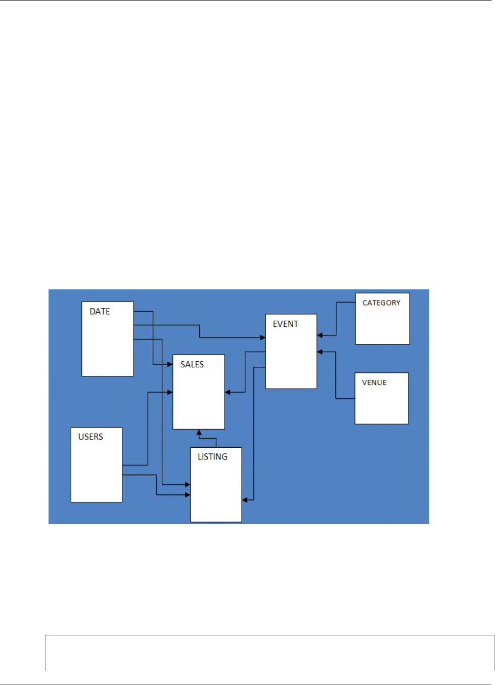
Amazon Redshift Database Developer Guide
Sample Database
Topics
•CATEGORY Table (p. 958)
•DATE Table (p. 958)
•EVENT Table (p. 959)
•VENUE Table (p. 959)
•USERS Table (p. 960)
•LISTING Table (p. 960)
•SALES Table (p. 961)
Most of the examples in the Amazon Redshift documentation use a sample database called TICKIT. This
small database consists of seven tables: two fact tables and five dimensions. You can load the TICKIT
dataset by following the steps in Step 6: Load Sample Data from Amazon S3 in the Amazon Redshift
Getting Started.
This sample database application helps analysts track sales activity for the fictional TICKIT web site,
where users buy and sell tickets online for sporting events, shows, and concerts. In particular, analysts
can identify ticket movement over time, success rates for sellers, and the best-selling events, venues, and
seasons. Analysts can use this information to provide incentives to buyers and sellers who frequent the
site, to attract new users, and to drive advertising and promotions.
For example, the following query finds the top five sellers in San Diego, based on the number of tickets
sold in 2008:
select sellerid, username, (firstname ||' '|| lastname) as name,
city, sum(qtysold)
from sales, date, users
API Version 2012-12-01
957
Amazon Redshift Database Developer Guide
CATEGORY Table
where sales.sellerid = users.userid
and sales.dateid = date.dateid
and year = 2008
and city = 'San Diego'
group by sellerid, username, name, city
order by 5 desc
limit 5;
sellerid | username | name | city | sum
----------+----------+-------------------+-----------+-----
49977 | JJK84WTE | Julie Hanson | San Diego | 22
19750 | AAS23BDR | Charity Zimmerman | San Diego | 21
29069 | SVL81MEQ | Axel Grant | San Diego | 17
43632 | VAG08HKW | Griffin Dodson | San Diego | 16
36712 | RXT40MKU | Hiram Turner | San Diego | 14
(5 rows)
The database used for the examples in this guide contains a small data set; the two fact tables each
contain less than 200,000 rows, and the dimensions range from 11 rows in the CATEGORY table up to
about 50,000 rows in the USERS table.
In particular, the database examples in this guide demonstrate the key features of Amazon Redshift table
design:
• Data distribution
• Data sort
• Columnar compression
CATEGORY Table
Column Name Data Type Description
CATID SMALLINT Primary key, a unique ID value for each row. Each row
represents a specific type of event for which tickets are bought
and sold.
CATGROUP VARCHAR(10) Descriptive name for a group of events, such as Shows and
Sports.
CATNAME VARCHAR(10) Short descriptive name for a type of event within a group,
such as Opera and Musicals.
CATDESC VARCHAR(30) Longer descriptive name for the type of event, such as
Musical theatre.
DATE Table
Column Name Data Type Description
DATEID SMALLINT Primary key, a unique ID value for each row. Each row
represents a day in the calendar year.
CALDATE DATE Calendar date, such as 2008-06-24.
API Version 2012-12-01
958
Amazon Redshift Database Developer Guide
EVENT Table
Column Name Data Type Description
DAY CHAR(3) Day of week (short form), such as SA.
WEEK SMALLINT Week number, such as 26.
MONTH CHAR(5) Month name (short form), such as JUN.
QTR CHAR(5) Quarter number (1 through 4).
YEAR SMALLINT Four-digit year (2008).
HOLIDAY BOOLEAN Flag that denotes whether the day is a public holiday
(U.S.).
EVENT Table
Column Name Data Type Description
EVENTID INTEGER Primary key, a unique ID value for each row. Each row
represents a separate event that takes place at a specific
venue at a specific time.
VENUEID SMALLINT Foreign-key reference to the VENUE table.
CATID SMALLINT Foreign-key reference to the CATEGORY table.
DATEID SMALLINT Foreign-key reference to the DATE table.
EVENTNAME VARCHAR(200) Name of the event, such as Hamlet or La Traviata.
STARTTIME TIMESTAMP Full date and start time for the event, such as
2008-10-10 19:30:00.
VENUE Table
Column Name Data Type Description
VENUEID SMALLINT Primary key, a unique ID value for each row. Each row
represents a specific venue where events take place.
VENUENAME VARCHAR(100) Exact name of the venue, such as Cleveland
Browns Stadium.
VENUECITY VARCHAR(30) City name, such as Cleveland.
VENUESTATE CHAR(2) Two-letter state or province abbreviation (United
States and Canada), such as OH.
VENUESEATS INTEGER Maximum number of seats available at the venue, if
known, such as 73200. For demonstration purposes,
this column contains some null values and zeroes.
API Version 2012-12-01
959

Amazon Redshift Database Developer Guide
USERS Table
USERS Table
Column Name Data Type Description
USERID INTEGER Primary key, a unique ID value for each row. Each row
represents a registered user (a buyer or seller or both)
who has listed or bought tickets for at least one event.
USERNAME CHAR(8) An 8-character alphanumeric username, such as
PGL08LJI.
FIRSTNAME VARCHAR(30) The user's first name, such as Victor.
LASTNAME VARCHAR(30) The user's last name, such as Hernandez.
CITY VARCHAR(30) The user's home city, such as Naperville.
STATE CHAR(2) The user's home state, such as GA.
EMAIL VARCHAR(100) The user's email address; this column contains random
Latin values, such as turpis@accumsanlaoreet.org.
PHONE CHAR(14) The user's 14-character phone number, such as (818)
765-4255.
LIKESPORTS, ... BOOLEAN A series of 10 different columns that identify the user's
likes and dislikes with true and false values.
LISTING Table
Column Name Data Type Description
LISTID INTEGER Primary key, a unique ID value for each row. Each row
represents a listing of a batch of tickets for a specific
event.
SELLERID INTEGER Foreign-key reference to the USERS table, identifying the
user who is selling the tickets.
EVENTID INTEGER Foreign-key reference to the EVENT table.
DATEID SMALLINT Foreign-key reference to the DATE table.
NUMTICKETS SMALLINT The number of tickets available for sale, such as 2 or 20.
PRICEPERTICKET DECIMAL(8,2) The fixed price of an individual ticket, such as 27.00 or
206.00.
TOTALPRICE DECIMAL(8,2) The total price for this listing
(NUMTICKETS*PRICEPERTICKET).
LISTTIME TIMESTAMP The full date and time when the listing was posted, such
as 2008-03-18 07:19:35.
API Version 2012-12-01
960
Amazon Redshift Database Developer Guide
SALES Table
SALES Table
Column Name Data Type Description
SALESID INTEGER Primary key, a unique ID value for each row. Each row
represents a sale of one or more tickets for a specific event,
as offered in a specific listing.
LISTID INTEGER Foreign-key reference to the LISTING table.
SELLERID INTEGER Foreign-key reference to the USERS table (the user who
sold the tickets).
BUYERID INTEGER Foreign-key reference to the USERS table (the user who
bought the tickets).
EVENTID INTEGER Foreign-key reference to the EVENT table.
DATEID SMALLINT Foreign-key reference to the DATE table.
QTYSOLD SMALLINT The number of tickets that were sold, from 1 to 8. (A
maximum of 8 tickets can be sold in a single transaction.)
PRICEPAID DECIMAL(8,2) The total price paid for the tickets, such as 75.00 or
488.00. The individual price of a ticket is PRICEPAID/
QTYSOLD.
COMMISSION DECIMAL(8,2) The 15% commission that the business collects from the
sale, such as 11.25 or 73.20. The seller receives 85% of
the PRICEPAID value.
SALETIME TIMESTAMP The full date and time when the sale was completed, such
as 2008-05-24 06:21:47.
API Version 2012-12-01
961

Amazon Redshift Database Developer Guide
Time Zone Names
Appendix: Time Zone Names and
Abbreviations
Topics
•Time Zone Names (p. 962)
•Time Zone Abbreviations (p. 971)
The following lists contain most of the valid time zone names and time zone abbreviations that can be
specified with the CONVERT_TIMEZONE Function (p. 672).
Time Zone Names
The following list contains most of the valid time zone names that can be specified with the
CONVERT_TIMEZONE Function (p. 672). For a current, complete of list time zone names, execute the
following command.
select pg_timezone_names();
Even though some of the time zone names in this list are capitalized initialisms or acronyms (for
example; GB, PRC, ROK), the CONVERT_TIMEZONE function treats them as time zone names, not time
zone abbreviations.
Africa/Abidjan
Africa/Accra
Africa/Addis_Ababa
Africa/Algiers
Africa/Asmara
Africa/Asmera
Africa/Bamako
Africa/Bangui
Africa/Banjul
Africa/Bissau
Africa/Blantyre
Africa/Brazzaville
Africa/Bujumbura
Africa/Cairo
Africa/Casablanca
Africa/Ceuta
Africa/Conakry
Africa/Dakar
Africa/Dar_es_Salaam
Africa/Djibouti
Africa/Douala
Africa/El_Aaiun
Africa/Freetown
Africa/Gaborone
Africa/Harare
Africa/Johannesburg
Africa/Juba
Africa/Kampala
Africa/Khartoum
API Version 2012-12-01
962

Amazon Redshift Database Developer Guide
Time Zone Names
Africa/Kigali
Africa/Kinshasa
Africa/Lagos
Africa/Libreville
Africa/Lome
Africa/Luanda
Africa/Lubumbashi
Africa/Lusaka
Africa/Malabo
Africa/Maputo
Africa/Maseru
Africa/Mbabane
Africa/Mogadishu
Africa/Monrovia
Africa/Nairobi
Africa/Ndjamena
Africa/Niamey
Africa/Nouakchott
Africa/Ouagadougou
Africa/Porto-Novo
Africa/Sao_Tome
Africa/Timbuktu
Africa/Tripoli
Africa/Tunis
Africa/Windhoek
America/Adak
America/Anchorage
America/Anguilla
America/Antigua
America/Araguaina
America/Argentina/Buenos_Aires
America/Argentina/Catamarca
America/Argentina/ComodRivadavia
America/Argentina/Cordoba
America/Argentina/Jujuy
America/Argentina/La_Rioja
America/Argentina/Mendoza
America/Argentina/Rio_Gallegos
America/Argentina/Salta
America/Argentina/San_Juan
America/Argentina/San_Luis
America/Argentina/Tucuman
America/Argentina/Ushuaia
America/Aruba
America/Asuncion
America/Atikokan
America/Atka
America/Bahia
America/Bahia_Banderas
America/Barbados
America/Belem
America/Belize
America/Blanc-Sablon
America/Boa_Vista
America/Bogota
America/Boise
America/Buenos_Aires
America/Cambridge_Bay
America/Campo_Grande
America/Cancun
America/Caracas
America/Catamarca
America/Cayenne
America/Cayman
America/Chicago
America/Chihuahua
API Version 2012-12-01
963

Amazon Redshift Database Developer Guide
Time Zone Names
America/Coral_Harbour
America/Cordoba
America/Costa_Rica
America/Creston
America/Cuiaba
America/Curacao
America/Danmarkshavn
America/Dawson
America/Dawson_Creek
America/Denver
America/Detroit
America/Dominica
America/Edmonton
America/Eirunepe
America/El_Salvador
America/Ensenada
America/Fort_Wayne
America/Fortaleza
America/Glace_Bay
America/Godthab
America/Goose_Bay
America/Grand_Turk
America/Grenada
America/Guadeloupe
America/Guatemala
America/Guayaquil
America/Guyana
America/Halifax
America/Havana
America/Hermosillo
America/Indiana/Indianapolis
America/Indiana/Knox
America/Indiana/Marengo
America/Indiana/Petersburg
America/Indiana/Tell_City
America/Indiana/Vevay
America/Indiana/Vincennes
America/Indiana/Winamac
America/Indianapolis
America/Inuvik
America/Iqaluit
America/Jamaica
America/Jujuy
America/Juneau
America/Kentucky/Louisville
America/Kentucky/Monticello
America/Knox_IN
America/Kralendijk
America/La_Paz
America/Lima
America/Los_Angeles
America/Louisville
America/Lower_Princes
America/Maceio
America/Managua
America/Manaus
America/Marigot
America/Martinique
America/Matamoros
America/Mazatlan
America/Mendoza
America/Menominee
America/Merida
America/Metlakatla
America/Mexico_City
America/Miquelon
API Version 2012-12-01
964

Amazon Redshift Database Developer Guide
Time Zone Names
America/Moncton
America/Monterrey
America/Montevideo
America/Montreal
America/Montserrat
America/Nassau
America/New_York
America/Nipigon
America/Nome
America/Noronha
America/North_Dakota/Beulah
America/North_Dakota/Center
America/North_Dakota/New_Salem
America/Ojinaga
America/Panama
America/Pangnirtung
America/Paramaribo
America/Phoenix
America/Port_of_Spain
America/Port-au-Prince
America/Porto_Acre
America/Porto_Velho
America/Puerto_Rico
America/Rainy_River
America/Rankin_Inlet
America/Recife
America/Regina
America/Resolute
America/Rio_Branco
America/Rosario
America/Santa_Isabel
America/Santarem
America/Santiago
America/Santo_Domingo
America/Sao_Paulo
America/Scoresbysund
America/Shiprock
America/Sitka
America/St_Barthelemy
America/St_Johns
America/St_Kitts
America/St_Lucia
America/St_Thomas
America/St_Vincent
America/Swift_Current
America/Tegucigalpa
America/Thule
America/Thunder_Bay
America/Tijuana
America/Toronto
America/Tortola
America/Vancouver
America/Virgin
America/Whitehorse
America/Winnipeg
America/Yakutat
America/Yellowknife
Antarctica/Casey
Antarctica/Davis
Antarctica/DumontDUrville
Antarctica/Macquarie
Antarctica/Mawson
Antarctica/McMurdo
Antarctica/Palmer
Antarctica/Rothera
Antarctica/South_Pole
API Version 2012-12-01
965

Amazon Redshift Database Developer Guide
Time Zone Names
Antarctica/Syowa
Antarctica/Vostok
Arctic/Longyearbyen
Asia/Aden
Asia/Almaty
Asia/Amman
Asia/Anadyr
Asia/Aqtau
Asia/Aqtobe
Asia/Ashgabat
Asia/Ashkhabad
Asia/Baghdad
Asia/Bahrain
Asia/Baku
Asia/Bangkok
Asia/Beirut
Asia/Bishkek
Asia/Brunei
Asia/Calcutta
Asia/Choibalsan
Asia/Chongqing
Asia/Chungking
Asia/Colombo
Asia/Dacca
Asia/Damascus
Asia/Dhaka
Asia/Dili
Asia/Dubai
Asia/Dushanbe
Asia/Gaza
Asia/Harbin
Asia/Hebron
Asia/Ho_Chi_Minh
Asia/Hong_Kong
Asia/Hovd
Asia/Irkutsk
Asia/Istanbul
Asia/Jakarta
Asia/Jayapura
Asia/Jerusalem
Asia/Kabul
Asia/Kamchatka
Asia/Karachi
Asia/Kashgar
Asia/Kathmandu
Asia/Katmandu
Asia/Khandyga
Asia/Kolkata
Asia/Krasnoyarsk
Asia/Kuala_Lumpur
Asia/Kuching
Asia/Kuwait
Asia/Macao
Asia/Macau
Asia/Magadan
Asia/Makassar
Asia/Manila
Asia/Muscat
Asia/Nicosia
Asia/Novokuznetsk
Asia/Novosibirsk
Asia/Omsk
Asia/Oral
Asia/Phnom_Penh
Asia/Pontianak
Asia/Pyongyang
API Version 2012-12-01
966

Amazon Redshift Database Developer Guide
Time Zone Names
Asia/Qatar
Asia/Qyzylorda
Asia/Rangoon
Asia/Riyadh
Asia/Riyadh87
Asia/Riyadh88
Asia/Riyadh89
Asia/Saigon
Asia/Sakhalin
Asia/Samarkand
Asia/Seoul
Asia/Shanghai
Asia/Singapore
Asia/Taipei
Asia/Tashkent
Asia/Tbilisi
Asia/Tehran
Asia/Tel_Aviv
Asia/Thimbu
Asia/Thimphu
Asia/Tokyo
Asia/Ujung_Pandang
Asia/Ulaanbaatar
Asia/Ulan_Bator
Asia/Urumqi
Asia/Ust-Nera
Asia/Vientiane
Asia/Vladivostok
Asia/Yakutsk
Asia/Yekaterinburg
Asia/Yerevan
Atlantic/Azores
Atlantic/Bermuda
Atlantic/Canary
Atlantic/Cape_Verde
Atlantic/Faeroe
Atlantic/Faroe
Atlantic/Jan_Mayen
Atlantic/Madeira
Atlantic/Reykjavik
Atlantic/South_Georgia
Atlantic/St_Helena
Atlantic/Stanley
Australia/ACT
Australia/Adelaide
Australia/Brisbane
Australia/Broken_Hill
Australia/Canberra
Australia/Currie
Australia/Darwin
Australia/Eucla
Australia/Hobart
Australia/LHI
Australia/Lindeman
Australia/Lord_Howe
Australia/Melbourne
Australia/North
Australia/NSW
Australia/Perth
Australia/Queensland
Australia/South
Australia/Sydney
Australia/Tasmania
Australia/Victoria
Australia/West
Australia/Yancowinna
API Version 2012-12-01
967

Amazon Redshift Database Developer Guide
Time Zone Names
Brazil/Acre
Brazil/DeNoronha
Brazil/East
Brazil/West
Canada/Atlantic
Canada/Central
Canada/Eastern
Canada/East-Saskatchewan
Canada/Mountain
Canada/Newfoundland
Canada/Pacific
Canada/Saskatchewan
Canada/Yukon
CET
Chile/Continental
Chile/EasterIsland
CST6CDT
Cuba
EET
Egypt
Eire
EST
EST5EDT
Etc/GMT
Etc/GMT+0
Etc/GMT+1
Etc/GMT+10
Etc/GMT+11
Etc/GMT+12
Etc/GMT+2
Etc/GMT+3
Etc/GMT+4
Etc/GMT+5
Etc/GMT+6
Etc/GMT+7
Etc/GMT+8
Etc/GMT+9
Etc/GMT0
Etc/GMT-0
Etc/GMT-1
Etc/GMT-10
Etc/GMT-11
Etc/GMT-12
Etc/GMT-13
Etc/GMT-14
Etc/GMT-2
Etc/GMT-3
Etc/GMT-4
Etc/GMT-5
Etc/GMT-6
Etc/GMT-7
Etc/GMT-8
Etc/GMT-9
Etc/Greenwich
Etc/UCT
Etc/Universal
Etc/UTC
Etc/Zulu
Europe/Amsterdam
Europe/Andorra
Europe/Athens
Europe/Belfast
Europe/Belgrade
Europe/Berlin
Europe/Bratislava
Europe/Brussels
API Version 2012-12-01
968

Amazon Redshift Database Developer Guide
Time Zone Names
Europe/Bucharest
Europe/Budapest
Europe/Busingen
Europe/Chisinau
Europe/Copenhagen
Europe/Dublin
Europe/Gibraltar
Europe/Guernsey
Europe/Helsinki
Europe/Isle_of_Man
Europe/Istanbul
Europe/Jersey
Europe/Kaliningrad
Europe/Kiev
Europe/Lisbon
Europe/Ljubljana
Europe/London
Europe/Luxembourg
Europe/Madrid
Europe/Malta
Europe/Mariehamn
Europe/Minsk
Europe/Monaco
Europe/Moscow
Europe/Nicosia
Europe/Oslo
Europe/Paris
Europe/Podgorica
Europe/Prague
Europe/Riga
Europe/Rome
Europe/Samara
Europe/San_Marino
Europe/Sarajevo
Europe/Simferopol
Europe/Skopje
Europe/Sofia
Europe/Stockholm
Europe/Tallinn
Europe/Tirane
Europe/Tiraspol
Europe/Uzhgorod
Europe/Vaduz
Europe/Vatican
Europe/Vienna
Europe/Vilnius
Europe/Volgograd
Europe/Warsaw
Europe/Zagreb
Europe/Zaporozhye
Europe/Zurich
GB
GB-Eire
GMT
GMT+0
GMT0
GMT-0
Greenwich
Hongkong
HST
Iceland
Indian/Antananarivo
Indian/Chagos
Indian/Christmas
Indian/Cocos
Indian/Comoro
API Version 2012-12-01
969

Amazon Redshift Database Developer Guide
Time Zone Names
Indian/Kerguelen
Indian/Mahe
Indian/Maldives
Indian/Mauritius
Indian/Mayotte
Indian/Reunion
Iran
Israel
Jamaica
Japan
Kwajalein
Libya
MET
Mexico/BajaNorte
Mexico/BajaSur
Mexico/General
Mideast/Riyadh87
Mideast/Riyadh88
Mideast/Riyadh89
MST
MST7MDT
Navajo
NZ
NZ-CHAT
Pacific/Apia
Pacific/Auckland
Pacific/Chatham
Pacific/Chuuk
Pacific/Easter
Pacific/Efate
Pacific/Enderbury
Pacific/Fakaofo
Pacific/Fiji
Pacific/Funafuti
Pacific/Galapagos
Pacific/Gambier
Pacific/Guadalcanal
Pacific/Guam
Pacific/Honolulu
Pacific/Johnston
Pacific/Kiritimati
Pacific/Kosrae
Pacific/Kwajalein
Pacific/Majuro
Pacific/Marquesas
Pacific/Midway
Pacific/Nauru
Pacific/Niue
Pacific/Norfolk
Pacific/Noumea
Pacific/Pago_Pago
Pacific/Palau
Pacific/Pitcairn
Pacific/Pohnpei
Pacific/Ponape
Pacific/Port_Moresby
Pacific/Rarotonga
Pacific/Saipan
Pacific/Samoa
Pacific/Tahiti
Pacific/Tarawa
Pacific/Tongatapu
Pacific/Truk
Pacific/Wake
Pacific/Wallis
Pacific/Yap
API Version 2012-12-01
970

Amazon Redshift Database Developer Guide
Time Zone Abbreviations
Poland
Portugal
PRC
PST8PDT
ROK
Singapore
Turkey
UCT
Universal
US/Alaska
US/Aleutian
US/Arizona
US/Central
US/Eastern
US/East-Indiana
US/Hawaii
US/Indiana-Starke
US/Michigan
US/Mountain
US/Pacific
US/Pacific-New
US/Samoa
UTC
WET
W-SU
Zulu
Time Zone Abbreviations
The following list contains all of the valid time zone abbreviations that can be specified with the
CONVERT_TIMEZONE Function (p. 672).
For a current, complete of list time zone abbreviations, execute the following command.
select pg_timezone_abbrevs();
ACSST
ACST
ACT
ADT
AESST
AEST
AFT
AKDT
AKST
ALMST
ALMT
AMST
AMT
ANAST
ANAT
ARST
ART
AST
AWSST
AWST
AZOST
AZOT
AZST
AZT
API Version 2012-12-01
971

Amazon Redshift Database Developer Guide
Time Zone Abbreviations
BDST
BDT
BNT
BORT
BOT
BRA
BRST
BRT
BST
BTT
CADT
CAST
CCT
CDT
CEST
CET
CETDST
CHADT
CHAST
CHUT
CKT
CLST
CLT
COT
CST
CXT
DAVT
DDUT
EASST
EAST
EAT
EDT
EEST
EET
EETDST
EGST
EGT
EST
FET
FJST
FJT
FKST
FKT
FNST
FNT
GALT
GAMT
GEST
GET
GFT
GILT
GMT
GYT
HKT
HST
ICT
IDT
IOT
IRKST
IRKT
IRT
IST
JAYT
JST
KDT
KGST
API Version 2012-12-01
972

Amazon Redshift Database Developer Guide
Time Zone Abbreviations
KGT
KOST
KRAST
KRAT
KST
LHDT
LHST
LIGT
LINT
LKT
MAGST
MAGT
MART
MAWT
MDT
MEST
MET
METDST
MEZ
MHT
MMT
MPT
MSD
MSK
MST
MUST
MUT
MVT
MYT
NDT
NFT
NOVST
NOVT
NPT
NST
NUT
NZDT
NZST
NZT
OMSST
OMST
PDT
PET
PETST
PETT
PGT
PHOT
PHT
PKST
PKT
PMDT
PMST
PONT
PST
PWT
PYST
PYT
RET
SADT
SAST
SCT
SGT
TAHT
TFT
TJT
TKT
API Version 2012-12-01
973

Amazon Redshift Database Developer Guide
Time Zone Abbreviations
TMT
TOT
TRUT
TVT
UCT
ULAST
ULAT
UT
UTC
UYST
UYT
UZST
UZT
VET
VLAST
VLAT
VOLT
VUT
WADT
WAKT
WAST
WAT
WDT
WET
WETDST
WFT
WGST
WGT
YAKST
YAKT
YAPT
YEKST
YEKT
Z
ZULU
API Version 2012-12-01
974

Amazon Redshift Database Developer Guide
Document History
The following table describes the important changes in each release of the Amazon Redshift Database
Developer Guide after May 2018. For notification about updates to this documentation, you can subscribe
to an RSS feed.
API version: 2012-12-01
Latest documentation update: December 3, 2018
For a list of the changes to the Amazon Redshift Cluster Management Guide, see Amazon Redshift Cluster
Management Guide Document History.
For more information about new features, including a list of fixes and the associated cluster version
numbers for each release, see Cluster Version History.
update-history-change update-history-description update-history-date
DROP EXTERNAL DATABASE You can drop an external
database by including the DROP
EXTERNAL DATABASE clause
with a DROP SCHEMA command.
December 3, 2018
Cross-region UNLOAD You can UNLOAD to an Amazon
S3 in another AWS Region
by specifying the REGION
parameter.
October 31, 2018
Automatic Vacuum Delete Amazon Redshift automatically
runs a VACUUM DELETE
operation in the background, so
you rarely, if ever, need to run a
DELETE ONLY vacuum. Amazon
Redshift schedules the VACUUM
DELETE to run during periods
of reduced load and pauses the
operation during periods of high
load.
October 31, 2018
Automatic Distribution When you don't specify a
distribution style with a CREATE
TABLE statement, Amazon
Redshift assigns an optimal
distribution style based on
the table data. The change
in distribution occurs in the
background, in a few seconds.
October 31, 2018
Fine grained access control for
the AWS Glue Data Catalog
You can now specify levels of
access to data stored in the AWS
Glue data catalog.
October 15, 2018
UNLOAD with data types You can specify the MANIFEST
VERBOSE option with an
UNLOAD command to add
metadata to the manifest file,
October 10, 2018
API Version 2012-12-01
975

Amazon Redshift Database Developer Guide
including the names and data
types of columns, file sizes, and
row counts.
Add multiple partitions using a
single ALTER TABLE statement
For Redshift Spectrum external
tables, you can combine multiple
PARTITION clauses in a single
ALTER TABLE ADD statement.
For more information, see Alter
External Table Examples.
October 10, 2018
UNLOAD with header You can specify the HEADER
option with an UNLOAD
command to add a header line
containing column names at the
top of each output file.
September 19, 2018
New system table and views SVL_S3Retries, SVL_USER_INFO,
and STL_DISK_FULL_DIAG
documentation added.
August 31, 2018
Support for nested data in
Amazon Redshift Spectrum
You can now query nested data
stored in Amazon Redshift
Spectrum tables. For more
information, see Tutorial:
Querying Nested Data with
Amazon Redshift Spectrum.
August 8, 2018
SQA on by default Short query acceleration (SQA)
is now enabled by default for all
new clusters. SQA uses machine
learning to provide higher
performance, faster results,
and better predictability of
query execution times. For more
information, see Short Query
Acceleration.
August 8, 2018
Amazon Redshift Advisor You can now get tailored
recommendations on how to
improve cluster performance
and reduce operating costs from
the Amazon Redshift Advisor.
For more information, see
Amazon Redshift Advisor.
July 26, 2018
Immediate alias reference You can now refer to an
aliased expression immediately
after you define it. For more
information, see SELECT List.
July 18, 2018
Specify compression type when
creating an external table
You can now specify
compression type when creating
an external table with Amazon
Redshift Spectrum. For more
information, see Create External
Tables.
June 27, 2018
API Version 2012-12-01
976
Amazon Redshift Database Developer Guide
Earlier Updates
PG_LAST_UNLOAD_ID Documentation added for
a new System Information
function: PG_LAST_UNLOAD_ID.
For more information, see
PG_LAST_UNLOAD_ID.
June 27, 2018
ALTER TABLE RENAME COLUMN ALTER TABLE now supports
renaming columns for external
tables. For more information,
see Alter External Table
Examples.
June 7, 2018
Earlier Updates
The following table describes the important changes in each release of the Amazon Redshift Database
Developer Guide before June 2018.
Change Description Date Changed
COPY from
columnar formats
COPY now supports loading from files on Amazon
S3 that use Parquet and ORC columnar data formats.
For more information, see COPY from Columnar Data
Formats (p. 431)
May 17, 2018
Dynamic maximum
run time for SQA
By default, workload management (WLM) now
dynamically assigns a value for the short query
acceleration (SQA) maximum run time based on analysis
of your cluster's workload. For more information, see
Maximum Run Time for Short Queries (p. 292).
May 17, 2018
New column in
STL_LOAD_COMMITS
The STL_LOAD_COMMITS (p. 823) system table has a new
column, file_format.
May 10, 2018
New columns in
STL_HASHJOIN and
other system log
tables
The STL_HASHJOIN (p. 819) system table has three new
columns, hash_segment, hash_step, and checksum.
Also, a checksum was added to STL_MERGEJOIN,
STL_NESTLOOP, STL_HASH, STL_SCAN, STL_SORT,
STL_LIMIT, and STL_PROJECT.
May 17, 2018
New columns in
STL_AGGR
The STL_AGGR (p. 800) system table has two new
columns, resizes and flushable.
April 19, 2018
New options for
REGEX functions
For the REGEXP_INSTR (p. 745) and
REGEXP_SUBSTR (p. 748) functions, you can now specify
which occurence of a match to use and whether to
perform a case-sensitive match. REGEXP_INSTR also
allows you specify whether to return the position of the
first character of the match or the position of the first
character following the end of the match.
March 22, 2018
New columns in
system tables
The tombstonedblocks, tossedblocks, and batched_by
columns were added to the STL_COMMIT_STATS (p. 806)
system table. The localslice column was added to the
STV_SLICES (p. 884) system view.
March 22, 2018
API Version 2012-12-01
977
Amazon Redshift Database Developer Guide
Earlier Updates
Change Description Date Changed
Add and drop
columns in external
tables
ALTER TABLE (p. 365) now supports ADD COLUMN and
DROP COLUMN for Amazon Redshift Spectrum external
tables.
March 22, 2018
Amazon Redshift
Spectrum new AWS
Regions
Redshift Spectrum is now available in the Mumbai and
São Paulo Regions. For a list of supported Regions, see
Amazon Redshift Spectrum Regions (p. 149).
March 22, 2018
Table limit
increased to 20,000
The maximum number of tables is now 20,000 for
8xlarge cluster node types. The limit for large and
xlarge node types is 9,900. For more information, see
Limits (p. 477).
March 13, 2018
Amazon Redshift
Spectrum support
for JSON and Ion
Using Redshift Spectrum, you can reference files with
scalar data in JSON or Ion data formats. For more
information, see CREATE EXTERNAL TABLE (p. 452).
February 26, 2018
IAM role chaining
for Amazon
Redshift Spectrum
You can chain AWS Identity and Access Management
(IAM) roles so that your cluster can assume other roles
not attached to the cluster, including roles belonging to
another AWS account. For more information, see Chaining
IAM Roles in Amazon Redshift Spectrum (p. 158).
February 1, 2018
ADD PARTITION
supports IF NOT
EXISTS
The ADD PARTITION clause for ALTER TABLE now
supports an IF NOT EXISTS option. For more information,
see ALTER TABLE (p. 365).
January 11, 2018
DATE data for
external tables
Amazon Redshift Spectrum external tables now support
the DATE data type. For more information, see CREATE
EXTERNAL TABLE (p. 452).
January 11, 2018
Amazon Redshift
Spectrum new AWS
Regions
Redshift Spectrum is now available in the Singapore,
Sydney, Seoul, and Frankfurt Regions. For a list of
supported AWS Regions, see Amazon Redshift Spectrum
Regions (p. 149).
November 16, 2017
Short query
acceleration
in Amazon
Redshift workload
management (WLM)
Short query acceleration (SQA) prioritizes selected short-
running queries ahead of longer-running queries. SQA
executes short-running queries in a dedicated space, so
that SQA queries aren't forced to wait in queues behind
longer queries. With SQA, short-running queries begin
executing more quickly and users see results sooner. For
more information, see Short Query Acceleration (p. 291).
November 16, 2017
WLM reassigns
hopped queries
Instead of canceling and restarting a hopped query,
Amazon Redshift workload management (WLM) now
reassigns eligible queries to a new queue. When WLM
reassigns a query, it moves the query to the new queue
and continues execution, which saves time and system
resources. Hopped queries that are not eligible to
be reassigned are restarted or canceled. For more
information, see WLM Query Queue Hopping (p. 288).
November 16, 2017
API Version 2012-12-01
978

Amazon Redshift Database Developer Guide
Earlier Updates
Change Description Date Changed
System log access
for users
In most system log tables that are visible to users, rows
generated by another user are invisible to a regular user
by default. To permit a regular user to see all rows in
user-visible tables, including rows generated by another
user, run ALTER USER (p. 377) or CREATE USER (p. 490)
and set the SYSLOG ACCESS (p. 378) parameter to
UNRESTRICTED.
November 16, 2017
Result caching With result caching, when you run a query Amazon
Redshift caches the result. When you run the query
again, Amazon Redshift checks for a valid, cached
copy of the query result. If a match is found in the
result cache, Amazon Redshift uses the cached result
and doesn’t execute the query. Result caching is
enabled by default. To disable result caching, set the
enable_result_cache_for_session (p. 949) configuration
parameter to off.
November 16, 2017
Column metadata
functions
PG_GET_COLS (p. 787) and
PG_GET_LATE_BINDING_VIEW_COLS (p. 788) return
column metadata for Amazon Redshift tables, views, and
late-binding views.
November 16, 2017
WLM queue
hopping for CTAS
Amazon Redshift workload management (WLM)
now supports query queue hopping for CREATE
TABLE AS (p. 483) (CTAS) statements as well as read-
only queries, such as SELECT statements. For more
information, see WLM Query Queue Hopping (p. 288).
October 19, 2017
Amazon Redshift
Spectrum manifest
files
When you create a Redshift Spectrum external table, you
can specify a manifest file that lists the locations of data
files on Amazon S3. For more information, see CREATE
EXTERNAL TABLE (p. 452).
October 19, 2017
Amazon Redshift
Spectrum new AWS
Regions
Redshift Spectrum is now available in the EU (Ireland)
and Asia Pacific (Tokyo) Regions. For a list of supported
AWS Regions, see Amazon Redshift Spectrum
Considerations (p. 149).
October 19, 2017
Amazon Redshift
Spectrum added file
formats
You can now create Redshift Spectrum external tables
based on Regex, OpenCSV, and Avro data file formats. For
more information, see CREATE EXTERNAL TABLE (p. 452).
October 5, 2017
Pseudocolumns for
Amazon Redshift
Spectrum external
tables
You can select the $path and $size pseudocolumns in a
Redshift Spectrum external table to view the location and
size of the referenced data files in Amazon S3. For more
information, see Pseudocolumns (p. 172).
October 5, 2017
Functions to
validate JSON
You can use the IS_VALID_JSON (p. 762) and
IS_VALID_JSON_ARRAY (p. 763) functions to check for
valid JSON formatting. The other JSON functions now
have an optional null_if_invalid argument.
October 5, 2017
API Version 2012-12-01
979
Amazon Redshift Database Developer Guide
Earlier Updates
Change Description Date Changed
LISTAGG DISTINCT You can use the DISTINCT clause with the
LISTAGG (p. 594) aggregate function and the
LISTAGG (p. 621) window function to eliminate
duplicate values from the specified expression before
concatenating.
October 5, 2017
View column names
in uppercase
To view column names in SELECT
results in uppercase, you can set the
describe_field_name_in_uppercase (p. 949) configuration
parameter to true.
October 5, 2017
Skip header lines in
external tables
You can set the skip.header.line.count property in
the CREATE EXTERNAL TABLE (p. 452) command to skip
header lines at the beginning of Redshift Spectrum data
files.
October 5, 2017
Scan row count WLM query monitor rules uses the scan_row_count
metric to return the number of rows in a scan step. The
row count is the total number of rows emitted before
filtering rows marked for deletion (ghost rows) and
before applying user-defined query filters. For more
information, see Query Monitoring Metrics (p. 301).
September 21, 2017
SQL user-defined
functions
A scalar SQL user-defined function (UDF) incorporates
a SQL SELECT clause that executes when the function is
called and returns a single value. For more information,
see Creating a Scalar SQL UDF (p. 248).
August 31, 2017
Late-binding views A late-binding view is not bound to the underlying
database objects, such as tables and user-defined
functions. As a result, there is no dependency between
the view and the objects it references. You can create
a view even if the referenced objects don't exist.
Because there is no dependency, you can drop or alter
a referenced object without affecting the view. Amazon
Redshift doesn't check for dependencies until the view
is queried. To create a late-binding view, specify the
WITH NO SCHEMA BINDING clause with your CREATE
VIEW statement. For more information, see CREATE
VIEW (p. 493).
August 31, 2017
OCTET_LENGTH
function
OCTET_LENGTH (p. 741) returns the length of the
specified string as the number of bytes.
August 18, 2017
ORC and Grok files
types supported
Amazon Redshift Spectrum now supports the ORC and
Grok data formats for Redshift Spectrum data files. For
more information, see Creating Data Files for Queries in
Amazon Redshift Spectrum (p. 164).
August 18, 2017
RegexSerDe now
supported
Amazon Redshift Spectrum now supports the RegexSerDe
data format. For more information, see Creating Data
Files for Queries in Amazon Redshift Spectrum (p. 164).
July 19, 2017
New columns added
to SVV_TABLES and
SVV_COLUMNS
The columns domain_name and remarks were added to
SVV_COLUMNS (p. 897). A remarks column was added to
SVV_TABLES (p. 926).
July 19, 2017
API Version 2012-12-01
980
Amazon Redshift Database Developer Guide
Earlier Updates
Change Description Date Changed
SVV_TABLES and
SVV_COLUMNS
system views
The SVV_TABLES (p. 926) and SVV_COLUMNS (p. 897)
system views provide information about columns and
other details for local and external tables and views.
July 7, 2017
VPC no longer
required for
Amazon Redshift
Spectrum with
Amazon EMR Hive
metastore
Redshift Spectrum removed the requirement that
the Amazon Redshift cluster and the Amazon EMR
cluster must be in the same VPC and the same subnet
when using an Amazon EMR Hive metastore. For
more information, see Working with Amazon Redshift
Spectrum External Catalogs (p. 167).
July 7, 2017
UNLOAD to smaller
file sizes
By default, UNLOAD creates multiple files on Amazon S3
with a maximum size of 6.2 GB. To create smaller files,
specify the MAXFILESIZE with the UNLOAD command.
You can specify a maximum file size between 5 MB and
6.2 GB. For more information, see UNLOAD (p. 566).
July 7, 2017
TABLE PROPERTIES You can now set the TABLE PROPERTIES numRows
parameter for CREATE EXTERNAL TABLE (p. 452) or
ALTER TABLE (p. 365) to update table statistics to reflect
the number of rows in the table.
June 6, 2017
ANALYZE
PREDICATE
COLUMNS
To save time and cluster resources, you can choose to
analyze only the columns that are likely to be used as
predicates. When you run ANALYZE with the PREDICATE
COLUMNS clause, the analyze operation includes only
columns that have been used in a join, filter condition, or
group by clause, or are used as a sort key or distribution
key. For more information, see Analyzing Tables (p. 223).
May 25, 2017
IAM Policies for
Amazon Redshift
Spectrum
To grant access to an Amazon S3 bucket only using
Redshift Spectrum, you can include a condition that
allows access for the user agent "AWS Redshift/
Spectrum". For more information, see IAM Policies for
Amazon Redshift Spectrum (p. 154).
May 25, 2017
Amazon Redshift
Spectrum Recursive
Scan
Redshift Spectrum now scans files in subfolders as
well as the specified folder in Amazon S3. For more
information, see Creating External Tables for Amazon
Redshift Spectrum (p. 171).
May 25, 2017
Query Monitoring
Rules
Using WLM query monitoring rules, you can define
metrics-based performance boundaries for WLM queues
and specify what action to take when a query goes
beyond those boundaries—log, hop, or abort. You
define query monitoring rules as part of your workload
management (WLM) configuration. For more information,
see WLM Query Monitoring Rules (p. 299).
April 21, 2017
API Version 2012-12-01
981
Amazon Redshift Database Developer Guide
Earlier Updates
Change Description Date Changed
Amazon Redshift
Spectrum
Using Redshift Spectrum, you can efficiently query and
retrieve data from files in Amazon S3 without having
to load the data into tables. Redshift Spectrum queries
execute very fast against large datasets because Redshift
Spectrum scans the data files directly in Amazon S3.
Much of the processing occurs in the Amazon Redshift
Spectrum layer, and most of the data remains in Amazon
S3. Multiple clusters can concurrently query the same
dataset on Amazon S3 without the need to make copies
of the data for each cluster. For more information, see
Using Amazon Redshift Spectrum to Query External
Data (p. 148)
April 19, 2017
New system tables
to support Redshift
Spectrum
The following new system views have been added to
support Redshift Spectrum:
•SVL_S3QUERY (p. 920)
•SVL_S3QUERY_SUMMARY (p. 921)
•SVV_EXTERNAL_COLUMNS (p. 902)
•SVV_EXTERNAL_DATABASES (p. 902)
•SVV_EXTERNAL_PARTITIONS (p. 903)
•SVV_EXTERNAL_TABLES (p. 904)
•PG_EXTERNAL_SCHEMA (p. 938)
April 19, 2017
APPROXIMATE
PERCENTILE_DISC
aggregate function
The APPROXIMATE PERCENTILE_DISC (p. 590) aggregate
function is now available.
April 4, 2017
Server-side
encryption with
KMS
You can now unload data to Amazon S3 using server-side
encryption with an AWS Key Management Service key
(SSE-KMS). In addition, COPY (p. 390) now transparently
loads KMS-encrypted data files from Amazon S3. For
more information, see UNLOAD (p. 566).
February 9, 2017
New authorization
syntax
You can now use the IAM_ROLE,
MASTER_SYMMETRIC_KEY, ACCESS_KEY_ID,
SECRET_ACCESS_KEY, and SESSION_TOKEN parameters
to provide authorization and access information for
COPY, UNLOAD, and CREATE LIBRARY commands.
The new authorization syntax provides a more flexible
alternative to providing a single string argument to the
CREDENTIALS parameter. For more information, see
Authorization Parameters (p. 404).
February 9, 2017
Schema limit
increase
You can now create up to 9,900 schemas per cluster. For
more information, see CREATE SCHEMA (p. 470).
February 9, 2017
Default table
encoding
CREATE TABLE (p. 471) and ALTER TABLE (p. 365) now
assign LZO compression encoding to most new columns.
Columns defined as sort keys, columns that are defined as
BOOLEAN, REAL, or DOUBLE PRECISION data types, and
temporary tables are assigned RAW encoding by default.
For more information, see ENCODE (p. 474).
February 6, 2017
API Version 2012-12-01
982
Amazon Redshift Database Developer Guide
Earlier Updates
Change Description Date Changed
ZSTD compression
encoding
Amazon Redshift now supports ZSTD (p. 125) column
compression encoding.
January 19, 2017
PERCENTILE_CONT
and MEDIAN
aggregate functions
PERCENTILE_CONT (p. 600) and MEDIAN (p. 597) are
now available as aggregate functions as well as window
functions.
January 19, 2017
User-defined
function (UDF) User
Logging
You can use the Python logging module to create
user-defined error and warning messages in your
UDFs. Following query execution, you can query
the SVL_UDF_LOG (p. 930) system view to retrieve
logged messages. For more information about user-
defined messages, see Logging Errors and Warnings in
UDFs (p. 255)
December 8, 2016
ANALYZE
COMPRESSION
estimated reduction
The ANALYZE COMPRESSION command now reports
an estimate for percentage reduction in disk space
for each column. For more information, see ANALYZE
COMPRESSION (p. 382).
November 10, 2016
Connection limits You can now set a limit on the number of database
connections a user is permitted to have open
concurrently. You can also limit the number of concurrent
connections for a database. For more information, see
CREATE USER (p. 490) and CREATE DATABASE (p. 448).
November 10, 2016
COPY sort order
enhancement
COPY now automatically adds new rows to the table's
sorted region when you load your data in sort key order.
For specific requirements to enable this enhancement, see
Loading Your Data in Sort Key Order (p. 235)
November 10, 2016
CTAS with
compression
CREATE TABLE AS (CTAS) now automatically assigns
compression encodings to new tables based on the
column's data type. For more information, see Inheritance
of Column and Table Attributes (p. 485).
October 28, 2016
Time stamp with
time zone data type
Amazon Redshift now supports a time stamp with time
zone (TIMESTAMPTZ (p. 327)) data type. Also, several
new functions have been added to support the new
data type. For more information, see Date and Time
Functions (p. 663).
September 29, 2016
Analyze threshold To reduce processing time and improve overall system
performance for ANALYZE (p. 380) operations, Amazon
Redshift skips analyzing a table if the percentage of rows
that have changed since the last ANALYZE command
run is lower than the analyze threshold specified by the
analyze_threshold_percent (p. 948) parameter. By default,
analyze_threshold_percent is 10.
August 9, 2016
New
STL_RESTARTED_SESSIONS
system table
When Amazon Redshift restarts a session,
STL_RESTARTED_SESSIONS (p. 843) records the new
process ID (PID) and the old PID.
August 9, 2016
Updated the Date
and Time Functions
documentation
Added a summary of functions with links to the Date
and Time Functions (p. 663), and updated the function
references for consistency.
June 24, 2016
API Version 2012-12-01
983
Amazon Redshift Database Developer Guide
Earlier Updates
Change Description Date Changed
New columns in
STL_CONNECTION_LOG
The STL_CONNECTION_LOG (p. 807) system table
has two new columns to track SSL connections. If you
routinely load audit logs to an Amazon Redshift table,
you will need to add the following new columns to the
target table: sslcompression and sslexpansion.
May 5, 2016
MD5-hash password You can specify the password for a CREATE USER (p. 490)
or ALTER USER (p. 377) command by supplying the MD5-
hash string of the password and user name.
April 21, 2016
New column in
STV_TBL_PERM
The backup column in the STV_TBL_PERM (p. 886)
system view indicates whether the table is included
in cluster snapshots. For more information, see
BACKUP (p. 476).
April 21, 2016
No-backup tables For tables, such as staging tables, that won't contain
critical data, you can specify BACKUP NO in your CREATE
TABLE (p. 471) or CREATE TABLE AS (p. 483) statement
to prevent Amazon Redshift from including the table
in automated or manual snapshots. Using no-backup
tables saves processing time when creating snapshots and
restoring from snapshots and reduces storage space on
Amazon S3.
April 7, 2016
VACUUM delete
threshold
By default, the VACUUM (p. 584) command now reclaims
space such that at least 95 percent of the remaining rows
are not marked for deletion. As a result, VACUUM usually
needs much less time for the delete phase compared to
reclaiming 100 percent of deleted rows. You can change
the default threshold for a single table by including the
TO threshold PERCENT parameter when you run the
VACUUM command.
April 7, 2016
SVV_TRANSACTIONS
system table
The SVV_TRANSACTIONS (p. 928) system view records
information about transactions that currently hold locks
on tables in the database.
April 7, 2016
Using IAM roles to
access other AWS
resources
To move data between your cluster and another AWS
resource, such as Amazon S3, Amazon DynamoDB,
Amazon EMR, or Amazon EC2, your cluster must have
permission to access the resource and perform the
necessary actions. As a more secure alternative to
providing an access key pair with COPY, UNLOAD, or
CREATE LIBRARY commands, you can now you specify
an IAM role that your cluster uses for authentication and
authorization. For more information, see Role-Based
Access Control (p. 424).
March 29, 2016
VACUUM sort
threshold
The VACUUM command now skips the sort phase for any
table where more than 95 percent of the table's rows are
already sorted. You can change the default sort threshold
for a single table by including the TO threshold PERCENT
parameter when you run the VACUUM (p. 584) command.
March 17, 2016
API Version 2012-12-01
984
Amazon Redshift Database Developer Guide
Earlier Updates
Change Description Date Changed
New columns in
STL_CONNECTION_LOG
The STL_CONNECTION_LOG (p. 807) system table has
three new columns. If you routinely load audit logs to
an Amazon Redshift table, you will need to add the
following new columns to the target table: sslversion,
sslcipher, and mtu.
March 17, 2016
UNLOAD with bzip2
compression
You now have the option to UNLOAD (p. 566) using bzip2
compression.
February 8, 2016
ALTER TABLE
APPEND
ALTER TABLE APPEND (p. 374) appends rows to a target
table by moving data from an existing source table.
ALTER TABLE APPEND is usually much faster than a
similar CREATE TABLE AS (p. 483) or INSERT (p. 520) INTO
operation because data is moved, not duplicated.
February 8, 2016
WLM Query Queue
Hopping
If workload management (WLM) cancels a read-only
query, such as a SELECT statement, due to a WLM
timeout, WLM attempts to route the query to the next
matching queue. For more information, see WLM Query
Queue Hopping (p. 288)
January 7, 2016
ALTER DEFAULT
PRIVILEGES
You can use the ALTER DEFAULT PRIVILEGES (p. 361)
command to define the default set of access privileges to
be applied to objects that are created in the future by the
specified user.
December 10, 2015
bzip2 file
compression
The COPY (p. 390) command supports loading data from
files that were compressed using bzip2.
December 10, 2015
NULLS FIRST and
NULLS LAST
You can specify whether an ORDER BY clause should rank
NULLS first or last in the result set. For more information,
see ORDER BY Clause (p. 554) and Window Function
Syntax Summary (p. 612).
November 19, 2015
REGION keyword
for CREATE LIBRARY
If the Amazon S3 bucket that contains the UDF library
files does not reside in the same AWS Region as your
Amazon Redshift cluster, you can use the REGION option
to specify the region in which the data is located. For
more information, see CREATE LIBRARY (p. 468).
November 19, 2015
User-defined scalar
functions (UDFs)
You can now create custom user-defined scalar functions
to implement non-SQL processing functionality provided
either by Amazon Redshift-supported modules in
the Python 2.7 Standard Library or your own custom
UDFs based on the Python programming language.
For more information, see Creating User-Defined
Functions (p. 248).
September 11, 2015
Dynamic
properties in WLM
configuration
The WLM configuration parameter now supports applying
some properties dynamically. Other properties remain
static changes and require that associated clusters
be rebooted so that the configuration changes can
be applied. For more information, see WLM Dynamic
and Static Configuration Properties (p. 297) and
Implementing Workload Management (p. 285).
August 3, 2015
API Version 2012-12-01
985
Amazon Redshift Database Developer Guide
Earlier Updates
Change Description Date Changed
LISTAGG function The LISTAGG Function (p. 594) and LISTAGG Window
Function (p. 621) return a string created by concatenating
a set of column values.
July 30, 2015
Deprecated
parameter
The max_cursor_result_set_size configurationparameter
is deprecated. The size of cursor result sets are
constrained based on the cluster's node type. For more
information, see Cursor Constraints (p. 497).
July 24, 2015
Revised COPY
command
documentation
The COPY (p. 390) command reference has been
extensively revised to make the material friendlier and
more accessible.
July 15, 2015
COPY from Avro
format
The COPY (p. 390) command supports loading data in
Avro format from data files on Amazon S3, Amazon EMR,
and from remote hosts using SSH. For more information,
see AVRO (p. 409) and Copy from Avro Examples (p. 444).
July 8, 2015
STV_STARTUP_RECOVERY_STATEThe STV_STARTUP_RECOVERY_STATE (p. 885) system
table records the state of tables that are temporarily
locked during cluster restart operations. Amazon Redshift
places a temporary lock on tables while they are being
processed to resolve stale transactions following a cluster
restart.
May 25, 2015
ORDER BY optional
for ranking
functions
The ORDER BY clause is now optional for certain window
ranking functions. For more information, see CUME_DIST
Window Function (p. 616), DENSE_RANK Window
Function (p. 617), RANK Window Function (p. 630),
NTILE Window Function (p. 626), PERCENT_RANK
Window Function (p. 627), and ROW_NUMBER Window
Function (p. 632).
May 25, 2015
Interleaved Sort
Keys
Interleaved sort keys give equal weight to each column
in the sort key. Using interleaved sort keys instead
of the default compound keys significantly improves
performance for queries that use restrictive predicates
on secondary sort columns, especially for large tables.
Interleaved sorting also improves overall performance
when multiple queries filter on different columns in the
same table. For more information, see Choosing Sort
Keys (p. 140) and CREATE TABLE (p. 471).
May 11, 2015
Revised Tuning
Query Performance
topic
Tuning Query Performance (p. 257) has been expanded
to include new queries for analyzing query performance
and more examples. Also, the topic has been revised
to be clearer and more complete. Amazon Redshift
Best Practices for Designing Queries (p. 32) has more
information about how to write queries to improve
performance.
March 23, 2015
SVL_QUERY_QUEUE_INFOThe SVL_QUERY_QUEUE_INFO (p. 908) view summarizes
details for queries that spent time in a WLM query queue
or commit queue.
February 19, 2015
API Version 2012-12-01
986
Amazon Redshift Database Developer Guide
Earlier Updates
Change Description Date Changed
SVV_TABLE_INFO You can use the SVV_TABLE_INFO (p. 926) view to
diagnose and address table design issues that can
influence query performance, including issues with
compression encoding, distribution keys, sort style, data
distribution skew, table size, and statistics.
February 19, 2015
UNLOAD uses
server-side file
encryption
The UNLOAD (p. 566) command now automatically
uses Amazon S3 server-side encryption (SSE) to encrypt
all unload data files. Server-side encryption adds
another layer of data security with little or no change in
performance.
October 31, 2014
CUME_DIST window
function
The CUME_DIST Window Function (p. 616) calculates the
cumulative distribution of a value within a window or
partition.
October 31, 2014
MONTHS_BETWEEN
function
The MONTHS_BETWEEN Function (p. 687) determines the
number of months between two dates.
October 31, 2014
NEXT_DAY function The NEXT_DAY Function (p. 688) returns the date of the
first instance of a specified day that is later than the given
date.
October 31, 2014
PERCENT_RANK
window function
The PERCENT_RANK Window Function (p. 627) calculates
the percent rank of a given row.
October 31, 2014
RATIO_TO_REPORT
window function
The RATIO_TO_REPORT Window Function (p. 631)
calculates the ratio of a value to the sum of the values in
a window or partition.
October 31, 2014
TRANSLATE
function
The TRANSLATE Function (p. 758) replaces all occurrences
of specified characters within a given expression with
specified substitutes.
October 31, 2014
NVL2 function The NVL2 Expression (p. 660) returns one of two values
based on whether a specified expression evaluates to
NULL or NOT NULL.
October 16, 2014
MEDIAN window
function
The MEDIAN Window Function (p. 623) calculates the
median value for the range of values in a window or
partition.
October 16, 2014
ON ALL TABLES
IN SCHEMA
schema_name
clause for GRANT
and REVOKE
commands
The GRANT (p. 516) and REVOKE (p. 527) commands
have been updated with an ON ALL TABLES IN SCHEMA
schema_name clause. This clause allows you to use a
single command to change privileges for all tables in a
schema.
October 16, 2014
IF EXISTS clause
for DROP SCHEMA,
DROP TABLE, DROP
USER, and DROP
VIEW commands
The DROP SCHEMA (p. 503), DROP TABLE (p. 504), DROP
USER (p. 507), and DROP VIEW (p. 508) commands have
been updated with an IF EXISTS clause. This clause causes
the command to make no changes and return a message
rather than terminating with an error if the specified
object doesn’t exist.
October 16, 2014
API Version 2012-12-01
987
Amazon Redshift Database Developer Guide
Earlier Updates
Change Description Date Changed
IF NOT EXISTS
clause for CREATE
SCHEMA and
CREATE TABLE
commands
The CREATE SCHEMA (p. 470) and CREATE TABLE (p. 471)
commands have been updated with an IF NOT EXISTS
clause. This clause causes the command to make no
changes and return a message rather than terminating
with an error if the specified object already exists.
October 16, 2014
COPY support for
UTF-16 encoding
The COPY command now supports loading from data files
that use UTF-16 encoding as well as UTF-8 encoding. For
more information, see ENCODING (p. 418).
September 29, 2014
New Workload
Management
Tutorial
Tutorial: Configuring Workload Management (WLM)
Queues to Improve Query Processing (p. 90) walks
you through the process of configuring Workload
Management (WLM) queues to improve query processing
and resource allocation.
September 25, 2014
AES 128-bit
Encryption
The COPY command now supports AES 128-bit
encryption as well as AES 256-bit encryption when
loading from data files encrypted using Amazon S3
client-side encryption. For more information, see Loading
Encrypted Data Files from Amazon S3 (p. 195).
September 29, 2014
PG_LAST_UNLOAD_COUNT
function
The PG_LAST_UNLOAD_COUNT function returns
the number of rows that were processed in the most
recent UNLOAD operation. For more information, see
PG_LAST_UNLOAD_COUNT (p. 792).
September 15, 2014
New
Troubleshooting
Queries section
Troubleshooting Queries (p. 280) provides a quick
reference for identifying and addressing some of the
most common and most serious issues you are likely to
encounter with Amazon Redshift queries.
July 7, 2014
New Loading Data
tutorial
Tutorial: Loading Data from Amazon S3 (p. 70) walks you
through the process of loading data into your Amazon
Redshift database tables from data files in an Amazon S3
bucket, from beginning to end.
July 1, 2014
PERCENTILE_CONT
window function
PERCENTILE_CONT Window Function (p. 628) is an
inverse distribution function that assumes a continuous
distribution model. It takes a percentile value and a sort
specification, and returns an interpolated value that
would fall into the given percentile value with respect to
the sort specification.
June 30, 2014
PERCENTILE_DISC
window function
PERCENTILE_DISC Window Function (p. 629) is an inverse
distribution function that assumes a discrete distribution
model. It takes a percentile value and a sort specification
and returns an element from the set.
June 30, 2014
GREATEST and
LEAST functions
The GREATEST and LEAST (p. 658) functions return the
largest or smallest value from a list of expressions.
June 30, 2014
Cross-region COPY The COPY (p. 390) command supports loading data from
an Amazon S3 bucket or Amazon DynamoDB table that
is located in a different region than the Amazon Redshift
cluster. For more information, see REGION (p. 397) in the
COPY command reference.
June 30, 2014
API Version 2012-12-01
988
Amazon Redshift Database Developer Guide
Earlier Updates
Change Description Date Changed
Best Practices
expanded
Amazon Redshift Best Practices (p. 26) has been
expanded, reorganized, and moved to the top of the
navigation hierarchy to make it more discoverable.
May 28, 2014
UNLOAD to a single
file
The UNLOAD (p. 566) command can optionally unload
table data serially to a single file on Amazon S3 by
adding the PARALLEL OFF option. If the size of the data
is greater than the maximum file size of 6.2 GB, UNLOAD
creates additional files.
May 6, 2014
REGEXP functions The REGEXP_COUNT (p. 744), REGEXP_INSTR (p. 745),
and REGEXP_REPLACE (p. 746) functions manipulate
strings based on regular expression pattern matching.
May 6, 2014
New Tutorial The new Tutorial: Tuning Table Design (p. 45) walks you
through the steps to optimize the design of your tables,
including testing load and query performance before and
after tuning.
May 2, 2014
COPY from Amazon
EMR
The COPY (p. 390) command supports loading
data directly from Amazon EMR clusters. For more
information, see Loading Data from Amazon
EMR (p. 196).
April 18, 2014
WLM concurrency
limit increase
You can now configure workload management (WLM)
to run up to 50 queries concurrently in user-defined
query queues. This increase gives users more flexibility
for managing system performance by modifying WLM
configurations. For more information, see Defining Query
Queues (p. 285)
April 18, 2014
New configuration
parameter to
manage cursor size
The max_cursor_result_set_size configuration
parameter defines the maximum size of data, in
megabytes, that can be returned per cursor result set
of a larger query. This parameter value also affects the
number of concurrent cursors for the cluster, enabling
you to configure a value that increases or decreases the
number of cursors for your cluster.
For more information, see DECLARE (p. 496) in this guide
and Configure Maximum Size of a Cursor Result Set in the
Amazon Redshift Cluster Management Guide.
March 28, 2014
COPY from JSON
format
The COPY (p. 390) command supports loading data in
JSON format from data files on Amazon S3 and from
remote hosts using SSH. For more information, see COPY
from JSON Format (p. 428) usage notes.
March 25, 2014
New system table
STL_PLAN_INFO
The STL_PLAN_INFO (p. 833) table supplements the
EXPLAIN command as another way to look at query plans.
March 25, 2014
New function
REGEXP_SUBSTR
The REGEXP_SUBSTR Function (p. 748) returns the
characters extracted from a string by searching for a
regular expression pattern.
March 25, 2014
New columns for
STL_COMMIT_STATS
The STL_COMMIT_STATS (p. 806) table has two new
columns: numxids and oldestxid.
March 6, 2014
API Version 2012-12-01
989
Amazon Redshift Database Developer Guide
Earlier Updates
Change Description Date Changed
COPY from SSH
support for gzip and
lzop
The COPY (p. 390) command supports gzip and lzop
compression when loading data through an SSH
connection.
February 13, 2014
New functions The ROW_NUMBER Window Function (p. 632)
returns the number of the current row. The STRTOL
Function (p. 755) converts a string expression of
a number of the specified base to the equivalent
integer value. PG_CANCEL_BACKEND (p. 778) and
PG_TERMINATE_BACKEND (p. 779) enable users to cancel
queries and session connections. The LAST_DAY (p. 686)
function has been added for Oracle compatibility.
February 13, 2014
New system table The STL_COMMIT_STATS (p. 806) system table provides
metrics related to commit performance, including the
timing of the various stages of commit and the number of
blocks committed.
February 13, 2014
FETCH with single-
node clusters
When using a cursor on a single-node cluster, the
maximum number of rows that can be fetched using the
FETCH (p. 515) command is 1000. FETCH FORWARD ALL
is not supported for single-node clusters.
February 13, 2014
DS_DIST_ALL_INNER
redistribution
strategy
DS_DIST_ALL_INNER in the Explain plan output indicates
that the entire inner table was redistributed to a single
slice because the outer table uses DISTSTYLE ALL. For
more information, see Join Type Examples (p. 263) and
Evaluating the Query Plan (p. 133).
January 13, 2014
New system tables
for queries
Amazon Redshift has added new system tables that
customers can use to evaluate query execution for
tuning and troubleshooting. For more information,
see SVL_COMPILE (p. 899), STL_SCAN (p. 849),
STL_RETURN (p. 844), STL_SAVE (p. 848)
STL_ALERT_EVENT_LOG (p. 801).
January 13, 2014
Single-node cursors Cursors are now supported for single-node clusters.
A single-node cluster can have two cursors open at a
time, with a maximum result set of 32 GB. On a single-
node cluster, we recommend setting the ODBC Cache
Size parameter to 1,000. For more information, see
DECLARE (p. 496).
December 13, 2013
ALL distribution
style
ALL distribution can dramatically shorter execution
times for certain types of queries. When a table uses ALL
distribution style, a copy of the table is distributed to
every node. Because the table is effectively collocated
with every other table, no redistribution is needed during
query execution. ALL distribution is not appropriate for
all tables because it increases storage requirements and
load time. For more information, see Choosing a Data
Distribution Style (p. 129).
November 11, 2013
API Version 2012-12-01
990
Amazon Redshift Database Developer Guide
Earlier Updates
Change Description Date Changed
COPY from remote
hosts
In addition to loading tables from data files on Amazon
S3 and from Amazon DynamoDB tables, the COPY
command can load text data from Amazon EMR clusters,
Amazon EC2 instances, and other remote hosts by
using SSH connections. Amazon Redshift uses multiple
simultaneous SSH connections to read and load data in
parallel. For more information, see Loading Data from
Remote Hosts (p. 200).
November 11, 2013
WLM Memory
Percent Used
You can balance workload by designating a specific
percentage of memory for each queue in your workload
management (WLM) configuration. For more information,
see Defining Query Queues (p. 285).
November 11, 2013
APPROXIMATE
COUNT(DISTINCT)
Queries that use APPROXIMATE COUNT(DISTINCT)
execute much faster, with a relative error of about 2%.
The APPROXIMATE COUNT(DISTINCT) function uses a
HyperLogLog algorithm. For more information, see the
COUNT Function (p. 593).
November 11, 2013
New SQL functions
to retrieve recent
query details
Four new SQL functions retrieve details about recent
queries and COPY commands. The new functions make
it easier to query the system log tables, and in many
cases provide necessary details without needing to
access the system tables. For more information, see
PG_BACKEND_PID (p. 786), PG_LAST_COPY_ID (p. 790),
PG_LAST_COPY_COUNT (p. 789),
PG_LAST_QUERY_ID (p. 791).
November 1, 2013
MANIFEST option
for UNLOAD
The MANIFEST option for the UNLOAD command
complements the MANIFEST option for the COPY
command. Using the MANIFEST option with UNLOAD
automatically creates a manifest file that explicitly lists
the data files that were created on Amazon S3 by the
unload operation. You can then use the same manifest
file with a COPY command to load the data. For more
information, see Unloading Data to Amazon S3 (p. 242)
and UNLOAD Examples (p. 571).
November 1, 2013
MANIFEST option
for COPY
You can use the MANIFEST option with the COPY (p. 390)
command to explicitly list the data files that will be
loaded from Amazon S3.
October 18, 2013
System tables for
troubleshooting
queries
Added documentation for system tables that are
used to troubleshoot queries. The STL Tables for
Logging (p. 798) section now contains documentation
for the following system tables: STL_AGGR, STL_BCAST,
STL_DIST, STL_DELETE, STL_HASH, STL_HASHJOIN,
STL_INSERT, STL_LIMIT, STL_MERGE, STL_MERGEJOIN,
STL_NESTLOOP, STL_PARSE, STL_PROJECT, STL_SCAN,
STL_SORT, STL_UNIQUE, STL_WINDOW.
October 3, 2013
CONVERT_TIMEZONE
function
The CONVERT_TIMEZONE Function (p. 672) converts
a timestamp from one time zone to another, with the
option to automatically adjust for daylight savings time.
October 3, 2013
API Version 2012-12-01
991

Amazon Redshift Database Developer Guide
Earlier Updates
Change Description Date Changed
SPLIT_PART
function
The SPLIT_PART Function (p. 753) splits a string on the
specified delimiter and returns the part at the specified
position.
October 3, 2013
STL_USERLOG
system table
STL_USERLOG (p. 859) records details for changes that
occur when a database user is created, altered, or deleted.
October 3, 2013
LZO column
encoding and LZOP
file compression.
LZO (p. 122) column compression encoding combines
a very high compression ratio with good performance.
COPY from Amazon S3 supports loading from files
compressed using LZOP (p. 416) compression.
September 19, 2013
JSON, Regular
Expressions, and
Cursors
Added support for parsing JSON strings, pattern
matching using regular expressions, and using cursors
to retrieve large data sets over an ODBC connection. For
more information, see JSON Functions (p. 761), Pattern-
Matching Conditions (p. 345), and DECLARE (p. 496).
September 10, 2013
ACCEPTINVCHAR
option for COPY
You can successfully load data that contains invalid UTF-8
characters by specifying the ACCEPTINVCHAR option with
the COPY (p. 390) command.
August 29, 2013
CSV option for
COPY
The COPY (p. 390) command now supports loading from
CSV formatted input files.
August 9, 2013
CRC32 The CRC32 Function (p. 732) performs cyclic redundancy
checks.
August 9, 2013
WLM wildcards Workload management (WLM) supports wildcards for
adding user groups and query groups to queues. For more
information, see Wildcards (p. 287).
August 1, 2013
WLM timeout To limit the amount of time that queries in a given WLM
queue are permitted to use, you can set the WLM timeout
value for each queue. For more information, see WLM
Timeout (p. 288).
August 1, 2013
New COPY
options 'auto' and
'epochsecs'
The COPY (p. 390) command performs automatic
recognition of date and time formats. New time formats,
'epochsecs' and 'epochmillisecs' enable COPY to load data
in epoch format.
July 25, 2013
CONVERT_TIMEZONE
function
The CONVERT_TIMEZONE Function (p. 672) converts a
timestamp from one timezone to another.
July 25, 2013
FUNC_SHA1
function
The FUNC_SHA1 Function (p. 733) converts a string using
the SHA1 algorithm.
July 15, 2013
max_execution_time To limit the amount of time queries are permitted to use,
you can set the max_execution_time parameter as part
of the WLM configuration. For more information, see
Modifying the WLM Configuration (p. 293).
July 22, 2013
Four-byte UTF-8
characters
The VARCHAR data type now supports four-byte UTF-8
characters. Five-byte or longer UTF-8 characters are
not supported. For more information, see Storage and
Ranges (p. 323).
July 18, 2013
API Version 2012-12-01
992

Amazon Redshift Database Developer Guide
Earlier Updates
Change Description Date Changed
SVL_QERROR The SVL_QERROR system view has been deprecated. July 12, 2013
Revised Document
History
The Document History page now shows the date the
documentation was updated.
July 12, 2013
STL_UNLOAD_LOG STL_UNLOAD_LOG (p. 858) records the details for an
unload operation.
July 5, 2013
JDBC fetch size
parameter
To avoid client-side out of memory errors when retrieving
large data sets using JDBC, you can enable your client
to fetch data in batches by setting the JDBC fetch size
parameter. For more information, see Setting the JDBC
Fetch Size Parameter (p. 284).
June 27, 2013
UNLOAD encrypted
files
UNLOAD (p. 566) now supports unloading table data to
encrypted files on Amazon S3.
May 22, 2013
Temporary
credentials
COPY (p. 390) and UNLOAD (p. 566) now support the use
of temporary credentials.
April 11, 2013
Added clarifications Clarified and expanded discussions of Designing Tables
and Loading Data.
February 14, 2013
Added Best
Practices
Added Amazon Redshift Best Practices for Designing
Tables (p. 26) and Amazon Redshift Best Practices for
Loading Data (p. 29).
February 14, 2013
Clarified password
constraints
Clarified password constraints for CREATE USER and
ALTER USER, various minor revisions.
February 14, 2013
New Guide This is the first release of the Amazon Redshift Developer
Guide.
February 14, 2013
API Version 2012-12-01
993
