PDF Rnews 2006 2
PDF Rnews_2006-2 CRAN: R News
User Manual: PDF CRAN - Contents of R News
Open the PDF directly: View PDF ![]() .
.
Page Count: 72
- Editorial
- S4 Classes for Distributions
- The regress function
- Processing data for outliers
- Analysing equity portfolios in R
- GroupSeq: Designing clinical trials using group sequential designs
- Using R/Sweave in everyday clinical practice
- changeLOS: An R-package for change in length of hospital stay based on the Aalen-Johansen estimator
- Balloon Plot
- Drawing pedigree diagrams with R and graphviz
- Non-Standard Fonts in PostScript and PDF Graphics
- The doBy package
- Normed division algebras with R: Introducing the onion package
- Resistor networks R: Introducing the ResistorArray package
- The good, the bad, and the ugly---Review of Paul Murrell's new book: ``R Graphics''
- Changes in R
- Changes on CRAN
- R Foundation News
- News from the Bioconductor Project
- Forthcoming Events: DSC 2007

News
The Newsletter of the R Project Volume 6/2, May 2006
Editorial
by Paul Murrell
Welcome to the first regular issue of R News for 2006.
This is a bumper issue, with a thirteen contributed
articles. Many thanks to the contributors and review-
ers for all of the enthusiasm and effort that they put
into these articles.
This issue begins with some “methodological”
papers. Peter Ruckdeschel, Matthias Kohl, Thomas
Stabla, and Florian Camphausen introduce their
distr package, which provides a set of S4 classes and
methods for defining distributions of random vari-
ables. This is followed by an article from David Clif-
ford and Peter McCullagh on the many uses of the
regress package, then Lukasz Komsta describes his
outliers package, which contains general tests for
outlying observations.
The next set of articles involve applications of R
to particular settings. David Kane and Jeff Enos de-
scribe their portfolio package for working with eq-
uity portfolios. Roman Pahl, Andreas Ziegler, and
Inke König discuss the GroupSeq package for de-
signing clinical trials. Using Sweave in clinical prac-
tice is the topic of Sven Garbade and Peter Burgard’s
article, while M. Wangler, J. Beyersmann, and M.
Schumacher focus on length of hospital stay with the
changeLOS package.
Next, there are three graphics articles. Nitin Jain
and Gregory Warnes describe the “balloonplot”, a
tool for visualizing tabulated data. Jung Zhao ex-
plains how to produce pedigree plots in R, and Brian
Ripley and I describe some improvements in R’s font
support for PDF and PostScript graphics output.
SAS users struggling to make the transition to R
might enjoy Søren Højsgaard’s article on his doBy
package and the contributed articles are rounded out
by two pieces from Robin Hankin: one on the onion
package for normed division algebras and one on
the ResistorArray package for analysing resistor net-
works.
David Meyer provides us with a review of the
book “R Graphics”.
This issue accompanies the release of R version
2.3.0. Changes in R itself and new CRAN packages
Contents of this issue:
Editorial ...................... 1
S4 Classes for Distributions . . . . . . . . . . . 2
The regress function . . . . . . . . . . . . . . . . 6
Processing data for outliers . . . . . . . . . . . 10
Analysing equity portfolios in R . . . . . . . . . 13
GroupSeq: Designing clinical trials using
group sequential designs . . . . . . . . . . . 21
Using R/Sweave in everyday clinical practice . 26
changeLOS: An R-package for change in
length of hospital stay based on the Aalen-
Johansen estimator . . . . . . . . . . . . . . . 31
BalloonPlot .................... 35
Drawing pedigree diagrams with R and
graphviz..................... 38
Non-Standard Fonts in PostScript and PDF
Graphics..................... 41
The doBy package . . . . . . . . . . . . . . . . . 47
Normed division algebras with R: Introducing
the onion package . . . . . . . . . . . . . . . 49
Resistor networks R: Introducing the Resis-
torArray package . . . . . . . . . . . . . . . . 52
The good, the bad, and the ugly—Review of
Paul Murrell’s new book: “RGraphics” . . . 54
ChangesinR.................... 54
Changes on CRAN . . . . . . . . . . . . . . . . 64
R Foundation News . . . . . . . . . . . . . . . . 70
News from the Bioconductor Project . . . . . . 70
Forthcoming Events: DSC 2007 . . . . . . . . . 71

Vol. 6/2, May 29, 2006 2
that have appeared since the release of R 2.2.0 are de-
scribed in the relevant regular sections. There is also
an update of individuals and institutions who are
providing support for the R Project via the R Foun-
dation and there is an announcement and call for
abstracts for the DSC 2007 conference to be held in
Auckland, New Zealand.
A new addition with this issue is “News from
the Bioconductor Project” by Seth Falcon, which de-
scribes important features of the 1.8 release of Bio-
conductor packages.
Finally, I would like to remind everyone of the
upcoming useR! 2006 conference. It has attracted
a huge number of presenters and promises to be a
great success. I hope to see you there!
Paul Murrell
The University of Auckland, New Zealand
paul@stat.auckland.ac.nz
S4 Classes for Distributions
by Peter Ruckdeschel, Matthias Kohl, Thomas Stabla, and
Florian Camphausen
distr is an Rpackage that provides a conceptual treat-
ment of random variables (r.v.’s) by means of S4–
classes. A mother class Distribution is introduced
with slots for a parameter and for methods r,d,p,
and q, consecutively for simulation and for evalu-
ation of the density, c.d.f., and quantile function of
the corresponding distribution. All distributions of
the base package are implemented as subclasses. By
means of these classes, we can automatically gener-
ate new objects of these classes for the laws of r.v.’s
under standard mathematical univariate transforma-
tions and under convolution of independent r.v.’s. In
the distrSim and distrTEst packages, we also pro-
vide classes for a standardized treatment of simula-
tions (also under contamination) and evaluations of
statistical procedures on such simulations.
Motivation
Rcontains powerful techniques for virtually any use-
ful distribution using the suggestive naming conven-
tion [prefix]<name> as functions, where [prefix]
stands for r,d,p, or q, and <name> is the name of the
distribution.
There are limitations of this concept: You can
only use distributions that are already implemented
in some library or for which you have provided an
implementation. In many natural settings you want
to formulate algorithms once for all distributions, so
you should be able to treat the actual distribution
<name> as if it were a variable.
You may of course paste together a prefix and
the value of <name> as a string and then use
eval(parse(....)). This is neither very elegant nor
flexible, however.
Instead, we would prefer to implement the algo-
rithm by passing an object of some distribution class
as an argument to a function. Even better, though,
we would use a generic function and let the S4-
dispatching mechanism decide what to do at run-
time. In particular, we would like to automatically
generate the corresponding functions r,d,p, and q
for the law of expressions like X+3Y for objects Xand Y
of class Distribution, or, more generally, of a trans-
formation of X,Yunder a function f:R2→Rwhich
is already realized as a function in R.
This is possible with package distr. As an exam-
ple, try1
> require("distr")
Loading required package: distr
[1] TRUE
> N <- Norm(mean=2,sd=1.3)
> P <- Pois(lambda=1.2)
> (Z <- 2*N+3+P)
Distribution Object of Class: AbscontDistribution
> plot(Z)
> p(Z)(0.4)
[1] 0.002415384
> q(Z)(0.3)
[1] 6.70507
> r(Z)(10)
[1] 11.072931 7.519611 10.567212 3.358912
[5] 7.955618 9.094524 5.293376 5.536541
[9] 9.358270 10.689527
0 20
0.00 0.06 0.12
Density of AbscontDistribution
grid
d(x)(grid)
0 20
0.0 0.4 0.8
CDF of AbscontDistribution
grid
p(x)(grid)
0.0 0.4 0.8
0 10 20 30
Quantile of AbscontDistribution
p(x)(grid)
grid
Figure 1: density, c.d.f. and quantile function of Z
1From version 1.7 on, additionally some startup message is shown after require(); confer Ruckdeschel et al. (2005, Section 5).
R News ISSN 1609-3631

Vol. 6/2, May 29, 2006 3
Comment:
Nand Pare assigned objects of classes "Norm" and
"Pois", respectively, with corresponding parameters.
The command Z <- 2*N+3+P generates a new distribu-
tion object and assigns it to Z— an object of class
"AbscontDistribution". Identifying N,P,Zwith r.v.’s dis-
tributed according to these distributions, L(Z) = L(2N+
3+P). Hence, p(Z)(0.4) returns P(Z≤0.4);q(Z)(0.3)
returns the 30%-quantile of Z;r(Z)(10) generates 10
pseudo random numbers distributed according to Z; and
the plot command produces Figure 1.
Concept
Our class design is deliberately open so that our
classes may easily be extended by any volunteer in
the Rcommunity; loose ends are multivariate dis-
tributions, time series distributions, and conditional
distributions. As an exercise, the reader is encour-
aged to implement extreme value distributions from
package evd. The greatest effort will be the docu-
mentation.
As to the naming of the slots, our goal was to pre-
serve naming and notation from the base package
as far as possible so that any programmer familiar
with Scould quickly use our distr package. In ad-
dition, as the distributions already implemented in R
are all well tested and programmed, we use the exist-
ing r,d,p, and q-functions wherever possible, simply
wrapping them in small code sniplets to our class hi-
erarchy. All this should make intensive use of object
orientation in order to be able to use inheritance and
method overloading.
Contrary to the standard R-functions like rnorm,
we only permit length 1 for parameters like mean, be-
cause we see the objects as implementations of uni-
variate random variables, for which vector-valued
parameters make no sense; rather one could gather
several objects with possibly different parameters in
a vector or list of distributions. Of course, the origi-
nal functions rnorm, etc., remain unchanged and still
allow vector-valued parameters.
Organization in classes
Loosely speaking, distr contains distribution classes
and corresponding methods, distrSim simulation
classes and corresponding methods, and distrTEst
an evaluation class and corresponding methods.
The latter two classes are to be considered only as
tools that allow a unified treatment of simulations
and evaluation of statistical estimation (perhaps also
later, tests and predictions) under varying simulation
situations.
Distribution classes
The Distribution class and its descendants imple-
ment the concept of a random variable/distribution
in R. They all have a param slot for a parameter, an
img slot for the range of the corresponding r.v., and
r,d,p, and qslots.
Subclasses
At present, the distr package is limited to univari-
ate distributions; these are derived from the subclass
UnivariateDistribution, and as typical subclasses,
we introduce classes for absolutely continuous (a.c.)
and discrete distributions — AbscontDistribution
and DiscreteDistribution. The latter has an
extra slot support, a vector containing the sup-
port of the distribution, which is truncated to the
lower/upper TruncQuantile in case of an infinite
support. TruncQuantile is a global option of distr
described in Ruckdeschel et al. (2005, Section 4).
As subclasses we have implemented all paramet-
ric families from the base package simply by pro-
viding wrappers to the original R-functions of form
[prefix]<name>. More precisely, as subclasses of
class AbscontDistribution, we have implemented
Beta,Cauchy,Chisq,Exp,Logis,Lnorm,Norm,Unif,
and Weibull; to avoid name conflicts, the F-, t-, and
Γ-distributions are implemented as Fd,Td,Gammad.
As subclasses of class DiscreteDistribution, we
have implemented Binom,Dirac,Geom,Hyper,
NBinom, and Pois.
Parameter classes
The param slot of a distribution class is of class
Parameter. With method liesIn, some checking is
possible; for details confer Ruckdeschel et al. (2005).
Simulation classes and evaluation class
Simulation classes and an evaluation class are pro-
vided in the distrSim and distrTEst packages, re-
spectively. As a unified class for both “real” and sim-
ulated data, DataClass serves as a common mother
class for both types of data. For simulations, we
gather all relevant information in the derived classes
Simulation and, for simulations under contamina-
tion, ContSimulation.
When investigating properties of a procedure by
means of simulations, one typically evaluates this
procedure on a lot of simulation runs, giving a re-
sult for each run. These results are typically worth
storing. To organize all relevant information about
these results, we introduce an Evaluation class.
For details concerning these groups of classes,
consult Ruckdeschel et al. (2005).
R News ISSN 1609-3631

Vol. 6/2, May 29, 2006 4
Methods
We have made available quite general arithmetical
operations for our distribution objects, generating
new image distributions automatically. These arith-
metics operate on the corresponding r.v.’s and not
on the distributions. (For the latter, they only would
make sense in restricted cases like convex combina-
tions.)
Affine linear transformations
We have overloaded the operators "+","-","*",
and "/" such that affine linear transformations
that involve only single univariate r.v.’s are avail-
able; i.e., expressions like Y=(3*X+5)/4 are permit-
ted for an object Xof class AbscontDistribution
or DiscreteDistribution (or some subclass),
producing an object Ythat is also of class
AbscontDistribution or DiscreteDistribution (in
general). Here the corresponding transformations of
the d,p, and q-functions are determined analytically.
Unary mathematical operations
The math group of unary mathematical operations
is also available for distribution classes; so expres-
sions like exp(sin(3*X+5)/4) are permitted. The
corresponding r-method consists in simply perform-
ing the transformation on the simulated values of X.
The corresponding (default-) d-, p- and q-functions
are obtained by simulation, using the technique de-
scribed in the following subsection.
Construction of d,p, and qfrom r
For automatic generation of new distributions, in
particular those arising as image distributions un-
der transformations of correspondingly distributed
r.v.’s, we provide ad hoc methods that should be
overloaded by more exact ones wherever possible:
Function RtoDPQ (re)constructs the slots d,p, and q
from slot r, generating a certain number Kof ran-
dom numbers according to the desired law, where
Kis controlled by a global option of the distr pack-
age, as described in Ruckdeschel et al. (2005, Sec-
tion 4). For a.c. distributions, a density estimator is
evaluated along this sample, the distribution func-
tion is estimated by the empirical c.d.f., and, finally,
the quantile function is produced by numerical in-
version. Of course the result is rather crude as it
relies only on the law of large numbers, but in this
manner all transformations within the math group
become available.
Convolution
A convolution method for two independent r.v.’s
is implemented by means of explicit calculations
for discrete summands, and by means of the FFT2
if one of the summands is a.c. This method au-
tomatically generates the law of the sum of two
independent variables Xand Yof any univariate
distributions — or, in S4-jargon, the addition op-
erator "+" is overloaded for two objects of class
UnivariateDistribution and corresponding sub-
classes.
Overloaded generic functions
Methods print,plot, and summary have been over-
loaded for our new classes Distribution (pack-
age distr), DataClass,Simulation,ContSimulation
(package distrSim), as well as EvaluationClass
(package distrTEst), to produce “pretty” out-
put. For Distribution,plot displays the den-
sity/probability function, the c.d.f. and the quan-
tile function of a distribution. For objects of class
DataClass — or of a corresponding subclass — plot
graphs the sample against the run index, and in the
case of ContSimulation, the contaminating variables
are highlighted by a different color. For an object of
class EvaluationClass,plot yields a boxplot of the
results of the evaluation.
Simulation
For the classes Simulation and ContSimulation in
the distrSim package, we normally will not save the
current values of the simulation, so when declaring a
new object of either of the two classes, the slot Data
will be empty (NULL). We may fill the slot by an ap-
plication of the method simulate to the object. This
has to be redone whenever another slot of the object
is changed. To guarantee reproducibility, we use the
slot seed. This slot is controlled and set through Paul
Gilbert’s setRNG package. For details confer Ruck-
deschel et al. (2005).
Options
Contrary to the generally preferable functional style
in S, we have chosen to set a few “constants” glob-
ally in order to retain binary notation for operators
like "+". Analogously to the options command in R,
you can specify a number of these global constants.
We only list them here; for details consult Ruckde-
schel et al. (2005) or see ?distroptions. Distribution
options include
•DefaultNrFFTGridPointsExponent
•DefaultNrGridPoints
•DistrResolution
2Details to be found in Kohl et al. (2005)
R News ISSN 1609-3631
Vol. 6/2, May 29, 2006 5
•RtoDPQ.e
•TruncQuantile
These options may be inspected/modified by means
of distroptions() and getdistrOption() which
are defined just in the same way as options() and
getOption().
System/version requirements etc.
As our packages are completely written in R, there
are no dependencies on the underlying OS. After
some reorganization the three packages distr,distr-
Sim, and distrTEst, as described in this paper, are
only available from version R 2.2.0 on, but there
are precursors of our packages running under older
versions of R; see Ruckdeschel et al. (2005). For the
control of the seed of the random number genera-
tor in our simulation classes in package distrSim,
we use Paul Gilbert’s package setRNG, and for our
startup messages, we need package startupmsg —
both packages to be installed from CRAN. Packages
distr,distrSim, and distrTEst are distributed under
the terms of the GNU GPL Version 2, June 1991 (see
http://www.gnu.org/copyleft/gpl.html).
Examples
In the demo folder of the distr package, the interested
reader will find the sources for some worked out
examples; we confine ourselves to discussing only
one (the shortest) of them — NormApprox.R: In ba-
sic statistic courses, 12-fold convolution of Unif(0, 1)
variables is a standard illustration for the CLT. Also,
this is an opaque generator of N(0, 1)–variables; see
Rice (1988, Example C, p. 163).
> N <- Norm(0,1) # a standard normal
> U <- Unif(0,1)
>U2<-U+U
> U4 <- U2 + U2
> U8 <- U4 + U4
> U12 <- U4 + U8
> NormApprox <- U12 - 6
In the 3rd to 6th line, we try to minimize the num-
ber of calls to FFT for reasons of both time and ac-
curacy; in the end, NormApprox contains the centered
and standardized 12-fold convolution of Unif(0, 1).
Keep in mind, that instead of U <- Unif(0,1), we
might have assigned any distribution to Uwithout
having to change the subsequent code — except for
a different centering/standardization. For a more so-
phisticated use of FFT for convolution powers see
nFoldConvolution.R in the demo folder.
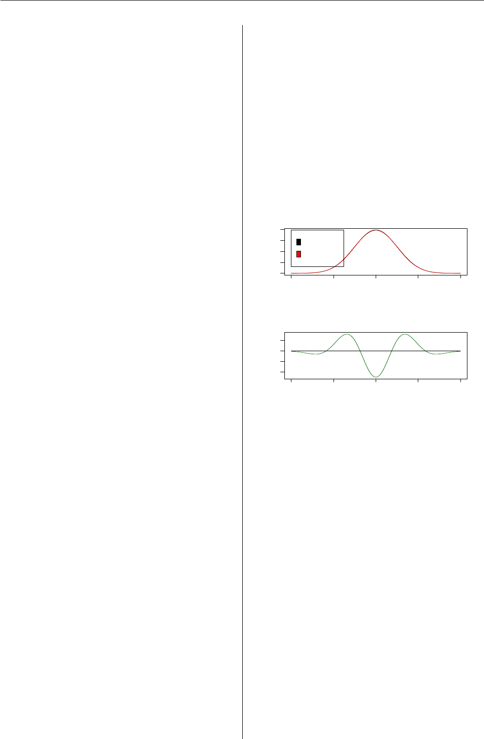
Next we explore the approximation quality of
NormApprox for N(0, 1)graphically (see Figure 2):
> par(mfrow = c(2,1))
> x <- seq(-4,4,0.001)
> plot(x, d(NormApprox)(x), type = "l",
+ xlab = "", ylab = "Density",
+ main = "Exact and approximated density")
> lines(x, d(N)(x), col = "red")
> legend(-4, d(N)(0),
+ legend = c("NormApprox",
+ "Norm(0,1)"), fill = c("black", "red"))
> plot(x, d(NormApprox)(x) - d(N)(x),
+ type = "l", xlab = "",
+ ylab = "\"black\" - \"red\"",
+ col = "darkgreen", main = "Error")
> lines(c(-4,4), c(0,0))
−4 −2 0 2 4
0.0 0.2 0.4
Exact and approximated density
Density
NormApprox
Norm(0,1)
−4 −2 0 2 4
−0.004 0.000
Error
"black" − "red"
Figure 2: densities of N(0, 1)and NormApprox and their differ-
ence
Details/odds and ends
For further details of the implementation, see Ruck-
deschel et al. (2005). In particular, we recommend
Thomas Stabla’s utility standardMethods for the au-
tomatic generation of S4-accessor and -replacement
functions. For more details, see ?standardMethods.
For odds and ends, consult the web-page for our
packages,
http://www.uni-bayreuth.de/departments/
/math/org/mathe7/DISTR/.
Acknowledgement
We thank Martin Mächler and Josef Leydold for their
helpful suggestions in conceiving the package. John
Chambers also gave several helpful hints and in-
sights. We got stimulating replies to an RFC on
r-devel by Duncan Murdoch and Gregory Warnes.
We also thank Paul Gilbert for drawing our attention
to his package setRNG and making it available in a
stand-alone version.
R News ISSN 1609-3631

Vol. 6/2, May 2006 6
Bibliography
J. M. Chambers. Programming with Data. A
guide to the S language. Springer, 1998. URL
http://cm.bell-labs.com/cm/ms/departments/
sia/Sbook/.
M. Kohl, P. Ruckdeschel, and T. Stabla. Gen-
eral Purpose Convolution Algorithm for
Distributions in S4-Classes by means of
FFT. Technical Report. Also available under
http://www.uni-bayreuth.de/departments/
math/org/mathe7/RUCKDESCHEL/pubs/comp.pdf,
Feb. 2005.
J. A. Rice. Mathematical statistics and data analysis.
Wadsworth & Brooks/Cole Advanced Books &
Software, Pacific Grove, California, 1988.
P. Ruckdeschel, M. Kohl, T. Stabla, and F. Cam-
phausen. S4 Classes for Distributions— a manual
for packages distr,distrSim,distrTEst, ver-
sion 1.7, distrEx, version 0.4-3, May 2006.
http://www.uni-bayreuth.de/departments/
math/org/mathe7/DISTR.
Peter Ruckdeschel
Matthias Kohl
Thomas Stabla
Florian Camphausen
Mathematisches Institut
Universität Bayreuth
D-95440 Bayreuth
Germany
peter.ruckdeschel@uni-bayreuth.de
The regress function
An R function that uses the Newton Raphson al-
gorithm for fitting certain doubly linear Gaussian
models.
by David Clifford and Peter McCullagh
Introduction
The purpose of this article is to highlight the
many uses of the regress function contained in the
regress package. The function can be used to fit lin-
ear Gaussian models in which the mean is a linear
combination of given covariates, and the covariance
is a linear combination of given matrices. A Newton-
Raphson algorithm is used to maximize the residual
log likelihood with respect to the variance compo-
nents. The regression coefficients are subsequently
obtained by weighted least squares, and a further
matrix computation gives the best linear predictor
for the response on a further out-of-sample unit.
Many Gaussian models have a covariance struc-
ture that can be written as a linear combination of
matrices, for example random effects models, poly-
nomial spline models and some multivariate mod-
els. However it was our research on the nature of
spatial variation in crop yields, McCullagh and Clif-
ford (2006), that motivated the development of this
function.
We begin this paper with a review of the kinds of
spatial models we wish to fit and explain why a new
function is needed to achieve this. Following this
we discuss other examples that illustrate the broad
range of uses for this function. Uses include basic
random effects models, multivariate linear models
and examples that include prediction and smooth-
ing. The techniques used in these examples can also
be applied to growth curves.
Spatial Models
McCullagh and Clifford (2006) model spatial depen-
dence of crop yields as a planar Gaussian process in
which the covariance function at points z,z0in the
plane has the form
σ2
0δz−z0+σ2
1K(|z−z0|)(1)
with non-negative coefficients σ2
0and σ2
1. In the
first term, Dirac’s delta is the covariance function for
white noise, and is independent on non-overlapping
sets. The second term is a stationary isotropic covari-
ance function from the Matérn class or power class.
McCullagh and Clifford (2006) proposed that the
spatial correlation for any crop yield is well de-
scribed by a convex combination of the Dirac func-
tion and the logarithmic function associated with
the de Wijs process. The de Wijs process (de Wijs,
1951,1953) is a special case of both the Matérn and
power classes and is invariant to conformal transfor-
mation. The linear combination of white noise and
the de Wijs process is called the conformal model.
We examined many examples from a wide variety
of crops worldwide, comparing the conformal model
against the more general Matérn class. Apart from
a few small-scale anisotropies, little evidence was
found of systematic departures from the conformal
model. Stein (1999) is a good reference for more de-
tails on spatial models.
It is important to point out that the de Wijs pro-
cess and certain other boundary cases of the Matérn
family are instances of generalized covariance func-
tions corresponding to intrinsic processes. The fitting
R News ISSN 1609-3631

Vol. 6/2, May 2006 7
of such models leads to the use of generalized co-
variance matrices that are positive definite on certain
contrasts. Such matrices usually have one or more
negative eigenvalues, and as such the models cannot
be fitted using standard functions in R.
Clifford (2005) shows how to compute the gener-
alized covariance matrices when yields are recorded
on rectangular plots laid out on a grid. For the
de Wijs process this is an analytical calculation and
the spatialCovariance package in R can be used to
evaluate the covariance matrices.
In order to illustrate exactly what the spatial
model looks like let us consider the Fairfield Smith
wheat yield data (Fairfield Smith,1938). We wish to
fit the conformal model to this dataset and to include
row and column effects in our model of the mean.
Assume at this point that the following information
is loaded into R: the yield yand factors row and col
that indicate the position of each plot.
The plots are 6 inches by 12 inches in a regular
grid of 30 rows and 36 columns with no separations
between plots. Computing the covariance matrix in-
volves two steps. The first stage called precompute
is carried out once for each dataset. The second stage
called computeV is carried out for each member of the
Matérn family one wishes to fit to the model.
require("spatialCovariance")
foot <- 0.3048 ## convert from ft to m
info <- precompute(nrows=30,ncols=36,
rowwidth=0.5*foot,
colwidth=1*foot,
rowsep=0,colsep=0)
V <- computeV(info)
The model we wish to now fit to the re-
sponse variable yobserved on plots of common area
|A|=0.0465m2is
y∼row +col +spatial error
where the spatial error has generalized covariance
structure
Σ=σ2
0|A|I+σ2
1|A|2V. (2)
The fact that yield is an extensive variable means
one goes from Equation 1to Equation 2by aggre-
gating yield over plots, i.e. by integrating the covari-
ance function over plots. We fit this model using the
regress function. One can easily check that Vhas a
negative eigenvalue and hence the model cannot be
fitted using other packages such as lme for example.
require("regress")
model1 <- regress(y~row+col,~V,identity=TRUE)
In order to determine the residual log likelihood
relative to a white noise baseline, we need to fit the
model in which σ2
1=0, i.e. Σ=σ2
0|A|I. The resid-
ual log likelihood is the difference in log likelihood
between these two models.
> BL <- regress(y~row+col,~,identity=TRUE)
> model1$llik - BL$llik
[1] 12.02406
> summary(model1,fixed.effects=FALSE)
Maximised Resid. Log Likelihood is -4373.721
Linear Coefficients: not shown
Variance Coefficients:
Estimate Std. Error
identity 39243.69 2139.824
V 60491.21 19664.338
The summary of the conformal model shows that
the estimated variance components are ˆσ2
0|A|=
39.2 ×10⁴and ˆσ2
1|A|2=6.05 ×10⁴. The standard
errors associated with each parameter are based on
the Fisher Information at the point of convergence.
Random Effects Models
Exchangeable Gaussian random effects models, also
known as linear mixed effects models Pinheiro
and Bates (2000), can also be fitted using regress.
However the code is not optimised to use the
groupedData structure like lmer is and regress can-
not handle the large datasets that one can fit using
lmer,Bates (2005).
The syntax for basic models using regress is
straightforward. Consider the example in Venables
and Ripley (2002)[p. 286] which uses data from Yates
(1935). In addition to the treatment factors N and
V, corresponding to nitrogen levels and varieties, the
model has a block factor B and a random B:V inter-
action.
The linear model is written explicitly as
ybnv =µ+αn+βv+ηb+ζbv +bnv (3)
where the distribution of the random effects are
ηb∼N(0,σ2
B),ζbv ∼N(0,σ2
B:V)and
bnv ∼N(0,σ2), all independent with indepen-
dent components, Venables and Ripley (2002). The
regress syntax mirrors how the model is defined in
(3).
oats.reg <- regress(Y~1+N+V,~B+I(B:V),
identity=TRUE,data=Oats)
Similar syntax is used by the lmer function but
the residual log likelihoods reported by the two func-
tions are not the same. The difference is attributable
in part to the term +1
2log |X>X|, which is constant
for comparison of two variance-component models,
but is affected by the basis vectors used to define
the subspace for the means. The value reported by
regress is unaffected by the choice of basis vectors.
R News ISSN 1609-3631

Vol. 6/2, May 2006 8
While the regress function can be used for ba-
sic random effects models, the lmer function can be
used to fit models where the covariance structure
cannot be written as a linear combination of known
matrices. The regress function does not apply to
such models. An example of such a model is one that
includes a random intercept and slope for a covariate
for each level of a group factor. A change of scale for
the covariate would result in a different model unless
the intercept and slope are correlated. In lmer the
groupedData structure automatically includes a cor-
relation parameter in such a model. See Bates (2005)
for an example of such a model.
Multivariate Models Using regress
In this section we show how to fit a multivari-
ate model. The example we choose to work
with is a very basic multivariate example but
the method illustrates how the complex models
can be fitted. Suppose that the observations are
i.i.d bivariate normal, i.e. Yi∼N(µ,Σ)where
µ=µ1
µ2and Σ=σ2
1ρσ1σ2
ρσ1σ2σ2
2. The goal is
to estimate the parameter (µ1,µ2,σ2
1,σ2
2,γ=ρσ1σ2).
Let Ydenote a vector of the length 2ncre-
ated by concatenating the observations for each
unit. The model for the data can be written as
Y∼N(Xµ,In⊗Σ)where X=1⊗I2and 1 is
a vector of ones of length n. Next we use the fact that
one can write Σas
Σ=σ2
11 0
0 0+γ0 1
1 0+σ2
20 0
0 1
to express the model as Y∼N(Xµ,D)where
D=σ2
1In⊗1 0
0 0+γIn⊗0 1
1 0+σ2
2In⊗0 0
0 1.
The code to generate such data and to fit such
a model is given below, note that A⊗B=
kronecker(A,B) in R.
library("regress")
library("MASS") ## needed for mvrnorm
n <- 100
mu <- c(1,2)
Sigma <- matrix(c(10,5,5,10),2,2)
Y <- mvrnorm(n,mu,Sigma)
## this simulates multivariate normal rvs
y <- as.vector(t(Y))
X <- kronecker(rep(1,n),diag(1,2))
V1 <- matrix(c(1,0,0,0),2,2)
V2 <- matrix(c(0,0,0,1),2,2)
V3 <- matrix(c(0,1,1,0),2,2)
sig1 <- kronecker(diag(1,n),V1)
sig2 <- kronecker(diag(1,n),V2)
gam <- kronecker(diag(1,n),V3)
reg.obj <- regress(y~X-1,~sig1+sig2+gam,
identity=FALSE,start=c(1,1,0.5))
The summary of this model shows that the es-
timated mean parameters are ˆµ1=1.46 and ˆµ2=
1.78. The estimates for the variance components are
ˆσ2
1=9.25, ˆσ2
2=10.27 and ˆγ=3.96. The true param-
eter is (µ1,µ2,σ2
1,σ2
2,γ=ρσ1σ2)=(1, 2, 10, 10, 5).
Maximised Residual Log Likelihood is -315.48
Linear Coefficients:
Estimate Std. Error
X1 1.461 0.304
X2 1.784 0.320
Variance Coefficients:
Estimate Std. Error
sig1 9.252 1.315
sig2 10.271 1.460
gam 3.963 1.058
A closed form solution exists for the estimate of
Σin this case, ˆ
Σ=1
n−1(Y−¯
Y)>(Y−¯
Y)where Y
denotes the n×2 matrix of observations. Our com-
puted result can be checked using:
> Sig <- var(Y)
> round(Sig, 3)
[,1] [,2]
[1,] 9.252 3.963
[2,] 3.963 10.271
It may be of interest to fit the sub-model with equal
variances, σ2=σ2
1=σ2
2, a case for which no closed
form solution exists. This model can be fitted us-
ing the code shown below. The estimate for σ2is
ˆσ2=9.76 and we can see that the difference in resid-
ual log likelihood between the sub-model and the
full model is only 0.16 units.
> sig <- sig1+sig2
> reg.obj.sub <- regress(y~X-1,~sig+gam,
+ identity=FALSE,start=c(1,.5))
> summary(reg.obj.sub)
Maximised Residual Log Likelihood is -315.65
Linear Coefficients:
Estimate Std. Error
X1 1.461 0.312
X2 1.784 0.312
Variance Coefficients:
Estimate Std. Error
sig 9.761 1.059
gam 3.963 1.059
R News ISSN 1609-3631
Vol. 6/2, May 2006 9
The argument start allows one to specify the
starting point for the Newton-Raphson algorithm.
Another argument pos allows one to force certain
parameters to be positive or negative, in this exam-
ple we may only be interested in cases with negative
correlation. By default the support for the variance
components is the real line.
Prediction and Smoothing
regress can also be used to implement smoothing
and best linear prediction, McCullagh (2005)[exam-
ple 5]. Stein (1999) notes that in the geostatistical lit-
erature best linear prediction is also known as krig-
ing and in effect
BLP(x) = E(Y(x)|data)
for an out-of-sample unit whose x-value is x.
Smoothing usually requires the choice of a band-
width in each example, Efron (2001), but bandwidth
selection occurs automatically through REML esti-
mation of polynomial spline models. This is best
illustrated by the cubic spline generalized covari-
ance function (Wahba,1990;Green and Silverman,
1994). The cubic spline model has a two-dimensional
kernel spanned by the constant and linear functions
of x. Consequently the model matrix Xmust include
∼1+x, but could also include additional functions.
●
●
●
●
●
●
●
●
●
●
●
●
●
●
●
●
●
●
●
●
●
●
●
●●
●
●
●●●
●
●
●
●
●
●●
●
●
●
●
●
●●
●
●
●
●
●
0.0 0.2 0.4 0.6 0.8 1.0
1.0
1.5
2.0
x
y
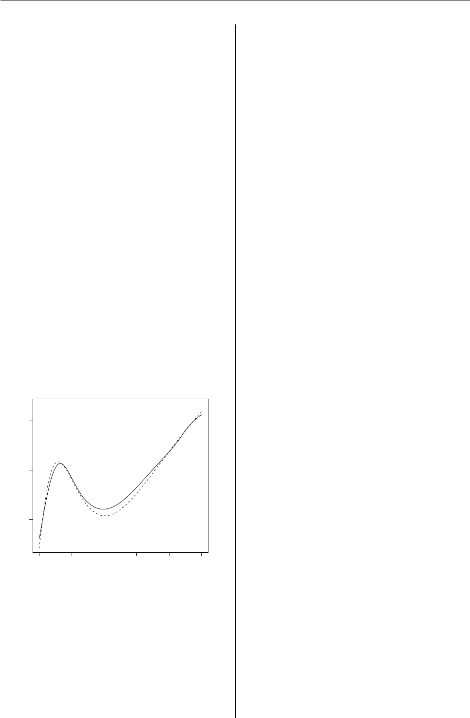
Figure 1: Smoothing spline and best linear predictor
fitted by REML.
In the code below we simulate data as in Wahba
(1990)[p. 45], but after generating data for one hun-
dred points in the unit interval we take a sample of
these points to be used for fitting purposes. The goal
of fitting a smooth curve to the data is achieved by
the best linear predictor, which is a cubic spline. The
spline is computed at all x-values and has knots at
the observed values. This experiment can be carried
out in the following four steps.
## 1: Data simulation
n <- 101
x <- (0:100)/100
prb <- (1 + cos(2*pi*x))/2
## indicator which x-values are observed
obs <- (runif(n) < prb)
mu <- 1 + x + sin(3*log(x+0.1))/(2+x)
## full data
y <- mu + rnorm(n,0,0.1)
## 2. Fit the cubic spline to observed data
one <- rep(1,n)
d <- abs(x %*% t(one) - one %*% t(x))
V <- d^3
X <- model.matrix(y~1+x)
fit <- regress(y[obs]~X[obs,],~V[obs,obs],
identity=TRUE)
## 3. BLP at all x given the observed data
wlsfit <- X%*%fit$beta
blp <- wlsfit + fit$sigma[1]*V[,obs]
%*% fit$W%*%(y-wlsfit)[obs]
## 4. Plot of results
plot(x[obs],y[obs], xlab="x",ylab="y")
lines(x,mu,lty=2)
lines(x,blp)
The results of this experiment can be seen in Fig-
ure 1. The points are the observed data, the solid line
is the best linear predictor and the dashed line shows
the function used to generate the data.
Bibliography
D. Bates. Fitting linear mixed models in R. RNews, 5
(1), May 2005.
D. Clifford. Computation of spatial covariance matri-
ces. Journal of Computational and Graphical Statistics,
14(1):155–167, 2005.
H. de Wijs. Statistics of ore distribution. Part I: fre-
quency distribution of assay values. Journal of the
Royal Netherlands Geological and Mining Society, 13:
365–375, 1951. New Series.
H. de Wijs. Statistics of ore distribution. Part II: The-
ory of binomial distribution applied to sampling
and engineering problems. Journal of the Royal
Netherlands Geological and Mining Society, 15:125–
24, 1953. New Series.
B. Efron. Selection criteria for scatterplot smoothers.
Annals of Statistics, 2001.
H. Fairfield Smith. An empirical law describing het-
erogeneity in the yields of agricultural crops. Jour-
nal of Agricultural Science, 28:1–23, January 1938.
R News ISSN 1609-3631

Vol. 6/2, May 2006 10
P. Green and B. Silverman. Nonparametric Regression
and Generalized Linear Models. Chapman and Hall,
London, 1994.
P. McCullagh. Celebrating Statistics: Papers in hon-
our of Sir David Cox on his 80th birthday, chapter
Exchangeability and regression models, pages 89–
113. Oxford, 2005.
P. McCullagh and D. Clifford. Evidence for confor-
mal invariance of crop yields. Accepted at Proceed-
ings of the Royal Society A, 2006.
J. Pinheiro and D. Bates. Mixed-effects models in S and
S-PLUS. New York : Springer-Verlag, 2000.
M. Stein. Interpolation of Spatial Data: Some Theory for
Kriging. Springer, 1999.
W. Venables and B. Ripley. Modern Applied Statistics
with S. Springer-Verlag New York, Inc., 4th edition,
2002.
G. Wahba. Spline Models for Observational Data. SIAM,
Philadephia, 1990.
F. Yates. Complex experiments. Journal of the Royal
Statistical Society (Supplement), 2:181–247, 1935.
David Clifford, CSIRO
Peter McCullagh, University of Chicago
David.Clifford@csiro.au
pmcc@galton.uchicago.edu
Processing data for outliers
by Lukasz Komsta
The results obtained by repeating the same measure-
ment several times can be treated as a sample com-
ing from an infinite, most often normally distributed
population.
In many cases, for example quantitative chemi-
cal analysis, there is no possibility to repeat measure-
ment many times due to very high costs of such vali-
dation. Therefore, all estimates and parameters of an
experiment must be obtained from a small sample.
Some repeats of an experiment can be biased by
crude error, resulting in values which do not match
the other data. Such values, called outliers, are very
easy to be identified in large samples. But in small
samples, often less than 10 values, identifying out-
liers is more difficult, but even more important. A
small sample contaminated with outlying values will
result in estimates significantly different from real
parameters of whole population (Barnett,1994).
The problem of identifying outliers in small sam-
ples properly (and making a proper decision about
removing or leaving suspicious data) is very old and
the first papers discussing this problem were pub-
lished in the 1920s. The problem remained unre-
solved until 1950s, due to lack of computing technol-
ogy to perform valid Monte-Carlo simulations. Al-
though current trends in outlier detection rely on ro-
bust estimates, the tests described below are still in
use in many cases (especially chemical analysis) due
to their simplicity.
Dixon test
All concepts of outlier analysis were collected by
Dixon (1950) :
1. chi-squared scores of data
2. score of extreme value
3. ratio of range to standard deviation (two oppo-
site outliers)
4. ratio of variances without suspicious value(s)
and with them
5. ratio of ranges and subranges
The last concept seemed to the author to have the
best performance and Dixon introduced his famous
test in the next part of the paper. He defined several
coefficients which must be calculated on an ordered
sample x(1),x(2),··· ,x(n). The formulas below show
these coefficients in two variants for each of them -
when the suspicious value is lowest and highest.
r10 =x(2)−x(1)
x(n)−x(1)
,x(n)−x(n−1)
x(n)−x(1)
(1)
r11 =x(2)−x(1)
x(n−1)−x(1)
,x(n)−x(n−1)
x(n)−x(2)
(2)
r12 =x(2)−x(1)
x(n−2)−x(1)
,x(n)−x(n−1)
x(n)−x(3)
(3)
r20 =x(3)−x(1)
x(n)−x(1)
,x(n)−x(n−2)
x(n)−x(1)
(4)
r21 =x(3)−x(1)
x(n−1)−x(1)
,x(n)−x(n−2)
x(n)−x(2)
(5)
r22 =x(3)−x(1)
x(n−2)−x(1)
,x(n)−x(n−2)
x(n)−x(3)
(6)
The critical values of the above statistics were not
given in the original paper, but only discussed. A
year later (Dixon,1951) the next paper with critical
R News ISSN 1609-3631

Vol. 6/2, May 2006 11
values appeared. Dixon discussed the distribution of
his variables in a very comprehensive way, and con-
cluded that a numerical procedure to obtain critical
values is available only for sample with n=3. Quan-
tiles for other sample sizes were obtained in this pa-
per by simulations and tabularized.
Dixon did not publish the 0.975 quantile for his
test, which is needed to perform two-sided test at
95% confidence level. These values were obtained by
interpolation later (Rorabacher,1991) with some cor-
rections of typographical errors in the original Dixon
table.
Grubbs test
Another criteria for outlying observations proposed
by Dixon were discussed at the same time by Grubbs
(1950). He proposed three variants of his test. For
one outlier
G=|xoutlying −x|
s,U=S2
1
S2(7)
For two outliers on opposite tails
G=xmax −xmin
s,U=S2
2
S2(8)
For two outliers on the same tail
U=G=S2
2
S2(9)
where S2
1is the variance of the sample with one
suspicious value excluded, and S2
2is the variance
with two values excluded.
If the estimators in equation (7) are biased (with
nin denominator), then simple dependence occurs
between Sand U:
U=1−1
n−1G2(10)
and it makes Uand Gstatistics equivalent in their
testing power.
The Gdistribution for one outlier test was dis-
cussed earlier (Pearson and Chekar,1936) and the
following formula can be used to approximate the
critical value:
G=tα/n,n−2sn−1
n−2+t2
α/n,n−2
(11)
When discussing (8) statistics, Grubbs gives only
Gvalues, because Uwas too complicated to calcu-
late. He writes “. . . the limits of integration do not turn
out to be functions of single variables and the task of com-
puting the resulting multiple integral may be rather diffi-
cult.”
The simple formula for approximating critical
values of Gvalue (range to standard deviation) was
given by David, Hartley and Pearson (1954):
G=v
u
u
t
2(n−1)t2
α/n(n−1),n−2
n−2+t2
α/n(n−1),n−2
(12)
The ratio of variances used to test for two outliers
on the same tail (9) is not available to integrate in a
numerical manner. Thus, critical values were simu-
lated by Grubbs and must be approximated by inter-
polation from tabularized data.
Cochran test
The other test used to detect crude errors in exper-
iment is the Cochran test (Snedecor and Cochran,
1980). It is designed to detect outlying (or inlying)
variance in a group of datasets. It is based on sim-
ple statistics - the ratio of maximum (or minimum)
variance to the sum of all variances:
C=S2
max
∑S2(13)
The critical value approximation can be obtained
using the following formula:
C=1
1+ (k−1)F
α/k,n(k−1),n
(14)
where kis the number of groups, and nis the
number of observations in each group. If groups
have different length, the arithmetic mean is used as
n.
The R implementation
Package outliers, available now on CRAN, contains
a set of functions for performing these tests and cal-
culating their critical values. The most difficult prob-
lem to solve was introducing a proper and good
working algorithm to provide quantile and p-value
calculation of tabularized distribution by interpola-
tion.
After some experiments I have decided to use re-
gression of 3rd degree orthogonal polynomial, fitted
to four given points, taken from the original Dixon
or Grubbs table, nearest to the argument. When an
argument comes from outside of tabularized range,
it is extrapolated by fitting a linear model to the first
(or last) two known values. This method is imple-
mented in the internal function qtable, used for cal-
culation of Dixon values and Grubbs values for two
outliers at the same tail.
R News ISSN 1609-3631
Vol. 6/2, May 2006 12
0.0 0.2 0.4 0.6 0.8 1.0
0.0 0.2 0.4 0.6 0.8 1.0
alpha
quantile
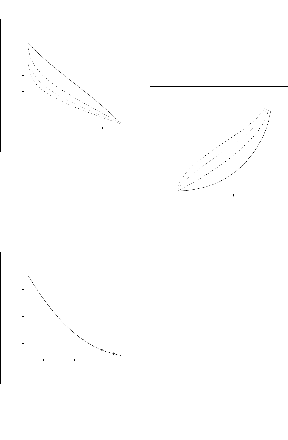
Figure 1: Interpolated quantile curves of Dixon test
for n=3 (solid), n=4 (dashed), n=5 (dotted) and
n=6 (dotdashed).
The proposed algorithm provides a good
continuity-like effect of quantile calculation as
shown on Figures (1) and (3). Critical values can be
obtained by qdixon, qgrubbs, qcochran. The cor-
responding reverse routines (calculating p-values)
are named pdixon, pgrubbs, pcochran. The conti-
nuity effect of reverse functions is depicted on Figure
(2)
0.65 0.70 0.75 0.80 0.85 0.90 0.95
0.00 0.02 0.04 0.06 0.08 0.10 0.12
Q
p−value
Figure 2: Interpolated p-value curve of Dixon test
for n=4, with percentage points given in original
Dixon table
The most important functions implemented in
the package are: dixon.test,grubbs.test and
cochran.test. According to the given parameters,
these functions can perform all of the tests men-
tioned above. Additionally, there is an easy way to
obtain different kinds of data scores, by the scores
function.
It is also possible to obtain the most suspicious
value (the largest difference from the mean) by the
outlier function. If this value is examined and
proved to be an outlier, it can be easily removed or
replaced by the arithmetic mean by rm.outlier.
0.0 0.2 0.4 0.6 0.8 1.0
0.0 0.1 0.2 0.3 0.4 0.5 0.6
alpha
quantile
Figure 3: Interpolated quantile curves of Grubbs test
for two outliers on one tail; n=4 (solid), n=5
(dashed), n=6 (dotted) and n=7 (dotdashed).
Examples
Suppose we have six measurements, where the last
one is visually larger than the others. We can now
test, if it should be treated as an outlier, and removed
from further calculations.
> x = c(56.5,55.1,57.2,55.3,57.4,60.5)
> dixon.test(x)
Dixon test for outliers
data: x
Q = 0.5741, p-value = 0.08689
alternative hypothesis: highest value 60.5 is an outlier
> grubbs.test(x)
Grubbs test for one outlier
data: x
G = 1.7861, U = 0.2344, p-value = 0.06738
alternative hypothesis: highest value 60.5 is an outlier
> scores(x) # this is only example, not recommended for
small sample
[1] -0.2551552 -0.9695897 0.1020621 -0.8675276 0.2041241
[6] 1.7860863
> scores(x,prob=0.95)
[1] FALSE FALSE FALSE FALSE FALSE TRUE
> scores(x,prob=0.975)
[1] FALSE FALSE FALSE FALSE FALSE FALSE
>
R News ISSN 1609-3631

Vol. 6/2, May 2006 13
As we see, both tests did not reject the null hy-
pothesis and the suspicious value should not be re-
moved. Further calculations should be done on the
full sample.
Another example is testing a simple dataset for
two opposite outliers, and two outliers at one tail:
> x = c(41.3,44.5,44.7,45.9,46.8,49.1)
> grubbs.test(x,type=11)
Grubbs test for two opposite outliers
data: x
G = 2.9908, U = 0.1025, p-value = 0.06497
alternative hypothesis: 41.3 and 49.1 are outliers
> x = c(45.1,45.9,46.1,46.2,49.1,49.2)
> grubbs.test(x,type=20)
Grubbs test for two outliers
data: x
U = 0.0482, p-value = 0.03984
alternative hypothesis: highest values 49.1 , 49.2 are outliers
>
In the first dataset, the smallest and greatest value
should not be rejected. The second example rejects
the null hypothesis: 49.1 and 49.2 are outliers, and
calculations should be made without them.
The last example is testing for outlying variance.
We have calculated variance in 8 groups (5 measure-
ments in each group) of results and obtained: 1.2, 2.5,
2.9, 3.5, 3.6, 3.9, 4.0, 7.9. We must check now if the
smallest or largest variance should be considered in
calculations:
> v = c(1.2, 2.5, 2.9, 3.5, 3.6, 3.9, 4.0, 7.9)
> n = rep(5,8)
> cochran.test(v,n)
Cochran test for outlying variance
data: v
C = 0.2678, df = 5, k = 8, p-value = 0.3579
alternative hypothesis: Group 8 has outlying variance
sample estimates:
12345678
1.2 2.5 2.9 3.5 3.6 3.9 4.0 7.9
> cochran.test(v,n,inlying=TRUE)
Cochran test for inlying variance
data: v
C = 0.0407, df = 5, k = 8, p-value < 2.2e-16
alternative hypothesis: Group 1 has inlying variance
sample estimates:
12345678
1.2 2.5 2.9 3.5 3.6 3.9 4.0 7.9
>
The tests show that first group has inlying vari-
ance, significantly smaller than the others.
Bibliography
V. Barnett, T. Lewis. Outliers in statistical data. Wiley.
W.J. Dixon. Analysis of extreme values. Ann. Math.
Stat., 21(4):488-506, 1950.
W.J. Dixon. Ratios involving extreme values. Ann.
Math. Stat., 22(1):68-78, 1951.
D.B. Rorabacher. Statistical Treatment for Rejection
of Deviant Values: Critical Values of Dixon Q Pa-
rameter and Related Subrange Ratios at the 95 per-
cent Confidence Level. Anal. Chem. , 83(2):139-146,
1991.
F.E. Grubbs. Sample Criteria for testing outlying ob-
servations. Ann. Math. Stat. , 21(1):27-58, 1950.
E.S. Pearson, C.C. Chekar. The efficiency of statisti-
cal tools and a criterion for the rejection of outlying
observations. Biometrika , 28(3):308-320, 1936.
H.A. David, H.O. Hartley, E.S. Pearson. The distri-
bution of the ratio, in a single normal sample, of
range to standard deviation. Biometrika , 41(3):482-
493, 1954.
G.W. Snedecor, W.G. Cochran. Statistical Methods.
Iowa State University Press , 1980.
Lukasz Komsta
Department of Medicinal Chemistry
Skubiszewski Medical University of Lublin, Poland
luke@novum.am.lublin.pl
Analysing equity portfolios in R
Using the portfolio package
by David Kane and Jeff Enos
Introduction
R is used by major financial institutions around the
world to manage billions of dollars in equity (stock)
portfolios. Unfortunately, there is no open source R
package for facilitating this task. The portfolio pack-
age is meant to fill that gap. Using portfolio, an an-
alyst can create an object of class portfolioBasic
(weights only) or portfolio (weights and shares),
examine its exposures to various factors, calculate
its performance over time, and determine the contri-
butions to performance from various categories of
stocks. Exposures, performance and contributions
are the basic building blocks of portfolio analysis.
R News ISSN 1609-3631

Vol. 6/2, May 2006 14
One Period, Long-Only
Consider a simple long-only portfolio formed from
the universe of 30 stocks in the Dow Jones Industrial
Average (DJIA) in January, 2005. Start by loading and
examining the input data.
> library(portfolio)
> data(dow.jan.2005)
> summary(dow.jan.2005)
symbol name
Length:30 Length:30
Class :character Class :character
Mode :character Mode :character
price sector
Min. : 21.0 Industrials :6
1st Qu.: 32.1 Staples :6
Median : 42.2 Cyclicals :4
Mean : 48.6 Financials :4
3rd Qu.: 56.0 Technology :4
Max. :103.3 Communications:3
(Other) :3
cap.bil month.ret
Min. : 22.6 Min. :-0.12726
1st Qu.: 53.9 1st Qu.:-0.05868
Median : 97.3 Median :-0.02758
Mean :126.0 Mean :-0.02914
3rd Qu.:169.3 3rd Qu.: 0.00874
Max. :385.9 Max. : 0.04468
> head(dow.jan.2005)
symbol name price
140 AA ALCOA INC 31.42
214 MO ALTRIA GROUP INC 61.10
270 AXP AMERICAN EXPRESS CO 56.37
294 AIG AMERICAN INTERNATIONAL GROUP 65.67
946 BA BOEING CO 51.77
1119 CAT CATERPILLAR INC 97.51
sector cap.bil month.ret
140 Materials 27.35 -0.060789
214 Staples 125.41 0.044681
270 Financials 70.75 -0.051488
294 Financials 171.04 0.009441
946 Industrials 43.47 -0.022600
1119 Industrials 33.27 -0.082199
The DJIA consists of exactly 30 large US stocks.
We provide a minimal set of information for con-
structing a long-only portfolio. Note that cap.bil
is market capitalization in billions of dollars, price
is the per share closing price on December 31, 2004,
and month.ret is the one month return from Decem-
ber 31, 2004 through January 31, 2005.
In order to create an object of class
portfolioBasic, we can use this data and form a
portfolio on the basis of a “nonsense” variable like
price.
> p <- new("portfolioBasic",
+ date = as.Date("2004-12-31"),
+ id.var = "symbol", in.var = "price",
+ sides = "long", ret.var = "month.ret",
+ data = dow.jan.2005)
An object of class "portfolioBasic" with 6 positions
Selected slots:
name: Unnamed portfolio
date: 2004-12-31
in.var: price
ret.var: month.ret
type: equal
size: quintile
> summary(p)
Portfolio: Unnamed portfolio
count weight
Long: 6 1
Top/bottom positions by weight:
id pct
1 AIG 16.7
2 CAT 16.7
3 IBM 16.7
4 JNJ 16.7
5 MMM 16.7
6 UTX 16.7
In other words, we have formed a portfolio of
the highest priced 6 stocks out of the 30 stocks in
the DJIA. The id.var argument causes the portfo-
lio to use symbol as the key for identifying securi-
ties throughout the analysis. in.var selects the vari-
able by which stocks are ranked in terms of desir-
ability. sides set to long specifies that we want a
long-only portfolio. ret.var selects the return vari-
able for measuring performance. In this case, we are
interested in how the portfolio does for the month of
January 2005.
The default arguments to portfolioBasic form
equal-weighted positions; in this case, each of the 6
stocks has 16.67% of the resulting portfolio. The de-
faults also lead to a portfolio made up of the best 20%
(or quintile) of the universe of stocks provided to
the data argument. Since 20% of 30 is 6, there are 6
securities in the resulting portfolio.
Exposures
Once we have a portfolio, the next step is to analyse
its exposures. These can be calculated with respect
to both numeric or factor variables. The method
exposure will accept a vector of variable names.
> exposure(p, exp.var = c("price", "sector"))
numeric
variable exposure
1 price 85.1
R News ISSN 1609-3631

Vol. 6/2, May 2006 15
sector
variable exposure
2 Industrials 0.500
1 Financials 0.167
3 Staples 0.167
4 Technology 0.167
The weighted average price of the portfolio is
85. In other words, since the portfolio is equal-
weighted, the average share price of AIG, CAT, IBM,
JNJ, MMM, and UTX is 85. This is a relatively high
price, but makes sense since we explicitly formed the
portfolio by taking the 6 highest priced stocks out of
the DJIA.
Each of the 6 stocks is assigned a sector and 3 of
them are Industrials. This compares to the 20% of
the entire universe of 30 stocks that are in this sec-
tor. In other words, the portfolio has a much higher
exposure to Industrials than the universe as a whole.
Similarly, the portfolio has no stocks from the Com-
munications, Cyclicals or Energy sectors despite the
fact that these make up almost 27% of the DJIA uni-
verse.
Performance
Time plays two roles in the portfolio class. First,
there is the moment of portfolio formation. This is
the instant when all of the data, except for future re-
turns, is correct. After this moment, of course, things
change. The price of AIG on December 31, 2004 was
$65.67, but by January 5, 2005 it was $67.35.
The second role played by time on the portfolio
class concerns future returns. ret.var specifies a re-
turn variable which measures the performance of in-
dividual stocks going forward. These returns can be
of any duration — an hour, a day, a month, a year —
but should generally start from the moment of port-
folio formation. In this example, we are using one
month forward returns. Now that we know the port-
folio’s exposures at the start of the time period, we
can examine its performance for the month of Jan-
uary.
> performance(p)
Total return: -1.71 %
Best/Worst performers:
id weight ret contrib
2 CAT 0.167 -0.08220 -0.01370
3 IBM 0.167 -0.05234 -0.00872
6 UTX 0.167 -0.02583 -0.00431
1 AIG 0.167 0.00944 0.00157
4 JNJ 0.167 0.02018 0.00336
5 MMM 0.167 0.02790 0.00465
The portfolio lost 1.7% of its value in January. The
worst performing stock was CAT (Caterpillar), down
more than 8%. The best performing stock was MMM
(3M), up almost 3%. The contrib (contribution) of
each stock to the overall performance of the portfo-
lio is simply its weight in the portfolio multiplied by
its return. The sum of the 6 individual contributions
yields -1.7%.
Contributions
The contributions of individual stocks are not that in-
teresting in and of themselves. More important is
to examine summary statistics of the contributions
across different categories of stocks. Consider the use
of the contribution method:
> contribution(p, contrib.var = c("sector"))
sector
variable weight contrib roic
5 Communications 0.000 0.00000 0.00000
6 Conglomerates 0.000 0.00000 0.00000
7 Cyclicals 0.000 0.00000 0.00000
8 Energy 0.000 0.00000 0.00000
1 Financials 0.167 0.00157 0.00944
2 Industrials 0.500 -0.01336 -0.02671
9 Materials 0.000 0.00000 0.00000
3 Staples 0.167 0.00336 0.02018
4 Technology 0.167 -0.00872 -0.05234
10 Utilities 0.000 0.00000 0.00000
contribution, like exposure, accepts a vector of
variable names. In the case of sector, the contribu-
tion object displays the 10 possible values, the total
weight of the stocks for each level and the sum of the
contributions for those stocks. Only 4 of the 10 lev-
els are represented by the stocks in the portfolio. The
other 6 levels have zero weight and, therefore, zero
contributions.
The sector with the biggest weight is Industrials,
with half of the portfolio. Those 3 stocks did poorly,
on average, in January and are therefore responsible
for -1.3% in total losses. There is only a single Tech-
nology stock in the portfolio, IBM. Because it was
down 5% for the month, its contribution was -0.87%.
Since IBM is the only stock in its sector in the portfo-
lio, the contribution for the sector is the same as the
contribution for IBM.
The last column in the display shows the roic —
the return on invested capital — for each level. This
captures the fact that raw contributions are a func-
tion of both the total size of positions and their re-
turn. For example, the reason that the total contri-
bution for Industrials is so large is mostly because
they account for such a large proportion of the port-
folio. The individual stocks performed poorly, on
average, but not that poorly. Much worse was the
performance of the Technology stock. Although the
total contribution from Technology was only 60% of
that of Industrials, this was on a total position weight
only 1/3 as large. In other words, the return on total
capital was much worse in Technology than in Indus-
trials even though Industrials accounted for a larger
share of the total losses.
R News ISSN 1609-3631

Vol. 6/2, May 2006 16
Think about roic as useful in determining con-
tributions on the margin. Imagine that you have the
chance to move $1 out of one sector and into another.
Where should than initial dollar come from? Not
from the sector with the worst total contribution. In-
stead, the marginal dollar should come from the sec-
tor with the worst roic and should be placed into the
sector with the best roic. In this example, we should
move money out of Technology and into Staples.
contribution can also work with numeric vari-
ables.
> contribution(p, contrib.var = c("cap.bil"))
cap.bil
rank variable weight contrib roic
1 1 - low (22.6,50.9] 0.167 -0.013700 -0.08220
2 2 (50.9,71.1] 0.333 0.000345 0.00103
4 3 (71.1,131] 0.000 0.000000 0.00000
3 4 (131,191] 0.500 -0.003787 -0.00757
5 5 - high (191,386] 0.000 0.000000 0.00000
Analysing contributions only makes sense in the
context of categories into which each position can
be placed. So, we need to break up a numeric vari-
able like cap into discrete, exhaustive categories. The
contribution function provides various options for
doing so, but most users will be satisfied with the
default behavior of forming 5 equal sized quintiles
based on the distribution of the variable in the entire
universe.
In this example, we see that there are no portfo-
lio holdings among the biggest 20% of stocks in the
DJIA. Half the portfolio comes from stocks in the sec-
ond largest quintile. Within each category, the anal-
ysis is the same as that above for sectors. The worst
performing category in terms of total contribution is
the smallest quintile. This category also has the low-
est roic.
One Period Long-Short
Having examined a very simple long-only portfo-
lio in order to explain the concepts behind exposures,
performance and contributions, it is time to consider a
more complex case, a long-short portfolio which uses
the same underlying data.
> p <- new("portfolioBasic",
+ date = as.Date("2004-12-31"),
+ id.var = "symbol", in.var = "price",
+ type = "linear", sides = c("long",
+ "short"), ret.var = "month.ret",
+ data = dow.jan.2005)
An object of class "portfolioBasic" with
12 positions
Selected slots:
name: Unnamed portfolio
date: 2004-12-31
in.var: price
ret.var: month.ret
type: linear
size: quintile
> summary(p)
Portfolio: Unnamed portfolio
count weight
Long: 6 1
Short: 6 -1
Top/bottom positions by weight:
id pct
12 UTX 28.57
5 IBM 23.81
2 CAT 19.05
8 MMM 14.29
1 AIG 9.52
10 PFE -9.52
9 MSFT -14.29
11 SBC -19.05
6 INTC -23.81
4 HPQ -28.57
Besides changing to a long-short portfolio, we
have also provided a value of “linear” to the type
argument. As the summary above shows, this yields
a portfolio in which the weights on the individual
positions are (linearly) proportional to their share
prices. At the end of 2004, the lowest priced stock
in the DJIA was HPQ (Hewlett-Packard) at $20.97.
Since we are using price as our measure of desirabil-
ity, HPQ is the biggest short position. Since we have
not changed the default value for size from “quin-
tile,” there are still 6 positions per side.
> plot(p)
Weight vs. in.var
price (in.var)
weight
−0.3
−0.2
−0.1
0.0
0.1
0.2
0.3
20 40 60 80 100
●
●
●
●
●
●
●
●
●
●
●
●
Weight distribution
weight
count
0
5
10
15
20
25
−0.2 0.0 0.2
Figure 1: Plot of a portfolioBasic object.
R News ISSN 1609-3631
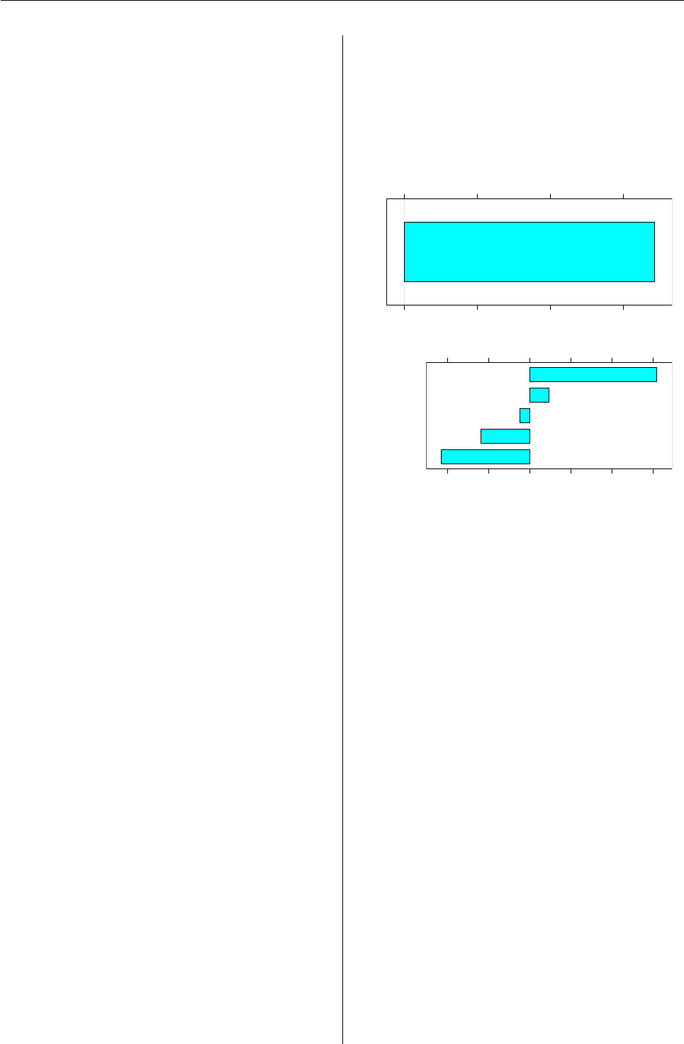
Vol. 6/2, May 2006 17
Figure 1shows the result of calling plot on this
portfolio object. The top plot displays the relation-
ship between position weights and their correspond-
ing in.var values, while the bottom plot shows a his-
togram of position weights.
The display for the exposure object is now some-
what different to accommodate the structure of a
long-short portfolio.
> exposure(p, exp.var = c("price", "sector"))
numeric
variable long short exposure
1 price 92.6 -24.2 68.4
sector
variable long short exposure
2 Industrials 0.6190 0.0000 0.6190
1 Financials 0.0952 0.0000 0.0952
3 Staples 0.0476 -0.0952 -0.0476
5 Communications 0.0000 -0.2381 -0.2381
4 Technology 0.2381 -0.6667 -0.4286
The long exposure to price is simply the
weighted average of price on the long side of the
portfolio, where the weighting is done in proportion
to the size of the position in each stock. The same
is true on the short side. Since a linear weighting
used here emphasises the tail of the distribution, the
long exposure is greater than the long exposure of
the equal weighted portfolio considered above, $93
versus $85.
Since the weights on the short side are actually
negative — in the sense that we are negatively ex-
posed to positive price changes in these stocks —
the weighted average on the short side for a positive
variable like price is also negative. Another way to
read this is to note that the weighted average price
on the short side is about $24 but that the portfolio
has a negative exposure to this number because these
positions are all on the short side.
One reason for the convention of using a negative
sign for short side exposures is that doing so makes
the overall exposure of the portfolio into a simple
summation of the long and short exposures. (Note
the assumption that the weights on both sides are
equal. In future versions of the portfolio package,
we hope to weaken these and other requirements.)
For this portfolio, the overall exposure is 68. Because
the portfolio is long the high priced stocks and short
the low priced ones, the portfolio has a positive ex-
posure to the price factor. Colloquially, we are “long
price.”
A similar analysis applies to sector exposures. We
have 62% of our long holdings in Industrials but zero
of our short holdings. We are, therefore, 62% long In-
dustrials. We have 24% of the longs holdings in Tech-
nology, but 67% of the short holdings; so we are 43%
short Technology.
Calling plot on the exposure object produces a
bar chart for each exposure category, as seen in Fig-
ure 2. Since all numeric exposures are grouped to-
gether, a plot of numeric exposure may only make
sense if all numeric variables are on the same scale.
In this example, the only numeric exposure we have
calculated is that to price.
> plot(exposure(p, exp.var = c("price",
+ "sector")))
numeric exposure
exposure
price
0 20 40 60
sector exposure
exposure
Technology
Communications
Staples
Financials
Industrials
−0.4 −0.2 0.0 0.2 0.4 0.6
Figure 2: Plot of an exposure object for a single pe-
riod. Bar charts are sorted by exposure.
The performance object is similar for a long-short
portfolio.
> performance(p)
Total return: 2.19 %
Best/Worst performers:
id weight ret contrib
2 CAT 0.1905 -0.08220 -0.01566
5 IBM 0.2381 -0.05234 -0.01246
12 UTX 0.2857 -0.02583 -0.00738
3 DIS -0.0476 0.02986 -0.00142
1 AIG 0.0952 0.00944 0.00090
8 MMM 0.1429 0.02790 0.00399
6 INTC -0.2381 -0.04019 0.00957
10 PFE -0.0952 -0.10152 0.00967
11 SBC -0.1905 -0.06617 0.01260
4 HPQ -0.2857 -0.06581 0.01880
The portfolio was up 2.2% in January. By de-
fault, the summary of the performance object only
provides the 5 worst and best contributions to re-
turn. HPQ was the biggest winner because, though
it was only down 7% for the month, its large weight-
ing caused it to contribute almost 2% to overall per-
formance. The 19% weight of CAT in the portfolio
placed it as only the third largest position on the long
side, but its -8% return for the month made it the
biggest drag on performance.
R News ISSN 1609-3631

Vol. 6/2, May 2006 18
The contribution function provides similar out-
put for a long-short portfolio.
> contribution(p, contrib.var = c("cap.bil",
+ "sector"))
cap.bil
rank variable weight contrib roic
1 1 - low (22.6,50.9] 0.0952 -0.01566 -0.16440
2 2 (50.9,71.1] 0.3810 0.01399 0.03671
3 3 (71.1,131] 0.0952 0.01260 0.13235
4 4 (131,191] 0.3095 -0.00103 -0.00334
5 5 - high (191,386] 0.1190 0.01202 0.10098
sector
variable weight contrib roic
1 Communications 0.1190 0.0112 0.0939
6 Conglomerates 0.0000 0.0000 0.0000
7 Cyclicals 0.0000 0.0000 0.0000
8 Energy 0.0000 0.0000 0.0000
2 Financials 0.0476 0.0009 0.0189
3 Industrials 0.3095 -0.0191 -0.0616
9 Materials 0.0000 0.0000 0.0000
4 Staples 0.0714 0.0106 0.1488
5 Technology 0.4524 0.0183 0.0404
10 Utilities 0.0000 0.0000 0.0000
As in the last example, the weight column reflects
the proportion of the portfolio invested in each cate-
gory. In this case, we have 45% of the total capital
(or weight) of the long and short sides considered to-
gether invested in the Technology sector. We know
from the exposure results above that most of this is
invested on the short side, but in the context of con-
tributions, it does not matter on which side the capi-
tal is deployed.
> plot(contribution(p, contrib.var = c("cap.bil",
+ "sector")))
roic by cap.bil
roic
(191,386]
(131,191]
(71.1,131]
(50.9,71.1]
(22.6,50.9]
−0.15 −0.10 −0.05 0.00 0.05 0.10
roic by sector
roic
Utilities
Technology
Staples
Materials
Industrials
Financials
Energy
Cyclicals
Conglomerates
Communications
−0.05 0.00 0.05 0.10 0.15
Figure 3: Plot of a contribution object for a single pe-
riod.
Plotting objects of class contribution produces
output similar to plotting exposures, as can be seen
in Figure 3. This time, however, we see values of
roic plotted against the categories that make up each
contrib.var. For numeric variables, roic for each
interval is shown; numeric intervals will always ap-
pear in order.
Multi-Period, Long-Short
Analysing a portfolio for a single time period is a
useful starting point, but any serious research will
require considering a collection of portfolios over
time. The help pages of the portfolio package pro-
vide detailed instructions on how to construct a
portfolioHistory object. Here, we will just load up
the example object provided with the package and
consider the associated methods for working with it.
> data(global.2004.history)
> global.2004.history
An object of class "portfolioHistory"
Contains:
Object of class "exposureHistory"
Number of periods: 12
Period range: 2003-12-31 -- 2004-11-30
Data class: exposure
Variables: numeric currency sector
Object of class "performanceHistory"
Number of periods: 12
Period range: 2003-12-31 -- 2004-11-30
Data class: performance
Object of class "contributionHistory"
Number of periods: 12
Period range: 2003-12-31 -- 2004-11-30
Data class: contribution
Variables: currency sector liq.w
Note that the portfolios analysed in this object
were created on a monthly frequency for 2004 using a
universe of the 500 largest global stocks each month.
Market capitalization in billions of dollars (cap.bil)
was used as a measure of desirability, so the portfo-
lio is long the mega-large caps and short the merely
typical large caps.
We have designed the architecture of the portfo-
lio package so that working with multi-period port-
folios is similar to working with single period portfo-
lios. For starters, we can call the exposure method on
objects of class portfolioHistory just as we called
them on objects of class portfolio. An added call to
summary prints a summary of the returned object.
> summary(exposure(global.2004.history))
Mean exposure:
numeric
R News ISSN 1609-3631
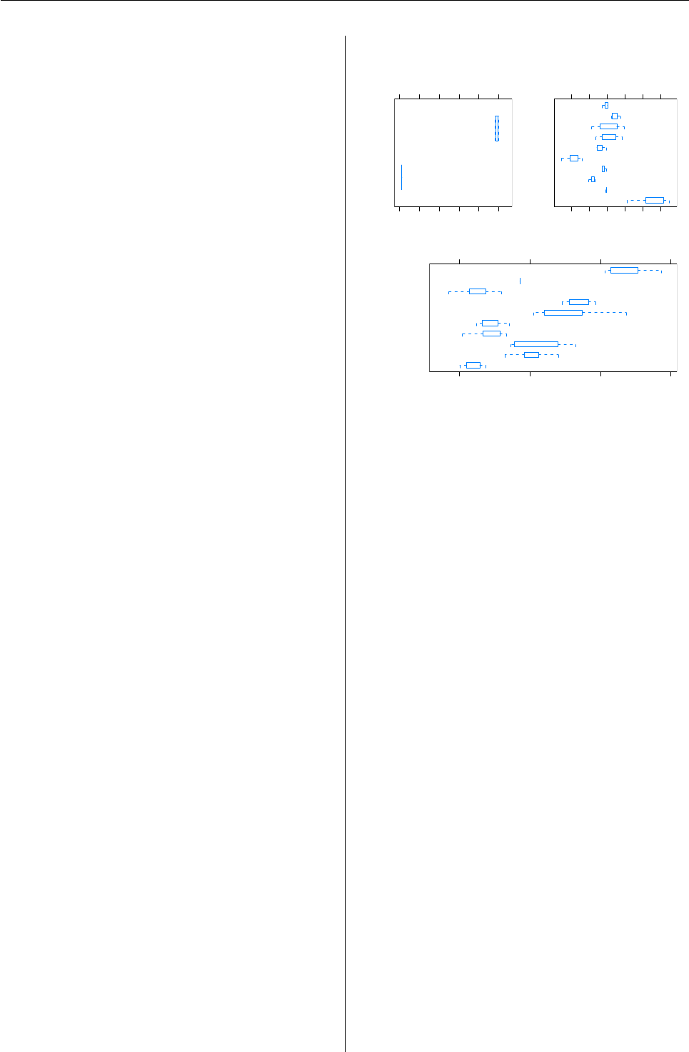
Vol. 6/2, May 2006 19
variable long short exposure
11 cap.bil 109.20 -10.483 98.71
1 liq.w 1.22 0.822 2.04
currency
variable long short exposure
6 JPY 0.062978 -0.158931 -0.095952
8 SEK 0.000948 -0.040208 -0.039260
5 HKD 0.000000 -0.017283 -0.017283
1 AUD 0.001242 -0.005734 -0.004491
7 NOK 0.000000 -0.003949 -0.003949
9 SGD 0.000000 -0.000438 -0.000438
3 EUR 0.179902 -0.176904 0.002998
4 GBP 0.113589 -0.109119 0.004470
2 CHF 0.042340 -0.019232 0.023108
10 USD 0.598999 -0.468202 0.130797
sector
variable long short exposure
10 Utilities 0.00803 -0.08832 -0.080290
3 Cyclicals 0.04980 -0.12475 -0.074945
7 Materials 0.00112 -0.05876 -0.057636
6 Industrials 0.04147 -0.09762 -0.056152
2 Conglomerates 0.00000 -0.00356 -0.003563
9 Technology 0.08784 -0.08730 0.000545
8 Staples 0.24521 -0.23168 0.013532
5 Financials 0.24544 -0.19245 0.052982
4 Energy 0.10328 -0.03456 0.068719
1 Communications 0.19144 -0.05385 0.137588
The difficulty in considering exposures — basi-
cally a static concept about how the portfolio looks
at this moment — in the context of a time series of
portfolio objects is that it is not obvious how to
summarize the exposures over time, especially in the
context of a portfolio whose overall size is changing.
In this release of the portfolio package, we will sim-
ply report the average exposure for all time periods.
For this example portfolio, it is easy to see that the
portfolio is long the biggest stocks. The average mar-
ket capitalization is over $100 billion on the long side
versus only $10 billion on the short side. This cap
exposure causes the portfolio to take a similar “bet”
on liquidity, since larger stocks are, on average, more
liquid than smaller stocks. The liq.w variable is our
measure of liquidity — basically how much stock is
traded on a “typical” day — scaled to have mean 0
and variance 1 for the universe.
The currency and sector exposures are, like-
wise, simple averages of the of the 12 monthly ex-
posures. Even though the portfolio is constructed
without reference to currency or sector, it still ends
up with non-trivial exposures to these variables. In
a typical month, the portfolio is 14% long Communi-
cations and 10% short Japan.
Plotting the exposureHistory object yields box
and whisker plots of net exposure for each exposure
variable, as in Figure 4.
> plot(exposure(global.2004.history))
numeric exposure
exposure
liq.w
cap.bil
0 20 40 60 80 100
●
●●
currency exposure
exposure
USD
SGD
SEK
NOK
JPY
HKD
GBP
EUR
CHF
AUD
−0.10 0.00 0.05 0.10 0.15
●
●
●
●
●
●
●
●
●
●
●
●
sector exposure
exposure
Utilities
Technology
Staples
Materials
Industrials
Financials
Energy
Cyclicals
Conglomerates
Communications
−0.1 0.0 0.1 0.2
●
●
●
●
●
●
●
●
●
●
● ●
Figure 4: Plot of an exposureHistory object.
The performance method aggregates perfor-
mance for each individual time period into an overall
figure and provides a listing of the largest contribu-
tions.
> summary(performance(global.2004.history))
Performance summary (frequency = 12):
ret
mean -0.0081
mean (ann) -0.0971
sd 0.0152
sd (ann) 0.0527
sharpe -1.8439
Best period:
date ret
2004-03-31 2004-03-31 0.0149
Worst period:
date ret
2004-10-31 2004-10-31 -0.0292
Top/Bottom performers (total contribution):
id contrib
140 EBAY 0.00423
231 MRW.LN 0.00387
234 MU 0.00357
338 XOM 0.00337
196 JNJ 0.00333
211 LTR -0.00416
323 VOLVB.SS -0.00453
329 WLP -0.00474
227 MON -0.00494
11 5201 -0.00555
R News ISSN 1609-3631
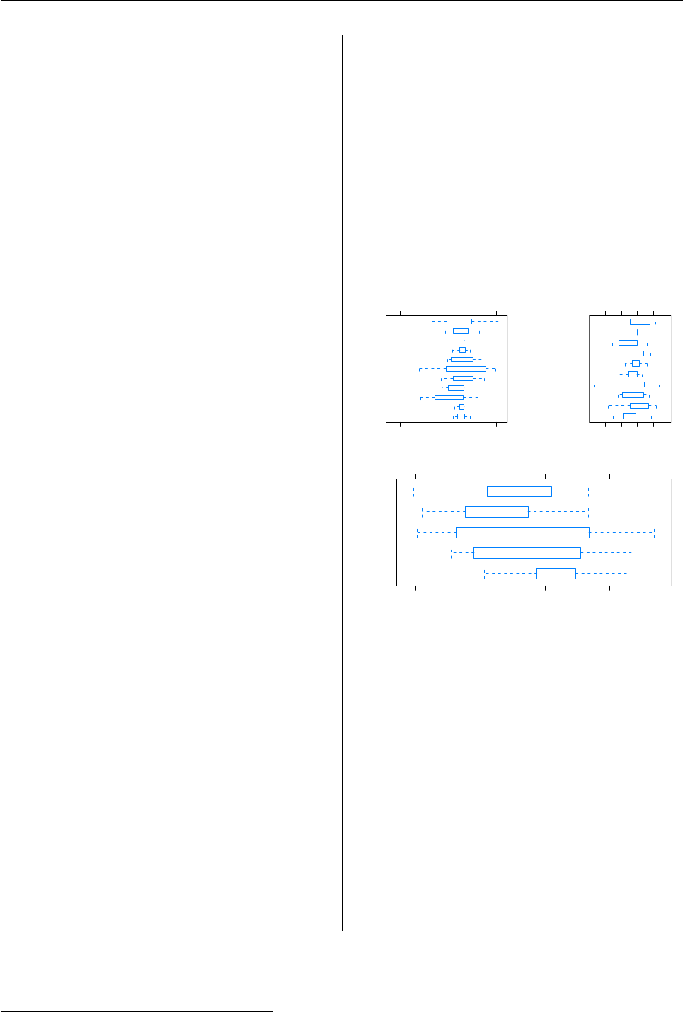
Vol. 6/2, May 2006 20
The best month for the portfolio was April 2004
when it earned 1.5%. The worst month was a loss of
almost 3% in November. The biggest contributor on
the positive side was EBAY. The mean annualized re-
turn of the portfolio is almost -10%; the annualized
volatility is 5.3%. Sharpe ratios — defined1as the
mean return divided by the standard deviation of re-
turn — are generally not provided for unprofitable
portfolios, but the ratio here is -1.8.
Note that the portfolioHistory object does not
keep a record of every position for each time pe-
riod. By design, it only retains summary informa-
tion, albeit on a stock-by-stock basis. We want to be
able to use this package for high frequency data —
say, a decade worth of daily portfolios — so it is not
easy (or even possible) to manipulate an object which
maintains information for every stock for each time
period.
As with the exposure method, the contribution
method works with portfolioHistory objects in the
same way that it works with portfolio objects.
> summary(contribution(global.2004.history))
Mean contribution:
currency
variable weight contrib roic
1 AUD 0.003488 -0.00014179 -0.02622
2 CHF 0.030786 0.00000868 -0.00291
11 DKK 0.000000 0.00000000 0.00000
3 EUR 0.178403 -0.00104765 -0.00620
4 GBP 0.111354 -0.00048120 -0.00409
5 HKD 0.008641 0.00011748 -0.00720
6 JPY 0.110954 0.00005111 -0.00273
21 NOK 0.001974 -0.00012765 -0.03745
7 SEK 0.020578 -0.00111390 -0.04674
31 SGD 0.000219 -0.00000963 -0.01264
8 USD 0.533601 -0.00534746 -0.00996
sector
variable weight contrib roic
1 Communications 0.12610 0.0008478 0.00814
11 Conglomerates 0.00179 -0.0000746 -0.01039
2 Cyclicals 0.08961 -0.0025430 -0.02863
3 Energy 0.07077 0.0008145 0.01384
4 Financials 0.22484 -0.0010191 -0.00416
5 Industrials 0.07153 -0.0014918 -0.01990
6 Materials 0.03067 -0.0002470 -0.01246
7 Staples 0.24511 -0.0036175 -0.01483
8 Technology 0.09007 0.0002594 0.00231
9 Utilities 0.04950 -0.0011930 -0.02607
liq.w
variable weight contrib roic
1 1 - low 0.2628 -0.00390 -0.0140
2 2 0.1607 -0.00545 -0.0349
3 3 0.0668 -0.00136 -0.0197
4 4 0.0952 -0.00167 -0.0156
5 5 - high 0.4144 0.00384 0.0090
Again, the basic approach consists of calculat-
ing the contributions for each time period separately,
saving those results, and then presenting an average
for the entire period.
Figure 5shows the plot of the resulting
contributionHistory object. As with exposure his-
tory, the box and whisker plot shows the median and
quartile range of variable values over the given time
period.
> plot(contribution(global.2004.history))
roic by currency
roic
USD
SGD
SEK
NOK
JPY
HKD
GBP
EUR
DKK
CHF
AUD
−0.2 −0.1 0.0 0.1
●
●
●
●
●
●
●
●
●
●
●
● ●
● ●
●
●
roic by sector
roic
Utilities
Technology
Staples
Materials
Industrials
Financials
Energy
Cyclicals
Conglomerates
Communications
−0.10 0.00 0.05
●
●
●
●
●
●
●
●
●
●
● ●
● ●●
roic by liq.w
roic
5 − high
4
3
2
1 − low
−0.10 −0.05 0.00 0.05
●
●
●
●
●●
Figure 5: Plot of a contributionHistory object.
Conclusion
The current release of the portfolio package is meant
to serve as a proof-of-concept. Relatively sophisti-
cated portfolio analytics are possible using an open
source package. Although money management is
largely a zero-sum game — every dollar that I make
is a dollar that someone else has lost — there is no
reason why we might not cooperate on the tools that
we all use.
David Kane and Jeff Enos
Kane Capital Management, Cambridge, Massachusetts,
USA
david@kanecap.com and jeff@kanecap.com
1The definition of the Sharpe ratio subtracts the risk free rate from the mean return in the numerator. But, in the context of a long-short
portfolio, this is typically ignored.
R News ISSN 1609-3631

Vol. 6/2, May 2006 21
GroupSeq: Designing clinical trials using
group sequential designs
by Roman Pahl, Andreas Ziegler, and Inke R. König
Introduction
Clinical trials are the gold standard to prove su-
periority of new interventions. An attractive vari-
ant to these studies is to use group sequential de-
signs (Ziegler et al.,2003). Widely used since their
introduction in the 1970s and 1980s, many differ-
ent versions of group sequential designs have been
developed. Common to all these designs is their
complex computation for which software tools are
required. In this context, existing software tools
like ADDPLAN (http://www.addplan.com/) often
are not free of charge, making it valuable to consider
freely distributed software alternatives.
GroupSeq provides a set of several methods for
computing group sequential boundaries of well es-
tablished group sequential designs, among others
the designs by Pocock (1977) and O‘Brien and Flem-
ing (1979). More precisely, the original designs are
approximated by the α-spending function approach
which was introduced by Lan and DeMets (1983) and
Kim and DeMets (1987), for which a Fortran pro-
gram by Reboussin et al. (2003) has been available.
For GroupSeq, the latter implementation was com-
pletely recoded in R, and, in addition, new features
were added. For instance, GroupSeq allows one to
calculate exact Pocock bounds beside the estimated
ones obtained by the α-spending approach.
Furthermore, as an important feature, this ap-
plication is embedded in a graphical user interface
(GUI) using the Tcl/Tk interface in the R tcltk pack-
age. Note that there is also a graphical user inter-
face by Reboussin et al. (2003) although it only runs
under Windows. In contrast, the GroupSeq GUI is
available on several platforms, and, moreover, pro-
vides customization possibilities; i.e., the user may
create as many windows as desired. Thus, he or she
may perform multiple tasks such as computing and
comparing several designs at the same time.
The computations yield valid results for any test
which is based on normally distributed test statistics
with independent increments, survival studies, and
certain longitudinal designs. Using the α-spending
function approach, interim analyses need not be
equally spaced, and their number need not be speci-
fied in advance.
Group sequential tests
This paper only gives a basic introduction to group
sequential designs. For a comprehensive overview
of this topic, see, e.g., Jennison and Turnbull (2000)
and Wassmer (2001).
The classical theory of testing goes back to Ney-
man and Pearson (1928) and is based on a sample of
fixed size. In this sample, the null hypothesis H0is
tested against an alternative hypothesis H1. A sig-
nificance level αhas to be defined a priori, which
implies the probability of the null hypothesis being
falsely rejected. Importantly, the evaluation always
takes place at the end after all observations have been
made.
By contrast, group sequential designs allow con-
secutive testing, with possible rejection of the null
hypothesis after observation of each group in a se-
quence of groups. Therefore, the significance levels
corresponding to each group have to be adjusted ap-
propriately. Many different group sequential designs
have been developed. The main difference among
these is the manner of allocating the specific signifi-
cance levels. A further distinction consists in equally
sized groups as in classical group sequential testing
(Pocock,1977;O‘Brien and Fleming,1979) versus un-
equally sized groups (Kim and DeMets,1987).
Determining critical regions
Normally one wants to compare two population
mean values µ1and µ2—i.e., one wants to tests the
null hypothesis H0:µ1=µ2against the alternative
hypothesis H1:µ16=µ2. Consider a standard nor-
mally distributed Zstatistic
Z=X1−X2
qσ2
1/n1+σ2
2/n2
(1)
with X1,X2being the means of two independent
samples of sizes n1,n2which are distributed as
N(µ1,σ2
1)and N(µ2,σ2
2). Assuming n1=n2=n
and σ2
1=σ2
2=σ2, analogously to (1), one can define
a statistic per group k :
Zk=X1k−X2k
σrnk
2
The standardized overall statistic until group kthen
is defined as
Z∗
k=∑k
j=1√njZj
q∑k
j=1nj
R News ISSN 1609-3631

Vol. 6/2, May 2006 22
In contrast to Z1,Z2, ..., ZK, the Z∗
1,Z∗
2, ..., Z∗
Kare sta-
tistically dependent on each other. The joint multi-
variate normal distribution of Z∗
1,Z∗
2, ..., Z∗
Ktherefore
has to be computed numerically.
A specific group sequential design is character-
ized by its regions ξkwith k=1, 2, ..., K-1, where ξk
denotes the region in which the study continues; i.e.,
H0has not been rejected by then. The last acceptance
region in the sequence is denoted ξK, and the proba-
bility of type I error for test Kis given by
1−PH0 K
\
k=1{Z∗
k∈ξk}!,
where PH0denotes the distribution of Z∗
kunder H0.
One obtains the corresponding power with regard to
the alternative hypothesis H1by
1−PH1 K
\
k=1{Z∗
k∈ξk}!.
The α-spending function approach
Theα-spending function, or use function, approach was
introduced by Lan and DeMets (1983) and Kim and
DeMets (1987). It allows analyses at arbitrary points
of time in the study and hence of arbitrarily sized
groups. This is achieved via the α-spending function
α∗(tk)which determines the type I error "spent" until
time point tk, with kdenoting the k-th interim analy-
sis. Usually, the entire period of analysis is standard-
ized to one so that 0 <t1<t2<... <tK=1, with
tk=∑k
i=1ni/N.
Given the maximum sample size Nand the α-
spending function α∗(tk), the critical regions are ob-
tained by recursive calculation. Setting t1=n1/N,
one obtains
PH0(|Z∗
1|≥u1) = α∗(t1)(2)
for the first critical region. Analogously to (2), the
remaining probabilites are obtained by
PH0(
k−1
\
i=1{|Z∗
i|<ui}∩|Z∗
k|≥uk) = α∗(tk)−α∗(tk−1).
The α-spending function approach thus is a very
flexible tool for designing various studies because
neither group size nor number of interim analyses
have to be specified in advance. All calculations per-
formed by GroupSeq are based on the α-spending
approach. In this context, the classic designs are es-
timated as special cases by the following α-spending
functions:
• Pocock:
α∗
1(tk) = αln[1+ (e−1)tk]
• O’Brien and Fleming:
α∗
2(tk) = 41−ΦΦ−1(1−α/4)/√tk
Implementation
The program by Reboussin et al. (2003) constituted
the basis for GroupSeq. Recoding in R followed the
software engineering principles of unitization and
re-usability; i.e., the tasks were divided into many
subfunctions, which also allows improvement in fur-
ther development. One goal consisted in maintain-
ing the performance of the application. This was
achieved by converting the “low level syntax” of
Fortran into R specific functions as well as vector
and matrix operations. Some algorithms also were
slightly improved, e.g., by using Newton’s method
for optimization, replacing a bisection method. The
interested reader is referred to the source code which
is commented in detail. As it turned out, the per-
formance of GroupSeq is generally comparable with
the Fortran implementation. Notable differences oc-
cur only when the number of interim analyses rises
to more than ten. This, however, will usually not oc-
cur in practice. Still, efficiency could be improved
by outsourcing some computations into compiled
C/C++ code.
A main focus was on improving the user inter-
face. At the time of development of GroupSeq, the
Fortran program only provided a command line in-
terface. Because of this, GroupSeq was embedded
in a GUI using Tcl/Tk, making it available for every
platform on which R runs. The customization of the
GUI is left to the user who may create a separate win-
dow for each task, which allows any arrangement
and positioning on the desktop. For those who are
familiar with the program by Reboussin et al. (2003),
the menu structure of that program was retained in
GroupSeq.
Additionally, GroupSeq provides new features
that are not part of the program by Reboussin et al.
(2003). Specifically, new functionality is included
that allows the user to compute exact Pocock bounds.
Package features
GroupSeq provides a GUI using the Tcl/Tk interface
in the R tcltk package. Hence, GroupSeq’s usage is
almost self-explanatory. After loading the package,
the program starts automatically. The user will see
the menu shown in Figure 1.
A task is chosen by selecting an appropriate line
and confirming with “Perform Selected Task”. For
the purpose of multitasking, the user may open as
many task windows as desired. Every task is pro-
cessed independently. Choosing task “-1- Compute
Bounds” will lead to the dialog box given in Figure 2.
R News ISSN 1609-3631
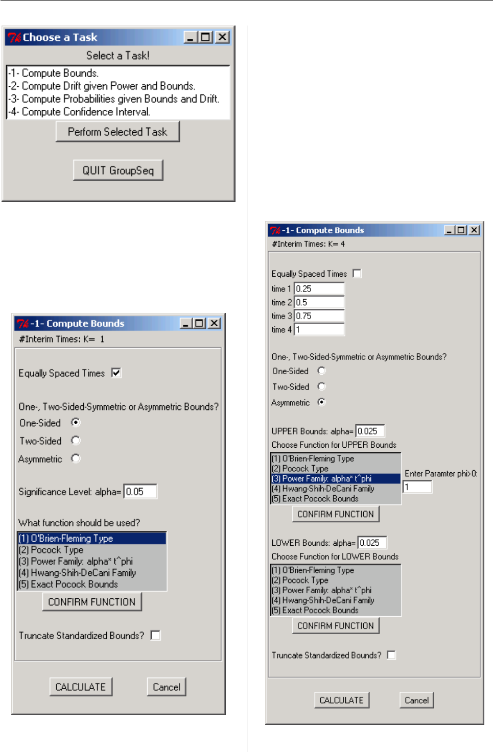
Vol. 6/2, May 2006 23
Figure 1: Menu on program start.
The number of interim analyses is selected by a
drop down menu at the top of the window. An
α-spending function can be selected and must be
confirmed by the “CONFIRM FUNCTION” button.
Figure 2: Window after “-1- Compute Bounds” was
chosen.
The user may choose between (1) and (2) which are
estimates of the classic designs by Pocock (1977) and
O‘Brien and Fleming (1979), respectively. (3) corre-
sponds to the design proposed by Kim and DeMets
(1987), and (4) to a family of functions proposed by
Hwang et al. (1990). Finally, (5) calculates the exact
bounds for the Pocock design. All GroupSeq operat-
ing windows are designed so that irrelevant informa-
tion is concealed. For example, if the user chooses to
use unequal time points and different spending func-
tions for upper and lower bounds, the window will
appear as shown in Figure 3, with GroupSeq provid-
ing meaningful default values.
Figure 3: User specification in “-1- Compute Bounds”.
R News ISSN 1609-3631
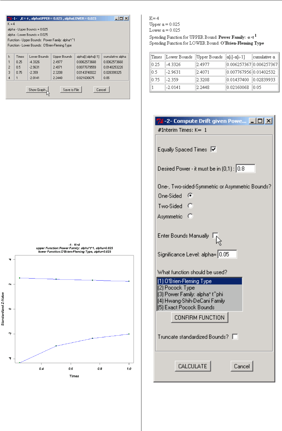
Vol. 6/2, May 2006 24
Figure 4: Displaying results of calculated bounds.
Pressing the “CALCULATE” button at the bottom of
the window initiates the calculation, and each of the
results is shown in a new, separate window. Figure
4 gives an example. The parameter values that were
used in the computation are shown at the top part of
the window, and the most important parameters can
also be seen in the blue window title bar. This feature
helps the user to keep track of many windows when
elaborating many designs at once. The results of the
computation are presented in a table. In the case of
task -1-, the resulting bounds,αspent per stage, and
αspent in total are displayed. In a next step, the re-
sulting critical bounds can be visualized by choosing
“Show Graph” (see Figure 5) which requires the R
graphics environment.
Figure 5: Graphical visualization of results.
By using the option “Save to file”, the results may
be saved into a table in common *.html-file for-
mat, which conserves meta information and there-
fore provides the possibility of further processing
(see Figure 6).
Figure 6: Saved results (viewed in Mozilla Firefox).
Figure 7: “-2- Compute drift given power and bounds”
was chosen.
Choosing task “-2- Compute drift given power and
bounds” from the main menu will lead to the win-
dow shown in Figure 7. Besides specifying the de-
R News ISSN 1609-3631
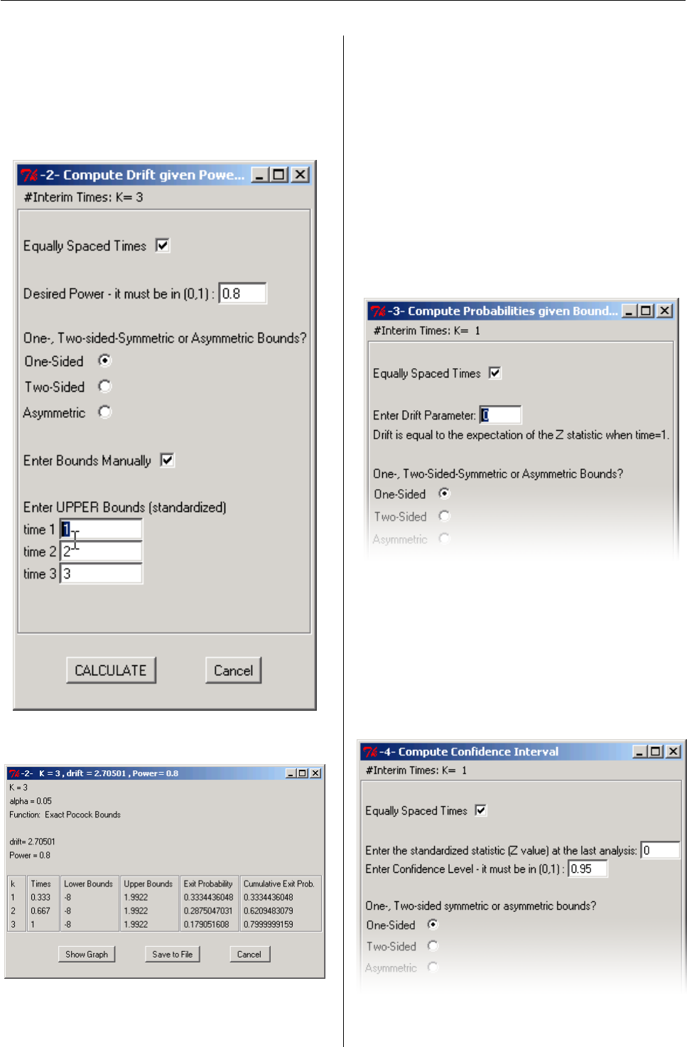
Vol. 6/2, May 2006 25
sired power, the user may enter specific bounds in-
stead of computing them with a spending function.
Activating the corresponding check box changes the
current window as shown in Figure 8. Calculating
the effect under the alternative hypothesis leads to
the window shown in Figure 9.
Figure 8: User enters specific bounds.
Figure 9: Displaying results of calculated drift under
re-specified power (here: Exact Pocock Bounds were
used).
The table contains exit probabilities (i.e., 1 −β) cor-
responding to the probability per stage of rejecting
the null hypothesis under the alternative. The effect
(drift) hereby is implicitly given by the pre-specified
power. The cumulative exit probabilities, in turn,
sum up to the power at last analysis.
Task “-3- Compute drift given power and bounds”
works the other way around. Specifying a certain
drift, which, again, corresponds to the expected ef-
fect size at last analysis (see Figure 10), exit probabil-
ities, resulting in the overall power at last analysis,
are calculated. The computation, of course, also de-
pends on the given bounds and interim times.
Figure 10: User enters drift in Task -3- window (detail).
Finally, users may select task “-4- Compute confidence
interval”. As shown in Figure 11, the confidence level
and the overall effect (as a Z-value) have to be en-
tered.
Figure 11: User enters confidence level and desired effect
in Task -4- window (detail).
R News ISSN 1609-3631
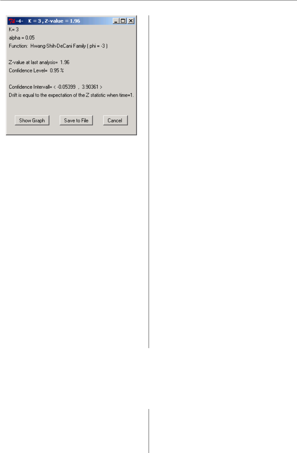
Vol. 6/2, May 2006 26
Figure 12: Resulting confidence interval
(Two-Sided-Bounds).
The window displaying the calculated confidence in-
terval differs somewhat from the other windows (see
Figure 12), as no table is presented. The bounds still
can be visualized using “Show Graph”, however.
Future development
Future versions of GroupSeq will include addi-
tional software ergonomic improvements such as
a status bar during calculation. Additionally, an
“undo” function will be added, as well as a fea-
ture to let users specify their own default values,
thereby achieving more efficiency in frequent use of
GroupSeq. Furthermore, it is planned to implement
adaptive group sequential designs.
Bibliography
I. K. Hwang, W. J. Shih, and J. S. DeCani. Group
sequential designs using a family of type I er-
ror probability spending functions. Statistics in
Medicine, 9:1439–1445, 1990.
C. Jennison and B. W. Turnbull. Group Sequential
Methods with Applications to Clinical Trials. Chap-
man & Hall/CRC, 2000.
K. Kim and D. DeMets. Design and analysis of group
sequential tests based on the type I error spending
rate function. Biometrika, 74:25–36, 1987.
K. K. G. Lan and D. L. DeMets. Discrete sequential
boundaries for clinical trials. Biometrika, 70:659–
663, 1983.
J. Neyman and E. S. Pearson. On the use and inter-
pretation of certain test criteria for purposes of sta-
tistical interference. Biometrika, 20A:263–295, 1928.
P. C. O‘Brien and T. R. Fleming. A multiple testing
procedure for clinical trials. Biometrics, 35:549–556,
1979.
S. J. Pocock. Group sequential methods in the de-
sign and analysis of clinical trials. Biometrika, 64:
191–199, 1977.
D. M. Reboussin, D. L. DeMets, K. Kim, and K. K. G.
Lan. Programs for Computing Group Sequential
Boundaries Using the Lan-DeMets Method, Ver-
sion 2.1. 2003. URL http://www.biostat.wisc.
edu/landemets/.
G. Wassmer. Statistische Testverfahren für gruppense-
quentielle und adaptive Pläne in klassischen Studien.
Alexander Mönch Verlag, Köln, 2001.
A. Ziegler, G. Dahmen, I. R. König, G. Wassmer,
P. Hildebrand, and M. Birth. Accelerating clinical
trials by flexible designs. Good Clinical Practice Jour-
nal, 10:16–19, 2003.
Roman Pahl
roman.pahl@gmx.de
Andreas Ziegler
ziegler@imbs.uni-luebeck.de
Inke R. König
Inke.Koenig@imbs.uni-luebeck.de
Institute of Medical Biometry and Statistics
University at Lübeck, Germany
Using R/Sweave in everyday clinical
practice
by Sven Garbade and Peter Burgard
The Sweave package by Friedrich Leisch is a pow-
erful tool to combine R with L
A
T
EX facilities for text
formatting (R Development Core Team,2005;Leisch,
2002a,b). Sweave allows the dynamic generation of
statistical reports by using literate data analysis. A
further application of Sweave is the package vignette
(Leisch,2003). An introduction to the abilities of
Sweave can be found on Friedrich Leisch’s Home-
R News ISSN 1609-3631

Vol. 6/2, May 2006 27
page (URL: http://www.ci.tuwien.ac.at/~leisch/)
and in several publications, for example Leisch
(2002b,c).
Some issues ago Damian Betebenner wrote an ar-
ticle on how to use R/Sweave in batch mode for au-
tomatic generation of prototype reports (Betebenner,
2005). His article pointed out very helpful and in-
structive notes on how to combine R and Sweave in
batch processing and how to use control structures
with Sweave.
Our article focuses on a combination of
R/Sweave/TclTk in batch mode to produce statis-
tical reports of a neuropsychological examination.
The emphasis of this article is on the background,
functional range and handling of our tool and its use
in our hospital.
Background and Motivation
We routinely use the computer based neuropsycho-
logical test-battery CORTEX (COntextual Reaction
Time EXercises) in our metabolic polyclinic for clin-
ical diagnostics, monitoring and evaluation. A neu-
ropsychological test-battery is a set of several psycho-
logical tests, each testing a specific function of the
brain. The emphasis of our tests is on cognitive
skills, namely visual short term memory, detection
and recognition abilities. The results from the tests
give an insight into a patient’s cognitive state, and
are useful for further diagnostics and treatment rec-
ommendations.
Currently six different tests are bundled in the
battery. An investigation with all six tests lasts about
one hour. Here we describe briefly the six tests; for a
more detailed description of some of these tests and
their theoretical background see Burgard et al. (1997).
The first test is a simple visuomotor reaction task
requiring the testee to press the button of a response
panel as fast as possible after a square appears on the
monitor screen (Test Reaction). The test CPT (Contin-
uous Performance Task) measures sustained atten-
tion by a binary choice task. The testee is required
to press the response button of the dominant hand
as quickly as possible when four dots appear, and
the response button of the non-dominant hand when
three or five dots appear. The LDT (Letter Detection
Task) requires the testee to scan four letters displayed
in a rectangular layout around the center of the com-
puter screen for one, two or three target letters. The
number of target letters determines task difficulty. In
the VWM (Visual Working Memory) task the testee
sees a 7×7 matrix filled with black and white squares
for one second. After a retention interval of four sec-
onds, the previous matrix and three other matrixes
are shown, and the testee has to click on the previ-
ously shown matrix. Task difficulty is determined
by similarity between the target matrix and the three
comparative matrixes. The Dual Task contains three
different tasks and the testee has to deal with visual
and auditory stimuli. In the first task, the testee has
to press a response button as fast as possible when
a particular tone among other tones is played; in the
second task, large or small rectangles are displayed
in random order and the testee has to press a but-
ton when the small rectangle appears. The third task
is a combination of both; i. e., the testee has to press
a response key when the small rectangle or the par-
ticular tone is played. The Tracking task is a test of
the ability of eye-hand coordination. The testee has
to pursue manually with the mouse pointer a ran-
domly moving target on the computer screen. The
target is presented among 10 other moving objects.
To complicate this task, the movements of the mouse
pointer are delayed. The results of each test are saved
as integer variables in a tab-separated text file.
The neuropsychological tests and the analysis
tool for generating statistical reports are imple-
mented on a notebook computer running a Debian
GNU/Linux system. The response panel is con-
nected to the computer with a USB data acquisition
board (USB-DUX). Using a notebook guarantees mo-
bility and the neuropsychological examinations can
be arranged in almost every room in our clinic.
The motivation for the present project was the
need for a tool which could be easily operated by
psychologists, nurses, physicians, etc., to generate
immediately after testing a statistical report based on
the results of the neuropsychological tests.
Handling and functional range
A screen-shot of the main window is shown in Fig-
ure 1. A click on the Help button starts a PDF viewer
showing an instruction manual, and the Quit button
closes the application.
The process to generate a statistical report with
our tool can be summarized in four steps:
1. The user selects with radio buttons the neu-
ropsychological test for which a report should
be generated.
2. The user browses the file system and chooses
one or more raw data files associated with
the selected neuropsychological test. Choos-
ing data files from several testees as well as re-
peated measurements of the same testee is pos-
sible.
3. The user can add information about the tes-
tee and investigator not provided by the data
files from the neuropsychological test-battery,
for example, names, diagnosis, date of birth,
etc.
4. When all raw data files are selected, the user
generates the statistical report with a single
mouse click.
R News ISSN 1609-3631
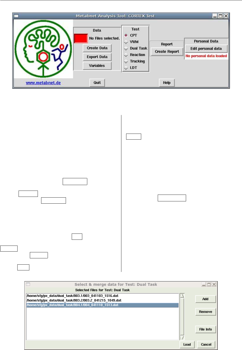
Vol. 6/2, May 2006 28
Figure 1: Screen shot of the main window. The label on top of the Data frame indicates that no data files are
selected.
The main window has four frames with several
buttons. The following paragraphs describe briefly
the functions and use of the program.
Data. The first frame, Data, integrates buttons for
loading and exporting data files. On top of this
group, information about how many data files were
loaded by the user and for which test the report will
be generated is displayed.
The data frame can be exported to a tab-separated
text file with a click on the Export data button. The
variables in the data frame could be inspected by a
click on Variables .
A click on the Create Data button opens the dia-
log shown in Figure 2. The dialog provides buttons
for browsing the filesystem, selecting, deleting and
inspecting raw data files saved by the neuropsycho-
logical test-battery. Once a file is selected, its name
and path are shown in the list.
The callback function for the Add button opens a
file selection dialog to browse the file system. With
Remove the user can delete a marked data file from
the list. The File Info button calls a function to dis-
play the content of a marked data file.
The Load button calls a function which does sev-
eral computations. First, duplicate entries are iden-
tified. Then the selected files shown in the list wid-
get are merged into a data frame. Clicking on the
Cancel button closes the dialog without applying
any changes.
Test. The Test frame is a set of several radio but-
tons. The value of the activated radio button defines
the Sweave file associated with a statistical report.
The value is also used to create the window title and
label in Figure 2.
Report. The Create Report button calls the function
responsible for constituting the correct command
generating the statistical report. When the report
is created successfully, a PDF viewer will be started
showing the generated report.
Personal Data. Clicking the button in this frame
opens a new window where the user can add infor-
mation not provided by the raw data from the test-
battery (see Figure 3). These data concern the name
of the testee, diagnosis and date of birth, the values
of medical parameters, the investigator’s name, and
Figure 2: The dialog for creating the data frame with some raw data files selected. The last file in the list is
marked by a mouse click.
R News ISSN 1609-3631
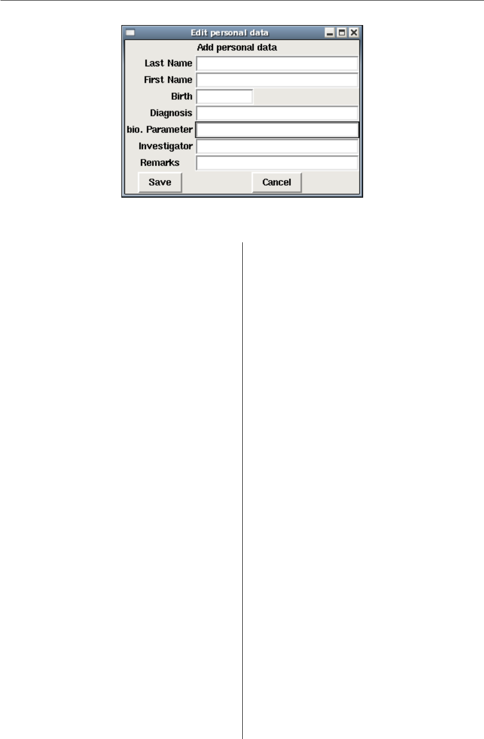
Vol. 6/2, May 2006 29
Figure 3: The dialog for adding additional information about testee and investigator.
possible remarks. Only information that is present is
included in the statistical report.
The red label in the Personal Data frame in the
main window (see Figure 1) changes to a green col-
ored label "Personal data loaded" when any text is sup-
plied. When all characters from the text entries are
deleted, the label color changes back to red and the
label text to "No personal data loaded."
Variables and statistics
The results of each neuropsychological test are saved
as integer variables in a tab-separated text file, one
row per trial and one column per variable. The data
files are saved in separate directories, one directory
for each neuropsychological test. The amount of
saved data depends on the neuropsychological test.
Examples of saved variables are the reaction time a
testee needed to respond to the appearance of a stim-
ulus, the number of stimuli on the screen the tes-
tee had to attend to, the mode of the response, e. g.,
wrong, correct or false alarm (that is the testee re-
ported that there was a target to respond to, but in-
deed there was none), or the distance in pixels be-
tween the mouse pointer and the target to pursue.
Because all variables are saved as integers, the
program recodes integer variables representing a
grouping variable into a factor variable, e. g., 0/1 to
wrong/correct response.
The raw data files from the test-battery provide
no information about the ID (Identification Num-
ber) of the testee or date of psychological examina-
tion. But the file name does: The ID, date and num-
ber of the examination are extracted from the file-
name. The names of the data files have the pat-
tern id_date_time.dat, e. g. 004_041110_1513.dat
for testee 004 tested on 10 November 2004 at 15:13
o’clock (see marked file in Figure 2). A function splits
the filename at the underscores and builds three fac-
tor variables coding the ID, date and time of exam-
ination and the session, that is the number of ex-
amination. The first part code of the filename is
only evaluated until the first dot ".", e. g. 001 and
001.MSUD result in the same ID 001. This gives the
investigator the possibility to include some more in-
formation into the file name without disturbing the
computation of the ID, date and session factors.
The statistical reports are compiled using the ba-
sic L
A
T
EXarticle class and have about three to five
pages, depending on the neuropsychological test.
Each report consists of a fixed part, that is a header
and a basic analysis, and a second part covering a de-
tailed statistical description of the variables acquired
by the neuropsychological test.
The header contains a logo, the address of our
hospital, a title, and the issue date of the report. Then
variables from the text entries of the personal data
dialog (see Figure 3) are included, when available.
The subsequent basic analysis lists the number of tes-
tees, trials and dates of examination, and names of
the data files the statistics are based on.
The second part describes the results of the neu-
ropsychological test by tables and graphics, mostly
scatter plots and trellis graphics. The statistical re-
ports were designed to give a first glance into the
data, and therefore they have a primarily descriptive
character. In most cases, for each variable of inter-
est (e. g. the reaction time from the Reaction test) the
mean, median and standard deviation across testees
and number of examinations are computed and dis-
played graphically. So a report allows the compari-
son of the results from one or more testees at several
dates of examination.
Some remarks about the implemen-
tation
In principle, our tool has two parts: An R/TclTk
function containing all routines for the graphical user
interface (GUI) and data manipulation, and several
R News ISSN 1609-3631
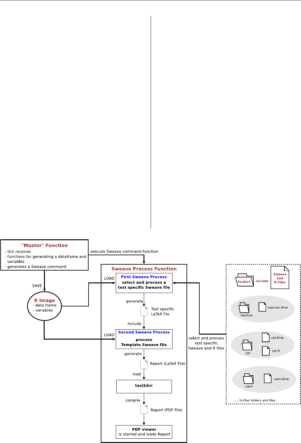
Vol. 6/2, May 2006 30
Sweave style files with R/L
A
T
EX routines for dynamic
generation of statistical reports. A simple flowchart
of the tool is shown in Figure 4.
The GUI was built with the tcltk package that
comes with R. For a short but comprehensive intro-
duction to the tcltk package see Dalgaard (2001), the
Homepage of Wettenhall and of course the R help
pages.
The R/TclTk function holds the rank of a "master"
function. It provides dialogs for the user and defines
and calls R functions to generate a data frame suit-
able to load within an Sweave file. Further it con-
stitutes the correct command to generate the desired
statistical report.
The code chunks in Sweave files have no access
to variables within the running "master" function. To
supply the Sweave files with all necessary data, the
"master" function saves an R image which includes
all variables and a data frame created from the se-
lected raw data files. The variables are, for example,
names, investigator, and diagnosis that come from
the dialog in Figure 3, as well as some other vari-
ables that might be used to create a statistical report,
e. g., the value of the activated radio button in the
Test frame in the main window, and the path and
names of the selected raw data files.
To generate the statistical report, two Sweave
processes are started sequentially. Both Sweave
processes load the previously saved R image.
An Sweave process first evaluates the test-specific
Sweave file; the second Sweave command processes
the template Sweave file and includes the previ-
oulsy generated test-specific L
A
T
EX file. The result-
ing L
A
T
EX file is then processed by pdfL
A
T
EX using the
texi2dvi() function in package tools. When the re-
port is generated successfully, a PDF reader showing
the statistical report is started.
Because the program has to deal with different
Sweave and R files, each report is built in a sepa-
rate directory which includes an Sweave file for the
test-specific routines and sometimes an additional
file with R functions. The template Sweave file and
the R image are stored in a shared directory. In this
way, a more maintainable structure can be achieved.
Summary
Our purpose was to introduce a tool we developed
with a combination of R, Sweave and the tcltk pack-
age and which we now use routinely in our everyday
clinical practise. The sophisticated statistical analysis
and graphic capabilities of R can be bundled with
Sweave and TclTk to build an application allowing
the user to generate a comprehensive report of a neu-
ropsychological examination immediately after test-
Figure 4: Simple flowchart of the application.
R News ISSN 1609-3631

Vol. 6/2, May 2006 31
ing, even without statistical expertise.
This software is currently in a testing phase and
under active development. We still are adapting
some of the statistical reports to the needs of the
users and maybe we will expand the number of tests
of our neuropsychological test-battery and therewith
the range of statistical reports our tool supports. But
so far, we can point out that using R/Sweave/TclTk
is much more powerful compared to data analysis
of test results in the past. Some of the neuropsycho-
logical tests we briefly reported about ran formerly
in an old version of MS-DOS, and subsequent data
analysis was a bit hampered because exporting the
raw data from an examination to a statistical analy-
sis system was necessary. After reprogramming the
neuropsychological tests on a modern computer sys-
tem with the facilities of R, it was a relatively sim-
ple matter to combine the neuropsychological test-
battery with a convenient tool for exploring the data.
One further improvement we are considering is
an interface for connecting our tool to a data base sys-
tem. This offers the opportunity to save and reload
easily the data from an examination.
Acknowledgment
We would like to thank an anonymous reviewer who
gave us helpful remarks on a previous version of this
manuscript, as well as suggestions about how to im-
prove our code.
Bibliography
D. Betebenner. Using control structures with Sweave.
R News, 5(1):40–44, May 2005. URL http://CRAN.
R-project.org/doc/Rnews/.
P. Burgard, F. Rey, A. Rupp, V. Abadie, and J. Rey.
Neuropsychologic functions of early treated pa-
tients with phenylketonuria, on and off diet: re-
sults of a cross-national and cross-sectional study.
Pediatric Research, 41:368–374, 1997.
P. Dalgaard. A primer on the R-Tcl/Tk package.
R News, 1(3):27–31, September 2001. URL http:
//CRAN.R-project.org/doc/Rnews/.
F. Leisch. Sweave: Dynamic generation of statistical
reports using literate data analysis. Presented at
”Österreichische Statistiktage 2002”, Vienna, Aus-
tria, October 23–25 2002a.
F. Leisch. Sweave, part I: Mixing R and L
A
T
EX. R
News, 2(3):28–31, December 2002b. URL http:
//CRAN.R-project.org/doc/Rnews/.
F. Leisch. Sweave user manual. URL http://www.
ci.tuwien.ac.at/~leisch/Sweave. Institut für
Statistik und Wahrscheinlichkeitstheorie, Technis-
che Universität Wien, Vienna, Austria, 2002c.
F. Leisch. Sweave, part II: Package vignettes. R
News, 3(2):21–24, October 2003. URL http://
CRAN.R-project.org/doc/Rnews/.
R Development Core Team. R: A Language and Envi-
ronment for Statistical Computing. R Foundation for
Statistical Computing, Vienna, Austria, 2005. URL
http://www.R-project.org. ISBN 3-900051-07-0.
USB-DUX. URL http://www.linux-usb-daq.co.
uk/.
J. Wettenhall. URL http://bioinf.wehi.edu.au/
~wettenhall/RTclTkExamples/.
Sven Garbade and Peter Burgard
University Hospital for Pediatric
and Adolescent Medicine
Department of General Pediatrics
METABNET - Epidemiological Register
D-69120 Heidelberg, Germany
www.metabnet.de
Sven.Garbade@med.uni-heidelberg.de
changeLOS: An R-package for change in
length of hospital stay based on the
Aalen-Johansen estimator
by M. Wangler, J. Beyersmann, and M. Schumacher
Introduction
Length of hospital stay (LOS) is used to assess the
utilization of hospital resources, the costs and the
general impact of a disease. Change in LOS due
to a complication is frequently used to assess the
impact and the costs of a complication. Promi-
nent examples include nosocomial infections and ad-
verse drug events. In a data analysis, it is impor-
tant to regard the timing of events: A complica-
R News ISSN 1609-3631
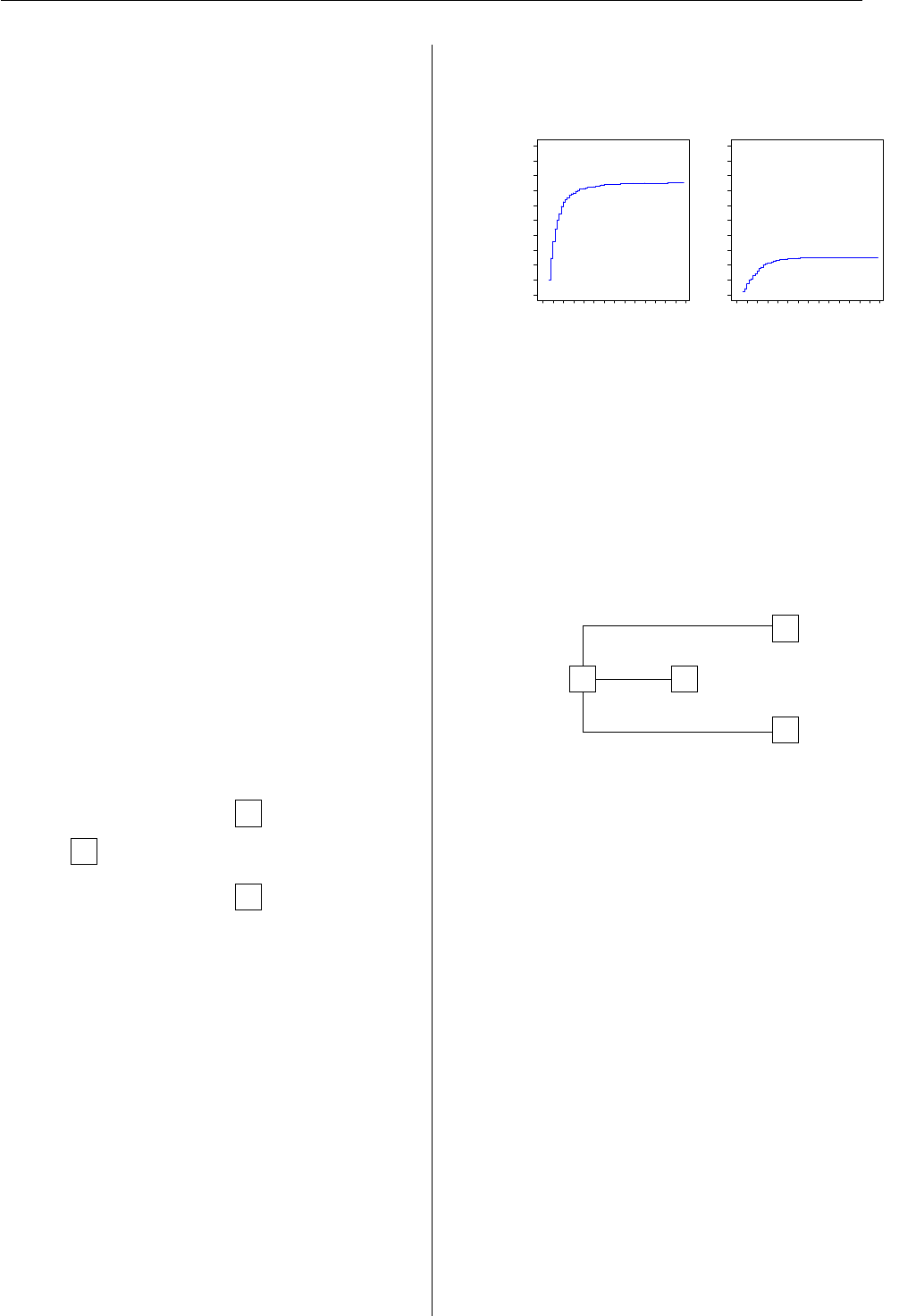
Vol. 6/2, May 2006 32
tion can only have an effect on LOS, once it has oc-
curred. Classical methods of two-group compari-
son, including matching, are commonly used, but
inadequate. Multi-state models provide a suitable
framework for analyzing change in LOS. For an
overview on multi-state models cf. (Andersen and
Keiding,2002). Change in LOS has been considered
in a multi-state framework by (Schulgen and Schu-
macher,1996), (Schulgen et al.,2000), (Beyersmann
et al.,2006) and (Beyersmann,2005). We introduce
an R package to adequately analyze change in LOS.
The R package is based on multi-state model theory.
The main features are:
• Describe multi-state models
• Compute and plot transition probabilities
(Aalen - Johansen estimator)
• Compute and plot change in LOS
The estimation techniques used are fully nonpara-
metric, allowing for a time-inhomogeneous Markov
process, i.e. the future development of the pro-
cess depends only on the state currently occupied;
the Markov assumption may be dropped for estima-
tion of state occupation probabilities (Glidden,2002).
However, at present, adjusting for covariates is not
included. In both these aspects, the package change-
LOS differs from the package msm.
Simple example: Competing Risks
A simple example for a multi-state model is the com-
peting risks model, shown in the following figure:
0
1
2
1
PPPPPPP
Pq
Alive
Discharge
Death
Figure 1: Multi-state model: competing risks
With our R package changeLOS it is possible to:
• describe the state names and possible transi-
tions (function msmodel(...)):
012
0 TRUE TRUE TRUE
1 FALSE TRUE FALSE
2 FALSE FALSE TRUE
• compute the Aalen-Johansen estimator for
the matrix of transition probabilities (function
aj(...)): P(s,t), time interval (s,t]. These are
the Cumulative Incidence Functions: P01(0, t),
P02(0, t)
• plot the temporal dynamics of the data il-
lustrated by transition probabilities (function
plot.aj(...)):
0 5 10 20 30 40 50 60 70
0.0 0.1 0.2 0.3 0.4 0.5 0.6 0.7 0.8 0.9 1.0
Time t
Estimate of P01(0,t)
P
^01(0,t)
0 5 10 20 30 40 50 60 70
0.0 0.1 0.2 0.3 0.4 0.5 0.6 0.7 0.8 0.9 1.0
Time t
Estimate of P02(0,t)
P
^02(0,t)
Figure 2: Cumulative Incidence Functions
Change in LOS
The model
The following model is used to analyze change in
LOS due to a complication, or in general, an inter-
mediate event:
0
No
complication -
-
-
1
Complication
QQQQ
Qs
3 2Discharge
3Death
Figure 3: Multi-state model: change in LOS
The first step is to describe the mult-state model
with the function msmodel(...):
## possible transitions
> tra <- matrix(F, 4, 4)
> diag(tra) <- T
> tra[1, ] <- T
> tra[2, 3:4] <- T
## describe the multi-state model
> my.model <- msmodel(c("0","1","2","3"),
tra, cens.name="cens")
The data set
A real data set (Grundmann et al.,2005) comes with
the package and can be loaded by
> data(los.data)
> los.data[1:4,]
and looks like the following example:
R News ISSN 1609-3631
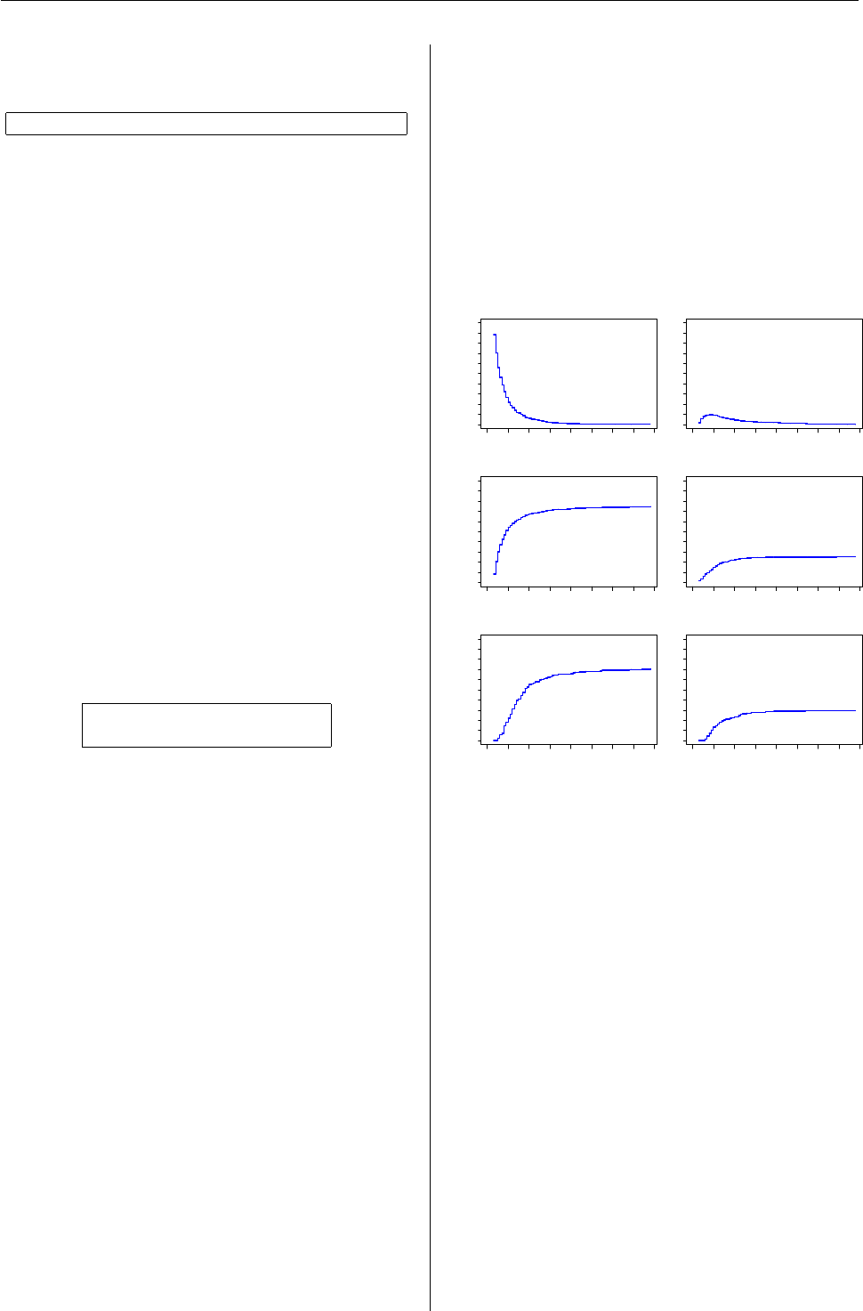
Vol. 6/2, May 2006 33
adm.id j.01 j.02 j.03 j.12 j.13 cens
1 12 Inf 3 Inf Inf Inf Inf
2 32 Inf Inf 20 Inf Inf Inf
341 20 Inf Inf 40 Inf Inf
4 175 6 Inf Inf Inf Inf 26
. . . . . . .
los.data has one row per patient and includes
the variables j.01, j.02, j.03, j.12, j.13 and
cens.The variables starting with ’j’ will hold the
time when a respective transition(or ’jump’) was
observed. E.g., the third patient experiences a com-
plication 20 days after admission to hospital and is
being discharged 40 days after admission. Entries
for non-observed transitions have to be set to infin-
ity, which is represented in R by Inf. In addition, if
a patient is censored, i.e. still in hospital by the end
of the study, the variable cens is set to the time when
censoring occurred. If the patient is not censored, it
is set to Inf.
Before further computations, the patient-orientated
data set los.data must be transformed to a
transition-orientated data set:
> my.observ <- prepare.los.data(x=los.data)
Then the data set looks like:
id from to time
1 12 0 2 3
2 32 0 3 20
341 0 1 20
441 1 2 40
5 175 0 1 6
6 175 1 cens 26
. . . . .
Now each row represents a transition. E.g. for the
patient with the id 41 there are two entries: one entry
for the transition from state 0 to state 1 and one entry
for the transition from state 1 to state 2.
The Aalen-Johansen estimator
> my.trans <- trans(model=my.model,
observ=my.observ)
computes the Aalen - Johansen estimator for the ma-
trix of transition probabilities P(u−,u)for all ob-
served transition times u. The entry (l,m)of the
matrix denotes the estimated probability that state m
has been reached by time u given state l has been oc-
cupied just before time u. The estimator for P(u−,u)
is described by (Andersen et al.,1993) at the bottom
of p. 288. Non-diagonal entries (h,j)are given as
the number of observed transitions from state hto
state j, divided by the number of individuals in state
hjust prior to time u. The diagonal elements are cho-
sen such that the sum of each row equals 1.
The Aalen-Johansen estimator for P(s,t)can then
be computed as matrix product of all matrices
P(u−,u)for all transition times u in (s,t]:
> my.aj <- aj(my.trans,s=0,t=80)
The temporal dynamics of the data can be illustrated
by the transition probabilities:
> plot(my.aj,c("0","0","0","0","1","1"),
c("0","1","2","3","2","3"))
0 10 20 30 40 50 60 70 80
0.0 0.3 0.6 0.9
Time t
Estimate of P00(0,t)
P
^00(0,t)
0 10 20 30 40 50 60 70 80
0.0 0.3 0.6 0.9
Time t
Estimate of P01(0,t)
P
^01(0,t)
0 10 20 30 40 50 60 70 80
0.0 0.3 0.6 0.9
Time t
Estimate of P02(0,t)
P
^02(0,t)
0 10 20 30 40 50 60 70 80
0.0 0.3 0.6 0.9
Time t
Estimate of P03(0,t)
P
^03(0,t)
0 10 20 30 40 50 60 70 80
0.0 0.3 0.6 0.9
Time t
Estimate of P12(0,t)
P
^12(0,t)
0 10 20 30 40 50 60 70 80
0.0 0.3 0.6 0.9
Time t
Estimate of P13(0,t)
P
^13(0,t)
Figure 4: Aalen -Johansen estimator for P00(s,t),
P01(s,t),P02(s,t),P03(s,t),P12(s,t),P13(s,t)
Epected change in LOS
The function clos estimates the expected change in
length of stay (LOS) associated with an intermedi-
ate event (IE), using the Aalen-Johansen estimator
for the matrix of transition probabilities.
> los <- clos(model=my.model,observ=my.observ)
los will be a an object of class clos. This object is a
list which contains among others the following argu-
ments:
•cLOS: change in LOS
•e.given.1: estimates E(LOS |state 1 on day t )
for each day
•e.given.0: estimates E(LOS |state 0 on day t )
for each day
•weights: weights for the weighted average
R News ISSN 1609-3631
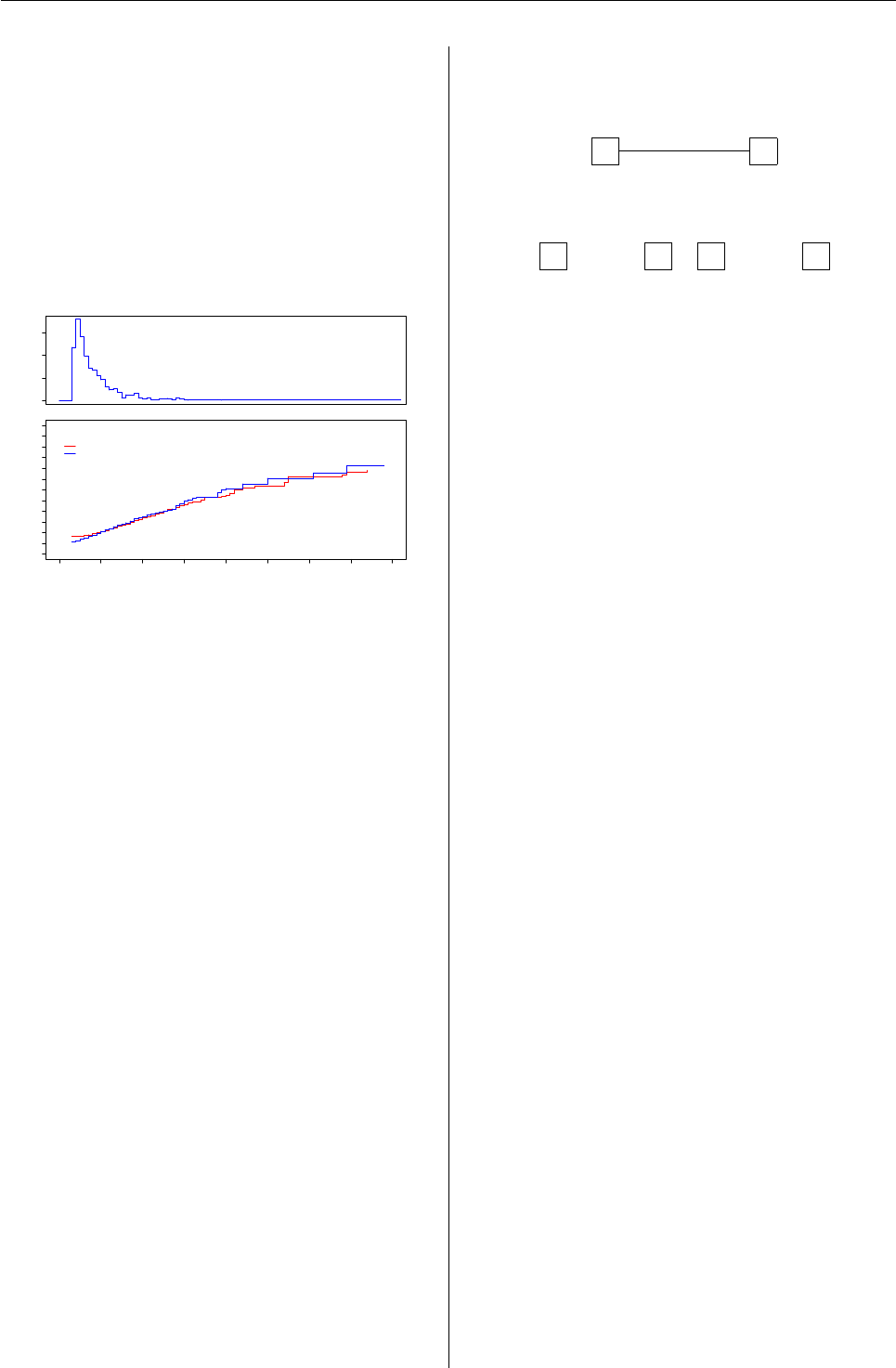
Vol. 6/2, May 2006 34
•trans: matrices of transition probabilities
P(u−,u)for all observed transition times u
The expected change in LOS is computed as the
difference between e.given.1 and e.given.0 for
each day and the overall change in LOS cLOS as a
weighted average of these quantities. Figure 5 shows
the graph obtained by plotting change in LOS:
> plot(los, xlim=c(0,80), ylim.1=c(0,120))
Weights
0.00 0.05 0.10 0.15
0 10 20 30 40 50 60 70 80
0 20 40 60 80 100 120
Time t
Expected LOS
Intermediate event by time t
No intermediate event by time t
Figure 5: Expected change in LOS due to a complica-
tion visualized
> summary(los)
The summary for objects of class clos displays the
following values (absolute and in percent):
• Number of observed patients
• Number of patients being discharged
• Number of patients who die
• Number of patients being censored
• Number of patients who experienced the inter-
mediate event (IE)
• Number of patients who experienced the IE be-
ing discharged
• Number of patients who experienced the IE
and died
• Number of patients who experienced the IE
and were censored
Progressive Disability Model
Change in LOS and impact of an intermediate event
on mortality can also be investigated in a so-called
progressive disability model, shown in Figure 6.
This multi-state model can be described and the
Aalen-Johansen estimator for transition probabilities
can be computed with our R package changeLOS:
0
No
complication 1Complication
2
Discharge
3
Death
4
Discharge
5
Death
-
JJJJ
J^
JJJJ
J^
Figure 6: Progressive disability model
Here, the first state carries information on
whether or not an individual has passed through the
intermediate state.
Summary
In order to get realistic information on change in
LOS due to a complication, it is crucial to ade-
quately account for the timing of events. This can
be achieved as outlined by (Beyersmann et al.,2006).
However, while tools of standard survival analysis
have become an integral part of most statistical soft-
ware packages, the multi-state methods envisaged
by (Beyersmann et al.,2006) and (Beyersmann,2005)
are less accessible. We have introduced the R pack-
age changeLOS so that it is freely available, easy to
use and allows people to visualize the situation at
hand.
changeLOS is an R package to:
• describe any multistate model
• compute and visualize transition probabilities
(Aalen-Johansen estimator)
• compute and visualize change in LOS
Bibliography
P. Andersen, Ø. Borgan, R. D. Gill, and N. Kei-
ding. Statistical models based on counting pro-
cesses. Springer Series in Statistics. New York, NY:
Springer., 1993.
P. Andersen and N. Keiding. Multi-state models for
event history analysis. Statistical Methods in Medi-
cal Research, 11(2):91–115, 2002.
J. Beyersmann. On change in length of stay associated
with an intermediate event: estimation within multi-
state models and large sample properties. PhD the-
sis, University of Freiburg, Faculty of Mathematics
and Physics, Germany, 2005. URL www.freidok.
uni-freiburg.de/volltexte/1843/.
R News ISSN 1609-3631

Vol. 6/2, May 2006 35
J. Beyersmann, P. Gastmeier, H. Grundmann, S. Bär-
wolff, C. Geffers, M. Behnke, H. Rüden, and
M. Schumacher. Use of Multistate Models to As-
sess Prolongation of Intensive Care Unit Stay Due
to Nosocomial Infection. Infection Control and Hos-
pital Epidemiology, 27:493-499, 2006.
D. Glidden. Robust innference for event probabili-
ties with non-Markov data. Biometrics, 58:361–368,
2002.
H. Grundmann, S. Bärwolff, F. Schwab, A. Tami,
M. Behnke, C. Geffers, E. Halle, U. Göbel,
R. Schiller, D. Jonas, I. Klare, K. Weist, W. Witte,
K. Beck-Beilecke, M. Schumacher, H. Rüden, and
P. Gastmeier. How many infections are caused
by patient-to-patient transmission in intensive care
units? Critical Care Medicine (in press), 2005.
G. Schulgen, A. Kropec, I. Kappstein, F. Daschner,
and M. Schumacher. Estimation of extra hospital
stay attributable to nosocomial infections: hetero-
geneity and timing of events. Journal of Clinical Epi-
demiology, 53:409–417, 2000.
G. Schulgen and M. Schumacher. Estimation of pro-
longation of hospital stay attributable to nosoco-
mial infections. Lifetime Data Analysis, 2:219–240,
1996.
Matthias Wangler
mw@imbi.uni-freiburg.de
Balloon Plot
Graphical tool for displaying tabular data
by Nitin Jain and Gregory R. Warnes
Introduction
Numeric data is often summarized using rectangular
tables. While these tables allow presentation of all
of the relevant data, they do not lend themselves to
rapid discovery of important patterns. The primary
difficulty is that the visual impact of numeric values
is not proportional to the scale of the numbers repre-
sented.
We have developed a new graphical tool, the
“balloonplot”, which augments the numeric values
in tables with colored circles with area proportional
to the size of the corresponding table entry. This
visually highlights the prominent features of data,
while preserving the details conveyed by the nu-
meric values themselves.
In this article, we describe the balloonplot, as
implemented by the balloonplot function in the
gplots package, and describe the features of our im-
plementation. We then provide an example using the
“Titanic” passenger survival data. We conclude with
some observations on the balloonplot relative to the
previously developed “mosaic plot”.
Function description
The balloonplot function accepts a table (to be dis-
played as found) or lists of vectors for x (column
category), y (row category) and z (data value) from
which a table will be constructed.
The balloonplot function creates a graphical ta-
ble where each cell displays the appropriate numeric
value plus a colored circle whose size reflects the rel-
ative magnitude of the corresponding component.
The area of each circle is proportional to the fre-
quency of data. (The circles are scaled so that the
circle for largest value fills the available space in the
cell.)
As a consequence, the largest values in the table
are “spotlighted” by the biggest circles, while smaller
values are displayed with smaller circles. Of course,
circles can only have positive radius, so the radius of
circles for cells with negative values are set to zero.
(A warning is issued when this “truncation” occurs.)
Of course, when labels are present on the table
or provided to the function, the graphical table is
appropriately labeled. In addition, options are pro-
vided to allow control of various visual features of
the plot:
• rotation of the row and column headers
• balloon color and shape (globally or individu-
ally)
• number of displayed digits
• display of entries with zero values
• display of marginal totals
• display of cumulative histograms
• x- and y-axes group sorting
• formatting of row and column labels
• traditional graphics parameters (title, back-
ground, etc.)
R News ISSN 1609-3631
Vol. 6/2, May 2006 36
Example using the Titanic data set
For illustration purposes, we use the Titanic data
set from the datasets package. Titanic provides
survival status for passengers on the tragic maiden
voyage of the ocean liner “Titanic”, summarized ac-
cording to economic status (class), sex, and age.
Typically, the number of surviving passengers are
shown in a tabular form, such as shown in Figure 1.
●●●
●●●
●●●
●●●
1st 2nd 3rd Crew
Child
Adult
Male
Female
Male
Female
Age Sex
Class
5 11 13 0
1 13 14 0
57 14 75 192
140 80 76 20
BalloonPlot : Surviving passengers
Figure 1: Tabular representation of survived popula-
tion by gender and age
Figure 1was created by calling balloonplot with
the balloon color set to match the background color
and most options disabled. Note that one must ac-
tively focus on the individual cell values in order to
see any pattern in the data.
Now, we redraw the table with light-blue circles
(‘balloons’) superimposed over the numerical values
(Figure 2). This is accomplished using the code:
library(gplots)
data(Titanic)
# Convert to 1 entry per row format
dframe <- as.data.frame(Titanic)
# Select only surviving passengers
survived <- dframe[dframe$Survived=="Yes",]
attach(survived)
balloonplot(x=Class,
y=list(Age, Sex),
z=Freq,
sort=TRUE,
show.zeros=TRUE,
cum.margins=FALSE,
main=
"BalloonPlot : Surviving passengers"
)
title(main=list("Circle area is proportional to\
number of passengers",
cex=0.9),
line=0.5)
detach(survived)
●●●
●●●
●●●
●●●●
203 118 178 212
29
28
338
316
711
1st 2nd 3rd Crew
Child
Adult
Male
Female
Male
Female
Age Sex
Class
5 11 13 0
1 13 14 0
57 14 75 192
140 80 76 20
BalloonPlot : Surviving passengers
Circle area is proportional to number of passengers
Figure 2: Balloon plot of surviving individuals by
class, gender and age
With the addition of the blue “spotlights”, whose
area is proportional to the magnitude of the data
value, it is easy to see that only adult females and
adult male crew members survived in large num-
bers. Also note the addition of row and column
marginal totals.
Of course, the number of surviving passengers
is only half of the story. We could create a simi-
lar plot showing the number of passengers who did
not survive. Alternatively, we can simply add sur-
vival status as another variable to the display, setting
the color of the circles to green for passengers who
survived, and magenta for those who did not (Fig-
ure 3). This conveys considerably more information
than Figures 1 and 2 without substantial loss of clar-
ity. The large magenta circles make it clear that most
passengers did not survive.
To further improve the display, we add a visual
representation of the row and column sums (Figure
4). This is accomplished using light grey bars behind
the row and column headers. The length of each bar
is proportional to the corresponding sum, allowing
rapid visual ascertainment of their relative sizes. We
have also added appropriately colored markers ad-
jacent to the headers under “Survived” to emphasize
the meaning of each color.
R News ISSN 1609-3631

Vol. 6/2, May 2006 37
●
●
●●●●
●●●●
●●●
●●●
●●●●
●●●●
325 285 706 885
35
17
1329
109
29
28
338
316
2201
1st 2nd 3rd Crew
No
Yes
Child
Adult
Child
Adult
Male
Female
Male
Female
Male
Female
Male
Female
Survived Age Sex
Class
0 0 35 0
0 0 17 0
118 154 387 670
4 13 89 3
5 11 13 0
1 13 14 0
57 14 75 192
140 80 76 20
BalloonPlot : Passenger Class by Survival, Age and Sex
Circle area is proportional to number of passengers
Figure 3: Balloon plot of Titanic passengers by gen-
der, age and class. Green circles represent passengers
who survived and magenta circles represent the pas-
sengers who did not survive.
attach(dframe)
colors <- ifelse( Survived=="Yes", "green",
"magenta")
balloonplot(x=Class,
y=list(Survived, Age, Sex),
z=Freq,
sort=FALSE,
dotcol=colors,
show.zeros=TRUE,
main="BalloonPlot : Passenger Class \
by Survival, Age and Sex")
points( x=1, y=8, pch=20, col="magenta")
points( x=1, y=4, pch=20, col="green")
title(main=list("Circle area is proportional to \
number of passengers", cex=0.9), line=0.5)
detach(dframe)
It is now easy to see several facts:
• A surprisingly large fraction (885/2201) of pas-
sengers were crew members
• Most passengers and crew were adult males
• Most adult males perished
• Most women survived, except in 3rd class
• Only 3rd class children perished
●
●
●●●●
●●●●
●●●
●●●
●●●●
●●●●
325 285 706 885
35
17
1329
109
29
28
338
316
2201
1st 2nd 3rd Crew
No
Yes
Child
Adult
Child
Adult
Male
Female
Male
Female
Male
Female
Male
Female
Survived Age Sex
Class
0 0 35 0
0 0 17 0
118 154 387 670
4 13 89 3
5 11 13 0
1 13 14 0
57 14 75 192
140 80 76 20
BalloonPlot : Passenger Class by Survival, Age and Sex
●
●
Circle area is proportional to number of passengers
Figure 4: Balloon plot of all the passengers of Titanic,
stratified by survival, age, sex and class
Perhaps the most striking fact is that survival is
lowest among 3rd class passengers for all age and
gender groups. It turns out that there is a well known
reason for this difference in survival. Passengers
in 1st and 2nd class, as well as crew members, had
better access to the lifeboats. Since there were too
few lifeboats for the number of passengers and crew,
most women and children among the 1st class, 2nd
class and crew found space in a lifeboat, while many
of the later arriving 3rd class women and children
were too late: the lifeboats had already been filled
and had moved away from the quickly sinking ship.
Discussion
Our goals in developing the balloonplot were
twofold: First, to improve ability of viewers to
quickly perceive trends. Second, to minimize the
need for viewers to learn new idioms. With these
goals in mind, we have restricted ourselves to sim-
ple modifications of the standard tabular display.
Other researchers have pursued more general ap-
proaches to the visual display of tabular data. (For
a review of that work, see Hartigan and Kleiner
(Hartigan and Kleiner,1981) or Friendly (Friendly,
1992).) One of the most popular methods developed
by these researchers is the mosaic plot (Snee,1974).
We have previously experimented with mosaic
plots. Unfortunately, we found that they do not lend
themselves to rapid ascertainment of trends, partic-
ularly by untrained users. Even trained users find
that they must pay careful attention in order to de-
code the visual information presented by the mosaic
plot. In contrast, balloonplots lend themselves to
very quick perception of important trends, even for
R News ISSN 1609-3631

Vol. 6/2, May 2006 38
users who have never encountered them before.
While there are, of course, tasks for which mosaic
plot is preferable, we feel that the balloonplot serves
admirably to allow high-levels patterns to be quickly
perceived by untrained users.
Conclusion
Using the well worn Titanic data, we have shown
how balloonplots help to convey important aspects
of tabular data, without obscuring the exact numeric
values. We hope that this new approach to visu-
alizing tabular data will assist other statisticians in
more effectively understanding and presenting tab-
ular data.
We wish to thank Ramon Alonso-Allende
allende@cnb.uam.es for the discussion on R-help
which lead to the development of balloonplot, as
well as for the code for displaying the row and col-
umn sums.
Bibliography
M. Friendly. Graphical methods for categorical data.
Proceedings of SAS SUGI 17 Conference, 1992.
J. A. Hartigan and B. Kleiner. Mosaics for contin-
gency tables. Computer Science and Statistics: Pro-
ceedings of the 13th Symposium on the Interface. New
York: Springer-Verlag, 1981.
R. D. Snee. Graphical display of two-way contin-
gency tables. The American Statistician, 28:9–12,
1974.
Gregory R. Warnes, Pfizer Inc., USA
gregory.r.warnes@pfizer.com
Nitin Jain, Smith Hanley Inc, USA
nitin.jain@pfizer.com
Drawing pedigree diagrams with R and
graphviz
by Jing Hua Zhao
Human genetic studies often involve data collected
from families and graphical display of them is useful.
The wide interest in such data over years has led to
many software packages, both commercial and non-
commercial. A recent account of these packages is
available (Dudbridge et al.,2004), and a very flex-
ible package Madeline (http://eyegene.ophthy.
med.umich.edu/madeline/index.html) is now re-
leased under the GNU General Public License. A
comprehensive list of many packages, including
the package LINKAGE (Terwilliger and Ott,1994)
for human parametric linkage analysis and GAS
(Genetic Analysis System, http://users.ox.ac.uk/
~ayoung/gas.html) for some other analyses, can be
seen at the linkage server at Rockefeller University
(http://linkage.rockefeller.edu).
Here I describe two functions in R that are
able to draw pedigree diagrams; the first be-
ing plot.pedigree in kinship developed for S-
PLUS by Terry Therneau and Beth Atkinson and
ported to R by the author, and the second
pedtodot in gap based on David Duffy’s gawk
script (http://www2.qimr.edu.au/davidD/Course/
pedtodot) that requires graphviz (http://www.
graphviz.org). Both are easy to use and can draw
many pedigree diagrams quickly to a single file,
therefore can serve as alternatives to some programs
that only offer interactive use.
Representation of pedigrees
The key elements to store pedigrees using a database
is via the so-called family trios each containing in-
dividual’s, father’s and mother’s IDs. Founders,
namely individuals whose parents are not in the
pedigree, are set to be zero or missing. Individual’s
gender (e.g. 1=male, 2=female) is included as auxil-
iary information, together with pedigree ID in order
to maintain multiple pedigrees in a single database,
each record of which indicates a node in the pedigree
graph.
For instance, information for pedigree numbered
10081 in genetic analysis workshop 14 (GAW14,
http://www.gaworkshop.org) is shown as follows.
pid id father mother sex affected
10081 1 2 3 2 2
10081 2 0 0 1 1
10081 3 0 0 2 2
10081 4 2 3 2 2
10081 5 2 3 2 1
10081 6 2 3 1 1
10081 7 2 3 2 1
10081 8 0 0 1 1
10081 9 8 4 1 1
10081 10 0 0 2 1
10081 11 2 10 2 1
10081 12 2 10 2 2
R News ISSN 1609-3631
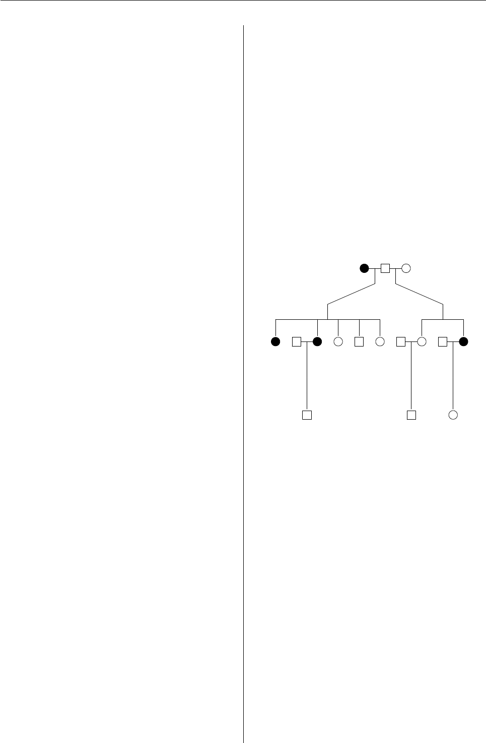
Vol. 6/2, May 2006 39
10081 13 0 0 1 1
10081 14 13 11 1 1
10081 15 0 0 1 1
10081 16 15 12 2 1
Here all IDs are integers with obvious meanings
just described, and the variable affected indicates
if an individual is alcoholic (1=nonalcoholic, 2=alco-
holic) according to DSMIIIR and Feighner definition
ALDX1 in the dataset.
In human genetic linkage studies, this is also
called pre-makeped format since these IDs can also
be string variables, e.g. individuals’ names, and a
utility program makeped in LINKAGE can be used
to generate the serial integer IDs and perform simple
checks on errors in family structure(s).
Suppose this is kept in a text file called 10081.pre,
we use
pre <- read.table("10081.pre",header=TRUE)
to read it into object pre.
The pedigree-drawing algorithm
Typically, in a pedigree diagram males and fe-
males are shown in squares and circles, respectively.
Spouses can form marriage nodes from which nodes
for children are derived. It is also customary to draw
pedigree diagrams top down, so that children at a
given generation could have children of their own
in the next generation. This implies that the concep-
tually simple algorithm for pedigree drawing would
involve sorting members of a pedigree by generation
and align members of the same generation horizon-
tally and those at different generations vertically. In
other words, the family is drawn as a directed graph
with members as nodes and ordered by their genera-
tion numbers. The algorithm could be more involved
if there are marriage loops in the family, i.e. overlap-
ping generations, or if the pedigree is too large to fit
in a single page. More details on the algorithmic as-
pects of pedigree-drawing (Tores and Barillot,2001)
can be found for interested readers.
Fortunately, there is software publicly available
that implements this algorithm. Among these the
most notable is graphviz (http://www.graphviz.
org) consisting of programs dot,dotty,neato and
lneato. In the following section two implemen-
tations of the pedigree-drawing algorithm with or
without use of graphviz will be described.
Drawing pedigree diagrams with R
and graphviz
via plot.pedigree in kinship
Package kinship was developed for linear mixed
and mixed-effects Cox models of family data, but
it has function plot.pedigree for drawing pedigree
diagrams. As an S3 function for class ‘pedigree’, it
can be used as plot if supplied with argument with
class ‘pedigree’.
library(kinship)
attach(pre)
par(xpd=TRUE)
ped <- pedigree(id,father,mother,sex,affected)
plot(ped)
This gives Figure 1. We can use R devices such
as postscript to keep the diagram as an outside
file, e.g., postscript("10081.ps"); plot(ped);
dev.off(). Either postscript or pdf format can hold
more than one pedigree diagrams.
3
1
9
2
8
14
10
4
16
56713 11 15 12
Figure 1: Pedigree 10081 by kinship
via pedtodot in gap
The diagram produced by plot.pedigree in
kinship is a still image so that nodes in the pedigree
graph can not be pulled and dragged. This might
not be trivial to implement. However, we can use
graphviz to achieve this. A nice feature of the pack-
age its ability to interpret dot language, which is in
ASCII format that allows for text-editing. Keeping
this in mind, we can simply generate a dot file for
given pedigree(s) using dot syntax.
library(gap)
pedtodot(pre)
By default, this generates 10081.dot which can be
used by dot, e.g. dot -Tps -ofigure2.ps 10081.dot giv-
ing Figure 2.
R News ISSN 1609-3631
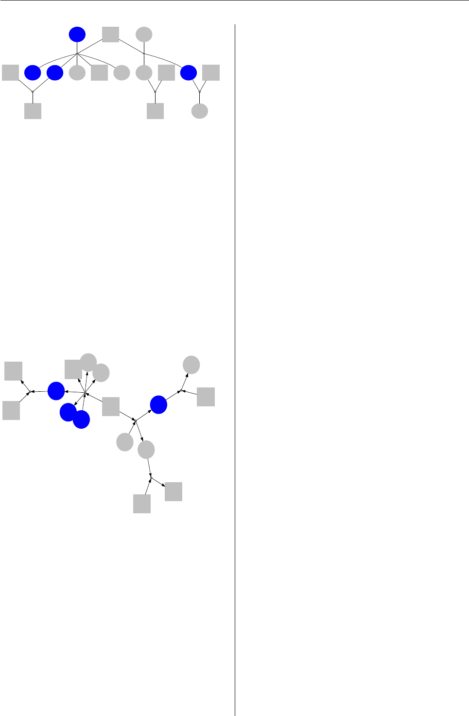
Vol. 6/2, May 2006 40
1
23
45678
9
10
11 1213
14
15
16
Figure 2: Pedigree 10081 by dot
Alternatively, we use
library(gap)
pedtodot(pre,dir="forward")
Besides dot, we can also use neato -Tps -o figure3.ps
10081.dot, giving a more liberal graph (Figure 3).
Its unusual looking makes it appealing for exposing
the peeling algorithm in the likelihood calculation of
pedigrees.
1
2
3
4
5
67
8
9
10
11
12
13
14
15
16
Figure 3: Pedigree 10081 by neato
A single file containing all pedigree diagrams
can be generated through the use of R sink com-
mand and screen output using sink=FALSE op-
tion in pedtodot. For example, given that all the
pre-makeped pedigrees are contained in the object
gaw14ped, we can use the following command,
sink("gaw14.dot")
pedtodot(gaw14ped,sink=FALSE)
sink()
to generate a complete list of pedigree diagrams
available from the web site http://www.mrc-epid.
cam.ac.uk/~jinghua.zhao/r-progs.htm.
Summary and further remarks
Further information about the two functions is avail-
able from the packages themselves. Note that
plot.pedigree in kinship does not require pedigree
ID be specified, while pedtodot in gap does. Unlike
plot.pedigree,pedtodot requires graphviz to visu-
alize graphics, but can be edited with dotty, and be
printed out in multiple pages when a pedigree dia-
gram is too big to fit in a single page. Both can pro-
duce a set of pedigree diagrams in a single file.
Although makeped is a utility program in LINK-
AGE, this function is also available in package gap.
If the pedigree file is in post-makeped format, then
the option makeped=TRUE can be used. However,
pedtodot can also use string IDs, or file in the so-
called GAS format in which gender can take values
‘m’, ‘f’, etc.
Most pedigrees in current studies have moderate
sizes, therefore sparse two-dimensional arrays are
used to keep track of marriages and children from
them, which are in turn used in generating dot script.
This is less efficient than the original gawk script in
that the latter use individual IDs directly to index
the marriage arrays, leading to shorter code and bet-
ter use of memory. In addition, further improvement
is possible by introducing other features available in
the dot language.
It is notable that R package sem has function
path.diagram to generate dot file and the Bio-
conductor (http://www.bioconductor.org) pack-
age Rgraphviz also uses graphviz. If more such
packages appear, it is desirable to be familiar with
the dot language and/or have support for it in R. Al-
though as yet human genetic linkage and genome-
wide association analysis is not widely conducted
with R, this might change in the near future, as has
been demonstrated by the great success of the Bio-
conductor project. I believe the two R functions de-
scribed in this note will be very useful to researchers
in their genetic data analysis.
Bibliography
F. Dudbridge, T. Carver, and G. Williams. Peli-
can: pedigree editor for linkage computer analysis.
Bioinformatics, 20(14):2327–2328, 2004.
F. Tores and E. Barillot. The art of pedigree drawing:
algorithmic aspects. Bioinformatics, 17(2):174–179,
2001.
R News ISSN 1609-3631

Vol. 6/2, May 2006 41
J. Terwilliger and J. Ott. Handbook of Human Genetic
Linkage. The Johns Hopkins University Press, Bal-
timore, 2001.
Jing Hua Zhao
MRC Epidemiology Unit
jinghua.zhao@mrc-epid.ac.uk
Non-Standard Fonts in PostScript and PDF
Graphics
by Paul Murrell and Brian Ripley
Introduction
By default, all of the text produced by R graphics de-
vices uses a sans-serif font family (e.g., Helvetica),
and in a PostScript or PDF plot only text in West-
ern European languages has been handled until re-
cently. This article describes several ways in which
the range of font families has been extended for R
2.3.0.
It has been possible to change the overall font
family that is used to draw text within a plot (Mur-
rell,2004), but the choice of font family for PDF and
PostScript devices was largely restricted to the set of
Adobe Core 14 fonts—Helvetica (4 faces), Times (4
faces), Courier (4 faces), Symbol, and ZapfDingbats
(see Table 1). As from R 2.3.0 much more choice is
available.
The examples in this article are written follow-
ing the conventions needed for a modern Unix-alike
operating system such as Linux, but will work with
minor changes (for example to the locale names) on
most other R platforms including Windows.
A little terminology will be helpful. A charac-
ter is an abstract concept, and a glyph is a visual
representation of a character. Characters can have
more than one representation, for example crossed
and uncrossed sevens, and the variants on Greek let-
ters much loved by mathematicians (see ?plotmath).
This matters as East Asian languages may write the
same character in different ways.1
Minor conveniences
The default font family on a PDF or PostScript device
can be controlled using the family argument. For ex-
ample, the expression pdf(family="Times") opens a
PDF device with the default font family set to Times
(a serif font). This is the simplest way to select a font
family, if the same font (possibly in different faces,
e.g. bold) is to be used for all of the text in a plot.
Prior to R 2.3.0, only a fixed set of font families
could be specified via the family argument (mostly
related to the Adobe Core 14 fonts), but it is now pos-
sible to specify any valid font family as the default.
For example, the expression pdf(family="mono")
opens a PDF device with the default font family set
to be a mono-spaced font (by default Courier on PDF
and PostScript devices).
The section on “Font databases” later in this arti-
cle will clarify what constitutes a “valid” font family.
Changing font family in-line
While it has been possible for some time to be able
to change the font family within a plot (e.g., have the
title in Times and the remaining labels in Helvetica),
in the traditional graphics system, this change could
only be made via the par() function.
It is now also possible to specify the family ar-
gument in low-level traditional graphics functions.
For example, if the default font family was sans-serif,
adding a label to a plot with a serif font used to re-
quire code of the form ...
> op <- par(family="serif")
> text("A label")
> par(op) # restore the setting
. . . but now the same thing can be achieved by the
following code.
> text("A label", family="serif")
Interationalization
As Martin Maechler likes to say, R has ‘for ever’
supported ISO Latin 1, the character set of the ma-
jor2Western European languages. Further interna-
tionalization features were introduced into R in ver-
sion 2.1.0 (Ripley,2005), which allowed users in non-
Western-European locales to use variable names and
produce output in their native language.
There was good support for graphical devices on
Windows, and as from R 2.3.0 on NT-based versions
of Windows it is even possible to change to another
language and output in that language.
The support for the X11() graphics device was as
good as the X server could provide, often limited by
1http://en.wikipedia.org/wiki/Han_unification
2The definition is rather circular, as those are the languages written in Latin-1. Icelandic is the most prominent exception.
R News ISSN 1609-3631

Vol. 6/2, May 2006 42
Table 1: Predefined font families for the PDF and PostScript devices which cover most of the Adobe Core 14
fonts. The Adobe Core fonts are usually available with Adobe (Acrobat) Reader and in PostScript printers and
viewers. The ZapfDingbats font is always included in PDF files produced by R, being used to draw small
circles.
"Helvetica" "Times" "Courier"
Helvetica Times Courier
Helvetica-Bold Times-Bold Courier-Bold
Helvetica-Oblique Times-Italic Courier-Oblique
Helvetica-BoldOblique Times-BoldItalic Courier-BoldOblique
Symbol Symbol Symbol
the availability of glyphs unless extras fonts were in-
stalled and are selected.
These features did not at first include graphical
output on PDF or PostScript devices, but this has
been much improved in R 2.3.0, with support for
many Eastern European and Asian locales.
European and Cyrillic fonts
R now automatically selects an appropriate encod-
ing for PDF and PostScript output based on your lo-
cale. In multi-byte locales such as those using UTF-
8, an appropriate single-byte encoding is chosen, so
now the PDF and PostScript devices allow encodings
other than ISO Latin 1.
For example, consider the character ´n, which is
needed in a Polish locale to write ‘hello’. This char-
acter is part of the ISO Latin 2 character set. For
demonstration purposes, we will temporarily switch
to a Polish locale using the following call:
> Sys.setlocale(category="LC_CTYPE",
locale="pl_PL.utf8")
Now when we start a PDF or PostScript device, it au-
tomatically selects an ISO Latin 2 encoding so that the
appropriate characters are available.
To show an example for users who do not have a
Polish keyboard, we will use an explicit Unicode es-
cape sequence to enter the character we want. This
will only work in UTF-8 locales in R 2.3.0.3
> library(grid)
> pdf("polish.pdf", width=3, height=0.8)
> grid.text(" Dzie\u0144 dobry
is hello in Polish ")
> dev.off()
Dzień dobry
is ’hello’ in Polish
On systems without access to UTF-8 locales, we
can achieve the same thing by switching to a Latin-2
locale: a Windows4user could write
> Sys.setlocale(category="LC_CTYPE",
locale="polish")
> grid.text(" Dzie\xf1 dobry
is hello in Polish ")
It is still possible to explicitly specify an encoding
when starting the pdf device if the automated selec-
tion is not correct on your platform.
This process ought to work well whenever the
language you want can be written in a single-byte
locale: this includes all the Western and Eastern
European, Cyrillic and Greek languages written in
ISO 8859-1 (Western), -2 (Eastern), -5 (Cyrillic), -7
(Greek), -13 (Baltic rim), 15 (Western with Euro) and
KOI8-R, KOI8-U and the equivalent Microsoft code-
pages.
Installed fonts
By specifying the correct encoding you can create
aPDF or PostScript file that contains the correct de-
scription of the characters you want, but if you actu-
ally want to view or print that text, you also need
to have an appropriate font installed on your system
that contains the relevant characters.
In the above example we were fortunate because
the default Helvetica font does include the glyph ´n.
In general, you may have to specify an appropriate
font (and ensure that it is installed on your system!).
The section “Font databases” will describe the issue
of specifying new fonts in detail.
Even if the glyph is known to R, it may not be
known to your viewer. For example, to view non-
Western European languages with Adobe Reader
you may need to install a Central European font
pack.5
A word of warning: the Adobe Core fonts are
often replaced by clones. This happens both in
3Unicode escape sequences will work in all locales in R 2.3.1 on platforms which support multi-byte character sets.
4NT4, 2000 or later, or (untested) a Polish-language version of 95/98/ME.
5http://www.adobe.com/products/acrobat/acrrasianfontpack.html
R News ISSN 1609-3631

Vol. 6/2, May 2006 43
PostScript viewers (ghostscript uses the equivalent
URW fonts) and PDF viewers (recent versions of
Adobe Reader use multiple-master fonts) as well as
in some printers. So it can be hard to tell if you
have exceeded the set of glyphs that can reasonably
be assumed to be always available. If you use any-
thing beyond ISO Latin 1, it is safest to embed the
fonts (see below). However, for local use where up-
to-date URW fonts can be assumed the coverage is
much wider including Eastern European and Cyril-
lic glyphs.
CJK fonts
Some support has also been added for locales with
very large character sets, such as the Chinese,
Japanese, and Korean (CJK) ideographic languages.
On PDF and PostScript devices, it is now possible to
select from a small set of font families covering many
of the glyphs used in writing those languages.
There are tens of thousands of (originally) Chi-
nese characters which are common to Chinese
(where they are called hanzi), Japanese (kanji), and
Korean (hanja). However, different glyphs may be
used, for example in Simplified Chinese (used in
most of PR China and in Singapore) and Traditional
Chinese (used in Taiwan and some of PR China).
For example, the following code selects one of the
CJK font families to display ‘hello’ in (Traditional)
Chinese.
> pdf("chinese.pdf", width=3, height=1)
> grid.text("\u4F60\u597D", y=2/3,
gp=gpar(fontfamily="CNS1"))
> grid.text(
"is hello in (Traditional) Chinese",
y=1/3)
> dev.off()
is 'hello' in (Traditional) Chinese
Note that we select the CJK font family only to dis-
play Chinese: although these font families can dis-
play English, they do so poorly. You should switch
back to a more standard font such as Helvetica for
producing Latin characters.
The appropriate CJK fonts include non-Chinese
glyphs, for example Hiragana and Katakana for use
in Japanese and Hangul for use in Korean.
Again, R does not check whether the fonts are
properly installed on your system. For example,
in order to view the file chinese.pdf with Adobe
Reader, you will have to download the Traditional
Chinese font pack.6
The CJK font families available in R have been
chosen because they are widely (or freely) available
for common print or viewing technology. Table 2lists
the font families and where they can be obtained.
The CJK fonts can be used in mathematical for-
mulas (see ?plotmath), but the metric information
on the sizes of characters is not as good as for Type 1
fonts, so the result may not be aesthetically pleasing.
Note that in this example we did not need to se-
lect an appropriate UTF-8 locale. It will in fact work
in any UTF-8 locale, and also in the older multi-byte
locales used on Unix-alikes (such as EUC-JP) and in
the double-byte locales used on Windows for the CJK
languages.
Font databases
In the previous two sections we mentioned that, in
addition to having the correct encoding, you may
also have to specify an appropriate font in order to
get all of the characters that you need. Here is an
example where that becomes necessary: we want to
write ‘hello’ in Russian and the Cyrillic characters
are not included in Helvetica; so we need to specify
a font that does contain Cyrillic characters. (A sim-
pler workaround would be to use the URWHelvetica
family which does since 2002 include Cyrillic glyphs,
but the versions installed with ghostscript on Win-
dows are from 2000. So we need to illustrate a more
general procedure.)
Again, we will pretend to be Russian temporarily
by setting the locale for the R session:
> Sys.setlocale(category="LC_CTYPE",
locale="ru_RU.utf8")
Now the single-byte encoding is automatically set to
ISO Latin 5, but we must also specify a font that con-
tains Cyrillic characters. We will generate a new one
using the function Type1Font() and specifying the
font name and a path to metric (.afm) files for the
font.
The font used in this example is from the PSCyr
font pack7. For this demonstration, the files have
only been downloaded to a local directory (not for-
mally installed) to keep the path manageable8. The
following command creates a Type 1 font object.
6http://www.adobe.com/products/acrobat/acrrasianfontpack.html
7ftp://ftp.vsu.ru/pub/tex/font-packs/pscyr
8The location of the installed .afm files will vary depending on your system. Most of the fonts used in this article are from T
EX packages,
so on a Linux system they might reside in /usr/share/texmf/fonts/afm/public/<fontpackname>.
R News ISSN 1609-3631

Vol. 6/2, May 2006 44
Table 2: The CJK fonts available for use in R. These were collected from examples found on various systems,
and suggestions of Ei-ji Nakama.
Font family name
in the font database PostScript font name PDF font name
"Japan1" HeiseiKakuGo-W5: a Linotype
Japanese printer font.
KozMinPro-Regular-Acro: from the
Adobe Reader 7.0 Japanese Font
Pack
"Japan1HeiMin" HeiseiMin-W3: a Linotype Japanese
printer font.
HeiseiMin-W3-Acro: a version of
the PostScript font, from the Adobe
Reader 4.0 Japanese Font Pack.
"Japan1GothicBBB" GothicBBB-Medium: a Japanese-
market PostScript printer font.
GothicBBB-Medium
"Japan1Ryumin" Ryumin-Light: a Japanese-market
PostScript printer font.
Ryumin-Light
"Korea1" Baekmuk-Batang: a True-
Type font found on some
Linux systems, and from ftp:
//ftp.mizi.com/pub/baekmuk/.
HYSMyeongJoStd-Medium-Acro:
from the Adobe Reader 7.0 Korean
Font Pack
"Korea1deb" Batang-Regular: a TrueType font
found on some Linux systems, prob-
ably the same as Baekmuk-Batang.
HYGothic-Medium-Acro: from the
Adobe Reader 4.0 Korean Font Pack.
"CNS1" (Traditional Chinese) MOESung-Regular: from Ken
Lunde’s CJKV resources; can be
installed for use with ghostscript
MSungStd-Light-Acro: from the
Adobe Reader 7.0 Traditional Chi-
nese Font Pack.
"GB1" (Simplified Chinese) BousungEG-Light-GB: a True-
Type font found on some
Linux systems, and from
ftp://ftp.gnu.org/pub/non-gnu/
chinese-fonts-truetype/.
STSong-Light-Acro: from the
Adobe Reader 7.0 Simplified Chi-
nese Font Pack.
R News ISSN 1609-3631

Vol. 6/2, May 2006 45
> RU <- Type1Font(
"TimesNewRomanPSMT-Regular",
c("fonts/afm/public/pscyr/times.afm",
"fonts/afm/public/pscyr/timesbd.afm",
"fonts/afm/public/pscyr/timesi.afm",
"fonts/afm/public/pscyr/timesbi.afm"))
This next command registers the Type 1 font in the
font database for PDF devices. The database records
all valid font family names for use with PDF devices.
After this, for the duration of the current R session,
the font family "RU" can be used as a font family
name in graphics functions.
> pdfFonts(RU=RU)
Now we can use this font family like any other and
to produce Cyrillic characters (we do not assume a
Russian keyboard so fake typing the Cyrillic keys by
specifying the appropriate Unicode values9).
> pdf("russian.pdf", width=3, height=0.8)
> grid.text("\u0417\u0434\u0440
\u0430\u0432\u0441\u0442\u0432
\u0443\u0439\u0442\u0435
is hello in Russian (Cyrillic)",
gp=gpar(fontfamily="RU"))
> dev.off()
Здравствуйте
is ’hello’ in Russian (Cyrillic)
A separate function, postscriptFonts(), is pro-
vided for querying and modifying the font database
for PostScript devices, and there is a CIDFont() func-
tion for defining new CJK (CID-keyed) fonts10.
Embedding fonts
The Russian example above is not quite complete yet.
If you try to view it with Adobe Reader, it will almost
certainly not look as we intended11. The problem is
that Adobe Reader knows nothing about the PSCyr
font so it substitutes a font it knows about, trying to
make it look as close as possible to the font we’ve
asked for.
By defining a Type 1 font object, we have given R
enough information about the Cyrillic font to create
aPDF or PostScript file, but if we want to view that
file or print it, we may also have to install the font for
the viewing software or the printer. Furthermore, if
we want to share the file with someone else (e.g., put
it on the web), then that someone else may have to
install the font.
The best solution to all of these problems is to em-
bed (enough of) the font within the file itself. This
means that the font becomes part of the document
and viewing software or printers do not need any
additional information to display or print the text.
(Note that licence restrictions on the fonts may limit
or prohibit this approach.)
The new R function embedFonts() performs this
task (by calling ghostscript12).
Here is how to embed the PSCyr fonts for the
russian.pdf plot; the file russianembed.pdf is the
result. Because we have the fonts in a local direc-
tory, we must specify a font path so that ghostscript
knows where to find the font.
> embedFonts("russian.pdf",
outfile="russianembed.pdf",
fontpaths="fonts/type1/public/pscyr")
For most of the examples in this article we have em-
bedded the fonts using this function, which is why
you can view all of these different character sets
without having to download any extra fonts.
A Computer Modern fonts example
Computer Modern fonts are the fonts designed by
Donald Knuth for the T
EX system (Knuth,1984) and
are the default fonts used in L
A
T
EX (Lamport,1994).
For a long time, it has been possible to make
use of Computer Modern fonts to produce PostScript
plots specifically for inclusion in L
A
T
EX documents
via a special "ComputerModern" font family (see
?postscript). However, this mechanism does have
some limitations: some characters are not available
(e.g., less-than and greater-than signs, curly braces,
and a number of mathematical symbols) and, more
importantly, it does not work for PDF output. A sim-
ple way to avoid these restrictions is to use a different
set of Computer Modern fonts that contain a more
complete set of characters.
Gaining access to a wider set of Computer Mod-
ern characters can be achieved simply by using a
version of the Computer Modern fonts that has
9This series of Unicode characters has been broken across lines for this article due to typesetting limitations; do not reproduce these
line breaks if you want to try this code yourself. Also, as there are at least three incompatible single-byte encodings for Russian, we do not
attempt to show how this might be done other than on a UTF-8 system.
10Defining a new CID-keyed font for use with PDF devices requires in-depth knowledge of Adobe font technology and the font itself,
so is not recommended except perhaps for expert users.
11What this actually looks like for you will depend on the fonts you have installed for Adobe Reader, however it is unlikely that you
will have the PSCyr fonts so it should at least look different to the “correct” output; on a vanilla Linux system, the Cyrillic characters are
all missing, and the Latin text is a serif font.
12Ghostscript should be installed already on most Linux systems and is available as a standard download and install for Windows
(http://www.cs.wisc.edu/~ghost/). You may need to tell R where ghostscript is installed via the environment variable R_GSCMD.
R News ISSN 1609-3631

Vol. 6/2, May 2006 46
been reordered and regrouped for different encoding
schemes. We will use two such fonts in this example.
The first set of fonts is the CM-LGC font pack13,
which provides a Type 1 version of most of the Com-
puter Modern fonts with an ISO Latin 1 encoding
(e.g., a less-than sign will produce a less-than sign,
not an upside-down exclamation mark as in T
EX).
The second font is a special Computer Modern sym-
bol font14 developed by Paul Murrell which covers
almost all of the Adobe Symbol encoding (for pro-
ducing mathematical formulas).
The following code demonstrates the use of the
CM-LGC fonts and the special Computer Modern
symbol font to produce a PDF format “plot” that in-
cludes mathematical symbols. The fonts have again
been unpacked in a local directory.
First of all, we define a new Type 1 Font object for
these fonts and register it with the PDF font database:
> CM <- Type1Font("CM",
c(paste("cm-lgc/fonts/afm/public/cm-lgc/",
c("fcmr8a.afm", "fcmb8a.afm",
"fcmri8a.afm", "fcmbi8a.afm"),
sep=""),
"cmsyase/cmsyase.afm"))
> pdfFonts(CM=CM)
Now we can use this font family in a PDF plot:
pdf("cm.pdf", width=3, height=3,
family="CM")
# ... much drawing code ommitted ...
dev.off()
Finally, we can embed these fonts in the docu-
ment so that we can embed the plot in other doc-
uments (such as this article) for anyone to view or
print.
> embedFonts("cm.pdf",
outfile="cmembed.pdf",
fontpaths=
c("cm-lgc/fonts/type1/public/cm-lgc",
"cmsyase"))
The final result is shown in Figure 1.
Summary
With R 2.3.0, it is now easier to produce text in PDF
and PostScript plots using character sets other than
English. There is built-in support for a wider range of
encodings and fonts and there is improved support
for making use of non-standard fonts in plots. There
is also now a utility for embedding fonts so that plots
can be more easily included in other documents and
shared across systems.
We believe that it is now possible for users to
produce high-quality graphical output in all human
languages with a sizeable number of R users. Any-
one whose native language is not covered is invited
to contribute suitable encoding files and locale map-
pings so our coverage can be extended.
Computer Modern Font Comparison
cm−lgc < > { } ...
cmr
cmsyase ∑∑ ≠≠ ∏∏ ...
cmsy
Figure 1: A “plot” that demonstrates the use of Com-
puter Modern fonts in PDF output.
Acknowledgements
Ei-ji Nakama provided the initial patch of the C code
for non-ISO Latin 1 encodings in multi-byte locales,
and for CJK (CID-keyed) font support, and he and
colleagues have patiently explained Japanese typog-
raphy to us.
Bibliography
D. Knuth. The T
EXbook. Addison-Wesley, Reading,
MA, 1984.
L. Lamport. L
A
T
EX: a document preparation system.
Addison-Wesley, Reading, MA, 1994.
P. Murrell. Fonts, lines, and transparency in R graph-
ics. R News, 4(2):5–9, September 2004. URL http:
//CRAN.R-project.org/doc/Rnews/.
B. D. Ripley. Internationalization features of R 2.1.0.
R News, 5(1):2–7, May 2005. URL http://CRAN.
R-project.org/doc/Rnews/.
Paul Murrell
The University of Auckland, New Zealand
paul@stat.auckland.ac.nz
Brian D. Ripley
University of Oxford, UK
ripley@stats.ox.ac.uk
13http://www.ctan.org/tex-archive/help/Catalogue/entries/cm-lgc.html, and available as a package for some Linux systems.
14http://www.stat.auckland.ac.nz/~paul/R/CM/CMR.html
R News ISSN 1609-3631

Vol. 6/2, May 2006 47
The doBy package
by Søren Højsgaard
This article is not about rocket science; in fact it is not
about science at all. It is a description of yet another
package with utility functions.
I have used R in connection with teaching gener-
alized linear models and related topics to Ph.d. stu-
dents within areas like agronomy, biology, and vet-
erinary science at the Danish Institute of Agricultural
Sciences.
These students, many of whom are familiar with
the SAS system, have almost all come to appreciate R
very quickly. However, they have also from time to
time complained that certain standard tasks are hard
to do in R – and certainly harder than in SAS. The
doBy package is an attempt to make some of these
standard tasks easier.
Airquality data
The presentation of the package is based on the
airquality dataset which contains air quality mea-
surements in New York, May to September 1973.
(Note that months are coded as 5, . . . , 9).
> head(airquality)
Ozone Solar.R Wind Temp Month Day
1 41 190 7.4 67 5 1
2 36 118 8.0 72 5 2
3 12 149 12.6 74 5 3
4 18 313 11.5 62 5 4
5 NA NA 14.3 56 5 5
6 28 NA 14.9 66 5 6
The summaryBy function
With the summary procedure of SAS (PROC SUMMARY)
one can easily calculate things like “the mean and
variance of xfor each combination of two factors A
and B”. To calculate mean and variance of Ozone
and Wind for each combination of Month, do:
> summaryBy(Ozone + Wind ~ Month,
+ data = airquality, FUN = c(mean,
+ var), prefix = c("m",
+ "v"), na.rm = TRUE)
Month m.Ozone m.Wind v.Ozone v.Wind
1 5 23.62 11.623 493.9 12.471
2 6 29.44 10.267 331.5 14.207
3 7 59.12 8.942 1000.8 9.217
4 8 59.96 8.794 1574.6 10.407
5 9 31.45 10.180 582.8 11.980
The result above can clearly be obtained in other
ways. For example by using the aggregate function,
the summarize function in the Hmisc package or by
> a <- by(airquality, airquality$Month,
+ function(d) {
+ c(mean(d[, c("Ozone",
+ "Wind")], na.rm = T),
+ diag(var(d[, c("Ozone",
+ "Wind")], na.rm = T)))
+ })
> do.call("rbind", a)
However, my students have found this somewhat
cumbersome!
The orderBy function
Ordering (or sorting) a data frame is possible with
the orderBy function. Suppose we want to order the
dataframe by Temp and by Month (within Temp) and
that the ordering should be decreasing. This can be
achieved by:
> x <- orderBy(~Temp + Month,
+ data = airquality, decreasing = T)
The first lines of the result are:
Ozone Solar.R Wind Temp Month Day
120 76 203 9.7 97 8 28
122 84 237 6.3 96 8 30
121 118 225 2.3 94 8 29
123 85 188 6.3 94 8 31
126 73 183 2.8 93 9 3
127 91 189 4.6 93 9 4
Again, this can clearly be achieved in other ways,
but presumably not with so few commands as above.
The splitBy function
Suppose we want to split data into a list of
dataframes, e.g. one dataframe for each month. This
can be achieved by:
> x <- splitBy(~Month, data = airquality)
Information about the grouping is stored as a
dataframe in an attribute called groupid:
> attr(x, "groupid")
Month
1 1
2 2
3 3
4 4
5 5
R News ISSN 1609-3631

Vol. 6/2, May 2006 48
The sampleBy function
Suppose we want a random sample of 50% of the ob-
servations from a dataframe. This can be achieved
with:
> sampleBy(~1, frac = 0.5, data = airquality)
Suppose instead that we want a systematic sam-
ple of every fifth observation within each month.
This is achieved with:
> sampleBy(~Month, frac = 0.2,
+ data = airquality, systematic = T)
The subsetBy function
Suppose we want to take out those rows within each
month for which the the wind speed is larger than
the mean wind speed (within the month). This is
achieved by:
> subsetBy(~Month, subset = "Wind>mean(Wind)",
+ data = airquality)
Note that the statement "Wind>mean(Wind)" is eval-
uated within each month.
The esticon function
Consider a linear model which explains Ozone as a
linear function of Month and Wind:
> airquality <- transform(airquality,
+ Month = factor(Month))
> m <- lm(Ozone ~ Month * Wind,
+ data = airquality)
> coefficients(m)
(Intercept) Month6 Month7
50.748 -41.793 68.296
Month8 Month9 Wind
82.211 23.439 -2.368
Month6:Wind Month7:Wind Month8:Wind
4.051 -4.663 -6.154
Month9:Wind
-1.874
When a parameter vector βof (systematic) effects
have been estimated, interest is often in a particu-
lar estimable function, i.e. linear combination λ>β
and/or testing the hypothesis H0:λ>β=β0where
λis a specific vector defined by the user.
Suppose for example we want to calculate the
expected difference in ozone between consequtive
months at wind speed 10 mph (which is about the
average wind speed over the whole period).
The esticon function provides a way of doing so.
We can specify several λvectors at the same time by
row–binding of λ>:
> Lambda <- rbind(c(0, -1, 0,
+ 0, 0, 0, -10, 0, 0, 0),
+ c(0, 1, -1, 0, 0, 0, 10,
+ -10, 0, 0), c(0, 0,
+ 1, -1, 0, 0, 0, 10,
+ -10, 0), c(0, 0, 0,
+ 1, -1, 0, 0, 0, 10,
+ -10))
> esticon(m, Lambda)
Confidence interval ( WALD ) level = 0.95
beta0 Estimate Std.Error t.value
1 0 1.2871 10.238 0.1257
2 0 -22.9503 10.310 -2.2259
3 0 0.9954 7.094 0.1403
4 0 15.9651 6.560 2.4337
DF Pr(>|t|) Lower.CI Upper.CI
1 106 0.90019 -19.010 21.585
2 106 0.02814 -43.392 -2.509
3 106 0.88867 -13.069 15.060
4 106 0.01662 2.959 28.971
In other cases, interest is in testing a hypothesis
of a contrast H0:Λβ=β0where Λis a matrix. For
example a test of no interaction between Month and
Wind can be made by testing jointly that the last four
parameters in mare zero (observe that the test is a
Wald test):
> Lambda <- rbind(c(0, 0, 0, 0,
+ 0, 0, 1, 0, 0, 0), c(0,
+ 0, 0, 0, 0, 0, 0, 1, 0,
+ 0), c(0, 0, 0, 0, 0, 0,
+ 0, 0, 1, 0), c(0, 0, 0,
+ 0, 0, 0, 0, 0, 0, 1))
> esticon(m, Lambda, joint.test = T)
X2.stat DF Pr(>|X^2|)
1 22.11 4 0.0001906
For a linear normal model, one would typically
prefer to do a likelihood ratio test instead. However,
for generalized estimating equations of glm–type (as
dealt with in the packages geepack and gee) there is
no likelihood. In this case esticon function provides
an operational alternative.
Observe that another function for calculating con-
trasts as above is the contrast function in the De-
sign package but it applies to a narrower range of
models than esticon does.
Final remarks
The ease in using the data oriented functions lies in
that 1) the formula language is used in the specifi-
cation of both the variables and the grouping and 2)
the functions take a data argument. My “biologically
oriented” students (and ditto collegues) seem to ap-
preciate that.
R News ISSN 1609-3631

Vol. 6/2, May 2006 49
On their wishlist are facilities along the line of the
ESTIMATE and LSMEANS statements available in many
SAS procedures (including GLM,MIXED and GENMOD)
for easy specification of various contrasts (LSMEANS is
sometimes also denoted “population means”). While
LSMEANS are often misused (and certainly misinter-
preted) such facilities would be nice to have in R.
I would like to encourage anyone who has imple-
mented such facilities in a reasonable level of gen-
erality to come forward.
Søren Højsgaard
Statistics and Decision Analysis Unit
Department of Genetics and Biotechnology
Danish Institute of Agricultural Sciences
Tjele, Denmark
sorenh@agrsci.dk
Normed division algebras with R:
Introducing the onion package
The eccentric cousin and the crazy old uncle
by Robin K. S. Hankin
Preface
An algebra is a vector space Vover a field (here the
real numbers) in which the vectors may be multi-
plied. In addition to the usual vector space axioms,
one requires, for any λ,µ∈and x,y,z∈V:
•x(λy+µz) = λxy +µxz
•(λy+µz)x=λyx +µzx
where multiplication is denoted by juxtaposition;
note the absence of associativity. A division algebra
is a nontrivial algebra in which division is possible:
for any a∈Vand any nonzero b∈V, there exists
precisely one element xwith a=bx and precisely
one element ywith a=yb. A normed division al-
gebra is a division algebra with a norm ||·|| satisfy-
ing ||xy|| =||x|| ||y||.
There are precisely four normed division alge-
bras: the reals themselves ( ), the complex num-
bers ( ), the quaternions ( ) and the octonions ( );
the generic term is “onion”, although the term in-
cludes other algebras such as the sedenions.
The R programming language (Develop-
ment Core Team,2004) is well-equipped to deal with
the first two: here, I introduce the onion package,
which provides some functionality for the quater-
nions and the octonions, and illustrate these interest-
ing algebras using numerical examples.
Introduction
Historically, the complex numbers arose from a num-
ber of independent lines of inquiry and our current
understanding of them (viz z=x+iy; the Argand
plane) developed over the eighteenth and nineteenth
centuries.
Hamilton was one of many mathematicians to at-
tempt to extend the complex numbers to a third di-
mension and discover what would in our terminol-
ogy be a three dimensional normed division alge-
bra. We now know that no such thing exists: divi-
sion algebras all have dimension 2nfor nsome non-
negative integer.
Hamilton came upon the multiplicative structure
of the quaternions in a now-famous flash of inspira-
tion on 16th October 1843: the quaternions are ob-
tained by adding the elements i,j, and kto the real
numbers and requiring that
i2=j2=k2=i jk =−1. (1)
A general quaternion is thus written a+bi +c j +dk
with a,b,c,dbeing real numbers; complex arithmetic
is recovered if c=d=0. Hamilton’s relations above,
together with distributivity and associativity, yield
the full multiplication table and the quaternions are
the unique four dimensional normed division alge-
bra.
However, Hamilton’s scheme was controversial
as his multiplication was noncommutative: a shock-
ing suggestion at the time. Today we recognize many
more noncommutative operations (such as matrix
multiplication), but even Hamilton had difficulty
convincing his contemporaries that such operations
were consistent, let alone worth studying.
The octonions
The fourth and final normed division algebra is that
of the octonions. These were discovered around 1844
and are an eight-dimensional algebra over the reals.
The full multiplication table is given by Baez (2001).
Package onion in use
A good place to start is function rquat(), which
returns a quaternionic vector of a specified length,
whose elements are random small integers:
R News ISSN 1609-3631

Vol. 6/2, May 2006 50
> library(onion)
> x <- rquat(5)
> names(x) <- letters[1:5]
> print(x)
abcde
Re43213
i 32341
j 24231
k 33444
This quaternionic vector, of length 5, is of the
form of a four-row matrix. The rownames are the
standard basis for quaternions, and their entries may
be manipulated as expected; for example, we may set
component kto be component jplus 10:
> k(x) <- j(x) + 10
> x
abcde
Re43213
i 32341
j 24231
k 12 14 12 13 11
Quaternionic vectors behave largely as one might ex-
pect. For example, we may concatenate awith a ba-
sis quaternion (the four bases are represented in the
package by H1,Hi,Hj, and Hk) and multiply the result
by the first element:
> c(x, Hk) * x[1]
abcde
Re -141 -170 -149 -170 -125 -12
i 24 -3 18 9 23 2
j 16 4 12 23 -11 -3
k 96 100 72 65 81 4
And indeed we may explicitly verify that quater-
nionic multiplication is not commutative using the
commutator() function, returning xy −yx:
> y <- rquat(5)
> commutator(x, y)
abcde
Re00000
i 20 12 32 98 62
j -42 -48 -24 -44 -40
k 2 12 -4 -20 -2
It is possible to verify that quaternionic
multiplication is associative using function
associator(x,y,z) which returns (xy)z−x(yz)
and is thus identically zero for associative operators:
> associator(x, y, rquat(5))
abcde
Re00000
i 00000
j 00000
k 00000
Compare the octonions, which are not associative:
> associator(roct(3), roct(3),
+ roct(3))
[1] [2] [3]
Re000
i 472 -408 242
j -158 112 -66
k -106 -408 84
l -492 128 506
il 506 54 -700
jl 250 298 610
kl -160 518 -768
Many transcendental functions operate on
onions, via a reasonably straightforward generaliza-
tion of the complex case. Consider the square root,
defined as exp(log(x)/2). That this obeys similar
rules to the usual square root may be demonstrated
for octonions by calculating √x√x−x, and showing
that its modulus is small:
> x <- roct(3)
> Mod(sqrt(x) * sqrt(x) - x)
[1] 7.601583e-15 5.291934e-15
[3] 4.110825e-15
showing acceptable accuracy in this context. How-
ever, many identities that are true for the real or com-
plex case fail for quaternions or octonions; for exam-
ple, although log(x2) = 2 log(x), it is not generally
the case that log(xy) = log(x) + log(y), as we may
verify numerically:
> x <- rquat(3)
> y <- rquat(3)
> Mod(log(x * x) - 2 * log(x))
[1] 0.000000e+00 3.845925e-16
[3] 0.000000e+00
> Mod(log(x * y) - log(x) - log(y))
[1] 0.0000000 0.6770686 1.1158104
Practical applications
I now show the quaternions in use: they can be used
to rotate an object in 3D space in an elegant and nat-
ural way. If we wish to rotate vector v, considered to
be a triple of real numbers, we first identify its three
components with the imaginary part of a quaternion
with zero real part (i.e., v=0+v1i+v2j+v3k).
Then the transformation defined by
v−→ v0=zvz−1
R News ISSN 1609-3631
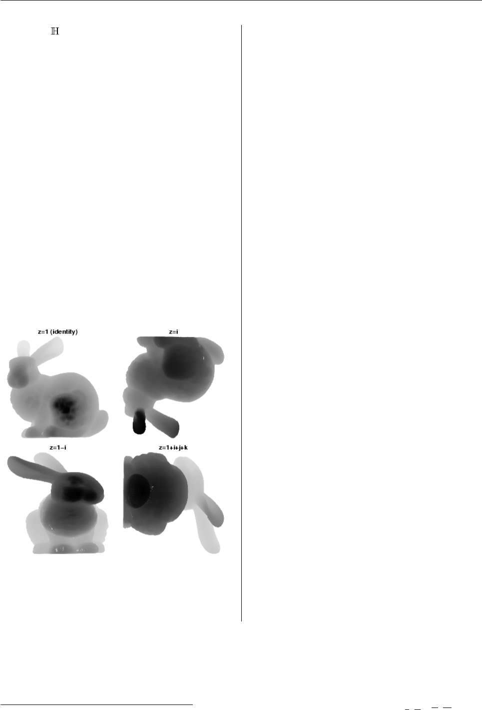
Vol. 6/2, May 2006 51
where z∈, is a rotation1. Note that the noncom-
mutativity of the quaternions means that the map-
ping is not necessarily the identity. This scheme may
be used to produce Figure 1.
> data(bunny)
> par(mfrow = c(2, 2))
> par(mai = rep(0.1, 4))
> p3d(rotate(bunny, H1), box = FALSE,
+ d0 = 0.4, r = 1e+06, h = NULL,
+ pch = 16, cex = 0.3, theta = 0,
+ phi = 90, main = "z=1 (identity)")
> p3d(rotate(bunny, Hi), box = FALSE,
+ d0 = 0.4, r = 1e+06, h = NULL,
+ pch = 16, cex = 0.3, theta = 0,
+ phi = 90, main = "z=i")
> p3d(rotate(bunny, H1 - Hj),
+ box = FALSE, d0 = 0.4,
+ r = 1e+06, h = NULL, pch = 16,
+ cex = 0.3, theta = 0, phi = 90,
+ main = "z=1-i")
> p3d(rotate(bunny, Hall), box = FALSE,
+ d0 = 0.4, r = 1e+06, h = NULL,
+ pch = 16, cex = 0.3, theta = 0,
+ phi = 90, main = "z=1+i+j+k")
Figure 1: The Stanford Bunny (Turk,2005) in various
rotations, plotted using p3d(). Depth cue is via pro-
gressive greying out of points further from the eye,
as though viewed through a mist
Translating between quaternionic rotation and
(say) the equivalent orthogonal matrix is straightfor-
ward.
Conclusions
Quaternions and octonions are interesting and in-
structive examples of normed division algebras.
Quaternions are a natural and efficient representa-
tion of three dimensional rotations and this paper in-
cludes a brief illustration of their use in this context.
Octonions’ applicability to physics is currently
unclear, but a steady trickle of papers has appeared
in which the octonions are shown to be related to
spinor geometry and quantum mechanics (see Baez,
2001, and references therein). Reading the literature,
one cannot help feeling that octonions will eventu-
ally reveal some deep physical truth. When this hap-
pens, the onion package ensures that R will be ready
to play its part.
Acknowledgments
I would like to acknowledge the many stimulating
and helpful comments made by the R-help list over
the years.
Bibliography
J. C. Baez. The octonions. Bulletin of the American
Mathematical Society, 39(5):145–205, 2001.
R Development Core Team. R: A language and envi-
ronment for statistical computing. R Foundation for
Statistical Computing, Vienna, Austria, 2004. URL
http://www.R-project.org. ISBN 3-900051-07-0.
G. Turk. The Stanford bunny, 2005. Stanford
University Computer Graphics Laboratory,
http://graphics.stanford.edu/data/3Dscanrep/.
Robin Hankin
National Oceanography Centre, Southampton
European Way
Southampton
United Kingdom
SO14 3ZH
r.hankin@noc.soton.ac.uk
1The real part of v0is again zero and thus may be interpreted as a three-vector. It is straightforward to prove that v·w=v0·w0. In R id-
iom, one would numerically verify these identities by evaluating d <- (z*v/z) %.% (z*w/z) - v %.% w (where v,w,z are quaternions)
and observing that Mod(d) is small.
R News ISSN 1609-3631
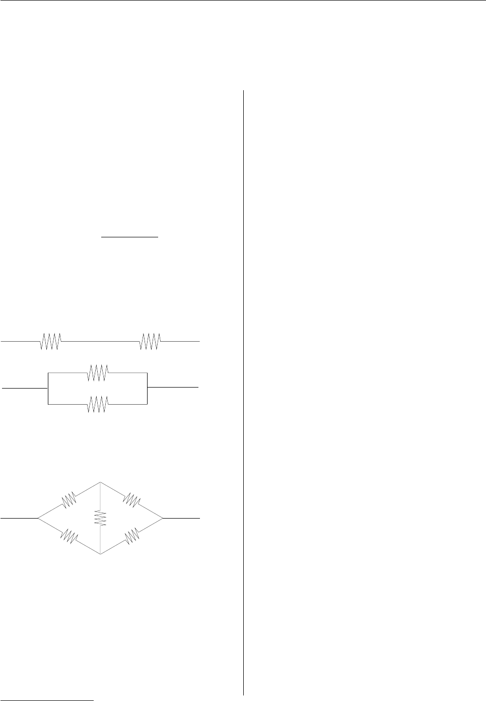
Vol. 6/2, May 2006 52
Resistor networks R: Introducing the
ResistorArray package
Electrical properties of resistor networks
by Robin K. S. Hankin
Introduction
Many elementary physics courses show how resis-
tors combine in series and parallel (Figure 1); the
equations are
Rseries =R1+R2(1)
Rparallel =1
R1−1+R2−1. (2)
However, these rules break down for many systems
such as the Wheatstone bridge (Figure 2); the reader
who doubts this should attempt to apply equations 1
and 2and find the resistance between points A and B
in the general case.
R
R
R R
1
1
2
2
Figure 1: Two resistors in series (top) and parallel
(bottom)
R
R
12
A B
23 R34
24
R23
R
1 4
3
2
Figure 2: The Wheatstone bridge
This paper introduces ResistorArray (Hankin,
2005), an R (R Development Core Team,2005) pack-
age to determine resistances and other electrical
properties of such networks.
Although this paper uses the language of elec-
trical engineering, the problem considered is clearly
very general: many systems are composed of iso-
lated nodes between which some quantity flows and
the steady states of such systems are generally of in-
terest.
Package ResistorArray has been applied to such
diverse problems as the diffusion of nutrients among
fungal hyphae networks, the propagation of salinity
between (moored) oceanographical buoys, and hy-
draulic systems such as networks of sewage pumps.
Matrix formulation
The general problem of determining the resistance
between two nodes of a resistor network requires
matrix techniques1.
Consider a network of nnodes, with node icon-
nected to node jby a resistor of resistance Ri j. Then
the network has a “conductance matrix” Lwith
Li j =−1/Ri j if i6=j
∑k:k6=j1/Rk j if i=j.(3)
Thus Lis a symmetrical matrix, whose row sums and
column sums are zero (and therefore is singular).
Then the analogue of Ohm’s law (viz V=IR)
would be
Lv=i(4)
where v= (v1,...,vn)is a vector of potentials
and i= (i1,...,in)is a vector of currents; here ipis
the current flow in to node p. Equation 4is thus a re-
statement of the fact that charge does not accumulate
at any node.
Each node of the circuit may either be fed a known
current2and we have to calculate its potential; or it is
maintained at a known potential and we have to cal-
culate the current flux into that node to maintain that
potential. There are thus nunknowns altogether.
Thus some elements of vand iare known and
some are unknown. Without loss of generality, we
may partition these vectors into known and un-
known parts: v= (vk0,vu0)0and i= (iu0,ik0)0.
Thus the known elements of vare vk= (v1,...,vp)0:
these would correspond to nodes that are maintained
at a specified potential; the other elements vu=
(vp+1,...,vn)0correspond to nodes that are at an un-
known potential that we have to calculate.
The current vector imay similarly be decom-
posed, but in a conjugate fashion; thus elements iu=
(i1,...,ip)0correspond to nodes that require a cer-
tain, unknown, current to be fed into them to
1The method described here is a standard application of matrix algebra, but does not appear to be described in the literature. Many
books and papers, such as Doyle and Snell (1984), allude to it; but a formal description does not appear to have been published.
2This would include a zero current: in the case of the Wheatstone bridge of Figure 2, nodes 2 and 3 have zero current flux so i2and i3
are known and set to zero.
R News ISSN 1609-3631

Vol. 6/2, May 2006 53
maintain potentials vk; the other elements ik=
(ip+1,...,in)0would correspond to nodes that have
a known current flowing into them and whose po-
tential we seek.
Equation 4may thus be expressed in terms of a
suitably partitioned matrix equation:
A B
BTCvk
vu=iu
ik(5)
where, in R idiom, A=L[1:p,1:p],B=L[1:p,(p+1):n],
and C=L[(p+1):n,(p+1):n]. Straightforward matrix
algebra gives
vu=C−1ik−BTvk(6)
iu=A−BC−1BTvk+BC−1ik(7)
Equations 6and 7are implemented by circuit().
Package ResistorArray in use
Consider the Wheatstone Bridge, illustrated in Fig-
ure 2. Here the resistance between node 1 and node 4
is calculated; all resistances are one ohm except R34,
which is 2 ohms. This resistor array may be viewed
as a skeleton tetrahedron, with edge 1–4 missing. We
may thus use function tetrahedron() to generate
the conductance matrix; this is
R> L <- tetrahedron(c(1, 1, Inf, 1, 1, 2))
[,1] [,2] [,3] [,4]
[1,] 2 -1 -1.0 0.0
[2,] -1 3 -1.0 -1.0
[3,] -1 -1 2.5 -0.5
[4,] 0 -1 -0.5 1.5
Observe that L[1,4]==L[4,1]==0, as required.
The resistance may be determined by function
circuit(); there are several equivalent methods.
Here node 1 is earthed—by setting it to zero
volts—and the others are given a floating poten-
tial; viz v=c(0,NA,NA,NA). Then one amp is fed
in to node 4, zero amps to nodes 2 and 3, and
node 1 an unknown current, to be determined; viz
currents=c(NA,0,0,1). The node 1-to-node 4 resis-
tance will then be given by the potential at node 4:
R> circuit(L, v = c(0, NA, NA, NA),
+ currents = c(NA, 0, 0, 1))
$potentials
[1] 0.0000000 0.5454545 0.4545455
[4] 1.1818182
$currents
[1] -1 0 0 1
Thus the resistance is about 1.181818Ω, compar-
ing well with the theoretical value of 117/99Ω. Note
that the system correctly returns the net current re-
quired to maintain node 1 at 0 V as −1 A (which is
clear from conservation of charge). The potential dif-
ference between nodes 2 and 3 indicates a nonzero
current flow along R23; currents through each resis-
tor are returned by function circuit() if argument
give.internal is set to TRUE.
Conclusions
Package ResistorArray solves a problem that is fre-
quently encountered in electrical engineering: de-
termining the electrical properties of resistor net-
works. The techniques presented here are applica-
ble to many systems composed of isolated nodes be-
tween which some quantity flows; the steady states
of such systems generally have an electrical ana-
logue.
This paper explicitly presents a vectorized so-
lution method that uses standard numerical tech-
niques, and discusses the corresponding R idiom.
Acknowledgements
I would like to acknowledge the many stimulating
and helpful comments made by the R-help list over
the years.
Bibliography
P. G. Doyle and J. L. Snell. Random walks and electric
networks. The Mathematical Association of Amer-
ica, 1984.
R. K. S. Hankin. ResistorArray: electrical properties of
resistor networks, 2005. R package version 1.0-9.
R Development Core Team. R: A language and envi-
ronment for statistical computing. R Foundation for
Statistical Computing, Vienna, Austria, 2005. URL
http://www.R-project.org. ISBN 3-900051-07-0.
Robin Hankin
National Oceanography Centre, Southampton
European Way
Southampton
United Kingdom
SO14 3ZH
r.hankin@noc.soton.ac.uk
R News ISSN 1609-3631

Vol. 6/2, May 2006 54
The good, the bad, and the ugly—Review
of Paul Murrell’s new book: “RGraphics”
by David Meyer
At the DSC 2001 workshop
in Vienna, Ross Ihaka pre-
sented an overview on the
“old” Rgraphics system us-
ing the title: “The good, the
bad, and the ugly”, basi-
cally meaning that the tra-
ditional graphics system, al-
beit flexible, was getting old
and the interface was cum-
bersome in several aspects.
Think, e.g., of the mysteries
of the dozens of par() pa-
rameters whose lengthy help
page most useRs keep browsing on a regular ba-
sis to filter out the appropriate settings. Thanks to
Paul Murrell’s new book, the secrets of both tradi-
tional graphics and the new, modern grid system
get unveiled, preventing useRs from writing “ugly”
code. Starting from scratch, both architectures are
presented and compared in detail, complemented
with illustrative examples and summary tables. The
text not only covers basic elements such as points,
lines, segments, and text, but also discusses the most
important high-level plot functions available in base
R, as well as some popular extension packages such
as scatterplot3d. In addition, a clear effort has
been made to enable the readers to develop their own
graphical methods, in the Rspirit of “users becoming
developers”.
The first part of the book covers the traditional
graphics system. It starts with some simple plots us-
ing plot() and friends, and proceeds with a detailed
chapter on customizing, covering all low-level and
high-level par() settings, multiple plots, annotation,
and more complex, superposed plots. Even experi-
enced users will discover “new” features. For exam-
ple, most people will be familiar with line types—
but what about the various line join and line ending
styles, or the correct handling of fonts?
The second part is devoted to grid, the new
graphics system developed by the book author him-
self. Murrell chooses a practical approach and first
introduces the lattice package, R’s version of Trellis
graphics. After giving an overview on all high-level
lattice functions, the author provides customization
examples. Only after this “teaser” is the reader con-
fronted with the basic elements of the grid package.
The text explains the idea behind concepts like units,
graphical context, viewports, and how existing plot
elements can easily be integrated in more complex
displays. Particular emphasis is given to the possibil-
ities of interactive plot modifications and off-screen
computations. Finally, a whole chapter is devoted to
the development of new grid-based functions and
objects that can be reused by others.
Paul Murrell’s book is the first publication en-
tirely devoted to Rgraphics, written by the authorita-
tive expert in the field. It is definitely a must-have for
novices and professionals alike, the ultimate guide to
the power (and beauty) of Rgraphics.
David Meyer
Department of Information Systems and Operations, Vi-
enna University of Economics and Business Administra-
tion
Augasse 2-6, A-1090 Wien, Austria
david.meyer@wu-wien.ac.at
Changes in R
by the R Core Team
User-visible changes
• In the grid package there are new ’arrow’ argu-
ments to grid.line.to(),grid.lines(), and
grid.segments() (grid.arrows() has been
deprecated).
The new ’arrow’ arguments have been added
BEFORE the ’name’, ’gp’ and ’vp’ arguments
so existing code that specifies any of these ar-
guments *by position* (not by name) will fail.
•all.equal() is more stringent, see the PR#8191
bug fix below.
• The data frame argument to transform() is no
longer called ’x’, but ’_data’. Since this is an in-
valid name, it is less likely to clash with names
given to transformed variables. (People were
getting into trouble with transform(data,
x=y+z).)
R News ISSN 1609-3631

Vol. 6/2, May 2006 55
New features
•arima.sim() has a new argument ’start.innov’
for compatibility with S-PLUS. (If not supplied,
the output is unchanged from previous ver-
sions in R.)
•arrows() has been changed to be more simi-
lar to segments(): for example col=NA omits
the arrow rather than as previously (undocu-
mented) using par("col").
•as.list() now accepts symbols (as given by
as.symbol() aka as.name()).
•atan2() now allows one complex and one nu-
meric argument.
• The ’masked’ warnings given by attach() and
library() now only warn for functions mask-
ing functions or non-functions masking non-
functions.
• New function Axis(), a generic version of
axis(), with Date and POSIX[cl]t meth-
ods. This is used by most of the stan-
dard plotting functions (boxplot, contour,
coplot, filled.contour, pairs, plot.default, rug,
stripchart) which will thus label x or y axes ap-
propriately.
•pbeta() now uses TOMS708 in all cases and
so is more accurate in some cases (e.g. when
lower.tail = FALSE and when one of the shape
parameters is very small).
•[qr]beta(),[qr]f() and [qr]t() now have a
non-centrality parameter.
•[rc]bind() and some more cases of sub-
assignment are implemented for raw matrices.
(PR8529 and 8530)
• The number of lines of deparsed calls printed
by browser() and traceback() can be limited
by the option "deparse.max.lines". (Wish of
PR#8638.)
• New canCoerce() utility function in "meth-
ods" package.
•[pq]chisq() are considerably more accurate
for moderate (up to 80) values of ncp, and
lower.tail = FALSE is fully supported in that re-
gion. (They are somewhat slower than before.)
•chol(pivot = TRUE) now gives a warning if
used on a (numerically) non-positive-definite
matrix.
•chooseCRANmirror() consults the CRAN mas-
ter (if accessible) to find an up-to-date list of
mirrors.
•cov.wt() is more efficient for ’cor = TRUE’ and
has a new ’method’ argument which allows
’Maximum Likelihood’.
•do.call() gains an ’envir’ argument.
•eigen() applied to an asymmetric real matrix
now uses a tolerance to decide if the result is
complex (rather than expecting the imaginary
parts of the eigenvalues to be exactly zero).
• New function embedFonts() for embedding
fonts in PDF or PostScript graphics files.
•fisher.test() now uses p-values computed
via hypergeometric distributions for all 2 by 2
tables. This might be slightly slower for a few
cases, but works much better for tables with
some large counts.
There is a new option to simulate the p-value
for larger than 2 x 2 tables.
•for() now supports raw vectors as the set of
indices.
•getNativeSymbolInfo() is vectorized for the
’name’ argument. It returns a named list of Na-
tiveSymbolInfo objects, but is backward com-
patible by default when called with a character
vector of length 1, returning the NativeSymbol-
Info object.
•help.search() no longer attempts to handle
packages installed prior to R 2.0.0, and reports
the current path to the package (rather than
where it was originally installed: this informa-
tion is not shown by the print() method).
• Added "hexmode" to parallel "octmode".
•install.packages() now does tilde expan-
sion on file paths supplied as ’pkgs’.
•install.packages() has additional argu-
ments ’configure.args’ and ’clean’ which allow
the caller to provide additional arguments to
the underlying R CMD INSTALL shell com-
mand when installing source packages on a
Unix-alike.
•is.loaded() has a new argument ’type’ to con-
fine the search to symbols for .C, .Fortran, .Call
or .External: by default it looks for a symbol
which will match any of them. It is now inter-
nal and not primitive, so argument matching
works in the usual way.
• The symmetry test for matrices used in
eigen() has been “exported” as the ’matrix’
method of a new S3-generic isSymmetric().
• .leap.seconds and the internal adjustment code
now know about the 23rd leap second on 2005-
12-31: the internal code uses a run-time test to
see if the OS does.
R News ISSN 1609-3631

Vol. 6/2, May 2006 56
• The ’col’ argument of legend() now defaults
to par("col") (which defaults to "black", the
previous default), so that the lines/symbols are
shown in the legend in the colour that is used
on the plot.
•log2() and log10() call C functions of the
same name if available, and will then be more
likely to be precise to machine accuracy.
•new.packages() gains a ... argument to pass
e.g. ’destdir’ to install.packages(). (Wish of
PR#8239.)
•nls() now supports ’weights’.
• The vector passed as the first argument of the
’fn’ and ’gr’ arguments of optim() has the
names (if any) given to argument ’par’.
•options(expressions) is temporarily in-
creased by 500 during error-handling. This
enables e.g. traceback() to work when the
error is reaching the limit on the nesting of ex-
pressions.
•page() accepts general R objects, not just
names (and previously undocumented) charac-
ter strings. This allows the object to be specified
as a call, for example. More options are allowed
in its ’...’ argument.
•pairs() allows a wider class of inputs, in-
cluding data frames with date and date-time
columns.
•par() and the in-line use of graphical parame-
ters produce more informative error messages,
distinguishing between non-existent pars and
inappropriate use of valid pars.
Graphical parameters ’family’, ’lend’, ’ljoin’
and ’lmitre’ can now be set in-line.
There is no longer a warning if non-settable
pars are used in-line, but there is an appropri-
ate warning if unknown pars are passed.
The length limit for the ’family’ parameter has
been increased to 200 bytes, to allow for the
names of some CID-keyed fonts in multi-byte
locales.
• The pdf() device now allows ’family’ to
be specified in the same generality as
postscript().
• The pdf() device writes /FontDescriptor en-
tries for all fonts except the base 14, and does
not write font entries for unused fonts.
• Plotmath allows ’vartheta’, ’varphi’ and ’var-
sigma’ (or ’stigma’) as synonyms for ’theta1’,
’phi1’ and ’sigma1’, and the help page has a
note for TeX users.
•plot.xy() now takes its default arguments
from the corresponding par() settings, so
points(type="l") and lines(type="p") be-
have in the same way (and more obviously, also
for type="b").
•poly() has a new argument ’raw’, mainly for
pedagogical purposes.
• The class "POSIXlt" now supports fractional
seconds (as "POSIXct" has always done). The
printing of fractional seconds is controlled by
the new option "digits.secs", and by default is
off.
•postscript() supports family = "Computer-
ModernItalic" for Computer Modern with italic
(rather than slanted) faces.
• The postscript()/pdf() font metrics for the
14 standard fonts (only, not the rest of the com-
mon 35) have been updated to versions from
late 1999 which cover more glyphs. There are
also a few differences in the metrics and hence
the output might be slightly different in some
cases.
• The way families can be specified for
postscript() and pdf() has been expanded
to include CID-keyed fonts, with new func-
tions Type1Font() and CIDFont() to set up
such fonts families.
•prettyNum() has new arguments ’pre-
serve.width’ and ’zero.print’. When the former
is not "none", as in calls from format() and
formatC(), the resulting strings are kept at the
desired width when possible even after adding
of ’big.mark’ or ’small.mark’.
•proc.time() and system.time() now record
times to 1 ms accuracy where available (most
Unix-like systems).
• The initialization methods for the quasi()
family have been changed to depend on the
variance function, and in particular to work
better for the "mu(1-mu)" variance function.
(PR#8486)
•read.table() gains a ’flush’ argument passed
to scan().
•require() now takes a ’lib.loc’ argument.
• The second argument ’size’ to sample() is re-
quired to have length 1, so that errors when
supplying arguments are more easily detected.
• The default is now compress = !ascii in save()
(but not save.image).
R News ISSN 1609-3631

Vol. 6/2, May 2006 57
•scan() and write.table() now have some in-
terruptibility, which may be useful when pro-
cessing very large files.
• A new heuristic test, seemsS4Object() is
supplied, along with a similar C-level test,
R_seemsS4Object(object). The test detects
probable S4 objects by their class’s attribute.
See the help page.
• S3 classes can now be made non-virtual S4
classes by supplying a prototype object in the
arguments to setOldClass().
•splinefun() returns a function that now also
has a ’deriv’ argument and can provide up to
the 3rd derivative of the interpolating spline,
thanks to Berwin Turlach.
•stopifnot(A) now gives a better error mes-
sage when A has NAs, and uses "not all TRUE"
when A has length >= 2.
•str()’s default method has a new argu-
ment ’strict.width’ which can be used to
produce strict ’width’ conforming output.
A new options(str = list(strict.width =
*)) setting allows one to control this for a whole
session.
•summary.nls() has a new argument ’correla-
tion’ that defaults to FALSE (like summary.lm).
•Sys.sleep() has sub-millisecond resolution on
Unix-alikes with gettimeofday().
•Sys.time() now has sub-millisecond accuracy
on systems supporting the POSIX call gettime-
ofday, and clock-tick accuracy on Windows.
• The new function timestamp() adds a time
stamp to the saved command history on con-
soles which support it.
• New function tcrossprod() for efficiently
computing x %*% t(x) and x %*% t(y).
• The suffix used by tempfile() is now in hex
on all platforms and guaranteed to be at least 6
hex digits (usually 8).
•trace() now works more consistently and
more like its documentation, in particular the
assertions about old tracing being removed for
new. For debugging purposes (of R) a mech-
anism for debugging the trace computations
themselves was added. See trace.R.
• The implementation of trace() has beem
made more general by calling a function to do
the trace interaction, and recover() now de-
tects trace calls to trim the irrelevant code un-
derneath.
•unserialize() can now also read a byte
stream from a raw vector.
• The useDynLib() directive in the NAMES-
PACE file now accepts the names of the na-
tive/foreign symbols that are to be resolved in
the DLL for use in .C/.Call/.Fortran/.External
calls. These can be used as regular R vari-
ables instead of the (routine name, PACK-
AGE) pairs currently recommended. Alterna-
tive names can be given for the R variables
mapping to these symbols. The native routine
registration information can also be used di-
rectly via useDynLib(name, .registration =
TRUE). See the ’Writing R Extensions’ manual
for more details.
checkFF() (package ’tools’) has been updated
accordingly.
•validObject() has an option complete=TRUE
that recursively checks the objects in the slots.
Not used when new(...) checks validity.
• New Vectorize() function, a wrapper for
mapply().
•write.ftable() has gained an argument ’ap-
pend = FALSE’ (thanks to Stephen Weigand).
• On Unix-alikes, X11() now has arguments
to request the initial position of the win-
dow, and ’gamma’ defaults to the value of
getOptions("gamma"). These changes are con-
sistent with the windows() device.
•X11() and the Unix-alike data entry window
can have properties (including geometry) set
by X resources: see their help files.
•xy.coords() &xyz.coords() now have
NULL defaults for their ’y’ or ’y’ and ’z’ ar-
guments. This is more consistent with their
earlier documentation, and may be convenient
for using them.
• Non-syntactic names of list elements are now
printed quoted by backticks rather than double
quotes.
• There is some basic checking for imminent C
stack overflow (when the evaluation depth and
the user interrupts are checked). On systems
with suitable OS support (not Windows), seg-
faults from C stack overflow are caught and
treated as an R error.
New function Cstack_info() reports on stack
size and usage.
options(expressions) reverts to the default
of 5000 now that stack checking is in place.
R News ISSN 1609-3631

Vol. 6/2, May 2006 58
• Package tcltk does not try to initialize Tk
on Unix-alikes unless a DISPLAY variable is
present. This allows packages dependent on
tcltk to be installed without access to an X
server.
• The code used to guess timezone offsets where
not supplied by the OS uses a different algo-
rithm that is more likely to guess the summer-
time transitions correctly.
• Package tools contains translation tables
’Adobe_glyphs’ and ’charset_to_Unicode’.
• Changed the environment tree to be rooted
in an empty environment, available as
emptyenv().baseenv() has been modified
to return an environment with emptyenv() as
parent, rather than NULL.
• gettext has been updated to 0.14.5.
• PCRE has been updated to version 6.4.
• The method $.DLLInfo resolves the specified
symbol in the DLL, returning a NativeSymbol-
Info object. Use [[ to access the actual values in
the DLLInfo object.
• On systems with either vasprintf or both
va_copy and a vsnprintf which reports the
size of buffer required, connections such as
gzfile() and bzfile() can now write arbi-
trarily long lines, not just 100000 chars.
• The R session temporary directory is now set
in C code using the same algorithm whether
or not the shell front-end is used and on all
platforms. This looks at environment variables
TMPDIR, TMP and TEMP in turn, and checks
if they point to a writable directory.
• Some of the classical tests put unnecessary re-
strictions on the LHS in the formula interface
(e.g., t.test(x+y ~ g) was not allowed).
• On suitably equipped Unix-alike systems, seg-
faults, illegal operations and bus errors are
caught and there is a simple error-handler
which gives the user some choice as to what to
do in interactive use. [Experimental.]
On Windows access violations and illegal in-
structions are caught with a simple error han-
dler. [Experimental.]
• Tracebacks now include calls such as
.C/.Fortran/.Call, which will help if errors oc-
cur in R code evaluated by compiled code and
in tracebacks presented by the segfault etc han-
dlers.
• Treatment of signature objects and method
definition objects has been modified to give
cleaner printing and more consistency in the
treatment of signatures. A sometimes useful
utility, methodSignatureMatrix(), is now ex-
ported.
• R refrains from printing a final EOL upon ex-
iting the main loop if the quiet flag is on and
if the save action is known (e.g. this is true for
–slave).
Deprecated & defunct
• The deprecated and undocumented use of
atan() with two arguments has been removed:
instead use atan2().
•write.table0() is defunct in favour of
write.table().
•format.char() is defunct in favour of
format.default().
• Support for the long-deprecated (and no
longer documented) arguments –min-vsize –
min-nsize –max-vsize –max-nsize –vsize –nsize
of R CMD BATCH has been removed.
• The ’debian’ subdirectory has been removed
from the sources.
• The ’vfont’ argument of axis() and mtext()
has been removed: use par(family=) instead.
• The unused graphical parameter "type" has
been removed: it invited confusion with the
’type’ argument to default methods of plot(),
points() and lines().
•nlsMethod() and profiler() are no longer
exported from the stats namespace (and
nlsMethod.plinear() is no longer registered
as a method, as nlsMethod() was not generic).
• The re-named tcltk functions tkcmd, tkfile.tail,
tkfile.dir, tkopen, tkclose, tkputs, and tkread
are now formally deprecated.
• Argument ’col’ of bxp() is now formally dep-
recated.
• Use of NULL as an environment is deprecated
and gives a warning.
•postscriptFont() is deprecated in favour of
Type1Font() (which is just a change of name).
•La.chol() and La.chol2inv() are deprecated
(they have since R 1.7.0 been the same as the
default options of chol() and chol2inv()).
•La.svd(method = "dgesvd") is deprecated.
R News ISSN 1609-3631

Vol. 6/2, May 2006 59
• The use of install.R and R_PROFILE.R files in
packages is deprecated: use the DESCRIPTION
file instead to arrange to save an image or to
load dependent packages.
The following command-line options to IN-
STALL are deprecated (use the fields in the DE-
SCRIPTION file instead): -s –save –no-save –
lazy –no-lazy –lazy-data –no-lazy-data
• Graphical parameter ’tmag’ (which is long un-
used) is deprecated.
Internationalization
A set of patches supplied by Ei-ji Nakama has been
incorporated.
• New postscript encodings for CP1253, CP1257
and Greek (ISO 8859-7).
• Support for East Asian CID-keyed fonts in
pdf() and postscript(). Although these usu-
ally contain Latin characters no accurate AFMs
are available and so CID-keyed fonts are in-
tended only for use with CJK characters.
• Wide-character width functions wc[s]width are
provided that overcome problems found with
OS-supplied ones (and those previously used
by R on Windows). This means that double-
width CJK characters are now supported on
all platforms. It seems that the width of some
characters (and not just CJK characters) de-
pends on which CJK locale’s fonts are in use
and also on the OS.
Revised wide-character classification functions
are provided for use on Windows, AIX and Ma-
cOS X to replace deficient OS-supplied ones.
• There is support for MBCS charsets in the
pictex() graphics device, and rotated (by 90
degrees) text may work better.
• The \u (and \U except on Windows) notation
for characters which is supported by the parser
in all MBCS charsets is now always interpreted
as a Unicode point, even on platforms which
do not encode wchar_t in Unicode. These are
now a syntax error in single-byte locales.
• The default encoding for postscript() and
pdf() is chosen to be suitable for the current
locale, if that is a single-byte locale which is
supported. This covers European (including
Greek) and Cyrillic languages.
In UTF-8 locales, a suitable single-byte encod-
ing is chosen for postscript() and pdf(), and
text translated to it.
•xfig() gains an ’encoding’ argument.
• There are some message translations into Span-
ish.
Installation changes
• The encoding files for pdf()/postscript()
have been moved to directory ’enc’ in package
’grDevices’.
• Support for MBCS is only enabled if iconv is
found and it supports enough conversions. (li-
biconv does.)
• In an MBCS locale, make check now translates
the graphics examples from Latin-1. This en-
sures that they will work correctly in UTF-8:
it is possible that in other MBCS locales they
will now fail (rather than work completely in-
correctly).
• There is a new test, ’test-Docs’, which as part of
’make check-devel’ tests the code in the docu-
mentation. Currently it runs doc/manual/R-
{exts,intro}.R and the compiled code in R-
exts.c.
• The workaround to allow an external
LAPACK-containing BLAS such as libsunperf
to be used with the internal LAPACK has been
removed. If you have such a library you may
now need to use –with-lapack. It is no longer
possible to use some older versions of libsun-
perf, e.g. Forte 7 on 64-bit builds.
• A substitute for mkdtemp is provided, so it is
now always used for R_TempDir.
• Most of the functions checked for by ’config-
ure’ also have declarations checked for in the
appropriate header.
• The top-level documentation files AUTHORS,
COPYING.LIB, COPYRIGHTS, FAQ, RE-
SOURCES, THANKS have been moved to doc,
and COPYING and NEWS are installed there.
The file Y2K has been removed from the distri-
bution.
• The extension .lo is no longer used in building
R (only in the optional build of libRmath.so):
this allows a considerable simplification of the
Makefiles.
• Direct support for f2c has been removed: it can
still be used via a script which makes it look
like a Fortran compiler. (src/scripts/f77_f2c is
an example of such a script.)
• There is a new flag SAFE_FFLAGS which is
used for the compilation of dlamc.f. It is set
by configure for known problem cases (recent
g77 and gfortran), but can be overridden by the
user.
R News ISSN 1609-3631

Vol. 6/2, May 2006 60
• The standard autoconf macros for large-file
support are now used, and these are enabled
unless –disable-largefile is specified. This re-
places –enable-linux-lfs (and is now selected by
default).
• Visibility attributes are used where sup-
ported (gcc4/gfortran on some platforms, also
gcc3/g77 on FC3 and partially elsewhere). The
main benefit should be faster loading (and per-
haps better optimized code) in some of the dy-
namic shared objects (e.g. libR.so and stats.so).
• The *PICFLAGS are taken to be -fpic rather
than -fPIC where possible. This will make no
difference on most platforms: -fPIC is needed
on Sparc (and still used there), but -fpic should
give slightly better performance on PowerPC
(although -fPIC is used on PPC64 as it is
needed to build libR.so there).
• More use is made of inlining for small utility
functions such as isReal. Because this can only
be done portably with C99 constructs (and we
know of no actual implementation), this is only
done for the GNU C compiler.
• There is an experimental feature to allow
shared installations of sub-architectures. See
the R-admin manual.
• All platforms now use R’s internal implemen-
tation of strptime, which allows fractional sec-
onds. (The major platforms were already using
it.)
• The dlcompat work-around for old Mac OS X
systems (<= 10.2) has been removed. External
dlcompat must be installed if needed.
Utilities
• R CMD check now uses an install log by de-
fault.
• R CMD check works for packages whose pack-
age name is different from the directory name
in which it is located.
• R CMD INSTALL now uses more randomness
in the temporary directory name even on sys-
tems without mktemp -d.
• R CMD f77 has been removed now that f2c is
no longer supported.
• The version string shown in the startup mes-
sage and by "R –version", and that stored in
variable R.version.string, are now in exactly
the same format.
• The base name of a help file needs to be valid
as part of a file:// URL, so R CMD check now
checks that the names are ASCII and do not
contain % .
• R CMD check now warns about unknown sec-
tions in Rd files, and invalid names for help,
demo and R files, as well as unlikely file names
in the ’src’ directory. The latter is controlled by
option –check-subdirs and by default is done if
checking a tarball without a configure script.
R CMD build excludes invalid files in the
’man’, ’R’ and ’demo’ subdirectories.
•\usepackage[noae]{Sweave} in the header of
an Sweave file supresses auto-usage of the ae
package ("almost European" fonts) and T1 in-
put encoding.
Documentation
• Rd format now allows \var{} markup inside
\code{} and \examples{}.
• Markup such as --,---, < and > is handled bet-
ter when converting .Rd files to [C]HTML.
• There is new markup \link[=dest]{name} to
generate a link to topic ’dest’ which is shown
as ’name’, and \linkS4class{abc} which ex-
pands to \link[=abc-class]{abc}, for cross-
referencing the recommended form of docu-
mentation for S4 classes.
Package Installation
• There is now some support for Fortran 90/95
code in packages: see ‘Writing R Extensions’.
• Installation of man sources and demos is now
done by R code. The restrictions on the names
of help files, R files and of demos are now en-
forced (see ‘Writing R Extensions’).
• Packages that contain compiled code can now
have more than one dot in their name even on
Windows.
• The Meta/hsearch.rds database saved now
contains LibPath="". This information is now
always recreated when help.search() is run,
but the field is retained for back-compatibility.
•update.packages() now has a ’...’ argument
to be passed to install.packages(), includ-
ing the formerly separate arguments ’destdir’
and ’installWithVers’.
• Make macros AR and RANLIB are now de-
clared in etc/Makeconf for use by packages
that wish to make static libraries.
R News ISSN 1609-3631

Vol. 6/2, May 2006 61
C-level facilities
• qgamma and rgamma in Rmath.h now check
for non-positive arguments.
• The BLAS that ships with R now contains
the complete set of double-complex BLAS rou-
tines, rather than just those used in R.
<R_ext/BLAS.h> has been corrected to add
the missing double-precision BLAS functions
drotmg and drotm, and to exclude lsame
(which is a Lapack auxiliary function and is
now declared in <R_ext/Lapack.h>). It also in-
cludes the double complex routines added for
this release of R provided Fortran doublecom-
plex is usable on the platform.
• <R_ext/BLAS.h> and <R_ext/Lapack.h> now
declare all the entry points as ’extern’.
• The flag SAFE_FFLAGS is made available to
packages via etc/Makeconf and R CMD con-
fig. It can be used where optimization needs to
be defeated, e.g. in LAPACK setup.
• getNativeSymbolInfo has a withRegistra-
tionInfo argument which causes the address
field to be a reference to the registration in-
formation if it is available for that symbol. If
the registration information is not available,
the address is a reference to the native sym-
bol. The default is FALSE which is backward
compatible, returning just the address of the
symbol and ignoring registration information.
• errorcall and warningcall are now declared in
<Rinternals.h> (they might be needed in front-
ends).
• R_FlushConsole and R_ProcessEvents are now
declared in <R.h>.
• The R_Sock* functions supporting socket con-
nections are no longer declared in R-ftp-http.h
as they are not loaded into R itself, and are now
hidden in the module’s DLL on suitable sys-
tems.
Bug fixes
• Quoted arguments to the R script after –
args are now passed quoted to the R exe-
cutable and so will be shown as expected by
commandArgs(). (They were previously split at
whitespace even inside quotes on Unix-alikes
but not on Windows.)
•axis() now supports pars ’xaxp’/’yaxp’ as in-
line arguments.
•sort() now does not return inappropriate at-
tributes such as "dim" and "tsp": it only returns
names.
sort(x, partial=) no longer returns un-
sorted names, and drops names (since it is sup-
plied for efficiency).
• Use of non-central F in pf() gives accurate val-
ues for larger ncp.
• R CMD build –binary does a better job of clean-
ing up after failure to re-make vignettes.
• reg-test-1.R tested system(intern=TRUE)
which depends on popen and so is not sup-
ported on all platforms.
• Changed apparent mis-spelling of "Gibraltar"
in dataset ’eurodist’.
•sysconf() is now used to find the number of
clock ticks/second: under some circumstances
glibc reported CLK_TCK = 60 when the true
value was 100.
•identical() was not allowing for embedded
nuls in character strings. (NB: the comparison
operators including == do not, and never will.)
• The profile() and profiler() methods for
"nls" objects now support algorithm = "plinear"
and algorithm = "port".
• The signal handlers for signals USR1 and USR2
where not restored if the signal arrived when
interrupts were suspended.
• Certain combinations of S4 inheritance could
cause inherited methods to override some di-
rectly specified methods.
• Some cases of named signatures in calls to
setMethod() caused errors.
•all.equal() is now more consistent and
"picky" about mismatching attributes, in partic-
ular names(); this is a part of the propositions
by Andy Piskorkski (PR#8191).
•load() when applied to a connection leaves it
open/not as it found it, and checks explicitly
for having a binary readable connection.
• The p-values given by stat.anova() (called
from several anova() methods) are now NA
(rather than spurious) if non-nested models
give rise to changes in deviance with a differ-
ent sign from changes in degrees of freedom.
• Built-ins were reported as the relevant call in C-
level error()s iff R profiling was in progress.
Now they are never reported.
• Too-long signatures (with no names) were not
being caught in setMethod().
R News ISSN 1609-3631

Vol. 6/2, May 2006 62
• Slot names in prototype() are being more
thoroughly checked.
•signif() is more likely to follow the ’round to
even’ rule for exactly representable numbers,
e.g. signif(0.25, 1). (Related to PR#8452.)
•nls() now works correctly with some low-
dimensional fits, e.g. with one or zero non-
linear parameters.
•glm() could give an inappropriate error mes-
sage if all possible coefficients were invalid
(e.g. a log-linear binomial model with no in-
tercept and a not all positive predictor).
•solve() gives clearer error messages for some
incorrect usages. (PR#8494 and similar)
• The gaussian() family was missing the
’valideta’ component (which could be needed
for the "inverse" link function).
The starting values supplied by the gaussian
family could be invalid for the "log" and "in-
verse" link functions. This is now reported.
•data.matrix() did not work correctly on zero-
row data frames. (PR#8496 and other prob-
lems.)
• The DSC comments in the files from
postscript(onefile=FALSE) now label all
files as having page 1 of 1, as some other soft-
ware seems to expect that.
• The axis labels chosen for logarithmic axis are
now less likely to be linear and inappropriate
(when the range is more than 10 and less than
100). (PR#1235)
• Staircase lines (types "s" and "S") are now
drawn continuously rather than a point at a
time and so line types, mitring and so on work.
(PR#2630)
• Calling par(mfg) before doing any plotting re-
sulted in NewPage never being called on the
device, which in turn resulted in incorrect out-
put for postcript() and pdf() devices. (Re-
ported by Marc Schwartz in discussion of the
non-bug PR#7820.)
• terms.formula needed to add parentheses to
formulae with terms containing ’|’. (PR#8462)
•pbirthday() and qbirthday() now also work
for very improbable events — those you are
typically *not* interested in.
• Only source help files starting with an upper-
or lower-case letter or digit and extension .Rd
or .rd are documented to be processed. This is
more liberal in that starting with a digit is now
also allowed, but the rule is now enforced.
•nls(algorthm="port") was always taking
positive numeric differences and so could ex-
ceed the upper bounds.
•methods:::.asEnvironmentPackage() was
not allowing for versioned installs.
•.find.package() now reports which
package(s) it cannot find in case it stops with
an error.
• The standard Unix-alike version of
file.show() gives an informative message if
it cannot open a file rather than the (possibly
incorrect) ’NO FILE’.
•window() did not allow non-overlapping
ranges with extend = TRUE. (PR#8545)
•pbinom(size = 0) now returns correct values
(not NaN). (PR#8560)
•[dp]binom(x, *) for x < 0 now always returns
0 (PR#8700). Analogous change in pgeom(),
pnbinom() and ppois().
•[dqpr]geom() and [dpqr]nbinom() now all
consistently accept prob = 1 but not prob = 0.
qgeom(prob=1) now gives the correct values
(not -1).
• INSTALL on Unix-alikes was not loading de-
pendent packages when preparing for lazy-
loading.
•qcauchy(1) now gives +Inf instead of just a
very large number.
•df(0, f1, *) now properly returns Inf, 1, or 0
forf1<,=,or>2.
•qbinom(),qnbinom() and qpois() now use a
better search and normally reach the answer
very quickly when it is large (instead of being
slow or infinite-looping).
•pt(x, df) lost accuracy in the far tails (when
|x| > 1e154) for small df (like df = 0.001 for
which such extremes are not unlikely).
•dbeta(x, a, b) underflowed internally and
incorrectly gave 0 for very small x and a.
• None of the warnings about convergence fail-
ures or loss of precision in nmath (distribution
and special functions) were being reported to
the R user.
• dnt was missing from standalone nmath (un-
der Unix-alikes).
•split() now accepts factors with numeric (but
not storage mode integer) codes.
R News ISSN 1609-3631

Vol. 6/2, May 2006 63
• The utilities such as ’check’ now report active
version numbers again, as SVN ’last changed
revision’ numbers.
•addmargins() did not accept a name for ’FUN’,
only an expression.
• ’+’ for POSIXt objects now takes the tzone from
whichever object has it, so date+x is the same
as x+date if x is numeric.
•mean.default() and var() compute means
with an additional pass and so are often more
accurate, e.g. the variance of a constant vector
is (almost) always zero and the mean of such
a vector will be equal to the constant value to
machine precision. (PR#1228)
sum(),prod(),mean(),rowSums() and friends
use a long double accumulator where avail-
able and so may be more accurate. (This is
particularly helpful on systems such as Sparc
and AMD64 where long double gives consider-
ably greater exponent range and precision than
double.)
•read.dcf() now gives a warning on mal-
formed lines.
• add1.[g]lm now try harder to use the environ-
ment of the formula in the orginal fit to look
for objects such as the ’data’ and ’subset’ argu-
ments.
•gaussian()$aic was inconsistent with e.g. the
lm results from AIC() and extractAIC() for
weighted fits: it treated the weights as case
weights and not variance factors.
•system() on Unix-alikes ignored non-logical
values of ’intern’ and treated ’intern = NA’ as
true.
•as.table() now produces non-NA rownames
when converting a matrix of more than 26
rows. (PR#8652)
• Partial sorting used an algorithm that was in-
tended only for a few values of ’partial’ and
so could be far slower than a full sort. It now
switches to a barebones full sort for more than
10 values of ’partial’ and uses a more efficient
recursive implementation for 2...10.
•summary.glm() returned an estimate of disper-
sion of Inf for a gaussian glm with zero resid-
ual degrees of freedom and then treated that as
a known value. It now uses the estimate NaN,
which is consistent with summary.lm().
•Sys.sleep() on Unix-alikes was restricted to
about 2147 seconds and otherwise might never
have returned. (PR#8678)
•is(obj, Cl) could wrongly report TRUE
when Cl was a classUnion and multiple inheri-
tance was involved.
• confint[.lm / .default] used label "100 %" for
level = 0.999
• Empty entries (i.e., extraneous ",") in NAMES-
PACE files now give a better error message
early at parsing time instead of a less compre-
hensible one later at load time.
•all.equal(n1, n2) could erroneously return
NA when n1, n2 contained large integers.
•anova.mlm() didn’t handle multi-df effects
properly in the single-model case (PR#8679)
•anova.mlm() had its colnames mangled by
data.frame() (needed check.names=FALSE).
•summary.glm() gave an NA estimate of disper-
sion for fits with zero weights. (PR#8720)
•qhyper() had too small a tolerance for right-
continuity on some platforms so was not al-
ways an inverse to phyper().
•rownames<-.data.frame() tested the
length(s) of the replacement value(s)
before coercion, which can change the
length (e.g. for class "POSIXlt"). Ditto
dimnames<-.data.frame().
•max() and min() ignored the largest/smallest
representable integer, as well as Inf/-Inf.
(PR#8731)
•write.table() assumed factors had integer
codes: it now allows malformed factors with
numeric codes (and otherwise throws an error).
• Worked around a Solaris restriction which
meant that Sys.sleep() was only effective for
times of up to one second.
•sink(, split=TRUE) now works correctly, but
is allowed only on platforms that support
va_copy or __va_copy. (PR#8716)
•factanal(),prcomp() and princomp() now
only check that columns in the model frame
that will be used are numeric (they previously
also checked columns which were part of neg-
ative terms in the formula).
• Misuse of $ in apply could corrupt memory.
(PR#8718)
•apply() could fail if the function returned
NULL (e.g. if there was a single row).
•registerS3method() failed due to a typo. (It
was almost never used.)
R News ISSN 1609-3631

Vol. 6/2, May 2006 64
• Registering an S3 method for an S3 generic in
another package that was converted to an S4
generic in the same package as the S3 method,
registered the method in the wrong place.
•Recall() used lookup for the function in use
and so could fail if that was an S3 method not
on the search path.
• Rdconv -t Ssgm failed if it encountered
\link[opt]{arg}.
•uniroot() did not give a warning (as docu-
mented) if it failed to converge in ’maxiter’
steps. (PR#8751)
• eapply (and as.list.environment) did not
work for the base environment/namespace.
(PR#8761)
• Added protection in configure against systems
for which using xmkmf fails to eport a C or C++
compiler.
•expand.grid() was constructing a data frame
’by hand’ and so setting integer row.names
(which are documented to be character).
It now sets character row names, and
row.names.data.frame() coerces to character.
•qbeta() used == on volatile doubles for its con-
vergence test, which failed with gcc 3.3.x on
ix86 Linux. We now use a less fragile test (and
lose a negligible amount of accuracy).
•ls.str() was missing inherits=FALSE, and so
could have reported on an object of the same
name but a different mode in the enclosure of
the given environment.
• logLik.nls assumed that sigma^2 had been es-
timated, but did not count this in the ’df’ at-
tribute.
Changes on CRAN
by Kurt Hornik
New contributed packages
BayesTree Software accompanying the paper
“Bayesian Additive Regression Trees” by
Chipman, George and McCulloch (2005), see
http://gsbwww.uchicago.edu/fac/robert.
mcculloch/research. By Hugh Chipman and
Robert McCulloch.
BayesValidate Implements the software validation
method described in the paper “Validation of
Software for Bayesian Models using Posterior
Quantiles” (Cook, Gelman, and Rubin, 2005).
It inputs a function to perform Bayesian in-
ference as well as functions to generate data
from the Bayesian model being fit, and repeat-
edly generates and analyzes data to check that
the Bayesian inference program works prop-
erly. By Samantha Cook.
CTFS The CTFS Large Plot Forest Dynamics Analy-
ses. By Pamela Hall.
CVThresh Carries out a level-dependent cross-
validation method for the selection of a thresh-
olding value in wavelet shrinkage. This pro-
cedure is implemented by coupling a con-
ventional cross validation with an imputation
method due to a limitation of data length, a
power of 2. It can be easily applied to classical
leave-one-out and k-fold cross validation. Since
the procedure is computationally fast, a level-
dependent cross validation can be performed
for wavelet shrinkage of various data such as a
data with correlated errors. By Donghoh Kim
and Hee-Seok Oh.
DescribeDisplay Produce publication quality
graphics from output of GGobi’s describe dis-
play plug-in. By Hadley Wickham, Di Cook,
and Andreas Buja.
FLCore Contains the core classes and methods for
FLR, a framework for fisheries modeling and
management strategy simulation in R. Devel-
oped by a team of fisheries scientists in various
countries. More information can be found at
http://flr-project.org/, including a devel-
opment mailing list. By the FLR Team and var-
ious contributors. Initial design by Laurence T.
Kell & Philippe Grosjean.
FactoMineR Exploratory data analysis. By François
Husson, Sébastien Lê, and Jérémy Mazet.
FortranCallsR Teaches how to implement Fortran
Code calling R functions. By Diethelm Wuertz.
FracSim Perform simulation of one- and two-
dimensional fractional and multifractional
Lévy motions. By S. Déjean and S. Cohen.
FunCluster Performs a functional analysis of mi-
croarray expression data based on Gene On-
tology & KEGG functional annotations. From
expression data and functional annotations
R News ISSN 1609-3631

Vol. 6/2, May 2006 65
FunCluster builds classes of putatively co-
regulated biological processes through a spe-
cially designed clustering procedure. By Cor-
neliu Henegar.
GammaTest A suite of Gamma test analysis tools.
By Samuel E. Kemp.
GroupSeq Performing computations related to
group sequential boundaries. The computa-
tions are done via the alpha sending approach
i.e., interim analyses need not to be equally
spaced, and their number need not to be spec-
ified in advance. It is appropriate for any trial
based on normally distributed test statistics
with independent increments, survival studies,
and certain longitudinal designs. Among other
things it computes critical boundaries for var-
ious spending functions and for prespecified
power and drift. Confidence intervals are also
obtained. The package provides this in a GUI
and users have the option of graphical output
of the results and/or saving designs into ‘.html’
file tables allowing further processing. By Ro-
man Pahl.
HSAUR Functions, data sets, analyses and exam-
ples from the book “A Handbook of Statisti-
cal Analyses Using R” by Brian S. Everitt and
Torsten Hothorn, Chapman & Hall/CRC, 2006.
The first chapter of the book, which is enti-
tled “An Introduction to R”, is completely in-
cluded in this package, for all other chapters,
a vignette containing all data analyses is avail-
able. By Brian S. Everitt and Torsten Hothorn.
JointGLM Joint modeling of mean and dispersion
through two interlinked GLM’s. By Mathieu
Ribatet and Bertrand Iooss.
LoopAnalyst Tools to conduct Levins’ Loop Anal-
ysis. Loop analysis makes qualitative predic-
tions of variable change in a system of causally
interdependent variables, where “qualitative”
means sign only (i.e., increases, decreases, non
change, and ambiguous). This implementation
includes output support for graphs in ‘.dot’
file format for use with visualization software
such as graphviz (http://www.graphviz.org).
Loop Analyst provides tools for the construc-
tion and output of community matrices, com-
putation and output of community effect ma-
trices, tables of correlations, adjoint, absolute
feedback, weighted feedback and weighted
prediction matrices, and feedback, path and
loop enumeration tools. By Alexis Dinno.
LowRankQP Routines and documentation for solv-
ing quadratic programming problems where
the hessian is represented as the product of two
matrices. By J. T. Ormerod and M. P. Wand.
PK Estimation of pharmacokinetic parameters. By
Martin J. Wolfsegger and Thomas Jaki.
QCA Performs the Quine-McCluskey algorithm
for Qualitative Comparative Analysis, as de-
scribed in “The Comparative Method. Mov-
ing beyond qualitative and quantitative strate-
gies” by Charles C. Ragin, Berkeley: University
of California Press, 1987. It currently handles
about 8 conditions and one outcome. While
theoretically it could handle more conditions,
it requires a lot of computer resources and
is memory hungry; future versions will have
more functions to address this problem, as well
as functions for fuzzy-set QCA. The package
doesn’t currently handle missing values in the
data, therefore it is not yet possible to perform
simplifying assumptions. By Adrian Dusa.
RBloomberg Fetch data from Bloomberg. By Robert
Sams.
RWeka An R interface to Weka (Version 3.4.7). Weka
is a collection of machine learning algorithms
for data mining tasks written in Java, con-
taining tools for data pre-processing, classifi-
cation, regression, clustering, association rules,
and visualization. Both the R interface and
Weka itself are contained in the RWeka pack-
age. For more information on Weka see
http://www.cs.waikato.ac.nz/ml/weka/. By
Kurt Hornik, with contributions from Christian
Buchta, Torsten Hothorn, Alexandros Karat-
zoglou, David Meyer, and Achim Zeileis.
RcppTemplate Package template illustrating the use
of the Rcpp R/C++ interface class library. By
Dominick Samperi.
Rmdr R-Multifactor Dimensionality Reduction
(MDR), a nonparametric and genetic model-
free alternative to logistic regression for detect-
ing and characterizing nonlinear interactions
among discrete genetic and environmental at-
tributes. By Mounir Aout, with contributions
from C. Wachter.
StoppingRules Stopping rules for microarray clas-
sifiers. By Wenjiang J. Fu et al. (functions) and
M. T. Mader (packaging).
VDCutil The VDC system is an open source digital
library system for quantitative data. This pack-
age supports on-line analysis using VDC and
Zelig,accuracy, and R2HTML. By Micah Alt-
man and Akio Sone.
actuar Collection of functions related to actuarial
science applications, namely credibility theory
and risk theory, for the moment. The package
also includes the famous Hachemeister (1975)
data set. By Vincent Goulet and Sébastien Au-
clair.
R News ISSN 1609-3631

Vol. 6/2, May 2006 66
aplpack Functions for drawing some special plots:
stem and leaf, bagplot, Chernoff faces, and an
inspection of a 3-dimensional point cloud. By
Peter Wolf.
blockrand Create randomizations for block random
clinical trials. Can also produce a PDF file of
randomization cards. By Greg Snow.
calibrate Draw calibrated scales with tick marks on
(non-orthogonal) variable vectors in scatter-
plots and biplots. By Jan Graffelman.
classInt Choose univariate class intervals for map-
ping or other graphics purposes. By Roger Bi-
vand.
clusterRepro Validate microarray clusters via repro-
ducibility. By Amy Kapp and Rob Tibshirani.
cocorresp Fits predictive and symmetric co-
correspondence analysis (CoCA) models to
relate one data matrix to another data ma-
trix. More specifically, CoCA maximizes the
weighted covariance between the weighted av-
eraged species scores of one community and
the weighted averaged species scores of an-
other community. CoCA attempts to find pat-
terns that are common to both communities.
Original Matlab routines by C.J.F. ter Braak
and A.P. Schaffers. R port by Gavin L. Simp-
son. Function simpls based on simpls.fit
from package pls by Ron Wehrens and Bjorn-
Helge Mevik.
coxrobust Fit robustly proportional hazards regres-
sion model. By Tadeusz Bednarski and Filip
Borowicz.
crq Quantile regression for randomly censored data.
By Stephen Portnoy, with contributions from
Tereza Neocleous and Roger Koenker.
cwhmisc A bundle of miscellaneous functions by
Christian W. Hoffmann. Contains pack-
ages cwhmath,cwhplot,cwhprint,cwhstring,
cwhstat, and cwhtool.
data.table Data frames without rownames. The
white book specifies that data frames must
have rownames. This package defines a new
class data.table which operates just like a
data.frame, but uses up to 10 times less mem-
ory, and can be up to 10 times faster to create
(and copy). It also takes the opportunity to al-
low subset() and with() like expressions for
subscripting. By Matt Dowle.
denpro Provides tools to visualize (1) multivari-
ate density functions and density estimates
with level set trees, (2) level sets with shape
trees, (3) multivariate data with tail trees, (4)
scales of multivariate density estimates with
mode graphs and branching maps, and (5)
anisotropic spread with 2D volume functions
and 2D probability content functions. With
level set trees one visualizes mode structure,
with shape trees one visualizes shapes of level
sets of unimodal densities, and with tail trees
one visualizes connected data sets. The ker-
nel estimator is implemented but the package
may be applied for visualizing other density es-
timates, which have to be setwise constant. By
Jussi Klemelä.
diveMove Functions to filter and summarize time-
depth recorder (TDR) data, and miscellaneous
functions for handling location data. By Sebas-
tian P. Luque.
doBy Facilities for groupwise computations. By
Søren Højsgaard.
drc Non-linear regression analysis for multiple
curves with focus on concentration-response,
dose-response and time-response curves used,
for example, in environmental sciences, phar-
macology, toxicology and weed science. By
Christian Ritz and Jens Strebig.
ecodist Dissimilarity-based analysis functions in-
cluding ordination and Mantel test functions,
intended for use with spatial and community
data. By Sarah Goslee and Dean Urban.
femmeR Plot and summarize results calculated by
the modeling environment FEMME (Soetaert,
2002). By Henrik Andersson, Andreas Hof-
mann and Karline Soetaert.
financial Time value of money, cash flows and other
financial functions. By Lukasz Komsta.
fuzzyRankTests Fuzzy rank tests and confidence in-
tervals. By Charles J. Geyer.
gamair Data sets used in the book “Generalized Ad-
ditive Models: An Introduction with R” by Si-
mon Wood, CRC, 2006. By Simon Wood.
ggplot Grammar of graphics based plots for R. See
http://had.co.nz/ggplot/ for more informa-
tion. By Hadley Wickham.
glmpath A path-following algorithm for L1regular-
ized generalized linear models and Cox pro-
portional hazards model. By Mee Young Park
and Trevor Hastie.
grnnR Synthesizes a generalized regression neu-
ral network from the supplied training data,
P(atterns) and T(argets). By Arnold Arrington.
gsubfn Miscellaneous string utilities. By G.
Grothendieck.
R News ISSN 1609-3631

Vol. 6/2, May 2006 67
haplo.ccs Estimates haplotype and covariate rela-
tive risks in case-control data by weighted
logistic regression. Diplotype probabilities,
which are estimated by EM computation with
progressive insertion of loci, are utilized as
weights. By Benjamin French and Thomas
Lumley.
hddplot Use known groups in high-dimensional
data to derive scores for plots. Cross-validated
linear discriminant calculations determine the
optimum number of features. Test and training
scores from successive cross-validation steps
determine, via a principal components calcu-
lation, a low-dimensional global space onto
which test scores are projected, in order to plot
them. Further functions are included for didac-
tic purposes. By John Maindonald.
hdrcde Computation of highest density regions in
one and two dimensions and kernel estimation
of univariate density functions conditional on
one covariate. By Rob Hyndman.
hybridHclust Hybrid hierarchical clustering via
mutual clusters. By Hugh Chipman and
Rob Tibshirani, with tsvq code originally from
Trevor Hastie.
igraph Routines for creating and manipulating
graphs, and graph visualization. It can handle
graphs with millions of vertices and edges. By
Gabor Csardi.
km.ci Computes various confidence intervals for
the Kaplan-Meier estimator, namely: Petos CI,
Rothman CI, CI’s based on Greenwoods vari-
ance, Thomas and Grunkemeier CI and the si-
multaneous confidence bands by Nair and Hall
and Wellner. By Ralf Strobl.
knnFinder Finds the pnumber of near neighbors for
every point in a given data set in O(Mlog M)
time. By Samuel E. Kemp.
kzft Functions implementing Kolmogorov-
Zurbenko Fourier transform based peri-
odograms and smoothing methods. By Wei
Yang and Igor Zurbenko.
lmomco Implements the statistical theory of L-
moments including L-moment estimation,
probability-weighted moment estimation, pa-
rameter estimation for numerous familiar and
not-so-familiar distributions, and L-moment
estimation for the same distributions from the
parameters. L-moments are derived from the
expectations of order statistics and are linear
with respect to the probability-weighted mo-
ments. L-moments are directly analogous to
the well-known product moments; however, L-
moments have many advantages including un-
biasedness, robustness, and consistency with
respect to the product moments. This package
is oriented around the FORTRAN algorithms
of J.R.M. Hosking, and the nomenclature for
many of the functions parallels that of the
Hosking library. Numerous additional features
are added to aid in extension of the breadth of
L-moment application. Much theoretical exten-
sion of L-moment theory has occurred in recent
years. E.A.H. Elamir and A.H. Seheult have
developed the trimmed L-moments, which are
implemented in this package. Further, recent
developments by Robert Serfling and Peng
Xiao have extended L-moments into multivari-
ate space; the so-called sample L-comoments
are implemented here. The supported dis-
tributions with moment type shown as L (L-
moments) or TL (trimmed L-moments) include
the Cauchy(TL), Exponential(L), Gamma(L),
Generalized Extreme Value(L), Generalized
Lambda(L/TL), Generalized Logistic (L), Gen-
eralized Normal(L), Generalized Pareto(L/TL),
Gumbel(L), Normal(L), Kappa(L), Pearson
Type III(L), and Wakeby(L). By William H.
Asquith.
longitudinal General data structures and func-
tions for longitudinal data with multiple vari-
ables, repeated measurements, and irregularly
spaced time points. It also implements a
shrinkage estimator of dynamical correlation
and dynamical covariance. By Rainer Opgen-
Rhein and Korbinian Strimmer.
lsa Latent Semantic Analysis (LSA). The basic idea
of LSA is that texts do have a higher order (la-
tent semantic) structure which, however, is ob-
scured by word usage (e.g., through the use of
synonyms or polysemy). By using conceptual
indices that are derived statistically via a trun-
cated singular value decomposition (a two-
mode factor analysis) over a given document-
term matrix, this variability problem can be
overcome. By Fridolin Wild.
lspls Implements the LS-PLS (least squares — par-
tial least squares) method described in for in-
stance Jørgensen, K., Segtnan, V. H., Thyholt,
K., Næs, T. (2004) A Comparison of Methods
for Analysing Regression Models with Both
Spectral and Designed Variables. Journal of
Chemometrics,18(10), 451–464. By Bjørn-Helge
Mevik.
mapLD Measures linkage disequilibrium and con-
structs haplotype blocks using the method de-
scribed in Gabriel et al (2002) and Wall &
Prichard (2003). By Peter Hu and Jared Lunce-
ford, with contributions from Xiang Yu, Bret
Musser and Peggy Wong.
R News ISSN 1609-3631

Vol. 6/2, May 2006 68
monreg Estimates monotone regression and vari-
ance functions in a nonparametric model. By
Kay Pilz and Steffanie Titoff, with earlier de-
velopments by Holger Dette and Kay Pilz.
nltm Implements nonlinear transformation models
(proportional odds, Gamma frailty, propor-
tional hazards, ) for survival analysis, see
Tsodikov (2003) “Semiparametricmodels: a
generalized self-consistency approach”, Jour-
nal of the Royal Statistical Society B,65, Part 3,
759–774. By Gilda Garibotti and Alexander
Tsodikov.
numDeriv Accurate Numerical Derivatives. By
Paul Gilbert.
nws Coordination and parallel execution facilities,
as well as limited cross-language data ex-
change, using the netWorkSpaces server devel-
oped by Scientific Computing Associates, Inc.
By Nick Carriero with support and contribu-
tions from Gregory R. Warnes.
pbatR A frontend to the PBAT software, automati-
cally reading in the output from the pbat pro-
gram and displaying the corresponding fig-
ure when appropriate (i.e., PBAT-logrank). In-
cludes support for multiple processes. By
Christoph Lange (PBAT) and Thomas Hoff-
mann (R interface).
pcaPP Robust PCA by Projection Pursuit. By Pe-
ter Filzmoser, Heinrich Fritz, and Klaudius
Kalcher.
polyapost Generate dependent samples from a non-
full dimensional polytope via a Markov Chain
sampler. By Glen Meeden and Radu Lazar.
portfolio Classes for analyzing and implementing
portfolios. By Jeff Enos and David Kane.
pwr Power analysis functions along the lines of Co-
hen (1988). By Stéphane Champely.
quantregForest Quantile Regression Forests is a
tree-based ensemble method for estimation of
conditional quantiles. It is particularly well
suited for high-dimensional data. Predictor
variables of mixed classes can be handled. By
Nicolai Meinshausen.
rJava Low-level interface to Java VM very much like
.C/.Call and friends. Allows creation of ob-
jects, calling methods and accessing fields. By
Simon Urbanek.
rake Raking a survey data set entails re-weighting a
sample by making the sample marginal totals
agree with the population marginal totals for
two survey response variables. Raking is a ro-
bust technique that is often useful for dealing
with nonresponse. This package streamlines
the process of Raking by creating the special
rake class, which is essentially a summary of
the sample weights. By Toby Dylan Hocking.
rankreg Obtain rank regression estimator for the
AFT model with right censored data. Test-
ing a given value of the regression coefficient
and Re-sampling variance estimator can also
be computed. By Mai Zhou; Splus original of
aft.fun by Jin Zhezhen.
rda Shrunken Centroids Regularized Discriminant
Analysis for classification in high dimensional
data. By Yaqian Guo, Trevor Hastie, and Robert
Tibshirani.
relaimpo Provides several metrics for assessing rel-
ative importance in linear models. These can
be printed, plotted and bootstrapped. The rec-
ommended metric is lmg, which provides a de-
composition of the model explained variance
into non-negative contributions. There is a ver-
sion of this package available that additionally
provides a new and also recommended metric
called pmvd. If you are a non-US user, you
can download this extended version from Ul-
rike Groemping’s web site. By Ulrike Groemp-
ing.
rggobi An interface from R to ggobi for program-
matic dynamic, interactive visualization. By
Duncan Temple Lang, Debby Swayne, Hadley
Wickham, and Michael Lawrence.
riv Finds a robust instrumental variables estimator
using a high breakdown point S-estimator of
multivariate location and scatter matrix. By
Beat Kaufmann, with contributions from R. H.
Zamar and G. V. Cohen-Freue.
roblm Robust regression estimators. By Matias
Salibian-Barrera.
robustbase “Essential” Robust Statistics. The goal is
to provide tools for analyzing data with robust
methods. This includes regression method-
ology including model selections and mul-
tivariate statistics where we strive to cover
the upcoming book “Robust Statistics, Theory
and Methods” by Maronna, Martin and Yohai;
Wiley 2006. By Valentin Todorov, Andreas
Ruckstuhl, Matias Salibian-Barrera, and Martin
Maechler, based on code by many authors, no-
tably Peter Rousseeuw, Christophe Croux, see
file ‘Copyrights’.
rrp Random Recursive Partitioning method to
match, missing data imputation and nonpara-
metric classification and prediction. By S. M.
Iacus.
R News ISSN 1609-3631

Vol. 6/2, May 2006 69
rtiff Read TIFF format images and return them as a
pixmap object. Because the resulting object can
be very large for even modestly sized TIFF im-
ages, images can be reduced as they are read
for improved performance. This package is a
wrapper around libtiff (http://www.libtiff.
org), on which it depends. By using libtiff’s
high-level TIFFReadRGBAImage function, this
package inherently supports a wide range of
image formats and compression schemes. It
also provides an implementation of the Ridler
Autothresholding algorithm for easy genera-
tion of binary masks. By Eric Kort.
rv Simulation-based random variable object class.
By Jouni Kerman.
scope Calculate, per data frame row, a value that
depends on information in a relevant subset
of rows and columns. These functions create
and refine scope objects, which identify rele-
vant rows on a per-row basis. Columns can be
aggregated within relevant scopes to aid iden-
tification of a row of interest, from which an ar-
bitrary column value can be selected. By Tim
Bergsma.
scuba Dive profiles, decompression models and gas
calculations for scuba diving. By Adrian Bad-
deley.
seas Capable of deriving seasonal statistics, such
as “normals”, and analysis of seasonal data,
such as departures. This package also has
graphics capabilities for representing seasonal
data, including boxplots for seasonal param-
eters, and bars for summed normals. There
are many specific functions related to climatol-
ogy, including precipitation normals, tempera-
ture normals, cumulative precipitation depar-
tures and precipitation interarrivals. However,
this package is designed to represent any time-
varying parameter with a discernible seasonal
signal, such as found in hydrology and ecology.
By M. W. Toews.
seewave Functions for analyzing, manipulating,
displaying, editing and synthesizing time
waves (particularly sound). This package
processes time analysis (oscillograms and en-
velopes), spectral content, resonance quality
factor, cross correlation and autocorrelation,
zero-crossing, dominant frequency, 2D and 3D
spectrograms. By Jérôme Sueur, Thierry Aubin
and Caroline Simonis-Sueur.
smatr Provides methods of fitting bivariate lines in
allometry using the major axis (MA) or stan-
dardised major axis (SMA), and for making
inferences about such lines. The available
methods of inference include confidence inter-
vals and one-sample tests for slope and eleva-
tion, testing for a common slope or elevation
amongst several allometric lines, constructing
a confidence interval for a common slope or el-
evation, and testing for no shift along a com-
mon axis, amongst several samples. By David
Warton, translated to R by John Ormerod.
spgwr Functions for computing geographically
weighted regressions based on work by
Chris Brunsdon, Martin Charlton and Stew-
art Fortheringham, http://ncg.nuim.ie/ncg/
GWR/index.htm. By Roger Bivand and Danlin
Yu.
ssanv Functions to calculate sample size for two-
sample difference in means tests. Does adjust-
ments for either nonadherence or variability
that comes from using data to estimate param-
eters. By Michael Fay.
sudoku Generates, plays, and solves Sudoku puz-
zles. The GUI playSudoku() needs pack-
age tkrplot if you are not on Windows. By
David Brahm and Greg Snow, with contribu-
tions from Curt Seeliger and Henrik Bengtsson.
surveillance A framework for the development
and the evaluation of outbreak detection al-
gorithms in routinely collected public health
surveillance data. Currently contains an im-
plementation of the procedures described in
Stroup et al (1989) and Farrington et al (1996),
a Bayesian approach and the method used at
the Robert Koch Institute, Germany. Contains
several real-world data sets and the ability to
simulate outbreak data. By M. Höhle, C. Lang,
and A. Riebler.
tcltk2 A series of widgets (themed controls, tktable,
combobox, multi-column list, etc.) and various
functions (under Windows: DDE exchange, ac-
cess to the registry and icon manipulation) to
supplement tcltk. By Philippe Grosjean.
tgp Bayesian semiparametric and nonstationary re-
gression by treed Gaussian processes with
jumps to the limiting linear model (LLM). Spe-
cial cases also implemented include Bayesian
linear models, linear CART, stationary separa-
ble and isotropic Gaussian process regression.
Provides 1-d and 2-d plotting functions (with
projection and slice capabilities) and tree draw-
ing, designed for visualization of tgp-class out-
put. By Robert B. Gramacy.
truncgof Goodness-of-fit tests and some adjusted
exploratory tools allowing for left truncated
data. By Thomas Wolter.
tsfa Extraction of Factors from Multivariate Time Se-
ries. By Paul Gilbert and Erik Meijer.
R News ISSN 1609-3631

Vol. 6/2, May 2006 70
twang Functions for propensity score estimating
and weighting, nonresponse weighting, and
diagnosis of the weights. By Greg Ridgeway,
Dan McCaffrey, Andrew Morral.
untb Utilities for biodiversity data. Includes the
simulation of ecological drift under Hubbell’s
Unified Neutral Theory of Biodiversity, and the
calculation of various diagnostics such as Pre-
ston curves. By Robin K. S. Hankin.
wccsom SOM networks for comparing patterns
with peak shifts. By Ron Wehrens.
Other changes
• Packages fdim and sound were resurrected
from the Archive.
• Packages Malmig,nlrq and nprq were moved
from the main CRAN section to the Archive.
Kurt Hornik
Wirtschaftsuniversität Wien, Austria
Kurt.Hornik@R-project.org
R Foundation News
by Kurt Hornik
Donations and new members
Donations
Christof Schramm (Germany)
Gordon Blunt (UK)
BC Cancer Agency (Canada)
David Kinniburgh (UK)
Richard Leeuw (USA)
New benefactors
Numbers Internation Pty Ltd, Australia
Institute of Mathematical Statistics, USA
New supporting institutions
Department of Statistics, University of California at
Los Angeles, USA
Department of Statistics, Brigham Young University,
USA
Max-Planck-Institut für demographische Forschung
(MPI), Rostock, Germany
Center für digitale Systeme, Freie Universität Berlin,
Germany
New supporting members
Axel Benner (Germany)
Gordon Blunt (UK)
Christopher Brown (USA)
Seth Falcon (USA)
Jutta Gampe (Germany)
Jerome Goudet (Switzerland)
Philippe Grosjean (Belgium)
Leopoldo E. Guzman (USA)
Lorenz Gygax (Switzerland)
Matthias Kohl (Germany)
Ralph Leonhardt (Germany)
A.I. McLeod (Canada)
Katharine Mullen (Netherlands)
Christophe Pouzat (France)
Michael H. Prager (USA)
Manel Salamero (Spain)
Keith Satherley (Australia)
Gordon Smyth (Australia)
Arthur J. Stock (Canada)
Matthew Wilkes (UK)
Alejandro Veen (USA)
Kurt Hornik
Wirtschaftsuniversität Wien, Austria
Kurt.Hornik@R-project.org
News from the Bioconductor Project
by Seth Falcon
On April 27, 2006 the Bioconductor project released
version 1.8 designed for the 2.3 release series of
R. This release brings 35 newly contributed pack-
ages for a total of 173 packages. The sustained
increase in the number of contributed packages
demonstrates that the ideas of “publishing software,
not just papers about software” and “reproducible
research” have been adopted by many bioinformati-
cians around the world.
To help navigate the growing collection of pack-
ages, we’ve implemented a categorization system,
inspired by Achim Zeileis’ and Kurt Hornik’s ctv
package, called biocViews. The views generated
by biocViews integrate Bioconductor’s three main
R News ISSN 1609-3631

Vol. 6/2, May 2006 71
package repositories (software, annotation data, and
experiment data) and provide users with assistance
in finding packages appropriate for their analy-
sis needs. You can see the views for yourself by
browsing to http://bioconductor.org/packages/
1.8/BiocViews.html. The views that a given
package appears in are determined through the
biocViews field in the package’s ‘DESCRIPTION’ file.
Developers can control the categorization of their
packages by setting the values of this field.
Another new addition with the 1.8 release is a
collection of microarray annotation support pack-
ages for Affymetrix GeneChips. These cdf and probe
packages are produced by the Molecular and Behav-
ioral Neuroscience Institute (MBNI) at the Univer-
sity of Michigan. These new packages are funda-
mentally different from standard packages based on
the Affymetrix probe set designations; each probe
sequence is blasted against the current UniGene
build and then filtered using a particular annota-
tion source such as GenBank, Entrez Gene, EN-
SEMBL, or Tigr. Only those probes that blast to
a unique genomic sequence are retained, so each
probe set interrogates only one transcript. There are
also packages designed for special situations such as
analyzing chimpanzee samples with human chips,
and packages with 3’ biased probe sets for analyz-
ing samples that may contain degraded mRNA. A
word of caution is perhaps in order. The results
obtained using the new packages will be different
from those obtained with the standard packages;
despite the advantage of more up-to-date annota-
tion source data, it is not clear that the results based
upon the new cdf packages should be preferred. For
more information, visit the MBNI web page http:
//brainarray.mhri.med.umich.edu/Brainarray/
Database/CustomCDF/genomic_curated_CDF.asp.
Looking towards the 1.9 release, the core team
will be working on improvements to allow Biocon-
ductor to work with larger datasets and focusing on
integrating new core classes that will allow represen-
tation of data from array-based technologies such as
SNP and tiling arrays.
To this end, we have begun a redesign of our an-
notation data packages to allow them to use SQLite
rather than R environments as the underlying data
storage mechanism. This will provide additional
flexibility, a slight decrease in disk use, and a sig-
nificantly smaller memory footprint. The SQLite-
based annotation packages will have a compatibil-
ity layer that will allow most programs that work
with the current annotation packages to continue to
function without change. However, we recommend
interested users to familiarize themselves with the
RSQLite package.
Many of our users are unable to process their
microarray data on their current hardware due to
memory limitations and we anticipate these prob-
lems to increase as more investigators attempt to pro-
cess larger numbers of arrays simultaneously and
as high-throughput technologies like SNP chips and
tiling arrays become more popular. To address these
issues, we will be working on bounded memory al-
gorithms. As a starting point, we will implement
a microarray normalization routine that will allow
processing of an arbitrary number of arrays while re-
quiring memory for just three arrays.
Seth Falcon
Fred Hutchinson Cancer Research Center
sfalcon@fhcrc.org
Forthcoming Events: DSC 2007
The fifth conference on Directions in Statistical Com-
puting will take place in Auckland, New Zealand,
on February 15 and 16, 2007. This conference will
deal with future directions in (open source) statisti-
cal computing and graphics.
Call for Papers
We invite abstracts on topics presenting innovations
or exciting applications of statistical computing.
A web page offering more information on DSC
2007 and on-line registration is available at http://
www.stat.auckland.ac.nz/dsc-2007/ Please send
all abstracts to dsc-2007@stat.auckland.ac.nz.
We hope to see you in Auckland!
The organizing committee:
Paul Murrell, Ross Ihaka, David Scott, and Thomas Yee.
dsc-2007@stat.auckland.ac.nz
R News ISSN 1609-3631

Vol. 6/2, May 2006 72
Editor-in-Chief:
Paul Murrell
Department of Statistics
The University of Auckland
Private Bag 92019
Auckland
Editorial Board:
Torsten Hothorn and John Fox.
Editor Programmer’s Niche:
Bill Venables
Editor Help Desk:
Uwe Ligges
Email of editors and editorial board:
firstname.lastname @R-project.org
R News is a publication of the R Foundation for Sta-
tistical Computing, communications regarding this
publication should be addressed to the editors. All
articles are copyrighted by the respective authors.
Please send submissions to regular columns to the
respective column editor, all other submissions to
the editor-in-chief or another member of the edi-
torial board (more detailed submission instructions
can be found on the R homepage).
R Project Homepage:
http://www.R-project.org/
This newsletter is available online at
http://CRAN.R-project.org/doc/Rnews/
R News ISSN 1609-3631
