Sentaurus.SProcess.User Guide

User Manual:

Open the PDF directly: View PDF .
Page Count: 1226 [warning: Documents this large are best viewed by clicking the View PDF Link!]

Return to Front Page
Sentaurus™ Process User Guide

Sentaurus™ Process User

Guide

Version I-2013.12, December 2013

ii Sentaurus™ Process User Guide

I-2013.12

information that is the property of Synopsys, Inc. The software and documentation are furnished under a license agreement and

may be used or copied only in accordance with the terms of the license agreement. No part of the software and documentation may

be reproduced, transmitted, or translated, in any form or by any means, electronic, mechanical, manual, optical, or otherwise, without

prior written permission of Synopsys, Inc., or as expressly provided by the license agreement.

Destination Control Statement

All technical data contained in this publication is subject to the export control laws of the United States of America.

Disclosure to nationals of other countries contrary to United States law is prohibited. It is the reader’s responsibility to

determine the applicable regulations and to comply with them.

Disclaimer

SYNOPSYS, INC., AND ITS LICENSORS MAKE NO WARRANTY OF ANY KIND, EXPRESS OR IMPLIED, WITH

REGARD TO THIS MATERIAL, INCLUDING, BUT NOT LIMITED TO, THE IMPLIED WARRANTIES OF

MERCHANTABILITY AND FITNESS FOR A PARTICULAR PURPOSE.

Trademarks

Synopsys and certain Synopsys product names are trademarks of Synopsys, as set forth at

http://www.synopsys.com/Company/Pages/Trademarks.aspx.

All other product or company names may be trademarks of their respective owners.

Synopsys, Inc.

700 E. Middlefield Road

Mountain View, CA 94043

www.synopsys.com

Sentaurus™ Process User Guide iii

I-2013.12

Contents

About This Guide xxxi

Audience . . . . . . . . . . . . . . . . . . . . . . . . . . . . . . . . . . . . . . . . . . . . . . . . . . . . . . . . . . . . xxxii

Related Publications . . . . . . . . . . . . . . . . . . . . . . . . . . . . . . . . . . . . . . . . . . . . . . . . . . . xxxii

Typographic Conventions. . . . . . . . . . . . . . . . . . . . . . . . . . . . . . . . . . . . . . . . . . . . . . . xxxii

Customer Support . . . . . . . . . . . . . . . . . . . . . . . . . . . . . . . . . . . . . . . . . . . . . . . . . . . . xxxiii

Accessing SolvNet. . . . . . . . . . . . . . . . . . . . . . . . . . . . . . . . . . . . . . . . . . . . . . . . . xxxiii

Contacting Synopsys Support . . . . . . . . . . . . . . . . . . . . . . . . . . . . . . . . . . . . . . . . xxxiii

Contacting Your Local TCAD Support Team Directly. . . . . . . . . . . . . . . . . . . . . xxxiv

Acknowledgments. . . . . . . . . . . . . . . . . . . . . . . . . . . . . . . . . . . . . . . . . . . . . . . . . . . . xxxiv

Chapter 1 Getting Started 1

Overview. . . . . . . . . . . . . . . . . . . . . . . . . . . . . . . . . . . . . . . . . . . . . . . . . . . . . . . . . . . . . . . 1

Setting Up the Environment . . . . . . . . . . . . . . . . . . . . . . . . . . . . . . . . . . . . . . . . . . . . . . . . 2

Starting Sentaurus Process . . . . . . . . . . . . . . . . . . . . . . . . . . . . . . . . . . . . . . . . . . . . . . . . . 2

Starting Different Versions of Sentaurus Process . . . . . . . . . . . . . . . . . . . . . . . . . . . . . 3

Using a Command File . . . . . . . . . . . . . . . . . . . . . . . . . . . . . . . . . . . . . . . . . . . . . . . . . . . . 3

Example: 1D Simulation. . . . . . . . . . . . . . . . . . . . . . . . . . . . . . . . . . . . . . . . . . . . . . . . . . . 4

Defining Initial 1D Grid . . . . . . . . . . . . . . . . . . . . . . . . . . . . . . . . . . . . . . . . . . . . . . . . 4

Defining Initial Simulation Domain . . . . . . . . . . . . . . . . . . . . . . . . . . . . . . . . . . . . . . . 5

Initializing the Simulation . . . . . . . . . . . . . . . . . . . . . . . . . . . . . . . . . . . . . . . . . . . . . . . 5

Choosing Process Models and Parameters . . . . . . . . . . . . . . . . . . . . . . . . . . . . . . . . . . 6

Setting Up a Meshing Strategy . . . . . . . . . . . . . . . . . . . . . . . . . . . . . . . . . . . . . . . . . . . 6

Growing Screening Oxide . . . . . . . . . . . . . . . . . . . . . . . . . . . . . . . . . . . . . . . . . . . . . . . 6

Measuring Oxide Thickness . . . . . . . . . . . . . . . . . . . . . . . . . . . . . . . . . . . . . . . . . . . . . 8

Depositing Screening Oxide . . . . . . . . . . . . . . . . . . . . . . . . . . . . . . . . . . . . . . . . . . . . . 8

Tcl Control Statements . . . . . . . . . . . . . . . . . . . . . . . . . . . . . . . . . . . . . . . . . . . . . . . . . 9

Implantation. . . . . . . . . . . . . . . . . . . . . . . . . . . . . . . . . . . . . . . . . . . . . . . . . . . . . . . . . . 9

Saving the As-Implanted Profile . . . . . . . . . . . . . . . . . . . . . . . . . . . . . . . . . . . . . . . . . 10

Thermal Annealing, Drive-in, Activation, and Screening Oxide Strip . . . . . . . . . . . . 11

Example: 2D Simulation. . . . . . . . . . . . . . . . . . . . . . . . . . . . . . . . . . . . . . . . . . . . . . . . . . 12

Defining Initial Structure and Mesh Refinement. . . . . . . . . . . . . . . . . . . . . . . . . . . . . 12

Implanting Boron. . . . . . . . . . . . . . . . . . . . . . . . . . . . . . . . . . . . . . . . . . . . . . . . . . . . . 15

Growing Gate Oxide . . . . . . . . . . . . . . . . . . . . . . . . . . . . . . . . . . . . . . . . . . . . . . . . . . 15

Defining Polysilicon Gate . . . . . . . . . . . . . . . . . . . . . . . . . . . . . . . . . . . . . . . . . . . . . . 16

Working with Masks . . . . . . . . . . . . . . . . . . . . . . . . . . . . . . . . . . . . . . . . . . . . . . . 16

Polysilicon Reoxidation. . . . . . . . . . . . . . . . . . . . . . . . . . . . . . . . . . . . . . . . . . . . . . . . 17

Saving Snapshots. . . . . . . . . . . . . . . . . . . . . . . . . . . . . . . . . . . . . . . . . . . . . . . . . . . . . 18

Contents

iv Sentaurus™ Process User Guide

I-2013.12

Remeshing for LDD and Halo Implants . . . . . . . . . . . . . . . . . . . . . . . . . . . . . . . . . . . 18

Implanting LDD and Halo. . . . . . . . . . . . . . . . . . . . . . . . . . . . . . . . . . . . . . . . . . . . . . 19

Forming Nitride Spacers . . . . . . . . . . . . . . . . . . . . . . . . . . . . . . . . . . . . . . . . . . . . . . . 20

Remeshing for Source/Drain Implants . . . . . . . . . . . . . . . . . . . . . . . . . . . . . . . . . . . . 20

Implanting Source/Drain . . . . . . . . . . . . . . . . . . . . . . . . . . . . . . . . . . . . . . . . . . . . . . . 21

Transferring to Device Simulation . . . . . . . . . . . . . . . . . . . . . . . . . . . . . . . . . . . . . . . 21

Remeshing for Device Simulation . . . . . . . . . . . . . . . . . . . . . . . . . . . . . . . . . . . . . 21

Contacts . . . . . . . . . . . . . . . . . . . . . . . . . . . . . . . . . . . . . . . . . . . . . . . . . . . . . . . . . 22

Saving the Structure . . . . . . . . . . . . . . . . . . . . . . . . . . . . . . . . . . . . . . . . . . . . . . . . 23

Extracting 1D Profiles . . . . . . . . . . . . . . . . . . . . . . . . . . . . . . . . . . . . . . . . . . . . . . . . . 23

Adaptive Meshing: 2D npn Vertical BJT . . . . . . . . . . . . . . . . . . . . . . . . . . . . . . . . . . . . . 24

Overview . . . . . . . . . . . . . . . . . . . . . . . . . . . . . . . . . . . . . . . . . . . . . . . . . . . . . . . . . . . 24

Defining Initial Structure. . . . . . . . . . . . . . . . . . . . . . . . . . . . . . . . . . . . . . . . . . . . . . . 26

Adaptive Meshing Settings . . . . . . . . . . . . . . . . . . . . . . . . . . . . . . . . . . . . . . . . . . . . . 27

Buried Layer . . . . . . . . . . . . . . . . . . . . . . . . . . . . . . . . . . . . . . . . . . . . . . . . . . . . . . . . 28

Epi Layer . . . . . . . . . . . . . . . . . . . . . . . . . . . . . . . . . . . . . . . . . . . . . . . . . . . . . . . . . . . 29

Sinker Region . . . . . . . . . . . . . . . . . . . . . . . . . . . . . . . . . . . . . . . . . . . . . . . . . . . . . . . 29

Base Region . . . . . . . . . . . . . . . . . . . . . . . . . . . . . . . . . . . . . . . . . . . . . . . . . . . . . . . . . 30

Emitter Region. . . . . . . . . . . . . . . . . . . . . . . . . . . . . . . . . . . . . . . . . . . . . . . . . . . . . . . 30

Backend . . . . . . . . . . . . . . . . . . . . . . . . . . . . . . . . . . . . . . . . . . . . . . . . . . . . . . . . . . . . 31

Full-Text Versions of Examples . . . . . . . . . . . . . . . . . . . . . . . . . . . . . . . . . . . . . . . . . . . . 32

1D NMOS . . . . . . . . . . . . . . . . . . . . . . . . . . . . . . . . . . . . . . . . . . . . . . . . . . . . . . . . . . 32

2D NMOS . . . . . . . . . . . . . . . . . . . . . . . . . . . . . . . . . . . . . . . . . . . . . . . . . . . . . . . . . . 33

2D npn Vertical Bipolar. . . . . . . . . . . . . . . . . . . . . . . . . . . . . . . . . . . . . . . . . . . . . . . . 38

Chapter 2 The Simulator Sentaurus Process 43

Overview. . . . . . . . . . . . . . . . . . . . . . . . . . . . . . . . . . . . . . . . . . . . . . . . . . . . . . . . . . . . . . 43

Interactive Graphics . . . . . . . . . . . . . . . . . . . . . . . . . . . . . . . . . . . . . . . . . . . . . . . . . . . . . 44

Command-Line Options . . . . . . . . . . . . . . . . . . . . . . . . . . . . . . . . . . . . . . . . . . . . . . . . . . 45

Interactive Mode . . . . . . . . . . . . . . . . . . . . . . . . . . . . . . . . . . . . . . . . . . . . . . . . . . . . . 46

Fast Mode . . . . . . . . . . . . . . . . . . . . . . . . . . . . . . . . . . . . . . . . . . . . . . . . . . . . . . . . . . 47

Terminating Execution . . . . . . . . . . . . . . . . . . . . . . . . . . . . . . . . . . . . . . . . . . . . . . . . 47

Environment Variables . . . . . . . . . . . . . . . . . . . . . . . . . . . . . . . . . . . . . . . . . . . . . . . . . . . 47

File Types Used in Sentaurus Process . . . . . . . . . . . . . . . . . . . . . . . . . . . . . . . . . . . . . . . 48

Syntax for Creating Input Command Files . . . . . . . . . . . . . . . . . . . . . . . . . . . . . . . . . . . . 50

Tcl Input. . . . . . . . . . . . . . . . . . . . . . . . . . . . . . . . . . . . . . . . . . . . . . . . . . . . . . . . . . . .50

Material Specification . . . . . . . . . . . . . . . . . . . . . . . . . . . . . . . . . . . . . . . . . . . . . . . . . 52

Aliases . . . . . . . . . . . . . . . . . . . . . . . . . . . . . . . . . . . . . . . . . . . . . . . . . . . . . . . . . . . . . 52

Default Simulator Settings: SPROCESS.models File. . . . . . . . . . . . . . . . . . . . . . . . . . . . 53

Compatibility With Previous Releases . . . . . . . . . . . . . . . . . . . . . . . . . . . . . . . . . . . . . . . 54

Parameter Database. . . . . . . . . . . . . . . . . . . . . . . . . . . . . . . . . . . . . . . . . . . . . . . . . . . . . . 55

Contents

Sentaurus™ Process User Guide v

I-2013.12

Parameter Inheritance . . . . . . . . . . . . . . . . . . . . . . . . . . . . . . . . . . . . . . . . . . . . . . . . . 57

Materials in Parameter Database . . . . . . . . . . . . . . . . . . . . . . . . . . . . . . . . . . . . . . . . . 57

Like Materials: Material Parameter Inheritance. . . . . . . . . . . . . . . . . . . . . . . . . . . 57

Interface Parameters . . . . . . . . . . . . . . . . . . . . . . . . . . . . . . . . . . . . . . . . . . . . . . . . 58

Regionwise Parameters and Region Name-handling. . . . . . . . . . . . . . . . . . . . . . . . . . 58

Viewing the Defaults: Parameter Database Browser . . . . . . . . . . . . . . . . . . . . . . . . . . . . 60

Starting the Parameter Database Browser . . . . . . . . . . . . . . . . . . . . . . . . . . . . . . . . . . 62

Browser PDB Functions . . . . . . . . . . . . . . . . . . . . . . . . . . . . . . . . . . . . . . . . . . . . . 62

PDB Preferences. . . . . . . . . . . . . . . . . . . . . . . . . . . . . . . . . . . . . . . . . . . . . . . . . . . 64

Viewing Parameters Stored in TDR Files . . . . . . . . . . . . . . . . . . . . . . . . . . . . . . . . . . 65

Creating and Loading Structures and Data . . . . . . . . . . . . . . . . . . . . . . . . . . . . . . . . . . . . 66

Understanding Coordinate Systems. . . . . . . . . . . . . . . . . . . . . . . . . . . . . . . . . . . . . . . 66

Wafer Coordinate System. . . . . . . . . . . . . . . . . . . . . . . . . . . . . . . . . . . . . . . . . . . . 66

Simulation Coordinate System (Unified Coordinate System) . . . . . . . . . . . . . . . . 67

Visualization Coordinate Systems . . . . . . . . . . . . . . . . . . . . . . . . . . . . . . . . . . . . . 68

Defining the Structure: The line and region Commands . . . . . . . . . . . . . . . . . . . . . . . 70

Creating the Structure and Initializing Data . . . . . . . . . . . . . . . . . . . . . . . . . . . . . . . . 71

Defining the Crystal Orientation . . . . . . . . . . . . . . . . . . . . . . . . . . . . . . . . . . . . . . . . . 73

Automatic Dimension Control. . . . . . . . . . . . . . . . . . . . . . . . . . . . . . . . . . . . . . . . . . . 74

Saving and Visualizing Structures. . . . . . . . . . . . . . . . . . . . . . . . . . . . . . . . . . . . . . . . 75

Saving a Structure for Restarting the Simulation . . . . . . . . . . . . . . . . . . . . . . . . . . 76

Saving a Structure for Device Simulation . . . . . . . . . . . . . . . . . . . . . . . . . . . . . . . 77

Saving Doping Information in SiC and GaN for Device Simulations . . . . . . . . . . 79

Saving 1D Profiles for Inspect . . . . . . . . . . . . . . . . . . . . . . . . . . . . . . . . . . . . . . . . 79

Saving 1D TDR Files from 2D and 3D Simulations . . . . . . . . . . . . . . . . . . . . . . . 79

The select Command (More 1D Saving Options) . . . . . . . . . . . . . . . . . . . . . . . . . 80

Loading 1D Profiles: The profile Command . . . . . . . . . . . . . . . . . . . . . . . . . . . . . . . . 80

References. . . . . . . . . . . . . . . . . . . . . . . . . . . . . . . . . . . . . . . . . . . . . . . . . . . . . . . . . . . . . 80

Chapter 3 Ion Implantation 81

Overview. . . . . . . . . . . . . . . . . . . . . . . . . . . . . . . . . . . . . . . . . . . . . . . . . . . . . . . . . . . . . . 81

Selecting Models . . . . . . . . . . . . . . . . . . . . . . . . . . . . . . . . . . . . . . . . . . . . . . . . . . . . . 84

Dios or Default Tables . . . . . . . . . . . . . . . . . . . . . . . . . . . . . . . . . . . . . . . . . . . . . . 85

Taurus Tables . . . . . . . . . . . . . . . . . . . . . . . . . . . . . . . . . . . . . . . . . . . . . . . . . . . . . 86

TSUPREM-4 Native Implant Tables . . . . . . . . . . . . . . . . . . . . . . . . . . . . . . . . . . . 86

Multirotation Implantation. . . . . . . . . . . . . . . . . . . . . . . . . . . . . . . . . . . . . . . . . . . . . . 88

Energy Contamination Implantation . . . . . . . . . . . . . . . . . . . . . . . . . . . . . . . . . . . . . . 88

Adaptive Meshing during Implantation. . . . . . . . . . . . . . . . . . . . . . . . . . . . . . . . . . . . 89

Coordinate System . . . . . . . . . . . . . . . . . . . . . . . . . . . . . . . . . . . . . . . . . . . . . . . . . . . . . . 89

Coordinates for Implantation: Tilt and Rotation Angles . . . . . . . . . . . . . . . . . . . . . . . 89

2D Coordinate System. . . . . . . . . . . . . . . . . . . . . . . . . . . . . . . . . . . . . . . . . . . . . . . . . 91

Contents

vi Sentaurus™ Process User Guide

I-2013.12

Analytic Implantation . . . . . . . . . . . . . . . . . . . . . . . . . . . . . . . . . . . . . . . . . . . . . . . . . . . . 92

Primary Distribution Functions . . . . . . . . . . . . . . . . . . . . . . . . . . . . . . . . . . . . . . . . . . 94

Gaussian Distribution: gaussian . . . . . . . . . . . . . . . . . . . . . . . . . . . . . . . . . . . . . . . 94

Pearson Distribution: pearson. . . . . . . . . . . . . . . . . . . . . . . . . . . . . . . . . . . . . . . . . 95

Pearson Distribution with Linear Exponential Tail: pearson.s. . . . . . . . . . . . . . . . 96

Dual Pearson Distribution: dualpearson. . . . . . . . . . . . . . . . . . . . . . . . . . . . . . . . . 97

Point-Response Distribution: point.response . . . . . . . . . . . . . . . . . . . . . . . . . . . . . 98

Screening (Cap) Layer-dependent Moments . . . . . . . . . . . . . . . . . . . . . . . . . . . . . . . . 98

Lateral Straggle . . . . . . . . . . . . . . . . . . . . . . . . . . . . . . . . . . . . . . . . . . . . . . . . . . . . . . 99

Depth-dependent Lateral Straggle: Sentaurus Process Formulation . . . . . . . . . . 100

Depth-dependent Lateral Straggle: Dios Formulation . . . . . . . . . . . . . . . . . . . . . 100

Depth-dependent Lateral Straggle: Taurus Formulation . . . . . . . . . . . . . . . . . . . 101

Analytic Damage: Hobler Model. . . . . . . . . . . . . . . . . . . . . . . . . . . . . . . . . . . . . . . . 101

Datasets . . . . . . . . . . . . . . . . . . . . . . . . . . . . . . . . . . . . . . . . . . . . . . . . . . . . . . . . . . . 103

Tables. . . . . . . . . . . . . . . . . . . . . . . . . . . . . . . . . . . . . . . . . . . . . . . . . . . . . . . . . . . . . 104

Implantation Table Library. . . . . . . . . . . . . . . . . . . . . . . . . . . . . . . . . . . . . . . . . . 104

File Formats . . . . . . . . . . . . . . . . . . . . . . . . . . . . . . . . . . . . . . . . . . . . . . . . . . . . . 106

Multilayer Implantations . . . . . . . . . . . . . . . . . . . . . . . . . . . . . . . . . . . . . . . . . . . . . . 111

Lateral Integration . . . . . . . . . . . . . . . . . . . . . . . . . . . . . . . . . . . . . . . . . . . . . . . . . . . 113

Local Layer Structure in 2D. . . . . . . . . . . . . . . . . . . . . . . . . . . . . . . . . . . . . . . . . 113

Primary Direction and Scaling . . . . . . . . . . . . . . . . . . . . . . . . . . . . . . . . . . . . . . . 115

Point-Response Interface . . . . . . . . . . . . . . . . . . . . . . . . . . . . . . . . . . . . . . . . . . . . . . 116

Analytic Damage and Point-Defect Calculation . . . . . . . . . . . . . . . . . . . . . . . . . . . . 117

Implantation Damage . . . . . . . . . . . . . . . . . . . . . . . . . . . . . . . . . . . . . . . . . . . . . . 118

Point-Defect Calculation . . . . . . . . . . . . . . . . . . . . . . . . . . . . . . . . . . . . . . . . . . . 118

Backscattering Algorithm . . . . . . . . . . . . . . . . . . . . . . . . . . . . . . . . . . . . . . . . . . . . . 120

Multiple Implantation Steps. . . . . . . . . . . . . . . . . . . . . . . . . . . . . . . . . . . . . . . . . . . . 121

Preamorphization Implantation (PAI) Model. . . . . . . . . . . . . . . . . . . . . . . . . . . . 121

CoImplant Model . . . . . . . . . . . . . . . . . . . . . . . . . . . . . . . . . . . . . . . . . . . . . . . . . 122

Profile Reshaping. . . . . . . . . . . . . . . . . . . . . . . . . . . . . . . . . . . . . . . . . . . . . . . . . . . . 125

Ge-dependent Analytic Implantation. . . . . . . . . . . . . . . . . . . . . . . . . . . . . . . . . . . . . 127

Analytic Molecular Implantation. . . . . . . . . . . . . . . . . . . . . . . . . . . . . . . . . . . . . . . . 128

Molecular Implantation with Supplied Implant Tables . . . . . . . . . . . . . . . . . . . . 130

BF2 Implant . . . . . . . . . . . . . . . . . . . . . . . . . . . . . . . . . . . . . . . . . . . . . . . . . . . . . 130

Damage Calculation . . . . . . . . . . . . . . . . . . . . . . . . . . . . . . . . . . . . . . . . . . . . . . . 131

Performing 1D or 2D Analytic Implantation in 3D Mode. . . . . . . . . . . . . . . . . . . . . 131

Implantation on (110)/(111) Wafers Using (100) Implant Tables. . . . . . . . . . . . . . . 132

Monte Carlo Implantation. . . . . . . . . . . . . . . . . . . . . . . . . . . . . . . . . . . . . . . . . . . . . . . . 133

Running Sentaurus MC or Crystal-TRIM . . . . . . . . . . . . . . . . . . . . . . . . . . . . . . . . . 133

Structure of Target Material . . . . . . . . . . . . . . . . . . . . . . . . . . . . . . . . . . . . . . . . . . . 136

Composition . . . . . . . . . . . . . . . . . . . . . . . . . . . . . . . . . . . . . . . . . . . . . . . . . . . . . 136

Contents

Sentaurus™ Process User Guide vii

I-2013.12

Single-Crystalline Materials. . . . . . . . . . . . . . . . . . . . . . . . . . . . . . . . . . . . . . . . . 137

Amorphous Materials . . . . . . . . . . . . . . . . . . . . . . . . . . . . . . . . . . . . . . . . . . . . . . 139

Polycrystalline Materials . . . . . . . . . . . . . . . . . . . . . . . . . . . . . . . . . . . . . . . . . . . 139

Molar Fractions. . . . . . . . . . . . . . . . . . . . . . . . . . . . . . . . . . . . . . . . . . . . . . . . . . . 140

Sentaurus MC Physical Models. . . . . . . . . . . . . . . . . . . . . . . . . . . . . . . . . . . . . . . . . 141

Binary Collision Theory. . . . . . . . . . . . . . . . . . . . . . . . . . . . . . . . . . . . . . . . . . . . 141

Electronic Stopping Model. . . . . . . . . . . . . . . . . . . . . . . . . . . . . . . . . . . . . . . . . . 148

Damage Accumulation and Dynamic Annealing . . . . . . . . . . . . . . . . . . . . . . . . . 149

Crystal-TRIM Physical Models. . . . . . . . . . . . . . . . . . . . . . . . . . . . . . . . . . . . . . . . . 155

Single-Crystalline Materials. . . . . . . . . . . . . . . . . . . . . . . . . . . . . . . . . . . . . . . . . 155

Amorphous Materials . . . . . . . . . . . . . . . . . . . . . . . . . . . . . . . . . . . . . . . . . . . . . . 156

Damage Buildup and Crystalline–Amorphous Transition . . . . . . . . . . . . . . . . . . 158

Internal Storage Grid for Implantation Damage. . . . . . . . . . . . . . . . . . . . . . . . . . 159

Molecular Implantations . . . . . . . . . . . . . . . . . . . . . . . . . . . . . . . . . . . . . . . . . . . . . . 161

MC Implantation into Polysilicon . . . . . . . . . . . . . . . . . . . . . . . . . . . . . . . . . . . . . . . 162

MC Implantation into Compound Materials with Molar Fractions. . . . . . . . . . . . . . 163

MC Implantation into Silicon Carbide. . . . . . . . . . . . . . . . . . . . . . . . . . . . . . . . . . . . 165

Recoil Implantation . . . . . . . . . . . . . . . . . . . . . . . . . . . . . . . . . . . . . . . . . . . . . . . . . . 166

Plasma Implantation . . . . . . . . . . . . . . . . . . . . . . . . . . . . . . . . . . . . . . . . . . . . . . . . . 167

Simple Source. . . . . . . . . . . . . . . . . . . . . . . . . . . . . . . . . . . . . . . . . . . . . . . . . . . . 168

Complex Source . . . . . . . . . . . . . . . . . . . . . . . . . . . . . . . . . . . . . . . . . . . . . . . . . . 168

Deposition of Material . . . . . . . . . . . . . . . . . . . . . . . . . . . . . . . . . . . . . . . . . . . . . 169

Knock-on and Knock-off Effect. . . . . . . . . . . . . . . . . . . . . . . . . . . . . . . . . . . . . . 169

Conformal Doping . . . . . . . . . . . . . . . . . . . . . . . . . . . . . . . . . . . . . . . . . . . . . . . . 170

Other Plasma Implantation–related Parameters and Procedures . . . . . . . . . . . . . 170

MC Implantation Damage and Point-Defect Calculation . . . . . . . . . . . . . . . . . . . . . 172

Sentaurus MC Damage Calculation . . . . . . . . . . . . . . . . . . . . . . . . . . . . . . . . . . . 172

Crystal-TRIM: Damage Probability . . . . . . . . . . . . . . . . . . . . . . . . . . . . . . . . . . . 173

Point Defects. . . . . . . . . . . . . . . . . . . . . . . . . . . . . . . . . . . . . . . . . . . . . . . . . . . . . 174

Statistical Enhancement. . . . . . . . . . . . . . . . . . . . . . . . . . . . . . . . . . . . . . . . . . . . . . . 176

Trajectory Splitting. . . . . . . . . . . . . . . . . . . . . . . . . . . . . . . . . . . . . . . . . . . . . . . . 176

Dose Split . . . . . . . . . . . . . . . . . . . . . . . . . . . . . . . . . . . . . . . . . . . . . . . . . . . . . . . 177

Trajectory Replication . . . . . . . . . . . . . . . . . . . . . . . . . . . . . . . . . . . . . . . . . . . . . 178

Datasets . . . . . . . . . . . . . . . . . . . . . . . . . . . . . . . . . . . . . . . . . . . . . . . . . . . . . . . . . . . 179

Boundary Conditions and Domain Extension. . . . . . . . . . . . . . . . . . . . . . . . . . . . . . . . . 180

Unified Implant Boundary Conditions . . . . . . . . . . . . . . . . . . . . . . . . . . . . . . . . . . . 181

Implant Boundary Conditions using PDB Commands . . . . . . . . . . . . . . . . . . . . . . . 181

Monte Carlo Implant . . . . . . . . . . . . . . . . . . . . . . . . . . . . . . . . . . . . . . . . . . . . . . 182

Analytic Implant. . . . . . . . . . . . . . . . . . . . . . . . . . . . . . . . . . . . . . . . . . . . . . . . . . 185

Smoothing Implantation Profiles . . . . . . . . . . . . . . . . . . . . . . . . . . . . . . . . . . . . . . . . . . 186

Automatic Extraction of Implant Moments . . . . . . . . . . . . . . . . . . . . . . . . . . . . . . . . . . 187

Contents

viii Sentaurus™ Process User Guide

I-2013.12

Required Parameters . . . . . . . . . . . . . . . . . . . . . . . . . . . . . . . . . . . . . . . . . . . . . . . . . 188

Optional Parameters. . . . . . . . . . . . . . . . . . . . . . . . . . . . . . . . . . . . . . . . . . . . . . . . . . 188

Output Format . . . . . . . . . . . . . . . . . . . . . . . . . . . . . . . . . . . . . . . . . . . . . . . . . . . . . . 189

Utilities. . . . . . . . . . . . . . . . . . . . . . . . . . . . . . . . . . . . . . . . . . . . . . . . . . . . . . . . . . . .189

Loading External Profiles . . . . . . . . . . . . . . . . . . . . . . . . . . . . . . . . . . . . . . . . . . . . . . . . 190

Loading Files Using load.mc. . . . . . . . . . . . . . . . . . . . . . . . . . . . . . . . . . . . . . . . . . . 190

Automated Monte Carlo Run. . . . . . . . . . . . . . . . . . . . . . . . . . . . . . . . . . . . . . . . . . . 191

Multithreaded Parallelization of 3D Analytic Implantation . . . . . . . . . . . . . . . . . . . . . . 191

Multithreaded Parallelization of Sentaurus MC Implantation . . . . . . . . . . . . . . . . . . . . 192

References. . . . . . . . . . . . . . . . . . . . . . . . . . . . . . . . . . . . . . . . . . . . . . . . . . . . . . . . . . . . 193

Chapter 4 Diffusion 197

Overview. . . . . . . . . . . . . . . . . . . . . . . . . . . . . . . . . . . . . . . . . . . . . . . . . . . . . . . . . . . . . 197

Basic Diffusion . . . . . . . . . . . . . . . . . . . . . . . . . . . . . . . . . . . . . . . . . . . . . . . . . . . . . . . . 198

Obtaining Active and Total Dopant Concentrations . . . . . . . . . . . . . . . . . . . . . . . . . 200

Transport Models. . . . . . . . . . . . . . . . . . . . . . . . . . . . . . . . . . . . . . . . . . . . . . . . . . . . 201

Recombination and Reaction Models . . . . . . . . . . . . . . . . . . . . . . . . . . . . . . . . . . . . 203

Boundary Conditions . . . . . . . . . . . . . . . . . . . . . . . . . . . . . . . . . . . . . . . . . . . . . . . . . 203

Other Materials and Effects . . . . . . . . . . . . . . . . . . . . . . . . . . . . . . . . . . . . . . . . . . . . 204

General Formulation . . . . . . . . . . . . . . . . . . . . . . . . . . . . . . . . . . . . . . . . . . . . . . . . . . . . 204

Transport Models . . . . . . . . . . . . . . . . . . . . . . . . . . . . . . . . . . . . . . . . . . . . . . . . . . . . . . 205

ChargedReact Diffusion Model. . . . . . . . . . . . . . . . . . . . . . . . . . . . . . . . . . . . . . . . . 206

React Diffusion Model. . . . . . . . . . . . . . . . . . . . . . . . . . . . . . . . . . . . . . . . . . . . . . . . 212

ChargedPair Diffusion Model . . . . . . . . . . . . . . . . . . . . . . . . . . . . . . . . . . . . . . . . . . 214

Pair Diffusion Model . . . . . . . . . . . . . . . . . . . . . . . . . . . . . . . . . . . . . . . . . . . . . . . . . 216

ChargedFermi Diffusion Model. . . . . . . . . . . . . . . . . . . . . . . . . . . . . . . . . . . . . . . . . 217

Fermi Diffusion Model . . . . . . . . . . . . . . . . . . . . . . . . . . . . . . . . . . . . . . . . . . . . . . . 219

Constant Diffusion Model . . . . . . . . . . . . . . . . . . . . . . . . . . . . . . . . . . . . . . . . . . . . . 220

NeutralReact Diffusion Model. . . . . . . . . . . . . . . . . . . . . . . . . . . . . . . . . . . . . . . . . . 220

Carbon Diffusion Model. . . . . . . . . . . . . . . . . . . . . . . . . . . . . . . . . . . . . . . . . . . . 221

Nitrogen Diffusion Model . . . . . . . . . . . . . . . . . . . . . . . . . . . . . . . . . . . . . . . . . . 222

Mobile Impurities and Ion-Pairing . . . . . . . . . . . . . . . . . . . . . . . . . . . . . . . . . . . . . . 223

Solid Phase Epitaxial Regrowth Model . . . . . . . . . . . . . . . . . . . . . . . . . . . . . . . . . . . . . 224

Level-Set Method . . . . . . . . . . . . . . . . . . . . . . . . . . . . . . . . . . . . . . . . . . . . . . . . . . . 224

Phase Field Method . . . . . . . . . . . . . . . . . . . . . . . . . . . . . . . . . . . . . . . . . . . . . . . . . . 227

Flash or Laser Anneal Model . . . . . . . . . . . . . . . . . . . . . . . . . . . . . . . . . . . . . . . . . . . . . 229

Dopant Diffusion in Melting Laser Anneal . . . . . . . . . . . . . . . . . . . . . . . . . . . . . . . . 232

Guideline for Parameter Setting . . . . . . . . . . . . . . . . . . . . . . . . . . . . . . . . . . . . . . 233

Saving a Thermal Profile . . . . . . . . . . . . . . . . . . . . . . . . . . . . . . . . . . . . . . . . . . . . . . 234

Boundary Conditions . . . . . . . . . . . . . . . . . . . . . . . . . . . . . . . . . . . . . . . . . . . . . . . . . 235

Structure Extension . . . . . . . . . . . . . . . . . . . . . . . . . . . . . . . . . . . . . . . . . . . . . . . . . . 235

Contents

Sentaurus™ Process User Guide ix

I-2013.12

Intensity Models for Flash Anneal. . . . . . . . . . . . . . . . . . . . . . . . . . . . . . . . . . . . . . . 236

Gaussian Model . . . . . . . . . . . . . . . . . . . . . . . . . . . . . . . . . . . . . . . . . . . . . . . . . . 236

Table Lookup Method . . . . . . . . . . . . . . . . . . . . . . . . . . . . . . . . . . . . . . . . . . . . . 237

User-specified Model . . . . . . . . . . . . . . . . . . . . . . . . . . . . . . . . . . . . . . . . . . . . . . 238

Intensity Model for Scanning Laser. . . . . . . . . . . . . . . . . . . . . . . . . . . . . . . . . . . . . . 238

Control Parameters . . . . . . . . . . . . . . . . . . . . . . . . . . . . . . . . . . . . . . . . . . . . . . . . . . 240

Notes . . . . . . . . . . . . . . . . . . . . . . . . . . . . . . . . . . . . . . . . . . . . . . . . . . . . . . . . . . . . . 242

Diffusion in Polysilicon . . . . . . . . . . . . . . . . . . . . . . . . . . . . . . . . . . . . . . . . . . . . . . . . . 242

Isotropic Diffusion Model . . . . . . . . . . . . . . . . . . . . . . . . . . . . . . . . . . . . . . . . . . . . . 243

Grain Shape and the Grain Growth Equation. . . . . . . . . . . . . . . . . . . . . . . . . . . . 243

Diffusion Equations . . . . . . . . . . . . . . . . . . . . . . . . . . . . . . . . . . . . . . . . . . . . . . . 246

Anisotropic Diffusion Model. . . . . . . . . . . . . . . . . . . . . . . . . . . . . . . . . . . . . . . . . . . 248

Diffusion in Grain Interiors . . . . . . . . . . . . . . . . . . . . . . . . . . . . . . . . . . . . . . . . . 248

Grain Boundary Structure. . . . . . . . . . . . . . . . . . . . . . . . . . . . . . . . . . . . . . . . . . . 249

Diffusion along Grain Boundaries . . . . . . . . . . . . . . . . . . . . . . . . . . . . . . . . . . . . 249

Segregation Between Grain Interior and Boundaries. . . . . . . . . . . . . . . . . . . . . . 251

Grain Size Model . . . . . . . . . . . . . . . . . . . . . . . . . . . . . . . . . . . . . . . . . . . . . . . . . 252

Surface Nucleation Model . . . . . . . . . . . . . . . . . . . . . . . . . . . . . . . . . . . . . . . . . . 253

Grain Growth . . . . . . . . . . . . . . . . . . . . . . . . . . . . . . . . . . . . . . . . . . . . . . . . . . . . 254

Interface Oxide Breakup and Epitaxial Regrowth . . . . . . . . . . . . . . . . . . . . . . . . 255

Dependence of Polysilicon Oxidation Rate on Grain Size. . . . . . . . . . . . . . . . . . 257

Boundary Conditions . . . . . . . . . . . . . . . . . . . . . . . . . . . . . . . . . . . . . . . . . . . . . . . . . 258

Boundary Conditions for Grain Growth Equation . . . . . . . . . . . . . . . . . . . . . . . . 258

Dopant Diffusion Boundary Conditions. . . . . . . . . . . . . . . . . . . . . . . . . . . . . . . . 258

Dopant Diffusion in SiGe . . . . . . . . . . . . . . . . . . . . . . . . . . . . . . . . . . . . . . . . . . . . . . . . 260

Bandgap Effect . . . . . . . . . . . . . . . . . . . . . . . . . . . . . . . . . . . . . . . . . . . . . . . . . . . . . 260

Potential Equation . . . . . . . . . . . . . . . . . . . . . . . . . . . . . . . . . . . . . . . . . . . . . . . . . . . 261

Effects on Point-Defect Equilibrium Concentrations . . . . . . . . . . . . . . . . . . . . . . . . 262

Effect of Ge on Point-Defect Parameters . . . . . . . . . . . . . . . . . . . . . . . . . . . . . . . . . 263

Impact of Ge on Extended-Defect Parameters . . . . . . . . . . . . . . . . . . . . . . . . . . . . . 263

Impact of Dopant Diffusivities . . . . . . . . . . . . . . . . . . . . . . . . . . . . . . . . . . . . . . . . . 263

SiGe Strain and Dopant Activation . . . . . . . . . . . . . . . . . . . . . . . . . . . . . . . . . . . . . . 264

Germanium–Boron Pairing . . . . . . . . . . . . . . . . . . . . . . . . . . . . . . . . . . . . . . . . . . . . 264

Initializing Germanium–Boron Clusters . . . . . . . . . . . . . . . . . . . . . . . . . . . . . . . 265

Diffusion in III–V Compounds. . . . . . . . . . . . . . . . . . . . . . . . . . . . . . . . . . . . . . . . . . . . 265

Material Conversion . . . . . . . . . . . . . . . . . . . . . . . . . . . . . . . . . . . . . . . . . . . . . . . . . 265

Physical Parameter Interpolation. . . . . . . . . . . . . . . . . . . . . . . . . . . . . . . . . . . . . . . . 266

Dopant Diffusion . . . . . . . . . . . . . . . . . . . . . . . . . . . . . . . . . . . . . . . . . . . . . . . . . . . . 267

ChargedReact Model . . . . . . . . . . . . . . . . . . . . . . . . . . . . . . . . . . . . . . . . . . . . . . 267

Fermi Model . . . . . . . . . . . . . . . . . . . . . . . . . . . . . . . . . . . . . . . . . . . . . . . . . . . . . 271

Constant Model. . . . . . . . . . . . . . . . . . . . . . . . . . . . . . . . . . . . . . . . . . . . . . . . . . . 271

Contents

xSentaurus™ Process User Guide

I-2013.12

Activation Model . . . . . . . . . . . . . . . . . . . . . . . . . . . . . . . . . . . . . . . . . . . . . . . . . . . . 271

Point-Defect Diffusion. . . . . . . . . . . . . . . . . . . . . . . . . . . . . . . . . . . . . . . . . . . . . . . . 272

Poisson Equation . . . . . . . . . . . . . . . . . . . . . . . . . . . . . . . . . . . . . . . . . . . . . . . . . . . . 274

MoleFractionFields . . . . . . . . . . . . . . . . . . . . . . . . . . . . . . . . . . . . . . . . . . . . . . . . . . 274

Pressure-dependent Defect Diffusion . . . . . . . . . . . . . . . . . . . . . . . . . . . . . . . . . . . . . . . 275

Electron Concentration . . . . . . . . . . . . . . . . . . . . . . . . . . . . . . . . . . . . . . . . . . . . . . . . . . 276

Poisson Equation for Hetero-junctions . . . . . . . . . . . . . . . . . . . . . . . . . . . . . . . . . . . 278

Bandgap Narrowing. . . . . . . . . . . . . . . . . . . . . . . . . . . . . . . . . . . . . . . . . . . . . . . . . . 280

Epitaxy . . . . . . . . . . . . . . . . . . . . . . . . . . . . . . . . . . . . . . . . . . . . . . . . . . . . . . . . . . . . . . 282

Using LKMC for Deposition Shape . . . . . . . . . . . . . . . . . . . . . . . . . . . . . . . . . . . . . 283

Epi Doping. . . . . . . . . . . . . . . . . . . . . . . . . . . . . . . . . . . . . . . . . . . . . . . . . . . . . . . . . 284

Initialization of Dopant Clusters in Epi . . . . . . . . . . . . . . . . . . . . . . . . . . . . . . . . 284

Epi Auto-Doping . . . . . . . . . . . . . . . . . . . . . . . . . . . . . . . . . . . . . . . . . . . . . . . . . . . . 285

Epi Doping Using Resistivity . . . . . . . . . . . . . . . . . . . . . . . . . . . . . . . . . . . . . . . . . . 286

Epi Growth Settings: Low-Temperature Epitaxy . . . . . . . . . . . . . . . . . . . . . . . . . . . 286

Simulating Facet Growth during Selective Epitaxy . . . . . . . . . . . . . . . . . . . . . . . . . 287

Controlling Where Facets Form . . . . . . . . . . . . . . . . . . . . . . . . . . . . . . . . . . . . . . 288

Time-stepping. . . . . . . . . . . . . . . . . . . . . . . . . . . . . . . . . . . . . . . . . . . . . . . . . . . . 288

Other Effects on Dopant Diffusion . . . . . . . . . . . . . . . . . . . . . . . . . . . . . . . . . . . . . . . . . 289

Pressure-dependent Dopant Diffusion. . . . . . . . . . . . . . . . . . . . . . . . . . . . . . . . . . . . 289

Diffusion Prefactors. . . . . . . . . . . . . . . . . . . . . . . . . . . . . . . . . . . . . . . . . . . . . . . . . . 290

High-Concentration Effects on Dopant Diffusion. . . . . . . . . . . . . . . . . . . . . . . . . . . 291

Hydrogen Effects on Dopant Diffusion. . . . . . . . . . . . . . . . . . . . . . . . . . . . . . . . . . . 291

Dopant Activation and Clustering. . . . . . . . . . . . . . . . . . . . . . . . . . . . . . . . . . . . . . . . . . 292

Dopant Active Model: None . . . . . . . . . . . . . . . . . . . . . . . . . . . . . . . . . . . . . . . . . . . 292

Dopant Active Model: Solid . . . . . . . . . . . . . . . . . . . . . . . . . . . . . . . . . . . . . . . . . . . 293

Dopant Active Model: Precipitation . . . . . . . . . . . . . . . . . . . . . . . . . . . . . . . . . . . . . 293

Initializing Precipitation Model . . . . . . . . . . . . . . . . . . . . . . . . . . . . . . . . . . . . . . 294

Dopant Active Model: Transient . . . . . . . . . . . . . . . . . . . . . . . . . . . . . . . . . . . . . . . . 296

Initializing Transient Model. . . . . . . . . . . . . . . . . . . . . . . . . . . . . . . . . . . . . . . . . 298

Dopant Active Model: Cluster. . . . . . . . . . . . . . . . . . . . . . . . . . . . . . . . . . . . . . . . . . 299

Initializing Cluster Model. . . . . . . . . . . . . . . . . . . . . . . . . . . . . . . . . . . . . . . . . . . 301

Dopant Active Model: NeutralCluster. . . . . . . . . . . . . . . . . . . . . . . . . . . . . . . . . . . . 301

Initializing NeutralCluster Model. . . . . . . . . . . . . . . . . . . . . . . . . . . . . . . . . . . . . 303

Carbon Cluster . . . . . . . . . . . . . . . . . . . . . . . . . . . . . . . . . . . . . . . . . . . . . . . . . . . 303

Nitrogen Cluster . . . . . . . . . . . . . . . . . . . . . . . . . . . . . . . . . . . . . . . . . . . . . . . . . . 304

Dopant Active Model: FVCluster . . . . . . . . . . . . . . . . . . . . . . . . . . . . . . . . . . . . . . . 304

Initializing the FVCluster Model . . . . . . . . . . . . . . . . . . . . . . . . . . . . . . . . . . . . . 306

Dopant Active Model: Equilibrium . . . . . . . . . . . . . . . . . . . . . . . . . . . . . . . . . . . . . . 306

Dopant Active Model: BIC . . . . . . . . . . . . . . . . . . . . . . . . . . . . . . . . . . . . . . . . . . . . 307

Initializing BIC Model . . . . . . . . . . . . . . . . . . . . . . . . . . . . . . . . . . . . . . . . . . . . . 309

Contents

Sentaurus™ Process User Guide xi

I-2013.12

Dopant Active Model: ChargedCluster . . . . . . . . . . . . . . . . . . . . . . . . . . . . . . . . . . . 309

Initializing ChargedCluster Model. . . . . . . . . . . . . . . . . . . . . . . . . . . . . . . . . . . . 312

Dopant Active Model: ComplexCluster . . . . . . . . . . . . . . . . . . . . . . . . . . . . . . . . . . 312

Initializing ComplexCluster Model . . . . . . . . . . . . . . . . . . . . . . . . . . . . . . . . . . . 314

Dopant and Dopant-Defect Cluster Initialization . . . . . . . . . . . . . . . . . . . . . . . . . . . 315

Dopant Trapping at EOR Defects . . . . . . . . . . . . . . . . . . . . . . . . . . . . . . . . . . . . . . . 316

Initializing Dopant Trapping in EOR Model . . . . . . . . . . . . . . . . . . . . . . . . . . . . 319

Defect Clusters . . . . . . . . . . . . . . . . . . . . . . . . . . . . . . . . . . . . . . . . . . . . . . . . . . . . . . . . 319

Defect Cluster Model: None . . . . . . . . . . . . . . . . . . . . . . . . . . . . . . . . . . . . . . . . . . . 320

Defect Cluster Model: Equilibrium . . . . . . . . . . . . . . . . . . . . . . . . . . . . . . . . . . . . . . 320

Defect Cluster Model: 311. . . . . . . . . . . . . . . . . . . . . . . . . . . . . . . . . . . . . . . . . . . . . 320

Initializing 311 Model . . . . . . . . . . . . . . . . . . . . . . . . . . . . . . . . . . . . . . . . . . . . . 327

Defect Cluster Model: Loop . . . . . . . . . . . . . . . . . . . . . . . . . . . . . . . . . . . . . . . . . . . 328

Direct Model. . . . . . . . . . . . . . . . . . . . . . . . . . . . . . . . . . . . . . . . . . . . . . . . . . . . . 328

Size-dependent Model . . . . . . . . . . . . . . . . . . . . . . . . . . . . . . . . . . . . . . . . . . . . . 329

Initializing Loop Model . . . . . . . . . . . . . . . . . . . . . . . . . . . . . . . . . . . . . . . . . . . . 330

Defect Cluster Model: LoopEvolution . . . . . . . . . . . . . . . . . . . . . . . . . . . . . . . . . . . 331

Initializing LoopEvolution Model . . . . . . . . . . . . . . . . . . . . . . . . . . . . . . . . . . . . 332

Defect Cluster Model: FRENDTECH . . . . . . . . . . . . . . . . . . . . . . . . . . . . . . . . . . . . 333

Initializing FRENDTECH Model. . . . . . . . . . . . . . . . . . . . . . . . . . . . . . . . . . . . . 336

Defect Cluster Model: 1Moment . . . . . . . . . . . . . . . . . . . . . . . . . . . . . . . . . . . . . . . . 337

Interstitial . . . . . . . . . . . . . . . . . . . . . . . . . . . . . . . . . . . . . . . . . . . . . . . . . . . . . . . 337

Vacancy . . . . . . . . . . . . . . . . . . . . . . . . . . . . . . . . . . . . . . . . . . . . . . . . . . . . . . . . 339

Initializing 1Moment Model. . . . . . . . . . . . . . . . . . . . . . . . . . . . . . . . . . . . . . . . . 341

Defect Cluster Model: 2Moment . . . . . . . . . . . . . . . . . . . . . . . . . . . . . . . . . . . . . . . . 341

Interstitial . . . . . . . . . . . . . . . . . . . . . . . . . . . . . . . . . . . . . . . . . . . . . . . . . . . . . . . 341

Vacancy . . . . . . . . . . . . . . . . . . . . . . . . . . . . . . . . . . . . . . . . . . . . . . . . . . . . . . . . 343

Initializing 2Moment Model. . . . . . . . . . . . . . . . . . . . . . . . . . . . . . . . . . . . . . . . . 345

Defect Cluster Model: Full . . . . . . . . . . . . . . . . . . . . . . . . . . . . . . . . . . . . . . . . . . . . 346

Interstitial . . . . . . . . . . . . . . . . . . . . . . . . . . . . . . . . . . . . . . . . . . . . . . . . . . . . . . . 346

Vacancy . . . . . . . . . . . . . . . . . . . . . . . . . . . . . . . . . . . . . . . . . . . . . . . . . . . . . . . . 349

Initializing Full Model . . . . . . . . . . . . . . . . . . . . . . . . . . . . . . . . . . . . . . . . . . . . . 352

Ion Implantation to Diffusion . . . . . . . . . . . . . . . . . . . . . . . . . . . . . . . . . . . . . . . . . . . . . 353

Initializing Solution Variables . . . . . . . . . . . . . . . . . . . . . . . . . . . . . . . . . . . . . . . . . . . . 355

Boundary Conditions . . . . . . . . . . . . . . . . . . . . . . . . . . . . . . . . . . . . . . . . . . . . . . . . . . . 357

HomNeumann . . . . . . . . . . . . . . . . . . . . . . . . . . . . . . . . . . . . . . . . . . . . . . . . . . . . . . 357

Natural . . . . . . . . . . . . . . . . . . . . . . . . . . . . . . . . . . . . . . . . . . . . . . . . . . . . . . . . . . . . 358

Surface Recombination Model: PDependent . . . . . . . . . . . . . . . . . . . . . . . . . . . . 358

Surface Recombination Model: InitGrowth . . . . . . . . . . . . . . . . . . . . . . . . . . . . . 360

Surface Recombination Model: Simple . . . . . . . . . . . . . . . . . . . . . . . . . . . . . . . . 360

Surface Recombination Model: Normalized . . . . . . . . . . . . . . . . . . . . . . . . . . . . 360

Contents

xii Sentaurus™ Process User Guide

I-2013.12

Modifying Point-Defect Equilibrium Values at Surface . . . . . . . . . . . . . . . . . . . 361

Segregation . . . . . . . . . . . . . . . . . . . . . . . . . . . . . . . . . . . . . . . . . . . . . . . . . . . . . . . . 361

Surface Recombination Model: Default. . . . . . . . . . . . . . . . . . . . . . . . . . . . . . . . 362

Surface Recombination Model: PairSegregation . . . . . . . . . . . . . . . . . . . . . . . . . 362

Dirichlet . . . . . . . . . . . . . . . . . . . . . . . . . . . . . . . . . . . . . . . . . . . . . . . . . . . . . . . . . . . 364

ThreePhaseSegregation . . . . . . . . . . . . . . . . . . . . . . . . . . . . . . . . . . . . . . . . . . . . . . . 365

Surface Recombination Model: Default. . . . . . . . . . . . . . . . . . . . . . . . . . . . . . . . 366

Surface Recombination Model: PairSegregation . . . . . . . . . . . . . . . . . . . . . . . . . 368

Trap . . . . . . . . . . . . . . . . . . . . . . . . . . . . . . . . . . . . . . . . . . . . . . . . . . . . . . . . . . . . . .369

TrapGen . . . . . . . . . . . . . . . . . . . . . . . . . . . . . . . . . . . . . . . . . . . . . . . . . . . . . . . . . . . 369

Continuous. . . . . . . . . . . . . . . . . . . . . . . . . . . . . . . . . . . . . . . . . . . . . . . . . . . . . . . . . 369

Periodic Boundary Condition . . . . . . . . . . . . . . . . . . . . . . . . . . . . . . . . . . . . . . . . . . . . . 370

Boundary Conditions at Moving Interfaces . . . . . . . . . . . . . . . . . . . . . . . . . . . . . . . . . . 370

Enhanced and Retarded Diffusion . . . . . . . . . . . . . . . . . . . . . . . . . . . . . . . . . . . . . . . 370

Conserving Dose . . . . . . . . . . . . . . . . . . . . . . . . . . . . . . . . . . . . . . . . . . . . . . . . . . . . 371

Common Dopant and Defect Dataset Names . . . . . . . . . . . . . . . . . . . . . . . . . . . . . . . . . 371

References. . . . . . . . . . . . . . . . . . . . . . . . . . . . . . . . . . . . . . . . . . . . . . . . . . . . . . . . . . . . 377

Chapter 5 Atomistic Kinetic Monte Carlo Diffusion 381

Overview. . . . . . . . . . . . . . . . . . . . . . . . . . . . . . . . . . . . . . . . . . . . . . . . . . . . . . . . . . . . . 381

KMC Method . . . . . . . . . . . . . . . . . . . . . . . . . . . . . . . . . . . . . . . . . . . . . . . . . . . . . . . . . 382

Operating Modes. . . . . . . . . . . . . . . . . . . . . . . . . . . . . . . . . . . . . . . . . . . . . . . . . . . . . . . 382

Atomistic Mode . . . . . . . . . . . . . . . . . . . . . . . . . . . . . . . . . . . . . . . . . . . . . . . . . . . . . 383

Restrictions. . . . . . . . . . . . . . . . . . . . . . . . . . . . . . . . . . . . . . . . . . . . . . . . . . . . . . 383

Implant . . . . . . . . . . . . . . . . . . . . . . . . . . . . . . . . . . . . . . . . . . . . . . . . . . . . . . . . . 384

Diffuse . . . . . . . . . . . . . . . . . . . . . . . . . . . . . . . . . . . . . . . . . . . . . . . . . . . . . . . . . 385

Nonatomistic Mode . . . . . . . . . . . . . . . . . . . . . . . . . . . . . . . . . . . . . . . . . . . . . . . . . . 386

Atomistic/Nonatomistic Translation . . . . . . . . . . . . . . . . . . . . . . . . . . . . . . . . . . . . . 387

Sano Method. . . . . . . . . . . . . . . . . . . . . . . . . . . . . . . . . . . . . . . . . . . . . . . . . . . . . 388

Simulation Domain . . . . . . . . . . . . . . . . . . . . . . . . . . . . . . . . . . . . . . . . . . . . . . . . . . . . . 389

Recommended Domain Size . . . . . . . . . . . . . . . . . . . . . . . . . . . . . . . . . . . . . . . . . . . 389

Internal Grid . . . . . . . . . . . . . . . . . . . . . . . . . . . . . . . . . . . . . . . . . . . . . . . . . . . . . . . . . . 390

Randomization . . . . . . . . . . . . . . . . . . . . . . . . . . . . . . . . . . . . . . . . . . . . . . . . . . . . . . . . 392

Boundary Conditions . . . . . . . . . . . . . . . . . . . . . . . . . . . . . . . . . . . . . . . . . . . . . . . . . . . 392

Parallelism. . . . . . . . . . . . . . . . . . . . . . . . . . . . . . . . . . . . . . . . . . . . . . . . . . . . . . . . . . . . 393

How Parallelism Works. . . . . . . . . . . . . . . . . . . . . . . . . . . . . . . . . . . . . . . . . . . . . . . 393

Estimating CPU Time . . . . . . . . . . . . . . . . . . . . . . . . . . . . . . . . . . . . . . . . . . . . . . . . . . . 394

Atomistic Diffusion Simulation with Sentaurus Process KMC . . . . . . . . . . . . . . . . . . . 395

Units. . . . . . . . . . . . . . . . . . . . . . . . . . . . . . . . . . . . . . . . . . . . . . . . . . . . . . . . . . . . . .396

Space Management . . . . . . . . . . . . . . . . . . . . . . . . . . . . . . . . . . . . . . . . . . . . . . . . . . 397

Materials and Space. . . . . . . . . . . . . . . . . . . . . . . . . . . . . . . . . . . . . . . . . . . . . . . . . . 398

Contents

Sentaurus™ Process User Guide xiii

I-2013.12

Supported Materials. . . . . . . . . . . . . . . . . . . . . . . . . . . . . . . . . . . . . . . . . . . . . . . . . . 399

Material Alloying. . . . . . . . . . . . . . . . . . . . . . . . . . . . . . . . . . . . . . . . . . . . . . . . . . . . 402

Point Defects. . . . . . . . . . . . . . . . . . . . . . . . . . . . . . . . . . . . . . . . . . . . . . . . . . . . . 403

Ambiguous Alloying . . . . . . . . . . . . . . . . . . . . . . . . . . . . . . . . . . . . . . . . . . . . . . 403

Time Management . . . . . . . . . . . . . . . . . . . . . . . . . . . . . . . . . . . . . . . . . . . . . . . . . . . 403

Simulation and CPU Times . . . . . . . . . . . . . . . . . . . . . . . . . . . . . . . . . . . . . . . . . . . . 404

Parallelism and CPU Time . . . . . . . . . . . . . . . . . . . . . . . . . . . . . . . . . . . . . . . . . . 406

Snapshots . . . . . . . . . . . . . . . . . . . . . . . . . . . . . . . . . . . . . . . . . . . . . . . . . . . . . . . 407

Movie . . . . . . . . . . . . . . . . . . . . . . . . . . . . . . . . . . . . . . . . . . . . . . . . . . . . . . . . . . 407

Time Internal Representation and Limitations . . . . . . . . . . . . . . . . . . . . . . . . . . . . . 408

Particles. . . . . . . . . . . . . . . . . . . . . . . . . . . . . . . . . . . . . . . . . . . . . . . . . . . . . . . . . . . . . . 408

Particle Types . . . . . . . . . . . . . . . . . . . . . . . . . . . . . . . . . . . . . . . . . . . . . . . . . . . . . . 408

Particles in Models . . . . . . . . . . . . . . . . . . . . . . . . . . . . . . . . . . . . . . . . . . . . . . . . 410

Alias . . . . . . . . . . . . . . . . . . . . . . . . . . . . . . . . . . . . . . . . . . . . . . . . . . . . . . . . . . . 411

Colors . . . . . . . . . . . . . . . . . . . . . . . . . . . . . . . . . . . . . . . . . . . . . . . . . . . . . . . . . . 411

Particles and Parameters. . . . . . . . . . . . . . . . . . . . . . . . . . . . . . . . . . . . . . . . . . . . 411

Undefining Particles . . . . . . . . . . . . . . . . . . . . . . . . . . . . . . . . . . . . . . . . . . . . . . . 414

Defect Types . . . . . . . . . . . . . . . . . . . . . . . . . . . . . . . . . . . . . . . . . . . . . . . . . . . . . . . 414

Point Defects, Impurities, Dopants, and Impurity-paired Point Defects . . . . . . . . . . . . 415

Interstitials and Vacancies . . . . . . . . . . . . . . . . . . . . . . . . . . . . . . . . . . . . . . . . . . . . . 415

Impurities. . . . . . . . . . . . . . . . . . . . . . . . . . . . . . . . . . . . . . . . . . . . . . . . . . . . . . . . . . 418

Migration (Diffusion) . . . . . . . . . . . . . . . . . . . . . . . . . . . . . . . . . . . . . . . . . . . . . . 418

Breakup. . . . . . . . . . . . . . . . . . . . . . . . . . . . . . . . . . . . . . . . . . . . . . . . . . . . . . . . . 419

Percolation . . . . . . . . . . . . . . . . . . . . . . . . . . . . . . . . . . . . . . . . . . . . . . . . . . . . . . 421

Parameters . . . . . . . . . . . . . . . . . . . . . . . . . . . . . . . . . . . . . . . . . . . . . . . . . . . . . . 421

Parameter Examples . . . . . . . . . . . . . . . . . . . . . . . . . . . . . . . . . . . . . . . . . . . . . . . 422

Hopping Mode . . . . . . . . . . . . . . . . . . . . . . . . . . . . . . . . . . . . . . . . . . . . . . . . . . . . . . 423

The short Mode. . . . . . . . . . . . . . . . . . . . . . . . . . . . . . . . . . . . . . . . . . . . . . . . . . . 423

The long Mode . . . . . . . . . . . . . . . . . . . . . . . . . . . . . . . . . . . . . . . . . . . . . . . . . . . 423

The double Mode . . . . . . . . . . . . . . . . . . . . . . . . . . . . . . . . . . . . . . . . . . . . . . . . . 424

The longdouble Mode. . . . . . . . . . . . . . . . . . . . . . . . . . . . . . . . . . . . . . . . . . . . . . 424

Enabling and Disabling Interactions . . . . . . . . . . . . . . . . . . . . . . . . . . . . . . . . . . . . . 424

Interaction Rules. . . . . . . . . . . . . . . . . . . . . . . . . . . . . . . . . . . . . . . . . . . . . . . . . . 425

Examples . . . . . . . . . . . . . . . . . . . . . . . . . . . . . . . . . . . . . . . . . . . . . . . . . . . . . . . 426

Defining Nonstandard Interactions . . . . . . . . . . . . . . . . . . . . . . . . . . . . . . . . . . . . . . 427

Interaction Rules. . . . . . . . . . . . . . . . . . . . . . . . . . . . . . . . . . . . . . . . . . . . . . . . . . 427

Example . . . . . . . . . . . . . . . . . . . . . . . . . . . . . . . . . . . . . . . . . . . . . . . . . . . . . . . . 428

Stress Effects on Point Defects, Impurities, Dopants, and Impurity-Paired Point Defects

428

Migration Energy . . . . . . . . . . . . . . . . . . . . . . . . . . . . . . . . . . . . . . . . . . . . . . . . . 429

Binding Energy. . . . . . . . . . . . . . . . . . . . . . . . . . . . . . . . . . . . . . . . . . . . . . . . . . . 429

Alloys. . . . . . . . . . . . . . . . . . . . . . . . . . . . . . . . . . . . . . . . . . . . . . . . . . . . . . . . . . . . . 430

Contents

xiv Sentaurus™ Process User Guide

I-2013.12

Alloy Diffusion. . . . . . . . . . . . . . . . . . . . . . . . . . . . . . . . . . . . . . . . . . . . . . . . . . . 431

Alloy Effects. . . . . . . . . . . . . . . . . . . . . . . . . . . . . . . . . . . . . . . . . . . . . . . . . . . . . 432

Introducing Alloys in the Simulation . . . . . . . . . . . . . . . . . . . . . . . . . . . . . . . . . . 432

Damage Accumulation Model: Amorphous Pockets . . . . . . . . . . . . . . . . . . . . . . . . . . . 432

Shape . . . . . . . . . . . . . . . . . . . . . . . . . . . . . . . . . . . . . . . . . . . . . . . . . . . . . . . . . . . . . 434

Growth . . . . . . . . . . . . . . . . . . . . . . . . . . . . . . . . . . . . . . . . . . . . . . . . . . . . . . . . . . . . 434

Recombination. . . . . . . . . . . . . . . . . . . . . . . . . . . . . . . . . . . . . . . . . . . . . . . . . . . . . . 434

Parameters . . . . . . . . . . . . . . . . . . . . . . . . . . . . . . . . . . . . . . . . . . . . . . . . . . . . . . 435

Emission. . . . . . . . . . . . . . . . . . . . . . . . . . . . . . . . . . . . . . . . . . . . . . . . . . . . . . . . . . . 436

Parameters . . . . . . . . . . . . . . . . . . . . . . . . . . . . . . . . . . . . . . . . . . . . . . . . . . . . . . 437

Amorphous Pockets Life Cycle . . . . . . . . . . . . . . . . . . . . . . . . . . . . . . . . . . . . . . . . . 439

Parameters . . . . . . . . . . . . . . . . . . . . . . . . . . . . . . . . . . . . . . . . . . . . . . . . . . . . . . 440

Interactions of Amorphous Pockets. . . . . . . . . . . . . . . . . . . . . . . . . . . . . . . . . . . . . . 440

Interaction with Point Defects: I and V . . . . . . . . . . . . . . . . . . . . . . . . . . . . . . . . 440

Interaction with Impurities . . . . . . . . . . . . . . . . . . . . . . . . . . . . . . . . . . . . . . . . . . 441

Extended Defects . . . . . . . . . . . . . . . . . . . . . . . . . . . . . . . . . . . . . . . . . . . . . . . . . . . . . . 442

{311} Defects (ThreeOneOne) . . . . . . . . . . . . . . . . . . . . . . . . . . . . . . . . . . . . . . . . . 442

Shape . . . . . . . . . . . . . . . . . . . . . . . . . . . . . . . . . . . . . . . . . . . . . . . . . . . . . . . . . . 443

Capture . . . . . . . . . . . . . . . . . . . . . . . . . . . . . . . . . . . . . . . . . . . . . . . . . . . . . . . . . 444

Emission . . . . . . . . . . . . . . . . . . . . . . . . . . . . . . . . . . . . . . . . . . . . . . . . . . . . . . . . 444

Recombination . . . . . . . . . . . . . . . . . . . . . . . . . . . . . . . . . . . . . . . . . . . . . . . . . . . 446

Interactions . . . . . . . . . . . . . . . . . . . . . . . . . . . . . . . . . . . . . . . . . . . . . . . . . . . . . . 446

Dislocation Loops . . . . . . . . . . . . . . . . . . . . . . . . . . . . . . . . . . . . . . . . . . . . . . . . . . . 447

Shape . . . . . . . . . . . . . . . . . . . . . . . . . . . . . . . . . . . . . . . . . . . . . . . . . . . . . . . . . . 447

Capture . . . . . . . . . . . . . . . . . . . . . . . . . . . . . . . . . . . . . . . . . . . . . . . . . . . . . . . . . 448

Emission . . . . . . . . . . . . . . . . . . . . . . . . . . . . . . . . . . . . . . . . . . . . . . . . . . . . . . . . 448

Interactions . . . . . . . . . . . . . . . . . . . . . . . . . . . . . . . . . . . . . . . . . . . . . . . . . . . . . . 450

Voids . . . . . . . . . . . . . . . . . . . . . . . . . . . . . . . . . . . . . . . . . . . . . . . . . . . . . . . . . . . . . 451

Shape . . . . . . . . . . . . . . . . . . . . . . . . . . . . . . . . . . . . . . . . . . . . . . . . . . . . . . . . . . 452

Capture . . . . . . . . . . . . . . . . . . . . . . . . . . . . . . . . . . . . . . . . . . . . . . . . . . . . . . . . . 453

Emission . . . . . . . . . . . . . . . . . . . . . . . . . . . . . . . . . . . . . . . . . . . . . . . . . . . . . . . . 453

Recombination . . . . . . . . . . . . . . . . . . . . . . . . . . . . . . . . . . . . . . . . . . . . . . . . . . . 454

Interactions . . . . . . . . . . . . . . . . . . . . . . . . . . . . . . . . . . . . . . . . . . . . . . . . . . . . . . 454

Amorphization and Recrystallization . . . . . . . . . . . . . . . . . . . . . . . . . . . . . . . . . . . . . . . 454

Amorphous Defects . . . . . . . . . . . . . . . . . . . . . . . . . . . . . . . . . . . . . . . . . . . . . . . . . . 456

Material. . . . . . . . . . . . . . . . . . . . . . . . . . . . . . . . . . . . . . . . . . . . . . . . . . . . . . . . . 456

Shape . . . . . . . . . . . . . . . . . . . . . . . . . . . . . . . . . . . . . . . . . . . . . . . . . . . . . . . . . . 456

Growth . . . . . . . . . . . . . . . . . . . . . . . . . . . . . . . . . . . . . . . . . . . . . . . . . . . . . . . . . 456

Recombination . . . . . . . . . . . . . . . . . . . . . . . . . . . . . . . . . . . . . . . . . . . . . . . . . . . 456

Diffusion in Amorphous Materials . . . . . . . . . . . . . . . . . . . . . . . . . . . . . . . . . . . . . . 456

Direct diffusion. . . . . . . . . . . . . . . . . . . . . . . . . . . . . . . . . . . . . . . . . . . . . . . . . . . 457

Contents

Sentaurus™ Process User Guide xv

I-2013.12

Parameters . . . . . . . . . . . . . . . . . . . . . . . . . . . . . . . . . . . . . . . . . . . . . . . . . . . . . . 457

Indirect Diffusion . . . . . . . . . . . . . . . . . . . . . . . . . . . . . . . . . . . . . . . . . . . . . . . . . 457

Impurity Clusters in Amorphous Materials . . . . . . . . . . . . . . . . . . . . . . . . . . . . . . . . 459

Recrystallization . . . . . . . . . . . . . . . . . . . . . . . . . . . . . . . . . . . . . . . . . . . . . . . . . . . . 460

KMC: Quasiatomistic Solid Phase Epitaxial Regrowth. . . . . . . . . . . . . . . . . . . . 460

LKMC: Fully Atomistic Modeling of Solid Phase Epitaxial Regrowth . . . . . . . 463

Defect Generation during SPER. . . . . . . . . . . . . . . . . . . . . . . . . . . . . . . . . . . . . . 467

Redistributing Damage. . . . . . . . . . . . . . . . . . . . . . . . . . . . . . . . . . . . . . . . . . . . . 469

Impurity Sweep/Deposit. . . . . . . . . . . . . . . . . . . . . . . . . . . . . . . . . . . . . . . . . . . . 470

Impurity Clusters. . . . . . . . . . . . . . . . . . . . . . . . . . . . . . . . . . . . . . . . . . . . . . . . . . . . . . . 472

Shape . . . . . . . . . . . . . . . . . . . . . . . . . . . . . . . . . . . . . . . . . . . . . . . . . . . . . . . . . . . . . 473

Diffusion . . . . . . . . . . . . . . . . . . . . . . . . . . . . . . . . . . . . . . . . . . . . . . . . . . . . . . . . . . 474

Parameters . . . . . . . . . . . . . . . . . . . . . . . . . . . . . . . . . . . . . . . . . . . . . . . . . . . . . . 474

Limitations . . . . . . . . . . . . . . . . . . . . . . . . . . . . . . . . . . . . . . . . . . . . . . . . . . . . . . 475

Growth . . . . . . . . . . . . . . . . . . . . . . . . . . . . . . . . . . . . . . . . . . . . . . . . . . . . . . . . . . . . 475

Initial Seeds . . . . . . . . . . . . . . . . . . . . . . . . . . . . . . . . . . . . . . . . . . . . . . . . . . . . . 477

Percolation . . . . . . . . . . . . . . . . . . . . . . . . . . . . . . . . . . . . . . . . . . . . . . . . . . . . . . 477

Parameters . . . . . . . . . . . . . . . . . . . . . . . . . . . . . . . . . . . . . . . . . . . . . . . . . . . . . . 478

Emission. . . . . . . . . . . . . . . . . . . . . . . . . . . . . . . . . . . . . . . . . . . . . . . . . . . . . . . . . . . 479

Parameters . . . . . . . . . . . . . . . . . . . . . . . . . . . . . . . . . . . . . . . . . . . . . . . . . . . . . . 480

Recombination. . . . . . . . . . . . . . . . . . . . . . . . . . . . . . . . . . . . . . . . . . . . . . . . . . . . . . 481

Parameters . . . . . . . . . . . . . . . . . . . . . . . . . . . . . . . . . . . . . . . . . . . . . . . . . . . . . . 481

Frank–Turnbull Mechanism . . . . . . . . . . . . . . . . . . . . . . . . . . . . . . . . . . . . . . . . . . . 481

Parameters . . . . . . . . . . . . . . . . . . . . . . . . . . . . . . . . . . . . . . . . . . . . . . . . . . . . . . 482

Complementary Recombination . . . . . . . . . . . . . . . . . . . . . . . . . . . . . . . . . . . . . . . . 483

Parameters . . . . . . . . . . . . . . . . . . . . . . . . . . . . . . . . . . . . . . . . . . . . . . . . . . . . . . 484

Complementary Emission . . . . . . . . . . . . . . . . . . . . . . . . . . . . . . . . . . . . . . . . . . . . . 484

Parameters . . . . . . . . . . . . . . . . . . . . . . . . . . . . . . . . . . . . . . . . . . . . . . . . . . . . . . 485

Charge Dependency. . . . . . . . . . . . . . . . . . . . . . . . . . . . . . . . . . . . . . . . . . . . . . . . . . 485

Neutral Reactions . . . . . . . . . . . . . . . . . . . . . . . . . . . . . . . . . . . . . . . . . . . . . . . . . 485

Nonneutral Reactions . . . . . . . . . . . . . . . . . . . . . . . . . . . . . . . . . . . . . . . . . . . . . . 485

Interactions. . . . . . . . . . . . . . . . . . . . . . . . . . . . . . . . . . . . . . . . . . . . . . . . . . . . . . . . . 487

Complex Impurity Clusters . . . . . . . . . . . . . . . . . . . . . . . . . . . . . . . . . . . . . . . . . 487

Parameters . . . . . . . . . . . . . . . . . . . . . . . . . . . . . . . . . . . . . . . . . . . . . . . . . . . . . . 488

Setting Up Impurity Clusters in a Material . . . . . . . . . . . . . . . . . . . . . . . . . . . . . . . . 489

Fermi-Level Effects: Charge Model . . . . . . . . . . . . . . . . . . . . . . . . . . . . . . . . . . . . . . . . 490

Sentaurus Process KMC Approach . . . . . . . . . . . . . . . . . . . . . . . . . . . . . . . . . . . . . . 491

Assumptions. . . . . . . . . . . . . . . . . . . . . . . . . . . . . . . . . . . . . . . . . . . . . . . . . . . . . . . . 491

Formation Energies for Charged Species . . . . . . . . . . . . . . . . . . . . . . . . . . . . . . . . . 492

Parameters . . . . . . . . . . . . . . . . . . . . . . . . . . . . . . . . . . . . . . . . . . . . . . . . . . . . . . 493

Binding Energies for Particles . . . . . . . . . . . . . . . . . . . . . . . . . . . . . . . . . . . . . . . . . . 493

Contents

xvi Sentaurus™ Process User Guide

I-2013.12

Binding Energies for Impurity Clusters. . . . . . . . . . . . . . . . . . . . . . . . . . . . . . . . . . . 493

Temperature Dependency . . . . . . . . . . . . . . . . . . . . . . . . . . . . . . . . . . . . . . . . . . . . . 494

Parameters . . . . . . . . . . . . . . . . . . . . . . . . . . . . . . . . . . . . . . . . . . . . . . . . . . . . . . 494

Charge Attractions and Repulsions . . . . . . . . . . . . . . . . . . . . . . . . . . . . . . . . . . . . . . 495

Fermi-Level Computation . . . . . . . . . . . . . . . . . . . . . . . . . . . . . . . . . . . . . . . . . . . . . 495

Parameters . . . . . . . . . . . . . . . . . . . . . . . . . . . . . . . . . . . . . . . . . . . . . . . . . . . . . . 496

Updating Charged States . . . . . . . . . . . . . . . . . . . . . . . . . . . . . . . . . . . . . . . . . . . . . . 497

Electronic Concentrations and Charge-State Ratios. . . . . . . . . . . . . . . . . . . . . . . 497

Mobile Particles . . . . . . . . . . . . . . . . . . . . . . . . . . . . . . . . . . . . . . . . . . . . . . . . . . 498

Pairing and Breakup Reactions. . . . . . . . . . . . . . . . . . . . . . . . . . . . . . . . . . . . . . . 498

Electric Drift . . . . . . . . . . . . . . . . . . . . . . . . . . . . . . . . . . . . . . . . . . . . . . . . . . . . . . . 499

Bandgap Narrowing. . . . . . . . . . . . . . . . . . . . . . . . . . . . . . . . . . . . . . . . . . . . . . . . . . 500

Narrowing due to Dopant Concentration . . . . . . . . . . . . . . . . . . . . . . . . . . . . . . . 500

Narrowing due to Strain . . . . . . . . . . . . . . . . . . . . . . . . . . . . . . . . . . . . . . . . . . . . 501

Narrowing due to Presence of an Alloy . . . . . . . . . . . . . . . . . . . . . . . . . . . . . . . . 504

Bandgap Narrowing Use . . . . . . . . . . . . . . . . . . . . . . . . . . . . . . . . . . . . . . . . . . . 504

Charge Model and Boron Diffusion Example . . . . . . . . . . . . . . . . . . . . . . . . . . . . . . 505

Charge Model and Arsenic Diffusion Example. . . . . . . . . . . . . . . . . . . . . . . . . . . . . 506

Interfaces and Surfaces . . . . . . . . . . . . . . . . . . . . . . . . . . . . . . . . . . . . . . . . . . . . . . . . . . 507

Different Interface Models. . . . . . . . . . . . . . . . . . . . . . . . . . . . . . . . . . . . . . . . . . . . . 508

Interfaces for Self-Silicon Point Defects . . . . . . . . . . . . . . . . . . . . . . . . . . . . . . . . . . 509

Capture . . . . . . . . . . . . . . . . . . . . . . . . . . . . . . . . . . . . . . . . . . . . . . . . . . . . . . . . . 509

Emission . . . . . . . . . . . . . . . . . . . . . . . . . . . . . . . . . . . . . . . . . . . . . . . . . . . . . . . . 509

Stress. . . . . . . . . . . . . . . . . . . . . . . . . . . . . . . . . . . . . . . . . . . . . . . . . . . . . . . . . . . 510

Alloys . . . . . . . . . . . . . . . . . . . . . . . . . . . . . . . . . . . . . . . . . . . . . . . . . . . . . . . . . . 511

Parameters . . . . . . . . . . . . . . . . . . . . . . . . . . . . . . . . . . . . . . . . . . . . . . . . . . . . . . 511

Oxidation-enhanced Diffusion (OED) Model . . . . . . . . . . . . . . . . . . . . . . . . . . . 512

Interfaces for Impurities. . . . . . . . . . . . . . . . . . . . . . . . . . . . . . . . . . . . . . . . . . . . . . . 514

Simple Material Side . . . . . . . . . . . . . . . . . . . . . . . . . . . . . . . . . . . . . . . . . . . . . . 514

Full Material Side . . . . . . . . . . . . . . . . . . . . . . . . . . . . . . . . . . . . . . . . . . . . . . . . . 516

Oxidation. . . . . . . . . . . . . . . . . . . . . . . . . . . . . . . . . . . . . . . . . . . . . . . . . . . . . . . . . . . . . 518

Epitaxial Deposition . . . . . . . . . . . . . . . . . . . . . . . . . . . . . . . . . . . . . . . . . . . . . . . . . . . . 519

Parameters . . . . . . . . . . . . . . . . . . . . . . . . . . . . . . . . . . . . . . . . . . . . . . . . . . . . . . 521

Including New Impurities . . . . . . . . . . . . . . . . . . . . . . . . . . . . . . . . . . . . . . . . . . . . . . . . 522

Impurities Diffusing without Pairing. . . . . . . . . . . . . . . . . . . . . . . . . . . . . . . . . . . . . 525

Normal Diffusion . . . . . . . . . . . . . . . . . . . . . . . . . . . . . . . . . . . . . . . . . . . . . . . . . 525

Diffusion without Pairing . . . . . . . . . . . . . . . . . . . . . . . . . . . . . . . . . . . . . . . . . . . 525

Reports . . . . . . . . . . . . . . . . . . . . . . . . . . . . . . . . . . . . . . . . . . . . . . . . . . . . . . . . . . . . . . 526

Models Used Report . . . . . . . . . . . . . . . . . . . . . . . . . . . . . . . . . . . . . . . . . . . . . . . . . 526

Particle Distribution Report. . . . . . . . . . . . . . . . . . . . . . . . . . . . . . . . . . . . . . . . . . . . 527

Cluster Distribution Report . . . . . . . . . . . . . . . . . . . . . . . . . . . . . . . . . . . . . . . . . . . . 528

Contents

Sentaurus™ Process User Guide xvii

I-2013.12

Defect Activity Report. . . . . . . . . . . . . . . . . . . . . . . . . . . . . . . . . . . . . . . . . . . . . . . . 528

Interactions Report. . . . . . . . . . . . . . . . . . . . . . . . . . . . . . . . . . . . . . . . . . . . . . . . . . . 530

PointDefect . . . . . . . . . . . . . . . . . . . . . . . . . . . . . . . . . . . . . . . . . . . . . . . . . . . . . . 530

AmorphousPocket . . . . . . . . . . . . . . . . . . . . . . . . . . . . . . . . . . . . . . . . . . . . . . . . 531

ThreeOneOne . . . . . . . . . . . . . . . . . . . . . . . . . . . . . . . . . . . . . . . . . . . . . . . . . . . . 531

Loop . . . . . . . . . . . . . . . . . . . . . . . . . . . . . . . . . . . . . . . . . . . . . . . . . . . . . . . . . . . 531

ImpurityCluster. . . . . . . . . . . . . . . . . . . . . . . . . . . . . . . . . . . . . . . . . . . . . . . . . . . 531

Interface . . . . . . . . . . . . . . . . . . . . . . . . . . . . . . . . . . . . . . . . . . . . . . . . . . . . . . . . 532

Event Report . . . . . . . . . . . . . . . . . . . . . . . . . . . . . . . . . . . . . . . . . . . . . . . . . . . . . . . 532

PointDefect . . . . . . . . . . . . . . . . . . . . . . . . . . . . . . . . . . . . . . . . . . . . . . . . . . . . . . 532

AmorphousPocket . . . . . . . . . . . . . . . . . . . . . . . . . . . . . . . . . . . . . . . . . . . . . . . . 533

ThreeOneOne . . . . . . . . . . . . . . . . . . . . . . . . . . . . . . . . . . . . . . . . . . . . . . . . . . . . 534

Loop . . . . . . . . . . . . . . . . . . . . . . . . . . . . . . . . . . . . . . . . . . . . . . . . . . . . . . . . . . . 534

ImpurityCluster. . . . . . . . . . . . . . . . . . . . . . . . . . . . . . . . . . . . . . . . . . . . . . . . . . . 534

Amorphous Defects . . . . . . . . . . . . . . . . . . . . . . . . . . . . . . . . . . . . . . . . . . . . . . . 535

Lattice Atoms . . . . . . . . . . . . . . . . . . . . . . . . . . . . . . . . . . . . . . . . . . . . . . . . . . . . 535

Simple Materials. . . . . . . . . . . . . . . . . . . . . . . . . . . . . . . . . . . . . . . . . . . . . . . . . . 535

Extracting KMC-related Information . . . . . . . . . . . . . . . . . . . . . . . . . . . . . . . . . . . . . . . 536

Transferring Fields from KMC to Continuum Information: deatomize . . . . . . . . . . 536

Smoothing Out Deatomized Concentrations . . . . . . . . . . . . . . . . . . . . . . . . . . . . 537

Adding and Obtaining Defects in Simulations: add, defects.add, and defects.write. 539

Using the Sentaurus Process Interface. . . . . . . . . . . . . . . . . . . . . . . . . . . . . . . . . . . . 541

The select, print, WritePlx, and plot Commands . . . . . . . . . . . . . . . . . . . . . . . . . 541

The init Command . . . . . . . . . . . . . . . . . . . . . . . . . . . . . . . . . . . . . . . . . . . . . . . . 542

The struct Command . . . . . . . . . . . . . . . . . . . . . . . . . . . . . . . . . . . . . . . . . . . . . . 542

The load Command . . . . . . . . . . . . . . . . . . . . . . . . . . . . . . . . . . . . . . . . . . . . . . . 542

The deposit Command . . . . . . . . . . . . . . . . . . . . . . . . . . . . . . . . . . . . . . . . . . . . . 542

The diffuse Command . . . . . . . . . . . . . . . . . . . . . . . . . . . . . . . . . . . . . . . . . . . . . 543

Nonatomistic Mode . . . . . . . . . . . . . . . . . . . . . . . . . . . . . . . . . . . . . . . . . . . . . . . 543

Atomistic Mode . . . . . . . . . . . . . . . . . . . . . . . . . . . . . . . . . . . . . . . . . . . . . . . . . . 543

Calling Directly the Sentaurus Process KMC Kernel . . . . . . . . . . . . . . . . . . . . . . . . 543

Writing and Displaying TDR Files with KMC Information . . . . . . . . . . . . . . . . 544

Inquiring about KMC Profiles, Histograms, and Defects . . . . . . . . . . . . . . . . . . . . . 547

The histogram Option. . . . . . . . . . . . . . . . . . . . . . . . . . . . . . . . . . . . . . . . . . . . . . 548

The profile Option . . . . . . . . . . . . . . . . . . . . . . . . . . . . . . . . . . . . . . . . . . . . . . . . 551

The supersaturation Option . . . . . . . . . . . . . . . . . . . . . . . . . . . . . . . . . . . . . . . . . 554

The defects Option . . . . . . . . . . . . . . . . . . . . . . . . . . . . . . . . . . . . . . . . . . . . . . . . 555

The dose Option . . . . . . . . . . . . . . . . . . . . . . . . . . . . . . . . . . . . . . . . . . . . . . . . . . 557

The materials Option . . . . . . . . . . . . . . . . . . . . . . . . . . . . . . . . . . . . . . . . . . . . . . 559

The acinterface Option . . . . . . . . . . . . . . . . . . . . . . . . . . . . . . . . . . . . . . . . . . . . . 560

Common Dopant and Point-Defect Names . . . . . . . . . . . . . . . . . . . . . . . . . . . . . . . . 560

Contents

xviii Sentaurus™ Process User Guide

I-2013.12

Advanced Calibration for Sentaurus Process KMC . . . . . . . . . . . . . . . . . . . . . . . . . . . . 565

References. . . . . . . . . . . . . . . . . . . . . . . . . . . . . . . . . . . . . . . . . . . . . . . . . . . . . . . . . . . . 566

Chapter 6 Alagator Scripting Language 571

Operators. . . . . . . . . . . . . . . . . . . . . . . . . . . . . . . . . . . . . . . . . . . . . . . . . . . . . . . . . . . . . 571

Binary and Unary Operators . . . . . . . . . . . . . . . . . . . . . . . . . . . . . . . . . . . . . . . . . . . 571

Simple Functions . . . . . . . . . . . . . . . . . . . . . . . . . . . . . . . . . . . . . . . . . . . . . . . . . . . . 572

Differential Functions . . . . . . . . . . . . . . . . . . . . . . . . . . . . . . . . . . . . . . . . . . . . . . . . 573

Special Functions. . . . . . . . . . . . . . . . . . . . . . . . . . . . . . . . . . . . . . . . . . . . . . . . . . . . 573

The diag Operator. . . . . . . . . . . . . . . . . . . . . . . . . . . . . . . . . . . . . . . . . . . . . . . . . 573

String Names . . . . . . . . . . . . . . . . . . . . . . . . . . . . . . . . . . . . . . . . . . . . . . . . . . . . . . . 574

Solution Names and Subexpressions: Terms. . . . . . . . . . . . . . . . . . . . . . . . . . . . . . . 574

Constants and Parameters . . . . . . . . . . . . . . . . . . . . . . . . . . . . . . . . . . . . . . . . . . . . . 575

Alagator for Diffusion. . . . . . . . . . . . . . . . . . . . . . . . . . . . . . . . . . . . . . . . . . . . . . . . . . . 575

Basics. . . . . . . . . . . . . . . . . . . . . . . . . . . . . . . . . . . . . . . . . . . . . . . . . . . . . . . . . . . . . 576

Setting Boundary Conditions. . . . . . . . . . . . . . . . . . . . . . . . . . . . . . . . . . . . . . . . . . . 578

Dirichlet Boundary Condition . . . . . . . . . . . . . . . . . . . . . . . . . . . . . . . . . . . . . . . 578

Segregation Boundary Condition . . . . . . . . . . . . . . . . . . . . . . . . . . . . . . . . . . . . . 578

Natural Boundary Condition . . . . . . . . . . . . . . . . . . . . . . . . . . . . . . . . . . . . . . . . 579

Interface Traps . . . . . . . . . . . . . . . . . . . . . . . . . . . . . . . . . . . . . . . . . . . . . . . . . . . 579

External Boundary Condition. . . . . . . . . . . . . . . . . . . . . . . . . . . . . . . . . . . . . . . . 580

Using Terms. . . . . . . . . . . . . . . . . . . . . . . . . . . . . . . . . . . . . . . . . . . . . . . . . . . . . . . . 580

Callback Procedures . . . . . . . . . . . . . . . . . . . . . . . . . . . . . . . . . . . . . . . . . . . . . . . . . 582

Callbacks during Execution of diffuse Command . . . . . . . . . . . . . . . . . . . . . . . . 583

Using Callback Procedures . . . . . . . . . . . . . . . . . . . . . . . . . . . . . . . . . . . . . . . . . . . . 586

Setup Procedure: InitProc. . . . . . . . . . . . . . . . . . . . . . . . . . . . . . . . . . . . . . . . . . . 587

Preprocessing and Postprocessing Data: diffPreProcess, UserDiffPreProcess,

diffPostProcess, UserDiffPostProcess . . . . . . . . . . . . . . . . . . . . . . . . . . . . . . . . 591

Complex Initialization Procedures: InitSolve and EquationInitProc . . . . . . . . . . 592

Diffusion Summary: pdb, TclLib, SPROCESS.models . . . . . . . . . . . . . . . . . . . . . .594

Alagator for Generic Growth . . . . . . . . . . . . . . . . . . . . . . . . . . . . . . . . . . . . . . . . . . . . . 596

Basics. . . . . . . . . . . . . . . . . . . . . . . . . . . . . . . . . . . . . . . . . . . . . . . . . . . . . . . . . . . . . 596

Epi Reactions . . . . . . . . . . . . . . . . . . . . . . . . . . . . . . . . . . . . . . . . . . . . . . . . . . . . 598

Callback Procedures . . . . . . . . . . . . . . . . . . . . . . . . . . . . . . . . . . . . . . . . . . . . . . . . . 600

Setup Procedure: InitGrowth . . . . . . . . . . . . . . . . . . . . . . . . . . . . . . . . . . . . . . . . 602

Equation Procedure: EquationGrowthProc . . . . . . . . . . . . . . . . . . . . . . . . . . . . . 603

Epitaxy Growth Rate: GrowthRateProc . . . . . . . . . . . . . . . . . . . . . . . . . . . . . . . . 605

Generic Growth Summary: pdb, TclLib, SPROCESS.models . . . . . . . . . . . . . . . . . 606

Modifying Diffusion Models . . . . . . . . . . . . . . . . . . . . . . . . . . . . . . . . . . . . . . . . . . . . . 608

UserAddEqnTerm and UserSubEqnTerm . . . . . . . . . . . . . . . . . . . . . . . . . . . . . . . . . 608

UserAddToTerm and UserSubFromTerm. . . . . . . . . . . . . . . . . . . . . . . . . . . . . . . . . 609

Contents

Sentaurus™ Process User Guide xix

I-2013.12

References. . . . . . . . . . . . . . . . . . . . . . . . . . . . . . . . . . . . . . . . . . . . . . . . . . . . . . . . . . . . 610

Chapter 7 Advanced Calibration 611

Overview. . . . . . . . . . . . . . . . . . . . . . . . . . . . . . . . . . . . . . . . . . . . . . . . . . . . . . . . . . . . . 611

Using Advanced Calibration. . . . . . . . . . . . . . . . . . . . . . . . . . . . . . . . . . . . . . . . . . . . . . 611

Additional Calibration by Users . . . . . . . . . . . . . . . . . . . . . . . . . . . . . . . . . . . . . . . . . . . 612

Chapter 8 Oxidation and Silicidation 615

Oxidation. . . . . . . . . . . . . . . . . . . . . . . . . . . . . . . . . . . . . . . . . . . . . . . . . . . . . . . . . . . . . 615

Basic Oxidation . . . . . . . . . . . . . . . . . . . . . . . . . . . . . . . . . . . . . . . . . . . . . . . . . . . . . 616

Temperature Cycles . . . . . . . . . . . . . . . . . . . . . . . . . . . . . . . . . . . . . . . . . . . . . . . . . . 616

Ambients and Gas Flows . . . . . . . . . . . . . . . . . . . . . . . . . . . . . . . . . . . . . . . . . . . . . . 617

Specifying Gas Flows. . . . . . . . . . . . . . . . . . . . . . . . . . . . . . . . . . . . . . . . . . . . . . 618

Computing Partial Pressures. . . . . . . . . . . . . . . . . . . . . . . . . . . . . . . . . . . . . . . . . 619

In Situ Steam-generated Oxidation. . . . . . . . . . . . . . . . . . . . . . . . . . . . . . . . . . . . 620

Oxidant Diffusion and Reaction . . . . . . . . . . . . . . . . . . . . . . . . . . . . . . . . . . . . . . . . 620

Transition to Linear and Parabolic Rate Constants . . . . . . . . . . . . . . . . . . . . . . . 622

Massoud Model . . . . . . . . . . . . . . . . . . . . . . . . . . . . . . . . . . . . . . . . . . . . . . . . . . 623

Orientation-dependent Oxidation . . . . . . . . . . . . . . . . . . . . . . . . . . . . . . . . . . . . . 624

Stress-dependent Oxidation . . . . . . . . . . . . . . . . . . . . . . . . . . . . . . . . . . . . . . . . . 624

Trap-dependent Oxidation . . . . . . . . . . . . . . . . . . . . . . . . . . . . . . . . . . . . . . . . . . 626

Dopant-dependent Oxidation . . . . . . . . . . . . . . . . . . . . . . . . . . . . . . . . . . . . . . . . 627

Diffusion Prefactors . . . . . . . . . . . . . . . . . . . . . . . . . . . . . . . . . . . . . . . . . . . . . . . 629

Oxidation with Dielectric on Top . . . . . . . . . . . . . . . . . . . . . . . . . . . . . . . . . . . . . . . 630

N2O Oxidation. . . . . . . . . . . . . . . . . . . . . . . . . . . . . . . . . . . . . . . . . . . . . . . . . . . . . . 630

SiC Oxidation . . . . . . . . . . . . . . . . . . . . . . . . . . . . . . . . . . . . . . . . . . . . . . . . . . . . . . 630

In Situ Steam-generated Oxidation . . . . . . . . . . . . . . . . . . . . . . . . . . . . . . . . . . . . . . 632

Silicide Models . . . . . . . . . . . . . . . . . . . . . . . . . . . . . . . . . . . . . . . . . . . . . . . . . . . . . . . . 634

TiSi2 Growth Kinetics. . . . . . . . . . . . . . . . . . . . . . . . . . . . . . . . . . . . . . . . . . . . . . . . 634

TiSi2 Formation Reactions . . . . . . . . . . . . . . . . . . . . . . . . . . . . . . . . . . . . . . . . . . . . 635

Tungsten-, Cobalt-, and Nickel-Silicide Models . . . . . . . . . . . . . . . . . . . . . . . . . . . . 637

Stress-dependent Silicidation. . . . . . . . . . . . . . . . . . . . . . . . . . . . . . . . . . . . . . . . . . . 637

Oxygen-retarded Silicidation. . . . . . . . . . . . . . . . . . . . . . . . . . . . . . . . . . . . . . . . . . . 638

Triple-Point Control. . . . . . . . . . . . . . . . . . . . . . . . . . . . . . . . . . . . . . . . . . . . . . . . . . 639

Dopants and Defects in Oxides and Silicides . . . . . . . . . . . . . . . . . . . . . . . . . . . . . . . . . 640

Numerics . . . . . . . . . . . . . . . . . . . . . . . . . . . . . . . . . . . . . . . . . . . . . . . . . . . . . . . . . . . . . 640

Outer Time Loop . . . . . . . . . . . . . . . . . . . . . . . . . . . . . . . . . . . . . . . . . . . . . . . . . . . . 640

Inner Time Loop . . . . . . . . . . . . . . . . . . . . . . . . . . . . . . . . . . . . . . . . . . . . . . . . . . . . 641

References. . . . . . . . . . . . . . . . . . . . . . . . . . . . . . . . . . . . . . . . . . . . . . . . . . . . . . . . . . . . 642

Contents

xx Sentaurus™ Process User Guide

I-2013.12

Chapter 9 Computing Mechanical Stress 643

Overview. . . . . . . . . . . . . . . . . . . . . . . . . . . . . . . . . . . . . . . . . . . . . . . . . . . . . . . . . . . . . 643

Material Models . . . . . . . . . . . . . . . . . . . . . . . . . . . . . . . . . . . . . . . . . . . . . . . . . . . . . . . 644

Viscoelastic Materials . . . . . . . . . . . . . . . . . . . . . . . . . . . . . . . . . . . . . . . . . . . . . . . . 645

Maxwell Model. . . . . . . . . . . . . . . . . . . . . . . . . . . . . . . . . . . . . . . . . . . . . . . . . . . 645

Standard Linear Solid Model . . . . . . . . . . . . . . . . . . . . . . . . . . . . . . . . . . . . . . . . 646

Purely Viscous Materials. . . . . . . . . . . . . . . . . . . . . . . . . . . . . . . . . . . . . . . . . . . . . . 648

Shear Stress–dependent Viscosity . . . . . . . . . . . . . . . . . . . . . . . . . . . . . . . . . . . . 648

Purely Elastic Materials. . . . . . . . . . . . . . . . . . . . . . . . . . . . . . . . . . . . . . . . . . . . . . . 649

Anisotropic Elastic Materials. . . . . . . . . . . . . . . . . . . . . . . . . . . . . . . . . . . . . . . . . . . 650

Cubic Crystal Anisotropy . . . . . . . . . . . . . . . . . . . . . . . . . . . . . . . . . . . . . . . . . . . 650

Orthotropic Model . . . . . . . . . . . . . . . . . . . . . . . . . . . . . . . . . . . . . . . . . . . . . . . . 651

Plastic Materials. . . . . . . . . . . . . . . . . . . . . . . . . . . . . . . . . . . . . . . . . . . . . . . . . . . . . 653

Incremental Plasticity . . . . . . . . . . . . . . . . . . . . . . . . . . . . . . . . . . . . . . . . . . . . . . 653

Deformation Plasticity . . . . . . . . . . . . . . . . . . . . . . . . . . . . . . . . . . . . . . . . . . . . . 655

Viscoplastic Materials . . . . . . . . . . . . . . . . . . . . . . . . . . . . . . . . . . . . . . . . . . . . . . . . 656

Anand Model . . . . . . . . . . . . . . . . . . . . . . . . . . . . . . . . . . . . . . . . . . . . . . . . . . . . 656

Power Law Creep . . . . . . . . . . . . . . . . . . . . . . . . . . . . . . . . . . . . . . . . . . . . . . . . . 658

Swelling . . . . . . . . . . . . . . . . . . . . . . . . . . . . . . . . . . . . . . . . . . . . . . . . . . . . . . . . . . . 660

Mole Fraction–dependent Mechanical Properties . . . . . . . . . . . . . . . . . . . . . . . . . . . 661

Deprecated Syntax for Mole Fraction–dependent Mechanical Properties of Binary

Compounds. . . . . . . . . . . . . . . . . . . . . . . . . . . . . . . . . . . . . . . . . . . . . . . . . . . . . 663

Temperature-dependent Mechanical Properties . . . . . . . . . . . . . . . . . . . . . . . . . . . . 664

Deprecated Syntax for Temperature-dependent Mechanical Properties . . . . . . . 665

Plane Stress Analysis . . . . . . . . . . . . . . . . . . . . . . . . . . . . . . . . . . . . . . . . . . . . . . . . . . . 665

Equations: Global Equilibrium Condition . . . . . . . . . . . . . . . . . . . . . . . . . . . . . . . . . . . 666

Boundary Conditions . . . . . . . . . . . . . . . . . . . . . . . . . . . . . . . . . . . . . . . . . . . . . . . . . . . 667

Example: Applying Boundary Conditions. . . . . . . . . . . . . . . . . . . . . . . . . . . . . . . . . 669

Pressure Boundary Condition . . . . . . . . . . . . . . . . . . . . . . . . . . . . . . . . . . . . . . . . . . 670

Advanced Dirichlet Boundary Condition . . . . . . . . . . . . . . . . . . . . . . . . . . . . . . . . . 670

Periodic Boundary Condition . . . . . . . . . . . . . . . . . . . . . . . . . . . . . . . . . . . . . . . . . . 670

Time Step Control. . . . . . . . . . . . . . . . . . . . . . . . . . . . . . . . . . . . . . . . . . . . . . . . . . . . . . 672

Stress-causing Mechanisms . . . . . . . . . . . . . . . . . . . . . . . . . . . . . . . . . . . . . . . . . . . . . . 672

Stress Induced by Growth of Material. . . . . . . . . . . . . . . . . . . . . . . . . . . . . . . . . . . . 672

Densification-induced Stress . . . . . . . . . . . . . . . . . . . . . . . . . . . . . . . . . . . . . . . . . . . 673

Selectively Switching Off Grid Movement . . . . . . . . . . . . . . . . . . . . . . . . . . . . . 673

Stress Caused by Thermal Mismatch. . . . . . . . . . . . . . . . . . . . . . . . . . . . . . . . . . . . . 674

Lattice Mismatch . . . . . . . . . . . . . . . . . . . . . . . . . . . . . . . . . . . . . . . . . . . . . . . . . . . . 675

Using the Lattice Mismatch Model . . . . . . . . . . . . . . . . . . . . . . . . . . . . . . . . . . . 677

Total Concentration Model. . . . . . . . . . . . . . . . . . . . . . . . . . . . . . . . . . . . . . . . . . 678

Reference Concentration Model. . . . . . . . . . . . . . . . . . . . . . . . . . . . . . . . . . . . . . 679

Contents

Sentaurus™ Process User Guide xxi

I-2013.12

Strained Deposition . . . . . . . . . . . . . . . . . . . . . . . . . . . . . . . . . . . . . . . . . . . . . . . . . . 679

Edge Dislocation . . . . . . . . . . . . . . . . . . . . . . . . . . . . . . . . . . . . . . . . . . . . . . . . . . . . 680

Intrinsic Stress . . . . . . . . . . . . . . . . . . . . . . . . . . . . . . . . . . . . . . . . . . . . . . . . . . . . . . 682

Stress Rebalancing after Etching and Deposition . . . . . . . . . . . . . . . . . . . . . . . . . . . 683

Automated Tracing of Stress History. . . . . . . . . . . . . . . . . . . . . . . . . . . . . . . . . . 683

Saving Stress and Strain Components . . . . . . . . . . . . . . . . . . . . . . . . . . . . . . . . . . . . . . 684

Description of Output Variables . . . . . . . . . . . . . . . . . . . . . . . . . . . . . . . . . . . . . . . . 684

Tracking Maximum Stresses . . . . . . . . . . . . . . . . . . . . . . . . . . . . . . . . . . . . . . . . . . . 690

References . . . . . . . . . . . . . . . . . . . . . . . . . . . . . . . . . . . . . . . . . . . . . . . . . . . . . . . . . . . 690

Chapter 10 Mesh Generation 693

Overview. . . . . . . . . . . . . . . . . . . . . . . . . . . . . . . . . . . . . . . . . . . . . . . . . . . . . . . . . . . . . 693

Mesh Refinement . . . . . . . . . . . . . . . . . . . . . . . . . . . . . . . . . . . . . . . . . . . . . . . . . . . . . . 694

Viewing Mesh Refinement. . . . . . . . . . . . . . . . . . . . . . . . . . . . . . . . . . . . . . . . . . 695

Static Refinement. . . . . . . . . . . . . . . . . . . . . . . . . . . . . . . . . . . . . . . . . . . . . . . . . . . . 695

Standard Refinement Boxes . . . . . . . . . . . . . . . . . . . . . . . . . . . . . . . . . . . . . . . . . 695

Interface Refinement Boxes . . . . . . . . . . . . . . . . . . . . . . . . . . . . . . . . . . . . . . . . . 696

Interface Offsetting Refinement Boxes . . . . . . . . . . . . . . . . . . . . . . . . . . . . . . . . 696

Refinement Inside a Mask . . . . . . . . . . . . . . . . . . . . . . . . . . . . . . . . . . . . . . . . . . 697

Refinement Near Mask Edges . . . . . . . . . . . . . . . . . . . . . . . . . . . . . . . . . . . . . . . 698

Adaptive Refinement . . . . . . . . . . . . . . . . . . . . . . . . . . . . . . . . . . . . . . . . . . . . . . . . . 699

Adaptive Refinement Criteria. . . . . . . . . . . . . . . . . . . . . . . . . . . . . . . . . . . . . . . . 700

Localizing Adaptive Meshing using refinebox Command. . . . . . . . . . . . . . . . . . 706

Examples . . . . . . . . . . . . . . . . . . . . . . . . . . . . . . . . . . . . . . . . . . . . . . . . . . . . . . . 707

Adaptive Meshing during Diffusion. . . . . . . . . . . . . . . . . . . . . . . . . . . . . . . . . . . 707

Adaptive Meshing during Implantation . . . . . . . . . . . . . . . . . . . . . . . . . . . . . . . . 708

Tips for Adaptive Meshing. . . . . . . . . . . . . . . . . . . . . . . . . . . . . . . . . . . . . . . . . . 709

Default Refinement . . . . . . . . . . . . . . . . . . . . . . . . . . . . . . . . . . . . . . . . . . . . . . . . . . 710

Refinement Box Manipulations: Using transform.refinement . . . . . . . . . . . . . . . . . 711

Mesh Settings . . . . . . . . . . . . . . . . . . . . . . . . . . . . . . . . . . . . . . . . . . . . . . . . . . . . . . . . . 712

Controlling Mesh during Oxidation . . . . . . . . . . . . . . . . . . . . . . . . . . . . . . . . . . . . . . . . 714

TS4 Mesh Library . . . . . . . . . . . . . . . . . . . . . . . . . . . . . . . . . . . . . . . . . . . . . . . . . . . 714

Control Parameters in TS4Mesh. . . . . . . . . . . . . . . . . . . . . . . . . . . . . . . . . . . . . . 715

Moving Mesh and Mechanics Displacements . . . . . . . . . . . . . . . . . . . . . . . . . . . . . . 717

Grid Spacing . . . . . . . . . . . . . . . . . . . . . . . . . . . . . . . . . . . . . . . . . . . . . . . . . . . . . . . 717

Grid Cleanup . . . . . . . . . . . . . . . . . . . . . . . . . . . . . . . . . . . . . . . . . . . . . . . . . . . . . . . 717

Maximum-allowed Rate of Growth. . . . . . . . . . . . . . . . . . . . . . . . . . . . . . . . . . . . . . 718

Miscellaneous Tricks . . . . . . . . . . . . . . . . . . . . . . . . . . . . . . . . . . . . . . . . . . . . . . . . . 718

Meshing for 3D Oxidation. . . . . . . . . . . . . . . . . . . . . . . . . . . . . . . . . . . . . . . . . . . . . 719

MovingMesh . . . . . . . . . . . . . . . . . . . . . . . . . . . . . . . . . . . . . . . . . . . . . . . . . . . . . . . 719

UseLines: Keeping User-defined Mesh Lines . . . . . . . . . . . . . . . . . . . . . . . . . . . . . . . . 722

Contents

xxii Sentaurus™ Process User Guide

I-2013.12

Using line Commands after init Command . . . . . . . . . . . . . . . . . . . . . . . . . . . . . . . . 723

Dimension within Current Spatial Dimension . . . . . . . . . . . . . . . . . . . . . . . . . . . 723

Dimension Greater Than Current Spatial Dimension. . . . . . . . . . . . . . . . . . . . . . 723

Creating More Than One Structure . . . . . . . . . . . . . . . . . . . . . . . . . . . . . . . . . . . 724

The UseLines and transform Commands. . . . . . . . . . . . . . . . . . . . . . . . . . . . . . . . . . 725

The reflect Command . . . . . . . . . . . . . . . . . . . . . . . . . . . . . . . . . . . . . . . . . . . . . . 725

The stretch Command. . . . . . . . . . . . . . . . . . . . . . . . . . . . . . . . . . . . . . . . . . . . . . 725

The rotate Command . . . . . . . . . . . . . . . . . . . . . . . . . . . . . . . . . . . . . . . . . . . . . . 725

The translate Command . . . . . . . . . . . . . . . . . . . . . . . . . . . . . . . . . . . . . . . . . . . . 725

The cut Command . . . . . . . . . . . . . . . . . . . . . . . . . . . . . . . . . . . . . . . . . . . . . . . . 725

Examples . . . . . . . . . . . . . . . . . . . . . . . . . . . . . . . . . . . . . . . . . . . . . . . . . . . . . . . . . . 725

Testing line Commands . . . . . . . . . . . . . . . . . . . . . . . . . . . . . . . . . . . . . . . . . . . . 725

Showing Clearing Lines for a New Structure. . . . . . . . . . . . . . . . . . . . . . . . . . . . 726

Data Interpolation . . . . . . . . . . . . . . . . . . . . . . . . . . . . . . . . . . . . . . . . . . . . . . . . . . . . . . 727

Troubleshooting . . . . . . . . . . . . . . . . . . . . . . . . . . . . . . . . . . . . . . . . . . . . . . . . . . . . . . . 727

Chapter 11 Structure Generation 731

Overview. . . . . . . . . . . . . . . . . . . . . . . . . . . . . . . . . . . . . . . . . . . . . . . . . . . . . . . . . . . . . 731

Functionality . . . . . . . . . . . . . . . . . . . . . . . . . . . . . . . . . . . . . . . . . . . . . . . . . . . . . . . 731

Etching . . . . . . . . . . . . . . . . . . . . . . . . . . . . . . . . . . . . . . . . . . . . . . . . . . . . . . . . . 732

Deposition. . . . . . . . . . . . . . . . . . . . . . . . . . . . . . . . . . . . . . . . . . . . . . . . . . . . . . . 732

Masks and Photoresist . . . . . . . . . . . . . . . . . . . . . . . . . . . . . . . . . . . . . . . . . . . . . 732

Geometry Creation and Transformations . . . . . . . . . . . . . . . . . . . . . . . . . . . . . . . 732

Etching and Deposition Types and Options . . . . . . . . . . . . . . . . . . . . . . . . . . . . . . . . . . 733

Etching. . . . . . . . . . . . . . . . . . . . . . . . . . . . . . . . . . . . . . . . . . . . . . . . . . . . . . . . . . . . 733

Etching Tips . . . . . . . . . . . . . . . . . . . . . . . . . . . . . . . . . . . . . . . . . . . . . . . . . . . . . 736

Etching Type: Isotropic . . . . . . . . . . . . . . . . . . . . . . . . . . . . . . . . . . . . . . . . . . . . 736

Etching Types: Anisotropic and Directional . . . . . . . . . . . . . . . . . . . . . . . . . . . . 737

Etching Types: Polygonal and CMP . . . . . . . . . . . . . . . . . . . . . . . . . . . . . . . . . . 740

Etching Type: Fourier. . . . . . . . . . . . . . . . . . . . . . . . . . . . . . . . . . . . . . . . . . . . . . 741

Etching Type: Crystallographic . . . . . . . . . . . . . . . . . . . . . . . . . . . . . . . . . . . . . . 744

Etching Type: Trapezoidal . . . . . . . . . . . . . . . . . . . . . . . . . . . . . . . . . . . . . . . . . . 745

Etching Type: Piecewise Linear. . . . . . . . . . . . . . . . . . . . . . . . . . . . . . . . . . . . . . 749

Deposition . . . . . . . . . . . . . . . . . . . . . . . . . . . . . . . . . . . . . . . . . . . . . . . . . . . . . . . . . 751

Mask Naming . . . . . . . . . . . . . . . . . . . . . . . . . . . . . . . . . . . . . . . . . . . . . . . . . . . . 752

Deposition Type: Isotropic. . . . . . . . . . . . . . . . . . . . . . . . . . . . . . . . . . . . . . . . . . 752

Deposition Types: Fill and Polygonal . . . . . . . . . . . . . . . . . . . . . . . . . . . . . . . . . 752

Deposition Type: Crystallographic. . . . . . . . . . . . . . . . . . . . . . . . . . . . . . . . . . . . 753

Deposition Type: Fourier . . . . . . . . . . . . . . . . . . . . . . . . . . . . . . . . . . . . . . . . . . . 754

Deposition Type: Trapezoidal . . . . . . . . . . . . . . . . . . . . . . . . . . . . . . . . . . . . . . . 755

Selective Deposition. . . . . . . . . . . . . . . . . . . . . . . . . . . . . . . . . . . . . . . . . . . . . . . 756

Contents

Sentaurus™ Process User Guide xxiii

I-2013.12

Fields in Deposited Layers . . . . . . . . . . . . . . . . . . . . . . . . . . . . . . . . . . . . . . . . . . 756

Stress Handling . . . . . . . . . . . . . . . . . . . . . . . . . . . . . . . . . . . . . . . . . . . . . . . . . . . . . 757

Shape Library. . . . . . . . . . . . . . . . . . . . . . . . . . . . . . . . . . . . . . . . . . . . . . . . . . . . . . . 757

PolyHedronSTI. . . . . . . . . . . . . . . . . . . . . . . . . . . . . . . . . . . . . . . . . . . . . . . . . . . 758

PolyHedronSTIaccc . . . . . . . . . . . . . . . . . . . . . . . . . . . . . . . . . . . . . . . . . . . . . . . 760

PolyHedronSTIaccv . . . . . . . . . . . . . . . . . . . . . . . . . . . . . . . . . . . . . . . . . . . . . . . 761

PolyHedronCylinder. . . . . . . . . . . . . . . . . . . . . . . . . . . . . . . . . . . . . . . . . . . . . . . 762

PolygonWaferMask . . . . . . . . . . . . . . . . . . . . . . . . . . . . . . . . . . . . . . . . . . . . . . . 762

PolyHedronEpiDiamond . . . . . . . . . . . . . . . . . . . . . . . . . . . . . . . . . . . . . . . . . . . 763

The mask and photo Commands. . . . . . . . . . . . . . . . . . . . . . . . . . . . . . . . . . . . . . . . . . . 764

Photoresist Masks . . . . . . . . . . . . . . . . . . . . . . . . . . . . . . . . . . . . . . . . . . . . . . . . . . . 767

Boolean Masks. . . . . . . . . . . . . . . . . . . . . . . . . . . . . . . . . . . . . . . . . . . . . . . . . . . . . . 767

Line Edge Roughness Effect . . . . . . . . . . . . . . . . . . . . . . . . . . . . . . . . . . . . . . . . . . . 769

Mirrored Boundary Conditions . . . . . . . . . . . . . . . . . . . . . . . . . . . . . . . . . . . . . . 771

Geometry Transformations . . . . . . . . . . . . . . . . . . . . . . . . . . . . . . . . . . . . . . . . . . . . . . . 772

Refinement Handling during Transformation . . . . . . . . . . . . . . . . . . . . . . . . . . . 773

Contact Handling during Transformation. . . . . . . . . . . . . . . . . . . . . . . . . . . . . . . 773

The transform reflect Command . . . . . . . . . . . . . . . . . . . . . . . . . . . . . . . . . . . . . . . . 774

Refinement Handling during Reflection. . . . . . . . . . . . . . . . . . . . . . . . . . . . . . . . 774

The transform stretch Command . . . . . . . . . . . . . . . . . . . . . . . . . . . . . . . . . . . . . . . . 774

Refinement Handling during Stretch . . . . . . . . . . . . . . . . . . . . . . . . . . . . . . . . . . 775

The transform cut Command . . . . . . . . . . . . . . . . . . . . . . . . . . . . . . . . . . . . . . . . . . . 775

Refinement Handling during Cut . . . . . . . . . . . . . . . . . . . . . . . . . . . . . . . . . . . . . 776

The transform flip Command and Backside Processing . . . . . . . . . . . . . . . . . . . . . . 776

Refinement Handling during Flip. . . . . . . . . . . . . . . . . . . . . . . . . . . . . . . . . . . . . 777

The transform rotate Command. . . . . . . . . . . . . . . . . . . . . . . . . . . . . . . . . . . . . . . . . 777

Refinement Handling during Rotation . . . . . . . . . . . . . . . . . . . . . . . . . . . . . . . . . 778

The transform translate Command . . . . . . . . . . . . . . . . . . . . . . . . . . . . . . . . . . . . . . 778

MGOALS Interface. . . . . . . . . . . . . . . . . . . . . . . . . . . . . . . . . . . . . . . . . . . . . . . . . . . . . 778

MGOALS Boundary-moving Algorithms. . . . . . . . . . . . . . . . . . . . . . . . . . . . . . . . . 778

MGOALS Boundary-moving Parameters . . . . . . . . . . . . . . . . . . . . . . . . . . . . . . 780

MGOALS 3D Boundary-moving Algorithms . . . . . . . . . . . . . . . . . . . . . . . . . . . . . . 782

Summary of MGOALS Etching and Deposition Algorithms . . . . . . . . . . . . . . . . . . 783

MGOALS Backward Compatibility. . . . . . . . . . . . . . . . . . . . . . . . . . . . . . . . . . . 784

Boundary Repair Algorithm . . . . . . . . . . . . . . . . . . . . . . . . . . . . . . . . . . . . . . . . . 785

Inserting Segments in One Dimension . . . . . . . . . . . . . . . . . . . . . . . . . . . . . . . . . . . 785

Inserting Polygons in Two Dimensions. . . . . . . . . . . . . . . . . . . . . . . . . . . . . . . . . . . 785

Inserting Polyhedra in Three Dimensions . . . . . . . . . . . . . . . . . . . . . . . . . . . . . . . . . 786

Reading Polyhedra from a TDR Boundary File . . . . . . . . . . . . . . . . . . . . . . . . . . 786

Creating a Rectangular Prism. . . . . . . . . . . . . . . . . . . . . . . . . . . . . . . . . . . . . . . . 787

Extruding a 2D Polygon . . . . . . . . . . . . . . . . . . . . . . . . . . . . . . . . . . . . . . . . . . . . 787

Contents

xxiv Sentaurus™ Process User Guide

I-2013.12

Creating a Polyhedron from Its Constituent Polygonal Faces . . . . . . . . . . . . . . . 788

Sentaurus Structure Editor Interface: External Mode. . . . . . . . . . . . . . . . . . . . . . 788

Inserting Polyhedra. . . . . . . . . . . . . . . . . . . . . . . . . . . . . . . . . . . . . . . . . . . . . . . . 789

Structure Assembly in MGOALS Mode . . . . . . . . . . . . . . . . . . . . . . . . . . . . . . . . . . 790

Multithreading . . . . . . . . . . . . . . . . . . . . . . . . . . . . . . . . . . . . . . . . . . . . . . . . . . . . . . 790

Sentaurus Structure Editor Interface. . . . . . . . . . . . . . . . . . . . . . . . . . . . . . . . . . . . . . . . 791

Sentaurus Topography Interface . . . . . . . . . . . . . . . . . . . . . . . . . . . . . . . . . . . . . . . . . . . 794

Sentaurus Topography . . . . . . . . . . . . . . . . . . . . . . . . . . . . . . . . . . . . . . . . . . . . . . . . 794

Sentaurus Topography 3D . . . . . . . . . . . . . . . . . . . . . . . . . . . . . . . . . . . . . . . . . . . . . 796

Examples. . . . . . . . . . . . . . . . . . . . . . . . . . . . . . . . . . . . . . . . . . . . . . . . . . . . . . . . . . . . . 797

Using Polygon and Rectangle Mask in 2D Simulation . . . . . . . . . . . . . . . . . . . . . . . 797

3D Etching after 2D LOCOS Simulation (Sentaurus Structure Editor Interface). . . 797

Using Layout File for 3D Etching (Sentaurus Structure Editor Interface) . . . . . . . . 799

3D Trench Etching, Sloped Sidewall with Predefined Angle (Sentaurus Structure Editor

Interface). . . . . . . . . . . . . . . . . . . . . . . . . . . . . . . . . . . . . . . . . . . . . . . . . . . . . . . 803

3D Etching after 2D LOCOS Simulation using MGOALS. . . . . . . . . . . . . . . . . . . . 805

Structure Assembly in MGOALS . . . . . . . . . . . . . . . . . . . . . . . . . . . . . . . . . . . . . . . 807

Polygon Creation and Insertion in MGOALS2D . . . . . . . . . . . . . . . . . . . . . . . . . . . 809

Polyhedron Creation and Insertion in MGOALS . . . . . . . . . . . . . . . . . . . . . . . . . . . 812

Reading a TDR file. . . . . . . . . . . . . . . . . . . . . . . . . . . . . . . . . . . . . . . . . . . . . . . . 812

Extruding a 2D Polygon . . . . . . . . . . . . . . . . . . . . . . . . . . . . . . . . . . . . . . . . . . . . 813

Creating a Polyhedron using Polygons. . . . . . . . . . . . . . . . . . . . . . . . . . . . . . . . . 814

Defining a Brick . . . . . . . . . . . . . . . . . . . . . . . . . . . . . . . . . . . . . . . . . . . . . . . . . . 815

References. . . . . . . . . . . . . . . . . . . . . . . . . . . . . . . . . . . . . . . . . . . . . . . . . . . . . . . . . . . . 816

Chapter 12 ICWBEV Plus Interface for Layout-driven Simulations 817

Overview. . . . . . . . . . . . . . . . . . . . . . . . . . . . . . . . . . . . . . . . . . . . . . . . . . . . . . . . . . . . . 817

ICWBEV Plus Introduction for TCAD Users. . . . . . . . . . . . . . . . . . . . . . . . . . . . . . . . . 818

Opening GDSII Layout Files. . . . . . . . . . . . . . . . . . . . . . . . . . . . . . . . . . . . . . . . . . . 818

Graphical User Interface of ICWBEV Plus. . . . . . . . . . . . . . . . . . . . . . . . . . . . . . . . 819

Sentaurus Markups . . . . . . . . . . . . . . . . . . . . . . . . . . . . . . . . . . . . . . . . . . . . . . . . . . 820

Stretch Utility. . . . . . . . . . . . . . . . . . . . . . . . . . . . . . . . . . . . . . . . . . . . . . . . . . . . . . . 822

Renaming Markups . . . . . . . . . . . . . . . . . . . . . . . . . . . . . . . . . . . . . . . . . . . . . . . . . . 824

Auxiliary Layers . . . . . . . . . . . . . . . . . . . . . . . . . . . . . . . . . . . . . . . . . . . . . . . . . . . . 825

Editing Polygons . . . . . . . . . . . . . . . . . . . . . . . . . . . . . . . . . . . . . . . . . . . . . . . . . . . . 826

Resizing a Rectangle . . . . . . . . . . . . . . . . . . . . . . . . . . . . . . . . . . . . . . . . . . . . . . 826

Converting a Rectangle to a Polygon . . . . . . . . . . . . . . . . . . . . . . . . . . . . . . . . . . 827

Nonaxis-aligned Simulation Domains. . . . . . . . . . . . . . . . . . . . . . . . . . . . . . . . . . . . 827

Files Relevant to ICWBEV Plus–TCAD Sentaurus . . . . . . . . . . . . . . . . . . . . . . . . . . . . 828

Saving the Sentaurus Markup File. . . . . . . . . . . . . . . . . . . . . . . . . . . . . . . . . . . . . . . 829

Contents of Sentaurus Markup File . . . . . . . . . . . . . . . . . . . . . . . . . . . . . . . . . . . . . . 830

Contents

Sentaurus™ Process User Guide xxv

I-2013.12

Reloading the Markup File . . . . . . . . . . . . . . . . . . . . . . . . . . . . . . . . . . . . . . . . . . . . 831

Saving the TCAD Layout File. . . . . . . . . . . . . . . . . . . . . . . . . . . . . . . . . . . . . . . . . . 832

Contents of TCAD Layout File . . . . . . . . . . . . . . . . . . . . . . . . . . . . . . . . . . . . . . . . . 833

Reloading the TCAD Layout File . . . . . . . . . . . . . . . . . . . . . . . . . . . . . . . . . . . . . . . 834

ICWBEV Plus Batch Mode and Macros. . . . . . . . . . . . . . . . . . . . . . . . . . . . . . . . . . . . . 834

Starting ICWBEV Plus in Batch Mode . . . . . . . . . . . . . . . . . . . . . . . . . . . . . . . . . . . 834

ICWBEV Plus Macros. . . . . . . . . . . . . . . . . . . . . . . . . . . . . . . . . . . . . . . . . . . . . . . . 834

Tcl-based Macros for Layout Parameterization. . . . . . . . . . . . . . . . . . . . . . . . . . . . . 835

TCAD Layout Reader of Sentaurus Process. . . . . . . . . . . . . . . . . . . . . . . . . . . . . . . . . . 835

Loading the TCAD Layout . . . . . . . . . . . . . . . . . . . . . . . . . . . . . . . . . . . . . . . . . . . . 836

Finding Simulation Domains. . . . . . . . . . . . . . . . . . . . . . . . . . . . . . . . . . . . . . . . . . . 836

Finding Layer Names and Layer IDs. . . . . . . . . . . . . . . . . . . . . . . . . . . . . . . . . . . . . 836

Selecting the Simulation Domain . . . . . . . . . . . . . . . . . . . . . . . . . . . . . . . . . . . . . . . 837

Loading a GDSII Layout . . . . . . . . . . . . . . . . . . . . . . . . . . . . . . . . . . . . . . . . . . . . . . 837

Finding Domain Dimensions. . . . . . . . . . . . . . . . . . . . . . . . . . . . . . . . . . . . . . . . . . . 838

Finding Bounding Box of Domain . . . . . . . . . . . . . . . . . . . . . . . . . . . . . . . . . . . . . . 838

Interface with line Commands. . . . . . . . . . . . . . . . . . . . . . . . . . . . . . . . . . . . . . . . . . 839

Creating Masks . . . . . . . . . . . . . . . . . . . . . . . . . . . . . . . . . . . . . . . . . . . . . . . . . . . . . 839

Layout-driven Meshing . . . . . . . . . . . . . . . . . . . . . . . . . . . . . . . . . . . . . . . . . . . . . . . 841

Layout-driven Contact Assignment. . . . . . . . . . . . . . . . . . . . . . . . . . . . . . . . . . . . . . 842

Aligning Wafer and Simulation Domain. . . . . . . . . . . . . . . . . . . . . . . . . . . . . . . . . . 844

Additional Query Functions. . . . . . . . . . . . . . . . . . . . . . . . . . . . . . . . . . . . . . . . . . . . 846

Chapter 13 Extracting Results 849

Overview. . . . . . . . . . . . . . . . . . . . . . . . . . . . . . . . . . . . . . . . . . . . . . . . . . . . . . . . . . . . . 849

Saving Data Fields . . . . . . . . . . . . . . . . . . . . . . . . . . . . . . . . . . . . . . . . . . . . . . . . . . . . . 849

Selecting Fields for Viewing or Analysis . . . . . . . . . . . . . . . . . . . . . . . . . . . . . . . . . . . . 850

Obtaining 1D Data Cuts . . . . . . . . . . . . . . . . . . . . . . . . . . . . . . . . . . . . . . . . . . . . . . . . . 851

Examples. . . . . . . . . . . . . . . . . . . . . . . . . . . . . . . . . . . . . . . . . . . . . . . . . . . . . . . . . . . . . 851

Determining the Dose: Layers . . . . . . . . . . . . . . . . . . . . . . . . . . . . . . . . . . . . . . . . . . . . 853

Extracting Values and Level Crossings: interpolate. . . . . . . . . . . . . . . . . . . . . . . . . . . . 854

Extracting Values during diffuse Step: extract . . . . . . . . . . . . . . . . . . . . . . . . . . . . . . . . 854

Optimizing Parameters Automatically. . . . . . . . . . . . . . . . . . . . . . . . . . . . . . . . . . . . 855

Fitting Routines: FitLine, FitArrhenius, FitPearson, and FitPearsonFloor. . . . . . . . . . . 856

Resistivity . . . . . . . . . . . . . . . . . . . . . . . . . . . . . . . . . . . . . . . . . . . . . . . . . . . . . . . . . . . . 857

Sheet Resistance . . . . . . . . . . . . . . . . . . . . . . . . . . . . . . . . . . . . . . . . . . . . . . . . . . . . . . . 859

References. . . . . . . . . . . . . . . . . . . . . . . . . . . . . . . . . . . . . . . . . . . . . . . . . . . . . . . . . . . . 860

Chapter 14 Numerics 861

Overview. . . . . . . . . . . . . . . . . . . . . . . . . . . . . . . . . . . . . . . . . . . . . . . . . . . . . . . . . . . . . 861

Contents

xxvi Sentaurus™ Process User Guide

I-2013.12

Setting Parameters of the Iterative Solver ILS . . . . . . . . . . . . . . . . . . . . . . . . . . . . . . . . 862

Partitioning and Parallel Matrix Assembly. . . . . . . . . . . . . . . . . . . . . . . . . . . . . . . . . . . 864

Matrix Size Manipulation . . . . . . . . . . . . . . . . . . . . . . . . . . . . . . . . . . . . . . . . . . . . . . . . 867

Node and Equation Ordering . . . . . . . . . . . . . . . . . . . . . . . . . . . . . . . . . . . . . . . . . . . . . 867

Time Integration . . . . . . . . . . . . . . . . . . . . . . . . . . . . . . . . . . . . . . . . . . . . . . . . . . . . . . . 868

Time-Step Control. . . . . . . . . . . . . . . . . . . . . . . . . . . . . . . . . . . . . . . . . . . . . . . . . . . . . . 869

Time-Step Control for PDEs . . . . . . . . . . . . . . . . . . . . . . . . . . . . . . . . . . . . . . . . . . . 869

Error Control for PDEs . . . . . . . . . . . . . . . . . . . . . . . . . . . . . . . . . . . . . . . . . . . . . . . 871

Time-Step Control for Mechanics . . . . . . . . . . . . . . . . . . . . . . . . . . . . . . . . . . . . . . . 871

Convergence Criteria . . . . . . . . . . . . . . . . . . . . . . . . . . . . . . . . . . . . . . . . . . . . . . 872

Time-Step Adjustment . . . . . . . . . . . . . . . . . . . . . . . . . . . . . . . . . . . . . . . . . . . . . 873

Time-Step Cutback. . . . . . . . . . . . . . . . . . . . . . . . . . . . . . . . . . . . . . . . . . . . . . . . 874

References. . . . . . . . . . . . . . . . . . . . . . . . . . . . . . . . . . . . . . . . . . . . . . . . . . . . . . . . . . . . 875

Appendix A Commands 877

Syntax Conventions . . . . . . . . . . . . . . . . . . . . . . . . . . . . . . . . . . . . . . . . . . . . . . . . . . . . 877

Example of Command Syntax . . . . . . . . . . . . . . . . . . . . . . . . . . . . . . . . . . . . . . . . . . 878

Common Arguments . . . . . . . . . . . . . . . . . . . . . . . . . . . . . . . . . . . . . . . . . . . . . . . . . 879

alias . . . . . . . . . . . . . . . . . . . . . . . . . . . . . . . . . . . . . . . . . . . . . . . . . . . . . . . . . . . . . . . . . 880

ambient . . . . . . . . . . . . . . . . . . . . . . . . . . . . . . . . . . . . . . . . . . . . . . . . . . . . . . . . . . . . . . 881

ArrBreak . . . . . . . . . . . . . . . . . . . . . . . . . . . . . . . . . . . . . . . . . . . . . . . . . . . . . . . . . . . . . 883

Arrhenius. . . . . . . . . . . . . . . . . . . . . . . . . . . . . . . . . . . . . . . . . . . . . . . . . . . . . . . . . . . . . 884

beam . . . . . . . . . . . . . . . . . . . . . . . . . . . . . . . . . . . . . . . . . . . . . . . . . . . . . . . . . . . . . . . . 885

bound. . . . . . . . . . . . . . . . . . . . . . . . . . . . . . . . . . . . . . . . . . . . . . . . . . . . . . . . . . . . . . . . 887

Compatibility . . . . . . . . . . . . . . . . . . . . . . . . . . . . . . . . . . . . . . . . . . . . . . . . . . . . . . . . . 888

contact . . . . . . . . . . . . . . . . . . . . . . . . . . . . . . . . . . . . . . . . . . . . . . . . . . . . . . . . . . . . . . . 889

contour . . . . . . . . . . . . . . . . . . . . . . . . . . . . . . . . . . . . . . . . . . . . . . . . . . . . . . . . . . . . . . 894

CutLine2D. . . . . . . . . . . . . . . . . . . . . . . . . . . . . . . . . . . . . . . . . . . . . . . . . . . . . . . . . . . .896

define. . . . . . . . . . . . . . . . . . . . . . . . . . . . . . . . . . . . . . . . . . . . . . . . . . . . . . . . . . . . . . . . 897

defineproc . . . . . . . . . . . . . . . . . . . . . . . . . . . . . . . . . . . . . . . . . . . . . . . . . . . . . . . . . . . . 898

DeleteRefinementboxes . . . . . . . . . . . . . . . . . . . . . . . . . . . . . . . . . . . . . . . . . . . . . . . . . 900

deposit . . . . . . . . . . . . . . . . . . . . . . . . . . . . . . . . . . . . . . . . . . . . . . . . . . . . . . . . . . . . . . . 901

diffuse . . . . . . . . . . . . . . . . . . . . . . . . . . . . . . . . . . . . . . . . . . . . . . . . . . . . . . . . . . . . . . . 908

doping . . . . . . . . . . . . . . . . . . . . . . . . . . . . . . . . . . . . . . . . . . . . . . . . . . . . . . . . . . . . . . . 917

element . . . . . . . . . . . . . . . . . . . . . . . . . . . . . . . . . . . . . . . . . . . . . . . . . . . . . . . . . . . . . . 919

Enu2G . . . . . . . . . . . . . . . . . . . . . . . . . . . . . . . . . . . . . . . . . . . . . . . . . . . . . . . . . . . . . . . 920

Enu2K . . . . . . . . . . . . . . . . . . . . . . . . . . . . . . . . . . . . . . . . . . . . . . . . . . . . . . . . . . . . . . . 921

equation. . . . . . . . . . . . . . . . . . . . . . . . . . . . . . . . . . . . . . . . . . . . . . . . . . . . . . . . . . . . . . 922

etch . . . . . . . . . . . . . . . . . . . . . . . . . . . . . . . . . . . . . . . . . . . . . . . . . . . . . . . . . . . . . . . . . 923

exit. . . . . . . . . . . . . . . . . . . . . . . . . . . . . . . . . . . . . . . . . . . . . . . . . . . . . . . . . . . . . . . . . . 930

extract . . . . . . . . . . . . . . . . . . . . . . . . . . . . . . . . . . . . . . . . . . . . . . . . . . . . . . . . . . . . . . . 931

Contents

Sentaurus™ Process User Guide xxvii

I-2013.12

fbreak . . . . . . . . . . . . . . . . . . . . . . . . . . . . . . . . . . . . . . . . . . . . . . . . . . . . . . . . . . . . . . . 933

fcontinue . . . . . . . . . . . . . . . . . . . . . . . . . . . . . . . . . . . . . . . . . . . . . . . . . . . . . . . . . . . . . 933

fexec . . . . . . . . . . . . . . . . . . . . . . . . . . . . . . . . . . . . . . . . . . . . . . . . . . . . . . . . . . . . . . . . 934

fproc . . . . . . . . . . . . . . . . . . . . . . . . . . . . . . . . . . . . . . . . . . . . . . . . . . . . . . . . . . . . . . . . 934

fset. . . . . . . . . . . . . . . . . . . . . . . . . . . . . . . . . . . . . . . . . . . . . . . . . . . . . . . . . . . . . . . . . . 934

gas_flow . . . . . . . . . . . . . . . . . . . . . . . . . . . . . . . . . . . . . . . . . . . . . . . . . . . . . . . . . . . . . 935

graphics . . . . . . . . . . . . . . . . . . . . . . . . . . . . . . . . . . . . . . . . . . . . . . . . . . . . . . . . . . . . . . 938

grid . . . . . . . . . . . . . . . . . . . . . . . . . . . . . . . . . . . . . . . . . . . . . . . . . . . . . . . . . . . . . . . . . 940

help . . . . . . . . . . . . . . . . . . . . . . . . . . . . . . . . . . . . . . . . . . . . . . . . . . . . . . . . . . . . . . . . . 950

icwb. . . . . . . . . . . . . . . . . . . . . . . . . . . . . . . . . . . . . . . . . . . . . . . . . . . . . . . . . . . . . . . . . 951

icwb.contact.mask. . . . . . . . . . . . . . . . . . . . . . . . . . . . . . . . . . . . . . . . . . . . . . . . . . . . . . 954

icwb.create.all.masks . . . . . . . . . . . . . . . . . . . . . . . . . . . . . . . . . . . . . . . . . . . . . . . . . . . 956

icwb.create.mask. . . . . . . . . . . . . . . . . . . . . . . . . . . . . . . . . . . . . . . . . . . . . . . . . . . . . . . 957

icwb.refine.mask . . . . . . . . . . . . . . . . . . . . . . . . . . . . . . . . . . . . . . . . . . . . . . . . . . . . . . . 959

implant . . . . . . . . . . . . . . . . . . . . . . . . . . . . . . . . . . . . . . . . . . . . . . . . . . . . . . . . . . . . . . 961

init . . . . . . . . . . . . . . . . . . . . . . . . . . . . . . . . . . . . . . . . . . . . . . . . . . . . . . . . . . . . . . . . . . 978

insert . . . . . . . . . . . . . . . . . . . . . . . . . . . . . . . . . . . . . . . . . . . . . . . . . . . . . . . . . . . . . . . . 982

integrate. . . . . . . . . . . . . . . . . . . . . . . . . . . . . . . . . . . . . . . . . . . . . . . . . . . . . . . . . . . . . . 985

interface. . . . . . . . . . . . . . . . . . . . . . . . . . . . . . . . . . . . . . . . . . . . . . . . . . . . . . . . . . . . . . 988

interpolate . . . . . . . . . . . . . . . . . . . . . . . . . . . . . . . . . . . . . . . . . . . . . . . . . . . . . . . . . . . . 991

KG2E . . . . . . . . . . . . . . . . . . . . . . . . . . . . . . . . . . . . . . . . . . . . . . . . . . . . . . . . . . . . . . . 993

KG2nu. . . . . . . . . . . . . . . . . . . . . . . . . . . . . . . . . . . . . . . . . . . . . . . . . . . . . . . . . . . . . . . 994

kmc . . . . . . . . . . . . . . . . . . . . . . . . . . . . . . . . . . . . . . . . . . . . . . . . . . . . . . . . . . . . . . . . . 995

KMC2PDE . . . . . . . . . . . . . . . . . . . . . . . . . . . . . . . . . . . . . . . . . . . . . . . . . . . . . . . . . . 1007

layers . . . . . . . . . . . . . . . . . . . . . . . . . . . . . . . . . . . . . . . . . . . . . . . . . . . . . . . . . . . . . . . 1008

line. . . . . . . . . . . . . . . . . . . . . . . . . . . . . . . . . . . . . . . . . . . . . . . . . . . . . . . . . . . . . . . . . 1010

line_edge_roughness. . . . . . . . . . . . . . . . . . . . . . . . . . . . . . . . . . . . . . . . . . . . . . . . . . . 1013

load . . . . . . . . . . . . . . . . . . . . . . . . . . . . . . . . . . . . . . . . . . . . . . . . . . . . . . . . . . . . . . . . 1016

LogFile . . . . . . . . . . . . . . . . . . . . . . . . . . . . . . . . . . . . . . . . . . . . . . . . . . . . . . . . . . . . . 1019

mask . . . . . . . . . . . . . . . . . . . . . . . . . . . . . . . . . . . . . . . . . . . . . . . . . . . . . . . . . . . . . . . 1020

mater . . . . . . . . . . . . . . . . . . . . . . . . . . . . . . . . . . . . . . . . . . . . . . . . . . . . . . . . . . . . . . . 1025

math. . . . . . . . . . . . . . . . . . . . . . . . . . . . . . . . . . . . . . . . . . . . . . . . . . . . . . . . . . . . . . . . 1027

mgoals . . . . . . . . . . . . . . . . . . . . . . . . . . . . . . . . . . . . . . . . . . . . . . . . . . . . . . . . . . . . . . 1037

optimize. . . . . . . . . . . . . . . . . . . . . . . . . . . . . . . . . . . . . . . . . . . . . . . . . . . . . . . . . . . . . 1042

paste . . . . . . . . . . . . . . . . . . . . . . . . . . . . . . . . . . . . . . . . . . . . . . . . . . . . . . . . . . . . . . . 1046

pdbDelayDouble . . . . . . . . . . . . . . . . . . . . . . . . . . . . . . . . . . . . . . . . . . . . . . . . . . . . . . 1048

pdbdiff. . . . . . . . . . . . . . . . . . . . . . . . . . . . . . . . . . . . . . . . . . . . . . . . . . . . . . . . . . . . . . 1049

pdbDopantLike . . . . . . . . . . . . . . . . . . . . . . . . . . . . . . . . . . . . . . . . . . . . . . . . . . . . . . . 1050

pdbExprDouble . . . . . . . . . . . . . . . . . . . . . . . . . . . . . . . . . . . . . . . . . . . . . . . . . . . . . . . 1051

pdbGet and Related Commands . . . . . . . . . . . . . . . . . . . . . . . . . . . . . . . . . . . . . . . . . . 1052

pdbIsAvailable . . . . . . . . . . . . . . . . . . . . . . . . . . . . . . . . . . . . . . . . . . . . . . . . . . . . . . . 1054

Contents

xxviii Sentaurus™ Process User Guide

I-2013.12

pdbLike . . . . . . . . . . . . . . . . . . . . . . . . . . . . . . . . . . . . . . . . . . . . . . . . . . . . . . . . . . . . .1055

pdbSet and Related Commands . . . . . . . . . . . . . . . . . . . . . . . . . . . . . . . . . . . . . . . . . . 1056

pdbUnSet-related Commands . . . . . . . . . . . . . . . . . . . . . . . . . . . . . . . . . . . . . . . . . . . . 1059

PDE2KMC . . . . . . . . . . . . . . . . . . . . . . . . . . . . . . . . . . . . . . . . . . . . . . . . . . . . . . . . . . 1060

photo . . . . . . . . . . . . . . . . . . . . . . . . . . . . . . . . . . . . . . . . . . . . . . . . . . . . . . . . . . . . . . . 1061

plot.1d . . . . . . . . . . . . . . . . . . . . . . . . . . . . . . . . . . . . . . . . . . . . . . . . . . . . . . . . . . . . . . 1063

plot.2d . . . . . . . . . . . . . . . . . . . . . . . . . . . . . . . . . . . . . . . . . . . . . . . . . . . . . . . . . . . . . . 1066

plot.tec. . . . . . . . . . . . . . . . . . . . . . . . . . . . . . . . . . . . . . . . . . . . . . . . . . . . . . . . . . . . . . 1070

plot.xy . . . . . . . . . . . . . . . . . . . . . . . . . . . . . . . . . . . . . . . . . . . . . . . . . . . . . . . . . . . . . . 1076

point . . . . . . . . . . . . . . . . . . . . . . . . . . . . . . . . . . . . . . . . . . . . . . . . . . . . . . . . . . . . . . . 1078

point.xy . . . . . . . . . . . . . . . . . . . . . . . . . . . . . . . . . . . . . . . . . . . . . . . . . . . . . . . . . . . . . 1080

polygon . . . . . . . . . . . . . . . . . . . . . . . . . . . . . . . . . . . . . . . . . . . . . . . . . . . . . . . . . . . . . 1082

polyhedron . . . . . . . . . . . . . . . . . . . . . . . . . . . . . . . . . . . . . . . . . . . . . . . . . . . . . . . . . . 1086

PowerDeviceMode . . . . . . . . . . . . . . . . . . . . . . . . . . . . . . . . . . . . . . . . . . . . . . . . . . . . 1089

print.1d . . . . . . . . . . . . . . . . . . . . . . . . . . . . . . . . . . . . . . . . . . . . . . . . . . . . . . . . . . . . . 1090

print.data . . . . . . . . . . . . . . . . . . . . . . . . . . . . . . . . . . . . . . . . . . . . . . . . . . . . . . . . . . . . 1092

profile . . . . . . . . . . . . . . . . . . . . . . . . . . . . . . . . . . . . . . . . . . . . . . . . . . . . . . . . . . . . . . 1093

RangeRefineboxes . . . . . . . . . . . . . . . . . . . . . . . . . . . . . . . . . . . . . . . . . . . . . . . . . . . . 1096

reaction . . . . . . . . . . . . . . . . . . . . . . . . . . . . . . . . . . . . . . . . . . . . . . . . . . . . . . . . . . . . . 1099

refinebox . . . . . . . . . . . . . . . . . . . . . . . . . . . . . . . . . . . . . . . . . . . . . . . . . . . . . . . . . . . .1101

region . . . . . . . . . . . . . . . . . . . . . . . . . . . . . . . . . . . . . . . . . . . . . . . . . . . . . . . . . . . . . . 1110

sde . . . . . . . . . . . . . . . . . . . . . . . . . . . . . . . . . . . . . . . . . . . . . . . . . . . . . . . . . . . . . . . . . 1114

select . . . . . . . . . . . . . . . . . . . . . . . . . . . . . . . . . . . . . . . . . . . . . . . . . . . . . . . . . . . . . . . 1117

SetAtomistic . . . . . . . . . . . . . . . . . . . . . . . . . . . . . . . . . . . . . . . . . . . . . . . . . . . . . . . . . 1121

SetDFISEList . . . . . . . . . . . . . . . . . . . . . . . . . . . . . . . . . . . . . . . . . . . . . . . . . . . . . . . . 1122

SetDielectricOxidationMode . . . . . . . . . . . . . . . . . . . . . . . . . . . . . . . . . . . . . . . . . . . . 1124

SetFastMode . . . . . . . . . . . . . . . . . . . . . . . . . . . . . . . . . . . . . . . . . . . . . . . . . . . . . . . . . 1126

setMobilityModel . . . . . . . . . . . . . . . . . . . . . . . . . . . . . . . . . . . . . . . . . . . . . . . . . . . . . 1127

SetPlxList . . . . . . . . . . . . . . . . . . . . . . . . . . . . . . . . . . . . . . . . . . . . . . . . . . . . . . . . . . .1128

SetTDRList . . . . . . . . . . . . . . . . . . . . . . . . . . . . . . . . . . . . . . . . . . . . . . . . . . . . . . . . . . 1129

SetTemp . . . . . . . . . . . . . . . . . . . . . . . . . . . . . . . . . . . . . . . . . . . . . . . . . . . . . . . . . . . . 1130

SetTS4ImplantMode . . . . . . . . . . . . . . . . . . . . . . . . . . . . . . . . . . . . . . . . . . . . . . . . . . . 1131

SetTS4MechanicsMode . . . . . . . . . . . . . . . . . . . . . . . . . . . . . . . . . . . . . . . . . . . . . . . . 1132

SetTS4OxidationMode . . . . . . . . . . . . . . . . . . . . . . . . . . . . . . . . . . . . . . . . . . . . . . . . . 1133

SetTS4PolyMode . . . . . . . . . . . . . . . . . . . . . . . . . . . . . . . . . . . . . . . . . . . . . . . . . . . . . 1134

SheetResistance. . . . . . . . . . . . . . . . . . . . . . . . . . . . . . . . . . . . . . . . . . . . . . . . . . . . . . . 1135

simDelayDouble . . . . . . . . . . . . . . . . . . . . . . . . . . . . . . . . . . . . . . . . . . . . . . . . . . . . . . 1136

simGetBoolean . . . . . . . . . . . . . . . . . . . . . . . . . . . . . . . . . . . . . . . . . . . . . . . . . . . . . . . 1137

simGetDouble . . . . . . . . . . . . . . . . . . . . . . . . . . . . . . . . . . . . . . . . . . . . . . . . . . . . . . . . 1138

simSetBoolean . . . . . . . . . . . . . . . . . . . . . . . . . . . . . . . . . . . . . . . . . . . . . . . . . . . . . . . 1139

simSetDouble . . . . . . . . . . . . . . . . . . . . . . . . . . . . . . . . . . . . . . . . . . . . . . . . . . . . . . . . 1140

Contents

Sentaurus™ Process User Guide xxix

I-2013.12

slice . . . . . . . . . . . . . . . . . . . . . . . . . . . . . . . . . . . . . . . . . . . . . . . . . . . . . . . . . . . . . . . . 1141

smooth. . . . . . . . . . . . . . . . . . . . . . . . . . . . . . . . . . . . . . . . . . . . . . . . . . . . . . . . . . . . . . 1144

solution . . . . . . . . . . . . . . . . . . . . . . . . . . . . . . . . . . . . . . . . . . . . . . . . . . . . . . . . . . . . . 1145

sptopo . . . . . . . . . . . . . . . . . . . . . . . . . . . . . . . . . . . . . . . . . . . . . . . . . . . . . . . . . . . . . . 1148

stdiff . . . . . . . . . . . . . . . . . . . . . . . . . . . . . . . . . . . . . . . . . . . . . . . . . . . . . . . . . . . . . . . 1149

strain_profile . . . . . . . . . . . . . . . . . . . . . . . . . . . . . . . . . . . . . . . . . . . . . . . . . . . . . . . . . 1150

stressdata . . . . . . . . . . . . . . . . . . . . . . . . . . . . . . . . . . . . . . . . . . . . . . . . . . . . . . . . . . . . 1151

StressDependentSilicidation . . . . . . . . . . . . . . . . . . . . . . . . . . . . . . . . . . . . . . . . . . . . . 1156

strip . . . . . . . . . . . . . . . . . . . . . . . . . . . . . . . . . . . . . . . . . . . . . . . . . . . . . . . . . . . . . . . . 1157

struct . . . . . . . . . . . . . . . . . . . . . . . . . . . . . . . . . . . . . . . . . . . . . . . . . . . . . . . . . . . . . . . 1158

substrate_profile . . . . . . . . . . . . . . . . . . . . . . . . . . . . . . . . . . . . . . . . . . . . . . . . . . . . . . 1163

tclsel . . . . . . . . . . . . . . . . . . . . . . . . . . . . . . . . . . . . . . . . . . . . . . . . . . . . . . . . . . . . . . . 1164

temp_ramp . . . . . . . . . . . . . . . . . . . . . . . . . . . . . . . . . . . . . . . . . . . . . . . . . . . . . . . . . . 1166

term . . . . . . . . . . . . . . . . . . . . . . . . . . . . . . . . . . . . . . . . . . . . . . . . . . . . . . . . . . . . . . . . 1173

topo . . . . . . . . . . . . . . . . . . . . . . . . . . . . . . . . . . . . . . . . . . . . . . . . . . . . . . . . . . . . . . . . 1176

transform . . . . . . . . . . . . . . . . . . . . . . . . . . . . . . . . . . . . . . . . . . . . . . . . . . . . . . . . . . . .1177

transform.refinement. . . . . . . . . . . . . . . . . . . . . . . . . . . . . . . . . . . . . . . . . . . . . . . . . . . 1182

translate . . . . . . . . . . . . . . . . . . . . . . . . . . . . . . . . . . . . . . . . . . . . . . . . . . . . . . . . . . . . . 1186

UnsetAtomistic . . . . . . . . . . . . . . . . . . . . . . . . . . . . . . . . . . . . . . . . . . . . . . . . . . . . . . . 1187

UnsetDielectricOxidationMode . . . . . . . . . . . . . . . . . . . . . . . . . . . . . . . . . . . . . . . . . . 1189

update_substrate . . . . . . . . . . . . . . . . . . . . . . . . . . . . . . . . . . . . . . . . . . . . . . . . . . . . . . 1190

WritePlx . . . . . . . . . . . . . . . . . . . . . . . . . . . . . . . . . . . . . . . . . . . . . . . . . . . . . . . . . . . .1191

Contents

xxx Sentaurus™ Process User Guide

I-2013.12

Sentaurus™ Process User Guide xxxi

I-2013.12

About This Guide

The Synopsys Sentaurus™ Process tool is an advanced 1D, 2D, and 3D process simulator

suitable for silicon and nonsilicon semiconductor devices. It features modern software

architecture and state-of-the-art models to address current and future process technologies.

Sentaurus Process simulates all standard process simulation steps, diffusion, implantation,

Monte Carlo (MC) implantation (Taurus MC or Crystal-TRIM), oxidation, etching, deposition,

and silicidation. Capabilities in 3D include meshing of 3D boundary files through the

MGOALS library, implantation through the Imp3D module from FhG Erlangen, mechanics

(stress and strain), diffusion, a limited capability for 3D oxidation, and an interface to

Sentaurus Structure Editor, which is the 3D geometry editing tool based on the ACIS solid

modeling library.

Sentaurus Process uses the Alagator scripting language that allows users to solve their own

diffusion equations. Alagator can be used to solve any diffusion equation including dopant,

defect, impurity, and oxidant diffusion equations. Simulation of 3D diffusion is handled exactly

as for 1D and 2D. Therefore, all the advanced models and user programmability available in

1D and 2D can be used in 3D. In addition, a set of built-in calibrated parameters is available

with Advanced Calibration.

The main chapters are:

■Chapter 1 describes how to run Sentaurus Process.

■Chapter 2 presents an overview of how Sentaurus Process operates.

■Chapter 3 presents the ion implantation technique used in Sentaurus Process.

■Chapter 4 provides information on the dopant and defect diffusion models and parameters.

■Chapter 5 describes atomistic kinetic Monte Carlo diffusion.

■Chapter 6 discusses the Alagator scripting language for solving diffusion equations.

■Chapter 7 provides details about using Advanced Calibration in Sentaurus Process.

■Chapter 8 describes the oxidation models.

■Chapter 9 describes the computation of mechanical stress.

■Chapter 10 describes the mesh algorithms and meshing parameters available in Sentaurus

Process.

■Chapter 11 discusses etching and deposition, and other geometry manipulations available

in Sentaurus Process.

■Chapter 12 presents strategies for using the ICWorkBench EVPlus–TCAD Sentaurus

interface.

■Chapter 13 presents strategies for analysing simulation results.

About This Guide

Audience

xxxii Sentaurus™ Process User Guide

I-2013.12

■Chapter 14 discusses numerics-related issues, time integration methods, and the linear

solvers used in Sentaurus Process.

■Appendix A lists the available commands, including descriptions, options, and examples.

Audience

This user guide is intended for users of the Sentaurus Process software package.

Related Publications

For additional information about Sentaurus Process, see:

■The TCAD Sentaurus release notes, available on SolvNet® (see Accessing SolvNet on

page xxxiii).

■Documentation available through SolvNet at https://solvnet.synopsys.com/DocsOnWeb.

Typographic Conventions

Convention Explanation

<> Angle brackets

{} Braces

[] Brackets

() Parentheses

Blue text Identifies a cross-reference (only on the screen).

Bold text Identifies a selectable icon, button, menu, or tab. It also indicates the name of a field or an

option.

Courier font

Identifies text that is displayed on the screen or that the user must type. It identifies the names

of files, directories, paths, parameters, keywords, and variables.

Italicized text Used for emphasis, the titles of books and journals, and non-English words. It also identifies

components of an equation or a formula, a placeholder, or an identifier.

Menu > Command Indicates a menu command, for example, File > New (from the File menu, select New).

NOTE: Identifies important information.

About This Guide

Customer Support

Sentaurus™ Process User Guide xxxiii

I-2013.12

Customer Support

Customer support is available through SolvNet online customer support and through

contacting the Synopsys support center.

Accessing SolvNet

SolvNet includes an electronic knowledge base of technical articles and answers to frequently

asked questions about Synopsys tools. SolvNet also gives you access to a wide range of

Synopsys online services, which include downloading software, viewing documentation, and

entering a call to the Synopsys support center.

To access SolvNet:

1. Go to the SolvNet Web page at https://solvnet.synopsys.com.

2. If prompted, enter your user name and password. (If you do not have a Synopsys user name

and password, follow the instructions to register with SolvNet.)

If you need help using SolvNet, click Help on the SolvNet menu bar.

Contacting Synopsys Support

If you have problems, questions, or suggestions, you can contact Synopsys support in the

following ways:

■Go to the Synopsys Global Support Centers site on www.synopsys.com. There you can find

e-mail addresses and telephone numbers for Synopsys support centers throughout the

world.

■Go to either the Synopsys SolvNet site or the Synopsys Global Support Centers site and

open a case online (Synopsys user name and password required).

About This Guide

Acknowledgments

xxxiv Sentaurus™ Process User Guide

I-2013.12

Contacting Your Local TCAD Support Team Directly

Send an e-mail message to:

■support-tcad-us@synopsys.com from within North America and South America.

■support-tcad-eu@synopsys.com from within Europe.

■support-tcad-ap@synopsys.com from within Asia Pacific (China, Taiwan, Singapore,

Malaysia, India, Australia).

■support-tcad-kr@synopsys.com from Korea.

■support-tcad-jp@synopsys.com from Japan.

Acknowledgments

Sentaurus Process is based on the 2000 and 2002 releases of FLOOPS written by

Professor Mark Law and coworkers at the University of Florida. Synopsys acknowledges the

contribution of Professor Law and his advice in the development of Sentaurus Process. For

more information about TCAD at the University of Florida, visit

http://www.swamp.tec.ufl.edu.

Sentaurus Process Kinetic Monte Carlo is based on DADOS written by Professor Martin Jaraiz

and coworkers at the University of Valladolid, Spain. Synopsys acknowledges Professor Jaraiz’

contribution and advice. For more information, visit http://www.ele.uva.es/~simulacion/

KMC.htm.

Sentaurus™ Process User Guide 1

H-2013.03

CHAPTER 1 Getting Started

This chapter describes how to run Sentaurus Process and guides you

through a series of examples.

This chapter is not a comprehensive reference but is intended to introduce some of the more

widely used features of Sentaurus Process in a realistic context. For new users, the sections

Interactive Mode on page 46, Syntax for Creating Input Command Files on page 50, and

Creating the Structure and Initializing Data on page 71 would be useful to refer to while

reading this chapter. For more advanced users who need to adjust model parameters, Like

Materials: Material Parameter Inheritance on page 57 would be useful. For the TCAD

Sentaurus Tutorial and examples, go to:

$STROOT/tcad/$STRELEASE/Sentaurus_Training/index.html

where STROOT is an environment variable that indicates where the Synopsys TCAD

distribution has been installed, and STRELEASE indicates the Synopsys TCAD release number.

Overview

Sentaurus Process is a complete and highly flexible, multidimensional, process modeling

environment. With its modern software architecture and extensive breadth of capabilities,

Sentaurus Process is a state-of-the-art process simulation tool. Calibrated to a wide range of

the latest experimental data using proven calibration methodology, Sentaurus Process offers

unique predictive capabilities for modern silicon and nonsilicon technologies.

Sentaurus Process accepts as input a sequence of commands that is either entered from

standard input (that is, at the command prompt) or composed in a command file. A process

flow is simulated by issuing a sequence of commands that corresponds to the individual

process steps. In addition, several commands allow you to select physical models and

parameters, grid strategies, and graphical output preferences, if required. You should place

parameter settings in a separate file, which is sourced at the beginning of input files using the

source command.

In addition, a special language (Alagator) allows you to describe and implement your own

models and diffusion equations.

1: Getting Started

Setting Up the Environment

2Sentaurus™ Process User Guide

H-2013.03

Setting Up the Environment

The STROOT environment variable is the TCAD Sentaurus root directory, and you must set this

variable to the installation directory of TCAD Sentaurus. The STRELEASE environment

variable can be used to specify the release of the software to run, for example, H-2013.03. If

STRELEASE is not set, the default version is used which is usually the last version installed.

To set the environment variables:

1. Set the TCAD Sentaurus root directory environment variable STROOT to the TCAD

Sentaurus installation directory, for example:

* Add to .cshrc

setenv STROOT <Sentaurus directory>

* Add to .profile, .kshrc, or .bashrc

STROOT=<Sentaurus directory>; export STROOT

2. Add the <Sentaurus directory>/bin directory to the user path.

For example:

* Add to .cshrc:

set path=(<Sentaurus directory>/bin $path)

* Add to .profile, .kshrc, or .bashrc:

PATH=<Sentaurus directory>/bin:$PATH

export PATH

Starting Sentaurus Process

You c an run S entauru s Pro ce ss in either the interactive mode or batch mode. In the interactive

mode, a whole process flow can be simulated by entering commands line-by-line as standard

input. To start Sentaurus Process in the interactive mode, enter the following on the command

line:

> sprocess

Sentaurus Process displays version and host information, followed by the Sentaurus Process

command prompt. You now can enter Sentaurus Process commands at the prompt:

sprocess>

1: Getting Started

Using a Command File

Sentaurus™ Process User Guide 3

H-2013.03

This is a flexible way of working with Sentaurus Process to test individual process steps or

short sequences, but it is inconvenient for long process flows. It is more useful to compile the

command sequence in a command file, which can be run in batch mode or inside Sentaurus

Workbench.

To run Sentaurus Process in batch mode, load a command file when starting Sentaurus Process,

for example:

> sprocess input.cmd

Starting Different Versions of Sentaurus Process

You can s elect a sp ecifi c re le ase and ver sion number of Sentaurus Process using the -rel and

-ver options:

> sprocess -rel <rel_number> -ver <version_number>

For example:

> sprocess -rel H-2013.03

The command:

> sprocess -rel H-2013.03 -ver 1.2 nmos_fps.cmd

starts the simulation of nmos_fps.cmd

using the 1.2 version of Release H-2013.03 as long as

this version is installed.

Using a Command File

As an alternative to entering Sentaurus Process commands line-by-line, the required sequence

of commands can be saved to a command file, which can be written entirely by users or

generated using Ligament. To save time and reduce syntax errors, you can copy and edit

examples of command files in this user guide or use Ligament to create a template.

If a command file has been prepared, run Sentaurus Process by typing the command:

sprocess <command_filename>

Alternatively, you can automatically start Sentaurus Process through the Scheduler in

Sentaurus Workbench. By convention, the command file name has the extension .cmd. (This is

the convention adopted in Sentaurus Workbench.)

1: Getting Started

Example: 1D Simulation

4Sentaurus™ Process User Guide

H-2013.03

The command file is checked for correct syntax and then the commands are executed in

sequence until the simulation is stopped by the command exit or the end of the file is reached.

Since Sentaurus Process is written as an extension of the tool command language (Tcl), all Tcl

commands and functionalities (such as loops, control structures, creating and evaluating

variables) are available in the command files. This results in some limitations in syntax control

if the command file contains complicated Tcl commands. Syntax-checking can be switched off

with the command-line option -n, for example:

sprocess -n inputfile

Sentaurus Process ignores character strings starting with # (although Sentaurus Workbench

interprets # as a special character for conditional statements). Therefore, this special character

can be used to insert comments in the simulation command file.

A file with the extension .log is created automatically whenever Sentaurus Process is run from

a command line, that is, outside the Sentaurus Workbench environment. This file contains the

run-time output, which is generated by Sentaurus Process and is sent to standard output. When

Sentaurus Process is run by using a command file <root_filename>_fps.cmd, the output

file is named <root_filename>_fps.log.

When Sentaurus Process is run in Sentaurus Workbench, no log file is created. Instead, the file

<root_filename>_fps.out is generated as a copy of the standard output. For a complete

list of all commands, see Appendix A on page 877.

Example: 1D Simulation

Many widely used process and control commands are introduced in the context of a nominal

n-channel MOSFET process flow. The MOSFET structure is simulated in 1D and

2D, and the processing of the isolation is excluded.

In this section, a simple 1D process simulation is performed.

Defining Initial 1D Grid

The initial 1D grid is defined with the line command:

line x location=0.0 spacing= 1<nm> tag=SiTop

line x location= 10<nm> spacing= 2<nm>

line x location= 50<nm> spacing= 10<nm>

line x location=300<nm> spacing= 20<nm>

line x location=0.5<um> spacing= 50<nm>

line x location=2.0<um> spacing=0.2<um> tag=SiBottom

0.18 µm

1: Getting Started

Example: 1D Simulation

Sentaurus™ Process User Guide 5

H-2013.03

The first argument of the line specifies the direction of the grid. For 1D, this is always x.

The grid spacing is defined by pairs of the location and spacing keywords. The keyword

spacing defines the spacing between two grid lines at the specified location. Sentaurus

Process expands or compresses the grid spacing linearly in between two locations defined in

the line command.

NOTE Units in Sentaurus Process can be specified explicitly by giving the units

in angle brackets. For most cases, the default unit of length is

micrometer. Therefore, the statements location=2.0<um> and

location=2.0 are equivalent. In this section, units are given

explicitly.

You c an label a line w ith th e tag keyword for later use in the region command.

Defining Initial Simulation Domain

The initial simulation domain is defined with the region command:

region Silicon xlo=SiTop xhi=SiBottom

The keyword Silicon specifies the material of the region. The keywords xlo and xhi take

tags as arguments, which are defined in the line command.

NOTE For 2D and 3D, the additional keywords ylo, yhi, zlo, and zhi are

used to define rectangular or cuboidal regions. In general, the initial

simulation domain can consist of several regions.

Initializing the Simulation

The simulation is initialized with the init command:

init concentration=1.0e15<cm-3> field=Boron

Here, the initial boron concentration in the silicon wafer (as defined in the previous region

command) is set to .

1015 cm 3–

1: Getting Started

Example: 1D Simulation

6Sentaurus™ Process User Guide

H-2013.03

Choosing Process Models and Parameters

The set of physical models and parameters to be used is declared with the

AdvancedCalibration command:

AdvancedCalibration I-2013.12

This command loads the Advanced Calibration set of models and parameters. This is

recommended for accurate process simulation of all silicon and germanium technologies. For

more information about the Advanced Calibration models and parameters, refer to the

Advanced Calibration for Process Simulation User Guide.

Setting Up a Meshing Strategy

The initial grid is valid until the first command that changes the geometry, such as oxidation,

deposition, and etching. For these steps, a remeshing strategy must be defined.

The Sentaurus Mesh meshing engine tries to preserve the initial mesh as much as possible and

only modifies the mesh in the new layers and in the vicinity of the new interfaces.

To define a remeshing strategy, use:

pdbSet Grid SnMesh min.normal.size 0.003

pdbSet Grid SnMesh normal.growth.ratio.2d 1.4 ;# this is for 1D and 2D

where:

■The command pdbSet is used to set the parameter value in parameter database (PDB).

■The parameter min.normal.size determines the grid spacing of the first layer starting

from the interface in micrometers.

■The parameter normal.growth.ratio.2d determines how fast the grid spacing can

increase from one layer to another. This parameter is unitless.

■The semicolon hash mark (; #) indicates the end of the command line and starts the inline

comments.

Growing Screening Oxide

The 1D process simulation is started by thermally growing a thin layer of sacrificial screening

oxide:

gas_flow name=O2_1_N2_1 pressure=1<atm> flowO2=1.2<l/min> flowN2=1.0<l/min>

diffuse temperature=900<C> time=40<min> gas_flow=O2_1_N2_1

1: Getting Started

Example: 1D Simulation

Sentaurus™ Process User Guide 7

H-2013.03

The gas_flow statement is used to specify the gas mixture. The name keyword defines a

gas_flow record for later use in a diffuse command. The pressure of the ambient gas is set

to 1 atm, and the flows of oxygen and nitrogen are set to 1.2 l/minute and 1.0 l/minute,

respectively.

NOTE Other gas flow parameters, such as ambient gases and partial pressures,

can be defined as well (see gas_flow on page 935 for details).

The thermal oxidation step is started with the diffuse command. Here, the wafer is exposed

to the oxidizing gases, defined in the gas_flow statement, for 20 minutes at an ambient

temperature of .

NOTE More options, such as temperature ramps and numeric parameters, are

available (see Oxidation on page 615 for details).

Sentaurus Process prints information about the progress of the oxidation step:

Anneal step: Time=40min, Ramp rate=0C/s, Temperature=900.0C

Temperature > minT. Diffusion: On Reaction: On Assembly: Serial

SProcess parallel assembly thread count = 1

Reaction : 0s to 0.0001s step : 0.0001s temp: 900.0C

SProcess Pardiso thread count = 1

Mechanics: 0s to 0.0001s step : 0.0001s temp: 900.0C

--- --- --- --- --- --- --- --- --- --- --- --- --- --- --- --- --- --- --- --

Initializing:

--- --- --- --- --- --- --- --- --- --- --- --- --- --- --- --- --- --- --- --

Initialization is done.

--- --- --- --- --- --- --- --- --- --- --- --- --- --- --- --- --- --- --- --

Diffusion: 0s to 0.0001s step (d): 0.0001s temp: 900.0C

Reaction : 0.0001s to 0.0001712s step : 7.125e-05s temp: 900.0C

Mechanics: 0.0001s to 0.0001712s step : 7.125e-05s temp: 900.0C

Diffusion: 0.0001s to 0.0001712s step (d): 7.125e-05s temp: 900.0C

Reaction : 0.0001712s to 0.0002387s step : 6.741e-05s temp: 900.0C

Mechanics: 0.0001712s to 0.0002387s step : 6.741e-05s temp: 900.0C

Diffusion: 0.0001712s to 0.0002387s step (d): 6.741e-05s temp: 900.0C

...

Reaction : 37.29min to 40min step : 2.714min temp: 900.0C

Mechanics: 37.29min to 40min step : 2.714min temp: 900.0C

Diffusion: 37.29min to 40min step (d): 2.714min temp: 900.0C

Elapsed time for diffuse 41.34s

900°C

1: Getting Started

Example: 1D Simulation

8Sentaurus™ Process User Guide

H-2013.03

Measuring Oxide Thickness

To measure the thickness of the thermally grown oxide, use:

select z=1

layers

The select command chooses a quantity for postprocessing. Selecting 1 is a way to obtain

the material thicknesses.

The layers command prints a list of regions with their respective top and bottom coordinates.

This command also gives the integral over the selected quantity in each region. Having selected

1, the integral equals the thickness (in units of cm):

{ Top Bottom Integral Material }

{ -6.178796082035e-03 3.676329713272e-03 9.855125795306e-07 Oxide }

{ 3.676329713272e-03 2.000000000000e+00 1.996323670287e-04 Silicon }

Here, 3.67 nm of silicon was consumed in the thermal oxidation process, and the final oxide

thickness is 9.85 nm.

NOTE Internally, Sentaurus Process uses centimeters (cm) as the unit for

length.

Selecting boron, the output of layers command would look like:

{ Top Bottom Integral Material }

{ -6.178796082035e-03 3.676329713272e-03 3.012697967871e+09 Oxide }

{ 3.676329713272e-03 2.000000000000e+00 1.969873116640e+11 Silicon }

The integral boron concentration in the silicon layer is:

(1)

which is consistent with the specified wafer doping.

Depositing Screening Oxide

A faster alternative to the simulation of the oxide growth is to deposit an oxide layer and to

simulate afterwards a thermal cycle to account for the thermal budget during the oxidation.

This is an efficient way to emulate the creation of the screen oxide if oxidation-enhanced

diffusion (OED) and the silicon consumption during the oxidation are not important.

1.97 11

×10 cm 2–115

×10 cm 3–24–

×10 cm 3.67 7–

×10 cm–()=

1: Getting Started

Example: 1D Simulation

Sentaurus™ Process User Guide 9

H-2013.03

To deposit a 10 nm layer of screening oxide and perform a thermal cycle in an inert

environment, use:

deposit Oxide type=isotropic thickness=10.0<nm>

diffuse temperature=900<C> time=40<min>

The diffuse command assumes an inert environment if no gas flow is specified.

When you want to omit the oxide growth but OED is not negligible, specification of a reacting

ambient together with the following flag:

pdbSetBoolean Grid Reaction.Modify.Mesh 0

switches on OED without applying velocities to the mesh nodes. This is often used in three

dimensions.

Tcl Control Statements

Tcl constructs can be freely used in the command file of Sentaurus Process. (For an

introduction to Tcl, refer to the Tool Command Language module in the TCAD Sentaurus

Tutorial.)

The following code segment simulates oxidation or performs a deposition depending on the

value of the Tcl variable SCREEN:

set SCREEN Grow

if { $SCREEN == "Grow" } {

#--- Growing screening oxide -----------------------------------------

gas_flow name=O2_1_N2_1 pressure=1<atm> flowO2=1.2<l/min> flowN2=1.0<l/min>

diffuse temperature=900<C> time=40<min> gas_flow=O2_1_N2_1

} else {

#--- Depositing screening oxide --------------------------------------

deposit Oxide type=isotropic thickness=10.0<nm>

diffuse temperature=900<C> time=40<min>

}

Implantation

To implant arsenic with an energy of 50 keV, a dose of , an implant tilt of , and

a wafer rotation , use:

implant Arsenic energy=50<keV> dose=1e14<cm-2> tilt=7<degree> \

rotation=0<degree>

1014 cm 2–

7°

0°

1: Getting Started

Example: 1D Simulation

10 Sentaurus™ Process User Guide

H-2013.03

where “\” immediately followed by a new line (without any space in between) is used to

continue a command line. Sentaurus Process reports:

Species = Arsenic

Dataset = Arsenic

Energy = 30keV

Dose (WaferDose) = 1e+14/cm2

BeamDose = 1.0075e+14/cm2

Tilt = 7deg

Rotation = 0deg

Temperature = 300.00K

Total implant time: 0.61sec

- - - - - - - - - - - - - - - - - - - - - - - - - - - - - - - - - - - - - -

Dose in: Silicon_1 Oxide_1 Total

Silicon Oxide

Boron 1.9699e+11 3.0127e+09 2.0000e+11

Arsenic 9.9703e+13 2.7722e+12 1.0247e+14

Int 9.4629e+07 7.8031e+02 1.1463e+08

Vac 8.9179e+09 1.3391e+06 8.9393e+09

ICluster 2.2353e+07 9.8551e+00 4.2353e+07

O2 1.9963e-04 2.6215e+10 3.6215e+10

B4 3.0629e-10 0.0000e+00 3.0629e-10

- - - - - - - - - - - - - - - - - - - - - - - - - - - - - - - - - - - - - -

The report shows that due to the nonzero tilt angle, Sentaurus Process adapted the beam dose

so that the total dose deposited on the wafer is as specified. The slice angle denotes the angle

between the simulation plane and the normal to the wafer flat. By default, the simulation

domain is parallel to the wafer flat.

The report shows the integrated doping concentrations for each species and region.

Saving the As-Implanted Profile

To save the as-implanted profile, use:

SetPlxList { BTotal Arsenic_Implant }

WritePlx 1DasImpl.plx

The SetPlxList command defines which solution variables are to be saved in the .plx file.

Here, only the total (chemical) boron and the as-implanted arsenic concentrations are saved. If

the SetPlxList command is omitted, all available solutions are saved in the .plx file by

default.

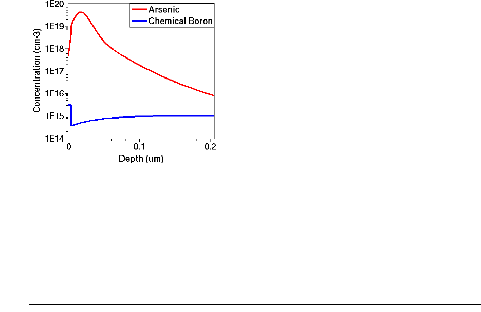
1: Getting Started

Example: 1D Simulation

Sentaurus™ Process User Guide 11

H-2013.03

Besides the file name, here 1DasImpl.plx, the WritePlx command also accepts a material

specifier, which restricts the plot to the given material. For 2D and 3D structures, the x-, y-, or

z-coordinates of the 1D cutline must be given.

Figure 1 As-implanted arsenic profiles and background boron concentration

Figure 1 shows the as-implanted arsenic profiles and the background boron concentration. The

black vertical line marks the oxide–silicon interface. Note the boron depletion at the interface,

which is caused by boron segregation during the oxide growth.

Figure 1 is generated by loading the .plx file into Inspect with:

> inspect 1DasImpl.plx

Thermal Annealing, Drive-in, Activation, and Screening

Oxide Strip

To anneal the damage during implantation, or to drive the dopants deeper into the substrate, or

to activate the implanted dopants in an inert environment, use:

diffuse temperature=1000<C> time=30<min>

strip Oxide

SetPlxList { BTotal BActive AsTotal AsActive }

WritePlx 1Danneal.plx

Here, the structure is annealed at a constant temperature of for 30 minutes. The

annealing is performed in an inert gas because no particular environment is specified.

1000°C

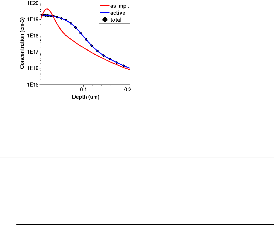
1: Getting Started

Example: 2D Simulation

12 Sentaurus™ Process User Guide

H-2013.03

The annealed profiles are written to the file 1Danneal.plx. The total (chemical)

concentration of boron and arsenic, as well as the respective electrically active (substitutional)

concentrations are saved.

Figure 2 Comparison of as-implanted and annealed arsenic profiles

Figure 2 compares the as-implanted and the annealed arsenic profiles. It is generated by

loading both .plx files into Inspect with:

> inspect 1DasImpl.plx 1Danneal.plx

Example: 2D Simulation

Many widely used process and control commands are introduced in the context of a nominal

n-channel MOSFET process flow. The MOSFET structure is simulated in 2D, and

the processing of the isolation is excluded. A simplified treatment is presented using only

default parameters and models.

Defining Initial Structure and Mesh Refinement

The command math coord.ucs is used to switch on the unified coordinate system (UCS).

Using the UCS is recommended because the default behavior is to rotate the structure when

saving and loading to the DF–ISE coordinate system. With the UCS, the structure is not

rotated. Therefore, the axes in Tecplot SV match the axes in the Sentaurus Process command

file. It is recommended to insert this as the first command in the command file.

The line command is used to:

■Define the initial size of the structure.

0.18 µm

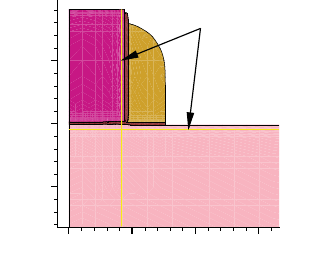
1: Getting Started

Example: 2D Simulation

Sentaurus™ Process User Guide 13

H-2013.03

■Subdivide the structure.

Mesh refinement starts from the user-defined subdivisions; therefore, the specification of lines

helps to compartmentalize mesh refinement. In turn, compartmentalization of the mesh

prevents moving boundaries, and therefore, moving mesh refinement from affecting

geometrically static areas. Whenever mesh lines move, interpolation must be used to obtain

new field values, such as dopant concentrations, and this introduces errors in the simulation.

During the polysilicon reoxidation step, the oxide–silicon and oxide–polysilicon boundaries

move, and this interface movement may cause mesh lines to move. This could be prevented by

inserting lines as follows:

line x location= 0.0

line x location= 3.0<nm> ;# just deeper than reox in silicon

line x location= 10.0<um>

line y location= 0.0

line y location= 85.0<nm> ;# just deeper than reox in poly

line y location= 0.4<um>

To minimize this effect, the silicon and polysilicon regions are isolated from the moving

interfaces by introducing lines immediately inside the final oxide depth in both regions as

shown in Figure 3.

Figure 3 Final structure showing placement of user-defined lines: these lines are used to

isolate silicon and polysilicon regions from boundary movement at the oxide

interfaces

Sentaurus Process uses coordinate systems such that 1D, 2D, and 3D simulations are

consistent. Independent of the current simulation dimension, the positive x is into the wafer; y

is positive to the right, and z is positive out of the page.

NOTE By default, the simulation dimension is promoted only when necessary.

Therefore, until a mask is introduced, the simulation remains in 1D.

Similarly, when going from 2D to 3D, until a 3D mask is introduced

0 0.1 0.2 0.3

-0.1

0.1

User-defined mesh lines

1: Getting Started

Example: 2D Simulation

14 Sentaurus™ Process User Guide

H-2013.03

(one that varies in the z-direction in the defined simulation domain), the

simulation remains in 2D.

The initial simulation domain is defined with the region command. Many, if not most,

simulations start with a block of silicon. The shorthand for this situation is to define a region

of silicon that spans all defined lines:

region Silicon

The region command also can be used to define a new region between specified lines. To limit

the size of the region to be less than all defined lines, the lines must be given a tag with the tag

parameter. These tags are used in the region command with the xlo, xhi, ylo, yhi, zlo,

and zhi parameters.

Finally, the initial mesh and background doping is specified using the init command as

follows:

init concentration=1.0e+15<cm-3> field=Phosphorus wafer.orient=100

Here, an n-doped substrate with a phosphorus concentration of is used. The wafer

orientation is set to 100, which is the default.

The Advanced Calibration set of physical models and parameters is loaded (this is the

recommended choice for accurate process simulation):

AdvancedCalibration I-2013.12

Usually, localized refinement is defined by introducing refinement boxes. This strategy

prevents excessive mesh that can result if mesh refinement is based solely on the line

command (with the spacing parameter). Lines specified with the line command run the

entire length (or breadth or depth) of the structure.

The refinement boxes can be inserted at any time during the simulation. The simplest form of

the refinement box, used in this example, consists of minimum and maximum coordinates

where the refinement box is valid and local maximum mesh spacing in the x-, y- and

z-directions. A refinement box specified for a 2D simulation will be applied to 1D if it is valid

for y = 0.0. Similarly a 3D refinement box will be applied if it covers z = 0.0.

The following refinement boxes specify refinement only in the x-direction for the 1D part of

the simulation:

#--- Refinement in vertical direction ---------------------------------

refinebox clear ;# remove all default refinement

refinebox min = 0 max = 50.0<nm> xrefine = {2.0<nm> 10.0<nm>}

refinebox min = 50.0<nm> max = 2.0<um> xrefine = {10.0<nm> 0.1<um> 0.2<um>}

refinebox min = 2.0<um> max = 10.0<um> xrefine = {0.2<um> 2.0<um>}

1015 cm 3–

1: Getting Started

Example: 2D Simulation

Sentaurus™ Process User Guide 15

H-2013.03

The other type of refinement box used in this example is the interface refinement type. Interface

refinement is a graded refinement that is refined near an interface in the perpendicular direction

and relaxed away from the interface. Using the refinebox command, you can specify

interface refinement using the interface.materials or interface.mat.pairs

parameter:

■Use interface.materials to indicate refinement will occur at all interfaces to the

specified materials.

■Use interface.mat.pairs to choose interface refinement only at specific material

interfaces.

#--- Interface refinement ---------------------------------------------

refinebox interface.materials = { PolySilicon Silicon }

For more details on mesh refinement, see Mesh Refinement on page 694.

Implanting Boron

First, three sets of boron implants are performed:

implant Boron dose=2.0e13<cm-2> energy=200<keV> tilt=0 rotation=0

implant Boron dose=1.0e13<cm-2> energy= 80<keV> tilt=0 rotation=0

implant Boron dose=2.0e12<cm-2> energy= 25<keV> tilt=0 rotation=0

The first high-energy implant creates the p-well, the second medium-energy implant defines a

retrograde boron profile to prevent punch-through, and the third low-energy implant is for a Vt

adjustment.

Growing Gate Oxide

The gate oxide is grown at a temperature of for 10 minutes in pure oxygen using:

diffuse temperature=850<C> time=10.0<min> O2

select z=Boron

layers

The layers command shows that the thickness of the grown oxide is 3.2 nm:

{ Top Bottom Integral Material }

{ -2.500551327519e-03 7.862861879285e-04 1.247399405710e+10 Oxide }

{ 7.862861879285e-04 1.000000000000e+01 3.197435354292e+13 Silicon }

For details, see Measuring Oxide Thickness on page 8.

850°C

1: Getting Started

Example: 2D Simulation

16 Sentaurus™ Process User Guide

H-2013.03

Defining Polysilicon Gate

The polysilicon gate is created using:

deposit PolySilicon type=isotropic thickness=0.18<um>

mask name=gate_mask left=-1 right=90<nm>

etch PolySilicon type=anisotropic thickness=0.2<um> mask=gate_mask

etch Oxide type=anisotropic thickness=0.1<um>

First, of polysilicon is deposited over the entire structure. The keyword

type=isotropic means that the layer is grown equally in all directions, but since the

simulation is in 1D, it would be the same as type=anisotropic.

A mask is defined to protect the gate area with the mask command. In this project, only half of

the transistor is simulated. Therefore, the left edge of the gate mask is unimportant. In general,

you should run the mask over the sides of the simulation to prevent round-off errors that could

prevent complete mask coverage. The name gate_mask is associated with this mask for later

reference.

The first etch command refers to the previously defined mask and, therefore, only the exposed

part of the polysilicon is etched. The requested etching depth is larger than the

deposited layer. This overetching ensures that no residual islands remain. The etching is

specified to be anisotropic, that is, the applied mask is transferred straight down, without any

undercut.

The second etch statement does not refer to any masks. However, the polysilicon naturally

acts as a mask for this selective etching process. Again, a considerable overetching is specified.

Working with Masks

Masks must be defined before they are used. For example, ex_mask blocks processing from

–1 to 2 and from 4 to 20 :

mask clear

mask name=ex_mask segments = { -1.0<um> 2.0<um> 4.0<um> 20.0<um> }

segments

specifies a list of coordinates of mask segments. Several mask segments can be

specified at the same time. The first coordinate defines the beginning of a segment; the second

defines the end of the segment; the third defines the beginning of the segment; and so forth. In

3D simulations, mask segments are extended across the entire structure in the z-direction.

0.18 µm

0.2 µm()

µm

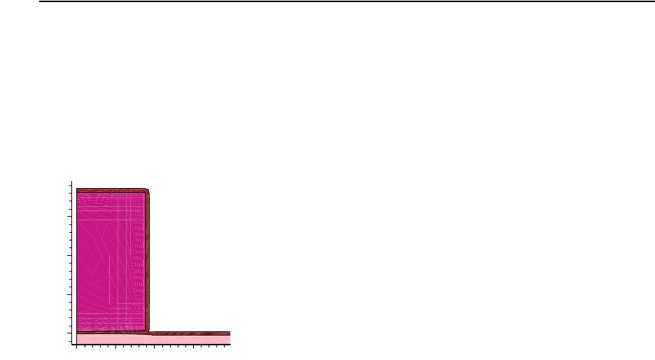
1: Getting Started

Example: 2D Simulation

Sentaurus™ Process User Guide 17

H-2013.03

Masks can be inverted using the negative option. For example, etch_mask prevents

processing from 2 to 4 :

mask clear

mask name=etch_mask segments = { -1.0<um> 2.0<um> 4.0<um> 20.0<um> } negative

Commands that use masking include etch, photo, and deposit.

Polysilicon Reoxidation

To release stresses, a thin oxide layer is grown on the polysilicon before the spacer formation:

diffuse temperature=900<C> time=10.0<min> O2

In all diffusion steps, Sentaurus Process automatically deposits a thin native oxide layer before

starting oxidation. This layer is always present on silicon exposed to air and quickly forms on

newly created interfaces.

Figure 4 Polysilicon reoxidation

During oxidation, mesh movement is controlled by the TSUPREM-4 mesh library in 2D. In 1D

and 3D, it is controlled by an internal moving-boundary mesh algorithm. Both of these moving-

boundary algorithms perform local atomic mesh operations (element removal, edge splitting,

edge flipping, and so on) which leave the rest of the mesh untouched. Mesh points are moved

with the material to maintain dopant dose conservation and the dopant segregation condition at

oxide–silicon and oxide–polysilicon interfaces. Figure 5 shows a close-up of the mesh after the

µm

0 0.05 0.1 0.15

-0.15

-0.1

-0.05

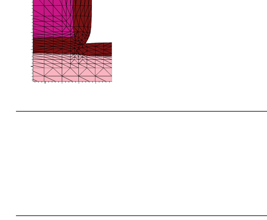
1: Getting Started

Example: 2D Simulation

18 Sentaurus™ Process User Guide

H-2013.03

polysilicon reoxidation step has been performed. Note that the mesh in the brown oxide layer

follows the growth contours.

Figure 5 Mesh in thin oxide layer and in adjacent polysilicon and silicon

Saving Snapshots

To save a snapshot of the current structure, the struct command is used. For example:

struct tdr= NMOS4

The keyword tdr specifies that the snapshot is saved in the TDR file format. The argument

specifies the stem used for the file name. Here, the file NMOS4_fps.tdr is created. The figures

in this section were generated from such snapshots.

For more information about the TDR format, refer to the Sentaurus™ Data Explorer User

Guide.

Remeshing for LDD and Halo Implants

Next, the LDD and halo implants are performed. Before that, however, the mesh must be

refined to properly capture the implant. The previously defined refinement boxes specified

vertical refinement with the xrefine parameter.

Now, lateral refinement is required to resolve the source and drain extensions (also known as

low-doped drain (LDD)) as well as the halo implants. This is accomplished by introducing a

new refinebox command that specifies:

■Lateral refinement using the yrefine parameter.

■Additional vertical refinement using the xrefine parameter.

0.080.085 0.09 0.095

-0.01

-0.005

0.005

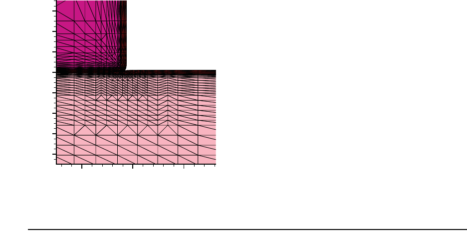
1: Getting Started

Example: 2D Simulation

Sentaurus™ Process User Guide 19

H-2013.03

NOTE When specifying multiple overlapping refinement, the most refined

specification (smallest edge length) wins.

refinebox silicon min= {0.0 0.045<um>} max= {0.1<um> 0.125<um>} \

xrefine= 0.01<um> yrefine= 0.01<um>

grid remesh

The min and max keywords take x-, y-, and z-coordinates. Not all coordinates must be

specified. For example, if only one number is given for minimum, it means that refinement

applies to all y- and z-coordinates less than the max coordinate.

NOTE The refinebox command only specifies a refinement criterion, but the

mesh is not changed. The grid remesh command forces a remesh.

Figure 6 A combination of overlapping refinement boxes is used to define a finer mesh for

LDD and halo; if multiple criteria overlap, the finest mesh specification wins

Implanting LDD and Halo

The LDD and halo implants are performed using:

#--- LDD implantation -------------------------------------------------

implant Arsenic dose=4e14<cm-2> energy=10<keV> tilt=0 rotation=0

#--- Halo implantation: Quad HALO implants ----------------------------

implant Boron dose=1.0e13<cm-2> energy=20<keV> tilt=30<degree> \

rotation=0 mult.rot=4

diffuse temperature=1050<C> time=5.0<s>

0.05 0.1 0.15

-0.06

-0.04

-0.02

0.02

0.04

0.06

0.08

1: Getting Started

Example: 2D Simulation

20 Sentaurus™ Process User Guide

H-2013.03

The LDD implant uses a high dose of and a relatively low energy of 10 keV.

The halo is created by a quad implant using the mult.rot parameter, that is, the implant is

performed in four steps. Each step is separated in rotation by 360/4 = starting with the

specified rotation of 0. This is performed to ensure that the boron penetrates well into the

channel at the tips of the source–drain extensions. Again, a relatively high total dose of

is used.

The implants are activated with a short thermal cycle or rapid thermal anneal (RTA).

Forming Nitride Spacers

The nitride spacers are formed using:

#--- Nitride spacer ---------------------------------------------------

deposit Nitride type=isotropic thickness=60<nm>

etch Nitride type=anisotropic thickness=84<nm> isotropic.overetch=0.01

etch Oxide type=anisotropic thickness=10<nm>

First, a uniform, 60-nm thick layer of nitride is deposited over the entire structure. The keyword

type=isotropic ensures that the growth rate of the layer is the same in all directions. Then,

the nitride is etched again; however, now an anisotropic etching is used. This means that the

nitride deposited on the vertical sides of the gate is not fully removed and can serve as masks

for the source/drain implants. For this step, an isotropic overetch is specified. Specifying a

fraction of the etch thickness, 0.01 implies a 1% isotropic component. This is needed because

the oxide formed during poly oxidation has a nonvertical sidewall. Without the small

isotropic.overetch, a small nitride residual would remain. Finally, the thin oxide layer

grown during the poly reoxidation step is removed.

Remeshing for Source/Drain Implants

Next the source/drain implants are performed. However, before that, the mesh is refined again.

refinebox Silicon min= {0.04<um> 0.11<um>} max= {0.18<um> 0.4<um>} \

xrefine= 0.01<um> yrefine= {0.02<um> 0.05<um>}

grid remesh

This refinement box ensures that the grid is fine enough in the vertical direction to resolve the

junction depth.

410

× cm 2–

90°

110

× cm 2–

1: Getting Started

Example: 2D Simulation

Sentaurus™ Process User Guide 21

H-2013.03

Implanting Source/Drain

The source and drain regions are created using:

implant Arsenic dose=5e15<cm-2> energy=40<keV> tilt=7<degree> \

rotation=-90<degree>

diffuse temperature=1050<C> time=10.0<s>

To ensure a low resistivity of the source and drain regions, this implant step uses a very high

dose of . A tilt of is used to reduce channeling and a rotation of

ensures that the plane of incident is parallel to the gate stack, such that the tilt angle does

not lead to asymmetry between the source and drain.

Transferring to Device Simulation

To transfer from process simulation to device simulation, the normal steps are:

■The structure bottom is cropped.

■The full transistor is created by reflecting about the symmetry plane.

■A new mesh strategy is specified appropriate for device simulation.

■Contacts are specified.

■The struct command is called which remeshes and saves the structure.

Remeshing for Device Simulation

The following example shows the standard technique used to produce a structure and mesh

appropriate for device simulation. First, the structure bottom is truncated; then a new mesh

strategy is introduced:

#--Remove bottom of structure------------------------------------------

transform cut location= 1.00 down

#--Change refinement strategy and remesh-------------------------------

refinebox clear

line clear

pdbSet Grid Adaptive 1

pdbSet Grid AdaptiveField Refine.Abs.Error 1e37

pdbSet Grid AdaptiveField Refine.Rel.Error 1e10

pdbSet Grid AdaptiveField Refine.Target.Length 100.0

pdbSet Grid SnMesh DelaunayType boxmethod

refinebox name= Global refine.min.edge= {0.01 0.01} \

510

× cm 2–

7°

90–°

7°

1: Getting Started

Example: 2D Simulation

22 Sentaurus™ Process User Guide

H-2013.03

refine.max.edge= {0.1 0.1} refine.fields= { NetActive } \

def.max.asinhdiff= 0.5 adaptive

refinebox name= SiGOX min.normal.size= 0.2<nm> normal.growth.ratio= 1.4 \

max.lateral.size= 5.0<nm> min= {-0.01 -0.1} max= {0.01 0.1} \

interface.materials= {Silicon}

refinebox name= GDpn1 min= {0.0 0.04} max= {0.06 0.1} xrefine= 0.005 \

yrefine= 0.005 silicon

refinebox name= TopActive min= {0.0 0.0} max= {0.3 0.4} \

refine.min.edge= {0.02 0.02} refine.max.edge= {0.05 0.05} \

refine.fields= { NetActive } def.max.asinhdiff= 0.5 \

adaptive silicon

grid remesh

#--Reflect ---------------------------------------------------------

transform reflect left

The new mesh strategy uses a combination of interface refinement, fixed boxwise refinement,

and adaptive refinement on dopants.

Contacts

Next, contacts are added to the structure using the contact command. These contacts are

added to structure files upon writing. They are not present in the internal Sentaurus Process

structure, but are added only as required when writing the structure. There are two types of

contact specification:

■Box: For these contacts, you specify a box and a material, and all interfaces of that material

that are inside the box become the contact.

■Point: For this contact, you specify a point inside a chosen region. The chosen region is

removed, and all interfaces between the chosen region and bulk materials become part of

the contact.

In the following example, only box-type contacts are used:

#--- Contacts ---------------------------------------------------------

contact name= "substrate" bottom Silicon

contact name= "source" box Silicon adjacent.material= Gas \

xlo= 0.0 xhi= 0.005 ylo= -0.4 yhi= -0.2

contact name= "drain" box Silicon adjacent.material= Gas \

xlo= 0.0 xhi= 0.005 ylo= 0.2 yhi= 0.4

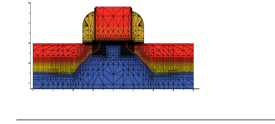
1: Getting Started

Example: 2D Simulation

Sentaurus™ Process User Guide 23

H-2013.03

contact name= "gate" box PolySilicon xlo= -0.181 xhi= -0.05 \

ylo= -0.088 yhi= 0.088

Saving the Structure

To save the structure, use:

struct tdr=NMOS !Gas

The file NMOS_fps.tdr is created with contacts and can be loaded into Sentaurus Device to

obtain device electrical characteristics.

Figure 7 Final structure showing contacts and refinement appropriate for device simulation

Extracting 1D Profiles

You can save 1D profiles at any point in the process flow using:

SetPlxList {BTotal NetActive}

WritePlx NMOS_channel.plx y=0.0 silicon

as well as:

struct tdr=NMOS_channel.tdr y=0.0

For details, see Saving the As-Implanted Profile on page 10.

-0.4 -0.3 -0.2 -0.1 0 0.1 0.2 0.3 0.4

-0.2

-0.1

0.1

0.2

1: Getting Started

Adaptive Meshing: 2D npn Vertical BJT

24 Sentaurus™ Process User Guide

H-2013.03

Adaptive Meshing: 2D npn Vertical BJT

A simple 2D npn vertical bipolar transistor example is introduced to show how the adaptive-

meshing capabilities in Sentaurus Process can be used to ease mesh setup and allow for mesh

evolution during dopant diffusion. For examples, see 2D npn Vertical Bipolar on page 38.

For all the applications involving long thermal diffusion steps or simulations of relatively large

structures (in which doping profiles may evolve greatly), using static mesh criteria is

impracticable because it requires using a fine mesh in many parts of the simulation domain.

Moreover, the placement of the refinement boxes is not straightforward because often the

location of gradients and junctions at the end of the thermal steps is not precisely known. For

such purposes, adaptive meshing could be used. Using this feature, you only have to define

some refinement criteria, more or less stringent depending on the level of accuracy required.

The meshing engine checks the mesh and decides automatically where, when, and if the mesh

needs to be refined.

Overview

Adaptive meshing can be switched on globally with:

pdbSet Grid Adaptive 1

which creates a default adaptive box covering the entire structure.

Adaptive refinement parameters can be set in the following ways:

■Fieldwise in the PDB with the pdbSet command

■Boxwise as parameters of the refinebox command

■Materialwise, specifying a material in a box definition

■Regionwise, specifying a region in a box definition

To prevent the number of mesh points from growing too large, switch off the keep.lines

option (which is switched on by default in silicon) when using adaptive meshing:

refinebox !keep.lines

Many different refinement criteria have been implemented in Sentaurus Process for flexibility

in handling different types of field and structure. For a complete list and detailed descriptions

of the refinement criteria, see Adaptive Refinement Criteria on page 700.

1: Getting Started

Adaptive Meshing: 2D npn Vertical BJT

Sentaurus™ Process User Guide 25

H-2013.03

The criteria in the following example are the most commonly used and are referred to as

relative difference and local dose error. Each computes the so-called desired edge length

(DEL), which is defined formally as:

DEL = min (l

* MaxError/Error)

where l12 is the length of the edge between two mesh points 1 and 2. Error (computed

internally) is the error between points 1 and 2, and MaxError (set by users) is the maximum

allowable error. The right-hand side of the expression is computed over all the fields that can

be refined (by default, all the solution variables): the minimum value is the DEL for the

corresponding criterion. The expression for Error and the name and the meaning of

MaxError vary from criterion to criterion. For the relative difference criterion, these quantities

have the form:

Error = 2*|C

- C

|/(C

+ C

+ alpha)

MaxError = R

where and are the concentration of the field in points 1 and 2, respectively, is the

relative error that sets the maximum-allowed change of the field across an edge, and alpha is

the absolute error, a type of cutoff threshold below which refinement is smoothed out. They can

be set in the PDB as follows:

pdbSet Grid Boron Refine.Abs.Error 1e15

pdbSet Grid Boron Refine.Rel.Error 0.5

or in the refinebox commands as:

refinebox name=Active refine.fields= {Boron Arsenic} \

rel.error= {Boron=0.5 Arsenic=0.5} abs.error= {Boron=2e15 Arsenic=1e16} \

Adaptive min= {-1.0 -0.1} max= {2.0 16.0}

For the definition of Error and MaxError for the local dose error criterion, see Local Dose

Error Criteria on page 703.

All the edges are compared to DEL to check the percentage of long edges by using the

following additional parameter:

pdbSetDoubleArray Grid Refine.Factor {X 2.0 Y 2.0}

These coefficients can be set directionwise and act in the following way: An edge is defined as

long when it is larger than Refine.Factor*DEL for at least one of the selected refinement

criteria. When the percentage of long edges is larger than certain values, adaptive refinement

is actually triggered. This value can be set as:

pdbSet Grid Refine.Percent 0.01

When adaptive meshing is switched on, it automatically affects refinement whenever a mesh is

generated (such as after geometry-changing operations). During the diffuse command, the

1: Getting Started

Adaptive Meshing: 2D npn Vertical BJT

26 Sentaurus™ Process User Guide

H-2013.03

mesh is checked after a certain number of steps that can be separately set depending on the

nature of the diffusion step:

pdbSet Diffuse Compute.Regrid.Steps 10 ;# during inert annealings

pdbSet Diffuse Growth.Regrid.Steps -1 ;# during oxidation and silicidation

pdbSet Diffuse Epi.Regrid.Steps -1 ;# during epitaxy

When the number of long edges is larger than Refine.Percent, remeshing is performed. The

mesh quality check can be omitted by setting:

pdbSet Grid Refinement.Check 0

which can save some CPU time when performing simulations on large meshes, where the mesh

checking is time consuming.

NOTE Formally, the adaptive-meshing feature consists of field-based and

implant-based adaptation. There is a small difference in the way

refinement criteria are applied. For details, see Adaptive Meshing

during Implantation on page 708 and Interval Refinement on page 704.

However, as the two modules use the same parameters, you do not need

to define them twice.

NOTE Adaptive-meshing syntax to set up parameters is the same in any

dimension.

The relative error criterion is effective in refining doping profiles in steep gradient regions. In

the vicinity of maxima and minima, the profiles are almost flat and some loss of accuracy may

occur there. Further reduction of Rel.Error would increase significantly the number of

points in the steep slope with negligible improvements at the peaks. In that case, the max dose

loss criterion can be used more effectively. This explains why the combination of these two

criteria provides an optimum adaptive-remeshing strategy.

Defining Initial Structure

The command math coord.ucs is used to switch on the unified coordinate system (UCS).

Using the UCS is recommended because the default behavior is to rotate the structure when

saving and loading to the DF–ISE coordinate system. With the UCS, the structure is not

rotated. Therefore, the axes in Tecplot SV match the axes in the Sentaurus Process command

file. It is recommended to insert this as the first command in the command file.

The line commands are used to compartmentalize the structure according to the meshing

strategy described in the previous example:

line x loc= 2.0<um>

line x loc= 4.0<um> tag=SubTop

1: Getting Started

Adaptive Meshing: 2D npn Vertical BJT

Sentaurus™ Process User Guide 27

H-2013.03

line x loc= 6.0<um>

line x loc= 10.0<um> tag=SubBottom

line y loc= 0.0<um> tag=SubLeft

line y loc=1.5<um>

line y loc=2.5<um>

line y loc=8<um>

line y loc=13<um>

line y loc=22<um>

line y loc=24<um>

line y loc=30.0<um> tag=SubRight

Along the x-axis, few lines are specified: the two tagged ones are needed to define the initial

silicon substrate. The other two lines are defined to have uniform spacing within the box

defined to refine the buried layer. Along the y-axis, more lines are defined because a coarse

initial mesh would degrade the quality of the mesh resulting from adaptation during

implantation. These lines are set corresponding to the mask edges: This information is usually

known to users, especially if the simulation starts from a layout, and the process flow is set up

in Ligament.

Adaptive Meshing Settings

As previously mentioned, adaptive parameters can be set in different ways, which lead to

different refinement strategies:

pdbSet Grid Adaptive 1

pdbSet Grid AdaptiveField Refine.Abs.Error 1e25

pdbSet Grid AdaptiveField Refine.Rel.Error 2.0

pdbSet Grid Damage Refine.Min.Value 1e25

pdbSet Grid Damage Refine.Max.Value 1e25

pdbSet Grid Damage Refine.Target.Length 1

Here the following strategy is used:

■The default relative difference–type refinement is switched off by setting high values for

absolute and relative errors and for the interval damage refinement.

■When parameters are set for AdaptiveField, they are applied to all the existing fields

that can be refined.

■Actual refinement will be then controlled in specific regions by using refineboxes.

Three refinement boxes are defined as the structure and the process flow clearly identifies three

main significant areas: buried layer, collector region, and base-emitter region:

refinebox name=BL refine.fields= {Antimony Phosphorus} \

rel.error= {Antimony=0.6 Phosphorus=0.6} \

1: Getting Started

Adaptive Meshing: 2D npn Vertical BJT

28 Sentaurus™ Process User Guide

H-2013.03

abs.error= {Antimony=1e16 Phosphorus=1e16} Adaptive min= {2.0 -0.1} \

max= {10.1 30.1} refine.min.edge= {0.2 0.4} max.dose.error= {Antimony=1e8} \

The min and max parameters set an xy pair of coordinates to define the extent of the box. The

keyword all means that refinement must be applied to all materials. When using a material

name, refinement is applied to the specified material only.

NOTE More than one adaptive type can be specified in the same box. In the BL

box, the relative difference and local dose loss criteria are selected by

specifying the parameters rel.error or abs.error and

max.dose.error, respectively.

refinebox name=Sinker refine.fields= {Phosphorus Arsenic} \

rel.error= {Phosphorus=0.5 Arsenic=0.5} \

abs.error= {Phosphorus=5e15 Arsenic=1e16} Adaptive min= {-1.0 16} \

max= {2.0 30.1} refine.min.edge= {0.1 0.2}

refinebox name=Active refine.fields= {Boron Arsenic} \

rel.error= {Boron=0.5 Arsenic=0.5} abs.error= {Boron=2e15 Arsenic=1e16} \

Adaptive min= {-1.0 -0.1} max= {2.0 16.0} refine.min.edge= {0.025 0.05} \

The BL box is defined to refine the buried layer: a high level of accuracy is not required here

and the values are more relaxed than in the other boxes. The refine.min.edge parameter

adds the additional directionwise constraint not to refine edges below the specified values

(units in micrometers).

The Sinker box is defined to refine the n-doped collector region, which contacts the buried

layer. More restrictive values are used in it.

The Active box is used to refine the base–emitter region. Higher accuracy is required here to

properly catch the base length, which all the main electrical parameters of the device are a

function of:

pdbSet Diffuse Compute.Regrid.Steps 10

pdbSet Grid Refine.Percent 0.01

According to these last two commands, the mesh is checked every 10 diffusion steps in inert

annealings, and remeshing is performed if there are more than 0.01% of long edges.

Buried Layer

The buried layer is obtained with high-energy and high-dose antimony implantation:

deposit material= {Oxide} type=isotropic time=1 rate= {0.025}

implant Antimony dose=1.5e15<cm-2> energy=100<keV>

etch material= {Oxide} type=anisotropic time=1 rate= {0.03}

1: Getting Started

Adaptive Meshing: 2D npn Vertical BJT

Sentaurus™ Process User Guide 29

H-2013.03

Before the implantation, 25 nm of a screening oxide is deposited. Here an alternate syntax is

used to specify the deposit material. The deposited oxide thickness is determined by the

product of rate and time. The implantation is performed with default angles (tilt of and

rotation of ). After the implantation, the oxide is etched to clean the surface and to prepare

it for the subsequent epi step.

Epi Layer

For speed and simplicity, an epitaxial regrowth step is not performed here. Instead, a simpler

deposition of a silicon layer with arsenic concentration is followed by a

diffusion step:

deposit material= {Silicon} type=isotropic time=1 rate= {4.0} Arsenic \

concentration=1e15<cm-3>

diffuse temp=1100<C> time=60<min> maxstep=4<min>

The maximum diffusion step is limited to 4 minutes to avoid having too much diffusion

between two subsequent adaptive remeshing steps. An alternative would be to reduce

Compute.Regrid.Steps, but this would lead to numerous remeshings at the beginning of

the annealing when the time step is small.

The following sections describe the process steps to create sinker, base, and emitter regions. At

the end of each group of steps, results are saved in TDR files.

Sinker Region

This is the beginning of the 2D simulation. A 50-nm screening oxide is deposited before the

phosphorus implantation to contact the buried layer. The Sinker mask protects the silicon area

where the base will be created. The Photo command is used to deposit the photoresist (mask

definition not shown here). The subsequent annealing is long (5 hours). For this reason, the

maximum time step is allowed to increase up to 8 minutes.

Figure 8 on page 30 shows the doping concentration distribution at this point of the simulation:

deposit material= {Oxide} type=isotropic time=1 rate= {0.05}

photo mask=Sinker thickness=1

implant Phosphorus dose=5e15<cm-2> energy=200<keV>

strip Resist

diffuse temp=1100<C> time=5<hr> maxstep=8<min>

struct tdr=vert_npn2

7°

90°

115

×10 cm 3–

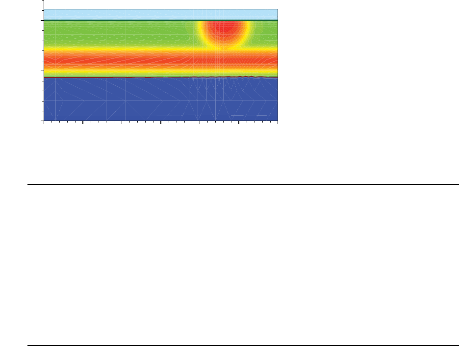
1: Getting Started

Adaptive Meshing: 2D npn Vertical BJT

30 Sentaurus™ Process User Guide

H-2013.03

Figure 8 Doping concentration after phosphorus implantation and diffusion to contact

antimony buried layer

Base Region

The p-doped base region is created with a dose of implanted boron followed by

a 35-minute inert annealing:

photo mask=Base thickness=1

implant Boron dose=1e14<cm-2> energy=50<keV>

strip Resist

diffuse temp=1100<C> time=35<min> maxstep=4<min>

struct tdr=vert_npn3

Emitter Region

The highly n-doped emitter region is created with a dose of implanted arsenic

followed by a 25-minute inert annealing. Emitter mask is designed such that arsenic is

implanted also in the sinker region to increase the doping concentration at the collector contact.

In addition to a TDR file, 1D profiles are extracted. Figure 9 on page 31 shows the final doping

distribution:

photo mask=Emitter thickness=1

implant Arsenic dose=5e15<cm-2> energy=55<keV> tilt=7 rotation=0

strip Resist

diffuse temp=1100<C> time=25<min> maxstep=4<min>

struct tdr=vert_npn4

0 5 10 15 20 25 30

114

×10 cm 2–

515

×10 cm 2–

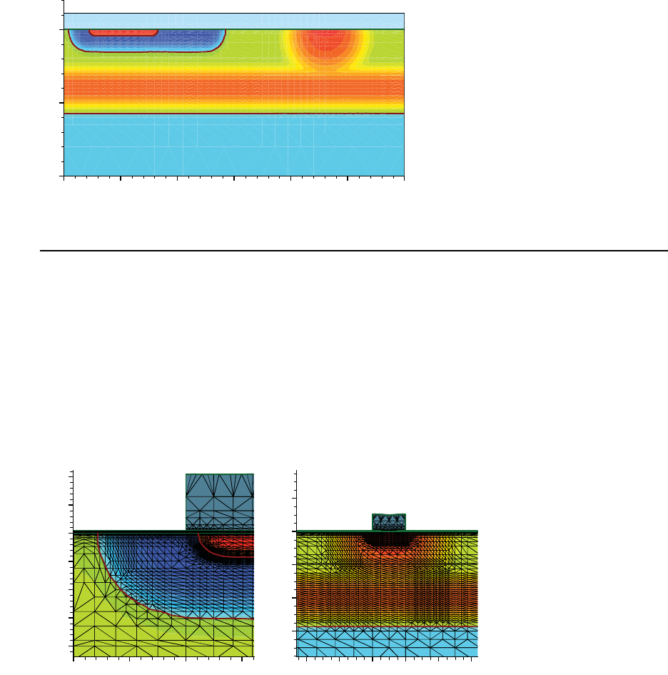
1: Getting Started

Adaptive Meshing: 2D npn Vertical BJT

Sentaurus™ Process User Guide 31

H-2013.03

SetPlxList {BTotal SbTotal AsTotal PTotal}

WritePlx Final.plx y=5.0

WritePlx Sinker.plx y=23.0

Figure 9 Final doping distribution

Backend

The real backend steps are not simulated here. A sequence of masked etching and deposition

steps are used to define emitter, base, and collector contacts:

etch material= {Oxide} type=anisotropic time=1 rate= {0.055} mask=Contact

deposit material= {Aluminum} type=isotropic time=1 rate= {1.0}

etch material= {Aluminum} type=anisotropic time=1 rate= {1.1} mask=Metal

struct tdr=vert_npn5

Figure 10 shows some details of the final mesh.

Figure 10 Details of final mesh: (left) the emitter–base region and (right) the buried layer

with collector contact

0 5 10 15 20 25 30

0 1 2 3

-1

-0.5

0.5

1.5

1820 22 24 26 28

-2

1: Getting Started

Full-Text Versions of Examples

32 Sentaurus™ Process User Guide

H-2013.03

The relative difference criterion refines the doping profiles, not the junctions. Obviously, if the

profiles are reproduced correctly, the junctions also will be in the right place. To obtain a

junction-like refinement with the relative difference criterion, set abs.error close to the

doping level of the less-doped side of the junction. A more effective way is to select

NetDoping as the field to be refined and apply to it the inverse hyperbolic sine (asinh)

difference criterion (for details, see Inverse Hyperbolic Sine (asinh) Difference Criteria on

page 702).

Full-Text Versions of Examples

The following full-text versions of the examples allow convenient electronic copying of text

into Sentaurus Process command files.

1D NMOS

# 1D Grid definition

#-------------------

line x location=0.0 spacing= 1<nm> tag=SiTop

line x location= 10<nm> spacing= 2<nm>

line x location= 50<nm> spacing= 10<nm>

line x location=300<nm> spacing= 20<nm>

line x location=0.5<um> spacing= 50<nm>

line x location=2.0<um> spacing=0.2<um> tag=SiBottom

# Initial simulation domain

#--------------------------

region Silicon xlo=SiTop xhi=SiBottom

# Initialize the simulation

#--------------------------

init concentration=1.0e15<cm-3> field=Boron

# Set of physical models and parameters

# ----------------------------------------------

AdvancedCalibration 2013.12

# Settings for automatic meshing in newly generated layers

#---------------------------------------------------------

pdbSet Grid SnMesh min.normal.size 0.003

1: Getting Started

Full-Text Versions of Examples

Sentaurus™ Process User Guide 33

H-2013.03

pdbSet Grid SnMesh normal.growth.ratio.2d 1.4 ;# this is for 1D and 2D

set SCREEN Grow

if { $SCREEN == "Grow" } {

# Growing screening oxide

#------------------------

gas_flow name=O2_1_N2_1 pressure=1<atm> flowO2=1.2<l/min> flowN2=1.0<l/min>

diffuse temperature=900<C> time=40<min> gas_flow=O2_1_N2_1

# Measuring the oxide thickness

#------------------------------

select z=1

layers

} else {

# Depositing screening oxide

#---------------------------

deposit material= {Oxide} type=isotropic time=1.0 rate= {0.01}

diffuse temperature=900<C> time=40<min>

}

# Implanting Arsenic

#-------------------

implant Arsenic energy=30<keV> dose=1e14<cm-2> tilt=7<degree> \

rotation=0<degree>

# Plotting out the "as implanted" profile

#----------------------------------------

SetPlxList { BTotal Arsenic_Implant }

WritePlx 1DasImpl.plx

# Thermal annealing

#------------------

diffuse temperature=1000<C> time=30<min>

strip Oxide

SetPlxList { BTotal BActive AsTotal AsActive }

WritePlx 1Danneal.plx

2D NMOS

#----------------------------------------------------------------------

# 2D nMOSFET (0.18um technology)

#----------------------------------------------------------------------

math coord.ucs

1: Getting Started

Full-Text Versions of Examples

34 Sentaurus™ Process User Guide

H-2013.03

pdbSet Oxide Grid perp.add.dist 1e-7

#--- Specify lines for outer boundary and to separate moving boundaries

# from the rest of the structure------------------------------------

line x location= 0.0

line x location= 3.0<nm> ;# just deeper than reox in silicon

line x location= 10.0<um>

line y location= 0.0

line y location= 85.0<nm> ;# just deeper than reox in poly

line y location= 0.4<um>

#--- Silicon substrate definition -------------------------------------

region silicon

#--- Initialize the simulation ----------------------------------------

init concentration=1.0e+15<cm-3> field=Phosphorus

# Set of physical models and parameters

# ------------------------

AdvancedCalibration 2013.12

#--- Refinement in vertical direction ---------------------------------

refinebox clear

refinebox min = 0 max = 50.0<nm> xrefine = {2.0<nm> 10.0<nm>}

refinebox min = 50.0<nm> max = 2.0<um> xrefine = {10.0<nm> 0.1<um> 0.2<um>}

refinebox min = 2.0<um> max = 10.0<um> xrefine = {0.2<um> 2.0<um>}

#--- Interface refinement ---------------------------------------------

refinebox interface.materials = { PolySilicon Silicon }

#--- Sentaurus Mesh settings for automatic meshing in newly generated layers -

pdbSet Grid SnMesh min.normal.size 1.0e-3 ;# in micrometers

pdbSet Grid SnMesh normal.growth.ratio.2d 1.4 ;# used in 1D and 2D

#--- Create starting mesh from lines and refinement

grid remesh

#--- p-well, anti-punchthrough & Vt adjustment implants ---------------

implant Boron dose=2.0e13<cm-2> energy=200<keV> tilt=0 rotation=0

implant Boron dose=1.0e13<cm-2> energy= 80<keV> tilt=0 rotation=0

implant Boron dose=2.0e12<cm-2> energy= 25<keV> tilt=0 rotation=0

#--- p-well: RTA of channel implants ----------------------------------

diffuse temperature=1050<C> time=10.0<s>

1: Getting Started

Full-Text Versions of Examples

Sentaurus™ Process User Guide 35

H-2013.03

#--- Saving structure -------------------------------------------------

struct tdr=NMOS1 FullD; # p-Well

#--- Gate oxidation ---------------------------------------------------

diffuse temperature=850<C> time=10.0<min> O2

select z=Boron

layers

struct tdr=NMOS2 FullD; # GateOx

#--- Poly gate deposition ---------------------------------------------

deposit poly type=isotropic thickness=0.18<um>

#--- Poly gate pattern/etch -------------------------------------------

# MGoals settings for etch/depo

mgoals accuracy=2e-5

mask name=gate_mask segments = { -1 90<nm> }

etch poly type=anisotropic thickness=0.2<um> mask=gate_mask

etch oxide type=anisotropic thickness=0.1<um>

struct tdr=NMOS3 ; # PolyGate

#--- For graphics, first run "tecplot_sv -s:ipc" and uncomment

# the next line before running this file

# graphics on

#--- Poly reoxidation -------------------------------------------------

diffuse temperature=900<C> time=10.0<min> O2

struct tdr=NMOS4 ; # Poly Reox

#--- LDD implantation -------------------------------------------------

refinebox silicon min= {0.0 0.045<um>} max= {0.1<um> 0.125<um>} \

xrefine= 0.01<um> yrefine= 0.01<um>

grid remesh

implant Arsenic dose=4e14<cm-2> energy=10<keV> tilt=0 rotation=0

SetPlxList { BTotal Arsenic_Implant }

WritePlx 1DasImpl.plx y= 0.25<um>

diffuse temperature=1050<C> time=0.1<s> ; # Quick activation

struct tdr=NMOS5 ; # LDD Implant

#--- Halo implantation: Quad HALO implants ----------------------------

implant Boron dose=1.0e13<cm-2> energy=20<keV> \

tilt=30<degree> rotation=0 mult.rot=4

#--- RTA of LDD/HALO implants -----------------------------------------

diffuse temperature=1050<C> time=5.0<s>

1: Getting Started

Full-Text Versions of Examples

36 Sentaurus™ Process User Guide

H-2013.03

struct tdr=NMOS6 ; # Halo RTA

#--- Nitride spacer ---------------------------------------------------

deposit nitride type=isotropic thickness=60<nm>

etch nitride type=anisotropic thickness=84<nm> isotropic.overetch=0.01

etch oxide type=anisotropic thickness=10<nm>

struct tdr=NMOS7 ; # Spacer

#--- N+ implantation --------------------------------------------------

refinebox silicon min= {0.04<um> 0.11<um>} max= {0.18<um> 0.4<um>} \

xrefine= 0.01<um> yrefine= {0.02<um> 0.05<um>}

grid remesh

implant Arsenic dose=5e15<cm-2> energy=40<keV> \

tilt=7<degree> rotation=-90<degree>

SetPlxList { BTotal Arsenic_Implant }

WritePlx 1DasImpl2.plx y= 0.25<um>

#---- N+ implantation & final RTA -------------------------------------

diffuse temperature=1050<C> time=10.0<s>

struct tdr=NMOS8 ; # S/D implants

# - 1D cross sections

SetPlxList {BTotal NetActive}

WritePlx NMOS_channel.plx y=0.0 silicon

SetPlxList {AsTotal BTotal NetActive}

WritePlx NMOS_ldd.plx y=0.1 silicon

SetPlxList {AsTotal BTotal NetActive}

WritePlx NMOS_sd.plx y=0.35 silicon

#----------------------------------------------------------------------#

#Transfer to device simulation

#----------------------------------------------------------------------#

#--Remove bottom of structure------------------------------------------

transform cut location= 1.00 down

#--Change refinement strategy and remesh-------------------------------

refinebox clear

line clear

pdbSet Grid Adaptive 1

pdbSet Grid AdaptiveField Refine.Abs.Error 1e37

pdbSet Grid AdaptiveField Refine.Rel.Error 1e10

1: Getting Started

Full-Text Versions of Examples

Sentaurus™ Process User Guide 37

H-2013.03

pdbSet Grid AdaptiveField Refine.Target.Length 100.0

pdbSet Grid SnMesh DelaunayType boxmethod

refinebox name= Global \

refine.min.edge= {0.01 0.01} refine.max.edge= {0.1 0.1} \

refine.fields= { NetActive } def.max.asinhdiff= 0.5 adaptive

refinebox name= SiGOX \

min.normal.size= 0.2<nm> normal.growth.ratio= 1.4 \

max.lateral.size= 5.0<nm> min= {-0.01 -0.1} max= {0.01 0.1} \

interface.materials= {Silicon}

refinebox name= GDpn1 \

min= {0.0 0.04} max= {0.06 0.1} xrefine= 0.005 yrefine= 0.005 \

silicon

refinebox name= TopActive \

min= {0.0 0.0} max= {0.3 0.4} \

refine.min.edge= {0.02 0.02} refine.max.edge= {0.05 0.05} \

refine.fields= { NetActive } def.max.asinhdiff= 0.5 \

adaptive silicon

grid remesh

#--- Reflect ---------------------------------------------------------

transform reflect left

#--- Contacts ---------------------------------------------------------

contact name= "substrate" bottom Silicon

contact name= "source" box Silicon adjacent.material= Gas \

xlo= 0.0 xhi= 0.005 ylo= -0.4 yhi= -0.2

contact name= "drain" box Silicon adjacent.material= Gas \

xlo= 0.0 xhi= 0.005 ylo= 0.2 yhi= 0.4

contact name= "gate" box PolySilicon \

xlo= -0.181 xhi= -0.05 ylo= -0.088 yhi= 0.088

#--- Final ---------------------------------------------------------

struct tdr=NMOS !Gas

1: Getting Started

Full-Text Versions of Examples

38 Sentaurus™ Process User Guide

H-2013.03

2D npn Vertical Bipolar

# 2D NPN Vertical Bipolar Transistor

#-----------------------------------

math coord.ucs

line x loc= 2.0<um>

line x loc= 4.0<um> tag=SubTop

line x loc= 6.0<um>

line x loc= 10.0<um> tag=SubBottom

line y loc= 0.0<um> tag=SubLeft

line y loc=1.5<um>

line y loc=2.5<um>

line y loc=8<um>

line y loc=13<um>

line y loc=22<um>

line y loc=24<um>

line y loc=30.0<um> tag=SubRight

# Diffuse settings to speed up simulation

#----------------------------------------

pdbSet Diffuse IncreaseRatio 8.0

pdbSet Diffuse ReduceRatio 0.5

# Mesh settings

#--------------

mgoals normal.growth.ratio=2.0 accuracy=2e-5 min.normal.size=10<nm> \

max.lateral.size=30.0<um> minedge=1e-5

pdbSet Grid Adaptive 1

pdbSet Grid AdaptiveField Refine.Abs.Error 1e25

pdbSet Grid AdaptiveField Refine.Rel.Error 2.0

pdbSet Grid Damage Refine.Min.Value 1e25

pdbSet Grid Damage Refine.Max.Value 1e25

pdbSet Grid Damage Refine.Target.Length 1

pdbSet Diffuse Compute.Regrid.Steps 10

pdbSet Grid Refine.Percent 0.01

refinebox interface.mat.pairs= {Silicon Oxide}

refinebox name=BL refine.fields= {Antimony Phosphorus} \

rel.error={Antimony=0.6 Phosphorus=0.6} \

1: Getting Started

Full-Text Versions of Examples

Sentaurus™ Process User Guide 39

H-2013.03

abs.error= {Antimony=1e16 Phosphorus=1e16} \

Adaptive min= "2.0 -0.1" max= "10.1 30.1" \

refine.min.edge= {0.2 0.4} max.dose.error= {Antimony=1e8}

refinebox name=Sinker refine.fields= {Phosphorus Arsenic} \

rel.error= {Phosphorus=0.5 Arsenic=0.5} \

abs.error= {Phosphorus=5e15 Arsenic=1e16} \

Adaptive min= {-1.0 16} max= {2.0 30.1} refine.min.edge= {0.1 0.2}

refinebox name=Active refine.fields= {Boron Arsenic} \

rel.error= {Boron=0.5 Arsenic=0.5} \

abs.error= {Boron=2e15 Arsenic=1e16} \

Adaptive min= {-1.0 -0.1} max= {2.0 16.0} \

refine.min.edge= {0.025 0.05}

# Masks definition

#-----------------

mask name=Sinker segments= {-1 22 24 35} negative

mask name=Base segments= {-1 1.5 13 35} negative

mask name=Emitter segments= {-1 2.5 8 22 24 35} negative

mask name=Contact segments= {-1 3.5 7 10 12 22.5 23.5 35}

mask name=Metal segments= {-1 2 8 9 13 22 24 35} negative

# Creating initial structure

#---------------------------

region Silicon xlo=SubTop xhi=SubBottom ylo=SubLeft yhi=SubRight

init concentration=1e+15<cm-3> field=Boron

# Set of physical models and parameters

# ------------------------

AdvancedCalibration 2013.12

# Buried layer

#-------------

deposit material= {Oxide} type=isotropic time=1 rate= {0.025}

implant Antimony dose=1.5e15<cm-2> energy=100<keV>

etch material= {Oxide} type=anisotropic time=1 rate= {0.03}

# Epi layer

#----------

deposit material= {Silicon} type=isotropic time=1 rate= {4.0} \

Arsenic concentration=1e15<cm-3>

diffuse temp=1100<C> time=60<min> maxstep=4<min>

1: Getting Started

Full-Text Versions of Examples

40 Sentaurus™ Process User Guide

H-2013.03

struct tdr=vert_npn1

SetPlxList {BTotal SbTotal AsTotal PTotal}

WritePlx Buried.plx

# Sinker

#-------

deposit material= {Oxide} type=isotropic time=1 rate= {0.05}

photo mask=Sinker thickness=1

implant Phosphorus dose=5e15<cm-2> energy=200<keV>

strip Resist

diffuse temp=1100<C> time=5<hr> maxstep=8<min>

struct tdr=vert_npn2

# Base

#-----

photo mask=Base thickness=1

implant Boron dose=1e14<cm-2> energy=50<keV>

strip Resist

diffuse temp=1100<C> time=35<min> maxstep=4<min>

struct tdr=vert_npn3

# Emitter

#--------

photo mask=Emitter thickness=1

implant Arsenic dose=5e15<cm-2> energy=55<keV> tilt=7 rotation=0

strip Resist

diffuse temp=1100<C> time=25<min> maxstep=4<min>

struct tdr=vert_npn4

SetPlxList {BTotal SbTotal AsTotal PTotal}

WritePlx Final.plx y=5.0

WritePlx Sinker.plx y=23.0

# Back end

#---------

etch material= {Oxide} type=anisotropic time=1 rate= {0.055} mask=Contact

deposit material= {Aluminum} type=isotropic time=1 rate= {1.0}

etch material= {Aluminum} type=anisotropic time=1 rate= {1.1} mask=Metal

1: Getting Started

Full-Text Versions of Examples

Sentaurus™ Process User Guide 41

H-2013.03

struct tdr=vert_npn5

exit

1: Getting Started

Full-Text Versions of Examples

42 Sentaurus™ Process User Guide

H-2013.03

Sentaurus™ Process User Guide 43

H-2013.03

CHAPTER 2 The Simulator Sentaurus Process

This chapter provides an overview of how Sentaurus Process

operates.

The syntax and features of the command file are described, followed by an overview of the

Sentaurus Process parameter database, which contains all of the model parameters and

technical details regarding the running of the tool.

For new users, see Syntax for Creating Input Command Files on page 50, Creating and

Loading Structures and Data on page 66, and Interactive Mode on page 46. For advanced users

who need to adjust model parameters, see Parameter Database on page 55. For the TCAD

Sentaurus Tutorial and examples, go to:

$STROOT/tcad/$STRELEASE/Sentaurus_Training/index.html

where STROOT is an environment variable that indicates where the Synopsys TCAD

distribution has been installed, and STRELEASE indicates the Synopsys TCAD release number.

Overview

To familiarize users with the different formatting used in this documentation, input commands

from either a command file or the command line are presented this way:

sprocess -v

An example of output from Sentaurus Process is:

****************************************************************************

*** Sentaurus Process ***

*** Version H-2013.03 ***

*** (1.5, amd64, linux) ***

*** ***

*** The board of regents of the University of Florida ***

*** Synopsys, Inc. ***

*** ***

*** This software and the associated documentation are confidential ***

*** and proprietary to Synopsys, Inc. Your use or disclosure of this ***

*** software is subject to the terms and conditions of a written ***

*** license agreement between you, or your company, and Synopsys, Inc. ***

2: The Simulator Sentaurus Process

Interactive Graphics

44 Sentaurus™ Process User Guide

H-2013.03

****************************************************************************

Compiled Fri Jan 25 00:56:50 PDT 2013 on tcadamd12

Started at: Wed Jan 16 09:44:59 2013 (PDT)

User name: iavci

Host name: tcadintel1

PID: 12010

Architecture: x86_64

Operating system: Linux rel. 2.6.9-55.ELsmp ver. #1 SMP Fri Apr 20 16:36:54 EDT

2007

Interactive Graphics

There are two options for interactive graphics in Sentaurus Process:

■An X-Windows-based graphical display (which will be phased out in future releases)

■An interface to Tecplot SV (which will eventually replace the X-Windows display)

The interface of Tecplot SV is available on all platforms and can be used in 1D, 2D, and 3D.

The interface can be started with the simple command graphics on. The X-Windows-based

viewer is launched with either the plot.1d or plot.2d command (see plot.1d on page 1063

and plot.2d on page 1066). When the graphics command is used, graphical updating is

performed automatically.

The Sentaurus Process–Tecplot SV interface is designed to minimize the effects of the start-up

time of Tecplot SV. The usual mode of operation is to have one Tecplot SV window, which has

interprocess communication (IPC) enabled, and to start and stop Sentaurus Process many

times.

Because of the variability in user environments, automated start-up of Tecplot SV from inside

Sentaurus Process is not reliable. Therefore, to use the Sentaurus Process–Tecplot SV

interface, you must first start an IPC-enabled Tecplot SV from the UNIX command line before

starting the Sentaurus Process–Tecplot SV interface from within Sentaurus Process. To start an

IPC-enabled Tecplot SV, issue the following from the UNIX command line:

unix> tecplot_sv -s:ipc

Each time Sentaurus Process is started, it connects to the Tecplot SV window opened by the

above command and creates a new frame where the graphical output is sent. The name of the

frame contains the process ID, the user name, and the name of the computer where Sentaurus

Process is run.

NOTE It is not necessary that the computer where Tecplot SV is launched is the

same as the computer where Sentaurus Process is run, but the home

2: The Simulator Sentaurus Process

Command-Line Options

Sentaurus™ Process User Guide 45

H-2013.03

directory of the user should be the same on both computers (using NFS

or similar networking file-sharing).

In addition, it is possible to have multiple Sentaurus Process jobs sending graphics output to a

single Tecplot SV for comparing multiple simulations in real time. For more information, see

Tecplot SV User Guide, Launching or Connecting to Tecplot SV on page 13).

NOTE There is a convenient control mechanism built into Tecplot SV located

in a dialog box, which is displayed by selecting View > Sentaurus

Interface. In the dialog box, buttons allow you to pause and continue

Sentaurus Process so that the graphics can be more closely examined

when the structure or data in Sentaurus Process changes rapidly.

It is sometimes convenient to use the fbreak command when using interactive graphics. This

command pauses Sentaurus Process in the input command file where the fbreak command

occurs, allowing adjustments to be made to the display settings such as mesh on or off,

selection of field to view, and range of color scale. The fbreak command puts Sentaurus

Process into interactive mode and the command prompt ‘sprocess>’ appears in the terminal

window from which Sentaurus Process was run. After adjustments to the graphics have been

made, the command fcontinue can be entered, which will resume Sentaurus Process

execution.

In Sentaurus Workbench or batch mode (that is, sprocess -u or sprocess -b), the

commands fbreak and fcontinue have no effect. Therefore, these commands can be placed

in a Sentaurus Workbench project.

Command-Line Options

Table 1 lists the command-line options that are available in Sentaurus Process.

Table 1 Command-line options

Option Short name Function

--batchMode -b

Switch off graphics.

--diff NA

Diff mode. To see differences in data and Sentaurus

Process parameter settings between two TDR files.

Interpolation is used to compare results from different

meshes. Usage:

sprocess --diff <file1> <file2>

where <file1> and <file2> are TDR files.

--FastMode -f

Generate structure, no diffusion, no Monte Carlo

implantation, no partial differential equation (PDE) solve,

and so on.

2: The Simulator Sentaurus Process

Command-Line Options

46 Sentaurus™ Process User Guide

H-2013.03

Interactive Mode

Sentaurus Process runs in interactive mode if no command file is given. In this mode,

commands can be entered (at the command prompt) line-by-line and are executed immediately.

It is useful to run Sentaurus Process in the interactive mode for the following reasons:

■When debugging Tcl code, the program does not quit if a Tcl error is found. The error is

displayed and you are prompted again for input. You can source a command file repeatedly

if required.

■To easily obtain pdb parameter names and defaults with the pdbGet command.

■To print the list of built-in functions with the help command, and to print the list of Tcl

procedures with the info procs command.

■To obtain command parameter names and defaults for any built-in command by using the

params flag available in all built-in functions.

Another use of the interactive mode is to pause the simulation using the fbreak command.

When the simulation is paused in interactive mode, the state of the simulator can be queried

using a number of commands including grid, mater, select, and so on. Pausing the

simulation can also be useful when using interactive graphics as described in Interactive

Graphics on page 44.

--GENESISeMode -u

Switch off log file creation.

--home <directory> -o <directory>

Set SPHOME to <directory>.

--noSyntaxCheck -n

Switch off syntax check.

--pdb -p

Run Parameter Database Browser showing parameters as

they are set during run-time. Include default parameters

and parameters from the input command file if specified.

--ponly

Same as --pdb, but only shows parameters set in input

command file; does not show default parameters.

--quickSyntaxCheck -q

Only check syntax of branches that are true.

--syntaxCheckOnly -s

Only check syntax, no execution.

-v

Print header with version number.

-h

Print use and command-line options.

-x

Test floating-point exception handling.

-X

Switch off floating-point exception catching.

Table 1 Command-line options

Option Short name Function

2: The Simulator Sentaurus Process

Environment Variables

Sentaurus™ Process User Guide 47

H-2013.03

Fast Mode

When working on a new process flow, it is particularly useful to run Sentaurus Process a few

times using the fast mode (-f command-line option). Developing a new process flow can be

complex, involving many etch, deposit, and photo steps, some with masks; sometimes

adjustments are required. In the fast mode, all diffusion, Monte Carlo implantation, and 3D

remeshing commands are ignored. Only process commands for structure generation and

analysis are performed. In this mode, when in three dimensions, all struct commands will

only write a boundary into the TDR file, since the simulation mesh is not synchronized with

the modified structure.

Terminating Execution

You can t erm in ate a ru nnin g Se nta ur us Proce ss job in several ways. In some cases, the

termination will take time or will fail for other reasons. The most fail-safe method is to use the

UNIX command:

kill -9 <process_id>

where <process_id> is the process ID number of the running Sentaurus Process job which

can be obtained with the UNIX ps command. This sends a signal SIGKILL to the

corresponding Sentaurus Process job, which will cause the job to terminate immediately.

If Sentaurus Process is run directly from a UNIX shell, usually you can terminate the run by

using shortcut keys. The key sequence is interpreted by the shell command, which sends a

signal to the job in the foreground. Usually, Ctrl+C sends a SIGINT signal and Ctrl+\

(backslash) sends a SIGQUIT signal. The running Sentaurus Process job catches all SIGINT

signals and waits for three signals to be caught (in case it was typed accidentally) before

terminating itself. However, Sentaurus Process does not catch the SIGQUIT signal, so this

signal will typically cause Sentaurus Process to terminate immediately.

Because the exact behavior may depend on your UNIX shell, the operating system, and the

local configuration, refer to the manual for the UNIX shell you are running or contact your

local systems administrator for more information.

Environment Variables

The Sentaurus Process binary relies on a number of supporting files found using the

environment variables SPHOME and SCHOME. To change default models and parameters without

modifying the installed Sentaurus Process files, copy the default SPHOME and SCHOME

2: The Simulator Sentaurus Process

File Types Used in Sentaurus Process

48 Sentaurus™ Process User Guide

H-2013.03

directories and set the environment variables (SPHOME and SCHOME) to the location of the

modified directories.

By default, SPHOME and SCHOME are set based on the Synopsys standard environment variables

STROOT and STRELEASE, and by the version number of Sentaurus Process using:

SPHOME

= $STROOT/tcad/$STRELEASE/lib/sprocess-<version number>

SCHOME = $STROOT/tcad/$STRELEASE/lib/score-<version number>

The SPHOME directory has two major subdirectories, TclLib and ImpLib, where:

■The directory $SPHOME/TclLib contains all the default model selections in a file

SPROCESS.models.

■The Tcl files are located in directory $SPHOME/TclLib and $SCHOME/TclLib.

■The subdirectory $SCHOME/Params contains the Sentaurus Process parameter database

(see Parameter Database on page 55).

■The subdirectory $SPHOME/ImpLib contains all the implant tables.

File Types Used in Sentaurus Process

The main file types used in Sentaurus Process are:

■Sentaurus Process command file (*.cmd)

This file, which is the main input file type for Sentaurus Process, contains all the process

steps and can be edited. It is referred to as the command file or input file.

■Log file (*.log)

This file is generated by Sentaurus Processs during a run. It contains information about

each processing step, and the models and values of physical parameters used in it. The

amount of information written to the log file can be controlled by the info parameter,

which is available in nearly every command and the global default info level, 0, can be

changed with pdbSet InfoDefault <level>. The higher the info level, the more

information is logged, but it is not recommended to use <level> > 2 for normal use

because many normally unnecessary operations are performed for higher info levels which

can slow execution.

■TDR boundary file (*_bnd.tdr)

This format stores the boundaries of the structure without the bulk mesh or fields. This file

can be used as the structure file for the meshing engine Sentaurus Mesh and can be loaded

into Tecplot SV for viewing. The name of a TDR boundary file can be specified in the tdr

parameter of the init command of Sentaurus Process, and then the loaded boundary will

be meshed using the MGOALS meshing library.

2: The Simulator Sentaurus Process

File Types Used in Sentaurus Process

Sentaurus™ Process User Guide 49

H-2013.03

■TDR grid and doping file (*_fps.tdr)

TDR files can be used to split and restart a simulation. Such restart files are saved in the

struct tdr=filename command because restarting requires interface data, parameter

and command settings, mesh ordering information as well as bulk grid and data. If

either !pdb or !interfaces is specified in the struct command, the TDR file will not

be suitable for restarting. The TDR file can be loaded into Sentaurus Process in the init

command, but the results of the subsequent simulation steps might differ in the simulation

with the split and restart compared to a simulation of the entire flow in one attempt. TDR

files store the following types of information:

• Geometry of the device and the grid.

•Distribution of doping and other datasets in the device.

•The internal structure of the mesh in Sentaurus Process required to restore the

simulation mesh to the same state in memory that is present at the time of saving the

file. Restart files store coordinates and field values without scaling them to DF–ISE

units; files that cannot be restarted store coordinates and field values scaled to DF–ISE

units.

• Finally, by default, Sentaurus Process stores all changes to the parameter database

made after initial loading the database and all commands that create objects later

referenced, such as refinement boxes and masks in the TDR file. A TDR file can be

either reloaded into Sentaurus Process to continue the simulation or be loaded into

Tecplot SV for visualization.

The parameter settings stored in a TDR file can be viewed using pdbBrowser

-nopdb -tdr <tdrfile> (see Viewing Parameters Stored in TDR Files on page 65

for details).

For more information about the TDR file format, refer to the Sentaurus™ Data Explorer

User Guide.

■DF–ISE doping and refinement file (*_msh.cmd)

This file stores doping and mesh refinement commands and, along with the boundary file,

it is used as input for the Synopsys meshing engines. This file is usually saved by the user

at the end of a simulation.

■DF–ISE file (*.plx)

This DF–ISE file format is used for saving 1D distributions of the doping concentration or

other fields in a specified 1D cross section. This file can be viewed by loading it into

Inspect.

2: The Simulator Sentaurus Process

Syntax for Creating Input Command Files

50 Sentaurus™ Process User Guide

H-2013.03

Syntax for Creating Input Command Files

This section is intended for users who want to create input command files manually, that is,

outside the Ligament environment. It is important to remember that Sentaurus Process is

written as an extension of the tool command language (Tcl). This means that the full capability

and features of Tcl are available in the input command files as well as the interactive mode of

Sentaurus Process.

Standard Tcl syntax must be followed; for example, a hash symbol (#) at the beginning of a

line denotes a comment and the dollar sign ($) is used to obtain the value of a variable. Major

features of Tcl include for loops, while loops, and if then else structures, switch

statements, file input and output, sourcing external files, and defining procedures (functions).

Var ia bles ca n b e n um ber s, s tr ing s, l ists , or arrays. Refer to the literature for more

information [1].

Before execution of the command file takes place, the syntax of the file is checked. This is

accomplished by first modifying the command file so that all branches of control structures

such as if, then else, and switch commands are executed. In addition, a special flag is set

so that no structure operations or operations that depend on the structure are performed. This

allows the syntax check to run quickly, but thoroughly. Sometimes, the modifications made to

the command file during syntax checking interfere with the definition or redefinition of Tcl

variables, generating a false syntax error. In these cases, switch off syntax checking for part of

a command file using the special CHECKOFF and CHECKON commands:

# Skip syntax check for part of command file

# The CHECKOFF/CHECKON commands must start at the beginning of the line

# and be the only command on the line

CHECKOFF

if { $mode } {

array set arr $list1

} else {

set arr $list2 ;# error only if both branches are executed

}

CHECKON

# further commands are syntax checked

Tcl Input

Sentaurus Process has been designed to optimize the use of the Tcl. Some examples of this

interaction include:

■Command parameter values are evaluated with Tcl. For example, expr can appear in the

value of an expression, that is, parameter=[expr $pp/10.0] is valid Sentaurus Process

2: The Simulator Sentaurus Process

Syntax for Creating Input Command Files

Sentaurus™ Process User Guide 51

H-2013.03

syntax. This particular expression sets the parameter parameter to the value of pp/10 if

the Tcl variable pp was previously defined with the Tcl set command.

■Tcl expressions may appear in model parameter values in the parameter database. In some

cases, Sentaurus Process parameters are set with Tcl commands to be a function of other

parameters.

■Sentaurus Process contains many callback procedures, which can be redefined by users to

provide flexibility. For example, a callback procedure is used to initialize defects after

implantation.

■Many modular built-in functions are available for postprocessing, which can be combined

into a Tcl script to create powerful analytic tools.

■There are special Sentaurus Process versions of set (fset) and proc (fproc), which are

stored in TDR files. When simulations are restarted using a TDR file, the settings given by

fset and fproc from the previous simulation will be available.

Other syntax rules to consider when writing input command files are:

■One command is entered on one line only. There are two exceptions to this rule:

•A backslash (\) is used to extend a command on to multiple lines if it appears as the last

character on the line.

• If there is an opening brace, Tcl will assume the command has not finished until the

line containing the matching closing brace.

■Command parameters have the following form:

• Boolean parameters are true if the name appears on the line. They are false if they are

preceded by an exclamation mark (!).

•Parameters that are of type integer or floating point must appear as

parameter=value pairs.

• String parameters are enclosed, in general, in double quotation marks (""), for

example, parameter="string value".

• Lists can appear enclosed in double quotation marks or braces, for example,

parameter= { item1 item2 ... } or parameter= " item1 item2 ...".

It is necessary to have a space between the equal sign and the opening brace.

NOTE It is important to separate the equal sign from the parameter value by a

space because Tcl delimiters such as ‘"’ and ‘{’ are ignored if they

appear in the middle of a string. Sentaurus Process can handle no space

between an equal sign and a double quotation mark, but it cannot correct

the case where there is no space between an equal sign and an opening

brace.

2: The Simulator Sentaurus Process

Syntax for Creating Input Command Files

52 Sentaurus™ Process User Guide

H-2013.03

Material Specification

Materials are specified the same way for all commands that require a material parameter. For

a bulk material, specify only one material. For an interface material, specify two materials: one

with a slash (/) and one without a slash.

Some examples are:

oxide ;# This command applies to oxide.

silicon /oxide ;# This command applies to the Si-SiO2 interface

The complete list of materials available can be found in the file:

$STROOT/tcad/$STRELEASE/lib/score-<version number>/TclLib/tcl/Mater.tcl

In that file, the lines that contain mater add create a material. For more information about

creating new materials, see mater on page 1025.

NOTE Materials present in the Mater.tcl file do not necessarily have

parameters in the parameter database. Attention must be paid to

initializing parameters for a new material.

Aliases

Sentaurus Process allows more control over the names of command parameters and

abbreviations of parameter names. These aliases only apply to parameters of built-in Sentaurus

Process commands, and the pdbSet and pdbGet family of commands.

This permits clarity and uniformity to commonly used names. Another benefit is that it is easier

to maintain backward compatibility for parameter names while not restricting future parameter

names that could conflict with common abbreviations (that is, V could refer to either vacancy

or void).

An explicit list of allowed aliases is maintained in the $SCORE/TclLib directory (see

Environment Variables on page 47 for information about how the location of the TclLib

directory is determined). The alias command is used to view and extend the list of allowed

aliases.

To print the list of aliases:

sprocess> alias -list

2: The Simulator Sentaurus Process

Default Simulator Settings: SPROCESS.models File

Sentaurus™ Process User Guide 53

H-2013.03

To view the alias of a parameter name, for example, Vac:

sprocess> alias Vac

Vacancy

If an alias does not exist, the same parameter name is returned:

sprocess> alias NotAParam

NotAParam

To create a new alias for a parameter name, for example, the alias Vaca for the parameter

Vacancy:

sprocess> alias Vaca

Vaca

sprocess> alias Vaca Vacancy

sprocess> alias Vaca

Vacancy

Default Simulator Settings: SPROCESS.models File

Sentaurus Process starts a simulation by reading the SPROCESS.models file in the $SPHOME/

TclLib directory. This file defines various default parameters and directories used during the

simulation such as setting:

■The path for Tcl library files

■The path for Advanced Calibration Tcl library files

■The path for implant tables

■Default material names

■The math parameters for 1D, 2D, and 3D oxidation and diffusion simulations

■Default solution names

■Default diffusion callback procedures

■Default oxidation or silicidation reactions

■Default oxidation or silicidation solution callback procedures

■Default epitaxial growth callback procedures

The SPROCESS.models file is read once at the beginning of the simulation. You can override

any of the default parameters after the file is read.

2: The Simulator Sentaurus Process

Compatibility With Previous Releases

54 Sentaurus™ Process User Guide

H-2013.03

Compatibility With Previous Releases

Occasionally, the default parameter and model settings change in Sentaurus Process to ensure

that the default behavior gives robust, accurate, and computationally efficient results on current

production technologies. Usually, when new models and algorithms are developed, they are

optional. After some experience is gained, the default can be changed to take advantage of the

new model or algorithm.

The old model and algorithm settings are collected into a file for each release and are available

so that you can recover results from previous releases. Each file contains only those parameter

changes that occurred for that particular release, so that if the release specified in the

Compatibility command is older than the most recent release, the most recent release

parameters are set first, followed by older releases in reverse chronological order.

For example, the command Compatibility F-2011.09 issued for Version H-2013.03 will

first apply parameters consistent with H-2013.03, then parameters consistent with G-2012.06,

and finally parameters consistent with F-2011.09. Aliases are available for the release name so

you do not need to know the release foundation letter. For example, 2012.06 can be used

instead of G-2012.06.

The files with the compatibility parameter settings are stored in $STROOT/tcad/

$STRELEASE/lib/sprocess/TclLib/Compatibility. These files are a useful list of all

default parameter changes for each release.

NOTE As a result of the repair of code flaws and because of numeric accuracy

limitations, exact reproduction of results from previous releases is not

always possible.

NOTE If the Compatibility command is used, it must be the first command

in an input file so that all subsequent commands that depend on the

defaults take into account the compatibility setting.

For example:

# Apply defaults of the 2012.06 release (first line of input file)

Compatibility 2012.06

NOTE Default parameter and algorithm settings of the tools Sentaurus Mesh,

Sentaurus Structure Editor, and the MGOALS library are not changed

by the Compatibility command. For MGOALS library backwards

compatibility, see Summary of MGOALS Etching and Deposition

Algorithms on page 783. To obtain backwards compatible default

parameters and settings for Sentaurus Mesh and Sentaurus Structure

2: The Simulator Sentaurus Process

Parameter Database

Sentaurus™ Process User Guide 55

H-2013.03

Editor, see the backwards compatibility mechanisms described for those

tools in the corresponding manual sections.

Parameter Database

The Sentaurus Process parameter database stores all Sentaurus Process material and model

parameters as well as global information needed for save and reload capabilities. There is a

hierarchical directory tree inside the Params directory, which stores the default values. (To

locate the Params directory, see Environment Variables on page 47.)

Data is retrieved by using the pdbGet command and is set by using the pdbSet command. The

pdbGet and pdbSet commands are checked for correctness of syntax and they print the

allowed parameter names if a mistake is made. These commands are used to obtain and set all

types of data stored in the database: Boolean, string, double, double array, and switch.

The higher level pdbSet and pdbGet commands call lower-level type-specific commands

(pdbGetSwitchString, pdbGetDoubleArray, pdbGetString, pdbGetDouble,

pdbGetSwitch, pdbGetBoolean, pdbSetDoubleArray, pdbSetString,

pdbSetBoolean, pdbSetDouble, and pdbSetSwitch) that are not checked for errors and,

therefore, are not recommended for typical use. These commands have a slight performance

advantage and are used internally.

You c an se t s om e p ar ameter s in a reg io n-sp ecific manner. Regions can be named with the

region and deposit commands and, if region-specific parameters exist, they will override

the material-specific parameters if any. However, there are many circumstances where this will

not give the desired behavior. In that case, you must create a new material that inherits its

parameters from an existing material. Then, you must change the material properties of the new

material as needed. For more information, see Like Materials: Material Parameter Inheritance

on page 57.

Inside the Params directory are subdirectories that define the highest level nodes in the

database. Inside each subdirectory is a file Info, which contains parameters of that level. In

addition, directories in the database have named files that contain parameters, which are under

the node defined by the file name. For example, in the Params database, there is a directory

called Silicon, which contains a file Info. The parameters inside Info are located under the

Silicon node. As another example, inside the Silicon directory is another file

Interstitial that contains parameters under the Interstitial node, which is under the

Silicon node.

Inside the files of the parameter database are commands that set database parameters. The

commands have the form:

array set $Base { <NAME> { <TYPE> <VALUE> } }

2: The Simulator Sentaurus Process

Parameter Database

56 Sentaurus™ Process User Guide

H-2013.03

where:

■<NAME> is the parameter name.

■<TYPE> is one of Boolean, String, Double, DoubleArray, or Switch.

■<VALUE> is a Tcl expression that sets the default value.

It is often necessary to enclose the <VALUE> expression in braces. Some Tcl procedures have

been created to increase the usefulness of <VALUE> expressions. For example, in many places

in the database, the built-in function Arrhenius is used to set the value of a parameter.

Parameters that contain a Tcl function are evaluated at each diffusion time step so that

temperature-dependent parameters will update correctly during a temperature ramp. It is

important to remember that the Arrhenius function uses the global Tcl variable for

temperature, which defaults to room temperature.

If you start Sentaurus Process and call the pdbGet command of a parameter that contains an

Arrhenius function, it will return the value of that parameter at room temperature. The

temperature can be changed with the SetTemp function. Subsequent calls to the Arrhenius

command through pdbGet return values based on the given temperature. In addition, the

diffusion command changes the global temperature for each time step, and the temperature

after diffusion will be same as the temperature in the last diffusion time step.

Other functions that appear in the pdb parameters are DiffLimit, which calculates a

diffusion-limited reaction rate given the diffusivity of the two reacting species, and pdbGet*

functions, which allow parameters to be set as a function of other parameters.

For the DoubleArray type, a Tcl list is set that is ordered pairwise:

{key1 value1 key2 value2 ...} where the parameter setting for key1 is value1.

Material parameters can be stored under the known region name. To set and obtain the

parameter value, use the region name instead of the material name. If the parameter is not found

under the region name, it is taken from the material of that region.

Sentaurus Process writes directly to the parameter database in a number of ways. Mostly this

is performed to save information for save and reload capabilities using the TDR format. Data

written by the program into the parameter database is not available within the default Params

directory or the Parameter Database Browser (PDB), but can be read using the pdbGet

command.

For information about the TDR format, refer to the Sentaurus™ Data Explorer User Guide.

2: The Simulator Sentaurus Process

Parameter Database

Sentaurus™ Process User Guide 57

H-2013.03

Parameter Inheritance

The parameter database has a parameter inheritance feature where parameters at a certain level

or node can inherit the parameters from another node at the same level. The inherited

parameters can be overwritten with new values. Inheritance is indicated by the presence of a

special parameter named Like. In one of the parameter database files, the Like parameter is

specified as follows:

array set $Base {Like <Node>}

which means that parameters at the level of the file inherit parameters from <Node>, which

should be another node at the same level. For example, the file:

Params/Silicon/Arsenic/Info

contains the line array set array set $Base {Like Dopant}, which indicates that

Arsenic in Silicon should inherit the common parameters of all Dopant species in

Silicon. Other parameters specified in that file indicate parameter settings specific to

Arsenic in Silicon.

It is also possible to use inheritance to create new parameters from the command line using the

pdbLike command (see pdbLike on page 1055 ). For example, assuming MyBoron is defined

as solution:

pdbLike Silicon MyBoron Boron

inherits Boron parameters including user-defined and callback parameters for MyBoron in

silicon. The new parameters are used to set up diffusion equations for MyBoron.

Materials in Parameter Database

Like Materials: Material Parameter Inheritance

The parameters of a material can be inherited from the parameters of another material using

the special Like parameter in the PDB. When this is the case, the two materials are referred to

as like materials. This can be used to specify different settings in different regions. First, a new

material is created and made to be like an existing material using:

mater add name = <NewMat> new.like = <ExistingMat>

where:

■<NewMat> is the name of the material being created.

■<ExistingMat> is the name of the material whose parameters will be inherited.

2: The Simulator Sentaurus Process

Parameter Database

58 Sentaurus™ Process User Guide

H-2013.03

NOTE It is important to use the mater command instead of directly creating

the Like parameter because the mater command will make all

interfaces to <NewMat> Like the appropriate interface to

<ExistingMat>.

NOTE Reaction specifications, such as oxidation, silicidation, and epitaxy, are

not stored in the PDB. Therefore, for a new material to react, a new

reaction command must be issued (see reaction on page 1099).

Interface Parameters

When using the PDB commands and the Alagator language, interfaces are specified as a pair

of materials separated by an underscore (_), for example, Gas_Oxide and Oxide_Silicon.

The official name follows alphabetic order, and the first letter is capitalized. However, aliases

are provided that allow their order to be reversed; some shorter names are allowed; and all

lowercase is generally available.

As an example of setting an interface parameter, the following command sets the numeric

tolerance Abs.Error at the gas–silicon interface to 1e3:

pdbSet Gas_Silicon Vac Abs.Error 1e3

Regionwise Parameters and Region Name-handling

Many parameters in the parameter database can be specified regionwise including parameters

related to meshing, parameters for both analytic implantation and MC implantation, and

mechanics parameters. Those parameters used by Alagator as part of equations and terms,

however, cannot be specified regionwise: this includes all dopant diffusion parameters and all

oxidation and silicidation parameters. For the rest of the parameters, internally, the program

checks if there is a regionwise specification of the parameter; if not, the materialwise

specification is used.

The name of regions can be specified with the region command and deposit command;

however, the name should not contain an underscore (_) or a period (.) because these characters

have special meaning. During the course of the simulation, geometric operations such as etch

and reflect can split regions in two. If this happens, the history of the region is maintained

through its name. For example, if a region is originally named layer1 and it is etched into two

pieces, they will be named layer1.1 and layer1.2 according to rules given below.

These two regions will inherit the parameters of layer1. Furthermore, parameters for

layer1.1 and layer1.2 also can be specified separately. If a subsequent step such as a

deposit reunites layer1.1 and layer1.2, the region will be given the name layer1.

Conversely, if layer1.1 is split into two regions, the regions will be named layer1.1.1 and

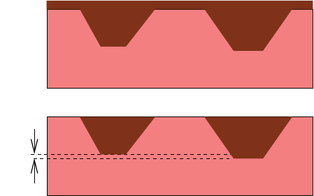
2: The Simulator Sentaurus Process

Parameter Database

Sentaurus™ Process User Guide 59

H-2013.03

layer1.1.2, and so on. In this way, regionwise parameter specification is preserved for the

life of the region or its parts.

The numbering of split regions is performed according to the spatial location of the pieces. The

lowest point of each piece to be renamed is found (in the coordinate system of Sentaurus

Process, this would be the largest x-coordinate). To avoid numeric noise, the coordinates are

compared with a specified epsilon given by pdbGet Grid RenameDelta (hereafter, referred

to as RN). If the x-coordinates of the pieces to be renamed are not within RN of each other, the

regions are ordered from lowest to highest, that is, from the highest x-coordinate to the lowest.

If any piece has its lowest coordinate within RN, its y-coordinate is compared, that is, from the

lowest coordinate to the highest.

For example, in Figure 11, layer1 is split into two regions and the quantity deltax is less

than RN, so the region on the left is given the name layer1.1 and the region on the right is

given the name layer1.2. If deltax had been greater than RN, the region on the right would

have been given the name layer1.1 because it would have been considered lower than the

region on the left. Similarly, in three dimensions, first x and y are compared, and if they are

both within RN, z is used for ordering, that is, from the lowest coordinate to the highest.

Figure 11 Illustration of region-naming rules

You c an ap pl y t he ab ove operat io n to the whole structure with grid rename. In this case, all

the regions are renamed similarly to the above rules but, instead of the root being chosen by the

user, all regions of the same material have the root given by the names of the materials and the

extension is _<n> where <n> is the region number, for example Silicon_1, Silicon_2, and

so on. This should only be used as a postprocessing step because all region-specific parameters

no longer apply when the name of a region has changed.

For example, if two oxide layers are grown, one with steam (if it is the first oxide region, its

name would be Oxide_1) and one from pure O2 (which would be Oxide_2 if it were the

second oxide region), they can have different densities. This can be considered in an MC

implantation using:

pdbSetDouble Oxide_1 MassDensity <wet oxide density>

layer1

deltax layer1.1 layer1.2

2: The Simulator Sentaurus Process

Viewing the Defaults: Parameter Database Browser

60 Sentaurus™ Process User Guide

H-2013.03

pdbSetDouble Oxide_2 MassDensity <dry oxide density>

where <wet oxide density> and <dry oxide density> would be replaced with values

given in g/cm3.

Viewing the Defaults: Parameter Database Browser

The Parameter Database Browser (PDB) is a graphical representation of the Sentaurus Process

parameter database that allows you to view and edit parameters. The PDB has three distinct

areas (see Figure 12 on page 61):

■Parameter hierarchy overview in a tree structure representation.

■Parameter information in a spreadsheet representation. The columns are:

•Parameter

•Type

•Value

•Unit

•Evaluate

• Comment

•Tool

•Info Level (hidden by default)

■Graphic window to plot parameter dependence on the temperature.

The status bar has three indicators that show:

■The temperature used in temperature-dependent functions such as Arrhenius.

■The temperature point set for the x-axis.

■The x-coordinate and y-coordinate of the pointer in the graphic window.

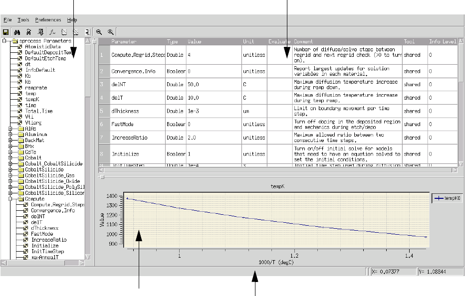
2: The Simulator Sentaurus Process

Viewing the Defaults: Parameter Database Browser

Sentaurus™ Process User Guide 61

H-2013.03

Figure 12 Parameter Database Browser

Spreadsheet

Representation

Tree Structure

Representation

Graphic Window Status Bar

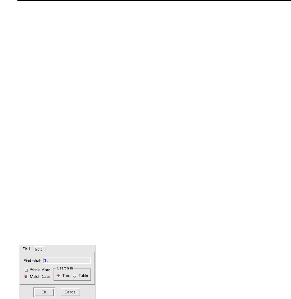
2: The Simulator Sentaurus Process

Viewing the Defaults: Parameter Database Browser

62 Sentaurus™ Process User Guide

H-2013.03

Starting the Parameter Database Browser

To start the PDB from the command line, enter:

pdbBrowser

This searches for the database in the same location as Sentaurus Process. You can set the

environment variables SPHOME and SCHOME to change the location of the parameter database

for the PDB and Sentaurus Process (see Environment Variables on page 47 for details). To view

parameters in an input file merged with defaults, use:

sprocess --pdb <input command file>

or to view only the parameters specified as input in a command file, use:

sprocess --ponly <input command file>

Browser PDB Functions

The following functions are available:

Figure 13 Find dialog box

Export Tree Saves the whole parameter database into a specified file in the tab-

delimited format. The fields of the file are Parameter Name, Type,

Value Evalua tion , Original Value, and Comments.

Find and Find Next Matches the pattern entered against parameter names according to the

selected options. Patterns can include regular Tcl expressions. The

match is highlighted when found (see Figure 13).

Goto Line Highlights a table row or tree node that corresponds to the number

entered.

2: The Simulator Sentaurus Process

Viewing the Defaults: Parameter Database Browser

Sentaurus™ Process User Guide 63

H-2013.03

NOTE Yo u c an z oo m b y d ra gging t he mou se . To z oom o ut , u se th e m idd le

mouse button, or click the Zoom Out and Zoom Off buttons.

NOTE To display a shortcut menu, right-click a parameter for plotting and

evaluation in the tree and table areas.

Figure 14 Arrhenius Fit dialog box

Plot (Applies only to parameters of type double and double array.) Plots

the dependency of the selected parameter on the temperature in

logarithmic coordinates versus 1/T. The default set of temperature

values is {700.0 800.0 900.0 1000.0 1100.0}. The resulting

graphs are displayed in the graphic window; otherwise, an error

message is displayed.

Plot Over The same as Plot but it does not clear the graphic window of previous

graphs.

Evaluate Evaluates the value of the selected parameter and displays the result

in the Evaluate column of the table. Values can contain Tcl

expressions.

Edit Opens the appropriate database file with an editor regardless of the

user write-permissions, but the standard installation will switch off

write permissions for the database. The default editor, SEdit, can be

changed. The PDB Browser is updated upon file saving.

Parameter

Information

Double-clicking a nonempty table row allows you to view the

corresponding parameter information in a separate window. To close

the window, click the Close button.

Arrhenius Fit Finds the best prefactor and energy for an Arrhenius fit of a given

profile, taken from the list of temperature–value pairs. The results can

be plotted in the graphic window.

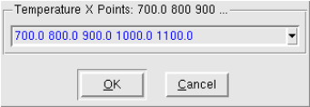
2: The Simulator Sentaurus Process

Viewing the Defaults: Parameter Database Browser

64 Sentaurus™ Process User Guide

H-2013.03

PDB Preferences

The PDB allows you to reset the default settings for the following values by using the

Preferences menu, shortcut keys, or shortcut menu of the graphic window:

Figure 15 Reset Temperature Points dialog box

Preferences > Font > Family

Changes the font family.

Preferences > Font > Size

Changes the font size.

Preferences > Cursor

Changes the style of the pointer.

Preferences > Graph > Set Temperature

The global temperature used in the temperature-dependent functions;

the default is 1000.0.

Preferences > Graph > Reset X Points

The x-axis temperature point set; the default set is

{700.0 800.0 900.0 1000.0 1100.0}.

Preferences > Graph > Data Point Symbol

Node Tip: hide / show.

Preferences > Info Level

Shows or hides the Info Level column of the table.

Preferences > Editor > Change Editor

Resets the default editor.

2: The Simulator Sentaurus Process

Viewing the Defaults: Parameter Database Browser

Sentaurus™ Process User Guide 65

H-2013.03

Viewing Parameters Stored in TDR Files

Parameters stored in TDR files can be viewed using the pdbBrowser command run from the

UNIX command line instead of through Sentaurus Process. By default, the PDB reads

parameters from the Sentaurus Process database directory (which can be changed with the

SPHOME and SCHOME environment variables). In addition, parameters stored in a TDR file can

be read in using the -tdr <filename> option of the PDB. Parameters that appear in the

database are overwritten by those contained in the TDR file, so the resultant parameter set will

be the same as if Sentaurus Process had read in the file. On the other hand, it is also useful to

know which parameters are only in the TDR file. To read only those parameters, the database

reading can be switched off using the -nopdb command-line option.

For example:

> pdbBrowser -tdr n10_fps.tdr

reads the Sentaurus Process PDB and then reads parameters from n10_fps.tdr file

overwriting values contained in the database.

For example:

> pdbBrowser -nopdb -tdr n10_fps.tdr

reads only the parameters in n10_fps.tdr file.

Preferences > Editor > Reset Update Time

Resets the update interval.

Preferences > Graph > X Scale

Resets the scale to logarithmic or linear.

Preferences > Graph > Y Scale

Resets the scale to logarithmic or linear.

Tools > Info Level Chooses which parameters to display ranging from basic parameters

to all parameters.

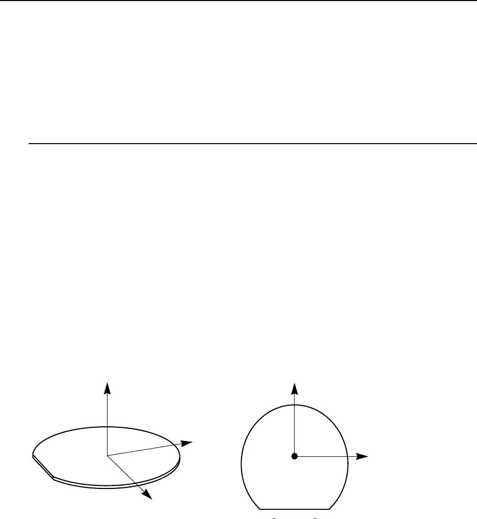
2: The Simulator Sentaurus Process

Creating and Loading Structures and Data

66 Sentaurus™ Process User Guide

H-2013.03

Creating and Loading Structures and Data

The first step in most simulations is either to load an existing structure or to create a new one.

New structures are created through a combination of the line, region, and init commands.

The initial mesh is a tensor-product mesh where the density of lines is specified in the line

command, and the regions are defined by specifying tags in the line commands and defined

in the region command. The initial regions are always defined as axis-aligned rectangles in

2D and axis-aligned bricks in 3D.

Understanding Coordinate Systems

Sentaurus Process and related tools use different coordinate systems. The most commonly

encountered coordinate systems include wafer coordinates, simulation coordinates, and

visualization coordinates.

Wafer Coordinate System

The wafer coordinate system is fixed with respect to the wafer flat or notch, and is used to

define the relationship of all other coordinate systems to the physical wafer. The wafer

coordinate system is shown in Figure 16.

The wafer x- and y-axes form a naturally oriented coordinate system when the wafer is drawn

with the flat pointing down as shown in Figure 16. This coordinate system is used for layout

information, such as mask locations, and for setting a cutline using the CutLine2D command.

Figure 16 Wafer coordinate system

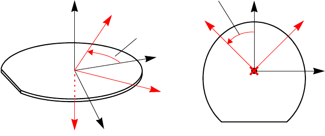
2: The Simulator Sentaurus Process

Creating and Loading Structures and Data

Sentaurus™ Process User Guide 67

H-2013.03

Simulation Coordinate System (Unified Coordinate System)

The simulation coordinate system is used to define the mesh for the simulation. All coordinates

that are specified with respect to the mesh are given in simulation coordinates. This includes

all coordinates that are given in the Sentaurus Process command file.

The simulation coordinate system has the x-axis pointing into the wafer and the y-axis rotated

with respect to the wafer y-axis. The simulation coordinate system is shown in Figure 17.

Simulations in 1D use only the x-axis. Simulations in 2D use only the x- and y-axes.

Figure 17 Simulation coordinate system (slice.angle = 45)

The rotation of the simulation axes with respect to the wafer axes is given by the slice.angle

parameter of the init command. The slice angle is measured from the wafer y-axis to the

simulation y-axis with positive angles counterclockwise about the wafer z-axis.

YSZS

slice.angle

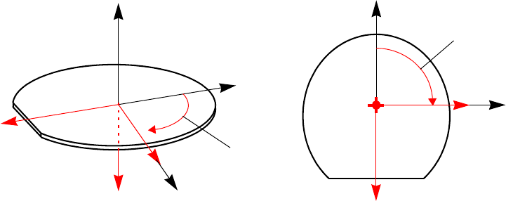
2: The Simulator Sentaurus Process

Creating and Loading Structures and Data

68 Sentaurus™ Process User Guide

H-2013.03

The default value of slice.angle is set to . This causes the simulation y-axis to match

the wafer x-axis, which is the usual cut direction through the layout for 2D simulations. The

default simulation coordinate system is shown in Figure 18.

Figure 18 Default simulation coordinate system (slice.angle = –90)

Visualization Coordinate Systems

Two systems can be used for visualization:

■The unified coordinate system (UCS)

■The DF–ISE coordinate system

Unified Coordinate System

To use the UCS, specify:

math coord.ucs

This system of coordinates is explained in Simulation Coordinate System (Unified Coordinate

System) on page 67.

NOTE The UCS is the recommended way of visualization and may become the

default in the future.

DF–ISE Coordinate System

The DF–ISE coordinate system is the default for visualizing TDR files. It can be set explicitly

by:

math coord.dfise

90°–

YS XW

slice.angle

XSYS

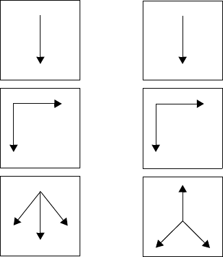
2: The Simulator Sentaurus Process

Creating and Loading Structures and Data

Sentaurus™ Process User Guide 69

H-2013.03

The DF–ISE coordinate system is used by the DF–ISE and some TDR file formats as well as

Tecplot SV. Unlike the simulation coordinate system in which the x-axis points into the wafer

for 1D, 2D, and 3D, the visualization coordinate system has different axis conventions for 1D,

2D, and 3D. Figure 19 shows the relationship between simulation coordinates and DF–ISE

coordinates.

Figure 19 Simulation and DF–ISE coordinate systems

The only difference between UCS coordinates and DF–ISE coordinates is that different

conventions are used to label the axes. Sentaurus Process automatically converts the axis labels

when reading and writing DF–ISE or TDR files.

The relationship between DF–ISE coordinates and UCS coordinates shown in Figure 19

applies to all values of slice.angle. In other words, the DF–ISE system is not fixed with

respect to the wafer system. It always has the same rotation with respect to the wafer coordinate

system as the simulation coordinate system.

Figure 20 on page 70 shows the relationship between simulation coordinates and visualization

coordinates.

Simulation Coordinates

DF-ISE Coordinates

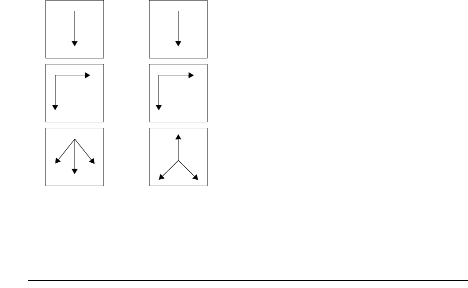
2: The Simulator Sentaurus Process

Creating and Loading Structures and Data

70 Sentaurus™ Process User Guide

H-2013.03

Figure 20 Simulation and visualization coordinate systems

The tensor components, for example, mechanical stresses, in 2D and 3D are the same in UCS

coordinates. For a conversion table for the stress components in 2D and 3D DF–ISE coordinate

systems, see Chapter 9 on page 643. This also applies to other second-order symmetric tensors.

Defining the Structure: The line and region Commands

The line and region commands are used together to define the structure. In the init

command, the structure is actually formed. Care must be taken when creating a structure

because there are few checks for errors.

These rules must be followed to obtain a valid structure:

■If this is not the first structure being created in a command file, the command line clear

must be issued to remove line commands and stored mesh ticks.

■Line locations must be given in increasing order.

■The region boundaries are defined by tagged lines. Tagged lines are created with the line

command where the parameter tag has been set (as well as the location parameter).

■At least one region command must be given to define the substrate.

■Regions must have a material specification, except for the substrate case described

below.

■Regions must have the same dimensionality as the line commands used (that is, if line y

is given, a 2D region is expected with ylo and yhi set).

Simulation Coordinates

Visualization Coordinates

2: The Simulator Sentaurus Process

Creating and Loading Structures and Data

Sentaurus™ Process User Guide 71

H-2013.03

■The spacing parameter is used to create lines between user-defined lines, so that not every

line must be specified in the command file. Sentaurus Process smoothly grades the line

density between user-defined lines to match as closely as possible the spacing at each user-

defined line. In addition, there will be lines at locations given by the location parameter

of the line command. By default, the spacing parameter is extremely large, so that if it

is not set, only lines given by the location parameter will be in the mesh.

■The *lo parameter refers to the lowest coordinate value, that is, the location of the line

corresponding to the xlo tag must be less than the coordinate corresponding to the xhi tag.

■The region command can be used to tag a region as a substrate in two ways:

•If the region is being defined with the material name and the parameters *hi and *lo,

the Boolean keyword substrate will tag this region as the substrate.

•If the structure is being loaded from a previously saved file, the command:

region name=<region_name> substrate

will tag the region with region_name as the name of the substrate. This is the only

occasion when the region command will be called after the init command.

Considerations when creating structures are:

■For 2D and 3D simulations, it is advantageous to create a coarse mesh in the lateral (that

is, y- or z-directions) because lines created with the line command run all the way through

the structure. Often, finer spacing in the y- or z-direction is needed near the surface;

whereas, further in the bulk, a coarser spacing is required (to minimize the size of the

problem).

■When MGOALS is used for etching and deposition, or meshing, it automatically creates a

local refinement near interfaces that does not run the length of the structure.

■To specify refinement boxes, use the refinebox command. Control over the meshing

parameters for MGOALS is explained in Chapter 11 on page 731.

Creating the Structure and Initializing Data

The init command is used to create the structure. If the line and region commands have

been given to create a structure from the beginning, the init command does not require any

options. It will take the structure definition and create a new structure.

Many process steps such as etching, deposition, diffusion, and implantation require a gas mesh.

By default, Sentaurus Process does not add a gas mesh during the init command, but delays

creating the gas mesh until it is needed. To add the gas mesh immediately, use the command:

pdbSet Grid AddGasMesh 1

2: The Simulator Sentaurus Process

Creating and Loading Structures and Data

72 Sentaurus™ Process User Guide

H-2013.03

NOTE The parameter must be set before the init command to generate the

gas mesh during the init command.

There are several ways to initialize fields at the time the initial structure is created from line

and region commands:

■To initialize data everywhere in the structure, a field specification can be given in the init

command.

■To initialize data in one particular region only, a field specification is given in the region

command.

In both the init and region commands, the field parameter specifies the name of the data

field that will be created and either the concentration parameter or the resistivity

parameter is used to specify the value created. Although initialization was intended for

dopants, a field with any name can be initialized with the concentration parameter.

However, it will create a field with nodal values and, because stresses are computed on

elements, it should not be used for initializing stress values (use the stressdata command or

the select command for this). The resistivity parameter only works for fields that have

the resistivity parameters set (which by default are only As, B, P, Sb, and In in silicon).The

init command also is used to read a structure from a file. In this case, the parameter name

serves as the type specification, and the value of the parameter is the file name or root name (in

the case of DF–ISE), for example:

init dfise=file ;# Read 'file.grd' and 'file.dat'.

# If not available try 'file.grd.gz' and 'file.dat.gz'

init dfise=file.grd ;# Only read a structure (no data) from 'file.grd'

# or 'file.grd.gz'

init tdr=file ;# Read a geometry, data, and pdb parameters from

# 'file.tdr'.

init bnd=file ;# Read a bnd file and mesh it.

The TDR format is used to restart a simulation by default when creating ‘splits’ in Sentaurus

Workbench. This format stores all pdb parameter settings as well as numerous other settings

coming from commands (see Saving a Structure for Restarting the Simulation on page 76).

The bnd parameter is used to load boundaries that are then meshed by MGOALS. In this case,

the structure is meshed with the constrained Delaunay mesher, which makes use of lines

coming from the line command.

The init command is used to specify the principal wafer orientation (wafer.orient), the

lateral crystal orientation of the wafer flat or notch (flat.orient), and the slice.angle

for the implant command, that is angle:

init wafer.orient= { <j> <k>} flat.orient= { <j> <k>} slice.angle=<n>

where , <j>, and <k> are the crystallographic (Miller) indices. For more information about

the wafer orientation and the slice angle, see 2D Coordinate System on page 91.

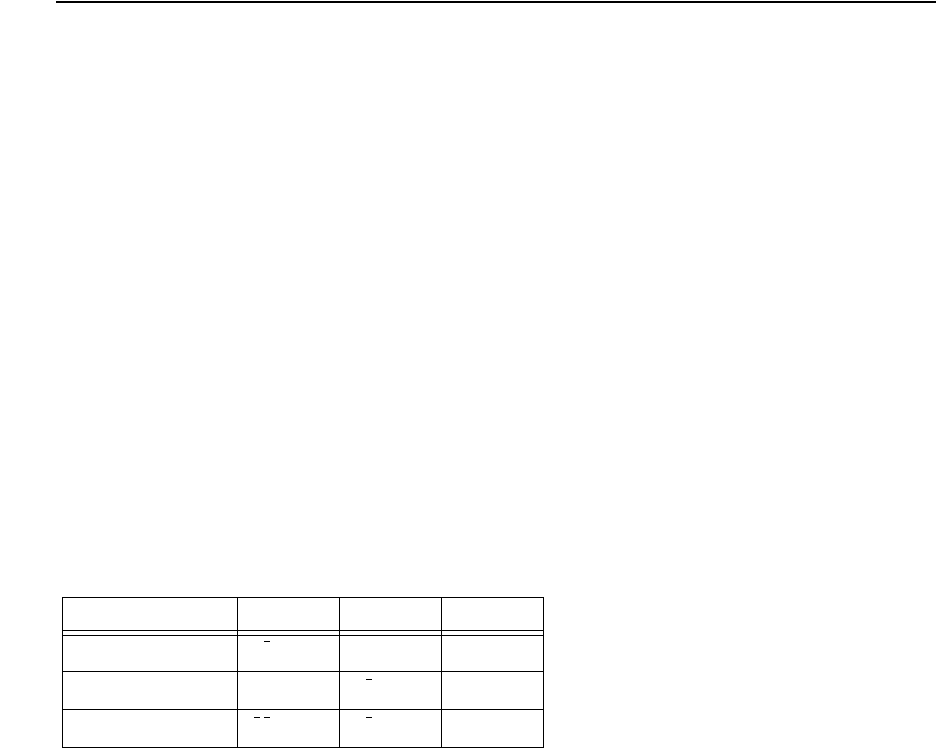
2: The Simulator Sentaurus Process

Creating and Loading Structures and Data

Sentaurus™ Process User Guide 73

H-2013.03

You al so can se t the slice.angle by using a 2D cutline, for example:

init slice.angle= [CutLine2D <x1> <y1> <x2> <y2>]

The first two values define the start point, and the third and fourth values define the endpoint

in the wafer plane. The two points are defined in the wafer coordinate system (see

Understanding Coordinate Systems on page 66).

Defining the Crystal Orientation

The crystal orientation of the wafer is established by specifying the Miller indices of the wafer

surface and the wafer flat. The wafer.orient and flat.orient parameters of the init

command specify the Miller indices of the wafer z- and y-axes, respectively. The wafer surface

orientation (z-axis) is set using wafer.orient= { <j> <k>} where , <j>, and <k>

are the crystallographic (Miller) indices. The flat orientation (y-axis) can be set arbitrarily, but

it must be orthogonal to the wafer surface orientation. The default surface orientation is 100

and the default flat orientation is a 110 direction for all values of wafer.orient.

NOTE The wafer.orient and flat.orient parameters of the init

command apply to orthorhombic crystal systems only (such as silicon).

For information on how to change the crystal orientation in hexagonal

systems, see MC Implantation into Silicon Carbide on page 165. Setting

info=2 in the implant command confirms user-defined settings for

each region in the log file only.

Table 2 lists the crystallographic directions of the wafer axes for the most common

crystallographic orientations of the wafer as shown in Figure 16 on page 66.

Sentaurus Process also allows you to define different crystal orientations for different regions

by using the commands:

pdbSetDoubleArray <region_name> crystal.orient <double array>

pdbSetDoubleArray <region_name> flat.orient <double array>

Ta bl e 2 M i l le r i n d i ce s o f wa fer a xe s fo r e a c h va lu e o f wa fer.o r i en t

(wafer axes are defined in Figure 16)

Wafer orientation XW Y

W Z

100

110[]

001[]

110

001[]

110[]

111

112[]

110[]

111[]

2: The Simulator Sentaurus Process

Creating and Loading Structures and Data

74 Sentaurus™ Process User Guide

H-2013.03

To facilitate simulations of hybrid orientation technology (HOT), Sentaurus Process predefines

three materials (Silicon, Silicon110, and Silicon111) for crystalline silicon. These

materials have exactly the same properties, except for the default crystal orientations that are

<100>, <110>, and <111> for Silicon, Silicon110, and Silicon111, respectively.

Automatic Dimension Control

The maximum dimension of a simulation is determined by the specified line commands;

line x commands define the extensions in the vertical direction and are required for 1D, 2D,

and 3D simulations. If, in addition, line y commands are specified, the maximum dimension

of the simulation will be at least 2D and, if also line z commands are specified, the maximum

dimension of the simulation will be three dimensions. By default, Sentaurus Process delays the

creation of a full-dimensional structure until it becomes necessary. This means that if you

specify a 2D structure where all regions span the entire simulation domain in the y-direction,

Sentaurus Process will create a 1D structure.

When a 2D or 3D mask is used in an etch, a deposit, or a photo command, Sentaurus

Process automatically extrudes the structure and the mesh into the appropriate dimension and

copies the data. This delay of creating a full-dimensional structure can be switched off in the

init command by using the option !DelayFullD. To increase the dimension manually, use

the grid command. If a 2D structure is required, that is, both the line x and line y

commands but no line z commands have been specified, grid 2D or grid FullD will

cause a 2D structure to be created.

Similarly, if line x, line y, and line z commands have been specified, grid 2D can be

used to extrude a 1D structure to two dimensions, and a 1D or 2D structure is extruded to three

dimensions using grid 3D or grid FullD. This functionality also can be used to increase

the dimension of structures loaded from files. After the structure has been loaded, line

commands can be issued and the dimension of the structure will increase automatically when

necessary or manually using the grid command.

Sentaurus Process does not provide a facility to reduce the dimension of a simulation.

When structures are saved to DF–ISE files or TDR files (other than TDR restart files), the

current maximum dimension as specified with line commands is used by default in the file.

The dimension of the simulation itself is not affected. To save files in the current dimension,

the !FullD parameter of the struct command can be used (see Saving and Visualizing

Structures on page 75). TDR restart files are always saved in the dimension currently used in

the simulation.

2: The Simulator Sentaurus Process

Creating and Loading Structures and Data

Sentaurus™ Process User Guide 75

H-2013.03

Saving and Visualizing Structures

Sentaurus Process supports two file formats for reading and writing structures: TDR and the

older DF–ISE. Both the TDR and DF–ISE formats allow saving the structure geometry with

and without the bulk mesh and data, and with contacts. These files contain simply connected

regions to operate smoothly with other Synopsys TCAD tools. One important option available

for saving TDR and DF–ISE files is to omit saving gas regions because this may cause

problems for other tools.

The TDR format allows for the saving and loading of geometry and data information along

with pdb parameters. For more information about file types and standard file extensions, see

File Types Used in Sentaurus Process on page 48.

The TDR format is the preferred file format over the DF–ISE format. TDR files can be used to

split a simulation, and restart and continue the simulation as if no file save or file load was

performed. Besides the simulation grid and data, additional information is stored to facilitate

such a restart. Only TDR files provide such restart capability; simulation results will differ if a

simulation is performed in one contiguous run compared to saving and loading the intermediate

state into _bnd.tdr or DF–ISE files.

Setting the parameter math coord.<coord name> configures whether the visualization

coordinates will be identical to the simulation ones (when using coord.ucs) or will follow

the DF–ISE criteria (when using coord.dfise).

When using DF–ISE, it is important to understand the difference between the simulation

coordinates used by Sentaurus Process and the coordinates seen in Tecplot SV. For Sentaurus

Process, the positive x-direction always points into the substrate in 1D, 2D, and 3D. TDR and

Tecplot SV have different axis directions in 1D, 2D, and 3D. With coord.dfise, Sentaurus

Process rotates the structure into the DF–ISE coordinate system when saving the structure and

rotates the structure back when reading it.

Figure 19 on page 69 shows the relation between the UCS and DF–ISE coordinates. The

exposed surface of the substrate is oriented upwards; that is, the ‘up’ direction is always in the

negative x-direction in the UCS.

To select the fields stored in TDR files, use the SetTDRList command. Each field name in the

SetTDRList command is added to the list of fields, which are usually saved (if the field is

present in the structure). This command also takes as arguments the macro parameters

Dopants and Solutions, and their negative counterparts !Solutions and!Dopants.

Solutions refers to variables of partial differential equations (PDEs). The solution variables

must be stored in a TDR file if that file is to be used to continue a simulation. The parameter

Dopants refers to the total and active dopant concentration fields. By default, TDR files are

saved with both Solutions and Dopants names in SetTDRList. However, this requires

2: The Simulator Sentaurus Process

Creating and Loading Structures and Data

76 Sentaurus™ Process User Guide

H-2013.03

many fields to be stored in the TDR files and, sometimes, it is more convenient to have fewer

fields.

To do this, set !Solutions in SetTDRList, which unselects all fields. Then, specify the field

names to be stored in the TDR file (see SetAtomistic on page 1121 for saving KMC fields).

Saving a Structure for Restarting the Simulation

When saving files using the TDR format, the current state of the parameter database is, by

default, saved in the file. The parameter database contains all of the information necessary to

restart a simulation including:

■Model settings

■Parameter settings

■Mesh settings from the mgoals command

■Refinement boxes from the refinebox command

■Temperature ramps from the temp_ramp command

■Gas flow specifications from the gas_flow command

■Line specifications from the line command

■Region specifications from the region command

■Reaction specifications from the reaction command

■Specifications for point, polygon, polyhedron

■Doping specifications with the doping command

■User materials created with the mater command

■Contact definitions created with the contact command

■Mask definitions created with the mask command

■Solution commands can be optionally stored using the store parameter of the solution

command

■Term commands can be optionally stored using the store parameter of the term

command

■Global Tcl variables can be stored with fset

■Tcl procedures can be stored using fproc

By default, when loading a TDR file, the changes in the parameter database are read in from

the TDR file and are applied. For information about the TDR format, refer to the Sentaurus™

Data Explorer User Guide.

2: The Simulator Sentaurus Process

Creating and Loading Structures and Data

Sentaurus™ Process User Guide 77

H-2013.03

When saving a TDR file, the coordinate system used for visualization is also included in the

file and is used by Tecplot SV when opening it. The visualization coordinate system can be

changed using the math pdb command.

For the UCS, use:

math pdb coord.ucs

For the DF–ISE coordinate system, use:

math pdb coord.dfise

Saving a Structure for Device Simulation

In general, there are three main steps to saving a structure appropriate for device simulation:

1. Define contacts.

2. Remesh the structure with appropriate refinement for device simulation.

3. Save the structure with contacts and with Delaunay weights.

Contacts are defined using the contact command. There are two main ways to define

contacts, either:

■Using a box where the contact is created at the intersection of a material interface and a box.

■Using a point contact in which a region is specified by giving a point inside the region; then

all boundaries of this region become a contact.

The contact is given a name and, if the command is executed multiple times with the same

contact and the add parameter, the contact will include all parts specified. There are also

options for creating a contact on the outer boundaries and so on. For more information, see

contact on page 889.

Remeshing the structure is needed to create a mesh that is better suited to device simulation.

Typically, this means discarding process-based refinements, creating a very fine mesh under

the channel, and refining on the p-n junction. A typical sequence of steps is:

■Clear the process mesh:

refinebox clear

line clear

■Reset default settings for adaptive meshing:

pdbSet Grid AdaptiveField Refine.Abs.Error 1.e37

pdbSet Grid AdaptiveField Refine.Rel.Error 1e10

pdbSet Grid AdaptiveField Refine.Target 100.0

2: The Simulator Sentaurus Process

Creating and Loading Structures and Data

78 Sentaurus™ Process User Guide

H-2013.03

■Set high-quality Delaunay meshes:

pdbSet Grid SnMesh DelaunayType boxmethod

■Set mesh spacing near interfaces:

mgoals min.normal.size=<n> normal.growth.ratio=<n>

■Set which interfaces will have interface refinement:

refinebox interface.materials= {Silicon}

■Specify adaptive refinement:

pdbSet Grid Adaptive 1

■Specify lines if necessary:

line y loc= $Ymin+0.001

line z loc= $Zmin+0.001

■Specify refinement boxes, for example:

refinebox min= {<n> <n> <n>} max= {<n> <n> <n>} \

xrefine= <n> yrefine=<n> zrefine=<n> ;# gate refinement

refinebox refine.fields=NetActive max.asinhdiff= {NetActive= 1.0} \

refine.min.edge=<n> Silicon ;# adaptive refinement on NetActive

■If using the IC WorkBench EV Plus interface, it may be useful to consider using the

icwb.refine.mask command (see Chapter 12 on page 817 and icwb.refine.mask on

page 959 for more information).

In these steps, <n> are coordinates or edge lengths in micrometers, and

normal.growth.ratio is a unitless ratio.

To save the structure, use the command struct tdr=<filename> !Gas. This command

causes a remesh if necessary, stores any contacts that have been defined previously, and

includes fields required for device simulation.

Delaunay weights can be saved in the structure intended for device simulation by setting these

parameters before generating the mesh:

pdbSet Grid SnMesh StoreDelaunayWeight 1

pdbSet Grid Contact.In.Brep 1

The first parameter StoreDelaunayWeight creates the field variable Delaunay–Voronoï

weight (DelVorWeight) that is used in the weighted box method in Sentaurus Device. The

second parameter Contact.In.Brep switches on an experimental feature that creates

contacts in the boundary representation (brep) and prevents changes to the mesh that can

locally invalidate the Delaunay weight.

2: The Simulator Sentaurus Process

Creating and Loading Structures and Data

Sentaurus™ Process User Guide 79

H-2013.03

Saving Doping Information in SiC and GaN for Device Simulations

Basic process simulation capabilities such as etching, deposition, and implantation with Monte

Carlo are available for multicomponent materials, for example, silicon carbide (SiC) and

gallium nitride (GaN). However, there are no activation models for dopants in these materials.

To create active doping concentration fields that are equal to their associated total fields, when

saving a file for transfer to device simulation, use the diffuse command with zero time, for

example:

diffuse time=0 temperature=900

struct tdr= <file name>

Saving 1D Profiles for Inspect

To store .plx files, use the WritePlx command. The command SetPlxList selects the

fields to be stored in the .plx file. The command SetPlxList is similar to the

SetDFISEList command, except that no fields are selected by default. Only the field names

specified in SetPlxList are stored in the .plx file (see SetPlxList on page 1128 and WritePlx

on page 1191).

Saving 1D TDR Files from 2D and 3D Simulations

The command struct also saves a 1D TDR file if the proper cutting coordinates are specified.

In 2D, only one cutting coordinate is needed (either x or y; coordinate z makes no sense here).

In 3D, the command saves the intersection of the planes specified by two cutting coordinates

(for example, specifying x and z will save the y line containing those x- and z-coordinates). In

addition to storing the mesh and data, these files save any contacts that apply at the cut point,

so that the file can be loaded into Sentaurus Device for electrical analysis. This file can be

visualized with Tecplot SV.

For example, in a 2D simulation, the following command:

struct tdr=filename y=0.5

picks up all the x-coordinates with y=0.5 and saves them in a 1D TDR file.

In addition, in a 3D simulation, the following command:

struct tdr=filename x=0.2 z=0.1

saves the y-coordinates with x=0.2 and z=0.1 as a 1D TDR file.

For more information, see struct on page 1158.

2: The Simulator Sentaurus Process

References

80 Sentaurus™ Process User Guide

H-2013.03

The select Command (More 1D Saving Options)

The select command is a versatile command for many operations such as viewing results,

postprocessing, and initializing or changing datasets. The basic command is:

select z=<expression>

where <expression> is an Alagator expression (see Chapter 6 on page 571). A simple

example of an <expression> is the name of a data field such as Potential and VTotal.

The value of the expression is stored in the selected field.

This selected field can be viewed with print.data or print.1d, for example, or the

integrated values can be obtained using the layers command. The select command can also

be used to set an existing data field or create a new data field, for example:

select z=1.0 name=MyDataField ;# create a new datafield named MyDataField

# and set it to 1.0 (everywhere)

select z= 0.1*Vacancy name=Void store ;# Set Void equal to 0.1*Vacancy

Loading 1D Profiles: The profile Command

The profile command is used to load a 1D profile into 1D, 2D, or 3D structures. The file to

be read should contain one x-coordinate data pair per line. Both linear (using the linear

parameter) and logarithmic interpolation (default) are available. Profiles are loaded by using:

profile infile = file.dat name = Boron

Sentaurus Process reads the file file.dat and sets the field Boron accordingly.

References

[1] B. B. Welch, Practical Programming in Tcl & Tk, Upper Saddle River, New Jersey:

Prentice Hall PTR, 3rd ed., 2000.

Sentaurus™ Process User Guide 81

H-2013.03

CHAPTER 3 Ion Implantation

The chapter presents the ion implantation technique used in

Sentaurus Process.

Overview

Ion implantation is one of the most widely used processing techniques to introduce impurity

atoms into semiconductor materials. In Sentaurus Process, either analytic functions or the

Monte Carlo (MC) method is used to compute the distribution of implanted ions and the

implantation damage. Analytic implantation models use the simple Gaussian and Pearson as

well as the advanced dual Pearson functions. The implantation damage with analytic models is

calculated according to the Hobler model [1]. The MC method uses a statistical approach to the

calculation of the penetration of implanted ions into the target and accumulation of crystal

damage based on the binary collision approximation [2].

Analytic implantation simulates the spatial distribution of the implanted ions based on the

selected distribution function, which is described by moments. The distribution moments

depend on the ionic species, implantation energy, dose, and tilt and rotation angles. Sets of

moments for a given range of implantation parameters are provided in the form of lookup

tables. Sentaurus Process can use implantation tables in the Dios format, TSUPREM-4

formats, and the Taurus Process table format. The implantation data available includes the

default tables [3], the Advanced Calibration tables [4], the Taurus table set [5], and the original

Tasch tables [6].

Sentaurus Process handles 1D, 2D, and 3D geometries for both analytic implantation

simulations and MC simulations. The algorithms for analytic implantation are an integral part

of Sentaurus Process; whereas, MC simulations are performed with the binary collision code

Sentaurus MC [7] or Crystal-TRIM [8].

Analytic ion implantation is performed using the implant command:

implant <dopant> [energy=<n>] [dose=<n>] [tilt=<n>] [rotation=<n>]

Sentaurus Process simulates an analytic implantation step producing output such as:

---------------------------------------------------------------- implant -----

implant energy=35.00<keV> dose=1.00e.+14<cm-2> tilt=7.00<degree>

rotation=-90.00<degree> Boron

------------------------------------------------------------------------------

Species = Boron

3: Ion Implantation

Overview

82 Sentaurus™ Process User Guide

H-2013.03

Dataset = Boron

Energy = 35keV

Dose (WaferDose) = 1e+14/cm2

BeamDose = 1.0075e+14/cm2

Tilt = 7deg

Tilt2D = 7deg

Rotation = -90deg

Slice angle = -90deg

Temperature = 300.00K

For a description of the analytic implantation mode, see Analytic Implantation on page 92.

To switch from analytic implantation to MC implantation with Sentaurus MC, use the logical

switch sentaurus.mc (or its alias tmc):

implant <dopant> [energy=<n>] [dose=<n>] [tilt=<n>] [rotation=<n>]

[sentaurus.mc]

To switch from analytic implantation to MC implantation with Crystal-TRIM, use the logical

switch crystaltrim (or its alias ctrim):

implant <dopant> [energy=<n>] [dose=<n>] [tilt=<n>] [rotation=<n>]

[crystaltrim]

If the cascades switch is used in addition to sentaurus.mc or crystaltrim, the MC

implantation is run in the full-cascade mode. For a description of Sentaurus MC and the

Crystal-TRIM mode, see Monte Carlo Implantation on page 133.

An external profile can be loaded using the load.mc switch:

implant <dopant> [energy=<n>] [dose=<n>] [tilt=<n>] [rotation=<n>]

[load.mc] [file=<c>]

A TDR file must be specified with the file selector. load.mc works with files created by

either Sentaurus MC or Crystal-TRIM. For a full description of the file-loading mode, see

Loading External Profiles on page 190.

The implantation energy in the implant <dopant> facility is given in keV by default. The

implantation dose has two modes:

■The wafer dose (WaferDose), which refers to the expected dose in the structure after the

implantation is finished. This dose is measured in ions per .

■Alternatively, the implantation dose can mean the beam dose (BeamDose).

In the wafer dose mode, the final implanted dose does not depend on the wafer orientation with

respect to the ion beam. In the beam dose mode, the final implanted dose may change as tilt

and rotation angles change. For a discussion of the meaning and implications of the tilt and

rotation angles, see Coordinate System on page 89. All angles are measured in degrees.

cm2

3: Ion Implantation

Overview

Sentaurus™ Process User Guide 83

H-2013.03

The mode of the implant dose can be specified with the following pdb switches:

pdbSet ImplantData DoseControl {Default WaferDose BeamDose}

The default value of DoseControl switch is Default, in which case, the mode of implant

dose is chosen automatically based on the implant table format. If the currently selected

implant tables are in Taurus/TSUPREM-4 format, the beam dose mode is used automatically.

Otherwise, the wafer dose mode is applied. If the DoseControl switch is set to WaferDose,

the wafer dose mode is used for all implantations regardless of table formats, likewise for

BeamDose.

NOTE To obtain consistent results and prevent unexpected dose mode, it is

strongly recommended to always set the DoseControl parameter at

the start of command files to either WaferDose or BeamDose.

To override these global settings, use the logical switch beam.dose in the implant

command:

implant <dopant> [dose=<n>] [beam.dose !beam.dose]

NOTE The main parameters for the implant statements energy, dose, tilt,

and rotation must always be specified. Otherwise, default values are

chosen that may not reflect the assumed process conditions.

In addition to energy, dose, tilt, and rotation, you can specify the implant temperature

and the dose rate. Temperature and current are recognized as parameters by the format moment

tables of Taurus Process.

If the structure is completely covered by photoresist, you can omit an implantation step by

using the following pdb command:

pdbSet ImplantData ResistSkip 1

By default, it is not omitted.

The amount of information printed to the log file and displayed is controlled by the parameter

info in the implant command. The value of info must be set to an integer value between 0

and 2. The higher the value, the more detailed information is printed to the log file and

displayed. Output messages with an information level less than 3 can be easily understood by

typical users.

NOTE Messages with info=3 or more are better understood by users with

greater knowledge of the Sentaurus Process implantation code and is

reserved for debugging.

3: Ion Implantation

Overview

84 Sentaurus™ Process User Guide

H-2013.03

Selecting Models

The implanted species must be a previously initialized species. To initialize an implantation

species, use the implant species=<dopant> facility, that is:

implant species=<dopant> <material> [imp.table=<file>] [model] [damage]

NOTE This command does not perform an implantation step. It is distinguished

from the standard use of the implant command by the keyword

species (or tables).

Here, dopant can be any name, while material should be an initialized material (see

Material Specification on page 52). To select the implantation table file, containing moments

for the primary and lateral distributions, use the keyword imp.table. The <model> switch

selects the implant model. The available choices are discussed in Primary Distribution

Functions on page 94. The following models are available:

■Gaussian distribution: gaussian

■Single Pearson distribution: pearson

■Single Pearson distribution with linear exponential tail: pearson.s

■Dual Pearson distribution: dualpearson

■External distribution: point.response

To switch on damage calculation, use the damage flag.

The following command, for example, changes the default implantation table for boron in

silicon to my_table.tab and the implant model to pearson. It also switches off the damage

calculation for boron in silicon:

implant species=Boron Silicon imp.table=my_table.tab pearson !damage

At the beginning of a Sentaurus Process run, all species are initialized automatically using the

implant species=<dopant> facility.

Table 3 lists the species that are supported and recognized in a Sentaurus Process run.

Table 3 Overview of default species initialized by Sentaurus Process

Atomic species Molecular Description

Aluminum, Antimony, Arsenic,

Boron, Carbon, Fluorine,

Gallium, Germanium, Indium,

Nitrogen, Phosphorus,

Silicon

AsH2,BF2,

B10H14,

B18H22, BCl2,

C2B10H12,

C2B10H14,PH2

Used in analytic and MC implantation. Implant tables

are available for atomic species and molecular BF2.

For other molecular species, implantation is performed

based on the tables for primary dopant species (As, B,

or P).

3: Ion Implantation

Overview

Sentaurus™ Process User Guide 85

H-2013.03

You ca n ove rw rite o r ex te nd th es e set ti ngs at any time during a Sentaurus Process run. There

are three principal ways to change the initial settings. With the previously described command,

you can change the settings for one pair of dopant species and material. To overwrite the

settings for one particular dopant species in all materials, use:

implant [species=<dopant>] tables=<name>

The <name> string selects a set of tables and model switches. Internally, Sentaurus Process

executes a set of implant species=<dopant> <material> commands, which set the

implant parameters for one pair of dopant species and material, respectively.

NOTE The keyword tables=<name> does not refer to a particular table or

table name. It sets all tables and model switches for the species in all

materials using a Tcl procedure.

The possible choices for <name> are discussed in Tables on page 104. The following settings

are available:

■Mixed dual Pearson and single Pearson tables: Default

■Taurus Process table set: Taurus

■University of Texas tables: Tasch

■Single Pearson tables used in Dios: Dios

■TSUPREM-4 native implant tables: TSuprem4

Dios or Default Tables

For example, the following command changes all implant specifications for the species boron

from the default to the Dios implantation tables and models:

implant species=Boron tables=Dios

If the above command is given without the keyword species, that is:

implant tables=<name>

Argon, Beryllium, Bromine,

Cadmium, Chlorine, Helium,

Hydrogen, Iodine, Iron,

Krypton, Lead, Magnesium,

Neon, Oxygen, Selenium,

Sulfur, Tellurium, Tin,

Titanium, Xenon, Zinc

No implantation tables are available. Analytic

implantation will abort. Recommended for use in MC

only.

Table 3 Overview of default species initialized by Sentaurus Process

Atomic species Molecular Description

3: Ion Implantation

Overview

86 Sentaurus™ Process User Guide

H-2013.03

the implant tables and model switches are overwritten for all species in all materials. The

default setting for <name> is Default and the command:

implant tables=Default

is equivalent to the (default) initialization of all species and models at the beginning of each

Sentaurus Process run.

Taur us Tabl e s

The command:

implant tables=Taurus [data.suf=<suffix>] [dam.suf=<suffix>]

switches to the Taurus mode. This means that Sentaurus Process uses the same moment tables

as the Taurus Process implant library in TSUPREM-4. The file names for Taurus tables are

conventionally named as <ion>_in_<material>_<suffix> and

<ion>_damage_in_<material>_<suffix> for implant data and damage data,

respectively. The default suffix is standard for both implant data and damage data. The

optional parameters data.suf and dam.suf can be used to change the default suffix for

implant data and damage data, respectively. By using different suffices, different tables for the

same species/material combination can coexist in the same directory.

In addition, if tables=Taurus was specified, several models are switched on that are not used

by default. These models are:

■Beam dose control: beam.dose (see Overview on page 81)

■Proportional range scaling: range.sh (see Multilayer Implantations on page 111)

■Effective channelling suppression: eff.channeling.suppress (see Screening (Cap)

Layer-dependent Moments on page 98)

■Profile reshaping: profile.reshaping (see Profile Reshaping on page 125)

■Preamorphization implants (PAI): pai (see Preamorphization Implantation (PAI) Model

on page 121)

NOTE This does not give the same results as TSUPREM-4; however, the

results are similar.

TSUPREM-4 Native Implant Tables

Sentaurus Process also can read implant tables in TSUPREM-4 native format. To select native

TSUPREM-4 implant tables, use the command:

implant [species=<c>] tables=TSuprem4 [ts4.prefix=<c>]

3: Ion Implantation

Overview

Sentaurus™ Process User Guide 87

H-2013.03

If species is specified, TSUPREM-4 implant tables are applied to this particular species only.

If species is not specified, implant tables are applied to all TSUPREM-4 supported species,

which include antimony, arsenic, BF2, boron, fluorine, indium, fluorine, and phosphorus.

The name of the TSUPREM-4 native implant table conventionally uses the species name or the

species name with a prefix. Eight different implant tables in silicon are distinguished by a

prefix. For example, chboron (which means channeling boron) is one of the boron implant

tables in silicon.

The parameter ts4.prefix takes one of the followings values: default, none, le, ch,

dual, ut, tr, or scr:

■The default value is ts4.prefix=default, which selects TSUPREM-4 default implant

tables, that is, antimony, fluorine, chboron, dual.ars, dual.pho, dual.bf2, and

tr.indium for antimony, fluorine, boron, arsenic, phosphorus, BF

2, and indium,

respectively.

■If ts4.prefix=none, no prefix is added, so the TSUPREM-4 implant tables (antimony,

boron, and so on) are used for antimony, boron, and so on, respectively. If the

corresponding table for a species in a material is not available, the default table is used.

■If ts4.prefix=le or ch, then le<species> or ch<species> tables are selected, for

example, leboron or chboron for boron implantation. If the corresponding table for a

species in a material is not available, the default table is used.

■If ts4.prefix=dual, ut, tr, or scr, then <prefix>.<species> tables are selected,

for example, dual.boron, ut.boron, tr.boron, and scr.boron for boron

implantation. If the corresponding table for a species in a material is not available, the

default table is used.

You also can use your own TSUPREM-4 native-formatted implant tables by using the

following command:

implant species=<dopant> <material> imp.table=<file> ts4.species=<name>

ts4.material=<name>

imp.table specifies the file name (which should have the file-name extension .ts4) that

contains implant moment tables in TSUPREM-4 format, such as mys4imp0.ts4. If the file is

in the same directory where Sentaurus Process is being run, then only the name of the file is

needed for imp.table; otherwise, the full path is required. ts4.species specifies the

TSUPREM-4 table name for the dopant, which is one of the predefined impurity names in the

implant data file. For example, in the standard s4imp0, the valid names for boron implant are

boron, leboron, chboron, ut.boron, tr.boron, and scr.boron. ts4.material

specifies the material name used in TSUPREM-4, which is one of the predefined material

names in the implant data file. For example, in the standard s4imp0, the material names

include silicon, polysilicon, oxide, nitride, and so on.

3: Ion Implantation

Overview

88 Sentaurus™ Process User Guide

H-2013.03

If not specified, ts4.species and ts4.material default to the species name (for example,

Boron) and the material name (for example, Silicon) used in Sentaurus Process,

respectively.

NOTE Ensure that these names match exactly the names in the TSUPREM-4

implant data file. While these names are not case sensitive, they cannot

be abbreviated. For example, while ts4.material=Polysilicon is

acceptable; ts4.material=poly will result in an error.

Multirotation Implantation

The simulation of multirotation implantations for both the MC and analytic methods is

controlled by the integer parameter mult.rot=<n>. If mult.rot is set to a number higher

than 1, an implantation with a revolving ion beam is simulated. Starting with the user-defined

rotation angle, Sentaurus Process performs mult.rot implantations with the same energy

and tilt in one implant command.

The rotation angle is incremented by ( )/mult.rot and, for each implantation step, the

dose is the 1/mult.rot-th part of the user-specified dose.

Energy Contamination Implantation

Sentaurus Process has a built-in feature for implantation with energy contamination, in which

a fraction of the nominal dose has a different energy than the specified energy. To perform an

energy contamination implantation, you must specify the parameter contamination in the

implant command. The syntax is:

implant dose=<n1> energy=<n2>

contamination= {energy=<n3> dose.fraction=<fraction>} ...

Then, Sentaurus Process treats the implantation as two separate implantations in the following

order:

implant dose=<n1*fraction> energy=<n3> ...

implant dose=<n1*(1-fraction)> energy=<n2> ...

360°

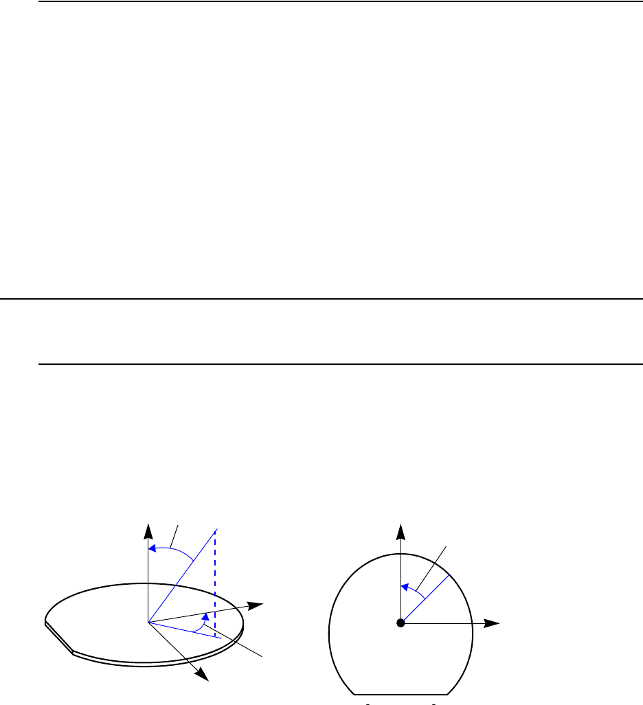
3: Ion Implantation

Coordinate System

Sentaurus™ Process User Guide 89

H-2013.03

Adaptive Meshing during Implantation

Adaptive meshing during implantation is active whenever adaptive meshing is switched on,

that is, pdbGet Grid Adaptive returns a 1. It also can be switched on by specifying the

parameter Adaptive in the implant command. For details, see Adaptive Meshing during

Implantation on page 708.

Since generally analytic implantation and MC implantation produce similar results, MC

implantation can take advantage of this similarity for adaptive meshing. When adaptive

meshing is active, MC implantation will first call analytic implantation for mesh refinement.

At the end of analytic implantation, the concentration generated by the analytic implantation is

discarded, while the new mesh is used for MC implantation. If the analytic implantation fails

for whatever reasons (such as no implant tables for certain materials), Sentaurus Process issues

a warning, and the MC implantation proceeds with the original mesh.

Coordinate System

Coordinates for Implantation: Tilt and Rotation Angles

Regardless of whether a simulation is 1D, 2D, or 3D, the direction of the ion beam is defined

relative to the wafer coordinate system (see Figure 16 on page 66) by the values of the tilt and

rotation parameters of the implant command. Figure 21 shows the tilt and rotation angles in

the wafer coordinate system.

Figure 21 Tilt and rotation angles for implantation; beam angle shown corresponds

to tilt = 20 and rotation = 45

The tilt and rotation angles are measured from the ion beam to the wafer z-axis and wafer y-

axis, respectively. In this definition, the tilt angle is always positive, and between (inclusive)

rotation

tilt ion beam

0°

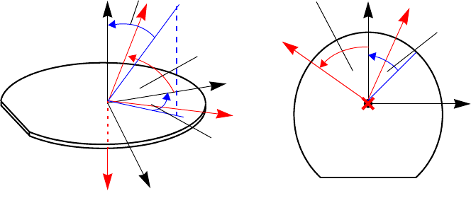
3: Ion Implantation

Coordinate System

90 Sentaurus™ Process User Guide

H-2013.03

and . However, for convenience, a negative tilt angle is allowed, and it is converted

automatically to a positive tilt by adding to the specified rotation angle. The rotation

angle is positive when the beam is rotated in the clockwise direction about the wafer z-axis,

and it is negative when it is counterclockwise.

Since the tilt and rotation angles are measured with respect to the wafer axes, the direction of

the beam in the simulation coordinate system depends on the slice angle.

Figure 22 shows the relationship between wafer coordinates, simulation coordinates, and the

beam direction.

Figure 22 Tilt and rotation angles for implantation; angles shown correspond to tilt = 20,

rotation = 45, and slice.angle = 60

The default values of tilt and rotation are and , respectively; in other words, by

default the incident ion beam is directed parallel to the wafer flat tilted away from the wafer x-

axis. For the default slice angle of , this corresponds to an ion beam in the simulator xy

plane, tilted away from the simulator y-axis. In a 2D simulation, the default ion beam comes

from the left side.

Figure 23 on page 91 shows the projection into the wafer plane of the direction from which the

beam strikes the wafer for tilt > 0 and various rotation angles.

The default simulation coordinate system (slice.angle = -90) is also shown.

90°

180°

slice.angle

rotation

tilt

rotation

ion beam

7°

90°–

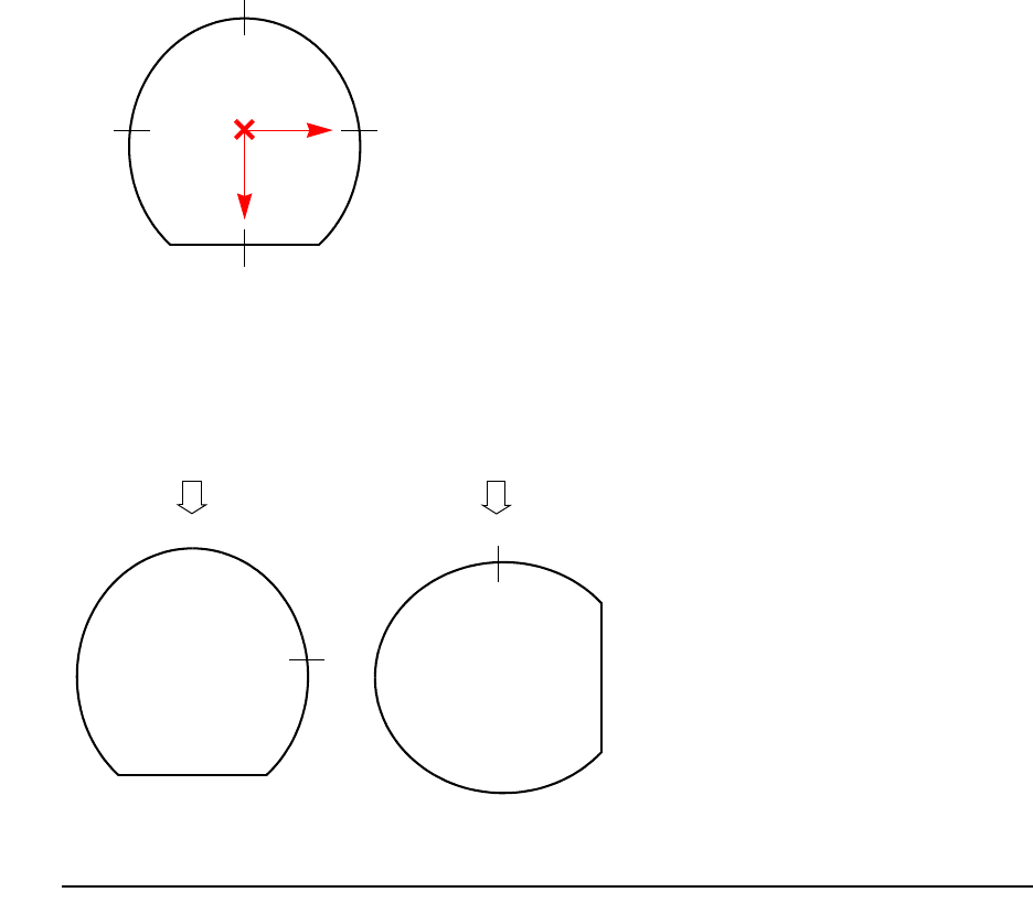
3: Ion Implantation

Coordinate System

Sentaurus™ Process User Guide 91

H-2013.03

Figure 23 Implant rotation directions for positive tilt

Figure 24 shows clearly that the orientations shown in Figure 23 are consistent with the

conventions defined in Figure 21 on page 89. A rotation of corresponds to rotating the

wafer a quarter turn counterclockwise.

Figure 24 Rotating wafer and fixed beam direction

2D Coordinate System

In a 2D simulation, the orientation of the 2D simulation plane with respect to the wafer

coordinate system must be defined. The angle between the 2D simulation plane and the y-axis

is set by the slice.angle. The default value is , which orients the 2D simulation plane

parallel to the wafer flat. The transformed y-axis (ys) is the y-axis in the 2D simulation plane.

–90o90o

180o

90°

90o

rotate wafer +90o

90o

ion beam ion beam

90°–

3: Ion Implantation

Analytic Implantation

92 Sentaurus™ Process User Guide

H-2013.03

There are two ways to set slice.angle in the init command:

■To set directly, use:

init slice.angle=<n>

■To set by specifying a 2D cutline, use:

init slice.angle=[CutLine2D <x1> <y1> <x2> <y2>]

The <x1> and <y1> define the start point, and <x2> and <y2> define the end point in the wafer

plane. The two points are in the wafer coordinate system (for more information on coordinate

systems, see Understanding Coordinate Systems on page 66).

In general, the tilt projected to the 2D simulation plane is different from the tilt value. It is

given by the geometric relation:

(2)

The angle tilt2D can be found in the output of Sentaurus Process and can be negative

depending on the rotation angle and slice angle.

The tilt value defines the relation between the wafer dose (dose), which is given at the

command line by default and the dose, which would have to be specified in the beam-dose

mode to obtain the same final implanted dose, that is:

(3)

BeamDose2D as it appears in the Sentaurus Process output is defined using tilt2D, that is:

(4)

Analytic Implantation

Analytic implantation is performed using empirical point-response distributions. Point-

response distributions are generated using the method of moments. The moments representing

the primary and lateral point-response functions are taken from implantation tables.

For the purposes of 2D simulations based on analytic functions, an ion beam incident at the

point is assumed to generate a distribution function .

tilt2D()cos tilt()cos

2tilt

()cos 2tilt

()sin 2rotation+slice.angle

()cos⋅+

-----------------------------------------------------------------------------------------------------------------------------------------------------------=

BeamDose dose

tilt

()cos

--------------------------=

BeamDose2D dose

tilt2D()cos

---------------------------=

ξη,()

Fx y ξη,,,()

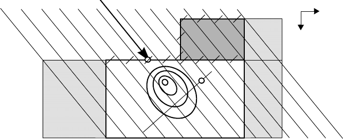
3: Ion Implantation

Analytic Implantation

Sentaurus™ Process User Guide 93

H-2013.03

To calculate the concentration of the implanted species at a point of the simulation

domain, the superposition of all distribution functions of all possible points of incidence

must be computed:

(5)

where is the total dose per exposed area and is the doping profile.

Figure 25 Point-response distribution for a particle incident at the point ( ) at the

surface; intervals are used for lateral integration at the point (x, y); shaded

regions to left and right mark the lateral extension elements

The 2D distribution functions are always assumed to be given as a product of two 1D

distribution functions orthogonal to each other: a primary distribution function and a

lateral distribution function :

(6)

To perform the computation of the convolution integral in 2D, Sentaurus Process uses a set of

lateral intervals perpendicular to the projected ion beam. A local 1D layer structure is

computed in each interval. The spacing and width of these intervals depend on the complexity

of the exposed gas surface.

In 3D, Sentaurus Process uses a slightly different algorithm. The point-response function is a

3D function. The lateral function is also used in the third direction:

(7)

assuming an axially symmetric point-response function. The lateral integration is performed in

the plane perpendicular to the ion beam. For each point in the lateral integration plane, again,

a local 1D layer structure is computed.

xy,()

ξs()ηs()(,)Γgas

∈

Cx,y() NdFxyξs()ηs(),, ,()sd

Γgas



Cxy,()

(ξ,η)

(x,y)

ξη,

fpx()

flx()

Fxyξη,,,()fpxξs()–()flyηs()–()⋅=

flx()

Fxyzξη Θ,,,, ,()fpxξs()–()flyηs()–()flzΘs()–()⋅⋅=

3: Ion Implantation

Analytic Implantation

94 Sentaurus™ Process User Guide

H-2013.03

Primary Distribution Functions

Primary distribution functions can be set for a dopant/material combination using:

implant species=<dopant> <material>

[{gaussian pearson pearson.s dualpearson point.response}]

The previous model selection is used if no selection for <model> is made. The primary

distribution is used to represent the point-response function in 1D or the vertical point-response

in 2D and 3D. Point-response functions are characterized by moments.

The first moment, the projected range , is defined as:

(8)

while the higher moments are defined as:

(9)

The standard deviation , the skewness , and the kurtosis are defined as:

(10)

(11)

(12)

Gaussian Distribution: gaussian

(13)

(14)

(15)

Rpxfx() xd⋅⋅

∞–

∞



mixR

–()

ifx() xd⋅⋅

∞–

∞



σm2

γm3

σ3

------=

βm4

σ4

------=

fpx() 1

2πσ

-------------- xR

–()

2σ2

----------------------–





exp=

γ0=

β3=

3: Ion Implantation

Analytic Implantation

Sentaurus™ Process User Guide 95

H-2013.03

Pearson Distribution: pearson

The Pearson distributions are the solution to the following differential equations:

(16)

(17)

Different types of Pearson distribution are distinguished by different values of and :

(18)

(19)

(20)

The Pearson–IV distribution is given by:

(21)

Sentaurus Process automatically switches between the Pearson–IV, Pearson–V, and Pearson–

VI distribution functions depending on the conditions for and given in Eq. 18 to Eq. 20.

The factor is chosen to fulfill the normalization condition:

(22)

dfy() ya–

b0b1y⋅b2y2

⋅++

----------------------------------------------fy()⋅, yxR

–==

1γσ β 3+()⋅⋅

--------------------------------–==

b0σ24β3γ2

–()⋅

------------------------------------–=

b22β3γ2

–6–

------------------------------–=

A10β12γ2

–18–=

0γ32<<

β48 39γ26γ24+()

32⁄

32 γ2

–

-------------------------------------------------------------> Type IV

0γ32<<

β48 39γ26γ24+()

32⁄

32 γ2

–

-------------------------------------------------------------= Type V

0γ32<<

3 1.5 γ⋅+β48 39γ26γ24+()

32⁄

32 γ2

–

-------------------------------------------------------------

<< Type VI

fpy() Kb

2y2b1yb

2b2

--------

----- 2a+

4b2b0b1

–

------------------------------–2b2yb

4b2b0b1

–

------------------------------







atan







exp⋅=

fpx()xd

∞–

∞

1=

3: Ion Implantation

Analytic Implantation

96 Sentaurus™ Process User Guide

H-2013.03

Pearson Distribution with Linear Exponential Tail: pearson.s

A linear exponential tail is added to the Pearson distribution. This is performed in an attempt

to describe more accurately the profile tails for some implantations, that is:

(23)

where is the Pearson distribution, is a transition function, and is the exponential tail.

The decay length of the exponential tail is give by the parameter :

(24)

The constants and are computed from the continuity conditions:

(25)

and:

(26)

NOTE Exponential tail distributions are available with the Dios tables.

However, care is required when using the exponential tail for

implantation with large tilt angles. The -fit in these tables was

performed for a standard tilt in amorphous materials and does not

apply to large tilt angles or strong channeling conditions.

fpx()

Ppx()0xx

max

<≤,

Pvx()xmax x<xa

≤,

Plx()xax∞<≤,











lexp

xmax :Pmax Ppxmax

():= maxPpx()=

xaxmax

≥:PaPpxa

():= 1

---Ppxmax

()=

Pvx() Ppxmax

() A1xx

max

–()

2Bx x

max

–()

+()exp⋅=

Plx() Ppx() xx

max

–

lexp

--------------------Ppxmax

() xx

max

–

lexp

--------------------–





exp⋅⋅+=

Plxa

() Pvxa

()=

dPlx()

xaxd

dPvx()

P′a

=:=

3Pa

Pmax

------------

xaxmax

–()

------------------------------P′a

Paxaxmax

–()

----------------------------------–=

2Pa

Pmax

------------

ln–

xaxmax

–()

------------------------------P′a

Paxaxmax

–()

------------------------------------+=

lexp

7°

3: Ion Implantation

Analytic Implantation

Sentaurus™ Process User Guide 97

H-2013.03

Dual Pearson Distribution: dualpearson

The most advanced primary distributions are available with the dual Pearson function [9],

which can be chosen with the switch dualpearson. The dual Pearson model includes a

superposition of two Pearson functions:

(27)

The head and tail functions are two independent Pearson functions. The head function accounts

for the profile of ions that do not channel (nonchanneling or amorphous part). The tail function

accounts for the channeled ions that form the characteristic tail in the implantation profile.

A dualpearson function is characterized by nine parameters: the two sets of four Pearson

parameters and the ratio between the amorphous and channeling doses. These parameters are

usually taken from moment table files.

You can s et t he i ndivi du al m ome nts di re ctly in the Sentaurus Process command line, for

example:

implant species=<dopant> <material> [rp=<n>] [stdev=<n>] [gamma=<n>]

[beta=<n>] [rp2=<n>] [stdev2=<n>] [gamma2=<n>] [beta2=<n>] [ratio=<n>]

[lat.stdev=<n>] [lat.stdev2=<n>]

This overwrites the parameters found in the specified implant table. Using this facility, it is also

possible to force the Pearson distributions in the dualpearson and pearson models to

behave like a Gaussian distribution, for example:

implant species=Boron Silicon pearson gamma=0 beta=3

The first statement sets the implantation model to a Pearson distribution. The parameters are

read from the default table. The skewness and kurtosis are set according to Eq. 14 and Eq. 15,

overwriting the values found in the table. This results in a Gaussian distribution for the function

characterizing the amorphous part of the profile.

You can en able or di sa bl e indivi du al m ome nts us in g <moment>.isset pdb switches, where

<moment> is the name of the moments such as rp, stdev, rp2, stdev2, and so on. For

example:

pdbSetBoolean Silicon Boron rp.isset 0

This command would disable a user set value for rp.

fpx() ratio fhead x() 1ratio–()ftail x()⋅+⋅=

3: Ion Implantation

Analytic Implantation

98 Sentaurus™ Process User Guide

H-2013.03

NOTE All moments set at the command line are ignored after a new implant

table is selected, or an implant table has been specified again using the

implant species=<species> <material> imp.file=<name>

command. In this case, the moments from this new implant table will

then be used, regardless of which moments have been set previously at

the command line.

Point-Response Distribution: point.response

See Point-Response Interface on page 116.

Screening (Cap) Layer-dependent Moments

Cap layer–dependent implant tables are used to describe correctly the screening of the ion

beam in the structure. The implant moments in a particular region generally depend on the

combined thickness of all layers above this region. The moments are parameterized with

respect to the effective thickness , which is defined as:

(28)

that is, as the sum over the thicknesses of all layers above the current layer multiplied by

corresponding efficiency factors . These factors can be set for a particular material and a

species using:

implant species=Boron Oxide eff.caplayer.thick 1.0

The default value is 1 for all materials other than silicon, where it is set to zero. Therefore,

silicon layers are effectively not included in the total effective cap layer thickness.

If the implant table for a specific <material>/<species> combination does not contain an

explicit cap layer dependence, the effective channeling suppression model is used. This model

suppresses the channeling tail by multiplying the channeling part in Eq. 27 by a factor

calculated according to:

(29)

cap

cap tj fj

eff

ji<



eff

rsuppress

rsuppress 1

---CR

phead,

()

phead,

()CR

ptail,

()+

--------------------------------------------------------

⋅MinRatio

--------------------------------





Exponent–

-----------------------------------------------------------------------------------------------------------------------------------------------=

3: Ion Implantation

Analytic Implantation

Sentaurus™ Process User Guide 99

H-2013.03

where and are the peak concentrations of the unscaled profile, and

is defined as:

(30)

using the values of for the amorphous (head) part of the profile for all layers above the

present layer. The amorphous part of the profile is multiplied by to conserve the

total dose.

MinRatio is the minimum value of the ratio . The parameters MinRatio and Exponent

can be set in the parameter database, that is:

pdbSet <material> <species> MinRatio

pdbSet <material> <species> Exponent

The model is applied only for values of greater than MinRatio and effective cap layer

thickness greater than 2.1 nm. The effective channeling suppression model can be switched on

using:

implant species=<species> <material> [eff.channeling.suppress]

The model remains inactive for explicitly cap layer–dependent implant tables.

NOTE This model is switched off by default and is switched on in the Taurus/

TSUPREM-4 mode.

Lateral Straggle

The lateral straggling of the distribution of implanted ions is specified by defining a lateral

distribution function, which is a Gaussian distribution with a lateral standard deviation :

(31)

In general, the lateral standard deviation depends on the vertical depth of the profile. The depth

dependence can be switched on or off for a particular combination of dopant species and

material using the flag depth.dependent:

implant species=<dopant> <material> [depth.dependent]

phead,

()

ptail,

()

σti

Rpi

-------



1rsuppress

–

σl

flxy,() 1

2πσ

lx()

------------------------y2

2σl

2x()

-----------------–







exp=

3: Ion Implantation

Analytic Implantation

100 Sentaurus™ Process User Guide

H-2013.03

The lateral standard deviation can also be set in the command line using the keyword

lat.stdev:

implant species=<dopant> <material> [lat.stdev=<n>] [lat.stdev2=<n>]

where lat.stdev2 sets the lateral standard deviation for the tail function. If either

lat.stdev or lat.stdev2 is set, Sentaurus Process switches to the depth-independent

lateral straggling. All depth.dependent switches are ignored in this case.

An additional scaling factor for both the depth-dependent and depth-independent lateral

standard deviation can be used to vary the lateral straggling:

implant species=<dopant> <material> [lat.scale=<n>] [lat.scale2=<n>]

Depth-dependent Lateral Straggle: Sentaurus Process Formulation

If a TSUPREM-3-compatible implantation table is used (.s3), the depth-dependent lateral

standard deviation is calculated according to:

(32)

where lstdev and lv are parameters taken from the implantation table. There are two

independent sets of parameters for the two Pearson functions in the dualpearson model. This

formulation also is used with the Tasch implantation tables.

Depth-dependent Lateral Straggle: Dios Formulation

If a Dios-compatible implantation table is used, the depth-dependent lateral standard deviation

is calculated using a vector of five parameters p1, p2, ..., p5. The following formula is

applied [10]:

(33)

There is only one set of these parameters in each table entry. In the case of the dualpearson

implant model (see Eq. 33), the same set of parameters p1, p2, ... p5 together with the

standard deviation of the first Pearson function described by stdev is applied to both the

amorphous and the channeling part of the distribution.

σlx() lstdev x

lstdev lv⋅

------------------------------–





exp⋅=

σlx() stdev max 0.01

p1 p2 x⋅

------------- p3+





⋅





exp p1 p4 x⋅

------------- p5+





⋅





exp+





log 



-----------------------------------------------------------------------------------------------------------------------------------------







⋅=

3: Ion Implantation

Analytic Implantation

Sentaurus™ Process User Guide 101

H-2013.03

Depth-dependent Lateral Straggle: Taurus Formulation

If a TSUPREM-4/Taurus-compatible implantation table is used, the depth-dependent lateral

standard deviation is calculated using two parameters:

(34)

The depth-independent standard deviation and the depth-dependent slope are read

from the moment table.

This formulation is compatible with the Dios formulation (see Depth-dependent Lateral

Straggle: Dios Formulation) for the following conditions: , . The

remaining parameters can be translated as follows:

(35)

Analytic Damage: Hobler Model

The damage distribution is calculated using Eq. 33 and Eq. 6, p. 93. The primary and lateral

distribution functions are taken from the literature [10]. The primary function consists of a

Gaussian function and an exponential tail, joined continuously with continuous first

derivatives. The distribution is normalized. The normalization factors are and , and

is the number of Frenkel defects per ion.

Three types of primary function are distinguished:

■Type 0

A simple Gaussian distribution with the primary range and the standard deviation :

(36)

■Type 1

For light ion species:

(37)

σlx() σ

01∆σ x

------1–









⋅=

σ0

∆σ

p4 0=

p1 p5⋅∞–=

σ0stdev p2 p3+()⋅=

∆σ p2 p2 p3+()⁄=

Nvac

fpx() Nvacc1

–()

2σ2

----------------------–





exp=

fpx()

Nvacc1x





, x x0

≤exp

Nvacc2

–()

2σ2

----------------------–





, x x0

>exp







3: Ion Implantation

Analytic Implantation

102 Sentaurus™ Process User Guide

H-2013.03

where is the decay length of the exponential function. The joining point is calculated

by:

(38)

■Type 2

For heavier ions, the exponential tail is directed towards the bulk:

(39)

In this model, four parameters , , , and are required. These parameters were

obtained by MC simulations between 1 keV and 300 keV. If damage calculation is switched

on, that is, if:

implant species=<dopant> damage

has been set, Sentaurus Process generates these parameters using an internal lookup table,

which contains the original data available for boron, BF2, phosphorus, arsenic, and antimony

in silicon.

NOTE For some other species, the parameters of these original species are used

that are closest with respect to the atomic number in the periodic table

of elements. Nitrogen uses the boron parameters. Silicon and aluminum

use the phosphorus parameters. Germanium and gallium use the arsenic

parameters, and indium uses the antimony parameters. Damage

calculation is automatically switched off for any other species.

Type 0 is used for boron at energies E < 20 keV, phosphorus at E < 55 keV, and arsenic at

E>170keV. Type1 is applied to boron and phosphorus elsewhere, and Type 2 is applied to

arsenic at energies below 170 keV and antimony at all energies.

The lateral distribution is modeled using Eq. 33. The five lateral parameters p1, p2, ...,

p5 are provided in the internal lookup table.

An alternative to the internal lookup table is to load a table file similar to the implant tables.

The keyword for this is dam.table:

implant species=<dopant> <material> [dam.table=<name>]

x0Rp

σ2

------–=

fpx()

Nvacc2

–()

2σ2

----------------------–







, x x0

≤exp

Nvacc1





, x x0

>exp







Nvac

3: Ion Implantation

Analytic Implantation

Sentaurus™ Process User Guide 103

H-2013.03

This overwrites the internal lookup table for the above mentioned species using the parameters

from the table instead. In addition, it enables damage calculation for species other than the

original ones.

Datasets

Several datasets are used to store the as-implanted profile and the implantation damage. Point-

defect profiles are created at the end of the implantation step. Datasets with the ending

_Implant contain profiles generated during subsequent implant steps. These datasets are

deleted at the beginning of the next diffuse step.

Table 4 Datasets used in analytic implantation step

Dataset Description

Damage

Accumulative damage (damage history). At the end of an implant step, the

Damage_LastImp concentration is added using DFactor. This dataset is

deleted by the diffuse command.

Damage_LastImp

Damage created during the last implant step. This dataset is deleted at the end

of the implant step.

Accumulative density of the dopant concentration. At the end of an implant

step, the <dopant>_LastImp concentration is added to <dopant>.

<dopant>_Implant

Accumulative density of the dopant concentration. At the end of an implant

step, the <dopant>_LastImp concentration is added to

<dopant>_Implant. This dataset is deleted by the diffuse command.

<dopant>_LastImp

As-implanted dopant concentration that contains the profile generated during the

last implant step. This dataset is deleted at the end of the implant step.

Int_Implant

Accumulative interstitial profile updated at the end of an implant step.

Vac_Implant

Accumulative vacancy profile updated at the end of an implant step.

Int<component>_Implant

Accumulative interstitial profiles in multicomponent material with

DistinctDefects set to true, where <component> is the component

of the composition of the material. For example, in SiC, interstitial profiles

include IntSilicon_Implant and IntCarbon_Implant.

Vac<component>_Implant

Accumulative vacancy profiles in multicomponent material with

DistinctDefects set to true, where <component> is the component

of the composition of the material. For example, in SiC, interstitial profiles

include VacSilicon_Implant and VacCarbon_Implant.

3: Ion Implantation

Analytic Implantation

104 Sentaurus™ Process User Guide

H-2013.03

Tables

Implantation Table Library

The implantation table library is located at $SPHOME/ImpLib/.

Dios Tables

The subdirectory Dios/ contains the tables used by default in Dios. This tables can be made

the default tables for all species in Sentaurus Process by using:

implant tables=Dios

For arsenic, antimony, phosphorus, indium, germanium, gallium, nitrogen, and aluminum, the

data in these tables are taken from the literature [3]. The values for boron are obtained from

simulations with the 1D process simulator TESIM [11]. The values for energies MeV are

taken from the literature [2]. These tables provide moments that can be used with the Gaussian

and Pearson implantation models.

Taurus Tables

The directory Taurus/ contains the Taurus Process implant tables for boron, BF2, phosphorus,

germanium, indium, antimony, and arsenic. To select these tables as the default, use the

keyword Taurus:

implant tables=Taurus

The tables contain calibrated data from sub-keV to above 10 MeV. The calibration was

performed using both SIMS data and Taurus MC calculations [5].

Default Tables

The directory Default/ contains tables extracted from MC simulations with Crystal-

TRIM [4], which are tabulated in DIOS format. The data are available for arsenic, antimony,

BF2, boron, phosphorus, indium, and germanium in silicon, polysilicon, oxide, and nitride.

These tables provide moments that can be used with all implantation models including the

dualpearson model. For silicon, dual Pearson moments are available that depend on energy,

tilt, dose, and cap-layer thickness. For polysilicon, oxide, and nitride, single Pearson moments

are available that depend on energy and tilt only.

The tables cover different energy ranges. The tilt angles range from to , and the oxide

thickness ranges from 0 nm to 100 nm. There are tables for low, medium, and high doses for

all species except germanium where only one table for a medium to high dose is available.

1≥

0°

60°

3: Ion Implantation

Analytic Implantation

Sentaurus™ Process User Guide 105

H-2013.03

Sentaurus Process selects the correct table depending on the implant dose. These tables

constitute most of the default tables used in Sentaurus Process.

The default tables used in Sentaurus Process are selected by using the command:

implant tables=Default

This implant command not only selects the tables from the Default/ directory for arsenic,

antimony, BF2, boron, phosphorus, indium, and germanium in silicon, polysilicon, oxide, and

nitride, but also selects the tables from the Taurus/ directory for carbon, fluorine, and

germanium in silicon, polysilicon, oxide, and nitride (see Table 5). For all other species and

materials, the respective Dios tables are used.

NOTE Outside the specified range, the Default implant tables may fall back

to the Dios tables. Therefore, near the boundaries of the Default

tables, inconsistent results may occur.

Ta bl e 5 D e fa u l t t a bl es

Species Table file Energy range [keV]

Arsenic

<material>As_1e12-5e13.tab

<material>As_1e13-8e14.tab

<material>As_2e14-6e15.tab

0.5–400

Antimony

<material>Sb_1e12-5e13.tab

<material>Sb_1e13-5e14.tab

<material>Sb_2e14-1e16.tab

1.5–600

BF2

<material>BF2_1e12-5e13.tab

<material>BF2_1e13-8e14.tab

<material>BF2_2e14-6e15.tab

0.5–400

Boron

<material>B_1e12-4e13.tab

<material>B_1e13-6e14.tab

<material>B_16e13-8e15.tab

0.2–517 (silicon)

0.2–480 (other materials)

Carbon

carbon_in_<material>_standard

0.2–400

Fluorine

fluorine_in_<material>_standard

0.2–400

Germanium

germanium_in_<material>_2007

0.6–800

Indium

<material>In_1e12-4e13.tab

<material>In_1e13-6e14.tab

<material>In_16e13-8e15.tab

1–400

Phosphorus

<material>P_1e12-4e13.tab

<material>P_1e13-6e14.tab

<material>P_16e13-8e15.tab

0.3–400

0.12–3000 (10.0 upgrade)

3: Ion Implantation

Analytic Implantation

106 Sentaurus™ Process User Guide

H-2013.03

Tasch Tables

The directory Tasch/ contains the University of Texas (UT) implant tables for boron, BF2,

phosphorus, and arsenic in silicon [12]. For all other materials and species, single Pearson

tables are available. The tables can be selected to be the default by using the keyword Tasch:

implant tables=Tasch

The tables cover different energy ranges. The boron table ibout1.s3 contains cap layer–

dependent implantation moments valid for thicknesses between 1.5–40 nm. The moments in all

other tables are cap-layer independent.

The valid range for the tilt is to and, for the rotation, the range is to . These

tables provide data to be used with all implant models.

The single Pearson tables provide only energy-dependent data covering the range between

10 keV and 1000 keV.

TSuprem4 Tables

The directory TSuprem4/ contains the TSUPREM-4 native implant tables, s4imp0.ts4, for

boron, BF2, phosphorus, indium, antimony, and arsenic. To select these tables as the default,

use the keyword TSuprem4 with an optional prefix:

implant tables=TSuprem4 [ts4.prefix=<c>]

These tables contain the original implant moments of TSUPREM-4.

File Formats

Sentaurus Process handles a variety of table formats. The table format of the implantation table

is automatically recognized by Sentaurus Process from the file extension.

Table 6 Tasch tables

Species Table file Energy range [keV]

Arsenic

iasut0.s3

7–180

BF2

ibfut0.s3

0.5–65

Boron

ibout0.s3

ibout1.s3

0.5–80

15–80

Phosphorus

iphut0.s3

15–180

0°

10°

0°

45°

3: Ion Implantation

Analytic Implantation

Sentaurus™ Process User Guide 107

H-2013.03

Single-Pearson Table File Format: <file>.sp

This format provides the simplest table format that can be used with Sentaurus Process. It

contains energy-dependent entries for the moments to be used with the (single) pearson or

gaussian model.

NOTE These tables cannot be used with the dualpearson model.

The format of the table entries is:

energy rp stdev gamma beta lat.stdev

There is no dependence of the moments on dose, tilt, rotation, or cap layer thickness. Lines

with an asterisk in the first column are treated as comment lines. Missing or incomplete blocks

are not properly read when the file is parsed.

SUPREM-III Table File Format: <file>.s3

This format allows the handling of energy, dose, tilt, rotation, and cap-layer thickness–

dependent dual Pearson moments. A SUPREM-III implant table file consists of two sections:

one for the primary moments and one for lateral moments. Both sections start with a header,

which contains the parameter range covered by the table.

The header is organized as follows:

*Energies:

NumberOfEnergies energy1 energy2 ...

*Tilts:

NumberOfTilts tilt1 tilt2 ...

*Rotations:

NumberOfRotations rotation1 rotation2 ...

*Doses:

NumberOfDoses dose1 dose2 ...

*Thickness:

NumberOfThickness thickness1 thickness2 ...

NOTE The order of these entries must not be changed.

Lines with an asterisk in the first column are treated as comment lines. A table entry for a

particular combination of lookup parameters has the format:

rp stdev gamma beta rp2 stdev2 gamma2 beta2 ratio1

rp stdev gamma beta rp2 stdev2 gamma2 beta2 ratio2

...

rp stdev gamma beta rp2 stdev2 gamma2 beta2 ratio<NumberOfDoses>

3: Ion Implantation

Analytic Implantation

108 Sentaurus™ Process User Guide

H-2013.03

Each line contains eight dualpearson moments and the ratio as defined in Eq. 27, p. 97. The

entries are ordered increasingly with respect to cap layer thickness, energy, tilt, and rotation.

NOTE There is no automatic check of the ordering of the table entries.

The tables are for one species/material combination only. The cap-layer thickness, rp, rp2,

stdev, and stdev2 should be given in micrometers and the angles, in degrees. The energy

values must be specified in keV. No units must be specified in the tables.

The lateral part is organized in the same manner. Corresponding to the header information, the

entries are ordered in the same manner as in the primary part. Each entry has the format:

<void> lstdev lv lstdev2 lv2

The first item is void and can be used for information purposes. The parameters are used in

Eq. 32, p. 100 to calculate the depth-dependent lateral standard deviation. The units for

lstdev and lstdev2 are micrometers, whereas lv and lv2 are unitless.

Dios Table File Format: <file>.tab

The Dios table file format for implantation data files allows for dependencies on energy, dose,

tilt, rotation, and the cap-layer thickness. It provides the primary moments for all implantation

models including the dualpearson model. Parameters for depth-dependent lateral straggling

are available as well. The format of the table entries is:

# Look up parameters

material species thickness rotation tilt energy NumberOfFunctions

NumberOfDoses

# Primary moments

rp stdev <void> gamma beta lexp <void>

rp2 stdev2 <void> gamma2 beta2 lexp2 <void>

# Channeling table

dose ChannelingDose

...

# Lateral straggling

p1 p2 p3 p4 p5

Lines with a # character in the first column are treated as comment lines. Missing or incomplete

blocks are not read properly when the file is parsed.

The first block contains entries for the material and species names, cap-layer thickness, rotation

angle, tilt angle, and energy. The NumberOfFunctions defines the number of components of

the primary distribution function. A maximum of two functions are allowed. NumberOfDoses

defines the number of entries in the channeling table. Each entry consists of a dose and the

corresponding channeling dose. All doses are expected to be positive.

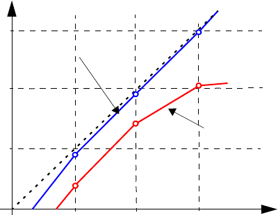
3: Ion Implantation

Analytic Implantation

Sentaurus™ Process User Guide 109

H-2013.03

Figure 26 Piecewise linear nonchanneling and channeling dose for a dual Pearson profile

as represented in default channeling table

The ratio between the amorphous part and channeling part in Eq. 27, p. 97 is calculated from

the channeling table using:

(40)

where the value for ChannelingDose is interpolated linearly using the value of the implant

Dose.

The second block contains the moments for all the components of the primary distribution

function. Parameters, which by definition do not exist for the function the set describes, are

ignored.

NOTE Some entries are always ignored since they are not used in the implant

models of Sentaurus Process. For example, the last moment entry

(<void>) is always disregarded.

The third block contains the channeling table ordered with increasing dose, and the fourth

block contains parameters for the depth-dependent lateral straggling.

NOTE The entries must be increasingly ordered with respect to the cap-layer

thickness, rotation, tilt, and energy, so that the values for various

energies (but the same other three parameters) follow each other. All

data entries for the same material–dopant combination should follow

each other with no interruption by entries for another material–dopant

combination. The cap-layer thickness, rp, rp2, stdev, and stdev2

should be given in micrometers and the angles, in degrees. The energy

values must be specified in keV. No units must be specified in the tables.

1013 1014 10

To tal D os e

Channeling Dose

Nonchanneling Dose

Dose

1013

1014

ratio 1ChannelingDose

dose

--------------------------------------------–=

3: Ion Implantation

Analytic Implantation

110 Sentaurus™ Process User Guide

H-2013.03

Damage Table File Format: <file>.dam

The damage tables for the Hobler damage model are similar to the Dios table file format, which

allows for dependencies on energy, tilt, and rotation. The Hobler damage model table provides

the primary moments for the damage model. Moments for depth-dependent lateral straggling

are available as well. The format of the table entries is:

# Look up parameters

material species rotation tilt energy

# Primary moments

rp stdev decay nvac type

# Lateral straggling

p1 p2 p3 p4 p5

The syntax is the same as for the Dios table format. The item decay refers to the parameter ,

and the item nvac refers to the parameter in Analytic Damage: Hobler Model on

page 101. The item type refers to the type of Hobler model.

Taurus Table Format: <file>

The Taurus table format, which is the most general table format used in Sentaurus Process,

handles data for all implant and damage models. Implant table files in the Taurus format have

no file extension; that is, an implant table file without a file extension is considered to be in the

Taurus format. It contains a file header and a block of numeric data. The file header consists of

a list of names of the implant conditions. The names should be lowercase only. The following

names are recognized:

energy tilt rotation dose screen temperature current

The sequence of these names can be arbitrary. Some names from this list can be omitted. The

following units should be used for the implant conditions:

energy,[keV]

tilt,[degrees]

rotation,[degrees]

dose,[cm-2]

screen,[um]

temperature,[K]

current,[mA/cm2]

The numeric data consists of an arbitrary number of lines that form the lookup tables for

implant conditions and implant moments. Each line should contain a list of numeric values for

the implant conditions followed by the implant moments. The numeric values should be

separated by space.

Nvac

3: Ion Implantation

Analytic Implantation

Sentaurus™ Process User Guide 111

H-2013.03

The number of the numeric values should be the same on each line. There should be at least

n+4 values per line for a gaussian profile, n+6 values per line for a pearson profile, and

n+13 values per line for a dualpearson profile, where n is the number of the implant

conditions specified in the file header.

The sequence of implant conditions should correspond exactly to the sequence of implant

condition names in the file header. The sequence of the implant moments in one line is fixed

as follows:

Any line that starts with a double slash // is considered a comment and is omitted. Always put

the double slash at the first position in the line.

If the requested set of implant conditions does not have an exact match in the lookup table, a

multidimensional linear interpolation is used. If a requested implant condition extends beyond

the range of the lookup table, the closest value from the lookup table is used.

If the lookup table contains several lines with identical sets of the implant conditions, only the

last set is used, and all the previous lines are discarded.

If a table contains data for the Hobler damage model, the following sequence of moments is

used:

rp stdev lat.stdev lat.slope gamma beta decay nvac

Multilayer Implantations

Point-response functions are valid only for a single material layer. For multiple layers of

different materials, the point-response functions must be combined in a way that corrects the

effect of the different stopping power in the covering layers. This must be performed for each

lateral interval taking into account the local layer sequence parallel to the ion beam. Two

algorithms are available in Sentaurus Process: numerical range scaling (NRS) [13] and dose-

matching [12]. Both algorithms calculate a shift applied to the primary point-response

function. Sentaurus Process also provides an option no, which switches off the matching. In

this case, is set to zero in all layers.

The matching algorithm can be selected globally by using the command:

pdbSet ImplantData MatchControl { no | range | dose }

Gaussian:

rp stdev lat.stdev lat.slope

Pearson:

gamma beta

Dual Pearson:

rp2 stdev2 lat.stdev2 lat.slope2 gamma2 beta2 ratio

δi

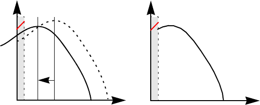
3: Ion Implantation

Analytic Implantation

112 Sentaurus™ Process User Guide

H-2013.03

The default value of MatchControl is range. In addition, you can select locally the matching

algorithm with the keyword match in each implant command:

implant <dopant> [match={no range dose}]

The locally selected algorithm overwrites the one globally set in the PDB.

The NRS algorithm accounts for the different stopping power in different materials using the

ratio of the projected ranges of the materials.

Figure 27 NRS algorithm: the point-response function in the second material is shifted and

rescaled (left) due to existence of a layer with different stopping power (shaded

region); the new profile is combined from the point response in the first layer and

shifted point response in the second layer (right).

The shift in the -th layer is calculated according to:

(41)

where represents the thickness of the -th layer. The profiles are matched

according to:

(42)

where is a rescaling factor that satisfies the normalization condition. The point-response

function in the first layer is always used without a shift.

The proportional range shift model is used to shift the channeling portion of the implant profile

independent of the amorphous part. To calculate the shift of the channeling part, the shift of the

amorphous part is scaled by the ratio of the channeling range and the amorphous range:

(43)

δ2

Rp2+δ2Rp2

C(x)

δitj1Rpi

Rpj

-------–





j1=

ji<



tjdjdj1–

–=

Cx() fp1x() for 0 xd

αifpi xδi

–()⋅ for di1–xd







αi

δitail,δihead,

Rpi tail,

Rpi head,

-----------------------

3: Ion Implantation

Analytic Implantation

Sentaurus™ Process User Guide 113

H-2013.03

The proportional range scaling can be switched on with:

implant <species> [range.sh]

The default setting for this model is off. In the Taurus/TSUPREM-4 mode, the switch is set to

on.

The dose-matching algorithm can be selected with the option dose. The shift is calculated

according to the dose accumulated in the above layers:

(44)

where is the position of the top of the -th layer. The dose is the integral over the

primary point-response function.

Lateral Integration

Local Layer Structure in 2D

Local 1D layer structures are defined for a set of lateral intervals. These lateral intervals are

chosen perpendicular to the projection of the ion beam into the simulation plane as shown in

Figure 28 on page 115.

The width of the lateral intervals is controlled by several parameters set in the parameter

database. The default values can be changed by using:

pdbSet ImplantData LateralGridSpacing <n>

pdbSet ImplantData VerticalGridSpacing <n>

Starting from an initial grid, the intervals are bisected until a certain limit is reached. This limit

is set by LateralGridSpacing, which has the default value of . Then, the intervals

are bisected again until a certain vertical limit is reached. This limit is set by

VerticalGridSpacing with the default value of .

The lateral integration is limited to a certain range of intervals to the left and right of a mesh

node. This integration range depends on the maximum lateral standard deviation applied to the

structure.

δi

δidideff

–=

Dsofar fpx()xd

deff



Dsofar

0.01 µm

3: Ion Implantation

Analytic Implantation

114 Sentaurus™ Process User Guide

H-2013.03

Control over the lateral integration is possible by setting the number of lateral standard

deviations used to set the integration range:

(45)

The value of can be set by using:

pdbSet ImplantData NumLateralStdev <n>

The default value is 5, which means that the total lateral integration width is 10 .

In 3D, the integration is performed over a square grid in the plane perpendicular to the ion

beam. The grid is centered about a mesh node. It has a fixed size and resolution. The size is

controlled by the parameter:

pdbSet ImplantData NumLateralStdev3D <n>

having the same meaning as the corresponding 2D parameter. The default value is 3.5. Each

interval is subdivided by a certain number of grid points. The subdivision can be set by using:

pdbSet ImplantData NumGridPoints3D <n>

so that the total number of grid points is:

(46)

The default value for NumGridPoints3D

is 4. Therefore, the total number of grid points is

784. The size of the integration grid is the parameter that limits the time performance of

analytic implantation in 3D.

The lateral intervals are expanded by a certain amount over the left and right boundaries of the

2D device to ensure flat profiles on the left and right sides. This extension depends on the

implantation tilt and the maximum lateral standard deviation. The maximum extension can

be controlled from the parameter database. The value can be changed by using:

pdbSet ImplantData MaxLateralExtension <n>

The default is set to . A similar extension is applied in three dimensions.

Cxy,() fpx()flxy',()y'd

yNσlmax,

–

yNσlmax,



σlmax,

2NumLateralStdev3D NumGridPoints3D⋅⋅()

1.5 µm

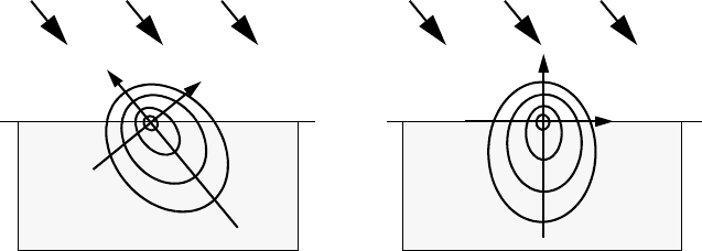
3: Ion Implantation

Analytic Implantation

Sentaurus™ Process User Guide 115

H-2013.03

Primary Direction and Scaling

The interpretation of the range and lateral range parameters depends on the value of the

implantation parameter primary. This can be set by using:

implant <dopant> [primary={beam wafer}]

The option beam switches to the beam projection mode. In this case, the primary moments are

applied along the projection of the ion beam onto the simulation plane, and the lateral

integration is performed perpendicular to the projection of the ion beam. This is the default

mode in Sentaurus Process. The option wafer switches to the wafer normal mode. Here, the

primary distribution function and the moments are interpreted orthogonally to the wafer

surface.

Figure 28 Beam projection mode (left) and wafer normal mode (right) for analytic

implantation

An implant table can be declared angle-dependent or angle-independent by using:

implant species=<dopant> [angle.dependent]

Tilt-dependent and rotation-dependent data values extracted from SIMS measurements, or

user-specified range parameters are assumed to be angle dependent. On the other hand,

theoretical range parameters, such as those calculated by LSS theory, are assumed to be angle

independent.

For the same pair of tilt and rotation parameters, different projected tilt angles can be

observed in the 2D simulation plane. This angle is called tilt2D and depends on both

rotation and slice.angle. Profiles in quasi-1D parts of the structure away from mask

edges depend on the choice of slice.angle. Exactly the same 1D profiles can be observed

only for symmetric primary distribution functions like the ones used in the Gaussian model and

only if the primary and lateral standard deviations have the same value.

To ensure, at least approximately, that the same depth profiles are obtained for different rotation

angles, and for different dimensions, the range parameters for the primary distribution function

fl(y)

fl(y)fp(x)

fp(x)

3: Ion Implantation

Analytic Implantation

116 Sentaurus™ Process User Guide

H-2013.03

are scaled depending on tilt (for 1D and 3D), or tilt2D (for 2D). For example, the projected

range is scaled as follows:

(47)

For tilt implants, the integrated dopant profile depends on not only the primary range

parameters ( , , and so on), but also the lateral straggling ( ). To ensure that the same

depth profiles are obtained approximately for different rotation angles, and for different

dimensions, the primary standard deviation is scaled as follows:

(48)

Note that if the ratio is too large, the scaling of the primary standard deviation may not

be possible. In such a case, Sentaurus Process issues a warning message and continues by

assuming .

The scaling factor , which is used to scale and , is selected with respect to the values

of primary and angle.dependent, as shown in Table 7.

Point-Response Interface

This feature allows the use of externally generated point responses in analytic implantation. As

an alternative to using implant tables, it replaces the moment-based point-response

distributions. Only 1D primary distributions can be loaded with Sentaurus Process.

To use the point-response interface, the implant model must be changed to point.response,

that is:

implant spec=<dopant> <material> point.response file=<name> y.position=<n>

Ta bl e 7 S c a li ng fa c to r for t h e p r im ar y r a ng e

Dimension

primary !angle.dependent angle.dependent

wafer

beam

wafer

beam

wafer

beam

′Rpsr

⋅=

σp

σl

σp′sr

2σp

⋅1sr

–()σ

⋅+=

σlσp

⁄

σ'pσp

σp

srtilt()cos=

sr1=

srtilt()cos=

sr1=

srtilt()cos=

sr1=

tilt()cos

tilt2D()cos

---------------------------=

tilt2D()cos

---------------------------=

srtilt()cos=

sr1=

tilt()cos

---------------------------=

3: Ion Implantation

Analytic Implantation

Sentaurus™ Process User Guide 117

H-2013.03

To revert to the moment-based point-response distribution, switch to one of the analytic

implantation functions, that is, to switch to the dual Pearson model for boron in silicon:

implant spec=Boron Silicon dualpearson

The default table setting can be used again since it has not been overwritten by the

point.response flag.

The external primary distribution function and the damage are read from a plx file. A separate

file can be selected for each dopant–material combination with the file selector and the above

command.

The 1D MC implantation run is started to generate the data if the file is not found. This run is

fully automated. The MC implantation model can be chosen by using the following command:

pdbSet MCImplant model {sentaurus.mc | crystaltrim}

The default MC model is sentaurus.mc. The 1D layer structure for this run consists of an

oxide layer on top and a layer of the specified material. The thickness of the oxide layer is

chosen as the total effective overlayer thickness at some point of reference at the gas surface of

the structure. The position of this point at the y-axis is specified with the y.position

parameter.

The integration routine treats the data as a continuous set to be used in the material as specified.

In the convolution integral computation, the zero of the x-axis is locally matched to the surface

of the structure.

The initial damage for the MC implantation simulation is taken from the damage already

present in the device along a line starting from the surface at the y.position normal to the

wafer surface.

The external profiles are interpreted as taken normal to the wafer surface. Therefore, the

direction of the primary distribution should be switched from beam to wafer (see Primary

Direction and Scaling on page 115). In addition, the multilayer matching method should be set

to dose-matching (see Multilayer Implantations on page 111), that is:

implant <dopant> primary=wafer match=dose

The value for the primary range is taken from the implant table if match=range is set.

Analytic Damage and Point-Defect Calculation

The analytic implantation facility can generate damage profiles that are stored in the dataset

Damage and interstitial and vacancy profiles that are stored in the datasets Int_Implant and

Vac_Implant, respectively.

3: Ion Implantation

Analytic Implantation

118 Sentaurus™ Process User Guide

H-2013.03

Implantation Damage

The damage to the crystal is calculated on the basis of analytic damage models. Sentaurus

Process calculates the damage using the model by Hobler and Selberherr [1]. Damage

calculation for a species in a material can be switched on using the logical switch damage:

implant species=<dopant> <material> [damage]

A damage profile is calculated if the damage switch is set and the moments are found in the

internal lookup table. Sentaurus Process can use the moments provided by Hobler [1] as

described in Analytic Damage: Hobler Model on page 101. At the end of an implantation step,

the damage for this step (damage_LastImp) is added to the Damage profile (damage history)

using:

(49)

where + indicates the total damage as the sum of new damage and existing damage.

The default value for the DFactor is 1, which can be changed in at the implant command

line or in the parameter database:

implant <dopant> [dfactor=<n>]

pdbSetDouble <material> <dopant> DFactor <n>

Point-Defect Calculation

Elemental Materials

The interstitial and vacancy profiles are calculated in a postprocessing step at the end of the

implant command. The model used to calculate point defects is selected with the

defect.model selector:

implant <dopant> [defect.model= {plus.one | effective.plus.n |

frenkel.pair | user.defined}]

The plus.one switch selects the ‘+1’ model to calculate the interstitial and vacancy profiles

from the as-implanted profile at a particular implantation step <dopant>_LastImp:

(50)

where IFactor and VFactor are material-dependent factors that can be set in the parameter

database. For example, for boron in silicon, this is performed by using:

pdbSet Silicon Boron IFactor <n>

Damage += DFactor Damage_LastImp⋅

Int_Implant += IFactor <dopant>_LastImp⋅

Vac_Implant += VFactor <dopant>_LastImp⋅

3: Ion Implantation

Analytic Implantation

Sentaurus™ Process User Guide 119

H-2013.03

The internal default values are 1 for IFactor and zero for VFactor. This is motivated by a

simple lattice site balance argument: for each dopant atom that is assumed after implantation

on a lattice site, one free interstitial is produced. The global values for IFactor and VFactor

can be overwritten at the implant command line:

implant <dopant> <material> [ifactor=<n>] [vfactor=<n>]

The effective.plus.n model dynamically calculates an NFactor using an energy-

dependent and a dose-dependent fitting formula after Hobler [14]. The NFactor replaces the

IFactor in Eq. 50. This ‘+n’ model provides an improved way to calculate the interstitial

profile for heavy ions and low implant doses. Under these implant conditions, the NFactor can

significantly deviate from one [14].

A third model can be chosen with the selector frenkel.pair. Here, the interstitial and

vacancy profiles are calculated from the damage and dopant profiles resulting from the last

implantation step:

(51)

where <dopant>_LastImp term accounts for the extra interstitials coming from substituted

dopants. FPIFactor and FPVFactor can be set in the parameter database, and can be

overwritten by parameters fp.ifactor and fp.vfactor at the implant command line.

If crit.dose is defined, the given value of IFactor in the plus.one and damage models

for point defects is taken from:

(52)

The user.defined switch allows you to define your own algorithms to calculate interstitial

and vacancy profiles. It is expected that users will define the algorithm in the

UserPointDefectModel procedure. For example:

proc UserPointDefectModel { Species Name Energy Dose Model IFactor \

VFactor CDose } {

...

}

where Species is the name of the implanted species; Name is the name of the dopant; Energy

is the implant energy; Dose is the implant dose; Model is the implant model (for example,

tables or sentaurus.mc or crystaltrim); IFactor and VFactor are the interstitial and

vacancy factors; and CDose is the critical dose.

Int_Implant += FPIFactor Damage_LastImp IFactor <dopant>_LastImp⋅+⋅

Vac_Implant += FPVFactor Damage_LastImp⋅

IFactor IFactor min 1crit.dose

dose

----------------------------,





⋅=

3: Ion Implantation

Analytic Implantation

120 Sentaurus™ Process User Guide

H-2013.03

Multicomponent Materials

In multicomponent materials, such as silicon carbide (SiC), the material is composed of

different types of atom. When an impurity is implanted into SiC, both silicon and carbon lattice

atoms can be displaced, thereby forming silicon interstitials or carbon interstitials, and leaving

behind silicon-site or carbon-site vacancies. Instead of classifying them together as interstitials

or vacancies, as in silicon, Sentaurus Process provides a mechanism to distinguish different

types of interstitial or vacancy.

To generate distinct types of point defect in multiple-component materials, you must switch on

the DistinctDefects flag, for example:

pdbSetBoolean SiliconCarbide DistinctDefects 1

By default, this flag is true for SiC but false for other materials. As a result, instead of

Int_Implant and Vac_Implant, the generated point-defect datasets in SiC are

IntSilicon_Implant, IntCarbon_Implant, VacSilicon_Implant, and

VacCarbon_Implant.

In this model, the total point-defect concentration is computed in the same way as the elemental

material. The implantation parameters defect.model, ifactor, vfactor, fp.ifactor,

and fp.vfactor in the implant command still work. ifactor and vfactor are scaling

factors for interstitial profiles and vacancy profiles, respectively, in the plus.one defect

model; while fp.ifactor and fp.vfactor are scaling factors for interstitial profiles and

vacancy profiles, respectively, in the frenkel.pair defect model. The same Tcl procedure

CalcPlusNFactor calculates automatically the plus factors for the effective.plus.n

defect model.

Then, the individual point-defect concentration is computed by multiplying the total point-

defect concentration by the fraction of each component. The fraction of each component is, by

default, their stoichiometric weight, but it can be changed in the parameter database with the

parameters IFactor.Fraction and VFactor.Fraction. For example, in SiC:

pdbSet SiC Composition Component0 IFactor.Fraction <n>

pdbSet SiC Composition Component1 IFactor.Fraction <n>

pdbSet SiC Composition Component0 VFactor.Fraction <n>

pdbSet SiC Composition Component1 VFactor.Fraction <n>

Backscattering Algorithm

During the implantation, some particles may be backscattered and lost to the ambient. Analytic

implantation accounts for this effect by assuming that the portion of the distribution which

sticks out of the structure is backscattered from the surface, resulting in less dose implanted in

the structure. This backscattering model – the TS4 backscattering model – is switched off by

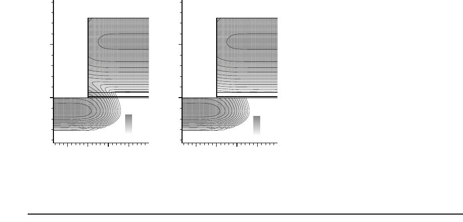
3: Ion Implantation

Analytic Implantation

Sentaurus™ Process User Guide 121

H-2013.03

default. To switch on the model, either specify the logical switch ts4.backscattering in

the implant command or use the global switch:

pdbSet ImplantData TS4Backscattering 1

In addition to the TS4 backscattering model, Sentaurus Process uses an advanced integration

algorithm that accounts for particles backscattered from the surface. The lateral integration for

a mesh node also is performed over 1D intervals above the surface. The point response is taken

from the surface layer. The contributions from backscattered ions make a difference in the

profile of vertical mask edges. The mask example in Figure 29 illustrates the difference.

The backscattering algorithm is switched on by default. To switched off the algorithm, use

either the logical switch !backscattering in the implant command, or use the global

switch:

pdbSet ImplantData Backscattering 0

Figure 29 Boron implantation at a vertical mask edge (left) with backscattering

and (right) without backscattering; tilt angle is 0o and energy is 35 keV

Multiple Implantation Steps

Preamorphization Implantation (PAI) Model

A structure already has implantation-related damage by the time an implantation is performed.

This damage contributes to the suppression of the channeling tail. This applies to a series of

-0.5

-0.2 0 0.2 0.4

-0.5

2.8e+18

1.7e+15

1.0e+12

-0.2 0 0.2 0.4

2.8e+18

1.7e+15

1.0e+12

3: Ion Implantation

Analytic Implantation

122 Sentaurus™ Process User Guide

H-2013.03

implantations performed without intermediate anneals. In this case, an equivalent amorphous

thickness is extracted as:

(53)

where Damage denotes the preexisting implant damage in terms of Frenkel pairs and

PAIThreshold is a normalization parameter that can be specified in the parameter database:

pdbSet <material> <species> PAIThreshold <n>

The extracted equivalent amorphous thickness is added to the total amorphous layer thickness.

If the implant table contains screen (cap) layer-dependent data, the total amorphous thickness

is used as a parameter to select the implant moments as described in Screening (Cap) Layer-

dependent Moments on page 98. Otherwise, the profile reshaping model and the effective

channeling suppression model are used.

The integral over the preamorphizing damage assumes periodic boundary conditions for the

structure in 2D.

The PAI model can be switched on using:

implant <species> energy=<n> dose=<n> pai

NOTE The switch is off by default. The model is switched on for the Taurus

implant tables.

CoImplant Model

The fraction of the ions described by the second Pearson function is taken from implantation

tables, which have been created for single ion implantation steps. This treatment is acceptable

only for low-dose implantations, which create little crystal damage, but leads to a severe

overestimation of the ion channeling in successive implantations with medium and high doses.

Without a thermal annealing step in between several ion implantations, the crystal damage of

the first implantations remains present and reduces the ion channeling of the subsequent

implantations. The channeling tail is lowered. Besides the PAI model as previously mentioned,

analytic implantation provides the CoImplant (CI) model, which also takes this effect into

account. In contrast to the PAI model in which the implant moments are modified locally for

each cutline during the integration, the CI model modifies the channeling ratio globally for

each implant. The CI model is switched on using the command:

pdbSetBoolean ImplantData UseCoImplant 1

tieqv,

PAIThreshold

-------------------------------------------Damage xd



ji≤



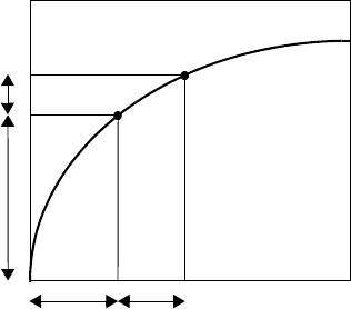
3: Ion Implantation

Analytic Implantation

Sentaurus™ Process User Guide 123

H-2013.03

The CI model is switched on by default.

NOTE The CI model is active only for Default implant tables, and does not

affect any other implant tables.

The CI model considers damage produced by analytic or MC implantation steps. The damage

information is used in subsequent analytic implantation steps to estimate the channeling ratio.

Using a least-square fit, an equivalent dose is calculated. This dose is chosen as the dose

that would give the same amount of damage in one implant step (using the present species and

implant conditions) as the preexisting damage, that is:

(54)

This is used to calculate the channeling dose from the total channeling dose and the

equivalent channeling dose, that is:

(55)

The channeling dose is calculated from the total dose using the differential channeling dose

technique (see Figure 30). is the channeling dose corresponding to an implantation of

into undamaged silicon.

Figure 30 Channeling dose as a function of dose

In Figure 30, due to the creation of damage during implantation, the number of channeling ions

increases sublinearly with the total ion dose, and eventually saturates at very high total doses.

The damage from previous implantations is set equivalent to a dose . The dose of the

additional implantation is shifted and, consequently, the gradient / and, therefore,

the dual Pearson ratio are reduced.

Deq

damage Deq x()][damagepreexist

–()

2xd

min=

new

new Dc

total Dc

–=

total

eq Dc

new

Dcnew

Dnew

Dceq

Deq Dose

Channeling Dose

Deq

new

Dnew

3: Ion Implantation

Analytic Implantation

124 Sentaurus™ Process User Guide

H-2013.03

Both and are stored in lookup tables. The channeling dose is used to

calculate the new ratio for the dualpearson model (see Primary Distribution Functions on

page 94).

This simple model is very accurate for mixed species implantations and works best in cases of

subsequent implantations with similar energies. The model is only available for the Default

implant mode.

The simplest way to calibrate the strength of de-channeling is given by using the effective

damage factor that scales the calculated equivalent dose:

pdbSetDouble ImplantData <species> EffDamFac <factor>

The default value is 1. Increased values lead to less channeling; lower values increase the

channeling of the species specified.

To calibrate the effective damage factor depending on parameters of the implantation, the

following procedure must be overwritten:

proc CI::coimp_dosesofar_calib { species energy dose tilt rotation } {

switch $species {

Boron { set cuc <expression_for_Boron> }

default { set cuc 1.0 }

}; # end of switch

return $cuc

}

Sometimes, it will be necessary to reset the accumulated damage field internally used by the

CI model. This can be achieved by using:

CI::Reset

To save and load the accumulated damage field, use:

CI::Save <filename>

CI::Load <filename>

The loaded damage is added to existing accumulated damage. The accumulated damage

produced by any implantation history can be checked with:

CI::Get_Damage_pdb Accumulated_Damage

This returns a list containing the vector describing the damage in the wafer on a logarithmic

depth scale. A zero vector means no damage history is seen by any follow-up table

implantation.

For more details about the CI model, see [15].

total

new

3: Ion Implantation

Analytic Implantation

Sentaurus™ Process User Guide 125

H-2013.03

To choose the PAI or CI model, use the global switch DamageControl:

pdbSet ImplantData DamageControl {Default PAI CoImplant}

The default value of DamageControl is Default in which the PAI model is automatically

switched on when Taurus tables are used; whereas, the CI model is chosen when default tables

are used. If DamageControl is set to PAI, the PAI model is active for all subsequent

implantations regardless of which tables are used. If this switch is set to CoImplant, the CI

model is used for all subsequent implantations (note that the CI model only supports default

tables), and PAI is disabled even for Taurus tables.

NOTE Both the PAI and CI models are designed to take into account the pre-

existing damage. However, the PAI model modifies the implant

moments locally, while the CI model modifies the channeling ratio

globally. Generally, for a complex structure, the PAI model is more

accurate at the expense of longer computation time.

NOTE The CI model was designed to work on the same structure among a

sequence of implant steps. If the structure changes between implants,

erroneous results could occur.

NOTE To avoid double-counting the damage effect, when the PAI model is

active, the CI model is disabled automatically.

Profile Reshaping

Traditionally, it is believed that the first peak of the implanted profile in monocrystalline silicon

is due to random scattering and is described by the first Pearson distribution in the dual-Pearson

analytic model. The second peak (or hump) of the implanted distribution is attributed to ion

channeling and is described by the second Pearson distribution in the dual Pearson model.

This approach works well for implantations with tilt angles above approximately , where

the position and width of the first Pearson distribution do not change as a function of the screen

oxide thickness. However, for low tilt implantations (below ), the position and width of the

first Pearson distribution changes considerably (up to 50%) with the thickness of the screen

oxide.

Typically, for a low tilt implantation performed into bare silicon, the first Pearson distribution

shifts deeper into the substrate and is much wider than for a similar high tilt implantation. As

the screen oxide thickness increases, the projected range and the standard deviation of the first

Pearson distribution relax to their respective values at high tilt angles due to reduced

channeling. Physically, this means that, for a low tilt implantation, even the first peak contains

a considerable number of channeled ions. To model this effect, it is necessary to reshape both

4°

3: Ion Implantation

Analytic Implantation

126 Sentaurus™ Process User Guide

H-2013.03

Pearsons in the dual Pearson model. This profile reshaping complements the reduction in

channeling fraction provided by the effective channeling suppression model.

For ions with explicit dependency on the screen oxide thickness in the implant tables, this

change in shape is addressed automatically. Otherwise, a shift is added to the projected range,

the standard deviation, and the lateral standard deviation of both Pearson distributions. The

shift is given by:

(56)

where:

■ is the shift for moment .

■ is the shift factor for moment .

■ is the cap layer thickness.

■ is the value of moment at high tilt value ( ).

■ is the value of moment at a given low tilt angle.

■For historical reasons, is the standard deviation of the first Pearson distribution.

However, this normalization quantity can be switched to the projected range by using the

command:

pdbSet ImplantData ProfileReshaping.Rp 1

The shift factor parameters of the profile reshaping model can be set in the parameter database,

that is:

pdbSet <material> <species> RangeFactor

pdbSet <material> <species> SigmaFactor

pdbSet <material> <species> ChannelingRangeFactor

pdbSet <material> <species> ChannelingSigmaFactor

The value of RangeFactor is used when calculating the shift of the projected range; the value

of SigmaFactor is used for both the standard deviation and the lateral standard deviation.

Setting a shift factor to zero effectively switches off this model for the respective moments.

Higher values of the shift factor lead to a faster transition from a low tilt profile to a high tilt

profile, with increasing amorphous layer thickness. By default, the shift factors are zero in all

materials except silicon.

The profile reshaping model can be switched on using:

implant <species> [profile.reshaping]

The model remains inactive for explicitly cap layer–dependent implant tables.

∆i1e

αit–

----------

–







MHiMLi

–()=

∆i

αi

MHi

7°

MLi

3: Ion Implantation

Analytic Implantation

Sentaurus™ Process User Guide 127

H-2013.03

NOTE This model is switched off by default and is switched on in the Taurus/

TSUPREM-4 mode.

Ge-dependent Analytic Implantation

SiGe material technology is used widely in stress engineering to improve device performance

(such as mobility). In addition, the depth of the source/drain junctions in Si(1–x)Ge(x) can be

remarkably reduced with an increase of the Ge content, which results from, not only the

reduced boron diffusion for PMOS source/drain, but also the reduced projected range and

channeling in as-implant itself.

Since the average mass of the atomic nucleus of the target is heavier in SiGe than in pure

silicon, a scattering angle from a nuclear collision is larger. In addition, SiGe has a larger

electronic stopping power than silicon due to the higher electron density. Therefore, similar to

the PAI model, the Ge effect on implantation can be modeled by using similar models for

profile reshaping and effective channeling suppression.

In this model, the equivalent germanium thickness is first extracted:

(57)

where denotes the germanium concentration and GeThreshold is a normalization

parameter that can be specified in the parameter database:

pdbSet <material> <species> GeThreshold <n>

The following formulas are then used for the projected range reduction and the standard

deviation shift:

(58)

(59)

where:

Ge.RangePreFactor

Ge.RangeFactor

Ge.SigmaPreFactor

Ge.SigmaFactor

tGe, eqv 1

GeThreshold

--------------------------------------------CGe xd



CGe

∆RPGe,Ge.RangePreFactor–RP0,1Ge.RangeFactor–tGe, eqv

RP0,

----------------⋅





exp–





⋅⋅=

∆σGe Ge.SigmaPreFactor–σGe 0,1Ge.SigmaFactor–tGe, eqv

RP0,

----------------⋅





exp–





⋅⋅=

3: Ion Implantation

Analytic Implantation

128 Sentaurus™ Process User Guide

H-2013.03

can be specified respectively in the parameter database as:

pdbSet <material> <species> Ge.RangePreFactor <n>

pdbSet <material> <species> Ge.RangeFactor <n>

pdbSet <material> <species> Ge.SigmaPreFactor <n>

pdbSet <material> <species> Ge.SigmaFactor <n>

Similar formulas also exist for the channeling projected range and channeling standard

deviation shifts with the parameter names:

Ge.ChannelingRangePreFactor

Ge.ChannelingRangeFactor

Ge.ChannelingSigmaPreFactor

Ge.ChannelingSigmaFactor

Finally, the following formula is used for effective channeling suppression:

(60)

where Ge.Sup.Ratio and Ge.Sup.Exponent can be specified in the parameter database:

pdbSet <material> <species> Ge.Sup.Ratio <n>

pdbSet <material> <species> Ge.Sup.Exponent <n>

Analytic Molecular Implantation

Sentaurus Process allows implanting arbitrary molecular species (such as BF2 and B10H14).

The implantation can proceed with or without the implant tables for the molecular species. If

implant tables are not available for the molecular species, an approximate calculation of the

dopant distribution is performed based on the tables for primary dopant species. Therefore, the

only requirement for molecular implantation is that the implant data tables are available for the

primary dopant species (such as B, As, or P). The primary dopant species, for which the profile

is calculated, is specified with the dataset parameter in the implant command:

implant species=<molecule> dataset=<dopant>

To switch on the damage calculation in silicon for the molecular implant, use:

implant species=<molecule> Silicon damage

rGe rGe 0,

Ge.Sup.Ratio

Ge.Sup.Ratio tGe, eqv

RP0,

----------------+

-----------------------------------------------------------------------







Ge.Sup.Exponent

⋅=

3: Ion Implantation

Analytic Implantation

Sentaurus™ Process User Guide 129

H-2013.03

In a molecule, the implant energy is shared by several atoms according to:

(61)

where is the energy of the -th species, is the atomic mass, and is the statistical

weight according to the stoichiometry of the molecule. The constituent and stoichiometry of

the molecule are defined in the PDB.

You c an de fin e n ew mo le cul ar s pec ies wi th pdb commands. For example, you can define

carborane as follows:

pdbSetString ImplantData Carborane Atom0 Name Boron

pdbSetDouble ImplantData Carborane Atom0 StWeight 10

pdbSetString ImplantData Carborane Atom1 Name Hydrogen

pdbSetDouble ImplantData Carborane Atom1 StWeight 14

Then to initialize the species, use the command:

implant species=Carborane dataset=Boron

After the above two steps are performed, you can use carborane like any other predefined

implant species. For example, use the following command to perform analytic implantation for

carborane:

implant

Carborane

energy=10 dose=1e14

NOTE The dose specified for molecular implantation is the dose for the

molecular species. In the above example, the implanted dose for

carborane is . Therefore, the boron dose is ,

and the hydrogen dose is .

For convenience, Sentaurus Process predefines the following molecular species: BF2 (BF2),

BCl2 (BCl2), B10H14 (B10H14), B18H22 (B18H22), C2B10H14 (C2B10H14), AsH2 (AsH2),

and PH2 (PH2).

Depending on whether the implant tables are supplied for the molecular species, analytic

molecular implantation will proceed in two different ways:

■With supplied implant tables

■Without supplied implant tables

Eienergy Mi

wjMj



-------------------⋅=

114

×10 cm 2–

115

×10 cm 2–

1.4 15

×10 cm 2–

3: Ion Implantation

Analytic Implantation

130 Sentaurus™ Process User Guide

H-2013.03

Molecular Implantation with Supplied Implant Tables

If the implant tables are available for the molecular species (for example, BF2), the

implantation proceeds in the same way as the atomic species; in other words, the specified

energy and dose are used to look up the moments in the implant tables. No scaling is applied

to energy, dose, or the resulting profiles.

The implant tables can be specified for a molecular species with the command:

implant species=<molecule> <material> imp.table=<file> dam.table=<file>

The implant data files should be placed in the current working directory or the full path to the

file should be specified in imp.table.

Molecular Implantation without Supplied Implant Tables

If the implant tables are not available for the molecular species, Sentaurus Process performs an

approximate calculation of the dopant distribution using the implant tables for the primary

dopant species. The energy for the -th species (which is assumed to be the primary dopant

species) is calculated using Eq. 61.

Assuming that there are dopant atoms in a molecule, the molecular implantation is

equivalent to a single atomic species implantation with the energy and dose equal to and

(where dose is the molecular dose), respectively. and are used for

implant moments lookup. Then, the dopant distribution is calculated in the same way as atomic

implant.

BF2 Implant

BF2 is a special molecular species in analytic implant because both boron and fluorine

distributions are calculated in Sentaurus Process. By default, the fluorine profile is simply a

boron profile multiplied by two. However, you can turn on the following switch to enable the

separate calculation of fluorine distribution by using the fluorine implant tables:

pdbSet ImplantData TS4FluorineMode 1

When TS4FluorineMode is true, the fluorine profile will be computed using the fluorine

tables in the same way as in TSUPREM-4.

Nidose×

3: Ion Implantation

Analytic Implantation

Sentaurus™ Process User Guide 131

H-2013.03

Damage Calculation

If damage tables are not supplied for the molecular species, the damage also can be calculated

using the internal damage tables for the primary dopant species. The Boolean parameter

FullDamage can be used to control the amount of damage for the molecular species:

pdbSetBoolean ImplantData <molecule> FullDamage <bool>

If FullDamage is true, the calculated damage is multiplied by a scaling factor:

(62)

This damage scaling factor roughly takes into account the damage produced by all atomic

species (including the primary dopant species) and is consistent with the damage calculation

used in TSUPREM-4 for BF2 implantation.

Performing 1D or 2D Analytic Implantation in 3D Mode

Because analytic implantation performs lateral integration differently for one, two, and three

dimensions, it may result in slightly different profiles from vertical 1D cuts, even though the

same implant moments are used. In addition, for a 2D structure, the vertical 1D profiles also

may be different depending on the beam direction on the simulation plane or not, in other

words, depending on the rotation angles.

To obtain the same results in one, two, or three dimensions, or with different rotation angles,

Sentaurus Process provides an option to perform 1D or 2D implantation in 3D mode, in which

case, a 1D or 2D structure will first be extruded into a pseudo-3D structure. In other words,

only the surfaces and interfaces (not the bulk) will be extended in the y- or z-direction or both

directions, with the boundary conditions being taken into account. In the case of PAI, damage

integration is performed in a real 1D or 2D structure. Then, the lateral integration proceeds in

exactly the same way as in a 3D analytic implantation. This ensures consistent results for 1D,

2D, and 3D implantation.

To switch on this option, use either the Boolean parameter extrude in the implant command

or the global pdb switch:

pdbSet ImplantData Extrude 1

wjMj



-------------------=

3: Ion Implantation

Analytic Implantation

132 Sentaurus™ Process User Guide

H-2013.03

Implantation on (110)/(111) Wafers Using (100) Implant

Tables

The Sentaurus Process software distribution typically includes a large set of implant tables for

Si(100) wafers, but it does not include any implant tables for Si(110) or Si(111) wafers.

However, you sometimes need to perform process simulations on (110) or (111) wafers. Since

the Si(100) implant moments cannot be used directly for Si(110) or Si(111) wafers, certain

transformations of implant moments are required to use these tables for Si(110) or Si(111)

wafers.

Since SIMS depth profiles are measured along the wafer normal direction, the extracted

implant moments also are obtained with respect to the wafer normal direction. On the other

hand, analytic implantation is usually calculated by using the beam direction as its primary

direction. If the beam direction is coincidental with the normal direction, the implant moments

can be used directly without modification. However, for tilt implantations, the beam direction

does not coincide with the wafer normal direction. In this case, implant moments to be applied

to the primary beam direction must be scaled, or transformed, to reproduce the 1D profiles in

the wafer normal direction. See Primary Direction and Scaling on page 115 for more details.

Essentially, the projected range is scaled as follows:

(63)

where is the scaling factor, and the primary standard deviation is scaled as follows:

(64)

To use Si(110) implant tables for Si(110) or Si(111) implantations, you must calculate the

corresponding angles on the (100) wafers from the specified implantation angles on the (110)

or (111) wafers. For typical implantations (for example, tilt=), these angles are very large.

When you know the corresponding angle on the (100) wafer, you can use Eq. 63 and Eq. 64 to

transform and . Eq. 63 works by simple geometry consideration. Eq. 64 works

reasonably well for small tilt implantations and, in theory, is accurate for isotropic amorphous

material. However, due to ion channeling, Eq. 64 may not be good under all situations.

′Rpsr

⋅=

σp

σp′sr

2σp

⋅1sr

–()σ

⋅+=

7°

σp

3: Ion Implantation

Monte Carlo Implantation

Sentaurus™ Process User Guide 133

H-2013.03

Therefore, the following options for scaling are provided:

■Case 0 (constant):

■Case 1 (linear):

■Case 2 (standard):

The default scaling is the same as the scaling (linear scaling). These cases can be

selected by using the command:

pdbSet ImplantData StdevScalingMode {0 | 1 | 2}

Monte Carlo Implantation

Running Sentaurus MC or Crystal-TRIM

Sentaurus Process is capable of the atomistic simulation of ion implantation using either the

Monte Carlo (MC) simulator Sentaurus MC, which is an improved multithreaded version of

Taurus MC [7], or Crystal-TRIM [8], which originated from the Transport of Ions in Matter

(TRIM) code [2]. MC implantation simulates ion implantation into single-crystalline materials

or into amorphous materials of arbitrary composition. In Sentaurus Process, to select MC

implantation at the command line, use:

implant <dopant> [crystaltrim | sentaurus.mc]

Alternatively, to select MC implantation as the default implantation model, use a global switch:

pdbSet ImplantData MonteCarlo 1

pdbSet MCImplant model [crystaltrim | sentaurus.mc]

When MonteCarlo is set to 1, Sentaurus Process performs all the implantations using one of

the selected MC models (crystaltrim

sentaurus.mc).

NOTE For simplicity, you could use the alias tmc instead of sentaurus.mc

or ctrim instead of crystaltrim. For example, you may initiate

Sentaurus MC implant with the following command:

implant <dopant> energy=<n> tmc

Fundamental implantation parameters, such as the implantation energy and dose, and the

orientation of the ion beam with respect to the substrate must be specified using energy, dose,

tilt, and rotation in the same way as for analytic implantation.

σp

σp′σ

σp

′σpsr

⋅=

σp′sr

2σp

⋅1sr

–()σ

⋅+=

σp

3: Ion Implantation

Monte Carlo Implantation

134 Sentaurus™ Process User Guide

H-2013.03

To run MC implantation in a full-cascade mode or improved BCA (iBCA) damage model, use

the cascades or iBCA switch:

implant <dopant> [ctrim | tmc] [cascades | iBCA]

or using a global switch:

pdbSet MCImplant cascades 1

pdbSet MCImplant iBCA 1

In the KMC mode, to specify the dose rate of the implantation, use the dose.rate parameter:

implant <dopant> [ctrim | tmc] [cascades | iBCA] [dose.rate=<n>]

If dose.rate is specified, it is assumed to be a uniform dose rate in units of cm–2/s. If it is not

specified, a Tcl procedure will be called:

proc DoseRate {dose} { ... }

which returns an implantation time as a function of implantation dose. By default, it is a

uniform dose rate; that is, DoseRate is a linear function of dose. However, you can specify

any monotonic function to take into account the particular implantation equipment setup or

scanning patterns.

During the implantation, pseudoparticles representing a part of the whole dose are started from

the start surface, which is constructed above the target, parallel to the wafer surface. For 2D

and 3D target geometries, the start surface is subdivided into segments of equal size for which

the required implantation dose is accumulated. The size of these segments can be controlled by

setting:

pdbSet MCImplant Intervals dy <n>

pdbSet MCImplant Intervals dz <n>

For 1D structures, no subdivision is performed. The number of pseudoparticles that will be

started per segment can be set in the parameter database or at the command line:

pdbSet MCImplant Particles <n>

3: Ion Implantation

Monte Carlo Implantation

Sentaurus™ Process User Guide 135

H-2013.03

or:

implant <dopant> [crystaltrim | sentaurus.mc] [particles=<n>]

The default value is 1000. Increasing this number leads to better accuracy and an increase in

simulation time. Together with the sizes of the segments, this parameter determines the

statistical weight of each pseudoparticle.

Launching particles are assumed to be traveling along the direction as specified by the tilt and

rotation angles. However, there is usually a small angular divergence of the ion beam so that

the particles form a right circular cone in which particles are assumed to be uniformly

distributed. To specify BeamDivergence angle (the angle between the cone axis and the cone

surface), use:

pdbSet MCImplant BeamDivergence <n>

Parameters controlling the electronic and nuclear stopping as well as the damage accumulation

are available in the parameter database (see Parameter Database on page 55). You can set these

parameters in there.

If the information level is set to 1 or above, a progress report similar to the following will be

shown during the progress of implant:

implanted orig equiv active repl traject CPU time

particles traject classes segm OK fail step total

.............................................................................

1300( 5%) 84 4 26 1216 6 0.22 0.22

2600( 10%) 170 4 26 2430 9 0.21 0.43

3900( 15%) 262 4 26 3638 16 0.21 0.64

5200( 20%) 349 4 26 4851 24 0.30 0.94

6500( 25%) 437 4 26 6063 29 0.47 1.41

7800( 30%) 523 4 26 7277 33 0.28 1.69

...... ...... ......

22100( 85%) 1894 4 5 20206 131 3.15 7.27

23400( 90%) 2875 4 5 20525 272 5.20 12.47

24700( 95%) 3837 4 5 20863 394 4.75 17.22

24960( 96%) 4029 4 5 20931 419 0.99 18.21

25220( 97%) 4231 4 5 20989 453 1.13 19.34

25480( 98%) 4422 4 5 21058 472 0.90 20.24

25740( 99%) 4628 4 1 21112 483 0.93 21.17

26000(100%) 4888 4 0 21112 483 0.45 21.62

.............................................................................

Pseudo particles:

implanted : 26000

lost : 0 (0%)

Trajectories : 4888

Equivalence classes: 4

3: Ion Implantation

Monte Carlo Implantation

136 Sentaurus™ Process User Guide

H-2013.03

where:

■implanted particles: The total number of pseudoparticles implanted, which is, at the

end of the simulation, equal to the product of the specified number of particles and the

total number of segments of the implant surface. This number includes both the calculated

number of particles and the successfully replicated number of particles. The percentage of

already finished particles is also indicated in parentheses.

NOTE In a multithreaded implant, the thread ID is also shown before the

percentage. For example, 6500 (2: 25%) means that thread #2 has

implanted 6500 particles and finished 25%.

■orig traject: The original number of trajectories that are based on the physical

calculations.

■equiv classes: The number of equivalent classes in the current structure as detected by

probing ions. For more details on equivalent classes and probing ions, see Trajectory

Replication on page 178.

■active segm: The number of currently active segments of the implant surface. At the

beginning of the implant, this number is equal to the total number of start segments. This

number should decrease as the implant progresses. At the end of the implantation, the

number becomes zero as all segments have the required implant dose and become

deactivated.

■repl traject (OK and fail): The number of replicated trajectories. The number of

successfully replicated trajectories is shown in the OK column; whereas, the number of

unsuccessful trajectories is shown in the fail column.

■CPU time (step and total): This CPU time includes the time spent for the current step

and the total CPU time for the current implant.

For 2D structures, the progress of an ion implantation step can be graphically viewed using the

switch ion.movie, for example:

implant <dopant> [ctrim | tmc] [ion.movie]

Structure of Target Material

MC implantation simulates the motion of energetic particles in amorphous materials and

single-crystalline materials.

Composition

For each material, the composition is set in the parameter database. The composition can be

found in the <material> -> Composition entry. For each <n>-component of the material,

3: Ion Implantation

Monte Carlo Implantation

Sentaurus™ Process User Guide 137

H-2013.03

the entry Component<n> gives the name and the stoichiometric weight, for example, for

GaAs:

GaAs -> Composition -> Component0 -> Name = Gallium

GaAs -> Composition -> Component0 -> StWeight = 1

GaAs -> Composition -> Component1 -> Name = Arsenic

GaAs -> Composition -> Component1 -> StWeight = 1

or for silicon nitride:

Nitride -> Composition -> Component0 -> Name = Silicon

Nitride -> Composition -> Component0 -> StWeight = 3

Nitride -> Composition -> Component1 -> Name = Nitrogen

Nitride -> Composition -> Component1 -> StWeight = 4

The composition for both single-crystalline and amorphous materials is set this way.

Single-Crystalline Materials

Lattice Structure

In the case of a single-crystalline material, the positions of target atoms are calculated based

on the lattice type. Crystal-TRIM supports zinc-blende (Zincblende) lattice only, while

Sentaurus MC supports several lattice types that include simple cubic (Sc), body-center cubic

(Bcc), face-center cubic (Fcc), zinc-blende (Zincblende), and hexagonal (Hexagonal)

lattices. To set the lattice type, use:

pdbSet <material> LatticeType [Sc | Bcc | Fcc | Zincblende | Hexagonal]

Lattice Constants

To change the lattice constant defined in the parameter database, use:

pdbSet <material> LatticeConstant <n>

For all lattice types, Sentaurus MC defines different lattice constants for three different axes.

To define the other two lattice constants, use:

pdbSet <material> LatticeConstant_b <n>

pdbSet <material> LatticeConstant_c <n>

If LatticeConstant_b and LatticeConstant_c are not defined, LatticeConstant is

used for all three axes. For a hexagonal lattice, LatticeConstant_b should be equal to

LatticeConstant.

3: Ion Implantation

Monte Carlo Implantation

138 Sentaurus™ Process User Guide

H-2013.03

Polytypes

For hexagonal systems, there may exist many different crystal structures due to the different

stacking sequence along the -axis, which is perpendicular to the plane formed by three -

axes ( , , and ). This is called polytypism. Four different polytypes are supported in

Sentaurus MC, and you can select them using the following command:

pdbSet <material> Polytype {2H 3C 4H 6H}

The default polytype for silicon carbide (SiC) is 4H. For more details, see MC Implantation

into Silicon Carbide on page 165.

Atomic Basis

The crystal structure consists of an atomic basis attached to the lattice points. A basis can be a

single atom or a group of atoms attached to each lattice point. In Sentaurus MC, for simple

crystals (such as a single-atom basis with simple cubic, face-centered cubic, or body-centered

cubic lattice and binary compounds with zinc-blende and hexagonal lattice), the undisturbed

positions of the lattice sites are constructed automatically using the information of the lattice

type, the polytype (if hexagonal lattice), and the lattice constants. For more complex crystal

structures, the positions of basis atoms should be specified with the pdb parameter

BasisVector. The units of basis vectors are lattice constants in three crystallographic axes.

For example, for zinc-blende silicon, the positions of two basis silicon atoms can be specified

as follows:

Silicon -> Composition -> Component0 -> Name = Silicon

Silicon -> Composition -> Component0 -> StWeight = 1

Silicon -> Composition -> Component0 -> BasisVector = {0 0 0 0.25 0.25 0.25}

For another example, NaCl has a face-centered cubic (Fcc) lattice with an atomic basis of two

atoms. The positions of Na and Cl can be specified as follows:

NaCl -> Composition -> Component0 -> Name = Sodium

NaCl -> Composition -> Component0 -> StWeight = 1

NaCl -> Composition -> Component0 -> BasisVector = {0 0 0}

NaCl -> Composition -> Component1 -> Name = Chloride

NaCl -> Composition -> Component1 -> StWeight = 1

NaCl -> Composition -> Component1 -> BasisVector = {0.5 0.5 0.5}

In Crystal-TRIM, the positions of lattice sites of the basic cell are set in the parameter database

in MCImplant -> Lattice -> Zincblende -> Cell0 in the natural coordinate system

of crystal. The unit is one-half of the lattice constant. The undisturbed positions of all lattice

sites of an ideal zinc blende–type crystal can be obtained from the basic cell by shifting the

atomic positions in the directions of the crystallographic axes. Therefore, for any given position

of the projectile, only the immediate crystalline environment is generated and rebuilt every

time the projectile moves out of the current crystalline cell.

3: Ion Implantation

Monte Carlo Implantation

Sentaurus™ Process User Guide 139

H-2013.03

The entry MCImplant -> Lattice -> Zincblende -> Cell1 is a complementary basic

cell and gives the configuration that is obtained by shifting Cell0 by one-half of the lattice

constant.

Thermal Vibrations

The thermal vibrations of the target atoms are important for the treatment of the motion of a

projectile in single-crystalline material. In MC implantation, only instantaneous thermal

displacements of target atoms from their ideal lattice sites are considered.

The displacements are assumed to obey a 3D Gaussian distribution with a root-mean-square

obtained by the Debye model. The Debye temperature is set in the parameter database and can

be changed with:

pdbSet <material> DebyeTemperature <n>

The default Debye temperature is 519 K for silicon.

The substrate temperature for the Debye model can be set by:

pdbSetDouble MCImplant Temperature <n>

The default substrate temperature is 300 K.

Amorphous Materials

The structure of an amorphous material is described in a simplified manner by assuming an

average interatomic distance in the target material.

Variable Mass Density

It is possible to use a dataset MassDensity as the mass density of an amorphous material:

pdbSetBoolean <material> VariableMassDensity 1

Using molar fractions (see Molar Fractions on page 140) is disabled in these materials.

Polycrystalline Materials

A polycrystalline material is characterized by its crystal orientation and grain size. Crystal

orientation (one of 100, 110, and 111) can be specified by using a material-specific command:

pdbSet <material> CrystalOrient <n>

3: Ion Implantation

Monte Carlo Implantation

140 Sentaurus™ Process User Guide

H-2013.03

There are two different ways to change the crystallinity (Amorphous, Crystalline, and

Polycrystalline) of a material. If parameter Crystallinity is available (which is true

for polysilicon) in the PDB, use this switch to set the crystallinity, for example:

pdbSet PolySilicon Crystallinity Polycrystalline

This command makes MC implantation models consider both crystal orientation and grain size

for polysilicon.

If Crystallinity does not exist for a material, use parameters Amorphous and Granular:

pdbSet <material> Amorphous 0

pdbSet PolySilicon Granular 1

The first command switches off the amorphous treatment, and the second command makes MC

implantation models consider the grain size.

For more details on ion implantation into polysilicon, see MC Implantation into Polysilicon on

page 162.

Molar Fractions

It is possible to define a compound material with a spatially-dependent molar fraction. For

example, for single-crystalline silicon, the following PDB entry:

array set $Base {BinaryCompounds {String {

{ SiliconGermanium GeTotal "GeTotal/[pdbGetDouble Si LatticeDensity]" }

}}}

specifies a binary compound Si1–xGex with the mole fraction of Ge calculated from the

germanium concentration (GeTotal) divided by the silicon lattice density. Due to more

computational demands, a minimum Ge concentration is required to trigger MC implantation

models to treat this material in a more sophisticated way. To specify this minimum

concentration, use the command:

pdbSet Silicon SiliconGermanium.MCmin 1e20

If the concentration of Ge in any of the mesh elements of silicon regions exceeds

, MC models treat silicon as a compound material. In this case, the average

charge and mass of the material is calculated individually for each mesh element. The lattice

constant, the nonlocal electron stopping power, and the Debye temperature are linearly

interpolated based on the mole fractions. For more details, see MC Implantation into

Compound Materials with Molar Fractions on page 163.

110

× cm 3–

3: Ion Implantation

Monte Carlo Implantation

Sentaurus™ Process User Guide 141

H-2013.03

Sentaurus MC Physical Models

The Sentaurus MC implantation model, which is an improved, multithreaded version of Taurus

MC, was designed to be generally accurate and predictive with minimum user calibrations for

most implant conditions. It has been calibrated from sub-keV to above 10 MeV, and for

different implant conditions including random implant direction, <100>, <111>, and <110>

channeling directions, with the same set of parameters for boron, phosphorus, and arsenic

implants [7]. It also is accurate for other implant species such as BF2, F, Al, Ge, In, and Sb

[7][16]. For a detailed discussion of the physical models in Sentaurus MC and an extensive

comparison with experimental SIMS profiles from sub-keV to above 10 MeV and with other

MC simulators, refer to the literature [7][16]. This section briefly outlines the pertinent theory

and models.

The calculation used in the Sentaurus MC model assumes that ions lose energy through two

processes:

■Nuclear scattering, where the nucleus of the ion elastically scatters off the nucleus of an

atom in the target. This interaction is based on the binary collision theory and is described

in the following section.

■Interaction of the ion with the electrons of the target atoms. This mechanism is inelastic

and does not alter the direction of the motion of the ion.

Therefore, the total change in energy of the ion after the -th collision is the sum of the nuclear

energy loss and the electronic energy loss :

(65)

Binary Collision Theory

Sentaurus MC implantation models the energy loss of nuclear collision according to the

classical binary scattering theory. The basic assumption of the mechanism for the energy loss

of nuclear collision is that the ion interacts with only one target atom at a time. This assumption

enables the use of the binary scattering theory from classical mechanics [17].

Consider a particle of mass and kinetic energy approaching a stationary particle with

mass . The impact parameter, , is the distance of closest approach if the particle is not

deflected and gives a convenient measure of how close the collision is. After collision, the first

particle deviates from its original course by an angle .

∆En

∆Ee

EiEi1–∆En

–∆Ee

–=

3: Ion Implantation

Monte Carlo Implantation

142 Sentaurus™ Process User Guide

H-2013.03

Energy Loss

It can be shown that the first particle loses kinetic energy:

(66)

where:

■ is the energy lost by particle 1.

■ is its energy before collision.

■ is the integral.

(67)

where is the inverse separation between the two particles. is the potential

between the two particles (assumed to be repulsive), and:

(68)

is the reduced energy in the center of mass coordinates.

The upper limit of the integral, , is the inverse distance of closest approach of the two

particles and is given by the solution to the equation:

(69)

Scattering Angle

The angle by which particle 1 is deflected is given by:

(70)

NOTE For , approaches zero.

∆En

----------4M1M2

M1M2

+()

---------------------------- cos2bI()=

∆En

Isd

1Vs()

-----------– b2s2

–

-----------------------------------------

smax



s1r⁄=

Vs()

1M1M2

⁄+

----------------------------=

smax

1Vs

max

()

-------------------– b2smax

–0=

cosθ

1 0.5 1 M2

-------+∆EnE0

⁄–

1∆EnE0

⁄–

------------------------------------------------------------=

∆EnE0

⁄1«

3: Ion Implantation

Monte Carlo Implantation

Sentaurus™ Process User Guide 143

H-2013.03

Dimensionless Form

Eq. 66 to Eq. 70 are the basic equations for classical two-body scattering. The scattering

integral, Eq. 67, can be cast into a dimensionless form by assuming the potential has the form:

(71)

where:

■ is the charge on particle 1.

■ is the charge on particle 2.

■ is the constant.

(72)

is an arbitrary function of , to be defined later, and is a unit of length. Taurus

MC uses the so-called universal screening length [18]:

(73)

and a dimensionless impact parameter:

(74)

and a dimensionless energy:

(75)

Using Eq. 71, Eq. 74, and Eq. 75 in the scattering integral Eq. 67 and making the substitution

gives:

(76)

From Eq. 66, the quantity of interest is , which becomes:

(77)

Therefore, using Eq. 77, can be evaluated in terms of the dimensionless variables

and , without reference to the charge or mass of a particular particle.

Vs() Z1Z2k1sg aus()=

k1q2

4πε0

------------14.39495 10 7–

×keVµm==

us()

aus

au0.8854 10 4–

×0.529

0.23 Z2

0.23

+()

---------------------------------- µm=

bnba

⁄=

εauEr

Z1Z2k1

-----------------=

s′aus=

-----= s′d

1s′gs′()εbn

2s′2

–⁄–

-------------------------------------------------------

s′max



cos2bI()

cos2bI() cos2bn

s′d

1s′gs′()εbn

2s′2

–⁄–

-------------------------------------------------------

s′max



cos2bl()

3: Ion Implantation

Monte Carlo Implantation

144 Sentaurus™ Process User Guide

H-2013.03

Coulomb Potential

As an example of the above procedure, consider the Coulomb potential between two particles:

(78)

or:

(79)

In this case, . Then, from Eq. 77:

(80)

with:

(81)

from a solution of Eq. 69.

Then, the integral can be evaluated exactly, giving:

(82)

For a given impact parameter and incident energy , the dimensionless and can be

obtained from Eq. 74 and Eq. 75, giving from Eq. 82. Then, the energy loss due to

the collision is given by Eq. 66, and the angle at which particle 1 leaves the collision is given

by Eq. 70.

Universal Potential

For the simple form of the Coulomb potential used in the previous example, the scattering

integral can be solved analytically. For more realistic interatomic potentials, however, the

scattering integral cannot be evaluated analytically.

Vr() Z1Z2k1

-----------------=

Vs() Z1Z2k1s=

us()1=

cos2bI() cos2bn

s′d

1s′ε bn

2s′2

–⁄–

------------------------------------------

s′max



s′max

14bn

2ε2

+1–





2εbn

------------------------------------------=

cos2bI() 1

14bn

2ε2

-----------------------=

cos2bI()

3: Ion Implantation

Monte Carlo Implantation

Sentaurus™ Process User Guide 145

H-2013.03

For example, the universal potential [18] that is used in Sentaurus MC is:

(83)

An analytic solution does not exist since the upper limit of the integral in Eq. 67 is given by

Eq. 69, which becomes a transcendental equation with this potential. In Taurus MC, the

quantity , in its dimensionless form (Eq. 77), is numerically integrated for a wide

range of its parameters and . These results are stored in tables. Then, at each collision,

is obtained from these tables. This scheme eliminates the need to find for each

collision, minimizing the amount of arithmetic operations performed during the calculation of

the trajectory of an ion, while retaining accuracy.

Tables for the universal potential over a wide range of energies and impact parameters are

provided for immediate use in Taurus MC. These tables span the normalized energy range of

and the normalized impact parameter range . For , the

Coulombic form (Eq. 83) is used. Values of are not encountered for ion–atom

combinations of interest at energies above the energy at which the ion is assumed to have

stopped (5 eV). For values of , the ion is assumed to be undeflected.

Implantation into Amorphous Materials

This section describes how the binary scattering theory of the previous section is used to

calculate ion trajectories in an amorphous solid. Assume an ion with kinetic energy hits a

target with an angle with respect to the target normal. The surface of the target is assumed

to be at , with increasing vertically into the target. To set the incident energy in

the implant command, use the Energy parameter. To specify the incident angle in the

implant command, use the tilt parameter.

Given the atomic density for the target material, the mean atomic separation between

atoms in the target is . Between scattering events, the ion is assumed to travel a

distance:

(84)

As the ion enters the target material, it approaches the first target atom with impact parameter

, defined in the previous section. The probability of finding a target atom between and

is given by:

(85)

for .

Vr() Z1Z2k

---------------0.18175e3.1998ra

⁄–0.50986e0.94229r–au

⁄

0.28022e0.4029ra

⁄–0.028171e0.20162ra

⁄–

cos2bI()

smax

10 5–ε100≤≤

0bn30≤≤

ε100>

ε10 5–

bn30>

θ0

y0=

θ0

Ndens

1Ndens

()⁄13⁄

L1Ndens

()⁄13⁄

bδb+

wb()δb2πNdens

23⁄b δb=

b1πNdens

23⁄

⁄<

3: Ion Implantation

Monte Carlo Implantation

146 Sentaurus™ Process User Guide

H-2013.03

If is a uniformly distributed random number between 0 and 1, the probability distribution

gives:

(86)

Given the above definitions, the algorithm for calculating the energy loss through nuclear

collisions experienced by the ion proceeds as follows:

■A random number between 0 and 1 is chosen.

■The normalized impact parameter for this collision is calculated from Eq. 74 and Eq. 86:

(87)

■The ion energy, , is normalized to:

(88)

from Eq. 68, p. 142 and Eq. 75, p. 143.

■Now, the value of can be obtained from the tables, and Eq. 66, p. 142 gives the

energy loss due to nuclear scattering:

(89)

where nucl.cor is an empirical nuclear-scattering correction factor with a default value

of 1.0, which can be changed in the parameter database by using:

pdbSetDouble <material> <dopant> nucl.cor <n>

This procedure is repeated for each collision event.

Implantation into Crystalline Materials

The binary collision calculation for crystalline materials proceeds in the same way as in the

amorphous case, except that the selection of the collision partners of the projectile with target

atoms is conducted in a more sophisticated manner.

Instead of using the density of the target material and a random number, Sentaurus MC

determines the collision partners based on the position of the projectile relative to the sites on

an idealized lattice. The algorithm for selecting the collision partners is based on

Rrand

bRrand

πNdens

23⁄

----------------=

----- Rrand

πNdens

23⁄

----------------=

εauE0

1M1M2

⁄+()Z1Z2k1

---------------------------------------------------=

cos2bI()

∆E0nucl.cor E⋅0 4M1M2

M1M2

+()

---------------------------- cos2bI()=

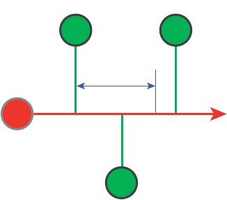
3: Ion Implantation

Monte Carlo Implantation

Sentaurus™ Process User Guide 147

H-2013.03

MARLOWE [19]. Sentaurus MC implantation uses a sophisticated multibody collision

algorithm to simulate the collisions of well-channeled particles, as shown in Figure 31.

Figure 31 Illustration of “simultaneous” collision, and definition of the d.sim parameter

If the distance of two or more projected target atoms to the undeflected trajectory of the

incident particle is less than d.sim (simultaneous collision distance), then the multibody

collision algorithm is invoked. For example, in Figure 31, 1 and 2 are considered to be

simultaneous collisions, but 3 is not. To change the default value of d.sim, use the command:

pdbSetDouble <material> d.sim <n>

The scattering events are computed for each target individually, and the final moment and

energy of the incident particle are computed by applying momentum and energy conservation

principles.

The simultaneous collisions are handled in the same way as for MARLOWE, except for the

location of the turning point. In MARLOWE, the turning point is assumed to be the average of

those of the simultaneous collision partners. In Sentaurus MC, the turning point is placed at a

point determined by the collision with the minimum impact parameter. Simulations have

indicated that such a scheme obtains better results for ultralow energy implantations, while it

has little impact on implantation energies above 5 keV. This allows Sentaurus MC to treat the

entire implantation energy range, including ultralow energy and very high energy, with the

same model, in exactly the same way.

Ion channeling, which is the preferential penetration of implanted ions along crystal axes or

planes, occurs naturally due to the inclusion of the crystal structure of the lattice. Both axial

and planar channeling show enhanced penetrations. The effect of the tilt and rotation

parameters is much more pronounced for implants into crystalline silicon than into amorphous

silicon.

d.sim

Lattice Atoms

Incident Particle

3: Ion Implantation

Monte Carlo Implantation

148 Sentaurus™ Process User Guide

H-2013.03

Electronic Stopping Model

A moving ion loses energy by inelastic electronic processes, which include both nonlocal and

local stopping power. Sentaurus MC uses the same electronic stopping model for both

amorphous and crystalline materials. For each collision, the energy loss due to electronic

stopping is:

(90)

(91)

(92)

where is the scaled dimensionless energy.

nloc.pre and nloc.exp are specified in the material parameter database and can be changed

by using:

pdbSet <material> <dopant> nloc.pre <n>

pdbSet <material> <dopant> nloc.exp <n>

Nonlocal Electronic Stopping

Nonlocal electronic stopping acts as the dragging (frictive) force on moving ions, which is

proportional to the ion velocity and is independent of the impact parameter:

(93)

(94)

where is the free flight path between collisions and is the ion energy at the stopping

power maximum.

The quantities and are given by [7][20]:

(95)

(96)

∆Eexnl ∆Enl

exloc ∆Eloc

⋅+⋅=

xnl xloc

+1=

xnl min nloc.pre εnloc.exp 1,⋅()=

∆Enl

eLN

dens Se

⋅⋅=

SeLSS.pre Ses Emfes

1–

⋅⋅ ⋅=

Ses

fes

Ses

1.212 Z1

76⁄ Z2

23⁄Z2

23⁄

32⁄

12⁄

-------------------------------------------------------=

fes

E0Em

⁄

E0Em

⁄EmE0

⁄e2–++()ln

---------------------------------------------------------------------





δ2⁄Em

-------





δ2⁄

+1δ⁄

3: Ion Implantation

Monte Carlo Implantation

Sentaurus™ Process User Guide 149

H-2013.03

where:

■ is the ion atomic number.

■ is the composite target atomic number.

■ is the base of natural logarithm.

■ is a fitting parameter.

LSS.pre is specified in the material parameter database; to change it, use:

pdbSet <material> <dopant> LSS.pre <n>

Local Electronic Stopping

Local electronic loss is a result of the electron exchange between the moving ion and the target

atom, which is based on the Oen–Robinson model [21] and is dependent on the impact

parameter:

(97)

(98)

(99)

where scr.par is an adjustable screening length parameter that you can change by using:

pdbSet <material> <dopant> scr.par <n>

Damage Accumulation and Dynamic Annealing

As the ions travel through a crystalline target, they collide with the target atoms and displace

many of them from their lattice sites. In the binary collision approximation (BCA) code, it is

assumed that, if the transferred energy exceeds a certain threshold, the target atom is displaced

and, at this lattice site, a vacancy is generated. When the displaced atom comes to rest, it is

identified as an interstitial. This defect production rate can be evaluated either by the modified

Kinchin–Pease formula [22] or by simulating the full cascade. Sentaurus MC provides both

types of damage calculation.

δ1.425=

∆Ee

loc Se

2πa2

------------ b

---–





exp⋅=

0.3

-------

⋅=

fscr.par 1.45

25⁄

-------------

⋅=

3: Ion Implantation

Monte Carlo Implantation

150 Sentaurus™ Process User Guide

H-2013.03

Damage Accumulation Models

The default damage model calculates the deposit energy for each collision, which is

then converted to the number of point defects (Frenkel pairs) using the modified Kinchin–

Pease formula [22]:

(100)

where and disp.thr = 15 eV for silicon by default.

If the cascades switch is specified in the implant command, Sentaurus MC traces all of the

generated secondary recoils. After each collision, a calculation is performed to determine the

trajectories of the silicon lattice atoms that are knocked from their sites in the lattice by

collisions with implanted ions. A silicon atom is assumed to be knocked from its site when it

absorbs an energy greater than a damage threshold casc.dis from a collision.

The silicon atoms freed from the lattice can, in turn, knock other atoms from their sites so that

cascades of damage result. Sentaurus MC calculates the trajectories of these knock-ions with

the same detail as the implanted ions. A vacancy is assumed to have formed whenever a lattice

atom is knocked from its site. An interstitial is assumed to have formed whenever a silicon

lattice atom that has been knocked from its site comes to rest. This damage model can be used

to calculate the different profiles of interstitials and vacancies, that is, I–V separations.

disp.thr and casc.dis are specified in the material PDB and you can change them using:

pdbSet <material> <dopant> disp.thr <n>

pdbSet <material> <dopant> casc.dis <n>

Dynamic Annealing

Not all of the defects as calculated above will survive; some of the generated defects will

recombine within the cascade as well as with the preexisting defects. To achieve computational

efficiency, Sentaurus MC uses a statistical approach to account for the I–V recombination in

both intracascades and intercascades. The encounter probability of the projectile with

interstitials also is accounted for statistically. The net increase of the defects in a local region

with defect concentration is:

(101)

In the cascade damage model, surv.rat and sat.par are replaced with casc.sur and

casc.sat. To conserve particle numbers, interstitials and vacancies are recombined in pairs,

and the model distinguishes between recoiled interstitials and recoiled lattice atoms. When an

interstitial is recoiled, the local interstitial number decreases by one and no vacancy is

produced. On the other hand, when a lattice atom is recoiled, a vacancy is created. However,

defect recombination must be considered.

EDx()

nx() κED2disp.thr⋅()⁄()=

κ0.8=

Cx()

∆nx() surv.rat nx() 1sat.par Cx()⋅

Ndens

--------------------------------------–





⋅⋅=

3: Ion Implantation

Monte Carlo Implantation

Sentaurus™ Process User Guide 151

H-2013.03

The intracascade recombination is accounted for by a factor casc.sur, while intercascade

recombination is accounted for by a probability , which describes that the

vacancy is not located within the capture radius of an interstitial.

When a recoil comes to rest, it is only allowed to recombine with vacancies from previous

cascades, which is described by a factor , but not with those of the same

cascade since this recombination has already been accounted for by vacancy intracascade

recombination in the previous step. surv.rat and casc.sur are specified in the material

PDB and you can change them using:

pdbSet <material> <dopant> surv.rat <n>

pdbSet <material> <dopant> casc.sur <n>

For light implant species, damage could saturate at certain concentrations due to the balance

between defect production and dynamic annealing. Damage saturation is controlled by the

parameters sat.par and casc.sat for the default damage model and cascade damage

model, respectively. The default value is 1 for all implant species. Therefore, with the default

parameter, the maximum damage is equal to the lattice density. If, for example, sat.par is set

to 4.35, damage saturates at 23% of the lattice density and cannot exceed the amorphization

threshold (1.15e22 cm–3 by default). Therefore, the crystal will never be amorphized in this

case. To change these parameters, use:

pdbSetDouble <material> <dopant> sat.par <n>

pdbSetDouble <material> <dopant> casc.sat <n>

NOTE For heavy species, a single cascade may amorphize the crystal.

Therefore, the intracascade parameter sat.par may not prevent the

amorphization even if it is set to a very large value.

Damage De-Channeling

The accumulated damage has a significant effect on the destination of the subsequent ions,

thereby altering the shape of the impurity profiles. This effect is known as damage de-

channeling. Sentaurus MC handles this problem by switching from the crystalline model to the

amorphous model based on the damage that has accumulated in the substrate. If the local defect

concentration is greater than the amorphization threshold, this local region is assumed to

be amorphized, and the amorphous collision model is used for this local region.

For the local regions with defect concentrations below the amorphization threshold, the

probability of selecting the amorphous model is proportional to the local defect concentration

and a random number call. The amorphous collision model is selected when:

(102)

1NIN⁄dens

()–

1NvN⁄dens

()–

Cx()

Rrand amor.par Cx()

Ndens

------------⋅<

3: Ion Implantation

Monte Carlo Implantation

152 Sentaurus™ Process User Guide

H-2013.03

Increasing amor.par makes the profiles more like those implants into amorphous materials.

For the cascade damage model, amor.par is replaced with casc.amo. The parameters

amor.par and casc.amo are specified in the material PDB, and you can change them using:

pdbSet <material> <dopant> amor.par <n>

pdbSet <material> <dopant> casc.amo <n>

NOTE For low energy implants, due to very shallow projected ranges, the mesh

near the surface should be refined to account fully for the damage de-

channeling effect.

NOTE The amorphization process is not explicitly simulated by

Sentaurus MC. However, for the MC model, by common practice, when

a critical amount of damage is accumulated in a certain region, a crystal/

amorphous phase transition is assumed to occur in this region. For a

silicon target, this critical amorphization threshold is approximately

25% of the lattice density. Therefore, if the defect concentration reaches

more than for silicon, this region is considered to be

amorphized. Using this criterion, Sentaurus MC predicts the onset of

amorphization and the thicknesses of the amorphous layers for high-

dose implantations.

Improved Binary Collision Approximation Damage Model

During implantation, energetic ions penetrate into the target and lose their energy through

collisions with atoms and electrons. It is traditionally assumed that only energy deposited in

the form of nuclear collisions contributes to damage generation; whereas, energy transfers to

the electronic system are taken as inelastic losses. While energetic atoms are in the ballistic

regime (that is, they have energies well above the displacement threshold casc.dis), they can

be well simulated using binary collision approximation (BCA) algorithms. However, as their

energy decreases to the thermal regime (around and below the displacement threshold),

multiple interactions with target atoms become important. Molecular dynamics (MD)

simulations demonstrate that energy transfers among atoms at this low-energy regime can

generate amorphous pockets, thereby generating more damage than BCA models. The

improved BCA (iBCA) damage model is an attempt to simulate MD simulation results within

the framework of BCA.

The iBCA damage model implemented in Sentaurus MC implant is largely based on an the

published article [23] (for the detailed physical basis of the model, refer to this article).

This section briefly describes the model, its usage, and the parameters that are accessible to

users.

1.15 1022

× cm 3–

3: Ion Implantation

Monte Carlo Implantation

Sentaurus™ Process User Guide 153

H-2013.03

The procedure followed in the iBCA model is:

1. The collision phase of the cascade is simulated with the conventional BCA model.

2. The BCA simulation provides the position of Frenkel pairs generated during the cascade,

the remaining energy of the recoils at the end of their trajectories, and the position and

energy of all the atoms that receive any amount of energy above the minimum energy

(MinHotEnergy). These particles are called hot particles.

3. At the end of the collision phase, there is a set of vacancies, interstitials, and hot particles.

Within BCA, the energy conservation principle applied to elastic binary collisions implies that

the energy of the incident particle must be equal to its energy after the collision plus the recoil

energy plus the energy required to take the recoil away from its lattice site.

A moving atom stops when its energy is insufficient to generate more subcascades. However,

the remaining energy of the generated interstitial at the end of its trajectory can still contribute

to generate more damage if low-energy interactions were modeled. To consider this effect

within the iBCA model, the residual energy of each generated interstitial is equally shared with

its neighboring atoms. Ballistic collision only considers the impinging atom and the closest

target atom (two-body interactions); however, as energy decreases, collisions with several

target atoms occur more often, and groups of energetic atoms are created as the cascade

develops (many body interactions).

After this energy rearrangement, you evaluate which atoms are disordered taking into account

their efficiencies:

(103)

where is the energy density, and and are the threshold energy density and damage

generation cost, respectively. If the calculated efficiency of a given atom is below zero, it is not

disordered.

If is between 0 and 1, the atom is disordered with a random probability given by its

efficiency. If is 1 or greater, the atom is disordered and a random neighbor is disordered

with the probability given by the remaining efficiency and so on.

To simulate the energy diffusion process: First, evaluate the efficiency of those atoms with the

highest amount of energy in their environment. Second, repeat the process until no further

energy remains to create more disordered atoms.

This scheme for damage generation can be regarded as a combination of the two traditional

BCA approaches for damage description. As in the full-cascade BCA, ion and recoil

trajectories are followed to generate damage at the atomic level and to provide the individual

positions of Frenkel pairs, but you also must consider the energy deposited in atoms not

eff ρET

–

---------------=

eff

eff 1–()

3: Ion Implantation

Monte Carlo Implantation

154 Sentaurus™ Process User Guide

H-2013.03

displaced by ballistic collisions. This energy is used to generate thermally disordered atoms

following a scheme similar to the modified Kinchin–Pease approach. Nevertheless, since the

residual deposited energies that are being considered to determine efficiencies are always at the

low-energy regime, the local character of damage generation is guaranteed. In addition, the

damage efficiency expression accounts for phase transformation (melting) and heat dissipation

through the dependency of the parameters and on the number of energetic neighbors.

This feature captures the nonlinear effects on damage generation due to the proximity of

several energetic atoms as it occurs in molecular implants.

To activate the iBCA damage model, specify iBCA in the implant command or switch on the

global switch:

pdbSet MCImplant iBCA 1

You can calibrate the iBCA damage model by changing the minimum energy for hot particles

(MinHotEnergy) and the maximum distance for the local neighbors

(DistLocalNeighbors):

pdbSet Silicon MinHotEnergy <n>

pdbSet Silicon DistLocalNeighbors <n>

By default, MinHotEnergy is 1 eV, and DistLocalNeighbors is 3.84e-4 .

In addition, you can calibrate the model by changing the formulas for the threshold energy

density (Et_iBCA) and the damage generation cost (Dc_iBCA) by modifying Tcl procedures.

As noted in the article [23], the default Tcl procedures for these quantities are defined as:

proc Et_iBCA { ln } {

set et [expr 11.348 * pow($ln+1, -0.837) + 0.931]

return $et;

}

proc Dc_iBCA { ln } {

set dc [expr 11.211*exp(-0.146*$ln + 0.00158*$ln*$ln)];

return $dc;

}

where ln is the number of local neighbors.

NOTE To avoid nonphysical results, only fine-tuning of these formulas is

recommended.

NOTE Because the iBCA damage model is substantially more CPU intensive

than the cascade damage model, only low-energy implant is practical

for this damage model.

µm

3: Ion Implantation

Monte Carlo Implantation

Sentaurus™ Process User Guide 155

H-2013.03

Crystal-TRIM Physical Models

Crystal-TRIM simulation is based on the binary collision approximation (BCA), which

represents the motion of ions in the target material as a set of binary collisions with the target

atoms [2].

BCA is valid in a wide range of projectile energies, from approximately 100 eV to many MeV.

It can, therefore, be employed over the whole range of energies of interest for ion implantation.

For energies below approximately 100 eV, collective interactions may play an increasingly

important role and BCA may become invalid. Nevertheless, the applications of Crystal-TRIM

to ultra low-energy implants lead to results that are still sufficiently good compared with

experimental data.

At each collision, the projectile loses a part of its energy due to elastic nuclear scattering at

target atoms and inelastic electronic iterations. The particles are assumed to come to rest if their

energy is in the order of 15 eV.

Single-Crystalline Materials

Nuclear Collisions and Collision Cascades

Nuclear scattering is treated by classical mechanics using a Coulomb-screened pair potential

(ZBL potential [18]). If the energy transfer to the target atoms exceeds the so-called

displacement threshold (approximately 15 eV for silicon), the target atom can leave its site and

become displaced (primary recoil).

By default, only the trajectories of implanted ions are simulated. The number of vacancies and

displaced target atoms produced at each collision is calculated approximately using the

modified Kinchin–Pease formula.

A full cascade–type of simulation is performed if the keyword cascades is used. The

trajectories of energetic recoils are calculated in the same way as for the original ions. A

primary recoil with sufficiently high initial energy can generate more recoils (collision

cascade). While both methods yield correct range profiles, only the full-cascade simulation

produces physically correct profiles of vacancies and displaced atoms. However, a full-cascade

simulation requires more computational time.

In single-crystalline silicon, vacancies and recoils are often identified with the vacancies and

interstitials responsible for transient-enhanced diffusion (TED) of dopants. The choice of a

diffusion model determines whether the full-cascade mode of Crystal-TRIM must be applied.

3: Ion Implantation

Monte Carlo Implantation

156 Sentaurus™ Process User Guide

H-2013.03

Electronic Stopping

Electronic energy loss of the projectile is treated using semiempirical models.

For crystalline target materials, the loss depends on the local electronic density in the

environment of the projectile. Therefore, the use of a local approach is particularly important

for investigations of channeling effects in single-crystalline substrates.

A simplified local approach, the so-called modified Oen–Robinson formula [21], is used. The

parameter CEX1 describes the variation of the electron density for a projectile moving in the

<110> direction of the crystal, while CEX2 does the same for any other direction. The value for

CEX1 and CEX2 are set in the parameter database and can be changed by using:

pdbSet <material> <dopant> CEX1 <n>

The value for CEX1 should be close to 1 or at least within the range of 0.5 and 3. The default

value for CEX2 is 2.

The automatic calibration of these parameters can be switched off individually using

AutoCEX1, AutoCEX2.

Amorphous Materials

Nuclear Collisions

In amorphous materials, nuclear collisions are described by assuming that consecutive binary

collisions are completely uncorrelated. The only structural parameter that influences nuclear

scattering is the average interatomic distance in the target material, which determines the

maximum free flight-path length to the next collision and the maximum impact parameter.

By default, the impact parameter is assumed to be distributed uniformly between zero and its

maximum value. The free flight-path length is constant and equal to the average interatomic

distance. Alternatively, a slightly different description of the structure of the amorphous

material is possible using the switch AdvancedAmorph:

pdbSet <material> <dopant> AdvancedAmorph 1

In this case, the free flight-path length is assumed to have a half-Gaussian distribution above

the interatomic distance scaled with a value of the parameter AMAV. The standard deviation is

controlled by the parameter AMDEV.

3: Ion Implantation

Monte Carlo Implantation

Sentaurus™ Process User Guide 157

H-2013.03

The default values are AMAV=1 and AMDEV=0, which correspond to setting AdvancedAmorph

0. The values of AMAV and AMDEV can be set in the parameter database:

pdbSet <material> <dopant> AMAV { <n> <n> <n> <n> }

pdbSet <material> <dopant> AMDEV { <n> <n> <n> <n> <n> <n> }

The set of parameters is given as an array. A pair of entries always specifies the number and

the value of the parameter, that is:

pdbSet Silicon Boron AMAV {0 -1.25e-4 1 0.93}

sets the two parameters for the calculation of AMAV to –1.25 and 0.93, respectively.

AMAV and AMDEV are made dependent on the atomic number of an implanted ion and its energy.

For arsenic, boron, and phosphorus in silicon, calibrated values are available in the parameter

database, and the AdvancedAmorph flag is set to 1. The calibration can overwrite external

settings of these parameters performed with pdbSet. To switch off the calibration, use:

pdbSet Silicon Boron AutoAMAV 0

A similar parameter is available for AMDEV.

NOTE This model should not be applied to implantation energies below 10–

20 keV. For low-energy implants, especially of boron, the default values

lead to wrong results. You should select AMAV and AMDEV manually,

where AMAV should be close to 1 and AMDEV should be a positive

number.

A single-crystalline material can also be treated as amorphous by setting:

pdbSet <material> Amorphous 1

Table 8 Values for AMAV and AMDEV used in Crystal-TRIM AdvancedAmorph mode

Energy [keV] B/BF2 P As

AMAV AMDEV AMAV AMDEV AMAV AMDEV

10 0.9287 0.0275 0.8888 0.0700 0.9490 0.0400

30 0.9262 0.0141 0.8963 0.0700 0.9490 0.0400

50 0.9237 0.0113 0.9038 0.0700 0.9490 0.0400

100 0.9175 0.0088 0.9225 0.0700 0.9490 0.0400

200 0.9050 0.0000 0.9600 0.0700 0.9490 0.0400

400 0.8800 0.0000 1.0350 0.0700 0.9490 0.0400

3: Ion Implantation

Monte Carlo Implantation

158 Sentaurus™ Process User Guide

H-2013.03

Electronic Stopping

A nonlocal approach based on the ZBL formula [18] is used for amorphous materials. This

formula uses an average density of electrons and has only one fitting parameter, Lambda. This

factor is used for the scaling of the ion-screening length in the ZBL electronic-stopping cross

section. Default values of Lambda are also set in the parameter database. Values of Lambda

close to 1 (between 0.7 and 1.5) are recommended. The automatic calibration of this parameter

can be switched off by using AutoLambda.

Damage Buildup and Crystalline–Amorphous Transition

The damage accumulation leading to de-channeling of ions and recoils, and the subsequent

crystalline–amorphous transition is described by a phenomenological model [22]. It can be

completely switched off by using:

pdbSet Ctrim DamageAccumulation No

This switches off both the damage accumulation and de-channeling. During the current implant

step, no additional damage will be produced and the existing predamage will have no effect.

Two other model options are available.

Full Amorphization Above a Critical Value

This model leads to full amorphization in mesh elements if the damage probability reaches a

critical limit and is chosen by setting:

pdbSet Ctrim DamageAccumulation Full

Below a certain threshold described by the parameter DCrit, the damage probability PD is

assumed to depend linearly on the nuclear energy deposition per atom ( ). The

proportionality factor is DAcc. If PD is greater than this value, the volume element is

completely amorphized and PD = 1, that is:

(104)

In most cases, DCrit should be less than DAcc to allow amorphization for high implantation

doses.

DAcc En, DAcc En

⋅DCrit≤⋅

1 , DAcc En

⋅DCrit>







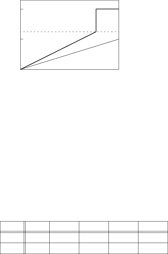
3: Ion Implantation

Monte Carlo Implantation

Sentaurus™ Process User Guide 159

H-2013.03

Figure 32 Onset of amorphization after reaching DCrit for two values of DAcc

Saturation at Critical Value

pdbSet Ctrim DamageAccumulation Saturation

According to this model, below a threshold value DCrit, the damage probability PD has the

same linear behavior as in the ‘full’ model, but cannot grow above DCrit:

(105)

For both models, the values of the parameters DAcc and DCrit depend mainly on the atomic

number of the implanted ion.

Table 9 lists values for some species. The automatic calibration for these values can be

switched off using AutoDAcc and AutoDCrit.

Internal Storage Grid for Implantation Damage

By default, Crystal-TRIM stores the accumulated damage at the mesh. This makes the damage

accumulation dependent on the mesh and can lead to errors if the mesh is too coarse. Typically,

the amorphous boundary depends nonlocally on the mesh size closer to the surface of the

structure.

Ta bl e 9 Va l u es fo r DAc c an d D Cr it fo r m o s t i m po r t an t sp ec i es

BF2 As, Ga, Ge In, Sb, Sn B, C, N Al, P, Si

DAcc 0.15 0.3 0.3 0.1 0.2

DCrit 0.02 0.05 0.05 0.99 0.1

Vacancy Concentration

1.0

0.5

0.0

Damage Probability PD

DCrit

DAcc=0.8

DAcc=0.5

DAcc En, DAcc En

⋅DCrit≤⋅

DCrit , DAcc En

⋅DCrit>







3: Ion Implantation

Monte Carlo Implantation

160 Sentaurus™ Process User Guide

H-2013.03

An internal grid can be used to accumulate and store as-implanted damage. This can be

switched on by using:

pdbSet Ctrim UseInternalGrid 1

This allows for a mesh-independent storage of the damage information. You can control the

grid spacing by using:

pdbSet Ctrim InternalGridSpacing <n>

In each grid cell, the accumulated as-implanted damage and the amorphization flag are stored.

During postprocessing, the accumulated as-implanted damage is transferred (interpolated)

from the internal grid to Sentaurus Process elements and then to Sentaurus Process nodes.

If two or more Crystal-TRIM steps directly follow each other, you can choose to leave the as-

implanted damage stored on the internal grid instead of transferring it to the mesh. The switch

keepdamage.igrid must be used within the implant command:

implant As crystaltrim keepdamage.igrid

The default is !keepdamage.igrid.

NOTE If keepdamage.igrid is used, the Sentaurus Process Damage dataset

will not be incremented in the postprocessing. If the subsequent

processing step is not a Crystal-TRIM implantation, the damage

information will be lost.

To access the damage information, which was stored on the internal grid during the previous

Crystal-TRIM implantation, the switch predamage.igrid (default is !predamage.igrid)

must be used within the implant command: An example is:

# first step

# no damage post-processing, keep damage on internal grid for the following

# steps

implant As crystaltrim keepdamage.igrid

# second step

# use pre-damage on igrid from the previous step

# no damage post-processing: one more step follows

implant B crystaltrim predamage.igrid keepdamage.igrid

# third step

# use pre-damage on igrid

implant P crystaltrim predamage.igrid

NOTE It is not possible to save the information from the internal grid to a file

using the struct command after the current Crystal-TRIM step.

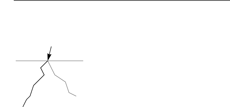
3: Ion Implantation

Monte Carlo Implantation

Sentaurus™ Process User Guide 161

H-2013.03

Molecular Implantations

The MC method allows for the implantation of molecular ions or atomic cluster species such

as BF2. The assumption is that the molecule immediately breaks up into its constituents upon

impact on a solid surface.

Figure 33 Schematic of molecular implantation of BF2; one trajectory is calculated

for each atomic species, w is the weight assigned to the species

This is a valid approximation if the binding energy of the molecule is considerably smaller than

the implant energy (for example, for BF2: EB ~ 9 eV).

The implant energy is shared by several atoms according to:

(106)

where is the energy of the -th species, is the atomic mass, and is the statistical

weight according to the stoichiometry of the molecule.

The constituents move as separate particles. However, particles of different species are not

completely independent because of the interaction through the implantation damage.

Sentaurus Process supports several molecular species: BF2 (BF2), BCl2 (BCl2), B18H22

(B18H22), AsH2 (AsH2), and PH2 (PH2). An implantation of B18H22, for example, can be

performed with:

implant B18H22 energy=100 [ctrim | tmc]

BF2+

F (w=2)

B (w=1)

Ta r g et Surfa ce

Eienergy Mi

wjMj



-------------------⋅=

3: Ion Implantation

Monte Carlo Implantation

162 Sentaurus™ Process User Guide

H-2013.03

The atomic masses, statistical weights, and the molecular composition are available in the

parameter database. A full molecular implantation is performed if the keyword

full.molecular is explicitly set, that is:

implant <dopant> [ctrim | tmc] full.molecular

In this case, the trajectories for all atomic species are calculated. At the end of the simulation,

datasets for each ballistic constituent of the original molecule are generated. This is the default.

Only the trajectory of the significant species (B in the case of BF2) is calculated

if !full.molecular is chosen.

NOTE This feature is available to both Sentaurus MC and Crystal-TRIM.

MC Implantation into Polysilicon

Polysilicon has three states of crystallinity:

■Amorphous

■Crystalline

■Polycrystalline

By default polysilicon is considered amorphous and can be treated as a single-crystalline or

polycrystalline material by using:

pdbSet PolySilicon Crystallinity Crystalline

pdbSet PolySilicon Crystallinity Polycrystalline

Crystal orientation (one of 100, 110, and 111) can be specified using the material-specific pdb

command:

pdbSet PolySilicon CrystalOrient 110

This command sets the crystal orientation for all polysilicon regions to <110>.

If the crystallinity is set to Polycrystalline, MC implantation checks for the existence of

the GSize dataset or GrainSize parameter. If neither is found, the grain model is disabled,

and the material is assumed to be single crystalline. The default grain size is [cm],

and can be changed with the command:

pdbSet PolySilicon GrainSize <n>

or by initializing the GSize dataset:

select z=<n> name=GSize

The units for both GrainSize and GSize are centimeters.

510

5–

3: Ion Implantation

Monte Carlo Implantation

Sentaurus™ Process User Guide 163

H-2013.03

The grain size also can be scaled with the GrainFactor parameter:

pdbSet PolySilicon GrainFactor <n>

The default GrainFactor is 1.

The polycrystalline model works by frequently switching between the crystal algorithm and

the amorphous algorithm. The probability of switching from the crystal model to the

amorphous model is determined by the accumulative path length in crystal (pathlength) and

polycrystalline grain size (GrainSize). It switches from the crystal model to the amorphous

model if:

(107)

where is a random number between 0 and 1. The polycrystalline model shares the same

random number sequence with other modules in MC implantation. Therefore, if the random

seed is reset, the random numbers used in the polycrystalline model are changed as well.

After an amorphous collision is processed, the pathlength is reset to zero, and the crystal

model is selected. The pathlength is accumulated again. The model used for the next

collision is again determined by the same rules. This process is repeated until the particle exits

the polycrystalline region.

NOTE This feature is available to both Sentaurus MC and Crystal-TRIM.

MC Implantation into Compound Materials with Molar

Fractions

A compound material with a spatially dependent molar fraction can be defined in the PDB. For

example, for single-crystalline silicon, the following PDB entry:

array set $Base {BinaryCompounds {String {

{ SiliconGermanium GeTotal "GeTotal/[pdbGetDouble Si LatticeDensity]" }

}}}

specifies a binary compound Si1–xGex with the mole fraction of Ge calculated from the

germanium concentration (GeTotal) divided by the silicon lattice density. This is the default

setting for SiliconGermanium in the PDB. MC models support implants into these

compound materials (binary, ternary, and quaternary).

Compound materials are detected automatically by using CompoundNumber,

BinaryCompound, TernaryCompound, QuaternaryCoumpound in the PDB. Due to more

computational demands, a minimum concentration is required to trigger MC implantation

pathlength Rrand GrainFactor GrainSize⋅()⋅>

Rrand

3: Ion Implantation

Monte Carlo Implantation

164 Sentaurus™ Process User Guide

H-2013.03

models to treat this material in a more sophisticated way. To specify this minimum

concentration, for example, use:

pdbSet Silicon SiliconGermanium.MCmin 1e20

If the concentration of GeTotal in any mesh node of silicon regions is greater than or equal to

, MC implantation model treats this material as a binary compound

SiliconGermanium. In this case, the average charge and mass of the material are calculated

individually for each mesh element. Lattice constant, nonlocal electron stopping power, and

Debye temperatures are interpolated linearly based on the mole fractions. The lattice is

constructed with the primary material, and each lattice site is assigned to a type of atom with

probability proportional to their mole fractions.

Sentaurus MC considers the fact that each specific lattice site will be occupied with certain

types of atoms only. Therefore, the substitution of the lattice atoms occurs only for those with

the same Group number. The default group number for each type of atom is the same as that

in the periodic table. To change the group number, for example, use:

pdbSet ImplantData Carbon Group 4

For example, in compound material Si1–x–yGexCy, Ge and C have the same group number (IV)

as Si, so both of them can substitute silicon atoms in its lattice sites.

Another example is InxGa1–xAs1-yPy; In and Ga belong to the same group (III), and As and P

belong to the same group (V). Suppose Ga occupies site 0, and As site 1 in zinc-blende

structures, then In can only occupy site 0, and P site can only occupy 1 with the occupation

probabilities proportional to their mole fractions.

Generally MC implant parameters, LatticeConstant, DebyeTemperature, and LSS.pre

vary with the mole fraction. In previous releases, the mole–fraction dependence of MC implant

parameters in compound material is assumed to be linear between base materials. In Version

H-2013.03, there are more options for II-V compounds:

■If a physical parameter is not specified in a ternary (or quaternary) material, the parameter

value is extracted by the linear interpolation with the parameter values of their base binary

materials. This is the default behavior.

■If the parameter is defined for the compound material, the given parameter value is used.

■If <parameter>.XTable is defined for compound material, the piecewise linear

interpolation specified with this table is used. For example:

pdbSetDoubleArray InGaAs LatticeConstant.XTable {<x1> <v1> ... <xn> <vn>}

■If <parameter>.XTable is undefined for compound material, <parameter>.X2 can be

used to define a quadratic interpolation. For example:

pdbSetDouble InGaAs LatticeConstant.X2 <n>

110

× cm 3–

3: Ion Implantation

Monte Carlo Implantation

Sentaurus™ Process User Guide 165

H-2013.03

To use these new parameter interpolation options, turn on the following switch:

pdbSet MCImplant Compound.Interpolation 1

By default, linear interpolation of physical parameters is used.

NOTE Although this feature is available to both Sentaurus MC and Crystal-

TRIM, you are strongly encouraged to use Sentaurus MC implant for

better results.

MC Implantation into Silicon Carbide

Sentaurus MC supports ion implantation into crystalline silicon carbide (SiliconCarbide)

with hexagonal lattice. The hexagonal system has four crystallographic axes: three -axes

(, , ) forming a plane, and a -axis that is normal to the plane. The crystallographic

planes and directions normally are described with four Miller indices (hkil). For the hexagonal

system, since the sum of the first three indices is zero, the third index sometimes can be

omitted.

Silicon carbide exists in many different crystal structures, called polytypes. All polytypes have

a hexagonal frame with a carbon atom situated above the center of a triangle of Si atoms and

underneath a Si atom belonging to the next layer. The difference among the polytypes is the

stacking sequence between the succeeding double layers of carbon and silicon atoms. For

example, 2H-SiC, 4H-SiC, and 6H-SiC have the AB, ABCB, and ABCACB stacking

sequences, respectively. 3C-SiC has an ABC stacking sequence and is the only form of SiC

with a zinc-blende crystal lattice structure. The default polytype for SiC is 4H. To change to a

different polytype, use the following command:

pdbSet SiliconCarbide Polytype {2H 3C 4H 6H}

NOTE The lattice constants may be different for different polytypes. For

convenience, Tcl procedures (set2H-SiC, set3C-SiC, set4H-SiC,

and set6H-SiC) are provided to set to different SiC polytypes.

Two silicon carbide wafer orientations (<0001> and <11-20>) are supported. To specify these

wafer orientations, use the pdb command:

pdbSet SiliconCarbide CrystalOrient {0001 1120}

The default wafer orientation is <0001>. For (0001) SiC wafer; the primary flat orientation is

<10-10>. For (11-20) SiC wafer, the primary flat orientation is <0001>.

For details of the model and comparison with experimental data for various implant conditions,

see [24].

3: Ion Implantation

Monte Carlo Implantation

166 Sentaurus™ Process User Guide

H-2013.03

A miscut of – typically exists in SiC (1000) wafers. Sentaurus MC implantation takes

into account this wafer miscut by specifying caxis.tilt and caxis.rotation in the init

command. caxis.tilt is the angle by which the wafer normal is tilted with respect to the

a-axis in the crystal coordinate system. caxis.rotation is the angle that specifies the

direction into which the wafer normal is tilted. The default value of caxis.rotation is 0,

that is, the projection of the wafer normal to the crystal plane, formed by the b-axis and c-axis,

is coincidental to the <110> direction in silicon. If caxis.rotation=90, the wafer normal is

tilted by caxis.tilt towards the right with respect to the crystal coordinate system. (Or, in

terms of the simulation coordinate system, if caxis.rotation=90, the crystal coordinate

system is tilted towards the left with respect to the wafer normal.) By default, there is no wafer

miscut, that is, caxis.tilt=0.

Here is a simple example illustrating how to perform an MC implantation in SiC:

# Set up the structure

line x loc=0.0 tag=oxtop spac=0.001

line x loc=0.0015 tag=top spac=0.001

line x loc=0.5 spac=0.0025

line x loc=2.0 tag=bot spac=0.01

region Oxide xlo=oxtop xhi=top

region SiliconCarbide xlo=top xhi=bot

# Specify wafer miscut

init caxis.tilt=4 caxis.rotation=0

# Choose different polytype (default is 4H-SiC)

set6H-SiC

# Do the implantation

implant Aluminum energy=60 dose=1e13 tilt=0 rot=0 sentaurus.mc \

particles=10000 info=2

# Save the result

struct tdr=sic

NOTE This feature is available to Sentaurus MC only.

Recoil Implantation

Sentaurus MC implantation provides a general model for recoil implant, such as an oxygen

knock-on effect. Generally, recoil species are handled the same way as cascade atoms, except

that no vacancies are created at the displaced sites and the recoil species are not recorded as

interstitials when they stop. Instead, a separate dataset is created for each recoil species.

3.5°

8.5°

3: Ion Implantation

Monte Carlo Implantation

Sentaurus™ Process User Guide 167

H-2013.03

The recoil species is specified in the material composition. For example, to simulate the oxygen

knock-on effect, the following is defined in the parameter database:

Oxide -> Composition -> Component0 -> Name = Silicon

Oxide -> Composition -> Component0 -> StWeight = 1

Oxide -> Composition -> Component1 -> Name = Oxygen

Oxide -> Composition -> Component1 -> StWeight = 2

Oxide -> Composition -> Component1 -> Recoil = 1

To initiate oxygen recoil implant simulation, you must specify the keyword recoils in the

implant command:

implant <dopant> energy=<n> dose=<n> recoils

The datasets Oxygen_Implant and Oxygen are created, which contain displaced oxygen

distributions that can be used to analyze the oxygen knock-on effect.

NOTE This feature is available to Sentaurus MC implantation only.

Plasma Implantation

Three-dimensional tri-gate devices (FinFETs) have been employed at the 22 nm node and are

expected to continue at and beyond the 16 nm node. Doping of FinFETs must be 3D, and

conformal doping with plasma implantation (PLAD) is a promising approach. Likewise,

doping of planar devices is challenging, and PLAD offers capabilities not available in beamline

implantations.

To offer this simulation capability, Sentaurus Process provides a PLAD doping module that

accurately reflects both the hardware and process signatures as well as the physical properties

of the associated deposition, etching, sputtering, implantation, knock-on, defect creation, and

annihilation processes. This MC implantation module includes the following features:

■Perform alternating steps of deposition and MC implantation. The number of steps can be

specified by users.

■Deposition of material on the surface is performed isotropically (that is, constant growth

rate over the surface). The thickness is specified by users. A minimum thickness is imposed

by the program, which reduces the number of steps if necessary to prevent the deposition

of a layer that is too thin. The deposit material should be defined as usual, and material

composition of the layer must be specified by users.

■The MC implantation module allows the specification of multiple ions incidents on the

wafer. The ion species should be defined before implantation as usual, and some typical ion

species used in plasma implantation will be predefined. You can specify the dose, energy

distribution, and angular distribution of each ion species. The dose for each ion is applied

evenly for each step.

3: Ion Implantation

Monte Carlo Implantation

168 Sentaurus™ Process User Guide

H-2013.03

■An empirical model for conformal doping, in which the level of conformity can be

specified by users.

■In addition to computing the concentration of ions that penetrate through the deposited

overlayer, the MC implantation module allow for atoms to be knocked out of the overlayer

and into the wafer and tracks damage and amorphization as usual.

You mu st d efi ne the plasma so urc e bef or e impl an tatio n c an b e p erfo rm ed . To avo id ove rly

complex syntax in the implant command, Sentaurus Process provides two ways to specify the

plasma source: simple source and complex source.

Simple Source

Assuming that the multiple ion species in plasma have the same energy and angle distributions,

simply specify the multiple species as a list in the implant command (other parameters such

as dose, energy, tilt, and so on can be specified like a regular implantation):

plasma.source = {<species1>=<n> <species2>=<n> <species3>=<n> ...}

where:

■plasma.source specifies a list of ion species to be implanted. These species must be

predefined in ImplantData as usual.

■The number after each species is the fraction of the total dose (as specified by the dose

parameter) for the given species.

■All these species will have the same energy, tilt, en.stdev, and tilt.stdev as

specified.

Complex Source

In more complex cases, different species may have different energy and angle distributions. In

this case, each species can be specified with their own implantation parameters (energy,

tilt, en.stdev, and tilt.stdev). So for each species, define it with an implant

command:

implant species=<species1> energy=<n> tilt=<n> en.stdev=<n> tilt.stdev=<n>

implant species=<species2> energy=<n> tilt=<n> en.stdev=<n> tilt.stdev=<n>

implant species=<species3> energy=<n> tilt=<n> en.stdev=<n> tilt.stdev=<n>

...

where <species1>, <species2>, <species3> must be predefined in ImplantData as

usual. Only parameters that are different from the default values must be specified.

Then, you can perform the real implantation in the same way as in the simple source case:

implant plasma.source= {<species1>=<n> <species2>=<n> ...} dose=<n> energy=<n>

3: Ion Implantation

Monte Carlo Implantation

Sentaurus™ Process User Guide 169

H-2013.03

tilt=<n> en.stdev=<n> tilt.stdev=<n> ...

where:

■plasma.source specifies a list of ion species to be implanted. These species must be the

same as those in previous implant commands.

■The regular implantation parameters (dose, energy, and so on) will be the default for

those species that are not specified. Essentially, this syntax is consistent with that for the

simple source and reduces to the simple source if no implantation parameters are specified

for each individual species.

Deposition of Material

To specify the deposition of the material during implantation, use the plasma.deposit

parameter in the implant command:

implant plasma.source= {<species1>=<n> <species2>=<n> ...}

plasma.deposit= {material=<c> thickness=<n> steps=<n>}

dose=<n> energy=<n> tilt=<n> ...

where:

■material is the name of the material to be deposited, which must be specified before the

implantation.

■thickness is the total thickness of the deposit material.

■steps is the number of steps of deposition.

The deposition and implantation are performed alternatively. If plasma.deposit is not

specified, or material is not specified, or thickness is not specified (or is equal to zero),

no deposition is performed.

Knock-on and Knock-off Effect

The MC implantation module simulates the dopant knock-on and knock-off effect by

specifying the recoils parameters in the implant command. In addition, you must specify

the recoil species to be simulated in material composition.

For example, assuming the deposit material is BHx, and Atom0 is Boron, the following

commands specify Boron as a recoil species:

pdbSetString BHx Composition Atom0 Name Boron

pdbSetDouble BHx Composition Atom0 StWeight 1

pdbSetBoolean BHx Composition Atom0 Recoil 1

pdbSetString BHx Composition Atom1 Name Hydrogen

pdbSetDouble BHx Composition Atom1 StWeight <x>

3: Ion Implantation

Monte Carlo Implantation

170 Sentaurus™ Process User Guide

H-2013.03

Conformal Doping

Conformal doping is an important characteristic in plasma implantation. However, due to the

complexity of plasma dynamics that involves manybody long-range interactions, the exact

mechanism for conformal doping in plasma implantation is still not well understood.

Physically, this may be possible if one of the following mechanisms or their combination

occurs, for example, in a trench:

■The ions become ionized anywhere in the ambient (including inside the trenches) and start

their acceleration towards the silicon surface.

■The ions scatter off other particles in the plasma/ambient (including inside the trenches)

and change their direction.

To account for such effects, an empirical model has been developed that is compatible with the

current plasma implantation. In this model, instead of launching all ions from above the device,

as in standard implantation, some ions are launched along the device surface (that is, the solid–

ambient interface). A fraction of ions launched along the surface can be specified by the

parameter conformity in the implant command:

implant <dopant> energy=<n> dose=<n> conformity=<n> sentaurus.mc

where conformity is a number between 0 and 1.0. For example, if conformity=0, you will

obtain standard plasma implantation results, and if conformity=1, you will obtain fully

conformal doping.

Other Plasma Implantation–related Parameters and Procedures

Sentaurus Process provides a simple model for taking into account the energy and tilt angle

distributions of the plasma source. Given the mean and standard deviation of the implantation

energy and tilt angles, Sentaurus MC implantation samples the given energy and tilt

distributions for each implantation particle. After the implantation energy and tilt angle are

determined, the particle tracing is computed using a standard procedure.

In addition to the normal implantation parameters, such as energy and tilt, you can specify the

standard deviation of implantation energy (en.stdev) or the standard deviation of the tilt

angle (tilt.stdev) or both. For example:

implant <dopant> plasma dose=<n> energy=<n> en.stdev=<n> tilt=<n>

tilt.stdev=<n> sentaurus.mc

where the implantation parameters energy and tilt are the mean energy and mean tilt,

respectively.

You a lso c an spe ci fy t he mi nimum e ne rg y th at is allowed for implantation using the command:

pdbSet MCImplant MinEnergyCutoff <n>

3: Ion Implantation

Monte Carlo Implantation

Sentaurus™ Process User Guide 171

H-2013.03

Energy below the minimum energy will be truncated. The default minimum energy is zero. In

addition, you can specify the maximum energy that is allowed by using the command:

pdbSet MCImplant MaxNumStdevCutoff <n>

MaxNumStdevCutoff must be an integer (default is 5). The highest energy for a given implant

should not exceed the mean energy by the amount of en.stdev x MaxNumStdevCutoff.

Energy higher than this number will be truncated.

Energy Distributions

The energetic distribution of different molecular and atomic ions, after extraction from the

plasma, is known to cover the range from zero to the maximum energy , which is equal

to the product of the ion charge multiplied by the extraction voltage. Sentaurus Process allows

easy selection and addition of various energy distribution models. In addition to the default

Gaussian distribution, Sentaurus Process implements an alternative Burenkov model [25]. In

this model, the energy distribution, as presented by Tian et al. [26] as an integral number of

particles having their energy in a given interval, can be written in a differential form as

follows [25]:

(108)

The energy distribution presented in Eq. 108 is normalized, that is, the integral over all

possible energies of the extracted ions, ranging from 0 to , is equal to one. Burenkov et

al. have shown that by using the energy distribution given by Eq. 108, excellent agreement can

be obtained between simulations and experiments for BF3 plasma implantation [25].

Tilt Angle Distributions

Three different tilt angle distributions are offered in plasma implant. You can select a different

tilt angle distribution model by using:

pdbSet MCImplant PlasmaEnergyDistributionModel\

{Gaussian | Gaussian.Solid.Angle | Gaussian.3D}

The default Gaussian model:

(109)

This is a first order approximation in which the number of particles per solid angle has a sharp

maximum at tilt=0. This may not be ideal in certain situations.

Emax

fE() 5

6Emax

⋅

-------------------E

Emax

-----------





16/–

⋅=

fE()

Emax

ftilt() 1

2πσ

-------------- 1

---tilt

------





–





exp=

3: Ion Implantation

Monte Carlo Implantation

172 Sentaurus™ Process User Guide

H-2013.03

The Gaussian.Solid.Angle is:

(110)

Here, the additional factor tilt considers that the solid angle which corresponds to a tilt angle

is proportional to the tilt angle. Note that the standard deviation ( ) has a slightly different

meaning from regular Gaussian distribution. In other words, only 1-1/e = 63.2% of ions will be

in the interval [0, ].

For Gaussian.3D (suggested by Burenkov et al.), you must add a random 3D vector, in which

each component has a random Gaussian distribution to the vertical unit vector, and calculate

the corresponding tilt angle. In this case, the knock-on process in the plasma may lead to

additional ion energy which has Gaussian distribution. Here again, has a different meaning

from standard Gaussian distribution; in other words, only ~40% of ions are within the interval

[0, ].

To select a different energy distribution model, use:

pdbSet MCImplant PlasmaEnergyDistributionModel {Gaussian | Burenkov}

To provide maximum flexibility for energy and tilt angle distributions, you also can provide

your own distributions by modifying the following Tcl procedures in Plasma.tcl:

Plasma::Energy_Distribution { energy stdev }

Plasma::Tilt_Distribution { mean stdev }

NOTE Sentaurus Process does not check the validity of these user-defined

distributions. If you change these distributions, you must provide the

correct distributions to ensure the correct implantation results.

NOTE This feature is available to Sentaurus MC implantation only.

MC Implantation Damage and Point-Defect Calculation

Sentaurus MC Damage Calculation

The damage in a Sentaurus MC implantation is computed either using the Kinchin–Pease

formula [22] (default) or with full cascades if the cascades parameter is specified in the

implant command. For details on damage calculations, see Damage Accumulation and

Dynamic Annealing on page 149. The calculation of the damage datasets for Sentaurus MC is

ftilt() tilt

2πσ

-------------- 1

---tilt

------





–





exp=

3: Ion Implantation

Monte Carlo Implantation

Sentaurus™ Process User Guide 173

H-2013.03

consistent with the analytic implantation model. At the end of an implantation step, the damage

for this step (Damage_LastImp) is added to the Damage profile using:

(111)

where + indicates the total damage as the sum of new damage and existing damage. The default

value for MCDFactor is 1 and can be changed at the implant command line or in the

parameter database:

implant <dopant> [tmc] [mc.dfactor=<n>]

pdbSetDouble <material> <dopant> MCDFactor <n>

The accumulated damage is taken into account automatically for subsequent MC

implantations, unless the Damage dataset is reset by the diffuse command.

Crystal-TRIM: Damage Probability

Defect accumulation in single-crystalline material and de-channeling due to the implantation

damage are treated dynamically using a phenomenological model [22]. The model is based on

the assumption of the formation of complex defects, such as amorphous pockets (APs) during

ion implantation.

The damage information calculated during Crystal-TRIM simulations is stored in the damage

probability dataset PD. This information is used in the model of APs to treat the nuclear

collisions in the partially damaged crystalline region. Within a certain volume element, PD

gives the probability that the collision can be treated as if the material were amorphous. The

material is locally considered to be completely amorphized if PD = 1.

The PD dataset is not deleted after an implant step and, consequently, can be reused in

subsequent Crystal-TRIM runs (damage history).

If the PD dataset has been deleted or has not yet been created, the Damage dataset is used to

initialize the damage history in all crystalline materials:

(112)

where Threshold is the amorphous threshold, which is the minimum of the lattice density and

amorphous density. Both parameters can be set in the parameter database:

pdbSet <material> LatticeDensity <n>

pdbSet <material> AmorpDensity <n>

At the end of the simulation, the Damage dataset is increased according to:

(113)

Damage += MCDFactor Damage_LastImp⋅

PD = Damage / Threshold, max(PD) = 1

Damage = Damage + PD_LastImp Threshold⋅

3: Ion Implantation

Monte Carlo Implantation

174 Sentaurus™ Process User Guide

H-2013.03

Point Defects

Elemental Material

Point-defect profiles after a MC run can be generated from the ballistic dopant profile using the

plus.one or effective.plus.n model, or from the ballistic vacancy (Frenkel pair) and

recoil profiles using the frenkel.pair model. The effective.plus.n model is the

default for all MC simulations. In this case, the ballistic dopant profile <dopant>_LastImp

is used according to Eq. 50, p. 118.

Interstitial and vacancy profiles can also be calculated using the ballistic vacancy dataset

Vac_LastImp generated during a MC run. The switch defect.model must be set to

frenkel.pair:

implant <dopant> [crystaltrim | sentaurus.mc] [defect.model=frenkel.pair]

Using the MC-specific factors MCIFactor and MCVFactor, the profiles are calculated

according to:

(114)

The default values for MCIFactor, MCVFactor, and IFactor are 1. These factors can be

changed in the parameter database:

pdbSet <material> <dopant> IFactor <n>

pdbSet <material> <dopant> MCIFactor <n>

pdbSet <material> <dopant> MCVFactor <n>

or on the command line:

implant <dopant> [crystaltrim | sentaurus.mc] [ifactor=<n>] [mc.ifactor=<n>]

[mc.vfactor=<n>]

Setting ifactor, mc.ifactor, and mc.vfactor in the implant command overwrites the

parameter database entries.

If cascades is enabled in MC implantation and the point-defect model is set to

frenkel.pair, the interstitial and vacancy profile is calculated using the concentration of the

recoil and vacancy as calculated based on the physics model:

implant <dopant> [crystaltrim | sentaurus.mc] [cascades] \

[defect.model=frenkel.pair]

Int_Implant += MCIFactor Vac_LastImp IFactor <dopant>_LastImp⋅+⋅

Vac_Implant += MCVFactor Vac_LastImp⋅

3: Ion Implantation

Monte Carlo Implantation

Sentaurus™ Process User Guide 175

H-2013.03

In this case, the interstitial and vacancy densities increase according to the following:

(115)

Multicomponent Materials

In multicomponent materials, such as silicon carbide (SiC), the material is composed of

different types of atom. When an impurity is implanted into SiC, both silicon and carbon lattice

atoms can be displaced, thereby forming silicon interstitials or carbon interstitials, and leaving

behind silicon-site or carbon-site vacancies. Instead of classifying them together as interstitials

or vacancies, as in silicon, Sentaurus Process provides a mechanism to distinguish different

types of interstitial or vacancy.

To generate distinct types of point defect in multiple-component materials, you must switch on

the DistinctDefects flag, for example:

pdbSetBoolean SiliconCarbide DistinctDefects 1

By default, this flag is true for SiC but false for other materials. As a result, instead of

Int_Implant and Vac_Implant, the generated point-defect datasets in SiC are

IntSilicon_Implant, IntCarbon_Implant, VacSilicon_Implant, and

VacCarbon_Implant.

In this model, the total point-defect concentration is computed the same way as the elemental

material. The implantation parameters defect.model, ifactor, vfactor, mc.ifactor,

and mc.vfactor in the implant command still work. ifactor and vfactor are scaling

factors for interstitial profiles and vacancy profiles, respectively, in the plus.one defect

model; while mc.ifactor and mc.vfactor are scaling factors for interstitial profiles and

vacancy profiles, respectively, in the frenkel.pair defect model. The same Tcl procedure

CalcPlusNFactor calculates automatically the plus factors for the effective.plus.n

defect model.

Then, the individual point-defect concentration is computed by multiplying the total point-

defect concentration by the fraction of each component. The fraction of each component is, by

default, their stoichiometric weight, but it can be changed in the parameter database with the

parameters IFractor.Fraction and VFactor.Fraction.

For example, in SiC:

pdbSet SiC Composition Component0 IFactor.Fraction <n>

pdbSet SiC Composition Component1 IFactor.Fraction <n>

pdbSet SiC Composition Component0 VFactor.Fraction <n>

pdbSet SiC Composition Component1 VFactor.Fraction <n>

Int_Implant += <recoil>_LastImp <dopant>_LastImp+

Vac_Implant += <vacancy>_LastImp

3: Ion Implantation

Monte Carlo Implantation

176 Sentaurus™ Process User Guide

H-2013.03

If cascades is enabled in MC implantation and the point-defect model is set to

frenkel.pair, the interstitial and vacancy profile is calculated using the concentration of the

recoils and vacancies as calculated based on the physical model.

In this case, the interstitial and vacancy densities increase according to the following:

(116)

Statistical Enhancement

The energetic pseudoparticles in a MC simulation are statistical objects representing several

actual particles or only a fraction of an actual particle. Pseudoparticles start their motion at a

plane above the target parallel to the wafer surface. The starting surface is subdivided into

segments of equal size. The size of these segments can be controlled by setting dy and dz in

the MCImplant -> Intervals entry in the parameter database.

The number of pseudoparticles can be set by using:

pdbSet MCImplant Particles <n>

or:

implant <dopant> [crystaltrim | sentaurus.mc] [particles=<n>]

The default value for particles is 1000. The random number generator can be started with

a specified random seed. The integer value used can be set with the parameter RandomSeed:

pdbSet MCImplant RandomSeed <n>

The default is 1. Random seeds also can be chosen randomly by using the internal clock,

thereby giving different results for different runs. This feature is useful for statistical analysis

for MC implantations. To use this feature, use the following command:

pdbSet MCImplant Randomize 1

Trajector y Splittin g

Trajectory splitting artificially increases the number of trajectories calculated in regions with

low trajectory density. It can be switched on or off by using:

pdbSet MCImplant TrajectorySplitting 1

Int<component>_Implant += <component>_LastImp IFactor.Fraction <dopant>_LastImp⋅+

Vac<component>_Implant += <vacancy-component>_LastImp

3: Ion Implantation

Monte Carlo Implantation

Sentaurus™ Process User Guide 177

H-2013.03

If a projectile reaches an element with a small trajectory density, a split point is set, that is, the

particle is replaced by two daughter particles having half the statistical weight of the mother

projectile. Then, the trajectories of both daughter particles are simulated in the same manner

as for the original particle. Further splitting may occur that leads to a splitting tree related to

the mother projectile. At a split point, the two daughter projectiles start under identical

conditions.

However, the consideration of thermal vibrations of target atoms leads to a deviation of the

trajectories of the daughter projectiles after a few collisions. In this manner, a high number of

different particle trajectories with low statistical weight is obtained, which leads to an

important decrease of the statistical noise in the tail parts of the dopant distribution.

In Sentaurus MC, the maximum depth of the splitting tree is defined by a global parameter

MaxSplitLevels:

pdbSet MCImplant MaxSplitLevels <n>

In Crystal-TRIM, a similar parameter is defined for each species. For a given ion species, the

maximum depth of the splitting tree is defined by the parameter MaxSplits:

pdbSet <material> <dopant> MaxSplits <n>

pdbSet <material> <dopant> MaxSplitsPerElement <n>

The parameter MaxSplitsPerElement defines the maximum number of split events within

one element.

NOTE The trajectory splitting model is available to both Sentaurus MC and

Crystal-TRIM.

Dose Split

In the conventional pseudoparticle Monte Carlo approach, all particles have the same

weighting. In contrast, dose split algorithm uses smart particle weighting with first-coming

ions weighing less than later ions. This prevents crystalline from amorphizing too quickly,

thereby allowing more ions to enter the channeling regions. This model can drastically reduce

the noises of the channeling tails. By default, dose split is switched off. To activate the model,

use the command:

pdbSet MCImplant DoseSplit 1

The dose split model is especially effective for high-dose amorphizing implants, such as

arsenic implant with a dose of . For a typical run, the CPU time is about 2 to 3

times slower than that without dose split for the same number of particles. However, dose split

improves the statistics in the channeling tails by at least two orders of magnitude.

815

×10 cm 2–

3: Ion Implantation

Monte Carlo Implantation

178 Sentaurus™ Process User Guide

H-2013.03

To achieve the same statistical significance, the conventional approach requires at least 100

times more particles; this means that the effective speedup is about 30 to 50 times.

NOTE The dose split model is available to Sentaurus MC only.

Trajectory Replication

The trajectory replication algorithm uses the fact that in almost all 2D or 3D target structures,

several regions with 1D topology can be found. A particle trajectory going through such a part

can be copied many times by shifting its origin. Within the 1D region, each shifted trajectory

is a valid particle trajectory. Its reproduction by copying is much faster than its physical

calculation.

The subdivision into 1D parts or equivalence classes is performed automatically during the

implantation. A subdivision is performed using the segments of the start surface. At the

beginning, all the start segments are in the same equivalence class.

First, the whole trajectory tree is calculated including splits and recoils. The increments of all

concentration-type values between entering and leaving a grid element are stored for each

trajectory point (at least one per grid element). A start segment is chosen from the same

equivalence class. The starting point of the copy trajectory is set randomly within this start

segment. The point where the copied trajectory enters the material is found in the same way as

for the original trajectory. The vector between the first material point of the master and the

copied trajectory serves as a shift vector. All the increments of the master trajectory are

transferred point by point into grid elements that correspond to the shifted points.

If the materials are not identical within geometry tolerance ( ), or the initial

damage is different by more than 1% at the master and the replica points, replication fails and

the start segment is taken out of the present equivalence class and placed into a new equivalence

class. The generation of new equivalence classes stops after a certain number of particles has

been implanted. These initial particles are called probing ions.

Due to the random nature of ion trajectories, for the same structure, the equivalent classes as

discovered by the probing ions could be slightly different depending on the random seeds,

implanted species, or the number of probing ions.

The number of probing ions is empirically set to the total number of start segments. However,

depending on the situation, this number may be too small for 2D simulations; whereas, it may

be too large for 3D simulations. You can control this number by using the command:

pdbSet MCImplant ReplicationLearningFactor <n>

After this command, the new number of probing ions will be equal to the original number of

probing ions multiplied by ReplicationLearningFactor. Generally, the more probing

ions, the more equivalent classes will be created for a given structure. More equivalent classes

1.5 4–

×10 µm

3: Ion Implantation

Monte Carlo Implantation

Sentaurus™ Process User Guide 179

H-2013.03

will reduce the ratio of the replicated trajectories to the calculated trajectories, thereby

providing more accurate results at the expense of more CPU time.

The total number of implanted particles is given as the number of start segments multiplied by

the number of particles per segment, which can be set by using the parameter particles. Due

to the replication, the number of physically calculated trajectories is usually much smaller and

is given rather by the number of equivalence classes multiplied by particles.

The trajectory replication algorithm is based on the heuristic argument that the 1D part of the

structure should be equivalent. However, some parts of the 1D region may be close to the

sidewalls. Therefore, the dopant concentration is contributed to not only from the direct

exposure to the ion beam, but also from the particles scattered from the sidewalls and re-

entering the 1D region. In such situations (such as high-energy implant into a photoresist mask

or pocket implants), trajectory replication may not give accurate results near the sidewalls. In

addition, for high tilt pocket implants, saving CPU time by trajectory replication is limited.

Therefore, under such circumstances, you should switch off the trajectory replication.

NOTE Trajectory replication is switched on by default. To switch off trajectory

replication, use the global switch:

pdbSet MCImplant TrajectoryReplication 0

NOTE This feature is available in both Sentaurus MC and Crystal-TRIM.

Datasets

The datasets used in a MC run follow the same naming conventions as those used in analytic

implantation. Datasets unique to the MC implantation method are:

■The ballistic vacancy density Vac_LastImp.

■The damage probability PD, which is used to store and initialize damage history in

Crystal-TRIM.

■The nuclear energy deposition EnergyDeposition, which is created in Sentaurus MC

implantation.

Table 10 Datasets used in MC implantations

Dataset Description

EnergyDeposition

Accumulated energy deposition (in units of ) from nuclear collisions.

This dataset is created in Sentaurus MC implant only.

eV/cm3

3: Ion Implantation

Boundary Conditions and Domain Extension

180 Sentaurus™ Process User Guide

H-2013.03

Boundary Conditions and Domain Extension

Boundary conditions are needed in ion implantation simulations to account for the geometry

effects (such as shadowing) and lateral scattering of the implied structure. Both of these effects

require knowledge of the materials and damage concentration outside the simulation domain.

The required information is synthesized by the definition of the boundary conditions. The

following subsections describe how to specify these boundary conditions.

Damage

Accumulative damage (damage history). This dataset is deleted by the

diffuse command. For Sentaurus MC, at the end of an implant step, the

Damage_LastImp concentration is added to Damage, similar to analytic

implantation. For Crystal-TRIM, damage is generated using the PD dataset after

an implant step.

Damage_LastImp

Damage created during the last implant step. This dataset is used by

Sentaurus MC only.

Accumulative density of the dopant concentration. At the end of an implant

step, the <dopant>_LastImp concentration is added to <dopant>.

<dopant>_Implant

Accumulative density of the dopant concentration. At the end of an implant

step, the <dopant>_LastImp concentration is added to

<dopant>_Implant. This dataset is deleted by the diffuse command.

<dopant>_LastImp

Ballistic dopant concentration generated during the last implant step. It is

reset at the beginning of each implant step.

Int_Implant

Accumulative interstitial profile updated at the end of an implant step.

Int<component>_Implant

Accumulative interstitial profiles in multicomponent material with

DistinctDefects set to true, where <component> is the component

of the composition of the material. For example, in SiC, interstitial profiles

include IntSilicon_Implant and IntCarbon_Implant.

Damage probability. This dataset is used by Crystal-TRIM only.

Vac_Implant

Accumulative vacancy profile updated at the end of an implant step.

Vac_LastImp

Ballistic vacancy density generated during the last implant step.

Vac<component>_Implant

Accumulative vacancy profiles in multicomponent material with

DistinctDefects set to true, where <component> is the component

of the composition of the material. For example, in SiC, interstitial profiles

include VacSilicon_Implant and VacCarbon_Implant.

Table 10 Datasets used in MC implantations

Dataset Description

3: Ion Implantation

Boundary Conditions and Domain Extension

Sentaurus™ Process User Guide 181

H-2013.03

Unified Implant Boundary Conditions

NOTE This is the preferred method for specifying implant boundary

conditions.

Sentaurus Process has two different sets of implant boundary conditions: one for analytic

implant and one for MC implant. To ensure consistent results between analytic and MC

implant, Sentaurus Process provides a unified method for specifying implant boundary

conditions. This method uses the implant command to specify the boundary conditions with

the following syntax:

implant boundary.conditions = {left=<c> right=<c> front=<c> back=<c>}

where the valid keywords are Periodic, Reflect, or Extend.

In contrast to the boundary conditions specified by PDB commands, if Periodic or Reflect

is specified in the implant command, TruePeriodic and TrueReflect will be used for

MC implant since these ensure the most consistent results between analytic and MC implants.

You do not n ee d to sp ec ify boundary conditions for all four sides. Extend boundary condition

is assumed for unspecified sides, except for periodic boundary conditions. Since periodic

boundary conditions must be paired, left and right or front and back, they must have the

same periodic boundary conditions. For simplicity, you need only specify periodic boundary

conditions on one side; the other side is automatically assumed to have the same periodic

boundary condition. If the other side is specified for a different type of boundary condition,

Sentaurus Process issues a warning and uses a periodic boundary condition.

Implant Boundary Conditions using PDB Commands

Although not recommended, these boundary conditions can be directly specified using PDB

commands. Advanced users can use these commands to adjust the implant boundary conditions

under certain circumstances.

NOTE Because this method for specifying implant boundary conditions is

obsoleted, you should use it only if it is absolutely necessary when

creating new input files.

3: Ion Implantation

Boundary Conditions and Domain Extension

182 Sentaurus™ Process User Guide

H-2013.03

Monte Carlo Implant

Boundary conditions determine how particles leaving the simulation domain at its outer

boundaries will be processed. It is assumed that the simulation domain is rectangular if viewed

from the top and is contained between:

LeftBoundary and RightBoundary (y-direction)

and:

BackBoundary and FrontBoundary (z-direction)

Legacy Periodic Boundary Conditions

In this boundary condition, boundaries exist only in solid regions. In solid regions, when a

particle reaches one side of the boundary, it is moved to the other side of the boundary.

However, in ambient (or gas), particles are free to enter or exit. Therefore, Periodic boundary

condition in MC implant only means translating the position of particles from one boundary to

the opposite boundary in solid regions. It takes the structure as it is, and does not extend to form

a true periodic structure.

To select these boundary conditions, use the following commands:

pdbSet MCImplant BoundaryPeriodicY 1

pdbSet MCImplant BoundaryPeriodicZ 1

This switches on Periodic boundary conditions in the left-right and front-back, respectively.

NOTE Because this boundary condition is obsoleted, you should not use it

when creating new input files.

TruePeriodic Boundary Conditions

This boundary condition considers the device as a true periodic structure. To select

TruePeriodic boundary conditions, use:

pdbSet MCImplant TruePeriodicY 1

pdbSet MCImplant TruePeriodicZ 1

TruePeriodicY and TruePeriodicZ are applied to left and right, and front and back,

respectively.

NOTE TruePeriodic has precedence over legacy Periodic boundary

condition and other types of boundary conditions. When Periodic is

specified in the implant command for unified boundary conditions,

3: Ion Implantation

Boundary Conditions and Domain Extension

Sentaurus™ Process User Guide 183

H-2013.03

TruePeriodic boundary condition is selected automatically in MC

implant.

Legacy Reflect Boundary Conditions

pdbSet MCImplant LeftBoundary Reflect

pdbSet MCImplant RightBoundary Reflect

pdbSet MCImplant FrontBoundary Reflect

pdbSet MCImplant BackBoundary Reflect

A particle hitting the boundary will have its position and direction of motion reflected with

respect to the boundary plane.

TrueReflect Boundary Conditions

Instead of reflecting the direction of the moving particles at the boundary, Sentaurus Process

provides a new boundary condition TrueReflect, which automatically reflects the structure,

performs the implantation, and then cuts the structure to its original domain. To specify the

TrueReflect boundary condition, use:

pdbSet MCImplant LeftBoundary TrueReflect

pdbSet MCImplant RightBoundary TrueReflect

pdbSet MCImplant FrontBoundary TrueReflect

pdbSet MCImplant BackBoundary TrueReflect

NOTE When Reflect is specified in the implant command for unified

boundary conditions, TrueReflect boundary condition is

automatically selected in MC implant.

NOTE Generally, reflective boundary conditions (including both Reflect and

TrueReflect) can be used only if there are the same reflect-symmetric

ion beams, such as tilt=0 (or projected tilt2D=0 in 2D), or

approximately, multiple rotation implantations. To improve

performance, averaging of the simulation results (including dopant and

damage fields) over the original and reflected domains can be

performed. If tilt (or tilt2D) < , Sentaurus Process automatically

averages the simulation results. In the case of mult.rot implantations

(or a sequence of multiple implant commands consisting of

mult.rot implantation), no automatically averaging is performed.

However, you can specify average in the implant command to do the

averaging. To overwrite such default behaviors, specify average or

!average in the implant command.

NOTE In cases where average is applied successfully, TrueReflect

generally achieves more accurate results than Reflect without the

significant performance penalty.

2°

3: Ion Implantation

Boundary Conditions and Domain Extension

184 Sentaurus™ Process User Guide

H-2013.03

Extending the Simulation Domain

pdbSet MCImplant LeftBoundary Extend

pdbSet MCImplant RightBoundary Extend

pdbSet MCImplant BackBoundary Extend

pdbSet MCImplant FrontBoundary Extend

The simulation domain is artificially extended in the corresponding direction. This

compensates for the decay of the profile near the boundaries of the simulation domain.

Sentaurus Process determines these extension lengths automatically by using tilt,

rotation, and slice.angle, and the user-defined parameters MinExtension and

ExtensionLength:

(117)

where the function is between 0 and 1. If tilt equals 0, equals 0. Therefore, for tilt

equals 0, extension length equals MinExtension. The default value for MinExtension is

0.1 , which is usually sufficient for low-energy implants. For high-energy implants, you

may need to increase MinExtension to avoid decaying concentration near the boundaries.

To control the size of the extension, use:

pdbSet MCImplant ExtensionLength <n>

pdbSet MCImplant MinExtension <n>

Transparent Boundary

pdbSet MCImplant LeftBoundary Transparent

pdbSet MCImplant RightBoundary Transparent

pdbSet MCImplant BackBoundary Transparent

pdbSet MCImplant FrontBoundary Transparent

All particles crossing the boundary leave the simulation domain and are lost.

NOTE For given boundary conditions other than Transparent, it is important

that the boundaries, which are lines in 2D and planes in 3D, are

continuous, that is, they should show no holes. The crossing of a particle

can only be registered if it happens within the material region. The

particle will finally leave the structure if it crosses the side while in a gas

region.

Ext Length MinExtension ExtensionLength ftilt rotation slice.angle,,()⋅+=

µm

3: Ion Implantation

Boundary Conditions and Domain Extension

Sentaurus™ Process User Guide 185

H-2013.03

Analytic Implant

Analytic implantation uses the same syntax as MC implantation for specifying boundary

conditions. It is assumed that the simulation domain is rectangular if viewed from the top and

is contained between:

LeftBoundary and RightBoundary (y-direction)

and:

BackBoundary and FrontBoundary (z-direction)

Extended Boundary Condition

pdbSet ImplantData LeftBoundary Extend

pdbSet ImplantData RightBoundary Extend

pdbSet ImplantData FrontBoundary Extend

pdbSet ImplantData BackBoundary Extend

The simulation domain is extended artificially in the corresponding direction. This

compensates for the decay of the profile near the boundaries of the simulation domain. The

extended structure is removed after the implant is completed. Extend is the default boundary

condition for ion implantation. To control the size of the lateral extension, use:

pdbSet ImplantData MaxLateralExtension <n>

Reflective Boundary Condition

pdbSet MCImplant LeftBoundary Reflect

pdbSet MCImplant RightBoundary Reflect

pdbSet MCImplant BackBoundary Reflect

pdbSet MCImplant FrontBoundary Reflect

In reflective boundary condition, a reflected image with respect to the domain boundary is first

constructed. Depending on the boundary condition specified on the other side, the composite

structure is either extended (if the other side is extended) or repeated (if the other side is also

reflective). The added structure including the reflected image is removed after the implant is

completed.

NOTE This boundary condition is equivalent to the TrueReflect boundary

condition in MC implant.

Periodic Boundary Condition

pdbSet ImplantData BoundaryPeriodicY 1

pdbSet ImplantData BoundaryPeriodicZ 1

3: Ion Implantation

Smoothing Implantation Profiles

186 Sentaurus™ Process User Guide

H-2013.03

These commands switch the periodicity in the left–right or front–back direction, respectively.

An array of periodic images is constructed outside the simulation domain before the implant is

performed. These added periodic images are removed after the implant is finished.

NOTE This boundary condition is equivalent to the TruePeriodic boundary

condition in MC implant.

Smoothing Implantation Profiles

The implantation profiles as produced by MC simulations are typically noisy, especially in low

concentration regions. This may sometimes cause converging problems or may require a very

small time step in diffusion. To overcome this problem, Sentaurus Process provides a facility

for smoothing the implant profiles.

The smoothing is enabled by using the following simple diffusion equation:

(118)

where:

■ is the concentration.

■ is the diffusion coefficient.

■ is the characteristic diffusing distance.

Smoothing All As-Implanted Profiles

To smooth all as-implanted profiles, specify the Boolean parameter smooth in the implant

command or, alternatively, use the global switch Smoothing, which can be specified as

follows:

pdbSet MCImplant Smoothing 1

In this case, all as-implanted fields are smoothed including dopant, damage, and point-defect

profiles.

Smoothing Dopant and Damage Fields

For flexibility, Sentaurus Process also provides facilities for smoothing selected fields by using

parameter smooth.field=<list of fields>. If this parameter is specified, only the

specified fields are smoothed. The valid fields are <dopant> or Damage. For example, for BF2

implantation, the valid fields are Boron, Fluorine, or Damage. Note that point defects

(interstitial and vacancy) are generally not independent and cannot be specified in

t∂

∂CDC∇⋅()–0=

Dt⋅

3: Ion Implantation

Automatic Extraction of Implant Moments

Sentaurus™ Process User Guide 187

H-2013.03

smooth.field. In addition, depending on the point-defect model used, the smoothing of

dopant or damage fields also may cause the point defects being smoothed.

You can control smoothing behavior by specifying the parameter

smooth.distance=<double array>. This list specifies the smoothing distances (diffusing

distance) for each of the fields as specified in smooth.field. If this list is missing, the

smoothing distances are retrieved from the PDB:

pdbSetDouble MCImplant Smooth <dopant> Smooth.Distance <n>

If no pdb parameter is available for a given species, the global default (2 nm) is used.

Smoothing Point Defects

If only point defects are smoothed, you must use the smooth command after the implant

command (instead of specifying smooth or smooth.field in the implant command). The

syntax is as follows:

smooth smooth.field=<list of fields> smooth.distance=<double array>

This is a general command that can be used to smooth any field. For example, to smooth point

defects after implantation, use the command:

smooth smooth.field= {Int_Implant Vac_Implant} smooth.distance= {1<nm> 5<nm>}

NOTE If using the smooth command to smooth a field, the pdb parameter for

smooth distance will not be read. Therefore, smooth.distance must

be specified in the smooth command if it is different from the default

2nm.

Automatic Extraction of Implant Moments

Implant moments are one of the most critical elements in analytic implantation. By default,

Sentaurus Process provides a large set of implant tables that cover many species and materials,

and a wide range of implantation conditions. However, occasionally, users want to explore new

species, new materials, or the implantation parameter space, which is outside of the supplied

implant tables. In this case, you need to do the experiments or to run the MC implantation

simulations to obtain accurate implantation profiles. Automatically extracting implant

moments bridges the gap of converting these raw profiles into the moments that can be used in

analytic implantation.

The critical part of automatic extraction of implant moments is the optimization (or least square

fit) algorithm, that is, given a profile or a set of pairs of data points , optimize the

xiyi

(,)

3: Ion Implantation

Automatic Extraction of Implant Moments

188 Sentaurus™ Process User Guide

H-2013.03

parameter set of the model function , so that the sum of the squares of the errors at

each point becomes minimal:

(119)

Sentaurus Process uses the same optimizer as TSUPREM-4, which implements the popular

Levenberg–Marquardt algorithm, also known as the damped least-squares method. Since this

algorithm only finds the local minimum, the initial parameter values may affect the extracted

results.

Required Parameters

To extract the moments, you must specify the parameters extract.moments and data.file

in the implant command. The parameter extract.moments simply indicates that instead of

performing an implantation or setting implantation parameters, the implant command is used

to extract implant moments. The parameter data.file specifies the ASCII data file from

where implant moments will be extracted.

Optional Parameters

To better control the extraction process, the following optional parameters are available in the

implant command:

■dualpearson (default), gaussian, and pearson specify the type of moments to be

extracted.

■rp, stdev, gamma, beta, rp2, stdev2, gamma2, beta2, and ratio specify the initial

values for optimization. If not specified, initial values will be guessed from the profile data.

■data.units, data.xco, data.col, data.xlo, data.xhi, data.min, and

data.max specify how the data in data.file will be interpreted and retrieved.

■max.iter specifies the maximum number of iterations allowed in the optimization loop.

Default is 500.

■tolerance specifies the tolerance of target errors. Default is 0.1.

fxβ,()

Sβ() yifx

iβ,()–[]

i1=



3: Ion Implantation

Automatic Extraction of Implant Moments

Sentaurus™ Process User Guide 189

H-2013.03

Output Format

Extracting implant moments provides two types of output, at the same time, to facilitate further

manipulation of the moments:

■Command line. This is useful for copying and inserting the output into the implant

command. The extracted moments are printed on the screen and in the log file in the format:

rp=<n> stdev=<n> gamma=<n> beta=<n> ...

■Tcl list. The output list of moments has the format:

{model dualpearson rp <n> stdev <n> gamma <n> beta <n> ...}

The output Tcl list can be converted into a Tcl array by using array set, which then can be

used to access the moments conveniently. For example:

set moms [implant extract.moments data.file=myfile]

array set m $moms

LogFile ''model = $m(model)''

LogFile ''rp = $m(rp)''

LogFile ''stdev = $m(stdev)''

Utilities

The Tcl script ImplantTableMaker can be used to guide users through selecting

implantation conditions to automatically create a Taurus format implant table from MC

implantations. This script must be run in interactive mode, and you must input various implant

parameters that are necessary to create an implant table. The resulting table is named

<species>_in_<material>_mystandard.

NOTE Since each implant profile is extracted independently, and the

Levenberg–Marquardt optimization algorithm can only find the local

minima, slightly different profiles may result in totally different implant

moments. Interpolation between these moments may not give optimal

results. Therefore, when using the Tcl script ImplantTableMaker, the

quality of implant tables cannot be guaranteed.

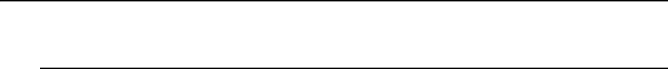
3: Ion Implantation

Loading External Profiles

190 Sentaurus™ Process User Guide

H-2013.03

Loading External Profiles

Loading Files Using load.mc

Precomputed profiles can be loaded to a given structure using the load.mc facility in

Sentaurus Process, that is:

implant <dopant> load.mc file=<name>

If the load.mc switch is set in the implant command, Sentaurus Process takes the TDR file

specified with the file selector and loads the datasets into the present structure. Interpolation

of the datasets is performed if the structure in the TDR file is different from the present

structure.

Sentaurus Process attempts to find the doping profiles required from the implant species and

the damage probability (for Crystal-TRIM) or damage dataset (for Sentaurus MC). For

example, in the following statement:

implant Boron load.mc file=my_data energy=10 dose=1e14

Sentaurus Process opens the files my_data{_fps}.tdr, and checks for the datasets

Boron_LastImp and PD_LastImp (for Crystal-TRIM) or Damage_LastImp (for

Sentaurus MC). If successful, these datasets are restored. If one or more of the required

datasets is missing, the respective fields remain empty. Then, during implantation

postprocessing, Boron_LastImp and Damage_LastImp are added to the Boron_Implant

and Damage datasets.

The following options are available in 2D structures:

■shift=<n>: Shifts the dataset along the y-axis.

■flip: Flips the dataset; the default is a flip to the left.

■left, right: Specifies the flipping direction.

■multiply=<n>: Multiplies the dopant data in the dataset by a factor; the damage remains

untouched.

NOTE The switch load.mc restores the datasets from the files without

checking the implant conditions specified in the implant command.

Therefore, load.mc by itself does not require the implant parameters

such as energy and dose be specified. However, Advanced Calibration

and CoImplant models may use these parameters (energy and dose)

for their calculations. Therefore, it is recommended that energy and

dose always be specified along with load.mc.

3: Ion Implantation

Multithreaded Parallelization of 3D Analytic Implantation

Sentaurus™ Process User Guide 191

H-2013.03

Automated Monte Carlo Run

If no TDR file with the specified name is found or the file selector is empty, a separate run

of Crystal-TRIM or Sentaurus MC is started to generate these files and the required datasets,

depending on the setting of the MC implantation model in the PDB (default is

sentaurus.mc):

pdbSet MCImplant model {crystaltrim | sentaurus.mc}

Sentaurus Process internally switches from the load.mc to crystaltrim or sentaurus.mc

mode. All implant parameters related to MC implantation (particles, cascades,

full.molecular) are used in this run.

NOTE The load.mc feature is designed to reuse precomputed MC results.

However, the profiles to load do not necessarily need to be generated

using the MC method.

Example

implant BF2 dose=1e14 energy=40 tilt=20 rotation=-90 load.mc \

file=bf2_1e14_40 particles=500 cascades

In the first run of this command, Sentaurus Process checks for the TDR file with the name

bf2_1e14_40. Since there is no file with this name, a full-cascade Crystal-TRIM or

Sentaurus MC run is started using the process parameters specified. At the end, the TDR file

bf2_1e14_40_fps.tdr is saved. The following are stored as well:

■All datasets related to the BF2 impurity profile (Boron_LastImp, Fluorine_LastImp).

■The damage probability (PD_LastImp) or damage (Damage_LastImp).

■The recoil profile (Silicon_LastImp) and vacancy profile (Vac_LastImp) because the

command is run in the full-cascade mode.

In a subsequent run of the same command, Sentaurus Process loads and restores these datasets

in a preprocessing step. The postprocessing is the same as after a MC run.

Multithreaded Parallelization of 3D Analytic Implantation

Parallel processing has become ubiquitous with the advent of multicore processors. The

performance of 3D analytic implantation can be improved dramatically by exploiting the

parallel processing power of multicore processors. In multithreaded mode, each thread works

on separate nodes, sharing the workload, thereby reducing the computation time.

3: Ion Implantation

Multithreaded Parallelization of Sentaurus MC Implantation

192 Sentaurus™ Process User Guide

H-2013.03

To engage the multithreaded parallelization of 3D analytic implantation, use the math

command:

math [ numThreads = <n> | numThreadsImp3d = <n> ]

where numThreads is a general keyword for MC implantation, 3D analytic implantation,

KMC, matrix assembly, and linear solver. However, numThreadsImp3d has a higher priority

over numThreads for 3D analytic implants and can be used to create the number of threads

specifically for 3D analytic implantation, which is different from that for other multithreaded

operations. The value of numThreads or numThreadsImp3d must be equal to the number of

cores in multicore processors.

You al so ca n mod ify t he stack s ize for each thread using the command:

math [ threadStackSize = <n> ]

The default stack size ( bytes) is usually sufficient for 3D analytic implantation.

Multithreaded Parallelization of Sentaurus MC

Implantation

NOTE This feature is available to Sentaurus MC only.

The performance of MC implantation (Sentaurus MC) also can be significantly improved by

using multithreaded parallelization. In this approach, a large job with many particles ( ) is

divided into multiple ( ) separate jobs with a smaller number of particles ( ). Sentaurus

Process then creates multiple threads and launches instances of Sentaurus MC implant.

Each instance of Sentaurus MC implant runs independently on its own thread. After these

threads are finished, the results are averaged, thereby improving the effective execution speed

for a large job.

To engage the multithreaded parallelization of Sentaurus MC implantation, use the math

command:

math [ numThreads = <n> | numThreadsMC = <n> ]

where numThreads is a general keyword for MC implantation, 3D analytic implantation,

KMC, matrix assembly, and linear solver. However, numThreadsMC has higher priority over

numThreads for MC implants and can be used to create the number of threads specifically for

Sentaurus MC implant, which is different from that for other multithreaded operations. The

value of numThreads or numThreadsMC should be equal to the number of cores in multicore

processors.

218 262144=

Nm⁄

3: Ion Implantation

References

Sentaurus™ Process User Guide 193

H-2013.03

You al so ca n mod ify t he stack s ize for each thread using the command:

math [ threadStackSize = <n> ]

The default stack size ( bytes) is usually sufficient for MC implantation.

References

[1] G. Hobler and S. Selberherr, “Two-Dimensional Modeling of Ion Implantation Induced

Point Defects,” IEEE Transactions on Computer-Aided Design, vol. 7, no. 2, pp. 174–

180, 1988.

[2] J. P. Biersack, “Basic Physical Aspects of High Energy Implantation,” Nuclear

Instruments and Methods in Physics Research, vol. B35, no. 2, pp. 205–214, 1988.

[3] J. F. Gibbons, W. S. Johnson, and S. W. Mylroie, Projected Range Statistics:

Semiconductors and Related Materials, Pennsylvania: Dowden, Hutchinson & Ross,

2nd ed., 1975.

[4] C. Zechner et al., “New Implantation Tables for B, BF2, P, As, In and Sb,” in 14th

International Conference on Ion Implantation Technology (IIT), Taos, NM, USA,

pp. 567–570, September 2002.

[5] S. Tian, V. Moroz, and N. Strecker, “Accurate Monte Carlo Simulation of Ion

Implantation into Arbitrary 1D/2D/3D Structures for Silicon Technology,” in MRS

Symposium Proceedings, Silicon Front-End Junction Formation—Physics and

Technology, vol. 810, San Francisco, CA, USA, pp. 287–292, April 2004.

[6] S. J. Morris et al., “An Accurate and Efficient Model for Boron Implants Through Thin

Oxide Layers into Single-Crystal Silicon,” IEEE Transactions on Semiconductor

Manufacturing, vol. 8, no. 4, pp. 408–413, 1995.

[7] S. Tian, “Predictive Monte Carlo ion implantation simulator from sub-keV to above

10 MeV,” Journal of Applied Physics, vol. 93, no. 10, pp. 5893–5904, 2003.

[8] M. Posselt, “Crystal-TRIM and Its Application to Investigations on Channeling Effects

During Ion Implantation,” Radiation Effects and Defects in Solids, vol. 130–131,

pp. 87–119, 1994.

218 262144=

3: Ion Implantation

References

194 Sentaurus™ Process User Guide

H-2013.03

[9] A. F. Tasch et al., “An Improved Approach to Accurately Model Shallow B and BF2

Implants in Silicon,” Journal of the Electrochemical Society, vol. 136, no. 3, pp. 810–

814, 1989.

[10] G. Hobler, E. Langer, and S. Selberherr, “Two-Dimensional Modeling of Ion

Implantation with Spatial Moments,” Solid-State Electronics, vol. 30, no. 4, pp. 445–

455, 1987.

[11] A. Stolmeijer et al., “General Expressions for the Impurity Distributions of B and P

Implanted in SiO2,” Journal of the Electrochemical Society, vol. 135, no. 9, pp. 2309–

2311, 1988.

[12] FLOOPS process and device simulator: http://www.flooxs.tec.ufl.edu/, October 2013.

[13] H. Ryssel, W. Krüger, and J. Lorenz, “Comparison of Monte Carlo Simulations and

Analytical Models for the Calculation of Implantation Profiles in Multilayer Targets,”

Nuclear Instruments and Methods in Physics Research, vol. B19/20, no. 20, pp. 40–44,

1987.

[14] G. Hobler and V. Moroz, “Initial Conditions for Transient Enhanced Diffusion: Beyond

the Plus-Factor Approach,” in International Conference on Simulation of

Semiconductor Processes and Devices (SISPAD), Athens, Greece, pp. 34–37, September

2001.

[15] S. Strauss et al., “Analytic model for ion channeling in successive implantations in

crystalline silicon,” Materials Science and Engineering B, vol. 124–125, pp. 376–378,

December 2005.

[16] S. Tian, “Accurate Monte Carlo simulation of fluorine and BF2 ion implantation into

crystalline silicon,” Nuclear Instruments and Methods in Physics Research B, vol. 215,

no. 3-4, pp. 403–412, 2004.

[17] H. Goldstein, Classical Mechanics, Cambridge, Massachusetts: Addison-Wesley Press,

1950.

[18] J. F. Ziegler, J. P. Biersack, and U. Littmark, “The Stopping and Range of Ions in

Solids,” The Stopping and Ranges of Ions in Matter, vol. 1, New York: Pergamon Press,

1985.

[19] M. T. Robinson and I. M. Torrens, “Computer simulation of atomic-displacement

cascades in solids in the binary-collision approximation,” Physical Review B, vol. 9,

no. 12, pp. 5008–5024, 1974.

[20] J. Lindhard and M. Scharff, “Energy Dissipation by Ions in the kev Region,” Physical

Review, vol. 124, no. 1, pp. 128–130, 1961.

[21] O. S. Oen and M. T. Robinson, “Computer Studies of the Reflection of Light Ions from

Solids,” Nuclear Instruments and Methods, vol. 132, pp. 647–653, 1976.

[22] M. Posselt et al., “Modeling of Damage Accumulation during Ion Implantation into

Single-Crystalline Silicon,” Journal of the Electrochemical Society, vol. 144, no. 4,

pp. 1495–1504, 1997.

3: Ion Implantation

References

Sentaurus™ Process User Guide 195

H-2013.03

[23] I. Santos et al., “Improved atomistic damage generation model for binary collision

simulations,” Journal of Applied Physics, vol. 105, p. 083530, April 2009.

[24] S. Tian, “Monte Carlo Simulation of Ion Implantation in Crystalline SiC With Arbitrary

Polytypes,” IEEE Transactions on Electron Devices, vol. 55, no. 8, pp. 1991–1996,

2008.

[25] A. Burenkov et al., “Simulation of BF3 Plasma Immersion Ion Implantation into

Silicon,” in 19th International Conference on Ion Implantation Technology (IIT),

Valladolid, Spain, pp. 233–236, June 2012.

[26] X. B. Tian, D. T. K. Kwok, and P. K. Chu, “Modeling of incident particle energy

distribution in plasma immersion ion implantation,” Journal of Applied Physics, vol. 88,

no. 9, pp. 4961–4966, 2000.

3: Ion Implantation

References

196 Sentaurus™ Process User Guide

H-2013.03

Sentaurus™ Process User Guide 197

I-2013.12

CHAPTER 4 Diffusion

This chapter provides information on the continuum models for

dopant and defect diffusion models and parameters. (For an

atomistic approach, see Chapter 5.)

Overview

During the fabrication process, dopants are introduced into the substrate with different

concentration profiles. As processing proceeds through various thermal annealing cycles, the

dopants diffuse and redistribute through the structure. The following effects contribute to

dopant redistribution and can be modeled by Sentaurus Process:

■Dopant (de)activation

■Dopant–defect interaction

■Chemical reactions at interfaces and in bulk materials

■Material flow

■Moving material interfaces

■Internal electric fields

Sentaurus Process is designed to address the challenges of integrated-circuit process modeling.

As technology development continues, the need for new process models increases. The

Alagator language is a versatile way to add and modify diffusion models quickly. This chapter

describes the diffusion models in Sentaurus Process. To modify or add new diffusion models,

see Modifying Diffusion Models on page 608.

The diffuse command represents the main simulation capabilities of Sentaurus Process. It

simulates:

■Thermal annealing of impurities.

■Material growth processes during annealing, for example, oxidation, silicidation, and

epitaxy (see Epitaxy on page 282 and Oxidation on page 615).

■Process-induced stress (see Chapter 9 on page 643).

4: Diffusion

Basic Diffusion

198 Sentaurus™ Process User Guide

I-2013.12

Basic Diffusion

The diffuse command is used to model the diffusion of impurities under oxidizing and non-

oxidizing conditions. The options of the diffuse command set diffusion conditions as well

as time-stepping options. (See diffuse on page 908 for all options.) For example, a command

for a simple non-oxidizing annealing at a temperature of for 10 s is:

diffuse temperature=900<C> time=10<s>

If you want to perform the same anneal with a wet (H2O) oxidizing ambient, execute the

following command:

diffuse temperature=900<C> time=10<s> H2O

A simple temperature ramp can be specified directly in the diffuse command by the keyword

ramprate. This keyword sets the change in the temperature over time:

diffuse temperature=900<C> time=10<min> O2 ramprate=10<C/min>

This example describes a dry oxidation of 10 minutes, starting at and ending at

. The same example can be repeated using the temp_ramp command as follows:

temp_ramp name=MyTempRamp temperature=900 time=10 O2 ramprate=10<C/min>

diffuse temp.ramp=MyTempRamp

The first line creates a temperature ramp with given conditions, and the second line specifies a

diffusion referring to this temperature ramp.

To describe more complex temperature cycles within one diffuse command, multiple

instances of the temp_ramp command can be used. A temperature ramp can consist of several

segments and, for each segment, one temp_ramp command is required. In addition, segments

can be grouped by using the same name for each segment. For example, a ramp-up, plateau,

and ramp-down can be specified as:

temp_ramp name=MyCycle temperature=500<C> time=5<min> H2O ramprate=100<C/min>

temp_ramp name=MyCycle temperature=1000<C> time=10<min> O2

temp_ramp name=MyCycle temperature=1000<C> time=10<min> ramprate=-50<C/min> \

last

diffuse temp.ramp=MyCycle

The keyword last in the third temp_ramp command declares the last segment of the

temperature ramp.

Sentaurus Process allows for thermal oxidation from O2 and H2O. The gas_flow command

is used to specify a mixed gas flow by specifying directly either the partial pressures of the gas

components or the flow [volume/time]. If the flows are defined, they are converted to partial

900°C

1000°C

4: Diffusion

Basic Diffusion

Sentaurus™ Process User Guide 199

I-2013.12

pressures by taking ratios. The use of the gas_flow command is similar to the temp_ramp

command; however, multiple gas flows using the same name must not be specified. When a

gas_flow is specified, it can be referred to from both the temp_ramp and diffuse

commands:

gas_flow name=MyGasFlow pH2O=0.5 pO2=0.5 pH2=0.1

To invoke the gas flow specification as given above, use:

temp_ramp name=MyTempRamp temperature=1000<C> time=10<min> gas.flow=MyGasFlow

diffuse temp.ramp=MyTempRamp

or:

diffuse temperature=1000<C> time=10<min> gas.flow=MyGasFlow

Sentaurus Process also allows you to select various diffusion models for point defects and

dopants (see Transport Models on page 205). Diffusion model setting and parameter setting are

performed with the pdbSet command. The basic settings are:

pdbSet <material> Dopant DiffModel <model>

where <model> can be any of Constant, Fermi, Pair, React, ChargedFermi,

ChargedPair, or ChargedReact.

Epitaxy can be simulated if either the Epi (also known as epi) or LTE ambient is specified in

either the temp_ramp or diffuse command. If Epi is specified, Silicon will grow on

Silicon and PolySilicon will grow on PolySilicon. If the LTE ambient is specified,

Silicon will again grow on Silicon, but PolySilicon will grow on Oxide, Nitride, and

PolySilicon.

pdbSet Silicon Dopant DiffModel Pair

diffuse temperature=800<C> time=60<min> Epi thick=0.01 \

epi.doping = {Germanium = 8e21}

This example sets the dopant diffusion model for all dopants in silicon to the Pair model and

grows a 0.01 thick epi layer with a Germanium concentration of .

It is also possible to set the initial diffusion time-step and the minimum annealing temperature

with the diffuse command.

diffuse temp.ramp=MyCycle minT=600<C> init=0.01<s>

This example uses the temp_ramp created in the earlier example. The initial time step is set to

0.01 s and the minimum annealing temperature is set to . The diffusion and reaction

equations will be switched off below but the mechanics will be solved.

µm

810

600°C

4: Diffusion

Basic Diffusion

200 Sentaurus™ Process User Guide

I-2013.12

If you want to set the minimum annealing temperature and initial time-step globally for all

diffusion commands, the following commands can be used:

pdbSet Diffuse minT {<n>}

pdbSet Diffuse InitTimeStep {<n>}

It is also possible to set minimum and maximum temperature limits for the annealing process

using the following commands:

pdbSet Diffuse minAnnealT <n>

pdbSet Diffuse maxAnnealT <n>

If the annealing temperature goes above or below these limits, Sentaurus Process will quit with

an error message.

See Viewing the Defaults: Parameter Database Browser on page 60 for other parameters

related to Diffuse.

Obtaining Active and Total Dopant Concentrations

By default, active and total dopant concentrations are only updated during diffusion steps. For

example, after an implant, the active concentrations (BoronActiveConcentration,

ArsenicActiveConcentration, and so on) and the total concentrations

(BoronConcentration, ArsenicConcentration, and so on) are not modified, which

makes them out of date.

Similarly for other commands that can change the dopant concentrations, the active and total

concentrations are not updated. These commands include, but are not limited to, select,

load, init, and profile.

After one of these commands is issued, the active and total dopant concentrations may not be

current. To update the active and total dopant concentrations use the diffuse time=0 ...

command.

NOTE To update the active and total concentrations of the dopants without

dopant redistribution, the diffuse command with zero time can be

used. For example, to calculate the active dopant concentration at

for the chosen diffusion model, use:

diffuse time=0.0 temperature=850

NOTE Since the diffuse command performs the recrystallization and the

initialization of clusters even with zero time, it must not be added

between consecutive implantation steps.

850°C

4: Diffusion

Basic Diffusion

Sentaurus™ Process User Guide 201

I-2013.12

See diffuse on page 908 for all options of the diffuse command.

Transport Models

Sentaurus Process has several basic transport models with varying levels of complexity for

computing flux, . This diversity of models is needed to balance accuracy with simulation

times, which vary widely depending on the model selection:

■The React (see React Diffusion Model on page 212) and ChargedReact (see

ChargedReact Diffusion Model on page 206) diffusion models, also known as five-stream

diffusion models, are the most advanced dopant diffusion models in Sentaurus Process.

They solve up to three separate equations per dopant – a substitutional dopant – and up to

two dopant–defect pairs and two defect equations. The ChargedReact model is the most

accurate model available in Sentaurus Process. but because of the large number of

equations required, it also is the most computationally expensive. The React model, which

is an uncharged version of the ChargedReact model, is provided for backward

compatibility.

■The Pair (see Pair Diffusion Model on page 216) and ChargedPair (see ChargedPair

Diffusion Model on page 214) diffusion models, also known as three-stream diffusion

models, assume that dopant–defect pairs are in local equilibrium but still solve for separate

point-defect equations. These models solve one equation per dopant and two defect

equations. The ChargedPair diffusion model allows the pairing coefficients to vary with

charge state. These models are the most commonly used for advanced CMOS processes as

they represent a balance between accuracy and computational expense. For extremely fast

ramp rates or for customized initial conditions, the ChargedReact model or React model

is a better choice. The Pair model, which is an uncharged version of the ChargedPair

model, is provided for backward compatibility.

■The Fermi (see Fermi Diffusion Model on page 219) and ChargedFermi (see

ChargedFermi Diffusion Model on page 217) diffusion models both assume that point

defects as well as dopant–defect pairs are in equilibrium. The ChargedFermi diffusion

model allows the diffusivity of each charge state to be set separately. An uncharged version

of the model is provided for backward compatibility. These models can be used for long-

term high-temperature anneals where the transient effect of annealing implant damage is

minimal.

■The Constant diffusion model (see Constant Diffusion Model on page 220), unlike all

other transport models, assumes a constant diffusivity and no electric-field effect, and is

used mainly for dopant diffusion in oxide.

The selection of transport model is specified as follows:

pdbSet <material> Dopant DiffModel <model>

4: Diffusion

Basic Diffusion

202 Sentaurus™ Process User Guide

I-2013.12

where <model> must have one of the valid diffusion model names – Constant, Fermi, Pair,

React, ChargedFermi, ChargedPair, or ChargedReact.

It is also possible to select a different diffusion model for each dopant in the same material. In

this case, use the command:

pdbSet <material> <dopant> DiffModel <model>

where <dopant> is a valid dopant name (for example, Boron).

The ChargedFermi, ChargedPair, and ChargedReact diffusion models take into account

each charged point defect individually. Otherwise, they are very similar to the Fermi and Pair

diffusion models.

NOTE Even though you can select any diffusion model individually for each

dopant, it is not recommended to mix the ChargedFermi,

ChargedPair, or ChargedReact models with the uncharged

versions.

Ta bl e 11 S um m ar y o f d o p a nt d i f fu s io n m o de l s an d p a r a me te rs

pdb command Diffusion model

Type

ChargedReact

React

ChargedPair

Pair

ChargedFermi

Fermi

Constant

pdbSet <material> <dopant> <defect> D Diffusivity

XXXX

pdbSet <material> <dopant> <defect> Dstar Diffusivity

pdbSet <material> <dopant> Dstar Diffusivity

pdbSet <material> <defect> D Diffusivity

XXXXX

pdbSet <material> <dopant> <defect> ChargePair Pairing Coeff.

pdbSet <material> <dopant> <defect> Binding Pairing Coeff.

pdbSet <material> <dopant> <defect> kfFTM Rate

pdbSet <material> <dopant> <defect> kfKickOut Rate

pdbSet <material> <defect> ChargeStates Charging Coeff.

XXXXX

pdbSet <material> <defect> ChargeStatesScale Charging Coeff.

XXXXX

pdbSet <material> <defect> Cstar Concentration

XXXXXXX

pdbSet <material> <defect> KbulkChargeStates Charging Coeff.

XXXXX

4: Diffusion

Basic Diffusion

Sentaurus™ Process User Guide 203

I-2013.12

In Table 11, <material> is a valid material name, <dopant> is a valid dopant name, and

<defect> is either Int or Vac.

Recombination and Reaction Models

Many reactions and recombination models are available in Sentaurus Process. Different

diffusing species such as dopants, defects, and impurities will all have different recombination

and reaction terms. These terms come from the following models:

■Dopant clusters–solid solubility, transient, and dopant–defect cluster models (see Dopant

Activation and Clustering on page 292).

■Defect clusters–Equilibrium, {311}, Loop, LoopEvolution, 1Moment, 2Moment,

Full, and FRENDTECH models (see Defect Clusters on page 319).

■Impurity species:

• Carbon model, Nitrogen model (see NeutralReact Diffusion Model on page 220).

• Fluorine model (see Dopant Active Model: FVCluster on page 304).

Boundary Conditions

Sentaurus Process can simulate various boundary conditions for dopants and defects. You can

select eight different boundary conditions:

■HomNeumann can be applied to any boundary (see HomNeumann on page 357).

■Natural is for point defects (see Natural on page 358).

■Segregation is for dopants (see Segregation on page 361).

■Dirichlet is for dopants and defects (see Dirichlet on page 364).

■ThreePhaseSegregation is for dopants (see ThreePhaseSegregation on page 365).

■GrainBoundarySegregation is for dopants in polycrystalline materials (see Boundary

Conditions on page 258).

■GrainGrainBoundarySegregation is for dopants in polycrystalline materials (see

Boundary Conditions on page 258).

■Trap is for dopants such as fluorine and nitrogen in trap-dependent oxidation.

■TrapGen is for dopants such as nitrogen in N2O oxidation.

■Continuous is for dopants used only during epi growth (see Continuous on page 369).

The Natural and Dirichlet boundary conditions consider interstitial injection during

oxidation for oxidation-enhanced diffusion (OED) of dopants.

4: Diffusion

General Formulation

204 Sentaurus™ Process User Guide

I-2013.12

Other Materials and Effects

In addition to generic transport and recombination and reaction models, other effects can be

simulated:

■Polysilicon model (see Diffusion in Polysilicon on page 242).

■SiGe diffusion model (see Dopant Diffusion in SiGe on page 260).

■Epitaxy (see Epitaxy on page 282).

General Formulation

The general expression for the particle current of a diffusing species of charge is given by:

(120)

where is the concentration, is the diffusivity, is the electron concentration, and is

the intrinsic electron concentration.

The continuity equation for species of charge is given by:

(121)

where the recombination/reaction term is split into two parts: is a possible contribution

coming from the transport model selection (see Transport Models on page 205) and can

contain terms from other reactions, which are most often clustering reactions but could include

any type of reaction. Reactions that transform species into another species will introduce

positive terms into the expression for . Total dopant concentration of dopant will be

equal to the sum of all dopants, dopant–defect pairs, and any related clusters (for example,

For the models that do not consider different charge states, computation of the electron

concentration by default is given by the charge neutrality condition , where

is given by the active dopant concentrations (for example, where is the

active donor concentration and is the active acceptor concentration). For the charged

models, the charge states of the defects or defect pairs are considered individually.

JAcd–Ac

----





c–∇Acn

----









dAc

t∂

∂Ac

∇J•Ac

–RAc

trans RAc

clus

–+=

RAc

trans

RAc

clus

RAc

clus

ATotal

cAcApair

cAclus

++=

n–pN∆++ 0=

N∆

∆NN

dNa

–=

4: Diffusion

Transport Models

Sentaurus™ Process User Guide 205

I-2013.12

It is expected that the charge reactions are in equilibrium, so that the ratio in the various charged

states is set by the Fermi level:

(122)

where is a reference charge state, which is chosen as 0 for interstitials and vacancies, and is

chosen as the dopant charge for dopant–defect pairs. The are parameters that are set by

default to an Arrhenius expression. In addition, for the charged models, it is necessary to solve

a coupled equation for the electron concentration. The default equation is the same as for the

uncharged case, that is, the charge neutrality equation but, in this case,

is a function of because it contains contributions from charged defects or charged defect

pairs as well as dopants. It is also possible for both the charged and uncharged models to solve

the Poisson equation (see Electron Concentration on page 276).

Transport Models

Transport models compute the particle flux of dopants and are the core diffusion models solved

by Sentaurus Process. In addition to particle flux, pairing reactions can be computed depending

on the transport model selection. Transport models are usually used with one or more

clustering or activation models available. The reaction or clustering models will not modify the

dopant flux, but will compute terms to be added to from Eq. 121. The models are

described in detail here.

The selection of the transport model is made with the command:

pdbSet <material> <dopant> DiffModel <model>

where <material> is the material name; <dopant> can be either "Dopant" to apply to all

dopants or a named dopant such as boron, arsenic, phosphorus, antimony, and indium; and

<model> is one of the models ChargedReact, React, ChargedPair, Pair,

ChargedFermi, Fermi, or Constant.

Ta bl e 1 2 S o l ut io n na m es

Symbol Boron Arsenic Phosphorus Antimony Indium

Boron Arsenic Phosphorus Antimony Indium

BoronInt ArsenicInt PhosphorusInt AntimonyInt IndiumInt

BoronVac ArsenicVac PhosphorusVac AntimonyVac IndiumVac

BActive AsActive PActive SbActive InActive

Acr+kAcCAr

----



c()–

kAc

n–pN∆++ 0=

N∆

Rclus

CAI

CAV

4: Diffusion

Transport Models

206 Sentaurus™ Process User Guide

I-2013.12

The transport for point defects is computed when Compute.Point.Defect is set to 1:

pdbSet <material> Compute.Point.Defect <0 | 1>

ChargedReact Diffusion Model

The ChargedReact diffusion model is the most general transport model in Sentaurus Process.

The model has an immobile substitutional dopant and up to two mobile charged dopant–defect

pair species. Mobile charged point defects are also included in the model.

The following reactions are considered:

(123)

(124)

(125)

(126)

(127)

The differential equations that are solved in this model are:

(128)

(129)

Ta bl e 1 3 Po i n t- d e fe c t n a m es

Symbol Interstitial Vacancy

Int Vac

EqInt EqVac

IntNeutralStar VacNeutralStar

IntNeutral VacNeutral

CX0

AzIi

+AI zj+()ij–()e–↔

AzVi

+AV zj+()ij–()e–↔

IiVj

+ij+()e–↔

AI zi+()

+Azij+()e–↔

AV zi+()

+Azij+()e–↔

t∂

∂CARAI

–RAV

–RAI V,RAV I,RA

clus

–++=

t∂

∂CAI ∇J•AI

–RAI RAI V,

–RAI

clus

–+=

4: Diffusion

Transport Models

Sentaurus™ Process User Guide 207

I-2013.12

(130)

(131)

(132)

where is the concentration of substitutional (and assumed to be immobile) dopants, is

the concentration of ‘free’ defects of type (either interstitials or vacancies), in other words,

those defects not in clusters or pairs. The reaction rates of the different species ( ) are defined

later in this section.

Next, the flux of the mobile defect pair is considered. Working with Eq. 120, p. 204 for the

charged pairs, the equation will be written in terms of the total concentration of pairs.

It is expected that the dopant-defect pairing reaction is in equilibrium, therefore, a set of

constants for this pairing is defined:

(133)

where is either I or V, is the charge of the dopant , and is the pairing coefficient for

the pair , and is given by:

(134)

To set , use:

pdbSet <material> <dopant> <defect> ChargePair <c> {<n>}

where <material> is a material name (see), <dopant> is one of the existing Sentaurus

Process dopants, <defect> is either Interstitial or Vacancy, <c> is the charge state, and

<n> is a Tcl expression that returns a number – it can be simply a number.

One commonly used Tcl procedure for setting parameters is Arrhenius. This procedure takes

a prefactor and an energy as arguments and returns .

t∂

∂CAV ∇J•AV

–RAV RAV I,

–RAV

clus

–+=

t∂

∂CIJI

∇•–RIV RAI

–– RAV I,

–RI

clus

–=

t∂

∂CVJV

∇•–RIV R–AV

–RAI V,

–RV

clus

–=

CAXzc+kAXcCAzCXc

kAXc

kAXckAXc

0k–AXc

kBT

-------------







exp=

kAXc

prefactor energy

–

kBT

--------------------





exp⋅

4: Diffusion

Transport Models

208 Sentaurus™ Process User Guide

I-2013.12

The flux of the pairs is computed from Eq. 120, p. 204:

(135)

where is the total concentration of pairs that is the sum of the concentrations of pairs at

every charge state and is an effective diffusivity of dopant point-defect pairs at charge

state and is related to the self diffusivity by:

(136)

where is the equilibrium concentration of the neutral defects and is related to the total

equilibrium intrinsic concentration of defect by:

(137)

The quantities and , which by default follow an Arrhenius law, can be

changed by using the command:

pdbSet <material> <defect> Cstar {<n>}

To set , use:

pdbSet <material> <dopant> <defect> D <c> {<n>}

A set of equilibrium-charging constants, , for defect is defined:

(138)

where is either I or V, and is the charging coefficient for the defect and is given by:

(139)

JAX JAXc



–=

DAXc

----





c–z–CAX

CX0

*kAXqkXq

----





q–



-------------------------------------------------- n

----











∇



–=

CAX

DAXc

dAXc

DAXcCX0

*kAXckXcd

AXc

DAXc

0D–AXc

kBT

---------------







exp=

CX0

*CXintrinsic()

kXc



-----------------------------=

CIintrinsic()

CVintrinsic()

DAXc

kXc

CXckXcCX0

----





c–

kXc

kXckXc

0k–Xc

kBT

----------







exp=

4: Diffusion

Transport Models

Sentaurus™ Process User Guide 209

I-2013.12

To set , use:

pdbSet <material> <defect> ChargeStates <c> {<n>}

NOTE The neutral charge state must always be 1.0.

Similar to the pairs, the defect fluxes are computed from Eq. 120, p. 204:

(140)

where is the total concentration of defects that is the sum of the concentrations of defect

at every charge state and is the diffusivity of the defect of charge state and is given by:

(141)

To set , use:

pdbSet <material> <defect> D <c> {[Arrhenius <prefactor> <energy>]}

Now, the reaction rates can be written by considering Eq. 123, p. 206 to Eq. 127, p. 206 and

the general formula for the rate of all combinations of charge states:

(142)

Therefore, summing all possible charge states gives:

(143)

(144)

(145)

kXc

JXJXc



–=

kXcD

----





c–CX



kXq

----





q–



---------------------------------------------- CX

-------







∇–=

DXc

DXcdXc

DXc

0D–Xc

kBT

------------







exp=

DXc

AaBbABcca–b–()e+↔+

RAaBbc,, kAaBbc,,

fCAaCBbkAaBbc,,

rCABc

----





ca–b–()

–





RAX KAX

fCACX

CAX

KAX

----------–







–≡

RAI V,KAI V,

fCAICVKAX

rCI

*CV

*CA

–()≡

RAV I,KAV I,

fC(AVCIKAX

rCI

*CV

*CA)–≡

4: Diffusion

Transport Models

210 Sentaurus™ Process User Guide

I-2013.12

where:

(146)

(147)

(148)

(149)

where is the forward reaction rate for the kick-out mechanism, and is either interstitial

or vacancy, and are forward reaction rates for the Frank–Turnbull mechanism and

is the equilibrium constant.

The forward ( ) kick-out reaction rates can be set by using the following commands:

pdbSet <material> <dopant> <defect> kfKickOut <c> {<n>}

where c is the charge state. By default, kfKickOut values for each charge state are given as:

(150)

where is the hopping length, which can be set using the command:

pdbSet <material> <dopant> <defect> lambdaK

Similarly, the forward ( , ) Frank–Turnbull reaction rates can be defined using the

commands:

pdbSet <material> <dopant> <defect> kfFTM <i,j> {<n>}

KAX

KfXKOikXi

----





i–



kXc

----





c–



---------------------------------------------

≡

KAX

kAXikXi

----





i–



kXc

----





c–



---------------------------------------

≡

KAI V,

AIiVj

,FTkAIikVj

----



ij+()–



kAIc

----





c–kVz

----





z–



----------------------------------------------------------------------------

≡

KAV I,

AViIj

,FTkAVikIj

----



ij+()–



kAVc

----





c–kIz

----





z–



----------------------------------------------------------------------------

≡

KAX

KAI V,

KAV I,

KAX

KfXKOi j,

KfXKOi

DAXi

*kXi



kX0λ2

---------------------------------

≡

KAI V,

KAV I,

4: Diffusion

Transport Models

Sentaurus™ Process User Guide 211

I-2013.12

NOTE The indices of the forward recombination rates have the form of .

Both and are integers and are separated by a comma; no space is

allowed between the indices.

The I–V recombination reaction is given as:

(151)

where:

(152)

The superscript ‘*’ refers to the equilibrium concentration, and the subscripts and are for

the interstitials and vacancies, respectively. The subscripts are the charge states of the

defects. is the bulk recombination rate for interstitials and vacancies at the charge stated

and , respectively. The bulk recombination rate for each charged point defect can be

set using the command:

pdbSet <mater> <defect> KbulkChargeStates <i,j> {<n>}

The equilibrium concentration of the unpaired point defect can be calculated by:

(153)

where is the scaled charging coefficient for the defect and can be set by using:

pdbSet <material> <defect> ChargeStatesScale <c> {<n>}

is set to as a default.

NOTE The indices for the parameter KbulkChargeStates have the form of

. Both and are integers and are separated by a comma; no space

is allowed between the indices.

ij,

RIV KIV CICVCI

*CV

–()=

KIV

CIintrinsic()

*CVintrinsic()

*CV

*kIzkVz



----------------------------------------------------------KIiVjkIikVj

----



ij+()–



zij,,

KIiVj

*CXintrinsic()

kXc

----





c–



------------------------------=

kXc

ij,

4: Diffusion

Transport Models

212 Sentaurus™ Process User Guide

I-2013.12

React Diffusion Model

The React model is similar to the ChargedReact model, except that the reaction rates are

not charge state–dependent and the electron concentration is computed directly from the net

doping concentration. In addition, the Frank–Turnbull mechanism is not considered.

The reactions considered are:

(154)

(155)

where is the dopant, is the interstitial, and is the vacancy.

The following set of differential equations represents the model:

(156)

(157)

(158)

where is the concentration of substitutional (and assumed to be immobile) dopant and

is the concentration of ‘free’ defects of type (either interstitials or vacancies), that is, those

defects not in clusters or pairs.

Next, the flux of the mobile–defect pair is considered. In this model, the reaction rates are

assumed to be independent of the charge state, so the pair charging constants are only needed

for the flux of the pairs and are absorbed into the diffusivity of the pairs in this way:

(159)

AI+AI↔

AV+AV↔

t∂

∂CARAI

–RAV

–RA

clus

–=

t∂

∂CAX JAX

∇•–RAX RAX

clus

–+=

t∂

∂CXJX

∇•–RIV

–RAX

–RX

clus

–=

JAX

DAXc

----





c–z–







–

BAX

------------------------------------------------CAX

----------n

----





∇=

4: Diffusion

Transport Models

Sentaurus™ Process User Guide 213

I-2013.12

where is the charge state of dopant , is either interstitial or vacancy, and is the

effective diffusivity of dopant point-defect pair at charge state and is related to the bare

diffusivity, by:

(160)

where is a set of equilibrium charging constants for defect defined by Eq. 138, p. 208

and Eq. 139, p. 208, and is the equilibrium concentration of the neutral defects defined by

Eq. 137, p. 208.

To set , use:

pdbSet <material> <dopant> <defect> D <c> {<n>}

where:

■<material> is a material name (see Material Specification on page 52).

■<dopant> is one of the existing Sentaurus Process dopants.

■<defect> is either Interstitial or Vacancy.

■<c> is the charge state.

■<n> is a Tcl expression that returns a number; it can be simply a number.

One commonly used Tcl procedure for setting parameters is Arrhenius. This procedure takes

a prefactor and an energy as arguments and returns .

You ca n mod if y t he enti re arr ay with t he co mmand (for example, arsenic–vacancy pairs):

pdbSet Si Arsenic Vac D {

0 {[Arrhenius 0.0 3.45]}

-1 {[Arrhenius 12.8 4.05]}

}

The defect flux is the same as the ChargedReact model and is given by Eq. 140, p. 209.

The reaction can be written as:

(161)

where is either interstitial or vacancy, is the binding coefficient of defect and dopant

, is the rate constant for the chemical reaction, and is the active portion of .

DAXc

dAXc

DAXcCX0

*BAXkXcd

AXc

DAXc

0D–AXc

kBT

---------------







exp=

kXc

CX0

DAXc

prefactor energy

–

kBT

--------------------





exp⋅

RAX KAXr CA

+CX

CAX

BAX

----------–





≡

BAX

KAXr

4: Diffusion

Transport Models

214 Sentaurus™ Process User Guide

I-2013.12

The binding term between the defect and dopant also follows the Arrhenius law:

(162)

The term can be changed with the command:

pdbSet <material> <dopant> <defect> Binding {<n>}

The chemical reaction term is expressed with:

(163)

and can be modified by using the command:

pdbSet <material> <dopant> <defect> Krate {<n>}

The defect recombination rate is the same as in the ChargedReact model and is given by

Eq. 151, p. 211.

ChargedPair Diffusion Model

The ChargedPair diffusion model assumes that the dopant–defect pairs are in local

equilibrium with the dopant and defect concentration. Point defects themselves are not

assumed to be in equilibrium. The kick-out mechanism that describes the dopant–defect

pairing is given by:

(164)

(165)

and is assumed to be in equilibrium. In these two equations, is the dopant, is the interstitial,

is the vacancy, and is the charge state.

The differential equations solved with this model are:

(166)

(167)

BAX BAX0

BAXE

–

----------------





exp=

KrKr0

K–rE

------------





exp=

RIV

AzIc

+AI zc+()

↔

AzVc

+AV zc+()

↔

t∂

∂CAJA

∇•–RA

clus

–=

t∂

∂CXtotal

() JXJA

∇•–∇•–RIV

–RX

clus

–=

4: Diffusion

Transport Models

Sentaurus™ Process User Guide 215

I-2013.12

where is the total interstitial concentration including dopant–defect pairs

but excluding clusters, is the sum of AI and AV pair fluxes, is the defect flux, and

is the total dopant concentration excluding clusters.

To write an expression for the pair fluxes, it is necessary to first define the equilibrium

constants, , for the pairing reactions:

(168)

where is either interstitial or vacancy, is the charge state of the point defect, is the

active portion of , and is the concentration of the neutral point defect . The ionization

equilibrium constant is given by Eq. 138, p. 208 and Eq. 139, p. 208.

The pairing coefficients for the dopant–defect pairs with different charge states, , can be

modified with the command:

pdbSet <material> <dopant> <defect> ChargePair <c> {<n>}

where <material> is a material name (see Material Specification on page 52), <dopant> is

one of the existing Sentaurus Process dopants, <defect> is either Interstitial or

Vacancy, <c> is the charge state, and <n> is a Tcl expression that returns a number; it can be

simply a number.

The flux for the impurity is given by:

(169)

where is the effective diffusivity of dopant point-defect pair at charge state , is the

charge state of dopant , is the active portion of , is the concentration of the neutral

point defect , and is the equilibrium concentration of the same defect and is given by

Eq. 137, p. 208.

The effective diffusivity is related to the bare dopant–defect diffusivity, , by:

(170)

You ca n set by us in g:

pdbSet <material> <dopant> <defect> D <c> {<n>}

CXtotal CXCAX

+≡

kAXc

CAX CA

+CX0kAXckXc

----





c–



≡

CX0

kXc

kAXc

JADAXc

----





c–z–CA

+CX0

CX0

-------- n

----











∇

cX,



–=

DAXc

CX0

dAXc

DAXcCX0

*kXck

AXcdAXc

DAXc

0D–AXc

kBT

---------------







exp=

DAXc

4: Diffusion

Transport Models

216 Sentaurus™ Process User Guide

I-2013.12

NOTE Diffusion coefficients for the ChargedPair model and Dstar for

the ChargedFermi model include the interstitial efficiency factors.

Both the flux for the defects ( ) and the defect recombination rate ( ) are the same as the

ChargedReact model and are given by Eq. 140, p. 209 and Eq. 151, p. 211, respectively.

Pair Diffusion Model

The Pair diffusion model is similar to the ChargedPair model except that the reaction rates

are not charge state–dependent, and the electron concentration is computed directly from the

net doping concentration. In addition, the Frank–Turnbull mechanism is not considered. The

kick-out mechanism, which describes the dopant–defect pairing, is given by:

(171)

(172)

and is assumed to be in equilibrium. In these two equations, is the dopant, is the interstitial,

and is the vacancy.

As in the ChargedPair model, the following set of differential equations is solved:

(173)

(174)

where is the total interstitial concentration including dopant–defect pairs

but excluding clusters, is the sum of AI and AV pair fluxes, is the defect flux, and

is the total dopant concentration excluding clusters.

An equilibrium constant for the pairing reactions is defined and given by:

(175)

where is either interstitial or vacancy, is the binding coefficient of defect and dopant

, and is the active portion of .

The binding term between the defect and dopant also follows the Arrhenius law:

(176)

RIV

AI+AI↔

AV+AV↔

t∂

∂CAJA

∇•–RA

clus

–=

t∂

∂CXtotal

() JXJA

∇•–∇•–RIV

–RX

clus

–=

CXtotal CXCAX

+≡

CAX BAXCA

+CX

≡

BAX

BAX BAX0

BAXE

–

----------------





exp=

4: Diffusion

Transport Models

Sentaurus™ Process User Guide 217

I-2013.12

The term can be changed with the command:

pdbSet <material> <dopant> <defect> Binding {<n>}

The flux for the impurity is given by:

(177)

where represents the diffusivity of dopant point-defect pairs at charge state , is the

charge state of dopant , is the active portion of , and is either interstitial or vacancy.

The effective diffusivity is related to the bare dopant–defect diffusivity, , by:

(178)

where is the equilibrium concentration of the neutral point defect and the ionization

equilibrium constant, , is defined by Eq. 138, p. 208 and Eq. 139, p. 208.

To modify diffusivity terms, use the command:

pdbSet <material> <dopant> <defect> D <charge> {<n>}

Both the flux for the defects ( ) and the defect recombination rate ( ) are the same as the

ChargedReact model and are given by Eq. 140, p. 209 and Eq. 151, p. 211, respectively.

ChargedFermi Diffusion Model

The ChargedFermi diffusion model is similar to the ChargedPair diffusion model, except

that charged point defects are considered to be in equilibrium; no point-defect equations are

solved for inert diffusion conditions if the point defect clusters are not turned on. If the point

defect clusters are turned on or the oxidation is on, the point defect equations will be turned on

automatically. The substitutional dopants are immobile and the total dopant flux is due to the

dopant–defect pairs. The following set of differential equations is solved along with the

potential equation Eq. 354, p. 276:

(179)

JADAXc

----





c–z–CA

+CX

-------n

----











∇

cX,



–=

DAXc

dAXc

DAXcCX0

*kXcBAXdAXc

DAXc

0D–AXc

kBT

---------------







exp=

CX0

kXc

RIV

t∂

∂CAJA

∇•–=

4: Diffusion

Transport Models

218 Sentaurus™ Process User Guide

I-2013.12

As in the ChargedPair model, a set of pairing constants ( ) that define the pair

concentration is defined:

(180)

where:

■ is either interstitial or vacancy.

■ is the charge state of the point defect.

■ is the charge state of dopant .

■ is the active portion of .

The ionization equilibrium constant is given by Eq. 138, p. 208 and Eq. 139, p. 208.

The dopant flux is given by:

(181)

where:

■ is the effective diffusivity of dopant point–defect pairs at charge state .

■ is the concentration of the neutral point defect .

■ is the equilibrium concentration of the same defect and is given by Eq. 137, p. 208.

■ will be equal to if the point-defect equations are switched off.

■ is related to the bare diffusivity by:

(182)

To set use:

pdbSet <material> <dopant> <defect> Dstar <c> {<n>}

The pairing coefficients for the dopant–defect pairs with different charge states, , can be

defined with the command:

pdbSet <material> <dopant> <defect> ChargePair <c> {<n>}

NOTE If the point-defect clusters are switched off and oxidation is switched

on, only the interstitial point-defect equation will be switched on.

kAXc

CAX CA

+CX0kAXckXc

----





c–



≡

kXc

JADAXc

----





c–z–CA

+CX0

CX0

-------- n

----











∇

cX,



–=

DAXC

CX0

DAXC

dAXc

DAXcCX0

*kAXckXcd

AXc

DAXc

0D–AXc

kBT

---------------







exp=

DAXc

kAXc

4: Diffusion

Transport Models

Sentaurus™ Process User Guide 219

I-2013.12

Fermi Diffusion Model

The Fermi diffusion model is more complex than the Constant diffusion model. It assumes

that point defects are in equilibrium and it includes electric-field effects. Therefore, the point-

defect equations are not solved.

As in the ChargedPair model, the following set of differential equations is solved:

(183)

where is the sum of AI and AV pair fluxes, and is the total dopant concentration

including clusters.

An equilibrium constant for the pairing reactions is defined and given by:

(184)

where is either interstitial or vacancy, is the binding coefficient of defect and dopant

, and is the active portion of . The dopant flux is given by:

(185)

where:

■ is the charge state of the point defect.

■ is the charge state of dopant .

■ is the active portion of .

■ is either interstitial or vacancy.

■ is the effective diffusivity of dopant point-defect pairs at charge state and is related

to the bare diffusivity by:

(186)

The pairing ratio only appears in the formula for and cannot be modified independently

in the Fermi model. You can set by using:

pdbSet <material> <dopant> <defect> Dstar <c> {<n>}

t∂

∂CAJA

∇•–=

CAX BAXCA

+CX

≡

BAX

JADAXc

----





c–z–CA

----









∇

Xc,



–=

DAXC

dAXc

DAXcCX0

*BAXkXcd

AXc

DAXc

0D–AXc

kBT

---------------







exp=

BAX

DAXc

4: Diffusion

Transport Models

220 Sentaurus™ Process User Guide

I-2013.12

Constant Diffusion Model

The Constant diffusion model is the simplest diffusion model used in Sentaurus Process and

is mainly for dopant diffusion in oxide. It assumes that there is no interaction between dopants

and point defects, and that there are no electric-field effects on dopant diffusion. The point-

defect equations are also switched off. The impurity diffusion is given by:

(187)

where is the intrinsic diffusivity of the impurity and is the active portion of .

The diffusivity follows the Arrhenius law:

(188)

For example, the command:

pdbSet Silicon Arsenic Dstar {[Arrhenius 6.66e-2 3.44]})

sets the to and to 3.44 eV. The general format of the command

is:

pdbSet <material> <dopant> Dstar {<n>}

NOTE Unlike the ChargedFermi model, Dstar is not defined as an array for

the Constant model.

NeutralReact Diffusion Model

NeutralReact diffusion in silicon is close to the React model (see React Diffusion Model

on page 212) except that there are no charged atoms. The model can be switched on using the

command:

pdbSet <material> <dopant> DiffModel NeutralReact

NeutralReact diffusion in silicon is described by a kick-out mechanism [1]. Other

mechanisms such as dissociation and clustering can also be taken into account. In the

integration in Sentaurus Process, each of these mechanisms is described by one or more terms:

(189)

(190)

t∂

∂CADstar CA

∇()∇•=

Dstar

Dstar Dstar0

DstarE

–

-------------------





exp=

Dstar0

6.66 10 2–

× cm2/s

DstarE

AI+AI↔

AI V+A↔

4: Diffusion

Transport Models

Sentaurus™ Process User Guide 221

I-2013.12

where is the substitutional dopant, is the mobile dopant–interstitial pair, is interstitial,

and is vacancy. The first reaction is the kick-out reaction and the second one is the

dissociation reaction. These reaction can be written as:

(191)

(192)

where:

■ is the concentration of substitutional dopant atoms.

■ is the concentration of mobile dopant atoms.

■ and are the forward reaction rates.

■ and are the binding coefficients.

To set, use:

pdbSet <material> <dopant> Interstitial Kf {<n>}

pdbSet <material> <dopant> Vacancy Kf {<n>}

pdbSet <material> <dopant> Interstitial Bind {<n>}

pdbSet <material> <dopant> Vacancy Bind {<n>}

The differential equations that describe the model are:

(193)

(194)

where is the diffusivity of mobile dopant–interstitial pairs and can be set using the

command:

pdbSet <material> <dopant> Interstitial D 0 {<n>}

Carbon Diffusion Model

Carbon diffusion is a typical example for the NeutralReact diffusion model. The kick-out

reaction rate is defined by:

pdbSet Silicon Carbon Interstitial Kf {\

[expr ([pdbGetElement Si Carbon D 0]/([pdbDelayDouble Si Carbon\

MigrationLength]* [pdbDelayDouble Si Carbon\

MigrationLength]*[pdbDelayDouble Si Int Cstar]))]\

}

RKickOut KfI CACIBAICAI

–()≡

RDissociation KfV CAICVCI

*CV

*BAVCA

–()≡

CAI

KfI

KfV

BAI

BAV

t∂

∂CARDissociation RKickOut

–=

t∂

∂CAI DAI0CAI

∇()RKickOut RDissociation

–+∇•=

DAI0

4: Diffusion

Transport Models

222 Sentaurus™ Process User Guide

I-2013.12

will set to .

is the migration length (cm) of carbon atoms and is the diffusivity of carbon, and these

parameters can be set using the commands:

pdbSet <material> Carbon MigrationLength {<n>}

pdbSet <material> Carbon D 0 {<n>}

For the details of the carbon-clustering model, see Carbon Cluster on page 303.

Nitrogen Diffusion Model

Nitrogen diffusion is defined according to the Constant diffusion model by default. However,

instead of the Constant model, the NeutralReact diffusion model can be used for nitrogen

diffusion. If the NeutralReact model is specified for nitrogen diffusion, the nitrogen dimer

forms and diffuses. The dimer is formed by the following reaction:

(195)

In the above reaction, is the monomer, in other words, nitrogen interstitial , and

denotes the dimer , which has the solution name NDimer. The nitrogen monomer and

dimer equations are formulated by:

(196)

(197)

(198)

(199)

(200)

The reaction for dimer formation is given by:

(201)

KfI

DC0

λ2CI

*intrinsic()

----------------------------------------

DC0

NI NI+N2↔

()

t∂

∂CNRDissociation RKickOut

–RNV

–=

t∂

∂CNI DNI0CNI

∇()RKickOut RDissociation

–RN2

–+∇•=

t∂

∂CN2DN2CN2

∇()RN2RN2V

–+∇•=

t∂

∂CN2VRN2VRN2V2

–=

t∂

∂CN2V2RN2V2

RN2

RN2KfN2CNICNI BN2CN2

–()≡

4: Diffusion

Transport Models

Sentaurus™ Process User Guide 223

I-2013.12

where:

■ is the concentration of nitrogen monomers.

■ is the concentration of nitrogen dimers.

■ is the forward reaction rate.

■ is the binding coefficient.

To set, use:

pdbSet <material> NDimer Kf {<n>}

pdbSet <material> NDimer Bind {<n>}

NOTE NDimer is a cluster of nitrogen which can be diffused by the

NeutralReact diffusion model and initialized by nitrogen cluster

initialization. For details on the nitrogen clusters NV, N2V, a n d N 2V2,

see Nitrogen Cluster on page 304.

Mobile Impurities and Ion-Pairing

The ion-pairing model includes the pairing of positively and negatively charged dopant

ions [2][3][4]. Ion-pairing reduces the diffusivity of dopants where the concentration of

dopants of the opposite type is large. The ion-pairing model assumes that positively charged

donors can bind with negatively charged acceptors to form neutral pairs. The ion-pairing model

is significant because it allows the dependency of the impurity diffusivity to be modeled in both

n-type and p-type materials. In particular, it reduces the effective diffusivity of boron in n-type

materials without affecting its diffusivity at high p-type concentrations.

The model reduces the mobile concentration of dopant species by the following factors:

for donor species (202)

for acceptor species (203)

where:

■ and are the total concentrations of electrically active donors and acceptors,

respectively.

■ is the concentration of ion pairs.

■ and are the ion-pairing factors for donors and acceptors, respectively.

CNI

CN2

KfN2

BN2

fpd 1Np

------–





fpa 1Np

------–





fpd

fpa

4: Diffusion

Solid Phase Epitaxial Regrowth Model

224 Sentaurus™ Process User Guide

I-2013.12

The concentration of ion pairs is given by:

(204)

The parameter is given by:

(205)

where Ion.Pair.Omega is a parameter for material; the default value for silicon and

polysilicon is 6.0 [3].

The ion-pairing model is enabled or disabled for each material by the Ion.Pair parameter.

By default, it is disabled for all materials.

Solid Phase Epitaxial Regrowth Model

The solid phase epitaxial regrowth (SPER) model simulates the movement of amorphous and

crystalline boundaries due to the recrystallization of the amorphous silicon and the dopant

dynamics during such process. The SPER model is switched on by:

pdbSet Diffuse SPER 1

The boundary movement is described with the specific solution fields, either the distance field

by the level-set method or the phase field by the phase-field method. You can select one of the

models by:

pdbSet Diffuse SPER.Model {LevelSet | PhaseField} ;# default=LevelSet

Level-Set Method

The level-set method solves the equation for the distance field , which is named with

AmorpDistance:

(206)

where:

■ is the recrystallization velocity perpendicular to a boundary surface.

■ is positive in an amorphous region, negative in a crystalline region, and zero at an

amorphous–crystalline boundary.

---NdNaΩ++()NdNaΩ++()

24NdNa

––()=

Ω

ΩIon.Pair.Omega ni

⋅=

ϕ∂

t∂

------ v∇ϕ+0=

4: Diffusion

Solid Phase Epitaxial Regrowth Model

Sentaurus™ Process User Guide 225

I-2013.12

The velocity is defined by:

(207)

where:

■ is the scaling factor.

■ is the orientation-dependent velocity.

■ is the scaling factor of velocity near surfaces.

■ is the shortest distance from the surface.

■ is the characteristic length for velocity reduction near surfaces.

pdbSet Silicon SPER V.Factor {<expression>} ;# f_v (unitless)

pdbSet Silicon SPER V100 {<n>} ;# cm/sec

pdbSet Silicon SPER V110 {<n>} ;# cm/sec

pdbSet Silicon SPER V111 {<n>} ;# cm/sec

pdbSet Silicon SPER VsurfScale {<n>} ;# s_v (unitless)

pdbSet Silicon SPER VsurfScaleLength {<n>} ;# L_vr (um)

The tensor mesh structure to solve the level-set equation is defined by:

pdbSet Grid SPER TensorMeshSpacing {X <n> Y <n> Z <n>} ;# (um)

The level-set algorithm used is the general time-stepping initial-value formulation as described

in MGOALS Interface on page 778.

It is assumed that all dopant atoms are mobile in an amorphous region. The diffusion

coefficient of the mobile species in the amorphous region is specified by:

pdbSet Silicon <dopant> DAmor {<n>} ;# cm2/sec

It has been experimentally observed that during regrowth of an amorphous layer, dopants can

be swept along by the amorphous–crystalline boundary. The physical mechanism for this

sweeping behavior is not well understood. To model this effect, a phenomenological model has

been introduced as follows:

(208)

where:

■ is the user-defined multiplication factor.

■ is the local speed of distance variation.

■ is the characteristic length of dopant drift.

■ is the drift probability near material interfaces.

vvori V100 V110 V111,,()11sv

–() d

Lvr

-------–





exp–





⋅⋅=

vori

Lvr

t∂

∂X∇fDαvDLd11P–() d

Ldr

--------–





exp–





X∇αS





⋅=

4: Diffusion

Solid Phase Epitaxial Regrowth Model

226 Sentaurus™ Process User Guide

I-2013.12

■ is the shortest distance from material interfaces.

■ is the characteristic length for drift reduction near material interfaces.

■ is the amorphous state calculated by:

(209)

where is the phase transition width. is 1.0 and 0.0 in a completely amorphous and

crystalline region, respectively.

■ is the shifted amorphous state given by:

(210)

pdbSet Silicon SPER PhaseTransWidth {<n>} ;# w_T (um)

pdbSet Silicon SPER DriftWidth {<n>} ;# w_D (um)

pdbSet Silicon SPER DriftFactor {<expression>} ;# f_D (unitless)

pdbSet Silicon SPER DriftDistance {<n>} ;# d_D (um)

pdbSet Silicon SPER SurfaceDriftProbability {<n>} ;# P (unitless)

pdbSet Silicon SPER DriftReductionLength ;# L_dr (um)

pdbSetDouble Silicon <dopant> SPER.DriftLength {<n>} ;# L_d (um)

The parameters SurfaceDriftProbability and DriftReductionLength can be

specified for a specific dopant by:

pdbSetDouble Silicon <dopant> SPER.SurfaceDriftProbability {<n>}

pdbSetDouble Silicon <dopant> SPER.DriftReductionLength {<n>}

To control the clustering rate in the region between amorphous and crystalline regions, an

additional term can be defined by:

pdbSetString Si <cluster> SPERBoundaryTerm {<expression>}

pdbSetString Si <dopant> SPERBoundaryTerm {<expression>}

NOTE The term added by SPERBoundaryTerm of <cluster> must be

correctly subtracted by SPERBoundaryTerm of <dopant> so that the

total dose conservation is kept, for example:

pdbSetString Si As3 SPERBoundaryTerm "-1e1*(0.99*AsTotal-3.0*As3)"

pdbSetString Si Arsenic SPERBoundaryTerm "3e1*(0.99*AsTotal-3.0*As3)"

Ldr

α1

---erfc⋅ϕ

------–()=

αS

---erfc⋅ϕdD

–

----------------–()=

4: Diffusion

Solid Phase Epitaxial Regrowth Model

Sentaurus™ Process User Guide 227

I-2013.12

The full equation of a dopant is described by:

(211)

where is defined by SPERBoundaryTerm.

The maximum time step during SPER is set by:

(212)

Phase Field Method

Since the level-set method requires Cartesian grids to calculate the distance field, it may cause

instability from the difficult time-step control as well as the interpolation error due to the

decoupled method with the different mesh structure. The phase field method uses a consistent

mesh structure, so that the phase and the other solutions are coupled seamlessly into the

hydrodynamic Scharfetter–Gummel discretization scheme, which improves the convergence if

there is high drift due to an abrupt phase change.

The phase field method solves the equation for the phase field , which is named with

SPERPhase:

(213)

where:

■, , and are the relaxation time, the phase transition width, and the phase (–1 for

completely amorphous, 1 for completely crystalline), respectively.

■ and are given by the parameters PhaseTransWidth and Lambda.Fac, respectively.

The inverse of the relaxation time is calculated by:

(214)

where:

■ and are the isotropic and anisotropic multiplication factors, respectively.

■ is the relaxation rate.

t∂

∂X1α–()

t∂

∂X

crystal

α∇ Damor∇X





⋅∇++fDαvDLd11P–() d

Ldr

--------–





exp–





X∇αS





R9ϕ2

---------–







exp⋅–⋅

tmax

∆min SPER.TimeStepScale WT

max v()

-----------------

⋅SPER.MaxTimeStep,()=

τϕ∂

t∂

------ w2∇2ϕϕ

21–()ϕλϕ

21–()–()–=

τ1–fisofanisoREaniso ESv ESs

---------------------------------------------–





exp=

fiso

faniso

4: Diffusion

Solid Phase Epitaxial Regrowth Model

228 Sentaurus™ Process User Guide

I-2013.12

■, and are the orientation-dependent, the hydrostatic stress–dependent, and

shear stress–dependent activation energies, respectively.

(215)

(216)

(217)

pdbSet Silicon SPER Relax.Rate {<n>} ;# R(1/sec)

pdbSet Silicon SPER R.Fac {<expression>} ;# f_iso (unitless)

pdbSet Silicon SPER R.Fac.Aniso {100 <n> 110 <n> 111 <n>} ;# f_aniso (unitless)

pdbSet Silicon SPER E.Aniso {100 <n> 110 <n> 111 <n>} ;# E_aniso (eV)

pdbSet Silicon SPER VFrecrys {<n>} ;# (cm-3)

pdbSet Silicon SPER Shear.Coupling {<n>} ;# (eV)

The phase field method assumes no diffusion in a crystalline region during SPER, so that the

diffusion equation of a dopant is formulated by:

(218)

where is the chemical potential energy difference to cause the dopant segregation at an

amorphous–crystalline boundary.

is given by the parameter SPER.Energy that you can define with a string expression:

pdbSet Silicon <dopant> SPER.Energy {<expression>} ;# E_seg (eV)

The maximum time step during SPER is set by:

(219)

As soon as regrowth is completed, the dopant activation in the regrowth region is performed

with the pdb parameter AmInit or the term ${Sol}AmInit.

NOTE Since the dopant active concentration is initialized after regrowth is

completed, the evaluated values of some terms, such as ${Sol}Total

and ${Sol}Active can be incorrect during SPER.

Eaniso

ESv

ESs

Eaniso E.Aniso ϕ∇

ϕ∇

------------

⋅

100 110 111,,



ESv PVFrecrys⋅=

ESs Shear.Coupling εxy εyz εzx

++()⋅=

X∂

t∂

------ 1ϕ–

------------





∇Damor∇XD

amorXEseg

---------- ∇ϕ+





⋅=

Eseg

tmax

∆min SPER.TimeStepScale τmin

----------

⋅SPER.MaxTimeStep,()=

4: Diffusion

Flash or Laser Anneal Model

Sentaurus™ Process User Guide 229

I-2013.12

Flash or Laser Anneal Model

The flash or laser anneal model becomes necessary for an advanced process that requires

diffusionless, but high activation. The model can simulate the inhomogeneous thermal

distribution, which results in better accuracy for stress calculation as well as heat transfer delay

to the region in which the devices form. The flash or laser model is not available for 3D

simulation yet.

The solution name of the local temperature (in kelvin) is Temperature. The model is

switched on by specifying the Boolean parameter laser in a diffusion statement. For example:

diffuse temperature=500 time=1<ms> laser

For a melting laser anneal, the phase field variable is introduced to describe whether the

material is liquid or solid. The solution name of the phase is HeatPhase. The melting laser

anneal model is invoked by switching on the Boolean parameter Use.Melting.Laser:

pdbSet Heat Use.Melting.Laser 1

The heat transfer equation is:

(220)

where:

■, , and are the conductivity, the mass density, and the specific heat capacity,

respectively. and can depend on temperature.

■ is the unit mass latent heat (Eq. 232). The phase-dependent term takes the heat

consumption (or generation) due to the solid-to-liquid (or liquid-to-solid) phase change

into account.

and vary with the liquid or solid phase as follows:

(221)

(222)

pdbSet <material> SpecificHeatCapacity {<expression>} ;# Cps (J/kg/K)

pdbSet <material> Liquid.SpecificHeatCapacity {<expression>} ;# Cpl (J/kg/K)

pdbSet <material> ThermalConductivity {<expression>} ;# ks (W/cm/K)

pdbSet <material> Liquid.ThermalConductivity {<expression>} ;# kl (W/cm/K)

ρcP

∂T

∂t

------ κT∇()∇•G30ρLϕ21ϕ–()

t∂

∂ϕ

++=

cPϕcPs 1ϕ–()cPl

κϕκ

s1ϕ–()κ

4: Diffusion

Flash or Laser Anneal Model

230 Sentaurus™ Process User Guide

I-2013.12

The heat generation rate is calculated by:

(223)

where , , and represent the intensity, absorptivity, and depth, respectively. The

absorptivity is given by the user-defined expression:

pdbSet <material> Absorptivity {<expression>} ;# cm-1

See Intensity Models for Flash Anneal on page 236 and Intensity Model for Scanning Laser on

page 238 for the intensity models.

The governing equation of the phase field is given by:

(224)

where:

■, , and are the melting interface mobility, the surface tension, and the interface

thickness, respectively. and depend on material crystallinity.

■ is the seed function to start melting.

■ is the interface response function to describe the front moving velocity of the flat

melting interface:

(225)

(226)

where the subscripts and of and indicate the amorphous and crystalline materials,

respectively. The is the degree of the structural disorder in a material that is calculated

by:

(227)

where is the Frenkel pair concentration by implantation damage, and is the

amorphous threshold to determine the amorphous and crystal transition.

pdbSet <material> Melting.Interface.Mobility {<n>} ;# uc (cm4/J/sec)

pdbSet <material> Amorphous.Melting.Interface.Mobility {<n>} ;# ua (cm4/J/sec)

pdbSet <material> Surface.Tension {<n>} ;# gammac (J/cm2)

pdbSet <material> Amorphous.Surface.Tension {<n>} ;# gammaa (J/cm2)

pdbSet <material> AmorpDensity {<n>} ;# Dmax (cm-3)

GIααld

l0=

ld=



–





exp⋅=

∂ϕ

∂t

------ µγ ϕ∇2µγ

δ2

------ϕ1ϕ–()12ϕ–()5vint

------- ϕ21ϕ–()

2sTϕ,()++–=

sTϕ,()

νint

µαµ

a1α–()µ

γαγ

a1α–()γ

α1

---1 10 DFP

Dmax

------------









tanh+





DFP

Dmax

4: Diffusion

Flash or Laser Anneal Model

Sentaurus™ Process User Guide 231

I-2013.12

The seed function is modeled by:

(228)

where is the melting point. and are the multiplier and the temperature to control

initial melting. The seed term in Eq. 224 is switched off when is reduced to less than the

SeedOffPhase value:

pdbSet Heat Seed.Factor {<expression>} ;# fs (unitless)

pdbSet Heat Seed.Temperature {<n>} ;# Ts (K)

pdbSet Heat SeedOffPhase {<n>} ;# unitless

It is known that the melting point varies with the dopant concentration, such as for germanium,

as well as material crystallinity. The melting point is calculated by:

(229)

where , , and are the degree of structural disorder, and the melting point of

amorphous material and crystalline material, respectively. is the concentration of the

dopant that affects the melting point. For example:

pdbSet Silicon Melting.Point 1690 ;# Tmc0

pdbSet Silicon Amorphous.Melting.Point 1420 ;# Tma0

pdbSet Silicon Dop.Dep.Melting.Point { Ge {960 1211} } ;# Tma1 and Tmc1

The interface response function is modeled by the Frenkel–Wilson law [5]:

(230)

where is the lattice density. The liquid-to-solid interface transfer rate is given by:

(231)

where the model can be selected by:

pdbSet <material> Melting.Velocity.Model {Arrhenius | FulcherVogel}

The latent heat and the liquid-to-solid interface transfer rate depend on crystallinity as follows:

(232)

sTϕ,() fs

δ2

µγ

------ϕ11

---erfc TT

–

----------------()–





–=

TmαTma0Tma1Tma0

–()

Cmax

------------+





1α–()Tmc0Tmc1Tma0

–()

Cmax

------------+





Tma0

Tmc0

Vint

Vint v1ρLC

max

⁄

kTTm

-----------------------TT

–()





exp–





Cmax

v0H

------–





for Arrhenius modelexp

v0f

kT T

–()

-----------------------–





for Vogel–Fulcher modelexp







LαLa1α–()Lc

4: Diffusion

Flash or Laser Anneal Model

232 Sentaurus™ Process User Guide

I-2013.12

(233)

(234)

(235)

(236)

(237)

where the subscripts and indicate the parameter for the amorphous and crystalline

materials, respectively.

pdbSet <material> Latent.Heat {<n>} ;# Lc (J/kg)

pdbSet <material> Amorphous.Latent.Heat {<n>} ;# La (J/kg)

pdbSet <material> Melting.Velocity.0 {<n>} ;# v0c (cm/sec)

pdbSet <material> Melting.Velocity.E {<n>} ;# Hc (eV)

pdbSet <material> Amorphous.Melting.Velocity.0 {<n>} ;# v0a (cm/sec)

pdbSet <material> Amorphous.Melting.Velocity.E {<n>} ;# Ha (eV)

pdbSet <material> FV.Melting.Velocity.0 {<n>} ;# v0c (cm/sec)

pdbSet <material> FV.Melting.Velocity.E {<n>} ;# Hc (eV)

pdbSet <material> FV.Melting.Velocity.T {<n>} ;# Tgc (K)

pdbSet <material> FV.Amorphous.Melting.Velocity.0 {<n>} ;# v0a (cm/sec)

pdbSet <material> FV.Amorphous.Melting.Velocity.E {<n>} ;# Ha (eV)

pdbSet <material> FV.Amorphous.Melting.Velocity.T {<n>} ;# Tga (K)

Dopant Diffusion in Melting Laser Anneal

Since a melting or solidification process occurs too quickly to observe the dopant diffusion in

a solid region, it is assumed that the dopant atoms diffuse only by entropic force and

temperature gradient. The different chemical potentials of dopants at liquid, solid, and

boundary regions induce the segregation. During melting laser anneal, the temperature varies

greatly depending on the location. Therefore, the dopant diffusion equation must be solved by

coupling it to the heat equation (Eq. 220) and the phase equation (Eq. 224):

(238)

v0αv0a1α–()v0c

HαHa1α–()Hc

v0fαv0fa 1α–()v0fc

BαBa1α–()Bc

Tg0αTga 1α–()Tgc

t∂

∂CDCeq

Ceq0

----------- CCeq0

Ceq

-----------





∇





∇•=

4: Diffusion

Flash or Laser Anneal Model

Sentaurus™ Process User Guide 233

I-2013.12

(239)

(240)

where:

■, , and are the dopant diffusivities in a liquid, a liquid–solid interface, and

solid regions, respectively. is calculated by an Arrhenius formula with global

temperature.

■ and are the chemical potential energies in a solid state and an interface state

relative to that in a liquid state, respectively.

pdbSet Heat Max.Liquid.Phase {<n>} ;# phi_L (unitless)

pdbSet Heat Min.Solid.Phase {<n>} ;# phi_S (unitless)

pdbSet <material> <dopant> Dliquid.0 {<n>} ;# cm2/sec

pdbSet <material> <dopant> Dliquid.E {<n>} ;# eV

pdbSet <material> <dopant> Dils.0 {<n>} ;# cm2/sec

pdbSet <material> <dopant> Dils.E {<n>} ;# eV

pdbSet <material> <dopant> Dstar {<n>} ;# cm2/sec (Dsolid)

pdbSet <material> <dopant> Melting.Seg.E {<n>} ;# eV

pdbSet <material> <dopant> Melting.Intf.Seg.E {<n>} ;# eV

To solve the dopant diffusion equation by coupling it with the heat and phase equations, use:

solution name= <solution> Heat

By default, it is applied to boron, phosphorus, arsenic, antimony, and indium impurities.

The instant recrystallization of an amorphous region, that is, the initialization of cluster

solutions, is performed before diffusion. The cluster solutions are reset to zero in a melted

region during diffusion by multiplying by the cluster solutions, which implies that all

dopants in a liquid region are activated fully. Like the cluster solutions, the point-defect and

defect-cluster solutions are reset to zero in liquid regions.

Guideline for Parameter Setting

The default value ( cm) of the variable Heat.Phase.Width (interface thickness ) is

typically good for simulation of melting depths nm. For the larger melting depths (such

Dliquid Dils Dliquid

–()

ϕL

------ for ϕϕ

≤()+

Dils for ϕLϕϕ

≤<()

Dsolid Dils Dsolid

–()

1ϕ–

1ϕ–S

--------------- for ϕSϕ≤()+

ϕDsolid 1ϕ–()Dliquid if ϕLϕS

>()+







Ceq

Ceq0

----------- ϕEseg 16ϕ21ϕ–()

2Eintf

----------------------------------------------------------------–







exp=

Dliquid

Dils

Dsolid

Eseg

Eintf

17–

×10

~100

4: Diffusion

Flash or Laser Anneal Model

234 Sentaurus™ Process User Guide

I-2013.12

as ), a value of cm can reduce the simulation time and still maintain

reasonable accuracy:

pdbSet Si Heat.Phase.Width 1e-7 ;# (cm)

Mesh spacing in the molten region must always be smaller than Heat.Phase.Width ( ) to

obtain proper convergence. A larger mesh spacing results in a faster simulation and less noise.

Larger values of can speed up convergence even for a fixed mesh spacing. The simulated

dopant distribution depends on both mesh spacing and . For an equidistant 1D mesh, the

simulation results are almost the same for all mesh spacing < . For an inhomogeneous 1D

mesh, the simulated melting front speed changes when the solid–liquid interface reaches the

region of mesh inhomogeneity, unless the maximum mesh spacing is smaller than . A

mesh finer than may result in a larger CPU time. This basically means that mesh

refinements are allowed only if the background mesh is finer than . Therefore, an

equidistant mesh should be used in the melting region whenever possible.

If mesh spacing is not smaller than the inverse of absorptivity ( ), a numerical error appears

in the expression for heat generation. The total integrated dose of scaled HeatRate is a good

indicator for the presence of such an error which can be checked in the output file. For example,

for a 0.5-nm mesh and an cm-1, the scaled HeatRate dose is equal to

. The analytic total integrated HeatRate dose is equal to . A difference

of more than may cause pronounced increase of the melting depth. Two solutions are

possible:

■A finer mesh at the outer silicon interface. It may be limited by the increase of CPU time

related to the mesh inhomogeneity constraint previously described.

■The laser fluence can be multiplied by the factor TotalHeatRateDose. This is

performed automatically when pdbSet Heat Correct.Energy.Dose 1 is applied.

This option obtains good results at mesheswhen mesh spacing does not satisfy the criteria

mesh spacing << .

Saving a Thermal Profile

To save the thermal profile computed during this step to a file, use the write.temp.file

parameter of the diffuse command. In a subsequent simulation, you can use this file to create

a temperature ramp using the read.temp.file parameter of the temp_ramp command. For

more information, see diffuse on page 908 and term on page 1173.

1 µm

~2 7–

×10

δ8⁄

α1.46 6

×10=

1.0004 14

×10

1.0 14

×10

1.0 3–

×10

1.0 14

×10

1α⁄

4: Diffusion

Flash or Laser Anneal Model

Sentaurus™ Process User Guide 235

I-2013.12

Boundary Conditions

At the top surface, that is, the gas interface, the heat emission flux from the top material is given

by:

(241)

where is the environment temperature specified by temperature in the diffuse

command.

At the bottom, the boundary condition depends on whether the thermal resistor is attached. If

AttachThermalResistor is switched on, the emission flux at bottom is calculated by:

(242)

where and are the wafer thickness and the bottom coordinate of a simulation structure,

respectively. Otherwise:

(243)

The wafer thickness in micrometers is specified by:

pdbSet Heat WaferThickness <n>

At the sides, the flux is calculated by:

(244)

By default, SideHeatTransfer is set to zero for all materials.

Structure Extension

The heat transfer is much faster in comparison with an impurity or a point-defect diffusion. For

example, in silicon, the diffusion length of the heat temperature is 20–30 times longer than that

of interstitials at . Therefore, solving the heat equation requires a much larger structure

size than for diffusion equations. The model provides the method to temporarily extend the

current structure for solving the heat equation, and then recovers the original structure after

finishing the laser or flash anneal. The downward extension is controlled by the Boolean

parameter ExtendBottom.

F5.6703–10 12–Emissivity T4T0

–()⋅⋅ ⋅=

Fκ

twxbot

–

--------------------





–TT

–()=

xbot

FHeatSinkTransfer–TT

–()=

FSideHeatTransfer–TT

–()=

800°C

4: Diffusion

Flash or Laser Anneal Model

236 Sentaurus™ Process User Guide

I-2013.12

The location of the extended bottom is specified by WaferThickness, for example:

pdbSet Heat ExtendBottom 1

pdbSet Heat WaferThickness 700

which are defined by default.

Since the flash light source transfers heat to the whole wafer surface at the same time, no heat

flux is assumed at the structure sides so that you do not have to extend the structure along the

side directions. However, since the laser anneal scans a wafer by beaming a laser on a localized

spot, the structure must be extended to the side directions to correctly take into account the heat

transfer from the beamed spot. The extended distance in micrometers to the sides is defined

with:

pdbSet Heat SideExtension <n>

To reduce the computation time for the extension, one side among the left and right sides is

extended first, and then the extended structure is reflected on the side that is defined by:

pdbSet Heat ReflectSide <Left | Right | None>

For example, the following statements specify an extension of in the right direction

and a reflection of the extended structure on the left side:

pdbSet Heat SideExtension 200

pdbSet Heat ReflectSide Left

When ReflectSide is set to None, each side (that is, both the left and right sides) is extended.

The material of all the extended regions is set to HeatSubstrate. The thermal properties of

the HeatSubstrate material are defined internally to the same as the BulkMaterial

material (default value: Si). In the region of HeatSubstrate, only the heat equation is solved.

Intensity Models for Flash Anneal

Intensity can be specified by a Gaussian model, or a table lookup method, or a user-specified

model:

pdbSet Heat Intensity.Model { Gaussian | Table | User }

Gaussian Model

200 µm

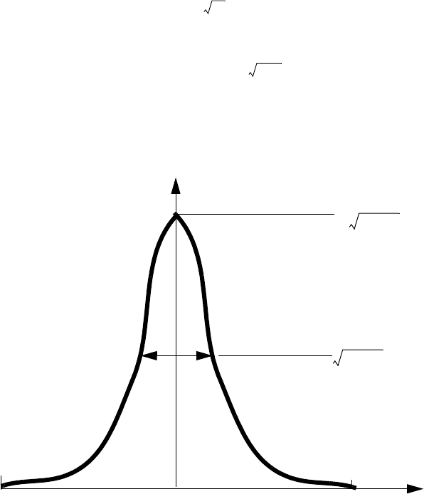
4: Diffusion

Flash or Laser Anneal Model

Sentaurus™ Process User Guide 237

I-2013.12

The intensity can be given by the Gaussian profile as follows:

(245)

(246)

where Pulse is the full width at half maximum (FWHM) time interval. The parameter

Fluence is the energy dose in .

Figure 34 Heat Intensity for flash anneal with respect to time

Table Lookup Method

The table of time versus intensity can be given by:

pdbSet Heat Intensity.Table { <t1> <I1> <t2> <I2> ... <tn> <In> }

The intensity values in the table can be scaled by:

pdbSet Heat Intensity.Table.Factor {<n>}

IFluence

2πts

-------------------------tt

–()

2ts

-------------------–







exp=

Pulse

22 2ln

-------------------=

J/cm2

Time

Gaussian

PULSE

22π⁄ln Fluence/Pulse⋅

2π⁄ln Fluence/Pulse⋅

03 t

s6 ts

4: Diffusion

Flash or Laser Anneal Model

238 Sentaurus™ Process User Guide

I-2013.12

User-specified Model

You c an de fine t he h eat i nt ensit y profi le by us in g IntensityProfile (unit is ). The

heating time, that is, the light-sourcing time for the user-specified intensity is given by the

parameter HeatingTime. For example, for the sum of two different Gaussian intensities:

set ttime "\[simGetDouble Heat time\]"

set rt2pi [expr sqrt(2*3.141592)]

set tp1 3e-3 #from 3*sigma = 3*1e-3

set tp2 6e-3 #from 3*sigma = 3*2e-3

set ts1 2e-6 #from 2*sigma*sigma = 2*1e-3*1e-3

set ts2 8e-6 #from 2*sigma*sigma = 2*2e-3*2e-3

pdbSet Heat HeatingTime 12e-3

pdbSet Heat IntensityProfile "1e4/$rt2pi*exp(-((($ttime-$tp1)^2)/$ts1)) \

+2.5e3/$rt2pi*exp(-((($ttime-$tp2)^2)/$ts2))"

Here, [simGetDouble Heat time] returns the current time that is used to solve the heat

equation.

Intensity Model for Scanning Laser

The scanning laser beam is characterized with the scanning speed (cm/s), the beam width

(), and the beam fading distance () by diffraction:

pdbSet Heat ScanSpeed <n>

pdbSet Heat BeamWidth <n>

pdbSet Heat BeamFadeDistance <n>

The intensity specification for laser beam precedents that of a flash light source. When a

positive ScanSpeed is specified, the laser scanning model is assumed and the heat intensity is

calculated with the laser beam parameters.

J/cm2/s

µm

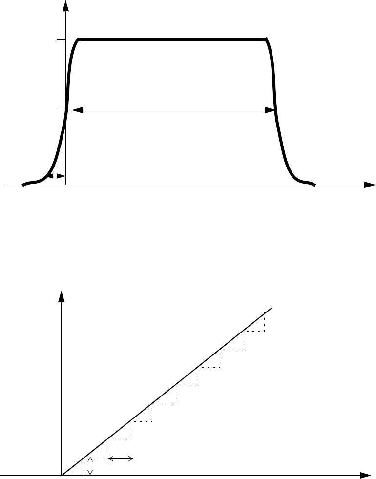
4: Diffusion

Flash or Laser Anneal Model

Sentaurus™ Process User Guide 239

I-2013.12

Two complementary error functions are multiplied to generate the laser beam intensity as

shown in Figure 35.

Figure 35 Heat intensity profile for laser beam

The laser beam moves by the distance (BeamWidth-BeamOverlap) after (BeamWidth-

BeamOverlap)/ScanSpeed anneal time step. As BeamOverlap approaches BeamWidth,

the simulation accuracy is improved.

Figure 36 Beam location along time

0Distance

BeamWidth

0.0786

0.5

1.0

I/BeamIntensity

BeamFadeDistance

1/4 erfc(-y/BeamFadeDistance) erfc((y-BeamWidth)/BeamFadeDistance)

Beam Location

Time

reality

model

(BeamWidth-BeamOverlap)/ScanSpeed (10-4s)

(BeamWidth-BeamOverlap)(um)

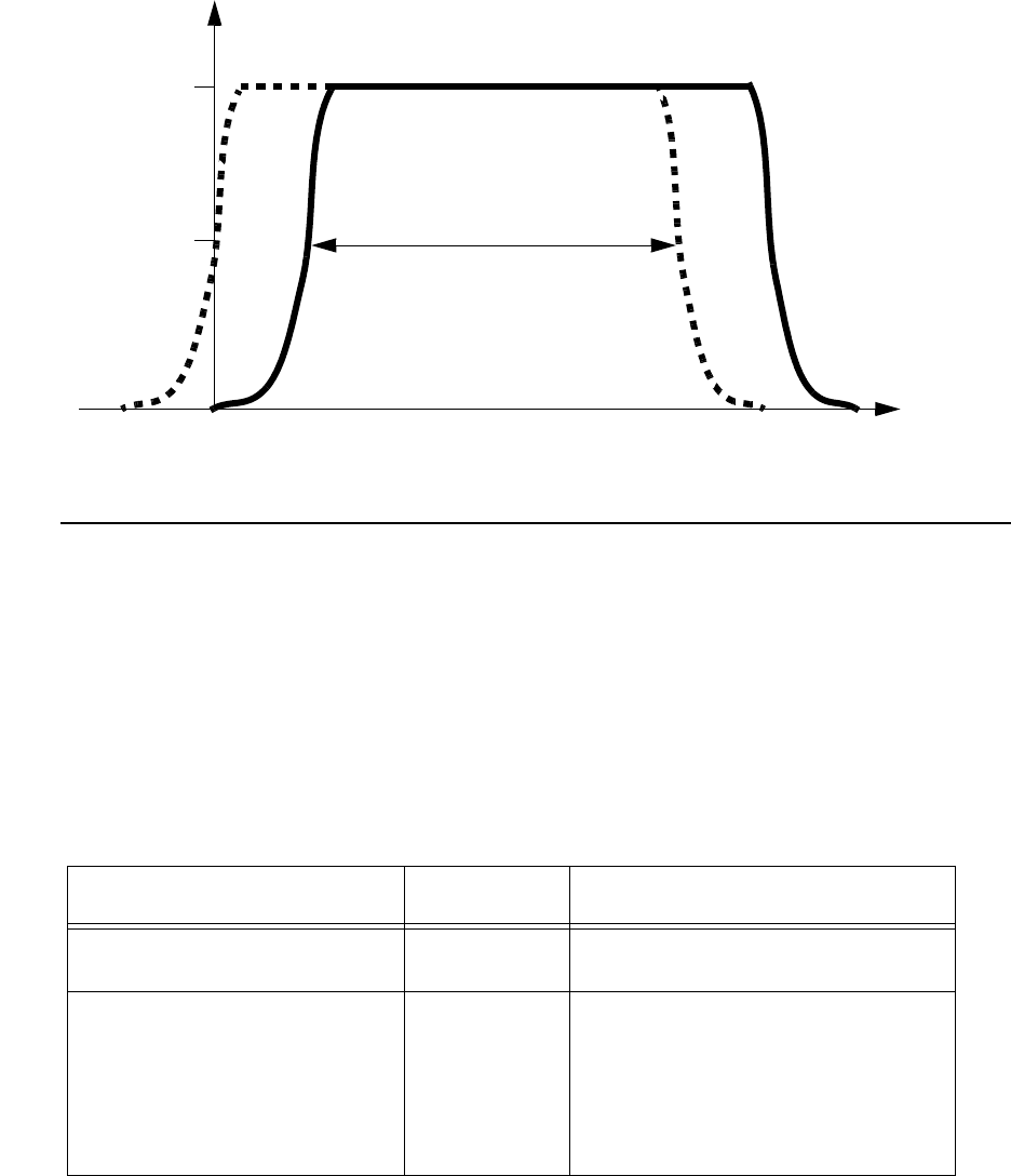
4: Diffusion

Flash or Laser Anneal Model

240 Sentaurus™ Process User Guide

I-2013.12

Figure 37 Laser beam displacement at each time step

Control Parameters

Table 14 lists the control parameters. These parameters must be used with:

pdbSet Heat

For example:

pdbSet Heat HeatingTime 12e-3

pdbSet Heat MaxTimeStep 500

Ta bl e 14 C on t ro l p a ra m e te rs

Parameter (with available options) Default value

Unit (if applicable)

Description

AttachThermalResistor <0|1> 0

Used to attach the thermal resistor to the

bottom. Options are 0 | 1.

BulkMaterial <material> Si

Indicates that the global temperature for solving

diffusion equations will be calculated by

averaging the local temperatures at interfaces of

the specified material. In addition, the material

HeatSubstrate of the extended region

will have the same thermal properties as

BulkMaterial ones.

0Distance

0.5

1.0

I/BeamIntensity

t = 0 s t=(BeamWidth-BeamOverlap)/ScanSpeed (10-4s)

BeamOverlap

4: Diffusion

Flash or Laser Anneal Model

Sentaurus™ Process User Guide 241

I-2013.12

ExtendBottom <0|1> 1

Extends bottom of the simulation structure to

the WaferThickness thickness. Options

are 0|1.

HeatingTime <n> 0.0

Defines the time the heating source is switched

on. Not applicable to the scanning laser model.

HeatSinkTransfer <n> 1e5

Defines the heat transfer rate coefficient at the

extended structure bottom. Only applicable

when AttachThermalResistor is set

to 0.

MaxTimeStep <n> 600.0

Defines the maximum time step for solving the

heat equation.

ReflectSide <Left|Right|None> Left

Specifies the side at which the structure will be

reflected after extending the structure to the

other side by SideExtension. Only

applicable for positive SideExtension.

Options are Left | Right | None.

SideExtension <n> 0.0

Defines the extended distance to side. The

extended region is set to the

HeatSubstrate material, which has the

same thermal properties as the

BulkMaterial ones. Note that only the

heat equation is solved in the region of

HeatSubstrate.

TempAverageBox

"<x1,y1,z1,x2,y2,z2>"

–Defines the box area to average the local

temperatures for calculating the global

temperature. It must be satisfied that x1<=x2

and y1<=y2 and z1<=z2.

pdbSet Heat TempAverageBox

"-0.1 0.1 0.0 1.0 2.0 0.0"

TimeSampleSize <n> 20.0

Specifies the number of time steps during the

sourcing of the heat energy. Not applicable to

the scanning laser model. The maximum time

step is given by the minimum time step among

MaxTimeStep and

for HeatingTime <= 0.0, or

HeatingTime/TimeSampleSize.

UpdateHeatRate <0|1> 0

Updates heat rate at each time step. Options are

0 | 1.

Ta bl e 14 C on t ro l p a ra m e te rs

Parameter (with available options) Default value

Unit (if applicable)

Description

W/(cm2K)

µm

3Pulse ⋅

TimeSampleSize 22ln⋅

----------------------------------------------------------------------- (ms)

4: Diffusion

Diffusion in Polysilicon

242 Sentaurus™ Process User Guide

I-2013.12

Notes

■It takes three times the standard deviation time to reach the peak intensity. After six times

the standard deviation time, the heat source is switched off.

■The global temperature, which is calculated by averaging the local temperature

distribution, is used for solving the diffusion equations.

■When the Boolean parameter UseTemperatureField in mechanics is on, the local

temperature is used for solving the mechanics equations.

■The global temperature is calculated by:

(247)

where and are the volume and the local temperature at a node in BulkMaterial

material. By default, the nodes on the nonreflecting surfaces of BulkMaterial are taken.

When you set TempAverageBox, the nodes within the specified box are taken.

Diffusion in Polysilicon

Polysilicon has a microstructure composed of small monocrystalline grains of different

crystalline orientation. The grains are separated by 2D surfaces – the grain boundaries.

Sentaurus Process uses a two-stream model to simulate polycrystalline or granular materials.

Granular diffusion can be switched on with:

pdbSet PolySilicon Arsenic DiffModel Granular

WaferThickness <n> 700.0

Defines the wafer thickness to which the

simulation structure is to be extended if

ExtendBottom is set to 1.

Ta bl e 14 C on t ro l p a ra m e te rs

Parameter (with available options) Default value

Unit (if applicable)

Description

µm

Tglobal

ViTi

i1=



i1=



--------------------=

4: Diffusion

Diffusion in Polysilicon

Sentaurus™ Process User Guide 243

I-2013.12

Isotropic Diffusion Model

The dopant concentration for species is split into a fraction of dopants in the grain and a

fraction of dopants in the grain boundary, that is:

(248)

Here, denotes the total concentration inside the grain per grain volume and denotes the

concentration inside the grain boundaries per grain boundary volume. Both quantities are

defined in the entire polysilicon region representing average concentrations.

The ratio of grain volume to the polysilicon volume is known as the volume share. The volume

share of the grain regions depends on the shape and size of the grain. The volume share of

the grain boundary is defined as:

(249)

The grain volume share and grain boundary share are defined by the terms GVolShare and

GbVolShare, respectively.

The concentration of the grain boundary is assumed to be electrically inactive. The grain

density is identified with the active portion of the total concentration . The active

concentration is stored in the dataset <dopant>Active. The grain boundary concentration

is stored in the dataset <dopant>Gbc and is initialized with the portion of the

total dopant concentration in the grain boundary . In the absence of clusters, the total

dopant concentration is given as:

(250)

Grain Shape and the Grain Growth Equation

The microscopic shape and size of the grains is not described in the model. Instead the size,

orientation, and type of a prototype grain is used to compute all parameters that depend on the

grain size.

The growth model can be switched on by:

pdbSet PolySilicon Dopant DiffModel Granular

CAfgcA

gfgb cA

⋅+⋅=

fgb 1fg

–=

gb fgb cA

⋅=

fgb CA

⋅

CAfgCA

+CA

+⋅=

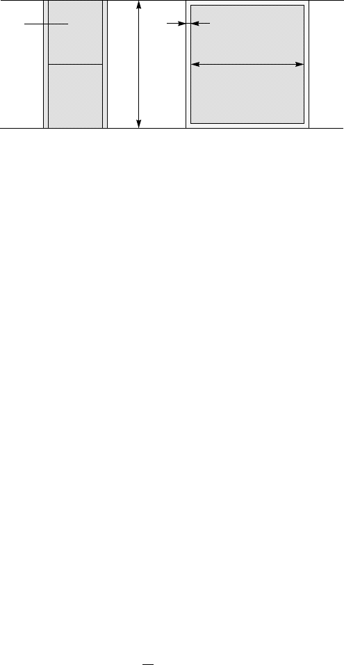
4: Diffusion

Diffusion in Polysilicon

244 Sentaurus™ Process User Guide

I-2013.12

In Sentaurus Process, a columnar grain structure is assumed by default. The grains are assumed

to be columns that are oriented along the vertical axis, extending through the entire

polycrystalline layer.

Figure 38 Columnar (left) and cubic (right) grains: is the grain size, is the grain

boundary thickness, and is the layer thickness

The grain size defines the average edge length of the square cross section of the columns.

The grain size is stored in the dataset GSize. The volume share of the grain region is given as:

(251)

For cubic grains, the volume share is:

(252)

The grain shape and the initial values for the grain size (cm) and grain boundary thickness

(cm) can be set in the parameter database, that is:

pdbSet PolySilicon GrainShape <model>

pdbSet PolySilicon GrainSize 5.0e-6

pdbSet PolySilicon GrainBoundaryThickness 5.0e-8

where <model> is either Columnar or Cubic. It is assumed that the layer thickness is a

constant value set as:

pdbSet PolySilicon LayerThickness 1.0e-6

The grains grow during thermal processes. During the grain growth, the volume share of the

grains increases and the volume share of the grain boundary decreases. The grain growth is

modeled by:

(253)

δδ

Lδ+

------------





Lδ+

------------





dLLτ2a0b0

2Dλ

-------------------------=1

-----+

-------------- 1cgb



CSi

---------------–







⋅⋅

4: Diffusion

Diffusion in Polysilicon

Sentaurus™ Process User Guide 245

I-2013.12

where denotes the ratio between the grain boundary volume inside the polycrystalline layer

and the grain boundary volume at the material interfaces of the polycrystalline layer bounding

other materials. The grain size, , is represented with the solution name GSize and can be

monitored like other solution fields.

The grain growth parameters can be specified in the parameter database in the material entry.

The following names are used: Tau, Lambda, and A0. The parameter is twice the

lattice spacing of silicon. The Arrhenius values for the various contributions to the silicon self-

diffusivity can be specified with the parameter Dself.

For columnar grains:

(254)

(255)

For cubic grains, this is:

(256)

(257)

The grain shape switches from Columnar to Cubic when the grain size reaches the layer

thickness and the grain shape is set to Columnar, that is:

pdbSet PolySilicon GrainShape Columnar

This is the default. No switching is performed if the grain shape is set to Cubic. The grain

growth equation is solved with the dopant diffusion equations.

Note that the GSize and the dopant distribution in the grain boundary <dopant>Gbc are not

reset automatically at the beginning of a new diffusion step. The pdb switch GbcNew can be

used to reset the grain size dataset GSize to the current value of GrainSize, that is:

pdbSet PolySilicon GrainSize 1e-6

pdbSet PolySilicon GbcNew 1

will reset the grain size in polysilicon to 10 nm. It also resets the <dopant>Gbc dataset to the

value calculated using the grain size and the grain-boundary volume share.

2Lδ+()d

2Lδ+()

------------------------=

dLL12Lδ+()

2Lδ+()d

------------------------+





τ2a0b0

2Dλ

------------------------- 1cgb



CSi

---------------–







⋅=

3L23Lδδ

++()d

2Lδ+()

--------------------------------------------- 1

---–=

dLLd3L23Lδδ

++()Lδ+()

d3L23Lδδ

++()Lδ+()

–

------------------------------------------------------------------------τ2a0b0

2Dλ

------------------------- 1cgb



CSi

---------------–







⋅=

4: Diffusion

Diffusion in Polysilicon

246 Sentaurus™ Process User Guide

I-2013.12

The GSize and the initial <dopant>Gbc distribution in a newly deposited layer can be

specified in the fields and in the values list in the deposit command, that is:

deposit PolySilicon type=isotropic rate=1.0 time=0.1 fields= {GSize Arsenic} \

values= {4e-6 1e19}

This will initialize the GSize to 40 nm and the arsenic concentration to a constant value of

. The ArsenicGbc solution will be created and the value of the corresponding

dataset will be set automatically.

Diffusion Equations

The diffusion in polycrystalline materials is modeled with two separate diffusion fluxes for the

diffusion of inside the grains and the diffusion of along the grain boundaries. The

diffusion inside the grain regions is modeled as for crystalline silicon with the ChargedFermi

diffusion model. The diffusion fluxes are scaled with the ratio of the grain boundary volume to

the polysilicon volume, that is:

(258)

(259)

For details on the ChargedFermi model parameters, see ChargedFermi Diffusion Model on

page 217. The diffusivity for the grain interior is set as usual for the ChargedFermi

model, for example:

pdbSet PolySilicon Boron Int Dstar \

{ 0 {[Arr 0.743e2 3.56]} 1 {[Arr 0.617e2 3.56]} }

For the fluxes along the grain boundaries, the gradient of the concentration in the grain

boundary is multiplied by a constant diffusivity and the grain boundary volume share :

(260)

(261)

The grain boundary diffusivity can be set in the parameter database using:

pdbSet PolySilicon Arsenic Dgb {[Arrhenius 1100.0 3.53]}

1019 cm 3–

JAf–gDAXc

----





c–z–CA

----









∇

Xc,



t∂

∂CAJA

∇•–R–=

DAXc

fgb

t∂

∂CA

∇•–R+=

gb f–gbDA

gb 1cA

CSi

--------–







()∇=

4: Diffusion

Diffusion in Polysilicon

Sentaurus™ Process User Guide 247

I-2013.12

In polycrystalline materials, a segregation reaction is assumed to occur at the surface of the

grains. The reaction describes the exchange of dopants between grain and grain boundary

regions. The reaction term is given as:

(262)

The segregation term depends on the transport coefficient , multiplied by the grain surface

area per unit volume of polysilicon .

The transport coefficient can be specified in the parameter database using:

pdbSet PolySilicon Arsenic Ksgb {[Arrhenius 1.630e4 3.586]}

The dopant segregation coefficient for the segregation between the grain and grain boundary

can be specified by using:

pdbSet PolySilicon Arsenic Sgb {[Arrhenius 2.75 -0.44]}

The grain surface area per unit volume depends on the grain structure. For columnar

grain structures, this is:

(263)

and, for cubic grains, this is:

(264)

Ta bl e 1 5 S o l ut io n na m es

Symbol Boron Arsenic Phosphorus Antimony Indium

Boron Arsenic Phosphorus Antimony Indium

BoronGbc ArsenicGbc PhosphorusGbc AntimonyGbc IndiumGbc

BActive AsActive PActive SbActive InActive

Ta bl e 1 6 S o l ut io n na m es fo r g ran ul ar m od e l

Symbol Solution name

GSize

RaL()KC

+1cA

CSi

--------–







⋅cA

------- 1CA

CSi

--------–







⋅–⋅⋅=

aL()

aL() 4L⋅

+()

--------------------=

aL() 6L2

⋅

+()

--------------------=

4: Diffusion

Diffusion in Polysilicon

248 Sentaurus™ Process User Guide

I-2013.12

Anisotropic Diffusion Model

The behavior of dopants in polycrystalline materials is strongly influenced by the boundaries

between crystalline grains. Dopant atoms tend to segregate from the interior of a grain to the

boundaries, which provide paths for rapid diffusion. The rate of segregation depends on the rate

of grain growth, while the number of diffusion paths along the boundaries depends on the grain

size. In addition, the boundaries of the polycrystalline material act like grain boundaries,

providing sites for electrically inactive dopant atoms and paths for diffusion. The diffusion

equations for the grain-interior and grain-boundary components of the doping profile are

solved separately. The equations are coupled by terms describing the segregation between the

grain interiors and grain boundaries. To determine the rate of segregation and the density of

grain-boundary diffusion paths, you also solve for the growth in grain size during high-

temperature processing. The boundaries of the polycrystalline region are included as explicit

grain boundaries in the diffusion and segregation equations. The model has been implemented

in Sentaurus Process [6][7][8][9].

The model is invoked by specifying the polycrystalline material, for example:

pdbSet PolySilicon PolyCrystalline 1

To set the model to the TSUPREM-4 compatible mode, use the command:

SetTS4PolyMode

Diffusion in Grain Interiors

Redistribution of dopants in polycrystalline materials occurs by the parallel diffusion of

dopants through the interiors of grains and along grain boundaries.

In the grain interiors, diffusion of the active dopant is given by:

(265)

where is the active concentration in the grain interior. The diffusivity and electric field

in the grain interior are calculated from the electron concentration , which is in turn

calculated from the doping concentrations . accounts for the segregation of dopant to

grain boundaries as described in Segregation Between Grain Interior and Boundaries on

page 251.

The parameter Grain.Crystallinity specifies the initial crystallinity of the grain interiors.

If Grain.Crystallinity is set to Crystalline, the initial active concentration is

determined by the pdb parameter AcInit or the term ${Sol}AcInit. If

∂cg

∂t

-------- ∇Dg

–∇cgzscg

qEg

---------

–





G–⋅–=

4: Diffusion

Diffusion in Polysilicon

Sentaurus™ Process User Guide 249

I-2013.12

Grain.Crystallinity is set to Amorphous, the initial active concentration is determined

by the pdb parameter AmInit or the term ${Sol}AmInit. The initialization is performed for

the remainder after some implantation atoms go to a grain boundary according to Eq. 274,

p. 251.

Grain Boundary Structure

Diffusion along grain boundaries is described in terms of the dopant concentration per unit

area of grain boundary , and the average area of grain boundaries per unit volume:

(266)

where is the average area of grain boundaries per unit volume in the bulk of the poly layer

and accounts for the dopant at interfaces between poly and other materials (or ambient).

is inversely proportional to the average grain size :

(267)

where GBGeomFactor is a geometric factor specified for the polycrystalline material, for

example:

pdbSet PolySilicon GBGeomFactor 2.0

is a function of position defined by the fact that its integral over any volume is equal to the

area of the polysilicon interface passing through that volume:

(268)

The concentration of dopants in the grain boundaries per unit volume of material is then given

by:

(269)

Diffusion along Grain Boundaries

The diffusion of dopant in the grain boundaries is given by:

(270)

The diffusivity and electric field along the grain boundaries are calculated from the

electron concentration ; is calculated by assuming that the net donor and acceptor

cgb

ρ′ ρ δif

δif

ρGBGeomFactor

------------------------------------------------=

δif

Aif

δif Vd

Aif

gb ρ′cgb

∂cA

∂t

-----------∇FDgb

–∇cgb zscgb

qEgb

------------

–





G+⋅–=

Dgb

Egb

ngb

4: Diffusion

Diffusion in Polysilicon

250 Sentaurus™ Process User Guide

I-2013.12

concentrations are calculated from , the equilibrium dopant concentrations in the grain

interior near the grain boundary, where is the segregation coefficient given by Eq. 276,

p. 251. accounts for the segregation of dopant to grain boundaries as described in

Segregation Between Grain Interior and Boundaries on page 251.

Diffusivity is given by:

(271)

Dgb and Dgb.Fermi are defined by:

pdbSet <material> <dopant> Dgb <value>

pdbSet <material> <dopant> Dgb.Fermi <array>

is a tensor that describes the diffusion paths available to dopant in the grain boundaries. It is

composed of two parts: . describes the available paths within the

bulk of the poly layer. For a horizontal poly layer, it is given by:

(272)

Because of the columnar grain structure, Dgb.F22 is larger than Dgb.F11, which implies that

diffusion through the layer is faster than diffusion parallel to the layer.

Dgb.F11 and Dgb.F22 are defined for the polycrystalline material, for example:

pdbSet PolySilicon Dgb.F11 1.0

pdbSet PolySilicon Dgb.F22 2.0

describes the available paths for diffusion along material interfaces. In the vicinity of a

horizontal interface, it has the value:

(273)

For the interface between polysilicon and silicon, the phenomenon of interfacial breakup

accompanied by epitaxial realignment can occur, as described in Interface Oxide Breakup and

Epitaxial Regrowth on page 255. is the fraction of the polysilicon–silicon interface that has

broken up. For layers or interfaces that are not horizontal, and are rotated by the angle

of the layer or interface, respectively, with respect to the horizontal axis.

cgb K⁄

Dgb

Dgb Dgb Dgb.Fermi ngb

--------





c–

⋅



⋅=

b1Fbu

–()Fif

Fbdiag Dgb.F22

----------------------------Dgb.F11

----------------------------





Fif

Fif diag 0 δ,if δif

,()=

Fbu

Fif

4: Diffusion

Diffusion in Polysilicon

Sentaurus™ Process User Guide 251

I-2013.12

Segregation Between Grain Interior and Boundaries

When dopant is initially introduced into a polycrystalline material, some of the dopant

occupies sites in the interior of a grain and some occupies sites on a grain boundary. The initial

segregation of dopant is given by:

(274)

GBMaxDensity, GMaxConc, and GSegInit represent the density of available sites on grain

boundaries, and in the grain interiors and the initial segregation entropy, respectively. In the

case of ion implantation, and describe the additional dopant introduced by the

implantation; dopant that is present before the implantation is not redistributed.

Dopant atoms are free to move between sites in the interior of a grain and sites on the grain

boundary during high-temperature processing. The rate of segregation is given by:

(275)

The segregation coefficient is given by [10]:

(276)

GBMaxDensity, GMaxConc, GSegInit, and Sgb are defined for dopants, for example:

pdbSet PolySilicon Dopant GBMaxDensity 2.5e15

pdbSet PolySilicon Dopant GMaxConc 5e22

pdbSet PolySilicon Dopant GSegInit 1.0

pdbSet PolySilicon Boron Sgb {[Arrhenius 0.2 -0.38]}

The segregation velocities associated with the bulk of the poly region and the material

interfaces are given by:

(277)

GBVFactor is the parameter for the material. KsgbFactor and , which is defined by Vsgb,

are specified for dopants. For example:

pdbSet PolySilicon GBVFactor 1.33

pdbSet PolySilicon Dopant KsgbFactor {[Arr 4.0 0.0]}

pdbSet PolySilicon Dopant Vsgb {[Arr 1e7 3.0]}

cgb

GBMaxDensity

GMaxConc

------------------------------------------------GSegInit cg

cgb

Gρqb1Fbu

–()δ

ifqif

+()f

gb cgf

cgb

-------

–





KGBMaxDensity

GMaxConc

------------------------------------------------Sgb=

GBVFactor

------------------------------------∂Lg

∂t

---------KsgbFactorDg

------+=

qif

4: Diffusion

Diffusion in Polysilicon

252 Sentaurus™ Process User Guide

I-2013.12

and are the fractions of unfilled interior and boundary sites:

(278)

(279)

where the sum is taken over all the dopant species present in the structure. is the fraction

of the polysilicon–silicon interface that has broken up, as described in Interface Oxide Breakup

and Epitaxial Regrowth on page 255.

Grain Size Model

The grains in the polycrystalline material are assumed to be oriented as columns that extend

through the wafer. The structure is characterized by , the average grain size in the lateral

direction (in other words, in the plane of the layer), and a vector describing the orientation of

the columnar grains.

The initial grain size is determined by the temperature of the poly deposition process:

(280)

where:

■ is the deposition temperature (specified on the deposit command) in degree Celsius.

■ is the thickness of the amorphous silicon layer produced by low-temperature deposition.

■ is the distance from the bottom of the layer.

For high-temperature depositions, grain size depends on the thickness specified in the

deposit command. Dividing a deposition into multiple smaller depositions produces

different results for the grain size. For low-temperature depositions, the material is assumed to

be amorphous (a negative grain size is reported in printing or plotting). The initial grain size is

calculated from the thickness of the amorphous layer at the beginning of the next diffusion

step.

Frac.TA, GrainSize, GrainSizeFactor, and GrainSizeTempC are the material

parameters, for example:

pdbSet PolySilicon Frac.TA 0.5

pdbSet PolySilicon GrainSize 5e-6 ;# cm

pdbSet PolySilicon GrainSizeFactor {[Arr 0.1 0.0]}

pdbSet PolySilicon GrainSizeTempC 600.0

fgb

g1cg

GMaxConc

--------------------------------–=

gb 1cgb

GBMaxDensity

------------------------------------------------



–=

Fbu

max Frac.TA taGrainSize,×() TcGrainSizeTempC≤

GrainSize 2GrainSizeFactor⋅+ z⋅ TcGrainSizeTempC>











4: Diffusion

Diffusion in Polysilicon

Sentaurus™ Process User Guide 253

I-2013.12

Surface Nucleation Model

An alternative model for the standard grain size model (see Grain Size Model on page 252) is

the surface nucleation model. In this model, grains are assumed to grow from small clusters

formed at the early stages of deposition. The kinetics of nucleation, under this assumption,

determines the average distance between clusters, thereby, the average starting grain size near

the surface upon which deposition occurs. The model for atomistic nucleation is derived from

rate equations for growth, surface diffusion, and desorption [11]. Several different regimes are

considered:

■Large deposition rates (compared to surface diffusion or evaporation) are labeled

“complete condensation”.

■Conditions where the deposition rate between surface diffusion and evaporation are labeled

“incomplete condensation”.

■Low deposition rates are labeled “extremely incomplete condensation”.

Besides the deposition rates, two types of nuclei are considered: 2D or 3D islands. The

following formulas are used to compute the nucleation density:

(281)

where and are given by Table 17 on page 254. The choice of regime is set with:

pdbSet SNG.Model <regime>

where <regime> is one of Complete, Initially.Incomplete, Extreme.Incomplete,

or None (default) meaning the model is switched off.

0RpE

------





exp=

4: Diffusion

Diffusion in Polysilicon

254 Sentaurus™ Process User Guide

I-2013.12

NOTE Default values for parameters of the surface nucleation model have not

been calibrated for any process. They have simply been set to give

approximately the same values as the grain size model in polysilicon

diffusion. This model is in an experimental state. The default values of

the model may change in the future if reasonable values can be found

for typical technology conditions.

Grain Growth

The growth of the grains during high-temperature processing is given by [12]:

(282)

Ta bl e 1 7 Fo r mu l as fo r s ur fa c e n u c l e a ti on m od e l

Regime 3D islands 2D islands

Extremely

incomplete

Incomplete

Complete

Table 18 Parameters of surface nucleation model set with

pdbSet PolySilicon <parameter> <value>

Symbol Parameter Name

Island dimension

SNG.Island.Dim

SNG.Growth.Flux

SNG.Prefactor

SNG.Critical.Island.Size

SNG.Adsorption.Energy

SNG.Diffusion.Energy

SNG.Critical.Island.Energy

---i=

---Eii1)EaEd)–+()+()=

pi=

ii1)EaEd)–+()+=

---i=

---EiiEa

+()=

---=

iiEa

pii2.5+()⁄=

iiEd

+()i2.5+()⁄=

pii2+()⁄=

iiEd

+()i2+()⁄=

∂Lg

∂t

---------1

----- A0 DselfFactor Dself Egb

-------- Fseg GEA

+××××=

4: Diffusion

Diffusion in Polysilicon

Sentaurus™ Process User Guide 255

I-2013.12

A0, DselfFactor, and Dself represent the empirical geometric factor, the enhancement

factor of silicon self-diffusivity at the grain boundary, and the silicon self-diffusivity in the

vicinity of a grain boundary, respectively:

pdbSet PolySilicon A0 6.0

pdbSet PolySilicon DselfFactor {[Arrhenius 5.6e-6 -1.73]}

pdbSet PolySilicon Dself { -2 {[Arrhenius 5.6e-6 2.86]}

-1 0.0

0 {[Arrhenius 4.29e-7 2.18]}

1 0.0

2 0.0 }

is the surface energy per atom associated with the grain boundary [12][13][14];

models the segregation drag effect; and models epitaxial regrowth of the poly layer (see

Interface Oxide Breakup and Epitaxial Regrowth on page 255).

(283)

(284)

is the thickness of the polycrystalline layer.

The segregation drag effect reduces the grain growth rate [15]:

(285)

SegDragExponent is defined for the material, for example:

pdbSet PolySilicon SegDragExponent 2.0

Interface Oxide Breakup and Epitaxial Regrowth

A thin interfacial oxide layer is typically present between a deposited polysilicon layer and any

underlying single-crystal silicon. This interfacial oxide presents a barrier to epitaxial

realignment of the poly layer. With sufficient high-temperature processing, the oxide layer

breaks up into a discrete set of small spheres, allowing epitaxial regrowth of the poly to

proceed.

Egb

Fseg

GEA

Egb 2LatticeSpacing Tu⋅⋅()

2Lambda 1

1Lambda.hfn

----------------------------------------------Lambda.1 Lg

tpoly

-----------







⋅⋅=

2tpoly Lg

–

-------------------------- Lgtpoly

tpoly

----------- Lgtpoly

≥











tpoly

Fseg 1cgb

GBMaxDensity

------------------------------------------------







SegDragExponent–

4: Diffusion

Diffusion in Polysilicon

256 Sentaurus™ Process User Guide

I-2013.12

The oxide breakup is modelled by the formation of voids in the interfacial oxide layer

[16]–[19]. The radius of the voids increases as:

(286)

where:

■ is a constant.

■ is the initial oxide thickness.

■ is the activation energy of the breakup process.

■ is initialized to zero whenever poly is deposited on exposed silicon.

The fraction of the interface that is broken up is given by:

(287)

where is the areal density of the voids.

The parameters for the model are specified in terms of a characteristic breakup time for the

thinnest (5 Å) interfacial oxide layers:

(288)

is defined with the parameter PolyOxBreakTime, for example:

pdbSet PolySilicon PolyOxBreakTime {[Arrhenius 1.0 -5.0]} ;# seconds

(289)

In the present implementation, assume that all polycrystalline or single-crystalline interfaces

share a common oxide thickness given by:

(290)

PolyOxThickness is defined in the material:

pdbSet PolySilicon PolyOxThickness 5e-8 ;# cm

Rvoid

dRvoid

----------------β

tox

------ exp Ebu

--------

–





×=

tox

Ebu

Rvoid

Fbu 1exp πNEARvoid

–()–=

NEA

tbu

·3

πNEAβ

--------------------- expEbu

--------

×≡

tbu

dRvoid

----------------1

tbu

------ 5A

tox

-------





3 1

πNEA

------------------=

tox PolyOxThickness=

4: Diffusion

Diffusion in Polysilicon

Sentaurus™ Process User Guide 257

I-2013.12

Epitaxial regrowth is modeled by increasing the poly grain size to a value larger than the

thickness of the poly layer. This grain growth is described by in Eq. 273, p. 250 for the

grain size:

(291)

It serves as a driving force for epitaxial regrowth from the interface at the silicon–polysilicon

interface. Parameters for this model are given by:

(292)

pdbSet PolySilicon EpiGrowthVelocity {[Arrhenius 100.0 3.0]} ;# cm2/sec

Dependence of Polysilicon Oxidation Rate on Grain Size

It has been observed experimentally that the oxidation rate for fine-grained polysilicon is faster

than for coarser-grained polycrystalline or single-crystalline silicon, presumably because of

enhanced oxidation at the grain boundaries.

This enhancement can be modeled by assuming a faster surface reaction rate where grain

boundaries intersect the oxide–poly interface:

(293)

where:

(294)

is the surface reaction rate in the absence of grain boundaries, is the reaction rate at a grain

boundary, and:

(295)

is the fraction of the surface within a distance of a grain boundary. The enhancement

factor at grain boundaries is specified as:

(296)

pdbSet Oxide_PolySilicon H2O GBFactor {[Arr 10.0 0.0]}

pdbSet Oxide_PolySilicon O2 GBFactor {[Arr 10.0 0.0]}

pdbSet Oxide_PolySilicon N2O GBFactor {[Arr 10.0 0.0]}

GEA

GEA FbuvEAδif

vEA EpiGrowthVelocity=

ks1f–()kgfkgb

--- Cox

---------=

kgb

fmin Tδ

------1,





Tδ2⁄

kgb

-------GBFactor=

4: Diffusion

Diffusion in Polysilicon

258 Sentaurus™ Process User Guide

I-2013.12

The effective thickness of the grain boundaries is given by , where

GBEffThick is specified for each material.

Boundary Conditions

Boundary Conditions for Grain Growth Equation

Several boundary conditions to control the grain size (GSize) in the grain growth equation are

available. The reflective (HomNeumann) boundary condition assumes that the interface value

grows like the bulk value. The minimum value (MinimumSize) boundary condition sets the

interface value at the minimum value for GSize. The minimum value is set with:

pdbSet <material> GSize minConc {<n>}

The initial size (InitialSize) boundary condition fixes the interface value at the initial value

of GSize.

The boundary conditions can be switched on using:

pdbSet Oxide_PolySilicon <dopant> BoundaryCondition [

{HomNeumann

MinimumSize InitialSize}]

The default setting for the grain growth boundary condition is HomNeumann.

Dopant Diffusion Boundary Conditions

There are three additional segregation-type boundary conditions available with the

polycrystalline diffusion model. The first can be selected with:

pdbSet Oxide_PolySilicon Arsenic BoundaryCondition GrainBoundarySegregation

The total dopant fluxes at the interfaces between the grain boundary and the neighboring layer

are balanced. The fluxes are given by:

(297)

where is the concentration of dopant on the other side of the interface, is the grain

boundary concentration, is the transfer rate, and is the segregation rate

of dopant in the grain boundary. To set these parameters, use:

pdbSet <interface material> <dopant> Transfer {<n>}

pdbSet <interface material> <dopant> SegregationGb {<n>}

TδGBEffThick=

jn•kTransfer CA

other CA

fgbsgkgb

Segregation

----------------------------------------------–







other

kTransfer

kgb

Segregation

4: Diffusion

Diffusion in Polysilicon

Sentaurus™ Process User Guide 259

I-2013.12

The coefficient is the grain–grain boundary segregation coefficient.

To select the second boundary condition, use:

pdbSet Oxide_PolySilicon Arsenic BoundaryCondition

GrainGrainBoundarySegregation

The total dopant fluxes at the interfaces between the grain and the neighboring layer and the

grain boundary and neighboring layer are balanced. The fluxes are given by:

(298)

(299)

and:

(300)

where is the active concentration of dopant in the grain and is the segregation

rate of dopant in the grain. To set this parameter, use:

pdbSet <interface material> <dopant> Segregation {<n>}

To select the third boundary condition, use:

pdbSet Oxide_PolySilicon Arsenic BoundaryCondition \

BulkGrainBoundarySegregation

The total dopant fluxes at the interfaces between the grain and the neighboring layer and

between the grain and the grain boundary are balanced. The fluxes are given by:

(301)

(302)

jgn•kTransfer CA

other fgCA

kSegregation

-----------------------------–







jgb n•kTransfer CA

other CA

sgkgb

Segregation

---------------------------------------–







jn•jgn•jgb n•+=

kSegregation

jn•kTransfer CA

other fgCA

kSegregation

-----------------------------–







jgb n•kTransfer

fgCA

kSegregation

-----------------------------CA

fgbsgkgb

Segregation

----------------------------------------------–







4: Diffusion

Dopant Diffusion in SiGe

260 Sentaurus™ Process User Guide

I-2013.12

NOTE For the anisotropic polycrystalline model, use the Segregation model

for the boundary condition:

pdbSet PolySilicon_Silicon Boron BoundaryCondition Segregation

pdbSet Oxide_PolySilicon Boron BoundaryCondition Segregation

pdbSet Gas_PolySilicon Boron BoundaryCondition Segregation

Dopant Diffusion in SiGe

The presence of germanium in silicon affects the dopant diffusion in various ways. First, the

band gap of silicon is lowered in the presence of germanium. Second, germanium affects the

point-defect equilibrium concentration. In addition, germanium can pair with boron forming

an immobile but electrically active species.

Bandgap Effect

The effect of the bandgap narrowing on the dopant diffusion arises from the change in the

intrinsic carrier concentration . This has been implemented in Sentaurus Process as

follows:

(303)

where is bandgap narrowing due to germanium content. It can be defined using the

command:

pdbSet <material> Germanium delEg {<n>}

The band gap, delEg ( ), is a function of germanium concentration and is given by:

(304)

(305)

(306)

(307)

where [20] is the bandgap narrowing in strained silicon, [21] is the bandgap

narrowing in the relaxed silicon, is a pseudomorphic factor that shows the degree of the

niSi()

niniSi()e

Eg∆–

2kT

--------------

Eg∆

Eg∆Egs∆Egr∆Egs∆–()1Fpm–()+≡

Egs

∆0.835x21.01x–=

Egr

∆0.33x20.55x–=

xCGe

5.0 22

×10

---------------------=

Egs∆

Egr∆

Fpm

4: Diffusion

Dopant Diffusion in SiGe

Sentaurus™ Process User Guide 261

I-2013.12

relaxation, and is the germanium fraction in silicon. is calculated with respect to lattice

mismatch in the substrate. For example:

(308)

where:

■ is the lattice-spacing of the silicon-germanium region.

■ is the lattice-spacing of silicon.

■ is the lattice-spacing calculated in the mechanics.

If the system is fully relaxed, is zero. If it is fully strained, is one. will be used

if the germanium percentage is greater than 0.1%, and the bandgap narrowing effects due to

other strain sources will be ignored (see Pressure-dependent Defect Diffusion on page 275).

Potential Equation

The permittivity of “Ge-doped” silicon can be calculated by the following formula, in which

is the germanium concentration in silicon:

(309)

where and are defined as PDB parameters:

pdbSet Ge Potential Permittivity 15.8

pdbSet Si Potential Permittivity 11.7

This calculation is included when setting:

pdbSetString Si CompSpecies "Germanium"

pdbSetBoolean Si Potential PermittivityContentEffect 1

The product of the density-of-states in the conduction and valence bands, , is

multiplied by the factor defined as:

pdbSetFunction Si Ge factorNcNv [GefactorNcNv]

when the following PDB value is set:

pdbSetBoolean Si Potential BandgapContentEffect 1

Such a factor can be defined as:

(310)

Fpm

Fpm aSiGe a–()

aSiGe aSi

–

---------------------------=

aSiGe

aSi

Fpm

Eg∆

xGe

ε1xGe

–()ε

Si xGe

+×ε

×=

εSi

εGe

NcNv

1xGe

–0.47 0.81⁄×()

34⁄

4: Diffusion

Dopant Diffusion in SiGe

262 Sentaurus™ Process User Guide

I-2013.12

with the following line:

fproc GefactorNcNv { } { return "(1.0-(Germanium/5.0e22)*0.47/0.81)^0.75" }

Effects on Point-Defect Equilibrium Concentrations

The introduction of germanium acts thermodynamically on the equilibrium of the silicon

matrix. Compressive strain increases the equilibrium concentration of vacancies and decreases

the equilibrium concentration of interstitials, and the tensile strain has the opposite effect on

the point-defect equilibrium concentrations [22][23].

These effects are modeled in Sentaurus Process by modifying the equilibrium point-defect

concentrations:

(311)

(312)

where is the equilibrium concentration of point defects (interstitial or vacancy), and

is the activation volume change of equilibrium point defects due to the pressure .

The following set of commands can be used to modify :

pdbSet Silicon Interstitial Volume 8.59e-24

pdbSet Silicon Vacancy Volume -5.52e-24

To switch on strain effects on point defects, set the following switches:

pdbSet Silicon Interstitial CStarMod FermiPressureDependent

pdbSet Silicon Vacancy CStarMod FermiPressureDependent

is the total activation volume change of equilibrium point defects due to the presence

of germanium and is calculated from the activation volume change , the lattice

mismatch coefficient , and the germanium fraction in the structure (see Eq. 312). These

quantities can be modified using the following commands:

pdbSet Silicon Germanium Interstitial delVol 11.8

pdbSet Silicon Germanium Vacancy delVol 25.6

pdbSet Silicon Germanium LatticeMismatch 0.0425

NOTE delVol is given in units of eV and Volume is given in units of .

*CX

*Si P 0≡,()e

VXPV

GeX

∆+∆()–

--------------------------------------------

VGeX

∆VolGeX a∆SiGe

CGe

522

×10

-----------------∆=

∆

VGeX

∆

VolGeX

∆

a∆SiGe

cm3

4: Diffusion

Dopant Diffusion in SiGe

Sentaurus™ Process User Guide 263

I-2013.12

Effect of Ge on Point-Defect Parameters

In this version of Sentaurus Process, you can define the arbitrary Alagator expressions for the

point-defect basic parameter prefactors. The names of terms used for the vacancy and

interstitial equilibrium concentration are VacCStarFactor and IntCStarFactor,

respectively. Corresponding terms for the vacancy and interstitial diffusivity are

VacDiffFactor and IntDiffFactor. These expressions can be used to include the effect

of germanium on point-defect parameters. For example, the prefactor for the vacancy

equilibrium concentration in SiGe can be calculated as follows:

MultiplyTerm Si VacCStarFactor "exp((1.088*($x_Ge))*$Vt_i)"

where x_Ge is the germanium content, and

Vt_i

is in .

NOTE The MultiplyTerm command is not saved to the TDR files. If the input

file is split, the command must be included in the new input file.

Impact of Ge on Extended-Defect Parameters

The parameters IClusterDissIntFactor, C311DiffIntFactor, and CLoopTransfer

(used in the Full model for I-clusters) can be used to include the impact of germanium on

extended defects.

Impact of Dopant Diffusivities

The germanium chemical effect is simulated by the activation energy correction using

diffusivity prefactors. For example, in the case of boron, it is performed by the term

BoronIntDiffFactor, which can be defined in silicon:

MultiplyTerm Si BoronIntDiffFactor "exp(-0.227*($x_Ge)*$Vt_i)"

NOTE The MultiplyTerm command is not saved to the TDR files. If the input

file is split, the command must be included in the new input file.

During assembly of the diffusion equations, Sentaurus Process checks each dopant and

material for whether such diffusion factors exist. The diffusivity through dopant–interstitial or

dopant–vacancy pairs is then multiplied by the corresponding diffusion enhancement factors.

A separation between interstitial and vacancy effects is necessary because with increasing

germanium content of SiGe, the fractions of diffusion mediated by dopant–interstitial and

dopant–vacancy pairs change.

1(kT)⁄

eV 1–

4: Diffusion

Dopant Diffusion in SiGe

264 Sentaurus™ Process User Guide

I-2013.12

SiGe Strain and Dopant Activation

The solid solubility of dopants depends on the strain. In general, for compressive strain, the

solubility of atoms smaller than silicon increases; whereas, the solubility of larger atoms

decreases. In the Transient model, the stress effect is taken into account by introducing the

pressure-dependent parameters Solubility and TotalSolubility:

(313)

An example of the definition of boron pressure-dependent solid solubility is:

pdbSet Si B SS.Factor "exp(3.636e-24*Pressure*$kT_i)"

pdbSet Si B Total.SS.Factor "exp(3.636e-24*Pressure*$kT_i)"

Since the emission rate for the silicon side in the three-phase segregation model is proportional

to the solid solubility, a corresponding modification also must be included in the boundary

condition. For example, this can be achieved by the following line for boron:

pdbSetString Si B Side.SS.Factor "exp(3.636e-24*Pressure_Silicon*$kT_i)"

NOTE You can define the arbitrary Alagator expressions for the dopant solid

solubility prefactors in Sentaurus Process. The name of strings used for

the solid solubility, the total solid solubility, and the emission rate

correction are SS.Factor, Total.SS.Factor, and

Side.SS.Factor, respectively.

Germanium–Boron Pairing

Germanium can pair with boron and the pairs are known to be electrically active [24] but not

mobile:

(314)

In Sentaurus Process, this reaction is modeled with the following differential equation:

(315)

where is the concentration of germanium–boron pairs, is the concentration of

germanium, is the concentration of boron, and and are the forward reaction rate

and equilibrium constant, respectively.

SP() SP(0)P– VkT⁄()exp==

Ge B GeB↔+

t∂

∂CGeB Kf CGeCBKbCGeB

–()=

CGeB

CGe

4: Diffusion

Diffusion in III–V Compounds

Sentaurus™ Process User Guide 265

I-2013.12

You ca n spec if y the m od el pa rameters with the commands:

pdbSet Silicon Germanium Boron Kf {<n>}

pdbSet Silicon Germanium Boron Kb {<n>}

Germanium diffusion is modeled by assuming a constant diffusion model:

(316)

where is the diffusivity of germanium and can be set using the command:

pdbSet Silicon Germanium Dstar {<n>}

NOTE The germanium–boron cluster model is switched off by default. To

switched it on, use:

solution add name=GeB ifpresent = "Germanium Boron" !negative

Of course, if boron is present in silicon, the reaction in Eq. 315 is automatically added to

Eq. 316.

Initializing Germanium–Boron Clusters

Initially, germanium–boron cluster concentrations are set to zero. If there is an existing cluster

concentration field, the field is used. To initialize the cluster concentration field, use the

select command in the input command file.

Diffusion in III–V Compounds

This section discusses diffusion in III–V compounds.

Material Conversion

At the beginning of a diffusion, the adjacent III–V materials or a III–V material doped with

other group III or V atoms can be merged into the proper ternary or quaternary compound

Ta bl e 1 9 S o l ut io n na m es fo r g er m an iu m m o d el

Symbol Solution name

Germanium

GeB

t∂

∂CGe DC

∇()∇•=

CGe

CGeB

4: Diffusion

Diffusion in III–V Compounds

266 Sentaurus™ Process User Guide

I-2013.12

materials. The conversion is performed when the Boolean parameter

Convert.IIIVMaterials is switched on:

pdbSet Diffuse Convert.IIIVMaterials <0|1> ;# default 1

When different III–V material regions are adjacent and there is a common material derived

from each III–V material, the regions merge into the common derived material region. For

example, if the neighbor region of a GaAs material region is InAs, two regions are merged and

converted into InGaAs material if InGaAs is the derived material from both GaAs and InAs.

The derived material is specified by:

pdbSet <material> Derived.Materials { <derivedmaterial list> }

For example:

pdbSet GaAs Derived.Materials { InGaAs AlGaAs GaPAs }

pdbSet InAs Derived.Materials { InPAs InGaAs }

When group III or group V atoms are doped into a III–V material, and the atoms are a different

species from the components of the material, the material is converted to the new III–V

material with the component list, including the doping species, if the doping concentration

exceeds the minimum concentration Min.Conv.Conc for conversion. For example, when

indium atoms are doped into a GaAs material region, GaAs is converted to InGaAs if InGaAs

is one of the derived materials of GaAs, and the maximum concentration of indium atoms in

the region exceeds the indium Min.Conv.Conc parameter value of InGaAs:

pdbSet InGaAs Indium Min.Conc {<n>}

The atoms of the material components are filled into the region before the material conversion

for the mole fraction calculation and the interdiffusion simulation.

Physical Parameter Interpolation

The parameter for the mole fraction of a ternary (or quaternary) material is specified by:

pdbSet <material> MoleFraction.Atoms { x <atom> } ;# ternary

pdbSet <material> MoleFraction.Atoms { x <atom1> y <atom2> } ;# quaternary

For example:

pdbSet InGaAs MoleFraction.Atoms { x Gallium } ;# In

(1-x)

(x)

pdbSet AlInGaAs MoleFraction.Atoms {x Aluminum y Indium} ;# Al

(x)

(y)

(1-x-y)

4: Diffusion

Diffusion in III–V Compounds

Sentaurus™ Process User Guide 267

I-2013.12

If a physical parameter is not specified on a ternary (or quaternary) material, the parameter

value is extracted by the linear interpolation with the parameter values of their base materials

that is, binary materials. For the value of the parameter of material :

(317)

(318)

(319)

NOTE For the energy bandgap and affinity, the second-order mole-fraction

dependency can be specified (see details in Table 22 on page 278).

Dopant Diffusion

To model dopant diffusion in a III–V material, the following assumptions are applied:

■Point defects diffuse by the second nearest neighbor hopping.

■Group II dopants react only with group III point defects.

■Group VI dopants react only with group V point defects.

■There are no antisite defects.

■The charging reaction is in equilibrium.

■There are two types of vacancy (that is, at group III and V sites): VacIII and VacV.

Since the substitutional concentrations of group IV dopants on group III sites and group V sites

are modeled and calculated separately, the autocompensation effect due to the amphoteric

behavior is implicitly taken into account.

ChargedReact Model

(320)

(321)

(322)

PIIIAx()

IIIB1x–()

VCPIIIAVCxP

IIIBVC1x–()⋅+⋅=

PIIIAx()

IIIBy()

IIIC1x–y–()

VDPIIIAVDxP

IIIBVDyP

IIICVD

1x–y–()⋅+⋅+⋅=

PIIIAx()

IIIB1x–()

VCy()

VD1y–() PIIIAVCxy PIIIAVDx1y–()PIIIBVC

1x–()yP

IIIBVD

1x–()1y–()⋅+⋅+⋅+⋅=

∂AI

∂t

---------∇DAImjηj–









ηzAm

–AIm

αAIm

-----------ηzAm







∇







RAYm

ko()



+⋅RAIVm

ft()

–









∂AV

∂t

-----------∇DAVmjηj–









ηzAm

–AVm

αAVm

------------ ηzAm







∇







RAVm

ko()

+⋅RAVYm

ft()



–









∂Ams,

∂t

-------------- RAYm

ko()



–RAVm

ko()

–RAIVm

ft() RAVYm

ft()



++=

4: Diffusion

Diffusion in III–V Compounds

268 Sentaurus™ Process User Guide

I-2013.12

where:

(323)

(324)

(325)

(326)

and (327)

and (328)

(329)

(330)

(331)

(332)

RAYm

ko() kAYmj

ko()

Ymi,∗φYmjηj–









Ams,

Ym∗

--------- AIm

αAIm

-----------Yms,

Yms,∗

--------------

–







RAVm

ko() kAVmj

ko()

Vmi,∗φVmjηj–









Ams,

Vm∗

----------AVm

αAVm

------------–







RAIVm

ft() kAImjk

ft() αAImj,Vmi,∗φVmkηjk+()–

jk,









AIm

αAIm

-----------Vm

Vm∗

----------Ams,

–







RAVYm

ft() kAVmjk

ft() αAVmj,Ymi,∗φYmkηjk+()–

jk,









AVm

αAVm

------------ Ym

Ym∗

--------- Ams,

Yms,

Yms,∗

--------------

–







αAImαAImj,ηj–



αAImj,DAImjdAImj

⁄≡

αAVmαAVmj,ηj–



αAVmj,DAVmjdAVmj

⁄≡

AIIII

αAIIIIη1–

αAIIIIη1–αAIVη1rIIIV

⁄+

------------------------------------------------------------ AI=

AIV

αAIVη1

rIIIVαAIIII

η1–αAIVη1

---------------------------------------------------------AI=

AVIII

αAVIIIη1–

αAVIIIη1–αAVVη1rIIIV

⁄+

--------------------------------------------------------------- AV=

AVV

αAVVη1

rIIIVαAVIII

η1–αAVVη1

----------------------------------------------------------- AV=

4: Diffusion

Diffusion in III–V Compounds

Sentaurus™ Process User Guide 269

I-2013.12

Ta bl e 2 0 D e s c r i pt i o n o f s y m b ol s fo r t h e Ch ar g e d Re ac t m od e l

Symbol Description Unit

The Mendeleev group number of a constituent atom of III–V material, . Unitless

Substitutional dopant concentration at group lattice sites.

Dopant–interstitial pair concentration. For example, is SiInt for Silicon.

Dopant–group interstitial pair concentration.

Dopant–vacancy pair concentration. For example, is SiVac for Silicon.

Dopant–group vacancy pair concentration.

Self-interstitial concentration. For example, is GaInt or InInt, and is

AsInt in InGaAs.

Constituent atom concentration. For example, is Gallium or Indium, and

is Arsenic in InGaAs.

Self-interstitial concentration in equilibrium (Eq. 346, p. 272).

Self-interstitial concentration in intrinsic equilibrium:

pdbSet InGaAs GaInt Cstar {<n>}

Constituent atom concentration in equilibrium:

pdbSet InGaAs Gallium CsubStar {<n>}

Charge-state fractions of self-interstitials: . is specified,

for example, by:

pdbSet GaAs GaInt ChargeStates { -2 <n> ... 2 <n> }

Unitless

Va can cy conc entr atio n. i s VacIII and is VacV.

Va can cy conc entr atio n in equ ilib rium (Eq. 347, p. 272).

Va can cy conc entr atio n in int rins ic equi libr ium:

pdbSet GaAs VacIII Cstar {<n>}

Charge-state fractions of vacancies: . is specified, for

example, by:

pdbSet GaAs VacIII ChargeStates { -2 <n> ... 2 <n> }

Unitless

Effective diffusivity of dopant–group interstitial:

pdbSet <mat> <dopant> IntIII D { -2 <n> ... 2 <n> }

pdbSet <mat> <dopant> IntV D { -2 <n> ... 2 <n> }

Effective diffusivity of dopant–group vacancy:

pdbSet <mat> <dopant> VacIII D { -2 <n> ... 2 <n> }

pdbSet <mat> <dopant> VacV D { -2 <n> ... 2 <n> }

Self-diffusivity of dopant–group interstitial:

pdbSet <mat> <dopant> IntIII Dpair { -2 <n> ... 2 <n> }

pdbSet <mat> <dopant> IntV Dpair { -2 <n> ... 2 <n> }

mIIIV,{}∈

Ams,

cm 3–

AIm

cm 3–

AVm

cm 3–

YIII

cm 3–

Yms,

YIII s,

cm 3–

Ymi,

cm 3–

Yms,

cm 3–

φYm

φYmjφYmj′φ

Ymj′



⁄=

φYmj′

VIII

cm 3–

Vmi,

cm 3–

φVm

φVmjφVmj′φ

Vmj′



⁄=

φVmj′

DAIm

cm2/s

DAVm

cm2/s

dAIm

cm2/s

4: Diffusion

Diffusion in III–V Compounds

270 Sentaurus™ Process User Guide

I-2013.12

Self-diffusivity of dopant–group vacancy:

pdbSet <mat> <dopant> VacIII Dpair { -2 <n> ... 2 <n> }

pdbSet <mat> <dopant> VacV Dpair { -2 <n> ... 2 <n> }

Ratio of dopant–group interstitial pair concentration to substitutional concentration

in equilibrium.

Unitless

Ratio of dopant–group vacancy pair concentration to substitutional concentration in

equilibrium.

Unitless

Charge of ionized substitutional atom at group lattice sites. Unitless

Ratio of electron concentration to intrinsic carrier concentration ( ). Unitless

Kick-out reaction rate at which kicks out , generates , and increases the

mole fraction of .

Kick-out reaction rate at which reacts with and generates a dopant–vacancy

pair .

Frank–Turnbull reaction rate at which reacts with and generates a

substitutional dopant .

Frank–Turnbull reaction rate at which reacts with , generates a substitutional

dopant , and increases the mole fraction of .

Reaction rate constant associated with , for example:

pdbSet GaAs Si Gallium kfKickOut { -2 <n> ... 2 <n> }

Reaction rate constant associated with , for example:

pdbSet GaAs Si VacV kfKickOut { -2 <n> ... 2 <n> }

Reaction rate constant associated with , for example:

pdbSet GaAs Si VacIII kfFTM { {-2,-2} <n> ... {2,2} <n> }

Reaction rate constant associated with , for example:

pdbSet GaAs Si Gallium kfFTM { {-2,-2} <n> ... {2,2} <n> }

Ratio of the substitutional concentration at group III lattice sites to group V sites in

intrinsic equilibrium. . Applies only to group IV dopants. For

example:

pdbSet GaAs Si Csub.Ratio {<n>}

Unitless

Ta bl e 2 0 D e s c r i pt i o n o f s y m b ol s fo r t h e Ch ar g e d Re ac t m od e l

Symbol Description Unit

dAvm

cm2/s

αAIm

αAVm

zAm

⁄

RAYm

ko()

Ams,

AIm

cm 3–/s

RAVm

ko()

Ams,

AVm

cm 3–/s

RAIVm

ft()

AIm

Ams,

cm 3–/s

RAVYm

ft()

AVm

Ams,

cm 3–/s

kAYm

ko()

RAYm

ko()

cm 3–/s

kAVm

ko()

RAVm

ko()

cm 3–/s

kAIVm

ft()

RAIVm

ft()

cm 3–/s

kAVYm

ft()

RAVYm

ft()

cm 3–/s

rIIIV

rIIIV AIII s,AVs,

⁄()≡i∗

4: Diffusion

Diffusion in III–V Compounds

Sentaurus™ Process User Guide 271

I-2013.12

Fermi Model

The point-defect concentrations are assumed to be at thermal equilibrium:

(333)

where:

(334)

(335)

Constant Model

The point-defect concentrations are assumed to be at intrinsic equilibrium:

(336)

where:

(337)

(338)

Activation Model

The solid solubility model can be specified. For more information, see Dopant Active Model:

Solid on page 293.

For group IV dopants, the amount of substitutional concentration on group III and group V sites

is reduced by the ratio of a given parameter Csub.Clust.Ratio to the clustering

concentration, respectively:

(339)

∂A

∂t

------ ∇DImDVm

+()η

–Ams,ηzm

()∇





⋅



AIII s,

η1–

η1–η1rIIIV

⁄+

------------------------------------As

AVs,

η1

rIIIVη1–η1

-------------------------------- As

∂A

∂t

------ ∇D∗Ams,

()∇()⋅



AIII s,

11rIIIV

⁄+

--------------------------- As

AVs,

rIIIV 1+

-------------------- As

AIII s,

+AIII s,

11Csub.Clust.Ratio⁄+

---------------------------------------------------------AsAs

–()–=

4: Diffusion

Diffusion in III–V Compounds

272 Sentaurus™ Process User Guide

I-2013.12

(340)

Point-Defect Diffusion

(341)

(342)

(343)

where:

(344)

(345)

(346)

(347)

Ta bl e 2 1 D e s c r i pt i o n o f s y m b ol s fo r t h e pa i r d i f f u si on m o de l

Symbol Description Unit

The Mendeleev group number of a constituent atom of III–V material, . Unitless

Self-interstitial concentration. For example, is GaInt or InInt, and is

AsInt in InGaAs.

Constituent atom concentration. For example, is Gallium or Indium, and

is Arsenic in InGaAs.

AVs,

+AVs,

Csub.Clust.Ratio 1+

--------------------------------------------------AsAs

–()–=

∂Ym

∂t

----------∇dYmj,Ymi,∗φYmjηj–









Ym∗

---------







∇







RYVm

–RYY′m

Y′m



–RAYm

ko() RAVYm

ft()

+()



–⋅=

∂Vm

∂t

---------- ∇dVmj,Vmi,∗φVmjηj–









Vm∗

----------







∇







RYVm



–RAVm

ko() RAIVm

ft()

+()



–⋅=

∂Yms,

∂t

--------------RYVmRYY′m

Y′m

RAYm

ko() RAVYm

ft()

+()



++=

RYVmkYVmjYmi,∗φYmj

()Vmi,∗φVmk

()η

jk+()–

jk,









Ym∗

--------- Vm

Vm∗

----------Yms,

Yms,∗

--------------–







RYY′mkYY′mjY′ms,∗Ymi,∗φYmj

()η

j–









Ym∗

--------- Y′ms,

Y′ms,∗

--------------- Y′m

Y′m∗

----------- Yms,

Yms,∗

--------------–







Ym∗Ymi,∗φYmjηj–



Vm∗Vmi,∗φVmjηj–



mIIIV,{}∈

YIII

cm 3–

Yms,

YIII s,

cm 3–

4: Diffusion

Diffusion in III–V Compounds

Sentaurus™ Process User Guide 273

I-2013.12

Self-interstitial concentration in equilibrium (Eq. 346, p. 272).

Self-interstitial concentration in intrinsic equilibrium:

pdbSet InGaAs GaInt Cstar {<n>}

Constituent atom concentration in equilibrium:

pdbSet InGaAs Gallium CsubStar {<n>}

Charge-state fractions of self-interstitials: . is specified,

for example, by:

pdbSet GaAs GaInt ChargeStates { -2 <n> ... 2 <n> }

Unitless

Va can cy conc entr atio n. i s VacIII and is VacV.

Va can cy conc entr atio n in equ ilib rium (Eq. 347, p. 272).

Va can cy conc entr atio n in int rins ic equi libr ium:

pdbSet GaAs VacIII Cstar {<n>}

Charge-state fractions of vacancies: . is specified, for

example, by:

pdbSet GaAs VacIII ChargeStates { -2 <n> ... 2 <n> }

Unitless

Self-interstitial diffusivity:

pdbSet InGaAs GaInt D { -2 <n> ... 2 <n> }

Vacancy diffusivity:

pdbSet GaAs VacIII D { -2 <n> ... 2 <n> }

Ratio of electron concentration to intrinsic carrier concentration ( ). Unitless

Kick-out reaction rate at which kicks out , generates , and increases the

mole fraction of . See Eq. 323, p. 268 for details.

Kick-out reaction rate at which reacts with and generates a dopant–vacancy

pair . See Eq. 324, p. 268 for details.

Frank–Turnbull reaction rate at which reacts with and generates a

substitutional dopant . See Eq. 325, p. 268 for details.

Frank–Turnbull reaction rate at which reacts with , generates a substitutional

dopant , and increases the mole fraction of . See Eq. 326, p. 268 for details.

Interstitial–vacancy bulk recombination rate for group .

Kick-out reaction rate at which kicks out and occupies the lattice site by

generating . The reaction increases the mole fraction of but decreases that of .

Reaction rate constant associated with , for example:

pdbSet GaAs GaInt KbulkChargeStates { -2 <n> ... 2 <n> }

Reaction rate constant associated with , for example:

pdbSet InGaAs GaInt Indium kfKickOut { -2 <n> ... 2 <n> }

Ta bl e 2 1 D e s c r i pt i o n o f s y m b ol s fo r t h e pa i r d i f f u si on m o de l

Symbol Description Unit

cm 3–

Ymi,

cm 3–

Yms,

cm 3–

φYm

φYmjφYmj′φ

Ymj′



⁄=

φYmj′

VIII

cm 3–

Vmi,

cm 3–

φVm

φVmjφVmj′φ

Vmj′



⁄=

φVmj′

dYm

cm2/s

dVm

cm2/s

⁄

RAYm

ko()

Ams,

AIm

cm 3–/s

RAVm

ko()

Ams,

AVm

cm 3–/s

RAIVm

ft()

AIm

Ams,

cm 3–/s

RAVYm

ft()

AVm

Ams,

cm 3–/s

RYVm

cm 3–/s

RYY′m

Y'ms,

Y'm

cm 3–/s

kYVm

RYVm

cm 3–/s

kYY′m

RYY′m

cm 3–/s

4: Diffusion

Diffusion in III–V Compounds

274 Sentaurus™ Process User Guide

I-2013.12

Poisson Equation

(348)

The band structure parameter (Eq. 359, p. 278) relies on the mole-fraction dependent affinity

and energy bandgap. For details, see Poisson Equation for Hetero-junctions on page 278.

MoleFractionFields

The Tcl procedure MoleFractionFields returns the list of the constituent atom

concentrations for given mole-fractions by considering that the lattice density of an alloy varies

with mole-fractions. The usage is:

MoleFractionFields <alloy> <x-mole-fraction> <y-mole-fraction>

where y-mole-fraction is required only for quaternary materials.

For example:

sprocess> MoleFractionFields InGaAs 0.53

Indium = 9.514445e+21 Gallium = 1.072906e+22

sprocess> MoleFractionFields AlInGaAs 0.2 0.4

Aluminum = 4.122000e+21 Indium = 8.244000e+21 Gallium = 8.244000e+21

The proc MoleFractionFields is useful for adding the constituent atoms into a deposited

layer, for example:

deposit InGaAs thickness=0.1 fields.values= “[MoleFractionFields InGaAs 0.53]

Be=1e17”

εrε0ψθ–()∇()∇•

qp n–zAmAms,

()



zAm j+()α

AImj,ηj–

()









AIm

αAIm

-----------zAm j+()α

AVmj,ηj–

()









AVm

αAVm

------------







jYmi,∗φYmjηj–









Ym∗

--------- jVmi,∗φVmjηj–









Vm∗

----------+























–=

4: Diffusion

Pressure-dependent Defect Diffusion

Sentaurus™ Process User Guide 275

I-2013.12

Pressure-dependent Defect Diffusion

Eq. 153, p. 211 shows that depends on the Fermi level. However, you can select one of the

available models (Constant, FermiLevelDependent, FermiPressureDependent)

using the command:

pdbSet <material> <defect> CStarMod <model>

where defect is interstitial or vacancy, and model is one of the available models.

The Constant model simply sets to , the FermiLevelDependent model is

given in Eq. 153, and the FermiPressureDependent model includes both Fermi effects and

pressure-field effects.

The pressure effects are modeled in Sentaurus Process by modifying the equilibrium point-

defect concentrations:

(349)

where is the total equilibrium concentration of point defect (interstitial or vacancy).

is the activation volume change of equilibrium point defects due to the pressure and is given

by:

(350)

(351)

where is the dilatation, is the measure of the sphericity of the interstitial, is the radius

of the vacancy, is the Poisson ratio of silicon, is the surface tension of the vacancy, and

is the shear modulus of silicon. The following set of commands can be used to modify :

pdbSet Silicon Interstitial Volume 8.59e-24

pdbSet Silicon Vacancy Volume -5.52e-24

The unit of Volume is .

CXintrinsic()

*CX

*Si P 0≡,()e

VXP∆()

-------------------–

∆

∆ε4πro

∆-2πrs

231η–()

1η+

-----------------Γ

---=

∆

cm3

4: Diffusion

Electron Concentration

276 Sentaurus™ Process User Guide

I-2013.12

Electron Concentration

To calculate the electron concentration or, alternatively, the electron potential, Sentaurus

Process solves either the Poisson equation or charge balance equation. By default, the

ChargedReact, ChargedPair, and ChargedEquilibrium models all solve the charge

balance equation. The uncharged models do not require a separate equation because the

electron concentration can be computed directly from the net doping.

The Poisson equation is given by:

(352)

where is the permittivity, is the potential, and are the electron and hole

concentrations, and is the net charge.

Electrons and holes are always assumed to be in equilibrium, such that:

(353)

The charge balance equation is:

(354)

In Eq. 352 and Eq. 354, the must be calculated. The net charge is given by:

(355)

where:

■ is the charge state of the defect , interstitial, or vacancy.

■ is the concentration of the defect in the charge state .

■ is the charge state of dopant .

■ is the dopant and defect pair.

You ca n ex clud e or i nc lu de th e c ha rge d do pa nt –de fe ct pai rs or ch arg ed d ef ec ts in Eq. 355, for

example:

pdbSet Si Dopant ChargeModel DopantOnly

pdbSet Si Dopant ChargeModel DopantDefect

The first command, which is the default behavior for dopants, includes only the charged

dopants in silicon in Eq. 355. The second command includes the charged dopants as well as the

charged dopant–defect pairs in Eq. 355.

εψ∇()∇•qp n–N∆+()–=

∆N

pn ni

n–pN∆++ 0=

∆N

N∆zjCAj

cCXc

zjc+()CAjX

+()

Xcj,,



++=

CXc

AjX

4: Diffusion

Electron Concentration

Sentaurus™ Process User Guide 277

I-2013.12

In a similar way:

pdbSet Si Defect ChargeModel None

pdbSet Si Defect ChargeModel Defect

The first command, which is the default behavior for defects, excludes the charged defects in

silicon in Eq. 355 and the second command includes them.

NOTE The diffusion models Constant, Fermi, Pair, and React always

exclude the charged dopant–defect pairs.

The Poisson equation is switched on or off with the command:

pdbSet Si Potential Poisson 1 | 0

NOTE The above switch is used to switch from or to the Poisson equation to or

from the charge balance equation.

If it is switched off, the charged defects and charged dopant–defect pairs are not included in

Eq. 355, and Eq. 356 is used to calculate the potential:

(356)

where is , and is the intrinsic concentration of electrons and can be set using the

command:

pdbSet <material> Potential ni {<n>}

To switch on or off the solution of the Poisson equation or the charge balance equation,

regardless of the diffusion model selected, use the commands:

pdbSetBoolean Potential ForcedTurnOff 0/1

pdbSetBoolean Potential ForcedTurnOn 1/0

NOTE If the potential equation is switched off, charge neutrality is assumed. If

the selected diffusion or cluster models use complex charges, this may

lead to instability in the code.

ψ1

Vti

------ 1

2ni

------- N∆N∆24ni

++()





log=

Vti

1kT⁄

4: Diffusion

Electron Concentration

278 Sentaurus™ Process User Guide

I-2013.12

Poisson Equation for Hetero-junctions

(357)

where:

(358)

and (359)

(360)

(361)

(362)

(363)

Table 22 Description of symbols for Poisson equation

Symbol Description Unit

Intrinsic Fermi potential. V

Band structure parameter. V

Va cuu m pe rmitt iv it y ( ) . F /m

Relative permittivity:

pdbSet <material> Potential Permittivity {<n>}

Unitless

Ratio of electron concentration to intrinsic carrier concentration ( ). Unitless

Affinity that depends on the mole fraction . If Affinity is specified on the

material, then .

Otherwise, , where is

calculated by Physical Parameter Interpolation on page 266.

pdbSet <material> Potential Affinity {<n>}

pdbSetDouble <material> Potential Affinity.X1 {<n>}

pdbSetDouble <material> Potential Affinity.X2 {<n>}

εrε0ψθ–()∇()∇•qp n–N∆+()–=

qθχ

------kT

------Nc

------





ln++=

qψ

-------





exp=

qψ

-------–





exp=

NcNc300 T

300

---------





32⁄

NvNv300 T

300

---------





32⁄

niNcNv

2kT

---------–





exp=

EgEg300 Egα

3002

300 β+

------------------ T2

Tβ+

-------------–





ε0

8.854 12–

×10 F/m

εr

⁄

χAffinity Affinity.X1 xAffinity.X2 x1x–()⋅+⋅+=

χχ

interpolated Affinity.X2 x1x–()⋅+=

χinterpolated

4: Diffusion

Electron Concentration

Sentaurus™ Process User Guide 279

I-2013.12

Turning on Use.DOS specifies to use the density-of-state to calculate the intrinsic carrier

concentration. If Use.DOS is turned off, is set to 0.0 and is given by the PDB parameter

ni:

pdbSet Silicon Potential Use.DOS 0

To solve Poisson’s equation in insulators or to apply the Dirichlet boundary condition at

conductor surfaces, use:

pdbSet <mat> Potential Poisson 1

For example:

pdbSet Oxide Potential Poisson 1

pdbSet Aluminum Potential Poisson 1

NOTE Dirichilet boundary condition is automatically applied at metal–

insulator or metal–semiconductor interfaces only when Poisson’s

equations are on in both neighboring materials.

NOTE Continuous boundary condition is automatically applied at insulator–

insulator, insulator–semiconductor, semiconductor–semiconductor

only when Poisson’s equations are on in both neighboring materials.

Band gap at 300 K, which depends on the mole fraction . If Eg300 is

specified on the material, then .

Otherwise, , where

is calculated by Physical Parameter Interpolation on page 266.

pdbSet <material> Potential Eg300 {<n>}

pdbSetDouble <material> Potential Eg300.X1 {<n>}

pdbSetDouble <material> Potential Eg300.X2 {<n>}

Bandgap modification for temperature dependency:

pdbSet <material> Potential Eg.Alpha {<n>}

Temperature constant for band gap depending on temperature:

pdbSet <material> Potential Eg.Beta {<n>}

Density-of-states of a conduction band.

Density-of-states of a conduction band at 300 K:

pdbSet <material> Potential Nc300 {<n>}

Density-of-states of a valence band.

Density-of-states of a valence band at 300 K:

pdbSet <material> Potential Nv300 {<n>}

Table 22 Description of symbols for Poisson equation

Symbol Description Unit

Eg300

Eg300 Eg300 Eg.X1 xEg.X2 x1x–()⋅+⋅+=

Eg300 Eg300interpolated Eg.X2 x1x–()⋅+=

Eg300interpolated

Egα

cm 3–

Nc300

cm 3–

Nv300

cm 3–

4: Diffusion

Electron Concentration

280 Sentaurus™ Process User Guide

I-2013.12

To define a conductor, set Conductor and WorkFunction parameters. For example:

pdbSet Aluminum Conductor 1

pdbSet Aluminum Potential WorkFunction 4.1

The default conductors are set as follows:

To specify to turn on Poisson for all material regions in a simulation structure, use:

pdbSet Compute All.Poisson 1

Bandgap Narrowing

If bandgap narrowing effects need to be considered, Sentaurus Process uses the effective

intrinsic electron density, , instead of . is given by:

(364)

where is the reduction in the bandgap energy of silicon and is defined as:

(365)

where is the user-defined bandgap narrowing and can be set using:

pdbSet <material> Potential delEg {<n>}

Ta bl e 23 D efa u l t c o nd u ct o r m at e r ia ls

Material Work Function (eV)

Aluminum

4.10

Colbalt

5.00

ColbaltSilicide

4.76

Copper

4.70

Nickel

5.20

NickelSilicide

4.84

Platium

5.50

Titanium

4.33

Tungsten

4.80

TungstenSilicide

4.76

TiSilicide

4.56

nie

nie nie

Eg∆

2kT

----------–

∆Eg

Eg∆Egu∆Egs∆+=

Egu∆

4: Diffusion

Electron Concentration

Sentaurus™ Process User Guide 281

I-2013.12

is the bandgap narrowing due to strain in the structure. To switch on this effect, the

intrinsic electron density model (niMod) must be set to StrainDependent. To select the

model, use:

pdbSet <material> Potential niMod <model>

niMod can have either the value Constant or StrainDependent. The Constant model

will ignore .

If the StrainDependent model is selected, will be calculated [25] using:

(366)

(367)

where is the strain in the respected direction, and are the dilatational deformation

potentials for the conduction and valence band valleys, respectively.

To set, use:

pdbSet Silicon Potential Ec Dilatational {

1 -8.6

2 -8.6

3 -8.6

}

pdbSet Silicon Potential Ev Dilatational {

1 -2.1

2 -2.1

}

and are the deviatoric deformation potential of conduction and

valence band valleys. They can be set using the commands:

pdbSet Si Potential Ec Deviatoric(1) {

1 9.5

2 0.0

3 0.0

}

pdbSet Si Potential Ec Deviatoric(2) {

1 0.0

2 9.5

3 0.0

}

pdbSet Si Potential Ec Deviatoric(3) {

1 0.0

2 0.0

Egs∆

Eci∆Dci εxx εyy εzz

++()Dcxiεxx Dcyiεyy Dcziεzz

+++=

Evi∆Dvi εxx εyy εzz

++()=

0.5Dvbi

2εxx εyy

–()

2εyy εzz

–()

2εzz εxx

–()

++()Dvdi

2εxy

2εxz

2εyz

++()+()±

Dci Dvi

Dcxi Dcyi Dczi

Dvbi Dvdi

4: Diffusion

Epitaxy

282 Sentaurus™ Process User Guide

I-2013.12

3 9.5

}

pdbSet Si Potential Ev Deviatoric(1) {

1 0.5

2 4.0

}

pdbSet Si Potential Ev Deviatoric(2) {

1 0.5

2 4.0

}

Sentaurus Process uses the averaged values of conduction and valence bands energies,

(368)

(369)

The bandgap narrowing becomes:

(370)

NOTE is ignored where (see Dopant Diffusion in

SiGe on page 260).

Epitaxy

Epitaxial growth is simulated when an Epi type ambient is specified on either the diffuse

command or in a temp_ramp ramp used by the diffuse command.

By default, two Epi type ambients are available: one is called Epi and the other is called LTE.

If Epi is specified, Silicon will grow on Silicon and PolySilicon will grow on

PolySilicon. If the LTE ambient is specified, Silicon will again grow on Silicon, but

PolySilicon will grow on Oxide, Nitride, and PolySilicon. The layer thickness is

specified with the thick parameter and doping is specified with the epi.doping parameter.

Epitaxy is solved using the Alagator general growth scheme (see Alagator for Generic Growth

on page 596). This allows the creation of new epi growth modes (that is, specifying which

materials grow) and material-dependent growth rates.

Eci,Evi∆∆

Ec∆kT 1

---e

Eci∆

------------–

i1=









log–=

Ev∆kT 1

---e

Evi∆

------------

i1=









log=

Egs∆Ec∆Ev∆–=

Egs∆

Germanium

5e22

------------------------------- 0.1%>

4: Diffusion

Epitaxy

Sentaurus™ Process User Guide 283

I-2013.12

An unlimited number of species can be incorporated into the epitaxial layer. Doping is

specified using the epi.doping and epi.doping.final parameters in either the diffuse

command or a temp_ramp included in a diffuse command. The parameters <material>

<solution> Cepi0 and <material> <solution> CepiE set the default value of fields

in the growing material. The defaults are overwritten by setting the epi.doping and

epi.doping.final parameters of the diffuse or temp_ramp commands. The same set of

equations as for the single-crystalline silicon is solved for the epitaxial silicon during the

diffusion step simulation. If the growth temperature goes below the minimum diffusion

temperature, the diffusion equations will be switched off, but the boundary conditions for

dopant incorporation will be applied. The Continuous boundary condition is applied to all

the mobile species at the interface between the epitaxial layer and single-crystalline silicon to

take into account the variable jump.

It is also possible to incorporate the auto-doping of dopants during the epitaxial growth using

the auto.doping parameter in either the diffuse command or a temp_ramp included in a

diffuse command. Auto-doping can be switched on only for dopants that are not listed in the

epi.doping or epi.doping.final parameters (see Epi Auto-Doping on page 285).

In certain examples, it is easier to specify resistivity to obtain the required doping concentration

in the epi layer. The resistivity can be specified using the epi.resist parameter in either the

diffuse command or a temp_ramp included in a diffuse command.

Two different methods can be selected to simulate the epitaxial growth. The epi.model

parameter of the diffuse command is used to switch between them:

■If epi.model=0 (default), a moving-boundary algorithm similar to the oxidation one is

applied.

■If epi.model=1, alternating doped deposition and inert annealing steps are used. Model 1

supports selective epitaxy, graded doping, and material-dependent growth rates, and can be

used with both the Sentaurus Structure Editor and MGOALS modes. Furthermore, for 3D

epitaxy, Model 1 is recommended because of the computational time and reliability issues

related to moving boundaries (Model 0) in 3D.

To set the grid spacing, use the epi.layers parameter. This sets the number of grid layers

that are deposited during the corresponding diffuse or temp_ramp steps.

NOTE Model 1 is recommended for 3D epitaxy and can be used with 2D.

Using LKMC for Deposition Shape

The shape of the growing epi layer can be controlled by lattice KMC (LKMC) to obtain more

realistic deposition shapes without having the performance penalty associated with pure

4: Diffusion

Epitaxy

284 Sentaurus™ Process User Guide

I-2013.12

atomistic mode. To use this mode, specify lkmc on the diffuse command and the pdb

parameter KMC Epitaxy, for example:

pdbSet KMC Epitaxy 1

diffuse time=1<s> temperature=550 Epi lkmc epi.thickness=0.02

In this example, the LKMC epi growth rate will be scaled such that the <100> direction (by

default the fastest direction) will grow 0.02 µm/s. For more information about controlling

LKMC epitaxy, see Epitaxial Deposition on page 519.

Epi Doping

Two parameters of the diffuse and temp_ramp commands are used to control doping:

epi.doping and epi.doping.final. Both parameters take a list of parameters, that is,

dopant and field names, as their arguments.

If a dopant or field name appears in only one of the lists or in both of the lists with the same

value, the value of the doping is constant throughout the step. If the dopant or field appears in

both lists with different values, a linear gradient of the doping is applied. For example:

temp_ramp name=t1 temperature=550 t.final=700 time=1<min>

temp_ramp name=t1 t.final=700 time=5<min> Epi thick=0.1<um> \

epi.doping = { Boron=1e18 Germanium=1e21 } \

epi.doping.final = { Germanium=5e21 }

diffuse temp.ramp=t1

In this example, epitaxy is simulated after an inert temperature ramp. During epitaxy, the boron

concentration is a constant , and germanium is ramped from to

. In addition, all these parameters can be set in the diffuse command, for

example:

diffuse temperature=700 time=5<min> LTE \

epi.doping.final = { Arsenic=1e18 } thick = 0.1<um>

In this case, a constant arsenic doping of is applied to an LTE epitaxial growth.

Initialization of Dopant Clusters in Epi

The dopant cluster concentration in an epitaxial layer is initialized by:

(371)

1018 cm 3–

1021 cm 3–

510

× cm 3–

1018 cm 3–

∆CAclust i,CAdoping clust i,, f+Aclust i,max CAdoping dopant,EpiIni–0.0,()⋅=

4: Diffusion

Epitaxy

Sentaurus™ Process User Guide 285

I-2013.12

where:

(372)

EpiInit and FractionEpi are specified by:

pdbSet <material> <dopant> EpiInit {<n>}

pdbSet <material> <cluster> FractionEpi {<n>}

The list of epi.doping can include both a dopant and its cluster solutions, for example:

epi.doping= { Boron= 1e20 B4= 1e19 }

With EpiInit= , the concentrations of active boron (Boron) and B4 (B4) are set to

and ( + ( – )/4); in other words, , respectively.

Epi Auto-Doping

The auto.doping parameter of the diffuse and temp_ramp commands controls doping.

The parameter takes a list of parameters, that is, dopant and field names, as its arguments. If a

dopant or field name appears in auto.doping and in either epi.doping or

epi.doping.final, auto-doping of this dopant is ignored. For example:

temp_ramp name=t1 temperature=550 t.final=700 time=1<min>

temp_ramp name=t1 t.final=700 time=5<min> Epi thick=0.1<um> \

auto.doping = { Boron Germanium } epi.doping = { Germanium=1e21 } \

diffuse temp.ramp=t1

In this example, only auto-doping of boron is simulated. The parameter auto.doping

switches on the following model automatically at Gas and epitaxially grown material interface:

(373)

where is the transfer rate, is the segregation rate, is the peak value of

the dopant concentration in the auto-doped region, is the minimum value of the dopant

concentration, is the decay rate of the auto-doping, and is the dopant concentration.

These parameters can be modified using the commands:

pdbSet <interface material> <dopant> TransferAutoDoping <n>

pdbSet <interface material> <dopant> SegregationAutoDoping <n>

pdbSet <interface material> <dopant> Cstar <n>

pdbSet <interface material> <dopant> minConc <n>

fAclust i,

FractionEpii



-------------------------------------=

219

×10

219

×10

119

×10

120

×10

219

×10

319

×10

jn•kTransfer CA

kDecay∆t

---------------------





–

min







kSegregation

-----------------------------–







kTransfer

kSegregation

min

kDecay

4: Diffusion

Epitaxy

286 Sentaurus™ Process User Guide

I-2013.12

pdbSet <interface material> <dopant> DecayRate <n>

where <interface material> is the Gas and epitaxially grown material interface. In

Eq. 373, is the percentage of the simulation time since the diffusion started, and is the

total simulation time from the beginning to the end of diffusion. Eq. 373 is created

automatically and stored in a term called <dopant>AutoDoping. You can overwrite this by

defining your own reactions.

For example:

term name=BoronAutoDoping EpiOnSilicon /Gas add eqn = \

"1e-3*(1e16-Boron_EpiOnSilicon/0.1)"

NOTE Since the model does not solve equations in gas, the dose loss or gain of

the dopant is expected.

Epi Doping Using Resistivity

The epi.resist parameter of the diffuse and temp_ramp commands controls doping.

The parameter takes a list of parameters, that is, dopant name and resistivity, as its argument.

If more than one dopant name appears in the list, the doping concentration is calculated

individually for each dopant by ignoring the other ones. For example:

temp_ramp name=t1 temperature=550 t.final=700 time=1<min>

temp_ramp name=t1 t.final=700 time=5<min> Epi thick=0.1<um> \

epi.resist= { Arsenic=1e-2 Phosphorus=2e-3 }

diffuse temp.ramp=t1

In this example, epitaxy is simulated after an inert temperature ramp. During epitaxy, the

arsenic concentration is a constant and the phosphorus concentration is

. In addition, all of these parameters can be set in the diffuse command, for

example:

diffuse temperature=700 time=5<min> LTE \

epi.resist= { Arsenic=1e-2 Phosphorus=2e-3 } thick= 0.1<um>

The doping concentration calculations use the silicon-based mobility models (see Resistivity

on page 857).

Epi Growth Settings: Low-Temperature Epitaxy

Several parameters are available to allow for the simulation of effects seen in low-temperature

epitaxy (LTE). LTE growth can result in the growth of polysilicon on insulators such as oxide

∆t

4.3 1019

× cm 3–

9.7 1019

× cm 3–

4: Diffusion

Epitaxy

Sentaurus™ Process User Guide 287

I-2013.12

and nitride after a seed layer has nucleated. In addition, the growth rate may depend on the

starting material where the growth is occurring. To allow different growth rates and nucleation

times, Sentaurus Process uses temporary materials with distinct names that are converted back

to standard names at the end of the diffusion command. For example, during LTE,

LTEOnOxide is grown on oxide, and LTEOnSilicon is grown on silicon (there are also the

materials LTEOnPolySilicon and LTEOnNitride). After the diffusion step is complete,

LTEOnOxide is converted to PolySilicon, and LTEOnSilicon is converted to Silicon.

In addition, be aware that after material conversion, regions will merge if there are interfaces

with the same material on both sides.

To set the nucleation delay for LTE growth on oxide, use:

pdbSet Gas_<starting material> <ambient> NucleationDelay <n>

where <n> is in seconds. For the case of LTEOnOxide, <starting material> is Oxide and

<ambient> is LTE.

NOTE The exposure time is not saved, so nucleation must happen within one

diffuse command (use the temp_ramp command to create long

diffusion steps with optional ramp-up or ramp-down).

The growth rate for all materials is determined by default from the native layer thickness as

well as the thick and time parameters of the diffuse or temp_ramp commands. However,

the growth rate can be set manually using a callback procedure like this:

pdbSet <growing material>_Gas <ambient> GrowthRateProc <proc name>

Inside <proc name>, you should set the pdb parameter GrowthReaction. For example:

pdbSet Gas_LTEOnOxide LTE GrowthRateProc MyGRProc

proc MyGrProc { Mat Sol } {

set myGrowthRate 1.0e-7 ;# in cm/s

pdbSetString $Mat $Sol GrowthReaction "$myGrowthRate"

}

It is possible to set GrowthReaction to any Alagator expression not involving derivative

expressions or element values.

Simulating Facet Growth during Selective Epitaxy

There are two ways to switch on faceting:

■Using the angles.factors parameter of the temp_ramp (or diffuse) command.

■Using the PDB parameter <epimat gas interface> angles.factors along with

setting the parameter pdbSet Grid AnisotropicGrowth 1.

4: Diffusion

Epitaxy

288 Sentaurus™ Process User Guide

I-2013.12

The syntax for both angles.factors parameters is similar:

temp_ramp angles.factors= {

<interface material1>= { angle1(degrees) factor1(unitless) \

angle2 factor2 ...} \

<interface material2> = ... \

}

or:

pdbSet <interface material> angles.factors {

angle1(degrees) factor1(unitless) angle2 factor2 ...

}

where the interface material would be, for example, EpiOnSilicon_Gas for epi growth on

silicon and Gas_LTEOnSilicon for LTE on silicon. There are aliases for all materials, so the

order of the interface materials is not important.

To form facets, a large range of degrees near 0 that have a factor of 1.0 is needed. For larger

angles, the factor should monotonously decrease to 0 at the required facet angle. For example,

to form facets during epi on silicon, the following setting could be used:

temp_ramp thick=<thick> epi time=<time> temperature=<temp> epi.layers=<nlay> \

angles.factors = {

EpiOnSilicon_Gas = { 0.0 1.0 20.0 1.0 35.0 0.0 }

}

Controlling Where Facets Form

By default, facets form at all triple points. To switch off these facets, use:

pdbSet AnisoGrowthTriplePoints 0

By default, facets will not form on the outer boundaries. To switch on faceting on the outer

boundary, use:

pdbSet AnisoGrowOuterBoundaries 1

Time-stepping

This algorithm and anisotropic growth in general can be inherently unstable. If a ‘bump’

develops during growth, it may persist or perhaps even grow larger. To prevent bumps from

forming, it is necessary to take small time steps. The parameter dThicknessAnisoGrowth

can be used to control time-stepping during anisotropic growth. It sets a maximum thickness

per time step:

pdbSet Diffuse dThicknessAnisoGrowth <thickness in um> #; default 0.001um

35°

4: Diffusion

Other Effects on Dopant Diffusion

Sentaurus™ Process User Guide 289

I-2013.12

Other Effects on Dopant Diffusion

Pressure-dependent Dopant Diffusion

Dopant diffusivities can be enhanced or retarded due to stress or pressure. In addition to this,

shrinking device dimensions can cause significant stress or pressure gradients affecting dopant

diffusion further [25]. With this model, Sentaurus Process allows diffusivities and gradients to

be multiplied by user-defined factors as follows:

(374)

where is the concentration, is the diffusivity, and and are user-definable terms.

You can define both factors. To switch the model on or off, use the command:

pdbSet <material> <dopant> StressModel <model>

where model is None (off, default value) or PDependent (on).

For the definition of terms, see Chapter 6 on page 571.

For example, in the case of specified boron in silicon, this is given by:

term name=BoronIntSSFactor add Silicon eqn = {User defined equation}

term name=BoronIntSPFactor add Silicon eqn = {User defined equation}

To allow Sentaurus Process to use these terms, specify a term with the name

<dopant><defect>SSFactor or <dopant><defect>SPFactor.

If the model is switched on and you do not provide the terms, and are calculated as:

(375)

(376)

where and are activation volumes and can be set using the commands:

pdbSet <material> <dopant> <defect> delVolV {<n>}

pdbSet <material> <dopant> <defect> delVolS {<n>}

jDD

DSP

----------

∇–=

DSS

DSP

DSS

DSP

DSS e

VVP∆()

-------------------–

DSP e

VSP∆()

------------------–

∆VV

∆VS

4: Diffusion

Other Effects on Dopant Diffusion

290 Sentaurus™ Process User Guide

I-2013.12

Diffusion Prefactors

Dopant diffusivities can be enhanced or retarded due to various new process conditions. If a

new model does not exist to simulate the observed behavior, you may want to multiply the

existing diffusivity with a prefactor. Sentaurus Process allows diffusivities to be multiplied by

user-defined factors as follows:

(377)

where is the concentration, is the diffusivity, and is the diffusion prefactor. For

example, in the case of specified boron in silicon, this is given by:

term name=BoronDiffFactor add Silicon eqn = "exp(0.042 * $Vti * 125 * \

Germanium / 5e22)"

The effective diffusivity of boron ( ) will be multiplied by

BoronDiffFactor. (For the definition of terms, see Using Terms on page 580.) Sentaurus

Process also allows each dopant–defect diffusivity to be multiplied by a different user-defined

factor:

(378)

where is the diffusivity of the dopant–interstitial pair, is the diffusivity of the dopant–

vacancy pair, and and are the diffusion prefactors for each dopant–defect pair. For

example:

term name=BoronIntDiffFactor add Silicon eqn = "exp(0.042 * $Vti * 125 * \

Germanium / 5e22)"

term name=BoronVacDiffFactor add Silicon eqn = "exp(0.042 * $Vti * 25 * \

Germanium / 5e22)"

In this example, diffusivity of boron–interstitial pairs ( ) and the diffusivity of boron–

vacancy pairs ( ) will be multiplied by BoronIntDiffFactor and

BoronVacDiffFactor, respectively.

To allow Sentaurus Process to use these terms, specify a term with the name

<dopant>DiffFactor or <dopant><defect>DiffFactor.

Anisotropic (optionally stress-dependent) diffusivities can be specified using the diffusion

prefactors as well. To do this, the diag operator must be used when specifying the diffusion

prefactor. For more information, see Special Functions on page 573.

jDD

FC∇–=

DBDBI DBV

CIDIF DCVDVF

+()C∇–=

DCI

DCV

DIF

DVF

DBI

DBV

4: Diffusion

Other Effects on Dopant Diffusion

Sentaurus™ Process User Guide 291

I-2013.12

High-Concentration Effects on Dopant Diffusion

To model experimentally observed sharp increases in arsenic diffusion in silicon at high dopant

concentrations, diffusivity coefficients must be modified. Dunham and Wu [26] proposed that

interactions of vacancies with more than one dopant result in the enhancement of dopant–

vacancy pair diffusivity by a factor:

(379)

(380)

where is the active concentration of arsenic, and cm–3 and for

arsenic. The correction factor can be applied to all dopant–defect pairs as long as the

parameters are supplied. The model can be switched on with the command:

pdbSet <material> <dopant> <defect> HighConcDiffEffect 1

The default of the model is off (0). The model parameters are set using the command:

pdbSet <material> <dopant> <defect> Cref {<n>}

pdbSet <material> <dopant> <defect> Cpow {<n>}

For example:

pdbSet Silicon Arsenic Vacancy Cref 1.6e20

pdbSet Silicon Arsenic Vacancy Cpow 4.0

Hydrogen Effects on Dopant Diffusion

To model experimentally observed sharp increases in boron diffusion in oxide at the presence

of hydrogen, diffusivity coefficients of boron must be modified. Chakravarthi et al.[27]

proposed that the presence of hydrogen results in the enhancement of boron diffusivity by the

following factor:

(381)

(382)

where is the active concentration of hydrogen, and cm–3 and for

boron. If hydrogen is present in the structure, the enhancement factor for boron will be applied

automatically.

jDD

FC∇–=

DF1CA

Cref

----------





Cpow

CAs

Cref 220

×10∼

Cpow 4∼

jDD

FC∇–=

DF1CH

Cref

----------





Cpow

Cref 115

×10∼

Cpow 1∼

4: Diffusion

Dopant Activation and Clustering

292 Sentaurus™ Process User Guide

I-2013.12

The model parameters are set using the command:

pdbSet <material> Hydrogen <dopant> Cref {<n>}

pdbSet <material> Hydrogen <dopant> Cpow {<n>}

For example:

pdbSet Oxide Hydrogen Boron Cref 1.6e20

pdbSet OxideHydrogen Boron Cpow 4.0

The correction factor can be applied to other dopants if the dopant is given in the dopant list

using the command:

pdbSet <material> Hydrogen Dopants <list>

where <list> is the list of dopants. For example:

pdbSet Oxide Hydrogen Dopants "Boron Arsenic"

The diffusion of hydrogen itself is modeled using the constant diffusion model (see Constant

Diffusion Model on page 220).

Dopant Activation and Clustering

It is possible to select a different clustering or activation model for each dopant in different

materials with the command:

pdbSet <material> <dopant> ActiveModel <model>

where <dopant> is a valid dopant name and <model> is one of the valid active models (None,

Solid, Transient, Cluster, ChargedCluster, BIC, FVCluster, or Equilibrium).

NOTE BIC is valid only for boron and is not recommended because the

ChargedCluster model is better suited for modeling boron–

interstitial clusters. FVCluster is valid only for fluorine.

Dopant Active Model: None

If ActiveModel is set to None, all dopants are assumed to be active. No solid solubility or

dopant clustering effects will be taken into account for dopant activation.

4: Diffusion

Dopant Activation and Clustering

Sentaurus™ Process User Guide 293

I-2013.12

Dopant Active Model: Solid

If ActiveModel is set to Solid, a simple solid solubility for the dopant activation is

considered:

(383)

is calculated by:

(384)

where is the multiplication factor that is defined by:

pdbSet <material> <dopant> SS.Factor <expression>

and the solid solubility of the dopant that can be set with:

pdbSet <material> <dopant> Solubility {<n>}

when SS.Model is set to Analytic. However, when SS.Model is set to Table, the solid

solubility is taken from the temperature-versus-solid solubility table.

The SS.Model is defined by:

pdbSet <material> <dopant> SS.Model <Analytic or Table>

The temperature-versus-solid solubility table is defined by:

pdbSet <material> <dopant> SS.Table <temp1 ss1 temp2 ss2 ... temp# ss#>

With the table, the solid solubility for the given temperature is logarithmically interpolated or

extrapolated when the given temperature is out of range.

Dopant Active Model: Precipitation

Setting ActiveModel to Precipitation or setting ActiveModel to the other activation

model the list of More.Active.Model.List including Precipitation solves the

transient equation:

(385)

+CA

ssCA

ss CA

+()

--------------------------=

SS fC

ss0

⋅=

SS0

CAppt

∂

t∂

-----------------CAppt CAppt

–

τAppt

----------------------------------–=

4: Diffusion

Dopant Activation and Clustering

294 Sentaurus™ Process User Guide

I-2013.12

with the constraint:

(386)

is the precipitates concentration of the dopant and is the equilibrium precipitates

concentration given by:

(387)

where:

■ is the total chemical concentration.

■ represents the total dopant concentration in other clusters than precipitates.

■ is the equilibrium active concentration calculated by Dopant Active Model:

Equilibrium on page 306.

in Eq. 386 and Eq. 387 are included only when the other clustering model is invoked

with the list of More.Active.Model.List, for example:

pdbSet Si Boron More.Active.Model.List { Precipitation }

pdbSet Si Boron ActiveModel Transient

The time constant is given by:

for (388)

for (389)

The solution for is named with <species name>Ppts; for example, BPpts for boron

precipitates. The parameters ClusteringTime and DeclusteringTime are defined for the

precipitates in the material, for example:

pdbSet Silicon BPpts ClusteringTime {[Arr 8e-16 -4.2]}

pdbSet Silicon BPpts DeclusteringTime {[Arr 8e-16 -4.2]}

is the minimum active concentration defined by the parameter MinimumActive, for

example:

pdbSetString Silicon Boron MinimumActive "0.0"

Initializing Precipitation Model

The initialization of the precipitation concentration depends on the value of the parameters

AmInit and AcInit. The initial level of active concentration in amorphized and crystalline

0.0 CAppt max CAnCACl CAmin

–



–0.0,()≤≤

CAppt

*CAnCACl CAEq

–



–=

nCACl



CAEq

nCACl



τAppt

τAppt ClusteringTime=

CAppt CAppt

≤

τAppt DeclusteringTime=

CAppt CAppt

CAppt

CAmin

4: Diffusion

Dopant Activation and Clustering

Sentaurus™ Process User Guide 295

I-2013.12

regions can be specified per dopant as AmInit and AcInit, respectively. You can specify the

AmInit and AcInit parameters using:

pdbSet <material> <dopant> AcInit {<n>}

pdbSet <material> <dopant> AmInit {<n>}

If the AcInit parameter is not defined, the solid solubility of the dopant is used to calculate

the AcInit parameter. If you want AcInit and AmInit to be a function of other fields for a

specific dopant, define the terms <dopant>AcInit and <dopant>AmInit in your input files.

The precipitation model can be used with other activation models, for example:

pdbSet Si B ActiveModel BIC

pdbSet Si B More.Active.Model.List { Precipitation }

NOTE The items allowed in More.Active.Model.List are

Precipitation or ComplexCluster. The equilibrium activation

model cannot be used with the precipitation model.

When the precipitation model is invoked with other activation models, the initial

concentrations of the clusters and the precipitates are set as follows.

In the amorphous region:

(390)

(391)

where the fraction ratio for precipitation and for the cluster of other activation

model are written as:

(392)

(393)

In the crystalline region:

(394)

(395)

CAppt fAppt max CAAmInit–0.0,()⋅=

CAclust i,fAclust i,max CAAmInit–0.0,()⋅=

fAppt

fAclust i,

fAppt

FractionAmorppt

FractionAmorppt FractionAmordopant FractionAmori



-------------------------------------------------------------------------------------------------------------------------------------------------=

fAclust i,

FractionAmori

FractionAmorppt FractionAmordopant FractionAmori



-------------------------------------------------------------------------------------------------------------------------------------------------=

∆CAppt fAppt max CAimplant AcInit–0.0,()⋅=

∆CAclust i,fAclust i,max CAimplant AcInit–0.0,()⋅=

4: Diffusion

Dopant Activation and Clustering

296 Sentaurus™ Process User Guide

I-2013.12

where:

(396)

(397)

The parameters FractionAmor and FractionCryst for the precipitation are written as:

pdbSet <material> <precipitates> FractionAmor <number>

pdbSet <material> <precipitates> FractionCryst <number>

Dopant Active Model: Transient

If ActiveModel is set to Transient, a transient dopant-cluster model is used. The transient

dopant cluster is more complicated than the simple, solid solubility model. The following set

of equations is solved along with the appropriate diffusion model equations:

(398)

where:

■ is the forward-clustering reaction rate.

■ is the de-clustering rate.

■ is the active dopant concentration.

■ is the concentration of clusters.

■ is the number of substitutional dopants.

■ is the number of electrons participating in the reaction.

■ is the electron concentration.

■ is the intrinsic electron concentration.

■ is the electron concentration assuming that the dopant reached the limits of solid

solubility.

fAppt

FractionCrystppt

FractionCrystppt FractionCrystdopant FractionCrysti



----------------------------------------------------------------------------------------------------------------------------------------------=

fAclust i,

FractionCrysti

FractionCrystppt FractionCrystdopant FractionCrysti



----------------------------------------------------------------------------------------------------------------------------------------------=

t∂

∂CAC kf

----





kc1

118

×10

-----------------





kc1–lc

kcKFfwd CA

()

lcKFbwdkbnss

()

zlcni

zlc

–CAC

----





zlc

–





CAC

nss

4: Diffusion

Dopant Activation and Clustering

Sentaurus™ Process User Guide 297

I-2013.12

These quantities can be set using the commands:

pdbSet <material> <dopant> Kc {<n>}

pdbSet <material> <dopant> Lc {<n>}

pdbSet <material> <dopant> KcEqu {<n>}

pdbSet <material> <dopant> CluRate {<n>}

where KcEqu and CluRate correspond to and . Initialization of transient dopant clusters

is explained in Ion Implantation to Diffusion on page 353. The default value of KcEqu is

calculated by using:

(399)

where is the solid solubility of the unpaired dopant and is the solid solubility of total

concentration of the dopant. can be set directly using the command:

pdbSet Silicon Arsenic KcEqu 1e66

or can be set indirectly using the commands:

pdbSet Silicon Arsenic Solubility 1e20

pdbSet Silicon Arsenic TotSolubility 1e21

and its modifying factors:

pdbSet Silicon Arsenic SS.Factor 1

pdbSet Silicon Arsenic Total.SS.Factor 1

In addition, and are forward and backward reaction factors, respectively. They

can be defined as:

term name = <dopant>TClusterForwardFac <mater>

eqn = { User defined equation }

term name = <dopant>TClusterBackwardFac <mayer>

eqn = { User defined equation }

If they are not defined, their default value is 1.

Ta bl e 2 4 S o l ut io n na m es fo r t ra n s ie n t mo d el

Symbol Boron Arsenic Phosphorus Antimony Indium

B4 As3 P3 Sb3 In3

KcEqu lc

Css

Csstot Css

–

----------------------------







Css

Csstot

KcEqu

KFfwd

KFbwd

CAC

4: Diffusion

Dopant Activation and Clustering

298 Sentaurus™ Process User Guide

I-2013.12

Initializing Transient Model

If you switch on the transient dopant cluster model or cluster model, initialization of the dopant

clusters is performed in the diffPreProcess procedure (see Ion Implantation to Diffusion

on page 353). The initialization of the dopant-cluster concentration depends on the value of the

parameters AmInit and AcInit. The initial level of active concentration in amorphized and

crystalline regions can be specified per dopant as AmInit and AcInit, respectively.

You ca n specif y the AmInit and AcInit parameters using:

pdbSet <material> <dopant> AcInit {<n>}

pdbSet <material> <dopant> AmInit {<n>}

If the AcInit parameter is not defined, the solid solubility of the dopant is used to calculate

the AcInit parameter. If you want AcInit and AmInit to be a function of other fields for a

specific dopant, define the terms <dopant>AcInit and <dopant>AmInit in your input files.

For example:

term name=ArsenicAcInit silicon add eqn = "Germanium/5e22 * [pdbDelayDouble

Silicon Arsenic Solubility]"

term name=ArsenicAmInit silicon add eqn = "Germanium/5e22*1e19"

In this case AcInit and AmInit for arsenic are replaced with ArsenicAcInit and

ArsenicAmInit.

If the dopant concentration is lower than AcInit in crystalline regions, dopants are considered

to be active. If the dopant concentration is higher than AcInit, the number of active dopants

is initially AcInit, and the concentration of clustered dopants is given by Dopant – AcInit.

The following outlines the initilization of dopant clusters.

In crystalline regions:

(400)

In amorphous regions:

(401)

where Dopant is the dopant name (for example, Boron, B4, and Boron_Implant).

Smoothing also can be applied to dopant profiles using the parameter AmorpGamma (see Ion

Implantation to Diffusion on page 353).

Dopant = Dopant + min(AcInit, Dopant_Implant)

DopantCluster = DopantCluster + Dopant_Implant - min(AcInit, Dopant_Implant)

Dopant = min(AmInit, Dopant+DopantCluster+Dopant_Implant)

DopantCluster = Dopant + DopantCluster + Dopant_Implant

min(AmInit, Dopant+DopantCluster+Dopant_Implant)–

4: Diffusion

Dopant Activation and Clustering

Sentaurus™ Process User Guide 299

I-2013.12

Dopant Active Model: Cluster

If ActiveModel is set to Cluster, a dopant–defect cluster model is used. The model is

primarily implemented to simulate arsenic–vacancy clusters, but if the model parameters are

provided, it is possible to simulate other dopant–defect clusters.

The model assumes that arsenic–vacancy clusters are formed in silicon during arsenic

deactivation [28][29]. It is also assumed that neutral clusters ( ) are formed. Different

charge states are taken into account by:

(402)

(403)

(404)

where denotes interstitial charge, and are the electron and hole densities, and and

are the dopant and defect sizes, respectively.

The following commands can be used to set the reacting defect species, and , respectively:

pdbSet <material> <dopant> ClusterDefects <c>

pdbSet <material> <dopant> <defect> ClusterSizes {{<n> <n>}}

for example:

pdbSet Silicon Arsenic ClusterDefects Vac

pdbSet Silicon Arsenic Vacancy ClusterSizes {{4 1}}

where 4 is the number of arsenic atoms in the cluster and 1 is the number of vacancies in the

cluster. They form the As4Vacancy clusters.

NOTE Cluster sizes are defined as {i j} where i and j are integers and are

separated by a space.

The reaction rate for the cluster formation can be written as:

(405)

where is the active arsenic concentration, is the arsenic–vacancy cluster

concentration, is the neutral interstitial concentration, is the electron concentration,

AsmVk

mAs f AsmVkkI j[]

+↔+

fmkj–()e if kj m–()0<,=

fmkj–()h if kj m–()0≥,=

RjKfjCAs

----





mkj–KrjCAsmVkCI0

----





–≡

CAs

CAsmVk

CI0

4: Diffusion

Dopant Activation and Clustering

300 Sentaurus™ Process User Guide

I-2013.12

is the intrinsic electron concentration, is the forward reaction rate, and is the backward

reaction rate. An additional assumption was made for all :

(406)

Then, the total rate is the sum of over all :

(407)

The forward reaction rate can be set using the command:

pdbSet <material> <dopant> <defect> CluRateChargeStates {<n>}

for example:

pdbSet Silicon Arsenic Vacancy CluRateChargeStates

{-2 {[Arrhenius 5.0e-42 7.8]}

-1 {[Arrhenius 5.0e-42 7.8]}

0 {[Arrhenius 5.0e-42 7.8]}

1 {[Arrhenius 5.0e-42 7.8]}

2 {[Arrhenius 5.0e-42 7.8]}}

The equilibrium reaction rate is calculated by:

(408)

where is the electron concentration assuming that arsenic reached the limits of solid

solubility and is the equilibrium concentration of interstitials. is given as:

(409)

where is the solid solubility of the unpaired arsenic dopants and is the solid

solubility of total arsenic concentration.

You c an either s et the so lid solu bi lity values or using the commands:

pdbSet Silicon Arsenic Solubility 1e20

pdbSet Silicon Arsenic TotSolubility 1e21

pdbSet Silicon Arsenic Vac KcEqu 1e66

Kfj

Krj

Kfj

------- Kequ

----





CAs

----





KequCAsmVkCI0

–







Kfj

Kequ

KcEqu

nss

-------





()

-------------------------------=

nss

KcEqu

KcEqu mCss

Csstot Css

–

----------------------------







Css

Csstot

KcEqu

4: Diffusion

Dopant Activation and Clustering

Sentaurus™ Process User Guide 301

I-2013.12

In addition, Solubility and TotSolubility can be changed through their modifying

factors:

pdbSet Silicon Arsenic SS.Factor 1

pdbSet Silicon Arsenic Total.SS.Factor 1

NOTE For high-concentration effects, see High-Concentration Effects on

Dopant Diffusion on page 291. For smoothing dopant profiles around

amorphous to crystalline regions, see Ion Implantation to Diffusion on

page 353.

Initializing Cluster Model

Initially, dopant–interstitial cluster concentrations (for example, As4Vac) are set to zero. If

there is an existing cluster concentration field, the field is used. If there are amorphized regions,

dopant–defect pairs and clusters are redistributed in these regions (see Dopant and Dopant-

Defect Cluster Initialization on page 315). In addition, you can initialize any of the cluster

concentration fields using the select command in the command file.

Dopant Active Model: NeutralCluster

The NeutralCluster model assumes that all reactants as well as clusters are neutral. If the

NeutralCluster model is selected, the following reactions are taken into account:

(410)

(411)

(412)

(413)

(414)

(415)

Ta bl e 2 5 S o l ut io n fo r cl us te r mo d e l

Symbol Arsenic

As4Vac

CAsmVk

AiIjI+AiIj1+

↔

AiIjV+AiIj1–

↔

AiIjAI+Ai1+Ij1+

↔

AiVjV+AiVj1+

↔

AiVjI+AiVj1–

↔

AiVjAV+Ai1+Vj1+

↔

4: Diffusion

Dopant Activation and Clustering

302 Sentaurus™ Process User Guide

I-2013.12

where are the number of dopant and defect atoms in the cluster, respectively. The clusters

can be specified using the command:

pdbSet <material> <dopant> <defect> ClusterSizes <list>

For example, the carbon clusters are defined by:

pdbSet Silicon Carbon Interstitial ClusterSizes {{1 0} {1 1} {2 0} {2 1} {3 1}}

NOTE This sets up the diffusion equations for , , , , and .

Cluster sizes given in the ClusterSizes list increase in size. For

example, the following is incorrect:

pdbSet Si Boron Int ClusterSizes { {1 0} {3 1} {1 1} }

NOTE If you add new cluster sizes, you must define the aliases for the new

clusters, for example:

alias C2I2 Carbon2Int2

The reactions are written as:

(416)

(417)

(418)

(419)

(420)

(421)

where:

■, , , , , and are the forward reaction rates.

■, , , , , and are the binding coefficients.

To set these parameters, use the following commands:

pdbSet <material> <dopant> Interstitial KfCluster <cluster> {<n>}

pdbSet <material> <dopant> Vacancy KfCluster <cluster> {<n>}

pdbSet <material> <dopant> <pair> KfCluster <cluster> {<n>}

pdbSet <material> <dopant> Interstitial BindCluster <cluster> {<n>}

ij,

C2I

C3I

RIAI KfIAiIjCAiIjCIBIAiIj

CAiIj1+

–()≡

RVAI KfVAiIjCAiIjCVBVAiIj

CAiIj1–

–()≡

RAI KfAIAiIjCAiIjCAI BAIAiIjCAi1+Ij1+

–()≡

RVAV KfVAiVjCAiVjCVBVAiVj

CAiVj1+

–()≡

RIAV KfIAiVjCAiVjCIBIAiVj

CAiVj1–

–()≡

RAV KfAVAiVjCAiVjCAV BAVAiVjCAi1+Vj1+

–()≡

KfIAiIj

KfVAiIj

KfAIAiIj

KfIVAiVj

KfIAiVj

KfAVAiVj

BIAiIj

BVAiIj

BAIAiIj

BVAiVj

BIAiVj

BAVAiVj

4: Diffusion

Dopant Activation and Clustering

Sentaurus™ Process User Guide 303

I-2013.12

pdbSet <material> <dopant> Vacancy BindCluster <cluster> {<n>}

pdbSet <material> <dopant> <pair> BindCluster <cluster> {<n>}

where <cluster> is a valid cluster name (for example, C2, C2I, C3I, C3I2), and <pair> is

a dopant–interstitial pair (for example, CarbonInt) or a dopant–vacancy pair.

For example:

pdbSet Silicon Carbon CarbonInt KfCluster C3I2 {[Arrhenius 1e-10 0.3]}

sets the forward reaction rate of the CarbonInt and C3I2 reaction to {[Arrhenius 1e-10

0.3]}.

Initializing NeutralCluster Model

Initially, cluster concentrations are set to zero. If there is an existing cluster concentration field,

the field is used. If there are amorphized regions, dopant–defect pairs and clusters are

redistributed in these regions (see Dopant and Dopant-Defect Cluster Initialization on

page 315).

In addition, you can initialize any of the cluster concentration fields using the select

command in the command file.

Carbon Cluster

The carbon-clustering model uses the NeutralCluster model. The following solutions are

solved for the carbon model.

Ta bl e 2 6 S o l ut io n na m es fo r c ar bo n mo de l

Symbol Solution name

Carbon

CarbonInt

C2I

C3I

C3I2

C4I2

C4I3

C2I

C3I

C3I2

C4I2

C4I3

4: Diffusion

Dopant Activation and Clustering

304 Sentaurus™ Process User Guide

I-2013.12

Nitrogen Cluster

The nitrogen-clustering model uses the NeutralCluster model. The following solutions are

solved for the nitrogen model.

NDimer is a cluster; therefore, it is initialized by FractionAmor and/or FractionCryst in

the same way as other cluster initializations.

NOTE If an activation model other than NeutralCluster is used for

nitrogen, the reactions between Nitrogen and NDimer are turned off.

NV is not a mobile pair but an immobile cluster. For example, the reaction is defined by:

pdbSet Si N Vac ClusterSizes { {1 0} {1 1} }

pdbSet Si N Vac KfCluster N {[expr [DiffLimit Silicon Vac 0.0]]}

pdbSet Si N Vac BindCluster N {[Arr 5e22 1.58]}

Dopant Active Model: FVCluster

If ActiveModel is set to FVCluster, the fluorine–vacancy cluster model is used. The model

based on fluorine–point defect interaction is implemented [30]. The primary reactions used in

the model are:

(422)

C5I3

C5I4

Ta bl e 2 7 S o l ut io n na m es fo r n it ro ge n m o de l

Symbol Solution name

Nitrogen

NitrogenInt

NDimer

N2V

N2V2

Ta bl e 2 6 S o l ut io n na m es fo r c ar bo n mo de l

Symbol Solution name

C5I3

C5I4

N2V

N2V2

F3VI+3F↔

4: Diffusion

Dopant Activation and Clustering

Sentaurus™ Process User Guide 305

I-2013.12

(423)

where is mobile fluorine, is interstitial, is vacancy, and is an immobile cluster

(three fluorine atoms bound to a vacancy). The model assumes that is the dominant

cluster.

These reactions can be written as:

(424)

(425)

where and are the forward reaction rates. They can be defined using the commands:

pdbSet <material> Fluorine F3V KfI {<n>}

pdbSet <material> Fluorine F3V KfV {<n>}

is the diffusivity of neutral interstitials, is the concentration of fluorine–vacancy

clusters, is the concentration of fluorine, and and are the concentration of

interstitials and vacancies, respectively.

Quantities with a superscript (*) correspond to their equilibrium values. The equilibrium value

of can be set by:

pdbSet <material> Fluorine F3V Cstar {<n>}

The differential equations that describe the model are:

(426)

(427)

The fluorine diffusion coefficient, , can be set using the command:

pdbSet <material> Fluorine Dstar {<n>}

The quantity is subtracted from and the quantity is added to .

F3V3FV+↔

F3V

R1KI

≡DI0CF3VCI

CF3V

------------–







R2KV

≡DI0CF3V

3CV

CF3V

*CI

*CV

--------------------------–







DI0

CF3V

t∂

∂CFD0CF

∇()∇•3R13R2

++=

t∂

∂CF3VR1

–R2

–=

clus

4: Diffusion

Dopant Activation and Clustering

306 Sentaurus™ Process User Guide

I-2013.12

NOTE The fluorine model is switched off by default. To switch it on, use the

following commands:

solution add name = Fluorine ifpresent = "Fluorine" !negative

solution add name = F3V ifpresent = "F3V Fluorine" !negative

Initializing the FVCluster Model

You c an select a diff er ent ini ti alizat io n model for fluorine with the command:

pdbSet <material> Fluorine FVCluster.Init <model>

where <model> is either FV.Full or DAC.

If the FV.Full model is selected, it is assumed that the complete fluorine dose is implanted as

fluorine–vacancy clusters ( ). Since the ‘+1’ model is used to generate the excess

interstitials, this effectively introduces interstitials of a concentration equal to , except in

amorphous regions.

If the DAC model is selected, initially, the fluorine–vacancy cluster concentration is set to zero.

If there is an existing cluster concentration field, this field is used. If there are amorphized

regions, clusters are redistributed in these regions (see Dopant and Dopant-Defect Cluster

Initialization on page 315). In addition, you can initialize any of the cluster concentration fields

using the select command in the input command file.

NOTE The DAC model does not modify the vacancy field during initialization

of F3V.

Dopant Active Model: Equilibrium

If ActiveModel is set to Equilibrium, solid solubility or dopant clustering is considered.

In the clustering model, the active concentration of the dopant, , is obtained by solving:

(428)

where and are clustering parameters and can be set by:

pdbSet <material> <dopant> Kctn {<n>}

Ta bl e 2 8 S o l ut io n na m es fo r f lu or i n e mo de l

Symbol Solution name

Fluorine

F3V

CF3V

CAS CA

+KCTNCA

()+KCTN.F

KCTN

KCTN.F

4: Diffusion

Dopant Activation and Clustering

Sentaurus™ Process User Guide 307

I-2013.12

pdbSet <material> <dopant> Kctn.F {<n>}

is also given by:

(429)

where is the total unpaired dopant concentration, and is calculated as described in

Dopant Active Model: Solid on page 293.

If the clustering parameters and are zero, the active concentration is determined

by Eq. 429; otherwise, Eq. 428 is solved numerically.

When the parameter Equil.Active.Conc is specified, the expression of

Equil.Active.Conc is evaluated for the active concentration in equilibrium, instead of

calculating Eq. 428 and Eq. 429. For example:

pdbSet Si B Equil.Active.Conc "(Boron>1E19)?(1E19):(Boron)"

Dopant Active Model: BIC

ActiveModel can be set to BIC for boron. The model is implemented to simulate boron–

interstitial clusters (BICs).

The model makes no assumptions regarding the diffusion model to generate the diffusion

equation for the substitutional and the mobile species. However, it should be used with either

the Pair or React model. The model does not take charge-state–dependent reaction rates into

account.

The following types of clustering reaction are taken into account:

(430)

(431)

Table 29 Solution names for equilibrium model

Symbol Boron Arsenic Phosphorus Antimony Indium

BoronEqu ArsenicEqu PhosphorusEqu AntimonyEqu IndiumEqu

CAS

SS CA1.1CA

–()

0.4CA

-------------------------------------–











CA0.9CA

0.9CA

SS CACA

≤≤

CA1.1CA

KCTN.F

KCTN

CAS

BiIjI+BiIj1+

↔

BiIjV+BiIj1–

↔

4: Diffusion

Dopant Activation and Clustering

308 Sentaurus™ Process User Guide

I-2013.12

(432)

where are the number of boron and interstitial atoms in the cluster , respectively.

The clusters can be specified using the command:

pdbSet Silicon Boron Interstitial ClusterSizes <list>

For example:

pdbSet Silicon Boron Interstitial ClusterSizes {{1 0} {1 1} {1 2} {2 1} \

{3 1} {3 2}}

will set up the diffusion equations for , , , and .

NOTE Cluster sizes given in the ClusterSizes list are increasing in size. For

example, the following command is incorrect:

pdbSet Si B Int ClusterSizes { {1 0} {3 1} {1 1} }

The reactions are written as:

(433)

(434)

(435)

where , , and are the forward reaction rates, and , , and are

the binding coefficients.

To set these parameters, the following commands can be used:

pdbSet <material> Boron Interstitial KfCluster <cluster> {<n>}

pdbSet <material> Boron Vacancy KfCluster <cluster> {<n>}

pdbSet <material> Boron BoronInt KfCluster <cluster> {<n>}

pdbSet <material> Boron Interstitial BindCluster <cluster> {<n>}

pdbSet <material> Boron Vacancy BindCluster <cluster> {<n>}

pdbSet <material> Boron BoronInt BindCluster <cluster> {<n>}

where <cluster> is a valid cluster name, for example, BI2, B2I, B3I, B3I2.

For example:

pdbSet Silicon Boron BoronInt KfCluster B3I2 {[Arrhenius 1e-10 0.3]}

BiIjBI+Bi1+Ij1+

↔

ij,

BiIj

BI2

B2I

B3I

B3I2

RIKfIBiIjCBiIjCIBIBiIj

CBiIj1+

–()≡

RVKfVBiIjCBiIjCVBVBiIj

CBiIj1–

–()≡

RCI KfBIBiIj

CBiIjCBI BBIBiIj

CBi1+Ij1+

–()≡

KfIBiIj

KfVBiIj

KfBIBiIj

BIBiIj

BVBiIj

BBIBiIj

4: Diffusion

Dopant Activation and Clustering

Sentaurus™ Process User Guide 309

I-2013.12

sets the forward reaction rate of the BoronInt and B3I2 reaction to {[Arrhenius 1e-10

0.3]}.

The differential equations for the clusters are:

(436)

The reactions , , and are added to the appropriate point-defect equations, and

substitutional and mobile boron diffusion equations.

Initializing BIC Model

Initially, boron–interstitial cluster concentrations (for example, B3I) are set to zero. If there is

an existing cluster concentration field, the field is used. If there are amorphized regions, boron

defect pairs, and clusters are redistributed in these regions. For details, see Dopant and Dopant-

Defect Cluster Initialization on page 315. In addition, you can initialize any of the cluster

concentrations field using the select command in the input command file.

Dopant Active Model: ChargedCluster

ActiveModel can be set to ChargedCluster for dopant. The model is implemented to

simulate dopant-defect clusters including different charge states.

The model makes no assumptions regarding the diffusion model to generate the diffusion

equation for the substitutional and the mobile species. However, it should be used with either

the Pair or ChargedPair or React or ChargedReact model.

The following types of clustering reaction are taken into account:

(437)

Table 30 Solution names for BIC model

Symbol Solution name

Boron

BoronInt

BI2

B2I

B3I

B3I2

t∂

∂BiIjR–IR–VRBI

–=

RBI

CBI

CBI2

CB2I

CB3I

CB3I2

CAmIn

cCI

+CAmIn1+

yyc–z–()e+↔

4: Diffusion

Dopant Activation and Clustering

310 Sentaurus™ Process User Guide

I-2013.12

(438)

(439)

(440)

where:

■ are the number of dopant and interstitial atoms in the cluster , respectively, and

they are the number of dopant and vacancy atoms in the cluster , respectively.

■ are the concentration of interstitials and vacancies.

■ are different charge states of clusters and point defects.

The clusters can be specified using the command:

pdbSet Silicon <dopant> <defect> ClusterSizes <list>

For example:

pdbSet Silicon Boron Interstitial ClusterSizes {{1 0} {1 1} {1 2} {2 1} \

{3 1} {3 2}}

sets up the diffusion equations for , , , and .

NOTE Cluster sizes given in the ClusterSizes list are increasing in size. For

example, the following command is incorrect:

pdbSet Si Boron Int ClusterSizes { {1 0} {3 1} {1 1} }

The reactions are written as:

(441)

(442)

(443)

(444)

CAmIn

cCAI

+CAm1+In1+

yyc–z–()e+↔

CAmIn

cCV

+CAmIn1–

yyc–z–()e+↔

CAmIn

cCAV

+CAm1+In1–

yyc–z–()e+↔

mn,

CAmIn

CAmVn

CICV

cyz,,

BI2

B2I

B3I

B3I2

RAmIn1+KfAmIn1+CAmIn

cCI

zKrAmIn1+CAmIn1+

----





yc–z–()

–





≡

RAm1+In1+KfAm1+In1+CAmIn

cCAI

zKrAm1+In1+CAm1+In1+

----





yc–z–()

–





≡

RAmIn1–KfAmIn1–CAmIn

cCV

zKrAmIn1–CAmIn1–

----





yc–z–()

–





≡

RAm1+In1–KfAm1+In1–CAmIn

cCAV

zKrAm1+In1–CAm1+In1–

----





yc–z–()

–





≡

4: Diffusion

Dopant Activation and Clustering

Sentaurus™ Process User Guide 311

I-2013.12

where:

■, , , and are the forward reaction rates.

■, , , and are the equilibrium constants.

The forward reaction rates are a function of the lattice spacing ( ), the capture radius factor

( ), and the diffusion of point defect ( ) or dopant-defect pair ( ):

(445)

(446)

(447)

(448)

To set the capture radius factor parameter, use the following command:

pdbSet <material> <dopant> <defect|mobile> CaptureRadiusFactor <cluster> \

{<expression>}

where mobile is the mobile species (for example, BoronInt, BoronVac). For example:

pdbSet Silicon Boron BoronInt CaptureRadiusFactor B2 1.3

means that the capture radius for is 1.3 times the lattice spacing.

The equilibrium conditions are calculated internally using:

(449)

where is the cluster degeneracy, is the cluster charge, and is the formation energy

of the cluster.

To set these parameters, use the following commands:

pdbSet <material> <dopant> <defect> ClusterDegeneracy <cluster> {<n>}

pdbSet <material> <dopant> <defect> ClusterCharge <cluster> {<n>}

pdbSet <material> <dopant> <defect> ClusterFormE <cluster> {<expression>}

where <cluster> is a valid cluster name, for example, BI2, B2I, B3I, B3I2.

KfAmIn1+

KfAm1+In1+

KfAmIn1–

KfAm1+In1–

KrAmIn1+

KrAm1+In1+

KrAmIn1–

KrAm1+In1–

zDV

DAI

zDAV

KfAmIn1+ α 4πLrAmIn1+DI

KfAm1+In1+ α 4πLrAm1+In1+DAI

KfAmIn1– α 4πLrAmIn1–DV

KfAm1+In1– α 4πLrAm1+In1–DAV

B2BoronInt+B3I↔

CAmIn

cNCA

522

×10()

m1–

-------------------------------- CI

------ n

----



m–c–e

Eform

------------

Eform

4: Diffusion

Dopant Activation and Clustering

312 Sentaurus™ Process User Guide

I-2013.12

For example:

pdbSet Silicon Boron Int ClusterFormE B3I2 {0.3}

sets the formation energy of cluster B3I2 to 0.3 eV.

The differential equations for the clusters are:

(450)

The reactions are added to the appropriate point-defect equations, and substitutional and

mobile boron diffusion equations.

Initializing ChargedCluster Model

Initially, dopant–interstitial cluster concentrations (for example, B3I) are set to zero. If there is

an existing cluster concentration field, the field is used. If there are amorphized regions,

dopant-defect pairs and clusters are redistributed in these regions (see Dopant and Dopant-

Defect Cluster Initialization on page 315).

In addition, you can initialize any of the cluster concentration fields using the select

command in the command file.

Dopant Active Model: ComplexCluster

The reaction of the ComplexCluster model is as follows:

(451)

Table 31 Solution names for ChargedCluster model

assuming the base defect is boron

Symbol Solution name

Boron

BoronInt

BI2

B2I

B3I

B3I2

t∂

∂CAmInRAmIn1+

–RAm1+In1+

–RAmIn1–

–RAm1+In1–

–=

CBI

CBI2

CB2I

CB3I

CB3I2

n1Xn

2Yn

3P1n4e++ + Xn1Yn2P2m1,m2P3m3e++↔

4: Diffusion

Dopant Activation and Clustering

Sentaurus™ Process User Guide 313

I-2013.12

where:

■ and denote two different dopant species.

■ is a complex cluster.

■, , and denote point defects, that is, either a Si self-interstitial or vacancy.

■ indicates an electron.

The reaction is formulated by:

(452)

is the normalization factor which is specified by:

term name=${X

2,m1

}NormValue <material> add eqn=<equation>

By default, is set to the intrinsic carrier concentration, .

The chemical elements of the complex cluster are defined by:

pdbSetDoubleArray <material> <X

2,m1

> Component.List \

{<X> <n

> <Y> <n

> <P

> <m

For example:

pdbSetDoubleArray Silicon BCI Component.List { Boron 1 Carbon 1 Int 1 }

When the charge state of the complex cluster, , , and are given, the other unknowns

, , and are determined automatically.

, , and are specified by:

pdbSetDoubleArray <material> <X

2,m1

> Product.List \

{<P

> <m

> <Electron or Hole> <|m

|>}

For example:

pdbSetDoubleArray Silicon BCI Product.List { Electron 1 }

pdbSetDoubleArray Silicon BCI ChargeState { 0 1.0 }

With the two examples above, the reaction is defined as follows:

(453)

Xn1Yn2P2m1,

fni

CA1

Cnorm

---------------







n1CA2

Cnorm

---------------







n2P1

------







n3n

----





n4KrCXn1Yn2P2m1,

------







m2n

----





–=

Cnorm

Xn1Yn2P2m1,

fni

-------







-------







----



 KrCBCI

----





–=

4: Diffusion

Dopant Activation and Clustering

314 Sentaurus™ Process User Guide

I-2013.12

The forward and reverse reaction rates, and , are calculated by:

(454)

(455)

where , , and are specified by:

pdbSetDouble <material> <X

2,m1

> KF <number>

pdbSetDouble <material> <X

2,m1

> KR <number>

term name=${X

2,m1

}KFFactor <material> add eqn=<equation>

term name=${X

2,m1

}KRFactor <material> add eqn=<equation>

By default, and are set to 1.0.

Initializing ComplexCluster Model

The initialization of the clusters in the ComplexCluster model is performed in a similar way

to that of the precipitation model (see Initializing Precipitation Model on page 294).

The ComplexCluster model can be used with other activation models, for example:

pdbSet Si B ActiveModel BIC

pdbSet Si B More.Active.Model.List { ComplexCluster }

NOTE The items allowed in More.Active.Model.List are

Precipitation or ComplexCluster.

For the initialization of the clusters with the other activation models, see Initializing

Precipitation Model on page 294.

When the multiple dopant species are involved in the reaction of the ComplexCluster model,

the initialization is more complicated because the dose conservations of both dopant species

must be satisfied. For example, the silicon substrate is doped with boron atoms

and carbon atoms, and the following specifications for their activation models

and initializations are given by:

pdbSet Si B ActiveModel ComplexCluster

pdbSet Si C ActiveModel ComplexCluster

pdbSet Si B AmInit 4E19

pdbSetDouble Si C AmInit 1E19

pdbSet Si BCI FractionAmor 1.0

In the amorphous region, the initial boron active concentration needs to be set to

. This means that the BCI concentration must be , while the initial

active concentration of carbon is set to . Therefore, the BCI concentration is

KffactorfKf0

×=

KrfactorrKr0

×=

factorf

factorr

factorf

factorr

110

× cm 3–

110

× cm 3–

410

× cm 3–

610

× cm 3–

110

× cm 3–

4: Diffusion

Dopant Activation and Clustering

Sentaurus™ Process User Guide 315

I-2013.12

supposed to be set to . In this case, the smaller BCI concentration

is set for BCI, so that the active concentration of carbon is adjusted to ; although,

AmInit for carbon is given as .

Dopant and Dopant-Defect Cluster Initialization

If you switch on the BIC, ChargedCluster, CarbonCluster, React, ChargedReact, or

NeutralReact model, initialization of the dopant and dopant-defect clusters are performed

in the diffPreProcess procedure (see Ion Implantation to Diffusion on page 353). It is

possible to redistribute dopants and dopant-defect clusters in the amorphous and crystalline

regions after implantation.

The initialization of the dopant and dopant-defect clusters depends on the value of the

parameters AmInit, AcInit, FractionCryst, and FractionAmor. The initial level of

active concentration of dopants in amorphized and crystalline regions can be specified per

dopant as AmInit and AcInit, respectively. You can specify the AmInit and AcInit

parameters by using:

pdbSet <material> <dopant> AcInit {<n>}

pdbSet <material> <dopant> AmInit {<n>}

If the AcInit or AmInit parameter is not defined, the default value of is used. If you

want AcInit and AmInit to be a function of other fields for a specific dopant, define the terms

<dopant>AcInit and <dopant>AmInit in your input files. For example:

term name=ArsenicAcInit silicon add eqn = "Germanium/5e22 * [pdbDelayDouble

Silicon Arsenic Solubility]"

term name=ArsenicAmInit silicon add eqn = "Germanium/5e22*1e19"

In this case, AcInit and AmInit for arsenic are replaced with ArsenicAcInit and

ArsenicAmInit.

The FractionCryst and FractionAmor parameters are used to calculate the fraction of

dopants and dopant-defect clusters in crystalline and amorphized regions. To specify the

FractionCryst and FractionAmor parameters, use:

pdbSetDouble <material> <dopant | cluster> FractionCryst {<n>}

pdbSetDouble <material> <dopant | cluster> FractionAmor {<n>}

The following outlines the initilization of dopant clusters.

910

× cm 3–

610

× cm 3–

410

× cm 3–

110

× cm 3–

510

4: Diffusion

Dopant Activation and Clustering

316 Sentaurus™ Process User Guide

I-2013.12

In crystalline regions:

(456)

(457)

In amorphous regions:

(458)

(459)

where:

■Dopant is the dopant name (for example, Boron).

■DopantCluster is the cluster name (for example, B4I2).

■DopantTotal is the total dopant (for example, Boron+4*B4I2).

■Dopant_Implant is the implanted dopant (for example, Boron_Implant).

■DopantSize is the size of the dopant (for example, 4 for B4I2).

Dopant Trapping at EOR Defects

To simulate dopant trapping at EOR defects [31], interstitial clusters must be switched on (311

or 2Moment), loops must be switched on, and one of the following dopant diffusion models

also must be used:

■React (see React Diffusion Model on page 212)

■ChargedReact (see ChargedReact Diffusion Model on page 206)

■NeutralReact (see NeutralReact Diffusion Model on page 220)

To switch on the model, use:

pdbSet <material> <dopant> EORTrap { 1 | 0 }

Crytalline% FractionCryst

DopantSize FractionCryst

Dopant|Cluster



------------------------------------------------------------------------------------------=

MaxDopant = max(Dopant_Implant – AcInit,0)

DopantCluster = DopantCluster + Crystalline% MaxDopant×

Dopant = Dopant + Dopant_Implant – MaxDopant + Crystalline% MaxDopant×

Amorphous% FractionAmor

DopantSize FractionAmor

Dopant|DopantCluster



--------------------------------------------------------------------------------------------------------=

MaxDopant = max(DopantTotal + Dopant_Implant – AmInit,0)

DopantCluster = Amorphous% MaxDopant×

Dopant = DopantTotal + Dopant_Implant – MaxDopant Amorphous% MaxDopant×+

4: Diffusion

Dopant Activation and Clustering

Sentaurus™ Process User Guide 317

I-2013.12

The following type of clustering reactions are taken into account:

(460)

(461)

(462)

where is the mobile dopant, is the concentration of mobile dopants trapped at {311}

defects, and is the concentration of mobile dopants trapped at dislocation loops.

For these reactions:

■The first reaction describes the capture and release of mobile dopants at {311} defects.

■The second one describes the capture and release of mobile dopants at dislocation loops.

■The last reaction explains the transformation of mobile dopants trapped at a {311} defect

to mobile dopants trapped at a dislocation loop.

The capture rate for the mobile dopant and {311} defect reaction is written as:

(463)

where is the forward reaction rate, is the concentration of interstitials in {311}

defects and is the density of traps along the {311} defects for the mobile dopants.

To change , use:

pdbSet <material> <dopant> EORForwardReaction <trapped dopant> <n>

where <trapped dopant> is (for example, B311). For boron, it is currently set to:

(464)

where is the capture radius and is the diffusivity of neutral dopant defect pair, .

To change the capture radius, use:

pdbSet <material> <dopant> EORCaptureRadius <trapped dopant> <n>

is proportional to the length of the {311} defect. It is defined as a term and is user

definable:

term name = EORDopant311_Max <material> add eqn = {c}

CAI CA311 CA311 1+↔+

CAI CADL CADL 1+↔+

CA311 CADL

→

CAI

CA311

CADL

RA311

capture kf311 C311Cmax

311 CA311

–()≡

kf311

C311

Cmax

311

kf311

CA311

kf311 4πrA311CAIDAI

rA311

DAI

CAI

Cmax

311

4: Diffusion

Dopant Activation and Clustering

318 Sentaurus™ Process User Guide

I-2013.12

The release rate for the mobile dopant and {311} defect reaction is written as:

(465)

where is the emission rate of trapped mobile dopant from {311} defects. To change it,

use:

pdbSet <material> <dopant> EOREmissionRate <trapped dopant> <n>

The capture rate for the mobile dopant and dislocation loop reaction is written as:

(466)

where is the forward reaction rate and is the density of traps along the edge of

dislocation loops for the mobile dopants. To change , use:

pdbSet <material> <dopant> EORForwardReaction <trapped dopant> <n>

where <trapped dopant> is (for example, BDL). It is set to:

(467)

where is the capture radius. To change the capture radius, use:

pdbSet <material> <dopant> EORCaptureRadius <trapped dopant> <n>

is proportional to the density of dislocation loops. It is defined as a term and is user

definable:

term name = EORDopantDL_Max <material> add eqn = {c}

The release rate for the mobile dopant and dislocation loop reaction is written as:

(468)

where is the emission rate of trapped mobile dopant from a dislocation loop. To change

it, use:

pdbSet <material> <dopant> EOREmissionRate <trapped dopant> <n>

The unfaulting of {311} defects in the presence of trapped mobile dopants is given as:

(469)

RA311

release CA311EA311

≡

EA311

RADL

capture kfDL CDLCmax

DL CADL

–()≡

kfDL

Cmax

kfDL

CADL

kfDL πrADLCAIDAI

rADL

Cmax

RADL

release CADLEADL

≡

EADL

RA311 ADL→

Unfold KD311 DLoop→s311

CA311

C311

--------------≡

4: Diffusion

Defect Clusters

Sentaurus™ Process User Guide 319

I-2013.12

where is the unfaulting rate of {311} defects to dislocation loops and comes from

the Loop model (see Defect Cluster Model: Loop on page 328). is the size of {311} defect.

Initializing Dopant Trapping in EOR Model

Initially, trapped dopants at EOR are set to zero. If there is an existing cluster concentration

field, the field is used. If there are amorphized regions, dopant–defect pairs and clusters are

redistributed in these regions. For details, see Dopant and Dopant-Defect Cluster Initialization

on page 315. In addition, you can initialize any of the cluster concentration fields using the

select command in the command file.

Defect Clusters

The available cluster models are None, Equilibrium, 311, Loop, LoopEvolution,

FRENDTECH, 1Moment, 2Moment, Full, and the model is selected with the command:

pdbSet <material> <defect> ClusterModel <model>

where <defect> is interstitial or vacancy, and <model> is one of the valid model names.

These clusters play an important part in transient-enhanced diffusion (TED) of impurities

following ion implantation. The main effect of the models is to delay the onset of TED at low

temperatures and to distribute the diffusion enhancement over a longer period of time. This

eliminates the excessive diffusion at low temperatures that is predicted without any clustering.

In some cases, multiple cluster equations must be switched on. The following command can be

used:

pdbSet <material> <defect> MultiClusterModel < < cluster model> <list> >

For example:

pdbSet Silicon Int MultiClusterModel { Full {1Moment} }

Loop {311} }

Table 32 Solution names for EOR trap model

Symbol Solution name

BoronInt

B311

BDL

KD311 DLoop→

s311

CAI

CA311

CADL

4: Diffusion

Defect Clusters

320 Sentaurus™ Process User Guide

I-2013.12

switches on the 1Moment model if the interstitial cluster model Full is selected. In the same

way, it will switch on the 311 model if the interstitial cluster model Loop is selected.

For example:

pdbSet Si Int ClusterModel Full

pdbSet Si Int MultiClusterModel Full {2Moment Loop}

switches on the model given in [32].

In this model, seven equations are solved to describe the kinetics of self-interstitial clusters:

■Three data fields (I2, I3, I4) describe small interstitial clusters (SMICs).

■Two data fields (D311, density of {311} defects, and C311, density of interstitials bound

in {311} defects) describe the presence of {311} defects.

■Two data fields (DLoop, density of dislocation loops, and CLoop, density of interstitials

bound in dislocation loops) describe dislocation loops.

Defect Cluster Model: None

If ClusterModel is set to None, no point-defect clustering effects will be taken into account.

Defect Cluster Model: Equilibrium

If you set the model to Equilibrium, the following nonlinear algebraic equation along with

the related diffusion equations are solved:

(470)

where is the equilibrium constant, is either interstitial or vacancy, 4 is the size of the

cluster, and is the concentration of point-defect cluster. can be specified with:

pdbSet <material> <defect> KCluster {<n>}

NOTE The equilibrium cluster model is defined only for interstitials in silicon.

Defect Cluster Model: 311

If you set the defect cluster model to 311, the {311} point-defect model developed by Law and

Jones [33] is activated. It solves for the concentration of interstitials in the defects and the

concentration of defects , as well as for the concentration of interstitials in small

CX0

()

4kbCXC

–0=

CXC

C311

D311

4: Diffusion

Defect Clusters

Sentaurus™ Process User Guide 321

I-2013.12

interstitial clusters (SMICs). SMICs come in two types. The small type SmicS is assumed to

have a cluster size of 2. The larger type Smic is assumed to have a cluster size of = 4, by

default. This value is, however, user accessible:

pdbSet <material> C311 NSize {<n>}

Nucleation of defects occurs during the implantation process. Initial distribution of defects

comes from the implant code (see Ion Implantation to Diffusion on page 353), in particular, all

interstitials created during the implantation process are assumed to be in immobile SmicS.

Vacancies and interstitials recombine or may form di-interstitials and di-vacancies. Some

interstitials will also form small interstitial clusters (SmicS, Smic) or {311} defects. The SMICs

dissolve to the surface through the release of interstitials. The capture and release of interstitials

on the {311} defects occur only at the end of the defects and, therefore, are proportional to the

number of defects .

The reactions involved in the {311} model are given by:

(471)

(472)

(473)

(474)

where and are di-interstitials and di-vacancies, and is the binding coefficient

between the di-defect, for example, , and the base defect, (where refers to either I or V),

and is the forward reaction rate for the recombination of di-defects.

To change these variables, use the commands:

pdbSet <material> <di-defect> Kforward {<n>}

pdbSet <material> <di-defect> Bind {<n>}

(475)

(476)

(477)

(478)

Nsize

D311

II I

↔+

VV+V2

↔

RI2form kfCI

2BI2CI

–()=

RV2form kfCV

2BV2CV

–()=

BX2

I2VI↔+

V2IV↔+

V2I20↔+

RI2rec kfCI2CVCI2

*CV

*CI

------–







4: Diffusion

Defect Clusters

322 Sentaurus™ Process User Guide

I-2013.12

(479)

(480)

where is the equilibrium concentration of the respective defect or di-defect, and is the

forward reaction rate for the respective recombination process.

To change these variables, use the commands:

pdbSet <material> <di-defect> KRecomb {<n>}

pdbSet <material> <di-defect> KBiMole {<n>}

pdbSet <material> <di-defect> Cstar {<n>}

Aggregation or emission of interstitials from SmicS and Smic are given by:

(481)

(482)

This process increases the concentration of interstitials in SmicS by .

(483)

(484)

This process increases the concentration of interstitials in Smic by . is the forward

reaction rate for SMIC–interstitial reactions, and and are the binding

coefficients between interstitials and SMICs.

To change these variables, use the commands:

pdbSet <material> SmicS KfI {<n>}

pdbSet <material> SmicS Bind {<n>}

pdbSet <material> Smic KfI {<n>}

pdbSet <material> Smic Bind {<n>}

The recombination of SmicS or Smic with a vacancy or bi-vacancies is given by:

(485)

(486)

This process decreases the concentration of interstitials in SmicS by .

RV2rec kfCV2CICV2

*CI

*CV

-------

–







RI2V2rec kfCI2CV2CI2

*CV2

–()=

SmicS I+SmicS 1+()↔

RISmicSagg kfICSmicS CIBISmicS

–()=

1/cm3

Smic I+Smic 1+()↔

RISmicagg kfICSmic CIBISmic

–()=

1/cm3

kfI

BISmicS

BISmic

SmicS V+SmicS 1–()↔

RVSmicSrec kfVCVCSmicS

1/cm3

4: Diffusion

Defect Clusters

Sentaurus™ Process User Guide 323

I-2013.12

(487)

(488)

This process decreases the concentration of interstitials in Smic by .

(489)

(490)

This process decreases the concentration of interstitials in SmicS by .

(491)

(492)

This process decreases the concentration of interstitials in Smic by . and are the

diffusion-limited SMIC–(di-)vacancy capture rates and are defined as:

(493)

(494)

where and are the diffusivities of neutral vacancies and di-vacancies, and is the

lattice spacing of silicon.

To change these variables, use the commands:

pdbSet <material> Vacancy D 0 {<n>}

pdbSet <material> V2 D0 {<n>}

pdbSet <material> LatticeSpacing {<n>}

A Smic is assumed to contain interstitials, with a default value of 4. A SmicS contain two

interstitials less than a Smic. A SmicS can be converted to a Smic by combining with a di-

interstitial. Formation of a Smic from a SmicS and bi-interstitials is given by:

(495)

(496)

This process increases the concentration of interstitials in Smic by and decreases the

concentration of interstitials in SmicS by ( – 2) . is the forward reaction rate for

SMIC–di-interstitial reactions.

Smic V+Smic 1–()↔

RVSmicrec kfVCVCSmic

1/cm3

SmicS V2

+SmicS 2–()↔

RV2SmicSrec kfV2CV2CSmicS

2/cm3

Smic V2

+Smic 2–()↔

RV2Smicrec kfV2CV2CSmic

2/cm3

kfV

kfV2

kfV 4πaDV0

kfV 4πaDV2

DV0

DV2

Nsize

SmicS I2

+Smic→

RSmicform kfI2CSmicSCI2

Nsize

/cm3

Nsize

/cm3

kfI2

4: Diffusion

Defect Clusters

324 Sentaurus™ Process User Guide

I-2013.12

To change these variables, use:

pdbSet <material> SmicS KfI2 {<n>}

pdbSet <material> C311 NSize {<n>}

When a Smic combines with an additional di-interstitial, they form a {311} defect. Formation

of a new {311} defect from a Smic and bi-interstitials is given by:

(497)

(498)

This process increases the concentration of {311} defects by and the concentration of

interstitials in {311} defects by ( + 2) , and deceases the number of interstitials in a

Smic by . is the reaction rate.

To change these variables, use:

pdbSet <material> C311 KnI2 {<n>}

The emission of interstitials from {311} defects is given by:

(499)

(500)

This process decreases the concentration of interstitials in {311} defects by , but does

not change the number of {311} defects. The {311} defect simply became shorter. is the

concentration of interstitials in the {311} defects and is the decay rate.

To change these variables, use the commands:

pdbSet <material> C311 Decay {<n>}

The dissolution of a defect is given by:

(501)

(502)

This process changes the number of {311} defects, but does not affect the number of

interstitials in the {311} defects. The interstitials released in this process immediately

aggregate on other {311} defects. is the concentration of {311} defects and is the

defect decay rate.

I2Smic 311→+

R311nIform knI2CSmicCI2

1/cm3

Nsize

/cm3

Nsize

/cm3

knI2

C311 C311 1–()I+→

RC311Iem C311DRate

1/cm3

C311

DRate

D311 D311 1–→

RD311decay D311DRate

D311

DRate

4: Diffusion

Defect Clusters

Sentaurus™ Process User Guide 325

I-2013.12

A set of 14 interstitials can nucleate at the end of a {311} defect. The formation or dissolution

of a {311} defect from interstitials is given by:

(503)

(504)

This process increases the concentration of interstitials in {311} defects by 14 ; the

number of defects remains unchanged. is the forward reaction rate, is the capture

(reaction) range, and is the binding coefficient between the {311} defect and the

interstitial.

To change these variables, use:

pdbSet <material> C311 KfI {<n>}

pdbSet <material> C311 BindI {<n>}

pdbSet <material> C311 RangeI {<n>}

A set of 14 di-interstitials can nucleate at the end of a {311} defect. The formation of two {311}

defects from seven bi-interstitials is given by:

(505)

(506)

This process increases the concentration of interstitials in {311} defects by 28 ; the

number of defects remains unchanged. is the forward reaction rate, is the capture

(reaction) range, and is the binding coefficient between the {311} defect and the

interstitial.

To change these variables, use:

pdbSet <material> C311 BindI2 {<n>}

pdbSet <material> C311 KfI2 {<n>}

pdbSet <material> C311 RangeI2 {<n>}

A {311} defect can dissolve into interstitials or di-interstitials. The probability of this process

is proportional to the inverse length of the defect, which can be expressed as the ratio of the

concentration of defects and the concentration of interstitials in defects ( ). Then, the

dissolution of {311} defects is given by:

(507)

(508)

14I311↔

RC311Iform kfID31114RICIBD311I

–()=

/cm3

kfI

BD311I

14I2311↔

RC311I2form D311kfI214RI2CI2BD311I2

–()=

/cm3

kfI2

RI2

BD311I2

D311 C311

⁄

RD311Iem D31114CRate

D311

C311

----------- kfIRIBD311I

RD311I2em D31114CRate

D311

C311

----------- kfI2RI2BD311I2

4: Diffusion

Defect Clusters

326 Sentaurus™ Process User Guide

I-2013.12

This process does not change the number of free interstitials or the number of interstitials in

{311} defects. It is assumed that all interstitials were released from the defect aggregate in

other {311} defects. is the spontaneous combustion rate and gives the percentage of

interstitials dissolved from {311} defects by dissolution of all defects.

To change these variables, use:

pdbSet <material> C311 CombRate {<n>}

The following set of differential equations is solved with the {311} model. The point-defect

equations are:

(509)

(510)

The di-defect equations are:

(511)

(512)

where is the diffusivities of di-defects (where refers to either I or V).

To change these variables, use:

pdbSet <material> <di-defect> D0 {<n>}

The equation for is given by:

(513)

The equation for is given by:

(514)

CRate

t∂

∂CIJIRIV

–∇•–2RI2form

–RI2rec RV2rec

–RC311Iform

–+=

+RC311Iem RISmicSagg

–RISmicagg

–

t∂

∂CVJVRIV

–∇•–2RV2form

–RV2rec RI2rec

–RVSmicSrec

–RVSmicrec

–+=

t∂

∂CI2DI2CI2

∇()∇•RI2form RI2rec

–RI2V2rec

–RSmicform R311nIform RC311I2form

–––+=

t∂

∂CV2DV2CV2

∇()∇•RV2form RV2rec

–RI2V2rec

–RV2SmicSrec RV2Smicrec

––+=

DX2

SmicS

t∂

∂CSmicS RVSmicSrec

–2RV2SmicSrec

–RISmicSagg RSmicform

–+=

Smic

t∂

∂CSmic RVSmicrec

–2RV2Smicrec

–RISmicagg RSmicformNSize R311nIformNSize

++ +=

4: Diffusion

Defect Clusters

Sentaurus™ Process User Guide 327

I-2013.12

The equation for the density of {311} defects is given by:

(515)

The equation for the concentration of interstitials in {311} defects is given by:

(516)

The initialization of {311} defect fields is given in Ion Implantation to Diffusion on page 353.

NOTE Even though the {311} model and the model parameters are given in

general format, they are defined only for silicon. If these models need to

be used in other materials, their parameters must be copied.

Initializing 311 Model

The defect-cluster concentrations I2, V2, C311, SmicS, Smic, and D311 are initialized in the

diffPreProcess procedure. The model assumes that all the free implant interstitials

(Int_Implant) are transferred to SmicS. Initially, other transient defect-cluster

concentrations are set to zero. If there is an existing cluster concentration field, the field is used.

By default, clusters are assumed to break apart in the amorphous regions. You can specify the

percentage of clusters retained in the amorphous region per cluster solution variable using the

parameter AmPercent:

pdbSet <mater> <cluster> AmPercent {<n>}

Ta bl e 3 3 S o l ut io n na m es fo r 3 11 m od e l

Symbol Solution name

C311

D311

Smic

SmicS

t∂

∂CD311 RD311 decay

–RD311Iem

–2RD311I2em

–R311nIform

t∂

∂CC311 RC311Iem

–RC311Iform 2RC311I2fom Nsize 2+()R311nIform

++ +=

C311

D311

CSmic

CSmicS

CI2

CV2

4: Diffusion

Defect Clusters

328 Sentaurus™ Process User Guide

I-2013.12

For example:

(517)

(518)

The value of the AmPercent parameter must be between 0 and 1.

Defect Cluster Model: Loop

If you set the defect cluster model to Loop, the modified version of the dislocation loop

nucleation model [34] is used to solve for the concentration of interstitials in the defects

and the concentration of defects . The model assumes that the dislocation loops come

from unfaulted {311} defects. The unfaulting rate can be defect size–dependent or not.

The following switch can be used to change the unfaulting rate:

pdbSet <material> CLoop Unfault.Model <model>

where <model> is either Direct or SizeDependent.

Direct Model

If the Unfault.Model is set to Direct, the following reaction equations as well as the {311}

defect equations (see Defect Cluster Model: 311 on page 320) are solved:

(519)

(520)

(521)

where:

■ is the unfaulting rate of {311} defects to dislocation loops.

■ is the average radius of loops.

SmicS SmicS*AmPercent

SmicS+Int_Implant







=Amorphous regions

Crystalline regions

C311

C311*AmPercent

C311







=Amorphous regions

Crystalline regions

CLoop

DLoop

t∂

∂CLoop K311C311 2π2RLoopDLoopDI0KCLoop CICILoop

–()+=

CILoop

*CI

γΩ

bkT

---------





µbΩ

4πRLoopkT 1υ–()

--------------------------------------------- 8RLoop

-----------------









≡

t∂

∂DLoop K311D311 KDLoop

2DLoop

RLoop

------------------

–=

K311

RLoop

4: Diffusion

Defect Clusters

Sentaurus™ Process User Guide 329

I-2013.12

■ is the diffusivity of neutral interstitials.

■ is the shear modulus (dyn/ ).

■ is the stacking fault energy (dyn/cm).

■ is the atomic value of silicon ( ).

■ is the Poisson ratio.

■ is the magnitude of Burger’s vector.

■ and are fitting parameters for the model.

These parameters can be set using the following commands:

pdbSet <material> CLoop K311 {<n>}

pdbSet <material> Mechanics ShearModulus {<n>}

pdbSet <material> CLoop StackingFaultEng {<n>}

pdbSet <material> CLoop BurgersVec {<n>}

pdbSet <material> CLoop KCLoop {<n>}

pdbSet <material> DLoop KDLoop {<n>}

Size-dependent Model

If the Unfault.Model is set to SizeDependent, the following reaction equations and the

{311} defect equations (see Defect Cluster Model: 311 on page 320) are solved:

(522)

(523)

where is the scaling factor for the unfaulting rate and can be defined using the command:

pdbSet <material> CLoop KD311 {<n>}

is the user-defined term to further modify the unfaulting rate and can be defined using the

command:

term name=CLoopTransfer <material> eqn = {User defined Equation}

The model is used to simulate all three phases of dislocation nucleation and evolution:

nucleation, Ostwald ripening, and dissolution.

To modify the equilibrium concentration of interstitials at the loop boundaries ( ) by

complex prefactors, you can define the following terms in the command file:

term name=CLoopDissIntFactor silicon add eqn = { equation }

DI0

cm2

Ω

223–

×10

KCLoop

KDLoop

t∂

∂CLoop K311C311

2CT2π2RLoopDLoopDI0KCLoop CICILoop

–()+=

t∂

∂DLoop K311D311C311CTKD311

2π2RLoopDLoop

2DI0KCLoopCILoop

CLoop

------------------------------------------------------------------------------------–=

KD311

CILoop

4: Diffusion

Defect Clusters

330 Sentaurus™ Process User Guide

I-2013.12

increases dramatically as the loop radius becomes smaller. To avoid convergence

problems, is limited by a minimum loop radius ( ) and as follows:

(524)

The minimum radius and the damping factor are set with the commands:

pdbSet <material> CLoop RLoopMin {<n>}

pdbSet <material> CLoop DampFactor {<n>}

If the Loop model is used with the 2Moment model, to avoid convergence problems, the

interstitial evaporation terms in Eq. 562, Eq. 563, Eq. 564, and Eq. 565 are scaled by:

(525)

The damping factor for the {311} defects can be set:

pdbSet <material> C311 DampFactor {<n>}

Initializing Loop Model

Since the loop model relies on the {311} defect model, first, the {311} defect model is

initialized (see Initializing 311 Model on page 327). Then, the loop model fields CLoop and

DLoop are initialized. If there is no preexisting data field, the fields are set to and

, respectively. If there is an existing data field, the existing fields are used. By default,

the loops are assumed to break apart in the amorphous regions.

You c an s pe cif y the pe rc ent ag e of loops retained in the amorphous region per solution variable

using the parameter AmPercent:

pdbSet <mater> DLoop AmPercent {<n>}

pdbSet <mater> CLoop AmPercent {<n>}

For example:

(526)

Ta bl e 3 4 S o l ut io n na m es fo r l oo p mo de l

Symbol Solution name

CLoop

DLoop

CILoop

RLoopMin

CLoop

dFactor

CILoop

*CILoop

*RLoopMin

()CILoop

*RLoop

()

CILoop

*RLoopMin

()CILoop

*RLoop

()+

---------------------------------------------------------------------------------------- 1CLoop

dFactor

CLoop CLoop

dFactor

-------------------------------------------–







Rlimit 1C311

dFactor

C311

dFactor C311

---------------------------------------–







CLoop

DLoop

110

×10

DLoop

DLoop*AmPercent

DLoop







=Amorphous regions

Crystalline regions

4: Diffusion

Defect Clusters

Sentaurus™ Process User Guide 331

I-2013.12

(527)

The value of the AmPercent parameter must be between 0 and 1.

Defect Cluster Model: LoopEvolution

If you set the defect cluster model to LoopEvolution, the TS4 style loop evolution

model [35] is used. The rate of absorption of interstitials by dislocation loops is given by:

(528)

(529)

where:

■ is the average loop radius.

■ is the loop density.

■ is the diffusivity of interstitials.

■ is the fitting parameter.

■ is the shear modulus (dyn ).

■ is the stacking fault energy (dyn/cm).

■ is the atomic value of silicon ( ).

■ is the Poisson ratio.

■ is the magnitude of Burger’s vector.

These parameters can be set using the following commands:

pdbSet <material> CLoop ShearModulus {<n>}

pdbSet <material> CLoop StackingFaultEng {<n>}

pdbSet <material> CLoop BurgersVec {<n>}

pdbSet <material> CLoop KCLoop {<n>}

The evolution of the loop radius is given by:

(530)

where is the {111} planar density of silicon ( ).

CLoop

CLoop*AmPercent

CLoop







=Amorphous regions

Crystalline regions

RI2π2RLoopKCLoopDLoopDICICILoop

–()≡

CILoop

*CI

γΩ

bkT

---------





µbΩ

4πRLoopkT 1υ–()

--------------------------------------------- 8RLoop

-----------------









≡

RLoop

DLoop

KCLoop

/cm2

Ω

223–

×10

t∂

∂RLoop π

------ KCLoopDICICILoop

–()=

1.57 1015

× cm 2–

4: Diffusion

Defect Clusters

332 Sentaurus™ Process User Guide

I-2013.12

The equilibrium concentration of interstitials at the loop boundaries ( ) increases

dramatically as the loop radius becomes smaller. To avoid convergence problems, is limited

by a minimum loop radius ( ) as follows:

(531)

To set the minimum radius, use:

pdbSet <material> CLoop RLoopMin {<n>}

To set the density of loops to a fixed value, use:

pdbSet <mater> DLoop ConstantDensity {<n>}

Initializing LoopEvolution Model

To specify the initial loop radius, use:

pdbSet <mater> RLoop InitialRadius {<n>}

To set the density of loops to a fixed value, use:

pdbSet <mater> DLoop ConstantDensity {<n>}

or it will be calculated using the following:

(532)

where and can be set with:

pdbSet <material> CLoop Fraction {<n>}

pdbSet <material> CLoop Threshold {<n>}

NOTE If ConstantDensity is zero, Eq. 532 will be used.

Loops are produced in that portion of the structure where the interstitial concentration (due to

implant damage, before recombination) is in the range:

(533)

Ta bl e 3 5 S o l ut io n na m es fo r L oo pE vol ut io n m o d e l

Symbol Solution name

RLoop

CILoop

RLoopMin

Damp0

RLoop

RLoopMin

----------------------- Damp Damp04.605()

Damp04.605+

--------------------------------------≡;≡

RIRIRLoop

()1e–Damp()–

()≡

RLoop

DLoop

Fraction CIThreshold–()

πN0RLoop

-------------------------------------------------------------------=

Fraction

Threshold

Dmax Damage Dmin>>

4: Diffusion

Defect Clusters

Sentaurus™ Process User Guide 333

I-2013.12

and can be set:

pdbSet <material> CLoop Dmin {<n>}

pdbSet <material> CLoop Dmax {<n>}

The concentration of interstitials corresponding to the edge of the amorphous region is from

the work of Fair and Pappas [2]. The concentration of interstitials is not reduced by the

formation of end-of-range loops if DLoop is set to a constant value. Pre-existing dislocation

loops in the region are presumed to be destroyed by the implant.

NOTE In this model, CLoop and DLoop are terms. Therefore, they should be

converted to data fields with the select command or added to the plx/

DFISE list to save in a file.

Defect Cluster Model: FRENDTECH

If you set the model to FRENDTECH, this activates the extended defect model developed by

FRENDTECH partners [36][37][38]. The model assumes the following reactions:

(534)

(535)

where and are the interstitial defects consisting of and silicon atoms. The

reactions can be written as:

(536)

(537)

and the model is given by:

(538)

where is the density of defects containing atoms.

Dmax

Dmin

In1–I+In

↔

In1+InI+↔

In1+

n1+

R1kfn1–CIn1–krnCIn

–≡

R2kfnCInkrn1+CIn1+

–()–≡

t∂

∂CInR1R2

CIn

4: Diffusion

Defect Clusters

334 Sentaurus™ Process User Guide

I-2013.12

The emission rate is given by:

(539)

where:

■ is the diffusion coefficient of neutral interstitials.

■ is the equilibrium concentration of interstitials.

■ is the capture efficiency of the defect.

■ is its formation energy.

The capture rate is:

(540)

where is the concentration of interstitials. and can be defined using the command:

pdbSet <material> Interstitial BindCluster <cluster> {<n>}

where <cluster> is a valid cluster name (for example, I2, I3, I21) and <n> must be an

Arrhenius expression with a prefactor of and an activation energy of .

For example:

pdbSet Silicon Interstitial BindCluster I6 {[Arrhenius 3.82578e-07 -1.29]}

sets the to 3.82578 x 10–7 eV and to –1.29 eV for .

Since cluster sizes can change easily from a few atoms to a few thousand atoms, it is not

feasible to solve all cluster equations. Therefore, the number of equations to be solved is

reduced by using the method proposed by FRENDTECH partners [39]. The method allows for

the logarithmic discretization of clusters:

(541)

krn

krnDI0CI

*An1–

Reff

-------------e

E–fn

----------





DI0

An1–

Reff

-----------

Efn

kfn

kfnDI0CI

Reff

---------=

Reff

--------

Efn

Reff

--------

Efn

Reff

--------

Efn

n6=

dρu() 1eu–

-------+





eu–

2α

------- kFuα+ρuα+kFuα–ρuα–

–()–=

+1 eu–

-------–





eu–

2α

------- kRuα+ρuα+kRuα–ρuα–

–()

+e2u–

2α2

----------kFuα+ρuα+2kFuρu

–kFuα–ρuα–

+()

+e2u–

2α2

----------kRuα+ρuα+2kRuρu

–kRuα–ρuα–

+()

4: Diffusion

Defect Clusters

Sentaurus™ Process User Guide 335

I-2013.12

where is the density function, and is the step of the logarithmic discretization. and

are related to the capture and emission rate and by the relations:

(542)

(543)

The discretization is regular on a regularities scale. For example, the step in the reduced region

is calculated by:

(544)

where is the biggest cluster size, is the number of small interstitial clusters in the

linear region, and is the number of steps in the reduced region.

You can specify , , and using the following commands:

pdbSet <material> Int BiggestClusterSize {<n>}

pdbSet <material> Int NumberofSmallClusters {<n>}

pdbSet <material> Int logSteps {<n>}

For example:

pdbSet Silicon Int BiggestClusterSize 10000

pdbSet Silicon Int NumberofSmallClusters 11

pdbSet Silicon Int logSteps 5

allow Sentaurus Process to solve the cluster equations for I2, I3, I4, I5, I6, I7, I8, I9, I10,

I11, I12, I46, I177, I679, I2605, I10000.

The capture and emission rate and are stored in the parameter database for cluster sizes

less than 10. If you do not specify the rates for bigger clusters, they will be calculated using the

following formulas:

(545)

(546)

ρu()

kFu

kRu

kfn

krn

kFukf

kRukr

αnmax 1–()()log nlastlin 1+()log–

nlogsteps

-------------------------------------------------------------------------------=

nmax

nlastlin

nlogsteps

nmax

nlastlin

nlogsteps

kfn

krn

Reff

---------

311{}

4πaL 4πaW 8πa2

------









log 2a

------





log–11

2La+()

--------------------









log 2La+()

--------------------





log–+

---12a

------





La+

------------ 12La+()

--------------------





----------------------------------------------------------------------------------------------------------------------------------------------------------------------------------------------

-----------------------------------------------------------------------------------------------------------------------------------------------------------------------------------------------=

Estrain

nµb2L

2π1v–()

----------------------- 2W

--------





log µb2W

2π

-------------- θcos()

2θsin()

1v–

------------------









------





log+=

4: Diffusion

Defect Clusters

336 Sentaurus™ Process User Guide

I-2013.12

(547)

where:

■ and are the length and width of the {311} defect ( cm and

cm).

■ is the lattice spacing of silicon.

■ denotes the shear modulus of silicon ( dyn/cm).

■ is the Poisson ratio ( ).

■ is the length of Burger’s vector ( cm).

■ is the angle between Burger’s vector and the normal vector perpendicular to the plane of

the defect ( ).

■ is the stacking fault energy per atom ( eV).

Burger’s vector and the stacking fault energy can be set using the commands:

pdbSet <material> C311 BurgersVec {<n>}

pdbSet <material> Int StackingFauldEng {<n>}

NOTE Since FRENDTECH models solve for a range of cluster sizes,

simulations may be slower.

Initializing FRENDTECH Model

By default, the interstitial clusters are assumed to break apart in the amorphous regions. You

can specify the percentage of clusters retained in the amorphous region per solution variable

using the parameter AmPercent:

pdbSetDouble <mater> I200 AmPercent {<n>}

pdbSetDouble <mater> I100 AmPercent {<n>}

For example:

(548)

Table 36 Solution names for FRENDTECH model

Symbol Solution name

I10

Efn Estrain

n1+γn1+()⋅Estrain

nγn⋅+–+=

Ln510

9–

×⋅=

W410

7–

×=

µ7.55 1011

×=

v0.3=

b1.1 10 8–

×=

θ77.8°=

γ0.38=

CI2

CI3

CI10

I200

I200*AmPercent

I299







=Amorphous regions

Crystalline regions

4: Diffusion

Defect Clusters

Sentaurus™ Process User Guide 337

I-2013.12

Since not all clusters have been incorporated into the parameter database, the pdbSetDouble

command must be used; the shorthand pdbSet command cannot be used to specify these

parameters. The value specified for the AmPercent parameter must be between 0 and 1.

Defect Cluster Model: 1Moment

Interstitial

If you set the model to 1Moment, the model for the formation and dissolution of interstitial

clusters ({311} or {113} defects) is included. The 1Moment model uses a single equation to

calculate the total number of interstitials bound in clusters. The following nonlinear algebraic

equation along with the related diffusion equations are solved:

(549)

where is the concentration of clustered interstitials, and and describe cluster

interaction with interstitials and vacancies, respectively.

The interstitial interaction includes two terms describing the clustering of interstitials and one

describing the de-clustering:

(550)

where is the concentration of unclustered interstitials, and is the equilibrium

concentration of interstitials. The first term models nucleation of the interstitial clusters at high

interstitial supersaturation. The second term models growth of the interstitial clusters by

consuming free interstitials. The third term models dissolution of the interstitial clusters by

emitting interstitials. If the 1Moment model is used with the Full cluster model, Eq. 550 is

modified as follows:

(551)

where is given in Defect Cluster Model: Full on page 346. The smallest large

cluster forms when the small cluster captures one free interstitial by the reaction rate

. The vacancy interaction includes one recombination and one generation term:

(552)

t∂

∂CICluster RCI RCV

–=

CICluster

RCI

RCV

RCI Ikfi

()

Ifi

()

Isfi

-----------------Ikfc

()

Ifc

()

Isfc

----------------- CICluster IkfciCI

+()Ikr CICluster

()

Icr

–+=

RCI max 1+()RsIcl max 1+()

Ikfc

()

Ifc

()

Isfc

----------------- CICluster IkfciCI

+()Ikr CICluster

()

Icr

–+=

RsIcl max 1+()

RCV Vkrv

()

Vrv

()

Vsrv

--------------------CICluster

()

Vcrv Vkf CV

()

Vsfv CICluster

()

Vcfv

–=

4: Diffusion

Defect Clusters

338 Sentaurus™ Process User Guide

I-2013.12

where is the concentration of free vacancies and is the equilibrium concentration of

vacancies. The first term models dissolution of the interstitial clusters by consuming vacancies.

The second term models the emission of vacancies by the interstitial clusters.

To modify the dissolution rates and by complex prefactors, you can define the

following terms in the input file:

term name=IClusterDissIntFactor silicon add eqn = { equation }

term name=IClusterDissVacFactor silicon add eqn = { equation }

For extrinsic silicon, the prefactors can be made a function of to provide consistent TED

results.

If the 1Moment model is used with the Full cluster model, Eq. 552 is modified as follows:

(553)

where is given in Defect Cluster Model: Full on page 346. It is the reaction rate

of small interstitial clusters with vacancies. The reaction constants of the model can be

modified using the following commands:

pdbSet <material> ICluster Ikfi {<n>}

pdbSet <material> ICluster Ikfc {<n>}

pdbSet <material> ICluster Ikr {<n>}

pdbSet <material> ICluster Ifi {<n>}

pdbSet <material> ICluster Isfi {<n>}

pdbSet <material> ICluster Ifc {<n>}

pdbSet <material> ICluster Isfc {<n>}

pdbSet <material> ICluster Icf {<n>}

pdbSet <material> ICluster Icr {<n>}

pdbSet <material> ICluster Ikfci {<n>}

pdbSet <material> ICluster Vkrv {<n>}

pdbSet <material> ICluster Vrv {<n>}

pdbSet <material> ICluster Vsrv {<n>}

pdbSet <material> ICluster Vcrv {<n>}

pdbSet <material> ICluster Vkfv {<n>}

pdbSet <material> ICluster Vsfv {<n>}

pdbSet <material> ICluster Vcfv {<n>}

Ikr

Vkf

----





RCV max 1+()RsIcV max 1+()

V+krv

()

Vrv

()

Vsrv

--------------------CICluster

()

Vcrv Vkf CV

()

Vsfv CICluster

()

Vcfv

–=

RsIcV max 1+()

4: Diffusion

Defect Clusters

Sentaurus™ Process User Guide 339

I-2013.12

The changes are accompanied by corresponding inverse changes in . Therefore, clustering

reduces the number of free interstitials, while the dissolution of clusters releases interstitials.

Vacancy

If you set the model to 1Moment, the model for the formation and dissolution of vacancy

clusters or voids is included. The 1Moment model uses a single equation to calculate the total

number of vacancies bound in clusters. The following nonlinear algebraic equation along with

the related diffusion equations are solved:

(554)

where is the concentration of clustered vacancies, and and describe cluster

interaction with vacancies and interstitials, respectively.

The vacancy interaction includes two terms describing the clustering of vacancies and one

describing the declustering:

(555)

where is the concentration of unclustered vacancies, and is the equilibrium

concentration of vacancies. The first term models nucleation of the vacancy clusters at high

vacancy supersaturation. The second term models growth of the vacancy clusters by

consuming free vacancies. The third term models dissolution of the vacancy clusters by

emitting vacancies. If the 1Moment model is used with the Full cluster model, Eq. 555 is

modified as follows:

(556)

where is given in Defect Cluster Model: Full on page 346. The smallest large-

cluster forms when the small cluster captures one free vacancy by the reaction rate

Ta bl e 3 7 S o l ut io n na m es fo r 1 Mo me nt m o de l of i nt e r s ti t i a l s

Symbol Solution name

ICluster

CICluster

t∂

∂CVCluster RCV RCI

–=

CVCluster

RCV

RCI

RCV Vkfi

()

Vfi

()

Vsfi

-------------------Vkfc

()

Vfc

()

Vsfc

------------------- CVCluster VkfciCV

+()Vkr CVCluster

()

Vcr

–+=

RCV max 1+()RsVcl max 1+()

Vkfc

()

Vfc

()

Vsfc

------------------- CVCluster VkfciCV

+()Vkr CVCluster

()

Vcr

–+=

RsVcl max 1+()

4: Diffusion

Defect Clusters

340 Sentaurus™ Process User Guide

I-2013.12

The interstitial interaction includes one recombination and one generation term:

(557)

where is the concentration of free interstitials, and is the equilibrium concentration of

interstitials. The first term models dissolution of the vacancy clusters by consuming

interstitials. The second term models the emission of interstitials by the vacancy clusters.

To modify the dissolution rates and by complex prefactors, you can define the

following terms in the command file:

term name=VClusterDissVacFactor silicon add eqn = { equation }

term name=VClusterDissIntFactor silicon add eqn = { equation }

If the 1Moment model is used with the Full cluster model, Eq. 557 is modified as follows:

(558)

where is given in Defect Cluster Model: Full on page 346. It is the reaction rate

of small vacancy clusters with interstitials. The reaction constants of the model can be modified

using the following commands:

pdbSet <material> VCluster Vkfi {<n>}

pdbSet <material> VCluster Vkfc {<n>}

pdbSet <material> VCluster Vkr {<n>}

pdbSet <material> VCluster Vfi {<n>}

pdbSet <material> VCluster Vsfi {<n>}

pdbSet <material> VCluster Vfc {<n>}

pdbSet <material> VCluster Vsfc {<n>}

pdbSet <material> VCluster Vcf {<n>}

pdbSet <material> VCluster Vcr {<n>}

pdbSet <material> VCluster Vkfci {<n>}

pdbSet <material> VCluster Ikrv {<n>}

pdbSet <material> VCluster Irv {<n>}

pdbSet <material> VCluster Isrv {<n>}

pdbSet <material> VCluster Icrv {<n>}

pdbSet <material> VCluster Ikfv {<n>}

pdbSet <material> VCluster Isfv {<n>}

pdbSet <material> VCluster Icfv {<n>}

RCI Ikrv

()

Irv

()

Isrv

------------------CVCluster

()

Icrv Ikf CI

()

Isfv CVCluster

()

Icfv

–=

Vkr

Ikf

RCI max 1+()RsVcI max 1+()

Ikrv

()

Irv

()

Isrv

------------------CVCluster

()

Icrv Ikf CI

()

Isfv CVCluster

()

Icfv

–+=

RsVcI max 1+()

4: Diffusion

Defect Clusters

Sentaurus™ Process User Guide 341

I-2013.12

The changes are accompanied by corresponding inverse changes in . Therefore, clustering

reduces the number of free vacancies; while the dissolution of clusters releases vacancies.

Initializing 1Moment Model

The initial concentration of interstitial clusters or vacancy clusters after implantation is set in

the diffPreProcess procedure (see Ion Implantation to Diffusion on page 353) and can be

changed using the parameter InitPercent as follows:

pdbSet <material> ICluster InitPercent {<n>}

pdbSet <material> VCluster InitPercent {<n>}

InitPercent is the percentage of free implant interstitials used to initialize the model, for

example:

(559)

(560)

The value of InitPercent must be between 0 and 1. The model assumes that existing

interstitial or vacancy clusters in the amorphized region break apart.

Defect Cluster Model: 2Moment

Interstitial

If you set the model to 2Moment, the model for the formation and dissolution of interstitial

clusters ({311} or {113} defects) and conversion of {311} clusters into dislocation loops are

included [39]. The model calculates the first two moments of the size distribution of interstitial

clusters, in other words, the number of clusters and the number of interstitials contained in the

clusters. It can be used with the existing model for dislocation loops (LoopEvolution),

although it is designed to include modeling of at least some dislocation loops.

Ta bl e 3 8 S o l ut io n na m es fo r 1 Mo me nt m o de l fo r vac an ci es

Symbol Solution name

VCluster

CVCluster

ICluster Int_Implant*InitPercent







=Crystalline regions

Amorphous regions

VCluster Vac_Implant*InitPercent







=Crystalline regions

Amorphous regions

4: Diffusion

Defect Clusters

342 Sentaurus™ Process User Guide

I-2013.12

The 2Moment clustering model is an implementation of the Gencer analytic kinetic

precipitation model (AKPM). The density of clusters ( ) and concentration of interstitials

() contained in clusters are calculated as:

(561)

(562)

where and are the concentration and diffusivity of free interstitials. If the 2Moment

model is used with the Full cluster model, Eq. 561 and Eq. 562 are modified as follows:

(563)

(564)

, which gives the dependence of the dissolution rate on the average cluster size, is given

by:

(565)

where:

■ controls the dissolution of two atom clusters.

■ is the average number of interstitials in a cluster.

, which gives the dependence of the rate of interstitial release on the average cluster size,

is given by:

(566)

where and are chosen to make and continuous at . are the

solid solubility of smaller and larger clusters.

D311

C311

t∂

∂D311 DIλ0CI

2D311CIi

*Csγ0

–()=

t∂

∂C311 2t∂

∂D311 D+Iλ1D311 CICsCIi

*γ1

–()=

t∂

∂D311 RsIcl max 1+()

RsIcV max 1+()

DIλ0D311CIi

*Csγ0

––=

t∂

∂C311 max 1+()RsIcl max 1+()

RsIcV max 1+()

–()D+Iλ1D311 CICsCIi

*γ1

–()=

Csγ0

Css

s1–

-----------

CslK31

s1–

-----------















=sn

crit

311 D311

⁄=

Csγ1

Css

s2–

---------------1K02+()K2

---------------------------+

Csl 1K+4

K02+

---------------















=sn

crit

Csγ0

Csγ1

crit

Css,Csl

4: Diffusion

Defect Clusters

Sentaurus™ Process User Guide 343

I-2013.12

To modify and by complex prefactors, you can define the following terms in the

command file:

term name=C311DissIntFactor silicon add eqn = { equation }

To set the model parameters, use the following commands:

pdbSet <material> C311 Lambda0 {<n>}

pdbSet <material> C311 Lambda1 {<n>}

pdbSet <material> C311 K0 {<n>}

pdbSet <material> C311 K1 {<n>}

pdbSet <material> C311 K2 {<n>}

pdbSet <material> C311 Alpha {<n>}

pdbSet <material> C311 NCritical {<n>}

pdbSet <material> Int SolubilitySmall {<n>}

pdbSet <material> Int SolubilityLarge {<n>}

Eq. 561 models the nucleation and dissolution of two-atom clusters. is the capture length

for these processes.

Eq. 562 models the absorption and release of interstitials by clusters. The three terms on the

right side model the absorption of interstitials during nucleation, the absorption of interstitials

by nucleated clusters, and the release of interstitials by nucleated clusters. is the capture

length for absorption and release of interstitials by nucleated clusters. is the

concentration of interstitials in equilibrium with a population of large {311} clusters.

For , some of the {311} defects unfault to form dislocation loops. These dislocation

loops are included in the 2Moment model by modifying the cluster dissolution rates.

controls the dissolution rate when loops are present, and is the concentration of

interstitials in equilibrium with a population of large dislocation loops, .

Vacancy

If you set the model to 2Moment – the model for the formation and dissolution of vacancy

clusters – the model calculates the first two moments of the size distribution of vacancy

clusters, that is, the number of clusters and the number of vacancies contained in the clusters.

Ta bl e 3 9 S o l ut io n na m es fo r 2 Mo me nt m o de l of i nt e r s ti t i a l s

Symbol Solution name

C311

D311

Csγ0

Csγ1

λ0

λ1

CIi

*Css

crit

CIi

*Csl

CIiCsl

C311

D311

4: Diffusion

Defect Clusters

344 Sentaurus™ Process User Guide

I-2013.12

The 2Moment clustering model is an implementation of the Gencer analytic kinetic

precipitation model (AKPM). The density of clusters ( ) and concentration of vacancies

() contained in clusters are calculated as:

(567)

(568)

where and are the concentration and diffusivity of free vacancies.

If the 2Moment model is used with the Full cluster model, Eq. 567 and Eq. 568 are modified

as follows:

(569)

(570)

, which gives the dependence of the dissolution rate on the average cluster size, is given

by:

(571)

where:

■ controls the dissolution of two atom clusters.

■ is the average number of vacancies in a cluster.

, which gives the dependence of the rate of vacancy release on the average cluster size, is

given by:

(572)

are the solid solubility of clusters.

To modify and by complex prefactors, you can define the following terms in the

command file:

term name=CVoidDissVacFactor silicon add eqn = { equation }

Dvoid

Cvoid

t∂

∂Dvoid DVλ0CV

2DvoidCVi

*Csγ0

–()=

t∂

∂Cvoid 2t∂

∂Dvoid D+Vλ1Dvoid CVCsCVi

*γ1

–()=

t∂

∂Dvoid RsVcl max 1+()

RsVcI max 1+()

DVλ0DvoidCVi

*Csγ0

––=

t∂

∂Cvoid max 1+()RsVcl max 1+()

RsVcI max 1+()

–()D+Vλ1Dvoid CVCsCVi

*γ1

–()=

Csγ0

Csγ0Css

s1–

-----------=

void Dvoid

⁄=

Csγ1

Csγ1Css

s2–

---------------1K02+()K2

---------------------------+=

Css

Csγ0

Csγ1

4: Diffusion

Defect Clusters

Sentaurus™ Process User Guide 345

I-2013.12

To set the model parameters, use the following commands:

pdbSet <material> CVoid Lambda0 {<n>}

pdbSet <material> CVoid Lambda1 {<n>}

pdbSet <material> CVoid K0 {<n>}

pdbSet <material> CVoid K1 {<n>}

pdbSet <material> CVoid K2 {<n>}

pdbSet <material> Vac SolubilitySmall {<n>}

Eq. 567 models the formation and dissolution of di-vacancy clusters. is the capture length

for these processes.

Eq. 568 models the absorption and release of vacancies by clusters. The three terms on the right

side model the absorption of vacancies during di-vacancy cluster formation, the absorption of

vacancies by clusters, and the release of vacancies by clusters. is the capture length for

absorption and release of vacancies by clusters. is the concentration of vacancies in

equilibrium with a population of large vacancy clusters.

Initializing 2Moment Model

The initial concentration of interstitial clusters after implants is set in the diffPreProcess

procedure (see Ion Implantation to Diffusion on page 353). By default, clusters are assumed to

break apart in the amorphous regions. You can specify the percentage of clusters retained in the

amorphous region per cluster solution variable using the parameter AmPercent:

pdbSet <material> C311 AmPercent {<n>}

pdbSet <material> D311 AmPercent {<n>}

pdbSet <material> CVoid AmPercent {<n>}

pdbSet <material> DVoid AmPercent {<n>}

For example:

(573)

The value of the AmPercent parameter must be between 0 and 1.

Ta bl e 4 0 S o l ut io n na m es fo r 2 Mo me nt m o de l of va ca n ci es

Symbol Solution name

CVoid

DVoid

λ0

λ1

CVi

*Css

Cvoid

Dvoid

D311

D311*AmPercent

D311







=Amorphous regions

Crystalline regions

4: Diffusion

Defect Clusters

346 Sentaurus™ Process User Guide

I-2013.12

Defect Cluster Model: Full

Interstitial

If you set the defect cluster model to Full, the TS4 style transient small interstitial cluster

model is used. The reactions associated with the size-n small interstitial cluster is as follows:

(574)

(575)

(576)

(577)

denote the n-size interstitial small cluster; are the interstitials and vacancies. The

transient equation for the n-size small interstitial cluster is:

(578)

can be set using the following command:

pdbSet Si Int CL.Size {<n>}

and and are described as follows:

(579)

(580)

(581)

(582)

(583)

In1–I+In

↔

InI+In1+

↔

InV+In1–

↔

In1+V+In

↔

IV,

t∂

∂CnRcI n() RcV n()

–= 2nn

max

<≤

nmax

RcI n()

RcV n()

RcI n() RcI n 1–()n()→()

RcI n() n1+()→()

–=

RcV n() RcV n() n1–()→()

RcV n 1+()n()→()

–=

RcI n 1–()n()→()

kfi

n()

CIn 1–()

------ kri

n()

CIn()

–=

RcI n() n1+()→()

kfi

n1+()

CIn()

------ kri

n1+()

CIn 1+()

–=

RcV n() n1–()→()

krv

n()

CIn()

-------kfv

n()

CIn 1–()

–=

4: Diffusion

Defect Clusters

Sentaurus™ Process User Guide 347

I-2013.12

(584)

here:

(585)

(586)

(587)

(588)

(589)

(590)

(591)

To set the reaction rate constants, , use:

pdbSet Si I2 kfI {<i,j>} {<n>}

pdbSet Si I2 krI {<i,j>} {<n>}

pdbSet Si I2 kfV {} {<n>}

pdbSet Si I2 krV {} {<n>}

pdbSet Si I3 kfI {} {<n>}

pdbSet Si I3 krI {} {<n>}

pdbSet Si I3 kfV {} {<n>}

pdbSet Si I3 krV {} {<n>}

pdbSet Si I4 kfI {} {<n>}

pdbSet Si I4 krI {} {<n>}

pdbSet Si I4 kfV {} {<n>}

pdbSet Si I4 krV {} {<n>}

pdbSet Si I5 kfI {} {<n>}

RcV n 1+()n()→()

krv

n1+()

CIn 1+()

-------kfv

n1+()

CIn()

–=

kfi

n() CIi

*fnz

ikIz

----





z–



=n2>

kfi

2() CIi

-------- f2qz

ikIzkIq

----



zq+()–

zq,



=n2=

kri

n() CIi

*rnz

ikIz

----





z–



=n2>

kri

2() CIi

*r2qz

ikIzkIq

----



zq+()–

zq,



=n2=

kfv

n() CVi

*fnz

vkVz

----





z–



=n2>

kfv

2() CIi

*CVi

---------------- f2z

vkVz

----





z–



=n2=

krv

n() CVi

*rnz

vkVz

----





z–



fikfI fv

,kfV ri

,krI rv

,krV

== ==

4: Diffusion

Defect Clusters

348 Sentaurus™ Process User Guide

I-2013.12

The indices and are integers representing the charge state of interstitials and reacting

interstitials. The shorthand pdbSet command can be used for clusters up to size 5. For all other

clusters, the longhand pdbSetDoubleArray command must be used.

NOTE The indices for the parameters kfI and krI for I2 clusters have the form

. The indices are separated by a comma; no space is allowed between

the indices.

If you want to use same reaction rate constants for all charges, use:

pdbSet Si Int CL.All {1|0}

If CL.ALL is set to 1, the model uses the 0th indexed reaction rate constants (for example,

kfI(0,0) or kfI(0), krV(0) and so on) in the reaction calculation for all charged states.

To modify and by complex prefactors, you can define the following terms in the

command file, for example, for I2:

term name=I2DissIntFactor silicon add eqn = { equation }

term name=I2DissVacFactor silicon add eqn = { equation }

The net capture rate of free interstitials by the small interstitial clusters is given by:

(592)

The net capture rate of free vacancies by the small interstitial clusters is given by:

(593)

Ta bl e 41 S o lu t io n n am e s fo r f u ll m o d e l o f i n t e rs ti t i a l s

Symbol Solution name

ij,

kri

kfv

RsIcl Rcl 12→() Rcl n n 1+→()

n1=

max



RsIcV RcV n n 1+→()

n1=

max



CI2

CI3

CI4

CI5

4: Diffusion

Defect Clusters

Sentaurus™ Process User Guide 349

I-2013.12

Vacancy

If you set the defect cluster model to Full, the TSUPREM-4-style transient small-vacancy

cluster model is used. The reactions associated with the -size small interstitial cluster are:

(594)

(595)

(596)

(597)

where denotes the -size small vacancy cluster, and are the interstitials and vacancies.

The transient equation for the -size small vacancy cluster is:

(598)

can be set using:

pdbSet Si Vac CL.Size {<n>}

and are described as follows:

(599)

(600)

(601)

(602)

(603)

(604)

Vn1–V+Vn

↔

VnV+Vn1+

↔

VnI+Vn1–

↔

Vn1+I+Vn

↔

IV,

t∂

∂CnRcV n() RcI n()

–= 2nn

max

<≤

nmax

RcV n()

RcI n()

RcV n() RcV n 1–()n()→()

RcV n() n1+()→()

–=

RcI n() RcI n() n1–()→()

RcI n 1+()n()→()

–=

RcV n 1–()n()→()

kfv

n()

CVn 1–()

-------krv

n()

Cvn()

–=

RcV n() n1+()→()

kfv

n1+()

CVn()

-------krv

n1+()

CVn 1+()

–=

RcI n() n1–()→()

kri

n()

CVn()

------ kfi

n()

CVn 1–()

–=

RcI n 1+()n()→()

kri

n1+()

CVn 1+()

------ kfi

n1+()

CVn()

–=

4: Diffusion

Defect Clusters

350 Sentaurus™ Process User Guide

I-2013.12

here:

(605)

(606)

(607)

(608)

(609)

(610)

(611)

To set the reaction rate constants, , use:

pdbSet Si V2 kfV {<i,j>} {<n>}

pdbSet Si V2 krV {<i,j>} {<n>}

pdbSet Si V2 kfI {} {<n>}

pdbSet Si V2 krI {} {<n>}

pdbSet Si V3 kfV {} {<n>}

pdbSet Si V3 krV {} {<n>}

pdbSet Si V3 kfI {} {<n>}

pdbSet Si V3 krI {} {<n>}

pdbSet Si V4 kfV {} {<n>}

pdbSet Si V4 krV {} {<n>}

pdbSet Si V4 kfI {} {<n>}

pdbSet Si V4 krI {} {<n>}

pdbSet Si V5 kfV {} {<n>}

pdbSet Si V5 krV {} {<n>}

pdbSet Si V5 kfI {} {<n>}

pdbSet Si V5 krI {} {<n>}

pdbSet Si V6 kfV {} {<n>}

pdbSet Si V6 krV {} {<n>}

kfv

n() CVi

*fnz

ikVz

----





z–



=n2>

kfv

2() CVi

-------- f2qz

ikVzkVq

----



zq+()–

zq,



=n2=

krv

n() CVi

*rnz

ikVz

----





z–



=n2>

krv

2() CVi

*r2qz

ikVzkVq

----



zq+()–

zq,



=n2=

kfi

n() CIi

*fnz

ikIz

----





z–



=n2>

kfi

2() CIi

*CVi

---------------- f2z

ikIz

----





z–



=n2=

kri

n() CIi

*rnz

ikIz

----





z–



fvkfV fi

,kfI rv

,krV ri

,krI

====

4: Diffusion

Defect Clusters

Sentaurus™ Process User Guide 351

I-2013.12

pdbSet Si V6 kfI {} {<n>}

pdbSet Si V6 krI {} {<n>}

pdbSet Si V7 kfV {} {<n>}

pdbSet Si V7 krV {} {<n>}

pdbSet Si V7 kfI {} {<n>}

pdbSet Si V7 krI {} {<n>}

pdbSet Si V8 kfV {} {<n>}

The indices and are integers representing the charge state of vacancies and reacting

vacancies. The shorthand pdbSet command can be used for clusters up to size 8. For all other

clusters, the longhand pdbSetDoubleArray command must be used.

NOTE The indices for the parameters kfV and krV for V2 clusters have the

form of . The indices are separated by a comma; no space is allowed

between the indices.

If you want to use same reaction rate constants for all charges, use:

pdbSet Si Vac CL.All {1|0}

If CL.ALL is set to 1, the model uses the 0th indexed reaction rate constants (for example,

kfV(0,0) or kfV(0), krI(0) and so on) in the reaction calculation for all charged states.

To modify and by complex prefactors, you can define the following terms in the

command file, for example, for V2:

term name=V2DissVacFactor silicon add eqn = { equation }

term name=V2DissIntFactor silicon add eqn = { equation }

The net capture rate of free vacancies by the small vacancy clusters is given by:

(612)

The net capture rate of free interstitials by the small vacancy clusters is given by:

(613)

ij,

krv

kfi

RsVcl RcV 12→() RcV n n 1+→()

n1=

max



RsVcI RcI n n 1+→()

n1=

max



4: Diffusion

Defect Clusters

352 Sentaurus™ Process User Guide

I-2013.12

Initializing Full Model

The initial concentration of interstitial or vacancy clusters after implantation is set in the

diffPreProcess procedure (see Ion Implantation to Diffusion on page 353). By default,

clusters are assumed to break apart in the amorphous regions. You can specify the percentage

of clusters retained in the amorphous region per cluster solution variable using the parameter

AmPercent:

pdbSet <material> <cluster> AmPercent {<n>}

For example:

(614)

The value of the AmPercent parameter must be between 0 and 1.

In addition, you can specify the initial concentration of interstitial or vacancy clusters after

implantations by using the parameter InitPercent as follows:

pdbSet <material> <cluster> InitPercent {<n>}

The parameter InitPercent is the percentage of free implant interstitials or vacancies used

to initialize the model, for example:

(615)

The value of InitPercent must be between 0 and 1.

Ta bl e 4 2 S o l ut io n na m es fo r f ul l mo de l o f v a c an ci e s

Symbol Solution name

CV2

CV3

CV4

CV5

CV6

CV7

CV8

I4*AmPercent







=Amorphous regions

Crystalline regions

ICluster Int_Implant*InitPercent







=Crystalline regions

Amorphous regions

4: Diffusion

Ion Implantation to Diffusion

Sentaurus™ Process User Guide 353

I-2013.12

Ion Implantation to Diffusion

During the implantation, important data fields (see Chapter 3 on page 81) such as

Int_Implant, Vac_Implant, and Damage are created

Int_Implant and Vac_Implant represent the total number of interstitial and vacancy point-

defects coming from the ion implantation. Since it is possible that the point defects already

exist in the structure or amorphization occurred due to ion implantation, the point-defect fields

must be updated before any diffusion step.

Sentaurus Process calls a default procedure, diffPreProcess, to process these fields. The

main goal of the procedure is to process the point-defect fields and to store the processed fields

in the Interstitial and Vacancy data fields. These data fields represent the total number

of interstitials and vacancies that will be used to initialize the total number of unpaired

interstitials (Int) and vacancies (Vac) (see Initializing Solution Variables on page 355):

(616)

(617)

First, interstitials and vacancies from implants (Int_Implant, Vac_Implant) are added to

existing Interstitial and Vacancy fields in the crystalline regions. If the fields do not

exist, they are created and set to their equilibrium values.

The Damage field is used to determine whether the material is amorphized. The threshold value

for the amorphization can be set by:

pdbSet <material> AmorpDensity {<n>}

It is assumed that if a material amorphizes due to ion implantation, the amorphized portion of

the material will grow to a perfect crystalline material and point-defect densities in this region

will be equal to their thermal equilibrium values (see Eq. 617). If a material is an amorphized

material (that is, polysilicon), the point-defect densities in this material are set automatically to

their equilibrium values.

The abovementioned amorphization algorithm leads to very steep interstitial profiles at the

amorphous–crystalline boundary. This boundary can be softened using an error function. The

degree of smoothing can be controlled using the parameter AmorpGamma, that is:

pdbSet <material> AmorpGamma {<n>}

Interstitial Interstitial+Int_Implant







=Crystalline regions

Amorphous regions

Vacancy Vacancy+Vacancy_Implant







=Crystalline regions

Amorphous regions

4: Diffusion

Ion Implantation to Diffusion

354 Sentaurus™ Process User Guide

I-2013.12

The value of this parameter must be between 0 and 1, where 1 means a very steep transition.

Smoothing also will be applied to dopant profiles if the transient or cluster model is selected.

To find out whether a material is amorphous, use the commands:

pdbGet <material> Amorphous

pdbSet <material> Amorphous 1 or 0

When the point-defect concentrations are set to their equilibrium values in the amorphous

regions, their densities in non-amorphous regions are compared to the solid solubility values

of these defects in each material. If the solid solubility values are defined, the defect profiles

are cut off at the solid solubility values. To specify the solid solubility numbers for the

Interstitial and Vacancy fields, use:

pdbSet <material> Int TotSolubility {<n>}

pdbSet <material> Vac TotSolubility {<n>}

(618)

In addition to the processing of implant data fields, the diffPreProcess procedure

determines whether point-defect equations need to be solved. As a default behavior, Sentaurus

Process does not solve the defect equations if the dopant diffusion models are set to Fermi

(see Fermi Diffusion Model on page 219), Constant (see Constant Diffusion Model on

page 220), or ChargedFermi (see ChargedFermi Diffusion Model on page 217) in all

materials.

However, the interstitial point-defect equation will be solved for the same dopant diffusion

models if the oxidation is switched on and dopants are present in the structure. Both point-

defect equations are solved if the dopant diffusion models are set to Pair, React,

ChargedPair, or ChargedReact in any material.

Although it is not recommended, you may want to switch on or off the point-defect equations

for any chosen dopant diffusion model. In this case, use the commands:

pdbSetBoolean Defect Int ForcedTurnOff 1

pdbSetBoolean Defect Vac ForcedTurnOff 1

pdbSetBoolean Defect Int ForcedTurnOn 1

pdbSetBoolean Defect Vac ForcedTurnOn 1

NOTE These parameters are not in the parameter database and are provided for

advanced users.

To change the initialization of point defects in the amorphous regions, use:

pdbSet <material> Int Truncation.Model <model>

pdbSet <material> Vac Truncation.Model <model>

Interstitial min Interstitial, IntTotSolubility()=

Vacancy min Vacancy, VacTotSolubility()=

4: Diffusion

Initializing Solution Variables

Sentaurus™ Process User Guide 355

I-2013.12

where <model> is either None or Equilibrium. The default is None and follows the

initialization procedure previously explained in Initializing Solution Var ia ble s o n page 3 55.

The Equilibrium model sets the unpaired total interstitial (Int) and vacancy (Vac)

concentrations to the user-defined equilibrium values, (see Eq. 153, p. 211).

The diffPreProcess procedure also initializes the fluorine model (see Initializing the

FVCluster Model on page 306), the active dopant models Cluster and Transient (see

Initializing Transient Model on page 298), the {311} defect-clustering model (see Initializing

311 Model on page 327), and the 1Moment defect-clustering model (see Initializing 1Moment

Model on page 341).

When the preprocessing of the data fields is completed, most implant fields are deleted.

Sentaurus Process also calls the diffPostProcess procedure as soon as diffusion has

finished. In this procedure, remaining implant fields are cleared and total defect concentrations

are stored for use with the next diffusion command during initialization.

Initializing Solution Variables

Initialization of solution variables is typically a minor task in Sentaurus Process. You can

manipulate data and easily modify any data field using the select command (see select on

page 1117). Data fields can be added, subtracted, truncated, or manipulated in many ways.

You al so c an d efi ne sp ecial ca llback procedures to initialize solution variables in different

ways. This section covers the callback procedures and the keywords used by Sentaurus Process

to initialize solution variables.

No nonlinear or partial differential equations are solved to initialize dopant solutions. Dopant

data fields generated during implantation are simply added to existing ones. For example, if

you select the dopant diffusion model React (see React Diffusion Model on page 212), there

is no contribution to the dopant–defect pair fields from the implant. However, you can use the

select command to distribute dopants among the other fields as required.

Conversely, Sentaurus Process uses callback procedures (see Using Callback Procedures on

page 586) to initialize the total number of unpaired interstitials (Int) and vacancies (Vac),

which are used as solution names. Since extra dopant–defect equations are not solved for the

Pair, ChargedPair, or ChargedFermi dopant diffusion models, transferring all point

defects from implantation to their respective solution names may cause an artificial increase of

dopant–defect pairs in the structure. To prevent this artificial dopant–defect pair increase,

defects from implantation must be added to the total interstitials and vacancies.

There are two main callback procedures to initialize solution variables: InitSolve and

EquationInitProc. To initialize a solution variable, the keyword InitStep must be

4: Diffusion

Initializing Solution Variables

356 Sentaurus™ Process User Guide

I-2013.12

defined with the solution variable. This is different from the typical use of callback procedures

(see Using Callback Procedures on page 586):

pdbSetString <material> <solution> InitSolve <callback procedure>

pdbSetString <material> <solution> EquationInitProc <callback procedure>

The procedures take three arguments: a material, a solution, and the name of the callback

procedure. For example, the command:

pdbSetString Si Int InitSolve ResetInt

‘informs’ the code to invoke the ResetInit procedure every time that solutions are checked.

This is usually performed at the very beginning of a diffusion step.

The ResetInit procedure could be defined as:

proc ResetInit { Mat Sol } {

pdbUnSetString $Mat $Sol Equation

}

When a solution variable requires initialization, Sentaurus Process searches for whether the

EquationInitProc callback procedure is used for the solution name. If it is used, Sentaurus

Process executes the procedure given with the command. Otherwise, you must provide the

initialization equation. The command:

pdbSetString Si Int EquationInitProc InitializeInt

‘informs’ Sentaurus Process to call the procedure InitializeInt before parsing the

initialization equation for the solution Int.

The InitializeInt procedure could be defined as:

proc InitializeInit { Mat Sol } {

pdbSetString $Mat $Sol Equation "$Sol - 1e17"

}

In this case, the initialization equation for the solution name Int will be set to Int-1e17=0.

When the initialization is completed, Int will have the value of in the specified

material. This is a trivial example, but you can define any valid equation in this procedure.

For example, the default initialization equation for Int in Sentaurus Process, which can change

depending on the dopants and diffusion models, can be:

Interstitial - (Int + (I0 * BActive * (( [expr [Arrhenius 5.68 0.48] * \

[pdbGetDouble Si Boron Int Binding] ] + [expr 0.0 * \

[pdbGetDouble Si Boron Int Binding] ] * Noni) * Noni + ( \

110

4: Diffusion

Boundary Conditions

Sentaurus™ Process User Guide 357

I-2013.12

[expr [Arrhenius 5.68 0.42] * [pdbGetDouble Si Boron Int Binding] ] + \

[expr 0.0 * [pdbGetDouble Si Boron Int Binding] ] * Poni) * Poni + \

([expr 1.0 * [pdbGetDouble Si Boron Int Binding] ])))) = 0

where I0, BActive, Noni, and Poni are a function of the solution Int.

NOTE InitPostProcess (see Figure 86 on page 601) can be used to save

and plot solution variables after the initialization is completed.

Boundary Conditions

Different boundary conditions can be selected in Sentaurus Process:

■HomNeumann

■Natural

■Segregation

■Dirichlet

■ThreePhaseSegregation

■Trap

■Trapgen

■Continuous

Even though you can select any boundary conditions, they should be used with appropriate

species. It is possible to set a general boundary condition for all dopants or a specific boundary

condition for a single species, for example:

pdbSet Oxide_Silicon Boundary BoundaryCondition HomNeumann

pdbSet Oxide_Silicon Int BoundaryCondition Dirichlet

The first line switches the boundary condition for dopants at an oxide–silicon interface from

its default Segregation boundary condition to the HomNeumann boundary condition. The

second line sets the boundary condition at the oxide–silicon interface for interstitials to the

Dirichlet boundary condition.

HomNeumann

It is assumed that there are no fluxes and transfers across the interface. This is chosen by default

at the left, right, and bottom boundaries, and can be applied to any boundary.

4: Diffusion

Boundary Conditions

358 Sentaurus™ Process User Guide

I-2013.12

Natural

This is the default boundary condition for point defects at gas–silicon and oxide–silicon

interfaces. The normal flux across an outer surface is given by:

(619)

where is the surface recombination rate, and and are the concentration of interstitials

or vacancies and equilibrium concentration of interstitials and vacancies, respectively. The

equilibrium concentration of point defects at the surface can be modified using user-defined

parameters (see Modifying Point-Defect Equilibrium Values at Surface on page 361). There

are four surface recombination velocity models:

■PDependent

■InitGrowth

■Simple

■Normalized

To set the models, use:

pdbSet <interface material> <defect> Surf.Recomb.Vel <model>

where:

■<interface material> is an interface material name (see Material Specification on

page 52).

■<defect> is either Interstitial or Vacancy.

■<model> is one of the model names.

In each case, the surface recombination rate depends on the motion of the interface due to

oxidation.

Surface Recombination Model: PDependent

The PDependent model is the pressure-dependent surface recombination model. The flux that

takes into account the interstitial injection during oxidation is given by:

(620)

jn•hC C

–()=

jn•ks1kRat

Vox

VScale

---------------





kpow

kppow







CX0CX0

–()Gox

–=

4: Diffusion

Boundary Conditions

Sentaurus™ Process User Guide 359

I-2013.12

where:

■ is the surface recombination rate.

■ is the generation rate.

■ is the oxygen partial pressure.

■ is the local oxidation rate (ReactionSpeed).

■ is the reference oxidation rate for bare, undoped silicon.

■, , and are model parameters.

To modify these parameters, use:

pdbSet <interface material> <defect> Ksurf {<n>}

pdbSet <interface material> <defect> Scale {<n>}

pdbSet <interface material> <defect> Krat {<n>}

pdbSet <interface material> <defect> Kpow {<n>}

pdbSet <interface material> <defect> Kppow {<n>}

The generation term, , is given by:

(621)

, , and are model parameters to adjust the interstitial injection during oxidation.

To modify these parameters, use:

pdbSet <interface material> <defect> Gpow {<n>}

pdbSet <interface material> <defect> Ggpow {<n>}

pdbSet <interface material> <defect> theta {<n>}

is the lattice density of silicon and can be set by:

pdbSet <material> LatticeDensity {<n>}

is the scaling factor for the generation rate and given by:

(622)

(623)

(624)

Gox

Vox

VScale

kRat

kpow

kppow

Gox

Gox θVox Lden

Vox

VScale

---------------





Gpow

GgpowGScale

Gpow

Ggpow

Lden

GScale

G1Glow







=Glow 0 and Charged Model =

Glow 0≠

CXi

---------=

G1mm m 1ppp++++

mm n

----





2PotOx mn

----





PotOx 1pp

----





PotOx pp p

----





2PotOx

++++

---------------------------------------------------------------------------------------------------------------------------------------------------------=

4: Diffusion

Boundary Conditions

360 Sentaurus™ Process User Guide

I-2013.12

If the dopant diffusion model is set to ChargedFermi or ChargedPair or ChargedReact

and is zero, will be set to ; otherwise, it will be set to .

, , , , , and are model parameters that can be modified with the

commands:

pdbSet <interface material> <defect> PotOx {<n>}

pdbSet <interface material> <defect> mm {<n>}

pdbSet <interface material> <defect> m {<n>}

pdbSet <interface material> <defect> p {<n>}

pdbSet <interface material> <defect> pp {<n>}

pdbSet <interface material> <defect> Glow {<n>}

Surface Recombination Model: InitGrowth

The InitGrowth model is almost identical to PDependent (see Surface Recombination

Model: PDependent on page 358) surface recombination model except that is set

to 1 for nonoxidizing cases in Eq. 620.

Surface Recombination Model: Simple

The Simple model takes into account the interstitial injection through total free and

equilibrium point-defect concentrations during oxidation. The recombination flux is given by:

(625)

(626)

is given by Eq. 622.

Surface Recombination Model: Normalized

The Normalized model is a TSUPREM-4-type surface recombination model. This model

provides both the time dependence and the dependence on the oxidation conditions by using a

constant normalizing factor:

(627)

(628)

Glow

GScale

Glow

PotOx

Vox VScale

⁄

jn•ks1kRat

Vox

VScale

---------------









CXCX

–()Gox

–=

Gox θVox LdenGScale

GScale

jn•ksksvel

Vox

VScale

---------------kpow







CXCX

–()+



Gox

–=

Gox θLden Vox

Vox

VScale

---------------





Gpow

GScale

4: Diffusion

Boundary Conditions

Sentaurus™ Process User Guide 361

I-2013.12

To set the normalizing factor, use:

pdbSet <interface material> <defect> Ksvel {<n>}

is given by Eq. 622.

Modifying Point-Defect Equilibrium Values at Surface

The equilibrium value of point defects at the interface can be enhanced as follows:

(629)

is given by Eq. 624.

, , and are model parameters that can be modified with the commands:

pdbSet <interface material> <defect> VrefRate {<n>}

pdbSet <interface material> <defect> Fox {<n>}

pdbSet <interface material> <defect> Pox {<n>}

To switch on the enhancement, use the command:

pdbSet <interface material> <defect> HybridBC {1 | 0}

Segregation

This is the default boundary condition for dopants. The total dopant fluxes at the interfaces are

balanced. The fluxes are assumed to be proportional to the deviation from the segregation

equilibrium. The fluxes are given by:

(630)

where:

■is the concentration of dopant on one side of the interface.

■ is the concentration of dopant on the other side of the interface.

■ is the transfer rate.

■ is the segregation rate of dopant .

GScale

CX Enhanced

*CX

*1FoxG1

Vox

Vref

-------------





Pox







Vref

Fox

Pox

jn•hC

aCA

-------–







4: Diffusion

Boundary Conditions

362 Sentaurus™ Process User Guide

I-2013.12

If the charge states of the dopants must be included or the boundary condition for dopant defect

pairs must be set, use the command:

pdbSet <interface material> <dopant> Surf.Recomb.Model <diffmodel> <model>

where:

■<interface material> is an interface material name (see Material Specification on

page 52).

■<dopant> is a valid dopant name.

■<diffmodel> is the Constant or Fermi or ChargedFermi or Pair or ChargedPair

or React or ChargedReact dopant diffusion model.

■<model> is either Default or PairSegregation.

Surface Recombination Model: Default

If the surface recombination model is set to Default for any dopant diffusion model, the

segregation fluxes are given by:

(631)

To set these parameters, use the commands:

pdbSet <interface material> <dopant> Transfer {<n>}

pdbSet <interface material> <dopant> Segregation {<n>}

NOTE If the dopant diffusion model is set to React or ChargedReact,

will be the substitutional dopant.

Surface Recombination Model: PairSegregation

If the surface recombination model is set to PairSegregation for the Constant, Fermi,

ChargedFermi, Pair, or ChargedPair diffusion models, the segregation fluxes are given

by:

(632)

(633)

jn•kTransfer CA

aCA

kSegregation

-----------------------------–







jn•kTransferkrate

akrate

bCA

----





zCA

----





kSegregation

-----------------------------–







krate

ab⁄fI

CI0

-------

ab⁄

1fI

–()

CV0

--------

ab⁄







4: Diffusion

Boundary Conditions

Sentaurus™ Process User Guide 363

I-2013.12

where:

■ is the interstitial fraction of dopant trapping in equilibrium.

■ and are the parameters ( ) to control intersititial and vacancy injections

respectively.

To set, use:

pdbSet <interface material> <dopant> Trap.Fi {<n>}

pdbSet <interface material> <dopant> <defect> Scale.PairSegregation_${side}

{<n>}

To use the total unpaired interstitial concentration, instead of the neutral one, use:

pdbSet <interface material> <dopant> UseUnpairedTotalInt { 1|0 }

In this case, Eq. 633 will be:

(634)

If the dopant diffusion model is not Pair or ChargedPair model on interface side , is

set to 1. If the same is true for interface side , is set to 1.

If the surface recombination model is set to PairSegregation for React or ChargedReact

diffusion models, the segregation fluxes are given by:

(635)

(636)

(637)

(638)

γI

γV

0γIγV

,1≤≤

krate

ab⁄fI

------

ab⁄

1fI

–()

-------

ab⁄







krate

jn•kTransferkAIrate

aCI0

[]

bCA

----





zCAI

----





kSegregation kAIz

bkIz

----





z–



-------------------------------------------------------------------–







jn•kTransferkAVrate

aCV0

[]

bCA

----





zCAV

----





kSegregation kAVz

bkVz

----





z–



----------------------------------------------------------------------–







kAIrate

afI

CI0

[]

---------------krate

kAVrate

a1f–I

CV0

[]

----------------krate

4: Diffusion

Boundary Conditions

364 Sentaurus™ Process User Guide

I-2013.12

where and are the concentration of dopant-defect pairs. is the concentration of

the total unpaired dopant.

To use the total unpaired interstitial and vacancy concentrations, Eq. 637 and Eq. 638 will be:

(639)

(640)

Dirichlet

The Dirichlet boundary condition can be used with both point defects and dopants. However,

it can be set only at gas and any other material interfaces for dopants. In this way, ‘in-diffusion’

for a dopant can be simulated using the Dirichlet boundary condition. If the Dirichlet boundary

condition is selected, the defect or dopant concentration at the boundary is set to its equilibrium

value. The equilibrium value can be specified with:

pdbSet <material> <dopant|defect> Cstar <n>

where:

■<material> is a material name (see).

■<dopant> is a valid dopant name.

■<defect> is Interstitial or Vacancy.

■Cstar is the equilibrium value of the solution variable.

If the Dirichlet boundary condition is selected and the oxidation is switched on, the modified

Dirichlet boundary condition is used for interstitials. The equilibrium value of interstitial point-

defects at the interface is enhanced (see Modifying Point-Defect Equilibrium Values at Surface

on page 361) and the new equilibrium at the interface becomes:

(641)

CAI

CAV

kAIrate

afI

CI0

[]

---------------

kIc

----





c–



---------------------------- krate

kAVrate

a1f–I

CV0

[]

----------------

kVc

----





c–



------------------------------krate

CI0ox

*CI0

*1FoxG1

Vox

Vref

-------------





Pox







4: Diffusion

Boundary Conditions

Sentaurus™ Process User Guide 365

I-2013.12

ThreePhaseSegregation

Dose loss during diffusion can be modeled with three-phase segregation in Sentaurus Process.

Dopants can segregate from both silicon and oxide to the silicon–oxide interface where they

are considered inactive. The model in Sentaurus Process is based on the original model by Lau

et al.[40], and Oh and Ward [41]. The diffusion equation at the interface is given by:

(642)

where is the diffusivity of the dopant at the interface, and and are the flux towards

the interface from material and material , respectively.

The diffusivity at the interface can be defined by:

pdbSet <interface material> <dopant> D <c> {<n>}

where:

■<interface material> is an interface material name (see Material Specification on

page 52).

■<dopant> is one of the existing Sentaurus Process dopants.

■<c> is the charge state.

■<n> is a Tcl expression that returns a number; it can be simply a number.

NOTE Only a neutral charge state is considered at the interface.

The fluxes and depend on the surface recombination model used. The surface

recombination models are Default or PairSegregation, and can be set for different

diffusion models using the command:

pdbSet <interface material> <dopant> Surf.Recomb.Model <diffmodel> <model>

where:

■<diffmodel> is the Constant, Fermi, ChargedFermi, Pair, ChargedPair, React,

or ChargedReact dopant diffusion model.

■<model> is either Default or PairSegregation.

t∂

∂CAD0CA

∇∇ FaFb

++=

4: Diffusion

Boundary Conditions

366 Sentaurus™ Process User Guide

I-2013.12

Surface Recombination Model: Default

If the surface recombination model is set to Default for any dopant diffusion model, the

segregation fluxes are given by:

(643)

where:

■ is the trapping rate.

■ is the maximum number of sites in the adjacent bulk regions.

■ is the concentration of trapped dopant .

■ is the solid solubility of the dopant.

■ is the active concentration of dopant .

■ is the charge state of the dopant.

■ is the emission rate.

To set the model parameters, use:

pdbSet <interface material> <dopant> TrappingRate_<side> {<n>}

pdbSet <interface material> <dopant> EmissionRate_<side> {<n>}

pdbSet <interface material> CMax {<n>}

where <side> is one side of the interface and <interface material> is the interface

material. For example, the side would be either Oxide or Silicon for an oxide–silicon

interface.

Sentaurus Process allows the parameter to be multiplied by user-defined factors as

follows:

(644)

For example, in the case of oxide silicon interface, this is given by:

term name=CMaxFactor add Oxide /Silicon eqn = "exp(0.02)"

To allow Sentaurus Process to use this term, specify a term with the name CMaxFactor for the

interface material.

Similarly, you can modify and (the trapping and emission rates, respectively) using

user-defined factors such as:

and (645)

Fab⁄TRate

ab⁄CA

Tmax

[]

ab⁄CAi



–







[]

ab⁄n

----





ab⁄

ERate

ab⁄CACA

[]

ab⁄CA

[]

ab⁄

–()–=

TRate

Tmax

CAi

ERate

Tmax

CAFactor

Tmax CA

Tmax

TRate

ERate

TRate Factor–TRate

ERate Factor–ERate

4: Diffusion

Boundary Conditions

Sentaurus™ Process User Guide 367

I-2013.12

The rate factors are specified as follows:

term name=<dopant>EmissionRateFactor_<side> add <InterfaceMaterial1> /

<InterfaceMaterial2> eqn="<expr>"

term name=<dopant>TrappingRateFactor_<side> add <InterfaceMaterial1> /

<InterfaceMaterial2> eqn="<expr>"

The factors are specified for an interface, for a particular dopant and specific to the side from

which the interface is being approached. For example, given an oxide–silicon interface and an

arsenic dopant, the EmissionRateFactor from the oxide side can be specified as:

term name=ArsenicEmissionRateFactor_Oxide add Oxide /Silicon eqn="exp(2.0)"

You also can use the individual trap density by switching off the UseTotalInterfaceTrap

flag by:

pdbSet <interface material> <dopant> UseTotalInterfaceTrap 0

By default, the flag is switched on (1). If the flag is switched off, Eq. 643 becomes:

(646)

where is the maximum number of sites in the adjacent bulk region for this solution

variable.

To change this parameter, use:

pdbSet <interface material> <dopant> CMax {<n>}

NOTE If the dopant diffusion model is set to React or ChargedReact,

will be the substitutional dopant.

Sentaurus Process allows the parameter to be multiplied by user-defined factors as

follows:

(647)

For example, in the case of specified boron at the oxide–silicon interface, this is given by:

term name=BoronCMaxFactor add Oxide /Silicon eqn = "exp(0.02)"

To allow Sentaurus Process to use this term, specify a term with the name

<dopant>CMaxFactor for the interface material.

Fab⁄TRate

ab⁄CA

max

[]

ab⁄CA

–()CA

[]

ab⁄n

----





ab⁄

zERate

ab⁄CACA

[]

ab⁄CA

[]

ab⁄

–()–=

max

CAFactor

max CA

max

4: Diffusion

Boundary Conditions

368 Sentaurus™ Process User Guide

I-2013.12

Sentaurus Process also allows the parameter to be multiplied by a user-defined factor

defined as Side.SS.Factor, for example:

pdbSetString Si B Side.SS.Factor "exp(3.636e-24*Pressure_Silicon/$kbT)"

Surface Recombination Model: PairSegregation

If the Surface Recombination model is set to PairSegregation for the Pair or

ChargedPair dopant diffusion model, the segregation fluxes are given by:

(648)

To use the total unpaired interstitial concentration, instead of the neutral one, use the command:

pdbSet <interface material> <dopant> UseUnpairedTotalInt { 1|0 }

In this case, in Eq. 648 will be replaced with .

If the surface recombination model is set to PairSegregation for the React or

ChargedReact diffusion model, the segregation fluxes are given by:

(649)

where is the interstitial fraction of dopant trapping in equilibrium and can be set using the

command:

pdbSet <interface material> <dopant> Trap.Fi {<n>}

Fab⁄

CI0

-------

ab⁄

fITRate

ab⁄CV0

CV0

--------

ab⁄

1f–I

()TRate

ab⁄







×=

Tmax

[]

ab⁄CAi



–







[]

ab⁄n

----





ab⁄

CACA

[]–

ab⁄ERate

ab⁄

TRate

ab⁄

-------------







CX0

--------

ab⁄

------ ab⁄

Fab⁄

fITRate

ab⁄

CI0

[]

ab⁄

-------------------- CA

Tmax

[]

ab⁄CAi



–







CAI

[]

ab⁄n

----





ab⁄

kAIz

ab⁄kIz

ab⁄n

----





z–



-------------------------------------------- CACA

[]

ab⁄

–ERate

ab⁄

TRate

ab⁄

------------- CI0

[]

ab⁄







×=

1f–I

()TRate

ab⁄

CV0

[]

ab⁄

------------------------------ CA

Tmax

[]

ab⁄CAi



–







CAV

[]

ab⁄n

----





ab⁄

kAVz

ab⁄kVz

ab⁄n

----





z–



-------------------------------------------- CACA

[]

ab⁄

–ERate

ab⁄

TRate

ab⁄

------------- CV0

[]

ab⁄







4: Diffusion

Boundary Conditions

Sentaurus™ Process User Guide 369

I-2013.12

To use the total unpaired interstitial and vacancy concentration, in Eq. 649 will be scaled

with:

(650)

All other parameters have the usual meaning as explained above.

If the individual trap density is switched off, will be replaced with

and are the concentrations of dopant-defect pairs. is the concentration of the total

unpaired dopant. If the surface recombination model is set to PairSegregation for the

Constant, Fermi, or ChargedFermi diffusion model, the Default model will be used.

Trap

The Trap boundary condition is used to trap species at the interface. This boundary condition

is a combination of the Segregation model (see Segregation on page 361) and the

ThreePhaseSegregation model (see ThreePhaseSegregation on page 365).

The model is used mainly to trap nitrogen and fluorine during oxidation to reduce the oxidation

rate (see Trap-dependent Oxidation on page 626).

TrapGen

The TrapGen boundary condition defines not only dopant trapping, but also dopant generation

depending on the reaction velocity at a boundary.

Continuous

For all of the same material interfaces (for example, Silicon_Silicon), by default,

continuous flux and solution boundary conditions apply:

(651)

(652)

kXc

----





c–



------------------------------

Tmax

[]

ab⁄CAi



–





max

[]

ab⁄CA

–()

CAI

CAV

C1xi→()C2ix←()=

D1'C1n1

∇D2C2n2

∇=

4: Diffusion

Periodic Boundary Condition

370 Sentaurus™ Process User Guide

I-2013.12

where:

■Indices 1 and 2 indicate the two sides of the interface .

■ indicates the component of the dopant gradient normal to the interface.

■ is the diffusivity, and is the concentration of the solution variable.

If the boundary condition is not specified using the callback procedures for the solution

variable at the interface, the continuous boundary condition can be set using the command:

pdbSetBoolean <mater> <dopant> Continuous 1

where <mater> is the interface material, and <dopant> is the solution variable name. For

example:

pdbSetBoolean PolySilicon_Silicon Potential Continuous 1

will set the potential solution and its fluxes continuous at the polysilicon–silicon interface if

Potential is solved on both sides of the interface.

Periodic Boundary Condition

The periodic boundary condition can be applied when a device structure has a repetitive

pattern:

pdbSet Diffuse <Left | Right | Front | Back> Periodic <0 | 1>

The Front and Back definitions apply to 3D structures only.

Boundary Conditions at Moving Interfaces

Enhanced and Retarded Diffusion

During the growth of materials (for example, oxide and silicide), the reaction speed is

calculated at the moving interfaces. The data field is called ReactionSpeed. The reaction

speed can be used to simulate the enhanced dopant diffusion (for example, oxidation-enhanced

diffusion (OED)) or the retarded dopant diffusion (for example, oxidation-retarded diffusion

(ORD)) by allowing for the injection of interstitials and vacancies.

In Eq. 620, p. 358, the injection rate is given as a function of the reaction speed

ReactionSpeed) and is used to simulate OED effects.

Vox

4: Diffusion

Common Dopant and Defect Dataset Names

Sentaurus™ Process User Guide 371

I-2013.12

Conserving Dose

The mesh of the simulated structure is modified during the growth of materials with each

diffusion step. Some elements of the mesh will become bigger and some will shrink during this

process. The change in the element size from one diffusion step to another will artificially

change the dopant doses in the structure.

This artificial effect has two components. One is due to the change of element sizes and the

other is due to the material consumption at the moving boundaries. The first effect is accounted

for internally by applying an up-wind term to the solution equations. The second effect is

accounted for using the Alagator scripting language. If the total dopant concentration on one

side of the interface is different from the other side, the total concentration of the consumed

material is used.

For example, if you assume that there are no dopant clusters and the React diffusion model

for boron is selected on the silicon side and the Constant diffusion model is selected on the

oxide side of an oxide–silicon interface, the total boron concentration would be

Boron+BoronInt+BoronVac on the silicon side and Boron on the oxide side. Since the

consumed material is silicon during the oxidation, the dopant consumption due to growth is

passed using the command:

pdbSetString Oxide_Silicon Boron Consumed_Silicon \

"Boron_Silicon+BoronInt_Silicon+BoronVac_Silicon"

This is performed automatically. If the React diffusion model for boron was also selected on

the oxide side, the total dopant concentration on the oxide side would be

Boron+BoronInt+BoronVac, and the following command would be used:

pdbSetString Oxide_Silicon Boron Consumed_Silicon "Boron_Silicon"

Common Dopant and Defect Dataset Names

Sentaurus Process does not solve the diffusion equations for the total dopant or defect

concentrations, but solves the equations for the total unpaired dopant and defect

concentrations. Sentaurus Process monitors the total dopant and defect concentration through

various terms. Depending on the diffusion models selected, Sentaurus Process will update

these terms. For example, the commands:

pdbSet Silicon Dopant DiffModel React

pdbSet Silicon B ActiveModel None

will set the dopant diffusion model in silicon to React and the active model to None for boron

in silicon. Assuming that there is only boron in the structure, various terms and data fields will

4: Diffusion

Common Dopant and Defect Dataset Names

372 Sentaurus™ Process User Guide

I-2013.12

be created after the diffusion. The most important ones are Boron, BActive, BTotal,

BoronInt, BoronVac, Int, ITotal, Interstitial, Vac, VacTotal, and Vacancy.

Boron, BoronInt, BoronVac, Int, and Vac are the solution names:

If the cluster models for both interstitial and boron are switched on, as follows:

pdbSet Si Dopant DiffModel React

pdbSet Si B ActiveModel Transient

pdbSet Si I ClusterModel 1Moment

some of the previous fields will be updated. Two additional solution variables, ICluster and

B4, will be solved. ICluster is the clustered interstitials used with the 1Moment model (see

Defect Cluster Model: 1Moment on page 337), and B4 is the clustered boron used with the

Transient model (see Dopant Active Model: Transient on page 296).

The changed fields will be:

BActive

Active boron concentration. (Since the active model is none, it will be equal

to Boron).

Boron

Total unpaired boron concentration (for example, no clusters, no boron–

defect pairs).

BoronInt

Concentration of boron–interstitial pairs.

BoronVac

Concentration of boron–vacancy pairs.

BTotal

Boron + BoronInt + BoronVac = Total boron concentration.

Int

Total unpaired interstitial concentration.

Interstitial

Total interstitial concentration used to initialize Int. (In this example, it will

be Int.)

ITotal

Int + BoronInt = Total interstitial concentration.

Vac

Total unpaired vacancy concentration.

Vacancy

Total vacancy concentration used to initialize Vac. (In this example, it will

be Vac.)

VTotal

Vac + BoronVac = Total vacancy concentration.

BTotal

Boron + 4*B4 + BoronInt + BoronVac = Total boron concentration.

ITotal

Int + BoronInt + ICluster = Total interstitial concentration.

4: Diffusion

Common Dopant and Defect Dataset Names

Sentaurus™ Process User Guide 373

I-2013.12

If the diffusion and cluster models are changed as follows:

pdbSet Si Dopant DiffModel ChargedPair

pdbSet Si B ActiveModel Transient

pdbSet Si I ClusterModel Equilibrium

Sentaurus Process uses the ChargedPair diffusion model (see ChargedPair Diffusion Model

on page 214) and the Transient active model (see Dopant Active Model: Transient on

page 296) for boron, and the Equilibrium cluster model (see Defect Cluster Model:

Equilibrium on page 320) for interstitials.

In this case, Boron, B4, Int, and Vac will be the solution names. BoronInt and BoronVac

will not be solved, but there will be BoronInt and BoronVac terms to calculate boron–

interstitial and boron–vacancy concentrations. In this case, total unpaired Boron also will

include BoronInt and BoronVac since they are not solved. The important fields are:

NOTE If the dopant, defect, or cluster fields are modified by other process steps

(for example, implant, deposition, and so on), terms that define active

dopant concentration and total dopant concentration may not be current.

They be updated with the next diffusion step.

BActive

Boron – BoronInt – BoronVac = Active boron concentration.

Boron

Total unpaired boron concentration.

BoronInt

Concentration of boron–interstitial pairs calculated using Eq. 168, p. 215.

BoronVac

Concentration of boron–vacancy pairs calculated using Eq. 168.

BTotal

Boron + 4*B4 = Total boron concentration.

ICluster

Equilibrium interstitial concentration calculated using Eq. 470, p. 320.

Int

Total unpaired interstitial concentration.

Interstitial

Int + 4*ICluster + BoronInt = Total interstitial concentration used

to initialize Int.

ITotal

Int + 4*ICluster + BoronInt = Total interstitial concentration.

Vac

Total unpaired vacancy concentration.

Vacancy

Vac + BoronVac = Total vacancy concentration used to initialize Vac.

VTotal

Vac + BoronVac = Total vacancy concentration.

4: Diffusion

Common Dopant and Defect Dataset Names

374 Sentaurus™ Process User Guide

I-2013.12

Table 43 Variable names used in diffusion and reaction solvers

Name Comment Solution (S), Term (T), Data field (F)

Antimony

Total unpaired antimony concentration S, F

AntimonyGbc

Antimony grain boundary concentration S, F

AntimonyInit

Antimony–interstitial pair concentration T or (S, F) (depends on the model)

AntimonyVac

Antimony–vacancy pair concentration T or (S, F) (depends on the model)

Arsenic

Total unpaired arsenic concentration S, F

ArsenicGbc

Arsenic grain boundary concentration S, F

ArsenicInt

Arsenic–interstitial pair concentration T or (S, F) (depends on the model)

ArsenicVac

Arsenic–vacancy pair concentration T or (S, F) (depends on the model)

As3

Three-arsenic cluster concentration (default size

is three, user-configurable)

S, F

As4Vac

Four-arsenic and a vacancy cluster concentration S, F

AsActive

Arsenic active concentration T

AsTotal

Total arsenic concentration T (for example,

Arsenic+4*As4Vac)

Two-boron cluster concentration S, F

B2I

Two-boron and interstitial cluster concentration S, F

B2I2

Two-boron and two-interstitial cluster

concentration

S, F

B2I3

Two-boron and three-interstitial cluster

concentration

S, F

Three-boron cluster concentration S, F

B3I

Three-boron and interstitial cluster concentration S, F

B3I2

Three-boron and two-interstitial cluster

concentration

S, F

B3I3

Three-boron and three–interstitial cluster

concentration

S, F

B3I4

Three-boron and four-interstitial cluster

concentration

S, F

Four-boron cluster concentration (default size is

four, user-configurable)

S, F

BActive

Boron active concentration T

BI2

Boron and two-interstitial cluster concentration S, F

4: Diffusion

Common Dopant and Defect Dataset Names

Sentaurus™ Process User Guide 375

I-2013.12

Boron

Total unpaired boron concentration S, F

BoronGbc

Boron grain boundary concentration S, F

BoronInt

Boron–interstitial pair concentration T or (S, F) (depends on the model)

BoronVac

Boron–vacancy pair concentration T or (S, F) (depends on the model)

BTotal

Total boron concentration T (for example, Boron+2*B2I)

Two-carbon cluster concentration S, F

C2I

Two-carbon and interstitial cluster concentration S, F

C311

Concentration of interstitials trapped in {311}

defects

S, F

C3I

Three-carbon and interstitial cluster

concentration

S, F

C3I2

Three-carbon and two-interstitial cluster

concentration

S, F

C4I2

Four-carbon and two-interstitial cluster

concentration

S, F

C4I3

Four-carbon and three-interstitial cluster

concentration

S, F

C5I3

Five-carbon and three-interstitial cluster

concentration

S, F

C5I4

Five-carbon and four-interstitial cluster

concentration

S, F

C6I5

Six-carbon and five-interstitial cluster

concentration

S, F

C6I6

Six-carbon and six-interstitial cluster

concentration

S, F

Carbon

Total unpaired carbon concentration S, F

CarbonInt

Carbon–interstitial pair concentration S, F

CLoop

Concentration of interstitials trapped in

dislocation loops

T or (S, F) (depends on the model)

CTotal

Total carbon concentration T

D311

Density of {311} defects S, F

DLoop

Density of dislocation loops T or (S, F) (depends on the model)

EqInt

Equilibrium interstitial concentration T

Table 43 Variable names used in diffusion and reaction solvers

Name Comment Solution (S), Term (T), Data field (F)

4: Diffusion

Common Dopant and Defect Dataset Names

376 Sentaurus™ Process User Guide

I-2013.12

EqVac

Equilibrium vacancy concentration T

F3V

Three-fluorine and vacancy cluster concentration S, F

Fluorine

Total unpaired fluorine concentration S, F

FluorineTotal

Total fluorine concentration T

GeB

Germanium–boron pair concentration S, F

Germanium

Total unpaired germanium concentration S,F

GermaniumTotal

Total germanium concentration T

H2O

Wet oxidant concentration S, F

Two-interstitial cluster concentration S,F

ICluster

Interstitial cluster concentration T or (S, F) (depends on the model)

In3

Three-indium cluster concentration (default size

is three, user-configurable)

S, F

InActive

Indium active concentration T

Indium

Total unpaired indium concentration S, F

IndiumGbc

Indium grain boundary concentration S, F

IndiumInt

Indium–interstitial pair concentration T or (S, F) (depends on the model)

IndiumVac

Indium–vacancy pair concentration T or (S, F) (depends on the model)

Int

Total unpaired interstitial concentration S, F

Interstitial

Total interstitial concentration excluding cluster

solutions, used to initialize Int

IntNeutral

Neutral interstitial concentration (I0)T

InTotal

Total indium concentration T

IntTotal

Total interstitial concentration T

Dry oxidant concentration S, F

Three-phosphorus cluster concentration (default

size is three, user-configurable)

S, F

PActive

Phosphorus active concentration T

Phosphorus

Total unpaired phosphorus concentration S, F

PhosphorusGbc

Phosphorus grain boundary concentration S, F

PhosphorusInt

Phosphorus–interstitial pair concentration T or (S, F) (depends on the model)

Table 43 Variable names used in diffusion and reaction solvers

Name Comment Solution (S), Term (T), Data field (F)

4: Diffusion

References

Sentaurus™ Process User Guide 377

I-2013.12

References

[1] B. Colombeau and N. E. B. Cowern, “Modelling of the chemical-pump effect and C

clustering,” Semiconductor Science and Technology, vol. 19, no. 12, pp. 1339–1342,

2004.

[2] R. B. Fair and P. N. Pappas, “Diffusion of Ion-Implanted B in High Concentration P-

and As-Doped Silicon,” Journal of the Electrochemical Society, vol. 122, no. 9,

pp. 1241–1244, 1975.

[3] N. E. B. Cowern and D. J. Godfrey, “A Model for Coupled Dopant Diffusion in Silicon,”

in Fundamental Research on the Numerical Modelling of Semiconductor Devices and

Processes: Papers from NUMOS I, the First International Workshop on the Numerical

Modelling of Semiconductors, pp. 59–63, Dublin, Ireland: Boole Press, 1987.

[4] F. Wittel and S. T. Dunham, “Diffusion of phosphorus in arsenic and boron doped

silicon,” Applied Physics Letters, vol. 66, no. 11, pp. 1415–1417, 1995.

PhosphorusVac

Phosphorus–vacancy pair concentration T or (S, F) (depends on the model)

Potential

Electrostatic potential T or (S, F) (depends on the model)

PTotal

Total phosphorus concentration T

Sb3

Three-antimony cluster concentration (default

size is three, user-configurable)

S, F

SbActive

Antimony active concentration T

SbTotal

Total antimony concentration T

(for example,

Antimony+AntimonyVac)

Smic

Concentration of submicroscopic interstitial

clusters (default size 4)

S, F

SmicS

Concentration of smaller submicroscopic

interstitial clusters (default size 2)

S, F

Two-vacancy cluster concentration S, F

Vac

Total unpaired vacancy concentration S, F

Vacancy

Total vacancy concentration excluding cluster

solutions, used to initialize Vac

VacNeutral

Neutral vacancy concentration (V0)T

VacTotal

Total vacancy concentration T

Table 43 Variable names used in diffusion and reaction solvers

Name Comment Solution (S), Term (T), Data field (F)

4: Diffusion

References

378 Sentaurus™ Process User Guide

I-2013.12

[5] A. Mittiga, L. Fornarini, and R. Carluccio, “Numerical modeling of laser induced phase

transitions in silicon,” Applied Surface Science, vol. 154–155, pp. 112–117, February

2000.

[6] S. K. Jones and A. Gérodolle, “2D Process Simulation of Dopant Diffusion in

Polysilicon,” COMPEL, vol. 10, no. 4, pp. 401–410, 1991.

[7] A. Gérodolle and S. K. Jones, “Integration in the 2D Multi-layer Simulator TITAN of

an Advanced Model for Dopant Diffusion in Polysilicon,” in Simulation of

Semiconductor Devices and Process (SISDEP), Zurich, Switzerland, vol. 4, pp. 381–

387, September 1991.

[8] S. K. Jones et al., “Complete Bipolar Simulation Using STORM,” in IEDM Technical

Digest, San Francisco, CA, USA, pp. 931–934, December 1992.

[9] A. G. O’Neill et al., “A new model for the diffusion of arsenic in polycrystalline

silicon,” Journal of Applied Physics, vol. 64, no. 1, pp. 167–174, 1988.

[10] M. M. Mandurah et al., “Dopant segregation in polysilicon silicon,” Journal of Applied

Physics, vol. 51, no. 11, pp. 5755–5763, 1980.

[11] J. A. Venables, Introduction to Surface and Thin Film Processes, Cambridge University

Press, 2000.

[12] L. Mei and R. W. Dutton. “A Process Simulation Model for Multilayer Structures

Involving Polycrystalline Silicon,” IEEE Transactions on Electron Devices,

vol. ED-29, no. 11, pp. 1726–1734, 1982.

[13] L. Mei et al., “Grain-Growth Mechanisms in Polysilicon,” Journal of the

Electrochemical Society, vol. 129, no. 8, pp. 1791–1795, 1982.

[14] C. V. Thompson, “Secondary grain growth in thin films of semiconductors: Theoretical

aspects,” Journal of Applied Physics, vol. 58, no. 2, pp. 763–772, 1985.

[15] D. Gupta, D. R. Campbell, and P. S. Ho, “Grain Boundary Diffusion,” in Thin Films–

Interdiffusion and Reactions, New York: John Wiley & Sons, pp. 161–242, 1978.

[16] C. Hill and S. K. Jones, “Modelling Diffusion in and from Polysilicon Layers,” in MRS

Proceedings, Polysilicon Thin Films and Interfaces, San Francisco, CA, USA, no. 182,

pp. 129–140, April 1990.

[17] S. A. Ajuria and R. Reif, “Early stage evolution kinetics of the polysilicon/single-crystal

silicon interfacial oxide upon annealing,” Journal of Applied Physics, vol. 69, no. 2,

pp. 662–667, 1991.

[18] J. D. Williams, Epitaxial Alignment of Polycrystalline Silicon and Its Implications for

Analogue Bipolar Circuits, Ph.D. thesis, University of Southampton, UK, 1992.

[19] F. Benyaïch et al., “Kinetic and structural study of the epitaxial realignment of

polycrystalline Si films,” Journal of Applied Physics, vol. 71, no. 2, pp. 638–647, 1992.

[20] D. Dutartre et al., “Excitonic photoluminescence from Si-capped strained Si1-xGex

layers,” Physical Review B, vol. 44, no. 20, pp. 11525–11527, 1991.

4: Diffusion

References

Sentaurus™ Process User Guide 379

I-2013.12

[21] R. Braunstein, A. R. Moore, and F. Herman, “Intrinsic Optical Absorption in

Germanium-Silicon Alloys,” Physical Review, vol. 109, no. 3, pp. 695–710, 1958.

[22] A. Pakfar, “Dopant diffusion in SiGe: modeling stress and Ge chemical effects,”

Materials Science and Engineering, vol. B89, pp. 225–228, February 2002.

[23] M. J. Aziz, “Thermodynamics of diffusion under pressure and stress: Relation to point

defect mechanisms,” Applied Physics Letters, vol. 70, no. 21, pp. 2810–2812, 1997.

[24] R. F. Lever, J. M. Bonar, and A. F. W. Willoughby, “Boron diffusion across silicon–

silicon germanium boundaries,” Journal of Applied Physics, vol. 83, no. 4, pp. 1988–

1994, 1998.

[25] G. E. Pikus and G. L. Bir, “Effect of Deformation on the Hole Energy Spectrum of

Germanium and Silicon,” Fizika Tverdogo Tela, vol. 1, no. 11, pp. 1642–1658, 1959.

[26] S. T. Dunham and C. D. Wu, “Atomistic models of vacancy-mediated diffusion in

silicon,” Journal of Applied Physics, vol. 78, no. 4, pp. 2362–2366, 1995.

[27] S. Chakravarthi et al., “Modeling the Effect of Source/Drain Sidewall Spacer Process on

Boron Ultra Shallow Junctions,” in International Conference on Simulation of

Semiconductor Processes and Devices (SISPAD), Boston, MA, USA, pp. 159–162,

September 2003.

[28] P. Fastenko, Modeling and Simulation of Arsenic Activation and Diffusion in Silicon,

Ph.D. thesis, University of Washington, Seattle, WA, USA, 2002.

[29] S. Chakravarthi et al., “Modeling of Diffusion and Activation of Low Energy Arsenic

Implants in Silicon,” in MRS Spring Meeting Proceedings, Symposium C, vol. 717, San

Francisco, CA, USA, pp. C3.7.1–C3.7.6, April 2002.

[30] M. Diebel et al., “Investigation and Modeling of Fluorine Co-Implantation Effects on

Dopant Redistribution,” in MRS 2003 Spring Meeting Proceedings, Symposium D,

vol. 765, San Francisco, CA, USA, p. D6.15, April 2003.

[31] E. M. Bazizi et al., “Modelling of Boron Trapping at End-of-Range defects in pre-

amorphized ultra-shallow junctions,” Materials Science and Engineering B, vol. 154–

155, pp. 275–278, December 2008.

[32] N. Zographos, C. Zechner, and I. Avci, “Efficient TCAD Model for the Evolution of

Interstitial Clusters, {311} Defects, and Dislocation Loops in Silicon,” in MRS

Symposium Proceedings, Semiconductor Defect Engineering—Materials, Synthetic

Structures and Devices II, vol. 994, San Francisco, CA, USA, p. 0994–F10–01, April

2007.

[33] M. E. Law and K. S. Jones, “A New Model for {311} Defects Based on In-Situ

Measurements,” in IEDM Technical Digest, San Francisco, CA, USA, pp. 511–514,

December 2000.

[34] I. Avci et al., “Modeling extended defect ({311} and dislocation) nucleation and

evolution in silicon,” Journal of Applied Physics, vol. 95, no. 5, pp. 2452–2460, 2004.

4: Diffusion

References

380 Sentaurus™ Process User Guide

I-2013.12

[35] R. Y. S. Huang and R. W. Dutton, “Experimental investigation and modeling of the role

of extended defects during thermal oxidation,” Journal of Applied Physics, vol. 74,

no. 9, pp. 5821–5827, 1993.

[36] C. J. Ortiz et al., “Modeling of extrinsic extended defect evolution in ion-implanted

silicon upon thermal annealing,” Materials Science and Engineering B, vol. 114–115,

pp. 184–192, December 2004.

[37] C. J. Ortiz et al., “A physically based model for the spatial and temporal evolution of

self-interstitial agglomerates in ion-implanted silicon,” Journal of Applied Physics,

vol. 96, no. 9, pp. 4866–4877, 2004.

[38] E. Lampin et al., “Prediction of boron transient enhanced diffusion through the atom-by-

atom modeling of extended defects,” Journal of Applied Physics, vol. 94, no. 12,

pp. 7520–7525, 2003.

[39] E. Lampin et al., “Combined master and Fokker–Planck equations for the modeling of

the kinetics of extended defects in Si,” Solid-State Electronics, vol. 49, no. 7, pp. 1168–

1171, 2005.

[40] F. Lau et al., “A Model for Phosphorus Segregation at the Silicon–Silicon Dioxide

Interface,” Applied Physics A, vol. 49, pp. 671–675, 1989.

[41] Y.-S. Oh and D. E. Ward “A Calibrated Model for Trapping of Implanted Dopants at

Material Interface During Thermal Annealing,” in IEDM Technical Digest, San

Francisco, CA, USA, pp. 509–512, December 1998.

Sentaurus™ Process User Guide 381

I-2013.12

CHAPTER 5 Atomistic Kinetic Monte Carlo

Diffusion

This chapter describes an alternative, atomistic simulation approach

to the diffusion and activation processes in Sentaurus Process. It

also provides alternatives for faceted solid phase epitaxial regrowth

and epitaxial deposition. For a continuum approach, see Chapter 4.

All diffusion models previously described are based on the conventional (continuum)

simulation approach. The atomistic approach described in this chapter is based partially on the

kinetic Monte Carlo (KMC) diffusion simulator DADOS [1][2][3], and is available with the

optional Sentaurus Process Kinetic Monte Carlo license.

Overview

The continuum approach to modeling dopant diffusion in process simulation tools is used to

solve a system of partial differential equations (PDEs) that describe transport of the dopants

and conservation of the dose. This approach has proven to be useful in designing

semiconductor devices in the past, but several trends in the manufacturing process of sub-100-

nm devices may make it difficult to maintain a high predictability in future devices.

The shrinking thermal budget significantly reduces diffusion and, therefore, reduces the need

to accurately model diffusion. On the other hand, dopant activation phenomena, including the

formation of a variety of dopant-defect pairs and extended defects of different configurations,

often do not reach thermodynamic equilibrium and necessitate transient rather than

equilibrium simulation. In the continuum diffusion model, this requires the use of one equation

per each dopant-defect configuration, which leads to a large number of equations to be solved.

The trend of reducing device sizes results in a small number of impurity atoms (as small as tens

or hundreds) that determine the threshold voltage of a transistor. It is likely that a limit soon

will be reached where small discretized distribution can no longer be accurately modeled with

a continuum description.

A Monte Carlo (MC)–based diffusion simulation provides a valuable alternative to the

continuum approach. Computational resources required for the MC diffusion simulation are

decreasing with device dimension because they are proportional to the number of dopants and

defects in the device. On the other hand, resources for continuum simulations increase as

modeling of ever more complex nonequilibrium phenomena are required. This trend has

5: Atomistic Kinetic Monte Carlo Diffusion

KMC Method

382 Sentaurus™ Process User Guide

I-2013.12

already gone a long way towards making the KMC diffusion method competitive with the most

detailed continuum diffusion methods today in terms of the required computational resources.

Unlike the continuum approach, the large number of different dopant-defect configurations

does not present a problem for the MC approach, which simply needs to introduce the

probabilities for the additional reactions. These probabilities are calculated based on the

binding energies that can be plugged in directly from experiments, molecular dynamics, or ab

initio calculations.

Besides, atomistic implantation and diffusion models provide a natural way of determining

statistical variations for a specific process flow/device geometry combination.

KMC Method

Sentaurus Process Kinetic Monte Carlo (Sentaurus Process KMC) considers only defects and

impurities, and ignores the lattice, (except for some SPER and epitaxial deposition models).

This drastically reduces memory requirements compared to molecular dynamics or lattice

KMC techniques and allows you to investigate simulation domains that are large enough to

contain deep-submicron devices. As Sentaurus Process KMC tracks the diffusion and

interaction of defects, the fastest process is the jumping of a point defect with a period of

approximately s. When there are no mobile point defects in the structure, the time step is

increased automatically to an emission of mobile particles from the surface or from an

extended defect, which has a period of approximately s.

Therefore, typically, Sentaurus Process KMC would begin with time steps of approximately

s. As the point defects are trapped by the clusters and extended defects, Sentaurus

Process KMC switches automatically to the larger time steps of the order of s that are

large enough to model typical process steps.

Operating Modes

Sentaurus Process KMC can operate in two different modes:

■The atomistic mode handles data atomistically throughout the simulation and is expected

to be the most accurate method.

■The nonatomistic mode allows Sentaurus Process KMC to be used for only part of a

simulation. Sentaurus Process KMC transfers data back and forth to the continuum solver

to allow you to take advantage of the efficiency of the continuum solver for steps closer to

equilibrium and to allow Sentaurus Process KMC to handle one or more steps that are far

from equilibrium (such as fast RTA/flash annealing) to take advantage of its accuracy.

10 9–

10 3–

10 9–

10 3–

5: Atomistic Kinetic Monte Carlo Diffusion

Operating Modes

Sentaurus™ Process User Guide 383

I-2013.12

Atomistic Mode

When Sentaurus Process KMC is in atomistic mode, the data fields are handled completely

atomistically. To select the atomistic mode at the very beginning of the simulation, use:

SetAtomistic

The SetAtomistic command sets the parameter AtomisticData to true, allowing the

Sentaurus Process commands diffuse, deposit, etch, implant, init, line, photo,

profile, region, select, strip, and struct to work in the atomistic mode when

possible, and to properly synchronize Sentaurus Process KMC when the structure changes.

SetAtomistic also sets the diffuse method as Sentaurus Process KMC, and the implant

mode as MC implantation. Finally, it calls PDE2KMC to atomize the available continuum fields

into atomistic ones. The atomistic mode can be finished using:

UnsetAtomistic

The UnsetAtomistic command calls the procedure KMC2PDE to translate the atomistic

quantities to fields and finishes the atomistic mode.

When AtomisticData is true, Sentaurus Process KMC does not populate continuum data

fields with its own results, unless instructed to do so (using kmc deatomize).

Restrictions

The following restrictions apply when using the atomistic mode:

■Do not use the command transform stretch.

■The load command only accepts the options tdr and replace.

The other commands work as expected, although the ones listed in Table 44 have been

especially adapted to operate in this mode.

Table 44 Commands adapted to work in atomistic mode

Command Extension

deposit

Synchronizes the Sentaurus Process KMC structure after deposition.

diffuse

If the parameter kmc is specified or Diffuse KMC is set to 1 in the parameter database,

diffuse calls Sentaurus Process KMC. If AtomisticData is not set to 1, a new

KMC object is created, and it will be removed at the end of the diffusion step. Oxidation,

nitridation, epitaxial deposition, and so on are accepted.

etch

Synchronizes the Sentaurus Process KMC structure removing the etched material, its

contained particles, and setting the material to gas.

5: Atomistic Kinetic Monte Carlo Diffusion

Operating Modes

384 Sentaurus™ Process User Guide

I-2013.12

Implant

Sentaurus Process KMC requires the damage morphology (coordinates of each point defect)

for its damage accumulation model; this information is not available in analytic implantations.

In atomistic mode, implant automatically uses the Sentaurus MC model as well as the

cascades option for storing full cascades. The implantation time also is needed because while

implanting, Sentaurus Process KMC automatically performs diffusion at the specified

temperature (default is ambient). Typically, the temperature and time during the implantation

affect only slightly the distribution of dopants, but they may affect damage accumulation,

amorphization, and subsequent recrystallization and impurity cluster formation. The

implantation time is returned by the function DoseRate defined in the file Implant.tcl.

This time is computed by default using a fixed dose rate equal to /cm2s. If a dose rate

is specified in an implant command by the dose.rate argument, it is used to compute the

implantation time for this particular implantation instead.

implant

Works in MC mode and sends the cascades directly to Sentaurus Process KMC. Dynamic

annealing also is simulated during the implant using Sentaurus Process KMC.

init

If a background concentration is specified, it is atomized and passed as particles to Sentaurus

Process KMC.

line

Adds a new line to the Sentaurus Process KMC internal mesh, when possible.

load

Loads a Sentaurus Process KMC distribution from a TDR file and replaces the current one.

math

Accepts numThreadsKMC.

photo

Creates photoresist mask and synchronizes the new Sentaurus Process KMC structure.

profile

Loads and atomizes a profile.

region

When region changes the material, Sentaurus Process KMC is synchronized.

select

(Only when select creates a new field or modifies an existing one). If this field is known

by Sentaurus Process KMC, the Sentaurus Process KMC concentration of particles is

synchronized with the value of the field, removing or creating extra particles.

strip

Sentaurus Process KMC is synchronized with the new material. If there are particles in the

stripped materials, they are removed.

struct

Automatically deatomizes some Sentaurus Process KMC data fields to make them accessible

when saving to a file. It also saves Sentaurus Process KMC restart information.

transform

The Sentaurus Process KMC structure is updated after the transformation. Particles are

removed or modified depending on the particular materials being created or removed. The

option stretch is not allowed.

Table 44 Commands adapted to work in atomistic mode

Command Extension

112

×10

5: Atomistic Kinetic Monte Carlo Diffusion

Operating Modes

Sentaurus™ Process User Guide 385

I-2013.12

For each implant dose and surface size, the number of implanted ions is computed. For

example, boron dose in a simulation cell with a surface of and

250-nm depth implants boron cascades (being a cascade

one ion and all its generated damage). The information is passed to Sentaurus Process KMC

for annealing. These diffusion steps occur internally and are not user-specified, but the total

“diffused” time can be controlled by the function DoseRate explained above. Afterwards, the

implant report issued by Sentaurus Process KMC names the backscattered particles as outside

particles.

Molecular implants are allowed. To perform a molecular implant, specify the name of the

molecule as the implant species (see Implant on page 384). The components of implanted

molecules are introduced as isolated species in Sentaurus Process KMC; in other words, an

implanted BF2 molecule will split into 2F and 1B inside Sentaurus Process KMC.

Diffuse

For the first diffuse after the implant, the use of a small temperature ramp-up is recommended.

The time for this ramp-up should be chosen as realistically as possible. At the end of an

implant, the simulation cell contains the implanted ions plus a large amount of damage (point

defects). During the ramp-up, this damage recombines and forms different types of clusters.

The use of a realistic ramp-up produces more accurate results.

You ca n set t he pdb parameters automaticRampUp and automaticRampDown to true to

automatically perform ramps whenever the requested diffuse temperature is different from the

current one. These ramps are performed with a ramp rate specified by rampUpRate and

rampDownRate in C/s:

sprocess> pdbGet KMC rampUpRate

100

sprocess> pdbGet KMC automaticRampUp

Sentaurus Process KMC performs different annealings at different temperatures during the

ramp-up. The objective is to perform few large annealings at low temperature and short ones

at high temperatures. This maintains a high accuracy without spending too much time at low

temperatures (changes in the temperature have a performance penalty).

The way these ramp-ups are performed can be configured using the following parameters of

the parameter database:

sprocess> pdbGet KMC dTBase

2.0

sprocess> pdbGet KMC nInit

sprocess> pdbGet KMC dTLimit

20.0

110

× cm 2–

40 40× nm2

40 10 7–

×40×10 7–

×1014

×1600=

5: Atomistic Kinetic Monte Carlo Diffusion

Operating Modes

386 Sentaurus™ Process User Guide

I-2013.12

The temperature steps for the highest temperature (the end of the ramp-up or the beginning of

the ramp-down) are computed as:

(653)

where is dTBase and is nInit.

For example, using the above parameters, in a ramp-down from to , the first

annealing is performed at – , the second one is performed at

, and so on. When is greater than dTLimit, the value

dTLimit is taken.

NOTE The above parameters are used only for temperature ramps induced by

automaticRampUp or automaticRampDown. For temperature ramps

specified with the command temp_ramp, the parameters to control the

ramp are specified in the commands temp_ramp or diffuse.

Oxidation options are allowed in Sentaurus Process KMC. For more information, see

Oxidation-enhanced Diffusion (OED) Model on page 512 and Oxidation on page 518.

Nonatomistic Mode

Sentaurus Process KMC also can be used only for one diffusion step, synchronizing the status

of the simulation before and after the diffuse step. This is performed with the kmc parameter

in the diffuse command as follows:

diffuse kmc temperature=<n> time=<n>

When Sentaurus Process KMC runs with AtomisticData set to false, a new Sentaurus

Process KMC simulation is launched at the beginning of the diffuse command:

■First, it receives the information (atomized from the data fields).

■Second, the diffusion is completed and, at the end of this command, Sentaurus

Process KMC transfers the information to Sentaurus Process as data fields.

■Third, the Sentaurus Process KMC information is removed from memory.

This is similar to the following commands:

SetAtomistic

diffuse temperature=<n> time=<n>

UnsetAtomistic

∆Tbase

()

ninit n+

∆Tbase

ninit

600°C

500°C

600°C

210+598°C=

598°C2

11+

–594°C=

∆Tbase

()

ninit n+

5: Atomistic Kinetic Monte Carlo Diffusion

Operating Modes

Sentaurus™ Process User Guide 387

I-2013.12

Atomistic/Nonatomistic Translation

These transformations of information back and forth from concentrations to particles are

performed by the Tcl procedures PDE2KMC and KMC2PDE. These transformations may degrade

the accuracy of the obtained results. By default, the transformation to continuum data is

mapped to the ChargedReact (five-stream) model.

If you need to add a customize transformation, you can rewrite the procedures PDE2KMCUser

and KMC2PDEUser with your own map. PDE2KMCUser (KMC2PDEUser) returns a string

mapping the array of transformation from continuum to atomistic (atomistic to continuum).

KMC2PDEUser cannot modify already existing fields, but it adds new ones. These maps contain

three columns: the name of the original field, the name of the translated field, and the factor to

be applied during the translation. For example, the following will transfer a new helium field

into Sentaurus Process KMC:

fproc PDE2KMCUser {} {

return "Helium He 1 \

HeInt Hei 1 \

HeVac HeV 1"

}

PDE2KMC uses the PDB parameter KMC Si Damage TrimField to trim the PDE fields

exceeding this maximum value. This is useful to trim the concentration of Is and Vs in

amorphized regions to more realistic values, avoiding the wasteful creation of excessive point

defects. A value being at least 20% higher than the Sentaurus Process KMC amorphization

threshold is suggested to properly amorphize the material.

In addition to the standard translations, there are special built-in translations for total

concentrations such as BTotal (BoronConcentration) and AsTotal

(ArsenicConcentration) and for the field NetActive (DopingConcentration). The

computation of the total concentration is performed for dopants and germanium and takes into

account all species. For example, Bi contributes 1B atom to BTotal, and B2I3 contributes 2B

atoms. The field NetActive is computed by summing all charged particles including

substitutional dopants, charged dopant-defect pairs, charged clusters, and so forth. The

NetActive field is only computed in materials in which the Boolean pdb parameter KMC

<material> Semiconductor is true.

For further customization, you can overload the Tcl procedures with your own. For more

information on how to create and manipulate continuum and atomistic data, see select on

page 1117 and kmc on page 995.

NOTE KMC2PDE and PDE2KMC may consume CPU time in large simulations.

To improve efficiency, KMC2PDE keeps track of a previous translation

and does not perform a new one if the previous one is still valid.

5: Atomistic Kinetic Monte Carlo Diffusion

Operating Modes

388 Sentaurus™ Process User Guide

I-2013.12

Sano Method

The Sano method for converting particles to continuum profiles can be performed inside

Sentaurus Process. The conversion is performed using the same module as the one available in

Sentaurus Mesh.

For more details about this method, see Mesh Generation Tools User Guide, Defining Particle

Profiles on page 35 and Mesh Generation Tools User Guide, Appendix B on page 179.

To apply the Sano method to all dopants and the computed quantity NetActive, select the

sano option of the UnsetAtomistic command. However, to take full advantage of having

the Sano method inside Sentaurus Process, do the following:

1. Generate a mesh tailored for device simulation, including the use of adaptive refinement

based on NetActive.

2. Add contacts using the contact command.

3. Use the tdr=<filename> and !Gas option of the struct command that will, by

default, create a mesh with contacts present and appropriate for device simulation.

As an example:

# Place mesh settings before UnsetAtomistic command in 3D, because

# a new mesh will be created during UnsetAtomistic using the

# current refinement settings

pdbSet Grid Adaptive 1

refinebox adaptive refine.fields= { BActive AsActive NetActive } \

rel.error= { BActive = 1.1 AsActive = 1.1 NetActive = 1e30 } \

max.asinhdiff= { NetActive = 5 } \

target.length = 1e5 refine.min.edge = 0.5<nm>

UnsetAtomistic sano

contact name = c1 box xlo = 0.0 ylo = 0.0025 xhi = 0.04 yhi = 0.0125 \

silicon adjacent.material=oxide

contact name = c2 box xlo = 0.025 ylo = -0.01 xhi = 0.075 yhi = 0.01 \

silicon

struct tdr= n10 !Gas

The following parameter is available to control the accuracy of the Sano smoothing

computation:

pdbSet KMC SanoMethod <species> ScreeningFactor <n>

The screening factor sets the inverse of the screening length of the Sano method. The smaller

the screening factor, the smoother the profile and the longer the computation time.

5: Atomistic Kinetic Monte Carlo Diffusion

Simulation Domain

Sentaurus™ Process User Guide 389

I-2013.12

For more options of the UnsetAtomistic command, see UnsetAtomistic on page 1187. In

addition, smoothing and remeshing based on Sano fields can be called directly using the grid

command (see grid on page 940).

Simulation Domain

All Sentaurus Process KMC simulations are performed internally in a 3D domain. If the

Sentaurus Process structure is 1D or 2D, the missing lateral dimensions are created

automatically to form a 3D simulation domain for Sentaurus Process KMC. For a 2D structure,

the extension in the z-direction is taken from MinZum and MaxZum. For a 1D structure, the

default extension is MinYum to MaxYum and MinZum to MaxZum.

To change the default values, use:

pdbSet KMC MinYum <n>

pdbSet KMC MaxYum <n>

The Sentaurus Process KMC simulation domain is the same as the Sentaurus Process

simulation domain, including the top of the simulation, and it cannot be changed. For Y and Z,

the values MinYum, MinZum and MaxYum, MaxZum are used only when they are not set up in

the input file (because the dimensionality of the simulation is smaller).

Consequently, the Sentaurus Process KMC dimensions fit Sentaurus Process dimensions. The

size of the Sentaurus Process KMC simulation domain is reported in the output, for example:

KMC domain (-0.1, 0, 0) to (0.02, 0.02, 0.025) um Sentaurus domain (-0.1, 0, 0)

to (0.02, 0.02, 0) um.

Recommended Domain Size

For 3D simulations of deep-submicron transistors with twofold symmetry, you should make

the simulation domain size one-quarter of the transistor. The Sentaurus Process KMC domain

is automatically the same.

For a 1D simulation (that can be compared to SIMS data), Sentaurus Process KMC uses as

small as possible lateral domain sizes to save CPU time. However, simulation domains with

lateral sizes smaller than 20 nm may be too small to represent extended defects. If you are

interested in a 1D profile with less statistical noise, you should increase the lateral size.

NOTE The minimum recommended size for accurate implant cascades and

damage accumulation is 40 nm x 40 nm.

5: Atomistic Kinetic Monte Carlo Diffusion

Internal Grid

390 Sentaurus™ Process User Guide

I-2013.12

The lateral domain area is multiplied by the implant dose to obtain the number of ions

implanted. For high impurity concentration levels, you may obtain enough particles in a

relatively small simulation domain. For example, the implant dose of creates 16000

ions for the 40-nm x 40-nm lateral domain side. This might be sufficient to obtain low

statistical noise, while any further increase in the 40-nm x 40-nm lateral domain size only slows

the simulation.

To obtain good statistics for lower concentrations or lower doses, you must increase the lateral

size of the simulation domain. For example, an implant dose of creates only 16 ions

for the 40-nm x 40-nm lateral domain.

One way to reduce the statistical noise without increasing the waiting time is to use the KMC

parallel features available for 1D and 2D simulations. For more information, see Parallelism on

page 393.

NOTE When using Sentaurus Process KMC, try to use the smallest (but

realistic) domain possible. If the simulation is too noisy or not

representative, increase the lateral size. CPU time typically is

proportional to the surface area. If a simulation with a

surface takes 5 minutes to finish, you can expect a

simulation to take four times longer.

Internal Grid

Sentaurus Process KMC uses an internal grid to:

■Store the geometry and material assignments of the structure being simulated.

■Accelerate the search for possible interaction partners for each defect in the simulation.

■Compute the electronic properties.

■Be the minimum volume of amorphized silicon.

■Be the base to compute the concentrations written in the TDR file (using the kmc extract

tdrWrite command).

The Sentaurus Process KMC grid is a tensor-product grid. This grid is different and isolated

from the regular Sentaurus Process grid. The minimum size for each rectangular grid box is set

to and a minimum value <0.8 nm in any axes will not be accepted. There

is no maximum size. The grid is built using Sentaurus Mesh and can be adjusted using the

following pdb parameters (default values in parenthesis):

XGrading

Grading in the x-direction. (1.05)

YMinCell

Minimum cell size in y-direction [ ]. (1.5 nm)

1015 cm 2–

1012 cm 2–

20 20× nm2

40 40× nm2

0.8 0.8×0.8× nm3

µm

5: Atomistic Kinetic Monte Carlo Diffusion

Internal Grid

Sentaurus™ Process User Guide 391

I-2013.12

There are no XMinCell and XMaxCell for x. The maximum size for X is fixed to 100 nm, but

is further controlled with refinements, as explained below. The final mesh is similar to the one

obtained by Sentaurus Mesh using the following script:

tensor {

mesh {

mincellsize = 8e-4

maxcellsize direction "x" 1e-1

maxcellsize direction "y" $YMaxCell

mincellsize direction "y" $YMinCell

maxcellsize direction "z" $ZMaxCell

mincellsize direction "z" $ZMinCell

minbndcellsize = 8e-4

maxbndcellsize = 1e-3

grading = {$XGrading $XGrading}

}

where $Name means the value of the parameter. The default parameters are set to try to

minimize the Manhattan geometry at the interfaces, while maximizing the performance of the

simulation. All of these parameters can be set using pdbSet KMC, for example:

pdbSet KMC ZMaxCell 3e-3

Further customization can be added in the form of refinements. To refine the KMC internal

grid, the command refineBox, with the parameter kmc, is used. By default, Sentaurus

Process KMC applies one refinement when using SetAtomistic. This refinement is defined

as:

refinebox kmc min = { 0 0 } max = { 0.1 2 } xrefine = { 0.0012 0.0015 0.0015 }

This default refinement can be changed overwriting the procedure kmcDefaultRefinement

with a user-defined refinement. For example, to remove the default refinement only:

fproc kmcDefaultRefinement { } {

LogFile "Removing the default refinement (by not defining it)..."

YMaxCell

Maximum cell size in y-direction [ ]. (2.5 nm)

ZMinCell

Minimum cell size in z-direction [ ]. (1.5 nm)

ZMaxCell

Maximum cell size in z-direction [ ]. (2.5 nm)

Always3DMeshing

Use Sentaurus Mesh to extrude 2D into 3D. By default, it uses an internal

algorithm. (false)

NonUniformTensor

Use a nonuniform tensor grid (true) or use the old uniform tensor method

(false) and the obsolete parameters BitsBoxes and MinXum. Using the

old uniform tensor method is strongly discouraged.

µm

5: Atomistic Kinetic Monte Carlo Diffusion

Randomization

392 Sentaurus™ Process User Guide

I-2013.12

}

Finally, the lines and spacing specified with the line command also will be included in the

simulation if possible.

For more information on the internal grid and how it affects the simulation, see Materials and

Space on page 398.

Randomization

You can investigate statistical variations of a process flow by selecting a different seed for the

random number generator used by Sentaurus Process KMC in each run. You can specify the

value of the seed changing the parameter randomSeed in the parameter database:

pdbSet KMC randomSeed <n>

The seed can be set to any value from 0 to 31328.

Boundary Conditions

By default Sentaurus Process KMC uses periodic boundary conditions at the left, right, front,

and back sides of the simulation domain. To change these conditions, use the parameters KMC

PeriodicBC_Y and KMC PeriodicBC_Z.

There also is an option to use only periodic boundary conditions for extended defects like

{311}s and dislocation loops. To define this option, set DebugFlag to 4 in the PDB. This

option applies periodic boundary conditions only to the extended defects and still uses

reflective boundary conditions for everything else. You can use this option to reduce the lateral

simulation domain for investigating 1D simulations. Even when the lateral simulation domain

is comparable or smaller than the typical length of the extended defect, the periodic boundary

conditions allow you to obtain meaningful results.

NOTE This option should not be used for 3D simulations if there are lateral

variations in geometry or profiles.

When Sentaurus Process KMC detects an improper choice of the periodic boundary

conditions, it changes the periodic conditions:

** Warning **

KMC. The material structure is not the same in the plane y=0 and y=ymax.

Periodic boundary conditions for defects have been disabled!

5: Atomistic Kinetic Monte Carlo Diffusion

Parallelism

Sentaurus™ Process User Guide 393

I-2013.12

The boundary conditions for the x-axis are relective. You can transform them into a sink using

the parameter sinkProbBottom. This parameter is defined for any material. For example, to

specify that 20% of the incoming positive interstitials should be sunk when reaching the

maximum coordinate in silicon, use:

pdbSet KMC Silicon I sinkProbBottom IP 0.2

It is also possible to define sink boundary conditions for the y- and z-axis, independently of the

general mirror or periodic conditions described below. Similarly to the sinks defined in the x-

axis, a probability for particles crossing the boundary to be annihilated will be defined. This

probability is applied before the general boundary conditions. For example, if a 50% sink is

defined for interstitials at the left boundary, 50% of them surviving the sink will be either

mirrored or moved to the opposite side to simulate periodicity.

The parameter names for the y-axis are sinkProbLeft and sinkProbRight and, for the

z-axis, they are sinkProbFront and sinkProbBack.

Parallelism

You can use several CPUs during a Sentaurus Process KMC simulation. This feature is

configured with the math command:

math numThreadsKMC=<n>

where <n> is the number of threads to launch. When also using MC implantation, the number

of threads used by Sentaurus Process KMC overwrites the number of threads used by MC

implantation.

The KMC to PDE "smooth" algorithm (see Smoothing Out Deatomized Concentrations on

page 537) also can work in parallel:

math numThreadsDeatomize=<n>

Sentaurus Process KMC uses the sparallel licenses in the same way as Sentaurus Process

does. In particular, if no licenses are available, the code will continue in serial or abort

depending on the go.serial or go.abort options specified by the user.

How Parallelism Works

Sentaurus Process KMC works in parallel by assuming that there is no space anisotropy in the

z-direction. This assumption is trivially true for 1D and 2D simulations, and generally false for

3D simulations. Consequently, parallelism is only allowed in simulations that have a 1D or 2D

domain in Sentaurus Process (even when internally all atomistic simulations are 3D).

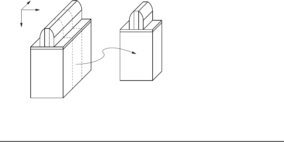
5: Atomistic Kinetic Monte Carlo Diffusion

Estimating CPU Time

394 Sentaurus™ Process User Guide

I-2013.12

The main simulation domain is divided into <n> subdomains; n is the number of threads to be

used. Each subdomain is then run as an independent simulation. Then, the boundary conditions

selected for the Z boundary are applied to the new Zi boundaries. At the end of the simulation

(implantation or diffusion), the main domain is recreated as the simple addition of all the

subdomains. All these “splits” and “forks” of the simulation domains are performed

automatically and are transparent to users.

When using parallelization, one big parallel simulation domain is run as several smaller

domains. At the end of the simulation, the third dimension will be collapsed and averaged to

produce a 2D result (third and second dimensions for 1D results). In any case, the subdomains

must be large enough to allow an accurate representation of the physics involved in the

simulation. In particular, since a minimum surface of 40 nm by 40 nm is recommended, the

minimum suggested size for parallel simulations is 40 nm in the y-axis and nm in the

z-axis, where is the number of threads.

When instructing Sentaurus ProcessKMC to work in parallel with

<n> threads, the domain is

divided into <n> subdomains in the z-direction, and each one is processed by a different CPU.

Later, the subdomains are appended together. These manipulations are transparent to users.

Figure 39 When Sentaurus Process KMC works in parallel with <n> threads, the domain is

divided into <n> subdomains in the z-direction, and each one is processed by a

different CPU. Later, the subdomains are appended together. Here, <n> = 3.

Estimating CPU Time

CPU time and memory required for KMC diffusion simulation are directly proportional to the

number of particles in the structure. For a typical 2-GHz machine, Sentaurus Process KMC

performs up to 1 million events (jumps) per second. In some 64-bit platforms, the number can

reach 2 million events per second.

n40×

CPU #1 #2 CPU #3

CPU #2

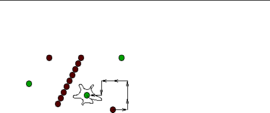
5: Atomistic Kinetic Monte Carlo Diffusion

Atomistic Diffusion Simulation with Sentaurus Process KMC

Sentaurus™ Process User Guide 395

I-2013.12

In equilibrium conditions without implant damage, concentrations of mobile species are low

and events are rare. Therefore, the simulation requires few events to reach the required

diffusion time and proceeds quickly.

For transient-enhanced diffusion after an implant step, it takes some time to anneal the implant

damage. Depending on the implant conditions, each implanted ion generates up to

interstitials and vacancies. Each interstitial and vacancy makes up to jumps before

recombining at the surface. This means that it takes approximately 1 second of CPU time to

anneal one implanted ion.

NOTE The above numbers are only estimations. The CPU speed differs

depending on the machine, operative system, and other factors.

Clustering and emission processes take longer internally than diffusion (hops) processes in

Sentaurus Process KMC, and similar numbers of simulated clustering or declustering

processes may lead to a larger wall clock time.

NOTE The use of parallelization also changes the time estimation (see

Parallelism on page 393).

NOTE The use of different hopping modes (KMC HoppingMode) also changes

the time needed to run the simulation, with doublelong being the

fastest mode (see Hopping Mode on page 423).

Atomistic Diffusion Simulation with Sentaurus

Process KMC

The nonlattice KMC method tracks only atoms in defects, while lattice silicon atoms are not

included as shown in Figure 40.

Figure 40 The nonlattice KMC method tracks only atoms in defects; lattice silicon atoms are

not included

103

105

311

5: Atomistic Kinetic Monte Carlo Diffusion

Atomistic Diffusion Simulation with Sentaurus Process KMC

396 Sentaurus™ Process User Guide

I-2013.12

In molecular dynamics, all lattice atoms and all defect atoms must be simulated, but in the

nonlattice KMC method, only defect atoms are considered. Lattice atoms vibrate with a high

frequency because of thermal energy and, occasionally, one of the point defects diffuses and

moves to a neighboring position. Since Sentaurus Process KMC uses the nonlattice KMC

method, it discards the lattice information and only follows the defect atoms. This greatly

affects CPU time, from approximately s for lattice vibrations to approximately s

for fast diffusing particles. During diffusion, moving particles can be captured by extended

defects that emit isolated particles with frequencies orders of magnitude smaller than

frequency of point defects jumps.

Sentaurus Process KMC takes the input parameters of migration, binding, emission energies,

and so on and simulates the frequencies at which these different events occur. Sentaurus

Process KMC starts with short time steps, but when the simulation evolves and the fast moving

point defects disappear, the average time step automatically changes to adapt to the new

situation.

Single particles can move alone or belong to an extended defect, like a {311}.

■For self-silicon point defects, in other words, interstitial and vacancy models, see Point

Defects, Impurities, Dopants, and Impurity-paired Point Defects on page 415.

■For diffusing dopants, see Impurities on page 418.

■For self-silicon extended defects, see Damage Accumulation Model: Amorphous Pockets

on page 432 and Extended Defects on page 442.

■For clusters involving dopants, see Impurity Clusters on page 472.

Units

The units used by Sentaurus Process KMC are:

■Micrometer ( ) for length

■Second (s) for time

■Electron volt (eV) for binding energies

■Atoms per for concentrations

■ for diffusivities

■ for stress activation volumes

10 13–

10 9–

µm

cm3

cm2s1–

nm3

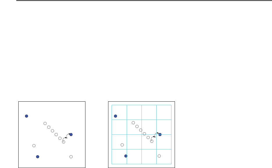
5: Atomistic Kinetic Monte Carlo Diffusion

Atomistic Diffusion Simulation with Sentaurus Process KMC

Sentaurus™ Process User Guide 397

I-2013.12

NOTE These units are standard in atomistic and continuum simulators.

Nevertheless, Sentaurus Process KMC internally uses a

nonconventional unit to measure frequencies. For consistency with

migration prefactors, frequencies are measured in diffusivity units in the

input parameter files. However, even for migration prefactors, which are

in diffusivity units to easily compare them with experimental numbers,

Sentaurus Process KMC must transform them to frequency units in .

This is performed using the expression , where is the average

jump distance.

Space Management

Sentaurus Process KMC assumes an orthogonal simulation cell to manage space. The

minimum and maximum x-, y-, and z-dimensions (that is, the bounding box) are passed to

Sentaurus Process KMC as simulation parameters. Sentaurus Process KMC assumes that the

x-axis is the depth of the silicon wafer; whereas, yz is the wafer area.

When Sentaurus Process KMC has the simulation cell size, it splits the space (see Figure 41)

using Sentaurus Mesh. This creates an internal grid inside the rectangular simulation boundary

box. This grid is used only by Sentaurus Process KMC and is fully isolated from the Sentaurus

Process finite-element mesh. These rectangular elements cannot be smaller than twice the jump

distance ( ). To customize the internal grid, see Internal Grid on page 390.

Figure 41 Sentaurus Process KMC divides the space (left) into small rectangular elements

(right); these elements are used for neighbor search, amorphization, and charge

models

Sentaurus Process KMC shows the number of elements in its output:

KMC domain (-0.1, 0, 0) to (0.3, 0.16, 0.05) um

KMC NonUniformTensor. Boxes: 430125

X=155 (1 - 100)nm

Y=111 (0.903641 - 1.7048)nm

Z=25 (2 - 2)nm

s1–

υ6D

λ2

-------=

0.8 nm

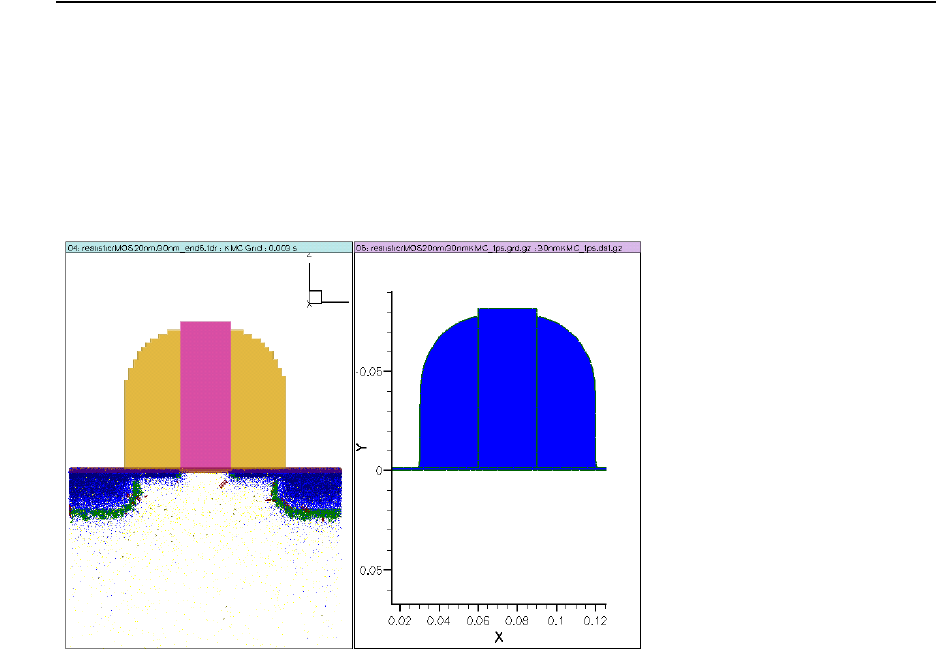
5: Atomistic Kinetic Monte Carlo Diffusion

Atomistic Diffusion Simulation with Sentaurus Process KMC

398 Sentaurus™ Process User Guide

I-2013.12

In the above example, the x-axis minimum cell is 1 nm and the maximum one is 100 nm. For

y, these values are 0.9 and 1.7 nm, respectively. Finally, all of the cells have the same size in

the z-axis: 2 nm. There are 155 cells in the x-direction, and 11 and 25 for y and z, respectively.

The total number of elements is 430125.

NOTE Memory allocation depends on the number of internal elements and on

the number of particles. To modify the number of internal elements

using the parameter, see Internal Grid on page 390.

To add user lines to the simulation, use the line command. You also can specify the option

spacing in this command. In this case, and in contrast with the nonatomistic mode, there is a

minimum size of 0.8 nm between lines. If you specify a very thin spacing, and Sentaurus Mesh

tries to add some lines later to better refine a surface, these last lines could be discarded in the

KMC mesh only to keep the 0.8 nm limitation. Because of this, the use of spacing is not

suggested, and it is usually better to rely on the results of Sentaurus Mesh.

Materials and Space

The transfer of materials from Sentaurus Process to Sentaurus Process KMC is

straightforward: Each Sentaurus Process KMC element is assigned to a material type.

Sentaurus Process KMC creates interfaces whenever two elements are set to different

materials, except when instructed not to do so. Consequently, the shape and interfaces assigned

by Sentaurus Process KMC depend on how smooth the shapes are and how fine the internal

elements are (see Figure 42).

Figure 42 Interfaces between materials have a Manhattan structure in Sentaurus

Process KMC; each element is assigned to a material, and elements are always

rectangular

KMC Original

5: Atomistic Kinetic Monte Carlo Diffusion

Atomistic Diffusion Simulation with Sentaurus Process KMC

Sentaurus™ Process User Guide 399

I-2013.12

The meshing algorithm included in Sentaurus Mesh tries to fit the interfaces using a

nonuniform tensor. This fit is perfect when the interfaces are flat, axis-aligned and there are no

limitations with the element size due to spacing or very thin features. Since the minimum

dimension for an element is 0.8 nm, interfaces thinner than that will not be accurately

represented.

After the material assignment, Sentaurus Process KMC checks that there are no mistakes in the

translation by reviewing the original interface elements and checking that there is a

corresponding KMC interface associated with them. Whenever this correspondence is not

satisfied, Sentaurus Process KMC issues a warning:

** Warning **

KMC. 1.79 percent of the Oxide/PolySilicon interface is lost when translating

to KMC. Please, review the results carefully.

... continuing execution

NOTE In some cases, these warnings may be produced by thin, but negligible,

structure shapes. In these cases, the percentage of interface lost is small.

When the percentage is significant, they point to important problems

that must be resolved before continuing the simulation.

Supported Materials

The materials already defined in Sentaurus Process KMC include:

■Silicon (crystalline silicon)

■Amorphous silicon

■Silicon oxide

■Polysilicon

■Nitride

■Gas

■Germanium

■Germanium oxide

■Amorphous germanium

Amorphous can be assigned by users, but it also is created automatically by changing the

crystalline regions during simulation when the damage reaches an amorphization level (see

Amorphization and Recrystallization on page 454).

5: Atomistic Kinetic Monte Carlo Diffusion

Atomistic Diffusion Simulation with Sentaurus Process KMC

400 Sentaurus™ Process User Guide

I-2013.12

The materials supported by Sentaurus Process KMC are defined in the PDB:

It is possible to define or remove materials, already known by Sentaurus Process, into

Sentaurus Process KMC. They only need to be added as true or false to this list. For

materials not defined in Sentaurus Process, they must be introduced to Sentaurus Process first

with mater add. For example, to add a new material called AnotherSilicon and to remove

Nitride:

pdbSet KMC Materials AnotherSilicon true

pdbSet KMC Materials Nitride false

sprocess> pdbGet KMC Materials

Silicon true

AmorphousSilicon true

Oxide true

PolySilicon true

Germanium true

AmorphousGermanium true

GeOxide true

Nitride true

Cobalt true

CobaltSilicide true

Nickel true

NickelSilicide true

Platinum true

PlatinumSilicide true

Titanium true

TiSilicide true

Tungsten true

TungstenSilicide true

Gas true

Unknown true

5: Atomistic Kinetic Monte Carlo Diffusion

Atomistic Diffusion Simulation with Sentaurus Process KMC

Sentaurus™ Process User Guide 401

I-2013.12

Every new material in Sentaurus Process KMC requires the following pdb parameters:

After the material is properly defined, the parameters for all the particles in this new material

must be defined as well. These parameters depend on the model defined for the new material

(for an overview of these parameters, see Including New Impurities on page 522). Finally,

parameters for all interfaces between the existing materials and the new material must also be

defined.

Model

The options are:

The discard model creates a material empty of particles (for example,

gas). All particles introduced in this material are discarded.

The simple model includes impurity clusters and simple diffusion of

dopants. It does not model Fermi-level dependencies, amorphization, solid

phase epitaxial regrowth (SPER), and extended defects. Oxide and nitride

are examples of ‘simple’ materials.

The full model allows all models: point defects (interstitials and

vacancies), extended defects, impurity clusters, damage accumulation,

amorphization, recrystallization, and the Fermi level–dependent diffusivity

models (for example, silicon).

ShortName

This is the short name of the material when reading parameters defined for

the interfaces. For example, the interface Oxide_Silicon contains the

parameters Eb_SurfOx and Eb_SurfSi, where Ox and Si are the short

names of silicon and oxide.

Semiconductor

A Boolean value. True for materials where DopingConcentration

(NetActive) should be computed and stored.

Crystalline

A Boolean value. True if the material is crystalline (silicon) and false if it is

amorphous (amorphous silicon).

Equivalent

Name of the amorphous/crystalline equivalent. For example, silicon will

have amorphous silicon as its equivalent, and the amorphous silicon

equivalent is silicon.

Oxide

Specify with true or false whether the material is an oxide or is not an

oxide, respectively. This is used for oxidation models. For example,

SiOxide and GeOxide have this field as true.

Alloy

Specify if this material can alloy with another material to form binary alloys

with corrections to activation energies. Write the alloy material here. For

example, for silicon alloying with germanium, write Germanium in the

Alloy field of the silicon material.

5: Atomistic Kinetic Monte Carlo Diffusion

Atomistic Diffusion Simulation with Sentaurus Process KMC

402 Sentaurus™ Process User Guide

I-2013.12

NOTE To minimize the work of defining parameters for a new material, it is

advisable to disable the materials that will not be used, thereby avoiding

to define parameters for the interfaces between those materials and the

new one. For the dopant parameters in the new material, you can “copy”

the parameters from another material and redefine only some of them.

Any other material existing in Sentaurus Process, but not defined by Sentaurus Process KMC,

is mapped as ‘Unknown’. The model for this material is discard, and all particles inside these

materials are discarded and removed. They do not need parameters because they contain no

particles to simulate.

Material Alloying

Sentaurus Process KMC allows materials containing an alloying element to be treated in a

quasi-atomistic framework. Such an alloying element is specified using the Alloy parameter

of the material specification. In the following, as an example, it is assumed that the material is

silicon and the alloy is germanium (although, this can be reversed, or any pair of materials can

be used with "full" modeling).

The quasi-atomistic framework means that alloy particles (Ge) are not created as particles, but

they will be taken into account as a field, so as to produce a local concentration. This saves

memory and speeds up the concentration. Diffusion of the alloying element is possible using

the model specified in Alloy Diffusion on page 431.

The inclusion of an alloy changes the bandgap narrowing as specified in Narrowing due to

Presence of an Alloy on page 504. Such a model uses a quadratic interpolation to smooth from

the band gap of the pure material to the band gap of the pure alloy. Since the positions in the

band gap of all particles are scaled with the total band gap, the positions for charged defects

are scaled accordingly.

All activation energies for diffusion-, emission-, and activation-related processes are corrected

by a term linear on the alloy concentration. If a given mechanism is simulated by following an

Arrhenius expression similar to:

(654)

the mechanisms under an alloy concentration are corrected by a linear term in the activation

energy with the concentration of the alloy (Ge):

(655)

The same applies to the formation energies of point defects and the potential energies of

impurity clusters. Examples of these corrections are available in Alloy Effects on page 432.

νPE–kBT⁄()exp=

νPEαGe[]+()–kBT⁄()exp=

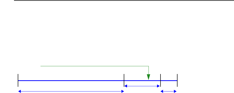
5: Atomistic Kinetic Monte Carlo Diffusion

Atomistic Diffusion Simulation with Sentaurus Process KMC

Sentaurus™ Process User Guide 403

I-2013.12

Point Defects

Sentaurus Process KMC can distinguish between different interstitials, depending on the

material, using different syntax. The syntax "I" refers to an interstitial in the particular

material where it is positioned; otherwise, a more concrete notation must be used. For example,

in a structure where the first half is Ge and the second half I, "I" refers to Gei in the first half

and Sii in the second half. While Sii, for example, would have the same meaning as in the

second half, but it would produce Si in the first half.

Ambiguous Alloying

Sentaurus Process KMC allows the use of a material (for example, Si) with an alloy (for

example, Ge) without having to define the material alloyed (Ge). Nevertheless, it is also

possible to define the alloyed material as the main material (Ge) with the other one as the

alloyed material (Si). However, having all alloys defined twice is ambiguous. For example,

Si0.2Ge0.8 can be defined as main Si with 80% Ge, or as main Ge with 20% Si.

The main material is the one specified in the input file as material. In this case, it can be

silicon, and then you can use the select command or similar to include 80% Ge (or

germanium) and 20% silicon. Unfortunately, the complexity of the models and their calibration

produce different results when these two ways to have the same alloy are used. To solve this

issue, using Si as the main material up to 80% Ge concentration and Ge up to 20% silicon is

suggested.

Time Management

The main component in Sentaurus Process KMC is an algorithm that sequentially selects the

possible random events (migration of point defects, emission of extended defects, and so on)

according to their corresponding frequencies, similar to the Bortz–Kalos–Liebowitz (BKL)

algorithm so widely used in KMC methods. Figure 43 illustrates the selection procedure for

the atomistic configuration shown in Figure 40 on page 395, consisting of three vacancies (V),

two interstitials (I), and one {311} defect.

Figure 43 Events are selected according to their rates, which in turn, depend on the current

atomistic configuration

rand

3000 3200 32100

V jump

I jump

{311} emission

5: Atomistic Kinetic Monte Carlo Diffusion

Atomistic Diffusion Simulation with Sentaurus Process KMC

404 Sentaurus™ Process User Guide

I-2013.12

Assuming the vacancy and interstitial migration frequencies are and ,

respectively, and the {311} emission rate is , to simulate 1 s, you have to simulate a total

of 3210 events. Consequently, simulating one event corresponds to simulating 1/3210 s. This

implies that the simulated time step is not fixed, but depends on the particular simulation

configuration. In addition, you must choose a V with a probability of 3000/3210, and Is and

{311} defects with probabilities of 200/3210 and 10/3210. A random number between 1 and

3210 (or 0 and 3209) is generated. For example, in Figure 43, the number 3147 selects an I

migration event.

After several migration events, when one interstitial reaches and interacts with a vacancy, the

simulator generates an IV pair called an amorphous pocket (AP) (see Damage Accumulation

Model: Amorphous Pockets on page 432).

The simulation contains two Vs, one Is, one IV, and one {311}. You can assume the IV pair will

recombine with a frequency of . The new random number will be between 1 and

2000 + 100 + 500 + 10 = 2610. Consequently, the time step will be 1/2610 s. If the IV

recombination event is chosen and this IV pair is annihilated, the new simulation contains only

two Vs, one I, and one {311}, and the following time step is 1/2110 s.

NOTE The time step is not a fixed quantity in Sentaurus Process KMC, but it

depends on the state of the simulation.

The current time step depends on two factors:

■Number of particles in the simulator

■Frequency of the events associated with the particles or defects or both

And these frequencies depend on three factors:

■Type of event

■Arrhenius plot associated with the event

■Temperature

Simulation and CPU Times

The time needed to complete a simulation depends on several factors:

■How fast the computer simulates one event

■How many events need to be simulated

■The hopping mode chosen

■The presence of lattice KMC models (for SPER and epitaxial deposition)

■Whether you use parallel capabilities

1000 s 1–

100 s 1–

10 s 1–

500 s 1–

5: Atomistic Kinetic Monte Carlo Diffusion

Atomistic Diffusion Simulation with Sentaurus Process KMC

Sentaurus™ Process User Guide 405

I-2013.12

The number of events to be simulated is inverse to the average time step (which changes during

the simulation, as explained above). The speed at which the simulator processes events depends

on the type of simulated events. Migration events usually are simulated rapidly. Simulations

involving changes in the electronic concentration or temperature or both are much slower

because updating the dependencies with the temperature and the Fermi level takes extra time.

Generally, the smaller the simulation, the shorter the time.

In simulations with implants, the implant MC module also adds time to the simulation while

computing the cascades. In amorphizing conditions, the Sentaurus Process KMC amorphous

model requires extra time to smooth out the damage and create amorphous layers. Finally,

simulations with strong gradients in the electronic concentration need more charge updates,

which take extra time.

During oxidation, several remeshings must be performed to update the Sentaurus

Process KMC structure to the new Sentaurus Process oxide thickness, consuming extra time.

Finally, the hopping mode allows you to chose whether long hops or double hops are allowed,

thereby speeding up the simulation. Both are switched on by default (see Hopping Mode on

page 423).

NOTE Yo u ca n es ti mate t he t im e n ee ded for simulation by running a small

simulation and assuming the CPU time is proportional to the number of

particles which is proportional to the surface area.

Sentaurus Process KMC shows the status of the current simulation, printing log messages each

time the temperature changes during a temperature ramp, or whenever there is a new snapshot

(see Snapshots on page 407). These log messages are as following:

Reaction : 31s to 63s step : 32s temp: 950.0C

Mechanics: 31s to 63s step : 32s temp: 950.0C

Diffusion: 31s to 63s step (d): 32s temp: 950.0C

KMC: Time(s) Temp(C) Events Events/s Average step(s) %Done

46.416 950.01 3600728007 1877077 4.749174e-08 7.74% (36% V)

Reaction : 1.05min to 2.117min step : 1.067min temp: 950.0C

Mechanics: 1.05min to 2.117min step : 1.067min temp: 950.0C

Diffusion: 1.05min to 2.117min step (d): 1.067min temp: 950.0C

KMC: Time(s) Temp(C) Events Events/s Average step(s) %Done

100.000 950.01 4742533558 1865695 4.692958e-08 16.67% (33% V)

Reaction : 2.117min to 4.25min step : 2.133min temp: 950.0C

Mechanics: 2.117min to 4.25min step : 2.133min temp: 950.0C

Diffusion: 2.117min to 4.25min step (d): 2.133min temp: 950.0C

KMC: Time(s) Temp(C) Events Events/s Average step(s) %Done

215.444 950.01 6881748852 1868310 5.396525e-08 35.91% (34% I)

Reaction : 4.25min to 7.125min step : 2.875min temp: 950.0C

Mechanics: 4.25min to 7.125min step : 2.875min temp: 950.0C

Diffusion: 4.25min to 7.125min step (d): 2.875min temp: 950.0C

Reaction : 7.125min to 10min step : 2.875min temp: 950.0C

5: Atomistic Kinetic Monte Carlo Diffusion

Atomistic Diffusion Simulation with Sentaurus Process KMC

406 Sentaurus™ Process User Guide

I-2013.12

Mechanics: 7.125min to 10min step : 2.875min temp: 950.0C

Diffusion: 7.125min to 10min step (d): 2.875min temp: 950.0C

KMC: Time(s) Temp(C) Events Events/s Average step(s) %Done

464.159 950.01 11927967061 1864825 4.928753e-08 77.36% (35% I)

Elapsed time for diffuse 7.8672e+03s

600.000 950.01 14721335445 1882323 4.862968e-08 100.00% (35% I)

It is easy to identify the log immediately after the Diffusion statement because it is preceded

by a “KMC:” header. In the above example, the total simulated (annealed) time is 600 s. The

(current) temperature is . A total of events has been simulated so far, and the

simulator processed 1.9 million events each CPU second. The averaged time step is

. Finally, Sentaurus Process KMC writes the particle with the biggest percentage

of diffusion jumps. In the example, the diffusion of the neutral interstitial (I) has taken 33 to

36% of the total diffused particles.

This information may change from one simulation to another, and also at different times during

the same simulation. The events per second and average step statistics are recomputed between

sentences.

Parallelism and CPU Time

Table 45 lists the CPU times that can be expected when running on different numbers of

threads. However, the exact time depends on the particular simulation.

The total simulation time is superlinear for and starts saturating for . The reason

for being superlinear for a small number of threads is that the CPU time depends superlinearly

on size. Consequently, simulating a size XYZ/n takes less CPU time than S/n. Nevertheless, as

increases, different mechanisms (such as the waiting time of threads to be synchronized)

conspire to degrade the total simulation time.

Ta bl e 4 5 A p p rox im at e C P U t im e s w he n u s i ng mu lt ip le t hr e ad s

Number of independent

threads

Approximate time Improvement

1 S 1x

2S/2.32.3x

4S/4.84.8x

8 S/8 8x

12 S/9.5 9.5x

16 S/10.5 10.5x

950°C

1.4 1010

4.9 10 8–

× s

n8<

n12≥

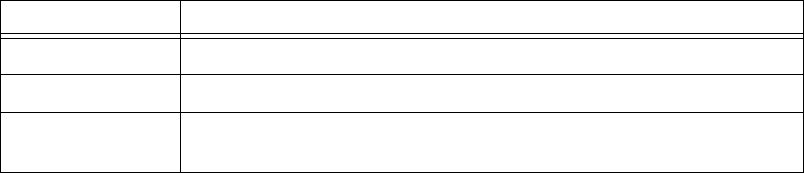
5: Atomistic Kinetic Monte Carlo Diffusion

Atomistic Diffusion Simulation with Sentaurus Process KMC

Sentaurus™ Process User Guide 407

I-2013.12

Snapshots

A snapshot is an interruption of the normal Sentaurus Process KMC simulation flow to print

the status of the simulation and to allow you to run a customizable Tcl command (see Movie

on page 407). To control these interruptions, set the pdb parameters listed in Table 46.

For example:

pdbSet KMC Decade 2

produces two snapshots per decade, as in:

Time(s) Temp(C) Events Events/s Average step(s) %Done

0.000 26.85 0

548.138 700.00 1 5.481385e+02 0.05% (35% I)

1492.073 700.00 5 2.359835e+02 0.15% (33% I)

3639.863 700.00 7867 2.731862e-01 0.36% (35% I)

10130.431 700.00 14553 9.707701e-01 1.01% (35% I)

31902.727 700.00 35862 1.021742e+00 3.19% (36% I)

100030.228 700.00 205821 169959 4.008467e-01 10.00% (35% I)

317268.817 700.00 668173 4.698554e-01 31.73% (34% I)

1000000.000 700.00 1754838 1086665 6.282812e-01 100.00% (35% I)

Movie

The Sentaurus Process KMC Movie command is similar to the Sentaurus Process Movie

command and executes the contents of the parameter KMC Movie any time a new snapshot is

generated. You can use this command interactively to obtain information about the simulation,

to add data to the TDR file of Sentaurus Process KMC, and so on.

For example, it can be used to add concentration information and the positions of particles to

the TDR file during the simulation:

pdbSet KMC Movie {kmc extract tdrAdd concentrations defects}

or to plot the evolution of damage while the simulation is still running:

pdbSet KMC Movie {

Ta bl e 46 S na p sh ot p ara me te rs

Parameter Description

Decade <n>

Sets how many snapshots will be generated per decade. 0 disables it.

InitOutputTime <n>

No snapshots per decade are generated when the simulated time is smaller than n.

maxSnapshots <n>

Maximum number of snapshots to be stored. After this limit is reached, the oldest

ones are erased to make space for the new ones.

5: Atomistic Kinetic Monte Carlo Diffusion

Particles

408 Sentaurus™ Process User Guide

I-2013.12

kmc deatomize name=ITotal; sel z=log(ITotal+1); plot.1d label=I clear;

kmc deatomize name=VTotal; sel z=log(VTotal+1); plot.1d label=V !clear

}

Time Internal Representation and Limitations

There are no internal limits for the frequencies used in Sentaurus Process KMC. Nevertheless,

very high frequencies (typically produced by small migration energies) can lead to slow

simulations.

Particles

Particles are represented in Sentaurus Process KMC with three spatial coordinates (x, y, z) and

two labels:

■The particle type label identifies the species, charge state, and role of the particle in the

simulation.

■The defect type indicates when the particles are agglomerated with others or when they

stand alone.

Particle Types

To obtain a list of the standard particles currently defined for Sentaurus Process KMC, use the

command:

sprocess> kmc particletypes

I V B As C F In O P Sb N H IMM IM IP IPP VMMM VMM VM VP VPP VPPP Asi AsiP AsV

AsVP AsVM Bi BiP BiM Ci FV FI Ini IniM InV InVM Pi PiP PV PVM PVP Sbi SbiP SbV

SbVP SbVM Ge Gei Si Sii

Dopants are user defined in Sentaurus Process KMC, while interstitials and vacancies are fixed

and cannot be customized. The standard list of interstitials and vacancies defined in Sentaurus

Process KMC is:

I Silicon self interstitial–neutral

IMM Silicon self interstitial-double negative

IM Silicon self interstitial–negative

IP Silicon self interstitial–positive

IPP Silicon self interstitial-double positive

5: Atomistic Kinetic Monte Carlo Diffusion

Particles

Sentaurus™ Process User Guide 409

I-2013.12

The dopants are defined in the parameter database. By default, particles for As, B, P, In, C, F,

N, Nn (N2), H, and Sb are defined. For example, the default particles for As, B, and P are:

NOTE Since P at the end of the name means positive, to specify a cluster

containing phosphorus, the P cannot be at the end in any case. This

means that AsiP is an arsenic–interstitial positive, while PAsi is a

phosphorus arsenic–interstitial cluster. Similarly, AsP will be

interpreted as arsenic positive, while PAs is phosphorus–arsenic.

VVacancy–neutral

VMMM Vacancy-triple negative

VMM Vacancy–double negative

VM Vacancy–negative

VP Vacancy–positive

VPP Vacancy–double positive

VPPP Vacancy-triple positive

As Substitutional arsenic–positive

Asi Interstitial arsenic–neutral

AsiP Interstitial arsenic–positive

AsV Vacancy arsenic–neutral

AsVM Vacancy arsenic–negative

AsVP Vacancy arsenic–positive

BSubstitutional boron–negative

Bi Interstitial boron–neutral

BiM Interstitial boron–negative

BiP Interstitial boron–positive

PSubstitutional phosphorus–positive

Pi Interstitial phosphorus–neutral

PiP Interstitial phosphorus–positive

PV Vacancy phosphorus–neutral

PVM Vacancy phosphorus–negative

PVP Vacancy phosphorus–positive

5: Atomistic Kinetic Monte Carlo Diffusion

Particles

410 Sentaurus™ Process User Guide

I-2013.12

NOTE These lists show the most commonly used particles, but the list is not

exhaustive. An exhaustive list contains all point defects (Is and Vs) with

charges from –3 to +3, and all impurity pairs with charges from –2 to +2.

Particles in Models

The dopants allowed in the simulation are defined in the parameter database under the label

KMC Impurities. The database lists the impurity name, the charge, and a Boolean parameter

indicating whether the particle is allowed in the Sentaurus Process KMC simulation.

The particle name and the charge must be delimited by a comma without spaces. For example,

in the case of arsenic and boron:

pdbSet KMC Impurities As,1 true

pdbSet KMC Impurities B,-1 true

When the dopant type has been defined, the paired particles(particles with I or V) can be

defined in KMC Pairs. The definitions are a string containing the name of the pair, the name

of the dopant, the type of pair (I or V) and the charge. These fields are separated with commas.

Finally, a Boolean parameter instructs Sentaurus Process KMC to take the particle into

account.

For arsenic and boron:

pdbSet KMC Pairs Asi,As,I,0 true

pdbSet KMC Pairs AsiP,As,I,1 true

pdbSet KMC Pairs AsV,As,V,0 true

pdbSet KMC Pairs AsVP,As,V,1 true

pdbSet KMC Pairs AsVM,As,V,-1 true

pdbSet KMC Pairs BV,B,V,0 false

pdbSet KMC Pairs Bi,B,I,0 true

pdbSet KMC Pairs BiP,B,I,0 true

pdbSet KMC Pairs BiM,B,I,-1 true

In the previous example, the particle boron vacancy is not defined (set to false). A particle is

not defined when it does not appear in the Pairs list, or when its Boolean variable is false.

The following rules must be followed when defining particles:

■The dopants used in the definitions of Pairs must exist in the list of impurities

■A charge n can only be defined when a charge n – 1 or n + 1 is already defined, except for

pairs with same charge states as their dopants.

■Charge states without possible pairing reactions cannot be defined.

■The charge must be –1, 0, or +1.

5: Atomistic Kinetic Monte Carlo Diffusion

Particles

Sentaurus™ Process User Guide 411

I-2013.12

■Pairs with neutral state; and with the charge of its dopant, always must be defined.

For example, when As+ is defined as an impurity, AsV+ can be defined. The existence of AsV+

allows you to define AsV0 and AsV-. AsV-- cannot be defined (no charge –2). For B-, you can

define Bi-, Bi0, and Bi+.

Alias

Aliases of particle names are defined in KMC aliases, which is a list of particle names and

alternative names separated by commas. These aliases are used only when Sentaurus

Process KMC tries to map a name as particles or defects. For example, if there is an alias such

as:

Bi BoronInt,BI

the commands:

kmc present defectname=Bi

kmc present defectname=BI

are the same, and:

sel z=1e19 name=Bi

sel z=1e19 name=BI

sel z=1e19 name=BoronInt

create fields with different names, but the atomized particle is the same (Bi).

Colors

You can cha ng e t he defa ult v isu alization color for the atomistic representation of particles and

defects in Tecplot SV, or add new colors to existing particles and defects. The list of colors is

KMC Colors, and it is an array of particle names and colors in #rrggbb format (red, green,

blue).

Particles and Parameters

New particles need new parameters. For every impurity specified in Impurities, a new file

must be created for each material folder and surface. The name of these files is obtained using

the command alias with the name of the Sentaurus Process KMC impurity as a parameter:

sprocess> alias B

Boron

5: Atomistic Kinetic Monte Carlo Diffusion

Particles

412 Sentaurus™ Process User Guide

I-2013.12

Table 47 lists the parameters required for materials defined to use the simple model.

When amorphous materials (where the best example is amorphous silicon) use the dangling

bond model (see Indirect Diffusion on page 457), the parameters listed in the previous table

plus those in Table 48 are required.

Table 49 lists the parameters used on interfaces.

Table 47 Nonsilicon material parameters

Parameter Description

Dm, Em

Diffusion parameters.

VD, VF

Activation volumes for stress.

sinkProbTop, sinkProbBottom, sinkProbLeft,

sinkProbRight, sinkProbFront, sinkProbBack

Boundary conditions.

Implement_Complex

Parameters for clustering.

ReactionsPointDefect, ReactionsCluster

Binary interactions.

Ta bl e 4 8 E x t ra p a ra me te rs fo r a mo r p h ou s ma te r ia ls

Parameter Description

EmGe, EfGe

Ge correction to migration energies.

gamma

Coefficient for dangling bond creation.

Db, Eb

Binding prefactor and energy.

Table 49 Parameters used on interfaces

Parameter Description

EBarrier_Surf?,

Eb_Surf?

Interface binding energies for dopants. ? denotes the material. Gas for gas, Si

for silicon, Ox for oxide, Ni for nitride, Po for polysilicon, and Unknown for

the rest.

Db_Surf

Surface emission prefactor for dopants.

EMax_Surf, C0Max_Surf

Maximum number of particles trapped at the surface.

Evaporation_Surf

Probability to evaporate (annihilate).

VF_Surf?

Activation volume for stress. ? denotes the material.

5: Atomistic Kinetic Monte Carlo Diffusion

Particles

Sentaurus™ Process User Guide 413

I-2013.12

Table 50 lists the parameters required for materials using full modeling.

Finally, amorphous, simple and full materials allow the definition of impurity clusters. These

clusters are defined using the parameters listed in Table 51.

For further explanations on these parameters, see the comments in the parameter database and

the model descriptions.

Ta bl e 5 0 F ul l ma te r i al p ar a m e t e rs

Parameter Description

Dm, Em

Diffusivities.

Db, Eb

Binding prefactors and energies.

VD, VF

Activation volumes for stress.

Electronic levels.

EfGe, EmGe

Corrections for germanium.

P_recrysDeposit, E_recrysDeposit,

recrysDepositThreshold, C0_recrysMaxActive,

E_recrysMaxActive, recrysMaxTotal,

recrysMaxSize, recrysDeposit_Complex, E_recrys,

E_recrys_exponent, recrysDeposit_Active,

e0_Complex

SPER model (recrystallization).

sinkProbTop, sinkProbBottom, sinkProbLeft,

sinkProbRight, sinkProbFront, sinkProbBack

Boundary conditions.

ReactionsPointDefect, ReactionsCluster,

ReactionsClusterI, ReactionsClusterV,

ReactionsClusterIV, ReactionsLoop,

ReactionsVoid, Reactions311

Binary interactions.

Table 51 Parameters used for impurity clusters

Parameter Description

Implement_Complex

Whether a cluster exists or not.

Etotal_Complex

Cluster potential energy.

e0_Complex

Cluster charge.

VF_Complex

Stress dependency.

CaptVol_Complex

Cluster capture volume used for emission.

D0_Cluster

Cluster emission prefactors.

EbarrierDopant_Complex, EbarrierIV_Complex

Cluster emission barriers.

Dm_Cluster, Em_Cluster

Cluster migration parameters

5: Atomistic Kinetic Monte Carlo Diffusion

Particles

414 Sentaurus™ Process User Guide

I-2013.12

Undefining Particles

Particles can be undefined erasing their definition in the parameter database or setting its

Boolean to false. If an impurity is undefined or erased, Sentaurus Process KMC also

undefines all its pairs.

For example, to undefine indium in a simulation, use:

pdbSet KMC Impurities In,-1 false

To undefine only boron interstitials with a positive charge, use:

pdbSet KMC Pairs BiP,B,I,1 false

NOTE Undefining particles that will not be used in the simulation saves some

small memory and CPU time. If an undefined dopant is used (for

example, it is implanted or introduced with select), it causes an error.

Defect Types

For a list of the defects implemented in Sentaurus Process KMC, use the command:

sprocess> kmc defecttypes

PointDefect AmorphousPocket Void ThreeOneOne Loop ImpurityCluster Interface

TwinDefect Amorphous LatticeAtom Rejected PD

Defects implemented in Sentaurus Process KMC include those listed in Table 52.

Table 52 Defects implemented in Sentaurus Process KMC

Defect Description

Amorphous

Amorphous region inside the crystalline silicon. Only I, V, impurity clusters, and dopants are

allowed. See Amorphization and Recrystallization on page 454.

AmorphousPocket

Disordered agglomeration of Is and Vs (damage). Only I and V particle types are allowed.

See Damage Accumulation Model: Amorphous Pockets on page 432.

ImpurityCluster

Impurity clusters. Agglomeration of dopants with Is or Vs. See Impurity Clusters on

page 472.

Interface

Dopants trapped in the interfaces (for example, Si/SiO2).

See Interfaces and Surfaces on page 507.

LatticeAtom

Atom in the silicon lattice used for SPER or epitaxial deposition. See LKMC: Fully

Atomistic Modeling of Solid Phase Epitaxial Regrowth on page 463

Loop

Dislocation loops. Extended Is defect. Only Is are allowed.

See Dislocation Loops on page 447.

5: Atomistic Kinetic Monte Carlo Diffusion

Point Defects, Impurities, Dopants, and Impurity-paired Point Defects

Sentaurus™ Process User Guide 415

I-2013.12

NOTE Not all possibilities of particle and defect types are allowed. Some

particle types, like the paired ones (Asi, BiM…), are only allowed as

PointDefect. Others, like As or B, can stand alone (PointDefect),

can be trapped in interfaces (Interface), or can belong to an impurity

clusters (ImpurityCluster). Neutral interstitials, for example, can

stand alone (PointDefect), can be in damaged clusters

(AmorphousPocket), {311} defects (ThreeOneOne), or dislocation

loops (Loop). Single particles can be mobile point defects (in other

words, interstitials and vacancies), immobile impurity atoms (like

substitutional boron and arsenic), and also mobile impurity-defect pairs

such as Bi or AsV. All are considered PointDefect.

Point Defects, Impurities, Dopants, and Impurity-paired

Point Defects

Interstitials and Vacancies

Interstitials and vacancies in Sentaurus Process KMC perform a diffusion event in each axis

(x, y, and z) at a frequency given by the expression:

(656)

Defect Description

PointDefect, PD

Single particles (IMM, IM, I, IP, IPP, VMM, VM, V, VP, VPP, As, and B) or paired ones

(Asi, AsiP, AsVM, AsV, AsVP, BiM, Bi, and BiP) that do not belong to any extended

defect or particle agglomeration; in other words, impurities, dopants, and impurity-paired

point defects.

Rejected

A particle coming from MC implant which is determined to be in a material which does not

support the particle. For example, a point defect in a simple material such as oxide.

ThreeOneOne

{311} rod-like extended defects. Only Is. are allowed.

See {311} Defects (ThreeOneOne) on page 442.

TwinDefect

Can be formed during SPER if the twin defect model is turned on. See Defect Generation

during SPER on page 467.

Void

Vacancy clusters with spherical shape. Only Vs are allowed. See Voids on page 451.

Table 52 Defects implemented in Sentaurus Process KMC

νjm

ν0m,

-----------Emσ'j∆Vpar σ'i∆Vort

()∆EmGe()+

ij≠









kBT()⁄–







exp⋅=

5: Atomistic Kinetic Monte Carlo Diffusion

Point Defects, Impurities, Dopants, and Impurity-paired Point Defects

416 Sentaurus™ Process User Guide

I-2013.12

where:

■ is the jump frequency for the axis .

■ is the prefactor.

■ is the migration energy.

■ are the principal stresses (the stresses in the coordinate system where all the stress

tensor nondiagonal components are null).

■ is the activation volume for stress-parallel diffusion.

■ is the activation volume for stress-perpendicular diffusion.

■ is the correction due to germanium concentration.

These parameters are called Dm (prefactor), Em (energy), VD (activation volumes), and EmGe

(for ) in the parameter database. They are defined only in the full model materials:

sprocess> pdbGet KMC Si I Dm

IMM 5e-2

IM 5e-2

I 5e-2

IP 5e-2

IPP 5e-2

sprocess> pdbGet KMC Si I Em

IMM 0.8

IM 0.8

I 0.8

IP 0.8

IPP 0.8

sprocess> pdbGet KMC Si I VD

IMM 0,0

IM 0,0

I 0,0

IP 0,0

IPP 0,0

sprocess> pdbGet KMC Si I EmGe

The activation volumes for parallel and perpendicular diffusion, respectively, are separated by

a comma (no spaces) in VD.

The stresses are produced by Sentaurus Process and imported by Sentaurus Process KMC.

This stress tensor is diagonalized to obtain the principal stresses . The directions x, y, and z

used in the equation refer to the system in which the stress tensor is diagonal.

NOTE Yo u ca n c alibr at e thes e p aram et ers if necessary to change the point-

defect diffusivity and DC product.

νjm

ν0m,

σ'i

∆Vpar

∆Vort

∆EmGe() α

mGe[]=

αm

σij

σ'i

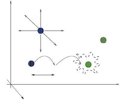
5: Atomistic Kinetic Monte Carlo Diffusion

Point Defects, Impurities, Dopants, and Impurity-paired Point Defects

Sentaurus™ Process User Guide 417

I-2013.12

Sentaurus Process KMC simulates point-defect migration, modifying the particle coordinates

in the orthogonal directions a fixed distance, called , which corresponds to the second

neighbor’s distance in the silicon lattice (0.384 nm). The value of can vary spacially (as

explained in Hopping Mode on page 423).

After each diffusion event, the charge state of the point defect is updated according to the new

local Fermi level (see Fermi-Level Effects: Charge Model on page 490 and Updating Charged

States on page 497). Whenever a jumping point defect encounters another particle, defect, or

interface, the jumping point defect interacts according to the specific situation. These

interactions are allowed depending on the following:

■Incoming species—for example, substitutional boron plus interstitial (B + I) is allowed,

and the incoming species form a boron interstitial. Boron plus vacancy is not allowed. This

interactions can be enabled or disabled in the parameter database.

■Energetics—Sentaurus Process KMC allows interactions for {311} defects, dislocation

loops, and pairing because the binding energies are greater than 0. For impurity clusters, if

the reaction is unfavourable, the newly formed defect breaks up and dissolves in the

original components or is rejected before reacting.

■Charge states—interactions between repulsive species are forbidden, except for the

‘percolation’ model (see Percolation on page 477).

Mobile particles can interact with other mobile particles or with the particles belonging to

extended defects, whenever they enter in the capture radius of the other particle or defect (see

Figure 44). The capture radius for a mobile particle is , assumed to be the same as the

jumping distance. For extended defects, the capture volume is the sum of the capture volumes

of its constituent particles. Mobile particles can interact with surfaces/interfaces as explained

in Interfaces and Surfaces on page 507.

Figure 44 Point defects diffuse by jumping a distance in any orthogonal direction and can

interact with neighbor particles

Jump

I+V InteractionLambda

Simulation Cell x

Particle Type: Interstitial

Defect: PointDefect

Coords: x1, y1, z1 Particle Type: Vacancy

Defect: PointDefect

Coords: x2, y2, z2

Possible

Migrations

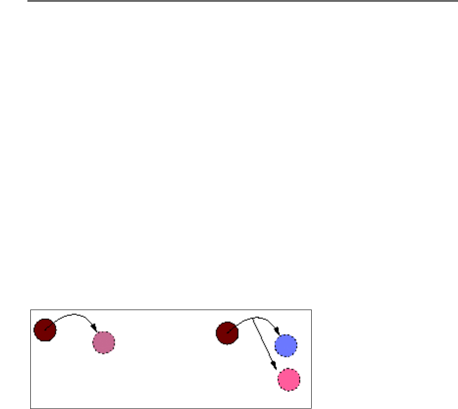
5: Atomistic Kinetic Monte Carlo Diffusion

Point Defects, Impurities, Dopants, and Impurity-paired Point Defects

418 Sentaurus™ Process User Guide

I-2013.12

Impurities

Isolated impurities in Sentaurus Process KMC can be in a substitutional state or can be paired

with interstitials or vacancies. Substitutional impurities are electrically active and typically

immobile. The acceptor and donor impurities (Groups III and V of the periodic table,

respectively) can move in silicon only by pairing with an interstitial or a vacancy, as shown in

the literature [4][5][6][7][8]. Other impurities, such as fluorine, may diffuse without the aid of

an extra I or V (see Impurities Diffusing without Pairing on page 525).

Impurity atoms are modeled like interstitials or vacancies. They have a position and a defect

type and particle type. The defect type is PointDefect, and the particle type characterizes the

species, charge state, and the presence of a paired I or V. For example, BiM indicates a

negatively charged boron paired with an interstitial.

NOTE Sentaurus Process KMC assumes interstitial particles and substitutional

particles paired with an interstitial as the same configuration; in other

words, Bi is the same as IB or BI, and there is only one position (three

coordinates) for it.

Paired impurities can perform two possible types of events (see Figure 45):

■Diffusion jump

■Breakup of the impurity–defect pair

Figure 45 Impurity pairs can diffuse or break up into a substitutional

plus an interstitial or a vacancy

NOTE Fluorine is modeled as an interstitial particle (in the default parameters,

not in Advanced Calibration). Consequently, fluorine diffuses without

pairing. See Impurities Diffusing without Pairing on page 525.

Migration (Diffusion)

The diffusion event is defined as for point defects (see Eq. 656, p. 415). Nevertheless, the

equation defines an instant diffusivity that is different from the effective diffusivity. Effective

Migration Breakup

5: Atomistic Kinetic Monte Carlo Diffusion

Point Defects, Impurities, Dopants, and Impurity-paired Point Defects

Sentaurus™ Process User Guide 419

I-2013.12

diffusivity measured in experiments involves a large number of microscopic migration steps

and long times. Microscopically, dopants diffuse using the kick-out mechanism. For example,

when an interstitial reacts with a substitutional boron, a boron–interstitial pair is generated:

. In contrast with the boron in substitutional position, the generated pair is mobile.

Then, begins to diffuse, using the diffusivity parameters specified in Eq. 656. After some

time, the interstitial boron breaks up, releasing the interstitial. This boron will not move until

a new incoming I reacts with it. Consequently, the macroscopic diffusivity is related not only

with the boron interstitial diffusivity, but also with its breakup frequency as:

(657)

depends on the Bi and I migration prefactors and on the Bi breakup prefactor.

is related with the Bi microscopic migration energy , the formation energy

of an interstitial and the Bi binding energy (assuming there are no stress or

SiGe corrections):

(658)

Finally, the total boron diffusivity is given as the sum of the contribution of all mobile species.

For boron interstitial, and assuming there are three mobile species, negative, neutral, and

positive:

(659)

where represents the microscopic pair diffusivity of charge .

Breakup

The breakup event for an interstitial-impurity pair can be described as:

(660)

where is an interstitial-impurity pair, is a substitutional impurity atom, and is an

interstitial silicon atom. This breakup event happens with a frequency given by:

(661)

where is the prefactor and is the activation energy, defined as the binding energy plus

the migration energy of the emitted species and the SiGe and stress corrections:

BI+Bi

→

Deff B() D0

eff B() Ediff B()

kBT

--------------------–





exp=

eff B()

Ediff B()

EmBi

()()

EfI()()

EbBi

()()

Ediff B() EmBi

()EfI() EbBi

()–+=

DB() DB

()

[]

B-

[]

---------- DB

()

[]

B-

[]

-----------DB

()

[]

B-

[]

-----------++=

()

AiAsI+↔

νbk ν0bk,Ebk kBT()⁄–()

---∆–Em

ikBT()⁄()exp

xyz,,



exp⋅=

ν0bk,

Ebk

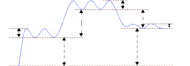
5: Atomistic Kinetic Monte Carlo Diffusion

Point Defects, Impurities, Dopants, and Impurity-paired Point Defects

420 Sentaurus™ Process User Guide

I-2013.12

(662)

where:

■ is the hydrostatic pressure, computed as the mean value of the

principal stresses.

■ are the activation volumes for the formation energies.

■ is the germanium concentration.

■ accounts for the variation of the formation energy with the germanium concentration.

The corrections to the migration energies induced by the stress and SiGe are (as previously

explained in Interstitials and Vacancies on page 415):

(663)

Sentaurus Process KMC assumes that the activation volume and the SiGe variation for the

formation energy do not depend on the charge. All the charge states of the same species share

the same activation volume and SiGe dependencies for the formation energy.

Figure 46 shows the energies for boron involved in this mechanism. It is easy to deduce that a

change in the formation energies due to stress and SiGe will change the binding energy as:

(664)

Figure 46 Energies involved in the kick-out mechanism for B–+ I0 = Bi–. Migration energy of

the interstitials and boron interstitial are specified in the parameter database as

Em. The binding energies are Eb, and the I formation energy is specified as

Eform. The formation energy for dopants in pure silicon is assumed to be 0

because the dopants are already in the simulation; the dopants are not created

by the system.

Ebk Ai

() EbAi

()EmI() P∆VfI() ∆VfA() ∆VfAi

()–+()Ge[]α(fI() α

fA() α

fAi

())–+++ +=

---–





σ'xσ'yσ'z

++()=

∆Vf

Ge[]

αf

∆Em

iσ'j∆Vpar αmGe[] σ'i∆Vort

()

ij≠



++=

∆EbBi

() ∆EfI() ∆EfB() ∆EfBi

()–+=

Em (Bi)

Em (I)

Eb (Bi)

Ef (Bi)

Em (I)

Ef (I)

Ef (B)

5: Atomistic Kinetic Monte Carlo Diffusion

Point Defects, Impurities, Dopants, and Impurity-paired Point Defects

Sentaurus™ Process User Guide 421

I-2013.12

Percolation

In a percolation event, an impurity can react with any other defect in its neighborhood without

need for diffusion. In this aspect, it can simulate the reactions that occur through distortions in

the lattice but without the need for the migration of particles. The neighborhood of the particle

is defined in the same way as for diffusing point defects.

The percolation rate, that is, the frequency at which the particle attempts to interact with any

valid defect in its neighborhood, is defined as:

(665)

where and are the prefactors for percolation, specified as input parameters. Percolation

only applies to substitutional dopants or impurities. It can provide an extra mechanism for

dopant deactivation at very high concentrations.

Parameters

The dopant diffusion parameters are stored in the parameter database for each material and

dopant, under the names Dm, Em for diffusivities, and Db, Eb for binding energies. Dm and Db

are prefactors, Em and Eb energies. The activation volumes for the formation energies have the

name VF and is called EfGe. The prefactor and the activation energy for percolation are

called D0_Percolation and E0_Percolation, respectively.

The following parameters can be changed:

pdbSet KMC <material> <Dopant> Dm <particle type> <value>

pdbSet KMC <material> <Dopant> Em <particle type> <value>

pdbSet KMC <material> <Dopant> Db <particle type> <value>

pdbSet KMC <material> <Dopant> Eb <particle type> <value>

pdbSet KMC <material> <Dopant> VF <particle type> <value>

pdbSet KMC <material> <Dopant> VD <particle type> <value>,<value>

pdbSet KMC <material> <Dopant> EfGe <particle type> <value>

pdbSet KMC <material> <Dopant> D0_Percolation <value>

pdbSet KMC <material> <Dopant> E0_Percolation <value>

For the migration energy, the prefactor, the SiGe dependency, and the activation volumes for

stresses, the specified material must be modeled as full or simple (in other words, any

material that does not discard particles). For binding energies, only the full materials are

valid. Percolation parameters are applied to simple and full materials.

Immobile species (substitutional dopants) have the migration prefactor set to 0, and the

migration energy high, to clarify that the species will not perform diffusion steps. Finally, since

Sentaurus Process KMC assumes substitutional atoms to be ionized (in other words, B– and

νper Pper Eper

kBT

---------–





exp=

αf

5: Atomistic Kinetic Monte Carlo Diffusion

Point Defects, Impurities, Dopants, and Impurity-paired Point Defects

422 Sentaurus™ Process User Guide

I-2013.12

As+), the binding parameters (both the prefactor and the binding energy) are only defined for

pairing reactions with a neutral I or V, like or . The binding

energies for the other breakup reactions are computed automatically using these parameters.

Parameter Examples

Silicon migration energies of boron particles:

sprocess> pdbGet KMC Si B Em

B 5.

BiM 0.5

Bi 0.25

BiP 1.1

Prefactors of the above energies:

sprocess> pdbGet KMC Si B Dm

B 0.

BiM 1.e-3

Bi 1.e-3

BiP 1.e-3

Migration energies for boron in oxide. The only allowed boron particle is B.

sprocess> pdbGet KMC Oxide B Em

B 3.53

Binding energy of boron in silicon:

sprocess> pdbGet KMC Si B Eb

BiM 0.3

and prefactor:

sprocess> pdbGet KMC Si B Db

BiM .37

Activation volumes for the formation energies of boron interstitial:

sprocess> pdbGet KMC Si B VF

BiM -0.0044

Variation of formation energy with Ge concentration:

sprocess> pdbGet KMC Si B EfGe

B–I0

+Bi

–

→

As+V0

+AsV+

→

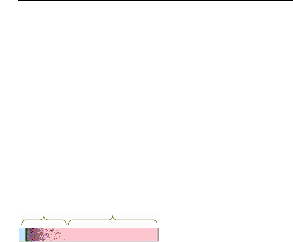
5: Atomistic Kinetic Monte Carlo Diffusion

Point Defects, Impurities, Dopants, and Impurity-paired Point Defects

Sentaurus™ Process User Guide 423

I-2013.12

Finally, the binding energy cannot be defined for any material but full model ones, the result

should be blank:

sprocess> pdbGet KMC PolySilicon B Eb

NOTE Yo u c an c hange the se pa ra met er s whenever necessary to calibrate

intrinsic and extrinsic dopant diffusivity under equilibrium conditions.

For nonequilibrium conditions, you also can change the extended

defects if necessary.

Hopping Mode

The parameter KMC HoppingMode controls the way Sentaurus Process KMC performs

diffusion events. This mode accepts the modes short, long, double, and longdouble, and

it is set by default to longdouble. Changing the hopping mode only changes the results

statistically (in other words, it is similar to changing the random seed); although, it may change

the CPU time significantly. The default hopping mode, longdouble, is the fastest one.

The short Mode

The short mode implies that the jumping distance for all the diffusion events is the same

and is equal to the second neighbor distance. In addition, only one diffusion event is performed

at a time.

The long Mode

The long mode implies that the code increases the hopping distance to , being an integer

number, in regions where there are no particles with which to interact. This increase improves

the performance of the code in this area (in theory, by a factor of ). In practice, the overall

speed improvement is a factor of 2 or smaller, mainly because the empty regions where there

are no particles to interact with are limited. The overhead is caused by the long mode

implementation.

Figure 47 Even if the long hop model is available, it is used only for particles diffusing

on empty volumes

nλ

Standard ‘short hop’

model

Volume suitable for using

the ‘long hop’ model

5: Atomistic Kinetic Monte Carlo Diffusion

Point Defects, Impurities, Dopants, and Impurity-paired Point Defects

424 Sentaurus™ Process User Guide

I-2013.12

The double Mode

Setting HoppingMode to double allows Sentaurus Process KMC to perform two diffusion

events in one. Nevertheless, to properly account for interactions, the intermediate diffusion

event is still simulated by Sentaurus Process KMC. Using this hopping mode saves 10% or less

of CPU time.

The longdouble Mode

The longdouble mode is the default mode and enables both long and double hops.

NOTE For more information on these models, refer to the literature [9].

Enabling and Disabling Interactions

Interactions between particles are important in Sentaurus Process KMC. Whenever one mobile

particle jumps into another particle, Sentaurus Process KMC tries to make both particles

interact. These interactions may or may not be possible depending on whether the interaction

is allowed and if it is energetically possible.

The interactions allowed between one mobile particle and other particles are specified in the

parameter database as the parameter ReactionsPointDefect. The interactions between this

type of defect are assumed to be always energetically favorable.

Consequently, changing the parameter ReactionsPointDefect is the only way to establish

whether a moving particle will interact with other (mobile or immobile) particles. To change

this parameter, use:

pdbSet KMC <material> <dopant> ReactionsPointDefect <string> <true/false>

This parameter needs a string and Boolean value. The Boolean value specifies if the interaction

is allowed (true) or not (false). The string contains the name of the two interacting particles,

separated by a comma. For example:

sprocess> pdbGet KMC Si C ReactionsPointDefect

C,I true

C,V false

C,Ci true

Ci,I true

Ci,V true

Ci,Ci true

5: Atomistic Kinetic Monte Carlo Diffusion

Point Defects, Impurities, Dopants, and Impurity-paired Point Defects

Sentaurus™ Process User Guide 425

I-2013.12

Therefore, in this example, the interaction between C and V is disabled. To enable it, use the

command:

pdbSet KMC Si C ReactionsPointDefect C,V true

When enabling an interaction, the result does not have to be specified because Sentaurus

Process KMC already knows it. The possible interaction results are:

The reactions for each single charged state must be introduced, so the charged I also interacts

with V and with other charged states of V:

sprocess> pdbGet KMC Si I ReactionsPointDefect

I,V true

I,VM true

I,VMM true

I,VP true

I,VPP true

IP,V true

IM,V true

IM,IP true

(...)

All interactions are listed in the parameter database. With that list of interactions, you can

understand which reactions are considered and how they work.

Interaction Rules

Sentaurus Process KMC does not accept all possible interactions within every two particles,

but only interactions with a physical meaning, or with an available model. Consequently, the

following rules apply:

■Reactions must include existing particles.

■Some reactions are only allowed in materials with full modeling.

PointDefect

Pairing reactions, in other words, dopants pairing with interstitials or

vacancies to generate dopant-interstitial or dopant-vacancy particles.

For example, B + I, or As + IM.

AmorphousPocket

Reaction of interstitials or vacancies between them.

For example, I+ IM, I+ V, or V + V. They involve both damage

formation (mixed I and V) and small cluster creation (only I or V).

ImpurityCluster

Reactions involving the formation of impurity clusters, in other words,

when the result has dopants and interstitials or vacancies with two or

more of each. For example, Bi + I or AsV + AsV.

5: Atomistic Kinetic Monte Carlo Diffusion

Point Defects, Impurities, Dopants, and Impurity-paired Point Defects

426 Sentaurus™ Process User Guide

I-2013.12

■Reactions for a pair must be defined in the file of the involved dopant (for example, a

reaction with Bi must be in the boron file, not in interstitial).

■If the result of a reaction does not exist, the reaction is discarded (in other words, the

reaction C + V is specified, but the particle CV is not defined).

■Repulsive reactions are not allowed (for example, Bi– + Bi

–) except for ‘percolation’

models such as As + As or B + B (see Percolation on page 477).

■Reactions must satisfy microscopic reversibility. For example, if the reverse reaction is not

possible, the reaction is discarded.

■Reactions creating impurity clusters must give a defined cluster. For example, Bi + Bi is

allowed as long as there is a B2I2 cluster defined; in this case, Bi + BiM would also be

allowed.

■Only reactions producing defined PointDefect, ImpurityCluster, or

AmorphousPocket are allowed. For example, Bi + C will produce an error message if

there is no BCI cluster defined.

Examples

The interactions for boron are:

sprocess> pdbGet KMC Si B ReactionsPointDefect

B,I true

Bi,I true

Bi,V true

BiM,V true

BiP,V true

B,Bi false

B,BiP true

B,IP true

Bi,Bi true

Bi,VM true

Bi,VMM true

Bi,VP true

Bi,VPP true

BiM,VP true

BiM,VPP true

BiP,VM true

BiP,VMM true

B and I can react, giving a mobile Bi particle. B and IP also give a Bi particle. The charge state

of the resulting Bi particle is computed automatically by Sentaurus Process KMC depending

on the Fermi level, temperature, and Bi levels in the band gap. B– + IM is an electrostatically

repulsive reaction, and is not allowed.

5: Atomistic Kinetic Monte Carlo Diffusion

Point Defects, Impurities, Dopants, and Impurity-paired Point Defects

Sentaurus™ Process User Guide 427

I-2013.12

Bi possible charge states are neutral, positive, and negative. The reactions for these also states

should be specified. Bi and its different charges can react with I, V, and Bi. Bi + I produces an

impurity cluster. Only reactions microscopically reversible are allowed. Because a BI2 cluster

breaks up as Bi + I, any nonrepulsive reaction involving Bi and I is allowed. Bi + V recombines

the IV pair, depositing substitutional boron. All nonrepulsive reactions between Bi and V are

allowed, and all are specified in this example. Finally, there are more ways to produce impurity

clusters including BiP + B, producing B2I, and , as long as giving

B2I2.

The reaction B + V is not specified here. Typing B,V false produces the same effect. Setting

this reaction to true implies defining a BV particle (and its parameters) and specifying

reactions for this BV particle, such as .

NOTE Only advanced users should change the default interaction list because

improper modifications can drastically change the diffusion models.

Defining Nonstandard Interactions

Sentaurus Process KMC allows you to define a nonstandard interaction. These interactions are

intended to provide a mechanism for exceptional models that are not possible to be

implemented using the standard models and interactions. These reactions are of the type:

(666)

A, B, and C must be single particles (point defects or dopants). They are defined as

SpecialReaction in the folder including the first species:

pdbSet KMC Si A SpecialReaction A,B,C true

The reactions defined with this mechanism are not reversible: C will not break into A and B

back.

Interaction Rules

The difference between a regular interaction and a nonstandard one is that the set of rules the

latter one obeys is a very reduced subset of the rules for the regular one. In particular, a

nonstandard interaction must follow only these rules:

■Reactions must include existing particles. The result is always a point defect, not a cluster

or another defect type.

■Reactions are only allowed in materials with full modeling.

■Reactions must be defined in the files of the involved dopant (for example, a reaction with

Bi must be in the boron file).

aBi

+B2I2

↔

ab⋅0≤

BVI+B→

AB+C→

5: Atomistic Kinetic Monte Carlo Diffusion

Point Defects, Impurities, Dopants, and Impurity-paired Point Defects

428 Sentaurus™ Process User Guide

I-2013.12

■If the result of a reaction does not exist, the reaction is discarded (that is, the reaction C +

V is specified, but the particle CV is not defined).

In particular, these reactions can be nonconservative. For example, you can define a carbon–

interstitial interaction giving arsenic ( ). These reactions are nonstandard because

they lack a physical sense, but they are allowed because they offer extra flexibility to define

new models.

Example

A model for nitrogen diffusion can be defined using a nonstandard interaction, in particular,

when you want to model the following:

(667)

(668)

where is mobile but is immobile. The second reaction is not a problem. You can

define a dopant called Nn to be , and make it mobile, and you can define an NnV as the

result of Nn + V. These reactions are standard. The problem is that it is impossible to have a N

+ N reaction giving as Nn using the standard mechanisms. For this exception, you define as

N and use the special reaction:

pdbSet KMC Si N SpecialReaction N,N,Nn true

NOTE Special reactions are printed in the log file:

KMC. Using special non-reversible reaction N + N -> Nn

Stress Effects on Point Defects, Impurities, Dopants, and

Impurity-Paired Point Defects

The stress model for Sentaurus Process KMC is disabled by default, but can be enabled by

setting the variable KMC Stress to 1:

pdbSet KMC Stress 1

or by adding the parameter kmc.stress in the command line of diffuse:

diffuse kmc.stress time=...

Sentaurus Process KMC uses the stress provided by Sentaurus Process, but Sentaurus

Process KMC does not compute it. The stress fields are updated from Sentaurus Process for

each diffuse step.

CI+As→

NiNi

+N2i,

→

N2i,VN

2V↔+

N2i,

N2V

N2i,

5: Atomistic Kinetic Monte Carlo Diffusion

Point Defects, Impurities, Dopants, and Impurity-paired Point Defects

Sentaurus™ Process User Guide 429

I-2013.12

Stress local dependency is introduced into Sentaurus Process KMC using the correction of the

migration and binding energies of point defects and impurity-paired point defects.

Stress also affects the bandgap narrowing, as explained in Bandgap Narrowing on page 500.

Migration Energy

An anisotropic correction to the migration energy is introduced as:

(669)

where are the corrections to the migration energy when diffusing in the axis; are

the principal stresses; and and are the activation volumes for diffusion parallel

and perpendicular to stress, respectively. They are included in the PDB as VD.

The relation between the axes and the standard ones is established by a rotation R tensor. This

tensor diagonalizes the stresses tensor:

(670)

The default setting of the parameter ChangeAxis is false which disables this rotation, using

the standard xyz axis instead of the ones.

NOTE Setting ChangeAxis to true changes the direction of hopping

depending on the local stresses. This, in turn, dramatically impacts

{311} dissolution because the structure is sensitive to the direction of

the migrating incoming particles.

For more information, see Interstitials and Vacancies on page 415.

Binding Energy

The binding energy of an impurity-paired point defect Ai is corrected by:

(671)

where is the activation volume for the formation energy. The activation energy for an

impurity-paired point-defect breakup is defined (without stress) as the sum of the binding

∆Exm

∆Eym

∆Ezm

∆Vpar ∆Vort ∆Vort

∆Vort ∆Vpar ∆Vort

∆Vort ∆Vort ∆Vpar

σ'x

σ'y

σ'z

∆Eim

σ'i

∆Vpar

∆Vort

R[]

σxx σxy σxz

σxy σyy σyz

σxz σyz σzz

R[]

σ'x00

0σ'y0

00σ'z

∆EbAi

() 1

---σxx σyy σzz

++()∆VfI() ∆VfAi

()–()=

∆Vf

5: Atomistic Kinetic Monte Carlo Diffusion

Point Defects, Impurities, Dopants, and Impurity-paired Point Defects

430 Sentaurus™ Process User Guide

I-2013.12

energy plus the migration energy of the emitted species (I for Ai). Then, an extra correction of

the migration energy of the emitted species under stress is needed.

Since the migration energy corrections depend on the axis, but the breakup of an impurity pair

in Sentaurus Process KMC does not, an average of the corrections for all the axes is performed,

and the frequency is computed as:

(672)

where is the breakup frequency when there is no stress.

For more information, see Impurities on page 418.

Alloys

Alloys are included in Sentaurus Process KMC simulations as a field instead of as a particle.

Using Ge as an example of an alloy in Si, it means that Sentaurus Process KMC discards the

particular position of Ge (the xyz coordinates) and only keeps track of how many Ge atoms

were introduced in each internal element. Doing this saves a huge amount of memory, while

allowing Sentaurus Process KMC to account for SiGe effects. Ge is handled as usual, except

for the following limitations:

■There are no Ge particles in the atomistic 3D plot.

■Ge (including implanted Ge) is shown as a field in the atomistic 3D plot.

■There are no events or reports associated with Ge because there are no Ge particles.

■There are no Ge models (for example, no Ge clusters) except for Ge diffusion.

This model can be used to:

■Simulate Ge diffusion.

■Include corrections to the migration and formation energies of point defects and impurity-

paired defects when diffusing in SiGe materials.

■Include bandgap corrections due to SiGe.

NOTE Sentaurus Process KMC considers the effect of germanium whenever

germanium is present. Continuum parameters (such as Silicon

SiliconGermanium.ConversionConc) do not affect Sentaurus

Process KMC simulations.

νstressbk νbk

0∆EbkBT()⁄–()

---∆Em

ikBT()⁄–()exp

xy z,,



exp=

ν0bk

5: Atomistic Kinetic Monte Carlo Diffusion

Point Defects, Impurities, Dopants, and Impurity-paired Point Defects

Sentaurus™ Process User Guide 431

I-2013.12

Alloy Diffusion

Ge will be used as an example of an alloy in Si material. Here, the Ge model diffusion

implemented has been based partially on [10]. This model defines the diffusion of Ge in an

indirect way through the use of of Is and Vs for a Si1–xGex material as:

(673)

where and are the transport capacity associated with Ge and Si interstitials in

Si1–xGex, respectively.

It can be assumed that these s follow the equation:

(674)

where , , , and are input parameters specified in the PDB. Both interstitials

and vacancies have a different .

NOTE The Ge diffusion model is switched on by default. To switched it off, set

and to null values.

Parameters and Parameter Examples

The parameters , , , and are specified in the PDB with the names

D0alphaSi, D0alphaGe, EalphaSi, and EalphaGe. In particular:

sprocess> pdbGet KMC Si I EalphaSi

0.4

sprocess> pdbGet KMC Si I EalphaGe

sprocess> pdbGet KMC Si I D0alphaSi

sprocess> pdbGet KMC Si I D0alphaGe

2.2

sprocess> pdbGet KMC Si V EalphaSi

0.25

sprocess> pdbGet KMC Si V EalphaGe

sprocess> pdbGet KMC Si V D0alphaSi

sprocess> pdbGet KMC Si V D0alphaGe

2.2

αI

Ge x()

Si x()

------------------=

Ge x()

Si x()

αx() α

0Si,

1x–α0Ge,

x1x–()ESi xEGe

kBT

-------------------------------------------–





exp=

α0Si,

α0Ge,

ESi

EGe

α0Si,

α0Ge,

α0Si,

α0Ge,

ESi

EGe

5: Atomistic Kinetic Monte Carlo Diffusion

Damage Accumulation Model: Amorphous Pockets

432 Sentaurus™ Process User Guide

I-2013.12

Alloy Effects

The following sections discuss alloy effects on point defects, impurities, dopants, and impurity-

paired point defects. In the next sections, Ge in silicon is used as an example for these models.

Migration and Formation Energies

The corrections and are added to the migration and

formation energies, respectively. is the germanium concentration, and are the

dependencies of energies with Ge concentration for migration and formation.

Binding Energy

The binding energy of an impurity-paired point defect is corrected by:

(675)

For more information, see Impurities on page 418.

Bandgap Narrowing

The Ge inclusion changes the band gap as explained in Bandgap Narrowing on page 500.

Introducing Alloys in the Simulation

Alloys can be introduced in the simulation by:

■Using implantation.

■Using the select command.

■Atomizing a previous continuum structure with the alloy.

■Using kmc add to explicitly add it.

■Depositing a layer doped with the alloy.

Damage Accumulation Model: Amorphous Pockets

Damage accumulation evolution, that is, the evolution of small interstitial and vacancy clusters

after ion implantations, is a crucial step that affects the subsequent formation of extended

defects and impurity clusters. This accumulation generates the transient-enhanced diffusion

(TED) of commonly used dopants, such as boron.

Experimentally, electron irradiation and light-ion implantation create isolated point defects

inside the silicon. In contrast, heavy ions generate highly disordered regions called amorphous

∆EmαmGe[]=

∆EfαfGe[]=

Ge[]

αmαf

∆EbAi

() Ge[]α

fI() α

fA() α

fAi

())–+()=

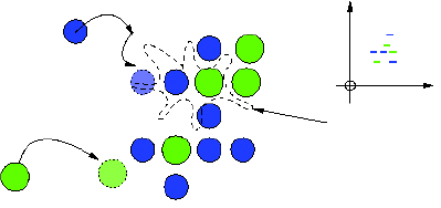
5: Atomistic Kinetic Monte Carlo Diffusion

Damage Accumulation Model: Amorphous Pockets

Sentaurus™ Process User Guide 433

I-2013.12

pockets (APs) as a consequence of the implanted cascades. Depending strongly on the

temperature, ion mass, and dose rate, this disordered region can dissolve as a result of internal

recombination or can grow until an amorphous layer is created. The activation energy for

annealing this damage varies in the literature, 0.9 eV [11] at room temperature, 1.2 eV for

to , but it is much less than the 2.7 eV reported for truly amorphized amorphous

layers. This means the damage accumulation depends on the dynamic annealing, ripening, and

dissolution history of the APs during the implant process. This annealing can have a quasi-

continuum range of activation energies.

There is much discussion on how this damage is annealed. Some papers point to an annealing

of the disordered region [12]: APs using an internal recombination of IV pairs rather than

through the emission of point defects. Only when the AP does not contain further IV pairs does

it begin to emit its remaining Is or Vs, behaving as a small I or V cluster.

Sentaurus Process KMC simulates the damage accumulation using APs, disordered collections

of point defects (Is and Vs) stable at low temperatures. APs dissolve fast at higher temperatures,

leaving only clusters with the net excess of Is or Vs. APs can contain IV pairs or only Is and Vs.

In the first case, APs try to recombine the pairs; in the second, APs behave as small clusters

and can emit their constituent particles. Whenever an AP containing only Is or Vs (but not IV

pairs) reaches a threshold size, the AP transforms into an extended defect ({311}s for Is, voids

for Vs).

APs can grow capturing new incoming point defects, and they can dissolve by internal

recombination of IV pairs or by particle emission when there are no more IV pairs (see

Figure 48).

Figure 48 Growth of APs showing their internal recombination

400°C

550°C

Growth

2D Projection

Internal Recombination

Amorphous Pocket

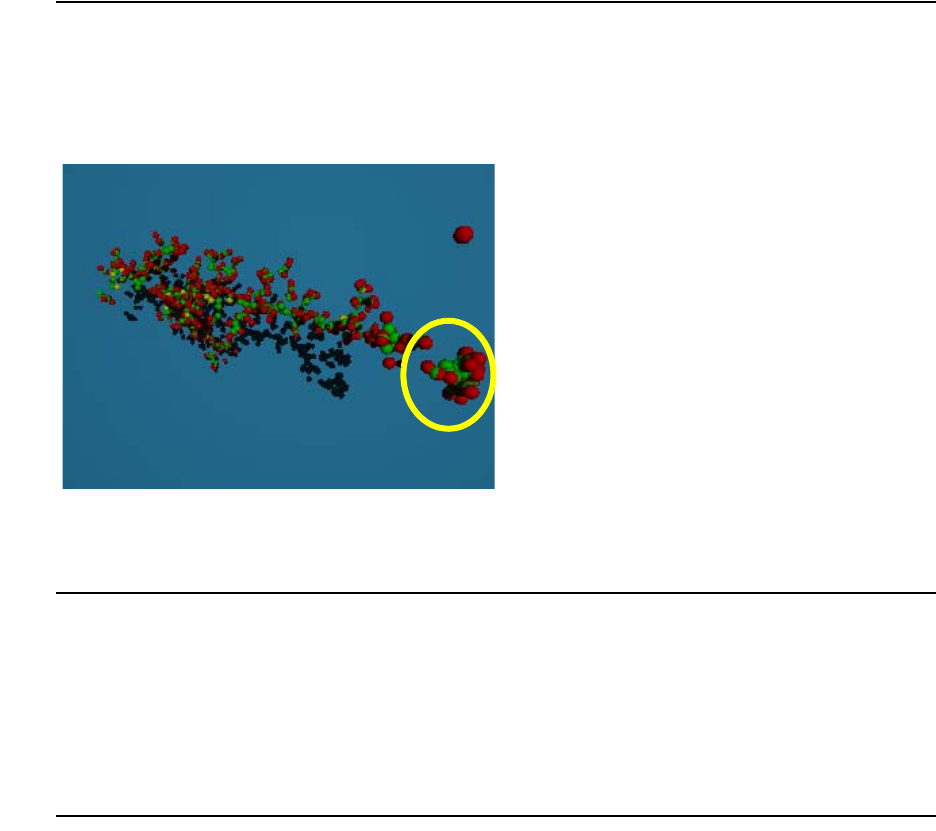
5: Atomistic Kinetic Monte Carlo Diffusion

Damage Accumulation Model: Amorphous Pockets

434 Sentaurus™ Process User Guide

I-2013.12

Shape

APs have an irregular shape. Sentaurus Process KMC does not reshape the defect as new;

incoming particles join the AP: particles are left in their incoming positions. Figure 49 shows

some APs resulting from an implanted cascade.

Figure 49 APs formed in Sentaurus Process KMC after some implanted as cascades:

interstitials are red, vacancies are green, arsenic is yellow

Growth

APs capture any incoming point defect (I or V) within their capture radius. The capture radius

of APs is the sum of all their constituent particles. Point defects with any charge state are

captured by APs containing both Is and Vs. Only neutral Is or Vs are captured when APs

contain only Is or only Vs.

Recombination

APs containing IV pairs (that is, APs with both interstitials and vacancies) can recombine pairs

using a recombination event, which recombines one I with one V at a time. This event is

performed with a frequency given by:

(676)

where the prefactor is called D0_AmorphousPocket in the parameter database, and

size is the size of the cluster.

νdiss ν0diss,sizeβEdiss size()P∆Vdiss αIV Ge[]++()–/kBT()()exp⋅=

ν0diss,

5: Atomistic Kinetic Monte Carlo Diffusion

Damage Accumulation Model: Amorphous Pockets

Sentaurus™ Process User Guide 435

I-2013.12

The size of a cluster InVm is a Tcl procedure of n and m specified in the file KMC.tcl under the

name getAmorphousPocketSize:

fproc getAmorphousPocketSize { sizeI sizeV } {

return [expr ($sizeI + $sizeV)/2]

}

It can be modified by users. is an exponent called ExponentAmorphousPocket.

depends on the size of the AP and is specified as a list of energies for each size

(Eb_AmorphousPocket). The different sizes are specified as IxeVx. If some energy is not

specified for a size, Sentaurus Process KMC takes the linear interpolation between the last two

specified values. For sizes higher than the last specified size, the last specified energy is

assigned automatically. is the Germanium correction to recombination

(Eb_AmorphousPocketGe) and finally, is the hydrostatic pressure and is the

activation volume for the AP dissolution (VFAmorphousPocket).

Parameters

The parameters needed by the damage accumulation model are specified using:

pdbSet KMC Si Damage <Parameter> <value>

An example of these parameters is:

sprocess> pdbGet KMC Si Damage D0_AmorphousPocket

0.0005

sprocess> pdbGet KMC Si Damage ExponentAmorphousPocket

0.66

sprocess> pdbGet KMC Si Damage VFAmorphousPocket

sprocess> pdbGet KMC Si Damage Eb_AmorphousPocket

IV 0.65

I199V199 2.4

sprocess> pdbGet KMC Si Damage Eb_AmorphousPocketGe

For the above parameters, the Eb_AmorphousPocket values for IxVx, with x > 1 and x < 199

will be generated by Sentaurus Process KMC as a linear interpolation between the points (1,

0.65) and (199, 2.4):

Silicon/Damage Eb_AmorphousPocket(IV) = 0.65

Silicon/Damage Eb_AmorphousPocket Interpolated (2) = 0.658838

Silicon/Damage Eb_AmorphousPocket Interpolated (3) = 0.667677

...

NOTE Yo u c an ch an ge the se pa ram et ers to calibrate the damage accumulation

model.

Ediss

αIV

∆Vdiss

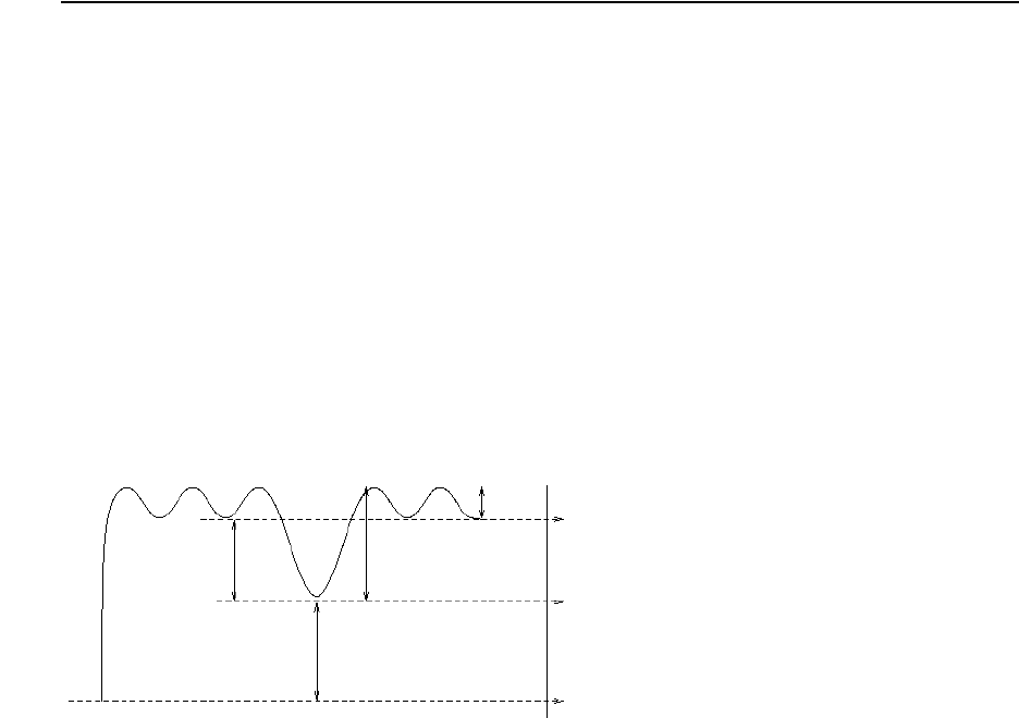
5: Atomistic Kinetic Monte Carlo Diffusion

Damage Accumulation Model: Amorphous Pockets

436 Sentaurus™ Process User Guide

I-2013.12

NOTE The maximum size allowed for IV clusters is I249V249.

Emission

When all IV pairs have been recombined, APs behave as small I or V clusters, allowing the

emission of their extra constituent particles. These defects emit neutral Is or Vs particles with

a frequency given by:

(677)

The prefactor is proportional to the input parameter D0_Cluster, but also includes a

dependency on the size of the cluster. The activation energy for emission of an X (in other

words, either I or V) is:

(678)

the sum of the corrected binding energy (that depends on the cluster size) and the migration

energy. The cluster size is defined as the number of contained Is or Vs (see Figure 50).

Figure 50 Energies involved in emission of an interstitial from an n-size cluster

D0_Cluster is the constant proportional to the emission prefactor, and Eb_Cluster is the

cluster binding energy, where dependency with size is explicitly assigned. For sizes bigger than

the last specified cluster, the binding energies are computed using:

(679)

where:

■ (Eb_LargeCluster) is the binding energy for the largest cluster.

■ (Eb_SmallestCluster) is the binding energy for the smallest cluster (size 1).

■ (exponent_Cluster) is the exponent, usually 2/3 or 3/4.

νemit ν0emit,E–emit size()/kBT()()exp⋅=

Eemit EbX() EmX() ∆EbX() ∆EmX()++ +=

E(n–1) + E(1)

E(n)

E(n–1)

Eb E diss

Ebsize()EbL,EbL,EbS,

–()

sizeasize 1–()

–

2a1–

-------------------------------------------

–=

EbL,

EbS,

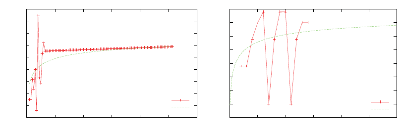
5: Atomistic Kinetic Monte Carlo Diffusion

Damage Accumulation Model: Amorphous Pockets

Sentaurus™ Process User Guide 437

I-2013.12

Figure 51 shows some binding energy values and compares them with the numbers obtained

using Eq. 679.

Figure 51 Interstitial cluster (left) and vacancy cluster (right) binding energies; discrete

values are assigned in the parameter database and the continuum energies are

computed using Eq. 679

Finally, the correction applied for the migration is the normal one:

(680)

and for the binding of the particle to the cluster is:

(681)

where is called VFCluster in the PDB and is the Germanium correction to

binding (Eb_ClusterGe).

Parameters

The parameters for Is and Vs emission are specified only for the silicon material. They can be

found in the interstitial and vacancy files included in the parameter database.

Prefactors

sprocess> pdbGet KMC Si I D0_Cluster

150.0

sprocess> pdbGet KMC Si V D0_Cluster

2.1

2.2

2.3

2.4

2.5

2.6

2.7

2.8

2.9

0 20 40 60 80 100 120

Binding Energy Eb [eV]

I Cluster Size

Interstitial Cluster Binding Energies

Discrete

Continuum energies

-0.5

0.5

1.5

2.5

3.5

0 5 10 15 20 25 30

Binding Energy E

[eV]

V Cluster Size

Vacancy Cluster Binding Energies

Discrete

Continuum energies

∆EmX() α

mGe[]

---∆Em

ikBT()⁄–()exp

xy z,,



∆EbX() P∆Vb

extended X() α

Cl Ge[]+=

∆Vb

extended

αCl

5: Atomistic Kinetic Monte Carlo Diffusion

Damage Accumulation Model: Amorphous Pockets

438 Sentaurus™ Process User Guide

I-2013.12

Energies

sprocess> pdbGet KMC Si I Eb_Cluster

I2 2.45

I3 2.45

(...)

I13 2.853

I103 2.889

sprocess> pdbGet KMC Si V Eb_Cluster

V2 1.4

V3 1.4

V4 2.4

(...)

For sizes between specified sizes (for example, I14 to I102), the parameters are computed as

linear interpolations of the specified values:

Silicon/I Eb_Cluster(I13) = 2.853

Silicon/I Eb_Cluster Interpolated (14) = 2.8534

(...)

Silicon/I Eb_Cluster Interpolated (102) = 2.8886

Silicon/I Eb_Cluster(I103) = 2.889

and parameters for Eq. 678, p. 436:

sprocess> pdbGet KMC Si I Eb_SmallestCluster

2.51

sprocess> pdbGet KMC Si I Eb_LargeCluster

3.09

sprocess> pdbGet KMC Si I exponent_Cluster

0.75

sprocess> pdbGet KMC Si V Eb_SmallestCluster

1.5

sprocess> pdbGet KMC Si V Eb_LargeCluster

3.7

sprocess> pdbGet KMC Si V exponent_Cluster

0.6667

NOTE When changing these parameters, their values affect not only the

damage accumulation model, but also the interstitial and vacancy

supersaturation and, consequently, the transient-enhanced diffusion

(TED). Because the damage accumulation model is the seed for

subsequent extended defects or recrystallization, these values also affect

the formation of extended defects.

5: Atomistic Kinetic Monte Carlo Diffusion

Damage Accumulation Model: Amorphous Pockets

Sentaurus™ Process User Guide 439

I-2013.12

Amorphous Pockets Life Cycle

Whenever two point defects (I + I, V + V or I + V) interact with each other, an AP is generated.

When the AP is formed, subsequent incoming Is or Vs are captured and added to the AP. If the

AP contains at least one IV pair, the AP recombines the IV pairs. The IV pair frequency depends

on the number of IV pairs present in the AP. If there is only Is or Vs in the AP, it emits Is or Vs.

The evolution of APs can follow three paths:

■APs can dissolve recombining internal IV pairs, emitting point defects, or both.

■AP containing only Is or Vs may be transformed into extended defects: {311} defects for

Is and voids for Vs.

■If the concentration of some of the boxes (the internal Sentaurus Process KMC grid

elements) containing the AP reaches a concentration threshold, the element is considered

amorphous and its particles are removed from the AP. Consequently, APs only exist in

crystalline silicon.

For example, assuming there is an AP with two Vs and seven Is (I7V2), since the AP contains

both Is and Vs, the only possible event is the recombination of IV pairs. The first IV pair

recombines with the recombination energy assigned to size 2, leaving an I6V1. The second

recombination energy, with a recombination energy assigned to size 1, leaves an I5 AP. This

AP begins to emit Is, with a frequency associated to its size (5). However, if it captures a V, it

becomes an I5V1 and must recombine the IV pair with an associated recombination size of 1.

An AP must satisfy the following conditions before being transformed into a {311} or void:

■It can contain only Is or only Vs, but not both.

■It must be bigger than or equal to a threshold size.

■Transition must be enabled.

The threshold size is specified with the parameters Min311Size and MinVoidSize for Is and

Vs, respectively. The transition is enabled by a value between 0 and 1. This value is computed

as:

(682)

The prefactor is specified as D0_APto311 for {311}s and D0_APtoVoid for voids, and the

energies as E_APto311 and E_APtoVoid. For {311}s are the corrections for pressure and

Ge; for voids :

.(683)

The volume correction is called VF311toLoop, and the Germanium one VF311toLoop.

0E∆E+()–()kBT()⁄()exp×=

∆E

∆E0=

∆EPV

311toLoop α311toLoop Ge[]+=

5: Atomistic Kinetic Monte Carlo Diffusion

Damage Accumulation Model: Amorphous Pockets

440 Sentaurus™ Process User Guide

I-2013.12

For , the transition is disabled; for , it is enabled. For , the value is rounded

to 1. Values between 0 and 1 establish a probability for the transition.

Parameters

Minimum sizes for the transitions:

sprocess> pdbGet KMC Si I Min311Size

sprocess> pdbGet KMC Si V MinVoidSize

Transition probabilities:

sprocess> pdbGet KMC Si Damage D0_APto311

200000000.0

sprocess> pdbGet KMC Si Damage E_APto311

1.3

sprocess> pdbGet KMC Si Damage D0_APtoVoid

200000000.0

sprocess> pdbGet KMC Si Damage E_APtoVoid

1.3

Interactions of Amorphous Pockets

To change the default AP interactions, use the parameters ReactionsClusterI,

ReactionsClusterV, and ReactionsClusterIV. These parameters control the reactions

between APs containing only interstitials, only vacancies, or both. APs can react not only with

Is and Vs, but also with dopants. In this latter case, the result of the reaction must be specified.

Interaction with Point Defects: I and V

To customize AP reactions, change the parameters defined for I, V, and IV clusters using the

command:

pdbSet KMC Si Damage <ReactionsClusterType> <species> <true/false>

For example, the command:

pdbSet KMC Si Damage ReactionsClusterI I false

disables the reaction for small clusters.

P0=

P1=

P1>

InI+In1+

→

5: Atomistic Kinetic Monte Carlo Diffusion

Damage Accumulation Model: Amorphous Pockets

Sentaurus™ Process User Guide 441

I-2013.12

Consequently, it disables the ripening of these clusters. The line:

pdbSet KMC Si Damage ReactionsClusterV I false

disables the recombination of I with small vacancy clusters.

Parameters

Small interstitial and vacancy clusters may react with neutral interstitials and vacancies.

Charged interstitials or vacancies are not allowed due to microscopic reversibility reasons:

sprocess> pdbGet KMC Si Damage ReactionsClusterI

I true

V true

sprocess> pdbGet KMC Si Damage ReactionsClusterV

I true

V true

APs with both Is and Vs accept interstitials or vacancies with any charge. In this case, because

they do not emit particles, there are no microscopic reversibility restrictions:

sprocess> pdbGet KMC Si Damage ReactionsClusterIV

I true

IP true

IM true

V true

VP true

VPP true

VM true

VMM true

Interaction with Impurities

APs do not trap impurities, but can interact with them. In this interaction, impurities can lose a

point defect, becoming substitutional (for example, ) or can gain some

of them being transformed into an impurity cluster (for example, ).

Consequently, the interaction within impurities and APs plays a crucial role in deactivating

dopants, typically during implantation and low-temperature anneals.

To control these interactions, use:

pdbSet KMC Si <impurity> <ReactionsClusterType> <species,result> <true/false>

ReactionsClusterType can be ReactionsClusterI for small I clusters,

ReactionsClusterV for small V clusters and ReactionsClusterIV for mixed clusters.

BiI2V3

+BI3V3

+→

BiI2V3

+BI2IV3

+→

5: Atomistic Kinetic Monte Carlo Diffusion

Extended Defects

442 Sentaurus™ Process User Guide

I-2013.12

For example, the reaction can be disabled for mixed clusters with:

pdbSet KMC Si B ReactionsClusterIV BiM,BI2 false

NOTE A comma must separate the incoming particle from the result, without

any space in between.

Parameters

The reactions between boron (for example) and mixed clusters can be displayed with:

sprocess> pdbGet KMC Si B ReactionsClusterIV

BiM,BI2 true

Bi,BI2 true

BiP,BI2 true

B,BI2 true

There are no reactions between boron and vacancy clusters:

sprocess> pdbGet KMC Si B ReactionsClusterV

The reactions between boron and small I clusters are disabled:

sprocess> pdbGet KMC Si B ReactionsClusterI

Bi,BI2 false

BiM,BI2 false

Extended Defects

Small clusters are defined as immobile agglomerations of interstitials or vacancies, and are

modeled using the AP defects previously explained. When the number of Is or Vs in these

clusters grows above a specified threshold, the small clusters are converted into extended

defects ({311} or void types). Finally, when the ripening of {311}s overcomes some limit, the

{311}s are transformed into dislocation loops.

{311} Defects (ThreeOneOne)

The {311} rod-like defects are associated with TED [13]. Consequently, they need a realistic

simulation, in both shape and energetic values. Its shape is like rectangular stripes of

interstitials lying on a {311} plane along a <110> direction. The paper [14] gives an atomic

model for its structure, whose stability has been confirmed by theoretical studies [15][16][17].

–InVm

+BI2In1–Vm

+→

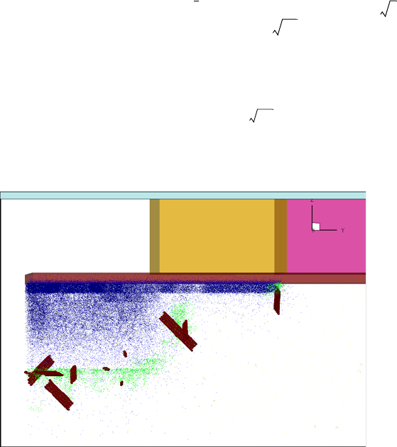
5: Atomistic Kinetic Monte Carlo Diffusion

Extended Defects

Sentaurus™ Process User Guide 443

I-2013.12

Shape

Sentaurus Process KMC models {311} defects as parallel stripes (rows) of I particles lying in

one of the twelve orientations, randomly chosen, of a {311} plane. The {311} shape is modeled

as Nr rows of Is lying on a line with a distance of between Is in the same line,

and as Nc columns keeping a distance of between them, with , the

silicon lattice constant.

The ratio between length ( ) and width ( ) is given by:

(684)

being . This ratio is maintained reshaping the {311} defect (that is, changing the

number of row and columns) when necessary (see Figure 52).

Figure 52 {311} defects are simulated by Sentaurus Process KMC as parallel stripes (rows)

of I particles lying in a {311} plane: red is silicon interstitials in {311}; green is I

and V in APs; and blue is arsenic

The {311} defects only exist above a size threshold. Smaller defects are assumed to be APs,

and they have an irregular shape (see Amorphous Pockets Life Cycle on page 439).

When {311} defects grow enough, they are transformed into dislocation loop defects (see

Dislocation Loops on page 447). The threshold size (number of interstitials) between {311}

defects and dislocation loops is assumed to follow an Arrhenius plot:

(685)

The formation energy of the dislocation loop must be smaller than the {311} formation energy

at the threshold size; otherwise, the threshold is taken as the size where both energies are equal.

<011>

a2⁄

a22 4⁄

a0.543 nm=

WCL≈

C0.5 nm=

size prefactor Ek

BT()⁄()exp×=

5: Atomistic Kinetic Monte Carlo Diffusion

Extended Defects

444 Sentaurus™ Process User Guide

I-2013.12

Both prefactor and E are parameters available in the database with names D0_311toLoop

and E_311toLoop, respectively.

Parameters

The parameters to control the transformation between {311}s and loops are specified for

interstitials in silicon:

sprocess> pdbGet KMC Si I D0_311toLoop

1.6

sprocess> pdbGet KMC Si I E_311toLoop

0.68

NOTE These parameters can be changed to fit the {311} to dislocation loop

transition size.

Capture

Each time a neutral I point defect interacts with an I belonging to a {311} defect, the {311}

captures the point defect. Since {311} defects grow and shrink at their ends, the new particle

is attached at the nearest end of the defect. When the end cannot grow because it is too close

to a interface or a boundary, the other end is used.

When 311DopantModel is set to 1, impurities also can be trapped. These trapped impurities

will remain in the captured location until they are re-emitted. Only neutral impurities (or

neutral impurity pairs) are captured and re-emitted.

Emission

To preserve microscopic reversibility between the capture and the emission processes, emitted

particles (neutral interstitials) are taken randomly from one of the two ends and released from

a random point at the {311} surface (see Figure 53 on page 445).

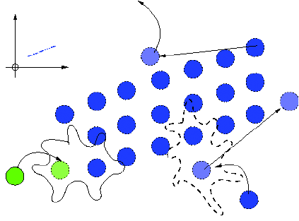
5: Atomistic Kinetic Monte Carlo Diffusion

Extended Defects

Sentaurus™ Process User Guide 445

I-2013.12

Figure 53 Recombination of defects in a {311} defect

The emission frequency is computed as in APs by:

(686)

where the considerations for the AP emission, including all the corrections, apply. The binding

energies are taken from the list supplied with the Eb_Cluster parameter. These energies are

shared with the APs. As explained above, for sizes less than a threshold value, defects are

considered APs. Otherwise, they are rearranged as {311} defects. Consequently, only binding

energies for sizes equal or bigger than APs-{311} threshold applies for {311} defects.

Corrections are applied for both pressure and Germanium content. These corrections are

specified as VF311 and Eb_311Ge, respectively.

{311}s may also emit captured dopants if the 311DopantModel is set to 1. The emission

frequency for them is:

(687)

being the prefactor and activation energy called D0_311 and Eb_311, respectively, in the PDB.

Parameters

For impurity re-emission, the parameters are:

sprocess> pdbGet KMC Si In D0_311

200.0

sprocess> pdbGet KMC Si In Eb_311

2.0

2D Projection

Emission

Recombination Growth

νemit ν0emit,E–emit size()P∆V311 α311 Ge[]++()/kBT)()()exp×=

νemit Ai

() ν

0emit,Ai

() Eemit Ai

()kBT()⁄()–()exp×=

5: Atomistic Kinetic Monte Carlo Diffusion

Extended Defects

446 Sentaurus™ Process User Guide

I-2013.12

Recombination

The {311} defects recombine incoming Vs with any charge by annihilation of the Is at the

nearest {311} defect end. When {311} defects dissolve, they do not become APs when the

threshold AP-{311} size is reached. The emission frequency depends on the binding energy,

and the binding energy only depends on the size of the defect. Since a interstitial cluster and a

small {311} defect have the same binding energy when they have the same size, the defect

shape affects only the capture volume, but not the emission frequency. Consequently,

rearranging {311} as small defects and vice versa only changes the capture volume, and these

changes are negligible for small clusters. Nevertheless, the capture volume differences between

small {311} defects and irregular clusters are negligible, and there is no information about the

shape of dissolving {311} defects.

Finally, when a {311} reaches size 2, it releases the particles as two interstitials and the {311}

disappears.

Interactions

Interactions between {311} defects and mobile particles can be modified with:

pdbSet KMC Si <I/V/Impurities> Reactions311 <species> <true/false>

Growth reactions ( ) are controlled with I, and recombination reactions ( ) with V.

{311} defects can break up paired dopants capturing the interstitial or recombining the vacancy

(for example, ). The remaining dopant will be immediately released or

captured (and re-emitted later) by the defect depending on the value of the parameter

311DopantModel (0 releases dopants, 1 traps it). A captured dopant can be re-emitted. These

reactions enable the {311} to decrease the impurity diffusion.

Only neutral Is react with {311} defects and, consequently, only paired dopants with the same

charge as the substitutional dopant react with {311} defects. Any charge state is allowed for

the recombination of vacancies.

Parameters

Use the following for growth and recombination:

sprocess> pdbGet KMC Si I Reactions311

I true

sprocess> pdbGet KMC Si V Reactions311

V true

InI+

InV+

BiIn

+BIn1+

+→

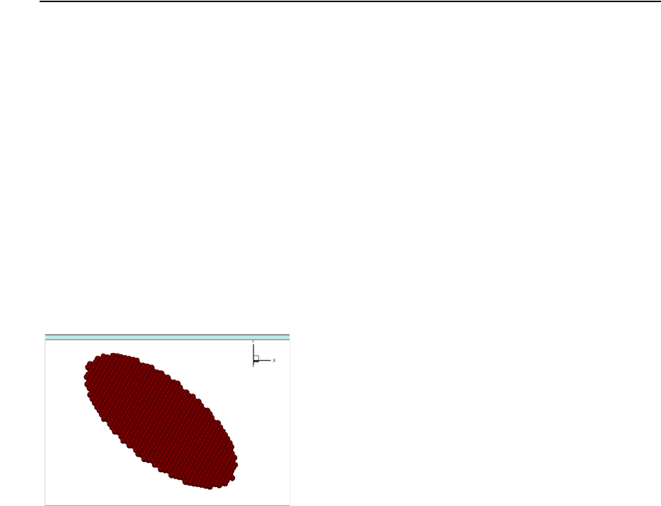
5: Atomistic Kinetic Monte Carlo Diffusion

Extended Defects

Sentaurus™ Process User Guide 447

I-2013.12

For paired impurity breakup (boron, for example), use:

sprocess> pdbGet KMC Si B Reactions311

BiM false

sprocess> pdbGet KMC Si I 311DopantModel

You can define the parameter 311DopantModel globally as a default for all dopants, but

define it locally with a different value that overwrites the global value for a particular dopant.

For example:

pdbSet KMC Si I 311DopantModel 0

pdbSetDouble KMC Si B 311DopantModel 1

sets the model for all the impurities as ‘release dopant,’ except for boron.

Dislocation Loops

Dislocation loops are planar defects lying on {111} planes [18]. A dislocation loop can be

either a faulted dislocation loop (FDL) or perfect dislocation loop (PDL). FDLs are circular

stacking faults surrounded by a dislocation line. PDLs are not implemented in Sentaurus

Process KMC.

{311} defects are the precursors of dislocation loops. When the implant conditions (available

concentration of I, distance to the free surface) are appropriate, {311} defects grow until they

reach the threshold size and transform into dislocation loops. Dislocation loops are more stable

than {311} defects; consequently, the supersaturation created by dislocation loops is lower.

Shape

The shape of dislocation loops is computed as a filled circle in a {111} orientation (see

Figure 54). All {111} orientations are allowed, and one is randomly chosen.

Figure 54 A dislocation loop taken from a Sentaurus Process KMC simulation

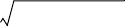
5: Atomistic Kinetic Monte Carlo Diffusion

Extended Defects

448 Sentaurus™ Process User Guide

I-2013.12

Capture

Dislocation loops capture any incoming neutral interstitial. The original position is lost, and

the particle is moved to the proper position in the disk. The capture radius is the sum of the

capture radius of the constituent particles.

When the ReactionsLoop is set and LoopDopantModel is true, dislocation loops capture

incoming impurities. When LoopDopantModel is false, the impurity is not captured.

However, when it carries a point defect (in other words, is an impurity pair), the pair is broken;

the impurity is deposited as a substitutional impurity; and the point defect reacts with the loop.

Emission

Dislocation loops emit neutral interstitials with a frequency given by:

(688)

includes both a prefactor and a linear dependency with the dislocation loop size, and

is the binding energy of the dislocation loop, which only depends on the size.

Sentaurus Process KMC computes the binding energies as:

(689)

The dislocation loop formation energies are taken from [19] as:

(690)

where:

■ is the loop radius.

■ is the stacking fault energy per unit area.

■ is the shear modulus.

■ is the Poisson ratio.

■ is Burger’s vector modulus.

■ is the silicon lattice parameter.

■ is the atomic density in a {111} plane, in .

The above parameters are specified in the parameter database. is called gamma, is mu,

is nu, and is named burgVectMod. The emission prefactor is called D0_Loop.

νemiss ν0emiss,

Ebloop,size()EmI() ∆EmI() ∆Ebloop,

++ +

kBT

----------------------------------------------------------------------------------------------------------–





exp×=

ν0emiss,

Ebloop,size()

Ebloop,size()EfI() Efloop,size 1–()Efloop,size()–+=

Efloop,size()πγR2a2µ

61 ν–()

--------------------R8R

-------





log⋅⋅ nEfI()–+=

Rsize πd111

()⁄=

d111

nm 2–

5: Atomistic Kinetic Monte Carlo Diffusion

Extended Defects

Sentaurus™ Process User Guide 449

I-2013.12

The corrections applied to the migration energy of interstitials are the usual ones:

(691)

and for the binding of the particle to the loop is:

(692)

where is called VFLoop, and is called Eb_LoopGe in the PDB.

Captured impurities (when LoopDopantModel is true) re-emit impurities into the bulk with a

frequency given by:

(693)

being the prefactor and activation energy called D0_Loop and Eb_Loop in the PDB,

respectively.

Parameters

The parameters needed for the simulation of dislocation loops are defined for interstitials in

silicon:

sprocess> pdbGet KMC Si I D0_311toLoop

1.6

sprocess> pdbGet KMC Si I E_311toLoop

0.68

sprocess> pdbGet KMC Si I D0_Loop

1000000.0

sprocess> pdbGet KMC Si I gamma

0.4375

sprocess> pdbGet KMC Si I mu

472

sprocess> pdbGet KMC Si I nu

0.3

sprocess> pdbGet KMC Si I burgVectMod

0.3135

sprocess> pdbGet KMC Si I VFLoop

sprocess> pdbGet KMC Si Eb_LoopGe

∆EmI() α

mGe[]

---∆Em

ikBT()⁄–()exp

xy z,,



∆Ebloop,P∆Vb

loop αloop Ge[]+=

∆Vb

loop

αloop

νemit Ai

() ν

0emit,Ai

() Eemit Ai

()kBT()⁄()–()exp×=

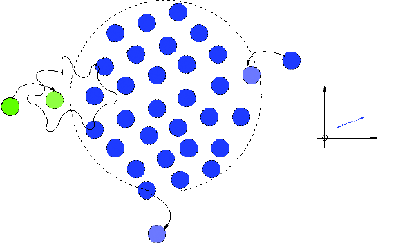
5: Atomistic Kinetic Monte Carlo Diffusion

Extended Defects

450 Sentaurus™ Process User Guide

I-2013.12

For impurity re-emission, the parameters are:

sprocess> pdbGet KMC Si In D0_Loop

200.0

sprocess> pdbGet KMC Si In Eb_Loop

2.0

NOTE These parameters can be changed to fit the dislocation loop formation

and dissolution.

Figure 55 shows how a dislocation loop grows capturing interstitials, and how it shrinks

recombining incoming vacancies or emitting interstitials.

Figure 55 Emission, capture, and recombination of point defects in a dislocation loop

Interactions

The interactions between dislocation loops and mobile particles are:

■Growth reactions. Only with neutral Is:

pdbSet KMC Si I ReactionsLoop I <true/false>

■Recombination reactions. Any vacancy:

pdbSet KMC Si I ReactionsLoop <V/VM/VP/VMM/VPP> <true/false>

■Impurity pairs break up and interact with the associated point defect (I or V). Only with

pairs with the substitutional charge state the same as the substitutional dopant (for example,

Bi– for B–). The interstitial or vacancy is trapped or recombined, and the dopant is released

(0) or trapped (1) depending on the model used. The model is specified for all dopants

(default value) using the parameter LoopDopantModel for interstitials.

Dislocation Loop

Recombination

Emission

Growth

2D Projection

5: Atomistic Kinetic Monte Carlo Diffusion

Extended Defects

Sentaurus™ Process User Guide 451

I-2013.12

This particular default can be overwritten for one particular dopant.

pdbSet KMC Si I LoopDopantModel <true/false>

pdbSetDouble KMC Si <dopant> LoopDopantModel <true/false>

Parameters

Loops trap interstitials, but the recombination of vacancies is disabled:

sprocess> pdbGet KMC Si I ReactionsLoop

I true

sprocess> pdbGet KMC Si V ReactionsLoop

V false

Loops can break up some paired dopants, for example, boron:

sprocess> pdbGet KMC Si B ReactionsLoop

BiM true

sprocess> pdbGet KMC Si I LoopDopantModel

Voids

Small vacancy defects have been reported (using paramagnetic resonance and

photoluminescence) [20][21][22][23]. Theoretical studies [24][25] indicate that some of these

small clusters can be particularly stable. Sentaurus Process KMC models these small clusters

as APs and, consequently, they have irregular shapes. Nevertheless, size-dependent binding

energies are considered for their V emission (see Damage Accumulation Model: Amorphous

Pockets on page 432).

Vacancy clusters appear as spheroidal voids when they are big enough to be seen by TEM [26].

Tight-binding molecular dynamics studies show that the binding energies are a function of the

cluster size [27] (see Figure 56 on page 452).

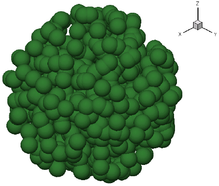
5: Atomistic Kinetic Monte Carlo Diffusion

Extended Defects

452 Sentaurus™ Process User Guide

I-2013.12

Figure 56 Voids are simulated with a spherical shape; this one contains 654 vacancies

Shape

The threshold size between irregular small vacancy clusters (APs) and voids is specified with

the parameter MINVoidSIZE. Another parameter, MAXVOIDSDIAM, is used to set up the

maximum-allowed diameter (in nanometers) for these defects.

Reshaping the small clusters into voids above the mentioned limit is necessary to maintain the

right volume/surface ratio, as the V cluster grows. A large cluster of n vacancies is reshaped to

be spheroidal, occupying the volume corresponding to the same number of silicon lattice sites.

Sentaurus Process KMC manages the void shape to assert that its density is correct.

Parameters

The parameters for voids are specified for silicon material and vacancy as species:

sprocess> pdbGet KMC Si V MinVoidSize

sprocess> pdbGet KMC Si V MaxVoidDiam

5.0

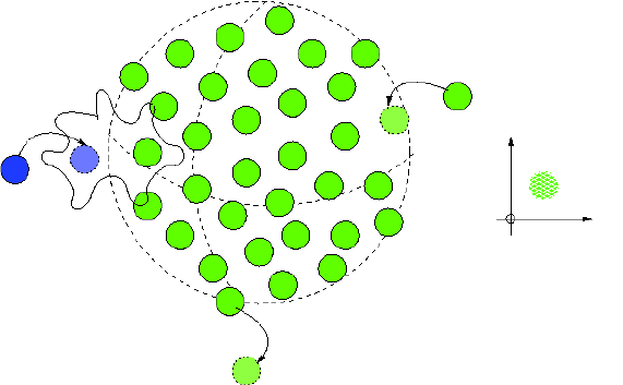
5: Atomistic Kinetic Monte Carlo Diffusion

Extended Defects

Sentaurus™ Process User Guide 453

I-2013.12

Capture

Voids capture neutral vacancies, rearranging them to have a spheroidal shape. Figure 57 shows

the possible interactions between voids and point defects.

Figure 57 Voids are big cluster vacancies with a spherical shape that grow trapping neutral

vacancies and shrink by recombination and vacancy emission

Emission

Vo i d s e m i t n e u t r a l va c a n c i e s w i t h a f r e q u e n c y :

(694)

is a prefactor which includes a constant and a dependency with the surface of the void, and

is the binding energy of a void. These binding energies are assigned in the

parameter database together with the small vacancy cluster binding energies. For information

on how to locate and modify them, see Amorphous Pockets Life Cycle on page 439. For voids,

only the values for sizes bigger than the AP-Void threshold apply.

Finally, corrections to the migration energy of vacancies and the binding of them to the void

are applied. The migration correction is the usual one:

(695)

and for the binding energy, it is corrected using the parameter for small vacancy clusters:

(696)

where is Eb_VoidGe.

Void

Recombination

Emission

Growth

2D Projection

νν

0Ebvoid,size()∆Ebvoid,EmV() ∆EmV()+++()kBT()⁄–()exp×=

ν0

Ebvoid,size()

∆EmV() α

mGe[]

---∆Em

ikBT()⁄–()exp

xy z,,



∆Ebvoid,P∆Vb

cluster V() α

void Ge[]+=

αvoid

5: Atomistic Kinetic Monte Carlo Diffusion

Amorphization and Recrystallization

454 Sentaurus™ Process User Guide

I-2013.12

Recombination

Voids recombine incoming interstitials with any charge.

Interactions

Interactions between void defects and other particles fall into these categories:

■Trapping of neutral vacancies (growth):

pdbSet KMC Si V ReactionsVoid V <true/false>

■Recombination of interstitials:

pdbSet KMC Si V ReactionsVoid <I/IM/IP> <true/false>

■Impurity pair breakup. Voids do not trap impurities, but they can trap or recombine the

interstitial or vacancy associated with a paired impurity. (For example,

). The pair must have the same charge as the substitutional dopant (in

other words, Bi– for B–, AsV+ for As+).

pdbSet KMC Si <impurity> ReactionsVoid <species> <true/false>

Parameters

Voids trap vacancies and recombine interstitials:

sprocess> pdbGet KMC Si V ReactionsVoid

V true

sprocess> pdbGet KMC Si I ReactionsVoid

I true

Voids may break up some pairs. For example, Bi– is disabled:

sprocess> pdbGet KMC Si B ReactionsVoid

BiM false

Amorphization and Recrystallization

A predictive atomistic process simulator must include an amorphization model. Nevertheless,

accounting for each particle and position during the amorphization, although possible [28], is

not convenient for the sizes, times, and computer resources involved in process modeling.

Despite this, amorphization involves the destruction of the lattice structure. Without a lattice,

the KMC method, which discards the lattice and tracks only defects, is opened to a

quasiatomistic approach, as explained in this section.

BiVn

+B–Vn1–

+→

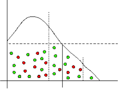
5: Atomistic Kinetic Monte Carlo Diffusion

Amorphization and Recrystallization

Sentaurus™ Process User Guide 455

I-2013.12

Figure 58 shows a generic damage concentration profile after an implant.

Figure 58 Damage concentration profile after an implant

There are two different concentrations in Figure 58 (A and C) and one concentration threshold

called Amorphization. This threshold is stored in the parameter database in the damage

section as AmorphizationThreshold:

sprocess> pdbGet KMC Si Damage AmorphizationThreshold

1.5e+22

NOTE Yo u c an c ha nge t his l im it if n ec essa ry. T he d am age a cc umul at ion m od el

is dependent on the AmorphizationThreshold.

The behavior of the simulator while adding new point defects (damage) differs depending on

the local concentration of the internal grid elements. A new point defect is inserted into a box

depending on the concentration of that box. If the concentration is smaller than the

Amorphization threshold (C, crystalline region), the point defect is inserted as it is. In other

words, a particle is placed inside the simulator with its three coordinates, the defect, and

particle type. Finally, the damage concentration can be higher than the amorphization threshold

(region A (amorphous) in Figure 58). In this case, if a particular crystalline volume (specified

by the parameter minAmorphousVol) has an averaged damage concentration larger than the

threshold, the entire internal volume is assumed to be amorphous. The atomistic 3D

coordinates for Is and Vs are discarded for amorphous boxes because the definition of a point

defect is now meaningless in an amorphous region, and only their concentration is stored.

Finally, the material of the internal box changes from crystalline (such as silicon) to amorphous

(such as amorphous silicon) and an interface, which is capable of simulating a three-phase

segregation model, is created between them.

NOTE For amorphous regions, the atomistic 3D information is discarded, and

only the number of particles is stored. When asking Sentaurus

Process KMC for the atomistic information (the 3D coordinates for

each particle), you should not expect to obtain Is and Vs in amorphous

regions.

Amorphization

a–c

5: Atomistic Kinetic Monte Carlo Diffusion

Amorphization and Recrystallization

456 Sentaurus™ Process User Guide

I-2013.12

NOTE To obtain the amorphous–crystalline interface, use the command:

kmc extract acinterface

Amorphous Defects

An amorphous defect is a special defect assigned to each grid element of Sentaurus

Process KMC with a damage level above the amorphization threshold.

Material

Amorphous defects are always associated with amorphous materials. Each amorphous internal

element is paired with an amorphous defect.

Shape

The shape of an amorphous defect coincides with the element containing it. Amorphous layers

are created as a set of several amorphous defects. Consequently, amorphous layers can follow

any complicated amorphous geometry, but always as a set of Sentaurus Process KMC

elements.

Growth

Amorphous defects do not grow because they are limited to the size of the element. Amorphous

layers grow when new elements are amorphized and become amorphous. These amorphous

elements capture any incoming particle.

Recombination

These defects can recombine their damage and become crystalline silicon. Amorphous defects

do not emit particles; recrystallization is the only event they can perform.

Diffusion in Amorphous Materials

Two models are available for diffusion in amorphous materials:

■A simpler, direct diffusion model

■An indirect diffusion model that uses dangling bonds as an intermediate species

5: Atomistic Kinetic Monte Carlo Diffusion

Amorphization and Recrystallization

Sentaurus™ Process User Guide 457

I-2013.12

To select the model to use, set KMC <material> Damage amorphous.bonds to true,

where <material> is the crystalline material.

Direct diffusion

Dopants can diffuse in amorphous materials using direct diffusion. The implemented

diffusivity is:

(697)

where the parameters and are input parameters.

Parameters

The parameters and needed for diffusion in amorphous materials are specified in the

PDB as Dm and Em, respectively, under the amorphized material:

pdbSet KMC <amorphous material> <dopant> Em <dopant> <value>

For example:

pdbSet KMC AmorphousSilicon B Em B 0.8

pdbSet KMC AmorphousSilicon B Dm B 1e-3

NOTE The alias aSi can be used for AmorphousSilicon.

Indirect Diffusion

The observed boron diffusion in amorphous silicon does not seem to obey a standard Fick’s

law with constant diffusivity prefactors and activation energy, thereby making the direct

diffusion model in amorphous silicon inaccurate. A different model has been proposed

[29][30] that relies on the presence and distribution of dangling bonds and floating bonds and

that interacts with the boron atoms. In this model, an initial number of dangling bonds

(threefold-coordinated atoms) and floating bonds (fivefold-coordinated atoms) is created

during amorphization.

These dangling bonds and floating bonds are allowed to evolve using a simple direct diffusion

for dangling bonds and for floating bonds. Dangling bonds and floating bonds can

interact with them, annihilating each other. Dangling bonds also can interact with boron (or any

other user-defined impurity) with a proportionality constant .

In this model, boron in amorphous silicon can exist in two different states: an immobile

fourfold-coordinated state and a highly mobile threefold-coordinated state. Boron

changes between these two states by capturing and releasing a dangling bond. The threefold

DmX() Dm0,X() EmX() kBT()⁄()–()exp=

Dm0,

5: Atomistic Kinetic Monte Carlo Diffusion

Amorphization and Recrystallization

458 Sentaurus™ Process User Guide

I-2013.12

mobile boron is allowed to diffuse with a simple Arrhenius plot. Boundary conditions can be

set at the AmorphousSilicon_Silicon and AmorphousSilicon_Oxide interfaces for

dangling bond (DB) and floating bond (DB) recombination. Finally, despite the initial

concentration of dangling bonds produced by amorphization, an extra contribution of

is added to produce a total DB concentration of:

(698)

where is a coefficient relating to the presence of boron atoms in amorphous silicon with an

excess of dangling bonds, and is the concentration of boron in amorphous silicon.

Consequently, the following reactions are allowed:

(699)

(700)

Implementation

To minimize the number of species and physical mechanisms, the implementation of indirect

diffusion through dangling bonds and FBs has been done by renaming:

■Dangling bonds as interstitials in amorphous silicon

■Floating bonds as vacancies in amorphous silicon

■ as substitutional boron in amorphous silicon

■ as interstitial boron in amorphous silicon

In this way, all that is needed is to allow I and V inclusion, and the following reactions in

amorphous silicon:

(701)

(702)

The B interaction with and further emission by are modeled as a regular kickout

mechanism. Consequently, the parameter is modeled indirectly through the binding energy

and prefactor of the pair.

When amorphizing an element with volume , an initial number of Is and Vs will be

created inside, where is the silicon density. If there are boron atoms inside or boron atoms

are introduced through implantation or any other means (for example, using the select or

profile commands), an extra number of Is will be introduced per boron atom.

γB[]

nBn0γB[]+=

B[]

DB FB+∅→

B4DB+B3

↔

IV+∅→

BI+Bi

↔

∆V

n0∆Vδ

5: Atomistic Kinetic Monte Carlo Diffusion

Amorphization and Recrystallization

Sentaurus™ Process User Guide 459

I-2013.12

Parameters

The parameters needed for this model are introduced in different places. If you want to model

the indirect diffusion of boron in amorphous silicon (other impurities or amorphous materials

are accepted also), you can use aSi as an alias for AmorphousSilicon.

Impurity Clusters in Amorphous Materials

Impurities diffusing in amorphous materials can interact with each other and form impurity

clusters. In contrast with impurity clusters in crystalline volumes, the amorphous impurity

clusters do not contain interstitials or vacancies, and are only an agglomeration of impurities.

Consequently, they can only re-emit the trapped impurities. With this exception, they behave

as regular impurity clusters. For further information, see Impurity Clusters on page 472.

Table 53 Parameters used for indirect diffusion in amorphous silicon

Parameter Description Symbol

KMC aSi amorphous.bond true

Model activation. None

KMC aSi I Dm I <value>

KMC aSi I Em I <value>

Dangling bond diffusion.

KMC aSi V Dm V <value>

KMC aSi V Em V <value>

Floating bond diffusion.

KMC aSi B Dm Bi <value>

KMC aSi B Em Bi <value>

B3 diffusion. None

KMC aSi B Eb Bi <value>

B3–B4 reaction rate.

KMC aSi B ReactionsPointDefect B,I true

.None

KMC Si Damage amorphous.n0 <value>

Initial dangling bond and floating bond

percentage (versus silicon density).

KMC aSi B gamma <value>

Number of dangling bonds created per

boron atom.

B4DB+B3

↔

5: Atomistic Kinetic Monte Carlo Diffusion

Amorphization and Recrystallization

460 Sentaurus™ Process User Guide

I-2013.12

Recrystallization

Two recrystallization models are implemented:

■The simple KMC quasiatomistic model assigns a recrystallization rate to each amorphous

defect for recrystallization simulations. No orientation dependencies are allowed.

■The fully atomistic model uses a lattice kinetic Monte Carlo (LKMC) method to simulate

the evolution of the amorphous–crystalline interface. This model includes orientation-

dependent solid phase epitaxial regrowth (SPER) and facet formation.

The recrystallization model is set up with:

pdbSet KMC <material> Damage Model.SPER <model>

where <material> is the crystalline material (typically, silicon), and <model> is one of the

following:

■LKMC model

■Simple KMC quasiatomistic model

KMC: Quasiatomistic Solid Phase Epitaxial Regrowth

Recrystallization is implemented as a special event performed by the amorphous defects. At a

given temperature, every amorphous defect can recombine all its internal damage, in other

words, recrystallize, with a frequency . The recrystallization of several amorphous

defects with different recrystallization frequencies, depending on their recrystallization axis

and the number of amorphous neighbors, generates an advancing recrystallization front, as can

be seen in Figure 59 on page 461.

νrecryst

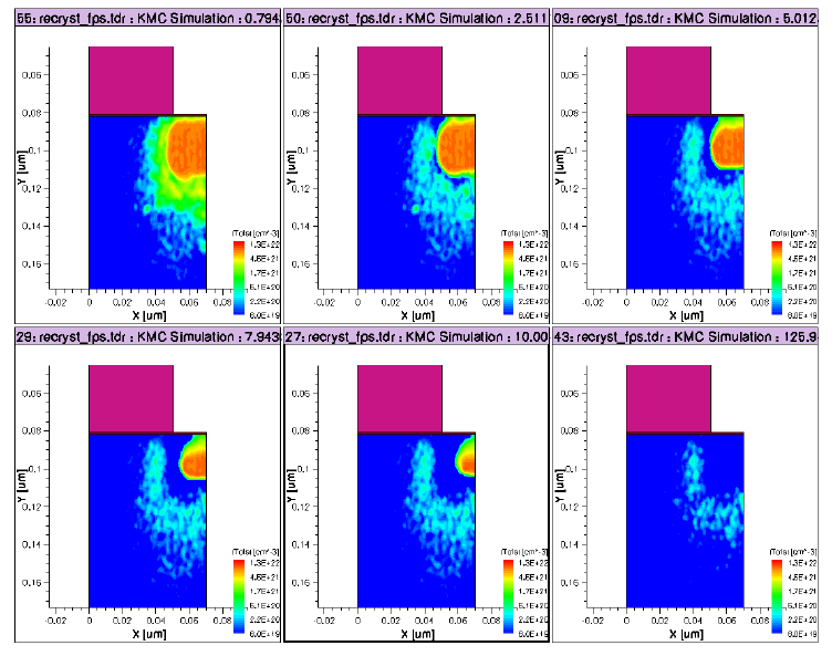
5: Atomistic Kinetic Monte Carlo Diffusion

Amorphization and Recrystallization

Sentaurus™ Process User Guide 461

I-2013.12

Figure 59 Source and gate of a transistor during SPER, as simulated by Sentaurus

Process KMC. The total concentration of interstitials is represented. The time

evolution is shown while the recrystallization front (a consequence of the

recrystallization of isolated amorphous defects) is moving. At the end, there is

only damage near the a-c interface. This remaining damage may form end-of-

range (EOR) defects.

Therefore, if w is the length of an amorphous defect in the recrystallization direction, the

frequency associated with the recrystallization is v/w. This recrystallization velocity v is

computed as an Arrhenius function that includes dependencies on both the local Fermi level

and the presence of impurities [31]:

(703)

parameters are specified as E_recryst. is the activation volume for SPER

(dependency on hydrostatic pressure) called VFRecryst, and n is the percentage of

amorphous material around a given element. The time it takes to recrystallize an amorphous

cell depends on the number of amorphous neighbors; the more neighbors that are amorphous,

the longer it takes. The longer recrystallization takes, the more stable the amorphous defect, so

Vn() V0

Fermi n() Erecryst n() P∆VSPER c++()–kBT()⁄()exp×=

Erecrys n()

∆VSPER

5: Atomistic Kinetic Monte Carlo Diffusion

Amorphization and Recrystallization

462 Sentaurus™ Process User Guide

I-2013.12

its activation energy is bigger. accounts for the prefactor, including dependency on the

Fermi level. This dependency is introduced as:

(704)

being and the input parameter called V0_recryst. Doping is the local amorphous

element doping, and is a calibration parameter (different for n-type and p-type materials)

called V0_recrys_ntype and V0_recrys_ptype, respectively.

Finally, takes into account the changes in SPER regrowth due to local impurity

concentration. This correction term is modeled as:

(705)

is the parameter controlling how much each impurity changes the planar

recrystallization activation energy (assumed to have 50% amorphous neighboring elements).

is an exponent to control how this correction depends on the dopant concentration. A null

impurity concentration gives a zero correction, while an impurity concentration of

produces . Consequently, represents the planar

recrystallization activation energy if the sample contains only the impurity, while allows it

to control the transition between these two opposite situations. These parameters are called

E_recrys and E_recrys_exponent, respectively in the PDB.

This model, in which elements with fewer amorphous neighbors recrystallize faster, extends

the ideas described in the literature [28] for amorphous elements. This simple method can

simulate the faster recrystallization of amorphous corners or thin amorphous panhandlers

embedded in crystalline silicon.

Finally, if a recrystallization event that will break the compactness of the amorphous layer is

detected, its recrystallization will be retarded by the parameter CompactFactor. This

prevents the formation of amorphous isolated islands and ensures a better compactness of the

amorphous material.

Parameters

The parameters for the recrystallization model are:

sprocess> pdbGet KMC Si Damage VFRecrys

sprocess> pdbGet KMC Si Damage V0_recrys

0 1.7e8

99 1.7e8

100 0

sprocess> pdbGet KMC Si Damage E_recrys

0 1.72

Fermi

Fermi n() V0n()1KDoping×+()=

V0n()

c1Impurity[]

5 1022

----------------------------







–







Erecrys 50() Impurity[]

5 1022

----------------------------





EfImpurity()+

Impurities



EfImpurity()

510

fImpurity()

Erecrys 50()–=

EfImpurity()

5: Atomistic Kinetic Monte Carlo Diffusion

Amorphization and Recrystallization

Sentaurus™ Process User Guide 463

I-2013.12

15 1.72

40 2.7

70 2.7

95 3.3

99 5

NOTE To produce consistent notation, the suffix has changed from recryst

to recrys.

The unspecified values between two specified ones are computed by linear interpolation.

The parameters controlling the Fermi level and impurity concentration dependencies are

specified for each dopant (and material). For example, for boron, they are:

sprocess> pdbGet KMC Si B E_recrys

2.7

sprocess> pdbGet KMC Si B E_recrys_exponent

LKMC: Fully Atomistic Modeling of Solid Phase Epitaxial Regrowth

It is well known that the SPER velocity depends on the substrate orientation with approximate

ratios of 20:10:1 for orientations (100), (110), and (111), respectively. In addition, the

recrystallization of thin layers in fin transistors is shown as an ‘arrow tip’ shape formed by two

(111) planes that slow down the SPER, leading to the formation of polycrystalline silicon in

regions still not recrystallized.

This model, based on the literature [32], introduces the lattice in the amorphous–crystalline

interface and assigns a recrystallization event to each of the atoms there. When an internal

mesh element is detected to be amorphous as explained in Amorphization and

Recrystallization on page 454, the silicon lattice is recreated around it. This lattice takes into

account the wafer orientation specified in the init command. Those lattice atoms belonging

to crystalline elements are assigned a “crystalline” flag, while those belonging to the

amorphous element are assigned an “amorphous” flag. This produces the initial amorphous–

crystalline interface. At this point, even when the amorphous–crystalline interface still follows

the contour of the internal mesh, it is formed by a set of individual lattice atoms.

From this point, different recrystallization rates are assigned to each atom at the interface. The

interface is defined as the set of lattice atoms that, having an amorphous state, has at least one

first neighbor with a crystalline state. Any other lattice atom that does not belong to this

interface has a recrystallization rate of 0. This means that crystalline-lattice atoms have a zero

probability of recrystallizing (because they are already crystalline).

5: Atomistic Kinetic Monte Carlo Diffusion

Amorphization and Recrystallization

464 Sentaurus™ Process User Guide

I-2013.12

In some cases where regular SPER is very slow, random nucleation and growth can produce

polysilicon material [33] not simulated here. Inclusion of defective silicon created during

SPER also is not simulated.

For amorphous lattice atoms belonging to the interface (in other words, surrounded by at least

one crystalline lattice atom), a SPER rate is assigned. The model assumes that an atom in the

amorphous phase must form two undistorted bonds with its first neighbors in the silicon phase

to become crystalline. For amorphous atoms close to a (001) surface, this happens naturally.

For (011) surfaces, two adjacent amorphous atoms have to cluster together so that each atom

has two undistorted bonds. Finally, for (111) orientations, three atoms are needed to cluster

together.

Consequently, there will be three different recrystallization prefactors – K(1), K(2), and K(3)

– depending on the number of amorphous atoms needed to complete two undistorted bonds.

These K(1), K(2), and K(3) prefactors will be related but not proportional to the different (001),

(011), and (111) SPER velocities. In particular, K(2) and K(3) are probabilities for two and

three atoms, respectively, to come together in an amorphous phase and form spontaneously

undistorted crystalline bonds between them. Consequently, K(2) is expected to be smaller than

K(1), and K(3) is expected to be smaller than K(2), by several orders of magnitude.

Each of these lattice atoms is given a recrystallization frequency of:

(706)

are the K(1), K(2), and K(3) prefactors explained above where:

■ is a Fermi-level correction similar to Eq. 704.

■ is taken as in Eq. 703.

■, , and are the absolute value of the shear stresses.

■ is a parameter coupling the shear stresses.

■ and are the same terms as those defined in Eq. 703.

Figure 60 on page 465 shows the evolution of an amorphized fin during SPER when this model

is used, after 2-, 4-, and 6-minute annealing at . When the arrow tip is formed by the

two lateral 111 planes, the recrystallization is almost stopped (middle and right images). The

planes are formed by the presence of the oxide–silicon interface. Since the oxide does not

provide the needed undistorted bonds for silicon recrystallization, it is used as a starting point

for the (111) plane formation.

A similar model using LKMC for epitaxial regrowth can be read in Epitaxial Deposition on

page 519.

νLKMC ν0

Fermi Kn() Erecryst

LKMC εxy εxz εyz

++()λP∆VSPER c+++()

kBT

-----------------------------------------------------------------------------------------------------------------------–







exp××=

Kn()

ν0

Fermi 1KDoping×+=

Erecryst

LKMC

Erecrys 50()

εxy

εxz

εyz

P∆VSPER

550°C

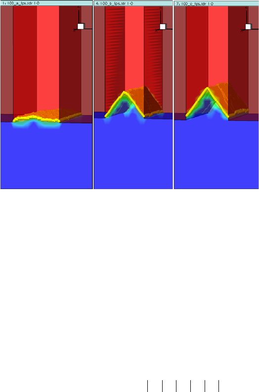
5: Atomistic Kinetic Monte Carlo Diffusion

Amorphization and Recrystallization

Sentaurus™ Process User Guide 465

I-2013.12

Figure 60 SPER evolution (blue is crystalline silicon; red is amorphous one) with time (left to

right) 2, 4, and 6 minutes at ) of a thin (20 nm) silicon fin. The oxide (brown

material) does not provide the correct template for the lattice atoms to form

undistorted bonds, stopping the recrystallization and leading the way to the (111)

planes. When the two (111) planes are formed, no further fast (100) SPER is

possible, and the SPER occurs through the very slow and defect-prone (111)

recrystallization.

Several corrections are applied to the recrystallization rate of a lattice atom. Three of them –

the pressure correction ( ), the impurity correction (through the term ), and the

Fermi-level correction ( ) – are the same in both this model and the simple KMC model

(see KMC: Quasiatomistic Solid Phase Epitaxial Regrowth on page 460).

Shear-Strain Correction

The correction for shear strain, , is unique to this model. Its inclusion

allows the LKMC model to successfully simulate the evolution of line-shaped amorphized

regions. The experimental rate at the corners of line-shaped amorphized regions is very small,

producing a pinching of the SPER interface at the corners [34]. This can be simulated with the

inclusion of this shear stress term [32]. The shear strain is generated during amorphization due

to the different density of the amorphous phase. The expansion of the amorphous phase is not

possible in embedded amorphous regions. The compression of the amorphous phase leads to a

sharp gradient of shear stress at the corners. The model uses the shear strain to simulate the

anomalous regrowth patterns and facet formation experimentally seen in rectangular-shaped

amorphized regions, as shown in Figure 61 on page 466.

550°C

P∆VSPER

ν0

Fermi

εxy εxz εyz

++()λ

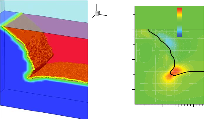
5: Atomistic Kinetic Monte Carlo Diffusion

Amorphization and Recrystallization

466 Sentaurus™ Process User Guide

I-2013.12

Figure 61 Recrystallization of a rectangular-shaped amorphous region using the LKMC

model in Sentaurus Process KMC

Figure 61 (left) shows the distribution of lattice atoms at the amorphous interface side. A (111)

plane, featuring a small nano-island, can be observed close to the interface. The trench formed

at the corner is due to the perturbation introduced by shear strain. Figure 61 (right) shows the

xy shear strain distribution; its maximum intensity occurs at the corner.

Since this model relies on the strain created by the different density of the amorphous material

versus the silicon one, some extra commands must be introduced in the script to account for it.

First, a new material to account for amorphous silicon in the mechanics simulator must be

introduced:

mater add name = Amorph

Mechanics properties for this new material must be defined:

pdbSetDoubleArray Silicon Amorph Conc.Strain {0 0 1 0.02}

pdbSetBoolean Silicon Mechanics UpdateStrain 1

and Sentaurus Process KMC must be instructed that stress is being taken into account:

pdbSet KMC Stress 1

Finally, the synchronization between the atomistic and the mechanics simulator is automatic.

After every mechanics step, the KMC Stress 1 parameter instructs Sentaurus Process KMC

to update the stress and strain fields. After each diffusion (atomistic diffusion) step, Sentaurus

Process KMC updates the “Amorph” distribution by automatically calling the procedure

KMCSync written in KMC.tcl. This procedure, which can be modified by the user but, in

X [µm]

Y [µm]

0.01 0.02 0.03 0.04

0.02

0.04

ElasticStrainELXY [1]

1.1e-02

6.1e-03

1.2e-03

-3.6e-03

-8.5e-03

-1.3e-02

5: Atomistic Kinetic Monte Carlo Diffusion

Amorphization and Recrystallization

Sentaurus™ Process User Guide 467

I-2013.12

principle, does not need to be, contains the lines responsible for updating the amorphous region

in mechanics to properly account for the strain and stress:

LogFile IL2 "A/C synchronization: KMC -> PDE"

kmc deatomize name=AC

sel Silicon z=1e22*AC name=Amorph store

Parameters

Table 54 lists the parameters used in this model. It is assumed that silicon (Si) is the crystalline

material and amorphous silicon (aSi) is the amorphous material.

Defect Generation during SPER

It is known that when (111) planes have formed in a simulation, the recrystallization beyond

these planes is defective, and silicon of low quality, or even polysilicon, is formed. A simple

predictive LKMC model for defect formation during SPER based on [35] and [36] is included.

Such modeling is performed by assigning two tags after every recrystallization event in the

lattice: a normal tag for sites sharing the substrate configuration, and a defective tag for sites

assumed not to bond to their neighbors and that form twin defects. Although this modeling

does not physically set the atoms in twin positions, but only assigns them a tag while remaining

Table 54 Parameters for LKMC model

Parameter name as typed in parameter database Description Symbol

KMC Si Damage Model.SPER <model>

Use LKMC to set the model, KMC to unset. None

KMC Si Damage prefactor.SPER.100 <value>

Value for the prefactor associated with 100 SPER. K(1)

KMC Si Damage prefactor.SPER.110 <value>

Value for the prefactor associated with 110 SPER. K(2)

KMC Si Damage prefactor.SPER.111 <value>

Value for the prefactor associated with 111 SPER. K(3)

KMC Si Damage Shear.Coupling <value>

Shear-strain coupling parameter.

KMC Si Damage VFRecrys <value>

SPER pressure correction (same as the KMC

model).

KMC Si Damage E_recrys 50 <value>

Activation energy for recrystallization (same as the

KMC model).

KMC Si Damage V0_recrys_ntype <value>

KMC Si Damage V0_recrys_ptype <value>

Fermi-level corrections (same as the KMC model).

KMC Si Damage E_recrys <value>

KMC Si Damage E_recrys_exponent <value>

Impurity corrections (same as the KMC model).

KMC Si Damage Lattice.Constant <value>

Lattice constant. None

∆VSPER

Erecryst

LKMC

ν0

Fermi

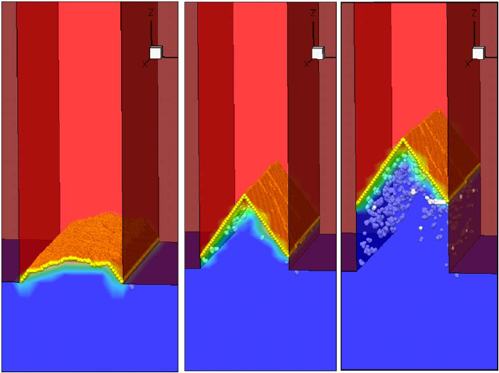
5: Atomistic Kinetic Monte Carlo Diffusion

Amorphization and Recrystallization

468 Sentaurus™ Process User Guide

I-2013.12

in a perfect crystalline position, it is sufficient to predict the defective regions in silicon and to

slow down SPER in a similar way to experiments [35][36].

The new defective sites are produced by two mechanisms:

■Recrystallization of (111) sites, having a probability Pdef of becoming defective.

■Recrystallization of atoms in the neighborhood of defective sites, inheriting such tags and

becoming also defective.

The definition of a coordination number, a keystone in this model to identify the microscopic

configurations, also is modified to distinguish between normal and defective sites. In this way,

the formation of defects slows down the recrystallization of neighboring sites.

The formed defects are represented in the non-LKMC module as an IV twin defect in the TDR

file. No actions are associated with them in the regular KMC simulator. Consequently, when

they are formed, twin defects do not disappear and do not interact with other particles. They

are created for users to identify the regions predicted to have highly defective silicon.

The only new parameter needed for the model is the probability of (111) recrystallizations to

produce twin defects. This parameter is specified in:

pdbSet KMC Si Damage probability.SPER.defect <0-1>

Figure 62 Evolution of a thin (20 nm width) amorphized silicon fin (amorphous is red,

crystalline is blue) annealed at 600oC; arrow-shaped a/c interface is represented

by yellow atoms and formation of defects (twins) is shown as white spheres

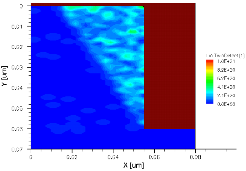
5: Atomistic Kinetic Monte Carlo Diffusion

Amorphization and Recrystallization

Sentaurus™ Process User Guide 469

I-2013.12

Figure 63 Concentration of twin defects representing defective silicon formation when

SPER is in an amorphous region close to SiO2 (silicon is blue, SiO2 is brown)

Figure 62 on page 468 and Figure 63 show two examples where twin-defect formation is

involved. Figure 62 represents the formation of defects during the SPER of a thin silicon fin.

Figure 63 shows the defective triangular-shaped region, bounded by a (111) plane, typical of

SPER close to SiO2-filled trenches.

Redistributing Damage

The recrystallization event forces all IV pairs inside an amorphous defect to recombine. The I

or V excess is redistributed to the neighboring amorphous boxes if any. Otherwise, the excess

is recombined at the surface. If there is no free surface/interface neighboring amorphous boxes,

it is left as point defects. If the recrystallization front has crossed several elements, the amount

of excess point defects can be high. When the defects are deposited in the crystalline silicon,

they grow and ripen into extended defects depending on the annealing conditions.

5: Atomistic Kinetic Monte Carlo Diffusion

Amorphization and Recrystallization

470 Sentaurus™ Process User Guide

I-2013.12

Parameters

The parameter depositExcessDamage controls whether to redistribute the excess or to

discard it. In simulations with buried amorphous layers, setting this parameter to true is

suggested:

sprocess> pdbGet KMC Si Damage depositExcessDamage

Impurity Sweep/Deposit

The recrystallization process may affect the impurity concentration. The recrystallization front

moves indium and other dopants away, changing the concentration profiles [37][38]. To model

this effect, the amorphous defects transfer impurities during recrystallization:

■Dopants usually (recrysDeposit) remain in the box or move away with the

recrystallization front (see Figure 64 on page 471). The two available models for this

movement are Elements and Hops, chosen by the RedistributionModel parameter:

•The

Elements model takes all the particles in one internal element and moves

to the adjacent one. If moving the dopant with the

recrystallization front increases the concentration of the neighboring element more

than a limit (recrysMaxTotal), it will be deposited in the current element, no matter

what its moving probability.

•The

Hops model goes particle-by-particle inside the affected element and decides

whether the particle should be displaced a second neighbor distance, depending on

recrysDeposit. If the particle is not displaced, it remains where it was. The

algorithm continues with the next particle (which may still be the same one, pushing it

again through the adjacent element little by little) until no more particles remain. To

prevent the concentration of displaced particles being too high, the algorithm forces the

deposit probability to be 1 when a particle has 25 or more dopant neighbors. The

algorithm corrects this probability by linear interpolation starting when the number of

neighbors is a given a percentage of 25. This percentage is controlled by the parameter

recrysDepositThreshold.

■When the box is recrystallized, if the remaining dopant concentration is bigger than the

solubility limit (C0_recrysMaxActive, E_recrysMaxActive) after SPER, the extra

dopants are deposited as impurity clusters. These clusters have a limited size, and there are

two different models to deposit these clusters depending on whether recrysMaxSize is

defined.

nrecrysDeposit×

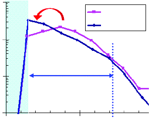
5: Atomistic Kinetic Monte Carlo Diffusion

Amorphization and Recrystallization

Sentaurus™ Process User Guide 471

I-2013.12

Figure 64 Impurity sweep example showing that arsenic has been pushed through the

surface during recrystallization or SPER

The parameters for the recrystallization model are defined only for impurities in silicon (or

other full material). P_recrysDeposit and E_recrysDeposit define (prefactor and

energy) the probability for a dopant remaining in the same box after the recrystallization front

passes. Setting this value to 1 disables the swept of impurities. recrysMaxTotal establishes

the maximum concentration piled up during SPER. recrysMaxActive is the maximum

allowed concentration of an active dopant in the recrystallized areas. Finally, if

recrysMaxSize is defined (and it is by default), the old model to limit the maximum size of

the deposited impurity clusters will be used. To undefine this parameter, use:

sprocess> pdbUnSetDouble KMC Si B recrysMaxSize

This instructs Sentaurus Process KMC to use the new model to deposit impurity clusters after

SPER. This model deposits the clusters specified in recrysDeposit_Complex with the

probabilities defined there.

Finally, the active dopants after SPER are deposited as substitutional impurities, but you can

change this default using recrysDeposit_Active. This parameter accepts a list of

impurities and impurity pairs with the probability to be deposited. For example:

sprocess> pdbSet KMC Si F recrysDeposit_Active F .1

sprocess> pdbSet KMC Si F recrysDeposit_Active Fi .9

This deposits 90% of the ‘active’ fluorine as Fi, and 10% as F.

NOTE Specifying a high probability for a cluster with a number of dopants

greater than 1 does not necessarily means that you will obtain only that

cluster. For example, if you specify that B2I should be 100% of the

deposited clusters, but Sentaurus Process KMC finds only one boron

particle in an element, Sentaurus Process KMC will not form a B2I.

1022

1021

1020

1019

Total A s

Swept As

Amorphous layer

before recrystallization

Depth [nm]

SiO2

Concentration [cm–3]

5: Atomistic Kinetic Monte Carlo Diffusion

Impurity Clusters

472 Sentaurus™ Process User Guide

I-2013.12

Parameters

The recrystallization parameters for dopants can be obtained as:

sprocess> pdbGet KMC Si As P_recrysDeposit

0.3

sprocess> pdbGet KMC Si As E_recrysDeposit

0.0

sprocess> pdbGet KMC Si As recrysMaxActive

1e+21

sprocess> pdbGet KMC Si As recrysMaxSize

sprocess> pdbGet KMC Si B recrysDeposit_Complex

B3I3 .40 B2I3 .30 BI2 .30

sprocess> pdbGet KMC Si B recrysDeposit_Active

B 1.0

To see which model is being used, use:

sprocess> pdbGet KMC Si Damage RedistributionModel

Elements

The concentration thresholds associated with each model are:

sprocess> pdbGet KMC Si B recrysMaxTotal

2e+22

sprocess> pdbGet KMC Si B recrysDepositThreshold

Impurity Clusters

At certain concentrations, dopants are electrically inactive in crystalline silicon [7]. At the

same time, high I concentration can make a fraction of boron electrically inactive even when

its concentration is below its solubility [39]. This phenomena can be explained by a BmIn

clustering mechanism [15][40] or dopant precipitation [7]. Sentaurus Process KMC considers

these mechanisms, implementing the impurity clusters.

Recent studies [41] show that boron precipitation in amorphous silicon occurs through

formation of a boron complex, thereby making the inclusion of impurity clusters in amorphous

materials necessary. Consequently, pure dopant clusters, , are allowed in amorphous

materials and other materials modeled as simple.

The AnBo...Xm impurity clusters allow powerful modeling of the interaction of several

impurities between them. For example, fluorine–boron clusters (FnBoIm and FnBoVm) can be

tried to explain the effects of boron coimplanted with fluorine, or AsnPoVm clusters to allow a

satisfactory explanation, as seen in [52]. Nevertheless, the most common use of impurity

5: Atomistic Kinetic Monte Carlo Diffusion

Impurity Clusters

Sentaurus™ Process User Guide 473

I-2013.12

clusters is the traditional one where only one dopant is present. Consequently, except where

indicated, the description of impurity clusters that follows assumes that the clusters are in the

more common form AnXm with only one impurity involved. Starting with Version I-2013.12,

impurity clusters have a simple model for diffusion, that is, they can migrate. For more

information, see Diffusion on page 474.

Finally, impurity clusters do not need to be neutral. Consequently, the charge state of each

impurity cluster can be defined by using the parameter e0_Complex. When needed, an

impurity cluster with a particular charge as AnXmcharge will be denoted. In addition, clusters

can react with charged particles, as long as the reaction is not between a cluster and a particle

with the same sign, in other words, it is not an electrostatic repulsive reaction.

To simplify the following descriptions, this section describes, the AnXm clusters with only one

impurity, and neutral reactions (in other words, reactions similar to

, ). To see how the model works when this is not the case,

see Charge Dependency on page 485.

NOTE Since P is used both for positive and phosphorus, clusters containing

phosphorus cannot have the P at the end of the cluster name. For

example, AsIP will be interpreted as a positive interstitial arsenic, while

AsPI or PAsI will be a phosphorus–arsenic–interstitial cluster; the same

is true for AsP, PAs, and so on.

Shape

An impurity cluster is an irregular agglomeration of impurities (A, B, ...) with or without

interstitials and vacancies (X) that can be written as AnBo...Xm, with n impurity atoms of type

A, o of type B, and so on, and m Is or Vs. If m = 0, it is a pure impurity cluster (the only ones

allowed in simple materials).

For Sentaurus Process KMC, the notation AnBo...Xm means any possible configurations with

n impurities of type A, o of type B, and so on, and m interstitial (vacancy) atoms. The

interstitial (vacancy) atoms can be both silicon self-interstitials or dopant atoms in an

interstitial position. Since Sentaurus Process KMC assumes all the AnBo...Xm configurations

to be the same with only one effective formation energy, A,B, ... are represented always as a

substitutional but inactive dopant or impurity, and X as a silicon interstitial or vacancy.

AnXm

aAXb

+An1+Xm1+

↔

ab+c=

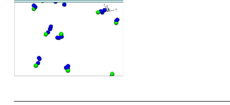
5: Atomistic Kinetic Monte Carlo Diffusion

Impurity Clusters

474 Sentaurus™ Process User Guide

I-2013.12

Figure 65 AsV impurity clusters simulated with Sentaurus Process KMC; blue is arsenic

and green is vacancy

Diffusion

A diffusion mechanism has been added to impurity clusters. This means that impurity clusters

can perform migration hops similar to the ones performed by point-defects, impurities, and

dopants. An impurity cluster migration event involves all its constituent particles: The whole

cluster is displaced. The particle coordinates are modified isotropically at a fixed distance of

= 0.384 nm in the orthogonal direction (parallel to the x-axis, y-axis, or z-axis).

The migration rate for impurity clusters is assumed to be:

(707)

where is the prefactor for each cluster, called Dm_Cluster in the parameter database,

and is the migration energy for each cluster, specified as Em_Cluster in the PDB.

Parameters

As previously stated, the names of the diffusion parameters for impurity clusters are

Dm_Cluster and Em_Cluster:

sprocess> pdbGet KMC Si As Dm_Complex As2V

1e-3

sprocess> pdbGet KMC Si As Em_Complex As2V

1.5

νmν0m,EmkBT⁄–()exp×=

ν0m,

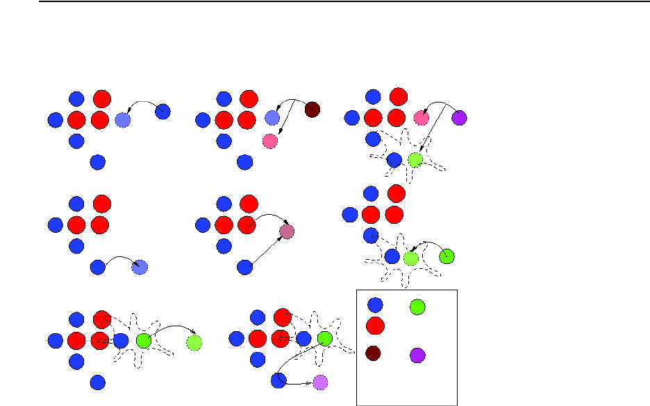
5: Atomistic Kinetic Monte Carlo Diffusion

Impurity Clusters

Sentaurus™ Process User Guide 475

I-2013.12

Limitations

The migration events for impurity clusters, although similar to the ones for single particles, do

not share all their features. In particular, the following limitation applies:

■The diffusivity for impurity defects is global, isotropic, and constant. There are no SiGe,

stress, strain, or charge dependencies on diffusivity.

■Impurity defects do not interact with interfaces at all (Si–SiO2 and so on). All interfaces

are considered mirrors.

■Periodic boundary conditions or mirror conditions are correctly applied to the limits of the

simulation box.

■There is no recombination probability at the boundaries. This means that the parameters

sinkProbTop, sinkProbBottom, sinkProbBack, sinkProbFront, sinkProbLeft,

and sinkProbRight do not apply to diffusing impurity clusters.

■Speedup migration does not apply to impurity cluster diffusion: no long hops or double

hops.

Growth

Impurity clusters grow trapping neutral mobile particles (see Figure 66).

Figure 66 Impurity clusters are disordered agglomerations of dopants and silicon point

defects that trap and emit particles. FT mechanisms and IV recombinations also

are possible.

(a) (b) (c)

(d) (e) (f)

(g) (h) I

Growth Growth Growth

Emission

Recombination

Frank–Turnbull

Frank–Turnbull and

Emission

Impurity Clusters

5: Atomistic Kinetic Monte Carlo Diffusion

Impurity Clusters

476 Sentaurus™ Process User Guide

I-2013.12

For an AnIm cluster, both I and Ai particles can be trapped:

(708)

The trapping is not automatic as it was for extended defects. In extended defects, the binding

energy is always positive, so the trapping is always allowed. For impurity clusters, the cluster

can grow in both Is (Vs) or dopants. The energy between the initial and final states is not always

favorable. Sentaurus Process KMC computes the probability for an impurity cluster AnIm to

trap an I or Ai as:

(709)

where:

(710)

and is an optional energy barrier.

The binding energies are computed using the potential impurity cluster energies:

(711)

(712)

The potential energy for the neutral , assuming that the substitutional is negative, is given

by , where the binding energy includes the pressure and Ge corrections.

The minus sign accounts for the fact that the binding must have a sign that is opposite that of

the potentials.

These potentials energies are computed as:

(713)

where is specified in the parameter database for each impurity in silicon as

Etotal_Complex. is the activation volume to take into account the hydrostatic

pressure dependency, also defined for each impurity cluster size as VF_Complex. The energy

barriers are called EbarrierIV_Complex and EbarrierDopant_Complex. The

EbarrierIV is defined for emission and capture of interstitials and vacancies, and

EbarrierDopant for dopants or paired dopants. For example, to set the potential energy of a

BIC, such as BI2 to some value:

pdbGet KMC Si B Etotal_Complex BI2 <n>

AnIm

aIb

+AnIm1+

↔

AnIm

aAi

+An1+Im1+

↔

Pcapture

Ecapture

kBT

--------------------–





exp=

EAnImcapture Ebarrier AnIm

()max 0 EAnImb

–,()+=

Ebarrier AnIm

()

EAnImb

EAnImbI() Epot AnIm1+

()Epot AnIm

()–=

EAnImbAi

() Epot An1+Im1+

()Epot AnIm

()–Epot Ai

()+=

E–bAi

–

()e–0,()Ai

()–

Epot AnIm

()Epot

0AnIm

()P∆Vpot AnIm

()+=

Epot

0AnIm

()

∆Vpot AnIm

()

5: Atomistic Kinetic Monte Carlo Diffusion

Impurity Clusters

Sentaurus™ Process User Guide 477

I-2013.12

and, for As4V:

pdbGet KMC Si As Etotal_Complex As4V <n>

Initial Seeds

The clusters , , , and are the initial seeds for the impurity cluster ripening. The

formation of is discussed in Percolation on page 477. The others are formed by the

reactions:

■

where and are the charge states for the reactants, and for the result. All these reactions

provide a cluster starting with impurities or impurity pairs. In the cases where for the

first reactions or for the last one, the reaction is not neutral, and the special

considerations of Charge Dependency on page 485 should be taken.

These initials seeds can be enabled and disabled independently by the parameter

ReactionsPointDefect, as explained in Enabling and Disabling Interactions on page 424.

Percolation

Some dopants deactivate without visible diffusion when they are in high concentrations [42].

They also can form impurity clusters [43]. Sentaurus Process KMC models this deactivation

allowing the substitutional dopants to interact with impurity clusters or with other dopants right

after its inclusion in the simulation (for example, after being implanted or selected).

As can react with As giving As2. Substitutional As does not migrate, so this reaction is only

possible when two arsenic are close enough to each other. The higher the arsenic concentration,

the higher this possibility. An As + As2 reaction and As3 + As reaction also are possible. These

species also are immobile. They react only when they are close enough. Consequently, the

probability of forming an As4 cluster using this mechanism is low because it needs four As

atoms close enough to each other. This probability increases with the concentration. With high

concentration, the probability is not negligible, and the substitutional As react with each other

forming As clusters and becoming inactive.

NOTE The reaction between two substitutional dopants to give an impurity

cluster is the only exception to the rule that two particles with the same

charge will not interact.

A2I

AI2

A2I2

AaAi

+A2Ic

↔

aIb

+AI2

↔

aAi

+A2I2

↔

AaAa

+A2

↔

ab+c≠

2ac≠

5: Atomistic Kinetic Monte Carlo Diffusion

Impurity Clusters

478 Sentaurus™ Process User Guide

I-2013.12

In simple materials, such as amorphous silicon, this ‘percolation’ model is the only one

allowing impurity clusters to be formed. Since all particles are neutral in simple materials, the

percolation reaction does not constitute an exception there.

Parameters

The potential and binding energies for impurity clusters are defined only in materials with

full and simple modeling, including amorphous. They are defined in arrays whose index is

the cluster name. For example, for F clusters:

sprocess> pdbGet KMC Si F Etotal_Complex

FV2 -4.20

F2 -0.5 F2V -4.63 F2V2 -7.07

F3 -1 F3V -7.08 F3V2 -9.04

F4 -1.5 F4V -7.12 F4V2 -11.47

F5 -3 F5V -8.5 F5V2 -13.29

F6 -4.5 F6V -9.7 F6V2 -16.09

F7V 3

FI2 -4.20

F2I -4.63 F2I2 -7.07

F3I -7.08 F3I2 -9.04

F4I -7.12 F4I2 -11.47

F5I -8.5 F5I2 -13.29

F6I -9.7 F6I2 -16.09

F7I 3

A particular value for only one element also can be obtained. The current potential energy for

As4V is:

sprocess> pdbGet KMC Si As Etotal_Complex As4V

-5.4

The barriers are, by default, not defined:

sprocess> pdbGet KMC Si F EbarrierIV_Complex

sprocess> pdbGet KMC Si F EbarrierDopant_Complex

The charge value for the clusters is retrieved with:

sprocess> pdbGet KMC Si F e0_Complex

sprocess> pdbGet KMC Si B e0_Complex

B3 0 B3I 0 B3I2 0 B3I3 0

B2 0 B2I 0 B2I2 0 B2I3 0

BI2 0

No value means that they are neutral.

5: Atomistic Kinetic Monte Carlo Diffusion

Impurity Clusters

Sentaurus™ Process User Guide 479

I-2013.12

NOTE The impurity cluster model and the activation or deactivation of clusters

can be calibrated further fitting the potential energies. For further

accuracy, Advanced Calibration also can be used.

When a particular energy for a particular configuration is not specified (in other words, when

input in the parameter file exists for an AnIm or AnVm impurity cluster), Sentaurus

Process KMC assumes this configuration to be unstable. When a barrier energy is not

specified, a value of 0 eV (no barrier) is assigned.

All impurities are allowed to form impurity clusters with I, V, or both. If an impurity does not

form impurity clusters, the default can be changed, modifying the parameters and the

interactions (see Interactions on page 487).

Emission

Impurity clusters can emit both neutral interstitials (vacancies) or mobile dopants:

(714)

(715)

Sentaurus Process KMC computes the emission frequencies as:

(716)

The emission energies are:

(717)

(718)

is the migration energy of the emitted species, and both and have

been shown above. The emission prefactors for dopant and I or V emission depend on the

model used.

When UseCaptVol_Complex is set to true, the emission prefactors are proportional to the

capture volumes of the impurity clusters:

■

AnImAnIm1–I+↔

AnImAn1–Im1–Ai

+↔

νemission ν0emission,

Eemission

kBT

----------------------–





exp×=

Eemission I() EmI() Ebarrier AnIm

()max 0 EAnImbI(),()++=

Eemission Ai

() EmAi

()Ebarrier AnIm

()max 0 EAnImbAi

(),()++=

EAnImbI()

EAnImbAi

()

ν0emission,Ai

() KA

()Vcapt AnIm

()=

ν0emission,I() KI()Vcapt AnIm

()=

5: Atomistic Kinetic Monte Carlo Diffusion

Impurity Clusters

480 Sentaurus™ Process User Guide

I-2013.12

is the capture volume for each impurity cluster, defined in the PDB as

CaptVol_Complex, and the constant is a parameter named D0_Cluster in the PDB.

NOTE The unit of the capture volumes is the capture volume of one single

point defect.

If UseCaptVol_Complex is set to false, Sentaurus Process KMC uses the default old

model, in which the capture volumes are internally fixed to be for emission and

for emission. The use of this default model is not suggested, since it does not lead to

microscopic reversibility.

When a particle is emitted, the impurity cluster tests if the number of remaining particles is

enough to maintain the cluster. If there is only an interstitial (vacancy) or an interstitial and a

dopant, the cluster dissolves leaving an interstitial or a mobile, paired dopant, respectively.

Parameters

The prefactor constants are:

sprocess> pdbGet KMC Si As D0_Cluster

As,AsV 2.1

As,V 10

sprocess> pdbGet KMC Si B D0_Cluster

B,Bi 3

B,I 150

The notation for these prefactors is as follows: two strings are needed, separated by a comma.

The second string represents the emitted particle for which the parameter is being defined. The

first string represents the type of cluster. This first string is needed to define a different prefactor

for emitting a Bi from a B cluster rather than from a hypothetical BF cluster. For example, the

emission of Bi from a B2I2 will use B,Bi, while from a B2F3I2 will use BF,Bi. This last one

can be defined in KMC Si B and KMC Si F, but if defined in both of them with different values,

it will produce an error.

The capture volume parameters are:

sprocess> pdbGet KMC UseCaptVol_Complex

sprocess> pdbGet KMC Si B CaptVol_Complex

B3 1 B3I 1 B3I2 2 B3I3 3

B2 1 B2I 1 B2I2 2 B2I3 2

BI2 1

The notation for capture volumes is as following: if only the cluster is specified, that applies to

all emissions for that particular size, but if a cluster size and a particular particle are specified,

Vcapt AnIm

()

min n m,()

5: Atomistic Kinetic Monte Carlo Diffusion

Impurity Clusters

Sentaurus™ Process User Guide 481

I-2013.12

separated by a comma, that applies to that cluster emitting only that particle. For example, the

following applies only to emission if I by B2I2:

pdbSet KMC Si B CaptVol_Complex B2I2,I 6

The rest of the parameters needed for emission are the same as in Growth on page 475.

Recombination

Impurity clusters can trap incoming neutral Vs (Is) and recombine them with internal Is (Vs):

(719)

The capture probability is:

(720)

The associated energies are:

(721)

and:

(722)

After the IV pair recombination, the cluster size is tested and, if necessary, dissolved, as

previously explained.

Parameters

The parameters used for recombination of point defects are the same as in Growth on page 475.

Frank–Turnbull Mechanism

A generalized Frank–Turnbull (FT) mechanism is the emission of a neutral V (I) from an AnIm

(AnVm) impurity cluster by the formation of a Frenkel pair (IV):

(723)

AnImV+AnIm1–

↔

Pcapture

Ecapture

kBT

--------------------–





exp=

EAnImcapture EAnImbEpot V()–Epot I()–=

EAnImbEA

nIm1–

()EA

nIm

()–=

AnImIVA

nIm

++ AnIm1+V+→→

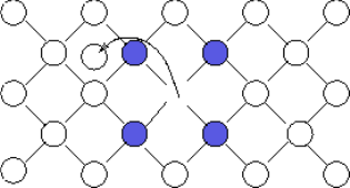
5: Atomistic Kinetic Monte Carlo Diffusion

Impurity Clusters

482 Sentaurus™ Process User Guide

I-2013.12

or:

(724)

Sentaurus Process KMC includes the FT mechanism to maintain microscopic reversibility.

Since impurity clusters recombine incoming Is or Vs, the opposite mechanism (FT) also is

needed. Usually, this mechanism is unfavorable, but for some particular configurations, the

energetic differences between them can enable the formation of IV pairs and, therefore, the

emission of particles using the FT mechanism (see Figure 67).

Figure 67 Example of FT mechanism: an As4 cluster can emit an interstitial to become an

As4V impurity cluster: blue is arsenic and white is silicon

The vacancy (interstitial) emission frequency is computed as:

(725)

being:

(726)

and:

(727)

where the potential energies for the clusters and the point defects include pressure and Ge

corrections.

Parameters

The parameters used are the same as in Growth on page 475. The potential energies for

interstitial and vacancies are specified for the material as Ef:

sprocess> pdbGet KMC Si I Ef

4.0

sprocess> pdbGet KMC Si V Ef

3.8

AnVmIVA

nVm

++ AnVm1+I+→→

νemission ν0emission,

Eemission

kBT

----------------------–





exp×=

Eemission V() EmV() max 0 EAnImbV(),()+=

EAnImbV() Epot I() Epot V() Epot AnIm1+

()Epot AnIm

()–++=

5: Atomistic Kinetic Monte Carlo Diffusion

Impurity Clusters

Sentaurus™ Process User Guide 483

I-2013.12

The corrections to the potential energies for I and V are VF and EfGe for pressure and Ge,

respectively:

sprocess> pdbGet KMC Si I EfGe

I 0.0

sprocess> pdbGet KMC Si I VF

I 0.0

The prefactor for I and V emission is computed automatically for impurity clusters with only

one dopant (for example, BnIm or AsnVm clusters) and must be specified for other cases. For

example, in a case with AsPV clusters, the prefactors for Frank–Turnbull emission are

specified as follows:

pdbSet KMC Si As D0_Cluster AsP,V 50

pdbSet KMC Si As D0_Cluster AsP,I 50

The following is also valid:

pdbSet KMC Si P D0_Cluster AsP,V 50

pdbSet KMC Si P D0_Cluster AsP,I 50

Complementary Recombination

Some impurities diffuse using both the interstitial and vacancy mechanisms. For these cases,

the impurity clusters can react with both of them. For example, an AnVm impurity cluster can

grow trapping AsV, as previously explained, and can interact with an incoming Asi, trapping

the As and recombining the I with one internal vacancy. This implies to take into account the

reaction:

(728)

These complementary recombinations of neutral particles are allowed with a probability of:

(729)

The capture energies are computed as:

(730)

AsnVmAsi

+Asn1+Vm1–

↔

Pcapture

Ecapture kBT()⁄–()exp Ecapture 0>

1Ecapture 0≤











Ecapture

Epot An1+Vm1–

()Epot AnVm

()–EfV()–EfI()–Epot Ai

()–m0>

Epot An1+Vm

()Epot AnVm

()–Epot Ai

()–EmI() EmAi

()–+ m0n1>,≡

iA→() m0n1≡,≡











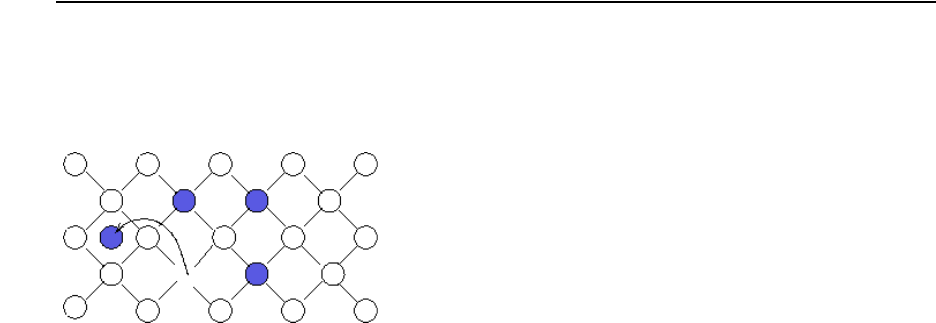
5: Atomistic Kinetic Monte Carlo Diffusion

Impurity Clusters

484 Sentaurus™ Process User Guide

I-2013.12

where is an internal parameter that cannot be changed.

Parameters

The parameters used are the same as in Frank–Turnbull Mechanism on page 481. The potential

energy for the paired dopant is the binding energy of the pair corrected with the Fermi-level

dependency.

Complementary Emission

To maintain microscopic reversibility, the reaction reverse to the complementary

recombination must be defined (see Figure 68).

Figure 68 Example of complementary emission: the cluster emits an interstitial that takes

an impurity and generates a vacancy; blue is arsenic and white is silicon

The equation for this process is:

(731)

Its emission frequency is computed using the emission frequency equation:

(732)

where:

(733)

iA→()

AnImAnImIV++ AVAn1–Im1+

+→→

Eemission EmAV

()max 0 EAnImbAV

(),()+=

EAnImbAV

() EfI() EfV() Epot An1–Vm1+

()Epot AnIm

()–++=

5: Atomistic Kinetic Monte Carlo Diffusion

Impurity Clusters

Sentaurus™ Process User Guide 485

I-2013.12

Parameters

The parameters used are the same as in Recombination on page 481.

For simple impurity clusters, those with only one impurity (BnIm, AsnVm, and so on), the

prefactor for emission is calculated automatically. For complex impurity clusters, (AsnPoVm

and so on), the prefactor must be written explicitly:

pdbSet KMC Si As D0_Cluster AsP,Asi 50

Charge Dependency

Neutral Reactions

In the previous discussions, all the impurity clusters are assumed to be neutral and,

consequently, there are no explicit charge Fermi-level dependencies. Nevertheless, there are

nonexplicit dependencies. In particular, for clusters emitting impurity-paired dopants, the

emission energy depends on the binding of the paired dopants, which, in turn, contains a Fermi-

level dependency.

The Fermi-level dependency of the binding energy is related to the level of the neutral-paired

dopant in the band gap. This level also depends on the temperature and the bandgap narrowing.

All the previous dependencies are included by default, except the indirect dependency on the

bandgap narrowing, which can be switched off and on using:

pdbSet KMC <material> BandGap Correct_Complex <true/false>

Nonneutral Reactions

Assume the following reaction:

(734)

The potential energy for is defined with respect to a ground state that produces the

impurity cluster in a neutral reaction. This means that:

(735)

BnIm

aBoIp

bXc

+→

BnIm

nB-mV0an+()–e-an+0<

an+()h+an+0>







5: Atomistic Kinetic Monte Carlo Diffusion

Impurity Clusters

486 Sentaurus™ Process User Guide

I-2013.12

is the ground state for . Consequently, an account of holes and electrons must be

followed during the reaction. In particular, calling the initial cluster and the final one , these

accounts are:

■,

The final state must account for the charge in the emitted particle. Calling the charge of the

substitutional dopant of the emitted species (in other words, if or

if ), the final accounts for holes and electrons are:

■

This allows writing the first energetic term for the binding energy as:

(736)

The second term is the obvious difference in potential energies:

(737)

The binding energy of the emitted particle is also needed, including the transition from the

neutral state to the current emitted state:

(738)

In addition, only in cases where a Frank–Turnbull emission is involved ( or

), the pair recombination energy is:

(739)

This gives a binding energy of:

(740)

That finally allows computing the emission energy:

(741)

AsnVm

+an+an+0>

0an+0<







-0an+0>

a–n–an+0<







hf1

+bo+no+0<

0ba+o<







ef1

-0bo+0>

b–o–bo+0<







d1–=

XcBi

d0=

XcIc

+hf1

+cd–cd–0>

0cd–0<







-ef1

-0cd–0>

dc–cd–0<







Ech esarg ei

-ef

–()EgeF

–()hi

+hf

–()eF

Eclusters Epot BnIm

()Epot BoIp

()–=

EbXc

() EbXd

()EX

ddc–()e-dc–0>

cd–()h+cd–0>







+Xc

→







XcVc

XcBVc

Erecom EfI() EfV()+=

EBnImbXc

() Ech esarg Eclusters

–– EbXc

()–Erecom

Eemission Xc

() EmXc

()Ebarrier BnIm

()max 0 EBnImbXc

(),()++=

5: Atomistic Kinetic Monte Carlo Diffusion

Impurity Clusters

Sentaurus™ Process User Guide 487

I-2013.12

NOTE All the previous energies (potential, binding, migration, and so on) are

computed including hydrostatic pressure, SiGe, and bandgap narrowing

local corrections.

Interactions

You can modify all the interactions involved in the impurity cluster model. The impurity

clusters can be enabled or disabled with the Boolean parameter Implement_Complex. For

example, to disable the FnVm impurity clusters, use:

pdbSet KMC Si F Implement_Complex 0

When the impurity clusters are enabled, you can set and unset the particular reactions using the

ReactionsCluster parameter:

pdbSet KMC Si <dopant> ReactionsCluster <reaction> <true/false>

where reaction is a string with two fields, separated by a comma. The first field is the name

of the impurity cluster, and the second is the name of the reacting particle. Spaces are not

allowed between these fields. The setting or unsetting of these reactions enables or disables the

specified reactions and its reverse ones. This is performed to maintain the microscopic

reversibility. For example, to disable the capture of a vacancy by As2 to growth to As2V:

pdbSet KMC Si As ReactionsCluster As2,V false

This also disables the inverse reaction, in other words, the emission of V by As2V. To e n a b l e

the recombination of I by an As4V cluster:

pdbSet KMC Si As ReactionsCluster As4V,I true

This reaction also enables the FT emission of I by As4, that is, .

Enabling a reaction does not mean that the reaction will happen; it depends on the energetics.

If the reaction is unfavorable, it will not occur (but the inverse will). Disabling a reaction will

forbid the reaction to occur, even if it is described by the parameters as favorable. Any reaction

not listed in ReactionsClusters is disabled.

Complex Impurity Clusters

To enable impurity clusters with more than one dopant (for example, an As2PV), the switches

for both the As and P clusters should be on:

pdbSetBoolean KMC Si As Implement_Complex 1

pdbSetBoolean KMC Si P Implement_Complex 1

As4As4VI+→

5: Atomistic Kinetic Monte Carlo Diffusion

Impurity Clusters

488 Sentaurus™ Process User Guide

I-2013.12

To enable the cluster reaction (assuming As2 is predefined), use the As or

the P to define the reaction. If both are used with different values, an error message will be

displayed. In this example, they are defined in As:

pdbSet KMC Si As ReactionsCluster As2,PV true

The energy and capture volume of this new cluster must be defined as usual:

pdbSet KMC Si P Etotal_Complex PAs2V -3.0

pdbSet KMC Si P CaptVol_Complex PAs2V 1.3

The I, V, and PV emission prefactors are:

pdbSet KMC Si P D0_Cluster PAs,I 0.5

pdbSet KMC Si P D0_Cluster PAs,V 0.5

pdbSet KMC Si P D0_Cluster PAs,PV 0.1

Finally, for AsV emission from the cluster As2PV, allow the reaction by

defining:

pdbSet KMC Si P ReactionsClusters PAs,AsV true

This also enables the formation of the clusters through the reaction of these particles.

Parameters

To show the parameters involved in the impurity cluster reactions, arsenic is used as an

example. AsV clusters are allowed:

sprocess> pdbGet KMC Si As Implement_Complex

Since AsV clusters are allowed in the Sentaurus Process KMC simulation, they require some

enabled reactions. The reactions are explained in Percolation on page 477 and allow

deactivation without arsenic diffusion:

sprocess> pdbGet KMC Si As ReactionsCluster

As2,As true

As3,As true

Reactions to grow capturing V and to shrink emitting them are:

As2,V true

As3,V true

As4,V true

As2PV+As2PV↔

AsP AsV+As2PV↔

5: Atomistic Kinetic Monte Carlo Diffusion

Impurity Clusters

Sentaurus™ Process User Guide 489

I-2013.12

Capture or emission of AsV is:

As2,AsV true

As3,AsV true

Recombination of interstitials and Frank–Turnbull emission of interstitials are:

As2V,I true

As3V,I true

As4V,I true

Recombination of interstitials, capture of arsenic, and emission of Asi are:

As2V,Asi true

As3V,Asi true

The following rules must be satisfied to allow a reaction between a particle and an impurity

cluster:

■The first field must be a correct impurity cluster, and the second must be a defined particle.

■The particle must be an interstitial or a vacancy of a paired dopant. The resulting cluster

must be defined (in Etotal_Complex and CaptVol_Complex).

■Only nonrepulsive interactions are allowed, except for percolation. The reactions do not

need to conserve the charge.

Impurity clusters require an initial impurity cluster or ‘seed’ to begin the ripening. This initial

cluster is formed with the reactions of two particles. These reactions are explained in Enabling

and Disabling Interactions on page 424.

Setting Up Impurity Clusters in a Material

To set up an impurity cluster in a material (for example, in amorphous silicon), the

following PDB parameters must be created:

■First, the cluster must be allowed:

pdbSetBoolean KMC aSi B Implement_Complex true

■Second, an emission prefactor for the cluster, cluster potential energies, barriers, capture

volumes, and stress corrections must be defined:

pdbSetDoubleArray KMC aSi B D0_Cluster { B 3.0 }

pdbSetDoubleArray KMC aSi B Etotal_Complex { B2 -0.45 B3 -2.5 }

pdbSetDoubleArray KMC aSi B EbarrierDopant_Complex { }

pdbSetDoubleArray KMC aSi B CaptVol_Complex { B2 1.5 B3 2.0 }

pdbSetDoubleArray KMC aSi B VF_Complex { }

5: Atomistic Kinetic Monte Carlo Diffusion

Fermi-Level Effects: Charge Model

490 Sentaurus™ Process User Guide

I-2013.12

■Third, for these clusters to form, you must introduce a reaction path:

pdbSetArray KMC aSi B ReactionsPointDefect { B,B true }

pdbSetArray KMC aSi B ReactionsCluster { B2,B true }

■None of this will happen without a mobile particle allowing for growing and emission:

pdbSet KMC aSi B Dm B 3.0e-3

pdbSet KMC aSi B Em B 2.1

NOTE The impurity cluster parameters (energies, barriers, capture volumes,

stress corrections) must be specified in the PDB only when the cluster

is implemented (with Implement_Complex true). This saves many

parameters in the description of impurities without impurity clusters.

Fermi-Level Effects: Charge Model

Point defects (I, V) and impurity atoms (B, As) can appear in different charge states in silicon,

while extended defects and impurity clusters have a fixed charge state in Sentaurus

Process KMC. Impurity atoms are neutral in materials using the simple model.

For example, interstitials and vacancies can be triple negative, double negative, double positive,

triple positive, neutral, positive, or negative. Some species and charged states are listed in

Table 55. You can customize these definitions. The maximum charge state for point defects is

and for impurity paired defects .

Ta bl e 55 S p ec i e s an d c h a r ge d s t at es o f Se nt au r us P ro c es s K M C

+++, I++, I+, I0, I-, I--, I---

IPPP, IPP, IP, I, IM, IMM, IMMM

+++, V++, V+, V0, V-, V--, V---

VPPP, VPP, VP, V, VM, VMM, VMMM

As As+, Asi+, Asi0, AsV+, AsV0, AsV-

As, AsiP, Asi, AsVP, AsV, AsVM

-, Bi+, Bi0, Bi-

B, BiP, Bi, BiM

0,Ci0

C, Ci

0, FI0, FV0

F, FI, FV

Sb Sb+,Sbi0, Sbi+, SbV-, SbV0, SbV+

Sb, Sbi, SbiP, SbVM, SbV, SbVP

3±

2±

5: Atomistic Kinetic Monte Carlo Diffusion

Fermi-Level Effects: Charge Model

Sentaurus™ Process User Guide 491

I-2013.12

Charge states can be modeled using different approaches. The most intuitive approach is

adding a charge ‘label’ to each particle. Nevertheless, because the migration energy (and

maybe some other parameters) change with the charged state, each of these states requires a

full set of parameters.

Sentaurus Process KMC Approach

No charge label is defined for the particles. The charge is implicitly assumed in each particular

particle, and there are different particles for each charged state. This implies the necessity of

defining the interactions one by one, according not only with the particle type, but also with its

charge state.

The charge is represented in a quasiatomistic approach to account for the fact that the electron

transport is several orders of magnitude faster than the atomic transport. The charge

magnitudes (for example, Fermi level and bandgap width) are associated with each internal box

in the simulation. Consequently, there can be local changes between different boxes, but the

charge magnitudes are considered to be homogenous in each Sentaurus Process KMC internal

element.

Assumptions

Sentaurus Process KMC takes the energy reference in the valence band. The following

assumptions also are taken:

■Charge reactions are faster than structural reactions [44]. Consequently, the charges are

updated instantaneously.

■Formation energy for neutral species (for example, Ef(I0)) are not dependent on the Fermi

level. Sentaurus Process KMC takes the formation energies for neutral species as

parameters using them to compute the energies for the nonneutral species.

■Potential energies for impurity clusters are not dependent on the Fermi level. For example,

Sentaurus Process KMC defines the potential energy for as the energy returned by

the system in the reaction (assuming that ).

■The electronic level dependency with temperature is proportional to the bandgap

temperature dependency. The same applies for the bandgap narrowing. This assumption

allows Sentaurus Process KMC to establish proportionality relations to compute the

In In-, Ini0, Ini-, InV0, InV-

In, Ini, IniM, InV, InVM

+, Pi0, Pi+, PV0, PV-, PV+

P, P i, PiP, PV, PVM, PVP

Ta bl e 55 S p ec i e s an d c h a r ge d s t at es o f Se nt au r us P ro c es s K M C

AsnVm

nAs+mV0na–()e-

++ AsnVm

→

na–0>

5: Atomistic Kinetic Monte Carlo Diffusion

Fermi-Level Effects: Charge Model

492 Sentaurus™ Process User Guide

I-2013.12

electronic levels and bandgap narrowing at different temperatures using a known value for

one particular temperature.

■Substitutional dopants are always ionized; that is, substitutional boron is always B– and

substitutional arsenic As+.

■The properties inside each Sentaurus Process KMC element are constant. Properties can

change between internal elements.

For further references on similar KMC charge models, see [1][45][46].

Formation Energies for Charged Species

Taking I+ as an example, in the reaction:

(742)

the energy needed to take an electron from an I0 and obtain I++ e– is denoted as e(+,0), and is

measured from the valence band. The formation energy for a positive interstitial is:

(743)

where is the Fermi level. Consequently, the concentration between different interstitial

charge species using as a reference the neutral concentration is:

(744)

(745)

The electronic levels (for T = 0 K) are specified in the parameter database as e0. They are

defined only for silicon. They can be changed with:

pdbSet KMC Si <I/V/impurity> e0 <species> <n>

for example:

pdbSet KMC Si I e0 IP 0.35

I0I+e-

+→

EfI+

() EfI0

() eFe+,0()–+=

[]

I+

[]

--------- eFe+,0()–

kBT

---------------------------





exp=

I-

[]

---------eFe0-,()–

kBT

---------------------------





exp=

5: Atomistic Kinetic Monte Carlo Diffusion

Fermi-Level Effects: Charge Model

Sentaurus™ Process User Guide 493

I-2013.12

Parameters

The bandgap levels for interstitials and vacancies can be retrieved with:

sprocess> pdbGet KMC Si I e0

IM 1.0

IP 0.35

sprocess> pdbGet KMC Si V e0

VMM 1.06

VM 0.6

VP 0.03

VPP 0.13

They also are specified for dopants, like As:

sprocess> pdbGet KMC Si As e0

AsVM 0.77

AsVP 0.3

AsiP 0.1

NOTE The modification of these parameters affects both extrinsic and intrinsic

diffusion.

Binding Energies for Particles

The binding energy needed for pairing and breakup reactions is only specified for the reaction

with the neutral interstitial or vacancy. For example, for boron, the binding energy is specified

for the reaction B– + I0 = Bi–. The other binding energies (for example, B– + I+ = Bi0) are

computed using the binding energy for the above reaction and the energy levels associated to

the charge transitions [46]:

(746)

The activation energy for the breakup is . Because electronic levels scale

with (as shown below), a slight dependency with T is introduced in these calculated binding

energies.

Binding Energies for Impurity Clusters

For an example of how to compute the binding energy for an impurity cluster, see Nonneutral

Reactions on page 485.

EbBi

() EbBi

()eB

()0-,()eI()+0,()–+=

EbBi

()EmI+

()+

5: Atomistic Kinetic Monte Carlo Diffusion

Fermi-Level Effects: Charge Model

494 Sentaurus™ Process User Guide

I-2013.12

Temperature Dependency

The bandgap width used in Sentaurus Process KMC is given by the expression [47]:

(747)

Using the assumption of proportionality with the band gap, Sentaurus Process KMC assumes

that the electronic levels at different temperatures can be computed as:

(748)

Effective state density of conduction and valence bands follows similar expressions:

(749)

(750)

Finally, Sentaurus Process KMC uses the values to compute the intrinsic levels and intrinsic

carrier densities:

(751)

(752)

Parameters

The needed parameters are specified in the parameter database under the folder BandGap:

Eg0

Bandgap width at 0 K ( ).

Agap

Bandgap width temperature dependency parameter ( ).

Bgap

Bandgap width temperature dependency parameter ( ).

Nc300

Effective state density for the conduction band, at 300 K ( ).

Nv300

Effective state density for the valence band, at 300 K ( ).

EgT() EgT=0()

AT2

BT+

-------------–=

ej 1j,+()T() ej 1j,+()0() EgT()

Eg0()

--------------×=

NcT() Nc300() T

300

---------





×expNc

NvT() Nv300() T

300

---------





×expNv

eiT() EgT()

-------------- kBT

---------



Nv

------





ln+=

niT() NcNv

EgT()

2kBT

--------------–





exp×=

Eg0()

Nc300()

Nv300()

5: Atomistic Kinetic Monte Carlo Diffusion

Fermi-Level Effects: Charge Model

Sentaurus™ Process User Guide 495

I-2013.12

They can be changed using pdbSet. For example, to set the bandgap width at 0 K, use:

pdbSet KMC Si BandGap Eg0 1.17

The parameters for the bandgap temperature dependency are defined for silicon in the

BandGap folder:

sprocess> pdbGet KMC Si BandGap Eg0

1.17

sprocess> pdbGet KMC Si BandGap Agap

0.000473

sprocess> pdbGet KMC Si BandGap Bgap

636.0

sprocess> pdbGet KMC Si BandGap Nc300

3.2e+19

sprocess> pdbGet KMC Si BandGap Nv300

1.8e+19

sprocess> pdbGet KMC Si BandGap expNc

1.5

sprocess> pdbGet KMC Si BandGap expNv

1.5

Charge Attractions and Repulsions

The short-range repulsions between charged particles have been implemented forbidding the

interactions between particles in the same charge state (except for the percolation reactions; see

Percolation on page 477). Long-range forces are considered automatically due to the bias

induced in the particle migration by the local Fermi level.

Fermi-Level Computation

Sentaurus Process KMC computes the Fermi level assuming charge neutrality and Fermi–

Dirac statistics. It simply makes the number of charges in each cell element equal to the

concentration of substitutional dopants and charged impurity clusters in the box. The presence

of mobile charged particles is neglected.

The charge concentration for each element is an average of the charge concentration in the

neighborhood. The averaging radius is taken as the parameter smoothRadius. The power of

expNc

Effective state density temperature dependency parameter (conduction).

expNv

Effective state density temperature dependency parameter (valence).

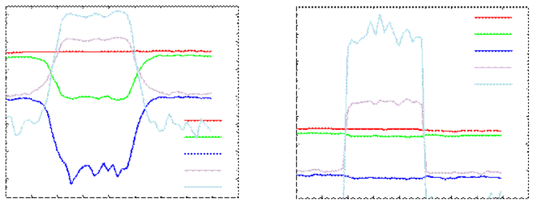
5: Atomistic Kinetic Monte Carlo Diffusion

Fermi-Level Effects: Charge Model

496 Sentaurus™ Process User Guide

I-2013.12

this average is controlled with the parameter smoothPower. This average is important because

of the atomistic nature of the simulation.

Without this averaging, a medium-dose doped sample, with some elements filled up with

particles and some empty ones, could be considered as a set of intrinsic (empty) boxes and a

few boxes with a very high concentration.

For example, a dopant concentration of corresponds to one particle in .

The volume of an internal element may be as small as . This means one particle per

10 boxes. Without any charge averaging, a moving interstitial would diffuse intrinsically in

nine empty boxes and extrinsically in one box. With the average, the interstitial ‘sees’ the right

concentration of and diffuses according to this concentration (see Figure 69).

Figure 69 Simulated vacancy profiles for a p-sample (from 30 to 60 nm) for different

vacancy charged states: (left) smoothing out the charge concentration and (right)

incorrect results without smoothing

Parameters

This smoothing is a default Sentaurus Process KMC feature performed by an ultrafast

algorithm and is controlled only by the cutoff radius (in nanometers) specified in the parameter

database:

sprocess> pdbGet KMC Si BandGap smoothRadius

110

× cm 3–

10 nm3

1 nm3

110

× cm3

1011

Concentration [cm–3]

Depth [nm]

10 20 30 40 50 60 70 80 90 100

1010

108

107

106

105

V–

V––

V+

V++

Depth [nm]

10 20 30 40 50 60 70 80 90 100

1014

Concentration [cm–3]

1013

108

107

1012

109

1010

1011

V–

V––

V+

V++

5: Atomistic Kinetic Monte Carlo Diffusion

Fermi-Level Effects: Charge Model

Sentaurus™ Process User Guide 497

I-2013.12

NOTE To switch off this local computation and to set up a constant, user-

defined dopant concentration, experienced users may want to use:

pdbSetDouble KMC setDopantConc <dopant concentration>

where dopant concentration is a positive quantity for n-type devices and

a negative one for p-type devices.

Updating Charged States

The charge model of Sentaurus Process KMC assumes that the electronic transport and

reactions are faster than the atomic transport and reactions. Therefore, it is necessary to

implement mechanisms to update the charge distribution (and the local Fermi level) that

follows the structural changes. Since the equilibrium ratios depend only on the Fermi level, it

is necessary to update them each time the Fermi level varies.

There are two reasons for local changes in the Fermi level:

■Mobile particles diffusing between elements with different Fermi levels

■Change of the electronic concentration in one element

Besides, each time a new particle appears or disappears because of pairing or breakup

reactions, it is necessary to ensure that the charge state of the new particle is consistent with its

local Fermi level.

Different mechanisms are implemented to maintain the right charge ratios. All are performed

at the same time, but they apply to different scenarios.

Electronic Concentrations and Charge-State Ratios

An update algorithm periodically reviews all the particles and updates the Fermi level and the

proportions of charged particles in each element. The algorithm:

■Smooths the charge distribution.

■Computes the Fermi level for each box using the charge neutrality assumption.

■Establishes the appropriate charge ratios.

NOTE This update algorithm slows down the simulation. It is crucial to follow

the changes in the Fermi level, but without spending too much CPU

time.

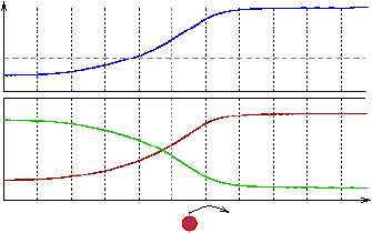
5: Atomistic Kinetic Monte Carlo Diffusion

Fermi-Level Effects: Charge Model

498 Sentaurus™ Process User Guide

I-2013.12

Mobile Particles

Mobile particles see different Fermi levels when they move from one element to another.

Therefore, it is needed to update its charge each time it crosses the boundaries between boxes.

At the same time, particles change their charge state to maintain the proper charge distribution;

consequently, they need extra updates. This is implemented with an algorithm that updates the

charge of mobile particles each time they perform a migration jump. This algorithm also

considers the migration frequency of each particle, as explained in [46], to avoid artificial

concentration increases in the slow diffusing species concentration.

Figure 70 A mobile particle (I–) sees different electronic properties when jumping from one

element to a different one. Its charge state must be updated to reproduce the

expected macroscopic concentration.

Pairing and Breakup Reactions

After pairing or breakup reactions, some species appear and disappear in the Sentaurus

Process KMC elements. To ensure that the concentration of these species maintains the correct

proportions, a breakup, pairing charge update mechanism is implemented. It computes the

probability of the new particles to be in a particular charge state.

Parameters

The charge update algorithm only uses one external parameter in the database called

ChargeVarPercent and accounts for the maximum relative error allowed for the Fermi-level

updates. This parameter is a compromise between accuracy and efficiency.

Decreasing its value leads to more accurate but slower simulations, and the charge model can

overload your computer resources.

Increasing its value speeds up the simulation at the cost of accuracy:

sprocess> pdbGet KMC ChargeVarPercent

0.25

NOTE Only small modifications to this parameter are recommended.

n(x) ni

1+(x)

1–7

1–(x)

Concentration

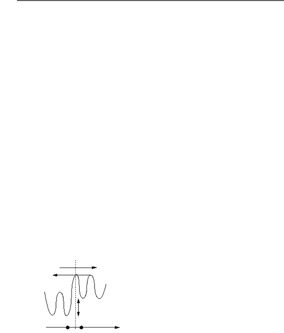
5: Atomistic Kinetic Monte Carlo Diffusion

Fermi-Level Effects: Charge Model

Sentaurus™ Process User Guide 499

I-2013.12

Electric Drift

The charge model of Sentaurus Process KMC considers the:

■Introduction of an electric field, related to the local charge variations.

■Existence of forces acting over the charged species; these forces generate a bias in the

diffusion – the electric drift.

Sentaurus Process KMC models electric bias modifying the jump probabilities to account for

the space anisotropy produced when an electric field is present.

A particle inside the electric field can jump in both directions, but the probability of jumping

following the electric field is higher. Consequently, a ‘migration barrier’ is implemented. The

barriers are related to the relative concentration of each species. For example, for an I+ jumping

from a position in a box to a position in a different box, if , where is

the probability of an interstitial having a positive charge, the jump is always possible.

Otherwise, there is a probability of of being rejected.

For an I+ particle, the jump is accepted with a probability of:

(753)

where typically, if there is no bandgap narrowing effects, and:

(754)

The subscripts 1 and 2 refer to magnitudes in different elements. Figure 71 shows an energy

diagram of this process. The number of rejected jumps for each axis is shown in a report at the

end of the annealing.

Figure 71 Energy diagram showing the jump process

()Px

()>

1Px

()[]–Px

()[]⁄

()

--------------eFe+,0()–[]

2eFe+,0()–[]

–

kBT

---------------------------------------------------------------------------







exp=

e+0,()

2e+0,()

()

--------------eF2eF1

–

kBT

----------------------







exp=

Jump Prob. = 1

Jump Prob. < 1

eF2 – eF1

x1x2

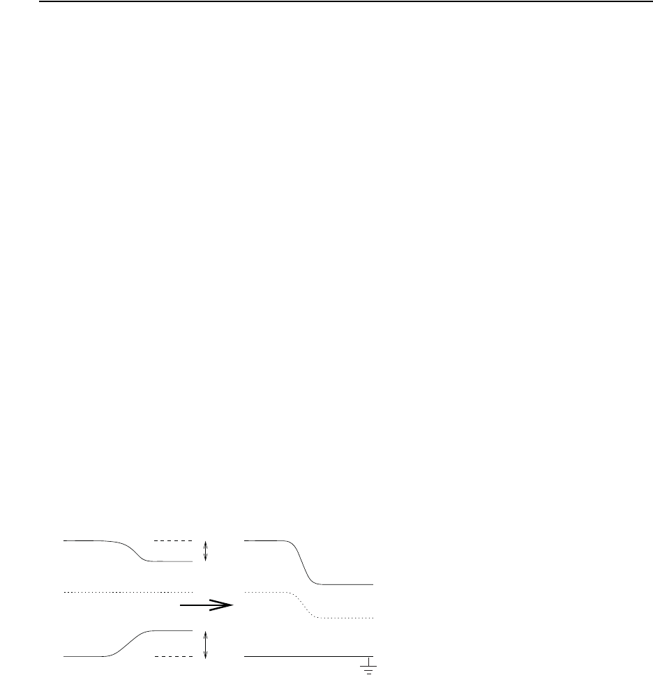
5: Atomistic Kinetic Monte Carlo Diffusion

Fermi-Level Effects: Charge Model

500 Sentaurus™ Process User Guide

I-2013.12

Bandgap Narrowing

Narrowing due to Dopant Concentration

Sentaurus Process KMC includes doping-induced energy shifts of the conductions band

minimum and the valence band maximum. The narrowing of the fundamental band gap is

presented as the function [48] for n-type semiconductors:

(755)

(756)

and for p-type semiconductors:

(757)

(758)

The total bandgap narrowing is:

(759)

Since the distance between bands shrinks, Eq. 759 gives negative values.

Figure 72 Bandgap narrowing; Sentaurus Process KMC assumes the valence band has

zero energy

∆Egdc Acn1/4 N+

1018

----------





1/4

Acn1/3 N+

1018

----------





1/3

Acn1/2 N+

1018

----------





1/2

++=

∆EgdvAvn1/4 N+

1018

----------





1/4

Avn1/3 N+

1018

----------





1/3

Avn1/2 N+

1018

----------





1/2

++=

∆Egdc Acp1/4 N-

1018

----------





1/4

Acp1/3 N-

1018

----------





1/3

Acp1/2 N-

1018

----------





1/2

++=

∆EgdvAvp1/4 N-

1018

----------





1/4

Avp1/3 N-

1018

----------





1/3

Avp1/2 N-

1018

----------





1/2

++=

∆Egd EgdcEgdv

–=

DEv

DEc

Ev=0

5: Atomistic Kinetic Monte Carlo Diffusion

Fermi-Level Effects: Charge Model

Sentaurus™ Process User Guide 501

I-2013.12

Parameters

The parameters and so on are extracted from [47] and are listed in the parameter

database for BandGap in silicon. For the conduction band:

pdbGet KMC Si BandGap Acn1_4

sprocess> pdbGet KMC Si BandGap Acn1_3

-0.01484

sprocess> pdbGet KMC Si BandGap Acn1_2

0.00078

sprocess> pdbGet KMC Si BandGap Acp1_4

-0.01627

sprocess> pdbGet KMC Si BandGap Acp1_3

sprocess> pdbGet KMC Si BandGap Acp1_2

-0.00018

For the valence band:

sprocess> pdbGet KMC Si BandGap Avn1_4

0.01508

sprocess> pdbGet KMC Si BandGap Avn1_3

sprocess> pdbGet KMC Si BandGap Avn1_2

0.00074

sprocess> pdbGet KMC Si BandGap Avp1_4

sprocess> pdbGet KMC Si BandGap Avp1_3

0.01846

sprocess> pdbGet KMC Si BandGap Avp1_2

-0.00263

Narrowing due to Strain

There are two models available for modeling the narrowing due to stress. A simple one and a

full narrowing model.

The full narrowing model is chosen setting the pdb parameter FullNarrowing to true. This

model is the same as in Bandgap Narrowing on page 280:

(760)

(761)

Acn1/4

Eci∆Dci εxx εyy εzz

++()Dcxiεxx Dcyiεyy Dcziεzz

+++=

Evi∆Dvi εxx εyy εzz

++()0.5Dvbi εxx εyy

–()

2εyy εzz

–()

2εzz εxx

–()

++()±=

+Dvdi εxy

2εxz

2εyz

++()

5: Atomistic Kinetic Monte Carlo Diffusion

Fermi-Level Effects: Charge Model

502 Sentaurus™ Process User Guide

I-2013.12

Sentaurus Process KMC also uses the averaged values of conduction and valence bands

energies:

(762)

(763)

defining the narrowing due to strain effects as:

(764)

The simple model computes the narrowing as:

(765)

where the parameter is called DiScalar.

When Ge is present, the narrowing is computed as a linear interpolation between the narrowing

produced by strain for pure Si ( ), and the one for pure Ge ( ). In this way, the total

narrowing for Si1–xGex is:

(766)

where is the relative Ge concentration specified in Si1–xGex.

Parameters

The parameters used for the full model for pure Si are defined in the Sentaurus Process KMC

dataset as:

sprocess> pdbGet KMC Si BandGap EcDilatational

1 -8.6

2 -8.6

3 -8.6

sprocess> pdbGet KMC Si BandGap EvDilatational

1 -2.1

2 -2.1

sprocess> pdbGet KMC Si BandGap EcDeviatoric(1)

1 9.5

2 0.0

3 0.0

Ecs

∆kT 1

---e

Eci∆

------------–

i1=









log–=

Evs

∆kT 1

---e

Evi∆

------------

i1=









log=

∆Egs ∆Ecs ∆Evs

–=

∆Egs Kεxεyεz

++=

∆Egs

∆Egs ∆Egs

Si x∆Egs

Ge ∆Egs

–()+=

5: Atomistic Kinetic Monte Carlo Diffusion

Fermi-Level Effects: Charge Model

Sentaurus™ Process User Guide 503

I-2013.12

sprocess> pdbGet KMC Si BandGap EcDeviatoric(2)

1 0.0

2 9.5

3 0.0

sprocess> pdbGet KMC Si BandGap EcDeviatoric(3)

1 0.0

2 0.0

3 9.5

sprocess> pdbGet KMC Si BandGap EvDeviatoric(1)

1 0.5

2 4.0

sprocess> pdbGet KMC Si BandGap EvDeviatoric(2)

1 0.5

2 4.0

The parameter for the simple model for pure Si is:

sprocess> pdbGet KMC Si BandGap DiScalar

1.75

The parameters used for pure Ge are similar to the ones for pure Si, but with the Ge. prefix:

sprocess> pdbGet KMC Si BandGap Ge.EcDilatational

1 0.59 2 0.59 3 0.59

sprocess> pdbGet KMC Si BandGap Ge.EvDilatational

1 -1.24 2 -1.24

sprocess> pdbGet KMC Si BandGap Ge.EcDeviatoric(1)

1 -9.42 2 0.0 3 0.0

sprocess> pdbGet KMC Si BandGap Ge.EcDeviatoric(2)

1 0.0 2 -9.42 3 0.0

sprocess> pdbGet KMC Si BandGap Ge.EcDeviatoric(3)

1 0.0 2 0.0 3 -9.42

sprocess> pdbGet KMC Si BandGap Ge.EvDeviatoric(1)

1 2.55 2 5.50

sprocess> pdbGet KMC Si BandGap Ge.EvDeviatoric(2)

1 2.55 2 5.50

sprocess> pdbGet KMC Si BandGap Ge.DiScalar

1.75

Finally, the simple (0) or full (1) narrowing models are selected:

sprocess> pdbGet KMC Si BandGap FullNarrowing

5: Atomistic Kinetic Monte Carlo Diffusion

Fermi-Level Effects: Charge Model

504 Sentaurus™ Process User Guide

I-2013.12

Narrowing due to Presence of an Alloy

The narrowing due to an alloy concentration is computed as (assuming, in this example, that

Ge is the alloy in Si material):

(767)

where is the germanium concentration, and are the parameters needed for the

quadratic interpolation between the silicon gap (1.12 eV) and the Ge gap (0.78 eV). They are

respectively called GeNarrowing and GeNarrowing2.

Parameters

sprocess> pdbGet KMC Si BandGap GeNarrowing

6.8e-24

sprocess> pdbGet KMC Si BandGap GeNarrowing2

This is simply (1.12-0.78)/5e22.

Bandgap Narrowing Use

The value of , computed as:

(768)

is used to correct , , , and the dopant levels in the gap, . For these last

ones, they are assumed to be proportional to the band gap. This means that these new values,

after applying the bandgap narrowing correction, are:

(769)

It is interesting to note that .

Whenever a Sentaurus Process KMC model needs a bandgap level, the bandgap narrowing–

corrected value is used. The only exception is the activation energy for the impurity pair

emission from impurity clusters where the narrowing correction can be controlled by:

pdbSet KMC <material> BandGap Correct_Complex <false/true>

NOTE The bandgap narrowing due to doping, stress, and SiGe is always

switched on by default. To disable it, set the proper parameters to zero.

∆EgGe Ge[]β

1β2Ge[]+()–=

Ge[]

β1β2

∆Eg

∆Eg∆Egdop ∆Egs ∆EgGe

++=

ejj 1+,()A()

corrected ejj 1+,()A()1∆Eg

----------+





∆Eg0<

5: Atomistic Kinetic Monte Carlo Diffusion

Fermi-Level Effects: Charge Model

Sentaurus™ Process User Guide 505

I-2013.12

Charge Model and Boron Diffusion Example

The known charged states of Bi are Bi–, Bi0, and Bi+ [21][22]. The three states are included in

Sentaurus Process KMC, although the inclusion of Bi+ is only important for systems far from

equilibrium. The pairing, breakup, and charge reactions related to Bi are represented in the

current Sentaurus Process KMC model by the reactions:

(770)

(771)

(772)

(773)

Direct breakup of Bi+ is not included because I++ is not implemented. Boron effective

diffusivity is given by the sum of the contribution of all mobile species:

(774)

Using the Maxwell–Boltzmann approximation, the previous equation is usually written as:

(775)

where is the interstitial supersaturation, and and are the hole concentration and the

intrinsic concentration, respectively.

The relations between the above diffusivity components and the microscopic parameters are

[46]:

(776)

(777)

I0B-

+Bi

↔

I+B-

+Bi

↔

-Bi

0Bi

↔↔

I0I+

↔

DB()

DB() DB

()

[]

B-

[]

----------DB

()

[]

B-

[]

-----------DB

()

[]

B-

[]

-----------++=

DB() SIDXB() DPB()

---- DPP B()p

----





++=

DXB() vcaptDI

()I0

[]

*νmBi

()

νbreak Bi

()

--------------------------

DPB() vcaptDI

()I0

[]

*νmBi

()

νbreak Bi

()

-------------------------- eB

()0-,()ei

–

kBT

------------------------------------





exp=

5: Atomistic Kinetic Monte Carlo Diffusion

Fermi-Level Effects: Charge Model

506 Sentaurus™ Process User Guide

I-2013.12

(778)

is the intrinsic level.

These expressions can be used as a bridge between the parameters of continuum simulators and

those used by Sentaurus Process KMC. The above continuum expression assumes Maxwell–

Boltzmann and quasi-equilibrium conditions, which are not needed in Sentaurus

Process KMC.

Charge Model and Arsenic Diffusion Example

A similar analysis can be performed for arsenic, which has both vacancy and interstitial

contributions, related to AsV and Asi defects. The arsenic reactions are:

(779)

(780)

(781)

(782)

and:

(783)

(784)

(785)

(786)

(787)

DPP B() vcaptDI

()I0

[]

*νmBi

()

νbreak Bi

()

--------------------------eB

()0-,()eB

()+,0()2ei

–+

kBT

------------------------------------------------------------------------





exp=

I0As+

+Asi

↔

I-As+

+Asi

↔

I0I-

↔

Asi

+Asi

↔

V0As+AsV+

↔+

V-As+AsV0

↔+

V-- As+AsV-

↔+

V0V-V--

↔↔

AsV+AsV0AsV-

↔↔

5: Atomistic Kinetic Monte Carlo Diffusion

Interfaces and Surfaces

Sentaurus™ Process User Guide 507

I-2013.12

All the previously mentioned contributions are included in KMC. Consequently:

(788)

which in continuum models is usually reduced to:

(789)

is the fraction of interstitial-assisted diffusion. Note, however, that this last continuum

description conveys several simplifying assumptions compared with the model included in

Sentaurus Process KMC. The common assumption that and fit an Arrhenius plot is

only true if the contributions of AsV+ and Asi+ have the same activation energy. The same

applies for the AsV0 and Asi0 contributions. The continuum equation also assumes that the

interstitial fraction, , is independent of the Fermi level (the same for the three charged states)

and is independent of the temperature.

Interfaces and Surfaces

An interface is the extension between two regions with different materials. The most common

interface is the silicon–oxide interface. Sentaurus Process KMC allows for modeling all

interfaces between two different materials.

As explained in Materials and Space on page 398, Sentaurus Process KMC divides the space

in small rectangular elements and assigns to each of them a material. The interfaces are the set

of element faces between different materials.

The element faces are independent. The interface behaves as the sum of all of its faces, but such

an ‘interface’ does not really exist. What exists are the element faces, all of them emitting and

trapping with different rates depending on its area, local stress, and so on. In the following

sections, these element faces are called interface.

Interfaces set the equilibrium concentration for self-silicon point defects and the solubility

concentration for impurities. Sentaurus Process KMC models the interfaces differently for

silicon point defects than for impurities.

DAs() DAsV

()

AsV+

[]

As+

[]

------------------DAs

()

Asi

[]

As+

[]

--------------DAsV

()

AsV0

[]

As+

[]

----------------- DAs

()

Asi

[]

As+

[]

--------------DAsV

()

AsV-

As+

[]

--------------

++ ++=

DAs() fISI1fI

–()SV

–[]DXAs()DMAs()

---- DMM As()

----





++×=

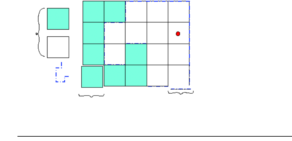
5: Atomistic Kinetic Monte Carlo Diffusion

Interfaces and Surfaces

508 Sentaurus™ Process User Guide

I-2013.12

Figure 73 Sentaurus Process KMC interfaces are the set of element faces between

different materials

Different Interface Models

The parameter Model specifies the behavior of an interface:

pdbSet KMC Oxide_Silicon Model Allcharges

The different models are:

Allcharges

Three-phase segregation model for dopants. Emission and capture of all the

charge states of point defects on materials with full modeling. Capture of

all the charge states of impurity-paired defects on materials with full

modeling.

Amorphous

When one material is full and the other is simple, this interface acts as an

asymmetric mirror. Particles going from the simple to the full material

are reflected, while particles going from the full to the simple material

are allowed to pass. No trapping or emission of particles on either side.

Interface

Three-phase segregation model for dopants. Emission and capture of neutral

point defects on materials with full modeling.

none

No interface between materials. This model is only possible when the model

of the materials involved in the interface is the same; that is, both are

simple or full.

Reflective

The interface acts as a mirror. Particles are not trapped. No emission of

particles on either side.

Boxes

SiO2

Interface

Small Box Face

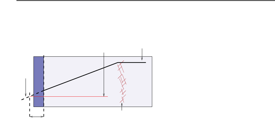
5: Atomistic Kinetic Monte Carlo Diffusion

Interfaces and Surfaces

Sentaurus™ Process User Guide 509

I-2013.12

Interfaces for Self-Silicon Point Defects

It is common to define a recombination length as the distance from the surface needed to

obtain the equilibrium concentration (see Figure 74).

Figure 74 Recombination length is the distance between the interface and the point in which

the prolongation of the point-defect concentration joins its equilibrium

concentration

The microscopic meaning of can be associated with the probability of a point defect being

trapped at the surface:

(790)

where is the point-defect jumping distance. The smaller , the better sink is the surface.

For interstitials in the silicon–oxide interface, it is close to a perfect sink with < 5 nm

[49][50].

Capture

Interfaces capture neutral interstitials and vacancies with the probability set in Eq. 790. When

is set to zero, the probability is set to 1, a perfect sink.

Emission

In [1], the point-defect (for example, interstitials) equilibrium concentration is related to the

interface frequency emission prefactor and energy as:

(791)

Extended defects ({311})

creating I supersaturation

I concentration

I equilibrium concentration

Silicon bar

Surface

Prolongation

x = 0

Recombination length

Ptrap

-----=

I[]

---D0FS

--------------EfI()

kBT

------------–





exp×=

5: Atomistic Kinetic Monte Carlo Diffusion

Interfaces and Surfaces

510 Sentaurus™ Process User Guide

I-2013.12

where the surface frequency emission is:

(792)

where:

■sites is the number of capture sites in the interface (proportional to its surface and equal

to ).

■ is the surface emission prefactor.

■ and are the migration and formation energies of the point defects, respectively.

■ are the regular corrections to migration and formation due to stress.

■ are the corrections to migration and formation due to Ge concentration,

explained below.

The point defects are emitted from a randomly chosen position at the surface. Only neutral Is

or Vs are emitted when the interface model is Interface. All charge states are emitted and

captured when using Allcharges. In equilibrium, these two models give the same results.

Stress

The presence of stress changes the migration and formation energy of interstitial and vacancies

and, consequently, the emission frequency. Each interface (where, as previously stated,

interface was called to the independent element faces) is oriented in a unique axis ‘j’, and the

projections of the principal axes into ‘j’ should be accounted. Then, the total emission

frequency is:

(793)

where are the projections of the principal axis into the surface axis. Finally, for each axis,

the migration and formation energies including stress effects are computed as:

(794)

where , , and are the perpendicular and parallel activation volumes for

diffusion and the activation volume for formation, respectively.

For more information on these parameters and the stress models, see Stress Effects on Point

Defects, Impurities, Dopants, and Impurity-Paired Point Defects on page 428.

νsites Ptrap

×D0FS 6

λ2

----- D0m,

×Em∆Em

stress ∆Em

Ge Ef∆Ef

stress ∆Ef

+++++

kBT

-----------------------------------------------------------------------------------------------------------------–







exp×=

----- YZ

D0FS

∆Em

stress ∆Ef

stress

∆Em

Ge ∆Ef

νPjaxisνaxis

axis

x'y'z',,



Pjaxis

stress Ef

stress

+EmEfσ'axis∆Vpar σ'i∆Vort

---∆Vfσ'i



iaxis≠



++ +=

∆Vort

∆Vpar

∆Vf

5: Atomistic Kinetic Monte Carlo Diffusion

Interfaces and Surfaces

Sentaurus™ Process User Guide 511

I-2013.12

Alloys

The presence of an alloy (assumed to be Ge in this example) changes the migration and

formation energy of point defects in the following way:

(795)

(796)

where is the germanium concentration, and are the dependencies of migration and

formation with germanium, specified as EmGe and EfGe in the PDB.

Parameters

The parameters that control the point-defect interface model can be found in the PDB by

looking in the Oxide_Silicon folder. By default, interfaces, other than the oxide–silicon

interface, have their point-defect interface model set to None and do not require any

parameters. The formation energies are listed for the material, not for the interface.

For example, the formation energy of interstitials in silicon is under Silicon, not in

Oxide_Silicon or any other interface.

The migration energies are displayed in the point defect section of the file (see Point Defects,

Impurities, Dopants, and Impurity-paired Point Defects on page 415). The surface values can

be easily obtained using the command line.

For example, for interstitials and vacancies in the silicon–oxide interface:

sprocess> pdbGet KMC Oxide_Silicon I D0FS_Si

5000.0

sprocess> pdbGet KMC Silicon I Ef

4.0

sprocess> pdbGet KMC Oxide_Silicon I RecLnm_Si

sprocess> pdbGet KMC Oxide_Silicon V D0FS_Si

800.0

sprocess> pdbGet KMC Silicon V Ef

3.8

D0FS_Mat Surface emission prefactor, . Mat is the short name of the

material.

Ef Formation energy, .

RecLnm_Mat Recombination length, . Mat is the short name of the material.

∆Em

Ge αGe[]=

∆Ef

Ge βGe[]=

Ge[]

αβ,

D0FS I()

EfI()

5: Atomistic Kinetic Monte Carlo Diffusion

Interfaces and Surfaces

512 Sentaurus™ Process User Guide

I-2013.12

sprocess> pdbGet KMC Oxide_Silicon V RecLnm_Si

and for vacancies in the silicon–gas interface:

sprocess> pdbGet KMC Gas_Silicon V D0FS_Si

800.0

sprocess> pdbGet KMC Gas_Silicon V RecLnm_Si

sprocess> pdbGet KMC Si V Ef

3.8

NOTE Yo u ca n mo dify t hese va lue s. Cha nges in the formation energy or

surface emission prefactor will modify the DC equilibrium product of

point defects and the diffusivity of all the species. A change, both in the

formation and migration parameters, that maintains the DC product

constant will not produce this undesirable effect, but may change the

extended defects dissolution times.

Oxidation-enhanced Diffusion (OED) Model

The current flux of I (V) across an outer surface in Sentaurus Process KMC is described in the

previous model as:

(797)

being:

(798)

and the jumping distance. An extra term is included to account for oxidation:

(799)

This term tries to combine the Sentaurus Process continuum model (see Surface

Recombination Model: PDependent on page 358) with an atomistic implementation. In

particular, its definition is:

(800)

where is a vectorial prefactor and is the normal to the interface, so that gives the

proper component for a planar, axis-oriented, interface in an internal element.

jn⋅KsI[] I*

[]–()=

---νmI()λ

2Lr

⁄=

jn⋅KsI[] I*

[]–()Gox

–=

Gox

Gox θn⋅()Vox Gscale

Vox

Vscale

--------------







Gpow EθP∆Vθ

kBT

---------------------------–





exp=

θn⋅()

5: Atomistic Kinetic Monte Carlo Diffusion

Interfaces and Surfaces

Sentaurus™ Process User Guide 513

I-2013.12

is the ReactionSpeed computed by the PDE solver in Sentaurus Process and used here

by Sentaurus Process KMC. and are additional model parameters to adjust the

interstitial injection. is a term defined to account for Fermi-level effects, and defined

similarly to the continuum one as:

(801)

is the activation energy for point-defect injection and, finally, is a parameter to include

a hydrostatic dependency for OED.

Consequently, this is a hybrid model in which the continuum solver computes and generates a

ReactionSpeed value to be used by Sentaurus Process KMC to compute the point-defect

injection prefactor.

NOTE Boundary movement is allowed in this model and is switched on by

default. This implies that the model serves to generate a more adequate

point-defect injection from the interface during oxidation processes,

while a remeshing mechanism changes the oxide thickness. If you do

not want the oxide thickness to change, set Grid

Reaction.Modify.Mesh to 0.

Parameters

Table 56 lists the parameters defined for the oxide–silicon interface only.

To use this model, call diffuse with any oxidation parameter (for a list of oxidation

parameters for diffuse, see diffuse on page 908).

Ta bl e 56 Par am et e rs us ed i n OE D m od e l

Parameter name Description

ox_Etheta

Activation energy .

ox_xtheta, ox_ytheta, ox_ztheta

Components for the vector used as a prefactor.

ox_VFtheta

Pressure correction .

ox_Vscale, ox_Gpow

ReactionSpeed control: and .

ox_pp, ox_p, ox_Ep, ox_m, ox_mm,

ox_Em, ox_pot

Parameters used to compute the Fermi-level dependencies introduced

by . In particular, prefactor and activation energies for pp, p,

m, and mm terms, and exponent.

Vox

Vscale

Gpow

Gscale

mm m 1ppp++++

mm n

----





2PotOx mn

----





PotOx 1pn

----





PotOx–pp n

----





2PotOx–

+++ +

--------------------------------------------------------------------------------------------------------------------------------------------------------------=

Eθ

∆Vθ

Eθ

∆Vθ

Vscale

Gpow

Gscale

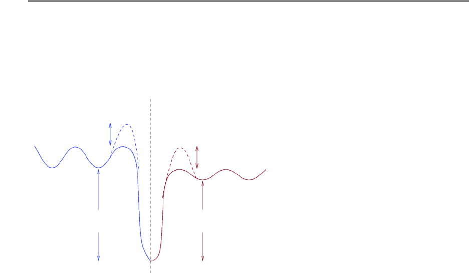
5: Atomistic Kinetic Monte Carlo Diffusion

Interfaces and Surfaces

514 Sentaurus™ Process User Guide

I-2013.12

Interfaces for Impurities

The interface model of impurities in Sentaurus Process KMC follows a three-phase segregation

model. Particles can be emitted to both sides of the interface or can stay trapped at the interface.

Figure 75 shows the atomistic mechanisms and energies for trapping and detrapping

impurities.

Figure 75 Dopants reaching the interface may be trapped by it with a different binding

energy for each interface side. Energy barriers for capture and emission also can

be present.

These interfaces are modeled between any two materials; however, depending on the material

model, the interface will behave differently.

Simple Material Side

The simple material side faces a material using the simple model. In these materials, only

direct diffusion of dopants is allowed. Since there are no paired dopant impurity point defects,

the model is as follows: Dopants arriving at the nonsilicon side may be captured with certain

probability, and they can be remitted later.

Capture

The capture probability is:

(802)

Oxide/Silicon Interface

Barrier (Si)

SiliconOxide

Barrier (Ox)

Binding (Ox) Binding (Si)

Pnon-Sicap A() Barrier A() kBT()⁄–()1Trapped A()

MaxTrapped A()

-------------------------------------------–





exp=

5: Atomistic Kinetic Monte Carlo Diffusion

Interfaces and Surfaces

Sentaurus™ Process User Guide 515

I-2013.12

where is the dopant being trapped, Barrier is the barrier energy, Trapped is the number of

particles trapped at the interface, and MaxTrapped is the maximum number of them that can be

trapped.

If the particle is trapped, there is a probability to evaporate (annihilate) the just-trapped dopant.

Emission

Interfaces emit particles to the nonsilicon side with a frequency given by:

(803)

The emission is proportional to the number of trapped dopants and to a parameter Pref that

acts as a prefactor. The emission energy is:

(804)

The migration energy contains stress and Ge corrections. The binding energy contains a

pressure correction:

(805)

Parameters

The energy barrier to a nonsilicon interface is introduced as EBarrier_Surf<mat>, where

<mat> is Si, aSi, Ox, Ni, Po Gas, and Unknown, or any other user-defined material short name:

The values are always specified in the interface parameter file:

sprocess> pdbGet KMC Oxide_Silicon B EBarrier_SurfOx

B 0.1

Si Silicon

aSi Amorphous silicon

Ox Oxide

Ni Nitride

Po PolySilicon

Gas Gas

Unknown Unknown

νnon-Siemiss A() Trapped A()Pref Ener kBT()⁄–()exp=

Ener A() Barrier A() EmA() Binding A()++=

∆Eb

surface A() P∆Vb

surface A()=

5: Atomistic Kinetic Monte Carlo Diffusion

Interfaces and Surfaces

516 Sentaurus™ Process User Guide

I-2013.12

The probability to evaporate a trapped particle is called Evaporation_Surf:

sprocess> pdbGet KMC Oxide_Silicon B Evaporation_Surf

B 0 Bi 0

The pressure correction to the binding energy of the dopants to the surface is given by the

parameter VF_Surf<mat>:

sprocess> pdbGet KMC Oxide_Silicon B VF_SurfOx

The maximum number of trapped particles per cubic centimeter follows an Arrhenius plot with

prefactor C0Max_Surf:

sprocess> pdbGet KMC Oxide_Silicon B C0Max_Surf

2e+14

and energy EMax_Surf:

sprocess> pdbGet KMC Oxide_Silicon B EMax_Surf

The prefactor for emission is called Db_Surf:

sprocess> pdbGet KMC Oxide_Silicon B Db_Surf

B 1e-3

Finally, the binding energy of dopants is Eb_Surf<mat>:

sprocess> pdbGet KMC Oxide_Silicon B Eb_SurfOx

B 0.28

Full Material Side

The particles transporting dopants (or impurities) in materials with full modeling are not

typically the dopants themselves, but impurity-paired point defects. In other words, an impurity

plus an interstitial or a vacancy. When these pairs reach the interface, if they are trapped, the

accompanying interstitial or vacancy is recombined, and the dopant itself is piled at the surface.

Consequently, the dopant cannot be emitted unless an incoming interstitial or vacancy reacts

with it, carrying it away from the interface.

Capture

Neutral (or charged, if the model Allcharges is selected) impurity-paired point defects are

trapped at the surface with a probability given by:

(806)

PSicap Ai

() Barrier Ai

()kBT()⁄–()1Trapped A()

MaxTrapped A()

-------------------------------------------–





exp=

5: Atomistic Kinetic Monte Carlo Diffusion

Interfaces and Surfaces

Sentaurus™ Process User Guide 517

I-2013.12

Different barriers can be assigned to andand, consequently, different recombination

probabilities. The number of trapped particles and maximum trapped particles is assigned to

the interface and is shared between both sides.

Emission

Particles are not emitted by themselves, but the interface allows particles to be moved to the

material bulk. Point defects (interstitials and vacancies) can react with the dopants trapped at

the surface, forming mobile impurity-paired point defects. The probability of these reactions

being successful depends on the binding of the dopant to the surface and the barrier energy:

(807)

where:

(808)

The binding is corrected with a pressure-dependent term:

(809)

Parameters

The parameters that control the maximum number of trapped particles have already been

discussed in Simple Material Side on page 514. The barrier energy is called

EBarrier_SurfSi:

sprocess> pdbGet KMC Oxide_Silicon As EBarrier_SurfSi

Asi 0.0

AsV 0.0

and the binding energy is Eb_SurfSi:

sprocess> pdbGet KMC Oxide_Silicon As Eb_SurfSi

Asi 0.1

AsV 0.1

The stress correction is given by:

sprocess> pdbGet KMC Oxide_Silicon B VF_SurfSi

Pemiss

Si Ai

() Ener Ai

()kBT()⁄–()exp=

Ener Ai

() Binding Ai

()Barrier Ai

()+=

∆Eb

surface Ai

() P∆Vb

surface Ai

()=

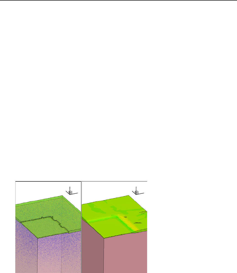
5: Atomistic Kinetic Monte Carlo Diffusion

Oxidation

518 Sentaurus™ Process User Guide

I-2013.12

Oxidation

Sentaurus Process KMC is fully coupled with oxidation. Consequently, any oxidation

conditions issued in the diffuse command of Sentaurus Process are transferred to Sentaurus

Process KMC. Setting Grid DoNotMove.Reaction to 1 (it is 0 by default) disables

boundary movement at the oxide–silicon interface. Otherwise, the Sentaurus Process oxidation

algorithm is allowed to work during the reaction step, and the new structure (with expanded

oxide) is imported into Sentaurus Process KMC immediately before the atomistic diffusion

step. The velocities at which the interfaces and the oxide move are used to compute the

displacement of the particles.

Sentaurus Process KMC uses the displacement to relocate the displaced particles and finishes

the remeshing. After this, regular atomistic diffusion occurs. Since there are several

interpolations performed in this process, minor inaccuracies in the final position of particles

can be introduced during remeshing, especially during large oxidations. Regular diffusion

occurring at the same time as oxidation should make these interpolation inaccuracies

negligible.

In principle, Sentaurus Process KMC can be used successfully for 1D, 2D, and 3D oxidation.

In particular, since the precision of the Sentaurus Process KMC solution does not depend on a

fine continuum mesh, a coarse Sentaurus Process mesh can be specified, increasing the

stability of oxidation, while the Sentaurus Process KMC part takes care of the position of

particles. The example in Figure 76 shows the results of such an approach.

Sentaurus Process KMC also allows OED (see Oxidation-enhanced Diffusion (OED) Model

on page 512).

Figure 76 Example of Sentaurus Process KMC coupled with an oxidation in 3D: (left) KMC

simulation in which the internal mesh is coupled to (right) continuum oxidation

simulation

5: Atomistic Kinetic Monte Carlo Diffusion

Epitaxial Deposition

Sentaurus™ Process User Guide 519

I-2013.12

Epitaxial Deposition

Epitaxial deposition can be performed by using one of the following:

■Regular Sentaurus Process epitaxy

■Native epitaxial deposition using an LKMC model based on [51]

This section describes the native epitaxy model only. The model is switched off by default and

must be switched on for the native epitaxy:

pdbSet KMC Epitaxy true

The model shares many features with LKMC (to fully understand this model, see LKMC: Fully

Atomistic Modeling of Solid Phase Epitaxial Regrowth on page 463).

NOTE The native epitaxy model can be used in both atomistic and

nonatomistic modes. When used in the nonatomistic mode with the

parameter lkmc specified on the diffuse command, doping and

diffusion are controlled by the continuum solver,. The deposition shape

is controlled by KMC. For more information, see Using LKMC for

Deposition Shape on page 283 .

The model introduces the silicon lattice and assigns a flag to each lattice position. This flag is

switched on for lattice positions that match the silicon material and is switched off for positions

lying in the gas. The simulator assigns a frequency to all the off positions to become on, that

is, to accept a silicon atom (coming from the gas). Only off lattice positions that have an on

lattice in the neighborhood have a frequency different from zero. Consequently, the silicon

grows slowly, simulating an epitaxial deposition.

The frequency for an off position at the silicon–gas interface to accept a silicon atom and

become on is:

(810)

where is the frequency for selective epitaxial growth (SEG), very similar to the one

written in Eq. 706, p. 464:

(811)

is a prefactor that accounts for the local microscopic growth for each

configuration. This prefactor depends on two variables: n and m. n can be 100, 110, or 111

defined very similarly to K(1), K(2), and K(3) in LKMC: Fully Atomistic Modeling of Solid

Phase Epitaxial Regrowth on page 463. m is used to distinguish between configurations with

νEpi K'νSEG

LKMC

×=

νSEG

LKMC

νSEG

LKMC KSEG

LKMC site() ESEG

LKMC ∆Esite()+

kBT

---------------------------------------------–







exp×=

KSEG

LKMC site()

5: Atomistic Kinetic Monte Carlo Diffusion

Epitaxial Deposition

520 Sentaurus™ Process User Guide

I-2013.12

the same n but different second neighbor coordination numbers. In this model, also published

in [51], 100 configurations only are split into three different ones: 100, 100.7, and 100.8 for

100 configurations with six or fewer, seven, and 8 or more second neighbor coordination

numbers.

is a correction energy applied to special sites. It is used to simulate the formation of

{311} facets during SEG. As such, only 1 site is defined to have a non null correction: the

{311} local configuration. This configuration is in two different situations a) and b). a) is a

(100) generic site that lacks half of its third neighbors, and b) is a (110) where the second atom

in the chain needed to define the place as 110 would have first coordination number equal to 2.

Assigning a slower rate to configuration a) prevents the {311} facet becoming a {111} facet.

The slower rate for configuration b) assures that the local {311} configuration is not broken by

a lateral (110) regrowth.

is an empirical factor to fit the epitaxial deposition thickness to the specified thickness. This

empirical factor is computed automatically by Sentaurus Process KMC trying to match the

thickness specified in the processing conditions. In particular:

(812)

where:

■thickness is the specified thickness.

■time is the annealing time.

■ is the length of a nanolayer of recrystallized silicon. A nanolayer is assumed to be

half the lattice constant.

■ is the frequency for recrystallization in a

pure (100) substrate.

■ is an empirical constant, available in the PDB as Damage

prefactor.thickness, that relates the microscopic growth of a lattice atom in a (100)

local neighborhood with the macroscopic growth of a (100) substrate.

This epitaxial deposition can create {111} facets and maintain the same (100):(110):(111)

growth rate as SPER. Under regular selective epitaxial conditions, the shapes generated agree

with experimental ones.

At the end of the LKMC epitaxial deposition, the simulator smooths the generated atomistic

interface and reinserts it into Sentaurus Process. The algorithm used to mesh the atomistic

shape uses the parameter KMC Simplify.Geometry. A bigger value provides a faster and

more stable insertion, but with a loss of surface details.

The inclusion of doping is possible during LKMC epitaxy. If a doping profile with a linear

change is indicated, the included doping will be linear with time, and not with thickness.

∆Esite()

K'Kthickness thickness νSEG

LKMC 100()time Knanolayer

××()⁄×=

Knanolayer

νSEG

LKMC 100()K100() ESEG

LKMC kBT()⁄–()exp×=

Kthickness

5: Atomistic Kinetic Monte Carlo Diffusion

Epitaxial Deposition

Sentaurus™ Process User Guide 521

I-2013.12

Finally, the generation of an LKMC starting surface from Sentaurus Process and the reinsertion

after LKMC epitaxy are delicate and time-consuming operations if they are performed only

once at the start of the diffuse command and at the end. This means that the state of the

simulator at intermediate steps during the diffuse command may not be synchronized with

the KMC simulator.

NOTE To avoid problems, the KMC Movie command is disabled during LKMC

epitaxy. In addition, the diffuse movie command must not be used

during LKMC epitaxial deposition.

Parameters

The parameters needed for this model are defined in the parameter database under KMC Si

Epitaxy. Table 57 lists the parameters for the site prefactors.

Table 58 lists the parameters for the activation energies.

Table 59 lists the parameters for the thickness.

As an example, some of these parameters can be obtained as:

sprocess> pdbGet KMC Si Epitaxy prefactor.SEG.100

3.3e+15

Table 57 Parameters for site prefactors

Parameter Description

prefactor.SEG.100.8

For (100) sites with 8 or more second neighbor coordination number

prefactor.SEG.100.7

For (100) sites with 7 second neighbor coordination number

prefactor.SEG.100

For (100) sites with 6 or fewer second neighbor coordination number

prefactor.SEG.110

For (110) sites

prefactor.SEG.111

For (111) sites

Table 58 Parameters for activation energies

Parameter Description

energy.SEG

Overall activation energy for SEG

energy.SEG.311

Correction for 311 planar SEG

Table 59 Parameters for the thickness

Parameter Description

prefactor.thickness

Empirical factor to fit the thickness in epitaxial growth

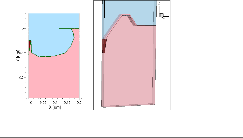
5: Atomistic Kinetic Monte Carlo Diffusion

Including New Impurities

522 Sentaurus™ Process User Guide

I-2013.12

sprocess> pdbGet KMC Si Epitaxy prefactor.SEG.100.8

1.8e+18

sprocess> pdbGet KMC Si Epitaxy prefactor.SEG.111

3.5e+14

sprocess> pdbGet KMC Si Epitaxy energy.SEG

2.7

Figure 77 shows an example of epitaxial deposition using LKMC.

Figure 77 (Left) Initial shape and (right) final shape after LKMC epitaxial deposition with

thickness of 175 nm

Including New Impurities

You can customize Sentaurus Process KMC to include other impurities not supported by

default. The modifications affect the parameter database and the file KMC.tcl. Nevertheless,

it is not necessary or recommended to modify the files included in the Sentaurus Process

distribution. All the modifications can be included in the input file.

For the parameter database, the pdbSet family of commands allows overwriting previous

values or defining new ones. For the procedures written in the file KMC.tcl, defining the new

procedure in the input file is enough; the new one will be executed instead of the old one.

The modifications include the following:

1. Include the new impurity X in Sentaurus Process KMC under the label named

KMC Impurities.

5: Atomistic Kinetic Monte Carlo Diffusion

Including New Impurities

Sentaurus™ Process User Guide 523

I-2013.12

2. Include the impurity-related particle pairs (Xi or XV or both) in KMC Pairs (see Particles

in Models on page 410). If your model does not have impurity pairs (in other words,

simple material), you do not need to specify them, including Dm and Em.

3. Be careful about which charge states you include because not all are allowed; you must

specify parameters for all those included.

4. Include possible aliases for the particle in KMC Aliases. If the particle already exists for

Sentaurus Process, include this name as an alias in Sentaurus Process KMC (see Alias on

page 411).

5. You can customize the colors for this particle (although it is optional) in Tecplot SV in

KMC Colors (see Colors on page 411).

6. To create parameters for the new particle, define the parameters explained in Particles and

Parameters on page 411 under KMC <mat> X, where <mat> is every material defined in

your simulation, and X is the name of the new defined dopant. Be sure to include all of

them. Parameters for the impurity cluster model are not needed if Implement_Complex

is set to false. All others require values since they specify how the surface and amorphous

regions interact with the new dopant X.

7. Specify the reactions for KMC <mat> X in ReactionsPointDefect. Typical reactions

here include the pair formation (such as X,I true) and impurity cluster formation (such

as Xi,X true). These reactions only need to be defined in materials with the full model.

8. Specify also the reactions with damage and extended defects if there are any. You can leave

these fields empty. See Interaction with Impurities on page 441, Interactions on page 446,

Interactions on page 450, and Interactions on page 454.

If you include impurity clusters, ensure the following:

1. Define reactions that create impurity clusters from two isolated particles.

2. Enable the right impurity clusters for your simulation with Implement_Complex (see

Impurity Clusters on page 472).

3. Fill the parameters for the impurity clusters. You can leave the energy barriers empty, but

you must specify Etotal_Complex energies and CaptVol_Complex capture volumes.

4. Write the reactions for your impurity clusters. If you have specified an energy for a

particular impurity cluster, then that impurity cluster should be reachable through some

reactions. Include the reactions with dopants and point defects in ReactionsCluster

(see Interactions on page 487).

5. If you need dopant deactivation without diffusion for high concentrations, see Percolation

on page 477.

5: Atomistic Kinetic Monte Carlo Diffusion

Including New Impurities

524 Sentaurus™ Process User Guide

I-2013.12

Finally, you must define some variables set in the KMC.tcl file placed in TclLib. This can

(and should) be performed locally in your input file:

1. Add the names of your new impurities and pairs to the nameOf array.

2. Complete the map of MC implantation to Sentaurus Process KMC with MCnameOf.

If you need to transfer information back and forth from continuum to KMC, you also must

modify the procedures PDE2KMCUser and KMC2PDEUser:

■Add the new particles and clusters to the lists in PDE2KMCUser. The first field is the field

name in Sentaurus Process (continuum models), the second is the name in Sentaurus

Process KMC, and the third is the conversion factor. For example:

fproc PDE2KMCUser {} {

return "Dopant X 1 \

DopantInt Xi 1 \

DopantVac XV 1 \

DopantCluster X2 .5 \

DopantCluster X3 .3333"

}

■Add the new particles in KMC2PDEUser. The first name is the name in Sentaurus

Process KMC, the second is the Sentaurus Process field, and the third is the factor. For

example:

fproc KMC2PDEUser { } {

return "X Dopant 1\

Xi DopantInt 1\

XV DopantVac 1\

X2 DopantCluster 1\

X3 DopantCluster 1.5\

X4 DopantCluster 2"

}

NOTE MCnameOf can be used to manipulate some KMC species without

actually implementing them. For example, an unknown implant can be

performed to simulate preamorphization. If Sentaurus Process KMC

does not support the unknown dopant, use

set MCnameOf(dopant) "I" to instruct the MC implantation code

to pass the dopant atoms as interstitials to Sentaurus Process KMC. This

way, all of the damage generated by an unknown dopant implant will be

correctly calculated and passed, and the dopant ions will be considered

to be silicon interstitials by Sentaurus Process KMC.

5: Atomistic Kinetic Monte Carlo Diffusion

Including New Impurities

Sentaurus™ Process User Guide 525

I-2013.12

Impurities Diffusing without Pairing

Sentaurus Process KMC allows impurities to diffuse using two different mechanisms:

■Normal diffusion

■Diffusion without pairing

Normal Diffusion

For impurities with +1 or –1 charge, in other words, dopants, the substitutional dopant is active,

but it does not diffuse. The substitutional dopant reacts with interstitials or vacancies, forming

a pair that diffuses. These pairs break up with a given frequency, releasing the dopants back

into the substitutional positions.

Diffusion without Pairing

For neutral impurities, the normal diffusion is still available. An alternative diffusion

mechanism is migration without pairing. In these cases, the impurity diffuses as it is, that is,

the substitutional impurity has a nonzero diffusivity and continues forming pairs with point

defects.

Diffusion without pairing has the following characteristics:

■The impurity has nonzero diffusivity. The pairs can exist, but they do not have to diffuse:

sprocess> pdbGet KMC Silicon F Dm

F 5e-3

FV 0

FI 0

sprocess> pdbGet KMC Silicon F Em

F .8

FV 5

FI 5

■When a pair (for example, FI) breaks up, Eq. 661 and Eq. 662, p. 420 still apply. The

migration energy of the impurity is not accounted for.

■The impurities cannot interact with extended defects, but their pairs can, as explained in

Extended Defects on page 442.

■Impurities interact with interfaces. Interfaces re-emit impurities.

■Impurity clusters are possible with some variations:

• Reactions within the impurities (for example, F + F) apply to the moving particles and

not only the percolation model.

5: Atomistic Kinetic Monte Carlo Diffusion

Reports

526 Sentaurus™ Process User Guide

I-2013.12

• Impurity clusters emit point defects and impurities, as explained in Emission on

page 436, but the capture and emission reactions for impurities are:

(813)

• Consequently, the binding energies involved in the capture and emission of impurities

will be:

(814)

• Recombination, FT, and complementary FT mechanism are implemented as well. The

binding energies for them are not changed since the emission recombination of Ai (for

AnIm clusters) or AV (for AnVm clusters) is not involved.

Reports

Sentaurus Process KMC prints several reports in the log file including:

■Models used

■Particle distribution

■Cluster distribution

■Defect activity

■Interactions

■Event

Models Used Report

Sentaurus Process KMC reports the models used immediately after being initialized. A

summary is printed for each impurity, dopant, and point defect:

+----------------+-------------------------------------------------+

| KMC models | Silicon |

+----------------+-------------------------------------------------+

|Interstitial | |

| DiffModel |Direct(I) |

| ChargeModel |I( -1 0 1 ) |

| ClusterModel |I+I AmorphousPocket Void ThreeOneOne Loop |

| SPERModel |Clean |

|Vacancy | |

| DiffModel |Direct(V) |

| ChargeModel |V( -2 -1 0 1 2 ) |

| ClusterModel |V+V AmorphousPocket Void ThreeOneOne |

AnImAA

n1+Im

↔+

EAnImbA() Epot An1+Im

()Epot AnIm

()–=

5: Atomistic Kinetic Monte Carlo Diffusion

Reports

Sentaurus™ Process User Guide 527

I-2013.12

| SPERModel |Clean |

|Arsenic | |

| DiffModel |Kick-out(Asi) Kick-out(AsV) |

| ChargeModel |Asi( 0 1 ) AsV( -1 0 1 ) |

| ClusterModel |As+As AsnVm |

| SPERModel |As4Vm 30% deposited 70% moved |

|Boron | |

| DiffModel |Kick-out(Bi) |

| ChargeModel |Bi( -1 0 1 ) |

| ClusterModel |BnIm AmorphousPocket Loop |

| SPERModel |B3Im 100% deposited 0% moved |

|Fluorine | |

| DiffModel |Direct(F) |

| ChargeModel |FI( 0 ) FV( 0 ) |

| ClusterModel |F+F FnIm FnVm |

| SPERModel |F2Im F2Vm 30% deposited 70% moved |

+----------------+-------------------------------------------------+

| Stress model | Disable |

+----------------+-------------------------------------------------+

| SPER model |Non-Lattice KMC |

+----------------+-------------------------------------------------+

This summary is printed for any particle allowed in the simulation, even if this particle is not

going to be used.

Particle Distribution Report

The activation report lists how many dopants exist per material and the state of the material:

-- KMC Particle distribution report

Material Dopant Total State

Ta bl e 60 S e nt au r us P ro ce ss K M C mo de ls

Model Description

ChargeModel

The particles and their allowed charged states are displayed.

ClusterModel

The interactions between the impurity or point defect and extended defects and clusters are

displayed.

DiffModel

The diffusion model can be direct or kick-out. Kick-out means that the particle does not

diffuse unless paired with an interstitial or vacancy.

SPERModel

Recrystallization model shows the percentage of dopant being deposited, and the bigger

deposited cluster, if any. Point defects are just cleaned during the recrystallization.

Stress model

Disabled or enabled.

SPER model

The algorithm for SPER can be non-lattice KMC (isotropic) or lattice KMC (anisotropic).

5: Atomistic Kinetic Monte Carlo Diffusion

Reports

528 Sentaurus™ Process User Guide

I-2013.12

Nitride As 28604 100.00% mobile

Oxide As 759 100.00% mobile

Oxide_Silicon As 1777 100.00% trapped

PolySilicon As 21986 100.00% mobile

Silicon As 58394 41.55% active

Oxide B 25 100.00% mobile

PolySilicon B 283 100.00% mobile

Silicon B 828 99.52% active

The different states depend on the material:

Cluster Distribution Report

This report shows the distribution of clusters versus size for each material and reports how

many clusters are in the simulation and their types:

-- KMC impurity cluster distribution report --

Name #number

--- Silicon ---

As4I 4889 As2 4062 As4 1110 As2V 571

As3I 121 As2I 95 As3 56 As3V 19

As4V 9 As4I2 6 B2I2 2

For example, in the above report, all the BICs are B2I2. The As–vacancy clusters are distributed

between different types, but the most common one is As4I.

Defect Activity Report

Sentaurus Process KMC displays the point defects, impurities, dopants, extended defects,

clusters, amorphous areas, recrystallizations, and surface emission accounted for during the

simulation:

-- KMC defect activity report --

First: Time Events Temp | Last: Time Events Temp Label

0.000 0.00e+00 27 | 3e-01 2.86e+09 672 PointDefect (I)

0.000 0.00e+00 27 | 2e-01 2.86e+09 772 PointDefect (V)

2.285897e-02 1.04e+06 27 | 75610 here PointDefect (As)

full material Particles can be active (substitutional dopant) or inactive (anything else).

simple material Particles can be mobile (single impurity) or immobile (impurity in a

cluster).

Interface Number of particles trapped at the interface.

5: Atomistic Kinetic Monte Carlo Diffusion

Reports

Sentaurus™ Process User Guide 529

I-2013.12

0.000 0.00e+00 27 | 1132 here PointDefect (B)

9.639 1.47e+06 27 | 4e-01 2.86e+09 572 PointDefect (IM)

1.657462e-01 1.08e+03 27 | 3e-01 2.86e+09 672 PointDefect (IP)

11.025 1.52e+06 27 | 2e-01 2.86e+09 722 PointDefect (VMM)

2.849592e-02 3.60e+01 27 | 2e-01 2.86e+09 722 PointDefect (VM)

103.606 2.99e+06 27 | 2e-01 2.86e+09 772 PointDefect (VP)

2.352941e-04 1.19e+07 650 | 1e-03 1.85e+09 1230 PointDefect (VPP)

6.114947e-01 1.08e+06 27 | 2e-01 2.86e+09 722 PointDefect (AsV)

13.397 1.60e+06 27 | 2e-01 2.86e+09 722 PointDefect (AsVM)

6.057627e-01 1.08e+06 27 | 2e-01 2.86e+09 772 PointDefect (AsVP)

0.000 1.04e+06 27 | 8e-01 2.86e+09 222 PointDefect (Asi)

8.988 1.45e+06 27 | 33 here PointDefect (AsiM)

9.790420e-01 1.10e+06 27 | 4e-01 2.86e+09 622 PointDefect (AsiP)

9.143608e-01 2.14e+04 27 | 6e-04 2.55e+07 1000 PointDefect (BV)

1.154401e-01 5.63e+02 27 | 1e-03 1.68e+09 1230 PointDefect (BVM)

1.501662e-01 9.14e+02 27 | 7e-04 3.78e+07 1040 PointDefect (BVP)

0.000 0.00e+00 27 | 3e-01 2.86e+09 672 PointDefect (Bi)

7.337895e-03 2.00e+00 27 | 3e-01 2.86e+09 672 PointDefect (BiM)

1.501662e-01 9.14e+02 27 | 1e-03 7.36e+08 1300 PointDefect (BiP)

0.000 0.00e+00 27 | 3e-02 2.85e+09 862 AmorphousPocket (I)

5.772006e-03 1.00e+00 27 | 1e-03 2.07e+09 1180 AmorphousPocket (V)

0.000 0.00e+00 27 | 2e-03 2.43e+09 1030 AmorphousPocket (IV)

3.254430e-04 1.29e+07 720 | 8e-04 1.36e+08 1130 Void

2.241841e-03 1.04e+07 950 | 1 here ThreeOneOne

0.000 1.04e+06 27 | 5111 here ImpurityCluster (AsI)

7.615 1.40e+06 27 | 599 here ImpurityCluster (AsV)

7.573 1.40e+06 27 | 5228 here ImpurityCluster (As)

1.154401e-02 6.00e+00 27 | 2 here ImpurityCluster (BI)

17.278 4.97e+06 27 | 7e-04 5.66e+07 1070 ImpurityCluster (B)

0.000 0.00e+00 27 | 1464 here Elements emitting I

0.000 0.00e+00 27 | 1464 here Elements emitting V

3.300695e-04 1.29e+07 730 | 936 here Elements emitting As

7.478722e-04 6.83e+07 1080 | 1e-03 2.15e+09 1130 Elements emitting Asi

47.284 2.31e+06 27 | 7e-04 6.21e+07 1110 amorphous (Recryst.)

0.000 0.00e+00 27 | 23025 here LatticeAtom

The report contains two columns with three subcolumns each. The first report shows when the

model was first used; the last report shows when the model was last used. If the model is still

being used, the number of particles or defects using it is displayed followed by “here.” The

three subcolumns report the time, number of simulated events, and temperature.

For example, the previous report shows the first {311} defect (ThreeOneOne) was formed at

, with a temperature of , and with one {311} still in the simulation. There

was silicon amorphous, from 47 s, to at . Since any anneal resets

the time to zero, the first time applies to a previous anneal or implant (since there is damage

accumulation, in other words, room temperature annealing, during implants).

2.2 10 3–

× s

950°C

27°C

6.7 10 4–

× s

1110°C

5: Atomistic Kinetic Monte Carlo Diffusion

Reports

530 Sentaurus™ Process User Guide

I-2013.12

For the interface models, the report shows how many interfaces are in the simulation (I and V),

and how many of them contain trapped dopants (936 for As). It also lists the first and last time

the interfaces let As go in the form of Asi.

This information shows how the different models were used during the simulation and when

the damage was annealed.

Interactions Report

This reports shows, for each material and interface, all the reactions between a mobile particle

(point defect or impurity-pair point defect) and the number of times they happened.

The first column lists the name of the interacting defect, the second the interaction itself, and

the third the number of times it happened from the beginning of the simulation. Columns 4, 5,

6, and 7 are the same as 2 and 3. This report explains which reactions may be important and

which are not. For example, in the report below, the reaction I+VP (31 times) is negligible in

comparison with I+V (111848 times) and does not play a significant role in this simulation for

the formation of AP.

Finally, depending on the defect reported, the output can be slightly different.

PointDefect

-- KMC interactions report --

Reaction #Times Reaction #Times Reaction #Times---

Silicon ---

PointDefect I+I 278778 I+V 111848 I+As 1435719

PointDefect I+B 644803 I+IM 862 I+IP 7856

PointDefect I+VMM 83 I+VM 3316 I+VP 31

PointDefect I+AsV 273 I+AsVP 2480 I+AsVM 35

PointDefect I+Bi 2809

PointDefect V+V 56907 V+As 25324 V+IM 103

PointDefect V+IP 3541 V+VMM 288 V+VM 4248

PointDefect V+VP 77 V+Asi 12480 V+AsiP 3405

PointDefect V+Bi 433 V+BiP 1924 V+BiM 44

PointDefect As+As 243 As+IM 1313602 As+VMM 38966

PointDefect As+VM 30332 As+AsVM 2666

PointDefect B+IP 285066 B+BiP 203

It includes the reaction between two mobile particles.

5: Atomistic Kinetic Monte Carlo Diffusion

Reports

Sentaurus™ Process User Guide 531

I-2013.12

Indirect Diffusion

When using the indirect diffusion model for amorphous materials, the results are similar to

crystalline ones, but I and V mean dangling bond and floating bond, respectively.

Reaction #Times Reaction #Times Reaction #Times

--- AmorphousSilicon ---

PointDefect I+V 40475 I+B 30707

AmorphousPocket

AmorphousPocket Ix+I 713391 Ix+V 210933 Ix+VMM 305

AmorphousPocket Ix+VM 4575 Ix+VP 25

AmorphousPocket Vx+I 31202 Vx+V 43040 Vx+IM 126

AmorphousPocket Vx+IP 11372 Vx+Bi 1281 Vx+BiM 47

AmorphousPocket IxVy+I 312602 IxVy+V 910338 IxVy+B 204

AmorphousPocket IxVy+IM 154 IxVy+IP 15555 IxVy+VMM 110

AmorphousPocket IxVy+VM 4930 IxVy+VP 5 IxVy+Bi 4683

AmorphousPocket IxVy+BiP 618 IxVy+BiM 106

It includes the reaction between small interstitial clusters (Ix), small vacancy clusters (Vx), and

APs including both Is and Vs (IxVy). To keep the report small, all the sizes are condensed into

only one Ix, Vx, or IxVy.

ThreeOneOne

ThreeOneOne Ix+I 1035217

All the {311} sizes are condensed under the term Ix.

Loop

Loop Ix+I 177885 Ix+BiM 10

All the dislocation loop sizes are written under the term Ix.

ImpurityCluster

ImpurityCluster B2+I 31 B2+Bi 6

ImpurityCluster B3+I 3

ImpurityCluster B2I+I 463 B2I+V 25 B2I+Bi 21

ImpurityCluster B3I+I 27591 B3I+V 1148

ImpurityCluster BI2+V 3835 BI2+Bi 278

ImpurityCluster B2I2+I 1518 B2I2+V 86 B2I2+Bi 1314

ImpurityCluster B3I2+I 26

ImpurityCluster B2I3+V 26

5: Atomistic Kinetic Monte Carlo Diffusion

Reports

532 Sentaurus™ Process User Guide

I-2013.12

ImpurityCluster As2+V 1728 As2+As 5 As2+AsV 1251

ImpurityCluster As3+V 100 As3+AsV 69

ImpurityCluster As4+V 3

ImpurityCluster As2V+I 56605 As2V+Asi 20411

ImpurityCluster As3V+I 87723 As3V+Asi 18437

ImpurityCluster As4V+I 1973488

Since impurity clusters are important for the correct activation and deactivation of dopants, and

their sizes are small numbers, all are written in the report.

Interface

--- Oxide_Silicon ---

Interface I 11364 I+As 73 V 1141

Interface AsV 410 Asi 1440

The name of each particle interacting with any interface, and the number of times it happened,

is reported last.

Event Report

The event report is the reverse of the reaction report. The reaction report shows the forward

reactions; the events report shows the reverse ones. Since the reactions and other events depend

strongly on the defects, this report changes from defect to defect.

PointDefect

-- KMC event report --

Name Jump X Jump Y Jump Z Break-up

PointDefect I 2921360317 2921305233 2921406601

PointDefect V 1285293026 1285290404 1285265687

PointDefect As 1120 1071 1163

PointDefect B 7 23 15

PointDefect IM 228653836 228646801 228625103

PointDefect IP 1074734274 1074760443 1074719693

PointDefect VMM 86102860 86115025 86090069

PointDefect VM 846251937 846307626 846269323

PointDefect VP 7881794 7875672 7878359

PointDefect Asi 1144728 1144688 1142864 832840

PointDefect AsiP 51512 52143 51812 1894402

PointDefect AsV 18255 17863 17967 30572

PointDefect AsVP 3544 3436 3438 22783

PointDefect AsVM 3585 3586 3460 37804

PointDefect Bi 13459181 13453297 13458878 257929

PointDefect BiP 94930 95115 95524

5: Atomistic Kinetic Monte Carlo Diffusion

Reports

Sentaurus™ Process User Guide 533

I-2013.12

PointDefect BiM 124899 123825 124860 670411

The second column shows the name of the mobile particle. The 3rd, 4th, and 5th columns show

how many diffusion events (hops or jumps) have every particle perform in the x-, y-, and z-axis,

respectively. In the absence of anisotropies, these three numbers must be approximately the

same. Finally, the last column shows the number of breakups. Since not all the mobile particles

can break up (for example, Bi will break in B + I, but I cannot break up), some of the particles

will have an empty column there. The relative number between the number of diffusion steps

and the number of breakups gives an estimation of the stability of the particle. The more stable

the particle (more diffusion events and less breakups), the larger its long-hop distance.

When using the double-hop model, the report looks like:

Name Jump >< Jump >> Jump >^ Break-up

PointDefect I 288583696 288599278 1154233402

PointDefect V 524892 527369 2103188

PointDefect IM 32935856 32946513 131772254

PointDefect IP 153307399 153285675 613169175

PointDefect VMM 373744 374963 1498954

PointDefect VM 256003 255776 1022437

PointDefect VP 309 260 1111

PointDefect VPP 4 4 10

PointDefect AsV 14570 14473 58109 47289

PointDefect AsVM 223313

PointDefect AsVP 348 371 1464 3547

PointDefect Asi 102330 102738 411863 839856

PointDefect AsiP 8695 8669 34730 843920

PointDefect BV 41 30 157 3

PointDefect BVM 166 181 682 280

PointDefect BVP 1

PointDefect Bi 26231 25952 104499 21468

PointDefect BiM 9798 9735 39016 42747

In this report, the third column reports the number of jumps in opposite directions. The fourth

column reports the number of jumps in the same direction, and the fifth column lists jumps in

orthogonal directions. For further information, see Hopping Mode on page 423.

AmorphousPocket

Name IV Recom I Emis V Emis

AmorphousPocket Ix 300905

AmorphousPocket Vx 59627

AmorphousPocket IxVy 802007

Ix are small interstitial clusters. They can only emit interstitials. Vx are small vacancy clusters

that can only emit vacancies. Finally, IxVy are APs. They can recombine (destroy) an internal

IV pair.

5: Atomistic Kinetic Monte Carlo Diffusion

Reports

534 Sentaurus™ Process User Guide

I-2013.12

ThreeOneOne

Name I Emis

ThreeOneOne Ix 1038899

{311}s can only emit neutral interstitials.

Loop

Name I Emis

Loop Ix 181927

Dislocation loops, like the {311}s, can only emit neutral interstitials.

ImpurityCluster

Name Emis

ImpurityCluster B3 10 V

ImpurityCluster B3I3 913 I 14203 Bi

ImpurityCluster B2I3 4710 I

ImpurityCluster B3I2 13570 I

ImpurityCluster B2I2 656 I

ImpurityCluster BI2 1 I 32 Bi

ImpurityCluster B2I 578 BiP

An impurity cluster (for example, a BIC) emits Bi and I. B2I also can emit BiP particles.

Finally, an internal Frenkel pair can be created, trapping the I and emitting the V. This has been

the case in this simulation for 10 B3 ( ). Since BV is not defined by default, it

cannot be emitted.

Name Emis

ImpurityCluster B3 1 V

ImpurityCluster B2 10 V

ImpurityCluster B3I2 6 I

ImpurityCluster C2I 3 I 1 V 32 Ci

ImpurityCluster B3I 1 V 6 Bi

ImpurityCluster B2I 107 Bi

ImpurityCluster CB2I 84 Bi 2 Ci

ImpurityCluster CBI 42 I 1 Bi

In this case, apart from more or less standard boron and carbon clusters, there is a hypothetical

carbon–boron–interstitial (CBI) cluster.

Two members of this CBI cluster are present here,

CB2I, emitting Bi and Ci, and CBI, emitting I and Bi.

B3B3IV+→

5: Atomistic Kinetic Monte Carlo Diffusion

Reports

Sentaurus™ Process User Guide 535

I-2013.12

Amorphous Defects

Name Recryst.

Amorphous Ele. 4932 B3I3 4598 B2I3 7087 BI2

This is an example of recrystallization depositing inactive boron in different cluster

configurations. In this case, the simulator tries to deposit the impurity clusters with a proportion

of 30%, 30%, and 40% for B3I3, B2I3, and BI2, respectively.

Lattice Atoms

Name SPER

LatticeAtom I 2070434

Example of output related with epitaxial growth, showing the number of atoms that were

incorporated into crystalline silicon.

Simple Materials

An event report is written for simple materials as well:

--- AmorphousSilicon ---

Name Jump >< Jump >> Jump >^ Break-up

PointDefect B 4 2 16

Name Recryst.

amorphous I 7575

Name Jump >< Jump >> Jump >^

Rejected PD As 9 42

Indirect Diffusion

The report for amorphous materials with indirect diffusion is similar to the one of crystalline

materials, but the I and V mean dangling bond and floating bond, respectively.

--- AmorphousSilicon ---

Name Jump >< Jump >> Jump >^ Break-up

PointDefect I 408765 409824 1637334

PointDefect V 244177 244724 975635

PointDefect Bi 456685 457074 1824373 30707

Name Jump >< Jump >> Jump >^

Rejected PD I 141130

Rejected PD V 85422

Rejected PD Bi 155922

5: Atomistic Kinetic Monte Carlo Diffusion

Extracting KMC-related Information

536 Sentaurus™ Process User Guide

I-2013.12

Extracting KMC-related Information

You c an r equest Se nta uru s Process K MC info rm ation in one of t he foll owi ng ways:

■Using the Sentaurus Process interface (in some cases, the information must be translated

to Sentaurus Process fields using kmc deatomize before calling the Sentaurus Process

commands):

•struct command

• With the

select, print, WritePlx, and plot commands

■Calling directly the Sentaurus Process KMC kernel:

• Writing Sentaurus Process KMC TDR files

• Extracting atomistic information with the

kmc extract command (see kmc on

page 995)

Calling Sentaurus Process KMC directly has the following advantages:

■More information can be obtained than using the regular interface.

■The atomistic continuum conversions needed to compute the concentrations are more

accurate.

■The atomistic information (in other words, 3D coordinates and shape of defects) can be

displayed.

■Simulations can be saved and loaded.

Transferring Fields from KMC to Continuum Information:

deatomize

Sentaurus Process KMC is independent of the mesh and fields of Sentaurus Process.

Consequently, after a diffusion in atomistic mode (see Atomistic Mode on page 383), there are

no Sentaurus Process fields to visualize. You can instruct Sentaurus Process KMC to create

fields with KMC information. For example, to deatomize the simulation and convert the 3D

positions into concentrations, use:

kmc deatomize name=<field>

When the field is created, Sentaurus Process KMC will not modify it unless there is a new

deatomize command. This means that the field is synchronized with the Sentaurus

Process KMC simulation when it is created. However, after that, if the simulation changes (for

example, performing another diffusion), the field will conserve the initial values.

5: Atomistic Kinetic Monte Carlo Diffusion

Extracting KMC-related Information

Sentaurus™ Process User Guide 537

I-2013.12

The fields created by kmc deatomize are:

■Concentration of particles (number of particles per volume unit). It could be substitutional

(B, As, ...), paired (AsV, Bi), and the charge state is included (AsV is neutral; AsVM is

negative). If these particles are mapped as mobile in the KMC.tcl file (see Including New

Impurities on page 522), the field will be computed as an average of time. Otherwise, the

field will contain the instantaneous concentration.

■Total concentration of impurities (number of particles in any defect per volume unit):

Itotal, BTotal,…

■Concentration in the interface (number of particles in the interface per volume unit):

BInterface, AsInterface…

■Concentration in amorphous material (number of particles in amorphous layers per volume

unit): AsAmorphous, BAmorphous…

■Concentration of a particular extended defect (number of defects, where one defect

contains more than one particle, per volume unit): I54, V23, I1026…

■Concentration of a particular AP (number of APs, where an AP contains more than one

particle): IV, I3V4…

■Concentration of a particular impurity cluster (number of impurity clusters, where an

impurity cluster contains more than one particle): B2I3, As4V…

■Active concentrations (active number of dopants per volume unit, net, p-type, n-type, and

total): NetActive, pNetActive, nNetActive, and tNetAtive.

■Germanium concentration: Ge.

Some fields compute the defect concentration (concentration of APs, impurity clusters, and

extended defects). You can transform them into particle concentrations multiplying by the size

of the defect.

For example, you can obtain the concentration of boron particles in B2, B3, BI2, and B2I2 in the

field BICs with the following set of commands:

kmc deatomize name=B2; kmc deatomize name=B3

kmc deatomize name=BI2; kmc deatomize name=B2I2

select z="2*B2 + 3*B3 + BI2 + 2*B2I2" name=BICs

Smoothing Out Deatomized Concentrations

The direct deatomization of Sentaurus Process KMC quantities into continuum mesh elements

produces values with strong gradients between neighboring elements. This is especially true

for small concentrations, where Sentaurus Process KMC contains a few particles that are

deatomized as an “all or nothing” distribution; that is, some cells may contain one particle, and

this is a concentration of , while others contain no particles, thereby having a zero

concentration.

1∆V()⁄

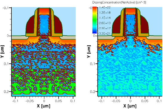
5: Atomistic Kinetic Monte Carlo Diffusion

Extracting KMC-related Information

538 Sentaurus™ Process User Guide

I-2013.12

In some cases, especially when the Sentaurus Process KMC output is used as a device

simulation input, a smoother concentration is desirable, as seen in Figure 78. This can be

performed by setting the PDB parameter:

KMC Smooth.Field <field> <number>

where:

■<field> is the field name to be smoothed (for example, NetActive).

■<number> is an integer.

Figure 78 Comparison of NetActive concentration in simulations performed with (left)

Smooth.Field equal to 0 (disabled) and (right) equal to 1

A value of 0 produces no smoothing; larger numbers produce more smoothed profiles. The

smoothing algorithm works as follows:

■For each node in the standard Sentaurus Process mesh, the number of particles

associated with the node is counted.

■The concentration set to that node is, in principle, , where is the Voronoï

volume associated with the node.

■ is compared to , where is the number specified in Smooth.Field for this field.

■If the field name does not exist in Smooth.Field, 0 is assumed.

■If , the smoothing algorithm applies. Starting at the node, the algorithm looks for

particles not associated with the Voronoï volume of the node, with an increasing radius.

■When particles are found in a radius , it stops searching. At this point, there are

particles inside the radius, outside the Voronoï volume, and inside the

Vo r o n o ï v o l u m e .

Voronoi

⁄

VVoronoi

NM<

MN–

5: Atomistic Kinetic Monte Carlo Diffusion

Extracting KMC-related Information

Sentaurus™ Process User Guide 539

I-2013.12

■Then, the concentration of the node will be:

(815)

where is the volume associated with a segment (1D), circle (2D), or circumference (3D)

of radius , and weight is the PDB value Smooth.Weight:

pdbSet KMC Smooth.Weight 0.01

This technique is not intended to perfectly conserve the total dose, but to fill the nodes with low

concentrations with values depending on the distance to the nearest particles. The factor

weight is included to limit the extra dose introduced in those nodes.

The Smooth.Field parameter is used whenever a deatomization is performed. This includes

calling directly kmc deatomize from the command line or indirectly through KMC2PDE or

another procedure.

NOTE The algorithm to smooth atomistic concentrations can be extremely

slow in simulations with a large number of nodes.

The smooth algorithm can be relatively slow for simulations with a large number of nodes or

a large number of particles. This can be resolved by calling it in parallel mode with the

following option:

math numThreadsDeatomize=<n>

This option is independent from the KMC parallel mode and does not interfere with it. It

applies to the smooth algorithm only, not to the whole deatomization.

Adding and Obtaining Defects in Simulations: add,

defects.add, and defects.write

Sentaurus Process KMC allows you to add defects to the simulation using the commands:

kmc add queue name=<defect name> coordx=<x> coordy=<y> coordz=<z> [amorphous]

[crystalline]

kmc add

First, the defects are queued in the creation queue with the command:

kmc add queue

You can queue as many defects as you want. Queueing a defect does not actually introduce it

in the simulation. You must use the command kmc add alone to empty all of the queue by

generating defects in the simulation.

Voronoi

⁄weight NM–()()VR

⁄+

5: Atomistic Kinetic Monte Carlo Diffusion

Extracting KMC-related Information

540 Sentaurus™ Process User Guide

I-2013.12

The option name specifies the defect to be created (examples are B, B2I4, I54, and

BInterface). The options coordx, coordy, and coordz provide the place where the defect

(or the center of mass of the defect) will be created. Finally, the optional arguments

amorphous and crystalline provide a way to tell the simulator whether this defect should

be created in an amorphous or a crystalline material. For example, if the current material is

crystalline, but the option amorphous is specified, the simulator not only creates a defect, but

also changes the material from crystalline to amorphous phase.

An alternative way to add defects to the simulation is using the defects.read command,

which requires the name of a text file to be specified with defects.read, for example:

kmc defects.read=my_filename

This command takes all the defects specified in the file and adds them consecutively in a very

similar way to the add command. Similar to the add command, only the center of mass is

specified for defects having more than one particle.

One line specifies one defect. The format of each line is:

defect_type defect_name coord_x coord_y coord_z

where:

■defect_type is the generic name of the defect, for example, PointDefect, Loop,

ThreeOneOne, Interface, ImpurityCluster.

■defect_name is the particular name of the defect, for example, B, P, I50, BiM, B3I2.

■coord_x, coord_y, coord_z are the coordinates (in nanometers) for the center of mass

of the defect.

For example:

Interface P 1.000000 11.250000 13.000000

PointDefect As 5.032000 5.320000 1.032000

ThreeOneOne I50 10.000000 10.222565 9.777436

PointDefect B 10.000000 5.000000 6.000000

PointDefect BiM 30.000002 5.000000 14.000000

ThreeOneOne I100 19.554871 20.445129 20.000000

Loop PI59 13.000000 13.000000 13.000000

PointDefect Bi 26.000000 26.000000 26.000000

ImpurityCluster B2I 6.235641 7.115777 7.077633

ImpurityCluster B3I2 4.287220 7.497602 4.604665

PointDefect Ge 6.696747 7.492962 0.834044

Similarly, the command kmc defects.write writes all the defects currently in the

simulation into a file with the above format. The name of the file must be specified as:

kmc defects.write=my_filename

5: Atomistic Kinetic Monte Carlo Diffusion

Extracting KMC-related Information

Sentaurus™ Process User Guide 541

I-2013.12

Files written with defects.write can be read later with defects.read. Since only the

center of mass of the particle is written, this is an inaccurate way to save a simulation. To save

a simulation, use instead struct or kmc extract tdrWrite.

Using the Sentaurus Process Interface

The select, print, WritePlx, and plot Commands

The commands select, print, WritePlx, and plot work as expected. If you need a field

for them, create it using kmc deatomize (see Transferring Fields from KMC to Continuum

Information: deatomize on page 536).

In particular, select creates particles inside Sentaurus Process KMC whenever the name of

the field is recognized as a particle or defect. These names are:

Example

For a typical situation with a 1D SIMS-like simulation (implant and anneal), the 1D profiles

can be extracted in a .plx file using WritePlx:

SetPlxList BTotal B

WritePlx file

Calling WritePlx without selecting the list with SetPlxList also works. It generates a list

of the most common fields:

WritePlx file

Dopants As, B, …

Impurities C,F, …

Paired particles Bi, AsV, Ci, …

Point defects I,V

Any of the above particles with a different charge IM, VPP, BiM, AsVP, …

Amorphous BAmorphous, AsAmorphous, …

Amorphous pockets IV, I4V5, …

Dopants or impurities in an interface BInterface, AsInterface, …

Extended defects I43, V21, …

Impurity clusters AsV4, BI2, …

5: Atomistic Kinetic Monte Carlo Diffusion

Extracting KMC-related Information

542 Sentaurus™ Process User Guide

I-2013.12

In nonatomistic mode, the fields must be deatomized first:

kmc deatomize name=BTotal

kmc deatomize name=B

The init Command

The init command works as expected. Background dopings can be assigned. A TDR file to

be loaded can also be assigned with:

init tdr=filename

and, if the file has been saved with Sentaurus Process KMC and contains atomistic information

(see the option defects for tdrAdd, kmc on page 995), Sentaurus Process will load it, and

the simulation can be continued.

NOTE Loading a file and continuing a simulation with init will give results

similar, but not identical, to performing the simulation without the save/

load process. The differences between the results are only statistical; in

other words, both represent possible solutions.

The struct Command

The struct command works as expected, except that by default it creates some extra fields to

be saved. It generates these extra fields by calling the function preKMC with the argument

struct. You can modify or customize this function in the KMC.tcl file. By default, preKMC

tries to generate and store fields similar to a five-stream model from the KMC information.

The struct command also saves restart information, allowing the Sentaurus Workbench

#split command to work properly with Sentaurus Process KMC.

The load Command

The load command accepts the options kmc and replace only. It is intended to load a TDR

Sentaurus Process KMC simulation to replace the existing one. It performs the necessary

conversions between the existing internal Sentaurus Process KMC and the one read from the

TDR file, conserving the existing one.

The deposit Command

The deposit command works as expected, including depositing doped layers.

5: Atomistic Kinetic Monte Carlo Diffusion

Extracting KMC-related Information

Sentaurus™ Process User Guide 543

I-2013.12

The diffuse Command

The diffuse command works as expected with Sentaurus Process KMC, except that the

diffusion is done with the atomistic solver. In particular, the options for oxidation and

silicidation are supported (see Oxidation on page 518). Epitaxial options also are supported.

For lattice LKMC epitaxy, see Epitaxial Deposition on page 519.

Nonatomistic Mode

When Sentaurus Process KMC operates in the nonatomistic mode (see Nonatomistic Mode on

page 386), it transforms the five-stream model fields into atomistic information before every

annealing and converts the atomistic information to five-stream model information after any

annealing. Sentaurus Process KMC is disabled between annealings; consequently, all

information should be accessed using the standard Sentaurus Process interface. The only way

to access atomistic information is by using the Movie option during the Sentaurus

Process KMC annealings.

The transformation from five-stream to atomistic information is performed in the function

preKMC with the argument diffuse in the KMC.tcl file. The function preKMC is called

automatically before a Sentaurus Process KMC diffusion in nonatomistic mode. After the

diffusion, the function postKMC, with argument diffuse, is invoked to convert the atomistic

information into five-stream fields. You can modify and customize both functions.

Atomistic Mode

When operating in atomistic mode, Sentaurus Process KMC does not automatically perform

any transformation from atomistic to continuum, or vice versa, except if the command struct

is called (see Atomistic Mode on page 383).

Calling Directly the Sentaurus Process KMC Kernel

The best way to access the atomistic information is by calling directly the Sentaurus

Process KMC kernel using the kmc command. The option extract of this command accesses

the KMC raw information directly and returns it in different formats, or creates a TDR file to

be opened with Sentaurus Workbench Visualization.

5: Atomistic Kinetic Monte Carlo Diffusion

Extracting KMC-related Information

544 Sentaurus™ Process User Guide

I-2013.12

Writing and Displaying TDR Files with KMC Information

The command:

kmc extract tdrWrite filename=<filename>

creates files to be displayed by Sentaurus Workbench Visualization. This file contains a

collection of states or snapshots. Each snapshots is taken at a particular time during the

simulation; the collection of snapshots gives information about the time evolution during the

simulation. Each snapshot can contain concentrations and histograms, atomistic information,

or both. These snapshots are created with the command:

kmc extract tdrAdd [concentrations] [defects] [stress] [histogram]

[visual={<fields>} [list={<fields>}]

The parameter concentrations includes a list of standard fields. These fields are the total

concentration for each particle, the time-averaged concentrations of mobile particles,

NetActive, the electronic concentration, the concentration of impurities in the surface,

amorphous and impurity clusters, and the concentration of point defects in APs, amorphous

layers, impurity clusters, and extended defects. These concentrations are displayed with the

same dimension as the simulation.

Since Sentaurus Process KMC always works in 3D, for 1D simulations, the displayed

concentrations are averaged for yz planes and, for 2D simulations, they are averaged in z-lines.

An extra A/C field also is stored to let you know whether the material is amorphous or

crystalline.

The histogram option includes a 2D graph representing the APs and impurity cluster

histograms. These histograms give the number of defects existing in the simulation for each

different size (I and V for APs, impurities, and point defects for impurity clusters). One-

dimensional histograms, giving the number of extended defects versus its size, are included as

well when using the histogram option. Stress and strain information can be added to these

concentrations and histograms with the stress option.

Figure 79 on page 545 shows one snapshot saved with the concentrations and histogram

options for a 2D simulation.

Regarding NetActive, the parameter KMC tdr smoothDopingConcentration controls

whether this concentration is smoothed. By default, it is not smoothed because smoothing it

artificially decreases the channel length. On the other hand, the smooth algorithm partially

removes irregularities and other atomistic features that may appear on the p-n junctions. This

smoothing is different than the one controlled by Smooth.Field and is explained in

Smoothing Out Deatomized Concentrations on page 537.

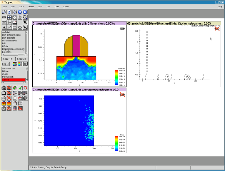
5: Atomistic Kinetic Monte Carlo Diffusion

Extracting KMC-related Information

Sentaurus™ Process User Guide 545

I-2013.12

While smoothDopingConcentration controls the smoothing of only NetActive in the

Sentaurus Process KMC TDR file, Smooth.Field controls the smoothing of any field when

translating the atomistic information into the continuum mesh concentration.

The parameter defects includes atomistic information about the defects in the simulation.

This atomistic information can be used to obtain an atomistic 3D plot that is independent of the

simulation dimensions. It offers the most realistic representation of the simulation.

Figure 79 Example of a TDR file of Sentaurus Process KMC displayed with Sentaurus

Workbench Visualization. The concentrations and histogram options have been

used; 1D histograms for clusters and 2D histograms for APs and impurity clusters

are included. The concentration (in this case, for a 2D simulation) for several

fields is included with this option.

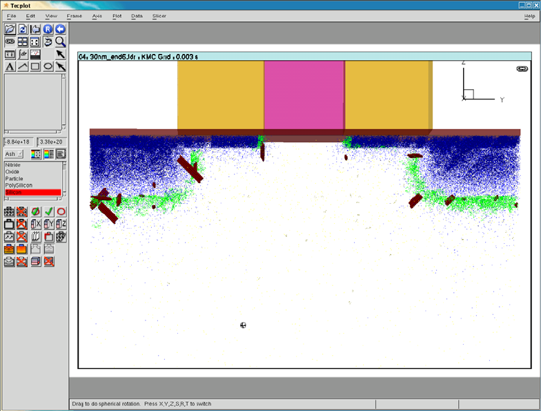
5: Atomistic Kinetic Monte Carlo Diffusion

Extracting KMC-related Information

546 Sentaurus™ Process User Guide

I-2013.12

Figure 80 shows an example of the information saved with the defects option.

Figure 80 Example of TDR file of Sentaurus Process KMC including atomistic information;

the defects option has been used

The defects option also includes extra information necessary to restart or load the simulation.

A file saved with this parameter can be reloaded into Sentaurus Process KMC, and the

simulation can be continued. To load the simulation, use the command init.

Using the KMC Movie option, you can include the command kmc extract tdrAdd to view

the evolution of the simulation with time.

Finally, the option visual stores atomistic 3D information in a way similar to defects. The

differences between using visual and defects are:

■Files saved with visual cannot be restarted.

■The visual option produces smaller file sizes than defects. In particular, visual stores

the defects, but it does not store the information needed to restart. The visual files are

intended for visualization purposes only.

■The visual option requires a list of defects, separated by commas, to be saved. The all

option saves all the defects.

5: Atomistic Kinetic Monte Carlo Diffusion

Extracting KMC-related Information

Sentaurus™ Process User Guide 547

I-2013.12

■Other valid defects include defect names (such as BiM or B2I3), general defect names

(such as ThreeOneOne), and material names (Silicon). This lets you control which

defects will be saved and visualized later, making it easier to visualize information without

saving a large file with all the 3D information.

Plotting Only Some Particles

Sentaurus Process visualization does not represent all the particles inside APs. Since the

number of particles (interstitials and vacancies) in APs can be large after an implant, only 1 in

50 particles is visualized by default. This default behavior is written in the TDR file as set by

the parameter VisualizeDamage:

sprocess> pdbGet KMC VisualizeDamage

Sentaurus Process visualization can overwrite the default set for each file using the option:

-s:psf n

where n is the new value of VisualizeDamage:

NOTE Setting VisualizeDamage to 1 causes Sentaurus Workbench

Visualization to plot all the particles present in the simulation. This

number can be very large immediately after an implant.

Time-averaged Concentration Name

The default field name for time-averaged concentrations in the TDR file is ‘mobile’, but it can

be defined with the parameter KMC tdr averageTag.

Inquiring about KMC Profiles, Histograms, and Defects

Besides the select command and the TDR files, you can access Sentaurus Process KMC

information using the kmc extract command (see kmc on page 995):

■kmc extract histogram—extracts histograms for extended defects, impurity defects,

and APs.

■kmc extract profile—extracts concentrations and stresses in 1D, 2D, and 3D.

■kmc extract supersaturation—extracts the concentration relative to the

equilibrium concentration for point defects.

■kmc extract defects—obtains the atomistic information of the defects.

■kmc extract dose—extracts doses, that is, concentrations in .

cm 2–

5: Atomistic Kinetic Monte Carlo Diffusion

Extracting KMC-related Information

548 Sentaurus™ Process User Guide

I-2013.12

■kmc extract materials—obtains information about the different materials in the

simulation.

■kmc extract acinterface—obtains the position of the amorphous–crystalline

interfaces in the simulation.

The histogram Option

kmc extract histogram name=[meansize [minsize=<n>]]

[materialname=<material>]

Sentaurus Process KMC includes several models where the defects are not isolated, but

agglomerated in extended defects that can contain many particles. The histogram option

allows you to extract information about the sizes (number of particles) of these extended

defects.

The histogram option needs a valid name to compute the following available histograms:

The optional parameter meansize displays the average size of clusters instead of displaying

the whole list of clusters when using this parameter. Without specifying minsize, the average

size begins with size 0.

Finally, the parameter materialname restricts the output to the material specified instead of

the whole simulation.

Interstitial-extended

defects

Set name=I to extract information about the small I clusters,

{311} defects, and dislocation loops.

Va ca nc y- ex te nd e d de fe ct s Se t name=V to extract information about the small V clusters

and voids.

B interstitial clusters or

other clusters with I

Set name=XI to extract information about the dopant named

‘X’. For example, for boron impurity clusters (BICs),

name=BI.

As vacancy clusters or

other clusters with V

Set name=XV. For example, set name=AsV to extract

information about the arsenic–vacancy clusters.

Cluster with multiple

impurities

For example, set name=PAs for clusters with both P and As.

Amorphous pockets Set name=IV.

…











5: Atomistic Kinetic Monte Carlo Diffusion

Extracting KMC-related Information

Sentaurus™ Process User Guide 549

I-2013.12

Interstitial Histograms

These histograms extract the number of defects in the simulation for each size. The histograms

contain information about the small, irregular clusters (see Amorphous Pockets Life Cycle on

page 439), {311} defects (for size bigger than the established limit), and dislocation loops. For

example:

LogFile [kmc extract histogram name=I]

gives a list of extended defects with I. In this example:

sprocess> LogFile [kmc extract histogram name=I]

I2 302

I3 104

I4 42

I5 12

I6 4

I72 1

I677 1

sprocess> LogFile [kmc extract histogram name=I meansize]

4.11373

sprocess> LogFile [kmc extract histogram name=I meansize minsize=10]

374.5

Vacancy-extended Defects Histogram

These histograms are similar to the interstitial-extended defects histogram, except that the

extracted number of particles versus size is for vacancies:

sprocess> LogFile [kmc extract histogram name=V]

V5 1

V7 2

V8 5

V9 2

V10 5

(...)

sprocess> LogFile [kmc extract histogram name=V meansize]

12.9143

sprocess> LogFile [kmc extract histogram name=V meansize minsize=10]

Amorphous Pockets Histogram

The AP histograms contain the number of cluster versus I and V size. APs with null Is or Vs

can be considered as APs or small I or V clusters.

sprocess> LogFile [kmc extract histogram name=IV]

I2 367

I3 69

5: Atomistic Kinetic Monte Carlo Diffusion

Extracting KMC-related Information

550 Sentaurus™ Process User Guide

I-2013.12

I4 22

I5 1

IV 823

I2V 249

I3V 61

I4V 23

I5V 2

V2 408

IV2 251

I2V2 111

(...)

The average size can be requested for these clusters. It will return values for both I and V:

sprocess> LogFile [kmc extract histogram name=IV meansize]

I2.3501V0.796781

The parameter meansize applies here and specifies the minimum size to begin the average for

both species.

Boron–Interstitial Clusters

The boron–interstitial cluster histogram offers information about the number of BICs for each

BIC configuration (BnIm).

sprocess> LogFile [kmc extract histogram name=BI]

B2I 16

B3I 347

sprocess> LogFile [kmc extract histogram name=BI meansize]

B2.95592I1

Arsenic–Vacancy Clusters

The arsenic–vacancy cluster histogram offers information about the number of arsenic and

vacancies in impurity clusters for each configuration (AsnIm):

sprocess> LogFile [kmc extract histogram name=AsV]

As2 277

As3 109

As4 3

As2V 752

As3V 281

As4V 178

sprocess> LogFile [kmc extract histogram name=AsV meansize]

As2.47V0.756875

5: Atomistic Kinetic Monte Carlo Diffusion

Extracting KMC-related Information

Sentaurus™ Process User Guide 551

I-2013.12

The profile Option

Sentaurus Process KMC computes the profiles concentration versus size as a convenient way

to directly obtain useful data.

kmc extract profile [timeaveraged] name=

[materialname=] [coordx=] [coordy=] [coordz=]

For example, 1D profiles can be compared with SIMS experiments. The profiles are an average

of the concentration of particles. For 3D, Sentaurus Process KMC takes a volume to be

averaged equal to an element defined by the parameters extractDeltaX, extractDeltaY,

and extractDeltaZ. For 2D and 1D, this volume includes all the elements in y and z,

respectively.

The parameter name chooses the profiles to be obtained. holes and electrons return the

concentration of holes and electrons, respectively. GapNarrowing returns the bandgap

narrowing, in eV. Stress can be stressXX, stressYY, and stressZZ, and strain is one of

strainXX, strainXY, strainXZ, strainXY, strainXZ, or strainYZ. A particle name

(like Bi, IM, or AsVP) returns the concentration of all the particles in the simulation matching

the given one. A cluster name (for example, As4V) will return the concentration of that cluster

in the simulation. For particles, the concentration of particles is returned; for clusters, the

concentration of clusters is returned. For example, an As4 cluster is considered to be four As

particles when you request the concentration of As, but only one defect when you request the

concentration of As4 clusters. An impurity name followed by the word “Total”, like BTotal,

will return the total profile of that impurity (active, inactive, in pairs, clusters and so on) in the

simulation.

When a particle profile is specified, the optional parameter defectname can be used to further

specify the kind of particle. For example, the command:

kmc extract profile name=I

computes the concentration of interstitials in any kind of defect, in other words, the total

interstitial concentration.

holes

electrons

particles BAs

i…,,()

clusters InVmBnIm…,,()

stress

strain

GapNarrowing

dopants

totals BTotal,AsTotal()











defectname=

ThreeOneOne

Interface

Loop

…











5: Atomistic Kinetic Monte Carlo Diffusion

Extracting KMC-related Information

552 Sentaurus™ Process User Guide

I-2013.12

The command:

kmc extract profile name=I defectname=ImpurityCluster

computes the concentration of interstitials in impurity clusters.

The parameter defectname should not be specified with cluster concentration, electrons,

holes, GapNarrowing, stresses or strains.

Finally, the parameter materialname restricts the output to the material specified instead of

the whole simulation.

The returned concentration has the same dimensionality as the performed simulation. Use the

optional parameters coordx, coordy, and coordz to change this default. These parameters

specify cutlines. For example, in a 3D simulation the command:

kmc extract profiles name=I

returns the concentration for all the volume elements in the simulation. The command:

kmc extract profiles name=I coordx=20<nm> coordz=10<nm>

returns a 1D profile with concentrations in the plane x = 20 <nm> and z = 10 <nm>.

Finally:

kmc extract profiles name=I coordx=20<nm> coordy=15<nm> coordz=10<nm>

returns only one value, the concentration at the specified point.

The use of the parameters coordx, coordy, and coordz depends on the simulation

dimensions. As previously explained, specifying coordx for 1D, 2D, or 3D simulations,

coordy for 2D or 3D, or coordz for 3D, returns the concentrations only on elements

including the specified cutlines. On the other hand, the use of coordy or coordz in 1D

simulations, or coordz in 2D, is quite different. In this case, the result returned is not averaged

for the whole remaining dimensions (y and z for 1D, z for 2D), but only calculated in the

specified cutlines. In other words, specifying coordy in a 3D simulation returns all the

concentrations in the x, z volumes for the y specified in coordy; while specifying coordy in

a 1D simulation returns concentrations versus the x-axis, but instead of being averaged for

every y and z, they will be averaged only for every z in the plane marked by coordy. In 3D, it

will reduce the size of the output (since only the output for the specified plane y is written). In

1D, the output has the same number of lines (one for each x position), but the concentration

displayed is different because it is averaged into z only, and not into y and z.

Sentaurus Process KMC returns the instantaneous concentration by default. For mobile

particles the instantaneous concentration does not usually contain any information rather than

noise. The parameter timeaveraged instructs Sentaurus Process KMC to return the average

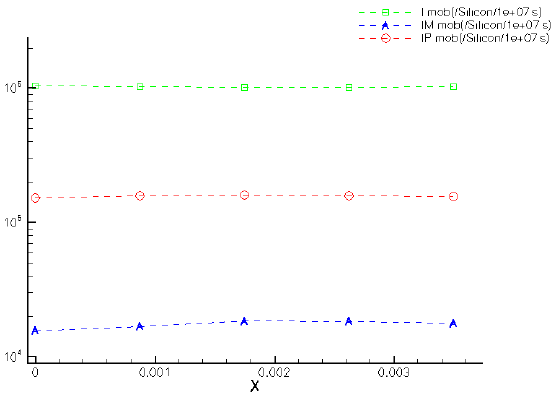
5: Atomistic Kinetic Monte Carlo Diffusion

Extracting KMC-related Information

Sentaurus™ Process User Guide 553

I-2013.12

concentration of mobile particles between the current time and the last time Sentaurus

Process KMC created a snapshot (see Snapshots on page 407).

For example, Figure 81 has been produced with the input script:

pdbSet KMC MaxYum 40e-3

pdbSet KMC MaxZum 40e-3

SetAtomistic

pdbSet KMC Movie ""

pdbSet IncrementalHops 0

line x loc=0.0 tag=xleft spacing = 0.002

line x loc=1.5e-3 tag=xmed spacing = 0.002

line x loc=5e-3 tag=xright spacing = 0.002

region oxide xlo=xleft xhi=xmed

region silicon xlo=xmed xhi=xright

init

diffuse time=1e7<s> temp=700 info=1

kmc extract tdrClear

kmc extract tdrAdd concentrations

kmc extract tdrWrite filename=equil

The concentrations of neutral, positive, and negative interstitials also can be obtained with:

sprocess> kmc extract profile timeaveraged name=IP coordx=2.5<nm>

162487

sprocess> kmc extract profile timeaveraged name=I coordx=2.5<nm>

1.0276e+06

sprocess> kmc extract profile timeaveraged name=IM coordx=2.5<nm>

18170.5

Figure 81 Equilibrium concentrations of neutral (green), positive (red), and negative (blue)

interstitials at 700oC

5: Atomistic Kinetic Monte Carlo Diffusion

Extracting KMC-related Information

554 Sentaurus™ Process User Guide

I-2013.12

The supersaturation Option

kmc extract supersaturation name=

Supersaturation is the current concentration relative to the equilibrium concentration:

(816)

Sentaurus Process KMC computes the supersaturation for Is and Vs. The current global

concentration is calculated involving a time average between the current time and the last

snapshot:

sprocess> LogFile [kmc extract supersaturation name=I]

1.00555

To obtain the supersaturation evolution with time, use the KMC Movie parameter as shown in

the following example:

SetAtomistic

set kmcSupersat ""

pdbSet KMC MaxYum 30e-3

pdbSet KMC MaxZum 30e-3

pdbSet KMC Movie {lappend kmcSupersat $time [kmc extract \

supersaturation name=I]}

pdbSet KMC automaticRampUp 1

line x loc=0.0 tag=xleft spacing = 0.002

line x loc=1.5e-3 tag=xmed spacing = 0.002

line x loc=350e-3 tag=xright spacing = 0.002

region oxide xlo=xleft xhi=xmed

region silicon xlo=xmed xhi=xright

init

implant Silicon energy=40 dose=2e13 tilt=7

diffuse time=100000<s> temp=600

LogFile $kmcSupersat

produces the results:

10.0007 4.29101e+07

21.5462 2.51728e+07

46.4218 1.58636e+07

100.004 1.41889e+07

215.493 7.67109e+06

464.238 3.44625e+06

1000.26 1.86513e+06

2156.46 477255

4645.69 322049







supersaturation X() X[]

X[]

-----------=

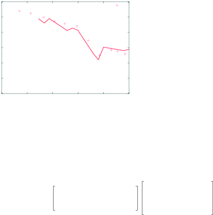
5: Atomistic Kinetic Monte Carlo Diffusion

Extracting KMC-related Information

Sentaurus™ Process User Guide 555

I-2013.12

10002.8 113849

21551.6 132116

46419.1 110329

100006 81506.4

Figure 82 shows a comparison with experimental results.

Figure 82 Supersaturation evolution with time, after a silicon implant (2 x 1013 dose, 40 keV

energy) annealed 1 x 105s at 600oC. (Experimental points modified from [50] to

use the same B diffusivity.) Points are experiments, lines are KMC.

The defects Option

The defects option allows access to the raw atomistic information of any simulation. The

obtained information must match the parameters name and defectname when they are

specified.

kmc extract defects

[countparticles] [countdefects] [materialname=<material>]

[acinterface]

When there are no restrictions, all defects are accessed. For example, for the following added

defects:

kmc add queue name=BI2 coordx=2<nm> coordy=2<nm> coordz=3<nm>

kmc add queue name=I2 coordx=3<nm> coordy=2e-3 coordz=4e-3

kmc add queue name=I3 coordx=4<nm> coordy=3<nm> coordz=1<nm>

kmc add

108

107

106

105

104

103

102

105

104

103

102

101

100

Time [s]

Interstitial Supersaturation

600oC

name particles BA

i…,,()

clusters InVmBnIm…,,()











defectname=

ThreeOneOne

Interface

Loop

…











5: Atomistic Kinetic Monte Carlo Diffusion

Extracting KMC-related Information

556 Sentaurus™ Process User Guide

I-2013.12

The obtained defects are:

sprocess> kmc extract defects

0.00201273 0.00238963 0.00298179 I ImpurityCluster 0

0.00196125 0.00204962 0.00249501 I ImpurityCluster 0

0.00177392 0.00225923 0.00247647 B ImpurityCluster 0

0.00320253 0.00162722 0.00466375 I AmorphousPocket 1

0.00222551 0.00139856 0.004411 I AmorphousPocket 1

0.0044946 0.00317389 0.00130069 I AmorphousPocket 2

0.00441116 0.00353071 0.000842549 I AmorphousPocket 2

0.00403856 0.00351353 0.00084327 I AmorphousPocket 2

sprocess> kmc extract defects name=I

0.00201273 0.00238963 0.00298179 I ImpurityCluster 0

0.00196125 0.00204962 0.00249501 I ImpurityCluster 0

0.00320253 0.00162722 0.00466375 I AmorphousPocket 1

0.00222551 0.00139856 0.004411 I AmorphousPocket 1

0.0044946 0.00317389 0.00130069 I AmorphousPocket 2

0.00441116 0.00353071 0.000842549 I AmorphousPocket 2

0.00403856 0.00351353 0.00084327 I AmorphousPocket 2

sprocess> kmc extract defects name=I defectname=ImpurityCluster

0.00201273 0.00238963 0.00298179 I ImpurityCluster 0

0.00196125 0.00204962 0.00249501 I ImpurityCluster 0

sprocess> kmc extract defects name=BI2

0.00201273 0.00238963 0.00298179 I ImpurityCluster 0

0.00196125 0.00204962 0.00249501 I ImpurityCluster 0

0.00177392 0.00225923 0.00247647 B ImpurityCluster 0

The six columns present in the output are:

■X-coordinate of the defect

■Y-coordinate of the defect

■Z-coordinate of the defect

■Particle name

■Defect name.

■Number of defect. Particles with the same number belong to the same defect.

NOTE The command kmc extract defects can produce large outputs.

When there are amorphous defects in the simulation, the result may not be the expected.

Amorphous defects do not store the damage, but only its concentration (see Amorphous

Defects on page 456). Consequently, amorphous defects will not report any interstitial or

vacancy inside them. Impurities are stored and displayed. Nevertheless, if the indirect diffusion

model is used in amorphous silicon, the dangling bonds, floating bonds, and mobile and

immobile impurities will be obtained as I, V, Bi and B (for boron) (see Indirect Diffusion on

page 457).

5: Atomistic Kinetic Monte Carlo Diffusion

Extracting KMC-related Information

Sentaurus™ Process User Guide 557

I-2013.12

The parameter materialname restricts the output to the material specified instead of the

whole simulation.

The options countparticles and countdefects do not display the atomistic information,

but they count the number of particles and defects, respectively, for the given conditions. For

example, this example shows how to count the particles and defects listed in the last example:

sprocess> kmc extract defects countparticles

sprocess> kmc extract defects countdefects

sprocess> kmc extract defects name=I countparticles

sprocess> kmc extract defects name=I defectname=AmorphousPocket countdefects

The parameter acinterface displays the lattice atoms belonging to the amorphous–

crystalline interface. All the lattice atoms can be obtained by using acinterface detailed.

This parameter generates an output only when the LKMC model is used for recrystallization

(see LKMC: Fully Atomistic Modeling of Solid Phase Epitaxial Regrowth on page 463).

The dose Option

The dose option extracts the concentration per surface unit (in other words, cm–2) for the

whole simulation cell. dose can be used to look at the evolution of the species with the time.

kmc extract dose

[countdefects] [materialname=<material>]

The parameters name and defectname restrict the species to compute the dose. name can be

any particle or defect. defectname can be specified only when name is a particle, and it

restricts the particles to be of the specified type. A list of defect types is obtained with kmc

defecttypes. A “total” name: the name of an impurity followed by the work “Total”, like

BTotal, applies to all the circumstances where the specified impurity is present, that is, in

clusters, substitutional, pairs, and so on.

This command counts the number of particles (such as kmc extract defects with the

same restrictions and the countparticles option) and it divides this number by the surface

area. Finally, the parameter materialname restricts the output to the material specified

name

Particles I AsV Bi

-…,,,()

Defects InVnInVmBnIm…,, , ,()

Totals AsTotal BTotal ...,,()











defectname

ImpurityCluster

ThreeOneOne

…











5: Atomistic Kinetic Monte Carlo Diffusion

Extracting KMC-related Information

558 Sentaurus™ Process User Guide

I-2013.12

instead of the whole simulation. For interfaces, instead of specifying a material name, specify

a particle name such as AsInterface, BInterface.

As an example, the following input file implants silicon into silicon and extracts the dissolution

of {311} during annealing:

set silicon_depth 350e-3

set size 50e-3

set SiO2gate 1.5e-3

SetAtomistic

set sol ""

pdbSet KMC Movie {lappend sol $time [kmc extract dose name=I \

defectname=ThreeOneOne]}

pdbSet KMC MaxZum $size

pdbSet KMC MaxYum $size

pdbSet KMC GasUm $SiO2gate

pdbSet KMC automaticRampUp true

line x loc=0.0 tag=xtop spacing = 0.002

line x loc=$silicon_depth tag=xbottom spacing = 0.002

region silicon xlo=xtop xhi=xbottom

init

deposit oxide fill coord=[expr -$SiO2gate]

implant silicon energy=40 dose=5e13 tilt=7

diffuse time=3100 temp=670

LogFile $sol

This example produces the results:

46.4176 2.88e+12

100.01 9.56e+12

215.464 1.104e+13

464.175 1.596e+13

1000 2.172e+13

2154.45 3.144e+13

4641.63 3.736e+13

10000 3.044e+13

21544.5 1.388e+13

46417.4 9.6e+11

100233 0

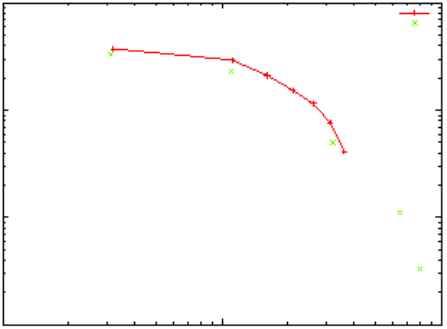
5: Atomistic Kinetic Monte Carlo Diffusion

Extracting KMC-related Information

Sentaurus™ Process User Guide 559

I-2013.12

Figure 83 shows the comparison with experimental data [8].

Figure 83 Dissolution of {311} extended defects at 670oC after a silicon into silicon implant

of 40 keV, 5 x 1013 cm–2

The materials Option

kmc extract materials [detailed] [coordx=] [coordy=] [coordz=]

The command kmc extract materials produces the list of materials currently in the

simulation:

sprocess> kmc extract materials

Silicon Oxide Gas

The option detailed produces a list of coordinates and materials. This list contains the same

number of dimensions as the simulation (except if you use coordx, coordy, or coordz). For

example, in a 1D simulation:

sprocess> kmc extract materials detailed

-0.002 Gas

-0.000625 Oxide

0.00075 Oxide

0.002125 Oxide

0.0035 Oxide

0.004875 Oxide

0.00625 Oxide

0.007625 Oxide

0.009 Oxide

0.010375 Silicon

0.01175 Silicon

0.013125 Silicon

0.0145 Silicon

Simulation

Experiment

1000 10000 100000

1014

1013

1012

1011

Interstitials in Extended Defects [cm–2]

Time [s]

5: Atomistic Kinetic Monte Carlo Diffusion

Extracting KMC-related Information

560 Sentaurus™ Process User Guide

I-2013.12

0.015875 Silicon

0.01725 Silicon

The parameters coordx, coordy, and coordz affect the output of detailed by changing its

dimensionality. They work exactly the same as in kmc extract profile (see The profile

Option on page 551).

The acinterface Option

kmc extract acinterface [coordx=] [coordy=] [coordz=]

The command kmc extract acinterface produces the list of amorphous–crystalline

interfaces found in the simulation given a 1D cutline. No extra options are needed in 1D. In 2D,

you must specify coordx or coordy. In 3D, you must specify two of three parameters

coordx, coordy, and coordz. For example, in 1D:

sprocess> kmc extract acinterface

Silicon Amorphous/Crystalline 0.0165

When the KMC model for SPER is detected, the option acinterface displays all the places

where the amorphous–crystalline field crosses the threshold specified in

KMC ACInterfaceAt. A value of 1 means perfectly amorphous and 0 means perfectly

crystalline. The default value is 0.9. The output also displays the materials at both sides of the

interface, displaying first the material with a smaller coordinate value. In this case, the interface

is at , and the transition is from Amorphous to Crystalline as the x-coordinate

increases. When the LKMC model is used for SPER, the parameter ACInterfaceAt is

ignored, and a more precise interface is extracted directly from the LKMC atomistic

information.

Common Dopant and Point-Defect Names

Several KMC commands contain a name=<particlename> parameter. Table 61 on page 561

lists several of these names and the commands where they are applicable. Since dopants can be

defined as needed, the names depend on the simulation parameters. In particular, they contain

names defined when using Advanced Calibration. A list of the names can be obtained using

kmc particletypes. Clusters also are included in the list. Since the number of different

clusters is large, only a partial cluster list is included as an example (see Table 62 on page 564).

The commands considered for the referenced tables, and the symbols used to represent them,

are:

■kmc add queue (Add)

■kmc extract profile (Pro)

■kmc extract histograms (His)

0.0165 µm

5: Atomistic Kinetic Monte Carlo Diffusion

Extracting KMC-related Information

Sentaurus™ Process User Guide 561

I-2013.12

■kmc extract dose (Dos)

■kmc extract defects (Def)

■kmc extract supersaturation (Sup)

■kmc deatomize (Dea)

■kmc present (Pre)

The defects used in the descriptions are:

■Point defects, self-silicon point defects like interstitials and vacancies.

■Extended defects, agglomeration of self-silicon point defects.

■Clusters, agglomeration of impurities or dopants, with or without point defects.

■Substitutional dopants or impurities.

■Paired dopants or impurities, paired with point defects.

■Amorphous pockets, agglomeration of point defects (also sometimes called damage).

■Defects attached to interfaces.

Ta bl e 61 N a me s us ed i n S e n ta u ru s Pr oc es s K M C

Name Description Used in

Neutral interstitial in point defects, clusters, and

extended defects

Sup, His, Add, Pro, Dos, Def, Dea, Pre

IMM

I--, point defect Add, Pro, Dos, Def, Dea, Pre

I-, point defect Add, Pro, Dos, Def, Dea, Pre

I+, point defect Add, Pro, Dos, Def, Dea, Pre

IPP

I++, point defect Add, Pro, Dos, Def, Dea, Pre

ITotal

Total interstitial concentration; similar to I + IMM +

IM + IP + IPP

Dea, Pre, Pro, Dos

Neutral vacancy in point defects, clusters, and

extended defects

Sup, His, Add, Pro, Dos, Def, Dea, Pre

VMMM

V---, point defect Add, Pro, Dos, Def, Dea, Pre

VMM

V--, point defect Add, Pro, Dos, Def, Dea, Pre

V-, point defect Add, Pro, Dos, Def, Dea, Pre

V+, point defect Add, Pro, Dos, Def, Dea, Pre

VPP

V++, point defect Add, Pro, Dos, Def, Dea, Pre

VPPP

V+++, point defect Add, Pro, Dos, Def, Dea, Pre

VTotal

Total vacancy concentration; similar to V +

VMMM + VMM + VM + VP + VPP + VPPP

Dea, Pre, Pro, Dos

5: Atomistic Kinetic Monte Carlo Diffusion

Extracting KMC-related Information

562 Sentaurus™ Process User Guide

I-2013.12

Boron, substitutional, at interfaces or in clusters Add, Pro, Dos, Def, Dea, Pre

Neutral-paired defect, boron vacancy Add, Pro, Dos, Def, Dea, Pre, His

BVM

BV-, paired defect Add, Pro, Dos, Def, Dea, Pre

BVP

BV+, paired defect Add, Pro, Dos, Def, Dea, Pre

Neutral-paired defect, boron interstitial Add, Pro, Dos, Def, Dea, Pre, His

BiM

Bi-, paired defect Add, Pro, Dos, Def, Dea, Pre

BiP

Bi+, paired defect Add, Pro, Dos, Def, Dea, Pre

BTotal

Total boron concentration; similar to B + BV +

BVM + BVP + Bi + BiM + BiP

Dea, Pre, Pro, Dos

BInterface

Boron at interfaces Add, Pro, Dos, Def, Dea, Pre

Arsenic, substitutional at interfaces or in clusters Add, Pro, Dos, Def, Dea, Pre

AsV

Neutral-paired defect of arsenic and a vacancy Add, Pro, Dos, Def, Dea, Pre, His

AsVM

AsV-, paired defect Add, Pro, Dos, Def, Dea, Pre

AsVP

AsV+, paired defect Add, Pro, Dos, Def, Dea, Pre

Asi

Neutral-paired defect of arsenic and an interstitial Add, Pro, Dos, Def, Dea, Pre, His

AsiM

Asi-, paired defect Add, Pro, Dos, Def, Dea, Pre

AsiP

Asi+, paired defect Add, Pro, Dos, Def, Dea, Pre

AsTotal

Total arsenic; similar to As + AsV + AsVM + AsVP

+ Asi + AsiM + AsiP

Dea, Pre, Pro, Dos

AsInterface

Arsenic attached at interfaces Add, Pro, Dos, Def, Dea, Pre

Carbon, substitutional, at interfaces or in clusters Add, Pro, Dos, Def, Dea, Pre

Neutral-paired defect of carbon and a vacancy Add, Pro, Dos, Def, Dea, Pre, His

Neutral-paired defect of carbon and an interstitial Add, Pro, Dos, Def, Dea, Pre, His

CInterface

Carbon attached at interfaces Add, Pro, Dos, Def, Dea, Pre

CTotal

Total carbon; similar to C + CV + Ci Dea, Pre, Pro, Dos

Fluorine, substitutional at interfaces or in clusters Add, Pro, Dos, Def, Dea, Pre

Neutral-paired defect of fluorine with an interstitial Add, Pro, Dos, Def, Dea, Pre, His

Neutral-paired defect of fluorine with a vacancy Add, Pro, Dos, Def, Dea, Pre, His

FTotal

Total fluorine; similar to F + FI + FV Dea, Pre, Pro, Dos

Ta bl e 61 N a me s us ed i n S e n ta u ru s Pr oc es s K M C

Name Description Used in

5: Atomistic Kinetic Monte Carlo Diffusion

Extracting KMC-related Information

Sentaurus™ Process User Guide 563

I-2013.12

FInterface

Fluorine attached at interfaces Add, Pro, Dos, Def, Dea, Pre

Indium, substitutional, at interfaces or in clusters Add, Pro, Dos, Def, Dea, Pre

InV

Neutral-paired defect of indium and a vacancy Add, Pro, Dos, Def, Dea, Pre, His

InVM

InV-, paired defect Add, Pro, Dos, Def, Dea, Pre

InVP

InV+, paired defect Add, Pro, Dos, Def, Dea, Pre

Ini

Neutral-paired defect of indium and an interstitial Add, Pro, Dos, Def, Dea, Pre, His

IniM

Ini-, paired defect Add, Pro, Dos, Def, Dea, Pre

IniP

Ini+, paired defect Add, Pro, Dos, Def, Dea, Pre

InTotal

Total indium; similar to In +InV + InVM + InVP +

Ini + IniM + IniP

Dea, Pre, Pro, Dos

InInterface

Indium attached at interfaces Add, Pro, Dos, Def, Dea, Pre

Phosphorus, substitutional, at interfaces or in

clusters

Add, Pro, Dos, Def, Dea, Pre

Neutral-paired defect of phosphorus and a vacancy Add, Pro, Dos, Def, Dea, Pre, His

PVM

PV-, paired defect Add, Pro, Dos, Def, Dea, Pre

PVP

PV+, paired defect Add, Pro, Dos, Def, Dea, Pre

Neutral-paired defect of phosphorus and an

interstitial

Add, Pro, Dos, Def, Dea, Pre, His

PiM

Pi-, paired defect Add, Pro, Dos, Def, Dea, Pre

PiP

Pi+, paired defect Add, Pro, Dos, Def, Dea, Pre

PTotal

Total phosphorus; similar to P + PV + PVM + PVP

+ Pi + PiM + PiP

Dea, Pre, Pro, Dos

PInterface

Phosphorus attached at interfaces Add, Pro, Dos, Def, Dea, Pre

Antimony, substitutional, at interfaces or in clusters Add, Pro, Dos, Def, Dea, Pre

SbV

Neutral-paired defect of antimony and a vacancy Add, Pro, Dos, Def, Dea, Pre, His

SbVM

SbV-, paired defect Add, Pro, Dos, Def, Dea, Pre

SbVP

SbV+, paired defect Add, Pro, Dos, Def, Dea, Pre

Sbi

Neutral-paired defect of antimony and an interstitial Add, Pro, Dos, Def, Dea, Pre, His

SbiP

Sbi+, paired defect Add, Pro, Dos, Def, Dea, Pre

SbTotal

Total antimony; similar to Sb + SbV + SbVM +

SbVP + Sbi + SbiP

Dea, Pre, Pro, Dos

Ta bl e 61 N a me s us ed i n S e n ta u ru s Pr oc es s K M C

Name Description Used in

5: Atomistic Kinetic Monte Carlo Diffusion

Extracting KMC-related Information

564 Sentaurus™ Process User Guide

I-2013.12

SbInterface

Antimony at interfaces Add, Pro, Dos, Def, Dea, Pre

Nitrogen, substitutional, at interfaces or in clusters Add, Pro, Dos, Def, Dea, Pre

NTotal

Total nitrogen, same as N Dea, Pre, Pro, Dos

NInterface

Nitrogen at interfaces Add, Pro, Dos, Def, Dea, Pre

N2, substitutional, at interfaces or in clusters Add, Pro, Dos, Def, Dea, Pre

NnV

Moving N2V particle Add, Pro, Dos, Def, Dea, Pre, His

NnTotal

Similar to Nn + NnV Dea, Pre, Pro, Dos

NnInterface

N2 stored at the interface Add, Pro, Dos, Def, Dea, Pre

Hydrogen, substitutional, at interfaces or in clusters Add, Pro, Dos, Def, Dea, Pre

HTotal

Total hydrogen, only H Dea, Pre, Pro, Dos

HInterface

Hydrogen at interfaces Add, Pro, Dos, Def, Dea, Pre

Germanium (stored as a field, not as a particle) Add, Pro, Dos, Def, Dea, Pre

Table 62 Some cluster names used in Sentaurus Process KMC

Name Comment Used in

Interstitial–vacancy amorphous pocket. His, Add, Pro, Dos, Def, Dea, Pre

I3V2

Amorphous pocket. Any other IxVy with x and y

integers is also valid.

Add, Pro, Dos, Def, Dea, Pre

Extended defect formed by eight interstitials. Any

other Ix, where x is an integer, is also valid.

Add, Pro, Dos, Def, Dea, Pre

Extended defect formed by four vacancies. Any

other Vx, with x an integer, is valid.

Add, Pro, Dos, Def, Dea, Pre

B2I3

Boron–interstitial cluster. Other integers are also

valid.

Add, Pro, Dos, Def, Dea, Pre

As4V

Arsenic–vacancy cluster. Other integers are also

valid.

Add, Pro, Dos, Def, Dea, Pre

B2IC3

Dopant cluster. Any combination of dopants with

(or without) interstitials or vacancies is valid.

Add, Pro, Dos, Def, Dea, Pre

P2As2I

Another example for dopant cluster Add, Prod, Dos, Def, Dea, Pre

Ta bl e 61 N a me s us ed i n S e n ta u ru s Pr oc es s K M C

Name Description Used in

5: Atomistic Kinetic Monte Carlo Diffusion

Advanced Calibration for Sentaurus Process KMC

Sentaurus™ Process User Guide 565

I-2013.12

Advanced Calibration for Sentaurus Process KMC

The default parameters used in Sentaurus Process KMC are inherited from previous versions

of Sentaurus Process KMC and may not be accurate for modern processing conditions. A more

accurate calibration for Sentaurus ProcessKMC has been performed by the Advanced

Calibration team and is available using the command:

AdvancedCalibration

This command includes the calibration of point-defect diffusivity, extended defects formation

and dissolution, boron diffusivity, boron–interstitial clustering process (activation and

deactivation of boron), surface trapping and re-emission of boron, and so on.

This command must be written after SetAtomistic since it detects the presence of an

atomistic simulation to load the Advanced Calibration parameters related to Sentaurus

Process KMC:

SetAtomistic

...

AdvancedCalibration

In cases where Advanced Calibration for Sentaurus Process KMC must be loaded, but it is not

possible to call it after SetAtomistic, the following workaround can be used. In particular,

this is the preferred mode to call Advanced Calibration for Sentaurus Process KMC in hybrid

simulations, and the only way to do it when using the kmc option in the diffuse command:

pdbSet AtomisticData 1

AdvancedCalibration

pdbSet AtomisticData 0

NOTE For more information on the Advanced Calibration parameters and

methodology, refer to the Advanced Calibration for Process Simulation

User Guide.

NOTE The use of Advanced Calibration is strongly recommended.

5: Atomistic Kinetic Monte Carlo Diffusion

References

566 Sentaurus™ Process User Guide

I-2013.12

References

[1] I. Martin-Bragado, Simulación atomística de procesos para Microelectrónica, Ph.D.

thesis, Universidad de Valladolid, Valladolid, Spain, 2004.

[2] M. Jaraiz et al., “Atomistic Front-End Process Modelling: A Powerful Tool for Deep-

Submicron Device Fabrication,” in International Conference on Simulation of

Semiconductor Processes and Devices (SISPAD), Athens, Greece, pp. 10–17, September

2001.

[3] N. Strecker, V. Moroz, and M. Jaraiz, “Introducing Monte Carlo Diffusion Simulation

into TCAD tools,” in Technical Proceedings of the International Conference on

Modeling and Simulation of Microsystems (Nanotech 2002), vol. 1, San Juan, Puerto

Rico, USA, pp. 462–465, April 2002.

[4] R. A. Casali, H. Rücker, and M. Methfessel, “Interaction of vacancies with interstitial

oxygen in silicon,” Applied Physics Letters, vol. 78, no. 7, pp. 913–915, 2001.

[5] N. Cowern and C. Rafferty, “Enhanced Diffusion in Silicon Processing,” MRS Bulletin,

vol. 25, no. 6, pp. 39–44, 2000.

[6] N. E. B. Cowern et al., “Impurity Diffusion via an Intermediate Species: The B-Si

System,” Physical Review Letters, vol. 65, no. 19, pp. 2434–2437, 1990.

[7] P. M. Fahey, P. B. Griffin, and J. D. Plummer, “Point defects and dopant diffusion in

silicon,” Reviews of Modern Physics, vol. 61, no. 2, pp. 289–388, 1989.

[8] P. A. Stolk et al., “Physical mechanisms of transient enhanced dopant diffusion in ion-

implanted silicon,” Journal of Applied Physics, vol. 81, no. 9, pp. 6031–6050, 1997.

[9] I. Martin-Bragado, N. Zographos, and M. Jaraiz, “Long and double hop kinetic Monte

Carlo: Techniques to speed up atomistic modeling without losing accuracy,” Materials

Science and Engineering B, vol. 154–155, pp. 202–206, December 2008.

[10] P. Castrillo et al., “Atomistic Modeling of Defect Diffusion in SiGe,” in International

Conference on Simulation of Semiconductor Processes and Devices (SISPAD), Vienna,

Austria, pp. 9–12, September 2007.

[11] P. J. Schultz et al., “Crystalline-to-amorphous transition for Si-ion irradiation of

Si(100),” Physical Review B, vol. 44, no. 16, pp. 9118–9121, 1991.

[12] T. Diaz de la Rubia and G. H. Gilmer, “Structural Transformations and Defect

Production in Ion Implanted Silicon: A Molecular Dynamics Simulation Study,”

Physical Review Letters, vol. 74, no. 13, pp. 2507–2510, 1995.

[13] D. J. Eaglesham et al., “Implantation and transient B diffusion in Si: The source of the

interstitials,” Applied Physics Letters, vol. 65, no. l8, pp. 2305–2307, 1994.

[14] S. Takeda, “An Atomic Model of Electron-Irradiation-Induced Defects on {113} in Si,”

Japanese Journal of Applied Physics, vol. 30, no. 4A, pp. L639–L642, 1991.

5: Atomistic Kinetic Monte Carlo Diffusion

References

Sentaurus™ Process User Guide 567

I-2013.12

[15] S. M. Hu, “Diffusion in Silicon and Germanium,” Atomic Diffusion in Semiconductors,

London: Plenum Press, pp. 217–350, 1973.

[16] J. Kim et al., “Extended Si {311} defects,” Physical Review B, vol. 55, no. 24,

pp. 16186–16197, 1997.

[17] M. Kohyama and S. Takeda, “Atomic structure and energy of the {113} planar

interstitial defects in Si,” Physical Review B, vol. 46, no. 19, pp. 12305–12315, 1992.

[18] B. de Mauduit et al., “Identification of EOR defects due to the regrowth of amorphous

layers created by ion bombardment,” Nuclear Instruments and Methods in Physics

Research B, vol. 84, no. 2, pp. 190–194, 1994.

[19] F. Cristiano et al., “Formation energies and relative stability of perfect and faulted

dislocation loops in silicon,” Journal of Applied Physics, vol. 87, no. 12, pp. 8420–8428,

2000.

[20] G. D. Watkins and J. W. Corbett, “Defects in Irradiated Silicon: Electron Paramagnetic

Resonance of the Divacancy,” Physical Review, vol. 138, no. 2A, pp. A543–A555,

1965.

[21] G. D. Watkins, “Defects in irradiated silicon: EPR and electron-nuclear double

resonance of interstitial boron,” Physical Review B, vol. 12, no. 12, pp. 5824–5839,

1975.

[22] G. D. Watkins, “Erratum: Defects in irradiated silicon: EPR and electron-nuclear double

resonance of interstitial boron,” Physical Review B, vol. 13, no. 10, p. 4644, 1976.

[23] B. Hourahine et al., “Identification of the hexavacancy in silicon with the optical

center,” Physical Review B, vol. 61, no. 19, pp. 12594–12597, 2000.

[24] D. J. Chadi and K. J. Chang, “Magic numbers for vacancy aggregation in crystalline Si,”

Physical Review B, vol. 38, no. 2, pp. 1523–1525, 1988.

[25] S. K. Estreicher, J. L. Hastings, and P. A. Fedders, “The ring-hexavacancy in silicon: A

stable and inactive defect,” Applied Physics Letters, vol. 70, no. 4, pp. 432–434, 1997.

[26] O. W. Holland and C. W. White, “Ion-induced damage and amorphization in Si,”

Nuclear Instruments and Methods in Physics Research B, vol. 59/60, pp. 353–362, July

1991.

[27] A. Bongiorno and L. Colombo, “Interaction between a monovacancy and a vacancy

cluster in silicon,” Physical Review B, vol. 57, no. 15, pp. 8767–8769, 1998.

[28] L. Pelaz et al., “Atomistic modeling of amorphization and recrystallization in silicon,”

Applied Physics Letters, vol. 82, no. 13, pp. 2038–2040, 2003.

[29] S. Mirabella et al., “Mechanism of Boron Diffusion in Amorphous Silicon,” Physical

Review Letters, vol. 100, p. 155901, 2008.

[30] I. Martin-Bragado and N. Zographos, “Indirect boron diffusion in amorphous silicon

modeled by kinetic Monte Carlo,” Solid-State Electronics, vol. 55, no. 1, pp. 25–28,

2011.

B80

5: Atomistic Kinetic Monte Carlo Diffusion

References

568 Sentaurus™ Process User Guide

I-2013.12

[31] N. Zographos and I. Martin-Bragado, “A Comprehensive Atomistic Kinetic Monte

Carlo Model for Amorphization/Recrystallization and its Effects on Dopants,” in MRS

Symposium Proceedings, Doping Engineering for Front-End Processing, vol. 1070,

p. 1070-E03-01, March 2008.

[32] I. Martin-Bragado and V. Moroz, “Facet formation during solid phase epitaxy regrowth:

A lattice kinetic Monte Carlo model,” Applied Physics Letters, vol. 95, p. 123123, 2009.

[33] R. Duffy et al., “Solid phase epitaxy versus random nucleation and growth in sub-20 nm

wide fin field-effect transistors,” Applied Physics Letters, vol. 90, no. 24, p. 241912,

2007.

[34] K. L. Saenger et al., “An examination of facet formation during solid phase epitaxy of

line-shaped amorphized regions in (001) and (011) Si,” Journal of Applied Physics,

vol. 101, no. 10, p. 104908, 2007.

[35] I. Martin-Bragado, “{111} local configurations: The main source of silicon defects

during solid phase epitaxial regrowth modeled by lattice kinetic Monte Carlo,” Applied

Physics Letters, vol. 98, no. 23, p. 233109, 2011.

[36] I. Martin-Bragado, “Importance of twin defect formation created by solid-phase

epitaxial growth: An atomistic study,” Scripta Materialia, vol. 66, no. 3–4, pp. 186–189,

2012.

[37] V. C. Venezia et al., “Dopant redistribution effects in preamorphized silicon during low

temperature annealing,” in IEDM Technical Digest, Washington, DC, USA, pp. 489–

492, December 2003.

[38] O. Dokumaci et al., “Transient Enhanced Diffusion and Dose Loss of Indium in

Silicon,” in MRS Symposium Proceedings, Si Front-End Processing—Physics and

Technology of Dopant-Defect Interactions, vol. 568, San Francisco, CA, USA, pp. 205–

210, April 1999.

[39] P. A. Stolk et al., “Trap-limited interstitial diffusion and enhanced boron clustering in

silicon,” Applied Physics Letters, vol. 66, no. 5, pp. 568–570, 1995.

[40] L. Pelaz et al., “B diffusion and clustering in ion implanted Si: The role of B cluster

precursors,” Applied Physics Letters, vol. 70, no. 17, pp. 2285–2287, 1997.

[41] S. Mirabella et al., “Mechanism of Boron Diffusion in Amorphous Silicon,” Physical

Review Letters, vol. 100, p. 155901, April 2008.

[42] D. C. Müller, Deactivation and Activation of Donors in Silicon, Series in

Microelectronics, vol. 151, Konstanz, Germany: Hartung-Gorre, 2004.

[43] P. M. Rousseau et al., “Arsenic deactivation enhanced diffusion: A time, temperature,

and concentration study,” Journal of Applied Physics, vol. 84, no. 7, pp. 3593–3601,

1998.

[44] C. Rafferty, “Progress in Predicting Transient Diffusion,” in International Conference

on Simulation of Semiconductor Processes and Devices (SISPAD), Cambridge, MA,

USA, pp. 1–4, September 1997.

5: Atomistic Kinetic Monte Carlo Diffusion

References

Sentaurus™ Process User Guide 569

I-2013.12

[45] I. Martin-Bragado et al., “Physical modeling of Fermi-level effects for decanano device

process simulations,” Materials Science and Engineering B, vol. 114–115, pp. 284–289,

December 2004.

[46] I. Martin-Bragado et al., “Fermi-level effects in semiconductor processing: A modeling

scheme for atomistic kinetic Monte Carlo simulators,” Journal of Applied Physics,

vol. 98, p. 053709, September 2005.

[47] C. Persson, U. Lindefelt, and B. E. Sernelius, “Band gap narrowing in n-type and p-type

3C-, 2H-, 4H-, 6H-SiC, and Si,” Journal of Applied Physics, vol. 86, no. 8, pp. 4419–

4427, 1999.

[48] S. C. Jain and D. J. Roulston, “A Simple Expression for Band Gap Narrowing (BGN) in

Heavily Doped Si, Ge, GaAs and GexSi1–x Strained Layers,” Solid-State Electronics,

vol. 34, no. 5, pp. 453–465, 1991.

[49] D. R. Lim, C. S. Rafferty, and F. P. Klemens, “The role of the surface in transient

enhanced diffusion,” Applied Physics Letters, vol. 67, no. 16, pp. 2302–2304, 1995.

[50] N. E. B. Cowern et al., “Transient enhanced diffusion in preamorphized silicon: the role

of the surface,” Nuclear Instruments and Methods in Physics Research B, vol. 148,

no. 1–4, pp. 257–261, 1999.

[51] I. Martin-Bragado and V. Moroz, “Modeling of {311} facets using a lattice kinetic

Monte Carlo three-dimensional model for selective epitaxial growth of silicon,” Applied

Physics Letters, vol. 98, no. 15, p. 153111, 2011.

[52] B. Sahli et al., “Ab initio calculations of phosphorus and arsenic clustering parameters

for the improvement of process simulation models,” Material Science and

Engineering B, vol. 154–155, pp. 193–197, December 2008.

5: Atomistic Kinetic Monte Carlo Diffusion

References

570 Sentaurus™ Process User Guide

I-2013.12

Sentaurus™ Process User Guide 571

H-2013.03

CHAPTER 6 Alagator Scripting Language

This chapter discusses the Alagator scripting language, which is

used to specify partial differential equations and boundary

conditions for use with diffusion simulations.

The equations are expressed in a Newton iteration–ready form. They are specified as text

strings that are assumed to be equal to zero. Most mathematical operators are supported to

specify equations, and various operators for differential terms are available. For terms that

include the gradient (grad) operator, Sentaurus Process automatically calculates the

divergence. It is not necessary to specify the divergence in the equations.

Binary operators, functions, constants, and parameters are supported. Care must be exercised

with Tcl expansion of variables and strings, as usually users want variables to be evaluated at

run-time, not when they are read.

Operators

The Alagator language operators and variables consist of binary operators, simple functions,

differential functions, string names, solution names, subexpressions, constants, and

parameters.

Binary and Unary Operators

Most common binary algebraic operators are supported. Addition (+), subtraction (–),

multiplication (*), and division (/) are included. Unary negation is also supported with the usual

mathematical rules applying. Typical precedence rules apply (see Table 63 on page 572).

Parentheses are supported for grouping operations. In addition to the basic four mathematical

operators, power (^) is also supported; for example, a^b raises a to the b power.

NOTE The Tcl command expr pow(a,b) is not supported in the Alagator

language when a and b do not evaluate to an integer or double value.

Many comparison operators are implemented. These do not support derivative operations, so

they cannot be used in the gradient expression. However, they can be used in the select

command (see select on page 1117). The operators >, <, >=, <=, ==, and != are implemented

6: Alagator Scripting Language

Operators

572 Sentaurus™ Process User Guide

H-2013.03

with their usual meanings. Care must be used with equals and not equals, since a comparison

of floating point values in this way can be problematic.

Logical operators and (&&) and or (||) are also provided for use with callbacks and

initialization. When these operators are used as part of a differential equation, care must be

taken as the Newton method does not ensure convergence for problems that are not first-order

continuous.

In addition to these, a conditional operator (?:) is provided, which takes three operands. The

first operand is a condition, the second operand is the value of the entire conditional expression

if the condition is true, and the third operand is the value of the entire conditional expression if

the expression is false. For example, the command:

sel z = "(Vac>1e15) ? (1e15) : (Vac)" name = Vac

sets the value of

Vac

to on mesh points where

Vac

is greater than and does

not change

Vac

on mesh points where

Vac

is smaller than . Since the select

command works on mesh nodes, the conditional operator is very useful for truncating profiles.

Simple Functions

All simple functions take one argument that must be enclosed in parentheses. The argument

can be any expression. Most common functions are available, including ‘exp’ natural

exponentiation, ‘log’ natural log, ‘log10’ log base 10, and ‘sqrt’ square root. Additionally, the

complementary error function ‘erfc’ and error function ‘erf’ are provided to help build initial

doping profiles. All of these functions have supported derivatives and can be used in the

specification of partial differential equations (PDE).

‘abs’ and ‘sign’ provide an absolute value and sign operation. The sign operation is positive if

the argument is greater than zero and minus one for less than zero. These functions do not

provide derivatives and cannot be used as part of a differential equation.

Ta bl e 63 O pe ra to r pr ec ed e nc e

Operator Description Operator Description

^Power&&Logical and

-Unary minus||Logical or

*, / Multiplication, division ?: Conditional operator

+, – Addition, subtraction , Comma operator for lists

<, <=, >=, >, ==, != Equality, inequality

110

6: Alagator Scripting Language

Operators

Sentaurus™ Process User Guide 573

H-2013.03

Differential Functions

The differential functions are used in partial differential equations only and are not evaluated

with the select command. There are two differential operators: ddt and grad. Time

derivatives are supported with the ddt operator. It takes a single argument and computes the

first-time derivative of the argument for use in a partial differential equation. Time-step

integration is provided automatically using the Bank–Rose TRBDF method [1].

Spatial derivatives are supported in two ways. A simple gradient is supported with grad.

Implied is the evaluation in a discrete sense and the integral around a control volume. For this

reason, div is not required. For example, A*B*grad(C) is treated as div(A*B*grad(C)).

Special Functions

The diag Operator

The special operator diag provides the modeling of anisotropic diffusion. The special operator

(anisotropic diffusion matrix) has the form:

(817)

where a, b, and c are any valid Alagator expression. It also can include diffusion solution

variables. For discretization, the diag operator projects the vector to the edge direction. For

1D structures, a must be specified. For 2D structures, a and b must be specified. For 3D

structures, a, b, and c must be defined.

The following expressions are valid:

ddt(C

)-D

*diag(a,b,c)*grad(C

)

ddt(C

)-D

*diag(a,b,c)*grad(C

)-D

*diag(g,h,i)*grad(C

)

ddt(C

)-D

*diag(a,b,c)*grad(C

)-D

*grad(C

)

# Addition of two diag operators (diag(...)+diag(...))

ddt(C

)-(D

*diag(a,b,c)+D

*diag(g,h,i))*grad(C1)

The following expressions are not valid:

# Multiplication of two diag operators (diag(...)*diag(...))

ddt(C1)-(D1*diag(a,b,c)*diag(g,h,i))*grad(C1)

# Division of two diag operators (diag(...)/(diag(...))

ddt(C1)-(D1*diag(a,b,c)/diag(g,h,i))*grad(C1)

diag(a,b,c)

a00

0b0

00c

≡

6: Alagator Scripting Language

Operators

574 Sentaurus™ Process User Guide

H-2013.03

# Addition of a diag operator with a constans (diag(...)+C)

ddt(C1)-(D1*diag(a,b,c,d,e,f)+D2)*grad(C1)

You c an use bui lt -in f un ction s to define a nis ot ro py. For ex amp le :

(818)

term name=BoronDiffFactor Silicon add eqn = "diag(exp(3.0*ElasticStrainKK_x \

* [simDelayDouble Diffuse Vti]),exp( -2.0 * ElasticStrainKK_y * \

[simDelayDouble Diffuse Vti]),1.0)"

The above command makes the effective diffusivity of boron anisotropic. If

<dopant>DiffFactor (see Alagator for Diffusion on page 575) is already defined (that is,

AdvancedCalibration), perform the following:

set locterm [term name=BoronDiffFactor Silicon print]

term name=BoronDiffFactor Silicon add eqn = "($locterm) * \

(diag(exp(3.0*ElasticStrainKK_x * [simDelayDouble Diffuse Vti]), \

exp( -2.0 * ElasticStrainKK_y * [simDelayDouble Diffuse Vti]),1.0))"

String Names

Strings that are not recognized as real numbers, operators, or functions are handed to the

resolution phase of the parser. These strings are compared to four sets of possible matches. The

first set is valid solution names created with the solution command (see solution on

page 1145). The second set is the data field name. The third set is named subexpressions

created with the term command (see term on page 1173). Finally, any remaining strings are

passed to the Tcl expression function to see if they can be parsed to a real number constant.

This allows parameters from the parameter database to be used in differential equations.

Solution Names and Subexpressions: Terms

Solution names (for example, Boron, 311) must match the string exactly as specified in the

solution command (see solution on page 1145). These are the most important resolutions

since they allow linking of the equations to the variables to be solved. Derivatives are

automatically taken of all equations with respect to each solution name found in the equation.

Terms are useful for common subexpressions. The string used in the equations must match

exactly the name given in the term command (see term on page 1173).

diag(e

3σx

---------





2σy

---------





–

1),,

3σx

---------





2σy

---------





–

00 1

≡

6: Alagator Scripting Language

Alagator for Diffusion

Sentaurus™ Process User Guide 575

H-2013.03

NOTE Terms and data fields with the same name can coexist in the structure.

During equation parsing, the term name will have higher priority than

the data field name for a region.

Constants and Parameters

Anything that does not match a term or solution is handed to the Tcl expression parser to see

if it evaluates as a valid expression. The result is treated as a constant. The evaluation of the

expression is performed again in the code if the temperature or time changes, so that parameters

can have explicit dependencies on these values.

When defining parameters, care must be given to the nested declaration. Especially when

parameters are derived using the pdbDelayDouble command from other parameters, the Tcl

expression parser may be unable to expand the whole expression and evaluate it correctly. For

example:

pdbSetDouble Si Test Param1 {[Arr 1 2]} (1)

pdbSetDouble Si Test Param2 {2.0*[pdbDelayDouble Si Test Param1]}(2)

pdbSetDouble Si Test Param3 {2.0*[pdbGetDouble Si Test Param1]}(3)

pdbGet Si Test Param2 (4)

pdbGet Si Test Param3 (5)

The first three lines set Param1, Param2, and Param3. Param2 and Param3 are derived

parameters from Param1. While Param2 uses pdbDelayDouble to obtain the value of

Param1, Param3 uses pdbGetDouble. When retrieving data, line 4 will return an error

message and line 5 will return a valid double number without an error message. The error

message is issued because pdbDelayDouble returns an expression of Param1, which is

treated as a string by the Tcl parser during the evaluation of Param2. To prevent such errors,

Param2 can be encapsulated with the expr command:

pdbSetDouble Si Test Param2 {[expr 2.0*[pdbDelayDouble Si Test Param1]]}

NOTE If Sentaurus Process cannot evaluate an expression correctly, it assumes

that it is zero.

Alagator for Diffusion

In this section, an example is used to illustrate how to specify equations using the Alagator

scripting language. The general expression for diffusion of species is given by:

(819)

t∂

∂CXD∇CX

∇•=

6: Alagator Scripting Language

Alagator for Diffusion

576 Sentaurus™ Process User Guide

H-2013.03

and will be translated to Alagator language as:

ddt(CX)-D*grad(CX) = 0

where CX is the solution variable and D is the diffusivity term (see Solution Names and

Subexpressions: Terms on page 574).

NOTE Do not specify the div operator in front of D*grad(CX); div is

implied.

NOTE The grad operator must work on function of solution variable.

NOTE Since the examples given in this chapter use parameters that are not in

the PDB, long-hand pdbSet commands are used (see pdbSet and

Related Commands on page 1056).

Basics

The simplest diffusion equation uses a constant diffusivity and can be described by Fick’s first

law and second law. Two main steps are required to initialize and solve this equation. First, a

solution must be defined (see solution on page 1145). Second, the equation must be entered

into the parameter database.

A minimum of two commands can be used to accomplish this, for example:

solution name=CX add !negative !damp solve

pdbSetString Silicon CX Equation "ddt(CX) - 1e-15*grad(CX)"

The first line creates a new solution named CX and adds it to the solution list. The solution

cannot take negative values and numeric damping is not applied to the updates of the Newton

iteration. The solution is always to be solved.

NOTE Aliases are defined only for pdb commands. In the above example, the

solution name used in the definition of partial differential equations

must match the one defined with the solution command.

The second line makes an entry into the parameter database. This is created for the material

Silicon and the solution variable CX. An entry is made for an Equation, which is the

predefined entry that Alagator looks for to find a differential equation. The string value set is

the differential equation that will be solved for this variable in this material. The equation uses

a time operator (ddt) and gradient operator (grad) to implement a simple diffusion equation.

The divergence operator is implied and computed as part of the discretization of the equations.

Whenever a gradient operator grad is in an Alagator script, it is assumed that the divergence

will be taken of that term during assembly.

6: Alagator Scripting Language

Alagator for Diffusion

Sentaurus™ Process User Guide 577

H-2013.03

In this example, the equation to be solved is d(CX)/dt-div(1.0e-15*grad(CX))=0. The

solution name in the equation (

CX) must also be identical to the name in the solution

command. The diffusivity in this example is hard wired to be .

In this first example, the diffusivity does not depend on the temperature. To use a temperature-

dependent diffusivity, use the following command lines:

set diff {[Arrhenius 0.138 1.37]}

pdbSetString Silicon CX Equation "ddt(CX) - $diff * grad(CX)"

In the first line, a local Tcl variable is created to hold a string representing the diffusivity. The

braces are necessary to prevent immediate evaluation of the Arrhenius function (see Arrhenius

on page 884). The Arrhenius function is a predefined helper function that allows for the simple

creation of Arrhenius expressions. It uses the temperature set by the diffusion command or

the SetTemp command (see SetTemp on page 1130). The presence of braces means that the

Arrhenius function is inserted directly into the parameter database equation and is evaluated

during the diffusion. For each diffusion time-step, the Arrhenius function will then be

evaluated at the current temperature.

A further enhancement can be made by adding the diffusivity to the parameter database. This

allows other users to change the value in the equation by accessing the properties directly. The

following changes make the equation dependent on the stored value in the database:

pdbSetDouble Silicon CX D {[Arrhenius 0.1 3.62]}

set diff [pdbDelayDouble Silicon CX D]

pdbSetString Silicon CX Equation "ddt(CX) - $diff * grad(CX)"

The first line sets the diffusivity in the database. This can be made permanent by directly

editing the hierarchy files. The second line uses pdbDelayDouble to return the expression

stored in the database. This is necessary so that the evaluation of the expression does not occur

until the diffuse command is executed. Now, the equation depends on the database entry.

(You can change this entry to observe the effect of different diffusivities on the final profile.)

In addition, it is possible to solve for CX only after it is introduced into the structure or

otherwise present in the material. This is performed by modifying the solution command:

solution name=CX !negative !damp ifpresent=CX add

The ifpresent option enables the solution as a variable for the diffusion equation only if a

real data field exists with that name. This means that only structures already having CX defined

(with the select command, for example) will solve the differential equation. This is useful

for controlling CPU time and matrix size by not requiring solutions of systems that do not have

that species present.

10 15– cm2/s

6: Alagator Scripting Language

Alagator for Diffusion

578 Sentaurus™ Process User Guide

H-2013.03

Setting Boundary Conditions

Dirichlet Boundary Condition

The previous example can be enhanced by adding a boundary condition to allow in-diffusion

of this species from a gas source. For simplicity, it is assumed that the gas source fixes the

surface concentration of species CX at .

The following two commands create this boundary condition:

pdbSetBoolean Gas_Silicon CX Fixed_Silicon 1

pdbSetString Gas_Silicon CX Equation_Silicon "CX_Silicon - 5.0e19"

Both commands work on the gas–silicon interface for the CX variable. The first command states

that the value is to be fixed on the silicon side, that is, a Dirichlet boundary condition is to be

applied. The keyword Fixed is used only with the Dirichlet boundary condition.

Fluxes will be ignored at this node and the boundary condition will control the concentration.

The _Silicon option on Fixed indicates the value is to be set on the silicon side. This is

critical because there can be three components on any interface, one for each material and one

for the interface. The second command sets the boundary condition equation on the silicon side

to be the concentration of .

NOTE Equations are set to zero by definition. The CX variable also has

_Silicon appended to indicate that the concentration is set on the

silicon side.

NOTE The interface names are lexically ordered. Most interface names are set

to the right order using the alias command (for example,

Silicon_Gas will be interpreted as Gas_Silicon). If a new interface

name is introduced, the order must be followed.

Segregation Boundary Condition

If a segregation-type boundary condition is needed, for example, at the oxide–silicon interface,

the following two commands will create this boundary condition:

pdbSetString Oxide_Silicon CX Equation_Oxide "(1.6e-7*(CX_Oxide - \

CX_Silicon/0.28))"

pdbSetString Oxide_Silicon CX Equation_Silicon "-(1.6e-7*(CX_Oxide - \

CX_Silicon/0.28))"

Of course, this boundary condition assumes that the diffusion equation for CX is solved in the

oxide region as well. Otherwise, the diffusion equations would be unbalanced at this interface.

510

× cm 3–

510

× cm 3–

6: Alagator Scripting Language

Alagator for Diffusion

Sentaurus™ Process User Guide 579

H-2013.03

Both of the commands work on the oxide–silicon interface. The _Silicon and _Oxide

options on Equation indicate the side of the interface to which the given flux will be applied.

The same options on the solution variable CX indicate whether the solution variable value at

this interface is taken from the oxide side or the silicon side. It should also be noted that the

fluxes have opposite signs. The first number ( ) in the flux equation is the transfer

coefficient and the second number (0.28) is the segregation coefficient.

Natural Boundary Condition

If a natural boundary condition is needed, the following three commands will create this

boundary condition:

set Ksurf {[Arrhenius 1.17e6 1.37]}

set CXStar {[Arrhenius 3.6e27 3.7]}

pdbSetString Gas_Silicon CX Equation_Silicon "- $Ksurf * (CX_Silicon - \

$CXStar)"

The first two lines set the surface recombination rate and the equilibrium concentration, and

the third line sets the equation. In this case, a flux is added to the equation on the silicon side,

so there is no need for the Fixed flag. Recombination at an interface obtains a negative sign

and generation obtains a positive sign. The variable again needs to have _Silicon appended

to indicate the value on the silicon side of the interface.

Interface Traps

Interfaces can act like traps for diffusing species. It is also possible that the trapped species may

diffuse along the interface and segregate into neighboring materials.

The following commands create this boundary condition:

set diff {[Arrhenius 5.e-14 1.2]}

set Ktrap {[Arrhenius 1.17e-2 1.37]}

set CXStar {[Arrhenius 3.6e27 3.7]}

pdbSetString Gas_Silicon CX Equation "ddt(CX) -$diff * grad(CX) - $Ktrap * \

(CX_Silicon - $CXStar)"

pdbSetString Gas_Silicon CX Equation_Silicon "-$Ktrap * (CX_Silicon - \

$CXStar)"

The first three lines set the diffusivity, trapping rate, and equilibrium concentration of CX at the

gas–silicon interface, respectively. The fourth line sets the trapping equation at the gas–silicon

interface. The solution variable name (CX) without the suffix _Silicon indicates the value at

this interface. The variable with _Silicon appended indicates the value on the silicon side of

the interface. The grad() operator has the usual meaning as previously explained (see Basics

1.6 10 7–

6: Alagator Scripting Language

Alagator for Diffusion

580 Sentaurus™ Process User Guide

H-2013.03

on page 576). The last term in the equation is the flux, which depends on the trapping rate. The

last line adds the corresponding flux to the equation on the silicon side.

External Boundary Condition

To set a boundary condition at the outer sides, use the command:

pdbSetString <material> <solution> Equation_<boundary> <string>

where:

■<material> is the material name.

■<solution> is the solution name.

■<boundary> is specified with one of the following: LeftSide, RightSide,

FrontSide, BackSide, or Bottom.

The specified equation is added to the bulk equation of the solution at the nodes on the specified

side.

Using Terms

It is possible to extend the previous example by introducing a new solution variable, CY, and

the following recombination reaction between CX and CY:

(820)

(821)

The reaction states that two species (CX and CY) annihilate each other when they react. is

the forward reaction rate, and and are the equilibrium values of the solution

variables. The new solution variable is assumed to diffuse according to Fick’s law of diffusion.

Building on the previous example, the above equation can be implemented by the following

command lines:

solution add name=CX !damp !negative solve

solution add name=CY !damp !negative solve

set Kf {[Arrhenius 4.2e-11 0.1]}

set CXStar {[Arrhenius 3.6e27 3.7]}

set CYStar {[Arrhenius 4.0e26 3.97]}

set RCXCY "$Kf * (CX * CY- $CXStar * $CYStar)"

set diff {[Arrhenius 0.138 1.37]}

XY+0↔

RCXCY KfCXCY CX*CY*

–()≡

CX∗

CY∗

6: Alagator Scripting Language

Alagator for Diffusion

Sentaurus™ Process User Guide 581

H-2013.03

pdbSetString Silicon CX Equation "ddt(CX) - $diff * grad(CX) + $RCXCY"

set diff {[Arrhenius 0.02 0.3]}

pdbSetString Silicon CY Equation "ddt(CY) - $diff * grad(CY) + $RCXCY"

The first two lines create solutions for CX and CY. The third line is the forward reaction rate.

The next two lines set the equilibrium concentrations of CX and CY. The sixth line sets the

RCXCY variable to be a subexpression for the recombination reaction. Any excess of CX and CY

is annihilated until the concentrations are at the equilibrium product. Finally, the diffusivity is

obtained and the equation is set, similar to the previous example. The recombination reaction

is added to both solution variable equations.

A common error is not to add reaction terms to all affected equations. When the recombination

is positive, it forces the time derivative to become negative to make the equation equal to zero.

The implementation cited above is difficult to read. The RCXCY variable is used more than once

and may need to be used in other equations. To reduce the maintenance of the code, a term can

be created and used everywhere, not only in the local scope where the term is defined (see term

on page 1173).

A term is a common subexpression that can be used in multiple instances. When the term

appears in multiple equations, the values are easily retrieved from memory and accumulated,

for example:

solution add name=CX !damp !negative solve

solution add name=CY !damp !negative solve

set Kf {[Arrhenius 4.2e-11 0.1]}

set CXStar {[Arrhenius 3.6e27 3.7]}

set CYStar {[Arrhenius 4.0e26 3.97]}

term name=RCXCY Silicon eqn = "$Kf * (CX * CY- $CXStar * $CYStar)"

set diff {[Arrhenius 0.138 1.37]}

pdbSetString Silicon CX Equation "ddt(CX) - $diff * grad(CX) + RCXCY"

set diff {[Arrhenius 0.02 0.3]}

pdbSetString Silicon CY Equation "ddt(CY) - $diff * grad(CY) + RCXCY"

This is almost identical to the previous example, except that a term was created, not a local

variable. Due to this change, the dollar sign (indicative of a Tcl variable) is no longer needed

in the equation. It has become a simple text string, which will be resolved to the term. The terms

are kept until you exit the simulator, so it can be used in other equations or in a select

command (if you want to monitor the recombination rates).

6: Alagator Scripting Language

Alagator for Diffusion

582 Sentaurus™ Process User Guide

H-2013.03

A further enhancement can be made by adding the diffusivity, equilibrium concentrations, and

reaction rate to the parameter database as previously. The following changes make the equation

dependent on the stored values in the database:

pdbSetDouble Silicon CX D {[Arrhenius 0.138 1.37]}

pdbSetDouble Silicon CY D {[Arrhenius 0.02 0.3]}

pdbSetDouble Silicon CX Kf {[Arrhenius 4.2e-11 0.1]}

pdbSetDouble Silicon CX Cstar {[Arrhenius 3.6e27 3.7]}

pdbSetDouble Silicon CY Cstar {[Arrhenius 4.0e26 3.97]}

solution add name=CX !damp !negative solve

solution add name=CY !damp !negative solve

set Kf [pdbDelayDouble Silicon CX Kf]

set CXStar [pdbDelayDouble Silicon CX Cstar]

set CYStar [pdbDelayDouble Silicon CY Cstar]

term name = RCXCY Silicon eqn = "$Kf * (CX * CY- $CXStar * $CYStar)"

set diff [pdbDelayDouble Silicon CX D]

pdbSetString Silicon CX Equation "ddt(CX) - $diff * grad(CX) + RCXCY"

set diff [pdbDelayDouble Silicon CY D]

pdbSetString Silicon CY Equation "ddt(CY) - $diff * grad(CY) + RCXCY"

As stated in the previous section, the first five lines use pdbDelayDouble to return the

expression stored in the database. This is necessary so that the evaluation of the expression does

not occur until the diffuse command is executed.

Callback Procedures

Callbacks allow additional ‘intelligence’ to be built into the equations by allowing procedures

to be called at run-time. These procedures build the Alagator equation strings according to

user-specified options. By selecting model switches, you can choose between different

physical models to be represented in the equation strings. By having callback procedures that

use a material name, a dopant name, or a defect name as arguments, the same type of equation

can be built for several materials, dopants, and defect species. In Sentaurus Process, all

frequently used equations are built-in callback procedures.

The callback procedure–related keywords in Alagator are:

■InitGrowth

■InitSolve

■InitProc

■EquationGrowthProc

6: Alagator Scripting Language

Alagator for Diffusion

Sentaurus™ Process User Guide 583

H-2013.03

■EquationInitProc

■EquationProc

■GrowthRateProc

InitGrowth and EquationGrowthProc are used to define generic growth equations (see

Alagator for Generic Growth on page 596), and GrowthRateProc is used with the epi model

(see Epitaxy on page 282). Using the pdbSet command, you can point Alagator to use various

Tcl callback procedures.

This section focuses on the remaining keywords. All of these keywords provide a Tcl callback

procedure name to Sentaurus Process:

Callbacks during Execution of diffuse Command

The Tcl callback procedures are called at various stages during the execution of a diffuse

command. In addition to the callback procedures, Sentaurus Process calls the

diffPreProcess Tcl procedure before executing the diffuse command and the

diffPostProcess Tcl procedure after executing the diffuse command. The default

behavior is described in Ion Implantation to Diffusion on page 353.

EquationInitProc

Provides the Tcl callback procedure name that sets up the

initialization equations.

EquationProc

Provides the Tcl callback procedure name that sets up diffusion

equations.

InitProc

Provides the Tcl callback procedure name that is usually used to reset

or delete existing parameter database equations or terms at the

beginning of a diffusion simulation.

InitSolve

Provides the Tcl callback procedure name that is used to reset or

delete existing parameter database equations or terms.

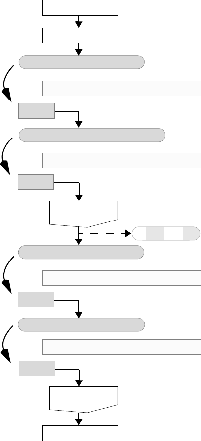
6: Alagator Scripting Language

Alagator for Diffusion

584 Sentaurus™ Process User Guide

H-2013.03

Figure 84 shows the flowchart of this process. Sections relating to generic growth are omitted.

They are explained in Alagator for Generic Growth on page 596.

Figure 84 Flowchart with calls to the callback procedures during the execution of a diffuse

command by Sentaurus Process; callbacks related to material growths are

omitted

diffuse

diffPreProcess

For each: solution and material

InitSolve callback procedure:

For each: marked solution and material

EquationInitProc callback procedure

Solve initialization

InitPostProcess

For each: solution and material

EquationProc callback procedure

Solve diffusion

diffPostProcess

InitProc callback procedure

For each: solution and material

equations

6: Alagator Scripting Language

Alagator for Diffusion

Sentaurus™ Process User Guide 585

H-2013.03

The diffPreProcess Procedure

The execution of every diffuse command starts with a call to the diffPreProcess Tcl

procedure. The diffPreProcess Tcl procedure is used to initialize various data fields or to

preprocess the existing data fields. For example, the truncation of interstitial and vacancy

profiles in the amorphous regions is performed in this procedure. In diffPreProcess, the

point-defect equations are switched on or off according to the diffusion models selected.

Initialization

After the execution of diffPreProcess, Sentaurus Process checks for all materials and

solution names, and whether a procedure name is specified for the keyword InitSolve for

the material and solution names. If a procedure name is defined, the procedure will be called,

using the material name and solution name as arguments.

Subsequently, Sentaurus Process checks for all marked materials and solutions to see if a

procedure name is specified with the keyword EquationInitProc for the solution variable

that needs to be initialized. If this is the case, the procedure will be executed with the material

name and solution name as arguments. Typically, in this procedure, the equation string is built,

which is to be solved at time=0 in the diffusion solver. Alternatively, if no callback procedure

name is defined for the keyword EquationInitProc for a material and solution, the equation

string to be used for the initialization can be specified directly on the command line.

After that, Sentaurus Process will solve the initialization equations for all materials and

solutions that need to be initialized. The initialization equations are solved for the initial

temperature of the temperature ramp specified in the diffuse statement. Such an initialization

is usually not required for all solutions. It is typically necessary for solutions whose initial

value depends in a complex way on the data fields (see Complex Initialization Procedures:

InitSolve and EquationInitProc on page 592).

If initialization is not required at all, it can be omitted using the !isolve option with the

diffuse command.

A Tcl procedure called InitPostProcess is provided for convenience. It is called after the

initialization is completed. It can be used to plot or save the solution variable profiles after the

initialization. By default, InitPostProcess is an empty procedure.

Building and Solving Diffusion Equations

After the initialization, Sentaurus Process checks for all materials and solution names to see

whether a procedure name is specified for the keyword InitProc. If the procedure is defined,

it will be called for the specified material name and solution name. These procedures are

usually used to set the equation strings to empty strings and to remove terms defined in

previous diffusion steps. By having empty equation strings, the equations and terms can be

built up piecewise, by adding expressions for each selected model that contributes to an

6: Alagator Scripting Language

Alagator for Diffusion

586 Sentaurus™ Process User Guide

H-2013.03

equation or a term. This is necessary because different diffusion models may be used for

different diffusion steps, and because additional species may be added between diffusion steps,

which may require terms to be added to the equations for existing species.

In the next step, Sentaurus Process checks for all materials and solution names to see whether

a procedure name is specified for the keyword EquationProc. If the procedure is defined, it

will be called with the material name and the solution name as parameters. These procedures

are used to set the diffusion equations for the solution variable. Alternatively, if no callback

procedure is defined for a material and a solution, the equation string can be set in a command

line without specifying any callback procedures.

NOTE If the callback procedure EquationProc is provided for a material

name and solution name, it will typically overwrite any equation

specified on the command line for this material and solution.

After the diffusion equations are set, Sentaurus Process solves the equations for the whole

temperature cycle specified in the diffuse statement.

The diffPostProcess Procedure

Finally, the procedure diffPostProcess will be called. The main purpose of the procedure

is to delete the data fields that are no longer needed and to store the total concentration of point

defects. The procedures diffPreProcess, diffPostProcess, and InitPostProcess

can be found in the Tcl library (see Ion Implantation to Diffusion on page 353) in the file

DiffProcess.tcl.

Using Callback Procedures

In this section, the previous examples will be implemented using callback procedures. First,

the callback procedure keywords InitProc and EquationProc will be explained since they

are the most widely used. Then, the examples will be expanded to include the use of other

keywords and procedures.

6: Alagator Scripting Language

Alagator for Diffusion

Sentaurus™ Process User Guide 587

H-2013.03

Setup Procedure: InitProc

The keyword InitProc is used to clean up equation strings. It specifies the name of the

callback procedure to be called by Sentaurus Process. For example, the first command below:

defines the ResetEquations procedure as the callback procedure of the solution variable CX

in silicon. The callback procedure itself takes two arguments: a material name and a solution

name. In this example, Sentaurus Process will call the ResetEquations procedure with two

arguments. The first argument Mat will be Silicon and the second argument Sol will be CX.

The argument names Sol and Mat are arbitrary, and they can be any valid Tcl variable but the

first argument is always the material name and the second argument is always the solution

name.

The procedure is called every time the solutions are checked during the diffusion. The

procedure prints the message 'This callback procedure unsets CX equation in

Silicon' and removes the pdb equation if it was defined.

Note that neither the solution name CX nor the material name Silicon is used in the

implementation of the ResetEquations callback procedure. Therefore, the callback

procedure is a generic procedure and can be used for several materials and solutions. This

example can be extended with the following commands:

pdbSetString Silicon CX InitProc ResetEquations

pdbSetString Silicon CY InitProc ResetEquations

pdbSetString Oxide CX InitProc ResetEquations

pdbSetString Oxide CY InitProc ResetEquations

In this case, the same callback procedure, ResetEquations, is used for the solution variables

CX and CY in the materials oxide and silicon. Sentaurus Process will print the following

messages:

This callback procedure unsets CX equation in Oxide.

This callback procedure unsets CX equation in Silicon.

This callback procedure unsets CY equation in Oxide.

This callback procedure unsets CY equation in Silicon.

The advantage of using callback procedures is clear. With four new command lines, the

equations for CX and CY in both oxide and silicon can be unset. At the same time, there is only

pdbSetString Silicon CX InitProc ResetEquations

proc ResetEquations { Mat Sol } {

LogFile "This callback procedure unsets $Sol equation in $Mat."

pdbUnSetString $Mat $Sol Equation

}

6: Alagator Scripting Language

Alagator for Diffusion

588 Sentaurus™ Process User Guide

H-2013.03

one callback procedure to maintain. If you change the callback procedure, the changes will

apply to all four settings.

Equation Procedure: EquationProc

The primary responsibility of the equation procedure is to construct the equation string. It uses

the keyword EquationProc in the parameter database. The keyword determines which

callback procedure name will be called by Sentaurus Process. For example, the first command

below:

defines the SetEquations procedure as the callback procedure of the solution variable CX in

silicon. The callback procedure itself takes two arguments: a material name and a solution

name. In this example, Sentaurus Process will call the SetEquations procedure with two

arguments. The first argument Mat will be Silicon and the second argument Sol will be CX.

The argument names Sol and Mat are arbitrary, and they can be any valid Tcl variable, but the

first argument is always the material name and the second argument is always the solution

name.

The SetEquations procedure is called every time the solutions are checked during the

simulation. In the above example, the procedure will print the message ‘This callback

procedure sets CX equation in Silicon.’ and will set the pdb equation for CX in

silicon.

NOTE Neither the solution name CX nor the material name Silicon is used in

the implementation of the SetEquations callback procedure.

Therefore, the callback procedure is a generic procedure. The equation

setting is similar to the one explained in Basics on page 576. The only

difference is that instead of using a solution name and material name,

only Tcl variables are used.

This example can be extended with the following commands:

pdbSetString Silicon CX EquationProc SetEquations

pdbSetString Silicon CY EquationProc SetEquations

pdbSetString Silicon CX EquationProc SetEquations

proc SetEquations { Mat Sol } {

LogFile "This callback procedure sets $Sol equation in $Mat."

pdbSetString $Mat $Sol Equation "ddt($Sol) -[Arrhenius 0.138 1.37]*grad($Sol)"

}

6: Alagator Scripting Language

Alagator for Diffusion

Sentaurus™ Process User Guide 589

H-2013.03

In this case, the same callback procedure, SetEquations, is used for the solution variables

CX and CY in silicon. Sentaurus Process will print the following messages:

This callback procedure sets CX equation in Silicon.

This callback procedure sets CY equation in Silicon.

The advantage of using callback procedures is clear. With two new command lines, you can set

the diffusion equations for CX and CY in silicon. At the same time, there is only one callback

procedure to maintain. If you change the callback procedure, the changes will apply to both

settings.

The above implementation uses the same diffusivity for both CX and CY. To use different

diffusivities for each solution variable, the callback procedure SetEquations must be

modified and diffusivities for each solution variable should be set as follows:

pdbSetString Silicon CX EquationProc SetEquations

pdbSetString Silicon CY EquationProc SetEquations

pdbSetDouble Silicon CX D {[Arrhenius 0.138 1.37]}

pdbSetDouble Silicon CY D {[Arrhenius 0.02 0.3]}

proc SetEquations { Mat Sol } {

LogFile "This callback procedure sets $Sol equation in $Mat."

set diff [pdbDelayDouble $Mat $Sol D]

pdbSetString $Mat $Sol Equation "ddt($Sol) - $diff * grad($Sol)"

}

The first change above is the setting of CX and CY diffusivities in the database. The second

change is in the SetEquations callback procedure. Instead of having a hard-wired diffusivity

number, pdbDelayDouble is used to obtain the expression stored in the database. Now, the

diffusivities depend on the database entry. You can change these entries to observe the effect

of different diffusivities on the final profile.

The example given in Using Terms on page 580 can be enhanced further by using both terms

and callback procedures as follows:

pdbSetDouble Silicon CX D {[Arrhenius 0.138 1.37]}

pdbSetDouble Silicon CY D {[Arrhenius 0.02 0.3]}

pdbSetDouble Silicon CX Kf {[Arrhenius 4.2e-11 0.1]}

pdbSetDouble Silicon CY Kf {[Arrhenius 4.2e-11 0.1]}

pdbSetDouble Silicon CX Cstar {[Arrhenius 3.6e27 3.7]}

pdbSetDouble Silicon CY Cstar {[Arrhenius 4.0e26 3.97]}

pdbSetString Silicon CX Recomb “CY”

pdbSetString Silicon CY Recomb “CX”

solution add name=CX !damp !negative solve

solution add name=CY !damp !negative solve

6: Alagator Scripting Language

Alagator for Diffusion

590 Sentaurus™ Process User Guide

H-2013.03

pdbSetString Silicon CX EquationProc SetEquations

pdbSetString Silicon CY EquationProc SetEquations

proc SetEquations { Mat Sol } {

LogFile "This callback procedure sets $Sol equation in $Mat."

set diff [pdbDelayDouble $Mat $Sol D]

set Kf [pdbDelayDouble $Mat $Sol Kf]

set Recomb [pdbGetString $Mat $Sol Recomb]

set CXStar [pdbDelayDouble $Mat $Sol Cstar]

set CYStar [pdbDelayDouble $Mat $Recomb Cstar]

term name = RCXCY $Mat eqn = "$Kf * ($Sol * $Recomb- $CXStar * $CYStar)"

pdbSetString $Mat $Sol Equation "ddt($Sol) - $diff * grad($Sol) + RCXCY”

}

First, the diffusivity, equilibrium concentration, and forward reaction rate for the

recombination of CX and CY are stored in the parameter database. Since CX and CY recombine

with each other, this information (Recomb) is also stored in the database. Then, the callback

procedure is modified to read these database entries. The Tcl variable Recomb in the callback

procedure will have the value of CY for CX and CX for CY. The forward recombination rate

RCXCY is the same for both solution variables. The callback procedure will be called once for

CX and once for CY. During each call, the term RCXCY will be created. Since the term name does

not depend on the solution name, the first term created during the CX equation setup will be

deleted during the CY equation setup. This is performed intentionally for this example since

both equations use exactly the same term. If you want to create a unique term for each call, the

callback procedure must be modified as follows:

proc SetEquations { Mat Sol } {

LogFile "This callback procedure sets $Sol equation in $Mat."

set diff [pdbDelayDouble $Mat $Sol D]

set Kf [pdbDelayDouble $Mat $Sol Kf]

set Recomb [pdbGetString $Mat $Sol Recomb]

set CXStar [pdbDelayDouble $Mat $Sol Cstar]

set CYStar [pdbDelayDouble $Mat $Recomb Cstar]

term name = R${Sol}${Recomb} $Mat eqn = "$Kf * ($Sol * $Recomb- $CXStar * \

$CYStar)"

pdbSetString $Mat $Sol Equation "ddt($Sol) - $diff * grad($Sol) + \

R${Sol}${Recomb}"

}

In this case, two terms will be created: RCXCY and RCYCX.

6: Alagator Scripting Language

Alagator for Diffusion

Sentaurus™ Process User Guide 591

H-2013.03

Preprocessing and Postprocessing Data: diffPreProcess,

UserDiffPreProcess, diffPostProcess, UserDiffPostProcess

Sentaurus Process can initialize solution variable fields on the command line using various

commands, such as select (see select on page 1117) and profile (see profile on

page 1093). If the initialization can be standardized, it is better to use the diffPreProcess

callback procedure. By default, diffPreProcess is used to initialize the data fields for

interstitials, vacancies, dopants, dopant clusters, dopant-defect clusters, and defect clusters (see

Ion Implantation to Diffusion on page 353). The procedure also switches on and off point-

defect solutions and various cluster solutions.

You ca n over writ e the pr oc ed ure diffPreProcess. For example:

proc diffPreProcess { } {

LogFile "This procedure is used to initialize data fields CX and CY"

sel z = "CX + 2.0e18 * exp( -(x-0.5)*(x-0.5) / (0.01 * 0.01) ) + 1.0" \

name=CX store

sel z = "CY + CX * 0.1" name=CY store

}

This procedure will create a Gaussian profile for the solution variable CX with a peak at the

depth x = 0.5 and a maximum concentration of . Ten percent of the CX profile will

be added to the existing data field CY.

More complex examples can be created by combining pdb commands and the Tcl callback

procedures, for example:

pdbSetDouble Silicon CY minDose 1e10

proc diffPreProcess { } {

LogFile "This procedure is used to initialize data fields CX and CY"

sel z = "CX + 2.0e18 * exp( -(x-0.5)*(x-0.5) / (0.01 * 0.01) ) + 1.0" \

name=CX store

sel z = CY

set dose [FindDose]

if { $dose > [pdbGetDouble Silicon CY minDose] } {

solution add name=CY !damp !negative solve

} else {

solution add name=CY !damp !negative nosolve

}

In this example, a parameter called minDose is created for CY in the database to set the

minimum allowed dose for diffusion to occur. In the callback procedure diffPreProcess,

218

×10 cm 3–

6: Alagator Scripting Language

Alagator for Diffusion

592 Sentaurus™ Process User Guide

H-2013.03

the CX profile is set as previously explained. The second and fourth lines calculate the dose of

CY in silicon. The ‘if-else’ statement retrieves the minimum dose value from the database. If

the existing dose of CY is below the minimum dose, the solution for CY is switched off;

otherwise, it is switched on.

To enforce additional actions to be performed upon diffusion preprocessing, it is not necessary

to overwrite the default implementation of the procedure diffPreProcess. Instead, to

preserve the default initialization of data fields, it is recommended to redefine the procedure

UserDiffPreProcess. By default, UserDiffPreProcess is an empty procedure and is

called from the procedure diffPreProcess as one of the last commands.

The callback procedure diffPostProcess is called at the end of diffusion. By default, it is

used to store the total concentrations of point defects and to delete some temporary data fields

such as Int_Implant and Vac_Implant. In the last command line of diffPostProcess,

the procedure UserDiffPostProcess is called, which is empty by default. If you want to

add commands to be executed after diffusion, it is recommended to redefine the procedure

UserDiffPostProcess.

Complex Initialization Procedures: InitSolve and EquationInitProc

In some cases, the initialization of solution variables can be very complex and cannot be

accomplished by using the select command (see select on page 1117). In these cases,

Sentaurus Process defines the initialization equations using the Alagator language and callback

procedures.

Assume that the CX solution variable is initialized by solving the following equation:

(822)

where is the total concentration of CX, and and are user-defined initialization

parameters. Depending on the value of and , you need to solve Eq. 822.

To initiate the initialization setup procedure, the solution name must be defined as:

solution add name=CX !damp !negative solve InitStep

The keyword InitStep allows this solution variable to be initialized.

CXTotal CX αCX()

CXTotal

6: Alagator Scripting Language

Alagator for Diffusion

Sentaurus™ Process User Guide 593

H-2013.03

The keyword InitSolve determines which callback procedure name will be called by

Sentaurus Process. For example, the first command below:

defines the ResetInitEquations procedure as the callback procedure of the solution

variable CX in silicon. The callback procedure itself takes two arguments: a material name and

a solution name. In this example, Sentaurus Process will call the ResetInitEquations

procedure with two arguments. The first argument Mat will be Silicon and the second

argument Sol will be CX. In this example, the solution variable CX is marked to be initialized

in silicon. If there is no such setting for the solution variable CY, CY will not be initialized.

After calling the callback procedures defined by InitSolve, Sentaurus Process will look for

an equation string for the solution variable. This is performed by defining a callback procedure

using the keyword EquationInitProc.

In this procedure, the equation string for initialization is constructed. For example, the first

command below:

defines the SetInitEquations procedure as the callback procedure of the solution variable

CX in silicon. The callback procedure itself takes two arguments: a material name and a

solution name. In this example, Sentaurus Process will call the SetInitEquations

procedure with two arguments. The first argument Mat will be Silicon and the second

argument Sol will be CX. The argument names Sol and Mat are arbitrary, and they can be any

valid Tcl variable, but the first argument is always the material name and the second argument

is always the solution name.

The EquationInitProc and EquationProc keywords work in the same way. The callback

procedure defined with the keyword EquationInitProc is called only during initialization.

pdbSetString Silicon CX

InitSolve ResetInitEquations

proc ResetInitEquations { Mat Sol } {

LogFile "This callback procedure unsets $Sol equation in $Mat during initialization."

pdbUnSetString $Mat $Sol Equation

}

pdbSetString Silicon CX

EquationInitProc SetInitEquations

proc SetInitEquations { Mat Sol } {

LogFile "This callback procedure sets $Sol equation in $Mat during initialization."

}

pdbSetString $Mat $Sol Equation "${Sol}_Implant - $Sol - ($alpha * $Sol)^$beta"

set alpha [pdbDelayDouble $Mat $Sol Alpha]

set beta [pdbDelayDouble $Mat $Sol Beta]

6: Alagator Scripting Language

Alagator for Diffusion

594 Sentaurus™ Process User Guide

H-2013.03

The callback procedure defined with the keyword EquationProc is called only during

diffusion. It is assumed that Alpha and Beta are already entered into the database and

CXTotal is defined.

Diffusion Summary: pdb, TclLib, SPROCESS.models

So far, it has been shown how to set up diffusion equations and boundary equations, and how

to initialize solution variables. The complete example can be divided into three major parts.

The first part is the pdb entries as follows:

pdbSetDouble Silicon CX D {[Arrhenius 0.138 1.37]}

pdbSetDouble Silicon CY D {[Arrhenius 0.02 0.3]}

pdbSetDouble Silicon CX Kf {[Arrhenius 4.2e-11 0.1]}

pdbSetDouble Silicon CY Kf {[Arrhenius 4.2e-11 0.1]}

pdbSetDouble Silicon CX Cstar {[Arrhenius 3.6e27 3.7]}

pdbSetDouble Silicon CY Cstar {[Arrhenius 4.0e26 3.97]}

pdbSetString Silicon CX Recomb "CY"

pdbSetString Silicon CY Recomb "CX"

pdbSetDouble Silicon CX Alpha {[Arrhenius 1.03103e-17 -0.4]}

pdbSetDouble Silicon CX Beta {4.0}

This part corresponds to the parameter database (see Parameter Database on page 55). All

default Sentaurus Process model parameters are stored in the parameter database. The second

part is the definition of the names of the solution variables and the names of the callback

procedures:

solution add name=CX !damp !negative solve

solution add name=CY !damp !negative solve

pdbSetString Silicon CX EquationProc SetEquations

pdbSetString Silicon CY EquationProc SetEquations

pdbSetString Silicon CX InitProc ResetEquations

pdbSetString Silicon CY InitProc ResetEquations

pdbSetString Gas_Silicon CY InitProc ResetEquations

pdbSetString Gas_Oxide CX InitProc ResetEquations

pdbSetString Silicon CX InitSolve ResetInitEquations

pdbSetString Silicon CX EquationInitProc SetInitEquations

The information for the default Sentaurus Process models are stored in the TclLib directory

(see Environment Variables on page 47) in the file SPROCESS.models, which is read by

Sentaurus Process as soon as the simulation starts. The file also contains information with

regard to solver types, implant directories, and material names.

6: Alagator Scripting Language

Alagator for Diffusion

Sentaurus™ Process User Guide 595

H-2013.03

The third part is the definition of diffusion and initialization models. The models are stored in

the TclLib directory (see Environment Variables on page 47):

proc UserDiffPreProcess { } {

LogFile "This procedure is used to initialize data fields CX and CY"

sel z = "CX + 2.0e18 * exp( -(x-0.5)*(x-0.5) / (0.01 * 0.01) ) + 1.0" \

name=CXTotal store

sel z = "CY + CXTotal * 0.1" name = CY store

}

proc ResetEquations { Mat Sol } {

LogFile "This callback procedure resets $Sol equation in $Mat."

pdbUnSetString $Mat $Sol Equation

}

proc SetEquations { Mat Sol } {

LogFile "This callback procedure sets $Sol equation in $Mat."

set diff [pdbDelayDouble $Mat $Sol D]

set Kf [pdbDelayDouble $Mat $Sol Kf]

set Recomb [pdbGetString $Mat $Sol Recomb]

set CXStar [pdbDelayDouble $Mat $Sol Cstar]

set CYStar [pdbDelayDouble $Mat $Recomb Cstar]

term name = RCXCY $Mat eqn = "$Kf * ($Sol * $Recomb- $CXStar * $CYStar)"

pdbSetString $Mat $Sol Equation "ddt($Sol) - $diff * grad($Sol) + RCXCY"

}

proc ResetInitEquations { Mat Sol } {

LogFile "This callback procedure unsets $Sol equation in $Mat during \

initialization."

pdbUnSetString $Mat $Sol Equation

}

proc SetInitEquations { Mat Sol } {

LogFile "This callback procedure sets $Sol equation in $Mat during \

initialization."

set alpha [pdbDelayDouble $Mat $Sol Alpha]

set beta [pdbDelayDouble $Mat $Sol Beta]

pdbSetString $Mat $Sol Equation "${Sol}_Implant - $Sol

- (($alpha*$Sol)^$beta)"

}

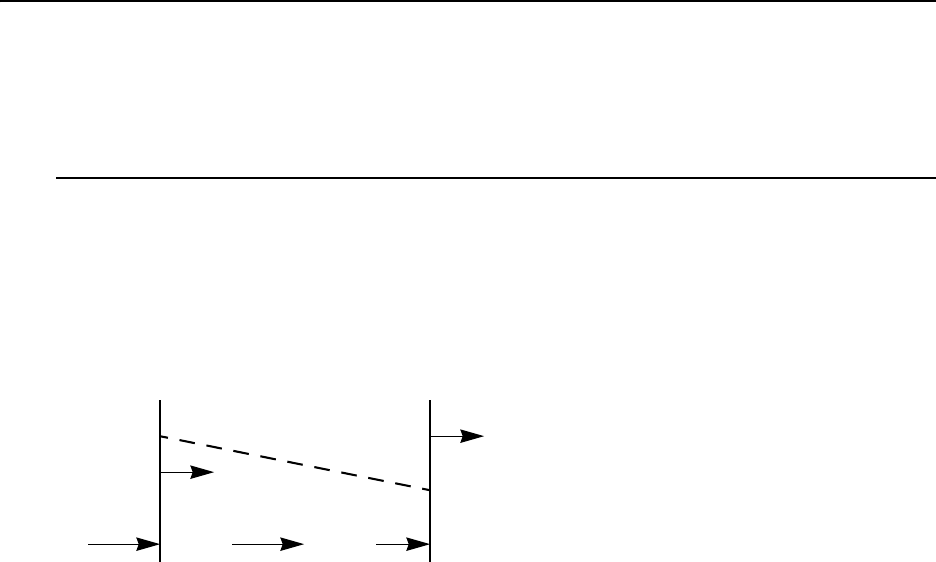
6: Alagator Scripting Language

Alagator for Generic Growth

596 Sentaurus™ Process User Guide

H-2013.03

Alagator for Generic Growth

The generic growth scheme uses most of the standard definitions used in diffusion. Read

Alagator for Diffusion on page 575 before continuing with this section.

Basics

In this section, examples of varying complexity are used to illustrate how to specify growth

equations using the Alagator scripting language. Most of the definitions are identical to those

of the diffusion equation. However, the keywords used to define the callback procedures and

the definition of solution variables differ. In addition, the reaction equations interact with the

reaction command.

Figure 85 Flux, ambient concentration, and motion of the growth front during the growth

process

Consider a reaction where the ambient GX reacts with silicon and forms a new material called

TEOS. The schematic in Figure 85 shows the ambient concentration at each interface and the

motion of the growth during the process. J represents the fluxes towards the Gas_TEOS and

Silicon_TEOS interfaces, and the flux of GX inside TEOS.

Since TEOS is a new material, first, it must be entered into the existing material list using the

command:

mater add name=TEOS

Then, the reacting materials must be defined using the reaction command (see reaction on

page 1099).

It is possible to create a reaction based on existing ambients, but in this case, a new react type

(named GX) ambient is created:

ambient name=GX react add

reaction name=TEOSreaction mat.l=Silicon mat.r=Gas mat.new=TEOS \

new.like=oxide ambient.name=GX diffusing.species=GX

nTEOS

Silicon

Gas

JGas_TEOS JTEOS JSilicon_TEOS

GXGas_TEOS

GXSilicon_TEOS

6: Alagator Scripting Language

Alagator for Generic Growth

Sentaurus™ Process User Guide 597

H-2013.03

Silicon (mat.l) is on the left side of the reacting interface and Gas (mat.r) is the material

on the right side of the reacting interface. The newly formed material (mat.new) at the reacting

interface is TEOS. The new material and its interfaces with other materials also are defined to

be like Oxide and Oxide interfaces (for example, TEOS = Oxide, PolySilicon_TEOS =

Oxide_PolySilicon). For the GX reaction, it requires an ambient, and the ambient name is

GX. The reaction will not occur unless the ambient GX is present in a gas flow or directly in the

diffuse command. (For more information about how to specify ambients, see Ambients and

Gas Flows on page 617.) Reactions that require a react-type ambient cannot have more than

one diffusing species name. If the reaction does not require an ambient, it can have multiple

names of diffusing species. In this case, the reaction occurs if the reacting interfaces exist in

the structure.

The reaction command automatically adds the diffusing species GX to the general solution

list. This is performed internally by using the command:

solution name=GX add !negative GrowthStep solve

where GrowthStep identifies this solution name as a reaction solution name. When the

solution name and the new material are defined, the reaction and diffusion equations are written

as follows:

pdbSetString TEOS GX Equation "ddt(GX)- \[Arrhenius 0.2 1.86\]*grad(GX)"

pdbSetString Gas_TEOS GX Equation_TEOS "-(GX_TEOS - 1e17)"

pdbSetString Silicon_TEOS GX Equation_TEOS "-5e-2*(GX_TEOS)"

pdbSetString Silicon_TEOS GX GrowthReaction " 5e-2*(GX_TEOS)"

The first line sets the diffusion equation of GX in TEOS. The next two lines set the boundary

fluxes at the Gas_TEOS and Silicon_TEOS interfaces. One of the commands works on the

Gas_TEOS interface and the other one works on the Silicon_TEOS interface. The _TEOS

option on Equation indicates the side of the interface to which the given flux will be applied.

The same option on the solution variable GX indicates that the solution variable value at this

interface is taken from the TEOS side. These settings are identical to the ones described in

Setting Boundary Conditions on page 578.

The last line is unique to the generic growth equations. The keyword GrowthReaction is

used to define the growth reaction flux at the reacting interface. In this example, the growth

reaction flux is identical to the diffusion flux at the reacting interface. In addition, the sign of

the growth reaction flux is the opposite of the sign of the diffusion flux.

Finally, it is necessary to specify the ambient in a gas flow (see gas_flow on page 935) and use

it with the diffusion command or specify it directly in the diffusion command in order

for the reaction to occur. For example:

gas_flow name=gxflw partial_pressure = { GX = 1.0 }

diffuse time=100 temp=1000 gas_flow = gxflw

6: Alagator Scripting Language

Alagator for Generic Growth

598 Sentaurus™ Process User Guide

H-2013.03

or:

diffuse time=100 temp=1000 GX

will both switch on reactions involving the ambient GX and will set the partial pressure of GX

to 1. Using the gas_flow command is more flexible in that the partial pressure can be set to

any value (not just 1.0) or the partial pressure can be computed from gas flows and gas

reactions.

Epi Reactions

This is an example of using the reaction command to create a new epitaxial growth mode:

ambient name=MyEpi epi add

# Now, create the new temporary material to be used during epi growth

# the name <Ambient>On<Material> is not necessary, it is just

# the same convention as used internally

mater name=MyEpiOnNitride add

reaction name= MyEpiOnNiReact mat.l=Nitride mat.r=Gas mat.new=MyEpiOnNitride \

ambient.name=MyEpi new.like=PolySilicon mat.final=PolySilicon

In this example, there is an additional parameter mat.final, which is the final name of the

epi material. There is a conversion from mat.new to mat.final at the end of the diffuse

command. For details on how to set up epi reactions and growth rates, see Epitaxy Growth

Rate: GrowthRateProc on page 605.

The model can be enhanced by adding the model parameters to the PDB. This allows other

users to change the values in the equations by accessing the properties directly. The following

changes make the equations dependent on the stored value in the database:

pdbSetDouble TEOS GX Dstar "\[Arrhenius 0.2 1.86\]"

pdbSetDouble Gas_TEOS GX Cstar "1e17"

pdbSetDouble Silicon_TEOS GX Kfd "5e-2"

pdbSetDouble Silicon_TEOS GX Kfg "5e-2"

set diff [pdbDelayDouble TEOS GX Dstar]

pdbSetString TEOS GX Equation "ddt(GX)- $diff * grad(GX)"

set GXStar [pdbDelayDouble Gas_TEOS GX Cstar]

pdbSetString Gas_TEOS GX Equation_TEOS "-(GX_TEOS - $GXStar)"

set GKfd [pdbDelayDouble Silicon_TEOS GX Kfd]

pdbSetString Silicon_TEOS GX Equation_TEOS "-$GKfd*(GX_TEOS)"

set GKfg [pdbDelayDouble Silicon_TEOS GX Kfg]

pdbSetString Silicon_TEOS GX GrowthReaction " $GKfg*(GX_TEOS)"

6: Alagator Scripting Language

Alagator for Generic Growth

Sentaurus™ Process User Guide 599

H-2013.03

The first lines set the diffusivity, equilibrium value of GX, and forward reaction rates for the

diffusion and growth fluxes in the database. This can be made permanent by directly editing

the hierarchy files. The pdbDelayDouble command is used to return the expression stored in

the database. This is necessary so that the evaluation of the expression does not occur until the

diffuse command is executed. Now, the equation depends on the database entry.

It is possible to use terms with the generic growth equations. For example:

pdbSetDouble TEOS GX Dstar "\[Arrhenius 0.2 1.86\]"

pdbSetDouble Gas_TEOS GX Cstar "1e17"

pdbSetDouble Silicon_TEOS GX Kfd "5e-2"

pdbSetDouble Silicon_TEOS GX Kfg "5e-2"

set diff [pdbDelayDouble TEOS GX Dstar]

pdbSetString TEOS GX Equation "ddt(GX)- $diff * grad(GX)"

set GXStar [pdbDelayDouble Gas_TEOS GX Cstar]

pdbSetString Gas_TEOS GX Equation_TEOS "-(GX_TEOS - $GXStar)"

term name = Reaction TEOS eqn = "GX"

set GKfd [pdbDelayDouble Silicon_TEOS GX Kfd]

pdbSetString Silicon_TEOS GX Equation_TEOS "-$GKfd*(Reaction_TEOS)"

set GKfg [pdbDelayDouble Silicon_TEOS GX Kfg]

pdbSetString Silicon_TEOS GX GrowthReaction "$GKfg*(Reaction_TEOS)"

a term called Reaction is created in TEOS. Note that the term also takes the _TEOS option to

indicate that the value of Reaction will be taken from the TEOS side.

The velocities regarding the growth reaction flux are calculated internally as follows:

(823)

where is the growth reaction flux defined using the pdbSetString command and

GrowthReaction keyword as previously explained. Beta is the stoichiometry of the growing

material, Expansion.Ratio is the conversion ratio from consumed material to the growing

material, and Density.Grow is the density of the growing material. The default values for

Beta, Expansion.Ratio, and Density.Grow are 1, 2.2, and , respectively. They

can be changed by using the following commands:

pdbSetDouble <interface material> <ambient> Beta <n>

pdbSetDouble <interface material> <ambient> Expansion.Ratio <n>

pdbSetDouble <interface material> <ambient> Density.Grow <n>

υGrowth

Beta

Expansion.Ratio * Density.Grow

---------------------------------------------------------------------------------FGrowth

FGrowth

2.2 22

×10

6: Alagator Scripting Language

Alagator for Generic Growth

600 Sentaurus™ Process User Guide

H-2013.03

For example, for the above example, you can change these values with the following

commands:

pdbSetDouble Silicon_TEOS GX Beta 1.1

pdbSetDouble Silicon_TEOS GX Expansion.Ratio 2.0

pdbSetDouble Silicon_TEOS GX Density.Grow 3e22

If Expansion.Ratio is set to 0, the material will dissolve but the new material will not form.

(For example, silicon will dissolve but no TEOS will form. This is useful for silicidation.)

Callback Procedures

Callbacks allow additional ‘intelligence’ to be built into the equations by allowing procedures

to be called at run-time. These procedures build the equation strings according to user-specified

options. By selecting model switches, the user can choose between different physical models

to be represented in the equation strings. Having callback procedures that use a material name

and a solution name as arguments, the same type of equation can be built for several materials,

dopants, and defect species. In Sentaurus Process, all frequently used equations are built-in

callback procedures.

There are six callback procedure–related keywords in Alagator: InitProc, InitSolve,

EquationInitProc, EquationProc, InitGrowth, and EquationGrowthProc.

InitProc, EquationInitProc, InitSolve, and EquationProc are used to define

generic diffusion equations (see Alagator for Diffusion on page 575). In this section, the

procedures specified by the keywords InitGrowth and EquationGrowthProc are

explained:

■InitGrowth provides the Tcl callback procedure name that is usually used to reset or

delete existing pdb equations or terms at the beginning of a diffusion simulation.

■EquationGrowthProc provides the Tcl callback procedure name that sets up equations

for material growth.

The Tcl callback procedures are called at various stages during the execution of the diffuse

command. In addition to the callback procedures, Sentaurus Process calls the

diffPreProcess Tcl procedure before executing the diffuse command, and the

diffPostProcess Tcl procedure after executing the diffuse command (see Ion

Implantation to Diffusion on page 353).

Figure 86 on page 601 shows the flowchart of the execution of a diffuse statement by

Sentaurus Process, including generic material growth. The sections regarding diffusion are

represented on a smaller scale and are shown in Figure 84 on page 584.

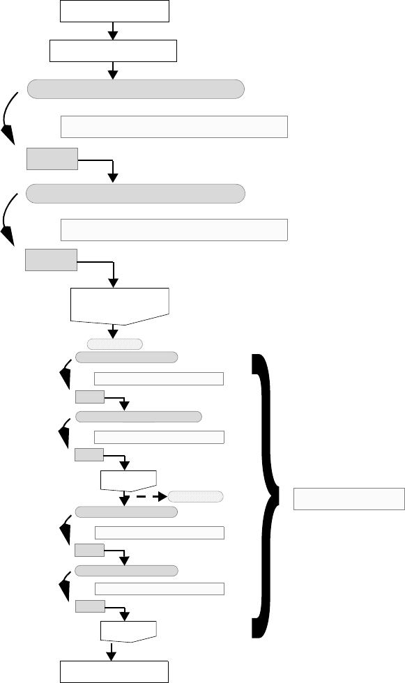
6: Alagator Scripting Language

Alagator for Generic Growth

Sentaurus™ Process User Guide 601

H-2013.03

Figure 86 Flowchart with calls to the callback procedures during execution of diffuse

command

growthPreProcess

diffuse

For each: reactant solution and material

InitGrowth callback procedure

For each: reactant solution and material

EquationGrowthProc callback procedure

Solve generic

diffPostProcess

growth equations

For each: solution and material

InitSolve callback procedure:

For each: marked solution and material

EquationInitProc callback procedure

Solve initialization

InitPostProcess

For each: solution and material

EquationProc callback procedure

Solve diffusion

InitProc callback procedure

For each: solution and material

equations

Diffusion process

diffPreProcess

6: Alagator Scripting Language

Alagator for Generic Growth

602 Sentaurus™ Process User Guide

H-2013.03

Setup Procedure: InitGrowth

The procedures specified by the keyword InitGrowth are used to clean up the equation

strings and terms. The keyword determines the callback procedure name to be called by

Sentaurus Process. For example, the first command below:

defines the ResetEquations procedure as the callback procedure of the solution variable GX

in silicon. The callback procedure itself takes two arguments: a material name and a solution

name. In this example, Sentaurus Process will call the ResetEquations procedure with two

arguments. The first argument Mat will be TEOS and the second argument Sol will be GX. The

argument names Sol and Mat are arbitrary, and they can be any valid Tcl variable, but the first

argument is always the material name and the second argument is always the solution name.

The above procedure ResetEquations will print the message ‘This callback

procedure unsets GX equation in TEOS.’ and will remove the pdb equation for GX

in TEOS if it was defined. Note that neither the solution name GX nor the material name TEOS

is used in the ResetEquations callback procedure. Therefore, the callback procedure is a

generic procedure. The example can be extended with the following commands:

pdbSetString TEOS GX InitGrowth ResetEquations

pdbSetString Gas_TEOS GX InitGrowth ResetEquations

pdbSetString Silicon_TEOS GX InitGrowth ResetEquations

In this case, the same callback procedure, ResetEquations, is used for the solution variables

GX inside TEOS, and at the Gas_TEOS and Silicon_TEOS interfaces. Sentaurus Process will

print the following messages:

This callback procedure resets GX equation in TEOS.

This callback procedure resets GX equation in Gas_TEOS.

This callback procedure resets GX equation in Silicon_TEOS.

Since the interface equations can be written for the interface material itself or the neighboring

materials, all of them must be unset including the growth reaction equation. In this case, you

can write a special Tcl procedure for the interfaces as follows:

proc ResetInterfaceEquations {Mat Sol} {

set mater1 [FirstMat $Mat]

set mater2 [SecondMat $Mat]

pdbSetString TEOS GX InitGrowth ResetEquations

proc ResetEquations { Mat Sol } {

LogFile "This callback procedure unsets $Sol equation in $Mat."

}

pdbUnSetString $Mat $Sol Equation

6: Alagator Scripting Language

Alagator for Generic Growth

Sentaurus™ Process User Guide 603

H-2013.03

pdbUnSetString $Mat $Sol Equation

LogFile "This callback procedure resets $Sol equation in $Mat."

pdbUnSetString $Mat $Sol Equation_$mater1

LogFile "This callback procedure resets $Sol equation in $Mat on $mater1 \

side."

pdbUnSetString $Mat $Sol Equation_$mater2

LogFile "This callback procedure resets $Sol equation in $Mat on $mater2 \

side."

pdbUnSetString $Mat $Sol GrowthReaction

LogFile "This callback procedure resets $Sol growth reaction equation in \

$Mat."

}

pdbSetString Gas_TEOS GX InitGrowth ResetInterfaceEquations

pdbSetString Silicon_TEOS GX InitGrowth ResetInterfaceEquations

The callback procedure, ResetInterfaceEquations, is similar to the ResetEquations

procedure. The commands FirstMat and SecondMat used in the procedure return the names

of the neighboring materials (for example, Gas and TEOS for Gas_TEOS). Then, the equations

set for either side of the interface or the interface are unset including the generic growth

reaction equation. This special procedure is called for GX at the Gas_TEOS and

Silicon_TEOS interfaces. Sentaurus Process will print the following messages:

This callback procedure resets GX equation in TEOS.

This callback procedure resets GX equation in Gas_TEOS.

This callback procedure resets GX equation in Gas_TEOS on Gas side.

This callback procedure resets GX equation in Gas_TEOS on TEOS side.

This callback procedure resets GX growth reaction equation in Gas_TEOS.

This callback procedure resets GX equation in Silicon_TEOS.

This callback procedure resets GX equation in Silicon_TEOS on Silicon side.

This callback procedure resets GX equation in Silicon_TEOS on TEOS side.

This callback procedure resets GX growth reaction equation in Silicon_TEOS.

Equation Procedure: EquationGrowthProc

The primary responsibility of the equation procedure is to construct the equation string for

material growth reaction. It uses the keyword EquationGrowthProc in the parameter

database. The keyword specifies the name of the callback procedure to be called by Sentaurus

Process.

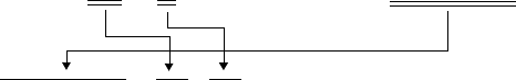
6: Alagator Scripting Language

Alagator for Generic Growth

604 Sentaurus™ Process User Guide

H-2013.03

For example, the first command below:

has the effect that, according to the flowchart presented in Figure 86 on page 601, Sentaurus

Process calls the procedure SetEquations with the arguments TEOS and GX.

The SetEquations procedure is called every time the solutions are checked during the

reaction. The procedure above will print the message ‘This callback procedure sets

GX equation in TEOS.’ and will set the pdb equation for GX in TEOS. Note that neither the

solution name GX nor the material name TEOS is used in the SetEquations callback

procedure. Therefore, the callback procedure is a generic procedure. The equation setting is

similar to the one explained in Basics on page 576. The only difference is that instead of using

a solution name and a material name, only Tcl variables are used. Since the interface equations

settings are different, this example can be extended with the following commands:

pdbSetString Gas_TEOS GX EquationProc SetInterfaceEquations

pdbSetString Silicon_TEOS GX EquationProc SetInterfaceEquations

proc SetInterfaceEquations { Mat Sol } {

set mater1 [FirstMat $Mat]

set mater2 [SecondMat $Mat]

if { [pdbIsAvailable $Mat $Sol Cstar] } {

set GXStar [pdbDelayDouble $Mat $Sol Cstar]

pdbSetString $Mat $Sol Equation_$mater2 "-(${Sol}_$mater2 - $GXStar)"

LogFile "This callback procedure sets $Sol equation in $Mat on $mater2 \

side."

} else {

set GKfd [pdbDelayDouble $Mat $Sol Kfd]

pdbSetString $Mat $Sol Equation_$mater2 "-$GKfd*(${Sol}_$mater2)"

LogFile "This callback procedure sets $Sol equation in $Mat on $mater2 \

side."

set GKfg [pdbDelayDouble $Mat $Sol Kfg]

pdbSetString $Mat $Sol GrowthReaction " $GKfg*(${Sol}_$mater2)"

LogFile "This callback procedure sets $Sol growth reaction equation in \

$Mat."

}

pdbSetString TEOS GX EquationGrowthProc SetEquations

proc SetEquations { Mat Sol } {

LogFile "This callback procedure sets $Sol equation in $Mat."

}

pdbSetString $Mat $Sol Equation "ddt($Sol) -$diff * grad($Sol)"

set diff [pdbDelayDouble $Mat $Sol Dstar]

6: Alagator Scripting Language

Alagator for Generic Growth

Sentaurus™ Process User Guide 605

H-2013.03

Here, the same callback procedure, SetInterfaceEquations, is used to set up the interface

equations on both the Gas_TEOS and Silicon_TEOS interfaces. The commands FirstMat

and SecondMat used in the procedure return the names of the neighboring materials (for

example, Gas and TEOS for Gas_TEOS). The command pdbIsAvailable returns true (1) if

the Cstar value is entered to the parameter database for the given solution name and material.

In this example, it will return true for the Gas_TEOS interface and false for the Silicon_TEOS

interface. Using this information and the ‘if-else’ statement, the equations can be set for the

Gas_TEOS and Silicon_TEOS interfaces. Now, the diffusivities, reaction rates, and

equilibrium values depend on the database entries.

Epitaxy Growth Rate: GrowthRateProc

The GrowthRateProc callback procedure can be used to set the GrowthReaction pdb

variable during epitaxial growth. The requirements are similar to EquationGrowthProc,

except that there can be a different GrowthRateProc for each epitaxial ambient. For example:

proc mygrproc { Mat Amb } {

pdbSetString $Mat $Amb GrowthReaction \

"([simDelayDouble Diffuse EpiThick]- \

[pdbDelayDouble $Mat $Amb NativeOffset])/ \

[simDelayDouble Diffuse AnnealStepTime]"

}

pdbSet Gas_LTEOnOxide LTE GrowthRateProc mygrproc

This example demonstrates a number of simulation status values that are available to the

GrowthRateProc implementer. The quantity simDelayDouble Diffuse EpiThick is

the value of the thick parameter set in the diffuse or temp_ramp commands. The quantity

pdbDelayDouble $Mat $Amb NativeOffset is set to the native layer thickness if a native

layer was deposited; otherwise, it is 0. Finally, simDelayDouble Diffuse

AnnealStepTime is the total time of the current temp_ramp segment or diffuse time.

If a new material is being deposited that is not a standard Sentaurus Process epi material, the

following parameters should be set:

pdbSetDouble <mat.new>_Gas <ambient.name> Expansion.Ratio 1.0

pdbSetDouble <mat.new>_Gas <ambient.name> Density.Grow 1.0

where <mat.new> is the name of the new material being grown and <ambient.name> is the

name of the ambient triggering the growth of <mat.new>.

The growthPreProcess Procedure

The execution of every diffuse command starts with a call to the growthPreProcess Tcl

procedure. The growthPreProcess Tcl procedure is used to initialize various reaction-

related data fields or to preprocess the existing data fields.

6: Alagator Scripting Language

Alagator for Generic Growth

606 Sentaurus™ Process User Guide

H-2013.03

To enforce additional actions to be performed upon generic growth preprocessing, it is not

necessary to overwrite the default implementation of the procedure growthPreProcess.

Instead, to preserve the default initialization of data fields, it is recommended to redefine the

procedure UserGrowthPreProcess. By default, UserGrowthPreProcess is an empty

procedure and is called from the procedure growthPreProcess as one of the last commands.

Generic Growth Summary: pdb, TclLib,

SPROCESS.models

So far, it has been shown how to set up reaction equations and fluxes. The complete example

can be divided into three major parts. The first part consists of pdb entries as follows:

pdbSetDouble TEOS GX Dstar "\[Arrhenius 0.2 1.86\]"

pdbSetDouble Gas_TEOS GX Cstar "1e17"

pdbSetDouble Silicon_TEOS GX Kfd "5e-2"

pdbSetDouble Silicon_TEOS GX Kfg "5e-2"

This part corresponds to the parameter database (see Parameter Database on page 55). All

default Sentaurus Process model parameters are stored in the parameter database. The second

part is the definition of reaction variable names, material names, and callback procedure

names:

mater add name=TEOS

reaction name=TEOSreaction mat.l=Silicon mat.r=Gas mat.new=TEOS \

new.like=oxide diffusing.species=GX ambient

pdbSetString TEOS GX InitGrowth ResetEquations

pdbSetString Gas_TEOS GX InitGrowth ResetInterfaceEquations

pdbSetString Silicon_TEOS GX InitGrowth ResetInterfaceEquations

pdbSetString Gas_TEOS GX EquationGrowthProc SetInterfaceEquations

pdbSetString Silicon_TEOS GX EquationGrowthProc SetInterfaceEquations

pdbSetString TEOS GX EquationGrowthProc SetEquations

The information for the default Sentaurus Process models is stored in the TclLib directory

(see Environment Variables on page 47) in the SPROCESS.models file, which is read by

Sentaurus Process as soon as the simulation starts. The file also contains information regarding

solver types, implant directories, and material names.

The third part is the definition of diffusion/reaction models. The models are stored in the

TclLib directory (see Environment Variables on page 47):

proc ResetEquations {Mat Sol} {

LogFile "This callback procedure resets $Sol equation in $Mat."

pdbUnSetString $Mat $Sol Equation

}

6: Alagator Scripting Language

Alagator for Generic Growth

Sentaurus™ Process User Guide 607

H-2013.03

proc ResetInterfaceEquations { Mat Sol } {

set mater1 [FirstMat $Mat]

set mater2 [SecondMat $Mat]

pdbUnSetString $Mat $Sol Equation

LogFile "This callback procedure resets $Sol equation in $Mat."

pdbUnSetString $Mat $Sol Equation_$mater1

LogFile "This callback procedure resets $Sol equation in $Mat on $mater1 \

side."

pdbUnSetString $Mat $Sol Equation_$mater2

LogFile "This callback procedure resets $Sol equation in $Mat on $mater2 \

side."

pdbUnSetString $Mat $Sol GrowthReaction

LogFile "This callback procedure resets $Sol growth reaction equation in \

$Mat."

}

proc SetEquations { Mat Sol } {

LogFile "This callback procedure sets $Sol equation in $Mat."

set diff [pdbDelayDouble $Mat $Sol Dstar]

pdbSetString $Mat $Sol Equation "ddt($Sol) - $diff * grad($Sol)"

}

proc SetInterfaceEquations { Mat Sol } {

set mater1 [FirstMat $Mat]

set mater2 [SecondMat $Mat]

if { [pdbIsAvailable $Mat $Sol Cstar] } {

set GXStar [pdbDelayDouble $Mat GX Cstar]

pdbSetString $Mat $Sol Equation_$mater2 "-(${Sol}_$mater2 - $GXStar)"

LogFile "This callback procedure sets $Sol equation in $Mat on $mater2 \

side."

} else {

set GKfd [pdbDelayDouble $Mat $Sol Kfd]

pdbSetString $Mat $Sol Equation_$mater2 "-$GKfd*(${Sol}_$mater2)"

LogFile "This callback procedure sets $Sol equation in $Mat on $mater2 \

side."

set GKfg [pdbDelayDouble $Mat $Sol Kfg]

pdbSetString $Mat $Sol GrowthReaction " $GKfg*(${Sol}_$mater2)"

LogFile "This callback procedure sets $Sol growth reaction equation in \

$Mat."

}

6: Alagator Scripting Language

Modifying Diffusion Models

608 Sentaurus™ Process User Guide

H-2013.03

Modifying Diffusion Models

In Sentaurus Process, all equations of dopant diffusion models are constructed using callback

procedures as previously explained. If you want to add a new expression to an existing equation

or term, or to subtract a new expression from an existing equation or term, one of the following

can be used:

■UserAddEqnTerm

■UserSubEqnTerm

■UserAddToTerm

■UserSubFromTerm

■MultiplyTerm

NOTE The UserAddEqnTerm, UserSubEqnTerm, UserAddToTerm,

UserSubFromTerm, and MultiplyTerm commands should not be

used within the callback procedures. They are designed to change

diffusion equations without using the callback procedures.

NOTE The UserAddEqnTerm, UserSubEqnTerm, UserAddToTerm,

UserSubFromTerm, and MultiplyTerm are saved to the TDR files.

If the input file is split, the commands must not be included in the new

input file. However a user defined variable or term used with these

command, the variable or term must be included in the new input file or

the variable must be saved with define command (see define on

page 897) and the term must be stored with the store parameter (see

term on page 1173).

UserAddEqnTerm and UserSubEqnTerm

The commands UserAddEqnTerm and UserSubEqnTerm allow you to add a new expression

to an existing solution variable equation or to subtract the new expression from an existing

solution variable equation. The commands have the format:

UserAddEqnTerm <material> <solution> <expression> <side>

UserSubEqnTerm <material> <solution> <expression> <side>

where:

■<material> is any valid material name.

■<solution> is any valid solution variable name.

■<expression> is the new expression to be added to or subtracted from the solution

variable.

6: Alagator Scripting Language

Modifying Diffusion Models

Sentaurus™ Process User Guide 609

H-2013.03

■<side> is the side of the interface material where the new expression will be added or

subtracted.

For example, the command:

UserAddEqnTerm Silicon CY "{2e-15*(CY*CY-1e-16*CX)}"

adds the expression "{2e-15*(CY*CY-1e-16*CX)}" to the Vac equation in silicon during

the PDE solve. Since the equations can be set in three different ways for interfaces, you have

the option to specify the side to which the expression will be added or subtracted. For example,

the commands:

UserAddEqnTerm Oxide_Silicon CX "(CX_Oxide - CX_Silicon)" Silicon

UserSubEqnTerm Oxide_Silicon CX "(CX_Oxide - CX_Silicon)" Oxide

add the expression "(CX_Oxide - CX_Silicon)" to the Oxide_Silicon interface

equation for CX on the Silicon side, and subtract the same expression from the

Oxide_Silicon interface equation for CX on the Oxide side, respectively. If no side

information is given, the expression will be added to the Oxide_Silicon interface equation

for CX.

UserAddToTerm and UserSubFromTerm

The commands UserAddToTerm and UserSubFromTerm are used to add a new expression

to an existing term or to subtract the new expression from an existing term. The commands

have the format:

UserAddToTerm <material> <term> <expression>

UserSubFromTerm <material> <term> <expression>

where:

■<material> is any valid material name.

■<term> is an existing term name.

■<expression> is the new expression to be added to or subtracted from the existing term.

For example the command:

UserAddToTerm Silicon

VTotal

"2*CX"

adds the expression "2*CX" to the term VTotal in silicon.

In the same way, the command:

UserSubFromTerm Silicon

VTotal

"2*CX"

6: Alagator Scripting Language

References

610 Sentaurus™ Process User Guide

H-2013.03

subtracts the expression "2*CX" from the term VTotal in silicon.

References

[1] R. E. Bank et al., “Transient Simulation of Silicon Devices and Circuits,” IEEE

Transactions on Electron Devices, vol. ED-32, no. 10, pp. 1992–2007, 1985.

Sentaurus™ Process User Guide 611

H-2013.03

CHAPTER 7 Advanced Calibration

This chapter provides details about the use of Advanced Calibration

in Sentaurus Process.

Overview

Synopsys’ Consulting and Engineering is working continually on improving the simulation

models and optimizing the model parameters for the latest technology. This effort is based on

long-standing experience of model calibration for customers and a comprehensive, growing

database of state-of-the-art secondary ion mass spectrometry (SIMS) profiles.

With Advanced Calibration in Sentaurus Process, you have a set of models and parameters that

have been calibrated to a broad range of technologies, from power devices to advanced CMOS.

With these parameters, you can obtain accurate results for many processes in device fabrication

such as ion implantation, dopant diffusion and activation, ultrashallow junction formation, and

surface dose loss.

The Advanced Calibration set of models and parameters is located in a single file. For the

current Sentaurus Process, it has the file name AdvCal_2013.12.fps and is located in the

directory $STROOT/tcad/$STRELEASE/lib/sprocess/TclLib/AdvCal.

The models and parameters of AdvCal_2013.12.fps are recommended for all technologies

for silicon, SiGe, and germanium substrates. The models have been tested extensively in 1D

and 2D simulations, and have proven to be accurate and robust.

Advanced Calibration also is available for Sentaurus Process Kinetic Monte Carlo (see

Advanced Calibration for Sentaurus Process KMC on page 565).

Using Advanced Calibration

Advanced Calibration is the recommended starting point for process simulation of all silicon-

based and germanium-based devices.To use Advanced Calibration in Sentaurus Process, at the

beginning of the input file, insert the line:

AdvancedCalibration

7: Advanced Calibration

Additional Calibration by Users

612 Sentaurus™ Process User Guide

H-2013.03

or:

AdvancedCalibration 2013.12

This will source the file $STROOT/tcad/$STRELEASE/lib/sprocess/TclLib/AdvCal/

AdvCal_2013.12.fps.

You have t he o pt ion t o use A dva nce d Ca lib ra tio n pa ram et ers a nd mo de ls f rom p revious

releases, for example:

AdvancedCalibration 2013.03

This will source the file $STROOT/tcad/$STRELEASE/lib/sprocess/TclLib/AdvCal/

AdvCal_2013.03.fps.

Additional Calibration by Users

Advanced Calibration is based on the assumption that all parameters that are not changed in

the parameter files are the Sentaurus Process default parameters. To use the Advanced

Calibration file AdvCal_2013.12.fps, it must be sourced before the real process

description.

You can f ur ther i nc rease th e a ccurac y of a c ertain technology by additional fine-tuning of

physical parameters. This should be performed by experienced users with a good

understanding of the diffusion models and callback procedures of Sentaurus Process.The best

way to perform this is to put all additional calibration in a user calibration file, for example,

user_calibration.fps. This file includes all project-specific changes of physical

parameters or callback procedures with respect to Advanced Calibration.

In the process simulation file, at the beginning of the process simulation, insert the lines:

AdvancedCalibration 2013.12

source ./user_calibration.fps

This method has two distinct advantages:

■There is a clear separation between the process flow, which is contained in the Sentaurus

Process input file, and the selection of physical models and parameters. During calibration

of Sentaurus Process for a specific technology, you can first set up the process flow in the

input file of Sentaurus Process and then improve the accuracy of the process simulation by

making changes only in their parameter file. Conversely, if you want to apply the same

models and parameters to a different process, it is only necessary to change the file

containing the process flow.

7: Advanced Calibration

Additional Calibration by Users

Sentaurus™ Process User Guide 613

H-2013.03

■The Advanced Calibration file is used as a starting point. The user calibration file (for

example, user_calibration.fps) is usually short and clear. You can see all parameter

changes with respect to the original Advanced Calibration at a glance.

NOTE For detailed documentation of the contents and physical models

included in Advanced Calibration as well as a discussion of its accuracy

and limitations, refer to the Advanced Calibration for Process

Simulation User Guide.

To accelerate process simulation for power technologies, use the procedures

AdvancedPowerDeviceMode and AdvancedPowerDeviceModeReset. For details, refer

to the Advanced Calibration for Process Simulation User Guide.

7: Advanced Calibration

Additional Calibration by Users

614 Sentaurus™ Process User Guide

H-2013.03

Sentaurus™ Process User Guide 615

I-2013.12

CHAPTER 8 Oxidation and Silicidation

This chapter describes the oxidation models available in Sentaurus

Process.

Oxidation

Sentaurus Process can simulate the thermal oxidation of silicon. Due to the conversion ratio

from Si to SiO2 being greater than one, new ‘volume’ is generated, which, in turn, leads to the

motion of materials and mechanical stress in the structure. The oxidation process has three

steps:

■Diffusion of oxidants (H2O, O2) from the gas–oxide interface through the existing oxide to

the silicon–oxide interface.

■Reaction of the oxidant with silicon to form new oxide1.

■Motion of materials due to the volume expansion, which is caused by the reaction between

silicon and oxide.

The oxidant diffusion equation is solved using the generic partial differential equation (PDE)

solver of Sentaurus Process. For the simulation of thermal oxidation, there are two

requirements:

■The silicon or polysilicon region is in contact with gas or an oxide region, which, in turn,

is in contact with gas.

■The diffuse command specifies a reactive atmosphere.

If silicon or polysilicon is in contact with gas at the beginning of a thermal oxidation, an initial

oxide layer is created automatically. The default thickness of this layer is 1.5 nm. The value of

the initial oxide thickness is specified in the parameter database by:

pdbSet Grid NativeLayerThickness 1.5e-7

which controls the native layer thickness for oxidation and silicidation. There are several ways

to specify a reactive atmosphere. Furthermore, temperature can vary during oxidation, and the

ambient can contain contributions from different oxidants. The following sections describe

how to handle these cases using Sentaurus Process.

It is important to note that oxidation occurs in conjunction with mechanics. The details of the

mechanical equations, boundary conditions, and material models are given in the next chapter.

1. In this chapter, oxide refers to SiO2.

8: Oxidation and Silicidation

Oxidation

616 Sentaurus™ Process User Guide

I-2013.12

Basic Oxidation

The diffuse command is used to specify two reactive ambients for oxidation, either H2O or

O2. The oxidation temperature and time must be given. For example, a command for a simple

oxidation using wet ambient temperature at for 10 minutes is:

diffuse temperature=1000<C> time=10<min> H2O

A simple temperature ramp can be specified directly in the diffuse command by the keyword

ramprate. This keyword sets the change in the temperature over time:

diffuse temperature=1000<C> time=10<min> O2 ramprate=10<C/min>

This example describes a dry oxidation of 10 minutes, starting at and ending at

NOTE The value of ramprate can be negative if the temperature is required

to decrease.

Temperature Cycles

The second example given in Basic Oxidation also can be specified by using the temp_ramp

command, for example:

temp_ramp name=MyTempRamp temperature=1000 time=10 O2 ramprate=10<C/min>

diffuse temp_ramp=MyTempRamp

The first line creates a temperature ramp with given conditions, and the second line specifies a

diffusion referring to this temperature ramp.

To describe more complex temperature cycles within one diffuse command, multiple

instances of the temp_ramp command can be used. A temperature ramp can consist of several

segments and, for each segment, one temp_ramp command is required. In addition, segments

can be grouped by using the same name for each segment. For example, a ramp-up, plateau,

and ramp-down can be specified as:

temp_ramp name=MyCycle temperature=1000<C> time=5<min> H2O ramprate=20<C/min>

temp_ramp name=MyCycle temperature=1100<C> time=10<min> O2

temp_ramp name=MyCycle temperature=1100<C> time=10<min> ramprate=-10<C/min>

diffuse temp_ramp=MyCycle

1000°C

1100°C

8: Oxidation and Silicidation

Oxidation

Sentaurus™ Process User Guide 617

I-2013.12

If you want to set the minimum and maximum reaction/oxidation time steps in minutes

globally, for all diffusion commands, the following commands can be used:

pdbSet Diffuse MinGrowthStep <n>

pdbSet Diffuse MaxGrowthStep <n>

See Parameter Database on page 55 for other diffusion-related parameters.

Ambients and Gas Flows

Sentaurus Process has a flexible scheme for dealing with gas flows. By default, several

ambients are available, and you can also create additional ones for new reactions (see reaction

on page 1099). Table 64 lists the ambients that are available by default.

The react and inert ambients can be specified in any combination using the gas_flow

command. The inert ambients are inert in the sense that they do not switch on material

reactions. However, inert ambients can be used in gas flows to change the partial pressure of

react ambients through gas reactions or just taking part of the total pressure as is the case with

N2, for example. As the name implies, react ambients cause material reactions to occur, such

as oxidation. The epi-type ambients trigger epitaxial growth and should not be used with any

other ambient.

To specify an ambient is present and to set the partial pressure to 1.0 * total pressure, use the

shorthand parameter name <ambient name> in the diffuse or gas_flow command. The

parameter pressure sets the total pressure and also is available on the diffuse or gas_flow

command line. The default for total pressure is 1 atm. Only one ambient should be specified

using the shorthand parameter <ambient name>. For epitaxy, specify the appropriate ambient

by name.

Ta bl e 64 Avai l a bl e a mb i en t s

Ambient name Ambient type Reactions

O2 react

Oxidation

H2O react

Oxidation

HCl inert

Gas reactions only

N2 inert

None

H2 inert

Gas reactions only

N2O react

Oxynitridation

Epi epi

Standard epitaxy

LTE epi

Low-temperature epitaxy

8: Oxidation and Silicidation

Oxidation

618 Sentaurus™ Process User Guide

I-2013.12

Specifying Gas Flows

The gas_flow command is used to specify a mixed gas flow by specifying directly either the

partial pressures of the gas components or the flow <volume/time>. When a gas_flow is

specified, it can be referred to from the temp_ramp and diffuse commands.

The gases present during diffusion can either be specified as partial pressures or using gas

flows. When using flow specifications, the partial pressure is computed from gas reactions, the

presence of inert gases, and the total pressure. Alternatively, the partial pressure can be

specified directly. The partial pressure can be set with either the p<ambient name>

parameters or the partial.pressure parameter of the gas_flow command:

gas_flow name=MyGasFlow pH2O=0.5 pO2=0.5

or:

gas_flow name=MyGasFlow partial.pressure = {H2O=0.5 O2=0.5}

Specifying directly in the diffuse command is also possible, for example:

diffuse pH2O=0.5 pO2=0.5 temperature=1000 time=10<min>

Instead of specifying partial pressures directly, the gas components can be given in terms of

flows using flow<ambient name> or the flows parameter, for example:

gas_flow name=MyGasFlow flowH2O=0.5 flowO2=0.5 flowH2=0.2 flowN2=1.0

or:

gas_flow name=MyGasFlow flows = {H2O=0.5 O2=0.5 H2=0.2 N2=1.0}

If flows are specified, Sentaurus Process calculates the partial pressures of the components

assuming a complete reaction of the gases. Because the only effect of inert ambients in

Sentaurus Process is to change the partial pressure of reacting ambients, inert ambients should

only be set using flows in the gas_flow command.

To invoke the gas flow specification as given above, use:

temp_ramp name=MyTempRamp temperature=1000<C> time=10<min> gas_flow=MyGasFlow

diffuse temp_ramp=MyTempRamp

or:

diffuse temperature=1000<C> time=10<min> gas_flow=MyGasFlow

8: Oxidation and Silicidation

Oxidation

Sentaurus™ Process User Guide 619

I-2013.12

Computing Partial Pressures

Given a flow of O2 in addition to a flow of H2 or HCl for example, a chemical reaction between

the components is taken into account: O2 is reduced and H

2O increases. A complete

stoichiometric reaction is assumed. The final flows1 after the reaction are computed in the

AmbientReactions procedure as shown in Eq. 824.

If :

(824)

else:

(825)

In the case where not all of the H2 is consumed by the reaction, a warning is displayed. If a

contribution of HCl is given, the equations read as follows.

If :

(826)

else:

(827)

1. The index init refers to the initial flows specified by users in the gas_flow command, and final describes the

flow after the chemical reaction.

flowO2init 0.5 flowH2init

⋅>

flowO2final flowO2init 0.5 flowH2init

⋅–=

flowH2Ofinal flowH2Oinit flowH2init

flowH2final 0=

flowO2final 0=

flowH2Ofinal flowH2Oinit 2flowO2⋅init

flowH2final flowH2init 2flowO2init

⋅–=

flowO2init flowHClinit

flowO2final flowO2init 0.5 flowHCl⋅init

–=

flowH2Ofinal flowH2Oinit flowHClinit

flowH2final 0=

flowO2final 0=

flowH2Ofinal flowH2Oinit 2flowO2⋅init

flowHClfinal flowHClinit flowO2init

–=

8: Oxidation and Silicidation

Oxidation

620 Sentaurus™ Process User Guide

I-2013.12

The final flows are used internally to compute the partial pressure of each component. Partial

pressures are the relevant quantity for the subsequent simulation. These are computed as:

(828)

where holds for a certain component of the gas mixture and pressure is the total

pressure.

In Situ Steam-generated Oxidation

Switching on the in situ steam-generated (ISSG) Boolean parameter in the gas_flow

command specifies that the gas flow condition is to be recognized for the ISSG oxidation (see

In Situ Steam-generated Oxidation on page 632). For example:

gas_flow name=ISSGflow pressure=12<torr> flowH2=6 flowO2=12 ISSG

Oxidant Diffusion and Reaction

For the rigorous simulation of the oxidation process, the dissolution of the oxidant species at

the gas–oxide interface, the transport through the existing or already grown oxide, and the

consumption at the oxide–silicon interface have to be simulated. The dissolution and

consumption are modeled by boundary conditions; for the oxidant transport, a diffusion

equation is solved in the oxide layer.

The oxidant species H2O, O2, and N2O are defined in the SPROCESS.models file (see Default

Simulator Settings: SPROCESS.models File on page 53) using the reaction command (see

reaction on page 1099):

reaction name=dryoxSi mat.l=Silicon mat.r=Gas mat.new=oxide \

diffusing.species=O2 ambient.name=O2

reaction name=wetoxSi mat.l=Silicon mat.r=Gas mat.new=oxide \

diffusing.species=H2O ambient.name=H2O

reaction name=n2ooxSi mat.l=Silicon mat.r=Gas mat.new=oxide

diffusing.species=N2O ambient.name=N2O

For mixed oxidant flows, for each species, one diffusion–reaction system is solved. For each

oxidant, one dataset is allocated: H2O or O2 or N2O [ ].

Growth reaction fluxes at the reacting interfaces are defined using the Alagator scripting

language (see Alagator for Generic Growth on page 596). These fluxes are divided internally

by the particle density of oxide in order to obtain the growth velocities. Manipulation of these

pComp pressure

flowCompfinal

Comp



---------------------------------------------

⋅=

Comp

1/cm3

8: Oxidation and Silicidation

Oxidation

Sentaurus™ Process User Guide 621

I-2013.12

fluxes is essential for the implementation of empirical growth models, such as the Massoud

model, which is not yet covered by a diffusion equation.

In the case of a mixed gas flow, the contributions of both fluxes are summed. At the reaction

front, the following reactions are assumed:

(829)

The conversion from Si to SiO2 leads to a volume increase of 125%, which leads to motion and

mechanical stresses in the compound.

The oxidant diffusion described by Fick’s law leads to the diffusion equation:

(830)

where is the diffusivity of the oxidant and is the particle flux. The flux of oxidants in the

normal direction to the surface, going from the gas region to the oxide, is given by:

(831)

where is the mass transfer coefficient and is the solid solubility of the oxidant. If is

sufficiently large, the concentration of oxidant at the gas–oxide interface is approximately

equal to the solid solubility.

The coefficient is defined in the parameter database as MassTransfer and can be set using

the commands:

pdbSet Gas_Oxide O2 MassTransfer <n>

pdbSet Gas_Oxide H2O MassTransfer <n>

pdbSet Gas_Oxide N2O MassTransfer <n>

The solid solubility is a function of the pressure:

(832)

where is the reference solid solubility.

Its value can be set using the following commands:

pdbSet Oxide O2|H2O|N2O CL0 <n>

pdbSet Oxide O2|H2O|N2O CLW <n>

where the symbol | stands for the logical or.

Si O2

+ SiO2

→

Si 2H2O+ SiO22H2

+→

t∂

∂cj∇+0 where jDc∇–=,=

jhc

*c–()⋅=

c*pComp cref

⋅=

cref

*cL0e

cLw

--------





–

8: Oxidation and Silicidation

Oxidation

622 Sentaurus™ Process User Guide

I-2013.12

The flux caused by the chemical reaction at the oxidation front is described by:

(833)

The stoichiometry coefficient is 1 for O2 and 2 for H2O, is the chemical reaction rate, and

is the particle density at the oxide–silicon interface. The reaction rate and diffusivity are

computed from the linear and parabolic rate constants used in the Deal–Grove model.

Transition to Linear and Parabolic Rate Constants

Assuming the stationary state in Eq. 830, the growth rate in the 1D case can be described by

the Deal–Grove model:

(834)

where describes the thickness of the 1D oxide layer. This equation can be solved

analytically. The parabolic rate constant is given by and the linear rate constant is given by

B/A. A deeper analysis reveals relations between the parabolic rate and diffusivity, and the

linear rate and reaction rate. Assuming :

(835)

where is the equivalent oxygen concentration in oxide, for example, it is equal to the

concentration of H2O and one half (1/2) the concentration of O2. Both the parabolic rate and

linear rate are functions of pressure and temperature. For the temperature dependency, two

Arrhenius functions, for a low-temperature and high-temperature regime, are available:

(836)

Taking pressure dependence into account, reads:

(837)

The parameters B0.h, BW.h, B0.l, BW.l, Bp.dep, and BT.break can be found in the

parameter database in Oxide H2O |O2 |N2O.

jβkc

csi

dxox

-----------B

2xox A+

---------------------=

xox

hk»

DβBcox

2c*

---------------=

kcox

------- B

---





≈

Cox

BT()

B0.h BW.h

kBT

------------–





, if TBT.break>exp⋅

B0.l BW.l

kBT

------------–





, elseexp⋅











BBpT,()BT()pComp

Bp.dep/[bar]

8: Oxidation and Silicidation

Oxidation

Sentaurus™ Process User Guide 623

I-2013.12

An equivalent set of equations is solved for the linear rate B/A:

(838)

with the corresponding set of parameters, BA0.h, BAW.h, BA0.l, BAW.l, BAp.dep, and

BAT.break. These can be found in the parameter database:

Oxide_Silicon H2O | O2 |N2O 100 | 110 | 100

Oxide_PolySilicon H2O | O2 |N2O 100 | 110 | 100

and can be set using the pdbSet command (for example, pdbSet O2 110 BA0.h <n> or

pdbSet H2O 100 BAT.break <n>).

Parameters defining the diffusivity and parabolic rate constant are bulk properties and,

therefore, are defined in oxide. Parameters defining the reaction rate and linear rate constants

are interface properties and, therefore, are defined on interfaces. This data can also depend on

the crystal orientation when crystalline materials are involved.

Massoud Model

The Massoud model is an empirical model that describes an enhanced growth rate in the initial

regime of the oxidation. The model can be seen as an extension of the Deal–Grove model and

is in good agreement with measurement. Sentaurus Process uses a slightly different form of the

originally suggested model:

(839)

is the one-dimensional unmasked oxide thickness. To account for the enhanced growth in

the initial regime, the second term of Eq. 839 contributes to the flux (compare with Eq. 834).

Both the parameters and depend on the crystal orientation and temperature:

(840)

--- T()

BA0.h BAW.h

kBT

----------------–





, if TBAT.break>exp⋅

BA0.l BAW.l

kBT

----------------–





, elseexp⋅











dxox

-----------B

2xox A+

---------------------Cxox

-------–





exp+=

xox

CT()

C0.h CW.h

kBT

------------–





, if TMBAT.break>exp⋅

C0.l CW.l

kBT

------------–





, elseexp⋅











8: Oxidation and Silicidation

Oxidation

624 Sentaurus™ Process User Guide

I-2013.12

(841)

The parameters L0.h, LW.h, L0.l, LW.l, C0.h, CW.h, C0.l, CW.1, and MBAT.break can be

found in the parameter database:

Oxide_Silicon O2 | H2O | N2O 100 | 110 | 111

Oxide_PolySilicon O2 | H2O | N2O 100 | 110 | 111

Orientation-dependent Oxidation

For different crystal orientations, different reaction rates can be applied. Internally, Sentaurus

Process computes the data fields Ori100, Ori110, and Ori111. If the normal vector on an

interface coincides with a certain crystal orientation, the value for this orientation is one; if it

is orthogonal, the value equals zero. Interpolation is used to compute the rates on orientations

not coinciding with the crystallographic directions.

When saving results in TDR format, these data fields are not stored; however, they can be

accessed by using the Alagator scripting language. The Tcl procedure proc

OxidantReaction creates the terms ReactionRateO2 and ReactionRateH2O:

(842)

The reaction rates , , and are computed from the linear rates B/A given for

different orientations. The parameters L0 and C used in the Massoud model depend on the

crystal orientation as well.

For information about the TDR format, refer to the Sentaurus™ Data Explorer User Guide.

Stress-dependent Oxidation

Stress-dependent oxidation (SDO) usually refers to the coupling of the oxidant diffusivity and

reaction rate to the local stress field. To handle the stress-dependent oxidant diffusion and

stress-dependent reaction rate, two data fields are created internally. The data field Pressure

is stored by default, while NStress is not; however, both can be accessed by using the

Alagator scripting language.

The data fields Pressure and NStress are defined as:

(843)

LT()

L0.h LW.h

kBT

-------------–





, if TMBAT.break>exp⋅

L0.l LW.l

kBT

-------------–





, elseexp⋅











<100>Ori100 k<110>Ori110 k<111>Ori111++=

k<100>

k<110>

k<111>

Pressure 1

---– σxx σyy σzz

++()=

8: Oxidation and Silicidation

Oxidation

Sentaurus™ Process User Guide 625

I-2013.12

and:

(844)

The components of the stress tensor are given by and the normal vector at the reaction front

is given by . The definition of NStress is only meaningful at an interface. If:

pdbSetBoolean Oxide Oxidant SDO 1

or:

pdbSet Oxide_PolySilicon H2O | O2 | N2O SDO 1

pdbSet Oxide_Silicon H2O | O2 | N2O SDO 1

is selected, the reaction rate and diffusivity are modified in the following way:

(845)

and:

(846)

The activation volume VD, being a bulk property, is defined in Oxide O2 |H2O |N2O. The

activation volume Vk controls the impact of the normal stress at the reaction front and,

therefore, is defined on interfaces:

Oxide_Silicon | Oxide_PolySilicon O2 | H2O | N2O

For example:

pdbSet Oxide_Silicon O2 Vk <n>

To fully enable stress-dependent reaction rate, use the command:

pdbSet Diffuse SDReactionRate 1

is the maximum stress factor and is used to cap the exponential parts. is defined in

Oxide O2 |H2O |N2O as MaxStressFactor.

For example:

pdbSet Oxide O2 MaxStressFactor <n>

NStress σjknjnk



–=

σjk

kNStress T,()kT()min Smax e

NStress Vk⋅

kBT

-----------------------------------------–















⋅=

DPressure T,()DT()min Smax e

Pressure VD⋅

kBT

---------------------------------------------–















⋅=

Smax

8: Oxidation and Silicidation

Oxidation

626 Sentaurus™ Process User Guide

I-2013.12

For improved numerical stability, the exponential part can be approximated by a reciprocal

function for a small exponent and a linear function for a large exponent. This option is switched

off by default and can be switched on with the following command:

pdbSet Mechanics TS4CappedExp 1

and replaces the maximum stress factor used to cap the exponential part.

Trap-dependent Oxidation

Impurities such as nitrogen and fluorine can be trapped at Oxide_Silicon interfaces during

oxidation. This will reduce the number of oxidizing sites; therefore, the oxidation rate is

reduced. To switch on the model, use the command:

pdbSet <interface material> O2 | H2O | N2O TrapDependent 1 | 0

The list of trapped impurities is given with the command:

pdbSet <interface material> O2 | H2O | N2O TrapList { Trapped impurity list }

For example, the following command switches on the trapping flux for nitrogen and fluorine:

pdbSet Oxide_Silicon O2 TrapList {Nitrogen Fluorine}

Two models are available for the trapping flux of impurities: Trap and TrapGen.

Trap Model

The trapping flux of impurities is described with the interface Trap model by ignoring the

detrapping flux. The total impurity flux at interfaces is the sum of the trapping flux into

interfaces and the two-phase segregation. This can be achieved by setting the boundary

condition to Trap (see Boundary Conditions on page 357). For example:

pdbSet Oxide_Silicon Nitrogen BoundaryCondition Trap

Since the surface reaction rate is proportional to the number of available oxidizing sites, the

rate of oxidant consumption at the oxidizing interface is given by:

(847)

where:

■ is the surface recombination rate.

■ is the oxidant concentration at the interface.

■ and are the impurity trapped density and the maximum trap density,

respectively.

sCoi 1σC

σTCMax

-------------------–





Coi

σC

σTCMax

8: Oxidation and Silicidation

Oxidation

Sentaurus™ Process User Guide 627

I-2013.12

The maximum trap density is orientation dependent and can be specified using the following

commands:

pdbSet <interface material> <trapped impurity> 100 CMax {<n>}

pdbSet <interface material> <trapped impurity> 110 CMax {<n>}

pdbSet <interface material> <trapped impurity> 111 CMax {<n>}

TrapGen Model

The interface TrapGen model calculates not only the trapping flux, but also the generation flux

of impurities. The generation flux by reaction due to the Gen.Ambient gas is added to the

Gen.Material side. For example:

pdbSet Oxide_Silicon Nitrogen BoundaryCondition TrapGen

pdbSet Oxide_Silicon Nitrogen Gen.Ambient N2O

pdbSet Oxide_Silicon Nitrogen Gen.Material Oxide

The generation flux in the interface TrapGen model is calculated by:

(848)

where:

■ is the generation density.

■ is the reaction velocity.

■ is the normalization velocity.

■ is the power of normalized velocity.

, , and are specified with the parameters Gen.Density, Gen.Vnorm, and

Gen.Power, respectively.

Dopant-dependent Oxidation

A dopant-dependent oxidation rate is incorporated through the electron concentration

dependence as:

(849)

where:

(850)

Fρvv

vnorm

-------------





αni

vnorm

kT n

-----,





kT()lc⋅=

lc 1γVCV1–()+=

8: Oxidation and Silicidation

Oxidation

628 Sentaurus™ Process User Guide

I-2013.12

(851)

and:

(852)

The quantities in Eq. 852 are given by the following formulas:

(853)

(854)

(855)

(856)

(857)

(858)

(859)

(860)

The dependence on carrier concentration is a function of the location along the oxidizing

interface.

Dopant-dependent oxidation is switched off by default and can be switched on for O2 and H2O,

respectively, with:

pdbSetBoolean Oxide_Silicon O2 DopantDependentReaction 1

pdbSetBoolean Oxide_Silicon H2O DopantDependentReaction 1

γVGAMMA0GAMMAW–

-------------------------------





exp×=

1C+ni

-----



 C_n

-----



 C=n

-----





+++

1C+C_C=

+++

------------------------------------------------------------------------------=

C+E+Ei

–

-----------------







exp=

C_EiE_

–

-----------------







exp=

C=2EiE_

–E=

–

---------------------------------







exp=

E+0.35eV=

E_Eg0.57eV–=

E=Eg0.12eV–=

------0.75 0.719()kTln+=

Eg1.17 4.73 4–

×10()T2

T636+

------------------------------------eV–=

8: Oxidation and Silicidation

Oxidation

Sentaurus™ Process User Guide 629

I-2013.12

In Eq. 851, the quantities GAMMA0 and GAMMAW can be set for O

2 and H

2O ambients,

respectively, as follows:

pdbSetDouble Oxide_Silicon O2 Gamma0 2360

pdbSetDouble Oxide_Silicon O2 GammaW 1.1

and:

pdbSetDouble Oxide_Silicon H2O Gamma0 2360

pdbSetDouble Oxide_Silicon H2O GammaW 1.1

The quantities and are defined as procedures called DFactorEg and DFactorEi, each

taking a single argument, which is temperature. If you want to overwrite them, use:

proc DFactorEg { temp } {

# enter the function here

}

Finally, Eq. 852 is implemented using the expressions for , , , and , where is

identically equal to 1. To overwrite them for O2 and H2O ambients, respectively, use:

pdbSetDoubleArray Oxide_Silicon O2 \

DopantReactFactor {1 <expr 1> 0 <expr 2> -1 <expr 3> -2 <expr4>}

and:

pdbSetDoubleArray Oxide_Silicon H2O \

DopantReactFactor {1 <expr 1> 0 <expr 2> -1 <expr 3> -2 <expr4>}

Diffusion Prefactors

The reactant diffusivities can be enhanced or retarded due to various new process conditions.

If a new model does not exist to simulate the observed behavior, you may want to multiply the

existing diffusivity with a prefactor. Sentaurus Process allows diffusivities to be multiplied by

user-defined factors. For example, in the case of specified O2 and H2O, these are given by:

term name=O2DiffFactor add Oxide eqn=1.0e18/(1.0*N2ox+1.0e18)

term name=H2ODiffFactor add Oxide eqn=1.0e18/(1.0*N2ox+1.0e18)

The effective diffusivity of O2 and H

2O will be multiplied by O2DiffFactor and

H2ODiffFactor, respectively. In this example, the diffusivity of both reactants will be a

function of the dataset N2ox. See Chapter 6 on page 571 for the definition of terms.

C+

C–

8: Oxidation and Silicidation

Oxidation

630 Sentaurus™ Process User Guide

I-2013.12

Oxidation with Dielectric on Top

Thermal oxidation of silicon with a dielectric on top can be simulated in Sentaurus Process

using an Alagator generic growth script. Besides the three oxidation steps outlined at the

beginning of this chapter, there are two additional ones:

■Diffusion of oxidants (H2O, O2) from the gas–dielectric interface through the dielectric to

the dielectric–oxide interface;

■Diffusion of oxidants (H2O, O2) from the dielectric to oxide.

The first step involves the dissolution of the oxidant species at the gas–dielectric interface and

the oxidant transport in the bulk dielectric. The second step is modeled by the boundary

condition between the dielectric and oxide.

This oxidation mode can be enabled or disabled with the commands

SetDielectricOxidationMode on page 1124 and UnsetDielectricOxidationMode on page 1189.

N2O Oxidation

In N2O oxidation or oxynitridation, nitrogen is trapped at Si–SiO2 interfaces so that the number

of oxidizing sites and, in turn, the oxidation rate are reduced. N2O oxidation is performed by

specifying the N2O parameter in the diffuse statement. For the thick oxidation regime (in

other words, the Deal–Grove model), the parameters for N2O oxidation are specified similar to

O2 or H2O. However, for thin oxidation, the Massoud model is modified by multiplying the

nitrogen effect as follows:

(861)

can be defined for each of the three available silicon orientations and for polysilicon by

specifying the N.Thin.Max values for the N2O ambient. For example:

pdbSet Oxide_Silicon N2O 100 N.Thin.Max {Double {[Arrhenius 1.55e14 0.0]}}

pdbSet Oxide_PolySilicon N2O 100 N.Thin.Max {Double {[Arrhenius 1.55e14 0.0]}}

SiC Oxidation

Carbon atoms are generated during SiC oxidation. Some carbon atoms diffuse into oxide and

react with diffusing oxidants. The reaction of carbon atoms with oxygen atoms generates

carbon oxide (CO). CO2 formation requires higher energy than CO formation, so that only CO,

which is assumed to evaporate instantly, is accounted for. Some carbon atoms are captured at

oxidizing interfaces and reduce the oxidant reaction rate. Although silicon atoms also are

rthin Cxox

-------–





exp 1 σN

σmax

------------–





σmax

8: Oxidation and Silicidation

Oxidation

Sentaurus™ Process User Guide 631

I-2013.12

generated and diffuse into oxide, it is assumed that the Si–O reaction mainly occurs at SiC–

oxide interfaces because Si diffusivity in oxide is very low. Therefore, two-stream, that is,

carbon and oxidant, diffusion in oxide is taken into account. The default parameter set is

provided for Si-face, that is, (0001) and C-face, that is, (0001) in both O2 and H2O ambients

and for (1120) in O2:

(862)

(863)

(864)

where:

■ is the carbon concentration in oxide, which is named CarbonReact.

■ is the reaction rate of a carbon atom and an oxidant.

■ is the diffusivity of a carbon atom in oxide.

■ is the oxidant concentration (O2 or H2O).

■ is the oxidant diffusivity that is calculated from the parabolic parameter B.

■ is the concentration for normalization (the Cox parameter of the oxidant is used).

■ is the captured carbon density at interfaces.

■ is the trapping rate of carbon atoms to the interface (cm3/s).

■ is the emission rate of carbon atoms from the interface (cm3/s).

■ is the maximum carbon concentration in oxide.

■ is the maximum carbon trap density at the interface (cm–2).

, , , , , and are given by, for example:

pdbSetDouble Oxide CarbonReact O2 Reaction.Rate <n>

pdbSetDouble Oxide CarbonReact Dstar <n>

pdbSetDouble Oxide CarbonReact CMax <n>

pdbSetDouble Ox_SiC CarbonReact 0001 O2 Trapping.Rate <n>

pdbSetDouble Ox_SiC CarbonReact 0001 O2 Emission.Rate <n>

pdbSetDouble Ox_SiC CarbonReact 0001 CMax <n>

At the oxide surface, the incoming fluxes of oxidants and carbon atoms into oxide are

expressed by:

(865)

∂COx

∂t

-------------DOx COx

∇()∇kbCC

COx

---------

–=

∂CC

∂t

---------- DCCC

∇()∇kbCC

COx

---------–=

∂σc

∂t

---------tσcmax,σc

–()CCeCCmax,σc

–=

COx

DOx

COx

σc

CCmax,

σcmax,

CCmax,

σcmax,

FOx hC

∗COx

–()=

8: Oxidation and Silicidation

Oxidation

632 Sentaurus™ Process User Guide

I-2013.12

(866)

where is the mass transfer rate of carbon atoms:

pdbSet Gas_Oxide CarbonReact MassTransfer <n>

At the SiC–oxide interface, the incoming fluxes of oxidants and carbon atoms into oxide are

modeled by:

(867)

(868)

where:

■ is the oxidant reaction rate at the interface, which is calculated from the B/A value.

■ is the ratio of the carbon generation rate to the oxidant reaction rate. is given by:

pdbSetDoubleArray Oxide_SiliconCarbide CarbonReact 0001 O2 Reaction.Factor <n>

NOTE The parameter interpolation of the arbitrary crystal orientation of

polytype crystalline materials is not supported yet. Therefore,

regardless of the surface geometry, uniform crystal orientation is

assumed, which is given by:

pdbSet SiliconCarbide Crystal.Orient <0001 | 000-1 | 11-20>

In Situ Steam-generated Oxidation

The low-pressure combustion of hydrogen–oxygen mixtures is effective in producing high-

quality oxides. Combustion-like chemical reactions are initiated over the heated wafer,

producing a high density of gas-phase radicals (O– and OH–) that react rapidly with silicon.

The model for such ISSG empirically describes the oxidation by the radical O–, which

dominates the typical ISSG oxidation. When the pressure is too low, which means the

hydrogen–oxygen mixtures flow too fast, the reactant residence time is too short for chemical

activity to occur. On the other hand, when the pressure increases over some extent, the oxygen-

atom density is localized and falls off rapidly downstream of the flame so that the narrow

reaction zone prevents oxygen atoms from reaching the wafer surface. The oxygen-atom

concentration at the wafer surface is modeled by [1]:

(869)

FCksCC

–=

FOx ki1σc

σcmax,

----------------–





COx

–=

FCrCFOx

∂σc

∂t

---------–=

C∗Cmax pH2flow(, )BPD αβPmax P;,,()RRZ Plim P;()⋅⋅=

8: Oxidation and Silicidation

Oxidation

Sentaurus™ Process User Guide 633

I-2013.12

calculates the maximum oxygen-atom concentration depending on the partial

pressure of hydrogen and the total flow of the hydrogen–oxygen mixtures:

(870)

(871)

(872)

(873)

determines the profile of the oxygen-atom concentration with a given

pressure. The dependence on the pressure is modeled by the beta prime distribution (BPD) as

follows:

(874)

(875)

where and are specified by the parameters Alpha and Beta, respectively. The pressure

at the peak oxygen-atom concentration, , is modeled as follows:

(876)

defines the rapid reaction zone where the oxygen atoms do not reach the silicon

surface:

(877)

(878)

The values of the parameters from Eq. 872 through Eq. 878 can be modified by:

pdbSet Oxide ISSG <parameter> <value>

Cmax pH2flow(, )

flow flowH2flowO2

pH2flowH2flow⁄=

Cmax pH2flow(, )Cmax pH2

()flow 1slm⁄()

C.FLOW.W

⋅=

Cmax pH2

()C.H2.L.0 min C.H2.Break pH2

,()

C.H2.L.W C.H2.H.S max pH2C.H2.Break–0,()⋅+⋅=

BPD αβPmax P;,,()

α1–1Pn

+()

α–β–

α1–

β1+

------------





α1–αβ+

β1+

-------------





α–β–

--------------------------------------------------------------=

α1–

β1+

------------ P

Pmax

------------⋅=

Pmax

Pmax P.Max.H2.0 pH2

P.Max.H2.W P.Max.Flow.0 flow 1slm⁄()

P.Max.Flow.W

⋅+⋅=

RRZ Plim P;()

---erfc P.Limit.Smooth PP

lim

–()1torr⁄⋅()=

Plim P.Limit.0 P.Limit.A P.Limit.B eP.Limit.W pH2

⋅–

⋅+





flow⋅+=

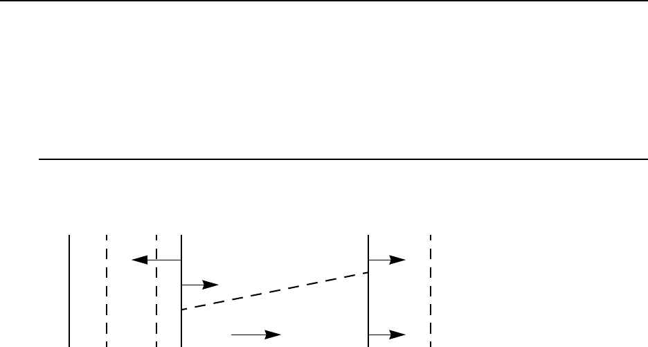
8: Oxidation and Silicidation

Silicide Models

634 Sentaurus™ Process User Guide

I-2013.12

The diffusivity and reaction rates of the oxygen atoms can be modified respectively by:

pdbSet Oxide ISSG D <value>

pdbSet Oxide_Silicon ISSG Ks <value>

The process conditions to invoke the ISSG oxidation are defined in the diffuse or gas_flow

commands, for example:

diffuse temp=1000 time=1 pressure=12<torr> flowH2=6 flowO2=12 ISSG

Silicide Models

Sentaurus Process allows you to define models for new materials and reactions. This ability has

been used to define models for the growth of titanium, tungsten, cobalt, and nickel silicides.

The following sections describe the kinetics of TiSi2 growth, the specification of the model and

parameters, and suggestions for modeling other silicides.

TiSi2 Growth Kinetics

Figure 87 Velocities in 1D silicidation process

Titanium silicide is assumed to form when silicon atoms react in the silicide with titanium at

the titanium silicide–titanium (TiSi2–Ti) interface. The dissolution of silicon and the

consumption of titanium lead to the deformation of the material layers in the structure.

NOTE While the discussion that follows describes the growth of TiSi2 on

silicon, it also applies to growth of TiSi2 on polycrystalline silicon.

The silicidation process has three main steps:

■Dissolution of silicon and diffusion of silicon atoms from the TiSi2–silicon interface

through the existing TiSi2 to the Ti–TiSi2 interface.

■Reaction of silicon with titanium to form new TiSi2.

υTiSi υ

Gas Ti TiSi2Si

CSi

υgrow

dissolve

8: Oxidation and Silicidation

Silicide Models

Sentaurus™ Process User Guide 635

I-2013.12

■Motion of materials due to the volume expansion, which is caused by the reaction between

diffused silicon and titanium, and also by the dissolution of silicon at the TiSi2–silicon

interface.

NOTE The name of the silicide reactant field (which represents the

concentration of silicon atoms in the silicide) is SiliconReact.

If silicon or polysilicon is in contact with titanium at the beginning of a thermal silicidation, an

initial TiSi2 layer is created automatically as in the case of oxidation. The thickness of this layer

is, by default, 1.5 nm.

The value of the initial TiSi2 thickness is specified in the parameter database by:

pdbSet Grid NativeLayerThickness 1.5e-7

which also controls the native layer thickness for oxidation.

Sentaurus Process automatically recognizes the silicidizing interfaces and switches on the

reaction equations.

TiSi2 Formation Reactions

At the TiSi2–silicon interface, there is the reaction:

(879)

where is the silicon as a diffusing species on the silicon material side and is the

silicon as a diffusing species on the TiSi2 material side. Therefore, silicon (on the Si side of the

interface) reacts to form silicon atoms (on the TiSi2 side of the interface). The reaction is

reversible, allowing for the reformation of silicon (if silicon is released by nitridation of TiSi2,

for example):

(880)

and are the diffusion flux and growth reaction flux, respectively, at the TiSi2–silicon

interface. The forward rate of this reaction depends only on temperature, while the reverse rate

is also proportional to the concentration of diffusing silicon atoms in TiSi2. is the

concentration of silicon in TiSi2 and is the equilibrium concentration of silicon at the

TiSi2–silicon interface. Beta is the stoichiometry of the growing material whose default is 1.0.

is the mass transfer coefficient.

SiSi SiTiSi2

↔

SiSi

SiTiSi2

RfKfCSi Cstar

–()≡

RgBeta Rf

≡

CSi

CStar

8: Oxidation and Silicidation

Silicide Models

636 Sentaurus™ Process User Guide

I-2013.12

To change them, use:

pdbSet Silicon_TiSilicide SiliconReact Kf <n>

pdbSet Silicon_TiSilicide SiliconReact Cstar <n>

pdbSet Silicon_TiSilicide SiliconReact Beta <n>

For each silicon atom removed from the silicon side of the interface, the volume of silicon is

reduced by:

(881)

where Density.Grow is the density of the growing material whose default value is .

To change it, use:

pdbSet Silicon_TiSilicide SiliconReact Density.Grow <n>

There is no new material formation at the TiSi2–silicon interface. Silicon dissolves at this

interface and is transported across the TiSi2 layer by simple diffusion:

(882)

where is the concentration of silicon in TiSi2 and is the diffusivity of silicon in TiSi2.

The following command changes the diffusivity:

pdbSet TiSilicide SiliconReact Dstar {<n>}

At the TiSi2–titanium interface, there is the reaction:

(883)

This reaction is assumed to be irreversible:

(884)

and are the diffusion flux and growth reaction flux, respectively, at the TiSi2–titanium

interface. The reaction rate is proportional to the concentration of diffusing silicon at the TiSi2

side of the interface. is the concentration of silicon in TiSi2 and is the equilibrium

concentration of silicon at the titanium–TiSi2 interface. Beta is the stoichiometry of the

growing material whose default is 0.5. is the mass transfer coefficient.

∆VBeta

Density.Grow

-----------------------------------=

522

×10

t∂

∂CSi Dstar CSi

∇()∇•=

CSi

Dstar

SiTiSi20.5Ti+0.5TiSi2TiSi2

→

RfKfCSi Cstar

–()≡

RgBeta Rf

≡

CSi

Cstar

8: Oxidation and Silicidation

Silicide Models

Sentaurus™ Process User Guide 637

I-2013.12

To change them, use:

pdbSet TiSilicide_Titanium SiliconReact Kf <n>

pdbSet TiSilicide_Titanium SiliconReact Cstar <n>

pdbSet TiSilicide_Titanium SiliconReact Beta <n>

The volumes of titanium and TiSi2 change according to:

(885)

where Expansion.Ratio is the conversion ratio from consumed material to the growing

material, and Density.Grow is the density of the growing material. The default values for

Expansion.Ratio and Density.Grow are 2.42 and , respectively. They can be

changed by using the commands:

pdbSet TiSilicide_Titanium SiliconReact Expansion.Ratio <n>

pdbSet TiSilicide_Titanium SiliconReact Density.Grow <n>

Tungsten-, Cobalt-, and Nickel-Silicide Models

The tungsten-, cobalt-, and nickel-silicide models are identical in form to the titanium-silicide

model. The parameters of the models are different, however, reflecting the differences between

the materials (see [2][3] for the tungsten-silicide model and [4][5] for the cobalt-silicide

model). The names of the relevant materials are Tungsten and TungstenSilicide (WSi2),

Cobalt and CobaltSilicide (CoSi2), and Nickel and NickelSilicide (NiSi).

Stress-dependent Silicidation

The stress-dependent silicidation model is experimental, and can become unstable and produce

irregular shapes. Fundamental changes to the model are possible in future releases.

Similar to oxidation, the silicide reaction rate and the reactant diffusivity can be affected by

local stress. For the silicide reaction, the speed of the reaction is assumed to be affected by the

total stress energy, so that the stress effect is incorporated symmetrically with respect to tension

versus compression.

To switch on stress-dependent diffusion, use the command:

StressDependentSilicidation <silicide>

where <silicide> can be set only to NickelSilicide.

V∆Beta

Expansion.Ratio * Density.Grow

---------------------------------------------------------------------------------=

2.34 22

×10

8: Oxidation and Silicidation

Silicide Models

638 Sentaurus™ Process User Guide

I-2013.12

When the stress-dependent silicidation model is switched on, the reaction rate given in Eq. 880

and Eq. 884 (that is, at both metal–silicide and silicon–silicide interfaces) is suppressed by the

normal stress:

(886)

Similarly, the diffusivity of the reactant SiliconReact becomes pressure dependent:

(887)

The activation volume VD is a bulk property and is defined in the silicide. The activation volume

Vk controls the impact of the normal stress at the reaction front and is defined on interfaces:

Nickel_NickelSilicide | NickelSilicide_Silicon

For example:

pdbSet Nickel_NickelSilicide SiliconReact Vk <n>

pdbSet NickelSilicide SiliconReact VD <n>

In addition to switching on stress dependency of the silicide reaction, the command

StressDependentSilicidation reduces the viscosity of the silicide to a point where

viscous relaxation occurs at typical silicidation temperatures (see StressDependentSilicidation

on page 1156). Similar mass relaxation effects have been proposed in the literature [6][7]. To

modify the relaxation of the silicide, use one or both of the following commands:

pdbSet NickelSilicide Mechanics Viscosity0 <n>

pdbSet NickelSilicide Mechanics ViscosityW <n>

Oxygen-retarded Silicidation

The silicidation process may be influenced by the presence of oxygen in the silicide. This

oxygen is assumed to enter the silicide at interfaces with silicon dioxide and to diffuse in the

silicide according to Fick’s law. The oxygen retards the reaction of silicon atoms at the silicide–

silicon and silicide–metal interfaces and the diffusion of silicon in the silicide; this is called

oxygen-retarded silicidation (ORS). The retardation factor is assumed to be in the form of:

(888)

where ORSOxygen is the retardant solution name. The model can be switched on and off by

using the command:

pdbSet TiSi2 Silicon ORS {0 | 1}

KfNStress T,()KfT() e

abs NStress()Vk⋅

kBT

--------------------------------------------------------





–

DPressure T,()DT() e

abs Pressure()VD⋅

kBT

------------------------------------------------------------





–

Rfactor 1ORSOxygen

122

×10

--------------------------------–≡

8: Oxidation and Silicidation

Silicide Models

Sentaurus™ Process User Guide 639

I-2013.12

If the model is on, is multiplied by of Eq. 880, p. 635, of Eq. 882, p. 636, and

of Eq. 884. You can define the retardation factors using the term command, for example:

term name=SiliconReactFactor add TiSilicide /Titanium \

eqn = "((1-ORSoxygen_TiSilicide/1e22)>0)?(1-ORSoxygen_TiSilicide/1e22):(0.0)"

term name=SiliconDiffFactor add TiSilicide \

eqn = "((1-ORSoxygen/1e22)>0)?(1-ORSoxygen/1e22):(0.0)"

term name=SiliconReactFactor add Silicon /TiSilicide \

eqn = "((1-ORSoxygen_TiSilicide/1e22)>0)?(1-ORSoxygen_TiSilicide/1e22):(0.0)"

NOTE The oxygen-retarded silicidation model can cause instabilities (such as

a zigzag shape of the silicide boundary) because of a high concentration

of silicon near the oxide. Solving the silicon diffusion equation in steady

state reduces such instability. It can be switched on using the command:

pdbSet NickelSilicide Silicon Steady 1

Triple-Point Control

During silicidation, triple points where more than two materials come together (such as oxide,

silicon, silicide node) may move inadvertently due to material consumption around the node.

To control the movement, a retardation factor around the triple point is applied to the velocities.

The retardation factor is assumed to be:

(889)

Factor is the suppression value at the triple point, and Distance is the rolloff length for

silicidation triple-point suppression. The distance determines how far the suppression factor

will be effective from the triple point. SDistance is the distance to the nearest node from the

triple point and is calculated internally. The other parameters can be changed using the

following commands:

pdbSet <mater> SilicidationTripleDistance {<n>}

pdbSet <mater> SilicidationTripleFactor {<n>}

where <mater> is the interface material (for example, Silicon_TiSilicide). If you want

to switch the triple-point control on or off, use the command:

pdbSet Mechanics SilicidationCorrection {1 | 0}

Rfactor

DStar

RFactor

2 1 2Factor–()

----------------------------------- SDistance

Distance

------------------------





atan+=

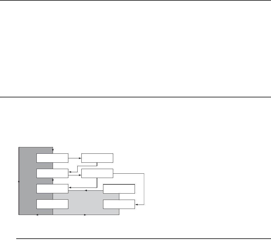
8: Oxidation and Silicidation

Dopants and Defects in Oxides and Silicides

640 Sentaurus™ Process User Guide

I-2013.12

Dopants and Defects in Oxides and Silicides

Dopants in oxides and silicides are modeled in the same way as in other nonsemiconductor

materials. Transport within a silicide or an oxide is governed by simple diffusion (in other

words, no electric field effects). For details on segregation at material interfaces, see Boundary

Conditions on page 357. Point defects can participate in reactions at interfaces with silicon.

While the current oxidation model specifies the generation of interstitials by the consumption

of silicon, the current titanium silicide model specifies the generation of vacancies by the same

mechanism.

Numerics

During oxidation or silicidation, one material grows at the expense of another material. To

handle the growth of materials, Sentaurus Process uses two different time loops – inner and

outer – as shown in Figure 88 for the case of oxidation.

Figure 88 Flowchart for simulation of material growth

Outer Time Loop

The diffusion equation for the oxidants is solved using the general PDE solver in Sentaurus

Process. In addition, a predictor for the next time step (oxidation time step) is computed. When

the concentrations of oxidants at the oxide–silicon interface are known, the corresponding

growth velocities can be computed. These velocities serve as a boundary condition for the

mechanics problem. After solving the mechanics problem, the velocity field in the entire

structure is known. At this point, the program enters the inner time loop.

Outer Time Loop

Inner Time Loop

Solve Oxidant

Diffusion

Solve Mechanics

Solve Dopant

Diffusion

Velocity at the

Reaction Front

Velocity Field

Remove Small

Elements

Move Mesh

Points

Compute Maximum

∆t on Given Mesh

8: Oxidation and Silicidation

Numerics

Sentaurus™ Process User Guide 641

I-2013.12

Inner Time Loop

Given a mesh and the velocity field, a time step (grid time step) can be computed so that

elements do not collapse when applying the velocities to the nodes of the mesh (moving mesh).

In the next time step, the dopant diffusion is solved using the general PDE solver and a

predictor for the next time step (diffusion time step) is computed. Then, mesh points are moved

according to the velocity field and, subsequently, small mesh elements are removed.

After removing small elements, the next grid time step is computed. The smaller of the two

time steps (grid time step and diffusion time step) is applied in the next time cycle. The inner

time loop runs as long as the time step of the outer loop (oxidation time step) is fulfilled. Then,

the code goes into its second time step of the outer loop. An example of typical output during

oxidation is:

...

Reaction Solve from 14.86min to 15.11min. Time step: 15.32s.

Mechanics Solve from 14.86min to 15.11min. Time step: 15.32s.

Diffusion Solve from 14.86min to 14.99min. Time step: 8.144s.

Diffusion Solve from 14.99min to 15.11min. Time step: 7.176s.

Reaction Solve from 15.11min to 15.37min. Time step: 15.4s.

Mechanics Solve from 15.11min to 15.37min. Time step: 15.4s.

Diffusion Solve from 15.11min to 15.25min. Time step: 8.361s.

Diffusion Solve from 15.25min to 15.29min. Time step: 2.077s.

Diffusion Solve from 15.29min to 15.37min. Time step: 4.967s.

...

This output reproduces the time-stepping scheme: Reaction Solve and Mechanics Solve

occur in the outer time loop; whereas, Diffusion Solve occurs in the inner time loop.

As previously mentioned, after solving the mechanics problem, velocities are given on all mesh

points. Mesh points are moved according to these velocities. This leads to a change in the

geometry and, in some cases, also to a change in the topology of the structure at each time step.

At a reactive interface, for example at the oxidation front, two velocities apply: one describes

the growth of a material and one describes the consumption of another material.

The velocity describing the growth of the material is used to solve the mechanics problem, and

the velocities describing the consumption of a material are used to update the structure or mesh.

Therefore, mesh elements on the growing side of the oxidation front are stretched, and

elements on the shrinking side are compressed. Edges on the growing side, which become too

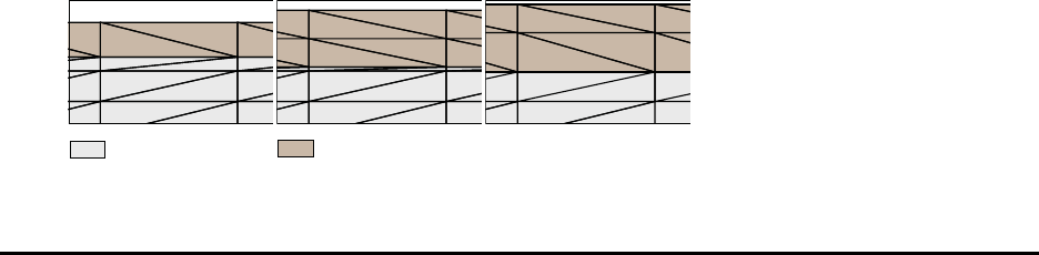
8: Oxidation and Silicidation

References

642 Sentaurus™ Process User Guide

I-2013.12

long with time, are split. Edges and elements on the shrinking side of the interface which

become too small are removed. This is demonstrated in Figure 89.

Figure 89 Meshing strategy during thermal oxidation

References

[1] N. Sullivan et al., “Exploring ISSG Process Space,” in 9th International Conference on

Advanced Thermal Processing of Semiconductors (RTP), Anchorage, AK, USA, pp. 95–

110, September 2001.

[2] S-L. Zhang, R. Buchta, and M. Östling, “A study of silicide formation from LPCVD-

tungsten films: Film texture and growth kinetics,” Journal of Materials Research, vol. 6,

no. 9, pp. 1886–1891, 1991.

[3] G. Giroult, A. Nouailhat, and M. Gauneau, “Study of a WSi2/polycrystalline silicon/

monocrystalline silicon structure for a complementary metal-oxide-semiconductor for a

compatible self-aligned bipolar transistor emitter,” Journal of Applied Physics, vol. 67,

no. 1, pp. 515–523, 1990.

[4] C. M. Comrie and R. T. Newman, “Dominant diffusing species during cobalt silicide

formation,” Journal of Applied Physics, vol. 79, no. 1, pp. 153–156, 1996.

[5] R. Stadler et al., “Ab initio calculations of the cohesive, elastic, and dynamical properties

of CoSi2 by pseudopotential and all-electron techniques,” Physical Review B, vol. 54,

no. 3, pp. 1729–1734, 1996.

[6] S.-L. Zhang and F. M. d’Heurle, “Stresses from solid state reactions: a simple model,

silicides,” Thin Solid Films, vol. 213, no. 1, pp. 34–39, 1992.

[7] F. Cacho et al., “Numerical modeling of stress build up during nickel silicidation under

anisothermal annealing,” Materials Science and Engineering B, vol. 135, no. 2, pp. 95–

102, 2006.

Silicon Oxide

Sentaurus™ Process User Guide 643

H-2013.03

CHAPTER 9 Computing Mechanical Stress

This chapter discusses the computation of mechanical stress in

Sentaurus Process.

Overview

Mechanical stress plays an important role in process modeling. It controls the structural

integrity of the device, the yield from the process depends on stresses, the mobility of charged

carriers is changed by stresses, and leakage currents also are a function of the stress in the

system.

On a finer scale, stresses can affect dopant diffusion rates by modifying the band gap. They can

affect oxidation rates and, therefore, can alter the shapes of thermally grown oxide layers.

In modern process flows, accurate computation of stress is important. However, there is a

continual trend toward designing process flows that produce the right types of stress in the

device. With appropriate stresses, device performance can be enhanced significantly.

Stress computation simulations are performed in four distinct steps:

■First, the equations for mechanics are defined. The equations used in Sentaurus Process

define force equilibrium in the quasistatic regime.

■Second, the boundary conditions for these equations are defined. For the elliptic equations

that arise from the equations of force equilibrium, boundary conditions are needed on all

boundaries. Sentaurus Process allows Dirichlet or Neumann boundary conditions provided

that certain minimum criteria are met. The minimum criterion is to constrain the structure

sufficiently so that it has no rigid body modes.

■Third, material properties are defined. This is the part where the relationship between

stresses and strains is defined. Some materials may hold stresses for a given strain without

relaxing; these are elastic materials. Others may relax the stresses away; these are viscous

or viscoelastic materials. Sentaurus Process provides viscoelastic constitutive equations

for the computation of mechanical stresses. By setting parameters appropriately, the border

cases of a purely viscous and a purely elastic material can be simulated as well. The

viscoelastic models used in Sentaurus Process provide a choice between the Maxwell

model and the Standard Linear Solid model. The viscosity can depend on the local shear

stresses, which make the viscosity a locally varying quantity and can lead to nonlinear

mechanical behavior. In addition to elastic and viscoelastic materials, there are other

materials to model irreversible deformation and temperature-dependent volume change.

9: Computing Mechanical Stress

Material Models

644 Sentaurus™ Process User Guide

H-2013.03

Sentaurus Process provides nonlinear material models for incremental plasticity,

deformation plasticity, viscoplasticity and creep, and swelling.

■Fourth, the mechanisms that drive the stresses are defined. In Sentaurus Process, this is

performed through intrinsic stresses, thermal mismatch, material growth, lattice mismatch

(silicon germanium), and densification. All these processes are additive in the linear elastic

regime. In the nonlinear regime, they must be updated from the available stress history.

Stress is solved in all materials. However, during an inert diffusion, the stress computation can

be switched off. Parameters describing material behavior, which will be introduced in this

chapter, can be found in the parameter database:

<material> Mechanics

Some examples are Viscosity0, ViscosityW.

In the following sections, the constitutive equations are discussed in detail. These tensor

equations can be split into two parts:

■The dilatational part, which corresponds to the trace of the tensor, describes the material

behavior in the case of a pure volume change.

■The deviatoric part describes an arbitrary deformation but without changing the volume.

For example, the strain tensor can be decomposed as follows:

(890)

This decomposition will be used in subsequent equations to discuss the constitutive equation

for the dilatational and deviatoric parts independently.

Material Models

Sentaurus Process implements the viscous, viscoelastic, and elastic models in a general

manner, where the viscous model and elastic model can be derived from the viscoelastic model.

The viscous and viscoelastic models use shear stress–dependent viscosity. The elastic model

also has the anisotropic elasticity where the elastic coefficients are dependent on the crystal

orientation. The plasticity models describe the material behavior beyond yield, independent of

the rate of loading. The viscoplasticity and creep models provide rate-dependent plastic

behavior, while the swelling material models provide temperature-dependent volume change.

εij ε'

deviatoric

---εkk









δij

dilatational

















9: Computing Mechanical Stress

Material Models

Sentaurus™ Process User Guide 645

H-2013.03

Viscoelastic Materials

The viscoelastic material response is characterized by elastic and viscous components. The

combined response depends on how elastic and viscous stresses or strains are coupled.

Sentaurus Process provides two commonly used combinations:

■Maxwell model

■Standard Linear Solid model

Maxwell Model

The viscoelastic behavior for the Maxwell model is obtained by combining elastic and viscous

responses in series. The stress–strain equations are written in terms of dilatational and shear

components. The equations for the volumetric part of the stress tensor1 take the form:

(891)

and:

(892)

where is the bulk viscosity. In addition, the relation of the stress and strain tensor to the

hydrostatic pressure is shown. The bulk modulus can be computed from the Poisson ratio

PoissRatio and Young’s modulus YoungsMod as:

(893)

The deviatoric part of the stress tensor is described by:

(894)

where is the shear viscosity. The shear modulus can be computed from the Poisson ratio

and Young’s modulus as:

(895)

1. The subscripts of vectors and tensors hold for the Cartesian coordinates x, y, and z.

·v

----- σv

ηvTσ,s

()

-----------------------+ 3ε

·v

σkk

3p–3σv

ηv

KYoungsMod

31 2 PoissRatio⋅–()

--------------------------------------------------------=

σ'

·ij

------- σ'

η'Tσ,s

()

---------------------+2ε'

·ij

η'

GYoungsMod

21 PoissRatio+()

-------------------------------------------------=

9: Computing Mechanical Stress

Material Models

646 Sentaurus™ Process User Guide

H-2013.03

By default, the viscoelastic response is applied to the deviatoric parts. The linear elastic model

is used for the pressure-volume response, that is:

(896)

To apply the viscoelastic response to both the deviatoric parts and the volumetric part, use:

pdbSet Mechanics NoBulkRelax 0

The shear viscosity is a function of the shear stress and the temperature , where:

(897)

Usually, the value of ViscosityW is negative and, therefore, the shear viscosity decreases

with increasing temperature. The bulk viscosity has a similar Arrhenius expression defined by

the parameters Viscosity0.K and ViscosityW.K. The dependency on the shear stress

is discussed in Shear Stress–dependent Viscosity on page 648.

Standard Linear Solid Model

In the Standard Linear Solid model, the material behavior is modeled by combining elastic

response in parallel with the Maxwell model-based viscoelastic response:

(898)

where is the elastic stress and is the viscoelastic stress. The difference compared to the

Maxwell model allows the total stress to be nonzero even after the viscoelastic stress has

relaxed away:

(899)

The dilatational and deviatoric components of the elastic and viscoelastic stresses are written

in the usual form:

(900)

(901)

(902)

σvKεkk



η'

η'T() Viscosity0 ViscosityW

kBT

--------------------------------–





exp⋅=

η'

σs

σij σij

el σij

σij

σij t∞→()σ

σv

el 3Kbaseεv

σ'ij

el 2Gbaseε'ij

·v

--------σv

ηvTσs

(, )

-----------------------+ 3ε

·v

9: Computing Mechanical Stress

Material Models

Sentaurus™ Process User Guide 647

H-2013.03

and:

(903)

where:

■ and are the bulk and shear moduli for the elastic response, respectively.

■ and are the bulk and shear moduli for the elastic part of the viscoelastic response,

respectively.

■ and are the bulk and shear viscosities, respectively.

■ and are the dilatational and deviatoric components of mechanical strain,

respectively.

To enable the Standard Linear Solid model, use:

pdbSetSwitch <material> Mechanics ViscoElasticity.Model SLS-Maxwell

The default value for the above parameter is Maxwell for the Maxwell model.

The elastic response for the Standard Linear Solid model is inactive, by default, so that the

material behavior is similar to that of the Maxwell model. The elastic response can be activated

by providing nonzero values for bulk and shear moduli:

pdbSetDouble <material> Mechanics BaseBulkModulus <n>

pdbSetDouble <material> Mechanics BaseShearModulus <n>

The material parameters for viscoelastic response are specified in the same manner as for the

Maxwell model. By default, the dilatational component of viscoelastic stress is assumed to be

purely elastic:

(904)

To activate viscoelastic response for the dilatation component, use:

pdbSet Mechanics NoBulkRelax 0

To visualize elastic and viscoelastic responses, this model provides additional output fields.

Stresses and strains for the elastic response can be viewed with the BaseStressEL and

BaseElasticStrainEL fields, respectively. Creep strains for the viscoelastic response

can be viewed with the CreepStrainEL field:

(905)

σ'

·ij

---------σ'

η'Tσs

(, )

----------------------+ 2ε'

·ij

Kbase

Gbase

ηv

η'

εv

ε'ij

σv

ve 3Kεv

εij

cr σv

3ηv

---------σ'ij

2η'

---------+









9: Computing Mechanical Stress

Material Models

648 Sentaurus™ Process User Guide

H-2013.03

The solution for viscoelastic stress is time dependent. It also becomes nonlinear when viscosity

is a function of viscoelastic shear stress. Therefore, the Newton method is used to solve for

stresses. At the end of each Newton iteration, a check is made on whether the convergence

criteria have been satisfied. More iterations are performed until all the criteria are satisfied

within the specified tolerance or until the maximum number of iterations is reached. For details

on convergence criteria and time-stepping for mechanics, see Time-Step Control for

Mechanics on page 871.

Purely Viscous Materials

Oxide and nitride, by default, are treated as viscoelastic materials. However, the viscosity is a

function of the temperature (see Eq. 897). With increasing temperature, the viscosity

decreases, that is, the material becomes increasingly more liquid. When the viscosity reaches

a very low value, the first term in Eq. 894 can be neglected:

(906)

Eq. 906 describes the deviatoric part of a purely viscous material. The relaxation time

typically gives a good estimate of the behavior of a viscoelastic material. If is

much greater than the process time, the material is in the elastic regime. The material behaves

viscoelastically if is in the range of the process time. If is very small, the material is in the

viscous regime.

Shear Stress–dependent Viscosity

For viscous and viscoelastic materials, the viscosity may depend on the temperature and the

shear stress . The temperature dependency is described by Eq. 897. The dependency on the

shear stress is given by:

(907)

The shear stress is computed from the local stress distribution based on the second invariant

of the deviatoric part of the stress tensor:

(908)

The viscosity breakdown value can be determined by:

(909)

σ'

η'Tσ,s

()

--------------------- 2ε'

·jk

=σ'

jk 2η'ε'

·jk

=⇔

τη'G⁄=

σs

ησ

sT,()ηT() σsσcrit

⁄

σsσcrit

⁄()sinh

-----------------------------------

⋅=

σs

---σ



'

σ'

σcrit

2kBT

vcrit

-------------=

9: Computing Mechanical Stress

Material Models

Sentaurus™ Process User Guide 649

H-2013.03

where:

(910)

By default, oxide and nitride are treated as viscoelastic materials with shear stress–dependent

viscosity. The values for Vcrit0 and VcritW also are set in the PDB:

pdbSetDouble <material> Mechanics Vcrit0

pdbSetDouble <material> Mechanics VcritW

Purely Elastic Materials

If the viscosity in Eq. 894 is chosen high enough, the second term on the left can be neglected

and the equation reads:

(911)

This equation describes the deviatoric part of a purely elastic material. By default, silicon and

polycrystalline silicon are treated as purely elastic materials. To achieve this, the viscosity of

these materials is set to .

NOTE and are the primary parameters describing elastic materials, and

not Young’s modulus and the Poisson ratio. When changing material

properties with the pdb command, only a change of the primary

parameters has an effect on the simulation. To obtain Young’s modulus

and the Poisson ratio, use the following commands, respectively (see

KG2E on page 993 and KG2nu on page 994):

KG2E <BulkModulus> <ShearModulus>

KG2nu <BulkModulus> <ShearModulus>

NOTE When material data is given in terms of Young’s modulus and the

Poisson ratio, use the following commands to convert them to the shear

modulus and the bulk modulus, respectively (see Enu2G on page 920

and Enu2K on page 921):

Enu2G <YoungsModulus> <PoissonRatio>

Enu2K <YoungsModulus> <PoissonRatio>

vcrit T() Vcrit0 VcritW

kBT

-------------------–





exp⋅=

σ'

·jk

-------- 2ε'

·jk

=σ'

jk 2Gε'

=⇔

140

×10 poise

9: Computing Mechanical Stress

Material Models

650 Sentaurus™ Process User Guide

H-2013.03

Anisotropic Elastic Materials

The stress and strain relations for anisotropic elastic materials can be described using:

(912)

where and are the components of the engineering stress and strain, respectively, and

is the component of the stiffness matrix. The engineering stress (i=1, …, 6) corresponds to

the stress-tensor components σxx, σyy, σzz, σxy, σyz, σxz, and the engineering strain

(j=1, …, 6) corresponds to the strain-tensor components εxx, εyy, εzz, 2εxy, 2εyz, 2εxz.

NOTE The engineering shear-strain components differ from the shear-strain

tensor components by a factor of 2.

Cubic Crystal Anisotropy

The mechanical responses of a crystalline solid vary along various crystal orientations. For a

cubic crystal, the axes of reference are chosen to be parallel to the crystal axes. In a coordinate

system with axes aligned along the crystal axes, the symmetric stiffness matrix C has the

following nonzero components:

C11 = C22 = C33, C12 = C23 = C13

C44 = C55 = C66

All other components are zeros. The anisotropic stress and strain relation is completely defined

when three independent modulus parameters C11, C12, and C44 are specified.

The degree of anisotropy for a given material can be measured by the departure from unity of

the ratio A = 2 C44/(C11 – C12). The anisotropic model reduces to the isotropic model if

the ratio A is equal to 1. When the simulation coordinate axes do not coincide with the crystal

axes, the stiffness matrix C must be transformed accordingly. For this, note that C is actually a

rank-4 tensor.

By default, the anisotropic elasticity model is switched off. The following command is required

to switch on the model:

pdbSet Silicon Mechanics Anisotropic 1

The values of these three modulus parameters with respect to the cubic crystal axis can be

defined using the following commands, which also show the default values for the crystalline

silicon:

pdbSet Silicon Mechanics C11 16.57E11

pdbSet Silicon Mechanics C12 6.39E11

pdbSet Silicon Mechanics C44 7.96E11

σiCijεj

σi

εj

Cij

σi

εj

9: Computing Mechanical Stress

Material Models

Sentaurus™ Process User Guide 651

H-2013.03

The unit for these default values is dyn/cm2.

This model depends on the wafer.orient and slice.angle parameters specified in the

init command.

Orthotropic Model

Orthotropic materials have three planes of symmetry. In a coordinate system with axes aligned

along the symmetry planes, the symmetric stiffness matrix C has the following nonzero

components:

C11, C22, C33, C44=C55=C66, C12=C21, C13=C31, C23=C32

Orientation

The symmetry planes of the model, by default, coincide with the simulation axes. You can

choose the symmetry plane directions by switching off this default:

pdbSetBoolean <mat> Mechanics Ortho.Axis.Sim.Aligned 0

and specifying the axes in the wafer coordinate system (see Wafer Coordinate System on

page 66). Then, these axes will depend on the slice.angle, wafer.orient, and

flat.orient arguments specified in the init command. If these arguments are not given

(and the above pdb flag is switched off), the default values of slice.angle, wafer.orient,

and flat.orient will be used. The default wafer in-plane symmetry plane directions are

given by wafer.orient= {0 0 1}, flat.orient= {1 1 0}, that is, at a angle to

the xy plane of the wafer coordinate system)

NOTE When the symmetry plane directions are specified, they remain the

same for the entire structure and cannot be set regionwise.

Orthotropic material properties can be described by specifying nine independent parameters,

namely, the Young’s moduli in the symmetry planes (E1, E2, E3), the directional shear moduli

(G12, G23, G13), and the directional Poisson ratios (ν12, ν13, ν23). The other directional Poisson

ratio are calculated from:

(913)

The stiffness matrix components are calculated from the specified material properties:

(914)

(915)

45°

υij

------ υji

------=

Ckk Ek1νijυji

–()=

Cij Eiυji υjkυki

+()=

9: Computing Mechanical Stress

Material Models

652 Sentaurus™ Process User Guide

H-2013.03

and .

By default, the orthotropic model is switched off, and it is switched on using the command:

pdbSet <material> Mechanics Orthotropic 1

The material properties can be specified as:

pdbSetDouble <material> Mechanics <material parameter> <n>

specifically:

pdbSet Silicon Mechanics YoungsModulus1 162E10

pdbSet Silicon Mechanics YoungsModulus2 162E10

pdbSet Silicon Mechanics YoungsModulus3 162E10

pdbSet Silicon Mechanics PoissonRatio12 0.28

pdbSet Silicon Mechanics PoissonRatio13 0.28

pdbSet Silicon Mechanics PoissonRatio23 0.28

pdbSet Silicon Mechanics ShearModulus12 63.28E10

pdbSet Silicon Mechanics ShearModulus13 63.28E10

pdbSet Silicon Mechanics ShearModulus23 63.28E10

The values given also are the default values used. The units for the Young’s modulus and shear

modulus are dyn/cm2.

Orthotropic thermal expansion also is considered in this material model, and different

coefficients of thermal expansion can be specified along the three symmetry planes:

pdbSet Silicon Mechanics ThExpCoeff1 3E-06

pdbSet Silicon Mechanics ThExpCoeff2 3E-06

pdbSet Silicon Mechanics ThExpCoeff3 3E-06

The specified values are the default values.

Temperature-dependent material properties can be specified for all the material parameters

specified above. The variation of a property can be specified as:

(916)

where the reference value is the material parameter value specified in the input deck.

The values can be specified as:

pdbSet <material> Mechanics <material parameter>Rate <n>

For example:

pdbSet Silicon Mechanics ThExpCoeff1Rate 0

ij k≠,

ξT() ξ

ref ξ

·TT

ref

–()+=

9: Computing Mechanical Stress

Material Models

Sentaurus™ Process User Guide 653

H-2013.03

Plastic Materials

Materials such as metals show linear elastic behavior at lower stresses but undergo permanent

deformation at higher stresses. At low temperatures, permanent deformation in these materials

is not sensitive to the rate of loading. Such material behavior is defined as plastic or elastic-

plastic. Depending on the type of loading, plastic deformations may be computed using

incremental plasticity or deformation plasticity.

To switch on the plastic material model, use the command:

pdbSet <material> Mechanics IsPlastic <n>

Incremental Plasticity

Plastic material behavior under nonmonotonic loading is modeled using incremental

formulation.

Incremental plasticity uses the von Mises yield criterion with associative flow and bilinear

hardening. The von Mises yield criterion for isotropic solid materials takes the form:

(917)

where is the back stress, is an isotropic hardening variable, and:

(918)

is a function describing the change of yield surface with progressive yielding. The Einstein

summation convention is used to define the tensor product in the above equation. is the

yield stress in uniaxial tension. is the isotropic hardening modulus, which is constant for

bilinear isotropic hardening. To set these two parameters, use the commands:

pdbSet <material> Mechanics FirstYield <n>

pdbSet <material> Mechanics Hardening.Modulus.Isotropic <n>

Under a small strain assumption, the strains (and strain rates) are decomposed additively:

(919)

where are the elastic strains, and are the plastic strains.

For incremental plasticity, the plastic strains are determined by the plastic flow rule:

(920)

Fσ'ij qij α,,()σ'ij qij

–()σ'ij qij

–()Yα()–0==

qij

Yα() 2

---σyHisoα+()=

σy

Hiso

ij εij

eεij

εij

·ij

pγ

·∂Q

∂σij

----------

9: Computing Mechanical Stress

Material Models

654 Sentaurus™ Process User Guide

H-2013.03

where is the slip rate, and is the plastic potential. Plastic flow is assumed to be volume

preserving, so that plastic strain is purely deviatoric:

(921)

For associative plastic flow, the plastic potential is set equal to the yield function . The

evolution of the isotropic hardening variable and the back-stress variable are given by:

(922)

and:

(923)

where is the kinematic hardening modulus, and is the equivalent plastic strain rate. To

set the kinematic hardening modulus, use the command:

pdbSet <material> Mechanics Hardening.Modulus.Kinematic <n>

For linear isotropic hardening, the hardening modulus is interpreted as the slope of the stress

versus the plastic strain curve (as obtained from uniaxial tension test) . It differs from

the elastic-plastic tangent modulus, which is defined as the slope of the stress versus total strain

curve .

For combined isotropic and kinematic hardening, a common choice for hardening moduli is:

; ; (924)

where is a constant.

To switch on the incremental plasticity model, use:

pdbSet <material> Mechanics Plasticity.Model Incremental

The rate equations are discretized using backward Euler scheme and then solved using a radial

return mapping algorithm (see [1] for more details).

The nonlinear nature of the plasticity model requires Newton iterations to achieve the

equilibrium state for each loading step. At the end of each iteration, a check on the satisfaction

of convergence criteria is made. More Newton iterations are performed until all the

convergence criteria are satisfied within the specified tolerance or until the maximum number

of iterations is reached. See Time-Step Control for Mechanics on page 871 for details on

convergence criteria and time-stepping for mechanics.

·0≥

εij

pδij 0ε'ij

εij

·e

·p2

---γ

·ij

---γ

·Hkin

σ'ij qij

–()

σ'kl qkl

–()σ'kl qkl

–()

---------------------------------------------------------=

Hkin

·p

Hiso

dσ

dεp

--------=

Eep dσ

dε

------=

Hkin 1β–()H=

Hiso βH=

β01,[]∈

9: Computing Mechanical Stress

Material Models

Sentaurus™ Process User Guide 655

H-2013.03

NOTE To define the plastic model, use nonzero values for the isotropic or the

kinematic hardening modulus along with yield stress. In the absence of

hardening, the numeric simulation of plastic deformation may become

unstable.

Deformation Plasticity

Plastic materials that do not have well-defined yield stress can be modeled using deformation

plasticity. This model is based on the Ramberg–Osgood formula [2][3], which is only valid for

monotonic loading. It is used mostly for plastic deformation around crack tips since it is well

suited to the J-integral calculation.

For one dimension, an additive decomposition of strains under a small strain assumption is

given as:

(925)

where and are material parameters, is the stress in one dimension, is the total strain

in one dimension, and is Young’s modulus.

Extending the formula to three dimensions, the strain components can be expressed as:

(926)

where is the equivalent stress.

The plastic flow is assumed to be associative and is governed by the von Mises yield criterion.

Under monotonic loading, the total plastic strain can be written as:

(927)

where is the total equivalent plastic strain.

Inverting the plastic strain expression gives:

(928)

with defining the work hardening exponent.

εε

eεp

+σ

--- ασy

-----





σy

-----





+==

elastic plastic

εij εij

eεij

+σ'ij

------- σkkδij

--------------+3

---ασy

-----





σeq

σy

--------







nσ'ij

σeq

--------

+==





















σeq 3

---σ'ijσ'ij

εij

---epσ'ij

σeq

--------=

epασy

-----





σeq

σy

-------





σeq σy

ασy

----------





()

---=

9: Computing Mechanical Stress

Material Models

656 Sentaurus™ Process User Guide

H-2013.03

To switch on the deformation plasticity model, use:

pdbSet <material> Mechanics Plasticity.Model Deformation

The deformation plasticity equations do not require any integration due to total stresses and

strains. However, the nonlinear expressions require Newton iterations to achieve the

equilibrium state for each loading step. At the end of each iteration, a check on the satisfaction

of convergence criteria is made. More Newton iterations are performed until all the

convergence criteria are satisfied within the specified tolerance or until the maximum number

of iterations is reached. See Time-Step Control for Mechanics on page 871 for details on

convergence criteria and time-stepping for mechanics.

NOTE Deformation plasticity must be used only with monotonic loading since

the equations are not valid for unloading. This model must be used if the

J-integral must be calculated around a crack tip with plastic strains.

Viscoplastic Materials

Materials, such as metals at high temperatures, exhibit rate-dependent plasticity also known as

viscoplasticity or creep. There are different ways to model such behavior:

■Anand model

■Power law creep

Anand Model

The Anand model [4][5] is used for rate-dependent plasticity that combines creep and plastic

deformation.

Assuming small strains, the strain rates and strains can be decomposed into elastic and

viscoplastic parts in an additive manner:

(929)

(930)

The elastic strains are evaluated using Hooke’s law, while the Anand model is used to evaluate

the viscoplastic part. The Anand model assumes that plastic deformation occurs at all values

of strain, so instead of a yield function, a constitutive equation is used to relate stresses to

viscoplastic strains.

·ij ε

·ij

eε

·ij

εij εij

eεij

9: Computing Mechanical Stress

Material Models

Sentaurus™ Process User Guide 657

H-2013.03

The flow rule for evolution of viscoplastic strains (volume preserving) is assumed to be of the

familiar form:

(931)

The equivalent viscoplastic strain rate at constant temperature is given by a constitutive

equation:

(932)

where is deformation resistance. It is defined in terms of an isotropic hardening function as:

(933)

The saturation value of deformation resistance at a given temperature and strain rate is

expressed as:

(934)

In the above formulation:

■ is a pre-exponential factor.

■ is the activation energy.

■ is the universal gas constant.

■ is absolute temperature in kelvin.

■ is the stress multiplier.

■ is the strain rate sensitivity.

■ is the constant of athermal hardening or softening.

■ is the exponent of athermal hardening or softening.

■ is the coefficient for the saturation value of deformation resistance.

■ is the exponent for the saturation value of deformation resistance.

Values for the material parameters and , and the initial value for

deformation resistance are obtained by fitting experimental data for stress–strain (obtained

from tension or compression tests conducted at various temperatures and strain rates) to the

above equations. For details on how to obtain such data, refer to the literature [4][6][7][8].

ε'

·ij

vp 3

---e

·vp σ'ij

σ'

---------σ'; σ'ijσ'ij

·vp fσ's,()AQ

-------–



 ξσ'

---------





sinh 1m⁄

exp==

·hs()e

·vp h01s

s∗

-----–





a1s

s∗

-----–





·vp a1≥;sgn==

s∗s

˜e

·vp

------- Q

-------





exp

AQξmh

0as

,,,, ,,

9: Computing Mechanical Stress

Material Models

658 Sentaurus™ Process User Guide

H-2013.03

To set these parameters, use the commands:

pdbSetDouble <material> Mechanics Viscoplasticity.A <n>

pdbSetDouble <material> Mechanics Viscoplasticity.Q <n>

pdbSetDouble <material> Mechanics Viscoplasticity.Xi <n>

pdbSetDouble <material> Mechanics Viscoplasticity.m <n>

pdbSetDouble <material> Mechanics Viscoplasticity.h0 <n>

pdbSetDouble <material> Mechanics Viscoplasticity.a <n>

pdbSetDouble <material> Mechanics Viscoplasticity.stilde <n>

pdbSetDouble <material> Mechanics Viscoplasticity.n <n>

pdbSetDouble <material> Mechanics Viscoplasticity.s0 <n>

NOTE For other materials, use the long form of the pdb commands to set

parameter values.

A new material named Solder has been added to the PDB to model viscoplastic behavior. The

default values for the above parameters for Solder material are based on 96.5Sn3.5Ag solder

alloy as reported in [6].

To solve the above nonlinear equations, the rate terms are discretized using the backward Euler

method, and the resulting algebraic equations are evaluated locally at every integration point

using the Newton–Raphson iterative scheme.

To switch on the viscoplastic material model, use the command:

pdbSet <material> Mechanics IsViscoPlastic <n>

This flag must be switched on during the simulation if viscoplastic deformation exists. The

nonlinear nature of the viscoplasticity model also requires Newton iterations to achieve

equilibrium of mechanics equations at each loading step. At the end of each iteration,

convergence criteria are checked. More iterations are performed until all the convergence

criteria are satisfied within the specified tolerance or until the maximum number of iterations

is reached. See Time-Step Control for Mechanics on page 871 for details on convergence

criteria and time-stepping for mechanics.

NOTE To avoid convergence problems, use small time steps at the beginning

of the analysis. You can increase the number of time steps later, during

the analysis, if it does not adversely affect the solution.

Power Law Creep

The power law creep [9], also known as the Bailey–Norton creep, assumes creep strain to be

of the following form:

(935)

·cr AQ

-------–





exp σnmt

˜m1–()

9: Computing Mechanical Stress

Material Models

Sentaurus™ Process User Guide 659

H-2013.03

where, for multiaxial loading:

■ is the equivalent creep strain rate.

■ is a pre-exponential factor.

■ is the activation energy.

■ is the universal gas constant.

■ is the absolute temperature in kelvin.

■ is the equivalent stress or the von Mises stress.

■ is the time (different from physical time).

■ and are exponents.

The above form is referred to as a time hardening form. A more commonly used form called

the strain hardening form is obtained by eliminating the time variable:

(936)

Under a small strain assumption, strains (and strain rates) can be decomposed additively as:

(937)

with creep strains being distinct from plastic strains.

Creep flow is assumed to be volume preserving ( ) and is governed by:

(938)

When incremental plasticity is also active, the creep flow rule is modified to account for

hardening:

(939)

where:

■ is the equivalent stress.

■ is the back stress for kinematic hardening.

■Plastic flow equations are solved simultaneously with creep flow.

·cr 2

---ε

·ij

crε

·ij

σ3

---σ'ijσ'ij

·cr mA Q

-------–





exp σnεcr

()

m1–()





----

εij εij

eεij

pεij

++=

εij

crδij 0=

·ij

cr 3

---ε

·cr σ'ij

-------





·ij

cr 3

---ε

·cr σ'ij qij

–

--------------------





σ3

---σ'ij qij

–()σ'ij qij

–()=

qij

9: Computing Mechanical Stress

Material Models

660 Sentaurus™ Process User Guide

H-2013.03

The material parameters , , , and are obtained by fitting experimental data. To set

these parameters, use the commands:

pdbSet <material> Mechanics Creep.A <n>

pdbSet <material> Mechanics Creep.Q <n>

pdbSet <material> Mechanics Creep.n <n>

pdbSet <material> Mechanics Creep.m <n>

NOTE For materials other than Solder, use the long form of these commands

to set parameter values.

The default values for the above parameters have been added to the PDB to the Solder

material based on the 96.5Sn3.5Ag solder alloy as reported in [10].

To solve the creep equations, the rate terms are discretized using the backward Euler method,

and the resulting algebraic equations are evaluated locally at every integration point using the

Newton–Raphson iterative scheme.

To switch on the creep material model, use the command:

pdbSet <material> Mechanics IsCreep <n>

This flag must be switched on during the simulation if creep deformation exists. The nonlinear

nature of the creep model also requires global Newton iterations to achieve equilibrium of

mechanics equations at each loading step. At the end of each iteration, convergence criteria are

checked. More iterations are performed until all the convergence criteria are satisfied within

the specified tolerance or until the maximum number of iterations is reached. See Time-Step

Control for Mechanics on page 871 for details on convergence criteria and time-stepping for

mechanics.

NOTE To avoid convergence problems, use small time steps at the beginning

of the analysis. You can increase the number of time steps later, during

the analysis, if it does not adversely affect the solution.

Swelling

Swelling refers to volumetric expansion of material. Swelling material behavior is defined by

specifying strain rates at various temperatures that are interpolated linearly. To switch on the

model, use the command:

pdbSetBoolean <material> Mechanics IsSwelling <n>

9: Computing Mechanical Stress

Material Models

Sentaurus™ Process User Guide 661

H-2013.03

The swelling strain rate data is specified with a double array:

pdbSetArray <material> Mechanics SwellingStrainRate

Temperature { <temp> {<SSR1> <SSR2> <SSR3>}

<temp> {<SSR1> <SSR2> <SSR3>} ... }

where <temp> is the temperature in degree Celsius, and <SSR1>, <SSR2>, and <SSR3> are

strain rates in the x-, y-, and z-direction, respectively, in .

Strain rates can be the same (isotropic) or different (anisotropic) in each of the three directions.

For cyclic temperature loading, strain rate data must be given for loading (temperature

increment) as well as unloading (temperature decrement). For example:

pdbSetDouble Mold Mechanics SwellingStrainRate Temperature {

27 {0.0 0.0 0.0}

77 {0.001 0.001 0.001}

127 {0.002 0.002 0.002}

80 {0.0012 0.0012 0.0012}

25 {0.0 0.0 0.0}

}

If strain rate data is not given for unloading, loading data is used for increasing as well as

decreasing temperatures.

Since strains are assumed to be small, swelling strain rates are added to other strain rates:

(940)

and are integrated over time to give total strains:

(941)

where for .

For a given material, only one set of strain rate data can be specified for a solve step. If

necessary, different strain rate data may be specified for the same material in a subsequent solve

step.

Mole Fraction–dependent Mechanical Properties

The mechanical properties of compound materials change with the ratio of substance

concentration, that is, mole fraction. The mole fraction is calculated with the interpolated

compound lattice density. Mole fraction dependency can be switched on with:

pdbSet Mechanics Compound.Interpolation 1

s1–

·ij ε

·ij

eε

·ij

εij εij

eεij

εij

sw ε

·ij

sw 0==

ij≠

9: Computing Mechanical Stress

Material Models

662 Sentaurus™ Process User Guide

H-2013.03

and is applied to:

■Bulk modulus and shear modulus for isotropic materials

■C11, C12, and C44 for anisotropic elastic materials

■Thermal expansion coefficient

The PDB parameters Derived.Materials and MoleFraction.Atoms are used to define

the compound material. The following commands define SiGe as a compound material:

pdbSetString Si Derived.Materials { SiGe }

pdbSetString Ge Derived.Materials { SiGe }

pdbSetArray SiGe MoleFraction.Atoms { x Ge }

The material SiGe is set to be a compound by default. More information about compound and

alloy materials can be found in Diffusion in III–V Compounds on page 265.

The mole fraction dependency for the above-listed mechanical properties can be defined

separately. By default, a linear interpolation is used. If the parameter is defined for the

compound material, the given parameter value is used.

SiGe is treated as material silicon with germanium concentration without material conversion

of the binary compound. Therefore, the current approach cannot be directly applied to material

SiGe.

The mole fraction of Si1–xGex is solved from the following equation:

(942)

The mole fraction definition here is different from the formulation used in older SiGe–related

models:

(943)

NOTE Do not mix the new syntax with the old syntax (see Deprecated Syntax

for Mole Fraction–dependent Mechanical Properties of Binary

Compounds on page 663). Some of the old syntax may exist in the

Advanced Calibration script.

xCGe

LDGexLD

Si 1x–()+

--------------------------------------------------=

xCGe

LDSi

-----------=

9: Computing Mechanical Stress

Material Models

Sentaurus™ Process User Guide 663

H-2013.03

Deprecated Syntax for Mole Fraction–dependent Mechanical

Properties of Binary Compounds

The mole fraction–dependent model for binary compounds can be applied to the following

elastic moduli:

■Bulk modulus and shear modulus for isotropic materials

■C11, C12, and C44 for anisotropic elastic materials

The parameter interpolation is computed by:

(944)

where:

■ denotes the elastic moduli of binary compound .

■ is the mole fraction.

■ is an interpolation function with and .

The mole fraction–dependent moduli for Si1–xGex are linear combinations of the elastic moduli

of each material. The binary compound Si1–xGex is treated as silicon regions with germanium.

The mole fraction of Si1–xGex is calculated as germanium concentration divided by the silicon

lattice density. The mole fraction–dependent model can be switched on for silicon with:

pdbSetBoolean Si IsCompound 1

Next, a list of binary compound materials with mole fraction–dependent elastic moduli is

created by:

pdbSetString Mechanics BCompoundList {Silicon Germanium}

Finally, the interpolation function is defined as a double array, in other words,

{x1 f1 x2 f2 x3 f3 ... }. For example, a linear interpolation function can be specified with:

pdbSetDoubleArray SiliconGermanium CompoundInterp {0 0 1 1}

For nonlinear relations, a piecewise linear interpolation profile is used.

The mole fraction dependency can be applied to thermal expansion coefficients of materials

using the command:

pdbSet Mechanics Compound.ThExpCoeff 1

when the binary compound model is switched on.

CAB CA1fx()–()CBfx()+=

CAB

A1x–Bx

f0() 0=

f1() 1=

9: Computing Mechanical Stress

Material Models

664 Sentaurus™ Process User Guide

H-2013.03

Temperature-dependent Mechanical Properties

The mechanical properties of materials are different at high temperature from those at room

temperature. The elastic modulus of typical materials decreases as temperature rises. Some

materials show non-negligible changes of mechanical properties at different temperatures.

The temperature dependency and mole fraction dependency are handled under the same PDB

switch. The temperature dependency can be switched on with:

pdbSet Mechanics Compound.Interpolation 1

and is applied to:

■Bulk modulus and shear modulus for isotropic materials

■C11, C12, and C44 for anisotropic elastic materials

■Thermal expansion coefficient

The temperature dependency for the above-listed mechanical properties can be defined

separately. The available options are:

■The linear dependency is defined with the PDB parameter <parameter>.T1. For

example:

pdbSet <mat> Mechanics BulkModulus.T1 <n>

■The parameter is then calculated with the formula:

where the unit of temperature is degree Celcius.

■The piecewise linear dependency can be specified with:

pdbSetDoubleArray SiliconGermanium Mechanics ShearModulus.TTable

{ <T1> <v1> ... <Tn> <vn> }

The temperature unit is degree Celcius.

The linear dependency defined by <parameter>.T1 is ignored.

NOTE Do not mix the new syntax with the old syntax (see Deprecated Syntax

for Temperature-dependent Mechanical Properties). Some of the old

syntax may exist in the Advanced Calibration script.

PT() PP.T1T26.85–()+=

9: Computing Mechanical Stress

Plane Stress Analysis

Sentaurus™ Process User Guide 665

H-2013.03

Deprecated Syntax for Temperature-dependent Mechanical Properties

The linear temperature dependency of the elastic moduli can be defined by a rate coefficient.

For isotropic elasticity, this parameter is specified with:

pdbSet <material> Mechanics YoungsModulusRate <n>

For anisotropic elasticity, the coefficients are defined with:

pdbSet <material> Mechanics C11Rate <n>

pdbSet <material> Mechanics C12Rate <n>

pdbSet <material> Mechanics C44Rate <n>

The linear temperature dependency can be applied to the thermal expansion coefficient using

the command:

pdbSet <material> Mechanics ThExpCoeffRate <n>

to specify the rate coefficient. For the nonlinear temperature-dependent thermal expansion

coefficient, a piecewise linear interpolation function is used. To switch on the model, use the

command:

pdbSet Mechanics Interp.ThExpCoeff 1

The piecewise linear function is specified with:

pdbSet <material> Mechanics ThExpCoeff.Interp {<temp> <LCTE> <temp>

<LCTE> ... }

For the first yield stress of plastic materials, an Arrhenius expression is used for the

temperature-dependent effect. The prefactor and exponent of the Arrhenius expression are

specified respectively with the following commands:

pdbSet <material> Mechanics FirstYield <n>

pdbSet <material> Mechanics FirstYieldW <n>

Plane Stress Analysis

In two-dimensional problems, the elastic models implemented above follow the plane strain

formulation by default. Under the plane strain assumption:

(945)

While this is good for structures where the strain in the third direction is very small compared

to the cross section, it would give inaccurate results for thin structures. Thin plate-like

εzz 0 σzz 0≠;=

9: Computing Mechanical Stress

Equations: Global Equilibrium Condition

666 Sentaurus™ Process User Guide

H-2013.03

structures where one dimension is very small compared to the other two can be modeled under

the plane stress assumption:

(946)

The strain is obtained as a function of other strains, for example, for purely elastic

structures:

(947)

The plane stress model can be switched on for a particular region using:

pdbSetBoolean <material> Mechanics PlaneStress 1

NOTE Yo u c an c ombine pla ne st ress a nd plane strain formulations within a

structure by switching on plane stress in only a few regions. However,

such a simulation is not advisable.

If both plane stress and plane strain regions are present in a structure, the material thickness of

regions can be specified by:

pdbSetDouble <material> Mechanics Thickness <d>

where <d> is specified in micrometers.

Equations: Global Equilibrium Condition

The equations for mechanics in Sentaurus Process are the quasistatic equations of force

equilibrium.

The strain rate tensor is related to the symmetric part of the velocity gradient and is given by:

(948)

Strain is then related to stresses through any of the material models defined in Material Models

on page 644. For all models, the global equilibrium condition is given by:

(949)

The above equations are solved using the finite-element method. The solution is a vector

representing the velocity components at each node. These velocities are used to compute the

εzz 0 σzz

;≠0=

εzz

εzz νε

xx εyy

+()–=

·jk

---vj

∂

------- vk

∂

-------+





∂σjk v()

∂

-------------------

0=

9: Computing Mechanical Stress

Boundary Conditions

Sentaurus™ Process User Guide 667

H-2013.03

strain and stresses. The stresses and the boundary conditions determine the mechanical state of

the system.

NOTE The stress and strain are derivatives of the velocity. They are, therefore,

computed at one order of accuracy lower than the solution variable. This

also means that they are discontinuous across the elements. When

visualized, the stress values may appear badly converged even if the

linear solver has converged.

In addition, the quasistatic mechanics equations are elliptic in nature and, therefore, are prone

to high levels of shape dependence. This is most frequently seen at gate corners during

polysilicon reoxidation steps or at the corners of the STI trench during liner oxidation. These

equations also exhibit a high sensitivity to the mesh modification algorithms at these corners.

NOTE At sharp corners, the mechanics equations have a singularity. Therefore,

it is not possible to discretize at a corner correctly using regular types of

element.

Boundary Conditions

Equations for stress equilibrium require boundary conditions to define the system completely.

Figure 90 Default mechanics boundary conditions in Sentaurus Process axis orientation

In Sentaurus Process, various boundary conditions can be selected using:

pdbSet Mechanics <side> BoundaryCondition <model>

where:

■<side> is Left, Right, Front, or Back.

■<model> is HomNeumann or Dirichlet.

Vx=0

Vy=0 Vy=0

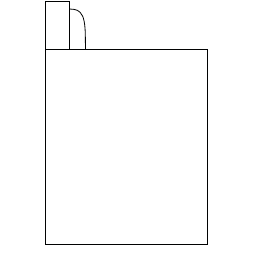
9: Computing Mechanical Stress

Boundary Conditions

668 Sentaurus™ Process User Guide

H-2013.03

The default boundary conditions are zero velocities in the direction perpendicular to the

boundary planes. Since velocities are set to fixed values along the boundaries, these boundary

conditions are referred to as Dirichlet boundary conditions in directions perpendicular to

boundary planes. The HomNeumann boundary condition is used when the plane must be free.

For example, if you want to set the ‘right’ plane to be free, use the command:

pdbSet Mechanics Right BoundaryCondition HomNeumann

The HomNeumann boundary condition implies a zero normal stress (shown in Figure 91).

Figure 91 HomNeumann boundary condition on ‘right’ boundary plane

Dirichlet boundary conditions are imposed using the penalty method, by default. To adjust the

penalty factor, use the command:

pdbSet Mechanics Boundary.Penalty.Factor {<n>}

The default penalty factor is 1.0e12. The larger this factor, the more accurate the enforcement

of Dirichlet boundary conditions. However, using an extremely large penalty factor could lead

to an ill-conditioned matrix and, therefore, could slow down the linear equation solver.

Alternatively, you can use the matrix reduction method to impose Dirichlet boundary

conditions. To choose the penalty method or matrix reduction method, use the command:

pdbSet Mechanics Boundary.Method.Type {<model>}

where {<model>} is either Penalty or MatrixReduction.

NOTE To ensure the structure is bounded by a perfect rectangle, the

displacements computed by these general boundary conditions are not

applied to the structure. However, they evaluate the stresses correctly.

This assumption is consistent with the small deformation assumption

within each mechanics time step.

Vx=0

Vy=0 sy=0

9: Computing Mechanical Stress

Boundary Conditions

Sentaurus™ Process User Guide 669

H-2013.03

Example: Applying Boundary Conditions

line x loc=-0.02 tag=e spacing=0.005

line x loc=0 tag=a spacing=0.005

line x loc=0.2 tag=b spacing=0.05

line y loc=0 tag=c spacing=0.05

line y loc=2 tag=d spacing=0.05

region silicon xlo=a xhi=b ylo=c yhi=d

region oxide xlo=e xhi=a ylo=c yhi=d

init !DelayFullD

pdbSetDouble Mechanics RefThExpCoeff 0

pdbSet Mechanics Right BoundaryCondition HomNeumann

pdbSet Oxide Mechanics Viscosity0 1e40

pdbSet Oxide Mechanics ViscosityW 0

temp_ramp name=tr1 temperature=600 ramprate=30<K/min> time=10<min>

diffuse temp_ramp=tr1

struct tdr=rampup

diffuse time=10 temp=900 wet

struct tdr=postout

Sentaurus Process also provides a general way to specify boundary conditions for stress

analysis through the stressdata command:

stressdata bc.location=<c> bc.value= { dx=<n> | dy=<n> | dz=<n> }

where:

■bc.location can be Left|Right|Front|Back|Bottom.

■dx, dy, and dz are used to specify displacement rates (default unit: cm/s).

The displacement rates are applied to the area defined through bc.location, where

Left|Right|Front|Back|Bottom refer to the outer boundary surfaces of the simulation

domain. At least at one node, the displacement along any coordinate system direction must be

fixed to remove the rigid body motion.

9: Computing Mechanical Stress

Boundary Conditions

670 Sentaurus™ Process User Guide

H-2013.03

Pressure Boundary Condition

The pressure boundary condition is used to apply uniform pressure on the exterior boundary.

The direction of the loading depends on the normal of the exterior surface. To apply the

pressure boundary condition, use the stressdata command, for example:

stressdata bc.location = <c> bc.value = {pressure=<n>}

where bc.location can be left, right, front, back, bottom.

Advanced Dirichlet Boundary Condition

A more advanced Dirichlet-type boundary condition also can be defined, which specifies both

the translational and rotational velocities on the boundaries. It is defined using the command:

stressdata bc.location=<c> bc.rotation.axis= {xa=<c> | ya=<c> | za=<c>} \

bc.value= {dx=<n> | dy=<n> | dz=<n> | rx=<n> | ry=<n> | rz=<n>}

where:

■bc.location can be Left|Right|Front|Back|Bottom.

■dx, dy, and dz specify displacement rates (default unit: cm/s).

■rx, ry, and rz specify rotational velocities (default unit: rad/s).

■xa, ya, and za specify the coordinates of the point around which the rotation occurs

(default unit: cm).

Periodic Boundary Condition

The periodic boundary condition is used for structures with a periodically repeating pattern.

This condition is used on periodic structures with assigned master and slave boundaries. The

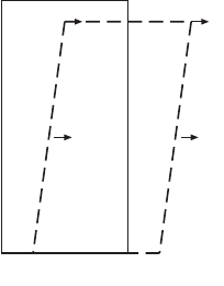
9: Computing Mechanical Stress

Boundary Conditions

Sentaurus™ Process User Guide 671

H-2013.03

slave boundary has the same deformation profile as the master boundary. In Figure 92, the left

and right boundaries are bound together by the periodic boundary condition.

Figure 92 Periodic boundary condition

To apply the periodic boundary condition to the outer bounding surfaces, use the command:

pdbSet Mechanics <Left | Right | Front | Back> Periodic 1

If this command is specified on a sidewall, the opposite sidewall is defined automatically as a

periodic boundary. Conflict of boundary condition definitions are checked on all sidewalls. For

example, to apply a periodic boundary condition on the left and right sidewalls, use one of the

following commands:

pdbSet Mechanics Left Periodic 1

pdbSet Mechanics Right Periodic 1

Both the periodic and coupling boundary conditions are implemented using the penalty

method. To adjust the penalty factor, use the command:

pdbSet Mechanics Constraint.Penalty.Factor <n>

The default penalty factor is . The larger this factor, the more accurately the periodic

or coupling boundary conditions will be enforced. Using an extremely large penalty factor

could lead to an ill-conditioned matrix and, therefore, slow down or even fail the linear

equation solver.

NOTE If you choose to apply periodic boundary conditions, all other boundary

conditions defined through the old pdbSet method will be ignored and

must be redefined using the stressdata command.

U = U ; U = U ...

2R2L

1L2R2L

1.0 13

×10

9: Computing Mechanical Stress

Time Step Control

672 Sentaurus™ Process User Guide

H-2013.03

Time Step Control

It may be necessary to use time step control when viscous or viscoelastic materials are present

in the structure. Usually, when other dopants also are present, the time steps will be sufficiently

limited by the diffusion solver. If dopants are not present or for materials with a low viscosity,

the time step control for the Maxwell model can be switched on with:

pdbSet Mechanics Visc.Step.Control 1

Time-stepping can be controlled with the displacement increment and with the relative

relaxation time. To switch on these two options, use:

pdbSet Mechanics Visc.Step Limit.Disp 1

and:

pdbSet Mechanics Visc.Step Limit.ScaleT 1

respectively. For more control parameters, see “Mechanics Visc.Step” in the Parameter

Database Browser.

For the standard linear solid model for viscoelasticity, time step control is activated

automatically (see Time-Step Control for Mechanics on page 871 for details).

Stress-causing Mechanisms

Every mechanical system needs a set of stress-driving mechanisms to reach a stressed state.

The stress-inducing mechanisms in Sentaurus Process are listed here.

Stress Induced by Growth of Material

During the oxidation process, volume is produced. Consuming silicon of volume 1 during

thermal oxidation produces oxide of volume 2.25. This process introduces velocities at a

growing interface: a velocity vector pointing into the silicon describes the proceeding of the

oxidation front, and a velocity vector pointing into the oxide accounts for the volume expansion

as described above. The latter is responsible for the generation of mechanical stresses and,

therefore, is used as a boundary condition for the mechanical problem.

9: Computing Mechanical Stress

Stress-causing Mechanisms

Sentaurus™ Process User Guide 673

H-2013.03

Densification-induced Stress

A typical densification process uses thermal heating to increase the density of a porous

material. As the material density increases, its volume shrinks and the volume shrinkage

generates stresses.

The densification-induced stress computation is switched on using the density.increase

parameter in the diffuse command or the temp_ramp command, such as:

diffuse temperature=1000<C> time=30<min> \

density.increase= {[<regionName> = value] [<material> = value]}

temp_ramp name=dens time=1 temp=1000 density.increase= { oxide=0.02 }

diffuse temp_ramp=dens

The total amount of density increase can be specified per material or per region for a given

diffuse (or temp_ramp) step as shown above. A proportional amount of density increase is

applied during each time step of the densification process.

The densification operation can be performed for all existing materials, as well as new

materials defined using the mater command:

mater add name=TEOS new.like=oxide

diffuse time=1 temp=1000 density.increase = { TEOS = 0.03 }

For densification processes involving large amounts of volume shrinkage, the material

boundaries and meshes can be updated using the following settings:

pdbSet Grid Inert.Modify.Mesh 1

pdbSetDouble TEOS Grid MinimumVelocity 0

For a complete densification process that has distinguished density changes, multiple diffuse

steps can be used with different density increases for each segment of the process.

Selectively Switching Off Grid Movement

The parameter MinimumVelocity can be used to selectively switch off point or interface

movement. This can be useful, for example, when a mechanics simulation computes a small

amount of boundary movement that is either unwanted or could cause element quality to suffer

in the vicinity, and the approximation of no movement is acceptable. In general, the command

is:

pdbSet <material> Grid MinimumVelocity <speed>

If <material> is a bulk material (no underscore), the parameter applies to bulk points. If the

speed of the bulk points is less than <speed> (in cm/s), Sentaurus Process truncates the speed

9: Computing Mechanical Stress

Stress-causing Mechanisms

674 Sentaurus™ Process User Guide

H-2013.03

to zero. This truncation is applied to material silicon by default. On the other hand, if

<material> is an interface material (having an underscore such as

PolySilicon_Silicon), the parameter only applies to points on that interface. This

truncation is applied to material Silicon by default.

NOTE The moving mesh operations can become unstable for values of

MinimumVelocity that are neither very large nor zero. Very large

values stop all motion, and 0 allows all motion.

Stress Caused by Thermal Mismatch

Temperature changes during the process described by the temp_ramp command or the

keyword ramprate in the diffuse command lead to stress in the structure caused by the

different thermal expansion coefficients of the relevant materials. When necessary, the stress

computation can be switched off by using the stress.relax flag:

diffuse temperature=1000<C> time=30<min> !stress.relax

NOTE If viscous or viscoelastic materials are present in the structure, the stress

distribution may change even without a change in the temperature due

to viscoelastic relaxation.

By default, stresses are computed during inert annealing for 2D simulations. To

apply !stress.relax to all inert annealing steps, use the command:

pdbSet Compute NoStressRelax 1

The thermal expansion coefficient for certain materials can be found in the parameter database

as follows:

<material> Mechanics ThExpCoeff

Thermal expansion only affects the dilatational part of the constitutive equation:

(950)

The change in the temperature is described by and is the relative

thermal expansion coefficient of a certain material with respect to the thermal expansion

coefficient of the substrate.

In certain examples, like bending, you may want to use absolute expansion coefficients instead

of relative. This can be achieved by setting a parameter called RefThExpCoeff as follows:

pdbSetDouble Mechanics RefThExpCoeff 0.

σkk 3Kεkk αrel∆T–()=

∆T

αrel αmat αsubs

–=

9: Computing Mechanical Stress

Stress-causing Mechanisms

Sentaurus™ Process User Guide 675

H-2013.03

All the thermal expansion coefficients are computed with respect to the substrate. This

reference value is changed by setting a certain region as substrate and resetting the thermal

expansion coefficient. A region can be tagged as the substrate in several ways:

■Use the substrate keyword when defining regions with the region command before the

init command.

■If a saved structure is being loaded into Sentaurus Process, a region is tagged as the

substrate with the command:

region name=<region_name> substrate

The reference thermal expansion coefficient can be directly set with:

pdbSetDouble Mechanics RefThExpCoeff <n>

This command overwrites the reference thermal expansion coefficient setting from the

substrate.

Materials expand differently in different temperature ranges. The linear dependency of the

thermal expansion coefficient on temperature can be specified by:

pdbSet Silicon Mechanics ThExpCoeffRate 4e-9

So the total thermal expansion coefficient at the elevated temperature can be expressed as:

(951)

where the room temperature is set to 300 K.

Lattice Mismatch

The presence of impurities, such as germanium and carbon, can change the lattice parameters

of crystalline silicon. This effect has been exploited in two ways technologically:

■Introducing an impurity during epitaxy to form a strained layer.

■Growing a substrate (typically, a very thick layer grown on a standard substrate) to produce

a customized lattice constant.

However, most technological applications are based on the first use, for example, when SiGe

source/drain pockets are grown on silicon substrates. For strained SiGe epitaxy, Sentaurus

Process automatically computes and applies the strain, and no user input is necessary.

aThExpCoeff ThExpCoeffRate+TRoomTemperature–()×=

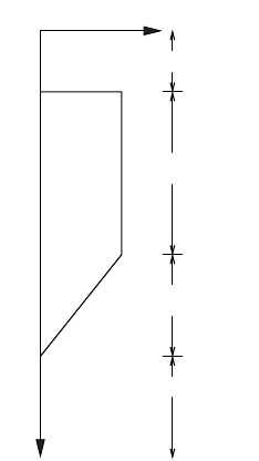
9: Computing Mechanical Stress

Stress-causing Mechanisms

676 Sentaurus™ Process User Guide

H-2013.03

For customized lattice-spacing substrates or other material systems, more setup of the tool is

required. This section explains the theory and implementation of this model and gives an

example. Figure 93 shows a simple SiGe wafer.

Figure 93 Simple SiGe wafer for customizing lattice-spacing

There are four main regions of the manufactured substrate. The silicon region has the graded

buffer layer where the Ge concentration increases linearly from zero to the required

concentration. The manufacturing process of this layer is designed such that all the dislocations

are forced energetically to nucleate here, and the wafer is completely relaxed. The relaxed layer

that is grown on top of the graded layer has no dislocations and no strain. The lattice-spacing

of this layer is determined by the Ge mole fraction. The lattice-spacing of this layer controls

the strains obtained in the top strained layer. The top strained layer is grown depending on the

kind of strain required. If this layer is to be in a tensile state, the Ge concentration here must be

less than that of the relaxed layer. In the case of a compressive state, the Ge concentration must

be greater than that of the relaxed layer. This layer has a thermodynamic limit on its thickness

since the strain energy it contains should be less than the dislocation nucleation energy. The

strain energy is directly proportional to the volume that is under the strain. The strain profile of

germanium in silicon is given approximately by:

(952)

where is the Ge mole fraction calculated as the germanium concentration divided by the

silicon lattice density.

In the relaxed region, Sentaurus Process modifies the lattice-spacing. This results in no stresses

due to the presence of germanium. In the strained region, the lattice-spacing is fixed by the

lattice-spacing in the relaxed region. Now, using the Ge mole fraction in the strained region,

Ge Concentration

Relaxed Layer

Graded Layer

Pure Silicon

Strained Layer

0.01

0.5

0.7

X µm

ε0.0425x=

9: Computing Mechanical Stress

Stress-causing Mechanisms

Sentaurus™ Process User Guide 677

H-2013.03

the effective unstrained lattice-spacing is computed, and the stresses are based on the difference

of the effective lattice-spacing and the lattice-spacing of the relaxed region.

For example, assume the strained layer has no Ge: The effective lattice-spacing is that of silicon

given by . The lattice-spacing of the relaxed SiGe part is, for example, . The strain in

the strained region is:

(953)

The strain computed using Eq. 953 is applied as a biaxial strain in the y- and z-directions.

Using the Lattice Mismatch Model

For the most common case of SiGe layers grown on silicon substrates, the model is switched

on by default, and strain is computed and updated as necessary. For simulating other material

systems, a few settings are required to instruct Sentaurus Process how the strain should be

computed.

If the substrate is not silicon or it is not the lowest most region in the substrate (that is, the

largest x-coordinate), you must identify the substrate region in the wafer. Use the region

command and include the keyword substrate for the appropriate region. If there is no

substrate defined in the loaded structure, use the following command to tag a region as a

substrate:

region name=<region_name> substrate

Regions isolated from the substrate by nonsubstrate materials must be tagged as substrate to

account for the lattice mismatch effect.

For systems other than SiGe, Sentaurus Process must know the strain profile of the field in the

substrate. The strain_profile command is used to specify this. The strain is specified as a

piecewise linear function of the mole fraction. For Ge in silicon, it is:

strain_profile Silicon species=Germanium strain= {0 0.0425} ratio= {0 1}

or:

pdbSet Silicon Germanium Conc.Strain {0 0 1 0.0425}

The lattice mismatch model for SiGe is switched on by default. Next, for customized lattice-

spacing substrates, the substrate must be given a strain profile. The strain profile can be

specified with the substrate_profile command or the profile command as a piecewise

linear function of the x-coordinate:

profile region=<region_name> name=Germanium \

concentration= {1e10 1e10 2e22 2e22 1e10 1e10} \

xcoord= {0 0.01 0.011 0.5 0.7 10} linear

LSi

LSiGe

εLSiGe LSi

–()LSi

⁄=

9: Computing Mechanical Stress

Stress-causing Mechanisms

678 Sentaurus™ Process User Guide

H-2013.03

The location of the top of the relaxed region must be specified in Sentaurus Process. Generally,

this should not be at the top of the relaxed layer (see Figure 93 on page 676) because

germanium diffusion during any anneal step can cause unrealistic stress values to appear in this

area. The best location for the top of the relaxed region is approximately two-thirds of the

relaxed layer thickness from the top of the relaxed layer. In this example, it is approximately

. This reference position can be set with the command:

pdbSet Silicon Mechanics TopRelaxedNodeCoord 0.35e-4

NOTE In most cases, when the simulation does not require any SiGe substrate

(for example, when SiGe source/drain pockets are grown on silicon

substrates), this parameter is not needed. The reference lattice-spacing

is the one of the substrate; Sentaurus Process detects automatically the

adjacent silicon-like regions and applies to them the lattice mismatch

model. For this reason, the value of this parameter defaults to the bottom

coordinate of the structure.

Finally, for these concentrations to take effect and all mechanics computations to occur, you

must add a short diffusion step if there is none.

The update_substrate command is deprecated. If used, the update_substrate

command should be called only once for initialization assuming all strain profiles have not

been accounted for lattice-mismatch strains.

During dopant redistribution, the lattice-spacing and lattice mismatch strains are updated, and

the doping concentration at the top of the relaxed layer may change. To disable automatic

updating of lattice-mismatch strains, use:

pdbSet Silicon Mechanics UpdateStrain 0

To switch off the lattice-spacing tracking at the top of the relaxed layer, use:

pdbSet Mechanics LatticeHistory 0

Total Concentration Model

The total concentration model computes the total contribution of lattice mismatch stress with

the current impurity concentration and the elastic moduli at the current temperature. For binary

compound materials, the elastic moduli are computed with the current mole fraction. With this

approach, the lattice mismatch stress is history independent and can change even with an

unchanged doping profile.

0.35 µm

9: Computing Mechanical Stress

Stress-causing Mechanisms

Sentaurus™ Process User Guide 679

H-2013.03

This is the default lattice mismatch model. To switch off this model by computing the lattice

mismatch stress increment with the elastic moduli during doping profile change, use the

command:

pdbSet Mechanics Total.Concentration.Model 0

Reference Concentration Model

The reference concentration model is a simplified lattice mismatch model, which does not

distinguish the relaxed region and strained region by specifying the location of the top of the

relaxed region. Only relative concentration accounts for the lattice-spacing and strain changes.

For example, the strain in SiGe is:

(954)

and the lattice-spacing is computed by , where is the lattice density

of silicon and is the reference Ge concentration in SiGe defined by:

pdbSet Silicon Germanium Ref.Concentration 1e22

The lattice-spacing and strain from this model may not be physical in the relaxed region.

The reference concentration model is used when the structure is flipped for backside

processing. To switch on this model, use the command:

pdbSet Mechanics Reference.Concentration.Model 1

Strained Deposition

Impurity-induced stress can be introduced locally during deposition to account for a lattice-

spacing change due to stress rebalancing. For example, the SiGe lattice-spacing during

unconstrained growth gradually returns to the unconstrained SiGe lattice-spacing. The lattice

mismatch effect should diminish during the SiGe growth.

ε0.0425 CGe Cref

–()CSi

⁄⋅=

LSiGe LSi 1ε+()⋅=

CSi

Cref

9: Computing Mechanical Stress

Stress-causing Mechanisms

680 Sentaurus™ Process User Guide

H-2013.03

The following steps are performed when strained deposition is enabled:

1. Deposit a new layer.

2. Apply a doping profile, and compute the lattice spacing of the newly deposited layer.

3. Set the lattice spacing of the deposited layer to that of the underlayer, and compute the

mismatch strain.

4. Perform stress relaxation to establish stress equilibrium, and update the lattice spacing.

5. Merge layers if needed.

To correctly catch the relaxation effect, the thickness of the deposited layer must be chosen

properly; a fine mesh is required. Multiple deposition can be particularly useful in such cases.

To switch on this model, use the command:

pdbSet Mechanics StrainedDeposition 1

and set the option Strained.Lattice in the deposit command.

The total concentration model is disabled during strained deposition. The reference

concentration model should not be used with strained deposition.

Edge Dislocation

The existence of crystal lattice defects, such as dislocation, affects the channel stress state. The

impact of edge dislocation is included by superposing the dislocation-induced stress field from

elasticity theory. Each edge dislocation can be defined with:

stressdata apply.dislocation dislocation.origin= {<n> <n> <n>}

para.orient= {<n> <n> <n>} perp.orient= {<n> <n> <n>} region=<c> <material>

where:

■dislocation.origin is the location of the dislocation core.

■para.orient specifies the direction of the edge dislocation or the direction of the half

plane.

■perp.orient is Burger’s vector in the perpendicular direction to the half plane.

Here, the magnitude of perp.orient is the slip distance. You must supply either a region

name or a material name. If region is specified, the stress field is superposed to this region.

If material is specified, the stress field is applied to all regions of crystalline material. To save

the edge dislocation geometry information to a TDR file for visualization, specify the

command option saveTDR with the edge dislocation definition.

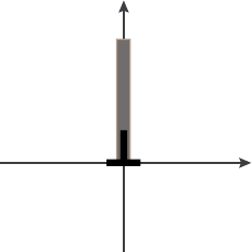
9: Computing Mechanical Stress

Stress-causing Mechanisms

Sentaurus™ Process User Guide 681

H-2013.03

Figure 94 Edge dislocation located at the origin O; n1 is Burger’s vector and n2 is the

direction of the half plane

Singularity exists in the analytic solution at the dislocation core. Without using a nonlinear

atomistic theory, the stresses in the core region within a few magnitudes of Burger’s vector to

the dislocation core are smoothed away. The factor for this core radius can be defined with:

pdbSet Mechanics Dislocation.Coresize.Factor 2.0

A prototype model for positioning the edge dislocations is available by minimizing the elastic

strain energy [11]. The stress field from each edge dislocation is superposed. The elastic strain

energy is determined after force equilibrium with edge dislocations at their initial locations.

The initial location of edge dislocation serves as the initial guess and can be defined by:

stressdata !apply.dislocation dislocation.origin= {<n> <n> <n>} \

para.orient= {<n> <n> <n>} perp.orient= {<n> <n> <n>} region=<c>

where:

■dislocation.origin is the initial location of the edge dislocation.

■!apply.dislocation is specified to delay applying the dislocation-induced stress field.

Multiple edge dislocations with different Burger’s vectors can be defined separately with this

syntax.

When all the edge dislocations for minimizing the elastic strain energy are specified, you can

start the optimization with the command:

stressdata origin.max= {<n> <n> <n>} origin.min= {<n> <n> <n>} \

optimize.dislocation

where origin.max and origin.min define the range of dislocation positions in the specified

region. Some additional parameters for optimization convergence control also can be defined

in this command (see stressdata on page 1151).

9: Computing Mechanical Stress

Stress-causing Mechanisms

682 Sentaurus™ Process User Guide

H-2013.03

The movement of edge dislocations depends on the gradient of the total elastic strain energy

computed from a discrete integral over all elements. The target of the optimization is set to -5

multiplied by the absolute value of the starting elastic strain energy. This factor can be changed

with:

pdbSetDouble Mechanics Energy.Optimization.Factor <n>

The coordinates of the edge dislocations after optimization are returned in a Tcl list formatted

as <x1> <y1> <x2> <y2> ... for two dimensions, and <x1> <y1> <z1> <x2> <y2>

<z2> ... for three dimensions. The final stress state remains the same as before the edge

dislocations are introduced. The edge dislocations may stop at the local minimum where the

elastic strain energy has not reached the global minimum. In such a case, a new optimization

step must be started with the initial guess of the edge dislocation positions adjusted based on

the previous optimization result. It is also helpful to refine the mesh.

Intrinsic Stress

Certain process steps require the deposition of materials with intrinsic stresses. Sentaurus

Process can be used to model these process steps. The intrinsic stresses (StressELXX,

StressELYY, StressELZZ, StressELXY, StressELYZ, StressELZX) can be prescribed in

the deposit command (see deposit on page 901). After stress relaxation, the resulting stresses

will be less than the prescribed ones by default. You can scale the prescribed stresses so that

for a flat surface, the relaxed stress will be the same as the prescribed stress. To scale the

stresses, use the command:

pdbSet Mechanics StressRelaxFactor 1

For deposition in 3D, you can specify stresses in specific layers using the stressdata

command (see stressdata on page 1151). For example:

stressdata nitride syyi=1.4e10

sets the yy component of the intrinsic stress in the nitride to .

1.4 10

×10 dyn/cm2

9: Computing Mechanical Stress

Stress-causing Mechanisms

Sentaurus™ Process User Guide 683

H-2013.03

For interconnect simulations, intrinsic stresses in metal lines can be modeled as width

dependent [12] with either a linear relation or a logarithmic relation, using the parameters

defined through the stressdata command:

■If modeled as a linear relation, the total intrinsic stresses are given by:

■If modeled as a natural logarithmic relation, the total intrinsic stresses are given by:

where are defined through the parameters sxxi, sxx1, sxx2, and base of

the stressdata command. The other two components ( and ) are defined in the same

way, and is calculated internally with respect to the region (not material) boundaries.

Stress Rebalancing after Etching and Deposition

When materials are removed from or added to a given structure, physical stress distributions

generally change with the corresponding geometry and boundary changes. In simulations, a

stress-rebalancing step is required to re-establish the stress equilibrium in the structure and to

conform the stress distributions to the new boundaries. By default, a stress-rebalancing

operation is called after etching or deposition is performed. To omit the stress-rebalancing step,

use:

pdbSet Mechanics EtchDepoRelax 0

Automated Tracing of Stress History

Thermal residual stress in a given device structure is a function of its fabrication history, which

consists of process steps at various temperatures and temperature ramps in between. To model

stress evolution accurately, all temperature ramps should be traced. When the pdb parameter

StressHistory is switched on, for example:

pdbSet Mechanics StressHistory 1

the temperature gaps between process steps such as diffusion, deposition, and etching are

detected and filled with instant stress-rebalancing, solving for thermal mismatch strains and

stresses.

σxx σxxi σxx1

------+=

σyy σyyi σyy1

------+=

σzz σzzi σzz1

------+=

σxx σxxi σxx2

------

ln+=

σyy σyyi σyy2

------

ln+=

σzz σzzi σzz2

------

ln+=

σxxi σxx1σxx2wb

,,,

9: Computing Mechanical Stress

Saving Stress and Strain Components

684 Sentaurus™ Process User Guide

H-2013.03

Saving Stress and Strain Components

By default, stress-tensor components are saved on both elements and nodes. The elastic

portions of the strain-tensor components also are saved on both elements and nodes by default.

The elastic strains are computed from stresses using isotropic elasticity by default. The

anisotropic elasticity also can be used for a given crystalline material when the corresponding

pdb parameter Anisotropic is set. The elastic strain-field computing and saving operation

can be omitted by using the following command:

pdbSet Mechanics saveElasticStrain 0

The stress tensor can be decomposed and the resulting dilatational and deviatoric stress

components can be saved on nodes when the following pdb parameter is switched on:

pdbSet Mechanics decomposeStress 1

Description of Output Variables

The mechanics module in Sentaurus Process assumes that stresses and strains are defined on

elements. However, not all tools can read or visualize element values. For this reason,

Sentaurus Process performs an element-to-node interpolation of stresses as a postprocessing

step and writes both forms of stresses to output.

The element stresses are prefixed by StressEL and the nodal stresses are prefixed by Stress.

The tensor components are given by the post-fix (XX, YY, ZZ, XY, YZ, ZX).

In history-dependent materials, you cannot create a simple, closed-form relation between

stresses and strains. It is useful, however, to compute the elastic part. The elastic component of

the strain is an indicator of the stored strain energy in the system. In addition, the elastic

component of the strain is the total strain in elastic materials such as silicon and polysilicon.

Pressure is one-third of the negative of the trace of the stress tensor:

(955)

The field LatticeSpacing represents the lattice-spacing of the crystal at the location of the

node. This is controlled by the presence of lattice-altering species such as germanium or carbon

in the structure. In addition, the strain_profile command must be specified.

In Sentaurus Process, the select command is used to perform Tcl-level and Alagator-level

operations. To access the stress components, use the select command.

---σii



–=

9: Computing Mechanical Stress

Saving Stress and Strain Components

Sentaurus™ Process User Guide 685

H-2013.03

The stresses and strains are represented as symmetric tensors. To access the xx, yy, and zz

components of nodal stress values, the variable references for the select command are

Stress_xx, Stress_yy, and Stress_zz, respectively. To access the xy, yz, and zx

components, use Stress_xy, Stress_yz, and Stress_zx, respectively.

For element values, the Boolean keyword element of the select command must be set to

true. To access the xx, yy, and zz components of the element stress values, the variable

references for the select command are StressEL_xx, StressEL_yy, and StressEL_zz,

respectively. To access the xy, yz, and zx components, use StressEL_xy, StressEL_yz, and

StressEL_zx, respectively.

The old variable names for accessing the components of stress and strain tensors are supported

as well. A comparison of the new names and the corresponding deprecated names is included

in Table 66 on page 688.

Table 65 presents descriptions of the mechanics-related output data and whether the variables

apply to elements or nodes.

Table 65 Variable names in Sentaurus Process output files

Variable name Element/Node Description Unit

Displacement_x

Node X component of displacement cm

Displacement_y

Node Y component of displacement cm

Displacement_z

Node Z component of displacement cm

ElasticStrainXX

Node XX component of elastic strain Unitless

ElasticStrainXY

Node XY component of elastic strain Unitless

ElasticStrainYY

Node YY component of elastic strain Unitless

ElasticStrainYZ

Node YZ component of elastic strain Unitless

ElasticStrainZX

Node ZX component of elastic strain Unitless

ElasticStrainZZ

Node ZZ component of elastic strain Unitless

PlasticStrainXX

Node XX component of plastic strain Unitless

PlasticStrainXY

Node XY component of plastic strain Unitless

PlasticStrainYY

Node YY component of plastic strain Unitless

PlasticStrainYZ

Node YZ component of plastic strain Unitless

PlasticStrainZX

Node ZX component of plastic strain Unitless

PlasticStrainZZ

Node ZZ component of plastic strain Unitless

PlasticStrainEQV

Node Equivalent plastic strain Unitless

9: Computing Mechanical Stress

Saving Stress and Strain Components

686 Sentaurus™ Process User Guide

H-2013.03

ViscoPlasticStrainXX

Node XX component of viscoplastic strain Unitless

ViscoPlasticStrainXY

Node XY component of viscoplastic strain Unitless

ViscoPlasticStrainYY

Node YY component of viscoplastic strain Unitless

ViscoPlasticStrainYZ

Node YZ component of viscoplastic strain Unitless

ViscoPlasticStrainZX

Node ZX component of viscoplastic strain Unitless

ViscoPlasticStrainZZ

Node ZZ component of viscoplastic strain Unitless

ViscoPlasticStrainEQV

Node Equivalent viscoplastic strain Unitless

CreepStrainELXX

Element XX component of creep strain Unitless

CreepStrainELXY

Element XY component of creep strain Unitless

CreepStrainELYY

Element YY component of creep strain Unitless

CreepStrainELYZ

Element YZ component of creep strain Unitless

CreepStrainELZX

Element ZX component of creep strain Unitless

CreepStrainELZZ

Element ZZ component of creep strain Unitless

CreepStrainELEQV

Element Equivalent creep strain Unitless

SwellingStrainELXX

Element XX component of swelling strain Unitless

SwellingStrainELXY

Element XY component of swelling strain Unitless

SwellingStrainELYY

Element YY component of swelling strain Unitless

SwellingStrainELYZ

Element YZ component of swelling strain Unitless

SwellingStrainELZX

Element ZX component of swelling strain Unitless

SwellingStrainELZZ

Element ZZ component of swelling strain Unitless

LatticeSpacing

Node Lattice-spacing cm

Pressure

Node Pressure Pa

StressELXX

Element XX component of element stress Pa

StressELXY

Element XY component of element stress Pa

StressELYY

Element YY component of element stress Pa

StressELYZ

Element YZ component of element stress Pa

StressELZX

Element ZX component of element stress Pa

StressELZZ

Element ZZ component of element stress Pa

StressXX

Node XX component of node stress Pa

Table 65 Variable names in Sentaurus Process output files

Variable name Element/Node Description Unit

9: Computing Mechanical Stress

Saving Stress and Strain Components

Sentaurus™ Process User Guide 687

H-2013.03

StressXY

Node XY component of node stress Pa

StressYY

Node YY component of node stress Pa

StressYZ

Node YZ component of node stress Pa

StressZX

Node ZX component of node stress Pa

StressZZ

Node ZZ component of node stress Pa

MisesStress

Node von Mises stress Pa

DeformationResistance

Node Deformation resistance Pa

ElasticEnergyDens

Node Elastic strain energy density J/m3

PlasticEnergyDens

Node Plastic strain energy density J/m3

ViscoPlasticEnergyDens

Node Viscoplastic strain energy density J/m3

CreepEnergyDensEL

Element Creep strain energy density J/m3

BaseStressELXX

Element XX component of elastic element stress for

Standard Linear Solid viscoelasticity model

BaseStressELXY

Element XY component of elastic element stress for

Standard Linear Solid viscoelasticity model

BaseStressELYY

Element YY component of elastic element stress for

Standard Linear Solid viscoelasticity model

BaseStressELYZ

Element YZ component of elastic element stress for

Standard Linear Solid viscoelasticity model

BaseStressELZX

Element ZX component of elastic element stress for

Standard Linear Solid viscoelasticity model

BaseStressELZZ

Element ZZ component of elastic element stress for

Standard Linear Solid viscoelasticity model

BaseElasticStrainELXX

Element XX component of elastic element strain for

Standard Linear Solid viscoelasticity model

Unitless

BaseElasticStrainELXY

Element XY component of elastic element strain for

Standard Linear Solid viscoelasticity model

Unitless

BaseElasticStrainELYY

Element YY component of elastic element strain for

Standard Linear Solid viscoelasticity model

Unitless

BaseElasticStrainELYZ

Element YZ component of elastic element strain for

Standard Linear Solid viscoelasticity model

Unitless

BaseElasticStrainELZX

Element ZX component of elastic element strain for

Standard Linear Solid viscoelasticity model

Unitless

Table 65 Variable names in Sentaurus Process output files

Variable name Element/Node Description Unit

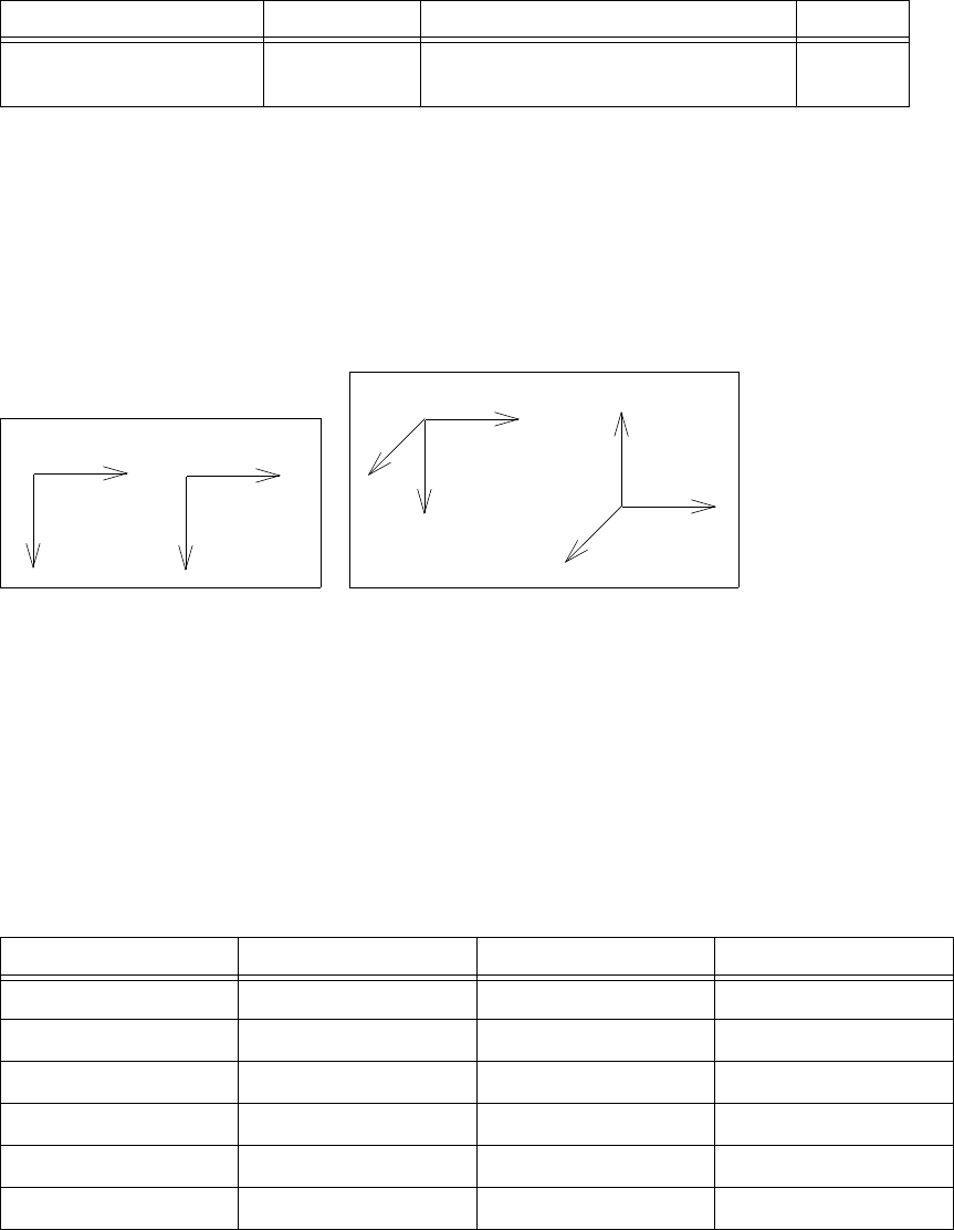
9: Computing Mechanical Stress

Saving Stress and Strain Components

688 Sentaurus™ Process User Guide

H-2013.03

NOTE The stresses and strains in the output file are according to the UCS,

unless you explicitly request to save in the DF–ISE coordinate system

by using the math coord.dfise command. The UCS is the same as

the Sentaurus internal coordinate system, but differs from the DF–ISE/

TDR coordinates. Therefore, it is important to note the directions of the

axes in 2D and 3D (see Figure 95).

Figure 95 (Left) Axis orientation in 2D and (right) axis orientation in 3D

The axis directions in DF–ISE/TDR coordinates are different in 2D and 3D in the UCS.

Figure 95 shows the axis orientation in 2D and in 3D. Consequently, the values of the stress

and strain components change.

For information about the TDR format, refer to the Sentaurus™ Data Explorer User Guide.

Table 66 maps the fields from the select command to the fields in the output files of

Sentaurus Process. The axis directions in Sentaurus Process are the same in 2D and 3D.

BaseElasticStrainELZZ

Element ZZ component of elastic element strain for

Standard Linear Solid viscoelasticity model

Unitless

Ta bl e 66 Va ri abl e na me s in o u t p ut f il es

Field name Field name (deprecated) 2D 3D

StressEL_xx StressELKK_x StressEL-YY StressEL-ZZ

StressEL_yy StressELKK_y StressEL-XX StressEL-YY

StressEL_zz StressELKK_z StressEL-ZZ StressEL-XX

StressEL_xy StressELIJ_x StressEL-XY -StressEL-YZ

StressEL_yz StressELIJ_y

Not applicable

StressEL-XY

StressEL_zx StressELIJ_z

Not applicable

-StressEL-ZX

Table 65 Variable names in Sentaurus Process output files

Variable name Element/Node Description Unit

UCS DF–ISE/TDR

9: Computing Mechanical Stress

Saving Stress and Strain Components

Sentaurus™ Process User Guide 689

H-2013.03

Stress_xx StressKK_x Stress-YY Stress-ZZ

Stress_yy StressKK_y Stress-XX Stress-YY

Stress_zz StressKK_z Stress-ZZ Stress-XX

Stress_xy StressIJ_x Stress-XY -Stress-YZ

Stress_yz StressIJ_y

Not applicable

Stress-XY

Stress_zx StressIJ_z

Not applicable

-Stress-ZX

Pressure

Not applicable

Pressure Pressure

MisesStress

Not applicable

MisesStress MisesStress

PrincipalStress1

Not applicable

PrincipalStress1 PrincipalStress1

PrincipalStress2

Not applicable

PrincipalStress2 PrincipalStress2

PrincipalStress3

Not applicable

PrincipalStress3 PrincipalStress3

ElasticStrain_xx ElasticStrainKK_x ElasticStrain-YY ElasticStrain-ZZ

ElasticStrain_yy ElasticStrainKK_y ElasticStrain-XX ElasticStrain-YY

ElasticStrain_zz ElasticStrainKK_z ElasticStrain-ZZ ElasticStrain-XX

ElasticStrain_xy ElasticStrainIJ_x ElasticStrain-XY -ElasticStrain-YZ

ElasticStrain_yz ElasticStrainIJ_y

Not applicable

ElasticStrain-XY

ElasticStrain_zx ElasticStrainIJ_z

Not applicable

-ElasticStrain-ZX

PlasticStrain_xx PlasticStrainKK_x PlasticStrain-YY PlasticStrain-ZZ

PlasticStrain_yy PlasticStrainKK_y PlasticStrain-XX PlasticStrain-YY

PlasticStrain_zz PlasticStrainKK_z PlasticStrain-ZZ PlasticStrain-XX

PlasticStrain_xy PlasticStrainIJ_x PlasticStrain-XY -PlasticStrain-YZ

PlasticStrain_yz PlasticStrainIJ_y

Not applicable

PlasticStrain-XY

PlasticStrain_zx PlasticStrainIJ_z

Not applicable

-PlasticStrain-ZX

PlasticStrainEQV

Not applicable

PlasticStrainEQV PlasticStrainEQV

ViscoPlasticStrain_xx ViscoPlasticStrainKK_x ViscoPlasticStrain-YY ViscoPlasticStrain-ZZ

ViscoPlasticStrain_yy ViscoPlasticStrainKK_y ViscoPlasticStrain-XX ViscoPlasticStrain-YY

ViscoPlasticStrain_zz ViscoPlasticStrainKK_z ViscoPlasticStrain-ZZ ViscoPlasticStrain-XX

ViscoPlasticStrain_xy ViscoPlasticStrainIJ_x ViscoPlasticStrain-XY -ViscoPlasticStrain-YZ

ViscoPlasticStrain_yz ViscoPlasticStrainIJ_y

Not applicable

ViscoPlasticStrain-XY

Ta bl e 66 Va ri abl e na me s in o u t p ut f il es

Field name Field name (deprecated) 2D 3D

9: Computing Mechanical Stress

References

690 Sentaurus™ Process User Guide

H-2013.03

The directionality is the same for other tensor fields such as StressEL and ElasticStrain.

Tracking Maximum Stresses

During a typical process flow, the maximum stresses may be reached in a process step and,

subsequently, the stresses may fall. If the material is prone to failure through delamination or

nucleation of dislocations, the failure may occur when the maximum stress is reached. To

always track the maximum stresses, set the following parameter:

pdbSet Mechanics SaveMaxStress 1

The StressMaxEL field is updated when the current stress is greater than the stored stress. In

this way, the maximum is maintained throughout the process flow. The maximum element

stresses and the von Mises stress are computed and stored.

By using the stressdata command (see stressdata on page 1151), a list of maximum stresses

(hot spots) and their locations can be obtained. The hot spots can be evaluated by one of the six

stress components (sxx, syy, szz, sxy, syz, and szx), the von Mises stress, the principal stress,

or the hydrostatic stress (negative pressure value or the pressure). The command returns a list

of maximum stress values (largest magnitude, largest tensile, largest compressive) and the

corresponding location coordinates.

References

[1] J. C. Simo and T. J. R. Hughes, Computational Inelasticity, vol. 7, New York: Springer,

1998.

[2] W. Ramberg and W. R. Osgood, Description of Stress-Strain Curves by Three

Parameters, National Advisory Committee for Aeronautics, Technical Note No. 902,

Washington, DC, USA, July 1943.

[3] J. Lubliner, Plasticity Theory, Macmillan: New York, 1990.

ViscoPlasticStrain_zx ViscoPlasticStrainIJ_z

Not applicable

-ViscoPlasticStrain-ZX

ViscoPlasticStrainEQV

Not applicable

ViscoPlasticStrainEQV ViscoPlasticStrainEQV

Displacement_x

Not applicable

Displacement-Y -Displacement-Z

Displacement_y

Not applicable

Displacement-X Displacement-Y

Displacement_z

Not applicable Not applicable

Displacement-X

Ta bl e 66 Va ri abl e na me s in o u t p ut f il es

Field name Field name (deprecated) 2D 3D

9: Computing Mechanical Stress

References

Sentaurus™ Process User Guide 691

H-2013.03

[4] S. B. Brown, K. H. Kim, and L. Anand, “An Internal Variable Constitutive Model for

Hot Working of Metals,” International Journal of Plasticity, vol. 5, no. 2 pp. 95–130,

1989.

[5] G. G. Weber et al., “An Objective Time-Integration Procedure for Isotropic Rate-

Independent and Rate-Dependent Elastic-Plastic Constitutive Equations,” International

Journal of Plasticity, vol. 6, no. 6, pp. 701–744, 1990.

[6] G. Z. Wang et al., “Applying Anand Model to Represent the Viscoplastic Deformation

Behavior of Solder Alloys,” Journal of Electronic Packaging, vol. 123, no. 3, pp. 247–

253, 2001.

[7] Q. Wang et al., “Anand Parameter Test for Pb-Free Material SnAgCu and Life

Prediction for a CSP,” in 8th International Conference on Electronic Packaging

Technology (ICEPT), Shanghai, China, pp. 1–9, August 2007.

[8] J. Wilde et al., “Rate Dependent Constitutive Relations Based on Anand Model for

92.5Pb5Sn2.5Ag Solder,” IEEE Transactions on Advanced Packaging, vol. 23, no. 3,

pp. 408–414, 2000.

[9] H. J. Frost and M. F. Ashby, Deformation-Mechanism Maps, Pergamon Press: Oxford,

1982.

[10] S. Wiese, F. Feustel, and E. Meusel, “Characterisation of constitutive behaviour of

SnAg, SnAgCu and SnPb solder in flip chip joints,” Sensors and Actuators A, vol. 99,

no. 1–2, pp. 188–193, 2002.

[11] R. Gatti et al., “Dislocation engineering in SiGe heteroepitaxial films on patterned Si

(001) substrates,” Applied Physics Letters, vol. 98, no. 12, p. 121908, 2011.

[12] Y.-C. Joo, J.-M. Paik, and J.-K. Jung, “Effect of Microstructure and Dielectric Materials

on Stress-Induced Damages in Damascene Cu/Low-k Interconnects,” in MRS

Symposium Proceedings, Materials, Technology and Reliability of Advanced

Interconnects, vol. 863, San Francisco, CA, USA, p. B7.6/O11.6, March 2005.

9: Computing Mechanical Stress

References

692 Sentaurus™ Process User Guide

H-2013.03

Sentaurus™ Process User Guide 693

H-2013.03

CHAPTER 10 Mesh Generation

This chapter describes the mesh algorithms and meshing parameters

available in Sentaurus Process.

Overview

Sentaurus Process automatically generates meshes as they are needed. The behavior of the

automatic-meshing scheme is different in 3D than in 1D and 2D because of the time required

to generate 3D meshes. In 1D and 2D, meshes are generated after every geometry operation

such as etch, deposit, and transform. In 3D, meshes are only generated immediately before

steps that require a bulk mesh, such as a diffuse or an implant command, and structure

saving. This scheme can reduce the time spent when there are multiple geometry-changing

steps without a diffuse or an implant command (or any other step requiring a mesh) in

between.

Sentaurus Process uses Sentaurus Mesh as its mesh generation engine. Details of the meshing

algorithms are provided, but for simplification, Sentaurus Mesh is used throughout.

The mesh generation process starts with a bisection algorithm, which places mesh points as

instructed by the user. Afterwards, the mesh elements are created using a modified Delaunay-

meshing algorithm. Refer to the Mesh Generation Tools User Guide for details about Sentaurus

Mesh.

The meshes generated within Sentaurus Process can be refined adaptively, statically, or as a

combination of adaptive and static refinements. The refinement can be specified using one of

the major types of refinement box:

■Field based (adaptive meshing)

■Mask based

■Uniform (standard)

■Interface axis-aligned

■Interface offsetting (offset normal to the interface)

All these refinement types are user controllable. In addition, Sentaurus Mesh enforces mesh

smoothing to limit the changes in element size from one element to the next. This smoothing

is important for mechanics accuracy and convergence behavior (see Mesh Refinement on

page 694).

10: Mesh Generation

Mesh Refinement

694 Sentaurus™ Process User Guide

H-2013.03

One important algorithm affecting refinement behavior is the UseLines algorithm. This

algorithm inserts lines created using the line command into the internal bisection algorithm

before any other lines are introduced. Further mesh refinement proceeds by bisecting the boxes

created by the UseLines lines. This has the effect of isolating static regions of a structure from

regions where the boundaries are moving due to geometric operations. Geometry movement

naturally causes perturbations to the mesh lines. The UseLines lines compartmentalize this

mesh movement to minimize solution degradation from interpolation. For more information,

see UseLines: Keeping User-defined Mesh Lines on page 722.

NOTE Because this internal bisection algorithm in Sentaurus Process is

different than the one used to create mesh refinement in the stand-alone

Sentaurus Mesh tool, it is not possible to create meshes identical to

those created with Sentaurus Mesh. However, element quality, stability,

and the Delaunay properties should be qualitatively the same.

Mesh Refinement

Mesh refinement is a two-step process:

■First, you define the refinement box.

■Second, the mesh is refined when the next remesh occurs either with an explicit

grid remesh call or during standard geometry modifications such as etch, deposit, clip,

or native layer formation.

The refinement boxes remain valid unless the list of refinement boxes is cleared with the

refinebox clear command.

All refinement boxes have refinement criteria that add mesh and constraints that can be used to

limit where the mesh refinement occurs. One type of refinement criteria is available for each

type of box, and it essentially defines the box type. The refinement criteria and, therefore, the

refinement box type can be either static or adaptive. All types of refinement box can be mixed

as required. The refinement box constraints are specified along with the refinement criteria in

the refinebox command and can be used in combination within one command.

The constraints available include:

■A material constraint using the materials parameter that takes a list of materials.

■Region constraints using the regions parameter that takes a list of region names.

■The min and max parameters that limit the size of the refinement box (which by default

applies to all of the space).

10: Mesh Generation

Mesh Refinement

Sentaurus™ Process User Guide 695

H-2013.03

Refinement information also can be extracted and written to a file readable by Sentaurus Mesh

using the mshcmd flag in conjunction with the tdr parameter of the struct command (see

struct on page 1158).

Viewing Mesh Refinement

To aid in setting mesh refinement, you can store the current minimum edge length in each

direction as a field using the command:

pdbSet Grid Set.Min.Edge 1

When specified, Sentaurus Process computes the smallest edge length in each direction and

saves it in three fields:

■MinXEdgeLength

■MinYEdgeLength (for 2D or 3D structures)

■MinZEdgeLength (for 3D structures)

In addition, it prints the average edge length to the screen.

Static Refinement

Standard Refinement Boxes

The standard refinement box allows you to specify a smoothly varying mesh density inside the

refinement box at three locations in the x-, y- and z-directions using the xrefine and

yrefine, and zrefine parameter lists, respectively. If all three xrefine, yrefine, and

zrefine values are specified, the mesh density varies quadratically in that direction. If two

are specified, the variation is linear from top to bottom. If only one value is specified, a constant

mesh density is assumed.

Refinement boxes also can be limited to refine only in one specific material or region using the

regions or materials parameter.

Examples

This is an example of specifying two refinement boxes and calling remesh:

refinebox min= {-0.25 0.4 0.0} max= {0.4 0.6 1.0} xrefine= {0.1 0.06 0.1} \

yrefine= {0.1 0.01 0.1} zrefine = {0.01} oxide

refinebox min= {0.6 0.6} max= {0.8 0.8} xrefine= 0.1 silicon

grid remesh

10: Mesh Generation

Mesh Refinement

696 Sentaurus™ Process User Guide

H-2013.03

NOTE Calculating the linear or quadratic variation of the mesh density when

two or three x-, y-, or z-direction values are given requires the

specification of min and max. If min and max are not specified and at

least one region is specified, the minimum and maximum values of the

bounding box for that region serve as min and max for the calculation.

If more than one region is specified, only the bounding box of the first

region is used for the calculation, although all regions are used as

constraints to the refinement.

Interface Refinement Boxes

Refinement near interfaces can be specified using the refinebox command. So it is possible

to have a large global default minimum interface mesh-spacing, for example, and a smaller

localized value inside a box. The parameters affecting interface refinement are demonstrated

in the following examples:

■Set the mesh criteria near the interface. This is the maximum size the first normal edge can

be, and it is possible for the edge to be 0.5 min.normal.size:

pdbSet Grid SnMesh min.normal.size <n>

■Set the growth rate of the edge size away from the interface:

pdbSet Grid SnMesh normal.growth.ratio.2d <n>

pdbSet Grid SnMesh normal.growth.ratio.3d <n>

■Set min.normal.size or normal.growth.ratio or both locally within a refinement

box:

refinebox min.normal.size = <n> normal.growth.ratio = <n> \

[interface.materials=<list> | interface.mat.pairs = <list of pairs>]

Interface Offsetting Refinement Boxes

In addition, the Sentaurus Mesh offsetting algorithm can be used to create offsetting layers at

interfaces by giving the offsetting keyword, which also permits regionwise interface

specification in addition to the materialwise possibility:

refinebox offsetting min.normal.size = <n> normal.growth.ratio = <n> \

[interface.materials=<list> | interface.mat.pairs = <list of pairs>] \

[interface.regions=<list> | interface.region.pairs = <list of pairs>]

For Sentaurus Mesh offsetting, an additional keyword offsetting.maxlevel defines the

number of layers to be generated at the interface.

10: Mesh Generation

Mesh Refinement

Sentaurus™ Process User Guide 697

H-2013.03

The offsetting.maxlevel can be defined globally using the mgoals command, or on a

materialwise or regionwise basis using the refinebox command as shown in the following

three possibilities:

mgoals offsetting.maxlevel =

refinebox offsetting.maxlevel = interface.materials= { <string list> }

refinebox offsetting.maxlevel = interface.regions= { <string list> }

NOTE For Sentaurus Mesh offsetting, offsetting.maxlevel can only be

defined on a material or region basis with interface.materials or

interface.regions or globally, not with interface.mat.pairs

or interface.region.pairs.

NOTE For Sentaurus Mesh offsetting, min.normal.size and

normal.growth.ratio can only be defined by material pair or region

pair with interface.mat.pairs or interface.region.pairs or

globally, not with interface.materials or interface.regions.

Offset-meshing parameters defined at interfaces using interface.mat.pairs or

interface.region.pairs are interpreted in a symmetric way by default. This means that,

given the specification of a material or region pair , the parameters are defined for both

at the interface and for at the interface. If the !double.side keyword is given,

Sentaurus Mesh interprets in a nonsymmetric way, that is, only for at the

interface.

Refinement Inside a Mask

Mask-based refinements are similar to standard refinements (see Standard Refinement Boxes

on page 695), except that they have an additional constraint that is defined by a volume

specified by a previously existing mask. This constraint is applied in addition to the normal box

constraint defined by the min and max parameters. Mask-based refinements are a way to have

layout driven refinements.

For example, if you specify min and max, the refinement area will be the intersection of the

specified rectangle and the mask. If you specify a material name, the final refinement will be

the intersection of the regions with such a material and the mask.

These constraints are specified using the refinebox command with the following options:

■A mask name (mask).

■Minimum and maximum coordinates in x where the refinement will be applied

(extrusion.min and extrusion.max).

■An optional parameter to see if the refinement should extend some distance apart from the

mask (extend).

x1x2

⁄

x1x2

⁄

10: Mesh Generation

Mesh Refinement

698 Sentaurus™ Process User Guide

H-2013.03

Negative masks are also allowed. Mask boundaries are never interpreted as being infinite in any

direction, even if they extend far from the simulation boundary. Consequently, shrinking a

refinement by specifying a negative extension parameter might leave a region uncovered, even

if the mask originally extended past the boundary. For example, if a mask from (–0.010 to 1)

covers a domain from (0 to 2), applying an extend parameter of –0.02 will produce a

refinement extending from (0.010 to 0.98), thereby leaving the region from 0 to 0.010

unrefined.

Example

First, create a mask, and then a refinement box can be issued:

polygon name=pol segments= { -0.5 -0.5 -.25 -.5 -.25 -.05 .25 -.05 .25 -.5 \

.5 -.5 .5 0 -.5 0 }

mask name = "Mask" polygons= { pol }

#now that there is a mask it can be used to produce a refinement.

refinebox name = "refi_mask" mask = "Mask" xrefine= { .075 .075 .075 } \

yrefine= { .075 .075 .075 } extrusion.min = 0 extrusion.max = 0.05 \

extend = -0.1

Refinement Near Mask Edges

Refinement also can be constrained to be near mask edges. This mask edge–based refinement

has three parameters available in the refinebox command:

■mask.edge.refine.extent

■mask.edge.mns

■mask.edge.ngr

The parameter mask.edge.refine.extent must be specified to switch on mask edge–

based refinement and to set the lateral extent of the refinement from the mask edge. Vertically,

the mask edge–based refinement can be controlled with the x-coordinate of the min and max

parameters. The minimum mesh spacing near the mask edge is set with mask.edge.mns (the

default is taken from the pdb parameter Grid SnMesh min.normal.size), and the growth

of the edge length away from the mask edge is specified with mask.edge.ngr (default is 1.0,

meaning the constant edges of lengths mask.edge.mns in the normal direction).

NOTE Similar to the pdb parameter Grid SnMesh min.normal.size,

actual edge lengths may be up to two times smaller than

mask.edge.mns at the mask edge because of the binary-tree

refinement algorithm.

An example of using mask edge–based refinement is:

polygon name=p1 segments= { 1.0 1.0 1.0 5.0 3.0 5.0 3.0 2.5 2.0 2.5 2.0 1.0 }

mask name=m1 polygons = p1

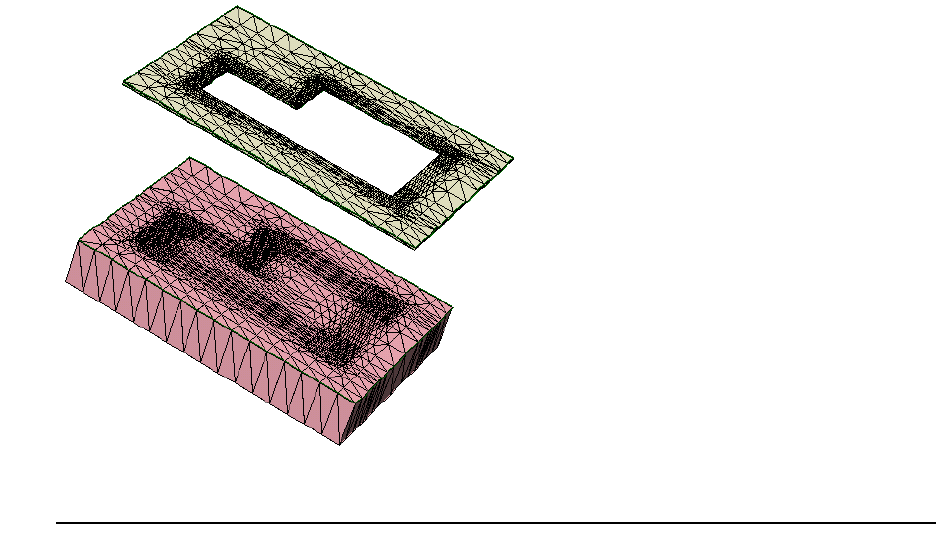
10: Mesh Generation

Mesh Refinement

Sentaurus™ Process User Guide 699

H-2013.03

refinebox clear

# Prevent mesh propagation by defining regular coarse mesh

refinebox yrefine = 0.5 zrefine = 0.5

# Add edge-based refinement

refinebox mask = m1 mask.edge.mns = 0.08 mask.edge.refine.extent = 0.25

grid remesh

The resist layer was created later using the command;

photo mask = m1 thickness = 0.05

Figure 96 shows the result.

Figure 96 Mask edge–based refinement shown on the mask and in silicon

Adaptive Refinement

Tailoring a mesh to a specific problem with static refinement boxes can be tedious and time-

consuming. In addition, for some applications, dopant profiles evolve so much during the

process that the areas where a finer mesh was needed at the beginning are very different from

the areas where a finer mesh is needed at the end.

To accurately capture the entire evolution with a static mesh, it is necessary to put a fine mesh

over large areas of the structure leading to long simulation times and large memory use.

Adaptive meshing in Sentaurus Process addresses these issues.

10: Mesh Generation

Mesh Refinement

700 Sentaurus™ Process User Guide

H-2013.03

The adaptive-meshing feature has a major component: field-based refinement.

For details, see Tips for Adaptive Meshing on page 709.

The refinement parameters and criteria are the same for adaptive implantation as for field-

based. When adaptive meshing is switched on, field-based refinement is performed during

every remesh step and for any dimension (in 1D, 2D, or 3D). This happens for all etch, deposit,

implant, native layer, regrid, and transform operations. In addition, during solve at a specified

step interval, a check of the current mesh is made to determine whether a remesh is required;

then the remesh is performed if necessary. For details, see Adaptive Meshing during Diffusion

on page 707. Finally, when adaptive meshing is used during implantation, in addition to

adaptively refining the newly implanted species and damage, adaptive refinement (also based

on existing fields) is applied simultaneously.

Adaptive Refinement Criteria

Numerous refinement functions are available to deal with differing fields and situations. All

functions involve some comparison between values on neighboring nodes and possible values

between neighboring nodes. In some cases, the same refinement function is available in

Sentaurus Mesh, and similar results to Sentaurus Mesh refinement will be obtained. The

following refinement criteria are available:

■Relative difference (default)

■Absolute difference

■Logarithmic difference

■Inverse hyperbolic sine (asinh) difference

■Gradient

■Local dose error

■Interval refinement

These refinements can be applied globally (default) or they can be limited as follows:

■Boxwise

■Materialwise

■Regionwise

Detailed descriptions of the refinement types, their respective control parameters, and

instructions for applying refinement constraints are given in subsequent sections. The default

adaptive meshing parameters have been set to apply only relative difference criteria to the

whole structure, and they typically produce a fairly coarse mesh. It is necessary to set one

criterion or more to produce a mesh sufficiently fine to reach a required accuracy.

10: Mesh Generation

Mesh Refinement

Sentaurus™ Process User Guide 701

H-2013.03

Adaptive meshing is switched off by default. To switch on adaptive meshing, use:

pdbSet Grid Adaptive 1

pdbSet Grid SnMesh UseLines 1 ;# Recommended with adaptive meshing

Relative Difference Criteria

The relative difference between two neighboring nodes is computed as follows:

(956)

where is the field value on node , and is the field-specific refinement parameters set

with:

pdbSet Grid <Field> Refine.Abs.Error <n>

or def.abs.error and abs.error, which are parameters of the refinebox command.

If the value of the expression in Eq. 956 is greater than the maximum relative difference, the

edge between node 1 and node 2 is split. To set the maximum relative difference, use:

pdbSet Grid <Field> Refine.Rel.Error <n>

or def.rel.error and rel.error, which are parameters of the refinebox command.

The quantity <Field> is the name of the field, and <n> is a unitless number for

Refine.Rel.Error and Refine.Abs.Error; the units are the same as the units of the field.

The default values for Refine.Abs.Error and Refine.Rel.Error are set from <Field>

= AdaptiveField, except for the standard dopants, point defects, and Damage that have

entries in the PDB.

The density of the mesh is sensitive to Refine.Rel.Error because it represents the target

relative change of the field across an edge. For many standard situations, a number of the order

of 1.25 gives a coarse mesh, and a number of approximately 0.5 often gives a fine mesh. The

parameter sets a smooth cutoff such that values of the field below result in no refinement.

NOTE The relative difference criteria should only be used with fields that are

always positive.

Absolute Difference Criteria

The absolute difference between two neighboring nodes is computed simply:

(957)

2C1C2

–

C1C2α++()

----------------------------------

C1C2

–

10: Mesh Generation

Mesh Refinement

702 Sentaurus™ Process User Guide

H-2013.03

where is the field value on node . If the value of the expression in Eq. 957 is greater than

the maximum absolute difference, the edge between nodes 1 and 2 is split. The maximum

allowable absolute difference can be set with:

pdbSet Grid <Field> Refine.Max.Difference <n>

Logarithmic Difference Criteria

The logarithmic (base 10) difference between two neighboring nodes is computed as follows:

(958)

where is the field value on node , and is the low value cutoff that can be set with:

pdbSet Grid <Field> Refine.Abs.Error <n>

or def.abs.error and abs.error, which are parameters of the refinebox command.

If the value of the expression in Eq. 958 is greater than the maximum logarithmic difference,

the edge between nodes 1 and 2 is split. To set the maximum logarithmic difference, use:

pdbSet Grid <Field> Refine.Max.LogDiff <n>

or def.max.logdiff and max.logdiff, which are parameters of the refinebox

command.

NOTE The logarithmic difference criteria should only be used with fields that

are always positive. Use the asinh criteria for fields that can have

negative values such as stresses.

Inverse Hyperbolic Sine (asinh) Difference Criteria

The asinh difference between two neighboring nodes is computed as follows:

(959)

where is the field value on node . If the value of the expression in Eq. 959 is greater than

the maximum asinh difference, the edge between nodes 1 and 2 is split. To set the maximum

asinh difference, use:

pdbSet Grid <Field> Refine.Max.AsinhDiff <n>

or def.max.asinhdiff and max.asinhdiff, which are parameters of the refinebox

command.

C1α+()log C2α+()log–

()asinh C2

()asinh–

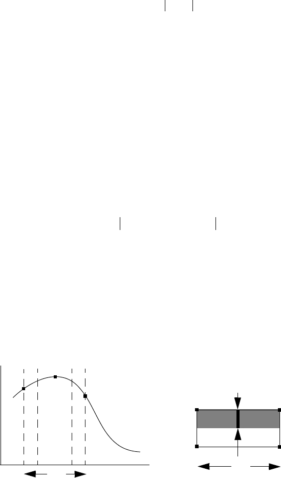
10: Mesh Generation

Mesh Refinement

Sentaurus™ Process User Guide 703

H-2013.03

Gradient Criteria

The gradient between two neighboring nodes is computed as follows:

(960)

where is the field value on node , and is the length of the edge between nodes and .

If the value of the expression in Eq. 960 is greater than the maximum gradient, the edge

between the two nodes is split. To set the maximum gradient, use:

pdbSet Grid <Field> Refine.Max.Gradient <n>

or def.max.gradient and max.gradient, which are parameters of the refinebox

command.

Local Dose Error Criteria

If an edge between two neighboring nodes is not split, the local dose error is computed as

follows:

(961)

where:

■ is the field value on node .

■ is the concentration at the midpoint between nodes and .

■ is the length of the edge between nodes and .

■ is the box size perpendicular to the edge between nodes and (see Figure 97).

Figure 97 (Left) One-dimensional and (right) 2D representation of dose loss criteria

The function in Figure 97 (left) is taken from the previous mesh (or from an analytic

implantation). The box with four points in Figure 97 (right) represents one cell of the mesh

C1C2

–

l12

-------------------

lij

0.5C12 0.25C–10.25C2

–l12s12

Cij

lij

sij

Cij

lij

sij

lij

10: Mesh Generation

Mesh Refinement

704 Sentaurus™ Process User Guide

H-2013.03

refinement tree. The shaded area is the part of the 2D field under consideration. The dose in the

shaded area is computed in two ways:

■As is

■If the edge between and is split

If the difference between these two ways is greater than max.dose.error, the edge is split.

The box size is 1.0 (unitless) in 1D; it is the box width (in cm) in 2D; and it is the box area

( ) perpendicular to the edge –

in 3D. If the value of the expression in Eq. 961 is greater

than the normalized maximum local dose error, the edge between the two nodes is split. The

local dose error can be set with:

pdbSet Grid <Field> Refine.Max.DoseError <n>

where <n> has units of , or def.max.dose.error and max.dose.error, which are

parameters of the refinebox command.

The local dose error is first multiplied by the simulation size before comparing it to the

expression in Eq. 961. The simulation size is 1.0 (unitless) in 1D, the simulation width (in cm)

in 2D, and the simulation lateral area in 3D (in ).

To estimate the total dose loss, you must estimate how many nodes carry a significant

concentration of the field in question and then multiply that number by the local dose error to

obtain approximately the maximum total dose error expected. (In practice, the dose error is

often considerably less than this.) This quantity is relatively easy to understand and is less

sensitive than some other parameters to process conditions.

Interval Refinement

Interval refinement provides a way to refine the mesh such that field values within a certain

interval are well resolved. Interval refinement produces mesh edges of a specified length

wherever the field values are within a specified interval. Four parameters are required to define

an interval refinement:

■A minimum and maximum value

■ and

■A target length,

■A target length scaling,

To preserve the anisotropy of the mesh, interval refinement examines each edge of a refinement

cell and calculates an effective edge length defined by:

(962)

cm 2–

Cmin

Cmax

leff

leff abs r1r2

–()C∇⋅()=

10: Mesh Generation

Mesh Refinement

Sentaurus™ Process User Guide 705

H-2013.03

where and are the endpoints of the edge, and is the average gradient of the field in

the refinement cell. Edges that are nearly parallel to the contours of the field have effective edge

lengths near zero. Edges that are nearly perpendicular to the contours have effective edge

lengths near their actual edge length. Since edges are split only when they are longer than a

given target length, edges that are parallel to the field contours are allowed to be longer than

those that are perpendicular.

Interval refinement will split any edge whose effective edge length exceeds the effective target

length. The effective target length is calculated differently depending on whether the field

values on the edge overlap the interval specified by (refinebox min.value) and

(refinebox max.value).

Let and be the values of the field on the endpoints of the edge. If the relation

is satisfied for any value of between and , the edge overlaps the

interval.

For edges that overlap the interval, the effective target length is exactly the target length that

you specify (refinebox target.length), that is:

(963)

For edges that do not overlap:

(964)

where is either or , is either or , and the values of and are

chosen to minimize the difference.

The formula for outside the interval produces a graded mesh with an edge length that falls

off parabolically with distance from the interval. Default values for the parameters of the

interval refinements are defined in the PDB.

Table 67 lists refinebox parameters in the left column that can be used to specify boxwise

refinement. The right column lists the corresponding PDB parameters that can be used to

specify refinement criteria globally.

Ta bl e 67 S um m ar y o f r e f i n e me n t p a ram et er s

refinebox parameter Corresponding entry in parameter database

def.rel.error, rel.error Grid <Field> Refine.Rel.Error

def.abs.error, abs.error Grid <Field> Refine.Abs.Error

def.max.difference, max.difference Grid <Field> Refine.Max.Difference

def.max.logdiff, max.logdiff Grid <Field> Refine.Max.LogDiff

C∇

Cmin

Cmax

Cmax CC

min

lteff lt=

lteff lt 1Ca

log Cb

log–+()

2s=

Cmin

Cmax

lteff

10: Mesh Generation

Mesh Refinement

706 Sentaurus™ Process User Guide

H-2013.03

Localizing Adaptive Meshing using refinebox Command

Adaptive meshing has been implemented through generalized refinement boxes. As such,

adaptive refinement and the refinement parameters themselves can be set in a boxwise manner.

The default adaptive refinement box covers the entire structure and relies on global parameters

and field-based parameters for its default values. If you specify an adaptive refinement box, the

default box is not created.

NOTE For field-based refinement, any adaptive refinebox that is manually

created overrides the default adaptive refinebox. The default adaptive

refinebox (that covers the entire structure) can be created explicitly

with the command refinebox adaptive.

You ca n c re at e o ne or m ore a da ptive re fin ement boxes with different parameters. The most

commonly used parameters control the size of the box (min and max), and the minimum and

maximum edge lengths (refine.min.edge and refine.max.edge).

The default list of fields upon which to refine includes all dopants, point defects, and clusters

in the structure. This list can be modified in several ways. For example, the following command

overrides the default list:

pdbSet Grid <field> DoNotAdapt 1

The next example adds Field1 and Field2 to the default list for this particular box:

refinebox refine.add.fields = { Field1 Field2 ... }

The following command redefines the list of fields to be used as the basis for refinement; if set,

this command overrides any add or subtract settings:

refinebox refine.fields = { Field1 Field2 ... }

def.max.asinhdiff, max.asinhdiff Grid <Field> Refine.Max.AsinhDiff

def.max.gradient, max.gradient Grid <Field> Refine.Max.Gradient

def.max.dose.error, max.dose.error Grid <Field> Refine.Max.DoseError

min.value Grid <Field> Refine.Min.Value

max.value Grid <Field> Refine.Max.Value

target.length Grid <Field> Target.Length (um)

target.length.scaling Grid <Field> Target.Length.Scaling

Ta bl e 67 S um m ar y o f r e f i n e me n t p a ram et er s

refinebox parameter Corresponding entry in parameter database

10: Mesh Generation

Mesh Refinement

Sentaurus™ Process User Guide 707

H-2013.03

Examples

To switch on adaptive meshing, use:

pdbSet Grid Adaptive 1

To apply adaptive meshing only inside a box and to set the anisotropic edge minimum in the

same box, use:

refinebox min= {0.0 0.0} max= {0.01 0.5} refine.min.edge= {0.001 0.25} adaptive

To refine only considering arsenic and boron, use:

refinebox refine.fields = {Arsenic Boron} adaptive

To create a default box and, in addition, to create a refinement box where is modified locally

for all species and is modified for only boron, use:

refinebox adaptive

refinebox min= {0.0 0.0} max= {0.01 0.5} def.rel.error= 0.9 \

abs.error= {Boron = 1.0e14} adaptive

Adaptive Meshing during Diffusion

Adaptive meshing during diffusion is switched on by default when adaptive meshing is

switched on (in other words, pdbGet Grid Adaptive returns 1). There is an additional

control that allows for the prevention of adaptive meshing at low temperatures, which is

specified like this:

pdbSet Grid Min.Adaptive.Temp <Temp C>

In any case, by default adaptive meshing is not performed during oxidation or silicidation. You

can switch on adaptive meshing during these steps by setting:

pdbSet Diffuse Compute.Regrid.Steps 10 ;# during inert annealings

pdbSet Diffuse Growth.Regrid.Steps -1 ;# during oxidation and silicidation

pdbSet Diffuse Epi.Regrid.Steps -1 ;# during epitaxy

where <number> is the fixed interval of time steps. For the first parameter

Compute.Regrid.Steps, the default is 10 steps and, for the other two, the default is –1,

meaning it is off by default. After the specified number of steps is taken, the mesh is checked

to see if the refinement criteria are satisfied (within some tolerance); a remesh is performed if

necessary. Currently, the use of adaptive meshing during oxidation and epitaxy is possible.

αF

10: Mesh Generation

Mesh Refinement

708 Sentaurus™ Process User Guide

H-2013.03

The refinement criteria check is performed as follows: Axis-aligned edges are checked to see

if they satisfy:

actual < Refine.Factor * error / maxerror (965)

where:

■Refine.Factor is a direction-dependent parameter of the PDB under Grid.

■error is the error functions given in Eq. 956–Eq. 961.

■maxerror is the maximum error parameter associated with each refinement type.

■actual is the ‘actual’ edge length.

There is a cutoff percentage PDB parameter Grid Refine.Percent that limits the percent

of edges that fail (Eq. 965) before a remesh is called. This check procedure is performed for

every Diffuse Compute.Regrid.Steps whether a remesh is called or not. You can omit

the refinement criteria check (which can be time-consuming for large meshes) and force a

remesh by setting:

pdbSet Grid Refine.Check 0

Table 68 summarizes the parameters available for adaptive meshing for diffusion.

Adaptive Meshing during Implantation

Adaptive meshing during implantation is active whenever adaptive meshing is switched on (in

other words, pdbGet Grid Adaptive returns 1). It also may be enabled or disabled for each

implant step using the adaptive parameter of the implant command.

Table 68 Adaptive meshing parameters

Parameter Comment

Compute Compute.Regrid.Steps

Number of diffusion steps before refinement criteria are checked to

decide if remeshing is required.

Compute Pre.Regrid.Save

To help with tailoring the mesh, files can be saved immediately before

adaptive remeshing occurs during diffusion. The files are named

<input_file_stub>_preregrid_###_fps.tdr

where <input_file_stub> would be, for example n1, if the

input file was n1_fps.cmd and ### is an increasing index starting

with 001.

Grid Refine.Check

If Grid Refine.Check is set to 1 (true), then refinement criteria

are checked and remeshing occurs if necessary.

If it is set to 0 (false), remeshing occurs without a check.

Grid Refine.Factor

Tolerance factor for marking an edge too long.

Grid Refine.Percent

Allowed percentage of edges too long.

10: Mesh Generation

Mesh Refinement

Sentaurus™ Process User Guide 709

H-2013.03

Adaptive meshing during implantation differs from adaptive meshing for other process steps in

one key respect: When performing an implantation step, the implanted concentrations are

defined by analytic expressions instead of discretized field values. Therefore, the final values

for the implanted fields are not known before the remeshing step begins so they must be

computed as the mesh is refined.

By default, refinement on damage is handled differently from refinement on dopants. For the

analysis of damage, the gradient is usually uninteresting, but the location of the crystal–

amorphous interface is often critical. Therefore, refinement should be added to the mesh, not

according to the damage gradient, but rather according to whether the damage is near the

crystal–amorphous threshold. This is accomplished using an interval refinement (see Interval

Refinement on page 704). By default, the minimum and maximum values of the interval are set

to the value of the crystal–amorphous threshold ( ). The target length is

, and the target length scaling is 1.0.

NOTE The default target-length setting of 2 nm can produce many mesh points

for amorphizing implants in 3D. You should first try using a larger

setting and then reduce it if necessary.

As the mesh is constructed, each cell of the refinement tree is evaluated to determine whether

the refinement criteria are satisfied. The criteria for as-implanted fields are computed for each

edge of the cell. If any criterion is not satisfied, the cell is split and the as-implanted

concentrations are computed at the newly introduced points. This process continues until all

refinement criteria are satisfied (or the minimum edge length is reached) for all cells on the

refinement tree. Therefore, the constructed mesh satisfies the refinement criteria for all fields

present in the structure, not solely the implanted fields.

For adaptive meshing during MC implantation, the analytic module is used to compute

refinement, the mesh is formed, and afterwards, the implant profiles are computed with the MC

module.

Tips for Adaptive Meshing

The following list gives useful suggestions when using adaptive meshing:

■When setting boxwise meshing criteria, remember that any global criteria you have

specified still apply inside the box. This means you cannot use boxwise meshing criteria to

establish less stringent meshing criteria (such as a larger relative error) inside a box because

the more stringent global criteria still apply. If you want to use different criteria for different

parts of the structure, set the global criteria to the least stringent criteria and use boxes for

more stringent criteria.

■To switch on adaptive meshing and use all the defaults, all that is needed is pdbSet Grid

Adaptive 1. The main parameter for adjusting the amount of refinement is pdbSet

Grid AdaptiveField Refine.Rel.Error, which defaults to 1.5. In many cases, this

1.15 1022

× cm 3–

0.002 µm

10: Mesh Generation

Mesh Refinement

710 Sentaurus™ Process User Guide

H-2013.03

does not refine sufficiently. Decreasing the value causes more refinement. The number of

mesh points is sensitive to this value, and it is not generally recommended to use a value

less than 0.25. This parameter generally meshes doping gradients well, but may leave the

peaks too coarse. To refine the peaks, the best criterion to use is maximum dose error (Grid

AdaptiveField Max.Dose.Error).

■To override the default refinement box used for field-based refinement (which covers the

whole structure and applies to all solution variables), you need only to create an adaptive

refinement box. To add criteria in addition to the default criteria, for example, to add finer

criteria under the gate while preserving standard parameters elsewhere, you can create your

own default refinement box. For example:

refinebox adaptive

refinebox min= {-0.01 -0.01} max= {0.15 0.05} adaptive def.rel.error=0.75

■The default refinement setting for implant damage can give too fine a mesh. Increase

Grid AdaptiveField Refine.Target.Length from the default value of 0.002 to

reduce refinement.

Default Refinement

In two dimensions, by default, interface refinement is applied to any interface in which one of

the neighboring bulk regions is of material Silicon, Polysilicon, or Oxide. In three

dimensions, by default, interface refinement is applied only to interfaces where one of the

neighboring bulk regions is Silicon. For other interfaces, the min.normal.size criterion

is not applied. To view currently defined refinement boxes (including default refinement

boxes), use:

refinebox print

Additional interface refinement can be specified with the command:

refinebox interface.materials= {<material1> <material2> ...}

This command specifies refinement at all interfaces to both <material1> and <material2>.

refinebox interface.mat.pairs= {<material1> <material2>}

This command specifies interface refinement at all interfaces where one side of the interface is

<material1> and the other side is <material2>.

The interfaces that are refined are the union of interface.materials (all interfaces

touching materials in the list) and interface.mat.pairs (only refined on material pairs

found in the list first and second, third and fourth, and so on).

The default min.normal.size for all interface refinement boxes including the default ones

is taken from the pdb parameter Grid SnMesh min.normal.size. Similarly, the default

10: Mesh Generation

Mesh Refinement

Sentaurus™ Process User Guide 711

H-2013.03

value of normal.growth.ratio for all interface refinement boxes is taken from the pdb

parameter Grid SnMesh normal.growth.ratio.2d in two dimensions and from Grid

SnMesh normal.growth.ratio.3d in three dimensions.

To add an interface refinement, use the refinebox command.

To remove an existing interface refinement, first do refinebox clear, and then start again.

Examples

The interfaces to be refined are defined as follows:

# Change the default min.normal.size (in micrometers)

pdbSet Grid SnMesh min.normal.size 2.0e-3

# Now modify which materials to apply interface refinement

# refine at all interfaces to silicon and poly (use the global min.normal.size

# and normal.growth.ratio)

refinebox clear

refinebox interface.materials= {silicon poly}

The next example shows refinement only at the silicon–oxide and polysilicon–oxide interfaces,

and specifies a local value for interface refinement parameters:

refinebox clear

refinebox min.normal.size = 0.005 normal.growth.ratio = 3 \

interface.mat.pairs= { Silicon Oxide PolySilicon Oxide }

Refinement Box Manipulations: Using

transform.refinement

Several transformation can be performed on refinement boxes using the

transform.refinement command. This command works like the transform command

(see Stress Handling on page 757), except for refinement boxes. This command accepts the

following options:

■Transformation – either translate, stretch, cut, rotate, flip, or reflect.

■Transformation options – depend on the type of transformation. A displacement is required

for translate, axis and angle for rotate, a box for cut, reflecting plane for reflect,

the length and direction for stretch, and so on.

■name – applies the transformation to a particular refinement box if specified or to all of

them otherwise.

■name.new – specifies the name of the transformed refinement.

10: Mesh Generation

Mesh Settings

712 Sentaurus™ Process User Guide

H-2013.03

■keep.original – specifies whether to keep the original. Specifying !keep.original

transforms the specified refinement box, while setting it to keep.original preserves the

original refinement box and creates a new transformed one. This option is useful when you

want to “copy and paste” refinements by, for example, translating them to a different

position while keeping the original in place.

For example:

transform.refinement name="refbox" name.new="newRefBox" \

translate= { 0.1 0 0 } keep.original

creates a new refinement called newRefBox identical to refbox but displaced in x.

Mesh Settings

The following tables list the parameters available for Sentaurus Mesh. To set the parameters in

Table 69, use:

pdbSet Grid SnMesh <Parameter name> <value>

Table 69 Parameters available for Sentaurus Mesh

Parameter Default Description

CoplanarityAngle 175

Any pair of faces with an angle of CoplanarityAngle

or more will be considered coplanar.

CoplanarityDistance 1.0e-6

Maximum deformation caused to the boundary when

swapping the edge shared by a pair of adjacent faces.

DecimateBeforeImprint true

Decimates the boundary before imprinting it with the axis-

aligned mesh.

DelaunayTolerance 1.0e-4

Specifies how close the ridges and boundary faces conform to

the Delaunay criterion.

DelaunayToleranceMat

Specifies an array pair of materials and tolerances to be used

in those materials. For example:

pdbSet Grid SnMesh DelaunayToleranceMat

{Silicon 0.01 Oxide 1.0}

DelaunayToleranceReg

Specifies an array pair of regions and tolerances to be used in

those regions.

DelaunayType constrained

Types of mesh generated by Sentaurus Mesh. Available types

are box method, conformal, or constrained.

DelPsc false

Indicates whether the Delaunay refinement for piecewise

smooth complex (DelPSC) algorithm is applied to the

boundary at the beginning of a mesh generation step.

0.1 µm

degrees

µm

10: Mesh Generation

Mesh Settings

Sentaurus™ Process User Guide 713

H-2013.03

DelPscAccuracy 1e-4

Specifies the accuracy used by the DelPSC algorithm when

approximating high-curvature areas. This parameter is used

during standard mesh generation (as opposed to using DelPSC

during oxidation).

EdgeProximity 0.05

Specifies the minimum ratio of the edges generated when an

edge is split.

FaceProximity 0.05

Specifies the minimum ratio of the faces generated when a

face is split.

ImprintCoplanarFacesOnly true

Imprints the binary tree on the coplanar sets of faces. This is

useful to avoid over-refinement in curved areas.

ImprintCoplanarityAngle 179

Angle used to decide when two faces are coplanar. If two

adjacent faces have an angle greater than this value, they will

be added to the set of faces to be imprinted with the binary

refinement tree cells.

max.box.angle.2d 120

Maximum angle in binary tree (2D only).

max.box.angle.3d 150

Maximum angle in binary tree (3D only).

MaxAspectRatio 1e6

Specifies the maximum-allowed aspect ratio of an element in

the binary tree.

MaxBoundaryCutRatio.2d 0.01

Specifies the maximum-allowed ratio between the lengths of

adjacent axis-aligned edges cutting material boundaries (2D

only).

MaxBoundaryCutRatio.3d 0.01

Specifies the maximum-allowed ratio between the lengths of

adjacent axis-aligned edges cutting material boundaries (3D

only).

MaxConnectivity 1e37

Specifies the maximum number of elements connected to a

point in the final mesh.

MaxNeighborRatio 3.0

Specifies the maximum-allowed ratio between the

circumscribed spheres of neighboring elements.

MaxPoints 100000

Maximum number of points allowed by the Sentaurus Mesh

delaunization module.

MaxSolidAngle 360

Specifies the maximum solid angle allowed in the elements of

the mesh (3D only).

MaxTetQuality 1e37

Specifies the minimum shortestEdge/

circumradius ratio allowed in the mesh (3D only).

MinAngle 0

Specifies the minimum angle allowed in the elements of the

mesh (2D only).

minedge 2.0e-6

Minimum edge length request.

Table 69 Parameters available for Sentaurus Mesh

Parameter Default Description

µm

degrees

µm

10: Mesh Generation

Controlling Mesh during Oxidation

714 Sentaurus™ Process User Guide

H-2013.03

Controlling Mesh during Oxidation

Oxidation creates new regions and dramatically alters the shape of existing ones. Controlling

the mesh is important. This section covers some mesh control methods.

TS4 Mesh Library

The TSUPREM-4 moving-boundary meshing library is available from within Sentaurus

Process (hereafter, referred to as the TS4 mesh library). By default, the TS4 mesh library

performs the 2D mesh update.

The following statement switches off the TS4 mesh library and specifies the use of the old

mesher:

pdbSet Grid UseTS4Mesh 0

2D.MeshLib is an alias of UseTS4Mesh.

The TS4 mesh library deposits the native oxide layer before oxidation by default. Since it

removes all grids inside a gas region, the simulation performance is improved without any loss

of accuracy. To use the MGOALS native layer in two dimensions, instead of the TS4 mesh

library, use the command:

pdbSet Grid UseTS4Native 0

SliverAngle 175

Limits the maximum dihedral angle on one element when the

delaunizer performs the sliver removal step.

SliverDistance 1e-2

Limits the amount of “damage” done to the standard Voronoï

diagram by the sliver removal algorithm. Note that the grid

produced by the sliver removal algorithm is weighted

Delaunay, so the standard Voronoï diagram is “damaged”

unless the Voronoï weights are stored (see the

StoreDelaunayWeight parameter). When the box

method library reads those weights, it calculates the correct

Voronoï diagram and coefficients to solve the PDEs.

StoreDelaunayWeight 0

When set to 1, stores the Delaunay–Voronoï weight

(DelVorWeight) for the box method library.

UseLines true

Specify 1 or 0. UseLines is specified in the line

command in the mesh generated by Sentaurus Mesh.

Table 69 Parameters available for Sentaurus Mesh

Parameter Default Description

degrees

µm

10: Mesh Generation

Controlling Mesh during Oxidation

Sentaurus™ Process User Guide 715

H-2013.03

2D.MeshLib.Native is an alias of UseTS4Native.

For silicidation, a gas mesh is used by default. The following statement forces the use of the

TS4-style gas mesh instead of the default gas mesh:

pdbSet Grid UseTS4GasMesh 1

Control Parameters in TS4Mesh

The control parameters are specified with:

pdbSet Grid TS4Mesh <control parameter> <value>

The available control parameters are:

■MergeSubAndAdd <0|1> (default: 1)

It optimizes the speed performance by merging the grid subtraction and addition

procedures.

■DoSubAfterStep <0|1> (default: 0)

Grid subtraction is performed after each diffusion step, while grid addition is performed

after each mechanics step followed by the diffusion step. Switching on this flag forces only

one diffusion step per each mechanics step. When this flag is switched on,

MergeSubAndAdd is ignored.

■SubTimeFactor <double> (default: 1.5)

The time step given by mechanics for grid removal is scaled by SubTimeFactor.

NOTE Do not change the default.

■MinSpaceOnInterface <double> (default: 2e-6 [ ])

The nodes on an interface mesh must be rebuilt after meshing on the moving boundary

since the bulk meshes along the interface can be added or removed. Instead of destroying

and rebuilding the interface mesh, the TS4 mesh library tries to reuse the original node data

on the interface mesh to minimize the interpolation error. The original nodes are detected

when the location difference is less than MinSpaceOnInterface.

NOTE Do not change the default.

■ExactGridSpace <0|1> (default: 1)

On the growing material side of the interface, the triangular mesh elements expand. To

maintain solution accuracy in the material (for example, calculating the diffusion of

oxidant in the oxide), you must add nodes to the growing material. The addition of nodes

µm

10: Mesh Generation

Controlling Mesh during Oxidation

716 Sentaurus™ Process User Guide

H-2013.03

to the growing material is controlled by perp.add.dist, ExactGridSpace, and

LocalGridSpace.

NOTE perp.add.dist is the grid control parameter of each material, for

example: pdbSet Oxide Grid perp.add.dist 0.01e-4

Precise grid spacing is obtained by adding new nodes in a growing layer at the distance

specified by perp.add.dist from the existing node in the layer. Because only one node

can be added at each point on an interface during a simulation time step, the size of the time

step may need to be reduced to achieve the required spacing. This reduction in the time step

can be disabled by specifying:

pdbSet Grid TS4Mesh ExactGridSpace 0

By default, ExactGridSpace is set to 1 to allow reducing the number of time steps to

control the grid spacing. The algorithm does not allow grid points to be added at spacings

less than 1 A, and control of the spacing may not be precise for spacings less than 2 A.

■LocalGridSpace <0|1> (default: 1)

The grid control algorithms and parameters apply to the entire structure. To avoid adding a

very fine grid in field regions when growing gate oxides, an option allows the grid spacing

to vary with the oxide growth rate. When LocalGridSpace is switched on, the grid

spacing to be used at each point in the growing material is:

h = (vmax/v) perp.add.dist

where v is the growth rate at a point in the structure, and vmax is the maximum growth rate

at all interfaces of the same type in the structure. LocalGridSpace is switched on by

default.

■OrderFlatTri <0|1> (default: 1)

When the area of a shrinking triangle becomes less than 1e-15 (cm2) after a time step, the

triangle is removed. When the shrinking triangle to be removed is located at a material

interface and the removal of the triangle will result in a bad mesh, the material type of the

shrinking triangle is replaced with the type of the growing neighbor material, instead of

removing it. When those triangles are adjacent to each other, the reordering algorithm for

the replacements smooths the interface shape after conversion.

■MinAreaRemovalRatio <double> (default: 10.0)

When a region has only one triangle surrounded by neighbors of different materials and its

area is less than MinAreaRemovalRatio multiplied by 1e-15 (cm2), the material type of

the triangle is replaced with the neighbor material that shares the longest edge with the

triangle.

■Min.Split.Distance <double> (default: 1e-8 [cm])

When multiple regions with the same material meet at one point, the point is split by

inserting new elements. The parameter determines the minimum split distance.

10: Mesh Generation

Controlling Mesh during Oxidation

Sentaurus™ Process User Guide 717

H-2013.03

Moving Mesh and Mechanics Displacements

The displacements computed by the mechanics solution during oxidation are applied to the

nodes after checking against the MinimumVelocity criterion defined for each region.

Velocity is the computed solution variable and is multiplied by the time step to compute

displacements. The nodes are moved by this amount.

The computed velocities are compared against MinimumVelocity and, if the computed

velocity is greater than MinimumVelocity, the displacements are computed and applied. The

MinimumVelocity is set with the command:

pdbSetDouble Silicon Grid MinimumVelocity <n>

Grid Spacing

Grid spacing in the growing region is controlled by perp.add.dist. The value is in units of

centimeter, and the edges in growing regions are checked to see whether they are nearly

perpendicular to the interface.

If they are perpendicular, they are split if their length exceeds the perp.add.dist number.

This value is set with the command:

pdbSet Oxide Grid perp.add.dist 2e-7 ;# unit is cm

Grid Cleanup

During oxidation or silicidation, the growing region increases at the expense of a shrinking

region. The shrinking regions then have a problem of small edges. Below a certain value, these

edges must be removed entirely, and the mesh around them must be adjusted.

The short edge criterion is specified by the Remove.Dist parameter, which is specified in

centimeters and is set as follows:

pdbSet Silicon Grid Remove.Dist 3e-8

NOTE Due to mesh quality constraints, this number must be kept above a value

of .

210

8–

× cm

10: Mesh Generation

Controlling Mesh during Oxidation

718 Sentaurus™ Process User Guide

H-2013.03

Maximum-allowed Rate of Growth

For a minimal simulation time, it would be best if the entire thickness growth were simulated

in one step. However, this is not possible. The reasons for this include:

■Nonconvergence of diffusion equations.

■Inability to track material interfaces if they grow more than one edge length of a triangle

or a tetrahedron, and so on.

In the new growing region, new nodes are introduced and the data is interpolated from the

nearby nodes; if growth is too fast, significant interpolation errors could occur.

The rate of growth can be controlled by the parameters dThickness and IncreaseRatio.

The dThickness parameter (specified in micrometers) defines the maximum-allowed

oxidation front displacement per time step and is set as follows:

pdbSet Diffuse dThickness 0.001

The IncreaseRatio parameter is the factor by which the time integration step is allowed to

grow.

Miscellaneous Tricks

Since Sentaurus Process oxidation does not allow the interface to traverse more than one

element thickness at a time, speed can be achieved by having elements with longer edge lengths

near the interface. This can be controlled by refinement boxes or the pdb parameter

Grid SnMesh min.normal.size. Large structures, like those used in power devices, may

need min.normal.size of , while submicron CMOS devices need .

The mesh away from the interface is unrefined based on the pdb parameter

Grid SnMesh normal.growth.ratio.3d. If the mesh is not unrefining fast enough, this

number can be increased.

In large structures, the interface fidelity may not need to be as tight as that of 45-nm or 32-nm

gate transistors. The MGOALS accuracy parameter can be increased to , which will

cause MGOALS to clean up interfaces of small (sub– ) features and ensure smooth long

edges that speed up oxidation.

These are options available to the process engineer; however, care must be exercised in varying

these parameters since they may affect the final structure significantly.

0.01 µm

8 Å

1 Å

10: Mesh Generation

Controlling Mesh during Oxidation

Sentaurus™ Process User Guide 719

H-2013.03

Meshing for 3D Oxidation

Maintaining a conformal high-quality mesh during the simulation of 3D oxidation is very

difficult because of the following requirements: moving boundaries, accurate dopant profiles,

dose conservation, minimization of the number of mesh points, and maintaining high-quality

mesh elements. In particular, handling the frequent collision of the oxidation front with points

inside the silicon, polysilicon, or gas regions can cause intractable problems for the local mesh

operations needed for maintaining dose conservation.

Before each diffusion time-step, the mesh is checked for the maximum possible time step until

the first tetrahedron element collapses (becomes flat). If necessary, the time step is reduced. In

the diffusion simulation, all mesh points are moved using the velocity and the time step. The

mesh topology is not changed during the diffusion time step. At the end of the diffusion time

step, the mesh quality is improved flat elements are removed allowing for the next time step to

be sufficiently large.

MovingMesh

This section describes an experimental feature that can be used for 3D oxidation. This feature

called MovingMesh is activated with the following command before the diffuse command:

pdbSet Grid Use.MovingMesh 1 ;# switched on by default

Three important parameters control MovingMesh:

pdbSet Oxide Grid perp.add.dist 0.005e-4 ;# centimeter

pdbSet Grid Remove.Dist 0.001e-4 ;# centimeter

pdbSet Grid MovingMesh Remove.Dist.On.Interface 0.0001e-4 ;# centimeter

The perp.add.dist parameter specifies the distance that the oxide interface can move

before new mesh points are inserted in the oxide. The unit is in centimeter.

The Remove.Dist parameter specifies the shortest distance the mesh vertices are allowed

from the interface into the bulk. Shorter than this distance, the vertices will be removed. Do not

specify a distance larger than the minimum material thickness. For a typical example with

1.5 nm native layer, Remove.Dist of 1.0 nm or less is appropriate. The unit is in centimeter.

The Remove.Dist.On.Interface parameter controls small triangles on material interfaces.

Triangles with an edge shorter than this distance will be removed. A smaller number makes the

interfaces smoother, but results in a larger number of triangles.

10: Mesh Generation

Controlling Mesh during Oxidation

720 Sentaurus™ Process User Guide

H-2013.03

The oxide interfaces can develop problematic geometric features like knife edges, noisy

surfaces, or extremely thin gaps. You can enable geometry repair and surface remeshing by

using:

pdbSet Grid MovingMesh Repair.Geometry 1 ;# switched on by default

The criteria to trigger geometry repair are based on the minimum dihedral angle and the

maximum face angle:

pdbSet Grid MovingMesh Repair.Geometry.Min.Dihedral.Angle 5 ;# degree

pdbSet Grid MovingMesh Repair.Geometry.Max.Face.Angle 175 ;# degree

If the minimum dihedral angle between two triangles is below the threshold or the maximum

face angle of a triangle is above the threshold, the geometry repair procedure starts.

The geometry repair procedure involves a multimaterial level-set (MLS) formulation. The

resolution of the level-set cell size is controlled by:

pdbSet Grid MovingMesh Repair.Geometry.Resolution 0.001 ;# micrometer

NOTE The parameter Repair.Geometry.Resolution should be, at most,

one-third the thickness of the thinnest region. Otherwise, the thin region

may be considered noise, and it disappears.

The boundary representation (brep) of the new geometry must go through a meshing algorithm

for curved surfaces called the Delaunay refinement for piecewise smooth complex (DelPSC)

that improves the quality of triangles on brep surfaces. This algorithm is enabled by:

pdbSet Grid MovingMesh Apply.Brep.DelPSC 1 ;# switched on by default

DelPSC performs adaptive sampling on ridges (1D geometric feature) according to the

refinement fields, the curvatures of the ridges, and the proximity among the ridges. On each

surface patch (2D geometric feature), DelPSC performs adaptive sampling according to the

refinement fields and the curvatures of the surface.

Ridge sampling also is controlled by:

pdbSet Grid MovingMesh Apply.Brep.DelPSC.Resolution 0.005 ;# micrometer

The above parameter ensures no ridge edge will be longer than the specification. It is useful,

for example, when you have a straight line (no curvature) next to curved surfaces. You want the

sampling points on the straight line to be fine enough to support the adjacent curved surfaces.

Note that you no longer require Apply.Brep.DelPSC.Resolution to be as small as the thin

native layer thickness, because of the adaptive sampling based on proximity between nearby

ridges.

10: Mesh Generation

Controlling Mesh during Oxidation

Sentaurus™ Process User Guide 721

H-2013.03

To control accuracy in high curvature areas, you can specify the acceptable distance between

the old and new curved surfaces using:

pdbSet Grid MovingMesh Apply.Brep.DelPSC.Accuracy 0.0001 ;# micrometer

These are typical settings for a small transistor structure:

pdbSet Oxide Grid perp.add.dist 2e-7 ;# cm 2nm

pdbSet Silicon Grid perp.add.dist 1e-6 ;# cm 10nm

pdbSet Grid Remove.Dist 9e-8 ;# cm 9A

pdbSet Grid MovingMesh Remove.Dist.On.Interface 3e-8 ;# cm 3A

pdbSet Grid MovingMesh Repair.Geometry.Resolution 3e-4 ;# um 3A

pdbSet Grid MovingMesh Apply.Brep.DelPSC.Resolution 3e-3 ;# um 3nm

pdbSet Grid MovingMesh Apply.Brep.DelPSC.Accuracy 1e-4 ;# um 1A

These are typical settings for a large power structure.

pdbSet Oxide Grid perp.add.dist 2e-6 ;# cm 20nm

pdbSet Silicon Grid perp.add.dist 1e-5 ;# cm 100nm

pdbSet Grid Remove.Dist 9e-7 ;# cm 9nm

pdbSet Grid MovingMesh Remove.Dist.On.Interface 3e-7 ;# cm 3nm

pdbSet Grid MovingMesh Repair.Geometry.Resolution 3e-3 ;# um 3nm

pdbSet Grid MovingMesh Apply.Brep.DelPSC.Resolution 3e-2 ;# um 30nm

pdbSet Grid MovingMesh Apply.Brep.DelPSC.Accuracy 1e-3 ;# um 1nm

MovingMesh has facilities for troubleshooting run-time failures. A typical setting would be:

# Switch on level-1 diagnostics

pdbSetDouble debugLevel MovingMesh 1 ;# switched off by default

# Save intermediate result every 100 time steps

pdbSetDouble Grid MovingMesh Save.Interval 100 ;# switched off by default

# Save diagnostic files for Repair.Geometry and DelPSC

pdbSetDouble Grid MovingMesh Repair.Geometry.Monitor 1

;# switched off by default

In level-1 diagnostics, the intermediate result will be saved after a certain number of time steps

in the files:

<NodeName>_MovingMeshGridTimeStep<xxxx>.tdr

The frequency of saving is specified by the Save.Interval parameter. The files are written

after mechanics and before diffusion to analyze the grid-limited time step.

In the event of failure in Repair.Geometry, the level-1 diagnostics will save files with names

such as:

<NodeName>_remeshBrep{In,MLS,PSC,Out}.tdr

<NodeName>_applyBrepDelPSC{In,Out}.tdr

10: Mesh Generation

UseLines: Keeping User-defined Mesh Lines

722 Sentaurus™ Process User Guide

H-2013.03

They are useful for checking whether the resolution parameters are adequate. The most likely

cause of failure is a too coarse resolution to capture thin oxide layers and other small geometric

features.

If the parameter Repair.Geometry.Monitor

is set to 1, the intermediate files with names

such as:

<NodeName>_remeshBrep_<xxxx>_{In,MLS,PSC,Out}.tdr

<NodeName>_applyBrepDelPSC_<xxxx>_{In,Out}.tdr

will be saved every time the repair geometry operation is triggered. These files are useful to

monitor how the MLS and DelPSC algorithms perform at various points in a simulation.

UseLines: Keeping User-defined Mesh Lines

During the init command, the line location and spacing specifications given by line

commands are expanded into ticks and stored in the PDB and in TDR files. This is performed

by default.

By carefully placing lines, you can isolate areas of the structure that changed (because of

etching, deposition, and so on) from those that do not (such as bulk silicon). In this way, the

mesh in areas that do not change will have the least amount of change, the least interpolation,

and the most accurate results. Even the mesh in regions that do change will have a similar

starting point and should also have minimal mesh-point movement coming from remeshing.

Lines for Sentaurus Process Kinetic Monte Carlo are stored separately from the lines used with

continuum solvers (in other words, Sentaurus Mesh meshes). By default, line commands are

applied to both KMC and continuum meshes. Use the parameter !kmc or!mgoals to not

apply a particular line command. For example, for a line command to apply only to

continuum, use line !kmc.

In the simplest case, all the line commands are specified before the init command, and they

are saved and reused every time a remesh is performed. However, there are other cases

described in the following sections that allow this feature to be more powerful.

All the line commands are specified before the init command, and they are saved and

reused every time a remesh is performed. However, there are other cases described in the

following sections that allow this feature to be more powerful.

10: Mesh Generation

UseLines: Keeping User-defined Mesh Lines

Sentaurus™ Process User Guide 723

H-2013.03

Using line Commands after init Command

The expansion of lines from line commands into ticks (in other words, all starting mesh line

locations) is performed only at the point that the lines in that direction are needed. For example,

x-lines are always expanded in the init command, but y-lines are only expanded when the

first etch with a mask is given. Therefore, it is possible to load a 1D structure, give y-lines, and

then expand to 2D, or give both y- and z-lines and expand to 3D.

After a particular direction or dimension is expanded, it is only possible to insert one tick at a

time in that direction using the line command (in other words, the spacing parameter is

thereafter ignored). For example, this could be because you identified the amorphous–

crystalline interface in silicon.

This is handled by specifying one of the following:

■The line command in a dimension greater than the current dimension. For example, a y-

line specification when the simulation is in 1D.

■The line command in a dimension at or less than the current dimension. For example,

either an x-line or a y-line specified when the simulation is in 2D.

For more information about the operating dimension, see Automatic Dimension Control on

page 74.

Dimension within Current Spatial Dimension

This is encountered if the user-specified x-lines and the current spatial dimension of analyses

is 1D. Or, it could happen if you specify x- or y-lines in 2D, or x-, y-, or z- lines in 3D.

In this case, the line command ignores the spacing parameter and tries to insert only one

tick as long as that tick (line) is not too close to an existing tick.

Inside the init command, the line commands are expanded into ticks using the spacing

specifications for the dimension as they are needed. When additional line commands are

given for dimensions where the ticks have already been expanded, the spacing parameter is

ignored and one additional tick is added as long as it is not too close to an existing tick.

Dimension Greater Than Current Spatial Dimension

This is encountered if you specified y- or z-lines, and the current spatial dimension of analyses

is 1D. Or, it could happen if you specify z-lines and the current spatial dimension of analyses

is 2D.

10: Mesh Generation

UseLines: Keeping User-defined Mesh Lines

724 Sentaurus™ Process User Guide

H-2013.03

In this case, the line command is considered in its entirety, and the spacing parameter is

used. All the intermediate lines are included in the list of ticks kept.

Creating More Than One Structure

You c an cr ea te mo re tha n o ne s tr uct ur e us in g line, region and init commands in one

command file when using the UseLines feature. To ensure lines from the first structure are

not inserted into subsequent structures, it is important to issue line clear before starting the

definition of a new structure. For example:

#####################################################

line x loc=0 spacing=0.001

line x loc=1 spacing=0.1

line y loc=0

line y loc=1

region silicon

init !DelayFullD

# initial structure gives 96 nodes

LogFile [grid qual nodes]

grid remesh

# after remesh, 112 nodes

# because Sentaurus Process adds interface refinement

LogFile [grid qual nodes]

####################################################

# the lines from above are removed

# to start a new structure

line clear

line x loc=0

line x loc=1

line y loc=0

line y loc=1

region silicon

init !DelayFullD

# this tiny structure has only have 8 nodes

LogFile [grid qual nodes]

grid remesh

# grid remesh gives 44 nodes

LogFile [grid qual nodes]

10: Mesh Generation

UseLines: Keeping User-defined Mesh Lines

Sentaurus™ Process User Guide 725

H-2013.03

The UseLines and transform Commands

The ticks must be handled in a special manner with the transform reflect, transform

stretch, transform rotate, transform translate and transform cut commands.

The reflect Command

In the reflected region, the ticks are created after applying lateral inversion along the

appropriate plane.

The stretch Command

On applying stretch at a given coordinate in a given direction, the existing ticks in the

stretched area are translated by the amount of the stretch. You must insert lines in the stretched

area appropriately.

The rotate Command

When applying rotate, the ticks also are rotated and properly transferred between x-ticks, y-

ticks and z-ticks.

The translate Command

The translate command shifts the ticks by the specified amount.

The cut Command

The lines in the part of the structure that is cut are deleted.

Examples

Testing line Commands

Use the following example to test line commands:

line x loc=0 tag=a spacing=0.05

line x loc=0.1 spacing=0.05

line x loc=1 tag=b spacing=0.05

line y loc=0 tag=c spacing=0.01

10: Mesh Generation

UseLines: Keeping User-defined Mesh Lines

726 Sentaurus™ Process User Guide

H-2013.03

line y loc=0.6 tag=d spacing=0.1

region silicon xlo=a xhi=b ylo=c yhi=d

init !DelayFullD

deposit oxide thickness=0.002 iso

grid remesh info=2

line y loc=0.026

line y loc=0.027

line y loc=0.028

line y loc=0.029

line y loc=0.025

line y loc=0.024

line y loc=0.023

grid remesh

deposit poly thickness=0.18 iso

mask name=m1 left=-0.1 right=0.025

etch aniso thickness=0.2 poly mask=m1

struct tdr=linetest

Showing Clearing Lines for a New Structure

Use the following example to show clearing lines and to prepare for another structure definition

within the same command file:

line x loc=0 tag=a spa=0.125

line x loc=1 tag=b spa=0.125

line y loc=0 tag=c spa=0.125

line y loc=1 tag=d spa=0.125

region silicon xlo=a xhi=b ylo=c yhi=d

init

grid FullD

line clear

line x loc=0 tag=a spa=0.125

line x loc=1 tag=b spa=0.125

line y loc=0 tag=c spa=0.125

line y loc=1 tag=d spa=0.125

region silicon xlo=a xhi=b ylo=c yhi=d

init

line y loc=0.3 spa=0.01

grid FullD

10: Mesh Generation

Data Interpolation

Sentaurus™ Process User Guide 727

H-2013.03

Data Interpolation

Sentaurus Process stores a copy of the mesh with all its data before performing any geometry-

changing operation. This is the reference mesh used to interpolate data onto the new mesh. In

3D, a mesh is generated only when it is necessary, so you can have multiple etch, deposit,

photo, and strip commands without the need to remesh in between. When a new mesh is

required, data is interpolated from the stored mesh and data.

Data interpolation is performed material-wise. This is important because some nodal data can

be discontinuous at material interfaces; for example, segregation causes a jump in

concentration at the silicon–oxide interface. In addition, the precise location of an interface can

change slightly due to numeric noise in geometry-moving algorithms. Therefore, it is

necessary to allow the data to be interpolated from points in the old mesh nearby, but only from

the same material.

Data also can be interpolated from materials that are Like materials (that is, the material in the

old mesh is Like the material in the new mesh, or the material in the new mesh is Like the

material in the old mesh). When interpolating data at an interface, the preference is to use data

from the same region, then data from the same material, and finally data from Like materials.

If no match is found, then 0 is set for all data at that point.

For data defined on elements, the overlap of elements from the old mesh to the new mesh is

used for weighting. Similar to nodal data, interpolation of elements near interfaces uses the

region, material, and Like material preference order.

Multithreaded interpolation can be used to speed up interpolation in large 3D structures.

Because of the memory-intensive nature of interpolation, typically, the performance benefit of

multithreading saturates at two threads and can even decrease when using more than four

threads. Therefore, for interpolation, the suggested maximum is to use two threads using the

command:

math numThreadsInterp=2

Troubleshooting

Sometimes, the mesh generation step fails and it is not clear what the problem may be. The

following are recommendations of where to look when problems arise during meshing:

■Set InfoDefault to 2 or higher, for example:

pdbSet InfoDefault 2

10: Mesh Generation

Troubleshooting

728 Sentaurus™ Process User Guide

H-2013.03

■When Sentaurus Mesh prints the message:

"Short edge 1e-8 around points (x1, y1, z1) (x2, y2, z2)"

look at the input structure around the coordinates (x1, y1, z1) or (x2, y2, z2), and

check whether there is a singularity in that area (a crack, fold, surface overlap, and so on).

Sometimes, these singularities are the product of an etching or a deposition step, and action

can be taken to improve the quality of the structure.

■Check the quality of the boundary printed for the steps preceding the mesh generation

process. In particular, the following line provides an indication of quality (this is output if

InfoDefault is 2 or higher):

minDihedralAngle: <angle> [near (x1, y1, z1),(x2, y2, z2)] at

region=Nitride_1.

If you see an angle of less than in the geometry, this may indicate a problem in the

structure at the given coordinates. The recommendation is then to look at the preceding

process steps in Tecplot SV, and to see whether they can be modified to avoid creating the

problem.

To visualize the problem area in Tecplot SV, you can create a rectangular zone that can be

used as a marker to identify the problem. Select Data > Create Zone > Rectangular, and

input a box where one of the corners is a coordinate reported by Sentaurus Mesh as

problematic. The second corner of the box must be calculated manually to give a box large

enough to be seen in the visualization window. Then, hide all materials except the box that

you created. Magnify the rectangular zone, and display the material that was reported in

the minDihedralAngle message. Now, you should see the artifact. Sometimes, you need

to rotate the structure around the rectangular box to see what is happening to the geometry.

■In addition to this, you may need to add !repair to the etch or deposit command. This

prevents the structure from being repaired and makes it easier to spot the problem in

Tecplot SV.

■It is recommended to frequently save snapshots of the boundary file of the structure,

especially before all mesh generation operations. This will help you to investigate possible

problems in the input to the mesh generator. To accomplish this, use the command:

struct tdr.bnd=fileName

3°

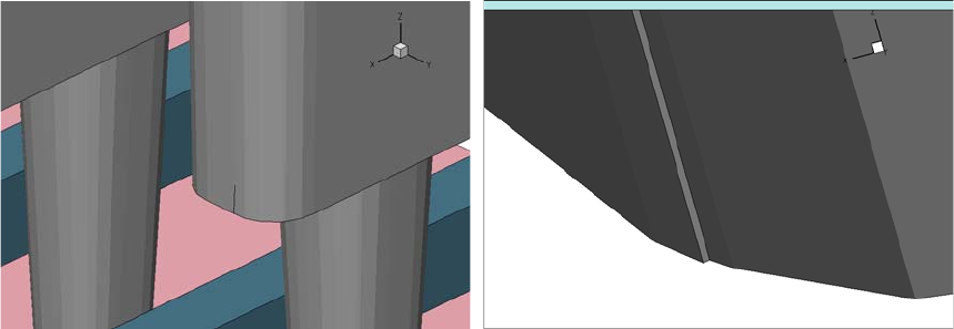
10: Mesh Generation

Troubleshooting

Sentaurus™ Process User Guide 729

H-2013.03

Figure 98 (Left) Example of artifact in geometry and (right) magnification of artifact

10: Mesh Generation

Troubleshooting

730 Sentaurus™ Process User Guide

H-2013.03

Sentaurus™ Process User Guide 731

H-2013.03

CHAPTER 11 Structure Generation

This chapter describes the etching, deposition, and other geometry

manipulations available in Sentaurus Process.

Overview

Sentaurus Process offers the following interfaces to perform etching and deposition:

■MGOALS (1D, 2D, and 3D)

■Sentaurus Structure Editor (3D only)

■Sentaurus Topography and Sentaurus Topography 3D (limited availability)

By default, Sentaurus Process uses an internal module, MGOAL, which is based on polygonal

boundary representations. This is the preferred module for performing geometric etching and

deposition because of its robust and flexible algorithms. The etching and deposition operations

are always simulated using geometric shapes or simple mathematical formulations; no physical

processes are simulated. For a description of the MGOALS interface, see MGOALS Interface

on page 778.

In 3D, Sentaurus Process offers and interfaces with the geometric library in Sentaurus Structure

Editor to perform basic and most common geometry-modeling process steps. For a description

of the Sentaurus Structure Editor interface, see Sentaurus Structure Editor Interface on

page 791.

For physical etch and deposition, Sentaurus Process provides an interface to Sentaurus

Topography and Sentaurus Topography 3D. For a description of the interfaces, see Sentaurus

Topography Interface on page 794.

Functionality

Sentaurus Process provides a number of etching and deposition operations, in addition to

purely geometric operations to help shape the geometry of the devices.

11: Structure Generation

Overview

732 Sentaurus™ Process User Guide

H-2013.03

Etching

The following types of etching are supported (see Etching on page 733 for more details):

Deposition

The following types of deposition are supported (see Deposition on page 751 for more details):

Masks and Photoresist

Masks offer an effect (similar to a masking layer) to limit the etch or deposition process to a

certain window or to provide a convenient way to mimic lithographic patterning (see The mask

and photo Commands on page 764).

Geometry Creation and Transformations

You als o c an create an d i nse rt polygo ns an d polyh ed ra , or re ad an ex isting 3D s tr uctur e f ro m a

file (see Inserting Polygons in Two Dimensions on page 785 and Inserting Polyhedra in Three

Dimensions on page 786).

The shape library provides commands for generating some special shapes in Sentaurus Process

(see Shape Library on page 757).

In addition, several geometric transformations are available including reflection, translation,

rotation, flipping, cutting, and stretching (see Geometry Transformations on page 772).

■Isotropic

■Anisotropic

■Directional

■Polygonal

■Trapezoidal

■Fourier

■Crystallographic

■Chemical-mechanical polishing (CMP)

■Piecewise linear

■Isotropic

■Anisotropic

■Directional

■Polygonal

■Fill

■Fourier

■Crystallographic

■Trapezoidal (3D only)

11: Structure Generation

Etching and Deposition Types and Options

Sentaurus™ Process User Guide 733

H-2013.03

Etching and Deposition Types and Options

Three main specifications are required for all etching and deposition steps:

■Etch or deposit type

■Material or materials to be etched, or material to be deposited

■Amount of material to be removed or deposited

Etching

The types of available etching are:

NOTE To remove materials exposed to the top gas, use the strip command

instead of the etch command. The strip command is used

specifically for this purpose. It is more straightforward, less prone to

user error, and more robust in delivering the expected results:

strip Photoresist

type=angles.rates

Etch according to a definition of a piecewise linear etch rate.

type=anisotropic

Etch in the vertical direction only.

type=cmp

Perform CMP. The coordinate of the new surface must be specified as

coord.

type=crystal

Angle-dependent etching where etch rate is dependent on the

crystallographic direction.

type=directional

Etch in one specific direction only.

type=fourier

Angle-dependent etching where etch rate is a cosine expansion of the

etching angle.

type=isotropic

Etch rate is uniform in all directions.

type=polygon

Etch according to a user-supplied polygon (2D only).

type=trapezoidal

Etching allowing undercut and taper angle specifications (2D only),

or taper and bottom angle specifications (3D).

11: Structure Generation

Etching and Deposition Types and Options

734 Sentaurus™ Process User Guide

H-2013.03

Each etch type requires the setting of parameters particular to that etch type. Many options are

available and certain options are available only with certain etch types. Table 70 summarizes

the syntax options for each etch type.

Table 70 Options for etch and deposit command syntax (E=etching, D=deposition)

Area Parameter name

isotropic

anisotropic

directional

cmp

polygon

fourier

crystal

trapezoidal

angles.rates

Rate

rate

ED ED ED E

angles.rates

coeffs

mat.coeffs

crystal.rate

Stop criteria

time

ED ED ED ED ED E E

thickness

ED ED ED ED

etchstop

EE E EE E

coord

etchstop.overetch

EE E EE E

isotropic.overetch

Shape

polygon

angle

undercut

a. In 2D when not using force.full.levelset.

bottom.angle

b. In 3D when not using force.full.levelset.

bottom.thickness

direction

ambient.rate

c. When used in conjunction with force.full.levelset.

Beam

sources

ED E

shadowing

EcDED ED E

shadowing.nonisotropic

Mesh

ast

ED ED ED E ED ED ED E

Adaptive

ED ED ED E ED ED ED E

Mode

force.analytic

EEE

force.full.levelset

ED E ED EdDd

d. Full level-set is the default scheme for Fourier and crystallographic.

EdDd E

11: Structure Generation

Etching and Deposition Types and Options

Sentaurus™ Process User Guide 735

H-2013.03

To specify the etch type, the parameter type is used. For some etch types, one of the following

keywords can be used instead as a shorthand for specifying type: isotropic,

anisotropic, trapezoidal, or cmp. The amount to be etched is specified as either

thickness (by specifying rate and time) or an etchstop material with etchstop.

Etch types have been implemented in Sentaurus Process using three different methods

(analytic, fast level-set, and general time-stepping level-set), which are described in MGOALS

Interface on page 778.

These methods may require different inputs to perform the steps and may take different effects

into account. The method is selected depending on the specified parameters and the structure

to be etched.

NOTE The simplest and fastest algorithm possible is chosen by default.

If simple isotropic, anisotropic, directional, or CMP etching of a single material is requested

and for polygonal etching, an analytic algorithm is tried first. The analytic algorithm is the

fastest and most accurate. However, in some cases, the resulting etching front might intersect

itself. Because the analytic algorithm cannot handle this situation, the fast level-set method is

used.

NOTE Although these methods are fast and can handle most simple etching

tasks, they do not consider shadowing or visibility effects, and they

cannot etch more than one material at a time.

The general time-stepping level-set method is chosen if you specify any rate versus angle-type

etching (Fourier or crystallographic), or if you choose to etch different materials at different

rates, or if the parameter force.full.levelset is specified. In addition, the general time-

stepping level-set method can handle multiple etching beams and, optionally, shadowing.

The general time-stepping level-set scheme used in Sentaurus Process has the same limitations

as all level-set methods:

■Sharp corners in the evolving front are rounded.

■Small front movement requires a fine level-set mesh, resulting in large memory use and

long simulation times.

■The accuracy is limited by the size of the level-set mesh.

Besides the etching type, the materials to be etched and the amount of material to etch must be

specified. The amount of material to be etched can be specified in three ways:

■Thickness

■Rate and time

■Using an etch stop

11: Structure Generation

Etching and Deposition Types and Options

736 Sentaurus™ Process User Guide

H-2013.03

The etch rate may be specified using etch beams that are created in the beam command. Beams

can be used only with the Fourier etch type. If an etch stop is specified, the etching stops as

soon as the specified material is exposed to gas.

In addition, a mask specification can be given for all etch types, except CMP and polygonal to

limit the areas where material is removed.

NOTE The trapezoidal etch type supports mask specification in 3D only.

Etching Tips

Some tips for etching are:

■If the total etch thickness is exactly the same thickness as the layer to be etched, numeric

roundoff errors can cause thin pieces of the material to be retained. You should etch a little

more (for example, 0.1%) than the thickness of the layer.

■Etching small thicknesses using a small isotropic.overetch or etching large

structures can cause MGOALS to allocate a large amount of memory and increase

simulation time to solve the level-set equation. The MGOALS parameter resolution can

be increased for the simplified boundary movement mode, and the parameters dx and dy

can be increased in the general boundary movement mode to reduce memory consumption.

However, this may impact the accuracy.

Etching Type: Isotropic

Isotropic etching removes material at the same rate in all directions. You can specify more than

one material to be etched isotropically, in which case, the generalized level-set boundary

movement module is invoked.

When isotropic etching uses the level-set method (either fast or general time-stepping), the

final surface is obtained by solving a differential equation on a discrete mesh.

NOTE To control errors in the fast level-set method, use the resolution

parameter in the mgoals command. For the general etch method, use

either resolution or the dx and dy parameters of the mgoals

command.

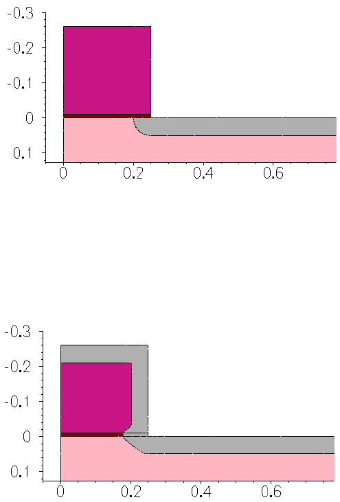
11: Structure Generation

Etching and Deposition Types and Options

Sentaurus™ Process User Guide 737

H-2013.03

An example of a single-material isotropic etch is (see Figure 99):

etch silicon thickness = 0.05 type=isotropic

Figure 99 Single-material isotropic etch

An example of a multiple-material isotropic etch is (see Figure 100):

mgoals resolution=0.04

etch material = {Silicon Oxide Poly} rate = {1.0 1.5 1.0} time = 0.05 \

type=isotropic info=2

Figure 100 Multiple-material isotropic etch

Etching Types: Anisotropic and Directional

Anisotropic etching is designed primarily to work with masks or masking layers. It also is

frequently used to create spacers. Anisotropic etching etches material away in a direction that

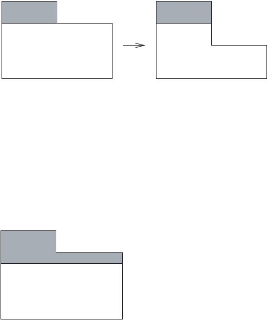
11: Structure Generation

Etching and Deposition Types and Options

738 Sentaurus™ Process User Guide

H-2013.03

is purely vertically downwards. It works well with structures such as those shown in

Figure 101.

Figure 101 Anisotropic etching

Anisotropic etching can take more than one material if the same rate is specified for all etched

materials. This can be useful to create multiple spacers since it does not produce small gaps

which are hard to avoid when etching one spacer at a time. If you want to use different rates for

each material then a better alternative can be Fourier etching.

If anisotropic etching is performed to etch the shaded region in the structure shown in

Figure 102, instabilities can arise. The resulting structure can be very different depending on

the numeric roundoff errors.

Figure 102 For this structure, anisotropic etching would not be stable

Anisotropic operations are sensitive to numeric noise at vertical or nearly vertical walls.

If the etch command is supposed to remove the entire layer, care must be taken to overetch by

a small amount to prevent thin regions remaining due to numeric roundoff error.

NOTE It is more robust and better to use the strip command to remove all

exposed layers of a certain material.

The directional etching method is similar to the anisotropic method. In this case, the specified

etching rate is applied in the direction of the etching beam. Visibility effects are not considered.

The etching window is determined from user-defined masks and from the exposed areas of the

etched material (see Figure 103 on page 739).

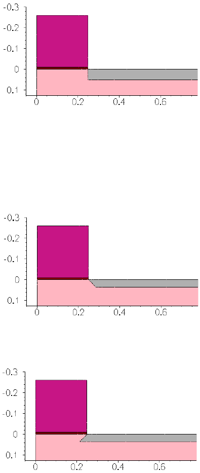
11: Structure Generation

Etching and Deposition Types and Options

Sentaurus™ Process User Guide 739

H-2013.03

For example:

etch silicon thickness = 0.05 type=anisotropic

Figure 103 Anisotropic etching

In the next example, directional etching is demonstrated. The parameter direction sets the

direction of the etching beam by setting values for {x y z}. This direction vector is normalized

to 1.0 before being used by the etching module.

etch material=silicon rate = 0.05 time=1.0 type=directional direction = {1 1}

Figure 104 Directional etching (angled wall)

etch material=silicon rate = 0.05 time=1.0 type=directional direction = {1 -1}

Figure 105 Directional etch undercutting

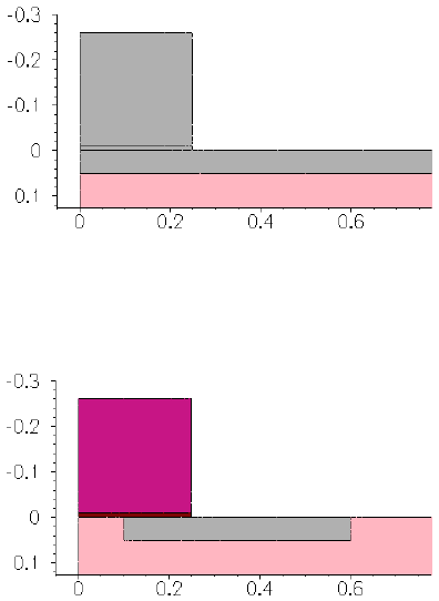
11: Structure Generation

Etching and Deposition Types and Options

740 Sentaurus™ Process User Guide

H-2013.03

Etching Types: Polygonal and CMP

Polygonal etching provides a way of modifying a region without having to define etching rates

or the direction of the etch. The specified polygon is used to intersect the mesh elements. The

elements inside the polygon are replaced by gas.

CMP is handled as a special case of polygonal etching. Mesh elements are intersected at the

specified coordinate. All elements of the specified material above the coordinate are reassigned

to gas.

etch type=cmp coord = 0.05 material=all

Figure 106 CMP

# Etch with polygon given as x1 y1 x2 y2 ... xn yn

etch type=polygon material=silicon polygon= {-0.1 0.1 0.1 0.1 0.1 0.6 -0.1 0.6}

Figure 107 Polygonal etch

11: Structure Generation

Etching and Deposition Types and Options

Sentaurus™ Process User Guide 741

H-2013.03

Etching Type: Fourier

In Fourier etching, the etching rate is a function of the angle between the incident etching beam

and the normal vector of the surface being etched. This allows for reasonably directional

etching with control of the slope of sidewalls. The coefficients are defined using coeffs

(for a single-material etch) or mat.coeffs (for a multimaterial etch), and the etching rate is

computed according to:

(966)

where:

■ is the angle between the incident beam and the normal to the surface being etched.

■ is the factor given in the beam command for beam .

Any number of coefficients can be given for each material. If the parameters are chosen

such that negative etch rates would result in some slope angles, no etching will occur on the

parts of the surface that have that slope. It is common to set the parameters such that the

etch rate for angles less than a certain angle are positive and drop below zero (resulting in no

etching) above that angle. This produces a trench with a rounded bottom and a sidewall given

by the angle where the etch rate drops to zero.

Fourier etching uses the full level-set model formulated after Lax–Friedrichs. This formulation

shows good stability, leading to good accuracy of etching wall-angle control. The Lax–

Friedrichs formulation results in slightly less corner sharpness.

Etching Beams

The beam command is used to define the direction and relative strength of etching beams to be

used with Fourier etching. The syntax is:

beam name=<beam_name> incidence=<angle> | direction= {<x> <y> <z>}

factor=<relative_strength>

The angle of incidence of each beam is specified either by the incidence parameter in the

beam command (incidence=0 defines a vertical beam), or by a direction vector, which is

normalized automatically to unit length. To be clear, the angle in Eq. 966 is measured from

the surface perpendicular to the angle of incidence for beam . The relative strength factor

is used to mix the strength of different beams. Each etching beam must be given a unique name.

Etching beams are assumed to be collimated, that is, a slight angular spread of beam direction

is not considered.

etch rate factoriAjθi

cosj

j0=



i0=



θi

factori

θi

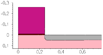
11: Structure Generation

Etching and Deposition Types and Options

742 Sentaurus™ Process User Guide

H-2013.03

The parameter sources of the etch command specifies the list of names of etching beams to

be used in an etch operation.

A Fourier etching example follows (see Figure 108):

mgoals resolution=0.02

beam name=src1 direction = {1 0 0} factor=1

etch material=silicon type=fourier sources = src1 coeffs = {0 0 1.0} time=0.05

Figure 108 Fourier etching

Through the selection of Fourier coefficients, the angle of the etching wall can be controlled to

a large degree. In particular, the first coefficient in the list, , corresponds to the equivalent

of the rate of isotropic etching. The second coefficient in the list, , corresponds

approximately to the equivalent of the rate of anisotropic or directional etching. The

approximate formula for determining the etch wall angle is given as:

(967)

where is the angle of the etch wall measured from the horizontal plane. For example, the

choice of and results in an etch wall at an angle of approximately

from the horizontal as shown in Figure 109 on page 743:

beam name=src1 direction= {0.1 0 0} factor=1

mgoals full.resolution= 0.05 resolution= 0.05

etch material= {silicon} type=fourier sources= {src1} coeffs= {-0.5 0.7071} \

time=1.0.

ϕA–0

---------

cos 1–

≈

A00.5–=

A10.7071=

45°

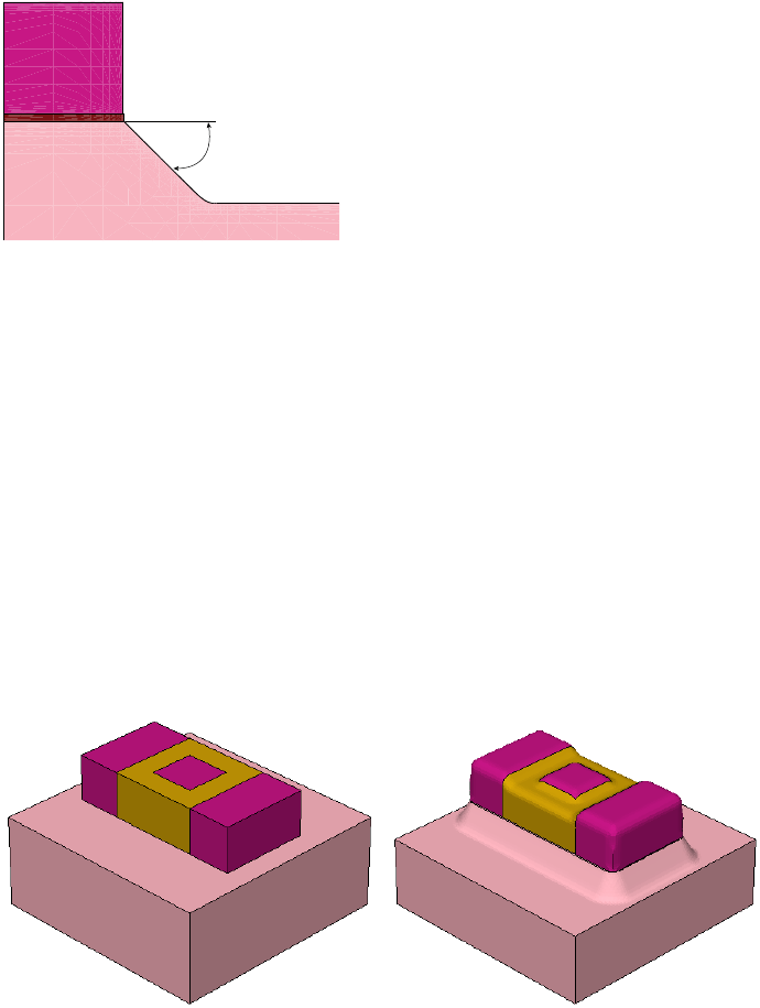
11: Structure Generation

Etching and Deposition Types and Options

Sentaurus™ Process User Guide 743

H-2013.03

Figure 109 Example of Fourier etch

Another Fourier etching example shows the functionality in 3D and how multiple rates for

multiple materials are specified using mat.coeffs. For 3D Fourier etching, also use the

command sde off.

Etching coefficients chosen for this example are illustrative and may not be physically

meaningful:

beam name=src1 direction= {1 0 0} factor=1

mgoals dx=0.1 dy=0.1 dz=0.1

sde off

etch info=10 sources= {src1} mat.coeffs= { Silicon= {-1 2} \

Nitride= {-0.7 1.2} Oxide= {0.01} PolySilicon= {-0.05 0.2} } type=fourier \

remesh=false time=1

Figure 110 Three-dimensional multimaterial Fourier etching example before etching (left)

before etching and (right) after etching

Currently, in 3D Fourier etching, shadowing is not implemented as it is in two dimensions.

11: Structure Generation

Etching and Deposition Types and Options

744 Sentaurus™ Process User Guide

H-2013.03

Keywords shadowing and shadowing.nonisotropic

The keyword shadowing.nonisotropic is used instead of shadowing when you want to

allow only the 0th-order Fourier coefficient to etch areas where the beam is shadowed. The

keyword shadowing prevents all Fourier etching in areas shadowed from the beam; while the

keyword shadowing.nonisotropic prevents only the Fourier coefficients of order one and

higher from etching in areas where the beam is shadowed.

Be aware that even when this parameter is specified, the 0th-order Fourier coefficient

should continue to etch areas where the beam is shadowed. This permits a pseudo-isotropic

etching that is independent of shadowing, while at the same time the full Fourier etching occurs

only in areas where the beam is not shadowed.

Etching Type: Crystallographic

The parameter crystal_rate defines etching rates for different crystallographic

orientations. These rates are used for type=crystal. For details on wafer orientation, see

Defining the Crystal Orientation on page 73. Crystallographic etching rates are specified in

crystal_rate as a list of Miller indices and corresponding etching rates. The currently

accepted indices are <100>, <110>, and <111>, as in the following example:

crystal_rate= {"<100>" =0.8 "<110>" =0.35 "<111>" =0.003}

Interpolation of the rate at a given point along the etch front is calculated as a linear

combination of the <100>, <110>, and <111> rates weighted by the component of the etch

front normal vector along the corresponding crystallographic direction.

NOTE You must add a space between the double quotation mark (") after the

orientation and the equal sign.

A crystallographic etching example follows (see Figure 111 on page 745):

etch material=silicon type=crystal crystal_rate= {"<100>" =1.0 "<110>" =0.5 \

"<111>" =0.001} time=0.25

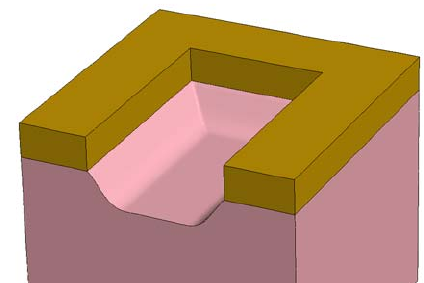
11: Structure Generation

Etching and Deposition Types and Options

Sentaurus™ Process User Guide 745

H-2013.03

Figure 111 Crystallographic etching

Etching Type: Trapezoidal

The trapezoidal etch model provides a simple but flexible approximation to a number of real

etching processes. The location of the etch is determined by masking layers (that is, layers of

nonetchable material that, if nonexistent, can be easily created with the photo command). In

3D, the etch location can be specified through the definition of a mask.

The trapezoidal model uses the following parameters to specify the shape of the region to be

removed:

■thickness specifies the vertical depth (or a combination of rate and time).

■angle specifies the angle (in degrees) of the resulting sidewalls.

■undercut specifies the horizontal penetration of the etch under the edges of the masking

layer. It only works in two dimensions.

■bottom.angle and bottom.thickness specify the angle and thickness of the sidewalls

for a second etching after thickness and angle are already etched (3D only).

These parameters can be used to approximate a number of real etching processes including:

■Combinations of vertical and isotropic etches.

■V-groove etches.

■Etches that produce retrograde sidewall profiles.

NOTE Trapezoidal etching is not supported by Sentaurus Structure Editor.

Consequently, the command sde off must be issued.

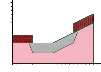
11: Structure Generation

Etching and Deposition Types and Options

746 Sentaurus™ Process User Guide

H-2013.03

Trapezoidal 2D Etching

An etch with the trapezoidal model is performed in three steps:

1. A vertical etch to depth thickness is performed. This etch does not apply to portions of

the surface that are masked by nonetchable materials or shadowed by etchable or

nonetchable materials; nor is it used on segments of the surface that form an angle greater

than angle to the horizontal.

2. A horizontal etch is performed. Surfaces that were exposed at the start of Step 1 are etched

horizontally by the distance undercut. Surfaces that were exposed during Step 1 are

etched by a distance proportional to the length of time between when they first became

exposed and the end of Step 1. Therefore, a sidewall exposed three-fourths of the way into

Step 1 is etched horizontally by one-fourth of undercut. (An exception is made when an

angle greater than is specified; this case is described below.)

3. Where overhangs of etchable material are present at the end of Step 2, a vertical upwards

etch (that is, in the direction) is performed. On surfaces that were exposed at the start of

Step 2, this etch is to a distance undercut. On surfaces that were first exposed during the

course of Step 2, the distance of this etch is reduced in proportion to the time from the start

of Step 2. This step approximates the undercutting of the mask due to the isotropic

component of the etch.

NOTE Trapezoidal etching using a mask definition is not supported in 2D.

When the thickness, angle, and undercut parameters satisfy the relationship:

(968)

the etch approximates a vertical etch with an isotropic component. This is the case whenever

two or fewer of the parameters thickness, angle, and undercut are specified with the

option Trapezoidal.Etch.Undercut set to 1 (default is 0):

pdbSet Grid Trapezoidal.Etch.Undercut 1

etch material=silicon type=trapezoidal thickness=0.25 undercut=0.1

Figure 112 Trapezoidal etching example 1

90°

thickness undercut angle()tan⋅=

X [µm]

Y [µm]

0 0.5 1 1.5 2

-0.5

0.5

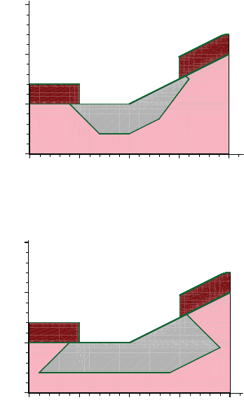
11: Structure Generation

Etching and Deposition Types and Options

Sentaurus™ Process User Guide 747

H-2013.03

The left half of Figure 112 on page 746 shows the result when etching a planar substrate. The

etch region is a trapezoid of depth thickness, extending a distance undercut beneath the

mask edge, and with a sidewall slope of angle degrees. The right half of Figure 112 shows the

result when etching a nonplanar surface.

Step 1 of the sequence etches the exposed surface vertically to a depth of thickness

micrometers. Step 2 etches the resulting sidewall in the horizontal direction, producing an

undercutting of the mask and the sloped sidewall. In this case, Step 3 also has an effect, etching

upwards from the undercut region. Therefore, the hook in the final silicon profile is the result

of approximating the isotropic component of the etch. In every case, the intersection between

the bottom of the etch region and the sidewall occurs directly under the edge of the mask.

Figure 113 and Figure 114 show what happens when Eq. 968 is not satisfied.

etch material=silicon type=trapezoidal thickness=0.3 undercut=0.1 angle=45

Figure 113 Trapezoidal etching example 2

etch material=silicon type=trapezoidal thickness=0.3 undercut=0.1 angle=135

Figure 114 Trapezoidal etching example 3

In Figure 113, you have thickness/undercut < tan(angle). In this case, the sloped sidewall

of the etch extends out under the opening in the mask. The intersection between the bottom of

the etch region and the sidewall is no longer directly beneath the edge of the mask. If the mask

opening is narrow enough, the bottom of the etch region disappears entirely, resulting in a V-

groove etch. To produce this etch shape, Step 1 of the etch process is modified to reduce the

X [µm]

Y [µm]

0 0.5 1 1.5

-0.5

0.5

X [µm]

Y [µm]

0 0.5 1 1.5 2

-0.5

0.5

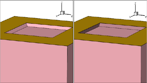
11: Structure Generation

Etching and Deposition Types and Options

748 Sentaurus™ Process User Guide

H-2013.03

depth of the vertical etch near the edges of the mask opening. Note that, in this situation, even

the smallest amount of nonetchable material can produce a triangular mound of unetched

material in the final structure.

Figure 114 on page 747 shows the case with an angle greater than . In this case, the bottom

of the etched region is wider than the opening in the masking layer, producing overhanging

sidewalls. This etch is accomplished by modifying Step 2 of the procedure to etch further

horizontally at the bottom of the sidewalls formed by Step 1 than at the top. The apparent etch

depth of at the right side of the mask opening is the result of a vertical etch

of the original sloped surface (Step 1) followed by a horizontal etch of the sloped

“bottom wall” that results from Step 1.

Trapezoidal 3D Etching

There are two possible cases for trapezoidal 3D etching:

■A thickness (or rate and time) and an angle (optional) are specified. If angle is not

specified, it is considered to be (vertical). In contrast with case 2, angle allows any

value between and . Figure 115 contains examples for both cases.

■A thickness (or rate and time) and an angle (optional) plus bottom.thickness and

bottom.angle (optional) are specified. If angle is not specified, it defaults to

(vertical). Here, a special condition applies: angle must be greater than or equal to ,

while bottom.angle must be smaller than or equal to . In other words, the first

etching penetrates behind the mask, while the second one does the opposite. Figure 116 on

page 749 shows an example of this type.

NOTE For 3D trapezoidal etching to succeed, the initial etching surface must

be more or less flat.

Figure 115 Trapezoidal 3D etching: (left) angle=45 thickness=0.3 and (right) angle = 110,

thickness=0.44

90°

0.5 µm

0.3 µm

0.4 µm

90°

0°

180°

90°

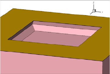
11: Structure Generation

Etching and Deposition Types and Options

Sentaurus™ Process User Guide 749

H-2013.03

Figure 116 Trapezoidal 3D etching produced with the options angle=110 thickness=0.3

bottom.angle=45 bottom.thickness=0.400

Trapezoidal Etching Using force.full.levelset

When the keyword force.full.levelset is specified in conjunction with trapezoidal

etching:

■Etch depth is controlled by rate and time, not by thickness.

■The parameter ambient.rate is used to approximate the underetch effect otherwise

available in the non-force.full.levelset case controlled in 2D by undercut. If

undercut is specified, ambient.rate will be approximated by , and

a warning message will be issued. The parameter ambient.rate also approximates

underetching, controlled in three dimensions in the non-force.full.levelset case by

the combination of angle, bottom.angle, and bottom.thickness.

■The parameters supported by the level-set solver such as shadowing become available.

■An additional parameter roundness (default value 1.0) can be used to increase the

curvature of etching sidewalls.

Etching Type: Piecewise Linear

In piecewise linear etching, the etch rate is a user-defined piecewise linear function of the angle

between the incident etching beam and the normal vector of the surface being etched. You

define the points of angle versus rate on a material-by-material basis, as per the following

syntax:

angles.rates= { \

materialA = { angleA

rateA

angleA

rateA

... angleA

rateA

} \

materialB = { angleB

rateB

angleB

rateB

... angleB

rateB

} \

...

}

where .

undercut time⁄

anglen1–anglen

≤

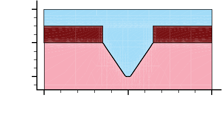
11: Structure Generation

Etching and Deposition Types and Options

750 Sentaurus™ Process User Guide

H-2013.03

The rates and angles are interpreted as follows:

■Angles are given in degrees in the range [ , ].

■The rate for angle < angle0 will be rate0, and the rate for angle > anglen will be 0.

■The rate is calculated as the linear interpolation of the nearest two angle/rate pairs within

which the angle lies.

While Fourier etching and trapezoidal etching also define the etch rate according to the angle

between the beam direction and the surface normal, a piecewise linear function is a more

general parameterization of etch rate versus angle that users control directly.

Etching Beams

The beam command defines the direction and relative strength of etching beams to be used with

piecewise linear etching (see Etching Beams on page 741).

The parameter sources of the etch command specifies the list of names of etching beams to

be used in an etching operation.

Example of Piecewise Linear Etching

This example is a piecewise linear etching (see Figure 117):

beam name=src1 direction= {1 0 0} factor=1

etch type=angles.rates sources=src1 time=0.2 \

angles.rates= { Silicon= { 25 1.0 45 0.3 } }

Figure 117 Piecewise linear etching

The piecewise linear function must be defined by users as smoothly as possible, avoiding

discontinuous changes, to ensure well-defined level-set results.

0°

180°

X [µm]

Y [µm]

0 0.5 1

-0.2

0.2

11: Structure Generation

Etching and Deposition Types and Options

Sentaurus™ Process User Guide 751

H-2013.03

Deposition

To specify the deposition type, use either the parameter type or one of the parameters

anisotropic, isotropic, fill, or fourier. To specify the thickness of the deposited

layer for isotropic and anisotropic deposition, use either the parameter thickness, or the

rate and time parameters. Besides the deposition type and thickness, you must specify the

material to be deposited (only one material is allowed per deposit command). To do this,

specify the material name in the command or the parameter material=<material_name>.

The following deposition types are supported:

The number of steps for a deposition is specified as steps=<n>. The specified time or

thickness is subdivided accordingly. Subdividing a deposition into several steps might be

useful if stresses are initialized in the deposited layer. A stressed film of a given thickness can

be deposited at the same time or in several steps. Sentaurus Process simulates stress

rebalancing after each deposition step. Multistep deposition is known to generate more realistic

stress profiles compared to depositing the entire layer and then performing one stress

rebalancing calculation.

By default, the material is deposited on the surface exposed to the upper gas region. If the

structure has buried gas bubbles, they will be left untouched. To deposit inside those gas

bubbles specify the fill.buried parameter in the deposit command.

type=anisotropic

Performs anisotropic deposition.

type=isotropic

Performs isotropic deposition.

type=fill

Performs a fill of the structure with the specified material up to the

coordinate specified with the parameter coord.

type=fourier

Performs Fourier deposition.

type=polygon

Performs a polygonal deposition which requires the polygon

argument. The specified polygon is used to intersect all mesh

elements of material gas. Then, elements inside the polygon are

assigned to the specified material. (Not available in 3D.)

type=trapezoidal

Performs a trapezoidal deposition which requires the angle and

thickness arguments. (3D only)

anisotropic

Equivalent to type=anisotropic.

isotropic

Equivalent to type=isotropic.

fill

Equivalent to type=fill.

fourier

Equivalent to type=fourier.

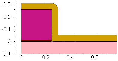
11: Structure Generation

Etching and Deposition Types and Options

752 Sentaurus™ Process User Guide

H-2013.03

Mask Naming

The name of a mask also can be specified in the deposit command. In this case, the material

is deposited outside the specified mask. Deposition inside a mask requires the mask to be

inverted by specifying the parameter negative in the mask command defining the mask (see

Photoresist Masks on page 767).

For deposition, the analytic method, the fast level-set method, and the full level-set method are

available. In 2D, the analytic method is the preferred method for performing deposition, and

the level-set method is used when the analytic method is not possible because a front collision

is detected. In 3D, the analytic method is used for anisotropic deposition, the fast level-set

method is used for isotropic deposition, and the full level-set method is used for Fourier

deposition.

In the newly deposited region, constant field values can be initialized. For isotropic deposition,

you can define piecewise linear solution fields as a function of the distance from the original

surface.

Deposition Type: Isotropic

For simple conforming deposition, the boundary is offset an equal distance in all directions.

An isotropic deposition example follows (see Figure 118):

deposit nitride thickness = 0.05 type=isotropic

Figure 118 Isotropic deposition

Deposition Types: Fill and Polygonal

Fill is a special case of polygonal deposition. The mesh elements of material gas are intersected

at the specified coordinate. Gas elements below the coordinate are reassigned to the specified

material.

NOTE Polygon deposition is not available in 3D.

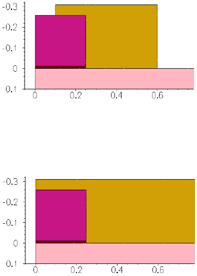
11: Structure Generation

Etching and Deposition Types and Options

Sentaurus™ Process User Guide 753

H-2013.03

Figure 119 is a polygonal deposition example:

deposit type=polygon material=nitride polygon= {0.1 0.1 0.1 0.6 -0.31 \

0.6 -0.31 0.1}

Figure 119 Polygonal deposition

Figure 120 shows a fill example:

deposit material=nitride type=fill coord= -0.31

Figure 120 Fill example

Deposition Type: Crystallographic

Crystallographic deposition takes advantage of the full level-set method to grow single

materials whose rate of growth is determined by the crystallographic directions. The crystal is

assumed to be cubic regardless of the material being deposited. Deposition rates can be set for

the <100>, <110>, and <111> directions. These rates will be applied to their respective

equivalent directions based on cubic symmetry, for example, the <100> rate will apply to the

<010>, <001>, <-100>, <0-10>, and <00-1> directions.

Figure 121 on page 754 is a crystallographic deposition example:

deposit type=crystal material=nitride time = 0.05 \

crystal.rate = { <100> = 1.0 <110> = 0.1 <111> = 0.05 }

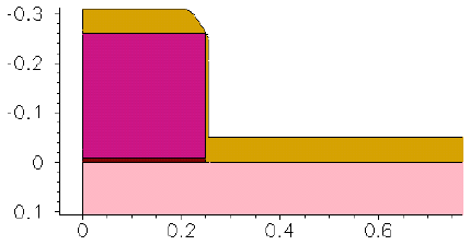
11: Structure Generation

Etching and Deposition Types and Options

754 Sentaurus™ Process User Guide

H-2013.03

Figure 121 Crystallographic deposition (vertical direction is <100>, lateral direction is <011>)

Crystallographic deposition also can be simulated using an atomistic technique (see Epitaxial

Deposition on page 519).

Deposition Type: Fourier

Fourier deposition takes advantage of the full level-set method to grow single materials whose

rate of growth is defined by a function of the angle between the surface normal of the material

boundary and the deposit beams. The definition and calculation of the deposit shape are exactly

analogous to the case of Fourier etching as described in Etching Type: Fourier on page 741.

For Fourier deposition, first, define the deposition beam in the same way as in Fourier etching:

beam name=<beam_name> incidence=<angle> | direction= {<x> <y> <z>}

factor=<relative_strength>

Use the sources and coeffs parameters in the same way as in Fourier etching, shown in the

following Fourier deposition example:

beam name=src1 direction= {1 0 0} factor=1

deposit nitride time=0.2 fourier sources= {src1} coeffs= { -0.3 0.7 }

The coeffs parameter has units of µm/minute and, by default, time is given in units of

minutes. The Fourier deposition in 3D is only available in the default sde off mode:

NOTE The relationship between the A0 and A1 parameters in Fourier

deposition can be used to create a good reproduction of the

TSUPREM-4 deposit parameter ANISOTRO by using the formula

A1/A0 = ANISOTRO – 1.

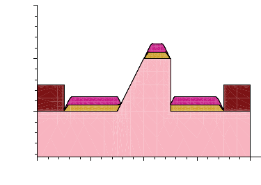
11: Structure Generation

Etching and Deposition Types and Options

Sentaurus™ Process User Guide 755

H-2013.03

Figure 122 Two-dimensional Fourier deposition: for purposes of illustration, nitride is

deposited selectively on silicon using Fourier deposition and, then, an additional

Fourier deposition step adding polysilicon is performed using nitride as the

selective deposit material

Deposition Type: Trapezoidal

Trapezoidal deposition creates a shape in 3D with sidewalls of a defined height and angle.

Height is defined by thickness. Angle is defined by angle, measured in degrees from horizontal,

where angle=90 is vertical; angle > spreads outward as height increases, and angle

< closes inward with increasing height.

NOTE Trapezoidal deposition is available only in 3D.

Separate outward and inward deposition steps can be used to create diamond-like shapes.

Trapezoidal deposition requires a flat starting surface, for which the fill command can be

used.

The syntax is demonstrated with the following example, whose results are shown in

Figure 124:

# first step deposition

deposit material= PolySilicon type=trapezoidal \

selective.material= Silicon thickness= 0.25 angle= 120

# provide flat surface for second step

deposit type=fill coord= -0.25 Resist

# second step deposition

deposit material= PolySilicon type=trapezoidal \

selective.material= PolySilicon thickness= 0.25 angle= 60

X [µm]

Y [µm]

0 1 2

0.5

1.50.5

90°

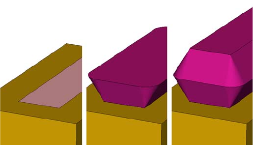
11: Structure Generation

Etching and Deposition Types and Options

756 Sentaurus™ Process User Guide

H-2013.03

Figure 123 Trapezoidal deposition. Left: Prior to deposition. Center: First step, deposition

with angle=120. Right: Second step, deposition with angle=60.

Selective Deposition

Selective deposition is optionally available. Using the selective.materials parameter,

you can select one or more materials to seed growth of the overlayer. When using 2D or 3D

MGOALS, multiple selective.materials can be specified. In 3D SDE mode, only one

material can be specified in the selective.materials list. Selective deposition can be used

with isotropic, anisotropic, or Fourier deposition types.

Fields in Deposited Layers

For isotropic deposition, piecewise linear fields can be specified in the deposited layer. A

doping command must be used for each field; each doping command must assign a unique

name. A list of names of the doping is then specified in the parameter doping of the deposit

command as a string array:

doping name=strainGe field=Germanium depths= {0 0.1} values= {1e22 1e22}

deposit material= oxide doping= {strainGe} type= isotropic \

thickness=0.1

These commands create a linear germanium field in the newly deposited oxide layer. Depth 0

corresponds to the initial surface (the bottom of the new layer).

Constant field values can be defined for all types of deposition as follows:

deposit material= oxide type= isotropic thickness=0.1 \

fields.values= {Vacancy=1e10 Germanium=2e22}

NOTE To create layers with intrinsic stress, use the field names StressELXX,

StressELXY, StressELYY, StressELZZ, StressELYZ, and

11: Structure Generation

Etching and Deposition Types and Options

Sentaurus™ Process User Guide 757

H-2013.03

StressELXZ. It is not necessary to specify all components of stress.

Those that are not specified are assumed to be initially at zero. If stresses

are added in this way, they will be rebalanced after the deposition is

completed. The actual value of the stress may differ from the value that

was deposited.

Constant concentrations can be defined for known solution fields (known solution fields must

have been defined before the deposit command, either in the SPROCESS.models file or the

command file of the user) as:

deposit material= {oxide} type= isotropic thickness= 0.1 Vacancy \

concentration=1e10

Stress Handling

In addition to optionally including an automatic ramp-up or ramp-down before etching and

deposition, by default, Sentaurus Process automatically rebalances the stresses after etching

and deposition. This updates the stress fields at the temperature of the etch or deposit step based

on the new geometry.

For the best stress results, it is necessary to control the temperature history. This includes

thermal ramp-up to process temperature, back to room temperature, and similarly ramp-up and

ramp-down for etch, and also for deposition. However, as a minimum, the elastic stress

rebalancing can be handled automatically by switching on the stress history (see Chapter 9 on

page 643 and Automated Tracing of Stress History on page 683).

It is sometimes useful to switch off this stress rebalancing step in 3D because the rebalance

triggers a new mesh to be created and, in 3D, meshing is delayed until it is needed. Therefore,

if you are more concerned about simulation time than stress accuracy, you should specify:

pdbSet Mechanics EtchDepoRelax 0

to allow multiple etch and deposit steps to be performed without a mesh being generated in

between.

Shape Library

The shape library provides commands for generating some special-shaped polyhedra in

Sentaurus Process. These shapes are created using Sentaurus Structure Editor. The shape

library is an interface to use those shapes in Sentaurus Process.

There are two ways to use the shapes from the shape library: MGOALS mode or SDE mode.

In MGOALS mode, polyhedra are created using Sentaurus Structure Editor. The generated

11: Structure Generation

Etching and Deposition Types and Options

758 Sentaurus™ Process User Guide

H-2013.03

polyhedra then can be inserted into a Sentaurus Process structure using the insert command.

The MGOALS mode is activated with the command sde off.

In SDE mode, polyhedra are not created directly. Instead, the Sentaurus Structure Editor

structure itself is modified by inserting the shapes (replacing other materials). To activate the

SDE mode, use the command sde on.

In both modes, the correct coordinate transformation for the UCS (specified using math

coord.ucs) and for the DF–ISE coordinate system (default, or specified using math

coord.dfise) is applied.

The commands available in the shape library are:

■PolyHedronSTI creates a shallow trench isolation (STI)–shaped polyhedron.

■PolyHedronSTIaccc creates an STI concave active corner-shaped polyhedron.

■PolyHedronSTIaccv creates an STI convex active corner-shaped polyhedron.

■PolyHedronCylinder creates a cylinder-shaped polyhedron.

■PolygonWaferMask creates a wafer mask polygon.

■PolyHedronEpiDiamond creates an epitaxial diamond-shaped polyhedron.

Additional commands that create parameterized custom shapes can be defined by users using

the scripting capabilities of Sentaurus Process and Sentaurus Structure Editor.

PolyHedronSTI

The syntax of the PolyHedronSTI command is:

PolyHedronSTI name direction X0 Y0 Depth Zmin Zmax Tsti Asti Hsti Rd Rb Ru

[material]

where:

■The name parameter is set to the name for the polyhedron.

■The direction parameter can be set to left, right, front, or back, which tells the facing

direction of the STI polyhedron.

■The optional material parameter is used to specific the material of the inserted shape in

the SDE mode. In the MGOALS mode, the material of the inserted shape can be specified

in the insert command.

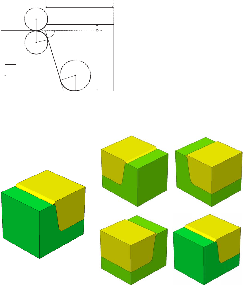
11: Structure Generation

Etching and Deposition Types and Options

Sentaurus™ Process User Guide 759

H-2013.03

■For other parameters, see Figure 124.

Figure 124 Parameters for generating STI-shaped polyhedron

Figure 125 shows some generated STI shapes in different directions. Figure 126 on page 760

shows STI shapes with different Tsti and Rb values.

Figure 125 STI-shaped polyhedra in different directions

(X0,Y0)

sti

Depth

sti

RightLeft

Front Back

Zmin

Zmax

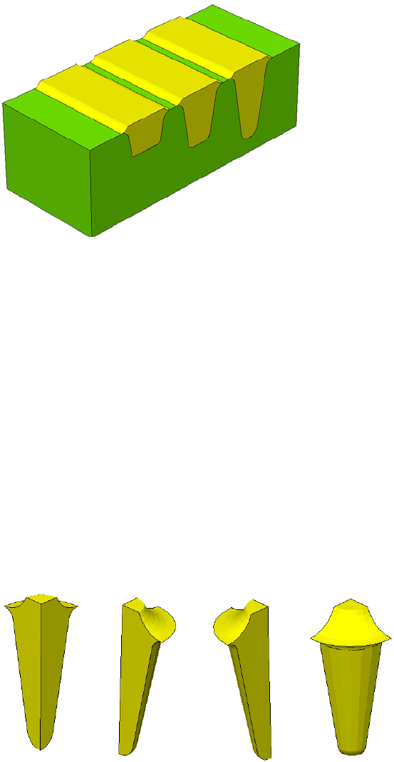
11: Structure Generation

Etching and Deposition Types and Options

760 Sentaurus™ Process User Guide

H-2013.03

Figure 126 STI-shaped polyhedra with different Tsti and Rb

PolyHedronSTIaccc

The syntax of the PolyHedronSTIaccc command is:

PolyHedronSTIaccc name direction X0 Y0 Z0 Tsti Asti Hsti Rd Rb Ru Rac

[material]

where:

■The name parameter is set to the name for the polyhedron.

■The direction parameter can be set to rb (right back), lb (left back), lf (left front), or

rf (right front).

■The Rac parameter is the radius of the STI concave corner.

■For other parameters, see Figure 124 on page 759.

Figure 127 shows STI concave corner-shaped polyhedra in different directions.

Figure 127 STI concave corner-shaped polyhedra in different directions: (from left to right)

left back, right back, left front, and right front

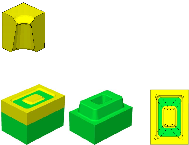
11: Structure Generation

Etching and Deposition Types and Options

Sentaurus™ Process User Guide 761

H-2013.03

PolyHedronSTIaccv

The syntax of the PolyHedronSTIaccv command is:

PolyHedronSTIaccv name direction X0 Y0 Z0 Depth Tsti Asti Hsti Rd Rb Ru Rac

[material]

where:

■The name parameter is set to the name for the polyhedron.

■Same as the PolyHedronSTIaccc command, the direction parameter can be set to rb,

lb, lf, or rf.

■The Rac parameter is the radius of the convex corner.

■For other parameters, see Figure 124 on page 759.

Figure 128 shows a generated STI convex corner-shaped polyhedron.

Figure 128 STI convex corner-shaped polyhedron

Figure 129 (left) shows a structure generated by combining the above three STI commands.

Figure 129 (right) illustrates the directions of the STI shapes.

Figure 129 (Left) STI structures and (right) polyhedron directions

Back

lb rb

Left Right

lf rf

Front

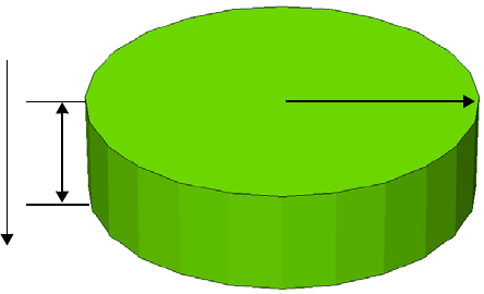
11: Structure Generation

Etching and Deposition Types and Options

762 Sentaurus™ Process User Guide

H-2013.03

PolyHedronCylinder

The syntax of the PolyHedronCylinder command is:

PolyHedronCylinder name X0 Y0 Z0 Rc Hc [material]

where:

■The name parameter is set to the name for the polyhedron.

■Other parameters give the center coordination, the radius, and the height for the cylinder

(see Figure 130).

Figure 130 Cylinder-shaped polyhedron

PolygonWaferMask

The syntax of the PolygonWaferMask command is:

PolygonWaferMask name Y0 Z0 Rw Lf

where:

■The name parameter is set to the name for the polyhedron.

■Other parameters give the location and size for the mask (see Figure 131 on page 763).

NOTE This command only works in MGOALS mode.

(Y0,Z0)Rc

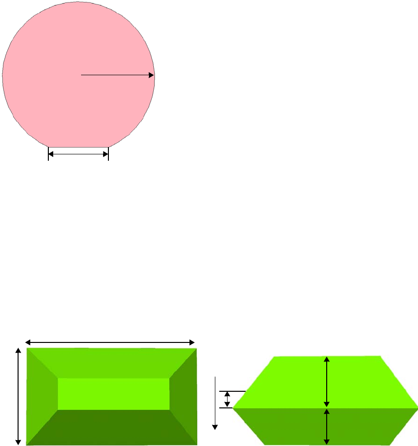
11: Structure Generation

Etching and Deposition Types and Options

Sentaurus™ Process User Guide 763

H-2013.03

Figure 131 Wafer mask-shaped polygon

PolyHedronEpiDiamond

The syntax of the PolyHedronEpiDiamond command is:

PolyHedronEpiDiamond name X0 Y0 Z0 Wepi Lepi Hup Hdown Drecess [material]

where:

■The name parameter is set to the name for the polyhedron.

■For other parameters, see Figure 132.

Figure 132 Epitaxial diamond-shaped polyhedron

(Y0,Z0)

Wepi

Lepi

(Y0,Z0)

Drecess

Hup

Hdown

11: Structure Generation

The mask and photo Commands

764 Sentaurus™ Process User Guide

H-2013.03

The mask and photo Commands

A quick way to mimic lithographic patterning is using the photo command. The photo

command takes a mask and effectively does a resist spin-on step followed by an exposure bake

and etch. The resist layer produced has vertical walls and is by default a negative of the mask,

but the positive sense can optionally be created as well.

In addition to the photo command, the etch and deposit commands allow you to specify a

mask directly. The parameter mask in the etch, deposit, and photo commands specifies the

name of one mask that has been previously defined using a mask command or by reading in

masks from a layout using the IC WorkBench EV Plus interface (see Chapter 12 on page 817).

The mask will have an effect similar to a masking layer; it limits the etch or deposition process

to a certain window. By default etching is not performed for points inside the mask, unless the

parameter negative is used in the mask definition. Similarly, deposition of a new layer in the

deposit command and of the photoresist layer in the photo command is performed outside

the mask unless the negative parameter is specified in the mask command in which case

deposition happens inside the mask only.

NOTE Always specify the masks and the simulation domain such that masks

do not end exactly on the boundary of the simulation domain, but end

inside or extend safely beyond the boundary of the simulation domain.

The mask command creates a mask. You can define the geometry of the mask directly in the

command file or can read masks from a layout file. Masks defined in the command file must

be given a name; otherwise, the names are read from the layout file.

If the parameter list is specified in a mask command, information about the existing masks

is printed. If name is specified as well, information about the specified mask is printed.

If the parameter clear is specified in a mask command, all previous mask definitions are

removed. If a name is specified as well, only the specified mask is removed.

A mask can be defined directly in the command file by using three different types of geometry

object:

■Segments

■Rectangles

■Polygons

Each mask may be composed of an arbitrary number of such objects.

11: Structure Generation

The mask and photo Commands

Sentaurus™ Process User Guide 765

H-2013.03

Segments are defined as:

mask name= pmask segments= { -0.1 0.6 0.7 1.1 }

Pairs of subsequent values define the y-coordinates of the beginning and end of one mask

segment. Therefore, an even number of coordinates must be specified in the segments

parameter. The pairs may be defined in arbitrary order, and the segments defined by pairs of

coordinates may touch or overlap each other. In 3D, masks defined by segments are extended

over the entire range of z-coordinates.

A rectangular mask is defined as:

mask name=nimask left=0.2 right=1 front=0.2 back=1 negative

The left and right parameters define the minimum and maximum extensions of the mask

along the y-axis; the front and back parameters define the minimum and maximum

extensions of the mask along the z-axis.

NOTE Only one rectangle can be specified per mask command. The front

and back parameters may be omitted; in this case, the mask is

equivalent to a mask with one segment. Additional mask commands

with the same name can be used to add rectangles. The rectangles

defined for a mask may arbitrarily intersect or touch each other.

Masks also can be defined by a list of names of polygons. These named polygons must have

been defined before the mask command using one polygon command for each named

polygon:

polygon name=LShape2 segments= {0.0 -1.5 0.0 -0.5 0.5 -0.5 0.5 1.5 1.5 \

1.5 1.5 -1.5}

mask name=Mask2 polygons= {LShape2} negative

NOTE The segments in the polygon command are defined as a sequence of y-

and z-coordinates. The polygon is closed implicitly by connecting the

last point to the first. Each polygon for a mask must not touch or

intersect itself. The polygon may be specified with arbitrary orientation

(clockwise or counterclockwise in the yz plane). It does not matter if

different polygons for a mask touch or intersect each other.

Masks also can be defined by a combination of all three types of geometry object: segments,

rectangles, and polygons. Different objects may touch or overlap each other.

In 1D, the entire simulation domain is masked if the coordinate origin is masked. Any point

along the y-axis in a 2D simulation and any point of the yz rectangle of the simulation domain

in a 3D simulation are inside the mask if they are contained in any one of the geometry objects

11: Structure Generation

The mask and photo Commands

766 Sentaurus™ Process User Guide

H-2013.03

defined for the mask. Specifying the parameter negative inverts the mask. In other words,

any point outside all the geometry objects defined for the mask is masked.

These commands can be used to invert a mask at any time after it has been defined:

mask name=aaa negative

mask name=aaa !negative

NOTE In the etch command, the masked area is not etched. While in the

photo and deposit commands, the photoresist or the specified

material is deposited in the unmasked area.

Masks can also be combined using a set of Boolean operations. The operations are specified

using the bool parameter (see Boolean Masks on page 767).

Layouts that have been defined in the GDSII format can be read into Sentaurus Process using

the ICWBEV Plus interface (see Chapter 12 on page 817). Alternatively, masks can also be

read from a layout file in DF–ISE format (default file extension .lyt). To read the layout

directly into Sentaurus Process, the name of the layout file must be specified as

layoutfile=aaa.lyt in a mask command.

All mask rectangles and polygons read from a .lyt file are converted into named polygons.

These polygons then are collected into masks according to the names contained in the .lyt file.

When using a layout file, the relation between the layout coordinate system and the Sentaurus

Process coordinate system may need to be defined. By default, the layout-x axis corresponds

to the Sentaurus Process z-axis. The layout-y axis corresponds to the Sentaurus Process y-axis.

This definition matches the default definition of the parameter slice.angle in the init

command and the coordinate x- and y-axes when displaying the Sentaurus Process simulation

results.

The coordinate transformation between the Sentaurus Process coordinate system and the

layout coordinate system can be defined in two ways:

■In the mask command that specifies the layout file, the name of one mask may be specified.

If a mask with the specified name is contained in the layout file, it is used to position and

orientate the simulation domain in the layout.

■Otherwise, a mask with the specified name must have been defined before using a mask

command. The specified mask is defined in layout coordinates. It may be defined as a

rectangle or a polygon, containing at least two points.

In the case of a rectangle defined in a mask command, the point with the minimum layout-x

and layout-y coordinate is used as the origin of the Sentaurus Process coordinate system. The

direction from (min.layout-x, min.layout-y) to (min.layout-x, max.layout-y) is

used as the Sentaurus Process y-axis.

11: Structure Generation

The mask and photo Commands

Sentaurus™ Process User Guide 767

H-2013.03

If a polygon of at least two points is used (for example, a mask defined as a polygon), the first

point defined is used to place the origin of the Sentaurus Process coordinate system. The

direction from the first to the second point of the mask is used as the orientation of the

Sentaurus Process y-axis.

The local coordinates of the specified mask with respect to the selected Sentaurus Process y-

axis and origin are used as default extensions of the simulation domain. If a polygon mask with

only two points is used, the default extension in the z-direction is 0. The default extension in

the y-direction is defined by the distance between the two points. The default extensions in the

y- and z-directions as defined by the mask are reported. If no extensions have been defined

using the line y command or the line z command or both commands, the default extensions

are defined for the simulation when the layout file is read.

If a layout file is loaded, but no mask name is specified, the Cutline2D command that may

have been specified in the init command to define the parameter slice.angle will be used

to orientate the coordinate systems. The first point specified in the Cutline2D command is

used as the origin of the Sentaurus Process coordinate system. The direction from the first to

the second point is chosen as the direction of the Sentaurus Process y-axis. If Cutline2D is

used, no default extensions of the simulation domain are defined.

Photoresist Masks

To define photoresist layers, use the photo command and specify a mask. Sentaurus Process

defines photoresist layers by specifying the minimum thickness of the resist and selecting the

name of a mask that has been defined by the mask command. By default, the photoresist will

be deposited outside the specified mask and will have a flat top similar to spin-on resist. If the

parameter negative has been specified when defining the mask, a photoresist is created

inside the mask.

Boolean Masks

Two masks can be combined using the bool parameter of the mask command. The Boolean

operations include: +, ^, * and –. In addition, masks can be transformed using the following

operations: rotate, scale, mirror, array, bias, over_under, under_over, and

offset.

The bool option only accepts simple expressions as described in the examples in Table 71.

Complex nested expressions (for example, bool= "(M1 + M2) – bias(–50, M3 + M4)")

are not possible in this implementation and, therefore, must be reduced to simple operations.

11: Structure Generation

The mask and photo Commands

768 Sentaurus™ Process User Guide

H-2013.03

In addition, the bool option cannot be used together with the layoutfile, polygon, and

negative options.

Ta bl e 71 B oo l e an o pe ra ti on s

Operation Example Description

+ bool= "mask1+mask2"

Unites (merges) mask1 and mask2.

– bool= "mask1-mask2"

Subtracts mask2 from mask1.

Note that this is a geometric subtraction. The

program takes mask1 and removes from it the

portion of mask2 which overlaps mask1.

In particular, the operation mask1 - mask2 is

not equivalent to mask1 + (-mask2)

* bool= "mask1*mask2"

Produces the intersection of mask1 and mask2.

^ bool= "mask1^mask2"

Produces a mask that contains the nonoverlapping

portions of mask1 and mask2 (XOR operation).

– bool= "-mask"

Produces a mask that is the complement of the

input mask.

rotate bool= "rotate(direction,mask)"

Produces a mask that is rotated with respect to the

input mask. The direction parameter can be

either left-90 or right-90.

scale bool= "scale(factor,mask)"

Produces a mask that is scaled with respect to the

input mask using the floating-point value of

factor.

mirror bool= "mirror(axis,mask)"

Mirrors a mask with respect to a local axis

specified by x or y.

array bool= "array(n

, n

, d

, mask)"

Produces an array of masks separated by a

distance specified with dx and dy.

bias bool= "bias(delta,mask)"

All mask edges on the input mask are offset in the

normal direction by the specified amount. A

positive delta value expands the mask, while a

negative delta shrinks it. Zero or negative area

sections of the mask are eliminated from the output

mask. Overlapping sections of the mask are

merged.

over_under bool= "over_under(delta, mask)"

Expands and then shrinks the input mask by delta.

This effectively merges areas in close proximity

and is equivalent to bias(delta, bias

(-delta, mask)).

under_over bool= "under_over(delta, mask)"

Shrinks and then expands the input mask by delta.

This eliminates small areas and is equivalent to

bias(delta, bias(-delta, mask)).

nxny

11: Structure Generation

The mask and photo Commands

Sentaurus™ Process User Guide 769

H-2013.03

Line Edge Roughness Effect

Line edge roughness (LER) is the deviation of feature edges from ideal straight lines due to

statistical fluctuations in photolithographic processes. Sentaurus Process uses the

line_edge_roughness command to apply randomized deviations to straight mask edges,

for example:

line_edge_roughness normal= "Z" masks= {mask1} correlation.length= 25.00<nm> \

standard.deviation= 5.00<nm> max.segment.length=5.00<nm>

The random noise function applied to mask edges by the line_edge_roughness

command is generated from the power spectrum of a Gaussian autocorrelation function. The

Gaussian autocorrelation shape is characterized by the standard deviation distance specified

by the standard.deviation parameter and the correlation length , specified by the

correlation.length parameter:

(969)

is obtained by Fourier synthesis, applying the inverse Fourier transform to Eq. 969, after

adding random phases. In this way, random deviations of the mask edges can be obtained from

run to run, which correspond to LER profiles having the same standard deviation and

correlation length .

These random deviations are added in discrete form to the mask edges in question. First, the

mask edge is subdivided into discrete segments complying with the user parameter

max.segment.length. Second, the deviation at each segment endpoint is added in the

direction normal to the initial mask edge orientation.

LER is applied by default to all edges of the mask. You can limit which edges in a named mask

are to receive LER by the parameter normal, which specifies either the y-axis (Y) or the z-axis

(Z). If normal is specified, only those edges in the named masks normal to the given axis are

chosen for LER to be applied. LER is applied only once per mask. Mask segments along the

device bounding box do not receive LER.

The parameter !random.reseed bypasses the reseeding of the random number generator

before the random phases are added. By using this parameter, the shape of the noise function

and, therefore, the LER result, can be reproduced from one run to the next if needed for

comparison.

offset bool= "offset(dy, dz, mask)"

Translates the mask by the specified amount. The

dz parameter is ignored in 2D.

Ta bl e 71 B oo l e an o pe ra ti on s

Operation Example Description

frandom

∆

Autocorrelation frandom

()∆

2πΛex2Λ2

⁄()–

frandom

∆

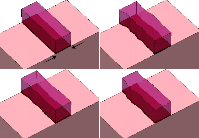
11: Structure Generation

The mask and photo Commands

770 Sentaurus™ Process User Guide

H-2013.03

The parameter random.seed can reproduce specific LER calculations from one run to the

next by setting the same random seed in both runs. When stored in a TDR file in split

simulations, the parameter random.seed is included when saving line_edge_roughness

to the TDR file, even if it is not specified by users, to ensure proper reproduction of the same

LER in a subsequent reload of the TDR file.

NOTE The structure is extruded automatically to three dimensions if it is less

than three dimensions and the line_edge_roughness command is

used.

Figure 133 Example of 3D structure with LER applied using different values of standard

deviation and correlation length : (A) no LER applied, (B) LER applied with

= 4 nm and = 20 nm, (C) LER applied with = 2 nm and = 20 nm, and

(D) LER applied with = 2 nm and = 12 nm

The following strategy is used to address the problem of nearly collinear LER mask points that

may trigger removal by decimation during meshing. Avoiding the decimation of nearly

collinear LER mask points is desirable because removing such points may perturb the power

spectrum of the Gaussian autocorrelation function represented by the mask shape and may also

result in meshing difficulties.

If the parameter max.tries is set to a nonzero value, LER masks are checked for nearly

collinear points, which would result in decimation by the mesher:

line_edge_roughness max.tries=30

If any points in the LER mask are decimated by the mesher, based on the current

mgoals accuracy setting, the LER mask is rejected and the LER generation process is

50 nm

∆

11: Structure Generation

The mask and photo Commands

Sentaurus™ Process User Guide 771

H-2013.03

restarted. After each restart, the detection and restart process is repeated until an acceptable

LER mask is generated or until the number of attempts exceeds max.tries.

When max.tries is exceeded, Sentaurus Process stops with an error message that suggests

using a smaller value of mgoals accuracy or a larger value of max.segment.length in

the line_edge_roughness command.

The default value of max.tries is 0, meaning no decimation check is performed, no retries

are attempted, and the initial mask LER is accepted as it is, even with nearly collinear points.

Mirrored Boundary Conditions

The addition of line edge roughness (LER) is inherently 3D and nonsymmetric, thus not easily

compatible as a simulation problem with the assumption of symmetry reduction. LER added

to a structure reduced by symmetry may produce rough geometrical transitions at joined

geometrical boundaries when pieces are reunited.

To accommodate the possibility of joining symmetry-reduced structures, an additional

keyword smooth.points defines smoothing of LER at structure boundaries. The default

value of smooth.points is 0 (zero), which turns off smoothing.

The use of nonzero smooth.points alters the LER function that creates mirrored boundary

conditions at the structure boundaries. The smoothing occurs at the intersection of masks with

the structure boundary sides. The parameter smooth.points defines the number of segments

in the discrete LER function, counting from the mask’s boundary edge, that should be adjusted

or smoothed. The length of segments in the discrete LER function is determined using

max.segment.length.

Smoothing is calculated by generating the LER function, then creating a virtual mirroring at

the structure boundary edge where a cubic spline interpolation is applied with a mirror

boundary condition. The spline fit is made with the LER at smooth.points from the

boundary. The smoothed LER function is then applied to the mask.

Applying nonzero values of smooth.points affects somewhat the randomness and power

spectrum characteristics of the LER offset function at the boundaries as a tradeoff for

permitting the smooth joining of symmetry-reduced structures.

11: Structure Generation

Geometry Transformations

772 Sentaurus™ Process User Guide

H-2013.03

Geometry Transformations

Transformations supported in Sentaurus Process are reflection, stretch, cut, rotation,

translation, and flip:

■The transform reflect command is used with left, right, front, or back to

perform the reflection centered on the outer boundary of the simulation domain. At the

reflection side, regions are not merged immediately to allow a clean transform cut

afterward if required. The grid can be merged with grid merge command manually, but

if not, the structure will naturally be merged for any geometry changing operation later

(except transform reflect). It is also possible to discard the original structure when

reflecting by specifying the optional parameter !keep.original.

■The transform stretch command is used to to extend the mesh. The algorithm cuts the

mesh in two pieces using a cut plane defined by the location parameter and the left,

right, front, or back parameters. The resulting pieces of mesh are translated

perpendicular to the cut plane to create a gap of size length in the direction given by the

left, right, front, or back parameters. After this translation, a set of new elements is

inserted to connect both sections of the mesh.

■The transform cut command is used to crop the structure. The algorithm cuts the mesh

in two pieces using a cut plane defined by the location parameter and the left, right,

front, or back parameters. If the location parameter is omitted, the algorithm will cut

the structure in the middle. The left, right, front, or back parameters tell the

algorithm to remove the portion of the structure along the given direction. For a more

general crop operation, the cut parameter can be used with the min and max parameters

that specify the cropping box.

■The transform rotate command is used to rotate a structure. An axis and angle

should be specified. Only , , and angles are allowed for the x-axis, and

for the y- and z-axis. In the case of 2D simulations, rotations will produce an

extruded 3D simulation.

■The transform translate command shifts the structure by the specified quantity.

In 2D, all transformations are performed internally by Sentaurus Process. In 3D, if the SDE

mode is on, the appropriate Scheme commands are dispatched to Sentaurus Structure Editor to

transform the structure. If the SDE mode is off, Sentaurus Process performs the reflect,

rotate, translate. stretch and cut operations internally.

NOTE The transformations stretch and flip are not supported by Sentaurus

Process KMC.

90°

180°

270°

180°

11: Structure Generation

Geometry Transformations

Sentaurus™ Process User Guide 773

H-2013.03

Refinement Handling during Transformation

All transformations apply to the existing refinements created with either the refinebox or the

line command by default.

To disable this feature, use:

Grid Transform.Updates.Refinement

false

Detailed descriptions of refinement handling are provided with each operation here.

Contact Handling during Transformation

The only special contact handling occurs during transform reflect. In this case, contacts

that straddle or touch the reflecting plane are enlarged to the reflected area (only one contact

remains). The remainder of the contacts are duplicated and are renamed by appending a suffix

as follows:

■For right or left reflection, the contact on the left after reflection will be named <original

contact name>.1 (where <original contact name> was the name of the contact

before the reflection operation), and the contact on the right after reflection will be named

<original contact name>.2.

■Similarly, for front or back reflection, the front contact (which has a larger z-coordinate)

will be named <original contact name>.2, and the back contact will be named

<original contact name>.1.

■For up or down reflection, the upper contact will be named <original contact

name>.1, and the lower contact will be named <original contact name>.2.

You ca n ren am e cont ac ts af te r th e reflect command, or at any time, using the command:

contact name= <old contact name> new.name= <new contact name>

For example, after reflection, you can use the command:

contact name= SourceDrainContact.1 new.name= Source

where the original contact name before reflection was SourceDrainContact.

NOTE It is recommended to specify all contacts after all transform operations

other than transform reflect to avoid problems during contact

creation.

11: Structure Generation

Geometry Transformations

774 Sentaurus™ Process User Guide

H-2013.03

The transform reflect Command

The transform reflect command is used to reflect the structure about the left, right, front,

or back boundary (at minimum y, maximum y, maximum z, or minimum z). If any remeshing

or other mesh modification operations are performed after a transform reflect command,

the symmetry will be lost. An extra !keep.original parameter discards the original

structure leaving only the reflected one.

Examples:

transform reflect left

transform reflect ymin

transform reflect front

transform reflect left !keep.original

NOTE The option remesh is disabled in reflect because it may disrupt the

symmetry of the reflected structure. However, the command grid

merge can be used afterward to remove same-material interfaces at the

reflecting plane.

Refinement Handling during Reflection

In the case of !keep.original, lines coming from both the line command and refinement

boxes are reflected along with the structure. However, when the original structure is kept, some

special handling is required.

Typically, during any geometry operation, lines created with the line command that have been

defined outside the bounding box will be removed. Therefore, there is no danger of the

reflected lines conflicting with the original lines.

For refinements created with refinement boxes, if the refinement box is constrained spatially

(that is, the min or max parameter has been used in the definition), then the box will be

duplicated, and the name of the new box will be reflected_<name> where <name> is the

name of the original refinement box. If the original and reflected refinement boxes overlap,

there is no problem since the refinement criteria are the same.

The transform stretch Command

The transform stretch command stretches the structure in the left, right, down, up, front,

or back directions at a given coordinate location by offsetting one side of the structure by the

specified length. If there is no vertical line of edges at the specified location, MGOALS creates

11: Structure Generation

Geometry Transformations

Sentaurus™ Process User Guide 775

H-2013.03

such a line and then stretches the structure. The data at the two ends of the stretched region is

exactly the same as that of the unstretched mesh.

Examples:

transform stretch location=0.001 length=5 right

transform stretch down loc=0.5 length=200 info=2

NOTE Do not use together with the atomistic mode (KMC).

Refinement Handling during Stretch

During the stretch operation, mesh lines that were created with the line command in the part

of the structure being stretched are translated with the structure. No new lines are introduced

into the expanded region. The refinement boxes that straddle the stretch location are increased

in size by the stretch distance to follow the structure.

The transform cut Command

The transform cut command cuts at or near the requested coordinate location. The location

defines a line in 2D or a plane in 3D that divides the structure into the left and right, or front

and back, or up and down parts. You can select the left/right, or front/back, or up/down region

to be removed. If a line of element edges in 2D or a plane of element faces in 3D can be

identified by MGOALS, the operation eliminates only the elements in the removed region. This

works well if a structure had been reflected and needs to be cut back to the original

(unreflected) structure. If a line of element edges in 2D or a plane of element faces in 3D cannot

be found, a mesh-cutting operation is performed. By default, MGOALS tries to find a mesh

line or plane near the specified coordinate. Then, MGOALS removes entire mesh elements

rather than cutting mesh elements to avoid arbitrarily small edges and poor element quality. To

disable the search feature and perform the operation exactly where specified, use

the !mesh.align option of the transform command, which will invoke a remesh

unless !remesh also is specified.

Examples:

transform cut location=0.5 right

transform cut left loc = 0.0

You also ca n use the cut command to crop the mesh by specifying a rectangle/brick defined

by the upper-left-front and lower-right-back corners, specified with the min and max

parameters. The cut operation retains the region enclosed by the rectangle/brick. By default,

MGOALS tries to find a mesh line or plane near the specified coordinate and removes the

whole mesh elements instead of cutting the mesh (which could lead to arbitrarily small edges

and poor element quality). To suppress searching of a nearby mesh line or plane and to perform

11: Structure Generation

Geometry Transformations

776 Sentaurus™ Process User Guide

H-2013.03

the operation exactly at the specified location, specify !mesh.align. This automatically

invokes a remeshing unless !remesh is specified.

Examples:

transform cut min= {-2 -1} max= {11 0}

transform cut min= {-10 1.35 0.15} max= {10 1.65 0.4}

Refinement Handling during Cut

During the cut operation, lines created with the line command that are outside of the

simulation domain after the cut are removed and, similarly, any refinement box that lies

completely outside the simulation domain after the cut is removed as well.

The transform flip Command and Backside Processing

The transform flip command was introduced specifically to allow a convenient way to

perform process steps on the back of a wafer. During the transform flip command, the

structure is rotated about a line by default in the center of the structure parallel to the y-

axis. Therefore, the structure is upside down after the flip and in the same location. Because

most operations in Sentaurus Process require a Gas region on top, a gas region is added

automatically. In addition, many meshing operations require a solid material at the bottom of

the structure, so the Gas region that was previously on top of the structure is converted to an

auxiliary material called BackMat. If the structure is flipped again, the reverse happens,

namely, BackMat is converted to Gas, and Gas is converted to BackMat. Any operation is

allowed on a structure that has been flipped one or more times; however, the current bottom of

the structure is never an active surface for any operation such as oxidation, epi, etching, and

deposition.

There is great flexibility in the handling of the auxiliary material at the back of the structure.

The material itself defaults to BackMat as mentioned, but you can choose another material

using the command pdbSet Grid Back.Material <material>.

The material BackMat inherits its parameters from (is Like) Gas so that it behaves like gas

for dopant diffusion simulation. For implantation, the material is converted to Photoresist

so no implant tables are required for this material. Similarly, for mechanics, the only way to

obtain Gas-like mechanics boundary conditions at interfaces to the back material is to use an

actual Gas region. Therefore, the back material is converted automatically to Gas before each

mechanics call and is converted back directly afterwards. Finally, when a region of material

BackMat is saved in a structure, it is first converted to Gas, so that other tools reading the

structure will have the proper material. However, it is also given a Sentaurus Process–specific

tag, so that Sentaurus Process knows the region should actually be BackMat.

180°

11: Structure Generation

Geometry Transformations

Sentaurus™ Process User Guide 777

H-2013.03

Another important point regarding mechanics simulations on flipped structures is that only a

modified version of the lattice mismatch model is available. With this model, the command

substrate top.relaxed.coord is no longer available for modification. Instead, the

lattice-mismatch strain is added using the reference concentration model. This model uses a

reference concentration and bases all strains directly on the difference between the strain field

and that reference (see Reference Concentration Model on page 679).

NOTE To avoid switching from the standard lattice mismatch model to the

reference concentration lattice mismatch model after transform

flip is used, switch on the reference concentration model. This should

be performed before initial structure creation using:

pdbSet Mechanics Reference.Concentration.Model 1

for those simulations using transform flip.

NOTE When performing laser annealing on a structure that has been flipped,

the following settings are recommended (see also Flash or Laser Anneal

Model on page 229):

pdbSet Grid Zero.Back.Material 0

mater add name= MyBackMat new.like=Silicon add

pdbSet Grid Back.Material MyBackMat

pdbSet ImplantData Back.Material MyBackMat

NOTE Do not use together with the atomistic mode (KMC).

Refinement Handling during Flip

Refinements during a flip operation are handled in the same way as refinements during

reflection in the case of !keep.original. Lines coming from both the line command and

refinement boxes are reflected along with the structure.

The transform rotate Command

The transform rotate command rotates the structure the specified angle in the specified

axis using (0,0,0) as the rotation center. It accepts two parameters axis and angle to specify

the rotation axis and angle, respectively. For Y and Z, 180 degrees can be specified. For X, 90,

180, and 270 degrees are allowed.

It might happen that during the rotation the existing initial gas has to be moved to a side or the

bottom of the structure instead of being at the top. In these cases, new gas will be added to the

top.

11: Structure Generation

MGOALS Interface

778 Sentaurus™ Process User Guide

H-2013.03

The transform rotate command applies to 3D and 2D simulations. For 2D simulations, a

rotation in the z-axis will produce another 2D simulation, but rotations in the x-axis and y-axis

will produce a structure equivalent to extruding the z-axis and then performing the rotation.

Refinement Handling during Rotation

During a rotation operation, lines coming from both the line command and refinement boxes

are rotated along with the structure.

The transform translate Command

The transform translate command does not change the aspect of the structure. It only

adds the coordinate specified in the translate parameter to all the nodes, that is, it displaces

the structure or shifts it in space. It is equivalent to changing the origin of coordinates by a fixed

quantity.

Similarly, mesh lines created with the line command and the bounding box of refinement

boxes (which are specified with the min and max parameters of the refinebox command) are

translated with the structure.

MGOALS Interface

By default, etching and deposition operations are performed using the MGOALS library in 1D,

2D, and 3D. The MGOALS library operates as follows:

■The starting structure is analyzed for the interfaces that will change during the operation.

■The geometry-changing operations are performed.

■In 2D, the entire structure is remeshed. During remeshing, nodes in the silicon region are

retained as much as possible in their original locations. In most cases, a high percentage of

the nodes are retained after remeshing. This minimizes interpolation errors. In 3D, the

structure is remeshed only if the next step requires an up-to-date mesh.

MGOALS Boundary-moving Algorithms

MGOALS uses either an analytic method or a fast level-set method to perform boundary-

modifying operations. In general, the analytic method is faster, less memory intensive, and

more accurate. However, it cannot handle deposition in concave regions or etching of convex

areas when there are boundary collisions and self-intersections.

11: Structure Generation

MGOALS Interface

Sentaurus™ Process User Guide 779

H-2013.03

The analytic method is fast, accurate, and uses a simplified string algorithm. Due to speed and

accuracy advantages, MGOALS always tries to perform an analytic operation. If self-

intersections are detected in the new boundary, MGOALS automatically switches from the

analytic method to the fast level-set method. Both the analytic and the fast level-set methods

can handle simple etch and deposition processes.

Besides the analytic method and the fast level-set method, a general time-stepping level-set

method is available to handle more complex etch types such as Fourier, crystallographic, and

multimaterial etching, and to include shadowing effects.

Both level-set methods use an approach similar to that described in [1]:

■First, the level-set method identifies the interface or the part of an interface to be moved.

This computation is based on nonetched overlayers, masks, and if necessary, visibility due

to directional constraints specified by the user.

■Second, evolution of the moving interface is performed using either the fast-marching

scheme, which solves the time-independent boundary-value formulation of the Hamilton–

Jacobi equation (or Eikonal equation), or “full levelset,” a time-dependent, initial-value

formulation of the same equation. The fast-marching scheme computes the new boundary

location for all times in a single step. The nature of the equation is such that it captures and

handles collisions. However, the equation cannot identify when the collision actually

occurred. The “full levelset” formulation which is a time-dependent, initial-value

formulation is used for multimaterial, Fourier, and crystallographic etching, and for

handling shadowing effects. Its time-stepping algorithm allows for recalculating the front

velocity at every time step.

In MGOALS, the fast-marching and level-set equations are solved on a separate Cartesian

mesh that is independent of the simulation grid. For a description of the parameters that control

the Cartesian mesh, see MGOALS Boundary-moving Parameters on page 780.

After solving the level-set equations, the newly created boundary is extracted from the level-

set function on the Cartesian mesh and then incorporated into the simulation mesh. The exact

replication of the extracted boundary in the mesh can be expensive and can transfer unwanted

noise from the level-set solution into the structure. To resolve these issues, MGOALS allows a

certain smoothing to be performed on the extracted boundary.

In 2D, to incorporate the new boundary into the simulation grid, a simplified meshing step is

performed. A simple mesh is created for the modified regions and connected to the mesh in

unchanged regions. Since this mesh is not suitable for process simulation, by default, a full

remesh is performed after each etching and deposition step.

In 3D, almost all boundary-modification operations performed by MGOALS use the analytic

method. The only exceptions are isotropic deposition and etching, which are performed using

the fast level-set method. The new material boundary is integrated into the structure using a set

of polyhedral Boolean operations.

11: Structure Generation

MGOALS Interface

780 Sentaurus™ Process User Guide

H-2013.03

MGOALS Boundary-moving Parameters

Parameters to specify the resolution of the Cartesian mesh and the interface/boundary fidelity

are defined in an mgoals command before the etch or deposit command. These parameters

are applied to the entire structure. The interface quality and resolution are controlled by

accuracy, resolution, and full.resolution. The actual size and placement of the

Cartesian mesh bounding box is calculated starting with the initial interface being etched,

extended based on the time and rates given by the user, or in the case of etchstop materials,

extended based on the distance from the initial front to the etchstop materials.

The accuracy Parameter

The accuracy parameter is used to control the noise and features at an interface. A small value

of accuracy allows only small deviations between the boundary extracted from the level-set

function and the piecewise linear segments incorporated into the simulation mesh. As a result,

a large number of small segments may be created. In addition, a value of accuracy that is too

small may interpret numeric noise as surface features, which MGOALS requires to reproduce

in the simulation mesh. The default value for accuracy is .

Figure 134 The curved surface represents the extracted new boundary and the piecewise

linear segments represent the simplified boundary incorporated into the

simulation mesh. The accuracy parameter ensures that u accuracy.

The resolution Parameter

The value of the resolution parameter controls the element size in the Cartesian mesh used

to perform level-set based etching and deposition. Since the thickness of the layer to be

deposited or etched is user specified, the grid size is defined as a fraction of the thickness of

the modified layer. The size of each grid element of the level-set mesh is given by the product

of the value of the resolution and the etch or deposit thickness.

The resolution is specified in the mgoals command and the etch or deposit thickness is

specified in the etch or deposit command, respectively. This scheme usually provides a

good approximation of the required level-set resolution and is computationally efficient. The

default value for resolution is 0.1.

NOTE Providing a small resolution parameter for thin layers may lead to

excessive time and memory consumption. For example, if an isotropic

deposit of 1 nm thickness is performed with resolution=0.1, a level-

set grid size of 1Å will result.

1.0 5–

×10 µm

≤

11: Structure Generation

MGOALS Interface

Sentaurus™ Process User Guide 781

H-2013.03

NOTE For a thick etching or deposition, it may be necessary to reduce the

resolution. For example, a deposition with

resolution=0.1 leads to a level-set grid size of 100 nm that may lead

to a poor approximation of sharp corners and rounded areas in the new

boundary.

General Time-Stepping Level-Set Parameters

The general time-stepping level-set method has a few additional parameters to control and

balance accuracy, simulation time, and memory use. Usually, the full time-stepping level-set

method is used in situations where more intricate boundaries will be generated. The full time-

stepping level-set method is needed for Fourier, crystallographic, and multimaterial etching

types, and for etching with shadowing on. It is also used if the force.full.levelset

parameter is given.

The full.resolution parameter can be used for the time-stepping level-set algorithm in the

same way resolution is used for the fast level-set algorithm. You also can specify the actual

spacing of the Cartesian mesh in the x-direction or y-direction or both directions, with the dx

and dy parameters (and the z-direction in 3D with dz). Reducing the mesh size causes the time-

stepping method to allocate more memory, to take smaller time steps, and to increase the solve

time for each time step, thereby increasing the overall simulation time.

NOTE In previous releases, the Upwind formulation of the time-stepping level-

set method provided users with the mgoals parameters

reinitfrequency and reinititerations to control the frequency

and quality of level-set reinitialization. The currently implemented

Lax–Friedrichs formulation does not provide these parameters to users,

since reinitialization is performed at every time step.

Level-Set Cartesian Mesh and Resolution: Internal Calculations

The Cartesian mesh extent or bounding box, the resolution and full.resolution

criteria, and the grid spacing criteria dx, dy, and dz interplay in the following ways.

The Cartesian mesh encompasses the initial interface between the Gas and all the materials the

user has defined to be etched. It also encompasses the entire movement of the etching front

expected throughout the entire etch process. In the case of time-based etching with the time

keyword, an etching distance is computed based on the requested etch time multiplied by the

maximum expected etch rate. The resolution or full.resolution keyword is then used

as the approximate mesh spacing unless overridden by dx, dy, or dz. The number of resulting

Cartesian mesh lines follows as required to achieve the desired mesh spacing within the

Cartesian mesh bounding box.

In the case of material etchstop, the bounding box of the Cartesian mesh is calculated based on

the initial Gas/etch-material interface, and its extent is determined by the position of etchstop

1 µm

11: Structure Generation

MGOALS Interface

782 Sentaurus™ Process User Guide

H-2013.03

materials in the simulation domain—the estimated maximum etching distance. The target

mesh spacing in 2D is the resolution or full.resolution multiplied by the estimated

maximum etching distance. In 3D, the target mesh spacing is set to the min.levelset.size,

as the estimated maximum etching distance is not calculated in 3D for this purpose. From the

Cartesian mesh bounding box size and the target mesh spacing, possibly overridden by dx, dy,

and dz, the number of Cartesian mesh lines is determined.

Limitations of Level Set

As a general approach, while level set is especially useful for shadowing, multimaterial,

sophisticated etch velocity functions (for example, surface normal dependent or crystal

direction dependent), and complex evolution of etch surfaces (that is, complicated structures),

it is generally not a good choice when sharp or exact corners, and straight or exact etch walls,

are required, such as in anisotropic etching.

This limitation is due to the implicit representation of the structure as a rectilinear grid of

distance functions used to calculate the evolution of the moving surfaces.

MGOALS 3D Boundary-moving Algorithms

In 3D, a combination of level set, fast marching, and analytic techniques are used to perform

geometric operations similar to the 2D mode. In 3D, MGOALS can reliably handle

complicated polyhedral boundaries. This mode can perform any of the geometric operations

contained in the deposit, etch, photo, polyhedron, and transform commands.

NOTE After any one of these process steps is performed in 3D, all subsequent

geometry operations should be performed using MGOALS.

The use of the level-set method for thin etches or deposits can be prohibitively CPU and

memory intensive, especially for large structures or for very thin etch or deposit steps. To

address this issue, etches and deposits less than 1 nm use the analytic method by default. The

thickness of this cutoff can be modified using the analytic.thickness parameter of the

mgoals command.

To produce meshes with the highest quality elements and the fewest points, you should reduce

the number of interfaces in the structure. This is especially true for 3D. However, because

region-merging is inconsistent with the paint-by-numbers mode, the default behavior in 3D is

not to merge regions. When the MGOALS mode is switched on, it is assumed that you are not

running the paint-by-numbers mode, so region-merging is switched on.

NOTE When the command sde off is specified, region-merging is switched

on regardless of the previous setting.

11: Structure Generation

MGOALS Interface

Sentaurus™ Process User Guide 783

H-2013.03

Summary of MGOALS Etching and Deposition Algorithms

Table 72 on page 783 summarizes the algorithms used internally to implement etching and

deposition:

■Level set (LF) – General time-stepping level-set algorithm with Lax–Friedrichs (LF)

formulation.

This is the most general algorithm. All level-set algorithms have the disadvantage of a

certain amount of rounding at corners and edges. The LF formulation has added stability,

which can result in slightly more rounding at corners and edges.

■Level set (UW) – General time-stepping level-set algorithm with Upwind (UW)

formulation.

The UW formulation is less stable and less reliable. This algorithm is used only for 2D

isotropic single-material etching with shadowing or for 2D isotropic multimaterial etching.

■Fastmarch (fast level-set method) – This is used in simple 1D or 2D directional and

anisotropic etching.

■Geometric – Three-dimensional etching algorithm creates a shaped boundary

representation tool, which is applied through Boolean operations to the existing structure

“blank” to obtain the final etching shape.

■Analytic – One-dimensional or 2D etching algorithm calculates and inserts an analytically

calculated etching shape into the device structure.

Table 72 Summary of etching algorithms used for different etching input parameters

Material Shadowing Etching type Structure

dimension

Etchstop mechanism

Time and rate Material Etchstop Thickness

Single material No shadowing Isotropic 1D/2D Analytic Level set (UW) Analytic

3D Geometric Level set (LF) Geometric

Fourier 1D/2D/3D Level set (LF) Level set (LF) Not supported

Directional 1D/2D Fastmarch Fastmarch Fastmarch

3D Geometric Level set (LF) Geometric

Anisotropic 1D/2D Fastmarch Fastmarch Fastmarch

3D Geometric Level set (LF) Geometric

11: Structure Generation

MGOALS Interface

784 Sentaurus™ Process User Guide

H-2013.03

MGOALS Backward Compatibility

Default parameters and algorithm settings used by the MGOALS library may change from

release to release in the pursuit of more accurate, more realistic, and more stable structure

generation results. To use default parameters and settings from a previous release, enter the

required release as a string parameter in the mgoals command, for example:

mgoals "G-2012.06"

Partial support for this backward compatibility is available starting with Version D-2010.03

with more complete support starting with Version E-2010.12.

Shadowing Isotropic 2D Level set (UW) Level set (UW) Level set (UW)

3D Level set (LF) Level set (LF) Level set (LF)

Fourier 2D/3D Level set (LF) Level set (LF) Not supported

Directional 2D/3D Level set (LF) Level set (LF) Level set (LF)

Anisotropic 2D/3D Level set (LF) Level set (LF) Level set (LF)

Multimaterial No shadowing Isotropic 2D Level set (UW) Level set (UW) Level set (UW)

3D Level set (LF) Level set (LF) Geometric

Fourier 2D/3D Level set (LF) Level set (LF) Not supported

Directional 2D Level set (LF) Level set (LF) Level set (LF)

3D Level set (LF) Level set (LF) Geometric

Anisotropic 2D Level set (LF) Level set (LF) Level set (LF)

3D Level set (LF) Level set (LF) Geometric

Shadowing Isotropic 2D Level set (UW) Level set (UW) Level set (UW)

3D Level set (LF) Level set (LF) Geometric

Fourier 2D/3D Level set (LF) Level set (LF) Not supported

Directional 2D Level set (LF) Level set (LF) Level set (LF)

3D Level set (LF) Level set (LF) Geometric

Anisotropic 2D Level set (LF) Level set (LF) Level set (LF)

3D Level set (LF) Level set (LF) Geometric

Table 72 Summary of etching algorithms used for different etching input parameters

Material Shadowing Etching type Structure

dimension

Etchstop mechanism

Time and rate Material Etchstop Thickness

11: Structure Generation

MGOALS Interface

Sentaurus™ Process User Guide 785

H-2013.03

Boundary Repair Algorithm

Anisotropic or directional operations can produce residual material when the walls of the

etched material are not perfectly vertical or aligned to the etching beam. These residual

materials usually cause problems to the mesh generator since they contain sharp angles and

small features that cannot be meshed. To correct this problem, MGOALS has implemented a

repair algorithm that analyzes the structure and eliminates small, unwanted features.

The repair algorithm can be used with the etch, deposit, and photo commands. Those

commands include a Boolean parameter named repair that controls the repair algorithm. The

repair algorithm is enabled by default in 3D and disabled in 2D. To activate or deactivate the

repair algorithm, include repair or !repair in the command specification. For example:

etch material= {Silicon} type=anisotropic rate = 0.001 time=1.0 !repair

Inserting Segments in One Dimension

The insert command defines and inserts regions defined by segments in one dimension. You

can choose which materials or regions are replaced, and the name and material of the new

region.

Multiple regions can be inserted in one step. However, to insert multiple regions, the name

cannot be specified. If multiple regions are inserted, machine-generated names are used. For

more information, see insert on page 982.

Inserting Polygons in Two Dimensions

Two-dimensional regions defined by polygons can be created and inserted directly into a 2D

simulation.

Polygons are created with the polygon command. This command accepts several options to

specify how to create the polygon:

■points is followed by a list of points defining the polygon.

■rectangle, with min and max, specifies the rectangle limits.

■segments is followed by pairs of numbers specifying the coordinate where each segment

starts and the previous one finishes.

■xy specifies the polygon will be created in the xy plane.

Since the standard use of the polygon command (see The mask and photo Commands on

page 764 and Using Polygon and Rectangle Mask in 2D Simulation on page 797) is to

create masks for etch, deposit and photo, the default coordinates are y and z for the

11: Structure Generation

MGOALS Interface

786 Sentaurus™ Process User Guide

H-2013.03

segments and min and max options. Consequently, the option xy must be specified in

order for the polygon to be created in the xy plane instead of the yz plane.

■tdr is followed by the name of a TDR file to import the polygon from, and the parameter

materials instructs the reader which polygon to read if there are many.

For examples of polygon creation, see Polygon Creation and Insertion in MGOALS2D on

page 809.

The insert command takes a mandatory polygon parameter containing the name of the

polygon and inserts it into the structure. It allows specifying the parameters

replace.materials, new.material, replace.regions, and new.region in a very

similar way to the insertion in 3D (see Inserting Polyhedra on page 789).

For an example of polygon insertion, see Polygon Creation and Insertion in MGOALS2D on

page 809.

Inserting Polyhedra in Three Dimensions

Regions defined by polyhedra can be inserted into an existing structure in three dimensions.

The polyhedron command creates a polyhedron <phname> and adds it to the internal

polyhedron list:

polyhedron name=<phname>

(tdr=<filename> [!rotate] [materials = {mat1 mat2}] [regions = { r1 r2 }])||

(brick = { <minx> <miny> <minz> <maxx> <maxy> <maxz> })||

(polygons = { <polname> } min=<value> max=<value> })||

(polygons = { <polname_1> ... <polname_n> })

You can build a polyhedron in four different ways; however, only one of them can be used at a

time in one polyhedron command:

■Reading it from a TDR boundary file.

■Creating a rectangular prism (brick) polyhedron.

■Extruding a 2D <polname> polygon in the x-dimension.

■Creating a polyhedron from the beginning using its constituent polygonal faces

<polname_1> to <polname_n>.

Reading Polyhedra from a TDR Boundary File

The polyhedron option:

tdr=<filename> [!rotate] [materials = {mat1 mat2}] [regions = { r1 r2 }]

11: Structure Generation

MGOALS Interface

Sentaurus™ Process User Guide 787

H-2013.03

reads all the polyhedra included in a TDR boundary file called <filename>.

The parameter materials is optional and is used to choose which materials are included. In

addition to explicit material names, the keyword bulk.materials is available to specify all

nongaseous materials.

The parameter regions is optional and is used to choose which regions of the boundary are

included.

If neither regions nor materials is specified, all regions are assumed to be included. If both

regions and materials are specified, the union of the two is assumed.

The extra option !rotate is used to avoid the automatic rotation that Sentaurus Process

performs when reading polyhedra to transfer them from the TDR boundary file (assumed to be

in DF–ISE coordinates) to the Sentaurus Process structure in Sentaurus Process coordinates.

Several polyhedra can be included in the TDR file. Any valid TDR boundary file is allowed,

regardless of the tool used to create it.

For an example, see Reading a TDR file on page 812.

Creating a Rectangular Prism

The polyhedron option:

brick = { <minx> <miny> <minz> <maxx> <maxy> <maxz> }

creates a rectangular prism given its two corners in Sentaurus Process coordinates.

For an example, see Defining a Brick on page 815.

Extruding a 2D Polygon

The polyhedron option:

polygons = { <polname> } min=<value> max=<value> }

takes an existing 2D polygon (created with the polygon command) and extrudes it in the

x-direction from min to max to build a 3D polyhedron. The command expects the polygon to

be planar. Only one polygon name is expected in the polygons list.

For an example, see Extruding a 2D Polygon on page 813.

11: Structure Generation

MGOALS Interface

788 Sentaurus™ Process User Guide

H-2013.03

Creating a Polyhedron from Its Constituent Polygonal Faces

The polyhedron option:

polygons = { <polname_1> ... <polname_n> }

builds a polyhedron given its definition as a set of polygons. The polygons are <polname_1>

to <polname_n>. Obviously, the command expects the polygon list to form a valid

polyhedron, that is, a compact, enclosed, nonintersecting 3D space. The polygons can be

created with the polygon command.

For an example, see Creating a Polyhedron using Polygons on page 814.

Sentaurus Structure Editor Interface: External Mode

This mode differs from the standard sde mode in that a structure can be created inside

Sentaurus Structure Editor independent of the existing Sentaurus Process structure. The

minimum syntax needed for creating an external structure is:

sde external { <sde commands> }

Where <sde commands> are scheme commands sent directly to Sentaurus Structure Editor.

As an option, a polyhedron can be specified to initialize the structure, and after sde

external, further geometric commands such as etch, deposit, and transform operate on

the external structure until the command sde off is specified. For more options for the sde

command, see sde on page 1114. To create a polyhedron from the external structure, the

parameter external.sde of the polyhedron command must be given. In the following

example, an aluminum sphere is inserted into the Sentaurus Process structure:

math coord.ucs

sde external {

(sdegeo:create-sphere (position 0.4 0.0 0.0) 0.9 "Aluminum" "Aluminum_1")

}

polyhedron name= sphere external.sde

sde off

insert polyhedron= sphere

NOTE Commands sent directly to Sentaurus Structure Editor through the sde

command need to consider the Sentaurus Process coordinate system. In

the previous example, the UCS coordinate system (same as Sentaurus

Process coordinate system) is used, so the x coordinate is vertical (–x is

up), and y and z are lateral directions. If math coord.ucs is not

specified, the z-axis is vertical (+z is up) and x and y are lateral.

11: Structure Generation

MGOALS Interface

Sentaurus™ Process User Guide 789

H-2013.03

Inserting Polyhedra

The insert command is:

insert polyhedron=<phname> [replace.materials= { mat1 mat2 }]

[replace.regions= {r1 r2 }] [new.material=<matname>] [new.region=<regname>]

NOTE The parameter polyhedron is mandatory and specifies the name of the

polyhedron with which to operate. This polyhedron must be previously

defined with the polyhedron command (see Inserting Polyhedra in

Three Dimensions on page 786).

The parameter replace.materials is optional and specifies a list that indicates the

materials to be replaced by the polyhedron. In addition to explicit material names, the keyword

bulk.materials is allowed. If bulk.materials is specified, it means that all materials in

the structure, except gas, will be replaced.

The parameter replace.regions is optional and specifies a list that indicates the regions to

be replaced by the polyhedron. If neither replace.regions nor replace.materials is

specified, it means that all materials are replaced. If both replace.regions and

replace.materials are specified, the union of the two is assumed.

The parameter new.material is optional. If set, all the regions in the polyhedron will change

to the specified material. This option does not change the polyhedron information except

temporarily during the duration of the insert command. The material name in the inserted

polyhedron is inserted, but not in the original polyhedron.

The parameter new.region is optional and valid only when there is one region. When set, the

region name is set to the specified one after insertion. The region name in the inserted

polyhedron is affected, but not the original polyhedron.

The insert command can be used to perform polyhedron etch and polyhedron deposit as well

as the more general polyhedron insert functionality. Polyhedron etch is performed by

specifying new.material=gas in the insert command or by creating a gas polyhedron.

Polyhedron deposit is performed by specifying replace.materials=gas in the insert

command as well as choosing one or more bulk regions or materials in the polyhedron

command, such as materials=bulk.materials or new.material=Silicon.

NOTE The boundaries of the polyhedra to be inserted must not overlap any

interfaces or outer boundaries of the structure. Otherwise, it is likely the

operation will fail.

For examples of polyhedron insertions, see Reading a TDR file on page 812, Extruding a 2D

Polygon on page 813, Creating a Polyhedron using Polygons on page 814, and Defining a

Brick on page 815.

11: Structure Generation

MGOALS Interface

790 Sentaurus™ Process User Guide

H-2013.03

Structure Assembly in MGOALS Mode

Sentaurus Process can read an existing 2D or 3D structure from a file and paste it into the

current 2D or 3D simulation, respectively.

To perform structure assembly, use:

paste direction = [back | front | left | right] tdr= <filename>

where:

■2D direction can be left, or right.

■3D direction can be back, front, left, or right.

■filename is the file to paste, in TDR format, which must be specified.

Sentaurus Process automatically shifts the structure read from the file to the appropriate

quantity in x, y, and z to fit to the current structure. Nevertheless, Sentaurus Process will not

automatically stretch the incoming structure. Consequently, for the operation to succeed, the

sizes of the pasting planes of the incoming structure and the existing one must be the same.

The values of the fields are conserved for each structure and are interpolated at the interface

between the structures.

NOTE Structure assembly requires that the structure read from the file must

have the same dimensionality, 2D or 3D, as the existing structure.

NOTE In 3D, structure assembly must be done in 3D mode. That is, structure

assembly is not available when sde on is specified.

Multithreading

Some of the more sophisticated etching and deposition types require the use of the level-set

method (such as multimaterial etching, crystal etching and deposition, Fourier etching and

deposition, use of etch stops or shadowing). This can be time-consuming, especially for 3D

summations. To minimize simulation time, the MGOALS library allows for a multithreaded

solution of the level-set equations.

The multithreaded operation can be invoked using:

math numThreads = <n>

or:

math numThreadsMGoals = <n>

11: Structure Generation

Sentaurus Structure Editor Interface

Sentaurus™ Process User Guide 791

H-2013.03

where <n> is an integer. It is suggested to keep <n> at or below 4 to obtain reliable speed

improvement.

Sentaurus Structure Editor Interface

By default, etching and deposition operations are performed using the MGOALS library in 1D,

2D and 3D. However, the Sentaurus Structure Editor can also be used to perform 3D etch,

deposit, and geometry transformation operations.

Sentaurus Structure Editor is a 3D geometry editor that uses the ACIS solid geometry modeling

kernel and the Scheme scripting language. Structures are created using CAD operations and

process emulation operations. All 3D etch, deposit, strip, photo, mask, and transform

commands are translated into appropriate Scheme commands that are then dispatched to

Sentaurus Structure Editor.

Sentaurus Structure Editor is integrated as a library in Sentaurus Process. The command

controlling Sentaurus Structure Editor from within Sentaurus Process is the sde command.

Sentaurus Structure Editor also can be used as a stand-alone tool to build the final structure by

using both its GUI and scripting capability. Then, the final structure can be used in Sentaurus

Process either as a boundary file or after remeshing the structure with one of the available

stand-alone mesh generation tools. The mesh or the boundary for the final structure is loaded

and before each implant or diffuse step, the material of all regions, not yet present in the

structure for the process step, is changed to gas.

Finally, there is an external mode. The Sentaurus Structure Editor external mode allows

independent (in other words, external) structures built in Sentaurus Structure Editor to be

inserted into structures created with MGOALS. This mode was designed to take advantage of

the best of MGOALS (advanced geometry-moving algorithms) and Sentaurus Structure Editor

(solid modeling capabilities). For more information on this mode, see Sentaurus Structure

Editor Interface: External Mode on page 788.

Hereafter, standard Sentaurus Structure Editor interface mode (sde on) will be referred to as

the SDE mode.

As usual, simulations may start in one or two dimensions. If a 3D mask is encountered and if

z-lines have been defined, the structure will be extruded to three dimensions, and if the SDE

mode is switched on, the Sentaurus Structure Editor interface will be initialized. All subsequent

structure-modifying steps in the etch, deposit, strip, photo, and transform commands

are dispatched to Sentaurus Structure Editor.

NOTE Reading a discretized 3D structure in Sentaurus Structure Editor can be

unstable; most isotropic operations (deposit or etch) will fail if this

11: Structure Generation

Sentaurus Structure Editor Interface

792 Sentaurus™ Process User Guide

H-2013.03

method to initialize Sentaurus Structure Editor had been used.

Therefore, when initializing a 3D simulation, you should store and

load .sat files, rather than simply loading a 3D TDR boundary or grid

file.

When the 3D structure has been initialized in Sentaurus Structure Editor, structure generation

commands (mask, etch, deposit, photo, strip, and transform) are translated by

Sentaurus Process into appropriate Scheme commands and then dispatched to Sentaurus

Structure Editor.

NOTE Currently, a few options of the etch command cannot be translated into

appropriate Scheme constructs: Fourier etching, trapezoidal etching,

crystallographic etching, and shadowing effects are not supported in

3D. The parameter etchstop only works with cmp but not with other

etch types.

The modified structure will be retrieved from Sentaurus Structure Editor and remeshed when

a command that requires the geometry and the mesh to be synchronized (for example,

implant, diffuse, and struct commands that write the mesh to a file) is found in the

Sentaurus Process command file.

This ‘lazy’ remeshing (only when needed) minimizes the number of 3D remeshing operations

and, therefore, increases both the robustness and speed of the 3D structure generation and

remeshing.

There is a separate command to configure and control the interface to Sentaurus Structure

Editor and to specify Scheme commands directly. The syntax of this Sentaurus Structure Editor

command is:

sde {<scheme command>} [on] [off] [remesh] [logfile=<c>] [SdeCheck]

The command:

sde on

must be specified in each 3D simulation so that the simulation is performed using the Sentaurus

Structure Editor interface.

By default MGOALS is used in 3D, but if sde mode has been switched on, it can be turned off

again using::

sde off

11: Structure Generation

Sentaurus Structure Editor Interface

Sentaurus™ Process User Guide 793

H-2013.03

The parameter logfile provides a file name to record all Scheme commands that are

dispatched to Sentaurus Structure Editor. At the end of the simulation, a complete Scheme

script is generated that can be used in a stand-alone run, for example:

sde -l logfile.scm

for debugging, testing different algorithms, or fine-tuning a few command parameters for

Sentaurus Structure Editor without rerunning the Sentaurus Process simulation. These

modified parameters and algorithm selections can later be incorporated into the etch,

deposit, and other commands by specifying the parameter sde in these commands:

deposit oxide thickness=5<nm> isotropic sde= {"algorithm" "lopx" "adaptive" \

#t "radius" 0.075}

etch silicon thickness=0.2<um> isotropic sde= {"algorithm" "lopx" "radius" \

0.07 "vexity" "convex" "blend-global" "steps" 1 "overetch" 0.2}

deposit oxide thickness=5<nm> isotropic sde= {"algorithm" "lopx"}

NOTE The Scheme language is incompatible with the Tcl used by Sentaurus

Process. Therefore, all Scheme commands and parameter settings must

be enclosed by a pair of braces. The opening brace must be on the same

line as the sde parameter.

In the sde command (not the parameter), the braces may contain any number of Scheme

commands, each of which starts on a new line.

Since the braces protect the Scheme commands and parameter settings from being parsed by

Tcl, they must not contain any calls to Tcl procedures in Tcl expressions. The Scheme language

provides its own set of expressions, parameter definitions, and other language constructs.

You s ho uld i nc rease t he defa ul t v erb osity level when working with the sde command:

pdbSet InfoDefault 1

The Sentaurus Structure Editor library does not provide any error-processing facility for errors

that have occurred during the solid modeling operations. This can become time consuming if

a structure generation step fails and a long diffuse or implant simulation is performed for

an incorrect structure. To avoid this, use a few runs with the -f command-line option to adjust

the commands and to verify that the proper structure is created. In addition, by default, all

boundary files that are written in struct commands in the fast mode and before remeshing

are read and checked for any geometric inconsistencies. If any defects are observed, the

simulation is stopped with an error. To prevent this checking, specify the

parameter !SdeCheck.

NOTE By default, Sentaurus Process performs stress relaxation at the end of

each etching and deposition step. This requires that a boundary-fitted

11: Structure Generation

Sentaurus Topography Interface

794 Sentaurus™ Process User Guide

H-2013.03

mesh be constructed at the end of each step. If you do not want to track

the stress through all the process steps, use the pdbSet Mechanics

EtchDepoRelax 0 command before starting 3D structure generation.

NOTE To prevent adjacent regions of the same material (for example gas

regions) from merging, switch off region-merging using the command

pdbSet Grid No3DMerge 1. During the process, as more regions

need to be considered (for example, nitride spacer), appropriate

materials must be reverted from gas to the required materials.

Finally, the option Grid Auto3DMergeAndSeparate (off by default) adds the following

commands at the end of photo and depo when switched on:

(sdegeo:bool-unite (find-material-id 'depositedMaterial'))

(sde:separate-lumps)

Only the last one is added after etching.

Sentaurus Topography Interface

Sentaurus Process provides an interface to both Sentaurus Topography, the 2D physical etch

and deposit simulator, and Sentaurus Topography 3D, the 3D physical etch and deposit

simulator.

Sentaurus Topography

Each sptopo command first transfers the current 2D geometry from Sentaurus Process to

Sentaurus Topography. Then, it dispatches the command to Sentaurus Topography. Finally, it

retrieves the modified 2D geometry from Sentaurus Topography and remeshes it using the

MGOALS mesher in 2D.

Sending a new geometry from Sentaurus Process to Sentaurus Topography has been restricted

to cases where the geometry has actually been modified in Sentaurus Process after last

retrieving the structure from Sentaurus Topography, for example, when using Sentaurus

Process etch or deposit command. Provisions also are made to detect whether Sentaurus

Topography has actually modified the structure or simply a definition of it; for example, a new

machine has been added to Sentaurus Topography. Remeshing is restricted to the commands

that actually have changed the structure.

11: Structure Generation

Sentaurus Topography Interface

Sentaurus™ Process User Guide 795

H-2013.03

During the syntax check, Sentaurus Topography commands are dispatched to Sentaurus

Topography and checked for syntactical correctness. The supported syntax of the sptopo

command is:

sptopo <sptopo command>

or:

sptopo {

...

}

The first form of the sptopo command allows use of all the usual Sentaurus Process Tcl

constructions in the parameter specifications of <sptopo_command>. This form of the

command is parsed through the Tcl interpreter. Otherwise, the syntax used for the

<sptopo_command> is the same as in each of the commands for a stand-alone Sentaurus

Topography run. In Sentaurus Process command files, each sptopo command must start with

the sptopo string.

The pair of braces in the second form of the command prevents this sptopo command from

being parsed by the Tcl interpreter. No Tcl expressions must be used in the second form of the

sptopo command. On the other hand, any number of Sentaurus Topography commands can

be provided in the second form of the command, each on a separate command line. If necessary,

the structure will be sent from Sentaurus Process to Sentaurus Topography once at the

beginning, and retrieved and remeshed once at the end of the entire command sequence.

Examples:

sptopo {

deposit material=Oxide thickness = 0.005

deposit material=PolySilicon thickness = 0.180

}

Two planar deposition steps are performed in Sentaurus Topography:

■The first fills the structure with oxide up to 5 nm above the top material position.

■The second adds a planar layer of 180 nm polysilicon.

The structure is sent to Sentaurus Topography once, retrieved, and remeshed once at the end of

both deposition steps.

If masks are required in a Sentaurus Topography simulation, segments can be specified in the

sptopo command as shown below. Alternatively, the Sentaurus Process photo command can

be used with a mask to define a photoresist layer that will protect certain areas from being

etched in a sptopo etch command.

11: Structure Generation

Sentaurus Topography Interface

796 Sentaurus™ Process User Guide

H-2013.03

The Sentaurus Process strip command or the command:

sptopo etch material=Photoresist complete

can be used later to remove the entire photoresist layer.

sptopo {

mask name=m1 s0=-1.1 e0=-0.3 s1=0.3 e1=1.1

etch material=PolySilicon depth=0.185 mask=m1

machetch name=oxe1 material=Oxide anisotropy=1 rate=1

etch machname=oxe1 time = 0.02 dx=0.03 dy=0.03 mask=m1

}

The preceding example defines a mask in Sentaurus Topography including:

■Geometric etching of polysilicon which is strictly vertical and restricted to the outside of

the specified mask segments

■An anisotropic etching machine

■Execution of an anisotropic oxide etching in Sentaurus Topography

To increase the default verbosity level when working with the sptopo command, use:

pdbSet InfoDefault 1

For a complete list of commands, parameters, and syntax rules of the Sentaurus Topography

simulator, refer to the Sentaurus™ Topography User Guide.

Sentaurus Topography 3D

Sentaurus Process provides an interface to Sentaurus Topography 3D. This interface makes

advanced etching and deposition models of Sentaurus Topography 3D available from within

Sentaurus Process.

The subset of 3D commands that are needed for etching and deposition is available through the

interface. One single command, topo, in Sentaurus Process enables all the interface

functionality. The topo command is followed by the respective Sentaurus Topography 3D

commands:

topo <Sentaurus Topography 3D command>

For a list of the supported Sentaurus Topography 3D commands, refer to the Sentaurus™

Topography 3D User Guide.

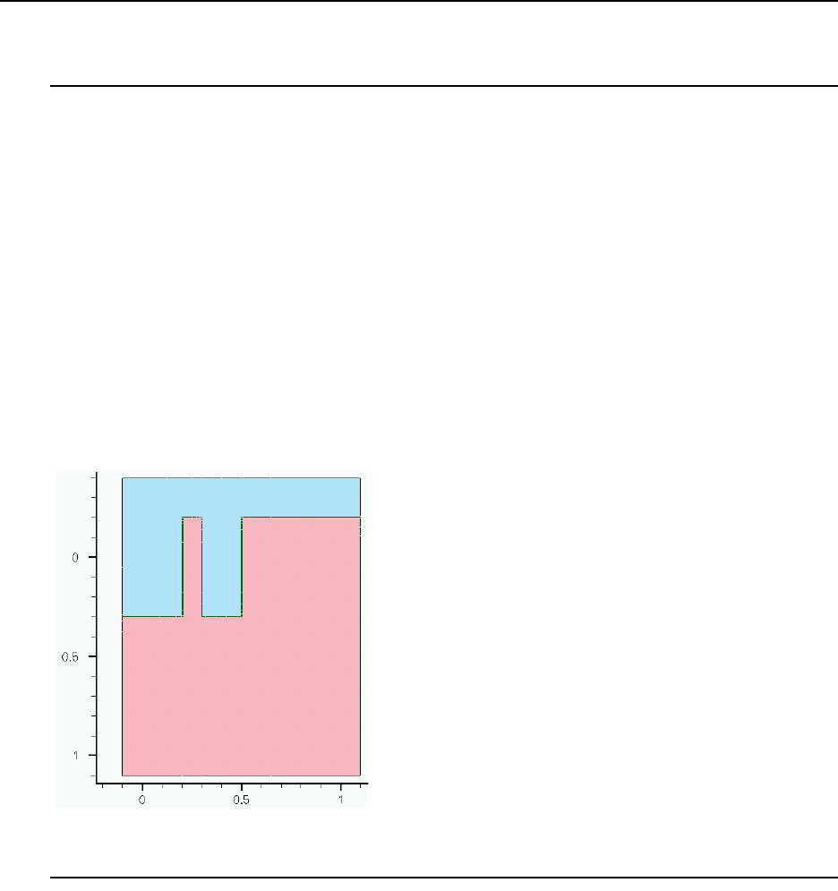
11: Structure Generation

Examples

Sentaurus™ Process User Guide 797

H-2013.03

Examples

Using Polygon and Rectangle Mask in 2D Simulation

line x loc=-0.3 tag=ox

line x loc=-0.2 tag=top

line x loc=1.1 tag=bot

line y loc=-0.1

line y loc=1.1

region silicon xlo=top xhi=bot

init

polygon name=LShape2 segments= {-0.1 -1.5 -0.1 -0.5 0.5 -0.5 0.5 1.5 1.5 \

1.5 1.5 -1.5}

mask name=Mask2 polygons= {LShape2} negative left=0.2 right=0.3 front=-0.1 \

back=0.2

etch silicon anisotropic thickness=0.5 mask=Mask2

struct tdr=final

Figure 135 Final result of 2D anisotropic etching with rectangle and polygon mask

3D Etching after 2D LOCOS Simulation (Sentaurus

Structure Editor Interface)

A 2D simulation result is loaded (LOCOS with nitride layer), modified in 2D, extruded to 3D,

and in 3D the polysilicon and oxide are etched.

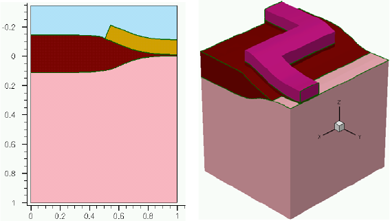
11: Structure Generation

Examples

798 Sentaurus™ Process User Guide

H-2013.03

# load a 2D locos structure

init tdr=initial

mgoals min.normal.size=0.02 accuracy=1e-4 max.box.angle=165 \

normal.growth.ratio=4

refinebox min= {-10 -10 -10} max= {10 10 10} xrefine=0.4 yrefine=0.4 \

zrefine=0.4

# --- allow expanding structure to 3D ---

line z loc=-0.6 spacing=0.1

line z loc=0.5 spacing=0.1

# still in 2D

strip nitride

deposit PolySilicon thickness=100<nm> isotropic

struct tdr=locos1

sde logfile=2d3d.scm on

pdbSet InfoDefault 1

polygon name=LShape2 segments= {-0.1 -0.4 0.6 -0.4 0.6 0.2 1.1 0.2 \

1.1 0.4 0.4 0.4 0.4 -0.2 -0.1 -0.2}

mask name=Mask2 polygons= {LShape2}

etch PolySilicon anisotropic mask=Mask2 thickness=0.41

etch Oxide thickness=30<nm> anisotropic

struct tdr=locos2

Figure 136 (Left) Initial 2D structure after LOCOS formation and (right) final result after

extruding to 3D and etching of poly and oxide

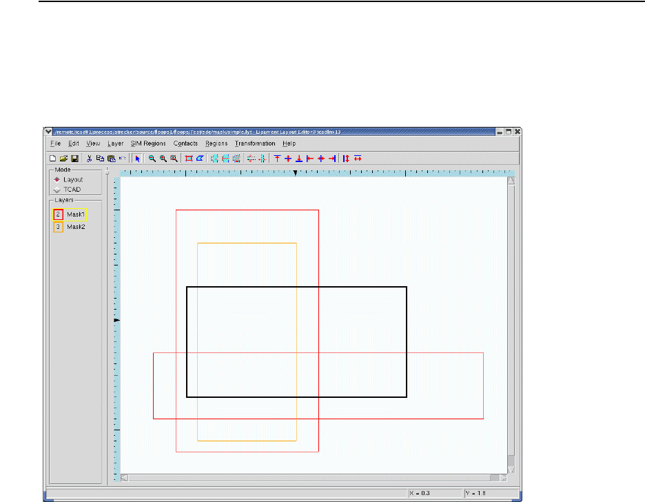
11: Structure Generation

Examples

Sentaurus™ Process User Guide 799

H-2013.03

Using Layout File for 3D Etching (Sentaurus Structure

Editor Interface)

This series of examples demonstrates how to use the layout file simple.lyt to define masks

for 3D etching.

Figure 137 View of simple.lyt file in Ligament Layout Editor

Input file mask0_fps.cmd: The origin of the Sentaurus Process coordinate system coincides

with the origin in simple.lyt; the y-axis of Sentaurus Process is aligned to the vertical axis

in simple.lyt:

line x loc=-0.25 tag=gastop spac=0.05

line x loc=0.0 tag=substop spac=0.01

line x loc=1.5 tag=subsbottom spac=0.2

line y loc=1.65 spac=0.1

line y loc=1.95 spac=0.1

line z loc=0.15 spac=0.1

line z loc=0.6 spac=0.1

region silicon xlo=substop xhi=subsbottom

mgoals min.normal.size=0.02 accuracy=1e-4 max.box.angle=165 \

normal.growth.ratio=4

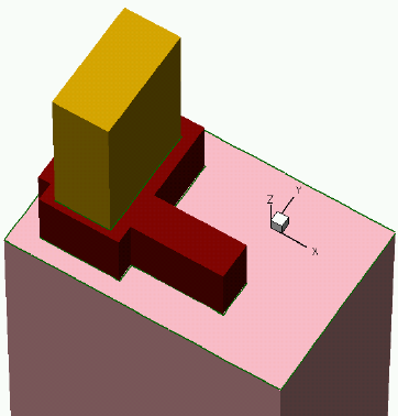
11: Structure Generation

Examples

800 Sentaurus™ Process User Guide

H-2013.03

refinebox min= {-10 -10 -10} max= {10 10 10} xrefine=0.2 yrefine=0.2 \

zrefine=0.2

refinebox interface.materials = {Silicon Oxide}

init

deposit oxide thickness=100<nm> isotropic

sde logfile=mask0.scm on

pdbSet InfoDefault 1

mask layoutfile=simple.lyt

# deposition with masks deposits where there is no mask

# so invert the mask used for deposition

mask name=Mask2 negative

deposit nitride thickness=0.25<um> anisotropic info=1 mask=Mask2

struct bndfile=mask0_0.bnd

etch oxide thickness=120<nm> type=anisotropic mask=Mask1

struct bndfile=mask0_1.bnd

struct tdr=mask0

Figure 138 Final structure after simulation of mask0_fps.cmd

11: Structure Generation

Examples

Sentaurus™ Process User Guide 801

H-2013.03

Input file mask1_fps.cmd: A Cutline2D is used to place the simulation domain in the layout

file. The extensions of the 3D simulation domain in the y- and z-directions must be specified

using line commands. The cutline is defined as the diagonal through the structure used in

mask1_fps.cmd, such that the Sentaurus Process origin is shifted and the coordinate system

is rotated compared to mask0_fps.cmd:

line x loc=-0.25 tag=gastop spac=0.05

line x loc=0.0 tag=substop spac=0.01

line x loc=1.5 tag=subsbottom spac=0.2

line y loc=0. spac=0.1

line y loc=0.4 spac=0.1

line z loc=-0.2 spac=0.1

line z loc=0.15 spac=0.1

region silicon xlo=substop xhi=subsbottom

mgoals min.normal.size=0.02 accuracy=1e-4 max.box.angle=165 \

normal.growth.ratio=4

refinebox min= {-10 -10 -10} max= {10 10 10} xrefine=0.2 yrefine=0.2 \

zrefine=0.2

refinebox interface.materials = {Silicon Oxide}

# define a coordinate transformation for a placement and rotation

# of a layout file

init slice.angle=[CutLine2D 1.65 0.15 1.95 0.6]

deposit oxide thickness=100<nm> isotropic

sde logfile=mask1.scm on

pdbSet InfoDefault 1

# do not specify any name ==> use the cutline from the init command

# to place the Sentaurus Process coordinate system in the layout.

# the first specified point becomes the origin of the Sentaurus Process

# coordinate system and the direction of the cutline becomes the direction

# of the Sentaurus Process z-axis.

mask layoutfile=simple.lyt

# deposition with masks deposits where there is no mask

# so invert the mask used for deposition

mask name=Mask2 negative

deposit nitride thickness=0.25<um> anisotropic info=1 mask=Mask2

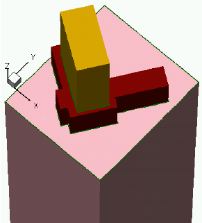
11: Structure Generation

Examples

802 Sentaurus™ Process User Guide

H-2013.03

struct bndfile=mask1_0.bnd

etch oxide thickness=120<nm> type=anisotropic mask=Mask1

struct bndfile=mask1_1.bnd

struct tdr=mask1

Figure 139 Final result of mask1_fps.cmd

Input file mask2_fps.cmd: A SIM3D mask is used, defined in the layout file:

# Use a layout file and place it according to the mask SIM3D, defined in the

# layout file itself.

# SIM3D defines an axis aligned rectangle in the layout plane. The point

# with the smallest layoutX and layoutY coordinates defines the

# origin of the Sentaurus Process coordinate system. The direction of the

# layoutX axis is used for the Sentaurus Process z-axis

# and the direction of the layoutY axis is used for the Sentaurus Process

# y-axis.

# The width of the rectangle (max(layoutX)-min(layoutX)) defines the

# default extension in Sentaurus Process z-direction.

# The height of the rectangle (max(layoutY)-min(layoutY)) defines the

# default extension in Sentaurus Process y-direction.

# If you specify line y and/or line z, your definitions are used.

# Otherwise the default extensions are used to define line y and line z

# when reading the layout file.

line x loc=-0.25 tag=gastop spac=0.05

line x loc=0.0 tag=substop spac=0.01

line x loc=1.5 tag=subsbottom spac=0.2

region silicon xlo=substop xhi=subsbottom

mgoals min.normal.size=0.02 accuracy=1e-4 max.box.angle=165 \

normal.growth.ratio=4

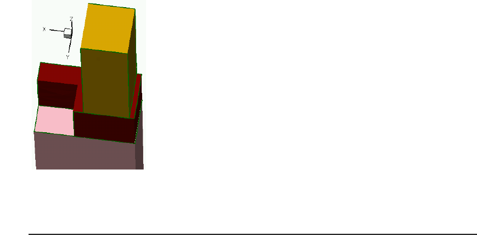
11: Structure Generation

Examples

Sentaurus™ Process User Guide 803

H-2013.03

refinebox min= {-10 -10 -10} max= {10 10 10} xrefine=0.2 yrefine=0.2 \

zrefine=0.2

refinebox interface.materials = {Silicon Oxide}

init

deposit oxide thickness=100<nm> isotropic

sde logfile=mask2.scm on

pdbSet InfoDefault 1

mask layoutfile=simple.lyt name=SIM3D

# In Sentaurus Process, deposition with masks deposits where

# there is no mask so invert the mask used for deposition

mask name=Mask2 negative

deposit nitride thickness=0.25<um> anisotropic info=1 mask=Mask2

struct bndfile=mask2_0.bnd

etch oxide thickness=120<nm> type=anisotropic mask=Mask1

struct bndfile=mask2_1.bnd

struct tdr=mask2

Figure 140 Final simulation result for mask2_fps.cmd; the y- and z-extensions are not

specified in the command file but are taken from the SIM3D mask in simple.lyt

(black line in Figure 137 on page 799)

3D Trench Etching, Sloped Sidewall with Predefined Angle

(Sentaurus Structure Editor Interface)

line x loc=-0.25 tag=gastop spac=0.05

line x loc=0.0 tag=substop spac=0.01

line x loc=0.5 tag=subsbottom spac=0.2

line y loc=0.0 spac=0.1

line y loc=0.4 spac=0.1

11: Structure Generation

Examples

804 Sentaurus™ Process User Guide

H-2013.03

line z loc=0 spac=0.1

line z loc=0.6 spac=0.1

region silicon xlo=substop xhi=subsbottom

mgoals min.normal.size=0.02 accuracy=1e-4 max.box.angle=165 \

normal.growth.ratio=4

refinebox min= {-10 -10 -10} max= {10 10 10} xrefine=0.2 yrefine=0.2 \

zrefine=0.2

refinebox interface.materials = {Silicon Oxide}

init concentration=1.4e+15<cm-3> field=boron wafer.orient=100

deposit oxide thickness=0.01 type=isotropic

fset NitrideThick 0.1

deposit nitride thickness=0.1 type=isotropic

mask name=STI left=-1 right=0.2 front=-1 back=0.4

deposit Photoresist isotropic thickness=0.5

sde logfile=sti3d.scm on

pdbSet InfoDefault 1

etch Photoresist anisotropic thickness=0.5*1.5 mask=STI

struct bndfile=photo1.bnd

fproc etchAngle { Angle Material Depth } {

set alpha [expr ${Angle}*atan(1.0)/45.0] ; #Degree to radiant conv.

set x1 [expr sin($alpha)] ; #x-component of etch directional vector

set x2 [expr cos($alpha)] ; #y-component of etch directional vector

set x3 [expr cos($alpha)] ; #z-component of etch directional vector

set etchRate [expr 1.0/sin($alpha)]

etch material=$Material time=$Depth type=directional \

direction= { $x1 $x2 $x3 } rate=$etchRate

}

fset NitrideAngle 89.0

etchAngle $NitrideAngle Nitride $NitrideThick*1.5

etch Oxide anisotropic thickness=0.02

strip Photoresist

fset TrenchAngle 84.0

fset TrenchDepth 0.2

etchAngle $TrenchAngle Silicon $TrenchDepth

struct bndfile=final.bnd

struct tdr=final

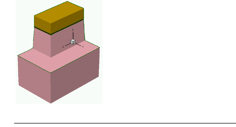
11: Structure Generation

Examples

Sentaurus™ Process User Guide 805

H-2013.03

Figure 141 Final result of simulation of STI etching with predefined sidewall angles

3D Etching after 2D LOCOS Simulation using MGOALS

An example, similar to 3D Etching after 2D LOCOS Simulation (Sentaurus Structure Editor

Interface) on page 797, but with some extra processing steps, can be performed using

MGOALS. The script is as follows:

# Switch off stress relaxation after depo/etch

pdbSet Mechanics EtchDepoRelax 0

# Load a 2D locos structure

init tdr=initial

mgoals resolution=0.2 min.normal.size=0.02 accuracy=1e-4 max.box.angle=165 \

norm

refinebox min= {-10 -10 -10} max= {10 10 10} xrefine=0.4 yrefine=0.4 zrefine=0.

# --- allow expanding structure to 3D ---

line z loc=-0.6 spacing=0.1

line z loc=0.5 spacing=0.1

# Still in 2D

strip nitride

deposit PolySilicon thickness=100<nm> isotropic

struct tdr=locos1

#sde logfile=2d3d.scm on

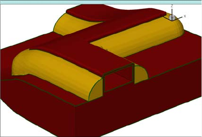
11: Structure Generation

Examples

806 Sentaurus™ Process User Guide

H-2013.03

sde off

pdbSet InfoDefault 2

pdbSet Grid sMesh 1

polygon name=LShape2 segments= {-0.1 -0.4 0.6 -0.4 0.6 0.2 1.1 0.2 1.1 0.4}

mask name=Mask2 polygons= {LShape2}

etch PolySilicon anisotropic mask=Mask2 thickness=0.41

struct tdr=locos2

etch Oxide thickness=30<nm> anisotropic

struct tdr=locos3

mgoals resolution=0.3

deposit oxide thickness=10<nm> isotropic

struct tdr=locos4

mgoals resolution=0.2

deposit nitride thickness=100<nm> isotropic

struct tdr=locos5

etch nitride thickness=120<nm> anisotropic

struct tdr=locos6 bnd

The initial 2D LOCOS structure (initial.tdr) is the left one represented in Figure 136 on

page 798. The sde off command is used to overwrite the standard setting and MGOALS is

used.

Figure 142 Script result simulated with MGOALS; polysilicon and silicon

are not shown to better reveal the structure features

11: Structure Generation

Examples

Sentaurus™ Process User Guide 807

H-2013.03

Structure Assembly in MGOALS

The following scripts creates a tdr file to be “pasted”

set gate 30e-3

set sti 55e-3

set sti_thick 100e-3

set gas_top 86e-3

set silicon_depth 300e-3

set zsize 640e-3

set SiO2gate 1.5e-3

set spacer 30e-3

set spacer_thick 30e-3

set extra 60e-3

set poly 80e-3

set factor 1.1

sde off

line x loc=0.0 tag=xtop

line x loc=$silicon_depth tag=xbottom

line y loc=0.0 tag=yleft

line y loc=[expr 2*$extra + 2*$spacer + 2*$sti + $gate] tag=yright spacing =

0.002

line z loc=0

line z loc=0.05

line z loc=0.1

region silicon xlo=xtop xhi=xbottom

init

#STI

set ll1 [expr 0]

set rr1 [expr $sti]

set ll2 [expr $sti + 2*$extra + 2*$spacer + $gate]

set rr2 [expr $ll2 + $sti]

mask negative name=sti_mask left=$ll1<um> right=$rr1<um>

mask negative name=sti_mask left=$ll2<um> right=$rr2<um>

etch silicon thickness=$sti_thick mask=sti_mask anisotropic

deposit oxide fill coord=[expr -$SiO2gate]

#poly gate

deposit polysilicon thickness=$poly isotropic

set ll3 [expr $sti + $extra+$spacer]

set rr3 [expr $ll3 + $gate]

mask name=gate_mask left=$ll3 right=$rr3

etch polysilicon mask=gate_mask anisotropic thickness=$poly

#spacer

deposit nitride thickness=$spacer_thick isotropic

etch nitride thickness=[expr $spacer_thick * $factor] anisotropic

11: Structure Generation

Examples

808 Sentaurus™ Process User Guide

H-2013.03

#rotate and transform into a 3D structure

transform rotate angle=90 axis = {X}

struct tdr=rotateX

Figure 143 on page 809 (upper right) shows the created structure.

Now, a simple structure is created with the same dimensions in the plane to be pasted and the

structures are put together:

set xsize 0.3

set ysize 0.1

set zsize 0.32

line x loc=0.0 tag=xleft

line x loc=$xsize/2 tag=xmed

line x loc=$xsize tag=xright

line y loc=0.0 tag=ybottom

line y loc=$ysize/2 tag=ymed

line y loc=$ysize tag=ytop

line z loc=0 tag=zinit

line z loc=$zsize/2 tag=zmed

line z loc=$zsize tag=zend

region oxide xlo=xleft xhi=xmed ylo=ymed yhi=ytop zlo=zinit zhi=zmed

region silicon xlo=xleft xhi=xmed ylo=ymed yhi=ytop zlo=zmed zhi=zend

region silicon xlo=xleft xhi=xmed ylo=ybottom yhi=ymed zlo=zinit zhi=zend

region silicon xlo=xmed xhi=xright ylo=ybottom yhi=ytop zlo=zinit zhi=zend

init

sde off

struct tdr = orig

paste direction = "right" tdr = "rotateX"

struct tdr = pasted_right

Figure 143 (upper left) shows the structure created before the paste operation, and the final

result is shown in the lower-left figure.

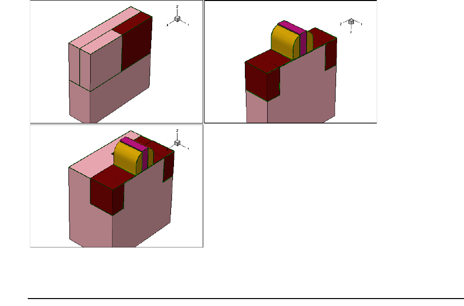
11: Structure Generation

Examples

Sentaurus™ Process User Guide 809

H-2013.03

Figure 143 (Upper left) The initial structure, (upper right) the structure read from the file, and

(lower left) the final structure after paste command

Polygon Creation and Insertion in MGOALS2D

The following script creates a 2D structure and saves it into a file:

set gate 30e-3

set sti 55e-3

set sti_thick 100e-3

set gas_top 86e-3

set silicon_depth 300e-3

set zsize 640e-3

set SiO2gate 1.5e-3

set spacer 30e-3

set spacer_thick 30e-3

set extra 60e-3

set poly 80e-3

set factor 1.1

refinebox min = { 0 0 } max = { 0.1 2 } xrefine = { 0.0012 0.0015 0.0015 }

line x loc=0.0 tag=xtop

line x loc=$silicon_depth tag=xbottom

line y loc=0.0 tag=yleft

line y loc=[expr 2*$extra + 2*$spacer + 2*$sti + $gate] tag=yright spacing =

11: Structure Generation

Examples

810 Sentaurus™ Process User Guide

H-2013.03

0.002

region silicon xlo=xtop xhi=xbottom

init

#STI

set ll1 [expr 0]

set rr1 [expr $sti]

set ll2 [expr $sti + 2*$extra + 2*$spacer + $gate]

set rr2 [expr $ll2 + $sti]

mask negative name=sti_mask left=$ll1<um> right=$rr1<um>

mask negative name=sti_mask left=$ll2<um> right=$rr2<um>

etch silicon thickness=$sti_thick mask=sti_mask anisotropic

deposit oxide fill coord=[expr -$SiO2gate]

#poly gate

deposit polysilicon thickness=$poly isotropic

set ll3 [expr $sti + $extra+$spacer]

set rr3 [expr $ll3 + $gate]

mask name=gate_mask left=$ll3 right=$rr3

etch polysilicon mask=gate_mask anisotropic thickness=$poly

#spacer

deposit nitride thickness=$spacer_thick isotropic

etch nitride thickness=[expr $spacer_thick * $factor] anisotropic

struct tdr=orig

Now, a triangular polygon is created in the xy plane and is called box:

point name=p1 coord = { -0.2 0.2 }

point name=p2 coord = { 0.2 0.25 }

point name=p3 coord = { 0.1 0.1 }

polygon name=box xy points = { p1 p2 p3 }

Finally, the triangular polygon is inserted into the original structure as Aluminum, but only in

the nitride and silicon materials:

insert polygon = "box" replace.materials = { "Silicon" "Nitride" } \

new.material = "Aluminum"

struct tdr=points

Figure 144 on page 811 (upper left) shows the initial structure, and the lower-left figure shows

the results after the insertion.

You a lso c an re ad th e po ly gon fro m a TD R fil e an d insert it later. The following script reuses

the files from the previous example by doing that. It reads the Aluminum material as a polygon,

and inserts it in the original script as oxide in silicon material only:

init tdr=orig

polygon name=box xy tdr = "points_bnd.tdr" materials = "Aluminum"

insert polygon = "box" replace.materials = "Silicon" new.material = "Oxide" \

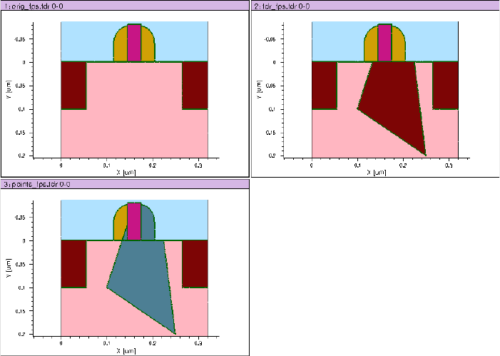
11: Structure Generation

Examples

Sentaurus™ Process User Guide 811

H-2013.03

info=4

struct tdr=tdr

Figure 144 (lower left) shows the results after the insertion.

Figure 144 Use of insert command in a 2D simulation: (upper left) initial 2D structure, (lower

left) triangular polygon being inserted in the initial structure for silicon and nitride

only, and (upper right) the results of reading the triangle of the lower-left figure

and inserting it as oxide in the silicon of the initial structure

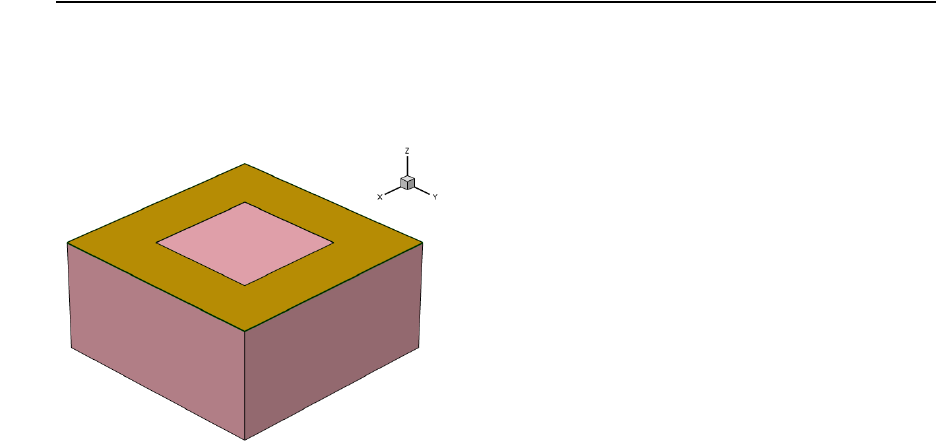
11: Structure Generation

Examples

812 Sentaurus™ Process User Guide

H-2013.03

Polyhedron Creation and Insertion in MGOALS

All the following examples use the structure in Figure 145 as a starting point to be modified by

polyhedron creation and insertion.

Figure 145 Initial 3D structure used for polyhedron creation and insertion examples

Reading a TDR file

This example uses two spheres created with Sentaurus Structure Editor using the following

script:

(sde:clear)

(sdegeo:create-sphere (position 3.0 3.0 4.7) 0.9 "Silicon" "Silicon_1")

(sdegeo:create-sphere (position 0.7 0.7 4.7) 0.9 "Gas" "Gas_2")

(sdeio:save-tdr-bnd "all" "sphere.tdr")

The spheres are inserted into Sentaurus Process. The gas sphere etches the material, while the

silicon one is deposited:

init tdr=initial

refinebox clear

sde off

polyhedron name=sphere tdr=sphere.tdr materials = { Silicon Gas }

insert polyhedron=sphere

struct bndfile=result

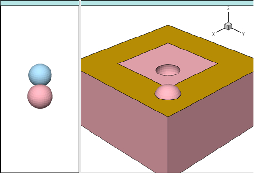
11: Structure Generation

Examples

Sentaurus™ Process User Guide 813

H-2013.03

Figure 146 shows the result of the above script.

Figure 146 (Left) Polyhedra included in a TDR boundary file and (right) effect of inserting

them in initial structure

Extruding a 2D Polygon

This example creates a simple 2D polygon – a triangle:

init tdr=initial

math coord.ucs

refinebox clear

sde off

polygon name=triangle segments = { -4.2 -3.0 3.2 0.5 -4.7 4.2 }

The polyhedron command uses the triangle to extrude in the x-direction:

polyhedron name=prism polygons = { triangle } min=-6 max=2

Finally, to insert it, specify new.material as gas to etch the extruded polygon:

insert polyhedron=prism new.material=Gas

struct bndfile=result

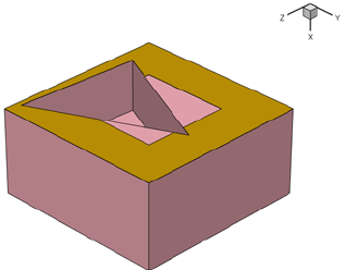
11: Structure Generation

Examples

814 Sentaurus™ Process User Guide

H-2013.03

Figure 147 shows the result.

Figure 147 Etching an extruded polygon

Creating a Polyhedron using Polygons

This example defines the polyhedra from the beginning using polygons:

init tdr=initial

refinebox clear

sde off

point name=p1 coord = { -6.5 2.0 2.0 }

point name=p2 coord = { -2.0 4.0 1.5 }

point name=p3 coord = { -2.0 2.0 3.0 }

point name=p4 coord = { -2.0 1.5 1.0 }

polygon name=face1 points = { p1 p2 p3 }

polygon name=face2 points = { p1 p3 p4 }

polygon name=face3 points = { p1 p2 p4 }

polygon name=face4 points = { p2 p3 p4 }

polyhedron name=tetrahedron polygons = { face1 face2 face3 face4 }

Now, the initial structure is etched using the new polyhedron:

insert polyhedron=tetrahedron new.material=Gas

struct bndfile=result

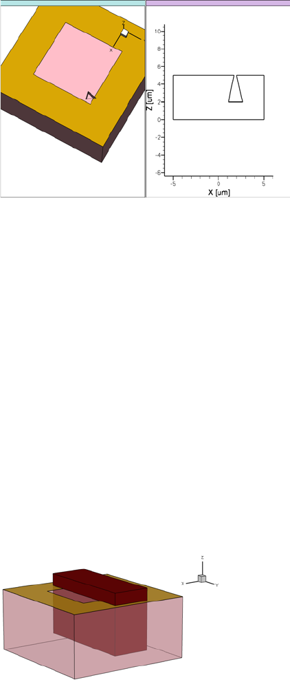
11: Structure Generation

Examples

Sentaurus™ Process User Guide 815

H-2013.03

Figure 148 shows the simulation results.

Figure 148 Etching of a polyhedron defined by using polygons: (left) 3D general view and

(right) y-plane cut view

Defining a Brick

The brick option provides a convenient way to define a rectangular prism by defining the

lower and upper corners. The script is as follows:

init tdr=initial

refinebox clear

sde off

polyhedron name=smallCube brick = { -6 -4 -2 -1 4.5 1 }

Now, you can use the polyhedron to insert an oxide brick into the simulation:

insert polyhedron=smallCube new.material=Oxide

struct bndfile=result

Figure 149 shows the result.

Figure 149 Oxide brick inserted in initial structure

11: Structure Generation

References

816 Sentaurus™ Process User Guide

H-2013.03

References

[1] J. A. Sethian, Level Set Methods and Fast Marching Methods: Evolving interfaces in

computational geometry, fluid mechanics, computer vision, and materials science,

Cambridge: Cambridge University Press, 1999.

Sentaurus™ Process User Guide 817

H-2013.03

CHAPTER 12 ICWBEV Plus Interface for

Layout-driven Simulations

This chapter presents strategies for using the IC WorkBench

EV Plus–TCAD Sentaurus interface.

Overview

The IC WorkBench EV Plus (ICWBEV Plus)–TCAD Sentaurus interface drives the TCAD

simulations from the GDSII or OASIS layout file provided by designers, which could be at any

level of integration in the hierarchy: full chip, test chip, or a single cell.

The TCAD simulation domain can be conveniently chosen using specific markups in the layout

file. A single process flow can be defined for all devices in the layout and can be applied easily

with minimal adjustments for 1D, 2D, and 3D simulation domains. For meshing, it provides

the unique feature of layout-driven meshing. Electrical contacts can be defined easily using

auxiliary masks.

This chapter includes the following sections:

■ICWBEV Plus Introduction for TCAD Users on page 818 provides basic ICWBEV Plus

training, especially with relevance to TCAD.

■Files Relevant to ICWBEV Plus–TCAD Sentaurus on page 828 introduces the relevant

files and file formats used in the ICWBEV Plus–TCAD Sentaurus interface. Specifically,

the Sentaurus markup file (*_mkp.mac) and TCAD layout file (*_lyt.mac).

■ICWBEV Plus Batch Mode and Macros on page 834 introduces working with macros and

running ICWBEV Plus in batch mode.

■TCAD Layout Reader of Sentaurus Process on page 835 presents the TCAD layout reader

of Sentaurus Process that provides a file-based interface between ICWBEV Plus and

Sentaurus Process.

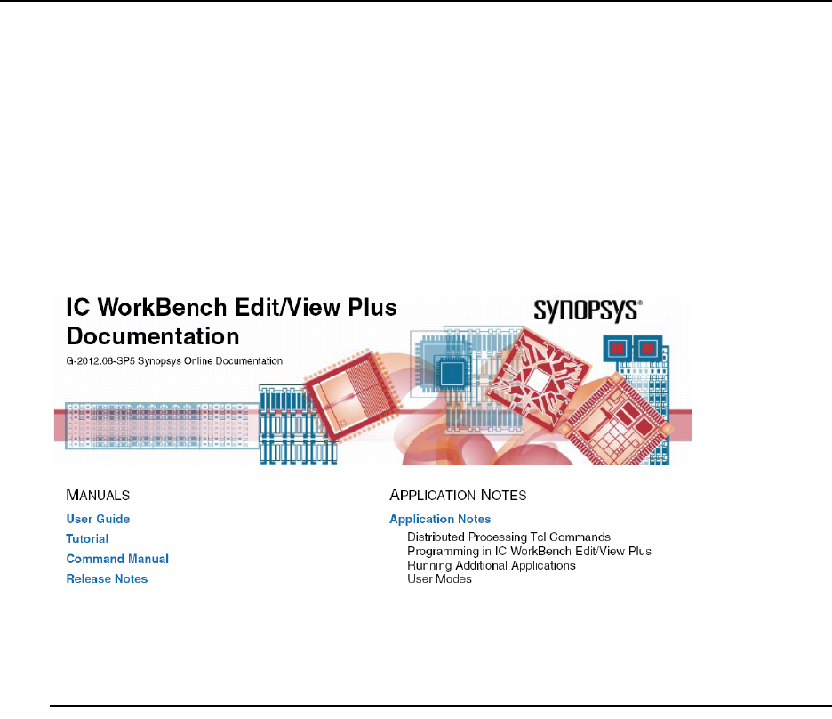
12: ICWBEV Plus Interface for Layout-driven Simulations

ICWBEV Plus Introduction for TCAD Users

818 Sentaurus™ Process User Guide

H-2013.03

ICWBEV Plus Introduction for TCAD Users

Before discussing the ICWBEV Plus–TCAD Sentaurus interface, it is important to have an

understanding of ICWBEV Plus itself.

The general ICWBEV Plus training is a good starting point. Here, the focus is mainly on

ICWBEV Plus operations that are most relevant to TCAD Sentaurus users.

For details, refer to the ICWBEV Plus tutorials and manuals, which are accessed through the

main window of ICWBEV Plus (Help > Topics). The homepage of the online documentation

is displayed (see Figure 150).

Figure 150 Homepage of ICWBEV Plus online documentation

The first step consists of opening a layout file, which is typically in GDSII format.

Opening GDSII Layout Files

To open a GDSII or an OASIS layout file:

1. Set the environment variable ICWBEV_USER to activate the ICWBEV Plus Sentaurus User

Mode:

setenv ICWBEV_USER SENTAURUS

2. Launch ICWBEV Plus by typing:

icwbev

3. Select the file to be opened: File > Open > Browse for GDSII > Select GDSII > Open.

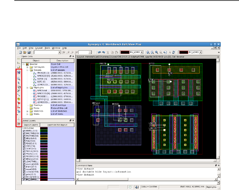
12: ICWBEV Plus Interface for Layout-driven Simulations

ICWBEV Plus Introduction for TCAD Users

Sentaurus™ Process User Guide 819

H-2013.03

NOTE Use ICWBEV Plus Version I-2013.12 or later. Earlier versions feature

a slightly different user interface. Refer to the Sentaurus™ Process

User Guide Version H-2013.03 for an introduction to the user interface

for earlier versions of ICWBEV Plus. For G-2012.06-SP5 versions of

ICWBEV Plus, use setenv ICWBEV_USER SENTAURUS_BETA to

activate the user interface described here.

Graphical User Interface of ICWBEV Plus

Figure 151 shows the graphical user interface (GUI) of ICWBEV Plus and illustrates the

typical layout of work, panes, and toolbars. The panes can be moved and reconfigured as

needed.

Figure 151 ICWBEV Plus main window, with TCAD Sentaurus–specific buttons (shown in

red box at left)

Figure 151 includes the following TCAD-relevant items in the GUI:

■The Open Cells pane contains details about layers and markups including the TCAD-

relevant markups.

■The Layout Layers pane shows the list of layers.

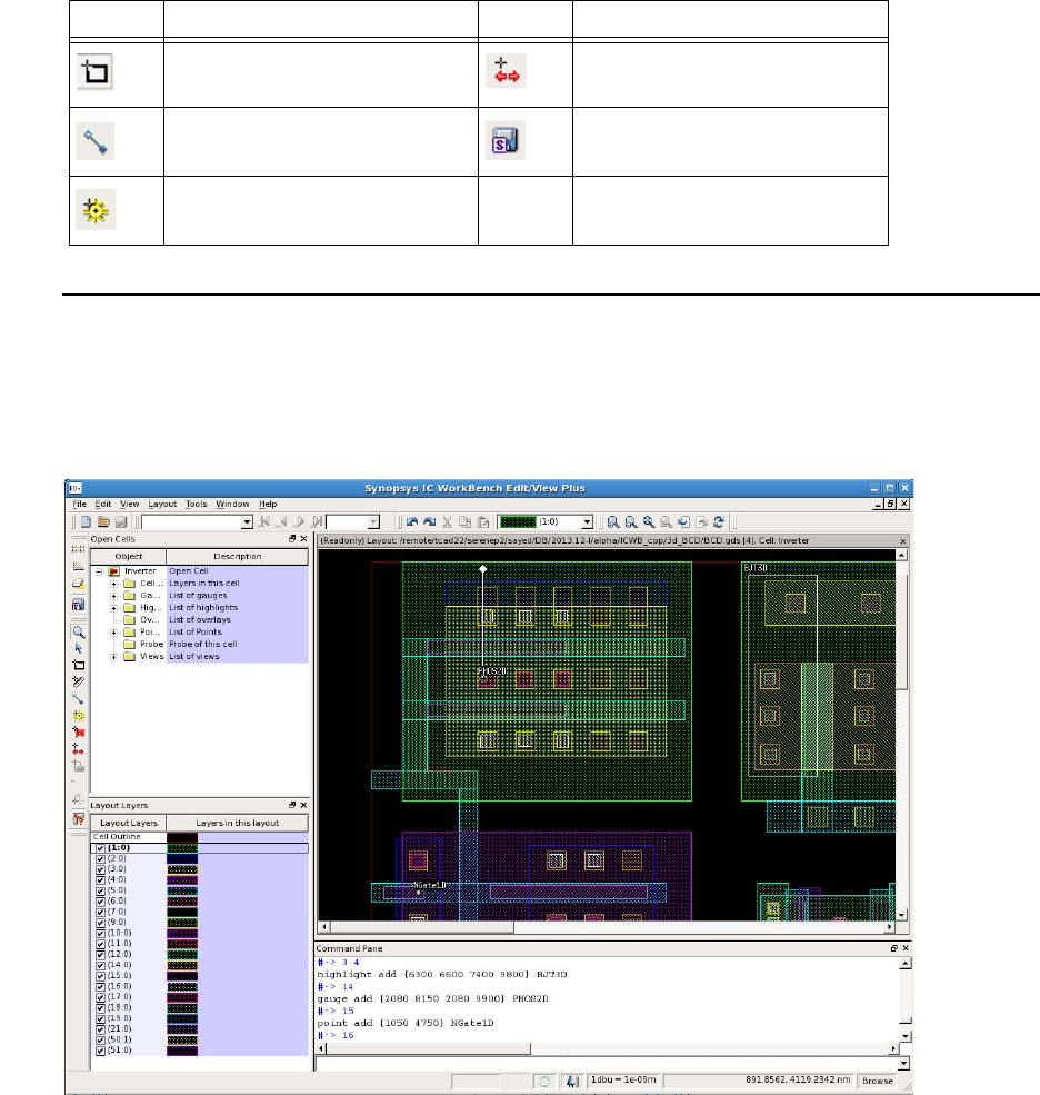
12: ICWBEV Plus Interface for Layout-driven Simulations

ICWBEV Plus Introduction for TCAD Users

820 Sentaurus™ Process User Guide

H-2013.03

■The Command Pane shows commands after GUI operations. Commands also can be

entered directly in this pane.

Table 73 describes the relevant toolbar buttons of the TCAD Sentaurus toolbar.

Sentaurus Markups

Sentaurus markups are used to add the simulation domain in 1D, 2D, and 3D domains as

needed. The Command Pane in Figure 152 shows the commands after adding Sentaurus

markups in the layout using GUI actions.

Figure 152 Adding Sentaurus markups to a layout

Table 73 TCAD Sentaurus–specific toolbar buttons

Button Description Button Description

3D simulation domain (highlight) Stretch utility

2D simulation domain (gauge) Save markups or save TCAD layout

1D simulation domain (point)

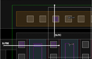
12: ICWBEV Plus Interface for Layout-driven Simulations

ICWBEV Plus Introduction for TCAD Users

Sentaurus™ Process User Guide 821

H-2013.03

To add a 3D simulation domain (highlight), a 2D simulation domain (gauge), or a 1D

simulation domain (point), click the respective toolbar button and draw a rectangle, a line, or a

point on the layout, respectively.

NOTE A 2D simulation domain (gauge) has a direction. The starting point is

given as an open diamond, and the endpoint is given as a filled diamond.

A gauge that runs parallel to an edge of a layer must have a finite

orthogonal distance to that edge. If a gauge is collinear with the edges

of a layer, this edge might not be included in the 2D mask.

The default naming convention is:

■For highlights, SIM3D<n>.

■For gauges, SIM2D<n>.

■For a point, SIM1D<n>.

where <n> is an automatically incremented number.

For 2D TCAD simulations, it can be useful to work with composite simulation domains, for

example, when the different contacts in a device layout cannot be connected by a single straight

line. In this case, it is not possible to perform a 2D device simulation after a 2D process step

using a single 2D simulation domain. However, a 2D TCAD simulation using a composite 2D

simulation domain is feasible. In this case, the various 2D cuts in the layout are daisy-chained

to form a composite 2D simulation domain.

An example of a composite simulation domain is shown in Figure 153, which shows a close-

up of the layout of a bipolar transistor with two 2D TCAD simulation domains. The simulation

domain labeled BJTBE cuts through two base–contact fingers and one emitter finger. The

simulation domain labeled BJTC cuts through the collector contact.

NOTE The two simulation domains are orthogonal and not contiguous.

Figure 153 Layout of a bipolar transistor with two 2D simulation domains: BJTBE cuts

through two base–contact fingers and one emitter finger, and BJTC cuts through

the collector contact

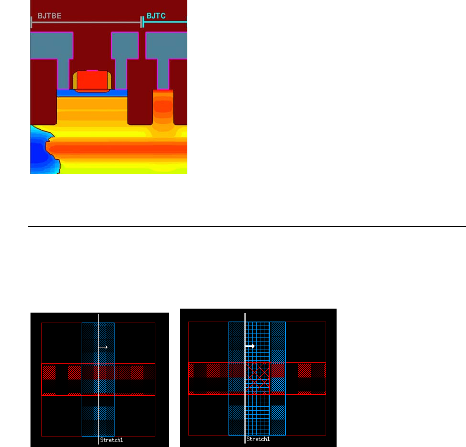
12: ICWBEV Plus Interface for Layout-driven Simulations

ICWBEV Plus Introduction for TCAD Users

822 Sentaurus™ Process User Guide

H-2013.03

Figure 154 shows the 2D TCAD simulation results obtained with a composite simulation

domain consisting of both the BJTBE and BJTC domains. Using a composite simulation

domain allows simulating a functional bipolar junction transistor (BJT) even for a 2D TCAD

simulation.

Figure 154 Two-dimensional TCAD simulation results using composite simulation domain

consisting of the 2D domains BJTBE and BJTC

Stretch Utility

The stretch utility provides a convenient way to parameterize a layout by inserting a uniformly

stretched segment into the layout. For example, this feature can be used to generate a set of

transistors that have different gate lengths but are otherwise identical.

Figure 155 (Left) Snapshot of sample ICWBEV Plus layout with stretch utility line and (right)

effective layout seen by Sentaurus Process when the layout is loaded with a

positive stretch amount

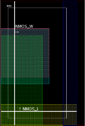
12: ICWBEV Plus Interface for Layout-driven Simulations

ICWBEV Plus Introduction for TCAD Users

Sentaurus™ Process User Guide 823

H-2013.03

A stretch line must be defined in ICWBEV Plus first. The stretch amount is set after loading

the TCAD layout with the Sentaurus Process command:

icwb stretch name= "<stretch-name>" value= <stretch-amount>

This feature can be used for simple parameterization of layouts for quantities such as threshold

rolloff. Figure 156 shows a close-up of the layout containing an NMOS transistor. In addition,

two stretch lines are shown. The stretch line labeled NMOS_W is used to vary gate width, and the

one labeled NMOS_L is used to vary the gate length in an NMOS.

To add a stretch line:

■Click the stretch utility toolbar button, and draw a line across the required region in the

layout.

NOTE The stretch line must cross the entire simulation domain to which it

should be applied. Stretch lines can be used for 2D and 3D simulation

domains.

Figure 156 Adding stretch lines in a layout to vary gate width and gate length

Figure 157 on page 824 shows the resulting changes in the NMOS gate width and gate length.

The default naming scheme for a stretch line is Stretch<n>.

For example, to apply a stretch at run-time in Sentaurus Process, use a command such as:

icwb stretch name= "NMOS_W" value=@Stretch@

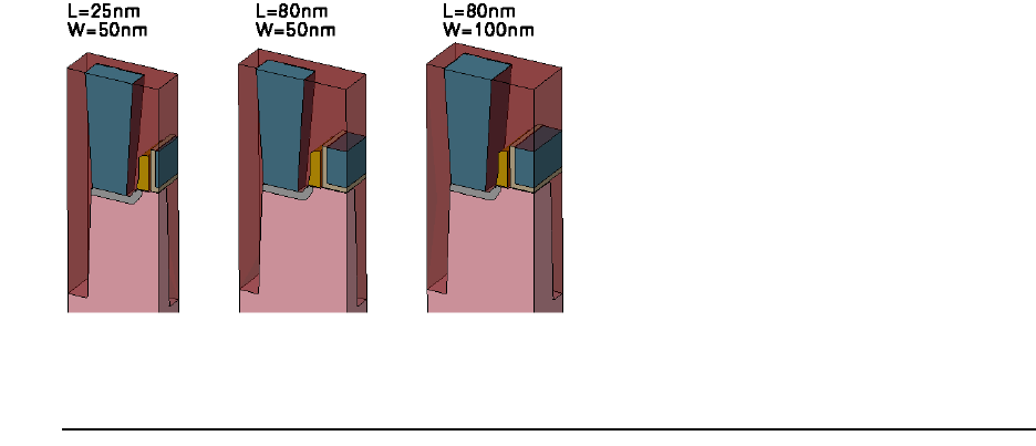
12: ICWBEV Plus Interface for Layout-driven Simulations

ICWBEV Plus Introduction for TCAD Users

824 Sentaurus™ Process User Guide

H-2013.03

where NMOS_W is the name of the stretch variable. Here, the amount of stretching is defined

using the Sentaurus Workbench variable @Stretch@. A positive stretch value is used for

expansion; a negative value leads to shrinkage.

Figure 157 Effect of stretch utility on 3D NMOS structure showing variation in width and

length

Renaming Markups

Markups can be renamed and edited.

To rename markups:

1. View > Views > Open Cells.

2. Expand the markup type, for example, Highlights.

3. Click the respective Sentaurus Process markup to edit the name.

4. Click the coordinates to edit the coordinate values.

Figure 158 on page 825 shows the Open Cells pane, displaying the list of Sentaurus Process

markups and their coordinates that can be edited as required.

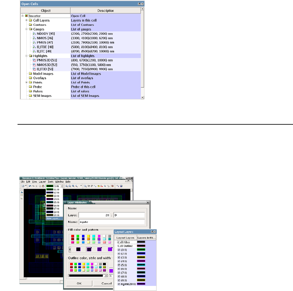
12: ICWBEV Plus Interface for Layout-driven Simulations

ICWBEV Plus Introduction for TCAD Users

Sentaurus™ Process User Guide 825

H-2013.03

Figure 158 Open Cells pane showing list of objects with descriptions

Auxiliary Layers

Auxiliary layers are used, for example, to denote the position of electrical contacts in a layout.

To add auxiliary layers, first a layer must be declared and attributes must be defined. Figure 159

illustrates how to define a layer and its attributes.

Figure 159 Defining a layer and its attributes

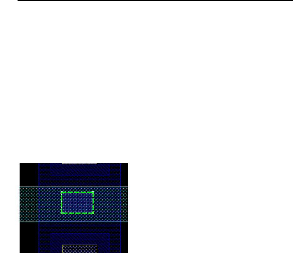
12: ICWBEV Plus Interface for Layout-driven Simulations

ICWBEV Plus Introduction for TCAD Users

826 Sentaurus™ Process User Guide

H-2013.03

To add auxiliary layers, draw a polygon defining the region of the layer:

1. Open the layout for editing: Edit > Cell.

2. Select the active layer.

3. Select the shape tool.

4. Draw a polygon.

Editing Polygons

If required, polygons can be edited. You can edit polygons by either:

■Resizing a rectangle.

■Converting a rectangle to a polygon.

Resizing a Rectangle

To resize a rectangle:

1. If not already open, open the layout for editing: Edit > Cell.

2. Activate the selector tool.

3. Click the polygon edge to select it.

4. Move the edge as needed.

Figure 160 shows a rectangle highlighted for editing.

Figure 160 Moving the edge of a rectangle: select the rectangle and drag an edge

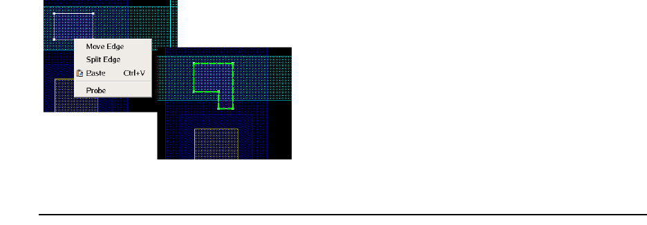
12: ICWBEV Plus Interface for Layout-driven Simulations

ICWBEV Plus Introduction for TCAD Users

Sentaurus™ Process User Guide 827

H-2013.03

Converting a Rectangle to a Polygon

To convert a rectangle to a polygon:

1. Click the polygon edge to select it.

2. Right-click and select Split Edge.

3. Move the edge as needed.

Figure 161 illustrates the procedure.

Figure 161 Converting a rectangle to a polygon

Nonaxis-aligned Simulation Domains

The ICWBEV Plus–TCAD Sentaurus interface supports nonaxis-aligned domains. To realize

nonaxis-aligned simulation domains, the GDSII layout is rotated by a given angle, and the

TCAD simulation domain is added as discussed in Sentaurus Markups on page 820.

To rotate a GDSII layout:

1. Layout > Transform.

2. In the Cell Transformation dialog box, enter the values of the fields as required.

Figure 162 on page 828 shows the transformation of a GDSII layout and the transformation

parameters.

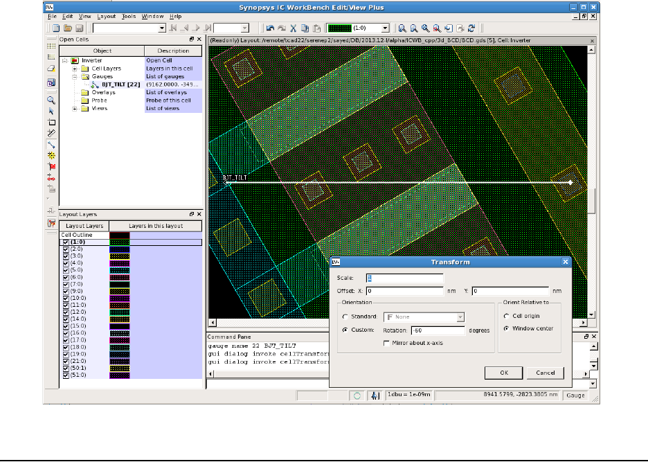
12: ICWBEV Plus Interface for Layout-driven Simulations

Files Relevant to ICWBEV Plus–TCAD Sentaurus

828 Sentaurus™ Process User Guide

H-2013.03

Figure 162 Rotation of layout with transformation parameters

Files Relevant to ICWBEV Plus–TCAD Sentaurus

After adding Sentaurus Process markups in ICWBEV Plus, the markup information is saved in

two different files:

■Sentaurus markup file: This file format is based on the standard ICWBEV Plus macro

language. It can be used to reload and re-edit Sentaurus Process markup. It also contains a

reference to the original, potentially large, GDSII file.

■TCAD layout file: This file format is used as an internal file format for the exchange of

layout information between ICWBEV Plus and TCAD Sentaurus. It is based on the

standard ICWBEV Plus macro language. This file is flat and does not contain a reference

to the GDSII file. It is a small file because it contains only the parts of the layout needed

for TCAD Sentaurus.

After performing the necessary operations on the layout file, save the resulting Sentaurus

markup file.

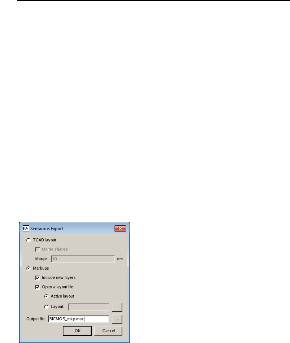
12: ICWBEV Plus Interface for Layout-driven Simulations

Files Relevant to ICWBEV Plus–TCAD Sentaurus

Sentaurus™ Process User Guide 829

H-2013.03

Saving the Sentaurus Markup File

To save a Sentaurus markup file:

1. Click the Save markups button (see Table 73 on page 820).

The Sentaurus Export dialog box is displayed (see Figure 163).

2. Select the Markups option.

3. If you have added auxiliary layers, which you do not want to store in the GDSII file, select

the Include new layers option.

NOTE Including new layers in the markup file keeps the original GDSII file

intact.

4. To open a specific layout file when reloading the markup file, select the Open a layout file

option:

a) Active layout: Select this option when using a centrally located GDSII layout. This

option is particularly useful when working with a very large full-chip layout.

b) Layout: Select this option when working with an edited or a local version of the GDSII

layout. Specify the name of the layout.

5. Type the file name in the Output file field.

The recommended extension for saving the file is _mkp.mac, for example,

BiCMOS_mkp.mac.

6. Click OK.

Figure 163 Sentaurus Export dialog box

12: ICWBEV Plus Interface for Layout-driven Simulations

Files Relevant to ICWBEV Plus–TCAD Sentaurus

830 Sentaurus™ Process User Guide

H-2013.03

The corresponding script command is:

sentaurus export markups <name>_lyt.mac [-newLayers]

[-active | -reference <gdsfilename>]

Contents of Sentaurus Markup File

This section describes a typical markup file with a brief explanation. For a description of

keywords, refer to the IC WorkBench EV Plus User Guide.

Version information:

# Sentaurus markups information - Wed Sep 11 15:11:17 2013

# Version - G-2012.06-SP5.355225 (Production)

Setting for treating self-intersection: By default, all layers are ORed. This convention is

expected by all subsequent tools and, therefore, this setting should not be altered.

default winding 1

Pointer to layout file:

layout open [<path>]/BICMOSinverter.gds Inverter

Global transformations:

cell transform 1 0 0 0 0

Layer declarations and display settings:

layer configure 1:0 -name NWELL -fill #00ff00 -pattern fill12-a

-outline #00ff00 -lineStyle solid -lineWidth 1

Open cell for editing (here, for adding new polygons):

cell edit_state 1

Auxiliary layers:

polygon -layer 20:0 {950 5150 950 5350 1150 5350 1150 5150}

...

Simulation domains:

point add {8900 8100} Emit1D

gauge add {2100 7900 2100 10000} PMOS

highlight add {7900 7550 9900 9900} BJT3D

...

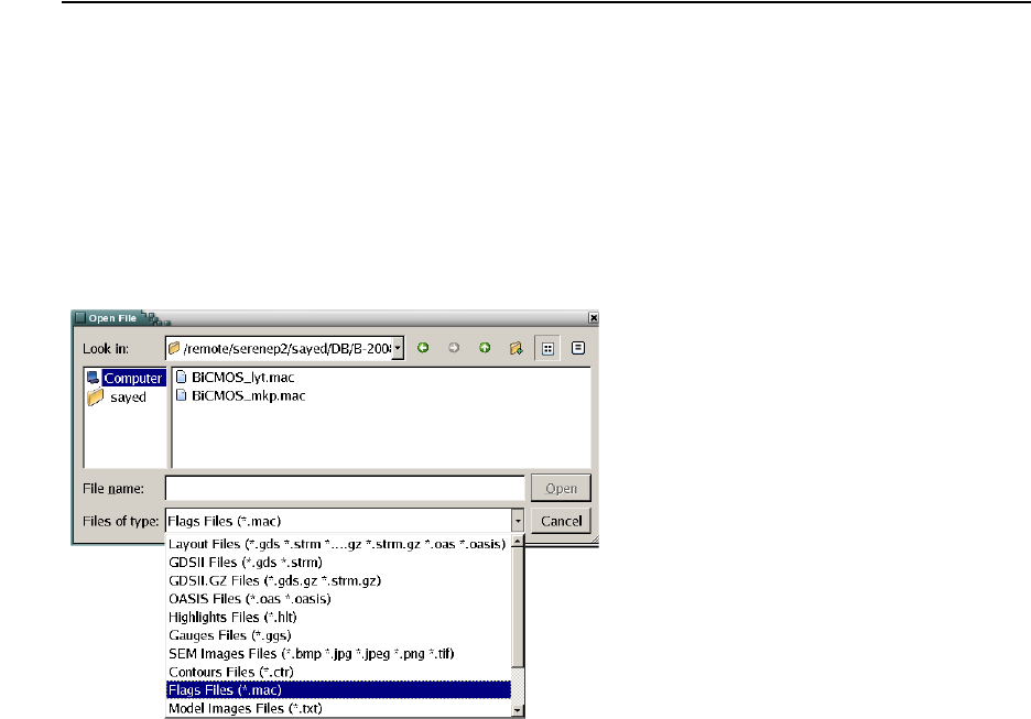
12: ICWBEV Plus Interface for Layout-driven Simulations

Files Relevant to ICWBEV Plus–TCAD Sentaurus

Sentaurus™ Process User Guide 831

H-2013.03

File end:

select clear

catch {view default}

Reloading the Markup File

To edit a markup file, you must reload it.

To reload a markup file:

1. File > Open.

The Open File dialog box is displayed (see Figure 164).

2. In the Files of type field, select Flag Files (*.mac) or Macro Files (*.mac).

Figure 164 Open File dialog box for reloading the markup file

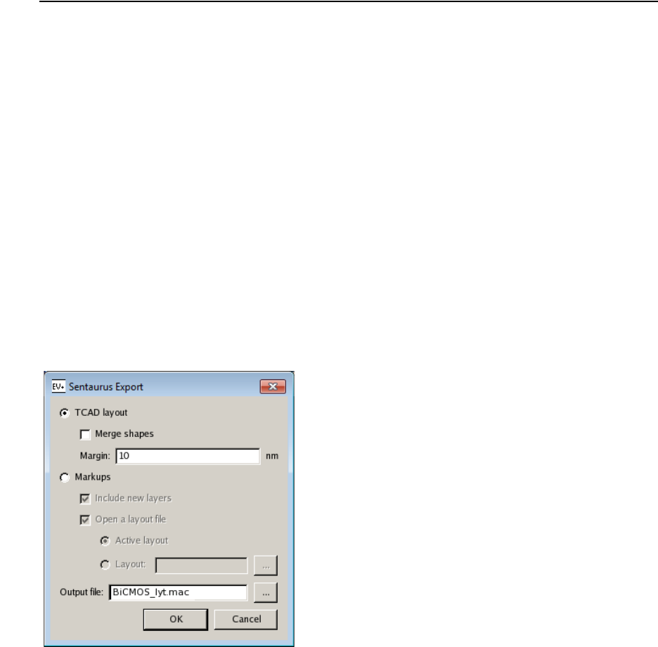
12: ICWBEV Plus Interface for Layout-driven Simulations

Files Relevant to ICWBEV Plus–TCAD Sentaurus

832 Sentaurus™ Process User Guide

H-2013.03

Saving the TCAD Layout File

To save the TCAD layout file:

1. Click the Save TCAD layout button (see Table 73 on page 820).

The Sentaurus Export dialog box is displayed (see Figure 165).

2. Select the TCAD layout option.

3. A layer in a layout can be defined by a large number of touching or overlapping polygons.

To merge all these polygons into a smaller number of possibly more complex polygons,

select the Merge shapes option.

4. For better viewing, layers are padded 10 units (nm). To change the padding value, edit the

Margin field.

5. Type the file name in the Output file field.

The recommended extension for the TCAD layout file is _lyt.mac, for example,

BiCMOS_lyt.mac.

6. Click OK.

Figure 165 Sentaurus Export dialog box, saving the TCAD layout file

The corresponding script command is:

sentaurus export layout <name>_lyt.mac [-merge | -noMerge] [-margin <number>]

12: ICWBEV Plus Interface for Layout-driven Simulations

Files Relevant to ICWBEV Plus–TCAD Sentaurus

Sentaurus™ Process User Guide 833

H-2013.03

Contents of TCAD Layout File

This section describes the contents of the TCAD layout file and the differences between the

contents of the Sentaurus markup file and TCAD layout file.

Version information: Same as Contents of Sentaurus Markup File on page 830.

Setting for treating self-intersection: Same as Contents of Sentaurus Markup File.

Pointer to layout file: Commented out.

Global transformations: Commented out.

Initialization of this self-contained layout:

layout new <cell name> -dbu 1e-09

Layer declarations and display settings: Same as Contents of Sentaurus Markup File.

File end: same as Contents of Sentaurus Markup File.

Simulation domains in a layout file are described below. Point, gauge, and highlight

coordinates are mentioned first, and all polygons associated with the given simulation domains

are listed:

■1D simulation domains:

point add {8900 8100} Emit1D

polygon -layer 1:0 {8890 8090 8910 8090 8910 8110 8890 8110}

...

■2D simulation domains:

gauge add {2100 7900 2100 10000} PMOS

rectangle -layer 1:0 {2090 10010 2110 7890}

...

■3D simulation domains:

highlight add {7900 7550 9900 9900} BJT3D

polygon -layer 1:0 {7890 7540 9910 7540 9910 9910 7890 9910}

...

12: ICWBEV Plus Interface for Layout-driven Simulations

ICWBEV Plus Batch Mode and Macros

834 Sentaurus™ Process User Guide

H-2013.03

Reloading the TCAD Layout File

For debugging purposes, reload the TCAD layout file.

To reload the file:

■File > Open > Macro File (*.mac).

NOTE Do not extract a TCAD layout from a reloaded TCAD layout. TCAD

layout files should always be extracted from the Sentaurus markup file.

ICWBEV Plus Batch Mode and Macros

Starting ICWBEV Plus in Batch Mode

To extract the TCAD layout file in batch mode, add the following command to the end of the

markup file:

sentaurus export layout <name>_lyt.mac [-merge | -noMerge] [-margin <number>]

exit

To start ICWBEV Plus in batch mode run the following command from the shell prompt:

> icwbev -nodisplay -run <name>_mkp.mac

ICWBEV Plus Macros

ICWBEV Plus macros can be used to create simple layouts. An example of a macro is:

default winding 1

layout new a -dbu 1e-09

cell transform 1.0 0.0 0 0.0 0.0

layer add 0:0

layer configure 0:0 -name {} -fill #ff0000

layer add 1:0

layer configure 1:0 -name {} -fill #ff0000

cell edit_state 1

polygon -layer 0:0 {0 0 0 100 50 100 50 0}

polygon -layer 1:0 {-25 25 75 25 75 75 -25 75}

select clear

catch {view default}

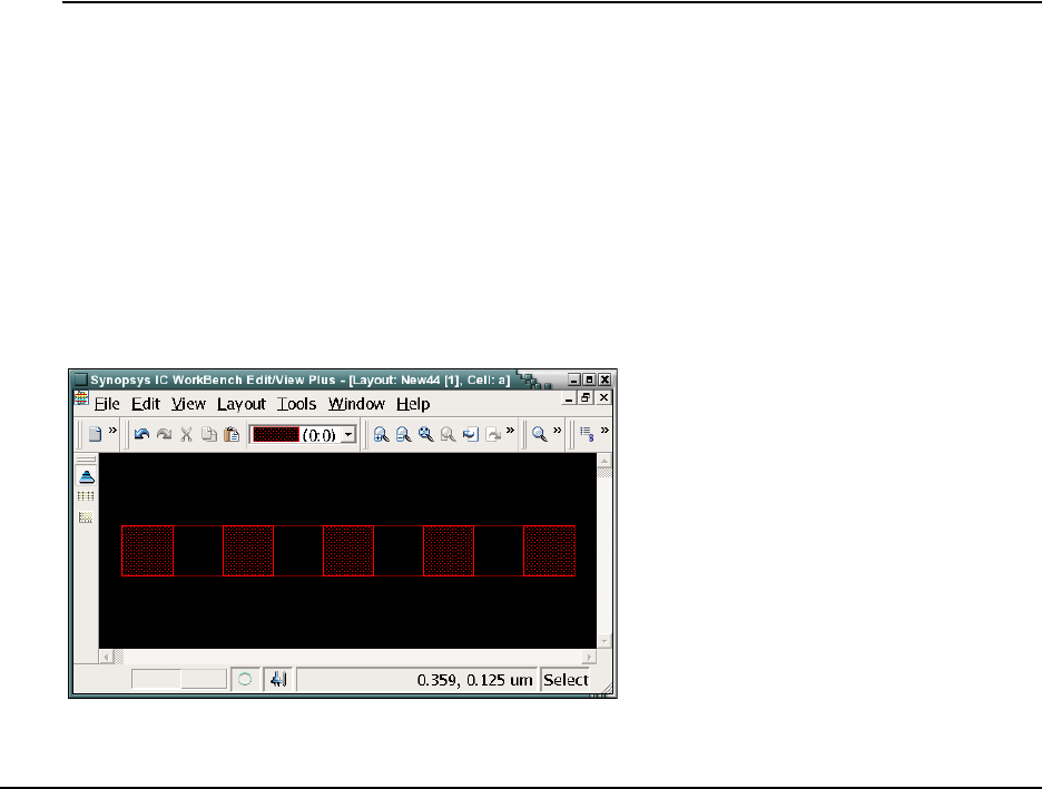
12: ICWBEV Plus Interface for Layout-driven Simulations

TCAD Layout Reader of Sentaurus Process

Sentaurus™ Process User Guide 835

H-2013.03

Tcl-based Macros for Layout Parameterization

The macro language of ICWBEV Plus is Tcl based. Figure 166 shows a rectangle that has been

replicated four times. The following Tcl command performs the replication:

layout new a -dbu 1e-09

layer configure 0:0 -name {}

cell edit_state 1

set SHIFTS [list 0 100 200 300 400]

foreach SHIFT $SHIFTS {

eval rectangle -layer 0:0 { $SHIFT 0 [expr 50+$SHIFT] 50 }

}

Figure 166 Shift operation using macros

TCAD Layout Reader of Sentaurus Process

The TCAD layout reader of Sentaurus Process provides a file-based interface between

ICWBEV Plus and Sentaurus Process. Some of its key features include:

■Loading the TCAD layout (optional rescaling)

■Layout query functions

■Selecting a simulation domain

■Applying stretches

■Creating masks

■Mask-driven meshing

■Mask-driven contact assignment

The following sections discuss these features in detail.

12: ICWBEV Plus Interface for Layout-driven Simulations

TCAD Layout Reader of Sentaurus Process

836 Sentaurus™ Process User Guide

H-2013.03

Loading the TCAD Layout

To load a TCAD layout in Sentaurus Process, use the following command:

icwb filename= "<filename.mac>" [scale=<scale>]

Coordinates found in the TCAD layout file are multiplied by the value of the optional

parameter scale as the file is read.

For example, to load the TCAD layout file BiCMOS_lyt.mac and apply a rescaling factor of

to convert the ICWBEVPlus default unit of nanometer to the Sentaurus Process

default unit of micrometer:

icwb filename= "BiCMOS_lyt.mac" scale=1e-3

Finding Simulation Domains

To generate a list of the simulation domains:

icwb list domains

For example:

set Domains [icwb list domains]

-> icwb: Domains -> Emit1D NBODY NMOS BJT3D PMOS3D

Finding Layer Names and Layer IDs

Each layer in the TCAD layout file has a unique ID of the form <int>:<int>, for example

3:0. A layer also can have an optional explicit layer name such as NWELL. If no explicit layer

name has been set in ICWBEV Plus, the TCAD layout reader uses the layer ID as the default

layer name. The TCAD layout reader refers to layers always by the layer name.

To find the layer names:

icwb list layerNames

For example:

set LNames [icwb list layerNames]

-> icwb: LNames -> NWELL NPDIFF POLY EMIT METAL CONT ndrain ngate nsource base

emitter collect

11000⁄

12: ICWBEV Plus Interface for Layout-driven Simulations

TCAD Layout Reader of Sentaurus Process

Sentaurus™ Process User Guide 837

H-2013.03

To find the layer IDs:

icwb list layerIDs

For example:

set LIDs [icwb list layerIDs]

-> icwb: LIDs -> 1:0 2:0 3:0 4:0 5:0 6:0 7:0 8:0

Selecting the Simulation Domain

To select a single or a composite simulation domain:

icwb domain = <domain-name> | <list-of-2d-domain-names>

For example, to select a single simulation domain (which can be 1D, 2D, or 3D):

icwb domain = { PMOS }

To define a composite simulation in 2D:

icwb domain = { NBODY NMOS PMOS BJTBE BJTC }

Loading a GDSII Layout

To load a GDSII layout directly in Sentaurus Process, use the command:

icwb gds.file=<c> cell=<c> layer.names= {<list>} layer.numbers= {<list>}

sim2d | sim3d= {<n>} [domain.name=<c>] [scale= <n>]

[stretches= {<c>= {<n>}}]

For example:

icwb gds.file= BCD.gds cell= Inverter \

layer.numbers= "1:0 2:0 3:0 4:0 5:0 6:0 7:0 8:0" \

layer.names= "NWELL NACTIVE PACTIVE NPLUS POLY PBASE EMIT CONT" \

sim3d = "6300 3500 7750 3750" \

stretches= {lgate= {7025 3400 7025 3850}} scale= 1e-3

The domain.name argument defines the name of the simulation domain. If no name is

specified, SIM3D is used for a 3D domain, and SIM2D is used for a 2D domain.

The domain will be set to be the current domain automatically, so you do not need to call

icwb domain=<c> before using other icwb commands.

12: ICWBEV Plus Interface for Layout-driven Simulations

TCAD Layout Reader of Sentaurus Process

838 Sentaurus™ Process User Guide

H-2013.03

NOTE The simulation domain and the stretches are defined using layout

coordinates.

This option does not support composite simulation domains.

This option does not require access to ICWBEV Plus.

Finding Domain Dimensions

To find the domain dimensions:

icwb dimension

This command returns 3 for 3D simulation domains (highlight), 2 for 2D simulation domains

(gauge), and 1 for 1D simulation domains (point).

For example:

set DIM [icwb dimension]

-> icwb: dimension -> 3

Finding Bounding Box of Domain

To find the coordinates of the bounding box of the simulation domain in the global layout

coordinates:

icwb bbox xmin | xmax | ymin | ymax

For example:

set LXmin [icwb bbox xmin] ; set LXmax [icwb bbox xmax]

set LYmin [icwb bbox ymin] ; set LYmax [icwb bbox ymax]

-> icwb: Layout Bounding Box -> 7.9 9.9 7.55 9.9

To find the coordinates of the bounding box that automatically recenters the simulation domain

to start at the origin:

icwb bbox left | right | back | front

For example:

set Ymin [icwb bbox left] ; set Ymax [icwb bbox right]

set Zmin [icwb bbox back] ; set Zmax [icwb bbox front]

> icwb: Centered Bounding Box -> 0 2.35 0 2

NOTE Sentaurus Process works with the centered coordinates.

12: ICWBEV Plus Interface for Layout-driven Simulations

TCAD Layout Reader of Sentaurus Process

Sentaurus™ Process User Guide 839

H-2013.03

Interface with line Commands

After storing the bounding box of the simulation domain in the Tcl variables such as Ymin,

Ymax, Zmin, and Zmax, these variables can be used in line commands to define the initial

substrate and mesh in Sentaurus Process. For example:

if { $DIM == 3 } {

line y location= $Ymin spacing=100.0 tag=left

line y location= $Ymax spacing=100.0 tag=right

line z location= $Zmin spacing=100.0 tag=back

line z location= $Zmax spacing=100.0 tag=front

set Ydim "ylo=left yhi=right"

set Zdim "zlo=back zhi=front"

} elseif { $DIM == 2 } {

line y location= $Ymin spacing=100.0 tag=left

line y location= $Ymax spacing=100.0 tag=right

set Ydim "ylo=left yhi=right"

set Zdim ""

} else {

line y location=-0.5 spacing=100.0 tag=left

line y location= 0.5 spacing=100.0 tag=right

set Ydim "ylo=left yhi=right"

set Zdim ""

}

eval region silicon xlo=top xhi=bot $Ydim $Zdim

Creating Masks

To create a mask from a layer:

icwb.create.mask layer.name= (<string>|<string list>)

[name= <string>] [polarity= (positive|negative)] [info=<n>]

[shift= {dy dz}] [stretchypos= {yo dy}] [stretchyneg= {yo dy}]

[stretchzpos= {zo dz}] [stretchzneg= {zo dz}]

Masks can be created in the following ways:

■Mask name defaults to the layer name:

icwb.create.mask layer.name= POLY

■Give an explicit name to the mask. For example, to distinguish between the positive mask

and negative counterparts:

icwb.create.mask layer.name= NWELL name= NWELL polarity= positive

icwb.create.mask layer.name= NWELL name= NOTNWELL polarity= negative

12: ICWBEV Plus Interface for Layout-driven Simulations

TCAD Layout Reader of Sentaurus Process

840 Sentaurus™ Process User Guide

H-2013.03

Several layers can be ORed to create a single mask. The following command illustrates the OR

procedure:

icwb.create.mask layer.name= "NPDIFF PPDIFF NPLUG PBASE" name= STI info=1

The info flag directs more detailed information about the mask creation process to the log file.

To automatically create mask layers with both polarities, use the following macro:

icwb.create.all.masks

The resulting mask names are <layername>_p for the positive version and <layername>_n

for the negative version.

The optional keywords shift, stretchypos, stretchyneg, stretchzpos, and

stretchzneg allow you to modify individual layers during the mask generation with

icwb.create.mask. For example, to generate a mask that corresponds to layer 1:0 shifted

by along the y-direction and by along the z-direction, use:

icwb.create.mask layer.name= 1:0 shift= {0.25 -0.1}

For 2D simulation domains, the z-shift can be omitted.

The keywords starting with the word stretch allow you to stretch individual layers in a

manner similar to the icwb stretch command. (The latter, however, is applied to all layers

and takes the location of the stretch from the TCAD layout file.) The remaining part of the

keyword determines if the stretch is applied along the y- or z-direction, and if the layer is

stretched to the positive or negative side of the stretch position. For example, to move the

vertices of layer 1:0, which have a y-coordinate less than 1.2 by –0.25 µm, use:

icwb.create.mask layer.name= 1:0 stretchyneg= {1.2 -0.25}

This command operates on layer vertex coordinates and does not check if the resulting polygon

is valid. When using these commands to shrink layers, you must ensure that the resulting

polygons are still well defined, for example, not self intersecting.

More than one shift and stretch keyword can be used in an icwb.create.mask

command. As these operations may not be commutative, you must note the order in which

these operations are applied if more than one is used. First, the shift is applied, and then

stretchypos, stretchyneg, stretchzpos, and finally stretchzneg are applied.

NOTE This order is hard coded and not influenced by the order the keywords

appear on the command line.

0.25 µm

0.1–µm

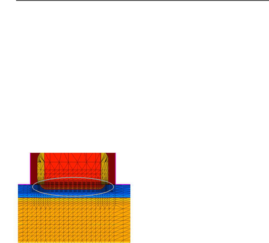
12: ICWBEV Plus Interface for Layout-driven Simulations

TCAD Layout Reader of Sentaurus Process

Sentaurus™ Process User Guide 841

H-2013.03

NOTE If you have a large layout with masks containing many polygons, it can

take some time until the Tcl function icwb.create.all.masks

parses and creates the masks. In this situation, you can use the command

icwb create.all.masks to create all the masks (see icwb on

page 951). This command works like the Tcl version but creates the

masks much faster.

Layout-driven Meshing

To create a refinement box that is tied to layers in the ICWB TCAD layout file:

icwb.refine.mask layer.name= (<string> | <string list>) [name= <string>]

[oversize=<n>] xtop=<n> xbot=<n> <other options> [info=<n>]

Layout-driven meshing can be particularly useful when meshing in critical regions, such as the

channel and emitter areas of BiCMOS devices. The following example illustrates the use of the

POLY layer for meshing placement:

icwb.refine.mask name= UnderPoly layer.name= POLY oversize= 0.1 \

xtop= -1.51 xbot= -1.35 info= xrefine= 0.02 yrefine= 0.02

icwb.refine.mask name= SiOxPo layer.name= POLY oversize= 0.1 \

xtop= -1.51 xbot= -1.35 min.normal.size= 0.005 \

interface.mat.pairs= {Silicon Oxide Silicon Polysilicon}

The oversize parameter gives the option to mesh in areas wider than the layer. Figure 167

and Figure 168 on page 842 demonstrate the use of the oversize parameter in the emitter

region of a BJT and the channel region of an NMOS, respectively.

Figure 167 Meshing in emitter region of BJT; the oversize parameter is set to 0.1 µm

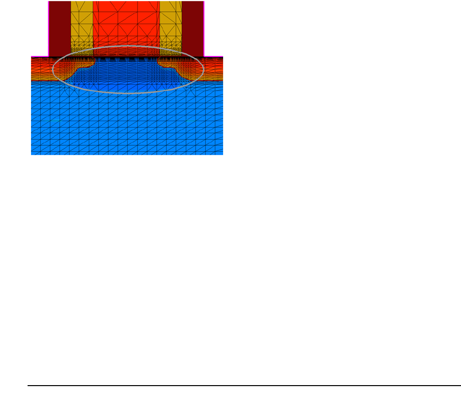
12: ICWBEV Plus Interface for Layout-driven Simulations

TCAD Layout Reader of Sentaurus Process

842 Sentaurus™ Process User Guide

H-2013.03

Figure 168 Meshing in channel region of NMOS; the oversize parameter is set to 0.1 µm

The utility command icwb.refine.mask interfaces with the standard refinebox command

by providing information about the refinement extent (minimum and maximum) based on the

selected layer.

NOTE The extent of the refinement box in the primary direction must be given

explicitly with the keywords xtop and xbot. Any other commands are

passed on.

Layout-driven mesh refinements are applied under the layer itself. They

cannot be applied under the inverse of a layer. Consider defining

auxiliary layers in ICWBEV Plus to facilitate layout-driven meshing in

areas that do not coincide with an existing layer.

This feature supports only layers with axis-aligned edges. Slanted edges

may result in a large number of refinement boxes, which may not

appropriately represent the original shape.

Layout-driven Contact Assignment

The icwb.contact.mask command creates contacts for subsequent device simulations that

are tied to a layer in the TCAD layout file. The command serves as an interface between the

TCAD layout and the Sentaurus Process contact command by automatically obtaining the

lateral placement of the contact from the specified layout layer, taking the vertical placement

from the argument list and passing all other options directly to the contact command. The

syntax of the command is:

icwb.contact.mask layer.name= (<string> | <string list>)

[name=<string>] <other options> [info=<n>]

12: ICWBEV Plus Interface for Layout-driven Simulations

TCAD Layout Reader of Sentaurus Process

Sentaurus™ Process User Guide 843

H-2013.03

The command supports both box and point contact types:

■A box-type contact consists of elements at the surface of one region or material inside the

box. The lateral extent of the box is determined automatically from the layer segment (2D)

or the polygon bounding box (3D), while the vertical extent is taken from the contact

command keywords xlo and xhi.

■A point-type contact contains all the boundary elements of one region. The lateral position

of the point is determined automatically as the midpoint of the layer segment (2D) or the

polygon bounding box (3D), while the vertical position is taken from the contact

command keyword x.

Often, there is no layer in the layout provided by designers that can be used readily for the

creation of contacts. In this case, add auxiliary layers in ICWBEV Plus to be used as markups

for device contacts.

The following example demonstrates the assignment of gate and drain contacts using layout-

driven contact assignment:

icwb.contact.mask layer.name= ndrain name= drain point aluminum \

replace x= -2.0

icwb.contact.mask layer.name= ngate name= gate box polysilicon \

adjacent.material=oxide xlo= -2.05 xhi= -1.95

The location in the primary direction must be given explicitly with either the keyword x for a

point-type contact, or with the keywords xlo and xhi for a box-type contact. Any other

command is passed on to the contact command. The keyword name is optional. If no name

is given, the name of the layer is used as the contact name.

Figure 169 on page 844 shows a layout on which auxiliary layers have been added for layout-

driven contact assignment. Figure 170 on page 844 shows the 2D boundary after the process

simulation with Sentaurus Process depicting the gate, drain, and source contacts.

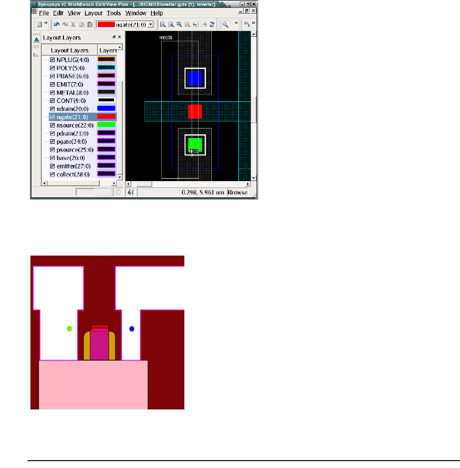
12: ICWBEV Plus Interface for Layout-driven Simulations

TCAD Layout Reader of Sentaurus Process

844 Sentaurus™ Process User Guide

H-2013.03

Figure 169 Auxiliary layers added for gate, source, and drain contacts are represented by

rectangles of solid color in the layout

Figure 170 Final boundary after TCAD simulation showing gate (red), drain (blue), and

source (green)

Aligning Wafer and Simulation Domain

To correctly support tilted process steps for 2D and 3D simulation domains, the alignment

between the wafer and the simulation domain must be declared using the slice.angle

keyword in the init command.

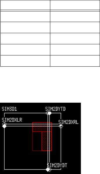
12: ICWBEV Plus Interface for Layout-driven Simulations

TCAD Layout Reader of Sentaurus Process

Sentaurus™ Process User Guide 845

H-2013.03

The TCAD layout reader command icwb slice.angle.offset returns the relative angle

of the active simulation domain so that the slice angle can be adjusted as needed.

Table 74 lists the returned slice.angle offset values for:

■A 3D simulation domain (SIM3D1).

■A 2D domain along the layout x-axis extending from left to right (SIM2DXLR), right to left

(SIM2DXRL), along the layout y-axis from top to bottom (SIM2DYTD) and bottom to top

(SIM2DYDT).

The following commands realize a tilted process:

set SliceAngle -90

set SliceOffset [icwb slice.angle.offset]

init silicon field=Boron concentration=1e13 \

slice.angle= [expr $SliceAngle+$SliceOffset]

implant phosphorus dose=4e12<cm-2> energy=100<keV> tilt=30 rot=0

Figure 171 shows a sample layout with a 3D simulation domain and the four 2D simulation

domains previously discussed. Figure 172 on page 846 and Figure 173 on page 846 show the

dopant profiles after the tilted implants for the different simulation domains.

Figure 171 Structure layout where implant is performed at highlighted L-shaped red region

Ta bl e 7 4 S l i c e a ng le o ff s et va lu es fo r di ffe r e n t d om ai ns

Domain SliceOffset value

SIM3D1 90

SIM2DXLR 0

SIM2DXRL 180

SIM2DYDT 90

SIM2DYTD –90

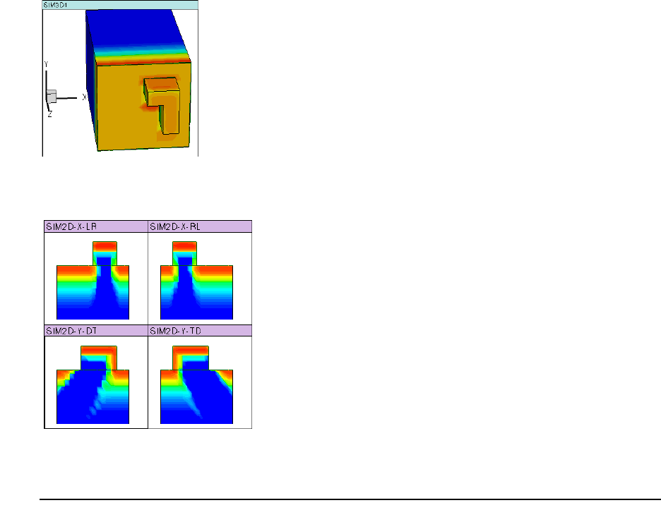
12: ICWBEV Plus Interface for Layout-driven Simulations

TCAD Layout Reader of Sentaurus Process

846 Sentaurus™ Process User Guide

H-2013.03

Figure 172 Three-dimensional implanted profile

Figure 173 Two-dimensional implanted profile for selected slice angles as mentioned in

Tab l e 74 o n pa g e 84 5

Additional Query Functions

The TCAD layout reader of Sentaurus Process provides additional layout query functions. For

example, the following command returns a list of segments in the given layer for a 2D

simulation domain:

set Segments [icwb list.segments layer.name= "<layer-name>"]

For a 3D simulation domain, the following command returns a list containing the bounding

boxes for all polygons in the given layer (this command also can be used for 2D):

set PolyBBoxes [icwb list polygon.bounding.boxes layer.name= "<layer-name>"]

For a 3D simulation domain, the following command returns a list containing a tessellated

representation of polygons in the given layer (this command also can be used for 2D):

set PolyTessel [icwb list polygon.tessellations layer.name= "<layer-name>"]

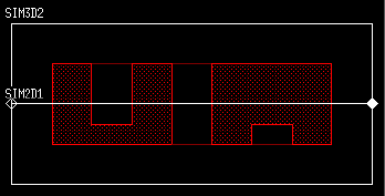
12: ICWBEV Plus Interface for Layout-driven Simulations

TCAD Layout Reader of Sentaurus Process

Sentaurus™ Process User Guide 847

H-2013.03

Figure 174 Sample layout containing two polygons

For example, Figure 174 shows a simple layout containing two polygons in layer 0:0. The

following commands:

■Load the TCAD layout file (here, called ORG_lyt.mac).

■Select the 2D simulation domain SIM2D1.

■Query the segment, the bounding boxes, and the tessellations:

icwb filename= "ORG_lyt.mac"

icwb domain= "SIM2D1"

set Segments [icwb list.segments layer.name= "0:0"]

LogFile "Segments $Segments"

# -> Segments 100 200 300 400 500 800

set BBoxes [icwb list polygon.bounding.boxes layer.name= "0:0"]

LogFile "BBoxes: $BBoxes"

# -> BBoxes: {100 0 200 0} {300 0 400 0} {500 0 800 0}

set Tessellations [icwb list polygon.tessellations layer.name= "0:0"]

LogFile "Tessellations: $Tessellations"

# -> Tessellations: {100 0 200 0} {300 0 400 0} {500 0 800 0}

NOTE The bounding box and tessellation queries are supported for 2D, and

they return flat rectangles. The returned y-values are the same as for the

segment query; however, zeros are padded for the z-direction.

When loading the 3D simulation domain SIM3D2, the set of rectangles returned by the

polygon.bounding.boxes query and the polygon.tessellations query are different:

icwb filename= "ORG_lyt.mac"

icwb domain= "SIM3D2"

set BBoxes [icwb list polygon.bounding.boxes layer.name= "0:0"]

LogFile "BBoxes: $BBoxes"

# -> BBoxes: {100 100 300 400} {100 500 300 800}

set Tessellations [icwb list polygon.tessellations layer.name= "0:0"]

LogFile "Tessellations: $Tessellations"

# -> Tessellations: {100 100 150 200} {100 200 150 300} {100 300 150 400}

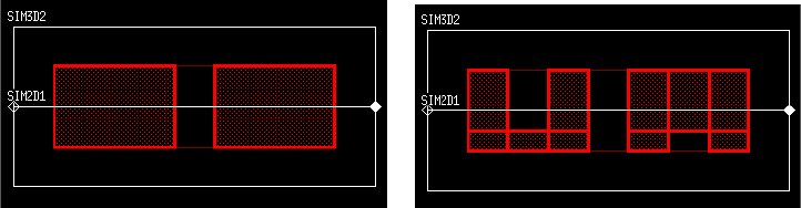
12: ICWBEV Plus Interface for Layout-driven Simulations

TCAD Layout Reader of Sentaurus Process

848 Sentaurus™ Process User Guide

H-2013.03

# {100 500 150 600} {100 700 150 800} {150 100 300 200} {150 300 300 400}

# {150 500 300 600} {150 600 300 700} {150 700 300 800}

The polygon.bounding.boxes query returns the bounding box rectangle for each polygon

in the layer, while the polygon.tessellations query breaks each polygon into a set of

rectangles and then returns these rectangles. The set of rectangles covers the same area as the

original polygon, while the bounding box rectangles may cover a larger area.

Figure 175 shows the rectangles returned by the two query functions as an ‘effective/

equivalent’ layout for better comparison with the original layout shown in Figure 174 on

page 847.

NOTE The tessellation procedure supports only polygons with axis-aligned

edges.

Figure 175 Set of rectangles returned by (left) polygon.bounding.boxes query and (right)

polygon.tessellations query for polygons shown in Figure 174

Sentaurus™ Process User Guide 849

H-2013.03

CHAPTER 13 Extracting Results

This chapter presents strategies for analyzing simulation results.

Overview

This chapter covers basic tasks such as obtaining a list of materials currently in the structure,

and obtaining 1D dopant profiles from 2D or 3D structures to more complex ones, such as

looping through all materials and extracting Pearson parameters for each material. The

following commands perform these tasks: select, slice, layers, interface,

interpolate, print.1d, FitPearson, mater, FitPearsonFloor, FitArrhenius, and

FitLine.

All these Sentaurus Process commands are built-in procedures designed to work with the tool

command language (Tcl). These commands allow you to take full advantage of the

programmability of the Sentaurus Process input language and provide a powerful framework

for performing complex customized tasks.

These commands return or accept a Tcl list to perform their respective functions. The Tcl list

can be viewed and processed by the user, passed to another function, written to a file, or read

from a file. For example, the slice command returns a Tcl list of pairs where the value

gives the depth and the value gives the value chosen with the select command. This

list can be viewed with the Tcl puts command, written to a file with the Tcl open and puts

commands, or processed with another command such as fitting a Pearson function to the profile

with the FitPearson command.

An understanding of basic Tcl commands and Tcl lists is helpful to utilize fully the flexibility

of these commands. For convenience, some basic aspects of Tcl are described to enable you to

work efficiently with these commands, and examples of basic results analysis are provided.

Saving Data Fields

Sentaurus Process automatically saves all solutions, active dopant concentrations, total dopant

concentrations, electrostatic potential, net active concentrations, point-defect concentrations,

and total point-defect concentrations along with mechanical stress results in a TDR file. The

total and active concentrations of dopants and the total concentration of defects are created only

after a diffusion step. Therefore, if there is no diffusion, some of these fields may be missing

µm[]

13: Extracting Results

Selecting Fields for Viewing or Analysis

850 Sentaurus™ Process User Guide

H-2013.03

in the TDR file. You can control the fields that will be saved in the TDR file using the

SetDFISEList command (see SetDFISEList on page 1122).

Since the active and total dopant concentrations are defined as terms in Sentaurus Process, they

are converted automatically to data fields with the same name when saved to TDR files.

Because the conversion is handled internally, the data fields are not kept in the memory.You

can create new data fields and store them in a TDR file. For example:

sel z= "BActive/BTotal" name=BActiveRatio store

will divide the active boron concentration by the total boron concentration and save the results

in a data field called BActiveRatio. The parameter store ensures that the newly created

field will be saved in a TDR file. To see whether a field will be saved in a TDR file, the select

command with the option permanent can be used (see select on page 1117), for example:

sel name= BActiveRatio permanent

will return 1 if the field will be saved in a TDR file. Otherwise, it will return 0.

Selecting Fields for Viewing or Analysis

Most analytic tasks begin with the select command, which is used to select a data field to be

viewed or operated on (see select on page 1117). A data field in Sentaurus Process is a quantity

that varies over the simulation domain, such as dopant concentration or electrostatic potential

distribution. The value of the data field is defined with an Alagator expression and is set with

z parameter of the select command.

The expression can be simply the name of a solution variable (such as Boron, H2O, or

Stress_x) or it can be a complex expression depending on what is required. If the expression

is the simple name of an existing data field, the select command selects this data field.

If it is more complex expression, the select command creates a corresponding data field and

then selects it, for example:

select z= BTotal ;# Select the total boron concentration

# term

select z= "Arsenic+Phosphorus-Boron" ;# Create and select a data field using

# solution variables

select z= log10(BActive) ;# Create and select a data field from

# the active boron concentration

The list of available data fields can be retrieved by using select list. The name that can

appear in the expression of the z parameter can be either a data field or a term.

13: Extracting Results

Obtaining 1D Data Cuts

Sentaurus™ Process User Guide 851

H-2013.03

A term is defined with the term command and is also an expression containing solution

variables, data fields, constants, and so on (see term on page 1173). Numerous terms are

created automatically in the diffuse command (see diffuse on page 908) and any of these

terms can be selected.

When a data field is selected (or created and selected) with the select command, the data field

can be viewed or operated on. The following commands can operate on the selected field:

slice, layers, interpolate, print.data, print.1d, and plot.1d.

Obtaining 1D Data Cuts

After a select command has been issued, you can obtain 1D cuts through the data along one

of the principal axes using the slice or print.1d command. The slice command returns

a list of coordinate data pairs. To make a cut perpendicular to x, specify the x parameter,

similarly for y and z.

The print.1d command returns a list of data-point lists. Each data-point list contains the

coordinate, data value, and the material name at that coordinate. Again, a cut perpendicular to

x is made by specifying the xparameter and, similarly, for the y and z cuts.

The plot.1d command can be used to view profiles with a temporary X11 graphics tool.

Examples

Sentaurus Process can run in interactive mode if there is no command file given on the

command line. In this case, you are prompted with the sprocess> prompt for commands. If

a command file is given, commands are read from this file. In interactive mode, the return value

of the commands is always displayed. You can set variables to the return value of a command

by using the syntax:

set var [command]

In this case, command is executed and a Tcl variable var is created if it does not already exist,

and the value of var is set to the return value of command. In addition, the return value of

command is displayed. It is also possible to write the return value to a user-defined file. The

following examples demonstrate the differences and functionality of the slice and print.1d

commands:

sprocess> select z=Vacancy

sprocess> slice y=0.6

{-1.000000e-02 4.804720e+16

-9.340278e-03 5.869015e+16

13: Extracting Results

Examples

852 Sentaurus™ Process User Guide

H-2013.03

...

0.000000e+00 5.969905e+17

0.000000e+00 7.075867e+17

7.421875e-04 7.618894e+17

...

sprocess> print.1d y=0.6

{ Distance Value Material }

{ -1.00000e-02 4.80472e+16 Oxide }

{ -9.34028e-03 5.86902e+16 Oxide }

...

{ 0.00000e+00 5.96991e+17 Oxide }

{ 0.00000e+00 7.07587e+17 Silicon }

{ 7.42188e-04 7.61889e+17 Silicon }

...

Here, the slice command returns raw coordinate data pairs, whereas print.1d returns a

header and coordinate data–material triplets. In both cases, the coordinates are given in

micrometers and the concentration is in .

To illustrate how data from these functions can be manipulated with Tcl, suppose you require

a 1D profile of Vacancy, which starts with 0.0 as the first coordinate, and the Vacancy

concentration to be in .

First, create a Tcl list from the data returned by the slice, and convert data in that list to a new

list, such as:

set myList[lindex [slice y=0.6] 0] ;# Create a new list from slice

# command called myList

set offset [lindex myList 0] ;# Grab the offset, that is, the

# first coordinate

list modList ;# Create new Tcl list where modified

# data will reside

foreach { coord data } $myList {\

lappend modList [expr $coord-$offset] ;#Convert coordinate by subtracting

# the offset and append to modlist

lappend modList [expr $data*1.0e-12] ;# Convert data to um^-3 units and

# append to modlist

}

The above example uses the following Tcl commands;

■lindex retrieves a given element of a list.

■list creates a list.

■lappend appends an element to the end of a list.

■expr evaluates a math expression.

■foreach is used for looping.

cm 3–

µm3–

13: Extracting Results

Determining the Dose: Layers

Sentaurus™ Process User Guide 853

H-2013.03

For example, to write modList to a file called xy.dat:

set fileID [open xy.dat w] ;# Use the Tcl open command

# to open a file for writing

foreach { x y } $modList { puts $fileID "$x $y" } ;# Write modList line by line

close $fileID

Determining the Dose: Layers

The layers command (see layers on page 1008) computes the dose of the selected data field

along one of the principal axes. The syntax to specify the cut is the same as the slice

command (see slice on page 1141). As with the other commands, the information is returned

as a list of lists:

sprocess> sel z=Vacancy

sprocess> set layerInfo [layers y=0.5]; # For a 2d structure,

either x or y must be specified

{ Top Bottom Integral Material}

{-2.06000e-01 -6.00000e-03 9.98843e+14 Silicon}

{-6.00000e-03 0.00000e+00 3.97970e+09e Oxide)

{ 0.00000e+00 1.00000e+00 2.81858e+05 PolySilicon}

The top and bottom coordinates are in micrometers. To obtain the total integrated dose along

y=0.5, use:

sprocess> set total 0

# Loop over layerInfo list of lists skipping header list,

# and retrieve the 3rd element of each list (first element has 0 index)

# which corresponds to the Integral for that layer.

sprocess> for { set i 1 } { $i < [llength $layerInfo] } { incr i } {

> set total [expr $total + [lindex [lindex $layerInfo $i] 2]]

sprocess> puts $total

9.991288377e+14

sprocess>

In addition to the Tcl commands used in the previous section, this example uses the following:

■llength returns the size of a given list.

■incr increases an integer by 1.

For more information about the layers command, see layers on page 1008.

13: Extracting Results

Extracting Values and Level Crossings: interpolate

854 Sentaurus™ Process User Guide

H-2013.03

Extracting Values and Level Crossings: interpolate

The interpolate command has two purposes: to obtain the position at which a profile

crosses a particular value and to retrieve a value at a particular location in space. Interpolation

is used to accomplish both tasks.

The four main parameters of this command are x, y, z, and val. The command operates on a

selected data field. In 1D, you must supply either x or val. If x is supplied, Sentaurus Process

returns the value at x. If val is supplied, Sentaurus Process returns the locations at which the

selected profile crosses val.

In 2D, two of the four parameters must be given (not z) and, in 3D, three of the four parameters

must be given. For example, in 2D, if x and val are given, the locations along x where val is

crossed are returned. If x and y are given, the value at this location is returned. For more

information, see interpolate on page 991.

Extracting Values during diffuse Step: extract

The extract command is used to extract historical data during diffuse steps. This

command allows you to define the data extraction script with the command parameter. The

extraction script is composed typically of the select command for choosing the data field for

extraction and the interpolate command for retrieving the value at a specified location.

Only values returned by the interpolate command, at each time step, are stored in the

historical data values.

For example, to extract the boron concentration at position in the silicon and the YY

component of the element stress at position in the oxide for each diffuse

substep:

extract name=etest command= {

sel z=Boron

interpolate Silicon x=0.04

sel z=StressEL_yy element

interpolate Oxide x=-0.001

}

This command must be defined before the diffuse step. After the diffuse steps of interest,

the following command retrieves the extracted data values for the defined extraction etest:

extract name=etest print

0.04 µm

0.001– µm

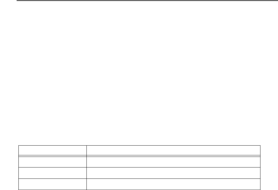
13: Extracting Results

Extracting Values during diffuse Step: extract

Sentaurus™ Process User Guide 855

H-2013.03

The values are returned as a Tcl list with the format:

<time1> <Boron1> <Syy1> <time2> <Boron2> <Syy2> ...

The following script demonstrates how to manipulate this list for more formatted output:

set extdata [extract name=etest print]

foreach { time bval sval } $extdata {

puts "$time $bval $sval"

}

Output from the above script is:

0.000000e+00 4.738727e+15 6.000000e+09

1.000000e-04 4.738727e+15 4.793201e+09

2.503231e-04 4.738727e+15 4.793201e+09

5.509694e-04 4.738727e+15 4.793201e+09

1.152262e-03 4.738727e+15 4.793201e+09

...

For more information, see extract on page 931.

Optimizing Parameters Automatically

Previously, users had to rely on the optimizer in Sentaurus Workbench to perform parameter

optimization. Sentaurus Process provides a built-in capability for parameter automatic

optimization with the new optimize command. To use this feature, a Tcl procedure must be

created which takes as input the current values of the parameters to be optimized, and returns

a corresponding result. Although writing the procedure is a small extra task for the user, this

design allows greater flexibility in the types of optimization that can be performed. The

procedure can specify anything from a simple analytic function to a complete process

simulation flow. The form of the result is a vector of values from which an error is computed

based on user-defined target data. This generic flow allows for a variety of applications (such

as dopant profiles resulting from multiple process steps or the thickness of an oxide layer).

To use the automatic parameter optimization feature, the Tcl procedure is introduced into an

input file or sourced from an external file before calling the new command optimize.

Table 75 lists some of the parameters available in the optimize command:

Table 75 Parameters for optimize

Parameter Name Description

model.function

Name of the user defined Tcl procedure

model.parameters

Names of the parameters to be optimized

param.init

Starting values of parameters

13: Extracting Results

Fitting Routines: FitLine, FitArrhenius, FitPearson, and FitPearsonFloor

856 Sentaurus™ Process User Guide

H-2013.03

The optimize command also allows you to weight target values, log the history of

optimization steps, and specify the maximum number of iterations and other convergence

criteria. For more details, see optimize on page 1042.

Fitting Routines: FitLine, FitArrhenius, FitPearson, and

FitPearsonFloor

The following commands provide fitting capabilities in Sentaurus Process:

■The FitLine command is used to find the best offset and slope for a given set of data, for

example:

sprocess> foreach temp { 700 800 900 1000 } {

> lappend dat $temp

> lappend dat [expr 110 + 10*$temp]

sprocess> FitLine $dat ;# Get the slope, offset, and correlation factor

10.0 110.0 1.0

■The FitArrhenius command is used to find the best prefactor and energy for an

Arrhenius fit of a given profile, for example:

sprocess> list dat ;# This is the list to be passed to FitArrhenius

sprocess> foreach temp { 700 800 900 1000 } {

> SetTemp $temp

> lappend dat $temp ;# dat will contain "temp" - "Arrhenius val" pairs

> lappend dat [Arrhenius 0.1 1.0]; ;# Arrhenius takes prefactor and

# activation energy

sprocess> FitArrhenius $dat ;# Send the list to FitArrhenius

0.0999999308634 1.00030363776 -0.999999999866 ;# Return prefactor, energy

# and corr factor

sprocess>

The FitArrhenius command takes a list of temperature–function pairs. The unit of

temperature is degree Celsius. The return value is a list where the first member is the

param.lower

Lower limits of parameters

param.upper

Upper limits of parameters

param.log

Parameters that vary logarithmically during optimization

target | target.file

Options used to specify the target values, either via a Tcl array or from a file

Table 75 Parameters for optimize

Parameter Name Description

13: Extracting Results

Resistivity

Sentaurus™ Process User Guide 857

H-2013.03

prefactor, the second member is the activation energy [eV], and the third member is the

correlation factor. Absolute values of the correlation factor close to one are desirable.

■The FitPearson command is used to extract the best Pearson parameters of a profile.

■The FitPearsonFloor command is a modification of FitPearson and is used to set a

floor for the data value so that only data points with values greater than the given floor are

used for the Pearson fit.

An example of using this command is one that contains the command PearsonProfile,

which can be called to create a Pearson–IV, Pearson–V, or Pearson–VI profile depending

on the parameters sent. It takes as its arguments the name of the data field to be created and

a list of parameters in this order: dose [cm–2], projected range, standard deviation,

skewness, and kurtosis. FitPearsonFloor takes the minimum value and a list of x y

values, which are to be fit to a Pearson. It returns parameters in the same order as the list

of parameters for PearsonProfile:

sprocess> PearsonProfile Arsenic {1e14 0.0650 0.0228 0.577 3.4390}

;# Corresponds to 100keV As implant

sprocess> select z= Arsenic

sprocess> FitPearsonFloor 1.0e10 [lindex [slice silicon] 0]

9.99999659675e+13 0.0649998507454 0.0227994405041 0.576718866676

3.4368839917

sprocess>

Resistivity

The background concentration of the wafer can be defined using the resistivity of the wafer.

You can define th e r es ist ivit y o f t he wa fer with the init command, which requires a field name

to calculate the background concentration. For example:

line x location = 0 tag=top

line x location = 10 tag=bot

region silicon xlo = top xhi = bot

init field=boron silicon resistivity=1.4

sets the boron concentration of the wafer to in silicon.

The resistivity is given in , and the resistivity is calculated by:

(970)

where:

■ is the electron density.

■ is the background concentration.

■ is the mobility.

1.08 16

×10 cm 3–

Ωcm

RHO qNµ()

1–

13: Extracting Results

Resistivity

858 Sentaurus™ Process User Guide

H-2013.03

Three mobility models can be selected using the command:

pdbSet <material> <dopant> Mobility.Model <model>

where

<model>

can be Model1 [1], or Model2

[2], or Model3 [3]. They are given as:

■Model1:

(971)

■Model2:

(972)

■Model3:

(973)

(974)

where , and are fitting

parameters for the empirical formulas.

The fitting parameters can be set using the following commands:

pdbSet <material> <dopant> uMin {<n>}

pdbSet <material> <dopant> uMin2{<n>}

pdbSet <material> <dopant> uMax {<n>}

pdbSet <material> <dopant> uM {<n>}

pdbSet <material> <dopant> uNr {<n>}

pdbSet <material> <dopant> uNs {<n>}

pdbSet <material> <dopant> uPC {<n>}

pdbSet <material> <dopant> uBeta{<n>}

pdbSet <material> <dopant> uAlpha {<n>}

pdbSet <material> <dopant> A0 {<n>}

pdbSet <material> <dopant> A1 {<n>}

pdbSet <material> <dopant> A2 {<n>}

pdbSet <material> <dopant> A3 {<n>}

µµ

min

µmax µmin

–

------





----------------------------+=

µµ

mine

------





–µmax µmin2

–

------





-------------------------------µm

1Ns

------





-----------------------–+=

µpµmine

------





–µmax

------





------------------------+=

µn10

A0A1XA

2X2A3X3

++ +

1B1XB

2X2B3X3

++ +

------------------------------------------------------------

------





log=

Nr, µmin, µmin2, µmax, µm, PC, A0, A1, A2, A3, B1, B2, B3β,

13: Extracting Results

Sheet Resistance

Sentaurus™ Process User Guide 859

H-2013.03

pdbSet <material> <dopant> B1 {<n>}

pdbSet <material> <dopant> B2 {<n>}

pdbSet <material> <dopant> B3 {<n>}

In addition to these models, a user-defined mobility model can be set using the command:

pdbSet <material> <dopant> Mobility.Equation <String Expression>

For example, the Mobility1 model for boron in silicon can be set using the command:

pdbSet Silicon Boron Mobility.Equation \

"(49.705+(467.729-49.705)/(1+abs(tNetActive/1.606e+17)^0.7))"

tNetActive

is the internal name for .

NOTE To change the model and default model paramters, use the

SetMobilityModel command (see setMobilityModel on page 1127).

Sheet Resistance

The sheet resistance and p-n junction depth of a semiconductor layer in the vertical direction

are calculated using the command:

SheetResistance <args>

where <args> must be the y–cross section in 2D, and the y– and z–cross sections in 3D. For

example, in 3D:

SheetResistance y=0.4 z=-0.1

The sheet resistance formula is given by:

(975)

where is mobility of the holes ( ) or electrons ( ) given in Eq. 971 or Eq. 972 or Eq. 973.

The active concentration of dopants is calculated at the last diffusion temperature. The electron,

, and hole, , concentrations are calculated assuming charge neutrality at a temperature of

300 K.

Sheet resistance can be calculated only after a diffusion statement or activation step. For

example:

diffuse time=0.0 temperatur=1000

qµnnµpp+()xd

pni

pni1+



---------------------------------------------------=

µX

13: Extracting Results

References

860 Sentaurus™ Process User Guide

H-2013.03

SheetResistance y=9.4 z=-0.1

Since not all data fields are stored in the TDR file, the sheet resistance may not be calculated

after loading the TDR file even though the last command was a diffusion command.

References

[1] D. A. Antoniadis, A. G. Gonzalez, and R. W. Dutton, “Boron in Near-Intrinsic <100>

and <111> Silicon under Inert and Oxidizing Ambients—Diffusion and Segregation,”

Journal of the Electrochemical Society, vol. 125, no. 5, pp. 813–819, 1978.

[2] G. Masetti, M. Severi, and S. Solmi, “Modeling of Carrier Mobility Against Carrier

Concentration in Arsenic-, Phosphorus-, and Boron-Doped Silicon,” IEEE Transactions

on Electron Devices, vol. ED-30, no. 7, pp. 764–769, 1983.

[3] W. R. Thurber et al., The Relationship Between Resistivity and Dopant Density for

Phosphorus- and Boron-Doped Silicon, National Bureau of Standards Special

Publication 400-64, Washington, DC, USA, May 1981.

Sentaurus™ Process User Guide 861

H-2013.03

CHAPTER 14 Numerics

This chapter discusses numerics-related issues, time integration

methods, and the linear solvers used in Sentaurus Process.

Overview

In Sentaurus Process, during the simulation of diffusion steps, three different sets of nonlinear

partial differential equations must be solved:

■Oxidant diffusion and reaction

■Dopant diffusion and reaction

■Stress equations

In the case of silicidation, the transport and reactions of dissolved silicon or dissolved metal is

handled similar to the oxidant diffusion and reaction.

The oxidant, dopant, and point-defect equations are solved on the simulation mesh using a

trapezoidal rule/backward differentiation formula (TRBDF) time discretization, a finite

volume (box) method for the spatial integration, and a Newton method to solve the nonlinear

equations.

For the discretization of the nonlinear stress equations, piecewise linear finite elements are

used. If stress history is tracked, the stress equations are solved, not only during the simulation

of diffusion steps, but also at the end of etch and deposit steps.

Various direct and iterative solvers are integrated in Sentaurus Process to solve the large

systems of linear equations in each Newton iteration. By default, for all equations in 1D

simulations and for mechanics equations in 2D simulations, the parallel direct solver

PARDISO is used. For diffusion equations in two dimensions and for all equations in three

dimensions, the iterative solver ILS is used. The solver can be selected using the math

command:

math ils

This command selects the solver ILS for all types of equation in 1D, 2D, and 3D. Separate

selections can be made for the various spatial dimensions and for the solution of mechanics

equations and diffusion equations (the same settings are used for both oxidant and

dopant–point defect equations).

14: Numerics

Setting Parameters of the Iterative Solver ILS

862 Sentaurus™ Process User Guide

H-2013.03

The parameters Flow and diffuse select the type of equation, and the parameter dim

specifies the spatial dimension:

math Flow dim=2 ils

math diffuse dim=2 pardiso

math Flow dim=3 pardiso

If a direct solver is used, a modified Newton method is used by default; Sentaurus Process tries

to avoid the recomputation and factorization of a new matrix and will reuse the last factorized

matrix, as long as the convergence rate remains sufficiently high. For the iterative solvers, by

default, a modified Newton scheme is used as well.

The math command is used to specify various parameters for the Newton iterations and to

define resources and specifications for the linear solvers (see math on page 1027).

For the default settings for ILS, refer to the parameter database browser (PDB). More detailed

settings for ILS can be made using pdbSet commands as described in the next section.

Setting Parameters of the Iterative Solver ILS

The iterative solver ILS is used by default to solve the linear systems for diffuse in 2D

simulations and for both Flow and diffuse in 3D simulations. Default parameters for ILS

have been added to the parameter database. To specify modified parameters for ILS, such as

the type of iterative scheme, the number of iterations, the output verbosity, or the memory

resources, use the pdbSet commands.

NOTE In the pdbSet commands, parameters must be specified separately for

each type of problem (Flow or diffuse) and for each dimension (1D,

2D, or 3D).

NOTE ILS is not recommended for use in 1D simulations because of the simple

structure of matrices arising in 1D cases. The default direct solver

PARDISO is the correct choice for 1D simulations.

Different ILS parameters can be specified for diffuse and Flow, both in 2D or 3D. In general,

the pdbSet command for the ILS parameters has the form:

pdbSet Math [diffuse | Flow] [2D | 3D] ILS.[command] [value]

The following ILS commands are available:

ILS.compact Boolean

ILS.fgmres.restart Double

ILS.gmres.restart Double

ILS.fit Double

14: Numerics

Setting Parameters of the Iterative Solver ILS

Sentaurus™ Process User Guide 863

H-2013.03

ILS.ilut.tau Double

ILS.leftPreconditioner Boolean

ILS.maxit Double

ILS.method String

ILS.nonsymmOrdering String

ILS.okayForModNewton Boolean

ILS.preconditioner String

ILS.recompute.ordering Double

ILS.refine.residual Double

ILS.refine.iterate Double

ILS.scaling String

ILS.symmOrdering String

ILS.tolabs Double

ILS.tolrel Double

ILS.tolunprec Double

ILS.useILSRCFile Boolean

ILS.verbose Double

To select the GMRES method, for example, gmres(60), use:

pdbSet Math diffuse 3D ILS.method gmres

pdbSet Math diffuse 3D ILS.gmres.restart 60

To specify the FlexibleGMRES method, for example, fgmres(40), to solve the stress

equations, use:

pdbSet Math Flow 3D ILS.method fgmres

pdbSet Math Flow 3D ILS.fgmres.restart 40

pdbSet Math Flow 3D ILS.fit 5

To select the efficient reuse mode (on each 3D diffuse time step, the costly reordering is applied

only once to a first Jacobian system), specify:

pdbSet Math diffuse 3D ILS.recompute.ordering 2

and to return to reordering for every system, use:

pdbSet Math diffuse 3D ILS.recompute.ordering 1

To improve the accuracy and convergence of iterative linear solvers, use an enhanced option

available in Version H-2013.03 by specifying (default value is 0):

pdbSet Math [diffuse | Flow] [2D | 3D] ILS.refine.iterate 1

To use the 3D diffuse gmres solver in the advanced parallel implementation, specify:

pdbSet Math diffuse 3D ILS.hpc.mode 3

14: Numerics

Partitioning and Parallel Matrix Assembly

864 Sentaurus™ Process User Guide

H-2013.03

In this command, the value 3 activates algorithmic improvements made in Versions H-2013.03

and H-2013.03, while the value 2 corresponds to Versions G-2012.06 and F-2011.09, and the

value 1 corresponds to Version E-2010.12.

To select the solvers for mechanics, STS2 or STCG2 for 2D, and STS3 or STCG3 for 3D, for

example, sts3, use:

pdbSet Math Flow 3D ILS.method sts3

pdbSet Math Flow 3D ILS.tolrel 1e-10

pdbSet Math Flow 3D ILS.ilut.tau 5e-4

pdbSet Math Flow 3D ILS.scaling diagsym

pdbSet Math Flow 3D ILS.nonsymmOrdering none

For the mechanics solvers STS2, STS3, STCG2, and STCG3, it is mandatory to specify

ILS.scaling

diagsym, and ILS.nonsymmOrdering as none. It is also recommended

to specify the value for the parameter ILS.ilut.tau

in the range of – .

To improve convergence of the mechanics solver STS2 or STS3, use an enhanced version of

the solver by specifying, respectively (default value is 0):

pdbSet Math Flow 2D ILS.refine.sts 1

or:

pdbSet Math Flow 3D ILS.refine.sts 1

The enhanced version takes advantage of results from previous solve steps, so the actual

performance gain can vary depending on the simulation setup, and it performs best when there

is a sequence of mechanical solve steps, as in temperature ramps.

To active the STS solver which improves robustness and speed, use:

pdbSet Math Flow 3D ILS.refine.sts 2

Partitioning and Parallel Matrix Assembly

Sentaurus Process can assemble the diffusion and mechanics matrices in parallel on multicore

machines. To switch on the parallel assembly, use:

math { numThreads = <n> | numThreadsAssembly = <n> }

where numThreads is the number of threads that would be used during the matrix assembly.

numThreads is a general keyword (see math on page 1027) used by both implant and linear

solvers. If you want to use a different number of threads for diffusion matrix assembly, use the

keyword numThreadsAssembly. If the number of threads is greater than 1, Sentaurus Process

first creates the threads.

54–

×10

55–

×10

14: Numerics

Partitioning and Parallel Matrix Assembly

Sentaurus™ Process User Guide 865

H-2013.03

To modify the thread stack size, use:

math threadStackSize = <n>

NOTE Parallel assembly of the matrix is performed only for inert anneals. It is

recommended that numThreadsAssembly does not exceed the

number of actual cores of the computer. Parallel assembly of the matrix

is not available for moving-boundary problems such as oxidation and

silicidation.

Sentaurus Process then partitions the mesh structure into levels, and each level is divided into

different domains at the beginning of the diffusion step. For example, Figure 176 shows a

structure with three levels. The first level (blue) (L0) has four domains: D0, D1, D2, and D3.

Elements belonging to each domain on the same level do not cross over to the other domains.

The second level (orange) (L1) also has four domains: D0, D1, D2, and D3. Again, the

elements on the same level do not cross over to the other domains. The third level (green) (L2)

has only one domain: D0. This is the last level and contains all the elements not included in the

previous levels.

To control the partitioning, use:

math { maxNumberOfDomains=<n> | NumberOfElementsPerDomain=<n> }

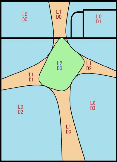
14: Numerics

Partitioning and Parallel Matrix Assembly

866 Sentaurus™ Process User Guide

H-2013.03

Figure 176 Partitioned mesh structure

NOTE maxNumberOfDomains is the maximum number of domains that each

level of partition can have. It is recommended that

maxNumberOfDomains equals or is greater than the number of threads

used. NumberOfElementsPerDomain is the number of elements that

should go to each domain.

The final number of domains at each level is determined by:

(976)

To partition the mesh, based on material type, give weight to each material using the command:

pdbSet <material> PartitionWeight <n>

For example:

pdbSet Silicon PartitionWeight 10

pdbSet Gas PartitionWeight 0

domains min maxNumberOfDomains Number of Edges

NumberOfElementsPerDomain

-----------------------------------------------------------------------------------(, )=

14: Numerics

Matrix Size Manipulation

Sentaurus™ Process User Guide 867

H-2013.03

gives more weight to silicon mesh elements than the gas mesh elements during partitioning.

This allows Sentaurus Process to distribute the work among the threads more evenly since there

is no matrix assembly for the gas mesh.

Partition weights for mechanics assembly can be specified separately with:

pdbSet <material> Mechanics PartitionWeight <n>

This allows balancing the workload among threads according to the stress analysis methods for

different material behaviors. If the partition weights for mechanics assembly are not defined,

the partition weights for diffusion assembly are used by default.

Matrix Size Manipulation

The size of the matrix used during diffusion assembly is automatically determined based on the

number of solution variables and nodes in the structure. In most cases the allocated matrix size

is more than sufficient. If the matrix size becomes insufficient during the assembly, the matrix

size will be increased automatically by 10%. You can change the default 10% value by using

the command:

pdbSet Math Matrix.Size.Scale <n>

where the value <n> should be greater than one.

You al so can in cr eas e t he au to mat ic ally de termined matrix size using the command:

pdbSet Math Assembly.Matrix.Size.Scale <n>

where the value <n> should be greater than one.

NOTE Be careful when choosing the matrix scaling values because it can

exhaust the computer memory for large scaling values.

Node and Equation Ordering

Because the order of nodes in meshes does not follow a specific order by default, adjacent

nodes may be far from each other in the internal node list. The order may not have much effect

on simulation time for small examples (such as 2D), but it may degrade 3D results. The nodes

in the structure can be ordered meshwise or globally using the command:

pdbSet Math < 1D | 2D | 3D > Reorder.Nodes <model>

where <model> is None (default), Mesh, or Global.

14: Numerics

Time Integration

868 Sentaurus™ Process User Guide

H-2013.03

The default order of equation numbering in the structure is based on the meshes. Each node in

the mesh receives an equation number from a solution variable and the same is repeated for the

next solution. This may create many distributed entries in the assembly matrix. Again, the order

may not greatly affect the simulation time for small examples (such as 2D), but it may degrade

3D results. It is possible to number equations based on solutions by taking a node in the mesh,

numbering it for each solution variable, and moving to the next node in the mesh. This creates

better-distributed entries in the assembly matrix. The order can be changed using the

command:

pdbSet Math < 1D | 2D | 3D > Reorder.Equations <model>

where <model> is None (default) or Solution.

Time Integration

The TRBDF method [1] is used for time integration by default for time-dependent problems.

It also is possible to choose the backward Euler method for the time integration. The following

command can be used to switch between methods:

math {tr_bdf | euler}

A TRBDF integration step consists of a trapezoidal step followed by a backward difference

step. A second trapezoidal solution is used to estimate the local truncation error and to

determine the size of the next time step.

The local truncation error can be estimated by either a Milne’s device (the default method) or

the divided difference method. The following command switches between methods:

math {milne | difference}

The local truncation error for the next time-step estimation can be modified using the

command:

pdbSet Math Time.Step.Function {<model>}

where <model> is Damped, UnDamped, or Linear. The Damped model applies a logarithmic

damping function to the truncation error if the error is greater than 1.0. The UnDamped model

does not modify the error. The Linear model applies a linear damping function to the

truncation error if the error is greater than 1.0. The Linear model matches that of

TSUPREM-4.

When the geometry of a simulation structure evolves, one cycle of the TRBDF time integration

requires the geometric coefficients at three incidents, that is, . To

reduce the computational time to calculate the geometric coefficients, especially in three

dimensions, the geometric coefficients at can be set to the interpolated values by

0t0∆tTR

+t0∆t+,,=

0∆tTR

14: Numerics

Time-Step Control

Sentaurus™ Process User Guide 869

H-2013.03

assuming that the coefficients change linearly during , which reduces the number of the box

method calls by one third:

pdbSet Math 3D Use.Interpolated.Geom.Coeff 1

or:

math dimension=3 use.interpolated.geom.coeff

Time-Step Control

This section discussed different time-step controls.

Time-Step Control for PDEs

Sentaurus Process provides automatic time-step control. You can modify some of the control

parameters.

The first time step of the diffuse command uses the initial time given with the diffuse

command (see diffuse on page 908).

In an ideal situation, oxidation, mechanics, and diffusion time steps are equal to each other, and

the next time step is increased by the IncreaseRatio:

(977)

where is the next diffusion time step, is the current time step, and is the

IncreaseRatio. The default for IncreaseRatio is 2.

Use the following command to change IncreaseRatio:

pdbSet Diffuse IncreaseRatio {<n>}

In some cases, the ideal time step can be solution limited , grid limited, or reduced:

■Solution limited is the case when the time step is shortened to decrease the local truncation

error; in a log file, such steps are marked by (s).

■Grid limited is the case when the time step is reduced because of a grid motion; in a log

file, such steps are marked by (g).

■Reduced is the case when the time step is reduced to prevent overstepping of oxidation or

mechanics steps; in log files, such steps are marked by (r).

∆t

tn1+Iratiotn

tn1+

Iratio

14: Numerics

Time-Step Control

870 Sentaurus™ Process User Guide

H-2013.03

If convergence is not achieved, the next time step is reduced by the ReduceRatio:

(978)

The following command can be used to change ReduceRatio:

pdbSet Diffuse ReduceRatio {<n>}

For more information about the convergence during diffusion, use the command:

pdbSet Diffuse Convergence.Info {1 | 0}

Typical output with information level=2 will look like:

Iter Potential Boron Arsenic Int Vac B4

1 4.345e-02 2.244e+01 2.512e+00 5.096e+03 1.835e+02 2.599e-06

-- -- -- -- -- -- -- -- -- -- -- -- -- -- -- -- -- -- -- -- -- -- -- -- -- --

Mesh: bulk Mater: Silicon

Org. Val. Org. Updt. Org.-Updt Apld. Updt. Error Location

Boron 5.7e+18 1.8e+17 5.5e+18 5.5e+18 3.1e+02 ( 1.7e-5, 0.0, 0.0 )

Arsenic 7.2e+16 3.1e+14 7.2e+16 7.2e+16 4.3e+01 ( 1.7e-5, 0.0, 0.0 )

Int 2.8e+12 -1.3e+13 1.5e+13 1.5e+13 4.5e+04 ( 1.5e-5, 0.0, 0.0 )

Vac 3.5e+14 5.5e+13 2.9e+14 2.9e+14 1.5e+03 ( 1.7e-5, 0.0, 0.0 )

Largest update: Int in Silicon @ ( 1.5e-5, 0.0, 0.0 )

where:

■Org.Val is the original value at the node.

■Org.Updt is the original update at the node.

■Org.-Updt is the Original Value – Original Update.

■Apld. Updt. is the applied update.

Sentaurus Process provides three time-step control models (TSCMs):

■A local model (LTS) based on the current time step and described above.

■Two history-based models involving all previous time steps within the diffuse command:

BPTS and NGLTS.

BPTS uses the biggest previous time step from the history, such that Eq. 977 is modified as:

(979)

NGLTS uses the latest nongrid limited time step, and Eq. 977 is modified as:

(980)

˜n1+Rratiotn1+

tn1+IratiotBPTS n,

tn1+IratiotNGLTS n,

14: Numerics

Time-Step Control

Sentaurus™ Process User Guide 871

H-2013.03

Use the following command to choose the TSCM:

pdbSet Diffuse TSCM <model>

where <model> can be LTS, BPTS, or NGLTS.

Error Control for PDEs

To control errors during transient simulation, Sentaurus Process uses the following to calculate

the error:

(981)

where the sum is taken over all solution variables, and is the update for solution .

TransRelErr and AbsErr are the transient relative error and absolute error for the solution

variables, respectively. They can be set using the commands:

pdbSet <mater> <solution> Transient.Rel.Error <n>

pdbSet <mater> <solution> Abs.Error <n>

where <mater> is the material name.

To control errors during nonlinear Newton iterations, Sentaurus Process uses the following to

calculate the error:

(982)

where RelErr is the relative error for the solution variables. It can be set using the command:

pdbSet <mater> <solution> Rel.Error <n>

NOTE If the error control parameter is not defined in the PDB for a material or

a solution, the long-hand command pdbSetDouble must be used.

Time-Step Control for Mechanics

Automatic time-step control for mechanics is activated only if the structure contains certain

nonlinear features that require Newton iterations, such as plasticity, viscoplasticity, and creep.

The size of the time step is adjusted based on satisfaction of certain convergence criteria.

----ui

soliTransRelErr AbsErr+×

-----------------------------------------------------------------------

2





i1=









12⁄

soli

----ui

soliRelErr AbsErr+×

--------------------------------------------------------- 

2





i1=









12⁄

14: Numerics

Time-Step Control

872 Sentaurus™ Process User Guide

H-2013.03

Convergence Criteria

To check the convergence of Newton iterations for mechanics equations [2][3], the criteria are:

■Force residual

■Energy

■Displacement

The force residual criterion checks the satisfaction of force equilibrium by comparing the

maximum norm of the residual ( ) against a reference value:

(983)

The reference value of the force residual is computed automatically by taking a norm of the

element force residual vector at the first Newton iteration in a time step.

The energy criterion checks the satisfaction of the minimization of energy at equilibrium by

comparing the change in energy against a reference value:

(984)

The reference value of energy is computed automatically by taking a dot product of the force

residual and the displacement increment ( ) vector at the first Newton iteration in a

time step.

The displacement criterion checks the satisfaction of the solution accuracy by comparing the

maximum norm of the displacement increment against a reference value:

(985)

The reference value of displacement is computed automatically by taking a norm of the

displacement increment vector at the start of the first Newton iteration in a time step.

The force residual and the energy criteria are checked by default. Optionally, the energy

criterion may be replaced by the displacement criterion. Use the following parameters to

activate or deactivate any of the convergence criteria:

pdbSet Mechanics Convergence.Force.Check <n>

pdbSet Mechanics Convergence.Energy.Check <n>

pdbSet Mechanics Convergence.Displacement.Check <n>

where <n> is either 0 (deactivate) or 1 (activate).

external F internal

–=

Rn1+

∞εRRn1+

≤

∆un1+

iRn1+

⋅ε

E∆unRn1+

⋅≤

∆uv∆t=

∆un1+

∞εu∆un

≤

14: Numerics

Time-Step Control

Sentaurus™ Process User Guide 873

H-2013.03

The choices for the force residual and the displacement reference value norms that can be set

using the following command are:

pdbSet Mechanics Convergence.Check.Norm [RMS | ABS]

where RMS refers to the root mean square value (default) and ABS refers to the mean absolute

value.

The reference values for any of the convergence criteria can be changed by using the

commands:

pdbSet Mechanics Convergence.Force.RefVal <n>

pdbSet Mechanics Convergence.Energy.RefVal <n>

pdbSet Mechanics Convergence.Displacement.RefVal <n>

where <n> is a suitable positive value.

By default, the tolerance for each of the convergence criteria is set to 0.001 and can be changed

by using the commands:

pdbSet Mechanics Convergence.Force.Tolerance <n>

pdbSet Mechanics Convergence.Energy.Tolerance <n>

pdbSet Mechanics Convergence.Displacement.Tolerance <n>

where <n> is a value between 0.0 and 1.0.

Convergence criteria are checked in every iteration until either they are satisfied or the

maximum number of Newton iterations is reached. The default value for the maximum number

of Newton iteration is 8, and this can be changed using the command:

pdbSet Mechanics MaxIterations <n>

where <n> is a value greater than zero.

Time-Step Adjustment

The first time step for solving mechanics equations is set to the initial time given with the

solve command. The size of subsequent time steps is decided based on the convergence

history of the preceding time step. The time-step size is extended if the preceding time step

converges quickly. The maximum value is limited to the maximum time given with the solve

command. The time-step size is reduced if the preceding time step takes too many iterations to

converge; it remains unchanged if the preceding time step takes a moderate number of

iterations to converge.

The time-step size also is adjusted to keep the viscoplastic or creep strain error or value within

tolerance when using such material models. The viscoplastic strain error or value is checked

14: Numerics

Time-Step Control

874 Sentaurus™ Process User Guide

H-2013.03

for Anand model (see Anand Model on page 656) while creep strain error or value is checked

for Power Law creep and Standard Linear Solid models (see Power Law Creep on page 658

and Standard Linear Solid Model on page 646). Use the following commands to change the

default settings for the viscoplastic or creep strain error or value:

pdbSet Mechanics StrainVP.Error.Tolerance <n>

pdbSet Mechanics StrainVP.Value.Tolerance <n>

pdbSet Mechanics StrainCr.Error.Tolerance <n>

pdbSet Mechanics StrainCr.Value.Tolerance <n>

where <n> is a value between 0.0 and 1.0 for both. By default, only the viscoplastic or creep

strain error criterion is used with a tolerance of 0.02.

Time-Step Cutback

An automatic time-step cutback procedure interrupts the Newton iteration loop and restarts the

time step with a smaller size when any of the following issues is encountered:

■Convergence criteria are not satisfied within the maximum number of Newton iterations.

■The solution converges very slowly over several iterations.

■The solution diverges over several iterations.

■Convergence criteria are satisfied, but viscoplasticity equations fail to converge.

■Convergence criteria are satisfied, but the viscoplastic or creep strain error or value is

greater than the tolerance.

To check convergence details during solve steps, specify info=1 in the solve command.

14: Numerics

References

Sentaurus™ Process User Guide 875

H-2013.03

References

[1] R. E. Bank et al., “Transient Simulation of Silicon Devices and Circuits,” IEEE

Transactions on Electron Devices, vol. ED-32, no. 10, pp. 1992–2007, 1985.

[2] O. C. Zienkiewicz and R. L. Taylor, The Finite Element Method, Butterworth-

Heinemann: Oxford, 5th ed., 2000.

[3] K. J. Bathe and A. P. Cimento, “Some Practical Procedures for the Solution of Nonlinear

Finite Element Equations,” Computer Methods in Applied Mechanics and Engineering,

vol. 22, no. 1, pp. 59–85, 1980.

14: Numerics

References

876 Sentaurus™ Process User Guide

H-2013.03

Sentaurus™ Process User Guide 877

I-2013.12

APPENDIX A Commands

This appendix describes the commands of Sentaurus Process.

Syntax Conventions

The commands are designed to optimize the use of the tool command language (Tcl).

The following conventions are used for the command syntax:

■Each command starts on a new line.

■A backslash (\) is used to extend a command on to multiple lines if it appears as the last

character on the line. It is not included on the last line of a command. For example:

icwb.refine.mask name= SiOxPo layer.name= POLY \

oversize= 0.1 xtop= -1.51 xbot= -1.35 min.normal.size= 0.005 \

interface.mat.pairs= {Silicon Oxide Silicon Polysilicon}

■Braces – { } – indicate a list. The braces are part of the syntax.

■Brackets – [ ] – indicate an optional argument. The brackets are not part of the syntax.

■Parentheses – ( ) – indicate grouping of arguments. The parentheses are not part of the

syntax.

■A vertical bar – | – indicates options, only one of which can be specified. Vertical bars are

not part of the syntax.

■Angle brackets – < > – indicate specific type of input. The angle brackets are not part of

the syntax.

NOTE An exception to this is that angle brackets must be included in the syntax

if units are specified in a command. For example:

line x location= 0<um> spacing= 0.02<um> tag= surf

■The following type identifiers are used:

•<c>: Replace with a string. In general, strings are enclosed in double quotation marks

(" "), for example:

line_edge_roughness normal= "Z" masks= {mask1} \

correlation.length= 25.00<nm> standard.deviation= 5.00<nm>

•: Replace with an integer.

•<n>: Replace with a floating-point number.

A: Commands

Syntax Conventions

878 Sentaurus™ Process User Guide

I-2013.12

•<list>: Replace with a Tcl list of values. The list must be enclosed in braces, for

example, min= {-5.0 0.0 0.0}.

•<field>: Replace with the name of a field.

•<material>: Replace with the name of a material.

•<solution>: Replace with the name of a solution.

■Boolean arguments are true (or on) if they appear on the command line (for example,

negative).

■Boolean arguments are false (or off) if they appear on the command line preceded by an

exclamation mark (for example, !negative).

Example of Command Syntax

An example of command syntax is:

command

argument1=<n>[<unit1>]

argument2=

argument3=

argument4

...

There are two types of argument:

■Named arguments must be specified with a value, for example, name=Germanium.

■Unnamed arguments supply only the value, for example, <material> would be replaced

by Oxide.

If you specify units for an argument:

■Omit spaces between the value and unit.

■Include the angle brackets with the unit, for example, xlo=5<um>.

If you specify lists:

■Lists must be enclosed in braces.

■Elements in the list must be separated by space.

■You m ust in se rt s pa ce between t he e qua l sign a nd the o pe ning br ac e. Fo r ex amp le :

transform translate= {-1 0 0}

A: Commands

Syntax Conventions

Sentaurus™ Process User Guide 879

I-2013.12

Common Arguments

Nearly all Sentaurus Process commands (with the exception of those implemented as Tcl

procedures as well as a few others) support two common optional arguments:

■info=

This argument sets the amount of information to be printed to the screen and the log file. It

can take the value 0, 1, or 2. The default is 0, which is the minimum amount. Higher values

give more details about the status of the simulation as well as model and parameter

selection information.

This argument can be used with any other argument combination for nearly all commands

that are not Tcl procedures.

For example, to specify that more information should be printed to the screen and the log

file for the etch command, use:

etch info= 2

■parameters

This argument prints all the available arguments for a command.

For example, to print the arguments for the extract command, use:

extract parameters

NOTE When you use the parameters argument, the complete list of

arguments for that command is generated. However, some of the

arguments in this list are not documented. These parameters are used for

debugging purposes only.

A: Commands

alias

880 Sentaurus™ Process User Guide

I-2013.12

alias

Sets and prints aliases.

Syntax

alias <c> [<c>] [-list]

Arguments

<c>

If one argument is specified, only one alias for this value is printed.

If two arguments are specified, a new alias is set.

-list

Prints a list of allowed aliases.

Description

This interactive mode command sets and prints aliases.

If the first argument is -list, a list of allowed aliases is printed. Otherwise, only one alias

corresponding to the first argument is printed.

Examples

Set a new alias of Temperature:

alias Temp

Temperature

Print the list of allowed aliases:

alias -list

Print an alias of Temp:

alias Temp

A: Commands

ambient

Sentaurus™ Process User Guide 881

I-2013.12

ambient

Creates new ambients for material growth reactions, such as oxidation or silicidation, or creates

a new epi growth mode.

Syntax

ambient

name=<c>

(add | clear | delete | list | print)

[epi | inert | react]

Arguments

add

Creates a new ambient.

clear

Clears all known ambients (only useful in very special situations).

delete

Deletes the named ambient.

epi, inert, react

When creating a new ambient, you can set the ambient type:

•epi ambients are used to create new epi growth modes or models.

•inert ambients are used in gas_flow commands to create gas reactions or to dilute

active ambients.

•react creates an active ambient and is used to define material growth reactions such

as oxidation.

list

Returns a Tcl list of all available ambients.

name

Defines the name to be used in the diffuse, gas_flow, reaction, and temp_ramp

commands to identify this ambient.

A: Commands

ambient

882 Sentaurus™ Process User Guide

I-2013.12

Prints all available ambients.

Description

The ambient names can be used in the diffuse, gas_flow, reaction, and temp_ramp

commands. Table 64 on page 617 lists the available ambients.

Examples

Create a new ambient for a new oxidation model:

ambient name= MyO2 add react

Create a new ambient for a new epi growth mode or model:

ambient name= MyEpi add epi

List the available ambients:

ambient list

See Also

diffuse on page 908

gas_flow on page 935

reaction on page 1099

temp_ramp on page 1166

A: Commands

ArrBreak

Sentaurus™ Process User Guide 883

I-2013.12

ArrBreak

Creates two Arrhenius expressions that depend on a break temperature.

Syntax

ArrBreak <n> <n> <n> <n> <n>

Arguments

<n>

The first argument is the prefactor and the second argument is the activation energy [eV]

of the first Arrhenius expression.

The third argument is the prefactor and the fourth argument is the activation energy [eV]

of the second Arrhenius expression.

The final argument is the break temperature [ ].

Description

This command creates two Arrhenius expressions and switches from the first expression to the

second one at the given break temperature.

The first Arrhenius expression is computed when the temperature is below the break

temperature. The second Arrhenius expression is computed when the temperature is equal to

or greater than the break temperature.

Examples

Create two Arrhenius expressions – and – with a break temperature

of . The first Arrhenius expression is computed when , and the second

Arrhenius expression is computed when :

ArrBreak 3.0 0.5 2.0 0.4 825.0

°C

3.0 e0.5–kBT⁄

2.0 e0.4–kBT⁄

825°C

T825°C<

T825°C≥

A: Commands

Arrhenius

884 Sentaurus™ Process User Guide

I-2013.12

Arrhenius

Creates an Arrhenius expression.

Syntax

Arrhenius <n> <n>

Arguments

<n>

The first argument is the prefactor and the second argument is the activation energy [eV]

of the Arrhenius expression.

Description

This command creates an Arrhenius expression.

Examples

Create the Arrhenius expression :

Arrhenius 4.0 0.5

4.0 e0.5–kBT⁄

A: Commands

beam

Sentaurus™ Process User Guide 885

I-2013.12

beam

Creates a beam for multiple-beam etching.

Syntax

beam

name=<c>

(direction= {<x> <y>} | incidence=<n>)

factor=<n>

[list]

Arguments

direction

Defines the angle of incidence of the beam using a direction vector. The specified direction

vector is normalized automatically to unit length.

factor

If multiple beams are defined, factor defines the relative strength of each beam.

incidence

Defines the angle of incidence of the beam. An angle of 0 is vertical. The angle is measured

counterclockwise, that is, a positive angle implies a beam ray entering from the upper left

towards the lower right. A negative angle implies a beam ray entering from the upper right

towards the lower left.

list

Returns a Tcl list of known beams.

name

Specifies the beam name to be referenced using sources of the etch command.

Description

This command defines the direction and relative strength of etchant beams. The beam name is

referenced in the etch command. The angle of incidence of the beam can be given using

direction or incidence. The relative strength factor is used to mix the strength of

different beams. Etchant beams are assumed to be collimated, that is, a slight angular spread of

beam direction is not taken into account.

A: Commands

beam

886 Sentaurus™ Process User Guide

I-2013.12

Examples

Define a vertical beam called source1 and a beam called source2 at half the strength of

source1 at an angle of (positive angle implies that the beam travels from the upper left

to the lower right). A third beam called source3 at one-tenth the strength of source1 enters

from the upper right slightly towards the lower left:

beam name= source1 incidence= 0 factor= 1

beam name= source2 incidence= 10 factor= 0.5

beam name= source3 direction= {1 -0.1} factor= 0.1

See Also

etch on page 923

10°

A: Commands

bound

Sentaurus™ Process User Guide 887

I-2013.12

bound

Extracts the boundary of a material or region, and returns the outline as a list of coordinates.

Syntax

bound

<material> | region=<c>

Arguments

Specifying a material extracts the boundary of all regions of the specified material. For

information about specifying materials, see Material Specification on page 52.

region

Specifying a region extracts the boundary of that region.

Description

This command is used to plot the limits of the regions for further processing. It returns a list of

lists of coordinates of the boundary. The outer lists are distinct parts of the regions. Each outer

list comprises a complete circle around that part. Each inner list contains coordinate pairs in

order around the regions. The coordinate pairs are written in xy order around the material.

NOTE This command is not available for 3D simulations.

Examples

Return the boundary of oxide material:

bound oxide

Return the boundary of the region named Silicon_1:

bound region= Silicon_1

A: Commands

Compatibility

888 Sentaurus™ Process User Guide

I-2013.12

Compatibility

Applies parameters consistent with the default values of a previous release.

Syntax

Compatibility <c>

Arguments

<c>

Specifies the release from which to apply parameters. Aliases are available for the release,

so it is not necessary to know the release foundation letter. For example, 2012.06 can be

used instead of G-2012.06.

Description

If used, this command must be the first command in the command file, so that all subsequent

commands that depend on the default values take into account the compatibility setting (see

Compatibility With Previous Releases on page 54.

Examples

Apply parameters consistent with Version G-2012.06:

Compatibility 2012.06

A: Commands

contact

Sentaurus™ Process User Guide 889

I-2013.12

contact

Defines a contact for subsequent device simulation. Intended only for adding contacts to

structures created for device simulation.

Syntax

contact

[add] [clear]

[depth=<n>] [list] [list.existing]

[left] [right] [back] [front] [top] [bottom]

[name=<c>] [new.name=<c>]

[print]

[region=<c>]

[SearchRadius=<n>][<m>|<cm>|<um>|<nm>]

[sidewall]

[width=<n>]

(

[box] [<material>] [adjacent.material=<c>] [cut.mesh]

[xlo=<n>][<m>|<cm>|<um>|<nm>]

[xhi=<n>][<m>|<cm>|<um>|<nm>]

[ylo=<n>][<m>|<cm>|<um>|<nm>]

[yhi=<n>][<m>|<cm>|<um>|<nm>]

[zlo=<n>][<m>|<cm>|<um>|<nm>]

[zhi=<n>][<m>|<cm>|<um>|<nm>] |

[point]

[x=<n>][<m>|<cm>|<um>|<nm>]

[y=<n>][<m>|<cm>|<um>|<nm>]

[z=<n>][<m>|<cm>|<um>|<nm>]

[replace]

)

Arguments

add

If the contact command is called multiple times with the same name, it overwrites the

previous definition by default. If add is specified, the contact command will instead add

to the existing contact indicated by name or create a new contact if it does not already exist.

adjacent.material

Specifies a second material for the contact. Only elements at the interface between the two

materials are allowed for the contact.

A: Commands

contact

890 Sentaurus™ Process User Guide

I-2013.12

box, point

Selects one of the supported contact types:

•A box-type contact consists of elements at the surface of one region or material inside

the box, defined for the contact. When choosing a box-type contact, the mesh is cut

where the box intersects the chosen region to give an accurate size for the contact (see

cut.mesh). Occasionally, this cutting produces poor quality mesh elements. In such

cases, cutting can be switched off with pdbSet Grid Cut.At.Contacts 0. Use

the line command to insert lines in the mesh to retain contact size accuracy if

required.

• A point-type contact contains all the boundary elements of one region. The region can

be specified or the material and the x-, y-, and z-coordinates of one point can be

specified to select the region.

clear

Clears the list of all contacts. If name is specified, clear removes only the specified

contact.

cut.mesh

By default, when a box contact is created, the mesh is cut at the contact borders to ensure

accurate contact dimensions. Specifying !cut.mesh switches off mesh cutting, providing

better element quality at the contact borders, but possibly sacrificing accuracy of the

contact borders. The contact will only include nodes of the existing mesh within the contact

borders.

depth

Depth of the contact in micrometers.

left, right, back, front, top, bottom

These arguments selectively switch on certain outer boundaries, which are the simulation

outer domain and not the bulk nongas outer boundary. Nongas outer boundaries are treated

like interfaces and can be specified using adjacent.material=gas.

By default, only top and bottom are switched on, and the rest are switched off. If any of

these arguments are specified, internal interfaces are switched off. In addition, sidewall

is equivalent to specifying all these arguments.

list

Prints a list of currently defined contacts.

A: Commands

contact

Sentaurus™ Process User Guide 891

I-2013.12

list.existing

Returns all contacts currently existing in the bulk structure if this Boolean parameter is

specified. Adding contacts to the mesh is delayed by default. However, additional contacts

that do not appear in the list returned with this parameter may be read directly from a file,

and thus exist in the structure.

Specifies the material for the contact. Contacts in DF–ISE and TDR files are always

defined as a set of surface elements. Only elements at the surface of volume regions of the

specified material are selected. For information about specifying materials, see Material

Specification on page 52.

name

Name of the contact.

new.name

Used with name to change the name of a contact from that specified by name to that

specified by new.name.

Prints the contact information.

region

Name of the volume region to be used for the contact. Only surface elements of that region

are selected for the contact.

replace

If specified, in the DF–ISE or TDR file, the material of the region of a contact is replaced

by gas for point contacts.

NOTE Sometimes, regions of material gas are not saved. The material of the

region in the subsequent simulation is not affected.

SearchRadius

If contacts have been read from a DF–ISE or TDR file, they are added to the current list of

contacts defined in Sentaurus Process. When saving the current structure to a DF–ISE or

TDR file, surface elements from the current simulation mesh are selected for the contacts

if all their points are in the vicinity of the original contact elements. Default unit: .

µm

A: Commands

contact

892 Sentaurus™ Process User Guide

I-2013.12

sidewall

Allows only surface elements on the external boundary of the simulation domain (left,

right, front, back) to be selected for a contact. By default, only surface elements at material

interfaces and surface elements at the top and bottom of the simulation domain are selected

for contacts. Default: false.

width

Width of the contact in micrometers.

x, y, z

Define the coordinates of a point for a point-type contact. If some coordinates of the point

are omitted, the region is selected using the specified coordinates only. Default unit: .

xlo, xhi, ylo, yhi, zlo, zhi

Define the low and high values in each of the coordinate directions for a box-type contact.

If some coordinates are omitted, the current bounds of the simulation domain are used.

Default unit: .

Description

This command defines new contacts, deletes contacts, and prints contact information. The

contact command can be called multiple times with the same name if the add argument is

specified. In this case, the contact will have multiple parts. Contacts are written to TDR files in

the struct command. They are not otherwise used in Sentaurus Process.

NOTE Contacts are only intended for structures written for device simulation.

They should be specified immediately before the final struct

command used to write a structure for device simulation.

NOTE Contacts are not transformed using the transform command.

NOTE If a TDR file containing a boundary or mesh is read into Sentaurus

Process (during the init command), contacts defined in this file are

added to the list of contacts.

Examples

List all available contacts:

contact list

Define a contact named gate, which will consist of boundary elements of the region

containing the point (-0.05,0.0). The region material will be replaced by gas:

µm

A: Commands

contact

Sentaurus™ Process User Guide 893

I-2013.12

contact name= gate x= -0.05 y= 0.0 replace point

Define a box-type contact containing the surface elements of an aluminum region inside the

specified box:

contact box Aluminum xlo= -0.01 ylo= -0.46 xhi= 0.1 yhi= -0.16 name= source

Define the substrate contact at the bottom of the simulation domain, and switch off interior

interfaces:

contact bottom name= substrate

Define a contact named lfcontact on the left side (minimum y-coordinate) and the front

(maximum z-coordinate) of the simulation domain for that part of the simulation domain inside

the box (0,0,0) -> (1,1,1) and not on any interior interfaces:

contact left front name= lfcontact xlo= 0 ylo= 0 zlo= 0 xhi= 1 yhi= 1 zhi= 1

See Also

integrate on page 985

line on page 1010

struct on page 1158

A: Commands

contour

894 Sentaurus™ Process User Guide

I-2013.12

contour

Plots a contour of the selected variable or named data field at the value specified on a 2D plot.

Syntax

contour

[color=<c>] [name=<c>] [print] [value=<n>]

[x=<n>][<m>|<cm>|<um>|<nm>]

[y=<n>][<m>|<cm>|<um>|<nm>]

[z=<n>][<m>|<cm>|<um>|<nm>]

Arguments

color

Specifies the line color of the contour. It can be any color supported by X11 hardware and

named in the color database.

name

Name of the data field. It allows plots to be created without using the select command.

Default: Z_Plot_Var.

Specifies that the contour values must be printed not plotted. The output is compatible with

xgraph. In addition, a set of Tcl lists is returned.

value

Specifies the value at which the contour line should be plotted. If boron has been selected,

a value of 1.0e16 would produce a line of constant boron concentration at that

concentration.

x, y, z

Specify the plane on which contouring is performed. In two dimensions, they need not be

specified. In three dimensions, two arguments must be specified to indicate the plane of

calculation of the contour. Default unit: .

Description

The value must be specified in the range of the computed variable. For example, if plotting log

boron, the value must be in the range 10 to 20 not 1e10 to 1e20.

µm

A: Commands

contour

Sentaurus™ Process User Guide 895

I-2013.12

The contour command assumes that the plot.2d command has been specified and that the

screen is configured to plot a 2D graphic. If this has not been set, the routine most likely will

produce unhelpful results.

Examples

Draw a line at an isoconcentration of :

contour value= 1e10

See Also

Compatibility on page 888

plot.2d on page 1066

slice on page 1141

1010

A: Commands

CutLine2D

896 Sentaurus™ Process User Guide

I-2013.12

CutLine2D

Computes the slice angle when given a cut in wafer coordinates.

Syntax

CutLine2D <x1> <y1> <x2> <y2>

Arguments

Endpoints of the simulation cutline in wafer coordinates.

Description

Given a cut in wafer coordinates defined by the endpoints (<x1>,<y1>) and (<x2>,<y2>), the

CutLine2D command computes the slice angle.

Examples

Set the cutline for the simulation from (0,0) to (1,0):

init slice.angle= [CutLine2D 0 0 1.0 0]

See Also

Understanding Coordinate Systems on page 66

init on page 978

A: Commands

define

Sentaurus™ Process User Guide 897

I-2013.12

define

Defines a Tcl variable.

Syntax

define <name> <value>

Arguments

<name>

Any user-defined parameter name.

<value>

Any number or string value.

Description

The define command is equivalent to the Tcl command set, except that variables defined

with set are not saved or re-stored in TDR files. Variables defined using the define command

are saved or re-stored.

The define and fset commands are equivalent.

Examples

Define the Tcl variable LG, which is stored in and loaded from a TDR file. It can be used in any

Tcl expression:

define LG 0.02

See Also

Tcl documentation for description of set syntax

A: Commands

defineproc

898 Sentaurus™ Process User Guide

I-2013.12

defineproc

Defines a Tcl procedure.

Syntax

defineproc <name> { <procedure_arguments> } {

<body_of_procedure>

}

Arguments

<name>

Name of the Tcl procedure.

<procedure_arguments>

Lists the arguments of the named Tcl procedure.

<body_of_procedure>

Describes the Tcl procedure.

Description

The defineproc command is equivalent to the Tcl command proc, except that procedures

defined with proc are not saved or re-stored in TDR files. Procedures defined using

defineproc are saved or re-stored.

The defineproc and fproc commands are equivalent.

Examples

Define the Tcl procedure relerr, which is stored in and loaded from a TDR file:

defineproc relerr { newVal RefVal name my_err } {

upvar my_err fl

set denom [ expr abs($newVal)+abs($RefVal)+1e-20 ]

set deviation [expr 100*abs(($RefVal - $newVal)/$denom)]

if { $deviation > 0.5 } {

LogFile IL0 "Compare: $name= $newVal, ref= $RefVal, relerr= $deviation

\n --> failed\n"

set fl [ expr $fl+1 ]

} else {

LogFile IL0 "Compare: $name= $newVal, ref= $RefVal, relerr= $deviation

ok\n"

A: Commands

defineproc

Sentaurus™ Process User Guide 899

I-2013.12

}

See Also

Tcl documentation for description of proc syntax

A: Commands

DeleteRefinementboxes

900 Sentaurus™ Process User Guide

I-2013.12

DeleteRefinementboxes

Deletes a set of refinement boxes based on a pattern.

Syntax

DeleteRefinementboxes pattern=<c>

Arguments

pattern

Specifies the pattern to use.

Description

This command finds all the refinement boxes with names that match the defined pattern and

deletes them. The pattern is expanded according to standard Tcl rules.

Examples

Delete all refinement boxes that have names such as root_1, root_2, and root_3:

DeleteRefinementboxes pattern= "root*"

A: Commands

deposit

Sentaurus™ Process User Guide 901

I-2013.12

deposit

Deposits a new layer.

Syntax

deposit

( [<material>] [anisotropic | crystal | fill | fourier | isotropic]

[coord=<n>][<m>|<cm>|<um>|<nm>]

[thickness=<n>][<m>|<cm>|<um>|<nm>] )

[1D] [Adaptive][angle=<n>]

[coeffs= {<A0> <A1> <A2> ... <An>}]

[crystal.rate= {"<100>"=<n> "<110>"=<n> "<111>"=<n>}]

[direction= <list>]

[doping= <list>]

([<fieldname>] | [species=<c>]

[concentration=<n>][<m-3>|<cm-3>|<um-3>|<nm-3>])

[fields.values= <list>]

[fill.buried]

[force.full.levelset]

[mask=<c>]

[mat.coeffs= {

<mat1>= {<A0> <A1> <A2> ... <An>}

<mat2>= {<A0> <A1> <A2> ... <An>}

...

<matn>= {<A0> <A1> <A2> ... <An>} }]

[material=<c>]

[polygon= <list>]

[rate=<n>]

[region.name=<c>]

[remesh] [repair]

[sde=<c>]

[selective.materials= <list>]

[shadowing] [shadowing.nonisotropic]

[sources= {<beam1> <beam2> ... <beamn>}]

[steps=<n>] [Strained.Lattice]

[temperature=<n>][<C>|<K>]

[time=<n>][<hr>|<min>|<s>]

polygon]|trapezoidal

Arguments

Usually, a polygon deposition automatically increases the dimension to two dimensions

before performing the operation. Specify 1D to prevent this behavior.

A: Commands

deposit

902 Sentaurus™ Process User Guide

I-2013.12

Adaptive

If specified, Adaptive switches on adaptive meshing for deposition. Parameters for

adaptive meshing are described in Adaptive Refinement on page 699. The default is the

return value of pdbGet Grid Adaptive.

angle

Specifies the side wall angle in degrees when using type=trapezoidal. An angle of

is vertical; > spreads outward with increasing deposit thickness; < closes inward

with increasing deposit thickness.

anisotropic, crystal, fill, fourier, isotropic

Specify the type of deposition:

•anisotropic defaults to vertically downward deposition.

•crystal specifies crystal deposition.

•fill is used to fill the structure with the specified material up to the specified

coordinate.

•fourier specifies Fourier-type deposition. When using Fourier deposition, the

coefficients must be specified using coeffs or mat.coeffs.

•isotropic implies the same rate in all directions.

These deposition types must be used with thickness or coord, not with rate and time.

coeffs

List of single-material coefficients used in Fourier deposition.

coord

Specifies the x-coordinate for type=fill. Default unit: .

crystal.rate

List of deposition rates defined per crystallographic direction in the format:

{"<100>"=<depo_rate> "<110>"=<depo_rate> "<111>"=<depo_rate>}

direction

Specifies the direction for directional deposition as a list of x- and y-coordinates of the

deposition vector. The x-coordinate must be positive. Positive-y indicates a right-pointing

deposition beam, and negative-y indicates a left-pointing beam.

90°

µm

A: Commands

deposit

Sentaurus™ Process User Guide 903

I-2013.12

doping

List of names of doping profiles that have been previously defined with the doping

command.

<fieldname>, species, concentration

These arguments allow a doped layer to be deposited. species specifies the name of the

data field to be incorporated (you can add a new user species this way). Instead of

specifying species, you can specify a field name (for example, boron, arsenic,

phosphorus, and indium). The default value and unit for concentration is .

fields.values

List of parameters where the parameter name is the name of the field to be introduced in

the deposited layer, and the value is the initial value. A list of fields of any name can be

initialized with this argument and, for solution variables or stress components, units are

accepted. For example:

fields.values= {boron= 1e18<cm-3>}

fill.buried

By default, the material is deposited on the surface exposed to the upper gas region. If the

structure has buried gas bubbles, they are untouched. Use fill.buried to deposit inside

those gas bubbles.

force.full.levelset

By default, the simplest algorithm is chosen to perform the deposition. However,

sometimes the algorithm chosen generates incorrect results if the topology of the structure

is complicated. Specifying force.full.levelset switches on the general level-set

time-stepping algorithm that correctly handles these structures.

mask

Name of a mask to be used for the deposition.

NOTE The material is deposited outside of the mask. If deposition inside the

mask is required, negative must be specified in the mask command.

mat.coeffs

List of multimaterial coefficients used in Fourier deposition with a different

set of coefficients defined for each material.

1010 cm 3–

A0A1…An

,,,

A: Commands

deposit

904 Sentaurus™ Process User Guide

I-2013.12

Allows the specification of the deposited material. For information about specifying

materials, see Material Specification on page 52.

material

Specifies the material to be deposited. Overrides the <material> specification.

polygon

Specifies a list of x- and y-coordinates for the deposition. This is used only for 2D

deposition with type=polygon. The list of coordinates must define a single polygon with

no self-intersections. The first and last points are connected implicitly to close the polygon.

The specified material is deposited inside the polygon. The default unit for the coordinates

is .

rate

Deposition rate. Default unit: /minute.

region.name

Name of the region created by the deposit command. The name must not contain an

underscore (_) or a period (.) because these characters have special meaning.

remesh

Performs a remeshing after the deposition.

repair

In 3D MGOALS mode, small regions are removed automatically by default. Sometimes,

this causes small gas bubbles in the structure or other problems. Use !repair to switch

off the small region removal.

sde

Specifies the arguments and algorithms for 3D Sentaurus Structure Editor. By default,

arguments such as rate, thickness, time, and type are translated into appropriate

Sentaurus Structure Editor commands.

If an algorithm is specified, it overwrites the algorithm used by default for isotropic or

anisotropic deposition, for example:

sde= {"algorithm" "lopx"}

sde= {"algorithm" "lopx" "radius" 0.07}

µm

A: Commands

deposit

Sentaurus™ Process User Guide 905

I-2013.12

selective.materials

Specifies that deposition will occur only on a list of selected materials. For 2D simulations,

MGOALS is used and multiple materials can be selected. For 3D simulations, the

Sentaurus Structure Editor interface is called and only one material can be selected. In

either case, only one material can be deposited.

shadowing

In two dimensions, switches on the inclusion of shadowing effects if

force.full.levelset is specified or for Fourier deposition. The visibility of each

surface area to each beam is calculated at every level-set time step. In 3D MGOALS mode,

this argument enables shadowing effects on both directional and anisotropic deposition.

The interface to Sentaurus Structure Editor ignores shadowing.

shadowing.nonisotropic

Use instead of shadowing to allow the 0th-order Fourier coefficient to deposit in areas

where the beam is shadowed.

sources

Defines the source beams for level-set deposition.

steps

Subdivides a deposition into more than one step. If necessary, stress relaxation is calculated

at the end of each step. Default: 1.

Strained.Lattice

Specifies strained deposition.

temperature

Deposition temperature used for stress relaxation only. Default value and unit: .

thickness

Thickness of the deposited layers. Default unit: .

time

Deposition time. It must be specified if the rate argument is used. Default unit: minute.

26.85°C

µm

A: Commands

deposit

906 Sentaurus™ Process User Guide

I-2013.12

type

Explicitly specifies the type of deposition to be performed:

•type=anisotropic performs deposition in the vertical direction only, which must be

used with the rate and time arguments.

•type=crystal performs crystallographic deposition. The crystal.rate argument

also must be specified.

•type=directional performs anisotropic etching using a specified direction.

•type=fill performs a fill of a specified material up to the coordinate specified with

the coord argument.

•type=fourier performs Fourier deposition, which requires the coefficients to be

specified with either coeffs or mat.coeffs.

•type=isotropic performs isotropic deposition, which must be used with the rate

and time arguments.

•type=polygon performs a polygonal deposition (in two dimensions), which requires

the polygon argument.

•type=trapezoidal performs a trapezoidal deposition, which requires the angle

and thickness arguments, and recommended selective.materials. This is

supported in 3D only.

Arguments: Deprecated

fields

List of fields to be introduced in the deposited layer. The data values for these fields are

specified with the values argument. For stresses, use the field names StressELXX,

StressELXY, StressELYY, StressELZZ, StressELXZ, StressELYZ. It is not

necessary to specify all stress components. Those not specified are assumed to be zero

initially and are updated during the stress rebalance at the end of the deposition.

values

Data values of the fields introduced in the deposited layer by the fields argument.

Description

This command simulates a deposition step.

A: Commands

deposit

Sentaurus™ Process User Guide 907

I-2013.12

Examples

Isotropic deposition of a oxide layer:

deposit thickness= 0.2 oxide isotropic

Same as above; thickness is defined by rate and time:

deposit rate= {0.2} material= {oxide} type= isotropic time= 1

Add an intrinsic isotropic stress of to the deposited nitride layer before the post-

deposition mechanics rebalancing step:

deposit thickness= 0.1 nitride \

fields.values= {StressELXX= 1e9<Pa> StressELYY= 1e9<Pa> \

StressELZZ= 1e9<Pa>}

See Also

doping on page 917

mask on page 1020

mgoals on page 1037

0.2 µm

109Pa

A: Commands

diffuse

908 Sentaurus™ Process User Guide

I-2013.12

diffuse

Simulates thermal annealing, densification, and any material growth process during annealing

– oxidation, silicidation, and epitaxy.

Syntax

diffuse

(temp.ramp=<c> |

time=<n>[<hr>|<min>|<s>] temperature=<n>[<C>|<K>])

[Adaptive]

[<ambient> O2 | H2O | N2O | N2 | H2 | HCl | Epi | LTE]

[angles.factors= {

[<interface_mat1>= <list>]

[<interface_mat2>= <list>] }]

[auto.doping= <list>]

[coeffs= {<A0> <A1> <A2> ... <An>}]

[crystal.rate= {"<100>"=<n> "<110>"=<n> "<111>"=<n>}]

[delNT=<n>][<C>|<K>]

[delT=<n>][<C>|<K>]

[delTox=<n>][<C>|<K>]

[density.increase= <regionName>=<n> | <material>=<n>]

[deposit.type=<c>]

[epi.doping= <list>]

[epi.doping.final= <list>]

[epi.layers=]

[epi.model=]

[epi.resist= {[<dopant1=<n>[<ohm-cm>]] [dopant2=<n>[<ohm-cm>]] ...}]

[epi.thickness=<n>][<m>|<cm>|<um>|<nm>]

[eqnInfo]

[flow<ambient>=<n>][<l/min>]

[flows= {

[<ambient1>=<n>][<l/min>]

[<ambient2>=<n>][<l/min>]

...}]

[gas.flow=<c>]

[iiiv.epi=<c>]

[init=<n>][<hr>|<min>|<s>]

[isolve] [ISSG]

[kmc] [kmc.stress] [laser] [lkmc]

[mat.coeffs= {

<mat1>= {<A0> <A1> <A2> ... <An>}

<mat2>= {<A0> <A1> <A2> ... <An>}

...

<matn>= {<A0> <A1> <A2> ... <An>} }]

[maxstep=<n>][<hr>|<min>|<s>]

[mgoals.native]

A: Commands

diffuse

Sentaurus™ Process User Guide 909

I-2013.12

[minT=<n>][<C>|<K>]

[movie=<c>]

[p<ambient>=<n>][<atm>|<GPa>|<MPa>|<KPa>|<Pa>|<dyn/cm2>]

[partial.pressure= {

[<ambient1>=<n>][<atm>|<GPa>|<MPa>|<KPa>|<Pa>|<dyn/cm2>]

[<ambient2>=<n>][<atm>|<GPa>|<MPa>|<KPa>|<Pa>|<dyn/cm2>]

...}]

[pressure=<n>][<atm>|<GPa>|<MPa>|<KPa>|<Pa>|<dyn/cm2>]

[ramprate=<n>][<C/s>|<K/s>|<C/min>|<K/min>]

[reload] [reloadHeat] [reloadReact]

[repair]

[sources= {<beam1> <beam2> ... <beamn>}]

[stress.relax]

[t.final=<n>][<C>|<K>]

[write.temp.file=<c>]

Arguments

Adaptive

If specified, Adaptive switches on adaptive meshing for this diffusion step. Parameters

for adaptive meshing are described in Adaptive Meshing during Diffusion on page 707.

The default is the return value of pdbGet Grid Adaptive.

Shorthand specification to set the ambient partial pressure the same as the total pressure. If

an ambient is specified this way, it must be the only ambient set in the diffuse command.

In addition to the oxidation-type ambients (O2, H2O, N2O, ISSG), the epitaxial ambients

Epi and LTE are available.

angles.factors

Specifies interface-specific anisotropic epi growth rate factors as a numeric list. This

argument specifies a piecewise linear growth rate factor versus angle for each growing

interface (the factors must be between 0 and 1). For example, to create a silicon facet

and a polysilicon facet, use:

angles.factors= {

EpiOnSilicon_Gas= {0.0 1.0 25.0 1.0 30 0.0}

EpiOnPolySilicon_Gas= {0.0 1.0 35.0 1.0 40 0.0}

}

auto.doping

List of species for which the auto-doping model will be switched on during epitaxial

growth.

30°

40°

A: Commands

diffuse

910 Sentaurus™ Process User Guide

I-2013.12

coeffs

List of single-material coefficients used in Fourier deposition when

epi.model=1 and deposit.type=fourier.

crystal.rate

List of etching rates defined per crystallographic direction in the format:

{"<100>"=<dep_rate> "<110>"=<dep_rate> "<111>"=<dep_rate>}

used for crystallographic deposition when epi.model=1 and deposit.type=crystal.

delNT

Defines the maximum temperature step during a temperature ramp-down if specified.

Default unit: degree Celsius. It also can be defined globally with the command:

pdbSet Diffuse delNT {<n>}

delT

Defines the maximum temperature step during a temperature ramp-up if specified. Default

unit: degree Celsius. It also can be defined globally with the command:

pdbSet Diffuse delT {<n>}

delTox

Defines the maximum temperature step during a temperature ramp for oxidation or growth

if specified. Default unit: degree Celsius. It also can be defined globally with the command:

pdbSet Diffuse delTox {<n>}

density.increase

Density increase. The value can be specified per region <regionName>=<n> or per

material <material>=<n>.

deposit.type

When epi.model=1, epitaxy is solved as a series of alternating deposition and diffuse

steps. This argument specifies the deposition type. The allowed values are:

•isotropic (default)

•crystal (in which case, crystal.rate must be specified)

•fourier (in which case, either coeffs or mat.coeffs must be specified)

A0A1…An

,,,

A: Commands

diffuse

Sentaurus™ Process User Guide 911

I-2013.12

epi.doping

List of parameters where the parameter name is the name of the species to be initialized

and the value is the initial value. A list of fields of any name can be initialized with this

argument and, for solution variables, units are accepted. For example:

epi.doping= {boron= 1e18<cm-3> GSize= 1<nm> myfield= 1}

epi.doping.final

List of parameters where the parameter name is the name of the species to be initialized

and the value is the final value. A list of fields of any name can be initialized with this

argument and, for solution variables, units are accepted. For example:

epi.doping.final= {boron= 1e18<cm-3> GSize= 1<nm> myfield= 1}

epi.layers

Number of layers of mesh lines required during epitaxial growth (for both epi.model=0

and epi.model=1). The default is –1, which indicates that 10 layers should be used if

epi.model=1, and 40 layers should be used if epi.model=0. However, if the global

parameter given by:

pdbSet Silicon Grid epi.perp.add.dist <n>

is set to a positive integer, epi.layers is ignored (whether set or not), and

epi.perp.add.dist is used to determine the distance between mesh lines.

For epi.model=1, the number of layers is adjusted if the deposited layer thickness is less

than the parameter Grid MinEpiDepositThickness in SDE mode or

Grid MinEpiDepositThicknessMGoals3D in 3d MGOALS mode.

epi.model

Specifies the epitaxial method to use:

•epi.model=0 (default) applies a moving-boundary algorithm similar to oxidation.

•epi.model=1 uses alternating doped deposition and inert annealing steps.

In three dimensions, epi.model=0 is not as stable or robust as epi.model=1, so

epi.model=1 is recommended.

epi.resist

List of parameters with dopant name and resistivity to calculate the background dopant

concentration. If more than one dopant name appears in the list, the doping concentration

is calculated individually for each dopant by ignoring the other ones.

epi.thickness

Sets the epitaxial layer thickness to be deposited. Default unit: .

µm

A: Commands

diffuse

912 Sentaurus™ Process User Guide

I-2013.12

eqnInfo

Prints the equation updates to the log file during the Newton iteration.

flow<ambient>, flows

List of gas flows in the reaction chamber. The gas flows are used to computed the partial

pressures of the active ambients (those causing material growth). Flows can be specified

using either a parameter name composed of flow + <ambient> (for example, flowO2 and

flowHCl where O2 and HCl are ambient names) or flows that takes a list of parameters

with the names of the ambients, for example:

flows= {O2= 1.0<l/min> HCl= 1.0<l/min>}

Table 64 on page 617 lists the available ambients, but this list can be extended by using the

ambient command. When a gas flow is specified as a combination of flows (and not when

using partial pressures), a complete reaction of the ambients is assumed to occur, for

example, O2 + 2H2 -> 2H2O. Besides gas reactions, the addition of inert gases changes the

partial pressure of the material-growing ambients. For example, if the flows of only N2 and

O2 are specified and are equal, the partial pressure of O2 will be <total pressure>/2.0

where <total pressure> is given by the pressure argument.

NOTE Flows and partial pressures must not be specified together in the same

gas_flow command.

gas.flow

Specifies a gas flow to be used for this diffusion step.

NOTE Do not use with other gas_flow command arguments or with the

temp_ramp command.

iiiv.epi

Specifies the name of an III-V material for epitaxial growth. An ambient should not be

specified if this parameter is specified.

init

First time step. The default is 0.0001 s, which is sometimes inappropriate for defect

simulations, particularly in cases of damage. Default unit: minute.

isolve

Switches off the initial solve for models that must have an equation solved to set the initial

conditions. In these cases, you can set an initial condition and switch off the default

initialization.

A: Commands

diffuse

Sentaurus™ Process User Guide 913

I-2013.12

ISSG

Switches on in situ steam-generated (ISSG) oxidation.

kmc

Allows the diffuse command to use Sentaurus Process Kinetic Monte Carlo (Sentaurus

Process KMC).

kmc.stress

Switches on the stress effect for Sentaurus Process KMC.

laser

Switches on laser annealing.

lkmc

Invokes the lattice kinetic Monte Carlo (LKMC) model during epitaxial growth without the

need to use a SetAtomistic simulation. The generation of the grown epitaxial surface is

performed by atomistic LKMC in a way that is transparent to users. Use lkmc for standard

continuum simulations with epitaxial LKMC growth.

mat.coeffs

List of multimaterial coefficients used in Fourier deposition when

epi.model=1 and deposit.type=fourier.

maxstep

Maximum time step. Default unit: minute.

mgoals.native

Use the MGOALS library to deposit a native oxide. This is often helpful with complex

structures that have several triple points.

minT

Minimum annealing temperature. If the diffusion temperature falls below this value, the

diffusion solver is switched off. If it occurs during a ramp, the time-stepping is altered such

that diffusion switches on or off exactly at this temperature. Default value and unit: .

movie

Allows you to specify actions that occur during the annealing step. For every time step of

the diffusion, the string value of the movie argument is executed.

A0A1…An

,,,

450°C

A: Commands

diffuse

914 Sentaurus™ Process User Guide

I-2013.12

p<ambient>, partial.pressure

List of the partial pressures of active ambients. Partial pressure specifications must not be

used with flow, flow<ambient>, or pressure specifications. Specify partial pressures

using either a parameter name composed of p + <ambient> (for example, pO2 and pN2O

where O2 and N2O are active ambient names) or partial.pressure that takes a list of

parameters with the names of the ambients, for example:

partial.pressure= {O2= 1.0<atm> N2O= 1.0<atm>}

Table 64 on page 617 lists the available ambients, but this list can be extended by using the

ambient command. These partial pressures are assumed to contribute to the oxidation or

user-defined reaction processes. No reaction between the species is assumed. Default unit:

atm.

NOTE Only the partial pressures of the active ambients are used directly in the

oxidation reaction equations, so setting the partial pressure of inactive

(in the sense that they cause the material growth reaction) ambients such

as N2 or HCl has no effect.

pressure

The (total) pressure of the ambient gas. This setting takes effect only if flows or

flow<ambient> is defined explicitly. If gas.flow is specified, the pressure is set in the

corresponding gas_flow command. Default value and unit: 1.0 atm.

ramprate

Temperature change during anneal. Default value and unit: .

reload, reloadHeat, reloadReact

Allows the diffusion, laser annealing, or reaction equation to be parsed at each time step.

repair

In 3D MGOALS mode, small regions are removed automatically by default. Sometimes,

this causes small gas bubbles in the structure or other problems. Use !repair to switch

off the removal of small regions.

sources

Defines deposition sources used in Fourier deposition when epi.model=1 and

deposit.type=fourier are specified.

stress.relax

Switches off relaxation of stresses during diffusion with an inert ambient. The default is

true for two dimensions and false for three dimensions.

0.0°C/s

A: Commands

diffuse

Sentaurus™ Process User Guide 915

I-2013.12

t.final

Final temperature for a temperature ramp-up or ramp-down. It is used if ramprate is not

given. The ramp time is calculated automatically. Default unit: degree Celsius.

temp.ramp

Name of a temperature ramp created with the temp_ramp command.

temperature

Annealing temperature. Default unit: degree Celsius.

time

Annealing time. Default unit: minute.

write.temp.file

Stores the thermal profile created during laser annealing. The format of the file is two

columns: time (in seconds) and temperature (in degree Celsius). This file can be used to

create a temp_ramp to allow subsequent simulations to use the computed temperature

profile without the need to resimulate laser annealing.

Arguments: Deprecated

epi.dopants

List of the data fields to be incorporated into the epitaxial layer. Deprecated in favor of

epi.doping.

Description

This command performs annealing (either continuum or KMC) or, if the diffusion time is set

to 0, it activates dopants and performs a stress update. The command arguments set diffusion

conditions as well as time-stepping options.

Diffusion model and parameter setting are performed with the pdbSet command. The basic

settings are:

pdbSet <material> Dopant DiffModel <model>

where <model> can be one of Constant, Fermi, Pair, React, ChargedFermi,

ChargedPair, or ChargedReact.

Temperature ramps are specified by first creating a list of ramping steps using the temp_ramp

command. Then, the ramp is applied using temp.ramp. All temp_ramp command arguments

can be specified with the diffuse command.

A: Commands

diffuse

916 Sentaurus™ Process User Guide

I-2013.12

To specify an oxidizing ambient, there are different methods:

■Use the shorthand <ambient> flags.

■Use flow<ambient> or p<ambient>.

■Use the gas_flow command and set the gas.flow argument to the name set in the

gas_flow command.

■Use gas_flow inside the temp_ramp command, and use temp.ramp to set the name of

the temp_ramp to be used.

Table 64 on page 617 lists the available ambients and includes O2, H2O, HCl, N2, H2, and N2O,

which can be used in oxidation specification, as well as two epi ambients Epi and LTE for

specifying epitaxial growth. For more information on Epi and LTE, see Epitaxy on page 282.

Examples

A simple low temperature anneal for 30 s:

diffuse time= 30<s> temp= 900

An oxidation step for a thick isolation oxide:

diffuse time= 90 temperature= 1000 H2O

A diffusion step using the temperature ramp named spike:

diffuse temp.ramp= spike

See Also

ambient on page 881

gas_flow on page 935

temp_ramp on page 1166

term on page 1173

900°C

A: Commands

doping

Sentaurus™ Process User Guide 917

I-2013.12

doping

Defines a named piecewise linear doping profile that can be used with the deposit command.

Syntax

doping

field=<c> name=<c>

depths= <list>

values= <list>

stress.values= <list>

[clear] [list] [location= vertex | element] [log.grad]

Arguments

clear

Clears all doping specifications.

depths

Numeric list of the depths at which the values are applied.

field

Name of the field; it can be the name of the dopant. For stresses, use the field names:

•StressELXX

•StressELXY

•StressELYY

•StressELZZ

•StressELXZ

•StressELYZ

It is not necessary to specify all stress components. Those not specified are assumed to be

zero initially and are updated during the stress rebalance at the end of deposition.

list

Returns the names of all doping specifications.

location

Location where the field is to be applied. Default: vertex.

A: Commands

doping

918 Sentaurus™ Process User Guide

I-2013.12

log.grad

Specifies a piecewise logarithmic doping profile.

name

Name of the profile to be used in the deposit command.

stress.values

Numeric list of the values of the stress field. The default unit is .

values

Numeric list of the values of the dopant field. The default unit is .

Description

This command allows a doping profile specification that can be used inside the deposit

command to add doping and other fields to the newly deposited layer (on either vertices or

elements).

Examples

Create a doping profile definition with the name init_boron that consists of a boron profile

linearly increasing from at the starting surface to at and beyond in the

deposited layer. This doping profile definition can be used with the deposit command to

create the specified profile:

doping name= init_boron field= Boron values= {1e10 1e20} depths= {0 0.1}

Add an intrinsic isotropic stress of to the deposited layer before the post-

deposition mechanics rebalancing step:

doping name= film_Sxx field= StressELXX stress.values= {1e9 1e9} depths= {0 1}

doping name= film_Syy field= StressELYY stress.values= {1e9 1e9} depths= {0 1}

doping name= film_Szz field= StressELZZ stress.values= {1e9 1e9} depths= {0 1}

See Also

deposit on page 901

dyn/cm2

cm 3–

110

×10

120

×10

0.1 µm

109dyn/cm2

A: Commands

element

Sentaurus™ Process User Guide 919

I-2013.12

element

Extracts the grid for a specified material and returns the grid as a list of coordinates.

Syntax

element <material> [region]

Arguments

Name of the material. For information about specifying materials, see Material

Specification on page 52.

region

Limits output to only one region if specified.

Description

This command can be used to plot the grid. It returns a list of coordinates that define the grid.

Each of the outer lists makes up a continuous line through the grid. Each inner list contains

coordinate pairs in order for that line.

NOTE This command is not available for 3D simulations.

Examples

Return the grid of oxide material:

element oxide

A: Commands

Enu2G

920 Sentaurus™ Process User Guide

I-2013.12

Enu2G

Computes the shear modulus from Young’s modulus and the Poisson ratio.

Syntax

Enu2G <n> <n>

Arguments

<n>

The first value is Young’s modulus.

The second value is the Poisson ratio.

Description

The same units are assumed for all moduli.

Examples

Compute the shear modulus from Young’s modulus (1.620e12 dyn/cm2) and the Poisson ratio

(0.28):

Enu2G 1.620e12 0.28

A: Commands

Enu2K

Sentaurus™ Process User Guide 921

I-2013.12

Enu2K

Computes the bulk modulus from Young’s modulus and the Poisson ratio.

Syntax

Enu2K <n> <n>

Arguments

<n>

The first value is Young’s modulus.

The second value is the Poisson ratio.

Description

The same units are assumed for all moduli.

Examples

Compute the bulk modulus from Young’s modulus (1.620e12 dyn/cm2) and the Poisson ratio

(0.28):

Enu2K 1.620e12 0.28

A: Commands

equation

922 Sentaurus™ Process User Guide

I-2013.12

equation

Allows test parsing and resolution of an equation string.

Syntax

equation eqn=<c> [nodal]

Arguments

eqn

String to be checked.

nodal

If specified, nodal returns the nodal part of the string specified by eqn.

Description

The equation string is parsed, broken into pieces, and derivatives are taken and printed. This

command is useful for debugging problems with the resolver and parsing, as equation strings

can be tried before being run.

Examples

Parse and resolve the string exp(Potential*$Vti):

equation eqn= "exp(Potential*$Vti)"

See Also

solution on page 1145

A: Commands

etch

Sentaurus™ Process User Guide 923

I-2013.12

etch

Removes part or all of an exposed layer.

Syntax

etch

[1D] [Adaptive] [ambient.rate=<n>] [angle=<n>]

[angles.rates= {

matA= {angleA0 rateA0 angleA1 rateA1 ... angleAn rateAn}

matB= {angleB0 rateB0 angleB1 rateB1 ... angleBn rateBn}

... }]

[anisotropic | cmp | isotropic | trapezoidal]

[bottom.angle=<n>] [bottom.thickness=<n>]

[coeffs= {<A0> <A1> <A2> ... <An>}]

[coord=<n>][<m>|<cm>|<um>|<nm>]

[crystal.rate= {"<100>"=<n> "<110>"=<n> "<111>"=<n>}]

[direction= <list>]

[etchstop= {<mat1> <mat2> ...} [etchstop.overetch=<n>]]

[force.full.levelset]

[isotropic.overetch=<n>]

[levelset.upwind]

[mask=<c>]

[mat.coeffs= {

<mat1>= {<A0> <A1> <A2> ... <An>}

<mat2>= {<A0> <A1> <A2> ... <An>}

...

<matn>= {<A0> <A1> <A2> ... <An>} }]

[<material>]

[material= <list>]

[polygon= <list>]

[rate= <list>]

[remesh] [repair] [roundness=<n>]

[sde=<c>]

[shadowing] [shadowing.nonisotropic]

[sources= {<beam1> <beam2> ... <beamn>}]

[temperature=<n>][<C>|<K>]

[thickness=<n>][<m>|<cm>|<um>|<nm>]

[time=<n>][<hr>|<min>|<s>]

polygon | trapezoidal]

[undercut=<n>]

A: Commands

etch

924 Sentaurus™ Process User Guide

I-2013.12

Arguments

Usually, a polygon etching automatically increases the dimension to two dimensions

before performing the operation. Set 1D to prevent this behavior.

Adaptive

If specified, Adaptive switches on adaptive meshing for this etching step. Parameters for

adaptive meshing are described in Adaptive Refinement on page 699. The default is the

return value of pdbGet Grid Adaptive.

ambient.rate

Used with type=trapezoidal and force.full.levelset to approximate the

underetch effect.

angle

Specifies the etching angle for type=trapezoidal.

angles.rates

Specifies a set of angle rate pairs that gives a piecewise linear etch rate versus angle. To be

stable, smaller angles must have a higher etch rate. Specify the etching rate to go to zero

above some angle produces facets.

anisotropic, cmp, isotropic, trapezoidal

Specifies the type of etching:

•anisotropic: Anisotropic etching.

•cmp: Chemical-mechanical polishing (CMP).

•isotropic: Isotropic etching.

•trapezoidal: Trapezoidal etching.

bottom.angle

Specifies the angle for the bottom of a trapezoidal etching in three dimensions.

bottom.thickness

Specifies the thickness for the bottom of a trapezoidal etching in three dimensions.

coeffs

List of single-material coefficients used in Fourier etching.

A0A1…An

,,,

A: Commands

etch

Sentaurus™ Process User Guide 925

I-2013.12

coord

The x-coordinate to work with type=cmp. Default unit: .

crystal.rate

List of etching rates defined per crystallographic direction in the format:

{"<100>"=<etch_rate> "<110>"=<etch_rate> "<111>"=<etch_rate>}

direction

Numeric list of x-, y-, and z-values specifying the etching direction for

type=directional.

NOTE All three values must always be specified. In two dimensions, the z-

value must always be zero.

etchstop

Materials, instead of time, can be given as etch-stopping criteria. In this case, etching

continues until any of the given etchstop materials is exposed. An additional overetch is

performed, with a time equal to etchstop.overetch (default: 10%) multiplied by the

accumulated time required to expose the first etchstop material.

In three dimensions, etchstop is ignored when Sentaurus Structure Editor is used.

NOTE Materials, in addition to time, can be given as etch-stopping criteria for

Fourier etching. If both time and etchstop are given, Fourier etching

stops when either of the two criteria is first met.

etchstop.overetch

When etchstop is defined, an additional overetch is performed when the first etchstop

material becomes exposed to gas. The duration of this overetch step is the already

performed etching time multiplied by etchstop.overetch. Default: 0.1 (10%).

force.full.levelset

By default, the simplest algorithm is chosen to perform the etching. However, sometimes,

the algorithm chosen generates incorrect results if the topology of the structure is

complicated. Specifying force.full.levelset switches on the general level-set time-

stepping algorithm, which correctly handles these structures.

isotropic.overetch

Specifies a required amount of isotropic etching following anisotropic etching. The

thickness is specified as a fraction of the anisotropic component. This argument is not

implemented in MGOALS3D.

µm

A: Commands

etch

926 Sentaurus™ Process User Guide

I-2013.12

levelset.upwind

Used with force.full.levelset to choose the Upwind formulation of the full level-

set algorithm. The Upwind algorithm is less stable and less robust than the Lax–Friedrichs

algorithm, which is the default.

mask

Name of the mask to be used for the etching.

mat.coeffs

List of multimaterial coefficients used in Fourier etching with a different set

of coefficients defined for each material.

Specifies the material to be etched. For information about specifying materials, see

Material Specification on page 52.

material

String list of materials for multimaterial etching.

polygon

Numeric list of x- and y-coordinates for type=polygon. The list of coordinates {x0 y0

x1 y1 x2 y2 ... xn yn} defines a single polygon that must not be self-intersecting.

The first and last points are connected implicitly to close the polygon. The material inside

the polygon is etched. The default unit of the coordinates is .

rate

Numeric list of etching rates. Default unit: /minute.

remesh

Performs remeshing after the etching.

repair

In MGOALS3D mode, small regions are removed automatically by default. Sometimes,

this causes small gas bubbles in the structure or other problems. Use !repair to switch

off the small region removal.

roundness

Tuning argument for the curvature of the etch sidewalls in the case of trapezoidal etching

when force.full.levelset is used. The default value is 1.0. Increased values up to 2.0

or 3.0 increase the curvature of the etch sidewall calculated by the level-set solver.

A0A1…An

,,,

µm

A: Commands

etch

Sentaurus™ Process User Guide 927

I-2013.12

sde

String used to specify parameters and algorithms for 3D Sentaurus Structure Editor. By

default, arguments such as rate, thickness, time, and type are translated into

appropriate Sentaurus Structure Editor commands. If an algorithm is specified using sde,

it overwrites the algorithm used by default for isotropic or anisotropic etching, for example:

sde= {"algorithm" "lopx"}

sde= {"algorithm" "lopx" "radius" 0.07}

shadowing

In two dimensions, shadowing switches on the inclusion of shadowing effects if

force.full.levelset is specified or for Fourier etching. The visibility of each surface

area to each beam is calculated at every level-set time step.

In MGOALS3D, shadowing enables shadowing effects on both directional and

anisotropic etching.

The Sentaurus Structure Editor interface ignores shadowing.

shadowing.nonisotropic

Used instead of shadowing to allow the 0th-order Fourier coefficient to etch areas where

the beam is shadowed.

sources

Defines the etching source beams for level-set etching.

temperature

Etching temperature. Default value and unit: .

thickness

Thickness that is removed in the etching. Default unit: .

time

Refers to the etching time. It must be specified if rate is used. Default value and unit:

1.0 minute.

NOTE If both time and etchstop are given for Fourier etching, the Fourier

etching stops when either of these two criteria is met.

26.85°C

µm

A: Commands

etch

928 Sentaurus™ Process User Guide

I-2013.12

type

Specifies the type of etching to be performed:

•type=anisotropic performs etching in the vertical direction only and must be used

with the rate and time arguments.

•type=cmp performs CMP and is used with the argument coord.

•type=crystal performs etching in two dimensions or three dimensions using etching

rates dependent on the crystallographic direction defined by the crystal.rate

argument.

•type=directional performs anisotropic etching in other directions and must be

used with the direction, rate, and time arguments.

•type=fourier performs angle-dependent etching in two dimensions or three

dimensions where the rate-versus-angle functions are defined by a cosine series using

coeffs or mat.coeffs.

•type=isotropic performs isotropic etching, which must be used with the rate and

time arguments.

•type=polygon performs polygonal etching in two dimensions and is used with the

polygon argument.

•type=trapezoidal performs TSUPREM-4-like trapezoidal etching in two

dimensions defined by the thickness, undercut, and angle arguments, and in

three dimensions defined by the thickness, angle, bottom.thickness, and

bottom.angle arguments.

undercut

Distance to etch below the nonetchable material in 2D trapezoidal etching.

Description

This command etches a layer exposed to the top gas. Several materials can be etched at the

same time. There are different modes to perform etching:

■The MGOALS mode uses either an analytic or a level-set method performed by the

MGOALS library.

■A general level-set time-stepping mode can handle more sophisticated etching capabilities

such as multimaterial etching, Fourier etching, multiple beam, and shadowing.

A: Commands

etch

Sentaurus™ Process User Guide 929

I-2013.12

Examples

Etch a silicon layer anisotropically in the direction indicated by direction. A mask

called m1 is used during etching:

etch time= 2.0 rate= {0.1} material= {silicon} type= directional \

direction= {1.0 1.0 0.0} mask= m1

Etch silicon for 0.1 minute at a rate of per minute, using source1 as the etching beam,

including shadowing effects, and with a Fourier response to the etchant defined by

and :

beam name= source1 factor= 1.0 incidence= -30

etch material= {silicon} shadowing sources= {source1} type= fourier \

coeffs= {0.1 0 0 1} time= 0.1

Define multimaterial Fourier etching for 0.2 minutes. The Fourier coefficients for each material

are given separately within mat.coeffs:

beam name= source_beam factor= 1.0 incidence= -30

etch material= {Silicon Nitride Oxide PolySi} sources= {source_beam} \

mat.coeffs= { Silicon= {0 0.5} Nitride= {0 1} Oxide= {0 0.75} \

PolySilicon= {0.5} } type= fourier time= 0.2

See Also

deposit on page 901

mask on page 1020

mgoals on page 1037

0.2 µm

1µm

A00.1=

A31=

A: Commands

exit

930 Sentaurus™ Process User Guide

I-2013.12

exit

Terminates the execution of Sentaurus Process.

Syntax

exit

Description

This command can be used in interactive mode as well as in command files.

See Also

fbreak on page 933

fcontinue on page 933

A: Commands

extract

Sentaurus™ Process User Guide 931

I-2013.12

extract

Extracts historical data during a diffuse step.

Syntax

extract

[clear]

[command= {<c> <c> ...}]

[name=<c>] [print]

[syntax.check.value=<c>]

Arguments

clear

Clears the stored historical data.

command

List of commands for data interpolation.

name

Name of data extraction.

Returns the extracted data values as a Tcl list with all interpolated variables.

syntax.check.value

Sets a value to be returned only during syntax-checking mode. Sometimes, the value

returned by a command can cause a false syntax-check error because the value returned by

the command would not be the value during the normal run mode. Setting this value avoids

such problems.

Description

Specifies the commands for data extraction during a diffuse step.

The extracted historical data can be returned as a Tcl list. Typically, the extracted data is in

internal units. Internal units are CGS; for example, the unit for stress is dyn/cm2.

A: Commands

extract

932 Sentaurus™ Process User Guide

I-2013.12

Examples

Extract and store the boron concentration at the position in the silicon for each diffuse

step:

extract name= etest command= {select z= Boron interpolate Silicon x= 0.04}

Return the extracted data values with the extraction name etest in a Tcl list (for example, if

two values are extracted in etest, the Tcl list takes the format <time1> <value1_1>

<value2_1> <time2> <value1_2> <value2_2> ...):

extract print name= etest

Clear all stored historical data:

extract clear

See Also

Extracting Values during diffuse Step: extract on page 854

interpolate on page 991

0.04 µm

A: Commands

fbreak

Sentaurus™ Process User Guide 933

I-2013.12

fbreak

Starts interactive mode.

Syntax

fbreak

Description

This command interrupts the execution of command files and starts the interactive mode.

See Also

exit on page 930

fcontinue

Resumes execution of command files.

Syntax

fcontinue

Description

This interactive mode command resumes the execution of command files in batch mode.

See Also

exit on page 930

fbreak

A: Commands

fexec

934 Sentaurus™ Process User Guide

I-2013.12

fexec

Executes system commands.

Syntax

fexec

Description

Executes system calls through the Tcl command exec (with exactly the same syntax). Using

fexec, the system calls are not executed during syntax-checking as they would be if the plain

exec command were used.

Examples

List the contents of the current directory:

fexec ls

See Also

Tcl documentation for description of exec syntax

fproc

The defineproc and fproc commands are equivalent.

See defineproc on page 898.

fset

The define and fset commands are equivalent.

See define on page 897.

A: Commands

gas_flow

Sentaurus™ Process User Guide 935

I-2013.12

gas_flow

Specifies a gas mixture for use with the diffuse or temp_ramp command.

Syntax

gas_flow

(clear | list | name=<c> | print)

[<ambient>]

[flow<ambient>=<n>][<l/min>]

[flows= {

[<ambient1>=<n>][<l/min>]

[<ambient2>=<n>][<l/min>]

...}]

[ISSG]

[p<ambient>=<n>][<atm>|<GPa>|<MPa>|<KPa>|<Pa>|<dyn/cm2>]

[partial.pressure= {

[<ambient1>=<n>][<atm>|<GPa>|<MPa>|<KPa>|<Pa>|<dyn/cm2>]

[<ambient2>=<n>][<atm>|<GPa>|<MPa>|<KPa>|<Pa>|<dyn/cm2>]

...}]

[pressure=<n>][<atm>|<GPa>|<MPa>|<KPa>|<Pa>|<dyn/cm2>]

Arguments

Shorthand specification to set the ambient partial pressure the same as the total pressure.

Only active ambients can be specified in this way, and only one ambient can be specified.

The active ambients are O2, H2O, and N2O.

clear

Clears the global list of gas mixtures.

flow<ambient>, flows

List of gas flows in the reaction chamber. The gas flows are used to compute the partial

pressures of the active ambients (those causing material growth). You can specify flows

using either a parameter name composed of flow + <ambient> (for example, flowO2 and

flowHCl where O2 and HCl are ambient names) or flows that takes a list of parameters

with the names of the ambients, for example:

flows= {O2= 1.0<l/min> HCl= 1.0<l/min>}

Table 64 on page 617 lists the available ambients, but this list can be extended by using the

ambient command. When a gas flow is specified as a combination of flows (and not when

using partial pressures), a complete reaction of the ambients is assumed to occur, for

example, O2 + 2H2 -> 2H2O.

A: Commands

gas_flow

936 Sentaurus™ Process User Guide

I-2013.12

Besides gas reactions, the addition of inert gases changes the partial pressure of the

material-growing ambients. For example, if the flows of only N2 and O2 are specified and

are equal, the partial pressure of O2 will be <total pressure>/2.0 where <total

pressure> is given by pressure.

NOTE Flows and partial pressures must not be specified together in the same

gas_flow command.

ISSG

Switches on in situ steam-generated oxidation.

list

Generates a list of gas mixtures and returns a Tcl list that can be operated on as such. The

default action for commands is to print the return, so if no handling is required, this

argument prints a list of names of defined gas mixtures. If a name is specified, that gas

mixture only is listed with details.

name

Identifies the gas mixture description and specifies it in a diffuse or temp_ramp

command.

p<ambient>, partial.pressure

List of the partial pressures of active ambients. Partial pressure specifications must not be

used with flows, flow<ambient>, or pressure specifications. You can specify partial

pressures using either a parameter name composed of p + <ambient> (for example, pO2

and pN2O where O2 and N2O are active ambient names) or partial.pressure that takes

a list of parameters with the names of the ambients, for example:

partial.pressure= {O2= 1.0<atm> N2O= 1.0<atm>}

Table 64 on page 617 lists the available ambients, but this list can be extended by using the

ambient command. These partial pressures are assumed to contribute to the oxidation or

user-defined reaction processes. No reaction between the species is assumed. Default unit:

atm.

NOTE Only the partial pressures of the active ambients are used directly in the

oxidation reaction equations, so setting the partial pressure of inactive

(in the sense that they cause the material growth reaction) ambients such

as N2 or HCl has no effect.

pressure

The (total) pressure of the ambient gas. Default value and unit: 1.0 atm.

A: Commands

gas_flow

Sentaurus™ Process User Guide 937

I-2013.12

Prints the gas flow information.

Description

This command specifies a gas mixture for thermal oxidation or user-defined gas material

reactions, and can be set in the diffuse command or temp_ramp command. Specification in

multiple temp_ramp commands allows changing the gas flow during a temperature ramp. If

gas flows are specified by flows, a complete gas reaction between the contributing gas types

is assumed. The partial pressure of the active ambients (for example, material-growing

ambients O2, H2O, and N2O) are the quantities directly needed to compute oxidation rates.

If flows is specified, the partial pressures are computed from gas reactions, the mix of

remaining gases after the reaction, and the total pressure. If partial pressures of the active

ambients are specified, they are used directly. The default value is 0 for all arguments, except

pressure. Table 64 on page 617 lists the available ambients and includes O2, H2O, HCl, N2,

H2, and N2O as well as two epi ambients Epi and LTE that do not apply to this command.

Examples

These are three equivalent flow specifications for the gas mixture myflow:

gas_flow name= myflow pressure= 0.8 flows= {O2= 3.1 H2O= 1.2 H2= 0.8}

gas_flow name= myflow pressure= 0.8 flowO2= 3.1 flowH2O= 1.2 flowH2= 0.8

gas_flow name= myflow pressure= 0.8 flowO2= 3.1 flows= {H2O= 1.2 H2= 0.8}

Similar syntax for partial pressures: Three equivalent specifications for the gas mixture mypp.

When setting partial pressures, pressure, flow<ambient>, and flows must not be used:

gas_flow name= mypp partial.pressure= {O2= 3.1 H2O= 1.2}

gas_flow name= mypp pO2= 3.1 pH2O= 1.2

gas_flow name= mypp pO2= 3.1 partial.pressure= {H2O= 1.2}

See Also

diffuse on page 908

term on page 1173

A: Commands

graphics

938 Sentaurus™ Process User Guide

I-2013.12

graphics

Updates or initiates graphics specified by the option command.

Syntax

graphics

[cmd=<c>] [configure=<c>] [connect] [display=<c>]

[host=<c>] [maxdepth] [on | off] [update]

Arguments

cmd

Specifies the update command. Default: plot.tec grd data.

configure

Runs a plot.tec configuration command. Any valid plot.tec argument can be

specified.

connect

Allows connection to the Tecplot SV interface.

display

Specifies the display for Tecplot SV. The default is the value of the DISPLAY environment

variable.

host

Specifies the host on which Tecplot SV will run. The default behavior is explained in

Tecplot SV User Guide, Launching or Connecting to Tecplot SV on page 13.

maxdepth

Specifies the command depth limit.

off

Disables automatic updating of graphics.

Enables automatic updating of graphics using the command given by cmd.

A: Commands

graphics

Sentaurus™ Process User Guide 939

I-2013.12

update

Executes the update command.

Description

This command controls automatic graphics updating or specifies a command sequence that

will be called automatically after structure- or data-changing steps. The default display uses an

interface to Tecplot SV. To use the interface, you must open an interprocess

communication–enabled Tecplot SV first from the command line, for example:

unix:> tecplot_sv -s:ipc

After the main window has opened, subsequent runs of Sentaurus Process connect to

Tecplot SV and open a new frame if the command graphics on is issued.

Examples

Specify the datasets to display:

graphics configure= "xyshow=Boron* Stress*"

Switch graphics on and use the Tecplot SV interface:

graphics on

Automatically call the old 2D graphics display for data- or structure-changing steps:

graphics on cmd= "plot.2d grid gas"

See Also

plot.tec on page 1070

A: Commands

grid

940 Sentaurus™ Process User Guide

I-2013.12

grid

Performs grid operations and computes statistics about the mesh.

Syntax

grid

elements | interface.nodes | interface.regions | max.angle |

max.connectivity | max.edge | max.volume | max.volume.ratio |

max.volume.ratio.location | min.angle | min.edge | min.edge.vertices |

total.volume | vertices]

[brep.faces | brep.min.angle | brep.min.angle.location | brep.min.edge |

brep.min.edge.location | brep.stats | brep.vertices]

[Gas] [interface.area] [interpolate]

[<material>]

[merge] [mesh.stats]

[mingrid=<n>][<m>|<cm>|<um>|<nm>]

[remesh [Adaptive]] | (2D | 3D | FullD) | refine.check]

[rename [print.names]]

[sano.list] [sano.materials] [sano.remesh] [sano.smooth]

[smooth.brep [

repair.resolution=<n>[<m>|<cm>|<um>|<nm>]

delpsc.resolution=<n>[<m>|<cm>|<um>|<nm>]

delpsc.accuracy=<n>[<m>|<cm>|<um>|<nm>]]][set.min.edge] [set.volume]

[syntax.check.value=<c>]

Arguments: Regridding, Renaming, Refinement

2D, 3D, FullD

Extrudes grid to higher dimension. The line commands must be issued before extruding

to a higher dimension. For two dimensions, at least two y-lines must have been specified.

For three dimensions, two y-lines and two z-lines must have been specified. FullD

extrudes to the highest possible dimension.

Adaptive

If specified, Adaptive switches on adaptive meshing if remesh is specified. Parameters

for adaptive meshing are described in Adaptive Refinement on page 699. The default is the

return value of pdbGet Grid Adaptive.

interpolate

Performs interpolation if remesh is specified.

A: Commands

grid

Sentaurus™ Process User Guide 941

I-2013.12

merge

Merges adjacent regions of the same material into one region.

NOTE Do not use in combination with other arguments.

mingrid

Specifies the minimum-allowed grid spacing. Default unit: .

print.names

Prints the region names if rename is specified.

refine.check

Returns 1 if remeshing is needed based on refinement criteria; otherwise, it returns 0.

remesh

If specified, the mesh is re-created using the active mesh generator.

rename

Renames all regions of the structure according to the material they contain and the smallest

y-coordinate point of the region, that is, from the bottom of the structure upwards. Multiple

regions of the same material with the smallest y-coordinate within the given coordinate

interval will increase the associated index towards the positive x-axis, from left to right (see

print.names).

set.min.edge

Must be used by itself. When specified, Sentaurus Process computes the smallest edge

length in each direction and saves it in three fields: MinXEdgeLength, MinYEdgeLength

(for 2D or 3D structures), and MinZEdgeLength (for 3D structures). In addition, this

argument stores the element volumes in the field ElementVolume. When set.min.edge

is specified, the average edge length in each direction is returned and can be used to set a

Tcl variable, for example:

set aveEdgeLength [grid set.min.edge]

set.volume

Sets element volumes as element values over the mesh. This field is not updated

automatically.

syntax.check.value

Sets a value to be returned only during syntax-checking mode. Sometimes, the value

returned by a command can cause a false syntax-check error because the value returned by

µm

A: Commands

grid

942 Sentaurus™ Process User Guide

I-2013.12

the command would not be the value during the normal run mode. Setting this value avoids

such problems.

Arguments: Grid Statistics

Gas

By default, quality (except volume) and bbox measures include the gas mesh. To exclude

gas in the quality or bbox measure, use !Gas.

If specified, limits the measured grid statistics to the specified material.

Arguments: Reporting Grid Statistics

bbox

Prints the bounding box of the structure (coordinates in ).

bbox.cm

Prints the bounding box of the structure (coordinates in cm).

bbox.um

Prints the bounding box of the structure (coordinates in ).

bulk.nodes

Returns the number of bulk nodes.

bulk.regions

Returns the number of bulk regions.

dimension

Returns the current simulation dimension.

elements

Returns the number of elements.

interface.area

Computes the area of interfaces. It can be limited to one particular interface by specifying

a material interface such as "Silicon /Oxide" ( in two dimensions, in three

dimensions).

µm

µm2

A: Commands

grid

Sentaurus™ Process User Guide 943

I-2013.12

interface.nodes

Returns the number of interface nodes.

interface.regions

Returns the number of interface regions.

max.angle

Returns the maximum angle in degrees between edges (two dimensions) or faces (three

dimensions).

max.connectivity

Returns the maximum number of edges connected to a single node.

max.edge

Returns the maximum edge length in .

max.volume

Returns the maximum element volume ( in two dimensions, in three

dimensions).

max.volume.ratio

Returns the maximum ratio of volumes of two elements that share the same face (three

dimensions only).

max.volume.ratio.location

Returns the location where the maximum volume ratio occurs (coordinates in ).

mesh.stats

Indicates that all bulk mesh statistics must be printed. Here, all mesh statistics are listed as

command arguments if they can be individually queried. They also are printed with

mesh.stats or are listed below if they are available only by using mesh.stats:

•bbox: Bounding box (minimum and maximum extents) of the mesh.

•bulk.nodes: Number of nodes in mesh excluding those in the interface meshes (this

gives two nodes for each vertex on an interface and one node for each bulk vertex).

•bulk.regions: Number of regions in the mesh.

•dimension: Simulation dimension.

•elements: Number of elements in the mesh.

µm

µm2

µm3

µm

A: Commands

grid

944 Sentaurus™ Process User Guide

I-2013.12

•interface.nodes: Number of interface nodes in mesh. This will be the same as the

number of interface vertices.

•interface.regions: Number of interface regions in the mesh.

•max.angle: Maximum of all angles of all elements in the mesh.

•max.connectivity: Maximum number of edges sharing one vertex in the mesh.

•max.edge: Length of maximum edge in the mesh (in ).

•max.volume: Maximum element volume (in where D is the dimension).

•max.volume.ratio: Maximum ratio of volumes (larger volume to smaller volume)

of neighboring elements.

•max.volume.ratio.location: Location where maximum ratio of volumes occurs.

•min.angle: Minimum of all angles of all elements in the mesh.

•min.edge: Length of minimum edge in the mesh (in ).

•min.edge.vertices: Endpoints of minimum edge.

•min.volume: Minimum element volume (in where D is the dimension).

•min.volume.location: Location of the center of the element with the minimum

volume.

•nodes: Total number of nodes in mesh. At interfaces, there are three nodes for each

vertex. In the bulk, there is one node for each vertex.

•obtuse: Percentage of triangles or tetrahedra that have obtuse angles.

•total.nodes: Same as nodes, that is, the total number of nodes in mesh.

•total.volume: Volume of mesh (in where D is the dimension).

•vertices: Number of vertices in mesh.

min.angle

Returns the minimum angle in degrees between edges (two dimensions) or faces (three

dimensions).

min.edge

Returns the minimum edge length in .

min.edge.vertices

Returns the vertices of the minimum edge.

µm

µmD

µm

µmD

µm

A: Commands

grid

Sentaurus™ Process User Guide 945

I-2013.12

min.volume

Returns the element with the smallest area in two dimensions (in ) or the smallest

volume in three dimensions (in ).

min.volume.location

Prints the location of the smallest element (coordinates in ).

nodes

Same as bulk.nodes.

obtuse

Returns the percentage of triangles or tetrahedra that have obtuse angles.

total.nodes

Returns the total number of nodes in the mesh. Note the difference between points and

nodes: There is a node for each region sharing an interface point in addition to each point

not on an interface.

total.volume

Returns the total volume of the bounding box (cm in one dimension, in two

dimensions, and in three dimensions). The unit of the angles reported is degree. If

none of these is chosen, all values are reported.

vertices

Returns the total number of vertices in the mesh.

Arguments: Boundary Representation (Brep) Statistics Reporting

brep.faces

Returns the number of faces in the brep.

brep.min.angle

Returns the brep minimum angle in degrees.

brep.min.angle.location

Returns the coordinates of the minimum angle (coordinates in ).

brep.min.edge

Returns the minimum edge length (in ) (three dimensions only).

cm2

µm3

µm

cm2

cm3

µm

A: Commands

grid

946 Sentaurus™ Process User Guide

I-2013.12

brep.min.edge.location

Returns the coordinates of the minimum edge length (three dimensions only) (coordinates

in ).

brep.stats

Indicates that all brep statistics must be printed. Here, all brep statistics are listed as

command arguments if they can be individually queried. They also are printed with

brep.stats or are listed below if they are available only by using brep.stats:

•brep.are.all.boundaries.on.bbox: Returns true if all outer boundaries are on

a flat bounding box; otherwise, false.

•brep.bbox: Returns the bounding box of the brep.

•brep.conformal: Returns true if the brep is conformal; otherwise, false.

•brep.dimension: Returns the dimension of the brep.

•brep.max.angle: Returns the brep maximum angle in degrees.

•brep.max.angle.from.flat: Returns -brep maximum angle (three

dimensions only).

•brep.max.angle.location: Returns the coordinates (in ) of the maximum

angle (three dimensions only).

•brep.min.dihedral.angle: Returns the minimum dihedral angle in degrees in the

brep (three dimensions only).

•brep.min.dihedral.angle.location: Returns the coordinates (in ) of the

minimum dihedral angle (three dimensions only).

•brep.min.dihedral.angle.material: Returns the material where the minimum

dihedral angle is located (three dimensions only).

•brep.regions: Returns the number of regions in the brep.

•brep.total.area: Returns the total brep interface area in three dimensions or the

bulk area in two dimensions (in ).

•brep.total.volume: Returns the brep volume (three dimensions only) (in ).

brep.vertices

Returns the number of vertices in the brep.

µm

180°

µm

µm2

µm3

A: Commands

grid

Sentaurus™ Process User Guide 947

I-2013.12

Arguments: Sano Smoothing and Remeshing

sano.list

Sets the list of fields for sano.remesh or sano.smooth operations. By default, the list

contains the active dopant concentrations. The field NetActive

(DopingConcentration) is updated automatically during Sano operations and does not

need to be explicitly included here.

sano.materials

Sets the list of materials where the Sano method is applied. The default is Silicon. It is

not recommended to include other materials unless special care is taken to configure

Sentaurus Process KMC for those materials because, by default, the KMC models are

simplistic in materials other than silicon.

sano.remesh

Switches on a special Sano remesh mode. Usually, remeshing based on Sano fields and

Sano field creation are performed with the UnsetAtomistic command (see

UnsetAtomistic on page 1187), which calls grid sano.remesh and grid

sano.smooth. More detail is provided here if nonstandard behavior is required. During

grid sano.remesh, certain fields – Sano fields – can be the target of adaptive

refinement. By default, the list of Sano fields contain active dopants.

NOTE With regard to the Sano remesh mode:

•NetActive (DopingConcentration) is updated automatically

using active Sano fields during sano.remesh.

•This mode does not create any new fields in the structure. Sano

fields can be created using sano.smooth in a separate grid

command.

• This mode does not automatically switch on adaptive meshing.

sano.smooth

Converts KMC particle distributions to finite-element fields using the Sano method.

Usually, this conversion is performed with the UnsetAtomistic command (see

UnsetAtomistic on page 1187), which calls grid sano.remesh and grid

sano.smooth. More detail is provided here if nonstandard behavior is required. The list

of fields that are converted by default contains the active dopants that are present. To

change this list, use sano.list.

NOTE With regard to sano.smooth:

•NetActive (DopingConcentration) is updated automatically

using Sano fields during sano.smooth.

A: Commands

grid

948 Sentaurus™ Process User Guide

I-2013.12

•It specifies that only KMC particles are converted to new finite-

element fields on the existing mesh; no remeshing occurs.

Arguments: Smoothing Boundary Representation (Brep)

smooth.brep

Removes noise and sharp features with Smooth boundary representation (brep). First a

multimaterial level-set algorithm removes any noise that may be present in the Brep. Then,

surface remeshing creates good-quality triangles on uneven surfaces using DelPSC

algorithm (Delaunay refinement for Piecewise Smooth Complex).

repair.resolution

Specifies the level-set cell size to remove noise and sharp features. It should be, at most,

one-third the thickness of the thinnest region. Otherwise, the thin region may be considered

noise and it disappears. Uses the default value from pdbGet Grid

Repair.Geometry.Resolution.

delpsc.resolution

Controls the size of small triangles in DelPSC algorithm. Uses the default value from

pdbGet Grid Apply.Brep.DelPSC.Resolution.

delpsc.accuracy

Controls the deviation between the new curved surfaces from DelPSC algorithm and the

surfaces from multimaterial level-set algorithm. Uses the default value from pdbGet Grid

Apply.Brep.DelPSC.Accuracy.

Description

This command allows you to:

■Remesh.

■Merge regions.

■Extrude.

■Rename regions.

■Measure and report on various mesh statistics.

■Measure and report on various boundary representation (referred to as brep) statistics.

■Convert KMC particles into finite-element fields using the Sano method.

■Remesh while adaptively refining Sano fields.

A: Commands

grid

Sentaurus™ Process User Guide 949

I-2013.12

To retrieve mesh or brep statistics, you can either:

■In a single pass, all statistics can be computed and returned in a Tcl array that can be

accessed by the name of the measured value, for example:

array set returnArray [grid mesh.stats]

set numNodes $returnArray(total.nodes)

set numElements $returnArray(elements)

■To retrieve only the required parameter, use:

set numNodes [grid nodes]

NOTE If you are interested in several mesh statistics, it is more efficient to

retrieve all statistics in one pass and read them from a Tcl array.

To limit grid or brep statistics to a particular material or interface, specify the material on the

command line. For example:

■To limit brep statistics to silicon, use:

grid brep.stats Silicon

■To limit brep statistics to the oxide–silicon interface, use:

grid brep.stats Silicon /Oxide

Several mesh statistics parameters compute a measure of element quality including:

■avg.element.quality (average element quality)

■best.element.quality

■worst.element.quality

■lt3.element.quality (percentage of elements whose quality is less than 0.3)

■gt6.element.quality (percentage of elements whose quality is greater than 0.6)

These arguments are computed and returned as part of mesh.stats, but they are not

separately available.

NOTE For the purpose of this command, quality is defined as:

•Triangles: 4.0 * sqrt(3.0) * area (sum of side lengths)

• Tetrahedra: The ratio of the radius of the inscribed sphere to the

radius of the circumsphere.

Examples

Recreate the mesh using currently specified refinements:

grid remesh

A: Commands

help

950 Sentaurus™ Process User Guide

I-2013.12

Report the percentage of obtuse elements in silicon:

grid obtuse silicon

Compute all mesh statistics, and then read the number of nodes and the number of elements

from the statistics array into numNodes and numElements, respectively:

array set returnArray [grid mesh.stats]

set numNodes $returnArray(total.nodes)

set numElements $returnArray(elements)

To have different Sano lists for remesh versus smoothing, use the following commands:

KMC2PDE

grid sano.remesh sano.list= BActive

grid sano.smooth sano.list= {AsActive BActive}

pdbSet Diffuse KMC 0

pdbSet Implant MC 0

pdbSet AtomisticData 0

kmc off

To remove noise and sharp features, use the brep command:

grid smooth.brep delpsc.resolution=0.02 delpsc.accuracy=0.0002 \

repair.resolution = 0.003

See Also

line on page 1010

help

Prints a list of all commands available in Sentaurus Process.

Syntax

help

Description

This command can be used in interactive mode as well as in command files.

A: Commands

icwb

Sentaurus™ Process User Guide 951

I-2013.12

icwb

IC WorkBench (ICWB)–related functions.

Syntax

icwb create.all.masks

icwb dimension

icwb domain=<c>

icwb domain= [list "<domain_name1>" "<domain_name2>" ... "<domain_namen>"]

icwb filename=<c> [scale=<n>]

icwb gds.file=<c> cell=<c> layer.names= {<list>} layer.numbers= {<list>}

sim2d | sim3d= {<n>} [domain.name=<c>] [scale=<n>] [stretches= {<c>= {<n>}}]

icwb layer.name=<c> list polygon.names

icwb list domains

icwb list (layerIDs | layerNames)

icwb list polygon.bounding.boxes layer.name=<c>

icwb list polygon.tessellations layer.name=<c>

icwb polygon.name=<c> list.segments

icwb slice.angle.offset

icwb stretch name=<c> value=<n>

Description

The keyword icwb introduces commands used to operate with ICWB TCAD layout files. The

different uses of the keyword icwb are given here, along with their syntax and corresponding

descriptions:

Returns the corresponding coordinate, which can be one of the following in either ICWB

coordinates (xmin, xmax, ymin, ymax) or Sentaurus Process coordinates (left, right,

front, back).

icwb create.all.masks

Faster version of the icwb.create.all.masks command; intended to create large

masks from complex layouts.

A: Commands

icwb

952 Sentaurus™ Process User Guide

I-2013.12

icwb dimension

Returns the dimension of the current domain. For the following domain types, the

corresponding value for dimension is returned:

• Point: 1

•Gauge: 2

• Highlight: 3

icwb domain=<c>

icwb domain= [list "<domain_name1>" "<domain_name2>" ... "<domain_namen>"]

Defines the current domain. Setting the name of the current domain is a prerequisite for

other ICWB commands that implicitly depend on the current domain being defined.

The second variation allows for the concatenation of multiple gauge domains, reorientated

into one linear simulation domain.

icwb filename=<c> [scale=<n>]

Reads an ICWB TCAD layout file with the extension .mac. Coordinates in the ICWB file

are multiplied by the optional scale argument as the file is read. The ICWB TCAD layout

file must be read as a prerequisite to other ICWB commands that act on the domains and

masks defined in that file.

icwb gds.file=<c> cell=<c> layer.names= {<list>} layer.numbers= {<list>}

sim2d | sim3d= {<n>} [domain.name=<c>] [scale=<n>]

[stretches= {<c>= {<n>}}]

Reads a GDSII layout file:

The gds.file argument specifies the input GDSII file name, and cell specifies the cell

name. The layer.numbers is a list of selected layers from the GDSII file, and

layer.names is a list of names for those layers.

The domain.name argument defines the name of the simulation domain. If no name is

specified, SIM3D is used for a 3D domain, and SIM2D is used for a 2D domain. The domain

will be set to be the current domain automatically, so you do not need to call icwb

domain=<c> before using other ICWB commands. However, you can call icwb

domain=<c> to set another preferred current domain.

sim2d | sim3d indicates whether it is a 2D or 3D simulation domain. The simulation

domain is defined by two points, with each point defined by x- and y-coordinates in the

GDSII coordinate system. For two dimensions, the two points are endpoints of a segment.

The segment must be horizontal or vertical in the GDSII coordinate system. For three

dimensions, the two points are the two opposite corners of the simulation domain. The first

point is the left-back corner and the second point is the right-front corner in the internal

coordinate system.

A: Commands

icwb

Sentaurus™ Process User Guide 953

I-2013.12

The stretches argument is a list of stretches, with each stretch having a name and being

defined by a segment with two points. For a 3D domain, the segment must cross the

bounding box of the domain. For a 2D domain, the segment must intersect with the 2D

domain.

The scale argument is the same as that in the icwb filename=<c> [scale=<n>]

command. Coordinates in the GDSII file are multiplied by scale as the file is read in to

Sentaurus Process.

This command can be called multiple times to set multiple simulation domains. The GDSII

layout file or the ICWB TCAD layout file must be read as a prerequisite to other ICWB

commands that act on the domains and masks defined in that file.

icwb layer.name=<c> list polygon.names

Lists polygon names given a layer name.

icwb list domains

Queries the names of the current domains.

icwb list (layerIDs | layerNames)

Returns a list of layer IDs or layer names of the ICWB TCAD layout file.

icwb list polygon.bounding.boxes layer.name=<c>

Returns the bounding box rectangle for each polygon in the layer.

icwb list polygon.tessellations layer.name=<c>

Breaks each polygon in the layer into a set of rectangles, and then returns these rectangles,

icwb polygon.name=<c> list.segments

Lists polygon segments given a polygon name.

icwb slice.angle.offset

Returns the relative angle of the active simulation domain.

icwb stretch name=<c> value=<n>

Applies the given stretch by the given amount to the current domains. The order of applied

stretches is important since the location of other stretches can change given the application

of one stretch.

A: Commands

icwb.contact.mask

954 Sentaurus™ Process User Guide

I-2013.12

icwb.contact.mask

Creates contacts for subsequent device simulations that are tied to a layer in the ICWB TCAD

layout file.

Syntax

icwb.contact.mask

layer.name= <c> | <list>

[name=<c>] [<other_arguments>]

Arguments

layer.name

Name of a layer in the ICWB TCAD layout file.

name

Name of the contact. The name defaults to the layer name.

<other_arguments>

Any other arguments supported by the contact command.

Description

This command serves as an interface between the ICWB TCAD layout and the contact

command by automatically obtaining the lateral placement of the contact from the specified

ICWB layer, taking the vertical placement from the argument list and passing all other options

directly to the contact command.

The icwb.contact.mask command supports both box-type and point-type contacts:

■A box-type contact consists of elements at the surface of one region or material inside the

box. The lateral extent of the box is determined automatically from the layer segment (two

dimensions) or the polygon bounding box (three dimensions), while the vertical extent is

taken from the contact command arguments xlo and xhi.

■A point-type contact contains all the boundary elements of one region. The lateral position

of the point is determined automatically as the midpoint of the layer segment (two

dimensions) or the polygon bounding box (three dimensions), while the vertical position is

taken from the contact command argument x.

For details on how to define contacts, see contact on page 889.

A: Commands

icwb.contact.mask

Sentaurus™ Process User Guide 955

I-2013.12

NOTE A layer used for layout-driven contact placements can consist of only a

single segment or polygon in each ICWB simulation domain. It may be

necessary to create auxiliary layers in IC WorkBench EV Plus for the

placement of contacts.

NOTE For 3D simulations, sometimes the placement of contacts in Sentaurus

Process causes meshing problems. In this case, use the similar layout-

driven contact placement feature in Sentaurus Structure Editor.

Examples

The following icwb.contact.mask commands create contacts for subsequent device

simulations tied to the layers named emitter and pdrain, respectively, in the example ICWB

TCAD layout file:

icwb.contact.mask layer.name= emitter box polysilicon \

adjacent.material= oxide xlo= -2.05 xhi= -1.95

icwb.contact.mask layer.name= pdrain name= drain point aluminum replace \

x= -2.0

A: Commands

icwb.create.all.masks

956 Sentaurus™ Process User Guide

I-2013.12

icwb.create.all.masks

Creates positive and negative mask versions for all layers found in the currently active ICWB

simulation domain.

Syntax

icwb.create.all.masks

Description

The names of the masks are given by the layer names and the suffix _p for the positive and _n

for the negative version of the mask.

For example, if the TCAD layout contains a layer with the name TRENCH, the corresponding

mask names are TRENCH_p and TRENCH_n.

NOTE Use the command-line option -n to suppress automatic syntax-

checking in Sentaurus Process when using this feature. The syntax-

checker cannot determine which masks are available. Therefore, it may

incorrectly flag the use of an unknown mask.

A: Commands

icwb.create.mask

Sentaurus™ Process User Guide 957

I-2013.12

icwb.create.mask

Creates a mask for subsequent use in etch, deposit, or photo commands from one or more

ICWB layers.

Syntax

icwb.create.mask

layer.name= <c> | <list>

[name=<c>]

[polarity= positive | negative]

[shift= {<dy> <dz>}]

[stretchyneg= {<yo> <dy>}] [stretchypos= {<yo> <dy>}]

[stretchzneg= {<zo> <dz>}] [stretchzpos= {<zo> <dz>}]

Arguments

layer.name

Name of one or more layers in the ICWB TCAD layout file. If more than one layer name

is given, the resulting mask is the union of the polygons (3D) or segments (2D) from all the

layers listed. (Use the icwb list layerNames command to obtain a list of all layer

names.)

name

Name of the mask. The mask name defaults to the layer name. If the layer name list

contains more than one entry, the first layer name is used.

polarity

Sets the polarity. Select negative to invert a mask. The polarity is assumed to be

positive by default, that is, points inside the mask are considered masked.

shift

Shifts the layers by the specified amount before creating the mask.

stretchyneg, stretchypos, stretchzneg, stretchzpos

Stretches the layer before creating the mask. The last four characters of the arguments

determine whether the stretch is applied along the y- or z-direction and whether the layer

is stretched to the positive or negative side of the stretch position.

More than one shift and stretch* argument can be used in the icwb.create.mask

command. As these operations may not commute, it is important to note the order in which

these operations are applied if more than one is used. First, shift is applied, and then

stretchypos, stretchyneg, stretchzpos, and finally stretchzneg are applied.

A: Commands

icwb.create.mask

958 Sentaurus™ Process User Guide

I-2013.12

Description

This command serves as an interface between the ICWB TCAD layout and the mask and

polygon commands, and provides a convenient way to generate 1D, 2D, and 3D masks

consisting of the points, segments, or polygons from one or more ICWB layers based on a

dimension-independent syntax. The command automatically determines the dimension of the

currently active ICWB simulation domain.

Examples

The following icwb.create.mask commands create masks from the corresponding layers

named by layer.name:

icwb.create.mask layer.name= NWELL polarity= negative

icwb.create.mask layer.name= NWELL name= NOTNWELL

icwb.create.mask layer.name= "NPDIFF PPDIFF NPLUG PBASE" name=STI info=1

icwb.create.mask layer.name= 1:0 stretchyneg= {1.2 -0.25}

See Also

deposit on page 901

etch on page 923

mask on page 1020

photo on page 1061

polygon on page 1082

A: Commands

icwb.refine.mask

Sentaurus™ Process User Guide 959

I-2013.12

icwb.refine.mask

Creates refinement boxes that are tied to layers in the ICWB TCAD layout file.

Syntax

icwb.refine.mask

layer.name= <c> | <list>

xbot=<n> xtop=<n>

[name=<c>] [oversize=<n>] [<other_arguments>]

Arguments

layer.name

Name of one or more layers in the ICWB TCAD layout file. If more than one layer name

is given, refinement boxes are created for the polygons (three dimensions) or segments

(two dimensions) from all mentioned layers.

name

Name of the refinement box. The name defaults to the layer name. If the layer name list

contains more than one entry, the first layer name is used. If more than one polygon (three

dimensions) or segment (two dimensions) is found, an index is appended to the refinement

box name.

<other_arguments>

Any other arguments supported by the refinebox command.

oversize

To refine an area wider than the polygon bounding box (three dimensions) or the segment

(two dimensions), specify a nonzero value (unit is ). This value is used to increase the

refinement boxes beyond the extent given by the polygon bounding boxes or segments.

xbot

Bottom or maximum x-coordinate of the refinement box extent.

xtop

Top or minimum x-coordinate of the refinement box extent.

µm

A: Commands

icwb.refine.mask

960 Sentaurus™ Process User Guide

I-2013.12

Description

This command serves as an interface between the ICWB TCAD layout and the refinebox

command by automatically obtaining the lateral dimension of the refinement box from the

specified ICWB layers, taking the vertical refinement box dimensions from the argument list,

and passing all other options directly to the refinebox command.

For a 2D or 3D ICWB simulation domain, a refinement box is created for each segment or

polygon found in the specified layers. For three dimensions, the lateral extent of respective

refinement boxes is given by an axis-aligned tessellation of the polygon.

Using oversize increases the area of refinement beyond the extent of the actual segments or

polygon bounding boxes. The nonzero value of oversize is subtracted from or added to the

minimum and maximum segment or polygon bounding box coordinates, respectively.

NOTE Layout-driven refinement is available only for the area under the given

layer itself, not for the inverse of a layer. If refinement is needed in an

area not covered by the layer, you must create the inverse of the layer as

an auxiliary layer explicitly in IC WorkBench EV Plus.

Examples

The following icwb.refine.mask commands create refinement boxes tied to the layer in the

ICWB TCAD layout file named POLY:

icwb.refine.mask name= UnderPoly layer.name= POLY oversize =0.1 \

xtop= -1.51 xbot= -1.35 xrefine= 0.02 yrefine= 0.02

icwb.refine.mask name= SiOxPo layer.name= POLY oversize= 0.1 \

xtop= -1.51 xbot= -1.35 min.normal.size= 0.005 \

interface.mat.pairs= {Silicon Oxide Silicon Polysilicon}

See Also

refinebox on page 1101

A: Commands

implant

Sentaurus™ Process User Guide 961

I-2013.12

implant

Specifies implantation model parameters and implants an ion species into a wafer.

Syntax

implant

[angle.dependent]

[beta=<n>] [beta2=<n>]

[boundary.conditions= {left=<c> right=<c> front=<c> back=<c>}

[cap.dependent]

[dam.suf=<c>] [dam.table=<c>] [damage] [data.suf=<c>] [dataset=<c>]

[depth.dependent]

[dualpearson | gaussian | pearson | pearson.s | point.response]

[eff.caplayer.thick=<n>] [eff.channeling.suppress]

[en.stdev=<n>] [energy=<n>]

[file=<c>]

[frenkel.pair.offset= {<n> <n> <n>}]

[gamma=<n>] [gamma2=<n>]

[ge.effect]

[i.plus.offset= {<n> <n> <n>}]

[imp.table=<c>]

[lat.scale=<n>][<m>|<cm>|<um>|<nm>]

[lat.scale2=<n>][<m>|<cm>|<um>|<nm>]

[lat.stdev=<n>][<m>|<cm>|<um>|<nm>]

[lat.stdev2=<n>][<m>|<cm>|<um>|<nm>]

[lexp=<n>] [lexp2=<n>]

[<material>]

[min.conc=<n>][<m-3>|<cm-3>|<um-3>|<nm-3>])

[ratio=<n>]

[rp=<n>][<m>|<cm>|<um>|<nm>]

[rp2=<n>][<m>|<cm>|<um>|<nm>]

[species=<c>]

[stdev=<n>][<m>|<cm>|<um>|<nm>]

[stdev2=<n>][<m>|<cm>|<um>|<nm>]

[tilt=<n>] [tilt.stdev=<n>]

[ts4.material=<c>] [ts4.prefix=<c>] [ts4.species=<c>]

[v.plus.offset= {<n> <n> <n>}]

[y.position=<n>] [z.position=<n>]

[Adaptive] [average]

[backscattering] [beam.dose]

[cascades]

[conformity=<n>]

[contamination= {energy=<n> dose.fraction=<n>}]

[crit.dose=<n>][<cm-2>]

A: Commands

implant

962 Sentaurus™ Process User Guide

I-2013.12

[crystaltrim | sentaurus.mc]

[current=<n>]

[data.col=<n>] [data.file=<c>]

[data.max=<n>] [data.min=<n>] [data.units=<c>]

[data.xcol=<n>] [data.xhi=<n>] [data.xlo=<n>]

[defect.model= effective.plus.n | frenkel.pair | plus.one | user.defined]

[dfactor=<n>]

[dose=<n>][<cm-2>]

[dose.rate=<n>][<cm-2/s>]

[en.stdev=<n>]

[energy=<n>][<eV>|<keV>|<MeV>]

[extract.moments] [extrude]

[flip ([left] | [right])]

[fp.ifactor=<n>] [fp.vfactor=<n>]

[full.molecular] [get.moments]

[iBCA] [ifactor=<n>] [ion.movie] [KMC] [load.mc]

[match= range | dose | no]

[material=<c>]

[max.iter=<n>]

[mc.dfactor=<n>] [mc.ifactor=<n>] [mc.vfactor=<n>]

[mult.rot=] [multiply=<n>]

[oxide.thickness=<n>][<m>|<cm>|<um>|<nm>]

[pai] [particles=<n>]

[plasma]

[plasma.deposit= {material=<c> thickness=<n> steps=<n>}]

[plasma.source= {<species1>=<n> <species2>=<n> ...}]

[point.implant]

[postprocess] [postprocessonly] [preprocess]

[primary= beam | wafer]

[profile.reshaping]

[randomize] [range.sh] [recoils]

[rotation=<n>][<degree>]

[rp.offset]

[save1d] [save1d.file=<c>] [save1d.unit=<c>]

[secondary.ions]

[shift=<n>]

[smooth]

[smooth.distance= {<double array>}]

[smooth.field= {<list>}]

[<species>]

[temperature=<n>]

[tilt=<n>][<degree>]

[tilt.stdev=<n>]

[tolerance=<n>]

[ts4.backscattering]

[vfactor=<n>]

A: Commands

implant

Sentaurus™ Process User Guide 963

I-2013.12

Arguments: Specifying Parameters

angle.dependent

Declares the tilt- and rotation-dependent range parameters in the implant table used. By

default, the Dios tables are all set to angle independent. For all other tables, angle-

dependent moments are assumed by default.

beta

Overwrites the kurtosis found in the specified implant table.

beta2

Overwrites the second kurtosis found in the specified implant table for the dual Pearson

model.

boundary.conditions= {left=<c> right=<c> front=<c> back=<c>}

Specifies the unified implant boundary conditions which will be used by both analytic and

MC implant. The valid keywords are Periodic, Reflect, or Extend.

cap.dependent

Specifies that the implant moments are cap (screening) layer dependent in the dual Pearson

model.

dam.suf

Specifies the file name suffix for Taurus™ tables that contain the required implant damage

data in the format <ion>_damage_in_<material>_<suffix>.

dam.table

Defines the implant table containing moments for the primary and lateral damage

distributions.

damage

Switches on or off the damage calculation based on the Hobler model.

data.suf

Specifies the file name suffix for Taurus tables that contain the required implant data in the

format <ion>_in_<material>_<suffix>.

dataset

Used for the data name that is created when an implantation is performed.

A: Commands

implant

964 Sentaurus™ Process User Guide

I-2013.12

depth.dependent

Switches on or off the lateral standard-deviation depth dependency.

dualpearson, gaussian, pearson, pearson.s, point.response

Specifies which type of distribution to use.

eff.caplayer.thick

Efficiency factor for the summation of layer thicknesses to calculate the total screening

(cap) layer thickness. Default: 1.

eff.channeling.suppress

Switches on the effective channeling suppression model. The default is 1 for the Taurus/

TSUPREM-4 mode, and 0 otherwise.

energy

Specifies the plasma implantation energy for the species. If energy is specified for a given

ion species, this energy will be used for this species instead of the common energy as

specified in the performing branch of the implant command. Used for plasma

implantation only. Default unit: keV.

en.stdev

Specifies the standard deviation of plasma implantation energy for the species. If

en.stdev is specified for a given ion species, its value will be used for this species instead

of the common energy as specified in the performing branch of the implant command.

Used for plasma implantation only. Default unit: keV.

file

Name of the file used in the point.response implantation model and the load.mc

mode.

frenkel.pair.offset

Specifies the amount of spatial shift for frenkel.pair. The actual shift occurs for

interstitials. This argument takes a list of numeric values. The first, second, and third values

in the list are taken as the x-, y-, and z-value, respectively. The missing value is treated as

zero.

gamma

Overwrites the skewness found in the specified implant table.

A: Commands

implant

Sentaurus™ Process User Guide 965

I-2013.12

gamma2

Overwrites the second skewness found in the specified implant table for the dual Pearson

model.

ge.effect

Specifies that the effect of Ge must be taken into account if its concentration is sufficiently

large. Default: false.

i.plus.offset

Specifies the amount of spatial shift for plus interstitials as a list of numeric values. The

first, second, and third values in the list are taken as the x-, y-, and z-value, respectively.

The missing value is treated as zero.

imp.table

Defines the implant table containing moments for the primary and lateral dopant

distributions.

lat.scale

Scaling factor for the lateral standard deviation. Default: 1. Default unit: unitless.

lat.scale2

Scaling factor for the second lateral standard deviation. Default: 1. Default unit: unitless.

lat.stdev

Overwrites the lateral standard deviation found in the specified implant table. Default unit:

lat.stdev2

Overwrites the second lateral standard deviation found in the specified implant table for the

dual Pearson model. Default unit: .

lexp

Overwrites the linear exponential tail length found in the specified implant table.

lexp2

Overwrites the second linear exponential tail length found in the specified implant table.

Specifies a material for which specification of model parameters is performed. For

information about specifying materials, see Material Specification on page 52.

µm

A: Commands

implant

966 Sentaurus™ Process User Guide

I-2013.12

min.conc

Minimum concentration of the implanted species. Default unit: .

ratio

Ratio between the amorphous part of the dose and the total dose for the dual Pearson

model.

Overwrites the projected range found in the specified implant table. Default unit: .

rp2

Overwrites the second projected range found in the specified implant table for the dual

Pearson model. Default unit: .

species

Name of one of the solution variables of the simulation, for example, Boron.

stdev

Overwrites the standard deviation found in the specified implant table. Default unit: .

stdev2

Overwrites the second standard deviation found in the specified implant table for the dual

Pearson model. Default unit: .

tables

Changes the implant tables and model switches in all materials. The settings are

overwritten for one particular species if species is specified. Otherwise, the implant

tables and model switches are overwritten for all species in all materials. The options that

correspond to different available tables are:

•Default (tables extracted from Monte Carlo simulations with Crystal-TRIM).

•AdvCal (makes the Default table data available in the Taurus Process table format).

•Dios (tables used by default in Dios).

•Tasch (University of Texas implant tables).

•Taurus (the Taurus Process table set).

•TSuprem4 (TSUPREM-4 native implant tables).

cm 3–

µm

A: Commands

implant

Sentaurus™ Process User Guide 967

I-2013.12

tilt

Specifies the tilt angle for the species. If tilt is specified for a given ion species, the tilt

angle as specified is used for this species instead of the common tilt as specified in the

performing branch of the implant command. Used for plasma implantation only.

tilt.stdev

Specifies the standard deviation of the tilt angle for the species. If tilt.stdev is specified

for a given ion species, its value is used for this species instead of the common value of

tilt.stdev as specified in the performing branch of the implant command. Used for

plasma implantation only.

ts4.material

Specifies the name of the material as used in TSUPREM-4. This is used for TS4-style

tables only.

ts4.prefix

Specifies the prefix used in TSUPREM-4 native implant tables. Valid prefixes include

default, none, ch, dual, le, tr, ut, and scr.

ts4.species

Specifies the TS4 implant table name for the dopant, for example, chboron, tr.arsenic.

This is used for TS4-style tables only.

v.plus.offset

Specifies the amount of spatial shift for plus vacancies as a list of numeric values. The first,

second, and third values in the list are taken as the x-, y-, and z-value, respectively. The

missing value is treated as zero.

y.position

Point of reference in the y-direction for the automated 1D Monte Carlo run.

z.position

Point of reference in the z-direction for the automated 1D Monte Carlo run.

Arguments: Performing Implantation

Adaptive

If specified, Adaptive switches on adaptive meshing for both analytic and Monte Carlo

implantation. Parameters for adaptive meshing are described in Adaptive Meshing during

Implantation on page 708. The default is the return value of pdbGet Grid Adaptive.

A: Commands

implant

968 Sentaurus™ Process User Guide

I-2013.12

average

Specifies whether to average the as-implanted profiles over the reflected domains in the

case of TrueReflect boundary conditions. The default is true if the tilt angle (or tilt2D

in the case of a 2D structure) is less than , and false otherwise.

backscattering

Switches on or off the integration algorithm that accounts for particles backscattered from

the surface. Default: true.

beam.dose

Switches to beam dose control. The default is 1 for the Taurus/TSUPREM-4 mode, and 0

otherwise.

cascades

Runs Monte Carlo simulations in a full-cascade mode. Default: false.

conformity

Specifies the conformal doping fraction between 0 and 1:

•conformity=0 is standard implantation.

•conformity=1 is fully conformal doping.

contamination= {energy=<n> dose.fraction=<n>}

Specifies the energy contamination implantation parameters, where energy is the

contaminated energy, and dose.fraction is the fraction of the specified dose. The

contaminated dose is dose.fraction x dose, while the main implantation dose is then

(1 – dose.fraction) x dose.

crit.dose

Defines a parameter used for the point-defect profile calculation in the plus.one and

frenkel.pair models in the case of analytic implantation.

crystaltrim, sentaurus.mc

Selects the simulation of ion implantation using a Monte Carlo simulator, either

Crystal-TRIM or Sentaurus MC.

current

Beam line current. Default value and unit: 0 A.

2°

A: Commands

implant

Sentaurus™ Process User Guide 969

I-2013.12

data.col

Specifies the column number of concentration data in data.file used by

extract.moments. Default: 2.

data.file

Specifies the file name of the data for extract.moments.

data.max

Specifies the maximum value of the concentration data to be loaded from data.file.

Concentration data above data.max is ignored by extract.moments. Default value and

unit: .

data.min

Specifies the minimum value of the concentration data to be loaded from data.file.

Concentration data smaller than data.min is ignored by extract.moments. Default

value and unit: .

data.units

Specifies the units of the depth (x-)coordinate in data.file. Valid values are um, nm, and

cm. Default: um.

data.xcol

Specifies the column number of the depth (x-)coordinate in data.file used by

extract.moments. Default: 1.

data.xhi

Specifies the maximum value of the depth (x-)coordinate to be loaded from data.file.

Depths greater than data.xhi are ignored by extract.moments. Default: .

data.xlo

Specifies the minimum value of the depth (x-)coordinate to be loaded from data.file.

Depths smaller than data.xlo are ignored by extract.moments. The default value is

the first depth data in data.file.

defect.model

Selects the model used to calculate point defects:

•The

effective.plus.n model dynamically calculates an NFactor using an energy-

dependent and a dose-dependent fitting formula.

130

×10 cm 3–

114

×10 cm 3–

110

×10

A: Commands

implant

970 Sentaurus™ Process User Guide

I-2013.12

•For frenkel.pair, interstitial and vacancy profiles are calculated from the damage

profile resulting from the last implantation.

•plus.one selects the +1 model.

•The

user.defined model allows you to define your own models.

dfactor

Scaling factor for the damage profile calculation in analytic implantation. Default: 1.

dose

Dose of the implantation. Default value and unit: .

dose.rate

Dose rate of the implantation. If dose.rate is specified in the implant command, its

value is used with the assumption of a uniform dose rate. If it is not specified, the dose rate

is calculated from the DoseRate Tcl procedure in Implant.tcl. This argument is useful

for KMC simulations only.

en.stdev

Standard deviation of implantation energy for plasma implantation. Default: 0.0. Used for

plasma implantation only.

energy

Implantation energy. Default value and unit: 250 keV.

extract.moments

Specifies that the implant command will extract the implant moments from the ASCII

data file as specified by data.file.

extrude

Extrudes the 1D or 2D structure into a pseudo-3D structure before analytic implantation.

This makes 1D or 2D simulation results nearly identical to those in three dimensions.

Default: false.

flip ([left] | [right])

Flips the profile loaded with load.mc to the left. Optionally, left and right are

direction specifiers for the flip argument.

114

×10 cm 2–

A: Commands

implant

Sentaurus™ Process User Guide 971

I-2013.12

fp.ifactor

Scaling factor for the interstitial profile calculation in the frenkel.pair model. Used for

analytic implantation only.

fp.vfactor

Scaling factor for the vacancy profile calculation in the frenkel.pair model. Used for

analytic implantation only.

full.molecular

Follows all particles in a Crystal-TRIM or SentaurusMC run for a molecular species.

Default: true.

get.moments

Returns the implant moments instead of performing the actual implantation. The return

value of the implant command is a list of key–value pairs. For example, for the Gaussian

model, the return list would be "model gaussian rp <n> stdev <n>". For the dual

Pearson model, the return list would be:

model dualpearson rp <n> stdev <n> beta <n> gamma <n> rp2 <n> stdev2 <n>

beta2 <n> gamma2 <n> ratio <n>

Default: false.

iBCA

Switches on the improved BCA (iBCA) damage model. Default: false. Used in

Sentaurus MC implantations only.

ifactor

Scaling factor for the interstitial profile calculation in the plus.one and frenkel.pair

models. It is used for the frenkel.pair model in the case of analytic implantation only.

Default: 1.

ion.movie

Plots the positions of implanted ions during a Monte Carlo run.

KMC

Switches on the KMC mode for Monte Carlo implantation (both Crystal-TRIM and

Sentaurus MC). In this mode, dynamic annealing is performed using Sentaurus Process

KMC.

A: Commands

implant

972 Sentaurus™ Process User Guide

I-2013.12

load.mc

Loads an external profile specified with file. You can select either Crystal-TRIM or

Sentaurus MC for an automated Monte Carlo run by setting the model parameter in the

parameter database, for example:

pdbSet MCImplant model crystaltrim

Default: sentaurus.mc.

match

Selects the algorithm of the simulation in multilayer structures:

•range (default) selects the numeric range scaling algorithm.

•dose selects the dose-matching algorithm.

•no switches off both algorithms.

material

Specifies the material for get.moments from which implant moments are extracted.

Default: silicon.

max.iter

Maximum number of iterations to extract the dual-Pearson implant moments from

data.file. Default: 500.

mc.dfactor

Scaling factor for the damage profile calculated by Sentaurus MC. Default: 1.

mc.ifactor

Scaling factor for the interstitial profile calculation in the frenkel.pair model. Used for

Monte Carlo simulations only.

mc.vfactor

Scaling factor for the vacancy profile calculation in the frenkel.pair model. Used for

Monte Carlo simulations only.

mult.rot

Specifies multiple stages of implantations at different rotation angles. For example,

mult.rot=4 means one-quarter of the dose is implanted at the first rotation angle, the next

quarter at the original rotation angle plus , the next quarter at the original rotation angle

plus , and the last quarter at the original rotation plus . Default: 1.

90°

180°

270°

A: Commands

implant

Sentaurus™ Process User Guide 973

I-2013.12

multiply

Profile loaded with load.mc is multiplied by this value.

oxide.thickness

Specifies the oxide thickness for get.moments. For oxide thickness–dependent implant

tables, the implant moments are interpolated with respect to the specified oxide thickness.

Default: 0.0. Default unit: .

pai

Switches on the preamorphization implant (PAI) mode. The PAI model takes

preamorphization into account by converting the damage into effective screening layer

thicknesses used for the moment lookup in screening (cap) layer–dependent tables. The

default is 1 for the Taurus/TSUPREM-4 mode, and 0 otherwise.

particles

Number of pseudoparticles that will be started per surface segment during Monte Carlo

simulations.

plasma

Switches on plasma implantation. Valid for Sentaurus MC implantations only.

plasma.deposit= {material=<c> thickness=<n> steps=<n>}

Specifies the parameters for deposition during plasma implantation, where material

specifies the deposit material, thickness specifies the total thickness of the deposited

material, and steps specifies the number of steps Sentaurus Process will perform

alternatively between Monte Carlo implantation and material deposition. The default

thickness is 0.0, and the default number of steps is 1.

plasma.source= {<species1>=<n> <species2>=<n> ...}

Specifies a list of plasma ion species where <species1>, <species2>, and so on can be

any predefined species, and the number after each species specifies the fraction of the total

dose as specified by dose.

point.implant

Switches on the point implant mode, in which all particles are implanted into a central

location of the implant surface. Valid for Sentaurus MC implantations only.

postprocess

Switches on postprocessing of *_LastImp datasets. Default: true.

µm

A: Commands

implant

974 Sentaurus™ Process User Guide

I-2013.12

postprocessonly

Postprocesses existing *_LastImp datasets only (implantation itself is omitted).

preprocess

Switches on preprocessing. Default: true.

primary

Defines the interpretation of the range and lateral range parameters:

•beam (default) switches to the beam projection mode. In this case, the primary

moments are applied along the projection of the ion beam onto the simulation plane,

and the lateral integration is performed perpendicular to the projection of the ion beam.

•wafer switches to the wafer normal mode. Here, the primary distribution function and

the moments are interpreted orthogonally to the wafer surface.

profile.reshaping

Switches on the profile reshaping model. The default is 1 for the Taurus/TSUPREM-4

mode, and 0 otherwise.

randomize

If specified, randomizes the random seed (by using an internal clock) each time the

command file is run. Therefore, each run will produce different results. Used for Monte

Carlo implantations only. Default: false.

range.sh

Switches on the proportional range shift mode. The channeling part of the profile is shifted

proportionally to the ratio of the amorphous and the channeling range. The shift is the same

for both contributions if the model is switched off. The default is 1 for the Taurus/

TSUPREM-4 mode, and 0 otherwise.

recoils

Switches to the recoil implantation mode, such as simulating the oxygen knock-on effect.

Used for Sentaurus MC implantations only. Default: false.

rotation

Rotation angle of the wafer in the implanter. Default value and unit: .

90–°

A: Commands

implant

Sentaurus™ Process User Guide 975

I-2013.12

rp.offset

Specifies the offset for the projected ranges of the first and second Pearson moments

extracted by extract.moments. The extracted projected ranges are shifted by

rp.offset. Default value and unit: .

save1d

Specifies that the 1D profiles as calculated by Sentaurus MC implantation will be saved in

(x,y) format. These saved files have the particle names as the file name extension. Valid for

1D or quasi-1D structures only.

save1d.file

Specifies the file name for the 1D profiles as calculated by Sentaurus MC implantation.

These saved files have the particle names as the file name extension. Valid for 1D or quasi-

1D structures only.

save1d.unit

Specifies the unit of the x-axis for the 1D profiles as calculated by Sentaurus MC

implantation. Valid units are A, nm, and .

secondary.ions

When this argument is switched off, secondary ion fields (for example, fluorine in a BF2

implantation) are not created for Monte Carlo implantation. Default: true.

shift

Shifts the profile loaded with load.mc by a certain amount along the y-axis.

smooth

Switches on smoothing of the as-implanted profiles after Monte Carlo implantation. If

smooth.field is not specified, all the as-implanted profiles are smoothed. Default: false.

smooth.distance

Specifies the smoothing distance for each field as specified in smooth.field. Default

value and unit: 2.0 nm.

smooth.field

Specifies a list of fields to be smoothed. The valid fields are dopant names or Damage. For

example, for BF2 implantation, Boron, Fluorine, or Damage are valid names.

Any of the previously defined species names can be specified.

0.0 µm

µm

A: Commands

implant

976 Sentaurus™ Process User Guide

I-2013.12

temperature

Implantation temperature (wafer temperature). Default value and unit: .

tilt

Angle normal to the substrate at which the impurity was implanted. Default value and unit:

tilt.stdev

Standard deviation of the tilt angle for plasma implantation. Default: 0.

tolerance

Error tolerance for convergence to extract the dual-Pearson implant moments from

data.file. Default value and unit: 0.1%.

ts4.backscattering

Switches the TS4 backscattering model on or off. In this model, the portion of the profile

distribution that sticks out of the solid structure is assumed to be lost, resulting in slightly

less dose than the nominal dose. Default: false.

vfactor

Scaling factor for the vacancy profile calculation in the plus.one and frenkel.pair

models. It is used for the frenkel.pair model in the case of analytic implantation only.

Default: 1.

Arguments: Deprecated

igrid.file

Specifies the file name for storing the damage information in the internal grid of Crystal-

TRIM. This is not used in Sentaurus MC.

keepdamage.igrid

Keeps the damage information stored at the internal grid between two runs of Crystal-

TRIM. This is not used in Sentaurus MC.

mpp

Switches on or off the multiprocess parallelization (MPP) feature for Monte Carlo

implantations. However, if the pdb parameter ParallelJobs is equal to 1, no parallel

jobs will be run even if mpp is on. Default: true.

26.84°C

7°

A: Commands

implant

Sentaurus™ Process User Guide 977

I-2013.12

predamage.igrid

Uses the damage from the internal grid for a Crystal-TRIM run. This is not used in

Sentaurus MC.

Description

There are two main branches to this command. The first allows you to specify parameters for

the analytic model. It can be performed by specifying tables or species. The second

performs an implantation into the current structure. Either analytic functions or Monte Carlo

simulations (Crystal-TRIM or Sentaurus MC) can be used.

Examples

Change all implant specifications for the species boron from the default to the Dios

implantation tables and models:

implant species= Boron tables= Dios

Change the default implant table for boron in silicon to my_table.tab and the implantation

model to pearson. In addition, switch off the damage calculation for boron in silicon:

implant species= Boron Silicon imp.table= my_table.tab pearson !damage

Specify a 100 keV implantation of phosphorus with a dose of . The previously

assigned data files and models are used to obtain range statistics:

implant Phosphorus dose= 1e14 energy= 100

Specify an implantation of arsenic with a dose of and energy of 60 keV.

Sentaurus MC simulation will be used. Point-defect profiles will be calculated from the

damage profile:

implant Arsenic dose= 1e15 energy= 60 sentaurus.mc defect.model= frenkel.pair

114

×10 cm 2–

115

×10 cm 2–

A: Commands

init

978 Sentaurus™ Process User Guide

I-2013.12

init

Sets up the mesh and background doping levels.

Syntax

init

[Adaptive] [bnd=<c>]

[caxis.rotation=<n>] [caxis.tilt=<n>]

[clear]

[concentration=<n>][<m-3>|<cm-3>|<um-3>|<nm-3>]

[DelayFullD] [dfise=<c>] [done]

[field=<c>]

[flat.orient= <list>]

[load.commands] [<material>]

[pdb] [pdb.only] [resistivity]

[sat=<c>] [scale=<n>] [sigmac=<c>]

[slice.angle=<n>][<degree>]

[tdr=<c>] [top]

[wafer.orient= <list>]

Arguments

Adaptive

When loading a TDR file containing geometry but no mesh, a mesh is generated

automatically. This argument determines whether adaptive meshing is used. The default is

the return value of pdbGet Grid Adaptive.

bnd

Selects the .bnd format file for reading. The command reads the (2D or 3D) boundary file

and meshes it with MGOALS using the arguments and refinement boxes previously

defined.

caxis.rotation

Specifies the orientation of the wafer miscut, that is, the rotation angle of the wafer normal

with respect to the crystal coordinate system. This argument is used in both analytic and

Sentaurus MC implantations. The default value and unit is , that is, the projection of the

wafer normal to the crystal plane formed by the b-axis and c-axis is coincidental to the

<110> direction in silicon.

0°

A: Commands

init

Sentaurus™ Process User Guide 979

I-2013.12

caxis.tilt

Specifies the magnitude of the wafer miscut, that is, the tilt angle of the wafer normal from

the crystal c-axis. This argument is used in both analytic and Sentaurus MC implantations.

The default value and unit is , that is, there is no wafer miscut.

clear

Clears all the current structure data in memory. Default: true.

concentration

Concentration of the incorporated data field. The only available unit is , but any nodal

quantity (with any internal unit) can be initialized with this argument if no unit is specified.

Default: 0.0.

DelayFullD

By default, Sentaurus Process generates a minimum-dimensional structure, which will be

extruded to higher dimensions when Sentaurus Process encounters a mask. To generate a

full-dimensional structure, use !DelayFullD.

dfise

Selects a pair of DF–ISE format files for reading. The .grd,.dat or.grd.gz,.dat.gz

extensions are searched for automatically. For example, if dfise=filename, Sentaurus

Process looks for filename.grd, filename.dat, or filename.grd.gz,

filename.dat.gz. The DF–ISE format has a different default orientation from the

internal format of Sentaurus Process. A rotation is applied to the structure.

done

Returns 1 if the initialization is performed; otherwise, returns 0.

field

Name of the data field to be initialized everywhere in the structure.

flat.orient

Crystal orientation of the wafer flat or notch specified as a numeric list. Default:

flat.orient= {1 1 0}.

load.commands

Loads the commands in the TDR format file. Default: true.

Specifies a material for doping. It must be used with the field argument.

0°

cm 3–

A: Commands

init

980 Sentaurus™ Process User Guide

I-2013.12

pdb

Loads pdb parameters along with geometry and data in the TDR file. Default: true.

pdb.only

Loads only pdb parameters without geometry and data in the TDR file. Default: false.

resistivity

Sets the value of the field by requesting a resistivity. This argument only works for fields

that have the resistivity pdb parameters set (which, by default, are only As, B, P, Sb, and

In in silicon).

sat

Specifies to read the structure file in the Sentaurus Structure Editor format.

scale

Coordinates of the input structure are divided by the specified value. The default is 1.0e4,

which converts the units of the DF–ISE coordinate system (micrometer) to the units used

by Sentaurus Process (centimeter).

sigmac

Specifies to read the structure file in Sigma-C 3D format.

slice.angle

Angle of the simulation domain with respect to the wafer coordinate system. Default value

and unit: .

The slice.angle can be specified using a CutLine2D command:

init slice.angle= [CutLine2D 1.65 0.15 1.95 0.6]

tdr

Specifies the TDR format file to read. The _fps.tdr extension is appended to the

specified file name automatically if one is not supplied.

The TDR file can contain a variety of information depending on which tool was used to

write the file. By default, Sentaurus Process writes files with sufficient information to

restart a simulation. This includes current parameter settings, stored commands (such as

polygon, mask, contact), bulk mesh and data, and, in three dimensions, a boundary (see

Saving a Structure for Restarting the Simulation on page 76). If such a file is specified, all

this data is read and used to restart the simulation. It is also possible to read TDR files that

include only bulk mesh and data, or only a boundary. If only a boundary is available,

Sentaurus Process creates a mesh using current refinement criteria. Finally, a TDR file can

contain information for restarting a Sentaurus Process KMC simulation with a KMC

90–°

A: Commands

init

Sentaurus™ Process User Guide 981

I-2013.12

structure and other restart information. This type of file is saved by the kmc extract

command if the atomistic mode is switched on (see Atomistic Mode on page 383 and Using

the Sentaurus Process Interface on page 541).

If the --fastMode option is on and init does not find the specified file, it looks for

bnd file instead.

For information about the TDR format, refer to the Sentaurus™ Data Explorer User

Guide.

top

Specifies that the gas is found at the smallest x-value (at the top of the structure). If !top

is specified, the gas is added at the highest x-value (at the bottom). Default: true.

wafer.orient

Wafer orientation specified as a numeric list. Default: wafer.orient= {0 0 1}.

Description

Sets up the mesh from either a rectangular specification or a file. The command also allows

initialization of the background doping concentration and type.

Examples

Read in a structure previously saved in tmp.grd.gz and tmp.dat.gz files:

init dfise= tmp

Finish a rectangular mesh and set up a boron doping of :

init field= Boron concentration= 1e15

See Also

CutLine2D on page 896

line on page 1010

region on page 1110

struct on page 1158

115

×10

A: Commands

insert

982 Sentaurus™ Process User Guide

I-2013.12

insert

Inserts segments into 1D structures, polygons into 2D structures, and polyhedra into 3D

structures.

Syntax

insert

polygon=<c> | polyhedron=<c> | segments= {<n1> <n2> ...}

[Adaptive]

[new.material=<c>] [new.region=<c>]

[replace.materials= {<mat1> ... <matn>}]

[replace.regions= {<reg1> ... <regn>}]

Arguments

Adaptive

If specified, Adaptive switches on adaptive meshing if remeshing. Parameters for

adaptive meshing are described in Adaptive Refinement on page 699. The default is the

return value of pdbGet Grid Adaptive.

new.material

Sets the material for the inserted segment, polyhedron, or polygon. This argument is

mandatory for all but TDR polyhedra or polygons.

new.region

Sets the name of the inserted region. It works with one segment or polygon only, that is, it

does not work if the segment, polygon, or polyhedron contains more than one region.

NOTE This argument is not allowed for TDR polyhedra.

polygon

Specifies the polygon to insert. Only polygons created with the xy argument of the

polygon command are allowed. The polygon argument fails if the simulation is three

dimensional, or if it is one dimensional and cannot be extruded to two dimensions because

there are no y-lines available.

polyhedron

Specifies the polyhedron to insert. It needs a 3D simulation or a simulation that can be

extruded to three dimensions.

A: Commands

insert

Sentaurus™ Process User Guide 983

I-2013.12

replace.materials

Specifies a list that indicates the materials to be replaced by the polyhedron. In addition to

explicit materials, the argument bulk.materials is allowed. If bulk.materials is

used, it means that all materials in the structure, except gas, will be replaced.

replace.regions

Specifies a list of regions to be replaced by the polyhedron.

segments

Segments are defined as a list of an even number of coordinates (in ). If more than two

coordinates are specified, unique region names are generated for each segment or region.

Description

Segments are defined using the segments argument, but polygons and polyhedra must be

defined using the polygon and polyhedron commands, respectively. You must specified one

of the segments, polyhedron, or polygon arguments.

When specified, replace.materials and replace.regions provide a list of materials

and regions to be replaced. If neither is specified, all materials will be replaced. If both are

specified, the union of them will be replaced. The new.material argument changes the

polyhedron material temporarily.

The insert command can be used to perform polyhedron or polygon etching and deposition

as well as the more general polyhedron or polygon insert functionality. Polyhedron or polygon

etching is performed by specifying new.material=gas or by creating a gas polyhedron. You

also can do the same in one dimension with segments, but this is the same as CMP or fill.

Polyhedron or polygon deposition is performed by specifying replace.materials=gas as

well as having one or more bulk materials in the polyhedron or polygon, or defining them

temporarily with new.material.

The insert command operates only in the MGOALS3D mode for polyhedra. If the SDE

mode is switched on, calling this command will set sde off.

Examples

Etch the structure using a polyhedron called prism:

insert polyhedron= prism new.material= Gas

µm

A: Commands

insert

984 Sentaurus™ Process User Guide

I-2013.12

Replace all materials in the structure with a polyhedron called smallCube, and fill the

polyhedron with oxide:

insert polyhedron= smallCube new.material= Oxide

Replace the nitride, and only the nitride, in the simulation with oxide inside the polyhedron

called smallCube:

insert polyhedron= smallCube replace.materials= {Nitride} new.material= Oxide

Replace all materials in the structure with a polygon called Channel, and fill the polygon with

material Silicon2, and the region is named ChannelRegion. This polygon can be inserted

without merging with neighboring silicon regions:

mater add name= Silicon2 new.like= Silicon alt.matername= Silicon

insert polygon= Channel new.material= Silicon2 new.region= ChannelRegion

See Also

Inserting Polyhedra in Three Dimensions on page 786

polygon on page 1082

polyhedron on page 1086

A: Commands

integrate

Sentaurus™ Process User Guide 985

I-2013.12

integrate

Returns the volume integration of the named quantity.

Syntax

integrate

[absolute] [average] [element] [interfaces]

[<material>]

[max= {<n> <n> <n>}]

[min= {<n> <n> <n>}]

[mode= mesh | boundary | jagged]

[name=<c>] [region=<c>]

[skipgas] [syntax.check.value=<c>]

Arguments

absolute

Specifies that integration is performed with the absolute values of the named quantity.

average

Specifies that the average value of the named quantity is computed and added to the

returned Tcl list.

element

Specifies that integration is performed elementwise. In this case, it is expected that the

quantity specified by name is an elemental quantity.

interfaces

Specifies that integration is performed on interface meshes.

Used to limit integration to regions of the specified material. For information about

specifying materials, see .

max

List of numbers defining the x-, y-, and z-coordinates of the lower-right front corner of the

cutting box in the internal coordinate system. For 1D, 2D, and 3D structures, a list of one,

two, or three numbers is required, respectively. The possible maximum number is used for

missing numbers.

A: Commands

integrate

986 Sentaurus™ Process User Guide

I-2013.12

min

List of numbers defining the x-, y-, and z-coordinates of the upper-left back corner of the

cutting box in the internal coordinate system. For 1D, 2D, and 3D structures, a list of one,

two, or three numbers is required, respectively. The possible minimum number is used for

missing numbers.

mode

Specifies the integration mode within a given box:

•The

mesh mode (default) uses a mesh-cutting algorithm.

•The

boundary mode for three dimensions cuts the boundary to a cuboid and remeshes

the cuboid using the given mesh refinements. The boundary mode is for 3D

simulations only.

•The

jagged mode includes all nodes contained entirely within the given box for

integration.

name

Quantity to be integrated. Default: Z_Plot_Var.

region

Limits integration to only the region specified.

skipgas

Specifies that integration is omitted on invisible meshes.

syntax.check.value

Sets a value to be returned only during syntax-checking mode. Sometimes, the value

returned by a command can cause a false syntax-check error because the value returned by

the command would not be the value during the normal run mode. Setting this value avoids

such problems.

Description

This command integrates the field specified with the name argument (by default, the last

unnamed select command field) over the entire structure or within a given box specified by

min and max. If material is specified, the integration is limited to regions of the given

material. If a region is specified, the integration is limited to only the named region.

The command by default expects the quantity to be nodal and the integration is performed

nodewise, but if element is given, an elemental quantity is expected and the integration

proceeds elementwise.

A: Commands

integrate

Sentaurus™ Process User Guide 987

I-2013.12

A Tcl list is returned where the first value is the integrated value.

The second value is the volume of the computed regions:

■In <value_unit>*cm for one dimension

■In <value_unit>* for two dimensions

■In <value_unit>* for three dimensions

where <value_unit> is the unit of the named quantity.

The third value is the dose (the integrated value divided by the simulated area in in all

dimensions). The fourth and fifth values are the minimum and maximum of the named

quantity, respectively. If average is specified, the averaged result for the named quantity is

appended to the returned Tcl list.

Examples

Return the integral boron in all silicon regions in the structure, the volume of all silicon regions,

and the combined boron dose in all silicon regions:

integrate silicon name= Boron

Return the integrated pressure elementwise in the entire structure (excluding gas) and the

volume of the structure (excluding gas):

select z= "1.0/3*(StressELXX+StressELYY+StressELZZ)"

integrate element

Return a list of integral, volume, dose, minimum, maximum, and average values of boron

within the box defined by the upper-left corner (0.0, 0.0) and the lower-right corner (10.0, 0.2):

integrate name= Boron average min= {0. 0.} max= {10. 0.2}

Return the integrated term BActive, the volume, and the combined dose in all silicon regions

in the structure. The term BActive is first converted to a temporary data field before

integration:

select z= BActive

integrate silicon

Return a list of integral, volume, dose, minimum, and maximum of boron within the cuboid

defined by the upper-left back corner (0.0, 0.0, 0.0) and the lower-right front corner (0.4, 0.4,

0.4):

integrate name= Boron mode= jagged min= {0. 0. 0.} max= {0.4 0.4 0.4}

cm2

cm3

cm 2–

A: Commands

interface

988 Sentaurus™ Process User Guide

I-2013.12

interface

Returns the location or the value of the selected data field at a material interface.

Syntax

interface

[All] [data] [<material>] [name=<c>]

[p1= {<n> <n> <n>} p2= {<n> <n> <n>}]

[precision=<n>]

[side=<c>]

[syntax.check.value=<c>]

[x=<n>][<m>|<cm>|<um>|<nm>]

[y=<n>][<m>|<cm>|<um>|<nm>]

[z=<n>][<m>|<cm>|<um>|<nm>]

Arguments

All

If specified, all interface locations are returned. Otherwise, only the first value is returned.

data

If specified, the value of the selected data field at the interface is returned.

Usually works with an interface description and returns the location or value of the selected

quantity at the interface. For information about specifying materials, see .

NOTE If an interface is not specified, an error occurs. If the specified interface

does not exist in the current structure, an error is reported.

name

Name of the data field to be returned when data is specified. Default: Z_Plot_Var.

p1, p2

Specify the two endpoints of a cutline. Both p1 and p2 must be specified together as a list

of numeric values. Only the first <dim> numbers from each list is read, where <dim> is the

spatial dimension of the simulation. Specifying the endpoints with p1 and p2 allows for

nonaxis-aligned cuts. Endpoints also can be used to limit axis-aligned cuts instead of

cutting through the entire structure.

A: Commands

interface

Sentaurus™ Process User Guide 989

I-2013.12

precision

Controls the number of precision digits of floating values (in scientific notation).

Default: 6.

side

Takes its value from one of the two bulk materials consisting of the interface or the

‘interface’ (literally) itself. If side is not specified, the ‘interface’ itself is assumed. If

side is specified as one of the bulk materials, the value of the selected data field for the

bulk material is returned. This argument is effective only if data is specified.

syntax.check.value

Sets a value to be returned only during syntax-checking mode. Sometimes, the value

returned by a command can cause a false syntax-check error because the value returned by

the command would not be the value during the normal run mode. Setting this value avoids

such problems.

x, y, z

Provide the description of a line to look for the interface. These arguments are unnecessary

in 1D simulations. In 2D simulations, one of x and y must be specified. In 3D simulations,

two of these must be specified. Default value and unit: .

Description

This command returns the position of an interface or returns the value of the selected data field

if data is specified. Therefore, the command can be used to prepare plots of material

thickness, silicon consumption, or material growth. It also is used to provide an argument to

the interpolate command, which returns a list if there is more than one interface. The list-

processing commands of Tcl, particularly lindex, are very helpful.

Examples

Return the silicon–oxide interface at a lateral position of :

interface y= 1.0 silicon /oxide

Return the top position of the oxide:

interface oxide /gas

Return any oxide–nitride interfaces between (1.0, 1.0) and (1.1, 1.1). This specification is valid

for one or two dimensions, but not three dimensions. In one dimension, it returns the interfaces

between 1.0 and 1.1:

interface p1= {1.0 1.0} p2= {1.1 1.1} Nitride /Oxide

0.0 µm

1.0 µm

A: Commands

interface

990 Sentaurus™ Process User Guide

I-2013.12

See Also

interpolate on page 991

plot.xy on page 1076

point.xy on page 1080

A: Commands

interpolate

Sentaurus™ Process User Guide 991

I-2013.12

interpolate

Returns the requested position or value at a specified location.

Syntax

interpolate

<material> [name=<c>]

[syntax.check.value=<c>]

[value=<n>]

[x=<n>][<m>|<cm>|<um>|<nm>]

[y=<n>][<m>|<cm>|<um>|<nm>]

[z=<n>][<m>|<cm>|<um>|<nm>]

Arguments

Limits the search to a single material. For information about specifying materials, see

Material Specification on page 52.

name

Name of a data field. This allows printing without using the select or tclsel

commands. Default: Z_Plot_Var.

syntax.check.value

Sets a value to be returned only during syntax-checking mode. Sometimes, the value

returned by a command can cause a false syntax-check error because the value returned by

the command would not be the value during the normal run mode. Setting this value avoids

such problems.

value, x, y, z

The combination of these arguments determines how the command operates:

• In 1D simulations, you must supply either

x or value. If x is supplied, Sentaurus

Process returns the value at x. If value is supplied, Sentaurus Process returns the

locations at which the selected profile crosses value.

• In 2D simulations, two of the four arguments must be given (not

z).

•In 3D simulations, three of the four arguments must be given.

For example, in 2D, if x and value are given, the locations along x where value is crossed

are returned. If x and y are given, the value at the location (x,y) is returned. The default

unit of x, y, and z is .

µm

A: Commands

interpolate

992 Sentaurus™ Process User Guide

I-2013.12

Description

This powerful command analyzes simulation results. It returns the interpolated value of one

coordinate given the other two coordinates in three dimensions defined by x- and y-variables,

and the data field. It also works for 1D simulations by returning values as a function of one

coordinate.

This command returns a Tcl list of values if more than one is found. For example, there may

be several junctions found along a given line. All of these are returned and can be processed by

standard Tcl list operations. In most cases, this command returns a single value. The returned

value is in internal units. Internal units are CGS; for example, the unit for stress is dyn/cm2.

In addition, this command can return the data value at a specified position in the structure or

return the position at which a specified data value occurs.

Examples

Return the value of the data field at the position ( , ) in the oxide:

interpolate oxide x= 1.0 y= 1.0

Return a list of zero crossings in silicon of the data field along the vertical line y = :

interpolate y= 0.0 silicon value= 0.0

Return a list of zero crossings in silicon along a horizontal line at a depth of :

interpolate silicon x= 2.0 value= 0.0

Return the value of the data field at :

interpolate x= 1.0 silicon

Return the the yy component of the element stress field at :

interpolate x= 1.0 oxide name=StressEL_yy

Return a list of zero crossings in silicon material:

interpolate silicon value= 0.0

See Also

interface on page 988

plot.xy on page 1076

point.xy on page 1080

1.0 µm

0.0 µm

2.0 µm

1.0 µm

A: Commands

KG2E

Sentaurus™ Process User Guide 993

I-2013.12

KG2E

Computes Young’s modulus from the bulk modulus and the shear modulus.

Syntax

KG2E <n> <n>

Arguments

<n>

The first value is the bulk modulus.

The second value is the shear modulus.

Description

The same units are assumed for all moduli.

Examples

Compute Young’s modulus from the bulk modulus 1.2272e12 dyn/cm2 and the shear modulus

6.328e11 dyn/cm2:

KG2E 1.2272e12 6.328e11

A: Commands

KG2nu

994 Sentaurus™ Process User Guide

I-2013.12

KG2nu

Computes the Poisson ratio from the bulk modulus and the shear modulus.

Syntax

KG2nu <n> <n>

Arguments

<n>

The first value is the bulk modulus.

The second value is the shear modulus.

Description

The same units are assumed for all moduli.

Examples

Compute the Poisson ratio from the bulk modulus 1.2272e12 dyn/cm2 and the shear modulus

6.328e11 dyn/cm2:

KG2nu 1.2272e12 6.328e11

A: Commands

kmc

Sentaurus™ Process User Guide 995

I-2013.12

kmc

Specifies options for the atomistic kinetic Monte Carlo (KMC) mode.

Syntax

kmc

add |

add queue name=<c> [amorphous | crystalline] [clustertype name=<c>]

[coordx=<n>][<m>|<cm>|<um>|<nm>]

[coordy=<n>][<m>|<cm>|<um>|<nm>]

[coordz=<n>][<m>|<cm>|<um>|<nm>] |

deatomize name=<c> [active] [<material>] |

defects.read=<c> |

defects.write=<c> [defectname=<c>] [materialname=<c>] |

defecttypes [<material>] |

(extract

acinterface

[coordx=<n>][<m>|<cm>|<um>|<nm>]

[coordy=<n>][<m>|<cm>|<um>|<nm>]

[coordz=<n>][<m>|<cm>|<um>|<nm>] |

defects

[name=<c>] ([acinterface] [detailed])

[countdefects] [countparticles]

[defectname=<c>] [materialname=<c>] |

dose [countdefects] [defectname=<c>] [materialname=<c>] [name=<c>] |

histogram name=<c> [materialname=<c>] [meansize [minsize=<n>]] |

materials

[coordx=<n>][<m>|<cm>|<um>|<nm>]

[coordy=<n>][<m>|<cm>|<um>|<nm>]

[coordz=<n>][<m>|<cm>|<um>|<nm>] [detailed] |

profile

name=<c>

[coordx=<n>][<m>|<cm>|<um>|<nm>]

[coordy=<n>][<m>|<cm>|<um>|<nm>]

[coordz=<n>][<m>|<cm>|<um>|<nm>]

[defectname=<c>] [materialname=<c>] [timeaveraged] |

supersaturation [name=<c>] |

tdrAdd [concentrations] ([defects] | [visual= <list>]) [histogram]

[list= <list>] [Stress] |

tdrClear |

tdrWrite [filename=<c>]) |

report

A: Commands

kmc

996 Sentaurus™ Process User Guide

I-2013.12

Arguments

acinterface

The kmc extract acinterface command returns the 1D coordinates of the

amorphous–crystalline transitions present in the simulation. If the simulation has

dimension, it needs cutlines, specified by coordx, coordy, or coordz.

The kmc extract defects acinterface command returns the atomistic position of

lattice atoms in the amorphous–crystalline interface, when using the LKMC

recrystallization mode.

active

Used by kmc deatomize to deatomize only the active part of a dopant.

add

Instructs Sentaurus Process KMC to add a new defect into the simulation cell. The defect

to be included must be first sent to the queue using kmc add queue. Here, the defect is

specified with name, and the coordinates with coordx, coordy, and coordz. When all

defects are in the queue, the command kmc add, without any arguments, passes the defects

from the queue to Sentaurus Process KMC, erasing the queue.

amorphous, crystalline

When added to kmc add, amorphous creates the defect and changes the material to

amorphous.

When used with kmc add, crystalline creates the defect in a crystalline phase of the

material, locally recrystallizing the area where the defect will be added when necessary.

clustertype

Defines the type of defect specified in name. For example, kmc add queue

clustertype name=I56 returns if this cluster is considered an amorphous pocket (AP),

a {311}, or a loop.

concentrations

Instructs Sentaurus Process KMC to generate concentration information to be included in

the TDR file. It is used with kmc extract tdrAdd.

coordx, coordy, coordz

Specify the x-, y-, and z-coordinates needed for the kmc add queue command. They also

are used to specify the cutlines in the kmc extract profile and kmc extract

materials commands. Default unit: .

N1–

µm

A: Commands

kmc

Sentaurus™ Process User Guide 997

I-2013.12

countdefects

Used with kmc extract defects to instruct Sentaurus Process KMC to count the

number of defects instead of listing the particles in the defects.

Used with kmc extract dose to compute the dose of defects, not particles. For example,

the dose of loops is different from the dose of particles in loops.

countparticles

Used with kmc extract defects to instruct Sentaurus Process KMC to count and return

the number of particles, instead of listing them.

deatomize

Instructs Sentaurus Process KMC to build a new data field and fill it with the

concentrations taken from the KMC simulation. name is the field to create. For

deatomize, the argument name also can be XTotal or NetActive, where X means any

dopant. It accepts the active argument to account for the active part of the dopant only.

defectname

Specifies an optional name of a defect (for example, ThreeOneOne, ImpurityCluster)

for:

•kmc defects.write

•kmc extract defects

•kmc extract dose

•kmc extract profile

This argument is used to further refine name. For example, if name=I, using defectname

refines these interstitials to interstitials as point defects, or in impurity clusters, and so on.

defects

kmc extract defects returns the defects currently present in the simulation.

kmc extract tdrAdd defects appends to the TDR file an atomistic 3D view of the

defects currently contained in the simulation, allowing for visualization, and loading and

continuing the simulation.

defects.read

Specifies the name of a text file from which to read its defects and to insert them in the

current simulation.

A: Commands

kmc

998 Sentaurus™ Process User Guide

I-2013.12

defects.write

Specifies the name of a text file into which to write all the current defects in the simulation.

Use defectname and materialname to filter the defects written.

defecttypes

Using kmc defecttypes returns the name of the defects that can be used by

defectname.

detailed

Produces different results depending on the context:

•kmc materials detailed returns the current list of materials for each internal

KMC element, including the element coordinates.

•kmc extract defects acinterface detailed works as kmc extract

defects acinterface, but returns all the lattice atoms in the LKMC model, and not

solely those belonging to the amorphous–crystalline interface.

dose

Using kmc extract dose returns doses (concentration in ). The argument

countdefects returns the dose of defects, instead of the dose of particles (which is the

default). The defects and particles included in this dose are refined with name and

defectname.

extract

kmc extract retrieves information about the current status of the KMC simulation. This

information is mainly concentrations, histograms, the atomistic positions of defects, and

the types of defect. kmc extract also is used to control the information written to the

TDR file.

It is mandatory to use another argument with kmc extract:

•acinterface returns the 1D coordinates of the amorphous–crystalline transitions

present in the simulation.

•defects returns the current list of particles in the simulation.

•dose computes and returns the dose of given particles or defects or both.

•histogram retrieves the number of defects depending on their size.

•materials retrieves the materials currently in the simulation.

•profile returns the concentration of particles, defects, electrons, and holes in the

simulation or any cutline of the simulation.

cm 2–

A: Commands

kmc

Sentaurus™ Process User Guide 999

I-2013.12

•supersaturation returns the concentration relative to equilibrium for interstitials

and vacancies.

•tdrAdd, tdrClear, and tdrWrite control the information to be written to the TDR

file.

filename

Specifies the name of the TDR file to be written by kmc extract tdrWrite.

histogram

kmc extract histogram returns the number of defects for each defect size. The

argument name determines the returned histogram. If name is XI or XV (X being a dopant

or impurity), it returns the histogram of impurity clusters for that dopant with Is or Vs. If

the name is I or V, it produces the histogram of I or V extended defects. Finally, if name=IV,

it returns the AP histograms.

If meansize is included, the returned value is not a list of defects and sizes, but the average

size for these defects. The minimum size for computing this average is zero by default, but

it can be changed using minsize.

kmc extract tdrAdd histogram includes histogram information in the TDR file.

list

Adds a list of fields to be included in the TDR file. This argument is used in kmc extract

tdrAdd. Any specific defect name is allowed, and generic defect names (as obtained by

kmc defecttypes) also are allowed. For example, I8 adds this cluster to the TDR file,

but AmorphousPockets adds any AP existing in the simulation.

Specifies the material name for kmc deatomize or kmc defecttypes. For information

about specifying materials, see .

materialname

Restricts the output to the material specified. materialname adds a condition to the

output of kmc extract defects, profile, dose, and histogram.

materials

kmc extract materials returns a list of materials currently present in the simulation.

kmc extract materials detailed returns the coordinates and the materials of the

KMC elements.

A: Commands

kmc

1000 Sentaurus™ Process User Guide

I-2013.12

materialtypes

Returns the subset of materials allowed in the Sentaurus Process KMC simulation. Any

material not listed here is assigned as ‘unknown’.

meansize

Used only with kmc extract histogram. It instructs Sentaurus Process KMC to

compute the average size for the specified defect type. The minimum size needed to take

the defect into account is 0, unless minsize is specified.

minsize

Used only with kmc extract histogram meansize. It instructs Sentaurus Process

KMC to use the specified value as the minimum size to take any cluster into consideration

when computing the average cluster size.

name

Specifies the name of the field, particle, or defect for the following arguments. In the

following, is the name of a valid dopant (such as B or As). Any defect means very

detailed defects such as B2I3, I8, I4V5, and AsV4. Any particle means point defects, dopants,

impurities, or impurity- and dopant-paired point defects in any charge state, that is, any

name obtained with kmc particletypes (for example, I, VMM, BiP, or F):

•add is the name of the defect or particle to be added. XAmorphous and XInterface also

are acceptable.

•clustertype is any defect.

•deatomize is any defect or any particle. XAmorphous, XInterface, XTotal,

NetActive, pNetActive, nNetAtive, and tNetActive also are valid.

•defects is any defect or any particle.

•dose is any defect or any particle.

•histogram: XI, XV, I, V, and IV are the only valid names.

•present is any defect or any particle. XAmorphous, XInterface, and XTotal also are

valid.

•profile is any defect or any particle. Holes, electrons, XAmorphous, and XInterface

also are valid.

•supersaturation allows only I or V.

off

Use kmc off to delete the Sentaurus Process KMC information and to remove the current

KMC object from memory.

A: Commands

kmc

Sentaurus™ Process User Guide 1001

I-2013.12

NOTE Use with caution.

particletypes

Returns a list of valid particle names. This list may change between simulations, depending

on the dopants specified in the parameter database.

PDEupdated

Returns true if the state of Sentaurus Process KMC did not change since the last time the

PDEs were synchronized (by using KMC2PDE).

present

Returns true when the species specified in name is in the KMC simulation.

profile

Using kmc extract profile returns concentrations. These concentrations contain 1D,

2D, or 3D information depending on the simulation dimension. Cutlines can be specified

with coordx, coordy, and coordz. Each of these arguments reduces the dimensions of

the output by 1. The concentrations in 1D simulations can be directly compared with SIMS

profiles.

The argument name specifies the particle or defect from which the concentration is

obtained. If name is a valid particle name (see particletypes), defectname can be

used with a valid defect name (see defecttypes) to further refine name. When a particle

is specified using name, profile returns the concentration of particles; otherwise, it

returns the concentration of defects.

Some particular names that can be used are:

•holes, electrons, GapNarrowing, and gap for electronic concentrations.

•stressXX, stressXY, stressZZ, strainXX, strainYY, strainZZ, strainXY,

strainXZ, and strainYZ for mechanical properties.

•dopants for the net active concentration.

•Ge for the germanium concentration.

queue

Adds the new defect, specified by name, into the simulation at the coordinates coordx,

coordy, and coordz. Adding defects to the queue will not put them in the KMC

simulation. To transfer the defects from the queue to the simulation, use kmc add without

any other arguments.

A: Commands

kmc

1002 Sentaurus™ Process User Guide

I-2013.12

report

Instructs Sentaurus Process KMC to generate a list of defects created during the simulation.

This list includes the first and last time the defect was seen and the temperature. If the

defect is still in the simulation, the report also gives the number of defects. In addition, a

report is printed automatically at the end of the diffuse and implant commands.

Stress

Using kmc extract tdrAdd stress adds the stress and strain distribution as imported

by Sentaurus Process KMC.

supersaturation

Using kmc extract supersaturation returns the value of the global supersaturation

(concentration over equilibrium concentration). The argument name must be specified; it

can only be or .

tdrAdd

Using kmc extract tdrAdd instructs Sentaurus Process KMC to add a new snapshot of

information ready to be written into a TDR file. This information is stored in memory and

is written using kmc extract tdrWrite. In addition, kmc extract tdrAdd without

arguments adds an empty snapshot. The tdrAdd options are:

•concentrations computes and adds 1D, 2D, or 3D concentrations for each particle

and defect.

•defects adds atomistic 3D information. It allows you to see the shape and position of

the defect, and to load and continue the simulation.

•histogram adds histograms for extended defects and impurity clusters.

•list adds user-specified defects. For example, concentrations only adds ‘I in

ThreeOneOne’, but list can be used to add I45, I65, and so on. Specifying the name of

a defect (as obtained in kmc defecttypes) adds all the clusters in this particular

defect for each existing size in the simulation.

•stress includes stress fields in the file.

•visual includes atomistic information for visualization purposes in the file.

tdrClear

kmc extract tdrClear removes all snapshots previously added using kmc extract

tdrAdd from memory.

A: Commands

kmc

Sentaurus™ Process User Guide 1003

I-2013.12

tdrWrite

kmc extract tdrWrite instructs Sentaurus Process KMC to write all snapshots

(previously added using tdrAdd) to a file. The name of the file is specified using

filename.

timeaveraged

Must be used with kmc extract profile. It generates time-averaged concentrations of

particles, instead of instantaneous ones. The averaging is performed between two

snapshots. Since timeaveraged only makes sense for mobile particles, the argument

name must be a valid particle not a defect.

visual

When added to kmc extract tdrAdd, it includes atomistic information that can be used

for visualization purposes only, and not for restarting (in contrast with kmc extract

defects).

visual attempts to produce a file as small as possible without losing atomistic

information. You must specify a list of the type of defects to be saved. Generic defects

(such as ThreeOneOne, Void), specific ones (such as B2I3), or materials (Silicon)

specified act as filters for the defects to be save.

To save all of them, use visual=all.

Description

This command sends direct instructions to Sentaurus Process Kinetic Monte Carlo (Sentaurus

Process KMC), which is used for diffusion. The main options are:

■add creates defects in the simulation.

■deatomize creates fields according to the atomistic concentrations.

■extract returns physical information (mainly concentrations) about the simulation. It has

different arguments including defects, dose, histogram, profile, tdrAdd,

tdrClear, and tdrWrite.

Examples

Create an I8 cluster, a mobile B in interstitial position, and the BIC B2I2 in the queue, and add

the queue to the KMC simulation:

kmc add queue coordx= 10<nm> coordy= 15<nm> coordz= 6<nm> name= I8

kmc add queue coordx= 3<nm> coordy= 8<nm> coordz= 7<nm> name= B2I2

kmc add queue coordx= 5<nm> coordy= 5<nm> coordz= 5<nm> name= Bi

kmc add

A: Commands

kmc

1004 Sentaurus™ Process User Guide

I-2013.12

Return whether an I543 is a ThreeOneOne or a loop in this simulation:

kmc clustertype name= I543

Create a BTotal data field, which will be computed by Sentaurus Process KMC including all

the boron in any defect in the simulation:

kmc deatomize name= BTotal

Create an As4V data field, filled with the As4V information taken from the KMC simulation:

kmc deatomize name= As4V

Return a list of the different defect types modeled by Sentaurus Process KMC:

kmc defecttypes

Return a list containing the particles currently in the KMC simulation, including its defect type,

defect number, and coordinates. Particles with the same defect number belong to the same

defect:

kmc extract defects

Return a list of each I particle currently in the KMC simulation:

kmc extract defects name= I

Return the B particles in impurity clusters currently in the simulation:

kmc extract defects name= B defectname= ImpurityCluster

Return the number of particles in B2I3 defects:

kmc extract defects name= B2I3 countparticles

Return the number of B2I3 defects in the simulation:

kmc extract defects name= B2I3 countdefects

Return a list of particles currently in the KMC simulation. It also returns the ‘hidden’ particles,

which are regenerated by Sentaurus Process KMC using internal information (see Damage

Accumulation Model: Amorphous Pockets on page 432):

kmc extract defects detailed

Return the As4V defects present in the simulation:

kmc extract defects name= As4V

A: Commands

kmc

Sentaurus™ Process User Guide 1005

I-2013.12

Return the electron concentration computed by Sentaurus Process KMC:

kmc extract profile name= electrons

Return the BIC histograms:

kmc extract histogram name= BI

Return the average size of I in extended defects. The minimum size to be included in this

average is set to 40:

kmc extract histogram name= I minsize= 40

Return the concentration of I2V3 defects:

kmc extract profile name= I2V3

Return the concentration of holes in the KMC simulation:

kmc extract profile name= holes

Return the concentration of boron in any defect:

kmc extract profile name= B

Return the concentration of substitutional boron:

kmc extract profile name= B defectname= PointDefect

Return the dose (concentration in ) of interstitials in {311}s:

kmc extract dose name= I defectname= ThreeOneOne

Return the list of materials currently present in the simulation:

kmc extract materials

Return the coordinates of each KMC element and its material:

kmc extract materials detailed

Return the concentration of mobile interstitials in the simulation:

kmc extract profile timeaveraged name= I

Return the interstitial supersaturation:

kmc extract supersaturation name= I

cm 2–

A: Commands

kmc

1006 Sentaurus™ Process User Guide

I-2013.12

Clear all the previous stored information, add a new snapshot with the concentration of

particles and the atomistic information for any defect, and write the information in a TDR file

called example.tdr. Since defects is included, this file also can be used to load and

continue the simulation:

kmc extract tdrClear

kmc extract tdrAdd concentrations defects

kmc extract tdrWrite filename= example.tdr

Return the list of materials supported by Sentaurus Process KMC:

kmc materialtypes

Return the list of particles supported by Sentaurus Process KMC. This list can be changed

using pdb commands:

kmc particletypes

Return true (1) or false (0) depending on the presence of BI2 in the simulation:

kmc present name= BI2

Exit Sentaurus Process KMC and remove all its associated information from memory:

kmc off

Print a list of the simulated defects with the first and last time they were seen and the

temperature in the simulation:

kmc report

In one dimension, return the concentration of B2I2 at x = 10 nm. In two dimensions, return the

concentration of B2I2 in the line x = 10 nm. In three dimensions, return the concentration of

B2I2 in the plane x = 10 nm:

kmc extract profile name= B2I2 coordx= 10<nm>

Return the concentration in the line y with x = 10 nm and z = 15 nm:

kmc extract profile name= B2I2 coordx= 10<nm> coordz= 15<nm>

Create a TDR snapshot with any {311} defect and the BI2 and B2I2 defects:

kmc extract tdrAdd list= {ThreeOneOne BI2 B2I2}

See Also

Chapter 5 on page 381

deposit on page 901

diffuse on page 908

A: Commands

KMC2PDE

Sentaurus™ Process User Guide 1007

I-2013.12

etch on page 923

implant on page 961

integrate on page 985

line on page 1010

photo on page 1061

profile on page 1093

region on page 1110

select on page 1117

stressdata on page 1151

struct on page 1158

KMC2PDE

Translates atomistic KMC information to Sentaurus Process.

Syntax

KMC2PDE

Description

This command translates the atomistic information stored in the KMC diffusion into

continuum five-stream quantities and transfers it into the standard Sentaurus Process mesh.

Consequently, there are two transformation involved here:

■Deatomization of particles into concentrations

■Translation of Sentaurus Process KMC field names into Sentaurus Process field names

The deatomization is performed in a standard way by calling kmc deatomize for each

existing Sentaurus Process KMC field. If the Sentaurus Process mesh is too coarse, the

continuum fields will look smooth, but some information may be lost. On the other hand, if the

Sentaurus Process mesh is too fine, isolated islands of concentration may form following its

corresponding atomistic concentrations.

The translation is made as accurately as possible by mapping as many KMC species into

similar five-stream fields. When this one-to-one mapping is not possible or not unique,

acceptable approximations can be taken. For example, Bi will be translated into BoronInt,

but B2I2, BI2, and so on will be translated into only BCluster. A complete list of these

translations is available in the file KMC.tcl.

See Also

UnsetAtomistic on page 1187

A: Commands

layers

1008 Sentaurus™ Process User Guide

I-2013.12

layers

Prints material interfaces and integrated data field values.

Syntax

layers

[<material>] [merge] [name]

[precision=<n>] [print.logfile]

[region.names] [syntax.check.value=<c>]

[x=<n>][<m>|<cm>|<um>|<nm>]

[y=<n>][<m>|<cm>|<um>|<nm>]

[z=<n>][<m>|<cm>|<um>|<nm>]

Arguments

Used to limit the reporting of layers to regions of the specified material. For information

about specifying materials, see Material Specification on page 52.

merge

Specifies that the adjacent regions with the same material should be merged. Default: false.

name

Name of a data field. This allows printing without using the select or tclsel

commands. Default: Z_Plot_Var.

precision

Controls the number of precision digits of floating values (in scientific notation).

Default: 12.

print.logfile

Allows output to be written to the log file.

region.names

Specifies that region names must be printed in addition to the material names for each

region in the structure.

syntax.check.value

Sets a value to be returned only during syntax-checking mode. Sometimes, the value

returned by a command can cause a false syntax-check error because the value returned by

A: Commands

layers

Sentaurus™ Process User Guide 1009

I-2013.12

the command would not be the value during the normal run mode. Setting this value avoids

such problems.

x, y, z

Specify the constant values of a line along which sectioning will be performed. In one

dimension, these arguments are not necessary. In two dimensions, only one of x or y can

be specified for a given device. Specifying x produces a horizontal slice through the device,

and y specifies a vertical slice. An easy way to remember this is that the cross section is

taken at the constant value specified. For a 3D simulation, two of these three arguments

must be specified. Default unit: .

Description

This command prints the material interfaces and integrates the selected data field in each

region. It is most useful for examining doping because it gives the integrated doping in each

layer. This command can be simulated with the interpolate and interface commands,

and it returns a Tcl list of each material.

Examples

In a 1D simulation, list all material interfaces:

layers

In a 2D simulation, list all material interfaces at a lateral position of and integrate the

data field named Boron:

layers y= 0.0 name= Boron

See Also

interface on page 988

interpolate on page 991

select on page 1117

tclsel on page 1164

µm

0.0 µm

A: Commands

line

1010 Sentaurus™ Process User Guide

I-2013.12

line

Specifies the position and spacing of mesh lines.

Syntax

line

location=<n>[<m>|<cm>|<um>|<nm>] (x | y | z)

[clear] [kmc] [mgoals]

[spacing=<n>][<m>|<cm>|<um>|<nm>]

[tag=<c>]

Arguments

clear

Clears lines in preparation for a new structure definition, or removes all ticks stored for the

UseLines method (see UseLines: Keeping User-defined Mesh Lines on page 722).

kmc, mgoals

Lines for KMC and MGOALS (continuum) meshes are stored separately. By default, line

commands are applied to both KMC and continuum meshes. Use negative values for these

arguments to not apply mesh lines to one or the other. For example, for a line command

to apply only to a continuum mesh, use !kmc.

location

Location along the chosen axis. Default unit: .

spacing

Local grid spacing. Each mesh line has a characteristic required spacing. Lines are graded

from one spacing to the next over the interval. The default is a spacing equal to the largest

interval between the neighboring lines. Default unit: .

tag

Lines can be labeled for later reference by region commands. The label can be any word.

x, y, z

Orientation of the mesh line. Specifying x places a mesh line at a constant x-value. A series

of line x commands would specify the horizontal grid locations during the simulation.

µm

A: Commands

line

Sentaurus™ Process User Guide 1011

I-2013.12

Description

All line commands must precede region commands, which in turn must be followed by the

init command. Lines must be given in increasing order.

When used to create the initial mesh, only rectilinear structures can be specified with the line

and region commands, that is, rectangular regions in two dimensions and cuboid-shaped

regions in three dimensions.

Sentaurus Process uses the unified coordinate system (UCS):

■x is the direction normal to the wafer with positive-x oriented into the bulk of wafer.

■y is perpendicular to the x-direction and lies along the wafer surface; y is in the lateral

direction.

■The z-direction is used for three dimensions, and the direction is given by .

By default, Sentaurus Process delays promoting a structure until it is necessary (by use of a

higher dimensional mask). The lines specifying the higher dimensions are stored until they are

needed. During the init command, the line and spacing information is expanded into mesh

‘ticks’ that are stored in the PDB. These ticks are used every time a mesh is created if

UseLines is switched on (see UseLines: Keeping User-defined Mesh Lines on page 722).

After an init command, if new lines are specified and UseLines is switched on, the

spacing argument is ignored, and only one tick or mesh line at a time may be added. To create

an entirely new structure, the command line clear must first be issued to clear old lines and

mesh ticks before issuing new line, region, and init commands.

Examples

There are three user-specified y-lines and two user-specified x-lines. Taking the y-lines as an

example, there is a finer spacing in the center than at the edges. After processing, Sentaurus

Process produces a mesh with x-lines at 0.0, 0.42, 0.69, 0.88, 1.0, 1.12, 1.31, 1.58, and 2.0.

Around the center, the spacing is 0.12, approximately what will be requested. At the edge, the

spacing is 0.42 because that is as coarse as it could become without having an interval ratio

greater than 1.5 (a fixed quantity). If the interval ratio was allowed to be 9, for example, there

would be one interval of 0.9 and one interval of 0.1 on each side. In this example, specifying a

spacing of 1 at the edges is redundant because that is what the spacing of the user-specified

lines was already:

line x location= 0 spacing= 0.02 tag= surf

line x location= 3 spacing= 0.5 tag= back

line y location= 0 spacing= 1 tag= left

line y location= 1 spacing= 0.1

line y location= 2 spacing= 1 tag= right

XY×

A: Commands

line

1012 Sentaurus™ Process User Guide

I-2013.12

See Also

init on page 978

region on page 1110

A: Commands

line_edge_roughness

Sentaurus™ Process User Guide 1013

I-2013.12

line_edge_roughness

Adds line edge roughness (LER) to named masks.

Syntax

line_edge_roughness

correlation.length=<n>[<m>|<cm>|<um>|<nm>]

masks= <list>

max.segment.length=<n>[<m>|<cm>|<um>|<nm>]

normal= "Y" | "Z"

standard.deviation=<n>[<m>|<cm>|<um>|<nm>]

[max.tries=<n>] [min.radius=<n>] [smooth.points=<n>]

[random.reseed] [random.seed=<n>]

Arguments

correlation.length

Specifies the correlation length of the randomized LER. Corresponds approximately to the

concept of wavelength. Default value and unit: 20 nm.

masks

Specifies as a list the names of masks to receive LER defined by the other arguments in the

line_edge_roughness command.

max.segment.length

Specifies the maximum segment length. Mask edges are subdivided into segments that are

approximately this size or smaller before LER deviation is added to each. Default value and

unit: 1 nm.

max.tries

Specifies the maximum number of LER mask generation attempts. For nonzero values,

detection of nearly collinear points is performed after LER generation, and the LER

process is restarted if decimation occurs based on the mgoals accuracy value. The

default value is 0, meaning that the LER mask is accepted as it is, with no decimation

detection.

min.radius

When normal is not specified, where two mask edges receiving LER meet, the corner is

first rounded before LER is applied. This allows a well-defined application of LER and

avoids discontinuous jumps in the resulting mask shape. The rounding radius is the greater

of min.radius and twice the correlation.length.

A: Commands

line_edge_roughness

1014 Sentaurus™ Process User Guide

I-2013.12

normal

Defines the normal axis. Only mask segments normal to this axis receive LER. This axis is

also the reference axis along which the LER deviation is added to the given mask segment.

The default is to add LER to all edges of the mask.

random.reseed

Before the calculation of LER, the random number generator is reseeded to ensure each call

of line_edge_roughness results in randomized noise that is uncorrelated with other

calls of line_edge_roughness.

To switch off random reseeding, use !random.reseed to reproduce the same LER from

call to call. Default: true.

random.seed

Used to reproduce specific LER calculations from one run to the next by setting the same

random seed in both runs. Ignored when !random.reseed is used.

smooth.points

Alters the LER function at the structure boundaries allowing for better mirrored boundary

conditions when uniting symmetry-reduced structure parts at those boundaries. Defines the

number of segments in the discrete LER function, counting from the mask’s boundary

edge, which should be adjusted or smoothed. Default: 0, implying no smoothing.

standard.deviation

Specifies the standard deviation of the randomized LER. Corresponds approximately to the

concept of added noise amplitude. Default value and unit: 2 nm.

Description

This command adds LER to the named masks, along the mask edges normal to the given

normal axis ("Y" or "Z"). LER can be added to a mask only once. See Boolean Masks on

page 767.

Examples

Add LER to the mask named mask1 along mask segments normal to the z-axis. These

segments are subdivided into smaller segments of length smaller than or equal to 5 nm. LER is

characterized by a correlation.length of 25 nm and standard.deviation of 5 nm.

The random number generator is reseeded automatically before LER is calculated:

line_edge_roughness normal= "Z" masks= {mask1} \

correlation.length= 25.00<nm> standard.deviation= 5.00<nm> \

max.segment.length= 5.00<nm>

A: Commands

line_edge_roughness

Sentaurus™ Process User Guide 1015

I-2013.12

See Also

Line Edge Roughness Effect on page 769

A: Commands

load

1016 Sentaurus™ Process User Guide

I-2013.12

load

Loads data from a file and interpolates it onto the current mesh.

Syntax

load

(dfise=<c> | grdfile=<c> datfile=<c> | tdr=<c>)

(merge | rename | replace | sum)

[actions= <list>] [fast.tdr.ave= <list>]

[offset= {<n> <n>}]

[shift=<n>] [species= <list>]

[transform= {<n> <n> <n> <n> <n> <n>}]

Arguments

actions, species

These lists specify species-by-species actions. The species name must be one of those in

the loaded .dat file. Each action in the actions list must be one of merge, rename,

replace, or sum.

dfise

Specifies the input file name. Sentaurus Process checks for all standard suffixes for both:

• Grid files (.

grd,_fps.grd,.grd.gz,_fps.grd.gz)

• Data files (.

dat,_fps.dat,.dat.gz,_fps.dat.gz)

fast.tdr.ave

Averages the data from a list of TDR files (all with identical meshes to the current mesh)

and replaces the current data with the averaged data from the files.

NOTE Do not use fast.tdr.ave with any other argument. To use it, specify

a list of files, for example:

fast.tdr.ave= {mydata1.tdr mydata2.tdr mydata3.tdr}

For 2D structures only. Performs a flip of the data in the indicated direction about the outer

boundary before interpolation. This argument must be used with a direction, for example,

flip front.

A: Commands

load

Sentaurus™ Process User Guide 1017

I-2013.12

grdfile, datfile

Specifies the exact names of the DF–ISE files (must not be used with dfise).

merge

Adds only new datasets that do not currently exist in the structure.

offset

For 2D structures only. Offsets the data by a vector before loading it.

rename

Adds new datasets and renames them by adding the suffix __load.

replace

Adds new datasets and replaces existing datasets with new datasets of the same name.

shift

Shifts the data laterally before loading it.

sum

Adds new datasets and sums matching datasets.

tdr

Specifies the input file name with TDR format. Sentaurus Process checks for standard file

names with the .tdr extension.

transform

Provides a general interface for translating or rotating the structure to be loaded before

interpolation.

In one dimension, one value must be specified: the shift in the x-coordinate.

In two dimensions, six values must be specified: rxx, ryx, rxy, ryy, offsetx, offsety.

In three dimensions, 12 values must be specified: rxx, ryx, rzx, rxy, ryy, rzy, rxz, ryz,

rzz, offsetx, offsety, offsetz. First, the offset is applied, and then the rotation

matrix is applied (it does not have to be an orthogonal matrix).

Description

This command interpolates data from TDR or DF–ISE grid and data files onto the current

mesh. The file to be loaded must have the same dimension as the existing structure. There are

several options for handling the new and old datasets. First, the actions can be applied

A: Commands

load

1018 Sentaurus™ Process User Guide

I-2013.12

individually to selected datasets using species and actions. If the species list appears,

the actions list must be specified and must have the same number of members as the

species list. If this is the case, only the species in the species list are taken from the external

datasets. If the species list does not appear, one of the global actions is used. The default

behavior is a global sum where new datasets are added and, if there is an existing dataset with

the same name, the external data is added (summed) with the existing dataset.

The other actions that can be performed are:

■merge takes only the new datasets that do not currently exist in the structure.

■rename renames new datasets by appending __load to the name, which can be

manipulated with the select command as required.

■replace replaces current datasets with new datasets of the same name.

■In atomistic mode, only tdr and replace can be used to replace the current simulation

contents with the particles stored in a TDR file.

Examples

Replace all existing datasets with those in the file in_fps.tdr:

load tdr= in replace

Load the TDR file in_fps.tdr, sum Arsenic_Implant with the existing

Arsenic_Implant (if available), and replace the existing Damage_Implant data field by the

one in the in_fps.tdr file:

load tdr= in species= {Arsenic_Implant Damage_Implant} actions= {sum replace}

See Also

select on page 1117

A: Commands

LogFile

Sentaurus™ Process User Guide 1019

I-2013.12

LogFile

Prints a message to the screen and to the log file.

Syntax

LogFile

<c>

[IL0 | IL1 | IL2 | IL3]

Arguments

<c>

Specifies the message to be printed to the screen and to the log file.

IL0, IL1, IL2, IL3

Specifies the information level.

Description

This command prints messages to the terminal window in which Sentaurus Process is running

and to the log file. If IL0, IL1, IL2, or IL3 is given and this command is called from within a

Sentaurus Process command, the message is printed only if the information level is equal to or

greater than the one specified.

Examples

Print the string "Step 25" to the log file and the screen:

LogFile "Step 25"

Print the contents of the Tcl variable DebugInfo only if info=1 or higher has been specified

in the calling command:

LogFile IL1 "$DebugInfo"

A: Commands

mask

1020 Sentaurus™ Process User Guide

I-2013.12

mask

Creates a mask for subsequent use in etch, deposit, or photo commands.

Syntax

mask

[bbox] [bool=<c>] [clear] [covered.status]

[cut.x=<n> (materials= <list> | regions= <list>)]

[get.segments] [get.segments.z]

[list] [name=<c>] [negative]

(

[layoutfile=<c>] [polygons= <list>] [segments= <list>] |

[left=<n>][<m>|<cm>|<um>|<nm>]

[right=<n>][<m>|<cm>|<um>|<nm>]

[front=<n>][<m>|<cm>|<um>|<nm>]

[back=<n>][<m>|<cm>|<um>|<nm>]

)

Arguments

bbox

Returns the mask bounding box. The command returns a list of lists where the values are

in centimeters: {ymin zmin} {ymax zmax}.

bool

Performs Boolean operations between masks. It cannot be used with layoutfile,

polygons, and negative. See Boolean Masks on page 767

clear

Clears the list of all masks. If name is specified, it clears only that mask.

covered.status

Used to obtain information about the coverage of the simulation domain. The following

strings may be returned:

•covered: The mask completely covers the simulation domain.

•uncovered: The mask does not cover the simulation domain at all.

A: Commands

mask

Sentaurus™ Process User Guide 1021

I-2013.12

•partial.2d: The mask partially covers the domain, but in a way that the mask does

not promote the simulation dimension (that is, the mask does not vary in the z-direction

over the simulation domain).

•partial: The mask partially covers the simulation domain, and its use in etching or

deposition forces the simulation to three dimensions.

cut.x, materials, regions

The cut.x argument is only available in two dimensions. It must be used with either

regions or materials to create a mask. The mask is created by taking a cut through the

set of regions created by a union of regions listed in regions and regions of one of the

materials listed in materials. The cut is taken at the x-coordinate specified by cut.x,

and the resulting outline is used to create the mask.

get.segments, get.segments.z

Retrieves segments that result from cutting the mask at z=get.segments.z. The default

value of get.segments.z is the midpoint of the simulation domain in the z-direction.

layoutfile

Name of a layout file in DF–ISE layout format. All masks defined in the layout file will be

read. By default, the origin of the layout file and the internal coordinate system coincide.

The lateral coordinate of the layout file will be used as the Sentaurus Process y-coordinate,

and the vertical coordinate of the layout file will be used as the Sentaurus Process

‘-z’-coordinate.

You ca n pla ce th e Senta ur us P roc es s s imulat io n domain anywhere in the layout file by

specifying either name together with layoutfile or a CutLine2D in the init

command. If name is specified, it must refer either to a mask that has been previously

defined or to one of the masks in the layout file (SIM3D or SIM2D).

If a rectangle mask is used, defined as SIM3D in the layout file or by referring to a

previously defined mask, the minimum coordinates of the rectangle define the origin of the

internal coordinate system. The layout –x-axis and –y-axis define the Sentaurus Process z-

axis and y-axis, respectively.

If CutLine2D or SIM2D or a polygon mask is used, the origin of the UCS is defined by

the first point. The direction of the Sentaurus Process y-axis is aligned to the direction of

the specified line. If a polygon mask is used, only the first two points are required for the

placement of the simulation domain in the layout file.

Default extensions of the 2D or 3D simulation domain in the y- and z-directions are defined

from the specified mask. For SIM2D or a two-point polygon, the default extension along

the y-axis is defined for a rectangle, polygon, or SIM3D mask; default extensions are

defined in both the y-direction and z-direction. If you did not specify line y and line z

commands, the default extensions are used.

A: Commands

mask

1022 Sentaurus™ Process User Guide

I-2013.12

left, right, front, back

Specify the corners of one rectangle. The rectangle is added to the current list for the mask.

If several rectangles must be specified for a mask, several mask commands must be used

with the same name. Default unit: .

list

Prints a list of all currently defined masks. If name is specified, it prints information for that

mask only.

name

Name of a mask. If used with clear or list, only the specified mask will be reported or

removed. If defining a new mask, name must be specified.

negative

Inverts the type of mask. By default, points inside the mask are considered masked. For

example, the commands mask name=xyz negative and mask name=zyx !negative

invert an existing mask xyz.

polygons

Specifies a mask as a list of named polygons. The named polygons must have been defined

using polygon commands.

segments

Specifies a list of coordinates of mask segments. Several mask segments can be specified

at the same time. The first coordinate defines the beginning of a segment, the second

coordinate defines the end of the segment, the third defines the beginning of the second

segment, and so on. In 3D simulations, mask segments are extended across the entire

structure in the z-direction. Default unit: .

Description

This command manages and creates masks for use with subsequent etch, deposit, or photo

commands. Mask definitions are stored in TDR files and re-stored when loading a TDR file in

the init command. Masks can be defined by rectangles, polygons, and segments, or they can

be read using the ICWBEV Plus interface (see Chapter 12 on page 817), or they can be read

from a DF–ISE layout file.

Masks are created additively. If more than one mask command is issued with the same name,

the union of the specified masks is assumed. To change a mask, first clear it and then assign a

new specification (in two separate calls to the mask command).

µm

A: Commands

mask

Sentaurus™ Process User Guide 1023

I-2013.12

Examples

Define a mask named field:

mask name= field left= 0.0 right= 10.0

The position of this mask is the same as in the previous example:

mask name= mgoals segments= {0.0 10.0}

Read the layout file and define the position and default extensions of the Sentaurus Process

simulation domain by one of the masks in the layout file. The default extensions of the

simulation domain are y: 0...length of SIM3D z: 0...width of SIM3D. They are ignored if you

defined line y and line z commands:

mask layoutfile= simple.lyt name= SIM3D

Define a mask as a two-point polygon, load the layout file, and align the origin and y-axis of

the default coordinate system with the specified mask. The default extension of the simulation

domain along the y-axis is 0...length of the segment:

polygon name= cutline segments= {1.65 0.15 1.95 0.6}

mask name= cutline polygons= {cutline}

mask layoutfile= simple.lyt name= cutline

Load a layout file, and align the origin and the y-axis of the default coordinate system with the

specified CutLine2D:

init slice.angle= [CutLine2D 1.65 0.15 1.95 0.6]

mask layoutfile= simple.lyt

NOTE There are no default extensions defined in this case. You must specify

line y explicitly.

# mask bbox example - return value in cm

mask name= m1 left= 0.1<um> right= 0.2<um> front= 0.3<um> back= 0.4<um>

set m1bbox [mask name= "m1" bbox]

# $m1bbox == {1.0e-05 3.0e-05} {2.0e-05 4.0e-05}

Return information about all masks in array format:

mask list

Return a list of mask names:

array set maskinfo [mask list]

LogFile "Mask names: [array names maskInfo]"

A: Commands

mask

1024 Sentaurus™ Process User Guide

I-2013.12

Print all information about the mask named PolygonMask:

array set polyInfo $maskInfo(PolygonMask)

LogFile "Contents of PolygonMask: [array names polyInfo]"

Print the number of polygons in the mask named PolygonMask:

LogFile "Number of polygons in PolygonMask: [llength $polyInfo(polygons)]"

Print the first polygon in the mask named PolygonMask:

LogFile "polygon 0 in PolygonMask: [lindex $polyInfo(polygons) 0]"

See Also

deposit on page 901

etch on page 923

photo on page 1061

point on page 1078

polygon on page 1082

A: Commands

mater

Sentaurus™ Process User Guide 1025

I-2013.12

mater

Returns a list of all materials in the current structure, and adds new materials to a global list.

Syntax

mater

[add] [alt.matername=<c>]

[bbox | bbox.cm | bbox.um] [cropped.bbox]

[Interface] [like.interpolate] [list.all]

[max= {<n> <n> <n>}] [min= {<n> <n> <n>}]

[name=<c>] [new.like=<c>]

[syntax.check.value=<c>]

Arguments

add

Adds a new material specified by name to the global material list.

alt.matername

Defines the alternative material to be used when saving a structure. When using the TDR

format, regions that are converted using alt.matername are converted back properly to

the simulation material when the TDR file is read in from the init command. Although

common materials such as SiGe and III–Vs are by default handled this way, special

situations may require additional conversions when transferring to device simulation.

bbox, bbox.cm, bbox.um

If specified, the mater command returns the maximum extents of the material in two

points in centimeter or micrometer.

cropped.bbox

Returns the cropped bounding box of a material within a user-defined bounding box.

Interface

Returns a list of interface materials in the current structure.

like.interpolate

Usually, the interpolation code interpolates data from and to materials that are like each

other (see Like Materials: Material Parameter Inheritance on page 57). Use

like.interpolate to prevent such interpolation.

A: Commands

mater

1026 Sentaurus™ Process User Guide

I-2013.12

list.all

Lists all the materials defined.

max, min

Specify the bounding box of a material. These arguments compute the cropped bounding

box of a material.

name

Name of the material.

new.like

Name of the existing material from which all default values are inherited. For newly created

materials, pdb parameters for this material are checked first and, if not found, the ‘Like’

material parameters are used (see Like Materials: Material Parameter Inheritance on

page 57).

syntax.check.value

Sets a value to be returned only during syntax-checking mode. Sometimes, the value

returned by a command can cause a false syntax-check error because the value returned by

the command would not be the value during the normal run mode. Setting this value avoids

such problems.

Description

This command returns a list of all materials in the current structure. The format of the list is

compatible with the material specification for the program. Bulk material names are returned

if no arguments are given. Interface materials can be obtained by using Interface.

This command also computes the cropped bounding box of a material that lies within a user-

specified bounding box defined by max and min. The name argument is given as input.

Examples

Add germanium material to the global material list and make it inherit the default values from

silicon material:

mater add name= Germanium new.like= Silicon

A: Commands

math

Sentaurus™ Process User Guide 1027

I-2013.12

math

Sets the numeric and matrix parameters. Parameters set with the math command are stored in

TDR files by default.

Syntax

math

[AMS.NegErrCntrl] [FTS.NegErrCntrl] [LocTrnErrCntrl] [NegErrCntrl]

[diffuse | flow]

[dimension= 1 | 2 | 3]

[pardiso | ils] [scale]

[fullNewton | modNewton]

[newtonDeriv] [newtonRate1=<n>] [newtonRate2=<n>]

[newtonStats=] [newtonSteps1=] [newtonTries1=]

[coord.dfise]

[coord.transform coord.translate (coord.read | coord.write)]

[coord.ucs] [coord.xyz] [coord.yxz] [coord.-zyx]

[maxNumberOfDomains=]

[NumberOfElementsPerDomain=]

[numThreads=]

[numThreadsAssembly=]

[numThreadsBoxMethod=]

[numThreadsDeatomize=]

[numThreadsILS=]

[numThreadsImp3d=]

[numThreadsInterp=]

[numThreadsKMC=]

[numThreadsMC=]

[numThreadsMGoals=]

[numThreadsPardiso=]

[numThreadsSano=]

[numThreadsSnMesh=]

[numThreadsTopo=]

[parallel.license= go.serial | go.wait | go.abort | go.recheck]

[threadStackSize=]

[limit.precision] [milne | difference] [tr_bdf | euler]

[use.interpolated.geom.coeff] [voronoitriangle]

A: Commands

math

1028 Sentaurus™ Process User Guide

I-2013.12

Arguments: Solver Selection

AMS.NegErrCntrl

Allows stricter error control for each solve time step after an adaptive meshing step by

calculating the error from negative updates instead of damped results.

diffuse, flow

Specifies the type of equation to which the command specification applies. If omitted, it

applies to all equation types.

dimension

Specifies the dimensionality to which the command specification applies. If omitted, it

applies to all dimensions.

FTS.NegErrCntrl

Allows stricter error control for the first solve time step by calculating the error from

negative updates instead of damped results.

LocTrnErrCntrl

Allows stricter error control for each solve time step by modifying the handling of negative

updates:

•1 (

|upd|/org*lte+abs)

•0 (

|upd|/org+lte*abs)

LocTrnErrCntrl can be switched on for individual solution variables in specific

materials using:

pdbSetBoolean <mater> <solution> LocTrnErrCntrl 1

NegErrCntrl

Allows stricter error control at each Newton iteration step by calculating the error from

negative updates instead of damped results. NegErrCntrl can be switched on for

individual solution variables in specific materials using:

pdbSetBoolean <mater> <solution> NegErrCntrl 1

pardiso, ils

Specifies the type of linear solver to apply to the system:

•pardiso selects the parallel direct solver PARDISO, which is based on the LU

factorization with pivoting of the matrix. PARDISO decomposes the matrix.

A: Commands

math

Sentaurus™ Process User Guide 1029

I-2013.12

•ils selects the iterative linear solver ILS, including preconditioners, iterative methods,

scaling, and convergence criteria. (You can change the default settings of ILS

parameters by specifying pdbSet Math commands.) To set ILS parameters in the

parameter database, see Setting Parameters of the Iterative Solver ILS on page 862.

scale

Applies row/column scaling to the matrix in an attempt to make it better conditioned. This

is a recommended argument. No scaling is performed if the modified Newton scheme

(modNewton) is used.

Arguments: Newton Method

fullNewton, modNewton

Specifies the type of nonlinear equation solver to use:

•fullNewton performs a matrix factorization at each step.

•modNewton tries to reuse one matrix factorization for several solve steps.

The full Newton method may be more robust, but it can use more solution time than the

modified Newton method:

•modNewton is the default in two dimensions for both PARDISO and ILS.

•modNewton is the default for ILS in three dimensions.

newtonDeriv

Allows the Jacobian computation to be switched on during the modified Newton step.

Default: false.

newtonRate1

For the modified Newton method, if the solution for any of the Newton steps 1 through

newtonSteps1 is newtonRate1 or more times better than the previous step, the next step

can be a solve-only step. Otherwise, the next step will perform a matrix factorization.

Default: 4.0.

newtonRate2

For the modified Newton method, if the solution for any of the Newton steps

newtonSteps1+1 onwards is newtonRate2 or more times better than the previous step,

the next step can be a solve-only step. Otherwise, the next step will perform a matrix

factorization. Default: 32.0.

newtonStats

Prints information on Newton iterations.

A: Commands

math

1030 Sentaurus™ Process User Guide

I-2013.12

newtonSteps1

For the modified Newton method, any of the Newton steps 1 through newtonSteps1 must

improve the solution by the factor newtonRate1 over the previous step. Otherwise, the

next step will be a full Newton step. For Newton steps newtonSteps1+1 onwards, the

solution at each step must improve by the factor newtonRate2. Otherwise, the next step

will be a full Newton step. Default: 12.

newtonTries1

Number of first modified Newton step breakdowns allowed before switching to the full

Newton method. Default: 2.

Arguments: Time Discretization

milne, difference

Controls whether the next time step is estimated using the Milne’s device or the divided

difference method. Default: milne.

tr_bdf, euler

Specifies the type of time discretization scheme to use. The options are TR-BDF(2) or the

backward Euler method. Default: tr_bdf.

Arguments: Parallel Processing

Sentaurus Process provides parallel processing for Monte Carlo implantation, interpolation,

3D analytic implantation, the KMC charge model, the matrix assembly, the box method, and

the linear solvers by generating multiple threads to accelerate simulations on multicore shared-

memory computers. By default, only one processor (thread) is used.

NOTE The number of threads must not exceed the number of actual CPUs

(cores) of the computer.

NOTE Observe the following general recommendations to obtain the best

results from a parallel run: Speedup is only obtained for sufficiently

large problems. In general, the mesh should have at least 10000 nodes.

Three-dimensional problems are good candidates for parallelization.

NOTE You must run a parallel job on an unloaded computer. As soon as

multiple jobs compete for processors, performance decreases

significantly (a parallel job could run even longer than a serial one).

NOTE The parallel execution of the matrix assembly on the solvers PARDISO

and ILS produces different rounding errors. Therefore, the number of

Newton iterations in particular may change.

A: Commands

math

Sentaurus™ Process User Guide 1031

I-2013.12

NOTE Parallel performance scalability of the different modules (such as

implant, assembly, and linear solver) can vary dramatically.

NOTE Yo u do n ot need to se t th e OpenMP environment variable

OMP_NUM_THREADS. You need only specify the number of threads

required in the math command.

To use more than one thread, specify the following arguments of the math command in the

command file:

maxNumberOfDomains

Modifies the maximum number of domains each level of partition can have (see

Partitioning and Parallel Matrix Assembly on page 864).

NumberOfElementsPerDomain

Modifies the number of elements that must go to each domain (see Partitioning and Parallel

Matrix Assembly on page 864).

numThreads

Specifies the number of parallel threads for Sentaurus Process. Applies to Sentaurus MC

implantation, interpolation, 3D analytic implantation, Sentaurus Process KMC, matrix

assembly, the box method, and the solvers PARDISO and ILS.

To run MGOALS, Sentaurus Process KMC, matrix assembly, the box method, or the

solvers with a different number of threads, specify the following arguments:

•numThreadsAssembly

•numThreadsBoxMethod

•numThreadsDeatomize

•numThreadsILS

•numThreadsImp3d

•numThreadsInterp

•numThreadsKMC

•numThreadsMC

•numThreadsMGoals

•numThreadsPardiso

• numThreadsSano

•numThreadsSnMesh

A: Commands

math

1032 Sentaurus™ Process User Guide

I-2013.12

•numThreadsTopo

Separately, these arguments have priority over numThreads.

numThreadsAssembly

Number of threads used for matrix assembly. Parallel assembly of the matrix applies only

to inert anneals.

numThreadsBoxMethod

Number of threads used for the box method.

numThreadsDeatomize

Number of threads used when deatomizing KMC particles into continuum finite-element

fields.

numThreadsILS

Number of threads for the ILS solver.

Some parallel implementations of a default diffusion iterative solver gmres can be

activated by the command:

pdbSet Math diffuse <2D | 3D> ILS.hpc.mode <0 | 1 | 2 | 3>

For the high-performance computing mode, the options are 0 (default), and the algorithmic

parallel enhancements are activated by:

•1 for Version E-2010.12

•2 for Versions F-2011.09, G-2012.06, and H-2013.03

•3 for Version I-2013.12

numThreadsImp3d

Number of threads used for 3D analytic implantation.

numThreadsInterp

Number of threads used for interpolation.

numThreadsKMC

Number of threads used for Sentaurus Process KMC diffusion.

NOTE Parallelism for Sentaurus Process KMC only works for 1D or 2D

Sentaurus Process simulations.

A: Commands

math

Sentaurus™ Process User Guide 1033

I-2013.12

numThreadsMC

Number of threads used for Sentaurus MC implantation. This value is over written by

numThreadsKMC when this last one is present.

numThreadsMGoals

Number of threads used for MGOALS-relatedoperations.

numThreadsPardiso

Number of threads when running PARDISO.

numThreadsSano

Number of threads used for the Sano method for KMC particle to finite-element field

smoothing computation.

numThreadsSnMesh

Number of threads when running the meshing engine.

numThreadsTopo

Number of threads used when calling Sentaurus Topography to perform etching and

deposition steps.

parallel.license

If you run a simulation in parallel mode but the number of parallel licenses is insufficient,

Sentaurus Process proceeds in serial mode (default behavior or if

parallel.license=go.serial is specified), or waits for parallel licenses

(parallel.license=go.wait), or aborts (parallel.license=go.abort). The

option parallel.license=go.recheck checks for parallel licenses at each parallel

step, regardless of whether or not the licenses were available at the previous step.

threadStackSize

Stack size for each thread. Default stack size is bytes (see Partitioning and

Parallel Matrix Assembly on page 864).

Arguments: Coordinate System Input and Output Selection

When saving structures and meshes, a coordinate transformation is applied. By default, the

transformation is to the TDR coordinate system (which is the same as the DF–ISE and

visualization coordinate systems discussed in Understanding Coordinate Systems on page 66).

NOTE This coordinate system is different for 1D, 2D, and 3D structures.

Arguments in this section can be used to change how files are written

218 262144=

A: Commands

math

1034 Sentaurus™ Process User Guide

I-2013.12

and read. Files written in alternative coordinate systems will be rotated

when read by other tools. Nevertheless, it can be useful to write files in

the Sentaurus Process native coordinate system to assist in writing

command files. Even though the structure will appear rotated when it is

displayed in Tecplot SV, the coordinates will match those in the

Sentaurus Process command file, which can be helpful when setting up

refinement boxes, masks, and so on.

coord.dfise

Reads or writes files in the DF–ISE coordinate system. This must be used only to revert

coordinate systems. If the dimension of the structure changes, math coord.dfise must

be recalled.

coord.transform, coord.translate, coord.read, coord.write

Both coord.transform and coord.translate allow a general coordinate

transformation through specification of a rotation matrix defined as follows:

coord.transform= {a11 a12 a13 a21 a22 a23 a31 a32 a33}

where aij (i=row, j=column) are the members of the rotation matrix, and:

coord.translate= {x y z}

specifies a translation vector (in the internal coordinate system).

Both coord.transform and coord.translate must be used with either coord.read

or coord.write to indicate the transformation is specifying the transformation for

reading or writing, respectively. When specifying coord.write, the inverse of the

specified transformation is applied when reading. When coord.read is specified, the

inverse transformation is applied when writing.

coord.ucs, coord.xyz

Reads and writes files in the unified coordinate system (UCS).

coord.yxz

Same as coord.dfise in two dimensions.

coord.-zyx

Same as coord.dfise in three dimensions.

A: Commands

math

Sentaurus™ Process User Guide 1035

I-2013.12

Arguments: General

limit.precision

For Intel x86 architecture, this argument limits floating-point operations to 64 bits instead

of the default 80 bits. This setting is applied by default to improve reproducibility among

different platforms.

use.interpolated.geom.coeff

Switches on the method to be used for interpolating geometric coefficients for TRBDF,

which reduces the number of box method calls by one third.

voronoitriangle

Switches on the internal box method calculation.

Description

This command is used to specify the:

■Different coordinate systems.

■Number of threads and the arguments used for parallel processing on shared-memory

computers.

■Default options on the matrix packages to be used for different equations.

■Arguments for the Newton method.

■Different time discretization schemes.

Examples

Use the ILS solver for mechanics in the 2D case:

math flow dim= 2 ils

Use the PARDISO solver with two threads for the PDE system in the 2D case and specify

nested dissection (ND) ordering for PARDISO:

math diffuse dim= 2 pardiso numThreadsPardiso= 2 scale

pdbSetDouble Pardiso.Ordering 2

NOTE To run in parallel mode, the solvers PARDISO and ILS must be used

with ND ordering for both the 2D and 3D cases. For example, to specify

ND ordering, use:

pdbSetDouble Pardiso.Ordering 2

pdbSet Math diffuse 2D ILS.symmOrdering nd

A: Commands

math

1036 Sentaurus™ Process User Guide

I-2013.12

Select the solver ILS for all equations in two dimensions. Print Newton statistics at the end of

each diffuse command. In the first case, the modified Newton method and the TR-BFDF(2)

methods are used. In the second case, the Euler and the full Newton methods are specified:

math dimension= 2 ils newtonStats= 1

math dimension= 2 ils newtonStats= 1 euler fullNewton

A: Commands

mgoals

Sentaurus™ Process User Guide 1037

I-2013.12

mgoals

Modifies the default parameters for geometric operations available in the MGOALS library.

Syntax

mgoals

[accuracy=<n>][<m>|<cm>|<um>|<nm>]

[analytic.thickness]

[aniso.etching.fragment.tol=<n>]

[aniso.etching.protect.materials]

[dx=<n> dy=<n> dz=<n>]

[fill.buried]

[force.analytic | force.full.levelset | force.full.levelset.depo |

force.full.levelset.etch]

[fourier.local.diffusivity]

[full.resolution=<n>][min.gas.thickness=<n>][<m>|<cm>|<um>|<nm>]

[max.number.levelset.cells=<n>]

[min.levelset.size=<n>][<m>|<cm>|<um>|<nm>]

[offsetting.maxlevel=]

[print.params]

[reinitfrequency=<n>] [reinititerations=<n>]

[remove.floating.regions]

[repair.2d] [repair.angle=<n>]

[resolution=<n>]

[use.brep.2d]

H-2013.03-SP2 | H-2013.03-SP1 |H-2013.03 |G-2012.06-SP2 | G-2012.06 |

F-2011.09-SP1 | F-2011.09 | E-2010.12 | D-2010.03]

Arguments

accuracy

Specifies the error that can be tolerated in transferring the new interface definition from the

level-set grid to the simulation grid. There is a compromise between smoothness and the

number of grid points. Smoother grids need more points on curved regions. Default value

and unit: .

analytic.thickness

For etching and deposition steps of layers of thickness of 1 nm or less, an analytic method

performs the etching because thin etches using the level-set method can be prohibitively

CPU and memory intensive. For very large or very small structures, a 1-nm cutoff may be

inappropriate, so this argument can be used to modify the thickness where the analytic

method is used.

1.0 5–

×10 µm

A: Commands

mgoals

1038 Sentaurus™ Process User Guide

I-2013.12

aniso.etching.fragment.tol

Removes fragments remaining from 3D anisotropic etching. The tolerance measures the

ratio of the volume and the surface of a region. Default: 1.0e-6.

aniso.etching.protect.materials

When switched on, the 3D anisotropic algorithm attempts to protect areas shadowed by

buried materials. Default: false.

dx, dy, dz

Explicitly set the level-set grid spacing in each direction. If set, these arguments override

the automatic setting of dx, dy, and dz, which uses resolution.

fill.buried

For deposition, material is deposited on the surface exposed to the upper gas region. With

fill.buried specified, deposition also occurs inside the buried gas bubbles that may

exist.

force.analytic

When performing isotropic etching or deposition, this argument forces the use of an

analytic algorithm instead of a level-set algorithm even when a boundary collision will

occur. For very large structures or very small etching or deposition thicknesses, the level-

set algorithm may consume too much memory and time.

force.full.levelset, force.full.levelset.depo, force.full.levelset.etch

Defines the general level-set time-stepping algorithm as the default algorithm for both

etching and deposition, or etching only, or deposition only, respectively.

fourier.local.diffusivity

Controls the artificial diffusion parameter. If fourier.local.diffusivity is

specified, the solution is more accurate but the corners are less sharp. For complex Fourier

rates, switch off fourier.local.diffusivity to enhance stability.

full.resolution

Usually, the full-time stepping level-set method is used in situations where more intricate

boundaries will be generated. The full-time stepping level-set method is needed for Fourier,

crystallographic, and multimaterial etching types, and for etching with shadowing on. This

argument allows a separate resolution setting for these cases. The default value is 0.025

compared to 0.1 for resolution.

A: Commands

mgoals

Sentaurus™ Process User Guide 1039

I-2013.12

max.box.angle

Specifies the maximum angle in the interior of any region where MGOALS can put locally

an exact Cartesian grid. Default value and unit: .

max.number.levelset.cells.

Issues a warning when the maximum number of cells used by the level-set mesh exceeds a

limit. The default value is cells (or 1000x1000x1000 cells).

min.gas.thickness

Minimum thickness of the gas layer at the top of the simulation structure. Default value and

unit: .

min.levelset.size

Specifies the minimum size for the level-set mesh. Usually, the level-set mesh size scales

with the operation according to the resolution factor and the etching or deposition

thickness. However, for thin etching or deposition steps, this may lead to a small level-set

mesh causing excessive memory use and simulation time. Often, it is not necessary (for

thin layers, a mesh size between thickness/2.0 and thickness/3.0 is usually sufficient). This

argument limits the mesh size and, therefore, limits computational expense. Default value

and unit: .

offsetting.maxlevel

Specifies the number of offsetting layers at an interface when Sentaurus Mesh offsetting is

used at an interface.

print.params

Prints the current MGOALS parameters.

reinitfrequency

Level-set reinitialization is performed every reinitfrequency time step in level-set

operations. A reinitialization algorithm is run to condition the level-set distance function to

reduce the effect of contour bunching, which can cause etching distances to be less than

expected. The default value is 0, which means that no reinitialization is performed.

reinititerations

The internal reinitialization algorithm reinitializes first the 0 level set and works outwards

from the front with higher numbers of iterations. Default: 1. This argument only comes into

operation if reinitfrequency is nonzero.

120°

1.0 7–

×10

0.1 µm

1.0 4–

×10 µm

A: Commands

mgoals

1040 Sentaurus™ Process User Guide

I-2013.12

remove.floating.regions

Determines whether MGOALS automatically removes regions that are not attached to the

bottom of the structure. Default: true.

repair.2d

Controls the default behavior of the boundary repair operation in two dimensions. By

default, boundary repairs are disabled in two dimensions.

repair.angle

Controls the dihedral angle at which repairs are performed. The algorithm attempts to

repair any surface section with a dihedral angle less than repair.angle. Default: .

resolution

Specifies the minimum number of level-set cells across the thickness of a deposited or

etched layer. For example, resolution=0.2 implies five cells. Default: 0.1.

use.brep.2d

Switches on the brep structure mode for two dimensions when handling structural changes

such as 2D etching and 2D deposition. Default: false.

The boundary representation (brep) structure mode in two dimensions handles structural

changes similarly to how structural changes are handled by default in three dimensions. A

brep of the structure is used and modified rather than the volume mesh.

Using brep reduces run-times by avoiding unnecessary meshing operations and increases

stability and accuracy by eliminating both boundary simplification and variable

interpolation associated with remeshing between structural modification operations.

H-2013.03-SP2, H-2013.03-SP1, H-2013.03, G-2012.06-SP2, G-2012.06,

F-2011.09-SP1, F-2011.09, E-2010.12, D-2010.03

Sets the backward compatibility of parameters and algorithms to the specified release.

Support is available for Versions H-2013.03-SP2, H-2013.03-SP1, H-2013.03, G-2012.06-

SP2, G-2012.06, F-2011.09-SP1, F-2011.09, E-2010.12, and D-2010.03 (partial

support).Description

Description

This command allows you to define parameters for MGOALS-related operations.

1°

A: Commands

mgoals

Sentaurus™ Process User Guide 1041

I-2013.12

Examples

Explicitly set the vertical level-set mesh spacing to and the horizontal level-set mesh

spacing to . Reinitialization of the level-set distance function is performed every five

time steps, and every reinitialization is performed to an internal iteration accuracy of four

iterations:

mgoals dx= 0.01 dy= 0.02 reinitfrequency= 5 reinititerations= 4

0.01 µm

0.02 µm

A: Commands

optimize

1042 Sentaurus™ Process User Guide

I-2013.12

optimize

Performs optimization of specified parameters to achieve desired target values.

Syntax

optimize

model.function = <c>

model.parameters = {c1 c2 c3 ...}

[param.init = {c1=<n> c2=<n> c3=<n> ...}]

[param.lower = {c1=<n> c2=<n> c3=<n> ...}]

[param.upper = {c1=<n> c2=<n> c3=<n> ...}]

[param.log = {c1 ...}]

target = {n} | target.file = <c>

[max.iter = <n>]

[tolerance = <n>]

[weight = {n}]

[min.abs = {n}]

[min.rel = {n}]

[history = <c>]

Arguments

history

Outputs the history of optimization to the file provided by the option. The history of

parameters, corresponding target results, and RMS errors are displayed in columns with

each row corresponding to each loop.

max.iter

Specifies the maximum number of iterations allowed in the optimization loop. Default is

500.

min.abs

Lists the minimum absolute error for each target. If specified, the list must be the same

length as the number of targets. It is the minimum target value for which absolute error is

used to calculate the target error during optimization. This value is compared with the

absolute target value. Default is given by pdbGetDouble Optimizer min.abs, which

defaults to 1.e-10 for all targets.

min.rel

Lists the minimum relative error for each target. If specified, the list must be the same

length as the number of targets. It is the minimum target ratio for which relative error is

used to calculate the target error during optimization. This value is compared with the ratio

A: Commands

optimize

Sentaurus™ Process User Guide 1043

I-2013.12

of the absolute target value to the maximum absolute target value. Default is given by

pdbGetDouble Optimizer min.rel, which defaults to 1.e-10 for all targets.

model.function

Provides the name of a user-defined Tcl procedure. The arguments of the procedure will be

those specified in model.parameters and be in the same order as in

model.parameters.

model.parameters

Lists names for the parameters that need to be optimized.

param.init

Lists initial values for the parameters that need to be optimized. Default value is 0.5, if not

specified.

param.lower

Lists lower bound values for the parameters that need to be optimized. Default value is 0.0,

if not specified.

param.upper

Lists upper bound values for the parameters that need to be optimized. Default value is 1.0,

if not specified.

param.log

Lists names for any parameters that you want its value varied logarithmically during

optimization.

target

Lists desired target data that the optimization attempted to achieve by varying the values of

parameters defined in model.parameters.

Note: If you use the target option for a fitting problem, you need to set up the independent

variable data through a Tcl global variable opt.independent.var. And you need to

ensure that the user-defined Tcl procedure returns a list of the results corresponding to the

independent variable data.

target.file

Specifies a text file (SIMS data, for example) which can be used instead of the target

parameter to set target values. The file has two columns of data: the first column contains

independent variable data; the second column contains corresponding target data. The

A: Commands

optimize

1044 Sentaurus™ Process User Guide

I-2013.12

independent variable and target data must be in pairs. You can either specify

target.file or target; you cannot have both.

tolerance

The root-mean-square (RMS) error for convergence criterion. The optimization terminates

when the RMS error of targets is smaller than tolerance. Default is given by

pdbGetDouble Optimizer Tolerance, which defaults to 0.1.

weight

Lists weighting factors for targets. If specified, the list must be the same length as the

number of targets. The weights are used to control the importance of individual targets in

calculations of the error during optimization. For a fitting problem since, you do not need

to specify weight since all targets have the same importance. Default is given by

pdbGetDouble Optimizer Weight, which defaults to 1.0 for all targets.

Description

This command allows users to optimize specified parameters to achieve desired target values.

Before using the optimize command, you must define a Tcl procedure which computes the

model’s results given a set of valid model parameters. The result of the command is a Tcl list

with the optimized parameters in the following format:

{c1 <n> c2 <n> ...}

Examples

This following example is a procedure to optimize the process conditions for the given oxide

thickness:

proc optFunc { temp dose}

{init tdr=init

implant Phosphorus dose=$dose energy=80

diffuse temperature=$temp time=20 O2

set z=NetActive name=NetActive store

set tox [interface Silicon /Oxide y=0.1]

set lox [interface Oxide /Gas y=0.1]

set thi [expr $tox -$lox]

return $thi

}

The optimize command with the above procedure would be:

optimize \

model.function = optFunc \

model.parameters = {temp dose} \

param.init = {temp=1000 dose=1E14} \

A: Commands

optimize

Sentaurus™ Process User Guide 1045

I-2013.12

param.lower = {temp=900 dose=1E12} \

param.upper = {temp=1200 dose=1E15} \

param.log = {dose} \

target = {0.06} \

max.iter = 500 \

tolerance = 0.1 \

min.abs = {1.e-10} \

min.rel = {1.e-10} \

history = test.dat

Following is an example procedure for a fitting problem. For fitting problem, we use

opt.independent.var global Tcl variable to store the independent variable data:

proc optFunc { cja vja mja} {

global {opt.independent.var}

foreach value ${opt.independent.var} {

lappend z [expr $cja/(1+$value/$vja)^mja]

}

return $z

}

The optimize command with the above procedure would be:

optimize \

model.function = optFunc \

model.parameters = {cja vja mja} \

param.init = {cja=0.2 vja=5. mja=0.5} \

param.lower = {cja=0.1 vja=2. mja=0.1} \

param.upper = {cja=0.4 vja=7. mja=0.9} \

target.file = model.dat \

max.iter = 500 \

tolerance = 0.1 \

history = test.dat

A: Commands

paste

1046 Sentaurus™ Process User Guide

I-2013.12

paste

Assembles 2D or 3D simulations by incorporating fragments from a TDR file.

Syntax

paste

tdr=<c>

direction= "left" | "right" | "front" | "back"

[Adaptive]

Arguments

Adaptive

If specified, Adaptive switches on adaptive meshing. Parameters for adaptive meshing

are described in Adaptive Refinement on page 699. The default is the return value of

pdbGet Grid Adaptive.

direction

Selects the side where to paste the incoming simulation. In 3D, the new structure can be

pasted on the left, right, front, or back side. In 2D, only left or right sides are used.

tdr

Name of the file to be imported and pasted into the current simulation.

Description

This command reads a TDR file containing valid geometry and appends it (pastes it) to the

current structure. The new structure is displaced automatically by the correct amount to

properly fit at the specified side, but the structures are not stretched automatically. If the

dimensions of nongas materials at the pasting sides are not the same, the command fails and

quits.

The dimension of all parts much match; 2D and 3D cannot be mixed. Also, in 2D, only the

direction values left and right are supported.

The paste command allows for the assembly of complex 2D or 3D structures by reading the

different pieces from TDR files and putting all of them together.

A: Commands

paste

Sentaurus™ Process User Guide 1047

I-2013.12

Examples

Append the structure in the file structure1_fps.tdr to the right side (maximum

y-coordinate) of the current structure:

paste tdr= "propertyx" direction= "right"

See Also

Inserting Polygons in Two Dimensions on page 785

struct on page 1158

A: Commands

pdbDelayDouble

1048 Sentaurus™ Process User Guide

I-2013.12

pdbDelayDouble

Retrieves an expression for a double parameter that will be evaluated at each time step during

diffusion.

Syntax

pdbDelayDouble <c> <c> ...

Arguments

<c>

This argument can be any double parameter declared in the parameter database and any

double parameter declared by the user in user-defined models. In all cases, the argument

must be specified with the full hierarchical path for the double parameter.

Description

This command is typically called from Alagator to retrieve a parameter expression. Since

among other things, the temperature can change during a diffusion step, the evaluation of

Arrhenius expressions must be delayed until the temperature is known. This command

provides this functionality.

Examples

Return an expression for D0 (not a value):

pdbDelayDouble Si B D0

A: Commands

pdbdiff

Sentaurus™ Process User Guide 1049

I-2013.12

pdbdiff

Compares the current structure with one from a TDR file.

Syntax

pdbdiff <c> <c>

Arguments

<c>

Specifies the full path or prefix of the TDR files to be compared. The prefix is the file name

without _fps.tdr.

Description

The command reports any differences between the parameters stored and any differences in

value.

Examples

Compare the pdb differences between n1_fps.tdr and n2_fps.tdr:

pdbdiff n1 n2

A: Commands

pdbDopantLike

1050 Sentaurus™ Process User Guide

I-2013.12

pdbDopantLike

Creates new dopants in materials.

Syntax

pdbDopantLike <c> <c>

Arguments

<c>

The first argument must be the name of the material.

The second argument must be the name of the new dopant.

Description

If dopants are not present in a material, an error message is displayed.

Examples

Create a new dopant called MyDopant in silicon. You can select dopant-related diffusion

switches (such as DiffModel and ActiveModel) for MyDopant:

pdbDopantLike Silicon MyDopant

A: Commands

pdbExprDouble

Sentaurus™ Process User Guide 1051

I-2013.12

pdbExprDouble

Retrieves an expression for a double parameter without evaluating.

Syntax

pdbExprDouble <c> <c> ...

Arguments

<c>

This argument can be any double parameter declared in the parameter database and any

double parameter declared by the user in user-defined models. In all cases, the argument

must be specified with the full hierarchical path for the double parameter.

Description

This command is typically called from Alagator to retrieve a parameter expression. If the

parameter depends on solution names, data fields, and so on, the evaluation of the expression

must be delayed until the solution time. This command provides this functionality.

Examples

Return an expression for Bulk (not a value):

pdbExprDouble Si Mechanics BulkModulus

A: Commands

pdbGet and Related Commands

1052 Sentaurus™ Process User Guide

I-2013.12

pdbGet and Related Commands

All these commands retrieve database parameters:

■pdbGet

■pdbGetArray

■pdbGetBoolean

■pdbGetDouble

■pdbDelayDouble

■pdbGetDoubleArray

■pdbGetElement

■pdbGetFunction

■pdbGetString

■pdbGetSwitch

■pdbGetSwitchString

Only pdbGet has syntax checking.

Syntax

pdbGet <c> <c> ...

Arguments

<c>

This argument can be any double parameter declared in the parameter database and any

double parameter declared by the user in user-defined models. In all cases, the argument

must be specified with the full hierarchical path for the double parameter.

Description

These commands are used to obtain parameters that reside in the property database, which is

hierarchical and is indicated by passing a series of strings to the command. In the command

file, the command pdbGet must replace all other pdbGet* commands because the type of the

parameter and the syntax are checked automatically.

If a parameter does not exist in the directory, the tool exits and prints a list of parameters that

can be found. Normal aliasing is applied to each string before the parameter is retrieved from

the database.

A: Commands

pdbGet and Related Commands

Sentaurus™ Process User Guide 1053

I-2013.12

The following commands all return 0 if the parameter is not found:

■pdbGetArray

■pdbGetBoolean

■pdbGetDouble

■pdbDelayDouble

■pdbGetDoubleArray

■pdbGetElement

■pdbGetFunction

■pdbGetString

■pdbGetSwitch

The command pdbGetSwitchString returns nothing if the parameter is not found.

These commands have a slight performance advantage and will not exit if a parameter has not

been defined, so they are preferred for Alagator scripting.

The command pdbGetSwitch returns an integer value of a switch, and the command

pdbGetSwitchString returns the string value. For example, if a switch has the choices a, b,

or c, and a is chosen, pdbGetSwitch returns 0, and pdbGetSwitchString returns a.

Examples

Retrieve the current value of StressHistory. The parameter StressHistory is known, but

if it is spelled incorrectly, Sentaurus Process exits and prints a list of known parameters at the

Mechanics level:

pdbGet Mechanics StressHistory

Retrieve StressHistory without syntax-checking. The command returns 0 if not found.

Sentaurus Process exits if there is a type mismatch between StressHistory and Boolean

(which is not the case in this example):

pdbGetBoolean Mechanics StressHistory

A: Commands

pdbIsAvailable

1054 Sentaurus™ Process User Guide

I-2013.12

pdbIsAvailable

Checks whether the given pdb command is available.

Syntax

pdbIsAvailable <c> <c> ...

Arguments

<c>

Specifies the pdb command.

Description

If the pdb command exists, the pdbIsAvailable command returns 1; otherwise, it returns 0.

Examples

Return 1 if the command "Silicon MyData" is available:

pdbIsAvailable Silicon MyData

A: Commands

pdbLike

Sentaurus™ Process User Guide 1055

I-2013.12

pdbLike

Creates new pdb parameter like an existing one in materials.

Syntax

pdbLike <c> <c> <c>Arguments

<c>

The first argument must be the name of the material.

The second argument must be the name of the new pdb parameter.

The third argument must be the name of the existing like pdb parameter.

Description

This command creates a new pdb parameter like an existing one in a material. It is usually used

to inherit all the parameters of a solution variable in a material for the new parameter (in other

words, new solution variable). If the like parameter is not present in a material, an error

message is displayed.

Examples

Create a new parameter called MyBoron in silicon:

pdbLike Silicon

MyBoron

Boron

MyBoron will inherit all the parameters defined for Boron in silicon including the user defined

ones. If MyBoron was defined as a solution name, all the inherited callback procedures names

and parameters will be used to build the diffusion equations. This is a fast way of introducing

a new dopant which is like an existing one.

See Also

solution on page 1145

A: Commands

pdbSet and Related Commands

1056 Sentaurus™ Process User Guide

I-2013.12

pdbSet and Related Commands

All of the following commands set database parameters:

■pdbSet

■pdbSetArray

■pdbSetBoolean

■pdbSetDouble

■pdbSetDoubleArray

■pdbSetElement

■pdbSetFunction

■pdbSetString

■pdbSetSwitch

Only pdbSet has syntax checking.

Syntax

pdbSet <c> <c> ... <value>

Arguments

<c>

This argument can be any parameter declared in the parameter database and any parameter

declared by the user in user-defined models. In all cases, the argument must be specified

with the full hierarchical path for the parameter.

<value>

The value associated with the type of the parameter. For example, a double value must be

given for the Double parameter type.

Description

These commands are used to set parameters that reside in the property database, which is

hierarchical and is indicated by passing a series of strings to the command. In the command

file, the command pdbSet must replace all other pdbSet* commands because the type of the

parameter and the syntax are checked automatically. If a parameter does not exist in the

directory, the tool exits and prints a list of parameters that can be found. Normal aliasing is

applied to each string before the parameter is retrieved from the database for all these

commands.

A: Commands

pdbSet and Related Commands

Sentaurus™ Process User Guide 1057

I-2013.12

The following commands all create a new parameter if one does not already exist:

■pdbSetArray

■pdbSetBoolean

■pdbSetDouble

■pdbSetDoubleArray

■pdbSetFunction

■pdbSetString

These commands have a slight performance advantage, and Sentaurus Process does not exit if

a parameter has not been defined, so they are preferred for Alagator scripting. The property

database uses the centimeter-gram-second (CGS) system of units [s, cm, g, , poise,

], except for activation energies [eV].

The command pdbSet checks the type of variable trying to be set and checks that type against

the <value> passed. The command pdbSetDouble takes a double for a value and, similarly,

pdbSetString takes a string and pdbSetBoolean takes a Boolean (1 or 0). The command

pdbSetSwitch will set a value for existing switches. If a switch is not found, a new one will

be created.

The command pdbSetArray defines the array for string data.

The data type DoubleArray has a special format and can be modified in several different ways

depending on the changes required.

This type is usually used for charge state–dependent parameters, in which case, the array index

refers to the charge state. For example, the database entry for Silicon Interstitial

ChargeStates is a list of length 10; the first entry is -2, the second entry is 0 (which means

ChargeStates[-2]=0), the third entry is -1, and the fourth is {[Arrhenius 5.68

0.48]}, which means ChargeStates[-1]=[Arrhenius 5.68 0.48] and so on.

There are also arrays that are intended for double sums. In this case, the array index entries have

a comma-separated field. For example, with Silicon Boron Interstitial kfKickOut,

the first entry (which corresponds to an array index) is {-2,-2}. The following examples show

how to set and change these types.

The command pdbSetElement modifies the value of one element in an array.

NOTE The arguments for pdbSetDouble, pdbSetDoubleArray, and

pdbSetBoolean must evaluate to numeric data. Calls to procedures or

to the pdbDelayDouble command in the arguments may cause errors

if they are not constructed correctly.

dyn/cm2

cm2/s

A: Commands

pdbSet and Related Commands

1058 Sentaurus™ Process User Guide

I-2013.12

Examples

Set the Dstar parameter for boron in silicon; exit with list if not found:

pdbSet Si B Dstar 1e-7

Set index 0 of ChargeStates to 0.1:

pdbSet Si Int ChargeStates 0 0.1

Set all members of ChargeStates (index 0 = 0.1, and so on):

pdbSet Si Int ChargeStates {0 0.1 1 0.2 3 0.3}

Set one index of a double array meant for double charge state indexing:

pdbSet Si B Int KfKickOut -2,1 {[expr 4.0*3.14159*([Arrhenius 0.1 0.2]+

[Arrhenius 0.3 0.4])]}

Now for the non-syntax-checked versions:

Set Dstar; create Dstar if it does not already exist (in this example, Dstar would exist):

pdbSetDouble Si B Dstar 1e-7

Set the DiffModel in silicon to Pair:

pdbSetSwitch Si Dopant DiffModel Pair

Create a new DoubleArray, index 0 = 0.1, and so on:

pdbSetDoubleArray Si MyVar MyArray {0 0.1 1 0.2 3 0.3}

pdbSetArray MyArray {0 abc 1 def 2 ghi}

pdbGetArray MyArray ;# print "0 abc 1 def 2 ghi"

pdbGetElement MyArray 1 ;# print "def"

pdbSetElement MyArray 1 jkl ;# modifies A[1] data from "def" to "jkl"

A: Commands

pdbUnSet-related Commands

Sentaurus™ Process User Guide 1059

I-2013.12

pdbUnSet-related Commands

All these commands unset database parameters:

■pdbUnSetBoolean

■pdbUnSetDouble

■pdbUnSetDoubleArray

■pdbUnSetString

Syntax

pdbUnSetBoolean <c> <c> ...

pdbUnSetDouble <c> <c> ...

pdbUnSetDoubleArray <c> <c> ...

pdbUnSetString <c> <c> ...

Arguments

<c>

This argument can be any parameter declared in the parameter database and any parameter

declared by the user in user-defined models. In all cases, the argument must be specified

with the full hierarchical path for the parameter.

Description

This command temporarily removes parameters from the parameter database during the

simulation.

Examples

The following command removes the list of Derived.Materials of InGaAs material:

pdbUnSetString InGaAs Derived.Materials

A: Commands

PDE2KMC

1060 Sentaurus™ Process User Guide

I-2013.12

PDE2KMC

Translates and transfers Sentaurus Process fields to Sentaurus Process KMC.

Syntax

PDE2KMC

Description

This command is called automatically when a switch from the PDE solver to the Sentaurus

Process KMC solver is detected. It translates the continuum concentrations into suitable

particle distributions to be used by Sentaurus Process KMC.

The atomization is performed using the select command with the appropriate KMC species

names.

The translation between PDE fields and KMC species is performed with a mapping that

translates the field names into their atomistic counterparts. This translation is made as

accurately as possible, but sometimes a perfect one-to-one mapping is not possible. In that

case, meaningful approximations are used. For example, ICluster is translated into I4.

A complete list of these translations is available in the file KMC.tcl.

See Also

SetAtomistic on page 1121

A: Commands

photo

Sentaurus™ Process User Guide 1061

I-2013.12

photo

Creates a photoresist layer of the specified thickness outside the mask.

Syntax

photo

[Adaptive] [mask=<c>] [repair] [sde= {<c>}]

[thickness=<n>][<m>|<cm>|<um>|<nm>]

Arguments

Adaptive

If specified, Adaptive switches on adaptive meshing. Parameters for adaptive meshing

are described in Adaptive Refinement on page 699. The default is the return value of

pdbGet Grid Adaptive.

mask

Name of the mask to be used to create the photoresist. The photoresist is deposited in the

openings of the mask.

repair

In MGOALS3D mode, small regions are removed automatically by default. Sometimes,

this causes small gas bubbles in the structure or other problems. Use !repair to switch

off the small region removal.

sde

String used to specify parameters and algorithms for 3D Sentaurus Structure Editor. By

default, mask and thickness are translated into appropriate Sentaurus Structure Editor

commands. If an algorithm is specified using sde, it overwrites the algorithm used by

default for isotropic or anisotropic etching, for example:

photo thickness= 2<um> mask= mask1 sde= {"algorithm" "lopx"}

thickness

Specifies the thickness of the photoresist. Default value and unit: .

Description

The mask must have been defined using a mask command. If the photoresist must be deposited

inside of the mask, the negative argument must be defined in the mask command.

2.0 µm

A: Commands

photo

1062 Sentaurus™ Process User Guide

I-2013.12

Examples

Create a resist layer 1-µm thick. The resist layer material will appear in open areas of mask

mask1. In other words, it will be the negative of mask1:

photo thickness= 2<um> mask= mask1

Create a resist layer 2-µm thick. The resist layer will have the same polarity as mask2:

photo mask= mask2

See Also

mask on page 1020

A: Commands

plot.1d

Sentaurus™ Process User Guide 1063

I-2013.12

plot.1d

Plots a 1D cross section.

Syntax

plot.1d

[boundary] [clear] [close] [color=<c>] [fix.ratio] [label=<c>]

[max= <list>] [min= <list>]

[name=<c>] [rescale] [symb=<c>] [title=<c>]

[x=<n>][<m>|<cm>|<um>|<nm>]

[y=<n>][<m>|<cm>|<um>|<nm>]

[z=<n>][<m>|<cm>|<um>|<nm>]

Arguments

boundary

Specifies that any material boundaries that are crossed must be drawn in as vertical lines

on the plot. Default: false.

clear

Specifies whether the graphics screen must be cleared before the graph is drawn. Default:

true (the screen is cleared).

Closes the plot window.

color

Specifies the line color for the plot. It can be any color supported by X11 hardware and

named in the color database.

fix.ratio

Specifies the x-, y-axis ratio to be fixed. Default: false.

label

Specifies the name of the line in the legend of the plot window. The default is the name of

the current dataset.

A: Commands

plot.1d

1064 Sentaurus™ Process User Guide

I-2013.12

max

List of numeric values that will be the ends of the x- and y-axis. The first argument is the

x-value and the second is the y-value. A single value is always interpreted as the x-value.

The default is the maximum extent of the current structure.

min

List of numeric values that will be the ends of the x- and y-axis. The first argument is the

x-value and the second is the y-value. A single value is always interpreted as the x-value.

The default is the minimum extent of the current structure.

name

Name of a data field. This allows plots to be created without using the select command.

Default: Z_Plot_Var.

rescale

Rescales the plot to fit the entire simulation domain.

symb

Specifies a symbol type to be drawn on the cross-sectional line. Each point is drawn with

the specified symbol. It defaults to no symbol. Whatever character is entered is placed at

each data point on the plot.

title

Specifies the title of the plot window.

x, y, z

Specify the constant values of a line along which sectioning is performed. In one

dimension, these arguments are not necessary. In two dimensions, only one of x or y can

be specified for a given device. Specifying x produces a horizontal slice through the device

and y specifies a vertical slice. An easy way to remember is that the cross section is taken

at the constant value specified. For a 3D simulation, two of these three values must be

specified. Default unit: .

Description

This command plots cross sections vertically or horizontally through the device with

arguments to provide for initialization of the graphics device and plotting of axes. This

command can optionally draw vertical lines whenever a material boundary is crossed.

µm

A: Commands

plot.1d

Sentaurus™ Process User Guide 1065

I-2013.12

Examples

Clear the screen, draw a set of axes, and draw the data along a horizontal cross section at

x = . Each point is drawn with symbol 1:

plot.1d x= 1.0 symb= 1 clear

Draw a horizontal cross section at x = on the previous set of axis. The line is labeled

Lateral in the legend:

plot.1d x= 2.0 clear label= Lateral

See Also

select on page 1117

slice on page 1141

1.0 µm

2.0 µm

A: Commands

plot.2d

1066 Sentaurus™ Process User Guide

I-2013.12

plot.2d

Plots a 2D xy graphic.

Syntax

plot.2d

[boundary] [clear] [close] [col.bound=<c>] [col.grid=<c>]

[edges] [faces] [fill] [fix.ratio] [gas] [grid] [kmc] [label.bound]

[max= <list>] [min= <list>]

[nodes] [rescale] [title=<c>]

[vector=<c>]

[vlength=<n>][<m>|<cm>|<um>|<nm>]

[vmax=<n>][<m>|<cm>|<um>|<nm>]

[x=<n> | y=<n> | z=<n>][<m>|<cm>|<um>|<nm>]

Arguments

boundary

Specifies that the device outline and material interfaces must be drawn. Default: false.

clear

Specifies that the graphics screen must be cleared before the graph is drawn. Default: true

(the screen is cleared).

Closes the plot window.

col.bound

Specifies the color of the boundary. Any valid X11 color can be specified.

col.grid

Specifies the color of the grid. Any valid X11 color can be specified.

edges

Prints the edge indices on the plot. Default: false.

faces

Prints the face indices on the plot. Default: false.

A: Commands

plot.2d

Sentaurus™ Process User Guide 1067

I-2013.12

fill

Specifies that the device must be drawn with the proper aspect ratio. If fill is false, the

device is drawn with the proper aspect ratio. If fill is true, the device is expanded to fill

the screen. Default: false.

fix.ratio

By default, the x to y ratio is now fixed. This can be switched off using !fix.ratio.

gas

Specifies that the grid in the gas must also be plotted. Default: false (no gas grid is shown).

grid

Specifies that the numeric grid on which the problem was solved must be drawn. Default:

false.

kmc

Plots particles in an atomistic KMC simulations as dots.

label.bound

Name of the material in the lower-left corner of the material region.

max

List of numeric values that will be the ends of the x- and y-axis, respectively. The first

argument is the x-value and the second is the y-value. A single value is always interpreted

as the x-value. The default is the maximum extent of the current structure. Default unit:

min

List of numeric values that will be the ends of the x- and y-axis, respectively. The first

argument is the x-value and the second is the y-value. A single value is always interpreted

as the x-value. The default is the minimum extent of the current structure. Default unit:

nodes

Prints the node indices on the plot. Default: false.

rescale

Rescales the plot to fit the whole simulation domain.

µm

A: Commands

plot.2d

1068 Sentaurus™ Process User Guide

I-2013.12

title

Specifies the title of the plot window.

vector

Name of a vector field. This indicates arrows proportional to the size of the vector and in

the direction of the vector at each node. This argument does not work in 3D simulations.

vlength

Scales the length of the vectors so that the maximum vector has length vlength. Default

value and unit: .

vmax

Use this as the maximum velocity instead of searching for it. Default unit: .

x, y, z

For 2D simulations, these arguments are unnecessary. In three dimensions, one of these

three must be specified to indicate the cutline through the structure. Default unit: .

Description

Usually, this command is used to look at material boundaries and grids; however, it also can be

used to plot a flow field. This command can be executed immediately before a contour

command to allow isoconcentration lines to be plotted in context with the structure.

To obtain standard color and other settings for the plot.2d window, use the following

command from the command line:

unix:> xrdb -merge ${STROOT}/tcad/${STRELEASE}/lib/score/XFloops

Examples

Draw the triangular grid and axis. Each material is plotted in a different color:

plot.2d grid

Draw the material interfaces with the minimum x- and y-values of and :

plot.2d boundary min= {2 5}

Draw the material interfaces and place symbols at each coordinate in the mesh:

plot.2d boundary diamonds

0.1 µm

µm

2.0 µm

5.0 µm

A: Commands

plot.2d

Sentaurus™ Process User Guide 1069

I-2013.12

Plot the Velocity vector field. The maximum arrow drawn will have a length of . The

plot surface will not be cleared:

plot.2d vector= Velocity vlength= 0.1 !clear

See Also

bound on page 887

Compatibility on page 888

contour on page 894

select on page 1117

slice on page 1141

0.1 µm

A: Commands

plot.tec

1070 Sentaurus™ Process User Guide

I-2013.12

plot.tec

Updates or initiates Sentaurus Process–Tecplot SV 1D, 2D, and 3D graphics.

Syntax

plot.tec

[autofit] [autorange] [command=<c>] [connect] [contourvar=<c>] [create.abs]

[data] [data.bool] [data.int] [data.real] [data.symtensor] [data.vector]

[data.element] [data.face] [data.node]

[delete.frames] [detach] [display] [double_prec]

[framebg] [framebgname] [framecolor] [framecolorname] [frameheader]

[frameheight] [framewidth] [frameposx] [frameposy]

[frameshiftx] [frameshifty] [frametransparent]

[framezoom] [framezoomx] [framezoomy]

[Grid] [host=<c>] [interfaces]

[launch.timeout=<n>] [legend] [loadfile=<c>]

[macro=<c>]

[port=<n>]

[reset.display] [reset.xyaxes]

[scale= lin | log | ash]

[set.variables= <list>] [start]

[suppressmat=<c>] [unsuppressmat=<c>]

[suppressvar=<c>] [unsuppressvar=<c>]

[terms]

[view.fit]

[x1auto] [x2auto] [x3auto] [x4auto] [x5auto] [xauto]

[y1auto] [y2auto] [y3auto] [y4auto] [y5auto] [yauto]

[x1log] [x2log] [x3log] [x4log] [x5log] [xlog]

[y1log] [y2log] [y3log] [y4log] [y5log] [ylog]

[x1max=<n>] [x1min=<n>] [x2max=<n>] [x2min=<n>] [x3max=<n>] [x3min=<n>]

[x4max=<n>] [x4min=<n>] [x5max=<n>] [x5min=<n>] [xmax=<n>] [xmin=<n>]

[y1max=<n>] [y1min=<n>] [y2max=<n>] [y2min=<n>] [y3max=<n>] [y3min=<n>]

[y4max=<n>] [y4min=<n>] [y5max=<n>] [y5min=<n>] [ymax=<n>] [ymin=<n>]

[xyautofit] [xyshow=<c>]

[y1axisvar=<n>] [y2axisvar=<n>] [y3axisvar=<n>] [y4axisvar=<n>]

[y5axisvar=<n>]

Arguments

autofit

Automatically fits the view for 2D and 3D modes after each update.

A: Commands

plot.tec

Sentaurus™ Process User Guide 1071

I-2013.12

autorange

Automatically resets the minimum and maximum data range for contour plots after each

update.

command

Specifies the command string used to launch the Tecplot SV process. Default:

"tecplot_sv -s:ipc".

connect

Permits connection to a running Tecplot SV process. Default: true.

contourvar

Selects the specified variable as the contour variable. By default, the first variable is

selected as the contour variable.

create.abs

Automatically creates an abs() dataset for each vector variable.

data

Sends new values of all variables to Tecplot SV.

data.bool, data.int, data.real, data.symtensor, data.vector

Enables data of the corresponding value type. The default is true for data.real,

data.symtensor, and data.vector.

data.element, data.face, data.node

Enables data of the corresponding location type. The default is true for all types.

delete.frames

Deletes the old frame when a new frame is created in Tecplot SV, due to switching from

1D to 2D mode, or from 2D to 3D mode. Default: true.

detach

Detaches the display from a process.

display

Specifies the host name and sequence number for display.

A: Commands

plot.tec

1072 Sentaurus™ Process User Guide

I-2013.12

double_prec

Uses double precision for all data transfers to Tecplot SV. This causes slower data transfer

and higher memory consumption in Tecplot SV. You must specify double_prec before

or together with start. The default is to use single precision.

framebg

Specifies the background color of the frame.

framebgname

Specifies the background color name of the frame.

framecolor

Specifies the header color of the frame.

framecolorname

Specifies the header color name of the frame.

frameheader

Enables display of the frame header.

frameheight, framewidth

Specify the height and width of the frame.

frameposx, frameposy

Specify the horizontal or vertical display position of the frame.

frameshiftx, frameshifty

Specify the horizontal or vertical distance that the frame shifts.

frametransparent

Sets the transparency display mode of the frame.

framezoom

Specifies the scaling factor of the frame.

framezoomx, framezoomy

Specify the horizontal or vertical scaling factor of the frame.

A: Commands

plot.tec

Sentaurus™ Process User Guide 1073

I-2013.12

Grid

Updates the grid (vertices and elements) in Tecplot SV.

host

Specifies the name of the host where Tecplot SV must be started or connected to.

interfaces

Enables interface regions to be displayed. Default: false.

launch.timeout

Specifies how many seconds Sentaurus Process must wait for a Tecplot SV response after

trying to start it. Default: 10 s.

legend

Displays the contour legend.

loadfile

Name of the file to load in to Tecplot SV.

macro

Sends a macro command to Tecplot SV (see examples). The macro language is

documented in the Tecplot 360™ Scr ipting Guide.

port

Specifies the port number for the Tecplot SV socket connection. Default: 2203.

reset.display

Resets to the display mode to the default.

reset.xyaxes

Resets the axis scale and the axis range for all axes.

scale

Sets the contouring scale to either lin, log, or ash for the variables specified by

set.variables. The set.variables argument must be specified with scale.

set.variables

Specifies a list of variables to be used with another argument such as scale. The variable

names can contain wildcards, for example, Stress*.

A: Commands

plot.tec

1074 Sentaurus™ Process User Guide

I-2013.12

start

Tries to connect to a running Tecplot SV process or to launch a new process. See

Tecplot SV User Guide, Chapter 5 on page 13 for detailed information on the behavior of

the start procedure.

suppressmat, unsuppressmat

Specifies the name of a material to be excluded or not excluded from the display.

suppressvar, unsuppressvar

Specifies the name of a variable to be excluded or not excluded from the display. A pattern

can be specified to exclude a set of variables, for example, *Interstitial*. Patterns are

matched using the Tcl_StringMatch() function.

terms

Enables term fields.

view.fit

Fits the view.

x1auto, x2auto, x3auto, x4auto, x5auto, xauto

y1auto, y2auto, y3auto, y4auto, y5auto, yauto

Enables automatic range resetting for the specified axis. Default: true.

x1log, x2log, x3log, x4log, x5log, xlog

y1log, y2log, y3log, y4log, y5log, ylog

Sets or unsets the logarithmic mode for the specified axis. The default is true for y-axes.

x1max, x1min, x2max, x2min, x3max, x3min, x4max, x4min, x5max, x5min,

xmax, xmin

y1max, y1min, y2max, y2min, y3max, y3min, y4max, y4min, y5max, y5min,

ymax, ymin

Sets the lower and upper range limits for the specified axis. This disables automatic range

resetting for the corresponding axis.

xyautofit

Resets all xy axes ranges to preset values after each update.

xyshow

Specifies the variables that must be displayed as xy mappings. Wildcards can be used in

the variable names.

A: Commands

plot.tec

Sentaurus™ Process User Guide 1075

I-2013.12

y1axisvar, y2axisvar, y3axisvar, y4axisvar, y5axisvar

Specifies the variable name to be displayed on the y-axis.

Description

This command starts Tecplot SV, connects to a running Tecplot SV process, or sends

commands or data to a running Tecplot SV process. After an instance of Tecplot SV with

interprocess communication enabled (that is, the command-line option tecplot_sv -

s:ipc) is running, subsequent Sentaurus Process runs will send graphics information to the

same (already running) Tecplot SV to avoid a delay in Tecplot SV startup. The plot.tec

command is called automatically by the graphics command.

Examples

Open Tecplot SV if a structure has already been created:

plot.tec start

Update graphics:

plot.tec grd data

Allow independent scaling of axes and fit the view:

plot.tec macro= "TWODAXIS AXISMODE = INDEPENDENT"

plot.tec view.fit

Save a Tecplot SV package file:

plot.tec macro= "SAVELAYOUT 'example.lpk' INCLUDEDATA = YES"

Prepare to display boron and stress data on separate y-axes, with the legend enabled, with linear

scaling for the stress variables, and with boron as the contouring variable for 2D mode:

plot.tec xyshow= "Boron* Stress*" \

y1axisvar= Boron* y2axisvar= Stress*!y2log y2min= -1e-6 y2max =1e-5 \

contourvar= Boron legend

plot.tec set.variables= Boron* scale= log

plot.tec set.variables= Stress* scale= lin

See Also

graphics on page 938

A: Commands

plot.xy

1076 Sentaurus™ Process User Guide

I-2013.12

plot.xy

Prepares an xy plot to draw on.

Syntax

plot.xy

[clear]

[max= <list>] [min= <list>]

[x.axis=<c>] [y.axis=<c>] [x.log] [y.log]

Arguments

clear

Clears the existing plot surface. Default: true.

max

List of numeric values that will be the ends of the x- and y-axis, respectively. The first

argument is the x-value and the second is the y-value. A single value is always interpreted

as the x-value. The default is the maximum extent of the current structure.

min

List of numeric values that will be the ends of the x- and y-axis, respectively. The first

argument is the x-value and the second is the y-value. A single value is always interpreted

as the x-value. The default is the minimum extent of the current structure.

x.axis, y.axis

Specify the labels for the x-axis and y-axis.

x.log, y.log

Specify whether there is a linear or log axis. If x.log or y.log is selected, the logarithm

of the values on the point.xy command are taken. The axis also will have log scale form.

Description

This command configures a 2D plot surface for use with the point.xy command. This

prepares the axis scaling and labels, and controls the log axes.

Using this command and the point.xy command could simulate all other commands in this

section.

A: Commands

plot.xy

Sentaurus™ Process User Guide 1077

I-2013.12

Examples

Prepare a plot area:

plot.xy min= {1 0.0} max= {3600 0.75} x.axis= Time y.axis= Thickness

See Also

point.xy on page 1080

select on page 1117

A: Commands

point

1078 Sentaurus™ Process User Guide

I-2013.12

point

Creates a point, for example, for a mask polygon.

Syntax

point

[clear]

[coord= {

<n>[<m>|<cm>|<um>|<nm>]

<n>[<m>|<cm>|<um>|<nm>]}]

[list] [name=<c>]

Arguments

clear

Clears the list of all points. If name is specified, it clears only this point information.

coord

Defines the coordinates of the point. For a 3D point, all three coordinates must be specified.

If only two are defined, a 2D layout point in the yz plane is assumed. Default unit: .

list

Returns the list of currently defined points. If name is given, it prints the information for

this point only.

name

Name of the point.

Description

This command defines a point in three dimensions or a 2D point in the yz plane. It can be used

to construct polygons to define masks.

Examples

Define a 2D point with the coordinates y = 0 and z = –1.5:

point name= p1 coord= {0 -1.5}

µm

A: Commands

point

Sentaurus™ Process User Guide 1079

I-2013.12

Print the list of defined points:

LogFile [point list]

See Also

mask on page 1020

polygon on page 1082

A: Commands

point.xy

1080 Sentaurus™ Process User Guide

I-2013.12

point.xy

Adds a line segment to a plot.

Syntax

point.xy

x=<n> y=<n>

[color=<c>] [move] [name=<c>] [symb=<c>]

Arguments

color

Specifies the color for the line. It can be any color supported by X11 hardware and named

in the color database.

move

Instead of drawing from the last point, the graphics pen is placed at this point without

moving. Using move with symb draws scatter plots.

name

Name of a line, so that points can be added to the line at a later time. The name can be any

valid character string and is used in the plot legend. If the named line does not exist, it is

created.

symb

The first character of this string is used to mark the line. If no symbol is specified, none will

be used. If a symbol is specified once for a line, it is used for all lines. Default: x.

x, y

Specify the values to be added to the plot.

Description

This command adds segments to a specified line on a plot surface using X-windows-based

plotting (plot.1d or plot.2d). The command is used to plot calculated values, data, or direct

outputs from the simulation. The values can be added to any named line.

A: Commands

point.xy

Sentaurus™ Process User Guide 1081

I-2013.12

Examples

Add x- and y-values to the line named Thickness:

point.xy x= 60.0 y= 0.1 name= Thickness

See Also

interface on page 988

interpolate on page 991

plot.xy on page 1076

select on page 1117

A: Commands

polygon

1082 Sentaurus™ Process User Guide

I-2013.12

polygon

Creates a polygon, for example, for a mask.

Syntax

polygon

clear |

list |

(name=<c>

[tdr=<c>] [materials= {<mat1> ... matn}] |

[max= {

<y>[<m>|<cm>|<um>|<nm>]

<z>[<m>|<cm>|<um>|<nm>]}]

[min= {

<y>[<m>|<cm>|<um>|<nm>]

<z>[<m>|<cm>|<um>|<nm>]}]

[rectangle] |

[points= {<point1> <point2> ... <pointn>}] [rectangle] |

[tdr=<c>] [regions= {<reg1> ... <regn>}] |

[segments= {

<y_1>[<m>|<cm>|<um>|<nm>]

<z_1>[<m>|<cm>|<um>|<nm>]

<y_2>[<m>|<cm>|<um>|<nm>]

<z_2>[<m>|<cm>|<um>|<nm>]

...

<y_n>[<m>|<cm>|<um>|<nm>]

<z_n>[<m>|<cm>|<um>|<nm>]}]

)

[xy]

Arguments

clear

Clears the list of all polygons. If name is specified, it clears only the named polygon.

list

Returns a list of all polygons. If name is given, it returns the information for this polygon

only.

materials

Specifies a material or list of materials that will be read when using tdr.

A: Commands

polygon

Sentaurus™ Process User Guide 1083

I-2013.12

max

Maximum point for a rectangular box. It must be used with rectangle to create a

rectangular polygon. The default is the structure bounding box maximum. Default unit:

min

Minimum point for a rectangular box. It must be used with rectangle to create a

rectangular polygon. The default is the structure bounding box minimum. Default unit:

name

Name of the polygon.

points

Lists the point names used to specify the polygon. A minimum of three must be specified.

The points must have been specified using the point command. The polygon is closed

implicitly by connecting the first and last points.

points also can be used with rectangle to specify a rectangular polygon. In this case,

two points must be given: the minimum and maximum points of the rectangle.

rectangle

Must be specified with max and min to define a rectangular box. Alternatively, two named

points can be given (using points) corresponding to the minimum and maximum of the

rectangle.

regions

Specifies a region or list of regions to be used when reading the polygon when using tdr.

segments

Lists the line segments in the yz plane (or the xy plane when xy is specified) used to specify

a polygon in three dimensions. The polygon is closed implicitly by connecting the first and

last points. A minimum of three segments must be given. Default unit: .

tdr

Name of the file from which to read the polygon. If you use tdr, you must specify xy. It

allows you to use materials and regions to further specify which polygon to be read from

the TDR file.

µm

A: Commands

polygon

1084 Sentaurus™ Process User Guide

I-2013.12

Defines the polygon in the xy plane instead of the default yz plane. When using xy, the

segments are defined as {x_1 y_1 ... x_n y_n}, and min and max as xy. You must

use xy when specifying tdr. Specifying xy typically means that the polygon will be used

for insertion rather than for masking.

Description

This command defines a mask or uses the polygon during an insertion. One of the following

must be used to create a polygon:

■points

■rectangle

■segments

■tdr

If named points are not given explicitly when forming polygons, they are generated

automatically during the creation of the polygon.

Examples

Create three identical rectangles using points and coordinates:

point name= p1 coord= {0.0 0.0}

point name= p2 coord= {0.0 -0.5}

point name= p3 coord= {0.5 -0.5}

point name= p4 coord= {0.5 0.0}

polygon name= Box1 points= {p1 p2 p3 p4}

polygon name= Box2 points= {p2 p4} rectangle

polygon name= Box3 min= {0.0 -0.5} max= {0.5 0.0} rectangle

Define an L-shaped polygon using 1D line segments:

polygon name= LShape \

segments= {0.0 -1.5 0.0 -0.5 0.5 -0.5 0.5 1.5 1.5 1.5 1.5 -1.5}

Read the aluminum material structure in the file points_bnd.tdr as a polygon called box:

polygon name= "box" xy tdr= "points_bnd.tdr" materials= "Aluminum"

Print the list of polygons that have been defined:

LogFile [polygon list]

Delete Box3:

polygon name= Box3 clear

A: Commands

polygon

Sentaurus™ Process User Guide 1085

I-2013.12

See Also

Inserting Polygons in Two Dimensions on page 785

insert on page 982

mask on page 1020

point on page 1078

A: Commands

polyhedron

1086 Sentaurus™ Process User Guide

I-2013.12

polyhedron

Creates and stores 3D polyhedra, mainly for later insertion.

Syntax

polyhedron

clear |

list |

(name=<c>

(external.sde

(tdr=<c> [regions= {<reg1> ... regn}]) |

[materials= {mat1 mat2 ... matn}] [rotate]) |

brick= {

minx[<m>|<cm>|<um>|<nm>]

miny[<m>|<cm>|<um>|<nm>]

minz[<m>|<cm>|<um>|<nm>]

maxx[<m>|<cm>|<um>|<nm>]

maxy[<m>|<cm>|<um>|<nm>]

maxz[<m>|<cm>|<um>|<nm>]} |

polygons= {<pol1> <pol2> ... <poln>} |

(polygons= <list> |

min= min_x[<m>|<cm>|<um>|<nm>]

max= max_x[<m>|<cm>|<um>|<nm>])

)

Arguments

brick

Creates a rectangular prism, given its two corners as minx miny minz and maxx maxy

maxz. Default unit: .

clear

Removes all the previously defined polyhedra from memory.

external.sde

Creates a polyhedron from an external Sentaurus Structure Editor structure (see Sentaurus

Structure Editor Interface on page 791).

list

Lists the currently defined polyhedra.

µm

A: Commands

polyhedron

Sentaurus™ Process User Guide 1087

I-2013.12

materials

It is used only with tdr and chooses which materials will be included in the file. In addition

to explicit material names, bulk.materials is available to specify all nongas materials.

max

Maximum x-coordinate for extrusion (see polygons). Default unit: .

min

Minimum x-coordinate for extrusion (see polygons). Default unit: .

name

Name of the polyhedron to be created.

polygons

This argument can be used in two contexts:

• When specifying a list of polygons that form a polyhedron, it builds such a polyhedron.

• When specifying one planar axis-oriented polyhedron, it extrudes (using

min and max)

that polygon in the x-direction to form a polyhedron.

regions

It is used only with tdr and chooses which regions of the TDR boundary file are included.

rotate

It is used with tdr and avoids the automatic rotation that Sentaurus Process performs when

reading polyhedra to transfer them from a TDR boundary file (assumed to be in DF–ISE

coordinates) to a Sentaurus Process structure (in Sentaurus Process coordinates).

tdr

Name of the TDR boundary file from which to read all the polyhedra.

Description

This command creates a polyhedron and stores it under the name specified. Different

mechanisms can be used to create the polyhedron. It can be read from a TDR boundary file,

defined as a brick, defined from the beginning using polygonal faces, or created as an extruded

polygon. When a polyhedron is defined, it can be used to perform polyhedron insertion using

the insert command.

µm

A: Commands

polyhedron

1088 Sentaurus™ Process User Guide

I-2013.12

Examples

Load the polyhedra containing silicon and gas from the boundary file sphere_bnd.tdr with

the name sphere:

polyhedron name= sphere tdr= sphere_bnd.tdr materials= {Silicon Gas}

Create a polyhedron named prism and extrude from x = to x = an already

existing polygon called triangle:

polyhedron name= prism polygons= {triangle} min= -6 max= 2

Using the polygons face1, face2, face3, and face4 (they must be correctly defined), build

a polyhedron called tetrahedron:

polyhedron name= tetrahedron polygons= {face1 face2 face3 face4}

Define a rectangular prism (brick shape) called smallPrism by using its two corners, that is,

minx = , miny = , minz = , and maxx = , maxy = ,

maxz =:

polyhedron name= smallPrism brick= {-6 -4 -2 -1 4.5 1}

See Also

Inserting Polyhedra in Three Dimensions on page 786

insert on page 982

6–µm

2µm

6–µm

4–µm

2–µm

1–µm

4.5 µm

1µm

A: Commands

PowerDeviceMode

Sentaurus™ Process User Guide 1089

I-2013.12

PowerDeviceMode

Sets diffusion models to match the pd.fermi model of TSUPREM-4 for power-device

applications. It also relaxes time-step controls and reduces mesh refinement around the

interfaces.

Syntax

PowerDeviceMode

Description

Sentaurus Process and TSUPREM-4 use different code and, sometimes, have different

assumptions or algorithms for diffusion. This command tries to minimize these differences by

setting appropriate switches that make the results of a Sentaurus Process simulation as close as

possible to those produced by TSUPREM-4 with the pd.fermi model for boron, phosphorus,

arsenic, antimony, and indium in silicon. This includes:

■Switch on Fermi model.

■Switch on solid solubility model.

■Switch on DopantOnly charge model.

■Switch on equilibrium activation model for arsenic.

■Switch on segregation model at oxide–silicon interface.

■Switch off dopant and defect clusters.

■Switch off point-defect equations.

■Relax time-step controls by modifying InitTimeStep, delT, delTox, delNT,

IncreaseRatio, ReduceRatio, and MaxGrowthStep.

■Switch on TSUPREM-4-style time-step controls.

■Reduce mesh refinement around the interfaces.

■Relax meshing criteria during boundary movement.

A: Commands

print.1d

1090 Sentaurus™ Process User Guide

I-2013.12

print.1d

Prints values along a 1D cross section.

Syntax

print.1d

[gas] [interfaces] [<material>] [name=<c>] [region=<c>]

[syntax.check.value=<c>]

[x=<n>][<m>|<cm>|<um>|<nm>]

[y=<n>][<m>|<cm>|<um>|<nm>]

[z=<n>][<m>|<cm>|<um>|<nm>]

Arguments

gas

By default, gas values are not reported. This argument allows the gas mesh to be included

in the extracted data.

interfaces

Prints interface data from the field specified by name. Values from all interfaces are

displayed on the screen and are organized by interface. For each point on the interface, a

set of numbers is displayed as follows:

•{x value} in one dimension

•{x y value} in two dimensions

•{x y z value} in three dimensions

where x, y, and z are the coordinates of the interface point, and value is the value of the

specified field.

Name of the material for which the data fields are printed.

name

Name of a data field. This allows printing without using the select command. The default

is to use the field specified in the most recent select command.

region

Name of the region for which the data fields are printed.

A: Commands

print.1d

Sentaurus™ Process User Guide 1091

I-2013.12

syntax.check.value

Sets a value to be returned only during syntax-checking mode. Sometimes, the value

returned by a command can cause a false syntax-check error because the value returned by

the command would not be the value during the normal run mode. Setting this value avoids

such problems.

x, y, z

Specify the constant values of a line along which sectioning is performed. In one

dimension, these parameters are not necessary. In two dimensions, only one of x or y can

be specified for a given device. Specifying x produces a horizontal slice through the device

and y specifies a vertical slice. An easy way to remember this is that the cross section is

taken at the constant value specified. For a 3D simulation, two of these three arguments

must be specified. Default unit: .

Description

This command is particularly useful for creating input for another xy plot. A Tcl list is returned

for all values. This allows subsequent processing (for example, integration) of the resulting

profile.

Examples

Print the selected value at x equal to :

print.1d x= 1.0

Print the data field named Arsenic along a vertical line at a lateral position of :

print.1d y= 1.0 name= Arsenic

See Also

plot.1d on page 1063

select on page 1117

tclsel on page 1164

µm

1.0 µm

A: Commands

print.data

1092 Sentaurus™ Process User Guide

I-2013.12

print.data

Writes data in x-, y-, and z-format.

Syntax

print.data

[name=<c>] [NODE | EDGE] [outfile=<c>]

[xlo=<n>][<m>|<cm>|<um>|<nm>] [xhi=<n>][<m>|<cm>|<um>|<nm>]

[ylo=<n>][<m>|<cm>|<um>|<nm>] [yhi=<n>][<m>|<cm>|<um>|<nm>]

[zlo=<n>][<m>|<cm>|<um>|<nm>] [zhi=<n>][<m>|<cm>|<um>|<nm>]

Arguments

name

Name of a data field. This allows printing without using the select command. Default:

Z_Plot_Var.

NODE, EDGE

Specifies either a node-based field or an edge-based field. Default: NODE.

outfile

Name of output file. The file is opened for writing, and any previous content is destroyed.

xlo, ylo, zlo, xhi, yhi, zhi

Specify a 3D bounding box. Only data within these limits is printed. Default value and unit:

Description

The file format is the x-position, y-position, and z-position. This command is used primarily to

write a data field for use with more sophisticated 3D plotting tools.

Examples

Print the data field named Boron:

print.data outfile= foo name= Boron

See Also

select on page 1117

0µm

A: Commands

profile

Sentaurus™ Process User Guide 1093

I-2013.12

profile

Reads a data file and constructs a data field.

Syntax

profile

infile=<c> name=<c>

[concentration=<n>] [logarithmic | linear] [<material>]

[max= {<n> <n> <n>}] [min= {<n> <n> <n>}]

[offset= {<n> <n> <n>}][<m>|<cm>|<um>|<nm>]

[region=<c>]

[x.sigma=<n>] [xcoord=<n>] [xscale=<n>]

[y.sigma=<n>] [ymin=<n>] [z.sigma=<n>]

Arguments

concentration

Specifies the concentration of the field at the specified xcoord.

infile

Name of the file to be read. If it is an ASCII data file, the file must be in a two-column

format with depth (in ) in column 1 and the variable in column 2. It also will read the

output of the print.1d command, which includes Tcl braces for list processing and the

material name. If it is a TDR file, it must be in the same dimension as the simulated device

structure and requires .tdr as the file extension.

logarithmic, linear

Interpolates data using either logarithmic or linear interpolation. The default is

logarithmic, which is usually more accurate for concentration profiles.

Name of the material to which the field profile is applied. For information about specifying

materials, see Material Specification on page 52.

max

List of numeric values defining the x-, y-, and z- coordinates of the lower-right front corner

of the 1D, 2D, or 3D rectangular box in the internal coordinate system into which the

profile is imported. For 1D, 2D, and 3D structures, a list of one, two, or three numbers is

required, respectively. The possible maximum number is used for missing numbers.

µm

A: Commands

profile

1094 Sentaurus™ Process User Guide

I-2013.12

min

List of numeric values defining the x-, y-, and z- coordinates of the upper-left back corner

of the 1D, 2D, or 3D rectangular box in the internal coordinate system into which the

profile is imported. For 1D, 2D, and 3D structures, a list of one, two, or three numbers is

required, respectively. The possible minimum number is used for missing numbers.

name

Name of the data field. This argument allows for the creation of arbitrary fields, for

example, a field called Measured.

offset

List of numeric values that specify the offsets in the x-, y-, and z-direction, respectively.

The missing values are treated as 0. These values will be subtracted from the x-, y-, and z-

coordinate, respectively, when creating the data field from the imported field. This

argument allows a profile to be shifted. Default value and unit: .

region

Name of the region to which the profile is applied.

x.sigma

Standard deviation of erfc falloff from a rectangular box in the x-direction. It must be

specified if a rectangular box is specified.

xcoord

Coordinate in the x-direction where the concentration will be defined.

xscale

The profile command assumes the x-dimension is in micrometers. This argument allows

you to scale the depth dimension if necessary. For example, if the depth is in ångströms,

must be specified. Default: 1.0.

y.sigma

Standard deviation of erfc falloff from a rectangular box in the y-direction. If it is not

specified, it takes the value of x.sigma.

ymin

Minimum-acceptable value of the data field. Values less than ymin in the data field are set

to ymin. This is useful for data that may approach zero when using logarithmic

interpolation.

0µm

14–

×10

A: Commands

profile

Sentaurus™ Process User Guide 1095

I-2013.12

z.sigma

Standard deviation of erfc falloff from a rectangular box in the z-direction. If it is not

specified, it takes the value of y.sigma.

Description

This command reads data fields from an ASCII data file or a TDR file, and adds them to the

structure. It allows you to read a doping profile from a SIMS measurement. In this case, if the

simulated structure is 2D or 3D, the data field is created uniformly in the lateral direction. This

command also allows you to read a field from a TDR file with the same dimension as the

simulated structure. You also can limit the extent of the imported profile within a rectangular

box by specifying min or max, or both. Outside this box, the profile falls off with a

complementary error function (erfc) with standard deviations given by x.sigma, y.sigma,

and z.sigma in the x-, y-, and z-direction, respectively.

Examples

Read a boron profile (this could be from a Monte Carlo implant code – UT MARLOWE). Scale

the depth by to convert the ångström of MARLOWE to micrometer. Since the output

of MARLOWE is sometimes zero, specify a minimum value of :

profile name= Boron infile= utmar.bor xscale= 1.0e-4 ymin= 1.0e14

Read a file named SIMS into a data field called Data. This can be performed to initialize a

device doping profile or to read in a measured profile that is the target of a diffusion extraction:

profile name= Data infile= SIMS

See Also

print.1d on page 1090

14–

×10

114

×10

A: Commands

RangeRefineboxes

1096 Sentaurus™ Process User Guide

I-2013.12

RangeRefineboxes

Creates a set of refinement boxes based on a mask, and a set of range and extent parameters.

All boxes share a set of global refinement settings, but each box can have additional local

refinement settings.

Syntax

RangeRefineboxes

boxes= {

drange=<drange1> [<box-specific_arguments>]

[drange=<drange2> [<box-specific_arguments>]]

...

}

mask=<c>

name=<c>

range=<c>

[<other_arguments>]

Arguments

<box-specific_arguments>

Any argument of the refinebox command. These arguments are applied only to the

individual refinement box. They can overwrite global parameters defined in the

<other_arguments> section.

boxes

A Tcl list containing a set of Tcl lists. Each Tcl list contains specific parameter settings for

one individual refinement box.

drange

Specifies the primary extent of an individual refinement box, which extends from xmin =

range – drange to xmax = range + drange.

mask

Specifies the mask under which the refinement is to be applied.

name

Specifies the root name for the set of refinement boxes. Each individual refinement box

inherits a name of the form <c>_<n>, where <c> is the value of the name argument and

<n> is a counter.

A: Commands

RangeRefineboxes

Sentaurus™ Process User Guide 1097

I-2013.12

<other_arguments>

Any valid argument of the refinebox command.

range

Specifies the center of the primary extent for all refinement boxes in the set. For example,

you can use range from an implant table to define a set of refinement boxes to resolve the

area that dopants penetrate in a subsequent implantation step.

Description

The refinement is applied to the area under the specified mask. The lateral extent is controlled

by the same arguments as in the refinebox command, for example,

mask.edge.refine.extent and mask.edge.mns.

The primary extent is defined by range and drange. The range argument is common to all

refinement boxes and may be taken as the range argument for a given implantation. The

drange argument can be set for each related refinement box separately.

As optional global default arguments, any argument from the refinebox command is

allowed. These arguments are applied to all refinement boxes of the set. For each individual

refinement box, an additional refinebox command can be set, which can overwrite globally

defined arguments or add new arguments. There are no limits on how many refinement boxes

can be in the set. The individual refinement boxes inherit the root name (specified by the name

argument) with a numeric suffix counter.

NOTE The RangeRefineboxes command makes one call to the refinebox

command per individual refinement box.

NOTE Yo u ca n us e the DeleteRefinementboxes command to remove the

entire set of refinement boxes created with the RangeRefineboxes

command.

Examples

Create a set of refinement boxes:

mask name= M1_p segments= {6 10}

array set moments [implant Arsenic dose= 5e13<cm-2> energy= 1000<keV> \

tilt= 0 rotation= 0 get.moments]

set range $moments(rp)

set sigma $moments(stdev)

eval RangeRefineboxes name= "RM1" mask= "M1_p" range= $range \

boxes= \{ \

{drange= $sigma xrefine= [expr $sigma/4.0] yrefine= [expr $sigma/4.0] \

extend= 0} \

A: Commands

RangeRefineboxes

1098 Sentaurus™ Process User Guide

I-2013.12

{drange= [expr 4*$sigma] xrefine= $sigma yrefine= $sigma \

extend= [expr 2*$sigma]} \

{drange= [expr 2*$sigma] mask.edge.mns= [expr $sigma/8.0] \

mask.edge.refine.extent= [expr 2*$sigma] mask.edge.ngr= 1} } \

extend= 1.0 xrefine= 0.5 yrefine= 0.5 info= 2

See Also

DeleteRefinementboxes on page 900

refinebox on page 1101

A: Commands

reaction

Sentaurus™ Process User Guide 1099

I-2013.12

reaction

Defines reacting materials and the new material that forms as the product of the reaction.

Syntax

reaction

(list | mat.l=<c> mat.r=<c> mat.new=<c> name=<c>)

[ambient.name] [clear] [delete]

[diffusing.species= <list>]

[mat.final=<c> new.like=<c>]

Arguments

ambient.name

Specifies an ambient-type reaction and which ambient must be present for this reaction to

occur.

clear

If a reaction is named, this argument clears the diffusing species list from that reaction. If

no reaction is named, it deletes all reactions (may only be useful in special situations).

delete

Deletes the named reaction.

diffusing.species

List of reactants for material growth reactions either ambient type or nonambient type. For

ambient-type reactions, the (one only) default diffusing species name is the ambient name,

but it can be changed using this argument. For nonambient reactions (such as silicidation),

multiple diffusing species can be listed. Reactants are added automatically to the global

solution list in the SetReactantSolutions procedure.

list

Lists the names of the already defined reactions.

mat.final

For reactions that use a temporary material during growth, mat.final can be set to

convert the temporary material to a final material after the diffuse step is finished. This is

usually used with epitaxial reactions to keep regions separated during growth and only

merged afterwards.

A: Commands

reaction

1100 Sentaurus™ Process User Guide

I-2013.12

mat.l, mat.r

Specify the material names for each side (left and right) of the interface before the reaction.

mat.new

Specifies a valid material name as the product of the reaction.

name

Name of the reaction. The argument name is used to identify the reactions during the

growth process.

new.like

Name of the existing material that the new material is behaving like. This includes the

existing material and other material interfaces. It is performed in the ReactantLike

procedure.

Description

The convention for interface materials is mat1_mat2 where the materials are ordered

alphabetically. For the purpose of this command, left refers to mat1 and right refers to mat2.

Both materials must be specified when using this command. Silicidation and oxidation rely on

this information.

Examples

Define a reaction named MyDryOx. The reaction will occur at the gas–silicon interface and the

new material will be oxide. For the reaction to occur, O2 must be present in the structure. It is

expected that you will provide the actual reaction equation for the interface using the Alagator

language:

reaction name= MyDryOx mat.l= Silicon mat.r= Gas mat.new= oxide \

diffusing.species= O2

In this example, silicon and titanium are the reacting materials. The product of the reaction is

titanium silicide. Two species, silicon and titanium, are needed for the reaction. It is expected

that you will provide the actual reaction equations for the interface using the Alagator

language:

reaction name= silicidation mat.l= Silicon mat.r= Titanium \

mat.new= TiSilicide diffusing.species= {Silicon Titanium} new.like= oxide

See Also

Alagator for Generic Growth on page 596

A: Commands

refinebox

Sentaurus™ Process User Guide 1101

I-2013.12

refinebox

Sets the local grid parameters and performs a grid refinement using the MGOALS library.

Syntax

refinebox

[3d] [Adaptive] [clear] [double.side]

[kmc] [list]

[(mask=<c> extrusion.min=<n> extrusion.max=<n>) [extend=<n>]

[mask.edge.mns=<n>] [mask.edge.ngr=<n>] [mask.edge.refine.extent=<n>]]

[<material>] [materials= <list>]

[max= <list>] [min= <list>]

[name=<c>]

[print]

[regions= <list>]

[xrefine= <list>]

[yrefine= <list>]

[zrefine= <list>]

[interface.mat.pairs= <list>]

[interface.materials= <list>]

[interface.region.pairs= <list>]

[interface.regions= <list>]

[max.lateral.size=<n>][<um>]

[min.normal.size=<n>][<um>]

[normal.growth.ratio=<n>]

[offsetting]

[offsetting.maxlevel=]

[abs.error= {<field1>=<n> <field2>=<n> ...}]

[def.abs.error=<n>]

[def.max.asinhdiff=<n>]

[def.max.difference=<n>]

[def.max.dose.error= n>]

[def.max.gradient=<n>]

[def.max.logdiff=<n>]

[def.rel.error=<n>]

[max.asinhdiff= {<field1>=<n> <field2>=<n> ...}]

[max.difference= {<field1>=<n> <field2>=<n> ...}]

[max.dose.error= {<field1>=<n> <field2>=<n> ...}]

[max.gradient= {<field1>=<n> <field2>=<n> ...}]

[max.logdiff= {<field1>=<n> <field2>=<n> ...}]

[max.value=<n>] [min.value=<n>]

[refine.add.fields= <list>]

[refine.dir.factor= <list>]

[refine.expr=<c>]

A: Commands

refinebox

1102 Sentaurus™ Process User Guide

I-2013.12

[refine.field.expr= {<field1>=<c> <field2>=<c> ...}

[refine.fields= <list>]

[refine.max.edge= <list>]

[refine.min.edge= <list>]

[refine.rm.fields= <list>]

[refine.type=<c>]

[rel.error= {<field1>=<n> <field2>=<n> ...}]

[target.length=<n>] [target.length.scaling=<n>]

Arguments

Specifies the refinement box for only three dimensions, or for only one dimension and two

dimensions. The default behavior is to always apply the refinement box. If 3d is specified,

the refinement box only applies to three dimensions. If !3d is specified, the refinement box

only applies to one dimension and two dimensions.

Adaptive

Specifies an adaptive refinement box. Adaptive refinement boxes are used during all

MGOALS remeshing operations (such as deposit, etch, photo, transform) but will

not be used during solve unless adaptive meshing is switched on (by using pdbSet Grid

Adaptive 1).

clear

When used without other arguments, clear deletes all previously defined refinement

boxes. When used with name, only the named refinement box is deleted.

double.side

If !double.side is specified with offsetting, interface.mat.pairs and

interface.region.pairs are interpreted in a nonsymmetric fashion by Sentaurus

Mesh. The default is double.side, that is, the specification of a material or region pair

is interpreted by Sentaurus Mesh as if the parameters were defined symmetrically

for both and .

extend

Optional extension when using a mask-driven refinement. This value can be positive (or

negative) and extends (shrinks) the refinement isotropically in y and z. The original mask

remains unchanged.

extrusion.max, extrusion.min

Maximum and minimum coordinates in the x-axis where the refinement will be applied

when using mask.

x1x2

⁄

x1x2

⁄

x2x1

⁄

A: Commands

refinebox

Sentaurus™ Process User Guide 1103

I-2013.12

kmc

Refines the internal KMC boxes only.

list

Lists the defined refinement boxes.

mask

Uses an existing mask name as an extra constraint to where the refinement will be applied.

If the refinement contains another spatial constraint (for example, using min and max), the

final application region is the intersection of the other constraints and the specified

extruded mask.

This argument requires specifying the box length in x (lacked by the mask) using

extrusion.min and extrusion.max, and optionally allows the use of extend, which

allows for the definition of layout (mask)-driven refinements.

mask.edge.mns

Specifies the minimum mesh size near the mask edge (actual edge length may be up to two

times smaller than this setting). This argument must be used with

mask.edge.refine.extent to have an effect.

mask.edge.ngr

Specifies the growth rate of refinement away from the mask edge This argument must be

used with mask.edge.refine.extent to have an effect. Default: 1.0 (no growth).

mask.edge.refine.extent

Specifies the distance from the mask edge over which edge-based refinement occurs. It

must be specified to obtain mask edge–based refinement.

Limits the refinement box to a particular material. By default, the refinement box applies

to all materials. For more information about specifying materials, see Material

Specification on page 52.

materials

Limits the refinement box to a list of materials. By default, the refinement box applies to

all materials. For more information about specifying materials, see Material Specification

on page 52.

A: Commands

refinebox

1104 Sentaurus™ Process User Guide

I-2013.12

max, min

Limits the extent of the refinement box. Both arguments take a Tcl list of numbers defining

the refinement box extent in the x-, y-, and z-axes. You can specify either one or both min

and max with a Tcl list of one, two, or three numbers for each argument. If one number is

specified, it is taken to be the limit in the x-axis. If two numbers are specified, they set limits

for the x-axis and y-axis. Similarly, three numbers specify a limit in all three axes. Default

unit: .

name

Name of the refinement box.

Prints information for all refinement boxes. If name is specified, only the named refinement

box information is printed.

regions

Limits the refinement box to a list of regions. By default, the refinement box applies to all

regions.

xrefine

List of three numbers defining the element sizes in the x-direction at the top, middle, and

bottom of the box. Default unit: .

yrefine

List of three numbers defining the element sizes in the y-direction at the left, middle, and

right of the box. Default unit: .

zrefine

List of three numbers defining the element sizes in the z-direction at the front, middle, and

back of the box. Default unit: .

Arguments: Interface Refinement Control

interface.mat.pairs

A set of pairs of materials where interface meshing will be switched on (1st and 2nd, 3rd

and 4th, and so on).

interface.materials

All interfaces that contain any of the materials listed here are refined using the

min.normal.size criterion. By default, in two dimensions, interface refinement is

µm

A: Commands

refinebox

Sentaurus™ Process User Guide 1105

I-2013.12

applied to all interfaces of Silicon, Polysilicon, or Oxide. In three dimensions,

interface refinement is only by default applied to interfaces of Silicon.

interface.region.pairs

A set of pairs of regions where interface meshing will be switched on (1st and 2nd, 3rd and

4th, and so on). This region-based interface specification is supported only for Sentaurus

Mesh offsetting, that is, when offsetting also is given.

interface.regions

Used only in conjunction with offsetting or offsetting.maxlevel to switch on

Sentaurus Mesh offsetting or to specify offsetting.maxlevel on a regionwise basis for

Sentaurus Mesh offsetting.

max.lateral.size

Specifies the maximum lateral spacing at the interface.

min.normal.size

Specifies the minimum edge spacing at interfaces for this box.

normal.growth.ratio

Specifies the edge-to-edge growth ratio moving away from an interface.

offsetting

When offsetting is specified along with interface.materials,

interface.mat.pairs, interface.regions, or interface.region.pairs, the

Sentaurus Mesh offsetting algorithm is used to generate offsetting layers at the given

interface.

offsetting.maxlevel

Specifies the number of offsetting layers at the interface when Sentaurus Mesh offsetting

is used, specified either by material or region using interface.materials or

interface.regions, respectively.

Arguments: Adaptive Meshing

abs.error

Sets a field-dependent value of the minimum significant field value.

def.abs.error

Sets the field-independent default value of the minimum significant field value.

A: Commands

refinebox

1106 Sentaurus™ Process User Guide

I-2013.12

def.max.asinhdiff

Sets the field-independent default value of the maximum inverse hyperbolic sine (asinh)

difference criteria.

def.max.difference

Sets the field-independent default value of the maximum absolute difference criteria.

def.max.dose.error

Sets the field-independent default value of the maximum local dose error criteria.

def.max.gradient

Sets the field-independent default value of the maximum gradient criteria.

def.max.logdiff

Sets the field-independent default value of the maximum logarithmic difference criteria.

def.rel.error

Sets the field-independent default value of the required relative change of a field across an

edge.

max.asinhdiff

Sets a field-dependent value of the inverse hyperbolic sine difference criteria.

max.difference

Sets a field-dependent value of the maximum absolute difference criteria.

max.dose.error

Sets a field-dependent value of the maximum local dose error criteria.

max.gradient

Sets a field-dependent value of the maximum gradient criteria.

max.logdiff

Sets a field-dependent value of the maximum logarithmic difference criteria.

max.value

Maximum interval value for interval refinement.

A: Commands

refinebox

Sentaurus™ Process User Guide 1107

I-2013.12

min.value

Minimum interval value for interval refinement.

refine.add.fields

List of fields to be added to the default list of fields considered for adaptive refinement.

refine.dir.factor

Applies adaptive refinement more strongly in one direction than another. A factor of 1 has

no effect. A factor less than 1 causes smaller edges in that direction.

For example, refine.dir.factor= {0.1 1.0} requests that, for a given adaptive

refinement expression value, edges in the x-direction be 10 times smaller than edges in the

y-direction.

refine.expr

Specifies a refinement expression. It takes any valid Alagator expression that produces a

node-based result.

NOTE Earlier releases required the diff() operator, but now, the diff

operator must not be used. Similar results can be obtained for earlier

releases by removing the diff operator.

refine.field.expr

Sets a field-dependent refinement expression.

refine.fields

Replaces the default list of fields considered for adaptive refinement. Solution variables

and terms can appear in the refine.fields list. (For a description of a term, see term on

page 1173.) The default list includes all dopants and point defects.

refine.max.edge

Sets the direction-dependent maximum edge length.

refine.min.edge

Sets the direction-dependent minimum edge length.

refine.rm.fields

Removes the specified fields from the default list of fields considered for adaptive meshing.

A: Commands

refinebox

1108 Sentaurus™ Process User Guide

I-2013.12

refine.type

Specifies the type of criteria to apply for adaptive refinement. Allowed values are

interval and error (default).

rel.error

Sets a field-dependent value of the required relative change of the refined field across an

edge.

target.length

Target length (in micrometers) for interval refinement.

target.length.scaling

Scaling factor used in the calculation of the effective target length for interval refinement.

Description

This command specifies mesh refinement. The following types of refinement box are available:

■Standard: Independent xrefine, yrefine, zrefine settings.

■Interface: Refinement near one or more interfaces.

■Adaptive: Adaptive refinement on fields.

■Plane: Planar refinement for crystal boundaries.

■Bulk mask: Confine refinement to an extruded boundary defined by a mask.

■Mask edge: Confine refinement to a specified distance from a specified mask.

All refinement boxes can be limited by material or spatially by specifying x-, y-, or z- minimum

or maximum limits.

Examples

Define two refinement boxes:

refinebox min= {-0.25 0.4} max= {0.4 0.6} xrefine= {0.1 0.06 0.1} \

yrefine= {0.1 0.01 0.1} oxide

refinebox min= {0.6 0.6} max= {0.8 0.8} xrefine= {0.1 0.03 0.1} \

yrefine= {0.1 0.03 0.1} silicon

Create an adaptive refinement box that applies maximum dose error criteria to the default list

of adaptive species, and effectively switch off relative error criteria, which is on by default:

refinebox adaptive def.rel.error= 100 def.max.dose.error= 5e9

A: Commands

refinebox

Sentaurus™ Process User Guide 1109

I-2013.12

Form the boundary for the refinement by extending (by ) an existing mask called

Mask1 extruded from to :

polygon name= pol segments= {-.5 -.5 .5 -.5 .5 .5 0 .5 0 0 -.5 0}

mask name= Mask1 polygons= {pol}

refinebox name= "ref1" mask= Mask1 yrefine= {0.05 0.075 0.075} \

extrusion.min= 0 extrusion.max= 0.05 extend= 0.2

See Also

Mesh Refinement on page 694

mask on page 1020

mgoals on page 1037

0.2 µm

0µm

0.05 µm

A: Commands

region

1110 Sentaurus™ Process User Guide

I-2013.12

region

Creates regions, marks substrates, and changes region materials.

Syntax

region

xlo=<c> [ylo=<c>] [zlo=<c>]

xhi=<c> [yhi=<c>] [zhi=<c>]

[alt.matername] [bbox | bbox.cm | bbox.um]

[change.material] [cropped.bbox] [exact.name]

[field=<c> (resistivity=<n>[<ohm-cm>] | concentration=<n>)]

[list | list.bulk | list.gas | list.interface]

[material]

[max= {<n> <n> <n>} min= {<n> <n> <n>}]

[name=<c>] [new.name=<c> point= {<n> <n> <n>}]

[substrate] [syntax.check.value=<c>] [volume] [zero.data]

Arguments

alt.matername

Specifies an alternative material to be used when saving a structure. When using the TDR

format, regions that are converted using alt.matername are correctly converted back to

the simulation material when the TDR file is read in from the init command. Although

common materials such as SiGe and III–Vs are by default handled this way, special

situations may require additional conversions when transferring to device simulation.

bbox, bbox.cm, bbox.um

If specified, the region command returns the maximum extents of the region in two

points. If bbox.cm is specified, it returns the maximum extents of the region in centimeter.

If bbox.um is specified, it returns the maximum extents of the region in micrometer.

change.material

Changes the material of an existing region (must be used with name). Changing the

material of selected regions (to and from gas) can be used to change the structure without

remeshing. Meshes of material gas are ignored in most process steps: implantation and

oxidation.

concentration

Specifies the value of the field directly.

A: Commands

region

Sentaurus™ Process User Guide 1111

I-2013.12

cropped.bbox

If specified, returns the cropped bounding box of a region that lies within a user-specified

bounding box.

exact.name

Usually when changing the material of a region, all ancestors of the named region (if there

are any) are converted as well as the named region if it exists (see Regionwise Parameters

and Region Name-handling on page 58).

If exact.name is switched on, only a region whose name exactly matches the name

argument will have its material changed. Default: false.

field

Name of a field to be initialized within this region.

list, list.bulk, list.gas, list.interface

Used to obtain a Tcl list of regions:

•list returns a list of all regions.

•list.bulk returns a list of nongas, noninterface regions (that is, all bulk regions).

•list.gas returns a list of gas regions.

•list.interface returns a list of interface regions.

Material of the region. For more information about specifying materials, see Material

Specification on page 52.

material

If specified, it returns the material name of the named region.

max, min

User-specified bounding box.

name

Name of the region. The name must not contain an underscore (_) or a period (.) because

these characters have special meaning.

A: Commands

region

1112 Sentaurus™ Process User Guide

I-2013.12

new.name, point

Used together to change the name of a region, where point must specify a point (a list of

doubles) within a region. The point must not be on or very near a border. The argument

new.name specifies the new name of the region.

resistivity

Sets the value of the field by requesting a resistivity. This argument only works for fields

that have the resistivity parameters in the PDB (which by default is only As, B, P, Sb, and

In in silicon).

substrate

Tags a named region as the substrate for subsequent analysis. Setting !substrate clears

the substrate tag. If no region name is specified and !substrate is set, all substrate tags

are cleared.

syntax.check.value

Sets a value to be returned only during syntax-checking mode. Sometimes, the value

returned by a command can cause a false syntax-check error because the value returned by

the command would not be the value during the normal run mode. Setting this value avoids

such problems.

xlo, ylo, zlo, xhi, yhi, zhi

Specify the bounds of the region. The <c> value must be one of the tags created in a

preceding line command.

volume

If specified, the region command returns the volume of the named region. The units will

be in cmD, where D is the simulation dimension.

zero.data

Usually when the material of a region is changed using change.material, all data in that

region is set to 0. Setting !zero.data leaves the data untouched. The default value for this

parameter is taken from pdbGet Grid default.zero.data, which allows a global

setting for this argument.

A: Commands

region

Sentaurus™ Process User Guide 1113

I-2013.12

Description

The region command has different applications:

■At the beginning of a simulation, the initial regions are created with the region command

in concert with the line command and the init command. The line command defines

where mesh lines go.

■The region command specifies between which mesh lines the regions are created and

what material the regions will be, and whether this region will be a substrate. It is used to

change the material of a region at any point in the simulation after the structure has been

initialized.

■The region command can be used to return a cropped bounding box of a region, specified

within a user-specified bounding box, defined by min and max along with a region name.

Examples

Create a new material MySilicon, and then change the material of a region named bulk to

MySilicon without changing the data:

mater name= MySilicon new.like= Silicon add

region name= bulk MySilicon change.material !zero.data

Change the region Gate to Gas before setting all fields to zero in Gate (zero.data defaults

to true):

region name= Gate Gas change.material

Create a 2D silicon region using the statements from the example for the line command:

region silicon ylo= left yhi= right xlo= surf xhi= back

Return a cropped bounding box of the region bulk that lies within the specified bounding box

defined by min and max:

region name= bulk min= {-5.0 0.0 0.0} max= {5.0 1.0 1.0} cropped.bbox

See Also

integrate on page 985

line on page 1010

A: Commands

sde

1114 Sentaurus™ Process User Guide

I-2013.12

sde

Dispatches commands to Sentaurus Structure Editor (only available for 3D simulations).

Syntax

sde

{<Sentaurus Structure Editor commands>}

[Adaptive] [external] [logfile=<c>] [off] [on]

[polyhedron=<c>] [polyhedron.material=<c>]

[remesh] [SdeCheck]

Arguments

Adaptive

If specified, Adaptive switches on adaptive meshing if remesh is given. Parameters for

adaptive meshing are described in Adaptive Refinement on page 699. The default is the

return value of pdbGet Grid Adaptive.

external

Puts the Sentaurus Structure Editor interface in external mode, which can be used to create

polyhedra to be inserted into a Sentaurus Process structure using MGOALS3D. When the

external mode is switched on, all geometry transformations such as etching and deposition

are applied to the external Sentaurus Structure Editor structure (see Sentaurus Structure

Editor Interface: External Mode on page 788).

logfile

Name of the file that will log all the Scheme commands dispatched to Sentaurus Structure

Editor. The recommended file extension is .scm. The file will contain both the Scheme

commands translated from Sentaurus Process etch, deposit, strip, photo, and

transform commands, and the user-specified Scheme commands inside the sde

command.

The log file can be used for fine-tuning and debugging in a stand-alone run of Sentaurus

Structure Editor such as:

sde -l mylogfile.scm

off

Switches off Sentaurus Structure Editor mode. Operations will be performed by the

MGOALS library instead.

A: Commands

sde

Sentaurus™ Process User Guide 1115

I-2013.12

Switches on Sentaurus Structure Editor for 3D geometry modeling. Even when Sentaurus

Structure Editor is the default engine for 3D etching and deposition, the sde on command

must always be specified to ensure that future simulations are performed using the same

algorithms.

polyhedron

Used for external mode only (see external). This polyhedron is used to initialize the

external Sentaurus Structure Editor interface. The material to be used for this polygon is

chosen using polyhedron.material.

polyhedron.material

Selects the material of the polyhedron that is used to initialize the external mode (see

external and polyhedron). Default: Silicon.

remesh

Forces a remesh at the end of the sde command.

Any number of sde commands in the Scheme scripting language. You must enclose the

Scheme commands in a pair of braces to protect them from the Tcl command interpreter.

The opening brace must be on the same line as the sde command, for example:

sde {

(sdepe:depo "thickness" 0.01 "type" "iso" "algorithm" "pt"

"max-chamfer-angle" 30 "steps" 1 "material" "Oxide")

(sdeio:save-dfise-bnd "all" "out1_sde.bnd")

}

SdeCheck

Performs a geometry check of every boundary file that is created by Sentaurus Structure

Editor. This helps to detect failures in the geometry-modeling part and prevents the

Sentaurus Process simulation from continuing after an incorrect boundary representation

is found.

Description

This command enables and configures the interface between Sentaurus Process and Sentaurus

Structure Editor. When sde on is specified, all 3D geometry modeling is performed using

Sentaurus Structure Editor. Sentaurus Process will translate geometry-modifying commands to

the Sentaurus Structure Editor language and retrieve the resulting modified structure when

necessary. The following commands are supported: etch, deposit, photo, strip, and

transform.

A: Commands

sde

1116 Sentaurus™ Process User Guide

I-2013.12

NOTE Scheme commands can be sent directly to Sentaurus Structure Editor

using the sde command, but they must be enclosed in a pair of braces

to prevent syntax errors in the Tcl interpreter. Several Scheme

commands can be specified inside one sde command; each of them

must start on a new line.

Examples

Enable the use of Sentaurus Structure Editor or geometry modeling, specify the log file for the

Scheme commands, and check all boundary files written by Sentaurus Structure Editor:

sde logfile= depo.scm on SdeCheck

pdbSet InfoDefault 1

Create a cuboid in Sentaurus Structure Editor with tapered sidewalls and save the structure to

bnd file:

sde {

(sdegeo:set-default-boolean "ABA")

(define r1 (sdegeo:create-cuboid (position 0 0.6 0)

(position 0.2 0.3 0.5) "Silicon" "Silicon_2"))

(define facelist (list (car (find-face-id (position 0.1 0.3 0.25)))

(car (find-face-id (position 0.2 0.5 0.25)))))

(sdegeo:taper-faces facelist (position 0.2 0.3 0.5) (gvector 0 0 1) 5)

(sdeio:save-dfise-bnd "all" "out1_sde.bnd")

}

NOTE The coordinates in the position vectors must be specified in DF–ISE

coordinates: x, y, z in the position vectors correspond to Sentaurus

Process z-, y-, and -x-coordinates.

See Also

For details about Scheme commands, refer to the Sentaurus™ Structure Editor User Guide.

A: Commands

select

Sentaurus™ Process User Guide 1117

I-2013.12

select

Selects the variable for display in all postprocessing commands.

Syntax

select

[delete] [edge.vector] [element] [interfaces] [list] [list.all]

[<material>]

([min | max] | [report.location])

[name=<c>] [node.evaluate] [permanent] [present]

[region=<c>] [store] [syntax.check.value=<c>] [value=<c>] [z=<c>]

Arguments

delete

Deletes the data field specified by name.

edge.vector

Computes the weighted field with respect to the edge orientation strongly favoring axis-

oriented edges. Used with adaptive meshing.

element

Computes the field on elements interpolating fields in the z expression if necessary.

If !element is specified and element fields appear in the z expression, those values are

interpolated to the nodes first.

interfaces

Computes the field or minimum or maximum on interfaces as well as bulk. Default: true

(include interfaces).

list

Returns a list of currently defined and named real data fields. This returns a full Tcl list for

use with those commands that require list variables.

list.all

Returns a list of currently defined and named data fields (for example, real data and vector

data). This returns a full Tcl list for use with commands that require list variables.

A: Commands

select

1118 Sentaurus™ Process User Guide

I-2013.12

Specifies the material to which the command applies. Different expressions for the data

field initialization in different materials can be used. For information about specifying

materials, see Material Specification on page 52.

min, max

Used with the name argument. When min or max is specified, the select command

returns the minimum or maximum of the field name. You can limit the query to either a

specific material using <material> or a specific region using region.

name

Name of the new data field. Default: Z_Plot_Var. This name is used by all the commands

when a plot name is not specified. This is a powerful feature, as solution fields also can be

created.

node.evaluate

Computes the divergence of a vector field at a node.

permanent

Returns 1 if the data field is written into permanent storage. If not, it returns 0.

present

Returns 1 if the data field with the name defined by name exists. If it does not exist, it

returns 0.

region

Name of the region. Specifies the region to which the command applies. Different

expressions for the data field initialization in different regions can be used.

report.location

Works with min and max. Reports the coordinate of the minimum or maximum value of

the selected field.

store

Sets the data field with the name defined by name to be written into permanent storage

when a structure file is output. Default: false.

syntax.check.value

Sets a value to be returned only during syntax-checking mode. Sometimes, the value

returned by a command can cause a false syntax-check error because the value returned by

A: Commands

select

Sentaurus™ Process User Guide 1119

I-2013.12

the command would not be the value during the normal run mode. Setting this value avoids

such problems.

value, z

Accepts an expression of data fields that are used to build a new data field. The operators

*, /, +, –, and ^ all work as expected. The vector variables are listed here. The data fields

available can be listed using the list argument. In addition to the listed data fields, the x-

and y-coordinates can be specified. Several functions also are available to operate on data

fields:

•abs: Absolute value

•erf: Error function

•erfc: Complementary error function

•exp: Exponential

•log: Logarithm

•log10: Logarithm base 10

•sqrt: Square root

Description

Data can be selected directly in most commands, but it is usually more effective to specify it

with the select command, which allows for manipulation of data fields and also will list all

currently defined data fields. The quantity can be computed on nodes (default) or elements

using the element argument. In either case, if necessary, interpolation will be performed to

obtain the proper value type (to obtain element values from nodal ones or vice versa).

NOTE The select command can be abbreviated to sel.

NOTE The select command always sets or retrieves data in internal units.

Internal units are CGS, for example, pressure is .

Examples

Select as the plot variable the base 10 logarithm of the MyData concentration:

select z= log10(MyData)

Select as the plot variable the MyData concentration minus a constant value of :

select z= (MyData - 5.0e14)

dyn/cm2

514

×10

A: Commands

select

1120 Sentaurus™ Process User Guide

I-2013.12

Select as the plot variable the difference between the MyData profile and an analytic profile.

This data field will be named MyField. The store argument indicates that the doping field

must be written into any saved structure files:

sel z= (MyData - 1.0e18 * exp ( y * y / 1.0e-8 )) name= MyField store

Set the value of the data field Pressure to (CGS units are used internally for

mechanics):

sel z= 1.0e9 name= Pressure store

Delete the MyField data field:

select name= MyField delete

Calculate the electric field in a new data field called ElectricField. The store argument

ensures that the new data field is stored to disk in subsequent calls of the struct command:

select z= "-diff(Potential)" edge.vector store name= ElectricField

List all available real data fields:

select list

Calculate the total heat field in a new data field called TotalHeat:

select z= "grad(Temperature)" node.evaluate store name= TotalHeat

See Also

All postprocessing commands

109dyn/cm2

A: Commands

SetAtomistic

Sentaurus™ Process User Guide 1121

I-2013.12

SetAtomistic

Sets the atomistic mode as the simulation mode.

Syntax

SetAtomistic

Description

This command switches the simulation domain to the atomistic mode. The following

commands are affected in this mode:

■deposit

■diffuse

■etch

■implant

■profile

■region

■select

■strip

■struct

If there are continuum fields, SetAtomistic automatically calls PDE2KMC to atomize the

fields and to make them available as an initial state for the KMC simulation.

See Also

Chapter 5 on page 381

A: Commands

SetDFISEList

1122 Sentaurus™ Process User Guide

I-2013.12

SetDFISEList

Sets a list of solution or term names to be included when saving DF–ISE format files.

Syntax

SetDFISEList

[Dopants]

[<solution/term names>]

[Solutions]

Arguments

Dopants

Dopants include the total and active dopant concentrations. Specifying !Dopants does not

save the total and active dopant concentrations, but still saves NetActive

(DopingConcentration). Default: true.

Any known fields listed on the command line are added to files saved with

struct dfise=<c>.

Solutions

Stores all solution variables (necessary for restarting a simulation). Using !Solutions

switches off all default savings (only fields specified by name will be saved to DF–ISE

files). Default: true.

Description

This command creates a solution or term name list that is passed to the struct command.

Depending on the arguments provided by users, solution names or dopant names can be

included or excluded from the fields that must be written to the DF–ISE files.

If the SetDFISEList command is executed without arguments, the default saving is used,

which includes all solutions, total and active dopant fields, and NetActive

(DopingConcentration).

Examples

Write only the VTotal field to the DF–ISE file:

SetDFISEList VTotal !Solutions

A: Commands

SetDFISEList

Sentaurus™ Process User Guide 1123

I-2013.12

Add the Vac and Temperature fields to those usually saved in DF–ISE files:

SetDFISEList Vac Temperature

Add the Int0, Intm, Vac0, and Vacpp fields to those usually saved in DF–ISE files:

SetDFISEList Int0 Intm Vac0 Vacpp

Save only NetActive, and the total and active dopants:

SetDFISEList !Solutions Dopants

See Also

SetTDRList on page 1129

struct on page 1158

A: Commands

SetDielectricOxidationMode

1124 Sentaurus™ Process User Guide

I-2013.12

SetDielectricOxidationMode

Sets the oxidation mode to grow oxide with dielectric on top.

Syntax

SetDielectricOxidationMode

[Continuous | Segregation]

[Dirichlet | MassTransfer]

Arguments

Continuous, Segregation

Sets continuous boundary conditions at the dielectric–oxide interface.

Sets segregation boundary conditions at the dielectric–oxide interface.

Specifies the name of the dielectric material to grow oxide underneath.

Dirichlet, MassTransfer

Sets Dirichlet boundary conditions at the gas–dielectric interface.

Sets mass transfer boundary conditions at the gas–dielectric interface.

Specifies the name of the oxidant.

Description

This command sets the related parameters and models for oxidation with a dielectric on top.

Boundary conditions at the gas–dielectric interface and the dielectric–oxide interface default

to Dirichlet and Continuous, respectively.

In addition, these settings can be changed using:

pdbSetString <Dielectric> <Oxidant> DielectricOxTransportBC MassTransfer

pdbSetString <Dielectric> <Oxidant> DielectricOxInterfaceBC Segregation

A: Commands

SetDielectricOxidationMode

Sentaurus™ Process User Guide 1125

I-2013.12

Enables oxidation with a nitride layer on top for O2 ambient and uses the mass transfer

boundary condition at the gas-dielectric interface and the segregation boundary condition at the

dielectric-oxide interface, respectively:

SetDielectricOxidationMode Nitride O2 MassTransfer Segregation

See Also

UnsetDielectricOxidationMode on page 1189

A: Commands

SetFastMode

1126 Sentaurus™ Process User Guide

I-2013.12

SetFastMode

Omits diffusion and Monte Carlo implantation to simulate the device geometry quickly.

Syntax

SetFastMode

Description

This command runs the simulation quickly without simulating dopants and defects. This can

be useful when setting up a command file to confirm quickly that the geometry is satisfactory

before simulating more computationally expensive steps.

To switch off implantation, use:

pdbSet ImplantData NoImplant 1

To switch off oxidation or reaction, use:

pdbSet Diffuse NoDiffusionReaction 1

This may be useful for 3D geometry simulation.

A: Commands

setMobilityModel

Sentaurus™ Process User Guide 1127

I-2013.12

setMobilityModel

Sets the mobility model and mobility model parameters in silicon and polysilicon for antimony,

arsenic, boron, indium and phosphorus.

Syntax

setMobilityModel

[model]

Arguments

model

Specifies the name of the mobility model. model can be Model1, Antoniadis, Model2,

Masetti, Model3, or Thurber, where Model1=Antoniadis, Model2=Masetti, and

Model3=Thurber.

Description

This command sets the related parameters and switches for the mobility model given in silicon

and polysilicon for antimony, arsenic, boron, indium and phosphorus. Set values are printed

into the log file.

Examples

Set mobility model to Masetti:

setMobilityModel Masetti

or:

setMobilityModel Model12

See Also

Resistivity on page 857

A: Commands

SetPlxList

1128 Sentaurus™ Process User Guide

I-2013.12

SetPlxList

Sets a list of solution and term names to be passed to the WritePlx command.

Syntax

SetPlxList [<solution/term names>]

Arguments

Defines the name list to be passed to the WritePlx command.

Description

This command sets the list of fields to be saved in the next call to WritePlx. The list can

contain solutions or term names.

Examples

Write a .plx file with the data fields Temperature and Potential:

SetPlxList {Temperature Potential}

WritePlx T_and_P.plx

See Also

WritePlx on page 1191

A: Commands

SetTDRList

Sentaurus™ Process User Guide 1129

I-2013.12

SetTDRList

Sets a list of solution or term names to be included when saving TDR format files.

Syntax

SetTDRList

[Dopants]

[<solution/term names>]

[Solutions]

Arguments

Dopants

Dopants include the total and active dopant concentrations. Specifying !Dopants does not

save the total and active dopant concentrations, but does save NetActive

(DopingConcentration). Default: true.

Any known fields listed on the command line are added to files saved with

struct tdr=<c>.

Solutions

Stores all solution variables (necessary for restarting a simulation). Using !Solutions

switches off all default savings (only fields specified by name will be saved to TDR files).

Default: true.

Description

This command stores solution or term names in a TDR format file.

A: Commands

SetTemp

1130 Sentaurus™ Process User Guide

I-2013.12

SetTemp

Sets the temperature value.

Syntax

SetTemp

<n>[<C>|<K>]

Arguments

<n>

Specifies the temperature. Default unit: degree Celsius.

Description

This command sets the temperature value. The value is also saved in a TDR file.

Examples

Set the temperature to :

SetTemp 1000.0

1000°C

A: Commands

SetTS4ImplantMode

Sentaurus™ Process User Guide 1131

I-2013.12

SetTS4ImplantMode

Sets implant-related parameters and models to match those of TSUPREM-4.

Syntax

SetTS4ImplantMode [Native | Taurus]

Arguments

Native

Makes simulation results close to those of the TSUPREM-4 native implanter.

Taurus

Makes simulation results close to those of the TSUPREM-4 Taurus implanter.

Description

Sentaurus Process and TSUPREM-4 use different codes and, sometimes, have different

assumptions or algorithms for analytic implantations. The SetTS4ImplantMode command

tries to minimize this difference by setting appropriate switches that make Sentaurus Process

simulation results as close as possible to those produced by TSUPREM-4. This includes:

■Use the beam dose.

■Switch on the ts4.backscattering model.

■Switch off the Sentaurus Process backscattering model.

■Switch on TS4FluorineMode which computes fluorine profiles using fluorine tables for

BF2 implant.

■In Taurus mode, also switch on the PAI model with the TSUPREM-4-compatible PAI

mode.

The results may not be exactly the same due to differences in numeric methods for some cases.

A: Commands

SetTS4MechanicsMode

1132 Sentaurus™ Process User Guide

I-2013.12

SetTS4MechanicsMode

Sets mechanics-related parameters and models to match those of TSUPREM-4.

Syntax

SetTS4MechanicsMode [2008.09 | advanced]

Arguments

2008.09

Used for backward compatibility.

advanced

Sets TSUPREM-4 advanced settings.

Description

This command sets mechanics-related parameters and models in Sentaurus Process to match

TSUPREM-4 settings. This includes:

■Viscoelastic model and parameters

■Elastic moduli

■Stress relaxation factor setting

■Stress smoothing setting

■Thermal mismatch coefficients

■Some settings for oxidation used for backward compatibility (these settings are the same

as the defaults in the PDB)

The above parameters are set to match TSUPREM-4 defaults. The results may differ due to

different numeric methods.

A: Commands

SetTS4OxidationMode

Sentaurus™ Process User Guide 1133

I-2013.12

SetTS4OxidationMode

Sets oxidation-related parameters and models to match those of TSUPREM-4.

Syntax

SetTS4OxidationMode [2008.09 | advanced]

Arguments

2008.09

Sets oxidation and mechanics parameters to Version A-2008.09 default values.

advanced

Sets parameters to TSUPREM-4 advanced settings.

Description

This command sets oxidation-related parameters and models in Sentaurus Process to match

TSUPREM-4 settings. This includes:

■Settings from SetTS4MechanicsMode

■Activation volumes of stress-dependent oxidation (SDO) reaction rate and diffusivity

■Activation volumes of stress-dependent viscosity

■Native layer thickness

■Stress-dependent oxidation flag

Because TSUPREM-4 has different values for the activation volume of stress-dependent

viscosity during oxidation and nonoxidation steps, it is recommended to call

SetTS4OxidationMode immediately before the oxidation step and call

SetTS4MechanicsMode after it.

The above parameters are set to match TSUPREM-4 defaults. The results may not be very

close due to differences in numeric methods for some cases.

A: Commands

SetTS4PolyMode

1134 Sentaurus™ Process User Guide

I-2013.12

SetTS4PolyMode

Sets the polycrystalline model to match those of TSUPREM-4.

Syntax

SetTS4PolyMode

Description

This command sets the related parameters and models for the polycrystalline model in

Sentaurus Process to match TSUPREM-4 settings.

A: Commands

SheetResistance

Sentaurus™ Process User Guide 1135

I-2013.12

SheetResistance

Calculates the sheet resistance and the p-n junction depth.

Syntax

SheetResistance

[x=<n>] [y=<n>] [z=<n>]

Arguments

x, y, z

Specify the cut position. For 1D simulations, no cut specification is necessary. For 2D

simulations, either x or y must be specified. For 3D simulations, two axes must be

specified. Default unit: .

Description

This command calculates the sheet resistance and the p-n junction depth of a semiconductor

layer in the vertical direction. It can only be used after a diffusion step.

Examples

Calculate the sheet resistance and the p-n junction depth of a 3D structure using the cutplane

y= and z = :

SheetResistance y= 0.4 z= -0.1

See Also

Chapter 13 on page 849

µm

0.5 µm

0.1–µm

A: Commands

simDelayDouble

1136 Sentaurus™ Process User Guide

I-2013.12

simDelayDouble

Retrieves the Tcl expression used to evaluate a double-precision simulator state variable.

Syntax

simDelayDouble <c> [<c>]

Arguments

<c>

This argument can be any double parameter declared in the parameter database and any

double parameter declared by the user in user-defined models. In all cases, the argument

must be specified with the full hierarchical path for the double parameter.

Description

This command is very similar to the simGetDouble command except that the evaluation of

the returned expression is delayed.

Examples

Return [simGetDouble Diffuse tempC], which is the unevaluated expression itself:

simDelayDouble Diffuse tempC

See Also

simGetDouble on page 1138

A: Commands

simGetBoolean

Sentaurus™ Process User Guide 1137

I-2013.12

simGetBoolean

Reads a global simulator state variable.

Syntax

simGetBoolean <c> [<c>]

Arguments

<c>

This argument can be any double parameter declared in the parameter database and any

double parameter declared by the user in user-defined models. In all cases, the argument

must be specified with the full hierarchical path for the double parameter.

Description

This command returns one of the following global simulator state variables:

■AmbientReactions

■IsEpi

■IsGrowing

■laser

■MaterialReactions

Examples

Return true if laser annealing is switched on:

simGetBoolean Diffuse laser

A: Commands

simGetDouble

1138 Sentaurus™ Process User Guide

I-2013.12

simGetDouble

Reads a double-precision simulator state variable.

Syntax

simGetDouble <c> [<c>]

Arguments

<c>

This argument can be any double parameter declared in the parameter database and any

double parameter declared by the user in user-defined models. In all cases, the argument

must be specified with the full hierarchical path for the double parameter.

Description

This command returns a simulator set global variable. These variables are:

■EpiThick

■PH2O

■pO2

■pressure

■ramprate

■temp

■tempC

■tempK

■time

■Vt

■Vti

If the variable is not defined, it returns zero.

Examples

Return the last diffusion temperature [K]:

simGetDouble Diffuse tempK

Return the oxygen partial pressure used during the simulation:

simGetDouble Diffuse pO2

A: Commands

simSetBoolean

Sentaurus™ Process User Guide 1139

I-2013.12

simSetBoolean

Sets a global simulator state variable.

Syntax

simSetBoolean <c> [<c>] <n>

Arguments

<c>

This argument can be any double parameter declared in the parameter database and any

double parameter declared by the user in user-defined models. In all cases, the argument

must be specified with the full hierarchical path for the double parameter.

<n>

Specifies the value of the variable.

Description

This command sets one of the following global simulator state variables:

■AmbientReactions

■IsEpi

■IsGrowing

■laser

■MaterialReactions

NOTE Modifying global simulator state variables may cause errors in the

simulation.

Examples

Set the value of the global simulator state variable laser to true:

simSetBoolean Diffuse laser 1

A: Commands

simSetDouble

1140 Sentaurus™ Process User Guide

I-2013.12

simSetDouble

Sets a double-precision simulator state variable.

Syntax

simSetDouble <c> [<c>] <n>

Arguments

<c>

This argument can be any double parameter declared in the parameter database and any

double parameter declared by the user in user-defined models. In all cases, the argument

must be specified with the full hierarchical path for the double parameter.

<n>

Specifies the value of the variable.

Description

This command sets one of the following global double-precision simulator state variables:

■PH2O

■pO2

■temp

■tempC

■tempK

■Vti

NOTE Modifying global simulator state variables may cause errors in the

simulation.

Examples

Set the last diffusion temperature to :

simSetDouble Diffuse temp 900.0

900°C

A: Commands

slice

Sentaurus™ Process User Guide 1141

I-2013.12

slice

Extracts a 1D data slice through a 2D to 3D simulation object.

Syntax

slice

[<material>] [mdist] [mx] [my] [mz] [name=<c>]

[p1= <list>]

[p2= <list>]

[side=<c>] [syntax.check.value=<c>]

[value=<n>]

[x=<n>][<m>|<cm>|<um>|<nm>]

[y=<n>][<m>|<cm>|<um>|<nm>]

[z=<n>][<m>|<cm>|<um>|<nm>]

[include.interfaces]

[only.interfaces]

Arguments

include.interfaces

Includes interface values with the returned data. At an interface, the distance coordinate of

the 3 nodes (2 bulk and 1 interface) will be the same, and the interface value will be inserted

between the 2 neighboring bulk values.

Specifies the material. For information about specifying materials, see Material

Specification on page 52.

mdist, mx, my, mz

Changes the reporting information when interface materials are selected. The interface

distance can be reported as projected along one of the three primary axes (mx, my, mz).

Alternately, it can be reported as the distance along the extracted line (mdist).

name

Name of the data field. Default: Z_Plot_Var.

only.interfaces

Returns interface values exclusively in the returned data. When specified, no bulk values

are returned.

A: Commands

slice

1142 Sentaurus™ Process User Guide

I-2013.12

p1, p2

Specify the start point and endpoint for the cutline. Each argument takes a list of numeric

values.

The first, second, and third values in the list are taken as the x-, y-, and z-value, respectively.

The missing value will be treated as zero. These arguments allow the slice command to

extract data along an arbitrary line. The output from the slice command is a list of

(distance, value) pairs, where distance is measured from the p1 point, and value is the

extracted value of the selected quantity along the line.

NOTE Error messages will be generated if p1 and p2 are mixed with x, y, z, or

value.

side

Takes the value from one of the two bulk materials consisting of the interface or ‘interface’

(literally) itself. If side is not specified, ‘interface’ itself is assumed. If side is specified

as one of the bulk materials, the value of the selected quantity for the bulk material at the

interface is returned. This argument is effective only if an interface material is specified.

syntax.check.value

Sets a value to be returned only during syntax-checking mode. Sometimes, the value

returned by a command can cause a false syntax-check error because the value returned by

the command would not be the value during the normal run mode. Setting this value avoids

such problems.

value, x, y, z

Specify a cutline for up to a four-dimensional solid, so that a 2D return is provided. For 1D

simulations, none of these arguments is required. For 2D simulations, one is required. For

3D simulations, two are required. These requirements are reduced by one if an interface

material has been specified. The default unit for x, y, and z is .

Description

This is an extremely powerful data analysis command. It extracts xy data along a slice through

a specified material. It returns a Tcl list of coordinate–value pairs, where the coordinate is the

distance [ ] along the reference segment, and the value is the local value of the argument

specified either with the -name option or, if that is not provided, in the most recent select

command. For example:

select z= Boron

set sliceRet [slice y= 0.5]

foreach { x value } $sliceRet {

LogFile "$x\t$value\n"

}

µm

A: Commands

slice

Sentaurus™ Process User Guide 1143

I-2013.12

This command will print and send to the log file the boron profile in x-coordinate value pairs

at y=0.5.

The command extracts the selected variables as a function of position along a constant line. In

one dimension, the command returns the concentration versus depth, for example. It also can

extract a constant contour of the data selected and returns the coordinates of the

isoconcentration line.

Examples

Return the selected variable as a function of depth at a constant lateral position of :

slice silicon y= 0.01

Return the x- and y-positions of a contour of the selected variable at 16.0:

slice silicon value= 16.0

Return the value of the selected quantity at the silicon side of the interface as a function of

distance from the start of the interface:

slice silicon /oxide mdist side= silicon

Return the boron concentration along a line passing through points (0, 0) and (1, 2):

slice name= Boron p1= {0 0} p2= {1. 2}

See Also

select on page 1117

tclsel on page 1164

0.01 µm

A: Commands

smooth

1144 Sentaurus™ Process User Guide

I-2013.12

smooth

Smooths a set of fields.

Syntax

smooth

smooth.field= <list>

[init=<n>][<hr>|<min>|<s>]

[smooth.distance= {<double array>}]

Arguments

init

Specifies the first time step for solving the smoothing equations. The default is 0.0001 s,

which is sometimes inappropriate for defect simulations, particularly in cases of damage.

Default unit: minute.

smooth.distance

Specifies the smoothing distance for each field as specified in smooth.field. Default:

2.0 nm.

smooth.field

List of fields to be smoothed. Any existing field can be specified.

Description

This command smoothes a set of fields with specified smooth distances.

Examples

Smooth the interstitial and vacancy implantation profiles with smooth distances of 2 nm and

3 nm, respectively:

smooth smooth.field= {Int_Implant Vac_Implant} smooth.distance= {2<nm> 3<nm>}

A: Commands

solution

Sentaurus™ Process User Guide 1145

I-2013.12

solution

Obtains and sets solution parameters for generic solutions using the Alagator language.

Syntax

solution

[add] [damp]

[DiffStep] [GrowthStep] [Heat] [InitStep] [list]

[material.list= <list>]

[name=<c>] [needsolution] [negative]

[nosolve | solve | ifpresent=<c>]

[present] [reset] [smooth] [store] [unit=<c>]

Arguments

add

Creates a new solution.

damp

Applies a damping algorithm to the Newton iteration.

DiffStep, GrowthStep, Heat, InitStep, smooth

Determines in which solver the solution variable will be solved:

•DiffStep variables are solved with the diffusion solver such as dopants and defects.

•GrowthStep variables are solved in the reaction step and are usually oxidants.

•Heat variables are solved during the laser annealing step.

•InitStep variables are solved during the initialization step.

•smooth variables are solved during smoothing steps (such as occurs when using the

smooth command).

list

Lists all the currently defined solutions.

material.list

List of materials where the solution variable will be solved. If the list is empty, the solution

variable will be solved only if the equations are set for a specific material.

A: Commands

solution

1146 Sentaurus™ Process User Guide

I-2013.12

name

The character string used for the solution. Capitalization is not ignored, for example,

Potential and potential are different. Abbreviations of names are not accepted.

needsolution

Returns true if the solution must be solved.

negative

Allows the specified solution to have negative values.

nosolve, solve, ifpresent

Only one of these options can be used at a time. They control the solution status for the next

command:

•nosolve means do not solve.

•solve switches on the solution status for the next command.

•ifpresent sets up a conditional solve.

If all the solutions in the specified list also are being solved, this solution is solved.

present

Returns true if the solution is defined and a data field matches the name.

reset

Allows reaction solution variables to be reset before the diffusion starts. Default: true.

store

Allows the solution command to be stored in a TDR file.

unit

Unit of the solution variable. Default: .

Description

This command creates and modifies solution names, and sets conditions for their inclusion in

the matrix assembly. Solutions also can be listed and checked.

cm 3–

A: Commands

solution

Sentaurus™ Process User Guide 1147

I-2013.12

Examples

Create a solution named Potential and always solve for it. Allow the solution to have

negative values and use damping on the Newton iteration updates:

solution name= Potential damp negative solve add

Create a solution name Vac and always solve for it. Do not use damping and do not allow

values to become negative:

solution name= Vac !damp !negative solve add

Create a solution named I2 and solve for it if Int and Vac are also present and being solved:

solution name= I2 !damp !negative ifpresent= {Int Vac} add

Return a list of all solutions:

solution list

Return a Boolean true if Vac has been defined and if there is a data field with the name Vac:

solution name= Vac present

See Also

term on page 1173

A: Commands

sptopo

1148 Sentaurus™ Process User Guide

I-2013.12

sptopo

Transfers structures and dispatches commands to Sentaurus Topography.

Syntax

sptopo {<Sentaurus Topography commands>}

Arguments

Any number of Sentaurus Topography commands. Enclose the commands in a pair of

braces to protect them from interpretation by the Tcl interpreter.

Description

This command transfers the boundary representation of the current structure and dispatches the

commands to Sentaurus Topography. After executing the commands in Sentaurus Topography,

the modified structure is retrieved and remeshed in Sentaurus Process.

NOTE A license for Sentaurus Topography must be available, and a version of

the Sentaurus Process binary with Sentaurus Topography included must

be installed.

Examples

Use Sentaurus Topography 3D to deposit 2 layers isotropically: Oxide thickness 0.005

(5 nm) and PolySilicon 0.18 :

sptopo {

deposit material= Oxide thickness= 0.005

deposit material= PolySilicon thickness= 0.180

}

See Also

Sentaurus™ Topography User Guide

For 3D operations, see topo on page 1176.

µm

A: Commands

stdiff

Sentaurus™ Process User Guide 1149

I-2013.12

stdiff

Compares the current structure with one from a TDR format file.

Syntax

stdiff <c>

Arguments

<c>

Specifies the full path or the prefix of a TDR file. The prefix is the file name without

_fps.tdr.

Description

This command reads the external TDR file, interpolates the data onto the current structure,

compares data, and reports if data exceeds the relative error criteria (subject to the absolute

error minimum value).

Examples

Compare field values in the current structure in memory with those contained in file:

n1_fps.tdr

Current structure:

stdiff n1_fps.tdr

A: Commands

strain_profile

1150 Sentaurus™ Process User Guide

I-2013.12

strain_profile

Defines the strain introduced by an impurity as a piecewise linear function of the mole fraction

in a given substrate.

Syntax

strain_profile

<material> ratio= <list>

species=<c> strain= <list>

Arguments

Substrate material where the strains are defined.

ratio

List of numeric values of the mole fraction of the species; ranges from 0 to 1.

species

Species in the substrate that cause the strain.

strain

List of numeric values of the strain caused by the specified mole fraction; ranges from 0 to

Description

The presence of certain materials such as germanium in silicon can modify the lattice spacing.

This command computes strains using the impurity mole fraction.

Examples

Defines the strain profile for germanium impurity in silicon:

strain_profile silicon species= Germanium ratio= {0 1} strain= {0 0.0425}

See Also

transform on page 1177

A: Commands

stressdata

Sentaurus™ Process User Guide 1151

I-2013.12

stressdata

This command:

■Defines the intrinsic stress of materials for use in stress calculations.

■Defines boundary conditions for stress analysis.

■Reports the maximum stress values and their locations.

■Prints anisotropic material matrix.

■Defines edge dislocation settings.

Syntax

stressdata

[<material> | region=<c>]

[sxxi=<n>][<atm>|<GPa>|<MPa>|<KPa>|<Pa>|<dyn/cm2>]

[syyi=<n>][<atm>|<GPa>|<MPa>|<KPa>|<Pa>|<dyn/cm2>]

[szzi=<n>][<atm>|<GPa>|<MPa>|<KPa>|<Pa>|<dyn/cm2>]

[sxyi=<n>][<atm>|<GPa>|<MPa>|<KPa>|<Pa>|<dyn/cm2>]

[syzi=<n>][<atm>|<GPa>|<MPa>|<KPa>|<Pa>|<dyn/cm2>]

[szxi=<n>][<atm>|<GPa>|<MPa>|<KPa>|<Pa>|<dyn/cm2>]

[base=<n>][<m>|<cm>|<um>|<nm>]

[sxx1=<n>][<atm>|<GPa>|<MPa>|<KPa>|<Pa>|<dyn/cm2>]

[syy1=<n>][<atm>|<GPa>|<MPa>|<KPa>|<Pa>|<dyn/cm2>]

[szz1=<n>][<atm>|<GPa>|<MPa>|<KPa>|<Pa>|<dyn/cm2>]

[sxx2=<n>][<atm>|<GPa>|<MPa>|<KPa>|<Pa>|<dyn/cm2>]

[syy2=<n>][<atm>|<GPa>|<MPa>|<KPa>|<Pa>|<dyn/cm2>]

[szz2=<n>][<atm>|<GPa>|<MPa>|<KPa>|<Pa>|<dyn/cm2>]

[bc.location= Left | Right | Front | Back | Bottom]

[bc.rotation.axis= {[xa=<n>] | [ya=<n>] | [za=<n>]}]

[bc.value= {

[dx=<n>] | [dy=<n>] | [dz=<n>] | [pressure=<n>] |

[pfx=<n>] | [pfy=<n>] | [pfz=<n>] |

[rx=<n>] | [ry=<n>] | [rz=<n>] }]

[point.coord= {<n> <n> <n>}]

[number=<n>]

[sxx] [syy] [szz] [sxy] [syz] [szx] [hs] [pr] [ps] [vms]

[print.anisotropic.matrix] [print.equiv.Poisson.matrix]

[print.equiv.YoungsMod.x] [print.equiv.YoungsMod.y]

[print.equiv.YoungsMod.z]

[print.equiv.ShearMod.xy] [print.equiv.ShearMod.yz]

[print.equiv.ShearMod.zx][

A: Commands

stressdata

1152 Sentaurus™ Process User Guide

I-2013.12

[apply.dislocation]

[name=<c>][saveTDR]

[dislocation.origin= {<n> <n> <n>}]

[para.orient= {<n> <n> <n>}]

[perp.orient= {<n> <n> <n>}]

[opt.maxiter=<n>] [opt.mindnrm=<n>] [opt.mindssq=<n>] [opt.tolerance=<n>]

[optimize.dislocation]

[origin.max= {<n> <n> <n>}]

[origin.min= {<n> <n> <n>}]

Arguments

Material in which the stress parameters are to be set.

region

Region where the stresses are to be applied.

sxxi, syyi, szzi, sxyi, syzi, szxi

Intrinsic stresses. Default unit: .

Arguments: Width-dependent Intrinsic Stress

base

Base width. Default unit: .

sxx1, syy1, szz1

Scale factors in linear width-dependent intrinsic stress.

sxx2, syy2, szz2

Scale factors in natural logarithmic width-dependent intrinsic stress.

Arguments: Boundary Conditions

bc.location

Specifies the area where the boundary conditions are applied.

Left | Right | Front | Back | Bottom refer to the outer boundary surfaces of

the simulation domain.

dyn/cm2

µm

A: Commands

stressdata

Sentaurus™ Process User Guide 1153

I-2013.12

bc.rotation.axis

Specifies the coordinates of the point around which rotational boundary conditions are

applied. Default unit: cm.

bc.value

Specifies the boundary condition types and values. The type can be:

•dx/dy/dz for the displacement rate (default unit: cm/s).

•pressure for pressure (default unit: ).

•pfx/pfy/pfz for point force (default unit: dyne).

•rx/ry/rz for rotational velocity (default unit: rad/s).

point.coord

Specifies the location where the point force is applied. Defualt unit: .

Arguments: Maximum Stress List

number

Specifies the number of the largest stress values to report.

sxx, syy, szz, sxy, syz, szx, hs, pr, ps, vms

Specifies from which stress component (sxx, syy, szz, sxy, syz, szx) or which derived

stress (vms is the von Mises stress, ps is the principal stress, hs is the hydrostatic stress,

and pr is the pressure) to extract the maximum stress values. Values for stress components

and principal stresses are computed at element centroid, while values for von Mises

stresses, hydrostatic stresses, and pressures are computed at nodes.

NOTE To extract maximum principal stresses, use:

pdbSet Mechanics Calculate.Principal.Stress 1

Arguments: Anisotropic Material Matrix

print.anisotropic.matrix

Prints the anisotropic material matrix.

print.equiv.Poisson.matrix

Prints equivalent Poisson’s ratio matrix.

dyn/cm2

µm

A: Commands

stressdata

1154 Sentaurus™ Process User Guide

I-2013.12

print.equiv.YoungsMod.x

Prints equivalent Young’s modulus in the x-direction.

print.equiv.YoungsMod.y

Prints equivalent Young’s modulus in the y-direction.

print.equiv.YoungsMod.z

Prints equivalent Young’s modulus in the z-direction.

print.equiv.ShearMod.xy

Prints equivalent shear modulus in the xy plane.

print.equiv.ShearMod.yz

Prints equivalent shear modulus in the yz plane.

print.equiv.ShearMod.zx

Prints equivalent shear modulus in the zx plane.

Arguments: Edge Dislocation

apply.dislocation

Indicates that an edge dislocation will be defined.

name

Specifies the name of the edge dislocation.

dislocation.origin

Specifies the location of the dislocation core.

para.orient

Specifies the direction of the edge dislocation.

perp.orient

Specifies the Burger’s vector in the perpendicular direction to the half plane. The

magnitude is the slip distance.

saveTDR

Saves the current defined edge dislocation to a TDR file for visualization. This should be

specified with the edge dislocation definition.

A: Commands

stressdata

Sentaurus™ Process User Guide 1155

I-2013.12

Arguments: Edge Dislocation–induced Strain Energy Minimization

opt.maxiter

Specifies the maximum number of iterations allowed in the optimization loop. Default:

500.

opt.mindnrm

Specifies the change in norm of the parameter vector for convergence. Default: 5e-3.

opt.mindssq

Specifies the relative change in the sum of the squares for convergence. Default:1e-5.

opt.tolerance

Specifies the tolerance of target errors. Default: 1e-3.

optimize.dislocation

Switches on the elastic strain energy minimization of edge dislocations defined

with !apply.dislocation.

origin.max

List of numbers defining the x-, y-, and z-coordinates of the lower-right front corner of the

bounding box for the location of the edge dislocation core.

origin.min

List of numbers defining the x-, y-, and z-coordinates of the upper-left back corner of the

bounding box for the location of the edge dislocation core.

Description

This command provides stress analysis parameters for input and output. Zero is the default

value for all intrinsic stress parameters. Wherever possible, use the deposit command with

specified stresses to apply intrinsic stresses.

Examples

Set the yy component of the intrinsic stress in nitride to :

stressdata nitride syyi= 1.4e10

1.4 10

×10 dyn/cm2

A: Commands

StressDependentSilicidation

1156 Sentaurus™ Process User Guide

I-2013.12

StressDependentSilicidation

Enables stress-dependent silicidation for a specified silicide.

Syntax

StressDependentSilicidation <silicide>

Arguments

Name of the silicide that will use the pressure-dependent model.

Description

In the model, reaction rates are normal stress dependent. The diffusivity of the reactant species,

silicon, (represented by the field SiliconReact) is pressure dependent, and the silicide is

allowed to relax.

Examples

Enables stress-dependent silicidation for nickel silicide:

StressDependentSilicidation NickelSilicide

See Also

Stress-dependent Silicidation on page 637

A: Commands

strip

Sentaurus™ Process User Guide 1157

I-2013.12

strip

Completely removes a layer exposed to the top gas region.

Syntax

strip <material> [remesh]

Arguments

The specified material, if exposed, is completely removed. For information about

specifying materials, see Material Specification on page 52.

remesh

By default, the structure is remeshed in two dimensions after strip. Setting !remesh

prevents remeshing. In three dimensions, the boundary is changed without generating a

mesh, so this argument has no effect in three dimensions. Preventing remeshing can save

time for very large structures.

Description

In two dimensions, the mesh is regenerated immediately. In three dimensions, only the

boundary is modified and the mesh is regenerated later when necessary.

Examples

Remove all oxide regions exposed to the top gas region:

strip oxide

A: Commands

struct

1158 Sentaurus™ Process User Guide

I-2013.12

struct

Writes files containing the structure or the mesh and solutions.

Syntax

struct

[Adaptive] [alt.maternames] [binary] [bnd]

[bndfile=<c>] [compress] [contacts] [datfile=<c>]

[dfise=<c> | tdr=<c>]

[FullD] [Gas] [grdfile=<c>] [interfaces]

[mshcmd] [pdb] [pdb.only]

[sat] [satfile=<c>] [scale=<n>]

[simplify=<n>] [tdr.bnd]

[visual.1D]

([x=<n>][<m>|<cm>|<um>|<nm>]

[y=<n>][<m>|<cm>|<um>|<nm>]

[z=<n>][<m>|<cm>|<um>|<nm>])

Arguments

Adaptive

In three dimensions, meshing is delayed until it is needed; to save a file, a mesh may need

to be created. Adaptive controls whether adaptive meshing is used. The default value is

the return of pdbGet Grid Adaptive.

alt.maternames

Saves alternative material names to DF–ISE or TDR format files. If you choose an

alternative name for a material using mater alt.matername or region

alt.matername, the alternative material name is used in the file when this argument is

specified. When writing DF–ISE files, the original material name is not available upon

loading. In TDR files, the material name also is stored in the file, so both the proper

material names and the alternative names are restored when loading a TDR file.

binary

Uses binary (not the default compressed ASCII) format when writing DF–ISE files.

bnd

Saves a boundary file in two dimensions and three dimensions along with the DF–ISE or

TDR file. Default: false.

A: Commands

struct

Sentaurus™ Process User Guide 1159

I-2013.12

bndfile, datfile, grdfile

Specify the corresponding file names separately.

compress

Writes compressed or uncompressed DF–ISE files. Default: true.

contacts

Writes contacts defined in the contact command into the boundary file. Default: true.

dfise

Saves files in DF–ISE format. The extensions _fps.grd and _fps.dat are added

automatically. Therefore, if dfise=filename is specified, Sentaurus Process saves the

files filename_fps.grd and filename_fps.dat.

The coordinate system for Sentaurus Process differs from the coordinate system in the

DF–ISE files. In Sentaurus Process, the x-direction is always perpendicular to the substrate

surface and the positive direction increases with depth into the substrate (the negative

direction is up). The y-direction and z-direction are parallel to the initial substrate surface

in two dimensions and three dimensions, respectively. In DF–ISE files, different coordinate

systems are used for 1D, 2D, and 3D simulations. In two dimensions, x is parallel to the

initial substrate surface and negative-y points up. In the 3D DF–ISE coordinate system,

positive-z is up, and x and y are parallel to the initial substrate surface. The appropriate

coordinate transformation is applied by default. To change the coordinate rotation, use the

math command.

FullD

If FullD is specified, the mesh is extruded to the maximum dimension allowed in the

simulation temporarily before saving the file. After saving the file, the simulation continues

in the same dimension as before.

If !FullD is specified, the saved files contain mesh and data in the dimension currently

used in the simulation.

NOTE When TDR restart files are saved, by default, no extrusion is performed.

Gas

By default, Sentaurus Process writes regions of material gas to DF–ISE, .bnd, and TDR

files. If !Gas is specified, regions of material gas are not saved.

interfaces

Saves interface data in DF–ISE and TDR files. Specify !interfaces to prevent storing

interface data. Default: true.

A: Commands

struct

1160 Sentaurus™ Process User Guide

I-2013.12

mshcmd

When specified with tdr, mshcmd writes a .cmd file with refinement information readable

by Sentaurus Mesh.

pdb

Saves pdb parameters along with the geometry and data in a TDR file.

pdb.only

Saves only pdb parameters (without geometry and data) in a TDR file.

sat

Enforces or prevents the saving of a Sentaurus Structure Editor restart file.

satfile

When using Sentaurus Structure Editor for 3D geometry-modeling steps, a Sentaurus

Structure Editor restart file is saved by default. The argument satfile defines the file

name. The default file extension is .sat.

When saving a 2D or 3D boundary file in .bnd or.tdr files, the extracted geometry is

simplified before saving to file. The double parameter simplify defines the maximum

deviation of the simplified boundary from the extracted geometry.

scale

The coordinates are multiplied by the specified value before writing them to the file. The

default is 1.0e4, which converts Sentaurus Process internal standard units (cm) to DF–ISE

units ( ).

simplify

When saving a 2D or 3D boundary file in .bnd or.tdr files, the extracted geometry is

simplified before saving to file. The double parameter simplify defines the maximum

deviation of the simplified boundary from the extracted geometry.

tdr

Saves a file in TDR format. The extension _fps.tdr is added automatically. By default,

all modifications to the parameter database are written to the TDR file to support splitting

and restarting simulations.

The coordinate system in TDR files is the same as DF–ISE files.

By default, TDR files can be used to split and restart simulations. Coordinates and field

values are stored with their unscaled internal values.

µm

A: Commands

struct

Sentaurus™ Process User Guide 1161

I-2013.12

If !Gas or!interfaces is specified, coordinates and field values are scaled to the

DF–ISE units, and information required for restarting is omitted.

For information about the TDR format, refer to the Sentaurus™ Data Explorer User

Guide.

tdr.bnd

Writes a TDR file that contains only the boundary representation.

visual.1D

Applies only to 1D simulations. If specified, Sentaurus Process orders the nodes when

writing them in a TDR file, so that the file can be easily visualized with Tecplot SV.

x, y, z

Specify a cutline for up to a 3D solid, so that a 1D TDR file is stored. For 1D simulations,

none of these arguments is required. For 2D simulations, one is required. For 3D

simulations, two are needed. Since the file is stored in TDR format, the tdr argument must

be used together with these arguments.

Description

This command writes the structure and the simulation mesh and field data to one or several

files. The data saved is from the current set of solution values.

Examples

Save the DF–ISE files output_fps.grd.gz and output_fps.dat.gz:

struct dfise= output

Write a file for device simulation (output_fps.tdr):

struct tdr= output !Gas

Write a TDR file with the current simulation mesh and data. By default, a restart file is written:

struct tdr= output

Write two files (output_fps.tdr and output_bnd.tdr):

struct tdr= output bnd

Write one file output_fps.bnd with the boundary representation in DF–ISE format:

struct bndfile= output

A: Commands

struct

1162 Sentaurus™ Process User Guide

I-2013.12

See Also

contact on page 889

integrate on page 985

math on page 1027

A: Commands

substrate_profile

Sentaurus™ Process User Guide 1163

I-2013.12

substrate_profile

Defines the impurity profile in the substrate.

Syntax

substrate_profile

<material> species=<c>

xcoord= <list>

concentration= <list>

Arguments

concentration

Numeric list of concentrations of the impurity at the specified xcoord.

Substrate material where the impurities will to be defined.

species

Name of the impurity.

xcoord

Numeric list of coordinates in x-direction where the concentration will be defined.

Description

This command defines the profile of a species in a substrate in a piecewise linear manner. The

piecewise linear function is given by the concentration corresponding to xcoord.

Examples

Defines the germanium profile in silicon substrate as a piecewise linear function:

substrate_profile Silicon species= Germanium \

xcoord= {0 0.01 0.011 0.5 0.7 10} \

concentration= {1e10 1e10 2e22 2e22 1e10 1e10}

See Also

transform on page 1177

A: Commands

tclsel

1164 Sentaurus™ Process User Guide

I-2013.12

tclsel

Selects the plot variable for the postprocessing routines.

Syntax

tclsel

[list] [<material>] [name=<c>]

[store] [vec] [z=<c>]

Arguments

list

Returns a list of currently defined and named data fields. The real data fields are listed by

default. Vector data fields can be listed using vec. This returns a Tcl list for use with those

commands that require list variables.

Specifies the material to which the command applies. Different expressions for the data

field initialization in different materials can be used. For information about specifying

materials, see Material Specification on page 52.

name

Name of the new data field. Default: Z_Plot_Var.

This is used by all commands when a plot name is not specified. This is a powerful feature,

as solution fields also can be created.

store

Controls whether the data field is written into permanent storage when a structure file is

output. Default: false.

vec

Lists the vector data fields. Default: false.

Accepts a Tcl expression that are used to build a new data field. All valid Tcl expressions

can be used in the string. Existing data fields are defined as Tcl variables, and the

expression is evaluated node-by-node with the updated value of the variable. In general,

this argument must be enclosed in braces, so that variable substitution is performed when

the string is parsed.

A: Commands

tclsel

Sentaurus™ Process User Guide 1165

I-2013.12

Description

This command specifies the plot variable for almost all other plot commands. It is a companion

to the select command, but it differs from the select command in that it accepts any general

Tcl expression. Data fields are made into Tcl variables and can be accessed with standard Tcl

variable methods.

Examples

Select as the plot variable the base 10 logarithm of the arsenic concentration:

tclsel z= {log10($Arsenic)}

Select as the plot variable the phosphorus concentration minus a constant value of :

tclsel z= {($Phosphorus - 5.0e14)}

Select as the plot variable the difference between the phosphorus and an analytic profile. This

data field will be named Doping. The store argument indicates that the doping field must be

written into any saved structure files:

tclsel z= {($Phosphorus - 1.0e18 * exp ( $y * $y / 1.0e-8 ))} \

name= Doping store

List all available real and vector data fields:

tclsel list vec

See Also

All postprocessing commands

514

×10

A: Commands

temp_ramp

1166 Sentaurus™ Process User Guide

I-2013.12

temp_ramp

Defines a temperature profile for use with the diffuse command.

Syntax

temp_ramp

(clear | list | name=<c>)

[<ambient>]

[angles.factors= {

[<interface_mat1>= <list>]

[<interface_mat2>= <list>] }]

[auto.doping= <list>]

[coeffs= {<A0> <A1> <A2> ... <An>}]

[crystal.rate= {"<100>"=<n> "<110>"=<n> "<111>"=<n>}]

[current.time=<n>][<hr>|<min>|<s>]

[delNT=<n>[<C>|<K>] | delT=<n>[<C>|<K>]]

[density.increase= <regionName>=<n> | <material>=<n>]

[deposit.type=<c>]

[epi.doping= <list>] [epi.doping.final= <list>]

[epi.layers=] [epi.model=]

[epi.resist= { [<dopant1=<n>[<ohm-cm>]] [<dopant2=<n>[<ohm-cm>]] ... }]

[epi.thickness=<n>][<m>|<cm>|<um>|<nm>]

[flow<ambient>=<n>][<l/min>]

[flows= {

[<ambient1>=<n>][<l/min>]

[<ambient2>=<n>][<l/min>]

}]

[gas.flow=<c>]

[hold] [ISSG] [last]

[mat.coeffs= {

<mat1>= {<A0> <A1> <A2> ... <An>}

<mat2>= {<A0> <A1> <A2> ... <An>}

...

<matn>= {<A0> <A1> <A2> ... <An>} }]

[p<ambient>=<n>][<atm>|<GPa>|<MPa>|<KPa>|<Pa>|<dyn/cm2>]

[partial.pressure= {

[<ambient1>=<n>][<atm>|<GPa>|<MPa>|<KPa>|<Pa> |<dyn/cm2>]

[<ambient2>=<n>][<atm>|<GPa>|<MPa>|<KPa>|<Pa> |<dyn/cm2>]

...}]

[pressure=<n>][<atm>|<GPa>|<MPa>|<KPa>|<Pa>|<dyn/cm2>]

[ramprate=<n>][<C/s>|<K/s>|<C/min>|<K/min>]

[read.temp.file=<c>]

[repair]

[reset.init.time]

[sources= {<beam1> <beam2> ... <beamn>}]

[t.final=<n>][<C>|<K>]

A: Commands

temp_ramp

Sentaurus™ Process User Guide 1167

I-2013.12

[temperature=<n>][<C>|<K>] |

[time=<n>][<hr>|<min>|<s>]

Arguments

Shorthand specification to set the ambient partial pressure the same as the total pressure. If

an ambient is specified this way, it must be the only ambient set in the temp_ramp

command.

angles.factors

Specifies interface-specific anisotropic epi growth rate factors. This argument specifies a

piecewise linear growth rate factor versus angle for each growing interface (the factors

must be between 0 and 1). For example, to create a silicon facet and a polysilicon

facet, specify:

angles.factors= {

EpiOnSilicon_Gas= {0.0 1.0 25.0 1.0 30 0.0}

EpiOnPolySilicon_Gas= {0.0 1.0 35.0 1.0 40 0.0}

}

auto.doping

String list of species for which the auto-doping model will be switched on during epitaxial

growth.

clear

Clears the global list of temperature ramps. When defining profiles, the action is to unite

the new definition with any prior profiles of the same name.

coeffs

List of single-material coefficients used in Fourier deposition when

epi.model=1 and deposit.type=fourier.

crystal.rate

List of etching rates defined per crystallographic direction in the format:

{"<100>"=<dep_rate> "<110>"=<dep_rate> "<111>"=<dep_rate>}

used for crystallographic deposition when epi.model=1 and deposit.type=crystal.

current.time

Returns the value of the ramp for the given time.

30°

40°

A0A1…An

,,,

A: Commands

temp_ramp

1168 Sentaurus™ Process User Guide

I-2013.12

delNT

Defines the maximum temperature step during a temperature ramp-down if specified.

Default unit: degree Celsius. It also can be defined globally with the command:

pdbSet Diffuse delNT {<n>}

delT

Defines the maximum temperature step during a temperature ramp-up if specified. Default

unit: degree Celsius. It also can be defined globally with the command:

pdbSet Diffuse delT {<n>}

density.increase

Applies densification model where the density increases in percentage. The increase value

can be specified per region <regionName>=<n> (where regionName is the name of an

existing region in the current structure) or per material <material>=<n> (where

material is the name of a material in the current structure).

deposit.type

When using epi.model=1, epitaxy is solved as a series of alternating deposition and

diffuse steps. This argument specifies the deposit type, and the allowed values are:

•isotropic (default)

•fourier (in which case, either coeffs or mat.coeffs must be specified as well)

•crystal (in which case, crystal.rate must be specified as well)

epi.doping

List of parameters where the parameter name is the name of the species to be initialized,

and the value is the initial value. A list of fields of any name can be initialized with this

argument. For solution variables, units are accepted, for example:

epi.doping= {boron= 1e18<cm-3> GSize= 1<nm> myfield= 1}

epi.doping.final

List of parameters where the parameter name is the name of the species to be initialized,

and the value is the final value. A list of fields of any name can be initialized with this

argument. For solution variables, units are accepted, for example:

epi.doping.final= {boron= 1e18<cm-3> GSize= 1<nm> myfield= 1}

epi.layers

Number of layers of mesh lines required during epitaxial growth (for epi.model=0).

Default: 40. You also can set globally a distance between mesh lines using:

A: Commands

temp_ramp

Sentaurus™ Process User Guide 1169

I-2013.12

pdbSet Silicon Grid epi.perp.add.dist <n>

If epi.perp.add.dist is set to a positive number, epi.layers is ignored.

epi.model

Select the method for epitaxial growth:

•epi.model=0 (default) applies a boundary-moving algorithm similar to oxidation.

•epi.model=1 uses alternating doped deposition and inert annealing steps.

epi.resist

List of parameters with dopant name and resistivity to calculate the background dopant

concentration. If more than one dopant name appears in the list, the doping concentration

is calculated individually for each dopant by ignoring the other ones.

epi.thickness

Sets the epitaxial layer thickness to be deposited. Default unit: .

flow<ambient>, flows

List of gas flows in the reaction chamber. The gas flows are used to compute the partial

pressures of the active ambients (those causing material growth). You can specify flows

using either a parameter name composed of flow + <ambient> (for example, flowO2 and

flowHCl where O2 and HCl are ambient names) or flows that takes a list of parameters

with the names of the ambients, for example:

flows= {O2= 1.0<l/min> HCl= 1.0<l/min>}

Table 64 on page 617 lists the available ambients, but this list can be extended by using the

ambient command. When a gas flow is specified as a combination of flows (and not when

using partial pressures), a complete reaction of the ambients is assumed to occur, for

example, O2 + 2H2 -> 2H2O. Besides gas reactions, the addition of inert gases will change

the partial pressure of the material-growing ambients. For example, if the flows of only N2

and O2 are specified and are equal, the partial pressure of O2 will be <total pressure>/

2.0 where <total pressure> is given by pressure.

NOTE Flows and partial pressures must not be specified in the same

temp_ramp command.

gas.flow

Specifies a gas flow to be used for this temp_ramp (must not be used with other gas_flow

arguments).

µm

A: Commands

temp_ramp

1170 Sentaurus™ Process User Guide

I-2013.12

hold

During this segment of the temperature ramp, hold gives the diffuse command the

opportunity to specify the time of the segment.

ISSG

Switches on in situ steam-generated (ISSG) oxidation.

last

Defines the final component of the temperature profile. There will be no more additions to

the ramp.

list

Generates a list of temperature profiles. It returns a Tcl list and can be operated on as such.

The default action for commands is to print the return, so if no handling is required, this

prints a list of names of defined temperature profiles. If a name is specified, the

temp_ramp command only is listed along with details about the ramps.

mat.coeffs

List of multimaterial coefficients used in Fourier deposition when

epi.model=1 and deposit.type=fourier.

name

Name used to identify the temperature ramp. Use this name in a subsequent diffuse

command.

p<ambient>, partial.pressure

List of the partial pressures of active ambients. Partial pressure specifications must not be

used with flows, flow<ambient>, or pressure specifications. Partial pressures can be

specified using either a parameter name composed of p + <ambient> (for example, pO2

and pN2O where O2 and N2O are active ambient names) or partial.pressure that takes

a list of parameters with the names of the ambients, for example:

partial.pressure= {O2= 1.0<atm> N2O= 1.0<atm>}

Table 64 on page 617 lists the available ambients, but this list can be extended by using the

ambient command. These partial pressures are assumed to contribute to the oxidation or

user-defined reaction processes. No reaction between the species is assumed. Default

unit: atm.

NOTE Only the partial pressures of the active ambients are used directly in the

oxidation reaction equations. Therefore, setting the partial pressure of

A0A1…An

,,,

A: Commands

temp_ramp

Sentaurus™ Process User Guide 1171

I-2013.12

inactive (in the sense that they cause a material growth reaction)

ambients, such as N2 and HCl, has no effect.

pressure

The (total) pressure of the ambient gas. Default value and unit: 1.0 atm. This setting takes

effect only if flows or flow<ambient> is defined explicitly. If gas.flow is specified,

the pressure is set in the corresponding gas_flow command.

ramprate

Temperature change during anneal. Default value and unit: .

read.temp.file

Reads a thermal profile from a file. It must not be used with any other thermal specification.

To create this profile file during laser annealing, use write.temp.file of the diffuse

command. The format of the file is two columns: time (in seconds) and temperature (in

degree Celsius). Lines beginning with a hash (#) are ignored.

repair

In MGOALS3D mode, small regions are removed automatically by default. Sometimes,

this causes small gas bubbles in the structure or other problems. Use !repair to switch

off removal of small regions.

reset.init.time

Starts each annealing step with the same initial time step.

sources

Defines deposition sources used in Fourier deposition when epi.model=1 and

deposit.type=fourier.

t.final

Final temperature for a temperature ramp-up or ramp-down. It is used if ramprate is not

given. The ramp time is calculated automatically.

temperature

Annealing temperature. Default unit: degree Celsius.

time

Annealing time. Default unit: minute.

0.0°C/s

A: Commands

temp_ramp

1172 Sentaurus™ Process User Guide

I-2013.12

Description

This command specifies multiple-step temperature ramps and holds. It can be used to construct

a complex temperature sequence to be simulated with the diffuse command (by specifying

temp.ramp of the diffuse command).

All gas_flow command arguments are available with the temp_ramp command. Table 64 on

page 617 lists the available ambients and includes O2, H2O, HCl, N2, H2, and N2O. To specify

epi, an epi-type ambient must be used. By default, two are available: Epi and LTE. For more

information, see Epitaxy on page 282.

Examples

Define the temperature profile named tr1 with a temperature rate of 10 K/s:

temp_ramp name= tr1 temp= 20 ramprate= 10<K/s> time= 100<s>

See Also

diffuse on page 908

gas_flow on page 935

A: Commands

term

Sentaurus™ Process User Guide 1173

I-2013.12

term

Defines a new subexpression for use in the equation specification of the Alagator language.

Syntax

term

[add] [clear] [delete] [eqn=<c>] [list]

[<material>]

[name=<c>] [print] [store]

Arguments

add

Creates a new term. A term with that name will be overwritten.

clear

Removes a term from the current set if the term exists. Otherwise, it clears the content of

all terms.

delete

Removes a term from the current set.

eqn

The string defines the equation part of the term. The equation must conform to all the

standard constraints of the Alagator language. Terms can be nested; the equation specified

here can refer to other terms. Parsing of the equation is performed during diffusion, so there

is no need for everything to be predefined.

list

Lists all the names of the current terms. This is returned as a Tcl list, so it can be used in

conjunction with all the list functionality.

If a material is specified, the term becomes specific for this material only. This allows the

same name to have different equations in different materials. For information about

specifying materials, see Material Specification on page 52.

name

Reference name for the term. This name is defined and is compared to strings found in the

equation parsing. Capitalization is important, and only exact matches are allowed.

A: Commands

term

1174 Sentaurus™ Process User Guide

I-2013.12

Prints the equation for the term matching the name specified. If no term matches, 0.0 is

returned. If the material name is not given, the first term with the matching name is returned

(for example, you may obtain VTotal in oxide instead of silicon).

store

Allows the term command to be stored in a TDR file.

Description

Terms are never required but can offer substantial computational benefit. Each term is

evaluated only once during assembly, and the results are cached. If multiple equations refer to

a term, the first equation to use it evaluates the expression and the remainder use the cached

values. Terms are usually used for expressions that need to appear in several partial differential

equations.

For example, a recombination term between vacancies and interstitials must appear in both the

vacancy and interstitial equation. A term can be used for the recombination and can be placed

in both partial differential equations. The recombination is then evaluated only once during the

assembly process.

Terms can be created, searched, and printed, which allow inquiries about terms to be made in

the various callback procedures. For example, the charge term in the Poisson equation can be

accumulated by obtaining the current charge and adding new pieces to the term.

Examples

Create a term named VTotal in silicon only. The keyword VTotal will be replaced with the

subexpression Vacancy+VacancyGbc:

term name= VTotal add silicon eqn= "Vacancy+VacancyGbc"

Create a term named Noni in silicon only. The equation will be the exponential of Potential

multiplied by $Vti. The normal rules for Tcl string variables and executions apply, so that Vti

must be a currently defined variable. The value will be replaced when the term command is

executed:

term name= Noni add silicon eqn= exp(Potential*$Vti)

This is the same as the previous example. The difference is the braces around the equation,

which delay variable expansion. The variable will not be expanded until the diffuse

command is executed. This is the more normal form. You want the Vti variable to be replaced

A: Commands

term

Sentaurus™ Process User Guide 1175

I-2013.12

with the value of the current temperature of the diffuse command, not the temperature at the

time of the term command execution:

term name= Noni add silicon eqn= {exp(Potential*$Vti)}

Return a list of all the current term names defined:

term list

Return the currently defined equation corresponding to the name Charge:

term name= Charge print

See Also

solution on page 1145

A: Commands

topo

1176 Sentaurus™ Process User Guide

I-2013.12

topo

Performs 3D etching and deposition using Sentaurus Topography 3D.

Syntax

topo {<Sentaurus Topography 3D commands>}

Arguments

All arguments of the topo command are described in the Sentaurus™ Topography 3D

User Guide.

Description

Physical etching and deposition are available through the interface to Sentaurus

Topography 3D and are executed using the topo command.

Commands entered into the topo command are passed directly to the Sentaurus

Topography 3D library. The exchange of the boundary between Sentaurus Process and

Sentaurus Topography 3D is handled automatically and only when required.

NOTE A licence for Sentaurus Topography 3D must be available, and a version

of the Sentaurus Process binary with Sentaurus Topography 3D

included must be installed.

A: Commands

transform

Sentaurus™ Process User Guide 1177

I-2013.12

transform

Reflects, stretches, cuts, flips, rotates, or translates a structure.

Syntax

transform

(cut | flip | reflect | rotate | stretch)

[Adaptive] [keep.original] [mesh.align] [remesh]

[angle=<n> axis= "X" | "Y" | "Z"]

[length=<n>][<m>|<cm>|<um>|<nm>]

[[location=<n>][<m>|<cm>|<um>|<nm>]

[max= {

<n>[<m>|<cm>|<um>|<nm>]

<n>[<m>|<cm>|<um>|<nm>]}

min= {

<n>[<m>|<cm>|<um>|<nm>]

<n>[<m>|<cm>|<um>|<nm>]}]

[translate= {

<n>[<m>|<cm>|<um>|<nm>]

<n>[<m>|<cm>|<um>|<nm>]}]

Arguments: cut

Adaptive

If specified, Adaptive switches on adaptive meshing if remesh is given. Parameters for

adaptive meshing are described in Adaptive Refinement on page 699. The default is the

return value of pdbGet Grid Adaptive.

cut

Crops the structure to a new bounding box (using max and min) or crops half the structure

(using left, right, front, back, up, or down).

left, right, front, back, up, down

Indicates a cut at a location given by the location argument, and specifies which half is

to be removed. These arguments must not be used with max and min.

A: Commands

transform

1178 Sentaurus™ Process User Guide

I-2013.12

location

Specifies the x-, y-, or z-coordinate (in the internal coordinate system) where the cut will

be made. Default: . The location argument is used with left, right, front,

back, up, or down to indicate which direction and side to cut.

max, min

The cut box can be specified by either:

•Both the

max and min arguments:

max= {maxx maxy maxz} min= {minx miny minz}

•One of left, right, front, back, up, down to specify an axis-aligned cut at the

coordinate given by location.

NOTE The max and min arguments must be used together. Do not use them

with any of the left, right, front, back, up, or down arguments.

mesh.align

By default, MGOALS cuts the structure at the nearest mesh line and does not perform a

remesh. If !mesh.align is specified, MGOALS cuts precisely at the specified

coordinates and remeshes the structure.

remesh

Available only for two dimensions. Forces a remesh after the transformation. However,

remeshing is always possible using the grid remesh command if required.

Arguments: flip

Adaptive

If specified, Adaptive switches on adaptive meshing. Parameters for adaptive meshing

are described in Adaptive Refinement on page 699. The default is the return value of

pdbGet Grid Adaptive.

flip

Selects the flip operation (flips from top to bottom). See The transform flip Command and

Backside Processing on page 776.

location

Selects the x-coordinate about which the structure will be flipped. By default, the middle

of the structure is chosen. Subsequent transform flip commands will, by default, use

the same location for flipping whether the default is used or a chosen location is used.

In three dimensions, the z-coordinate of the rotation is the middle of the structure in the

0.0 µm

A: Commands

transform

Sentaurus™ Process User Guide 1179

I-2013.12

z-direction. The location of the flip is also the fixed coordinate for mechanics simulations,

which is otherwise at the bottom of the structure when no flip has occurred.

Arguments: reflect

Adaptive

If specified, Adaptive switches on adaptive meshing. Parameters for adaptive meshing

are described in Adaptive Refinement on page 699. The default is the return value of

pdbGet Grid Adaptive.

keep.original

Retains the original structure after reflection (having both the original and the reflected

structure), or stores only the reflected structure when disabled with !keep.original.

Default: true.

left, right, front, back

Selects the side of the simulation domain at which the reflection is performed.

reflect

Indicates that a reflection will be performed.

ymin, ymax, zmin, zmax

Specify the location where the reflection is performed:

•ymin is the same as left.

•ymax is the same as right.

•zmin is the same as back.

•zmax is the same as front.

Arguments: rotate

Adaptive

If specified, Adaptive switches on adaptive meshing. Parameters for adaptive meshing

are described in Adaptive Refinement on page 699. The default is the return value of

pdbGet Grid Adaptive.

angle

Rotation angle. It must be one of 90, 180, or 270. Angles leading to structures having gas

in a side are not allowed. This means that only is allowed for y- and z-axes. Two-

dimensional simulations are extruded into three dimensions and are then rotated.

180°

A: Commands

transform

1180 Sentaurus™ Process User Guide

I-2013.12

axis

Rotation axis. It must be x, y, or z.

rotate

Indicates that a rotation will be performed.

Arguments: stretch

Adaptive

If specified, Adaptive switches on adaptive meshing. Parameters for adaptive meshing

are described in Adaptive Refinement on page 699. The default is the return value of

pdbGet Grid Adaptive.

left, right, front, back

Indicates which side of the structure will be moved.

length

Length of stretching. Default value and unit: .

location

The y- or z-coordinate (in the internal coordinate system) where the structure will be

stretched. Default value and unit: .

remesh

Specifies that a remesh will be performed. Default: true.

stretch

Indicates that a stretch operation will be performed.

Arguments: translate

translate

Translates the entire structure by specifying a translation vector:

translate= {translate_x translate_y translate_z}

Description

Previously, the cut and clip commands had slightly different behavior. Now, they are the

same and are referred to as the cut command. All operations work in both two and three

dimensions.

0µm

A: Commands

transform

Sentaurus™ Process User Guide 1181

I-2013.12

All these transformations, except flip and stretch, are also available in the KMC mode.

Examples

Both commands reflect the structure to the right side:

transform reflect right

transform reflect ymax

Reflect the structure to the right side and keep the reflected part only:

transform reflect right !keep.original

Stretch the structure to the right side. The structure left of 0.7 remains unchanged; the structure

to the right of 0.7 will be moved by 20 nm:

transform stretch location= 0.7 length= 0.02 right remesh

Cut the structure at y=0.7. The left part will be removed without remeshing:

transform cut location= 0.7 left !remesh

Cut the structure at x between and , and y between and :

transform cut min= {0<um> 0<um>} max= {1<um> 3<um>}

Shift the structure up in the x-direction by :

transform translate= {-1 0 0}

Flip the structure from top to bottom about its midpoint if it is the first flip, or store the flip

location for subsequent flips:

transform flip

Rotate the structure in the x-axis:

transform rotate axis= X angle= 90

See Also

Stress Handling on page 757

mgoals on page 1037

0µm

1µm

0µm

3µm

1µm

90°

A: Commands

transform.refinement

1182 Sentaurus™ Process User Guide

I-2013.12

transform.refinement

Reflects, stretches, cuts, flips, rotates, or translates a given refinement box or all refinement

boxes.

Syntax

transform.refinement

(cut | flip | reflect | rotate | stretch)

[angle=<n> axis= "X" | "Y" | "Z"]

[keep.original]

[length=<n>][<m>|<cm>|<um>|<nm>]

[name=<c>] [name.new=<c>]

[[location=<n>][<m>|<cm>|<um>|<nm>]

[max= {

<n>[<m>|<cm>|<um>|<nm>]

<n>[<m>|<cm>|<um>|<nm>]}

min= {

<n>[<m>|<cm>|<um>|<nm>]

<n>[<m>|<cm>|<um>|<nm>]}]

[translate=

<n>[<m>|<cm>|<um>|<nm>]

<n>[<m>|<cm>|<um>|<nm>]}]

Arguments: General

keep.original

Specifies whether to keep the original after the transformation. When keeping the original

refinement, the original is untouched, and a new one is created by transforming the original

refinement. Otherwise, the refinement itself is transformed.

name

Name of the refinement to apply the transformation.

name.new

Name of the transformed refinement. If not specified, a default name is given.

A: Commands

transform.refinement

Sentaurus™ Process User Guide 1183

I-2013.12

Arguments: cut

cut

Crops the refinement to a new bounding box (using max and min) or crops half of it (using

the left, right, front, back, up, or down arguments).

left, right, front, back, up, down

Indicates a cut at a location given by location, and specifies which half is to be removed.

These arguments must not be used with max and min.

location

Specifies the x-, y-, or z-coordinate where the cut is to be performed. The location

argument is used with left, right, front, or back to indicate which direction and side

to cut. Default: .

max, min

The cut box can be specified by either:

•Both the

max and min arguments:

max= {maxx maxy maxz} min= {minx miny minz}

•One of left, right, front, back, up, down to specify an axis-aligned cut at the

coordinate given by the location argument.

NOTE The max and min arguments must be used together. Do not use them

with any of the left, right, front, back, up, down arguments.

ymin, ymax, zmin, zmax

Specify the location where the refinement reflection is performed:

•ymin is the same as left.

•ymax is the same as right.

•zmin is the same as back.

•zmin is the same as front.

Arguments: flip

flip

Flips a refinement (top to bottom).

0.0 µm

A: Commands

transform.refinement

1184 Sentaurus™ Process User Guide

I-2013.12

location

Selects the x-coordinate about which the refinement will be flipped. By default, the middle

of the structure is chosen. Subsequent transform flip commands will, by default, use

the same location for flipping whether the default is used or a chosen location is used.

In three dimensions, the z-coordinate of the rotation is the middle of the structure in the z-

direction.

Arguments: reflect

left, right, front, back

Selects the side of the simulation domain at which the reflection is performed.

reflect

Indicates that a reflection will be performed.

Arguments: rotate

angle

Rotation angle. It must be 90, 180, or 270.

axis

Rotation axis. It must be x, y, or z.

rotate

Indicates that a rotation will be performed.

Arguments: stretch

left, right, front, back

Indicates which side of the refinement will be moved.

length

Length of stretching. Default value and unit: .

location

Specifies the y- or z-coordinate (in the internal coordinate system) where the refinement

will be stretched. Default value and unit: .

stretch

Indicates that a stretch operation will be performed.

0µm

A: Commands

transform.refinement

Sentaurus™ Process User Guide 1185

I-2013.12

Arguments: translate

translate

Translates the refinement by specifying a translation vector:

translate= {translate_x translate_y translate_z}

Description

A new transformed refinement box is created by default, while the old one is kept. This can be

overridden with !keep.original. The transformation applies to all existing refinements,

except if a name is specified. In this case, a transformed refinement name also can be specified

by using name.new.

Examples

Create a set of new refinements as reflections of all the current refinements to the right side:

transform.refinement reflect right

Create a new refinement called sbox1 by stretching the existing refinement box1 to the right

side. The area left of 0.7 remains unchanged; the structure to the right of 0.7 will be moved by

20 nm:

transform stretch location= 0.7 length= 0.02 right name= box1 name.new= sbox1

Cut all the existing refinements at y = 0.7. The left part will be removed:

transform cut location= 0.7 !keep.original

Create a new refinement new2 by copying and shifting r1 up in the x-direction by :

transform translate= {-1 0 0} name= r1 name.new= new2

Rotate the refinement refbox around the y-axis without changing its name:

transform rotate axis= "Y" angle= 270 name= refbox \

name.new= refbox !keep.original

See Also

Mesh Refinement on page 694

Stress Handling on page 757

refinebox on page 1101

transform on page 1177

1µm

270°

A: Commands

translate

1186 Sentaurus™ Process User Guide

I-2013.12

translate

Translates a named dataset with the specified offset.

Syntax

translate

[<material>]

[min=<n>]

[name=<c>]

[offset= {<n> <n> <n>}]

Arguments

If a material is specified, the dataset is translated in the specified material only. Otherwise,

the dataset is translated in all materials. For information about specifying materials, see

Material Specification on page 52.

min

Minimum value to fill the points with undefined value. Default: 0.0.

name

Name of a dataset. Default: Z_Plot_Var.

offset

List of numeric values, where the first, second, and third values in the list are taken as the

x-, y-, and z-value, respectively. The missing value is treated as zero.

Description

This command spatially shifts a profile (dataset) with the specified offset. If a material is

specified, the profile is shifted in the specified material only. Otherwise, the profile is shifted

in all materials. When a profile is shifted, the value at some points may become undefined, in

which case, these points are filled with a minimum value as specified by the min argument.

Examples

Shift the Boron data field with a shifting vector ( , , ):

translate name= Boron offset= {0.01 0.02}

0.01 µm

0.02 µm

0.0 µm

A: Commands

UnsetAtomistic

Sentaurus™ Process User Guide 1187

I-2013.12

UnsetAtomistic

Disables the atomistic KMC diffusion model and continues the simulation using the PDE

solver.

Syntax

UnsetAtomistic

[sano] [sano.list] [sano.materials]

Arguments

sano

Remeshes the Sentaurus Process finite-element mesh and converts KMC particles to finite-

element fields. To adaptively remesh on Sano fields and Sano-smoothed NetActive

(DopingConcentration), you must specify adaptive meshing parameters before

UnsetAtomistic.

Any adaptive criteria specified for a field that is in the Sano list will be applied to the Sano-

smoothed value of the field, and any criteria specified for NetActive will be applied by

default to NetActive computed from Sano-smoothed active fields. To set the list of Sano

fields, use sano.list, but by default the list contains the active dopants. The field

NetActive is updated automatically using Sano fields and does not need to be included

explicitly.

sano.list

Sets the list of Sano fields. These fields are converted from KMC particle distributions

using the Sano method and are used for adaptive remeshing, and subsequently converted to

finite-element fields on the newly created mesh. By default, the Sano list includes all active

dopants that are present. The field NetActive is updated automatically using Sano fields

and does not need to be included explicitly.

sano.materials

Sets the list of materials in which the Sano method is applied. By default, the list contains

only Silicon because this is the only material that by default has nontrivial KMC

diffusion models.

Description

This command transfers all information into the Sentaurus Process standard mesh (by calling

KMC2PDE), sets the atomistic mode to false, and deletes all atomistic-related information.

A: Commands

UnsetAtomistic

1188 Sentaurus™ Process User Guide

I-2013.12

Examples

Use the default conversion (closes mesh point) to convert discrete particles to continuum field

values:

UnsetAtomistic

Use the Sano method to convert phosphorus, arsenic, and boron particles to active

concentrations:

UnsetAtomistic sano sano.list= {PActive AsActive BActive}

A: Commands

UnsetDielectricOxidationMode

Sentaurus™ Process User Guide 1189

I-2013.12

UnsetDielectricOxidationMode

Disables the oxidation mode to grow oxide with dielectric on top.

Syntax

UnsetDielectricOxidationMode

Arguments

Specifies the name of the dielectric material to grow oxide underneath.

Specifies the name of the oxidant.

Description

This command disables the dielectric oxidation mode of material <Dielectric> and ambient

<Oxidant>. It deletes all the dielectric oxidation-related callback settings, the boundary

conditions, and the parameter settings.

Examples

Disables oxide growth with nitride on top for O2 ambient:

UnsetDielectricOxidationMode Nitride O2

See Also

SetDielectricOxidationMode on page 1124

A: Commands

update_substrate

1190 Sentaurus™ Process User Guide

I-2013.12

update_substrate

Sets up the substrate with impurities, strains, and modified lattice constants for analyses that

involve strained silicon layers.

NOTE This command is deprecated.

Syntax

update_substrate

top.relaxed.coord=<n>

Arguments

top.relaxed.coord

Top of the region that is totally relaxed from the lattice strains. It can be considered to be

the top point above which no dislocations can be found. The top.relaxed.coord is the

lowest x-coordinate below which the wafer is totally relaxed from the impurity-related

strains.

Description

This command takes into account the strains that certain impurities introduce to the wafer as

defined by the strain_profile command or in the PDB, and sets up the lattice constants

and strains in the substrate as defined in the region command. This command applies to the

impurity profile of the substrate as defined by the profile command or the

substrate_profile command.

This command must be called only once for initialization. It is recommended to replace it with

a short solve step and set:

pdbSet Silicon Mechanics UpdateStrain 1

A: Commands

WritePlx

Sentaurus™ Process User Guide 1191

I-2013.12

WritePlx

Writes a 1D .plx file.

Syntax

WritePlx

[<material>]

[x=<n>] [y=<n>] [z=<n>]

[include.interfaces]

[only.interfaces]

Arguments

Name of the output file.

NOTE The <filename> argument must be the first argument on the

WritePlx command line.

include.interfaces

Includes interface values with the returned data.At an interface, the distance coordinate of

the 3 nodes (2 bulk and 1 interface) will be the same, and the interface value will be inserted

between the 2 neighboring bulk values.

If a material is specified, only the plot from the given material is created. For information

about specifying materials, see Material Specification on page 52.

only.interfaces

Returns interface values exclusively in the returned data. When specified, no bulk values

are returned.

x, y, z

Specify the cut position. For 1D simulations, no cut specification is necessary. For 2D

simulations, either x or y must be specified. For 3D simulations, two axes must be

specified. It is also possible to shift .plx output files by specifying PlxShift variables.

Default unit: .

µm

A: Commands

WritePlx

1192 Sentaurus™ Process User Guide

I-2013.12

Description

This command makes a 1D profile along a given cutline and writes a .plx file of the solutions

and terms given in the list provided by the SetPlxList command. If the list is not provided,

only present solution names are written. If a material is specified, only data from the given

material is used to create the plot.

NOTE The <filename> argument must be the first argument on the

WritePlx command line.

Examples

Write a 1D .plx file at the y = cutline:

WritePlx 1.5.plx y= 1.5

Shift the axis by and write a 1D .plx file:

set PlxShift 0.2

WritePlx test.plx

See Also

SetPlxList on page 1128

1.5 µm

0.2 µm

Sentaurus.SProcess.User Guide

Navigation menu

Versions of this User Manual:

Views

Navigation