Torricelli Manual
User Manual:
Open the PDF directly: View PDF ![]() .
.
Page Count: 33

Torricelli: A software to determine atomic spatial
distribution from normal incidence x-ray standing wave
data
–Manual of version 3.8 –
See Ref. [1] for a review of the used theory and approximations.
The latest updates are available on www.torricelli-software.com.
F. C. Bocquet, G. Mercurio and M. Franke
September 14, 2018
i

ii
(Image in the Public Domain)
Preface
Torricelli is a software designed for the analysis of x-ray standing wave
(XSW) data. While the XSW technique has been employed for several decades,
to our knowledge no free, open source, user-friendly and well-documented pro-
gram for conducting XSW data analysis exists to date. Torricelli is there-
fore an attempt to fill this gap. The spatial distribution of atomic species with
respect to the atomic planes of a single crystal can be described by two param-
eters, the coherent position Pcand the coherent fraction Fc. The main target
of Torricelli is to determine this pair of parameters in the most accurate
way, and also provide the corresponding statistical errors [2, 1].
We encourage the readers to make suggestions that could improve the pro-
gram as well as the present manual. If you can program in python you are also
welcome to take part in the programming. Torricelli is distributed under the
GNU General Public License v3. You should have received a copy of the GNU
General Public License along with Torricelli. If not, see https://www.
gnu.org/licenses. This manual is distributed under the creative commons
Attribution-ShareAlike license (CC BY-SA 4.0), see https://creativecommons.
org/licenses/by-sa/4.0/legalcode.
We would like to thank particularly Tien-Lin Lee for discussing the fitting
equations and their implementation. Of course, all the Torricelli users are
also thanked for reporting small bugs, and encouraging development.
iii

Contents
Preface iii
Contents iv
1 Getting started 1
1.1 Installation ............................. 1
1.2 Conventions used in this manual . . . . . . . . . . . . . . . . . 2
1.3 Launching Torricelli ...................... 3
2 Theoretical reflectivity and phase 5
3 Import experimental data 9
4 Fit reflectivity 13
5 Fit yield 16
6 Argand diagram 19
7 Example data sets 21
7.1 C1s H-QFMLG on SiC(0001) . . . . . . . . . . . . . . . . . . . 21
7.2 N1s hBN on Cu(111) angluarResolved . . . . . . . . . . . . . . 21
8 Useful shortcuts 22
9 The folder structure of Torricelli 23
10 The folder structure of an analyzed data set 24
11 Miscellaneous 27
11.1 Reading or modifying the code . . . . . . . . . . . . . . . . . . 27
11.2 Few advices for efficiency . . . . . . . . . . . . . . . . . . . . . 27
Bibliography 28
iv

1
Getting started
1.1 Installation
Torricelli is an interpreted program. That means first you need to in-
stall Python and a few modules in order to be able to launch Torricelli
(which itself does not require any installation). Torricelli was programmed
in Python2.7 and PyQt4. Compatibility to Python3 and/or PyQt5 is not
supported at the moment. If you already have a scientific Python2.7 installa-
tion, you can test your installation by trying to import the following packages
in a python console:
>>> import scipy, numpy, cmath, lmfit
>>> import pyqtgraph
>>> from pyqtgraph.Qt import QtGui, QtCore
>>> from PyQt4.QtCore import pyqtSignal, pyqtSlot
>>> from PyQt4 import QtCore, QtGui
>>> import ConfigParser, csv, sip, colorsys
>>> import sys, string, os, datetime, glob, ast
>>> from distutils.version import StrictVersion
>>> from operator import itemgetter
That will load one by one all the necessary modules required by Torri-
celli.None of these lines should return any error message. If it does, that
means there are missing packages that should be installed, as explained in the
following. You may see a ’FutureWarning’ message depending on the version
you use. Also there is a small bug in one of the packages that is needed to run
Torricelli. There is a workaround explained after the installation instructions.
Linux
Simply install the following packages with your preferred package manager:
Pyhton2.7,PyQt4,pyqtgraph,numpy,scipy, and lmfit
Note Once Pyhton2.7 is installed, you can also use pip to install the rest
(useful to get the latest pyqtgraph version on some distributions).
1

CHAPTER 1. GETTING STARTED 2
Windows
We recommend to install the package manager Miniconda for Python 2.7
(https://conda.io/miniconda.html). During the installation, check the box add
Anaconda to the PATH (if not, you will have to use the anaconda prompt
for Torricelli, which is fine but less practical). After installation, execute the
following commands:
•conda install pyqt=4 numpy scipy
•pip install lmfit pyqtgraph
Mac
We recommand to install the package manager Homebrew (https://brew.sh).
After installation, execute the following commands in a console:
•brew install python
•sudo easy install pip (may not be necessary with the latest home-
brew version)
•pip install pyqt numpy scipy lmfit pyqtgraph
Small bug There is a tiny bug in the latest version of pyqtgraph (0.10.0).
The problematic line number and file name will display in the console (ImageExporter.py
at line 70) when you use Torricelli. A couple of int() must be added:
bg = np.empty((int(self.params[’width’]),
int(self.params[’height’]), 4), dtype=np.ubyte)
You will find the file in the directory ...\pyqtgraph\exporters in your
site-packages directory. If you do not know where your site-package folder is,
type
import site; site.getsitepackages() in the python console and it
will be displayed.
Upgrading packages
To upgrade any of the packages, one can simply run the following command:
conda update <package_name>
or
pip install <package_name> -U
depending on how you installed the package.
1.2 Conventions used in this manual
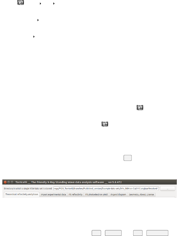
•cýHere folder: designates the sub-path in the folder containing
the Torricelli program.
CHAPTER 1. GETTING STARTED 3
•UýHere the file.txt: designates a file in a sub-folder of the
Torricelli program.
•cDýSome folder: designates the sub-path in the folder containing the
data to be analyzed.
•UDýAll data1.dat: designates a file in a sub-folder of the folder con-
taining the data to be analyzed.
•The coming references in bracket, like (n), indicate fields or buttons
marked in the region of interest of the program screenshot shown in the
figures.
1.3 Launching Torricelli
There are several possibilities to start Torricelli.
•We recommend to open a console, change directory (command cd on
Linux, Mac and Windows) to the program folder (cý) and execute
python Torricelli.py.
•One also can double click on the file UýTORRICELLI.py if it is exe-
cutable on your system.
•Do not start Torricelli from an interactive python shell.
Before starting an analysis, one must first define the directory that contains
your experimental files (cDý) (1), by clicking on the ... button (2). In this
folder, a cDýresults sub-folder is created and will contain all results (as
ASCII files and pictures).
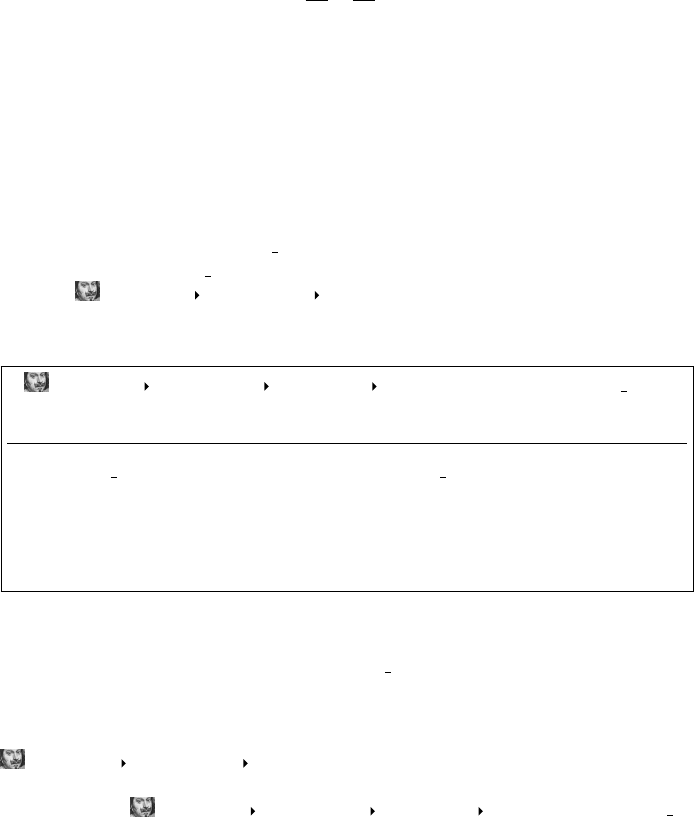
(1) (2)
(3)
Figure 1.1: The tab structure of Torricelli.
Torricelli is organized in tabs (3) (Fig. 1.1). There is a separate tab for
each important step of the data analysis. One can scroll from tab to tab with
the mouse wheel, or using the shortcuts Ctrl +PageUp and Ctrl +PageDown . In
this manual, a chapter is dedicated to each tab necessary to the data analy-
sis. The details of the algorithm are described in Ref. [1] and should be read
together with this manual.
We tried to add as much information as possible in ’tooltips’, see Fig. 1.2.
Rest the mouse cursor on a given object for one second, and a box will appear
with some explanations if there is anything to clarify.

CHAPTER 1. GETTING STARTED 4
Figure 1.2: Example of a tooltip on R2.
2
Theoretical reflectivity and phase
The calculation of the structure factors requires the knowledge of the (sample
and monochromator) crystallographic parameters: lattice constants, and list
of atoms in the unit cell. Besides, the Debye-Waller factor can also be added
if known.
There exist two databases of crystallographic parameters, for elemental
(WýCrystallographicData Elemental.csv) and for compound (WýCry
stallographicData Compound.csv) samples. They can be found in the
folder cýimports Databases Lattices. Each crystal has a dedicated
line, with comma separated values, e.g.,
Uýimports Databases Lattices CrystallographicData
Elemental.csv
Contains the lattice constants of all elemental crystal:
Z,Name,cell type,a,b,c,alpha,beta,gamma,checked values
14,Si,diamond,543.09,543.09,543.09,90,90,90,yes
28,Ni,faceCentered,352.4,352.4,352.4,90,90,90,no
29,Cu,faceCentered,361.49,361.49,361.49,90,90,90,yes
.
.
.
First comes the atomic number of the atom(s), the element name, the type
of unit cell, the three lattice lengths (a, b, c) in [pm], the three lattice angles
(α, β, γ) in [◦]. The last argument (checked values) specifies if the values has
already been used in the analysis of NIXSW data. This is then displayed in
the graphical user interface to draw the user’s attention on crystallographic
parameters that were taken from various references but not tested (see file U
ýimports Databases Database references.txt for the sources).
If your sample has a complex unit cell that is not in the database, you can create
a file named Uýimports Databases Lattices AtomCoordinates
name-of-unit-cell.csv that lists the relative position of all atoms. For
example, for the face-centered unit cell we have:
5
CHAPTER 2. THEORETICAL REFLECTIVITY AND PHASE 6
Uýimports Databases Lattices AtomCoordinates
faceCentered.csv
Atomic positions in the face centered unit cell:
Element,x (a),y (b),z (c)
A,0,0,0
A,.5,.5,0
A,.5,0,.5
A,0,.5,.5
Then just add a line in the Uýimports Databases Lattices Crystallo
graphicData *.csv file that indicates name-of-unit-cell in the col-
umn cell type as well as the atomic mass and the crystal parameters. After
restarting Torricelli, the new crystal will be included in the database.
Note If you successfully used not-checked-yet values in experiments, or in-
cluded new samples/unit cells into the database, please contact the developers
to include your values to the next version of Torricelli.
(1) (2)
(3)
(4)
(5)
(7)
(8)
(6)
(9)
(10)
(11) (12)
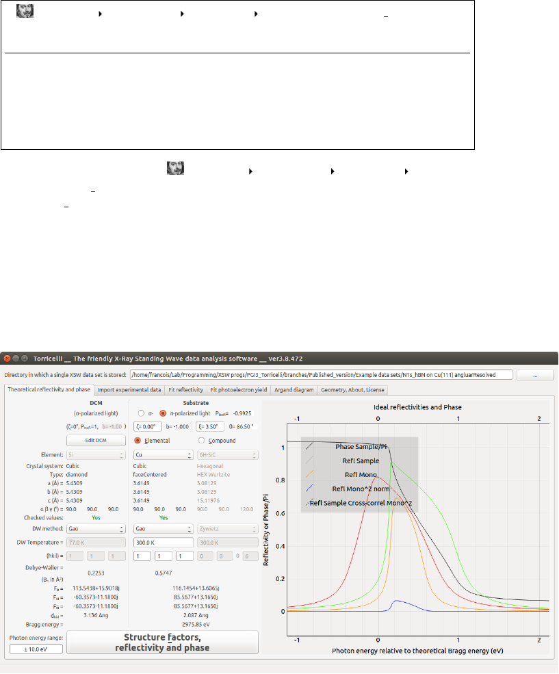
(13)
Figure 2.1: Screenshot of the Theoretical reflectivity and phase tab of Torri-
celli.
CHAPTER 2. THEORETICAL REFLECTIVITY AND PHASE 7
sample MCP
x-rays
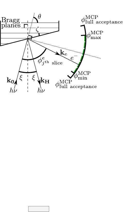
Figure 2.2: Definition of all angles used by Torricelli (ζand ξhave positive
values in the picture). This picture can also be found in the Geometry, About,
License tab of Torricelli.
In order to calculate structure factors necessary to simulate the theoretical
reflectivity and phase, the following steps need to be taken. First define the
photon energy range for which you wish to compute the theoretical curves (11)
(see Fig. 2.1). This must be larger than the experimental range. Then one
needs to specify the double crystal monochromator (DCM) (1) and sample (2)
parameters. The two beam-lines on which we have some experience (I09 at
the Diamond Light Source and ID32 at the ESRF) are both equipped with
a Si(111) DCM. In order to correctly calculate a theoretical reflectivity curve
corresponding to the experiments, Torricelli takes the DCM into account.
Typically, Si crystals are cooled with liquid nitrogen and have a temperature
of 77 K, and the (111) Bragg reflection is used. DCM parameters may be
changed by clicking the Edit DCM button (5). The light polarization is chosen
in (3). Now one needs to set up the sample. ζ(4) is the the angle between
the sample surface and the Bragg planes. ξ(4) is the deviation from perfect
normal incidence on the Bragg planes (ξ= 3.5◦at the I09 beamline). See all
angles depicted in Fig. 2.2. The parameters extracted from the database are
displayed in (6). If those values were used in an actual XSW experiment, Yes
will appear in (7). If No, please take the given values with care.

CHAPTER 2. THEORETICAL REFLECTIVITY AND PHASE 8
Important In the present state of the program, the DW Temper-
ature (9) only influences the calculation of the Debye-Waller fac-
tor. It does not affect the lattice parameter of your crystal. If
you want to use a different crystal temperature, we advise to cre-
ate a new line in the Uýimports Databases Lattices
CrystallographicData *.csv file, use an explicit name, and
adapt the lattice constant values.
Once you defined the sample (2), the hkl Miller indices of the wanted
Bragg planes reflection (10) and the type of Debye-Waller factor (8), click
on Structure factors, reflectivity and phase (12) to first compute the structure fac-
tors. If the Bragg reflection is allowed, the structure factor values will be dis-
played (11) and the sample reflectivity Rtheo
S(hν), sample phase Φtheo
S(hν)/π,
monochromator crystal reflectivity Rtheo
M(hν), the reflectivity of the double
crystal monochromator Rtheo
DCM (hν) = Rtheo
M2(hν), and cross-correlation be-
tween the sample reflectivity and the double crystal monochromator reflectivity
Rtheo
S+DCM (hν) = Rtheo
S?Rtheo
M2
Norm(hν) will be computed and displayed in
(13). Here and in the rest of the program, all curves are always shifted in
photon energy such that 0 eV corresponds to the theoretical Bragg energy.
Note From now on, Torricelli will remember the theoretical reflectivities
and phases, and one does not need to redo this step unless Torricelli is
restarted, or if data from a different sample are to be analyzed.
Auto-save After clicking on (12), the structural factors are be saved in
cDýresults Structure Factor.dat, the, theoretical curves are saved
in cDýresults Theoretical values.dat and a screenshot of the plot
is saved in cDýresults Theoretical values.png. If these files already
exist, they will be overwritten.

3
Import experimental data
Note For users of the I09 beam-line of the Diamond synchrotron, we advise
to use the I09DataBrowser, a small software that converts the raw data to
ASCII files ready to be used by CasaXPS and Torricelli. I09DataBrowser
is developed and maintained by the Torricelli team.
In the following, the steps to be taken to import and normalize reflectivity
and yield data are explained.
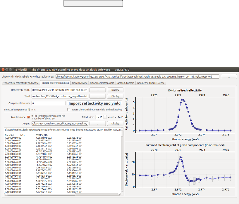
1. Choose the text files containing both the experimental reflectivity and
Iexp
0(the intensity of the incident x-ray beam) (1) in Fig. 3.1 and elec-
tron yield (2) curves (standard CasaXPS output), by clicking on the
corresponding ... button (3). They should have the following formats:
UDý*.refl:
Contains the reflectivity and the beam intensity:
Energy I refl I0
2460.92 224.0 215042.0
2460.99 225.0 214766.0
2461.05 258.0 214328.0
.
.
.
UDý*.txt or UDý*.ey:
Contains the yield of each components as well as the standard deviations:
Path of the file containing the full CasaXPS analysis (.vms)
Photon energy Reg Area(0) CPSeV StDev Reg Area CPSeV · · ·
2.460920e+003 3.558958e+005 8.186899e+002 · · ·
2.460990e+003 3.595590e+005 7.855856e+002 · · ·
2.461050e+003 3.510015e+005 7.930356e+002 · · ·
.
.
.
Note You can use the Display buttons (4) to quickly check the content
of a file, for instance, compatible number of points, or presence of some
9
CHAPTER 3. IMPORT EXPERIMENTAL DATA 10
aberrant points (11-13). If you decide to remove some points from the
data set, simply remove the corresponding lines in both files using a text
editor, and load again.
2. Choose which component (5), or which set of components Syou wish
to analyze. In the field Fit components you can list the components
numbers, separated by a space (e.g. ’1’ or ’3 2 5’), that will be analyzed.
Typically, a photoemission spectrum is fitted with one or more peaks,
here also called components. If there is more than one, they will be
summed. If nothing is given, the component 0 is the default. The com-
ponent number start from 0 for the leftmost column, and it increments
for columns going to the right. Every column with a component area
(12) should be immediately followed by a column with the corresponding
statistical errors (13).
3. By clicking on the Import reflectivity and yield button (6), the data are nor-
malized by Iexp
0, and displayed (14 and 15). Torricelli will automat-
ically check that both files have the same photon energies in the first
column (111). If the photon energies are not defined as shown in the
instance chosen for Fig. 3.1, this option can be removed by checking
Ignore the match between EY and Refl (8). This check does
not influence the data analysis, it only makes sure you are not mixing
different data files. In angular mode, this check is not performed.
(1)
(2)
(3) (4)
(5)
(7) (8)
(6)
(9)
(11) (12) (13)
(14)
(15)
(10)
Figure 3.1: Screenshot of the Import experimental data tab of Torricelli.

CHAPTER 3. IMPORT EXPERIMENTAL DATA 11
4. In the case of angular-resolved acquisition of photoelectrons, we recom-
mend to save each angular-resolved data set (slice) sequentially in the
yield file (for the same reflectivity file). It is then possible to choose the
slice number (9) to be analyzed by checking Angular mode. The cor-
responding φe
jmust be given in the file *.ang file (10) so that it can be
displayed in this tab, and also copied in the Fit Yield tab (See Fig. 2.2)
in view of the calculation of the photoemission correction parameters.
UDý*.ang: Contains the φe
jvalue corresponding to each slice j
# this file contains the angles corresponding to the centers of the slices
# File info: manually created file
# number of slices: 20
slice angle
0 116.6
1 113.8
2 111.0
3 108.2
4 105.4
5 102.6
.
.
..
.
.
In CasaXPS, you just have to put all spectra in the same folder before
you load. The file name is used to order the files. Note that by simply
scrolling on the slice number, the data are automatically imported (you
do not need to press the button (6)).
Note If the working directory (see (1) in Fig. 1.1) is changed, Torricelli
will try to find both the reflectivity, yield and angle files in this directory.
They should have the extensions .refl,.txt or .ey and .ang respectively.
If several files of the same type are present, the user has to choose the correct
file manually.
Important Do not forget that the definition of φe
jincludes ξ.

CHAPTER 3. IMPORT EXPERIMENTAL DATA 12
Important If you are using CasaXPS (or a similar program) to fit
your spectra you have to pay attention to the statistical error calcula-
tion. CasaXPS uses the Monte Carlo method to fit the data [2]. To
estimate the statistical errors CasaXPS introduces a theoretical noise
and assumes it to follow a Poisson distribution. This is a reasonable as-
sumption for pulse counted data. However in modern detectors which
rather use MCPs than channeltrons it can happen that your experimen-
tal noise is not Poisson distributed. In that case the statistical errors
from the fits of your spectra will be wrongly estimated. To check in
CasaXPS if your noise is Poisson distributed and to correct it, open
a spectrum and fit a region on a flat area (just background intensity)
of your spectrum using regression as background type. Than acti-
vate the display of the residuals. CasaXPS should show the Residual
STD of your region fit. If your noise is Poisson distributed this value
should be around 1. If that is not the case there is an option for a
correction. First select all your spectra. In the Processing window,
go to the tab Calculator and press the button Poisson Adjust Selection .
When you now check the residual STD they should be around 1. To
have the option Poisson Adjust you have to use at least version
2.3.17 PR 1.1 of CasaXPS.
Auto-save At this point nothing new is saved.
4
Fit reflectivity
The fit is performed by minimizing
RR(δhν, σ, R0, NR) = Rmodel (hν, σ)−Rexp(hν +δhν)−R0
NR
(4.1)
using the Levenberg-Marquardt method [3, 4, 5]. By default, the data points
in the residuals are not weighted by a standard error because the later is not
known. If one wishes to weight each reflectivity data point differently (e.g.,
if the standard errors are known), the code needs to be modified. The fitting
parameters are: the background R0, the normalization NR, the photon energy
shift δhν and the gaussian broadening σ. The initial guess of NRand R0are
(1)
(2) (3) (4) (5)
(7) (8)
(6)
(9)
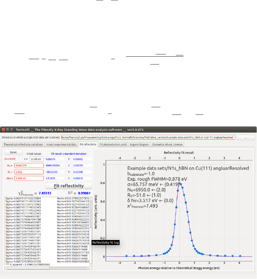
Figure 4.1: Screenshot of the Fit reflectivity tab of Torricelli.
13

CHAPTER 4. FIT REFLECTIVITY 14
such that the reflectivity difference between maximum and minimum as well as
origin are the same between the data points and the theoretical curve. δhν is
chosen such that the highest reflectivity point of the data and of the theoretical
curve lie at the same photon energy. The default initial value of σis 0.1. All
initial values are displayed in red and fit results in blue.
Note The lower the value σ, the better the crystal quality. The value of σ
for SiC is typically 0.05 eV, and for coinage metals 0.1-0.2 eV.
Press the Fit reflectivity (6) button (see Fig. 4.1). If the fit converges, the
normalized experimental data together with the fitting theoretical curve are
displayed as blue points and line (5), respectively. The experimental points
correspond to the first term of Eq. 4.1. The red line corresponds to Rtheo
S?
Rtheo
M2
Norm, that is without gaussian broadening (σ= 0).
If the fit does not converge, you can try to modify the initial parameters (2)
(e.g., increasing σusually helps to find convergence, the other values are usually
very good). The fit results are saved as text file and picture, see Chap. 10. It is
possible to reset the initial values to the guess made by Torricelli by clicking
on Reset (1).
In the absence of standard errors, the standard χ2
red is not defined. There-
fore, the Pearson’s chi-squared (χ2
Pearson, see Eq. 1.8 in Ref. [7]) and the coef-
ficient of determination (R2, see Sec. 1.3 and 11.2 in [8]) are displayed (7, 8)
in order to evaluate the quality of the fit [6, 8] without the knowledge of the
variance. They are defined as follows:
χ2
Pearson ≡1
DF X
exp.hν
Rexp(hν)−Rmodel(hν)2
Rmodel(hν)
and
R2≡1−SSres
SStot
,(4.2)
with DF the number of degree of freedom and
SSres =X
exp.hνRexp(hν)−Rmodel(hν)2(4.3)
SStot =X
exp.hνRexp(hν)−¯
Rexp2(4.4)
¯
Rexp =1
n
n
X
exp.hν
Rexp(hν) (4.5)
where the sums run over all experimental hν values, and nis the total the
number of experimental points. R2values range from 0 (bad fit) to 1 (good
fit).
Important If this fit is not good, it is of no use to continue the
analysis! Check the parameters you used for the sample crystal.

CHAPTER 4. FIT REFLECTIVITY 15
Auto-save After clicking (6), the fit results are saved as ASCII file and
pictures in cDýresults Exp refl norm centred.dat,cDýresults
Fit refl.log,cDýresults Fit result refl.png and cDýresults
Fit result refl.dat.
5
Fit yield
The fit is performed by minimizing
RY(PS
c, F S
c, NS
Y) = Ymodel
Shν, P S
c, F S
c, NS
Y, γ, φ
−Yexp
S(hν +δhν, φ)
NS
Y×NS
Y
σYexp
S(hν, φ)(5.1)
using the Levenberg-Marquardt method. The values of δhν and σare the result
of the reflectivity fit and are fixed to fit the yield. In the simplest case, there
(1) (2) (3)
(4) (5)
(7)
(8)
(6)
(9) (10) (11) (12)
(13)
(14)
(15) (16)
(17)
(18) (19)
(20) (21)
(22)
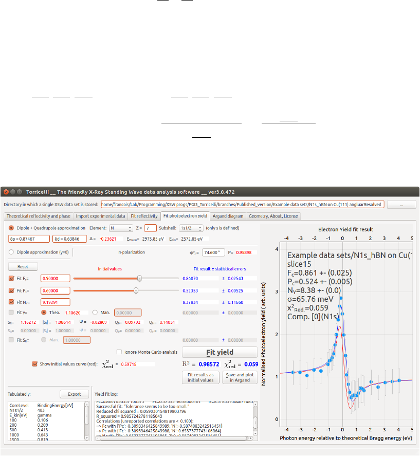
Figure 5.1: Screenshot of the Fit yield tab of Torricelli.
16
CHAPTER 5. FIT YIELD 17
are only three fitting parameters: the normalization factor NS
Y, the coherent
position Pcand fraction Fc. If the statistical error σYexp
S(hν, φ) are not known
or not reliable, it is possible to replace them by NS
Yin Eq. 5.1 by checking
Ignore Monte Carlo analysis (15) (see Fig. 5.1). It is possible to independently
fix/fit each of the fit variables by un/checking them (9).
The level of approximation to be used to treat the photoemission process can
be chosen: dipole (6) or dipole-quadrupole (1). Within the dipole-quadrupole
approximation, ∆ and the non-dipolar parameter γneed to be calculated. To
do so, the user must provide the element subject to photoemission (2) and
the sub-shell under consideration (3). The corresponding photoelectron kinetic
energy is then calculated and displayed EKin (5). This calculation ignores the
sample work function. EKin is used to interpolate the γ(13) value from the
database [9, 10], that is displayed in (20). Second, the value of EKin must
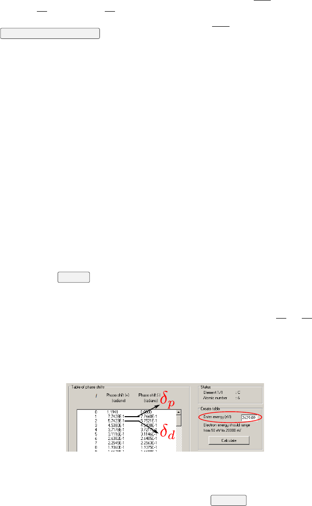
then be given in the NIST Electron Elastic-Scattering Cross-Section Database
version 3.2 (available on-line) to obtain δp and δd (4). A screenshot of the
program Elastic32 is given in Fig. 5.2. Afterwards, the user must copy the
δp and δd in Torricelli so that ∆ can be calculated. Finally, φe
j(7) is used
to calculate the polarization factor P(in case of π-polarization). The value
of φe
jis automatically updated if an angle file is given in the import tab, if
not this value must be given by hand. Once ξ,ζ,P,γand ∆ are known,
Torricelli can calculate the photoemission correction parameter to the yield
SR,SIand ψ. Even within the dipole approximation, the φe
jis needed (in case
of π-polarization) to properly calculate SR,SIand ψ. All initial values are
displayed in red.
Press the Fit yield button (16). If the fit converges, the normalized exper-
imental data together with the fitting theoretical curve are displayed as blue
points and line (22), respectively. The normalized statistical error are displayed
as vertical red bars. Nonphysical negative or greater than unity Fcor Pccan
still produce a very good fit. To overcome this, one has to set better initial
values. After having fitted once, it is possible to display the theoretical curve
with initial values in red (17). The initial values can be changed by typing the
value (10), or by moving the cursor (11). The red curve in (22) will instantly
average
average
Figure 5.2: Screenshot of the Elastic32 program, the NIST Electron
Elastic-Scattering Cross-Section Database to calculate δp and δd (Menu:
Database/Phase shifts). Enter the adequate kinetic energy of the photoemitted
electrons as calculated by Torricelli, and click Calculate .

CHAPTER 5. FIT YIELD 18
update. Press the Fit yield button (16) again once the initial values are set.
The fit results together with their standard deviation (12) are displayed, as
well as the coefficient of determination R2(see Chap. 4) and the χ2
red. Also,
each step of the optimization are displayed in (21), as well as further fit results
details. All fit result values are displayed in blue. It is possible to fit the γ(or
SR) if your sample is completely disordered and you are confident to fix Fcto
0.
Once satisfied with the fit results, click on Save and plot in Argand (19) to
store the results (including the standard deviations and all other relevant pa-
rameters) in a list of all gathered results (See Chap. 6).
Note The Monte-Carlo analysis in CasaXPS is usually slow. If you are in a
hurry (during a beam-time), you may want to avoid this step and tell Tor-
ricelli not to read in the error bars and click Ignore Monte Carlo analysis (15).
This will remove the error bar weight on the data points, by effectively setting
σYexp
S(hν, φ) = NS
Y. As a consequence, the error bars given by the fit proce-
dure are not defined anymore and should not be used. Also, χ2
red is not defined
anymore.
Auto-save In the cDýresults folder, pictures, normalized experimental
data, fitted theoretical data as well as fit results are saved/updated automati-
cally each time the Fit Yield button is pressed. The created RESULTS *.csv
file, that summarize the fit results and all used parameters, can be easily loaded
by another program to consult the data.
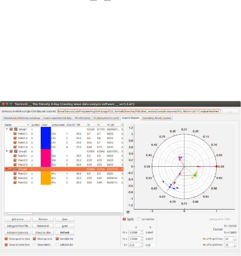
6
Argand diagram
In this tab it is possible to display the fit results of the electron yield curve on
an Argand diagram (2), a polar plot where each point is defined by a vector
with angle Pcand length Fc. The data are all listed in a list (1) and can be
grouped (see Fig. 6.1). The vector average position and fraction of each group
is automatically calculated and displayed (by default a + symbol and a line
from the origin). One can display/hide independently every single data point
(circle symbol by default, with the color of the group) or entire groups. One
can then move the data points from one group to another or within a group by
(1) (2)
(3) (4) (5)
(7) (8)(6)
(9) (10) (11)
(12) (13)
(14) (15)
(16)
Figure 6.1: Screenshot of the Argand diagram tab of Torricelli.
19

CHAPTER 6. ARGAND DIAGRAM 20
a simple drag and drop. The selected point/s is/are highlighted in (2). Press
Esc to clear the selection. Points and groups can be removed by pressing Del
on the keyboard, or clicking the Remove button in Torricelli. Double-click or
F2 on any value-field permits to amend the values (only possible is Editable list
is selected). If several points are selected, a right-click on the name, color or
symbol permit to apply the new property on the whole selection.
To add a group, just click on Add group (3). To insert values in the selected
group, one can either type-in the values manually (9), or choose the log file of
a fit (6), or by clicking the Save and plot in Argand button after having obtained
a satisfying fit ((19) in the previous chapter). In the latter case, a new point
is created in a group named like the working directory name. Furthermore,
all relevant values are also saved and displayed in the list (1). The content of
the list can be saved (5) in a text .csv file and reloaded at a later point (8).
The format is chosen so that it can be easily loaded by another program (see
Chap. 10 for the content details).
One can also decompose any data point Din the sum of two vectors (A
and B) (13). The Avector can be modified by moving it with the mouse (big
red circle in (2)), or by typing values. The Bwill be updated automatically.
ncorresponds to the respective amount of atoms populating each species. The
Symmetrize option forces Aand Bto have the same fraction.
By right-clicking in the diagram, one can export the picture by choosing
’Entire scene’. Several formats are possible, we advise though the .svg vector
format which allows the easy modification of the picture with a dedicated
program, like Inkscape.
Auto-save Additionally, the full content of the Argand diagram is automat-
ically saved regularly in the UDýautosave time description.csv file in
the working directory when the whole list is cleared, when the list is grouped
by slices, after inserting a new point, or when Torricelli is closed. In each
case, an explicit name is used.
The UDýresults RESULTS DataName TorricelliVersion.csv file
is created/updated each time the fit yield button is pressed in a given working
directory. It summarizes all fit results obtained from a single data set for each
Sand each slice. If the fit button is pressed several times for the same Sand
slice, only the last fit results are saved.
7
Example data sets
In the directory cýExamples data sets, two data sets are given. In the
following section, we give the fit results produced by Torricelli for a specific
set of parameters.
7.1 C1s H-QFMLG on SiC(0001)
The first is a C 1s core level on quasifreestanding monolayer graphene on 6H-
SiC(0001), using the reflection (006). The data are angle integrated. Using
π-polarization, ζ= 0, ξ= 3.5◦, the Zywietz DW method, the core level compo-
nent C1s QFMLG (i= 1), φe
j= 90◦and the dipole approximation, the reflec-
tivity fit result gives σ= 45.7 meV, NR= 14396, R0= 154 and δhν = 2.67 eV.
The yield fit result provides Fc= 0.871, Pc= 0.688, NY= 128891.17.
7.2 N1s hBN on Cu(111) angluarResolved
The second is a N 1s of hexagonal boron nitride monolayer grown on Cu(111)
using the (111) reflection. The data are angle-resolved. Using π-polarization,
ζ= 0, ξ= 3.5◦, the Gao DW method, the core level component N1s (i=
0), the slice j= 15, φe
j= 74.6◦and the dipole-quadrupole approximation
(δp = 0.87467, δd = 0.63846, γ= 1.10620), the reflectivity fit result gives
σ= 65.8 meV, NR= 6950, R0=−51 and δhν = 3.517 eV. The yield fit result
provides Fc= 0.861, Pc= 0.524, NY= 8.38.
21

8
Useful shortcuts
•General ones:
Alt +FPresses the big button you always want to press on the active
tab
Ctrl +PageDown Moves to the next tab
Ctrl +PageUp Moves to the previous tab
Mouse Wheel on tab Scroll through tabs
•In graphical sub-windows:
Mouse wheel zoom in/out
Left click + mouse move x/y translation
Right click + mouse move x/y re-scaling
Right click menu with more options, including export options
•In the Argand list of group and points:
Double click on value change the value in the selected field (Right-
click is several items are selected)
F2 on value change the value in the selected field
Double click on name change the name. If several points are selected,
a right-click will rename the selection with with increasing N: name N
Esc clear the item selection
22
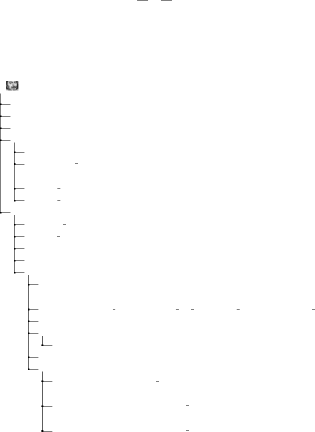
9
The folder structure of Torricelli
In the following we describe briefly all files present in the Torricelli program
folder tree.
cý............................................ Torricelli home folder
WýTorricelli.py.................execute this file to start Torricelli
WýCOPYRIGHT...............copy of the GNU General Public License v3
WýREADME ....................... Brief description of the files and folders
bûExample data sets
WýArgandTest.csv ...... few (Fc,Pc) points for the Argand diagram
WýArgand BigFileTest.csv..many (Fc,Pc) points for the Argand
diagram
`ýC1s H-QFMLG on SiC(0001)
`ýN1s hBN on Cu(111) angluarResolved
bûimports
Wýuser settings.......last settings used before closing Torricelli
WýGUI *............................................... gui modules
Wý*.png and *.svg......................................images
WýpyArgand.py............................Argand diagram library
bûDatabases
WýDatabase references.txt.....references for all files in the
database
WýNondipolar parameters of angular distribution Z1to100.ini
Wýf0.csv.............. f0 atomic scattering factor for all elements
bûf1 and f2...............all f1 and f2 atomic scattering factor
Wýsi.nff .................................... f1 and f2 for Si
`ýDW...............database necessary for the Debye-Waller factors
bûLattices
WýAtomCoordinates name-of-unit-cell.csv..relative
atomic position in this unit cell
WýCrystallographicData Compound.csvcrystallographic
parameters for compounds
WýCrystallographicData Elemental.csvcrystallographic
parameters for elemental crystals
23
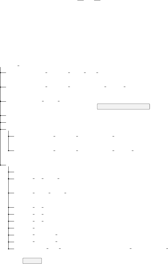
10
The folder structure of an analyzed data set
Example of directory in which a single XSW data set is stored. In the folder
býsum (depicted as cDý), here chosen as working directory, the folder cDýresults
will be created by Torricelli during the analysis.
bûC1s H-QFMLG on SiC(0001) or cDý
Wýi09-22758 C1sXSW Relf and I0.refl...reflectivity, Torricelli
input
Wýi09-22758 c1sxsw allregions 2Comp ShirleyBgd.txtelectron
yield (CasaXPS analysis output), Torricelli input
Wýautosave time description.csv.....Content of the Argand list
automatically saved after pressing the Save and Plot in Argand button
`ýslice1..................all data from the first angle-resolved data set
`ýslicen...................all data from the nth angle-resolved data set
bûsum...............all data from the sum of all angle-resolved data sets
Wýi09-22758 C1sXSW allRegions hnu.dat.core level measured
with a photon energy of hnu (CasaXPS input)
Wýi09-22758 c1sxsw allregions 2Comp ShirleyBgd.vmsCasaXPS
analysis file
bûresults
WýStructure Factor.dat ................... all structure factors
WýExp ey norm centred[0].dat....electron yield of component 0
normalised to I0and relative to EBragg
WýExp refl norm centred.dat...reflectivity normalised to I0and
relative to EBragg
WýFit ey comp[0].dat...best fit electron yield curve, component 0
WýFit ey comp[0].log.............log of the electron yield fitting
WýFit ey comp[0].png ......... image from electron yield fit result
WýFit refl.log ....................... log of the reflectivity fitting
WýFit result refl.dat ................. best fit reflectivity curve
WýFit result refl.png...........image from reflectivity fit result
WýRESULTS C1s H-QFMLG on SiC(0001) Torricelli verx.x.x.csv
list of results obtained from this working directory, updated after each click
on Fit yield
24

CHAPTER 10. THE FOLDER STRUCTURE OF AN ANALYZED DATA
SET 25
WýTheoretical values.dat...................theoretical curves
WýTheoretical values.png.......image of the theoretical curves
Few .png files simply record the graph displayed in Torricelli, for a quick
printout. The .dat files include actual data in ASCII that can be used in a
scientific plotting program to produce high quality figures. The exact content
of each of the .dat is now detailed (for programmers, we also included the
respective variable names.)
1. WýTheoretical values.dat
col1 Photon energy relative to the Bragg energy (self.Theory_photonEnergy)
col2 Reflectivity of the sample crystal (self.Theory_Refl_sample)
col3 Phase of the sample crystal (self.Theory_Phase_Sample)
col4 Reflectivity of the monochromator crystal (self.Theory_Refl_Monochromator)
col5 Phase of the monochromator crystal (self.Theory_Phase_Monochromator)
col6 Final convoluted reflectivity of both crystal and monochromator
(self.Theory_ReflSample_cc_ReflMono2)
2. WýExp refl norm centred.dat
col1 Photon energy shifted by δhν to fit the theoretical values
(self.Exp_photonEnergy_BraggCentered +δhν)
col2 Reflectivity normalized by Iexp
0for each photon energy, and multi-
plied by the average of all Iexp
0, then shifted by R0and multiplied by
NRto fit the theory ((self.Exp_Refl_Normalised - R0)/NR)
col3 Estimated statistical error on the reflectivity (square root of the pre-
viously normalized intensity) (self.Exp_Refl_Estimated_Error/NR)
3. WýFit result refl.dat
col1 Photon energy relative to the Bragg energy (self.Theory_photonEnergy)
col2 Theoretical reflectivity curve best fit, including the gaussian broad-
ening (bestFit_theo_refl)
4. WýFit refl.log : List of all tested parameters configurations tested
during the fitting procedure. The last one corresponds to the best fit.
5. WýExp ey norm centred[S].dat
col1 Photon energy shifted by δhν
(self.xsw_energies_BraggCentered +δhν)
col2 Electron yield of the component set Sprovided (for example) by
CasaXPS. It is normalized by Iexp
0for each photon energy, and multi-
plied by the average of all Iexp
0and divided by the NS
Y(self.xsw_ey_normalised/NS
Y)

CHAPTER 10. THE FOLDER STRUCTURE OF AN ANALYZED DATA
SET 26
col3 Statistical error of the electron yield of the component set Spro-
vided by CasaXPS normalized in the same way as the electron yield
itself
(self.xsw_ey_error_casaXPS/NS
Y) (NOTE that I09 DataBrowser
does not perform any normalisation)
6. WýFit ey comp[S].dat :
col1 Photon energy relative to the Bragg energy (self.Theory_photonEnergy)
col2 Electron yield best fit (self.Fit_Result_EY)
7. WýFit ey comp[S].log : List of all tested parameters configurations
tested during the fitting procedure. The last one corresponds to the best
fit. Each different value of the initial curve that is displayed will also be
saved in this file.
8. *.csv files: Contains the fit results parameters separated by a comma.
Each line correspond to a different data set. In the case of .csv file
created by the Argand diagram tab, there is also a line corresponding to
the average of all points contained in the group. The Wýautosave.csv
is rewritten each time the Save and plot in Argand button is clicked and con-
tains full content of the list visible in the Argand tab. The WýRESULT *.csv
file is updated each time you click the Fit yield button, and contains only
fit results from the data present in the working directory. It remembers
only the fit result of resulting from the last time you clicked Fit yield for
each set of component or angle chosen.

11
Miscellaneous
11.1 Reading or modifying the code
Reading or modifying a function that is related to a specific object (Button,
integer field, etc.) in the graphical user interface works as follows. One opens
the GUI_MainWindow.py file with the QtDesigner free software1to obtain
the object name. Then one can search the Torricelli.py file using a stan-
dard text editor to find which function is connected to this object. Both the
command connecting an object to a function and the function itself are in the
Torricelli.py file.
11.2 Few advices for efficiency
•Use the shortcuts! Once you chose the working directory and set all your
parameters/angles, you basically just have to press Alt +Fand Ctrl +
PageDown few times... And you are done!
•Use the folder structure created by the DataBrowser (as explained in
Chap. 10).
•Save the electron yield file in the folder created by the DataBrowser, and
use either a .txt or .ey extension.
•Select the new folder for each new measurement (top of the window),
then Torricelli will find all it needs automatically.
•It is a good habit to keep an eye on the console window. Typically
unexpected warnings or errors are displayed there.
•It is an open source software: it can be modified but the modifications
must maintain the same license.
Note Many file paths, folder paths and other settings are saved in the file
cýimports user settings. So when you close Torricelli, and open
it again, the program is already pre-configured for you.
1https://doc.qt.io/archives/qt-4.8/designer-manual.html
27
Bibliography
[1] F. C. Bocquet, G. Mercurio, M. Franke, G. van Staaten, S. Weiß, S.
Soubatch, C. Kumpf and F.S. Tautz – Torricelli: A software to de-
termine atomic spatial distributions from normal incidence x-ray standing
wave data.
Computer Physics Communications vol,page (2018).
[2] Mercurio, G. and Bauer, O. and Willenbockel, M. and Fairley, N. and
Reckien, W. and Schmitz, C. H. and Fiedler, B. and Soubatch, S. and
Bredow, T. and Sokolowski, M. and Tautz, F. S. – Adsorption height
determination of nonequivalent C and O species of PTCDA on Ag(110)
using x-ray standing waves.
Phys. Rev. B 87, 045421 (2013).
[3] K. Levenberg – A Method for the Solution of Certain Non-Linear Problems
in Least Squares.
Quart. Appl. Math 2, 164 (1944).
[4] D. W. Marquardt – An Algorithm for Least-Squares Estimation of Non-
linear Parameters.
J. Soc. Indust. Appl. Math. 11, 431 (1963).
[5] M. Newville, T. Stensitzki, D. B. Allen and A. Ingargiola – Lmfit: Non-
Linear Least-Square Minimization and Curve-Fitting for Python.
Zenodo, (2014).
[6] A. Glantz and B. K. Slinker – Primer of applied regression and analysis
of variance.
2nd edition, McGraw-Hill (2001).
[7] P. E. Greenwood and M. S. Nikulin – A guide to chi-squared testing.
John Wiley & Sons (1996).
[8] N. R. Draper and H. Smith – Applied Regression Analysis.
Wiley Series in Probability and Statistics, 3rd edition, Wiley-Interscience
(1998).
28
BIBLIOGRAPHY 29
[9] M. B. Trzhaskovskaya, V. I. Nefedov, V. G. Yarzhemsky – Photoelectron
angular distribution parameters for elements Z=1 to Z=54 in the photo-
electron energy range 100-5000 eV.
Atom. Data Nucl. Data Tables 77, 97 (2001).
[10] M. B. Trzhaskovskaya, V. I. Nefedov, V. G. Yarzhemsky – Photoelectron
angular distribution parameters for elements Z=55 to Z=100 in the pho-
toelectron energy range 100-5000 eV.
Atom. Data Nucl. Data Tables 82, 257 (2002).