User Manual
User Manual:
Open the PDF directly: View PDF ![]() .
.
Page Count: 20
IMT-2020 Channel Model (CM) Software
User Manual
Editors:
Zhang Jianhua
jhzhang@bupt.edu.cn
Tian Lei
tianlbupt@bupt.edu.cn
Mansoor Shafi
mansoor.shafi@spark.co.nz
Document Version: V2.0
May 30, 2018
IMT-2020 CM_BUPT—— User License
Copyright(c) 2018 Zhang Jianhua Lab, Beijing University of Posts and Telecommunications.
The software platform is open and any person or group is allowed, free of charge, to obtain a
copy of this simulation software and associated help documentation files. Users are permitted
to use the platform without restriction. But users should subject the following conditions:
1. The above copyright notice and this permission notice should be admitted and retained in
any copy of the software.
2. The software platform is developed for research of radio channel. If any person or group
wants to apply the platform in industry or any other fields, Zhang Jianhua Lab of BUPT
cannot give any guarantee of the accuracy about the result.
3. The software platform is developed by Zhang Jianhua Lab of BUPT. We reserve all the
rights for the final explanation.

Contents
1 Introduction ......................................................................................................................... 1
2 Installation ........................................................................................................................... 2
3 Model Framework ............................................................................................................... 3
3.1 Data Flow ..................................................................................................................... 3
3.2 Graphical User Interface description ............................................................................... 4
3.2.1 Antenna parameter Input ....................................................................................... 4
3.2.2 System parameter Input ......................................................................................... 5
3.2.3 Parameters Input for advanced modelling components ......................................... 5
3.3 Antenna Configuration ................................................................................................. 6
3.3.1 Antenna Array Geometry ...................................................................................... 6
3.3.2 Antenna Response ................................................................................................. 8
3.4 Scenario and Layout ..................................................................................................... 8
3.4.1 Network Layout ..................................................................................................... 8
3.4.2 Description of supported propagation scenarios.................................................... 9
3.5 Path loss ...................................................................................................................... 10
3.6 Large Scale Parameter ................................................................................................ 11
3.7 Small Scale Parameter ................................................................................................ 12
3.8 Channel Impulse Response ......................................................................................... 13
4 Description of Output results ............................................................................................. 14
5 Running example ............................................................................................................... 15
6 Reference ........................................................................................................................... 16
1
1 Introduction
The Zhang Jianhua Lab of BUPT provides the MATLAB implementation of the ITU-R
M.2412-0[1] channel document. The channel modeling method and principle are explained in
[JSAC][2] and detailed parameters and scenarios are described in [ITU-R M. 2412-0].The
software is named as IMT-2020 CM_BUPT. It is a multi-link simulation platform which can
generate a radio channel information between multiple Base Stations and multiple User
Terminals. This document will describe the framework of the simulation software in detail and
give some instruction about the function applied in the model. The more specific scenarios of
channel model and parameters can be found in the ITU-R M.2412-0.
In IMT-2020 CM_BUPT, users can choose the model A or model B provided in ITU-R M.2412-
0. All the scenario parameters are loaded in the platform. And users can set the number of
antennas and choose the type of them. Channel matrices can be generated for multiple BS-UT
links. And the path loss component is also included.
It should be noticed that the output of platform is the channel matrices. If users want the middle
variable, other operations may need, which are beyond the scope of the implemented channel
model.
2
2 Installation
IMT-2020 CM_BUPT simulation platform is based on the MATLAB software. The users have
to install a MATLAB software in their computers. In our test in fact, the test system is Windows
7 x64 and the MATLAB version is R2016b. The main function is “IMT-2020_CM_BUPTv2.p”.
Users can run the platform by “IMT-2020_CM_BUPTv2.p” or “IMT-2020_CM_BUPTv2.fig”.
The function includes the following modules:
%% IMT-2020 Channel Model Software
%% Copyright:Zhang Jianhua Lab, Beijing University of Posts and Telecommunications
(BUPT)
%% Editor:Zhang Jianhua (ZJH), Tian Lei (TL)
%% Version: 2.0 Date: May. 30, 2018
%% Antenna Configuration
% AntennaModelBs - Bs antenna pattern and calculate the antenna
% AntennaModelUt - Ut antenna pattern and calculate the antenna
% AntennaArray - Antenna type and how to place the antenna element
%
%% Scenario and Layout
% Scenario - Set the ITU-R M.2412-0 test environment parameters
% Layout - Generate the network information about BS and UT
% UtPosdistribution - User's distribution
% WrapAround - Link information after wrapping
%
%% Path loss
% GeneratePathloss - Generate the path loss of links
% LOSprobability - Determine whether the LOS link
%
%% Channel Parameters
% GenerateLSP - Generate the large scale parameters
% GenerateSSP - Generate the small scale parameters
% RayAngleOffset - Set the fixed offset of cluster angle to ray angle
%
%% Channel impulse response
% GenerateCIR - Generate the channel impulse response
%
%% Utility functions
% RMSDelaySpread - Calculate the delay spread
% AngleSpread - Calculate the angle spread
% prin_value_azimuth - Limit the azimuth angle to -180:180 degrees
% prin_value_zenith - Limit the zenith angle to 0:180 degrees
%
%% Advanced functions
3
% Blockage -add blockage loss for per link according to blockage model B
% GenerateCIR_SC - Generate the channel impulse response using spatial consistency
% GenerateSSP_SC - Generate the small scale parameters using spatial consistency
%
%% Test Example
% test - An example about how to create a simulation
3 Model Framework
3.1 Data Flow
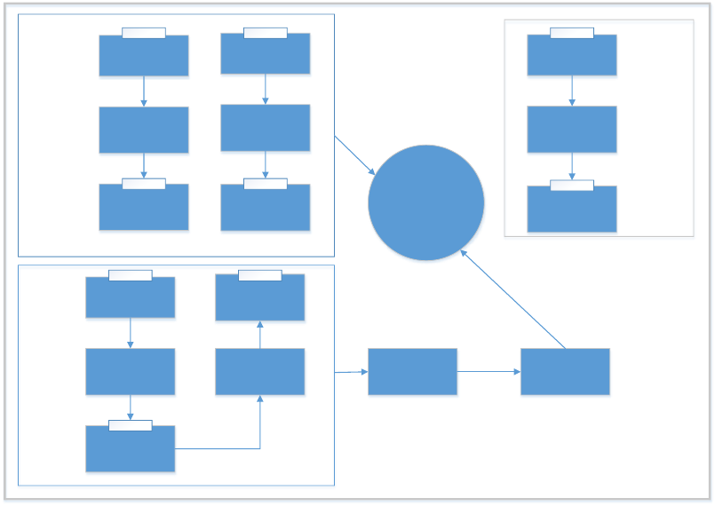
The CM implementation structure is shown in the block diagram given in Figure 1. The core of
the platform is to generate channel impulse response which contains three main modules. And
the three main modules are antenna module, layout and scenario module and path loss module
respectively. The antenna module aims to give the antenna locations and antenna responses.
Different network layout which contains information of BSs and UTs, as well as parameters
configuration in different scenarios, such as UMa, UMi and O2I is determined in the layout and
scenario module. The path loss module can be modeled as a separate user-supplied function
which aims to give the path loss and standard deviation of shadow fading per link.
The main data flow of the CM platform can be seen in the Figure 1. Input and output arguments
are defined in more detail in the following section.
AntennaArray.m
Number and type of
antenna,
carrier wavelength
INPUT
Position
information per
antenna element
OUTPUT
AntennaModel.m
Antenna direction
angle
INPUT
Antenna gain
in different
direction
OUTPUT
Antenna
Module
Layout.m
Frequcency,Scenario,
model type,user
numbers,etc
layoutpar
OUTPUT
INPUT
Scenario.m
(UMA/UMI/RMA
INH/O2I)
GenerateLSP.m
fixpar
OUTPUT
GenerateSSP.m
sigmas
Layout
and
Scenario
Module
GenerateCIR.m
GeneratePathloss.m
fixpar
layoutpar
Pathloss
SF_sigma
OUTPUT
INPUT
Path Loss
Module
Figure 1 The structure and data flow of CM platform
4
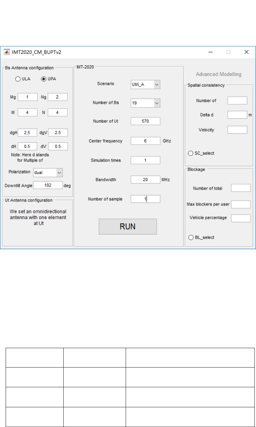
3.2 Graphical User Interface description
The file “IMT-2020_CM_BUPTv2.fig” is the interface of the platform. Users can directly open
this file to configure the simulation parameters and run the platform. The Graphical User
Interface (GUI) of IMT-2020_CM_BUPT v2.0 is shown in Figure. 2.
Figure 2 GUI of IMT-2020_CM_BUPT v2.0
3.2.1 Antenna parameter Input
The Ut antenna is set to be a single vertical-polarized omnidirectional antenna. The Bs antenna
can be configured according to the specific requirement. For the description of specific
parameters, you can refer to ITU-R M.2412 Page31.
Table 1 Antenna parameter configuration
Parameter name
Description
Note
ULA/UPA
Choice of
ULA/UPA
When ULA selected, Mg, Ng, N will be
automatically set to 1
Mg
Number of antenna
panel rows
-
Ng
Number of antenna
panel columns
-

5
M
Number of antenna
element rows
-
N
Number of antenna
element columns
-
dgH
The horizontal
distance between the
antenna panel
dgH should be greater than dH*(N-1)
the unit is the length of wavelength.
dgV
The vertical distance
between the antenna
panel
dgV should be greater than dV*(M-1)
the unit is the length of wavelength.
dH
The horizontal
distance between the
antenna unit
the unit is the length of wavelength.
dV
The vertical distance
between the antenna
unit
the unit is the length of wavelength.
Polarization
Choice of
polarization
Single and dual polarization options
Downtilt Angle
Antenna downtilt
angle
-
3.2.2 System parameter Input
The system parameters which are needed to be configured by users, are listed in Table 2.
Table 2 System parameter configuration
Parameter name
Description
Note
Scenario
Choice of scenario
According to ITU-R M.2412, the optional
scenarios are included in the popup menu
Number of Bs
Number of base
stations within the
base station
According to the actual situation, the
common used numbers of base stations
are included in the popup menu
Number of Ut
Number of user
terminal
-
Center frequency
Center frequency
-
Simulation times
Simulation times
-
Bandwidth
Bandwidth
-
Number of sample
points
Number of
sampling points
-
3.2.3 Parameters Input for advanced modelling components

6
Three advanced modelling components are implemented in the platform, which are “Spatial
Consistency” and “Blockage”.
Spatial Consistency Simulation Configuration
The spatial consistency part of this program is only applicable to the case of a single link.
When spatial consistency is selected, the ‘Number of Bs’ and ‘Number of Ut’ will be
automatically set to 1.
Table 3 Parameter description for spatial consistency
Parameter name
Description
Note
Number of points
Set the number of
inflection points
in the Ut moving
route.
-
Delta d
Set distance
resolution
Should be less than 1 meter
Velocity vector
Vector of velocity
Each inflection point contains 3 parameters.
The speed, horizontal moving direction, and
vertical moving direction are respectively.
The unit of speed is m/s.
The unit of horizontal moving direction is deg.
The unit of vertical moving direction is deg.
The length of input should be equal to point*3.
e.g. 10 45 90 10 45 0
Just enter the value in order is OK.
Blockage Simulation Configuration
The blockage part of this program is realized according to the blockage model II in ITU-R
M.2412.
Table 4 Parameter description for blockage
Parameter name
Description
Note
Number of total blockers
Set the total number of blockers within the base station
-
Max blockers per user
Set the maximum number of blockers for a user
-
Vehicle percentage
The percentage of vehicle blockers in all blockers
-
3.3 Antenna Configuration
3.3.1 Antenna Array Geometry
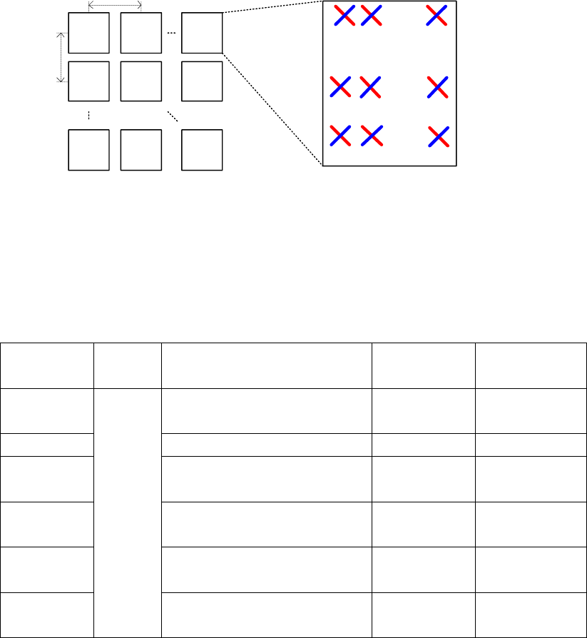
The BS antenna is modelled by a uniform rectangular panel array, comprising Mg Ng panels,
as illustrated in Figure 3 [1] with Mg being the number of panels in a column and Ng being the
number of panels in a row. Furthermore, the following properties apply:
- Antenna panels are uniformly spaced in the horizontal direction with a spacing of dg,H
7
and in the vertical direction with a spacing of dg,V.
- On each antenna panel, antenna elements are placed in the vertical and horizontal direction,
where N is the number of columns, M is the number of antenna elements with the same
polarization in each column.
- Antenna numbering on the panel illustrated in Figure 3 assumes observation of the antenna
array from the front (with x-axis pointing towards broad-side and increasing y-coordinate for
increasing column number).
- The antenna elements are uniformly spaced in the horizontal direction with a spacing of
dH and in the vertical direction with a spacing of dV.
- The antenna panel is either single polarized (P =1) or dual polarized (P =2).
The rectangular panel array antenna can be described by the following tuple
PNMNM gg ,,,,
.
NOTE: The user antenna defaults to an omnidirectional antenna element.
dg,H
dg,V
(0,0) (0,1) (0,N-1)
(M-1,N-1)
……
(M-1,0) (M-1,1)
(1,0) (1,1) (1,N-1)
……
……
……
……
……
……
Figure 3 Bs antenna model [1]
More details about the function AntennaArray.m can be seen in Table 5.
The full syntax for AntennaArray function is:
AA=AntennaArray (Mg,Ng,M,N,dgH,dgV,dH,dV,lambda)
Table 5 Short overview of input and output arguments for AntennaArray.m
Argument
name
Type
Description
Default
value
Note
Mg
input
the number of panels in a
column
-
-
Ng
the number of panels in a row
-
-
M
the number of antenna rows in
a panel
-
-
N
the number of columns in a
panel
-
-
dgH
Antenna panel spacing in
horizontal direction
-
-
dgV
Antenna panel spacing in
vertical direction
-
-

8
dH
Antenna spacing of one panel
in horizontal direction
-
-
dV
Antenna spacing of one panel
in vertical direction
-
-
lambda
Wavelength of used carrier
-
The default
space between
adjacent
elements is
half
wavelength
AA
output
Information of antenna array
-
-
3.3.2 Antenna Response
Antenna Response can be expressed by elevation angle
and azimuth angle
. The detailed
formulas can be seen from TABLE 9-11 in Report ITU-R M.2412-0. More details about the
function AntennaModel.m can be seen in Table 6.
The full syntax for AntennaModelBs function is:
AntennaGain=AntennaModelBs(phi, theta).
NOTE: User antenna gain defaults to 0 dB.
Table 6 Short overview of input and output arguments for AntennaModelBs.m
Argument
name
Type
Description
Default
value
Note
phi
input
Azimuth angle of arrival
or departure refer to each
element
-180:1:180
-
theta
Elevation angle of arrival
or departure refer to each
element
0:1:180
-
AntennaGain
output
3D antenna element
pattern
-
-
3.4 Scenario and Layout
3.4.1 Network Layout
CM implementation currently support system simulations for mutilple UT-BS links. So the
network layout includes information about: the height of the BS and the UT, the distance
between the BS and the UT, the LOS probability of the link, the frequency used in the
simulation, etc. Layout.m function almost defines all the parameters decided by users. After

9
implementing the function, all information required to generate LSP and SSP of each link can
be obtained. More details about Layout.m can be seen in Table 7.
The full syntax for Layout function is:
layoutpar=Layout(Input.Sce,Input.C, Input.N-user,Input.fc,Input.AA).
Table 7 Short overview of input and output arguments for Layout.m
Argument
name
Type
Description
Default
value
Note
Sce
input
Simulation scenario that
users choose
-
-
C
Elevation angle of arrival or
departure refer to each
element
1
Currently support one
BS
N_user
Number of subscribers for
all BS
-
-
fc
Carrier frequency in GHz
-
The range of
frequency is 0.5-100
GHz
AA
Configuration of antenna
array
-
-
layoutpar
output
Information of the network
layout
-
-
3.4.2 Description of supported propagation scenarios
The function scenario.m defines the necessary parameters of different propagation scenarios.
The supported scenarios of the platform are listed in Table 8. For details about the scenarios
definitions see Report ITU-R M.2412-0. The scenario-dependent parameter is currently
supported at center frequency of 0.5-100 GHz. More details about scenario.m can be seen in
Table 9.
The full syntax for path scenario function is:
fixpar=Scenario(Input.fc, layoutpar).
Table 8 Supported scenarios of the current platform
Scenario
Type
LOS/NLOS/O2I
Frequency
(GHz)
Note
InH
A/B
LOS/NLOS
0.5-100
InH 28G(Optional)
is provided
UMa
LOS/NLOS/O2I
10
0.5-100
-
UMi
LOS/NLOS/O2I
0.5-100
-
RMa
LOS/NLOS/O2I
0.5-100
-
Note: For model A, when
0.5 GHz fc 6 GHz
, the type of channel model is A1; when
6 GHz fc 100 GHz
, the type of channel model is A2.
Table 9 Short overview of input and output arguments for Scenario.m
Argument
name
Type
Description
Default
value
Note
fc
input
Carrier frequency in GHz
-
-
layoutpar
Information of network
layout
-
More details can be
seen from Layout.m
fixpar
output
A structure contains
parameters of different
scenarios
-
-
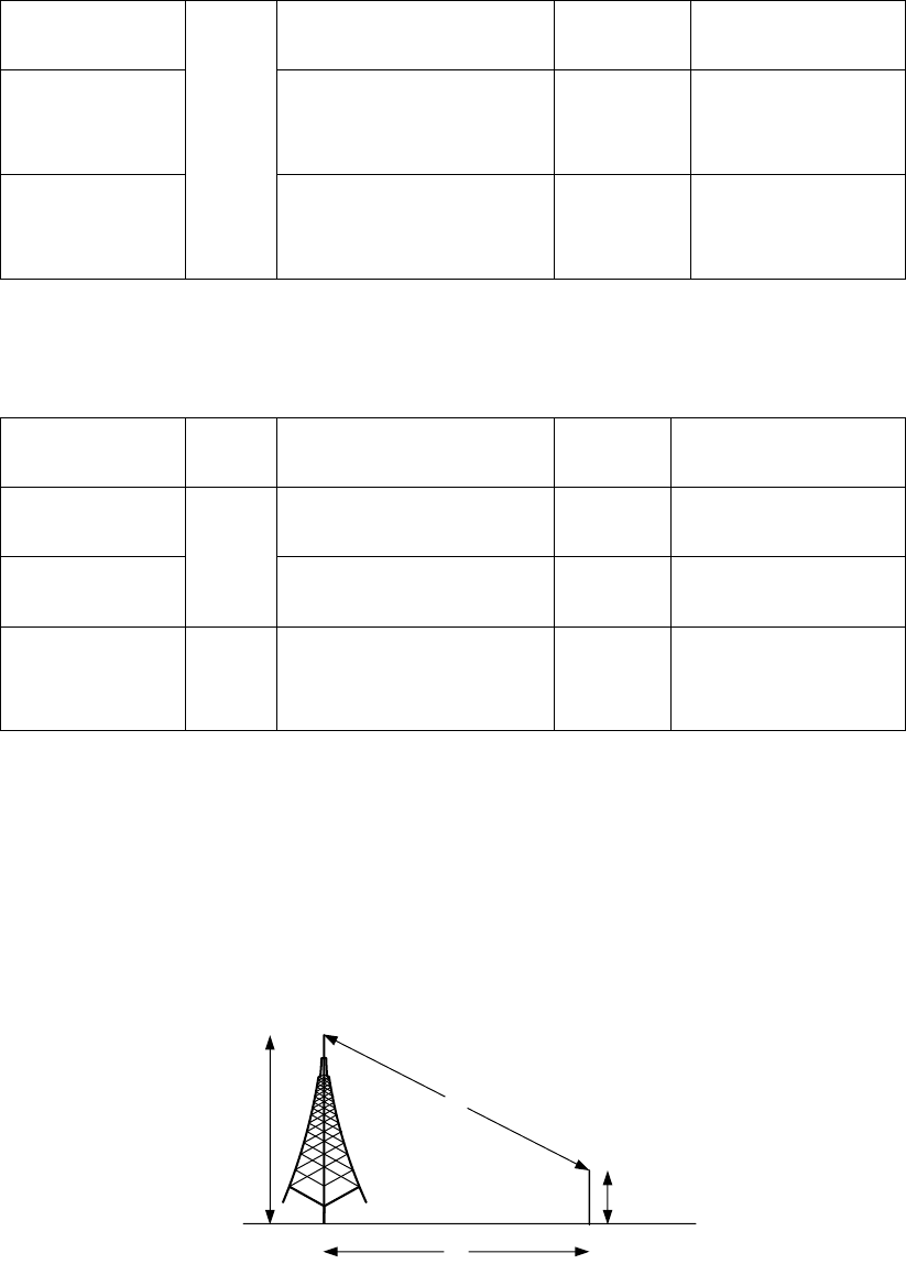
3.5 Path loss
The path loss modelling is based on ITU-R M.2412-0. The path loss models and their
applicability, including frequency ranges, are summarized in Tables A1-2 to A1-5 and the
distance definitions are indicated in Figure 4.
d2D
d3D
hUT
hBS
Figure 4 Definition of d2D and d3D for outdoor UTs
The full syntax for path loss function is:
[Pathloss, SF_sigma]=GeneratePathloss(layoutpar).
The detailed description of parameters is shown in Table 10.
Table 10 Short overview of input and output arguments for GeneratePathloss function

11
Argument
name
Type
Description
Helper
function
Note
layoutpar
input
Define positions of
BS and UT, their
assigned antenna
arrays and gives links
of interest for
simulation.
layout.m
The function layout
parameters should be
defined by user. For
example, the range of
radius of cells and
street width should be
set.
Pathloss
output
Multiple-link path loss
is supported currently.
-
-
SF_sigma
The number is the
same as that in
Scenario.m
-
Putting SF sigma here
is convenient for
adding shadow fading
to the CIR later.
Note: The application for scenarios are supported in InH_x, UMa_x, UMi_x, RMa_x.
3.6 Large Scale Parameter
In the channel modeling, it is usually assumed that statistical parameters on the same link or
different links have certain relevance. Usually these parameters include shadow fading, delay
spread and angle spread. There are two different link correlations in the GBSM, one is the
correlation between communication links formed by the same BS and different UT and the
other is the link formed between different BSs serving the same UT. In the actual channel
modeling process, the former is usually referred to as intra-site correlation, and the latter as
inter-site correlation. In the standard GBSM channel model, it is common to measure, analyze,
and model intra-station correlations, without regard for inter-station correlation.
The parameters are shown in Table 11.
Table 11 Descriptions of Large-scale parameters
Type
Parameter symbol
Description
LSP
Statistical
correlaton
parameers
SF[dB]
Shadow Fading, Log-normal Distribution
Random Variable.
K[dB]
The Rice factor ,defined as the ratio of LOS
power to all NLOS power; if the link is
NLOS transmission, the value is ignored or
assigned as 0 [
dB].
Root-mean-square (RMS) delay spread.
ASA
ESA
UT angle spread, root-mean-square (RMS)
angle spread.
ASD
ESD
BS angle spread, root-mean-square (RMS)
angle expansion.

12
The full syntax for large scale parameter function is:
sigmas=GenerateLSP(layoutpar, fixpar).
The detailed description of parameters is shown in Table 12.
Table 12 Short overview of input and output arguments for GenerateLSP
Argument
name
Type
Description
Helper
function
Note
layoutpar
input
Define positions of BS
and UT.
Layout.m
The scenario
information
should be set by
users.
fixpar
Extract the scenario
information from fixpar
for computing LSP.
Scenario.m
-
sigmas
output
Large-scale parameters
-
-
3.7 Small Scale Parameter
The small-scale fading parameters reflect the main characteristics of multipath clusters in a link,
including delay, power and spatial information. It directly establishes the connection with the
traditional GBSM channel modeling because all the delay and spatial information directly
reflect the scatters distribution information of the traditional GBSM. In addition, it should be
noted that these SSPs are also the key factors that reflect the characteristics of the entire wireless
channel. For example, the delay information determines the channel bandwidth of the entire
simulated channel, and the angle information determines the spatial spread information of the
entire channel.
The small scale parameters are shown in Table 13.
Table 13 Descriptions of Small-scale parameters
Type
Parameters symbol
Description
SSP
T
N] [ 3211
Τ
Cluster relative delay, generally obeying the
exponential distribution or uniform distribution
T
NPPP ] [ 3211
P
The average fading power of a cluster from the PDS,
is usually an exponential decay model.
AOD
MN
AOA
MN ΦΦ ,
Horizontal dimension AOA and AOD angle of ray
path from PAS, is generally Gaussian or Laplace
distribution; Each ray path in the cluster has the
same fading power and the ray angle is
symmetrically offset from the mean.
EOD
MN
EOA
MN ΘΘ ,
vertical dimension EOA and EOD angle of ray path
from the PAS, is generally Gaussian or Laplace
distribution.

13
HVMN
VH MN KK ,
The XPR of the ray path, is valid only for dual
polarized antennas, obeyed
log-normal distribution.
The full syntax for Small-scale parameters function is:
GenerateSSP(layoutpar, fixpar, Input.sim)
The detailed description of parameters is shown in Table 14.
Table14 Short overview of input and output arguments for GenerateSSP
Argument
name
Type
Description
Helper
function
Note
layoutpar
input
Define positions of BS
and UT, their assigned
antenna arrays and
gives links of interest
for simulation.
Layout.m
-
fixpar
Extract the scenario
information from fixpar
for computing LSP.
Scenario.m
-
sim
Number of simulations
-
Defined by users
3.8 Channel Impulse Response
Generate channel coefficients for each cluster n and each receiver and transmitter element pair
u, s and the channel coefficients are given by:
1
, , ,
, , , , , ,
NLOS
,, 1
1, , , , , , , , ,
, , , , , ,
, , , , , ,
exp exp
,
() ,exp exp
,exp 2
,
T
Mn m n m n m
rx u n m ZOA n m AOA
n
u s n mrx u n m ZOA n m AOA n m n m n m
tx s n m ZOD n m AOD
tx s n m ZOD n m AOD
jj
F
P
HtMFjj
Fj
F
, , , , , , , ,
0 0 0
ˆ ˆ ˆ
. . .
exp 2 exp 2
T T T
rx n m rx u tx n m tx s rx n m
r d r d r v
j j t
- - -
Note: The current version is up to the user to decide whether to add path loss and shadow fading. The
function of path loss is supported but it does not be added in the CIR. For LOS condition, see Report
ITU-R M.2412-0.
Considering that
NLOS
,, ()
u s n
Ht
is a constant function of the variable t, computers cannot represent
constant variable. So the platform samples CIR in the time domain according to Nyquist
sampling theorem. The number of sampling points is set by users. During a coherent time, the
sampling points of CIR are highly relevant. The number of sampling points during the coherent
time is 2. Besides, the coherent time is decided by Doppler shift.
The full syntax for channel impulse response function is:
GenerateCIR(fixpar,layoutpar,Input.sim,Input.BW, Input.T).
14
The detailed description of parameters is shown in Table 15.
Table 15 Short overview of input and output arguments for GenerateCIR
Argument
name
Type
Description
Helper
function
Note
layoutpar
input
Define positions of
BS and UT.
Layout.m
The scenario
information
should be set by
users.
fixpar
Extract the scenario
information from
fixpar for
computing LSP.
Scenario.m
-
sim
Number of
simulations
-
-
BW
Bandwidth of
simulations
-
-
T
Number of sampling
points of CIR in
time domain
-
-
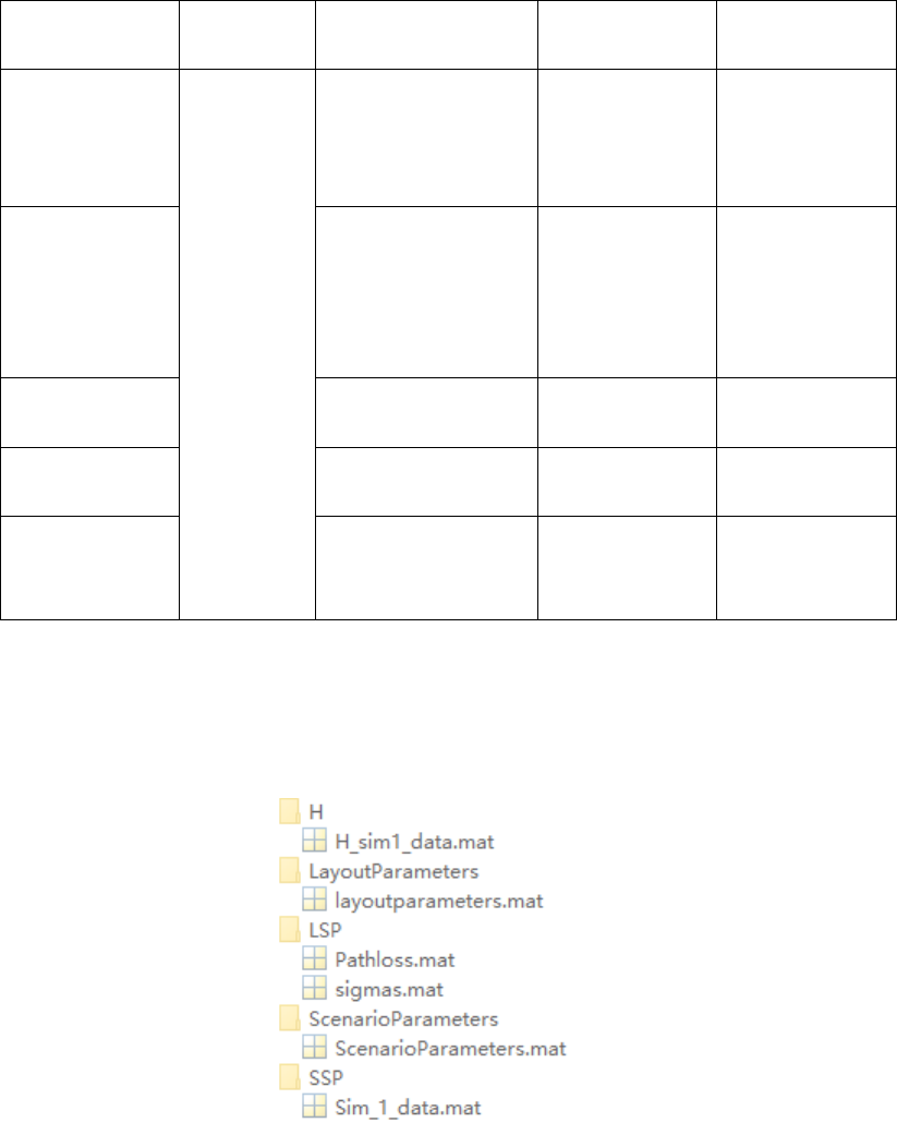
4 Description of Output results
Outputs of the CM platform are saved in pre-established folder. The example of output is shown
in Figure 5:
Figure 5 Example of outputs of CM platform
- Channel impulse response are saved in ‘H’ folder, CIR data consists of results of LOS link,
NLOS link and O2I link. The index of each link can be seen when load Channel impulse
reponse.The form of H is shown:
H=(S, U, N_cluster, T, link);
H is a Multidimensional matrix, S represent the number of transmit antennas, U represent
the number of receive antennas, N_cluter represent the number of clusters, T represent
15
sampling points, linkindex represent the number of links.
- Layout parameters are saved in ‘LayoutParameters’ folder. Link information, such as
propagation condition of each link can be seen in ‘LinkArray’ matrix. ‘Bs_sector_index’
matrix represents information about each Ut belonging to which BS and which sector.
For ‘LinkArray’ matrix, the first row represents the link index, the second row represents
the Propagation condition. For example, 0 represents NLOS, 1 represents LOS, 2
represents O2I.
For ‘Bs_sector_index’ matrix, the first row represents link index, the second row represents
Bs index, the third row represent sector index.
- The path loss information and correlated LSP parameters are saved in ‘LSP’ folder. Each
row of ‘sigmas’ matrix stores ASD,ASA,DS,SF,KF,ESD,ESA. Each column represents
each link. ‘Pathloss’ matrix stores path loss information.
- Scenario parameters are saved in ‘ScenarioParameters’ folder. It is a structure consists of
some parameters defined in [1].
- Small scale parameters of each link are saved in ‘SSP’ folder.
5 Running example
Here provides an example of the main procedure on generating coefficients of channel and
channel impulse response. In this example, the simulation frequency is at 6 GHz and UMi_A
is selected as the simulation scenario. The running results of CIR are stored in the folder ‘H’.
%% Channel coefficient generation for link with default settings.
%Create folder to store data
cd ./SSP;
delete *.mat;
cd ../;
cd ./H;
delete *.mat;
cd ../;
Input=struct('Sce','UMi_B',... %Set the scenario (InH_x, UMi_x, UMa_x, RMa_x)
'C',19,... %Set the number of Bs
'N_user',570,... %Set the total number of subscribers
'fc',6,... %Set the center frequency (GHz)
'AA',[1,1,10,1,1,2.5,2.5,0.5,0.5,102],... %AA=(Mg,Ng,M,N,P,dgH,dgV,dH,dV,downtilt)
BS antenna panel configuration,unit of d and dg is wave length.
'sim',1,... %Set the number of simulations
'BW',200,... %Set the bandwidth of the simulation(MHz)
'T',10 ); %Set the number of sampling points of CIR in time domain
layoutpar=Layout(Input.Sce,Input.C,Input.N_user,Input.fc,Input.AA);
[Pathloss,SF_sigma]=GeneratePathloss(layoutpar);%Generate path loss and shadow fading.
fixpar=Scenario(Input.fc,layoutpar);%Generate scenario information.
sigmas= GenerateLSP(layoutpar,fixpar);
GenerateSSP(layoutpar,fixpar,Input.sim,sigmas);%Generate small-scale parameters.
16
GenerateCIR(fixpar,layoutpar,Input.sim,Input.BW,Input.T);%Generate the channel coefficient.
6 Reference
[1] Series M. Guidelines for evaluation of radio interface technologies for IMT-2020.
REPORT ITU-R M.2412-0, 2017.
[2] Jianhua Zhang, Yuxiang Zhang, Yawei Yu, Ruijie Xu, Qingfang Zheng, Ping Zhang, “3D
MIMO: How Much Does It Meet Our Expectation Observed from Antenna Channel
Measurements?”, IEEE Journal on Selected Areas in Communications, vol. 35, no. 8, pp.
1887 – 1903, 2017.
