Guide For Users User
User Manual:
Open the PDF directly: View PDF ![]() .
.
Page Count: 4

Guide for Users
Jingwen Yang
2018-11-07
Pacakge Installation
AnceTran is an Rpackage that performs analyses of transcriptome evolution based on RNA-seq expression
data or ChIP-seq TF binding data. Here, we use HNF4A-binding data for 4 mice species as an example to
show how AnceTran works. A convenient way to install package from github is through devtools package:
install.packages('devtools')
devtools::install_github("jingwyang/AnceTran")
After installation, AnceTran can be loaded in the usual way:
library('AnceTran')
Input Format:
AnceTran package takes binding score data in certain format:
•Binding score file should be a text file in the matrix shape, Rows correspond to orthologous. Columns
correspond to sample names. Sample names are in format of “TaxaName_SubtaxaName_ReplicatesName”.
The example files are included in the AnceTran package, which can be found in extdata folder in the
package. One can load them in to take a look:
BindingScore.table =read.table(system.file('extdata','HNF4A_meanIntensity_4Mouse.txt',package = 'AnceTran'), header = T)
head(BindingScore.table[,1:5])
## GeneID BL6_HNF4A CAST_HNF4A SPRET_HNF4A CAR_HNF4A
## 1 ENSMUSG00000000001 244.6250 338.4167 159.0 96.5000
## 2 ENSMUSG00000000003 0.0000 41.0000 0.0 0.0000
## 3 ENSMUSG00000000028 184.5000 199.6875 289.4 107.0000
## 4 ENSMUSG00000000037 0.0000 0.0000 41.0 20.0000
## 5 ENSMUSG00000000049 224.2632 179.7917 191.5 120.1875
## 6 ENSMUSG00000000056 266.2500 317.0769 141.4 204.8333
Construction:
The construction function TFconstruct loads in the BindingScore data file, and wraps them in a list of
taxonTF objects (one taxaTF object).
library('AnceTran')
taxa.objects = tTFConstruct(BSFile=system.file('extdata','HNF4A_meanIntensity_4Mouse.txt',package = 'AnceTran'), taxa="all",tf="all",verbose = TRUE)
1

The construction process takes several minutes on a desktop computer depending on data size and hardware
performance. Specify “taxa” and “subtaxa” options in the function when using partial of your data. The
construction process will be faster. If you are hesitated to test the AnceTran, the package has already
bundled a constructed object and you can load the object through:
data(TF.objects)
Data filtering and normalization
We excluded genes whose TF binding score equals to 0 in all species. To account for differences in se-
quencing depths between species, we quantile-normalized these binding score values across species and also
log-transformed the values for the further analysis.
library('limma')
TF_table = TFtab(objects = TF.objects, taxa = "all",tf="all",rowindex = NULL,filtering = FALSE,normalize = FALSE,logrithm = FALSE)
keep<-rowSums((TF_table == 0)) <ncol(TF_table)
TF_table<-TF_table[keep,]
TF_table<-data.frame(log2(normalizeQuantiles(TF_table[,])+1))
Distance matrix
First, we generate an TF-binding distance matrix of these mice species using sOU method:
library('ape')
dismat <- TFdist.sou(bsMat = TF_table)
colnames(dismat)=colnames(TF_table)
rownames(dismat)=colnames(dismat)
dismat
## BL6_HNF4A CAST_HNF4A SPRET_HNF4A CAR_HNF4A
## BL6_HNF4A 0.0000000 0.0000000 0.0000000 0
## CAST_HNF4A 0.3588558 0.0000000 0.0000000 0
## SPRET_HNF4A 0.4497102 0.4869901 0.0000000 0
## CAR_HNF4A 0.6862219 0.7693106 0.6649105 0
TF-binding tree building
After the TF-binding distance matrix is created, you can construct character tree by Neighbor-Joining
method, and bootstrap values based on re-sampling orthologous genes with replacements can also be gener-
ated by boot.phylo function:
tf_tree <- NJ(dismat)
tf_tree <- root(tf_tree, outgroup = "CAR_HNF4A",resolve.root = T)
tf_tree <- no0br(tf_tree)
f <- function(xx) {
mat <- TFdist.sou(t(xx))
# the distance metrics here should be the same as you specified
# when you created the TF-binding distance matrix
2

colnames(mat) <- rownames(xx)
rownames(mat) <- colnames(mat)
root(NJ(mat), "CAR_HNF4A",resolve.root = T)
}
bs <- boot.phylo(tf_tree, t(TF_table), f, B=100)
##
Running bootstraps: 100 / 100
## Calculating bootstrap values... done.
tf_tree$node.label = bs
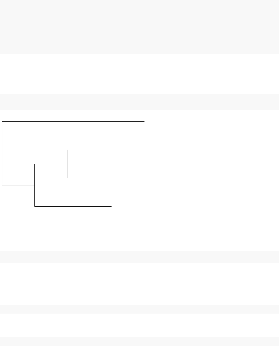
plot(tf_tree, show.node.label = TRUE)
BL6 HNF4A
CAST HNF4A
SPRET HNF4A
CAR HNF4A
100
100
100
By now, an TF-binding character tree is successfully constructed.
Creating variance co-variance matrix
var_mat <- varMatInv(dismat,TF_table,phy = tf_tree)
Ancestral TF-binding state estimation
Here, we extract the TF-binding values of gene MUP20 as an example:
mup20_binding <- TF_table[which(rownames(TF_table) == "ENSMUSG00000078672"),]
Then we infer the TF-binding scores at ancestral nodes of the TF-binding tree:
mup20_anc <- aee(mup20_binding, tf_tree, var_mat, select = "all")
Finally, we map these estimations on the 4 mice species tree to give a direct presentation of these values:
3

tf_tree$node.label <- sprintf("%.4f",mup20_anc$est)
tf_tree$tip.label <- paste0(tf_tree$tip.label, " ",sprintf("%.4f", mup20_binding))
plot(tf_tree, edge.color = "grey80",edge.width = 4,show.node.label = T,align.tip.label = T,main="Ancestial HNF4A-Binding Estimation of Gene MUP20")
Ancestial HNF4A−Binding Estimation of Gene MUP20
BL6 HNF4A 7.3259
CAST HNF4A 7.6619
SPRET HNF4A 7.1899
CAR HNF4A 7.9461
7.6058
7.4973
7.4697
4