WinSpec/32 Software User's Manual Win Spec 2.6 Spectroscopy User
User Manual:
Open the PDF directly: View PDF ![]() .
.
Page Count: 290 [warning: Documents this large are best viewed by clicking the View PDF Link!]
- Table of Contents
- Part 1 Getting Started
- Introduction
- Chapter 1 Installing and Starting WinSpec/32
- System Requirements
- Your System Components
- Installing the PCI Card Driver
- Installing the USB 2.0 Card Driver
- Installing the FireWire Card Driver
- Installing the GigE Ethernet Card Driver
- Installing WinSpec/32
- Changing Installed Components, Repairing, or Uninstalling/Reinstalling WinSpec/32
- Starting WinSpec/32
- Chapter 2 Basic Hardware Setup
- Introduction
- Basic Hardware Overview
- Entering the Default System Parameters into WinSpec
- Editing Controller and Detector Characteristics
- Entering the Data Orientation
- Entering the Interface Communication Parameters
- Entering the Cleans/Skips Characteristics
- Setting up a Spectrograph
- Specifying the Active Spectrograph
- Entering Grating Information
- Selecting and Moving the Grating
- Entering Information for Software-Controlled Slits and/or Mirrors
- Chapter 3 Initial Spectroscopic Data Collection
- Chapter 4 Initial Imaging Data Collection
- Introduction
- Temperature Control
- Cleans and Skips
- Experiment Setup Procedure (All Controllers and Unintensified Cameras)
- Experiment Setup Procedures (Intensified Cameras)
- Data Collection Procedures (Intensified Cameras)
- Data Collection Procedures (Controller-Specific)
- Data Collection (Unintensified Cameras)
- Chapter 5 Opening, Closing, and Saving Data Files
- Chapter 6 Wavelength Calibration
- Chapter 7 Spectrograph Calibration
- Chapter 8 Displaying the Data
- Introduction
- Screen Refresh Rate
- Data Displayed as a 3D Graph
- Data Window Context menu
- Labeling Graphs and Images
- Data Displayed as an Image
- Displaying circuit.spe
- Changing the Brightness Range
- Brightness/Contrast Control
- Selecting a Region of Interest
- Opening the Display Layout dialog
- Viewing Axes and Cross Sections
- Information box
- Autoranging the Intensity in a ROI
- Changing the Color of the Axes and Labels
- Specifying a New ROI and Intensity Range
- Displaying a Z-Slice
- Part 2 Advanced Topics
- Chapter 9 On-Line Data Acquisition Processes
- Chapter 10 Cleaning
- Chapter 11 ROI Definition & Binning
- Chapter 12 Correction Techniques
- Chapter 13 Spectra Math
- Chapter 14 Gluing Spectra
- Chapter 15 Post-Acquisition Mask Processes
- Chapter 16 Additional Post-Acquisition Processes
- Chapter 17 Printing
- Chapter 18 Pulser Operation
- Chapter 19 Custom Toolbar Settings
- Chapter 20 Software Options
- Part 3 Reference
- Appendix A System and Camera Nomenclature
- Appendix B WinSpec/32 First Light Instructions
- Appendix C Calibration Lines
- Appendix D Data Structure
- Appendix E Auto-Spectro Wavelength Calibration
- Appendix F CD ROM Failure Work-Arounds
- Appendix G WinSpec/32 Repair and Maintenance
- Appendix H USB 2.0 Limitations
- Appendix I Troubleshooting
- Introduction
- Camera1 (or similar name) on Hardware Setup dialog
- Controller Is Not Responding
- Data Loss or Serial Violation
- Data Overrun Due to Hardware Conflict message
- Data Overrun Has Occurred message
- Error Creating Controller message
- Ethernet Network is not accessible
- OrangeUSB USB 2.0 Driver Update
- Program Error message
- Serial violations have occurred. Check interface cable.
- Appendix J Glossary
- Warranty & Service
- Limited Warranty:
- Basic Limited One (1) Year Warranty
- Limited One (1) Year Warranty on Refurbished or Discontinued Products
- XP Vacuum Chamber Limited Lifetime Warranty
- Sealed Chamber Integrity Limited 12 Month Warranty
- Vacuum Integrity Limited 12 Month Warranty
- Image Intensifier Detector Limited One Year Warranty
- X-Ray Detector Limited One Year Warranty
- Software Limited Warranty
- Owner's Manual and Troubleshooting
- Your Responsibility
- Contact Information
- Limited Warranty:
- Index

4411-0048
Version 2.6B
December 11, 2012
*4411-0048*
Copyright 2001-2012 Princeton Instruments, a division of Roper Scientific, Inc.
3660 Quakerbridge Rd
Trenton, NJ 08619
TEL: 800-874-9789/609-587-9797
FAX: 609-587-1970
All rights reserved. No part of this publication may be reproduced by any means without the written
permission of Princeton Instruments, a division of Roper Scientific, Inc. ("Princeton Instruments").
Printed in the United States of America.
Adobe, Acrobat, Photoshop, and Reader are registered trademarks of Adobe Systems Incorporated in the
United States and/or other countries.
NIRvana is a trademark and Cascade, IsoPlane, PI-MAX, ProEM, and PyLoN are registered trademarks
of Roper Scientific, Inc.
InSpectrum is a trademark of Acton Research Corporation.
Jasc and Paint Shop Pro are registered trademarks of Jasc Software, Inc.
Pentium is a registered trademark of Intel Corporation.
PVCAM is a registered trademark of Photometrics Ltd.
Windows and Windows Vista are registered trademarks of Microsoft Corporation in the United States
and/or other countries.
The information in this publication is believed to be accurate as of the publication release date. However,
Princeton Instruments does not assume any responsibility for any consequences including any damages
resulting from the use thereof. The information contained herein is subject to change without notice.
Revision of this publication may be issued to incorporate such change.

iii
Table of Contents
Part 1 Getting Started .................................................... 17
Introduction ....................................................................................................... 19
Summary of Chapter Information ..................................................................................... 19
Part 1, Getting Started ................................................................................................ 19
Part 2, Advanced Topics ............................................................................................ 20
Part 3, Reference ........................................................................................................ 21
Online Help ....................................................................................................................... 21
Tool Tips and Status Bar Messages .................................................................................. 22
Additional Documentation ................................................................................................ 22
Chapter 1 Installing and Starting WinSpec/32 ............................................... 23
System Requirements ........................................................................................................ 23
Hardware Requirements ............................................................................................. 23
Operating System Requirements ................................................................................ 25
Your System Components ................................................................................................ 25
Installing the PCI Card Driver .......................................................................................... 27
Installing the USB 2.0 Card Driver ................................................................................... 27
WinSpec Version 2.5.25 and later .............................................................................. 28
Installing the FireWire Card Driver .................................................................................. 28
Installing the GigE Ethernet Card Driver ......................................................................... 28
Installing WinSpec/32 ....................................................................................................... 29
Installing from the CD ................................................................................................ 30
Installing from the FTP Site ....................................................................................... 30
Custom Installation Choices ....................................................................................... 31
Changing Installed Components, Repairing, or Uninstalling/Reinstalling
WinSpec/32 ................................................................................................................ 31
Starting WinSpec/32 ......................................................................................................... 32
Chapter 2 Basic Hardware Setup ..................................................................... 35
Introduction ....................................................................................................................... 35
Basic Hardware Overview ................................................................................................ 35
Entering the Default System Parameters into WinSpec .................................................... 37
Camera Detection Wizard .......................................................................................... 37
Editing Controller and Detector Characteristics ............................................................... 41
Entering the Data Orientation ........................................................................................... 45
Entering the Interface Communication Parameters .......................................................... 46
Entering the Cleans/Skips Characteristics ........................................................................ 47
Setting up a Spectrograph ................................................................................................. 50
Specifying the Active Spectrograph ................................................................................. 52
Entering Grating Information ........................................................................................... 52
Grating Parameters ..................................................................................................... 52
Selecting and Moving the Grating .................................................................................... 53
Entering Information for Software-Controlled Slits and/or Mirrors ................................. 54

iv WinSpec/32 Manual Version 2.6B
Entering Laser Excitation Information ............................................................................. 55
Chapter 3 Initial Spectroscopic Data Collection ............................................ 57
Introduction ....................................................................................................................... 57
Temperature Control ......................................................................................................... 58
Cleans and Skips ............................................................................................................... 59
Spectrograph ..................................................................................................................... 59
Experiment Setup Procedure (All Controllers and Unintensified Cameras) ..................... 59
Experiment Setup Procedures (Intensified Cameras) ....................................................... 63
Data Collection Procedures (Intensified Cameras) ........................................................... 63
Data Collection (Unintensified Cameras) ......................................................................... 63
Chapter 4 Initial Imaging Data Collection ....................................................... 65
Introduction ....................................................................................................................... 65
Temperature Control ......................................................................................................... 66
Cleans and Skips ............................................................................................................... 67
Experiment Setup Procedure (All Controllers and Unintensified Cameras) ..................... 67
Experiment Setup Procedures (Intensified Cameras) ....................................................... 70
Data Collection Procedures (Intensified Cameras) ........................................................... 71
Data Collection Procedures (Controller-Specific) ............................................................ 71
ST-133-Controller ...................................................................................................... 71
Focusing ............................................................................................................... 71
Data Collection .................................................................................................... 72
PentaMAX Controller ................................................................................................ 73
Focusing ............................................................................................................... 73
Data Collection .................................................................................................... 74
Data Collection (Unintensified Cameras) ......................................................................... 75
Chapter 5 Opening, Closing, and Saving Data Files ..................................... 77
Introduction ....................................................................................................................... 77
Opening Data Files ........................................................................................................... 77
Saving Data Files .............................................................................................................. 80
Saving Temporary Data Files ..................................................................................... 80
Data File tab ............................................................................................................... 81
Closing a Data File ........................................................................................................... 81
Deleting Data Files ........................................................................................................... 82
Chapter 6 Wavelength Calibration ................................................................... 83
Introduction ....................................................................................................................... 83
Changing the WinSpec/32 Calibration Method ................................................................ 83
Changing the Calibration Method ..................................................................................... 83
Calibration Menu .............................................................................................................. 84
Wavelength Calibration Procedure ................................................................................... 84
Save as Default ................................................................................................................. 87
No Data ...................................................................................................................... 87
Not Live Data ............................................................................................................. 87
Live Data .................................................................................................................... 87
Calibration, Display, and User Units ................................................................................ 87
Calibration Method ........................................................................................................... 88
Chapter 7 Spectrograph Calibration ............................................................... 89
Introduction ....................................................................................................................... 89
Preparation ........................................................................................................................ 89

Table of Contents v
Calibration Parameters ...................................................................................................... 90
Offset ................................................................................................................................ 92
Adjust ................................................................................................................................ 94
Dispersion ......................................................................................................................... 96
Chapter 8 Displaying the Data ......................................................................... 99
Introduction ....................................................................................................................... 99
Screen Refresh Rate ........................................................................................................ 100
Data Displayed as a 3D Graph ........................................................................................ 101
Displaying Hid-lamp.spe .......................................................................................... 101
5%-95% Display Range ........................................................................................... 104
Selecting a Region of Interest .................................................................................. 104
Information box ........................................................................................................ 105
Displaying a Single Strip .......................................................................................... 106
Cursor ....................................................................................................................... 107
Strip Selection .......................................................................................................... 107
Cursor Curve and Marker Curves ............................................................................ 108
Hidden Surfaces ....................................................................................................... 109
Data Window Context menu ........................................................................................... 110
Labeling Graphs and Images .......................................................................................... 111
Data Displayed as an Image ............................................................................................ 114
Displaying circuit.spe ............................................................................................... 114
Changing the Brightness Range ............................................................................... 115
Brightness/Contrast Control ..................................................................................... 116
Selecting a Region of Interest .................................................................................. 116
Opening the Display Layout dialog ......................................................................... 117
Viewing Axes and Cross Sections ............................................................................ 117
Information box ........................................................................................................ 118
Autoranging the Intensity in a ROI .......................................................................... 119
Relabeling the Axes.................................................................................................. 119
Changing the Color of the Axes and Labels ............................................................. 120
Specifying a New ROI and Intensity Range ............................................................ 120
Displaying a Z-Slice ................................................................................................. 121
Part 2 Advanced Topics .............................................. 123
Chapter 9 On-Line Data Acquisition Processes .......................................... 125
Introduction ..................................................................................................................... 125
On-Line Thresholding ..................................................................................................... 125
Description ............................................................................................................... 125
Parameters ................................................................................................................ 126
On-Line Absorbance ....................................................................................................... 126
Description ............................................................................................................... 126
On-Line YT ..................................................................................................................... 127
Description ............................................................................................................... 127
YT Area and Equation Setup Procedure .................................................................. 128
Baseline Correction .................................................................................................. 129
Changing/Deleting Areas and Equations ................................................................. 129
YT Analysis Acquisition Modes .............................................................................. 130
Focus .................................................................................................................. 130

vi WinSpec/32 Manual Version 2.6B
Snapshot ............................................................................................................. 131
Average .............................................................................................................. 132
YT Analysis Setup Procedure .................................................................................. 132
ASCII Output File ........................................................................................................... 134
Description ............................................................................................................... 134
Procedure .................................................................................................................. 134
Chapter 10 Cleaning ....................................................................................... 135
Introduction ..................................................................................................................... 135
Clean Cycles ................................................................................................................... 135
Continuous Cleans .......................................................................................................... 136
Continuous Cleans Instruction ........................................................................................ 138
ROIs and Cleaning .......................................................................................................... 138
Kinetics and Cleaning ..................................................................................................... 138
Chapter 11 ROI Definition & Binning ............................................................. 139
Overview ......................................................................................................................... 139
General ..................................................................................................................... 139
Spectroscopy Mode .................................................................................................. 140
Imaging Mode .......................................................................................................... 140
Binning (Group and Height parameters) ......................................................................... 140
Overview .................................................................................................................. 140
Hardware Binning .............................................................................................. 140
Software Binning ............................................................................................... 141
Spectroscopy Mode .................................................................................................. 141
Imaging Mode .......................................................................................................... 141
Defining ROIs ................................................................................................................. 142
Examples of Spectroscopy and Imaging ROIs ......................................................... 142
Constraints on Defining Multiple Regions of Interest (ROIs) ................................. 143
Methods of Defining and Storing ROIs ................................................................... 143
Chapter 12 Correction Techniques ............................................................... 147
Introduction ..................................................................................................................... 147
Background Subtraction ................................................................................................. 147
Background Subtraction with Intensified Detectors ................................................. 148
Flatfield Correction ......................................................................................................... 149
CCD Blemishes ............................................................................................................... 150
Cosmic Ray Removal ..................................................................................................... 151
Chapter 13 Spectra Math ................................................................................ 153
Introduction ..................................................................................................................... 153
Source Data and Destination Selection ........................................................................... 153
Operations ....................................................................................................................... 154
Operation Descriptions ................................................................................................... 155
Linear Operations ..................................................................................................... 155
Non-Linear Operations ............................................................................................. 155
Bitwise Operations ................................................................................................... 156
Binary Operations .................................................................................................... 156
Chapter 14 Gluing Spectra ............................................................................. 159
Introduction ..................................................................................................................... 159
Gluing Existing Spectra .................................................................................................. 159
Step and Glue .................................................................................................................. 160

Table of Contents vii
Theory ............................................................................................................................. 162
Calibration and ROI Offsets ........................................................................................... 164
Chapter 15 Post-Acquisition Mask Processes ............................................. 165
Introduction ..................................................................................................................... 165
Input tab.................................................................................................................... 165
Output tab ................................................................................................................. 165
Edge Enhancement ......................................................................................................... 166
Parameters tab .......................................................................................................... 166
Laplacian Masks ....................................................................................................... 167
Sobel Edge Detection ............................................................................................... 167
Edge Enhancement Procedure .................................................................................. 167
Sharpening Functions ..................................................................................................... 168
Parameters tab .......................................................................................................... 168
Sharpening Procedure .............................................................................................. 168
Smoothing Functions ...................................................................................................... 169
Parameters tab .......................................................................................................... 169
Smoothing Procedure ............................................................................................... 169
Morphological Functions ................................................................................................ 170
Parameters tab .......................................................................................................... 170
Morphological Procedure ......................................................................................... 171
Custom Filter .................................................................................................................. 172
Filter Matrix tab ....................................................................................................... 172
Custom Filter Procedure ........................................................................................... 172
Look Up Table ................................................................................................................ 173
Look Up Table tab .................................................................................................... 173
Look Up Table Procedure ........................................................................................ 173
Look Up Table Formats ........................................................................................... 174
Format 1 ............................................................................................................. 174
Format 2 ............................................................................................................. 175
References ....................................................................................................................... 175
Chapter 16 Additional Post-Acquisition Processes .................................... 177
Introduction ..................................................................................................................... 177
Input tab.................................................................................................................... 177
Output tab ................................................................................................................. 177
Threshold and Clipping .................................................................................................. 178
Procedure .................................................................................................................. 178
Cross Section .................................................................................................................. 179
Introduction .............................................................................................................. 179
Procedure .................................................................................................................. 179
Binning and Skipping ..................................................................................................... 180
Introduction .............................................................................................................. 180
Procedure .................................................................................................................. 180
Binning and Skipping Restrictions and Limitations ................................................. 181
Histogram Calculation .................................................................................................... 182
Introduction .............................................................................................................. 182
Procedure .................................................................................................................. 182
Chapter 17 Printing ......................................................................................... 183
Introduction ..................................................................................................................... 183
Setting up the Printer ...................................................................................................... 183
Printing Directly from WinSpec/32 ................................................................................ 184

viii WinSpec/32 Manual Version 2.6B
Print Preview ................................................................................................................... 184
Printing a Screen Capture ............................................................................................... 185
Saving as TIF and Printing ............................................................................................. 186
Chapter 18 Pulser Operation .......................................................................... 187
Introduction ..................................................................................................................... 187
PG200 Programmable Pulse Generator .......................................................................... 187
DG535 Digital Delay/Pulse Generator ........................................................................... 191
Programmable Timing Generator (PTG) ........................................................................ 194
SuperSYNCHRO Timing Generator .............................................................................. 198
Repetitive Mode Parameters ........................................................................................... 202
Sequential Mode Parameters ........................................................................................... 203
Timing Generator Interactive Trigger Setup ................................................................... 206
Timing Generator Interactive Gate Width and Delay ..................................................... 207
Chapter 19 Custom Toolbar Settings ............................................................ 209
Introduction ..................................................................................................................... 209
Displaying the Custom Toolbar ...................................................................................... 209
Customizing the Toolbar ................................................................................................ 209
Individual Dialog Item Descriptions ............................................................................... 210
Chapter 20 Software Options ......................................................................... 213
Introduction ..................................................................................................................... 213
Custom Chip (WXCstChp.opt) ....................................................................................... 213
Introduction .............................................................................................................. 213
Custom Timing (WXCstTim.opt) ................................................................................... 214
Introduction .............................................................................................................. 214
FITS (FITS.exe) .............................................................................................................. 214
Macro Record (WXmacrec.opt) ...................................................................................... 215
Spex Spectrograph Control (WSSpex.opt) ..................................................................... 216
Virtual Chip (WXvchip.opt) ........................................................................................... 216
Introduction .............................................................................................................. 216
Virtual Chip Setup .................................................................................................... 217
Experimental Timing ................................................................................................ 220
Tips ........................................................................................................................... 220
Part 3 Reference........................................................... 221
Appendix A System and Camera Nomenclature .......................................... 223
System, Controller Type, and Camera Type Cross-Reference ....................................... 223
System and System Component Descriptions ................................................................ 226
Systems: ................................................................................................................... 226
Controllers: ............................................................................................................... 228
Cameras/Detectors: .................................................................................................. 228
Pulsers: ..................................................................................................................... 229
High-Voltage Power Supplies: ................................................................................. 229
Miscellaneous Components: ..................................................................................... 229
Array Designators ........................................................................................................... 230
Appendix B WinSpec/32 First Light Instructions ......................................... 233
Imaging ........................................................................................................................... 233

Table of Contents ix
Assumptions ............................................................................................................. 233
Getting Started .......................................................................................................... 233
Setting the Parameters .............................................................................................. 233
Confirming the Setup ............................................................................................... 235
Spectroscopy ................................................................................................................... 236
Assumptions ............................................................................................................. 236
Getting Started .......................................................................................................... 236
Setting the Camera Parameters ................................................................................. 237
Setting the Spectrograph Parameters ........................................................................ 238
Confirming the Setup ............................................................................................... 238
Rotational Alignment and Focusing ......................................................................... 240
Acton Series Spectrograph ................................................................................. 240
IsoPlane SCT-320 Spectrograph ........................................................................ 242
Acquiring Data ......................................................................................................... 243
Shutdown .................................................................................................................. 243
Appendix C Calibration Lines ........................................................................ 245
Appendix D Data Structure ............................................................................ 247
Version 1.43 Header ....................................................................................................... 247
Version 1.6 Header ......................................................................................................... 248
Version 2.5 Header (3/23/04) ......................................................................................... 251
Start of Data (4100 - ) .............................................................................................. 255
Definition of Array Sizes ................................................................................................ 255
Custom Data Types Used In the Structure ...................................................................... 255
Reading Data ................................................................................................................... 256
Appendix E Auto-Spectro Wavelength Calibration ..................................... 257
Equations used in WinSpec Wavelength Calibration ..................................................... 257
WinSpec X Axis Auto Calibration ................................................................................. 259
Appendix F CD ROM Failure Work-Arounds ................................................ 261
Appendix G WinSpec/32 Repair and Maintenance ...................................... 263
Install/Uninstall WinSpec/32 Components at a Later Time ........................................... 263
Installing More than One Version of WinSpec/32 ......................................................... 265
PIHWDEF.INI & SESSION.DAT .................................................................................. 266
Uninstalling and Reinstalling .......................................................................................... 266
Appendix H USB 2.0 Limitations ................................................................... 267
Appendix I Troubleshooting .......................................................................... 269
Introduction ..................................................................................................................... 269
Camera1 (or similar name) on Hardware Setup dialog ................................................... 269
Controller Is Not Responding ......................................................................................... 270
Data Loss or Serial Violation .......................................................................................... 270
Data Overrun Due to Hardware Conflict message .......................................................... 270
Data Overrun Has Occurred message ............................................................................. 271
Error Creating Controller message ................................................................................. 272
Ethernet Network is not accessible ................................................................................. 272
OrangeUSB USB 2.0 Driver Update .............................................................................. 273
Program Error message ................................................................................................... 274
Serial violations have occurred. Check interface cable. ................................................. 275

x WinSpec/32 Manual Version 2.6B
Appendix J Glossary ...................................................................................... 277
Warranty & Service ......................................................................................... 279
Limited Warranty: ........................................................................................................... 279
Basic Limited One (1) Year Warranty ..................................................................... 279
Limited One (1) Year Warranty on Refurbished or Discontinued Products ............ 279
XP Vacuum Chamber Limited Lifetime Warranty .................................................. 279
Sealed Chamber Integrity Limited 12 Month Warranty ........................................... 280
Vacuum Integrity Limited 12 Month Warranty ....................................................... 280
Image Intensifier Detector Limited One Year Warranty .......................................... 280
X-Ray Detector Limited One Year Warranty .......................................................... 280
Software Limited Warranty ...................................................................................... 280
Owner's Manual and Troubleshooting ..................................................................... 281
Your Responsibility .................................................................................................. 281
Contact Information ........................................................................................................ 282
Index ................................................................................................................. 283
Figures
Figure 1. Opening WinSpec/32 via the Windows Start button ........................................ 32
Figure 2. Splash screen .................................................................................................... 33
Figure 3. Main WinSpec/32 window ............................................................................... 33
Figure 4. Setup menu ....................................................................................................... 35
Figure 5. Possible System Configurations ....................................................................... 36
Figure 6. Air-Cooled System (with Internal Controller) Diagram ................................... 36
Figure 7. Liquid- or Air-Cooled System (with External Controller) Diagram ................ 37
Figure 8. Cryo-Cooled System (with External Controller) Diagram ............................... 37
Figure 9. Camera Detection Wizard - Welcome dialog ................................................... 38
Figure 10. Camera Detection Wizard - Detected Hardware dialog ................................. 38
Figure 11. Camera Detection Wizard - Welcome (Manual selected) dialog ................... 39
Figure 12. Camera Detection Wizard - Optional Configuration Disk dialog .................. 39
Figure 13. Camera Detection Wizard - Test Image dialog .............................................. 40
Figure 14. Camera Detection Wizard - Finished dialog .................................................. 40
Figure 15. Hardware Setup|Controller/Camera tab .......................................................... 41
Figure 16. Display tab; left graphic applies to all controllers except ST-121; right graphic
applies to ST-121 only .............................................................................................. 45
Figure 17. Interface tab .................................................................................................... 46
Figure 18. Cleans/Skips tab ............................................................................................. 47
Figure 19. Vertical Skips ................................................................................................. 49
Figure 20. Spectrograph menu ......................................................................................... 50
Figure 21. Define Spectrograph dialog ............................................................................ 50
Figure 22. Install/Remove Spectrographs ........................................................................ 51
Figure 23. Gratings tab Setting the grating parameters .................................................. 52
Figure 24. Move Spectrograph Gratings tab .................................................................... 53
Figure 25. Define Spectrograph Slits/Mirrors tab ............................................................ 54
Figure 26. Slit width and Mirror selection tabs - Move Spectrograph dialog ................. 54
Figure 27. Entering the Laser Line Define Spectrograph Main tab ................................ 55
Figure 28. Temperature dialog ......................................................................................... 58
Figure 29. Experiment Setup: Main tab ........................................................................... 59
Figure 30. Experiment Setup dialog Timing tab .............................................................. 60
Figure 31. Data Corrections tab ....................................................................................... 60

Table of Contents xi
Figure 32. Generic ADC tab ............................................................................................ 61
Figure 33. ROI dialog ...................................................................................................... 61
Figure 34. Data File tab ................................................................................................... 62
Figure 35. File Browse dialog .......................................................................................... 62
Figure 36. Acquisition menu ........................................................................................... 63
Figure 37. Typical Mercury-Argon Spectrum ................................................................. 64
Figure 38. Temperature dialog ......................................................................................... 66
Figure 39. Experiment Setup|Main tab ............................................................................ 67
Figure 40. Timing tab ...................................................................................................... 68
Figure 41. Data Corrections tab ....................................................................................... 68
Figure 42. Generic ADC tab ............................................................................................ 69
Figure 43. ROI tab - imaging selected ............................................................................. 69
Figure 44. Data File tab ................................................................................................... 70
Figure 45. File Browse dialog .......................................................................................... 70
Figure 46. ST-133 Interactive Camera dialog ................................................................. 72
Figure 47. PentaMAX Interactive Operation dialog ........................................................ 73
Figure 48. Typical Data Acquisition Image ..................................................................... 75
Figure 49. Open dialog .................................................................................................... 77
Figure 50. High Intensity Lamp Spectrum ...................................................................... 78
Figure 51. Data File Save As dialog ................................................................................ 80
Figure 52. Save As Data Types........................................................................................ 80
Figure 53. Data File tab ................................................................................................... 81
Figure 54. Right-click File Operations menu .................................................................. 82
Figure 55. Calibration Usage dialog ................................................................................ 83
Figure 56. Calibration menu ............................................................................................ 84
Figure 57. Hg-Argon spectrum ........................................................................................ 85
Figure 58. Calibration Setup dialog after running Find Peaks routine on Hg-Argon
spectrum .................................................................................................................... 85
Figure 59. Spectrum after running Find Peaks routine .................................................... 86
Figure 60. Setup Calibration screen after selecting peaks and entering calibration
wavelengths .............................................................................................................. 86
Figure 61. Spectrum after Calibration ............................................................................. 87
Figure 62. Spectrograph Calibration dialog .................................................................... 91
Figure 63. Offset dialog ................................................................................................... 92
Figure 64. Peak Finder Examples .................................................................................... 93
Figure 65. Offset Spectrum for Zero-order Measurement ............................................... 94
Figure 66. Adjust dialog .................................................................................................. 95
Figure 67. Calibration Adjust Spectrum .......................................................................... 95
Figure 68. Dispersion dialog ............................................................................................ 96
Figure 69. Image display of 256 data strips ..................................................................... 99
Figure 70. 3D Image display of eight data strips ............................................................. 99
Figure 71. 3D graph with two data strips ....................................................................... 100
Figure 72. 3D graph with five data strips ...................................................................... 101
Figure 73. Open dialog .................................................................................................. 101
Figure 74. Display Layout dialog .................................................................................. 102
Figure 75. Hid-lamp.spe 3-D Graph .............................................................................. 103
Figure 76. Hid-lamp.spe 3D graph with region selected for viewing ............................ 104
Figure 77. Hide-lamp.spe 3D graph expanded to show defined region ......................... 105
Figure 78. Graphical Display with Information box ...................................................... 105
Figure 79. Single Strip displayed graphically ................................................................ 106
Figure 80. 3D Display with Cursor curve and Marker Curves ...................................... 108
Figure 81. 3D Plot with Hidden Surfaces ...................................................................... 110

xii WinSpec/32 Manual Version 2.6B
Figure 82. Data Window Context menu ....................................................................... 110
Figure 83. Normal Context menu .................................................................................. 111
Figure 84. ROI Context menu ........................................................................................ 111
Figure 85. Label Display action ..................................................................................... 112
Figure 86. Label Options subdialog ............................................................................... 112
Figure 87. Label text entry box ...................................................................................... 112
Figure 88. Data with Finished Label .............................................................................. 113
Figure 89. Edit box with line-wrapped label and finished label with same line wraps . 113
Figure 90. ROI resized to correct Line-wrapping .......................................................... 114
Figure 91. Display after changing Font Selection ......................................................... 114
Figure 92. Open dialog .................................................................................................. 115
Figure 93. Circuit.spe Image .......................................................................................... 115
Figure 94. Brightness/Contrast dialog ........................................................................... 116
Figure 95. Circuit.spe with Region Selected for Viewing ............................................. 116
Figure 96. Circuit.spe Expanded to show Defined Region ............................................ 117
Figure 97. Display Layout dialog .................................................................................. 117
Figure 98. Display Layout|Range tab ............................................................................ 117
Figure 99. Selecting the Large Cursor ........................................................................... 118
Figure 100. Circuit.spe with Axes and Cross-sections .................................................. 118
Figure 101. Information box .......................................................................................... 118
Figure 102. Display Layout|Axes tab ............................................................................ 119
Figure 103. Fonts dialog ................................................................................................ 119
Figure 104. Display Layout|Color tab ........................................................................... 120
Figure 105. Display Layout|Color dialog ...................................................................... 120
Figure 106. Multi-frame Data and a Z-Slice of that Data .............................................. 121
Figure 107. Experiment Setup|Processes tab ................................................................. 125
Figure 108. Online Thresholding Setup dialog .............................................................. 125
Figure 109. Absorbance Setup dialog ............................................................................ 126
Figure 110. YT Area & Equation Setup dialog ............................................................. 128
Figure 111. Equation Calculator dialog ......................................................................... 129
Figure 112. Experiment Setup|Process tab .................................................................... 132
Figure 113. YT Setup dialog .......................................................................................... 133
Figure 114. ASCII Output Setup dialog ........................................................................ 134
Figure 115. Clean Cycles in Freerun Operation ............................................................ 135
Figure 116. Cleans/Skips tab ......................................................................................... 136
Figure 117. Timing Tab: External Sync with Continuous Cleans Selected ................... 136
Figure 118. External Sync Timing Diagram .................................................................. 137
Figure 119. External Sync with Continuous Cleans Timing Diagram .......................... 137
Figure 120. Cleans/Skips tab: Continuous Cleans Instruction ....................................... 138
Figure 121. Assumed Array Orientation ........................................................................ 139
Figure 122. Single Full-width ROI ................................................................................ 142
Figure 123. Single Partial-width ROI ............................................................................ 142
Figure 124. Multiple Full-width ROIs ........................................................................... 142
Figure 125. Spectroscopy Mode Multiple Partial-width ROIs ...................................... 142
Figure 126. Imaging Mode Multiple ROIs with Different Widths ................................ 142
Figure 127. Multiple Imaging ROIs and Resulting Data ............................................... 143
Figure 128. Easy Bin dialog .......................................................................................... 144
Figure 129. ROI Setup tab (Spectroscopy Mode) .......................................................... 145
Figure 130. ROI Setup tab (Imaging Mode) .................................................................. 146
Figure 131. Data Corrections tab ................................................................................... 148
Figure 132. Blemish Files: CSV format and Tab Delimited format .............................. 150
Figure 133. Math dialog ................................................................................................. 153

Table of Contents xiii
Figure 134. Operation tab .............................................................................................. 155
Figure 135. Post-Process Glue dialog ............................................................................ 159
Figure 136. Step and Glue Setup dialog ........................................................................ 161
Figure 137. Input tab ...................................................................................................... 165
Figure 138. Output tab ................................................................................................... 165
Figure 139. Edge Enhancement| Parameters tab ............................................................ 166
Figure 140. Original Image (left) and Edge-detected Image (right) .............................. 167
Figure 141. Sharpening|Parameters tab ......................................................................... 168
Figure 142. Original Image (left) and Smoothed Image (right) ..................................... 169
Figure 143. Smoothing|Parameters tab .......................................................................... 169
Figure 144. Morphological|Parameters tab .................................................................... 170
Figure 145. Original Image (left) and Dilated Image (right) ......................................... 170
Figure 146. Original Image (left) and Eroded Image (right) ......................................... 170
Figure 147. Original Image (left) and Opened Image with Three Iterations (right) ...... 171
Figure 148. Filter Matrix tab .......................................................................................... 172
Figure 149. Look-Up Table ........................................................................................... 173
Figure 150. Input tab ...................................................................................................... 177
Figure 151. Output tab ................................................................................................... 177
Figure 152. Threshold and Clipping|Parameters tab ...................................................... 178
Figure 153. Example Cross Sections of an ROI ............................................................ 179
Figure 154. Cross Section|Parameters tab ...................................................................... 179
Figure 155. Post-processing Binning and Skipping|Parameters tab .............................. 180
Figure 156. Post-processing Histogram|Parameters tab ................................................. 182
Figure 157. Print Setup dialog ....................................................................................... 183
Figure 158. Print dialog ................................................................................................. 184
Figure 159. Print Preview window ................................................................................ 184
Figure 160. Pulsers dialog ............................................................................................. 187
Figure 161. PG200|Comm Port tab ................................................................................ 188
Figure 162. PG200|Triggers tab ..................................................................................... 188
Figure 163. PG200|Gating tab ....................................................................................... 189
Figure 164. PG200|Repetitive Gating Setup dialog ....................................................... 189
Figure 165. PG200|Sequential Gating Setup dialog ...................................................... 190
Figure 166. Camera State dialog .................................................................................... 191
Figure 167. DG535 dialog ............................................................................................. 191
Figure 168. DG535|Comm Port tab ............................................................................... 192
Figure 169. DG535|Triggers tab .................................................................................... 192
Figure 170. DG535|Gating tab ....................................................................................... 193
Figure 171. DG535|Repetitive Gating Setup ................................................................. 193
Figure 172. DG535|Sequential Gating Setup dialog ...................................................... 193
Figure 173. Camera State dialog .................................................................................... 194
Figure 174. Pulsers dialog ............................................................................................. 194
Figure 175. PTG|Triggers tab ........................................................................................ 195
Figure 176. PTG|Gating tab ........................................................................................... 195
Figure 177. PTG|Repetitive Gating Setup ..................................................................... 195
Figure 178. PTG|Sequential Gating Setup dialog .......................................................... 196
Figure 179. PTG|Aux. Trig. Out tab ............................................................................. 198
Figure 180. Camera State dialog ..................................................................................... 198
Figure 181. Pulsers dialog .............................................................................................. 199
Figure 182. SuperSYNCHRO dialog .............................................................................. 199
Figure 183. SuperSYNCHRO\Gating tab ...................................................................... 200
Figure 184. SuperSYNCHRO|Repetitive Gating dialog (Internal Trigger on left;
External Trigger on right) ....................................................................................... 200

xiv WinSpec/32 Manual Version 2.6B
Figure 185. SuperSYNCHRO|Sequential Gating dialog (Internal Trigger) .................. 201
Figure 186. SuperSYNCHRO|Sequential Gating dialog (External Trigger) ................. 201
Figure 187. SuperSYNCHRO|Trigger Out tab .............................................................. 202
Figure 188. Range Limits Exceeded Warning ............................................................... 204
Figure 189. Gate Width/Delay Sequence dialog ............................................................ 205
Figure 190. Sequence Values File dialog ...................................................................... 206
Figure 191. Timing Generator Interactive Trigger Setup dialog ................................... 206
Figure 192. Timing Generator Interactive Gate Width and Delay dialog ...................... 207
Figure 193. Default Custom Toolbar ............................................................................. 209
Figure 194. Customize Toolbar dialog .......................................................................... 209
Figure 195. Custom Chip tab ......................................................................................... 213
Figure 196. Custom Timing tab ..................................................................................... 214
Figure 197. FITS dialog ................................................................................................ 215
Figure 198. Macro Record dialog .................................................................................. 216
Figure 199. Install/Remove Spectrographs dialog ......................................................... 216
Figure 200. Virtual Chip Functional diagram ................................................................ 217
Figure 201. Virtual Chip dialog ..................................................................................... 217
Figure 202. Wavelength Calibration Spectrum ............................................................. 246
Figure 203. Relationships of and in terms of and ............................................. 258
Figure 204. Relationship between and the focal length, detector angle, and the distance
of - from image plane ............................................................................................ 259
Figure 205. WinSpec, WinView, or WinXTest Selection dialogs ................................. 263
Figure 206. Media Password dialog............................................................................... 264
Figure 207. Application Maintenance dialog ................................................................. 264
Figure 208. Select Features dialog ................................................................................. 264
Figure 209. WinSpec/32 has been successfully installed dialog ................................... 265
Figure 210. Exit or Install Another Program dialog ...................................................... 265
Figure 211. Camera1 in Camera Name Field................................................................. 269
Figure 212. Data Overrun Due to Hardware Conflict dialog ......................................... 270
Figure 213. Error Creating Controller dialog ................................................................ 272
Figure 214. Ebus Driver Installation Tool dialog .......................................................... 273
Figure 215. Program Error dialog .................................................................................. 274
Figure 216. Serial Violations Have Occurred dialog ..................................................... 275

Table of Contents xv
Tables
Table 1. PCI Driver Files and Locations ......................................................................... 27
Table 2. USB Driver Files and Locations ........................................................................ 28
Table 3. Cursor Appearance and Behavior for Images and Graphs ............................... 107
Table 4. Wavelength Calibration Lines (in nanometers) ............................................... 245
Table 5. Features Supported under USB 2.0 ................................................................. 267

xvi WinSpec/32 Manual Version 2.6B
This page intentionally left blank.
17
Part 1
Getting Started
Introduction ............................................................................................................ 19
Chapter 1, Installing and Starting WinSpec/32 ............................................. 23
Chapter 2, Basic Hardware Setup .................................................................... 35
Chapter 3, Initial Spectroscopic Data Collection ........................................ 57
Chapter 4, Initial Imaging Data Collection ..................................................... 65
Chapter 5, Opening, Closing, and Saving Data Files .................................. 77
Chapter 6, Wavelength Calibration ................................................................... 83
Chapter 7, Spectrograph Calibration ............................................................... 89
Chapter 8, Displaying the Data ......................................................................... 99

18 WinSpec/32 Manual Version 2.6B
This page intentionally left blank.

19
Introduction
The WinSpec manual has been written to give new users of Princeton Instruments
detector/camera systems step-by-step guides to basic data collection, storage, and
processing operations. The most up-to-date version of this software manual and other
Princeton Instruments manuals can be found and downloaded from
ftp://ftp.princetoninstruments.com/public/Manuals/Princeton Instruments/.
The WinSpec manual is divided into the following three parts:
Part 1, Getting Started, is primarily intended for the first time user who is familiar
with Windows-based applications or for the experienced user who wants to review.
These chapters lead you through hardware setup, experiment setup, data collection,
file handling, wavelength calibration, spectrograph setup and calibration and data
display procedures.
Part 2, Advanced Topics, goes on to discuss ancillary topics such as cleaning,
ROIs, binning, data correction techniques, printing, gluing spectra, Y:T analysis,
processing options, pulser operation and customizing the toolbar. These chapters are
more informational and less procedural than those in Part 1.
Part 3, Reference, contains appendices that provide additional useful information,
such as
commonly used system, controller type and camera type terminology provided in
Appendix A,
Hg, Ar, Ne calibration spectrum data and graph provided in Appendix C, and
data structure information provided in Appendix D.
Also included are appendices that address repair and maintenance of the WinSpec/32
software and installation work-arounds for situations where the CD ROM does not
support long file names.
A software hardware setup wizard guides you through the critical hardware selections the
first time you select Setup – Hardware. To properly respond to the wizard’s queries, you
may have to refer to your ordering information, such as exact detector model, A/D
converters, etc. Keep this information handy.
Even though the wizard will assist you in getting started, it will still be necessary to read
through this manual to familiarize yourself with the many data-collection and analysis
options available.
Note: Throughout the manual references are made to the PI-MAX camera/detector. This
camera/detector was previously called the I-MAX and the ICCD-MAX.
Summary of Chapter Information
Part 1, Getting Started
Introduction describes the contents of this manual as well as other information sources
including online Help and other documentation files.
Chapter 1 Installing and Starting WinSpec/32 lists system requirements and
describes how to install the WinSpec/32 software.

20 WinSpec/32 Manual Version 2.6B
Chapter 2 Basic Hardware Setup provides detailed instructions on how to
configure WinSpec/32 for operation with the hardware (detector,
controller, and spectrograph) in your particular system. Pulser
configuration is discussed in Chapter 18.
Chapter 3 Initial Spectroscopic Data Collection provides a procedure for
initial spectroscopic data collection, allowing users to gain some
operating familiarity before going on to more complex measurements.
Chapter 4 Initial Imaging Data Collection provides a procedure for initial
imaging data collection, allowing users to gain some operating
familiarity before going on to more complex measurements.
Chapter 5 Opening, Closing, and Saving Data Files describes how to open,
close and save data files in WinSpec/32.
Chapter 6 Wavelength Calibration describes how to calibrate the WinSpec/32
software for one position of the spectrograph grating.
Chapter 7 Spectrograph Calibration discusses how to calibrate the WinSpec/32
software for any position of the spectrograph gratings.
Chapter 8 Displaying the Data describes the data file display options.
Part 2, Advanced Topics
Chapter 9 On-Line Data Acquisition Processes describes data acquisition
processes that can be activated to occur during data acquisition. These
processes include on-line thresholding, on-line absorbance, on-line Y:T,
and ASCII output.
Chapter 10 Cleaning describes the cleaning features that are used while data
acquisition is idle to prevent the buildup of unwanted charge on the
array.
Chapter 11 ROI Definition & Binning describes how to set a region of interest (ROI),
so that data is only collected from the specified portion of the CCD array. It
also describes binning, the summing together of charge from several pixels,
on the array or in software during data acquisition. Simple or more
advanced binning options can be configured easily with WinSpec/32.
Chapter 12 Correction Techniques explains correction options such as
background subtraction and flatfield correction.
Chapter 13 Spectra Math covers WinSpec/32’s mathematical processing features.
Chapter 14 Gluing Spectra discusses gluing existing files or combining the data
acquisition and gluing operations under spectrograph control.
Chapter 15 Post-Acquisition Mask Processes describes digital mask-
operations that can be performed on the acquired data. Discussed are
Edge Enhancement, Sharpening, Smoothing, Custom Filter and
Morphological functions.
Chapter 16 Additional Post-Acquisition Processes describes additional
operations that can be performed on an acquired data set. Functions
covered include Threshold and Clipping, Cross Section, Binning and
Skipping, and Histogram.

Introduction 21
Chapter 17 Printing describes printing features of WinSpec/32. WinSpec/32 can
print directly to almost any Windows printer driver.
Chapter 18 Pulser Operation describes the operation of the Pulsers that can be
used with WinSpec/32.
Chapter 19 Custom Toolbar Settings describes the Custom Toolbar and explains
how to add/remove the available buttons.
Chapter 20 Software Options describes WinSpec/32 options that can also be
purchased from Princeton Instruments.
Part 3, Reference
Appendix A System and Camera Nomenclature provides a cross-reference table
for systems, controllers, and cameras/CCD arrays. It also provides brief
descriptions of systems and system components. CCD array related
abbreviations are also included.
Appendix B WinSpec/32 First Light Instructions provides procedures for
setting up and focusing a system while in Imaging mode and for setting
up, aligning, and focusing a system while in Spectroscopy mode.
Appendix C Calibration Lines contains wavelength tables and a detailed spectrum
for Mercury-Argon.
Appendix D Data Structure contains descriptions of the data structure for both
WinView/WinSpec 1.43 and for 1.6. The data structure for WinView/32
and WinSpec/32 is the same as that for WinView/WinSpec 1.6.
Appendix E Auto-Spectro Wavelength Calibration discusses the WinSpec/32
wavelength calibration algorithm.
Appendix F CD Failure Work-Arounds provides advice on how to successfully
complete the installation in situations where the CD ROM doesn’t
support long file names.
Appendix G WinSpec/32 Repair and Maintenance provides information on how
to repair, reinstall and uninstall WinSpec/32 components.
Appendix H USB 2.0 Limitations covers the currently known limitations
associated with operating under the USB 2.0 interface.
Appendix I Troubleshooting USB 2.0 provides solutions to communication
problems that may occur when operating under the USB 2.0 interface.
Appendix J Glossary includes brief definitions of terms used in relation to
WinSpec/32 and the system hardware.
Online Help
The WINSPEC.CHM online documentation contains:
information that is in this manual,
step-by-step instructions on how to use WinSpec functions,
reference information about WinSpec and its functions, and
context-sensitive help, which describes a screen or menu item that is being
pointed to or that is active when a Help button is clicked on.

22 WinSpec/32 Manual Version 2.6B
Tool Tips and Status Bar Messages
Placing the mouse cursor on a button and resting it there for a few seconds causes a brief
tool-tip message to appear that describes the button’s function. Tool tips are also
provided for the individual panes of the Status Bar (at the bottom of the WinSpec/32
window). Note that tool tips only appear at the desktop level. Tool tips are not provided
for the buttons on the individual dialogs and tabs.
More detailed descriptions for each button at the desktop level are provided at the left
side of the Status Bar. Status Bar help messages are also provided for the menu
selections.
Additional Documentation
Additional documentation can be found in the \WinSpec32\Documentation directory on
the hard drive where WinSpec/32 was installed. Among the files that may be in this
directory are:
WINHEAD.TXT This file contains documentation on the header structure for
WinSpec/32 or WinView/32 Data Files. TXT files can be opened
with any ASCII text editor.
WinX_readme.doc This is a read-me file that contains the latest information on new
features, fixed problems, and work-arounds for issues not yet solved.
WinX32 Automation 3.X for Visual Basic.pdf This file is stored in the directory
when the Visual Basic User Interface component is selected during
installation. It describes how to create your own Snap-Ins by using
Visual Basic Professional Edition and the WinX32 Automation files.
Requires Adobe® Acrobat® Reader®.
WinX32 Programming for Macro Record.pdf This file is stored in the directory
when the Macro option is installed. It provides detailed information
on how to create and edit macro programs for WinSpec/32. Requires
Adobe Acrobat Reader. The Macro option is not supplied with the
standard WinSpec/32 program.

23
Chapter 1
Installing and Starting WinSpec/32
To ensure that the computer you have can operate the Princeton Instruments equipment,
please first read the system requirements below carefully. WinSpec/32’s requirements
differ from those of previous versions of WinSpec.
After confirming that your computer meets all hardware and software requirements,
install WinSpec/32 according to the instructions in this chapter. Do not attempt to run the
software until you have read Chapters 2, 3 and 4, which discuss important hardware-
setup and data acquisition issues. Also, it is recommended that you install the Princeton
Instruments interface board in your computer before running the software. Instructions
for installing the interface board are provided in your Princeton Instruments hardware
manuals.
Note: If your computer and system were purchased together from Princeton Instruments,
the Interface card will have been installed at the factory.
System Requirements
The following information lists the system hardware and software requirements.
Hardware Requirements
Princeton Instruments camera and, if required by the camera, a Princeton Instruments
ST series controller with either a TAXI or USB 2.0 Interface Control module for
communication between controller and host computer.
Host Computer (TAXI Protocol):
Minimum is AT-compatible computer with 80486 (or higher) processor (50 MHz
or faster): Pentium® or better recommended.
Princeton Instruments (RSPI) high speed PCI or Photometrics high speed PCI
serial card. Computers purchased from Princeton Instruments are shipped with
the card installed.
Minimum of 32 Mbyte total RAM for CCDs up to 1.4 million pixels. Collecting larger
images at full frame or at high speed may require 128 Mbytes or more of RAM.
Hard disk with a minimum of 80 Mbytes available. A complete installation of the
program files takes about 17 Mbytes, and the remainder is required for data
storage. Collection of large images may require additional hard disk storage,
depending on the number of spectra collected and their size. Disk level
compression programs are not recommended.
ATTENTION
Not all computers are able to satisfy the software and data-transfer performance
requirements of Princeton Instruments systems. If you purchased a computer
through Princeton Instruments, it will have already been tested for proper operation
with a Princeton Instruments system and will have the Interface card installed.
Super VGA monitor and graphics card supporting at least 256 colors with at least
1 Mbyte of memory. Memory required will depend on desired display resolution.

24 WinSpec/32 Manual Version 2.6B
Two-button Microsoft-compatible serial mouse or Logitech three-button
serial/bus mouse.
Host Computer (USB 2.0 Protocol):
AT-compatible computer with Pentium 3 or better processor that runs at 1 GHz or
better.
Native USB 2.0 support on the motherboard or USB Interface Card (Orange
Micro 70USB90011 USB2.0 PCI is recommended for desktop computers and the
SIIG, Inc. USB 2.0 PC Card, Model US2246 is recommended for laptop
computers).
Minimum of 256 Mb of RAM.
CD-ROM drive.
Hard disk with a minimum of 80 Mbytes available. A complete installation of the
program files takes about 17 Mbytes and the remainder is required for data
storage, depending on the number and size of spectra collected. Disk level
compression programs are not recommended.
Super VGA monitor and graphics card supporting at least 256 colors with at least
1 Mbyte of memory. Memory requirement is dependent on desired display
resolution.
Two-button Microsoft compatible serial mouse or Logitech three-button
serial/bus mouse.
Host Computer (FireWire Protocol):
Pentium 3 or better processor running at 1 GHz or better.
Native FireWire (IEEE 1394a) support on the mother board or plug-in interface
card.
Minimum of 512 Mbytes of RAM.
CD-ROM drive.
Hard disk with a minimum of 1-2 Gbytes available. A complete installation of
the program files takes about 25 Mbytes and the remainder is required for data

Chapter 1 Installing and Starting WinSpec/32 25
Host Computer (GigE Protocol):
2 GHz Pentium 4 (or greater)
1 GB RAM (or greater)
CD-ROM drive
At least one unused PCI card slot (32-bit) (PCI 2.3 compliant 32-bit 33/66 MHz bus)
Super VGA monitor and graphics card supporting at least 65535 colors with at
least 128 Mbyte of memory. Memory requirement is dependent on desired
display resolution.
Hard disk with a minimum of 1 Gbyte available. A complete installation of the
program files takes about 50 Mbytes and the remainder is required for data
storage, depending on the number and size of images/spectra collected. Disk
level compression programs are not recommended. Drive speed of 10,000 RPM
recommended.
Mouse or other pointing device.
Operating System Requirements
TAXI Protocol: Windows® XP or Windows Vista® (32-bit) operating system.
USB 2 Protocol: Windows XP (with Service Pack 1) or Vista (32-bit).
FireWire Protocol: Windows XP (with Service Pack 2) or Vista (32-bit).
GigE Protocol: Windows XP (32-bit with SP3 or later) or Vista (32-bit).
Your System Components
Take a few minutes and enter the information in the table below. Various pieces of this
information will be required when you install WinSpec/32, when the Setup Wizard (see
Camera Detection wizard, page 37) runs, and when you begin entering component
information on the dialogs and tabs associated with Hardware Setup, Spectrograph Setup,
and Pulser Setup. Other information such as software version and hardware serial
numbers may be useful if you ever need to contact Customer Support.
System Component
Your System
Notes
Application Software
and Version
WinSpec Version 2.6.____
Found on the installation
CD or via the WinSpec
Help menu.
Software Options
Options (purchased
separately from
WinSpec) such as Macro
Record or Virtual Chip.
PVCAM® Driver
Yes / No
PVCAM driver is used to
run Photometrics
cameras, PhotonMAX,
Princeton Instruments
cameras with USB 2, and
the Acton InSpectrum™.

26 WinSpec/32 Manual Version 2.6B
System Component
Your System
Notes
Interface Card
Princeton Instruments PCI,
Tucson PCI, USB 2.0,
FireWire, GigE
Older systems use the
Princeton Instruments PCI.
Tucson PCI is required for
Photometrics cameras and
PhotonMAX. Newer
Princeton Instruments
systems use USB 2,
FireWire or GigE.
System Name
Refer to your order and
Appendix A
Controller
PentaMAX, ST-121, ST-133,
ST-133-2MHz, ST-133-5MHz,
ST-138, __________________
Refer to your order and
Appendix A
Controller Serial
Number
Refer to the serial label.
Typically, this is located
on the bottom of the unit.
Detector/Camera and
CCD Array
Refer to your order and
Appendix A
Detector/Camera Serial
Number
Refer to the serial label.
Typically, this is located
on the back of the unit.
Shutter Type
Small (25 mm), Large
( 35mm), None
Spectrograph Type
Acton, Spex, or
____________________
Pulser Type
DG535, PG200, PTG, or
SuperSYNCHRO
PTG is associated with
the PI-MAX and
PI-MAX2 cameras.
SuperSYNCHRO is
associated with PI-MAX3
and PI-MAX4 cameras.
Pulser Serial Number
Refer to serial label,
typically located on the
back of the unit and in the
lower left corner.

Chapter 1 Installing and Starting WinSpec/32 27
Installing the PCI Card Driver
Administrator privileges are required under Windows X, Vista (32-bit), and Windows 7
(32-bit) to install software and hardware.
Before installing the PCI card in your computer, install WinSpec. Then, turn the
computer off. Follow the instructions supplied with your computer for installing an
internal card and install the PCI card. After you have secured the card in the computer
and replaced the cover, turn the computer on. When Windows boots, it will try to install
the new hardware. If it cannot locate the driver, you will be prompted to enter the
directory path, either by keyboard entry or by using the browse function.
When WinSpec was installed, the required INF file was put into the Windows/INF
directory and PCI card driver file is put in the Windows/System32/ Drivers directory.
Windows
Version
PCI INF Filename
Located in "Windows"/INF
directory*
PCI Device Driver Name
Located in "Windows"/System32/Drivers
directory
Windows XP,
Vista (32-bit)
rspi.inf (in WINDOWS/INF,
for example)
rspipci.sys (in WINDOWS/System32/
Drivers, for example)
* The INF directory may be hidden.
Table 1. PCI Driver Files and Locations
Installing the USB 2.0 Card Driver
Administrator privileges are required under Windows XP, Vista (32-bit), and
Windows 7 (32-bit) to install software and hardware.
Before installing the Princeton Instruments USB2 Interface, install WinSpec. Then, we
recommend that you defragment the host computer's hard disk. This operation reduces
the time the computer spends locating files. Typically, the "defrag" utility "Disk
Defragmenter" can be accessed from the Windows® Start menu and can usually accessed
from the Programs/Accessories/System Tools subdirectory.
After defragmenting the hard disk, turn off the computer and make the USB cable
connections between the host computer and the ST-133. Then, turn the ST-133 on before
turning on the host computer.
At bootup, Windows will detect the Princeton Instruments USB2 Interface hardware (i.e.,
the USB 2.0 Interface Control module). You may be prompted to enter the directory
path(s) for the apausbprop.dll and/or the apausb.sys file(s), either by keyboard entry or by
using the browse function. When WinSpec was installed, the required INF, DLL, and
USB driver files were automatically put in the "Windows" directories shown in Table 2.

28 WinSpec/32 Manual Version 2.6B
Windows Version
USB INF Filename
Located in
"Windows"/INF
directory*
USB Properties DLL
Located in "Windows"/
System32 directory
USB Device Driver
Name
Located in "Windows"/
System32/Drivers
directory
Windows XP,
Vista (32-bit)
rsusb2k.inf (in
WINNT/INF, for
example)
apausbprop.dll (in
WINDOWS/System32, for
example)
apausb.sys (in
WINDOWS/
System32/Drivers, for
example)
* The INF directory may be hidden.
Table 2. USB Driver Files and Locations
WinSpec Version 2.5.25 and later
The PVCAM.INI file required by a PVCAM-supported camera (i.e., Princeton
Instruments camera with USB 2.0 interface, a PhotonMAX, a Photometrics camera, or an
Acton InSpectrum) will automatically be created when the Camera Detection Wizard
runs. One of the things this file contains is the default name for the camera (typically
"Camera1") that is displayed on the Hardware Setup|Controller/Camera tab. Because
this name is not particularly descriptive, you may want to change it by editing the
PVCAM.INI file: editing instructions are provided in "Camera1 (or similar name) on
Hardware Setup dialog", on page 269.
Installing the FireWire Card Driver
Administrator privileges are required under Windows XP, Vista (32-bit), and
Windows 7 (32-bit) to install software and hardware.
Quad-RO camera systems use FireWire (IEEE1394a) to communicate between the
camera and the host computer.
1. Check the connectors at the front or back of your computer for an existing
FireWire (IEEE1394a) port that matches the 1394a port on your camera.
2. If your PC does not have a functioning FireWire (1394a) port, you must install a
FireWire (IEEE 1394a) interface card. Refer to the interface card and computer
manufacturer's documentation for instructions.
Installing the GigE Ethernet Card Driver
Administrator privileges are required under Windows XP, Vista (32-bit), and
Windows 7 (32-bit) to install software and hardware.
NIRvana™, PI-MAX®3, ProEM®, and PyLoN® camera systems use the GigE Ethernet to
communicate between the camera and the host computer. For best performance,
Princeton Instruments recommends the Intel Pro/1000 GigE card.
1. Before installing WinSpec, install the interface card into the host computer.
When WinSpec is installed, it will replace the driver supplied with the card with
a high performance driver.
2. After you have finished installing WinSpec, make the cable connections between
the camera and computer, power on the camera, and then start up WinSpec.

Chapter 1 Installing and Starting WinSpec/32 29
Installing WinSpec/32
Caution
Because WinSpec/32 and WinView/32 contain files with the same name but different
content, do not install WinSpec/32 and WinView/32 software in the same directory.
Before installing WinSpec/32:
Verify that your computer meets the requirements listed on pages 23-24.
Check to see if the interface card has been installed. Note that the interface card
is not necessary if the computer will only be used for post-processing data. If you
plan to collect data and the card is not installed in your computer, you will need
to install it and add the hardware after WinSpec/32 is installed.
If installing under Windows XP, Vista (32-bit), Windows 7 (32-bit), make sure
that you are logged on as administrator of the computer. Otherwise, the
installation will fail because changes cannot be made to the Windows Registry.
Check to see if WinView/32 has been installed on your system.
Determine how you will be installing the software. WinSpec/32 is provided on a CD
shipped with the system or it can be installed from the Princeton Instruments FTP site.
During the installation process, you will be given the choice of Typical, Complete, or
Custom installation.
Click on Complete or Custom if you are using a SPEX spectrograph.
Typical: The most common application features will be installed. This choice is
recommended for most users. If you find out later that you need features that were
not installed, you can load the CD, enter the password, and install them via the
Application Maintenance dialog. See Appendix G, page 263, for more
information.
Complete: All application features will be installed. This choice is recommended
for best performance.
Custom: Allows you to choose which features to install and where they will be
installed. This choice is recommended for advanced users.

30 WinSpec/32 Manual Version 2.6B
Installing from the CD
1. Exit any software currently running. This will speed the installation of WinSpec/32.
2. Insert the WinSpec/32 CD into your CD drive. Windows will detect the CD and the
installation will begin automatically.
Note: If the auto-start feature has been disabled on your computer, click the desktop
Start button, select Run, key x:\Setup (where “x” is the letter designating your CD
drive) and press the Enter key on your keyboard. The install sequence will begin.
Caution
If your CD drive doesn't support the Windows long filenames, attempting the installation
causes the filenames to be truncated and the installation fails, generating an error
message like:
An error occurred during the move data process: -113
Component: Application\WinXSystem
File Group: WinXSystem
If this should happen, see Appendix F for workarounds.
3. Click on the program that you want to install. If you have clicked on "Install WinSpec/32
or WinView/32" you will be given additional choices on the next dialog.
4. After selecting the program, follow the instructions provided on the dialogs and
continue with the installation process. You can abort the installation at any time by
clicking on Cancel and following the instructions.
Installing from the FTP Site
If you are not sure how to access the FTP site, contact Princeton Instruments' Customer
Support Department for assistance. Contact information follows.
Princeton Instruments
3660 Quakerbridge Road
Trenton, NJ 08619 (USA)
Tel: 800-874-9789/609-587-9797
Fax: 609-587-1970
Customer Support E-mail: techsupport@princetoninstruments.com
For customer support and service outside the United States, see our web page at
www.princetoninstruments.com. An up-to-date list of addresses, telephone numbers, and
e-mail addresses of Roper Scientific's overseas offices and representatives is maintained
on the web page.
1. Log onto the FTP site and go to the Software/Official/Current directory.
2. Execute the program WinSpec.exe and follow the instructions on your screen. You can
abort the installation at any time by clicking on Cancel and following the instructions.

Chapter 1 Installing and Starting WinSpec/32 31
Custom Installation Choices
Help File: Loads the WinSpec Help System files (*.chm), both general and context-
sensitive Help.
Documentation: WinSpec manual
Sample Data: Creates a directory Data containing sample *.SPE files. This
directory is located beneath the one containing the WinSpec/32 files.
Diagnostic Programs: Loads diagnostics programs for specific cameras.
Spectrograph Support: Loads drivers for Acton spectrographs.
Pulser Support: Loads the pulser drivers, if required. Currently supported pulsers
include the SuperSYNCHRO, PTG, PG200, and the DG535 Timing Generator
(drives the PI-MAX pulsing circuits).
SnapIns: Loads the selected Snap-In files. When a Snap-In is installed, its button
will be added to the Snap-In toolbar.
PI Screen Saver: Loads the PI Screen Saver.
Visual Basic Interface: Allows DLLs programmed using Visual Basic 5 or higher
to be executed from WinSpec/32. Documentation is provided in the WinX32
Automation 3.X for Visual Basic manual.
Options: Allows you to install or uninstall WinSpec/32 options such as Imaging,
Macro Record, Spex, Custom Timing, and Custom Chip. Some options may require a
password.
Changing Installed Components, Repairing, or
Uninstalling/Reinstalling WinSpec/32
Refer to Appendix G.
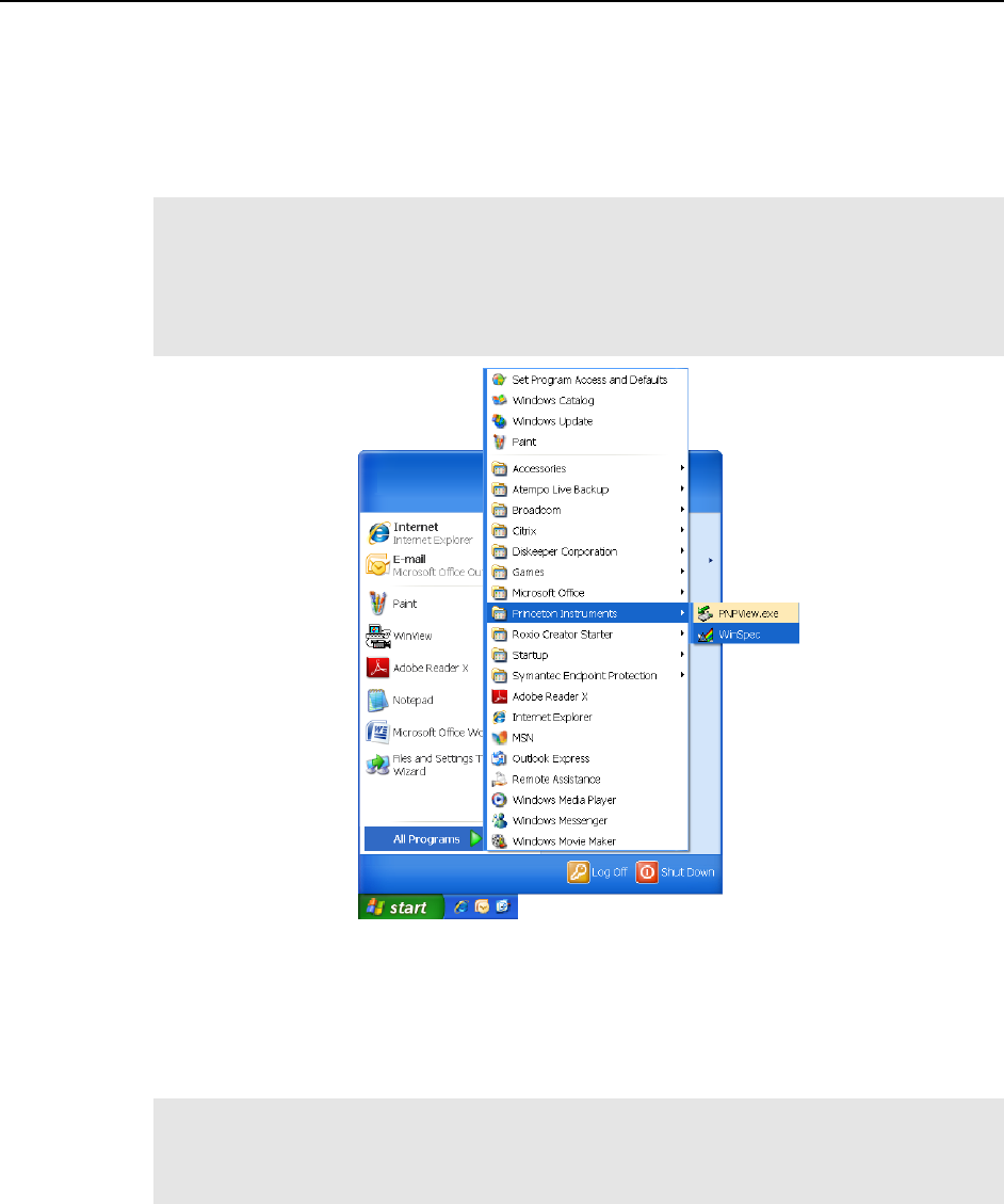
32 WinSpec/32 Manual Version 2.6B
Starting WinSpec/32
Before starting WinSpec/32, follow the hardware interconnection and power up
instructions in the hardware manuals supplied with your system. Then, click on the Start
button, select All Programs, and start WinSpec/32 by clicking on WinSpec32 in the
Princeton Instruments folder (see Figure 1).
Note: You can start WinSpec/32 even if you have not installed the interface card or if you
have not turned on the controller. If there is no interface card, WinSpec/32 will run in
"Demo" mode. This mode allows you to look at and post-process previously stored data
(such as the sample data installed with the software) and to become familiar with experiment
setup and data acquisition. Some features will not be available because the program looks for
information from the controller and camera while WinSpec/32 is loading and initializing.
Figure 1. Opening WinSpec/32 via the Windows Start button
While the software is booting, a splash screen such as the one shown in Figure 2 is
displayed until the software has finished loading and initializing. Then, the Main Menu
appears as shown in Figure 3. From there, you can access the program’s functions through
menu selection.
Note: If this is the first time you have installed and launched WinSpec/32, the Camera
Detection Wizard will pop up. This wizard allows you to specify the camera system and
load the default hardware settings before you can access the menu. See Chapter 2,
page 37 for more information about the Camera Detection Wizard.
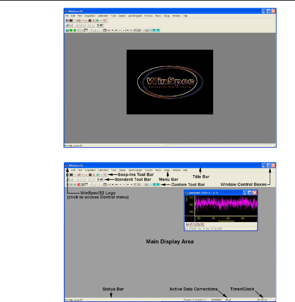
Chapter 1 Installing and Starting WinSpec/32 33
Figure 2. Splash screen
Figure 3. Main WinSpec/32 window
Values, labels, and alphanumeric data are usually entered from the keyboard. Selections and
screen control operations are usually done using a mouse or other graphical I/O device,
although keyboard selection shortcuts are provided. Mouse selection is typically done by
positioning the mouse cursor on the selection item and clicking the left mouse button. In
some case, clicking the right mouse button will bring up a dialog with additional information
or a special menu that allows additional operations to be performed.

34 WinSpec/32 Manual Version 2.6B
This page intentionally left blank.
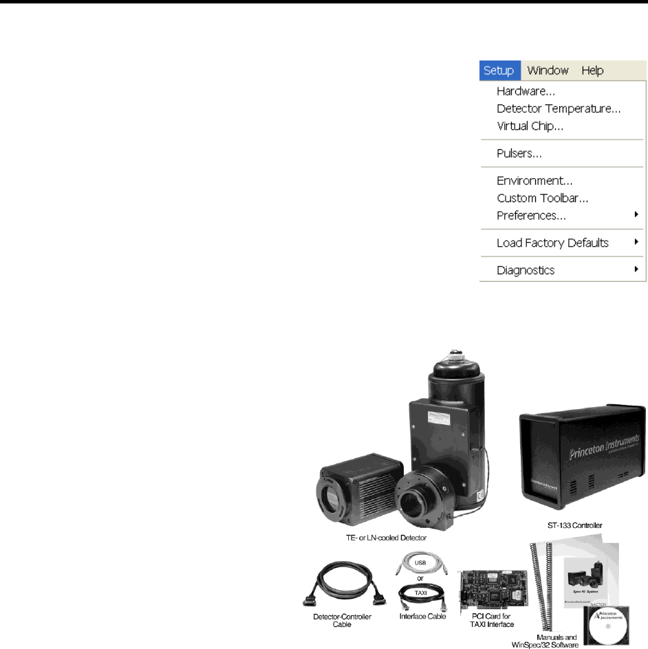
35
Chapter 2
Basic Hardware Setup
Introduction
This chapter provides an overview of the relationships
between the camera, the controller, and the host computer.
This overview is followed by a discussion of the Setup
Wizard that runs the first time you select Hardware from
the Setup menu (Figure 4). The remainder of the chapter
presents the Hardware Setup tabs so you will be able to
make the appropriate selections and entries for your system.
The chapters that follow describe how to configure a
spectrograph, set up a pulser, set up experiment parameters,
and control array temperature. Initial data acquisition is
discussed in Chapters 3 and 4.
Advanced functions such as Post-Processing, Custom Chip,
and Custom Timing are discussed in Part 2 of this manual.
Figure 4. Setup menu
Basic Hardware Overview
The basic components of a Princeton Instruments
system are: a camera (or detector), a controller
(external or internal), interconnecting cables, a
computer interface card, and the application
software (in this case WinSpec/32).
Note that other components such
as a computer, coolant
circulator, and pulser can also
be ordered.
The interface card, installed in
the host computer, permits
communication between the
host computer and the
controller (in some cases an
external controller such as an
ST-133).
The controller accepts input from the host
computer and WinSpec/32 and converts it to the appropriate control signals for the
camera. These signals allow you to specify the readout rate, binning parameters, regions
of interest, gain, and array temperature. After data is acquired in the camera, it is
transmitted to the controller where it is processed, transmitted to the host computer,
displayed in the WinSpec/32 window, and can be stored to disk.
Figure 5 illustrates possible system configurations (spectrometers and pulsers are not
shown). Figure 6 shows the interconnections for an air-cooled Princeton Instruments
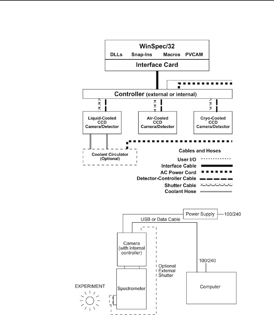
36 WinSpec/32 Manual Version 2.6B
camera with an internal controller, as well as interconnections to an optional external
shutter and spectrometer. Figure 7 and Figure 8 show the interconnections for a Princeton
Instruments system with an external controller, as well as interconnections to an optional
coolant circulator, an optional external shutter, and spectrometers.
Figure 5. Possible System Configurations
Figure 6. Air-Cooled System (with Internal Controller) Diagram
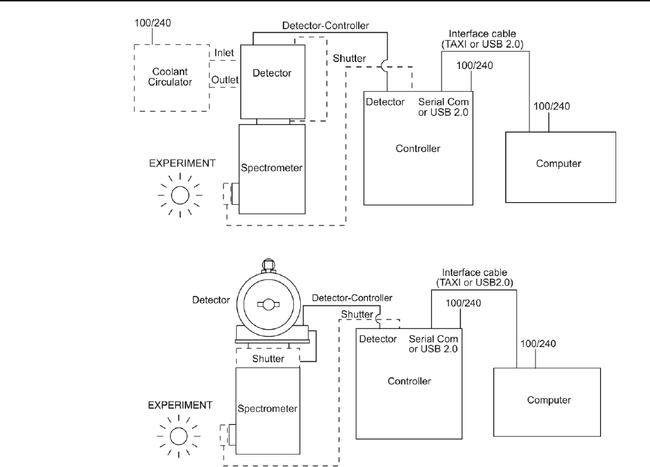
Chapter 2 Basic Hardware Setup 37
Figure 7. Liquid- or Air-Cooled System (with External Controller) Diagram
Figure 8. Cryo-Cooled System (with External Controller) Diagram
Entering the Default System Parameters into WinSpec
Camera Detection Wizard
The Camera Detection Wizard is used to load the WinSpec hardware setup parameter
fields with default values for a WinSpec-compatible camera system. The Camera
Detection Wizard runs automatically the first time you install WinSpec and can be
launched at a later date if you decide to control a different WinSpec-compatible camera.
The autodetection function can be used for Gigabit Ethernet-base camera systems
(PI-MAX3, PI-MAX4, NIRvana, ProEM, and PyLoN), FireWire-based camera systems
(Quad-RO), PVCAM-based camera systems (USB 1 interface, USB 2 interface,
Photometrics PCI, Acton InSpectrum, and PhotonMAX) and Princeton Instruments PCI
(TAXI) interface-based systems.
To Use the Autodetection Function:
1. Make sure the camera system is connected to the host computer and that it is
turned on.
2. Start WinSpec. The Camera Detection Wizard will automatically run if this is the
first time you have installed a Princeton Instruments WinX application
(WinView/32, WinSpec/32, or WinXTest/32) and a supported camera. Otherwise, if
you installing a new camera type, click on the Launch Camera Detection
Wizard… button on the Controller/CCD tab to start the wizard.
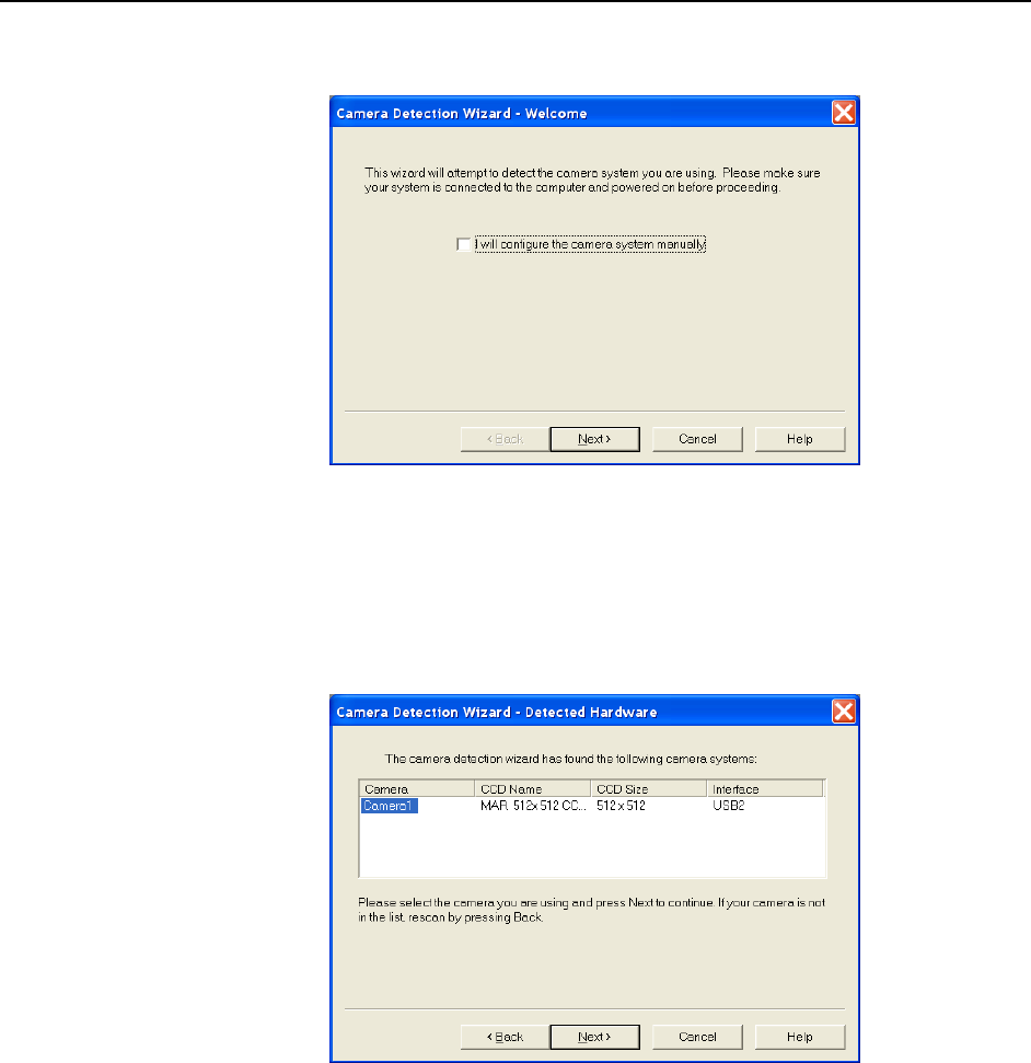
38 WinSpec/32 Manual Version 2.6B
3. On the Welcome dialog (Figure 9), leave the checkbox unselected and click on
Next.
Figure 9. Camera Detection Wizard - Welcome dialog
4. Select the system that you want to install.
If there are two camera systems connected to the host computer and turned on,
the wizard table should contain two listings.
If there are no systems listed, click on Back, check the cable connections and/or
turn on the camera system, and then click on Next.
Figure 10. Camera Detection Wizard - Detected Hardware dialog
If there are still no systems listed and the camera uses the GigE interface, click
on Cancel and contact your Information Technology specialist. UDP ports
20200-20202 (often closed by computer security functions such as an anti-
virus program or a firewall) must be open for WinX to detect a Princeton
Instruments camera using GigE.
5. Follow the instructions on the dialogs to perform the initial hardware setup: this
wizard enters default parameters on the Hardware Setup dialog tabs and gives you an
opportunity to acquire a test image to confirm the system is working.
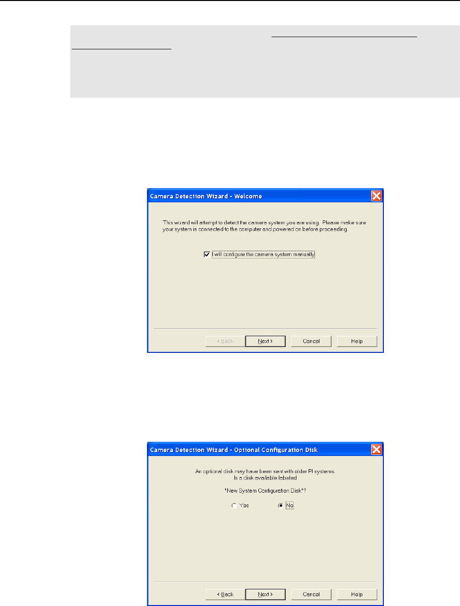
Chapter 2 Basic Hardware Setup 39
To Use the Manual Function:
Note: This function can only be used to install Princeton Instruments PCI (TAXI)
interface-based systems (both Princeton Instruments PCI (TAXI) and PVCAM-supported
systems can be installed by using the autodetection function previously described.). The
manual function is very similar to the Hardware Detection Wizard, but you are not given
the opportunity to install a PVCAM-based camera. In addition, unless you want to acquire
the optional test image, this function does not require that the system be turned on.
1. Start WinSpec. The Camera Detection Wizard will automatically run if this is the
first time you have installed a Princeton Instruments WinX application
(WinView/32, WinSpec/32, or WinXTest/32) and a supported camera. Otherwise, if
you installing a new camera type, click on the Launch Camera Detection
Wizard… button on the Controller/CCD tab to start the wizard.
2. On the Welcome dialog (Figure 11), select the checkbox and click on Next.
Figure 11. Camera Detection Wizard - Welcome (Manual selected) dialog
3. In most cases you will not be getting a New System Configuration Disk with
your system. Therefore, the default selection is "NO". If you do have such a disk,
you would select "YES" and follow the directions for loading the information
from that disk. Click on NEXT and follow the directions on the subsequent
dialogs for selecting the interface, controller, and detector/camera.
Figure 12. Camera Detection Wizard - Optional Configuration Disk dialog
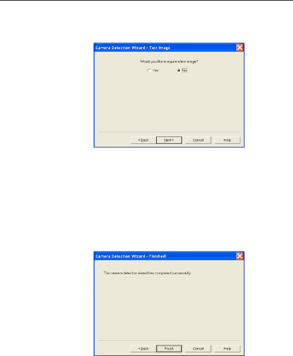
40 WinSpec/32 Manual Version 2.6B
4. When you have finished with these selections, you will see the Test Image
dialog (Figure 13). The default selection is "No". If you select "Yes", you must
make sure that the system is connected to the host computer and that the camera
system is turned ON before you click on the Next button.
Figure 13. Camera Detection Wizard - Test Image dialog
5. Depending on your radio button selection, the following will happen
"No": Clicking on the Next button will load the camera/controller default
parameters into WinSpec and pop up the Finished dialog.
"Yes": Assuming that the camera system is connected to the host computer
and turned on, clicking on the Next button will acquire a single frame of data
(using a 100 msec exposure time), load the camera/controller default parameters
into WinSpec, and pop up the Finished dialog.
6. Click on Finish to complete the camera installation.
Figure 14. Camera Detection Wizard - Finished dialog
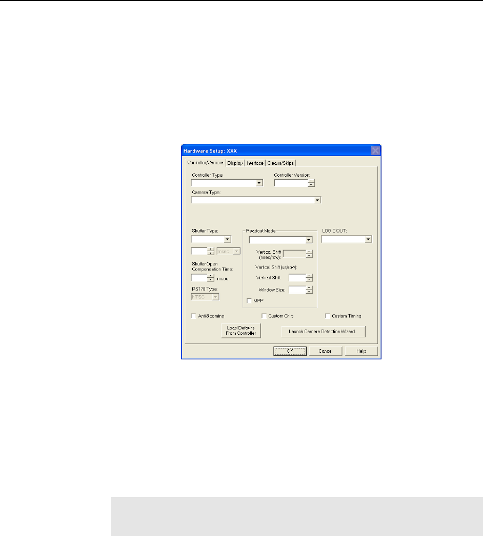
Chapter 2 Basic Hardware Setup 41
Editing Controller and Detector Characteristics
The Hardware Setup|Controller/Detector tab (may also be named Controller/Camera
or Controller/CCD depending on the hardware selections) is used to enter and update
Controller Type, Detector (Camera or CCD, depending on the system) Type and some of
the Controller/ Detector type parameters, such as Shutter Type and Readout Mode. The
Controller and Detector Type selections are perhaps the most fundamental and important
of all hardware selection decisions and directly influence the appearance of many other
WinSpec/32 screens and the selections provided on them. As a result, setting up the
software for use in any system should always begin with the Controller selection.
Figure 15. Hardware Setup|Controller/Camera tab
Figure 15 shows the fields and checkboxes that may be present on the Controller/Detector
tab. WinSpec/32 displays or hides features based on the selected controller, detector, and
readout mode. All of the features are described in the text that follows.
Controller Type (Camera Name): The currently selected Controller Type (Camera
Name) is displayed in this field. If you change the controller that is being used in the
system, choose the correct name from the selection list (displayed by clicking on the
button at the end of the field). Appendix A provides a cross-reference table for
systems, controllers, and CCD arrays.
Note: After you have selected the Controller Type, you can load the default
settings for your controller, camera, and array by clicking on Load Defaults
From Controller, if this button is present.
Controller Version: In the case of the ST-133 and PentaMAX controllers, different
versions have been released having different capabilities. The available software
selections will correctly reflect these differences when the proper version number
is specified in this box.
Camera Type: The selected Camera (Detector/CCD) Type is displayed in this field.
Clicking on the button at the end of the box drops the selection list so that the
selected type can be changed if necessary. Note that the listed camera types depend
on the controller selection, requiring that the controller type be specified first.
Shutter Type: There are six selections.

42 WinSpec/32 Manual Version 2.6B
None: If the camera has no shutter (frame-transfer or interline CCD array) and
is not an Intensified camera, select None.
Small: A small shutter is one that is typically 25 mm or smaller in diameter.
This setting represents a shutter compensation time of approximately 8 msec.
Large: A large shutter is one that is typically 35 mm and larger. In the case of a
camera having a very large CCD, such as the Kodak 2k × 2k, a large shutter
may have been installed. This setting represents a shutter compensation time
of approximately 28 msec.
Remote: Remote is primarily intended for spectroscopy applications where an
external shutter would be placed ahead of the entrance slit.
Electronic: Electronic only applies to operation with an intensified camera,
which would normally not be equipped with a mechanical shutter. This
selection would apply to both the Gate and Shutter/CW modes of the
IIC-100, IIC-200, IIC-300, MCP-100, and PI-MAX.
Custom: This shutter type is automatically selected if you are using a PVCAM-
supported camera. When Custom is the shutter type, you will be able to
enter the shutter close compensation time in the field below the shutter type.
Shutter close compensation time delays readout to allow time for the shutter
to fully close. The close value will vary depending on the camera and the
shutter used.
Phosphor Decay Time: Used by the PI-MAX3 and PI-MAX4 when running in
single trigger DIF mode to delay the shift behind mask for the first image.
Shutter Open Compensation Time: Delays the exposure until the shutter is
fully open. The open delay value will vary depending on the camera and the
shutter used.
Readout Mode: The readout mode is determined by the characteristics of the CCD
array and the controller. The possible choices are:
Full Frame: The entire chip can be read out.
Frame Transfer: Only the unmasked area of the chip can be read out. Frame
transfer is only available if the camera has a frame-transfer chip such as the
EEV 512 × 1024.
Interline: Provides 100% duty cycle operation. Interline is only available with a
camera having an interline chip such as the PI 1300 × 1030.
Kinetics: Kinetics is a special type of operation in which most of the CCD is
mechanically or optically masked, leaving a small section open to light. This
section is then read out very quickly. See the System or Controller manual
for more details on the CCD aspects of this readout mode.
DIF or Dual Image Feature: (MicroMAX, PI-MAX2, PI-MAX3, and
PI-MAX4 Interline only) Dual Image Feature (DIF) is a special feature that
allows images to be taken in pairs with very short exposure times (as small as
1 µs). For MicroMAX this feature is only available for factory modified
MicroMAX controller/Interline camera systems. The three MicroMAX DIF
timing modes are IEC (Internal Exposure Control), EEC (External Exposure
Control) and ESABI (Electronic Shutter Active Between Images). These modes
are in addition to Free Run mode. The two DIF timing modes for PI-MAX2,
PI-MAX3 and PI-MAX4 are Single Trigger and Dual Trigger.

Chapter 2 Basic Hardware Setup 43
Vertical Shift Time: This information appears for the Frame Transfer and
Kinetics modes. Reports the speed (in microseconds) at which a single row
will be shifted vertically. This information is based on the value in the Vertical
Shift box. The higher the value in that box, the longer the vertical shift time.
Note: If you are using a PVCAM-supported camera, the Vertical Shift rate is
expressed in nsec/row. Use the up/down arrows to change the Vertical Shift rate.
Vertical Shift: Determines the speed of the image transfer from the exposed area
of a frame-transfer chip to the masked area. Also sets the speed of image
transfer when operating in the Kinetics mode. Setting a lower value increases
the shift speed. A higher value gives a slower shift. If the shift is too fast, not all
of the charge will be transferred. If too slow, image smearing will be increased
due to the exposure that takes place while the transfer is in progress. The default
value gives good results in most measurements.
Note: If you are using a PVCAM-supported camera, this parameter is hidden
because the shift time is being adjusted via the Vertical Shift (nsec/row)
up/down arrows.
Window Size: Determines the height of the window for Kinetics mode. The
window size must be at least 1 row and less than or equal to the maximum
number of rows for the array.
MPP: This checkbox may appear if the CCD array is designed for MPP (multi-
pinned-phase) operation. When this box is checked, the array will be run in MPP
mode. Some MPP-capable arrays can also be run in Non-MPP mode (MPP box is
unchecked). Running in Non-MPP mode may result in higher dark current in
addition to larger full well capacity.
Note: MPP capability reduces the rate of dark-current generation by a factor of
20 or more, and thus relaxes CCD cooling requirements to the level where a
thermoelectric cooler is sufficient for most applications.
LOGIC OUT Output: The choices for the signal provided at the controller's
Output connector vary based on the selected Controller. If the LOGIC OUT field
doesn’t appear on the tab, the choice of output may be done via an internal
jumper (for information on how to set the jumper, contact factory Tech Support).
Depending on your system, the following choices may appear in the drop down
list:
Cleaning: This signal is high when an array Clean cycle is in progress and
otherwise low.
Logic 0: Establishes a TTL logic 0 at the Logic Out connector.
Logic 1: Establishes a TTL logic 1 at the Logic Out connector.
Note: LOGIC 0 and LOGIC 1 can be used to control an external device using
the application software.
Not FT Image Shift: This signal is low when a frame-transfer shift is in
progress and otherwise high.

44 WinSpec/32 Manual Version 2.6B
Not Ready: After a Start Acquisition command, this output changes state on
completion of the array cleaning cycles that precede the first exposure.
Initially high, it goes low to mark the beginning of the first exposure. In free
run operation it remains low until the system is halted. If a specific number
of frames have been programmed, it remains low until all have been taken,
then returns high.
Not Scan: Reports when the controller is finished reading out the CCD array.
NOT SCAN is high when the CCD array is not being scanned, then drops
low when readout begins, returning to high when the process is finished.
Shutter: This signal is low when the shutter is closed and goes high when the
shutter is activated, dropping low again after the shutter closes. In Gated
operation, SHUTTER is the correct choice and the signal should be applied
to the inhibit input of the pulser to prevent pulsing during readout.
Shutter Comp Time Pre: Delays the acquisition until the shutter (if present) is
fully open. The setting range is 0 to 30 ms. For single-strip spectroscopic
measurements, a setting of “0” is recommended.
RS170 Type: Selections are NTSC (US video standard) and PAL (European).
Show Custom Chip: Advanced feature. See Custom Chip discussion on page 213.
Show Custom Timing: Advanced feature. See Custom Timing discussion on
page 214.
Anti-Blooming: (THM 1024x1024FT CCD array) Checking this box activates
this CCD array's anti-blooming feature.
Load Defaults From Controller: Pops up the Load Factory Defaults From
NVRAM dialog so you can repopulate the fields and selections with the values
stored in the controller's non-volatile RAM.
Launch Camera Detection Wizard: Pops up the Camera Detection Wizard -
Welcome dialog so you can set up a new camera system or switch the active
camera system to another camera system already connected to the host computer.
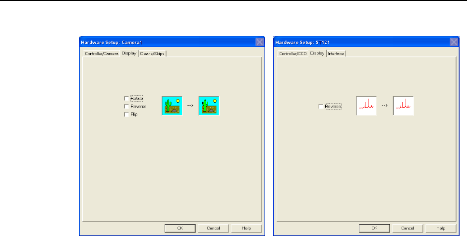
Chapter 2 Basic Hardware Setup 45
Entering the Data Orientation
Figure 16. Display tab; left graphic applies to all controllers except ST-121; right graphic
applies to ST-121 only
With the exception of the ST-121, the Display tab is the same for all controllers. Three
display options, Rotate, Reverse and Flip, are provided. This feature allows you to
compensate for CCD array or camera orientation. Before and after thumbnail illustrations
show the effect of each selection. If no option is selected, the thumbnails will be the
same. Any orientation can be achieved with the proper combination of Rotate, Reverse,
and Flip. In the case of the ST-121, only Reverse is provided.
Rotate: Rotates the image 90° counterclockwise.
Reverse: Reverses the image horizontally.
Flip: Flips the image vertically.
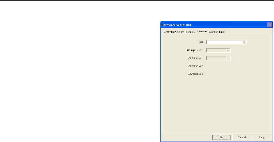
46 WinSpec/32 Manual Version 2.6B
Entering the Interface Communication Parameters
The Interface tab allows you to specify the
interface card installed in your computer and
to enter the I/O addresses (if required). This
functionality is particularly useful if you have
multiple PCI cards installed in the host
computer. Figure 17 shows all of the fields
and checkboxes that exist on the Interface
tab. WinSpec/32 will display and hide
features based on the interface card installed
in the host computer. All of the features are
described in the text that follows.
Type: Select the communications type
that will be used to transmit data
from the controller to the computer.
All communications types are not
available for all controllers and
computers. The "Demo" selection,
which allows the software to be
Figure 17. Interface tab
exercised but which does not support data transfer to the computer, would not
ordinarily be used in the field.
High Speed PCI: Select if a Princeton Instruments (RSPI) PCI high-speed
serial Interface card is installed in your computer and you want data transfer
to be interrupt driven. This choice would give the highest performance in
most situations.
PCI Timer: Allows data transfer to be controlled by a polling timer if using PCI
high-speed serial Interface card. Useful for troubleshooting possible interrupt
problems (computer crashes or system fails to return data). Note that data
transfer is slower in PCI Timer mode and data overrun more likely. Also PCI
Timer cannot be used to continuously acquire small Regions of Interest in
Safe Mode timing operation. PCI Timer is not compatible with Use
Interrupts operation, a timing mode available when using the ST-138
Controller.
Demo: Allows the software to be exercised without being connected to a
controller. This mode is used primarily for demonstration purposes or post-
processing of acquired data and cannot be used in an actual measurement.
Interrupt Level: The interrupt level for a PCI card is reported but cannot be
changed.
Card Number: This field only appears if more than one PCI card has been detected
in your computer. This field allows you to set up the communications parameters
so each card is uniquely addressed.
I/O Address: The I/O Address for a PCI card is reported but cannot be changed.
I/O Address 2 and 3: (High Speed PCI only) These addresses are reported but
cannot be changed; address selection is automatic and under computer control.
With other interfaces, these addresses are not displayed.
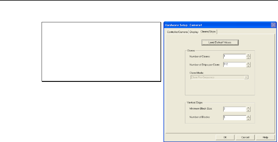
Chapter 2 Basic Hardware Setup 47
Entering the Cleans/Skips Characteristics
For most applications, the default settings
will give the best results. We advise
contacting the factory for guidance before
changing these parameters from their
default values. Exception: With a PI-MAX
camera, we suggest settings of Cleans 1 and
Strips per Clean 4, Minimum Block Size 16
and Number of Blocks 32.
Figure 18. Cleans/Skips tab
The Cleans/Skips tab allows you to
change the clean and skip parameters from
their default values or to reload the default
values. Figure 18 shows all of the fields
and checkboxes that exist on the
Cleans/Skips tab. WinSpec/32 will
display and hide features based on the
controller version. All of the features
shown are described in the text that
follows. Refer to Chapter 10, starting on
page 135, for additional information.
Load Default Values: Reloads the factory defaults from the NVRAM.
Cleans
Cleans are applied to the entire CCD array and remove charge that has accumulated on
the array while waiting for data acquisition to begin. The charge on the CCD chip is
transferred to the shift register and discarded to prevent charge buildup from occurring.
On completion of a setup, successive clean cycles occur normally. The Number of
Cleans and Number of Strips per Clean parameters allow you to program additional
clean cycles that will be performed after initiating the run but before any data are taken.
Number of Cleans: For most applications the default value should be used.
Clicking on the Load Default Values button and then selecting Yes will install
the default value. Values other than the default can be directly entered in the field
or selected via the spin buttons.
Number of Strips per Clean: Sets the number of CCD data strips to be
transferred and discarded during each clean. The maximum valid setting is
limited by the chip size. The default value will generally give good results.
Clean Mode: (Photometrics brand cameras) Sets when and how charge will be
cleared from the array while the camera is waiting to acquire data. Clearing
removes charge from the CCD by clocking the charge to the serial register then
directly to ground. This process is much faster than readout, because the charge
does not go through the readout node or the amplifier. Note that not all clearing
modes are available for all cameras. Be sure to check availability of a mode before
attempting to set it.
Clear Never: Never clear the CCD. Useful for performing readout after an
exposure has been aborted.
Caution

48 WinSpec/32 Manual Version 2.6B
Clear Pre-Exposure: Before each exposure, clears the CCD the number of
times specified by the Number of Cleans entry. This mode can be used in a
sequence. It is most useful when there is a considerable amount of time
between exposures.
Clear Pre-Sequence: Before each sequence, clears the CCD the number of
times specified by the Number of Cleans entry. If no sequence is set up, this
mode behaves as if the sequence has one exposure. The result is the same as
using Clear Pre-Exposure.
Clear Post-Sequence: Clears continuously after the sequence ends. The
camera continues clearing until a new exposure is set up or started, the abort
command is sent, the speed entry number is changed, or the camera is reset.
Clear Pre/Post-Sequence: Clears Number of Cleans times before each
sequence and clears continuously after the sequence ends. The camera
continues clearing until a new exposure is set up or started, the abort
command is sent, the speed entry number is changed, or the camera is reset.
Clear Pre-Exposure Post-Sequence: Clears Number of Cleans times before
each exposure and clears continuously after the sequence ends. The camera
continues clearing until a new exposure is set up or started, the abort
command is sent, the speed entry number is changed, or the camera is reset.
Use Continuous Cleans Instruction: This feature is supported by Version 5
(and higher) ST-133 controllers and will only appear if the detector/camera also
supports this feature. Continuous cleans instruction does horizontal shifts while
doing vertical shifts for a faster continuous clean. Check this box if you want to
apply the continuous cleans instruction to the continuous cleans function
available when External Sync timing mode (Experiment Setup|Timing tab) is
being used to acquire data. With this instruction, the delay between an External
Sync trigger and the start of exposure is minimized. Refer to Chapter 10,
starting on page 135, for more information about continuous cleans and
continuous cleans instruction.
Note: Older versions of the ST-133 controllers, as well as other controller types
and cameras, do not support this instruction.
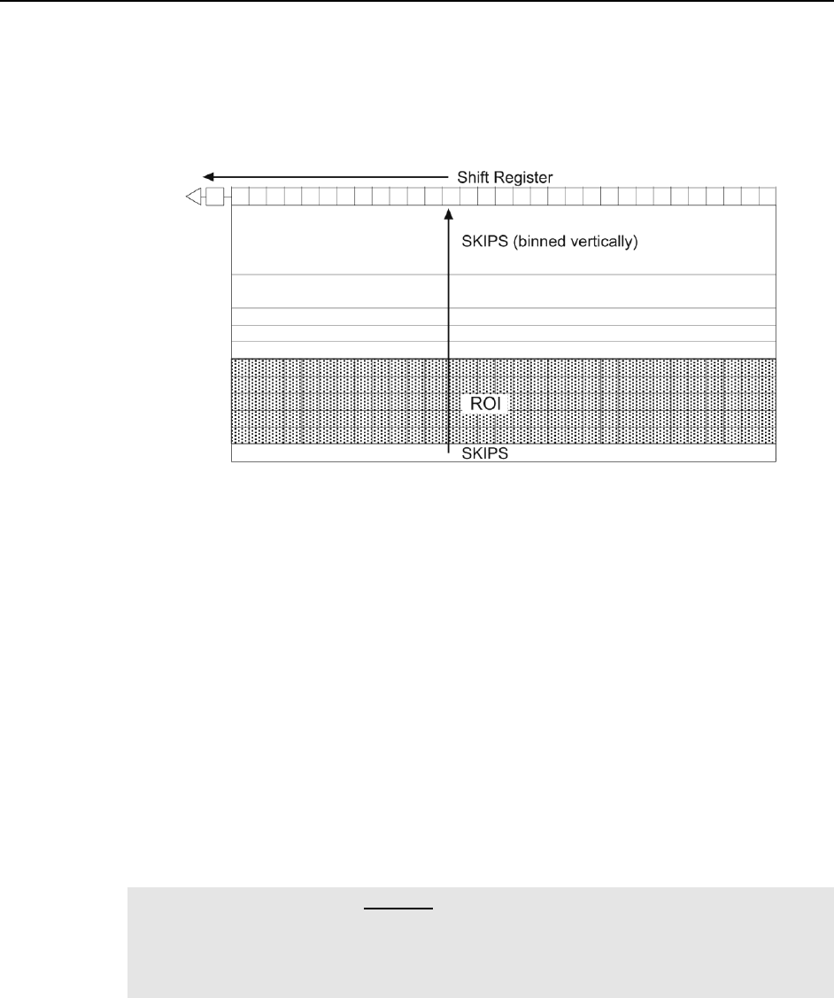
Chapter 2 Basic Hardware Setup 49
Vertical Skips
Vertical skips are associated with regions of interest (ROIs) that are smaller than the full
chip. This feature allows you to bin and quickly traverse the rows that precede and follow
the ROI. The rows to be processed and discarded are binned into blocks, each containing
a number of rows, with the Number of Blocks parameter determining how many blocks
there will be before and after the ROI.
Figure 19. Vertical Skips
The block size determines how quickly the region preceding and following the ROI will
be traversed. If the blocks are large, the region will be traversed quickly but there is the
possibility of overloading the shift register and causing blooming. With small blocks, the
risk of blooming will be minimized but the time to traverse will be large. WinSpec/32
uses an exponential algorithm to simultaneously achieve rapid traversing with minimal
risk of blooming. The first block, specified in rows, is as large as possible. Each
successive block is a factor of two smaller than the one preceding until the minimum
block size is reached. All remaining blocks are the minimum block size. By making the
first block as large as possible and subsequent blocks increasingly smaller, the region
preceding and following the region of interest is traversed as rapidly as possible while
minimizing risk of the shift register saturation.
Minimum Block Size: Sets the size, in rows, of the skip blocks that immediately
precede the data. The default value will generally give good results.
Number of Blocks: Sets the number of binned “skip” blocks preceding and
following the region of interest. The default value will generally give good
results.
Note: The 2-D OMA array does not support vertical skips; and all of the rows on the
array are read out and converted before the non-ROI information is discarded. The
default Vertical Skips settings of Minimum Block Size: 2 and Number of Blocks: 5,
while appearing to work, will result in invalid data. Instead, you must change these
settings to 1 and 256, respectively, for the 2-D OMA array.
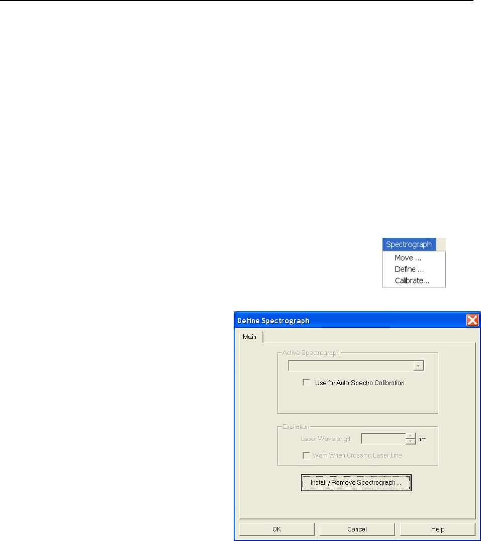
50 WinSpec/32 Manual Version 2.6B
Setting up a Spectrograph
WinSpec/32 allows you to control several types of spectrographs. More than one
spectrograph can be installed in the system at one time. The total number of
spectrographs is limited only by the number of free communication ports.
The following spectrograph operations can be performed after you define your
spectrograph:
moving a spectrograph grating,
automatic calibration of acquired data according to the spectrograph position,
changing to a different grating for some spectrographs, and
changing the entrance slit size and/or the selected mirror for some spectrographs.
The following steps explain how to set up a spectrograph. You must correctly install a
spectrograph before you can control any of its functions through WinSpec/32.
1. Make sure that the spectrograph is correctly connected to a host computer COM port.
2. Turn on the host computer and the spectrograph.
3. Wait for the spectrograph to finish initializing and then
boot WinSpec/32. If this is not done, although you will be
able to install the spectrograph, it will not be possible to
establish communications and an error message will result.
Figure 20. Spectrograph menu
4. Select Define on the
Spectrograph menu
(Figure 20). This will open the
Define Spectrograph dialog
(Figure 21).
5. On the Main tab, note the
Active Spectrograph text entry
box. If spectrographs have
previously been installed, the
active one will be indicated. If
no spectrograph has been
previously installed, the box
will be blank. Note there is a
checkbox that allows you to
designate a particular
spectrograph as the one that
will be used for doing an
Auto-Spectro Calibration.
Figure 21. Define Spectrograph dialog
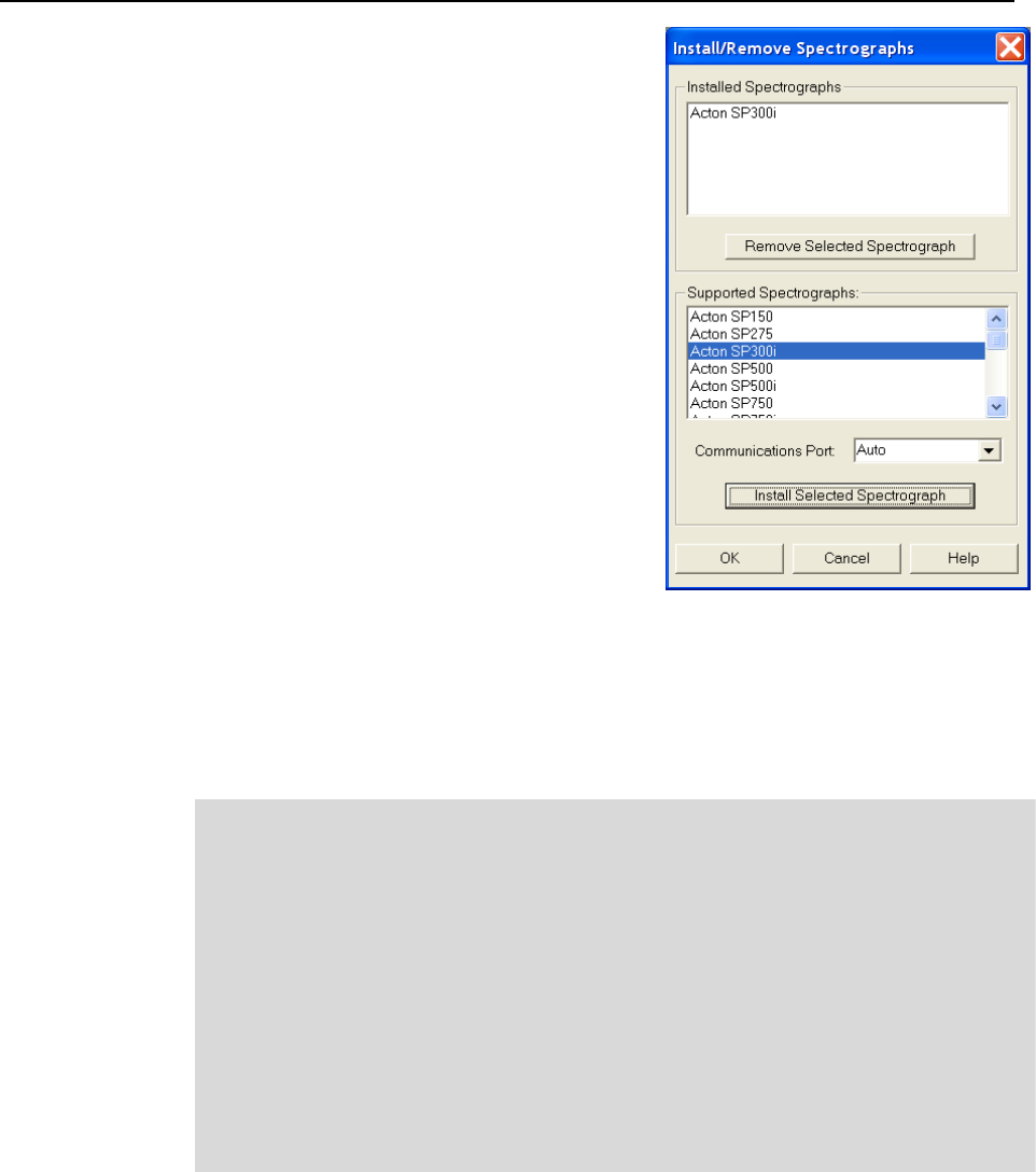
Chapter 2 Basic Hardware Setup 51
6. Click on Install/ Remove Spectrograph. This
will open the Install/Remove Spectrographs
dialog (Figure 22). The lower window lists the
supported Spectrographs. The upper window
lists those installed. To install a spectrograph,
select it from the list in the lower window, select
the Communications Port (Auto, COM1-
COM8, or DEMO) and click on Install
Selected Spectrograph. The installed
spectrograph will then appear in the upper
window. In the case of the example shown in
Figure 22, the selected spectrograph is an Acton
SP300i. When selecting a communications port
during the installation, keep in mind the
characteristics of the choices.
Auto: When WinSpec is started, it will look for
the spectrograph and communicate via the
port (USB or COM) at which it is found.
COM1-8: If you select a specific COM port,
WinSpec will only look for the spectrograph
at that port.
Figure 22. Install/Remove Spectrographs
DEMO: If you select DEMO, you can view the spectrograph-related dialogs and
functions without having an actual spectrograph.
If the spectrograph is not found when you install it, an error message is displayed. Even
if communication is not established, the spectrograph and its assigned port will be
added to the list (for example, Acton SP300i on COM2).
Notes:
1. To install another spectrograph, repeat the installation procedure.
2. To remove a spectrograph, select it in the upper box and click on Remove
Selected Spectrograph. The spectrograph’s name will be removed from the
upper window.
3. Multiple spectrographs can be assigned to a port. However, only one spectrograph
can be active at a time. If you have multiple spectrographs assigned to a port, make
sure that the active spectrograph (refer to the Active Spectrograph field on the
Main tab) is the one that is (or will be) physically connected to the port.
4. If you plan to install more than one spectrograph for a COM port, it would be a
good idea to make sure that the connection preferences are the same for all of the
spectrographs assigned to that port.
7. Click on OK to close the Install/Remove Spectrographs dialog.
8. If the newly installed spectrograph is the only installed spectrograph, the Use for
Auto-Spectro Calibration box will be checked by default. If more than one
spectrograph is installed, you need to check in the box for the spectrograph that is
attached to the active detector. The checked status indicates which spectrograph can
be automatically calibrated using the Spectrograph Calibration function, which
requires that the controller take data (see Chapter 7 for more information).
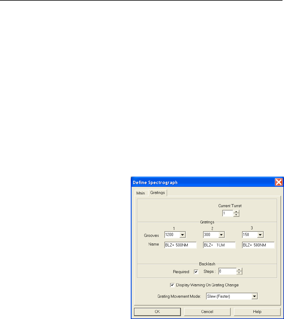
52 WinSpec/32 Manual Version 2.6B
Specifying the Active Spectrograph
If you have installed more than one spectrograph, you need to define the Active
(controlled) Spectrograph. If there is only one spectrograph, that one is the active one. If
there is more than one, than you must designate the active one. This can be done via the
Define Spectrograph|Main tab, the Move Gratings tab (to access, click on Move in
the Spectrograph menu) and via the Calibrate Spectrograph dialog (to access click
on Calibrate in the Spectrograph menu). On the Define Spectrograph|Main page the
selection is called Active Spectrograph, on the Move Gratings tab it is called
Spectrograph to Move, and in the Calibrate dialog it is called Spectrograph to
Calibrate. In all three locations the function is simply to specify the active spectrograph,
and changing the selection in one location is equivalent to changing it in all three. If only
one spectrograph has been installed, the box will not appear in the Move or Calibrate
dialogs, but the spectrograph model will be reported.
Entering Grating Information
Once you have installed a spectrograph, you may need to enter the grating information
for the spectrograph if the spectrograph cannot supply them automatically. This is
information that WinSpec/32 needs to move and calibrate the spectrograph correctly.
Grating information is supplied automatically for automated Acton spectrographs, as
stored in the spectrograph’s electronics.
Grating Parameters
The grating values are required
for the dispersion calculation
and for the selection of the
active grating. Some
spectrographs have
interchangeable grating turrets,
each able to mount up to 3
gratings. Where this is the
case, the grating information
may have to be separately
specified for each turret that
may be installed. These
parameters are specified on the
Gratings tab (Figure 23) of
the Define Spectrograph
dialog. In the case of
automated Acton
spectrographs, the grating
information is automatically
supplied.
Figure 23. Gratings tab
Setting the grating parameters
1. If there are two or more turrets, enter the number of the turrets.
2. Then from the Current Turret field, select the turret whose grating parameters will
be defined.
3. If entries are missing or incorrect, select the correct grooves/mm value for each
grating. Make sure that the gratings are listed in the proper order, Grating 1 listed
first, etc.
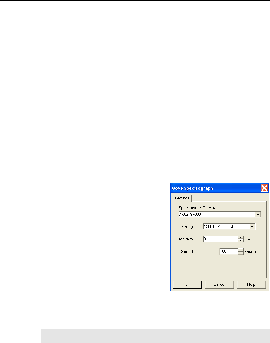
Chapter 2 Basic Hardware Setup 53
4. You can also enter a Name for each grating. This option is required if you are using
two gratings with the same groove density. If, for example, you have two gratings
with 300 grooves/mm, one blazed at 300 and one blazed at 500, you could enter
BLZ300 and BLZ500 in the Name boxes as identifiers. These are the Acton default
names. Then, when you subsequently go to the Move Spectrograph dialog to select
the active grating, they would then be listed as 300/BLZ300 and 300/BLZ500 and
there would be no possibility of confusing them.
5. If significant backlash occurs when moving the selected grating, check in the
Required box and then enter the number of steps required to correct for the
backlash.
6. If your spectrograph has more than one turret, replace the turret, change the Current
Turret value and enter the new grating information. WinSpec/32 will store and recall
the different sets of grating information for each turret.
7. Note that there is a checkbox for displaying a warning during a grating change. Since
the time to change a grating can vary widely, depending on the spectrograph, this
message could be very helpful.
8. If two rates are available for your spectrograph, you can also choose the rate, either
faster (slew) or slower (scan). The actual rate will depend on the spectrograph.
Depending on the spectrograph manufacturer and model, there may be a difference in
wavelength setting accuracy for the two speeds.
Selecting and Moving the Grating
Once the required groove and turret information
has been entered on the Define Spectrograph
Gratings tab, the next step is to select and move
the grating. These operations are performed using
the Gratings tab (Figure 24) of the Move
Spectrograph dialog. The procedure follows.
1. Open the Move Spectrograph dialog by
selecting Move from the Spectrograph menu.
2. On the Gratings tab, verify that the indicated
active spectrograph is the correct one.
3. Select the grating to be moved. The available
gratings were previously entered on the
Define Spectrograph Gratings tab.
4. Enter the new position (in nm) in the Move
to field.
Figure 24. Move Spectrograph Gratings
tab
5. Enter any speed settings and click on OK to execute the selections. The grating will
come to rest with the selected wavelength at the center of the CCD array.
Note: There may well be some finite error in the final position. This error can be
measured and compensated for using the Spectrograph Calibrate procedure.
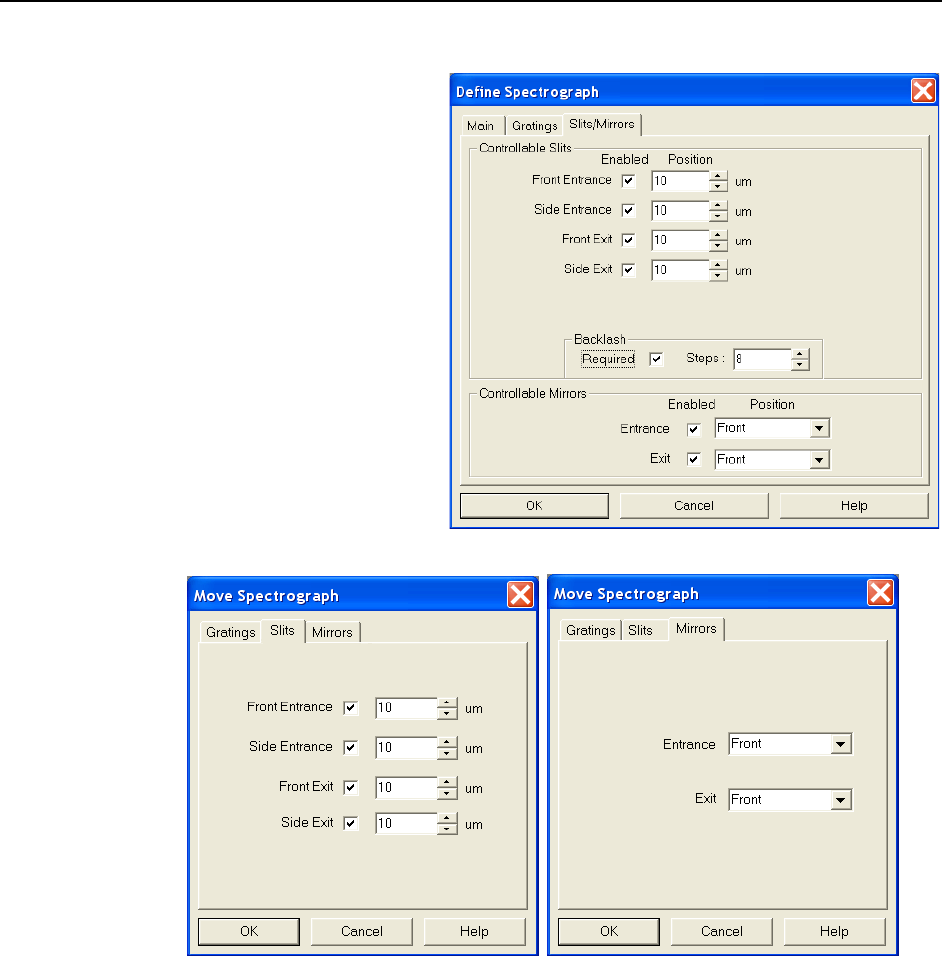
54 WinSpec/32 Manual Version 2.6B
Entering Information for Software-Controlled Slits and/or Mirrors
Some spectrometers allow you
to control the slit width and/or
do mirror selection under
software control. Where this is
the case, the Slits/Mirrors tab
(Figure 25) in the Define
Spectrograph dialog is used
to specify the controllable slits
and selectable mirrors. Actually
setting the slit width and
specifying which mirror to move
is accomplished via additional
tabs provided in the Move
Spectrograph dialog as shown
in Figure 26. Once the selections
are made, simply press OK to
execute them.
Figure 25. Define Spectrograph Slits/Mirrors tab
Figure 26. Slit width and Mirror selection tabs - Move Spectrograph dialog
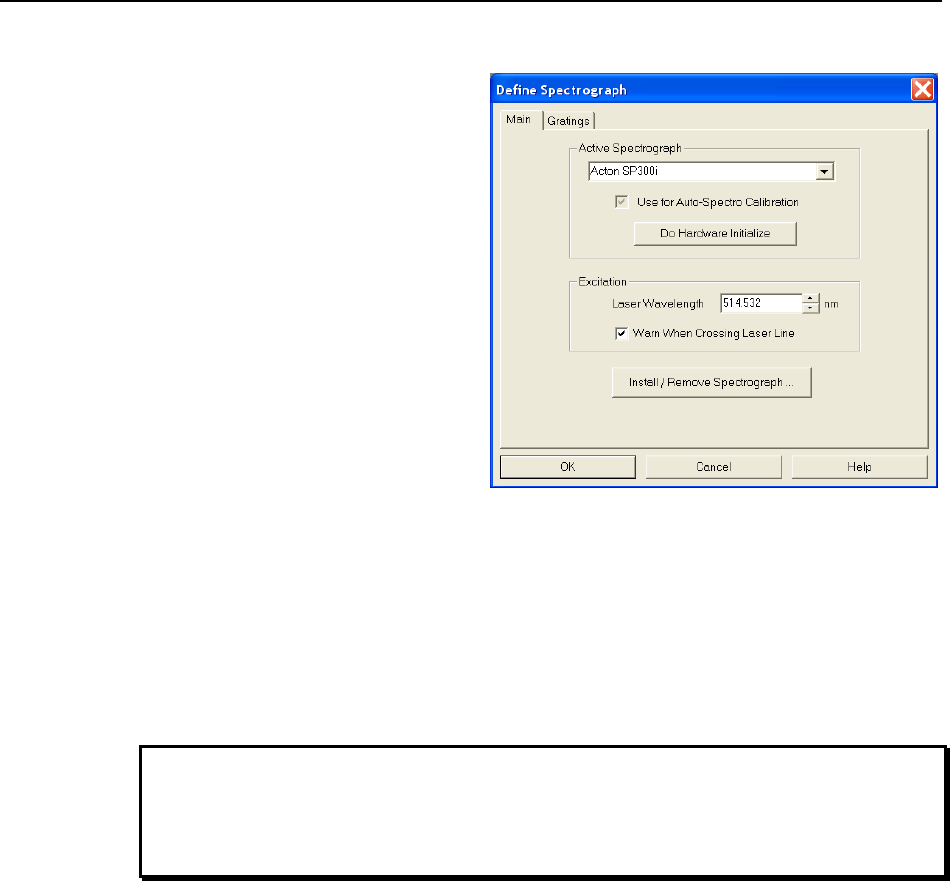
Chapter 2 Basic Hardware Setup 55
Entering Laser Excitation Information
If you want to be warned if the laser
will shine directly on the CCD, you
need to enter the Laser Wavelength.
This is done via the Main tab in the
Define Spectrograph dialog as
shown in Figure 27. The Warn
When Crossing Laser Line
selection tells WinSpec/32 to display
a message whenever the grating is
moved to where the laser light would
be visible to the detector. This is
critical for detectors that could be
damaged if exposed to high light
levels. Also, it will be necessary to
enter the laser wavelength if you
plan to work with units of relative
wavenumbers.
To allow WinSpec/32 to
display in units of relative
Figure 27. Entering the Laser Line
Define Spectrograph Main tab
wavenumbers, enter a Laser Wavelength in nanometers, to as many significant
digits as desired.
If you have a bright laser line, check the Warn when Crossing Laser Line box
and enter the Laser Wavelength in nm. WinSpec/32 will display a warning
message whenever the wavelength range viewable by the detector might fall on
or pass through the laser line.
The Warn When Crossing Laser Line is no guarantee that the detector will not be
damaged by overexposure. The correct display of the warning depends on all calibration
parameters being set correctly. Changing or moving gratings may cause the laser to
shine on the detector. Always block the source when moving or changing the grating to
avoid damage.
WARNING

56 WinSpec/32 Manual Version 2.6B
This page intentionally left blank.

57
Chapter 3
Initial Spectroscopic Data Collection
Introduction
The procedure in this chapter will enable you to begin collecting real data promptly.
Minimum requirements are assumed. If your system is more complex, e.g., requiring
consideration of complex timing and synchronization issues, you will have to carefully
study the other chapters of this manual as well as the manuals provided for the system
hardware components before data acquisition that addresses those needs will be possible.
Nevertheless, it is a good idea to begin with the simplest possible operating mode. This
approach will give you operating experience and familiarity that will prove very valuable
when you go to make more complex measurements. For additional information about the
various menus and dialogs, refer to the online Help topics. Note that controllers and
cameras ordinarily used for imaging are not discussed in this chapter, but rather in the
next chapter, “Initial Imaging Data Collection”.
Underlying assumptions for the following procedure are that the hardware installation,
including mounting the camera to the spectrograph, has been completed. A further
assumption is that the hardware and spectrograph setups as discussed in Chapter 2 have
been completed. The last assumption is that a suitable spectrographic source is available.
The mercury lines produced by ordinary fluorescent lights can be used. However, it will
be better to begin with a low-pressure gas-discharge lamp such as neon, mercury, or
mercury-argon, if one is available.
There are two data collection modes, Focus and Acquire:
In Focus mode operation, no frames of data are stored until Start Storage is
selected. This mode is particularly convenient for familiarization and setting up.
For ease in focusing, the screen refresh rate should be as rapid as possible,
achieved by operating with axes and cross-sections off.
In Acquire mode, every frame of data collected is stored. This mode would
ordinarily be selected during actual data collection. One limitation of Acquire
mode operation is that if data acquisition continues at too fast a rate for it to be
stored, data overflow will eventually occur. This could only happen in Fast Mode
operation.
Note: The following data collection procedures are done in the Focus mode but do not
cover rotational alignment and focusing of a camera to a spectrograph’s optics. Refer to
your camera system manual, your spectrograph manual, and/or Appendix B (page 236
and subsequent pages) of this manual for that information.

58 WinSpec/32 Manual Version 2.6B
1. If using a PI-MAX or PI-MAX2 intensified camera, initial data collection will be done in
the Shutter mode (Gate mode for PI-MAX3 and PI-MAX4). In both cases (Shutter and
Gate mode), the camera can be damaged if exposed to light overload. Before powering
the controller and camera, reduce the room light to reduce the risk of damage. Note that
intensifiers are particularly at risk in pulsed laser operation, where overload spot damage
can occur without raising the average current to where the overload detection circuits
will be activated. It is far better to be careful than sorry. Before proceeding, take the time
to carefully read the manual for your intensified camera.
2. Also, take particular care that your intensified camera is connected properly for shutter or
gate mode operation. Cabling and peripheral considerations for intensified cameras are
more complex than for unintensified cameras. Again, read your manual.
Temperature Control
Before continuing, the array temperature should be set to some easily achieved value in
the operating range and Temperature lock should be established. The way this is done
depends on the controller.
Temperature Control for a System using an ST-133 Controller or for a PVCAM-based
System
1. Open the WinSpec/32 Setup menu and click on
Detector Temperature. This will cause the
Temperature dialog to appear as shown in
Figure 28.
2. Set the Target Temperature to the desired
value (the default temperature is suggested for
initial data acquisition).
3. Click on the Set Temp. button. When the
Current Temperature: Unlocked message
Figure 28. Temperature dialog
changes to Current Temperature: Locked, temperature lock will have been
established.
Notes:
1. The ST-133 additionally has a Temp Lock LED on the Analog/Control module
(at the rear of the controller) that visually indicates when temperature lock
occurs.
2. If you are using the USB 2.0 interface or have a PVCAM-based system with
internal controller, the Detector Temperature dialog will not display current
temperature information while you are acquiring data.
Temperature Control for Other Systems
ST-121, ST-130 or ST-138 Controller: Change the dial setting on the front panel of
the Controller.
PentaMAX: Set the temperature on the front panel of the Temperature/Power Supply
unit.
MicroView: Not user-settable. Temperature is solely under software control.
WARNINGS!
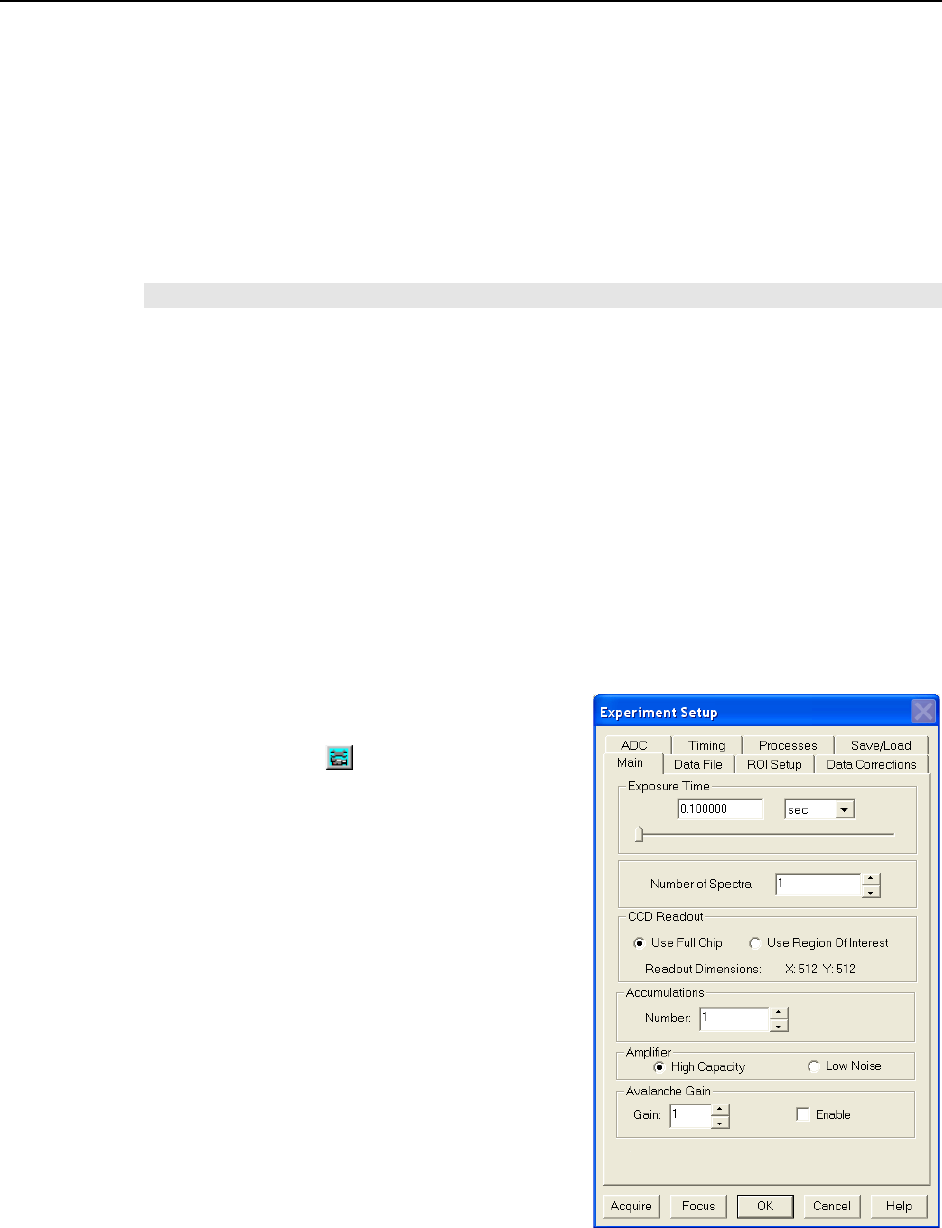
Chapter 3 Initial Spectroscopic Data Collection 59
Cleans and Skips
With some controllers, specifically the PentaMAX, ST-130, ST-133, ST-138, and
internal controllers, there is a Cleans/Skips tab in the Hardware Setup dialog. Cleans
are used to reduce charge buildup on the CCD array while waiting to begin data
acquisition (refer to Chapter 10 for more information). Skips are used when the Region of
Interest (ROI) is smaller than the full chip; they allow binning and quick traversing of the
rows that precede and follow the ROI. For the procedures that follow, load the default
values for these parameters by bringing the Cleans/Skips tab to the front, and then
clicking on Load Defaults followed by Yes.
Exception: With a PI-MAX camera, Cleans should be set to 1 and Strips per Clean to 4.
Spectrograph
Before a spectrum can be acquired, it is necessary that the spectrograph be powered and
properly installed as described in Chapter 2. It is not necessary to calibrate the
spectrograph. The default settings will be close enough for initial familiarization purposes.
However, it will be necessary to install the spectrograph. This is the procedure whereby the
WinSpec/32 software is informed of the spectrograph model, communications port, selected
gratings, slit-width and mirror selections if applicable. It is also necessary to establish
successful communications between the host computer and the spectrograph. These
considerations are all discussed in Chapter 2. Additional information for the individual
spectrometer setup and dialogs is provided in the online Help.
Experiment Setup Procedure (All Controllers and Unintensified
Cameras)
1. Open the Experiment Setup dialog (Figure
29) from the Acquisition menu or by
clicking on the button on the Custom
Toolbar.
2. On the Main tab, set the following
parameters.
Exposure time: 0.1 second.
Number of Spectra: 1
Use Full Chip: selected
Accumulations: 1
Amplifier (if available): High Capacity. If
this is a reported-only parameter, set it by
selecting FAST on the ADC tab.
Avalanche Gain (Cameras with
electron-multiplying CCDs): Set to 0
initially and disabled. Enable and increase
the gain for low-light level spectra.
Figure 29. Experiment Setup: Main tab
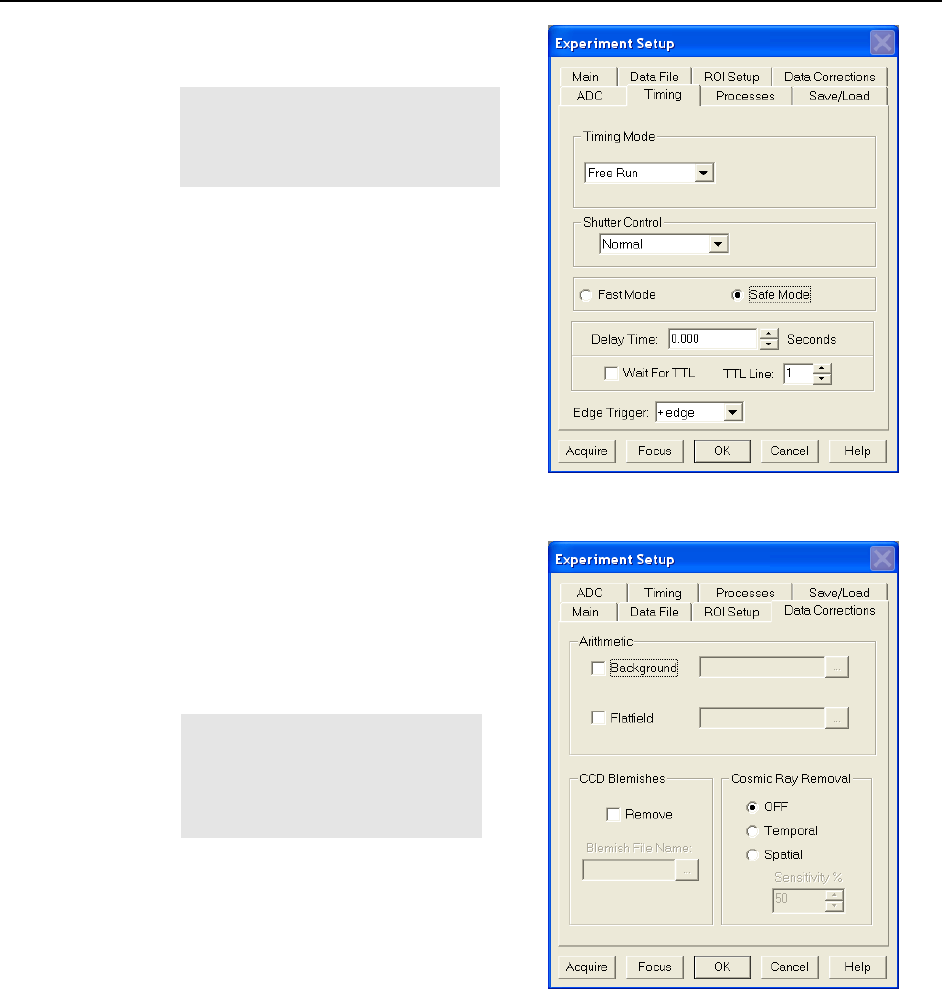
60 WinSpec/32 Manual Version 2.6B
3. On the Timing tab (Figure 30) set
the following parameters.
Note: Not all of these parameters
are provided for every controller
model. Ignore parameters that do
not apply to your system.
Timing Mode: Free Run
Triggered Mode: Not checked
Continuous Cleans: Not
checked
Shutter Control: Normal
Pre Open: Not checked
Safe Mode: Selected
External Trigger: Not checked
Edge Trigger: + edge
Delay time: 0
Use Interrupts: (ST-138 only)
Not checked
Figure 30. Experiment Setup dialog
Timing tab
4. On the Data Corrections tab
(Figure 31) all of the correction
functions should be OFF.
5. On the ADC tab (Figure 32), set
the parameters as they apply to
your particular system.
Note: Not all of these
parameters are provided for
every controller model. Ignore
parameters that do not apply to
your system.
Rate: ADC rate. Only those rates
available for your A/D
converter will be displayed,
making it necessary to
designate the A/D type first.
Select the maximum speed
allowed by the converter. If
Figure 31. Data Corrections tab
the camera is a PI-MAX with Thomson 512 CCD, select FAST. ST-130 owners
must confirm that their controller’s internal hardware jumpers are properly set for
the desired speed. See the ST-130 manual for details.
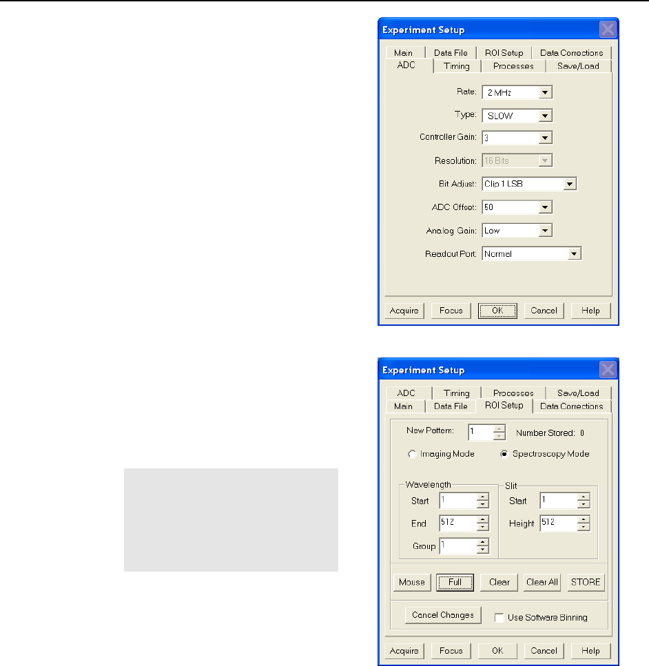
Chapter 3 Initial Spectroscopic Data Collection 61
Type: For systems having more
than one A/D converter, both
FAST and SLOW will be
available. Make this selection
before selecting the rate or
resolution.
Controller Gain (PentaMAX
only): Set to Gain 3
Resolution: Number of bits.
Choices limited by A/D type
selection.
Bit Adjust (ST-138 only): Set to
No Clip
ADC Offset (ST-133-5MHz
only): Use the default setting.
Analog Gain (ST-133): Medium
Readout Port: Normal
Figure 32. Generic ADC tab
6. On the ROI tab select
Spectroscopy Mode as shown in
Figure 33. The Use Full Chip
selection on the Main tab overrides
any ROI settings that may be
present.
Note: The choice of
Spectroscopy or Imaging is
only provided if the WinSpec/32
Imaging option has been installed.
If this choice is not present, the
default state is Spectroscopy.
7. No Processes tab functions
should be selected. For more
information about these functions,
see Chapter 9, page 125.
Figure 33. ROI dialog

62 WinSpec/32 Manual Version 2.6B
8. On the Data File tab, make the
following selections.
Auto Increment File Name
Enable: should be OFF.
Overwrite/Append Existing
Files: Select Overwrite (data
file will overwrite an existing
file having the same name).
Overwrite Confirmation: Check
this box so that you will be
warned that the specified file
name is already in use. If not
checked, the old data file will
be overwritten by the new one.
No warning is provided.
Data Type AutoSelect: Should
be selected.
Auto-save and prompts: Select
Don't auto-save or ask to
save. With this selection, you
will not receive a prompt when
Figure 34. Data File tab
a file is closed as a result of starting a data collection. A prompt will still be
issued if you close the file explicitly and it has not been saved since being
collected.
Use a New Window for each run: Leave unchecked.
9. Click on the button to
the right of the Name
field. This will open a
browse box. Select the
directory where you
want the stored file to
go. In the example
illustrated, the file name
is Testfile and it will be
stored in a directory
named Data. If the
filename doesn’t
automatically appear in
the browse box, type it
in. The file type should
be WinX Data (*.spe).
Figure 35. File Browse dialog
10. Click on the Save button to save the entered information and return to the
Experiment Setup dialog.
11. Click on OK. This will close the Experiment Setup dialog.
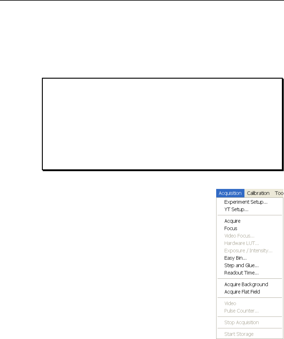
Chapter 3 Initial Spectroscopic Data Collection 63
Experiment Setup Procedures (Intensified Cameras)
Refer to your PI-MAX, PI-MAX3, or PI-MAX4 system manual for experiment setup
instructions. Cabling and peripheral considerations for intensified cameras are more complex
than for unintensified cameras.
Data Collection Procedures (Intensified Cameras)
Refer to your camera system manual for data collection instructions.
PI-MAX and PI-MAX2 Intensified Cameras: If working with an intensified camera,
the room light should be subdued so as to allow safe Shutter mode operation of the
camera. Intensified cameras are quite susceptible to damage from light overload in
Shutter mode operation and particularly subject to damage from light overload in Gate
mode operation with high-intensity pulsed light sources. See your PI-MAX manual for
detailed information.
PI-MAX3 and PI-MAX4 Intensified Cameras: If working with an intensified
camera, the room light should be subdued so as to allow safe Gate mode operation of
the camera. Intensified cameras are particularly subject to damage from light overload
in Gated mode operation with high-intensity pulsed light sources. See your PI-MAX3 or
PI-MAX4 manual for detailed information.
Data Collection (Unintensified Cameras)
The following data collection procedure works for all
controllers. However, it does not exercise some of the special
features, such as video monitor support, available on certain
controller models.
An underlying assumption is that a suitable light source is
available. Although fluorescent room lighting may be
adequate, it will probably prove more instructive to use a
standard lamp, such as a mercury-argon lamp that provided
the spectrum illustrated in Figure 37.
1. Select Focus from the Acquisition menu (Figure 36) to
begin collecting data. An acquisition can also be started
by clicking on the Focus button in the Experiment Setup
dialog or by clicking on the Focus button on the
Custom Toolbar. Data will be continuously acquired
and displayed.
2. While observing the displayed data, adjust the system
optics for the best possible spectrum (lines as high and
narrow as possible). Figure 37 shows a typical mercury-
argon spectrum. Your results could appear different
depending on the spectrograph grating used.
Figure 36. Acquisition
menu
WARNING

64 WinSpec/32 Manual Version 2.6B
Figure 37. Typical Mercury-Argon Spectrum
3. To store the most recent image, click Stop Acquisition on the Acquisition menu or
click on the Stop button on the Custom Toolbar.
4. Data acquisition will halt and the most recent image will be displayed. You can now
use the Save function on the File menu to save the data to a file having the name
specified on the Data File tab.
This completes the initial spectroscopy data acquisition routine that should work with any
Princeton Instruments brand Controller.

65
Chapter 4
Initial Imaging Data Collection
Introduction
Imaging is only possible if the WinSpec/32 software you are using has the Imaging
Option installed.
The procedure in this chapter will enable you to begin collecting real image data
promptly. Minimum requirements are assumed. If your system is more complex, e.g.,
requiring consideration of complex timing and synchronization issues, you will have to
carefully study the other chapters of this manual as well as the manuals provided for the
system hardware components before data acquisition that addresses those needs will be
possible. Nevertheless, it is a good idea to begin with the simplest possible operating
mode. This approach will give you operating experience and familiarity that will prove
very valuable when you go to make more complex measurements. For additional
information about the various menus and dialogs, refer to the online Help topics.
Underlying assumptions for the following procedure are that the hardware has been
installed per the instructions in the hardware manual(s) and that the hardware setup as
discussed in Chapter 2 has been completed. A further assumption is that a good imaging
subject is available. Often, a picture or optical target mounted on a wall or lab bench will
give good results. If initial data collection is to be done using a microscope, be sure to
read the chapter on microscopy in your system manual before attempting data collection.
There are two data collection modes, Focus and Acquire:
In Focus mode operation, no frames of data are stored until Start Storage is
selected. This mode is particularly convenient for familiarization and setting up. For
ease in focusing, the screen refresh rate should be as rapid as possible, achieved by
operating with axes and cross-sections off, and with Zoom 1:1 selected.
In Acquire mode, every frame of data collected is stored. This mode would
ordinarily be selected during actual data collection. One limitation of Acquire mode
operation is that if data acquisition continues at too fast a rate for it to be stored, data
overflow will eventually occur. This could only happen in Fast Mode operation.
Note: The following data collection procedures are done in the Focus mode but do not
cover the actual focusing of a camera. Refer to your camera system manual, your
spectrograph manual, and/or Appendix B (page 233 and subsequent pages) of this manual
for that information.
ATTENTION
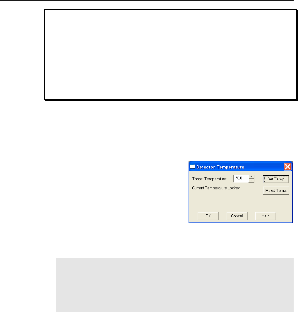
66 WinSpec/32 Manual Version 2.6B
1. If using a PI-MAX or PI-MAX2 intensified camera, initial data collection will be done in
the Shutter mode (Gate mode for PI-MAX3 and PI-MAX4). In both cases (Shutter and
Gate mode), the camera can be damaged if exposed to light overload. Before powering
the controller and camera, reduce the room light to reduce the risk of damage. Note that
intensifiers are particularly at risk in pulsed laser operation, where overload spot damage
can occur without raising the average current to where the overload detection circuits
will be activated. It is far better to be careful than sorry. Before proceeding, take the time
to carefully read the manual for your intensified camera.
2. Also, take particular care that your intensified camera is connected properly for shutter or
gate mode operation. Cabling and peripheral considerations for intensified cameras are
more complex than for unintensified cameras. Again, read your manual.
Temperature Control
Before continuing, the array temperature should be set to some easily achieved value in
the operating range and Temperature lock should be established. The way this is done
depends on the controller.
Temperature Control for a System using an ST-133 Controller or for a PVCAM-based
System
1. Open the WinSpec/32 Setup menu and click on
Detector Temperature. This will cause the
Temperature dialog to appear as shown in
Figure 38.
2. Set the Target Temperature to the desired
value (the default temperature is suggested for
initial data acquisition).
3. Click on the Set Temp. button. When the
Current Temperature: Unlocked message
Figure 38. Temperature dialog
changes to Current Temperature: Locked, temperature lock will have been
established.
Notes:
1. The ST-133 additionally has a Temp Lock LED on the Analog/Control module (at
the rear of the controller) that visually indicates when temperature lock occurs.
2. If you are using the USB 2.0 interface or have a PVCAM-based system with
internal controller, the Detector Temperature dialog will not display current
temperature information while you are acquiring data.
Temperature Control for Other Systems
ST-121, ST-130 or ST-138 Controller: Change the dial setting on the front panel of
the Controller.
PentaMAX: Set the temperature on the front panel of the Temperature/Power Supply
unit.
MicroView: Not user-settable. Temperature is solely under software control.
WARNINGS!
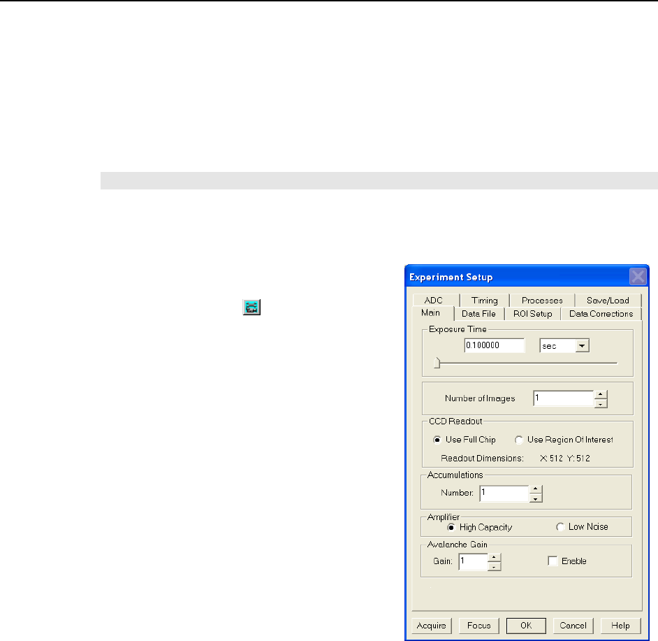
Chapter 4 Initial Image Data Collection 67
Cleans and Skips
With some controllers, specifically the PentaMAX, ST-130, ST-133, ST-138, and internal
controllers, there is a Cleans/Skips tab in the Hardware Setup dialog. Cleans are used to
reduce charge buildup on the CCD array while waiting to begin data acquisition. Skips are
used when the Region of Interest (ROI) is smaller than the full chip; they allow binning and
quick traversing of the rows that precede and follow the ROI. For the procedures that follow,
load the default values for these parameters by bringing the Cleans/Skips tab to the front,
and then clicking on Load Defaults followed by Yes.
Exception: With a PI-MAX camera, Cleans should be set to 1 and Strips per Clean to 4.
Experiment Setup Procedure (All Controllers and Unintensified
Cameras)
1. Open the Experiment Setup dialog
(Figure 39) from the Acquisition menu or
by clicking on the button on the
Custom Toolbar.
2. On the Main tab, set the following
parameters.
Exposure time: 0.1 second
Number of Spectra/Images: 1
Use Full Chip: selected
Accumulations: 1
Amplifier (if available): High Capacity.
If this is a reported-only parameter, set
it by selecting FAST on the ADC tab.
Avalanche Gain (Cameras with electron-
multiplying CCDs): Set to 0 initially
and disabled. Enable and increase the
gain for low-light level images.
Figure 39. Experiment Setup|Main tab
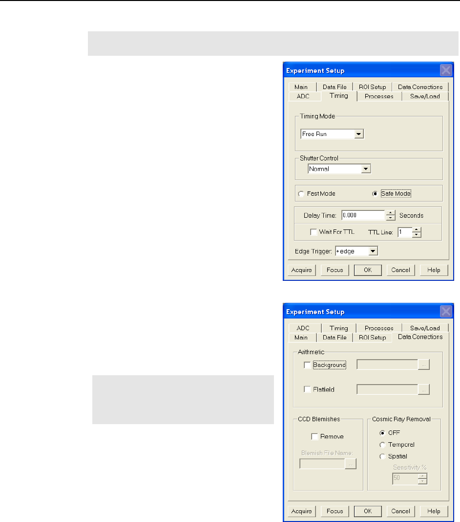
68 WinSpec/32 Manual Version 2.6B
3. On the Timing tab (Figure 40) set the following parameters.
Note: Not all of these parameters are provided for every controller model. Ignore
parameters that do not apply to your system.
Timing Mode: Free Run
Triggered Mode: Not checked
Continuous Cleans: Not checked
Shutter Control: Normal
Pre Open: Not checked
Safe Mode: selected
External Trigger: Not checked
Edge Trigger: + edge
Delay time: 0
Use Interrupts: (ST-138 only) Not
checked
Figure 40. Timing tab
4. On the Data Corrections tab (Figure 41) all
of the correction functions should be OFF.
5. On the ADC tab (Figure 42), set the
parameters as they apply to your particular
system.
Note: Not all of these parameters are
provided for every controller model.
Ignore parameters that do not apply to
your system.
Rate: ADC rate. Only those rates available
for your A/D converter will be displayed,
making it necessary to designate the A/D
type first. Select the maximum speed
allowed by the converter. ST-130 owners
must confirm that the internal hardware
jumpers of their controller are properly
set for the desired speed. See the ST-130
manual for details.
Figure 41. Data Corrections tab
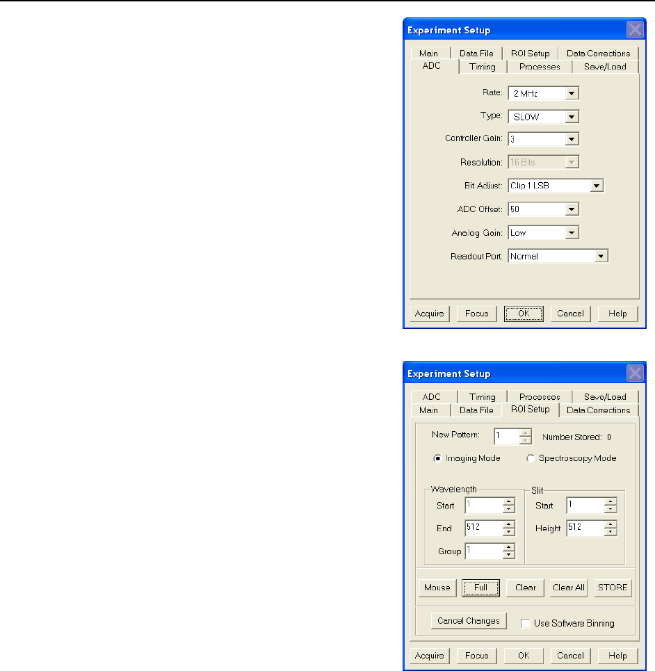
Chapter 4 Initial Image Data Collection 69
Type: For systems having more than one
A/D converter, both FAST and SLOW
will be available. Make this selection
before selecting the rate or resolution.
Controller Gain (PentaMAX only): Set
to Gain 3
Resolution: Number of bits. Choices
limited by A/D type selection.
Bit Adjust (ST-138 only): Set to No
Clip
ADC Offset (ST-133-5MHz only): Use
the default setting.
Analog Gain (ST-133): Medium
Readout Port: Normal
Figure 42. Generic ADC tab
6. On the ROI tab (Figure 43), select Imaging
Mode. WinSpec/32 operated in Imaging
Mode always uses the full chip area and
ROI considerations do not apply.
7. No Processes tab functions should be
selected. For more information about these
functions, see Chapter 9, page 125.
8. On the Data File tab (Figure 44), make the
following selections.
Auto Increment File Name Enable:
should be OFF.
Overwrite/Append Existing Files:
Select Overwrite (data file will
overwrite an existing file having the
same name).
Overwrite Confirmation: Check this
box so that you will be warned that the
specified file name is already in use. If
Figure 43. ROI tab - imaging selected

70 WinSpec/32 Manual Version 2.6B
not checked, the old data file will be
overwritten by the new one. No
warning is provided.
Data Type AutoSelect: Should be
selected.
Auto-save and prompts: Select Don't
auto-save or ask to save. With this
selection, you will not receive a prompt
when a file is closed as a result of
starting a data collection. A prompt
will still be issued if you close the file
explicitly and it has not been saved
since being collected.
Use a New Window for each run:
Leave unchecked.
Figure 44. Data File tab
9. Click on the button to the
right of the Name field. This
will open a browse box.
Select the directory where
you want the stored file to
go. In the example
illustrated, the file name is
TESTFILE1 and it will be
stored in a directory named
Data. If the file name doesn’t
automatically appear in the
browse box, type it in. The
file type should be WinX
Data (*.spe).
Figure 45. File Browse dialog
10. Click on the Save button to save the entered information and return to the
Experiment Setup dialog.
11. Click on OK. This will close the Experiment Setup dialog.
Experiment Setup Procedures (Intensified Cameras)
Refer to your PI-MAX, PI-MAX3, or PI-MAX4 system manual for experiment setup
instructions. Cabling and peripheral considerations for intensified cameras are more complex
than for unintensified cameras.

Chapter 4 Initial Image Data Collection 71
Data Collection Procedures (Intensified Cameras)
Refer to your camera system manual for data collection instructions.
PI-MAX and PI-MAX2 Intensified Cameras: If working with an intensified camera,
the room light should be subdued so as to allow safe Shutter mode operation of the
camera. Intensified cameras are quite susceptible to damage from light overload in
Shutter mode operation and particularly subject to damage from light overload in Gate
mode operation with high-intensity pulsed light sources. See your PI-MAX manual for
detailed information.
PI-MAX3 and PI-MAX4 Intensified Cameras: If working with an intensified
camera, the room light should be subdued so as to allow safe Gate mode operation of
the camera. Intensified cameras are particularly subject to damage from light overload
in Gated mode operation with high-intensity pulsed light sources. See your PI-MAX3 or
PI-MAX4 manual for detailed information.
Data Collection Procedures (Controller-Specific)
ST-133-Controller
The procedure that follows for these controllers is in two parts, Video Focusing and
Data Collection. In focusing, images are displayed on the video monitor (not the
computer monitor) and no data is collected. This allows rapid and easy adjustment of the
system optics. Once the settings have been optimized, data collection begun can begin.
If acquiring data with a PI-MAX, PI-MAX2, PI-MAX3, or PI-MAX4 intensified camera,
make sure the ambient light levels are low. Intensified cameras are quite susceptible to
damage from light overload in Shutter mode operation and particularly subject to
damage from light overload in Gate mode operation with high-intensity pulsed light
sources. Refer to your camera system manual for detailed information specific to
experiment setup and data acquisition for intensified cameras.
Focusing
This procedure applies for a system that includes an ST-133 Controller and a video
monitor connected to the Video port (BNC connector) on the controller. If your system
doesn’t include a video monitor, go to the Data Collection - All Controllers section,
which begins on page 75.
1. Select Video from the Acquisition menu. This will allow live data to be displayed
on your video monitor.
WARNING
WARNING
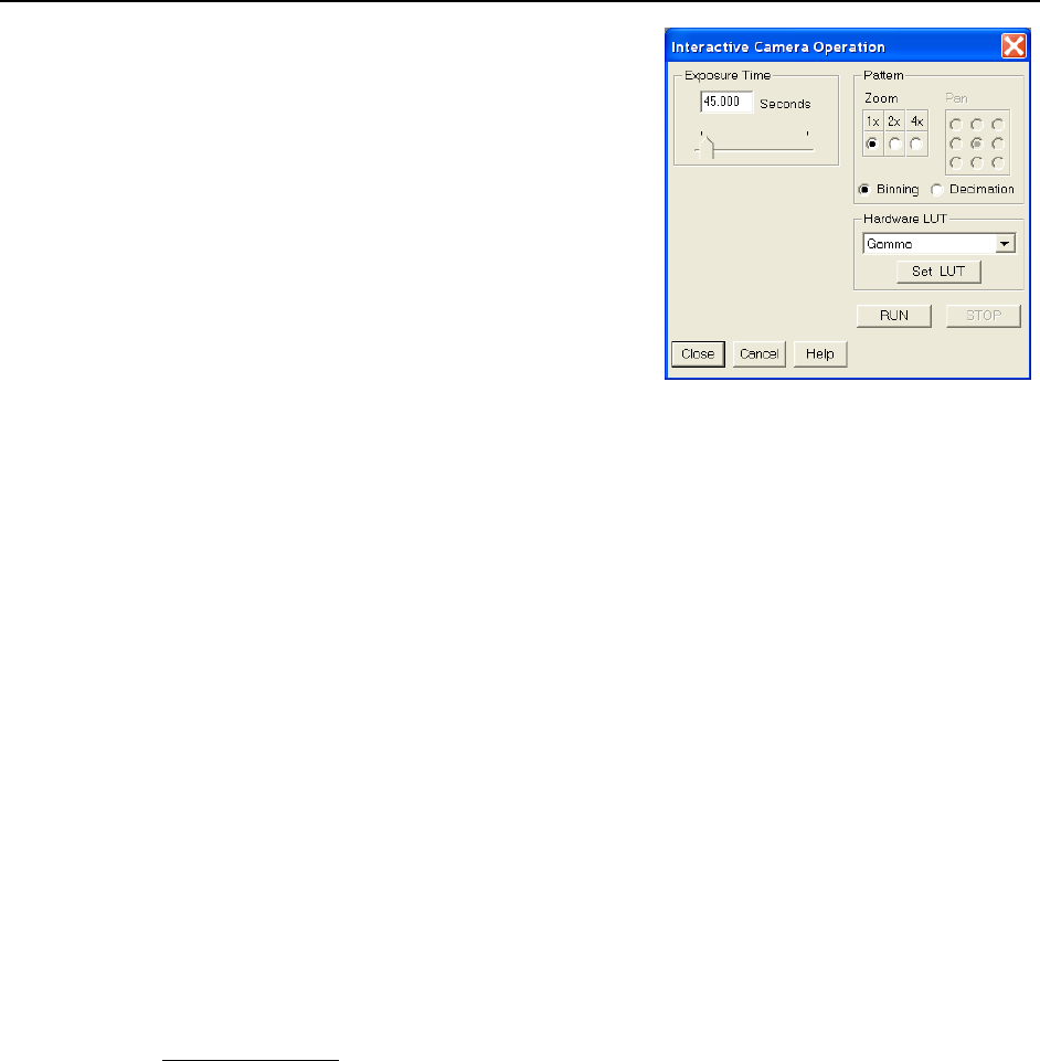
72 WinSpec/32 Manual Version 2.6B
2. Select Video Focus from the Acquisition
menu. The Interactive Camera dialog
(Figure 46) will open.
3. Click on the RUN button in the Interactive
Camera dialog. The camera will begin
acquiring pictures at the fastest possible rate will
and the image will be displayed on the video
monitor. Note that the image will not be
displayed on the computer monitor while the
Interactive Camera dialog is open.
4. Focus the system optics and set the
Interactive Camera dialog Exposure Time,
RS170 Scaling and Offset adjustments for
the best-viewed image. In addition to the
Exposure Time, Intensity Scaling and Offset
Figure 46. ST-133
Interactive Camera dialog
parameters, the Pattern parameters determine which CCD pixels will be displayed on
the video monitor. Note that, in Focus mode, the images will not appear at the
computer but only at the video monitor. If the number of pixels on the CCD is very
much larger than the number of video pixels, you can use the Pan function to select
any one of nine different subsets to display. The Zoom function gives additional
control. One-to-one mapping from the selected region to the screen occurs with 2×
selected. You may additionally have the option of selecting Binning, in which a
wider view is achieved by combining adjacent pixels, or Decimation, in which pixels
are discarded according to an algorithm.
The exposure time will be the same as that set via the Experiment Setup|Main tab.
The two exposure settings track. Changing it at either location should update the
other setting automatically. The Intensity Scaling, together with the Offset,
determines how the image data is mapped to the 256 gray-scale levels. Begin with the
Intensity Scaling set to “1 to 4096” (slider all the way to the right). Similarly, the
Offset setting should initially be set to 2 (slider all the way to left).
5. When no further improvement in the observed image can be obtained, click on Stop
in the Interactive Camera Operation dialog to halt focus-mode operation.
6. Click on Close to close the Interactive Camera Operation dialog and return to the
Experiment Setup dialog.
Data Collection
1. Click on Focus to begin collecting data. An acquisition can also be started by
clicking on Focus on the Acquisition menu or by clicking on the Focus button on
the Custom Toolbar. Images will be continuously acquired and displayed on the
computer screen and on the video monitor.
2. To store the most recent image, click Stop Acquisition on the Acquisition menu
or click on the Stop button on the Custom Toolbar. Data acquisition will halt and
the most recent image will be displayed. You can now use the Save function on the
File menu to save the data to a file having the name specified on the Data File tab.
3. If you want to initiate data acquisition, select Focus again. To store the new data to
disk, repeat Step 2.
This completes initial data acquisition with an ST-133 Controller.
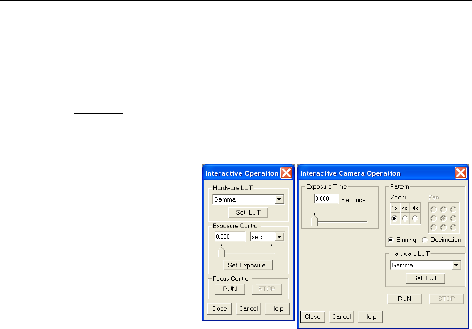
Chapter 4 Initial Image Data Collection 73
PentaMAX Controller
The procedure that follows for the PentaMAX Controller is in two parts, Focusing and
Data Collection. In focusing, images are displayed on the video monitor and no data is
collected. This allows rapid and easy adjustment of the system optics. Once the settings
have been optimized, focus mode operation should be ended and data collection
performed.
Focusing
This procedure applies for a PentaMAX system that includes a video monitor connected to
the Video port (BNC) of the PentaMAX. If your system does not include a video monitor, go
to the Data Collection - All Controllers section, which begins on page 75.
1. Select Video from the
Acquisition menu.
This will allow live
data to be displayed on
your video monitor.
2. Select Video Focus
from the Acquisition
menu. The Interactive
Operation dialog that
will be displayed
depends on the
PentaMAX version.
Version 5 and higher
will display the
righthand dialog
Figure 47. PentaMAX Interactive Operation dialog
shown in Figure 47. Earlier versions display the lefthand dialog.
3. Note the Hardware LUT field. This selection sets the scaling of the video display
only. Unless the signal is very weak, the best LUT choice will be Gamma.
4. Click on the RUN button in the Interactive Operation dialog. Data acquisition at
the fastest possible rate will commence immediately and the image will be displayed
on the video monitor. Note that the image will not be displayed on the computer
monitor while the Interactive Operation dialog is open.
5. Focus the system optics and, if necessary, adjust the Exposure Time in the
Interactive Camera dialog for the best-viewed image. The exposure time will be the
same as that set via the Experiment Setup|Main tab. The two exposure settings
track. Changing it at either location should update the other setting automatically.
6. When no further improvement in the observed image can be obtained, click on Stop
in the Interactive Operation dialog to halt focus mode operation.
7. Click on Close to close the Interactive Operation dialog and return to the
Experiment Setup dialog.

74 WinSpec/32 Manual Version 2.6B
Data Collection
1. Click on Focus to begin collecting data. Data collection can be initiated by means of the
Focus button in the Experiment Setup dialog, by selecting Focus from the
Acquisition menu, or by clicking on the Focus button of the Custom Toolbar.
Images will be continuously acquired and displayed on the computer screen.
2. To store the most recent image, click Stop Acquisition on the Acquisition menu
or click on the Stop button on the Custom Toolbar. Data acquisition will halt and
the most recent image will be displayed. You can now use the Save function on the
File menu to save the data to a file having the name specified on the Data File tab.
3. If you want to initiate data acquisition, select Focus again. To store the new data to
disk, again click Stop Acquisition on the Acquisition menu or click on the Stop
button.
This completes initial data acquisition with a PentaMAX Controller.
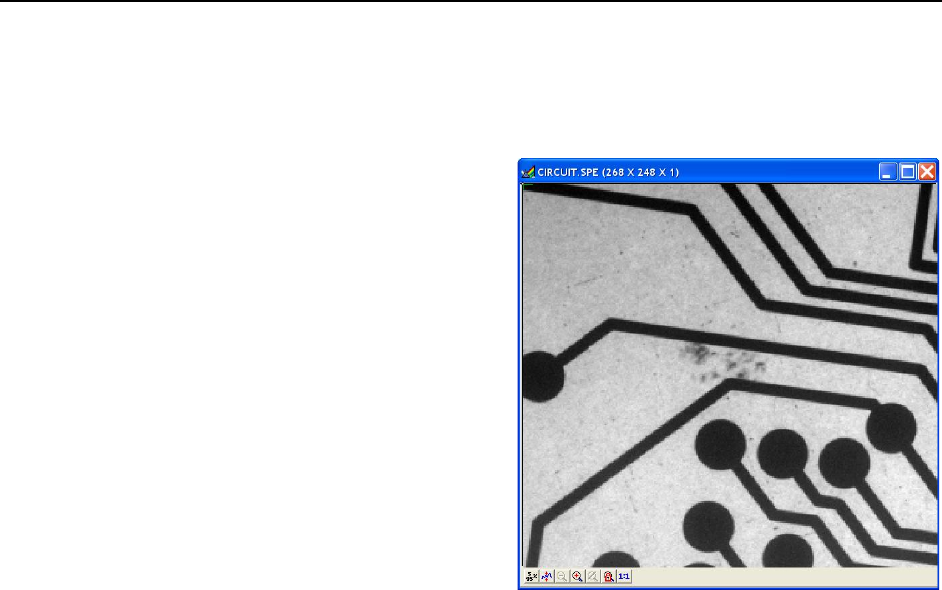
Chapter 4 Initial Image Data Collection 75
Data Collection (Unintensified Cameras)
The following data collection procedure works for all controllers. However, it doesn’t
exercise some of the special features, such as video monitor support, available on certain
controller models.
1. Click on Focus to begin collecting
data. Data collection can be
initiated by means of the Focus
button in the Experiment Setup
dialog, by clicking on Focus on the
Acquisition menu, or by clicking
on the Focus button of the
Custom Toolbar. Images will be
continuously acquired and
displayed.
2. Observe the displayed data and
adjust the system optics for the best
possible image. It may be necessary
to readjust the Exposure Time
(Experiment Setup|Main tab).
3. To store the most recent image,
click Stop Acquisition on the
Acquisition menu or click on the
Stop button on the Custom
Figure 48. Typical Data Acquisition Image
Toolbar.
4. Data acquisition will halt and the most recent image will be displayed. You can now
use the Save function on the File menu to save the data to a file having the name
specified on the Experiment Setup|Data File tab.
This completes the initial data acquisition routine, which should work with any Princeton
Instruments controller.

76 WinSpec/32 Manual Version 2.6B
This page intentionally left blank.
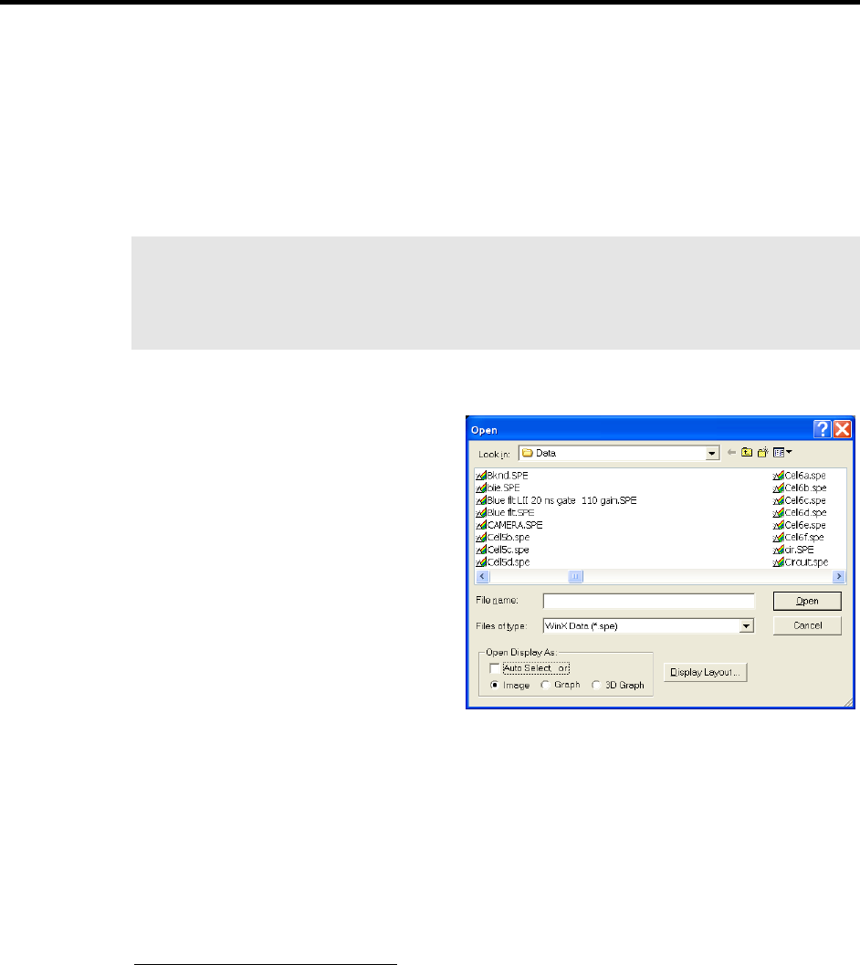
77
Chapter 5
Opening, Closing, and Saving Data Files
Introduction
This chapter discusses how to open, close, and save existing data files to disk. Options
for saving and deleting files will be explained. Data files created with temporary file
names should be saved to disk periodically. Files should be closed completely to
conserve RAM for data collection.
Data files can be deleted directly from WinSpec/32, without using the File Manager or
any other file utility.
Note: WinSpec/32 can read data files acquired with earlier versions of WinSpec.
Versions of WinSpec prior to 1.6 cannot read WinSpec/32 data files. Neither can versions
prior to 1.6 read data files that were collected with earlier versions and then opened,
modified and saved using WinSpec/32. This should be considered carefully before
modifying and saving old data files with WinSpec/32.
Opening Data Files
In WinSpec/32 files are opened
according to Win 95 conventions, as
follows.
1. Select Open from the File menu.
The File Open dialog will appear
(Figure 49).
2. Open the directory containing the
data files. Clicking on the button
at the right of the Look In field
opens a browser function,
allowing you to quickly and easily
access the correct folder. As
shown in Figure 49, the data files
will be listed below.
3. If you want the software to control
Figure 49. Open dialog
how the data will be displayed when the file is opened, check Auto Select. Leave
Auto Select unchecked if you want to retain control over whether the data will be
displayed as an Image, Graph or 3D Graph.
Auto Select is the factory default selection.* In addition, one of the three radio
buttons, Image, Graph or 3D Graph, will be selected but grayed out if Auto Select
* The open/display default selection can be changed and saved from the Display Layout
window.
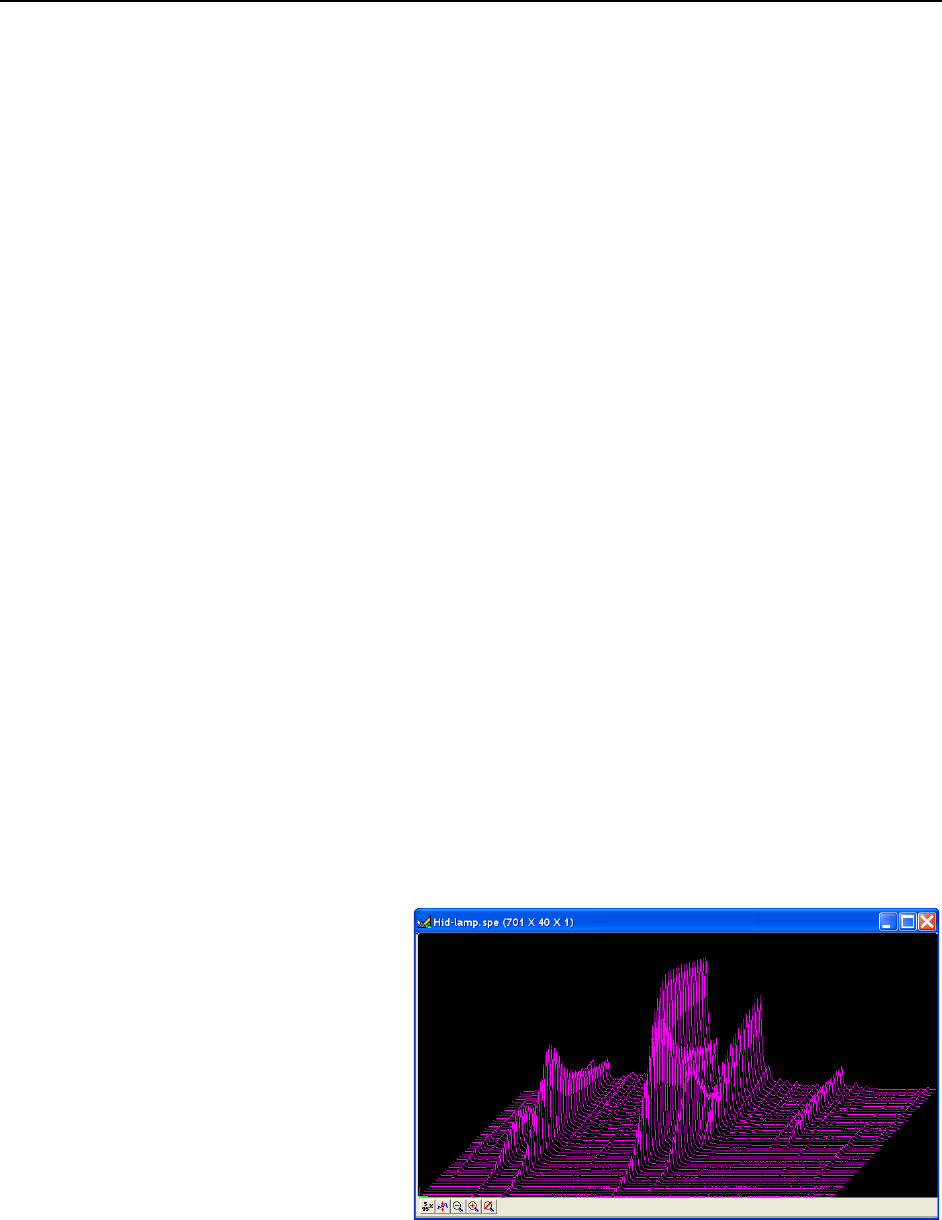
78 WinSpec/32 Manual Version 2.6B
is checked. If Auto Select is unchecked, the grayed out selection will become active
and govern how the file is opened.
When Auto Select is checked, the way the data is displayed depends on the
number of data strips it contains.
If there are eleven or more strips of data, they will be displayed as a normal
image, such as that shown in Figure 93 (page 115).
If there are at least three data strips but less than eleven, the data will be
plotted as a 3D Graph as shown in Figure 72 (page 101).
If there are only two strips of data, they will be displayed as graphs stacked
in a two-dimensional plot, the same as for a 3D Graph of two strips as shown
in Figure 71 (page 100).
A single strip will always be plotted as a simple X vs. Y plot. Note that from
two to ten strips, the intensity (Y axis) scale shifts position as required to
read true for the selected strip.
If Image is selected, all data points will be plotted as a function of the strip and
pixel number.
If 3D Graph is selected, multiple data strips will be plotted as a function of
intensity versus pixel number, the actual number of data strips plotted depending
on the 3D Layout display parameter settings. All of the strips could come from
the same frame, or, in the case of a file containing multiple frames, the same
numbered strip could come from each frame.
If Graph is selected, the selected data strip only will be plotted as a function of
intensity versus pixel number.
4. Note the Files of Type field, which allows you to select files for listing according to
their type. If WinXData (*.spe) is selected, only files of type *.spe will be listed.
This is the native WinSpec/32 format. If TIFF or 8-bit TIFF File (*.tif) is selected,
only files of the type *.tif will be listed. If All Files (*.*) is selected, all files in the
folder will be listed. WinSpec/32 can open either *.spe files or *.tif files (8-bit or
16-bit). Select type 8-bit TIFF File to open an 8-bit TIFF file. Select type TIFF File
to open a 16-bit TIFF file.
5. Either double-click on
the name of the file you
want to open or single-
click on the name and
then click on the Open
button. For example,
with 3D Graph selected,
double-clicking on
Hid-lamp.spe would
open that file, producing
the display shown in
Figure 50. Note that there
are many different ways
of controlling how the
image will be displayed,
as described in
Figure 50. High Intensity Lamp Spectrum

Chapter 5 Opening, Closing, and Saving Data Files 79
Chapter 8.
Multiple Files: It is also possible to open multiple files at the same time by using the
Win95 Shift + Click and Control + Click selection features.
To select a range of contiguously listed files for opening:
a. Hold the Shift key down and click on the first file in the range. The file will be
selected.
b. Then hold the Shift key down again and click on the last file in the range. That
file and all the files between the two designated files will be selected.
To select multiple files which are not listed contiguously:
a. Hold down the Ctrl key and then click on the first file. That file will be selected.
b. Then hold down the Ctrl key again and click on the second file. That file will
also be selected.
c. Proceed in similar fashion to select each file to be opened.
Once all files to be opened have been selected, click on Open (or double-click on a
selected file) and all of the selected files will be opened.
There are a number of additional options and operations that can be performed from the
Open dialog. For example, clicking the Display Layout button will directly open the
Display Layout dialog, described in Chapter 8. In addition, options for the organization
of the Open dialog itself can be selected by means of the icons to the right of the Look
In field, or by right-clicking the mouse anywhere in the file listing area of the box (but
not on a file name).
Right-clicking on a file name opens a Windows shortcut menu that provides a number of
additional operations, including open, delete, rename, print, properties, and edit
operations such as copy and cut.
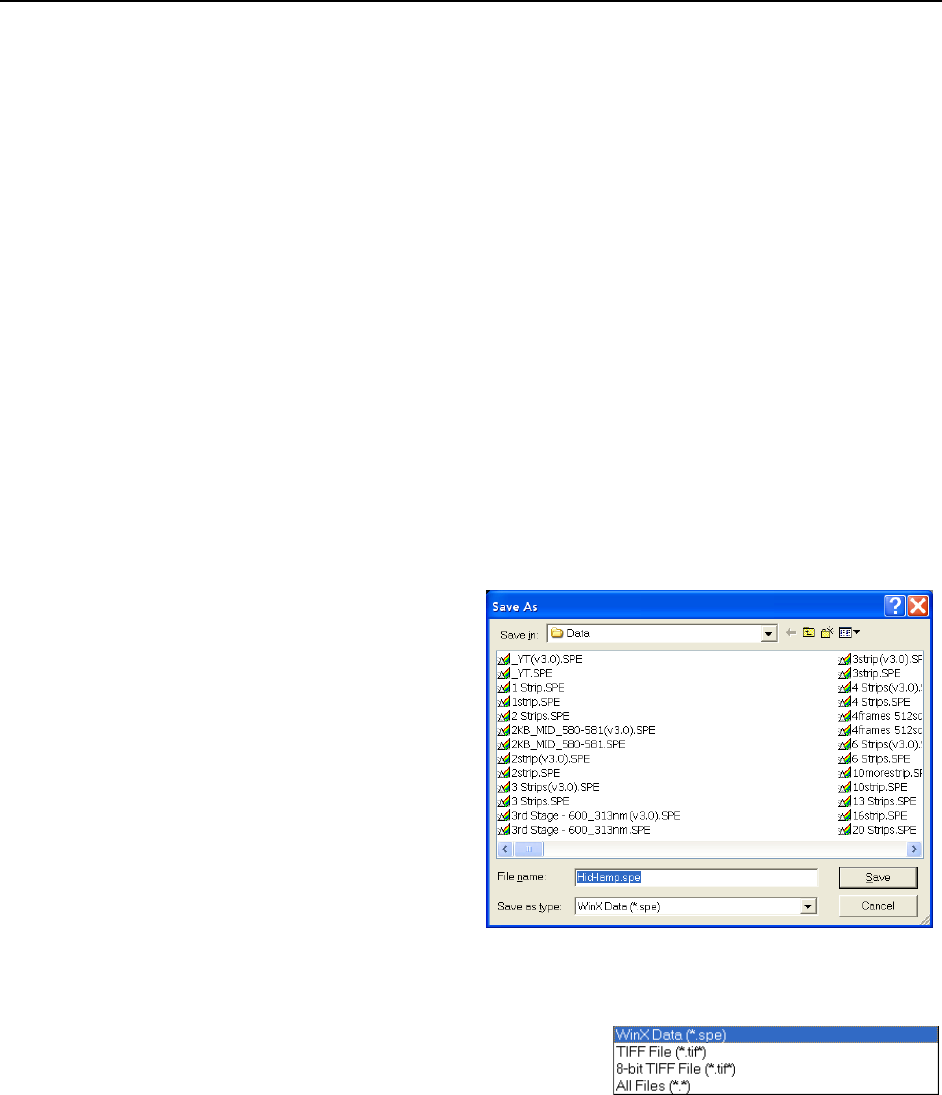
80 WinSpec/32 Manual Version 2.6B
Saving Data Files
Data files must be saved to disk before exiting the software. It is also recommended that
you save periodically when making measurements to minimize the overall risk of data
loss. If you exit and there are unsaved data files, you will be prompted to save them. The
File menu provides three Save commands, as follows.
Save: Saves the active data file using the original file name and type and in the
original directory (folder).
Save As: The Save As dialog is used to save the active data file to a user-specified
file name and directory. The file type can be changed.
Save All: Saves all open data files using the original file names and directories
(folders).
Sometimes during data collection or processing, windows will be opened and display
data with an <untitled #> title. These are temporary files, and they must be saved to disk
if you want to keep them. The Save As dialog performs this function. The Save As
dialog also allows you to open a file and save it with a different name.
Saving Temporary Data Files
The WinSpec/32 software allows you to work with temporary files, files with names like
<untitled 1>. To save these files, or to save any file to a new filename, perform the
following steps.
1. Select Save As from the File
menu. The Data File Save As
dialog (Figure 51) appears.
2. Open the directory where you
want the file saved. Clicking on
the button at the right of the
Save In field opens a browser
function that will allow you to
quickly and easily select the
target directory.
3. Type in a name for the file.
Windows 95 long file-name
convention applies. It is not
necessary to add the extension
since it will be added
automatically according to the
specified file type.
Figure 51. Data File Save As dialog
Save as type: Indicates the file type. The
data types currently supported are listed in
Figure 52. If All Files (*.*) is selected, you
will be able to save the file with any
extension. The file, however, will be saved
Figure 52. Save As Data Types
in the *.SPE file type format. Only the data is saved. This could have some
unexpected effects. For example, if you save a graph as a *.tif file, and then open
the file with an image editor, you will see the data presented as a single strip
image, not as a graph.
4. Click on OK to save the file or Cancel to close the Data File Save As dialog
without saving the file.

Chapter 5 Opening, Closing, and Saving Data Files 81
Data File tab
The Data File tab provides you with additional
control and flexibility in naming and saving
newly collected data. Because the settings on
this tab are applied to data acquisition, not post-
processing, make your entries before acquiring
data. The auto-save, auto-name, and auto-
increment features allow you to acquire data and
save it according to the filename template you
define. Also, you can take advantage of the
multiple open windows functionality and
specify that each new data run opens a new
window on the display window.
Figure 53. Data File tab
Closing a Data File
An open data window can be closed by clicking on the box at the upper right of the
window or by clicking on Close in the File menu. An open data window can be removed
from view by clicking on the box at the upper right of the window. The file will be
reduced to an icon on the task bar but the data will remain loaded in RAM. There may be
situations where you would want to do this to reduce desktop clutter. Unless you intend to
expand the file for display again, it is ordinarily better to actually close the file so that the
RAM it is using will be freed for other use. If the file has not been saved, you will be
prompted.
There are several ways of closing an open data window. Each is described below:
The box at the upper right of the data window will close that window only.
The box at the upper right of the window will also remove the data window from
view by reducing it to an icon on the task bar. There may be situations where you
would want to do this to reduce desktop clutter. However, the data will remain loaded
in RAM, reducing the memory available for data collection. Unless you intend to
expand the file for display again, it is ordinarily better to actually close the file so that
the RAM it is using will be freed for other use.
Close in the File menu closes all windows using the data set displayed in the active
data window. This may be important if New in the Window menu or in the Data
Window Context menu has been used to open additional windows with the same
data. Simply clicking on Close in the File menu will close all windows containing
the same data, regardless of how it is displayed.
Close in the Control menu, accessed by clicking on the WinSpec/32 icon at the left
end of the Title bar, closes WinSpec/32, as does double-clicking on the WinSpec/32
icon. Similarly, the key combination Alt+F4 also closes WinSpec/32.
Close All in the Window menu closes all open data files.
The key combination Ctrl+F4 closes the active window only.
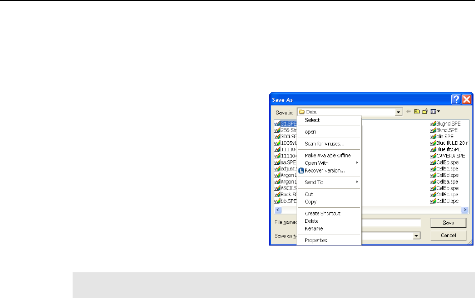
82 WinSpec/32 Manual Version 2.6B
Deleting Data Files
You can delete data files directly from within WinSpec/32, without having to close
WinSpec/32, and without having to use the Windows 95 Explorer or another file utility.
This is achieved using the File Operations menu, accessed by right-clicking on the file
name in the Open dialog, as explained below.
1. Select Open from the File menu.
Only files with the selected data type,
*.spe or *.tif, will be listed.
2. Position the mouse cursor on the name
of the file you want to delete and click
the right mouse button. This will open
the “right-click” File Operations
menu, as shown in Figure 54.
3. Click on Delete. Then answer yes to
the query asking whether you wish to
send the file to the recycling bin. The
file will be deleted and the File
Operations menu will close.
Figure 54. Right-click File Operations menu
Note: Click on the Open dialog Cancel button to exit the dialog without deleting any
files.
Multiple Files: It is also possible to delete multiple files at the same time by using the
Shift + Click and Control + Click selection features.
To select a range of contiguously listed files for deleting:
1. Hold the Shift key down and click on the first file in the range. The file will be
selected.
2. Then hold the Shift key down again and click on the last file in the range. That
file and all the files between the two designated files will be selected.
To select multiple files which are not listed contiguously:
1. Hold down the Ctrl key and then click on the first file. That file will be selected.
2. Then hold down the Ctrl key again and click on the second file. That file will
also be selected.
3. Proceed in similar fashion to select each file to be deleted.
Once all files to be deleted have been selected, right-click on a selected file to open the
File Operations menu. Then click on Delete to delete all of the selected files.
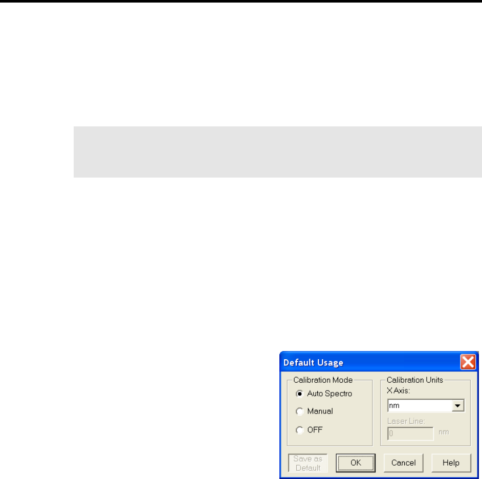
83
Chapter 6
Wavelength Calibration
Introduction
You can calibrate the WinSpec/32 software either by using the spectrograph stepper
motor position (spectrograph calibration) or by performing a wavelength calibration.
Spectrograph calibration, described in Chapter 7, precisely calibrates the movement of
the spectrograph gratings. Wavelength Calibration is good for one position of the grating
only. Once you move the grating (by hand or by controlling the stepper motor) a different
wavelength calibration must be performed for that spectrograph position.
Note: Even after the spectrograph setting is fixed, moving the sample, refocusing, or
almost any adjustment of the input optics can have an effect on the wavelength
calibration. For the most accurate calibration possible, Princeton Instruments
recommends recalibrating the system after any optical adjustment.
Changing the WinSpec/32 Calibration Method
Switching between Wavelength Calibration and Spectrograph Calibration is controlled
using the Usage dialog. This dialog determines whether calibration is turned on or off,
and which type of calibration is used. The display can be calibrated by controlling the
stepper motor of the spectrograph, called Spectrograph Calibration (discussed in
Chapter 7), or the display can be calibrated for a fixed spectrograph position by entering
the position of known peaks from a known source such as a mercury or neon lamp. The
calibration of the spectrograph for a fixed position is called Wavelength Calibration and
is described in this chapter.
Changing the Calibration Method
1. Select Usage from the Calibration
menu. The dialog in Figure 55 will be
displayed.
2. Select the desired method of calibration.
Auto Spectro selects Spectrograph
Calibration as described in
Chapter 7. A spectrograph
supported by WinSpec/32 must be
installed for this selection to be
available.
Manual applies the wavelength
Figure 55. Calibration Usage dialog
calibration to the active data. The calibration is performed using the Default
Calibration Setup dialog, accessed by selecting Setup on the Calibration
menu.
Off selects uncalibrated operation.
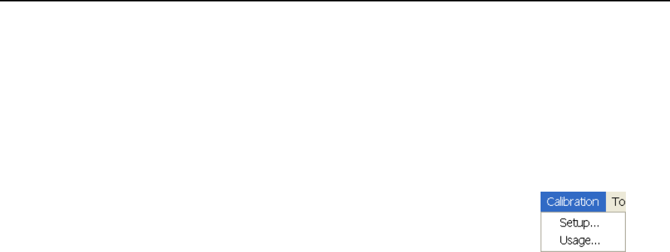
84 WinSpec/32 Manual Version 2.6B
3. Select the desired X Axis units. This option is only available if the data set is
calibrated. If relative wave numbers are selected, it will additionally be necessary
to enter the wavelength of the laser line.
4. Click on OK.
See the discussion of the Calibration Usage dialog in the online Help for details
concerning the Calibration Usage dialog selections.
Calibration Menu
The Calibration menu, which can be called by clicking on
Calibration in the menu bar, is shown in Figure 56. The
Calibration menu contains two items, Setup and Usage,
which call the Calibration Setup and Calibration Usage
dialogs. Brief descriptions follow.
Figure 56. Calibration menu
Setup: Once a single spectrum has been acquired or loaded, the menu item Setup
opens the Calibration Setup dialog. A calibration session consists of finding the
peaks, marking the known peaks to be used for calibration, and saving the
calibration data as the default or applying it to the active data set only.
Usage: Selects the Calibration mode and Units. Once the wavelength calibration has
been performed, it can be applied by selecting Manual or turned off by selecting
Off. Selections can either be saved as default power-up parameters or be applied
to the active data set only. For more information, see the online Help discussion
of the Calibration Usage dialog.
Wavelength Calibration Procedure
Before a wavelength calibration can be performed, it is necessary to either load a
spectrum or acquire one. For good calibration results, the spectrum should have well
defined peaks for which you know the wavelength. A calibration requires at least two
points defined by pixel and by units. Naturally the more points used, the more accurate
the calibration. The ideal calibration spectrum would have one peak at the start of the
array (or region of interest), one at the end of the array or region of interest, and one
midway between the end peaks. In real life, the ideal spectrum is seldom available, but
the closer you can come to this ideal the better the calibration results will be.
Figure 57 shows a mercury-argon spectrum that could serve as the basis for a good
calibration in many situations. Appendix C contains wavelength tables for Argon, Neon
and Mercury, together with a detailed spectrum for Hg-Argon.
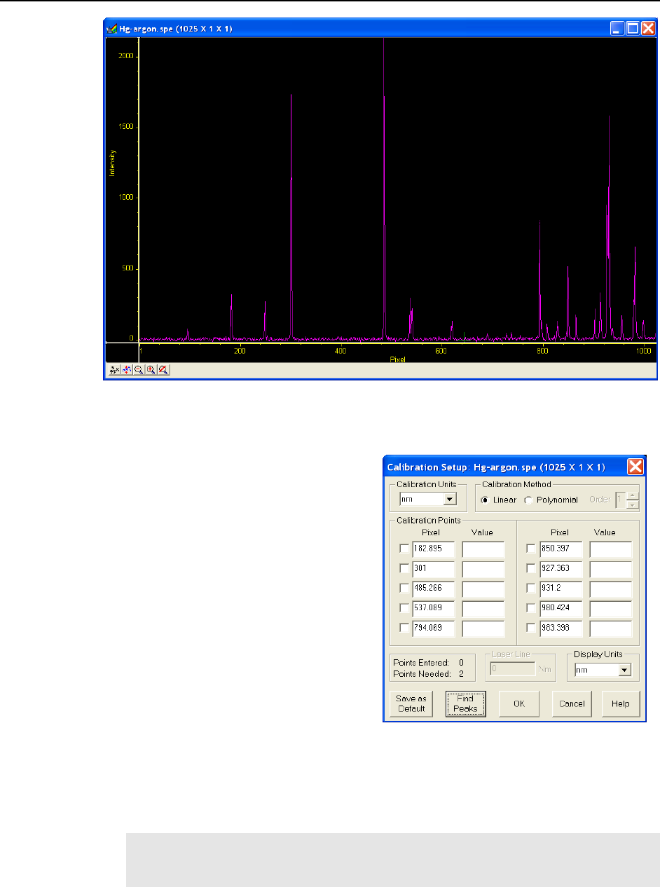
Chapter 6 Wavelength Calibration 85
Figure 57. Hg-Argon spectrum
Once you have the calibration spectrum displayed on the screen as the active data set,
proceed as follows.
1. Click on Setup in the Calibration
menu to open the Calibration Setup
dialog box. If a previous calibration
had been saved, the calibration values
would be listed. If no previous
calibration had been saved as the
default, no values would be listed. For
more information, see the online Help
for this dialog.
2. Click on Find Peaks. An automatic
peak finding routine will be
performed. The maximum number of
peaks is equal to one quarter the
number of displayed pixels. The pixel
values for the 10 highest peaks will be
shown in the Pixel boxes in the
Calibration Setup dialog as shown in
Figure 58. Note that the Find Peaks
routine causes a small red arrow to be
Figure 58. Calibration Setup dialog after running
Find Peaks routine on Hg-Argon spectrum
displayed above each peak found in the spectrum together with a notation indicating
the peak location in pixels (Figure 59).
Note: Each time the Find Peaks routine is initiated the displayed peak heights will
decrease. Clicking on the data window Autoscale button will restore their original
displayed height.
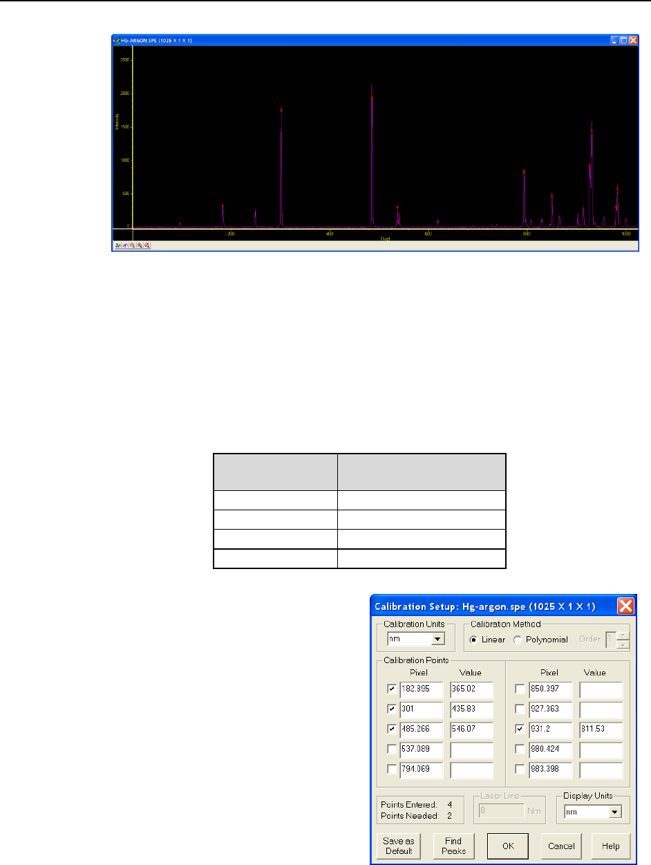
86 WinSpec/32 Manual Version 2.6B
Figure 59. Spectrum after running Find Peaks routine
3. Select the calibration points. For the example being considered, the peaks at 182.90,
301.00, 485.27 and 931.20 would be good choices. The decimal point locations are
based on the calculated center of peak, and not necessarily the largest intensity position.
4. Select the Calibration Units (if not nanometers) and select the Display Units. Both
the Calibration Units and the Display Units are nm (the default) in the example.
5. Manually enter the wavelength of the selected peaks. Appendix C contains
wavelength tables and a detailed spectrum for Hg-Argon. In our example, the
wavelengths for the selected peaks would be:
Peak Location
(Pixels)
Peak Location
(Wavelength in nm)
182.90
365.02
301.00
435.83
485.27
546.07
931.20
811.53
6. Once the wavelengths have been
entered for the selected peaks, check
the selection box to the left of the
Pixel box for each peak selected.
(Figure 60). A checkmark in the box
indicates that the peak is selected.
Note that wavelength values must be
entered for these peaks before the
selection box can be checked.
7. Click on OK. This completes the
wavelength calibration and the dialog
will close. At the same time, the
Calibration Mode selected in the
Usage dialog will automatically
change from Off to Manual.
Figure 60. Setup Calibration screen after selecting
peaks and entering calibration wavelengths
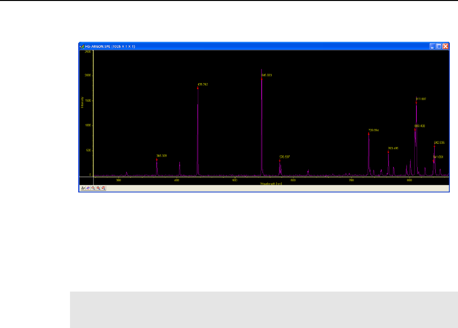
Chapter 6 Wavelength Calibration 87
The peak find routine display data (arrows and pixel number of each peak found) does
not change. The x-axis units will however change to reflect the display units.
Figure 61. Spectrum after Calibration
Save as Default
The Save as Default button in the Calibration Setup dialog determines whether a
calibration is temporary or permanent (until changed). Once a calibration has been saved
as the default, it will be automatically applied to subsequently acquired data. It will not
be applied to data files recalled from disk.
Note: The default state of the button, not only with respect to the button setting but also
with respect to whether it is disabled (grayed out and not user-settable) depends on the
situation, as follows.
No Data
If you open the Calibration Setup menu and there is no data, Save as Default will be
pressed and disabled, that is, it will be locked in the Save as Default state. Should you
then click on OK, no calibration values will be written to the Windows Registry.
Not Live Data
If there is data in the active window when you open the Calibration Setup menu, but the data
is not live, such as would be the case if it were recalled from disk, Save as Default is under
user control, with “not pressed” as the default state. Note that if the opened data file was
saved in a calibrated state, that calibration will be in effect when the file is opened, the
calibration values will be loaded in the calibration setup, and the data displayed.
Live Data
If the active window is displaying live data, Save as Default will be under user control
but in the selected or “pressed” state. If Save as Default is selected and you click on
OK, the calibration will be stored in the Windows Registry and will be automatically
applied to all subsequent acquired data, unless a new calibration is performed. If Save as
Default is unselected and you click on OK, the calibration in effect (i.e., in the
Calibration Setup dialog) will apply to the active data file only.
Calibration, Display, and User Units
The default Calibration Units are nanometers (nm). These units can be changed, with
the change taking effect immediately. Calibration units to choose from are nm

88 WinSpec/32 Manual Version 2.6B
(nanometers), cm-1 (wavenumbers), rel. cm-1 (relative wavenumbers), and user units
(units other than above). For relative wavenumbers only, the wavelength of the excitation
laser must be entered in the Laser Wavelength box in nm. Display unit choices are the
same, with the additional selection of pixels.
The Display Units selection can be different from the Calibration units, except in the
case of User Units. Under Display Units, the choices are pixels, nm (nanometers), cm-1
(wavenumbers), and rel. cm-1 (relative Raman shift wavenumbers). These units are the
ones shown on the X-axis whenever calibrated spectra are displayed. To display files
without calibration, even files collected with a specific calibration, select the pixel option
under Display Units.
User Units allow the operator to scale the spectra to any arbitrary unit.
Calibration Method
A calibration requires at least two points defined by pixel and by units. Naturally the
more points used, the more accurate the calibration. The points must always be defined
by pixel number, but nanometers can be changed to another unit if desired.
Two mathematical models can be used to fit the calibration to the data. The first, Least
Square, calculates a linear approximation of the fit by minimizing the sum of the squares
of the errors between the fit and the calibration points. Linear approximation is generally
sufficient. The Polynomial method uses a higher order function of the form a + bx + cx2
+ … where the “order” of the polynomial is the highest power of x used. The general rule
is:
(# Cal Peaks - 1) = Order
maximum order = 5
If four peaks are active in the Calibrate dialog, the order of the polynomial can be 2 or 3.
Even if ten peaks are used, the maximum order of the Polynomial is 5 (up to x5). As a
general guide, we advise calibrating using the Linear calibration method with widely
separated peaks as previous described. If the available peaks are clustered, a Polynomial
fit (using the smallest order possible) may give a good fit in the region of the calibration
peaks, but have increasing large deviation the further you get from them. In an extreme
case, there may even be two values for the same pixel, a clearly impossible condition that
will result in an error message.
With the Linear calibration method, at least two peaks are required to calibrate. For a
Polynomial calibration, the number of peaks must be at least one higher than the order of
the polynomial. This information is displayed at the lower left of the Calibration Setup
dialog. The lower Points value is the number of peaks required. The upper points value is
the number available for calibration. A peak is available if it has been found, its known
value has been entered, and the adjacent checkbox has been checked.

89
Chapter 7
Spectrograph Calibration
Introduction
You can calibrate the WinSpec/32 software by either using the spectrograph stepper
motor position (Spectrograph calibration) or by manual wavelength calibration.
Spectrograph calibration is achieved using the Calibrate selection on the Spectrograph
menu, and is described in detail in this chapter. Wavelength calibration, which is only
good for one position of the grating, is explained in Chapter 6.
The spectrograph calibration routine requires you to enter certain default values into a
series of dialogs. You are also required to have a known source, such as a mercury lamp,
placed near the entrance slit of the spectrograph. Once you have completed the following
calibration procedure, any movement of the spectrograph will be accounted for in the
display of spectral information.
Notes:
1. The spectrograph MUST be focused and aligned properly before a good calibration
can be achieved. Spectrograph focusing and alignment is an art onto itself and is
beyond the scope of this manual. Basically it consists of filling the aperture from a
broad light source and adjusting the focusing mirror for the sharpest image
(narrowest possible symmetrical peak) on the CCD. Focusing can also be
accomplished by moving the detector in and out. Different detectors and/or
spectrographs will have different means for doing this. In addition, it may be
necessary to rotate the detector so that the spectral line is perfectly vertical on the
CCD.
2. The Offset, Adjust and Dispersion parameter values for WinSpec/32 will not be
the same as they were with earlier versions of WinSpec. This is true even if the same
spectrograph is used. You cannot simply enter values you may have recorded when
using the earlier (16-bit) WinSpec versions. If you do, very large calibration errors
will be introduced. The calibration must be performed using the following procedure.
Preparation
1. Install the spectrograph, mounting it to the detector per the instructions in the
Detector manual, and turn it on. You may have to restart the WinSpec/32 software
after turning on the spectrograph.
2. Mount a suitable light source (mercury lamp preferred) near the entrance slit of the
spectrograph so that the light passes through the spectrograph onto the detector.
3. Review the Define Spectrograph selections and settings to be sure they are correct
for the calibration to be performed.
4. The Experiment Setup parameters must be set so that a spectrum can be acquired.
Using Easy Bin, select a single strip of several rows near the center of the CCD and
an exposure time between 0.1 and 0.5 seconds.

90 WinSpec/32 Manual Version 2.6B
5. A filename should have been entered for the test acquisitions using the Experiment
Setup|Data File tab. Also, Overwrite Confirmation should be turned off so you
will not see warning messages about overwriting data files. Exit the Experiment
Setup dialog by clicking on the OK button.
6. Acquire some data and display the data as a graph. Next position and size the data
window. We suggest locating it at the upper left and sizing it so that it doesn’t extend
more than half way across the screen. Then select Keep Window Placement on the
Display Layout|General tab, followed clicking on OK. This operation assures that
all data windows will fall in precisely the same spot and will be precisely the same
size, a configuration that conveys a significant convenience advantage when
calibrating.
Notes:
1. You must use the supplied cable to control the spectrograph. Do not use a standard 9-
pin serial cable, even if it worked with an earlier version of WinSpec.
2. If the spectrograph does not move or you get an error message such as
“Communication Error with Spectrograph”, the spectrograph setup is probably
incorrect. Check the power on the spectrograph, the cable connections, and the
settings in the Spectrograph dialog. Also try turning off and back on the
spectrograph, then closing and reopening the WinSpec/32 software.
3. If wavelength direction is reversed, you will not be able to calibrate successfully.
However, a warning message will be displayed. If this happens, open the Hardware
Setup dialog and select the Display tab. If Rotate is selected, toggle the Flip box. If
Rotate is not selected, toggle the Reverse box. Click on OK and then begin Offset
calibration again.
Calibration Parameters
1. Select Auto Spectro on the Usage dialog (to open, select Usage on the Calibration
menu). If the Use for Auto-Spectro Calibration checkbox on the Define
Spectrograph| Main tab was used to designate a particular spectrograph as the
one to be used for calibration purposes, that spectrograph will be automatically
selected.
2. If the Save as Default button on the Usage dialog is not already selected, select it
now.
3. Select Calibrate on the Spectrograph menu. This will open the Spectrograph
Calibration dialog (Figure 62).
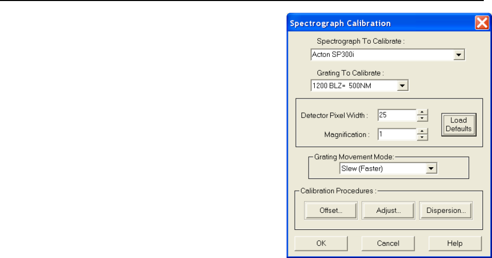
Chapter 7 Spectrograph Calibration 91
4. Be sure the correct Spectrograph to
Calibrate is selected. If another
spectrograph is indicated, click on the
down arrow at the right of the selection
box to display all of the installed
spectrographs and make the correct
selection. If only one spectrograph has
been installed, the selection box will not
appear but the spectrograph model will
be reported.
5. Be sure the correct Grating to
Calibrate is selected. Calibration is
grating specific. If the indicated grating
is incorrect, click on the arrow at the
right of the selection box to display the
available gratings and make the correct
selection.
6. Be sure the indicated value for the
Detector Pixel Width in microns is
correct. The default value will depend on
the type of CCD chip installed. Note that
Figure 62. Spectrograph Calibration
dialog
some design factors, such as a tapered fiber optic ahead of the chip, will change the
pixel size seen by the spectrograph and so will have to be taken into account in
determining the value to be entered.
7. Be sure the indicated Magnification value is correct for your spectrograph. This
parameter is determined by the geometry of the spectrograph. Contact your
spectrograph manufacturer if you have any questions about the magnification
parameter value.
8. Select the Grating Movement Mode, Slew or Scan. Operation with Slew selected
will be significantly faster than with Scan selected.
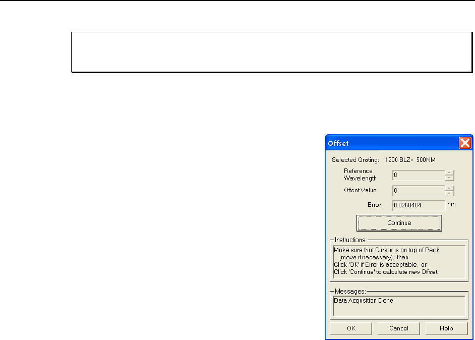
92 WinSpec/32 Manual Version 2.6B
Offset
You must begin calibration with the Offset procedure and end with the Dispersion
procedure. Performing the steps in this order is absolutely necessary for correct
calibration.
Theoretically, if you were to move your spectrograph to the zero order peak or any other
known peak, the peak would fall exactly on the center of the array. In the real world, the
mechanical tolerances of the mounting will probably result in the peak being a few pixels
off. The Offset procedure that follows allows you to correct for this small offset error.
1. Select Info on the View menu. The Info dialog
should be visible. This will help indicate the
status of spectrograph movement and data
collection.
2. In the Spectrograph Calibration dialog, click
on the Offset button. This will open the Offset
dialog (Figure 63).
3. The dialog that appears has a Reference
Wavelength entry box. This is the wavelength
where the spectrograph is set for the offset
measurement. All Acton spectrographs use the
zero order, that is, a setting of “0.”
4. Click on the Start Offset Procedure button.
The spectrograph should now move to the
reference wavelength and data acquisition will
commence. Then a peak-find will be performed
and the resulting data will be displayed.
Figure 63. Offset dialog
5. Figure 65 illustrates a typical Offset data acquisition. The reference peak should
appear near the center of the display and the cursor should be near or on the highest
point of the peak. If the peak is saturated, cancel, lower the exposure time, and repeat
the operation. The display X-axis should be calibrated (any units other than pixels). If
the X-axis is calibrated in pixels, select the desired units as the calibration units on
the Usage dialog (opened by selecting Usage from the Calibration menu).
Peak Finder
Before going on, you have to make a judgment regarding the location of the cursor
on the peak. There may be situations where you will need to readjust the cursor
position to get it precisely on the correct location. Although this should be a
relatively uncommon event, it could happen, and it is important to take a moment to
understand how the peak finder works, how it may appear to be in error when it in
fact it is not, and how it could come to be in error and require manual intervention to
correct the cursor position.
The peak finder works by taking the second derivative of the spectrum to find the
peaks. Each peak found is then divided in two so that the area to the left of the
divider equals the area to the right of the divider. The cursor is located at precisely
the point where the divider intersects the peak. Note that, depending on the shape of
the peak, the cursor may or may not end up precisely on the highest point. Figure 64
shows three possible peaks, and illustrates the action of the peak finder in each case.
Caution

Chapter 7 Spectrograph Calibration 93
Figure 64. Peak Finder Examples
Peak A is perfectly symmetrical. As you would expect, dividing it into two equal
areas and locating the cursor at the intersection of the divider with the peak will put
the cursor precisely at the highest point. Peak B, on the other hand, is not
symmetrical but rather extends further to the right than to the left. As a result, the
final cursor position is a little to the right of the highest point. This is the correct peak
location. Any attempt to “improve” it by manually moving the cursor to precisely the
highest point will degrade the offset computation. Note that moving the cursor
immediately changes the reported Error. Do not assume that this means the cursor
was not optimally located. Rather it indicates a possible optical problem and the
spectrograph may need to be realigned. Peak C is like peak A but is accompanied by
a number of noise spikes. The peak finder is quite sensitive and might well select one
of these spikes as the real peak and incorrectly place the cursor on the noise spike as
shown in C. If this happens, the correct action would be to manually adjust the cursor
position to the right so that it is on the true peak before going on.
Doublets are also a problem. At any stage of the calibration procedure the peak finder
might find the wrong peak of a doublet. For example, if using the 579.066 nm
mercury line in doing the Dispersion Calibration, you need to take care to check that
the peak finder hasn’t selected the 576.96 nm line instead. If it does, it is a simple
matter to move the manually move the cursor to the correct peak. Note that the zoom
function can also be controlled using the data window icons.
If it is difficult to see the precise cursor position, simply press the keyboard Insert
key to expand the display about the cursor position. The key may have to be pressed
several times to achieve the desired resolution. (Use the Delete key to return to the
original display.) If you do decide to move the cursor, note that each time a cursor-
positioning arrow key is pressed, the cursor will move one data point. Assuming no
horizontal binning is in effect, one data point will correspond to one pixel on the
array.
As a final comment, even if you should move the cursor when it was not necessary,
repeating the Calibration Offset cycle a few times will still achieve an optimum offset
adjustment.
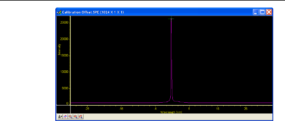
94 WinSpec/32 Manual Version 2.6B
Figure 65. Offset Spectrum for Zero-order Measurement
6. Note the reported Error value in the Offset dialog. The value is reported in nm.
Transposed to pixels it should be less than one pixel. The number of nm represented by
one pixel will depend, of course, on the dispersion of the grating.
7. Press Continue to initiate another offset computation cycle. The reported error should
decrease. Repeat the cycle two or three times – until no further reduction in the error can
be achieved. The final error value achieved may wander a bit with each cycle repetition,
reflecting the noise content of the spectrum.
8. Click on OK to close the Offset dialog and return to the Spectrograph Calibrate
dialog.
Adjust
Once you have adjusted the Offset for a reference wavelength (or for the zero order peak)
other wavelengths may still be improperly calibrated. To see why this is so, think of the
calibration in terms of the linear general equation:
y = mx + b
Although this is a simplified model, it suffices to show the basic relationships. The “b” term
can be thought of as the offset, which is adjusted to place the reference at precisely the center
of the array. The location of points away from the offset reference will be determined by the
“m” or slope term (as well as “b”) and the Adjust procedure allows “m” to be set so that
adjusting the spectrograph to other wavelengths will result in this wavelength falling on the
center of the array.
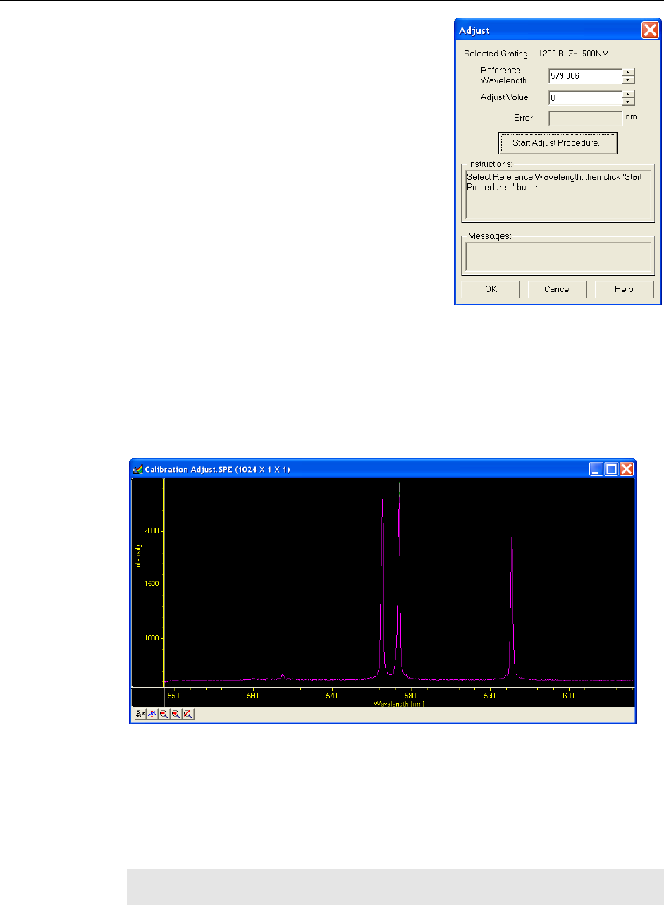
Chapter 7 Spectrograph Calibration 95
1. Click on the Adjust button to open the Adjust
dialog (Figure 66).
2. Enter as the Reference Wavelength a known line
in the observed spectrum, such as 579.066 for
Mercury. Next click the Start Adjust
Procedure button.
3. The spectrograph will move to the reference
wavelength and collect a spectrum. It will also
perform a peak-find operation and display the
acquired data. The reference peak should appear
somewhere near the center of the display and the
cursor should be on the peak at or near the
highest point.
4. Figure 67 illustrates a typical Adjust data
acquisition. The reference peak should appear near
the center of the display and the cursor should be
near or on the highest point of the peak.
Figure 66. Adjust dialog
5. As was the case for the Offset adjustment, before going on, you have to make a
judgment regarding the location of the cursor on the peak. Take particular care that
the proper peak has been found. If, for example, the peak finder places the cursor on
the 576 peak, manually move the cursor to the 579 peak. For additional information,
refer to the earlier discussion of how the peak finder works in the Calibration Offset
procedure.
Figure 67. Calibration Adjust Spectrum
6. Note the reported Error value in the Adjust dialog. The value is reported in nm.
Transposed to pixels it should be less than one pixel. The number of nm represented
by one pixel will depend, of course, on the dispersion of the grating. The nm/pixel
can be approximated by picking the difference in the location of the two peaks while
in pixel mode, and dividing the difference reported in calibration units in the
calibration mode.
Note: The absolute value of the peak is reported in the Info box. If it is not already
open, open it by selecting Info from the View menu.
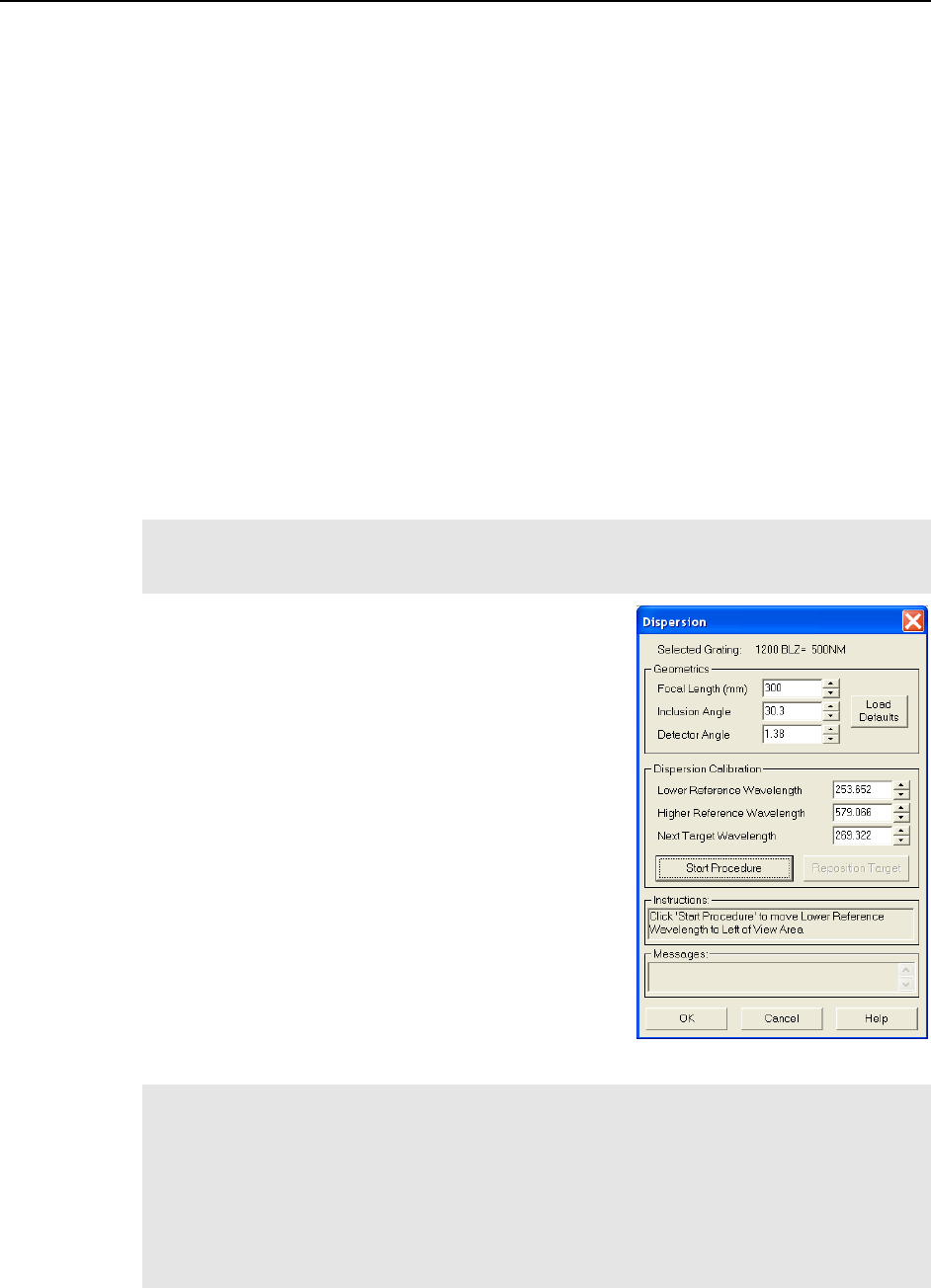
96 WinSpec/32 Manual Version 2.6B
7. Press Continue to initiate another Adjust computation cycle. The reported error
should decrease. Repeat the cycle two or three times – until no further reduction in
the error can be achieved. The final error value achieved may wander a bit with each
cycle repetition, reflecting the noise content of the spectrum.
8. Click OK to close the Adjust dialog and return you to the Spectrograph Calibrate
dialog.
Dispersion
Now that Offset and Adjust are complete, the spectrograph can move a target peak very
close to the center of the display. The final step is to calibrate the wavelength scaling so
that peaks on the far left or the far right in the window are also accurately calibrated. This
is called the Dispersion calculation, and again it is automated in WinSpec/32.
To adjust the Dispersion calculation you will make two measurements in the lower
spectral range (253.652 for Mercury); one measurement with the peak at the left edge of
the display and one with the peak at the right edge. Then you will make two
measurements in the upper spectral range (579.066 for Mercury). After these steps,
WinSpec/32 then tries to find the combination of Focal Length, Inclusion Angle, and
Detector Angle that minimizes the error.
Note: Some CCDs have very little response at 253.652. If this is the case for your
detector, it will be necessary to use a peak having a longer wavelength as the low value.
For mercury, the 435.833 line should prove suitable.
1. Click on the Dispersion button to open the
Dispersion dialog. If you have never calculated
the Dispersion before, click on the Default
button. This provides standard values for Focal
Length, Inclusion Angle, and Detector Angle
based on the manufacturer’s data for the active
spectrograph. If you have already run the
Dispersion calculation before and it provided
satisfactory values, they will be displayed and
should be used as your starting values.
2. Enter the Lower and Higher Reference
Wavelengths. For the mercury spectrum, use
253.652 (low) and 579.066 (high). Again, if your
CCD doesn’t have sufficient response to
calibrate at 253.652, it will be necessary to use a
different peak. It is not necessary to enter a
Target Wavelength. It will be calculated during
the procedure.
Figure 68. Dispersion dialog
Note: In the following steps, four data sets will be taken, each initiated by you. The
Start Procedure button initiates the first, and the same button, named Continue once
the first data set has been taken, is used to initiate each of the other three. After each data
set is taken, you have the option of adjusting the cursor position on the peak. However, as
previously explained, this will not be required or advisable in most instances. See the
Peak Finder discussion in the Calibration Offset procedure. The data sets are taken in the
following order:
1. Low peak (253.652) at the left of the display.

Chapter 7 Spectrograph Calibration 97
2. Low peak (253.652) at the right of the display.
3. High peak (579.066) at the left of the display.
4. High peak (579.066) at the right of the display.
3. Click on the Start Procedure button.
WinSpec/32 will acquire the first data set and display it. It will also calculate the
Target Wavelength so that the Lower Reference Wavelength peak appears near
the left edge of the display. The Target Wavelength is the wavelength the
spectrograph must move to in order for the reference wavelength to be properly
located near the edge of the display.
If the peak is outside the display, you should enter a Target Wavelength that
might be better and click the Reposition button. If the peak is too close to the
center of the display you should enter a slightly higher Target Wavelength and
click on the Reposition button. Once the peak appears near the left edge, check,
and if necessary adjust, the cursor position on the peak using the same criteria as
for the Offset and Adjust operations. Then click on Continue to Step 2 to
initiate the second data acquisition.
The spectrograph will acquire the second spectrum. If the peak is close to the
right edge of the display as expected, click on Continue to Step 3 to initiate the
third data set acquisition. If the peak is not in the right position, use the
Reposition button to move the spectrograph as required to position the low peak
near the right edge of the display. Then click on Continue to Step 3 to initiate
acquisition of the third data set.
The spectrograph will acquire the third spectrum, this time positioning the cursor
on the high peak at 579.066. If the peak is close to the left edge of the display as
expected, click on Continue to Step 4 to initiate the fourth data set acquisition.
If the peak is not in the correct position, use the Reposition button to move the
spectrograph as required to position the high peak near the left edge of the
display. Then click on Continue to Step 4 to initiate acquisition of the fourth
data set.
After completion of the fourth data set, once again check to be sure the cursor is
on the correct peak and manually move it if it is not.
After all four reference points are taken, WinSpec/32 begins an iterative process to find
the best values. This process is initiated by clicking on the Calculate Results button.
You will see the parameters change as WinSpec/32 performs the calculations. The
program stops when the best parameters are displayed in the Dispersion dialog. If
satisfied with the calibration, simply click on OK to make the save the final dispersion
parameters as part of the calibration data for the grating. Click on Cancel to revert back
to previously saved parameters. Note that you can also change the parameters manually
and click on OK to save them.
Having completed the calibration for one grating, select the next grating and repeat the
procedure. Continue until all available gratings have been calibrated.

98 WinSpec/32 Manual Version 2.6B
This page intentionally left blank.
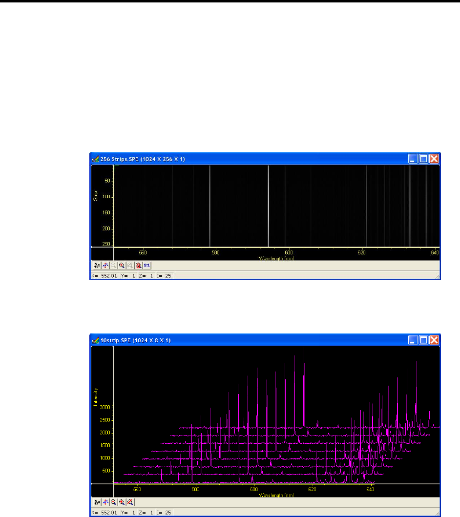
99
Chapter 8
Displaying the Data
Introduction
WinSpec/32 can display data as an image, as a two dimensional graph, or as a 3D Graph
(multiple strips from the same graph or the same strip from multiple frames). You can choose
to allow the software control how the data will be displayed or make the selection yourself.
To have WinSpec/32 control the data-display mode, simply select the Auto Select checkbox
provided on the File Open dialog and also on the Display Layout dialog. The Auto Select
algorithm makes the selection depending on the number of data strips as follows.
If there are eleven or more strips of data, they will be displayed as a normal image,
such as that shown in Figure 69.
Figure 69. Image display of 256 data strips
If there are at least three data strips but less than eleven, the data will be plotted as a
3D Graph as shown in Figure 70.
Figure 70. 3D Image display of eight data strips
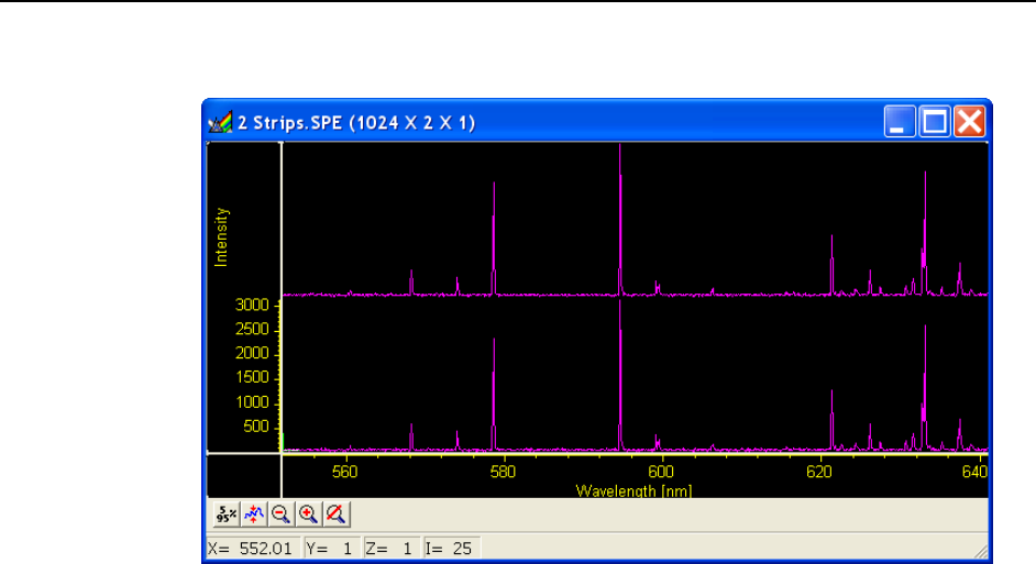
100 WinSpec/32 Manual Version 2.6B
If there are only two strips of data, they will be displayed as graphs stacked in a two-
dimensional plot, the same as for a 3D Graph of two strips.
Figure 71. 3D graph with two data strips
A single strip will always be plotted as a simple graph. Note that from two to ten strips,
the intensity (Y axis) scale shifts position as required to read true for the selected strip.
The file Open dialog and Display Layout dialog both contain the three display-mode
select radio buttons, Image, Graph and 3D Graph. If you want to control the data-
display mode yourself, simply leave Auto Select unchecked and the display mode will
correspond to whichever of the three radio buttons is selected.
Screen Refresh Rate
The Screen Refresh Rate is an important but often overlooked display performance
parameter. At times, such as when focusing, by making the screen refresh rate as rapid as
possible, the focusing operation may be much easier to perform than it would be with a
slow refresh rate. To obtain the fastest possible refresh rate, simply operate with the axes
and cross-sections both switched off (View menu) and with the Zoom factor set to 1:1.
Note that the Zoom 1:1 button on the Data Window toolbar is only present when viewing
an image. To check the refresh rate, click on the Status bar (bottom of screen)
Collection Status pane, which is immediately to the left of the Timer pane (right end of
Status bar). The refresh rate will be displayed in the Collection Status pane. Do not
confuse the screen refresh rate with the data collection rate.
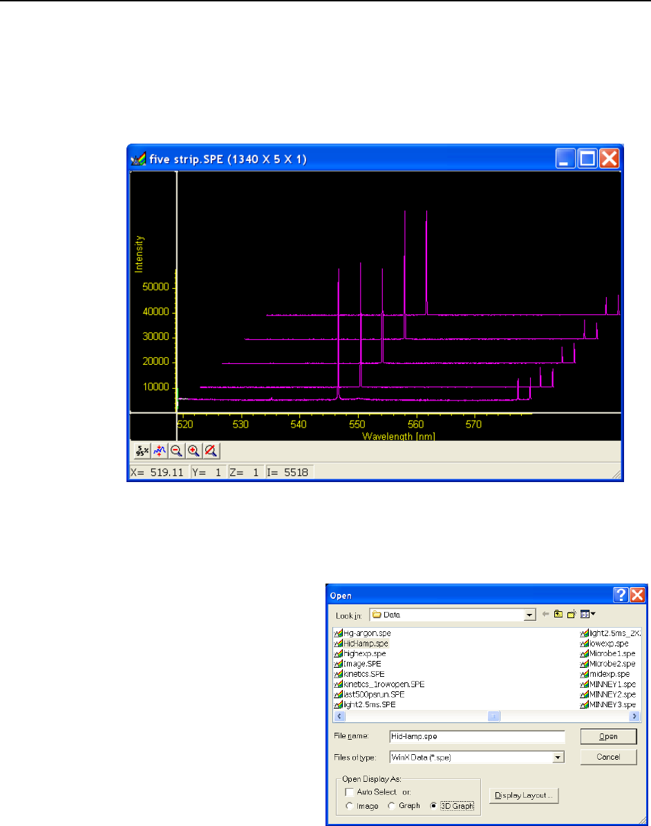
Chapter 8 Displaying the Data 101
Data Displayed as a 3D Graph
Data files can be opened as 3D graphs from the Open dialog. Figure 72 shows a 3D graph
with five data strips. Figure 71 (on the previous page) shows a 3D graph with two data
strips. Both examples illustrate the behavior of the Auto Select algorithm as discussed
on page 99. The following paragraphs contain procedures for opening and displaying
data in graphical format.
Figure 72. 3D graph with five data strips
Displaying Hid-lamp.spe
The data file used in this exercise is Hid-lamp.spe, one of the data files supplied with
your WinSpec/32 software.
1. From the File menu select
Open. The Open dialog
(Figure 73) will appear,
allowing you to select the
image to be opened. The Look-
In box provides a browser
function so that the directory
where the images are located
can be easily accessed. By
default the data directory is a
subdirectory of the WinSpec
program directory. Files of the
specified type (the WinSpec/32
data type is *.spe) in the
current directory and any
subdirectories are listed in the
box below the directory name.
Figure 73. Open dialog
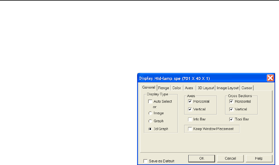
102 WinSpec/32 Manual Version 2.6B
2. The Image, Graph and 3D Graph radio buttons at the bottom of the box allow you
to select whether the file will be opened and displayed as an image, two-dimensional
graph or as a 3D graph. Select 3D Graph. (Auto Select should not be checked.)
3. From the data directory select the image file called Hid-lamp.spe. Click on the OK
button. A window of the appropriate dimensions should appear immediately. The
graph display may take a few seconds, depending on the speed of the computer. The
initial appearance of the display may vary depending on the initial Display Layout
parameter settings.
4. Select Layout on the
Display menu. The Display
Layout dialog will open as
shown in Figure 74.
5. Check and, if necessary, set
the following parameter
selections on each tab.
General tab
Display As: 3d Graph
Auto Select:
unchecked
Axes: both boxes
checked
Cross Sections: both
boxes checked
Tool Bar: checked
Keep Window
Placement: unchecked
Figure 74. Display Layout dialog
Range tab
Initial Autoscale: checked
Set to Full Range: checked
Frame: 1
Color tab: no changes
Axes tab
Horizontal axis: checked
Horizontal label: checked
Horizontal label string: Pixel
Vertical axis: checked
Vertical label: checked
Vertical label string: Intensity
3D Layout
3D Mode: Multi-strip; same frame selected
3D Properties: Remove Hidden Line checked; other two boxes unchecked.
Z Axis Endpoint: %X set to 20; %Y set to 40
3D Marker curves: Marker Curves unchecked; Curve set to 5
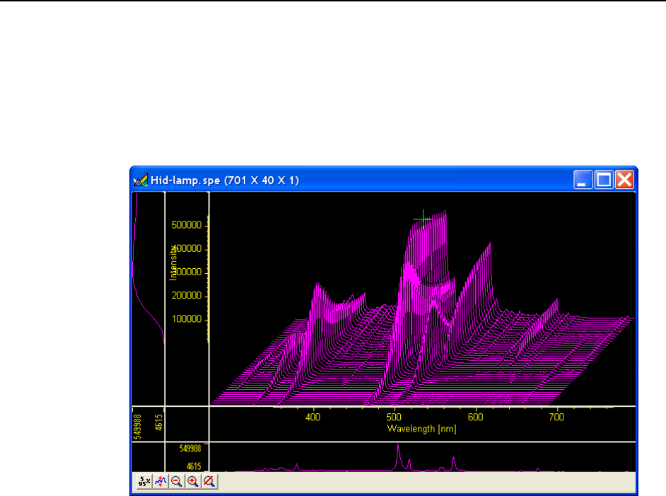
Chapter 8 Displaying the Data 103
6. Click on OK. The Display Layout dialog will close and the data display, exclusive
of the intensity profiles, should appear as shown in Figure 75. Each strip is displayed
as a plot of intensity vs. pixel number. The first strip is at the front and the last strip is
at the back. Initially the cursor will be at the lower left. Use the up arrow key to move
to a higher numbered strip and the right arrow key to move to a higher numbered
pixel on the strip. Then click the Intensity Autoscale key to scale the intensity
profiles. Note that clicking the mouse button at different points on the display will
change the pixel selection but not the strip.
Figure 75. Hid-lamp.spe 3-D Graph
7. Press the [Insert] key on the keyboard repeatedly. Each time it is pressed the display
expands about the cursor position. Then press the [Delete] key repeatedly to contract
the display, restoring the appearance of the data display.
8. Note the cross sectional displays in Figure 75. The vertical cross-section profiles the
intensity at the same point on each successive strip. The horizontal cross-section
profiles the intensity at each point on the same strip. If the large cursor is selected,
cursor projections will intersect the cross section to show indicate the cursor position.
These projections may not be visually aligned with the cursor position on the main
plot. This effect will be particularly noticeable with a long Z axis. Because of
perspective effects, the higher numbered strips will be further away and visually
smaller. The axes automatically adjust so that they read true for the strip on which the
cursor is located. However, because the cross-section profiles expand to use all of the
available space, they will not be in alignment visually with the cursor. The profile
shapes will be correct, and the point on the profiles intersected by the large cross-hair
extensions will accurately indicate the cursor position. Also, the information box will
accurately report the pixel number and intensity at the cursor position.
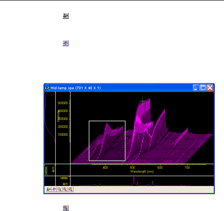
104 WinSpec/32 Manual Version 2.6B
5%-95% Display Range
1. Click on . The data display will shift so that it only fills the 5% to 95% region of
the window range. Had the data initially extended all the way to the window
boundary, the data display would have been slightly compressed to fit within the 5%-
95% range.
2. Click on , restoring the image to its initial appearance.
3. Before advancing to the next topic, open the View menu. Then select the Small
cursor and deselect Cross-Sections.
Selecting a Region of Interest
1. Using the mouse, drag a rectangular region on the image as shown in Figure 76.
Figure 76. Hid-lamp.spe 3D graph with region selected for viewing
2. Click on (Zoom In). The view will change so that only the selected region is
displayed as shown in Figure 77.
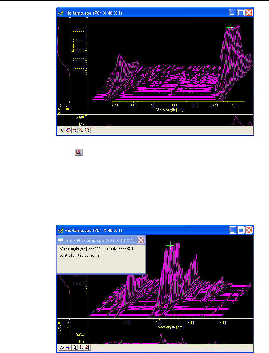
Chapter 8 Displaying the Data 105
Figure 77. Hide-lamp.spe 3D graph expanded to show defined region
3. Click on (Undo All Zoom-In). The original view will be restored.
Information box
On the View menu, select Info. The information box should appear as shown in
Figure 78. The first line reports the intensity and pixel number at the cursor position.
The second line reports the frame number, strip number, and the pixel number. The
intensity in A/D counts is reported at the X and Y position corresponding to the
cursor position. If a region is defined by dragging the mouse cursor, the region
coordinates, length and height will also be reported. You may have to lengthen the
Information box for all this information to appear.
Figure 78. Graphical Display with Information box
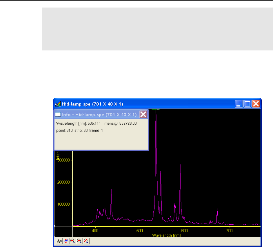
106 WinSpec/32 Manual Version 2.6B
Note: When you open the information box, it becomes the active window. To perform
operations in the data display window, such as changing the selected strip, you must
again make the data display window active by clicking the mouse cursor anywhere in the
data box. The data-window title bar will become highlighted, indicating that it is the
active window, and the cursor positioning functions will become operative again. The
data displayed in the information box will continue to be updated automatically.
Displaying a Single Strip
1. Open the Display Layout dialog by selecting Layout on the Display menu.
2. On the General tab, with Auto Select unselected, click on the Display
Type|Graph radio button and then on OK. The single data curve for the strip on
which the cursor is positioned will be displayed.
Figure 79. Single Strip displayed graphically
3. Try operating the cursor positioning keys to demonstrate their effect. The left/right
arrow keys move the cursor along the strip, and the up/down keys move it from strip
to strip. The [Home] and [End] keys move the cursor to the strip ends, and Shift +
Home and Shift + End move it the first strip and last strip, respectively. The
[Insert] and [Delete] keys expand or contract the data about the cursor position.
4. Restore the 3D display by selecting 3D Graph on the Display Layout|General tab.

Chapter 8 Displaying the Data 107
Cursor
The cursor’s appearance and behavior are a bit different with graphical plots than with
image plots, as detailed in the following table.
Selection
Image Plot
Graph
3D Graph
None
No Cursor
No Cursor
No Cursor
Small
Small cross; both mouse
and arrow keys can place
cursor at any pixel on
image. [Home] and
[End] keys move cursor
to end points on strip.
Shift + Home moves
cursor to first strip. Shift
+ End moves it to the
last.
Small cross; left/right
arrow keys select pixel
on strip; up/down arrow
keys select strip to be
displayed. [Home] key
moves to first pixel,
[End] key to last pixel.
Small cross; left/right
arrow keys change
selected pixel on strip;
[Home] key moves to
first pixel, [End] key to
last pixel. Up/down
arrow keys move cursor
from strip to strip. Shift
+ Home moves to first
strip, Shift + End to
last. Strips may all be
from same frame or each
may be from a different
frame.
Large
Large cross; rays extend
to edges of data set; with
projections through the
cross-section profiles if
displayed. Both mouse
and arrow keys can place
cursor at any pixel on
image. [Home] and
[End] keys move cursor
to end points on strip.
Shift + Home moves
cursor to first strip. Shift
+ End moves it to the
last strip.
Same as Small Cursor
and Graph combination.
Same as Small Cursor
and 3D Graph except
that cursor ray
projections through the
cross-section profiles are
provided. These will not
necessarily be visually
aligned with the cursor.
Table 3. Cursor Appearance and Behavior for Images and Graphs
Strip Selection
As described above, when displaying data as a graph, the up/down arrow keys can be used
to select a higher or lower numbered strip. This is true if displaying multiple strips or a
single strip. For additional utility where a large change is required, Shift + Home can be
used to move the selection to the first strip and Shift + End to move it to the last one.
Four of the Custom Toolbar buttons similarly allow the selected strip to be changed
when data is displayed as a graph.
Selects the first strip.
Selects the last strip.
Selects the next strip.
Selects the previous strip.
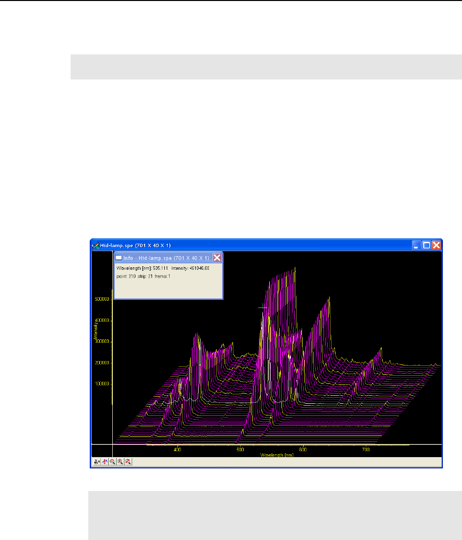
108 WinSpec/32 Manual Version 2.6B
These buttons have no effect on the strip selection when viewing data as an image.
Instead they select the first, last, next and previous frame respectively if the data set
contains multiple frames.
Note: When displaying the data as a graph, to view data from multiple frames, it is
necessary to select Same Strip - Multi Frame on the Display Layout|3D Layout tab.
It might further be noted that these buttons do not appear on the default Custom Toolbar.
Instead they must be added using the Customize Toolbar dialog, accessed by selecting
Custom Toolbar on the Setup menu.
Cursor Curve and Marker Curves
In analyzing a data display, it is often desirable to highlight the cursor curve and to have
every nth curve displayed in a different color as a convenient marker. WinSpec/32
provides these functions as demonstrated in the following procedure.
1. On the 3D Layout tab, select Highlight Cursor Curve and Marker Curves On.
Then press OK. The cursor curve and marker curves should be clearly delineated.
Note that on a color monitor they would be in contrasting colors and much easier to
see than in a black and white print as shown in Figure 80.
Figure 80. 3D Display with Cursor curve and Marker Curves
Note: Displaying the data with Highlight Cursor Curve displayed affects the time
required to step the cursor from curve to curve. If Highlight Cursor Curve is OFF, the
cursor can step without updating the entire display. If Highlight Cursor Curve is ON,
the entire display updates with each step, a considerably slower operation.
2. If the Cursor Curve and Marker Curves do not appear, the problem may be with the
assigned colors, which should be different from the normal graph color and different
from the background color. On the Display Layout|Color tab, it the Active 3D
Graphs button that allows the cursor-curve color to be set. The Marker Graphs
button is used to set the marker-curves color.

Chapter 8 Displaying the Data 109
Hidden Surfaces
The following procedure shows you how to shift the view to see the hidden or underside
of the data.
1. Open the Hid-lamp.spe file as a 3D graph: this sample file is supplied with WinSpec.
2. Open the Display Layout dialog and make the following changes.
Range: Change Y so that the range is “from 40 to 1” (not “from 1 to 40”).
3D Layout: Select Show Hidden Surface and deselect Highlight Cursor Curve
and Marker Curves On. Remove Hidden Lines should be selected. Change
the Z Axis Endpoint to X% 25 and Y% 0.
The Z Axis Endpoint can be set by entering values up to 80% X (either polarity)
and 80% Y (positive only) or graphically by using the mouse. If you click on
Adjust Z Graphically and then on OK, the Z Axis Adjust window will appear.
With the cursor in that window, depress the left mouse button, and drag the
cursor around the WinSpec/32 desktop until you see the desired axis orientation.
Then release the mouse button.
Because the data is displayed the moment you depress the mouse button and
then updated as you drag the cursor, you can see the effects of dragging the axis
while moving it. When working with a high-density data set, every nth line will
be suppressed during the adjustment so the process remains fast. When the data
is displayed as desired, releasing the mouse button will cause the entire data set
to be displayed with the new orientation.
TIP: Since you can move the cursor outside the data window, reducing the data
window size before adjusting the Z axis will give you greater range of motion
while dragging the axis.
3. Click on OK. The data should be redisplayed as shown in Figure 81, with the hidden
surface clearly visible.
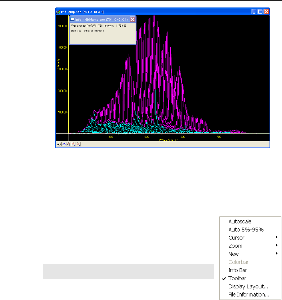
110 WinSpec/32 Manual Version 2.6B
Figure 81. 3D Plot with Hidden Surfaces
4. If the hidden surfaces are not clearly delineated, you may need to change their color.
Use the Normal Hidden Surface button on the Display Layout|Color tab to choose
a different hidden-surface color. Note that the Marker Hidden Surface button allows
you to set the color of the marker curves in hidden surface regions.
Data Window Context menu
For your convenience, the essential data window functions have
been gathered into a single menu, illustrated in Figure 82. This
menu, which is available whether the data is displayed as an
image, graph, or 3D graph, can be accessed by right-clicking
anywhere in the data display area. Brief descriptions of the
provided functions follow.
Note: Right-clicking inside an ROI will open the ROI context
menu.
Figure 82. Data
Window
Context menu
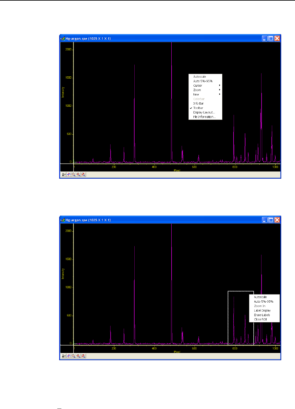
Chapter 8 Displaying the Data 111
Labeling Graphs and Images
For graphs and images, the normal context menu (right-click) is as shown in Figure 83.
Figure 83. Normal Context menu
This menu was changed for ROIs. If there is an ROI, and if the mouse is right-clicked in
the ROI, the context menu changes to that shown in Figure 84.
Figure 84. ROI Context menu
If the mouse is right-clicked outside the ROI, the normal menu (Figure 83) appears. The ROI
context menu (Figure 84) contains the usual actions pertaining to the ROI (autoscaling on the
region inside the ROI, and zooming in to the ROI region) plus three new actions:
Label Display: allows user labels to be placed on the display,
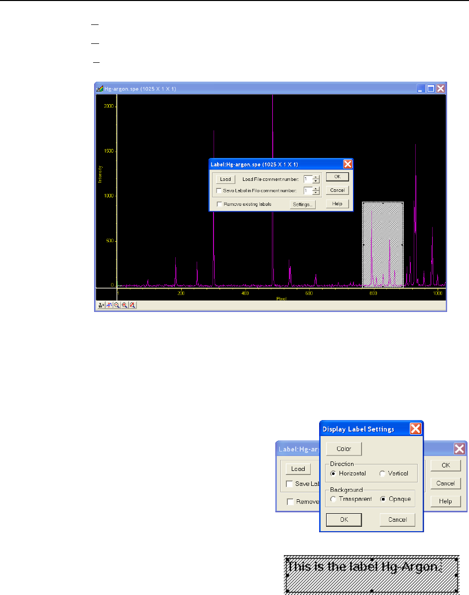
112 WinSpec/32 Manual Version 2.6B
Erase Labels: removes ALL user labels from the display, and
Close ROI: erases the ROI with no other action (it doesn’t move the cursor!).
The Label Display action brings up a dialog and opens an Edit box - Inside the ROI! as
shown in Figure 85.
Figure 85. Label Display action
The dialog allows loading a previously saved label (from one on the SPE file’s 5
comment fields); alternatively you can type the label into the edit box. The label can be
saved into a file’s comment field (when OK is clicked). The source comment field and
the destination comment field can be different.
Clicking Remove existing labels will erase all previous labels from the display before
adding the current label.
The Settings button brings up a dialog
with options for the label itself
(Figure 86). The Display Label Settings
dialog allows you to change the color of
the label text, to choose between an opaque
(white) background and a transparent
background, and choose whether the labels
are to run vertically or horizontally. The
opaque background works well with
images, where the label can get lost inside
the image.
The simplest way to label a display would be
to place the ROI where the label should
appear (the origin starts at the top left corner
of the ROI box), right-click inside the ROI
box, type the label text, and click OK.
Figure 86. Label Options subdialog
Figure 87. Label text entry box
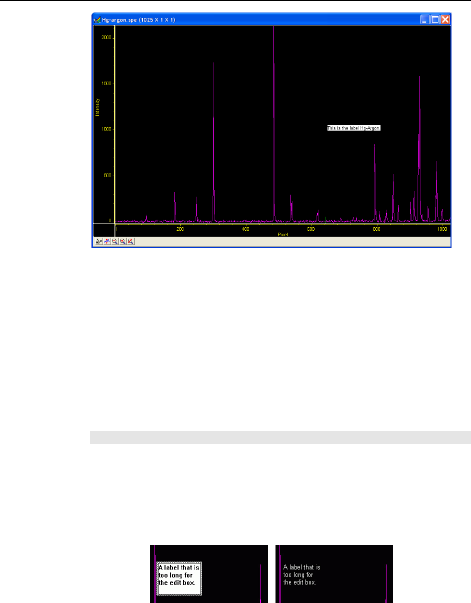
Chapter 8 Displaying the Data 113
Figure 88. Data with Finished Label
Figure 87 shows a label as entered in the label text entry box. Figure 88 shows the same
label as it will appear with the data after clicking on OK. Generally it is advisable to save
the label in a comment field; otherwise, once the label is printed and the display is closed,
the label will be lost. In fact, once the label is on the display, it cannot be edited.
However, if it has been saved, it can be edited, as follows.
1. Erase labels.
2. Call up the display label menu.
3. Load the label.
4. Edit the label in the edit box.
5. Check the Save Label box to save the changes.
6. Click OK to display the corrected label.
Note: Labels are displayed with the same font as is used for the axes labels.
To reposition the label, move or resize the ROI (and Edit) box before you
click on OK:
Moving the box, however, requires that you position the mouse very near the edge of the
box, because further in, the Edit box will capture the mouse. Resizing is done in the usual
way with the ROI box handles. If the ROI box is accidentally erased, just redraw a new one
in the desired location, and the Edit box will reappear. The Edit box wraps lines at the end of
the box, and the Label function will display the label as it appears in the box (Figure 89).
Figure 89. Edit box with line-wrapped label and finished label with same line wraps
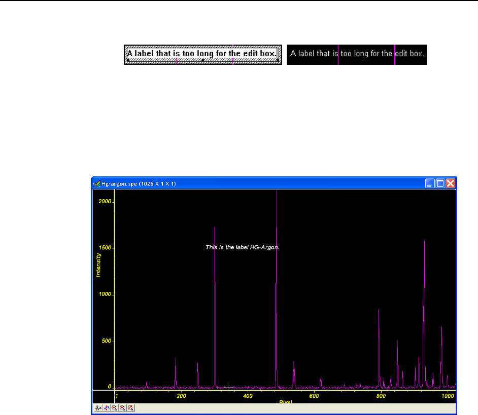
114 WinSpec/32 Manual Version 2.6B
To correct the line-wrapping:
Simply resize the ROI as shown in Figure 90.
Figure 90. ROI resized to correct Line-wrapping
To change the background or color:
The label must be erased and reprinted; it can only be altered inside the edit box.
To change the label font or font style:
Open the Display Layout|Axes tab, select Fonts… (this works even if axes are not
displayed), and make your changes. Figure 91 shows that the font style has been changed to
italic. Note that the axes labels are also italic.
.
Figure 91. Display after changing Font Selection
Data Displayed as an Image
WinSpec/32 can display data as an image, as a two dimensional graph, or as a 3 D Graph
(multiple strips from the same graph or the same strip from multiple frames). You can
choose to allow the software control how the data will be displayed or make the selection
yourself. To have WinSpec/32 control the data-display mode, simply check the Auto
Select checkbox provided in the File Open dialog and also in the Display Layout
dialog. The Auto Select algorithm makes the selection depending on the number of data
strips as described on page 99.
Displaying circuit.spe
The image used in this exercise is circuit.spe, one of the images supplied with your
WinSpec/32 software. Once you become comfortable working with this image, you
should have little difficulty in working with images from actual measurement data.
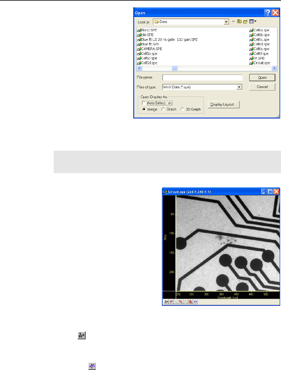
Chapter 8 Displaying the Data 115
1. From the File menu, select
Open. The Open dialog
(Figure 92) allows you to
select the image to be
opened. The Look-In field
provides a browser function
so you can easily find the
directory where the images.
By default, the data
directory is a subdirectory of
the directory where
WinSpec/32 was installed.
Subdirectory names and the
filenames of all files of the
specified type (the
WinSpec/32 data type is
*.spe) in the current
Figure 92. Open dialog
directory are listed in the box below the directory name. The WinSpec/32 data type is
WinXData (*.spe).
Note: The directory can be changed by changing the selection in the Look-In box.
The next time the Open dialog is opened, the new folder name will appear in the box
and its contents will be shown.
2. If the Auto Select checkbox is checked, deselect it. Then select Image.
3. From the data directory select the image
file called CIRCUIT.SPE. Click on the
OK button. A window of the appropriate
dimensions should appear immediately.
The image display (Figure 93) may take
a few seconds, depending on the speed of
the computer.
Figure 93. Circuit.spe Image
Changing the Brightness Range
1. Click on (5%-95%) (located beneath the displayed image as shown in Figure 93).
You will observe a moderate brightening of the image as it autoscales on the central 90%
of the image histogram. The brightest (pixels with high dark charge) and the darkest
pixels (pixels with low response) are ignored.
2. Click on the (Autoscale) button, restoring the image to its initial appearance.
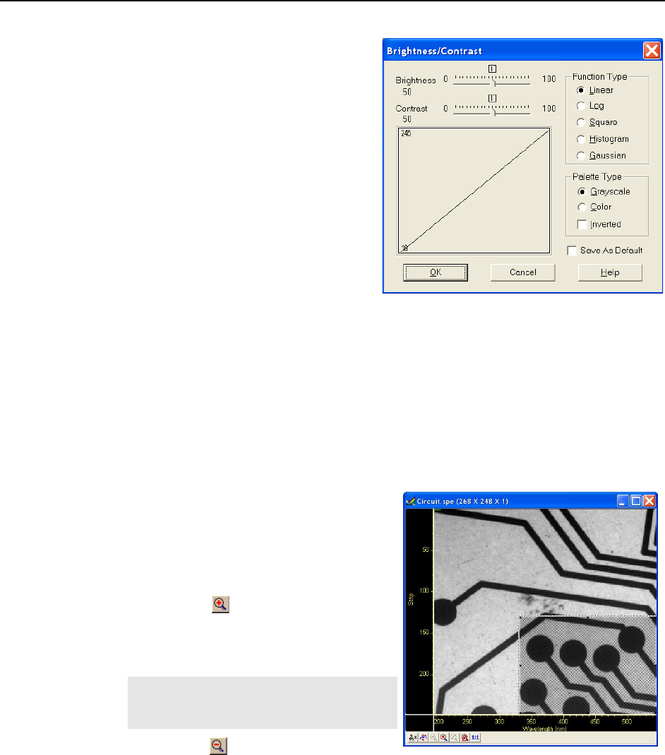
116 WinSpec/32 Manual Version 2.6B
Brightness/Contrast Control
Select Palette on the Display menu. This
will open the Brightness/Contrast dialog
(Figure 94). Note that the window includes
a plot of display brightness (Y axis) versus
data value (X axis). As settings are
changed, the displayed curve changes to
reflect the change in the transfer function.
(See the online Help for a detailed
discussion of the palette and transfer
function options.)
1. Change the brightness and contrast
settings to obtain the most pleasing
image display. Note that clicking on
the small square above the Brightness
scale and above the Contrast scale will
restore the default brightness and
contrast values (50).
Figure 94. Brightness/Contrast dialog
2. Try different Function and Palette Type selections to see the effect on the
displayed image. Note that the displayed curve will also change, reflecting the
change in the brightness transfer function. Until you gain more operating experience,
we suggest you leave the Function Type set to Linear, the Palette to Grayscale,
and the Brightness and Contrast both to 50.
3. Click on OK to close the dialog. Any setting changes will be applied.
Selecting a Region of Interest
1. Using the mouse, position the cursor at
one corner of the region to be defined,
depress the left mouse button, drag the
cursor to the diagonally opposite corner,
and release the mouse button. Refer to
Figure 95.
2. Click on the (Zoom In) button. The
view will change so that only the
selected region is displayed as shown in
Figure 96.
Note: The Display Layout Cursor tab
allows you to change how the ROI region
is displayed.
3. Click on the (Undo Zoom-In) Button.
The original view will be restored.
Figure 95. Circuit.spe with Region Selected
for Viewing
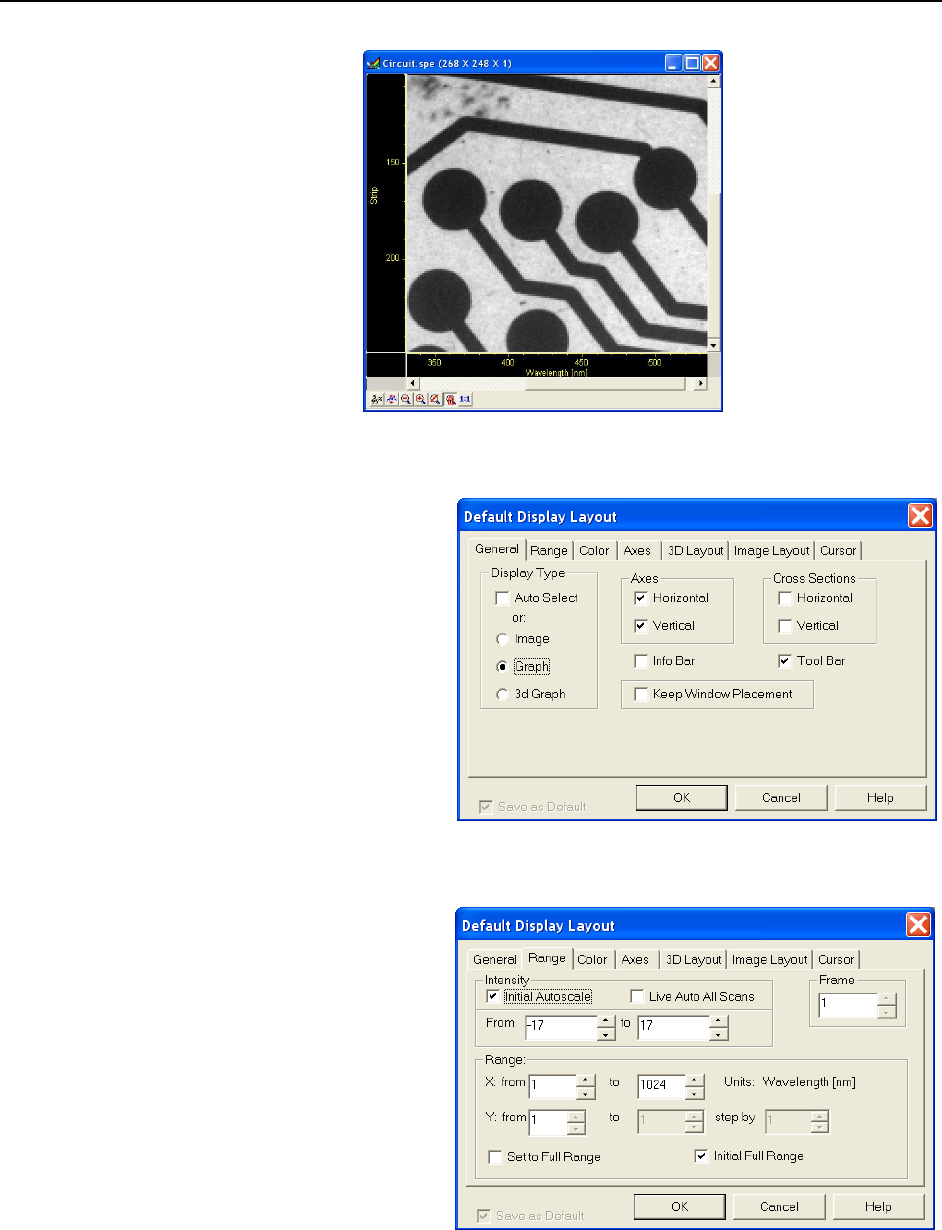
Chapter 8 Displaying the Data 117
Figure 96. Circuit.spe Expanded to show Defined Region
Opening the Display Layout dialog
With the image still open, select
Layout from the Display menu.
The Display Layout dialog will
open (Figure 97). Note that you
can also access the Display
Layout dialog by clicking on the
Display Layout button of the
Open dialog.
Figure 97. Display Layout dialog
Viewing Axes and Cross Sections
1. Still in the Display Layout
dialog, select Axes
Horizontal, Axes Vertical,
Cross Sections
Horizontal and Cross
Sections Vertical. Refer to
the online Help for
additional information on
Axes and Cross Sections.
2. Click on the Range tab
(Figure 98). Initial
Autoscale and Set to Full
Range should be selected.
The Frame number should be
“1.”
Figure 98. Display Layout|Range tab
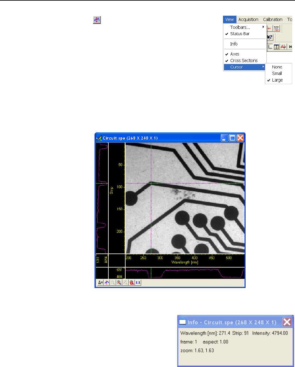
118 WinSpec/32 Manual Version 2.6B
3. Click on the OK button to close the Display Layout dialog.
4. Click on the (Autoscale) button at the bottom of the
image window. Then select the large cursor by clicking on
Cursor on the View menu and then on Large as shown in
Figure 99.
5. The display should now appear as shown in Figure 100.
The axes will be labeled in image pixels and strips with
respect to the CCD chip used to acquire the image. The
vertical image intensity profile at the cursor position will
be displayed to the left and the horizontal image intensity
profile at the bottom. The minimum and maximum values
for each profile are indicated. Note that you can use the
Figure 99. Selecting the
Large Cursor
mouse and drag the axes and profile boundaries to change the size of the profile display
regions. To change the cursor location, simply click the mouse at the new spot. The
cross-sectional graphs will change to reflect the profiles at the new location.
Figure 100. Circuit.spe with Axes and Cross-sections
Information box
On the View menu, select Info. The
information box should appear as shown in
Figure 101. The intensity in A/D counts is
reported at the pixel and strip position
corresponding to the cursor position. Also
reported are the Frame number, Aspect ratio,
and X and Y Zoom in effect. If a region is
defined by dragging the mouse cursor, the
region coordinates and diagonal length will
Figure 101. Information box
also be reported.
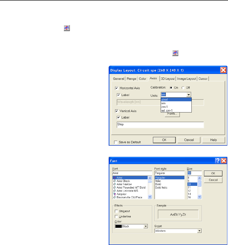
Chapter 8 Displaying the Data 119
Autoranging the Intensity in a ROI
1. Drag the mouse cursor to define a rectangular region of interest on the displayed
image.
2. Click on (Autoscale). The display will autorange to the intensity range in the
defined region. The effect will be an increase in contrast in the observed image.
Throughout the image, pixels darker or lighter than those in the defined region will
be displayed as black or white.
3. Click the mouse anywhere in the displayed image and click again to restore the
original image view.
Relabeling the Axes
1. Open the Display
Layout|Axes tab
(Figure 102). Note that the
checkboxes for Horizontal
Axis, Vertical Axis, and
the Label are all checked (If
unchecked, the
corresponding axis or label
would not be displayed.)
2. Change the axis label for both
axes. Then click on OK. The
displayed axes will no longer
be named Pixel and Strip,
but rather the new labels.
3. Try selecting different fonts
to see the effect. Only True-
type or Type 1 (Postscript)
fonts will work correctly.
Click on the Fonts button to
open the Fonts dialog,
change the various font
choices, and click on OK
twice. To return to the
original font choices, select
10 pt Arial Regular.
4. Reopen the Axes tab and
change the axis labels back
to their original designations
(Pixel for horizontal; Strip
for vertical).
Figure 102. Display Layout|Axes tab
Figure 103. Fonts dialog
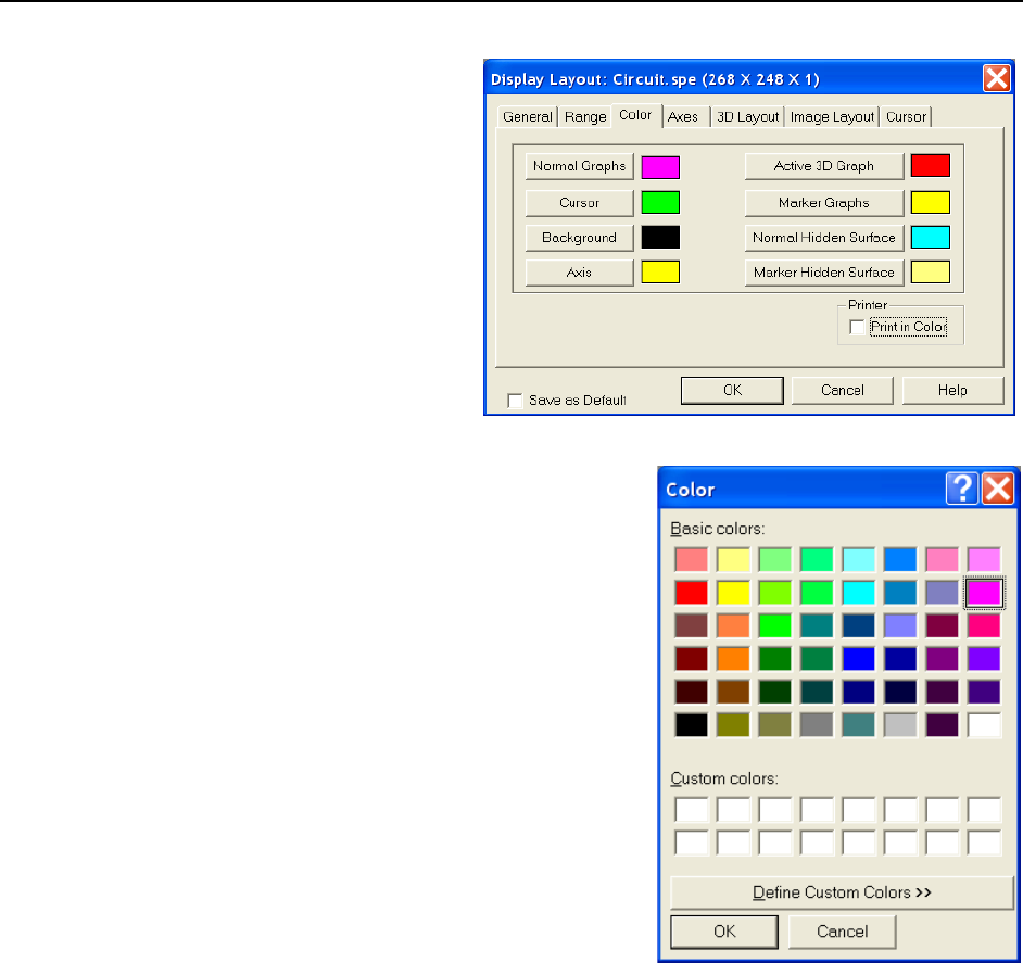
120 WinSpec/32 Manual Version 2.6B
Changing the Color of the Axes and Labels
1. Open the Color tab. Note
that there is a button for
each item to which a color
can be assigned and that the
current color for each item
is indicated in a color
swatch to the right of the
button. The default for the
Axis is yellow.
2. Click on Axis. The color
palette will open as shown
in Figure 104.
Figure 104. Display Layout|Color tab
3. Select a different color by clicking on the
swatch of the desired color. Then click on OK
to close the Color dialog and on OK again to
close the Display Layout dialog. The axes
and colors will now appear with the new color.
4. Repeating the process, open the Color dialog
again and restore the default color. Again, click
on OK to close the Color dialog and on OK
again to close the Display Layout dialog. The
axes and labels will now be displayed in the
original color.
Figure 105. Display Layout|Color
dialog
Specifying a New ROI and Intensity Range
1. Open the Display Layout|Range tab. Note that you can change the displayed
intensity range as well as the X-Y range.
2. Try entering more restricted ranges and note how the displayed image changes.
Changing the X-Y range by entering new values is functionally equivalent to
changing the displayed area by dragging the cursor as previously described. Selecting
a narrower intensity range results in pixels brighter and darker than the range limits
being displayed as white and black respectively. The effect is to increase the contrast
of the image. Each time a change is made, click on OK to close the Display Layout
dialog and observe the effect of the change.
3. On completing your display experiments, restore the defaults (Autoscale Intensity
and Full Range checked), close the Display Layout dialog, and close the data file.
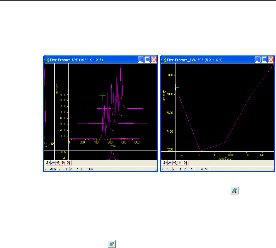
Chapter 8 Displaying the Data 121
Displaying a Z-Slice
A z-slice cuts across multiple frames at the cursor location and generates a new data file.
The number of points in the z-slice equals the number of frames in the source file. The
generated file name is the source file name appended with “_ZVU”. The X-axis is in time
units and the Y-axis is in intensity. Figure 106 shows an .SPE file containing five frames
and the z-slice .SPE file generated for the cursor location.
Figure 106. Multi-frame Data and a Z-Slice of that Data
1. Verify that the Custom Toolbar is visible and that that the Z-slice button is in
that toolbar. If the toolbar and/or the button are not present, refer to “Chapter 19
Custom Toolbar Settings,” starting on page 209, for information on how to display
the toolbar and add an available button.
2. Open a data file with multiple frames.
3. Position the cursor in the data window.
4. Click on the Z-slice button to generate the z-slice data file.

122 WinSpec/32 Manual Version 2.6B
This page intentionally left blank.
123
Part 2
Advanced Topics
Chapter 9, On-Line Data Acquisition Processes ......................................... 125
Chapter 10, Cleaning .......................................................................................... 135
Chapter 11, ROI Definition & Binning ............................................................. 139
Chapter 12, Correction Techniques ............................................................... 147
Chapter 13, Spectra Math ................................................................................. 153
Chapter 14, Gluing Spectra .............................................................................. 159
Chapter 15, Post-Acquisition Mask Processes .......................................... 165
Chapter 16, Additional Post-Acquisition Processes ................................. 177
Chapter 17, Printing ........................................................................................... 183
Chapter 18, Pulser Operation .......................................................................... 187
Chapter 19, Custom Toolbar Settings ........................................................... 209
Chapter 20, Software Options ......................................................................... 213

124 WinSpec/32 Manual Version 2.6B
This page intentionally left blank.
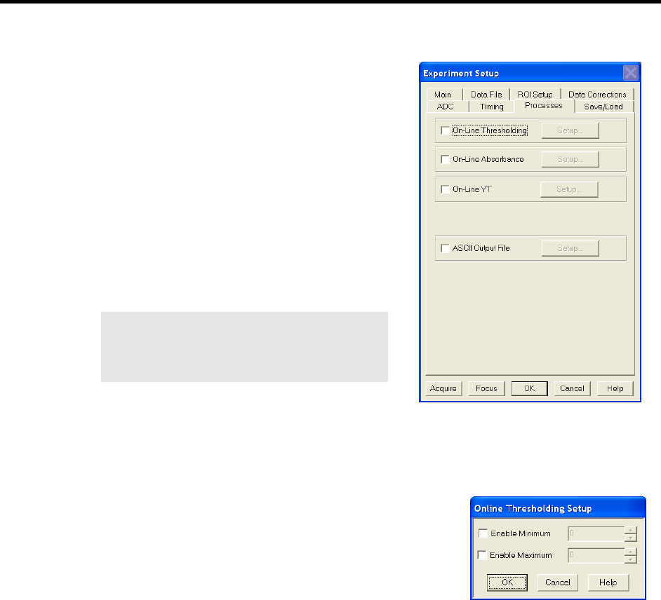
125
Chapter 9
On-Line Data Acquisition Processes
Introduction
The Processes tab on the Experiment Setup
dialog allows you to set up and activate up to
four different processes for automatic processing
of incoming data. It is most likely that you will
only activate one (such as on-line thresholding)
or two (such as on-line thresholding and ASCII
output file) at a time. Process activation occurs
when you select a checkbox. After you click in a
checkbox, you can then click on the Setup…
button and begin entering or reviewing the
parameters for the process. After you have
clicked on the OK button to activate one or more
processes, the active processes will be applied to
data being acquired.
Note: The on-line thresholding and
absorbance processes change the raw data. If
you want to retain raw data, you may want to
use a post-acquisition process instead.
Figure 107. Experiment Setup|Processes tab
On-Line Thresholding
Description
On-line thresholding allows a threshold test to be
performed on data as it is acquired. The threshold test
is performed after background subtraction and flatfield
correction but before software accumulation. Data that
falls within the threshold range returns a 1, data that
falls below the minimum threshold or above the
maximum returns a 0. In an experiment containing n
accumulations, only one data set is stored, but with the
data added from each accumulation. Thus, if a
Figure 108. Online Thresholding Setup
dialog
given bit contained data within the threshold range on 7 of 10 iterations, the value of the
bit in the acquired data set would be 7. The minimum and maximum levels can be
independently set and checkboxes allow the minimum and maximum threshold functions
to be independently toggled on or off.

126 WinSpec/32 Manual Version 2.6B
Parameters
Enable Minimum: The check box allows the Minimum threshold function to be
switched ON (checked) or OFF (unchecked). When the function is ON. you can enter
the minimum threshold level. This can be any positive or negative value in the range
of possible intensities provided the setting is lower than the Maximum setting. This
setting will be retained when the function is switched OFF.
When the Minimum threshold is ON and data is being acquired, any intensity value
below the set value will return a 0. Intensities higher than the Minimum setting will
return a 1, unless they also exceed the Maximum setting, in which case they will
return a 0. When the Minimum threshold is OFF, all intensities below the Maximum
will return a 1; intensities that exceed Maximum return 0.
Enable Maximum: The check box allows the Maximum threshold function to be
switched ON (checked) or OFF (unchecked). When the function is ON. you can enter
the maximum threshold level. This can be any positive or negative value in the range
of possible intensities provided the setting is higher than the Minimum setting. This
setting will be retained when the function is switched OFF.
When the Maximum threshold is ON and data is being acquired, any intensity value
above the set value will return a 0. When it is OFF, all intensities higher than the
Minimum will return a 1.
Note: Background subtraction can force negative values.
Procedure:
1. Select On-Line Thresholding on the Experiment Setup|Processes tab. The
Online Thresholding Setup dialog will open.
2. Set the Minimum and Maximum threshold enable status and set the threshold
values.
3. Click on OK to save your entries and close the dialog. Then click on Acquire or
Focus to start data acquisition.
On-Line Absorbance
Description
Absorbance is defined as the Log (base 10) IR/I, where IR is the reference spectrum and I
is the sample spectrum. Absorbance is also defined as the log of the inverse of the
transmission. Thus increasing absorbance means the transmission is decreasing and an
absorbance of zero means that IR = I.
Figure 109. Absorbance Setup dialog
The Absorbance Setup dialog allows either of two absorbance modes to be selected,
depending on the reference used. The reference signal I0 can be either live (Live
Reference Strip selected), or taken from a file (File Name selected and entered). If

Chapter 9 On-Line Data Acquisition Processes 127
live, then the experiment generally will have 2 strips, one reference and one sample (there
can be more than 2, up to n, with 1 reference and n-1 samples). Any strip in the ROI can
be selected. If taken from a file, then the file must have the same dimension as the live
data, and in this case, every strip in the file will be the reference for the corresponding
strip in the live data. The button at the right of the file name entry box opens a browser to
facilitate locating the file.
The largest signal for absorbance (live) is when the reference is full scale and the sample
is 1 and you are using an 18-bit A/D. With this configuration the largest signal for
absorbance (live) is the Log10 (262,144/1) = 5.42. The software therefore limits the signal
to 5.5. If the sample goes to zero or negative (background subtract), 5.5 is used as the
answer.
In the live mode, because IR equals I for the reference strip, this strip will always have an
absorbance of zero.
Procedure:
1. Select On-Line Absorbance on the Experiment Setup|Processes tab. The
Absorbance Setup dialog will open.
2. Set the Minimum and Maximum threshold enable status and set the threshold
values.
3. Click on OK to save your entries and close the dialog. Then click on Acquire or
Focus to initiate data acquisition.
On-Line YT
Description
Y:T Analysis allows you to easily monitor and study the way spectral data changes as a
function of time. This is particularly useful in characterizing time-dependent processes.
Y:T Analysis provides for defining areas on the data, where each area is a region
bounded by a starting and ending wavelength and containing a certain number of pixels
whose wavelength values lie within the region. The value of an area is the sum of the
intensities of the pixels in the area.
If a process study produces spectral lines that change with time, it may be useful to define
a separate area for each line of interest, where each line is precisely spanned by its area.
The value of each area can be the sum of the total intensities defined with respect to the
baseline, or the values can be baseline-corrected, in which case the value of each area is
the sum of the intensities with respect to an imaginary line joining the first and last pixels
of the area. This latter method is more accurate with a sloping baseline.
After areas have been defined, they can then be mathematically operated on as specified
in user-entered equations. These equations allow you to can add, subtract, multiply,
divide or otherwise manipulate up to eight areas. You can also include constants or even
other equations. The Y:T analysis modes provided give you control over when the
equation calculations will be performed, how many will be performed, and on which
acquired data they will be performed.
Each time equation calculations are performed, one Y:T analysis value is produced for
each equation. For example, in a one-hour experiment with one Y:T equation and a Y:T
sample time of one minute, at the end of the hour a Y:T analysis curve sixty points in
length would have been taken and stored. If two equations had been defined for the same
experiment, at the end of the hour there would be two Y:T curves, each sixty points in
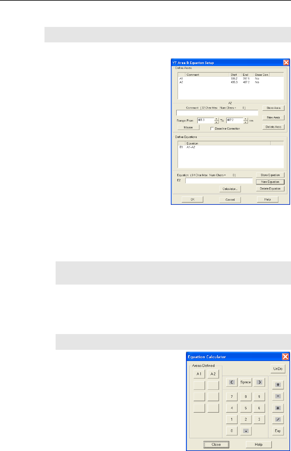
128 WinSpec/32 Manual Version 2.6B
length. An additional Y:T curve for the time will always be provided as well. These Y:T
curves are stored and can be displayed, printed, or processed the same as any other data.
Note: With on-line YT, the raw data are preserved. Two data sets are acquired and
displayed: the raw data and the YT data associated with it.
YT Area and Equation Setup Procedure
Before activating on-line YT analysis, you
must define the area(s) to be monitored and
enter the equation(s) to be used to perform
the Y:T analysis of spectral data as it is
acquired. For any given analysis, you can
use or delete previously stored equations or
define new ones. Y:T analysis will not take
place unless the On-Line YT check box on
the Experiment Setup|Processes tab is
checked.
The following procedure assumes that
there are no stored areas and equations.
1. Select YT Setup from the
Acquisition menu.
2. Click on New Area and begin entering
the range and baseline correction
choice for the area. You can enter up to
eight areas.
3. When you enter an area, you can either
Figure 110. YT Area & Equation Setup dialog
type in the Range X-axis start and end points or use the mouse to select the area on an
acquired spectrum and click on the Mouse button to make the entries. The units are
those specified in the spectrograph Calibration Usage dialog. When using the mouse to
enter the range, it is generally helpful to have the Info box displayed at the same time so
you can see the precise values of the start and end points.
Note: The area range is always stored internally in wavelength units. This assures
that, if the area is used for Y:T analysis on ROIs spanning different pixel range, the
starting and ending wavelengths for the area range will remain correct.
4. You can also enter a comment of up to 32 characters into the Comment field and
select/unselect baseline correction.
5. When you have finished describing the area, click on the Store Area button. The
area will be added to the Area Listing box at the top. Areas in the box are available
for entering into equations.
Note: An asterisk appearing before an area designator (e.g., *A2) indicates that the
area range is outside the wavelength calibrated range of the detector.
6. Repeat Steps 2 and 5 until you have entered the areas you plan to use.
7. Click on New Equation and begin entering an equation into the Equation field.
You can enter up 64 characters per equation (and its comment) and define up to four
equations. You can either type the new equation into the field or you can click on the
Calculator button to open the Equation Calculator dialog. If you use this dialog,
click on the appropriate buttons for your equation (the areas, values, and operands
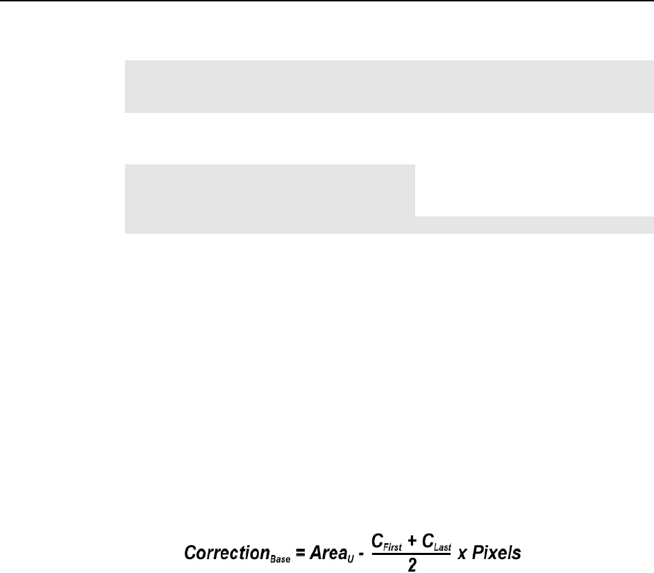
Chapter 9 On-Line Data Acquisition Processes 129
Figure 111. Equation Calculator
dialog
will appear in the Equation field as you click on the buttons). Close the dialog when
you have finished.
Note: To add a comment to an equation, follow the equation with a : and the
comment text. The colon indicates that what follows is not part of the equation. For
example, in the equation A1+A4:This is a test, “This is a test” is the comment.
8. Click on Store Equation to save the equation. The equation will be added to the
Equation Listing box. Equations in the box are available for YT Setup.
Note: An asterisk appearing before an
equation designator (e.g., *E3) indicates that
equation contains areas that lie outside the
calibration range of the detector.
9. Repeat Steps 7 and 8 until you have finished entering your equations.
10. When you have finished with area and equation entry and storage, click on OK to
close the YT Area & Equation Setup dialog.
11. You are now ready to begin entering acquisition parameters on the YT Setup dialog.
See “YT Analysis ” on page 130 for more information.
Baseline Correction
The value of each area is the sum of the intensities over the area’s specified range. The
value of an area can be calculated using the intensity heights with respect to the baseline
or using the intensity heights with respect to a straight line segment drawn between the
start and end points of the specified range. The latter results in a corrected area that is the
part of the total area above this line. Baseline Correction gives more accurate results on
sloping baselines.
Baseline correction is calculated by taking the uncorrected value or the area and
subtracting the area below the baseline. This calculation may be expressed as:
Where:
AreaU is the uncorrected value of the area.
CFirst is the first channel of the specified range.
CLast is the last channel of the specified range.
Pixels is the number of pixels in the area.
Changing/Deleting Areas and Equations
The parameters for an area or an equation can be changed by clicking on that area’s or
equation’s designator (at the far left of the item – A1 or E2, for example) in the
appropriate listing box and then keying new values for the parameter to be changed. The
changes do not take effect until the appropriate Store button is pressed.
Areas and equations that have been stored can be deleted. To delete an area or an
equation, simply click on the area’s or equation’s designator (A1 or E2, for example) in
the appropriate listing box and press the appropriate Delete button.
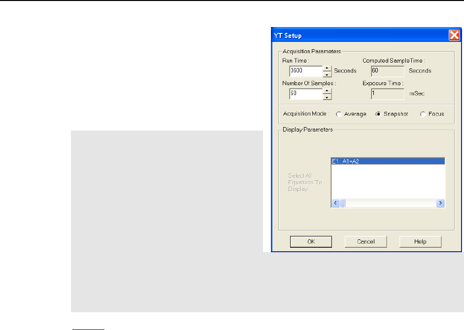
130 WinSpec/32 Manual Version 2.6B
YT Analysis Acquisition Modes
The YT Setup dialog settings determine
how the Y:T analysis will be performed
using the areas and equations defined via
the YT Areas and Equations Setup
dialog. YT Setup involves choosing and
Acquisition Mode and then entering
values for one or more Acquisition
Parameters.
Note: Generally data acquisition does not
occur at exactly even times. With a 1 msec
exposure time, there is still the readout
time for each data set to consider. In
reality, the Y:T point will be calculated
from the first data set processed on or after
the Y:T sample time expires. The actual
time the Y:T sample is taken is read using
the system clock relative to the start of data
acquisition, and the times are stored with
the Y:T data as the last Y:T curve. Since data acquisition is done using DMA under the
timing of the detector controller, the timing coming into the DMA buffer is very precise.
However, Y:T time is taken as the data is transferred from the DMA buffer and processed
for background subtraction and flat field. This is under the program control and may be
less precise; for longer sample times, this will probably not be noticeable.
Focus
Only the Y:T Number of Samples are set in this mode ( Exposure Time is simply that
set on the Experiment Setup|Main tab). An advantage of Focus mode is that no data is
missed. A disadvantage is that the amount of Y:T data stored can quickly become quite
large and much of it might be of limited value when studying a process that is changing
slowly. Focus mode can be quite useful for making an initial evaluation of a process.
Inspection of the Focus mode results might then suggest more productive Y:T analyses
that could then be made using either the Snapshot mode or the Average mode. How
Focus mode works is described in the following paragraph.
Assuming you had established two areas (A1 and A2) and one equation (E1 = A1+A2),
A1 would be the sum of the intensities over one specified range of data points and A2 the
sum of the intensities over a second specified range of data points on the spectrum.
Adding the two together yields one value for E1. Next, let us assume that you have
entered a Number of Samples value of 1,000. On starting data acquisition, for each and
every acquired data set, the Equation E1 calculation would be performed and the
resulting Y:T value stored. This process would continue until the specified Y:T Number
of Samples have been taken or until data acquisition stops or is stopped. Once the
specified number of Y:T points have been calculated and stored, data sets will continue to
be taken according to the Experiment Setup parameters but no more YT calculations
will be performed. There would be 1,000 points in the Y:T curve, each point equal to
A1+A2. The data set(s) and the Y:T curve would be displayed in separate windows. If
multiple equations (up to four) had been defined, they would be computed in order and
there would be a separate Y:T curve for each. Selecting 3D Graph on the Display
Layout|Main tab and deselecting Remove Hidden Lines on the Display Layout|3D
Layout tab would allow all of the Y:T curves and the time line curve to be viewed
Chapter 9 On-Line Data Acquisition Processes 131
simultaneously. If the selection is Graph, only one curve would be visible. The keyboard
cursor up/down arrow keys can be used to select the curve to be viewed.
Note: If there are four equations, there will be five curves. The fifth curve is a time line.
The time at a point is reported as the I value in the Info box.
Snapshot
In this mode, you set the Y:T Run Time and the Y:T Number of Samples that will be
taken. Snapshot mode allows convenient Y:T analyses of long processes to be easily
performed. In Snapshot mode, data may be taken at short intervals for a long period of
time, but a Y:T analysis is only done on the most recent data set at specified intervals.
Most of the data sets taken over the course of the experiment are skipped. For Y:T
analysis purposes, you only have access to the first strip of data if acquiring multiple
strips.
To better understand this process, assume an experiment designed to characterize a
process that will take about an hour. Assume a 1 msec Exposure Time and a repetition
rate that is high relative to the Y:T Sample Time. Since the experiment is expected to
last an hour, a reasonable Y:T Run Time setting might be 3600 seconds. Further suppose
that you wanted each Y:T curve to be 60 points long, accomplished by setting the Y:T
Number of Samples to 60. The Computed Sample Time would then be 60 seconds.
In other words, a Y:T calculation would be performed on the most recent single data set
at the end of each minute, regardless of how many data sets were acquired during that
minute.
Note: The Computed Sample Time (interval between Y:T calculations) indication
does not update instantly when the Run Time and Number of Samples are entered. To
force the update, modify Run Time, and then either press the [Tab] key on your
keyboard or click on another control.
On starting data acquisition, after one minute, the first Y:T analysis would be made, with
one Y:T value computed for each equation defined. The timer would reset to zero and
begin counting the second minute. At the end of that minute the second Y:T value would
be computed for each equation defined. This process would continue for 3600 seconds
(one hour). At the end of that time n Y:T curves, n being the number of equations, each
60 points in length, will have been acquired and stored. These could be displayed in the
same manner as for the Y:T Focus mode. As was the case for the Focus mode, data
acquisition will continue until it stops or is stopped.
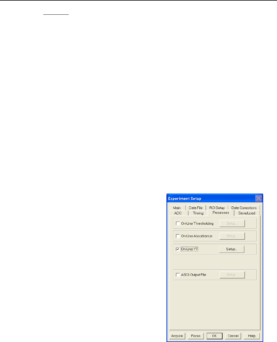
132 WinSpec/32 Manual Version 2.6B
Average
In this mode, as in the Snapshot mode, you set both the Y:T Run Time and the Y:T
Number of Samples that will be taken. Also, as in Snapshot mode, Average mode
allows convenient Y:T analyses of long processes to be easily performed. Unlike
Snapshot mode, however, no data is skipped even though only the specified number of
Y:T calculations are performed at the computed intervals. All of the acquired data is
stored in a buffer space over each interval. When the Y:T calculation is performed, it is
done on the average of all the data acquired over the preceding interval. For example, if
doing a one hour run with once a minute Y:T calculations, the data buffer would store all
of the data acquired for one minute. Then the Y:T computations would be done on the
average of the stored data to develop one Y:T point for each equation. After that the
buffer would be cleared and data storage for the next interval would begin anew. As with
the Focus and Snapshot modes, for Y:T analysis purposes, if there is more than one
data strip, only the first data strip is available for Y:T analysis purposes.
At the end of our hypothetical one hour run, n Y:T curves, n being the number of
equations, each 60 points in length, will have been acquired and stored. These could be
displayed in the same manner as for the Y:T Focus and Snapshot modes, previously
described. As is the case for the Focus and Snapshot modes, data acquisition will
continue until it stops or is stopped.
YT Analysis Setup Procedure
This procedure assumes that you have already defined the areas and equations to be used
for the analysis. See “YT Area and Equation Setup” on page 128 for the area and
equation setup procedure.
1. Select Experiment Setup from the
Acquisition menu.
2. Establish the Experiment Setup
parameters (Exposure Time and
Number of Spectra, for example) for
acquiring the data on which the Y:T
analysis is to be performed.
3. Click on the Processes tab and click
in the On-Line YT check box to turn
on Y:T analysis and activate the
Setup… button. Y:T analysis will take
place during any data acquisition run
initiated while this box remains
checked.
4. Click on the Setup… button to open
the Y:T Setup dialog.
Figure 112. Experiment Setup|Process tab
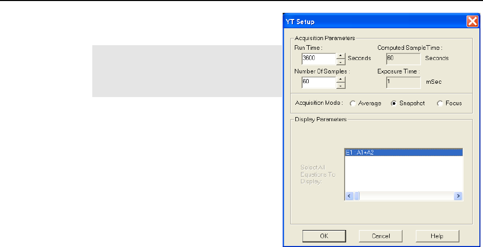
Chapter 9 On-Line Data Acquisition Processes 133
5. Select the Y:T Acquisition mode.
(Average, Snapshot or Focus).
Note: Exposure Time is set on the
Experiment Setup|Main tab.
Computed Sample Time is calculated
based on the other parameter values.
Average: In this mode, as in the
Snapshot mode, you set the Y:T
Run Time and the Y:T Number of
Samples that will be taken. Also, as
in the Snapshot mode, the Average
mode allows convenient Y:T
analyses of long processes to be
easily performed. Unlike the
Snapshot mode, however, no data is
skipped, even though only the
specified number of Y:T calculations
are performed at the computed
intervals.
Figure 113. YT Setup dialog
Snapshot: In this mode, you set the Y:T Run Time and the Y:T Number of
Samples that will be taken. The Snapshot mode allows convenient Y:T analyses
of long processes to be easily performed. Although data might be taken at short
intervals for a long period of time, a Y:T analysis is only done on the most recent
data set at specified intervals. Most of the data sets taken over the course of the
experiment are skipped. For Y:T analysis purposes, you only have access to the
first strip of data if acquiring multiple strips
Focus: In this mode you set the Y:T Number Of Samples only. Run Time and
Computed Sample Time are not displayed. Focus mode can be quite useful
for making an initial evaluation of a process and the results may suggest more
productive Y:T analyses that could then be made using either the Snapshot
mode or the Average mode. An advantage of Focus mode is that no data is
missed. A disadvantage is that the amount of Y:T data stored can quickly become
quite large, and much of it might be of limited value when studying a process that
is changing slowly.
6. Enter the Y:T Analysis parameter values appropriate to the acquisition mode.
7. Click on OK to save your entries and close the YT Setup dialog.
8. Click on Acquire or Focus to initiate data acquisition. As data are acquired, Y:T
points will be computed and stored. If multiple equations were defined (up to four are
possible), they would be computed in order and there would be a separate Y:T curve
for each. Selecting 3D Graph on the Display Layout|Main tab and deselecting
Remove Hidden Lines on the Display Layout|3D Layout tab would allow all of
the Y:T curves and the time line curve to be viewed simultaneously. If the selection
is Graph, only one curve would be visible. The keyboard cursor up/down arrow keys
can be used to select the curve to be viewed and the Info box shows which strip is
being displayed.

134 WinSpec/32 Manual Version 2.6B
ASCII Output File
Description
The ASCII Output process allows you to select and set
parameters for saving the data to an ASCII file. The
ASCII Output Setup dialog (Figure 114) allows you to
specify the delimiter and the line termination character to
be used when the data is stored in ASCII format. The
choice of delimiter and termination character depends on
the requirements of the program into which you will be
importing the data. When storing the file, WinSpec uses
the filename and location parameters entered on the
Experiment Setup|Data File tab.
Procedure
1. Select Experiment Setup from the Acquisition
menu.
2. Click on the Experiment Setup|Data File tab.
3. Enter the filename to be used when WinSpec
saves the .TXT file. Click on the browse button to the right of the Name field and
select the directory where the file should be saved. You can also select other file
saving parameters such as auto-increment, file overwrite, or file append.
4. Click on the Experiment Setup|Processes tab and select ASCII Output File.
5. Click on the Setup button to open the ASCII Output Setup dialog.
6. Set the Delimiter and Line Termination Characters and click on OK to save your
entries and close the dialog.
7. Click on Acquire or Focus to initiate data acquisition.
8. At the end of the acquisition, the .TXT file will be saved automatically. Depending
on your data file entries (Steps 2 and 3), the acquired data may also be saved
automatically as an SPE file or you can save it manually.
Figure 114. ASCII Output Setup
dialog
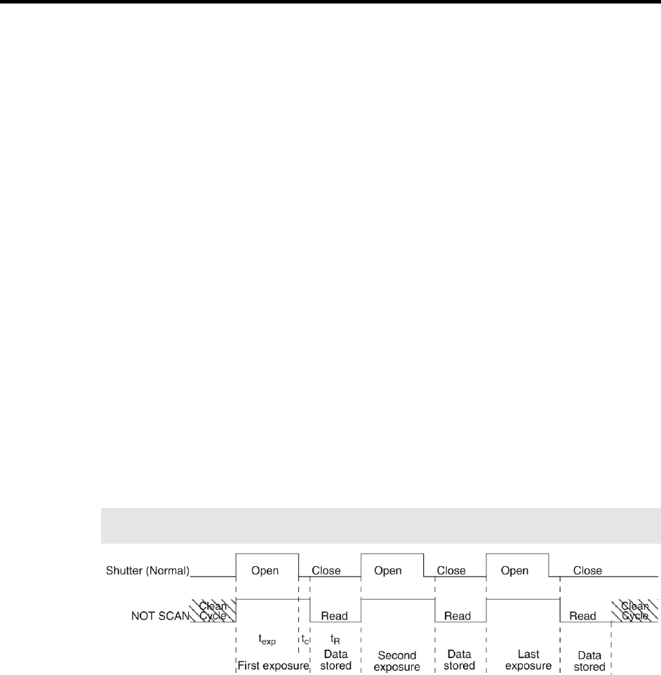
135
Chapter 10
Cleaning
Introduction
An acquisition is made up of an exposure period and a readout period. For the rest of the
time, the camera is waiting to be told to acquire spectra or images. During this waiting
period, charge generated from different sources builds up on the array unless some kind of
cleaning process is ongoing. Cleaning minimizes the impact of the unwanted signal (noise)
by row shifting the accumulated charge to the output register and then discarding it.
Depending on your system, WinSpec/32 will provide you with up to five cleaning features.
The most common cleaning feature is Clean Cycles, which occur until Acquire is selected
and may continue up to the entered number of cleans before exposure begins. If External
Synchronization is being used to control exposure, a feature called continuous cleans may be
used in addition to the standard clean cycles. Where the detector and controller support it, a
specialized version of continuous cleans Continuous Cleans Instruction can be used with the
External Sync timing mode. The readout of ROI information is enhanced by the Vertical
Skips feature. With Version 5 of the ST-133 Controller, continuous cleans for Kinetics is also
supported. All of these cleaning features and their interrelationships are described in the
sections that follow.
Clean Cycles
The basic cleaning function is implemented by clean cycles. These cycles start when you
turn the controller on and a clean pattern is programmed into the controller. Their
purpose is to remove charge that accumulates on the array while the camera not acquiring
data (i.e., exposing and reading out the array). The timing diagram below is for an
experiment set up to acquire three (3) spectra in Freerun timing mode with normal shutter
operation selected. In this diagram clean cycles occur before the first exposure and after
the last readout period.
Note: The start of the exposure is signaled by NOT SCAN going high but will not occur
until the current clean cycle has finished.
Figure 115. Clean Cycles in Freerun Operation
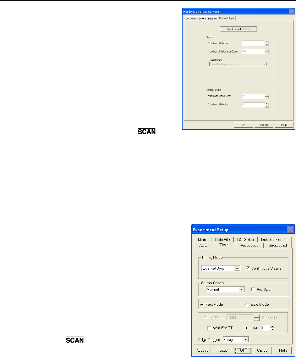
136 WinSpec/32 Manual Version 2.6B
The configuration of clean cycles is performed
on the Hardware Setup|Cleans/Skips tab
(Figure 116). When you set up the detector for
the first time, default values are automatically
inserted into these fields. These will give the best
results for most applications. Even so it is a good
idea to know what these entries mean with
regard to cleaning.
Let's begin with Number of Strips per Clean.
This parameter sets the number of rows that will
be shifted and discarded per clean cycle. While a
large number such as the number of rows in the
array may result in the best cleaning of the array,
the tradeoff is that there may be a significant
delay between the receipt of a start exposure
signal (NOT SCAN signal at the BNC
goes high) and the beginning of the actual
Figure 116. Cleans/Skips tab
exposure. This delay occurs because the current clean cycle must be completed before a start
exposure signal received during the cycle will be implemented. Typically, the default setting
is much smaller and in time critical experiments, the setting should be 1 or 2.
The Number of Cleans value is usually set to zero (0). These are additional clean cycles
that can be required after a start exposure signal is received and the current clean cycle has
finished. The maximum value for this entry depends on the controller. For example, the
range of values for an ST-133 is 0-7 and is 0-255 for an ST-138.
Continuous Cleans
Clean cycles will always occur but an additional
cleaning function called Continuous Cleans is
provided when the start of exposure is tied to an
external trigger (i.e., the experiment is being run in
External Sync timing mode.)
Figure 118 shows the timing diagram for an
experiment with External Sync trigger active on
the negative edge. Note that the timing diagram
shows two possible setups for the shutter. In the
first setup (Normal), the shutter is opened when
External Sync goes low. Because it takes time to
open a shutter, data may be missed while the
shutter is opening. In the second setup (Preopen),
the shutter is opened when the NOT SCAN signal
(at the BNC on the back of the ST-133)
goes high. The advantage is that the shutter is fully
opened when the exposure (triggered by External
Sync) begins. The disadvantage is that ambient
light is no longer being blocked from the array
Figure 117. Timing Tab: External Sync
with Continuous Cleans Selected
during the period between NOT SCAN going high and the External Sync going low.
Continuous cleans provides a way to get rid of the signal that accumulates on the array
during that interval.
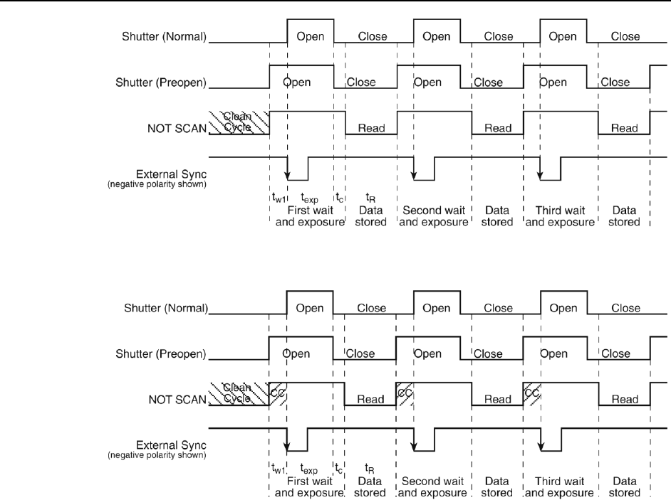
Chapter 10 Cleaning 137
Figure 118. External Sync Timing Diagram
Figure 119. External Sync with Continuous Cleans Timing Diagram
Figure 119 shows the same timing diagram with the addition of continuous cleans
(indicated by the shaded areas labeled CC). Continuous cleans are additional clean cycles
and defined by the same parameter values as the standard clean cycles. When the
External Sync trigger arrives during continuous cleaning, the current clean cycle must be
completed before the exposure will begin. In time critical experiments, the number of
rows per clean (set on the Hardware Setup|Controller/Camera tab) should be 1 or 2 to
minimize the delay.
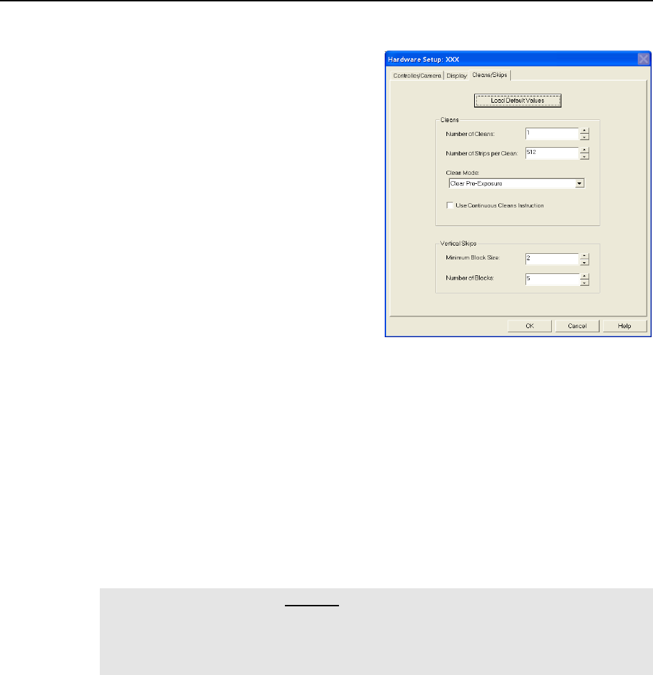
138 WinSpec/32 Manual Version 2.6B
Continuous Cleans Instruction
If the controller and the detector support it, a
specialized cleaning function can be used when
continuous cleans is active. This function,
"Continuous Cleans Instruction", can only be
activated if the checkbox for it is visible on the
Hardware Setup|Cleans/Skips tab (see
Figure 120).
Continuous cleans instruction does horizontal
shifts while doing vertical shifts for a faster
continuous clean. With this instruction, the
delay between an External Sync trigger and
the start of exposure is minimized.
Continuous cleans instruction will be used in
place of the standard continuous cleans if
both Use Continuous Cleans Instruction
on the Cleans/Skips tab and Continuous
Cleans on the Experiment Setup|Timing
tab are checked.
Figure 120. Cleans/Skips tab:
Continuous Cleans Instruction
ROIs and Cleaning
An ROI is a user-defined subsection of the array. As with full frames, the defined clean
cycles are used to keep charge from accumulating on the array while it is waiting for a start
exposure signal and after the data has been readout of the array. The specialized cleaning
function for an ROI – Vertical Skips – is applied when the ROI is read out. Vertical Skips
parameters are used to shorten the readout/discard time for the rows before and after the ROI.
Minimum Block Size sets the number of invalid rows (horizontal lines of the CCD) to
bin before the valid data. Number of Blocks sets the number of these blocks to shift and
discard before going to a geometric grouping algorithm. Refer to "Vertical Skips" on page
49 for detailed information about vertical skips and the grouping algorithm.
Note: The 2-D OMA array does not support vertical skips; and all of the rows on the
array are read out and converted before the non-ROI information is discarded. The
default Vertical Skips settings of Minimum Block Size: 2 and Number of Blocks: 5,
while appearing to work, will result in invalid data. Instead, you must change these
settings to 1 and 256, respectively, for the 2-D OMA array.
Kinetics and Cleaning
Kinetics is a special type of operation in which most of the CCD is mechanically or optically
masked, leaving a small section open to light. This section is then shifted under the mask
very quickly. The defined clean cycles are used to keep charge from accumulating on the
array while it is waiting for a start exposure signal and after the data has been readout of the
array. In addition to clean cycles, continuous cleans for kinetics is supported by Version 5 (or
higher) of the ST-133 Controller. For kinetics experiments, continuous cleans are only
applied between the first NOT SCAN low-to-high transition and the External Sync high-to-
low transition. Because of the speed at which the array is then shifted, exposed, and shifted
no further cleaning occurs until the last frame has been exposed and shifted. At that point, the
clean cycles begin again.
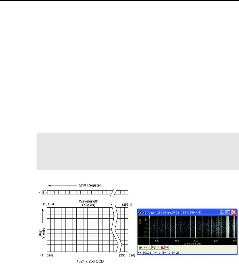
139
Chapter 11
ROI Definition & Binning
Overview
General
A Region of Interest (ROI) may be the entire CCD array or it may be a rectangular
subregion of the array. For data acquisition, the definition of such a region is done either
from the Easy Bin dialog (Figure 128, page 144) accessed from the Acquisition menu
or from the Experiment Setup|ROI Setup tab (Figure 129, page 145), accessible after
selecting Experiment Setup from the Acquisition menu. Easy Bin is a simple way of a
defining a single full chip width ROI. ROI Setup allows you to create multiple ROIs with
greater flexibility in ROI location and width.
Each ROI is defined in the X and Y direction by a start pixel, an end pixel, and a
group/height (binning) factor. After one or more regions have been defined and stored,
data acquisition will use these regions to determine which information will be read out
and displayed and which information will be discarded.
When ROIs are used to acquire data, the ROI parameter information (for the first 10
ROIs) is stored in the data file when that data is saved to disk. You can review this
information for the active data display by using the File Information functionality
(accessible from the File menu or from the Display Context menu).
Notes:
1. For Flatfield Correction, Background Subtraction, etc., the images must be exactly
the same size.
2. References to X and Y axes assume that the shift register is parallel to the X-axis and
that the data is shifted to the shift register in the Y direction. See Figure 121 below.
Figure 121. Assumed Array Orientation

140 WinSpec/32 Manual Version 2.6B
Spectroscopy Mode
In Spectroscopy Mode (the default if the Imaging option has not been installed), all pixels
in a column are automatically binned. The effect is to produce a single strip of data that is
then displayed as a spectrum. If Use Full Chip is selected, data acquisition will result in
as many data strips as there are pixel strips on the chip, allowing a full frame image to be
acquired. If Use Region of Interest is selected, data acquisition will result in as many
data strips (spectra) as there are defined ROIs.
Imaging Mode
In Imaging Mode (available only if the option has been installed) you have the ability to
acquire full-frame or ROI-specific images.
If the Imaging option has not been installed, images can only be acquired through the
Use Full Chip function (on the Experiment Setup|Main tab). When this is selected,
data acquisition will result in as many data strips as there are pixel strips on the chip,
allowing a full frame image to be acquired.
Binning (Group and Height parameters)
Overview
Binning is the process of adding the data from adjacent pixels together to form a single
pixel (sometimes called a super-pixel). The combination of pixels can be along the X-
axis, the Y-axis, or along both axes. The combination can occur while data is being
shifted into the shift register (hardware binning) or after the data has been sent to the host
computer (software binning). Both of these types of binning occur during data
acquisition. Post-acquisition binning can be performed on previously acquired data.
Hardware Binning
Hardware binning is performed before the signal is read out by the preamplifier and may
be used to improve the signal to noise (S/N) ratio. For signal levels that are readout-noise
limited this method improves S/N ratio linearly with the number of pixels grouped
together. For signals large enough so that the detector is photon shot noise limited, and
for all fiber-coupled ICCD detectors, the S/N ratio improvement is roughly proportional
to the square-root of the number of pixels binned.
Because hardware binning is performed while the signal is shifted into the readout
register, the readout time and the burden on computer memory are reduced. However,
this time and memory savings are at the expense of resolution. Since shift register pixels
typically hold only twice as much charge as image pixels, hardware binning of large
sections may result in saturation and “blooming,” spilling charge into adjacent pixels.
If you want to use hardware binning, you define the binning parameters on the
Experiment Setup|ROI tab. These settings will be used for acquiring data until you
change the ROI size or the amount of binning.
Notes:
1. If you have a PCI card, you may need to ensure that the number of pixels to be read
out is always an even number: a warning will appear if number of pixels needs to be
changed. If you are doing binning, the number of pixels digitized (after hardware
binning is complete) must be an even number.

Chapter 11 ROI Definition & Binning 141
2. The focal plane array (FPA) used in the 2-D OMA does not support hardware
binning but does support ROI selection. For this array, any binning must be
performed via the software binning function or as a post-acquisition process.
Software Binning
If blooming is an issue, you can use software binning instead of hardware binning.
Software binning is activated by checking Use Software Binning on the Experiment
Setup|ROI Setup tab. While software binning will prevent saturation of the CCD chip
shift register pixels, it is not as fast as hardware binning.
Note: The binning that is set up on the Experiment Setup|ROI Setup tab occurs while
data is being acquired. You can also perform post-acquisition binning on previously
acquired data. For more information, see "Binning and Skipping", page 180.
Spectroscopy Mode
X-axis binning can be used in spectroscopy mode to improve the signal-to-noise ratio.
However, in many instances a longer exposure time, higher light level, or use of an
intensified system may prove to be better ways of improving the signal-to-noise ratio in
that they do not degrade the resolution.
As stated earlier, Y-axis binning is the key factor that distinguishes spectroscopy readout
from imaging readout. In spectroscopy, all pixels in each column of an ROI (the entire
chip or a specified subregion) are automatically binned. The effect is to generate a single
strip of data that is then displayed as one spectrum.
In WinSpec, the ROI definition and binning parameters for spectroscopy are grouped
under the headings of Wavelength and Slit. The Wavelength (X-axis) parameters
determine the start point and length of a data strip and the amount of X-axis binning. By
default, the Group value is 1 (no binning) but can be increased to indicate the number of
pixels being binned to increase the sensitivity (at the expense of resolution). The Slit
(Y-axis) parameters determine the vertical location and height of the Y-axis columns.
When multiple ROIs are defined, all of the ROIs will have the same Wavelength values,
multiple data strips will be generated, and multiple spectra will be displayed. The Slit
values, however, may vary from ROI to ROI as long as the Slits do not overlap.
Imaging Mode
Imaging mode allows you to define rectangular groups of pixels (of any size) that will be
binned together to create an image rather than a spectrum. Separate Group parameter
values can be entered in the X and Y directions for every defined parameter to give you
the greatest possible flexibility in controlling the readout. Although modest binning may
be employed to increase the sensitivity, there is a tradeoff in that it adversely affects the
image resolution. As a result, binning when imaging is normally limited to a few pixels
vertically and horizontally.

142 WinSpec/32 Manual Version 2.6B
Defining ROIs
TIP: You can acquire a full-chip data set without losing your ROI definitions. To do so,
simply click on the Use Full Chip radio button on the Experiment Setup|Main tab. As
long as Use Full Chip is selected, the ROI setup parameters are ignored and data
collection will result in full frame data sets. To switch back to a defined ROI pattern,
click on the Use Region of Interest radio button on the Experiment Setup|Main tab.
Examples of Spectroscopy and Imaging ROIs
Figure 122-Figure 126 show possible ROI patterns. Note that the patterns in Figure 126
demonstrate varying size ROIs, a feature of Imaging Mode.
Figure 122. Single Full-width ROI
Figure 123. Single Partial-width ROI
Figure 124. Multiple Full-width ROIs
Figure 125. Spectroscopy Mode
Multiple Partial-width ROIs
Figure 126. Imaging Mode
Multiple ROIs with Different Widths
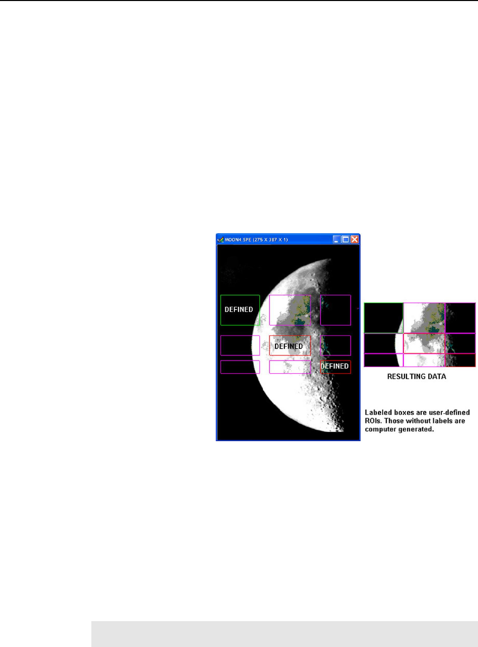
Chapter 11 ROI Definition & Binning 143
Constraints on Defining Multiple Regions of Interest (ROIs)
General: You may create more than 10 ROIs but when data is acquired using these
ROIs, the parameter information for only the first 10 ROIs will be stored when you save
the data.
Spectroscopy Mode:
1. ROIs cannot overlap. This places restrictions on the Slit (Y) values that can be
specified. For example, if Pattern 1 has a Slit Start value of 1 and a Slit Height 100,
the Start value for the next ROI must be greater than 100. If a Full pattern is selected
and stored, it overlaps all others, causing all data collections to be full-chip.
Figure 124 illustrates multiple full-width ROIs.
2. Once the first pattern is defined, all subsequent patterns are automatically assigned
the same X-axis starting, ending, and grouping values. The first pattern need not be
full width — any values in the chip range can be entered, but once stored, those
values will apply as well to subsequently defined patterns. The figures below
illustrate possible ROI patterns. Note the additional functionality available in
Imaging Mode (Figure 126).
Imaging Mode:
In this mode, ROIs can have
varying sizes and degrees of
overlap. However, when you
define multiple ROIs like
those in Figure 126, the
computer automatically
generates six “side-effect”
ROIs in the regions where
extensions of the strips and
columns of the defined ROIs
intersect. Both the defined
and computer generated
ROIs will be stored and the
data for both will be
displayed (see Figure 127).
The side-effect ROIs are
necessary to accommodate
hardware limitations.
Figure 127. Multiple Imaging ROIs and Resulting Data
Methods of Defining and Storing ROIs
A region of interest (full-width or partial width) can be defined by:
1. Opening the Easy Bin dialog and entering the values for a single, full chip wide
spectroscopy mode ROI.
2. Entering values for the Wavelength (X) and Slit (Y) parameters from the keyboard.
3. Dragging the mouse cursor on a displayed image to define a rectangular region and
then clicking the Mouse button. Before using this method, you must acquire a Full-
Chip image. Otherwise, you will get a "Size of Image in Active Window is
Incompatible with Current Chip Size" message when you try to define an ROI.
Note: In Spectroscopy mode, ROIs created via the mouse are limited to full chip
width like the ones depicted in Figure 124. This is not the case in Imaging mode.

144 WinSpec/32 Manual Version 2.6B
4. Defining the region with the mouse and then changing parameter values via the
keyboard before storing the pattern. This allows you to change a full-width ROI
created by mouse selection to a partial-width ROI like the one in Figure 125.
5. After an ROI is defined, its pattern can be stored, edited, or deleted. All defined areas
will be indicated on the displayed image after they have been stored. If a pattern is
being edited, its outline will be green and all other patterns will have red outlines. In
Imaging mode, purple outlines will be drawn if two or more patterns are defined that
do not have identical Wavelength Start and End points (these outlines represent
additional data that will be included in the image acquired using the ROI Setup). The
display of defined regions of interest is automatically updated when patterns are
added or cleared. Stored patterns are save to disk when you exit the WinSpec/32 and
are automatically loaded the next time you start the program.
Notes:
1. Right-clicking inside an ROI opens the ROI Context menu, which, in addition to
providing auto-scale and zoom functions, enables the labeling of image and graphical
data.
2. The Experiment Setup|Save/Load tab allows all experiment set parameters,
including ROI, to be saved in a user-designated file for later recall. See the discussion
of the Save/Load tab in the online Help.
Defining an ROI via Easy Bin:
Easy Bin allows you to define of a single, full chip
wide ROI.
1. Select Easy Bin from the Acquisition menu.
2. On the Easy Bin dialog (Figure 128), click on the
appropriate radio button:
Center 1: Establishes an ROI one pixel high.
Center 10: Establishes an ROI 10 pixel high.
Center 100: Establishes an ROI 100 pixel high.
All: Selects the full chip height.
User Defined: Allows you to set the Slit (Y-axis)
Start and End pixels. If you have a full chip
image displayed, you can use the mouse cursor
Figure 128. Easy Bin dialog
to create the bounding box for the ROI. Since all Easy Bin ROIs are full chip
width, only the box's height parameters will be used.
3. If you have selected User Defined, enter the start and end pixels. This allows you to
create an ROI that is not centered vertically on the chip.
4. Click on OK when you have finished.
To define multiple ROIs, ROIs that are not full chip width, and/or ROIs that are not
centered vertically on the chip, use the ROI Setup functions accessible from the
Experiment Setup dialog.
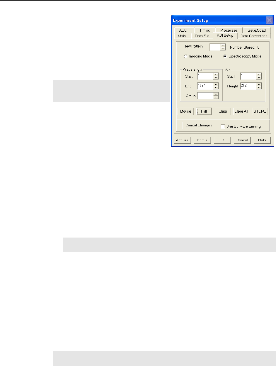
Chapter 11 ROI Definition & Binning 145
Defining ROIs by Keyboard entry:
1. Open the Experiment Setup dialog and
click on the ROI Setup tab to open the ROI
Setup tab (Figure 129).
2. Select the appropriate mode (Imaging or
Spectroscopy). If you do not have the
Imaging option, the Imaging Mode and
Spectroscopy Mode radio buttons will not
be present.
TIP: Acquire a full-chip image before
adding or editing ROI patterns. The existing
patterns will be superimposed on the image.
3. Note the Number Stored value. This will
tell you if how many ROIs have already
been stored. Depending on what you want
to do, you may want click on Clear or
Clear All to remove stored ROI patterns.
4. To add a new pattern, click on the spin
buttons (next to the Number Stored text)
until the text to the far left is New Pattern.
Figure 129. ROI Setup tab
(Spectroscopy Mode)
This will not be necessary if there are no patterns stored.
a. Enter the Wavelength (X-axis) Start, End, and Group values. The Group value
controls the X-axis binning: 1 indicates no binning; higher values indicate the
number of pixels being binned to increase the sensitivity at the expense of
resolution.
Spectroscopy Mode: When multiple ROIs are defined, the Wavelength
values for the first pattern are applied to the subsequent patterns created.
Imaging Mode: Multiple ROIs can have different Wavelength values.
TIP: If you're not sure of the chip size, open the Main tab and note the X and Y
values there.
b. Enter the Slit (Y-axis) Start, Height, and Group (if in Imaging Mode) values.
Spectroscopy Mode: Height controls the Y-axis binning: 1 indicates no
binning; higher values indicate the number of pixels being binned to generate
the strip of data. Do not overlap Slit values.
Imaging Mode: Height is the height of the image and Group determines
the Y-axis binning. Image ROIs can overlap.
c. Click on Store to store the newly created ROI. The Number Stored will be
updated. Repeat this process until you have finished adding ROIs.
5. To edit an existing pattern, click on the spin buttons until the pattern number is
displayed in the Edit Pattern field.
6. Then make your changes.
TIP: If you are changing the Wavelength (X-axis) values in Spectroscopy Mode,
select the first pattern and enter your changes there.
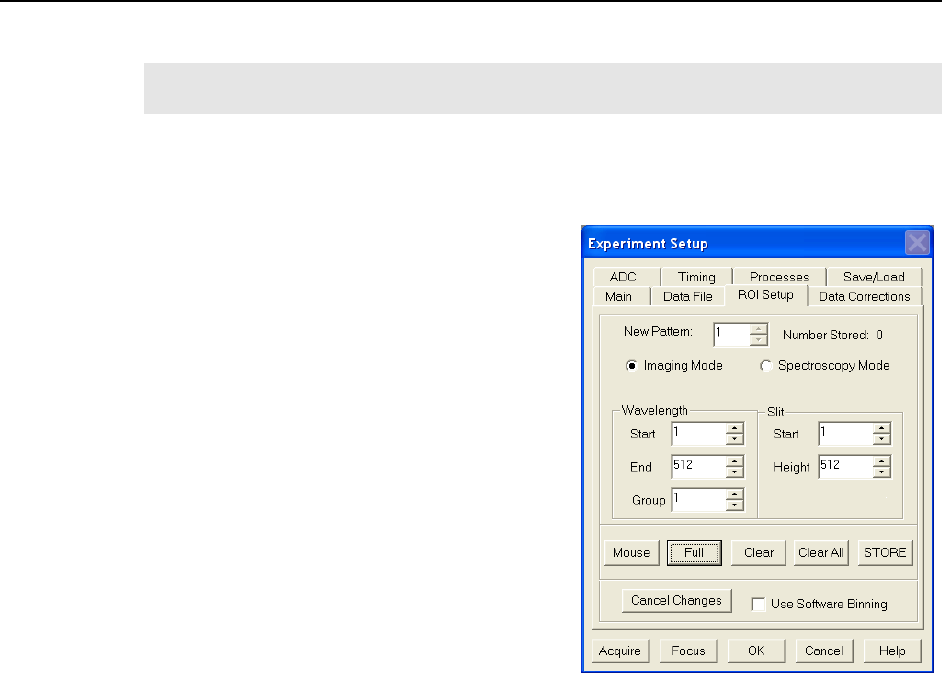
146 WinSpec/32 Manual Version 2.6B
7. Click on Store to store the changed ROI pattern.
Note: To scan the full CCD chip at any time, simply select the Use Full Chip radio
button (on the Main tab) and begin acquisition.
Defining ROIs by Mouse Input:
Often you can easily identify a region of interest by visually inspecting the full-chip
image. When this can be done, it is very easy to define the ROI graphically as follows.
1. First, click on the Use Full Chip radio
button (Experimental Setup Main tab) so
that a full-chip image will be acquired. Then
click on Run. Alternatively, if you already
have an image, open this image and display
it on screen.
2. Next click on the Use Region of Interest
radio button (Main tab). Then click on the
ROI Setup tab to display the ROI Setup tab.
If there are already regions stored, you will
now see them displayed as rectangles on the
displayed image.
3. Click on the spin button to the right of the
New/Edit Pattern field until the field label
says New Pattern (instead of Edit Pattern).
4. Use the mouse to drag an ROI box over the
desired region in the image display.
5. Click on Mouse (ROI tab) to enter the ROI
information. Once this information is
Figure 130. ROI Setup tab
(Imaging Mode)
displayed on the tab, you edit it.
6. Click on Store to save the new pattern.

147
Chapter 12
Correction Techniques
Introduction
Advanced data collection includes background subtraction, flatfield correction, CCD
blemishes removal and cosmic ray removal. The skillful use of these techniques can
significantly enhance measurement capabilities. Note that not all of these techniques will
be available in early releases of the software.
Background Subtraction
Princeton Instruments systems are adjusted so that data have a small offset. This offset
assures that small signals will not be missed. This offset can be subtracted after the signal
is acquired to prevent it from having any influence on the data.
Background subtraction allows you to automatically subtract any constant background in
your signal. This includes both constant offsets caused by the amplifier system in the
controller as well as time-dependent (but constant for a fixed integration time) buildup of
dark charge. Some users collect background spectra with the shutter open, including
ambient light in their background data. The background subtract equation is:
(Raw image data – Background) = Corrected image data.
When background and flatfield operations are both performed, background subtraction is
always performed first. The equation is the following:
(Raw image data – Background)/Flatfield = Corrected image data.
Below are instructions for collecting and using background data files.
Acquiring Background Files:
This operation is similar to normal data acquisition.
1. Use exactly the same temperature setting as will be used in data collection. Wait at
least 30 minutes after the detector has reached operating temperature to ensure
stability.
2. Set the same binning parameters, ROI and Exposure.
3. Select Acquire Background from the Acquisition menu. This will immediately
acquire a background file using the Experiment Setup parameters, only the shutter
will remain closed for most applications.
To acquire a background with the shutter open, or if the Acquire Background feature is too
restrictive in some other way, a background file can be collected as a normal data file. Once
the file is collected and stored, enter the filename in the Background Subtract filename
box on the Experiment Setup|Data Corrections tab (see Figure 131).
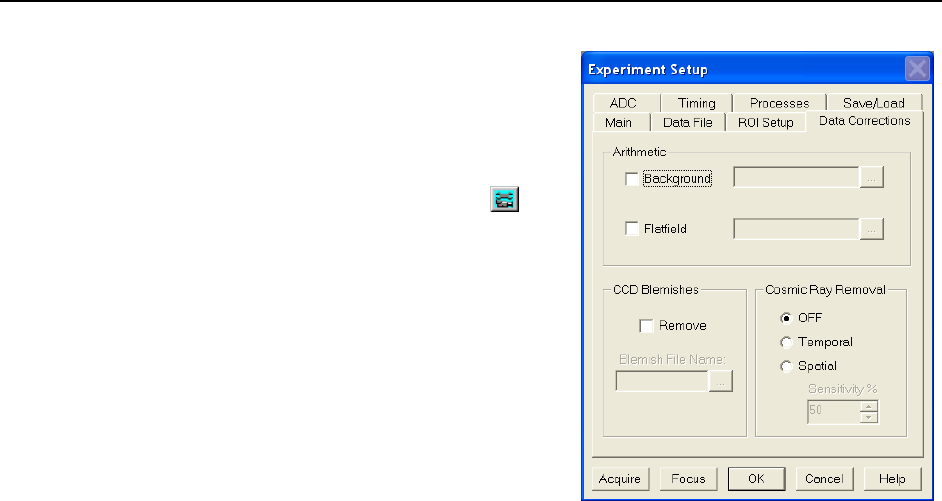
148 WinSpec/32 Manual Version 2.6B
Setting Automatic Background Subtraction:
These steps instruct the software to
automatically subtract a previously stored
background file from each new data
acquisition.
1. Select Experiment Setup from the
Acquisition menu or click on the
button on the Custom Toolbar. This will
open the Experiment Setup dialog.
2. Click on the Data Corrections tab. The
Data Corrections tab will be selected
(Figure 131).
3. Click on the Background checkbox to
turn on background subtraction. Type in
the name of a background file if it is in the
current directory. Alternatively, click on
the button at the end of the entry window
to open the file browser to select the
background file if it is in a different
directory.
Figure 131. Data Corrections tab
4. Once the Background filename has been entered, click on the OK button. This
saves the background filename for all future data acquisitions, or until the
Background is turned off.
The filename entered in the Background box will be subtracted from each new file
before it is displayed or stored. If both Flatfield and Background are selected, the
background will be subtracted first, before the flatfield correction.
Background Subtraction with Intensified Detectors
To properly perform background subtraction with an intensified detector, a new
background must be acquired whenever the intensifier gain setting is changed. This is
necessary because changing the intensifier gain also affects the dark charge of the
intensifier (EBI).

Chapter 12 Correction Techniques 149
Flatfield Correction
Flatfield correction allows you to divide out small nonuniformities in gain from pixel to
pixel. The instructions below set the flatfield correction to be performed before data are
saved to RAM or disk.
Acquiring a Flatfield File:
This operation is similar to normal data acquisition.
1. Use exactly the same temperature setting as will be used in data collection. Wait at least
30 minutes after the detector has reached operating temperature to ensure stability.
2. Set the same binning parameters and ROI. If you plan to use a background file with
data collection, select Background on the Experiment Setup|Data Corrections tab
and enter the name of the background file. This background file will be subtracted
from the flatfield file before it is saved to disk.
3. Illuminate the detector uniformly. The accuracy of this uniformity will be translated
into an accurate flatfield correction.
4. Select Acquire Flatfield from the Acquisition menu (Figure 36, page 63). This will
immediately acquire a flatfield file using the Experiment Setup parameters. Unlike
background subtraction, the shutter will open and close normally.
5. If background subtraction was selected, the background file will be subtracted from
the flatfield file before it is saved to disk.
If the Acquire Flatfield feature is found to be too limiting in some way, a flatfield file can be
collected as a normal data file. Once the file is collected, enter the filename in the Flatfield
Correction filename box on the Experiment Setup|Data Corrections tab (Figure 131).
Activating Automatic Flatfield Correction:
These steps instruct the software to automatically divide each new data file, pixel-by-
pixel, by the specified flatfield file.
1. Select Experiment Setup from the Acquisition menu or click on the button on
the Custom Toolbar. This will open the Experiment Setup dialog.
2. Click on the Data Corrections tab (Figure 131).
3. Click on the Flatfield checkbox to turn on Flatfield correction. Then type in the
name of a flatfield correction file in the current directory. Alternatively, click on the
button at the end of the field to open the file browser to select the flatfield correction
file if it is in a different directory.
4. Once the Flatfield filename has been specified, click on the OK button. This saves
the flatfield filename for all future data acquisitions, or until the Flatfield correction
is turned off.
Each pixel in a new file will be divided by the corresponding pixel in the Flatfield file. If
both Flatfield and Background are selected, the background will be subtracted first,
before the flatfield correction.
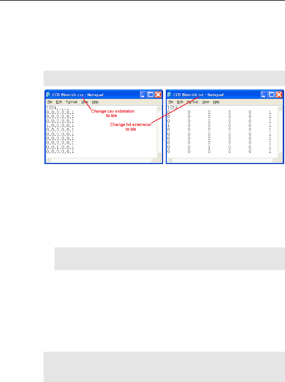
150 WinSpec/32 Manual Version 2.6B
CCD Blemishes
Pixels or columns specified as bad in the blemish file will be replaced by interpolated data
(based on the pixel before and the pixel after the bad pixel) as data is collected. After you
click on the Remove check box, you can select the appropriate blemish file. Clicking on
the button at the right of the Blemish File Name field opens a browse dialog so you can
locate and select a file. If you do not have a blemish file but have determined that there are
one or more bad pixels or columns, you can create a file to be used.
Note: CCD Blemishes removal may not be implemented in early releases of the
software.
Figure 132. Blemish Files: CSV format and Tab Delimited format
Creating a Blemish File:
1. Open an ASCII text editor or spreadsheet editor.
2. On the first line, key in the number of rows on the sensor. For example, you would
key in 1024 if the sensor format was 1024 x 1024.
3. Press [Enter].
4. For each pixel in a row, enter either a 0 (no blemish) or a 1 (blemish), a comma or tab
separator, and press [Enter] after you have completed the entries for that row. Figure
132 shows both comma and tab separated entries.
Note: In the files shown in Figure 132, the blemishes did not go beyond the sixth
column on the sensor. It was not necessary to enter values for the remaining blemish
free columns.
5. If there was only one column blemish and it started in row 1, column 6 of the sensor,
you would have five 0s and a 1 in the sixth position as shown in Figure 132. You
would repeat this entry in succeeding rows until you reached the limit of the blemish.
If there were also individual pixel defects you want corrected, you would replace the
appropriate 0s with 1s. Before you can use the blemish file, it must contain the initial
row indicating the sensor height and a row of values for each row on the sensor. The
blemish file for a 1024 high sensor would contain 1025 rows; for a 200 high sensor,
the file would contain 201 rows.
6. When you have finished entering the 0s and 1s, save the file with a .BLE extension.
Files with this extension are recognized by WinSpec as blemish files.
TIP: If you have a long array, use a spreadsheet that can save data to .CSV or .TXT files.
The numbered rows will help you keep track of where you are. When you have finished
with the data entry, save the data to a text file (.TXT extension) and then change the file
extension to .BLE.

Chapter 12 Correction Techniques 151
Cosmic Ray Removal
Removes highly localized spikes, such as would be caused by cosmic rays interacting
with the silicon of the CCD, from the data after it is acquired but before it is stored. Two
different techniques (in addition to OFF) can be selected. The Temporal technique
compares a series of spectra and requires no user parameters. The Spatial technique
compares the data with the set threshold level. If Spatial is selected, the Sensitivity setting
determines how large a data spike must be to be identified as a cosmic ray effect
(essentially the Sensitivity is a gain setting on the thresholding algorithm. A value of 0
will find 0 cosmics, while a setting of 100 will be most sensitive.). A setting of 50 will
give good results in most situations. Cosmic ray data is replaced by interpolated before-
and-after data.

152 WinSpec/32 Manual Version 2.6B
This page intentionally left blank.
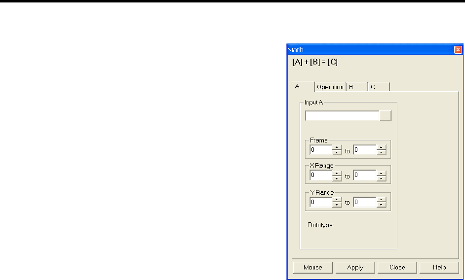
153
Chapter 13
Spectra Math
Introduction
A variety of mathematical operations can be
performed on WinSpec data files. This
functionality, called Spectra Math, is selectable
from the Process menu. The four tabs on the
Math dialog (Figure 133) allow you to select the
source file(s), operation, and the destination file
for the results of the selected mathematical
operation (displayed at the top of the dialog).
Additionally, you can use the mouse to specify an
ROI to be processed (available on tabs A and B).
Source Data and Destination Selection
As many as three data files can be involved in
math operations and there is a corresponding tab
for each of them, A, B, and C. A and B are
Input Files. C is always the Output File. Every
operation requires at least one Input File and an
Output File. Thus, every operation will require
using tabs A and C. In those cases where a
second Input File (or a constant) is required,
Figure 133. Math dialog
tab page B will also be used (see the online Help for detailed descriptions of the
individual Math tabs).
With but a few exceptions, the parameters on the three tabs are the same. Brief
descriptions follow.
Frame: If an input file contains multiple frames, you can specify the ones to be
processed. The default is to process all frames. You additionally have the option
of choosing not to write all of the frames processed to the Output File.
X and Y Range: You can specify the input file pixels to be processed. The default
is to process all pixels. You additionally have the option of restricting the X and
Y pixel range data written to the Output File. An alternative way to specify a
region is to use the mouse to define the region on the active data display of the
input file and then click on Mouse.
Input (Output) Filename: All three tabs have a field for entering the filename. In
each case there is a button at the end of the box which, when pressed, opens a
browser to make selecting and specifying filenames and locations as simple as
possible. In the case of the B tab, there is additionally a field for entering a
constant. Radio buttons are provided that activate one or the other of the two
fields. Either a constant value or a filename can be entered, but not both.

154 WinSpec/32 Manual Version 2.6B
Data Type: For the A and B tabs, the data type is reported only and cannot be
changed. In the case of the C (output) tab, you can specify the data type. Data
types include:
Byte: 8 bits; only the eight least significant data bits (levels 0 to 255) will be saved.
UnInt: Unsigned integer; 16 bits (0 to 65535)
Int: Signed integer; 16 bits (-32768 to 32767)
Long: Signed integer; 32 bits (-2,147,483,648 to 2,147,483,647)
Float: Floating point; 32 bits (-1.75494351e-38 to 3.402823466 e38)
Display Result: This checkbox appears on the C tab only. If checked, the output
image will be displayed as soon as the processing is complete.
Operations
On the Operation tab, the math operations are listed as either Linear or Non-Linear. The
operand(s) for math operations can be a single file, a file and a constant, or two files. In
addition to allowing you to perform these operations on entire files, WinSpec also allows
you to specify the frames (if multi-frame) and a region of interest (ROI).
When working with a single file, the specified operation is performed on each
pixel value of A and the result is written to the corresponding pixel of the Output
File, C. The operations available are grouped under the Non-Linear heading:
Log10 Absolute Value
Natural Log Bitwise Complement
Square Root Binary NOT
Squared
When working with a single file and a constant, the operation will be performed
on each pixel value of A, using the constant specified on the B tab, and the result
is written to the corresponding pixel of the Output File, C. The operations
available are grouped under the Linear heading:
Addition Min
Subtraction Max
Multiplication Bitwise AND
Division Bitwise OR
Bitwise Exclusive OR
When working with two files, corresponding pixels from the two files, A and B,
are operated on and the result is written to the corresponding pixel of the Output
File, C. The operations that can be performed are the same as for a Single file and
Constant described above.
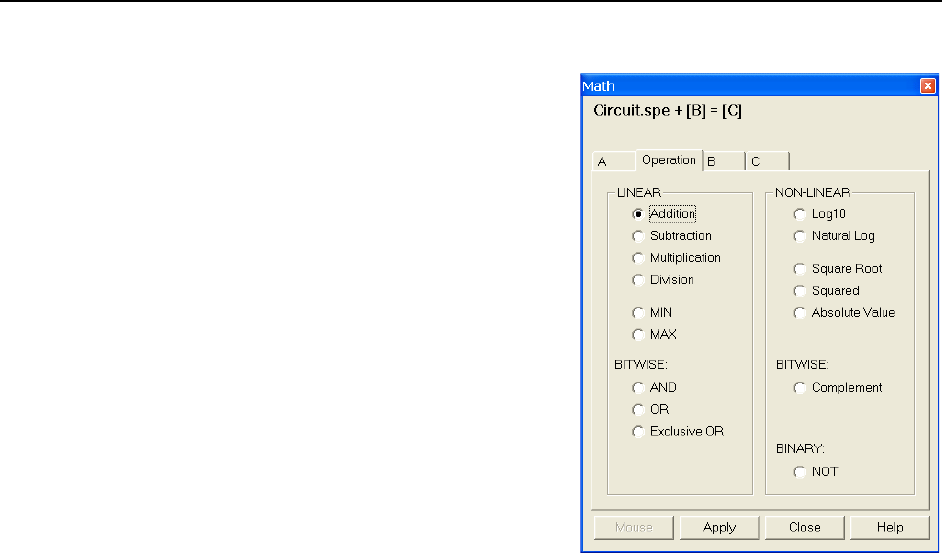
Chapter 13 Spectra Math 155
Operation Descriptions
Linear Operations
Addition: The A file is added, pixel by
pixel, to the B file and the results
written to the C file. It is also possible
to add a constant entered on the B tab to
each point on the A file, with the results
written to the C file.
Subtraction: The B file is subtracted,
pixel by pixel, from the A file and the
results are written to the new file. It is
also possible to subtract a constant
entered on the B tab from each point on
the A file, with the results written to the
C file.
Multiplication: The A file is multiplied,
pixel by pixel, by the B file and the
results written to the C file. It is also
possible to multiply each pixel of the A
file by a constant entered on the B tab,
with the results written to the C file.
Figure 134. Operation tab
Division: The A file is divided, pixel by pixel, by the B file and the results written
to the C file. It is also possible to divide each pixel of the A file by a constant
entered on the B tab, with the results written to the C file.
MIN: The A file is compared, pixel by pixel, with the B file and the smaller of the
two values written to the C file. It is also possible to compare each pixel of the A
file with a constant entered on the B tab, with the smaller of the two values
written to the C file.
MAX: The A file is compared, pixel by pixel, with the B file and the larger of the two
values written to the C file. It is also possible to compare each pixel of the A file
with a constant entered on the B tab, with the larger of the two values written to
the C file.
Non-Linear Operations
Log10: The Log10 of the A file is computed pixel by pixel and the results written to
the C file.
Natural Log: The natural log of the A file is computed pixel by pixel and the results
written to the C file.
Square Root: The square root of each point in the A file is computed and the result
written to the corresponding point of the C file.
Squared: Each point in the A file is squared and the result written to the
corresponding point of the C file.
Absolute: The absolute value of each point in the A file is computed and the result
written to the corresponding point of the C file.

156 WinSpec/32 Manual Version 2.6B
Bitwise Operations
AND: A bitwise AND operation is performed on the binary representation of each
pixel of the A file and each pixel of the B file, with the result written to the C
file. A twelve-bit example follows.
Bits
Decimal
Value
Pixel value in A
0 1 0 1 0 1 0 10 1 0 1
1365
Corresponding pixel value in B
0 0 0 0 0 0 1 1 1 1 1 1
63
Result written to C
0 0 0 0 0 0 0 1 0 1 0 1
21
OR: A bitwise OR operation is performed on the binary representation of each pixel
of the A file and each pixel of the B file, with the result written to the C file. An
eight-bit example follows.
Bits
Decimal
Value
Pixel value in A
0 1 0 1 0 1 0 10 1 0 1
1365
Corresponding pixel value in B
0 0 0 0 0 0 1 1 1 1 1 1
63
Result written to C
0 1 0 1 0 1 1 1 1 1 1 1
1407
Exclusive OR: A bitwise Exclusive OR operation is performed on the binary
representation of each pixel of the A file and each pixel of the B file, with the
result written to the C file. An eight-bit example follows.
Bits
Decimal
Value
Pixel value in A
0 1 0 1 0 1 0 10 1 0 1
1365
Corresponding pixel value in B
0 0 0 0 0 0 1 1 1 1 1 1
63
Result written to C
0 1 0 1 0 1 1 0 1 0 1 0
1386
Complement: For each pixel value n in the A file, the corresponding value in the
output file C is set to -1-n. Otherwise stated, each 0 becomes a 1 and each 1 a 0.
Binary Operations
NOT: For each pixel in the A file, all non-zero values yield a zero, and all zero
values (only) yield a one. The resulting values are written to the corresponding
point of the C file.

Chapter 13 Spectra Math 157
Procedure:
1. Select the operation to be performed on the Operation tab.
2. Enter the first input filename on the A tab.
3. If the operation involves two files or one file and a constant, enter the second file
name on the B tab or enter the value of the constant on the B tab.
4. If you want to process only part of the input images, change the Frame, X Range, and
Y Range values on the A tab, and also on the B tab if two files are involved.
Alternatively, use the mouse to draw an ROI in the active window and click the
Mouse button at the bottom of the dialog to enter those values.
5. Enter the name of the output file on the C tab. If you want to restrict the output data
range, change the Frame, X Range, and Y Range values as appropriate.
6. Select the output file data type.
7. If you want the output file to be displayed as soon as the processing is complete,
check the Display Result box.
8. Click on OK to begin processing or click on Cancel to cancel the operation.

158 WinSpec/32 Manual Version 2.6B
This page intentionally left blank.
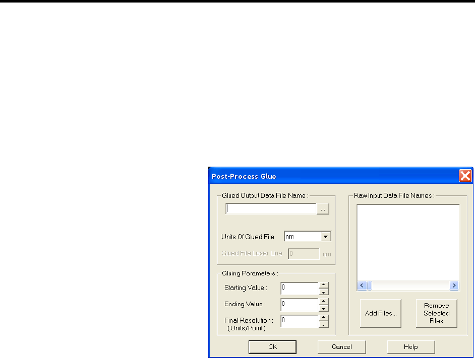
159
Chapter 14
Gluing Spectra
Introduction
There are two ways to glue together multiple exposures into a single contiguous
spectrum. The first is to take existing spectra that have already been calibrated and have
the WinSpec/32 software connect the spectra at the appropriate points. The second
method requires spectrometer control. With correctly calibrated spectrometer control, the
WinSpec/32 software can collect spectra and move the spectrometer, automating the
process of collecting a spectrum whose wavelength range can extend the full spectral
range of the detector.
Gluing Existing Spectra
You can glue any series of
existing data files, providing
that they all have been
properly calibrated in nm.
The files should overlap
some in order to provide
complete spectral data, but
this is not required by the
software. Any collection of
calibrated single spectrum
files can be used to create a
glued file. The only
requirements are that:
The files have been
wavelength
calibrated (either
manually or using
Figure 135. Post-Process Glue dialog
“Auto-Spectro”).
The files have the same number of frames and strips (it is not necessary that they
have the same number of pixels).
Procedure:
1. Take the series of data files you would like to glue and use the file manager to
rename them as a series such as EXP001.SPE, EXP002.SPE, etc. You do not
have to arrange these files in any particular order. These data files will not be
altered in any way by the following procedure.
2. From the Process menu select Glue. This will open the Post-Process Glue
dialog (Figure 135). For more information, see the online Help for this dialog.
3. Use the browser to select the files. The Add Files button opens a browser to
facilitate file selection.

160 WinSpec/32 Manual Version 2.6B
4. Enter the starting and ending wavelength values for the resulting file. If your
wavelength range includes values that are not covered by any of the files in your
series, the resulting spectrum will have some zero values. Any area where valid
data was available will be used to create the glued data.
5. Enter the final resolution you would like the final data file to have. This value is
in units per data point in the output file, so the lower the number the higher the
resolution and the more data points the glued file will contain. For a 2400 groove
per mm grating and a 0.3 m spectrometer a good final resolution would be about
0.1 nm per pixel. For a 1200 groove per mm grating this value would be 0.15 to
0.2 nm per pixel. The total number of data points in the resulting file cannot
exceed 65,535.
6. Enter the Glued Output Data File Name in the field provided. The glued data
will be contained in a single file.
7. If you change your mind about including one or more files in the resulting file,
highlight those files in the Raw Input Data File Names listing and click on
Remove Selected Files.
8. When you have finished selecting files, click on SET to execute the glue
operation.
Step and Glue
If you have spectrometer control through the WinSpec software, the easiest way to create
a glued spectrum is to let the software control both the data collection and the movement
of the spectrometer. The software will take an exposure and, while the shutter is closed,
will move the spectrometer to the next position. Unlike a monochromator with a single
point detector, the wavelength calibration will not depend on the speed and timing of the
stepper motor, only on its final position.
In this case you must set the amount of overlap you would like the spectra to have. The
overlapping data will be averaged for a smooth transition from one exposure to the next.
In addition to the glued data file, the numbered series of individual exposures remain in
the computer for later processing.
Procedure:
1. Make sure that you have a spectrometer already installed and properly calibrated.
This stepping and gluing procedure depends on having correct spectrometer
calibration.
2. Click on Calibration on the menu bar and then on Usage to open the Usage
dialog.
3. Select Auto-Spectro in the Usage dialog. Then select the Calibration units
(nm, cm-1 or rel. cm-1). Be sure the Save as Default button is clicked ON. Then
click on OK to close the Usage dialog.
4. From the Acquisition menu, select Step and Glue. The Step and Glue dialog
(Figure 136) will appear. For more information, see the online Help for this
dialog.
Note: Again, you must have Auto Spectro and either nm, cm-1 or rel. cm-1
selected as the Calibration Units on the Usage dialog (Calibration menu) in
order for the Step and Glue dialog to open. Failure to satisfy this prerequisite
will generate an error message.
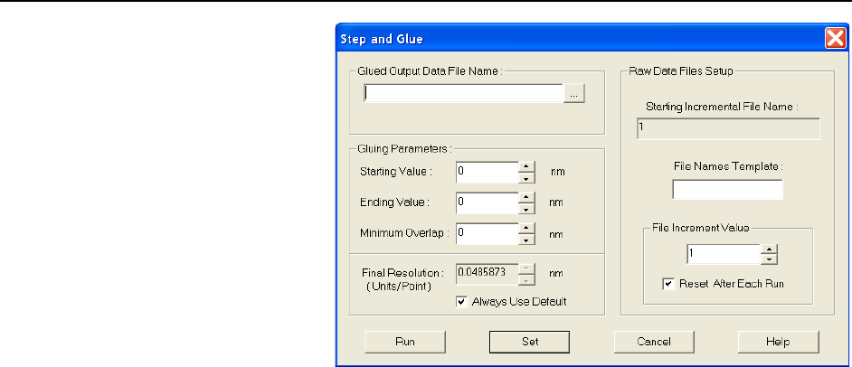
Chapter 14 Gluing Spectra 161
5. The glued data
will be collected
as a series of
incremental
files. These files
will then be
used to create a
single glued
data file. Enter
the name of the
File Name
Template, such
as EXP, in the
File Names
Template box.
There is
Figure 136. Step and Glue Setup dialog
provision for setting the starting File Increment Value. As each incremental file is
taken, the File Increment Value will increment by one. If the Reset After
Each Run box is checked, the File Increment Value will reset to one and the
subsequent set of incremental files will overwrite the first. If the Reset After
Each Run box is unchecked, the File Increment Values assigned to the next and
subsequent runs will start with the next digit after the last one used. No files will
be overwritten.
6. Enter the Starting Value, the Ending Value, and the Minimum Overlap in the
units selected. A good overlap would be about ten times the coverage of a single
pixel. To determine the coverage of a single pixel; click on Always Use
Default; the minimum resolution will be displayed in the Final Resolution edit
box (the resolution changes as the wavelength changes, decreasing at higher
wavelengths).
7. Enter a Final Resolution for the resulting file. Unless you require a certain
resolution, it is easiest to let the computer calculate the final resolution, based on
the spectrometer calibration and other known quantities. In the resulting file,
each point does not represent a physical pixel. The total number of data points in
the resulting file cannot exceed 65,536.
8. Click on SET to store the Step and Glue parameters. If the experiment is ready to
run, click on the RUN to begin collecting data. The software will collect one
exposure at each spectrometer position. It will automatically move the
spectrometer to the next position (with the correct amount of overlap) and collect
the next exposure. The software will collect as many exposures as needed.
During data collection, individual spectra may or may not be displayed, depending on the
time between spectra.

162 WinSpec/32 Manual Version 2.6B
Theory
The Glue operation is done in two stages. First the data in an input file is converted into
an intermediate file with the calibration of the output file, and then the converted file is
glued onto the output file.
The algorithm for the file conversion is based on the fact that the pixels have small but
finite dimensions; this means that each pixel has some wavelength coverage and is not
just a wavelength point. When WinSpec reports the wavelength of a pixel, it is actually
the wavelength at the center of the pixel. Since WinSpec uses a polynomial wavelength
calibration, the wavelength at the center of a pixel “x” is:
Wavelength (center) = A0 + A1x +… + Anx n;
and the wavelengths at the edges are given by:
Wavelength (edges) = A0 + A1(x ½) +… + An(x ½) n,
where the “+” is for one edge and the “-“ for the other.
The intermediate and output file data points also have a finite wavelength coverage, given
by the Final Resolution item on the Step and Glue or Post Process Glue dialog. For
example, with a Starting Value of 400 nm, Ending Value of 700 nm, and Final
Resolution of 1 nm, the Output File will have 301 data points, each with a coverage of 1
nm (The file itself will actually cover the range from 399.5 nm to 700.5 nm). The data
point at 500 nm will have a wavelength coverage from 499.5 nm to 500.5 nm. The
wavelength calibration of the Output File will be linear, and the wavelength at point “x”
given by:
Wavelength (center of point x) = Starting Value + Final Resolution (x - 1).
For each point in the Intermediate File, the conversion routine sums in values from all
pixels whose wavelength range overlaps the wavelength range of the data point. If the
pixel lies entirely within the range of the data point, then 100 % of its value is added; if a
pixel partially lies in the data point’s range, then the percentage of its value that is added
is equal to the percentage of the pixel’s wavelength range lying in the data point range. In
the above example, if an input file pixel had a value of 1234 and a wavelength range of
498.9 nm to 499.6 nm, then the amount summed into the 500 nm point (499.5-500.5)
would be
{(499.6 - 499.5) / (499.6 - 498.8)} 1234 = 154.25,
where (499.6 - 499.5) is the amount of pixel in data point range, (499.6 - 498.8) is the
coverage of the pixel, and 1234 the pixel’s value.
This algorithm, unlike a simple interpolation or curve fitting followed by interpolation,
maintains both the general spectral shape and the intensity content of the original files
(Interpolation could totally remove a peak if it were between two adjacent output data
point wavelengths). The algorithm is general, and doesn’t depend on the input files
having the same wavelength resolution or the same number of pixels.
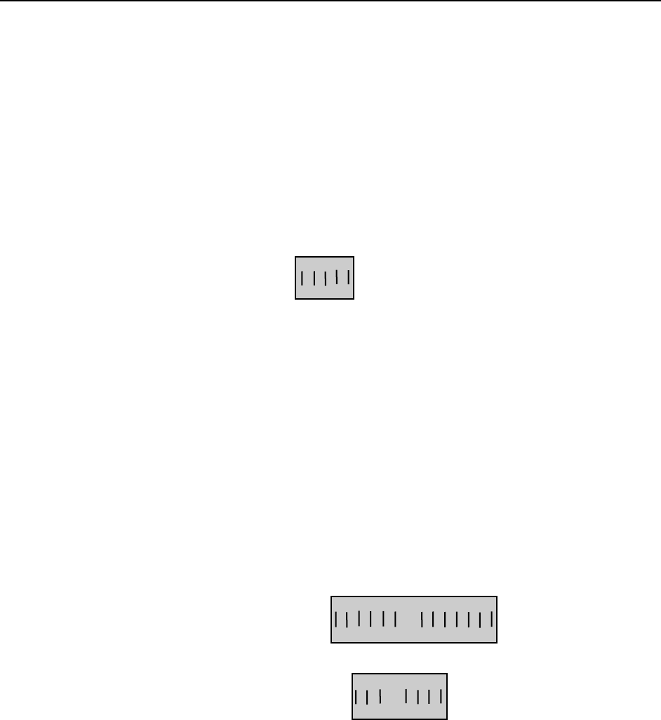
Chapter 14 Gluing Spectra 163
In the second stage of the operation, the intermediate file is glued into the output file. The
gluing is done in increasing wavelength point by point, based on the wavelength value of
the point. Initially the output file contains all zeroes. Files are glued into the output using
several rules, as follows.
For cases with no overlap between data in the intermediate file and the output
file, the intermediate file is just copied to the output file, point by point (pixels in
the input file that are outside the wavelength range of the output file are
discarded).
For cases where the intermediate data overlaps the output data, the data from the
two files are gradually blended over the overlap region. The most common
overlap case for step and glue will be where the intermediate file starts after the
output file has data, but before the output data has ended:
Output file ......... x x x x x x x x 0 0 0 0 0 0 0 0 0 0 0 0 0 ...
Intermediate file y y y y y y y y y y y y y y y y y y ...
There are five points in the above overlap region, and the result of the blending
would be (left to right):
overlap point number blending result
1 (5/6)x + (1/6) y
2 (4/6)x + (2/6) y
3 (3/6)x + (3/6) y
4 (2/6)x + (4/6) y
5 (1/6)x + (5/6) y
(If there is only 1 point in the overlap region then it would have (1/2)x + (1/2) y.)
Another case occurs when the intermediate file starts before the output and ends
after the output file has data. In this case also the data is blended across the
overlap region.
Since the glue is a general algorithm, there will be cases such as the following:
Output file ..... x x x x x x x x ... x x x x x x x x x x x x ...
Intermediate file y y y y y y ... y y y y y y y
or
Output file …000000x x x ... x x x x 0000000…
Intermediate file y y y y ... y y y y y y y y
In these cases, the composition of the result will be 50% Intermediate and 50%
Output.
One of the effects of the above rules is that multiple copies of the same file can be glued
and the result will be the same as if only one copy had been used. The blending allows a
smooth transition for files with broad spectra.

164 WinSpec/32 Manual Version 2.6B
Calibration and ROI Offsets
In an ideal world, when a CCD camera was attached to a spectrograph, the center of the
CCD array would coincide with the center of the spectrograph exit plane. In the real
world, they can be separated by several pixels, so that when the spectrograph goes to 0
nm, the peak can show up 5 pixels to the right of the array center, for example. It is the
function of the Calibration Offset is to compensate for this. It is a wavelength which,
when sent to the Acton, will cause the zero order to land in the center of the array. This
offset is then added to every wavelength sent to the Acton. This offset does not depend
on the scan pattern of the ROI used.
A second kind of Offset is used when "x" ROIs are programmed into the CCD. The
program is designed to keep the requested wavelength in the center of the ROI pattern (in
the center of a full x-axis display). If a full x-axis is scanned or if the ROI is symmetrical
(just ignore the first and last 10 pixels, e.g.), then this ROI Offset is zero. In the case of a
very asymmetrical ROI where the first 512 pixels of a 1024 pixel array are skipped, the
center of the array is "pixel" (1+1024)/2 = 512.5 and the center of the ROI is
(513+1024)/2 = 768.5. If the requested wavelength went to the center of the array rather
than the center of the ROI, it would be just outside the scanned pixels. The ROI Offset is
used to compensate for this. In this example, the ROI Offset is
768.5-512.5 = 256 pixels. This offset is converted to the equivalent wavelength (at the
requested wavelength) and subtracted (in this case) from the requested wavelength before
being sent to the Acton.
Suppose you have calibrated your 1200 g/mm grating on the 275 and the calibration
offset is 2.2057 nm (as reported on the Spectrograph | Calibrate | Offset menu).
Using the above ROI, when you ask for 0.00 nm, the 256 pixel ROI is converted to -
20.199 nm, and the value sent to the 275 is: 0+2.2057-20.199 = -17.98 nm.
The ROI Offset pixel to wavelength calculation uses the results of the dispersion
calibration. So, if a spectrograph is being calibrated using an asymmetrical ROI, the
calibration should be iterated at least once. Because the ROI Offset is calculated
separately from the Calibration Offset, once a spectrograph has been calibrated using one
ROI, the ROI pattern can be changed without affecting the calibration.
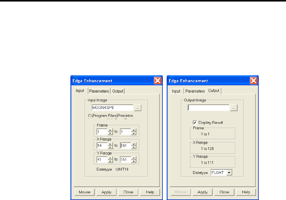
165
Chapter 15
Post-Acquisition Mask Processes
Introduction
Several post-acquisition mask processes, including Edge Enhancement, Sharpening,
Smoothing, a Custom Filter and Morphological Erode and Dilation operations, are
provided in the WinSpec/32 software. These processes all use the same Input and
Output tabs but have unique Parameters tabs. Since the Input and Output functionality
is identical for all of these processes, the Input and Output tabs are described below. The
Parameters tabs are described in the appropriate sections.
Figure 137. Input tab
Figure 138. Output tab
Input tab
The Input tab (Figure 137) selects the data to be operated on. You can specify the data
file, the frames within the file, and the X and Y range on the CCD. The input data-type is
reported. Note that the Mouse button at the bottom of the window allows you to use the
mouse to specify the region to be processed. Simply drag a box in the data region of the
active window and then click on Mouse. The Frame and Range parameters will assume
the values of the defined region. The Mouse button is only active when the Input tab is
selected.
Output tab
The Output tab (Figure 138) allows you to name the output file. It additionally allows
you to select whether the modified data is to be displayed and to select the data type. The
frame and X-Y range are reported information only.
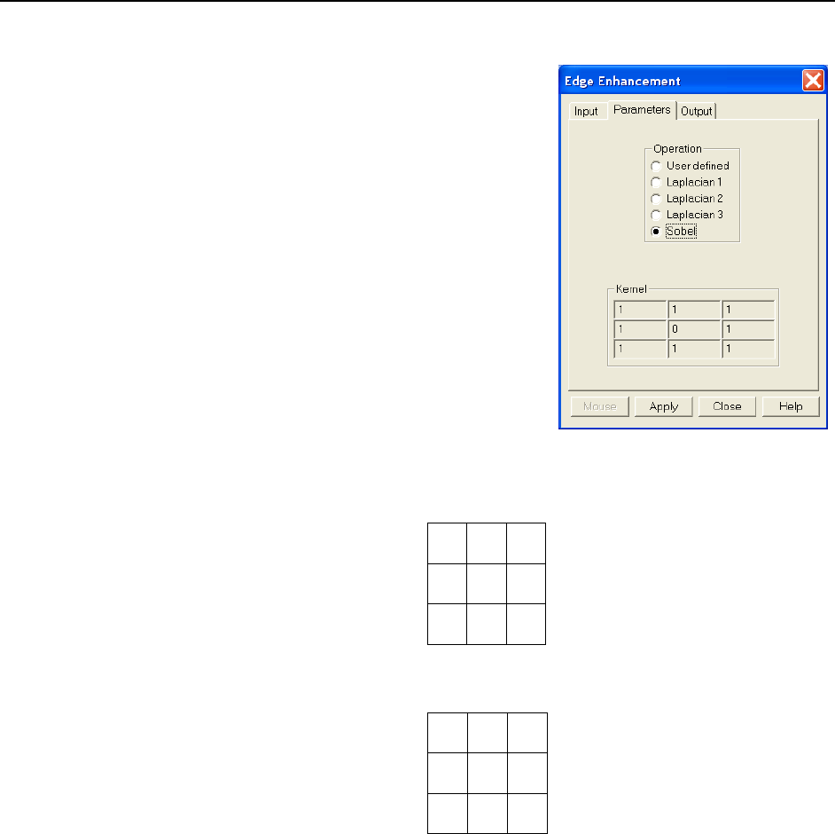
166 WinSpec/32 Manual Version 2.6B
Edge Enhancement
Parameters tab
Edge enhancement is accomplished by mask
operations defined by parameters entered on the
Parameters tab. These functions can enhance edges,
sharpen or smooth features, or erode or dilate an
image. How these images are processed is briefly
described below.
A mask is an n n matrix (n is 3 for all WinSpec/32
operations) that is placed over every n n subsection
of the image. Each parameter in the mask is
multiplied by the corresponding value of the image.
The results are summed and placed in the central
position in the output file. An example will help
illustrate the process.
The following is the Laplacian 1 mask, used to
enhance edges.
Figure 139. Edge Enhancement|
Parameters tab
-1
-1
-1
-1
8
-1
-1
-1
-1
Here is an example of a 3 3 subsection of an image. The middle pixel has the
coordinates 100, 100.
20
20
19
20
21
20
20
19
20
Multiply each pair of corresponding numbers, and sum the products.
(-1 20) + (-1 20) + (-1 19) + (-1 20) +
(8 21) + (-1 20) + (-1 20) + (-1 19) + (-1 20) = 10
The result is placed at position 100, 100 in the output image file. The mask is now placed
over the 9 pixels centered at 101, 100, and the procedure is repeated.
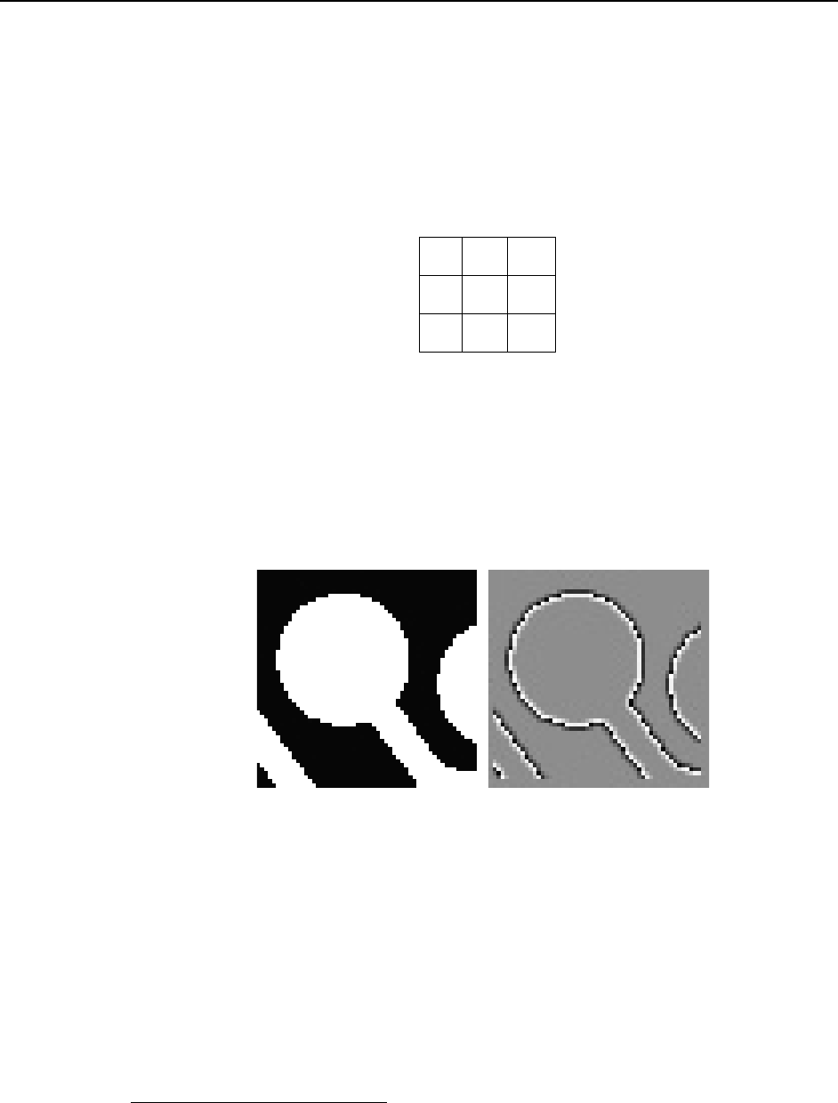
Chapter 15 Post-Acquisition Mask Processes 167
Laplacian Masks
The three Laplacian masks on the Edge Enhancement dialog operate just as described
above. Since the sum of the mask coefficients of the Laplacians sum to zero, the result of
a Laplacian operation on a region of uniform density is zero. Boundary features are
enhanced by varying degrees.
Sobel Edge Detection
The Sobel edge detection method is more involved, but produces greatly enhanced
features. Number the squares of the subregion of the image as follows:
A0
A1
A2
A7
A3
A6
A5
A4
The replacement for the center cell, called R, is1
R = [X2 + Y2]½
Where:
X = (A2 + 2A3 + A4) - (A0 + 2A7 + A6)
Y = (A0 + 2A1 + A2) - (A6 + 2A5 + A4)
Figure 140 illustrates the effect of edge detection on an image.
Figure 140. Original Image (left) and Edge-detected Image (right)
Edge Enhancement Procedure
Use the following procedure to perform Edge Enhancement on an image.
1. Select Edge Enhancement from the Process menu.
2. Enter the Input Image and Output Image names.
3. On the Input tab, select the data frame containing the data on which the operation is
to be performed.
4. If you want to process only part of the Input Image, enter the appropriate X-Y range
values. Alternatively, use the mouse to draw an ROI in the active window and click
the Mouse button at the bottom of the dialog to enter those values.
1 Pratt, William K., Digital Image Processing, John Wiley & Sons, New York, 1978, pp.
487-488.
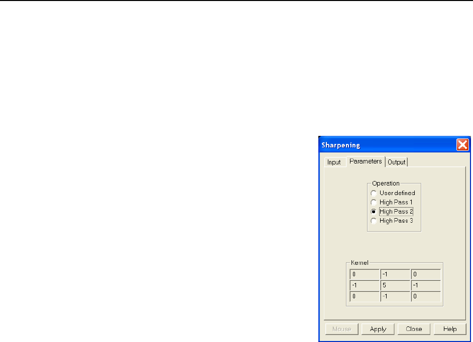
168 WinSpec/32 Manual Version 2.6B
5. Select one of the Operations. Since image features vary widely, it is best to simply
try the different operations to determine the best one.
6. To set a specialized 3 3 mask, select User Defined and change the Kernal
parameters to their new values.
7. Click on Apply to begin processing.
Sharpening Functions
Parameters tab
Sharpening is also accomplished by mask operations,
in this case parameters entered on the Sharpening|
Parameters tab. These masks, sometimes called high
pass filters, enhance regions of high contrast while not
affecting regions of low contrast.
Sharpening Procedure
Use the following procedure to sharpen an image.
1. Select Sharpening from the Process menu.
2. Enter the Input Image and Output Image
names.
3. On the Input tab, select the data frame containing
the data on which the operation is to be
performed.
4. If you want to process only part of the Input
Image, enter the appropriate X-Y range values.
Figure 141. Sharpening|Parameters
tab
Alternatively, use the mouse to draw an ROI in the active window and click the
Mouse button at the bottom of the dialog to enter those values.
5. Select one of the Operations. Since image features vary widely, it is best to simply
try the different operations to determine the best one.
6. To set a specialized 3 3 mask, select User Defined and change the Kernel
parameters to their new values.
7. Click on Apply to begin processing.
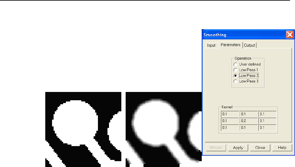
Chapter 15 Post-Acquisition Mask Processes 169
Smoothing Functions
Parameters tab
Smoothing is also accomplished by mask operations, in
this case parameters entered on the the Smoothing|
Parameters tab (Figure 143). These masks, sometimes
called low pass filters, attenuate regions with high
contrast, while leaving pixels in regions of low contrast
almost unchanged. Figure 142 illustrates the smoothing
filter effect.
Figure 142. Original Image (left) and Smoothed Image (right)
Figure 143. Smoothing|Parameters
tab
Smoothing Procedure
Use the following procedure to smooth an image.
1. Select Smoothing from the Process menu.
2. Enter the Input Image and Output Image names.
3. On the Input tab, select the data frame containing the data on which the operation is
to be performed.
4. If you want to process only part of the Input Image, enter the appropriate X-Y range
values. Alternatively, use the mouse to draw an ROI in the active window and click
the Mouse button at the bottom of the dialog to enter those values.
5. Select one of the Operations. Since image features vary widely, it is best to simply
try the different operations to determine the best one.
6. To set a specialized 3 3 mask, select User Defined and change the Kernal
parameters to their new values.
7. Click on Apply to begin processing.

170 WinSpec/32 Manual Version 2.6B
Morphological Functions
Parameters tab
Morphological operations are also accomplished by
mask operations, in this case parameters entered on
the Morphological|Parameters tab. There are
two basic morphological mask operations, Erode
and Dilate. The effect of the Erode process is to
reduce the size of a white region, while Dilation
increases it. All the options except for Block and
User Defined perform the operation in a specific
direction only. Block performs the operation in all
directions.
Note: Depending on the software version,
Iterations and the Open and Close functions may
be grayed out as in Figure 144. If these features are
not grayed out, Open is a number of erodes
(specified by Iterations) followed by the same
number of dilates. Close performs the dilates first
and then the erodes.
Examples of some morphological operations
follow. References are found at the end of this
Figure 144. Morphological|Parameters
tab
chapter. In each case the same binary image is shown to the left and the morphologically
processed image is shown to the right.
Figure 145. Original Image (left) and Dilated Image (right)
Figure 146. Original Image (left) and Eroded Image (right)

Chapter 15 Post-Acquisition Mask Processes 171
Figure 147. Original Image (left) and Opened Image with Three Iterations (right)
Morphological Procedure
Use the following procedure to morphologically process an image.
1. Select Morphological from the Process menu.
2. Enter the Input Image and Output Image names.
3. On the Input tab, select the data frame containing the data on which the operation is
to be performed.
4. If you want to process only part of the Input Image, enter the appropriate X-Y range
values. Alternatively, use the mouse to draw an ROI in the active window and click
the Mouse button at the bottom of the dialog to enter those values.
5. Select the desired Mask Type and Mask Operation.
6. To set a specialized 3 3 mask, select User Defined and change the Kernel
parameters to their new values.
7. Click on Apply to begin processing.

172 WinSpec/32 Manual Version 2.6B
Custom Filter
Filter Matrix tab
The Custom-Filter|Filter-Matrix tab
allows you to set the filter matrix
parameter values. The filter is applied to
the dataset specified via the Input tab
(page 165). The processed data is saved in
the file specified by the Output tab
(page 165).
Filtering is accomplished by mask
operations defined by parameters entered
in the matrix. These functions can enhance
edges, sharpen or smooth features, or erode
or dilate an image. How these images are
processed is briefly described below.
A mask is an n n matrix (n is 5, 7, 9 or
Figure 148. Filter Matrix tab
11) that is placed over every n n subsection of the image. Each parameter in the mask is
multiplied by the corresponding value of the image. The results are summed and placed
in the central position in the output file. Users can specify the Filter Size (5×5, 7×7, 9×9
or 11×11). The Filter Sum is displayed in the adjacent box.
The Load Defaults button sets the matrix parameters to their factory-default values.
When you click on this button, you will see a warning message "Will erase Data for
ALL Filter Sizes; Continue?" with Yes/No. "Yes" will erase ALL filter data before
loading the factory default values.
Custom Filter Procedure
Use the following procedure to apply a custom filter to an image.
1. Select Custom Filter from the Process menu.
2. Enter the Input Image and Output Image names.
3. On the Input tab, select the data frame containing the data on which the operation is
to be performed.
4. If you want to process only part of the Input Image, enter the appropriate X-Y range
values. Alternatively, use the mouse to draw an ROI in the active window and click
the Mouse button at the bottom of the dialog to enter those values.
5. Define the filter by entering the appropriate values into the matrix.
6. Click on Apply to begin processing.
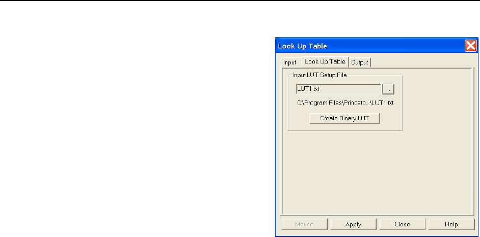
Chapter 15 Post-Acquisition Mask Processes 173
Look Up Table
Look Up Table tab
The Look Up Table function uses an
ASCII text file, provided by the user, to
translate pixel intensities from an input file
into different intensities in an output file.
The input file must be a raw data file
(unsigned 16-bit image) since the Look Up
Table mapping assumes a 0-65536 range of
intensity values in the input file. The map
file is a previously created text file (refer to
pages 174 and 175 for descriptions of the
LUT formats) that must be converted to a
binary map file for the actual operation.
After the text file is selected, clicking on
the Create Binary LUT button converts
the text information to binary format.
Clicking on Apply then remaps the image
intensities and redraws the data display
window appropriately.
Figure 149. Look-Up Table
Look Up Table Procedure
Use the following procedure to process data using the LUT.
1. Select Look Up Table from the Process menu.
2. Using the Input and Output tabs, enter the Input and Output file names.
3. On the Input tab, select the data frame containing the data on which the operation is
to be performed.
4. If you want to process only part of the Input Image, enter the appropriate X-Y range
values. Alternatively, use the mouse to draw an ROI in the active window and click
the Mouse button at the bottom of the dialog to enter those values.
5. Load the LUT. LUT files must be of the type *.TXT. The file name can be entered
directly or selected by using the browser (clicking on the button at the end of the field
opens the browser).
6. Click on the Create Binary LUT button to convert the text-LUT to binary.
7. Click on Apply to begin convert the input data values to the output values specified
per the LUT.

174 WinSpec/32 Manual Version 2.6B
Look Up Table Formats
The contents of a look-up table text file are entered using an ASCII text editor and the
file is saved with a .TXT extension. The format used within the file depends on the type
of remapping: one-to-one remapping of intensity levels or a user-defined selection of
input to output values.
Format 1
This format is for a one-to-one mapping of intensity levels. Imin and Imax (the minimum
and maximum input levels, inclusive) are supplied in the first line with a comma
delimiter. The subsequent values are supplied one output value per line. The mapping
assumes that all of the input intensities in the specified range are represented by an output
value. Therefore, the number of output values in the text file must cover the range
[(Imax-Imin) + 1]. Input levels below Imin are mapped to the value of Ofirst and input
levels above Imax are mapped to the value of Olast.
Imin,Imax Imin,Imax represents inclusive input range to be remapped
Ofirst Ofirst is the output value for Imin (or I1)
O2 O2 is the output value for I2
O3 O3 is the output value for I3
O4 O4 is the output value for I4
. .
. .
. .
Olast Olast is the output value for Imax
Example: The following example is for a one-to-one mapping. As stated previously, the
entries after Imin and Imax are output levels. Based on the Imin and Imax values, there
are 5 output values [(7-3) +1]. In this example, every input intensity less than 3 (Imin)
gets mapped to 20, 3 (Imin) is mapped to 20, 7 (Imax) is mapped to 10, and every input
intensity greater than 7 (Imax) is mapped to 10 (Olast). Input intensities 4, 5, and 6 are
mapped to 22, 23, and 26 respectively.
3,7
20
22
23
26
10

Chapter 15 Post-Acquisition Mask Processes 175
Format 2
This format is not a one-to-one mapping in that input intensities between Imin and Imax,
inclusive, can be omitted from the list of In,Out pairs. Imin and Imax (the minimum and
maximum input levels, inclusive) are supplied in the first line with a comma delimiter.
This format expects an arbitrary number of entries in the form of In,Out and the In,Out
pairs may be listed in any order. The In value must be between Imin and Imax, inclusive.
Anything less than Imin is mapped to the first Input mapping. Anything greater than
Imax gets mapped the output value of the last In,Out pair. Any input value not specified
in an In,Out pair is mapped to zero.
Imin,Imax Imin,Imax represents inclusive input range to be remapped
Ifirst,Ofirst Ofirst is the output value for Ifirst and for any intensity < Imin
I,O I is the input value and O is the output value
I,O O3 is the output value for I3
I,O O4 is the output value for I4
. .
. .
. .
Ilast,Olast Olast is the output value for Ilast and for any intensity > Imax
Example: The following is a custom mapping. As stated previously, the entries after
Imin and Imax represent are input,output levels. Imin and Imax are 3 and 7 respectively.
Everything less than 3 gets mapped to 13 (the first In,Out mapping). Everything greater
than 7 gets mapped to 12 (the last In,Out mapping). Since input values 3 and 4 are not
represented in an In,Out pair, these intensities will be mapped to 0.
3,7
6,13
5,11
7,12
References
To explore in further detail the theory and techniques of digital image processing, we
suggest the following texts:
1. Digital Image Processing, Gregory A. Baxes, Cascade Press, Denver, CO, 1984.
ISBN: 0-945591-00-4.
2. Digital Image Processing, R. C. Gonzalez, P. Wintz, Addison-Wesley, Reading, MA,
1977. ISBN: 0-201-11026-1.
3. Digital Picture Processing, A. Rosenfeld, A. C. Kak, Vol. 1 & 2, Academic Press,
New York, 1982. ISBN (Vol. 1): 0-12-1597-301-2, ISBN (Vol. 2): 0-12-597-302-0.
4. Digital Image Processing, W. K. Pratt, John Wiley, New York, 1978. ISBN: 0-471-
01888-0.

176 WinSpec/32 Manual Version 2.6B
This page intentionally left blank.
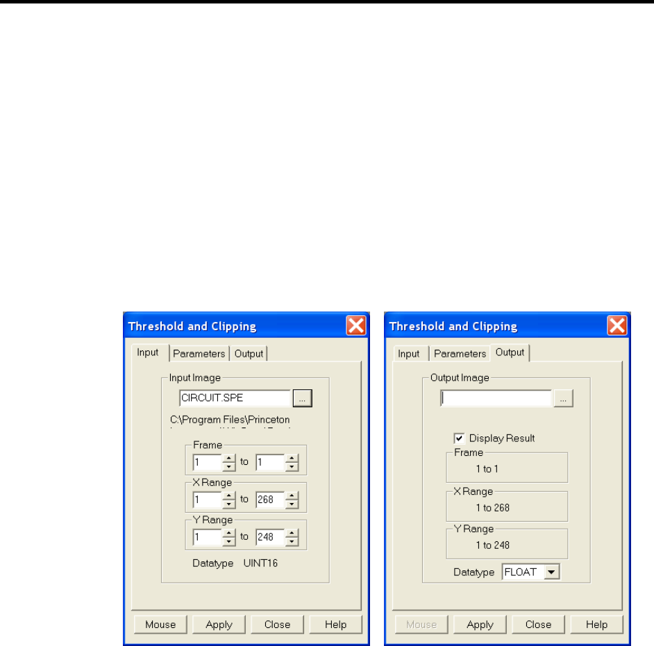
177
Chapter 16
Additional Post-Acquisition Processes
Introduction
The processes included in this chapter are accessible from Processes menu. These
processes all use the same Input and Output tabs but have unique Parameters tabs.
Since the Input and Output functionality is identical for all of these processes, the Input
and Output tabs are described below. The Parameters tabs are described in the
appropriate sections.
Input tab
The Input tab (Figure 150) selects the data to be operated on. You can specify the data
file, the frames within the file, and the X and Y range on the CCD. The input data-type is
reported. Note that the Mouse button at the bottom of the window allows you to use the
mouse to specify the region to be processed. Simply drag a box in the data region of the
active window and then click on Mouse. The Frame and Range parameters will assume
the values of the defined region. The Mouse button is only active when the Input tab is
selected.
Figure 150. Input tab
Figure 151. Output tab
Output tab
The Output tab (Figure 151) allows you to name the output file. It additionally allows
you to select whether the modified data is to be displayed and to select the data type. The
frame and X-Y range are reported information only.
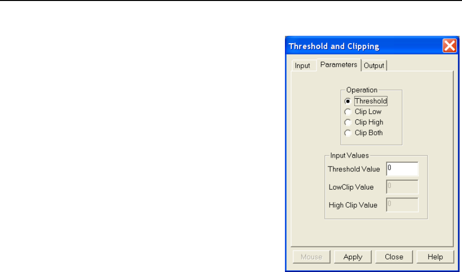
178 WinSpec/32 Manual Version 2.6B
Threshold and Clipping
Clipping an image causes pixels outside the
specified range to be changed. When Clip High
is selected, all pixels with values greater than the
Clip High value will be changed to the Clip
High value. When Clip Low is selected, all
pixels with values less than the Clip Low value
will be changed to the Clip Low value. Selecting
Clip Both will use both Clip High and Clip low
values during the same processing step.
The Threshold function converts an image to
binary (black and white). All intensity values
below the threshold setting are zero (black). All
those above become ones (white).
Procedure
1. Select Clipping/Threshold from the
Process menu.
2. On the Input tab, if the correct input image
does not appear in the Input Image box,
enter the complete file name or search for a
file using the browser, accessed by
Figure 152. Threshold and
Clipping|Parameters tab
the button to the right of the field.
3. On the Input tab, select the data frame containing the data on which the operation is
to be performed.
4. If you want to process only part of the Input Image, enter the appropriate X-Y range
values. Alternatively, use the mouse to draw an ROI in the active window and click
the Mouse button at the bottom of the dialog to enter those values.
5. On the Parameters tab, if a clipping operation is to be performed, select the clipping
option as described above. For a threshold operation, set the threshold level to the
desired value.
6. Enter the name of the Output Image on the Output tab. In later editions of the
software, it will additionally be possible to specify an output frame and data range.
7. Click on Apply to begin processing.
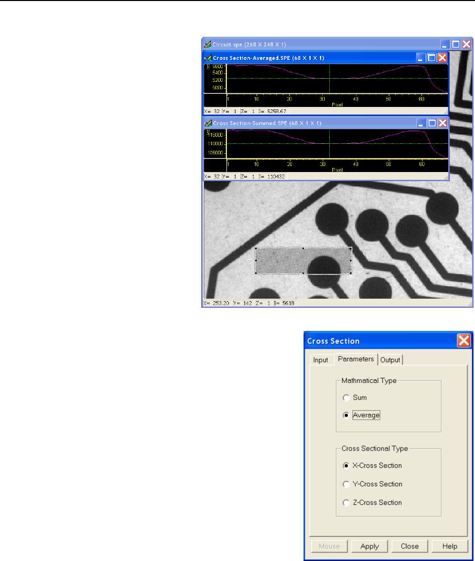
Chapter 16 Additional Post-Acquisition Processes 179
Cross Section
Introduction
Selecting Cross Section
on the Process menu
opens the Cross Section
dialog, which allows you to
separately display and store
horizontal and vertical
cross sections of an image.
Figure 153 shows two
X-axis cross sections
based on the same ROI.
The upper data is
averaged; the lower data is
summed.
Figure 153. Example Cross Sections of an ROI
Procedure
1. Select Cross Section from the Process
menu.
2. On the Input tab, if the correct input image
does not appear in the Input Image box, enter
the complete file name or search for a file
using the browser, accessed by the button to
the right of the field.
3. On the Input tab, select the data frame
containing the data on which the operation is
to be performed.
4. If you want to process only part of the Input
Image, enter the appropriate X-Y range
values. Alternatively, draw an ROI in the
active window using the mouse and click the
Mouse button at the bottom of the dialog to
enter those values.
5. On the Parameters tab, select either Sum
or Average. If Sum is selected, all
Figure 154. Cross Section|Parameters
tab
pixel values in the X, Y, or Z direction, according to whether X-Cross Section,
Y-Cross Section or Z-Cross Section is selected, will be summed to generate the
output. If Average is selected, the average of all of the pixel values in the X, Y, or Z
direction will be summed to produce the output.
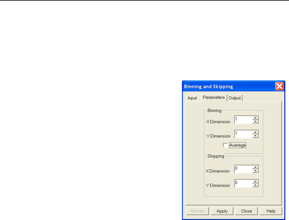
180 WinSpec/32 Manual Version 2.6B
6. On the Parameters tab, select X-Cross Section, Y-Cross Section or Z-Cross
Section, whichever is wanted.
7. Enter the name of the Output file on the Output tab. In later editions of the software,
it will additionally be possible to specify an output frame and data range.
8. Click on Apply to begin processing.
Binning and Skipping
Introduction
Selecting Binning on the Process menu
opens the Binning and Skipping dialog,
which allows binning to be accomplished in
software after the data has been collected. The
Parameters tab allows the bin size to be set
independently in the X and Y directions. The
Skipping parameter allows you to define the
interval between binned regions. The Skipping
parameter size can be independently set for X
and Y. There is also provision for either
averaging or summing the binned data points. If
Average is selected, each output data value will
be the average of the binned data values in each
region. If Average is unselected, each output
data value will be the sum of the binned data
values. The procedure follows.
Figure 155. Post-processing Binning and
Skipping|Parameters tab
Procedure
1. Select Binning and Skipping from the Process menu.
2. On the Input tab, if the correct input image does not appear in the Input Image box,
enter the complete file name or search for a file using the browser, accessed by the
button to the right of the field.
3. On the Input tab, select the data frame containing the data on which the operation is
to be performed.
4. If you want to process only part of the Input Image, enter the appropriate X-Y range
values. Alternatively, use the mouse to draw an ROI in the active window and click
the Mouse button at the bottom of the dialog to enter those values.
5. On the Parameters tab, set the X and Y bin size.
6. On the Parameters tab, select Average if the binned data values are to be averaged.
If the Average box is left unchecked, the binned values will be summed.
7. On the Parameters tab, set the Skip X and Y values. Data points that fall in the skip
zones do not contribute to the output. Skip values of zero are allowable, that is, no
points will be skipped. Leftover points at the end of a strip or column are discarded.

Chapter 16 Additional Post-Acquisition Processes 181
8. Enter the name of the Output file on the Output tab. In later editions of the software,
it will additionally be possible to specify an output frame and data range.
9. Click on Apply to begin processing.
Binning and Skipping Restrictions and Limitations
The following are some restrictions and limitations of the Binning and Skipping function.
This function can resize an image down to a minimum of 1 pixel but WinSpec/32
cannot display an image less than 2 × 2 pixels.
May cause data overflow in the output image if the output data type is selected as
“integer.” If data to be binned will exceed 32,000 counts, select Unint or Long.
The maximum binning and skipping size is the size of the input image. When the
maximum is reached, to increase the binning size you must first decrease the
skipping size, then increase the binning size.
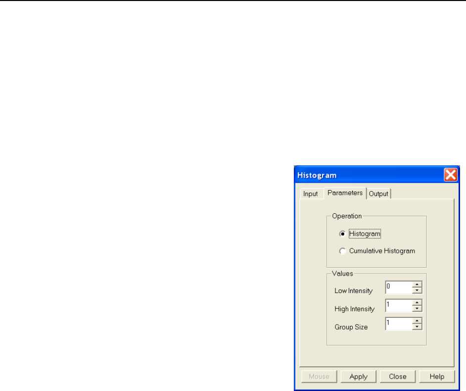
182 WinSpec/32 Manual Version 2.6B
Histogram Calculation
Introduction
Two types of histograms are available for graphing the distribution of intensities of an
image. The Histogram operation groups pixels of a similar intensity together. The X-
axis indicates the intensity, and the Y-axis displays the number of pixels in that intensity
range.
The Cumulative Histogram operation groups pixels of a similar intensity together, once
again using the X-axis to show intensity. This time, however, the Y-axis indicates the
total number of pixels with intensity less than or equal to the range. Thus the Cumulative
Histogram is always an increasing function.
Procedure
1. Select Histogram from the Process menu.
2. On the Input tab, if the correct input image
does not appear in the Input Image box, enter
the complete file name or search for a file
using the browser, accessed by the button to
the right of the field.
3. On the Input tab, select the data frame
containing the data on which the operation is
to be performed.
4. If you want to process only part of the Input
Image, enter the appropriate X-Y range
values. Alternatively, use the mouse to draw
an ROI in the active window and click the
Mouse button at the bottom of the dialog to
enter those values.
5. On the Parameters tab, select either
Histogram or Cumulative Histogram,
whichever is wanted.
Figure 156. Post-processing
Histogram|Parameters tab
6. On the Parameters tab, under Values, enter the Low Intensity and High Intensity
values. These are the Y-Max and Y-min. Then enter the Group Size, which is the
range of intensity that the software will group together as a single data point. In other
words, if the Group Size is 50, pixels having intensities in the range of 1-50 will be
counted and graphed as a single point on the histogram.
7. Enter the name of the Output file on the Output tab. In later editions of the software,
it will additionally be possible to specify an output frame and data range.
8. Click on Apply to begin processing.

183
Chapter 17
Printing
Introduction
WinSpec/32 can be used to print images directly. Methods are listed below both for direct
printing and for using the clipboard to transfer the image to another program for printing.
Setting up the Printer
1. Open the file you want to
print. Make sure that
window is the active one.
From the File menu, open
the Print Setup dialog
(Figure 157).
2. The Print Setup dialog is
similar to that found in
many Windows programs.
You can use the default
printer or select a specific
printer from the list of
installed devices. For
information on installing
printer drivers, consult the
Windows documentation.
Figure 157. Print Setup dialog
The Properties button shows more features of the selected printer driver – again, a
standard Windows feature.
3. Select the Paper Size and Source. The Landscape format (where the paper is
wider than it is tall) is probably the best way to print out data.
4. Click on OK to execute the printer setup selections or Cancel to exit the dialog
leaving the original settings unchanged.
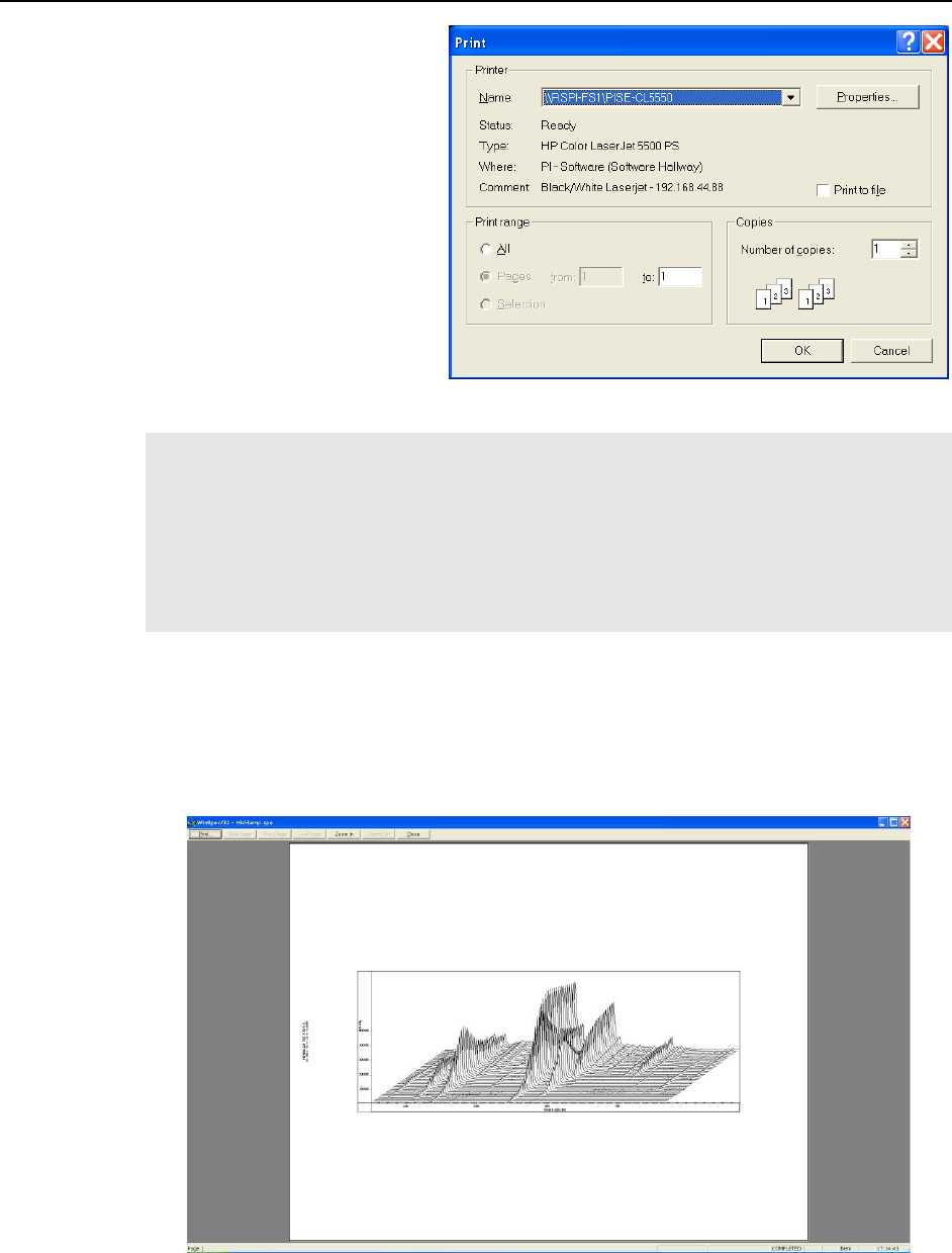
184 WinSpec/32 Manual Version 2.6B
Printing Directly from
WinSpec/32
This procedure assumes you
have already set up the printer
you will be using.
1. From the File menu, open the
Print dialog (Figure 158).
2. Select the number of copies
and pages (if a file contains
multiple frames, each will be
printed as a separate page).
3. Click on OK to initiate the
print.
Figure 158. Print dialog
Notes:
1. Once the Print Setup is properly configured, you can print the active window simply
by selecting Print from the File menu (shortcut Alt, F, P) or by clicking on the Print
button in the standard toolbar.
2. Color mapping to the printer may differ from that shown on the screen. To obtain the
desired output color mapping, you may wish to do a screen capture and then paste the
image into a graphics program for final adjustment before printing.
Print Preview
The Print Preview function gives you a quick idea of how the printed image will look. It
produces an “on-screen print” that looks as closely as possible like a “real” print,
allowing changes in the printer setup to be made quickly and conveniently. Figure 159
show the Print Preview window.
Figure 159. Print Preview window
The button functions are as follows.

Chapter 17 Printing 185
Print…: Opens the Print screen so a print can be initiated.
Next Page: If the file contains multiple frames, each one will occupy a different page.
The Next Page button allows you to step forward sequentially through all
available pages. If the file contains only one image, the Next Page button will
be grayed out.
Prev Page: Allows you to step backwards sequentially through the pages of a
multiple image file.
Two Page: Causes two pages to be displayed at a time in a side-by-side layout.
Zoom In: Allows you to zoom in on the previewed page, allowing a selected area to be
examined in detail. There are two zoom levels. Note that, if not at full zoom, the
cursor becomes a “magnifying glass” if positioned on the image area.
Zoom Out: Allows you to return to the normal (unzoomed) preview display.
Close: Closes the Print Preview window and returns you to the normal WinSpec/32
display.
Printing a Screen Capture
It is also possible to do a screen capture of the entire WinSpec/32 window. This is the
best way to capture such information as cross sections, scaling, and color lookup tables.
A limitation of screen shots is that the resulting image is based on the resolution of the
monitor, not the resolution of the image. For a 1 million pixel CCD, even a 600 × 800
video mode is not enough to show all the pixel information.
1. Display the desired image or images in WinSpec/32. Click once on the WinSpec/32
title bar to make this the active window.
2. Press Alt + Print Screen. This copies the entire contents of the WinSpec/32
window, including image or graph displays and dialog windows, to the clipboard.
Note: Alternatively, press Ctrl+C or select Copy on the Edit menu to copy an
image to the clipboard. This function only works on image displays and only on the
image itself (i.e., scales and cross section information is not transferred). However,
it has an advantage in that the full resolution of the image is retained.
Many text editors and graphics programs allow images to be pasted directly from the
clipboard. Paint Shop Pro, a shareware program, is one example of an inexpensive
program that can edit and save clipboard screen shots.
1. Open the application. Open a new file within that application.
2. Select Paste from the Edit menu. This will place the contents of the clipboard into
the application. If the image seems cut off, try opening a bigger blank image before
pasting the clipboard. The image is now an 8-bit color or grayscale image.
3. Crop the image, if desired. This feature is available in almost any image editing
program.
4. Select Print from the File menu. Print the file.
5. Save the file, if desired. TIFF is an excellent image format for either grayscale or
color shots.
Note: Screen-capture images lose the high dynamic range of the original. The Copy
function (Ctrl+C) retains the full resolution of the data file.

186 WinSpec/32 Manual Version 2.6B
Saving as TIF and Printing
It is also possible to save an image file directly to 8-bit Tif or 16-bit TIFF format by
using the Save As function on the File menu. The resulting file could then be copied to a
graphics editing program for further processing and then printed.
Images saved as 8-bit Tif can be opened with a variety of programs (for example,
Imaging for Windows (Kodak), Microsoft® Paint, Jasc® Paint Shop Pro®, or Adobe®
Photoshop®). The 16-bit TIFF format is not as widely supported. Images saved in this
format can be opened and processed with Adobe Photoshop.
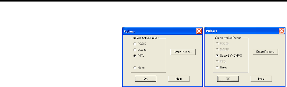
187
Chapter 18
Pulser Operation
Introduction
Four different pulser/timing
generators are available for
use with WinSpec/32. To
be available, pulser support
must have been installed as
described in the Installation
chapter. Pulser support is
then accessed by selecting
Pulsers on the Setup
Figure 160. Pulsers dialog
menu and then selecting the pulser to be used with the system.
Available selections include the Princeton Instruments brand PG200 Pulser, the Princeton
Instruments brand Programmable Timing Generator (PTG) plug-in module for the ST-
133 (high power ver. 3+), the Stanford Research Systems DG535 Digital Delay/Pulse
Generator with Inhibit Option, and the SuperSYNCHRO. The Model PG200 is available
for all Princeton Instruments intensified detectors except the PI-MAX family of
intensified cameras. The PI-MAX and PI-MAX2 require the PTG or DG535. In the case
of the PI-MAX3 or PI-MAX4 camera (which has an internal controller), its internal
pulser is the SuperSYNCHRO. All four pulser/timing generators are programmable from
WinSpec/32. Consult the applicable hardware manuals for detailed instructions on setup
and connection to other devices.
PG200 Programmable Pulse Generator
The PG200 is programmed via one of the serial ports of the computer, such as COM1 or
COM2. The choices provided by the tabs are the same ones that are available using the
PG200 front panel. Basic PG200 operation is reviewed in the following procedure.
1. Make sure the PG200 is connected to one of the serial ports of the computer. Later
you will tell WinSpec/32 the name of this port (COM1, COM2, etc.). The software
cannot automatically detect the location of the PG200.
2. Following the intensifier precautions listed in the hardware manuals, turn on the
PG200 Pulser and wait for it to initialize. If the PG200 is not turned on, the
WinSpec/32 software cannot program it.
3. Select Setup, then Pulsers, then PG200. Then click on the Setup PG200 button to
open the PG200 dialog. If PG200 is grayed out on the Pulsers dialog, PG200 pulser
support has not been installed.
4. Click on the Comm Port tab.
5. Select the Comm Port type, Serial or Demo. Serial must be selected to control the PG200.
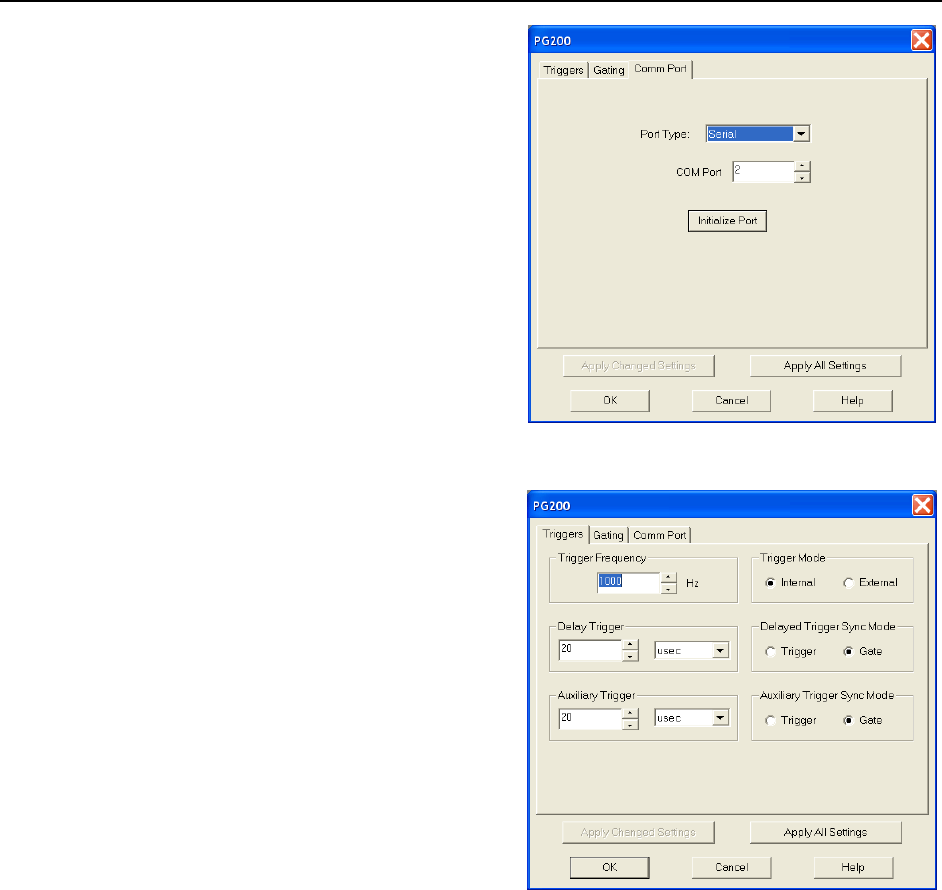
188 WinSpec/32 Manual Version 2.6B
6. Select the PG200 Comm Port.
Generally, the mouse is connected to
COM1 and the Pulser is connected to
COM2. COM ports 1 through 8 can
be selected.
7. Once you have selected the correct
port, click on Initialize Port, which
will cause the software to search for
the pulser. If it cannot find the pulser
on the specified port, such as would
occur if the pulser were not turned on
or if it were connected to a different
port, you will get an error message. If
this happens, check the cable
connections, check that the pulser is
powered, or try a different Comm
port.
Figure 161. PG200|Comm Port tab
8. Click on the Triggers tab
(Figure 162).
9. Select the Trigger mode, either
Internal, in which the PG200 free
runs, or External, in which it is
triggered from an external source.
10. If operating in the Internal trigger
mode, set the Trigger Frequency in
Hz. Consult the PG200 Manual to
determine the maximum Trigger
Frequency for a given set of
conditions.
The PG200 Delay Trigger and
Auxiliary Trigger outputs, are
programmed from the Triggers tab.
They produce trigger outputs that are
synchronized to and delayed from the
Figure 162. PG200|Triggers tab
trigger (Trigger Sync mode) or from the trailing edge of the gate pulse (Gate Sync
mode). In the Gate Sync mode, as the gate pulse changes its position and width, the
trigger outputs remain synchronized with the gate, moving with it. In the Trigger Sync
mode, the trigger outputs do not sweep with the gate but maintain their initial position.
The Delayed Trigger and Auxiliary Trigger outputs are independently programmable.
Programming the Delayed Trigger and Auxiliary Trigger Outputs:
1. Set the Delay Trigger and Aux Trigger initial delay.
2. Set the Delay Trigger output to be synchronized to either the Trigger or the Gate
pulse.
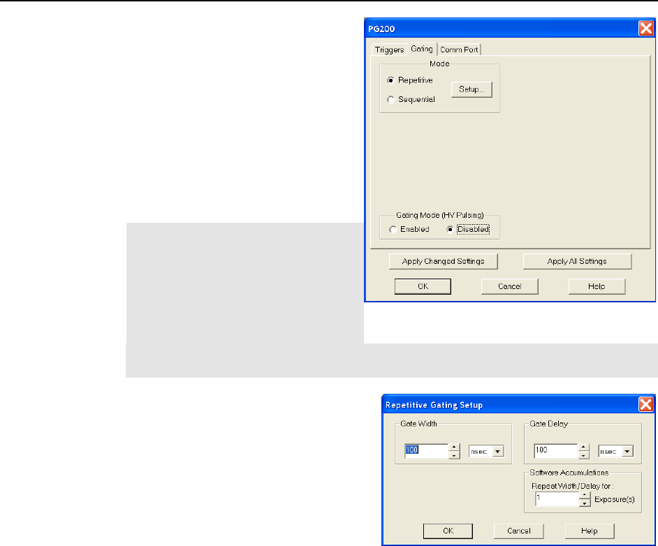
Chapter 18 Pulser Operation 189
3. Set the Aux Trigger output to be
synchronized to either the Trigger or
the Gate pulse.
4. Click on the Gating tab
(Figure 163).
5. Select Repetitive or Sequential and
then click on the adjacent Setup
button. For safety, the Gating Mode
(HV Pulsing) selection should be
Disabled.
Note: In setting the PG200 gating
parameters, whether for Repetitive or
Sequential operation, see your PG200
Manual for pulse width and delay
limitations. Note that gate pulses are
capacitively coupled in many
Princeton Instruments intensified
Figure 163. PG200|Gating tab
camera heads, so high duty cycles and gate widths longer than 1 ms may lead to
reduced gating efficiency.
Repetitive Mode
If Repetitive is selected, the Repetitive
Gating Setup dialog will appear as
shown in Figure 164. In the Repetitive
gating mode, the Gate Width and Gate
Delay remain constant over the course of
the measurement. Set the Gate Width
and Gate Delay to the desired values and
click on OK. The Repetitive Gating
Setup dialog will close and you will
return to the PG200 dialog.
Figure 164. PG200|Repetitive Gating Setup
dialog
Sequential Mode
If Sequential is selected, the Sequential Gating Setup dialog will appear as shown
in Figure 165. In the Sequential Gating mode, the Gate Width and Gate Delay do not
remain constant but change either linearly (Fixed) or exponentially as the
measurement progresses. Fixed is suited to sweeping over a time interval to locate
and recover an event that takes place at the same time with each iteration.
Exponential is well suited to fluorescence decay experiments where the effect under
study changes rapidly at the start of an experiment and then slower and slower,
following a logarithmic curve, as the experiment progresses.
If the measurement is to be done in the sequential gating mode, set the gating
parameters (see "Sequential Mode Parameters" on page 203 for more information)
as appropriate for your intended measurement and click on OK. The Sequential
Gating Setup dialog will close and you will return to the PG200 dialog.
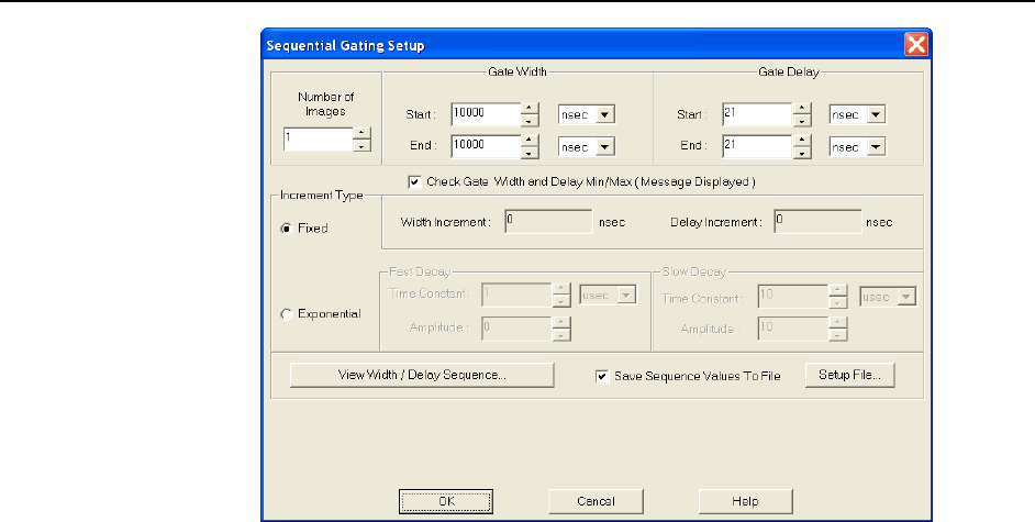
190 WinSpec/32 Manual Version 2.6B
Figure 165. PG200|Sequential Gating Setup dialog
6. Click on the Gating tab.
7. Select Gating Mode (HV Pulsing) Enabled to start gating the intensifier. Be sure
you have followed all intensifier precautions stated in the hardware manuals before
making this selection.
8. Click the Apply Changed Settings button. This writes all changed parameters to
the PG200. It may take several seconds, depending on the number of parameters that
have been changed. To set all of the parameters, click on the Apply All Settings
button.
9. Click on OK to close the dialog.
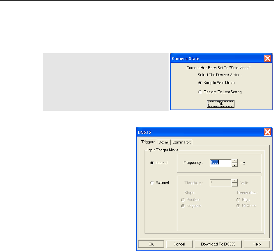
Chapter 18 Pulser Operation 191
DG535 Digital Delay/Pulse Generator
The DG535 is programmed via the IEEE-488 GPIB port of the computer (default GPIB
address is 15). The choices provided by the tabs are the same ones that are available using the
DG535 front panel. Basic DG535 operation is reviewed in the following procedure. The
individual tab selections are discussed in detail in the online Help topics.
Note: The DG535 is used to control the
PI-MAX gate functions. If the system is
equipped with a PI-MAX camera, the Camera
State dialog (Figure 166) will appear when the
software is started. Although the software
always initially places the PI-MAX in Safe
mode, you have the option of restarting with the
last setting (Shutter Mode or Gate Mode).
Figure 166. Camera State dialog
1. Make sure the DG535 is
connected to the computer’s
IEEE-488 GPIB port. Later
you will tell WinSpec/32 the
DG535’s GPIB address. The
default setting is 15.
2. Following all intensifier
precautions listed in the
hardware manuals, turn on the
DG535 and wait for it to
initialize. If the DG535 is not
turned on, the WinSpec/32
software will not be able to
program it.
3. Select Setup and then
Pulsers to open the Pulsers
dialog.
4. Select DG535. Then click on
Figure 167. DG535 dialog
the Setup DG535 button. The DG535 dialog will open.
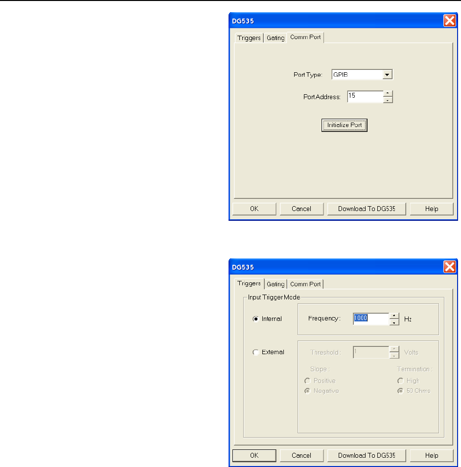
192 WinSpec/32 Manual Version 2.6B
5. Click on the Comm Port tab
(Figure 168).
6. For the Port Type select
GPIB. Then set the Port
Address to the GPIB address
of the DG535. Default setting
is 15.
7. Once you have selected the
correct port address, click on
Initialize Port. If the software
cannot find the pulser on this
port, such as if the pulser is
not turned on or if the address
setting incorrect, you will get
an error message. If this
happens, check the address,
check the cable connections
and check that the pulser is
powered.
Figure 168. DG535|Comm Port tab
8. Click on the Triggers tab
(Figure 169).
9. Select the Trigger mode,
either Internal, in which the
DG535 free runs, or
External, in which it is
triggered from an external
source.
10. If operating in the Internal
trigger mode, set the Trigger
Frequency in Hz. Consult
the DG535 Manual to
determine the maximum
Trigger Frequency that can be
used in your application.
11. If operating in the External
trigger mode, specify the
Slope, Threshold, and
Termination appropriate for
the trigger source.
Figure 169. DG535|Triggers tab
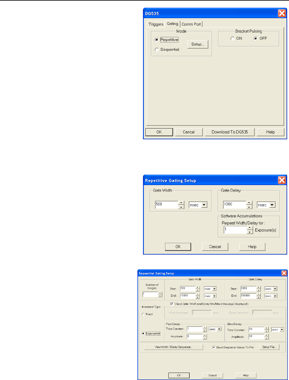
Chapter 18 Pulser Operation 193
12. Click on the Gating tab.
13. Select Repetitive or
Sequential and then click on
the adjacent Setup button.
Repetitive Mode: If
Repetitive is selected, the
Repetitive Gating setup
dialog will appear
(Figure 171). In this mode,
the Gate Width and Gate
Delay remain constant over
the course of the
measurement.
If operating in the
Repetitive Gating mode,
simply set the Gate Width
and Gate Delay to the
desired values and click
Figure 170. DG535|Gating tab
on OK. The Repetitive Gating Setup dialog will close and you will return to
the DG535 dialog.
Sequential Mode: If
Sequential is selected, the
Sequential Gating
Setup dialog will appear
as shown in Figure 172. In
the Sequential Gating
mode, the Gate Width and
Gate Delay do not remain
constant but change either
linearly or exponentially as
the measurement
progresses.
Figure 171. DG535|Repetitive Gating Setup
Linear is suited to
sweeping over a time
interval to locate and
recover and event
that takes place at the
same time with each
iteration.
Exponential is well
suited to
fluorescence decay
experiments where
the effect under
study changes
rapidly at the start of
an experiment and
then slower and
Figure 172. DG535|Sequential Gating Setup dialog
slower, following a logarithmic curve, as the experiment progresses. The
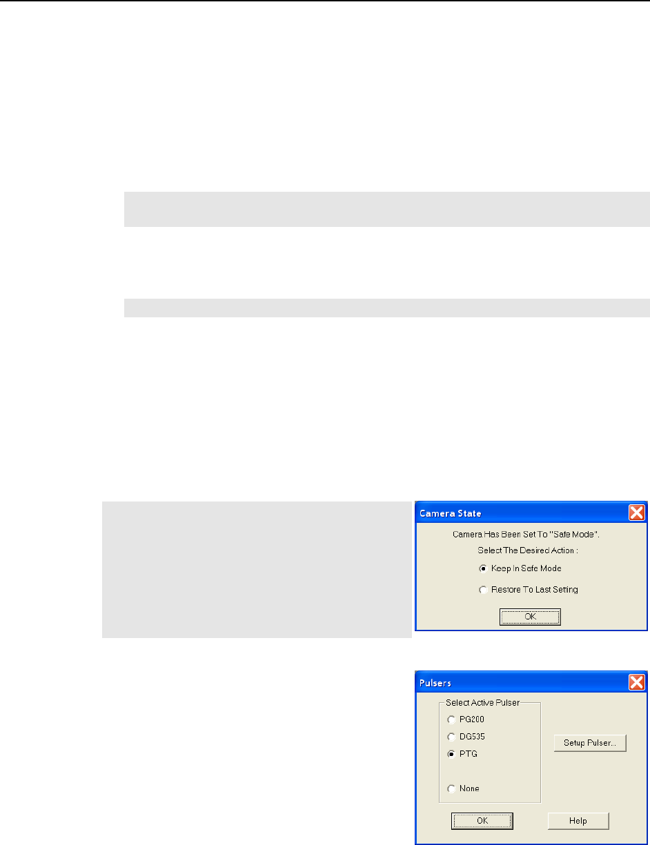
194 WinSpec/32 Manual Version 2.6B
resulting data points can be spline-fitted to generate the complete curve so
that the decay constant can be calculated, even where the data derives from
two decay processes occurring simultaneously.
If the measurement is to be done in the sequential gating mode, set the gating
parameters (see “Sequential Mode Parameters” on page 203 for more
information) as appropriate for your intended measurement and click on OK.
The Sequential Gating Setup dialog will close and you return to the
DG535 dialog.
14. Select Bracket Pulsing On or Off.
Note: Bracket pulsing is only useful in low duty factor gated measurements in the
UV with the PI-MAX camera. See your PI-MAX manual for detailed information.
15. After you have finished setting up the parameters, click on Download to DG535.
This writes all of the parameter values to the DG535.
16. Click on OK to close the window.
Note: The DG535 can also be controlled interactively as data is being collected.
Programmable Timing Generator (PTG)
Unlike the PG200 and the DG535, the PTG is not a free-standing instrument but rather a
plug-in module designed for installation in a special version of the ST-133 Controller.
This novel and highly integrated approach to timing generator design, with its advanced
high-speed electronics, low insertion delay and programmable functions, achieves
superior performance as the ultimate gate controller for the PI-MAX Intensified Camera.
Basic PTG operation is reviewed in the following procedure. The individual tab
selections are discussed in detail in the online Help topics.
Note: The gate functions of the PI-MAX camera
are controlled by the PTG. If the system is
equipped with a PI-MAX camera, the Camera
State dialog (Figure 173) will appear when the
software is started. Although the software always
initially places the PI-MAX in Safe mode, you
have the option of restarting with the last setting
(Shutter Mode or Gate Mode).
Figure 173. Camera State dialog
1. Following the intensifier precautions stated in
the hardware manuals, turn on the Controller
(PTG installed). If the Controller is not turned
on, the WinSpec/32 software will not be able
to control the PTG.
2. On the Setup menu select Pulsers to open
the Pulsers dialog.
3. Select PTG. Then click on the Setup Pulser
button. The PTG dialog (Figure 175) will open.
If PTG is grayed out on the Pulsers dialog,
PTG support has not been installed.
Figure 174. Pulsers dialog
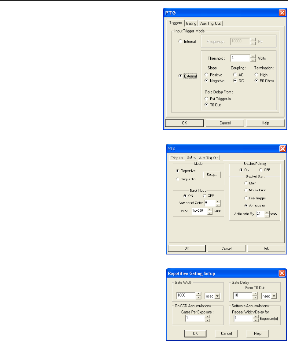
Chapter 18 Pulser Operation 195
4. Select the Trigger mode, either
Internal, in which the PTG free runs,
or External, in which it is triggered
from an external source.
5. If operating in the Internal trigger
mode, set the trigger Frequency in
Hz.
6. If operating in the External trigger
mode, specify the Threshold, Slope,
Coupling, Termination and Gate
Delay From appropriate for the
trigger source. Note that the gate delay
from the T0 connector is approximately
24 ns.
7. Click on the Gating tab
(Figure 176).
Figure 175. PTG|Triggers tab
8. Select Repetitive or Sequential and
then click on the adjacent Setup button.
Repetitive Mode
If Repetitive is selected, the Repetitive
Gating Setup dialog will appear as
shown in Figure 177. In the Repetitive
gating mode, the Gate Width and Gate
Delay remain constant over the course
of the measurement. If operating in the
Repetitive Gating mode, simply set the
Gate Width and Gate Delay to the
desired values and click on OK. The
Repetitive Gating Setup dialog will
close and you will return to the PTG
dialog.
Sequential Mode
If Sequential is selected, the
Sequential Gating Setup dialog will
appear as shown in Figure 178. In the
Sequential Gating mode, the Gate
Width and Gate Delay do not remain
constant but change either linearly
(Fixed) or exponentially as the
measurement progresses.
Figure 176. PTG|Gating tab
Figure 177. PTG|Repetitive Gating Setup
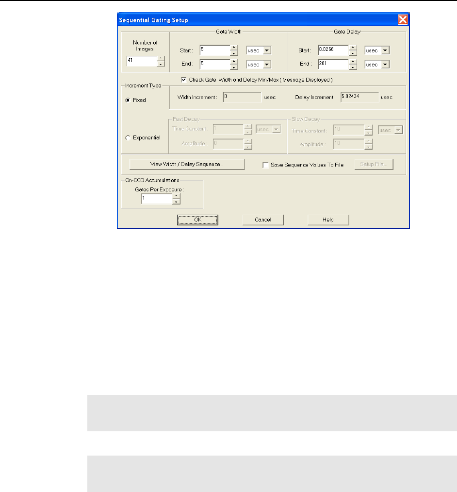
196 WinSpec/32 Manual Version 2.6B
Figure 178. PTG|Sequential Gating Setup dialog
Fixed is suited to sweeping over a time interval to locate and recover an event that
takes place at the same time with each iteration. Exponential is well suited to
fluorescence decay experiments where the effect under study changes rapidly at the
start of an experiment and then slower and slower, following a logarithmic curve, as
the experiment progresses. In any case, if the measurement is to be done in the
sequential gating mode, set the gating parameters (see “Sequential Mode
Parameters” on page 203 for more information) as appropriate for your intended
measurement and click on OK. The Sequential Gating Setup dialog will close and
you return to the PTG dialog.
9. Select Burst ON or OFF. If you select ON, each trigger will initiate a burst of gate
pulses. Set the number of pulses in the burst and their period.
Note: If Burst and Bracket Pulsing are both selected, the entire burst will be
bracketed but not the individual pulses within a burst. When both of these modes are
active, you must select Main+Burst for the Bracket Start.
10. Select Bracket Pulsing ON or OFF.
Note: Bracket pulsing is only useful in low duty factor gated measurements in the
UV with the PI-MAX camera. See your PI-MAX system manual for detailed
information.
11. If you select Bracket Pulsing ON, next select the Bracket Start appropriate to your
setup. Keep in mind that the on/off switching of the MCP bracket pulsing is slow,
taking about 500 ns to turn on and 200 ns to turn off.
The Bracket Start choices are:
Main: Main times the bracket start from the main trigger (either an external or an
internal trigger). Select this if the event of interest will occur at least 1 µs after
the main trigger (the 1 µs includes the 500 ns required to turn the MCP fully on).
Main+Burst: Select this if Burst mode is active. Brackets an entire burst but not
the individual pulses within a burst.

Chapter 18 Pulser Operation 197
Pre-Trigger: Allows you to capture an event that would otherwise occur while
the MCP was turning on. This selection requires that, in addition to the main
trigger at Ext Trig In, you trigger the PTG by a pulse applied to the Pre-Trig In
BNC. The pre-trigger must be at least 525 ns before the main trigger. After an
insertion delay of approximately 25 ns, the MCP will be gated on before the main
trigger occurs. The main trigger plus the gate delay and width parameters
determine the photocathode gating and the MCP turn off. Because the MCP is
gated on earlier, it is on for a longer period of time and therefore there is a slight
loss of on/off ratio. However, you would be able to capture a non-repetitive
event.
Anticipator: Select this if the experiment is repetitive, driven by an external
trigger at a constant frequency, and the event of interest would occur before the
MCP has fully turned on. It is critical that the trigger pulse be as jitter free as
possible, since the anticipator circuit will look at the pulse repetition rate (for the
first pulse to pulse period), and then anticipate each of the subsequent external
triggers in the series. In this way, the bracketing pulse is timed to lead the
photocathode gate pulse by the anticipate time entered in the Anticipate By
field. The on/off ratio in the UV is retained.
For proper operation, the bracketing pulse must begin at least 500 ns before the
gate pulse. The minimum Anticipator Time is 500 ns (or the minimum PI-MAX
bracket lead-time from EEPROM) minus the minimum Gate Delay time. For
example, with a minimum Gate Delay time of 200 ns, the minimum Anticipator
time would be 300 ns.
12. The Aux. Trig. Out tab sets the delay time of the Auxiliary Trigger Output with
respect to the PTG trigger time. The minimum delay is 24 ns and the longest is
10 ms. The resolution is 0.04 ns. The auxiliary timer's output is available through the
Aux. Trig. Out rear panel BNC for triggering other system components.
The Automate for Single Trigger Kinetics Delay check box will only appear if
you have set up the PTG for single trigger kinetics. When this box is checked, the
Delay from T0 box will be grayed out and the Delay from T0 will be automatically
calculated from the gate width + gate delay times whenever either or both of these
times is changed.
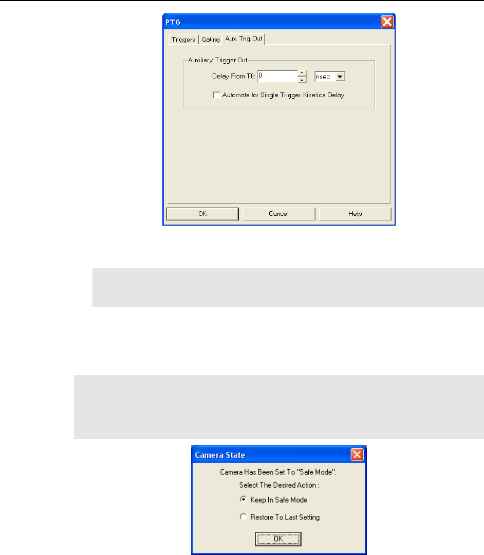
198 WinSpec/32 Manual Version 2.6B
Figure 179. PTG|Aux. Trig. Out tab
13. Click the OK button. This writes all of the parameter values to the PTG.
Note: The PTG can also be controlled interactively as data is being collected. For
more information, see “Timing Generator Interactive Trigger Setup,” starting on
page 206.
SuperSYNCHRO Timing Generator
SuperSYNCHRO is a timing generator that has been designed into the PI-MAX3 and
PI-MAX4. Basic SuperSYNCHRO operation is reviewed in the following procedure.
Note: The gate functions of the PI MAX3 or PI-MAX4 camera are controlled by the
SuperSYNCHRO. Because the system is equipped with a PI-MAX3 or PI-MAX4
camera, the Camera State dialog will appear when the software is started. Although the
software always initially places the camera in Safe mode, you have the option of
restarting with the last mode setting.
Figure 180. Camera State dialog
Procedure:
1. Following the intensifier precautions stated in the PI-MAX3 or PI-MAX4 system
manual, turn on the camera. Then start the WinSpec/32 software.
2. On the Setup menu select Pulsers to open the Pulsers dialog.
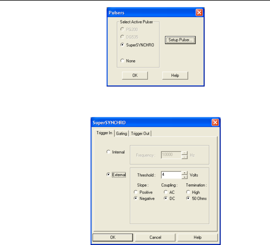
Chapter 18 Pulser Operation 199
Figure 181. Pulsers dialog
3. Select SuperSYNCHRO. Then click on the Setup Pulser button. The
SuperSYNCHRO dialog will open.
Figure 182. SuperSYNCHRO dialog
4. Select the Trigger In mode, either Internal, in which SuperSYNCHRO free runs, or
External, in which it is triggered from an external source.
5. If operating in the Internal trigger mode, set the trigger Frequency in Hz.
6. If operating in the External trigger mode, specify the Threshold, Slope, Coupling
and Impedance appropriate for the trigger source.
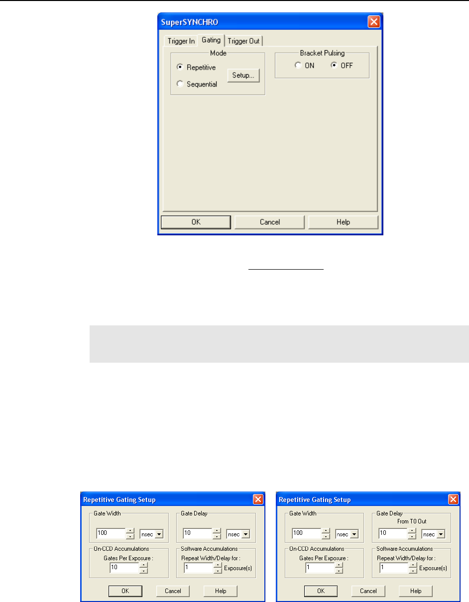
200 WinSpec/32 Manual Version 2.6B
Figure 183. SuperSYNCHRO\Gating tab
7. If the PI-MAX3 or PI-MAX4 has a Gen II intensifier, you can turn Bracket Pulsing
ON or OFF. When it is turned ON, the MCP will be biased OFF except for an
interval that brackets the timing of the photocathode gate. This minimizes optical
leakage through the photocathode to the UV-sensitive MCP when the photocathode
is gated Off. Bracket pulsing does not help in the visible region.
Note: Bracket pulsing is only useful in low duty factor gated measurements in the
UV with the PI-MAX3 or PI-MAX4 camera. See your PI-MAX3 or PI-MAX4
system manual for detailed information.
8. Click on the Gating tab.
9. Select Repetitive or Sequential and then click on the adjacent Setup button.
Repetitive Mode
If Repetitive is selected, the Repetitive Gating Setup dialog will appear. In the
Repetitive Gating mode, the Gate Width and Gate Delay remain constant over the course
of the measurement. If operating in the Repetitive Gating mode, simply set the Gate
Width and Gate Delay to the desired values and click on OK. The Repetitive Gating
Setup dialog will close and you will return to the SuperSYNCHRO dialog.
Figure 184. SuperSYNCHRO|Repetitive Gating dialog (Internal Trigger on left;
External Trigger on right)
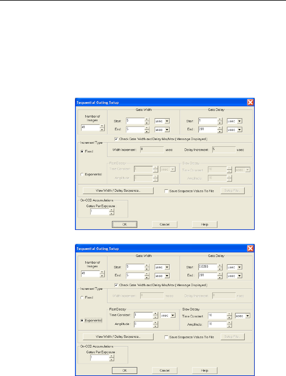
Chapter 18 Pulser Operation 201
Sequential Mode
If Sequential is selected, the Sequential Gating Setup dialog will appear. In the
Sequential Gating mode, the Gate Width and Gate Delay do not remain constant but change
either linearly (Fixed) or exponentially as the measurement progresses. Fixed is suited to
sweeping over a time interval to locate and recover an event that takes place at the same time
with each iteration. Exponential is well suited to fluorescence decay experiments where the
effect under study changes rapidly at the start of an experiment and then slower and slower,
following a logarithmic curve, as the experiment progresses. In any case, if the measurement
is to be done in the Sequential Gating mode, set the gating parameters as appropriate for your
intended measurement and click on OK. The Sequential Gating Setup dialog will close
and return you to the SuperSYNCHRO dialog.
Figure 185. SuperSYNCHRO|Sequential Gating dialog (Internal Trigger)
Figure 186. SuperSYNCHRO|Sequential Gating dialog (External Trigger)
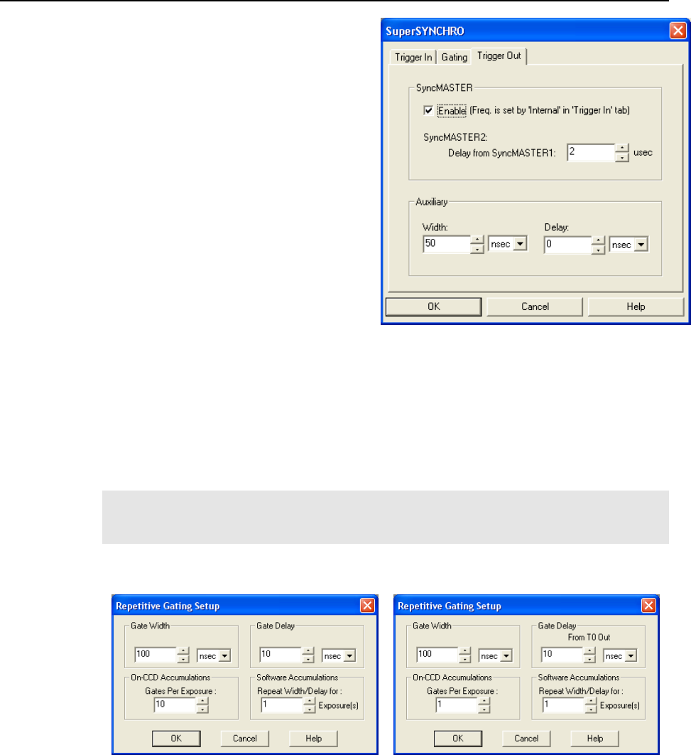
202 WinSpec/32 Manual Version 2.6B
10. The functions on the Trigger Out tab
(Figure 187) allow you to enable the
SyncMASTER trigger output from the
SyncMASTER1 and SyncMASTER2
connectors on the AUX I/O cable and
set up the Aux. Out signal at the AUX
OUT connector on the rear of the
PI-MAX3 or PI-MAX4.
When you enable SyncMASTER1,
the output of that connector will be at
the frequency entered on the
Trigger In tab.
The output of the SyncMASTER2
connector will be at the same
frequency as that of
SyncMASTER1. However, you can
enter a delay so the edges of that
signal will occur after the edges
Figure 187. SuperSYNCHRO|Trigger Out tab
of SyncMASTER1.
If you will be using the Aux. Out signal from the SuperSYNCHRO to trigger a
piece of equipment, enter the Auxiliary pulse width needed to trigger the
equipment. Then enter the pulse delay time. The delay is based on T0 (in effect it
is a delay from SyncMASTER1which also starts at T0).
11. Click the OK button. This writes all of the parameter values to SuperSYNCHRO.
Note: If you are acquiring data and decide that some of the trigger or gating parameters
need to be changed, you must stop data acquisition first. Then you can make the changes
and restart data acquisition.
Repetitive Mode Parameters
Gate Width: The starting and ending gate widths are independently set. The first Shot
will have the Starting gate width and the last Shot will have the Ending gate width.
This is true for both the Fixed and Exponential increment type.
Gate Delay: The starting and ending gate delay values are independently set. When
External Trigger is active, the first Shot will be taken at the Starting delay with
respect to T0 and the last Shot will occur at the Ending delay with respect to T0. This
is true for both the Fixed and Exponential increment type.
On-CCD Accumulations: Sets the number of gates to occur during an exposure.
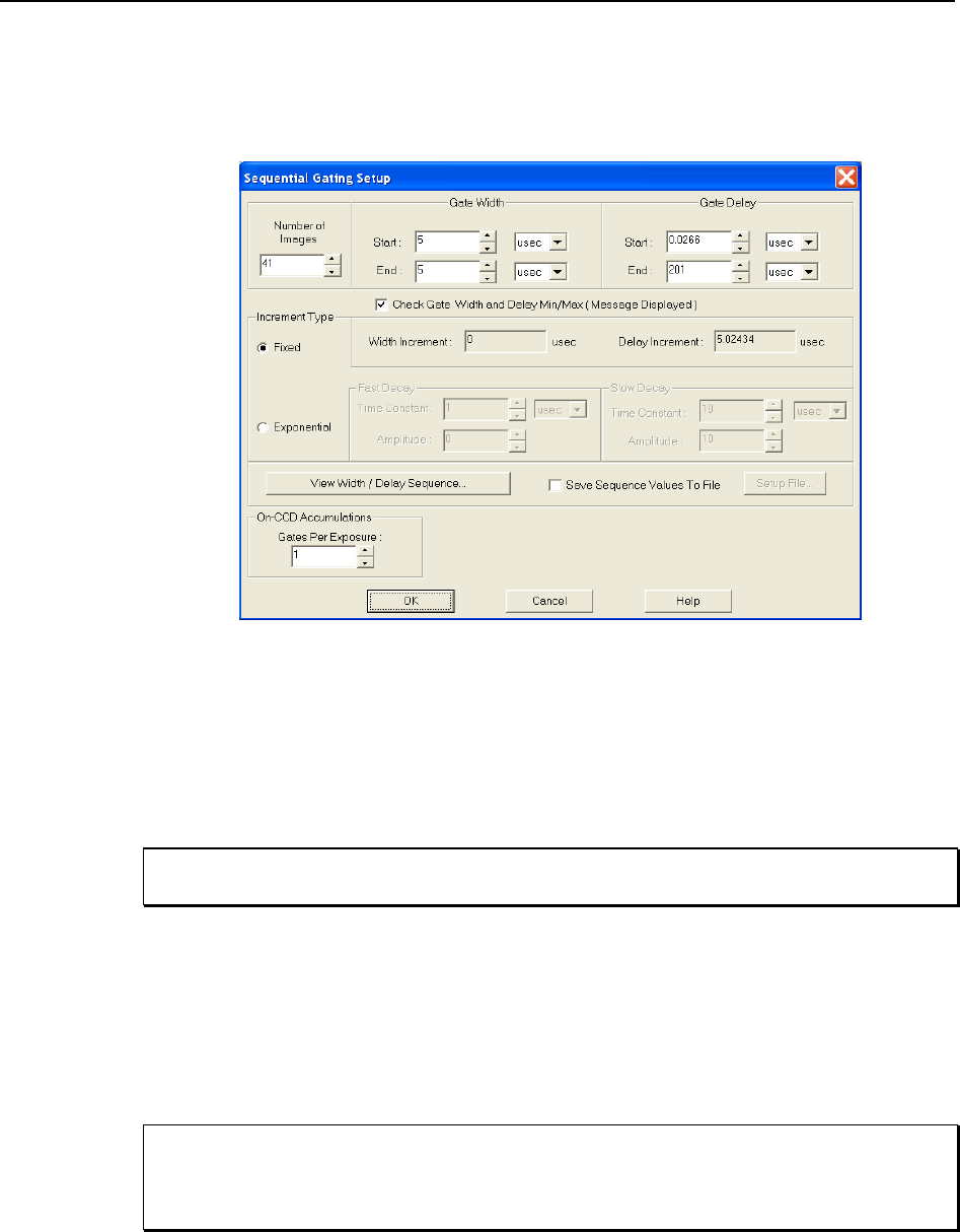
Chapter 18 Pulser Operation 203
Software Accumulations: Sets the number of exposures to be taken for each Shot.
Note that the number of Accumulations set here must be the same as the value set on
the Experiment Setup|Main tab for proper operation.
Sequential Mode Parameters
Number of Images: With an Accumulations setting of one, Number of Images equals
the number of exposures, each of which is followed by a readout. After each
exposure, the Gate Width and Gate Delay change as programmed before the next
exposure occurs. If multiple Accumulations are programmed, each exposure is
repeated n times, where n is the number of accumulations specified. Every
accumulation is processed before the gate delay and width change for the next shot.
The total number of exposures equals the specified Number of Images times the
number of Accumulations.
Accumulations can be set on the Sequential Gating Setup dialog and on the Experiment
Setup|Main tab. The two settings must be the same for proper operation.
Gate Width: The starting and ending gate widths are independently set. The first Shot
will have the Starting gate width and the last Shot will have the Ending gate width.
This is true for both the Fixed and Exponential increment type.
Gate Delay: The starting and ending gate delay values are independently set. The first
Shot will be taken at the Starting delay with respect to T0 and the last Shot will
occur at the Ending delay with respect to T0. This is true for both the Fixed and
Exponential increment type.
The precise timing of both the gate and signal at the camera will additionally depend on a
number of different delay mechanisms that can significantly affect the experiment. These
are discussed for the PI-MAX camera in some detail in Tips and Tricks section of the
PI-MAX/PI-MAX2, PI-MAX3 or PI-MAX4 system manual.
ATTENTION
ATTENTION
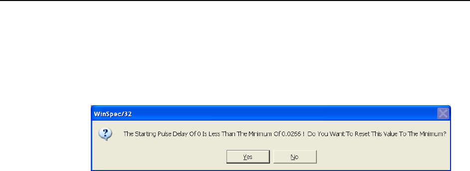
204 WinSpec/32 Manual Version 2.6B
Check Gate Width and Delay Min/Max (Message Displayed): If this box is
checked and you specify a gate width or delay outside the allowable range, a warning
message (Figure 188) will be displayed. Clicking Yes will cause the parameter in
question to be set to the limit value. Clicking No will cause the parameter setting to
be retained, but the actual value will still be the applicable minimum or maximum. If
the box is not checked, the applicable minimum or maximum will be established
automatically.
Figure 188. Range Limits Exceeded Warning
Fixed Increment Type: With this selection, the increment or change in Gate Width
and Gate Delay is the same from shot to shot. The actual increments depend on the
specified starting and ending values and on the Number of Images. The increment
values are calculated and reported in the associated fields.
Exponential Increment Type: With this selection, the increment or change in Gate
Width and Gate Delay changes from shot to shot. The precise delay and width of
each shot with respect to T0 is determined by the values entered for the Fast Decay
and Slow Decay Time Constant and Amplitude parameters. In fluorescent decay
experiments, for example, there will typically be two species contributing to the
output data, one of which decays much faster than the other. For example, there
might be a fast fluorophor with a decay time of at most a few nanoseconds, and a
slower one with a decay time of perhaps a hundred nanoseconds. By sweeping both
the delay and the width, and making provision for entering time constant and
amplitude information for two species, the sequential exponential algorithm is ideally
suited to making this type of measurement. At the start of the decay where the
amplitude is high but the decay is rapid, the gate pulses are narrow and close
together. Towards the end of the decay where the decay is slow, the gate pulses are
further apart but much wider to accommodate the lower signal amplitude. The result
is output data that is relatively constant in intensity over the decay time. This data can
be easily normalized by dividing each point by the exposure time and then using a
spline fit to recover the curve. The logarithm (base e) can then be taken to obtain a
straight line (or two lines successive line segments, each with a different slope for
two species). Tangents can be fitted to each segment to determine the rate constant
for each species.
Fast Decay
Time Constant: In a two species system, enter the decay time of the faster of the two
species. Note that it is not essential that you enter a value. If you have the decay
time information, you will get better data if the information is entered, but
acceptable results can be obtained in many situations by using the default. If there
is only one species, or if you want to discard the fast decay process, simply enter
zero for the Amplitude.
Note that the Gate Width and Gate Delay values need to be selected with some
care in fluorescence decay experiments. Typically the starting gate width will be
very narrow, perhaps 2 ns, and the final gate width should be wider by about the
ratio of the anticipated signal amplitude decrease over the course of the

Chapter 18 Pulser Operation 205
measurement timebase. Similarly, the starting gate delay has to take the various
insertion delays into account, and the final delay value might typically be set to a
value on the order of five times the anticipated decay time of the process.
Amplitude: This is the relative amplitude of the fast decay with respect to the slow one.
For example, if you know that the amplitude of the fast decay signal is typically five
times the amplitude of the slow decay signal, you could enter "5" for the fast decay
amplitude and "1" for the slow decay amplitude. Keep in mind that it is the ratio that
is being expressed. For example, there is no difference between entering fast and
slow amplitude values of "5" and "1" and entering fast and slow amplitude values of
"50" and "10." Note that the default values will give satisfactory results in many
measurements.
Slow Decay
Time Constant: In a two species system, enter the decay time of the slower of the
two species. Note that it is not essential that you enter a value. If you have the
decay time information, you will get better data if the information is entered, but
acceptable results can be obtained in many situations by using the default. If
there is only one species, or if you want to discard the fast decay process, simply
enter zero for the fast decay Amplitude.
Amplitude: This is the relative amplitude of the slow decay with respect to the fast
one. For example, if you know that the amplitude of the slow decay signal is
typically one-fifth the amplitude of the fast decay signal, you could enter "1" for
the slow decay amplitude and "5" for the fast decay amplitude. Keep in mind that
it is the ratio that is being expressed. For example, there is no difference between
entering slow and fast amplitude values of "1" and "5" and entering fast and slow
amplitude values of "10" and "50."
View Width/Delay Sequence: Opens
the Width/Delay Sequence dialog
(Figure 189) which lists the currently
programmed sequence of gate width
and gate delay values.
Save Sequence Values to File:
When this box is checked, the
sequence values will be saved on
completion of the run. The values
saved are those actually used to take
the data. The file could be recalled
later and used for data normalization
or other purposes.
Figure 189. Gate Width/Delay Sequence dialog
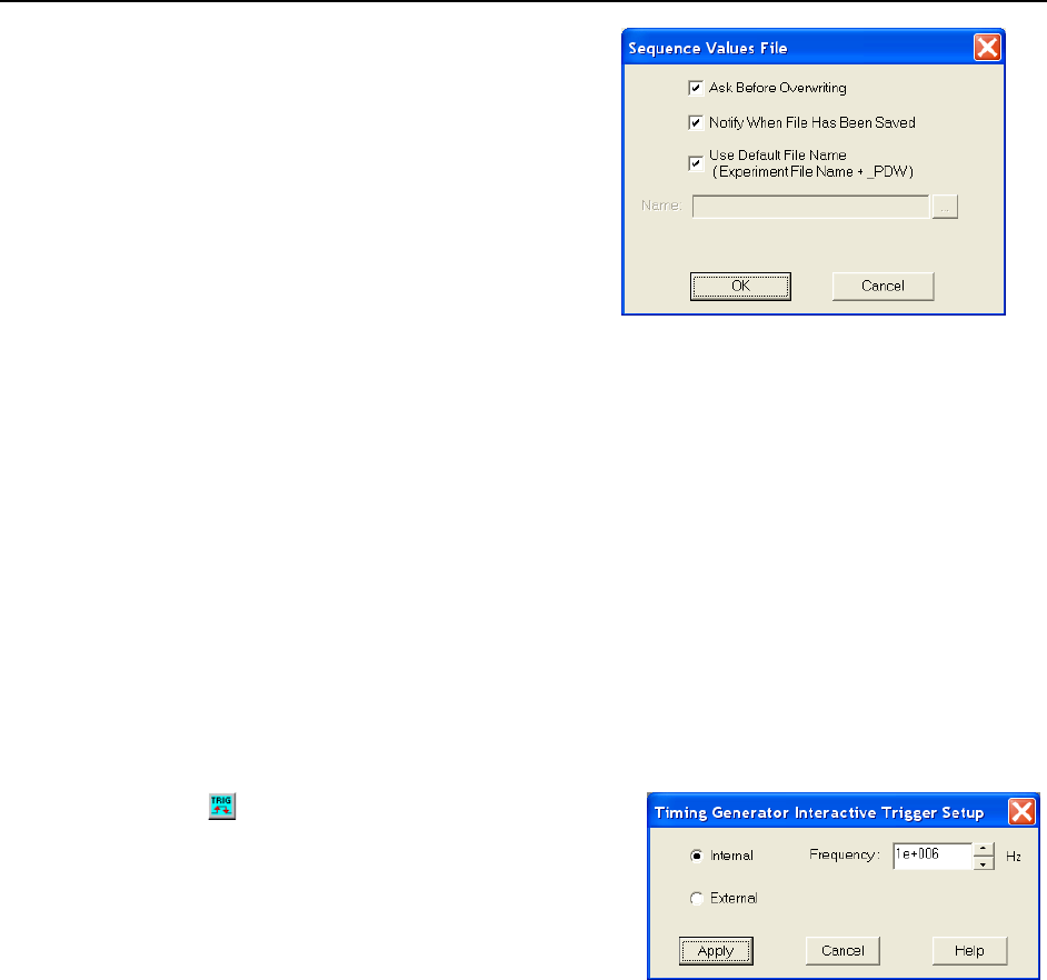
206 WinSpec/32 Manual Version 2.6B
Setup File: Opens the Sequence
Values File dialog (Figure 190),
which enables the following:
Ask Before Overwriting: If
checked, you will be queried
before a new sequence value file
overwrites an existing one. If
unchecked, overwriting can
occur without warning.
Notify When File Has Been
Saved: The file is saved at the
end of the data-acquisition run.
Figure 190. Sequence Values File dialog
You will be notified that this has occurred if this box is checked.
Use Default File Name: If checked, the sequence value file name will be
experiment file name, but with the extension PDW. If unchecked, you must enter
the name in the Name field.
Name: If not using the default name for the sequence value file, enter the file name
in the provided field. The button at the end of the box opens a browser to
facilitate assigning the file location.
On-CCD Accumulations: Sets the number of gates to occur during an exposure.
Software Accumulations: Sets the number of exposures to be taken for each Shot.
Note that the number of Accumulations set here must be the same as the value set on
the Experiment Setup|Main tab for proper operation.
Timing Generator Interactive Trigger Setup
The button on the Custom Toolbar, allows
you to select the PTG or DG535 trigger mode
(Internal or External) while acquiring data. In
the case of the SuperSYNCHRO must stop data
acquisition before you can make changes and
apply them.
Internal: The Timing Generator will create
its own trigger signals at the selected
frequency.
External: The Timing Generator will be
triggered by trigger signals that
originate in an external piece of
equipment.
Figure 191. Timing Generator Interactive
Trigger Setup dialog

Chapter 18 Pulser Operation 207
Timing Generator Interactive Gate Width and Delay
The button of the Custom
Toolbar, allows you to control the
Gate Width and Gate Delay
parameters of the PTG or DG535
Timing Generator while acquiring
data. In the case of the
SuperSYNCHRO, you must stop data
acquisition before you can make
changes and apply them.
Gate Width: Sets the duration of
the pulse applied to the
PI-MAX intensifier to gate
Figure 192. Timing Generator Interactive Gate
Width and Delay dialog
the photocathode. The units available are nanoseconds (ns), microseconds (µs),
or milliseconds (ms). Only some values are allowed, so the Timing Generator
will adjust the input value to the nearest allowable value.
Gate Delay: Sets the time between the beginning of the trigger pulse (either internal
or external) and the beginning of the photocathode gate pulse. The units available
are nanoseconds (ns), microseconds (µs), or milliseconds (ms). Only some values
are allowed, so the Timing Generator will adjust the input value to the nearest
allowable value.
Gates Per Exposure: Allows you to specify the number of times the photocathode
will be gated on during the exposure. Charge will accumulate on the CCD array
as those gates occur during the exposure and the accumulated charge will be
readout at the end of the exposure. The acquired data will contain signal from
multiple exposures and read noise from a single readout. Signal is limited by
pixel well capacity and the A/D converter (for a 16-bit A/D, this is 65536
counts).

208 WinSpec/32 Manual Version 2.6B
This page intentionally left blank.
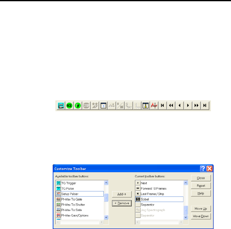
209
Chapter 19
Custom Toolbar Settings
Introduction
The Custom Toolbar feature of WinSpec/32 allows you one-button access to many
features or combinations of features available through the software. The Custom
Toolbar layout and the number of buttons displayed on the Custom Toolbar can easily
be changed.
Displaying the Custom Toolbar
1. To make the Custom Toolbar visible, select Toolbars and then Custom on the
View menu. The Custom Toolbar will appear on the desktop and its default
configuration will be as shown in Figure 193.
2. You can change position of the Custom Toolbar, its layout, and the number of
buttons it contains.
Figure 193. Default Custom Toolbar
Customizing the Toolbar
Although the Custom Toolbar defaults with the buttons shown in Figure 193, many
additional buttons are in fact available and can be added to the button using the
Customize Toolbar dialog (Figure 194). Buttons can be added or removed at any time
and the new configuration will be saved when the dialog is closed.
Figure 194. Customize Toolbar dialog

210 WinSpec/32 Manual Version 2.6B
Adding an Available Button:
1. Open the Customize Toolbar dialog by clicking on Custom Toolbar in the Setup
menu.
2. Referring to Figure 194, note that the buttons available for placement on the Custom
Toolbar are listed on the left. Buttons already on the toolbar are on the right.
3. To add an available button to the Custom Toolbar, first select it from the left-hand
list. You may have to scroll through the list of available buttons to find the one you
want. You can choose where to place the button by selecting a button on the right
side (which will then be highlighted). The new button will be placed before the
highlighted one.
4. Click on the Add button. The button will disappear from the list of Available
buttons and will be added to the list of Toolbar buttons.
5. Click on Close to close the dialog.
Removing a Button:
1. Open the Customize Toolbar dialog by clicking on Customize Toolbar in the
Setup menu.
2. Referring to Figure 194, note that buttons already on the toolbar are listed on the
right. Available but unused buttons are listed on the left.
3. To remove an available button from the Custom Toolbar, first select it from the
right-hand list. You may have to scroll through the listed buttons to find the one you
want.
4. Click on the Remove button. The button will disappear from the list of Toolbar
buttons and will be added to the list of Available buttons.
5. Click on Close to close the dialog.
Individual Dialog Item Descriptions
Available Buttons: You can select the button you wish to add to the Custom Toolbar
from this section. Many buttons, each with its own preassigned function as described
below, are available.
Toolbar Buttons: These are the buttons that will actually appear on the Custom
Toolbar.
Add: Causes the selected button on the Available Buttons list to be transferred to the
Toolbar buttons list before the selected button.
Remove: Causes the selected button on the Toolbar list to be transferred to the
Available Buttons list.
Close: This button closes the Custom Toolbar Assignment dialog and implements
changes made to the Custom Toolbar.
Reset: Restores the default Custom Toolbar configuration.
Help: Opens the context-sensitive help for the Custom Toolbar.
Move Up: Together with Move Down, Move Up determines the position of a given
button on the Custom Toolbar. Each time this button is clicked, the selected
button on the Toolbar buttons list moves up one position.

Chapter 19 Custom Toolbar Settings 211
Move Down: Together with Move Up, Move Down determines the position of a given
button on the Custom Toolbar. Each time this button is clicked, the selected
button on the Toolbar buttons list moves down one position.

212 WinSpec/32 Manual Version 2.6B
This page intentionally left blank.
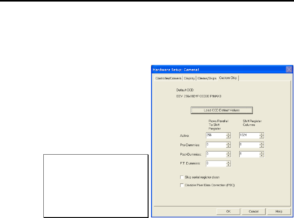
213
Chapter 20
Software Options
Introduction
The WinSpec/32 options described in this chapter can also be purchased from Princeton
Instruments. Contact Princeton Instruments Customer Support for order information.
Custom Chip (WXCstChp.opt)
Introduction
If this option has been installed,
selecting Show Custom Chip
check box on the
Controller/Camera tab adds the
Custom Chip tab to the dialog. The
Custom Chip parameters are shown
in Figure 195. The default values
conform to the physical layout of
the CCD array and are optimum for
most measurements.
Princeton Instruments does not
encourage users to change these
parameter settings. For most
applications, the default settings
will give the best results. We
strongly advise contacting the
factory for guidance before
customizing the chip definition.
Figure 195. Custom Chip tab
Normally, not all of the pixels in a CCD array are exposed and read out: a frame of “dummy”
pixels bounds the active area. These dummy pixels are usually masked and are not normally
read out. However, they could be read out by changing the chip definition in software. For
example, in the case of the EEV 256 × 1024 chip illustrated in Figure 195, the 256 active
rows are preceded by 0 dummy rows and followed by 0 dummy rows. There are 8 dummy
columns on one side of the active region and 8 dummy columns on the other side. By
changing the chip definition to increase the active area while decreasing the dummy settings,
the dummy cells would be read out. By doing so, one could measure the dark charge with
every readout. (Note that F.T. Dummies are chip-specific and are dummy rows at the
boundary of the masked and visible areas of a frame transfer device.)
Caution
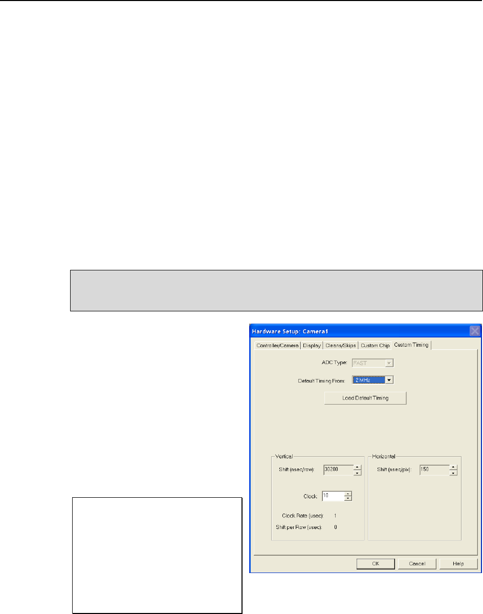
214 WinSpec/32 Manual Version 2.6B
It is also possible to increase image acquisition speed by reducing the size of the active area
in the definition. The result will be faster but lower resolution data acquisition. Operating in
this mode would ordinarily require that the chip be masked so that only the reduced active
area is exposed. This will prevent unwanted charge from spilling into the active area or
being transferred to the shift register.
By default, if there are no Pre-Dummy rows, the serial register will be cleared before
rows are shifted. If the Skip Serial Register Clean check box is selected when there are
no Pre-Dummy rows, the register cleanout will be skipped and the chip readout will be
faster. This feature is not available for PVCAM-supported cameras.
Pixel Bias Correction (not available for all cameras) is active by default. This function
generates a pixel bias correction scan code that is applied to the raw data to correct for
output amplifier and electronics drift. The correction is performed either on a line-by-line
or frame-by-frame basis depending on the camera. The correction process may add to the
readout time. If the Disable Pixel Bias Correction (PBC) check box is available on the
Custom Chip tab, you can disable pixel bias correction if you want to maximize the
readout time and are not concerned about drift. Disable the correction if you only want
raw (uncorrected) data.
Custom Timing (WXCstTim.opt)
Notes:
1. Fully supported by WinSpec Version 2.5.18.1 (and higher).
2. This option is not supported for 5 MHz systems.
Introduction
If this option has been installed,
selecting Show Custom Timing
check box on the Controller/
Camera (or Controller/Detector) tab
adds the Custom Timing tab to the
dialog. The Custom Timing selections
are shown in Figure 196. The default
timing parameter values have been
determined to give the fastest
possible performance without
compromising data acquisition
performance.
Princeton Instruments does not
encourage users to change these
parameter settings. For most
applications, the default settings
will give the best results. We
strongly advise contacting the
factory for guidance before
customizing the chip timing
parameters.
Figure 196. Custom Timing tab
FITS (FITS.exe)
FITS (Flexible Image Transport System) is the data format most widely used within
astronomy for transporting, analyzing, and archiving scientific data files. FITS is
Caution

Chapter 20 Software Options 215
primarily designed to store scientific data sets consisting of multidimensional arrays
(images) and 2-dimensional tables organized into rows and columns of information. The
FITS option allows you to acquire and save WinSpec/32 data in the FITS format. This
option also provides a file conversion function that allows you to convert existing
WinSpec/32 .SPE data files into the FITS format. F1 help is included with the option.
Acquiring data in the FITS format starts with setting up the experiment parameters in
WinSpec/32. With WinSpec still open, you then open the FITS.exe program (by opening
it at its directory location or by opening it from the Execute Macro dialog if the Macro
option has been installed). When you click on Run Experiment on the FITS dialog, the
experiment will begin. At completion of the experiment, the data will be displayed in
WinSpec and a FITS file will automatically be generated and saved.
Note: When this option is installed, the FITS.exe file is placed in the same directory as
the Winspec.exe file.
Figure 197. FITS dialog
Macro Record (WXmacrec.opt)
Macro Record is a convenient method to automate routines and repetitive data acquisition
and analysis tasks. A macro is created automatically whenever a sequence of operations
is performed in WinSpec. The recorded macro generates a VBScript file that can be
edited to provide maximum flexibility. For more information, refer to the WinSpec/32
online help and the PDF of the WinX32 Programming for Macro Record manual,
provided as part of the option package. Typically, the manual is stored in the
WinSpec32/Documentation directory when you install the option.
Note: As part of the Macro option installation, the Macro menu is added to the
WinSpec/32 menu bar.
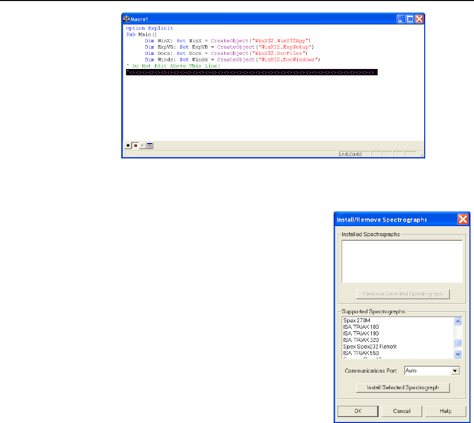
216 WinSpec/32 Manual Version 2.6B
Figure 198. Macro Record dialog
Spex Spectrograph Control (WSSpex.opt)
This option adds spectrograph support for the Spex
270M, ISA TRIAX 180, ISA TRIAX 190, ISA
TRIAX 320, and the Spex Spex232 Retrofit (older
Spex that have been retrofitted for RS-232
communication).
Figure 199. Install/Remove
Spectrographs dialog
Virtual Chip (WXvchip.opt)
Introduction
This option is used to set the parameters for Virtual Chip operation, a special fast-
acquisition technique that allows frame rates in excess of 100 fps to be obtained. For the
Virtual Chip selection be available on the WinSpec/32 Setup menu, it is necessary that:
the system is a PentaMAX or has an ST-133 Controller,
the camera has a frame transfer chip such as the EEV 512 × 512 FT,
the Frame Transfer readout mode is selected, and
the file WXvchip.opt is present in the same directory as the executable
WinSpec/32 program.
The virtual chip method of data acquisition requires that the chip be masked as shown in
Figure 200. Masking can be achieved by applying a mechanical or optical mask or by
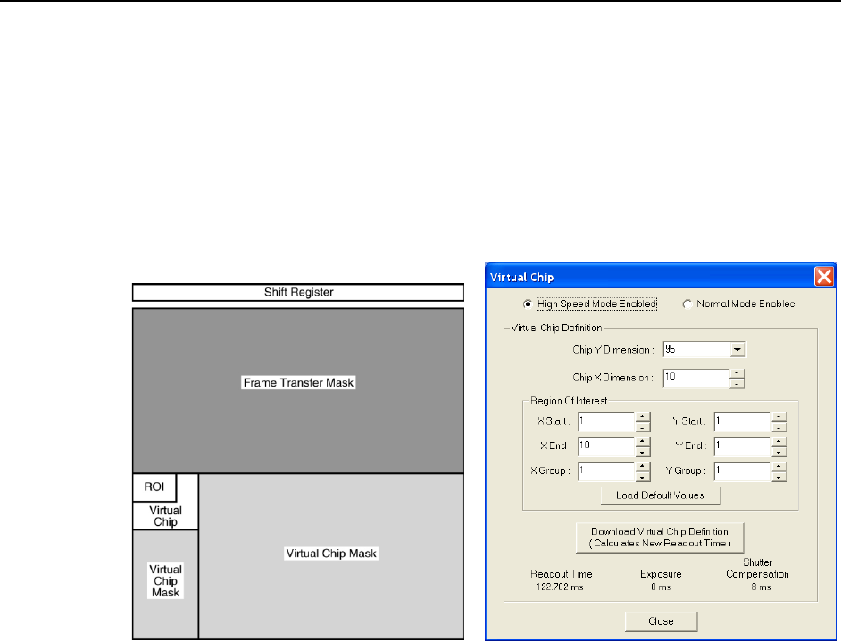
Chapter 20 Software Options 217
positioning a bright image at the ROI against a dark background on the remainder of the
array. In operation, images are continually piped down the CCD at extraordinarily high
frames per second (FPS).
The mini-frame transfer region is defined by an ROI as illustrated in Figure 200. The
charge from this ROI is shifted under the frame-transfer mask, followed by a readout
cycle of an ROI-sized region under the mask. Since the ROI is far from the serial register,
the stored image is just shifted repeatedly with the readout and the first few images
collected will not contain useful data. After the readout period, the next frame is shifted
under the mask and another ROI sized frame is read out. The net result is a series of
images, separated by spacer regions, streaming up the CCD under the mask.
Figure 200. Virtual Chip Functional diagram
Figure 201. Virtual Chip dialog
Virtual Chip Setup
The following procedure covers the basic hardware and software setup for Virtual Chip
operation.
Equipment:
Suitable Princeton Instruments detector with 512x512FT or other frame transfer
CCD array
Suitable ST-133
PCI Interface Card and High Speed Serial (TAXI) cable
Suitable Host Computer
Software:
WinSpec/32, version 2.4 or higher
WXvchip.opt installed in the same directory as the executable WinSpec/32
program.
Assumptions:
You are familiar with the WinSpec/32 software and have read the hardware
manuals.
Masking is for a 47x47 pixel Virtual Chip with its origin at 1,1.
Procedure:
1. Verify that the power is OFF for ALL system components (including the
host computer).

218 WinSpec/32 Manual Version 2.6B
2. Verify that the correct line voltages have been selected and that the correct
fuses have been installed in the ST-133.
3. Connect the TAXI cable to the interface card at the host computer and to the
Serial Com connector at the rear of the Controller. Tighten down the
locking screws.
4. Connect the Camera-Controller cable to the Detector connector on the
rear of the Controller and to the Detector connector at the rear of the
camera. Tighten down the locking screws.
5. If it has not been installed already, connect a line cord from the Power Input
module on the back of the Controller to a suitable AC power source.
6. Turn on the Controller.
7. Turn on the host computer and select the WinSpec/32 icon.
8. From the Setup menu, select Hardware, and enter the following settings:
Controller/CCD tab
Controller: PentaMAX or the appropriate ST-133 controller
Controller Version: 5
CCD Type: appropriate frame transfer array (EEV 512x512FT, for this
procedure)
Shutter Type: None
LOGIC OUT Output: Shutter
Readout Mode: Frame Transfer
Interface tab
Type: the appropriate interface card. For this procedure, the selection is
High Speed PCI.
Cleans/Skips tab
Number of Cleans: 1
Number of Strips per Clean: 512
Minimum Block Size: 2
Number of Blocks: 5
9. From the Acquisition menu, select Experiment Setup and enter the
following settings:
Main tab
Exposure Time: Enter a value. The exposure time can either be greater
than the readout time or it can be equal to the readout time. If you want
an exposure time > readout time, enter a value larger than the readout
time calculated when the virtual chip definition was downloaded. If you
want an exposure time = readout time, enter 000 sec.
Number of Images: Enter the desired number of images.
Use Region of Interest
Accumulations: 1
ADC tab
Type: FAST
ROI Setup tab: Make no changes to the settings on this tab unless you
have re-enabled Normal Operating Mode. ROI setup for Virtual Chip
(High Speed Mode) is performed through the Virtual Chip dialog.
10. From the Setup menu, select Virtual Chip, and enter the following settings:
High Speed Mode Enabled

Chapter 20 Software Options 219
Virtual Chip Definition: The settings below assume a 47x47 pixel virtual
chip. The X and Y dimensions are established by the external mask. The
virtual chip is fully flexible in the X direction. However, the set of
choices for the Y-dimension has been pre- selected for optimal
performance. Note that the origin point that Princeton Instruments uses
for a CCD array is 1,1.
Chip Y Dimension: 47. Select this dimension from the drop down list.
Chip X Dimension: 47. Enter this dimension manually.
11. Click on the Load Default Values button. This enters the default ROI
values. These values are: Start pixels of 1,1; End pixels based on the Chip Y
and Chip X dimensions; and Groups of 1.
Region of Interest: The settings below assume a 47x47 pixel ROI
(i.e., the entire virtual chip). An ROI that is a subset of the virtual chip
can be defined.
X Start: 1 Y Start: 1
X End: 47 Y End: 47
X Group: 1 Y Group: 1
Click on the Download Virtual Chip Definition button. This will
download the definition, set up the ROI, and calculate the readout time.
Observe the calculated readout time. If you need a shorter period, change
the settings (for example, enter a smaller Y-dimension or use binning in
the Y-direction) and click on the Download Virtual Chip Definition
button again.
Click on Close.
12. From the Setup menu, select Environment.
Note: When setting up for focusing, the number of Frames/Interrupt should
be left at 1.
DMA Buffer (Mb): By default, the buffer size is 8 Mb. Using the
following formula, calculate the amount of DMA memory required:
X × Y × #Frames × (2 bytes/pixel).
For example, the buffer size required for a 47x47 virtual array acquiring
1000 frames would be 47 × 47 × 1000 frames × (2 bytes/pixel) = 4.4 Mb.
If the calculated value is greater than 8 Mb, enter the appropriate size.
Note: This value is not enabled until you restart your computer.
Frames/Interrupt: If the number of frames is greater than 256 (the
preprogrammed slot limit for a PCI card), increase the number of
Frames/Interrupt value. Use the formula #Frames/256 and round the
result to the next highest integer to calculate that value. For example,
1000 frames/256 will result in 3.9, so enter 4.
Note: This value should be 1 for Focus mode.
13. Click on OK after you have finished entering the Environment settings.
14. Place a suitable target in front of the camera and click on Focus to verify
that the camera is seeing the target.
15. Make any focusing, gain, or other adjustments necessary to fine-tune the
image.
16. Stop running in Focus mode.

220 WinSpec/32 Manual Version 2.6B
17. Now click on Acquire.
Experimental Timing
Triggering can be achieved through the software via the Software Trigger timing mode
(selectable on the Experiment Setup dialog, Timing Mode tab) or it can be achieved
via the Ext Sync input on the rear of the camera. Triggering from the Ext Sync input
allows you to acquire a single image per TTL pulse. If Software Trigger has been
selected, back-to-back collection of the requested number of images will be initiated
when Acquire is selected: no further TTL trigger input is required.
Tips
If mechanical masking is used, the mask can be a static one (fixed dimensions) in
which case, multiple masks should be made to accommodate a variety of imaging
conditions. Alternatively, a more flexible mask can be manufactured by taking
two thin metal sheets with a square hole the size of the exposed region of the
CCD cut in the center. For a 512 × 512 pixel CCD array with 15 micron pixels,
the exposed region would be 7.68 mm × 7.68 mm. These masks should be
anodized black to prevent reflections in the optical system and they should be
very flat. These two sheets can then be slid relative to one another to achieve any
rectangular shape required. The sheets should be placed flat in the optical plane
and their openings should be centered on the optical axis. Ideally they should be
able to move with an accuracy of 2-3 pixels per step (30-45 microns) in the X
and Y directions.
Consult the factory for off-the-shelf optical masking accessories.
Running the camera in Free Run mode with 0.0 msec exposure time will result in
the fastest acquisition time. Under these conditions, the acquisition time is
limited by the readout time of the ROI (exposure time ≡ readout time).
When you return the system to "Normal" chip mode (radio button on Virtual
Chip dialog), you should also open the Experiment Setup dialog at the ROI
Setup tab and click on the ClearAll button to clear the ROI setup downloaded
for Virtual Chip operation.
If frame acquisition appears to be slow in Focus mode, check the
Frames/Interrupt value on the Environment dialog and reset the value to 1 if
it is greater than 1.
When processing large stacks of data, you may want to use a third-party
scientific image processing package.
Due to CCD design, you may see some edge artifacts when acquiring data from
the entire virtual chip. Crop these artifacts by defining an ROI that is slightly
smaller than the virtual chip dimensions.
221
Part 3
Reference
Appendix A, System and Camera Nomenclature ........................................ 223
Appendix B, WinSpec/32 First Light Instructions ....................................... 233
Appendix C, Calibration Lines ........................................................................ 245
Appendix D, Data Structure ............................................................................. 247
Appendix E, Auto-Spectro Wavelength Calibration .................................. 257
Appendix F, CD ROM Failure Workarounds ................................................ 261
Appendix G, WinSpec/32 Repair and Maintenance ................................... 263
Appendix H, USB 2.0 Limitations ................................................................... 267
Appendix I, Troubleshooting USB 2.0 ............................................................ 269
Appendix J, Glossary ........................................................................................ 277

222 WinSpec/32 Manual Version 2.6B
This page intentionally left blank.

223
Appendix A
System and Camera Nomenclature
System, Controller Type, and Camera Type Cross-Reference
Use the cross-reference table below if you need to determine the controller type and/or
camera/CCD type used by your system. This table is based on the Princeton Instruments
brand systems that are currently being sold by Roper Scientific, Inc. Many of these
systems incorporate non-volatile RAM (NVRAM) that has been factory programmed
with the default hardware setup parameters for the controller, camera, and CCD array
included in your system. If you know the controller type used by your system, you should
be able to download these default parameters. However, if this functionality is not
available for your system, you will need to manually enter the information.
Note: Because Marconi changed its name to e2v, you may see CCD types with the prefix
"MAR,” "EEV,” or "e2v.” These CCDs are manufactured by e2v.
System
Controller Type
Camera/CCD Type
2D-OMA V: 320
ST-133-5 MHz
XEN 320
I-PentaMAX (Gen II or Gen III)
PentaMAX*
EEV 512x512FT
MicroMAX: 512EBFT
ST-133
EEV 512x512FT CCD57
MicroMAX: 782Y
ST-133
PID 582x782
MicroMAX: 782YHS
ST-133-5 MHz
PID 582x782
MicroMAX: 1024B
ST-133
EEV 1024x1024 CCD 47_10
MicroMAX: 1300B
ST-133
EEV 1300x1340B
MicroMAX: 1300Y
ST-133
PID1030x1300
MicroMAX: 1300YHS
ST-133-5 MHz
PID1030x1300
MicroMAX: 1300YHS-DIF
ST-133-5 MHz
PID1030x1300
NIRvana:640 (formerly
PIoNIR:640)
N/A
PI InGaAs 640
OMA V:InGaAs 256
ST-133
InGaAs 1x256
OMA V:InGaAs 512
ST-133
InGaAs 1x512
* Does not support NVRAM function.

224 WinSpec/32 Manual Version 2.6B
System
Controller Type
Camera/CCD Type
OMA V:InGaAs 1024
ST-133
InGaAs 1x1024
PDA
ST-121*
Diode Array 1024
PhotonMAX: 512B
N/A
e2v CCD97B
PhotonMAX: 1024B
N/A
e2v CCD201B
PI-LCX: 400
ST-133
EEV 400x1340F
PI-LCX: 576
ST-133
EEV 576x384 (3 ph)
PI-LCX: 1242
ST-133
EEV 1152x1242 (3 ph)
PI-LCX: 1300
ST-133
EEV 1300x1340F
PI-MAX: 512HQ
ST-133
THM 512x512
PI-MAX: 512RB
ST-133
THM 512x512
PI-MAX: 512SB
ST-133
THM 512x512
PI-MAX: 512UV
ST-133
THM 512x512
PI-MAX: 1024HQ
ST-133
EEV 256x1024F CCD30
PI-MAX: 1024RB
ST-133
EEV 256x1024F CCD30
PI-MAX: 1024SB
ST-133
EEV 256x1024F CCD30
PI-MAX: 1024UV
ST-133
EEV 256x1024F CCD30
PI-MAX MG: 1024
ST-133
EEV 256x1024F CCD30
PI-MAX2:512 (Gen II or Gen III)
ST-133-5 MHz
THM 512x512
PI-MAX2:1003 (Gen II or Gen
III)
ST-133-5 MHz
KAI 1024x1024
PI-MAX3:1024i
N/A
Kodak KAI-1003
PI-MAX3:1024x256
N/A
e2v CCD 30-11
PI-MAX4:1024i
N/A
Kodak KAI-1003
PI‐MAX4:1024i-RF
N/A
Kodak KAI-1003
PI-MAX4:1024x256
N/A
e2v 256x1024F CCD 30-11
PI-MAX4:1024x256-RF
N/A
e2v 256x1024F CCD 30-11
PI-MTE: 1300B
ST-133, ST-133-2
MHz
EEV 1300x1340B

Appendix A System and Camera Nomenclature 225
System
Controller Type
Camera/CCD Type
PI-SCX: 1242
ST-133
EEV 1152x1242(6 ph)
PI-SCX: 1300
ST-133
EEV 1300x1340F
PI-SCX: 4300
ST-133
KAF 2084x2084 SCX
PI-SX: 400
ST-133
EEV 400x1340B
PI-SX: 512
ST-133
TEK 512x512DB
PI-SX: 1024
ST-133
TEK 1024x1024DB
PI-SX: 1300
ST-133
EEV 1300x1340B
PIoNIR:640 (now NIRvana:640)
N/A
PI InGaAs 640
PIXIS:100F, B, BR, R
N/A
EEV 100x1340F/B
PIXIS:400F, B, BR, R
N/A
EEV 400x1340F/B
PIXIS:512F, B
N/A
MAR 512x512 CCD 77
PIXIS:1024F, B
N/A
EEV 1024x1024 CCD 47-10
PIXIS-XF:1024
N/A
e2v 1024x1024 CCD 47-10
PIXIS-XO:100B
N/A
PI 1340x100B
PIXIS-XO:400B
N/A
PI 1340x400B
PIXIS-XO:512B
N/A
e2v 512x512B CCD 77-00
PIXIS-XO:1024B
N/A
e2v 1024x1024 CCD 47-10
PIXIS-XO:2KB
N/A
PI 2048x512B
ProEM:512B
N/A
e2v CCD97B
ProEM:512BK
N/A
PI exclusive
ProEM:1024B
N/A
e2v CCD201B
PyLoN:100F, B, BR
N/A
PI 1340x100B
PyLoN:100B, BR eXcelon
N/A
PI 1340x100B
PyLoN:400F, B, BR
N/A
PI 1340x400B
PyLoN:400B, BR eXcelon
N/A
PI 1340x400B
PyLoN-IR:1024-1.7
N/A
SUI 1024x1 InGaAs (LE-1.7)
PyLoN-IR:1024-2.2
N/A
SUI 1024x1 InGaAs (LE-2.2)

226 WinSpec/32 Manual Version 2.6B
System
Controller Type
Camera/CCD Type
Quad-RO:4096
N/A
FCD 4096x4096F MT
Quad-RO:4320
N/A
KAF 2084x2084 MT
Spec-10: 100, B, R, BR
ST-133
EEV 100x1340F, 100x1340B
Spec-10: 120
ST-133
HAM 124x1024
Spec-10: 120B
ST-133
HAM 122x1024B
Spec-10: 256, B, E
ST-133
EEV 256x1024F CCD30, B, OE
Spec-10: 400, B, R, BR
ST-133
EEV 400x1340F/B
Spec-10XP: 100, B, R, BR
ST-133-2MHz
EEV 100x1340F/B
Spec-10XP: 400, B, R, BR
ST-133-2MHz
EEV 400x1340F/B
SpectruMM:120
ST-133
HAM 124x1024
SpectruMM:120B
ST-133
HAM 122x1024B
SpectruMM:250
ST-133
HAM 252x1024
SpectruMM:250B
ST-133
HAM 250x1024B
VersArray: 512B, F
ST-133
TEK 512x512DB/DF
VersArray: 1024B, F
ST-133
TEK 1024x1024DB/DF
VersArray: 1300B, F
ST-133
EEV 1300x1340B/F
VersArrayXP: 512B, F
ST-133-2MHz
MAR 512x512 CCD77
VersArrayXP: 1K, KB
ST-133-2MHz
EEV 1024x1024 CCD47_10
System and System Component Descriptions
The following information briefly describes Princeton Instruments brand systems and the
system components. For more information, contact your Princeton Instruments
representative or Customer Support.
Systems:
2D-OMA V: Cryogenically-cooled focal plane array (FPA) based system for low light
level NIR imaging (0.8µm-1.7µm).
InSight: Includes an f/3.9 imaging spectrograph integrated with a high performance
digital CCD. The system is pre-aligned and focused at the factory, allowing for effortless
integration into experiments.
MicroMAX: Name used for some ST-133 based imaging systems, usually with an RTE
head. The 5 MHz version is characterized by duplex head cable
NIRvana (formerly PIoNIR): Compact, permanent vacuum camera platform with
internal controller. Designed for NIR spectroscopy and imaging.

Appendix A System and Camera Nomenclature 227
OMA V: Cryogenically-cooled Photodiode array (PDA) based system for spectroscopy
applications.
PDA: Low-cost spectroscopy system uses ST-121 controller.
PentaMAX: A/D electronics are in the head so no controller is necessary. Runs with PCI
card only. Both unintensified and intensified versions are available.
PhotonMAX: EMCCD (electron-multiplying CCD). Optimized for both traditional CCD
and "on-chip multiplication gain" operation. Internal controller. Vacuum guaranteed for
the life of the camera.
PI-Echelle: Spectrograph that achieves high spectral resolution over the entire
wavelength range of the camera (one of several compatible Princeton Instruments
cameras) without any moving parts. The system is ideal for both general spectroscopy
applications as well as Laser Induced Breakdown Spectroscopy.
PI-LCX: High-performance photon counting system. Medium X-ray, direct detection
PI-MAX: ICCD design with internal high voltage power and gating. Controller is
ST-133, and gating timing is provided by a DG535, PTG or other TTL timing source.
PI-MAX2: High speed PI-MAX. ICCD design with internal high voltage power and
gating. Controller is ST-133-5MHz, and gating timing is provided by a DG535, PTG or
other TTL timing source.
PI-MAX3: High speed PI-MAX. ICCD design with internal high voltage power and
gating with internal controller. Gate timing is controlled by the internal SuperSYNCHRO
timing generator or an external source.
PI-MAX4: High speed PI-MAX. ICCD design with internal high voltage power and
gating with internal controller. Gate timing is controlled by the internal SuperSYNCHRO
timing generator or an external source.
PI-MTE: Compact high-sensitivity digital imaging system designed to deliver scientific
performance inside high-vacuum chambers over long operation times.
PI-SCX: X-ray diffraction, fiberoptically-coupled detector.
PI-SX: High-sensitivity, deep-vacuum interface for soft X-ray acquisition.
PIoNIR (renamed NIRvana): Compact, permanent vacuum camera platform with
internal controller. Designed for NIR spectroscopy and imaging.
PIXIS: Compact, permanent vacuum camera platform with internal controller. Designed
for low-light-level spectroscopy and imaging.
PIXIS-XF: Compact, permanent vacuum camera platform with internal controller. Designed
for lens-free, indirect imaging of X-rays using phosphor screens or other Lambertian sources.
PIXIS-XO: Compact, vacuum open-nose camera platform with internal controller and
rotatable ConFlat flange. Designed for direct imaging of very low energy X-ray (< 30 eV).
ProEM: EMCCD (electron-multiplying CCD). Optimized for both traditional CCD and
“on-chip multiplication gain” operation. Internal controller. Air- and liquid-cooling.
Vacuum guaranteed for the life of the camera.
PyLoN: Liquid nitrogen cooled detector with internal controller and 1.7 liter Dewar capacity.
Quad-RO: High performance X-ray system. Systems can effectively provide X-ray
photon-counting capability with up to 16-bit dynamic range. 1:1 fiberoptic taper and
multi-port output. Thermoelectric cooling.

228 WinSpec/32 Manual Version 2.6B
SPEC-10: High performance, spectroscopy system. Wide variety of CCD arrays.
Thermoelectric or cryogenic cooling available.
SPEC-10XP: High performance spectroscopy system with "XP" lifetime vacuum. This
system can be thermoelectrically (air) cooled down to -80Cº and has software-selectable
six-speed digitization (up to 2 MHz).
SpectruMM: Name used for some ST-133 based spectroscopy systems with an RTE
head.
TriVista: Consists of three imaging-corrected Acton Research spectrographs that can be
used in single, double, and triple configurations. May incorporate PMT detectors and/or
one or more Princeton Instruments CCD detectors.
VersArray: High-performance, general purpose imaging system. Wide variety of CCD
arrays in imaging formats. Thermoelectric or cryogenic cooling available.
VersArrayXP: High-performance low-light imaging system for astronomy, MCP readout,
pressure-sensitive paint (PSP) / wind tunnel testing, semiconductor failure analysis, and
streak tube readout applications. Deep thermoelectric cooling (air).
Controllers:
ST-121: Diode array controllers shipped with diode array detectors, controlled by a PCI card.
ST-130: Obsolete controller but still supported in the WinX/32 software.
ST-133: Controller that can run the vast majority of Princeton Instruments brand
cameras, including MicroMAX, PI-MAX, Spec-10, PI-LCX, PI-MTE, PI-SCX, PI-SX,
OMA V, and VersArray. Different hardware types are needed to run different detectors
(for example, liquid nitrogen-cooled vs. thermoelectrically-cooled).
ST-133 2 MHz: ST-133 controller, characterized by six software-selectable ADC rates.
ST-133 5 MHz: ST-133 controller, characterized by duplex head cable.
ST-138: Older controller for TE, LN, ICCD, and ITE units. It offers a few special
features such as hardware accumulator. In general, this controller is being phased out.
Cameras/Detectors:
HCTE/CCD: See NTE/CCD and NTE 2.
ICCD: Standard, "classic" intensified camera, requires purging, has internal high voltage
power but requires external high voltage pulses for gating. Controlled by ST-133 or ST-138.
LN/CCD: Liquid nitrogen cooled detector, 1.5 liter Dewar is standard, can be run with
ST-138 or ST-133.
LN/InGaAs: Indium gallium arsenide detector controlled by a ST-133 controller
MTE 2: Miniature liquid cooled camera, designed for in vacuum chamber operation, can
be run with ST-133 controller. Included in a PI-MTE system.
NTE/CCD and NTE 2: Stands for new TE head. More cube shaped than the TE,
designed for maximum cooling. NTE 2 requires high-power version of ST-133.
RTE/CCD: Round thermoelectrically cooled camera, can be run with ST-133
controllers.
TE/CCD: Water- cooled camera, can be run with ST-138 or some ST-133 controllers.

Appendix A System and Camera Nomenclature 229
TEA/CCD: Forced air-cooled camera, can be run with ST-138 or some ST-133
controllers.
V/ICCD: Video intensified detector. Always shipped with its own control box, produces
standard video out so no interface card or software required. As of Version 2.5, this
detector will not be supported by WinX/32.
XP: TE/air-cooled camera with lifetime vacuum, can be run with ST-133 controllers.
Six-speed digitization is an option.
XTE: TE/air-cooled detector with cooling down to -100°C, can be run with ST-133
controllers.
Pulsers:
FG-100: Pulser with 5 nsec - 3 µsec gating, Gen II intensifiers only.
FG-101: Obsolete version of an ICCD unit, with internal high voltage power and gating.
PG-10: Pulser with 200 nsec to 6 msec gating, Gen II intensifiers only.
PG200: Software programmable pulser with 5 nsec to 80 msec gating. Highest
performance pulser with the most features, Gen II intensifiers only
PTG: Dedicated "programmable delay generator" board that generates TTL level pulses
to control intensifier gating in PI-MAX models. It is an option that sits in the third slot of
an ST-133 controller.
High-Voltage Power Supplies:
IIC-100: High voltage power supply for intensified cameras without internal high
voltage supplies (intensified PentaMAX, ITE, or lens-coupled intensified systems) for
CW operation only. Not necessary for ICCD or PI-MAX cameras. For gated operation of
intensified PentaMAX or ITE cameras buy the board version of the IIC-100, called the
MCP-100, built into the pulser. During manufacture, a Model IIC-100 is configured for
operation with a Gen II intensifier or with a Gen III intensifier, but not for operation
with both types.
IIC-200: Compact high voltage power supply for intensified cameras without internal
high voltage supplies (intensified PentaMAX, ITE, or lens-coupled intensified systems)
for gated and CW/Shutter operation. During manufacture, a Model IIC-200 is configured
for operation with a Gen II intensifier or with a Gen III intensifier, but not for operation
with both types.
IIC-300: Combined image intensifier power supply and moderate performance gating
pulse generator. Gated and CW/Shutter operation. PIV version available. During
manufacture, a Model IIC-300 is configured for operation with a Gen II intensifier or
with a Gen III intensifier, but not for operation with both types.
Miscellaneous Components:
OFA: An adapter for connecting a fiber optic input to a spectrometer. Two versions are
available for the best possible f/# matching, see the price list for details.
CC-100: Closed coolant circulator (not a chiller) designed for TE, TEA, or ICCD
cameras
UV Lens: f/1.2 catadioptric lens only for ICCD or PI-MAX cameras

230 WinSpec/32 Manual Version 2.6B
Array Designators
In the past, the designators in the following list were often used on camera serial labels to
identify the array in the camera.
B: Back-illuminated CCD
DDA: Dual diode array CCD
F: Front illuminated CCD, in many cases no letter is used
E: CCD made by EEV
T: CCD made by Thomson
K: CCD made by Kodak
H: CCD made by Hamamatsu
HS: "High speed" MicroMAX system runs at 5 MHz
FT: Frame transfer detector
M: MPP (multi-pin phasing) CCD
P: (Usually) CCD offered exclusively by Princeton Instruments
PDA: Photodiode array
R: Deep depletion
S: Usually refers to SITe arrays, also see TK
TK: CCD made by SITe (formerly Tektronix), sometimes labeled S
UV: UV-to-VIS standard lumogen coating for UV-response to 195 nm
UVAR: Permanent UV-to-NIR A/R coating on some SITe CCDs (not
lumogen/metachrome)
VISAR: Permanent VIS to NIR A/R coating on some SITe CCDs (not
lumogen/metachrome)
Y: Interline CCD made by Sony
/1: grade 1 CCD
/2: grade 2 CCD
/3: grade 3 CCD
64: array format is 1024 x 64 pixels
100: array format is 1340 x 100 pixels
128: array format is 1024 x 128 pixels
256: 256 element linear array
400: array format is 1340 x 400 pixels
512: array format is 512 x 512 pixels; or 512 elements for linear arrays
576: array format is 576 x 384 pixels
768: array format is 768 x 512 pixels
782: array format is 782 x 582 pixels
1000: array format is 1000 x 800 pixels
1024: array format is 1024 x 256 (EEV or Hamamatsu) or 1024 x 1024 (SITe)

Appendix A System and Camera Nomenclature 231
1100: array format is 1100 x 330 pixels
1242: array format is 1152 x 1242 pixels
1280: array format is 1280 x 1024 pixels
1300: array format is 1300 x 1030 pixels (Sony) or 1300 x 1340 pixels (EEV)
1317: array format is 1317 x 1035 pixels
1340: array format is 1340 x 100, 400, or 1300; family is exclusive to Princeton
Instruments
1536: array format is 1536 x 1032 pixels
2032: array format is 2025 x 2032 pixels
2500: array format is 2500 x 600, rectangular pixels
3072: array format is 3072 x 2048 pixels

232 WinSpec/32 Manual Version 2.6B
This page intentionally left blank.

233
Appendix B
WinSpec/32 First Light Instructions
Imaging
This section provides step-by-step instructions for acquiring an image for the first time. The
intent of this procedure is to help you gain basic familiarity with the operation of your
system and to show that it is functioning properly. Once basic familiarity has been
established, then operation with other configurations, ones with more complex timing
modes, can be performed.
Note: The additional setup steps required for the PI-MAX family of cameras have been
omitted.
Assumptions
The following procedure assumes that
1. You have already set up your system in accordance with the instructions in the
camera’s system manual and the “Part 1 Getting Started” section of this manual.
2. You are familiar with the application software.
3. The camera has a software-controlled internal shutter.
4. The system is being operated in imaging mode.
5. The target is a sharp image, text, or a drawing that can be used to verify that the
camera is "seeing" and can be used to maximize focus.
Getting Started
1. Mount a test target in front of the camera.
2. Power ON the camera (i.e., switch the controller or power supply ON).
Note: The camera must be turned on before WinSpec is opened, and WinSpec must
be closed before the camera is turned off.
3. Turn on the computer power.
4. Start the application software.
Setting the Parameters
Note: The following procedure is based on WinSpec/32: you will need to modify it if
you are using a different application. Basic familiarity with the WinSpec/32 software is
assumed. If this is not the case, you may want to review the software manual or have it
available while performing this procedure.
Set the software parameters as follows:
Environment dialog (Setup|Environment): Check the DMA Buffer size. Large
arrays (2048x2048, for example) require a buffer size on the order of 32 Mbytes.
If you change the buffer size, you will have to reboot the computer for this
memory allocation to be activated, and then restart WinSpec.

234 WinSpec/32 Manual Version 2.6B
Controller/Camera tab (Setup|Hardware): These parameters should be set
automatically to the proper values for your system.
Use PVCAM: Verify that this box is checked.
Note: This check box is not present on software versions 2.5.19.6 and
higher.
Controller type: This information is read from the camera.
Camera type: This information is read from the camera.
Shutter type: None or Small (System dependent).
Readout mode: Available modes are read from the camera. Select Full
frame.
Detector Temperature (Setup|Detector Temperature…): The default
temperature setting is read from the camera. When the array temperature reaches
the set temperature, the Detector Temperature dialog will report that the
temperature is LOCKED. Note that some overshoot may occur. This could cause
temperature lock to be briefly lost and then quickly re-established. If you are
reading the actual temperature reported by the application software, there may be
a small difference between the set and reported temperature when lock is
established. This is normal and does not indicate a system malfunction. Once
lock is established, the temperature will be stable to within ±0.05°C.
Note: The Detector Temperature dialog will not display temperature
information while you are acquiring data.
Cleans and Skips tab (Setup|Hardware): Click on Load Default Values and
click on Yes.
Experiment Setup|Main tab (Acquisition|Experiment Setup…):
Exposure Time: 100 ms
Accumulations & Number of Images: 1
Experiment Setup|ROI tab (Acquisition|Experiment Setup…): Use this
function to define the region of interest (ROI).
Imaging Mode: Select this mode.
Clicking on Full loads the full size of the chip into the edit boxes.
Experiment Setup |Timing tab (Acquisition|Experiment Setup…):
Timing Mode: Free Run
Shutter Control: Disabled Opened
Safe Mode vs. Fast Mode: Fast

Appendix B WinSpec First Light Instructions 235
Confirming the Setup
1. If you are using WinSpec/32 and the computer monitor for focusing, select Focus
from the Acquisition menu. Successive images will be sent to the monitor as
quickly as they are acquired.
2. Adjust the lens aperture, intensity scaling, and focus for the best image as viewed on
the computer monitor. Some imaging tips follow:
Begin with the lens blocked off and then set the lens at the smallest possible
aperture (largest f-stop number).
Make sure there is a suitable target in front of the lens. An object with text or
graphics works best.
Adjust the intensity scaling (by clicking the 5%-95% button at the bottom left
corner of the data window) and adjust the lens aperture until a suitable setting is
found. Once you’ve determined that the image is present, select a lower setting
for better contrast. Check the brightest regions of the image to determine if the
A/D converter is at full-scale. A 16-bit A/D is at full scale when the brightest
parts of the image reach an intensity of 65535. Adjust the aperture to where it is
just slightly smaller (higher f-stop) than the setting where maximum brightness
on any part of the image occurs.
Set the focus adjustment of the lens for maximum sharpness in the viewed image.
In the case of a camera with an F-mount, the camera lens adapter itself also has a
focus adjustment. If necessary, this focus can be changed to bring the image into
range of the lens focus adjustment.
3. After you have focused the camera, you can stop Focus mode, continue Focus
mode, begin Acquire mode, or wait for the CCD to reach the operating temperature
before going to Acquire mode.
Reminder: Because Shutter Control was set to Disabled Opened for focusing the
image, you may want to reset shutter operation to Normal before continuing in Focus
or Acquire mode.

236 WinSpec/32 Manual Version 2.6B
Spectroscopy
Overexposure Protection: Cameras that are exposed to room light or other continuous
light sources may become quickly saturated. If the camera is mounted to a spectrograph,
minimize the entrance slit of the spectrograph to reduce the incident light.
The following paragraphs provide step-by-step instructions for operating a camera in a
spectroscopy setup for the first time. The intent of this simple procedure is to help you gain
basic familiarity with the operation of your system and to show that it is functioning
properly. Once basic familiarity has been established, then operation with other
configurations, ones with more complex timing modes, can be performed. An underlying
assumption for the procedure is that the camera is to be operated with a spectrograph (such
as an Acton Series 2300 or IsoPlane®) on which it has been properly installed (refer to the
camera’s system manual or the quick start instructions shipped with the camera. A
suitable light source, such as a mercury pen-ray lamp, should be mounted in front of the
entrance slit of the spectrograph. Any light source with line output can be used. Standard
fluorescent overhead lamps have good calibration lines as well. If there are no "line"
sources available, it is possible to use a broadband source such as tungsten for the
alignment. If this is the case, use a wavelength setting of 0.0 nm for alignment purposes.
Note: The additional setup steps required for the PI-MAX family of cameras have been
omitted.
Assumptions
The following procedure assumes that:
1. You have already set up your system in accordance with the instructions in the
camera system manual and the “Part 1 Getting Started” section of this manual.
2. You are familiar with the application software.
3. The system is being operated in spectroscopy mode.
4. The camera does not have an internal shutter.
5. The spectrograph has an entrance slit shutter that is being controlled by the camera
via the Shutter connector.
If the camera has an internal shutter, DO NOT USE the Shutter connector to
drive a spectrograph entrance slit shutter. If both the camera and the spectrograph
have shutters, the entrance slit shutter will have to be removed or a Princeton
Instruments SHC-EXT Shutter Control Box may be used to control the opening
and closing of the entrance slit shutter. See the spectrograph manual.
Getting Started
1. Set the spectrograph entrance slit width to minimum (10 µm if possible).
2. Power ON the spectrograph (i.e., switch the power supply ON).
3. Mount a light source such as a Princeton Instruments Hg and Ne/Ar Dual Switchable
light source at the spectrograph entrance slit.
4. Mount the camera to the spectrograph exit port.
5. Connect the shutter cable between the entrance slit shutter and the camera’s Shutter
connector. If the camera is a ProEM or ProEM+, make sure the shutter knob for the
manual shutter is pushed in (i.e., manual shutter is open).
Caution
Caution

Appendix B WinSpec First Light Instructions 237
External Slit Shutter: A shutter assembly mounted externally to the
spectrograph has shutter cable that plugs into the Shutter connector.
Internal Slit Shutter: A shutter mounted internally has an external shutter
connector in the sidewall of the spectrograph. Connect a shutter cable from the
camera’s Shutter connector to that connector.
6. Power ON the camera (i.e., switch the power supply ON).
Note: With USB 2.0, the camera must be turned on before WinSpec is opened, and
WinSpec must be closed before the camera is turned off.
7. Turn on the computer power.
8. Start the application software.
Setting the Camera Parameters
Note: The following procedure is based on WinSpec/32: you will need to modify it if
you are using a different application. Basic familiarity with the WinSpec/32 software is
assumed. If this is not the case, you may want to review the software manual or have it
available while performing this procedure.
Set the software parameters as follows:
Environment dialog (Setup|Environment): Check the DMA Buffer size. Large
arrays (2048x2048, for example) require a buffer size on the order of 32 Mbytes. If
you change the buffer size, you will have to reboot the computer for this memory
allocation to be activated, and then restart WinSpec.
Controller|Camera tab (Setup|Hardware): These parameters should be set
automatically to the proper values for your system.
Use PVCAM: Verify that this box is checked.
Note: This check box is not present on software versions 2.5.19.6 and
higher.
Controller type: This information is read from the camera.
Camera type: This information is read from the camera.
Shutter type: Remote (entrance slit shutter). You would select None if the
camera had no shutter and was not controlling an entrance slit shutter.
Readout mode: Available modes are read from the camera. Select Full
frame.
Detector Temperature (Setup|Detector Temperature…): The default
temperature setting is read from the camera. When the array temperature reaches
the set temperature, the Detector Temperature dialog will report that the
temperature is LOCKED. Note that some overshoot may occur. This could cause
temperature lock to be briefly lost and then quickly re-established. If you are
reading the actual temperature reported by the application software, there may be
a small difference between the set and reported temperature when lock is
established. This is normal and does not indicate a system malfunction. Once
lock is established, the temperature will be stable to within ±0.05°C.
Note: The Detector Temperature dialog will not display temperature information
while you are acquiring data.

238 WinSpec/32 Manual Version 2.6B
Cleans and Skips tab (Setup|Hardware): Click on Load Default Values and
click on Yes.
Experiment Setup|Main tab (Acquisition|Experiment Setup…):
Exposure Time: 100 ms
Accumulations & Number of Images: 1
Experiment Setup|ROI tab (Acquisition|Experiment Setup…): Use this
function to define the region of interest (ROI).
Spectroscopy Mode: Selected
Clicking on Full loads the full size of the chip into the edit boxes.
Experiment Setup|Timing tab (Acquisition|Experiment Setup…):
Timing Mode: Free Run
Shutter Control: Disabled Opened.
Safe Mode vs. Fast Mode: Fast
Setting the Spectrograph Parameters
1. Define Spectrograph dialog (Spectrograph|Define): Click on
Install/Remove Spectrograph, highlight the appropriate spectrograph name in the
Supported Spectrographs list (for example, Acton SP-300i for an Acton
SP-2300i or Acton SCT320 for an IsoPlane), and click on Install Selected
Spectrograph.
2. Move Spectrograph dialog: Choose the grating to be move, and then set it to
500 nm if using a mercury lamp or to 0.0 nm if using a broadband source.
Confirming the Setup
1. Turn on the light source at the spectrograph entrance slit.
2. In WinSpec, select Focus (on the Acquisition menu or on the Experiment Setup
dialog) to begin data accumulation. Depending on the display settings, you should
see either a spectral band (image) or a graph. Background noise will decrease as the
camera cools to its default temperature.
3. Turn off the light source. The data displayed should change to a background noise
pattern or low intensity graph. If this occurs, you have confirmed that light entering
the spectrograph is being seen by the camera. Skip Steps 4-5 and continue to the
“Rotational Alignment and Focusing” topic on page 240.
4. If there is no difference between the data displayed when the light source is on or off:
a. Verify that the light source has power and is turned on.
b. If the camera is a ProEM or ProEM+, verify that the shutter knob for the manual
shutter is in the open position (i.e., pushed in).
c. Verify that the entrance slit is open at least 10 µm.
d. Check the Exposure Time (Experiment Setup Timing tab).
e. Confirm that Shutter Control is set to Normal (Experiment Setup Timing
tab).
f. Check the shutter cable connections.

Appendix B WinSpec First Light Instructions 239
g. Verify shutter operation. You should hear the shutter open and close while
running in Focus mode.
If you hear a shutter operating and you have done Steps a-f, turn the light source
on, wait a minute and then turn the light off while you view the data display. If
the problem is fixed, stop acquisition or continue to the “Rotational Alignment
and Focusing” topic on page 240; otherwise, stop data acquisition and
continue to Step h.
If you do not hear a shutter operating and you have done Steps a-f, stop data
acquisition and continue to Step h.
h. Make sure the spectrograph has an entrance slit shutter. An externally mounted
shutter is easily confirmed. Verifying an internally mounted shutter requires
access to the inside of the spectrograph: refer to the spectrograph manual for
instructions.
i. Check to see if the camera has an internal shutter. Loosen and remove the camera
from the spectrograph. If you see the CCD when you look into the front of the
camera, the camera does not have an internal shutter. Re-mount the camera to the
spectrograph.
j. If the camera and spectrograph both have shutters, permanent damage to the
shutter driver may occur. You can either disconnect and remove the entrance slit
shutter or control it via a Princeton Instruments SHC-EXT Control Box. To
disconnect and remove an entrance slit shutter:
External Slit Shutter: Disconnect the shutter cable and remove the shutter
assembly from the spectrograph entrance port.
Internal Slit Shutter: Disconnect the shutter cable. Removing an internally
mounted shutter requires access to the inside of the spectrograph: refer to the
spectrograph manual for removal instructions.
5. If you need more help, contact Customer Support. See page 282 for contact
information.
240 WinSpec/32 Manual Version 2.6B
Rotational Alignment and Focusing
The camera mounting hardware provides two degrees of freedom: rotation and focus.
Rotation means the physical rotation of the camera while watching a live display on the
monitor so that spectral lines will be perpendicular to the rows on the array. In this
context, focus means to physically move the camera back and forth through the focal
plane of the spectrograph while watching a live display until the optimal focus is
achieved. The following procedure, which describes the rotational alignment and
focusing operations with an Acton SP-2300i spectrograph, can be easily adapted to other
spectrographs. For IsoPlane SCT-320 alignment and focusing information, see “IsoPlane
SCT-320 Spectrograph” on page 242.
If the camera has an internal shutter, DO NOT USE the Shutter connector to drive a
spectrograph entrance slit shutter. If both the camera and the spectrograph have
shutters, the entrance slit shutter will have to be removed or a Princeton Instruments
SHC-EXT Shutter Control Box may be used to control the opening and closing of the
entrance slit shutter. See the spectrograph manual.
Acton Series Spectrograph
The initial rotational alignment assumes that you have already connected and turned on
the camera and spectrograph, have opened WinSpec, and identified the camera and
spectrograph. It also assumes that you have already confirmed the setup (see
“Confirming the Setup”, page 238).
After you have aligned the optics the first time, you may want to repeat the process to
fine tune the alignment.
If you have not already done so, mount a light source such as a Princeton Instruments
Hg and Ne/Ar Dual Switchable light source at the spectrograph’s entrance slit. Any
light source with line output can be used. Standard fluorescent overhead lamps have
good calibration lines as well. If there are no "line" sources available, it is possible to
use a broadband source such as tungsten for the alignment. If this is the case, use a
wavelength setting of 0.0 nm for alignment purposes.
Choose the grating to move, and then set it to 500 nm if using a mercury lamp or to
0.0 nm if using a broadband source.
Hint: Overhead fluorescent lights produce a mercury spectrum. Use a white card
tilted at 45 degrees in front of the entrance slit to reflect overhead light into the
spectrograph. Select 500 nm as the spectral line.
Verify that the slit is set to 10 µm at a minimum. If necessary, adjust the Exposure
Time to maintain optimum (near full-scale) signal intensity.
Wait until the camera temperature locks at its default temperature.
Make sure that the spectroscopy-mount adapter moves freely at the spectrograph (you
may need to loosen the two set screws that lock the sliding tube in place).
In WinSpec, select Focus (on the Acquisition menu or on the Experiment Setup
dialog) to begin data accumulation. Data will be continuously acquired and displayed but
will not be stored until you stop acquisition and use the Save function on the File menu.
Caution

Appendix B WinSpec First Light Instructions 241
Adjust the rotational alignment. To perform the alignment you can:
Rotate the camera while watching a live display of the line. Choose a peak to
monitor during the rotational alignment. This peak will go from broad to narrow and
back to broad. Leave the camera rotation set for the narrowest achievable peak.
Take an image, display the horizontal and vertical cursor bars, compare the
vertical bar to the line shape on the screen, and rotate the camera until the line
shape on the screen is parallel with the vertical bar.
Set up three ROIs (one at the top, middle, and bottom of the array) with 10 rows
binned for each via the Experiment Setup|ROIs tab, Then change the data
display via the Display Layout dialog, so that 3d Graph is selected (General
tab), the Z Axis Endpoints (3D Layout tab) are %X = 0 and % Y = 40, and the
Save as Default check box is checked. After clicking on OK, you should see
three stacked graphs. Aligning the large cursor with a prominent peak, rotate the
detector until the peak aligns with the cursor in all three ROIs.
Note: When aligning other accessories, such as fibers, lenses, optical fiber adapters, first
align the spectrograph to the slit. Then align the accessory without disturbing the camera
position. The procedure is identical to that used to focus the spectrograph (i.e., do the
alignment and focus operations while watching a live image).
The next step is to focus the camera. Slowly move the camera in and out of focus.
You should see the spectral line go from broad to narrow and back to broad.
Maximize the intensity level and minimize the FWHM of a selected peak or peaks.
You may want to use the Focus Helper function (Process|Focus Helper…) to
determine the narrowest line width: it can automatically locate peaks and generate a
report on peak characteristics during live data acquisition (see the WinSpec/32
on-line help for more information).
Note that the way focusing is accomplished depends on the spectrograph, as follows:
Long focal-length spectrographs such as the Acton SP-2300: The
mounting adapter includes a tube that slides inside another tube to move the
camera in or out as required to achieve optimum focus.
Short focal-length spectrographs: There is generally a focusing
mechanism on the spectrograph itself which, when adjusted, will move the optics
as required to achieve proper focus.
No focusing adjustment: If there is no focusing adjustment, either provided
by the spectrograph or by the mounting hardware, then the only recourse will be
to adjust the spectrograph’s focusing mirror.
Tighten the spectrograph set screws to secure the spectrograph adapter. Then stop
data acquisition.

242 WinSpec/32 Manual Version 2.6B
IsoPlane SCT-320 Spectrograph
Because the camera is mounted directly to the mounting plate on the IsoPlane, the
rotational alignment and focusing operations are different from the way that rotational
alignment and focusing are performed for an Acton Series spectrograph. The following
information assumes that you are familiar with the locations of the mounting plate,
Micrometer Compartment, and the locking set screw. If not, refer to the IsoPlane manual
supplied with the spectrograph.
The initial alignment assumes that you have already connected and turned on the camera
and spectrograph, have opened WinSpec, and identified the camera and spectrograph. It
also assumes that you have already confirmed the setup ((see “Confirming the Setup”,
page 238).
After you have aligned the optics the first time, you may want to repeat the process to
fine tune the alignment.
1. Mount a Princeton Instruments light source such as the dual HG/NeAr source in front
of the entrance slit of the spectrograph.
2. Select Move from the Spectrograph menu, choose the grating to move, and then set
it to 500 nm if using a mercury lamp or to 0.0 nm if using a broadband source.
3. Set the slit to 10 µm at a minimum. If necessary, adjust the Exposure Time to
maintain optimum (near full-scale) signal intensity.
4. Wait until the camera temperature locks at its default temperature.
5. Turn on Focus mode.
6. Adjust the rotational alignment. First, use a 9/64” hex wrench to loosen the four screws
at the corners of the camera mounting plate. To perform the alignment you can:
Rotate the camera while watching a live display of the line. Choose a peak to
monitor during the rotational alignment. This peak will go from broad to narrow
and back to broad. Leave the camera rotation set for the narrowest achievable
peak.
Take an image, display the horizontal and vertical cursor bars, compare the
vertical bar to the line shape on the screen, and rotate the camera until the line
shape on the screen is parallel with the vertical bar.
Set up three ROIs (one at the top, middle, and bottom of the array) with 10 rows
binned for each via the Experiment Setup|ROIs tab, Then change the data
display via the Display Layout dialog, so that 3d Graph is selected (General tab),
the Z Axis Endpoints (3D Layout tab) are %X = 0 and % Y = 40, and the Save as
Default check box is checked. After clicking on OK, you should see three stacked
graphs. Aligning the large cursor with a prominent peak, rotate the detector until the
peak aligns with the cursor in all three ROIs.
7. After completing the rotational alignment, re-tighten the four mounting plate screws.
The next steps are required for focusing the camera.
8. Remove the cover from the Micrometer Compartment.
9. Using a 3/32” hex wrench, loosen the locking set screw Refer to the IsoPlane manual
for the screw location.
10. While continuously acquiring data, adjust the micrometer until you maximize the
intensity level and minimize the FWHM of a selected peak or peaks.

Appendix B WinSpec First Light Instructions 243
11. Tighten down the locking set screw.
12. Place the Micrometer Cover on the spectrograph. Replace and tighten all of the cover
screws. Then stop acquisition.
Acquiring Data
1. After you have completed rotational alignment and focusing, you can stop running in
Focus mode.
2. Make any required changes to your experiment setup and software parameters.
Changes might include adjusting the exposure time, setting up an entrance slit
shutter, changing the timing mode to External Sync, lowering the temperature, or
resetting Shutter Control to Normal.
3. Begin running Acquire mode. Data will be acquired and displayed/stored based on
the experiment settings.
4. If you have completed data collection, you can leave the camera power on so the
array temperature will remain locked or you can shut down the system.
Shutdown
1. Close WinSpec.
2. Turn off the light source and the spectrograph.
3. Turn off the camera power.

244 WinSpec/32 Manual Version 2.6B
This page intentionally left blank.

245
Appendix C
Calibration Lines
MERCURY
184.91
226.22
302.15
404.66*
507.30*
625.14
730.04
194.17
237.83
312.57*
407.78
(2x253.65)
(2x312.57)
(2x365.02)
248.20
313.17
434.75
253.65**
334.15
435.84*
546.07*
626.34
760.95
265.20
365.02*
576.96
(2x313.17)
(3x253.65)
280.35
365.44
579.07
289.36
366.33
296.73
ARGON
394.90
404.44
696.54*
706.72
800.62
415.86*
727.29
801.48
416.42
738.40
810.37
418.19
750.39
811.53*
419.10
751.46
826.45
420.07*
763.51**
840.82
425.94
772.38*
842.46
427.22
794.82
430.01
433.36
NEON
336.99
533.08
603.00
702.41
837.76
341.79
534.11
607.43
703.24*
849.54
344.77
540.06
609.62*
705.91
863.46
346.66
585.25**
614.31*
717.39
865.44
347.26
588.19
616.36
724.52
878.20
352.05*
594.48
621.73
743.89
878.38
359.35
597.55
626.65
748.89
885.39
630.48
753.58
633.44
754.41
638.30*
640.23*
650.65*
653.29
659.90
667.83*
671.70
692.95
100
200
300
400
500
600
700
800
Table 4. Wavelength Calibration Lines (in nanometers)
* indicates strong line within a wavelength group
**indicates strongest line for the element
() indicates 2nd or 3rd order
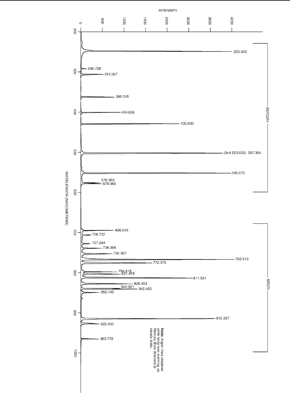
246 WinSpec/32 Manual Version 2.6B
Figure 202. Wavelength Calibration Spectrum

247
Appendix D
Data Structure
Version 1.43 Header
All WinView or WinSpec files (version 1.43) must begin with the following 4100 byte
header:
typedef WINXHEAD {
0 int dioden; /* CCD X dimension */
2 int avgexp; /* Not used by WinView */
4 int exposure; /* exposure if -1 see lexpos */
6 int datarange; /* Not used by WinView */
8 int mode; /* Not used by WinView */
10 float wexsy; /* Not used by WinView */
14 int asyavg; /* Not used by WinView */
16 int asyseq; /* Not used by WinView */
18 int linefreq; /* Not used by WinView */
20 int date0; /* Not used by WinView */
22 int date1; /* Not used by WinView */
24 int date2; /* Not used by WinView */
26 int date3; /* Not used by WinView */
28 int date4; /* Not used by WinView */
30 int ehour; /* Not used by WinView */
32 int eminute; /* Not used by WinView */
34 int noscan; /* # of stripes collected if -1 see */
/* lnoscan. */
36 int fastacc; /* Not used by WinView */
38 int avgtime; /* Not used by WinView */
40 int dmatotal; /* Not used by WinView */
42 int faccount; /* X dimension : Actual dim of image. */
44 int stdiode; /* Not used by WinView */
46 float nanox; /* Not used by WinView */
50 float calibdio[10]; /* Not used by WinView */
90 char fastfile[16]; /* fast access file. Not used by WinView */
106 int asynen; /* Not used by WinView */
108 int datatype; /* 0 -> float (4 byte) */
/* 1 -> long integer (4 byte) */
/* 2 -> integer (2 byte) */
/* 3 -> unsigned integer (2 byte) */
/* 4 -> String/char (1 byte) */
/* 5 -> double (8 bytes) Not implemented */
/* 6 -> byte (1 byte) */
/* 7 -> unsigned byte (1 byte) */
110 float calibnan[10]; /* Not used by WinView */
150 int rtanum; /* Not used by WinView */
152 int astdiode; /* Not used by WinView */
154 int int78; /* Not used by WinView */
156 int int79; /* Not used by WinView */
158 double calibpol[4]; /* Not used by WinView */
190 int int96; /* Not used by WinView */
192 int int97; /* Not used by WinView */
194 int int98; /* Not used by WinView */
196 int int99; /* Not used by WinView */
198 int int100; /* Not used by WinView */
200 char exprem[5][80]; /* comments */
600 int int301; /* Not used by WinView */
602 char label[16]; /* Not used by WinView */
618 int gsize; /* Not used by WinView */
620 int lfloat; /* Not used by WinView */
622 char califile[16]; /* calibration file. Not used by WinView */
638 char bkgdfile[16]; /* background file. Not used by WinView */
654 int srccmp; /* Not used by WinView */

248 WinSpec/32 Manual Version 2.6B
656 int stripe; /* number of stripes per frame */
658 int scramble; /* 0 - scramble, 1 – unscramble */
660 long lexpos; /* exposure val 32-bits(when exposure=-1) */
664 long lnoscan; /* no. of scan 32-bits(when noscan = -1) */
668 long lavgexp; /* no. of accum 32-bits(when avgexp = -1) */
672 char stripfil[16]; /* strip file. Not used by WinView */
688 char version[16]; /* SW version & date "01.000 02/01/90" */
704 int controller_type; /* 1-new st120, 2-old st120, */
/* 3-st130 type 1, 4-st130 type 2, */
/* 5-st138, 6-DC131, and ST133. */
/* YT_FILE_HEADER */
/* The YT variables are not used by WinView. */
706 int yt_file_defined; /* set TRUE for YT data file */
708 int yt_fh_calib_mode; /* calibration type*/
710 int yt_fh_calib_type; /* time-unit (calibration type) */
712 int yt_fh_element[12]; /* element number */
736 double yt_fh_calib_data[12]; /* data */
832 float yt_fh_time_factor; /* time-factor */
836 float yt_fh_start_time; /* start time */
840 int reverse_flag; /* set to 1 if data should be */
/* reversed, 0 do not reverse */
};
Version 1.6 Header
All WinView/WinSpec files (version 1.6) and WinView/32 and WinSpec/32 data files
must begin with the following 4100 byte header. Data files created under previous
versions of WinView/WinSpec can still be read correctly. However, files created under
the new versions (1.6 and higher) cannot be read by previous versions of
WinView/WinSpec.
Header Structure Listing
Decimal Byte
Offset
-----------
unsigned int dioden; /* 0 num of physical pixels (X axis) */
int avgexp; /* 2 number of accumulations per scan */
/* if > 32767, set to -1 and */
/* see lavgexp below (668) */
int exposure; /* 4 exposure time (in milliseconds) */
/* if > 32767, set to -1 and */
/* see lexpos below (660) */
unsigned int xDimDet; /* 6 Detector x dimension of chip */
int mode; /* 8 timing mode */
float exp_sec; /* 10 alternative exposure, in secs. */
int asyavg; /* 14 number of asynchron averages */
int asyseq; /* 16 number of asynchron sequential */
unsigned int yDimDet; /* 18 y dimension of CCD or detector. */
char date[10]; /* 20 date as MM/DD/YY */
int ehour; /* 30 Experiment Time: Hours (as binary) */
int eminute; /* 32 Experiment Time: Minutes(as binary) */
int noscan; /* 34 number of multiple scans */
/* if noscan == -1 use lnoscan */
int fastacc; /* 36 */
int seconds; /* 38 Experiment Time: Seconds(as binary) */
int DetType; /* 40 CCD/DiodeArray type */
unsigned int xdim; /* 42 actual # of pixels on x axis */
int stdiode; /* 44 trigger diode */
float nanox; /* 46 */
float calibdio[10]; /* 50 calibration diodes */
char fastfile[16]; /* 90 name of pixel control file */
int asynen; /* 106 asynchron enable flag 0 = off */
int datatype; /* 108 experiment data type */
/* 0 = FLOATING POINT */
/* 1 = LONG INTEGER */

Appendix D Data Structure 249
/* 2 = INTEGER */
/* 3 = UNSIGNED INTEGER */
float calibnan[10]; /* 110 calibration nanometer */
int BackGrndApplied; /* 150 set to 1 if background sub done */
int astdiode; /* 152 */
unsigned int minblk; /* 154 min. # of strips per skips */
unsigned int numminblk; /* 156 # of min-blocks before geo skps */
double calibpol[4]; /* 158 calibration coefficients */
unsigned int ADCrate; /* 190 ADC rate */
unsigned int ADCtype; /* 192 ADC type */
unsigned int ADCresolution; /* 194 ADC resolution */
unsigned int ADCbitAdjust; /* 196 ADC bit adjust */
unsigned int gain; /* 198 gain */
char exprem[5][80]; /* 200 experiment remarks */
unsigned int geometric; /* 600 geometric operations rotate 0x01 */
/* reverse 0x02, flip 0x04 */
char xlabel[16]; /* 602 Intensity display string */
unsigned int cleans; /* 618 cleans */
unsigned int NumSkpPerCln; /* 620 number of skips per clean. */
char califile[16]; /* 622 calibration file name (CSMA) */
char bkgdfile[16]; /* 638 background file name */
int srccmp; /* 654 number of source comp. diodes */
unsigned int ydim; /* 656 y dimension of raw data. */
int scramble; /* 658 0 = scrambled, 1 = unscrambled */
long lexpos; /* 660 long exposure in milliseconds */
/* used if exposure set to -1 */
long lnoscan; /* 664 long num of scans */
/* used if noscan set to -1 */
long lavgexp; /* 668 long num of accumulations */
/* used if avgexp set to -1 */
char stripfil[16]; /* 672 stripe file (st130) */
char version[16]; /* 688 version & date:"01.000 02/01/90" */
int type; /* 704 1 = new120 (Type II) */
/* 2 = old120 (Type I ) */
/* 3 = ST130 */
/* 4 = ST121 */
/* 5 = ST138 */
/* 6 = DC131 (PentaMAX) */
/* 7 = ST133 (MicroMAX/SpectroMax) */
/* 8 = ST135 (GPIB) */
/* 9 = VICCD */
/* 10 = ST116 (GPIB) */
/* 11 = OMA3 (GPIB) */
/* 12 = OMA4 */
int flatFieldApplied; /* 706 Set to 1 if flat field was applied */
int spare[8]; /* 708 reserved */
int kin_trig_mode /* 724 Kinetics Trigger Mode */
char empty[702]; /* 726 EMPTY BLOCK FOR EXPANSION */
float clkspd_us; /* 1428 Vert Clock Speed in micro-sec */
int HWaccumFlag; /* 1432 set to 1 if accum done by Hardware */
int StoreSync; /* 1434 set to 1 if store sync used. */
int BlemishApplied; /* 1436 set to 1 if blemish removal applied */
int CosmicApplied; /* 1438 set to 1 if cosmic ray removal done */
int CosmicType; /* 1440 if cosmic ray applied, this is type */
float CosmicThreshold; /* 1442 Threshold of cosmic ray removal. */
long NumFrames; /* 1446 number of frames in file. */
float MaxIntensity; /* 1450 max intensity of data (future) */
float MinIntensity; /* 1454 min intensity of data (future) */
char ylabel[LABELMAX]; /* 1458 y axis label. */
unsigned int ShutterType; /* 1474 shutter type. */
float shutterComp; /* 1476 shutter compensation time. */
unsigned int readoutMode; /* 1480 Readout mode, full, kinetics, etc. */
unsigned int WindowSize; /* 1482 window size for kinetics only. */
unsigned int clkspd; /* 1484 clock speed for kinetics & */
/* frame transfer. */
unsigned int interface_type; /* 1486 computer interface (isa-taxi, */
/* pci, eisa, etc.) */
unsigned long ioAdd1; /* 1488 I/O address of interface card. */
unsigned long ioAdd2; /* 1492 if more than one address for card */
unsigned long ioAdd3; /* 1496 */
unsigned int intLevel; /* 1500 interrupt level interface card */

250 WinSpec/32 Manual Version 2.6B
unsigned int GPIBadd; /* 1502 GPIB address (if used) */
unsigned int ControlAdd; /* 1504 GPIB controller address (if used) */
unsigned int controllerNum; /* 1506 if multiple controller system will */
/* have controller # data came from. */
/* (Future Item) */
unsigned int SWmade; /* 1508 Software which created this file */
int NumROI; /* 1510 number of ROIs used. If 0 assume 1 */
/* 1512 - 1630 ROI information .*/
struct ROIinfo { /* */
unsigned int startx; /* left x start value. */
unsigned int endx; /* right x value. */
unsigned int groupx; /* amount x is binned/grouped in hw. */
unsigned int starty; /* top y start value. */
unsigned int endy; /* bottom y value. */
unsigned int groupy; /* amount y is binned/grouped in hw. */
} ROIinfoblk[10]; /* ROI Starting Offsets: */
/* ROI 1 = 1512 */
/* ROI 2 = 1524 */
/* ROI 3 = 1536 */
/* ROI 4 = 1548 */
/* ROI 5 = 1560 */
/* ROI 6 = 1572 */
/* ROI 7 = 1584 */
/* ROI 8 = 1596 */
/* ROI 9 = 1608 */
/* ROI 10 = 1620 */
char FlatField[120]; /* 1632 Flat field file name. */
char background[120]; /* 1752 Background sub. file name. */
char blemish[120]; /* 1872 Blemish file name. */
float software_ver; /* 1992 Software version. */
char UserInfo[1000]; /* 1996-2995 user data. */
long WinView_id; /* 2996 Set to 0x01234567L if file was */
/* created by WinX */
-------------------------------------------------------------------------
Calibration Structures
There are three structures for the calibrations.
The Area Inside the Calibration Structure (below) is repeated two times.
xcalibration, /* 3000 - 3488 x axis calibration */
ycalibration, /* 3489 - 3977 y axis calibration */
Start of X Calibration Structure
double offset; /* 3000 offset for absolute data scaling */
double factor; /* 3008 factor for absolute data scaling */
char current_unit; /* 3016 selected scaling unit */
char reserved1; /* 3017 reserved */
char string[40]; /* 3018 special string for scaling */
char reserved2[40]; /* 3058 reserved */
char calib_valid; /* 3098 flag if calibration is valid */
char input_unit; /* 3099 current input units for */
/* "calib_value" */
char polynom_unit; /* 3100 linear UNIT and used */
/* in the "polynom_coeff" */
char polynom_order; /* 3101 ORDER of calibration POLYNOM */
char calib_count; /* 3102 valid calibration data pairs */
double pixel_position[10]; /* 3103 pixel pos. of calibration data */
double calib_value[10]; /* 3183 calibration VALUE at above pos */
double polynom_coeff[6]; /* 3263 polynom COEFFICIENTS */
double laser_position; /* 3311 laser wavenumber for relative WN */
char reserved3; /* 3319 reserved */
unsigned char new_calib_flag; /* 3320 If set to 200, valid label below */
char calib_label[81]; /* 3321 Calibration label (NULL term'd) */
char expansion[87]; /* 3402 Calibration Expansion area */
-------------------------------------------------------------------------

Appendix D Data Structure 251
Start of Y Calibration Structure
double offset; /* 3489 offset for absolute data scaling */
double factor; /* 3497 factor for absolute data scaling */
char current_unit; /* 3505 selected scaling unit */
char reserved1; /* 3506 reserved */
char string[40]; /* 3507 special string for scaling */
char reserved2[40]; /* 3547 reserved */
char calib_valid; /* 3587 flag if calibration is valid */
char input_unit; /* 3588 current input units for */
/* "calib_value" */
char polynom_unit; /* 3589 linear UNIT and used */
/* in the "polynom_coeff" */
char polynom_order; /* 3590 ORDER of calibration POLYNOM */
char calib_count; /* 3591 valid calibration data pairs */
double pixel_position[10]; /* 3592 pixel pos. of calibration data */
double calib_value[10]; /* 3672 calibration VALUE at above pos */
double polynom_coeff[6]; /* 3752 polynom COEFFICIENTS */
double laser_position; /* 3800 laser wavenumber for relative WN */
char reserved3; /* 3808 reserved */
unsigned char new_calib_flag; /* 3809 If set to 200, valid label below */
char calib_label[81]; /* 3810 Calibration label (NULL term'd) */
char expansion[87]; /* 3891 Calibration Expansion area */
-------------------------------------------------------------------------
End of Calibration Structures
char Istring[40]; /* 3978 special Intensity scaling string */
char empty3[80]; /* 4018 empty block to reach 4100 bytes */
int lastvalue; /* 4098 Always the LAST value in the header */
Version 2.5 Header (3/23/04)
The current data file used for WINX files consists of a 4100 (1004 Hex) byte header
followed by the data. Beginning with Version 2.5, many more items were added to the
header to make it a complete as possible record of the data collection. This includes
spectrograph and pulser information. Many of these additions were accomplished by
recycling old information that had not been used in previous versions. All data files
created under previous 2.x versions of WinView/WinSpec CAN still be read correctly.
HOWEVER, files created under the new versions (2.5 and higher) CANNOT be read by
previous versions of WinView/WinSpec OR by the CSMA software package.
Start of Header Information (0 - 2996)
Decimal
Byte
Offset
short ControllerVersion 0 Hardware Version
short LogicOutput 2 Definition of Output BNC
WORD AmpHiCapLowNoise 4 Amp Switching Mode
WORD xDimDet 6 Detector x dimension of chip.
short mode 8 timing mode
float exp_sec 10 alternative exposure, in sec.
short VChipXdim 14 Virtual Chip X dim
short VChipYdim 16 Virtual Chip Y dim
WORD yDimDet 18 y dimension of CCD or detector.
char date[DATEMAX] 20 date
short VirtualChipFlag 30 On/Off
char Spare_1[2] 32
short noscan 34 Old number of scans - should always be
-1
float DetTemperature 36 Detector Temperature Set
short DetType 40 CCD/DiodeArray type
WORD xdim 42 actual # of pixels on x axis
short stdiode 44 trigger diode

252 WinSpec/32 Manual Version 2.6B
float DelayTime 46 Used with Async Mode
WORD ShutterControl 50 Normal, Disabled Open, Disabled Closed
short AbsorbLive 52 On/Off
WORD AbsorbMode 54 Reference Strip or File
short CanDoVirtualChipFlag 56 T/F Cont/Chip able to do Virtual Chip
short ThresholdMinLive 58 On/Off
float ThresholdMinVal 60 Threshold Minimum Value
short ThresholdMaxLive 64 On/Off
float ThresholdMaxVal 66 Threshold Maximum Value
short SpecAutoSpectroMode 70 T/F Spectrograph Used
float SpecCenterWlNm 72 Center Wavelength in Nm
short SpecGlueFlag 76 T/F File is Glued
float SpecGlueStartWlNm 78 Starting Wavelength in Nm
float SpecGlueEndWlNm 82 Starting Wavelength in Nm
float SpecGlueMinOvrlpNm 86 Minimum Overlap in Nm
float SpecGlueFinalResNm 90 Final Resolution in Nm
short PulserType 94 0=None, PG200=1, PTG=2, DG535=3
short CustomChipFlag 96 T/F Custom Chip Used
short XPrePixels 98 Pre Pixels in X direction
short XPostPixels 100 Post Pixels in X direction
short YPrePixels 102 Pre Pixels in Y direction
short YPostPixels 104 Post Pixels in Y direction
short asynen 106 asynchron enable flag 0 = off
short datatype 108 experiment datatype
0 = float (4 bytes)
1 = long (4 bytes)
2 = short (2 bytes)
3 = unsigned short (2 bytes)
short PulserMode 110 Repetitive/Sequential
WORD PulserOnChipAccums 112 Num PTG On-Chip Accums
DWORD PulserRepeatExp 114 Num Exp Repeats (Pulser SW Accum)
float PulseRepWidth 118 Width Value for Repetitive pulse (usec)
float PulseRepDelay 122 Width Value for Repetitive pulse (usec)
float PulseSeqStartWidth 126 Start Width for Sequential pulse (usec)
float PulseSeqEndWidth 130 End Width for Sequential pulse (usec)
float PulseSeqStartDelay 134 Start Delay for Sequential pulse (usec)
float PulseSeqEndDelay 138 End Delay for Sequential pulse (usec)
short PulseSeqIncMode 142 Increments: 1=Fixed, 2=Exponential
short PImaxUsed 144 PI-Max type controller flag
short PImaxMode 146 PI-Max mode
short PImaxGain 148 PI-Max Gain
short BackGrndApplied 150 1 if background subtraction done
short PImax2nsBrdUsed 152 T/F PI-Max 2ns Board Used
WORD minblk 154 min. # of strips per skips
WORD numminblk 156 # of min-blocks before geo skps
short SpecMirrorLocation[2] 158 Spectro Mirror Location, 0=Not Present
short SpecSlitLocation[4] 162 Spectro Slit Location, 0=Not Present
short CustomTimingFlag 170 T/F Custom Timing Used
char ExperimentTimeLocal[TIMEMAX]172 Experiment Local Time as hhmmss\0
char ExperimentTimeUTC[TIMEMAX] 179 Experiment UTC Time as hhmmss\0
short ExposUnits 186 User Units for Exposure
WORD ADCoffset 188 ADC offset
WORD ADCrate 190 ADC rate
WORD ADCtype 192 ADC type
WORD ADCresolution 194 ADC resolution
WORD ADCbitAdjust 196 ADC bit adjust
WORD gain 198 gain
char Comments[5][COMMENTMAX] 200 File Comments
WORD geometric 600 geometric ops: rotate 0x01,reverse 0x02,
flip 0x04
char xlabel[LABELMAX] 602 intensity display string
WORD cleans 618 cleans
WORD NumSkpPerCln 620 number of skips per clean.
short SpecMirrorPos[2] 622 Spectrograph Mirror Positions
float SpecSlitPos[4] 626 Spectrograph Slit Positions
short AutoCleansActive 642 T/F
short UseContCleansInst 644 T/F
short AbsorbStripNum 646 Absorbance Strip Number
short SpecSlitPosUnits 648 Spectrograph Slit Position Units
float SpecGrooves 650 Spectrograph Grating Grooves
short srccmp 654 number of source comp.diodes

Appendix D Data Structure 253
WORD ydim 656 y dimension of raw data.
short scramble 658 0=scrambled,1=unscrambled
short ContinuousCleansFlag 660 T/F Continuous Cleans Timing Option
short ExternalTriggerFlag 662 T/F External Trigger Timing Option
long lnoscan 664 Number of scans (Early WinX)
long lavgexp 668 Number of Accumulations
float ReadoutTime 672 Experiment readout time
short TriggeredModeFlag 676 T/F Triggered Timing Option
char Spare_2[10] 678
char sw_version[FILEVERMAX] 688 Version of SW creating this file
short type 704 1 = new120 (Type II)
2 = old120 (Type I)
3 = ST130
4 = ST121
5 = ST138
6 = DC131 (PentaMax)
7 = ST133 (MicroMax/SpectroMax)
8 = ST135 (GPIB)
9 = VICCD
10 = ST116 (GPIB)
11 = OMA3 (GPIB)
12 = OMA4
short flatFieldApplied 706 1 if flat field was applied.
char Spare_3[16] 708
short kin_trig_mode 724 Kinetics Trigger Mode
char dlabel[LABELMAX] 726 Data label.
char Spare_4[436] 742
char PulseFileName[HDRNAMEMAX] 1178 Name of Pulser File with Pulse
Widths/Delays (for Z-Slice)
char AbsorbFileName[HDRNAMEMAX] 1298 Name of Absorbance File (if File Mode)
DWORD NumExpRepeats 1418 Number of Times experiment repeated
DWORD NumExpAccums 1422 Number of Time experiment accumulated
short YT_Flag 1426 Set to 1 if this file contains YT data
float clkspd_us 1428 Vert Clock Speed in micro-sec
short HWaccumFlag 1432 set to 1 if accum done by Hardware.
short StoreSync 1434 set to 1 if store sync used
short BlemishApplied 1436 set to 1 if blemish removal applied
short CosmicApplied 1438 set to 1 if cosmic ray removal applied
short CosmicType 1440 if cosmic ray applied, this is type
float CosmicThreshold 1442 Threshold of cosmic ray removal.
long NumFrames 1446 number of frames in file.
float MaxIntensity 1450 max intensity of data (future)
float MinIntensity 1454 min intensity of data future)
char ylabel[LABELMAX] 1458 y axis label.
WORD ShutterType 1474 shutter type.
float shutterComp 1476 shutter compensation time.
WORD readoutMode 1480 readout mode, full,kinetics, etc
WORD WindowSize 1482 window size for kinetics only.
WORD clkspd 1484 clock speed for kinetics & frame
transfer
WORD interface_type 1486 computer interface (isa-taxi, pci, eisa,
etc.)
short NumROIsInExperiment 1488 May be more than the 10 allowed in this
header (if 0, assume 1)
char Spare_5[16] 1490
WORD controllerNum 1506 if multiple controller system will have
controller number data came from. This
is a future item.
WORD SWmade 1508 Which software package created this file
short NumROI 1510 number of ROIs used. if 0 assume 1.
struct ROIinfo{
WORD startx left x start value.
WORD endx right x value.
WORD groupx amount x is binned/grouped in hw.
WORD starty top y start value.
WORD endy bottom y value.
WORD groupy amount y is binned/grouped in hw.

254 WinSpec/32 Manual Version 2.6B
} ROIinfoblk[ROIMAX]
ROI Starting Offsets:
ROI 1 = 1512
ROI 2 = 1524
ROI 3 = 1536
ROI 4 = 1548
ROI 5 = 1560
ROI 6 = 1572
ROI 7 = 1584
ROI 8 = 1596
ROI 9 = 1608
ROI 10 = 1620
char FlatField[HDRNAMEMAX] 1632 Flat field file name.
char background[HDRNAMEMAX] 1752 background sub. file name.
char blemish[HDRNAMEMAX] 1872 blemish file name.
float file_header_ver 1992 version of this file header
char YT_Info[1000] 1996-2995 Reserved for YT information
long WinView_id 2996 == 0x01234567L if file created by WinX
-------------------------------------------------------------------------------
Calibration Structures
There are three structures for the calibrations
The Area Inside the Calibration Structure (below) is repeated two times.
xcalibration, /* 3000 - 3488 x axis calibration */
ycalibration, /* 3489 - 3977 y axis calibration */
Start of X Calibration Structure (3000 - 3488)
double offset 3000 offset for absolute data scaling
double factor 3008 factor for absolute data scaling
char current_unit 3016 selected scaling unit
char reserved1 3017 reserved
char string[40] 3018 special string for scaling
char reserved2[40] 3058 reserved
char calib_valid 3098 flag if calibration is valid
char input_unit 3099 current input units for "calib_value"
char polynom_unit 3100 linear UNIT and used in the
"polynom_coeff"
char polynom_order 3101 ORDER of calibration POLYNOM
char calib_count 3102 valid calibration data pairs
double pixel_position[10] 3103 pixel pos. of calibration data
double calib_value[10] 3183 calibration VALUE at above pos
double polynom_coeff[6] 3263 polynom COEFFICIENTS
double laser_position 3311 laser wavenumber for relative WN
char reserved3 3319 reserved
BYTE new_calib_flag 3320 If set to 200, valid label below
char calib_label[81] 3321 Calibration label (NULL term'd)
char expansion[87] 3402 Calibration Expansion area
-------------------------------------------------------------------------------
Start of Y Calibration Structure (3489 - 3977)
double offset 3489 offset for absolute data scaling
double factor 3497 factor for absolute data scaling
char current_unit 3505 selected scaling unit
char reserved1 3506 reserved
char string[40] 3507 special string for scaling
char reserved2[40] 3547 reserved
char calib_valid 3587 flag if calibration is valid
char input_unit 3588 current input units for "calib_value"
char polynom_unit 3589 linear UNIT and used in the
"polynom_coeff"
char polynom_order 3590 ORDER of calibration POLYNOM
char calib_count 3591 valid calibration data pairs
double pixel_position[10] 3592 pixel pos. of calibration data
double calib_value[10] 3672 calibration VALUE at above pos

Appendix D Data Structure 255
double polynom_coeff[6] 3752 polynom COEFFICIENTS
double laser_position 3800 laser wavenumber for relative WN
char reserved3 3808 reserved
BYTE new_calib_flag 3809 If set to 200, valid label below
char calib_label[81] 3810 Calibration label (NULL term'd)
char expansion[87] 3891 Calibration Expansion area
-------------------------------------------------------------------------------
End of Calibration Structures (3978-4098)
char Istring[40] 3978 special intensity scaling string
char Spare_6[25] 4018
BYTE SpecType 4043 spectrometer type (acton, spex, etc.)
BYTE SpecModel 4044 spectrometer model (type dependent)
BYTE PulseBurstUsed 4045 pulser burst mode on/off
DWORD PulseBurstCount 4046 pulser triggers per burst
double PulseBurstPeriod 4050 pulser burst period (in usec)
BYTE PulseBracketUsed 4058 pulser bracket pulsing on/off
BYTE PulseBracketType 4059 pulser bracket pulsing type
double PulseTimeConstFast 4060 pulser slow exponential time constant (in
usec)
double PulseAmplitudeFast 4068 pulser fast exponential amplitude constant
double PulseTimeConstSlow 4076 pulser slow exponential time constant (in
usec)
double PulseAmplitudeSlow 4084 pulser slow exponential amplitude constant
short AnalogGain; 4092 analog gain
short AvGainUsed 4094 avalanche gain was used
short AvGain 4096 avalanche gain value
short lastvalue 4098 Always the LAST value in the header
Start of Data (4100 - )
4100 Start of Data
.
.
.
***************************** End of File ***************************
Definition of Array Sizes
HDRNAMEMAX = 120 Max char str length for file name
USERINFOMAX = 1000 User information space
COMMENTMAX = 80 User comment string max length (5 comments)
LABELMAX = 16 Label string max length
FILEVERMAX = 16 File version string max length
DATEMAX = 10 String length of file creation date string as ddmmmyyyy\0
ROIMAX = 10 Max size of roi array of structures
TIMEMAX = 7 Max time store as hhmmss\0
Custom Data Types Used In the Structure
BYTE = unsigned char
WORD = unsigned short
DWORD = unsigned long
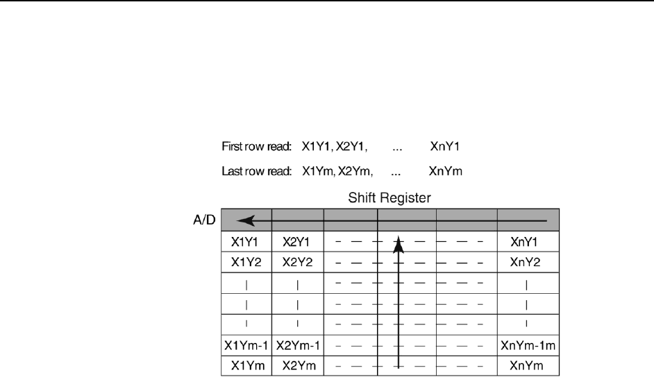
256 WinSpec/32 Manual Version 2.6B
Reading Data
Data follow the header beginning at offset 4100. In WinView/WinSpec, the data are
always stored exactly as they are collected. The order of the data depends on the
placement of the shift register. In the diagram below, the shift register is on the TOP of
the sensor. Each ROW of data is first shifted UP into the shift register and then LEFT.
The data are read (and stored) in this order:
The data are stored as sequential points and the X, Y, and Frame dimensions are
determined by the header.
The X dimension of the stored data is in "xdim" (Offset 42).
The Y dimension of the stored data is in "ydim" (Offset 656).
The size of a frame (in bytes) is:
One frame size = "xdim" x "ydim" x "datatype" (Offset 108)
The number of frames of data stored is in "NumFrames" (Offset 1446).

257
Appendix E
Auto-Spectro Wavelength Calibration
Equations used in WinSpec Wavelength Calibration
WinSpec/32 wavelength calibration is based on the grating equation for Czerny-Turner or
Ebert spectrographs (see Figure 203).
(m/d)- = sin + sin , or - = (d/m)(sin + sin ), (1)
where: - = wavelength at the center of the image plane,
m = diffraction order
d = distance between grooves (the inverse of grooves per mm), and
, = angles of the incident and exit beam relative to the grating normal.
The angles and are related to the inclusion angle, , and the rotational angle of the
grating, :
= - /2, and = + /2.
Thus the grating equation can be written as:
(m/d) - = sin ( - /2) + sin ( + /2) = 2 sin cos (/2),
and the grating angle is given by:
= asin {m- / (2d cos (/2))}. (2)
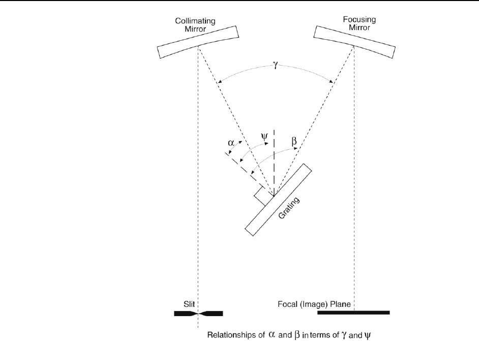
258 WinSpec/32 Manual Version 2.6B
Figure 203. Relationships of
and
in terms of
and
Note that the wavelength at the center of the exit plane does not depend on the focal
length, f. However, the wavelength at points off center depends on both the focal length
and the detector angle, (the angle of the image plane relative to the plane perpendicular
to the spectrograph focal axis at the center of the image plane; see Figure 204). For some
wavelength - relatively close to - (at the same grating angle),
-(d/m)(sin + sin ) = (d/m)(sin + sin (+)
= (d/m){sin ( - /2) + sin ( + /2 + )}. (3)
The angle depends on the focal length f, the detector angle , and the distance of
-from the center of the image plane, nx, where n is the number of pixels from the center
and x is the pixel width; the relationship is given by:
tan = (nx cos ) / (f + nx sin ), as shown in Figure 204. (4)
When the image plane is perpendicular, = 0, and this reduces to:
tan = (nx / f)
Using the known parameters of focal length f, detector angle , number of pixels from
center n, and pixel width x, first calculate the angle from equation 4. The grating angle
can be calculated using the known parameters center wavelength -, diffraction order
m, grating grooves per mm 1/d, and inclusion angle , from equation 2. Finally, the
wavelength at pixel n is calculated using equation 3.
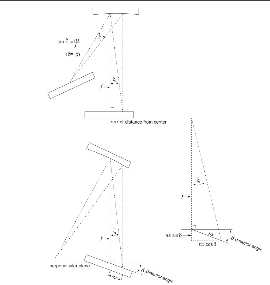
Appendix E Auto-Spectro Wavelength Calibration 259
Figure 204. Relationship between
and the focal length, detector angle, and the distance of
-
from image plane
WinSpec X Axis Auto Calibration
When “Calibration Usage” is set to “Auto Spectro” in WinSpec/32, the X Axis
calibration is done in the following steps after a wavelength change. First the wavelength
is calculated at each end of the array using the method above. Then these two points, plus
the third center wavelength point, are automatically fit to a 2nd order polynomial using the
wavelength calibration functions.

260 WinSpec/32 Manual Version 2.6B
This page intentionally left blank.

261
Appendix F
CD ROM Failure Work-Arounds
Although not common, there are CD drives that are not compatible with the Win ’95 long
filename convention. Attempting to install on such a system causes the filenames to be
truncated and the install fails, causing a message like:
An error occurred during the move data process: -113
Component: Application\WinXSystem
File Group: WinXSystem
Fortunately there are a couple of workarounds, both involving copying the install files to
the customer’s hard drive first, then installing the software from that location.
1. If possible, copy the files to the customer’s hard drive via another computer that
supports long file names. If the customer’s computer is part of a network then the
files can be copied first to the hard drive of a computer that supports long file names,
then transferred through the network to the customer’s hard drive. Check the list of
files below to make sure that the long filenames remain intact. Then install the
software from this location on the hard drive.
2. Copy the files to the customer’s hard drive from the customer’s CD-ROM, then fix
the names of the files that were truncated. There are only 7 files that are not DOS
compatible (8 + 3), so this at most a 10 minute job. Here are their abbreviated and
full filenames. (Not all of these files are used in the standard installation but all are
present on the CD.)
CLSSNA~1.CLS, rename to clsSnapIn.cls
PIXCMT~1.DLL, rename to PIXCMTXT32.dll
WINX_R~1.DOC, rename to WinX_readme.doc
WINX32~1.BAS, rename to Winx32Test.bas
WINX32~1.DOC, rename to Winx32 Automation - VB Version.doc
WINX32~1.FRM, rename to Winx32Test.frm
WINX32~1.FRX, rename to Winx32Test.frx

262 WinSpec/32 Manual Version 2.6B
This page intentionally left blank.

263
Appendix G
WinSpec/32 Repair and Maintenance
Note: When WinSpec/32 is installed, it modifies the Windows Registry file. If for any
reason you reinstall Windows, the Registry file may be replaced, and WinSpec/32 may
not run correctly. Reinstall WinSpec/32 to correct this problem.
Install/Uninstall WinSpec/32 Components at a Later Time
After you have installed WinSpec/32, you may want to install additional WinSpec/32
files or to uninstall selected files. To do so:
1. Start the installation program, click on CONTINUE, click on Install WinSpec/32 or
WinView/32, and then click on Install WinSpec/32 for Windows. Refer to Figure 205
below.
a. b.
c.
Figure 205. WinSpec, WinView, or WinXTest Selection dialogs
2. On the Enter Password dialog, enter the password and click on Next.
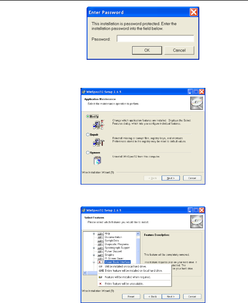
264 WinSpec/32 Manual Version 2.6B
Figure 206. Media Password dialog
3. Because WinSpec/32 was previously installed, the Application Maintenance
dialog (Figure 207) will be displayed.
Figure 207. Application Maintenance dialog
4. Select the Modify radio button and click on Next.
Figure 208. Select Features dialog
5. On the Select Features dialog, click on the feature you want to install or uninstall
and select the appropriate action from the list.
6. Then click on Next and follow the instructions on the dialogs.
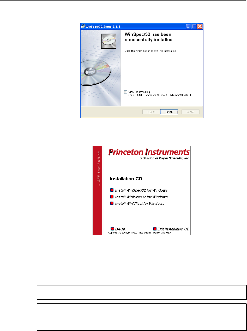
Appendix G WinSpec/32 Repair and Maintenance 265
7. Click on Finish when the WinSpec/32 has been successfully installed dialog is
displayed.
Figure 209. WinSpec/32 has been successfully installed dialog
8. Exit from the installation program or choose another program to install, perform
maintenance on, or uninstall.
Figure 210. Exit or Install Another Program dialog
Installing More than One Version of WinSpec/32
You can install more than one version of WinSpec/32, WinView/32 or any combination
of the two on a single computer. The install program will automatically create the new
directory.
Do not install both the WinSpec/32 and WinView/32 software packages in the same
directory.
Although several different versions of WinSpec/32 and/or WinView/32 can be installed
on the same computer without conflicts, you should not run more than one version at any
one time. The manner in which Princeton Instruments software allocates memory for data
collection precludes collecting data using two software packages at once.
Caution
Caution

266 WinSpec/32 Manual Version 2.6B
PIHWDEF.INI & SESSION.DAT
WinSpec/16 and PIHWDEF.INI: The hardware initialization file PIHWDEF.INI, is
included with 16-bit versions of WinSpec software. The file contains all of the hardware
settings necessary to get started and is read the first time WinSpec is executed. At the end of
the first operating session, the settings in effect are written to SESSION.DAT, which is read
the next time WinSpec software is operated so that the new session will begin with the same
settings that were in effect at the end of the previous one.
WinSpec/32 and the Windows Registry: WinSpec/32 doesn’t need PIHWDEF.INI or
SESSION.DAT, because it automatically stores the settings in the registry at the end of each
operating session. However, WinSpec/32 will read the WinSpec/16 PIHWDEF.INI or
SESSION.DAT if they are copied to the directory containing the WinSpec/32 software. This
allows users who are upgrading from a 16-bit version of WinSpec to WinSpec/32 to transfer
their previous operating settings to the new software. However, there is a constraint: if there
are settings in the registry (i.e., WinSpec/32 has been operated at least once), the software
will not read PIHWDEF.INI or SESSION.DAT unless the file date is newer than the date of
the stored registry settings. This problem can be avoided by simply copying PIHWDEF.INI
or SESSION.DAT to the WinSpec/32 directory before operating it the first time. If that
opportunity is lost, a newer SESSION.DAT can be created by booting the 16-bit WinSpec
software and then exiting the program in the usual manner. Similarly, a text editor could be
used to open/edit a copy of PIHWDEF.INI and then save it so that it has the current date.
Uninstalling and Reinstalling
If you suspect any of the WinSpec/32 files have become corrupt, you should first delete all
WinSpec/32 files, then reinstall the software from the CD or the FTP site. Follow the steps
below to remove WinSpec/32. Note that some files may remain. They will have to be
removed manually.
To uninstall WinSpec/32 from your computer:
1. Open the Windows Control Panel.
2. Double-click on Add/Remove Programs.
3. Highlight the WinSpec/32 version to uninstall and click on Add/Remove.
Notes:
1. The directory in which WinSpec/32 was originally installed will remain, as will
any files it contains that were not placed there during the original installation.
2. The Data directory created during the original installation may also be deleted.
Any data files you want to save should be copied to a safe location before
uninstalling.
3. The Version # and User identification will be removed from the registry.
However, the registry also contains much information that was placed there in
the course of setting up and operating the software. That information will remain
and will be available for use if WinSpec/32 is later reinstalled.
4. Follow the instructions on the dialogs.
To reinstall WinSpec/32 and any options, follow the procedure as described
beginning on page 23.

267
Appendix H
USB 2.0 Limitations
The following information covers the currently known limitations associated with
operating under the USB 2.0 interface.
Maximum cable length is 5 meters (16.4 feet)
1 MHz is currently the upper digitization rate limit for the ST-133 Controller.
Large data sets and/or long acquisition times may be subject to data overrun
because of host computer interrupts during data acquisition.
USB 2.0 is not supported by the Princeton Instruments PC Interface Library (Easy
DLLS).
Some WinView/WinSpec 2.5.X features are not fully supported with USB 2.0.
See the table below.
Feature
Supported with USB 2.0
in WinX 2.5.X
Remarks
Demo Port Capability
NO
DIF
NO
Kinetics
YES
WinX 2.5.18.1
Reset Camera to NVRAM
Defaults
NO
Temperature Lock Status
YES
WinX 2.5.x doesn’t
utilize hardware lock
status
PTG
YES
Virtual Chip
NO
Custom Timing
YES
WinX 2.5.18.1
Custom Chip
YES
WinX 2.5.18.1
Frames per Interrupt
NO
RS170 (Video Output)
NO
Online Exposure
NO
File Information
YES
Not all header info is
currently available in
WinX 2.5.x through
PVCAM
Overlapping ROIs
NO
Table 5. Features Supported under USB 2.0 (continued on next page)

268 WinSpec/32 Manual Version 2.6B
Feature
Supported with USB 2.0
in WinX 2.5.X
Remarks
Macro Record
YES
Macros recorded for
non-PVCAM cameras
may have to be re-
recorded to function
TTL I/O
NO
Table 5. Features Supported under USB 2.0

269
Appendix I
Troubleshooting
Introduction
The following information is provided for troubleshooting communication errors that
may occur.
Camera1 (or similar name) on Hardware Setup dialog
Figure 211. Camera1 in Camera Name Field
When a PVCAM-based camera is detected/selected during the Camera Detection Wizard
(formerly the Hardware Wizard), a default name such as Camera1 will be shown in the
Detected Hardware table and will be entered in the Camera Name (or Controller Type)
field on the Setup|Hardware|Controller/CCD tab. Because this name is not particularly
descriptive, you may want to change it. Such a change is made by editing the
PVCAM.INI file that is generated by Camera Detection Wizard.
To change the default Camera Name:
1. Using Notepad or a similar text editor, open PVCAM.INI, which is located in
the Windows directory (C:\WINNT, for example). You should see entries like
the ones below.
[Camera_1]
Type=1
Name=Camera1
Driver=apausb.sys
Port=0
ID=523459
2. Change the "Name=" entry to something more meaningful for you (for example,
ST133USB - to indicate that this is a PVCAM-based system using an ST-133
with a USB 2.0 interface) and save the edited file.
[Camera_1]
Type=1
Name=ST133USB
Driver=apausb.sys
Port=0
ID=523459
3. The new Camera Name (or Controller Type) name will now appear on the
Hardware Setup|Controller/Camera tab.

270 WinSpec/32 Manual Version 2.6B
Controller Is Not Responding
If this message pops up when you click on OK after selecting the "Interface Type" during
Hardware Setup (under the WinSpec/32 Setup menu), the system has not been able to
communicate with the Controller. Check to see if Controller has been turned ON and if
the interface card, its driver, and the interface cable have been installed.
If the Controller is ON, the problem may be with the interface card, its driver,
interrupt or address conflicts, or the cable connections.
If the interface card is not installed, close the application program and turn the
Controller OFF. Follow the interface card installation instructions in provided
with your interface card and cable the card to the SERIAL COM port on the rear
of the Controller. Then do a "Custom" installation of WinSpec/32 with the
appropriate interface component selected: "PCI Interface" or "ISA Interface",
depending on the interface card type. Be sure to deselect the interface component
that does not apply to your system.
Note: WinX (versions 2.5.25 and higher) does not support the ISA interface.
If the interface card is installed in the computer and is cabled to the SERIAL
COM port on the rear of the Controller, close the application program and turn
the Controller OFF. Check the cable connections and tighten the locking screws
if the connections are loose.
If the interface card was installed after WinSpec/32 has been installed, close that
application and do a "Custom" installation of it with the appropriate interface
component selected: "PCI Interface" or "ISA Interface", depending on the
interface card type. Be sure to deselect the interface component that does not
apply to your system.
Note: WinX (versions 2.5.25 and higher) does not support the ISA interface.
Data Loss or Serial Violation
You may experience either or both of these conditions if the host computer has been set
up with Power Saving features enabled. This is particularly true for power saving with
regard to the hard drive. Make sure that Power Saving features are disabled while you are
running WinSpec/32.
Data Overrun Due to Hardware Conflict message
Figure 212. Data Overrun Due to Hardware Conflict dialog
If this dialog appears when you try to acquire a test image, acquire data, or run in focus
mode, check the CCD array size and then check the DMA buffer size. A large array (for
example, a 2048x2048 array), requires a larger DMA buffer larger setting than that for a
smaller array (for example, a 512x512 array).

Appendix I Troubleshooting 271
To change the DMA buffer setting:
1. Note the array size (on the Setup|Hardware|Controller/CCD tab or the
Acquisition|Experiment Setup|Main tab Full Chip dimensions).
2. Open Setup|Environment|Environment dialog.
3. Increase the DMA buffer size to a minimum of 32 Mb (64 Mb if it is currently
32 Mb or 128 Mb if it is currently 64 Mb), click on OK, and close WinSpec.
4. Reboot your computer.
5. Restart WinSpec and begin acquiring data or focusing. If you see the message
again, increase the DMA buffer size.
Data Overrun Has Occurred message
Because of memory constraints and the way that USB transfers data, a "Data overrun has
occurred" message may be displayed during data acquisition. If this message is displayed,
take one or more of the following actions:
1. Minimize the number of programs running in the background while you are
acquiring data with WinSpec/32.
2. Run data acquisition in Safe Mode.
3. Add memory.
4. Use binning.
5. Increase the exposure time.
6. Defragment the hard disk.
7. Update the Orange Micro USB2 driver. See "OrangeUSB USB 2.0 Driver
Update", page 273.
If the problem persists, your application may be USB 2.0 bus limited. Since the host
computer controls the USB 2.0 bus, there may be situations where the host computer
interrupts the USB 2.0 port. In most cases, the interrupt will go unnoticed by the user.
However, there are some instances when the data overrun cannot be overcome because
USB 2.0 bus limitations combined with long data acquisition times and/or large data sets
increase the possibility of an interrupt while data is being acquired. If your experiment
requirements include long data acquisition times and/or large data sets, your application may
not be suitable for the USB 2.0 interface. Therefore, we recommend replacement of the USB
2.0 interface module with our TAXI interface module and Princeton Instruments PCI card. If
this is not the case and data overruns continue to occur, contact Customer Support (see
page 282 for contact information).
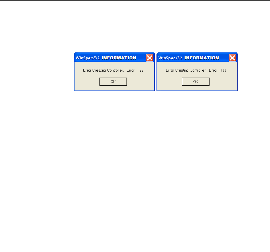
272 WinSpec/32 Manual Version 2.6B
Error Creating Controller message
This message may be displayed if you are using the USB 2.0 interface and have not run
the RSConfig.exe program (see previous topic), if the PVCAM.INI file has been
corrupted, or if the ST-133 was not turned on before you started WinSpec/32 and began
running the Hardware Setup wizard.
Figure 213. Error Creating Controller dialog
Error 129: Indicates that the problem is with the PVCAM.INI file. Close WinSpec/32,
run RSConfig, make sure the ST-133 is on, reopen WinSpec, and begin running the
Hardware Setup wizard.
Error 183: Indicates that the ST-133 is off. If you are running the Hardware Setup
wizard when this message appears, click on OK, turn on the ST-133, and, on the
PVCAM dialog, make sure Yes is selected and then click on Next. The Hardware
Setup wizard should continue to the Controller Type dialog.
Ethernet Network is not accessible
When the Princeton Instruments software is installed, all Intel Pro/1000 interface card
drivers found on the host computer are updated with the Intel Pro/1000 Grabber Adapter
(Vision High-Performance IP Device) driver provided by Pleora Technologies, Inc. If
this computer is connected to an Ethernet network via an Intel Pro/1000 card that does
not use the Pleora driver, the network connection will be broken.
To restore the driver for the Ethernet card that is used to connect to the network:
1. Locate the EbDriverTool32.exe file.
Download the EbDriverTool32.exe file to your computer from
ftp://ftp.princetoninstruments.com/public/Software/Official/WinX32/GigE/
Or open the default Pleora directory. Typically it is located at C:\Program
Files\Common Files\Pleora. The EbDriverTool32.exe (or EbDriverTool.exe)
file may be in a subdirectory.
2. Run the file.
3. When this program executes, select the appropriate Ethernet card and under the
Action category, choose “Install High-Performance IP Device Driver” from the
pulldown menu.
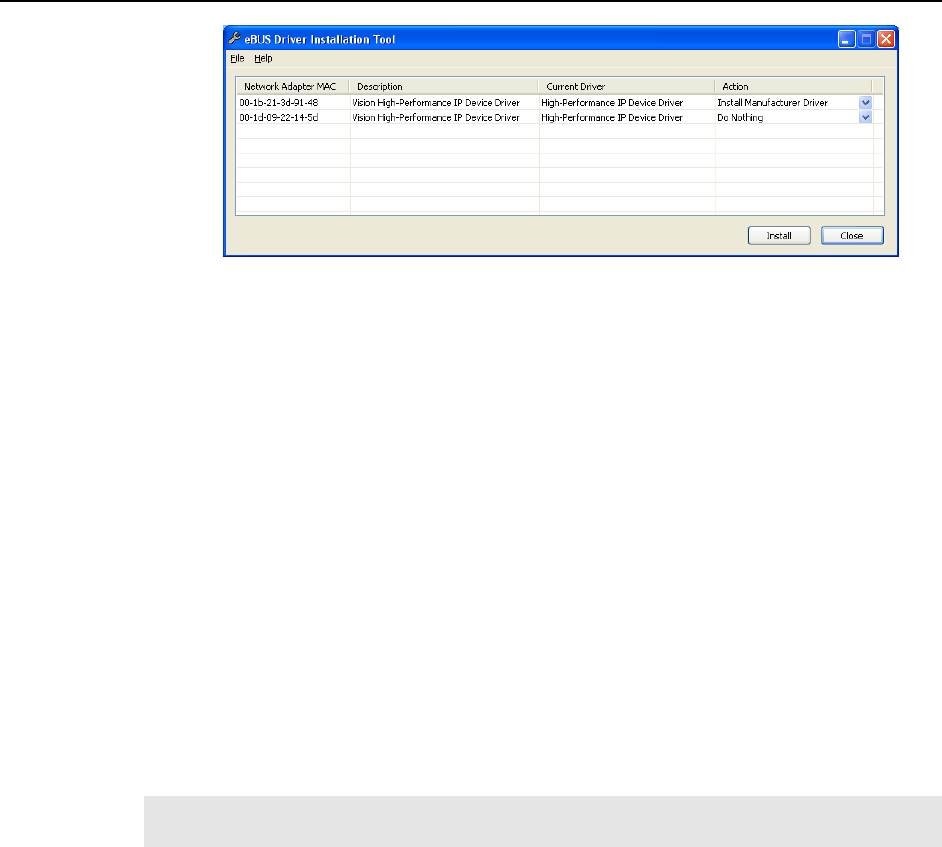
Appendix I Troubleshooting 273
Figure 214. Ebus Driver Installation Tool dialog
4. After making the selection, click on Install.
5. After the installation you may be asked to reboot the computer. If you are asked to
reboot, you can
Click on “Yes” to initiate the reboot.
Click on “No” to wait before rebooting. If you select “No,” you may be required
to close the eBUS Driver Installation Tool dialog. Reboot the computer at your
convenience.
6. Verify that the network connection has been re-established. If a reboot was required,
wait until the reboot has occurred before verifying the connection.
OrangeUSB USB 2.0 Driver Update
This procedure is highly recommended when a laptop computer will be used to
communicate with the ST-133. We recommend the SIIG, Inc. USB 2.0 PC Card, Model
US2246 if USB 2.0 is not native to the laptop's motherboard. To reduce the instances of
data overruns and serial violations, the OrangeUSB USB 2.0 Host Controller installed for
the SIIG card should be replaced by the appropriate Microsoft driver (Windows XP or
Vista (32-bit), depending on the laptop's operating system.)
Note: This procedure may also be performed for desktop computers that use the Orange
Micro 70USB90011 USB2.0 PCI.
1. Download and install Microsoft Service Pack 1 (for Windows XP) if the service pack
has not been installed.
2. From the Windows Start menu, select Settings|Control Panel.
3. Select System and then System Properties.
4. Select the Hardware tab and click on Device Manager button.
5. Expand Universal Serial Bus Controllers.
6. Right-mouse click on OrangeUSB USB 2.0 Host Controller and select
Properties.
7. On the Driver tab, click on the Update Driver… button. You may have to wait a
minute or so before you will be allowed to click on the button.
8. When the Upgrade Device Driver Wizard appears, click on Next. Select the
Search for a suitable driver … radio button.
9. On the next screen select the Specify a location checkbox.
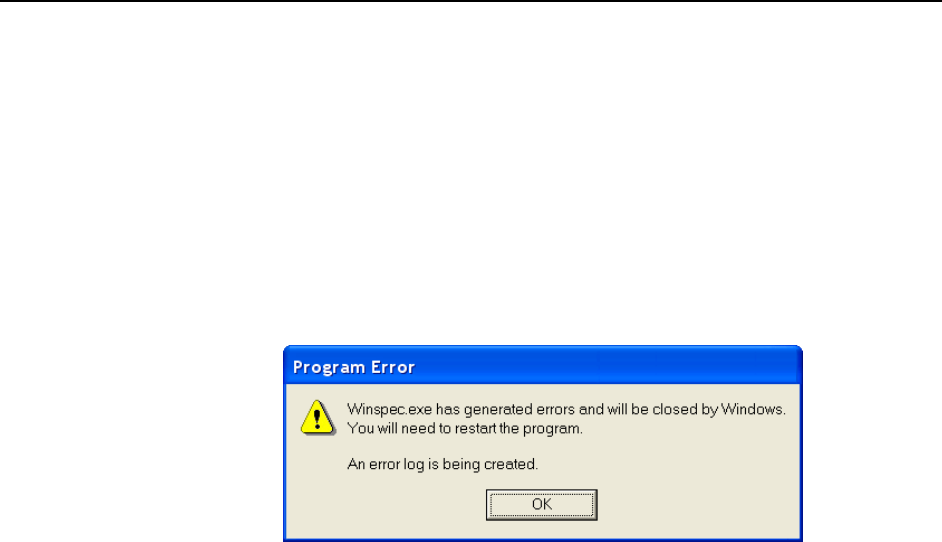
274 WinSpec/32 Manual Version 2.6B
10. Browse and select the location. Click on OK.
11. In the Driver Files Search Results window, check the Install one of the other
drivers check box.
12. Select the NEC PCI to USB Enhanced Host Controller B1 driver (Microsoft is
the provider). Click on Next and the installation will take place. When the
Completing the Upgrade Device Driver Wizard window appears, click on
Finish. You will then be given the choice of restarting the computer now or later.
According to the window text, the hardware associated with the driver will not work
until you restart the computer.
Program Error message
Figure 215. Program Error dialog
This dialog may appear if you have tried to acquire a test image, acquire data, or run in
focusing mode and the DMA buffer size is too small. A large array (for example, a
2048x2048 array), requires a larger setting than that for a smaller array (for example, a
512x512 array).
To correct the problem:
1. Click on OK.
2. Reboot WinSpec.
3. Note the array size (on the Setup|Hardware|Controller/CCD tab or the
Acquisition|Experiment Setup|Main tab Full Chip dimensions). If your
camera contains a large array (such as a 2048x2048 array), and the DMA buffer
size is too small, there will not be enough space in memory for the data set.
4. Open Setup|Environment|Environment dialog.
5. Increase the DMA buffer size to a minimum of 32 Mb (64 Mb if it is currently 32
Mb or 128 Mb if it is currently 64 Mb), click on OK, and close WinSpec.
6. Reboot your computer.
7. Restart WinSpec and begin acquiring data or focusing. If you see the message
again, increase the DMA buffer size.
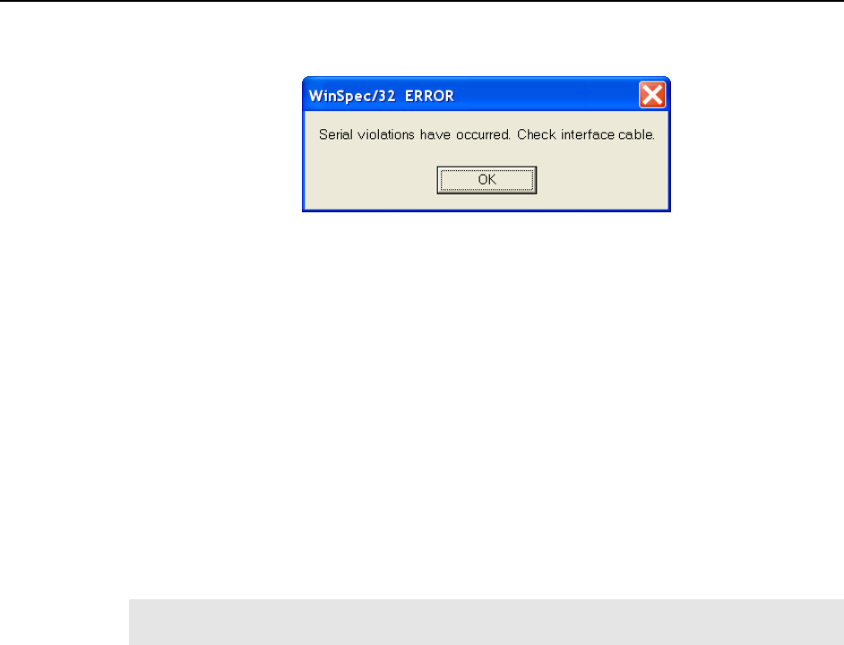
Appendix I Troubleshooting 275
Serial violations have occurred. Check interface cable.
Figure 216. Serial Violations Have Occurred dialog
This error message dialog will appear if you try to acquire an image or focus the camera
and either (or both) of the following conditions exists:
The camera system is not turned ON.
There is no communication between the camera and the host computer.
To correct the problem:
1. Turn OFF the camera system (if it is not already OFF).
2. Make sure the Detector-Controller cable is secured at both ends and that the
computer interface cable is secured at both ends.
3. After making sure that the cables are connected, turn the camera system power
ON.
4. Click OK on the error message dialog and retry acquiring an image or running in
focus mode.
Note: This error message will also be displayed if you turn the camera system OFF or a
cable comes loose while the application software is running in Focus mode.

276 WinSpec/32 Manual Version 2.6B
This page intentionally left blank.

277
Appendix J
Glossary
A/D converter: Analog-to-digital converter. In a CCD detector system, the electronic
circuitry that converts the analog information (continuous amplitudes) acquired by the
detector into the digital data (quantified, discrete steps) used for image display.
ADU: Analog-to-digital unit. A number representing a CCD's output. The relationship
between the ADUs generated and the number of electrons acquired on the CCD is
defined by the system gain. Intensities given in ADUs provide a convenient method for
comparing images and data generated by different detectors. Also referred to as count and
digital number.
Anti-blooming: Blooming is caused by saturation of one or more CCD pixels. This can
occur if the incoming light is too bright or when extensive serial and parallel binning is
being performed. When this saturation happens, the excess charge overflows into the
adjacent pixels and results in a streak or a blob appearing on the image. Anti-blooming is
traditionally controlled by specific CCD architecture designs that drain the excess charge.
Avalanche Gain: Also called "on-chip multiplication gain". A technology that enables
multiplication of charge (i.e., electrons) collected in each pixel of the CCD’s active array.
Secondary electrons are generated via an impact-ionization process that is initiated and
sustained when higher-than-typical voltages are applied to an “extended” portion of the
CCD’s serial register. Multiplying the signal above the read noise of the output amplifier
enables ultra-low-light detection at high operation speeds. (Some CCD cameras with on-
chip multiplication gain utilize two output amplifiers, an “on-chip multiplication gain”
amplifier that allows the camera to be used for low-light, high-speed applications and a
“traditional” amplifier for wide-dynamic-range applications.)
Backlash: Applied to the movement of gratings or slits, this is the amount of play
between gears when changing the direction of travel.
Bias: In a CCD detector system, the minimum intensity required for each exposure
(equivalent to performing a zero-second exposure with the shutter closed). Without
adding any light, the bias allows charge to be read out on the CCD while raising the
intensity level high enough to ensure that the detector does not deliver a negative number
to the A/D converter. (The A/D converter only works in the set of positive numbers and
has no instructions for processing negative numbers.) The bias may be user settable.
However, it is set at the factory and should remain stable over the lifetime of the detector
system.
Binning: Hardware binning is the process of combining the charge from adjacent pixels
in a CCD before the signal is read out by the preamplifier. A binning of 1 in both
directions reads out each pixel at full X-axis resolution. A binning of 2 in both directions
combines four pixels, cutting the X-axis resolution in half, but quadrupling the light-
collecting area. If the CCD chip shift register is being saturated due to hardware binning,
you can use software binning instead by checking Use Software Binning on the ROI
Setup tab. Note that software binning is not as fast as hardware binning.

278 WinSpec/32 Manual Version 2.6B
Cancel button: Exits a dialog without performing any processing. Any changes to the
dialog are lost.
Close button: Closes the dialog or window with no action taken.
Dark current: (1) The charge accumulated within a well, in the absence of light. (2) The
background current that flows in a charge-coupled device or image intensifier of a camera
system. Cooling the photodetector's primary imaging surface (i.e., the CCD's
photoconductor or the image intensifier's photocathode) can reduce or eliminate dark
current. Also called thermally generated charge. Dark current can be subtracted from an
image.
Gating: In an intensified detector system, the application of a voltage that switches the
image intensifier on and off in very short intervals. Gating improves temporal resolution.
Gating can be controlled by the programmed exposure time (Shutter Mode) or is
determined by the Pulser settings (Gate Mode).
Help button: Opens the context-sensitive help for the active tab or dialog.
Host computer: The primary or controlling computer for a detector.
Mouse button: Allows you to specify a region to be processed using the mouse.
Simply drag a box in the data region of the active window and then click on Mouse. The
Frame and Range parameters will assume the values of the defined region. Note that
the Mouse button is only active when the Input tab is selected.
MPP: Multi-pinned-phase operation. A mode that reduces the rate of dark current
generation by a factor of 20 or more, relaxing CCD cooling requirements to the level
where a thermoelectric cooler is sufficient for most applications. Also called inverted
operation.
NVRAM: Non-Volatile Random Access Memory. NVRAM contains factory-
programmed information about the controller and, in many cases, the camera/detector.
Process button: Causes the specified operation or process to be performed. The
process is performed on the data specified on the Input tab and saved using the file name
and data type specified on the Output tab.
PVCAM: Programmable Virtual Camera Access Method. An exclusive (Roper
Scientific) universal programming interface. A set of software library routines that
implements a detector or camera's operations in a hardware-independent, platform-
independent (or "virtual") suite of function calls. Once an application has been written to
control one PVCAM-enabled camera, all PVCAM-enabled cameras are then compatible
with that application.
ROI: Region of interest. A user-defined, rectangular area (a square is common) on a
CCD that is exposed and processed as an image.
Shutter Compensation Time: The time it takes for a mechanical shutter to open or
close. This time needs to be accounted for during hardware setup so the software can
allow enough time for the shutter to open before starting data acquisition and allow
enough time for it to close before reading out the array.

279
Warranty & Service
Limited Warranty:
Princeton Instruments, a division of Roper Scientific, Inc. ("Princeton Instruments", "us",
"we", "our") makes the following limited warranties. These limited warranties extend to
the original purchaser ("You", "you") only and no other purchaser or transferee. We have
complete control over all warranties and may alter or terminate any or all warranties at
any time we deem necessary.
Basic Limited One (1) Year Warranty
Princeton Instruments warrants this product against substantial defects in materials and /
or workmanship for a period of up to one (1) year after shipment. During this period,
Princeton Instruments will repair the product or, at its sole option, repair or replace any
defective part without charge to you. You must deliver the entire product to the Princeton
Instruments factory or, at our option, to a factory-authorized service center. You are
responsible for the shipping costs to return the product. International customers should
contact their local Princeton Instruments authorized representative/distributor for repair
information and assistance, or visit our technical support page at
www.princetoninstruments.com.
Limited One (1) Year Warranty on Refurbished or Discontinued
Products
Princeton Instruments warrants, with the exception of the CCD imaging device (which
carries NO WARRANTIES EXPRESS OR IMPLIED), this product against defects in
materials or workmanship for a period of up to one (1) year after shipment. During this
period, Princeton Instruments will repair or replace, at its sole option, any defective parts,
without charge to you. You must deliver the entire product to the Princeton Instruments
factory or, at our option, a factory-authorized service center. You are responsible for the
shipping costs to return the product to Princeton Instruments. International customers
should contact their local Princeton Instruments representative/distributor for repair
information and assistance or visit our technical support page at
www.princetoninstruments.com.
XP Vacuum Chamber Limited Lifetime Warranty
Princeton Instruments warrants that the cooling performance of the system will meet our
specifications over the lifetime of an XP style detector (has all metal seals) or Princeton
Instruments will, at its sole option, repair or replace any vacuum chamber components
necessary to restore the cooling performance back to the original specifications at no cost
to the original purchaser. Any failure to "cool to spec" beyond our Basic (1) year limited
warranty from date of shipment, due to a non-vacuum-related component failure (e.g.,
any components that are electrical/electronic) is NOT covered and carries NO
WARRANTIES EXPRESSED OR IMPLIED. Responsibility for shipping charges is as
described above under our Basic Limited One (1) Year Warranty.

280 WinSpec/32 Manual Version 2.6B
Sealed Chamber Integrity Limited 12 Month Warranty
Princeton Instruments warrants the sealed chamber integrity of all our products for a
period of twelve (12) months after shipment. If, at anytime within twelve (12) months
from the date of delivery, the detector should experience a sealed chamber failure, all
parts and labor needed to restore the chamber seal will be covered by us. Open chamber
products carry NO WARRANTY TO THE CCD IMAGING DEVICE, EXPRESSED OR
IMPLIED. Responsibility for shipping charges is as described above under our Basic
Limited One (1) Year Warranty.
Vacuum Integrity Limited 12 Month Warranty
Princeton Instruments warrants the vacuum integrity of “Non-XP” style detectors (do not
have all metal seals) for a period of up to twelve (12) months from the date of shipment.
We warrant that the detector head will maintain the factory-set operating temperature
without the requirement for customer pumping. Should the detector experience a Vacuum
Integrity failure at anytime within twelve (12) months from the date of delivery all parts
and labor needed to restore the vacuum integrity will be covered by us. Responsibility for
shipping charges is as described above under our Basic Limited One (1) Year Warranty.
Image Intensifier Detector Limited One Year Warranty
All image intensifier products are inherently susceptible to Phosphor and/or
Photocathode burn (physical damage) when exposed to high intensity light. Princeton
Instruments warrants, with the exception of image intensifier products that are found to
have Phosphor and/or Photocathode burn damage (which carry NO WARRANTIES
EXPRESSED OR IMPLIED), all image intensifier products for a period of one (1) year
after shipment. See additional Limited One (1) year Warranty terms and conditions
above, which apply to this warranty. Responsibility for shipping charges is as described
above under our Basic Limited One (1) Year Warranty.
X-Ray Detector Limited One Year Warranty
Princeton Instruments warrants, with the exception of CCD imaging device and fiber
optic assembly damage due to X-rays (which carry NO WARRANTIES EXPRESSED
OR IMPLIED), all X-ray products for one (1) year after shipment. See additional Basic
Limited One (1) year Warranty terms and conditions above, which apply to this
warranty. Responsibility for shipping charges is as described above under our Basic
Limited One (1) Year Warranty.
Software Limited Warranty
Princeton Instruments warrants all of our manufactured software discs to be free from
substantial defects in materials and / or workmanship under normal use for a period of
one (1) year from shipment. Princeton Instruments does not warrant that the function of
the software will meet your requirements or that operation will be uninterrupted or error
free. You assume responsibility for selecting the software to achieve your intended
results and for the use and results obtained from the software. In addition, during the one
(1) year limited warranty. The original purchaser is entitled to receive free version
upgrades. Version upgrades supplied free of charge will be in the form of a download
from the Internet. Those customers who do not have access to the Internet may obtain the
version upgrades on a CD-ROM from our factory for an incidental shipping and handling
charge. See Item 12 in the following section of this warranty ("Your Responsibility") for
more information.

Warranty & Service 281
Owner's Manual and Troubleshooting
You should read the owner’s manual thoroughly before operating this product. In the
unlikely event that you should encounter difficulty operating this product, the owner’s
manual should be consulted before contacting the Princeton Instruments technical support
staff or authorized service representative for assistance. If you have consulted the owner's
manual and the problem still persists, please contact the Princeton Instruments technical
support staff or our authorized service representative. See Item 12 in the following section
of this warranty ("Your Responsibility") for more information.
Your Responsibility
The above Limited Warranties are subject to the following terms and conditions:
1. You must retain your bill of sale (invoice) and present it upon request for service
and repairs or provide other proof of purchase satisfactory to Princeton
Instruments.
2. You must notify the Princeton Instruments factory service center within (30)
days after you have taken delivery of a product or part that you believe to be
defective. With the exception of customers who claim a "technical issue" with the
operation of the product or part, all invoices must be paid in full in accordance
with the terms of sale. Failure to pay invoices when due may result in the
interruption and/or cancellation of your one (1) year limited warranty and/or any
other warranty, expressed or implied.
3. All warranty service must be made by the Princeton Instruments factory or, at our
option, an authorized service center.
4. Before products or parts can be returned for service you must contact the
Princeton Instruments factory and receive a return authorization number (RMA).
Products or parts returned for service without a return authorization evidenced by
an RMA will be sent back freight collect.
5. These warranties are effective only if purchased from the Princeton Instruments
factory or one of our authorized manufacturer's representatives or distributors.
6. Unless specified in the original purchase agreement, Princeton Instruments is not
responsible for installation, setup, or disassembly at the customer’s location.
7. Warranties extend only to defects in materials or workmanship as limited above
and do not extend to any product or part which:
has been lost or discarded by you;
has been damaged as a result of misuse, improper installation, faulty or
inadequate maintenance or failure to follow instructions furnished by us;
has had serial numbers removed, altered, defaced, or rendered illegible;
has been subjected to improper or unauthorized repair;
has been damaged due to fire, flood, radiation, or other "acts of God" or other
contingencies beyond the control of Princeton Instruments; or
is a shutter which is a normal wear item and as such carries a onetime only
replacement due to a failure within the original 1 year Manufacturer
warranty.
8. After the warranty period has expired, you may contact the Princeton Instruments
factory or a Princeton Instruments-authorized representative for repair
information and/or extended warranty plans.

282 WinSpec/32 Manual Version 2.6B
9. Physically damaged units or units that have been modified are not acceptable for
repair in or out of warranty and will be returned as received.
10. All warranties implied by state law or non-U.S. laws, including the implied
warranties of merchantability and fitness for a particular purpose, are expressly
limited to the duration of the limited warranties set forth above. With the exception
of any warranties implied by state law or non-U.S. laws, as hereby limited, the
forgoing warranty is exclusive and in lieu of all other warranties, guarantees,
agreements, and similar obligations of manufacturer or seller with respect to the
repair or replacement of any parts. In no event shall Princeton Instruments' liability
exceed the cost of the repair or replacement of the defective product or part.
11. This limited warranty gives you specific legal rights and you may also have other
rights that may vary from state to state and from country to country. Some states
and countries do not allow limitations on how long an implied warranty lasts,
when an action may be brought, or the exclusion or limitation of incidental or
consequential damages, so the above provisions may not apply to you.
12. When contacting us for technical support or service assistance, please refer to the
Princeton Instruments factory of purchase, contact your authorized Princeton
Instruments representative or reseller, or visit our technical support page at
www.princetoninstruments.com.
Contact Information
Roper Scientific's manufacturing facility for this product is located at the following
address:
Princeton Instruments
3660 Quakerbridge Road
Trenton, NJ 08619 (USA)
Tel: 1-800-874-9789 / 1-609-587-9797
Fax: 1-609-587-1970
Customer Support E-mail: techsupport@princetoninstruments.com
For immediate support in your area, please call the following locations directly:
North America 800 899 1144 (toll free) or 609 587 9797
France +33 (1) 60 86 03 65
Germany +49 (0) 89 660 7793
Japan +81 (3) 5639 2741
UK & Ireland +44 (0) 1628 472 346
Singapore +65 6408 6240
China +86 10 659 16460
Otherwise, see our Support web page at www.princetoninstruments.com.
An up-to-date list of addresses and telephone numbers is posted on the
www.princetoninstruments.com/Support page. In addition, links on this
page to support topics allow you to send e-mail based requests to the
Customer Support group.

283
Index
#
3D Graph display ................................................... 101
3D Layout tab page
Z Axis Endpoint ................................................ 109
A-B
Absolute math operation ........................................ 155
Absorbance (on-line) process ................................ 126
Accessories, alignment of ........................................ 241
Active spectrograph, specifying .............................. 52
Acton Series spectrograph
focusing ............................................................. 241
rotational alignment ........................................... 240
Addition math operation ........................................ 155
Adjust calibration procedure ................................... 94
Adjust error .............................................................. 95
Alignment, rotational ............................................. 240
Amplitude .............................................................. 205
AND math operation ............................................. 156
Areas (Y:T) ............................................................ 127
ASCII output (on-line) process ............................. 134
Auto Select
at least three strips ............................................... 78
eleven or more strips ........................................... 78
two strips ............................................................. 78
Auto Select algorithm .............................................. 78
at least three strips ............................................... 99
eleven or more strips ............................................. 99
single strip ......................................................... 100
two strips ........................................................... 100
Auto Select Image, Graph or 3D Graph .................. 77
Auto-Spectro ................ See Spectrograph Calibration
AUX DLY'D TRIG OUT ...................................... 188
Avalanche gain .......................................... 59, 67, 277
Axis labeling ......................................................... 119
Background subtraction ................................. 147, 148
acquiring background files ................................ 147
automatic ........................................................... 148
Binary math operations .......................................... 156
Binning
constraints with PCI card .................. 140, 277, 278
hardware ............................................................ 140
in spectroscopy .................................................. 140
post-process ....................................................... 180
software ..................................................... 140, 141
Binning and Skipping
post processing .................................................. 180
procedure ........................................................... 180
Binning and Skipping (cont.)
restrictions and liminations ............................... 181
Bitwise math operations
AND .................................................................. 156
complement ....................................................... 156
exclusive OR ..................................................... 156
OR ..................................................................... 156
Block size ................................................................ 49
C
Calibration
menu .................................................................... 84
method ................................................................. 88
Off ....................................................................... 83
reference lines ................................................... 245
Setup dialog ......................................................... 85
structures ................................................... 250, 254
suitable light sources ................................. 240, 242
Camera Detection wizard ........................................ 37
Camera, rotation of ................................................ 241
Cautions
calibration sequence ............................................ 92
changing Cleans and Skips settings .................... 47
running different versions ................................. 265
WinSpec/32 and WinView/32 in same directory 29, 30
CCD Blemish removal ........................................... 150
Circuit.spe displayed ............................................. 114
Clean cycles ........................................................... 135
CLEANING signal .................................................. 43
Cleans/Skips tab page ............................................ 47
Cleans .................................................................. 47
Minimum Block Size........................................... 49
Number of Blocks ............................................... 49
Number of Cleans ............................................... 47
Number of Strips per Clean ................................. 47
Use Continuous Cleans Instruction ..................... 48
Cleans/Skips tab page parameters
Clean Mode .......................................................... 47
Vertical Skips ....................................................... 49
Clipping and Threshold procedure ........................ 178
Closing a data file ..................................................... 81
Color
axes, labels, graphs, background and surfaces .. 120
Communication Error with Spectrograph ................ 90
Complement math operation .................................. 156
Computer requirement ............................................. 23
Contact information ............................................... 282
Continuous cleans .................................................. 136
Continuous Cleans Instruction ........................ 48, 138
Correction techniques ............................................ 147

284 WinSpec/32 Manual Version 2.6B
Cosmic Ray removal ............................................. 151
Cross Sections (post processing) ............................. 179
Cross sections procedure ....................................... 179
Cursor Curve ......................................................... 108
Cursor functions
data displayed as graph or image ...................... 107
Custom Chip ............................................................ 44
Custom filter procedure ......................................... 172
Custom Timing ................................................ 44, 214
Custom Toolbar
adding a button .................................................. 210
customization of ................................................ 209
display ............................................................... 209
removing a button ............................................. 210
settings............................................................... 209
Custom Toolbar dialog box
Add .................................................................... 210
Available Buttons ............................................... 210
Close .................................................................. 210
Help ................................................................... 210
Move Down ....................................................... 211
Move Up ........................................................... 211
Remove ............................................................. 210
Reset .................................................................. 210
Toolbar Buttons ................................................. 210
Customer support ................................................... 282
D
Dark charge ........................................................... 148
Data collection (Initial)
PentaMAX ........................................................... 73
ST-133 ................................................................. 71
Data correction techniques .................................... 147
Data display types ..................................................... 99
Data displayed as 3D graph ................................... 101
Data displayed as graph
5%-95% display range ...................................... 104
brightness/contrast control ................................ 116
context window ................................................. 110
cursor ................................................................. 107
Cursor Curve ..................................................... 108
cursor functions ................................................. 107
displaying one strip ........................................... 106
hidden surfaces .................................................. 109
Information box ................................................ 105
Marker Curve .................................................... 108
multiple strips .................................................... 108
ROI .................................................................... 104
strip selection ..................................................... 107
Undo All Zoom In ............................................. 105
Zoom In ............................................................. 104
Data displayed as image
autoranging ROI ................................................ 119
axes and cross sections ...................................... 117
axes labeling ..................................................... 119
Data displayed as image (cont.)
brightness ........................................................... 115
color of axes and labels ..................................... 120
context window ................................................. 110
cursor functions ................................................. 107
Display Layout dialog box ................................ 117
Display Layout Range tab page ........................ 120
information box ................................................. 118
ROI .................................................................... 116
Data file compatibility ............................................. 77
Data File tab ............................................................ 81
Data files
closing .................................................................. 81
deleting ................................................................ 82
via File menu .................................................. 82
deleting multiple files .......................................... 82
iconizing .............................................................. 81
opening ................................................................ 77
reducing to icon ................................................... 81
saving .................................................................. 80
Data files (temporary), saving ................................. 80
Data start ................................................................ 256
Data structure
Ver 1.43 ............................................................. 247
Ver 1.6 and 32-bit versions ............................... 248
Ver 2.5 ............................................................... 251
Data Type, Save As ................................................. 80
Data Window Context menu ................................. 110
DELAYED TRIGGER OUT ................................. 188
Deleting data files .................................................... 82
Demo interface ........................................................ 46
Detector pixel width ................................................ 91
DG535
active mode ....................................................... 193
bracket pulsing .................................................. 194
continuous exponential mode ............................ 193
continuous linear mode ....................................... 193
Interactive Gate Width and Delay ..................... 207
Interactive Trigger Setup ................................... 206
operation of ........................................................ 191
port address ....................................................... 192
repetitive gating setup ......................................... 193
sequential gating setup ...................................... 193
slope, threshold & termination .......................... 192
trigger mode ...................................................... 192
DG535 Digital Delay/Pulse Generator .................. 187
Dispersion ................................................................ 96
Dispersion data sets ................................................. 97
Display color control ............................................. 120
Display tab page ...................................................... 45
Flip ...................................................................... 45
Reverse ................................................................ 45
Rotate .................................................................. 45
Displaying data as 3D graph .................................. 101
Division math operation ........................................ 155
Documentation, additional ....................................... 22

Index 285
E-F
EbDriverTool32 file .............................................. 272
EBI ......................................................................... 148
Edge Enhancement ........................................ 165, 177
Laplacian masks ................................................ 167
parameters ......................................................... 166
procedure ........................................................... 167
Sobel edge detection ......................................... 167
Equations (Y:T) ..................................................... 127
Ethernet network is not accessible ......................... 272
Exclusive OR math operation ................................ 156
Exponential Data type ........................................... 204
Files of Type text box .............................................. 78
Filter Matrix tab page custom filter ....................... 172
Find Peaks
effect on displayed peak height ........................... 85
in wavelength calibration procedure ................... 85
FireWire installation ................................................ 28
First light ....................................................... 233, 236
FITS converter ....................................................... 215
Fixed Increment type ............................................. 204
Flatfield corrections ............................................... 149
acquiring a flatfield file ..................................... 149
automatic ........................................................... 149
Focusing and alignment ......................................... 240
Focusing, spectroscopy .......................................... 241
FT IMAGE SHIFT signal ........................................ 44
Full lateral resolution ............................................. 277
G-H
Gate Delay ..................................................... 202, 203
Gate Width .................................................... 202, 203
Gigabit Ethernet
installation ........................................................... 28
Gluing spectra ........................................................ 159
existing data files ............................................... 159
final resolution .............................................. 160
Glued Data File Name .................................. 160
starting/ending wavelength values ................ 160
theory ................................................................ 162
GPIB default address setting ................................. 191
Graphics card ........................................................... 24
Graphs, labeling ..................................................... 111
Grating
name .................................................................... 53
parameters ........................................................... 52
selecting and moving ........................................... 53
turrets .................................................................. 52
Grouping in spectroscopy ...................................... 140
Hard disk ................................................................. 23
Hardware setup
Camera Detection wizard .................................... 37
Custom Chip ...................................................... 213
Custom Timing ................................................... 214
Display tab page .................................................. 45
Hardware setup (cont.)
Interface tab page ................................................. 46
overview .............................................................. 35
requirements ........................................................ 23
Hid-lamp.spe ......................................................... 101
High speed PCI interface ......................................... 46
Histograms
cumulative ......................................................... 182
post-processing .................................................. 182
procedure ........................................................... 182
standard ............................................................. 182
I-K
I/O address ............................................................... 46
I/O Address 2 & 3 ................................................... 46
IEEE-488 GPIB port ............................................... 191
Image, Graph and 3D Graph selection .................. 100
Images, labeling ..................................................... 111
Imaging data collection (Initial) .............................. 65
Experiment Setup procedure
steps common to all controller types .............. 67
PentaMAX ........................................................... 73
procedure for all controllers ................................ 75
Skips and Cleans .................................................. 67
ST-133 ................................................................. 71
temperature control ............................................. 66
Imaging mode ........................................................ 139
Information box as active window ........................ 106
Install/Remove Spectrographs dialog box ............... 51
Installation
aborting ............................................................... 30
FireWire driver .................................................... 28
from FTP site ....................................................... 30
GigE driver .......................................................... 28
multiple versions of WinSpec/32 ...................... 263
PCI card driver .................................................... 27
USB 2.0 driver .................................................... 27
Installing WinSpec/32 ............................................. 23
Intensifier gain, effect on dark charge ................... 148
Interface tab page ...................................................... 46
interrupt level ...................................................... 46
Type .................................................................... 46
Demo .............................................................. 46
high-speed PCI ............................................... 46
PCI Timer ....................................................... 46
Interrupt level .......................................................... 46
Interrupt tab page
I/O address .......................................................... 46
I/O address 2 and 3 .............................................. 46
Introduction to manual ............................................ 19
ISA interface card driver installation ..................... 270
IsoPlane spectrograph
focusing ............................................................. 242
rotational alignment ........................................... 242
Kinetics ............................................................ 42, 138

286 WinSpec/32 Manual Version 2.6B
L-M
Labeling graphs and images .................................. 111
Laser excitation ....................................................... 55
laser line .................................................................. 84
Least Squares Fit calibration method ...................... 88
Linear math operations .......................................... 155
Log10 math operation ............................................ 155
Logic 0 PentaMAX output ...................................... 43
Logic 1 PentaMAX output ...................................... 43
Look Up Table
formats ............................................................... 174
procedure ........................................................... 173
Macro Record ........................................................ 215
Magnification .......................................................... 91
Main menu ............................................................... 33
Manual wavelength calibration ............................... 83
Math
A, B and C tab pages ......................................... 153
data types
byte ................................................................ 154
float ............................................................... 154
int 154
long ............................................................... 154
unint .............................................................. 154
file tabs .............................................................. 153
operations
single file ...................................................... 154
single file and constant ................................. 154
Parameters
data type ........................................................ 154
display result ................................................. 154
Frame ............................................................ 153
Input (Output) file name ............................... 153
X and Y Range ............................................. 153
procedure ........................................................... 157
Mathematical Models
wavelength calibration ........................................ 88
MAX math operation ............................................. 155
Memory requirements ................................................ 23
Mercury spectrum, fluorescent lights .................... 240
MIN math operation .............................................. 155
Morphological
parameters ......................................................... 170
procedure ........................................................... 171
Mouse cursor ............................................................ 33
Mouse requirement .................................................. 24
Multiplication math operation ............................... 155
N-O
Natural Log math operation ................................... 155
Non-Linear math operations .................................. 155
NOT math operation .............................................. 156
NOT SCAN signal ................................................... 44
NOTREADY signal ................................................. 44
Number of Images ................................................. 203
Offset, Adjust and Dispersion parameters ............... 89
On-CCD Accumulations................................ 202, 206
On-line data acquisition processes
absorbance ......................................................... 126
ASCII output ..................................................... 134
thresholding ....................................................... 125
Y:T analysis ...................................................... 127
Online Help, overview ............................................. 21
Opening data files .................................................... 77
multiple files ........................................................ 79
Operations
Absolute ............................................................ 155
Addition ............................................................ 155
AND .................................................................. 156
Complement ...................................................... 156
Division ............................................................. 155
Exclusive OR .................................................... 156
Log10 ................................................................ 155
MAX ................................................................. 155
MIN ................................................................... 155
Multiplication .................................................... 155
Natural Log ....................................................... 155
NOT .................................................................. 156
OR ..................................................................... 156
Square Root ....................................................... 155
Squared .............................................................. 155
Subtraction ........................................................ 155
Options
Custom Chip ...................................................... 213
Custom Timing ................................................... 214
FITS .................................................................. 215
Macro Record .................................................... 215
SPEX/TRIAX support ....................................... 216
Virtual Chip ....................................................... 216
OR math operation ................................................ 156
Overexposure protection ....................................... 236
P-Q
Paper Size and Source ........................................... 183
PBC ..................................... See Pixel bias correction
PCI card driver installation ...................................... 27
PCI interface, binning constraints ......... 140, 277, 278
PCI Timer interface ................................................. 46
Peak finder function ................................................ 92
Peaks, Hg-Argon spectrum ...................................... 86
PentaMAX
data collection ...................................................... 74
focusing ............................................................... 73
PG200 pulser ......................................................... 187
continuous exponential mode ............................ 189
continuous linear mode ..................................... 189
operation of ....................................................... 187
repetitive gating setup ........................................ 189
sequential gating setup ...................................... 189
PIHWDEF.INI ....................................................... 266
Pixel bias correction .............................................. 214
Pixels, binning or grouping ................................... 140
Polynomial method of calibration ........................... 88

Index 287
Post-processing
binning and skipping ......................................... 180
cross sections ...................................................... 179
edge enhancement ............................................. 166
histograms ......................................................... 182
morphology ....................................................... 170
sharpening ......................................................... 168
smoothing .......................................................... 169
threshold and clipping ....................................... 178
Print Preview ......................................................... 184
Print Preview buttons
Close .................................................................. 185
Next Page ........................................................... 185
Prev Page ........................................................... 185
Print ................................................................... 185
Two Page ........................................................... 185
Zoom In ............................................................. 185
Zoom Out .......................................................... 185
Print Setup dialog box ........................................... 183
Printing from WinSpec/32 ..................................... 183
color mapping .................................................... 184
saving as *.TIF file before printing ................... 186
screen capture .................................................... 185
Process Mask operations ....................................... 165
references .......................................................... 175
PTG
active mode ....................................................... 195
Auxiliary Trigger output ................................... 197
continuous exponential mode ............................ 196
continuous linear mode ..................................... 196
Interactive Gate Width and Delay ..................... 207
Interactive Trigger Setup ................................... 206
operation of ....................................................... 194
repetitive gating setup ......................................... 195
sequential gating setup ...................................... 195
slope, threshold, termination & gate delay from
...................................................................... 195
trigger mode ...................................................... 195
Pulser operation ..................................................... 187
PVCAM.INI ............................................ 28, 269, 272
R-S
Reference Wavelength ............................................. 95
Registry .................................................................. 266
Registry file ........................................................... 263
Reinstallation of WinSpec/32 .................................. 266
ROI
defining a single region ..................................... 145
graphical input (mouse) ..................................... 146
image binning .................................................... 141
imaging mode .................................................... 139
setup mode ........................................................ 139
spectroscopy ...................................................... 141
spectroscopy mode ............................................ 139
Roper Scientific FireWire driver installation .......... 28
Roper Scientific GigE driver installation ................ 28
Roper Scientific USB2 driver installation ............... 27
Rotational alignment .............................................. 240
RS170 ...................................................................... 44
RSConfig.exe ........................................................ 272
Save As dialog box .................................................. 80
Save as Type ............................................................ 80
Save Sequence Values to File ................................ 205
Saving data files ...................................................... 80
Saving temporary data files ..................................... 80
SCAN signal ............................................................ 44
Screen capture, printing ......................................... 185
Sequential Mode Setup
Exponential Increment ...................................... 204
Fast Amplitude parameter ................................... 205
Fast decay and Slow decay ................................ 204
Fixed Increment ................................................ 204
Gate Delay ................................................. 202, 203
Gate Width ................................................ 202, 203
On-CCD Accumulations ........................... 202, 206
Save Sequence ........................................... 205, 206
sequential exponential algorithm ....................... 204
Slow
Amplitude parameter .................................... 205
Time Constant parameter .............................. 205
Software Accumulations ........................... 203, 206
Time Constant .................................................... 204
View Width/Delay ............................................ 205
SESSION.DAT ...................................................... 266
Setup
Common .............................................................. 29
Custom ................................................................. 29
Typical ................................................................. 29
Setup program ......................................................... 30
Sharpening
parameters ......................................................... 168
procedure ........................................................... 168
SHUTTER signal ..................................................... 44
Shutter type .............................................................. 42
Smoothing
parameters ......................................................... 169
procedure ........................................................... 169
Snapshot mode (Y:T) .................................... 131, 133
Sobel edge detection .............................................. 167
Software Accumulations................................ 203, 206
Spectra Math .......................................................... 153
Spectrograph
active ................................................................... 52
cable .................................................................... 90
focusing ..................................................... 240, 242
grating change warning ....................................... 53
Grating selection and moving ............................. 53
grating setup and selection .................................. 52
installation procedure .......................................... 50
magnification parameter ...................................... 91
overview .............................................................. 59
rotational alignment ................................... 240, 242
slit and port selections ......................................... 54

288 WinSpec/32 Manual Version 2.6B
Spectrograph calibration
(Linear) Adjust .................................................... 95
Adjust procedure ................................................. 94
Auto-Spectro method ...................... 51, 83, 90, 160
detector pixel width parameter ............................ 91
dispersion ............................................................ 96
dispersion data sets .............................................. 97
increasing error .................................................... 90
introduction to ..................................................... 89
linear calibration equation ................................... 94
manual ................................................................. 83
offset, reason for.................................................. 92
parameters ........................................................... 90
peak finder function ............................................ 92
preparation for ..................................................... 89
sequence .............................................................. 92
Use for Auto-Spectro Calibration checkbox ....... 51
Spectroscopy data collection (Initial) ...................... 57
Experiment Setup procedure
steps common to all controller types ............ 59
procedure for all controllers ............................... 63
Skips and Cleans ................................................. 59
temperature control ............................................. 58
Spectroscopy mode ................................................ 139
SPEX spectrometer installation ............................... 29
SPEX/TRIAX control ............................................ 216
Splash screen ............................................................ 32
Square Root math operation .................................. 155
Squared math operation ......................................... 155
Status Bar messages................................................. 22
Step and Glue
file overlap ........................................................ 160
file starting and ending values ........................... 161
incremental files ................................................ 161
overwriting incremental files............................. 161
SET and RUN ................................................... 161
Strip selection
Shift End key combination ................................. 107
Shift Home key combination .............................. 107
via Custom Toolbar ........................................... 107
Subtraction math operation .................................... 155
SuperSYNCHRO ................................................... 187
active mode ....................................................... 200
Auxiliary output ................................................ 202
continuous exponential mode ............................ 201
continuous linear mode ..................................... 201
Interactive Gate Width and Delay ..................... 207
operation of ....................................................... 198
repetitive gating setup ......................................... 200
sequential gating setup ........................................ 201
SyncMASTER outputs ...................................... 202
trigger mode ...................................................... 199
SyncMASTER ....................................................... 202
T-V
Target Wavelength .................................................. 97
Technical support .................................................. 282
Temperature
how done with each controller type .............. 58, 66
Temperature control .......................................... 58, 66
Threshold and Clipping procedure ........................ 178
Thresholding (on-line) process .............................. 125
TIFF files ............................................................... 186
Time Constant ....................................................... 204
Timing Generator Interactive Gate Width and Delay .. 207
Timing Generator Interactive Trigger Setup ......... 206
Tool tips ................................................................... 22
Troubleshooting ..................................................... 269
Turrets ..................................................................... 52
Uninstalling WinSpec/32 ........................................ 266
Upgrade Device Driver wizard .............................. 273
USB 2.0
data overrun ....................................................... 271
installation ........................................................... 27
Use for Auto-Spectro Calibration checkbox ........... 51
User Units ................................................................ 88
Vertical skips ................................................... 49, 138
View Width/Delay Sequence................................. 205
Virtual Chip ........................................................... 216
W-Z
Warn When Crossing Laser Line selection ............. 55
Warnings
Crossing Laser Line warning to guarantee of
protection ........................................................ 55
intensified cameras ......................................... 58, 66
susceptibility of intensified cameras to light overload
damage ...................................................... 58, 66
Warranties
image intensifier detector .................................. 280
one year ............................................................. 279
one year on refurbished/discontinued products . 279
owner's manual and troubleshooting ................... 281
sealed chamber .................................................. 280
software ............................................................. 280
vacuum integrity ................................................ 280
XP vacuum chamber ......................................... 279
x-ray detector .................................................... 280
your responsibility ............................................. 281
Wavelength calibration ............................................ 83
display units ........................................................ 88
effect of any optical adjustment .......................... 83
manual ................................................................. 83
Mercury-Argon spectrum ................................... 245
method selection .................................................. 83
modes and units ................................................... 84
procedure ............................................................. 84
Save as Default button ........................................ 87

Index 289
Website .................................................................. 282
Wizard
Camera Detection ................................................ 37
Upgrade Device Driver ..................................... 273
X axis wavelength calibration spectrum .................. 245
Y:T analysis (on-line) process
acquisition modes .............................................. 130
areas .................................................................. 127
Y:T analysis (on-line) process (cont.)
equations ........................................................... 127
overview ............................................................ 127
procedure ........................................................... 132
YT analysis ................................... See Y:T analysis…
Z Axis Endpoint .................................................... 109
Z-slice .................................................................... 121

290 WinSpec/32 Manual Version 2.6B
This page intentionally left blank.
