://link.springer.com/content/pdf/bbm%3A978 1 4939 2122 5%2F1 Bbm:978 5/1
User Manual: ://link.springer.com/content/pdf/bbm%3A978-1-4939-2122-5%2F1 R FAQ
Open the PDF directly: View PDF ![]() .
.
Page Count: 188 [warning: Documents this large are best viewed by clicking the View PDF Link!]
- A R
- A.1 Installing R—Initial Installation
- A.2 Installing R—Updating
- A.3 Using R
- A.3.1 Starting the R Console
- A.3.2 Making the Functions in the HH Package Available to the Current Session
- A.3.3 Access HH Datasets
- A.3.4 Learning the R Language
- A.3.5 Duplicating All HH Examples
- A.3.6 Learning the Functions in R
- A.3.7 Learning the lattice Functions in R
- A.3.8 Graphs in an Interactive Session
- A.4 S/R Language Style
- A.5 Getting Help While Learning and Using R
- A.6 R Inexplicable Error Messages—Some Debugging Hints
- B HH
- C Rcmdr: R Commander
- D RExcel: Embedding R inside Excel on Windows
- E Shiny: Web-Based Access to R Functions
- F R Packages
- G Computational Precision and Floating-Point Arithmetic
- G.1 Examples
- G.2 Floating Point Numbers in the IEEE 754 Floating-PointStandard
- G.3 Multiple Precision Floating Point
- G.4 Binary Format
- G.5 Round to Even
- G.6 Base-10, 2-Digit Arithmetic
- G.7 Why Is .9 Not Recognized to Be the Same as (.3 + .6)?
- G.8 Why Is (2)2 Not Recognized to Be the Same as 2?
- G.9 zapsmall to Round Small Values to Zero for Display
- G.10 Apparent Violation of Elementary Factoring
- G.11 Variance Calculations
- G.12 Variance Calculations at the Precision Boundary
- G.13 Can the Answer to the Calculation be Represented?
- G.14 Explicit Loops
- H Other Statistical Software
- I Mathematics Preliminaries
- I.1 Algebra Review
- I.2 Elementary Differential Calculus
- I.3 An Application of Differential Calculus
- I.4 Topics in Matrix Algebra
- I.4.1 Elementary Operations
- I.4.2 Linear Independence
- I.4.3 Rank
- I.4.4 Quadratic Forms
- I.4.5 Orthogonal Transformations
- I.4.6 Orthogonal Basis
- I.4.7 Matrix Factorization—QR
- I.4.8 Modified Gram–Schmidt (MGS) Algorithm
- I.4.9 Matrix Factorization—Cholesky
- I.4.10 Orthogonal Polynomials
- I.4.11 Projection Matrices
- I.4.12 Geometry of Matrices
- I.4.13 Eigenvalues and Eigenvectors
- I.4.14 Singular Value Decomposition
- I.4.15 Generalized Inverse
- I.4.16 Solving Linear Equations
- I.5 Combinations and Permutations
- I.6 Exercises
- J Probability Distributions
- K Working Style
- L Writing Style
- M Accessing R Through a Powerful Editor—With Emacs and ESS as the Example
- N LaTeX
- O Word Processors and Spreadsheets
- References
- Index of Datasets
- Index
Appendix A
R
R(R Core Team, 2015)isthelingua franca of data analysis and graphics. In this
book we will learn the fundamentals of the language and immediately use it for the
statistical analysis of data. We will graph both the data and the results of the anal-
yses. We will work with the basic statistical tools (regression, analysis of variance,
and contingency tables) and some more specialized tools. Many of our examples
use the additional functions we have provided in the HH package (Appendix B)
(Heiberger, 2015). The Rcode for all tables and graphs in the book is included in
the HH package.
In later appendices we will also look at the Rcmdr menu system (Appendix C),
RExcel integration of Rwith Excel (Appendix D), and the shiny package for inte-
gration of Rwith interactive html web pages (Appendix E).
A.1 Installing R—Initial Installation
Ris an open-source publicly licensed software system. Ris free under the GPL
(Gnu Public License).
Ris available for download on Windows,Macintosh OSX, and Linux com-
puter systems. Start at http://www.R-project.org. Click on “download R” in
the “Getting Started” box, pick a mirror near you, and download and install the most
recent release of R for your operating system.
Once Ris running, you will download several necessary contributed packages.
You get them from a running Rsession while connected to the internet. This
install.packages statement will install all the packages listed and additional
packages that these specified packages need.
©Springer Science+Business Media New York 2015
R.M. Heiberger, B. Holland, Statistical Analysis and Data Display,
Springer Texts in Statistics, DOI 10.1007/978-1-4939-2122-5
699
700 AR
A.1.1 Packages Needed for This Book—
Macintosh
and
Linux
Start R, then enter
install.packages(c("HH","RcmdrPlugin.HH","RcmdrPlugin.mosaic",
"fortunes","ggplot2","shiny","gridExtra",
"gridBase","Rmpfr","png","XLConnect",
"matrixcalc", "sem", "relimp", "lmtest",
"markdown", "knitr", "effects", "aplpack",
"RODBC", "TeachingDemos",
"gridGraphics", "gridSVG"),
dependencies=TRUE)
## This is the sufficient list (as of 16 August 2015) of packages
## needed in order to install the HH package. Should
## additional dependencies be declared by any of these packages
## after that date, the first use of "library(HH)" after the
## installation might ask for permission to install some more
## packages.
The install.packages command might tell you that it can’t write in a system
directory and will then ask for permission to create a personal library. The question
might be in a message box that is behind other windows. Should the installation
seem to freeze, find the message box and respond “yes” and accept its recommend
directory. It might ask you for a CRAN mirror. Take the mirror from which you
downloaded R.
A.1.2 Packages and Other Software Needed for This
Book—
Windows
A.1.2.1 RExcel
If you are running on a Windows machine and have access to Excel, then we rec-
ommend that you also install RExcel.TheRExcel software provides a seamless
integration of Rand Excel. See Appendix Dfor further information on RExcel,
including the download statements and licensing information. See Section A.1.2.2
for information about using Rcmdr with RExcel.
A.1 Installing R—Initial Installation 701
A.1.2.2 RExcel Users Need to Install Rcmdr as Administrator
Should you choose to install RExcel then you need to install Rcmdr as Adminis-
trator. Otherwise you can install Rcmdr as an ordinary user.
Start Ras Administrator (on Windows 7 and 8 you need to right-click the R
icon and click the “Run as administrator” item). In R, run the following commands
(again, you must have started Ras Administrator to do this)
## Tell Windows that R should have the same access to the
## outside internet that is granted to Internet Explorer.
setInternet2()
install.packages("Rcmdr",
dependencies=TRUE)
Close Rwith q("no"). Answer with nif it asks
Save workspace image? [y/n/c]:
A.1.2.3 Packages Needed for This Book—Windows
The remaining packages can be installed as an ordinary user. Rcmdr is one of the
dependencies of RcmdrPlugin.HH, so it will be installed by the following state-
ment (unless it was previously installed). Start R, then enter
## Tell Windows that R should have the same access to the
## outside internet that is granted to Internet Explorer.
setInternet2()
install.packages(c("HH","RcmdrPlugin.HH","RcmdrPlugin.mosaic",
"fortunes","ggplot2","shiny","gridExtra",
"gridBase","Rmpfr","png","XLConnect",
"matrixcalc", "sem", "relimp", "lmtest",
"markdown", "knitr", "effects", "aplpack",
"RODBC", "TeachingDemos",
"gridGraphics", "gridSVG"),
dependencies=TRUE)
## This is the sufficient list (as of 16 August 2015) of packages
## needed in order to install the HH package. Should
## additional dependencies be declared by any of these packages
## after that date, the first use of "library(HH)" after the
## installation might ask for permission to install some more
## packages.
702 AR
A.1.2.4 Rtools
Rtools provides all the standard Unix utilities (Cand Fortran compilers, command-
line editing tools such as grep,awk,diff, and many others) that are not in-
cluded with the Windows operating system. These utilities are needed in two
circumstances.
1. Should you decide to collect your Rfunctions and datasets into a package, you
will need Rtools to build the package. See Appendix Ffor more information.
2. Should you need to use the ediff command in Emacs for visual comparison
of two different versions of a file (yesterday’s version and today’s after some
editing, for example), you will need Rtools. See Section M.1.2 for an example
of visual comparison of files.
You may download Rtools from the Windows download page at CRAN. Please
see the references from that page for more details.
A.1.2.5 Windows Potential Complications: Internet, Firewall, and Proxy
When install.packages on a Windows machine gives an Error message that
includes the phrase “unable to connect”, then you are probably working behind
a company firewall. You will need the Rstatement
setInternet2()
before the install.packages statement. This statement tells the firewall to give
Rthe same access to the outside internet that is granted to Internet Explorer.
When the install.packages gives a Warning message that says you don’t have
write access to one directory, but it will install the packages in a different directory,
that is normal and the installation is successful.
When the install.packages gives an Error message that says you don’t have
write access and doesn’t offer an alternative, then you will have to try the package
installation as Administrator. Close R, then reopen Rby right-clicking the Ricon,
and selecting “Run as administrator”.
If this still doesn’t allow the installation, then
1. Run the Rline
sessionInfo()
2. Run the install.packages lines.
3. Highlight and pick up the entire contents of the Rconsole and save it in a text
file. Screenshots are usually not helpful.
4. Show your text listing to an Rexpert.
A.1 Installing R—Initial Installation 703
A.1.3 Installation Problems—Any Operating System
The most likely source of installation problems is settings (no write access to res-
tricted directories on your machine, or system-wide firewalls to protect against
offsite internet problems) that your computer administrator has placed on your
machine.
Check the FAQ (Frequently Asked Questions) files linked to at
http://cran.r-project.org/faqs.html.
For Windows, see also Section A.1.2.5.
If outside help is needed, then save the contents of the Rconsole window to show
to your outside expert. In addition to the lines and results leading to the problem,
including ALL messages that Rproduces, you must include the line (and its results)
sessionInfo()
in the material you show the expert.
Screenshots are not a good way to capture information. The informative way
to get the contents of the console window is by highlighting the entire window
(including the off-screen part) and saving it in a text file. Show your text listing to
an Rexpert.
A.1.4 XLConnect: All Operating Systems
The XLConnect package lets you read MS Excel files directly from Ron any oper-
ating system. You may use an Rstatement similar to the following
library(XLConnect)
WB <- ## pathname of file with some additional information
loadWorkbook(
## "c:/Users/rmh/MyWorkbook.xlsx" ## rmh pathname in Windows
"~/MyWorkbook.xlsx" ## rmh pathname in Macintosh
)
mydata <- readWorksheet(WB, sheet="Sheet1", region="A1:D11")
If you get an error from library(XLConnect) of the form
Error : .onLoad failed in loadNamespace() for ’rJava’
then you need to install java on your machine from http://java.com.Thejava
installer will ask you if you want to install ask as your default search provider. You
may deselect both checkboxes to retain your preferred search provider.
704 AR
A.2 Installing R—Updating
Ris under constant development with new releases every few months. At this writ-
ing (August 2015) the current release is R-3.2.2 (2015-08-14).
See the FAQ for general update information, and in addition the Windows FAQ
or MacOs X FAQ for those operating systems. Links to all three FAQs are available
at http://cran.r-project.org/faqs.html. The FAQ files are included in the
documentation placed on your machine during installation.
The update.packages mechanism works for packages on CRAN. It does not
work for packages downloaded from elsewhere. Specifically, Windows users with
RExcel installed will need to update the RExcel packages by reinstalling them as
described in Section D.1.2.
A.3 Using R
A.3.1 Starting the
R
Console
In this book our primary access to the Rlanguage is from the command line. On
most computer systems clicking the Ricon on the desktop will start an Rsession
in a console window. Other options are to begin within an Emacs window with M-x
R,tostartanR-Studio session, to start Rat the Unix or MS-DOS command line
prompt, or to start Rthrough one of several other R-aware editors.
With any of these, the Roffers a prompt “>”, the user types a command, R
responds to the user’s command and then offers another prompt “>”. A very simple
command-line interaction is shown in Table A.1.
Table A.1 Very simple command-line interaction.
> ## Simple R session
>3+4
[1] 7
> pnorm(c(-1.96, -1.645, -0.6745, 0, 0.6745, 1.645, 1.96))
[1] 0.02500 0.04998 0.25000 0.50000 0.75000 0.95002 0.97500
>
A.3 Using R705
A.3.2 Making the Functions in the HH Package Available
to the Current Session
At the Rprompt, enter
library(HH)
This will load the HH package and several others. All HH functions are now avail-
able to you at the command line.
A.3.3 Access HH Datasets
All HH datasets are accessed with the Rdata() function. The first six observations
are displayed with the head() function, for example
data(fat)
head(fat)
A.3.4 Learning the
R
Language
Ris a dialect of the Slanguage. The easiest way to learn it is from the manuals that
are distributed with Rin the doc/manual directory; you can find the pathname with
the Rcall
system.file("../../doc/manual")
or
WindowsPath(system.file("../../doc/manual"))
Open the manual directory with your computer’s tools, and then read the pdf or
html files. Start with the R-intro and the R-FAQ files. With the Windows Rgui,
you can access the manuals from the menu item Help >Manuals (in PDF).From
the Macintosh R.app, you can access the manuals from the menu item RHelp.
A Note on Notation: Slashes
Inside R, on any computer system, pathnames always use only the forward
slashes “/”.
In Linux and Macintosh, operating system pathnames use only the forward
slashes “/”.
706 AR
In Windows, operating system pathnames—at the MS-DOS prompt shell CMD,
in the Windows icon Properties windows, and in the Windows Explorer file-
name entry bar—are written with backslashes “\”. The HH package provides a
convenience function WindowsPath to convert pathnames from the forward slash
notation to the backslash notation.
A.3.5 Duplicating All HH Examples
Script files containing Rcode for all examples in the book are available for you to
use to duplicate the examples (table and figures) in the book, or to use as templates
for your own analyses. You may open these files in an R-aware editor.
See the discussion in Section B.2 for more details.
A.3.5.1 Linux and Macintosh
The script files for the second edition of this book are in the directory
HHscriptnames()
The script files for the first edition of this book are in the directory
HHscriptnames(edition=1)
A.3.5.2 Windows.
The script files for the second edition of this book are in the directory
WindowsPath(HHscriptnames())
The script files for the first edition of this book are in the directory
WindowsPath(HHscriptnames(edition=1))
A.3.6 Learning the Functions in
R
Help on any function is available. For example, to learn about the ancovaplot
function, type
?ancovaplot
A.3 Using R707
To see a function in action, you can run the examples on the help page. You can
do them one at a time by manually copying the code from the example section of a
help page and pasting it into the Rconsole. You can do them all together with the
example function, for example
example("ancovaplot")
Some functions have demonstration scripts available, for example,
demo("ancova")
The list of demos available for a specific package is available by giving the package
name
demo(package="HH")
The list of all demos available for currently loaded packages is available by
demo()
See ?demo for more information on the demo function.
The demo and example functions have optional arguments ask=FALSE and
echo=TRUE. The default value ask=TRUE means the user has to press the ENTER
key every time a new picture is ready to be drawn. The default echo=FALSE often
has the effect that only the last of a series of lattice or ggplot2 graphs will be dis-
played. See FAQ 7.22:
7.22 Why do lattice/trellis graphics not work?
The most likely reason is that you forgot to tell R to display the graph. lattice functions
such as xyplot() create a graph object, but do not display it (the same is true of ggplot2
graphics, and trellis graphics in S-Plus). The print() method for the graph object pro-
duces the actual display. When you use these functions interactively at the command line,
the result is automatically printed, but in source() or inside your own functions you will
need an explicit print() statement.
A.3.7 Learning the lattice Functions in
R
One of the best places to learn the lattice functions is the original trellis docu-
mentation: the S-Plus Users Manual (Becker et al., 1996a) and a descriptive paper
with examples (Becker et al., 1996b). Both are available for download.
A.3.8 Graphs in an Interactive Session
We frequently find during an interactive session that we wish to back up and com-
pare our current graph with previous graphs.
For Ron the Macintosh using the quartz device, the most recent 16 figures are
available by Command-leftarrow and Command-rightarrow.

708 AR
For Ron Windows using the windows device, previous graphs are available
if you turn on the graphical history of your device. This can be done with the
mouse (by clicking History >Recording on the device menu) or by entering the R
command
options(graphics.record = TRUE)
You can now navigate between graphs with the PgUpand PgDnkeys.
A.4 S/RLanguage Style
Sis a language. Ris a dialect of S. Languages have standard styles in which they
are written. When a language is displayed without paying attention to the style, it
looks unattractive and may be illegible. It may also give valid statements that are
not what the author intended. Read what you turn in before turning it in.
The basic style conventions are simple. They are also self-evident after they have
been pointed out. Look at the examples in the book’s code files in the directory
HHscriptnames()
and in the Rmanuals.
1. Use the courier font for computer listings.
This is courier.
This is Times Roman.
Notice that displaying program output in a font other than one for which it was
designed destroys the alignment and makes the output illegible. We illustrate the
illegibility of improper font choice in Table A.2 by displaying the first few lines
of the data(tv) dataset from Chapter 4 in both correct and incorrect fonts.
Table A.2 Correct and incorrect alignment of computer listings. The columns in the correct
example are properly aligned. The concept of columns isn’t even visible in the incorrect example.
Courier (with correct alignment of columns) Times Roman (alignment is lost)
> tv[1:5, 1:3] >tv[1:5, 1:3]
life.exp ppl.per.tv ppl.per.phys life.exp ppl.per.tv ppl.per.phys
Argentina 70.5 4.0 370 Argentina 70.5 4.0 370
Bangladesh 53.5 315.0 6166 Bangladesh 53.5 315.0 6166
Brazil 65.0 4.0 684 Brazil 65.0 4.0 684
Canada 76.5 1.7 449 Canada 76.5 1.7 449
China 70.0 8.0 643 China 70.0 8.0 643

A.4 S/RLanguage Style 709
2. Use sensible spacing to distinguish the words and symbols visually. This conven-
tion allows people to read the program.
bad: abc<-def no space surrounding the <-
good: abc <- def
3. Use sensible indentation to display the structure of long statements. Additional
arguments on continuation lines are most easily parsed by people when they
are aligned with the parentheses that define their depth in the set of nested
parentheses.
bad: names(tv) <- c("life.exp","ppl.per.tv","ppl.per.phys",
"fem.life.exp","male.life.exp")
good: names(tv) <- c("life.exp",
"ppl.per.tv",
"ppl.per.phys",
"fem.life.exp",
"male.life.exp")
Use Emacs (or other R-aware editor) to help with indentation. For example,
open up a new file tmp.r in Emacs (or another editor) and type the above
bad example—in two lines with the indentation exactly as displayed. Emacs in
ESS[S] mode and other R-aware editors will automatically indent it correctly.
4. Use a page width in the Commands window that your word processor and printer
supports. We recommend
options(width=80)
if you work with the natural width of 8.5in×11in paper (“letter” paper in the US.
The rest of the world uses “A4” paper at 210cm×297cm) with 10-pt type. If you
use a word processor that insists on folding lines at some shorter width (72 char-
acters is a common—and inappropriate—default folding width), you must either
take control of your word processor, or tell Rto use a shorter width. Table A.3
shows a fragment from an anova output with two different width settings for the
word processor.

710 AR
Table A.3 Legible and illegible printings of the same table. The illegible table was inappropriately
folded by an out-of-control word processor. You, the user, must take control of folding widths.
Legible:
> anova(fat2.lm)
Analysis of Variance Table
Response: bodyfat
Terms added sequentially (first to last)
Df Sum of Sq Mean Sq F Value Pr(F)
abdomin 1 2440.500 2440.500 101.1718 0.00000000
biceps 1 209.317 209.317 8.6773 0.00513392
Residuals 44 1061.382 24.122
Illegible (folded at 31 characters):
> anova(fat2.lm)
Analysis of Variance Table
Response: bodyfat
Terms added sequentially (first
to last)
Df Sum of Sq Mean Sq
F Value Pr(F)
abdomin 1 2440.500 2440.500
101.1718 0.00000000
biceps 1 209.317 209.317
8.6773 0.00513392
Residuals 44 1061.382 24.122
5. Reserved names. Rhas functions with the single-letter names c,s, and t.R
also has many functions whose names are commonly used statistical terms, for
example: mean,median,resid,fitted,data. If you inadvertently name an
object with one of the names used by the system, your object might mask the
system object and strange errors would ensue. Do not use system names for your
variables. You can check with the statement
conflicts(detail=TRUE)
A.5 Getting Help While Learning and Using R711
A.5 Getting Help While Learning and Using R
Although this section is written in terms of the Remail list, its recommendations ap-
ply to all situations, in particular, to getting help from your instructor while reading
this book and learning R.
Rhas an email help list. The archives are available and can be searched. Queries
sent to the help list will be forwarded to several thousand people world-wide and
will be archived. For basic information on the list, read the note that is appended to
the bottom of EVERY email on the R-help list, and follow its links:
R-help@r-project.org mailing list -- To UNSUBSCRIBE and more,
see https://stat.ethz.ch/mailman/listinfo/r-help
PLEASE do read the posting guide
http://www.R-project.org/posting-guide.html and
provide commented, minimal, self-contained, reproducible code.
R-help is a plain text email list. Posting in HTML mangles your code, making it
hard to read. Please send your question in plain text and make the code reproducible.
There are two helpful sites on reproducible code
http://adv-r.had.co.nz/Reproducibility.html
http://stackoverflow.com/questions/5963269/
how-to-make-a-great-r-reproducible-example
When outside help is needed, save the contents of the Rconsole window to show
to your outside expert. In addition to the lines and results leading to the problem,
including ALL messages that Rproduces, you must include the line (and its results)
sessionInfo()
in the material you show the expert.
Screenshots are not a good way to capture information. The informative way
to get the contents of the console window is by highlighting the text of the entire
window (including the off-screen part) and saving it in a text file. Show your text
listing to an Rexpert.
712 AR
A.6 RInexplicable Error Messages—Some Debugging Hints
In general, weird and inexplicable errors mean that there are masked function
names. That’s the easy part. The trick is to find which name. The name conflict
is frequently inside a function that has been called by the function that you called
directly. The general method, which we usually won’t need, is to trace the action
of the function you called, and all the functions it called in turn. See ?trace,
?recover,?browser, and ?debugger for help on using these functions.
One method we will use is to find all occurrences of our names that might
mask system functions. Rprovides two functions that help us. See ?find and
?conflicts for further detail.
find: Returns a vector of names, or positions of databases and/or frames that
contain an object.
•This example is problem because the user has used a standard function name
“data”foradifferent purpose
> args(data)
function (..., list = character(), package = NULL,
lib.loc = NULL, verbose = getOption("verbose"),
envir = .GlobalEnv)
NULL
> data <- data.frame(a=1:3, b=4:6)
> data
ab
114
225
336
> args(data)
NULL
> find("data")
[1] ".GlobalEnv" "package:utils"
> rm(data)
> args(data)
function (..., list = character(), package = NULL,
lib.loc = NULL, verbose = getOption("verbose"),
envir = .GlobalEnv)
NULL
>
conflicts: This function checks a specified portion of the search list for items
that appear more than once.
A.6 RInexplicable Error Messages—Some Debugging Hints 713
•The only items we need to worry about are the ones that appear in our working
directory.
> data <- data.frame(a=1:3, b=4:6)
> conflicts(detail=TRUE)
$.GlobalEnv
[1] "data"
$‘package:utils‘
[1] "data"
$‘package:methods‘
[1] "body<-" "kronecker"
$‘package:base‘
[1] "body<-" "kronecker"
> rm(data)
Once we have found those names we must assign their value to some other vari-
able name and then remove them from the working directory. In the above example,
we have used the system name "data" for one of our variable names. We must
assign the value to a name without conflict, and then remove the conflicting name.
> data <- data.frame(a=1:3, b=4:6)
> find("data")
[1] ".GlobalEnv" "package:utils"
> CountingData <- data
> rm(data)
> find("data")
[1] "package:utils"
>
Appendix B
HH
Every graph and table in this book is an example of the types of graphs and analytic
tables that readers can produce for their own data using functions in either base Ror
the HH package (Heiberger, 2015). Please see Section A.1 for details on installing
HH and additional packages.
When you see a graph or table you need, open the script file for that chapter and
use the code there on your data. For example, the MMC plot (Mean–mean Multiple
Comparisons plot) is described in Chapter 7, and the first MMC plot in that Chapter
is Figure 7.3. Therefore you can enter at the Rprompt:
HHscriptnames(7)
and discover the pathname for the script file. Open that file in your favorite R-aware
editor. Start at the top and enter chunks (that is what a set of code lines is called in
these files which were created directly from the manuscript using the Rfunction
Stangle) from the top until the figure you are looking for appears. That gives the
sequence of code you will need to apply to your own data and model.
B.1 Contents of the HH Package
The HH package contains several types of items.
1. Functions for the types of graphs illustrated in the book. Most of the graphical
functions in HH are built on the trellis objects in the lattice package.
2. Rscripts for all figures and tables in the book.
3. Rdata objects for all datasets used in the book that are not part of base R.
4. Additional Rfunctions, some analysis and some utility, that I like to use.
©Springer Science+Business Media New York 2015
R.M. Heiberger, B. Holland, Statistical Analysis and Data Display,
Springer Texts in Statistics, DOI 10.1007/978-1-4939-2122-5
715
716 BHH
B.2 RScripts for all Figures and Tables in the Book
Files containing Rscripts for all figures and tables in the book, both Second and
First Editions, are included with the HH package. The details of pathnames to the
script files differ by computer operating systems, and often by individual computer.
To duplicate the figures and tables in the book, open the appropriate script file
in an R-aware editor. Highlight and send over to the Rconsole one chunk at a
time. Each script file is consistent within itself. Code chunks later in a script will
frequently depend on the earlier chunks within the same script having already been
executed.
Second Edition: The Rfunction HHscriptnames displays the full pathnames
of Second Edition script files for your computer. For example, HHscriptnames(7)
displays the full pathname for Chapter 7. The pathname for Chapter 7 relative to the
HH package is HH/scripts/hh2/mcomp.r. Valid values for the chapternumbers
argument for the Second Edition are c(1:18, LETTERS[1:15]).
First Edition: First Edition script file pathnames are similar, for example, the
relative path for Chapter 7 is HH/scripts/hh1/Ch07-mcomp.r. The full path-
names of First Edition files for your computer are displayed by the Rstate-
ment HHscriptnames(7, edition=1). Valid values for the chapternumbers
argument for the First Edition are c(1:18).
The next few subsections show sample full pathnames of Second Edition script
filenames for several different operating systems.
B.2.1 Macintosh
On Macintosh the full pathname will appear as something like
> HHscriptnames(7)
7 "/Library/Frameworks/R.framework/Versions/3.2/Resources/
library/HH/scripts/hh2/mcomp.R"
B.2.2 Linux
On Linux, the full pathname will appear something like
> HHscriptnames(7)
7 "/home/rmh/R/x86_64-unknown-linux-gnu-library/3.2/HH/
scripts/hh2/mcomp.R"

B.4 HH and S+ 717
B.2.3 Windows
On Windows the full pathname will appear as something like
> HHscriptnames(7)
7 "C:/Users/rmh/Documents/R/win-library/3.2/HH/scripts/
hh2/mcomp.R"
You might prefer it to appear with Windows-style path separators (with the escaped
backslash that looks like a double backslash)
> WindowsPath(HHscriptnames(7), display=FALSE)
7 "C:\\Users\\rmh\\Documents\\R\\win-library\\3.2\\HH\
\scripts\\hh2\\mcomp.R"
or unquoted and with the single backslash
> WindowsPath(HHscriptnames(7))
7 C:\Users\rmh\Documents\R\win-library\3.2\HH\scripts\
hh2\mcomp.R
Some of these variants will work with Windows Explorer (depending on which
version of Windows) or your favorite editor, and some won’t.
B.3 Functions in the HH Package
There are many functions in the HH package, and in the rest of R, that you will
need to learn about. The easiest way is to use the documentation that is included
with R. For example, to learn about the linear regression function lm (for “Linear
Model”), just ask Rwith the simple “?” command:
?lm
and a window will open with the description. Try it now.
B.4 HH and S+
Package version HH 2.1-29 of 2009-05-27 (Heiberger, 2009) is still available at
CSAN. This version of the package is appropriate for the First Edition of the
book. It includes very little of the material developed after the publication of the
First Edition. Once I started using the features of R’s latticeExtra package it no
longer made sense to continue compatibility with S-Plus.HH 2.1-29 doesn’t have
data(); instead it has a datasets subdirectory.
Appendix C
Rcmdr: R Commander
The RCommander, released as the package Rcmdr (Fox, 2005; John Fox et al.,
2015), is a platform-independent basic-statistics GUI (graphical user interface) for
R, based on the tcltk package (part of R).
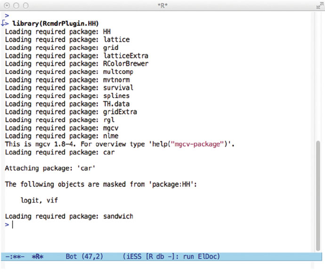
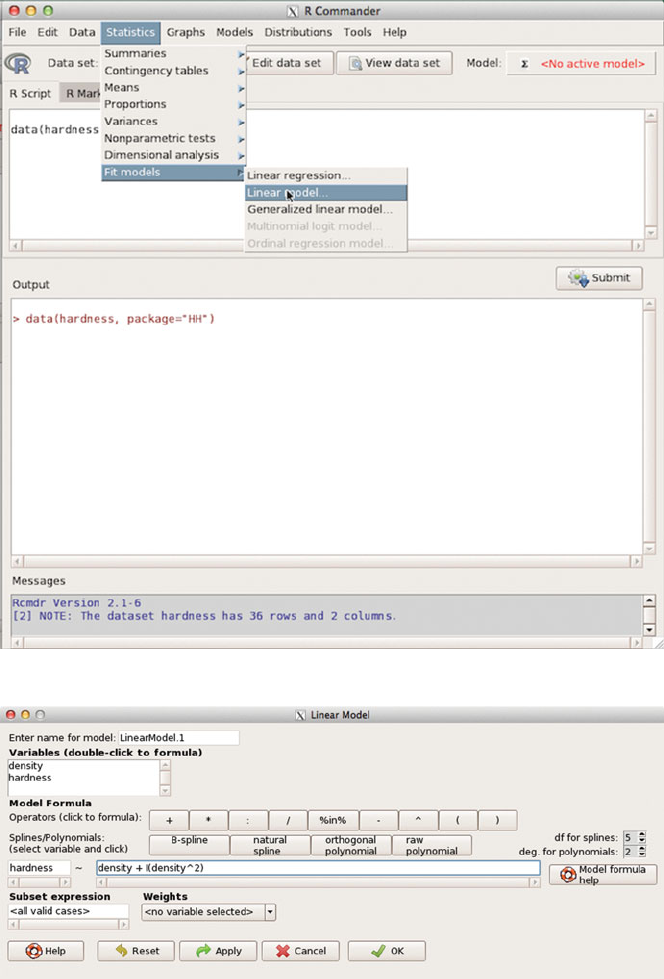
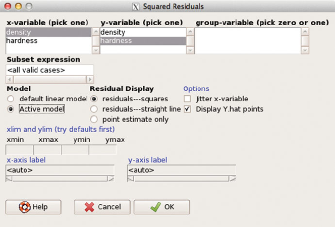
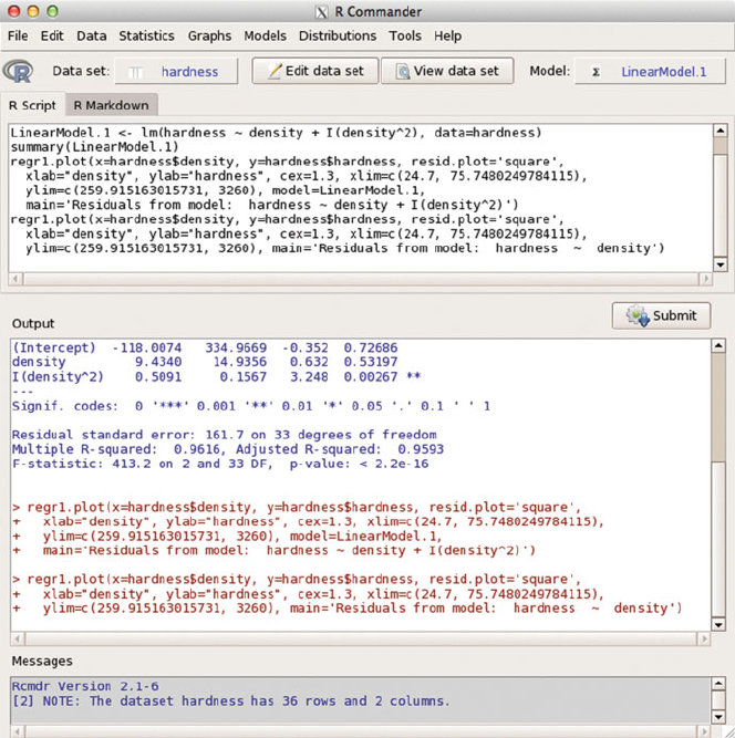
We illustrate how to use it by reconstructing the two panels of Figure 9.5 directly
from the Rcmdr menu. We load Rcmdr indirectly by explicitly loading our package
RcmdrPlugin.HH (Heiberger and with contributions from Burt Holland, 2015). We
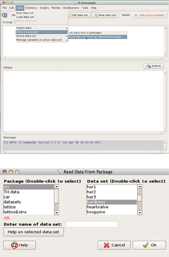
then use the menu to bring in the hardness dataset, compute the quadratic model,
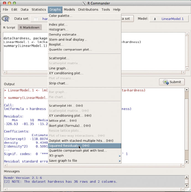
display the squared residuals for the quadratic model (duplicating the left panel of
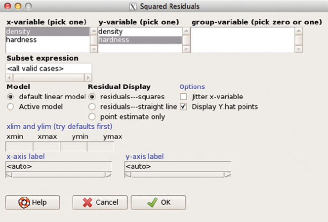
Figure 9.5), display the squared residuals for the linear model (duplicating the right
panel of Figure 9.5). The linear model was fit implicitly and its summary is not
automatically printed. We show the summary of the quadratic model.
Figures C.1–C.14 illustrate all the steps summarized above.
©Springer Science+Business Media New York 2015
R.M. Heiberger, B. Holland, Statistical Analysis and Data Display,
Springer Texts in Statistics, DOI 10.1007/978-1-4939-2122-5
719
C Rcmdr: R Commander 721
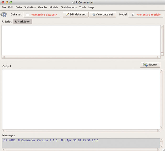
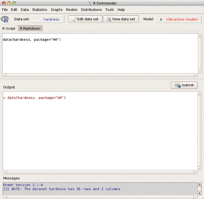
Fig. C.2 The Rcmdr window as it appears when first opened. It shows a menu bar, a tool bar, and
three subwindows.
C Rcmdr: R Commander 723
Fig. C.5 The Data set: item in the tool bar now shows hardness as the active dataset. The R
Script subwindow show the Rcommand that was generated by the menu sequence. The Output
subwindow shows the transcript of the Rsession where the command was executed. The Mes-
sages subwindow give information on the dataset that was opened.
C Rcmdr: R Commander 725
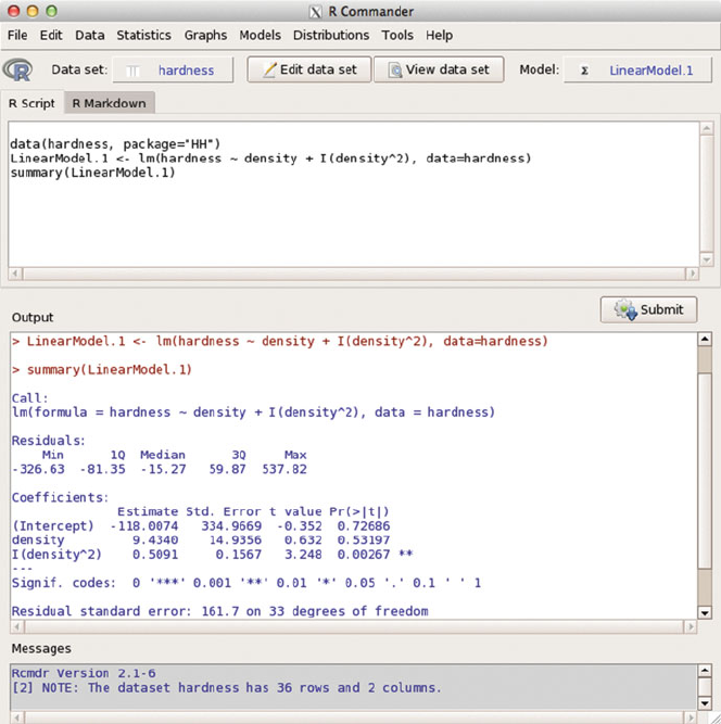
Fig. C.8 The Linear model menu item wrote the Rcommands shown in the RScriptsub-
window and executed them in the Output window. The model is stored in the R"lm" object
named LinearModel.1.TheModel: item in the tool bar now shows LinearModel.1 as the
active model.
728 C Rcmdr: R Commander
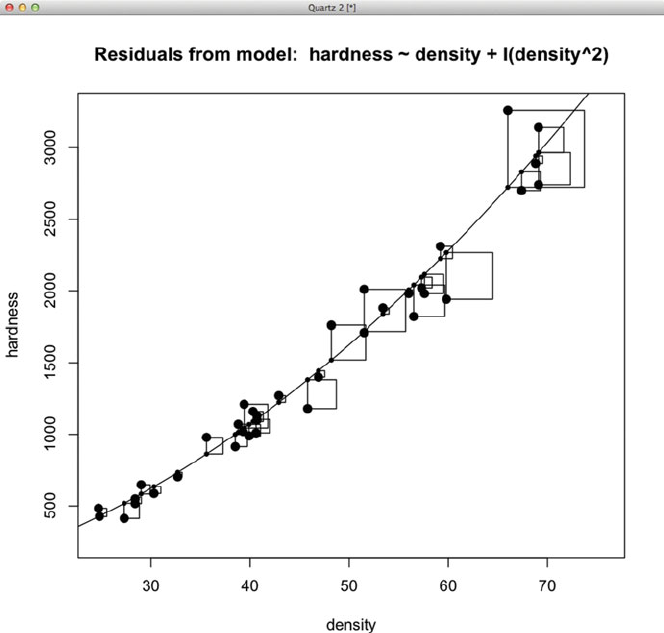
Fig. C.11 This is the squared residuals for the quadratic model (duplicating the right panel of
Figure 9.5).
730 C Rcmdr: R Commander
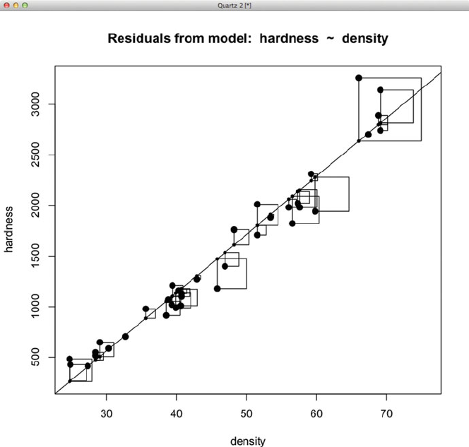
Fig. C.13 This is the squared residuals for the linear model (duplicating the left panel of
Figure 9.5).
Appendix D
RExcel: Embedding Rinside Excel
on Windows
If you are running on a Windows machine and have access to MS Excel, then we
recommend that you install RExcel (Baier and Neuwirth, 2007; Neuwirth, 2014).
RExcel is free of charge for “single user non-commercial use” with 32-bit Excel.
Any other use will require a license. Please see the license at rcom.univie.ac.at
for details.
RExcel seamlessly integrates the entire set of R’s statistical and graphical meth-
ods into Excel, allowing students to focus on statistical methods and concepts and
minimizing the distraction of learning a new programming language. Data can be
transferred between Rand Excel “the Excel way” by selecting worksheet ranges
and using Excel menus. RExcel has embedded the Rcmdr menu into the Excel
ribbon. Thus R’s basic statistical functions and selected advanced methods are avail-
able from an Excel menu. Almost all R functions can be used as worksheet functions
in Excel. Results of the computations and statistical graphics can be returned back
into Excel worksheet ranges. RExcel allows the use of Excel scroll bars and check
boxes to create and animate R graphics as an interactive analysis tool.
See Heiberger and Neuwirth (2009) for the book R through Excel: A Spreadsheet
Interface for Statistics, Data Analysis, and Graphics. This book is designed as a
computational supplement for any Statistics course.
RExcel works with Excel only on Windows.Excel on the Macintosh uses a
completely different interprocess communications system.
©Springer Science+Business Media New York 2015
R.M. Heiberger, B. Holland, Statistical Analysis and Data Display,
Springer Texts in Statistics, DOI 10.1007/978-1-4939-2122-5
733
734 D RExcel: Embedding Rinside Excel on Windows
D.1 Installing RExcel for Windows
You m us t hav e MS Excel (2007, 2010, or 2013) installed on your Windows
machine. You need to purchase Excel separately. Excel 2013 is the current ver-
sion (in early 2015). RExcel is free of charge for “single user non-commercial use”
with 32-bit Excel. Any other use will require a license.
D.1.1 Install
R
Begin by installing Rand the necessary packages as described in Section A.1.
D.1.2 Install Two
R
Packages Needed by
RExcel
You will also need two more Rpackages that must be installed as computer
Administrator.
Start R as Administrator (on Windows 7 and 8 you need to right-click the R
icon and click the “Run as administrator” item). In R, run the following commands
(again, you must have started Ras Administrator to do this)
## Tell Windows that R should have the same access to the outside
## internet that is granted to Internet Explorer.
setInternet2()
install.packages(c("rscproxy","rcom"),
repos="http://rcom.univie.ac.at/download",
type="binary",
lib=.Library)
library(rcom)
comRegisterRegistry()
Close Rwith q("no").Ifitasks
Save workspace image? [y/n/c]:
answer with n.
D.1 Installing RExcel for Windows 735
D.1.3 Install
RExcel
and Related Software
Go to http://rcom.univie.ac.at and click on the Download tab. Download
and execute the following four files (or newer releases if available)
•statconnDCOM3.6-0B2_Noncommercial
•RExcel 3.2.15
•RthroughExcelWorkbooksInstaller_1.2-10.exe
•SWord 1.0-1B1 Noncommercial SWord (Baier, 2014) is an add-in package
for MSword that makes it possible to embed Rcode in a MSword document.
The Rcode will be automatically executed and the output from the Rcode will
be included within the MSword document. SWord is free for non-commercial
use. Any other use will require a license. SWord is a separate program from
RExcel and is not required for RExcel.
These installer .exe files will ask for administrator approval, as they write in
the Program Files directory and write to the Windows registry as part of the
installation. Once they are installed, they run in normal user mode.
D.1.4 Install Rcmdr to Work with
RExcel
In order for RExcel to place the Rcmdr menu on the Excel ribbon, it is necessary
that Rcmdr be installed in the C:/Program Files/R/R-x.y.z/library direc-
tory and not in the C:/Users/rmh/*/R/win-library/x.y directory. If Rcmdr is
installed in the user directory, it must be removed before reinstalling it as Adminis-
trator. Remove it with the remove.packages function using
remove.packages(c("Rcmdr", "RcmdrMisc"))
Then see the installation details in Section A.1.2.2.
D.1.5 Additional Information on Installing
RExcel
Additional RExcel installation information is available in the Wiki page at
http://rcom.univie.ac.at
736 D RExcel: Embedding Rinside Excel on Windows
D.2 Using RExcel
D.2.1 Automatic Recalculation of an
R
Function
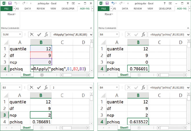
RExcel places Rinside the Excel automatic recalculation model. Figure D.1 by
Heiberger and Neuwirth was originally presented in Robbins et al. (2009)using
Excel 2007. We reproduce it here with Excel 2013.
Fig. D.1 Any Rfunction can be used in Excel with the RExcel worksheet function RApply.The
formula =RApply("pchisq", B1, B2, B3) computes the value of the noncentral distribution
function for the quantile-value, the degrees of freedom, and the noncentrality parameter in cells
B1,B2,andB3, respectively, and returns its value into cell B4. When the value of one of the
arguments, in this example the noncentrality parameter in cell B3, is changed, the value of the
cumulative distribution is automatically updated by Excel to the appropriate new value.
D.2 Using RExcel 737
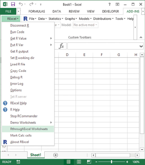
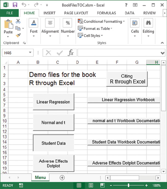
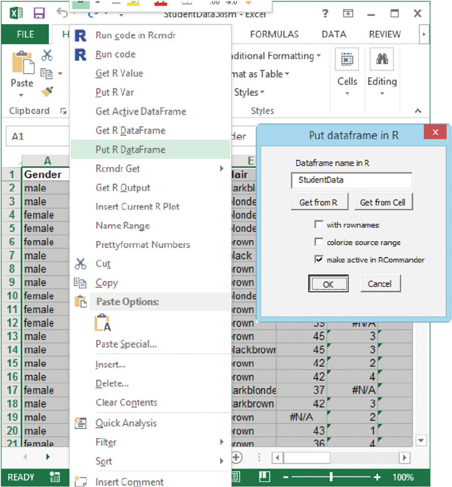
Fig. D.2 Retrieve the StudentData into Excel.FromtheRExcel Add-In tab, click
RthroughExcel Worksheets. This brings up the BookFilesTOC worksheet in Figure D.3.
D.2.2 Transferring Data To/From
R
and
Excel
Datasets can be transferred in either direction to/from Excel from/to R.In
Figures D.2–D.4 we bring in a dataset from an Excel worksheet, transfer it to R,
and make it the active dataset for use with Rcmdr.
The StudentData was collected by Erich Neuwirth for over ten years from
students in his classes at the University of Vienna. The StudentData dataset is
included with RExcel.
740 D RExcel: Embedding Rinside Excel on Windows
D.2.3 Control of a lattice Plot from an
Excel
/Rcmdr Menu
The example in Figures D.5–D.8 is originally from Heiberger and Neuwirth (2009)
using Excel 2007. We reproduce it here with Excel 2013. We made it the active
dataset for Rcmdr in Figures D.2–D.4.
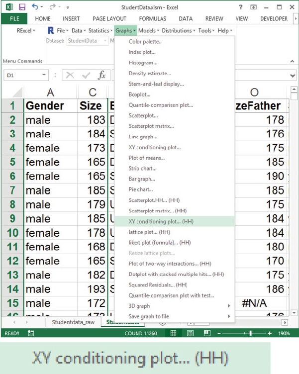
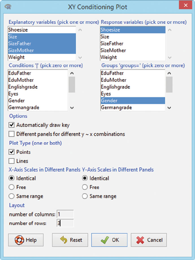
Fig. D.5 RExcel has placed the Rcmdr menu onto the Excel ribbon. Click the Graphs tab to
get the menu and then click XY conditioning plot. . . (HH) to get the Dialog box in Figure D.6.
The (HH) in the menu item means the function was added to the Rcmdr menu by our RcmdrPlu-
gin.HH package (Heiberger and with contributions from Burt Holland, 2015).
742 D RExcel: Embedding Rinside Excel on Windows
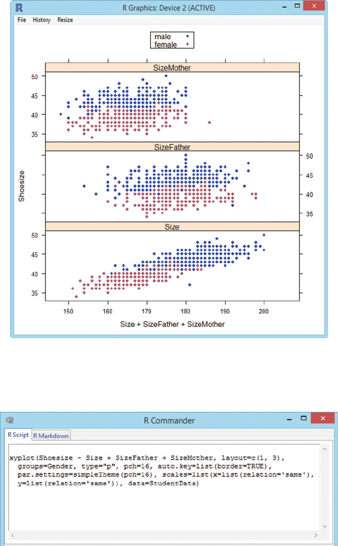
Fig. D.7 The graph is displayed. Shoesize is the student’s shoe size in Paris points (2/3 cm). Size
is the student’s height in cm. SizeFather and SizeMother are the heights of the student’s parents.
Fathers of both male and female students have the same height distribution as the male students.
Mothers of both male and female students have the same height distribution as the female students.
Fig. D.8 The generated Rcode is displayed.
Appendix E
Shiny: Web-Based Access to RFunctions
Shiny (Chang et al., 2015; RStudio, 2015)isanRpackage that provides an R
language interface for writing interactive web applications. Apps built with shiny
place the power of Rbehind an interactive webpage that can be used by non-
programmers. A full tutorial and gallery are available at the Shiny web site.
We have animated several of the graphs in the HH package using shiny.
©Springer Science+Business Media New York 2015
R.M. Heiberger, B. Holland, Statistical Analysis and Data Display,
Springer Texts in Statistics, DOI 10.1007/978-1-4939-2122-5
743
744 E Shiny: Web-Based Access to RFunctions
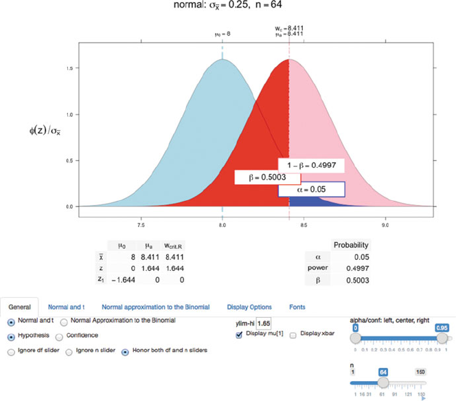
E.1 NTplot
The NTplot function shows significance levels and power for the normal or t-
distributions. Figure E.1, an interactive version of the top panel of the middle section
of Figure 3.20, is specified with
NTplot(mean0=8, mean1=8.411, sd=2, n=64, cex.prob=1.3,
shiny=TRUE)
Fig. E.1 This is an interactive version of Figure 3.20 constructed with the shiny package. Adjust-
ing the nslider at the bottom right can produce all three columns of Figure 3.20. Clicking the
button below the slider will dynamically move through all values of nfrom 1 through 150, includ-
ing the three that are displayed in Figure 3.20. There are additional controls on the Normal and t,
Display Options,andFonts tabs that will show the power and beta panels.
E.2 bivariateNormal 745
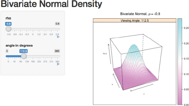
E.2 bivariateNormal
Figure E.2 is an interactive version of Figure 3.9 showing the bivariate normal den-
sity in 3D space with various correlations and various viewpoints.
shiny::runApp(system.file("shiny/bivariateNormal",
package="HH"))
Fig. E.2 This is an interactive version of Figure 3.9 constructed with the shiny package. Adjusting
the rho slider changes the correlation between xand y. Adjusting the angle in degrees slider
rotates the figure through all the viewpoint angles shown in Figure 3.10. Both sliders can be made
dynamic by clicking their buttons.
746 E Shiny: Web-Based Access to RFunctions
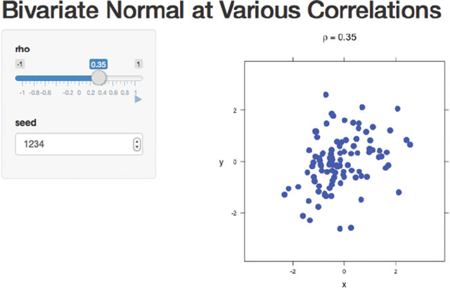
E.3 bivariateNormalScatterplot
Figure E.3 is a dynamic version of Figure 3.8 specified with
shiny::runApp(system.file("shiny/bivariateNormalScatterplot",
package="HH"))
Fig. E.3 This is an interactive version of Figure 3.8 constructed with the shiny package. Adjusting
the rho slider changes the correlation between xand y. By clicking the button, the figure will
transition through the panels of Figure 3.8.
E.4 PopulationPyramid 747
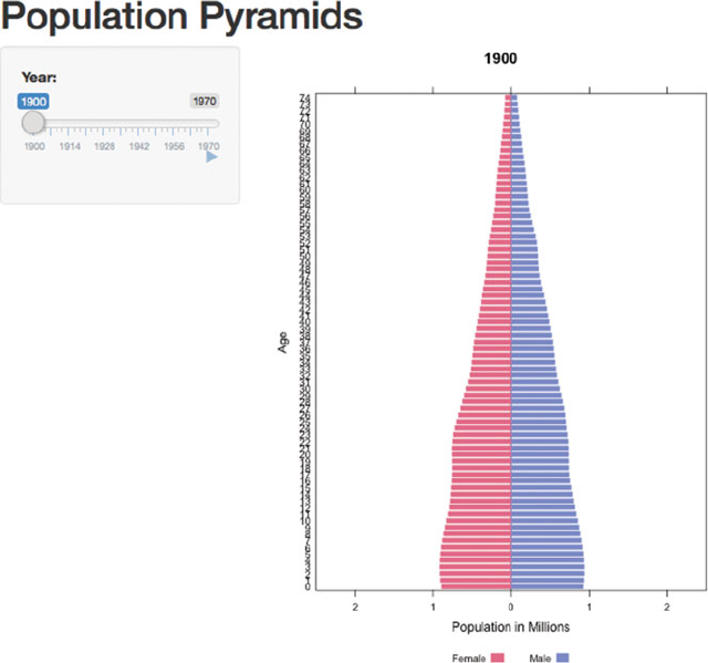
E.4 PopulationPyramid
Figure E.4 is an interactive version of Figure 15.19 showing the population pyramid
for the United States annually for the years 1900–1979 specified with
shiny::runApp(system.file("shiny/PopulationPyramid",
package="HH"))
Fig. E.4 This is an interactive version of Figure 15.19 constructed with the shiny package. Ad-
justing the Year slider changes the year in the range 1900–1970. By clicking the button, the
figure will dynamically transition through the panels of Figure 15.19.
Appendix F
RPackages
The Rprogram as supplied by R-Core on the CRAN (Comprehensive RArchive
Network) page (CRAN, 2015) consists of the base program and about 30 required
and recommended packages. Everything else is a contributed package. There are
about 6500 contributed packages (April 2015). Our HH is a contributed package.
F.1 What Is a Package?
Rpackages are extensions to R.
Each package is a collection of functions and datasets designed to work together
for a specific purpose. The HH package is designed to provide computing support
for the techniques discussed in this book . The lattice package (a recommended
package) is designed to provide xyplot and related graphics functions. Most of the
graphics functions in HH are built on the functions in lattice.
Packages consist at a minimum of functions written in R, datasets that can be
brought into the Rworking directory, and documentation for all functions and
datasets. Some packages include subroutines written in Fortran or C.
F.2 Installing and Loading RPackages
The base and recommended packages are installed on your computer when you
download and install Ritself. All other packages must be explicitly installed (down-
loaded from CRAN and placed into an R-determined location on your computer).
©Springer Science+Business Media New York 2015
R.M. Heiberger, B. Holland, Statistical Analysis and Data Display,
Springer Texts in Statistics, DOI 10.1007/978-1-4939-2122-5
749
750 F RPackages
The packages available at CRAN are most easily installed into your computer
with a command of the form
install.packages("MyPackage")
The RGUIs usually have a menu item that constructs this statement for you.
The functions in an installed package are not automatically available when you
start an Rsession. It is necessary to load them into the current session, usually with
the library function. Most examples in this book require you to enter
library(HH)
(once per R session) before doing anything else. The HH package loads lattice and
several additional packages.
The list of Rpackages installed on your computer is seen with the Rcommand
library()
The list of Rpackages loaded into your current Rsession is seen with the R
command
search()
F.3 Where Are the Packages on Your Computer?
Once a package has been installed on your computer it is kept in a directory (called a
“library” in Rterminology). The base and recommended packages are stored under
Ritself in directory
system.file("..")
Files inside the installed packages are in an internal format and cannot be read by
an editor directly from the file system.
Contributed packages will usually be installed in a directory in your user space.
In Windows that might be something like
C:/Users/yourloginname/Documents/R/win-library/3.2
or
C:/Users/yourloginname/AppData/Roaming/R/win-library/3.2
On Macintosh it will be something like
/Users/yourloginname/Library/R/3.2/library
You can find out where the installed packages are stored by loading one and then
entering
searchpaths()
(searchpaths() is similar to search() but with the full pathname included in the
output, not just the package name). For example,
library(HH)
searchpaths()
F.5 Writing and Building Your Own Package 751
F.4 Structure of an RPackage
The package developer writes individual source files. The Rbuild system (see the
Writing R Extensions manual) has procedures for checking coherency and then for
building the source package and the binaries.
The packages at CRAN are available in three formats. The source packages
(what the package designer wrote and what you should read when you want to read
the code) are stored as packagename.tar.gz files. The binary packages for Win-
dows arestoredaspackagename.zip files. The binary packages for Macintosh
are stored as packagename.tgz files.
F.5 Writing and Building Your Own Package
At some point in your analysis project you will have accumulated several of your
own functions that you quite frequently use. At that point it will be time to collect
them into a package.
We do not say much here about designing and writing functions in this book.
Begin with An Introduction to R in file
system.file("../../doc/manual/R-intro.pdf")
It includes a chapter “Writing your own functions”.
Nor do we say much here about building a package. The official reference is the
Writing R Extensions manual that also comes with Rin file
system.file("../../doc/manual/R-exts.pdf")
When you are ready, begin by looking at the help file
?package.skeleton
to see how the pieces fit together.
It will help to have someone work with you the first time you build a package.
You build the package with the operating system command
R CMD check YourPackageName
and then install it on your own machine with the command
R CMD INSTALL --build YourPackageName
The checking process is very thorough, and gets more thorough at every release
of R. Understanding how to respond to the messages from the check is the specific
place where it will help to have someone already familiar with package building.
752 F RPackages
F.6 Building Your Own Package with Windows
The MS Windows operating system does not include many programs that are cen-
tral to building Rpackages. You will need to download and install the most recent
Rtools from CRAN. See Section A.1.2.4 for download information.
You will need to include Rtools in your PATH environment variable to enable the
R CMD check packagename command to work. See “Appendix D The Windows
toolset” in R Installation and Administration manual at
system.file("../../doc/manual/R-admin.pdf")
Appendix G
Computational Precision and Floating-Point
Arithmetic
Computers use floating point arithmetic. The floating point system is not identical to
the real-number system that we (teachers and students) know well, having studied
it from kindergarten onward. In this section we show several examples to illustrate
and emphasize the distinction.
The principal characteristic of real numbers is that we can have as many digits
as we wish. The principal characteristic of floating point numbers is that we are
limited in the number of digits that we can work with. In double-precision IEEE
754 arithmetic, we are limited to exactly 53 binary digits (approximately 16 decimal
digits)
The consequences of the use of floating point numbers are pervasive, and present
even with numbers we normally think of as far from the boundaries. For detailed
information please see FAQ 7.31 in file
system.file("../../doc/FAQ")
The help menus in Rgui in Windows and R.app on Macintosh have direct links to
the FAQ file.
G.1 Examples
Let us start by looking at two simple examples that require basic familiarity with
floating point arithmetic.
1. Why is .9 not recognized to be the same as (.3 +.6)?
Table G.1 shows that .9 is not perceived to have the same value as .3+.6, when
calculated in floating point (that is, when calculated by a computer). The differ-
ence between the two values is not 0, but is instead a number on the order of
©Springer Science+Business Media New York 2015
R.M. Heiberger, B. Holland, Statistical Analysis and Data Display,
Springer Texts in Statistics, DOI 10.1007/978-1-4939-2122-5
753

754 G Computational Precision and Floating-Point Arithmetic
machine epsilon (the smallest number such that 1 +>1). In R, the standard
mathematical comparison operators recognize the difference. There is a function
all.equal which tests for near equality. See ?all.equal for details.
Table G.1 Calculations showing that the floating point numbers .9and.3+.6 are not stored the
same inside the computer. Rcomparison operators recognize the numbers as different.
> c(.9, (.3 + .6))
[1] 0.9 0.9
> .9 == (.3 + .6)
[1] FALSE
>.9-(.3+.6)
[1] 1.11e-16
> identical(.9, (.3 + .6))
[1] FALSE
> all.equal(.9, (.3 + .6))
[1] TRUE
Table G.2 √222 in floating point arithmetic inside the computer.
> c(2, sqrt(2)^2)
[1] 2 2
> sqrt(2)^2
[1] 2
> 2 == sqrt(2)^2
[1] FALSE
> 2 - sqrt(2)^2
[1] -4.441e-16
> identical(2, sqrt(2)^2)
[1] FALSE
> all.equal(2, sqrt(2)^2)
[1] TRUE

G.2 Floating Point Numbers in the IEEE 754 Floating-Point Standard 755
2. Why is √22not recognized to be the same as 2?
Table G.2 shows that the difference between the two values √22and 2 is not
0, but is instead a number on the order of machine epsilon (the smallest number
such that 1 +>1).
We will pursue these examples further in Section G.7, but first we need to intro-
duce floating point numbers—the number system used inside the computer.
G.2 Floating Point Numbers in the IEEE 754 Floating-Point
Standard
The number system we are most familiar with is the infinite-precision base-10
system. Any number can be represented as the infinite sum
±(a0×100+a1×10−1+a2×10−2+...)×10p
where pcan be any positive integer, and the values aiare digits selected from
decimal digits {0,1,2,3,4,5,6,7,8,9}. For example, the decimal number 3.3125
is expressed as
3.3125 =(3 ×100+3×10⁻¹+1×10⁻²+2×10⁻³+5×10−4)×100
=3.3125 ×1
In this example, there are 4 decimal digits after the radix point. There is no limit to
the number of digits that could have been specified. For decimal numbers the term
decimal point is usually used in preference to the more general term radix point.
Floating point arithmetic in computers uses a finite-precision base-2 (binary) sys-
tem for representation of numbers. Most computers today use the 53-bit IEEE 754
system, with numbers represented by the finite sum
±(a0×20+a1×2−1+a2×2−2+...+a52 ×2−52) ×2p
where pis an integer in the range −1022 to 1023 (expressed as decimal numbers),
the values aiare digits selected from {0,1}, and the subscripts and powers iare dec-
imal numbers selected from {0,1,...,52}. The decimal number 3.12510 is 11.01012
in binary.
3.312510 =11.01012=(1 ×20+1×2−1+0×2−2+1×2−3+0×2−4+
1×2−5)×210
=1.101012×210
756 G Computational Precision and Floating-Point Arithmetic
This example (in the normalized form 1.101012×210) has five binary digits (bits)
after the radix point (binary point in this case). There is a maximum of 52 binary
positions after the binary point.
Strings of 0 and 1 are hard for people to read. They are usually collected into
units of 4 bits (called a byte).
The IEEE 754 standard requires the base β=2 number system with p=53 base-
2 digits. Except for 0, the numbers in internal representation are always normalized
with the leading bit always 1. Since it is always 1, there is no need to store it and
only 52 bits are actually needed for 53-bit precision. A string of 0and 1is difficult
for humans to read. Therefore every set of 4 bits is represented as a single hexadec-
imal digit, from the set {0123456789abcdef}, representing the
decimal values {0123456789101112131415}. The 52 stored bits can be
displayed with 13 hex digits. Since the base is β=2, the exponent of an IEEE 754
floating point number must be a power of 2. The double-precision computer num-
bers contain 64 bits, allocated 52 for the significant, 1 for the sign, and 11 for the
exponent. The 11 bits for the exponent can express 211 =2048 unique values. These
are assigned to range from −2−1022 to 21023, with the remaining 2 exponent values
used for special cases (zero and the special quantities NaN and ∞).
The number 3.312510 is represented in hexadecimal (base-16) notation as
3.312510 =3.5016 =(1 ×160+a16 ×16−1+816 ×16−2)×210
=1.a816 ×210
=1.101010002×210
There are two hex digits after the radix point (binary point, not hex point because
the normalization is by powers of 210 not powers of 1610).
The Rfunction sprintf is used to specify the printed format of numbers. The
letter ain format sprintf("%+13.13a", x) tells Rto print the numbers in hex-
adecimal notation. The “13”s say to use 13 hexadecimal digits after the binary point.
See ?sprintf for more detail on the formatting specifications used by the sprintf
function. Several numbers, simple decimals, and simple multiples of powers of 1/2
are shown in Table G.3 in both decimal and binary notation.
G.3 Multiple Precision Floating Point
The Rpackage Rmpfr allows the construction and use of arbitrary precision
floating point numbers. It was designed, and is usually used, for higher-precision
arithmetic—situations where the 53-bit double-precision numbers are not precise

G.4 Binary Format 757
Table G.3 Numbers, some simple integers divided by 10, and some fractions constructed as multi-
ples of powers of 1/2. The i/10 decimal numbers are stored as repeating binaries in the hexadecimal
notation until they run out of digits. There are only 52 bits (binary digits) after the binary point.
For decimal input 0.1 we see that the repeating hex digit is “9” until the last position where it is
rounded up to “a”.
> nums <- c(0, .0625, .1, .3, .3125, .5, .6, (.3 + .6), .9, 1)
> data.frame("decimal-2"=nums,
+ "decimal-17"=format(nums, digits=17),
+ hexadecimal=sprintf("%+13.13a", nums))
decimal.2 decimal.17 hexadecimal
1 0.0000 0.00000000000000000 +0x0.0000000000000p+0
2 0.0625 0.06250000000000000 +0x1.0000000000000p-4
3 0.1000 0.10000000000000001 +0x1.999999999999ap-4
4 0.3000 0.29999999999999999 +0x1.3333333333333p-2
5 0.3125 0.31250000000000000 +0x1.4000000000000p-2
6 0.5000 0.50000000000000000 +0x1.0000000000000p-1
7 0.6000 0.59999999999999998 +0x1.3333333333333p-1
8 0.9000 0.89999999999999991 +0x1.cccccccccccccp-1
9 0.9000 0.90000000000000002 +0x1.ccccccccccccdp-1
10 1.0000 1.00000000000000000 +0x1.0000000000000p+0
enough. In this Appendix we use it for lower-precision arithmetic—four or five sig-
nificant digits. In this way it will be much easier to illustrate how the behavior of
floating point numbers differs from the behavior of real numbers.
G.4 Binary Format
It is often easier to see the details of the numerical behavior when numbers are dis-
played in binary, not in the hex format of sprintf("%+13.13a", x).TheRmpfr
package includes a binary display format for numbers. The formatBin function
uses sprintf to construct a hex display format and then modifies it by replacing
each hex character with its 4-bit expansion as shown in Table G.4.
Optionally (with argument scientific=FALSE), all binary numbers can be for-
matted to show aligned radix points. There is also a formatHex function which is
essentially a wrapper for sprintf. Both functions are used in the examples in this
Appendix. Table G.5 illustrates both functions, including the optional scientific
argument, with a 4-bit arithmetic example.

758 G Computational Precision and Floating-Point Arithmetic
Table G.4 Four-bit expansions for the sixteen hex digits. We show both lowercase [a:f] and up-
percase [A:F] for the hex digits.
> Rmpfr:::HextoBin
1234567
"0000" "0001" "0010" "0011" "0100" "0101" "0110" "0111"
89ABCDEF
"1000" "1001" "1010" "1011" "1100" "1101" "1110" "1111"
abcdef
"1010" "1011" "1100" "1101" "1110" "1111"
G.5 Round to Even
The IEEE 754 standard calls for “rounding ties to even”. The explanation here is
from help(mpfr, package="Rmpfr"):
The round to nearest ("N") mode, the default here, works as in the IEEE 754 standard: in
case the number to be rounded lies exactly in the middle of two representable numbers, it
is rounded to the one with the least significant bit set to zero. For example, the number 5/2,
which is represented by (10.1) in binary, is rounded to (10.0)=2 with a precision of two bits,
and not to (11.0)=3. This rule avoids the drift phenomenon mentioned by Knuth in volume
2ofThe Art of Computer Programming (Section 4.2.2).
G.6 Base-10, 2-Digit Arithmetic
Hex numbers are hard to fathom the first time they are seen. We therefore look at a
simple example of finite-precision arithmetic with 2 significant decimal digits.
Calculate the sum of squares of three numbers in 2-digit base-10 arithmetic. For
concreteness, use the example
22+112+152
This requires rounding to 2 significant digits at every intermediate step. The steps
are easy. Putting your head around the steps is hard.
We rewrite the expression as a fully parenthesized algebraic expression, so we
don’t need to worry about precedence of operators at this step.
((22)+(112)) +(152)
Now we can evaluate the parenthesized groups from the inside out.

G.6 Base-10, 2-Digit Arithmetic 759
Table G.5 Integers from 0 to 39 stored as 4-bit mpfr numbers. The numbers from 17 to 39 are
rounded to four significant bits. All numbers in the “16” and “24” columns are multiples of 2, and
all numbers in the “32” columns are multiples of 4. The numbers are displayed in decimal, hex,
binary, and binary with aligned radix points. To interpret the aligned binary numbers, replace the
“_” placeholder character with a zero.
> library(Rmpfr)
> FourBits <- mpfr(matrix(0:39, 8, 5), precBits=4)
> dimnames(FourBits) <- list(0:7, c(0,8,16,24,32))
> FourBits
’mpfrMatrix’ of dim(.) = (8, 5) of precision 4 bits
0 8 16 24 32
0 0.00 8.00 16.0 24.0 32.0
1 1.00 9.00 16.0 24.0 32.0
2 2.00 10.0 18.0 26.0 32.0
3 3.00 11.0 20.0 28.0 36.0
4 4.00 12.0 20.0 28.0 36.0
5 5.00 13.0 20.0 28.0 36.0
6 6.00 14.0 22.0 30.0 40.0
7 7.00 15.0 24.0 32.0 40.0
> formatHex(FourBits)
0 8 16 24 32
0 +0x0.0p+0 +0x1.0p+3 +0x1.0p+4 +0x1.8p+4 +0x1.0p+5
1 +0x1.0p+0 +0x1.2p+3 +0x1.0p+4 +0x1.8p+4 +0x1.0p+5
2 +0x1.0p+1 +0x1.4p+3 +0x1.2p+4 +0x1.ap+4 +0x1.0p+5
3 +0x1.8p+1 +0x1.6p+3 +0x1.4p+4 +0x1.cp+4 +0x1.2p+5
4 +0x1.0p+2 +0x1.8p+3 +0x1.4p+4 +0x1.cp+4 +0x1.2p+5
5 +0x1.4p+2 +0x1.ap+3 +0x1.4p+4 +0x1.cp+4 +0x1.2p+5
6 +0x1.8p+2 +0x1.cp+3 +0x1.6p+4 +0x1.ep+4 +0x1.4p+5
7 +0x1.cp+2 +0x1.ep+3 +0x1.8p+4 +0x1.0p+5 +0x1.4p+5
> formatBin(FourBits)
0 8 16 24 32
0 +0b0.000p+0 +0b1.000p+3 +0b1.000p+4 +0b1.100p+4 +0b1.000p+5
1 +0b1.000p+0 +0b1.001p+3 +0b1.000p+4 +0b1.100p+4 +0b1.000p+5
2 +0b1.000p+1 +0b1.010p+3 +0b1.001p+4 +0b1.101p+4 +0b1.000p+5
3 +0b1.100p+1 +0b1.011p+3 +0b1.010p+4 +0b1.110p+4 +0b1.001p+5
4 +0b1.000p+2 +0b1.100p+3 +0b1.010p+4 +0b1.110p+4 +0b1.001p+5
5 +0b1.010p+2 +0b1.101p+3 +0b1.010p+4 +0b1.110p+4 +0b1.001p+5
6 +0b1.100p+2 +0b1.110p+3 +0b1.011p+4 +0b1.111p+4 +0b1.010p+5
7 +0b1.110p+2 +0b1.111p+3 +0b1.100p+4 +0b1.000p+5 +0b1.010p+5
> formatBin(FourBits, scientific=FALSE)
08162432
0 +0b_____0.000 +0b__1000.___ +0b_1000_.___ +0b_1100_.___ +0b1000__.___
1 +0b_____1.000 +0b__1001.___ +0b_1000_.___ +0b_1100_.___ +0b1000__.___
2 +0b____10.00_ +0b__1010.___ +0b_1001_.___ +0b_1101_.___ +0b1000__.___
3 +0b____11.00_ +0b__1011.___ +0b_1010_.___ +0b_1110_.___ +0b1001__.___
4 +0b___100.0__ +0b__1100.___ +0b_1010_.___ +0b_1110_.___ +0b1001__.___
5 +0b___101.0__ +0b__1101.___ +0b_1010_.___ +0b_1110_.___ +0b1001__.___
6 +0b___110.0__ +0b__1110.___ +0b_1011_.___ +0b_1111_.___ +0b1010__.___
7 +0b___111.0__ +0b__1111.___ +0b_1100_.___ +0b1000__.___ +0b1010__.___

760 G Computational Precision and Floating-Point Arithmetic
((2
2)+(112)) +(152) ## parenthesized expression
((4) +(121) ) +(225) ## square each term
(4 +120 ) +220 ## round each term to two significant decimal digits
( 124 ) +220 ## calculate the intermediate sum
( 120 ) +220 ## round the intermediate sum to two decimal digits
340 ## sum the terms
Compare this to the full precision arithmetic
((2
2)+(112)) +(152) ## parenthesized expression
(4 +121 ) +225 ## square each term
( 125 ) +225 ## calculate the intermediate sum
350 ## sum the terms
We see immediately that two-decimal-digit rounding at each stage gives an answer
that is not the same as the one from familiar arithmetic with real numbers.
G.7 Why Is .9 Not Recognized to Be the Same as (.3 +.6)?
We can now continue with the first example from Section G.1. The floating point
binary representation of 0.3 and the floating point representation of 0.6 must be
aligned on the binary point before the addition. When the numbers are aligned by
shifting the smaller number right one position, the last bit of the smaller number has
nowhere to go and is lost. The sum is therefore one bit too small compared to the
floating point binary representation of 0.9. Details are in Table G.6.
G.8 Why Is √22Not Recognized to Be the Same as 2?
We continue with the second example from Section G.1. The binary representation
inside the machine of the two numbers √22and 2 is not identical. We see in
Table G.7 that they differ by one bit in the 53rd binary digit.
G.9 zapsmall to Round Small Values to Zero for Display
Rprovides a function that rounds small values (those close to the machine epsilon)
to zero. We use this function for printing of many tables where we wish to inter-
pret numbers close to machine epsilon as if they were zero. See Table G.8 for an
example.

G.9 zapsmall to Round Small Values to Zero for Display 761
Table G.6 Now let’s add 0.3 and 0.6 in hex:
0.3 +0x1.3333333333333p-2 = +0x0.9999999999999p-1 aligned binary (see below)
0.6 +0x1.3333333333333p-1 = +0x1.3333333333333p-1
-------------------------- ---------------------
0.9 add of aligned binary +0x1.cccccccccccccp-1
0.9 convert from decimal +0x1.ccccccccccccdp-1
We need to align binary points for addition. The shift is calculated by converting hex to bi-
nary, shifting one bit to the right to get the same p-1 exponent, regrouping four bits into hex
characters, and allowing the last bit to fall off:
1.0011 0011 0011 ... 0011 ×2−2→.1001 1001 1001 ... 1001 | 1/×2−1
> nums369 <- c(.3, .6, .3+.6, 9)
> nums369df <-
+ data.frame("decimal-2"=nums369,
+ "decimal-17"=format(nums369, digits=17),
+ hexadecimal=sprintf("%+13.13a", nums369))
> nums369df[3,1] <- "0.3 + 0.6"
> nums369df
decimal.2 decimal.17 hexadecimal
1 0.3 0.29999999999999999 +0x1.3333333333333p-2
2 0.6 0.59999999999999998 +0x1.3333333333333p-1
3 0.3 + 0.6 0.89999999999999991 +0x1.cccccccccccccp-1
4 9 9.00000000000000000 +0x1.2000000000000p+3
Table G.7 The binary representation of the two numbers √22and 2 is not identical. They differ
by one bit in the 53rd binary digit.
> sprintf("%+13.13a", c(2, sqrt(2)^2))
[1] "+0x1.0000000000000p+1" "+0x1.0000000000001p+1"
Table G.8 We frequently wish to interpret numbers that are very different in magnitude as if the
smaller one is effectively zero. The display function zapsmall provides that capability.
> c(100, 1e-10)
[1] 1e+02 1e-10
> zapsmall(c(100, 1e-10))
[1] 100 0

762 G Computational Precision and Floating-Point Arithmetic
G.10 Apparent Violation of Elementary Factoring
We show a simple example of disastrous cancellation (loss of high-order digits),
where the floating point statement
a2−b2(a+b)×(a−b)
is an inequality, not an equation, for some surprising values of aand b. Table G.9
shows two examples, a decimal example for which the equality holds so we can
use our intuition to see what is happening, and a hex example at the boundary of
rounding so we can see precisely how the equality fails.
Table G.9 Two examples comparing a2−b2to (a+b)×(a−b). On the top, the numbers are
decimal a=101 and b=102 and the equality holds on a machine using IEEE 754 floating point
arithmetic. On the bottom, the numbers are hexadecimal a=0x8000001 and b=0x8000002 and
the equality fails to hold on a machine using IEEE 754 floating point arithmetic. The outlined 0 in
the decimal column for a^2 with x=+0x8000000 would have been a 1 if we had 54-bit arithmetic.
Since we have only 53 bits available to store numbers, the 54th bit was rounded to 0 by the Round
to Even rule (see Section G.5). The marker in the hex column for a^2 with x=+0x8000000
shows that one more hex digit would be needed to indicate the squared value precisely.
Decimal Hex
100 =+0x64
x100 +0x1.9000000000000p+6
a <- x+1 101 +0x1.9400000000000p+6
b <- x+2 102 +0x1.9800000000000p+6
a^2 10201 +0x1.3ec8000000000p+13
b^2 10404 +0x1.4520000000000p+13
b^2 - a^2 203 +0x1.9600000000000p+7
(b+a) * (b-a) 203 +0x1.9600000000000p+7
Decimal Hex
134217728 =+0x8000000
x134217728 +0x1.0000000000000p+27
a <- x+1 134217729 +0x1.0000002000000p+27
b <- x+2 134217730 +0x1.0000004000000p+27
a^2 18014398777917440 +0x1.0000004000000p+54
b^2 18014399046352900 +0x1.0000008000001p+54
b^2 - a^2 268435460 +0x1.0000004000000p+28
(b+a) * (b-a) 268435459 +0x1.0000003000000p+28
G.12 Variance Calculations at the Precision Boundary 763
G.11 Variance Calculations
Once we understand disastrous cancellation, we can study algorithms for the cal-
culation of variance. Compare the two common formulas for calculating sample
variance, the two-pass formula and the disastrous one-pass formula.
Two-pass formula One-pass formula
⎛
⎜
⎜
⎜
⎜
⎜
⎝
n
i=1
(xi−¯x)2⎞
⎟
⎟
⎟
⎟
⎟
⎠/(n−1) ⎛
⎜
⎜
⎜
⎜
⎜
⎝⎛
⎜
⎜
⎜
⎜
⎜
⎝
n
i=1
x2
i⎞
⎟
⎟
⎟
⎟
⎟
⎠−n¯x2⎞
⎟
⎟
⎟
⎟
⎟
⎠/(n−1)
Table G.10 shows the calculation of the variance by both formulas. For x=(1,2,3),
var(x)=1 by both formulas. For x=(k+1,k+2,k+3), var(x)=1byboth
formulas for k≤107.Fork=108, the one-pass formula gives 0. The one-pass
formula is often shown in introductory books with the name “machine formula”.
The “machine” it is referring to is the desk calculator, not the digital computer.
The one-pass formula gives valid answers for numbers with only a few significant
figures (about half the number of digits for machine precision), and therefore does
not belong in a general algorithm. The name “one-pass” is reflective of the older
computation technology where scalars, not the vector, were the fundamental data
unit. See Section G.14 where we show the one-pass formula written with an explicit
loop on scalars.
We can show what is happening in these two algorithms by looking at the binary
display of the numbers. We do so in Section G.12 with presentations in Tables G.11
and G.12. Table G.11 shows what happens for double precision arithmetic (53 sig-
nificant bits, approximately 16 significant decimal digits). Table G.12 shows the
same behavior with 5-bit arithmetic (approximately 1.5 significant decimal digits).
G.12 Variance Calculations at the Precision Boundary
Table G.11 shows the calculation of the sample variance for three sequential num-
bers at the boundary of precision of 53-bit floating point numbers. The numbers in
column “15” fit within 53 bits and their variance is the variance of k+(1,2,3) which
is 1. The numbers 1016 +(1,2,3) in column “16” in Table G.11 require 54 bits for
precise representation. They are therefore rounded to 1016 +c(0,2,4) to fit within
the capabilities of 53-bit floating point numbers. The variance of the numbers in col-
umn “16” is calculated as the variance of k+(0,2,4) which is 4. When we place the
numbers into a 54-bit representation (not possible with the standard 53-bit floating
point), the calculated variance is the anticipated 1.
Table G.12 shows the calculation of the sample variance for three sequential
numbers at the boundary of precision of 5-bit floating point numbers. The numbers
{33, 34, 35}on the left side need six significant bits to be represented precisely.

764 G Computational Precision and Floating-Point Arithmetic
Table G.10 The one-pass formula fails at x=(108+1,108+2,108+3) (about half as many
significant digits as machine precision). The two-pass formula is stable to the limit of machine
precision. The calculated value at the boundary of machine precision for the two-pass formula is
the correctly calculated floating point value. Please see Section G.12 and Tables G.11 and G.12 for
the explanation.
> varone <- function(x) {
+ n <- length(x)
+ xbar <- mean(x)
+ (sum(x^2) - n*xbar^2) / (n-1)
+}
>x<-1:3
> varone(x)
[1] 1
> varone(x+10^7)
[1] 1
> ## half machine precision
> varone(x+10^8)
[1] 0
> varone(x+10^15)
[1] 0
> ## boundary of machine precision
>##
> varone(x+10^16)
[1] 0
> varone(x+10^17)
[1] 0
> vartwo <- function(x) {
+ n <- length(x)
+ xbar <- mean(x)
+ sum((x-xbar)^2) / (n-1)
+}
> x <- 1:3
> vartwo(x)
[1] 1
> vartwo(x+10^7)
[1] 1
> ## half machine precision
> vartwo(x+10^8)
[1] 1
> vartwo(x+10^15)
[1] 1
> ## boundary of machine precision
> ## See next table.
> vartwo(x+10^16)
[1] 4
> vartwo(x+10^17)
[1] 0
Following the Round to Even rule, they are rounded to {32, 34, 36}in the five-
bit representation on the right side. The easiest way to see the rounding is in the
scientific=FALSE binary presentation (the last section on both sides of the Ta-
ble G.12, repeated in Table G.13).
There is also a third formula, with additional protection against cancellation,
called the “corrected two-pass algorithm”.
y=x−¯x
(y−¯y)2/(n−1)
We define a function in Table G.14 and illustrate its use in a very tight boundary
case (the 54-bit column “16” of Table G.11) in Table G.15.

G.12 Variance Calculations at the Precision Boundary 765
Table G.11 Variance of numbers at the boundary of 53-bit double precision arithmetic. Column
“15” fits within 53 bits and the variance is calculated as 1. Column “16” requires 54 bits for
precise representation. With 53-bit floating point arithmetic the variance is calculated as 4. With
the extended precision to 54 bits, the variance is calculated as 1.
> x <- 1:3; p <- 15:16
> xx <- t(outer(10^p, x, ‘+‘)); dimnames(xx) <- list(x, p)
> print(xx, digits=17)
15 16
1 1000000000000001 10000000000000000
2 1000000000000002 10000000000000002
3 1000000000000003 10000000000000004
> formatHex(xx)
15 16
1 +0x1.c6bf526340008p+49 +0x1.1c37937e08000p+53
2 +0x1.c6bf526340010p+49 +0x1.1c37937e08001p+53
3 +0x1.c6bf526340018p+49 +0x1.1c37937e08002p+53
> var(xx[,"15"])
[1] 1
> var(xx[,"16"])
[1] 4
> x54 <- mpfr(1:3, 54)
> xx54 <- t(outer(10^p, x54, ‘+‘)); dimnames(xx54) <- list(x, p)
> xx54
’mpfrMatrix’ of dim(.) = (3, 2) of precision 54 bits
15 16
1 1000000000000001.00 10000000000000001.0
2 1000000000000002.00 10000000000000002.0
3 1000000000000003.00 10000000000000003.0
> vartwo(xx54[,"16"] - mean(xx54[,"16"]))
1 ’mpfr’ number of precision 54 bits
[1] 1
> ## hex for 54-bit numbers is not currently available from R.
>
> ## We manually constructed it here.
> formatHex(xx54) ## We manually constructed this
15 16
1 +0x1.c6bf5263400080p+49 +0x1.1c37937e080008p+53
2 +0x1.c6bf5263400100p+49 +0x1.1c37937e080010p+53
3 +0x1.c6bf5263400180p+49 +0x1.1c37937e080018p+53

766 G Computational Precision and Floating-Point Arithmetic
Table G.12 Numbers with six and five significant bits. The six-bit integers 33 and 35 on the left side cannot be expressed precisely with only five significant
bits. They are rounded to 32 and 36 in the five-bit representation on the right side. The variance of the numbers {33, 34, 35}is 1. The variance of the numbers
{32, 34, 36}is 4. Please see Section G.12 for the discussion of this table. Please see Table G.13 for additional details.
> y <- 1:3; q <- 3:5; yy <- t(outer(2^q, y, ‘+‘))
> yy6 <- mpfr(yy, 6); dimnames(yy6) <- list(y, q)
> yy6
’mpfrMatrix’ of dim(.) = (3, 3) of precision 6 bits
345
1 9.00 17.0 33.0
2 10.0 18.0 34.0
3 11.0 19.0 35.0
> vartwo(yy6[,"5"])
1 ’mpfr’ number of precision 53 bits
[1] 1
> formatBin(yy6)
345
1 +0b1.00100p+3 +0b1.00010p+4 +0b1.00001p+5
2 +0b1.01000p+3 +0b1.00100p+4 +0b1.00010p+5
3 +0b1.01100p+3 +0b1.00110p+4 +0b1.00011p+5
> formatBin(yy6, scientific=FALSE)
345
1 +0b__1001.00 +0b_10001.0_ +0b100001.__
2 +0b__1010.00 +0b_10010.0_ +0b100010.__
3 +0b__1011.00 +0b_10011.0_ +0b100011.__
> y <- 1:3; q <- 3:5; yy <- t(outer(2^q, y, ‘+‘))
> yy5 <- mpfr(yy, 5); dimnames(yy5) <- list(y, q)
> yy5
’mpfrMatrix’ of dim(.) = (3, 3) of precision 5 bits
345
1 9.00 17.0 32.0
2 10.0 18.0 34.0
3 11.0 19.0 36.0
> vartwo(yy5[,"5"])
1 ’mpfr’ number of precision 53 bits
[1] 4
> formatBin(yy5)
345
1 +0b1.0010p+3 +0b1.0001p+4 +0b1.0000p+5
2 +0b1.0100p+3 +0b1.0010p+4 +0b1.0001p+5
3 +0b1.0110p+3 +0b1.0011p+4 +0b1.0010p+5
> formatBin(yy5, scientific=FALSE)
345
1 +0b__1001.0 +0b_10001._ +0b10000_._
2 +0b__1010.0 +0b_10010._ +0b10001_._
3 +0b__1011.0 +0b_10011._ +0b10010_._

G.12 Variance Calculations at the Precision Boundary 767
Table G.13 This table focuses on the last displays in Table G.12. The last three bits in the 6-
bit display of 33 (001) show a 1 in the “1” position. The number is rounded to the nearest even
number (000) in the “2” digit (with a 0 in the “1” position) and truncated to (00 ) in the 5-bit
display. The last three bits (011) of 35 are rounded to the nearest even number (100) in the “2”
digit and truncated to (10 ) In both values, the resulting “2” digit is (0). The last three bits (010)
of 34 already have a (0) in the “1” digit and therefore no rounding is needed. The sample variance
of {33, 34, 35}is 1. When those numbers are rounded to five-bit binary, they become {32, 34, 36}.
The sample variance of {32, 34, 36}is 4.
6-bit binary rounded to 5-bit binary
displayed truncated equivalent
decimal binary as 6-bit to 5-bit decimal
33 +0b100001. +0b100000. +0b10000 .32
34 +0b100010. +0b100010. +0b10001 .34
35 +0b100011. +0b100100. +0b10010 .36
Table G.14 The corrected two-pass algorithm centers the data by subtracting the mean, and then
uses the two-pass algorithm on the centered data. It helps in some boundary conditions, for example
the one shown in Table G.15.
> vartwoC <- function(x) {
+ vartwo(x-mean(x))
+}
> x <- 1:3
> vartwoC(x)
[1] 1
> vartwoC(x+10^7)
[1] 1
> ## half machine precision
> vartwoC(x+10^8)
[1] 1
> vartwoC(x+10^15)
[1] 1
> ## boundary of machine precision
>##
> vartwoC(x+10^16)
[1] 4
> vartwoC(x+10^17)
[1] 0

768 G Computational Precision and Floating-Point Arithmetic
Table G.15 vartwo doesn’t work for some problems on the boundary, such as this example at
the boundary of 54-bit arithmetic. Summing the numbers effectively required one more significant
binary digit. Since there are no more digits available, the data was rounded and the variance is not
what our real-number intuition led us to expect. vartwoC does work.
> vartwo(xx54[,"15"])
1 ’mpfr’ number of precision 54 bits
[1] 1
> ## wrong answer. numbers were shifted one binary position.
> vartwo(xx54[,"16"])
1 ’mpfr’ number of precision 54 bits
[1] 2.5
> ## vartwoC protects against that problem and gets the right answer.
> vartwoC(xx54[,"16"])
1 ’mpfr’ number of precision 54 bits
[1] 1
> sum(xx54[1:2,"16"])
1 ’mpfr’ number of precision 54 bits
[1] 20000000000000004
> ## Adding the first two numbers effectively doubled the numbers which
> ## means the significant bits were shifted one more place to the left.
> ## The first value was rounded up. Looking at just the last three bytes
> ## (where the last three bits are guaranteed 0):
> ## +0x008p53 + 0x010p53 -> +0x010p53 + 0x010p53 -> +0x020p53
>
> sum((xx54)[1:3,"16"]) ## too high
1 ’mpfr’ number of precision 54 bits
[1] 30000000000000008
> sum((xx54)[3:1,"16"]) ## too low
1 ’mpfr’ number of precision 54 bits
[1] 30000000000000004
> sum((xx54)[c(1,3,2),"16"]) ## just right
1 ’mpfr’ number of precision 54 bits
[1] 30000000000000006

G.13 Can the Answer to the Calculation be Represented? 769
G.13 Can the Answer to the Calculation be Represented?
Chan et al. (1983) discuss various strategies needed to make sure that the fundamen-
tal goal of numerical analysis is achieved:
If the input values can be represented by the computer, and if the answer can be represented
by the computer, then the calculation should get the right answer.
It is very easy to construct an easy sum-of-squares problem for which naive cal-
culations cannot get the right answer. The programmer’s task is to get the right
answer.
The Pythagorean Theorem tells us that z=x2+y2will be an integer for several
well known sets of triples {x,y,z}. The triple {3,4,5}is probably the best known.
The triple {3k,4k,5k}for any kis also a triple which works. Table G.16 shows an
example of kfor which naive calculation fails, and for which Mod (modulus), one of
R’s base function, works. The goal is to understand how Mod is written.
Table G.16 The naive square-root-of-the-sum-of-squares algorithm gets the right answer in two
of the three cases shown here. Mod gets the right answer in all three cases.
>x<-3;y<-4
> sqrt(x^2 + y^2)
[1] 5
> Mod(x + 1i*y)
[1] 5
> x <- 3e100; y <- 4e100
> sqrt(x^2 + y^2)
[1] 5e+100
> Mod(x + y*1i)
[1] 5e+100
> x <- 3e305; y <- 4e305
> sqrt(x^2 + y^2)
[1] Inf
> Mod(x + y*1i)
[1] 5e+305

770 G Computational Precision and Floating-Point Arithmetic
The problem is that squaring arguments with a large exponent causes floating
point overflow, which Rinterprets as infinite. The repair, shown in the MyMod func-
tion in Table G.17, is to rescale the numbers to a smaller exponent and then take the
square root of the sum of squares. At the end the exponent is restored.
Table G.17 The MyMod function rescales the numbers and gets the right answer in all three cases.
Only the third case is shown here.
> MyMod <- function(x, y) {
+ XYmax <- max(abs(c(x, y)))
+ xx <- x/XYmax
+ yy <- y/XYmax
+
+ result <- sqrt(xx^2 + yy^2)
+
+ result * XYmax
+}
> x^2
[1] Inf
> y^2
[1] Inf
> MyMod(x, y)
[1] 5e+305
G.14 Explicit Loops
Desk calculator technology had different technical goals than digital computer tech-
nology. Entering the data manually multiple times was expensive and to be avoided.
Table G.18 shows a scalar version of the one-pass algorithm for calculating sample
variance. The explicit loop uses each entered value x[i] twice before going on to
the next value. The term one-pass refers to the single entry of the data value for
both accumulations (xi) and (x2
i)on the scalars in the vector x. Explicit scalar
loops are exceedingly slow in Rand are normally avoided. When we use vectorized
operations (as in statements such as sum(x^2)) the looping is implicit at the user
level and is done at machine speeds inside R.
We timed the scalar version of the one-pass algorithm along with the vector-
ized one-pass and two-pass algorithms. The explicitly looped one-pass algorithm
varoneScalar is much slower than the vectorized algorithms. The vectorized
onepass and twopass algorithms are about equally fast. Only the twopass al-
gorithm gives the correct calculation to the precision of the computer.

G.14 Explicit Loops 771
Table G.18 The one-pass formula written as a scalar loop. This made sense for desk calculators
because the user keyed in each number exactly once. It is about the most inefficient way to write
code for R. In this example it is about 60 times slower than the vectorized algorithms.
> varoneScalar <- function(x) {
+ ## This is a pedagogical example.
+ ## Do not use this as a model for writing code.
+ n <- length(x)
+ sumx <- 0
+ sumx2 <- 0
+ for (i in 1:n) {
+ sumx <- sumx + x[i]
+ sumx2 <- sumx2 + x[i]^2
+}
+ (sumx2 - (sumx^2)/n) / (n-1)
+}
> x <- 1:3
> varoneScalar(x)
[1] 1
> varoneScalar(x+10^7)
[1] 1
> ## half machine precision
> varoneScalar(x+10^8)
[1] 0
> xx <- rnorm(1000)
> ## explicit loops are much slower in R
> system.time(for (j in 1:1000) varoneScalar(xx))
user system elapsed
1.249 0.309 1.483
> system.time(for (j in 1:1000) varone(xx))
user system elapsed
0.020 0.002 0.021
> system.time(for (j in 1:1000) vartwo(xx))
user system elapsed
0.021 0.001 0.022
Appendix H
Other Statistical Software
The statistical analyses described in this book can be calculated with other software
than R.
Readers are welcome to work the examples and exercises in this book using other
software. All datasets used in either the text or exercises are available in ASCII
characters in csv (comma-separated-values) format in the zip file
http://astro.ocis.temple.edu/~rmh/HH2/HH2datasets.zip
The reader must be aware of several issues when using these datasets.
1. All data sets.
The first row of the csv file contains variable names. There is one fewer name
than columns of data with the convention that the initial unnamed column is the
row number or row name. Missing observations are coded NA. Factors are stored
as character strings. When converting them back to factors, verify that the factor
levels are ordered correctly. Names (row names, column names, level names for
factors, and values of character variables) may include blanks and other non-
alphanumeric characters.
2. Time Series datasets.
co2, elnino, employM16, nottem, ozone are stored one row per year in
twelve columns named with the month names. Missing observations are coded
NA. When converting this back to a time series in any software system, verify
that the months are identified as a factor in the correct calendar order. Factor
levels may include blanks and other non-alphanumeric characters.
product, tser.mystery.X, tser.mystery.Y, tser.mystery.Z, tsq
are stored as a single column named x. Read the problem description for any
other information.
©Springer Science+Business Media New York 2015
R.M. Heiberger, B. Holland, Statistical Analysis and Data Display,
Springer Texts in Statistics, DOI 10.1007/978-1-4939-2122-5
773
774 H Other Statistical Software
3. Very Long character strings.
SFF8121 contains very long character strings with embedded newline characters
and with embedded commas. It is the only csv file in this set that has been saved
with double quotes around all character strings.
Appendix I
Mathematics Preliminaries
A certain degree of mathematical maturity is a prerequisite for understanding the
material in this book. Many chapters in this book require a basic understanding of
these areas of mathematics:
•algebra
•differential calculus
•matrix algebra, with special attention devoted to quadratic forms, eigenvalues
and eigenvectors, transformations of coordinate systems, and ellipsoids in matrix
notation
•combinations and permutations
•floating point arithmetic
This appendix provides a brief review of these topics at a level comparable to the
book’s exposition of statistics.
I.1 Algebra Review
We begin with some topics in algebra, focusing on the case of two dimensions. The
labels xand yare given to the horizontal and vertical dimensions, respectively.
©Springer Science+Business Media New York 2015
R.M. Heiberger, B. Holland, Statistical Analysis and Data Display,
Springer Texts in Statistics, DOI 10.1007/978-1-4939-2122-5
775
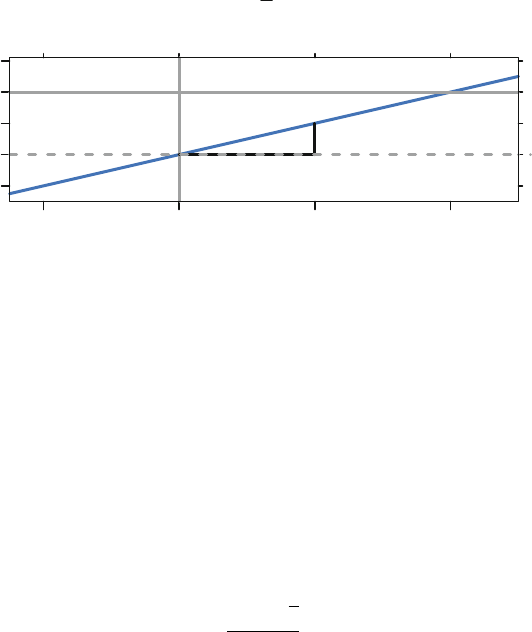
776 I Mathematics Preliminaries
I.1.1 Line
The general equation of a straight line is given by y=a+bx, where aand bare
constants with b±∞. The line in Figure I.1 intersects the y-axis at y=aand the
x-axis at x=−a/b, and has slope b.
+
y=−2+1
2 x =a+bx
x
y
−3
−2
−1
0
1
−2 0 2 4
+
2
1a
Fig. I.1 Straight line y=2+1/2xwith intercepts and slope indicated.
I.1.2 Parabola
The general equation of a parabola having a vertical axis is the quadratic equation
y=ax2+bx +cfor constants a,b,cwith a0. The graph of the parabola opens
upward if a>0 and attains a minimum when x=−b/2a. The graph opens down-
ward if a<0 and attains a maximum when x=−b/2a. The quantity d=b2−4ac
is called the discriminant. The parabola intersects the horizontal axis at
x=−b±√d
2a(I.1)
The number of intersections, or real roots, is 2, 1, or 0 according to whether d>,=,
<0. The parabola intersects the y-axis at y=c. Equation (I.1) is referred to as the
quadratic formula for solving the equation ax2+bx +c=0. We illustrate a parabola
opening upward in Figure I.2.
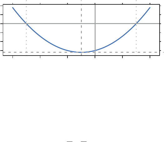
I.1 Algebra Review 777
y=(x+5)(x−3) =1x2+2x −15 =ax2+bx +c
x
y
−15
−10
−5
0
5
10
−6 −4 −2 0 2 4
root1root2
minimum
minimum
Fig. I.2 Parabola with x-roots and minimum indicated.
I.1.3 Ellipse
The equation
x2
a2+y2
b2=1
represents an ellipse centered at (0,0) with major and minor axes parallel to the
coordinate system. When a>b, the semimajor axis has length aand the semiminor
axis has length b. We graph a sample ellipse, with a=3 and b=2, in Figure I.3.
An ellipse centered at (μx,μ
y) is obtained by replacing xand yin the above with
x−μxand y−μy, respectively. Ellipses having axes nonparallel to the coordinate sys-
tem are important in statistics and will be discussed in Section I.4.13 as an example
of the use of matrix notation.
I.1.4 Simultaneous Equations
A common algebraic problem is the determination of the solution to two (or more)
simultaneous equations. In the case of two linear equations, the number of solutions
maybe0,1,or∞. There are no solutions if the equations are contradictory, such as
x+y=8 and x+y=9; there are an infinite number of solutions if one equation
is indistinct from the other, for example x+y=8 and 2x+2y=16. When there is
a unique solution, several approaches exist for finding it. One of these is adding a
carefully chosen multiple of one equation to the other equation so as to result in an
easily solved new linear equation involving just one variable. For example, suppose
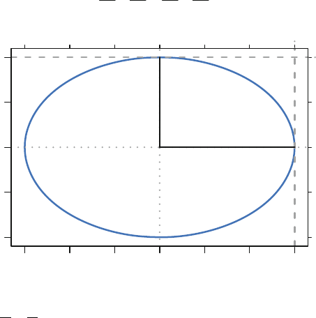
778 I Mathematics Preliminaries
x2
32+y2
22=x2
a2+y2
b2=1
x
y
−2
−1
0
1
2
−3 −2 −1 0 1 2 3
a
b
Fig. I.3 Ellipse x2
32+y2
22=1
the two equations are x+y=8 and 2x−3y=1. Adding three times the first equation
to the second yields 5x+0y=25, which implies x=5 and then y=3. We illustrate
in Figure I.4.
I.1.5 Exponential and Logarithm Functions
Two additional elementary functions are the exponential function and logarithmic
function. The exponential function y=c1ec2x(where c1,c2are nonzero constants)
has the property that the rate of change in yin response to a change in xis pro-
portional to the current value of y. The logarithmic function y=cln(x),x>0is
useful in situations when successive changes in xare geometrical (i.e., proportional
to the current value of x). The exponential function and the natural (to the base e)
logarithm are inverse to each other. We illustrate both in Figure I.5.
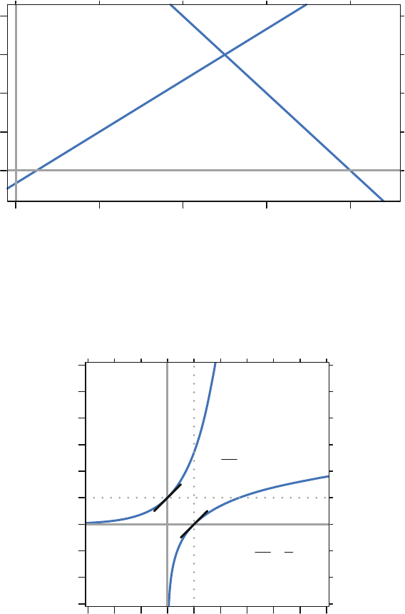
I.1 Algebra Review 779
x+y=8, 2x −3y =1
x
y
0
1
2
3
4
02468
+
x+y=8
2x−3y=1
(5, 3)
Fig. I.4 Solution of simultaneous equations at the intersection of the two straight lines described
by the equations.
x
y
−3
−2
−1
0
1
2
3
4
5
6
−3 −2 −1 0 1 2 3 4 5 6
y=dy
dx =ex
y=ln(x);dy
dx =1
x
Fig. I.5 Exponential and logarithmic functions with derivatives at x=0.

780 I Mathematics Preliminaries
x
y
0
1
2
3
4
5
6
7
8
9
10
012345678910
Fig. I.6 Asymptotes of the hyperbola y=1/xat the horizontal axis as x→∞and the vertical
axis as x→0+.
I.1.6 Asymptote
An asymptote is a straight line that is gradually approached by a curved line. This
concept is used to describe the ultimate behavior of the curved line. For example in
Figure I.6, the graph of y=1
xhas the horizontal axis as its asymptote as x→∞and
the vertical axis as its asymptote as x→0+.
I.2 Elementary Differential Calculus
If y=f(x) expresses the functional relationship between xand y,thederivative of y
with respect to x, denoted dy
dx or Dxyor f(x), is a new function of x. For each value
of x,f(x) gives the relative amount that ychanges in response to a small change in
x. For example, if y=f(x)=x2, then it can be shown that f(x)=2x. When x=3,
a small increase in xwill beget a sixfold increase in ybecause f(3) =2(3) =6.
Graphically, f(x0) is the slope of the straight line tangent to f(x)atx=x0.
If f(x)=a0+a1x+a2x2+...+amxm,anmth-degree polynomial, then f(x)=
a1+2a2x+3a3x2+...+mamxm−1. This rule can be used to differentiate (i.e., find the
derivative of) many common functions. If f(x) can be expressed as the product of
two functions, say f(x)=g(x)h(x), then its derivative is given by the product rule

I.3 An Application of Differential Calculus 781
f(x)=g(x)h(x)+g(x)h(x). This can be used, for example, to find the derivative
of (3x2+4x+5)(−8x2+7x−6) without first multiplying the quadratics.
The most important application of f(x) is in finding relative extrema (i.e., max-
ima or minima) of f(x). A necessary condition for x0to be an extremum of f(x)is
that f(x0)=0. This follows from the interpretation of the derivative as a tangent
slope. Additional investigation is needed to confirm that such an x0corresponds to
either a maximum or minimum, and then to determine which of the two it is. For
example, if f(x)=x3−3x, then f(x)=3x2−3. Setting f(x)=0, we find x=±1.
x=1 corresponds to a local minimum and x=−1 corresponds to a local maximum.
As another example, consider f(x)=x3. While for this function, f(0) =0, x=0is
neither a relative minimum nor a relative maximum of f(x).
Example of an Optimization Problem
A rectangular cardboard poster is to have 150 square inches for printed matter. It is
to have a 3-inch margin at the top and bottom and a 2-inch margin on each side. Find
the dimensions of the poster so that the amount of cardboard used is minimized.
Solution I.1. Let the vertical dimension of the printed matter be x. Then for the
printed area to be 150, the horizontal dimension of the printed matter is 150
x. Then
allowing for the margins, the vertical and horizontal dimensions of the poster are
x+6 and 150
x+4. The product of these dimensions is the area of the poster that we
seek to minimize: a(x)=174 +4x+900
x. Taking the derivative and setting it equal
to zero gives a(x)=4−900x−2=0, which leads to the positive solution x=15.
Thus the minimum-sized poster with required printed area is 21 inches high by 14
inches wide, and its printed area is 15 inches high by 10 inches wide.
I.3 An Application of Differential Calculus
We introduce Newton’s method for solutions of an equation of the form f(x)=0.
A common application is the need to solve f(x)=0 to find extrema, as discussed
in Section I.2. Many equations of this type are readily solvable by successively
moving toward isolation of a lone xon one side of the equation, or via a specialized
technique such as the quadratic formula. In other situations one must employ one
of the number of numerical techniques designed for this purpose, one of which is
Newton’s method.
Newton’s method has the disadvantage of requiring knowledge of the derivative
f(x), but it will often converge to a solution within a small number of iterations.
As with all procedures for dealing with this problem, one must start with a first

782 I Mathematics Preliminaries
approximation x0, and if this is “too far” from the solution x∗, the procedure may
fail to converge.
The idea behind Newton’s method is not difficult to understand. It is based on
the equation of the tangent line to f(x)atx=x0. If this tangent line intersects the
x-axis at x=x1, then
f(x0)=f(x0)
x0−x1→x1=x0−f(x0)
f(x0)
The iteration then proceeds with
x2=x1−f(x1)
f(x1)
and so on.
An Illustration of Newton’s Method
Consider solving f(x)=x3−x−5=0, f(x)=3x2−1, and let x0=2. You can
verify with Figure I.7 the following sequence:
ix
if(xi)
02.00000000 1.00100
11.90909091 4.8810−2
21.90417486 1.3810−4
31.90416086 1.1410−9
I.4 Topics in Matrix Algebra
We next provide an overview of selected topics from matrix algebra that are use-
ful in applied statistics. Not only do matrices (the plural of matrix) allow for
a more concise notation than scalar algebra, but they are an indispensable tool
for communicating statistical findings. Additional material on matrix algebra is
contained in the appendices of most books dealing with regression analysis, linear
models, or multivariate analysis.
A matrix is a rectangular array consisting of rrows and ccolumns. A vector is a
special type of matrix, having either ror cequal to 1. Data files are often arranged
as a matrix, such that each variable is one column and each observation is one row.
Systems of linear equations may be succinctly written in matrix notation.
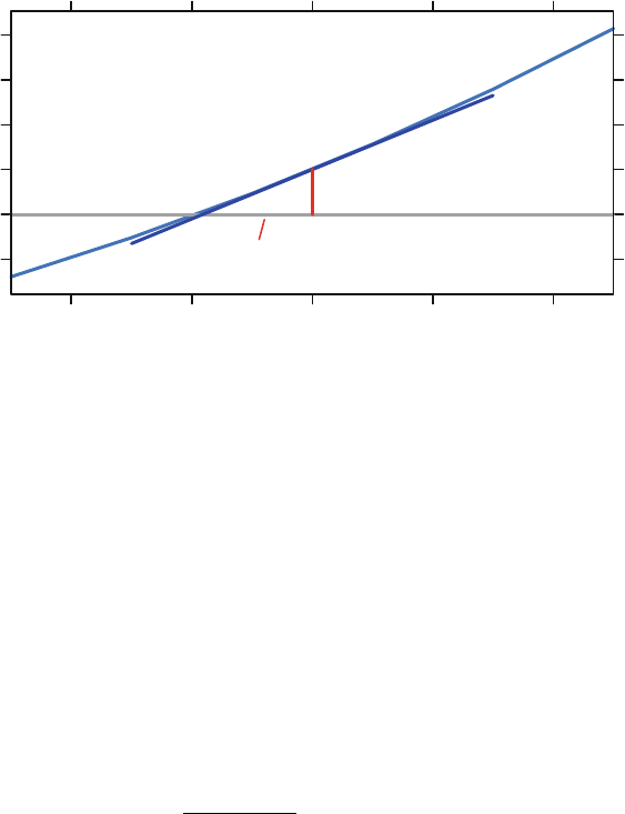
I.4 Topics in Matrix Algebra 783
x
y
−1
0
1
2
3
4
1.8 1.9 2.0 2.1 2.2
x0=2
x1=21 11 ++
x(2, 1)
y=−21 +f′(x0)x
f(x)=x3−x−5
Fig. I.7 An illustration of Newton’s Method.
Multivariate analysis involves probability distributions of random vectors rather
than scalar random variables. Each component of a random vector is a scalar ran-
dom variable. The variances and covariances of the components of a random vector
are arranged in a variance–covariance matrix. (Such a symmetric matrix V,also
called covariance matrix or dispersion matrix, has the variances on the main diago-
nal and the covariance between variables iand jin its row icolumn jposition. See
Section 3.3.5.) The multivariate normal distribution of the random k-vector xwith
mean vector μand covariance matrix V, with notation
x∼N(μ, V) (I.2)
and probability density function
f(x)=1
(2π)k/2|V|1/2e(x−μ)V−1(x−μ)/2(I.3)
is the most important distribution used in multivariate analysis. We give examples
of the bivariate (multivariate with k=2) normal in Sections 3.3.5 and J.4.2.
Matrices may be used to translate from one coordinate system to another. Orthog-
onal matrices perform rigid rotations in order to facilitate meaningful interpretation
of results.
784 I Mathematics Preliminaries
I.4.1 Elementary Operations
sum: If two matrices are of the same size, their sum is the new matrix of this size
comprised of the element-wise sums. The difference of two matrices of the same
size is defined similarly.
transpose: If Ais an r×cmatrix, then its transpose, denoted A,isthec×rmatrix
having columns identical to the rows of Aand conversely.
inner product: The inner product of two vectors of the same size, say u=
(u1,u2,...,uk)and v=(v1,v2,...,vk), is written uv=vu=k
i=1uivi, i.e.,
the sum of the products of the corresponding elements of the two vectors. The
inner product of a vector with itself yields the sum of squares of the elements of
this vector. A vector uis said to be normalized if uu=1, i.e., if its (Euclidean)
length equals 1. Two vectors uand vare said to be orthogonal if their inner prod-
uct is zero: uv=0.
matrix product: The matrix product AB of an r×cmatrix Awith an m×nmatrix
Bis defined when c=m. The element in row iand column jof AB is calculated
as the inner product of the ith row of Aand the jth column of B. The condition
c=massures that the vectors forming the inner products are of the same size.
Matrix addition has the mathematical properties of commutativity and associa-
tivity. Matrix multiplication has only associativity. When AB is defined, BA may
have different dimensions from AB or even be undefined.
Matrix multiplication is used when expressing systems of linear equations in
matrix notation. Earlier we considered the system x+y=8 and 2x−3y=1. If
we define the 2 ×1 vectors X=x
yand c=8
1and the 2 ×2matrixA=11
2−3,
then this system can be written AX =c. In this context, the matrix Ais referred
to as the coefficient matrix.
transpose: The transpose of the product of two matrices is the product of their
transposes in reverse order: (AB)=BA.
square: A matrix is said to be square if it has the same number of rows as columns.
identity: The n×nidentity matrix has ones on its main diagonal positions (those
where the row number equals the column number) and zeros everywhere else.
Thus, for example, the 3 ×3 identity matrix is
I3=⎛
⎜
⎜
⎜
⎜
⎜
⎜
⎝
100
010
001
⎞
⎟
⎟
⎟
⎟
⎟
⎟
⎠
The identity matrix plays the same role in matrix notation as does the number 1
in scalar notation: If Idenotes an identity matrix such that the indicated multipli-
cation is defined, then AI =Aand IA =A.

I.4 Topics in Matrix Algebra 785
Jn: We define Jnto be the n×nmatrix having all entries equal to 1.
symmetric: A square matrix Ais said to be a symmetric matrix if A=A.This
means that row number icorresponds to column number ifor all i.Letaij denote
the element in row iand column jof matrix A. Then if Ais square, its trace is
the sum of its main diagonal elements: trace(A)=iaii.
operation count: Numerical analysts count the number of multiplications in an al-
gorithm as an indicator of the costliness of the algorithm. A vector inner product
n
i=1aibi, for example, takes nmultiplications to complete. There are other op-
erations (indexing, adding) that must also be performed. Rather than report them
explicitly, we say instead that the amount of computation is proportional to the
number of multiplications. We indicate the proportionality by saying the oper-
ation count is O(n) (read as “big ‘O’ofn”). Similarly, the operation count for
matrix multiplication is proportional to n3and is reported as O(n3).
determinant: The determinant of a square matrix A, denoted |A|, is a scalar calcu-
lated from the elements of A.Inthe2×2 case where
A=a11 a12
a21 a22
the determinant is |A|=a11a22 −a21a12.If Ais a square coefficient matrix of a
system of linear equations (thus implying that the system has the same number
of equations as unknowns), then the system has a unique solution if and only
if |A|0. The determinant has useful mathematical properties, but is totally
impractical from a computational standpoint. It is almost never needed as an
intermediate calculation. There is almost always a cheaper way to calculate the
final answer.
nonsingular: If |A|0, then Ais said to be a nonsingular matrix. There is no
vector vother than v=0 such that Av ≡0.
inverse: A nonsingular matrix has associated with it a unique inverse, denoted
A−1. The inverse has the property that AA−1=A−1A=I. The unique solution to
a system of linear equations AX =cis then X=A−1c. For example, the inverse
of
A=a11 a12
a21 a22 is 1
|A|a22 −a12
−a21 a11
provided that |A|0. Note that this is a mathematical identity. It is not to be
interpreted as an algorithm for calculation of the inverse. As an algorithm it is
very expensive, requiring O(2n3) arithmetic operations for an n×nmatrix A.An
efficient algorithm requires only O(n3) operations.
singular: If |A|=0, then Ais said to be a singular matrix. There exists at least one
vector vother than v=0 such that Av ≡0. A singular matrix does not have an
inverse.
786 I Mathematics Preliminaries
idempotent: A square matrix Ais said to be an idempotent matrix if AA =A, i.e.,
Aequals the product of Awith itself. A simple example is
.5−.5
−.5.5
I.4.2 Linear Independence
AmatrixXconsists of a set of column vectors
X
n×(1+p)
=[1X1X2...Xp]=[X0X1X2...Xp]
The columns are numbered 0,1,...,p.
The matrix Xis said to have linearly dependent columns if there exists a nonzero
(1 +p)-vector such that
X=0
or, equivalently,
⎛
⎜
⎜
⎜
⎜
⎜
⎜
⎝
j
jXj⎞
⎟
⎟
⎟
⎟
⎟
⎟
⎠
n×1
=(0)
n×1
The matrix Xis said to have linearly independent columns if no such vector exists.
For example, the matrix
X
4×(1+4)
=⎛
⎜
⎜
⎜
⎜
⎜
⎜
⎜
⎜
⎜
⎜
⎜
⎜
⎝
11000
10100
10010
10001
⎞
⎟
⎟
⎟
⎟
⎟
⎟
⎟
⎟
⎟
⎟
⎟
⎟
⎠
(I.4)
has linearly dependent columns because there exists a vector =(−11111)
such
that X=0.
The matrix
X(,−1)
4×(1+3)
=⎛
⎜
⎜
⎜
⎜
⎜
⎜
⎜
⎜
⎜
⎜
⎜
⎜
⎝
1000
1100
1010
1001
⎞
⎟
⎟
⎟
⎟
⎟
⎟
⎟
⎟
⎟
⎟
⎟
⎟
⎠
(I.5)
has linearly independent columns because there exists no nonzero vector such that
X=0.
The rank of a matrix is the number of linearly independent columns it contains.
Both matrices above, Xand X(,−1) in Equations (I.4) and (I.5), have rank 4. For any

I.4 Topics in Matrix Algebra 787
matrix X, rank(X)=rank(XX). A full-rank matrix is one whose rank is equal to the
minimum of its row and column dimensions, that is,
rank A
r×c=min(r,c)
I.4.3 Rank
The rank of a matrix Ais the maximum number of linearly independent rows (equiv-
alently, the maximum number of linearly independent columns) the matrix has. For
example, the matrix
A=⎛
⎜
⎜
⎜
⎜
⎜
⎜
⎝
112
123
134
⎞
⎟
⎟
⎟
⎟
⎟
⎟
⎠
has rank 2 since columns 1 and 2 add to column 3, but any two of the columns are
linearly independent of one another (i.e., are not proportional to one another).
I.4.4 Quadratic Forms
Aquadratic form is a scalar resulting from the matrix product xAx, where xis a
k×1 vector and Ais a k×ksymmetric matrix. The matrix Ais termed the matrix
of the quadratic form. Complicated sums of squares and products as often occur in
an analysis of variance can be written as quadratic forms. If xhas a standardized
multivariate normal distribution x∼N(0,I) [see Equation (I.2)], then xAx has a
χ2-distribution with νdegrees of freedom if and only if Ais an idempotent matrix
with rank ν. For example, the numerator of the usual univariate sample variance,
n
i=1(xi−¯x)2, can be written as xAx where x=(x1,x2,...,xn)and A=In−1
nJn.
It can be shown that this matrix Ahas rank n−1, the degrees of freedom associated
with the sample variance.
If xis a random vector with expected value μand covariance matrix V, then the
expected value of the quadratic form xAx is
E(xAx)=μAμ+trace(AV)
Result (I.6) does not require that xhas a multivariate normal distribution.
A square symmetric matrix Ais said to be a positive definite (abbreviated p.d.)
matrix if xAx >0 for all vectors xother than a vector of zeros. The matrix associ-
ated with the quadratic form representation of a sum of squares is always p.d.

788 I Mathematics Preliminaries
I.4.5 Orthogonal Transformations
AmatrixMis said to be orthogonal if MM=I. An example is
M=⎛
⎜
⎜
⎜
⎜
⎜
⎜
⎜
⎜
⎜
⎜
⎜
⎜
⎜
⎝
1/√31/√21/√6
1/√3−1/√21/√6
1/√30−2/√6
⎞
⎟
⎟
⎟
⎟
⎟
⎟
⎟
⎟
⎟
⎟
⎟
⎟
⎟
⎠
A transformation based on an orthogonal matrix is called an orthogonal transfor-
mation. Such transformations are rotations that preserve relative distances: y=
Mx →yy=xMMx =xx. Orthogonal transformations are frequently enc-
ountered in statistics. A common use of them is to transform from a correlated set
of random variables xto an uncorrelated set y.
The columns of an orthogonal matrix are said to be orthonormal. The columns
are orthogonal to each other, that is M
,jM,j=0for jj. In addition, the columns
have been scaled so that M
,jM,j=1.
I.4.6 Orthogonal Basis
If rankA
r×c=p<min(r,c) and c≤r, then any set of plinearly independent
columns of Aconstitutes a basis for A. The set of all vectors that can be expressed
as a linear combination Xv of the columns of Ais called the column space of A,
denoted C(A). Therefore, C(A) is completely specified by any basis of A.Wesay
that the columns of the basis span the column space of A.
An orthogonal basis for Ais a basis for Awith the property that any two vectors
comprising it are orthogonal. Starting from an arbitrary basis for A, algorithms are
available for constructing an orthogonal basis for A. We show one algorithm, the
Gram–Schmidt process, in Section I.4.8.
Abasis set of column vectors for a matrix Xis a set of column vectors Uithat
span the same linear space as the original columns Xi. An orthogonal basis is a set
of column vectors that are mutually orthogonal, that is U
iUj=0forij.An
orthonormal basis is an orthogonal basis whose columns have been rescaled to have
norm Ui=U
iUi=1.
I.4 Topics in Matrix Algebra 789
I.4.7 Matrix Factorization—QR
Any rectangular matrix X
n×mcan be factored into the product of an matrix with or-
thogonal columns Q
n×m
and an upper triangular R
m×m
X
n×m
=Q
n×m
R
m×m
The columns of Qspan the same column space as the columns of the original
matrix X. This means that any linear combination of the columns of X,sayXv, can
be constructed as a linear combination of the columns of Q. Specifically, using the
associative law, Xv =(QR)v=Q(Rv).
The numerically efficient Rfunction qr is the computational heart of the linear
models and analysis of variance functions. The intermediate matrices Qand Rare
usually not explicitly produced. If you wish to see them, use the qr.Q and qr.R
functions. An example showing the QR factorization using the qr function is in
Table I.1.
An expository Rfunction illustrating the construction of the QR factorization is
in Section I.4.8.
I.4.8 Modified Gram–Schmidt (MGS) Algorithm
There are many algorithms available to construct the matrix factorization. We
show one, the Modified Gram–Schmidt (MGS) algorithm Bjork (1967). “Modified”
means that the entire presentation is in terms of the columns Qiof the matrix under
construction. The MGS algorithm is numerically stable when calculated in finite
precision. The original Gram–Schmidt (GS) algorithm, which constructs Qin terms
of the columns Xiof the original matrix, is not numerically stable and should not be
used for computation.
Let Xn×m=[X1X2...Xm]. The results of the factorization will be stored in Qn×m
and Rm×m. The columns of Xand Qand both the rows and columns of Rare num-
bered 1,...,m.

790 I Mathematics Preliminaries
Table I.1 Illustration of QR algorithm to factor Xinto the product of an orthogonal matrix and an
upper triangular matrix.
> X <- matrix(c(1,3,6,4,2,3,8,6,4,5,3,2), 4, 3)
>X
[,1] [,2] [,3]
[1,] 1 2 4
[2,] 3 3 5
[3,] 6 8 3
[4,] 4 6 2
> crossprod(X)
[,1] [,2] [,3]
[1,] 62 83 45
[2,] 83 113 59
[3,] 45 59 54
> ## use the efficient calculation
> X.qr <- qr(X)
> qr.Q(X.qr) ## display q
[,1] [,2] [,3]
[1,] -0.127 0.48139 0.8188
[2,] -0.381 -0.73969 0.4755
[3,] -0.762 -0.02348 -0.3038
[4,] -0.508 0.46965 -0.1057
> qr.R(X.qr) ## display r
[,1] [,2] [,3]
[1,] -7.874 -10.541 -5.7150
[2,] 0.000 1.374 -0.9041
[3,] 0.000 0.000 4.5301
> zapsmall(crossprod(qr.Q(X.qr))) ## identity
[,1] [,2] [,3]
[1,] 1 0 0
[2,] 0 1 0
[3,] 0 0 1
> crossprod(qr.R(X.qr)) ## reproduce crossprod(X)
[,1] [,2] [,3]
[1,] 62 83 45
[2,] 83 113 59
[3,] 45 59 54
> qr.X(X.qr) ## reproduce X
[,1] [,2] [,3]
[1,] 1 2 4
[2,] 3 3 5
[3,] 6 8 3
[4,] 4 6 2

I.4 Topics in Matrix Algebra 791
We will construct Qand Rin steps.
1. Initialize Rto 0.
R←0
2. Initialize Qto X.
Q←X
3. Initialize the column counter.
i←1
4. Normalize column Qi.
ri,i←Q
iQi
Qi←Qi/ri,i
If i=m, we are done.
5. For each of the remaining columns Qj,j=i+1,...,m, find the component of
Qjorthogonal to Qiby
ri,j←Q
iQj
Qj←Qj−Qiri,j
6. Update the column counter.
i←i+1
7. Repeat steps 4–6until completion.
An Rversion of this expository algorithm is in Table I.2. An example using the
expository function is in Table I.3.

792 I Mathematics Preliminaries
Table I.2 An expository algorithm for the Modified Gram–Schmidt Algorithm. The function is a
direct translation of the pseudo-code in Section I.4.8.
## modified Gram-Schmidt orthogonalization
mgs <- function(x) {
## modified Gram-Schmidt orthogonalization
## this is an expository algorithm
## this is not an efficient computing algorithm
## q[,j] is the normalized residual from the least squares fit of
## x[,j] on the preceding normalized columns q[,1:(j-1)]
n <- nrow(x)
m <- ncol(x)
q<-x
r <- matrix(0, m, m)
for (i in 1:m) {
r[i,i] <- sqrt(sum(q[,i]^2)) ## length of q[,i]
q[,i] <- q[,i] / r[i,i] ## normalize q[,i]
if (i < m) { ## if we still have columns to go
for (j in (i+1):m) {
r[i,j] <- sum(q[,i] * q[,j]) ## length of projection of q[,j] on q[,i]
q[,j] <- q[,j] - q[,i] * r[i,j] ## remove projection of q[,j] on q[,i]
}
}
}
list(q=q, r=r)
}

I.4 Topics in Matrix Algebra 793
Table I.3 Illustration of the expository algorithm for the Modified Gram–Schmidt Algorithm
shown in Table I.2. These are the same values (up to multiplication by −1) as calculated by the qr
function in Table I.1.
X <- matrix(c(1,3,6,4,2,3,8,6,4,5,3,2), 4, 3)
X
crossprod(X)
## use the expository function defined in the previous chunk
X.mgs <- mgs(X)
X.mgs ## q is orthogonal, r is upper triangular
## These are identical to the results of qr(X)
## up to the sign of the columns of q and the rows of r.
zapsmall(crossprod(X.mgs$q)) ## identity
crossprod(X.mgs$r) ## reproduces crossprod(X)
X.mgs$q %*% X.mgs$r ## reproduces X
I.4.9 Matrix Factorization—Cholesky
Any square positive definite matrix S
m×mcan be factored into the product of an upper
triangle matrix R
n×mand its transpose
S=RR
When Shas been constructed as the cross product S=XXof a rectangular matrix
X
n×m, then the upper triangular matrix Ris the same matrix we get from the QR
factorization.
S=XX=(QR)(QR)=R(QQ)R=RR
The numerically efficient Rfunction chol is illustrated in Table I.4.
I.4.10 Orthogonal Polynomials
Consider the k-vector v=(v1,v2,...,vk), where v1<v2< ... < vk. Construct a
matrix V=[v0,v1,v2,...,vk−1], where we use the notation vj=(vj
1,vj
2,...,vj
k)

794 I Mathematics Preliminaries
Table I.4 Illustration of Cholesky factorization of a square positive definite matrix into an upper
triangular factor and its transpose.
> X <- matrix(c(1,3,6,4,2,3,8,6,4,5,3,2), 4, 3)
> M <- crossprod(X)
>M
[,1] [,2] [,3]
[1,] 62 83 45
[2,] 83 113 59
[3,] 45 59 54
> chol(M)
[,1] [,2] [,3]
[1,] 7.874 10.541 5.7150
[2,] 0.000 1.374 -0.9041
[3,] 0.000 0.000 4.5301
> crossprod(chol(M)) ## reproduce M
[,1] [,2] [,3]
[1,] 62 83 45
[2,] 83 113 59
[3,] 45 59 54
An orthogonal basis Qconstructed from the matrix Vis called a set of orthogonal
polynomials. In the analysis of variance and related techniques, we often construct
dummy variables for ordered factors from a set of contrasts that are orthogonal
polynomials. See Figure 10.4 and the surrounding discussion in Section 10.4 for an
illustration.
I.4.11 Projection Matrices
Given any matrix X
n×m
=Q
n×m
R
m×m
the matrix PX
n×n
=X(XX)−1X=QQis a projection
matrix that projects an n-vector yonto the space spanned by the columns of X, that
is, the product PXyis in the column space C(X). If Xhas mcolumns and rank r≤m,
then the eigenvalues of PXconsist of r1s and m−r0s. See Table I.5.

I.4 Topics in Matrix Algebra 795
Table I.5 Projection of a 3-vector onto the space of its first two coordinates.
> X <- matrix(c(3,1,0, 1,2,0, 0,0,0), 3, 3)
> P <- cbind(qr.Q(qr(X))[, 1:2], 0)
>P
[,1] [,2] [,3]
[1,] -0.9487 0.3162 0
[2,] -0.3162 -0.9487 0
[3,] 0.0000 0.0000 0
> crossprod(P)
[,1] [,2] [,3]
[1,] 1 0 0
[2,] 0 1 0
[3,] 0 0 0
> y <- matrix(1:3)
>y
[,1]
[1,] 1
[2,] 2
[3,] 3
> P %*% y
[,1]
[1,] -0.3162
[2,] -2.2136
[3,] 0.0000
> sqrt(sum(y[1:2,]^2))
[1] 2.236
> sqrt(sum((P %*% y)^2))
[1] 2.236
I.4.12 Geometry of Matrices
We provide some details of the application to two-dimensional geometry. Each two-
dimensional vector represents a point; alternatively, a directed line segment from the
origin to this point. A 2 ×2 matrix postmultiplied by a vector transforms this point
to another point. Consider the orthogonal matrix
M=cos(θ)sin(θ)
−sin(θ) cos(θ)
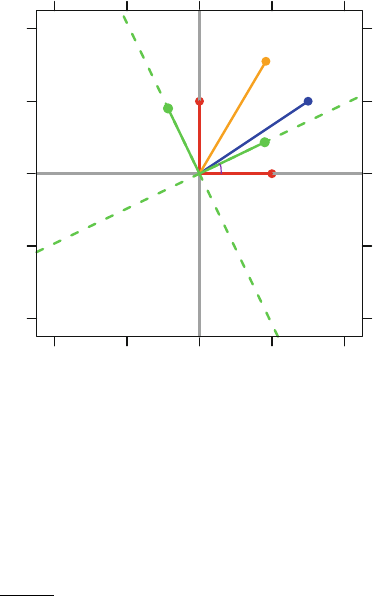
796 I Mathematics Preliminaries
x
y
−2
−1
0
1
2
−2 −1 0 1 2
u
v
θ
Fig. I.8 Rotation of a vector uand its coordinate system into vby angle θ.
and let ube a 2 ×1 vector representing a point in two dimensions. Then v=Mu
produces a new point vwhich is where uappears in the new coordinate system
formed by rotating the old one θdegrees around the origin. See Figure I.8.
If xand yare each two-dimensional vectors and θis the angle between them,
then cos(θ)=xy/√xxy
y=corr(x,y),the correlation between these two vectors.
Note that if the vectors are orthogonal so that xy=0, then cos(θ)=0 and θ=90◦.
I.4.13 Eigenvalues and Eigenvectors
Next we study the concepts of eigenvectors and eigenvalues of an n×nsymmetric
matrix V.
If Vξ=λξ, where ξis an n×1 vector and λis a scalar, then λis said to be
an eigenvalue of Vwith corresponding eigenvector ξ. Without loss of generality,
we can take the eigenvector to be normalized. Geometrically, the matrix Vtrans-
forms its eigenvectors into multiples of themselves. Any two distinct eigenvectors
are orthogonal: ξ
iξj=0,ij.Vcan be written as its spectral decomposition
V=iλiξiξ
i.Vcan be written as its eigenvalue factorization V =ΞΛΞ.
A matrix is nonsingular if and only if it has only nonzero eigenvalues. A matrix
is positive definite if and only if all of its eigenvalues are positive. The eigenvalues
of V−1are the reciprocals of the eigenvalues of V. The determinant of a matrix

I.4 Topics in Matrix Algebra 797
equals the product of its eigenvalues |V|=λi, and calculating the eigenvalues is
normally the most efficient way to calculate the determinant. The trace of a matrix
equals the sum of its eigenvalues trace(V)=λi.
Consider the problem of choosing xto maximize xVx subject to xx=1.The
maximum value is the largest eigenvalue of Vand is attained when xis the eigen-
vector corresponding to this eigenvalue. Similarly, xVx is minimized (subject to
xx=1) at the value of the smallest eigenvalue of V, occurring at the corresponding
eigenvector.
Here is an example of hand calculation of eigenvalues and eigenvectors. Consider
the 2 ×2matrix
V=21
11
Its 2 eigenvalues are the 2 scalar solutions λto the equation |V−λI|=0. Taking the
determinant leads to (2 −λ)(1 −λ)−1=0=⇒λ2−3λ+1=0=⇒λ=(3 ±
√5)/2,which expands to ≈2.618 or ≈0.382. (Note that we are explicit about the
approximation to 3 decimal digits. Our usual practice is not to round answers.) The
eigenvector ξ=ξ11
ξ21corresponding to λ≈2.618 is the solution to the equation Vξ≈
2.618ξ. This implies that 2ξ11 +ξ21 ≈2.618ξ11, and coupled with the normalization
restriction ξ2
11 +ξ2
21 =1 we find that ξ11 ≈.8507 and ξ21 ≈.5257. The eigenvector
corresponding to the other eigenvalue is found similarly.
As a geometric application of eigenvalues, consider the ellipse having equation
(x−μ)V−1(x−μ)=b. In statistics, this ellipse based on the inverse V−1is the form
of a confidence ellipse for μ.Letλ1<λ
2be the eigenvalues of Vwith corresponding
normalized eigenvectors ξ1=ξ11
ξ21,ξ
2=ξ12
ξ22.Then the semimajor axis of this ellipse
has length √λ2band the semiminor axis has length √λ1b. The angle between the
extension of the semimajor axis and the horizontal axis is arctan ξ12
ξ22 .
Continuing the example, we calculate the eigenvalues of V=21
11
in Table I.6
and graph the ellipse xVx =x21
11
x=1 in Figure I.9.
I.4.14 Singular Value Decomposition
Let Mbe an arbitrary r×cmatrix, Uthe r×rmatrix containing the eigenvectors
of MM, and Wthe c×cmatrix containing the eigenvectors of MM.LetΔbe
the r×cmatrix having δij =0(ij). If r≥c(the usual case in statistical
applications), define δii =the square root of the eigenvalue of MMcorresponding
to the eigenvector in the ith column of W.Ifr<c, define δii =the square root of
the eigenvalue of MMcorresponding to the eigenvector in the ith column of U.
Then the singular value decomposition of Mis M=UΔW. Note that the number of

798 I Mathematics Preliminaries
Table I.6 Eigenvalues and eigenvectors of V=21
11
.
> V <- matrix(c(2, 1, 1, 1), 2, 2)
>V
[,1] [,2]
[1,] 2 1
[2,] 1 1
> eV <- eigen(V)
>eV
$values
[1] 2.618 0.382
$vectors
[,1] [,2]
[1,] -0.8507 0.5257
[2,] -0.5257 -0.8507
> sqrt(eV$val) ## semimajor and semiminor axis lengths
[1] 1.618 0.618
> ## angle of axes in radians
> atan(c(eV$vec[2,1]/eV$vec[1,1], eV$vec[2,2]/eV$vec[1,2]))
[1] 0.5536 -1.0172
> ## = -pi/2 ## right angle
> diff(atan(c(eV$vec[2,1]/eV$vec[1,1], eV$vec[2,2]/eV$vec[1,2])))
[1] -1.571
nonzero diagonal values in Δis min(r,c). We show a numerical example in standard
mathematical notation in Table I.7. We show the same example calculated with the
svd function in Tables I.8 and I.9.
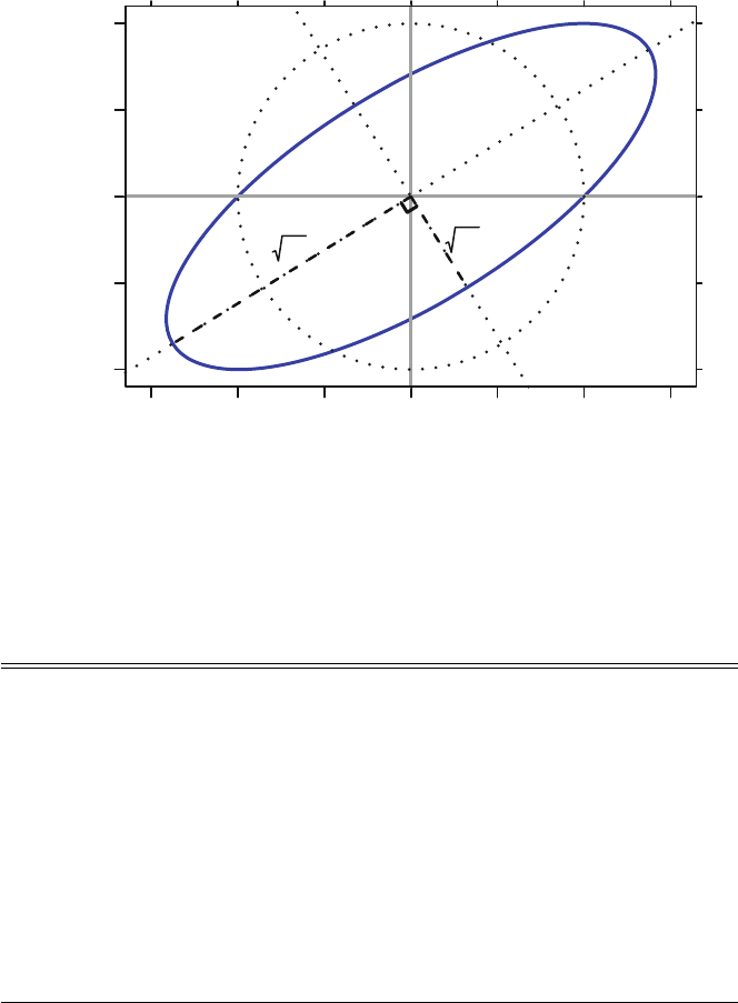
I.4 Topics in Matrix Algebra 799
x
y
−1.0
−0.5
0.0
0.5
1.0
−1.5 −1.0 −0.5 0.0 0.5 1.0 1.5
λ1λ2
ξ1
ξ2
Fig. I.9 Ellipse xVx =x21
11
x=1. We show the unit circle with the normalized eigenvectors,
the ellipse, and the semimajor and semiminor axes whose lengths are the eigenvalues multiplied
by the square root of the eigenvectors.
Table I.7 Matrix multiplication of the components of the Singular Value Decomposition of the
matrix Min Table I.9).
M=UΔV=
⎡
⎢
⎢
⎢
⎢
⎢
⎢
⎢
⎢
⎢
⎢
⎢
⎢
⎢
⎢
⎢
⎢
⎢
⎢
⎢
⎢
⎢
⎢
⎣
124
335
683
462
⎤
⎥
⎥
⎥
⎥
⎥
⎥
⎥
⎥
⎥
⎥
⎥
⎥
⎥
⎥
⎥
⎥
⎥
⎥
⎥
⎥
⎥
⎥
⎦
=
⎡
⎢
⎢
⎢
⎢
⎢
⎢
⎢
⎢
⎢
⎢
⎢
⎢
⎢
⎢
⎢
⎢
⎢
⎢
⎢
⎢
⎢
⎢
⎣
−0.2561 0.6098 −0.6935
−0.4102 0.6334 0.5907
−0.7125 −0.3674 0.1755
−0.5084 −0.3034 −0.3733
⎤
⎥
⎥
⎥
⎥
⎥
⎥
⎥
⎥
⎥
⎥
⎥
⎥
⎥
⎥
⎥
⎥
⎥
⎥
⎥
⎥
⎥
⎥
⎦
⎡
⎢
⎢
⎢
⎢
⎢
⎢
⎢
⎢
⎢
⎢
⎢
⎢
⎢
⎢
⎢
⎢
⎣
14.481 0.000 0.000
0.000 4.324 0.000
0.000 0.000 0.783
⎤
⎥
⎥
⎥
⎥
⎥
⎥
⎥
⎥
⎥
⎥
⎥
⎥
⎥
⎥
⎥
⎥
⎦
⎡
⎢
⎢
⎢
⎢
⎢
⎢
⎢
⎢
⎢
⎢
⎢
⎢
⎢
⎢
⎢
⎢
⎣
−0.5383 −0.7246 −0.4302
−0.2099 −0.3791 0.9012
0.8162 −0.5755 −0.0520
⎤
⎥
⎥
⎥
⎥
⎥
⎥
⎥
⎥
⎥
⎥
⎥
⎥
⎥
⎥
⎥
⎥
⎦

800 I Mathematics Preliminaries
Table I.8 Illustration of singular value decomposition, part I (to be continued in Table I.9).
> M <- matrix(c(1,3,6,4,2,3,8,6,4,5,3,2), 4, 3)
>M
[,1] [,2] [,3]
[1,] 1 2 4
[2,] 3 3 5
[3,] 6 8 3
[4,] 4 6 2
> M.svd <- svd(M)
> M.svd
$d
[1] 14.4806 4.3243 0.7825
$u
[,1] [,2] [,3]
[1,] -0.2561 0.6098 -0.6935
[2,] -0.4102 0.6334 0.5907
[3,] -0.7125 -0.3674 0.1755
[4,] -0.5084 -0.3034 -0.3733
$v
[,1] [,2] [,3]
[1,] -0.5383 -0.2099 0.81617
[2,] -0.7246 -0.3791 -0.57547
[3,] -0.4302 0.9012 -0.05198
> zapsmall(crossprod(M.svd$u))
[,1] [,2] [,3]
[1,] 1 0 0
[2,] 0 1 0
[3,] 0 0 1
> zapsmall(crossprod(M.svd$v))
[,1] [,2] [,3]
[1,] 1 0 0
[2,] 0 1 0
[3,] 0 0 1
> M.svd$u %*% diag(M.svd$d) %*% t(M.svd$v)
[,1] [,2] [,3]
[1,] 1 2 4
[2,] 3 3 5
[3,] 6 8 3
[4,] 4 6 2

I.4 Topics in Matrix Algebra 801
Table I.9 Illustration of singular value decomposition, part II (continued from Table I.8). Relation
between singular value decomposition and Eigenvalue decomposition.
> eigen(tcrossprod(M))
$values
[1] 2.097e+02 1.870e+01 6.123e-01 -5.978e-15
$vectors
[,1] [,2] [,3] [,4]
[1,] -0.2561 0.6098 0.6935 -0.2857
[2,] -0.4102 0.6334 -0.5907 0.2857
[3,] -0.7125 -0.3674 -0.1755 -0.5714
[4,] -0.5084 -0.3034 0.3733 0.7143
> eigen(crossprod(M))
$values
[1] 209.6877 18.7000 0.6123
$vectors
[,1] [,2] [,3]
[1,] -0.5383 -0.2099 0.81617
[2,] -0.7246 -0.3791 -0.57547
[3,] -0.4302 0.9012 -0.05198
> M.svd$d^2
[1] 209.6877 18.7000 0.6123
I.4.15 Generalized Inverse
For any rectangular matrix X
n×m
=UΔW, the Moore–Penrose generalized inverse is
defined as
X−=WΔ−1U
Since Δ=diag(δi) is a diagonal matrix, its inverse is Δ−1=diag(δ−1
i). The defini-
tion is extended to the situation when rank(X)<min(n,m)byusing0
−1=0. See
Table I.10 for an example.
When rank(X)=m=n, hence the inverse exists, the generalized inverse is equal
to the inverse.

802 I Mathematics Preliminaries
Table I.10 Illustration of the generalized inverse.
> M <- matrix(c(1,3,6,4,2,3,8,6,4,5,3,2), 4, 3)
>M
[,1] [,2] [,3]
[1,] 1 2 4
[2,] 3 3 5
[3,] 6 8 3
[4,] 4 6 2
> library(MASS)
> Mi <- ginv(M)
>Mi
[,1] [,2] [,3] [,4]
[1,] -0.7434 0.6006 0.22741 -0.35569
[2,] 0.4694 -0.4694 -0.06122 0.32653
[3,] 0.1808 0.1050 -0.06706 -0.02332
> zapsmall(eigen(M %*% Mi)$value)
[1] 1 1 1 0
> zapsmall(Mi %*% M)
[,1] [,2] [,3]
[1,] 1 0 0
[2,] 0 1 0
[3,] 0 0 1
> M.svd$v %*% diag(1/M.svd$d) %*% t(M.svd$u)
[,1] [,2] [,3] [,4]
[1,] -0.7434 0.6006 0.22741 -0.35569
[2,] 0.4694 -0.4694 -0.06122 0.32653
[3,] 0.1808 0.1050 -0.06706 -0.02332
I.4 Topics in Matrix Algebra 803
I.4.16 Solving Linear Equations
There are three cases.
I.4.16.1 n=m=rank(X)
Given a matrix X
n×mand an n-vector y, the solution βof the linear equation
y=Xβ
is uniquely defined by
β=X−1y
when Xis invertible, that is when n=m=rank(X).
I.4.16.2 n>m=rank(X)
When n>m=rank(X), the linear equation is said to be overdetermined. Some
form of arbitrary constraint is needed to find a solution. The most frequently used
technique is least-squares, a technique in which ˆ
βis chosen to minimize the norm
of the residual vector.
min
βy−Xβ2=
n
i=1⎛
⎜
⎜
⎜
⎜
⎜
⎜
⎝
yi−
m
j=1
xijβj⎞
⎟
⎟
⎟
⎟
⎟
⎟
⎠
2
The solution ˆ
βis found by solving the related linear equations
Xy=XXˆ
β
The solution is often expressed as
ˆ
β=(XX)−1(Xy)=X−y
This is a definition, not an efficient computing algorithm. The primary efficient
algorithm in Ris the QR algorithm as defined in qr and related functions, includ-
ing lm.

804 I Mathematics Preliminaries
I.4.16.3 m>p=rank(X)
When m>p=rank(X), there are an infinite number of solutions to the linear
equation. The singular value decomposition X=UΔWwill have m−pzero values
along the diagonal of Δ.Letβ0be one solution. Then
βγ=β0+W0
γ
where 0is a vector of pzeros and γis any vector of length m−p, is also a solution.
I.5 Combinations and Permutations
I.5.1 Factorial
For a positive integer n, the notation n!, read “nfactorial”, is used to indicate the
product of all the integers from 1 through n:
n!=n×(n−1) ×...×1=n×(n−1)!
The factorial of zero, 0!, is separately defined to equal 1.
Thus
nn=n=n((n−1)!)
00=1=1
11=1=1×1
22=2=2×1
33=6=3×2
44=24 =4×6
55=120 =5×24
.
.
..
.
.=.
.
.=.
.
.
I.5.2 Permutations
The notation nPp, read “npermute p”, indicates the number of ways to select p
distinct items from npossible items where two different orderings of the same p
items are considered to be distinct. Equivalently, nPpis the number of distinct ways
of arranging p items from npossible items:

I.6 Exercises 805
nPp=n!
(n−p)!
For example,
5P3=5!
(5 −3)! =5×4×3×2×1
2×1=5×4×3=60
I.5.3 Combinations
The notation nCpor n
p, read “nchoose p”, indicates the number of ways to select
pdistinct items from npossible items, where two different orderings of the same p
items are considered to be the same selection. Equivalently, nCpis the number of
distinct ways of choosing p items from npossible items:
n
p=nCp=n!
p!×(n−p)! =nPp
p!
For example,
5
3=5C3
2! =5!
3!(5 −3)! =5×4×3×2×1
(3 ×2×1)(2 ×1) =5×4
2×1=10
I.6 Exercises
Exercise I.1.
Start from the matrix in Equation (I.6)
A=⎛
⎜
⎜
⎜
⎜
⎜
⎜
⎝
112
123
134
⎞
⎟
⎟
⎟
⎟
⎟
⎟
⎠
Give an example of a basis for A. Then give an example of a vector in C(A) and also
a vector not in C(A). Give an example of an orthogonal basis of A, demonstrating
that it is orthogonal.
Verify that Equation (I.6) defines a family of solutions to the set of linear equations
with p=rank(X)<m.
Appendix J
Probability Distributions
We list, with some discussion, several common probability distributions. We illus-
trate 21 distributions, 20 distributions in the Rstats package and one in the HH
package, for which all three functions (d* for density, p* for probability, and q* for
quantile) are available. We also include the Studentized Range distribution for which
only the p* and q* functions are available, and the discrete multinomial and con-
tinuous multivariate normal. The d* functions give the density f(x) for continuous
distributions or the discrete density f(i) for discrete distributions. The p* functions
give the cumulative distribution, the probability that an observation is less than or
equal to the value x
F(x)=P(X≤x)=⎧
⎪
⎪
⎪
⎪
⎪
⎪
⎪
⎪
⎨
⎪
⎪
⎪
⎪
⎪
⎪
⎪
⎪
⎩
x
−∞
f(x)dx for continuous distributions
x
i=−∞
f(i) for discrete distributions
The q* functions give the quantiles F−1(p), that is the inverse of the probability
function F(x).
In the example illustrations all three functions (d*,p*, and q*) are shown and
evaluated at sample Xand for specific values of the parameters. For distributions
with finite support, the entire domain of xis shown. For distributions with infinite
support, the domain of xshowing most of the probability is shown.
For the continuous distributions, we show the plot of the density function. The
darker color shows the probability (area) to the left of x, and the lighter color shows
the probability (area) to the right of x.d*(X) gives the height of the density function
at X,p*(X) gives the probability (area) to the left of X, and q*(p) recovers Xfrom
the probability p.
©Springer Science+Business Media New York 2015
R.M. Heiberger, B. Holland, Statistical Analysis and Data Display,
Springer Texts in Statistics, DOI 10.1007/978-1-4939-2122-5
807
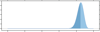
808 J Probability Distributions
For the discrete distributions, we show the plot of the discrete density function.
The darkest color shows the probability at X, the intermediate color shows the prob-
ability strictly left of X, and the lightest color shows the probability to the right of
X.d*(X) gives the probability at X,p*(X) gives the probability to the left of and
including X, and q*(p) recovers Xfrom the probability p.
We list the continuous central distributions in Section J.1, the continuous noncen-
tral distributions in Section J.2, and the discrete distributions in Section J.3. Within
each section the distributions are ordered alphabetically.
J.1 Continuous Central Distributions
J.1.1 Beta
dbeta(x, shape1 = 85.5, shape2 = 15.5)
x
0
2
4
6
8
10
0.0 0.2 0.4 0.6 0.8 1.0
> dbeta(.85, shape1=85.5, shape2=15.5)
[1] 11.22
> pbeta(.85, shape1=85.5, shape2=15.5)
[1] 0.5131
> qbeta(0.5131489, shape1=85.5, shape2=15.5)
[1] 0.85
This two-parameter distribution is often used to model phenomena restricted to
the range (0,1), for example sample proportions. It is used in Section 5.1.2 to con-
struct alternative one-sided confidence intervals on a population proportion.
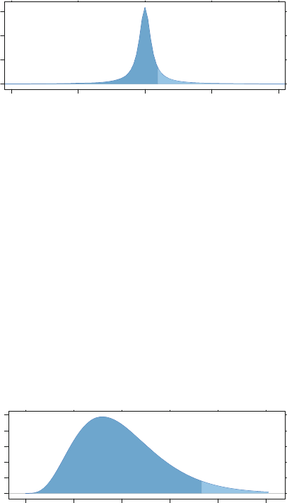
J.1 Continuous Central Distributions 809
J.1.2 Cauchy
dcauchy(x)
x
0.0
0.1
0.2
0.3
−20 −10 0 10 20
> dcauchy(1.96)
[1] 0.06574
> pcauchy(1.96)
[1] 0.8498
> qcauchy(0.8498286)
[1] 1.96
The Cauchy distribution is the same as the t-distribution with 1 degree of free-
dom. It’s special feature is that it does not have a finite population mean.
J.1.3 Chi-Square
dchisq(x, df = 10)
x
0.00
0.02
0.04
0.06
0.08
0.10
0 5 10 15 20 25
> dchisq(18.31, df=10)
[1] 0.01547
> pchisq(18.31, df=10)
[1] 0.95
> qchisq(0.9500458, df=10)
[1] 18.31
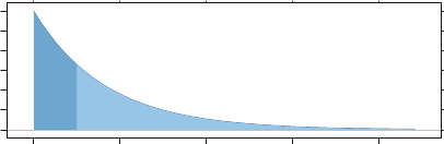
810 J Probability Distributions
The central χ2distribution with kdegrees of freedom is the distribution of the
sum of squares of kindependent standard normal r.v.’s. If k>2, a χ2r.v. has a
unimodal, positively skewed PDF starting at zero and asymptotically tapering to
the horizontal axis for large values. The mean of this distribution is k, and kis also
approximately its median if kis large. The r.v. [(n−1)s2]/σ2, where s2is the variance
of a normal sample, has a χ2distribution with n−1 degrees of freedom.
This distribution is used in inferences about the variance (or s.d.) of a single
population and as the approximate distribution of many nonparametric test statistics,
including goodness-of-it tests and tests for association in contingency tables.
J.1.4 Exponential
dexp(x, rate = 0.6)
x
0.0
0.1
0.2
0.3
0.4
0.5
0.6
02468
> dexp(1, rate=.6)
[1] 0.3293
> pexp(1, rate=.6)
[1] 0.4512
> qexp(0.4511884, rate=.6)
[1] 1
μis both the mean and standard deviation of this distribution. Rparameterizes
the exponential distribution with the rate 1/μ, the reciprocal of the mean μ.Times
between successive Poisson events with mean rate of occurrence μhave the expo-
nential distribution. The exponential distribution is the only distribution with the
“lack of memory” or “lack of deterioration” property, which states that the proba-
bility that an exponential random variable exceeds t1+t2given that it exceeds t1
equals the probability that it exceeds t2.
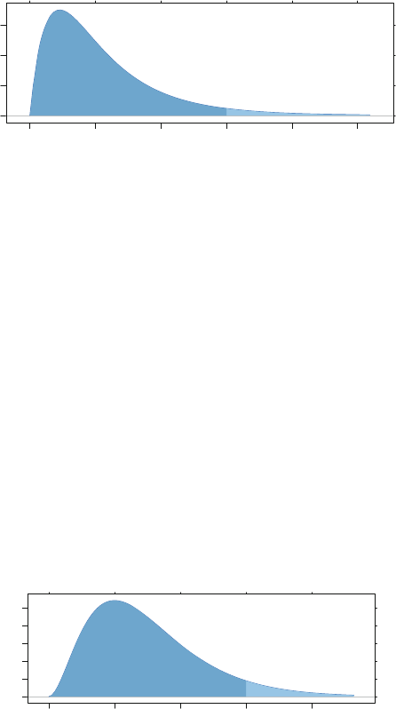
J.1 Continuous Central Distributions 811
J.1.5 F
df(x, df1 = 4, df2 = 20)
x
0.0
0.2
0.4
0.6
012345
> df(3, df1=4, df2=20)
[1] 0.0469
> pf(3, df1=4, df2=20)
[1] 0.9568
> qf(0.956799, df1=4, df2=20)
[1] 3
The Fdistribution is related to the χ2distribution. If Ui,fori={1,2},isaχ2r.v.
with νidegrees of freedom, and if U1and U2are independent, then F=U1/U2has
an Fdistribution with ν1and ν2df. This distribution is extensively used in problems
involving the comparison of variances of two normal populations or comparisons of
means of two or more normal populations.
J.1.6 Gamma
dgamma(x, shape = 3)
x
0.00
0.05
0.10
0.15
0.20
0.25
02468

812 J Probability Distributions
> dgamma(6, shape=3)
[1] 0.04462
> pgamma(6, shape=3)
[1] 0.938
> qgamma(0.9380312, shape=3)
[1] 6
From ?dgamma:
The Gamma distribution with parameters ’shape’ =a and ’scale’ =s has density
f(x)=1/(saΓ(a))x(a−1)e−(x/s)
for x≥0, a>0ands>0. (Here Γ(a) is the function implemented by R’s gamma() and
defined in its help. Note that a=0 corresponds to the trivial distribution with all mass at
point 0.)
The mean and variance are E(X)=a×sand Var(X)=a×s2.
The special case of the gamma distribution with shape=1 is the exponential
distribution.
J.1.7 Log Normal
dlnorm(x)
x
0.0
0.2
0.4
0.6
0510
> dlnorm(5)
[1] 0.02185
> plnorm(5)
[1] 0.9462
> qlnorm(0.9462397)
[1] 5
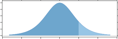
J.1 Continuous Central Distributions 813
Ar.v.Xis said to have a lognormal distribution with parameters μand σif
Y=ln(X)isN(μ, σ2); i.e., if Yis normal, then eYis lognormal. This is a positively
skewed unimodal distribution defined for x>0. It is commonly used as a good
approximation for positively skewed data, such as a distribution of income.
J.1.8 Logistic
dlogis(x)
x
0.00
0.05
0.10
0.15
0.20
0.25
−4 −2 0 2 4
> dlogis(2)
[1] 0.105
> plogis(2)
[1] 0.8808
> qlogis(0.8807971)
[1] 2
From ?dlogis:
The Logistic distribution with location=m and scale=s has distribution function
F(x)=1/1+exp (−(x−m)/s)
and density
f(x)=(1/s)exp
((x−m)/s)1+exp ((x−m)/s)−2.
It is a long-tailed distribution with mean mand variance (π2/3)s2.
qlogis(p) is the same as the well known logit function, logit(p)=log(p/(1 −p)), the
log odds function, and plogis(x) has consequently been called the inverse logit.
The distribution function is a rescaled hyperbolic tangent, plogis(x)=(1+tanh(x/2))/2,
and it is called a sigmoid function in contexts such as neural networks.

814 J Probability Distributions
J.1.9 Normal
dnorm(x, m = 0, s = 1)
x
0.0
0.1
0.2
0.3
0.4
−2 −1 0 1 2
> dnorm(1.645, m=0, s=1)
[1] 0.1031
> pnorm(1.645, m=0, s=1)
[1] 0.95
> qnorm(0.95, m=0, s=1)
[1] 1.645
This distribution was introduced in Section 3.4.2. If Zis standard normal N(0,1),
the standard normal density φand cumulative distribution Φfunctions are
φ(z)=1
√2πexp z2
2
Φ(Z)=Z
−∞
φ(z)dz
The general density, for random variable xwith mean μand variance σ2,is
f(x|μ, σ2)=1
σφx−μ
σ=1
√2πσ2exp (x−μ)2
2σ2
The term probit is an alternate notation for the inverse function Φ−1.
q=Φ−1(p)=probit(P)
is the inverse function such that p=Φ(q).
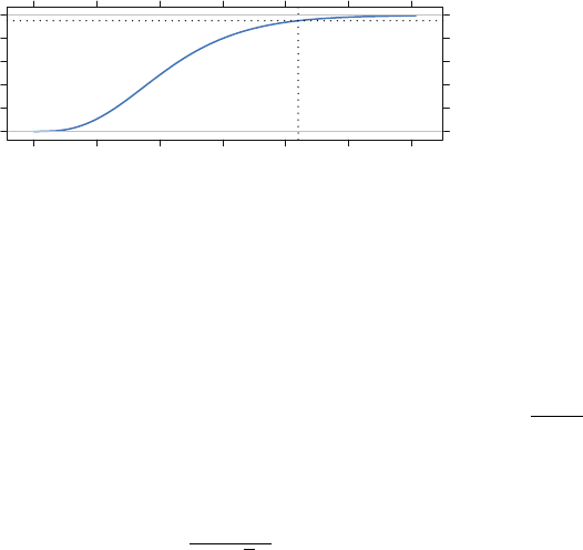
J.1 Continuous Central Distributions 815
J.1.10 Studentized Range Distribution
ptukey(x, nmeans=4, df=12)
x
0.0
0.2
0.4
0.6
0.8
1.0
0123456
> ptukey(4.199, nmeans=4, df=12)
[1] 0.95
> qtukey(0.95, nmeans=4, df=12)
[1] 4.199
This distribution is used in the Tukey multiple comparisons procedure discussed
in Section 6.3. Let ¯y(1) and ¯y(a)denote the smallest and largest means of samples of
size ndrawn from apopulations having a common variance σ2, and let s=√MSRes
be the estimate of σcalculated from the ANOVA table, for example, Table 6.2. Then
the random variable
Q=¯y(a)−¯y(1)
s/√n
has a Studentized range distribution with parameters aand dfRes =a(n−1). The
Studentized range distribution is defined on the domain 0 ≤q<∞.Rprovides the
ptukey and qtukey functions, but not the density function dtukey. We therefore
show the cumulative probability function instead of the density for the Studentized
range distribution.
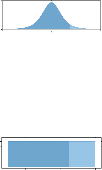
816 J Probability Distributions
J.1.11 (Student’s) T
dt(x, df = 4)
x
0.0
0.1
0.2
0.3
−4 −2 0 2 4
> dt(2, df=4)
[1] 0.06629
> pt(2, df=4)
[1] 0.9419
> qt(0.9419417, df=4)
[1] 2
This distribution was introduced in Section 3.4.3.
J.1.12 Uniform
dunif(x)
x
0.0
0.2
0.4
0.6
0.8
1.0
0.0 0.2 0.4 0.6 0.8 1.0
> dunif(.7)
[1] 1
> punif(.7)
[1] 0.7
> qunif(.7)
[1] 0.7
All real numbers between aand bare equally likely. The standard case has a=0
and b=1. Hypothesis tests work by mapping an appropriate null distribution to the
uniform (with the appropriate p* function in R).

J.2 Noncentral Continuous Probability Distributions 817
J.1.13 Weibull
dweibull(x, shape = 4)
x
0.0
0.5
1.0
1.5
0.0 0.5 1.0 1.5
> dweibull(1.3, shape=4)
[1] 0.5052
> pweibull(1.3, shape=4)
[1] 0.9425
> qweibull(0.9425075, shape=4)
[1] 1.3
From dweibull:
The Weibull distribution with ’shape’ parameter aand ’scale’ parameter bhas density given
by
f(x)=(a/b)(x/b)(a−1) exp(−(x/b)a)
for x>0. The cumulative distribution function is F(x)=1−exp(−(x/b)a)onx>0, the
mean is E(X)=bΓ(1 +1/a), and the Var(X)=b2Γ(1 +2/a)−(Γ(1 +1/a))2.
J.2 Noncentral Continuous Probability Distributions
In hypothesis testing, except in special cases such as testing with the normal distri-
bution, one deals with a central distribution when the null hypothesis is true and an
analogous noncentral distribution when the null hypothesis is false. Thus calcula-
tions of probabilities under the alternative hypothesis, as are required when doing
Type II error analysis and when constructing O.C. (beta curves) and power curves,
necessitate the use of noncentral distributions.
The forms of the t, chi-square, and Fdistributions we’ve considered thus far
have all been central distributions. For example, if ¯
Xis the mean and sthe standard
deviation of a random sample of size nfrom a normal population with mean μ, then
t=(¯x−μ)/(s/√n) has a central tdistribution with n−1 df. Suppose, however, that
the population mean is instead μ1,different from μ. Then tabove is said to have a
noncentral tdistribution with n−1 df and a noncentrality parameter proportional to
818 J Probability Distributions
((μ−μ1)/σ)2.(Ifμ=μ1, so that the noncentrality parameter is zero, the noncentral
tdistribution reduces to the central tdistribution.)
A noncentral chi-square (χ2) r.v. is a sum of squares of independent normal r.v.’s
each with s.d. 1 but at least some of which have a nonzero mean. A noncentral F
r.v. is the ratio of a noncentral chi-square r.v. to a central chi-square r.v., where the
two chi-squares are independent.
For tests using the t, chi-square, or Fdistribution, the power of the test (protection
against Type II errors) is an increasing function of the noncentrality parameter.
Noncentral distributions are specified with one more parameter than their cor-
responding central distribution. Consequently, tabulations of their cumulative dis-
tribution function appear much less frequently than those for central distributions.
Fewer statistical software packages include them. There is no noncentral normal dis-
tribution. The distribution under the alternative hypothesis is just an ordinary normal
distribution with a shifted mean.
The Rfunctions for noncentral t, chi-square, and FCDFs are the same as those
for the corresponding central distribution with the addition of an argument for the
noncentrality parameter ncp. The noncentrality parameter defaults to zero (hence to
a central distribution) if it is not specified.
The figures in Sections J.2.1,J.2.2, and J.2.3 show the noncentral distribution
along with the corresponding central distribution. This way it is possible to see that
a positive noncentrality parameter shifts the mode to the right.
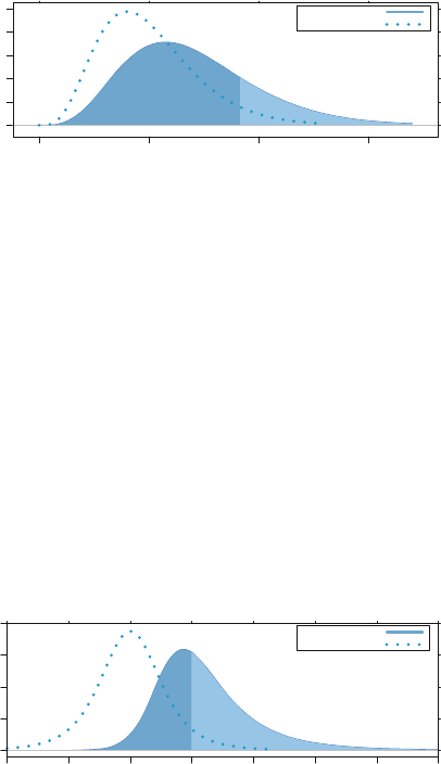
J.2 Noncentral Continuous Probability Distributions 819
J.2.1 Chi-Square: Noncentral
dchisq(x, df = 10, ncp = 4)
x
0.00
0.02
0.04
0.06
0.08
0.10
0102030
non−central
central
> dchisq(18.31, df=10, ncp=4)
[1] 0.0408
> pchisq(18.31, df=10, ncp=4)
[1] 0.7852
> qchisq(0.7852264, df=10, ncp=4)
[1] 18.31
See discussion in Section 14.8.2 and example in Figure D.1.
J.2.2 T: Noncentral
dt(x, df = 4, ncp = 2)
x
0.0
0.1
0.2
0.3
−202468
non−central
central
> dt(2, df=4, ncp=2)
[1] 0.3082
> pt(2, df=4, ncp=2)
[1] 0.4557
> qt(0.455672, df=4, ncp=2)
[1] 2
See examples in Figures 3.24, 5.2, and 5.10.
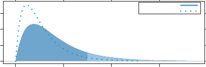
820 J Probability Distributions
J.2.3 F: Noncentral
df(x, df1 = 4, df2 = 20, ncp = 2)
x
0.0
0.2
0.4
0.6
0246
non−central
central
> df(3, df1=4, df2=20, ncp=2)
[1] 0.1062
> pf(3, df1=4, df2=20, ncp=2)
[1] 0.871
> qf(0.8710256, df1=4, df2=20, ncp=2)
[1] 3
See example in Section 6.5 and discussion in Section 14.8.2.
J.3 Discrete Distributions
Discrete distributions are defined to have nonzero values on a set of integers.
F(x)=P(X≤x)=
x
i=−∞
f(i)
The inverse functions (the q* functions in R) are sensitive to the precision of the
numerical representation.
Computers use finite precision floating point arithmetic, precise to 53 signifi-
cant binary digits (bits)—approximately 17 decimal digits. They do not use the real
number system that we are familiar with. Simple decimal repeating fractions such
as these are not stored precisely with finite precision machine arithmetic. All of the
individual values in this example are automatically rounded to 53 bits when they
are entered into the computer. None of them are exactly represented inside the com-
puter. See Appendix Gfor more on the floating point arithmetic used in computers.
In several of the discrete distribution examples here, it has been necessary to dis-
play the pvalues to 17 decimal digits in order to get the desired answer from the q*
functions.

J.3 Discrete Distributions 821
Here is a simple example, the 6-level discrete uniform (one fair die), to illustrate
the problem. In this example, rounding produces several results from the qdiscunif
function that are one unit off(either too large or too small).
F(i)
machine precision,
rounded to rounded to 53 bits,
if(i) fraction 4 decimal digits ≈17 decimal digits
11/61/60.1667 0.16666666666666666
21/62/60.3333 0.33333333333333331
31/63/60.5000 0.50000000000000000
41/64/60.6667 0.66666666666666663
51/65/60.8333 0.83333333333333337
61/66/61.0000 1.00000000000000000
> ## this is printing precision, not internal representation
> old.digits <- options(digits=7)
> ddiscunif(1:6, 6)
[1] 0.1666667 0.1666667 0.1666667 0.1666667 0.1666667 0.1666667
> pdiscunif(1:6, 6)
[1] 0.1666667 0.3333333 0.5000000 0.6666667 0.8333333 1.0000000
> qdiscunif(pdiscunif(1:6, 6), 6)
[1]123456
> round(pdiscunif(1:6, 6), 4) ## rounded to four decimal digits
[1] 0.1667 0.3333 0.5000 0.6667 0.8333 1.0000
> ## inverse after rounding to four decimal digits
> qdiscunif(round(pdiscunif(1:6, 6), 4), 6)
[1]113446
> options(old.digits)
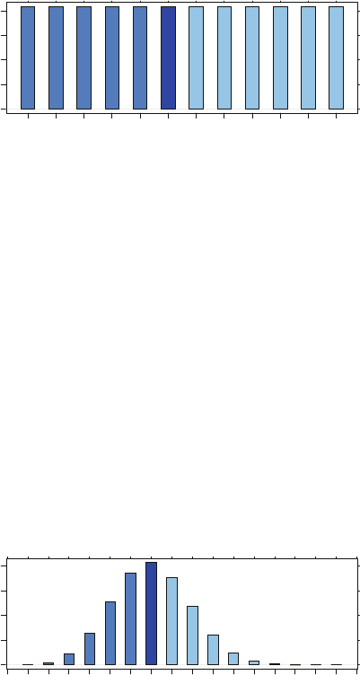
822 J Probability Distributions
J.3.1 Discrete Uniform
ddiscunif(x, size = 12)
x
0.00
0.02
0.04
0.06
0.08
123456789101112
> ddiscunif(6, size=12)
[1] 0.08333
> pdiscunif(6, size=12)
[1] 0.5
> qdiscunif(.5, size=12)
[1] 6
In the discrete uniform distribution, the integers from 1 to nare equally likely.
The population mean is (n+1)/2. The population variance is (n2−1)/12. The
distribution function is
J.3.2 Binomial
dbinom(x, size = 15, prob = 0.4)
x
0.00
0.05
0.10
0.15
0.20
0123456789101112131415

J.3 Discrete Distributions 823
> ## probability of exactly 6 Heads
> dbinom(6, size=15, prob=.4)
[1] 0.2066
> ## probability of 6 or fewer Heads
> ## extra precision is needed
> print(pbinom(6, size=15, prob=.4), digits=17)
[1] 0.60981315570892769
> ## q, the number for which the probability of seeing
> ## q or fewer Heads is 0.60981315570892769
> qbinom(0.60981315570892769, size=15, prob=.4)
[1] 6
The binomial distribution was introduced in Section 3.4.1. If Xhas a binomial
distribution with parameters n(n=size, number of coins tossed simultaneously)
and p(p=prob, probability of one coin landing Heads on one toss), then the bino-
mial distribution gives the probability of observing exactly Xheads.
J.3.3 Geometric
dgeom(x, prob = 0.5)
x
0.0
0.1
0.2
0.3
0.4
0.5
0123456789
> dgeom(3, prob=.5)
[1] 0.0625
> pgeom(3, prob=.5)
[1] 0.9375
> qgeom(0.9375, prob=.5)
[1] 3
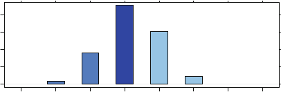
824 J Probability Distributions
From ?dgeom:
The geometric distribution with ’prob’ =p has density
p(x)=p(1 −p)x
for x=0,1,2, ..., 0<p≤1.
The quantile is defined as the smallest value xsuch that F(x)≥p,whereFis the
distribution function.
J.3.4 Hypergeometric
dhyper(x, m = 5, n = 6, k = 7)
x
0.0
0.1
0.2
0.3
0.4
01234567
> dhyper(3, m=5, n=6, k=7)
[1] 0.4545
> print(phyper(3, m=5, n=6, k=7), digits=17)
[1] 0.65151515151515149
> qhyper(0.65151515151515149, m=5, n=6, k=7)
[1] 3
The hypergeometric distribution is used in Chapter 15. We sample nitems with-
out replacement from a population of Nitems comprised of Msuccesses and N−M
failures. Then the number of successes Xobserved in the population is said to have
a hypergeometric distribution with parameters N,M,and n.
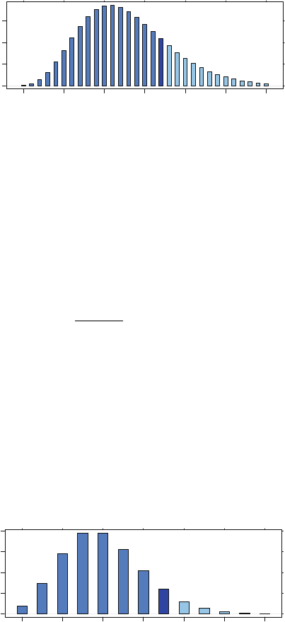
J.3 Discrete Distributions 825
J.3.5 Negative Binomial
dnbinom(x, size = 8.5, prob = 0.4)
x
0.00
0.02
0.04
0.06
0 5 10 15 20 25 30
> dnbinom(17, size=8.5, prob=.4)
[1] 0.04338
> print(pnbinom(17, size=8.5, prob=.4), digits=17)
[1] 0.81209497223034977
> qnbinom(0.81209497223034977, size=8.5, prob=.4)
[1] 17
The negative binomial distribution with size =nand prob =phas density
Γ(x+n)
Γ(n)x!pn(1 −p)x
for x=0,1,2,...,n>0, and 0 <p≤1.
This represents the number of failures which occur in a sequence of Bernoulli
trials before a target number of successes is reached. The mean is μ=n(1 −p)/p
and variance is n(1 −p)/p2.
J.3.6 Poisson
dpois(x, lambda = 4)
x
0.00
0.05
0.10
0.15
024681012
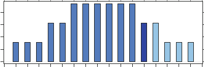
826 J Probability Distributions
> dpois(7, lambda=4)
[1] 0.05954
> print(ppois(7, lambda=4), digits=17)
[1] 0.94886638420715264
> qpois(0.94886638420715264, lambda=4)
[1] 7
Let the random variable Xbe the number of occurrences of some event that are
observed in a unit of time, volume, area, etc., and let λbe the mean number of
occurrences of the event per unit, assumed to be constant throughout the process that
generates the occurrences. Suppose that the occurrence(s) of the event in any one
unit are independent of the occurrence(s) of the event in any other nonoverlapping
unit. Then Xhas a Poisson distribution with parameter λ.
J.3.7 Signed Rank
dsignrank(x, n = 5)
x
0.00
0.02
0.04
0.06
0.08
0123456789101112131415
> dsignrank(11, n=5)
[1] 0.0625
> psignrank(11, n=5)
[1] 0.8438
> qsignrank(0.84375, n=5)
[1] 11
See the discussion in Section 16.3.2.
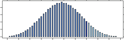
J.4 Multivariate Distributions 827
J.3.8 Wilcoxon
dwilcox(x, m = 4, n = 12)
x
0.00
0.01
0.02
0.03
0.04
0 5 10 15 20 25 30 35 40 45 50
> dwilcox(35, m=4, n=12)
[1] 0.02088
> print(pwilcox(35, m=4, n=12), digits=17)
[1] 0.9148351648351648
> qwilcox(0.9148351648351648, m=4, n=12)
[1] 35
See Table 16.7 for an example of a rank sum test.
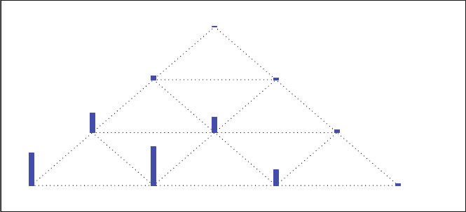
828 J Probability Distributions
J.4 Multivariate Distributions
J.4.1 Multinomial
dmultinom(x, prob = c(1,2,5))
0.244
0.146
0.029
0.002
0.293
0.117
0.012
0.117
0.023
0.016
003
102
201
300
012
111
210
021
120
030
> ## This example is based on ?dmultinom in R
> ## all possible outcomes of Multinom(N = 3, K = 3)
> X <- t(as.matrix(expand.grid(0:3, 0:3)))
> X <- X[, colSums(X) <= 3]
> X <- rbind(X, 3:3 - colSums(X))
> dimnames(X) <- list(letters[1:3], apply(X, 2, paste, collapse=""))
> Y <- round(apply(X, 2, function(x) dmultinom(x, prob = c(1,2,5))), 3)
> rbind(X, Y)
003 102 201 300 012 111 210 021 120 030
a 0.000 1.000 2.000 3.000 0.000 1.000 2.000 0.000 1.000 0.000
b 0.000 0.000 0.000 0.000 1.000 1.000 1.000 2.000 2.000 3.000
c 3.000 2.000 1.000 0.000 2.000 1.000 0.000 1.000 0.000 0.000
Y 0.244 0.146 0.029 0.002 0.293 0.117 0.012 0.117 0.023 0.016
The (discrete) multinomial distribution is a generalization of the binomial distri-
bution to the case of k>2 categories. Suppose there are nindependent trials, each
of which can result in just one of kpossible categories such that pjis the probability
of resulting in the jth of these kcategories. (Hence p1+p2+...+pk=1.) Let Xj
be the number of occurrences in category j. Then the vector (X1,X2, ..., Xk)issaid
to have a multinomial distribution with parameters n,p1,p2,...,pk.ItsPMFis
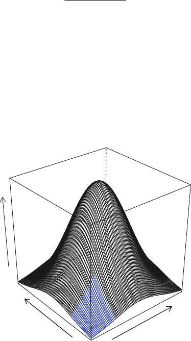
J.4 Multivariate Distributions 829
P(Xj=xj|j=1,...,k)=n!px1
1px2
2...pxk
k
x1!x2!...xk!,x1+x2+...xk=n
If a proportion pjof a population of customers prefers product number j,j=
1,...,k, among kproducts, then the multinomial distribution provides the probabil-
ity of observing any particular configuration of preferences among a random sample
of ncustomers.
J.4.2 Multivariate Normal
row
column
z
Bivariate Normal: dmvnorm(c(−1, −1))
> dmvnorm(c(-1, -1))
[1] 0.05855
> pmvnorm(upper=c(-1, -1))[1]
[1] 0.02517
> qmvnorm(0.02517, mean=c(0,0))$quantile
[1] -1
See Sections 3.3.5 and I.4 for examples.
Appendix K
Working Style
Working style in a computer environment depends on two interrelated concepts:
which programs you use and how you use them.
For statistical analysis we are recommending Ras the primary computational
tool. There are other very good programs, and it is imperative that you develop a
working understanding of several of them. See Appendix Hfor information on how
to use the datasets discussed in this book with other software.
An excellent text editor is an indispensable tool for the statistical analyst. The
editor is the single program in which we spend most of our time. We use it for
looking at raw data, for writing commands in the statistical languages we use, for
reading the output tables produced by our statistical programs, for writing reports,
and for reading and writing correspondence about our studies to our clients, consul-
tants, supervisors, and subordinates. We discuss our requirements for a text editor
in Section K.1. Our personal choice of editor is Emacs (Free Software Foundation,
2015), which we discuss in Appendix M. There are other excellent editors which
satisfy our requirements.
We discuss in Section K.2 the types of interaction that are possible with R.
We recommend in Section K.3 working with files of Rcommands. We discuss in
Section K.4 our recommendations for organization of the files within the operating
system’s directory structure.
K.1 Text Editor
As we indicated in the Preface on page ix, our goal in teaching statistical languages
is to make the student aware of the capabilities of the language for describing data
and their analyses. The language is approached through the text editor.
©Springer Science+Business Media New York 2015
R.M. Heiberger, B. Holland, Statistical Analysis and Data Display,
Springer Texts in Statistics, DOI 10.1007/978-1-4939-2122-5
831

832 K Working Style
We distinguish between the concepts of text editing (discussed in this Appendix)
and word processing (discussed in Appendix O). Text editing is moving characters
around on the screen with the expectation that they will stay where you put them.
This is critical when writing computer programs where the physical placement of
lines and characters on the page is part of what the computer program interprets. In
the Rlanguage the two layouts of the same characters in Table K.1 have completely
different interpretations.
Word processing is moving sentences, paragraphs, sections, figures, and cross-
references around. A word processor can be used as a text editor by manually turning
offmany of the word processing features.
Table K.1 Two different interpretations of the same characters {“3”, “+”, “4”}that depend on their
placement on separate lines. If the first set of input lines were reformatted according to English
language paragraph formatting rules it would be interpreted as if it were the second set, which has
a completely different meaning. This is the simplest possible example of why we make a distinction
between text editing and word processing.
RInput
Two lines One line
3 3+4
+4
ROutput
>3 >3+4
[1] 3 [1] 7
>+4
[1] 4
K.1.1 Requirements for an Editor
These are the requirements we place on any text editor that is to be used for inter-
acting with a computing language:
1. Permit easy modification of computing instructions and facilitate their resub-
mission for processing
2. Be able to operate on output as well as input
3. Be able to cut, paste, and rearrange text; to search documents for strings of text;
to work with rectangular regions of text
4. Be aware of the language, for example, to illustrate the syntax with appropriate
indentation and with color and font highlighting, to detect syntactic errors in
input code, and to check the spelling of statistical keywords
K.2 Types of interaction with R833
5. Handle multiple files simultaneously
6. Interact cleanly with the presentation documents (reports and correspondence)
based on the statistical results
7. Check spelling of words in natural languages
8. Permit placement of graphics within text.
9. Permit placement of mathematical expressions in the text.
10. Work with Unicode to give access to all character sets in all human languages.
K.1.2 Choice of Editor
Our preference for an editor is Emacs with ESS, which we discuss in Appendix M.
In Section M.5 we show how Emacs satisfies the requirements in Section K.1.1.
There are many other options for an editor, usually within the context of an Inte-
grated Development Environment (IDE), a software application that provides com-
prehensive facilities to computer programmers for software development. An IDE
normally consists of a source code editor, build-automation tools, and a debugger.
For more information on IDEs see Wikipedia (2015).
For an annotated list, with links to their webpages, of other editors and IDEs that
work with R, see Grosjean (2012).
We discuss word processors such as MS Word (Microsoft, 2015) in Section O.1.
In Section O.1.1 we show how MS Word satisfies some of the requirements in
Section K.1.
K.2 Types of interaction with R
1. CLI Command Line Interface: The user types Rstatements and the system re-
sponds with requested output. Examples: Rinashell/terminal/CMD window, R
in the *R* buffer in Emacs,Rin the Console window in the Rgui.exe for Win-
dows,theR.app for Macintosh, and the JGR package on all operating systems.
2. Menu or Dialog Box: Dropdown lists of command names, often with default
settings for arguments. This allows point and click access to many Rfunctions
with standard settings of options. The Rcmdr (R Commander) package described
in Appendix Cis such a system.
834 K Working Style
3. Spreadsheet. The RExcel system described in Appendix Dallows access to all R
functions from within the automatic recalculation mode of Excel for Windows.
The Rcmdr interface is incorporated into the Excel menu ribbon.
4. Web-based interface. Technology for embedding Rapplications within an html
page to provide interactive access to Rfunctions for non-programmers. See Ap-
pendix Efor a discussion of the shiny system.
5. Document based interface. The end user writes a document (book, paper, report)
in a standard document writing system (L
A
T
E
XorWord, for example) with em-
bedded Rcode. Three examples are Sweave (Leisch and R-core, 2014), knitr
(Xie, 2015), and SWord (Baier, 2014). The second edition of HH is written using
Sweave (see help(Sweave, package="utils")). All Rcode, leading to all
graphs and tables in the book, is included in the L
A
T
E
X source files for the chap-
ters. The code files for the HH package, located with the HHscriptnames()
function, were pulled from the L
A
T
E
XfilesbytheStangle function which is part
of the Sweave framework.
6. GUI Graphical User Interface: anything other than the command line interface.
K.3 Script File
Our personal working style (and the one we recommend to our readers) is to write a
file of commands (a script file with extension .R or .r) that specify the analysis, run
the commands and review the graphs and tables so produced, and then correct and
augment the analysis specifications. We construct the command file interactively.
Initially we write the code to read the data into the program and to prepare several
graphs and the initial tables. If there are errors (in typing or in programming logic),
we correct them in the file and rerun the commands. As we progress and gain insight
into what the data say, we add to the code to produce additional graphs and tables.
When we have finished, we have a file of commands that could be run as a batch job
to produce the complete output. We also have a collection of graphs and tables that
can be stored in additional files.
K.4 Directory Structure
When we have many files, we need to organize them within the directory structure
of our computer’s operating system.
K.4 Directory Structure 835
K.4.1 Directory Structure of This Book
This book is written in L
A
T
E
X (Lamport, 1994). Our organizational structure uses the
directory structure provided by the computer’s operating systems. For this book we
have a main directory (hh2) and subdirectories for code (containing .R files), tran-
scripts (.Rout) files, and figures (.pdf) files. The main directory contains all the
.tex files (one per chapter plus a master file), our L
A
T
E
X style file (hh2.sty), and
several other support files. We have a work directory parallel to the hh2 directory
for experiments with Rcode, for correspondence with our publisher, and for corre-
spondence with the people who were kind enough to read and comment on drafts of
this book.
The Rfunctions that we developed for the book, and all datasets used in the book,
are collected into the HH package (Heiberger, 2015) distributed through CRAN.
The master copy of the Rscripts for all figures and tables in the second edition
is included in the *.tex source files for the individual chapters. We use the Sweave
functions included in Rto execute the code directly from the *.tex files. When
we are ready to distribute the code, we pull the Rcode from the *.tex files with
the Stangle function (part of R’s Sweave system) and place them into the HH
package. The script files in the HH package for the book can be located by the
package user with the HHscriptnames() function.
We hope that readers of our book, and more generally users of R, design and
collect their own functions into a personal package (it doesn’t have to be distributed
through CRAN). Once you have more than a few functions that are part of your
working pattern, maintaining them in a package is much simpler than inventing
your own idiosyncratic way of keeping track of what you have. We say a few words
about building a package in Appendix F and refer you to the Rdocument
system.file("../../doc/manual/R-exts.pdf")
for complete information.
K.4.2 Directory Structure for Users of This Book
It is critical to realize that your work is yours. Your work is not part of the computer’s
operating system, nor of the installed software. The operating system, the editor, R,
and other software are kept in system directories. In order to protect the integrity of
the system you will usually not have write access to those locations.
You need a home directory, the one where you keep all your personal subdirecto-
ries and files. Your operating system automatically creates a HOME directory for you.
Rcan find its name with the command Sys.getenv("HOME"). Everything you do
should be in a subdirectory of your home directory.
836 K Working Style
For example, each time we teach a course, we create a directory for that course.
For last year’s course based on this book, we used the directory 8003.f14 directly
under the HOME directory. We have a subdirectory of the course directory for
the syllabus, for each class session, and for student records. We keep handouts,
Rscripts, and transcripts of the class Rsession as files within each class session’s
directory.
K.4.3 Other User Directories
We recommend a separate directory for each project. It will make your life much
easier a year from now when you try to find something.
Appendix L
Writing Style
Reports, including homework exercises, based on computer printout must be typed
correctly. We recommend L
A
T
E
X (the standard required by many statistics and math-
ematics journals, and the typesetting package with which we wrote this book). We
do accept other word processing software. Whichever software you use, you must
use it correctly. We discuss in this appendix some of the fundamentals about good
technical writing.
L.1 Typographic Style
Specific style issues that you must be aware of are
1. Fonts: Computer listings in R(and S-Plus and SAS and many other statistical
software systems) are designed for monowidth fonts (such as Courier) where all
characters (including spaces) are equally wide. These listings are unreadable in
Times Roman or any other proportional font. English text looks best in a propor-
tional font (where, for example, the letter “M” is wider than the letter “i”) such
as Times Roman. Table L.1 shows the difference with simple alphabetic text.
Table L.2 shows an example of the issue for computer listings. The Courier ren-
dition is consistent with the design of the output by the program designer. The
Times Roman is exactly the same text dropped into an environment that is in-
correctly attempting to space it in accordance with English language typesetting
rules. In our classes, we return UNREAD any papers that use a proportional
font for computer listings.
2. Alignment: Numbers in a column are to be aligned on decimal points. Alignment
makes it possible to visually compare printed numbers in columns. There are two
©Springer Science+Business Media New York 2015
R.M. Heiberger, B. Holland, Statistical Analysis and Data Display,
Springer Texts in Statistics, DOI 10.1007/978-1-4939-2122-5
837

838 L Writing Style
Table L.1 We placed a vertical rule after four characters on each line in both Courier and Times
Roman. The Courier rules are aligned because all characters in Courier are exactly the same width.
The Times Roman rules are not aligned because each character in Times Roman has its own width.
Courier
Wide and narrow.
Letters in each row align
with letters in the previous row.
Times Roman
Wide and narrow.
Letters in each row do not align
with letters in the previous row.
Table L.2 Routput displayed correctly in a monowidth font, and incorrectly in a proportional
font. The same text, the output from an Rsummary.data.frame call, is displayed in both fonts.
The unequal width of the characters in the Times Roman font destroys the vertical alignment that
is necessary for interpretation of this listing.
Courier (correct spacing)
> summary(ex0221)
weight code
Min.:23.20 1:35
1st Qu.:24.75 2:24
Median:25.70
Mean:25.79
3rd Qu.:26.50
Max.:31.10
Times Roman (incorrect spacing)
>summary(ex0221)
weight code
Min.:23.20 1:35
1st Qu.:24.75 2:24
Median:25.70
Mean:25.79
3rd Qu.:26.50
Max.:31.10
Table L.3 Alignment of decimal points in the numbers on the left makes it easy to compare the
magnitudes of the numbers. Centering of the numbers on the right, and therefore non-alignment of
decimal points, makes it difficult to compare the magnitudes of the numbers.
Correct Wrong
123.45 123.45
12.34 12.34
−4.32 −4.32
0.12 0.12
reasons for getting it wrong. One is carelessness. The other is blind copying from
a source that gets it wrong. We show an example of both alignments in Table L.3.
3. Minus signs and dashes: There are four distinct concepts that have four differ-
ent typographical symbols in well-designed fonts. On typewriters all four are

L.1 Typographic Style 839
usually displayed with the symbol “-” that appears on the hyphen key (next to
the number 0). You are expected to know the difference and to use the symbols
correctly.
Table L.4 shows an example of the correct usage of all four symbols and the keys
in L
A
T
E
X and MS Word.
Table L.4 Correct usage of all four dash-like symbols (- – −—) and the keys to generate them in
L
A
T
E
X and MS Word.
Symbol Use Example L
A
T
E
XMSWord
- hyphen compound word t-test --
– en dash range 100–120 -- ctrl-num -
−minus negation −12 $-$ Insert-menu/symbol. . . / −
— em dash apposition punctuation—like this --- alt-ctrl-num -
The misuse of dashes that touches my (rmh) hot button the most is misuse of
hyphen when minus is meant, for example
correct WRONG
+12.2 +12.2
−12.2 -12.2
In this wrong usage, the “+” and “-” are not aligned and consequently the decimal
point is not aligned.
4. Right margins and folding: Table L.5 intentionally misuses formatting to illus-
trate how bad it can look. This usually occurs when the Rwindow width is
wider than your word processor is willing to work with. Verify that you picked
an options()$width consistent with your word processor. You can make the
width narrower in Rby using the Rcommand
options(width=72)
5. Quotation marks: Quotation marks in Times Roman are directional. This is
“Times Roman correct” (with a left-sided symbol on the left and a right-sided
symbol on the right). This is ”Times Roman incorrect” (with the right-sided sym-
bol on both sides). In the typewriter font recognized by R, quotation marks are
vertical, not directional. and are the same on both sides. In typewriter font, this
is "typewriter correct" (same non-directional symbol on both sides).

840 L Writing Style
Table L.5 Intentional misuse of formatting. Never turn in anything that looks like these bad
examples. The top section has lines of text that extend beyond the right margin of the page. The
middle section is an Rtable that has been arbitrarily folded at 49 mono-spaced letter widths. The
bottom section retains the lines, but places them in a proportional font and ignores the alignment
of columns.
Do not allow the right margins of your work to run off
the edge of the page. It is hard to read text that isn’t visible.
Do not allow lines to be arbitrarily folded in a way that destroys the formatting.
This is particularly a problem if you copy output from
the RConsole window to an editor in a word-processing mode. Word proces-
sors (as distinct from text editors) by default enforce
English-language conventions (such as maximum line
length and proportional font) on code and output text that is designed for col-
umn alignment and a fixed-width font. Use an editor,
such as Emacs with ESS, that is aware of the Rformatting conventions. Most
word processors do have an option to set sections in
fixed-width Courier font and to give the write control of margins.
Folding
makes
this table
impossible to
read.
⎧
⎪
⎪
⎪
⎪
⎪
⎪
⎪
⎪
⎪
⎪
⎪
⎪
⎪
⎪
⎪
⎪
⎪
⎨
⎪
⎪
⎪
⎪
⎪
⎪
⎪
⎪
⎪
⎪
⎪
⎪
⎪
⎪
⎪
⎪
⎪
⎩
Sum of
Source DF Squares Mean Squa
re F Value Pr > F
Model 2 2649.816730 1324.9083
65 54.92 <.0001
Error 44 1061.382419 24.1223
28
Corrected Total 46 3711.199149
Column
alignment
ignored.
Table is
unreadable.
⎧
⎪
⎪
⎪
⎪
⎪
⎪
⎪
⎪
⎪
⎨
⎪
⎪
⎪
⎪
⎪
⎪
⎪
⎪
⎪
⎩
Sum of
Source DF Squares Mean Square F Value Pr >F
Model 2 2649.816730 1324.908365 54.92 <.0001
Error 44 1061.382419 24.122328
Corrected Total 46 3711.199149
L.2 Graphical Presentation Style 841
L.2 Graphical Presentation Style
Graphs designed for someone to read must be legible. Legibility includes the items
listed in this section and in Chapter 4 (some of which are repeated here).
L.2.1 Resolution
Figure L.1 shows the same graph drawn on a vector graphics device (pdf() in this
example) and a bitmap device (png() in this example).
Vector graphics devices define objects to be drawn in terms of geometrical prim-
itives such as points, lines, curves, and shapes or polygons. Vector graphics can be
magnified without pixalation. Current vector graphics formats are pdf,ps, and wmf.
By contrast bitmap (or raster) graphics devices define objects in terms of the
set of pixels used in one specific magnification. Further magnification gives larger
discrete dots and not smooth objects. Current bitmap formats are png,bmp,tif,
and gif.
Figure L.1 panels a and c are drawn with a vector graphics device. They are
clear and crisp at any magnification (two magnifications are shown here). Figure
L.1 panels b and d are drawn with a bitmapped graphics device. Panel b is not clear,
and the magified version in panel d is granular and fuzzy.
L.2.2 Aspect Ratio
The graphs are initially drawn for the device size they see at the time they are drawn.
The aspect ratio (the ratio of the width to height in graphic units) is set at that time.
Plotting symbols and text are positioned to look right at that initial magnification
with that size device. The graphs in Figure L.1 honor the aspect ratio. Both the x
and ydimensions are scaled identically in those panels.
Changing the aspect ratio after the graph has been drawn interferes with the mes-
sage of the graph. It is most evident when both axes use the same units, but is visible
even when the units are different.
The graph in Figure L.2 does not honor the aspect ratio, and the graph becomes
very hard to read. The width is stretched to twice its initial size and the height is
left at the original height. As a consequence, the circles used as plotting symbols
are stretched to ellipses. The font used for the labels is stretched to visually change
the shapes of the letters. About half of the zero characters look like circles. The
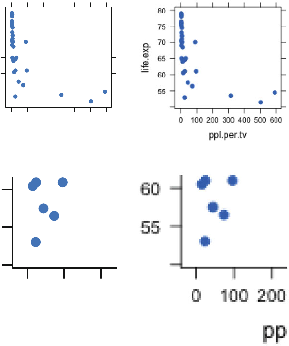
842 L Writing Style
ecived)pamtib(GNP.becived)rotcev(FDP.a
ppl.per.tv
life.exp
55
60
65
70
75
80
0 100 200 300 400 500 600
c. PDF (vector) device magnified d. PNG (bitmap) device magnified
pp
55
60
0 100 200
Fig. L.1 Panels a and b were drawn with the same command addressed to different devices. Panel
ausesthepdf vector device and panel b uses the png bitmap device. Even at low magnification
the difference between the two images is clear. The circle glyphs, the text, and the lines are crisp
on the vector device. The circle glyphs, the text, and the lines are granular on the bitmap device.
Panels c and d are the lower left corners of panels a and b magnified by a scale of 2. The vector
display is just as crisp at this magnification. The bitmap display is more granular and fuzzy. Not
even the straight lines are clear in panel d.
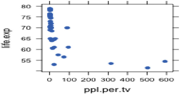
L.2 Graphical Presentation Style 843
PNG (bitmap) device stretched
Fig. L.2 The figure here is the same plot shown in Figure L.1 panel b, this time with its x-
dimension stretched. The circular glyphs are now ellipses. The thin numeral “0” are now circles.
The vertical straight lines are even fuzzier than before.
other half look different because the pixel break points are placed differently on the
underlying letter shapes.
It is possible to damage the aspect ratio even with a good typographic system
(I intentionally did so in Figure L.2 using L
A
T
E
X). Under normal circumstances in
L
A
T
E
X the aspect ratio is retained.
It is too easy to damage the aspect ratio with a drag-and-drop editing system
by stretching an image at the top, bottom, or sides of an image. It is also easy to
maintain the aspect ratio when controlling the size of an image, by stretching only
at the corners, and never stretching the top, bottom, or sides of an image.
L.2.3 Other Features
Other features to be aware of were discussed and illustrated in Chapter 4 and are
summarized here.
1. In scatterplot matrices, a NW–SE main diagonal has a consequence of multiple
axes of symmetry that interfere with easy reading. The (SW–NE) main diagonal
(the defaul in splom has a single axis of symmetry both within and between
panels. See the examples and discussion in Section 4.7 for more detail.
2. The panels in a scatterplot matrix should be square to emphasize the equivalence
of rows and columns. The intention of the scatterplot matrix is the comparison of
844 L Writing Style
y~xwith x~y, and maintaining the same scale in both orientations facilitates
the comparison of reflected panels. Compare Figures 4.10 and 4.11.
3. Choice of plotting symbols, open circles, closed circles, other symbols (triangles,
squares, etc), letters. See the itemized discussion in Section 4.1.
4. Choice of colors. See Section 4.10 for discussion of color vision.
5. Location of ticks and labels inside or outside the panels. In scatterplot matrices,
placing ticks and labels inside the main diagonal makes the frees more surface
area for the panels themselves. Compare Figures 4.10 and 4.11.
6. Space between panels. Compare Figures 4.10 and 4.11.
L.3 English Writing Style
1. Check spelling
•Select the right homophone (words that sound alike): brake vs break. Both
spellings will be accepted by a spell-checking program.
•Learn to spell technical words correctly. The following words seem to be par-
ticularly liable to misspelling:
– separate: The fourth letter is “a”.
– correlation: The letter “r” is doubled.
– collinear: The letter “l” is doubled.
– stationary: not moving
– stationery: writing paper and envelopes
– symmetric: The letter “m” is doubled.
– asymmetric: The letter “s” is single.
– Tukey: John W. Tukey
– turkey: a bird
•“p-value” is preferred (with pin math italic). “P-value” is not OK (with “P”
in uppercase roman).
•Spell people’s names correctly and with proper capitalization (John W. Tukey,
Dennis Cook).
2. Punctuation.
“.” “:” “,” “;” always touch the preceding character. They always have a space
after them.
L.4 Programming Style and Common Errors 845
L.4 Programming Style and Common Errors
1. Data entry: Use real variable names. The default variable names “X1” and “X2”
carry no information. Variable names like “height” and “weight” carry infor-
mation.
2. Data entry: probably you don’t need to do that step. Don’t reenter by hand the
numbers that you already have in machine-readable form.
3. Use dump("varname","") to get ASCII versions of Rvariables that can be
read back into Rwith no loss (of digits, labeling, attributes). The output from
the dump can be copied into email and copied back from email. The output from
the simpler print commands will frequently get garbled in email. See Table L.6
for an illustration where the original class of two of the columns is lost when
we neglected to use the dump function.
4. The Rfunction splom() for scatterplot matrices by default gives easy-to-read
plots with a single axis of symmetry over the entire set of square panels. The R
pairs() function (for all pairwise two-variable graphs) by default gives many
conflicting axes of symmetry and rectangular panels. See Figure 4.12 and the
accompanying discussion.
5. Analyze the experiment given you. Don’t ignore the block factor. Usually the
block sum of squares is removed first, before looking at the treatment effects.
In R, this is done by placing the block factor first in the model formula, for exa-
mple, in Section 12.9 we use aov(plasma ~ id + time) so the sequential
analysis of variance table will read
id
time
Residuals
This way, in non-balanced designs, the sequential sum of squares for the treat-
ment factor (time in this example) is properly adjusted for the blocking fac-
tor id.
6. We normally recommend the use of the Rcommand language, not a menu sys-
tem, when you are learning the techniques. You will get
•much better-looking output
•more control
•the ability to reproduce what you did
7. When GUI point-and-click operations have been used to construct preliminary
graphical (or tabular) views of the data, the commands corresponding to these
operations are frequently displayed. Rcmdr for example displays the generated
commands in its R Script window (see Figure C.14 for an example). These
commands can then be used as components in the construction of more complex
commands needed to produce highly customized graphs.

846 L Writing Style
Table L.6 We construct a data.frame and then display it twice, once by typing the variable name,
the second time by using the dump function. When we re-enter the typed text back to R,welosethe
structure of the data.frame. When we re-enter the dumped structure, we retain the original structure.
> tmp <- data.frame(aa=1:3, bb=factor(4:6), cc=letters[7:9],
+ dd=factor(LETTERS[10:12]), stringsAsFactors=FALSE)
> str(tmp)
’data.frame’: 3 obs. of 4 variables:
$ aa: int 1 2 3
$ bb: Factor w/ 3 levels "4","5","6": 1 2 3
$ cc: chr "g" "h" "i"
$ dd: Factor w/ 3 levels "J","K","L": 1 2 3
> tmp
aa bb cc dd
114gJ
225hK
336iL
> dump("tmp", "")
tmp <-
structure(list(aa = 1:3, bb = structure(1:3, .Label = c("4",
"5", "6"), class = "factor"), cc = c("g", "h", "i"),
dd = structure(1:3, .Label = c("J",
"K", "L"), class = "factor")), .Names = c("aa", "bb", "cc", "dd"
), row.names = c(NA, -3L), class = "data.frame")
> tmp <- read.table(text="
+ aabbccdd
+114gJ
+225hK
+336iL
+ ", header=TRUE)
> sapply(tmp, class)
aa bb cc dd
"integer" "integer" "factor" "factor"
> tmp <-
+ structure(list(aa = 1:3, bb = structure(1:3, .Label = c("4",
+ "5", "6"), class = "factor"), cc = c("g", "h", "i"),
+ dd = structure(1:3, .Label = c("J",
+ "K", "L"), class = "factor")), .Names = c("aa", "bb", "cc", "dd"
+ ), row.names = c(NA, -3L), class = "data.frame")
> sapply(tmp, class)
aa bb cc dd
"integer" "factor" "character" "factor"

L.5 Presentation of Results 847
8. Store results of an Rfunction call in a variable to permit easy extraction of var-
ious displays from the results. For example,
mydata <- data.frame(x=1:6, y=c(1,4,2,3,6,2))
my.lm <- lm( y~x,data=mydata)
summary(my.lm) ## summary() method on lm argument
old.mfrow <- par(mfrow=c(2,2)) ## four panels on the graphics device
plot(my.lm) ## plot() method on lm argument
par(old.mfrow) ## restore previous arrangement
coef(my.lm) ## coef() method on lm argument
anova(my.lm) ## anova() method on lm argument
resid(my.lm) ## resid() method on lm argument
predict(my.lm) ## predict() method on lm argument
9. Analysis of Variance requires that the classification factor be declared as a
factor. Otherwise you will get a nonsense analysis. The wrong degrees of
freedom for a treatment effect is usually the indicator that you forgot the
factor(treatment) command in R.
10. The degrees of freedom for a problem always comes from the Residual or
ERROR line of the ANOVA table. In multiple-stratum models, the Residual
line in each stratum provides the comparison value (denominator Mean Square
and degrees of freedom) for effects in that stratum.
11. Please use par(mfrow=c(2,2)) (as illustrated above in item 8) for plotting the
results of an lm() or aov(). That way the plot uses only one piece of paper,
not four.
12. All comparable graphs must be on the same scale—on the same axes is often
better. See Section 17.6.2, especially Figure 17.19, for an example of compara-
ble scaling in the top panels and noncomparable scaling in the bottom panels.
See Figure 4.9 for comparable scaling in Panels a and b and noncomparable
scaling in Panels c, d, and e.
L.5 Presentation of Results
This list is designed for our classroom setting. It is more generally applicable.
1. Use the minus sign “−4” in numbers. We do not accept hyphens “-4”. See
Table L.4.
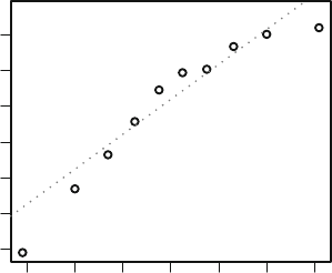
848 L Writing Style
−1.5 −1.0 −0.5 0.0 0.5 1.0 1.5
−2.0 −1.0 0.0 1.0
Theoretical Quantiles
Standardized residuals
lm(y ~ x)
Normal Q−Q
6
4
2
Fig. L.3 qqplot of a regression of noise. The usual three “largest” residuals are labeled, and none
of the labeled residuals are big.
2. For multiple comparisons we can use the MMC (Section 7.2) default of Tukey
pairwise comparisons. The mmc and mmcplot functions in the HH package are
built on the glht function in the multcomp package.
3. We don’t do multiple comparisons of blocks. We know there are differences.
That is why we chose to use that factor as a block, not as a treatment. See
Section 12.6.
4. Write an experiment description that tells the reader how to reproduce the
experiment.
5. Distinguish between “bigger than the others” and “big”. The plot.lm() la-
bels the three biggest points. It doesn’t care if they are significantly big. In
Figure L.3, for example, the qqplot of a regression of random noise, the usual
three “largest” residuals are labeled, and none of the labeled residuals are big.
6. summary.lm(...) doesn’t usually provide interesting information in designed
experiments. summary.aov(..., split=list()) is frequently interesting.
The ANOVA table in Table 12.13, for example, shows the partition of the 10-df
“strain nested within combination” into two easily interpretable 5-df sums of
squares, “strain within clover” and “strain within clover+alfalfa”. It is easy to
interpret these partitioned sums of squares along with the interaction means at
the bottom of Table 12.12 and in the upper-left panel of Figure 12.12.
Hadweusedsummary.lm we would have gotten information in Table 12.15 on
the regression coefficients for the dummy variables, and we would need to see
the dummy variables in Table 12.14 for the coefficients themselves to make any
sense.
7. Always state the conclusions in the context of the problem.

L.5 Presentation of Results 849
8. Please do not turn in impossible or illegal formatting. For example, the line
breaks in the middle of words or character strings in Table L.7 are unacceptable.
Table L.7 Impossible formatting in Routput.
## line break in the middle of a word
Residual standard error: 0.4811 on 10 degrees of fre
dom
## wrong: line break in string
plot(y ~ x, main="abc
def")
plot(y ~ x, ### correct
main="abc def")
9. Do not turn in lists or tables of data values in homework assignments. We know
the data values. In the classroom situation we gave them to you. You may show
a few observations to verify that you have read the data correctly. For example:
data(gunload)
head(gunload)
10. On the other hand, plots of the data are very interesting. We usually expect to
see appropriate plots of the data (scatterplot matrix, interaction plots, sets of
boxplots) and of the analysis.
11. We do not want a cover page for homework. This is our personal style. A class-
full of essentially empty cover pages weighs too much and wastes paper.
12. Use spacing for legibility, for example:
abc<--5+3 is hard to read.
abc <- -5 + 3 is easy to read.
13. When you copy output, particularly by mouse from a document in a monowidth
font to one with a default proportionally spaced font, make sure you keep the
original spacing and indentation.
14. Short, complete answers are best.
Appendix M
Accessing RThrough a Powerful Editor
—With Emacs and ESS as the Example
This Appendix is a discussion of the use of a powerful editor and programming en-
vironment. We use Emacs terminology and examples because we are most familiar
with it—we use Emacs with ESS as our primary editing environment. One of us
(RMH) is a coauthor of ESS.
Much of the discussion applies with only small changes to use of many of the
other high-quality editors. See Grosjean (2012) for an annotated list (with links) of
other editors that are used in programming R.
Emacs (Stallman, 2015) is a mature, powerful, and easily extensible text editing
system freely available under the GNU General Public License for a large number
of platforms, including Linux,Macintosh, and Windows.Emacs shares some fea-
tures with word processors and, more importantly, shares many characteristics with
operating systems. Most importantly, Emacs can interact with and control other
programs either as subprocesses or as cooperating processes.
The name “Emacs” was originally chosen as an acronym for Editor MACroS.
Richard M. Stallman got a MacArthur genius award in 1990 for the development
of Emacs.Emacs comes from the Free Software Foundation, also known as the
GNU project (GNU is Not Unix).
Emacs provides facilities that go beyond simple insertion and deletion: viewing
two or more files at once (see Figures M.1 and M.2); editing formatted text; visual
comparison of two similar files (Figure M.1); and navigation in units of characters,
words, lines, sentences, paragraphs, and pages. Emacs knows the syntax of each
programming language. It can provide automatic indentation of programs. It can
highlight with fonts or colors specified syntactic characteristics. Emacs is exten-
sible using a dialect of Lisp (Chassell, 1999; Graham, 1996). This means that new
functions, with user interaction, can be written for common and repeated text editing
tasks.
ESS (M¨
achler et al., 2015; Rossini et al., 2004) extends Emacs to provide a
functional, easily extensible, and uniform interface for multiple statistical packages.
©Springer Science+Business Media New York 2015
R.M. Heiberger, B. Holland, Statistical Analysis and Data Display,
Springer Texts in Statistics, DOI 10.1007/978-1-4939-2122-5
851
852 M Accessing RThrough a Powerful Editor—With Emacs and ESS as the Example
One of us (RMH) is a coauthor of ESS. Several of the other coauthors are mem-
bers of R-Core, the primary authors of Ritself. Currently ESS works with R,S+,
SAS,Stata,OpenBUGS/JAGS, and Julia. The online documentation includes an
introduction in file ESS/ess/doc/intro.pdf (an early version of Rossini et al.
(2004)). Online help is available from within Emacs and ESS.
M.1 Emacs Features
M.1.1 Text Editing
Most programming and documentation tasks fall under the realm of text editing.
This work is enhanced by features such as contextual highlighting and recognition
of special reserved words appropriate to the programming language in use. In ad-
dition, editor behaviors such as folding, outlining, and bookmarks can assist with
maneuvering around a file. We discuss in Appendix Kthe set of capabilities we
expect a text editing program to have. Emacs automatically detects mismatched
parentheses and other types of common syntax and typing mistakes.
Typesetting and word processing, which focus on the presentation of a document,
are tasks that are not pure text editing. Emacs shares many features with word
processing programs and cooperates with document preparation systems such as
L
A
T
E
X (discussed in Section N) and html (discussed in Appendix E).
We strongly recommend that students in our graduate statistics classes use
Emacs as their primary text editor. The primary reason for this recommendation is
that Emacs is the first general editor we know of that fully understands the syntax
and formatting rules for the statistical language Rthat we use in our courses. Other
editing systems designed to work with Rare described and linked to in the webpage
provided by Grosjean (2012). Emacs has many other advantages (listed above), as
evidenced by Richard Stallman having won a MacArthur award in 1992 for devel-
oping Emacs.
M.1.2 File Comparison
Visual file comparisons are one of the most powerful capabilities provided by
Emacs.Emacs’ediff function builds on the standard Unix diff command and
is therefore immediately available for Linux and Macintosh users. Windows users
must first install Rtools and place Rtools in the PATH (see Section F.6).
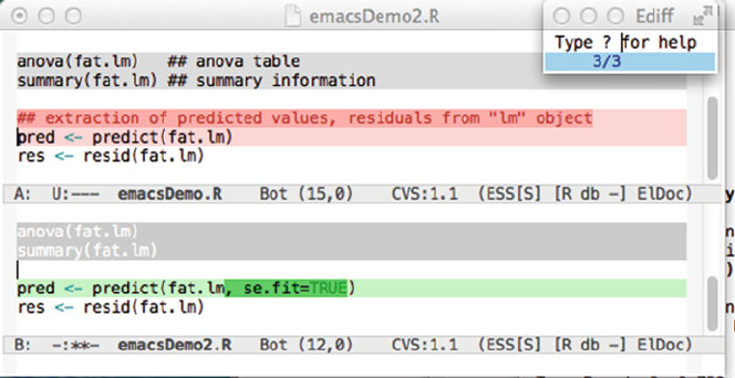
M.1 Emacs Features 853
Fig. M.1 ediff of two similar files. All mismatches between the two files are detected and
highlighted. The ediff control frame shows that we are currently in the third of three detected
differences between the two files. The matching sections of the third chunk are highlighted in light
pink in the top buffer and light green in the bottom buffer. The mismatching sections of the third
chunk are highlighted in darker pink in the top buffer and darker green in the bottom buffer.
For a simple example, let us compare the current version of our Rscript for a
homework exercise with the first version we started yesterday. Figure M.1 shows
the comparison.
M.1.3 Buffers
Emacs can work with many multiple files simultaneously. It brings each into a
buffer.Abuffer is copy of a file within the Emacs editor. Any editing changes
made to the contents of a buffer are temporary until the buffer is saved back into
the file system. A buffer can hold a file, a directory listing, an interactive session
with the operating system, or an interactive instance of another running program.
Emacs allows you to open and edit an unlimited number of files and login sessions
simultaneously, running each in its own buffer. The files or login sessions can be
local or on another computer, anywhere in the world. You can run simultaneous
multiple sessions. The size of a buffer is limited only by the size of the computer.
One of us (RMH) normally has several buffers visible and frequently has hundreds
of open buffers (several chapters, their code files, their transcript files, the console
buffer for R, help files, directory listings on remote computers, handouts for classes,
and a listing of the currently open buffers).
854 M Accessing RThrough a Powerful Editor—With Emacs and ESS as the Example
M.1.4 Shell Mode
Emacs includes a shell mode in which a terminal interaction runs inside an Emacs
buffer. The Unix terminology for the program that runs an interactive command
line session is a “shell”. There are several commonly used shell programs: sh is
the original and most fundamental shell program. Other Unix shell programs are
csh and bash. The MS-DOS prompt window (c:/Windows/System32/cmd.exe)
is the native shell program in MS Windows. We usually use the sh included in
Rtools as our shell under MS Windows.
A terminal interaction running inside an Emacs buffer is much more powerful
than one run in an ordinary terminal emulator window. The entire live login session
inside an Emacs buffer is just another editable buffer (with full search capability).
The only distinction is that both you and the computer program you are working
with can write to the buffer. This is exceedingly important because it means nothing
ever rolls offthe top of the screen and gets lost. Just roll it back. The session can be
saved to a file and then is subject to automatic backup to protect you from system
crash or loss of connection to a remote machine.
M.1.5 Controlling Other Programs
A shell running in an Emacs buffer is normally used to run another program (Rfor
example). Frequently we can drop the intermediate step and have Emacs run the
other program directly. ESS provides that capability for R. The advantage of running
Rdirectly through Emacs is that it becomes possible to design the interactivity that
allows a buffer containing Rcode to send that code directly to the running Rprocess.
ESS (see Section M.2) builds on shell mode to provide modes for interacting with
statistical processes. The terminal interaction can be local (on the same computer on
which Emacs is running) or remote (anywhere else).
M.2 ESS
Figure M.2 is a screenshot showing an interactive Emacs session. Emacs is a pow-
erful program, hence the figure is quite dense. We discuss many of its components
in the following subsections.
The discussion here is based on Rossini et al. (2004). ESS provides:
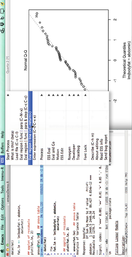
M.2 ESS 855
Fig. M.2 Interaction with Rprocess through Emacs with ESS.AnEmacs framewiththreebuffers is shown on the left. The top buffer shows the Rfile
emacsDemo.R that we are executing one line at a time. The cursor is at the end of the line anova(fat.lm), with the closing right paren and its matching left
paren highlighted together. The middle buffer *R* shows the Rprocess with the printed result from the anova(fat.lm) command. The down arrow
→
in the left
margin shows the beginning of the output from the most recently executed line. The bottom buffer *help[R](lm)* shows the help file from the Rcommand
?lm. In the center is the ESS menu. On the right is the graph drawn by the plot(fat.lm, 2) statement. More detail on this figure is presented in Section M.2.
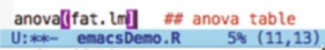
856 M Accessing RThrough a Powerful Editor—With Emacs and ESS as the Example
M.2.1 Syntactic Indentation and Color/Font-Based Source
Code Highlighting
The ESS interface includes a description of the syntax and grammar of each statisti-
cal language it knows about. This gives ESS the ability to edit the programming lan-
guage code, often more smoothly than with editors distributed with the languages.
The process of programming code is enhanced as ESS provides the user with a
clear presentation of the code with syntax highlighting to denote assignment, re-
served words, strings, and comments. The upper-left buffer (labeled emacsDemo.R)
in Figure M.2 contains an Rscript file. The mode-line for the buffer is in the “mode-
line” face indicating that this is the active buffer. The mode-lines for the other, in-
active, buffers in this figure are in the lighter-colored “mode-line-inactive” face. We
can tell from the ** in the mode-line that the file is still under construction. Those
two symbols would be replaced by -- once the file is saved.
In order to illustrate syntactic indentation, we show the statement fat.lm <-
lm(bodyfat ~ abdomin, data=fat) on two lines in Figure M.2. When we en-
tered the <RET> character after the comma, Emacs automatically indented the sec-
ond line of the statement and placed the cursor aligned with the first character after
the open paren.
The assignment arrow, a keyword in the language, is detected and colored in the
“constant” face. Comments indicated by “##” are colored in the “comment” face.
The cursor, represented by a blinking “|”, is redundantly located by the (11,13)
(indicating row and column in the file) in the mode-line. In this snapshot the cur-
sor immediately follows a closing paren “)”, hence both the closing paren and its
matching opening paren “(” are highlighted in the paren-match face. Mismatched
parens, as in Figure M.3,areshownintheparen-mismatch face.
Fig. M.3 Mismatched parens are shown in a glaring color to help protect the user from many
types of typographical errors.
M.2.2 Partial Code Evaluation
Emacs/ESS can send individual lines, entire function definitions, marked regions,
and whole edited buffers from the window in which the code is displayed for edit-
ing to the statistical language/program for execution. Emacs/ESS sends the code di-
rectly to the running program and receives the printed output back from the program
M.2 ESS 857
in an editable Emacs buffer (the *R* buffer). This is a major improvement over cut-
and-paste as it does not require switching buffers or windows.
We show this twice in Figure M.2. The dropdown menu is set to show the various
options on which subset of the buffer will be sent over. The menu also shows the
key-stroke combinations that can be typed directly and thereby avoid using the menu
at all. The cursor is on the line anova(fat.lm) and that line was sent over by this
command.
The *R* buffer has just received the command (the hooked down arrow
→
in the
left margin shows the beginning of the output from the most recently executed line).
The command and its output are displayed. In addition to receiving and executing
lines sent over from the script file, the *R* buffer is also an ordinary Rconsole and
the user can type directly into the *R* buffer.
ESS facilitates the editing of files of Rscripts by providing a means for loading
and error-checking of small sections of code (as illustrated in Figure M.2). This
allows for source-level debugging of batch files.
M.2.3 Object Name Completion
In addition, for languages in the Sfamily (Sdeveloped at Bell Labs, S+ from
TIBCO, and R)ESS provides object-name completion of user- and system-defined
functions and data, and filename completion for files in the computer.
M.2.4 Process Interaction
ESS builds on Emacs’s facilities to interface directly with the running Rprocess.
The output of the package goes directly to the editable *R* text buffer in Emacs.
Emacs has historically referred to processes under its control as “inferior”, ac-
counting for the name inferior ESS (iESS) shown in the mode-line of the *R*
buffer in Figure M.2. This mode allows for command-line editing and for recalling
and searching the history of previously entered commands. Filename completion,
and object-name and function-name completion are available. Transcripts are easily
recorded and can be edited into an ideal activity log, which can then be saved. ESS
intercepts calls to the internal help system for Rand displays the help files inside an
Emacs buffer (see the bottom left buffer in Figure M.2).
858 M Accessing RThrough a Powerful Editor—With Emacs and ESS as the Example
M.2.5 Interacting with Statistical Programs on Remote Computers
ESS provides the facility to edit and run programs on remote machines in the same
session and with the same simplicity as if they were running on the local machine.
M.2.6 Transcript Editing and Reuse
Once a transcript log is generated, perhaps by saving an iESS buffer, transcript
mode assists with reuse of part or all of the entered commands. It permits editing
and re-evaluating the commands directly from the saved transcript. This is useful
for demonstration of techniques as well as for reconstruction of data analyses. There
currently exist functions within ESS for “cleaning” transcripts from the R,S+, and
SAS languages back to source code by finding all input lines and isolating them
into an input file.
By default transcript files (files with extensions *.Rout *.rt *.Sout *.st)
open into read-only buffers. The intent is to protect the history of your analysis
sequence. If you need to make them writable, use C-x C-q.
M.2.7 Help File Editing (
R
)
ESS also provides an interface for writing help files for Rfunctions and packages
(see Appendix F). It provides the ability to view and execute embedded Rsource
code directly from the help file in the same manner as ESS normally handles code
from a source file. ESS Help mode provides syntax highlighting and the ability to
submit code from the help file to a running Rprocess.
M.3 Learning Emacs
There are several ways to learn Emacs. Whichever you choose, it will give you
access to the most comprehensive editing system.
M.3 Learning Emacs 859
M.3.1 GUI (Graphical User Interface)
Emacs provides a GUI (graphical user interface) with dropdown menus (shown
in Figure M.2) or with toolbar icons (not shown here). An excellent guide to menu-
based Emacs usage, with the delightful title “Emacs has no learning curve: Emacs
and ESS”, is available in Johnson (2015). Detailed help on Emacs is available from
the Help dropdown menu item.
M.3.2 Keyboard Interface
Emacs, in its present incarnation, goes back to 1984. A precursor goes back to
1976. One of us (RMH) started using Emacs about 1990. Emacs was originally
designed in a keyboard-only environment, long before mice and multi-windowed
“desktop” environments. We still prefer the keyboard as it is faster (once learned)
and has more capabilities than the menu-based GUI options. The dropdown menus
themselves show the keyboard equivalents. For keyboard-based usage use one or
more of
1. Tutorial. Enter “C-h t”. Then read the file and follow the instructions. You are
working with your own private copy of the TUTORIAL file, so you can practice
the keystrokes as suggested.
2. Manual. The manual is online in the hyperlinked Info system. It can be accessed
from the menu or by entering “C-h i”tobringuptheInfo: buffer.
3. Help. You can search within the dropdown Help menu. Or, to find help apropos
a topic, for example to answer the question “How do I save my current editing
buffer to a file?”, enter “C-h a save RET” and get a list of all commands with
save as part of their name. You probably want the command save-buffer and
will see that you can use that command by typing “C-x C-s”orbyusingthe
files pull-down menu.
4. Reference Card to Emacs keystroke commands. The Emacs reference card is
in the directory accessed by “C-h r C-x d ../etc/refcards”. The English
card is in file refcard.pdf. Several other languages are also available as files
with names **-refcard.pdf. Reference cards for other Free Software Founda-
tion programs are also in the same directory.
860 M Accessing RThrough a Powerful Editor—With Emacs and ESS as the Example
M.4 Nuisances with Windows and Emacs
When Rhas been started by an ordinary user, as opposed to Administrator, then
installed packages are placed into a personal library. The RGUI under Windows
uses the directory
"C:/Users/loginname/Documents/R/win-library/x.y"
as the location of your personal library. The *R* buffer inside Emacs uses
"C:/Users/loginname/AppData/Roaming/R/win-library/x.y"
as the location of your personal library. The notation x.y must be replaced by the
first two digits of your current version of R. For example, with R-3.3.0,"x.y"
would become "3.3". Neither will automatically see packages that were installed
into the directory used by the other. You must tell it about the other directory.
You can tell the RGUI to use the additional directory with the statement
.libPaths(
"C:/Users/loginname/AppData/Roaming/R/win-library/x.y")
You can tell *R* to use the additional directory with the statement
.libPaths(
"C:/Users/loginname/Documents/R/win-library/x.y")
M.5 Requirements
Emacs satisfies the requirements detailed in Section K.1.1.
1. ESS provides full interaction between the commands file, the statistical process,
and the transcript.
2. The statistical process runs in an Emacs buffer and is therefore fully searchable
and editable.
3. Cut and paste is standard.
4. Emacs comes with modes specialized for all standard computing languages (C,
C++,Fortran,VBA). ESS provides the modes for Rand S+ (and for SAS and
several others). Each mode by default highlights all keywords in its language,
is aware of recommended indentation patterns and other formatting issues, and
has communication with its associated running program.
5. Emacs handles multiple files as part of its basic design.
6. Emacs has a L
A
T
E
X mode, and therefore provides editing access to the best
mathematical typesetting system currently available anywhere.
7. Emacs has several text modes.
8. Several spell-check programs works with Emacs;weuseispell.
M.5 Requirements 861
9. Emacs permits embedding of graphics directly into the Emacs buffer.
10. Graphics in PDF, PostScript, and bitmap formats can be embedded into L
A
T
E
X
documents.
11. Emacs includes encoding (Unicode) for all human languages. Enter C-H h to
display the HELLO file, which lists many languages and characters.
Appendix N
L
A
T
E
X
We used L
A
T
E
X (Lamport, 1994) as the document preparation system for writing this
book. L
A
T
E
X knows all the intricacies of mathematical typesetting and makes it very
easy to include figures and tables into the manuscript. L
A
T
E
X is the standard required
by many statistics and mathematics journals. L
A
T
E
X can adapt to any standard style,
such as those used by book publishers and journals, or you can write your own.
The L
A
T
E
X document preparation system is written as a collection of macros for
Donald Knuth’s T
E
X program (Knuth, 1984). L
A
T
E
X adds to T
E
X a collection of
commands that simplify typesetting by letting the user concentrate on the structure
of the text.
T
E
X is a sophisticated program designed to produce high-quality typesetting,
especially for mathematical text. The T
E
X system was developed by Donald E.
Knuth at Stanford University. It is now maintained by CTAN, the Comprehensive
T
E
X Archiving Network (Comprehensive T
E
X Archiving Network, 2002). There are
several distributions available. We use MikT
E
X (Schenk, 2001) on Windows and
MacT
E
X (The TeX Users Group (TUG), 2014) on Macintosh.
The latex function in R(Heiberger and Harrell, 1994; Frank E Harrell et al.,
2014) may be used to prepare formatted typeset tables for a L
A
T
E
X document. Several
tables in this book (8.1, 9.1, 12.4, 15.5, and 15.8) were prepared in this way.
N.1 Organization Using L
A
T
E
X
There are several ways to approach L
A
T
E
X. The way we used for this book was to
write each chapter in its own file, and then combine them into book using the style
file provided by our publisher Springer.
©Springer Science+Business Media New York 2015
R.M. Heiberger, B. Holland, Statistical Analysis and Data Display,
Springer Texts in Statistics, DOI 10.1007/978-1-4939-2122-5
863
864 NL
A
T
E
X
N.2 Setting Equations
This is equation 8.1 as we typed it:
\begin{eqnarray*}
y_i = \beta_0 + \beta_1 x_i + \epsilon_i \cond{for $i=1,
\dots,n$}
\end{eqnarray*}
This is how it appears when typeset:
yi=β0+β1xi+ifor i=1,...,n
N.3 Coordination with R
The Second Edition of this book was written using the Sweave and Stangle func-
tions from the utils package. All Rcode is included within the L
A
T
E
X source for the
book. Stangle reads the L
A
T
E
X input files, isolates from the input files the actual
code that produced the tables and figures, and collects the code into the script files
that are included with the HH package. See help(Sweave, package="utils")
for details on writing using Sweave.
N.4 Global Changes: Specification of Fonts
In L
A
T
E
X, it is very easy to make global changes to a document style. For example,
placing programs and transcripts into a verbatim environment takes care of the
font. Should we later decide that we would like a different monowidth font, say
“Adobe Courier” instead of the default “Computer Modern Typewriter”, we include
the single statement \renewcommand{\ttdefault}{pcr} and then immediately
ALL instances of the typewriter font will change. We illustrate in Table N.1.
Compare this simple change of a single specification in L
A
T
E
X to the more labor-
intensive way of accomplishing the same task in a visual formatting systems (MS
Word, for example). In a visual formatting system, programs and transcripts must
be individually highlighted and then explicitly placed into Courier. Changing ALL
instances of the typewriter font requires manually highlighting and changing EACH
of them individually, one at a time.

N.4 Global Changes: Specification of Fonts 865
Table N.1 Switching the typewriter font (L
A
T
E
X command \tt)inL
A
T
E
X from the default “Com-
puter Modern Typewriter” to “Adobe Courier” and back.
This is the default Computer Modern Typewriter font.
%% switch to Adobe Courier
\renewcommand{\ttdefault}{pcr}
This is Adobe Courier font.
%% return to Computer Modern Typewriter
\renewcommand{\ttdefault}{cmtt}
And back to the Computer Modern Typewriter font.
Appendix O
Word Processors and Spreadsheets
Word processing is moving sentences, paragraphs, sections, figures, and cross-
references around. Most word processors can be used as a text editor by manually
turning offmany of the word processing features.
Spreadsheet software is used to operate on tables of numbers.
Microsoft Word and Microsoft Excel are the most prevalent word processor and
spreadsheet software systems. Most of what we say here applies to all such systems.
O.1 Microsoft Word
Microsoft Word is probably the most prevalent text editor and word processor today.
MS Word is configured by default as a word processor. It can be used as a text
editor by changing those default settings. The most critical features are the font and
the paragraph reflow. Courier (or another monowidth font in which all letters are
equally wide) should be used for program writing or for summary reports in which
your displayed output from Ris included. The software output from Ris designed
to look right (alignment and spacing) with monowidth fonts. It looks terrible, to
the point of illegibility, in proportional fonts. See examples in Section A.4 and Ap-
pendix L. Other word processor features to turn offare spell checking and syntax
checking, both of which are designed to make sense with English (or another natural
language) but not with programming languages.
©Springer Science+Business Media New York 2015
R.M. Heiberger, B. Holland, Statistical Analysis and Data Display,
Springer Texts in Statistics, DOI 10.1007/978-1-4939-2122-5
867
868 O Word Processors and Spreadsheets
If you are using an editor that thinks it knows more than you, be very sure that
the *.r,*.Rout, and *.rt files are displayed in Courier and fit within the margin
settings of the word processor.
O.1.1 Editing Requirements
MS Word satisfies some of the requirements detailed in Section K.1.1.
1. MS Word can edit the commands file. It does not interact directly with the
running statistical process; manual cut-and-paste is required.
2. The output from the statistical process is in a window independent of MS Word.
The output can be picked up and pasted into an MS Word window.
3. Cut and paste is standard.
4. When checking is on, MS Word will by default inappropriately check computer
programs for English syntax and spelling.
5. MS Word handles multiple files as part of its basic design.
6. Reports can be written and output text can be embedded into them;
7. MS Word has syntax and spell-checking facilities limited to the natural lan-
guage (English in our case).
8. Graphics can be pasted directly into an MS Word document.
9. Mathematical formulas can be entered in an MS Word document.
10. SWord and other connections between Rand MS Word.
11. MS Word works with Unicode, providing access to all character sets in all
human languages. On the Insert tab, click Symbols and then More Symbols.
In the font box, find Arial Unicode MS.
O.1.2 SWord
SWord (Baier, 2014) is an add-in package for MS Word that makes it possible to
embed Rcode in an MS Word document. The Rcode will be automatically executed
and the output from the Rcode will be included within the MS Word document.
SWord is free for non-commercial use. Any other use will require a license. Please
see Section D.1.3 for installation information.
O.2 Microsoft Excel 869
O.2 Microsoft Excel
Microsoft Excel is probably the most prevalent spreadsheet program today.
We believe MS Excel is well suited for two tasks: as a small-scale database
management system and as a way of organizing calculations. We do not recommend
Excel for the actual calculations.
O.2.1 Database Management
R(and S+ and SAS) can read and write Excel files. Since many people within an
organization collect and distribute their data in Excel spreadsheets, this is a very
important feature.
O.2.2 Organizing Calculations
Rcan be connected directly to Excel on Windows via RExcel (Baier and Neuwirth,
2007)usingDCOM, Microsoft’s protocol for exchanging information across pro-
grams. See Appendix Dfor further details and for download information. Used in
this way, Excel can be used similarly to the ways that Emacs and MS Word are
used. Excel can be used to control R, for example by putting Rcommands inside
Excel cells and making them subject to automatic recalculation. Or Rcan be in
control, and use Excel as one of its subroutines.
O.2.3 Excel as a Statistical Calculator
We believe Excel is usually a poor choice for statistical computations because:
1. As of this writing (Excel 2013 for Windows and Excel 2011 for Macintosh) at
least some of the built-in statistical functions do not include even basic numerical
protection.
Table O.1 and Figure O.1 show the calculation of the variance of three numbers
by R’s var function and Excel’s VAR function. Figure O.1 shows a simple set
of variance calculations where Excel reveals an algorithmic error. We show the
erroneous number as a hex number in Table O.2. For comparison, Table O.1
shows the correct calculations by R.
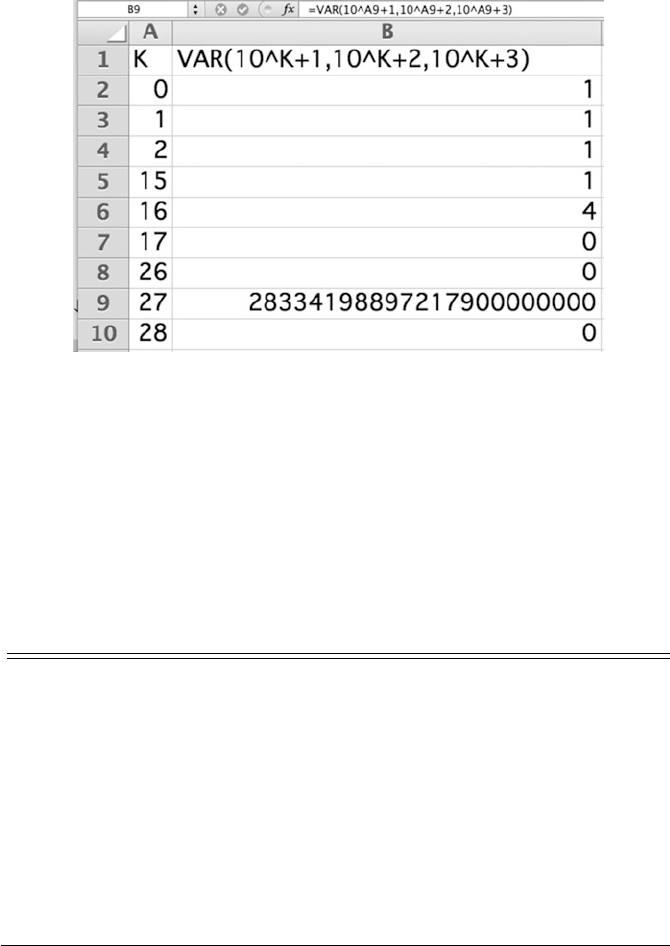
870 O Word Processors and Spreadsheets
Fig. O.1 Calculation of the variance by Excel for the sequence (10k)+1,(10k)+1,(10k)+1for
several values of k. The real-valued result for all values of kis exactly 1. The 2.833 ×10²² value
shown for k=27 is the indication of an erroneous algorithm in Excel.WeseethisforExcel 2013
on Windows and Excel 2011 on Macintosh. The floating point result for k=0 : 15 is exactly 1
as shown. The correct floating point result for all k>=17 is exactly 0. The floating point value 4
for k=16 is correct. We illustrate the correct floating point behavior in Section G.12.TableO.2
shows the hexadecimal display for the erroneous value.
Table O.1 Calculation of the variance by Rfor the sequence (10k)+1,(10k)+1,(10k)+1for
several values of k. The real-valued result for all values of kis exactly 1. Rgets the correct floating
point variance for all values of k. The floating point result for k=0 : 15 is exactly 1. The floating
point value 4 for k=16 is correct. The floating point result for k>=17 is exactly 0. We illustrate
the correct floating point behavior in Section G.12.
> k <- c(0, 1, 2, 15, 16, 17, 26, 27, 28)
> cbind(k=k, var=apply(cbind(10^k + 1, 10^k + 2, 10^k + 3), 1, var))
k var
[1,] 0 1
[2,] 1 1
[3,] 2 1
[4,] 15 1
[5,] 16 4
[6,] 17 0
[7,] 26 0
[8,] 27 0
[9,] 28 0

O.2 Microsoft Excel 871
Table O.2 The first statement shows the hex display of the number Excel shows in Figure O.1
as the result of var(1027 +1,1027 +2,1027 +3). It is very close to a pretty hex number suggesting
that there is a numeric overflow somewhere in the algorithm. The second statement shows the hex
display of the three input numbers. They are all identical to machine precision.
> sprintf("%+13.13a", 28334198897217900000000)
[1] "+0x1.8000000000007p+74"
> as.matrix(sprintf("%+13.13a", c(10^27 + 1, 10^27 + 2, 10^27 + 3)))
[,1]
[1,] "+0x1.9d971e4fe8402p+89"
[2,] "+0x1.9d971e4fe8402p+89"
[3,] "+0x1.9d971e4fe8402p+89"
Earlier versions of MS Excel got different wrong answers for the variance of
three numbers. Most notably MS Excel 2002 gets the right answer for 107and
the wrong answer for 108, suggesting that it was using the numerically unstable
one-pass algorithm. Later releases got different sets of wrong answers.
2. Most add-in packages are not standard and are not powerful. If add-ins are used
along with an introductory textbook, they will most likely be limited in capability
to the level of the text. They are unlikely to be available on computers in a work
situation.
RExcel is an exception. It uses Rfrom the Excel interface and therefore has all
the power and generality of R.
References
A.A. Adish, S.A. Esrey, T.W. Gyorkos, J. Jean-Baptiste, A. Rojhani, Effect of con-
sumption of food cooked in iron pots on iron status and growth of young children:
a randomised trial. Lancet 353(9154), 712–716 (1999)
A. Agresti, Categorical Data Analysis (Wiley, New York, 1990)
A. Agresti, B. Caffo, Simple and effective confidence intervals for proportions and
differences of proportions result from adding two successes and two failures. Am.
Stat. 54(4), 280–288 (2000)
Albuquerque Board of Realtors (1993). URL: http://lib.stat.cmu.edu/
DASL/Stories/homeprice.html
American Statistical Association, Career Center (2015). URL: http://www.
amstat.org/careers
O. Amit, R.M. Heiberger, P.W. Lane, Graphical approaches to the analysis of safety
data from clinical trials. Pharm. Stat. 7(1), 20–35 (2008). URL: http://www3.
interscience.wiley.com/journal/114129388/abstract
A.H. Anderson, E.B. Jensen, G. Schou, Two-way analysis of variance with corre-
lated errors. Int. Stat. Rev. 49, 153–167 (1981)
R.L. Anderson, T.A. Bancroft, Statistical Theory in Research (McGraw-Hill, New
York,1952)
V.L. Anderson, R.A. McLean, Design of Experiments (Marcel Dekker, New
York,1974)
D.F. Andrews, A.M. Herzberg, Data: A Collection of Problems from Many Fields
for the Student and Research Worker (Springer, New York,1985). URL: http://
lib.stat.cmu.edu/datasets/Andrews/
E. Anionwu, D. Watford, M. Brozovic, B. Kirkwood, Sickle cell disease in a British
urban community. Br. Med. J. 282, 283–286 (1981)
©Springer Science+Business Media New York 2015
R.M. Heiberger, B. Holland, Statistical Analysis and Data Display,
Springer Texts in Statistics, DOI 10.1007/978-1-4939-2122-5
873
874 References
P.K. Asabere, F.E. Huffman, Negative and positive impacts of golf course proximity
on home prices. Apprais. J. 64(4), 351–355 (1996)
T. Baier, Sword (2014). URL: http://rcom.univie.ac.at
T. Baier, E. Neuwirth, Excel :: Com :: R. Comput. Stand. 22(1), 91–108 (2007)
M.K. Barnett, F.C. Mead, A 24factorial experiment in four blocks of eight. Appl.
Stat. 5, 122–131 (1956)
R.A. Becker, J.M. Chambers, A.R. Wilks, The S Language; A Programming En-
vironment for Data Analysis and Graphics (Wadsworth & Brooks/Cole, Pacific
Grove, 1988)
R.A. Becker, W.S. Cleveland, S-PLUS Trellis Graphics User’s Manual (1996a).
URL: http://www.stat.purdue.edu/~wsc/papers/trellis.user.pdf
Becker, R.A., W.S. Cleveland, M.-J. Shyu, S.P. Kaluzny, A tour of trellis graph-
ics (1996b). URL: http://www2.research.att.com/areas/stat/doc/95.
12.color.ps
Y.Y.M. Bishop, S.E. Fienberg, P.W. Holland, Discrete Multivariate Analysis (MIT,
Cambridge,1975)
A. Bjork, Solving least squares problems by Gram–Schmidt orthogonalization. BIT
7, 1–21 (1967)
C.I. Bliss, Statistics in Biology (McGraw-Hill, New York, 1967)
C.R. Blyth, On Simpson’s paradox and the sure-thing principle. J. Am. Stat. Assoc.
67, 364–366 (1972)
B.L. Bowerman, R.T. O’Connell, Linear Statistical Models (Duxbury, Belmont,
1990)
G.E.P. Box, D.R. Cox, An analysis of transformations. J. R. Stat. Soc. B 26, 211–
252 (1964)
G.E.P. Box, W.G. Hunter, J.S. Hunter, Statistics for Experimenters (Wiley, New
York, 1978)
G.E.P. Box, G.M. Jenkins, Time Series Analysis: Forecasting and Control,revised
edn. (Holden-Day, San Francisco, 1976)
R.G. Braungart, Family status, socialization and student politics: a multivariate anal-
ysis. Am. J. Sociol. 77, 108–130 (1971)
C. Brewer, Colorbrewer (2002). URL: http://colorbrewer.org
L. Brochard, J. Mancebo, M. Wysocki, F. Lofaso, G. Conti, A. Rauss, G. Simon-
neau, S. Benito, A. Gasparetto, F. Lemaire, D. Isabey, A. Harf, Noninvasive
ventilation for acute exacerbations of chronic pulmonary disease. N. Engl. J. Med.
333(13), 817–822 (1995)
References 875
D.G. Brooks, S.S. Carroll, W.A. Verdini, Characterizing the domain of a regression
model. Am. Stat. 42, 187–190 (1988)
B.W. Brown Jr., Prediction analyses for binary data, in Biostatistics Casebook, ed.
by R.G. Miller Jr., B. Efron, B.W. Brown Jr., L.E. Moses (Wiley, New York, 1980)
M.B. Brown, A.B. Forsyth, Robust tests for equality of variances. J. Am. Stat.
Assoc. 69, 364–367 (1974)
Bureau of the Census, Statistical Abstract of the United States (U.S. Department of
Commerce, Washington, DC, 2001)
T.T. Cai, One-sided confidence intervals in discrete distributions. J. Stat. Plan.
Inference 131, 63–88 (2003). URL: http://www-stat.wharton.upenn.edu/
~tcai/paper/1sidedCI.pdf
E. Cameron, L. Pauling, Supplemental ascorbate in the supportive treatment of can-
cer: re-evaluation of prolongation of survival times in terminal human cancer.
Proc. Natl. Acad. Sci. USA 75, 4538–4542 (1978)
J.M. Chambers, W.S. Cleveland, B. Kleiner, P.A. Tukey, Graphical Methods for
Data Analysis (Wadsworth, Belmont, 1983)
T.F.C. Chan, G.H. Golub, R.J. LeVeque, Algorithms for computing the sample vari-
ance: analysis and recommendations.Am. Stat. 37(3), 242–247 (1983)
W. Chang, J. Cheng, J.J. Allaire, Y. Xie, J. McPherson, shiny: Web Applica-
tion Framework for R. R Package Version 0.11.1 (2015). URL: http://CRAN.
R-project.org/package=shiny
R. Chassell, Programming in Emacs Lisp: An Introduction. Free Software Foun-
dation, 2nd edn. (1999) URL: https://www.gnu.org/software/emacs/
manual/html_node/eintr/
T.W. Chin, E. Hall, C. Gravelle, J. Speers, The influence of Salk vaccination on the
epidemic pattern and spread of the virus in the community. Am. J. Hyg. 73, 67–94
(1961)
S. Chu, Diamond ring pricing using linear regression. J. Stat. Educ. 4(1996). URL:
http://www.amstat.org/publications/jse/v4n3/datasets.chu.html
W.S. Cleveland, Visualizing Data (Hobart Press, Summit, 1993)
W.S. Cleveland, R. McGill, Graphical perception: theory, experimentation, and
application to the development of graphical methods. J. Am. Stat. Assoc. 79,
531–554 (1984)
W.G. Cochran, G.M. Cox, Experimental Designs, 2nd edn. (Wiley, New York, 1957)
D.R. Collett, Modelling Binary Data (Chapman & Hall, London, 1991)
Comprehensive T
E
X Archiving Network CTAN (2002). URL: ftp://metalab.
unc.edu/pub/packages/TeX/index.html
876 References
W.J. Conover, M.E. Johnson, M.M. Johnson, A comparative study of tests for hom-
ogeneity of variances, with applications to the outer continental shelf bidding
data. Technometrics 23, 351–361 (1981)
Consumer Reports, Hot dogs, Consumer Reports (1986), pp. 366–367. URL:
http://lib.stat.cmu.edu/DASL/Stories/Hotdogs.html
R.D. Cook, S. Weisberg, Applied Regression Including Computing and Graphics
(Wiley, New York, 1999)
T. Cook, Convictions for Drunkenness (New Society, 1971)
CRAN, Comprehensive
R
Archive Network (2015). URL: http://CRAN.
R-project.org
Cytel Software Corporation, Logxact Statistical Software: Release 5 (2004). URL:
http://www.cytel.com/LogXact/logxact_brochure.pdf
S.R. Dalal, E.B. Fowlkes, B. Hoadley, Risk analysis of the space shuttle: pre-
challenger prediction of failure. J. Am. Stat. Assoc. 84, 945–957 (1989)
C. Darwin, The Effect of Cross- and Self-fertilization in the Vegetable Kingdom, 2nd
edn. (John Murray, London, 1876)
Data Archive, J. Stat. Educ. (1997). URL: http://www.amstat.org/
publications/jse/jse_data_archive.html
O.L. Davies, Design and Analysis of Industrial Experiments (Oliver and Boyd, Lon-
don, 1954)
O.L. Davies, P.L. Goldsmith (eds.), Statistical Methods in Research and Production,
4th edn. (Oliver and Boyd, London, 1972)
M.M. Desu, D. Raghavarao, Nonparametric Statistical Methods for Complete and
Censored Data, 1st edn. (Chapman & Hall, Boca Raton, 2003)
R. Dougherty, A. Wade (2006).URL: http://vischeck.com
D. Edwards, J.J. Berry, The efficiency of simulation-based multiple comparisons.
Biometrics 43, 913–928 (1987)
M.E. Ellis, K.R. Neal, A.K. Webb, Is smoking a risk factor for pneumonia for pat-
ients with chickenpox? Br. Med. J. 294, 1002 (1987)
J.D. Emerson, M.A. Stoto, Transforming data, in Understanding Robust and Exp-
loratory Data Analysis, ed. by D.C. Hoaglin, F. Mosteller, J.W. Tukey (Wiley,
New York, 1983)
L.W. Erdman, Studies to determine if antibiosis occurs among Rhizobia: 1. Between
Rhizobium meliloti and Rhizobium trifolii. J. Am. Soc. Agron. 38, 251–258
(1946)
J.L. Fleiss, Statistical Methods for Rates and Proportions, 2nd edn. (Wiley,
New York, 1981)
References 877
Forbes Magazine (1993). URL: http://lib.stat.cmu.edu/DASL/Datafiles/
ceodat.html
R.S. Fouts, Acquisition and testing of gestural signs in four young chimpanzees.
Science 180, 978–980 (1973)
J. Fox, Regression Diagnostics: An Introduction (Sage, Thousand Oaks, 1991)
J. Fox, The R Commander: a basic statistics graphical user interface to R. J. Stat.
Softw. 14(9), 1–42 (2005). URL: http://www.jstatsoft.org/v14/i09
E.H. Frank Jr., with contributions from Charles Dupont, and many others, Hmisc:
Harrell Miscellaneous. R Package Version 3.14-6 (2014). URL: http://CRAN.
R-project.org/package=Hmisc
Free Software Foundation, Emacs (2015). URL: http://www.gnu.org/
software/emacs/
R.J. Freund, R.C. Littell, SAS System for Regression (SAS Institute, Inc., Cary,
1991)
J.H. Goodnight, Tests of hypotheses in fixed effects linear models. Technical Report
R-101 (SAS Institute, Cary, 1978)
P. Graham, ANSI Common Lisp (Prentice Hall, Upper Saddle River, 1996)
M.J. Greenacre, Theory and Applications of Correspondence Analysis (Academic,
New York, 1984)
P. Grosjean, Ide/script editors. Annotated list with links to many editing environ-
ments for R. (2012). URL: http://www.sciviews.org/_rgui/
R.F. Gunst, R.L. Mason, Regression Analysis and Its Application: A Data-Oriented
Approach (Marcel Dekker, New York, 1980)
L.C. Hamilton, Saving water: a causal model of household conservation. Sociol.
Perspect. 26(4), 355–374 (1983)
L.C. Hamilton, Regression with Graphics (Brooks-Cole, Belmont, 1992)
D.J. Hand, F. Daly, A.D. Lunn, K.J. McConway, E. Ostrowski, A Handbook of Small
Data Sets (Chapman and Hall, London, 1994)
D.D. Harrison, D.E. Harrison, T.J. Janik, R. Cailliet, J.R. Ferrantelli, J.W. Hass,
B. Holland, Modeling of the sagittal cervical spine as a method to discrimi-
nate hypo-lordosis: results of elliptical and circular modeling in 72 asymptomatic
subjects, 52 acute neck pain subjects, and 70 chronic neck pain subjects. Spine
29(22):2485–2492 (2004)
D.E. Harrison, R. Cailliet, D.D. Harrison, T.J. Janik, B. Holland, Changes in sagittal
lumbar configuration with a new method of extension traction combined with
spinal manipulation and its clinical significance: non-randomized clinical control
trial. Arch. Phys. Med. Rehabil. 83(11), 1585–1591 (2002)
878 References
R.M. Heavenrich, J.D. Murrell, K.H. Hellman, Light Duty Automotive Technology
and Fuel Economy Trends through 1991 (U.S. Environmental Protection Agency,
Ann Arbor, 1991)
R.M. Heiberger, Computation for the Analysis of Designed Experiments (Wiley,
New York, 1989)
R.M. Heiberger, HH: Statistical Analysis and Data Display: Heiberger and
Holland. Spotfire S+Package Version 2.1-29 (2009). URL: http://csan.
insightful.com/PackageDetails.aspx?Package=HH
R.M. Heiberger, HH: Statistical Analysis and Data Display: Heiberger and Hol-
land. R Package Version 3.1-15 (2015). URL: http://CRAN.R-project.org/
package=HH
R.M. Heiberger, F.E. Harrell Jr., Design of object-oriented functions in S for screen
display, interface and control of other programs (SAS and L
A
T
E
X), and S pro-
gramming, in Computing Science and Statistics, vol. 26 (1994), pp. 367–371. The
software is available in both S-Plus and Rin library(hmisc). It is included in
the S-Plus distribution. It may be downloaded for Rfrom the contrib page of
the R Development Core Team (2004) website
R.M. Heiberger, B. Holland, Statistical Analysis and Data Display: An Intermediate
Course with Examples in
S-Plus
,
R
, and
SAS
, 1st edn. (Springer, New York,
2004)
R.M. Heiberger, B. Holland, Mean–mean multiple comparison displays for families
of linear contrasts. J. Comput. Graph. Stat. 14(4), 937–955 (2006)
R.M. Heiberger, E. Neuwirth, R through Excel: A Spreadsheet Interface for Statis-
tics, Data Analysis, and Graphics (Springer, New York, 2009). URL: http://
www.springer.com/978-1-4419-0051-7
R.M. Heiberger, N.B. Robbins, Design of diverging stacked bar charts for Likert
scales and other applications. J. Stat. Softw. 57(5), 1–32 (2014). URL: http://
www.jstatsoft.org/v57/i05/
R.M. Heiberger, P. Teles, Displays for direct comparison of ARIMA models. Am.
Stat. 56, 131–138, 258–260 (2002)
R.M. Heiberger, with contributions from H. Burt, RcmdrPlugin.HH: Rcmdr Support
for the HH Package. R Package Version 1.1-42 (2015). URL: http://CRAN.
R-project.org/package=RcmdrPlugin.HH
C.R. Hicks, K.V. Turner Jr., Fundamental Concepts in Design of Experiments,5th
edn. (Oxford, New York, 1999)
J.E. Higgens, G.G. Koch, Variable selection and generalized chi-square analysis of
categorical data applied to a large cross-sectional occupational health survey. Int.
Stat. Rev. 45, 51–62 (1977)
D.C. Hoaglin, F. Mosteller, J.W. Tukey (eds.), Understanding Robust and Exp-
loratory Data Analysis (Wiley, New York, 1983)
References 879
Y. Hochberg, A sharper Bonferroni procedure for multiple tests of significance.
Biometrika 75, 800–803 (1988)
Y. Hochberg, A.C. Tamhane, Multiple Comparison Procedures (Wiley, NewYork,
1987)
M. Holzer, Mild therapeutic hypothermia to improve the neurologic outcome after
cardiac arrest. N. Engl. J. Med. 346(8), 549–556 (2002)
D.W. Hosmer, S. Lemeshow, Applied Logistic Regression, 2nd edn. (Wiley, New
York, 2000)
J. Hsu, M. Peruggia, Graphical representations of Tukey’s multiple comparison
method. J. Comput. Graph. Stat. 3, 143–161 (1994)
R. Ihaka, P. Murrell, K. Hornik, J.C. Fisher, A. Zeileis, Colorspace: Color
Space Manipulation. R Package Version 1.2-4 (2013). URL: http://CRAN.
R-project.org/package=colorspace
R.L. Iman, A Data-Based Approach to Statistics (Duxbury, Belmont, 1994)
Insightful Corp., S-Plus Statistical Software: Release 6.1 (2002). URL: http://
www.insightful.com.
F. John et al., R Commander. R Package Version 2.1-6 (2015). URL: http://CRAN.
R-project.org/package=Rcmdr
N.L. Johnson, F.C. Leone, Statistics and Experimental Design in Engineering and
the Physical Sciences, vol. 2 (Wiley, New York, 1967)
P.E. Johnson, Emacs has no learning curve: Emacs and ess (2015). URL: http://
pj.freefaculty.org/guides/Rcourse/emacs-ess/emacs-ess.pdf
P.O. Johnson, F. Tsao, Factorial design and covariance in the study of individual
educational development. Psychometrika 10, 133–162 (1945)
R.W. Johnson, Fitting percentage of body fat to simple body measurements.
J. Stat. Educ. 4(1) (1996). URL: http://www.amstat.org/publications/
jse/archive.htm
D.E. Knuth, The T
E
Xbook (Addison-Wesley, Reading, 1984)
L. Krantz, 1999–2000 Jobs Rated Almanac: The Best and Worst Jobs—250 in All—
Ranked by More Than a Dozen Vital Factors Including Salary, Stress, Benefits
and More (St. Martins Press, New York, 1999). URL: http://www.hallmaps.
com/almanacs_yearbooks/29.shtml
L. Lamport, L
A
T
E
X: A Document Preparation System: User’s Guide and Reference
Manual (Addison-Wesley, Boston, 1994)
M. Lavine, Problems in extrapolation illustrated with space shuttle o-ring data.
J. Am. Stat. Assoc. 86, 919–921 (1991)
A.J. Lea, New observations on distribution of neoplasms of female breast in certain
European countries. Br. Med. J. 1, 488–490 (1965)
880 References
E.T. Lee, Statistical Methods for Survival Data Analysis (Lifetime Learning Publi-
cations, Belmont, 1980)
E. Lehmann, Nonparametrics—Statistical Methods Based on Ranks, revised first
edition (Prentice Hall, New York, 1998)
F. Leisch, R-core, Sweave: automatic generation of reports (2014). URL: https://
stat.ethz.ch/R-manual/R-devel/library/utils/doc/Sweave.pdf
A.Y. Lewin, M.F. Shakun, Policy Sciences, Methodology and Cases (Pergam-
mon, Oxford, 1976). URL: http://lib.stat.cmu.edu/DASL/Stories/
airpollutionfilters.html
R. Likert, A technique for the measurement of attitudes. Arch. Psychol. 140(55),
1–55 (1932)
R.J.A. Little, D.B. Rubin, Statistical Analysis with Missing Data, 2nd edn. (Wiley,
New York, 2002)
J. Longley, An appraisal of least squares programs for the electronic computer from
the point of view of the user. J. Am. Stat. Assoc. 62, 819–841 (1967)
A. Luo, T. Keyes, Second set of results in from the career track member survey, in
Amstat News (American Statistical Association, Arlington, 2005), pp. 14–15
M. M¨
achler, S. Eglen, R.M. Heiberger, K. Hornik, S.P. Luque, H. Redesting, A.J.
Rossini, R. Sparapani, V. Spinu, ESS (Emacs Speaks Statistics) (2015). URL:
http://ESS.R-project.org/
P. McCullagh, J.A. Nelder, Generalized Linear Models (Chapman and Hall, Lon-
don, 1983)
C.R. Mehta, N.R. Patel, P. Senchaudhuri, Efficient Monte Carlo methods for condi-
tional logistic regression. J. Am. Stat. Assoc. 95(449), 99–108 (2000)
W.M. Mendenhall, J.T. Parsons, S.P. Stringer, N.J. Cassissi, R.R. Million, T2 oral
tongue carcinoma treated with radiotherapy: analysis of local control and com-
plications. Radiother. Oncol. 16, 275–282 (1989)
D. Meyer, A. Zeileis, K. Hornik, The strucplot framework: visualizing multi-way
contingency tables with vcd. J. Stat. Softw. 17(3), 1–48 (2006). URL: http://
www.jstatsoft.org/v17/i03/
D. Meyer, A. Zeileis, K. Hornik, vcd: Visualizing Categorical Data. R Package Ver-
sion 1.2-13 (2012). URL: http://CRAN.R-project.org/package=vcd
Microsoft, Inc., Word (2015). URL: https://products.office.com/en-us/
Word
G.A. Milliken, D.E. Johnson, Analysis of Messy Data, vol. I (Wadsworth, Belmont,
1984)
D.C. Montgomery, Design and Analysis of Experiments, 4th edn. (Wiley, New York,
1997)
References 881
D.C. Montgomery, Design and Analysis of Experiments, 5th edn. (Wiley, New York,
2001)
D.S. Moore, G.P. McCabe, Introduction to the Practice of Statistics (Freeman, New
York, 1989)
F. Mosteller, J.W. Tukey, Data Analysis and Regression (Addison-Wesley, Reading,
1977)
J.D. Murray, G. Dunn, P. Williams, A. Tarnopolsky, Factors affecting the consump-
tion of psychotropic drugs. Psychol. Med. 11, 551–560 (1981)
P. Murrell, R Graphics, 2nd edn. (CRC, Boca Raton, 2011). URL: http://www.
taylorandfrancis.com/books/details/9781439831762/
R.H. Myers, Classical and Modern Regression with Applications, Chap. 5 (PWS-
Kent, Boston, 1990), p. 218
S.C. Narula, J.T. Wellington, Prediction, linear regression and the minimum sum of
errors. Technometrics 19, 185–190 (1977)
U.S. Navy, Procedures and Analyses for Staffing Standards Development:
Data/Regression Analysis Handbook (Navy Manpower and Material Analysis
Center, San Diego, 1979)
J.A. Nelder, A reformulation of linear models. J. R. Stat. Soc. 140(1), 48–77 (1977).
doi:10.2307/2344517
J. Neter, M.H. Kutner, C.J. Nachtsheim, W. Wasserman, Applied Linear Statistical
Models, 4th edn. (Irwin, Homewood, 1996)
E. Neuwirth, RColorBrewer: ColorBrewer Palettes. R Package Version 1.0-5
(2011). URL: http://CRAN.R-project.org/package=RColorBrewer
E. Neuwirth, RExcel (2014). URL: http://rcom.univie.ac.at
New Zealand Ministry of Research Science and Technology, Staying in science
(2006). URL: http://www.morst.govt.nz/Documents/publications/
researchreports/Staying-in-Science-summary.pdf
D.F. Nicholls, The analysis of time series—the time domain approach. Aust. J. Stat.
21, 93–120 (1979)
NIST, National Institute of Standards and Technology, Statistical Engineer-
ing Division (2002). URL: http://www.itl.nist.gov/div898/software/
dataplot.html/datasets.htm
NIST, National Institute of Standards and Technology, Data set of south-
ern oscillations, in NIST/SEMATECH e-Handbook of Statistical Meth-
ods (2005). URL: http://www.itl.nist.gov/div898/handbook/pmc/
section4/pmc4412.htm
Olympic Committee, Salt Lake City 2002 Winter Olympics (2001). URL: http://
www.saltlake2002.com
882 References
R.L. Ott, An Introduction to Statistical Methods and Data Analysis, 4th edn.
(Duxbury, Belmont, 1993)
S.C. Pearce, The Agricultural Field Experiment (Wiley, New York, 1983)
K. Penrose, A. Nelson, A. Fisher, Generalized body composition prediction equa-
tion for men using simple measurement techniques (abstract). Med. Sci. Sports
Exerc. 17(2), 189 (1985)
D.H. Peterson (ed.), Aspects of Climate Variability in the Pacific and the Western
Americas. Number 55 in Geophysical Monograph (American Geophysical Union,
Washington, DC, 1990)
R.G. Peterson, Design and Analysis of Experiments (Marcel Dekker, New
Yor k /Basel, 1985)
R Core Team, R: A Language and Environment for Statistical Computing (R
Foundation for Statistical Computing, Vienna, 2015). URL: http://www.
R-project.org/
R Development Core Team, R: A Language and Environment for Statistical Com-
puting (R Foundation for Statistical Computing, Vienna, 2004). URL: http://
www.R-project.org. ISBN 3-900051-00-3
W. Rasband, Imagej 1.46t (2015). URL: http://rsb.info.nih.gov/ij
N.B. Robbins, Creating More Effective Graphs (Chart House, Ramsey, 2005, reis-
sued 2013) [Originally Wiley-Interscience]
N.B. Robbins, R.M. Heiberger, E. Neuwirth, C. Ritter, Professional statistics
and graphics accessible from excel, in Presented at the Joint Statistics Meet-
ings (American Statistical Association, Washington, DC, 2009). URL: http://
rcom.univie.ac.at/papers/handoutJSM2009.pdf
W.S. Robinson, Ecological correlations and the behavior of individuals. Am. Sociol.
Rev. 15, 351–357 (1950)
A.J. Rossini, R.M. Heiberger, R.A. Sparapani, M. M¨
achler, K. Hornik, Emacs
Speaks Statistics (ESS): a multiplatform, multipackage development environment
for statistical analysis. J. Comput. Graph. Stat. 13(1), 247–261 (2004). URL:
http://dx.doi.org/10.1198/1061860042985
A.J. Rossman, Televisions, physicians, and life expectancy. J. Stat. Educ. (1994).
URL: http://www.amstat.org/publications/jse/archive.htm
RStudio, Shiny: a web application framework for r (2015). URL: http://shiny.
rstudio.com
D. Sarkar, Lattice: Multivariate Data Visualization with R (Springer, New York,
2008). URL: http://lmdvr.r-forge.r-project.org. ISBN 978-0-387-
75968-5
D. Sarkar, lattice: Lattice Graphics. R Package Version 0.20-29 (2014). URL:
http://CRAN.R-project.org/package=lattice
References 883
D. Sarkar, F. Andrews, latticeExtra: Extra Graphical Utilities Based on Lat-
tice. R Package Version 0.6-26 (2013). URL: http://CRAN.R-project.org/
package=latticeExtra
S. Sarkar, Some probability inequalities for ordered MTP2random variables: a proof
of the Simes conjecture. Ann. Stat. 26, 494–504 (1998)
SAS Institute, Inc., The four types of estimable functions, in SAS/STAT User’s Guide
(SAS Institute, Inc., Cary, 1999)
C. Schenk, MikTeX (2001). URL: ftp://metalab.unc.edu/pub/packages/
TeX/systems/win32/miktex
S.R. Searle, Linear Models (Wiley, New York, 1971)
H.C. Selvin, Durkheim’s suicide: further thoughts on a methodological classic, in
´
Emile Durkheim, ed. by R.A. Nisbet (Prentice Hall, Englewood Cliffs, NJ, 1965),
pp. 113–136
R.T. Senie, P.P. Rosen, M.L. Lesser, D.W. Kinne, Breast self-examinations and med-
ical examination relating to breast cancer stage. Am. J. Public Health 71, 583–590
(1981)
N. Shaw, Manual of Meteorology, vol. 1 (Cambridge University Press, Cambridge,
1942)
W.J. Shih, S. Weisberg, Assessing influence in multiple linear regression with in-
complete data.Technometrics 28, 231–240 (1986)
J. Simpson, A. Olsen, J.C. Eden, A Bayesian analysis of a multiplicative treatment
effect in weather modification. Technometrics 17, 161–166 (1975)
W. Smith, L. Gonick, The Cartoon Guide to Statistics (HarperCollins, New York,
1993)
G.W. Snedecor, W.G. Cochran, Statistical Methods, 7th edn. (Iowa State University
Press, Ames, 1980)
R.R. Sokal, F.J. Rohlf, Biometry, 2nd edn. (W.H. Freeman, New York, 1981)
R.M. Stallman, Emacs (2015). URL: http://www.gnu.org/software/emacs/
R.G.D. Steel, J.H. Torrie, Principles and Procedures of Statistics, 1st edn.
(McGraw-Hill, Auckland, 1960)
P.H. Sulzberger, The effects of temperature on the strength of wood, plywood and
glued joints. Technical Report (Aeronautical Research Consultative Committee,
Australia, Department of Supply, 1953)
N. Teasdale, C. Bard, J. LaRue, M. Fleury, On the cognitive penetrability of posture
control. Exp. Aging Res. 19, 1–13 (1993)
The TeX Users Group (TUG), The MacTeX-2014 Distribution (2014). URL:
http://tug.org/mactex/
884 References
TIBCO Software Inc., TIBCO Spotfire S+: Release 8.2 (2010). URL: https://
edelivery.tibco.com/storefront/eval/tibco-spotfire-s-/
prod10222.html
TIBCO Software Inc., The TIBCO Enterprise Runtime for
R Engine (2014). URL: http://spotfire.tibco.com/
discover-spotfire/what-does-spotfire-do/predictive-analytics/
tibco-enterprise-runtime-for-r-terr
R. Till, Statistical Methods for the Earth Scientist (Macmillan, London, 1974)
E.R. Tufte, The Visual Display of Quantitative Information, 2nd edn. (Graphics
Press, Cheshire, 2001)
J.W. Tukey, One degree of freedom for nonadditivity. Biometrics 5(3), 232–242
(1949)
W. Vandaele, Participation in illegitimate activities: Erlich revisited, in Deterrence
and Incapacitation, ed. by A. Blumstein, J. Cohen, D. Nagin (National Academy
of Sciences, Washington, DC, 1978), pp. 270–335
P.K. VanVliet, J.M. Gupta, Tham-v-sodium bicarbonate in idiopathic respiratory
distress syndrome. Arch. Dis. Child. 48, 249–255 (1973)
W.N. Venables, Exegeses on linear models, in Proceedings of the S-PLUS Users
Conference, Washington, DC (1998). URL: http://www.stats.ox.ac.uk/
pub/MASS3/Exegeses.pdf
W.N. Venables, B.D. Ripley, Modern Applied Statistics with S-PLUS, 2nd edn.
(Springer, New York, 1997)
H. Wainer, Graphical Tales of Fate and Deception from Napoleon Bonaparte to
Ross Perot (Copernicus Books, New York, 1997)
W.W.S. Wei , Time Series Analysis, Univariate and Multivariate Methods (Addison-
Wesley, Reading, 1990)
A.M. Weindling, F.M. Bamford, R.A. Whittall, Health of juvenile delinquents. Br.
Med. J. 292, 447 (1986)
S. Weisberg, Applied Linear Regression, 2nd edn. (Wiley, New York, 1985)
I. Westbrooke, Simpson’s paradox: an example in a New Zealand survey of jury
composition. Chance 11, 40–42 (1998)
P.H. Westfall, D. Rom, Bootstrap step-down testing with multivariate location shift
data. Unpublished (1990)
H. Wickham, Ggplot2: Elegant Graphics for Data Analysis (Springer, New York,
2009). URL: http://had.co.nz/ggplot2/book
Wikipedia, Integrated Development Environment (2015). URL: http://en.
wikipedia.org/wiki/Integrated_development_environment
L. Wilkinson, The Grammar of Graphics (Springer, New York, 1999)
References 885
A.F. Williams, Teenage passengers in motor vehicle crashes: a summary of cur-
rent research. Technical report (Insurance Institute for Highway Safety, Arling-
ton, 2001)
E.J. Williams, Regression Analysis (Wiley, New York, 1959)
N. Woods, P. Fletcher, A. Hughes, Statistics in Language Studies (Cambridge Uni-
versity Press, Cambridge, 1986)
World Almanac and Book of Facts, World Almanac and Book of Facts, 2002 edn.
(World Almanac Books, New York, 2001)
E.L. Wynder, A. Naravvette, G.E. Arostegui, J.L. Llambes, Study of environmental
factors in cancer of the respiratory tract in Cuba. J. Natl. Cancer Inst. 20, 665–673
(1958)
Y. Xie (2015). URL: http://cran.r-project.org/web/packages/knitr/
knitr.pdf
F. Yates, The analysis of multiple classifications with unequal numbers in the differ-
ent classes. J. Am. Stat. Assoc. 29, 51–56 (1934)
F. Yates, The Design and Analysis of Factorial Experiments (Imperial Bureau of
Soil Science, Harpenden, 1937)
Index of Datasets
A
abc 456
abrasion 310
acacia 573
animal 423
anneal 535
apple 502
B
balance 587
barleyp 421
batch 177
bean 535
blood 191
blyth 548
breast 260
budworm 605
byss 628
C
c3c4 232
catalystm 167, 189, 225
cc176 427
cereals 83
chimp 536
circuit 495
concord 110, 373
crash 524
crime 573
D
darwin 591
diamond 261
display 377
distress 592
draft70mn 83, 108, 191
drunk 539
E
eggs 472
elnino 643
employM16 692
esr 627
F
fabricwear 325, 344
fat 237, 263, 264, 285,
470
feed 418
filmcoat 441
filter 472
furnace 424
G
girlht 261
gunload 448
H
har1 164, 582, 583, 586
har2 165
hardness 110, 277, 373
heartvalve 472
hooppine 424
hospital 373
hotdog 332
houseprice 273, 274
hpErie 312, 343, 375
htwt 316
©Springer Science+Business Media New York 2015
R.M. Heiberger, B. Holland, Statistical Analysis and Data Display,
Springer Texts in Statistics, DOI 10.1007/978-1-4939-2122-5
887
888 Index of Datasets
I
icu 625, 627
income 261
intubate 575
ironpot 424
J
jury 575
K
kidney 373
L
lake 260
leukemia 627
lifeins 374
longley 287
lymph 610
M
manhours 313
market 476
mice 192
mileage 374
mortality 573
mpg 424
muscle 260
N
njgolf 88
notch 191
O
oats 482
operator 189
oral 575
ozone 688
P
patient 190
political 575
potency 191
pox 591
product 674
psycho 628
pulmonary 229
pulse 189, 590
R
radioact 536
rent 345
retard 422
rhiz.alfalfa 421
rhiz.clover 421, 468
S
salary 83
salinity 189
salk 563
seeding 591
selfexam 573
shipment 313
sickle 190
skateslc 422
spacshu 595, 598
spindle 476
sprint 313
surface 477
T
tablet1 191, 592
teachers 140
testing 421
tires 437, 474
tongue 625
tser.mystery.X 662
tser.mystery.Y 666
tser.mystery.Z 670
tsq 684
turkey 178, 179, 207, 450, 480
tv 39, 93, 708
U
usair 109, 306
uscrime 109, 313
V
vocab 130, 578, 579
vulcan 473
W
washday 475
water 110, 343
weightloss 201
weld 474
wheat 536
wool 472
workstation 397
Index
Symbols
Φ51
Φ70
α60, 63
β63
∩29–30
χ238
∪29–30
285
ε632
η37
μ36, 44
⊥
X38
ρ44
P (uppercase ρ)45
σ36, 44
σ236, 268
tdistribution 816
X+268
=271
˜ 271
A
absolute-sum-2 scaling 187, 222
accuracy 763
ACF see autocorrelation
acid phosphatase 610
ACM ix
added residual plots 305
added variable plots 301–304, 306, 356,
359
AEdotplot 120
Agresti 126
AIC see Akaike information criterion
Akaike information criterion 298, 309, 639
Akaike, Hirotugu 298
algebra 272, 775
algorithm 785
alias 479, 481, 494
alignment 15, 708, 837
time series 633
alternative hypothesis) 203
analysis of covariance see ANCOVA
analysis of deviance table 605
analysis of variance see ANOVA, 171
analysis of variance table see ANOVA table
analysis with concomitant variables see
ANCOVA
ANCOVA 113, 330–343, 428, 429, 434, 479,
501–512, 516, 520, 521
ancova 503
ANCOVA dummy variables 538
ANCOVA plot 353, 355, 428, 433, 513
ANOVA 167–193, 332, 377–425
computation 425
ANOVA table 168–172, 240, 347, 349, 351,
352, 354, 355, 386
antilogit 593, 594
ARIMA 632, 635
arithmetic 272
ARMA 636
ASCII format 17, 21
aspect ratio 841
asymmetry 104
autocorrelation 636
autoregression (AR) 633
B
backshift operator 632
backslash 705, 706
barchart 567
barplot 525, 532
©Springer Science+Business Media New York 2015
R.M. Heiberger, B. Holland, Statistical Analysis and Data Display,
Springer Texts in Statistics, DOI 10.1007/978-1-4939-2122-5
889
890 Index
baseline 570
batch 834
Bell Labs ix
bell-shaped curve 49
Bernoulli distribution 604
beta curve 64, 65, 69, 817
beta distribution 808
bias 59, 79
binary format 757
binomial distribution 48, 578–579, 822
binomial test 579
binomial, normal approximation 48
bitmap graphics 841
bivariate discrete distribution 539
bivariate normal distribution 45, 46
block 387
blocking factor 387, 388
bmp 841
Bonferroni inequality 200
Bonferroni method 200–201
Box, George E. P. 632
Box–Cox transformations 102, 472, 530
Box–Jenkins method 632
boxplot 42–44, 114, 333, 401, 449, 478
with control of position 114
Brown–Forsyth test 189–190
browser 712
build a package 751, 752
bunching 305
bwplot 437
byssinosis 628
C
Caffo 126
calculus 780, 781
cancellation 762, 763
cancer 609
carryover effect 497
Cartesian product 111–114, 121, 385
case 345, 558
case-control study 558
categorical variable 539
Cauchy distribution 809
cell 383, 539
cell means 383
Central Limit Theorem 54
central limit theorem 55, 56
Chambers, John M. ix
changeover design 497
chi-square analysis 539–545
chi-square distribution 543, 809
Cholesky Factorization 793
class variable 13
cluster random sampling 77
Cochran option 135
Cochran, William G. 562
code 20
coded data 421
coding 13, 207, 315–316, 321, 325, 342,
421
coefficient of determination 241, 242, 244,
256, 257, 298, 309
cohort study 559
collinearity 287–292, 373
color choice 113
color deficient vision 107
color palette 570
color vision 107
ColorBrewer 113
column space 324
combinations 805
command file 834
command language ix
common scaling 621
comparison value 527–529
computational precision 753
computing note 203
concomitant variable 330, 331
concomitant variables, analysis of see
ANCOVA
conditional probability 30
conditional sums of squares 466
conditional tests 464–470
confidence bands 251, 254, 259
logistic regression 598
confidence coefficient 60
confidence interval 58–63
matched pairs of means 139–141
one-sided 61
population mean 123, 129–130
population proportion 126–127
population variance 131
two means 134–136
two proportions 133–134
variance ratio 138
conflicts 712
conflicts, names 712
confounding 479–495, 559
conservative 200
consistency 60
console 704
contingency table 8
contingency tables 539–575
continuity 49
contrast matrix 224, 322
contrast vector 186
Index 891
contrasts 179, 183–188, 222, 223, 225, 315,
316, 322–327, 419, 420, 451, 622
arbitrary 222–224
orthogonal 181–182, 224–228, 489, 490
controls 558
Cook’s distance 360, 362, 366–368, 372
Cook, R. Dennis 362, 366
correction for continuity 49
correlation 44–47
correlation coefficient 243
Courier 837
court system 66
covariance 44–47
covariance adjustment 331, 336, 338, 511
covariance matrix 44, 45
covariance, analysis of see ANCOVA
covariate 330–332, 335, 336, 343
Cp297–299, 309
Cpplot 299, 310
CRAN 749
cross-product ratio 552
crossing 272, 425, 451, 453, 482
crossover design 479, 497–501
cumulative distribution 34, 35
D
Daniel, Cuthbert 297
data
categorical 13
continuous 14
count 13
discrete 14
importing 16
interval 13, 14, 578
missing 17, 21, 317
multivariate 14
ordered 13, 14, 578, 590
ratio 13, 14, 578
rearrangement 18
types of 13
data display 2, 239
data snooping 173
database management system 17
datasets 16
datasets for HH 19–20
debugger 712
debugging 712
dedication v
degrees of freedom 52, 277
deleted predicted value 360
deleted regression coefficients 360
deleted standard deviation 360, 364
deviance 605
DFBETAS 360
DFBETAS 362, 369–370
DFFITS 360
DFFITS 362, 367–368
diagnostic
logistic regression 619
diagnostic plot 528, 529
time series 646, 678
diagnostics
time series 638, 652
dichotomous 54, 273, 593, 623, 627
dichotomous response variable 622
differencing 635
direct effect 497
directory structure 834
disastrous cancellation 762, 763
discrete distribution 539
discrete uniform distribution 822
discretization 327
distribution see the name of the particular
distribution
diverging stacked barchart 115, 567
dotplot 522
dummy variable 315–321, 325, 336, 343,
456, 461–465, 534, 537
dummy variables 224
Dunnett procedure 201–206, 513–515
E
ECDF 256
ecological correlation 87, 441, 552
editors 831
efficiency 71, 385, 504
eigenvalues 796
elementary operations 783
Emacs 709, 851–861
buffer 853
shell mode 853
EmacsRot 855
Empirical CDF 256
empirical cumulative distribution plot 257,
258
EMS see expected mean squares, 488
epsilon, machine 754
error see residuals
ESS 851–861
estimate 57
estimation 55–62, 638
estimator 57
point 58–60
exact test 580
Excel, Microsoft 17, 869–871
expectation 36–37
expectation of sum 37, 269
expected mean squares 393
892 Index
expected mean squares 175–176, 192, 386,
393, 448, 450, 451, 488
experimental units 481, 492
exponential distribution 810
externally standardized residuals see
Studentized deleted residuals
extra sum of squares 276
F
F35
F-distribution 811
F-test 134, 139, 168, 171, 175–177, 186,
188, 240, 242, 590
factor 13, 167, 539
factorial 804
family (of related inferences) 199
familywise error rate 172, 199, 200
FAQ 7.22 707
FAQ 7.31 15, 753
figure 20
find 712
firewall 702
Fisher’s exact test 545–548, 564, 573
Fisher, Ronald A. 545
fitting constants 466, 467
fixed effects 167, 169, 388
fixed factor 169
fixed-width font 840
floating-point arithmetic 753
folding 710, 839
font 708, 837
forecasting 641, 661
foreign 17
formatting 840
forward slash 705, 706
fractional factorial design 479–481, 492–496
fractional replicate 481, 492
full model 274
FWE see familywise error rate
G
Gaussian elimination 268
generalized inverse 268, 801
generalized linear model 595, 604
geometric distribution 823
geometry 270
geometry of matrices 795
gif 841
glm see generalized linear model
Gnu Public License 699
GOF see goodness-of-fit
goodness-of-fit test 148–153, 158–160, 544,
578
portmanteau 639
GPL 699
Gram–Schmidt algorithm 789
grand mean 384
granularity 305
graph 401
graphical design 2, 9, 18, 116–121, 213,
620–622
ACF plot 695
ANCOVA plot 119, 332, 341, 342
ARIMA-trellis plot 119
barplot 525
boxplot 401, 456, 478
common scaling 621
construction 695
interaction plot 119, 385
logistic regression plot 117
MMC plot 119, 212–231
odds-ratio CI plot 121, 557, 558
ODOFFNA plot 119, 529, 530
regression diagnostic plots 350, 354, 371,
372
seasonal time series 650
squared residual plot 120
time series 642–645, 692–696
time series plot 694
graphical display
logistic regression 596–599
graphical user interface 116
graphics 841
GUI see graphical user interface
H
Haenszel, William 559
hat matrix 268–270, 363, 375
Heiberger, Mary Morris v
Helmert contrasts 323
hexadecimal notation 756, 871
HH 16, 715
HH package 705
hhcapture 20
hhpdf 20
HHscriptnames 706, 715, 716
HHscriptnames 20
hierarchical factorial relationship 397
high leverage point 269
higher way designs 427–477
histogram 39–40
Hochberg procedure 201
Holland, Andrew v
Holland, Ben v
Holland, Irene v
Holland, Margaret v
homogeneity of variance 114
hov see variance, homogeneity of
Index 893
Hsu, Jason 217
hypergeometric distribution 48, 545–547,
824
hypothesis test
matched pairs of means 139–141
one-sided 68
population mean 124–126
population proportion 127–129
population variance 131
two means 135–136
two variances 138
two-sided 68
hypothesis testing 62–67, 73, 74
I
identification 637
ill-conditioned data 287
imputation 17–18
indentation 709
independence 30, 33, 35, 542–544
indicator variable see dummy variable
inductive inference 2
inexplicable error messages 712
inexplicable messages 712
influence 350, 351, 367, 372
install 749
install.packages 699
integer scaling 188
interaction 5, 181, 330, 350, 378–385
models without 417–420
interaction plot 379, 385, 394, 409, 410, 420,
422–424, 430, 432, 444, 473, 474, 487,
495, 499, 526, 530, 531
internally standardized residuals see
standardized residuals
internet 702
intersection see ∩
isomeans grid 219
J
Jenkins, Gwilym M. 632
jitter 598
judicial system 66
K
Kolmogorov–Smirnov test 148
Kruskal–Wallis test 590–591
L
l’Hˆ
opital’s rule 104
ladder of powers 104, 530, 532
ladder-of-powers plot 114
lag 632
language
command ix
L
A
T
E
X 837, 863
L
A
T
E
X20
Latin square design 435–440, 474, 481, 492,
497, 498, 500, 504
lattice 517
lattice 707
latticeExtra 115
latticeExtra x, 156, 717
latticeExtra 118
LD50 605
least squares 236, 238, 239, 267, 314
least-squares geometry 263
least-squares plane 264
level 13, 167
leverage 250, 269, 270, 360, 362–364, 366
library, personal 700, 860
likelihood ratio 161
likelihood ratio test 162
likert 567
Likert scale 567
line width 839
linear dependence 322
linear equations 803
linear Identity 193, 194
linear identity 248
linear independence 786
linearly independent 316
link 593
link function 594, 603, 604
Linux 700
lmatPairwise 225
load 749
logistic distribution 813
logistic regression 114, 593–629
logistic regression plot 609
logit 593, 601, 813
logit scale 601
lognormal distribution 812
LogXact 624
longitudinal study 516
Loops 770
lung 628
lymph nodes 609
M
machine epsilon 760
machine epsilon 754
Macintosh 700
MAD 1, 190
main effect 384, 480
Mallows, Colin 297, 298
894 Index
Mann–Whitney test 586–590
Mantel, Nathan 559
Mantel–Haenszel test 559–565, 575
marginal means 383
marginal panels 113
marginality 466
margins 839
matrix
geometry 795
matrix algebra 783
matrix factorization 788
maximum likelihood 161, 236
maximum likelihood estimation 161–162
mean polish 528
mean square
error see mean square, residual
residual 242–244, 247, 248
mean square, residual 297
mean–mean display see MMC plot
median 37, 60
median polish 528
method of fitting constants 466
microplot 430, 431
microplots 120
Microsoft 867
Minitab 773
minus sign 838, 847
missing data 17, 21, see data, missing
missing values 17, 21
mixed model 393–394
MMC 431
MMC plot 175, 187, 206, 210–231, 381,
405, 408, 412–414, 435, 440, 443, 515
MMC, split plot 486, 489, 491
model 57
model formula 271
model specification 271–272, 450, 451,
456–462, 622
mono-width font 840
monowidth font 837
Moore–Penrose generalized inverse 268,
801
mosaic plot 114
moving average (MA) 634
mpfr 756
MSE see mean square, residual
multicollinearity see collinearity
multinomial distribution 828
multiple comparison procedures 172–175,
199–232, 513
multiple precision floating point 756
multiplicity 200, 207–208
multivariate distribution 44, 45
multivariate normal distribution 46, 783, 829
N
NA 21
name conflict 712
name conflicts 712
negative binomial distribution 825
Nelder, John A. 466
nested factorial experiment 448–453
nesting 272, 397–398, 411, 412, 448–453
new observation 247–252
New Zealand 572
Newton’s method 782
NID 169, 235, 356, 383
no-intercept models 261, 281
nominal variable 13
nonadditivity 527
noncentral 71, 74
noncentral chi-square distribution 818, 819
noncentral distribution 817–818
noncentral Fdistribution 818, 820
noncentral tdistribution 817–819
noncentrality parameter 817, 818
nonparametric methods 577–591
nonparametric procedures 169
normal approximation to the binomial 48, 49
normal distribution 49–50, 52, 53, 55, 56,
59, 62–64, 69, 70, 72, 74, 144, 814
normal equations 239, 268
normal probability plot 152–157, 255, 357,
358
normalized scaling 187
notch 43
numerical stability 763
O
O(n) 785
O.C. curve see operating characteristic curve
Object Oriented Programming 196, 197
odds 552–557, 593, 601
odds ratio 552–557, 559, 575, 624
odds scale 601
ODOFFNA 119
odoffna see one degree of freedom for
nonadditivity
one degree of freedom for nonadditivity
524–536
online files 16
OOP 196, 197
operating characteristic curve 63–65, 69, 73,
74, 817
operator symbols 272
optimization 781
order statistics 37
ordered categorical scale 567
ordered factor 326
Index 895
orientation 478
origin, regression through 261, 281
orthogonal basis set 406
orthogonal basis set 408, 413, 788
orthogonal contrasts see contrasts,
orthogonal, 405, 408, 412, 413
orthogonal matrix 783
orthogonal polynomials 325–330, 342, 793
orthogonal transformation 787
OSX 700
outlier 365, 577–579, 581, 582, 587
P
p-value 67
PAC F see autocorrelation
package 749
paired t-test 136, 581
pairwise 225
parameter 2
parameterization 323
parsimony 287, 292
partial F-tests 274–277
partial correlation 303
partial residual plots 301–306, 357, 359
partial residuals 301, 303, 305
pdf 841
permutations 804
personal library 700, 860
Peruggia, Mario 217
placebo 139, 558, 559
plots 481
p.m.f. see probability mass function
png 841
point cloud 264, 270
point estimator 58
Poisson distribution 165, 825
polynomial 325
polynomial contrasts 323, 325–330, 344,
489
polynomial function 632
polynomial model 277–281, 292
pooling 134, 417
population 2
population pyramid 573
portmanteau goodness-of-fit test 639
position 114
power 63, 142, 176, 200, 577, 818
power curve 63–65, 69, 73, 74, 817
power transformations 102
powers, ladder of 104
precision 15–16, 60, 328, 756, 758,
763
precision, computational 753
prediction 285–286
prediction bands 251, 254, 259
logistic regression 597, 598, 601
prediction interval 250–253, 260, 285–286
predictor matrix 270
predictor variable 263, 264, 273, 315, 316,
327
Preface vii
presentation of results 847
principle of marginality 466
probability 29–31
probability distribution see thenameofthe
particular distribution
probability distributions 30–54
probability mass function 33
probability scale 601
probit regression 595
programming style 845
projection matrix 268, 794
proportion 624
proportional font 840
prospective study 558–559
proxy 702
ps 841
psychometric scale 567
Q
QR decomposition 508, 788
quadratic form 787
quadratic identity 193, 194, 248
quadratic model 278–280
quantile plot 152–157, 164
quartiles 42, 43
questionnaire 567
quotation marks 839
R
R2, 112, 699
R Development Core Team x
R language 708
R2see coefficient of determination
adjusted 241, 242, 298, 309
r-f spread plot 256
random effcts 383
random effects 167, 173, 175, 382, 386, 388,
393–394, 448
random factor 173
random sample 2
random sampling 75
random shock 632
random variable 29–38
random vector 44, 783
randomization 75
randomization test 580
896 Index
randomized complete block design 388–390,
504
rank 14, 578, 582–591, 787
raster graphics 841
rating scale 567
RCBD see randomized complete block
design
Rcmdr 701, 719
recover 712
reduced model 274
regression analysis
diagnostics 345–375
multiple linear regression 263–310
simple linear regression 235–260
using dummy variables 315–341
regression coefficients 236, 238, 241, 243,
247, 249, 250, 266–268, 275, 311, 315,
321, 324, 325, 347, 349, 351
regression diagnostics 117, 254–257
relative risk 552–557
repeated measures design 497
reshape data 18
residual effect 497
residual effects design 497–501
residual mean square see mean square,
residual
residual plot 197, 254–256, 353, 356–357,
371, 372, 848
residual sum of squares see sum of squares,
residual
residuals 238, 247, 268
Resolution 493
resolution 841
response surface 421
response surface methodology 489
retrospective study 558–559, 573
RExcel 17, 700, 701, 733
rhizobium 400
risk factor 558
Rmpfr 756
root mean square error 240
round to even 758
rounding 15–16, 758
Rtools 702
r.v. see random variable
S
S+ x
S-Plus x, 112
sample 2
sample proportion 593
models 623
sample size 63
sample size determination 142–148
sampling 74–78
sampling distribution 54
SAS 372, 773
Satterthwaite option 136
scaled deviation 543
scaling 222
scatterplot 88–89, 114
scatterplot matrix 89–92, 95–100, 108,
116–117, 237, 259, 270, 273, 274, 276,
293, 307, 308, 317, 346, 348, 350, 356,
385, 518, 519, 609, 615, 617, 618
Scheff´
e procedure 206–209, 211
screenshots 702, 703, 711
script file 706, 834
s.d. see standard deviation
seasonal models 648–649
semantics 272
sequential sums of squares 466
sequential tests 464–470
setInternet2 702
Shapiro–Wilk test 154, 357
shiny 9, 45, 47, 50, 63, 65, 73, 146, 699,
743–747
sign test 578–582
signed rank distribution 826
significant 67
significant digits 763
simple effects 384, 410–416, 441–447, 474
simple random sampling 75
Simpson’s paradox 441, 548–552, 575
simultaneous confidence intervals 172–173
singular value decomposition 797
skewness 38–39
slash 705, 706
small multiples 114
space shuttle 595
spelling 833
split plot design 479, 481–490
splom see scatterplot matrix
spreadsheet 867
sprintf 756
Minitab 773
squared residual plot 239, 265
stacked barchart 567
standard deviation 36
standard error 54, 240, 245, 251
standard error of estimate 240, 269
standard error of sample mean 78–79
standardized residuals 360, 365–366
Stangle 20, 835
start value 102
stationarity 631
statistic 2
Index 897
statistical model 57, 169, 267, 311, 382–383,
448, 481
statistically significant 67
statistics 2
statistics profession 3
stem-and-leaf display 41, 317, 318, 579, 581
stepwise regression 292, 293, 297–298
all subsets 297
backward elimination 297
forward selection 297
stochastic process 632
stratified random sampling 76–77
strip label 92
Student’s tdistribution 50–52, 816, 817
Studentized deleted residuals 360, 362,
365–367
Studentized Range Distribution 396
Studentized range distribution 172, 396,
815
subplot 481
sufficiency 60
sum contrasts 323, 456–463
sum of random variables 37, 46
sum of squares 268
regression 241, 242
residual 240–242, 244
total 241, 242, 244
sum, expectation of 37
sums of squares 469
surveys 5
Sweave 20, 835
SWord 868
symmetry 98, 100
syntax 272
syntax highlighting 832
systematic random sampling 78
T
t distribution 148
tdistribution 50–52
t-test 140, 141, 253, 254, 581,
586
text editors 852, 867
tif 841
time series analysis 631–697
Times Roman 837
total sum of squares see sum of squares,
total
trace 712
trace factor 385
transcript 20
transformation 39, 100–106, 169, 306, 356,
577, 593
treatment 387
treatment combinations 383, 492
trellis 707
Trellis paradigm 111–113
Tukey procedure 172–173, 201, 211–212,
216, 338, 378, 380, 381, 395, 403–405,
408, 414, 431, 435, 437–440, 443
Tukey, John 38, 42, 524
Type I error 63–69
Type I Sum of Squares 272, 466–471
Type II error 63–66, 69, 817, 818
Type II Sum of Squares 466–467
Type III Sum of Squares 466
Type III Sum of Squares 380, 382, 466–471
Type IV Sum of Squares 467
typography 837
U
unbalanced design 468
unbalanced sampling 398
unbiased 59
Unicode 833
uniform distribution 816
union see ∪
V
values
missing 17, 21
variable selection 292–301
variance 36–37, 60, 870, 871
accuracy 763
homogeneity of 169, 188–190
variance function 603
variance inflation factor 291–293, 373
variance of median 60
variance stabilization 101, 530
variance, analysis of see ANOVA
variance-covariance matrix see covariance
matrix
vector graphics 841
Venables, William N. 466
VIF see variance inflation factor
vision, color 107
W
weibull distribution 817
weighted squares of means 466, 467
Welch two-sample t-test 136
whole plot 479, 481
whole plot error 482
Wilcoxon distribution 827
Wilcoxon signed-ranks test 582–586
Wilcoxon, Frank 582, 586
Wilk–Shapiro test 154, 357
898 Index
Windows 700, 701, 733, 860
WindowsPath 706
wmf 841
word processing 840
word processing software 710
word processor 867
Word, Microsoft 867, 868
working style 831
write a function 751, 752
writing style 837, 844, 847
X
X+268
x-factor 385
XLConnect 17, 703
xyplot 117
Y
Yates, Frank 466
Z
zapsmall 760
