Tikz Networkmanual Manual

User Manual:

Open the PDF directly: View PDF .
Page Count: 55

JÜRGEN HACKL

TIKZ-NETWORK

MANUAL

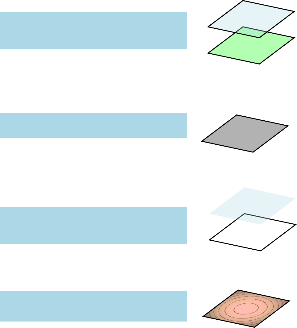
Layer β

Layer α

VERSION 0.5

The tikz-network package is still under development. Hence, changes in

the commands and functionality cannot be excluded.

version 0.5

https://github.com/hackl/tikz-network

Released, May 2018

Contents

1Introduction 5

1.1How to read this manual? ....................................... 6

1.1.1A few explanations ....................................... 6

1.1.2Inputs .............................................. 6

1.1.3Additional help ......................................... 7

1.2Installation ................................................ 7

1.3Additional necessary packages .................................... 7

2Simple Networks 9

2.1Vertex ................................................... 9

2.2Edge ................................................... 14

2.3Text .................................................... 20

3Complex Networks 23

3.1Vertices .................................................. 23

3.2Edges ................................................... 27

4Multilayer Networks 31

4.1Simple Networks ............................................ 31

4.2Complex Networks ........................................... 32

4.3Layers and Layouts ........................................... 33

4.4Plane ................................................... 34

5Default Settings 37

5.1General Settings ............................................. 37

5.2Vertex Style ............................................... 38

5.3Edge Style ................................................ 38

5.4Text Style ................................................. 39

5.5Plane Style ................................................ 39

6Troubleshooting and Support 41

6.1tikz-network Website ......................................... 41

6.2Getting Help ............................................... 41

6.3Errors, Warnings, and Informational Messages ........................... 41

6.4Package Dependencies ......................................... 41

A ToDo 43

A.1Code to ﬁx ................................................ 43

A.2Documentation ............................................. 43

A.3Features ................................................. 43

4CONTENTS

A.4Add-ons ................................................. 43

B Add-ons 45

B.1Python networks to TikZ with network2tikz ............................ 45

B.1.1Introduction ........................................... 45

B.1.2Installation ............................................ 46

B.1.3Usage ............................................... 46

B.1.4Simple example ......................................... 47

B.1.5The plot function in detail ................................... 50

Index 55

1Introduction

In recent years, complex network theory becomes more and more

popular within the scientiﬁc community. Besides a solid mathemat-

ical base on which these theories are built on, a visual representa-

tion of the networks allow communicating complex relationships to

a broad audience.

Nowadays, a variety of great visualization tools are available,

which helps to structure, ﬁlter, manipulate and of course to visu-

alize the networks. However, they come with some limitations,

including the need for speciﬁc software tools, difﬁculties to embed

the outputs properly in a L

EX ﬁle (e.g. font type, font size, addi-

tional equations and math symbols needed, . . . ) and challenges in

the post-processing of the graphs, without rerunning the software

tools again.

In order to overcome this issues, the package tikz-network was

created. Some of the features are:

• L

EX is a standard for scientiﬁc publications and widely used

• beside L

EX no other software is needed

• no programming skills are needed

• simple to use but allows 100% control over the output

• easy for post-processing (e.g. adding drawings, texts, equa-

tions,. . . )

• same fonts, font sizes, mathematical symbols, . . . as in the docu-

ment

• no quality loss of the output due to the pdf format

• networks are easy to adapt or modify for lectures or small exam-

ples

• able to visualize larger networks

• three-dimensional visualization of (multilayer) networks

• compatible with other visualization tools

6 introduction

1.1How to read this manual?

The aim of this manual is to describe the use of the tikz-network

library for visualizing networks. To ensure an easy use of the ele-

ments and to keep the clarity, this manual is structured as follows:

• In Chapter 2the elements to create simple networks (by hand)

in a plane are explained. Thereby, the use of the commands

\Vertex and \Edge are shown.

• How to create complex networks from external ﬁles1are ex- 1e.g. igraph or networkx

plained in Chapter 3. The main commands, therefore are \Vertices

and \Edges which are using the same options as in the simple

case.

• In Chapter 4, the visualization of multilayer networks is ex-

plained. Additional visualization tools such as \Plane and Layer

are introduced.

• The default settings used and how they can be modiﬁed is ex-

plained in Chapter 5.

• Information about troubleshooting and support is given in Chap-

ter 6

• Since this is the alpha version (0.1) of the package, features

which will be probably added and commands which have to

be ﬁxed are listed in Appendix B.

1.1.1A few explanations

The images in this manual are created with the tikz-network li-

brary or TikZ . The code used for this is speciﬁed for each image.

\begin{tikzpicture}

\filldraw (-.2,.2) circle (2pt) (.2,.2) circle (2pt);

\draw (0,0) circle (5mm) (-.3,-.1) .. controls (0,-.3) ..

(.3,-.1);

\end{tikzpicture}

Special additions which are needed for a better understanding

are shown in orange but are not in the sample code available.

\begin{tikzpicture}

\draw (0,0) .. controls (1,1) and (2,1) .. (2,0);

\end{tikzpicture}

1.1.2Inputs

The commands in the tikz-network library (e.g. \Vertex,\Edge)

always start with capital letters and DO NOT need a semicolon «;»

at the end. Boolean arguments start also with capital letters (e.g.

hNoLabeli). Arguments which need an user input, use are written in

small letters (e.g. hcolori).

tikz-network manual 7

Basically, one can distinguish between the mandatory argument

{ } and the optional argument [ ]. The ﬁrst values must be entered

compulsory. By contrast, nothing has to be entered for the optional

input. Additional features (e.g. hsizei)) can be activated when enter-

ing optional parameters.

When entering size values the base unit is always predeﬁned in

[cm]2, except for line widths which are dedined in [pt]. Percent- 2The default unit can be changed with

\SetDefaultUnit; see Section 5.1

age values % are always speciﬁed as decimal values; for example,

100% =1.0 and 10% corresponds to 0.1.

1.1.3Additional help

Is the manual not enough, occur some ambiguities or some TikZ

commands are unclear, please have a look in the “TikZ and PGF

Manual” from Till Tantau3.3http://mirror.switch.ch/ftp/

mirror/tex/graphics/pgf/base/doc/

pgfmanual.pdf

Should you have any further questions, please do not hesitate to

contact me.

1.2Installation

Actually, we can hardly speak of an installation since only the nec-

essary package tikz-network must be loaded in the preamble of

your document.

The current release of the package is available via CTAN4. A 4TODO! upload the package to

CTAN, and add here the link

release candidate for the next version of tikz-network is available

on github55https://github.com/hackl/

Is the package installed or the style ﬁle is stored in the folder

of the main ﬁle, so the library can be imported, as the following

example shows:

% ------------

% header

\documentclass{scrreprt}

% ------------

% packages

\usepackage{tikz-network}

1.3Additional necessary packages

To use all commands and options of TikZ , possibly some packages

need to be reloaded. These missing ﬁles (or their names) appear in

the error log when you convert the ﬁle. However, for the package

described in this manual, it is sufﬁcient to use the library and the

TikZ standard commands.

2Simple Networks

2.1Vertex

On essential command is \Vertex, which allow placing vertices in

the document and modify their appearance.

\Vertex[hlocal optionsi]{Name}

In order to be able to place a vertex, a non-empty Name argument is

required. This argument deﬁnes the vertex’s reference name, which

must be unique. Mathematical symbols are not allowed as name

as well as no blank spaces. The Name should not be confused with

the hlabeli, that is used for display; for example one may want to

display A1while the name will be A1.

For a \Vertex the following options are available:

Option Default Type Deﬁnition

x0measure x-coordinate

y0measure y-coordinate

size {} measure diameter of the circle

color {} color ﬁll color of vertex

opacity {} number opacity of the ﬁll color

shape {} string shape of the vertex

label {} string label

fontsize {} string font size of the label

fontcolor {} color font color of the label

fontscale {} number scale of the label

position center valuealabel position

distance 0measure label distance from the center

style {} string additional TikZ styles

layer {} number assigned layer of the vertex

NoLabel false Boolean delete the label

IdAsLabel false Boolean uses the Name as label

Math false Boolean displays the label in math mode

RGB false Boolean allow RGB colors

Pseudo false Boolean create a pseudo vertex

aeither measure or string

Table 2.1: Local options for the

\Vertex command.

The order how the options are entered does not matter. Changes

to the default Vertex layout can be made with \SetVertexStyle11see Section 5.2

\Vertex[hxi=measure,hyi=measure]{Name}

The location of the vertices are determined by Cartesian coordi-

nates in hxiand hyi. The coordinates are optional. If no coordinates

are determined the vertex will be placed at the origin (0, 0). The

10 simple networks

entered measures are in default units (cm). Changing the unites (lo-

cally) can be done by adding the unit to the measure2. Changes to 2e.g. x=1 in

the default setting can be made with \SetDefaultUnit3.3see Section 5.1

\begin{tikzpicture}

\Vertex{A}

\Vertex[x=1,y=1]{B}

\Vertex[x=2]{C}

\end{tikzpicture}

\Vertex[hsizei=measure]{Name}

The diameter of the vertex can be changed with the option hsizei.

Per default a vertex has 0.6 cm in diameter. Also, here the default

units are cm and have not to be added to the measure.

\begin{tikzpicture}

\Vertex[size=.3]{A}

\Vertex[x=1,size=.7]{B}

\Vertex[x=2.3,size=1]{C}

\end{tikzpicture}

\Vertex[hcolori=color]{Name}

To change the ﬁll color of each vertex individually, the option

hcolorihas to be used. Without the option hRGBiset, the default

TikZ and L

EX colors can be applied.

\begin{tikzpicture}

\Vertex[color = blue]{A}

\Vertex[x=1,color=red]{B}

\Vertex[x=2,color=green!70!blue]{C}

\end{tikzpicture}

\Vertex[hopacityi=number]{Name}

With the option hopacityithe opacity of the vertex ﬁll color can

be modiﬁed. The range of the number lies between 0 and 1. Where 0

represents a fully transparent ﬁll and 1 a solid ﬁll.

\begin{tikzpicture}

\Vertex[opacity = 1]{A}

\Vertex[x=1,opacity =.7]{B}

\Vertex[x=2,opacity =.2]{C}

\end{tikzpicture}

\Vertex[hshapei=string]{Name}

With the option hshapeithe shape of the vertex can be modiﬁed.

Thereby the shapes implemented in TikZ can be used, including:

circle,rectangle,diamond,trapezium,semicircle,isosceles triangle,....

\begin{tikzpicture}

\Vertex[shape = rectangle]{A}

\Vertex[x=1,shape = diamond]{B}

\Vertex[x=2,shape = isosceles triangle]{C}

\end{tikzpicture}

tikz-network manual 11

\Vertex[hlabeli=string]{Name}

In tikz-network there are several ways to deﬁne the labels of

the vertices and edges. The common way is via the option hlabeli.

Here, any string argument can be used, including blank spaces. The

environment $ $ can be used to display mathematical expressions.

foo bar u1

\begin{tikzpicture}

\Vertex[label=foo]{A}

\Vertex[x=1,label=bar]{B}

\Vertex[x=2,label=$u_1$]{C}

\end{tikzpicture}

\Vertex[hlabeli=string,hfontsizei=string]{Name}

The font size of the hlabelican be modiﬁed with the option

hfontsizei. Here common L

EX font size commands4can be used 4e.g. \tiny,\scriptsize,

\footnotesize,\small,....

to change the size of the label.

foo bar u1

\begin{tikzpicture}

\Vertex[label=foo,fontsize=\normalsize]{A}

\Vertex[x=1,label=bar,fontsize=\tiny]{B}

\Vertex[x=2,label=$u_1$,fontsize=\large]{C}

\end{tikzpicture}

\Vertex[hlabeli=string,hfontcolori=color]{Name}

The color of the hlabelican be changed with the option hfontcolori.

Currently, only the default TikZ and L

EX colors are supported5.5TODO! Add RGB option!

foo bar u1

\begin{tikzpicture}

\Vertex[label=foo,fontcolor=blue]{A}

\Vertex[x=1,label=bar,fontcolor=magenta]{B}

\Vertex[x=2,label=$u_1$,fontcolor=red]{C}

\end{tikzpicture}

\Vertex[hlabeli=string,hfontscalei=number]{Name}

Contrary to the option hfontsizei, the option hfontscaleidoes

not change the font size itself but scales the curent font size up

or down. The number deﬁnes the scale, where numbers between

0 and 1 down scale the font and numbers greater then 1 up scale

the label. For example 0.5 reduces the size of the font to 50% of its

originial size, while 1.2 scales the font to 120%.

foo bar u1

\begin{tikzpicture}

\Vertex[label=foo,fontscale=0.5]{A}

\Vertex[x=1,label=bar,fontscale=1]{B}

\Vertex[x=2,label=$u_1$,fontscale=2]{C}

\end{tikzpicture}

\Vertex[hlabeli=string,hpositioni=value,hdistancei=number]{Name}

Per default the hpositioniof the hlabeliis in the center of the ver-

tex. Classical TikZ commands6can be used to change the hpositioni6e.g. above,below,left,right,above left,

above right,. . .

12 simple networks

of the hlabeli. Instead, using such command, the position can be

determined via an angle, by entering a number between −360 and

360. The origin (0◦) is the yaxis. A positive number change the

hpositionicounter clockwise, while a negative number make changes

clockwise.

With the option, hdistanceithe distance between the vertex and

the label can be changed.

30◦

\begin{tikzpicture}

\Vertex[label=A,position=below]{A}

\Vertex[x=1,label=B,position=below,distance=2mm]{B}

\Vertex[x=2,label=C,position=30,distance=1mm]{C}

\end{tikzpicture}

\Vertex[hstylei={string}]{Name}

Any other TikZ style option or command can be entered via

the option hstylei. Most of these commands can be found in the

“TikZ and PGF Manual”. Contain the commands additional op-

tions (e.g.hshadingi=ball), then the argument for the hstyleihas to be

between { } brackets.

\begin{tikzpicture}

\Vertex[style={color=green}]{A}

\Vertex[x=1,style=dashed]{B}

\Vertex[x=2,style={shading=ball}]{C}

\end{tikzpicture}

\Vertex[hIdAsLabeli]{Name}

\Vertex[hNoLabeli,hlabeli=string]{Name}

hIdAsLabeliis a Boolean option which assigns the Name of the

vertex as label. On the contrary, hNoLabelisuppress all labels.

\begin{tikzpicture}

\Vertex[IdAsLabel]{A}

\Vertex[x=1,label=B,NoLabel]{B}

\Vertex[x=2,IdAsLabel,NoLabel]{C}

\end{tikzpicture}

\Vertex[hMathi,hlabeli=string]{Name}

The option hMathiallows transforming labels into mathematical

expressions without using the $ $ environment. In combination

with hIdAsLabeliallows this option also mathematical expressions

by the deﬁnition of the vertex Name.

A1B1C1

\begin{tikzpicture}

\Vertex[IdAsLabel]{A1}

\Vertex[x=1,label=B_1,Math]{B}

\Vertex[x=2,Math,IdAsLabel]{C_1}

\end{tikzpicture}

\Vertex[hRGBi,hcolori=RGB values]{Name}

tikz-network manual 13

In order to display RGB colors for the vertex ﬁll color, the op-

tion hRGBihas to be entered. In combination with this option, the

hcolorihast to be a list with the RGB values, separated by «,» and

within { }.77e.g. the RGB code for white:

{255, 255, 255}

\begin{tikzpicture}

\Vertex[RGB,color={127,201,127}]{A}

\Vertex[x=1,RGB,color={190,174,212}]{B}

\Vertex[x=2,RGB,color={253,192,134}]{C}

\end{tikzpicture}

\Vertex[hPseudoi]{Name}

The option hPseudoicreates a pseudo vertex, where only the

vertex name and the vertex coordinate will be drawn. Edges etc,

can still be assigned to this vertex.

\begin{tikzpicture}

\Vertex{A}

\Vertex[x=2,Pseudo]{B}

\end{tikzpicture}

\Vertex[hlayeri=number]{Name}

With the option hlayerithe vertex can be assigned to a speciﬁc

layer. More about this option and the use of layers is explained in

Chapter 4.

14 simple networks

2.2Edge

The second essential command is an \Edge, which allow connecting

two vertices.

\Edge[hlocal optionsi](Vertex i)(Vertex j)

Edges can be generated between one or two vertices. In the ﬁrst

case, a self-loop will be generated. As mandatory arguments the

Names of the vertices which should be connected must be entered

between ( ) brackets. In case of a directed edge, the order is impor-

tant. An edge is created from Vertex i (origin) to Vertex j (destina-

tion).

For an \Edge the following options are available:

Option Default Type Deﬁnition

lw {} measure line width of the edge

color {} color edge color

opacity {} number opacity of the edge

bend 0number angle out/in of the vertex

label {} string label

fontsize {} string font size of the label

fontcolor {} color font color of the label

fontscale {} number scale of the label

position {} string label position

distance 0.5number label distance from vertex i

style {} string additional TikZ styles

path {} list path over several vertices

loopsize 1cm measure size parameter of the self-loop

loopposition 0number orientation of the self-loop

loopshape 90 number loop angle out/in of the vertex

Direct false Boolean allow directed edges

Math false Boolean displays the label in math mode

RGB false Boolean allow RGB colors

NotInBG false Boolean edge is not in the background layer

Table 2.2: Local options for the \Edge

command.

The options hloopsizei,hlooppositioni, and hloopsizeiare only for

self-loops available.

\Edge(Vertex i)(Vertex j)

An edge is created between Vertex i and Vertex j.

\begin{tikzpicture}

\Vertex{A} \Vertex[x=2]{B}

\Edge(A)(B)

\end{tikzpicture}

\Edge[hlwi=measure](Vertex i)(Vertex j)

The line width of an edge can be modiﬁed with the option hlwi.

Here, the unit of the measure has to be speciﬁed. The default value

is 1.5 pt.

tikz-network manual 15

\begin{tikzpicture}

\Vertex{A} \Vertex[x=2]{B} \Vertex[x=2,y=-1]{C}

\Edge[lw=3pt](A)(B)

\Edge[lw=5pt](A)(C)

\end{tikzpicture}

\Edge[hcolori=color](Vertex i)(Vertex j)

To change the line color of each edge individually, the option

hcolorihas to be used. Without the option hRGBiset, the default

TikZ and L

EX colors can be applied.

\begin{tikzpicture}

\Vertex{A} \Vertex[x=2]{B} \Vertex[x=2,y=-1]{C}

\Edge[color=red](A)(B)

\Edge[color=green!70!blue](A)(C)

\end{tikzpicture}

\Edge[hopacityi=number](Vertex i)(Vertex j)

With the option hopacityithe opacity of the edge line can be

modiﬁed. The range of the number lies between 0 and 1. Where 0

represents a fully transparent ﬁll and 1 a solid ﬁll.

\begin{tikzpicture}

\Vertex{A} \Vertex[x=2]{B} \Vertex[x=2,y=-1]{C}

\Edge[opacity=.7](A)(B)

\Edge[opacity=.2](A)(C)

\end{tikzpicture}

\Edge[hbendi=number](Vertex i)(Vertex j)

The shape of the edge can be modiﬁed with the hbendioption. If

nothing is speciﬁed a straight edge, between the vertices, is drawn.

The number deﬁnes the angle in which the edge is diverging from

its straight connection. A positive number bend the edge counter

clockwise, while a negative number make changes clockwise.

45◦

70◦

\begin{tikzpicture}

\Vertex{A} \Vertex[x=2]{B}

\Edge[bend=45](A)(B)

\Edge[bend=-70](A)(B)

\end{tikzpicture}

\Edge[hlabeli=string](Vertex i)(Vertex j)

An edge is labeled with the option hlabeli. For the label any

string argument can be used, including blank spaces. The environ-

ment $ $ can be used to display mathematical expressions.

\begin{tikzpicture}

\Vertex{A} \Vertex[x=2]{B}

\Edge[label=X](A)(B)

\end{tikzpicture}

16 simple networks

\Edge[hlabeli=string,hfontsizei=string](Vertex i)(Vertex j)

The font size of the hlabelican be modiﬁed with the option

hfontsizei. Here common L

EX font size commands8can be used 8e.g. \tiny,\scriptsize,

\footnotesize,\small,....

to change the size of the label.

\begin{tikzpicture}

\Vertex{A} \Vertex[x=2]{B} \Vertex[x=2,y=-1]{C}

\Edge[label=X,fontsize=\large](A)(B)

\Edge[label=Y,fontsize=\tiny](A)(C)

\end{tikzpicture}

\Edge[hlabeli=string,hfontcolori=color](Vertex i)(Vertex j)

The color of the hlabelican be changed with the option hfontcolori.

Currently, only the default TikZ and L

EX colors are supported 9.9TODO! Add RGB option!

\begin{tikzpicture}

\Vertex{A} \Vertex[x=2]{B} \Vertex[x=2,y=-1]{C}

\Edge[label=X,fontcolor=blue](A)(B)

\Edge[label=Y,fontcolor=red](A)(C)

\end{tikzpicture}

\Edge[hlabeli=string,hfontscalei=color](Vertex i)(Vertex j)

Contrary to the option hfontsizei, the option hfontscaleidoes

not change the font size itself but scales the curent font size up

or down. The number deﬁnes the scale, where numbers between

0 and 1 down scale the font and numbers greater then 1 up scale

the label. For example 0.5 reduces the size of the font to 50% of its

originial size, while 1.2 scales the font to 120%.

\begin{tikzpicture}

\Vertex{A} \Vertex[x=2]{B} \Vertex[x=2,y=-1]{C}

\Edge[label=X,fontscale=.5](A)(B)

\Edge[label=Y,fontscale=2](A)(C)

\end{tikzpicture}

\Edge[hlabeli=string,hpositioni=string](Vertex i)(Vertex j)

Per default the hlabeliis positioned in between both vertices in

the center of the line. Classical TikZ commands10 can be used to 10 e.g. above,below,left,right,above left,

above right,. . .

change the hpositioniof the hlabeli.

\begin{tikzpicture}

\Vertex{A} \Vertex[x=2]{B} \Vertex[x=2,y=-1]{C}

\Edge[label=X,position=above](A)(B)

\Edge[label=Y,position={below left=2mm}](A)(C)

\end{tikzpicture}

\Edge[hlabeli=string,hdistancei=number](Vertex i)(Vertex j)

The label position between the vertices can be modiﬁed with the

hdistanceioption. Per default the hlabeliis centered between both

vertices. The position is expressed as the percentage of the length

between the vertices, e.g. of hdistancei=0.7, the label is placed at 70%

of the edge length away of Vertex i.

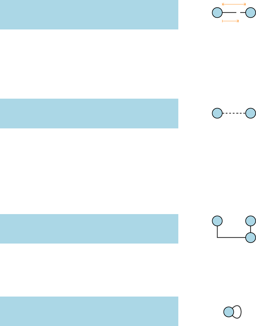
tikz-network manual 17

0.7

1.0

\begin{tikzpicture}

\Vertex{A} \Vertex[x=2]{B}

\Edge[label=X,distance=.7](A)(B)

\end{tikzpicture}

\Edge[hstylei=string](Vertex i)(Vertex j)

Any other TikZ style option or command can be entered via

the option hstylei. Most of these commands can be found in the

“TikZ and PGF Manual”. Contain the commands additional op-

tions (e.g.hshadingi=ball), then the argument for the hstyleihas to be

between { } brackets.

\begin{tikzpicture}

\Vertex{A} \Vertex[x=2]{B}

\Edge[style={dashed}](A)(B)

\end{tikzpicture}

\Edge[hpathi=list](Vertex i)(Vertex j)

In order to draw a ﬁnite sequence of edges which connect a se-

quence of vertices and/or coordinates, the option hpathican be

used11. The argument for this option has to be a list element indi- 11 TODO! currently labels and bend

edges are not supported!

cated by { } brackets, containing the Names of the intermediated

vertices. New coordinates, i.e. there is no vertex located, can be in-

sert with {hxi,hyi}. Arguments of the list, have to be seperated by

commas «,».

\begin{tikzpicture}

\Vertex{A} \Vertex[x=2]{B} \Vertex[x=2,y=-1]{C}

\Edge[path={A,{0,-1},C,B}](A)(B)

\end{tikzpicture}

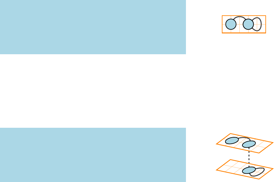
\Edge(Vertex i)(Vertex i)

Self-loops are created by using the same vertex as origin and

destination. Beside the options explained above, there are three

self-loop speciﬁc options: hloopsizei,hlooppositioni, and hloopshapei.

\begin{tikzpicture}

\Vertex{A}

\Edge(A)(A)

\end{tikzpicture}

\Edge[hloopsizei=measure](Vertex i)(Vertex i)

With the option hloopsizeithe length of the edge can be modi-

ﬁed. The measure value has to be insert together with its units. Per

default the hloopsizeiis 1 cm.

18 simple networks

\begin{tikzpicture}

\Vertex{A} \Vertex[x=1.3]{B}

\Edge[loopsize=.5cm](A)(A)

\Edge[loopsize=1.5cm](B)(B)

\end{tikzpicture}

\Edge[hlooppositioni=number](Vertex i)(Vertex i)

The position of the self-loop is deﬁned via the rotation angle

around the vertex. The origin (0◦) is the yaxis. A positive number

change the hlooppositionicounter clockwise, while a negative number

make changes clockwise.

45◦

70◦

\begin{tikzpicture}

\Vertex{A} \Vertex[x=1.5]{B}

\Edge[loopposition=45](A)(A)

\Edge[loopposition=-70](B)(B)

\end{tikzpicture}

\Edge[hloopshapei=number](Vertex i)(Vertex i)

The shape of the self-loop is deﬁned by the enclosing angle. The

shape can be changed by decreasing or increasing the argument

value of the hloopshapeioption.

45◦

\begin{tikzpicture}

\Vertex{A}

\Edge[loopshape=45](A)(A)

\end{tikzpicture}

\Edge[hDirecti](Vertex i)(Vertex j)

Directed edges are created by enabling the option hDirecti. The

arrow is drawn from Vertex i to Vertex j.

\begin{tikzpicture}

\Vertex{A} \Vertex[x=2]{B}

\Edge[Direct](A)(B)

\end{tikzpicture}

\Edge[Math, label=hstringi](Vertex i)(Vertex j)

The option hMathiallows transforming labels into mathematical

expressions without using the $ $ environment.

\begin{tikzpicture}

\Vertex{A} \Vertex[x=2]{B}

\Edge[Math,label=X_1](A)(B)

\end{tikzpicture}

\Edge[RBG, color=hRGB valuei](Vertex i)(Vertex j)

tikz-network manual 19

In order to display RGB colors for the line color of the edge, the

option hRGBihas to be entered. In combination with this option,

the hcolorihast to be a list with the RGB values, separated by «,» and

within { }.12 12 e.g. the RGB code for white:

{255, 255, 255}

\begin{tikzpicture}

\Vertex{A} \Vertex[x=2]{B} \Vertex[x=2,y=-1]{C}

\Edge[RGB,color={127,201,127}](A)(B)

\Edge[RGB,color={253,192,134}](A)(C)

\end{tikzpicture}

\Edge[hNotInBGi]{ﬁlename}

Per default, the edge is drawn on the background layer of the

tikzpicture. I.e. objects which are created after the edges appear

also on top of them. To turn this off, the option hNotInBGihas

to be enabled. Changes to the default setting can be made with

\EdgesNotInBG or \EdgesInBG13.13 See Section 5.3

\begin{tikzpicture}

\Vertex{A} \Vertex[x=2]{B} \Vertex[x=1,y=-.5]{C}

\Vertex[y=-1]{D} \Vertex[x=2,y=-1]{E}

\Edge[bend=-30](A)(B)

\Edge[bend=30,NotInBG](D)(E)

\end{tikzpicture}

20 simple networks

2.3Text

While TikZ offers multiple ways to label objects and create text

elements, a simpliﬁed command \Text is implemented, which

allow placing and modifying text to the networks.

\Text[hlocal optionsi]{string}

In order to be able to create a text, a non-empty string argument

is required. This argument is the actual text added to the ﬁgure.

Mathematical symbols are entered in the same way as in a normal

EX document, i.e. between $ $.

For a \Text the following options are available:

Option Default Type Deﬁnition

x0measure x-coordinate

y0measure y-coordinate

fontsize {} fontsize font size of the text

color {} color color of the text

opacity {} number opacity of the text

position center string position of the text to the origin

distance 0 cm measure distance from the origin

rotation 0number rotation of the text

anchor {} string anchor of the text

width {} number width of the text box

style {} string additional TikZ styles

layer {} number assigned layer of the text

RGB false Boolean allow RGB colors

Table 2.3: Local options for the \Text

command.

The order how the options are entered does not matter. Changes

to the default Text layout can be made with \SetTextStyle14 14 see Section 5.4

\Text[hxi=measure,hyi=measure]{string}

The location of the text is determined by Cartesian coordinates

in hxiand hyi. The coordinates are optional. If no coordinates are

determined the text will be placed at the origin (0, 0). The entered

measures are in default units (cm). Changing the unites (locally) can

be done by adding the unit to the measure15. Changes to the default 15 e.g. x=1 in

setting can be made with \SetDefaultUnit16.16 see Section 5.1

\begin{tikzpicture}

\Text{A}

\Text[x=1,y=1]{B}

\Text[x=2]{C}

\end{tikzpicture}

\Text[hfontsizei=font size]{string}

The font size of the text can be changed with the option hfontsizei.

Per default the font size of the text is deﬁned as \normalsize.

ABC

\begin{tikzpicture}

\Text[fontsize=\small]{A}

\Text[x=1,fontsize=\LARGE]{B}

\Text[x=2,fontsize=\Huge]{C}

\end{tikzpicture}

tikz-network manual 21

\Text[hcolori=color]{string}

To change the text color individually, the option hcolorihas to be

used. Without the option hRGBiset, the default TikZ and L

EX col-

ors can be applied.

ABC

\begin{tikzpicture}

\Text[color = blue]{A}

\Text[x=1,color=red]{B}

\Text[x=2,color=green!70!blue]{C}

\end{tikzpicture}

\Text[hopacityi=number]{string}

With the option hopacityithe opacity of the text can be modiﬁed.

The range of the number lies between 0 and 1. Where 0 represents a

fully transparent text and 1 a solid text.

A B C

\begin{tikzpicture}

\Text[opacity = 1]{A}

\Text[x=1,opacity =.7]{B}

\Text[x=2,opacity =.2]{C}

\end{tikzpicture}

\Text[hpositioni=string,hdistancei=measure]{string}

Per default the hpositioniof the text is in the center of the origin.

Classical TikZ commands17 can be used to change the hpositioniof 17 e.g. above,below,left,right,above left,

above right,. . .

the text.

With the option, hdistanceithe distance between the text and the

origin can be changed.

origin (0, 0)

above

below

left

above right

\begin{tikzpicture}

\Text[position=above]{above}

\Text[position=below]{below}

\Text[position=left,distance=5mm]{left}

\Text[position=above right,distance=5mm]{above right}

\end{tikzpicture}

\Text[hrotationi=number]{string}

With the hrotationi, the text can be rotated by entering a number

between −360 and 360. The origin (0◦) is the yaxis. A positive

number change the hpositionicounter clockwise, while a negative

number make changes clockwise.

75◦

\begin{tikzpicture}

\Text[rotation=30]{A}

\Text[x=1,rotation=45]{B}

\Text[x=2,rotation=75]{C}

\end{tikzpicture}

22 simple networks

\Text[hanchori=string]{string}

With the option hanchorithe alignment of the text can be changed.

Per default the text will be aligned centered. Classical TikZ com-

mands18 can be used to change the alignment of the text. 18 e.g. north,east,south,west,north east,

north west,. . .

S SW

\begin{tikzpicture}

\Text[anchor=north east]{NE}

\Text[x=1,anchor = south]{S}

\Text[x=2,anchor =south west]{SW}

\end{tikzpicture}

\Text[hwidthi=measure]{string}

With the option hwidthienabled, the text will break after the

entered measure.

2.5cm

This might be a

very long text.

\begin{tikzpicture}

\Text[width=2.5cm]{This might be a very long text.}

\end{tikzpicture}

\Text[hstylei={string}]{string}

Any other TikZ style option or command can be entered via

the option hstylei. Most of these commands can be found in the

“TikZ and PGF Manual”. Contain the commands additional options

(e.g.hﬁlli=red), then the argument for the hstyleihas to be between

{ } brackets.

A B C

\begin{tikzpicture}

\Text[style={draw,rectangle}]{A}

\Text[x=1,style={fill=red}]{B}

\Text[x=2,style={fill=blue,circle,opacity=.3}]{C}

\end{tikzpicture}

\Text[hRGBi,hcolori=RGB values]{string}

In order to display RGB colors for the text color, the option

hRGBihas to be entered. In combination with this option, the

hcolorihast to be a list with the RGB values, separated by «,» and

within { }.19 19 e.g. the RGB code for white:

{255, 255, 255}

ABC

\begin{tikzpicture}

\Text[RGB,color={127,201,127}]{A}

\Text[x=1,RGB,color={190,174,212}]{B}

\Text[x=2,RGB,color={253,192,134}]{C}

\end{tikzpicture}

\layer[hlayeri=number]{string}

With the option hlayerithe text can be assigned to a speciﬁc

layer. More about this option and the use of layers is explained in

Chapter 4.

3Complex Networks

While in Chapter 2the building blocks of the networks are in-

troduced, here the main strength of the tikz-network package is

explained. This includes creating networks based on data, obtained

from other sources (e.g. Python, R, GIS). The idea is that the lay-

out will be done by this external sources and tikz-network is used

make some changes and to recreate the networks in L

EX.

3.1Vertices

The \Vertices command is the extension of the \Vertex command.

Instead of a single vertex, a set of vertices will be drawn. This set

of vertices is deﬁned in an external ﬁle but can be modiﬁed with

\Vertices.

\Vertices[hglobal optionsi]{ﬁlename}

The vertices have to be stored in a clear text ﬁle1, preferentially 1e.g. .txt, .tex, .csv, .dat, . . .

in a .csv format. The ﬁrst row should contain the headings, which

are equal to the options deﬁned in Table 2.1. Option are separated

by a comma «,». Each new row is corresponds to a new vertex.

File: vertices.csv

id, x, y ,size,color ,opacity,label,IdAsLabel,NoLabel

A, 0, 0, .4 ,green , .9 , a , false , false

B, 1, .7, .6 , , .5 , b , false , false

C, 2, 1, .8 ,orange, .3 , c , false , true

D, 2, 0, .5 ,red , .7 , d , true , false

E,.2,1.5, .5 ,gray , , e , false , false

Only the hidivalue is mandatory for a vertex and corresponds

to the Name argument of a single \Vertex. Therefore, the same

rules and naming conventions apply as for the Name argument:

no mathematical expressions, no blank spaces, and the hidimust

be unique! All other options are optional. No speciﬁc order of the

options must be maintained. If no value is entered for an option,

the default value will be chosen2. The ﬁlename should not contain 2TODO! This is NOT valid for

Boolean options, here values for all

vertices have to be entered.

blank spaces or special characters. The vertices are drawn by the

command \Vertex with the ﬁlename plus ﬁle format (e.g. .csv). If

the vertices ﬁle is not in the same directory as the main L

EX ﬁle,

also the path has to be speciﬁed.

24 complex networks

\begin{tikzpicture}

\Vertices{data/vertices.csv}

\end{tikzpicture}

Predeﬁned \Vertex options can be overruled by the hglobal op-

tionsiof the \Vertices command; I.e. these options apply for all

vertices in the ﬁle. For the \Vertices the following options are

available:

Option Default Type Deﬁnition

size {} measure diameter of the circles

color {} color ﬁllcolor of vertices

opacity {} number opacity of the ﬁll color

style {} string additional TikZ styles

layer {} number assigned layer of the vertices

NoLabel false Boolean delete the labels

IdAsLabel false Boolean uses the Names as labels

Math false Boolean displays the labels in math mode

RGB false Boolean allow RGB colors

Pseudo false Boolean create a pseudo vertices

Table 3.1: Global options for the

\Vertices command.

The use of these options are similar to the options for a single

\Vertex deﬁned in Section 2.1.

\Vertices[hsizei=measure]{ﬁlename}

The diameter of the vertices can be changed with the option

hsizei. Per default a vertex has 0.6 cm in diameter. Also, here the

default units are cm and have not to be added to the measure.

\begin{tikzpicture}

\Vertices[size=.6]{data/vertices.csv}

\end{tikzpicture}

\Vertices[hcolori=color]{ﬁlename}

To change the ﬁll color for all vertices, the option hcolorihas

to be used. Without the option hRGBiset, the default TikZ and

EX colors can be applied.

\begin{tikzpicture}

\Vertices[color=green!70!blue]{data/vertices.csv}

\end{tikzpicture}

\Vertices[hopacityi=number]{ﬁlename}

With the option hopacityithe opacity of all vertices ﬁlls colors can

be modiﬁed. The range of the number lies between 0 and 1. Where 0

represents a fully transparent ﬁll and 1 a solid ﬁll.

tikz-network manual 25

\begin{tikzpicture}

\Vertices[opacity=.3]{data/vertices.csv}

\end{tikzpicture}

\Vertices[hstylei=string]{ﬁlename}

Any other TikZ style option or command can be entered via

the option hstylei. Most of these commands can be found in the

“TikZ and PGF Manual”. Contain the commands additional op-

tions (e.g.hshadingi=ball), then the argument for the hstyleihas to be

between { } brackets.

\begin{tikzpicture}

\Vertices[style={shading=ball,blue}]{data/vertices.csv}

\end{tikzpicture}

\Vertices[hIdAsLabeli]{ﬁlename}

\Vertices[hNoLabeli]{ﬁlename}

hIdAsLabeliis a Boolean option which assigns the hidiof the

single vertices as labels. On the contrary, hNoLabelisuppress all

labels.

\begin{tikzpicture}

\Vertices[IdAsLabel]{data/vertices.csv}

\end{tikzpicture}

\begin{tikzpicture}

\Vertices[NoLabel]{data/vertices.csv}

\end{tikzpicture}

\Vertices[hRGBi]{ﬁlename}

In order to display RGB colors for the vertex ﬁll colors, the op-

tion hRGBihas to be entered. Additionally, the RGB values have to

be speciﬁed in the ﬁle where the vertices are stored. Each value has

its own column with the caption hRi,hGi, and hBi.

File: vertices_RGB.csv

id, x, y ,size, color,opacity,label, R , G , B

A, 0, 0, .4 , green, .9 , a ,255, 0, 0

B, 1, .7, .6 , , .5 , b , 0,255, 0

C, 2, 1, .8 ,orange, .3 , c , 0, 0,255

D, 2, 0, .5 , red, .7 , d , 10,120,255

E,.2,1.5, .5 , gray, , e , 76, 55,255

The “normal” color deﬁnition can also be part of the vertex def-

inition. If the option hRGBiis not set, then the colors under hcolori

are applied.

26 complex networks

\begin{tikzpicture}

\Vertices[RGB]{data/vertices_RGB.csv}

\end{tikzpicture}

\Vertices[hPseudoi]{ﬁlename}

The option hPseudoicreates a pseudo vertices, where only the

names and the coordinates of the vertices wil be drawn. Edges etc,

can still be assigned to these vertices.

\Vertices[hlayeri=number]{ﬁlename}

With the option hlayeri, only the vertices on the selected layer are

plotted. More about this option and the use of layers is explained in

Chapter 4.

tikz-network manual 27

3.2Edges

The \Edges command is the extension of the \Edge command.

Instead of a single edge, a set of edges will be drawn. This set

of edges is deﬁned in an external ﬁle but can be modiﬁed with

\Edges.

\Edges[hglobal optionsi]{ﬁlename}

Like the vertices, the edges have to be stored in a clear text ﬁle3,3e.g. .txt, .tex, .csv, .dat, . . .

preferentially in a .csv format. The ﬁrst row should contain the

headings, which are equal to the options deﬁned in Table 2.2. Op-

tion are separated by a comma «,». Each new row is corresponds to

a new edge.

File: edges.csv

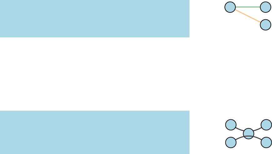
u,v,label,lw,color ,opacity,bend, R , G , B ,Direct

A,B, ab ,.5,red , 1 , 30, 0,120,255,false

B,C, bc ,.7,blue , 1 , -60, 76, 55,255,false

B,D, bd ,.5,blue , .5 , -60, 76, 55,255,false

A,E, ae , 1,green , 1 , 75,255, 0, 0,true

C,E, ce , 2,orange, 1 , 0,150,150,150,false

A,A, aa ,.3,black , .5 , 75,255, 0 ,0,false

The mandatory values are the huiand hviargument, which

corresponds to the Vertex i and Vertex j arguments of a single \Edge.

Edges can only create if a vertex exists with the same Name. All

other options are optional. No speciﬁc order of the options must be

maintained. If no value is entered for an option, the default value

will be chosen4. The ﬁlename should not contain blank spaces or 4TODO! This is NOT valid for

Boolean options, here values for all

vertices have to be entered.

special characters. The edges are drawn by the command \Edges

with the ﬁlename plus ﬁle format (e.g. .csv). If the edges ﬁle is not

in the same directory as the main L

EX ﬁle, also the path has to

be speciﬁed. In order to draw edges, ﬁrst, the vertices have to be

generated. Only then, edges can be assigned.

ab bc

aaa

\begin{tikzpicture}

\Vertices{data/vertices.csv}

\Edges{data/edges.csv}

\end{tikzpicture}

Predeﬁned \Edge options can be overruled by the hglobal optionsi

of the \Edges command; I.e. these options apply for all edges in the

ﬁle. For the \Edges the following options are available:

28 complex networks

Option Default Type Deﬁnition

lw {} measure line width of the edge

color {} color edge color

opacity {} number opacity of the edge

style {} string additional TikZ styles

vertices {} ﬁle vertices were the edges are assigned to

layer {} number edges in speciﬁc layers

Direct false Boolean allow directed edges

Math false Boolean displays the labels in math mode

NoLabel false Boolean delete the labels

RGB false Boolean allow RGB colors

NotInBG false Boolean edges are not in the background layer

Table 3.2: Global options for the

\Edges command.

The use of these options are similar to the options for a single

\Edge deﬁned in Section 2.2.

\Edges[hlwi=measure]{ﬁlename}

The line width of the edges can be modiﬁed with the option

hlwi. Here, the unit of the measure can be speciﬁed, otherwise, it is

in pt.

ab bc

aaa

\begin{tikzpicture}

\Vertices{data/vertices.csv}

\Edges[lw=2.5]{data/edges.csv}

\end{tikzpicture}

\Edges[hcolori=color]{ﬁlename}

To change the line color of all edges, the option hcolorihas to be

used. Without the option hRGBiset, the default TikZ and L

EX col-

ors can be applied.

ab bc

aaa

\begin{tikzpicture}

\Vertices{data/vertices.csv}

\Edges[color=green!70!blue]{data/edges.csv}

\end{tikzpicture}

\Edges[hopacityi=number]{ﬁlename}

With the option hopacityithe opacity of all edge lines can be

modiﬁed. The range of the number lies between 0 and 1. Where 0

represents a fully transparent ﬁll and 1 a solid ﬁll.

ab bc

aaa

\begin{tikzpicture}

\Vertices{data/vertices.csv}

\Edges[opacity=0.3]{data/edges.csv}

\end{tikzpicture}

tikz-network manual 29

\Edges[hstylei=string]{ﬁlename}

Any other TikZ style option or command can be entered via the

option hstylei. Most of these commands can be found in the “TikZ

and PGF Manual”.

ab bc

aaa

\begin{tikzpicture}

\Vertices{data/vertices.csv}

\Edges[style={dashed}]{data/edges.csv}

\end{tikzpicture}

\Edges[hDirecti]{ﬁlename}

Directed edges are created by enabling the option hDirecti. The

arrow is drawn from huito hvi.

ab bc

aaa

\begin{tikzpicture}

\Vertices{data/vertices.csv}

\Edges[Direct]{data/edges.csv}

\end{tikzpicture}

\Edges[Math]{ﬁlename}

The option hMathiallows transforming labels into mathematical

expressions without using the $ $ environment.

\Edges[hNoLabeli]{ﬁlename}

The option hNoLabelisuppress all edge labels.

\begin{tikzpicture}

\Vertices{data/vertices.csv}

\Edges[NoLabel]{data/edges.csv}

\end{tikzpicture}

\Edges[hRGBi]{ﬁlename}

In order to display RGB colors for the edge line colors, the option

hRGBihas to be entered. Additionally, the RGB values have to be

speciﬁed in the ﬁle where the vertices are stored. Each value has its

own column with the caption hRi,hGi, and hBi. The “normal” color

deﬁnition can also be part of the vertex deﬁnition. If the option

hRGBiis not set, then the colors under hcoloriare applied.

ab bc

aaa

\begin{tikzpicture}

\Vertices{data/vertices.csv}

\Edges[RGB]{data/edges.csv}

\end{tikzpicture}

\Edges[hNotInBGi]{ﬁlename}

Per default, the edges are drawn on the background layer of the

tikzpicture. I.e. objects which are created after the edges appear also

on top of them. To turn this off, the option hNotInBGihas to be

enabled.

30 complex networks

\Edges[hverticesi=ﬁlename]{ﬁlename}

Edges can be assigned to a speciﬁc set of \Vertices with the

option hverticesi. Thereby the argument ﬁlename is the same as used

for the \Vertices command. This option might be necessary if

multiple \Vertices are created and edges are assigned at the end.

\Edges[hlayeri={layer α,layer β}]{ﬁlename}

With the option hlayerionly the edges between layer αand β

are plotted. The argument is a tuple of both layers indicated by

{,}. More about this option and the use of layers is explained in

Chapter 4.

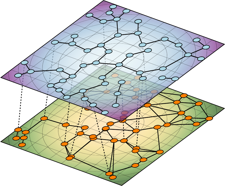
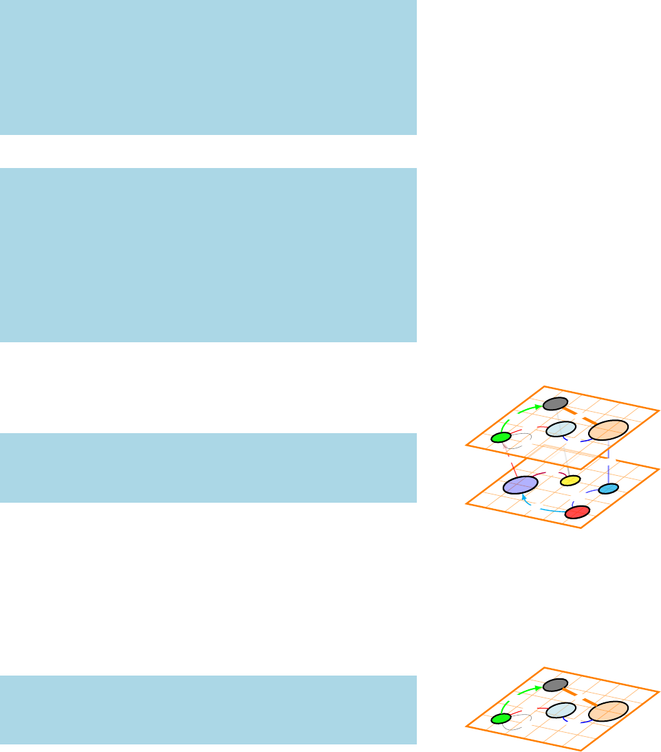
4Multilayer Networks

One of the main purposes of the tikz-network package is the illus-

tration of multilayer network structures. Thereby, all the previous

commands can be used. A multilayer network is represented as a

three-dimensional object, where each layer is located at a different

zplane. In order to enable this functionality, the option hmultilayeri

has to be used at the beginning of the tikzpicture.

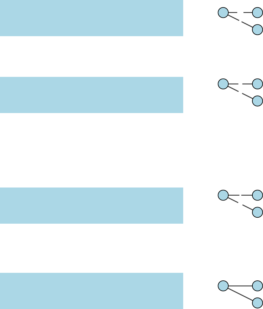
4.1Simple Networks

\Vertex[hlayeri=number]{Name}

With the option hlayerithe vertex can be assigned to a speciﬁc

layer. Layers are deﬁned by numbers (e.g. 1, 2, 3,. . . ). Working with

the hmultilayerioption, each \Vertex has to be assigned to a speciﬁc

layer. For the edge assignment no additional information is needed.

A B

\begin{tikzpicture}[multilayer]

\Vertex[x=0.5,IdAsLabel,layer=1]{A}

\Vertex[x=1.5,IdAsLabel,layer=1]{B}

\Vertex[x=1.5,IdAsLabel,layer=2]{C}

\Edge[bend=60](A)(B)

\Edge[style=dashed](B)(C)

\Edge(C)(C)

\end{tikzpicture}

Enabling the option hmultilayeri, returns the network in a two-

dimensional plane, like the networks discussed before. Setting

the argument hmultilayeri=3d, the network is rendered in a three-

dimensional representation. Per default, the layer with the lowest

number is on the top. This and the spacing between the layers can

be changed with the command \SetLayerDistance.

Layer 1

Layer 2

\begin{tikzpicture}[multilayer=3d]

\Vertex[x=0.5,IdAsLabel,layer=1]{A}

\Vertex[x=1.5,IdAsLabel,layer=1]{B}

\Vertex[x=1.5,IdAsLabel,layer=2]{C}

\Edge[bend=60](A)(B)

\Edge[style=dashed](B)(C)

\Edge(C)(C)

\end{tikzpicture}

32 multilayer networks

4.2Complex Networks

Similar as in Chapter 3introduced, layers can be assigned to the

vertices by adding a column hlayerito the ﬁle where the vertices are

stored.

File: ml_vertices.csv

id, x, y ,size, color,opacity,label,layer

A, 0, 0, .4 , green, .9 , a , 1

B, 1, .7, .6 , , .5 , b , 1

C, 2, 1, .8 ,orange, .3 , c , 1

D, 2, 0, .5 , red, .7 , d , 2

E,.2,1.5, .5 , gray, , e , 1

F,.1, .5, .7 , blue, .3 , f , 2

G, 2, 1, .4 , cyan, .7 , g , 2

H, 1, 1, .4 ,yellow, .7 , h , 2

File: ml_edges.csv

u,v,label,lw,color ,opacity,bend,Direct

A,B, ab ,.5,red , 1 , 30,false

B,C, bc ,.7,blue , 1 , -60,false

A,E, ae , 1,green , 1 , 45,true

C,E, ce , 2,orange, 1 , 0,false

A,A, aa ,.3,black , .5 , 75,false

C,G, cg , 1,blue , .5 , 0,false

E,H, eh , 1,gray , .5 , 0,false

F,A, fa ,.7,red , .7 , 0,true

D,F, df ,.7,cyan , 1 , 30,true

F,H, fh ,.7,purple, 1 , 60,false

D,G, dg ,.7,blue , .7 , 60,false

With the commands \Vertices and \Edges, the network can

be created automatically. Again the \Vertices vertices should be

performed ﬁrst and then the command \Edges.

Layer 2

Layer 1

ab bc

\begin{tikzpicture}[multilayer=3d]

\Vertices{data/ml_vertices.csv}

\Edges{data/ml_edges.csv}

\end{tikzpicture}

\Vertices[hlayeri=number]{ﬁlename}

\Edges[hlayeri={layer α,layer β}]{ﬁlename}

With the \Vertices option hlayerionly the vertices on the se-

lected layer are plotted. While, with the \Edges option hlayeri, the

edges between layer αand βare plotted. The argument is a tuple of

both layers indicated by {,}.

Layer 1

ab bc

\begin{tikzpicture}[multilayer=3d]

\Vertices[layer=1]{data/ml_vertices.csv}

\Edges[layer={1,1}]{data/ml_edges.csv}

\end{tikzpicture}

tikz-network manual 33

Plotting edges without deﬁning ﬁrst the vertices can be done

with the \Edges option hverticesi. This allows modifying speciﬁc

sets of Edges.

\begin{tikzpicture}[multilayer=3d]

\Edges[vertices=data/ml_vertices.csv,

layer={1,2},style=dashed]{data/ml_edges.csv}

\end{tikzpicture}

4.3Layers and Layouts

Besides adding vertices and edges to speciﬁc layers, every other

TikZ object can be drawn on such a layer using the Layer environ-

ment. With the option hlayeri=layer α, the position of the canvas can

be assigned to the speciﬁc layer.

\begin{Layer}[hlayeri=layer α]

\end{Layer}

ab bc

Layer 1

\begin{tikzpicture}[multilayer=3d]

\begin{Layer}[layer=1]

\draw[very thick] (-.5,-.5) rectangle (2.5,2);

\node at (-.5,-.5)[below right]{Layer 1};

\end{Layer}

\Vertices[layer=1]{data/ml_vertices.csv}

\Edges[layer={1,1}]{data/ml_edges.csv}

\end{tikzpicture}

\SetLayerDistance{measure}

With the command \SetLayerDistance the distance between

the layers and their orientation can be modiﬁed. Per default the

distance is set to −2\DefaultUnit (here cm). A negative number

implies that layers with a higher number will be stacked below

layers with a smaller number.

\SetCoordinates[hxAnglei=number,hyAnglei=number,hzAnglei=number,

hxLengthi=number,hyLengthi=number,hzLengthi=number]

The perspective of the three-dimensional plot can be modiﬁed

by changing the orientation of the coordinate system, which is

done with the command \SetCoordinates. Here the angle and

the length of each axis can be modiﬁed. Angles are deﬁned as

anumber in the range between −360 and 360. Per default, the

lengths of the axes are deﬁned by the identity matrix, i.e. no dis-

tortion. If the length ratio is changed x,y, and/or zvalues are

distorted. The \SetCoordinates command has to be entered before

the hmultilayerioption is called!

Layer 1

ab bc

\SetCoordinates[xAngle=-30,yLength=1.2,xLength=.8]

\begin{tikzpicture}[multilayer=3d]

\Vertices[layer=1]{data/ml_vertices.csv}

\Edges[layer={1,1}]{data/ml_edges.csv}

\end{tikzpicture}

34 multilayer networks

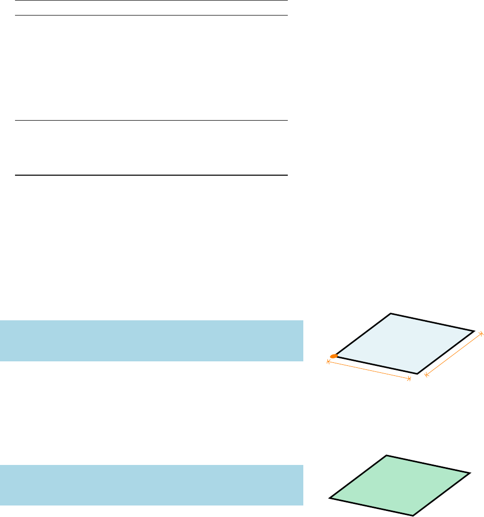
4.4Plane

To support the illustration of multilayer networks, the background

of the layer can be simply visualized with the command \Plane,

which allow to draw boundaries, grids and include images to the

layer.

\Plane[hoptionsi]

No obligatory arguments are needed. For a \Plane the following

options are available:

Option Default Type Deﬁnition

x0measure x-coordinate of the origin

y0measure y-coordinate of the origin

width 5 cm measure width of the plane

height 5 cm measure height of the plane

color vertexﬁll color ﬁll color of the plane

opacity 0.3number opacity of the ﬁll color

grid {} measure spacing of the grid

image {} ﬁle path to the image ﬁle

style {} string additional TikZ styles

layer 1number layer where the plane is located

RGB false Boolean allow RGB colors

NoFill false Boolean disable ﬁll color

NoBorder false Boolean disable border line

ImageAndFill false Boolean allow image and ﬁll color

InBG false Boolean plane is in the background layer

aeither measure or string

Table 4.1: Options for the \Plane

command.

\Plane[hxi=measure,hyi=measure,hwidthi=measure,hheighti=measure]

A\Plane is a rectangle with origin (hxi,hyi), a given hwidthi

and hheighti. The origin is deﬁned in the left lower corner and per

default (0, 0). The plane is default 5 cm (width) by 5 cm (height).

This default options can be changed with \SetPlaneWidth and

\SetPlaneHeight11See Section 5.5.

origin

width

height

\begin{tikzpicture}[multilayer=3d]

\Plane[x=-.5,y=-.5,width=3,height=2.5]

\end{tikzpicture}

\Plane[hcolori=color]

To change the ﬁll color of each plane individually, the option

hcolorihas to be used. Without the option hRGBiset, the default

TikZ and L

EX colors can be applied. Per default the default vertex

color is used.

\begin{tikzpicture}[multilayer=3d]

\Plane[x=-.5,y=-.5,width=3,height=2.5,color=green!70!blue]

\end{tikzpicture}

tikz-network manual 35

\Plane[hopacityi=number]

With the option hopacityithe opacity of the plane ﬁll color can be

modiﬁed. The range of the number lies between 0 and 1. Where 0

represents a fully transparent ﬁll and 1 a solid ﬁll. Per default the

opacity is set to 0.3.

\begin{tikzpicture}[multilayer=3d]

\Plane[x=-.5,y=-.5,width=3,height=2.5,opacity=.7]

\end{tikzpicture}

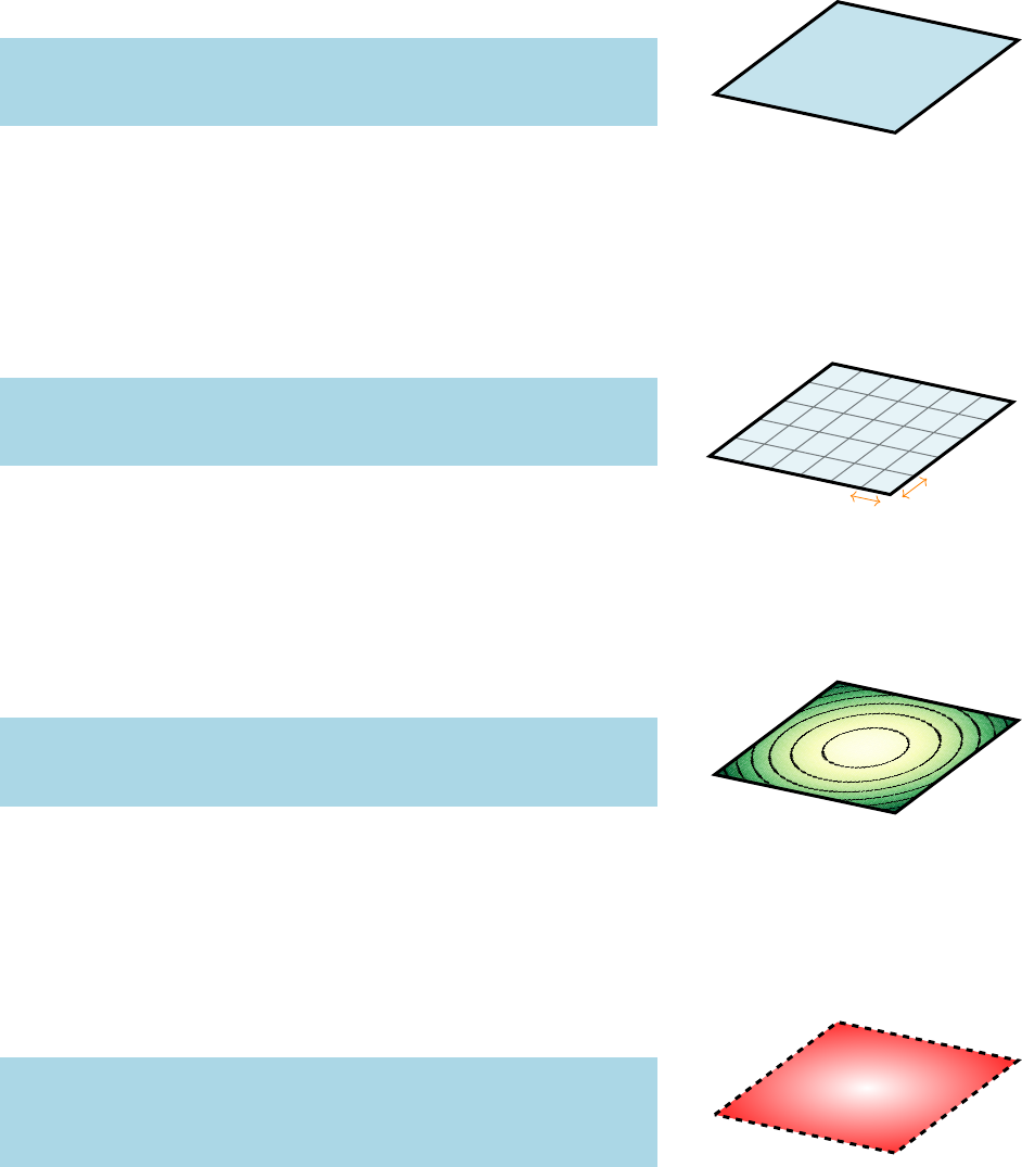
\Plane[hgridi=measure]

With the option hgridia grid will be drawn on top of the plane.

The argument of this option deﬁnes the spacing between the grid

lines. The entered measures are in default units (cm). Changing

the unites (locally) can be done by adding the unit to the measure2.2e.g. x=5 mm

Changes to the default setting can be made with \SetDefaultUnit3.3see Section 5.1

5mm

\begin{tikzpicture}[multilayer=3d]

\Plane[x=-.5,y=-.5,width=3,height=2.5,grid=5mm]

\end{tikzpicture}

\Plane[himagei=ﬁle]

An image can be assigned to a plane with the option himagei.

The argument is the ﬁle name and the folder where the image is

stored. The width and height of the ﬁgure is scaled to the size of

the plane. Without the option hImageAndFillithe image overwrite

the color options.

\begin{tikzpicture}[multilayer=3d]

\Plane[x=-.5,y=-.5,width=3,height=2.5,image=data/plane.png]

\end{tikzpicture}

\Plane[hstylei=string]

Any other TikZ style option or command can be entered via

the option hstylei. Most of these commands can be found in the

“TikZ and PGF Manual”. Contain the commands additional options

(e.g.hinner colori=color), then the argument for the hstyleihas to be

between { } brackets.

\begin{tikzpicture}[multilayer=3d]

\Plane[x=-.5,y=-.5,width=3,height=2.5,style={dashed,inner

color=white,outer color=red!80}]

\end{tikzpicture}

\Plane[hlayeri=number]

With the option hlayeri=layer α, the position of the plane can be

assigned to a speciﬁc layer. Per default the plane is drawn on layer

36 multilayer networks

Layer 2

\begin{tikzpicture}[multilayer=3d]

\SetLayerDistance{-1.5}

\Plane[x=-.5,y=-.5,width=3,height=2.5,color=green,layer=2]

\Plane[x=-.5,y=-.5,width=3,height=2.5]

\end{tikzpicture}

\Plane[hRGBi,hcolori=RGB values]

In order to display RGB colors for the plane ﬁll color, the op-

tion hRGBihas to be entered. In combination with this option, the

hcolorihast to be a list with the RGB values, separated by «,» and

within { }.44e.g. the RGB code for white:

{255, 255, 255}

\begin{tikzpicture}[multilayer=3d]

\Plane[x=-.5,y=-.5,width=3,height=2.5,RGB,color={0,0,0}]

\end{tikzpicture}

\Plane[hNoFilli]

\Plane[hNoBorderi]

hNoFilliis a Boolean option which disables the ﬁll color of the

plane and hNoBorderiis a Boolean option which suppress the bor-

der line of the plane.

Layer 2

\begin{tikzpicture}[multilayer=3d]

\SetLayerDistance{-1.5}

\Plane[x=-.5,y=-.5,width=3,height=2.5,layer=2,NoFill]

\Plane[x=-.5,y=-.5,width=3,height=2.5,NoBorder]

\end{tikzpicture}

\Plane[hImageAndFilli]

With the option hImageAndFilliboth, image and ﬁll color can be

drawn on a plane. The option hopacityiis applied to both objects.

\begin{tikzpicture}[multilayer=3d]

\Plane[x=-.5,y=-.5,width=3,height=2.5,image=data/plane.png,

color=red,opacity=.4,ImageAndFill]

\end{tikzpicture}

\Plane[hInBGi]

A plane is drawn on the current layer of the tikzpicture. I.e. ob-

jects which are created after the plane appear on top of it and ob-

jects created before below of it. With the option hInBGienabled, the

plane is drawn on the background layer of the tikzpicture.

5Default Settings

In order to customize the look of the networks, each layout setting

used can be modiﬁed and adapted. There are three categories:

General settings, vertex style, and edge style.

5.1General Settings

With the general settings mainly the sizes, distances and measures

of the networks can be modiﬁed.

\SetDefaultUnit{unit}

The command \SetDefaultUnit allows to change the units used

for drawing the network1, including diameters of the vertices, xand 1Except the line width, which are

deﬁned in pt.

ycoordinates or the distance between the layers. The default unit is

cm.

\SetDistanceScale{number}

With the command \SetDistanceScale, the distance between

the vertices can be scaled. Per default 1 cm entered corresponds to

1 cm drawn, i.e. \SetDistanceScale{1}. Decreasing or increasing

the scale changes the drawing distances between the vertices.

\SetLayerDistance{measure}

With the command \SetLayerDistance the distance between

the layers and their orientation can be modiﬁed. Per default, the

distance is set to −2. A negative number implies that layers with a

higher number will be stacked below layers with a smaller number.

\SetCoordinates[hxAnglei=number,hyAnglei=number,hzAnglei=number,

hxLengthi=number,hyLengthi=number,hzLengthi=number]

The perspective of the three-dimensional plot can be modiﬁed

by changing the orientation of the coordinate system, which is

done with the command \SetCoordinates. Here the angle and

the length of each axis can be modiﬁed. Angles are deﬁned as

anumber in the range between −360 and 360. Per default, the

length of the axes are deﬁned by the identity matrix, i.e. no dis-

tortion. If the length ratio is changed x,y, and/or zvalues are

distorted. The \SetCoordinates command has to be entered before

the hmultilayerioption is called!

38 default settings

5.2Vertex Style

The appearance of the vertices can be modiﬁed with the command

\SetVertexStyle. This command will change the default settings of

the vertices in the network.

\SetVertexStyle[document options]

The following options are available:

Option Default Type Deﬁnition

Shape circle text shape of the vertex

InnerSep 2pt measure separation space which will be

added inside the shape

OuterSep 0pt measure separation space outside the

background path

MinSize 0.6\DefaultUnit measure diameter (size) of the vertex

FillColor vertexﬁll color color of the vertex

FillOpacity 1number opacity of the vertex

LineWidth 1pt measure line width of the vertex boundary

LineColor black color line color of the vertex boundary

LineOpacity 1number line opacity of the vertex bound-

ary

TextFont \scriptsize fontsize font size of the vertex label

TextColor black color color of the vertex label

TextOpacity 1number opacity of the vertex label

TextRotation 0number initial rotation of the vertex

Table 5.1: Document style options for

the vertices.

5.3Edge Style

The appearance of the edges can be modiﬁed with the command

\SetEdgeStyle. This command will change the default settings of

the edges in the network.

\SetEdgeStyle[document options]

The following options are available:

Option Default Type Deﬁnition

LineWidth 1.5pt measure width of the edge

Color black!75 color color of the edge

Opacity 1number opacity of the edge

Arrow -latex text arrow shape of the directed edge

TextFont \scriptsize fontsize font size of the edge label

TextOpacity 1number opacity of the edge label

TextFillColor white color ﬁll color of the edge label

TextFillOpacity 1number ﬁll opacity of the edge label

InnerSep 0pt measure separation space which will be

added inside the shape

OuterSep 1pt measure separation space outside the back-

ground path

TextRotation 0number initial rotation of the edge label

Table 5.2: Document style options for

the edges.

\EdgesNotInBG

\EdgesInBG

Per default edges are drawn on the background layer, with the

command \EdgesNotInBG this can be disabled, while the command

\EdgesInBG restores the default setting.

tikz-network manual 39

5.4Text Style

The appearance of the text can be modiﬁed with the command

\SetTextStyle. This command will change the default settings of

the text.

\SetTextStyle[document options]

The following options are available:

Option Default Type Deﬁnition

TextFont \normalsize fontsize font size of the text

TextOpacity 1number opacity of the text

TextColor black color color of the text

TextOpacity 1number opacity of the text

InnerSep 2pt measure separation space which will be added

inside the shape

OuterSep 0pt measure separation space outside the back-

ground path

TextRotation 0number initial rotation of the text

Table 5.3: Document style options for

the planes.

5.5Plane Style

The appearance of the planes can be modiﬁed with the command

\SetPlaneStyle. This command will change the default settings of

the planes.

\SetPlaneStyle[document options]

The following options are available:

Option Default Type Deﬁnition

LineWidth 1.5pt measure width of the border line

LineColor black color color of the border line

LineOpacity 1number opacity of the border line

FillColor vertexﬁll color ﬁll color of the plane

FillOpacity 0.3number ﬁll opacity of the plane

GridLineWidth 0.5pt measure width of the grid lines

GridColor black color color of the grid lines

GridOpacity 0.5number opacity of the grid lines

Table 5.4: Document style options for

the planes.

\SetPlaneWidth{measure}

\SetPlaneHeight{measure}

With the commands \SetPlaneWidth and \SetPlaneHeight the

default size of the planes can be modiﬁed.

6Troubleshooting and Support

6.1tikz-network Website

The website for the tikz-network packages is located at https:

//github.com/hackl/tikz-network. There, you’ll ﬁnd the actual

version of the source code, a bug tracker, and the documentation.

6.2Getting Help

If you’ve encountered a problem with one of the tikz-network

commands, have a question, or would like to report a bug, please

send an email to me or visit our website.

To help me troubleshoot the problem more quickly, please try to

compile your document using the debug class option and send the

generated .log ﬁle to the mailing list with a brief description of the

problem.

6.3Errors, Warnings, and Informational Messages

The following is a list of all of the errors, warnings, and other mes-

sages generated by the tikz-network classes and a brief description

of their meanings.

Error: ! TeX capacity exceeded, sorry [main memory size=5000000].

The considered network is to large and pdflatex runs out of mem-

ory. This problem can be solved by using lualatex or xetex in-

stead.

6.4Package Dependencies

The following is a list of packages that the tikz-network package

rely upon. Packages marked with an asterisk are optional.

• etex

• xifthen

• xkeyval

• datatool

• tikz

–arrows

–positioning

–3d

–ﬁt

–calc

–backgrounds

AToDo

A.1Code to ﬁx

• change default entries for Boolean options in the vertices ﬁle.

A.2Documentation

• add indices to the manual.

• extended tutorial/example to the document.

• clean-up and document the .sty ﬁle.

• upload the package to CTAN, if it is appropriated tested.

A.3Features

• add a spherical coordinate system

A.4Add-ons

• add QGIS to tikz-network compiler

BAdd-ons

B.1Python networks to TikZ with network2tikz

B.1.1Introduction

network2tikz is a Python tool for converting network visualizations

into tikz-network ﬁgures, for native inclusion into your LaTeX

documents.

network2tikz works with Python 3and supports (currently) the

following Python network modules:

•cnet

•python-igraph

•networkx

•pathpy

• default node/edge lists

The output of network2tikz is a tikz-network ﬁgure. Because

you are not only getting an image of your network, but also the La-

TeX source ﬁle, you can easily post-process the ﬁgures (e.g. adding

drawings, texts, equations,...).

Since a picture is worth a thousand words a small example:

Alice

Bob

Claire

Dennis

#!/usr/bin/python -tt

# -*- coding: utf-8 -*-

nodes = [’a’,’b’,’c’,’d’]

edges = [(’a’,’b’), (’a’,’c’), (’c’,’d’),(’d’,’b’)]

gender = [’f’, ’m’, ’f’, ’m’]

colors = {’m’: ’blue’, ’f’: ’red’}

style = {}

style[’node_label’] = [’Alice’, ’Bob’, ’Claire’, ’Dennis’]

style[’node_color’] = [colors[g] for g in gender]

style[’node_opacity’] = .5

style[’edge_curved’] = .1

from network2tikz import plot

plot((nodes,edges),’network.tex’,**style)

(see above) gives

46 add-ons

\documentclass{standalone}

\usepackage{tikz-network}

\begin{document}

\begin{tikzpicture}

\clip (0,0) rectangle (6,6);

\Vertex[x=0.785,y=2.375,color=red,opacity=0.5,label=Alice]{a}

\Vertex[x=5.215,y=5.650,color=blue,opacity=0.5,label=Bob]{b}

\Vertex[x=3.819,y=0.350,color=red,opacity=0.5,label=Claire]{c}

\Vertex[x=4.654,y=2.051,color=blue,opacity=0.5,label=Dennis]{d}

\Edge[,bend=-8.531](a)(c)

\Edge[,bend=-8.531](c)(d)

\Edge[,bend=-8.531](d)(b)

\Edge[,bend=-8.531](a)(b)

\end{tikzpicture}

\end{document}

Tweaking the plot is straightforward and can be done as part of

your LaTeX workﬂow.

B.1.2Installation

network2tikz is available from the Python Package Index, so sim-

ply type

pip install -U network2tikz

to install/update. If your are intersted in the development ver-

sion of the module check out the github repository.

B.1.3Usage

1. Generate, manipulation, and study of the structure, dynamics,

and functions of your complex networks as usual, with your

preferred python module.

2. Instead of the default plot functions (e.g. igraph.plot() or

networkx.draw()) invoke network2tikz by

plot(G,’mytikz.tex’)

to store your network visualisation as the TikZ ﬁle mytikz.tex.

Load the module with:

from network2tikz import plot

Advanced usage:

Of course, you always can improve your plot by manipulating

the generated LaTeX ﬁle, but why not do it directly in Python?

To do so, all visualization options available in tikz-network are

also implemented in network2tikz. The appearance of the plot

can be modiﬁed by keyword arguments.11For a detailed explanation, please see

Section B.1.5.

tikz-network manual 47

my_style = {}

plot(G,’mytikz.tex’,**my_style)

The arguments follow the options described above in the man-

ual.

Additionally, if you are more interested in the ﬁnal output and

not only the .tex ﬁle, used

plot(G,’mypdf.pdf’)

to save your plot as a pdf, or

plot(G)

to create a temporal plot and directly show the result, i.e. similar

to the matplotlib function show(). Finally, you can also create a

node and edge list, which can be read and easily modiﬁed (in a

post-processing step) as showd above.

plot(G,’mycsv.csv’)

3. Compile the ﬁgure or add the contents of mytikz.tex into your

LaTeX source code. With the option hstandalonei=false only the

TikZ ﬁgure will be saved, which can then be easily included in

your L

EX document via \input{/path/to/mytikz.tex}.

B.1.4Simple example

For illustration purpose, a similar network as in the python-

igraph tutorial is used. If you are using another Python network

module, and like to follow this example, please have a look at

the provided examples.

Create network object and add some edges.

#!/usr/bin/python -tt

# -*- coding: utf-8 -*-

import igraph

from network2tikz import plot

net = igraph.Graph([(0,1), (0,2), (2,3), (3,4), (4,2), (2,5),

(5,0), (6,3),

(5,6), (6,6)],directed=True)

Adding node and edge properties.

48 add-ons

net.vs["name"] = ["Alice", "Bob", "Claire", "Dennis", "Esther", "

Frank", "George"]

net.vs["age"] = [25, 31, 18, 47, 22, 23, 50]

net.vs["gender"] = ["f", "m", "f", "m", "f", "m", "m"]

net.es["is_formal"] = [False, False, True, True, True, False, True

, False,

False, False]

Already now the network can be plotted.

plot(net)

Per default, the node positions are assigned uniform random. In

order to create a layout, the layout methods of the network pack-

ages can be used. Or the position of the nodes can be directly as-

signed, in form of a dictionary, where the key is the node id and the

value is a tuple of the node position in xand y.

layout = {0: (4.3191, -3.5352), 1: (0.5292, -0.5292),

2: (8.6559, -3.8008), 3: (12.4117, -7.5239),

4: (12.7, -1.7069), 5: (6.0022, -9.0323),

6: (9.7608, -12.7)}

plot(net,layout=layout)

This should open an external pdf viewer showing a visual rep-

resentation of the network, something like the one on the following

ﬁgure:

We can simply re-using the previous layout object here, but we

also speciﬁed that we need a bigger plot (8 ×8 cm) and a larger

margin around the graph to ﬁt the self loop and potential labels (1

cm).22Per default, all size values are based

on cm, and all line widths are deﬁned

in pt units. With the general option

hunitsithis can be changed, see Section

B.1.5.

plot(net, layout=layout, canvas=(8,8), margin=1)

In to keep the properties of the visual representation of your

network separate from the network itself. You can simply set up a

Python dictionary containing the keyword arguments you would

pass to plot and then use the double asterisk (**) operator to pass

your speciﬁc styling attributes to plot:

color_dict = {’m’: ’blue’, ’f’: ’red’}

visual_style = {}

# Node options

visual_style[’vertex_size’] = .5

visual_style[’vertex_color’] = [color_dict[g] for g in net.vs[’

gender’]]

visual_style[’vertex_opacity’] = .7

visual_style[’vertex_label’] = net.vs[’name’]

visual_style[’vertex_label_position’] = ’below’

# Edge options

visual_style[’edge_width’] = [1 + 2 *int(f) for f in net.es(’

is_formal’)]

visual_style[’edge_curved’] = 0.1

tikz-network manual 49

# General options and plot command.

visual_style[’layout’] = layout

visual_style[’canvas’] = (8,8)

visual_style[’margin’] = 1

# Plot command

plot(net,**visual_style) Alice

Bob

Claire

Dennis

Esther

Frank

George

Beside showing the network, we can also generate the latex

source ﬁle, which can be used and modiﬁed later on. This is done

by adding the output ﬁle name with the ending ’.tex’.

plot(net,’network.tex’,**visual_style)

produces

\documentclass{standalone}

\usepackage{tikz-network}

\begin{document}

\begin{tikzpicture}

\clip (0,0) rectangle (8.0,8.0);

\Vertex[x=2.868,y=5.518,size=0.5,color=red,opacity=0.7,label=Alice,position=below]{a}

\Vertex[x=1.000,y=7.000,size=0.5,color=blue,opacity=0.7,label=Bob,position=below]{b}

\Vertex[x=5.006,y=5.387,size=0.5,color=red,opacity=0.7,label=Claire,position=below]{c}

\Vertex[x=6.858,y=3.552,size=0.5,color=blue,opacity=0.7,label=Dennis,position=below]{d}

\Vertex[x=7.000,y=6.419,size=0.5,color=red,opacity=0.7,label=Esther,position=below]{e}

\Vertex[x=3.698,y=2.808,size=0.5,color=blue,opacity=0.7,label=Frank,position=below]{f}

\Vertex[x=5.551,y=1.000,size=0.5,color=blue,opacity=0.7,label=George,position=below]{g}

\Edge[,lw=1.0,bend=-8.531,Direct](a)(b)

\Edge[,lw=1.0,bend=-8.531,Direct](a)(c)

\Edge[,lw=3.0,bend=-8.531,Direct](c)(d)

\Edge[,lw=3.0,bend=-8.531,Direct](d)(e)

\Edge[,lw=3.0,bend=-8.531,Direct](e)(c)

\Edge[,lw=1.0,bend=-8.531,Direct](c)(f)

\Edge[,lw=3.0,bend=-8.531,Direct](f)(a)

\Edge[,lw=1.0,bend=-8.531,Direct](f)(g)

\Edge[,lw=1.0,bend=-8.531,Direct](g)(g)

\Edge[,lw=1.0,bend=-8.531,Direct](g)(d)

\end{tikzpicture}

\end{document}

Instead of the tex ﬁle, a node and edge list can be generates,

which can also be used with the library.

plot(net,’network.csv’,**visual_style)

The node list network_nodes.csv.

id,x,y,size,color,opacity,label,position

a,2.868,5.518,0.5,red,0.7,Alice,below

b,1.000,7.000,0.5,blue,0.7,Bob,below

c,5.006,5.387,0.5,red,0.7,Claire,below

d,6.858,3.552,0.5,blue,0.7,Dennis,below

e,7.000,6.419,0.5,red,0.7,Esther,below

f,3.698,2.808,0.5,blue,0.7,Frank,below

g,5.551,1.000,0.5,blue,0.7,George,below

The edge list network_edges.csv.

50 add-ons

u,v,lw,bend,Direct

a,b,1.0,-8.531,true

a,c,1.0,-8.531,true

c,d,3.0,-8.531,true

d,e,3.0,-8.531,true

e,c,3.0,-8.531,true

c,f,1.0,-8.531,true

f,a,3.0,-8.531,true

f,g,1.0,-8.531,true

g,g,1.0,-8.531,true

g,d,1.0,-8.531,true

B.1.5The plot function in detail

network2tikz.plot(network,hﬁlenamei=None,htypei=None,

h**kwdsi)

Parameters

network : network object

Network to be drawn. The network can be a cnet,networkx,

igraph,pathpy object, or a tuple of a node list and edge list.

ﬁlename : ﬁle, string or None, optional (default = None)

File or ﬁlename to save. The ﬁle ending speciﬁes the output.

i.e. is the ﬁle ending with .tex a tex ﬁle will be created; if

the ﬁle ends with ’.pdf’ a pdf is created; if the ﬁle ends with

.csv, two csv ﬁles are generated filename_nodes.csv and

filename_edges.csv. If the ﬁlename is a tuple of strings, the

ﬁrst entry will be used to name the node list and the second en-

try for the edge list; and if no ending and no type is deﬁned a

temporary pdf ﬁle is compiled and shown.

type : str or None, optional (default = None)

Type of the output ﬁle. If no ending is deﬁned trough the ﬁle-

name, the type of the output ﬁle can be speciﬁed by the type

option. Currently the following output types are supported:

’tex’,’pdf’,’csv’ and ’dat’.

kwds : keyword arguments, optional (default= no attributes)

Attributes used to modify the appearance of the plot. For details

see below.

Keyword arguments for node styles

node_size : size of the node. The default is 0.6cm.

node_color : color of the nodes. The default is light blue. Colors

can be speciﬁed either by common color names, or by 3-tuples

of ﬂoats (ranging between 0and 255 for the R, G and B compo-

nents).

node_opacity : opacity of the nodes. The default is 1. The range

of the number lies between 0and 1. Where 0represents a fully

transparent ﬁll and 1a solid ﬁll.

tikz-network manual 51

node_label : labels drawn next to the nodes.

node_label_position : Per default the position of the label is in the

center of the node. Classical TikZ commands can be used to

change the position of the label. Instead, using such command,

the position can be determined via an angle, by entering a num-

ber between -360 and 360. The origin (0) is the yaxis. A positive

number change the position counter clockwise, while a negative

number make changes clockwise.

node_label_distance : distance between the node and the label.

node_label_color : color of the label.

node_label_size : font size of the label.

node_shape : shape of the vertices. Possibilities are: ’circle’, ’rectan-

gle’, ’triangle’, and any other Tikz shape

node_style : Any other Tikz style option or command can be en-

tered via the option style. Most of these commands can be found

in the "TikZ and PGF Manual". Contain the commands addi-

tional options (e.g. shading = ball), then the argument for the

style has to be between { } brackets.

node_layer : the node can be assigned to a speciﬁc layer.

node_label_off : is Boolean option which suppress all labels.

node_label_as_id : is a Boolean option which assigns the node id as

label.

node_math_mode : is a Boolean option which transforms the labels

into mathematical expressions without using the $ $ environ-

ment.

node_pseudo : is a Boolean option which creates a pseudo node,

where only the node name and the node coordinate will be pro-

vided.

Keyword arguments for edge styles

edge_width : width of the edges. The default unit is point (pt).

edge_color : color of the edges. The default is gray. Colors can be

speciﬁed either by common color names, or by 3-tuples of ﬂoats

(ranging between 0and 255 for the R, G and B components).

edge_opacity : opacity of the edges. The default is 1. The range of

the number lies between 0and 1. Where 0represents a fully

transparent ﬁll and 1a solid ﬁll.

edge_curved : whether the edges should be curved. Positive num-

bers correspond to edges curved in a counter-clockwise direc-

tion, negative numbers correspond to edges curved in a clock-

wise direction. Zero represents straight edges.

52 add-ons

edge_label : labels drawn next to the edges.

edge_label_position : Per default the label is positioned in between

both nodes in the center of the line. Classical Tikz commands can

be used to change the position of the label.

edge_label_distance : The label position between the nodes can be

modiﬁed with the distance option. Per default the label is cen-

tered between both nodes. The position is expressed as the per-

centage of the length between the nodes, e.g. of distance = 0.7,

the label is placed at 70% of the edge length away of Vertex i.

edge_label_color : color of the label.

edge_label_size : font size of the label.

edge_style : Any other Tikz style option or command can be entered

via the option style. Most of these commands can be found in

the "TikZ and PGF Manual". Contain the commands additional

options (e.g. shading = ball), then the argument for the style has

to be between { } brackets.

edge_arrow_size : arrow size of the edges.

edge_arrow_width : width of the arrowhead on the edge.

edge_loop_size : modiﬁes the length of the edge. The measure value

has to be insert together with its units. Per default the loop size

is 1cm.

edge_loop_position : The position of the self-loop is deﬁned via the

rotation angle around the node. The origin (0) is the y axis. A

positive number change the loop position counter clockwise,

while a negative number make changes clockwise.

edge_loop_shape : The shape of the self-loop is deﬁned by the en-

closing angle. The shape can be changed by decreasing or in-

creasing the argument value of the loop shape option.

edge_directed : is a Boolean option which transform edges to di-

rected arrows. If the network is already deﬁned as directed net-

work this option is not needed, except to turn off the direction

for one or more edges.

edge_math_mode : is a Boolean option which transforms the labels

into mathematical expressions without using the $ $ environ-

ment.

edge_not_in_bg : Per default, the edge is drawn on the background

layer of the tikz picture. I.e. objects which are created after the

edges appear also on top of them. To turn this off, the option

edge_not_in_bg has to be enabled.

Keyword arguments for general options

tikz-network manual 53

units : string or tuple of strings, optional (default = (’cm’,’pt’))

Per default, all size values are based on cm, and all line widths

are deﬁned in pt units. Whit this option the input units can be

changed. Currently supported are: Pixel ’px’, Points ’pt’, Mil-

limeters ’mm’, and Centimeters ’cm’. If a single value is entered

as unit all inputs have to be deﬁned using this unit. If a tuple of

units is given, the sizes are deﬁned with the ﬁrst entry the line

widths with the second entry.

layout : dict A dictionary with the node positions on a 2-dimensional

plane. The key value of the dict represents the node id while the

value represents a tuple of coordinates (e.g. n = (x,y)). The initial

layout can be placed anywhere on the 2-dimensional plane.

margins : None, int, ﬂoat or dict, optional (default = None) The

margins deﬁne the ’empty’ space from the canvas border. If no

margins are deﬁned, the margin will be calculated based on the

maximum node size, to avoid clipping of the nodes. If a single

int or ﬂoat is deﬁned all margins using this distances. To deﬁne

different the margin sizes for all size a dictionary with in the

form of {’top’:2,’left’:1,’bottom’:2,’right’:.5} has to be

used.

canvas : None, tuple of int or ﬂoats, optional (default = (6,6)) Can-

vas or ﬁgure_size deﬁnes the size of the plot. The values entered

as a tuple of numbers where the ﬁrst number is width of the

ﬁgure and the second number is the height of the ﬁgure. If the

option units is not used the size is speciﬁed in cm. Per default

the canvas is 6 ×6 cm.

keep_aspect_ratio : bool, optional (default = True) Deﬁnes whether

to keep the aspect ratio of the current layout. If False, the layout

will be rescaled to ﬁt exactly into the available area in the canvas

(i.e. removed margins). If True, the original aspect ratio of the

layout will be kept and it will be centered within the canvas.

standalone : bool, optional (default = True) If this option is true, a

standalone latex ﬁle will be created. i.e. the ﬁgure can be com-

piled from this output ﬁle. If standalone is false, only the tikz

environment is stored in the tex ﬁle, and can be imported in an

existing tex ﬁle.

clean : bool, optional (default = True) Whether non-pdf ﬁles created

that are created during compilation should be removed.

clean_tex : bool, optional (default = True) Also remove the gener-

ated tex ﬁle.

compiler : str or None, optional (default = None) The name of the

LaTeX compiler to use. If it is None, cnet will choose a ﬁtting one

on its own. Starting with latexmk and then pdflatex.

54 add-ons

compiler_args : list or None, optional (default = None) Extra ar-

guments that should be passed to the LaTeX compiler. If this is

None it defaults to an empty list.

silent : bool, optional (default = True) Whether to hide compiler

output or not.

Keyword naming convention

In the style dictionary multiple keywords can be used to ad-

dress attributes. These keywords will be converted to an unique

key word, used in the remaining code. This allows to keep the key-

words used in igraph.

Keys Other valid keys

node vertex, v, n

edge link, l, e

margins margin

canvas bbox, ﬁgure_size

units unit

Table B.1: Keyword naming conven-

tion.

Index

\begin,33

class options

debug,41

debug class option, 41

debug messages, 41

\DefaultUnit,33,38

Edge

options, 14

style, 38

\Edge,6,14–19,27,28

Edges

options, 28

\Edges,6,27–30,32,33

\EdgesInBG,19,38

\EdgesNotInBG,19,38

\end,33

environments

Layer,6,33

tikzpicture,31

error messages, 41

\footnotesize,11,16

\layer,22

Layer environment, 6,33

\normalsize,20,39

Plane

options, 34

style, 39

\Plane,6,34–36

\scriptsize,11,16,38

\SetCoordinates,33,37

\SetDefaultUnit,7,10,20,35,37

\SetDistanceScale,37

\SetEdgeStyle,38

\SetLayerDistance,31,33,37

\SetPlaneHeight,34,39

\SetPlaneStyle,39

\SetPlaneWidth,34,39

\SetTextStyle,20,39

\SetVertexStyle,9,38

\small,11,16

Text

options, 20

style, 39

\Text,20–22

tikzpicture environment, 31

\tiny,11,16

Vertex

options, 9

style, 38

\Vertex,6,9–13,23,24,31

Vertices

options, 24

\Vertices,6,23–26,30,32

warning messages, 41

Tikz Networkmanual Manual

Navigation menu

Versions of this User Manual:

Views

Navigation