Ngspice User Manual
User Manual:
Open the PDF directly: View PDF ![]() .
.
Page Count: 370 [warning: Documents this large are best viewed by clicking the View PDF Link!]
- I Ngspice User Manual
- Introduction
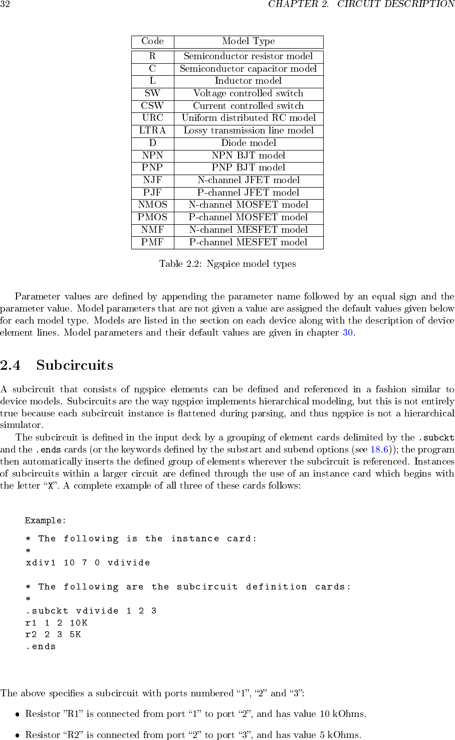
- Circuit Description
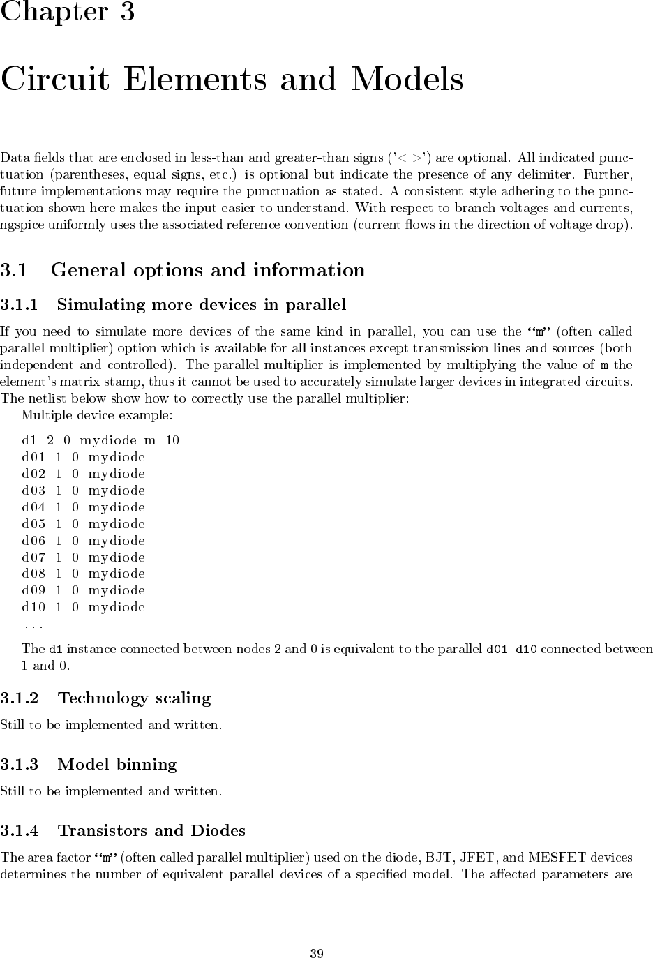
- Circuit Elements and Models
- General options and information
- Elementary Devices
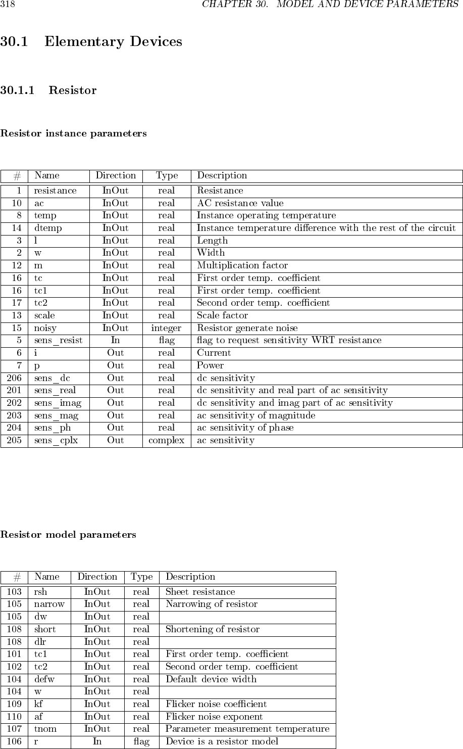
- Resistors
- Semiconductor Resistors
- Semiconductor Resistor Model (R)
- Resistors, dependent on expressions
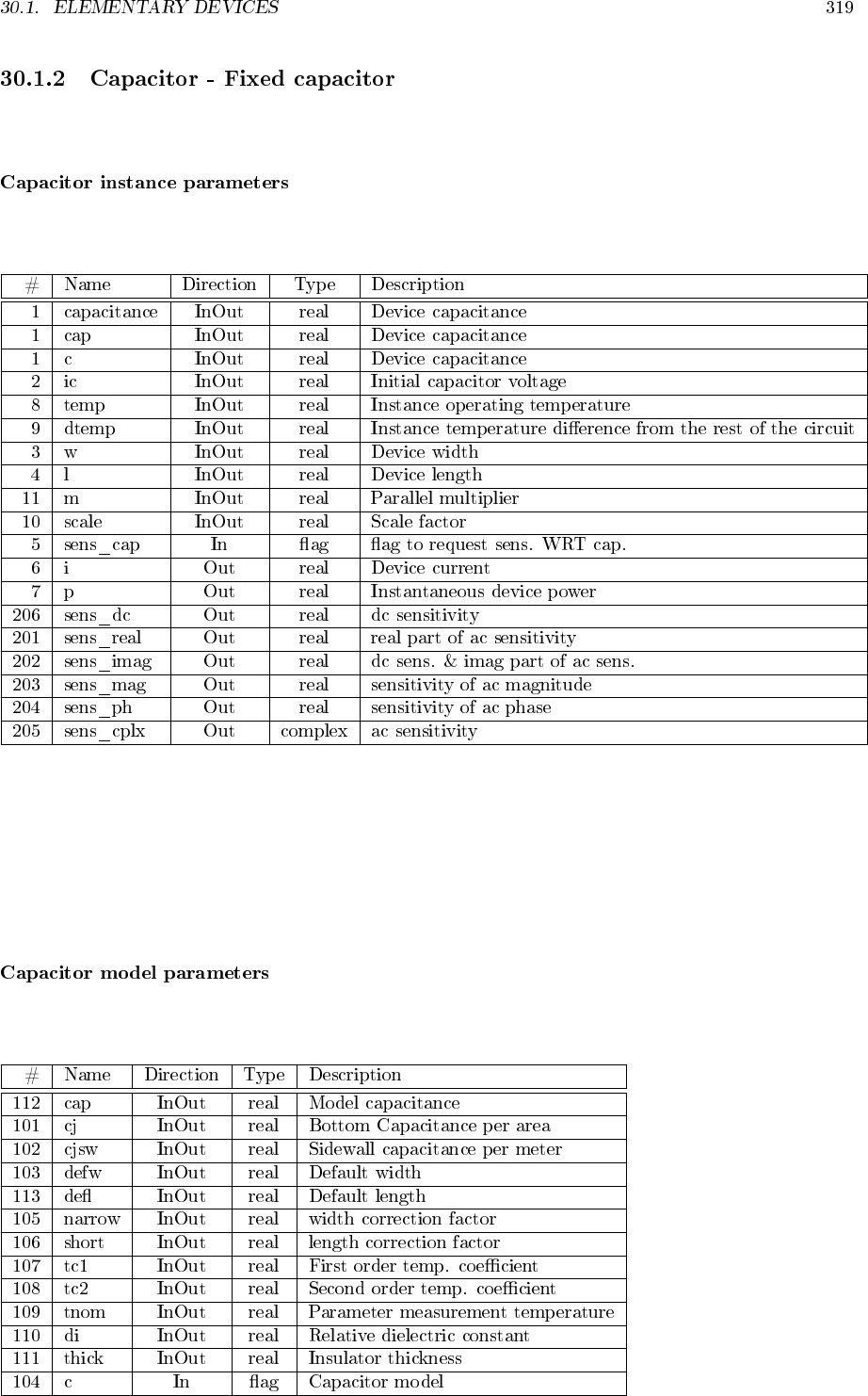
- Capacitors
- Semiconductor Capacitors
- Semiconductor Capacitor Model (C)
- Capacitors, dependent on expressions
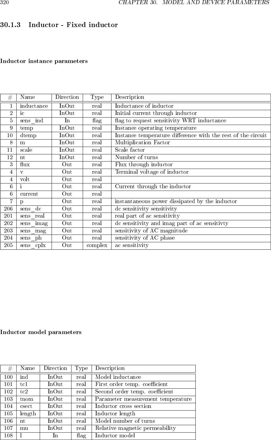
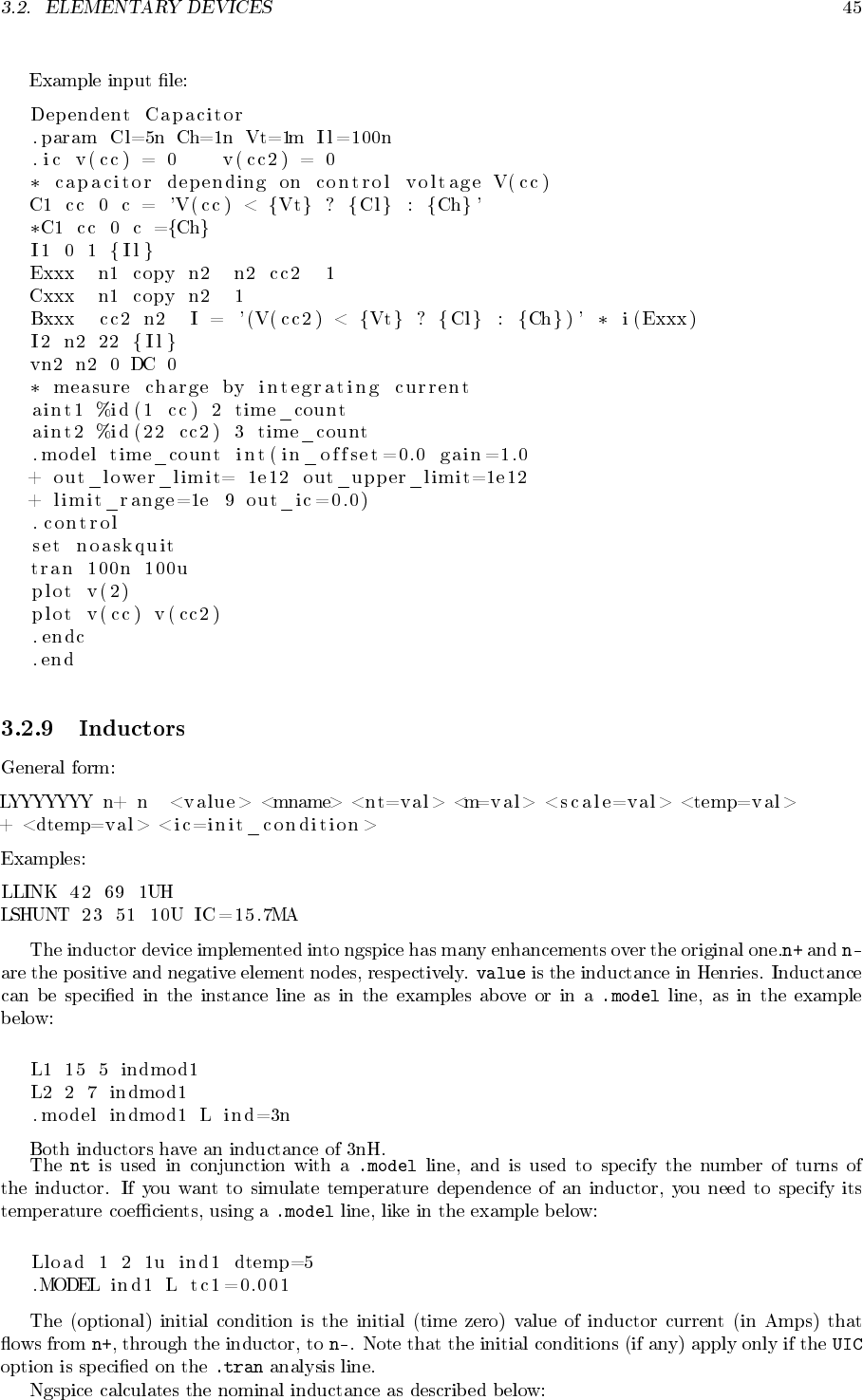
- Inductors
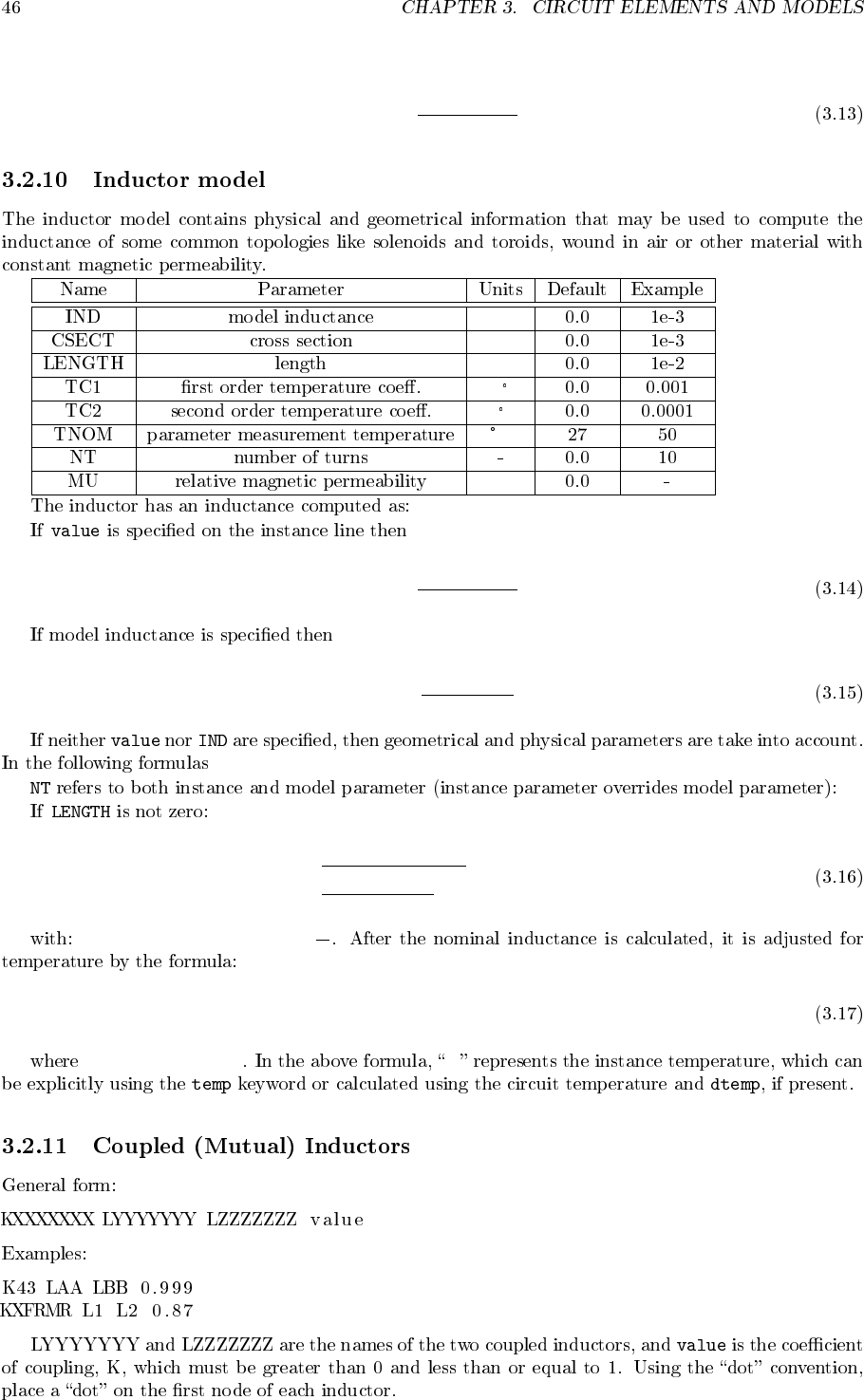
- Inductor model
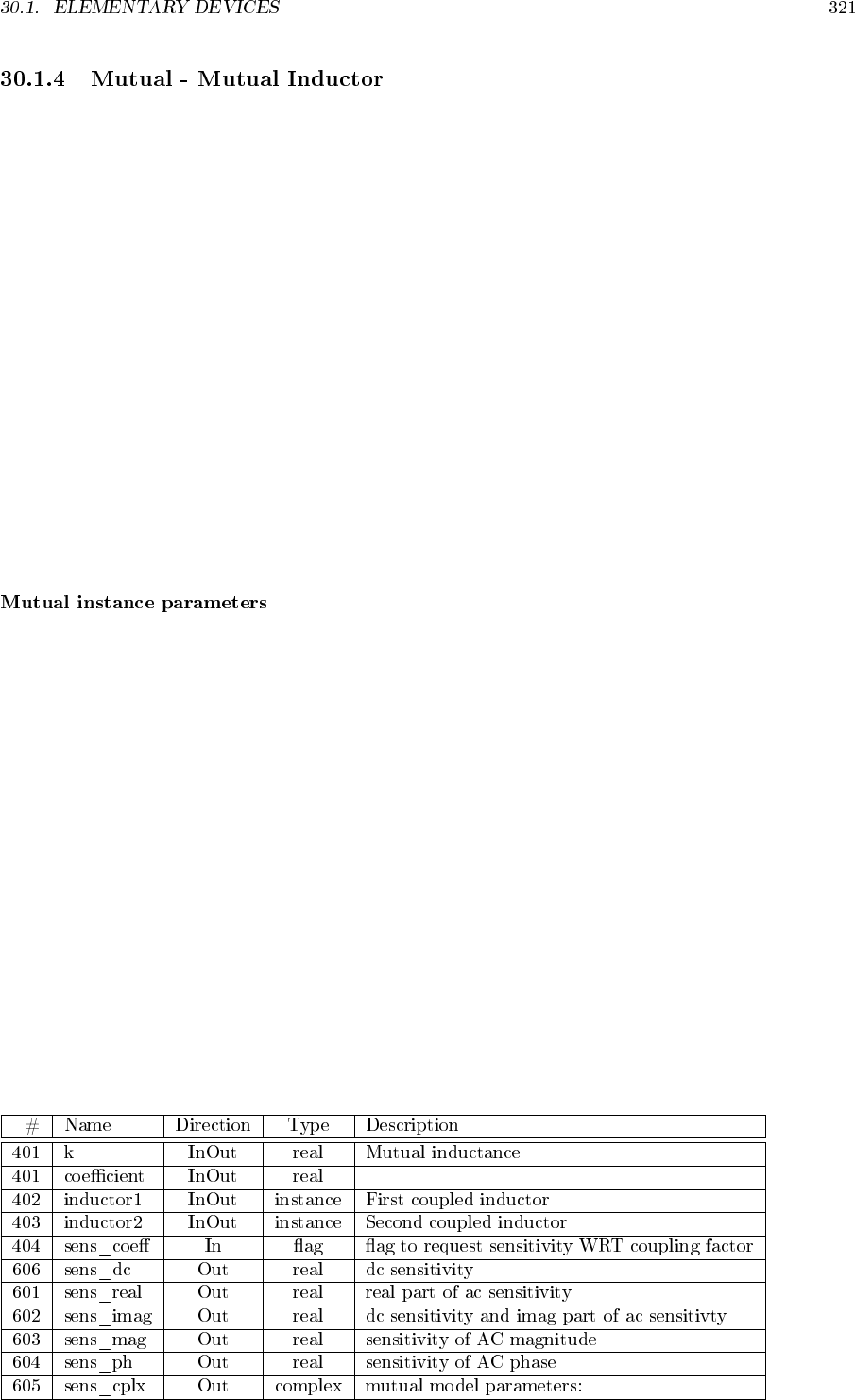
- Coupled (Mutual) Inductors
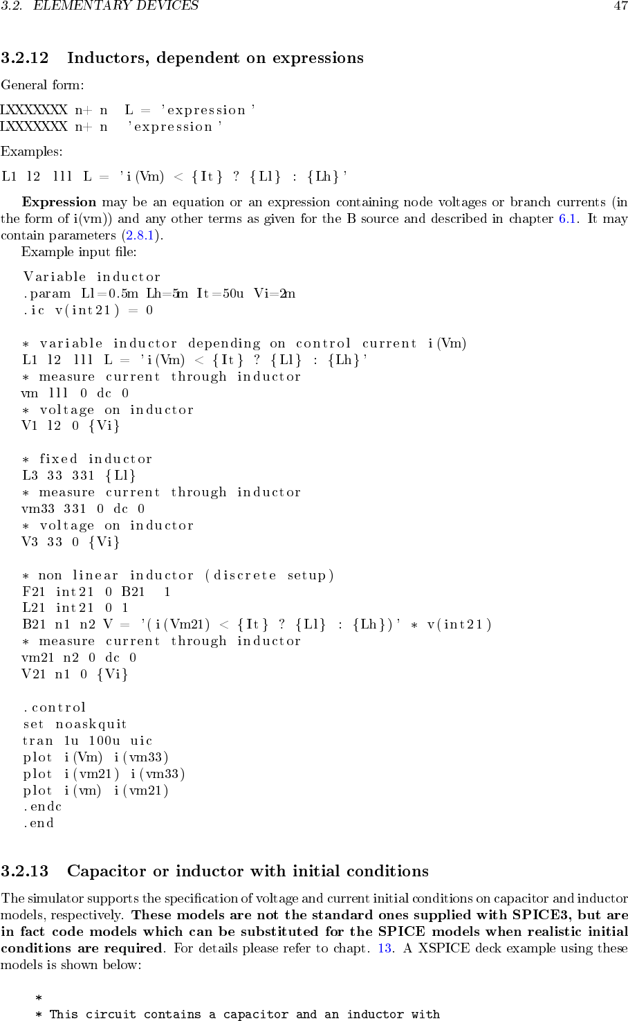
- Inductors, dependent on expressions
- Capacitor or inductor with initial conditions
- Switches
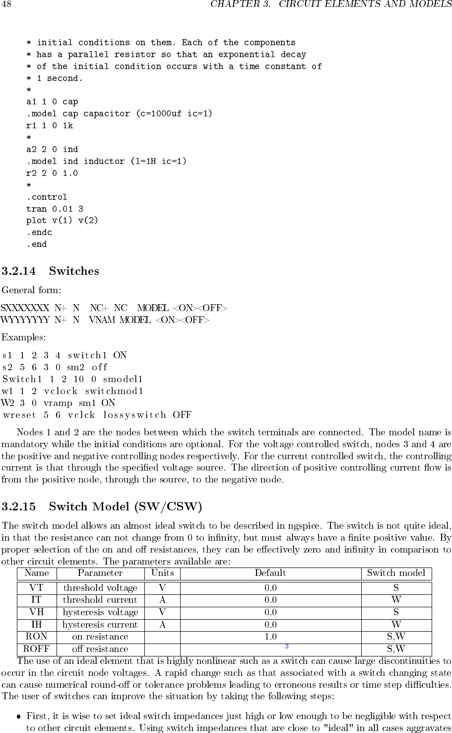
- Switch Model (SW/CSW)
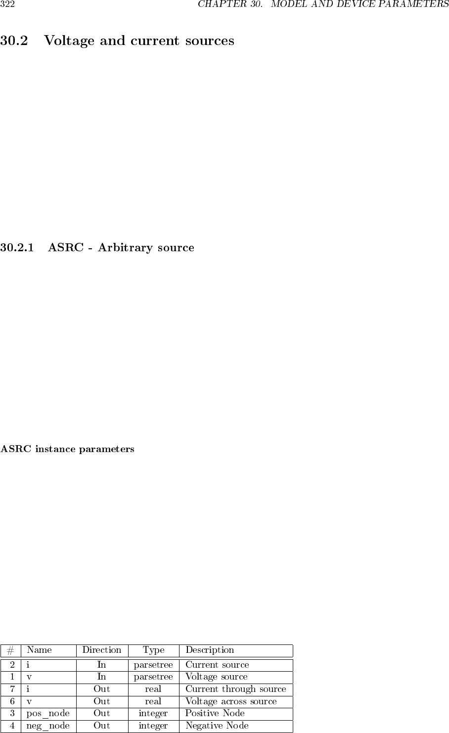
- Voltage and Current Sources
- Linear Dependent Sources
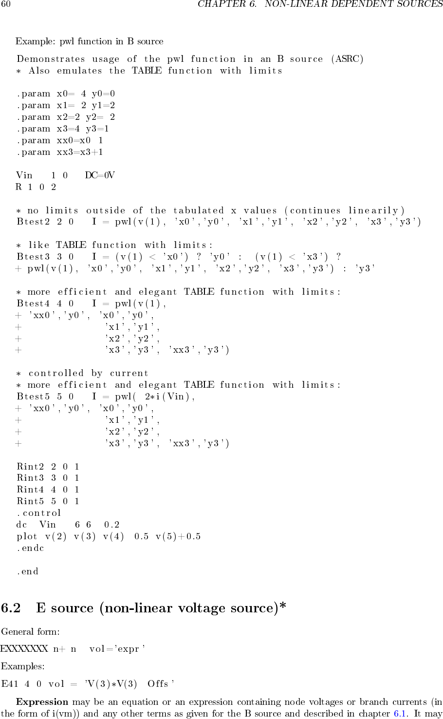
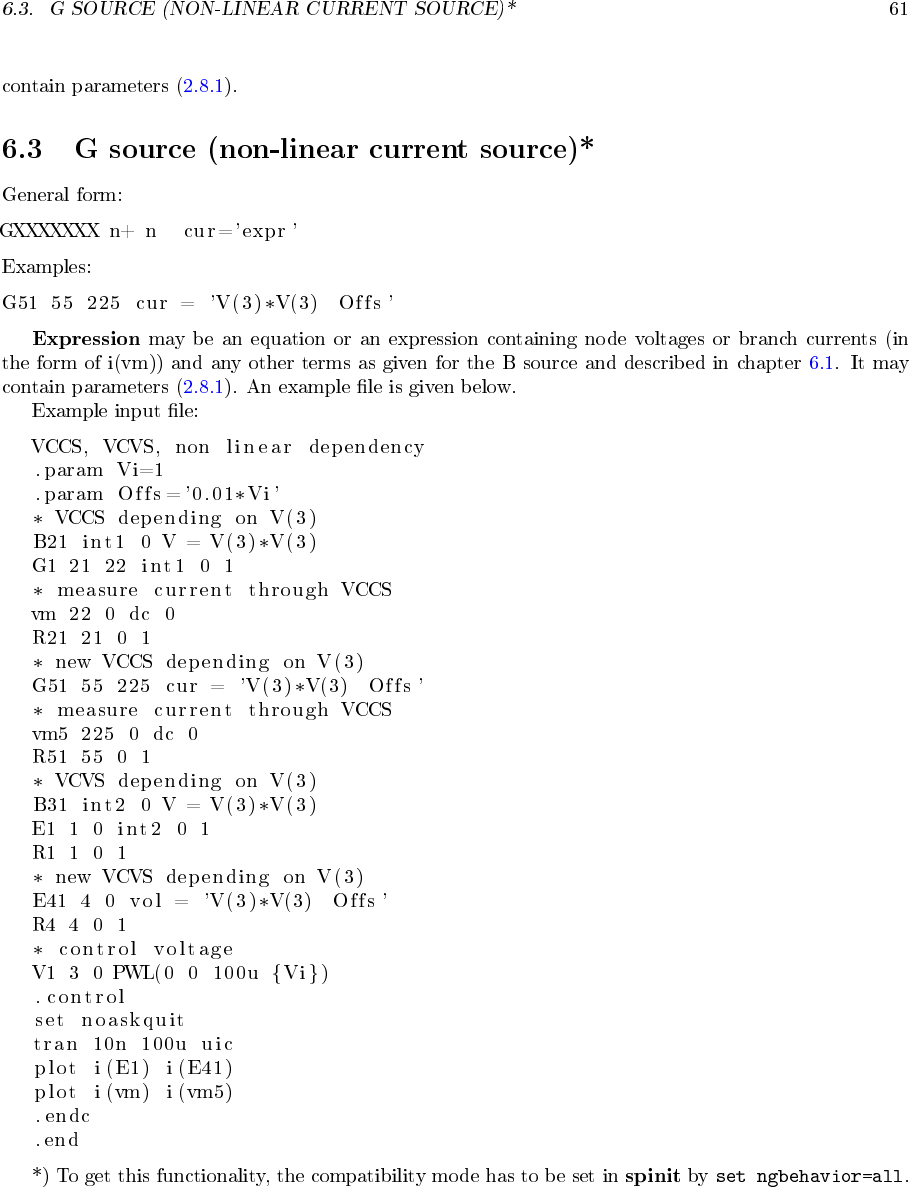
- Non-linear Dependent Sources
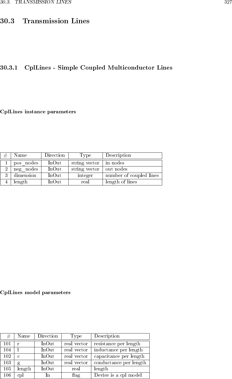
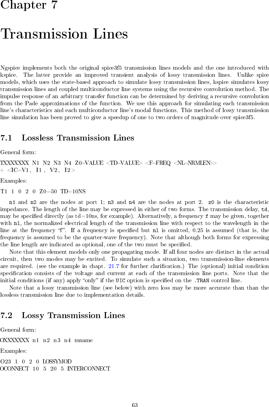
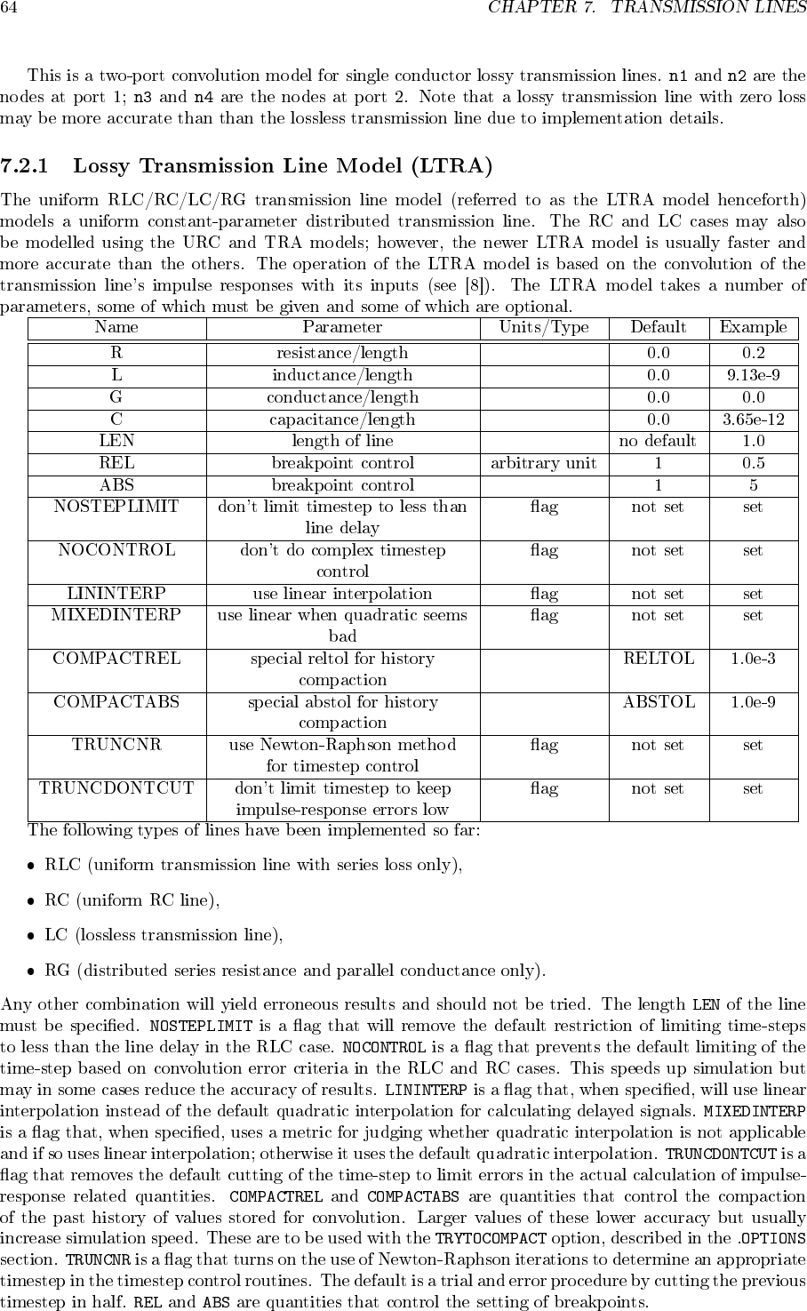
- Transmission Lines
- DIODEs
- BJTs
- JFETs
- MESFETs
- MOSFETs
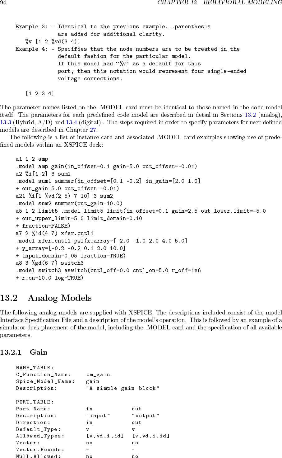
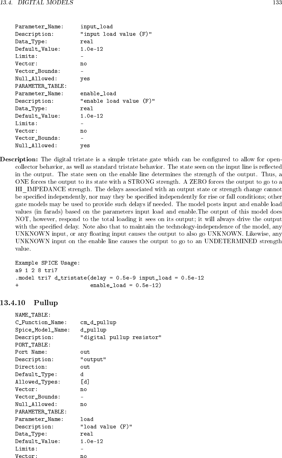
- Behavioral Modeling
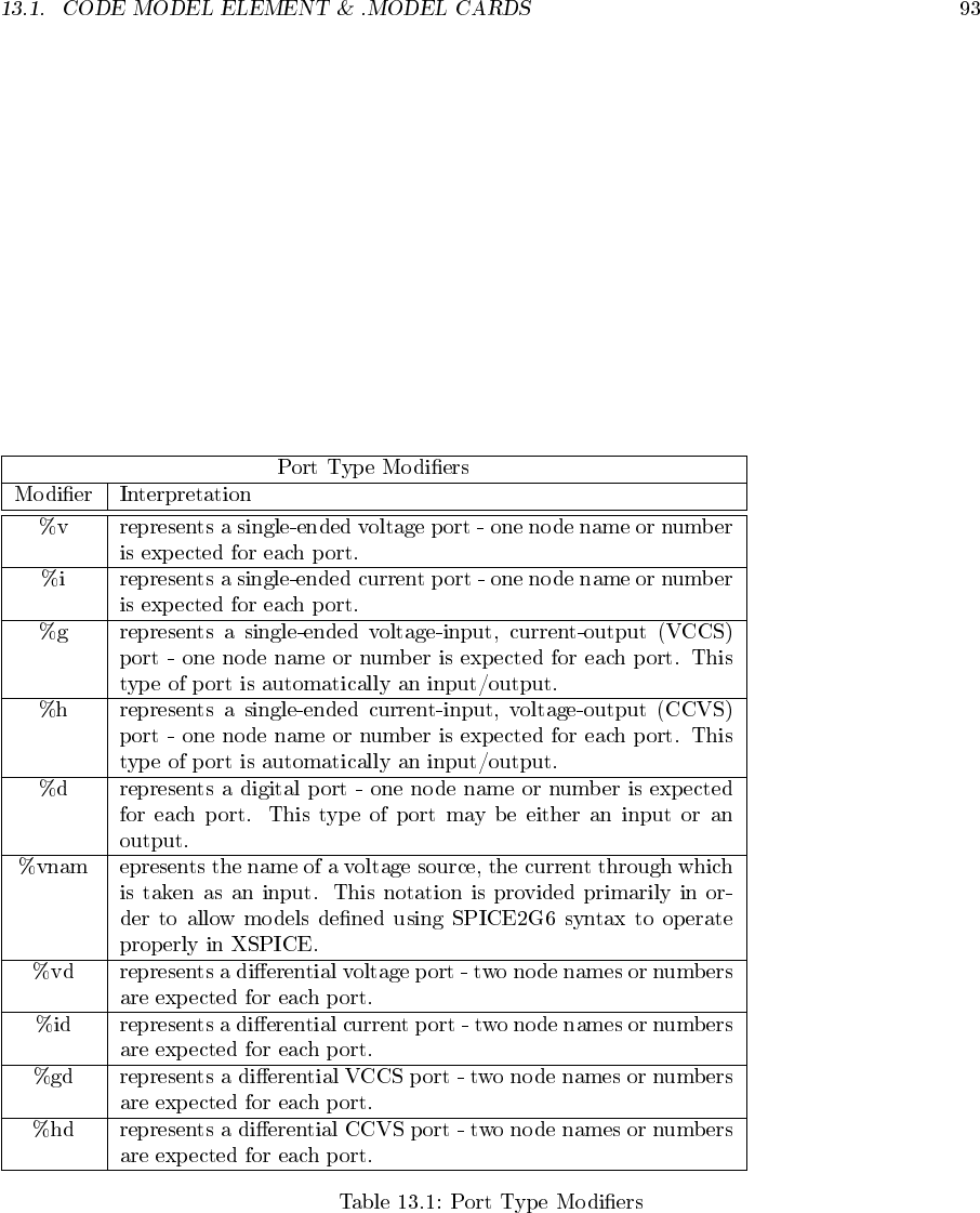
- Code Model Element & .MODEL Cards
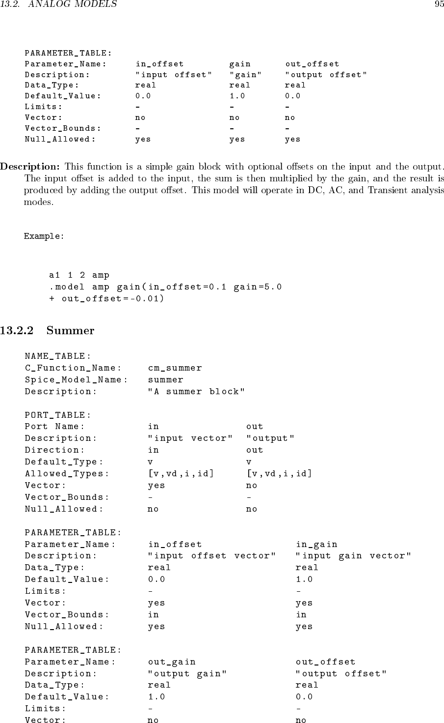
- Analog Models
- Gain
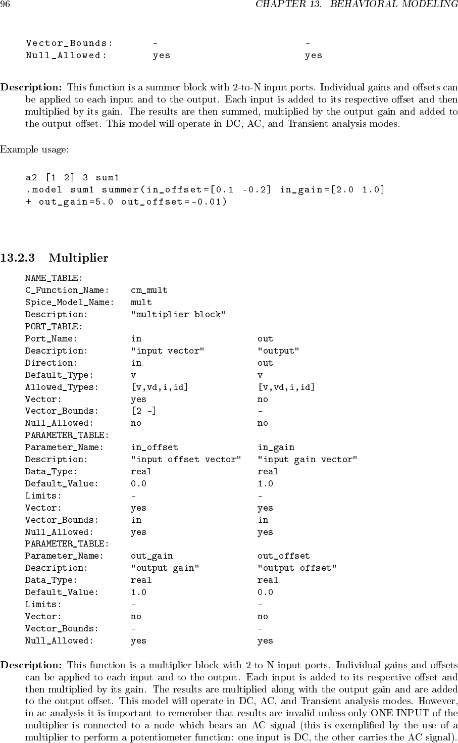
- Summer
- Multiplier
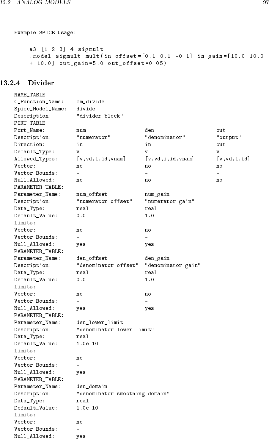
- Divider
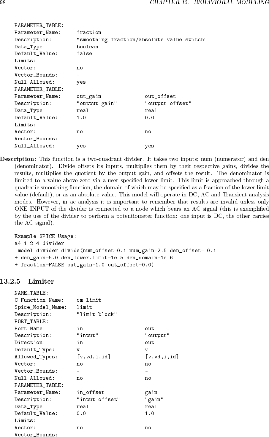
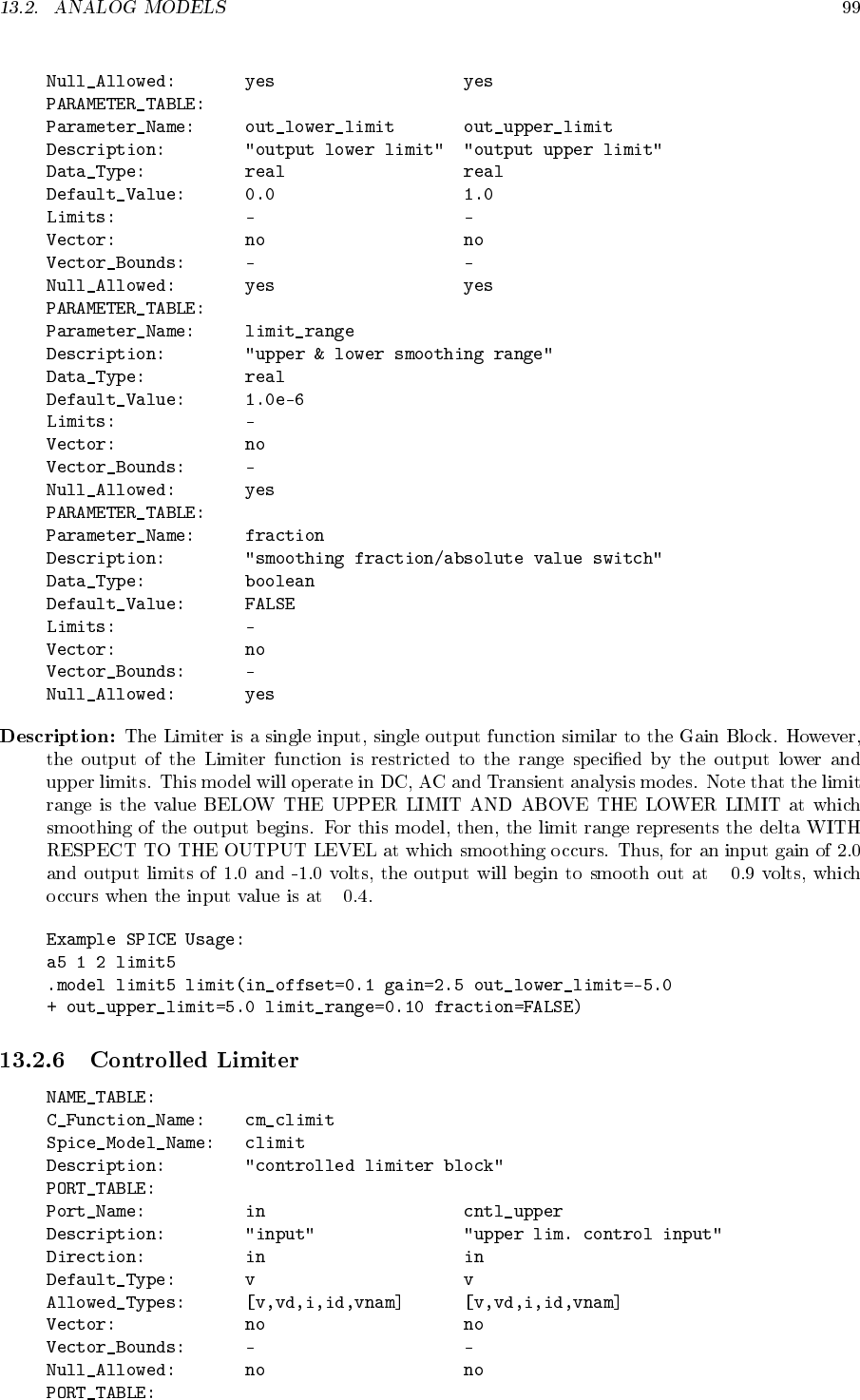
- Limiter
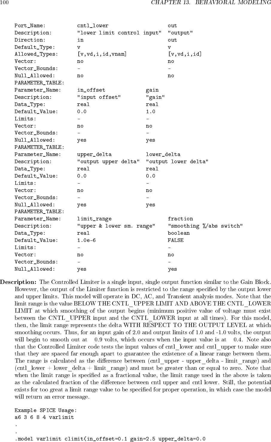
- Controlled Limiter
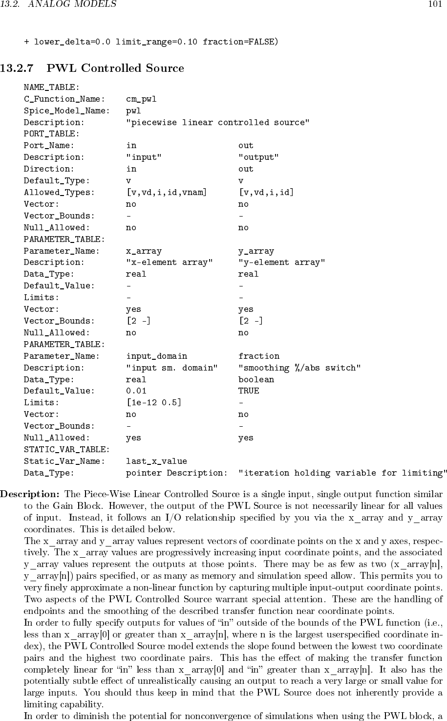
- PWL Controlled Source
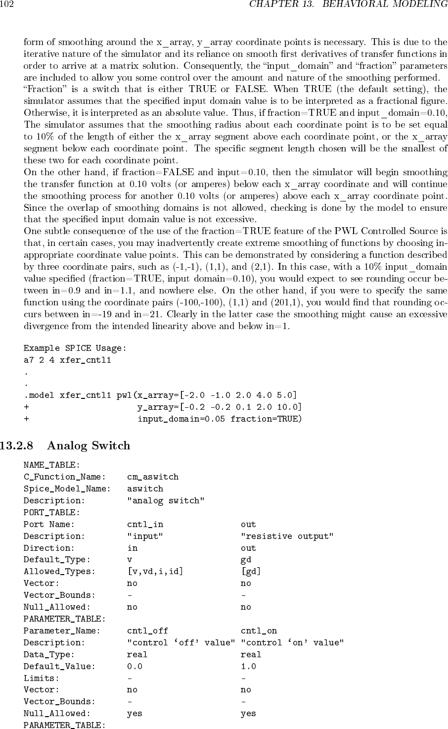
- Analog Switch
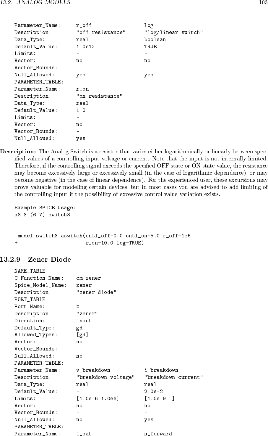
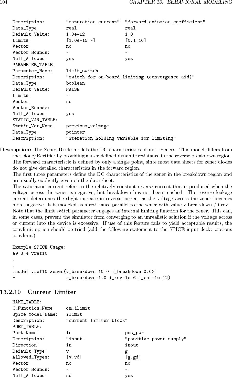
- Zener Diode
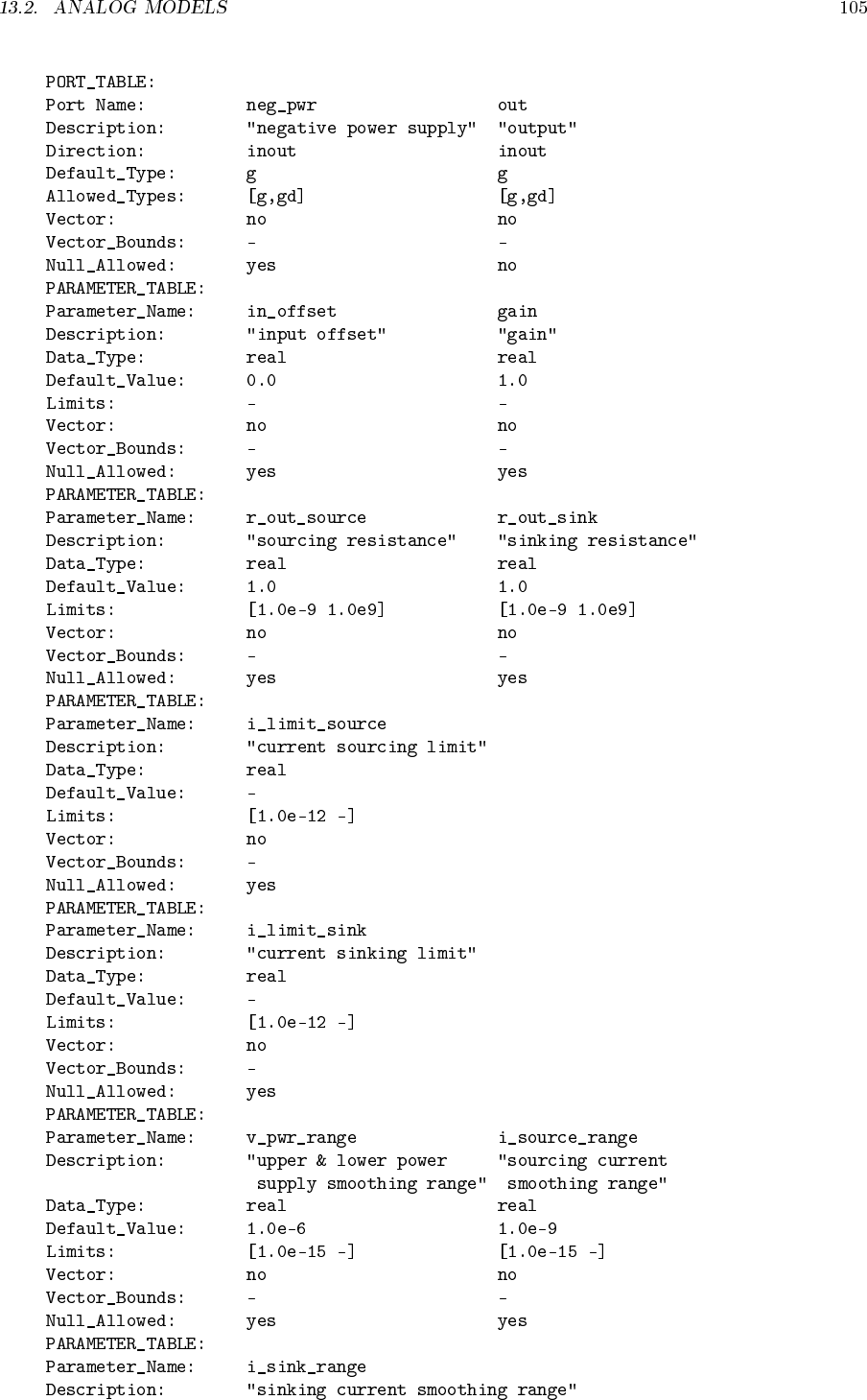
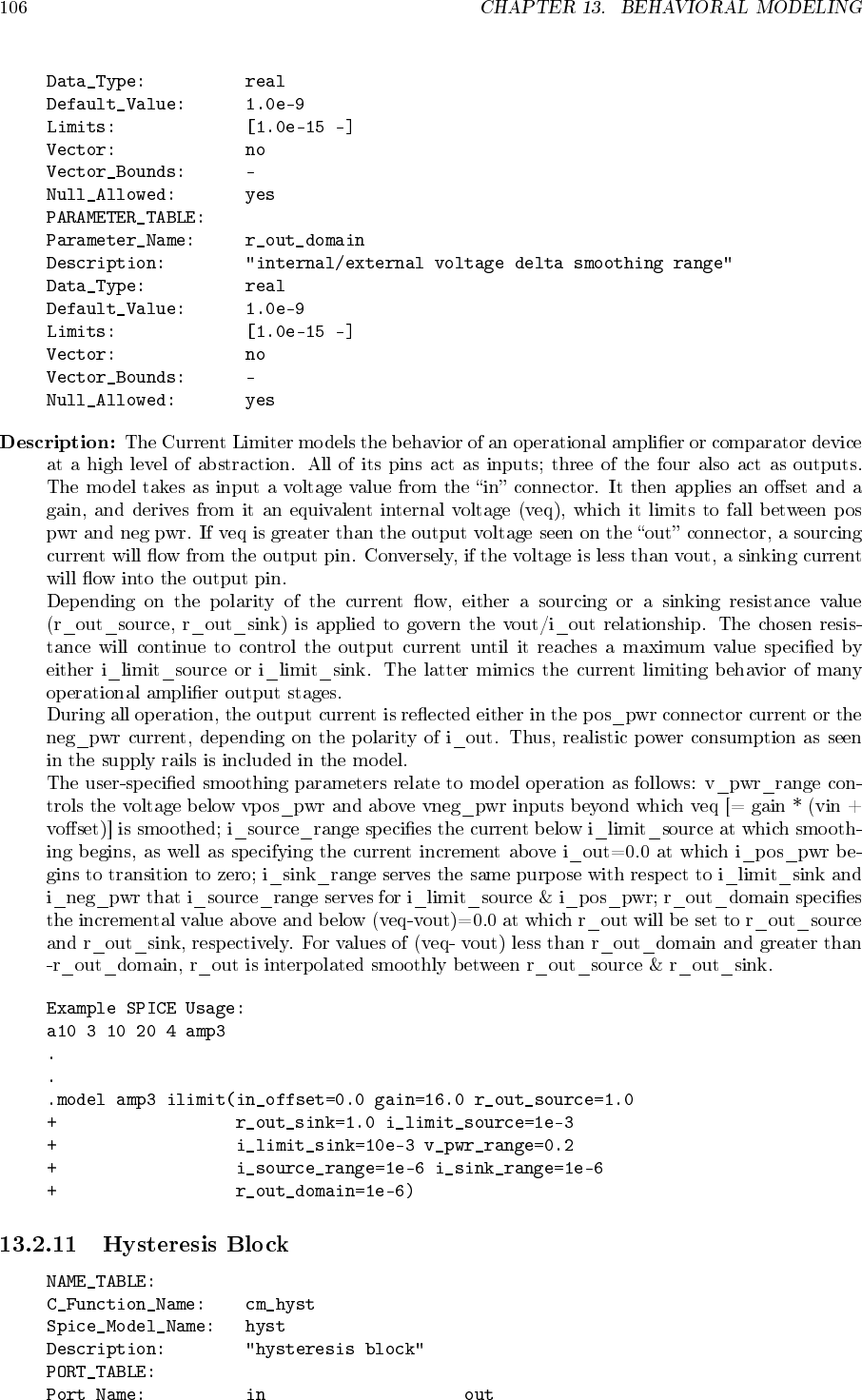
- Current Limiter
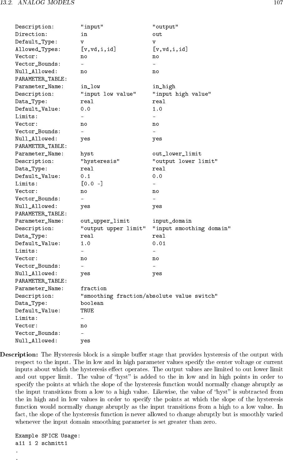
- Hysteresis Block
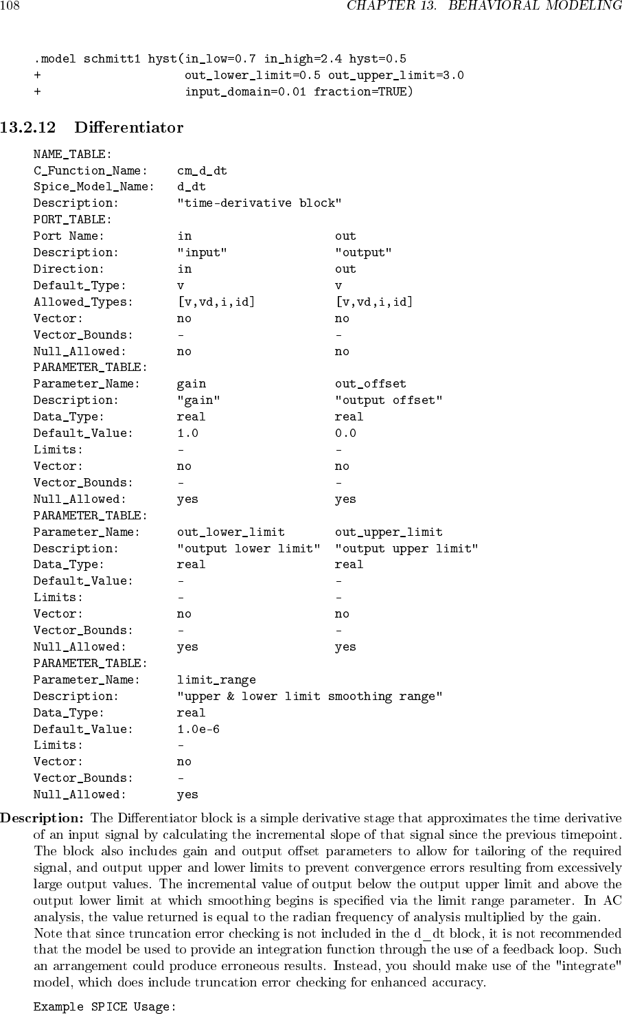
- Differentiator
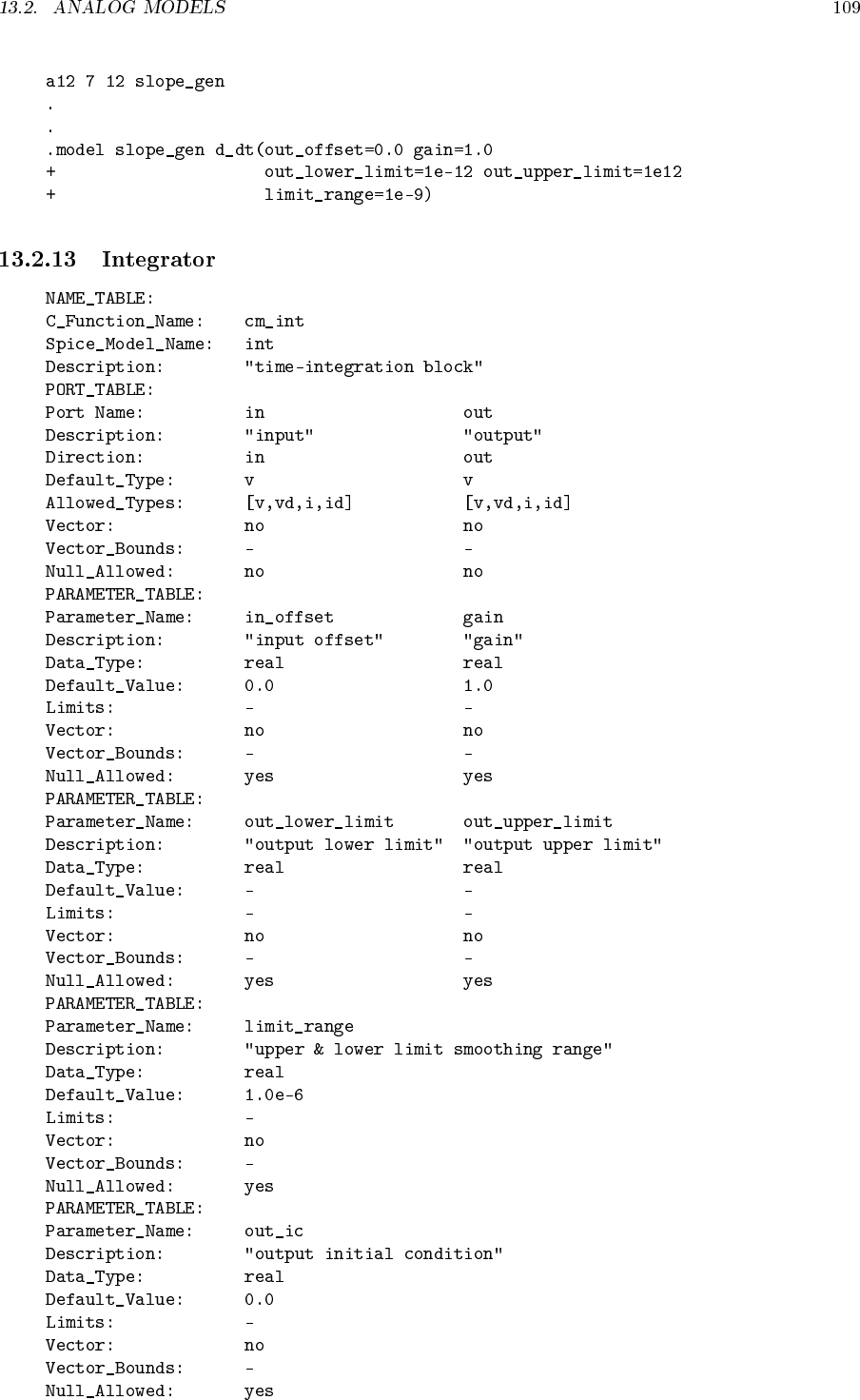
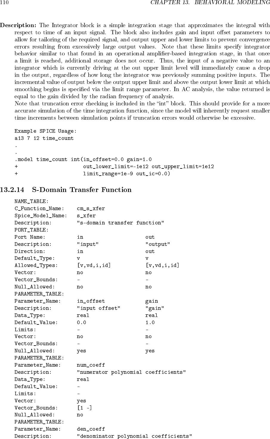
- Integrator
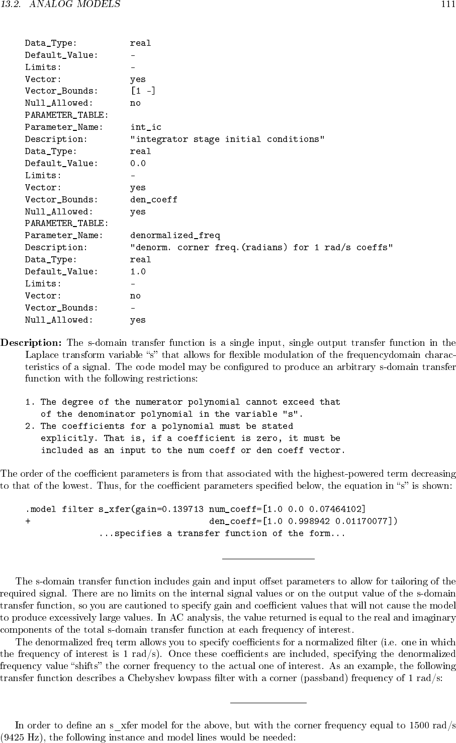
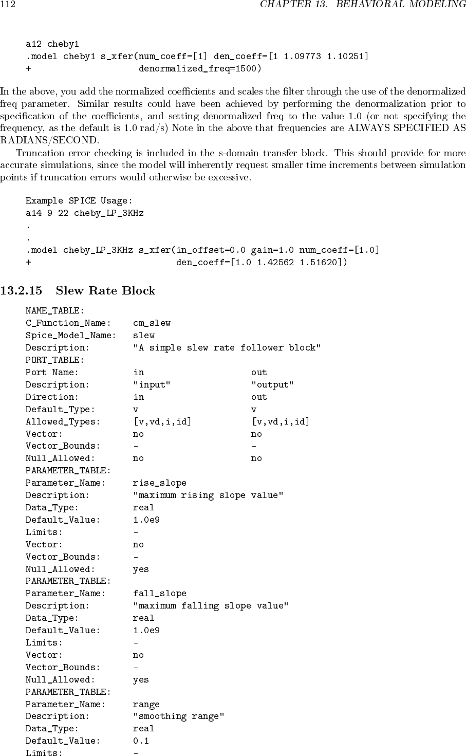
- S-Domain Transfer Function
- Slew Rate Block
- Inductive Coupling
- Magnetic Core
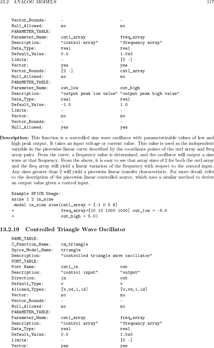
- Controlled Sine Wave Oscillator
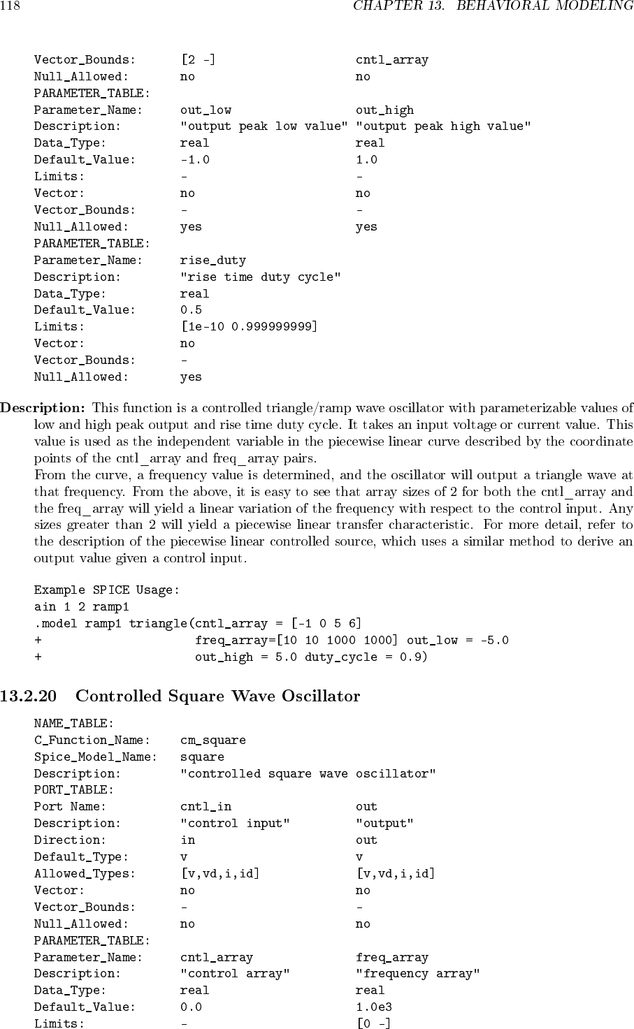
- Controlled Triangle Wave Oscillator
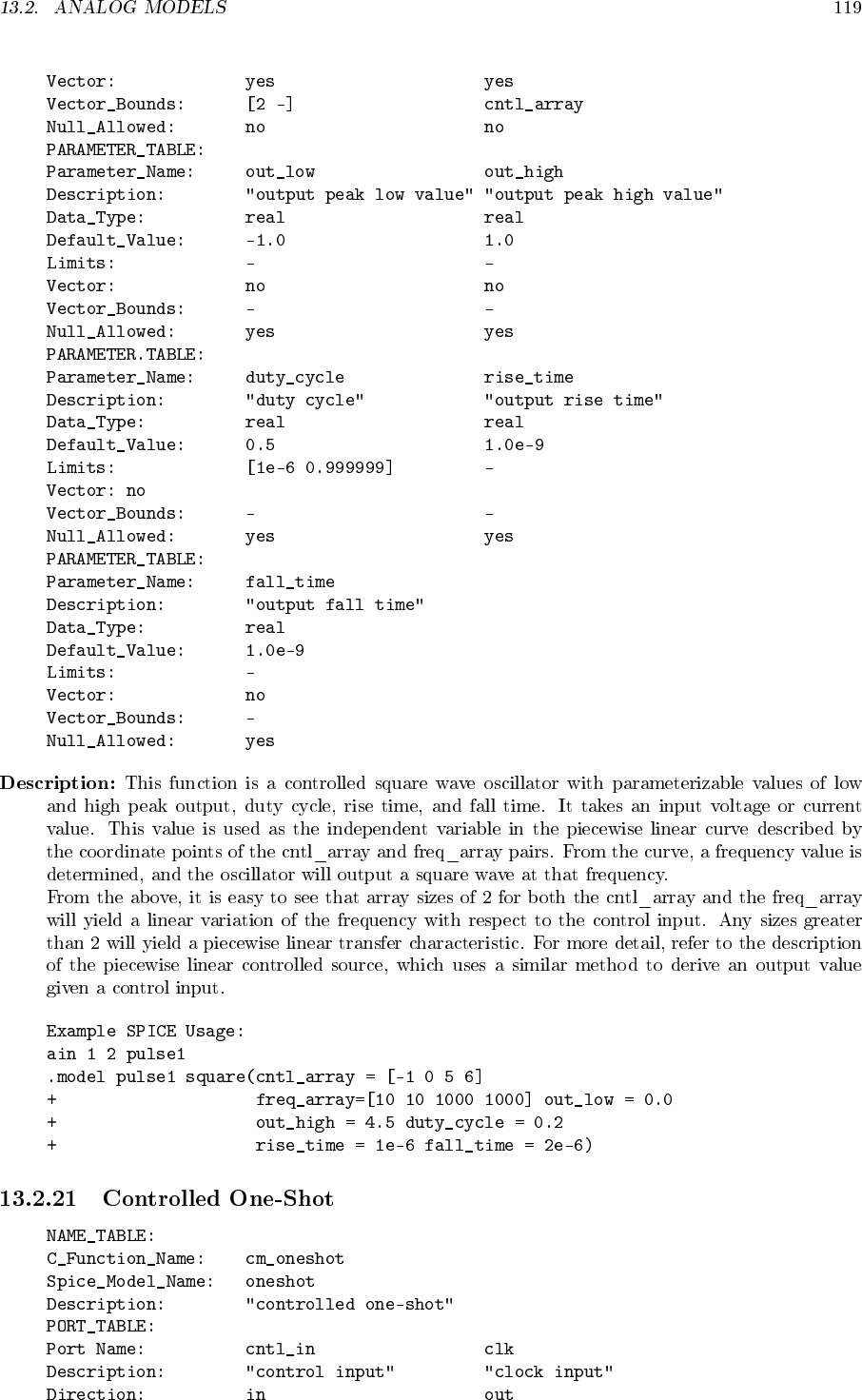
- Controlled Square Wave Oscillator
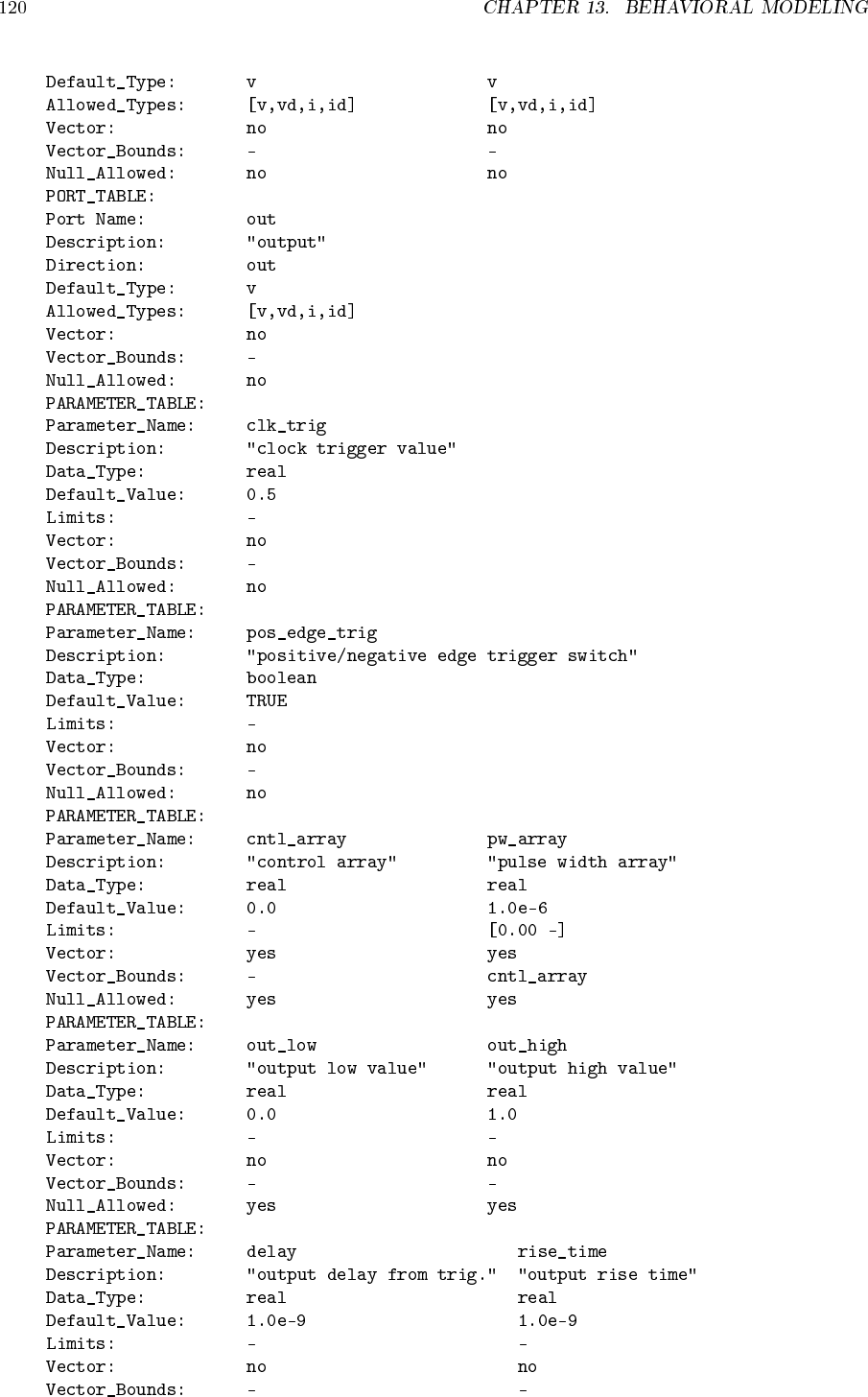
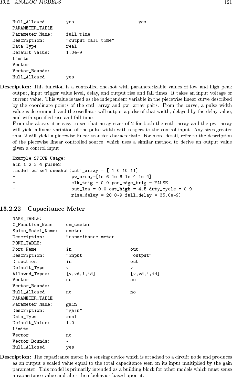
- Controlled One-Shot
- Capacitance Meter
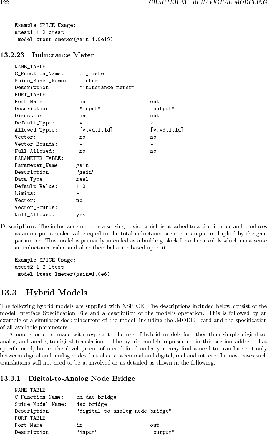
- Inductance Meter
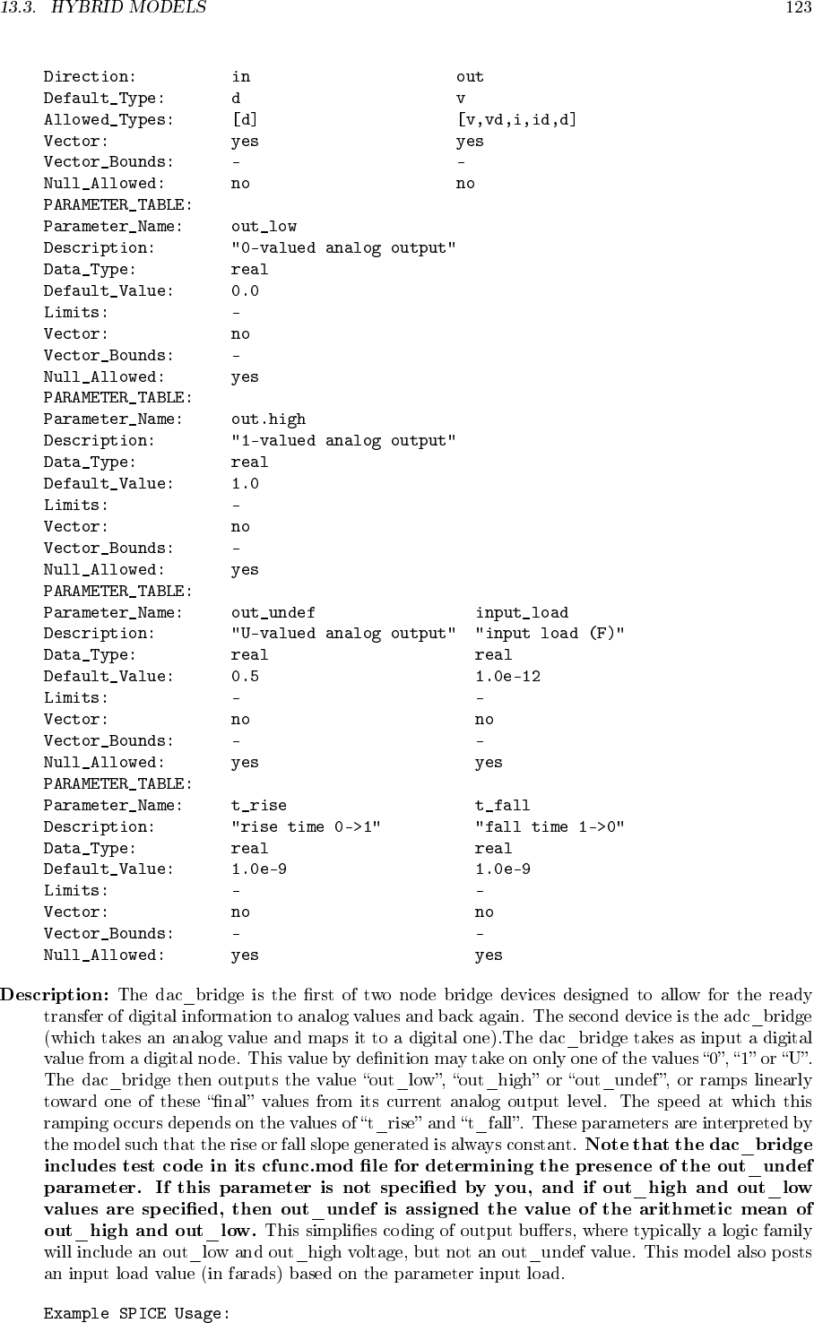
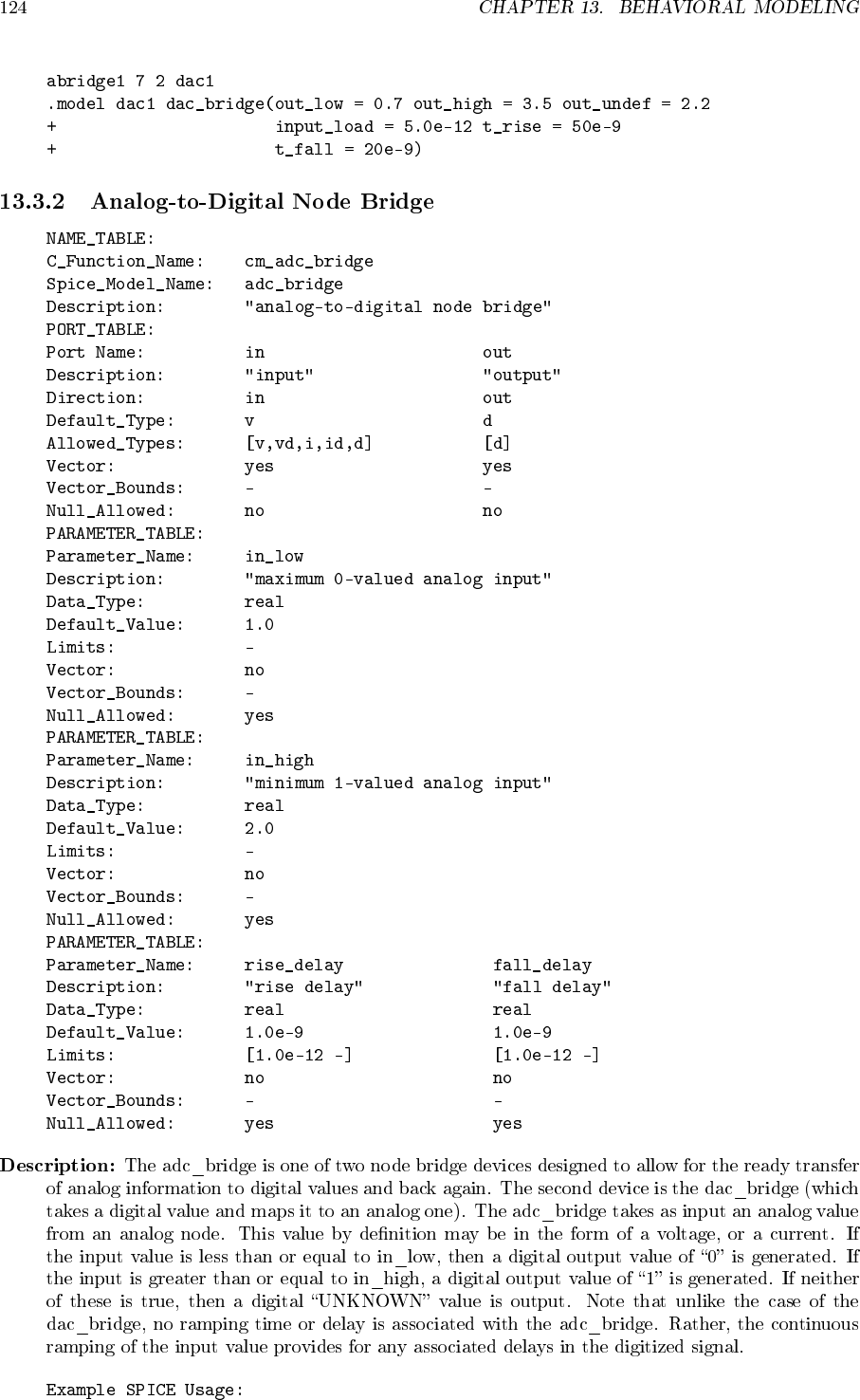
- Hybrid Models
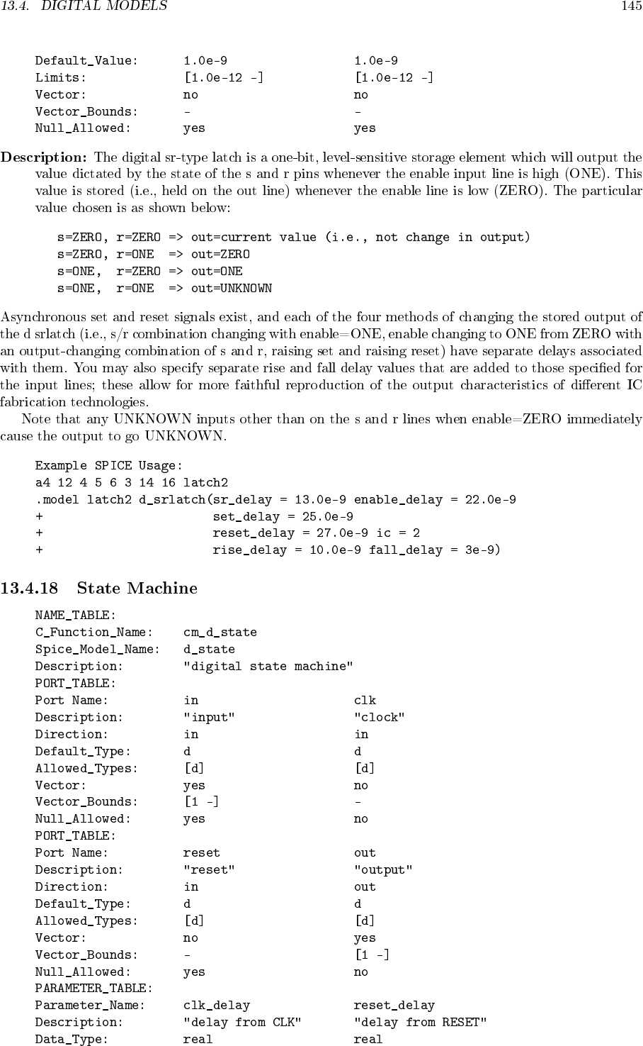
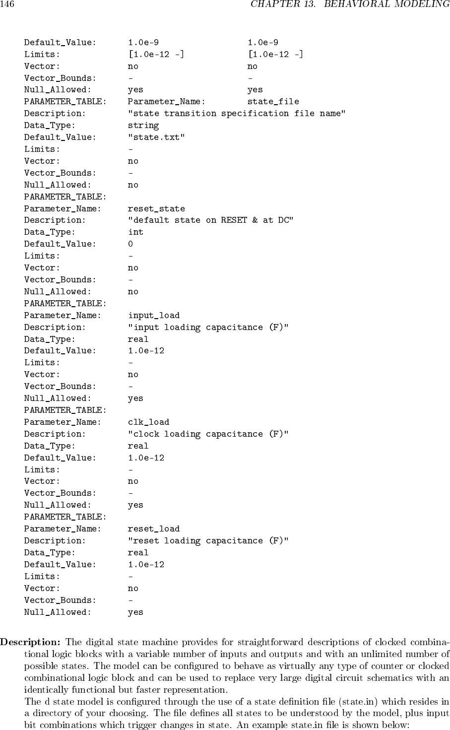
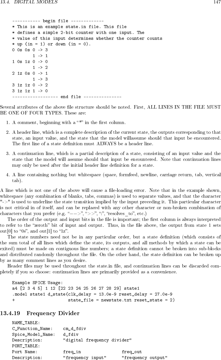
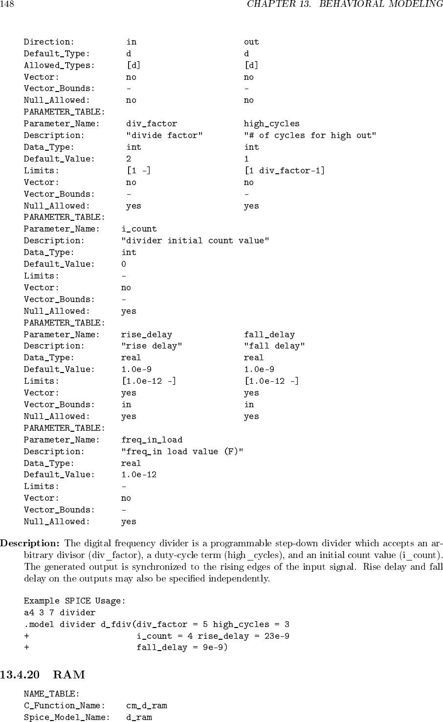
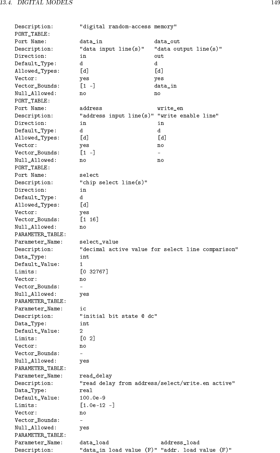
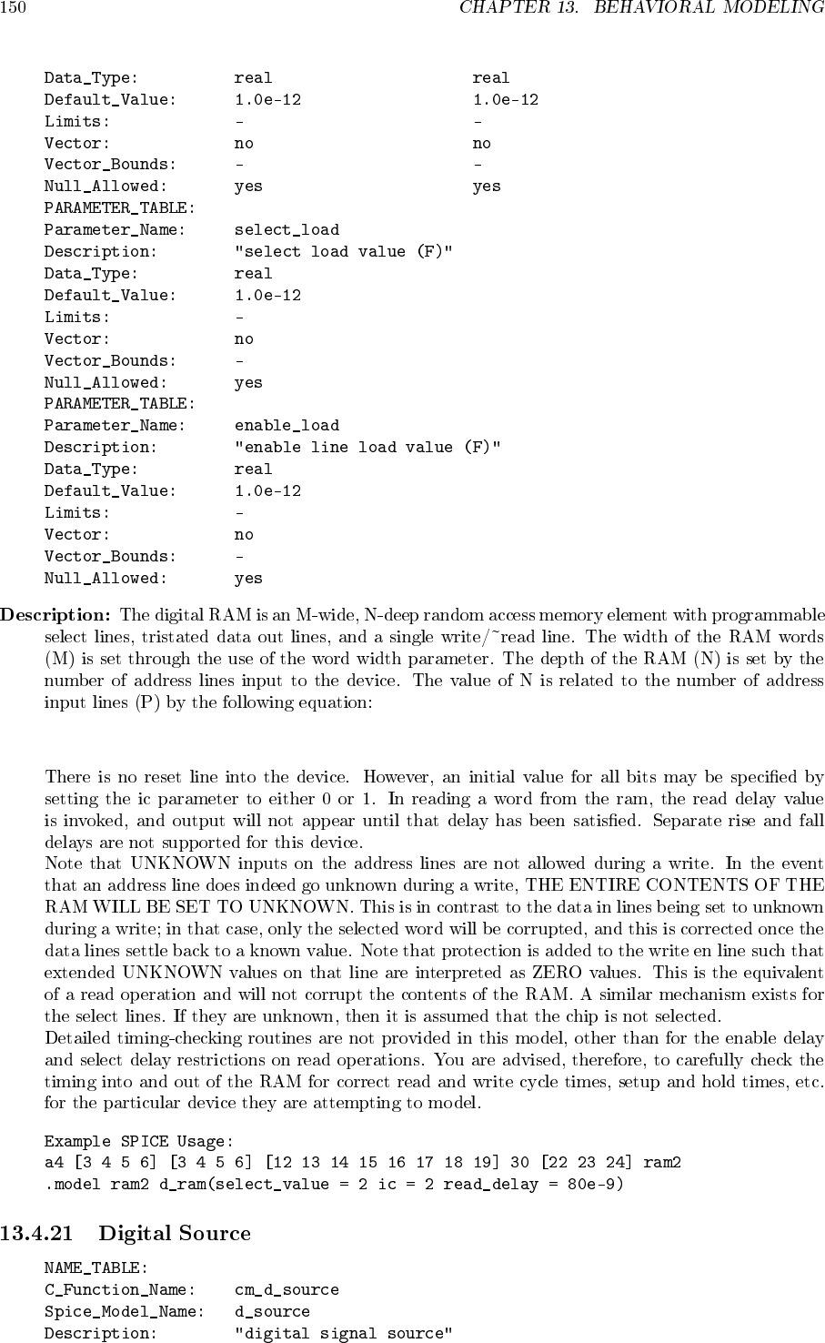
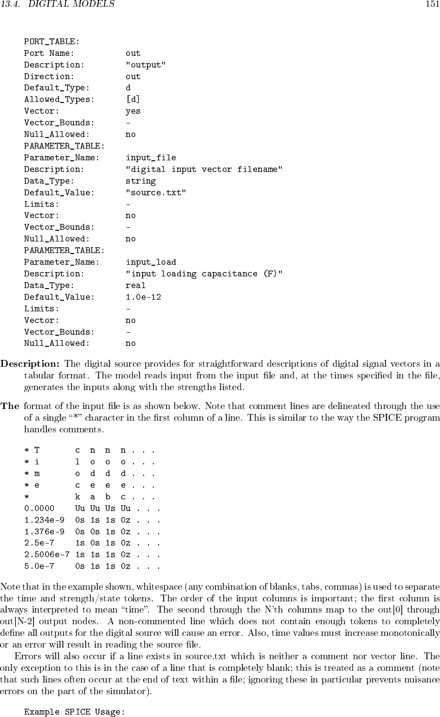
- Digital Models
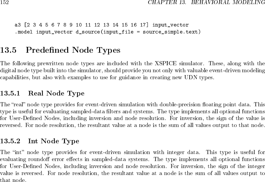
- Predefined Node Types
- Verilog A Device models
- Mixed-Level Simulation (ngspice with TCAD)
- Analyses and Output Control
- Simulator Variables (.options)
- Initial Conditions
- Analyses
- .AC: Small-Signal AC Analysis
- .DC: DC Transfer Function
- .DISTO: Distortion Analysis
- .NOISE: Noise Analysis
- .OP: Operating Point Analysis
- .PZ: Pole-Zero Analysis
- .SENS: DC or Small-Signal AC Sensitivity Analysis
- .TF: Transfer Function Analysis
- .TRAN: Transient Analysis
- .MEAS: Measurements after Op, Ac and Transient Analysis
- Batch Output
- Starting ngspice
- Introduction
- Where to obtain ngspice
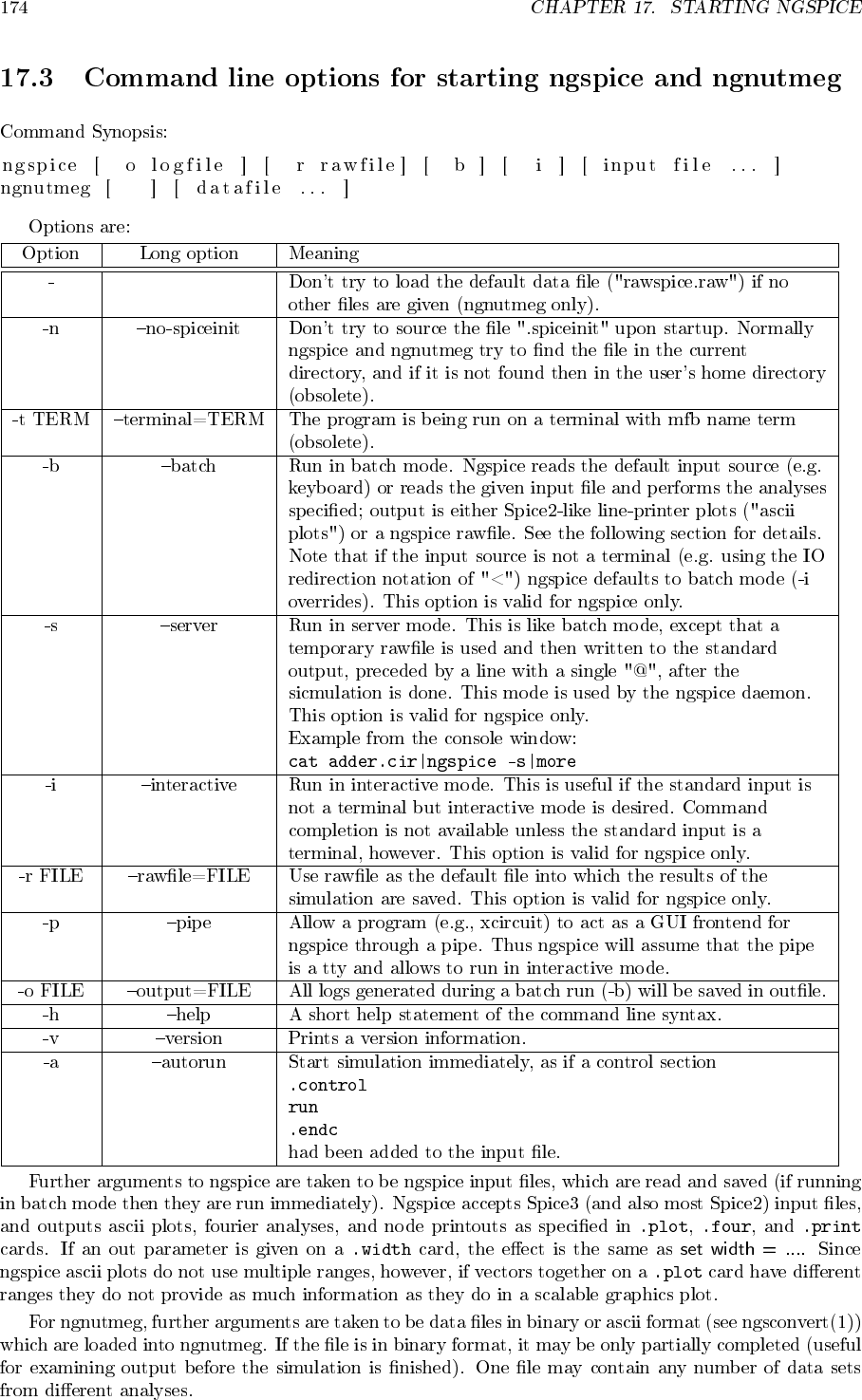
- Command line options for starting ngspice and ngnutmeg
- Starting options
- Standard configuration file spinit
- User defined configuration file .spiceinit
- Environmental variables
- Memory usage
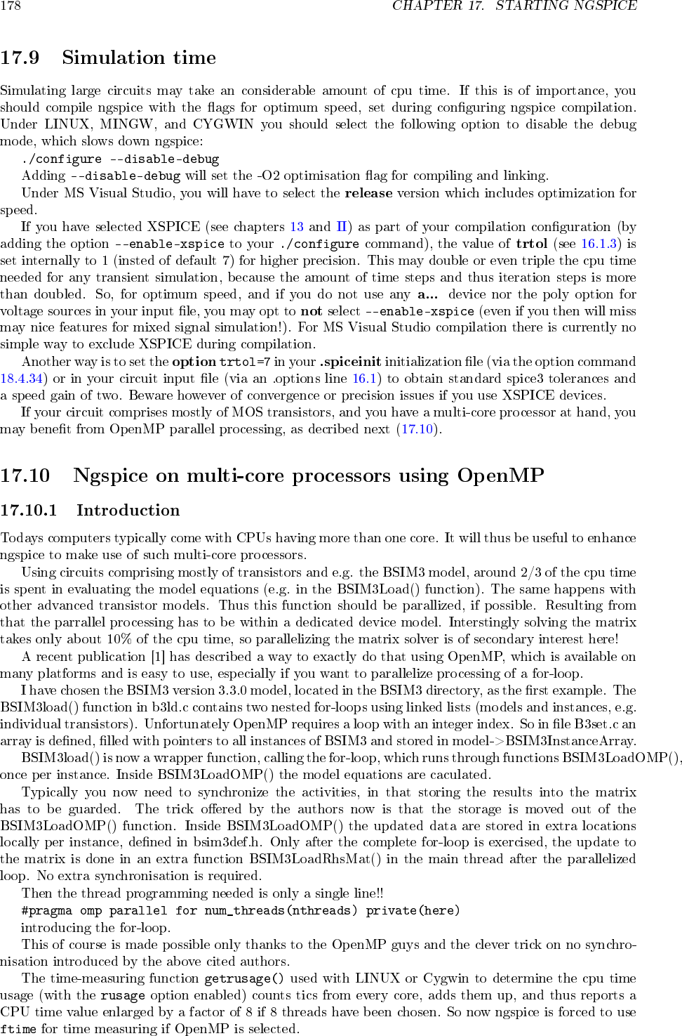
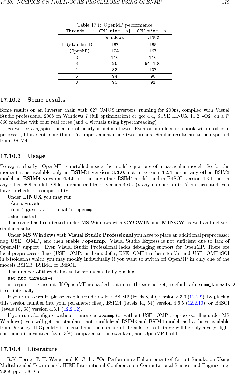
- Simulation time
- Ngspice on multi-core processors using OpenMP
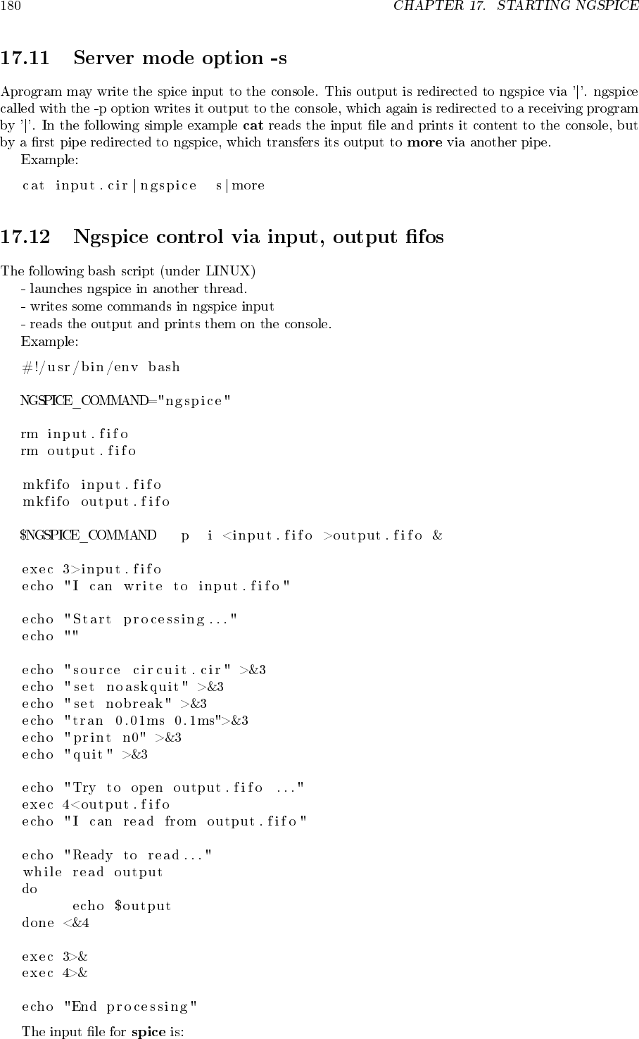
- Server mode option -s
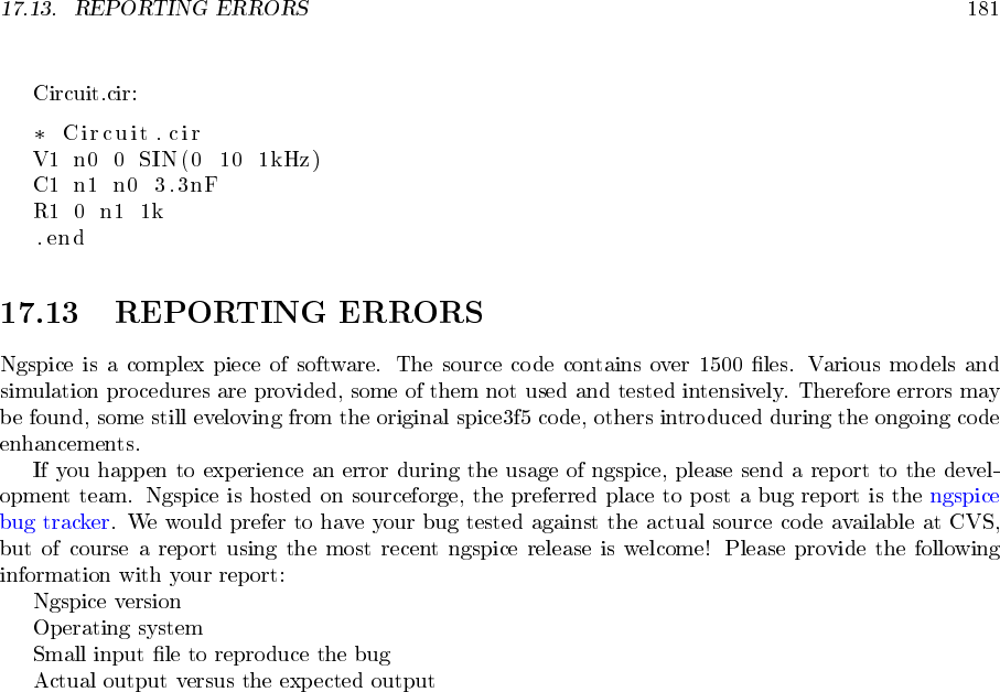
- Ngspice control via input, output fifos
- REPORTING ERRORS
- Interactive Interpreter
- Expressions, Functions, and Constants
- Plots
- Command Interpretation
- Commands
- Ac*: Perform an AC, small-signal frequency response analysis
- Alias: Create an alias for a command
- Alter*: Change a device or model parameter
- Altermod*: Change a model parameter
- Asciiplot: Plot values using old-style character plots
- Aspice*: Asynchronous ngspice run
- Bug: Mail a bug report
- Cd: Change directory
- Compose: Compose a vector
- Destroy: Delete a data set
- Dc*: Perform a DC-sweep analysis
- Define: Define a function
- Deftype: Define a new type for a vector or plot
- Delete*: Remove a trace or breakpoint
- Diff: Compare vectors
- Display: List known vectors and types
- Echo: Print text
- Edit*: Edit the current circuit
- FFT: fast Fourier transform of the input vector(s)
- Fourier: Perform a fourier transform
- Gnuplot: Graphics output via Gnuplot
- Hardcopy: Save a plot to a file for printing
- Help: Print summaries of Ngspice commands
- History: Review previous commands
- Iplot*: Incremental plot
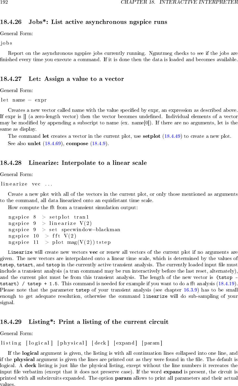
- Jobs*: List active asynchronous ngspice runs
- Let: Assign a value to a vector
- Linearize: Interpolate to a linear scale
- Listing*: Print a listing of the current circuit
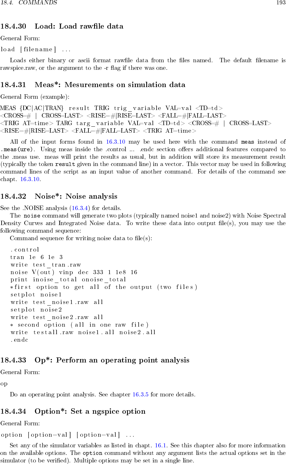
- Load: Load rawfile data
- Meas*: Mesurements on simulation data
- Noise*: Noise analysis
- Op*: Perform an operating point analysis
- Option*: Set a ngspice option
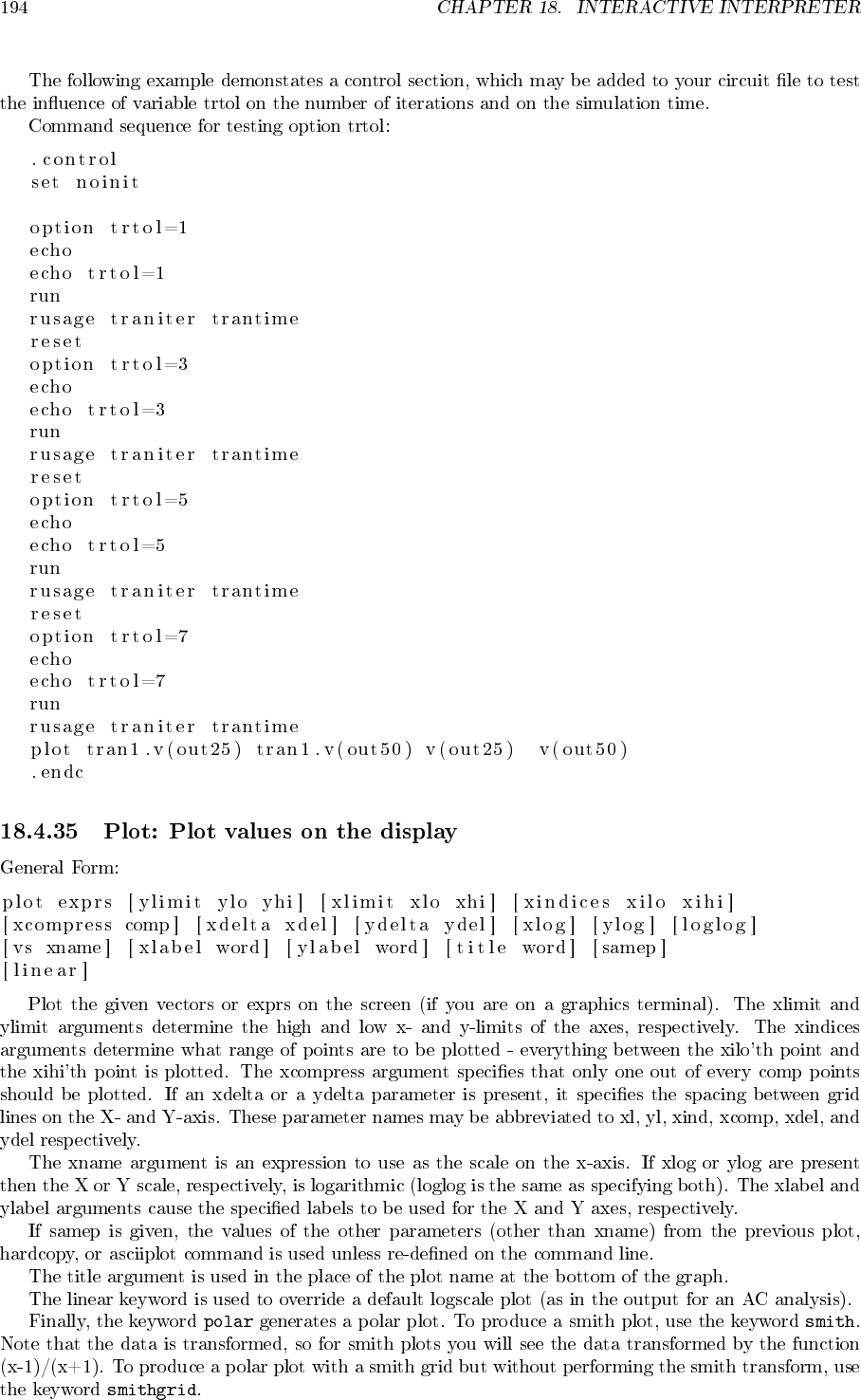
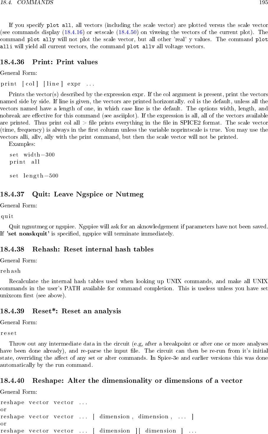
- Plot: Plot values on the display
- Print: Print values
- Quit: Leave Ngspice or Nutmeg
- Rehash: Reset internal hash tables
- Reset*: Reset an analysis
- Reshape: Alter the dimensionality or dimensions of a vector
- Resume*: Continue a simulation after a stop
- Rspice*: Remote ngspice submission
- Run*: Run analysis from the input file
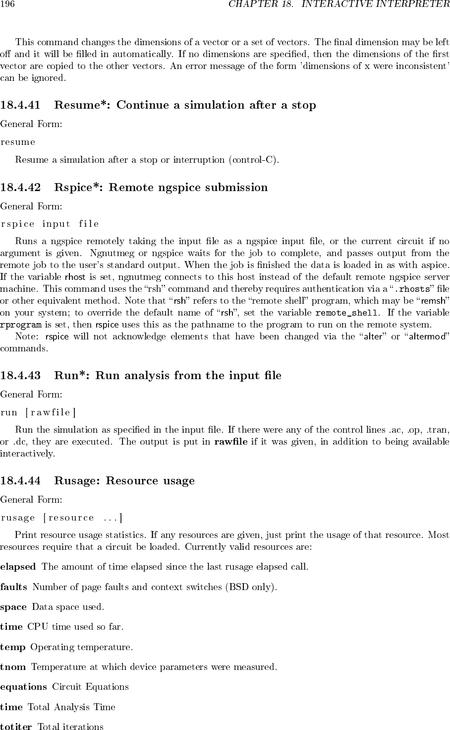
- Rusage: Resource usage
- Save*: Save a set of outputs
- Sens*: Run a sensitivity analysis
- Set: Set the value of a variable
- Setcirc*: Change the current circuit
- Setplot: Switch the current set of vectors
- Setscale: Set the scale vector for the current plot
- Settype: Set the type of a vector
- Shell: Call the command interpreter
- Shift: Alter a list variable
- Show*: List device state
- Showmod*: List model parameter values
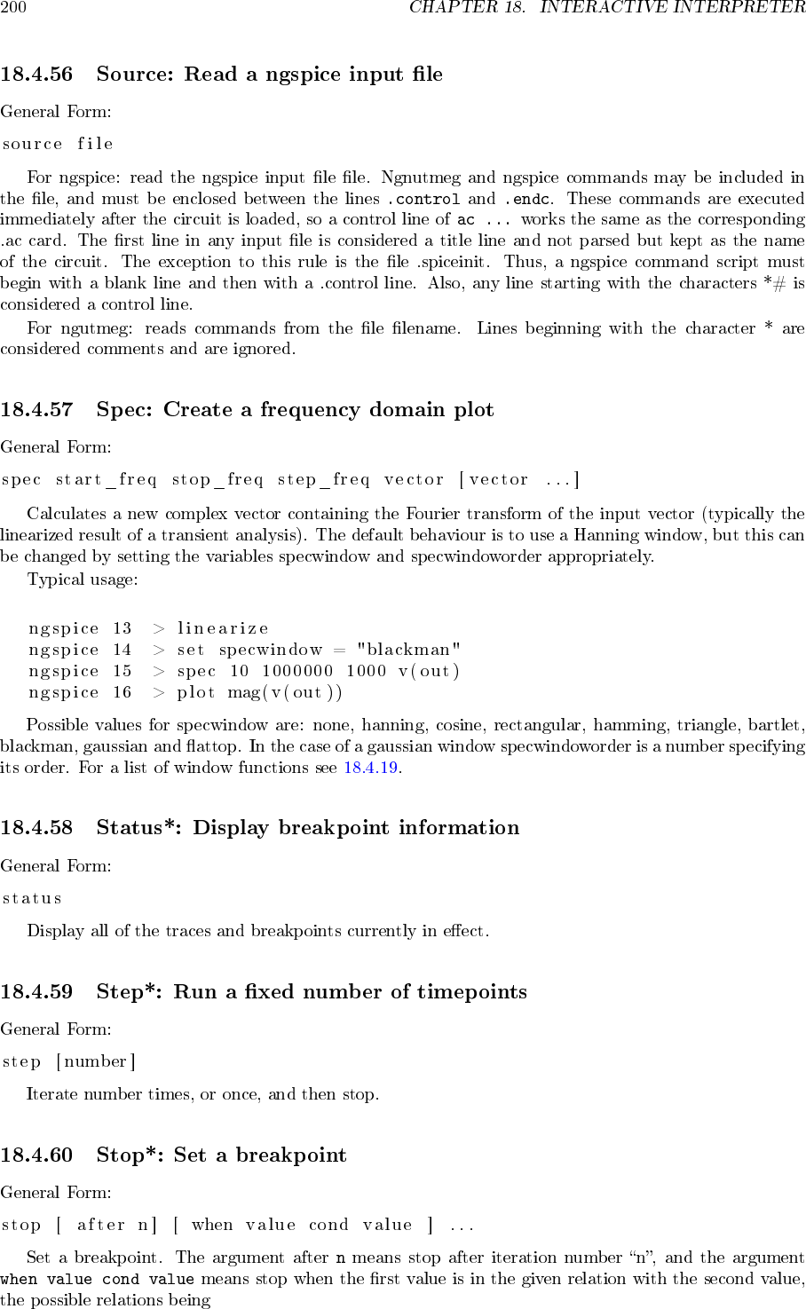
- Source: Read a ngspice input file
- Spec: Create a frequency domain plot
- Status*: Display breakpoint information
- Step*: Run a fixed number of timepoints
- Stop*: Set a breakpoint
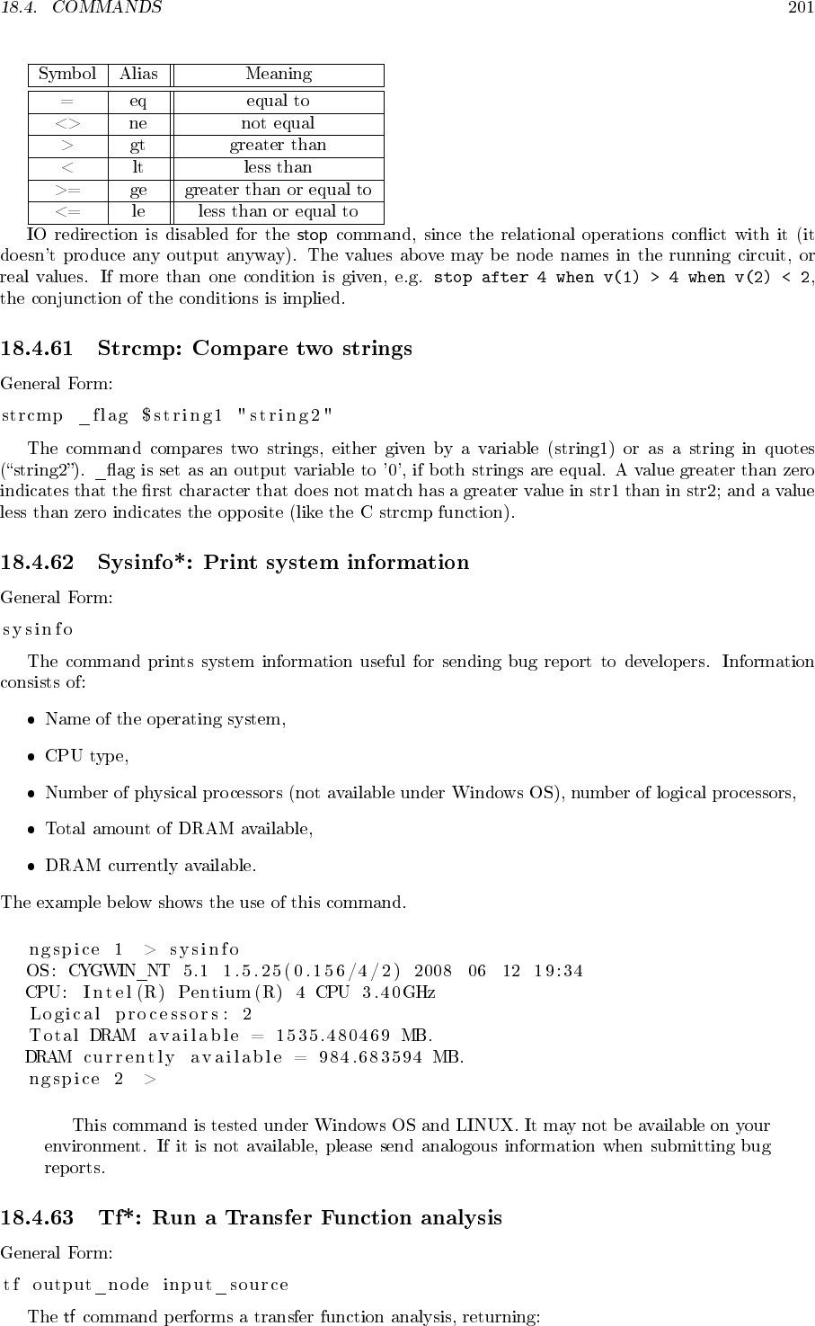
- Strcmp: Compare two strings
- Sysinfo*: Print system information
- Tf*: Run a Transfer Function analysis
- Trace*: Trace nodes
- Tran*: Perform a transient analysis
- Transpose: Swap the elements in a multi-dimensional data set
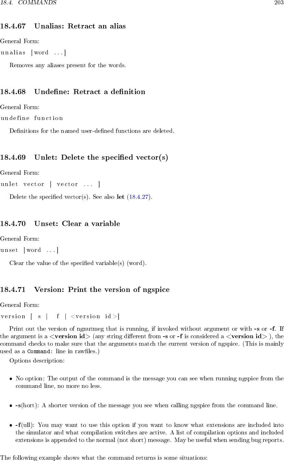
- Unalias: Retract an alias
- Undefine: Retract a definition
- Unlet: Delete the specified vector(s)
- Unset: Clear a variable
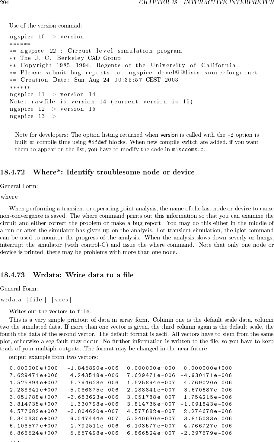
- Version: Print the version of ngspice
- Where*: Identify troublesome node or device
- Wrdata: Write data to a file
- Write: Write data to a file
- Xgraph: use the xgraph(1) program for plotting.
- Control Structures
- Variables
- Scripts
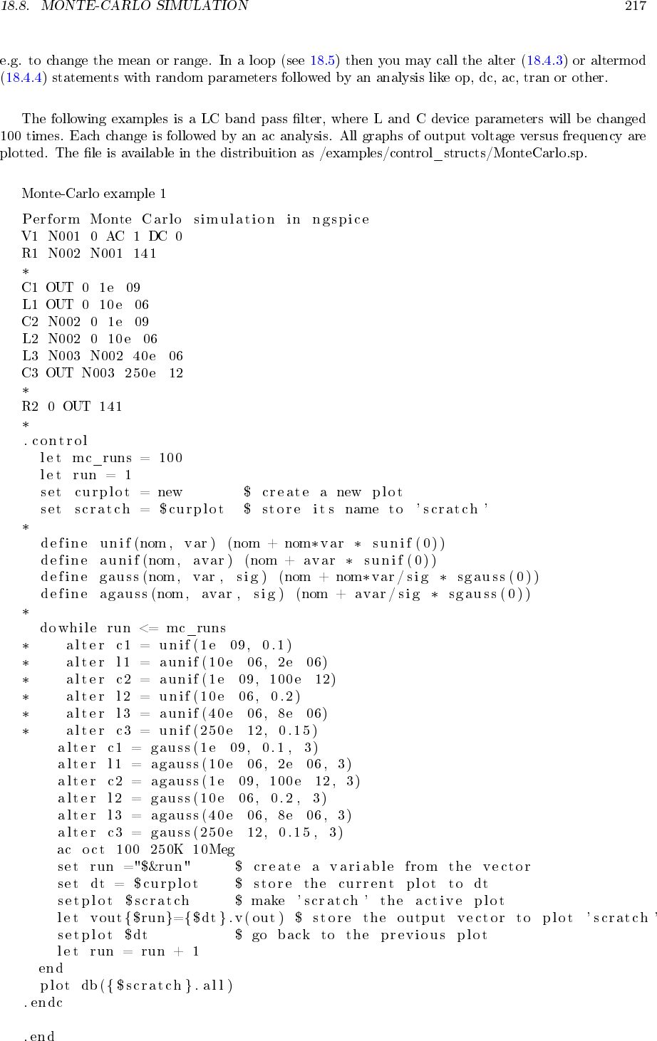
- Monte-Carlo Simulation
- MISCELLANEOUS (old stuff, has to be checked for relevance)
- Bugs (old stuff, has to be checked for relevance)
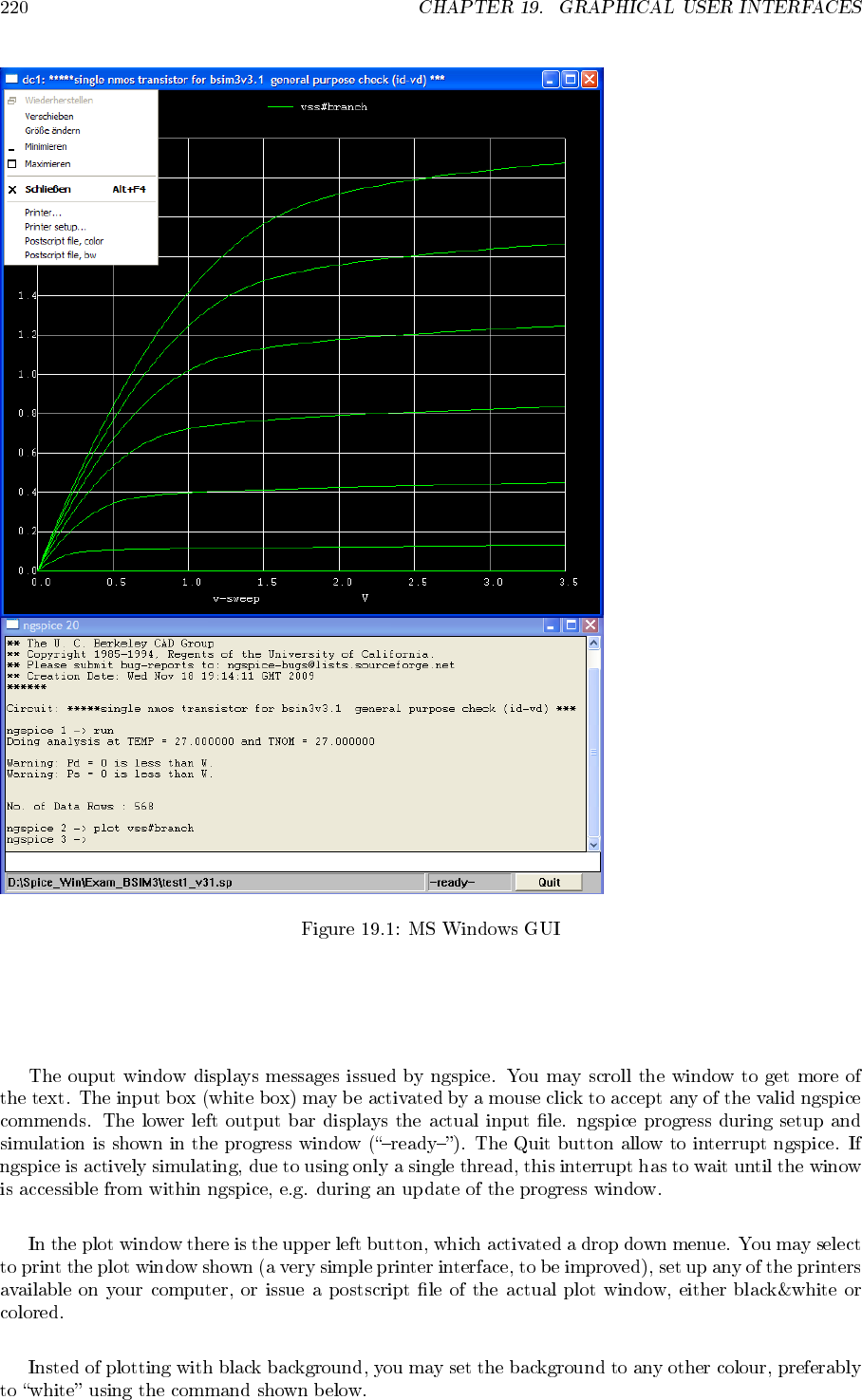
- Graphical User Interfaces
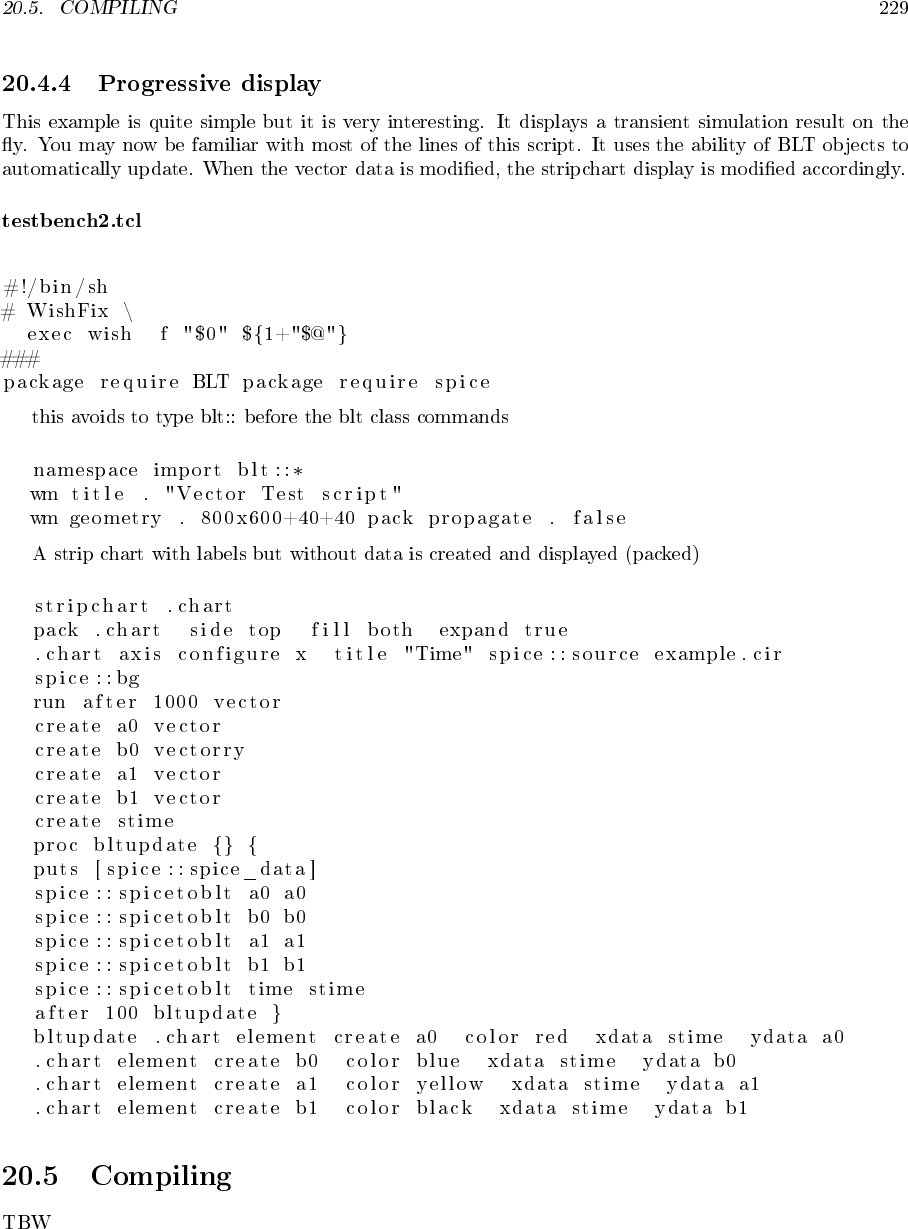
- TCLspice
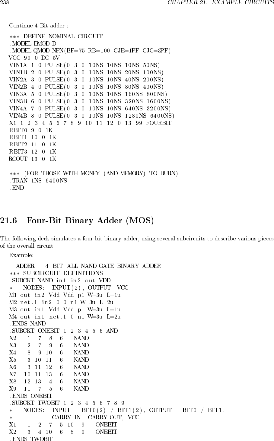
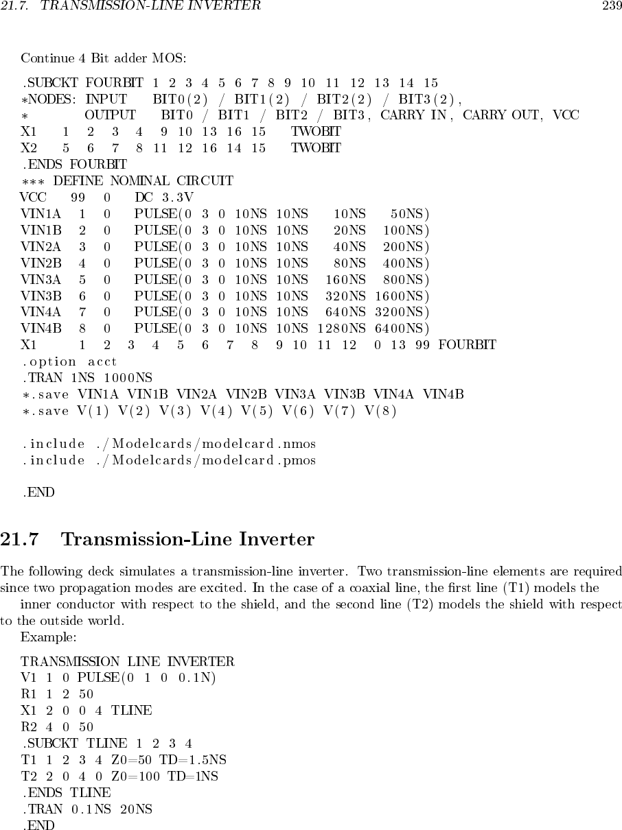
- Example Circuits
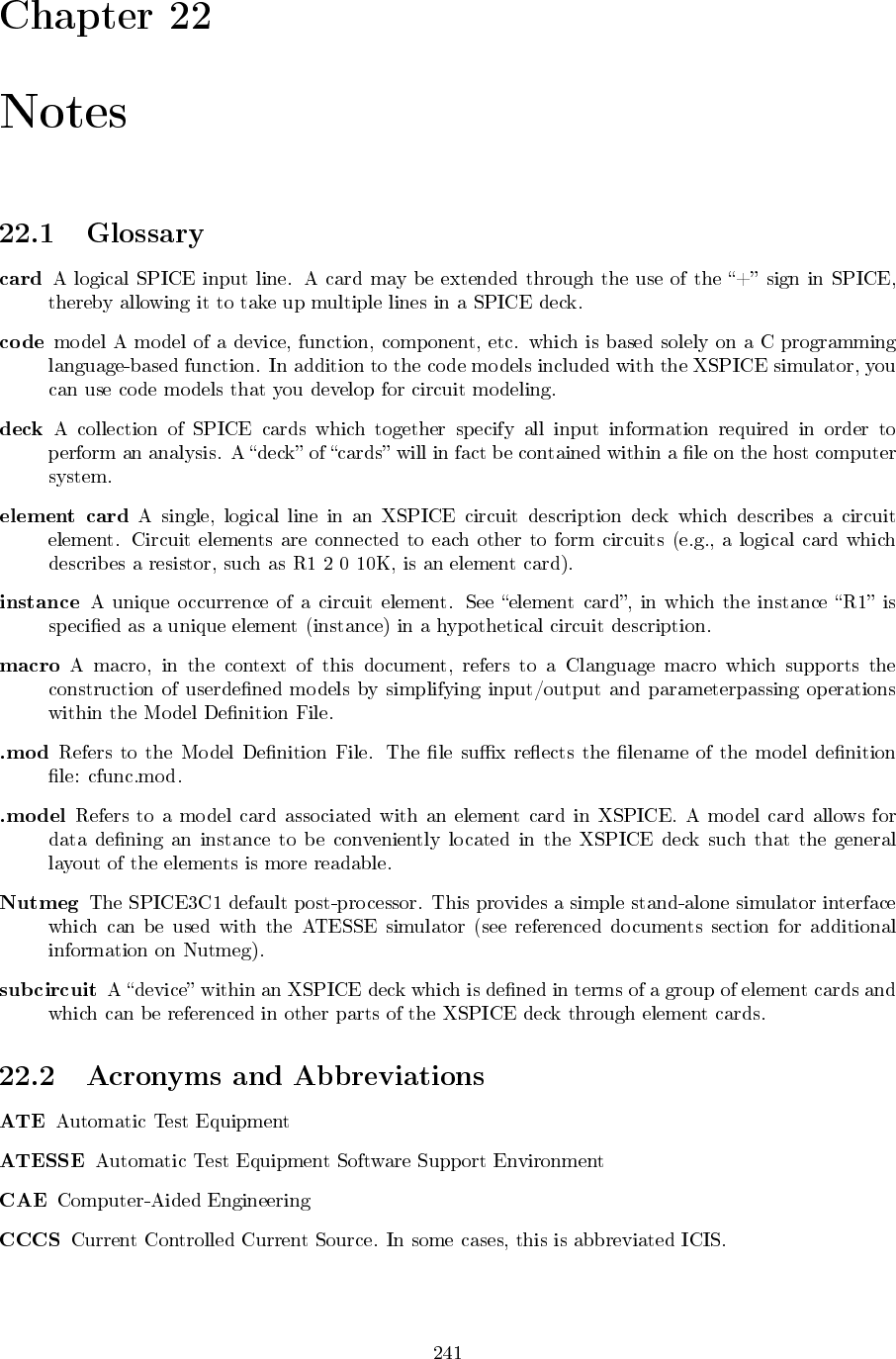
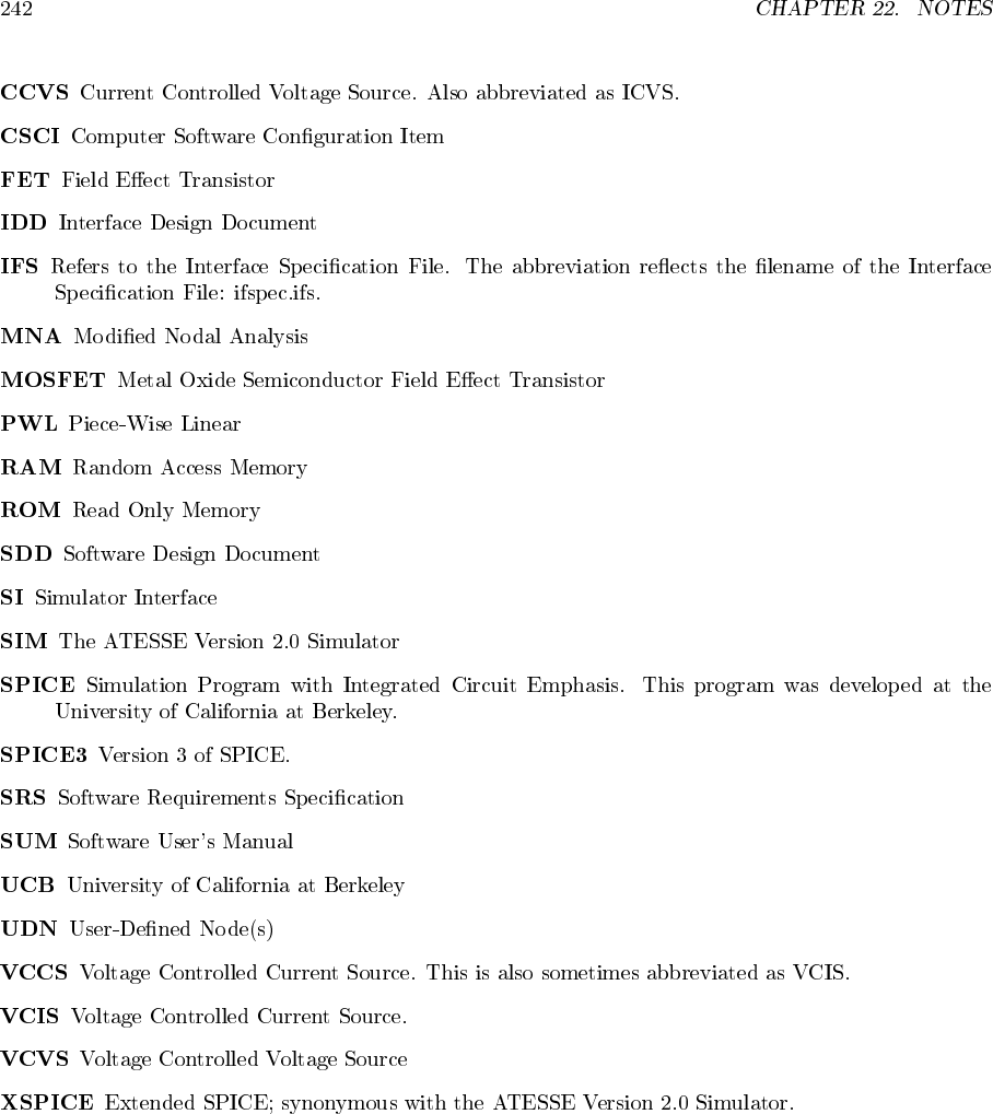
- Notes
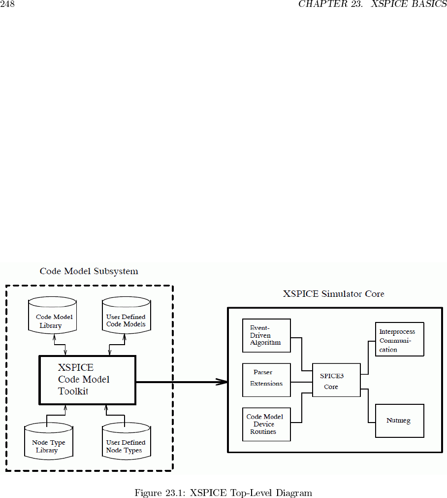
- II XSPICE Software User's Manual
- III CIDER
- IV Appendices
- Model and Device Parameters
- Elementary Devices
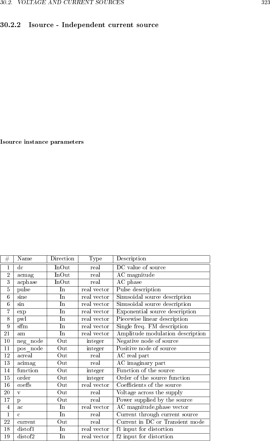
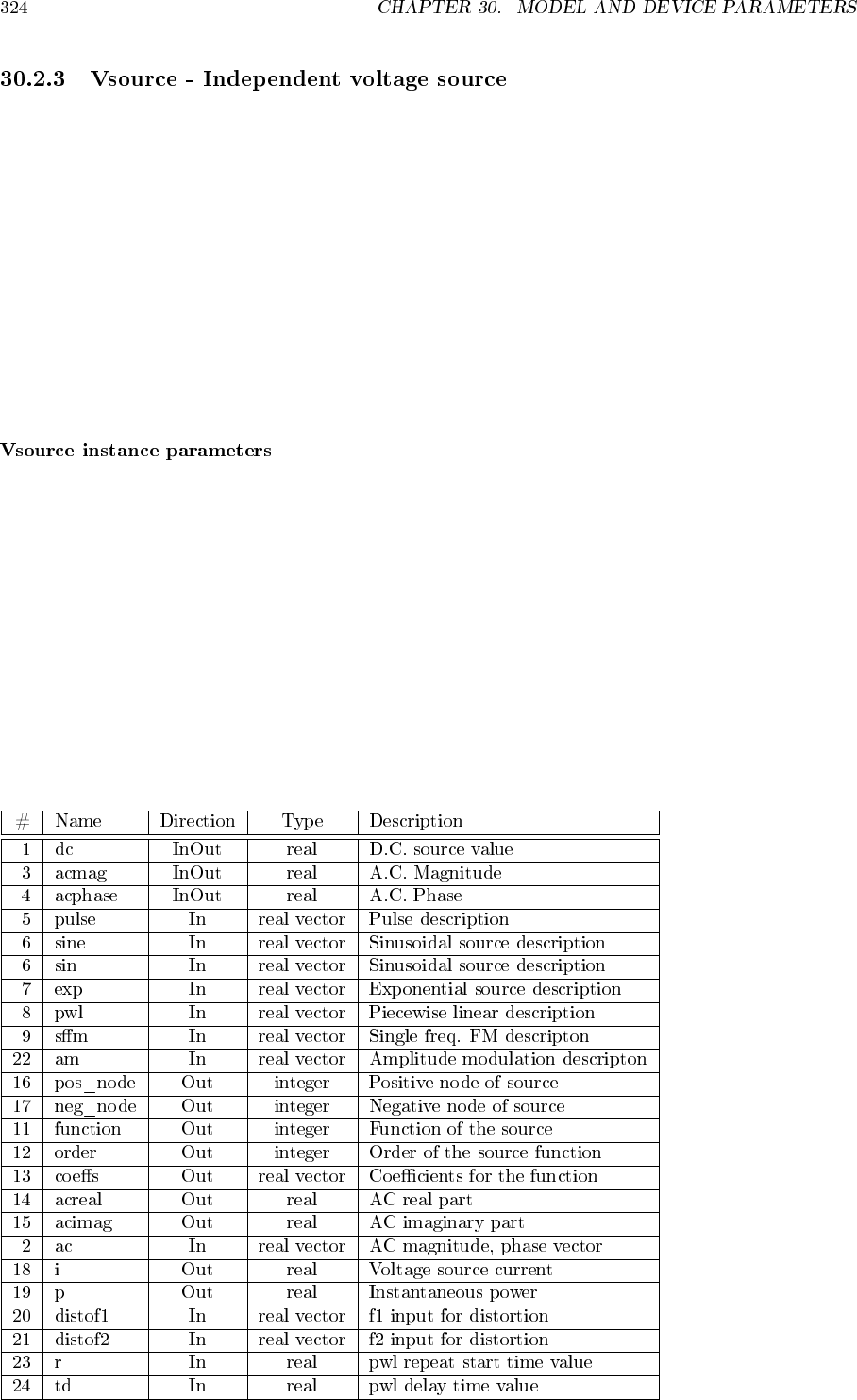
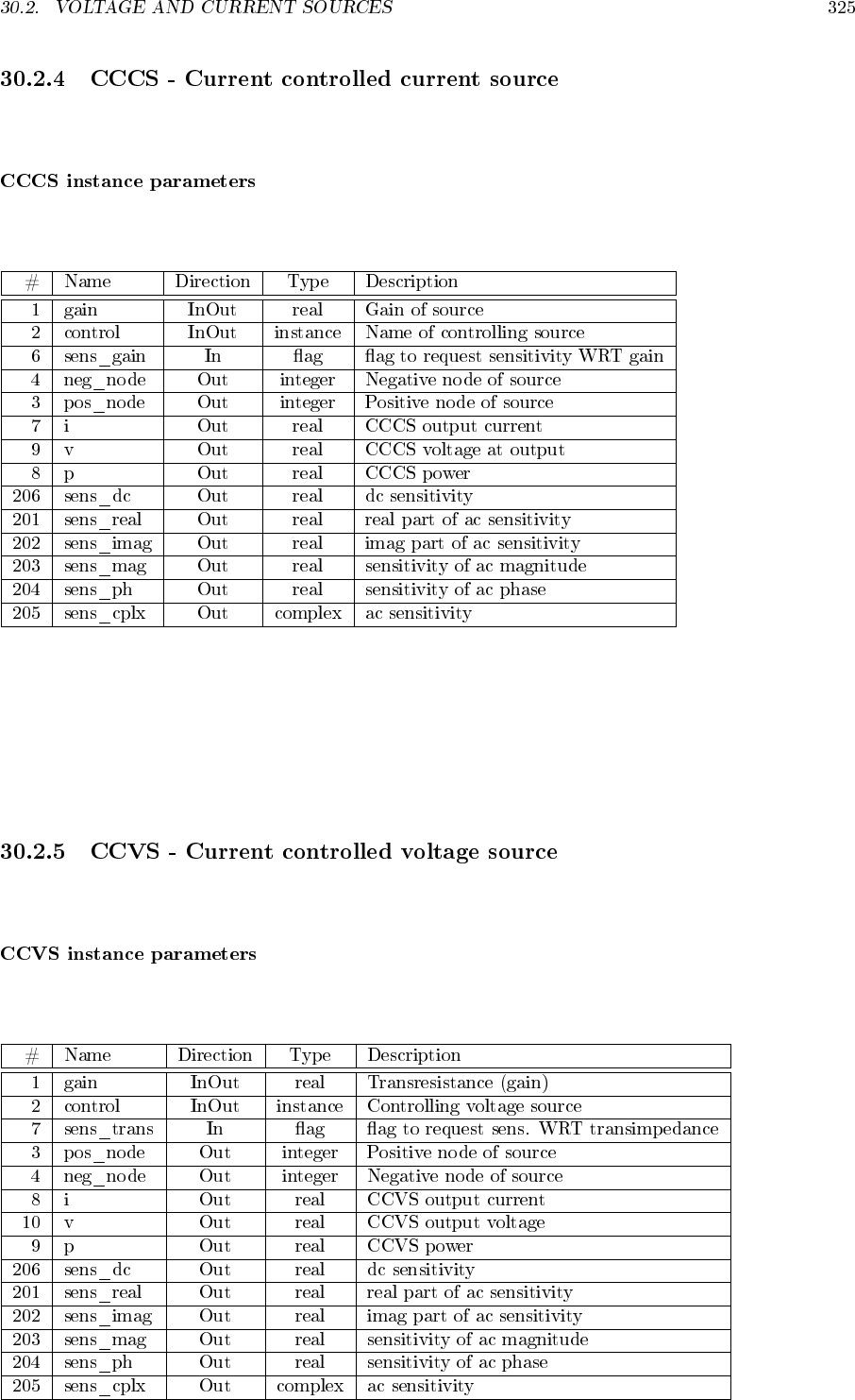
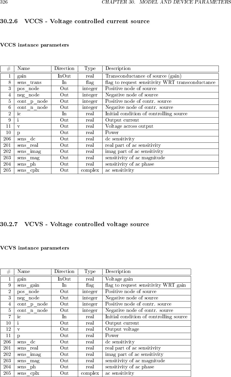
- Voltage and current sources
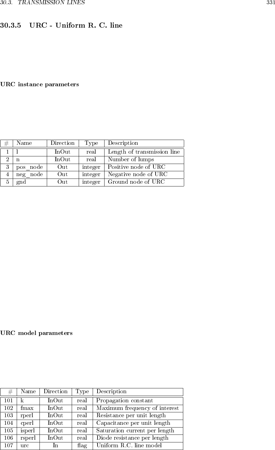
- Transmission Lines
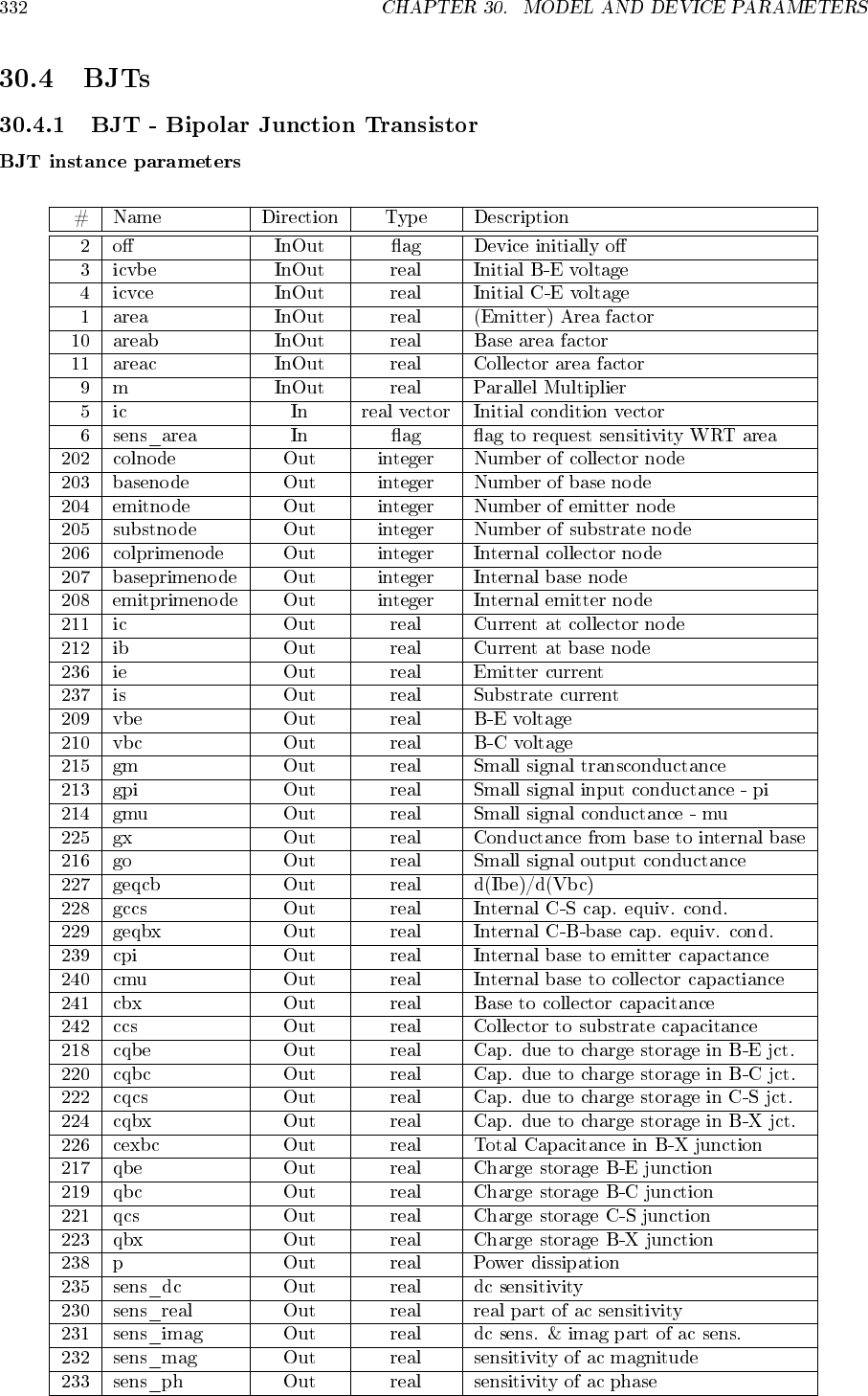
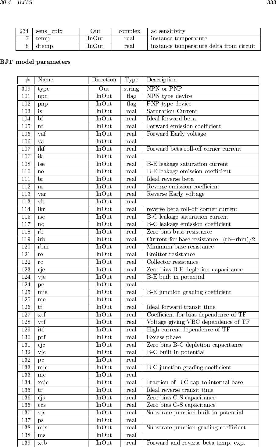
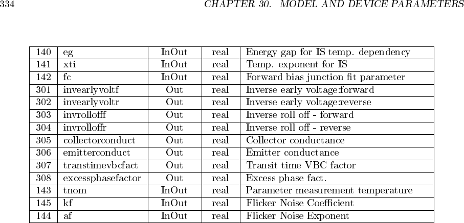
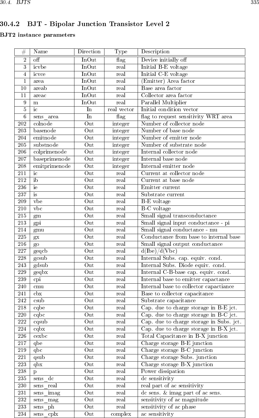
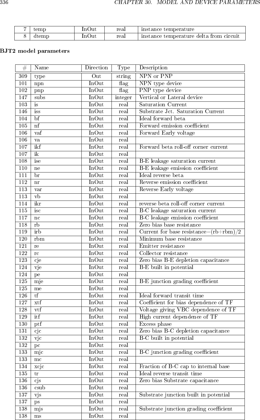
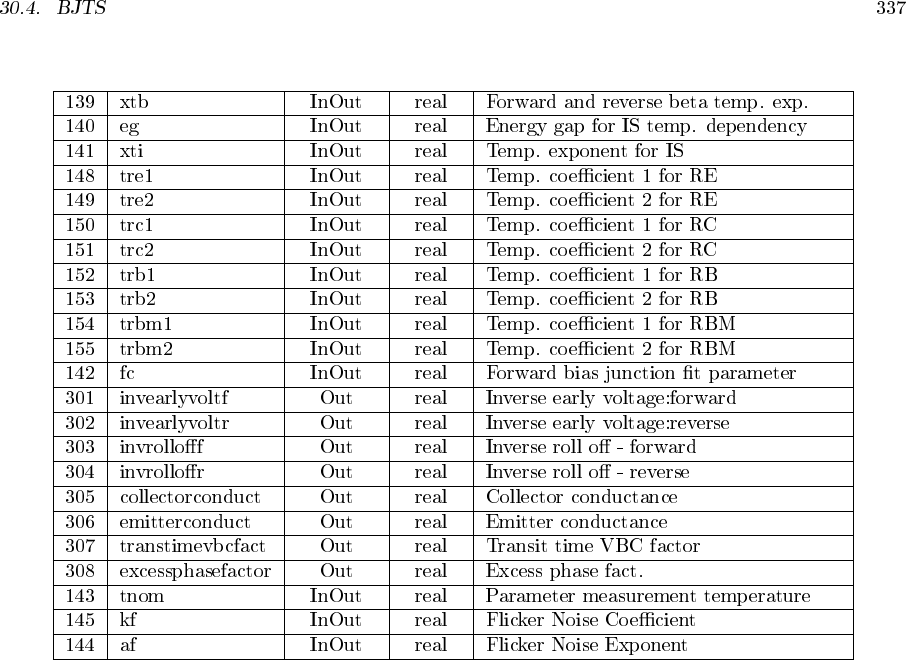
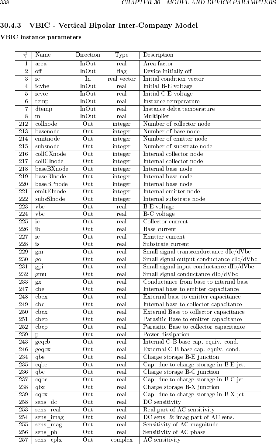
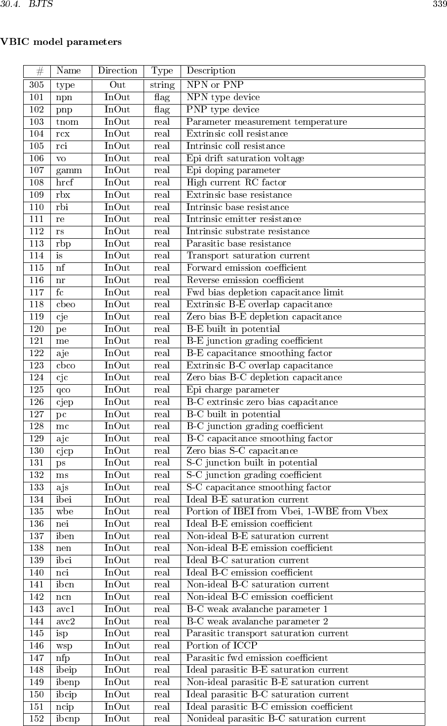
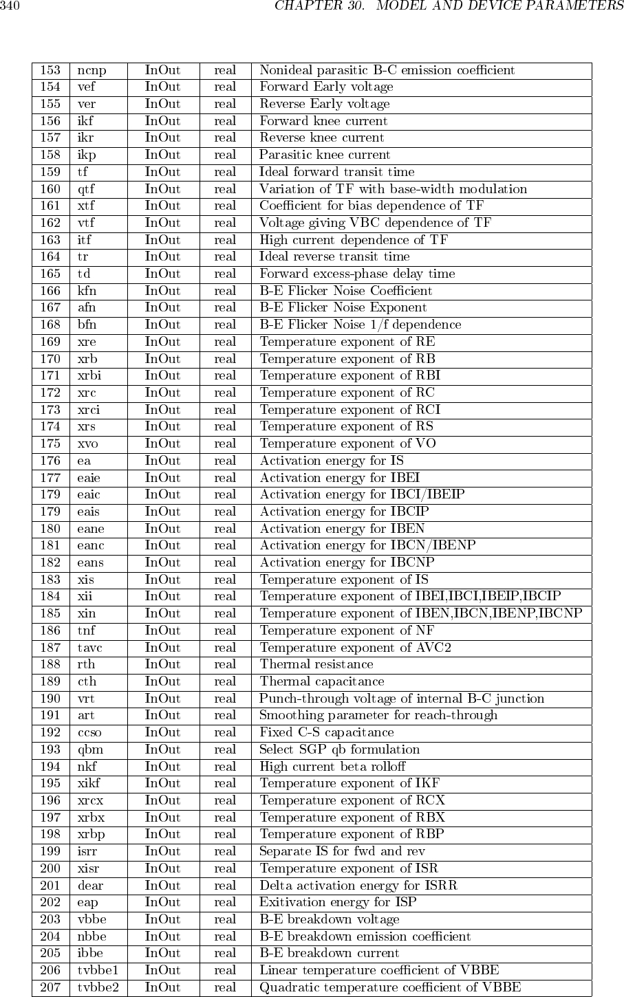
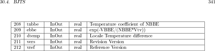
- BJTs
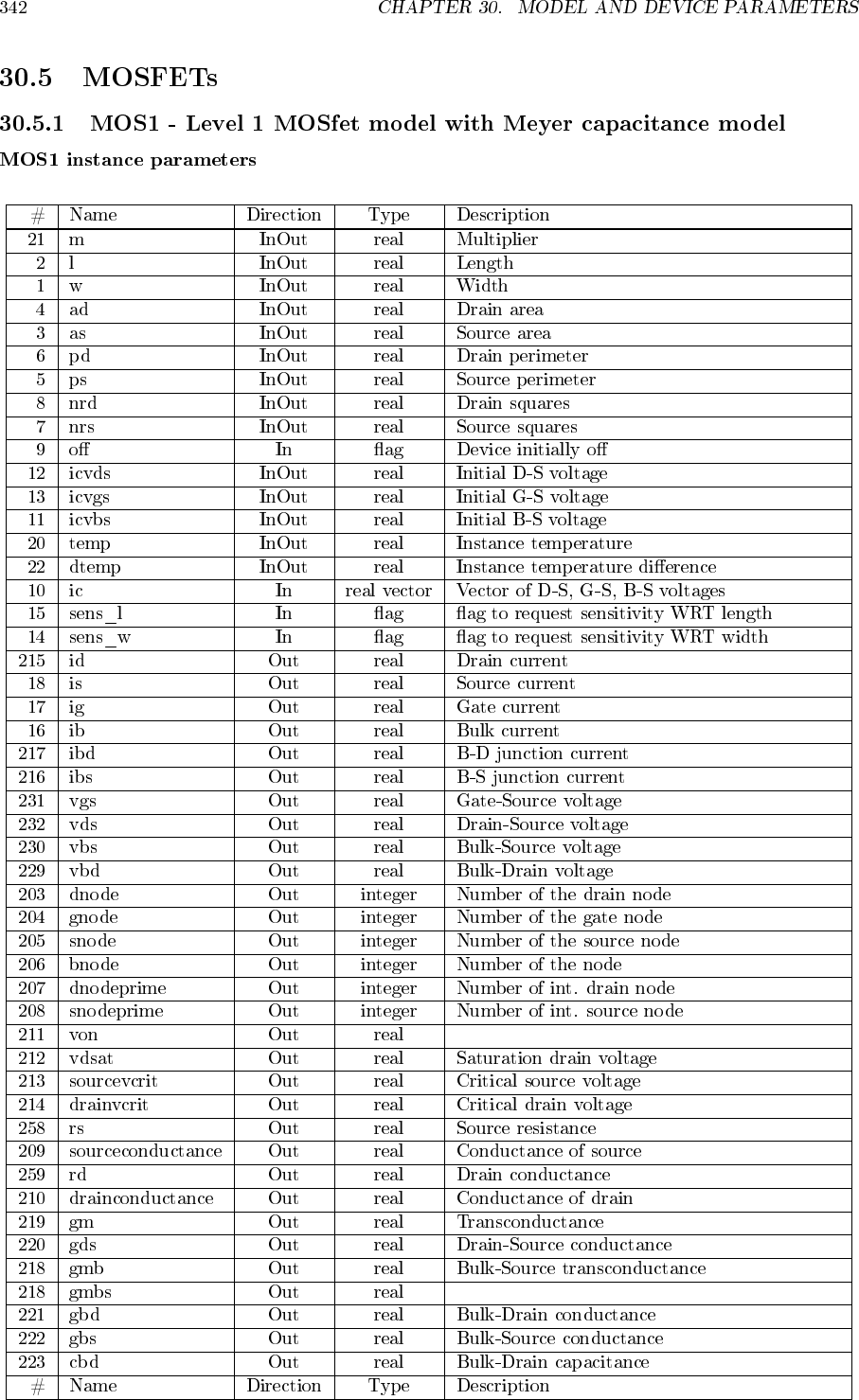
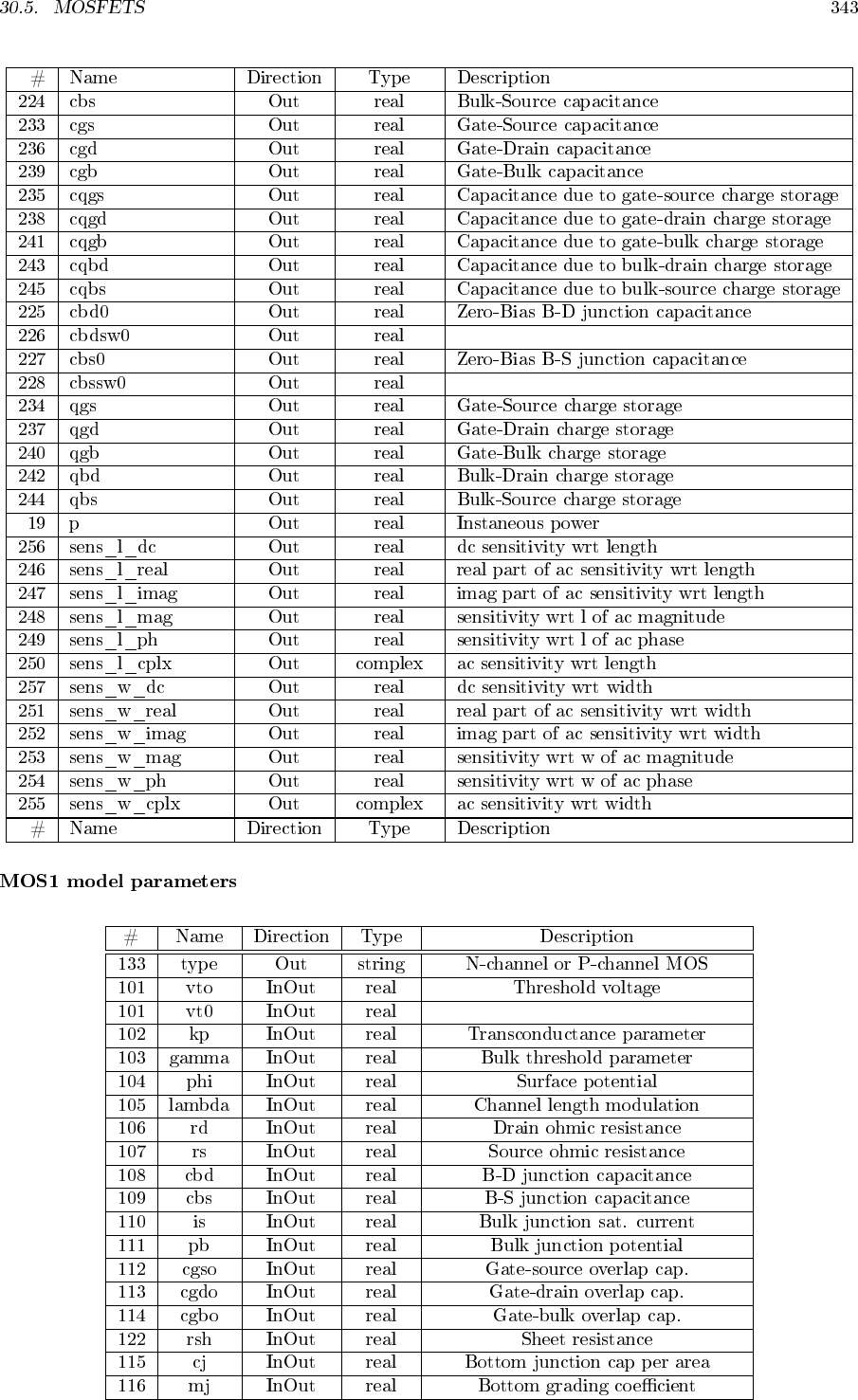
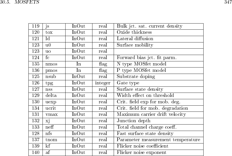
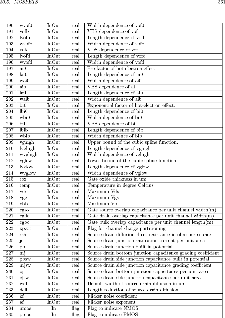
- MOSFETs
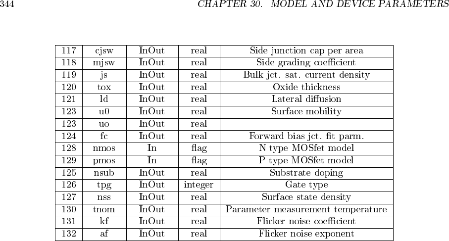
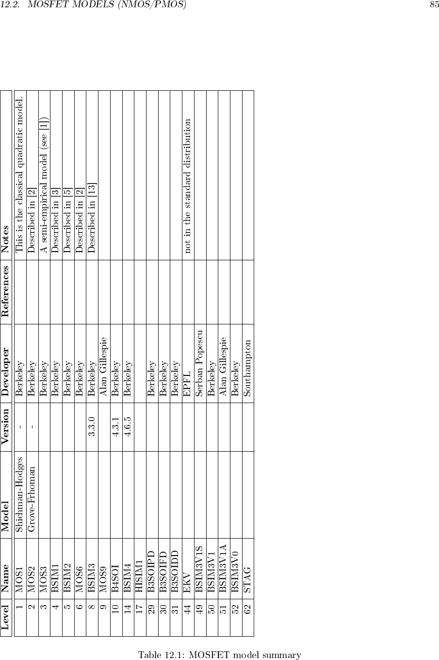
- MOS1 - Level 1 MOSfet model with Meyer capacitance model
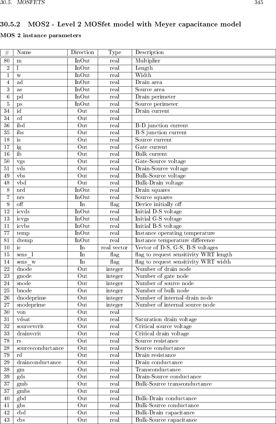
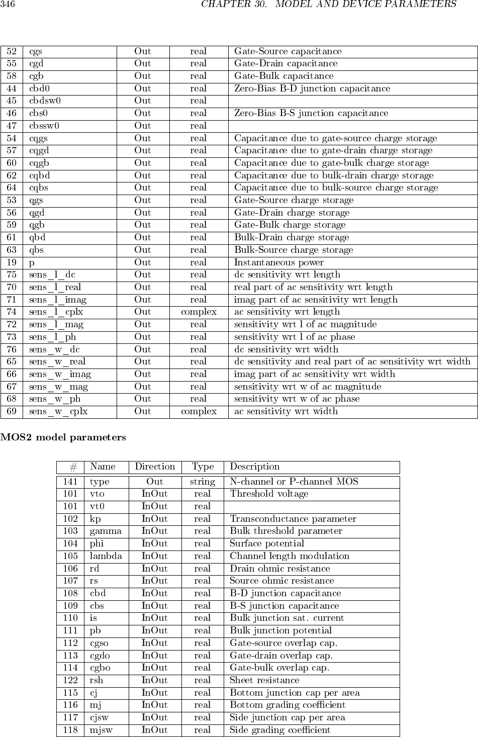
- MOS2 - Level 2 MOSfet model with Meyer capacitance model
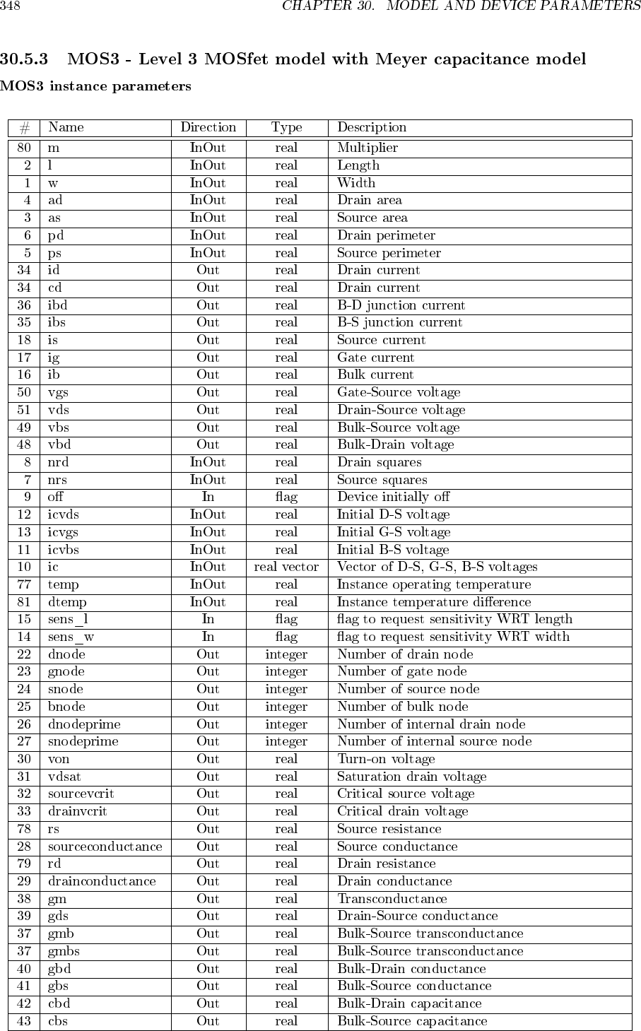
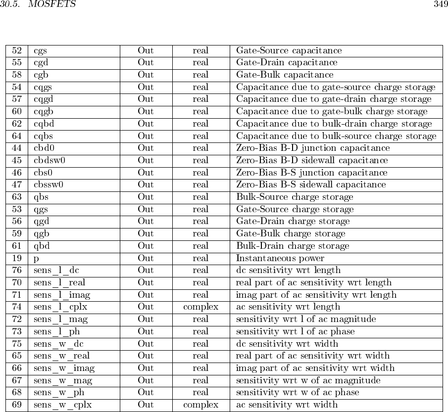
- MOS3 - Level 3 MOSfet model with Meyer capacitance model
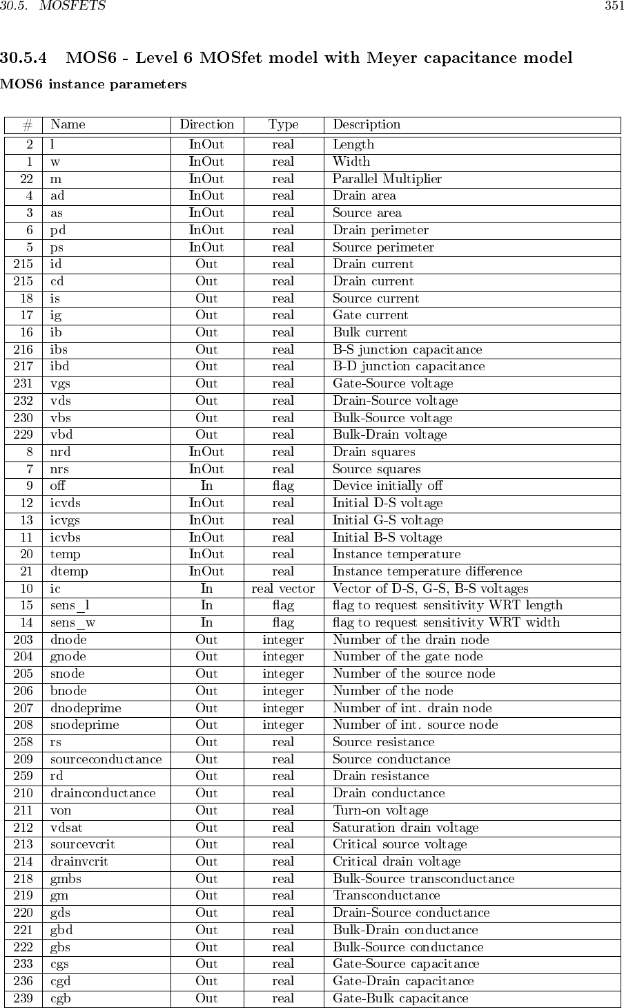
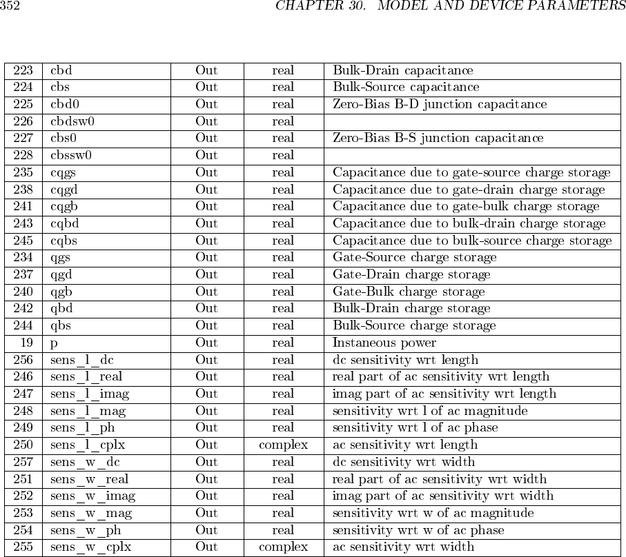
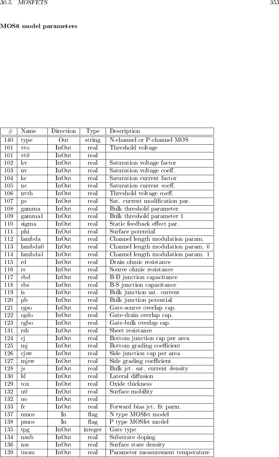
- MOS6 - Level 6 MOSfet model with Meyer capacitance model
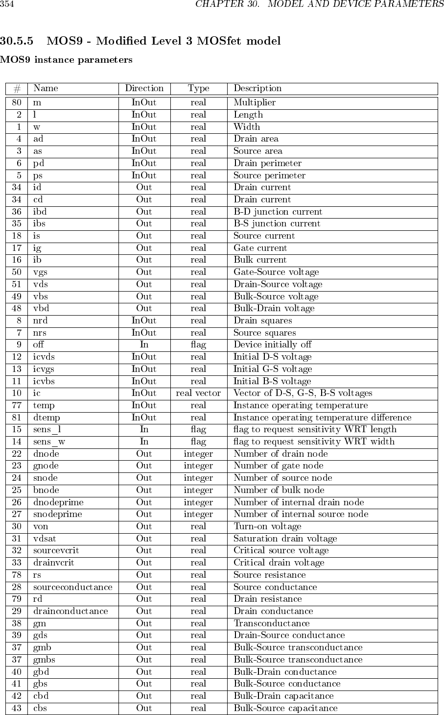
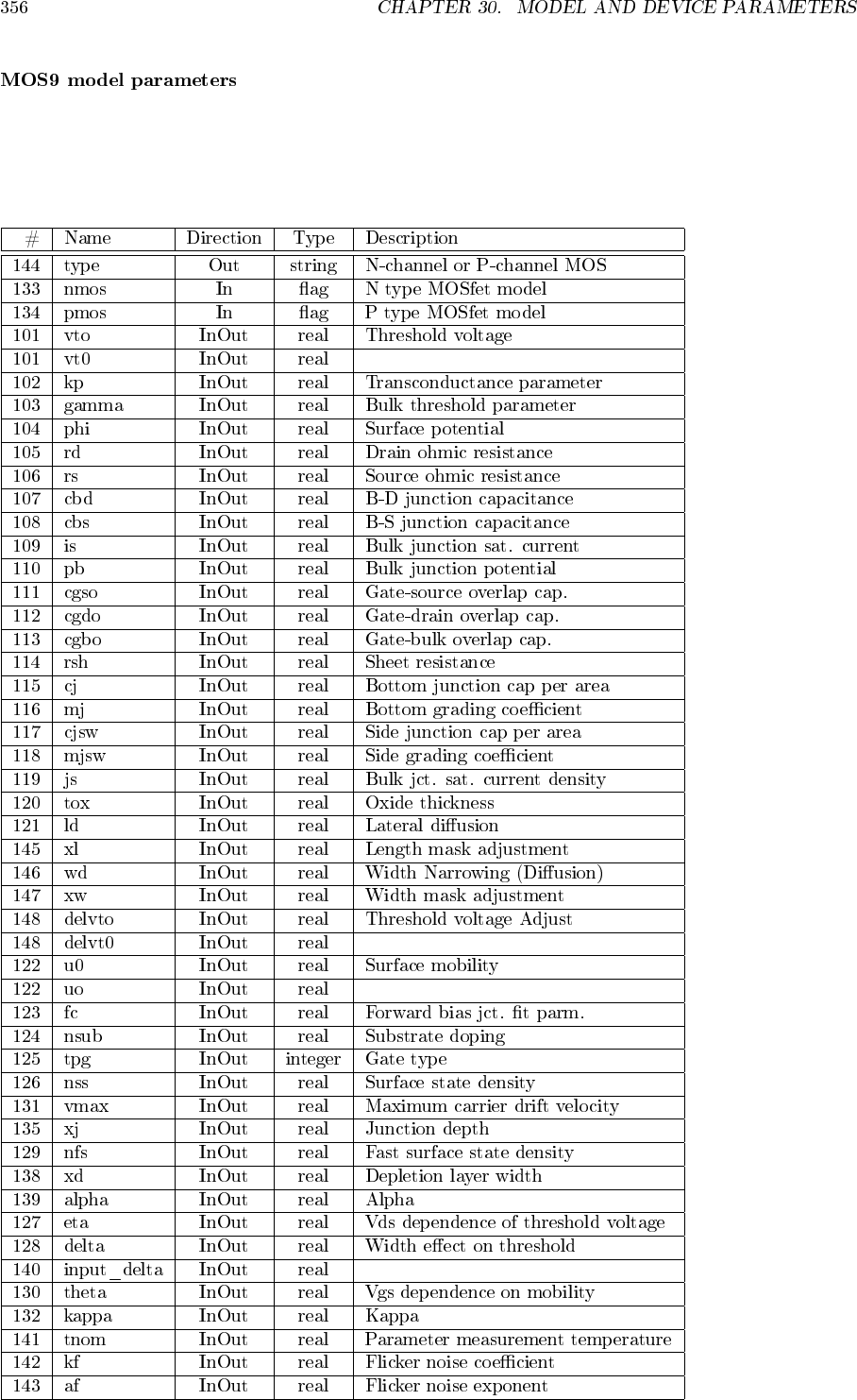
- MOS9 - Modified Level 3 MOSfet model
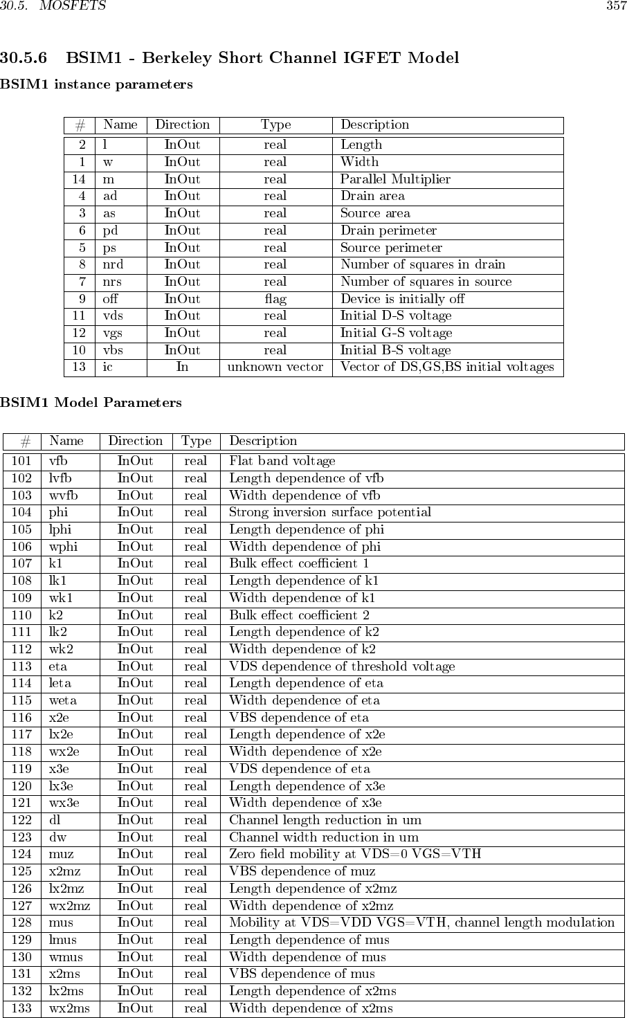
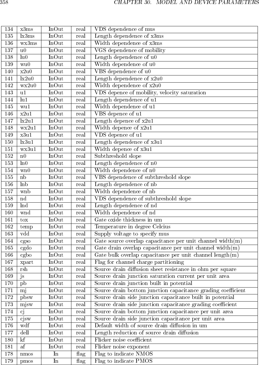
- BSIM1 - Berkeley Short Channel IGFET Model
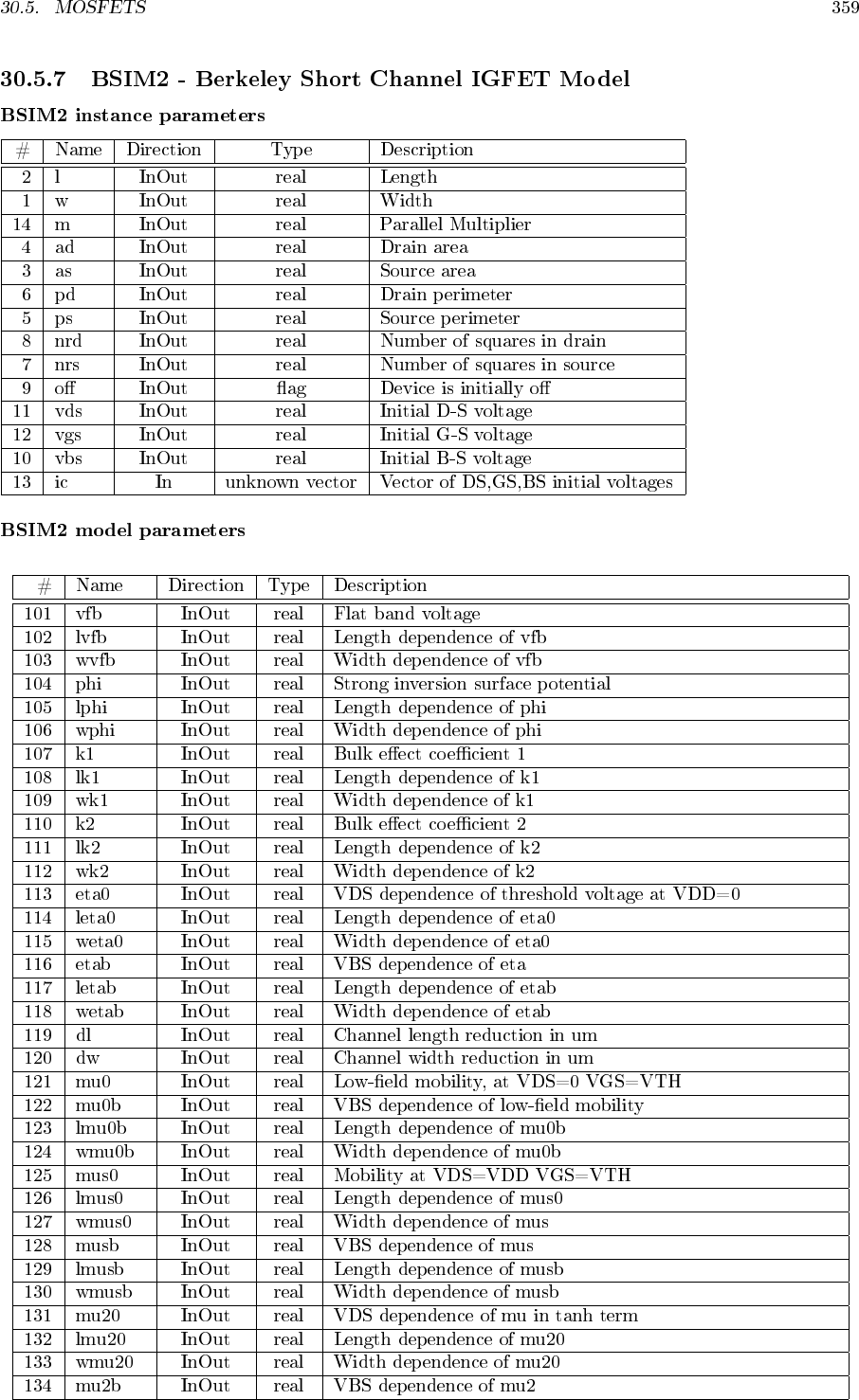
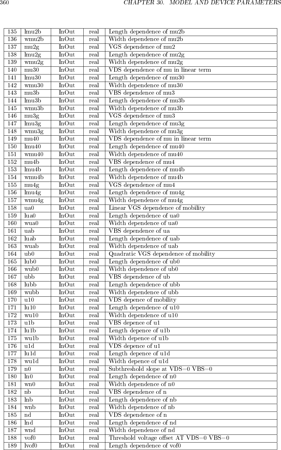
- BSIM2 - Berkeley Short Channel IGFET Model
- BSIM3
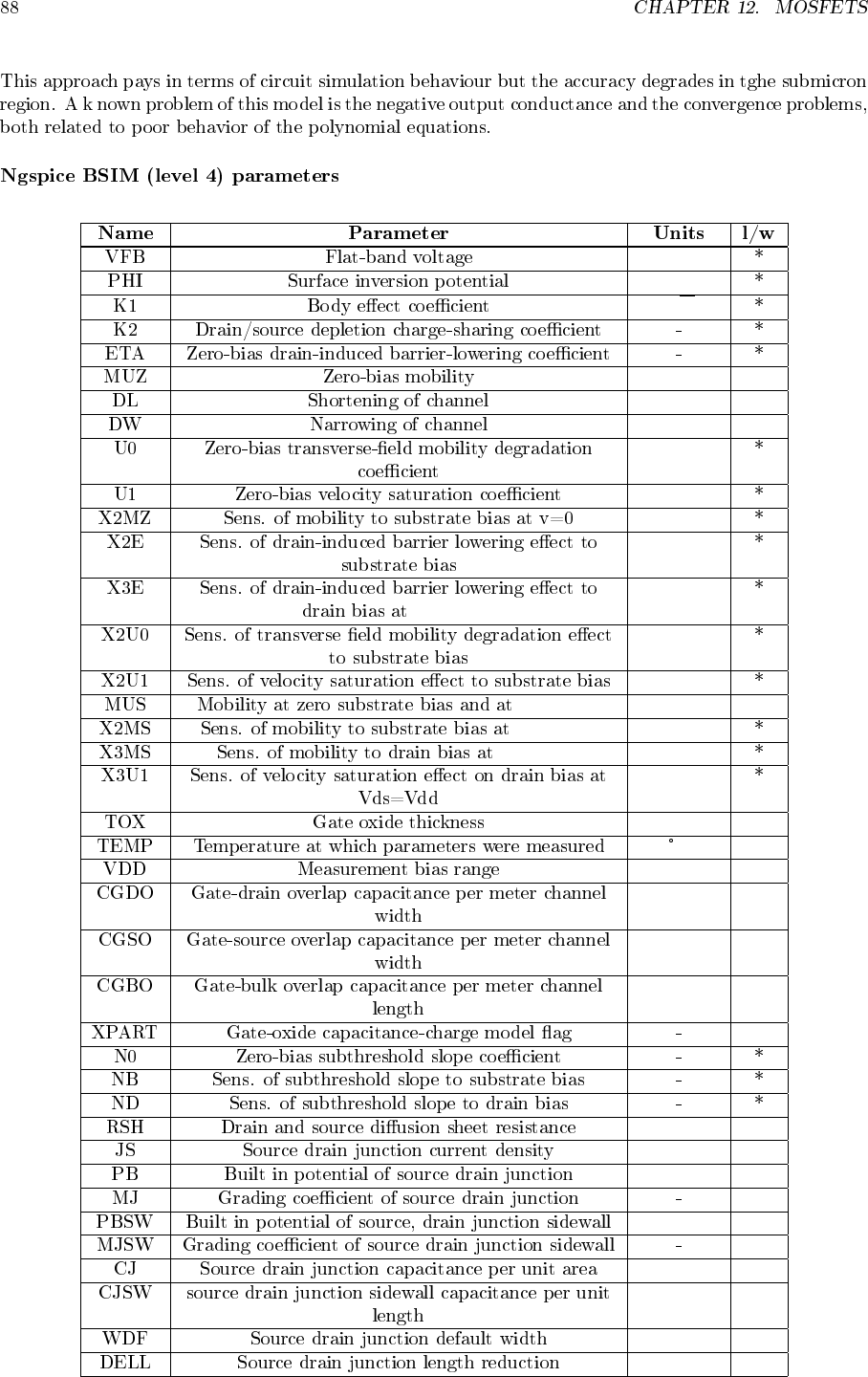
- BSIM4
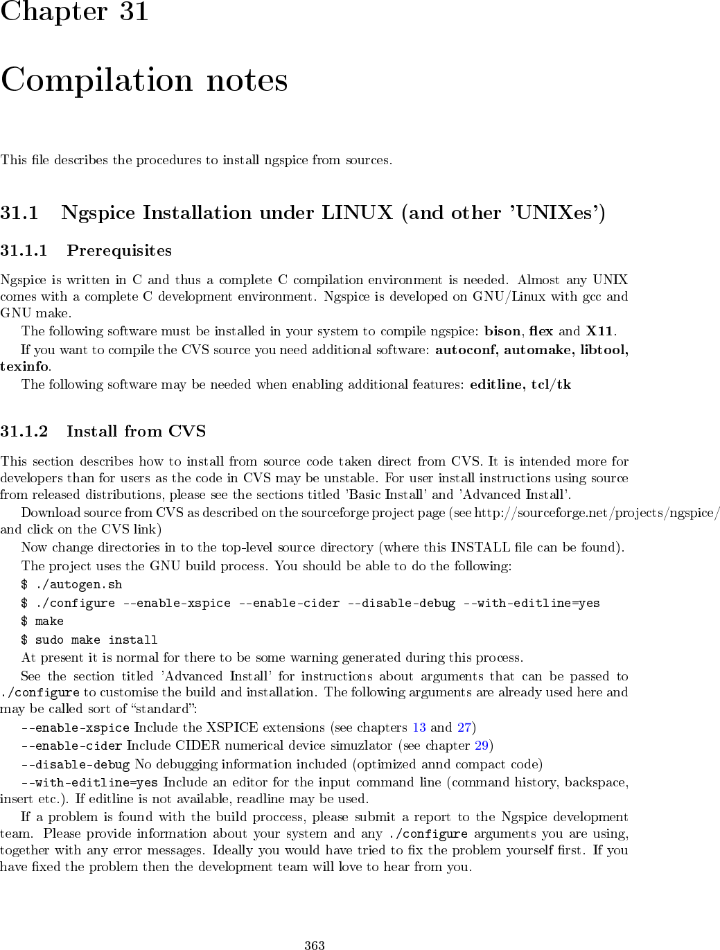
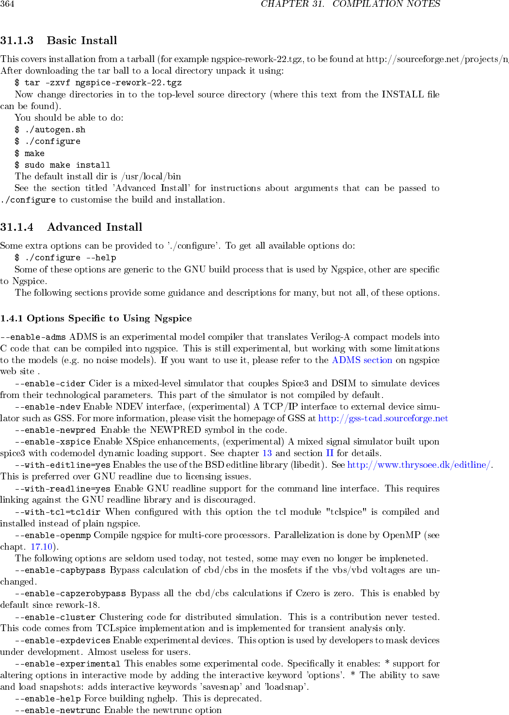
- Compilation notes
- Model and Device Parameters


N
XT I
U(T) = kT
qln NaNd
Ni(T)2!
k q Na
NdNiEg
M0U0
M0(T) = M0(T0)
T
T01.5
R(T) = R(T0)h1 + T C1(T−T0) + T C2(T−T0)2i
T T0T C1T C2
k
k+ 1)
v(k+1)
n−v(k)
n≤RELTOL ∗vnmax +VNTOL
vnmax = max v(k+1)
n,v(k)
n10−3
1µV
\
i(k+1)
branch −i(k)
branch≤RELTOL ∗ibrmax +ABSTOL
ibrmax = max \
i(k+1)
branch, i(k)
branch
\
ibranch
1012
109
106
103
25.4×10⁻⁶
10−3
10−6
10−9
10−12
10−15

−
−−−


F
F/m2
F/m
m
m
m
m
F/C
F/C2
C
F/m
m
Cnom = value ∗scale ∗m
Cnom = CAP ∗scale ∗m
C0= CJ(l−SHORT)(w−NARROW) + 2CJSW(l−SHORT + w−NARROW)
CJ = DI∗0
THICK if DI is specified,
CJ = SiO2
THICK otherwise.
0= 8.854214871e−12 F
mSiO2= 3.4531479969e−11 F
m
Cnom =C0∗scale ∗m
C(T) = C(TNOM)1 + T C1(T−TNOM) + T C2(T−TNOM)2
C(TNOM) = Cnom
T
−
−
−
−
−
−
−
Lnom =value ∗scale
m
H
m2
m
H/C
H/C2
C
H/m
Lnom =value ∗scale
m
Lnom =IND ∗scale
m
(Lnom =MU∗µ0∗NT2∗CSECT
LENGTH if MU is specified,
Lnom =µ0∗NT2∗CSECT
LENGTH otherwise.
µ0= 1.25663706143592e−6H
m
L(T) = L(TNOM)1 + T C1(T−TNOM) + T C2(T−TNOM)2
L(TNOM) = Lnom T

−
−
−
−
V A
V A
V A
V A
1
/T ST OP Hz
1
/sec
V(t) = (V0 if 0 ≤t< T D
V0 + V Ae−(t−T D)T HET A sin (2πF REQ (t−T D)) if T D ≤t < T ST OP
− −
V A
V A
V21 = V2−V1V12 = V1−V2
V(t) =
V1 if 0 ≤t < T D1,
V1 + V21 1−e−(t−T D1)
T AU1if T D1≤t < T D2,
V1 + V21 1−e−(t−T D1)
T AU1+V12 1−e−(t−T D2)
T AU2if T D2≤t < T ST OP.
− − − − − −
TiViVi
Ti
TiVi
V A
V A
1
/T ST OP Hz
1
/T ST OP Hz
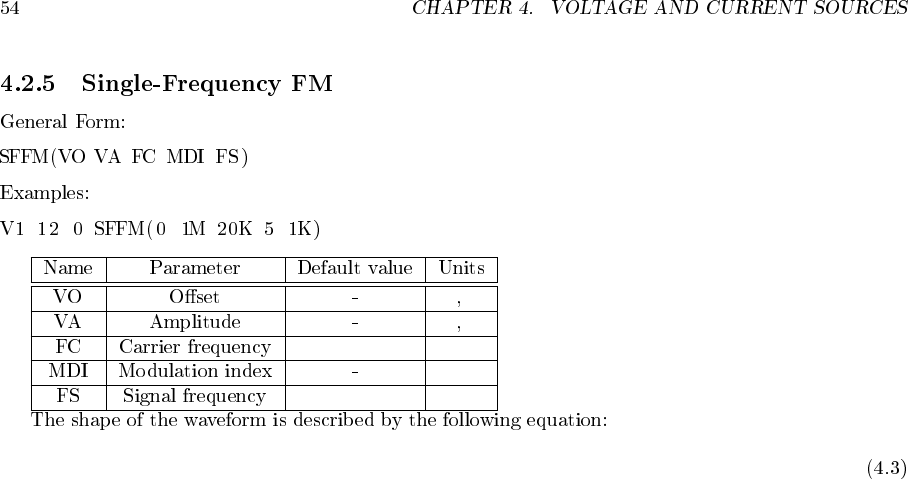
V(t) = VO+VAsin (2πF Ct +MDI sin (2πF St))


−
−
−

Ω
/unit
H/unit
mhos
/unit
F/unit
K
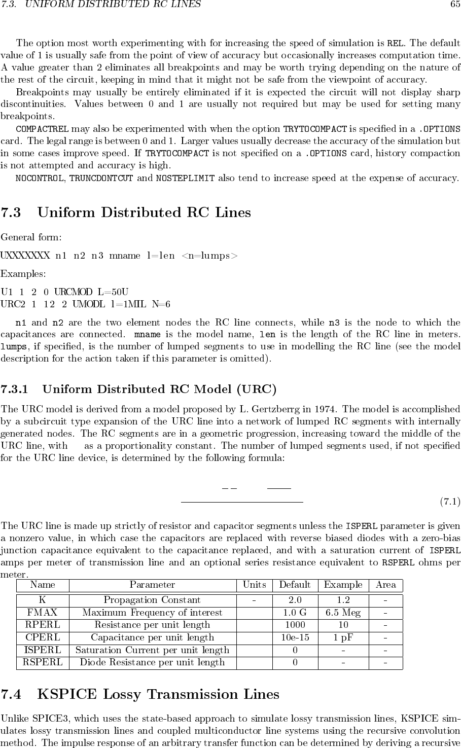
N=
log
Fmax R
L
C
L2πL2
(K−1)
K
2
log K
Hz
Ω
/m
F/m
A
/m
Ω
/m
− −
Ω
/unit
H/unit
mhos
/unit
F/unit
− − − −
− − −
Ω
/unit
H/unit
mhos
/unit
F/unit

−
V∞
A
A
A
A
A
Ω1
/area
F
F
V
V
eV
1.11 Si
0.69 Sbd
0.67 Ge
1
/C
1
/C2
C
1
/C
1
/C2
1
/C
1
/C2
3.0 pn
2.0 Sbd
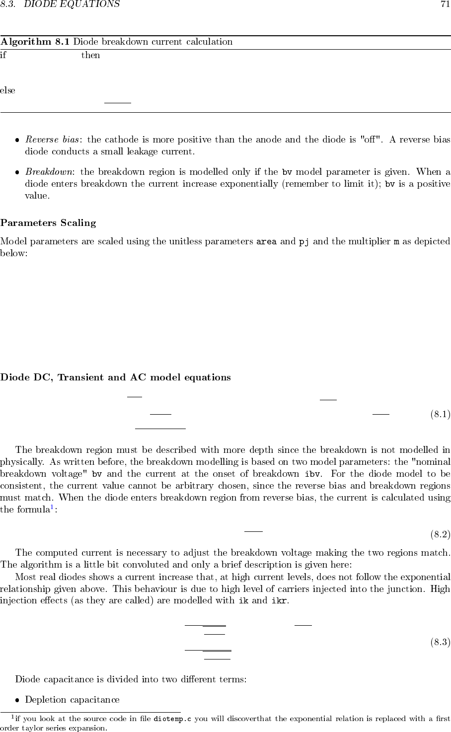
IBVef f < Ibdwn
IBVef f =Ibdwn
BVef f = BV
BVef f = BV −NVtln( IBVef f
Ibdwn )
AREAef f = AREA ·M
P Jeff = PJ ·M
ISef f = IS ·AREAeff + JSW ∗P Jef f
IBVef f = IBV ·AREAeff
IKef f = IK ·AREAeff
IKRef f = IKR ·AREAef f
CJef f = CJ0 ·AREAef f
CJPef f = CJP ·P Jeff
ID=
ISef f (eqVD
NkT −1) + VD∗GMIN, if VD≥ −3NkT
q
−ISef f [1 + ( 3NkT
qVDe)3] + VD∗GMIN, if −BVef f < VD<−3N kT
q
−ISef f (e
−q(BVef f +VD)
NkT ) + VD∗GMIN, if VD≤ −BVef f
Ibdwn =−ISef f (e
−qBV
NkT −1)
IDef f =
ID
1+rID
IKef f
,if VD≥ −3NkT
q
ID
1+rID
IKRef f
,otherwise.
CDiode =Cdif f usion +Cdepletion
Cdepletion =Cdeplbw +Cdeplsw
Cdiff usion = TT ∂IDef f
∂VD
Cdeplbw =(CJef f ·(1 −VD
VJ )−MJ,if VD<FC ·VJ
CJef f ·1−FC·(1+MJI)+MJ·VD
VJ
(1−FC)(1+MJ) , otherwise.
Cdeplsw =(CJPef f ·(1 −VD
PHP )−MJSW,if VD<FCS ·PHP
CJPef f ·1−FCS·(1+MJSW)+MJSW·VD
PHP
(1−FCS)(1+MJSW) , otherwise.
EGnom = 1.16 −7.02e−4·TNOM2
TNOM + 1108.0
EG(T)=1.16 −7.02e−4·T2
TNOM + 1108.0
IS(T) = IS ·elogf actor
N
JSW (T) = JSW ·elog f actor
N
logfactor =EG
Vt(TNOM) −EG
Vt(T)+ XTI ·ln( T
TNOM)
V J(T) = VJ ·(T
TNOM)−Vt(T)·3·ln( T
TNOM) + EGnom
Vt(TNOM) −EG(T)
Vt(T)
P HP (T) = PHP ·(T
TNOM)−Vt(T)·3·ln( T
TNOM) + EGnom
Vt(TNOM) −EG(T)
Vt(T)
CJ(T) = CJ ·1 + MJ ·(4.0e−4·(T−TNOM) −V J(T)
VJ + 1)
CJSW (T) = CJSW ·1 + MJSW ·(4.0e−4·(T−TNOM) −P HP (T)
PHP + 1)
T T (T) = TT ·(1 + TTT1 ·(T−TNOM) + TTT2 ·(T−TNOM)2)
MJ(T) = MJ ·(1 + TM1 ·(T−TNOM) + TM2 ·(T−TNOM)2)
RS(T) = RS ·(1 + TRS ·(T−TNOM) + TRS2 ·(T−TNOM)2)
i2
RS =4kT ∆f
RS
i2
d= 2qID∆f+KF ∗IAF
D
f∆f

A
A
V∞
A∞
A
V∞
A∞
A
Ω
A∞
Ω
Ω
Ω
F
V
V∞
A
F
V
F
V
eV
C
1
/C
1
/C2
1
/C
1
/C2
1
/C
1
/C2
1
/C
1
/C2

VT0V
βA
/V”
λ
1
/V
Ω
Ω
Cgs F
Cgd
F
V
ISA
C
−
−
m m2
m2
F/m2
VT0)
V
A
/V2
√V
V
λ)
1
/V
Ω
Ω
F
F
IS
A
V
F/m
F/m
F/m
Ω
/
F/m2
F/m
0.50 (level1)
0.33 (level2,3)
m
cm−3
cm−2
cm−2
m
m
cm2/V·sec
V/cm
m
/s
1
/V
C
P=P0+PL
Leffective
+PW
Weffective
Leffective =Linput −DL
Weffective =Winput −DW
V
V
√V
cm2/V·sec
µm
µm
1
/V
µ
/V
cm2/V2·sec
1
/V
Vds =Vdd
1
/V
1
/V2
µm
/V2
Vds =Vdd cm2/V2sec
Vds =Vdd cm2/V2sec
Vds =Vdd cm2/V2sec
µm
/V2
µm
C
V
F/m
F/m
F/m
Ω
/
A
/m2
V
V
F/m2
F/m
m
m

±
±
± ±
N(s)=0.139713 · { s2+0.7464102
s2+0.998942s+0.00117077 }
N(s)=0.139713 · { 1.0
s2+1.09773s+1.10251 }
µs
φ
φ
2P=N


C
C
µV
−
F1F2
F1
F2
F1+F2F1−F2(2F1)−F2F1
A
/BA B B
A < B < 1
F1+F2F1−F2
2F1−F2F1−F2=F2F1−F2
F2F1+F2= 2F1−F2
F1−F2= 51/100 F1<> 49/100 F1=F2
F2F1−F2
nF1+mF2
V2/Hz A2/Hz V2A2
− −


− − − −
−
− − −
−
− −
−
−

−
ω

−
−
−−
−
−− − −
−

−
−
−− −
−
−
−
−
−
− −
C=f(V)
−
−−
−
− −
−
−
− −
−
−
− − −
−
−
−
−
−
− − −
− − −
− − − −
−
− −
−
−
− − −
−
− − −
− − −
− − −
− − −

−
− −
−
−
−
− − −
− −
− −
− −
−
− − −
− − −
− −
− −
−− − −
−


− −
−
−
− −
−
− −
− −
− −
−
−
−
−


µm
µm
µm
µm
C/cm2
cm
/s
cm
/s
µm
µm µm ˙
A µm
µm
µm
µm
µm
− − − − − −

µm
µm
µm
µm
cm−3
µm
µm
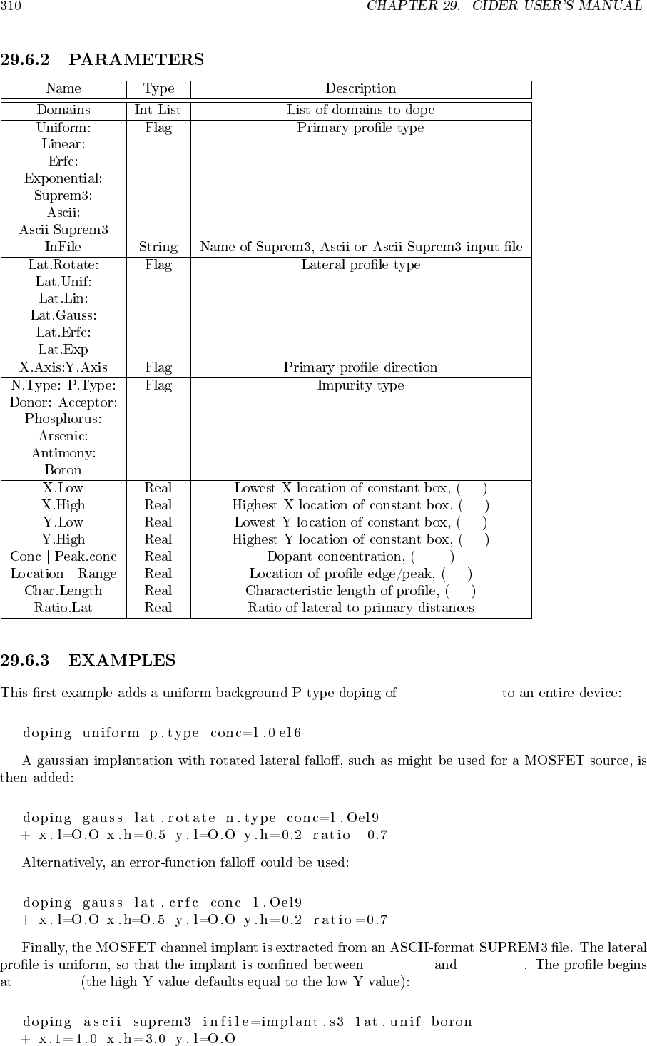
1.0×1016cm−3
−
−
X= 1µm X = 3µm
Y= 0µm
µm
µm
µm
µm
−
−
F/cm
cm−3
cm−3
eV/K
eV/cm−3
cm−3
eV/cm−3
cm−3
cm−3)
cm−3)
cm6/sec
cm6/sec
A
/cm2
K2
A
/cm2
K2
−