Derman Risk The Boys Guide HEDGE

User Manual:

Open the PDF directly: View PDF .
Page Count: 3

here is an unfortunate strain of

pedantry running through the teach-

ing of quantitative finance, one in-

volving an excess of abstraction, formality,

rigour and axiomatisation that makes the

subject unnecessarily daunting and diffi-

cult. Over the years I’ve seen a few too

many fresh graduates who, on being asked

why one believes one can obtain a cred-

ible value for an option, reply that it’s be-

cause of Girsanov’s theorem.

I’d like to think most of the useful as-

pects of quantitative finance are relative-

ly simple, and so, here is my rather

abbreviated poor man’s guide to the field.

Price and value

You must first distinguish between price

and value. Price is what you pay to acquire

a security; value is what it is worth. The

price is fair when it is equal to the value.

But what is the value? How do you es-

timate it? Judging value, in even the sim-

plest way, involves the construction of a

model or theory.

The one and only commandment of

quantitative finance

According to legend, Hillel, a famous sage,

was asked to recite the essence of God’s

laws while standing on one leg. “Do not

do unto others as you would not have them

do unto you,” he is supposed to have said.

“All the rest is commentary. Go and learn.”

You can summarise the essence of

quantitative finance on one leg too: “If

you want to know the value of a securi-

ty, use the price of another security that’s

as similar to it as possible. All the rest is

modelling. Go and build.”

The wonderful thing about this law,

when compared with almost everything

else in economics, is that it dispenses with

utility functions, those unobservable hid-

den variables whose ghostly presences

permeate economic theory. But don’t think

you can escape all human perceptions by

using this law; the models of quantitative

finance inevitably involve expectations

and estimates of future behaviour, and

those estimates and expectations are peo-

ple’s estimates.

Financial economists refer to their es-

sential principle as the law of one price,

or the principle of no risk-free arbitrage,

which states that: ‘Any two securities with

identical future payouts, no matter how

the future turns out, should have identi-

cal current prices.’

The law of one price is not a law of na-

ture. It’s a general reflection on the prac-

tices of human beings, who, when they

have enough time and information, will

grab a bargain when they see one. This

law usually holds in the long run, in well-

oiled markets with enough savvy partici-

pants, but there are always short-term or

even longer-term exceptions that persist.

Valuation by replication

How do you use the law of one price to

determine value? If you want to estimate

the value of a target security, the law of

one price tells you to find some other

replicating portfolio, a collection of more

liquid securities that, collectively, has the

same future payouts as the target, no mat-

ter how the future turns out. The target’s

value is then simply the price of the repli-

cating portfolio.

Where do models enter? It takes a

model to show that the target and the

replicating portfolio have identical future

payouts under all circumstances. To

demonstrate the identity of payouts, you

must specify what you mean by ‘all cir-

cumstances’ for each security, and find a

strategy for creating a replicating portfo-

lio that, in each future scenario, will have

identical payouts to those of the target.

Most of the mathematical complexity

in finance involves the description of the

range of future behaviour of each securi-

ty’s price.

There are two kinds of replication,

static and dynamic. A static replicating

portfolio is a collection of securities that,

once defined and never altered, repro-

duces the payout of a target security

under all future scenarios. Static replica-

tion is the simplest and most compre-

hensive method of valuation, but is

feasible only in the rare cases when the

target security closely resembles the liq-

uid securities available.

For more complex non-linear securi-

ties, such as stock options, static replicat-

ing portfolios are unavailable, but

sometimes you can find a dynamic repli-

cating portfolio, a mixture of liquid secu-

rities whose proportions, continually

adjusted by trading out of one security

and into another, will replicate the pay-

out of the target. Static or dynamic, the

initial price of the replicating portfolio is

the estimated value of the target.

Models are only models, toy-like de-

scriptions of idealised worlds. Simple

models envisage a simple future; more

sophisticated models incorporate a more

complex set of future scenarios that can

better approximate actual markets. But

no mathematical model will capture the

intricacies of human psychology. If you

listen to the models’ siren song for too

long, you may end up on the rocks or in

the whirlpool.

We now proceed to apply replication

The boy’s guide to

pricing and hedging

The law of one price is not a law of nature. It’s a

reflection on the practices of human beings, who,

when they have enough time and information,

will grab a bargain when they see one

Emanuel Derman

and the law of one price to various secu-

rities of interest.

Modelling (relatively) risk-free bonds

How do you value the promise of a fu-

ture payment? The simplest answer is: find

an institution whose liquid bonds have an

estimated risk of default similar to your

debtor’s and use that institution’s term

structure of interest rates to discount the

payouts of your target bond.

Why use interest rates? Because they

allow you to compare investments. Quot-

ing bond prices in terms of rates or yields

is a sort of model too, albeit a simple one

that projects bonds of different coupons

and maturities on to a one-dimensional

yield scale that’s more enlightening than

mere dollar price. The most easily em-

braceable models convert inexpressive

prices into a more eloquent one- or two-

dimensional scale that makes comparison

more intuitive.

Complex bonds, mortgages or swap-

tions, for example, whose payouts are

contingent on interest rates or other mar-

ket parameters, are best modelled using

dynamically replicating portfolios, as de-

scribed later.

The risk of stocks

A stock’s most germane characteristic is

the uncertainty of its return. About the

most elementary model of uncertainty is

the risk involved in flipping a coin. Fig-

ure 1 illustrates a similarly simple model

– the binary tree – for the evolution of

the price of a stock with return volatili-

over a small instant of time

∆t

. On

an up-move the price increases by the

percentage:

while on an equally probable down-move

it increases by only:

The volatility

is the measure of the

stock’s risk.

According to the law of one price, the

risk-free rate of return

must lie in the

zone between the up and down returns.

If both the up and down returns were

greater than the risk-free return, you

could create a portfolio long $100 of stock

and short $100 of a risk-free bond with

zero price and a paradoxically positive

payout under all future scenarios. Any

model with such possibilities is in trouble

before it leaves the ground.

This apparently naive ‘either-up-or-

down’ model captures much of the in-

herent risk of owning a stock and many

other risky securities. Repeated over and

over again for small time steps, it mimics

µσ∆− ∆tt

µσ∆+ ∆tt

the more-or-less continuous motion of

prices in a reasonable though imperfect

way, much as movies produce the illusion

of life by changing images at the rate of

24 frames a second.

Risk reduction by adding risk-free

bonds implies ‘more risk, more return’

hat future expected reward justifies a

particular present risk? This is the para-

mount question of life and finance. If you

know the future volaility of a stock σ,

what rate of return µ should you expect?

The law of one price tells you how

to value securities you can replicate, but

some payouts simply cannot be repli-

cated. Certain risk factors are intrinsic,

unavoidable, the thing in itself. We need

to extend the law of one price – same

payout, same return – to demand that

the same unavoidable risk should lead

to the same expected return, or, more

precisely, that risk factors with equal risk

should have equal expected return. We

can use this principle to determine the

rational relationship between risk and

return.

The key point is that, by adding a risk-

free short-term investment in a bond to

any risky position, one can reduce the

magnitude of the risk and return in a pre-

dictable manner while preserving the

risk’s character.

Figure 2 shows the binary tree for a

risk-free bond. It is degenerate: whether

the stock moves up or down, the bond

produces a guaranteed return

r∆t

. By

adding a risk-free bond of this type with

zero volatility to a stock of volatility

and

return

, you can commensurately reduce

both the risk and return of your invest-

ment. The binary tree for a 50:50 mix of

stock and cash suffers half the volatility

and produces half the expected excess re-

turn (

µ– r

) over the risk-free rate. The

principle of equal-unavoidable-risk-

equal-expected-return then dictates that

any security with half the risk produces

half the excess return, or, even more gen-

erally, that excess return is proportional

to risk, so that:

where

is the Sharpe ratio.

Risk reduction by diversification

implies the Sharpe ratio is zero

We have shown that since you can reduce

risk by keeping part of your money in

risk-free bonds, it follows that excess re-

turn is proportional to risk. But you can

also diminish risk by diversifying. If you

can accumulate a portfolio of so many un-

correlated unavoidable risks that their

µλσ−=r

risks cancel, so that the portfolio’s net

volatility is zero, then, by the law of one

price, since it is risk-free, it must produce

the risk-free rate of return. In that case,

each stock in the portfolio must earn the

risk-free rate too, so that

µ= r

and the

Sharpe ratio

must be zero.

If all risk factors can be cancelled by

diversification, investors should expect

only the risk-free return on any single

stock.

Risk reduction by hedging implies only

factor risk is rewarded

Stock markets aren’t truly amenable to

the total diversification we assumed

above. That’s because large financial

markets are more than a collection of in-

dividual uncorrelated risk factors. Expe-

rienced investors are always trying to

detect patterns in the universe of stock

returns. They perceive stocks as be-

longing to groups that have in common

their sensitivity to a particular asset, fac-

tor or set of factors.

Let

be the correlation of the returns



Down

Mean

Return

µ∆ tσ∆

µ∆tσ∆

–

µ∆ t

Risk-free

return zone

∆

Stock price

1. Evolution of a stock’s price

Cash

r∆t

∆t

Down

Return

2. Evolution of a risk-free bond’s price

between a stock

with volatility

and

some tradable risky asset

with volatili-

σM

. Because of the correlation between

each stock’s return and that of

, you can

hedge the

-related risk of any stock. If

you have $100 invested in a stock

, you

can short

times as many dollars of the

factor

against it, where

β= ρ(σ/σM)

the number of percentage points that stock

is expected to rise when

rises by 1%.

This factor-hedged portfolio, consisting of

a $100 long position in the stock combined

with

times as much of a short position

, will carry no net exposure to the

price of

, because any increase in the

price of the stock will, on average, be can-

celled by a correlated decrease in value of

the short position in

The net expected return on this factor-

hedged

-neutral portfolio is propor-

tional to the return of the stock

less

times the return of

, namely

µ– βµM

Assuming there are no other factors in-

fluencing the stock

, this residual risk is

unavoidable.

If you can diversify over a large

enough

-neutral portfolio of stocks so

that their accumulated unavoidable risk

cancels, then this

-neutral portfolio of

zero volatility must earn the risk-free rate

. The same must therefore be true of each

-neutral element of the portfolio. This

leads to the result that:

This is the result of the capital asset

pricing model or arbitrage pricing theo-

ry: in a world of rational investors, the ex-

cess return you can expect from buying

a stock is its

times the expected return

of its hedgeable factor. Put differently, you

can only expect to be rewarded for the

unavoidable factor risk of each stock,

since all other risk can be eliminated by

diversification.

The rationality of the investing world

is still hotly debated. In finance – a social

science overlaid with a useful veneer of

quantitative analysis – the exact truth is

hard to determine.

The choice-of-currency trick

It seems obvious that the value of a secu-

rity in dollars should be independent of

the currency (dollars, yen, shares of IBM,

etc) you choose for modelling its evolu-

tion. A little thought often suggests a nat-

ural choice of currency that can greatly

simplify thinking about a problem. Just as

stock analysts find it convenient to mea-

sure a stock’s price in units of projected

earnings rather than dollars, thereby mak-

ing stock comparison easier, so financial

modellers can sometimes cleverly choose

a more meaningful currency than the dol-

lar when valuing a complex security. Con-

vertible bonds, for example, which involve

an option to exchange a bond for stock,

can sometimes be fruitfully modelled by

choosing a bond itself as the natural valu-

ation currency. Financial mathematicians

call this trick ‘the choice of numeraire’.

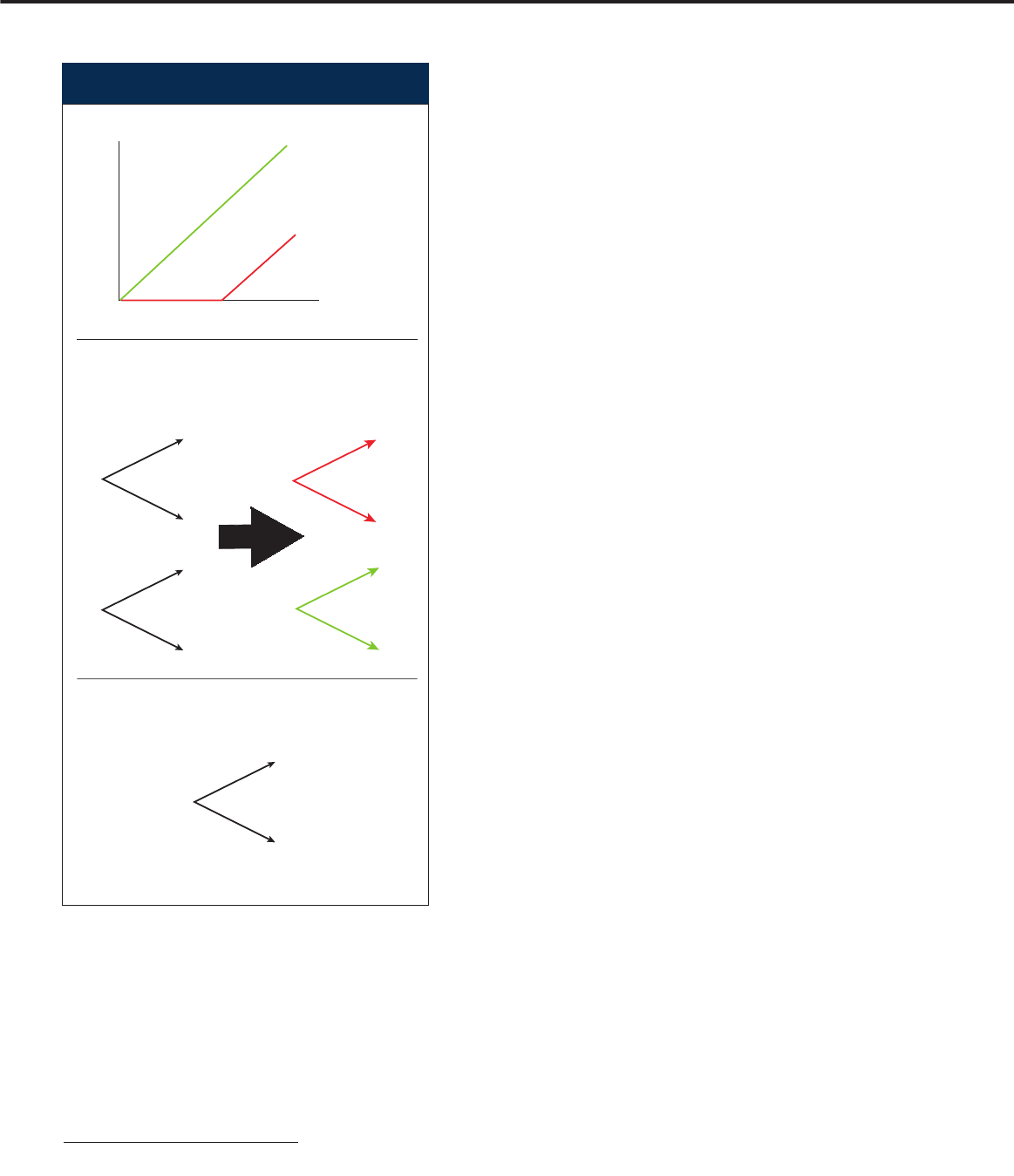
Derivatives are not independent

securities

A derivative is a contract whose value is

determined by the non-linear relation-

µβµ−

()

=−

()

ship between its payout and the value

of some other, simpler security called its

underlyer. The most interesting charac-

teristic of a derivative is the curvature of

its payout

C(S)

, as illustrated for a sim-

ple call option in figure 3.

If you know the price of a simple stock,

whose payout is linear, what is the value

of the non-linear option?

In the binary tree model, there are only

two possible states (up and down) for the

stock or the option after a time

∆t

. These

states are spanned by two independent

securities, the stock itself and a risk-free

bond. You can decompose the stock and

bond into a basis of two more elemental

securities –

and

1 – p

– each respec-

tively paying out in only one of the final

states, as shown in figure 3. By creating

a portfolio that is a suitable mixture of

these two securities, you can instanta-

neously replicate the payout of any non-

linear function

C(S)

over the next instant

of time

∆t

, no matter into which state the

stock evolves.

The value of the option is therefore

the price of the mixture of stock and

bond that replicates it. By choosing

∆t

to be infinitesimally small, you can re-

peat this replication strategy instant after

instant, so that, if the final payout

C(S)

is known, its dynamic replication at all

earlier times is determined. The value of

the replicating portfolio depends on the

size of the stock price movements in the

stock’s binary tree – that is, on the stock’s

volatility

. If you know the future

volatility, you can synthesise an option

out of stock and bonds.

The same strategy of dynamic repli-

cation can be extended to more complex

and realistic models of stock evolution,

as well as to the replication of derivatives

on all sorts of other underliers, as long

as there are enough independent under-

liers to span all future states.

Conclusion

Axiomatisation is helpful when axioms

hold true to a high degree of accuracy.

But, as Paul Wilmott aptly expressed it,

“every financial axiom ... ever seen is

demonstrably wrong”. Therefore, quan-

titative finance practitioners need to

know where best to spend their effort in

the grittily messy world they inhabit. In

preparing for that world it’s best to start

with the concrete and then proceed to

the abstract. ■

A stock is straight, an option curved

Stock S

Call option

(

strike $100

Payout

$100

Binary price trees for a stock

and a $1 investment in a

risk-free bond. The stock and bond can be decomposed into

a security

that pays out only in the up state and a security

1 –

that pays out only in the down state

Stock

Risk-free bond

1 –

1 +

∆

1 +

∆

Decompose

1 +

∆

1 +

∆

You can replicate an option's non-linear payout over each

instant by suitable investments in the elemental securities

and 1 –

(1 +

∆

)

= (

) ×

+ (

) × (1 –

)

3. A stock is straight, an option curved

1Wilmott, Paul, in the prologue to Derivatives,

John Wiley & Sons, 1998

Derman Risk The Boys Guide HEDGE

Navigation menu

Versions of this User Manual:

Views

Navigation