[U] User's Guide Stata User
User Manual:
Open the PDF directly: View PDF ![]() .
.
Page Count: 414 [warning: Documents this large are best viewed by clicking the View PDF Link!]
- Contents
- [IG] Installation Guide
- Simple installation
- Installing Stata for Windows
- Installing Stata for Mac
- Installing Stata for Unix
- Installation overview
- Find your installation DVD and paper license
- Obtain superuser access
- Create a directory for Stata
- Upgrading
- Install Stata
- Initialize the license
- Set the message of the day (optional)
- Verify that Stata is working
- Modify shell start-up script
- Update Stata if necessary
- Starting Stata
- Exiting Stata
- Troubleshooting Unix installation
- Troubleshooting Unix start-up
- Stata(console) starts but Stata(GUI) does not
- Platforms and flavors
- Documentation
- [GS] Getting Started
- [GSM] Mac
- Contents
- 1 Introducing Stata---sample session
- 2 The Stata user interface
- 3 Using the Viewer
- The Viewer's purpose
- Viewer buttons
- Viewer's function
- Viewing local text files, including SMCL files
- Viewing remote files over the Internet
- Navigating within the Viewer
- Printing
- Tabs in the Viewer
- Right-clicking on the Viewer window
- Searching for help in the Viewer
- Commands in the Viewer
- Using the Viewer from the Command window
- 4 Getting help
- 5 Opening and saving Stata datasets
- 6 Using the Data Editor
- 7 Using the Variables Manager
- 8 Importing data
- 9 Labeling data
- 10 Listing data and basic command syntax
- 11 Creating new variables
- 12 Deleting variables and observations
- 13 Using the Do-file Editor---automating Stata
- 14 Graphing data
- 15 Editing graphs
- 16 Saving and printing results by using logs
- 17 Setting font and window preferences
- 18 Learning more about Stata
- 19 Updating and extending Stata---Internet functionality
- A Troubleshooting Stata
- B Advanced Stata usage
- C More on Stata for Mac
- Subject index
- [GSU] Unix
- Contents
- 1 Introducing Stata---sample session
- 2 The Stata user interface
- 3 Using the Viewer
- The Viewer in Stata(GUI)
- The Viewer's purpose
- Viewer buttons
- Viewer's function
- Viewing local text files, including SMCL files
- Viewing remote files over the Internet
- Navigating within the Viewer
- Printing
- Tabs in the Viewer
- Right-clicking on the Viewer window
- Searching for help in the Viewer
- Commands in the Viewer
- Using the Viewer from the Command window
- 4 Getting help
- 5 Opening and saving Stata datasets
- 6 Using the Data Editor
- 7 Using the Variables Manager
- 8 Importing data
- 9 Labeling data
- 10 Listing data and basic command syntax
- 11 Creating new variables
- 12 Deleting variables and observations
- 13 Using the Do-file Editor---automating Stata
- 14 Graphing data
- 15 Editing graphs
- 16 Saving and printing results by using logs
- 17 Setting font and window preferences
- 18 Learning more about Stata
- 19 Updating and extending Stata---Internet functionality
- A Troubleshooting Stata
- B Advanced Stata usage
- C Stata manual pages for Unix
- conren
- stata
- Subject index
- [GSW] Windows
- Contents
- 1 Introducing Stata---sample session
- 2 The Stata user interface
- 3 Using the Viewer
- The Viewer's purpose
- Viewer buttons
- Viewer's function
- Viewing local text files, including SMCL files
- Viewing remote files over the Internet
- Navigating within the Viewer
- Printing
- Tabs in the Viewer
- Right-clicking on the Viewer window
- Searching for help in the Viewer
- Commands in the Viewer
- Using the Viewer from the Command window
- 4 Getting help
- 5 Opening and saving Stata datasets
- 6 Using the Data Editor
- 7 Using the Variables Manager
- 8 Importing data
- 9 Labeling data
- 10 Listing data and basic command syntax
- 11 Creating new variables
- 12 Deleting variables and observations
- 13 Using the Do-file Editor---automating Stata
- 14 Graphing data
- 15 Editing graphs
- 16 Saving and printing results by using logs
- 17 Setting font and window preferences
- 18 Learning more about Stata
- 19 Updating and extending Stata---Internet functionality
- A Troubleshooting Stata
- B Advanced Stata usage
- C More on Stata for Windows
- Subject index
- [GSM] Mac
- [U] User's Guide
- Contents
- Stata basics
- Elements of Stata
- 11 Language syntax
- 12 Data
- 13 Functions and expressions
- 13.1 Overview
- 13.2 Operators
- 13.3 Functions
- 13.4 System variables (_variables)
- 13.5 Accessing coefficients and standard errors
- 13.6 Accessing results from Stata commands
- 13.7 Explicit subscripting
- 13.8 Indicator values for levels of factor variables
- 13.9 Time-series operators
- 13.10 Label values
- 13.11 Precision and problems therein
- 13.12 References
- 14 Matrix expressions
- 14.1 Overview
- 14.2 Row and column names
- 14.3 Vectors and scalars
- 14.4 Inputting matrices by hand
- 14.5 Accessing matrices created by Stata commands
- 14.6 Creating matrices by accumulating data
- 14.7 Matrix operators
- 14.8 Matrix functions
- 14.9 Subscripting
- 14.10 Using matrices in scalar expressions
- 14.11 Reference
- 15 Saving and printing output---log files
- 16 Do-files
- 17 Ado-files
- 17.1 Description
- 17.2 What is an ado-file?
- 17.3 How can I tell if a command is built in or an ado-file?
- 17.4 How can I look at an ado-file?
- 17.5 Where does Stata look for ado-files?
- 17.6 How do I install an addition?
- 17.7 How do I add my own ado-files?
- 17.8 How do I install official updates?
- 17.9 How do I install updates to user-written additions?
- 17.10 Reference
- 18 Programming Stata
- 18.1 Description
- 18.2 Relationship between a program and a do-file
- 18.3 Macros
- 18.4 Program arguments
- 18.5 Scalars and matrices
- 18.6 Temporarily destroying the data in memory
- 18.7 Temporary objects
- 18.8 Accessing results calculated by other programs
- 18.9 Accessing results calculated by estimation commands
- 18.10 Storing results
- 18.11 Ado-files
- 18.12 Tools for interacting with programs outside Stata and with other languages
- 18.13 A compendium of useful commands for programmers
- 18.14 References
- 19 Immediate commands
- 20 Estimation and postestimation commands
- 20.1 All estimation commands work the same way
- 20.2 Standard syntax
- 20.3 Replaying prior results
- 20.4 Cataloging estimation results
- 20.5 Saving estimation results
- 20.6 Specifying the estimation subsample
- 20.7 Specifying the width of confidence intervals
- 20.8 Formatting the coefficient table
- 20.9 Obtaining the variance--covariance matrix
- 20.10 Obtaining predicted values
- 20.11 Accessing estimated coefficients
- 20.12 Performing hypothesis tests on the coefficients
- 20.13 Obtaining linear combinations of coefficients
- 20.14 Obtaining nonlinear combinations of coefficients
- 20.15 Obtaining marginal means, adjusted predictions, and predictive margins
- 20.16 Obtaining conditional and average marginal effects
- 20.17 Obtaining pairwise comparisons
- 20.18 Obtaining contrasts, tests of interactions, and main effects
- 20.19 Graphing margins, marginal effects, and contrasts
- 20.20 Dynamic forecasts and simulations
- 20.21 Obtaining robust variance estimates
- 20.22 Obtaining scores
- 20.23 Weighted estimation
- 20.24 A list of postestimation commands
- 20.25 References
- Advice
- 21 Entering and importing data
- 22 Combining datasets
- 23 Working with strings
- 24 Working with dates and times
- 25 Working with categorical data and factor variables
- 26 Overview of Stata estimation commands
- 26.1 Introduction
- 26.2 Means, proportions, and related statistics
- 26.3 Linear regression with simple error structures
- 26.4 Structural equation modeling (SEM)
- 26.5 ANOVA, ANCOVA, MANOVA, and MANCOVA
- 26.6 Generalized linear models
- 26.7 Binary-outcome qualitative dependent-variable models
- 26.8 ROC analysis
- 26.9 Conditional logistic regression
- 26.10 Multiple-outcome qualitative dependent-variable models
- 26.11 Count dependent-variable models
- 26.12 Exact estimators
- 26.13 Linear regression with heteroskedastic errors
- 26.14 Stochastic frontier models
- 26.15 Regression with systems of equations
- 26.16 Models with endogenous sample selection
- 26.17 Models with time-series data
- 26.18 Panel-data models
- 26.19 Multilevel mixed-effects models
- 26.20 Survival-time (failure-time) models
- 26.21 Treatment-effect models
- 26.22 Generalized method of moments (GMM)
- 26.23 Estimation with correlated errors
- 26.24 Survey data
- 26.25 Multiple imputation
- 26.26 Multivariate and cluster analysis
- 26.27 Pharmacokinetic data
- 26.28 Specification search tools
- 26.29 Power and sample-size analysis
- 26.30 Obtaining new estimation commands
- 26.31 References
- 27 Commands everyone should know
- 28 Using the Internet to keep up to date
- Subject and author index
- [D] Data Management
- Contents
- intro
- data management
- append
- assert
- bcal
- by
- cd
- cf
- changeeol
- checksum
- clear
- clonevar
- codebook
- collapse
- compare
- compress
- contract
- copy
- corr2data
- count
- cross
- data types
- datasignature
- datetime
- Syntax
- Types of dates and their human readable forms (HRFs)
- Stata internal form (SIF)
- HRF-to-SIF conversion functions
- Displaying SIFs in HRF
- Building SIFs from components
- SIF-to-SIF conversion
- Extracting time-of-day components from SIFs
- Extracting date components from SIFs
- Conveniently typing SIF values
- Obtaining and working with durations
- Using dates and times from other software
- Description
- Remarks and examples
- References
- Also see
- Syntax
- datetime business calendars
- datetime business calendars creation
- Syntax
- Description
- Remarks and examples
- Introduction
- Concepts
- The preliminary commands
- The omit commands: from/to and if
- The omit commands: and
- The omit commands: omit date
- The omit commands: omit dayofweek
- The omit commands: omit dowinmonth
- Creating stbcal-files with bcal create
- Where to place stbcal-files
- How to debug stbcal-files
- Ideas for calendars that may not occur to you
- Also see
- datetime display formats
- datetime translation
- Syntax
- Description
- Remarks and examples
- Introduction
- Specifying the mask
- How the HRF-to-SIF functions interpret the mask
- Working with two-digit years
- Working with incomplete dates and times
- Translating run-together dates, such as 20060125
- Valid times
- The clock() and Clock() functions
- Why there are two SIF datetime encodings
- Advice on using datetime/c and datetime/C
- Determining when leap seconds occurred
- The date() function
- The other translation functions
- Also see
- describe
- destring
- dir
- drawnorm
- drop
- ds
- duplicates
- edit
- egen
- encode
- erase
- expand
- expandcl
- export
- filefilter
- fillin
- format
- functions
- Description
- Mathematical functions
- Probability distributions and density functions
- Beta and noncentral beta distributions
- ibeta()
- betaden()
- ibetatail()
- invibeta()
- invibetatail()
- nibeta()
- invnibeta()
- Binomial distribution
- binomial()
- binomialp()
- binomialtail()
- invbinomial()
- invbinomialtail()
- Chi-squared and noncentral chi-squared distributions
- chi2()
- chi2den()
- chi2tail()
- invchi2()
- invchi2tail()
- nchi2()
- nchi2den()
- nchi2tail()
- invnchi2()
- invnchi2tail()
- npnchi2()
- Dunnett's multiple range distribution
- dunnettprob()
- invdunnettprob()
- F and noncentral F distributions
- F()
- Fden()
- Ftail()
- invF()
- invFtail()
- nF()
- nFtail()
- invnFtail()
- npnF()
- Gamma distribution
- gammap()
- gammaden()
- gammaptail()
- invgammap()
- invgammaptail()
- dgammapda()
- dgammapdada()
- dgammapdadx()
- dgammapdx()
- dgammapdxdx()
- Hypergeometric distribution
- hypergeometric()
- hypergeometricp()
- Negative binomial distribution
- nbinomial()
- nbinomialp()
- nbinomialtail()
- invnbinomial()
- invnbinomiailtail()
- Normal (Gaussian), log of the normal, and binormal distributions
- binormal()
- normal()
- normalden()
- invnormal()
- lnnormal()
- Poisson distribution
- poisson()
- poissonp()
- poissontail()
- invpoisson()
- invpoissontail()
- Student's t and noncentral Student's t distributions
- t()
- tden()
- ttail()
- invt()
- invttail()
- nt()
- ntden()
- nttail()
- invnttail()
- npnt()
- Tukey's Studentized range distribution
- tukeyprob()
- invtukeyprob()
- Random-number functions
- String functions
- abbrev()
- char()
- indexnot()
- itrim()
- length()
- lower()
- ltrim()
- plural()
- proper()
- real()
- regexm()
- regexr()
- regexs()
- reverse()
- rtrim()
- soundex()
- soundex_nara()
- strcat()
- strdup()
- string()
- strlen()
- strlower()
- strltrim()
- strmatch()
- strofreal()
- strpos()
- strproper()
- strreverse()
- strrtrim()
- strtoname()
- strtrim()
- strupper()
- subinstr()
- subinword()
- substr()
- trim()
- upper()
- word()
- wordcount()
- Programming functions
- autocode()
- byteorder()
- c()
- _caller()
- chop()
- clip()
- cond()
- e()
- e(sample)
- epsdouble()
- epsfloat()
- fileexists()
- fileread()
- filereaderror()
- filewrite()
- float()
- fmtwidth()
- has_eprop()
- inlist()
- inrange()
- irecode()
- matrix()
- maxbyte()
- maxdouble()
- maxfloat()
- maxint()
- maxlong()
- mi()
- minbyte()
- mindouble()
- minfloat()
- minint()
- minlong()
- missing()
- r()
- recode()
- replay()
- return()
- s()
- scalar()
- smallestdouble()
- Date and time functions
- bofd()
- Cdhms()
- clock()
- Cmdyhms()
- Cofc()
- cofC()
- Cofd()
- cofd()
- daily()
- date()
- day()
- dhms()
- dofb()
- dofC()
- dofc()
- dofh()
- dofm()
- dofq()
- dofw()
- dofy()
- dow()
- doy()
- halfyear()
- halfyearly()
- hh()
- hhC()
- hms()
- hofd()
- hours()
- mdy()
- mdyhms()
- minutes()
- mm()
- mmC()
- mofd()
- month()
- monthly()
- msofhours()
- msofminutes()
- msofseconds()
- qofd()
- quarter()
- quarterly()
- seconds()
- ss()
- ssC()
- tC()
- tc()
- td()
- th()
- tm()
- tq()
- tw()
- week()
- weekly()
- wofd()
- year()
- yearly()
- yh()
- ym()
- yofd()
- yq()
- yw()
- Selecting time spans
- Matrix functions returning a matrix
- Matrix functions returning a scalar
- Acknowledgments
- References
- Also see
- Description
- generate
- gsort
- hexdump
- icd9
- import
- import delimited
- import excel
- import haver
- import sasxport
- infile (fixed format)
- infile (free format)
- infix (fixed format)
- input
- inspect
- ipolate
- isid
- joinby
- label
- label language
- labelbook
- list
- lookfor
- memory
- merge
- missing values
- mkdir
- mvencode
- notes
- obs
- odbc
- order
- outfile
- pctile
- putmata
- range
- recast
- recode
- rename
- rename group
- reshape
- Syntax
- Menu
- Description
- Options
- Remarks and examples
- Description of basic syntax
- Wide and long data forms
- Avoiding and correcting mistakes
- reshape long and reshape wide without arguments
- Missing variables
- Advanced issues with basic syntax: i()
- Advanced issues with basic syntax: j()
- Advanced issues with basic syntax: xij
- Advanced issues with basic syntax: String identifiers for j()
- Advanced issues with basic syntax: Second-level nesting
- Description of advanced syntax
- Stored results
- Acknowledgment
- References
- Also see
- rmdir
- sample
- save
- separate
- shell
- snapshot
- sort
- split
- stack
- statsby
- sysuse
- type
- use
- varmanage
- webuse
- xmlsave
- xpose
- zipfile
- Subject and author index
- [G] Graphics
- Contents
- Introduction
- Commands
- graph
- graph bar
- Syntax
- Menu
- Description
- Options
- Remarks and examples
- Introduction
- Examples of syntax
- Treatment of bars
- Treatment of data
- Obtaining frequencies
- Multiple bars (overlapping the bars)
- Controlling the text of the legend
- Multiple over()s (repeating the bars)
- Nested over()s
- Charts with many categories
- How bars are ordered
- Reordering the bars
- Putting the bars in a prespecified order
- Putting the bars in height order
- Putting the bars in a derived order
- Reordering the bars, example
- Use with by()
- Video example
- History
- References
- Also see
- graph box
- graph combine
- graph copy
- graph describe
- graph dir
- graph display
- graph dot
- graph drop
- graph export
- graph manipulation
- graph matrix
- graph other
- graph pie
- graph play
- graph print
- graph query
- graph rename
- graph save
- graph set
- graph twoway
- graph twoway area
- graph twoway bar
- graph twoway connected
- graph twoway contour
- graph twoway contourline
- graph twoway dot
- graph twoway dropline
- graph twoway fpfit
- graph twoway fpfitci
- graph twoway function
- graph twoway histogram
- graph twoway kdensity
- graph twoway lfit
- graph twoway lfitci
- graph twoway line
- graph twoway lowess
- graph twoway lpoly
- graph twoway lpolyci
- graph twoway mband
- graph twoway mspline
- graph twoway pcarrow
- graph twoway pcarrowi
- graph twoway pccapsym
- graph twoway pci
- graph twoway pcscatter
- graph twoway pcspike
- graph twoway qfit
- graph twoway qfitci
- graph twoway rarea
- graph twoway rbar
- graph twoway rcap
- graph twoway rcapsym
- graph twoway rconnected
- graph twoway rline
- graph twoway rscatter
- graph twoway rspike
- graph twoway scatter
- Syntax
- Menu
- Description
- Options
- Remarks and examples
- Typical use
- Scatter syntax
- The overall look for the graph
- The size and aspect ratio of the graph
- Titles
- Axis titles
- Axis labels and ticking
- Grid lines
- Added lines
- Axis range
- Log scales
- Multiple axes
- Markers
- Weighted markers
- Jittered markers
- Connected lines
- Graphs by groups
- Saving graphs
- Video example
- Appendix: Styles and composite styles
- References
- Also see
- graph twoway scatteri
- graph twoway spike
- graph twoway tsline
- graph use
- palette
- set graphics
- set printcolor
- set scheme
- Options
- added_line_options
- added_text_options
- addplot_option
- advanced_options
- area_options
- aspect_option
- axis_choice_options
- Syntax
- Description
- Options
- Remarks and examples
- Usual case: one set of axes
- Special case: multiple axes due to multiple scales
- yaxis(1) and xaxis(1) are the defaults
- Notation style is irrelevant
- yaxis() and xaxis() are plot options
- Specifying the other axes options with multiple axes
- Each plot may have at most one x scale and one y scale
- Special case: Multiple axes with a shared scale
- Reference
- Also see
- axis_label_options
- axis_options
- axis_scale_options
- axis_title_options
- barlook_options
- blabel_option
- by_option
- cat_axis_label_options
- cat_axis_line_options
- clegend_option
- cline_options
- connect_options
- eps_options
- fcline_options
- fitarea_options
- legend_options
- line_options
- marker_label_options
- marker_options
- name_option
- nodraw_option
- play_option
- png_options
- pr_options
- ps_options
- rcap_options
- region_options
- rspike_options
- saving_option
- scale_option
- scheme_option
- std_options
- textbox_options
- tif_options
- title_options
- twoway_options
- Styles/concepts/schemes
- addedlinestyle
- alignmentstyle
- anglestyle
- areastyle
- axisstyle
- bystyle
- clockposstyle
- colorstyle
- compassdirstyle
- concept: gph files
- concept: lines
- concept: repeated options
- connectstyle
- gridstyle
- intensitystyle
- justificationstyle
- legendstyle
- linepatternstyle
- linestyle
- linewidthstyle
- marginstyle
- markerlabelstyle
- markersizestyle
- markerstyle
- orientationstyle
- plotregionstyle
- pstyle
- relativesize
- ringposstyle
- schemes intro
- scheme economist
- scheme s1
- scheme s2
- scheme sj
- shadestyle
- stylelists
- symbolstyle
- text
- textboxstyle
- textsizestyle
- textstyle
- ticksetstyle
- tickstyle
- Subject and author index
- [ME] Multilevel Mixed Effects
- Contents
- me
- mecloglog
- mecloglog postestimation
- meglm
- meglm postestimation
- melogit
- melogit postestimation
- menbreg
- menbreg postestimation
- meologit
- meologit postestimation
- meoprobit
- meoprobit postestimation
- mepoisson
- mepoisson postestimation
- meprobit
- meprobit postestimation
- meqrlogit
- meqrlogit postestimation
- meqrpoisson
- meqrpoisson postestimation
- mixed
- Syntax
- Menu
- Description
- Options
- Remarks and examples
- Introduction
- Two-level models
- Covariance structures
- Likelihood versus restricted likelihood
- Three-level models
- Blocked-diagonal covariance structures
- Heteroskedastic random effects
- Heteroskedastic residual errors
- Other residual-error structures
- Crossed-effects models
- Diagnosing convergence problems
- Survey data
- Stored results
- Methods and formulas
- Acknowledgments
- References
- Also see
- mixed postestimation
- Glossary
- Subject and author index
- [MI] Multiple Imputation
- Contents
- intro substantive
- intro
- estimation
- mi add
- mi append
- mi convert
- mi copy
- mi describe
- mi erase
- mi estimate
- Syntax
- Menu
- Description
- Options
- Remarks and examples
- Using mi estimate
- Example 1: Completed-data logistic analysis
- Example 2: Completed-data linear regression analysis
- Example 3: Completed-data survival analysis
- Example 4: Panel data and multilevel models
- Example 5: Estimating transformations
- Example 6: Monte Carlo error estimates
- Potential problems that can arise when using mi estimate
- Stored results
- Methods and formulas
- Acknowledgments
- References
- Also see
- mi estimate using
- mi estimate postestimation
- mi expand
- mi export
- mi export ice
- mi export nhanes1
- mi extract
- mi import
- mi import flong
- mi import flongsep
- mi import ice
- mi import nhanes1
- mi import wide
- mi impute
- Syntax
- Menu
- Description
- Options
- Remarks and examples
- Stored results
- Methods and formulas
- References
- Also see
- mi impute chained
- mi impute intreg
- mi impute logit
- mi impute mlogit
- mi impute monotone
- mi impute mvn
- mi impute nbreg
- mi impute ologit
- mi impute pmm
- mi impute poisson
- mi impute regress
- mi impute truncreg
- mi merge
- mi misstable
- mi passive
- mi predict
- Syntax
- Menu
- Description
- Options
- Remarks and examples
- Introduction
- Using mi predict and mi predictnl
- Example 1: Obtain MI linear predictions and other statistics
- Example 2: Obtain MI linear predictions for the estimation sample
- Example 3: Obtain MI estimates of probabilities
- Example 4: Obtain other MI predictions
- Example 5: Obtain MI predictions after multiple-equation commands
- Methods and formulas
- References
- Also see
- mi ptrace
- mi rename
- mi replace0
- mi reset
- mi reshape
- mi select
- mi set
- mi stsplit
- mi test
- mi update
- mi varying
- mi xeq
- mi XXXset
- noupdate option
- styles
- technical
- Description
- Remarks and examples
- Notation
- Definition of styles
- Adding new commands to mi
- Outline for new commands
- Utility routines
- u_mi_assert_set
- u_mi_certify_data
- u_mi_no_sys_vars and u_mi_no_wide_vars
- u_mi_zap_chars
- u_mi_xeq_on_tmp_flongsep
- u_mi_get_flongsep_tmpname
- mata: u_mi_flongsep_erase()
- u_mi_sortback
- u_mi_save and u_mi_use
- mata: u_mi_wide_swapvars()
- u_mi_fixchars
- mata: u_mi_cpchars_get() and mata: u_mi_cpchars_put()
- mata: u_mi_get_mata_instanced_var()
- mata: u_mi_ptrace_*()
- How to write other set commands to work with mi
- Also see
- workflow
- Glossary
- Subject and author index
- [MV] Multivariate Statistics
- Contents
- intro
- multivariate
- alpha
- biplot
- ca
- ca postestimation
- ca postestimation plots
- candisc
- canon
- canon postestimation
- cluster
- Syntax
- Description
- Remarks and examples
- Introduction to cluster analysis
- Stata's cluster-analysis system
- Data transformations and variable selection
- Similarity and dissimilarity measures
- Partition cluster-analysis methods
- Hierarchical cluster-analysis methods
- Hierarchical cluster analysis applied to a dissimilarity matrix
- Postclustering commands
- Cluster-management tools
- References
- Also see
- clustermat
- cluster dendrogram
- cluster generate
- cluster kmeans and kmedians
- cluster linkage
- cluster notes
- cluster programming subroutines
- cluster programming utilities
- cluster stop
- cluster utility
- discrim
- discrim estat
- discrim knn
- discrim knn postestimation
- discrim lda
- discrim lda postestimation
- discrim logistic
- discrim logistic postestimation
- discrim qda
- discrim qda postestimation
- factor
- factor postestimation
- hotelling
- manova
- manova postestimation
- matrix dissimilarity
- mca
- mca postestimation
- mca postestimation plots
- mds
- mds postestimation
- mds postestimation plots
- mdslong
- mdsmat
- measure_option
- mvreg
- mvreg postestimation
- mvtest
- mvtest correlations
- mvtest covariances
- mvtest means
- mvtest normality
- pca
- pca postestimation
- procrustes
- procrustes postestimation
- rotate
- rotatemat
- scoreplot
- screeplot
- Glossary
- Subject and author index
- [PSS] Power and Sample Size
- Contents
- intro
- GUI
- power
- power, graph
- power, table
- power onemean
- power twomeans
- power pairedmeans
- power oneproportion
- power twoproportions
- power pairedproportions
- power onevariance
- power twovariances
- power onecorrelation
- power twocorrelations
- power oneway
- power twoway
- power repeated
- unbalanced designs
- Glossary
- Subject and author index
- [R] Base Reference
- Contents
- Introduction
- A
- about
- adoupdate
- ameans
- anova
- anova postestimation
- areg
- areg postestimation
- asclogit
- asclogit postestimation
- asmprobit
- asmprobit postestimation
- asroprobit
- asroprobit postestimation
- B
- C
- centile
- ci
- clogit
- clogit postestimation
- cloglog
- cloglog postestimation
- cls
- cnsreg
- cnsreg postestimation
- constraint
- contrast
- Syntax
- Menu
- Description
- Options
- Remarks and examples
- Stored results
- Methods and formulas
- References
- Also see
- contrast postestimation
- copyright
- copyright apache
- copyright boost
- copyright freetype
- copyright icu
- copyright jagpdf
- copyright lapack
- copyright libpng
- copyright miglayout
- copyright scintilla
- copyright ttf2pt1
- copyright zlib
- correlate
- cumul
- cusum
- D
- E
- eform_option
- eivreg
- eivreg postestimation
- error messages
- esize
- estat
- estat classification
- estat gof
- estat ic
- estat summarize
- estat vce
- estimates
- estimates describe
- estimates for
- estimates notes
- estimates replay
- estimates save
- estimates stats
- estimates store
- estimates table
- estimates title
- estimation options
- exit
- exlogistic
- exlogistic postestimation
- expoisson
- expoisson postestimation
- F
- G
- gllamm
- glm
- glm postestimation
- glogit
- glogit postestimation
- gmm
- Syntax
- Menu
- Description
- Options
- Remarks and examples
- Introduction
- Substitutable expressions
- The weight matrix and two-step estimation
- Obtaining standard errors
- Exponential (Poisson) regression models
- Specifying derivatives
- Exponential regression models with panel data
- Rational-expectations models
- System estimators
- Dynamic panel-data models
- Details of moment-evaluator programs
- Stored results
- Methods and formulas
- References
- Also see
- gmm postestimation
- grmeanby
- H
- hausman
- heckman
- heckman postestimation
- heckoprobit
- heckoprobit postestimation
- heckprobit
- heckprobit postestimation
- help
- hetprobit
- hetprobit postestimation
- histogram
- I
- icc
- inequality
- intreg
- intreg postestimation
- ivpoisson
- ivpoisson postestimation
- ivprobit
- ivprobit postestimation
- ivregress
- ivregress postestimation
- ivtobit
- ivtobit postestimation
- J
- K
- L
- ladder
- level
- limits
- lincom
- linktest
- lnskew0
- log
- logistic
- logistic postestimation
- Description
- Syntax for predict
- Menu for predict
- Options for predict
- Remarks and examples
- predict without options
- predict with the xb and stdp options
- predict with the residuals option
- predict with the number option
- predict with the deviance option
- predict with the rstandard option
- predict with the hat option
- predict with the dx2 option
- predict with the ddeviance option
- predict with the dbeta option
- Methods and formulas
- References
- Also see
- logit
- logit postestimation
- loneway
- lowess
- lpoly
- lroc
- lrtest
- lsens
- lv
- M
- margins
- Syntax
- Menu
- Description
- Options
- Remarks and examples
- Introduction
- Obtaining margins of responses
- Example 1: A simple case after regress
- Example 2: A simple case after logistic
- Example 3: Average response versus response at average
- Example 4: Multiple margins from one command
- Example 5: Margins with interaction terms
- Example 6: Margins with continuous variables
- Example 7: Margins of continuous variables
- Example 8: Margins of interactions
- Example 9: Decomposing margins
- Example 10: Testing margins---contrasts of margins
- Example 11: Margins of a specified prediction
- Example 12: Margins of a specified expression
- Example 13: Margins with multiple outcomes (responses)
- Example 14: Margins with multiple equations
- Example 15: Margins evaluated out of sample
- Obtaining margins of derivatives of responses (a.k.a. marginal effects)
- Do not specify marginlist when you mean over()
- Use at() freely, especially with continuous variables
- Expressing derivatives as elasticities
- Derivatives versus discrete differences
- Example 16: Average marginal effect (partial effects)
- Example 17: Average marginal effect of all covariates
- Example 18: Evaluating marginal effects over the response surface
- Obtaining margins with survey data and representative samples
- Standardizing margins
- Obtaining margins as though the data were balanced
- Obtaining margins with nested designs
- Special topics
- Video examples
- Glossary
- Stored results
- Methods and formulas
- References
- Also see
- margins postestimation
- margins, contrast
- margins, pwcompare
- marginsplot
- Syntax
- Menu
- Description
- Options
- Remarks and examples
- Introduction
- Dataset
- Profile plots
- Interaction plots
- Contrasts of margins---effects (discrete marginal effects)
- Three-way interactions
- Continuous covariates
- Plots at every value of a continuous covariate
- Contrasts of at() groups---discrete effects
- Controlling the graph's dimensions
- Pairwise comparisons
- Horizontal is sometimes better
- Marginal effects
- Plotting a subset of the results from margins
- Advanced usage
- Video examples
- Addendum: Advanced uses of dimlist
- Acknowledgments
- References
- Also see
- matsize
- maximize
- mean
- mean postestimation
- meta
- mfp
- mfp postestimation
- misstable
- mkspline
- ml
- Syntax
- Description
- Options
- Options for use with ml model in interactive or noninteractive mode
- Options for use with ml model in noninteractive mode
- Options for use when specifying equations
- Options for use with ml search
- Option for use with ml plot
- Options for use with ml init
- Options for use with ml maximize
- Option for use with ml graph
- Options for use with ml display
- Options for use with mleval
- Option for use with mlsum
- Option for use with mlvecsum
- Option for use with mlmatsum
- Options for use with mlmatbysum
- Options for use with ml score
- Remarks and examples
- Stored results
- Methods and formulas
- References
- Also see
- mlexp
- mlexp postestimation
- mlogit
- mlogit postestimation
- more
- mprobit
- mprobit postestimation
- margins
- N
- nbreg
- nbreg postestimation
- nestreg
- net
- Syntax
- Description
- Options
- Remarks and examples
- Definition of a package
- The purpose of the net and ado commands
- Content pages
- Package-description pages
- Where packages are installed
- A summary of the net command
- A summary of the ado command
- Relationship of net and ado to the point-and-click interface
- Creating your own site
- Format of content and package-description files
- Example 1
- Example 2
- Additional package directives
- SMCL in content and package-description files
- Error-free file delivery
- References
- Also see
- net search
- netio
- news
- nl
- nl postestimation
- nlcom
- nlogit
- nlogit postestimation
- nlsur
- nlsur postestimation
- nptrend
- O
- P
- pcorr
- permute
- pk
- pkcollapse
- pkcross
- pkequiv
- pkexamine
- pkshape
- pksumm
- poisson
- poisson postestimation
- predict
- predictnl
- probit
- probit postestimation
- proportion
- proportion postestimation
- prtest
- pwcompare
- Syntax
- Menu
- Description
- Options
- Remarks and examples
- Stored results
- Methods and formulas
- References
- Also see
- pwcompare postestimation
- pwmean
- pwmean postestimation
- Q
- R
- ranksum
- ratio
- ratio postestimation
- reg3
- reg3 postestimation
- regress
- regress postestimation
- Description
- Predictions
- DFBETA influence statistics
- Tests for violation of assumptions
- Syntax for estat hettest
- Menu for estat
- Description for estat hettest
- Options for estat hettest
- Syntax for estat imtest
- Menu for estat
- Description for estat imtest
- Options for estat imtest
- Syntax for estat ovtest
- Menu for estat
- Description for estat ovtest
- Option for estat ovtest
- Syntax for estat szroeter
- Menu for estat
- Description for estat szroeter
- Options for estat szroeter
- Remarks and examples for estat hettest, estat imtest, estat ovtest, and estat szroeter
- Stored results for estat hettest, estat imtest, and estat ovtest
- Variance inflation factors
- Measures of effect size
- Methods and formulas
- Acknowledgments
- References
- Also see
- regress postestimation diagnostic plots
- regress postestimation time series
- #review
- roc
- roccomp
- rocfit
- rocfit postestimation
- rocreg
- rocreg postestimation
- rocregplot
- roctab
- rologit
- rologit postestimation
- rreg
- rreg postestimation
- runtest
- S
- T
- U
- V
- W
- X
- Z
- Author index
- Subject index
- [SEM] Structural Equation Modeling
- Contents
- Acknowledgments
- intro 1
- intro 2
- Description
- Remarks and examples
- Using path diagrams to specify standard linear SEMs
- Specifying correlation
- Using the command language to specify standard linear SEMs
- Specifying generalized SEMs: Family and link
- Specifying generalized SEMs: Family and link, multinomial logistic regression
- Specifying generalized SEMs: Family and link, paths from response variables
- Specifying generalized SEMs: Multilevel mixed effects (2 levels)
- Specifying generalized SEMs: Multilevel mixed effects (3 levels)
- Specifying generalized SEMs: Multilevel mixed effects (4+ levels)
- Specifying generalized SEMs: Multilevel mixed effects with random intercepts
- Specifying generalized SEMs: Multilevel mixed effects with random slopes
- Reference
- Also see
- intro 3
- intro 4
- Description
- Remarks and examples
- Differences in assumptions between sem and gsem
- sem: Choice of estimation method
- gsem: Choice of estimation method
- Treatment of missing values
- Variable types: Observed, latent, endogenous, exogenous, and error
- Constraining parameters
- Identification 1: Substantive issues
- Identification 2: Normalization constraints (anchoring)
- References
- Also see
- intro 5
- Description
- Remarks and examples
- Single-factor measurement models
- Item--response theory (IRT) models
- Multiple-factor measurement models
- Confirmatory factor analysis (CFA) models
- Structural models 1: Linear regression
- Structural models 2: Gamma regression
- Structural models 3: Binary-outcome models
- Structural models 4: Count models
- Structural models 5: Ordinal models
- Structural models 6: Multinomial logistic regression
- Structural models 7: Dependencies between response variables
- Structural models 8: Unobserved inputs, outputs, or both
- Structural models 9: MIMIC models
- Structural models 10: Seemingly unrelated regression (SUR)
- Structural models 11: Multivariate regression
- Structural models 12: Mediation models
- Correlations
- Higher-order CFA models
- Correlated uniqueness model
- Latent growth models
- Models with reliability
- Multilevel mixed-effects models
- References
- Also see
- intro 6
- Description
- Remarks and examples
- The generic SEM model
- Fitting the model for different groups of the data
- Which parameters vary by default, and which do not
- Specifying which parameters are allowed to vary in broad, sweeping terms
- Adding constraints for path coefficients across groups
- Adding constraints for means, variances, or covariances across groups
- Adding constraints for some groups but not others
- Adding paths for some groups but not others
- Relaxing constraints
- Reference
- Also see
- intro 7
- Description
- Remarks and examples
- Replaying the model (sem and gsem)
- Displaying odds ratios, incidence-rate ratios, etc. (gsem only)
- Obtaining goodness-of-fit statistics (sem and gsem)
- Performing tests for including omitted paths and relaxing constraints (sem only)
- Performing tests of model simplification (sem and gsem)
- Displaying other results, statistics, and tests (sem and gsem)
- Obtaining predicted values (sem)
- Obtaining predicted values (gsem)
- Using contrast, pwcompare, and margins (sem and gsem)
- Accessing stored results
- Also see
- intro 8
- intro 9
- intro 10
- intro 11
- intro 12
- Description
- Remarks and examples
- Is your model identified?
- Convergence solutions generically described
- Temporarily eliminate option reliability()
- Use default normalization constraints
- Temporarily eliminate feedback loops
- Temporarily simplify the model
- Try other numerical integration methods (gsem only)
- Get better starting values (sem and gsem)
- Get better starting values (gsem)
- Also see
- Builder
- Builder, generalized
- estat eform
- estat eqgof
- estat eqtest
- estat framework
- estat ggof
- estat ginvariant
- estat gof
- estat mindices
- estat residuals
- estat scoretests
- estat stable
- estat stdize
- estat summarize
- estat teffects
- example 1
- example 2
- example 3
- example 4
- example 5
- example 6
- example 7
- example 8
- example 9
- example 10
- example 11
- example 12
- example 13
- example 14
- example 15
- example 16
- example 17
- example 18
- example 19
- example 20
- example 21
- example 22
- example 23
- example 24
- example 25
- example 26
- example 27g
- example 28g
- example 29g
- example 30g
- example 31g
- example 32g
- example 33g
- example 34g
- example 35g
- example 36g
- example 37g
- example 38g
- Description
- Remarks and examples
- Random-intercept model, single-equation formulation
- Random-intercept model, within-and-between formulation
- Random-slope model, single-equation formulation
- Random-slope model, within-and-between formulation
- Fitting the random-intercept model with the Builder
- Fitting the random-slope model with the Builder
- Reference
- Also see
- example 39g
- example 40g
- example 41g
- example 42g
- example 43g
- example 44g
- example 45g
- example 46g
- gsem
- gsem estimation options
- gsem family-and-link options
- gsem model description options
- gsem path notation extensions
- gsem postestimation
- gsem reporting options
- lincom
- lrtest
- methods and formulas for gsem
- methods and formulas for sem
- nlcom
- predict after gsem
- predict after sem
- sem
- sem and gsem option constraints()
- sem and gsem option covstructure()
- sem and gsem option from()
- sem and gsem option reliability()
- sem and gsem path notation
- sem and gsem syntax options
- sem estimation options
- sem group options
- sem model description options
- sem option method()
- sem option noxconditional
- sem option select()
- sem path notation extensions
- sem postestimation
- sem reporting options
- sem ssd options
- ssd
- test
- testnl
- Glossary
- Subject and author index
- [ST] Survival Analysis
- Contents
- intro
- survival analysis
- Description
- Remarks and examples
- Introduction
- Declaring and converting count data
- Converting snapshot data
- Declaring and summarizing survival-time data
- Manipulating survival-time data
- Obtaining summary statistics, confidence intervals, tables, etc.
- Fitting regression models
- Sample size and power determination for survival analysis
- Converting survival-time data
- Programmer's utilities
- Epidemiological tables
- Reference
- Also see
- ct
- ctset
- cttost
- discrete
- epitab
- Syntax
- Menu
- Description
- Options
- Remarks and examples
- Incidence-rate data
- Stratified incidence-rate data
- Standardized estimates with stratified incidence-rate data
- Cumulative incidence data
- Stratified cumulative incidence data
- Standardized estimates with stratified cumulative incidence data
- Case--control data
- Stratified case--control data
- Case--control data with multiple levels of exposure
- Case--control data with confounders and possibly multiple levels of exposure
- Standardized estimates with stratified case--control data
- Matched case--control data
- Video examples
- Stored results
- Methods and formulas
- Unstratified incidence-rate data (ir and iri)
- Unstratified cumulative incidence data (cs and csi)
- Unstratified case--control data (cc and cci)
- Unstratified matched case--control data (mcc and mcci)
- Stratified incidence-rate data (ir with the by() option)
- Stratified cumulative incidence data (cs with the by() option)
- Stratified case--control data (cc with by() option, mhodds, tabodds)
- Acknowledgments
- References
- Also see
- ltable
- snapspan
- st
- st_is
- stbase
- stci
- stcox
- Syntax
- Menu
- Description
- Options
- Remarks and examples
- Cox regression with uncensored data
- Cox regression with censored data
- Treatment of tied failure times
- Cox regression with discrete time-varying covariates
- Cox regression with continuous time-varying covariates
- Robust estimate of variance
- Cox regression with multiple-failure data
- Stratified estimation
- Cox regression as Poisson regression
- Cox regression with shared frailty
- Stored results
- Methods and formulas
- Acknowledgment
- References
- Also see
- stcox PH-assumption tests
- stcox postestimation
- stcrreg
- stcrreg postestimation
- stcurve
- stdescribe
- stfill
- stgen
- stir
- stpower
- stpower cox
- stpower exponential
- Syntax
- Menu
- Description
- Options
- Remarks and examples
- Introduction
- Other ways of specifying the effect size
- Sample-size determination by using different approximations
- Sample-size determination in the presence of censoring
- Nonuniform accrual and exponential losses to follow-up
- The conditional versus unconditional approaches
- Link to the sample-size and power computation for the log-rank test
- Power determination
- Stored results
- Methods and formulas
- References
- Also see
- stpower logrank
- stptime
- strate
- streg
- streg postestimation
- sts
- sts generate
- sts graph
- sts list
- sts test
- stset
- Syntax
- Menu
- Description
- Options for use with stset and streset
- Options unique to streset
- Options for st
- Remarks and examples
- What are survival-time data?
- Key concepts
- Survival-time datasets
- Using stset
- Two concepts of time
- The substantive meaning of analysis time
- Setting the failure event
- Setting multiple failures
- First entry times
- Final exit times
- Intermediate exit and reentry times (gaps)
- if() versus if exp
- Past and future records
- Using streset
- Performance and multiple-record-per-subject datasets
- Sequencing of events within t
- Weights
- Data warnings and errors flagged by stset
- Using survival-time data in Stata
- References
- Also see
- stsplit
- stsum
- sttocc
- sttoct
- stvary
- Glossary
- Subject and author index
- [SVY] Survey Data
- Contents
- intro
- survey
- bootstrap_options
- brr_options
- direct standardization
- estat
- jackknife_options
- ml for svy
- poststratification
- sdr_options
- subpopulation estimation
- svy
- svy bootstrap
- svy brr
- svy estimation
- svy jackknife
- svy postestimation
- svy sdr
- svy: tabulate oneway
- svy: tabulate twoway
- svydescribe
- svymarkout
- svyset
- variance estimation
- Glossary
- Subject and author index
- [TE] Treatment Effects
- Contents
- treatment effects
- etpoisson
- etpoisson postestimation
- etregress
- etregress postestimation
- teffects
- teffects intro
- teffects intro advanced
- Description
- Remarks and examples
- Introduction
- Defining treatment effects
- The potential-outcome model
- Assumptions needed for estimation
- Comparing the ATE and ATET
- Overview of treatment-effect estimators
- RA estimators
- IPW estimators
- AIPW estimators
- IPWRA estimators
- Nearest-neighbor matching estimators
- Propensity-score matching estimators
- Choosing among estimators
- Model choice
- Acknowledgments
- References
- Also see
- teffects aipw
- teffects ipw
- teffects ipwra
- teffects multivalued
- teffects nnmatch
- teffects overlap
- teffects postestimation
- teffects psmatch
- teffects ra
- Glossary
- Subject and author index
- [TS] Time Series
- Contents
- intro
- time series
- arch
- arch postestimation
- arfima
- arfima postestimation
- arima
- arima postestimation
- corrgram
- cumsp
- dfactor
- dfactor postestimation
- dfgls
- dfuller
- estat acplot
- estat aroots
- fcast compute
- fcast graph
- forecast
- forecast adjust
- forecast clear
- forecast coefvector
- forecast create
- forecast describe
- forecast drop
- forecast estimates
- forecast exogenous
- forecast identity
- forecast list
- forecast query
- forecast solve
- irf
- irf add
- irf cgraph
- irf create
- Syntax
- Menu
- Description
- Options
- Remarks and examples
- Methods and formulas
- Impulse--response function formulas for VARs
- Dynamic-multiplier function formulas for VARs
- Forecast-error variance decomposition formulas for VARs
- Impulse{--}response function formulas for VECMs
- Algorithms for bootstrapping the VAR IRF and FEVD standard errors
- Impulse--response function formulas for ARIMA and ARFIMA
- References
- Also see
- irf ctable
- irf describe
- irf drop
- irf graph
- irf ograph
- irf rename
- irf set
- irf table
- mgarch
- mgarch ccc
- mgarch ccc postestimation
- mgarch dcc
- mgarch dcc postestimation
- mgarch dvech
- mgarch dvech postestimation
- mgarch vcc
- mgarch vcc postestimation
- newey
- newey postestimation
- pergram
- pperron
- prais
- prais postestimation
- psdensity
- rolling
- sspace
- sspace postestimation
- tsappend
- tsfill
- tsfilter
- Syntax
- Description
- Remarks and examples
- An example dataset
- A baseline method: Symmetric moving-average (SMA) filters
- An overview of filtering in the frequency domain
- SMA revisited: The Baxter--King filter
- Filtering a random walk: The Christiano--Fitzgerald filter
- A one-parameter high-pass filter: The Hodrick--Prescott filter
- A two-parameter high-pass filter: The Butterworth filter
- Methods and formulas
- Acknowledgments
- References
- Also see
- tsfilter bk
- tsfilter bw
- tsfilter cf
- tsfilter hp
- tsline
- tsreport
- tsrevar
- tsset
- tssmooth
- tssmooth dexponential
- tssmooth exponential
- tssmooth hwinters
- tssmooth ma
- tssmooth nl
- tssmooth shwinters
- ucm
- ucm postestimation
- var intro
- var
- var postestimation
- var svar
- var svar postestimation
- varbasic
- varbasic postestimation
- vargranger
- varlmar
- varnorm
- varsoc
- varstable
- varwle
- vec intro
- vec
- vec postestimation
- veclmar
- vecnorm
- vecrank
- vecstable
- wntestb
- wntestq
- xcorr
- Glossary
- Subject and author index
- [XT] Longitudinal Data/Panel Data
- Contents
- intro
- xt
- quadchk
- vce_options
- xtabond
- xtabond postestimation
- xtcloglog
- xtcloglog postestimation
- xtdata
- xtdescribe
- xtdpd
- xtdpd postestimation
- xtdpdsys
- xtdpdsys postestimation
- xtfrontier
- xtfrontier postestimation
- xtgee
- xtgee postestimation
- xtgls
- xtgls postestimation
- xthtaylor
- xthtaylor postestimation
- xtintreg
- xtintreg postestimation
- xtivreg
- xtivreg postestimation
- xtline
- xtlogit
- xtlogit postestimation
- xtnbreg
- xtnbreg postestimation
- xtologit
- xtologit postestimation
- xtoprobit
- xtoprobit postestimation
- xtpcse
- xtpcse postestimation
- xtpoisson
- xtpoisson postestimation
- xtprobit
- xtprobit postestimation
- xtrc
- xtrc postestimation
- xtreg
- xtreg postestimation
- xtregar
- xtregar postestimation
- xtset
- xtsum
- xttab
- xttobit
- xttobit postestimation
- xtunitroot
- Glossary
- Subject and author index
- [P] Programming
- Contents
- Combined subject table of contents
- intro
- automation
- break
- byable
- capture
- char
- class
- Description
- Remarks and examples
- 1. Introduction
- 2. Definitions
- 3. Version control
- 4. Member variables
- 5. Inheritance
- 6. Member programs' return values
- 7. Assignment
- 8. Built-ins
- 9. Prefix operators
- 10. Using object values
- 11. Object destruction
- 12. Advanced topics
- Appendix A. Finding, loading, and clearing class definitions
- Appendix B. Jargon
- Appendix C. Syntax diagrams
- Also see
- class exit
- classutil
- comments
- confirm
- continue
- creturn
- _datasignature
- #delimit
- dialog programming
- Description
- Remarks and examples
- 1. Introduction
- 2. Concepts
- 3. Commands
- 3.1 VERSION
- 3.2 INCLUDE
- 3.3 DEFINE
- 3.4 POSITION
- 3.5 LIST
- 3.6 DIALOG
- 3.6.1 CHECKBOX on/off input control
- 3.6.2 RADIO on/off input control
- 3.6.3 SPINNER numeric input control
- 3.6.4 EDIT string input control
- 3.6.5 VARLIST and VARNAME string input controls
- 3.6.6 FILE string input control
- 3.6.7 LISTBOX list input control
- 3.6.8 COMBOBOX list input control
- 3.6.9 BUTTON special input control
- 3.6.10 TEXT static control
- 3.6.11 TEXTBOX static control
- 3.6.12 GROUPBOX static control
- 3.6.13 FRAME static control
- 3.6.14 COLOR input control
- 3.6.15 EXP expression input control
- 3.6.16 HLINK hyperlink input control
- 3.7 OK, SUBMIT, CANCEL, and COPY u-action buttons
- 3.8 HELP and RESET helper buttons
- 3.9 Special dialog directives
- 4. SCRIPT
- 5. PROGRAM
- 5.1 Concepts
- 5.1.1 Vnames
- 5.1.2 Enames
- 5.1.3 rstrings: cmdstring and optstring
- 5.1.4 Adding to an rstring
- 5.2 Flow-control commands
- 5.2.1 if
- 5.2.2 while
- 5.2.3 call
- 5.2.4 exit
- 5.2.5 close
- 5.3 Error-checking and presentation commands
- 5.3.1 require
- 5.3.2 stopbox
- 5.4 Command-construction commands
- 5.4.1 by
- 5.4.2 bysort
- 5.4.3 put
- 5.4.4 varlist
- 5.4.5 ifexp
- 5.4.6 inrange
- 5.4.7 weight
- 5.4.8 beginoptions and endoptions
- 5.4.8.1 option
- 5.4.8.2 optionarg
- 5.5 Command-execution commands
- 5.5.1 stata
- 5.5.2 clear
- 5.6 Special scripts and programs
- 6. Properties
- 7. Child dialogs
- 7.1 Referencing the parent
- 8. Example
- Appendix A: Jargon
- Appendix B: Class definition of dialog boxes
- Appendix C: Interface guidelines for dialog boxes
- Frequently asked questions
- Also see
- discard
- display
- ereturn
- error
- estat programming
- _estimates
- exit
- file
- Syntax
- Description
- Options
- Remarks and examples
- Use of file
- Use of file with tempfiles
- Writing ASCII text files
- Reading ASCII text files
- Use of seek when writing or reading ASCII text files
- Writing and reading binary files
- Writing binary files
- Reading binary files
- Use of seek when writing or reading binary files
- Appendix A.1 $mskip hinmuskip $ Useful commands and functions for use with file
- Appendix A.2 $mskip hinmuskip $ Actions of binary output formats with out-of-range values
- Stored results
- Reference
- Also see
- file formats .dta
- findfile
- foreach
- Syntax
- Description
- Remarks and examples
- Introduction
- foreach { elax $mathsurround hbox {$Z$}@ mathinner {ldotp ldotp ldotp }mskip hinmuskip $} of local and foreach { elax $mathsurround hbox {$Z$}@ mathinner {ldotp ldotp ldotp }mskip hinmuskip $} of global
- foreach { elax $mathsurround hbox {$Z$}@ mathinner {ldotp ldotp ldotp }mskip hinmuskip $} of varlist
- foreach { elax $mathsurround hbox {$Z$}@ mathinner {ldotp ldotp ldotp }mskip hinmuskip $} of newlist
- foreach { elax $mathsurround hbox {$Z$}@ mathinner {ldotp ldotp ldotp }mskip hinmuskip $} of numlist
- Use of foreach with continue
- The unprocessed list elements
- Also see
- forvalues
- fvexpand
- gettoken
- if
- include
- java
- javacall
- levelsof
- macro
- Syntax
- Description
- Remarks and examples
- Formal definition of a macro
- Global and local macro names
- Macro assignment
- Macro extended functions
- Macro extended function for extracting program properties
- Macro extended functions for extracting data attributes
- Macro extended function for naming variables
- Macro extended functions for filenames and file paths
- Macro extended function for accessing operating-system parameters
- Macro extended functions for names of stored results
- Macro extended function for formatting results
- Macro extended function for manipulating lists
- Macro extended functions related to matrices
- Macro extended function related to time-series operators
- Macro extended function for copying a macro
- Macro extended functions for parsing
- Macro expansion operators and function
- The tempvar, tempname, and tempfile commands
- Manipulation of macros
- Macros as arguments
- Also see
- macro lists
- makecns
- mark
- matlist
- matrix
- matrix accum
- matrix define
- matrix dissimilarity
- matrix eigenvalues
- matrix get
- matrix mkmat
- matrix rownames
- matrix score
- matrix svd
- matrix symeigen
- matrix utility
- more
- nopreserve option
- numlist
- pause
- plugin
- postfile
- _predict
- preserve
- program
- program properties
- Project Manager
- putexcel
- quietly
- _return
- return
- _rmcoll
- rmsg
- _robust
- scalar
- serset
- signestimationsample
- sleep
- smcl
- Description
- Remarks and examples
- Introduction
- SMCL modes
- Command summary---general syntax
- Help file preprocessor directive for substituting repeated material
- Formatting directives for use in line and paragraph modes
- Link directives for use in line and paragraph modes
- Formatting directives for use in line mode
- Formatting directives for use in paragraph mode
- Directive for entering the as-is mode
- Directive for entering the Stata 6 help mode
- Inserting values from constant and current-value class
- Displaying characters using ASCII code
- Advice on using display
- Advice on formatting help files
- Also see
- sortpreserve
- syntax
- sysdir
- tabdisp
- timer
- tokenize
- trace
- unab
- unabcmd
- varabbrev
- version
- viewsource
- while
- window programming
- window fopen
- window manage
- Syntax
- Description
- Remarks and examples
- Also see
- window menu
- Syntax
- Description
- Remarks and examples
- Overview
- Clear previously defined menu additions
- Define submenus
- Define menu items
- Define separator bars
- Activate menu changes
- Add files to the Open Recent menu
- Keyboard shortcuts (Windows only)
- Examples
- Advanced features: Dialogs and built-in actions
- Advanced features: Creating checked menu items
- Putting it all together
- Also see
- window push
- window stopbox
- Subject and author index
- [M] Mata
- Contents
- Introduction to the Mata manual
- Introduction and advice
- intro
- ado
- first
- Description
- Remarks and examples
- Invoking Mata
- Using Mata
- Making mistakes: Interpreting error messages
- Working with real numbers, complex numbers, and strings
- Working with scalars, vectors, and matrices
- Working with functions
- Distinguishing real and complex values
- Working with matrix and scalar functions
- Performing element-by-element calculations: Colon operators
- Writing programs
- More functions
- Mata environment commands
- Exiting Mata
- Also see
- help
- how
- interactive
- Description
- Remarks and examples
- 1. Start in Stata; load the data
- 2. Create any time-series variables
- 3. Create a constant variable
- 4. Drop unnecessary variables
- 5. Drop observations with missing values
- 6. Put variables on roughly the same numeric scale
- 7. Enter Mata
- 8. Use Mata's st_view() function to access your data
- 9. Perform your matrix calculations
- Review
- Reference
- Also see
- LAPACK
- limits
- naming
- permutation
- returnedargs
- source
- tolerance
- Language definition
- intro
- break
- class
- Syntax
- Description
- Remarks and examples
- Notation and jargon
- Declaring and defining a class
- Saving classes in files
- Workflow recommendation
- When you need to recompile
- Obtaining instances of a class
- Constructors and destructors
- Setting member variable and member function exposure
- Making a member final
- Making a member static
- Virtual functions
- Referring to the current class using this
- Using super to access the parent's concept
- Casting back to a parent
- Accessing external functions from member functions
- Pointers to classes
- Also see
- comments
- continue
- declarations
- do
- errors
- exp
- for
- ftof
- goto
- if
- op_arith
- op_assignment
- op_colon
- op_conditional
- op_increment
- op_join
- op_kronecker
- op_logical
- op_range
- op_transpose
- optargs
- pointers
- pragma
- reswords
- return
- semicolons
- struct
- Syntax
- Description
- Remarks and examples
- Introduction
- Structures and functions must have different names
- Structure variables must be explicitly declared
- Declare structure variables to be scalars whenever possible
- Vectors and matrices of structures
- Structures of structures
- Pointers to structures
- Operators and functions for use with structure members
- Operators and functions for use with entire structures
- Listing structures
- Use of transmorphics as passthrus
- Saving compiled structure definitions
- Saving structure variables
- Reference
- Also see
- subscripts
- syntax
- version
- void
- while
- Commands for controlling Mata
- Index and guide to functions
- Mata functions
- intro
- abbrev()
- abs()
- adosubdir()
- all()
- args()
- asarray()
- ascii()
- assert()
- blockdiag()
- bufio()
- byteorder()
- C()
- c()
- callersversion()
- cat()
- chdir()
- cholesky()
- cholinv()
- cholsolve()
- comb()
- cond()
- conj()
- corr()
- cross()
- crossdev()
- cvpermute()
- date()
- deriv()
- designmatrix()
- det()
- _diag()
- diag()
- diag0cnt()
- diagonal()
- dir()
- direxists()
- direxternal()
- display()
- displayas()
- displayflush()
- Dmatrix()
- _docx*()
- dsign()
- e()
- editmissing()
- edittoint()
- edittozero()
- editvalue()
- eigensystem()
- eigensystemselect()
- eltype()
- epsilon()
- _equilrc()
- error()
- errprintf()
- exit()
- exp()
- factorial()
- favorspeed()
- ferrortext()
- fft()
- fileexists()
- _fillmissing()
- findexternal()
- findfile()
- floatround()
- fmtwidth()
- fopen()
- fullsvd()
- geigensystem()
- ghessenbergd()
- ghk()
- ghkfast()
- gschurd()
- halton()
- hash1()
- hessenbergd()
- Hilbert()
- I()
- inbase()
- indexnot()
- invorder()
- invsym()
- invtokens()
- isdiagonal()
- isfleeting()
- isreal()
- isrealvalues()
- issymmetric()
- isview()
- J()
- Kmatrix()
- lapack()
- liststruct()
- Lmatrix()
- logit()
- lowertriangle()
- lud()
- luinv()
- lusolve()
- makesymmetric()
- matexpsym()
- matpowersym()
- mean()
- mindouble()
- minindex()
- minmax()
- missing()
- missingof()
- mod()
- moptimize()
- Syntax
- Step 1: Initialization
- Step 2: Definition of maximization or minimization problem
- Step 3: Perform optimization or perform a single function evaluation
- Step 4: Post, display, or obtain results
- Utility functions for use in all steps
- Definition of M
- Setting the sample
- Specifying dependent variables
- Specifying independent variables
- Specifying constraints
- Specifying weights or survey data
- Specifying clusters and panels
- Specifying optimization technique
- Specifying initial values
- Performing one evaluation of the objective function
- Performing optimization of the objective function
- Tracing optimization
- Specifying convergence criteria
- Accessing results
- Stata evaluators
- Advanced functions
- Syntax of evaluators
- Syntax of type lf evaluators
- Syntax of type d evaluators
- Syntax of type lf* evaluators
- Syntax of type gf evaluators
- Syntax of type q evaluators
- Passing extra information to evaluators
- Utility functions
- Description
- Remarks and examples
- Conformability
- Diagnostics
- References
- Also see
- Syntax
- more()
- _negate()
- norm()
- normal()
- optimize()
- panelsetup()
- pathjoin()
- pinv()
- polyeval()
- printf()
- qrd()
- qrinv()
- qrsolve()
- quadcross()
- range()
- rank()
- Re()
- reldif()
- rows()
- rowshape()
- runiform()
- runningsum()
- schurd()
- select()
- setbreakintr()
- sign()
- sin()
- sizeof()
- solve_tol()
- solvelower()
- solvenl()
- sort()
- soundex()
- spline3()
- sqrt()
- st_addobs()
- st_addvar()
- st_data()
- st_dir()
- st_dropvar()
- st_global()
- st_isfmt()
- st_isname()
- st_local()
- st_macroexpand()
- st_matrix()
- st_numscalar()
- st_nvar()
- st_rclear()
- st_store()
- st_subview()
- st_tempname()
- st_tsrevar()
- st_updata()
- st_varformat()
- st_varindex()
- st_varname()
- st_varrename()
- st_vartype()
- st_view()
- st_viewvars()
- st_vlexists()
- stata()
- stataversion()
- strdup()
- strlen()
- strmatch()
- strofreal()
- strpos()
- strreverse()
- strtoname()
- strtoreal()
- strtrim()
- strupper()
- subinstr()
- sublowertriangle()
- _substr()
- substr()
- sum()
- svd()
- svsolve()
- swap()
- Toeplitz()
- tokenget()
- tokens()
- trace()
- _transpose()
- transposeonly()
- trunc()
- uniqrows()
- unitcircle()
- unlink()
- valofexternal()
- Vandermonde()
- vec()
- xl()
- Mata glossary of common terms
- Subject and author index
- [I] Index
- Subject index

STATA USER’S GUIDE
RELEASE 13
®
A Stata Press Publication
StataCorp LP
College Station, Texas

®
Copyright c
1985–2013 StataCorp LP
All rights reserved
Version 13
Published by Stata Press, 4905 Lakeway Drive, College Station, Texas 77845
Typeset in T
E
X
ISBN-10: 1-59718-115-3
ISBN-13: 978-1-59718-115-0
This manual is protected by copyright. All rights are reserved. No part of this manual may be reproduced, stored
in a retrieval system, or transcribed, in any form or by any means—electronic, mechanical, photocopy, recording, or
otherwise—without the prior written permission of StataCorp LP unless permitted subject to the terms and conditions
of a license granted to you by StataCorp LP to use the software and documentation. No license, express or implied,
by estoppel or otherwise, to any intellectual property rights is granted by this document.
StataCorp provides this manual “as is” without warranty of any kind, either expressed or implied, including, but
not limited to, the implied warranties of merchantability and fitness for a particular purpose. StataCorp may make
improvements and/or changes in the product(s) and the program(s) described in this manual at any time and without
notice.
The software described in this manual is furnished under a license agreement or nondisclosure agreement. The software
may be copied only in accordance with the terms of the agreement. It is against the law to copy the software onto
DVD, CD, disk, diskette, tape, or any other medium for any purpose other than backup or archival purposes.
The automobile dataset appearing on the accompanying media is Copyright c
1979 by Consumers Union of U.S.,
Inc., Yonkers, NY 10703-1057 and is reproduced by permission from CONSUMER REPORTS, April 1979.
Stata, , Stata Press, Mata, , and NetCourse are registered trademarks of StataCorp LP.
Stata and Stata Press are registered trademarks with the World Intellectual Property Organization of the United Nations.
NetCourseNow is a trademark of StataCorp LP.
Other brand and product names are registered trademarks or trademarks of their respective companies.
For copyright information about the software, type help copyright within Stata.
The suggested citation for this software is
StataCorp. 2013. Stata: Release 13 . Statistical Software. College Station, TX: StataCorp LP.
Contents
Stata basics
1Read this—it will help ..................................................... 3
2A brief description of Stata ................................................. 27
3Resources for learning and using Stata ........................................ 31
4Stata’s help and search facilities ............................................. 41
5Flavors of Stata ........................................................... 49
6Managing memory ........................................................ 53
7–more– conditions ......................................................... 57
8Error messages and return codes ............................................. 59
9The Break key ............................................................ 63
10 Keyboard use ............................................................. 65
Elements of Stata
11 Language syntax .......................................................... 73
12 Data .................................................................... 107
13 Functions and expressions .................................................. 141
14 Matrix expressions ........................................................ 161
15 Saving and printing output—log files ......................................... 177
16 Do-files ................................................................. 183
17 Ado-files ................................................................ 197
18 Programming Stata ........................................................ 203
19 Immediate commands ...................................................... 257
20 Estimation and postestimation commands ...................................... 261
Advice
21 Entering and importing data ................................................. 327
22 Combining datasets ........................................................ 337
23 Working with strings ...................................................... 339
24 Working with dates and times ............................................... 343
i

ii Contents
25 Working with categorical data and factor variables .............................. 351
26 Overview of Stata estimation commands ...................................... 369
27 Commands everyone should know ........................................... 391
28 Using the Internet to keep up to date ......................................... 393
Subject and author index ................................................... 401
Stata basics
1Read this—it will help ..................................................... 3
2A brief description of Stata ................................................. 27
3Resources for learning and using Stata ........................................ 31
4Stata’s help and search facilities ............................................. 41
5Flavors of Stata ........................................................... 49
6Managing memory ........................................................ 53
7–more– conditions ......................................................... 57
8Error messages and return codes ............................................. 59
9The Break key ............................................................ 63
10 Keyboard use ............................................................. 65
1
1Read this—it will help
Contents
1.1 Getting Started with Stata ................................................ 4
1.2 The User’s Guide and the Reference manuals ................................ 4
1.2.1 PDF manuals ................................................... 5
1.2.1.1 Video example ........................................ 5
1.2.2 Example datasets ................................................ 5
1.2.2.1 Video example ........................................ 7
1.2.3 Cross-referencing ............................................... 7
1.2.4 The index ...................................................... 7
1.2.5 The subject table of contents ...................................... 7
1.2.6 Typography .................................................... 7
1.2.7 Vignette ....................................................... 8
1.3 What’s new ............................................................ 8
1.3.1 What’s new (highlights) .......................................... 9
1.3.2 What’s new that you will want to know ............................. 14
1.3.3 What’s new in statistics (general) .................................. 17
1.3.4 What’s new in statistics (SEM) .................................... 19
1.3.5 What’s new in statistics (time series) ............................... 20
1.3.6 What’s new in statistics (longitudinal/panel data) ...................... 20
1.3.7 What’s new in statistics (survival analysis) ........................... 20
1.3.8 What’s new in data management ................................... 21
1.3.9 What’s new in Mata ............................................. 22
1.3.10 What’s new in programming ...................................... 23
1.3.11 What’s new, Mac only ........................................... 24
1.3.12 What’s more ................................................... 25
1.4 References ............................................................. 25
3

4[ U ] 1 Read this—it will help
A Complete Stata Documentation Set contains more than 11,000 pages of information in the following
manuals:
[GS]Getting Started with Stata (Mac,Unix, or Windows)
[U]Stata User’s Guide
[R]Stata Base Reference Manual
[D]Stata Data Management Reference Manual
[G]Stata Graphics Reference Manual
[XT]Stata Longitudinal-Data/Panel-Data Reference Manual
[ME]Stata Multilevel Mixed-Effects Reference Manual
[MI]Stata Multiple-Imputation Reference Manual
[MV]Stata Multivariate Statistics Reference Manual
[PSS]Stata Power and Sample-Size Reference Manual
[P]Stata Programming Reference Manual
[SEM]Stata Structural Equation Modeling Reference Manual
[SVY]Stata Survey Data Reference Manual
[ST]Stata Survival Analysis and Epidemiological Tables Reference Manual
[TS]Stata Time-Series Reference Manual
[TE]Stata Treatment-Effects Reference Manual:
Potential Outcomes/Counterfactual Outcomes
[I]Stata Glossary and Index
[M]Mata Reference Manual
In addition, installation instructions may be found in the Installation Guide, which comes in the
DVD case.
1.1 Getting Started with Stata
There are three Getting Started manuals:
[GSM]Getting Started with Stata for Mac
[GSU]Getting Started with Stata for Unix
[GSW]Getting Started with Stata for Windows
1. Learn how to use Stata—read the Getting Started (GSM,GSU, or GSW) manual.
2. Now turn to the other manuals; see [U] 1.2 The User’s Guide and the Reference manuals.
1.2 The User’s Guide and the Reference manuals
The User’s Guide is divided into three sections: Stata basics,Elements of Stata, and Advice. The
table of contents lists the chapters within each of these sections. Click on the chapter titles to see the
detailed contents of each chapter.
The Guide is full of a lot of useful information about Stata; we recommend that you read it. If
you only have time, however, to read one or two chapters, then read [U] 11 Language syntax and
[U] 12 Data.

[ U ] 1 Read this—it will help 5
The other manuals are the Reference manuals. The Stata Reference manuals are each arranged
like an encyclopedia—alphabetically. Look at the Base Reference Manual. Look under the name of
a command. If you do not find the command, look in the index. A few commands are so closely
related that they are documented together, such as ranksum and median, which are both documented
in [R]ranksum.
Not all the entries in the Base Reference Manual are Stata commands; some contain technical
information, such as [R]maximize, which details Stata’s iterative maximization process, or [R]error
messages, which provides information on error messages and return codes.
Like an encyclopedia, the Reference manuals are not designed to be read from cover to cover.
When you want to know what a command does, complete with all the details, qualifications, and
pitfalls, or when a command produces an unexpected result, read its description. Each entry is written
at the level of the command. The descriptions assume that you have little knowledge of Stata’s
features when they are explaining simple commands, such as those for using and saving data. For
more complicated commands, they assume that you have a firm grasp of Stata’s other features.
If a Stata command is not in the Base Reference Manual, you can find it in one of the other
Reference manuals. The titles of the manuals indicate the types of commands that they contain. The
Programming Reference Manual, however, contains commands not only for programming Stata but
also for manipulating matrices (not to be confused with the matrix programming language described
in the Mata Reference Manual).
1.2.1 PDF manuals
Every copy of Stata comes with Stata’s complete PDF documentation.
The PDF documentation may be accessed from within Stata by selecting Help >PDF Documen-
tation. Even more convenient, every help file in Stata links to the equivalent manual entry. If you are
reading help regress, simply click on [R]regress in the Title section of the help file to go directly
to the [R]regress manual entry.
We provide recommended settings for your PDF viewer to optimize it for Stata’s documentation at
http://www.stata.com/support/faqs/res/documentation.html.
1.2.1.1 Video example
PDF documentation in Stata
1.2.2 Example datasets
Various examples in this manual use what is referred to as the automobile dataset, auto.dta. We
have created a dataset on the prices, mileages, weights, and other characteristics of 74 automobiles
and have saved it in a file called auto.dta. (These data originally came from the April 1979 issue
of Consumer Reports and from the United States Government EPA statistics on fuel consumption;
they were compiled and published by Chambers et al. [1983].)
In our examples, you will often see us type
. use http://www.stata-press.com/data/r13/auto

6[ U ] 1 Read this—it will help
We include the auto.dta file with Stata. If you want to use it from your own computer rather than
via the Internet, you can type
. sysuse auto
See [D]sysuse.
You can also access auto.dta by selecting File > Example Datasets..., clicking on Example
datasets installed with Stata, and clicking on use beside the auto.dta filename.
There are many other example datasets that ship with Stata or are available over the web. Here is
a partial list of the example datasets included with Stata:
auto.dta 1978 Automobile Data
auto2.dta 1978 Automobile Data
autornd.dta Subset of 1978 Automobile Data
bplong.dta fictional blood pressure data
bpwide.dta fictional blood pressure data
cancer.dta Patient Survival in Drug Trial
census.dta 1980 Census data by state
citytemp.dta City Temperature Data
citytemp4.dta City Temperature Data
educ99gdp.dta Education and GDP
gnp96.dta U.S. GNP, 1967–2002
lifeexp.dta Life expectancy, 1998
network1.dta fictional network diagram data
network1a.dta fictional network diagram data
nlsw88.dta U.S. National Longitudinal Study of Young Women (NLSW, 1988 extract)
nlswide1.dta U.S. National Longitudinal Study of Young Women (NLSW, 1988 extract)
pop2000.dta U.S. Census, 2000, extract
sandstone.dta Subsea elevation of Lamont sandstone in an area of Ohio
sp500.dta S&P 500
surface.dta NOAA Sea Surface Temperature
tsline1.dta simulated time-series data
tsline2.dta fictional data on calories consumed
uslifeexp.dta U.S. life expectancy, 1900–1999
uslifeexp2.dta U.S. life expectancy, 1900–1940
voter.dta 1992 presidential voter data
xtline1.dta fictional data on calories consumed
All of these datasets may be used or described from the Example Datasets... menu listing.
Even more example datasets, including most of the datasets used in the reference manuals, are
available at the Stata Press website (http://www.stata-press.com/data/). You can download the datasets
with your browser, or you can use them directly from the Stata command line:
. use http://www.stata-press.com/data/r13/nlswork
An alternative to the use command for these example datasets is webuse. For example, typing
. webuse nlswork
is equivalent to the above use command. For more information, see [D]webuse.

[ U ] 1 Read this—it will help 7
1.2.2.1 Video example
Example data included with Stata
1.2.3 Cross-referencing
The Getting Started manual, the User’s Guide, and the Reference manuals cross-reference each
other.
[R]regress
[D]reshape
[XT]xtreg
The first is a reference to the regress entry in the Base Reference Manual, the second is a reference
to the reshape entry in the Data Management Reference Manual, and the third is a reference to the
xtreg entry in the Longitudinal-Data/Panel-Data Reference Manual.
[GSW] B Advanced Stata usage
[GSM] B Advanced Stata usage
[GSU] B Advanced Stata usage
are instructions to see the appropriate section of the Getting Started with Stata for Windows,Getting
Started with Stata for Mac, or Getting Started with Stata for Unix manual.
1.2.4 The index
At the end of each manual is an index for that manual. The Glossary and Index contains a combined
index for all the manuals.
To find information and commands quickly, you can use Stata’s search command; see [R]search.
At the Stata command prompt, type search geometric mean.search searches Stata’s keyword
database and the Internet to find more commands and extensions for Stata written by Stata users.
1.2.5 The subject table of contents
Asubject table of contents for the User’s Guide and all the Reference manuals except the Mata
Reference Manual is located in the Glossary and Index. This subject table of contents may also be
accessed by clicking on Contents in the PDF bookmarks.
If you look under “Functions and expressions”, you will see
[U] Chapter13 ......................................... Functions andexpressions
[D] datetime . . . . . . . . . . . . . . . . . . . . . . . . . . . . . . . Date and time (%t) values and variables
[D] egen ................................................. Extensionstogenerate
[D] functions ......................................................... Functions
1.2.6 Typography
We mix the ordinary typeface that you are reading now with a typewriter-style typeface that looks
like this. When something is printed in the typewriter-style typeface, it means that something is a
command or an option—it is something that Stata understands and something that you might actually
type into your computer. Differences in typeface are important. If a sentence reads, “You could list
the result . . . ”, it is just an English sentence— you could list the result, but the sentence provides
no clue as to how you might actually do that. On the other hand, if the sentence reads, “You could
list the result . . . ”, it is telling you much more—you could list the result, and you could do that
by using the list command.

8[ U ] 1 Read this—it will help
We will occasionally lapse into periods of inordinate cuteness and write, “We described the data
and then listed the data.” You get the idea. describe and list are Stata commands. We purposely
began the previous sentence with a lowercase letter. Because describe is a Stata command, it must
be typed in lowercase letters. The ordinary rules of capitalization are temporarily suspended in favor
of preciseness.
We also mix in words printed in italic type, such as “To perform the rank-sum test, type ranksum
varname, by(groupvar)”. Italicized words are not supposed to be typed; instead, you are to substitute
another word for them.
We would also like users to note our rule for punctuation of quotes. We follow a rule that is often
used in mathematics books and British literature. The punctuation mark at the end of the quote is
included in the quote only if it is a part of the quote. For instance, the pleased Stata user said she
thought that Stata was a “very powerful program”. Another user simply said, “I love Stata.”
In this manual, however, there is little dialogue, and we follow this rule to precisely clarify what
you are to type, as in, type “cd c:”. The period is outside the quotation mark because you should not
type the period. If we had wanted you to type the period, we would have included two periods at the
end of the sentence: one inside the quotation and one outside, as in, type “the orthogonal polynomial
operator, p.”.
We have tried not to violate the other rules of English. If you find such violations, they were
unintentional and resulted from our own ignorance or carelessness. We would appreciate hearing
about them.
We have heard from Nicholas J. Cox of the Department of Geography at Durham University, UK,
and express our appreciation. His efforts have gone far beyond dropping us a note, and there is no
way with words that we can fully express our gratitude.
1.2.7 Vignette
If you look, for example, at the entry [R]brier, you will see a brief biographical vignette of Glenn
Wilson Brier (1913–1998), who did pioneering work on the measures described in that entry. A few
such vignettes were added without fanfare in the Stata 8 manuals, just for interest, and many more
were added in Stata 9, and even more have been added in each subsequent release. Ten new vignettes
were added in Stata 13. A vignette could often appropriately go in several entries. For example,
George E. P. Box deserves to be mentioned in entries other than [TS]arima, such as [R]boxcox.
However, to save space, each vignette is given once only, and an index of all vignettes is given in
the Glossary and Index.
Most of the vignettes were written by Nicholas J. Cox, Durham University, and were compiled
using a wide range of reference books, articles in the literature, Internet sources, and information
from individuals. Especially useful were the dictionaries of Upton and Cook (2014) and Everitt and
Skrondal (2010) and the compilations of statistical biographies edited by Heyde and Seneta (2001)
and Johnson and Kotz (1997). Of these, only the first provides information on people living at the
time of publication.
1.3 What’s new
This section is intended for users of the previous version of Stata. If you are new to Stata, you
may as well skip to [U] 1.3.12 What’s more.
As always, Stata 13 is 100% compatible with the previous releases, but we remind programmers
that it is important to put version 12.1,version 12, or version 11, etc., at the top of old do-

[ U ] 1 Read this—it will help 9
and ado-files so that they continue to work as you expect. You were supposed to do that when you
wrote them, but if you did not, go back and do it now.
We will list all the changes, item by item, but first, here are the highlights.
1.3.1 What’s new (highlights)
Here are the highlights. There are more, and do not assume that because we mention a category,
we have mentioned everything new in the category. Detailed sections follow the highlights.
1. Long strings/BLOBs.
The maximum length of string variables increases from 244 to 2,000,000,000 characters. The
standard string storage types str1,str2,. . . ,str244 now continue to str2045, and after that
comes strL, pronounced sturl. All of Stata’s string functions work with two-billion-character-long
strings, as do the rest of Stata’s features, including importing, exporting, and ODBC.strL variables
can contain binary strings. New functions, fileread() and filewrite(), make it easy to read
and write entire files to and from strLs.
See [U] 12.4 Strings.
(BLOB stands for binary large object, jargon used by database programmers.)
2. Treatment effects.
A new suite of features allows you to estimate average treatment effects (ATE), average treatment
effects on the treated (ATET), and potential-outcome means (POMs). Binary, multilevel, and multi-
valued treatments are supported. You can model outcomes that are continuous, binary, count, or
nonnegative.
Treatment-effects estimators measure the causal effect of treatment on an outcome in observational
data.
Different treatment-effects estimators are provided for different situations.
When you know the determinants of participation (but not the determinants of outcome), inverse-
probability weights (IPW) and propensity-score matching are provided.
When you know the determinants of outcome (but not the determinants of participation), regression
adjustment and covariate matching are provided.
When you know the determinants of both, the doubly robust methods augmented IPW and IPW
with regression adjustment are provided. These methods are doubly robust because you need to
be right about only the specification of outcome, or of participation.
Also provided are two estimators that do not require conditional independence. Conditional inde-
pendence means that the treatment and observed outcome are uncorrelated conditional on observed
covariates. Put another way, conditional independence implies selection on observables. New esti-
mation commands etregress and etpoisson relax the assumption. (etregress is an updated
form of old command treatreg;etpoisson is new.)
See the all-new Stata Treatment-Effects Reference Manual, and in particular, see [TE]teffects
intro.
By the way, if treatment effects interest you, also see [SEM]example 46g, where we use gsem—
another new feature of Stata 13—to fit an endogenous treatment-effects model that can be modified
to allow for generalized linear outcomes and multilevel effects.
3. Multilevel mixed effects and generalized linear structural equation modeling (SEM).
In addition to standard linear SEMs, Stata now provides what we are calling generalized SEMs for
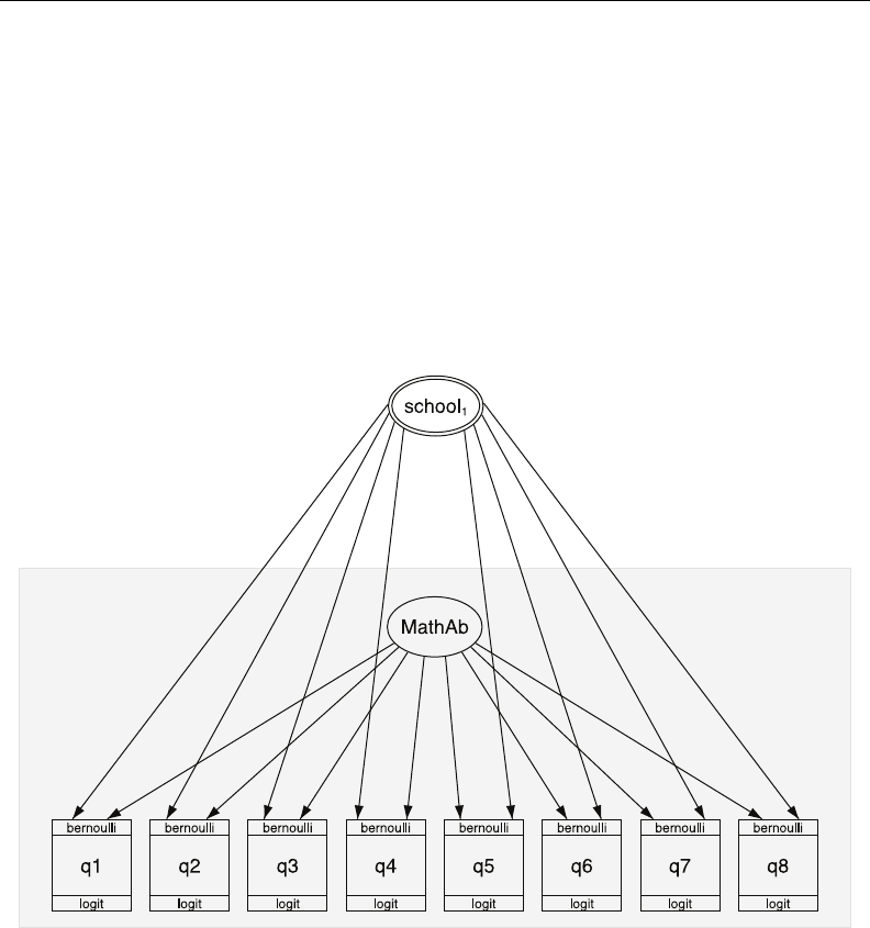
10 [ U ] 1 Read this—it will help
short. Generalized SEMs allow for generalized linear response functions and allow for multilevel
mixed effects.
Generalized linear response functions include binary outcomes (probit, logit, cloglog), count
outcomes (Poisson, negative binomial), categorical outcomes (multinomial logit), ordered outcomes
(ordered probit, ordered logit, ordered cloglog), and more, which is to say, generalized linear models
(GLMs).
Multilevel mixed effects include nested random effects such as effects within patient within doctor
within hospital and crossed random effects. Multilevel mixed effects also include random intercepts
and random slopes.
In the language of SEM, “multilevel mixed effects” means latent variables at different levels of the
data. This means Stata 13 can fit multilevel measurement models and multilevel structural equation
models.
See [SEM]intro 1.
Economists: See [SEM]example 45g, where we show how to use Stata 13’s new SEM features
to fit the Heckman selection model, which can be extended to generalized linear outcomes and
random effects and random slopes.
4. New multilevel mixed-effects models.
Multilevel mixed-effects estimation has been improved and expanded and is now the subject of its
own manual. Stata had 3 multilevel estimation commands; now it has 11.

[ U ] 1 Read this—it will help 11
The eight new multilevel mixed-effects estimation commands are
melogit logistic regression
meprobit probit regression
mecloglog complementary log-log regression
meologit ordered logistic regression
meoprobit ordered probit regression
mepoisson Poisson regression
menbreg negative binomial regression
meglm generalized linear models
These new estimation commands allow for constraints on variance components, provide robust and
cluster–robust standard errors, and are fast.
The three existing multilevel estimation commands have been renamed: xtmixed is now mixed,
xtmelogit is now meqrlogit, and xtmepoisson is now meqrpoisson. All three now present
results by default in the variance metric rather than the standard deviation metric.
As we said, multilevel mixed-effects modeling is now the subject of its own manual. See Stata
Multilevel Mixed-Effects Reference Manual, and in particular, see [ME]me.
5. Forecasts based on systems of equations.
Stata’s new forecast command allows you to combine estimation results from multiple Stata
commands or other sources to produce dynamic or static forecasts and produce forecast intervals.
You begin by fitting the equations of your model using Stata’s estimation commands, or you
can enter results that you obtained elsewhere. Then you use forecast to specify identities and
exogenous variables to obtain a baseline forecast. Once you produce the baseline forecast, you
can specify alternative paths for some variables and obtain forecasts based on those alternative
paths. Thus you can produce forecasts under alternative scenarios and explore impacts of differing
policies.
You can use forecast, for example, to produce macroeconomic forecasts.
40 50 60 70 80 90
1920 1925 1930 1935 1940
year
Total Income
40 50 60 70
1920 1925 1930 1935 1940
year
Consumption
−5 0 5
1920 1925 1930 1935 1940
year
Investment
20 30 40 50 60
1920 1925 1930 1935 1940
year
Private Wages
Solid lines denote actual values.
Dashed lines denote forecast values.
Dynamic Forecasts
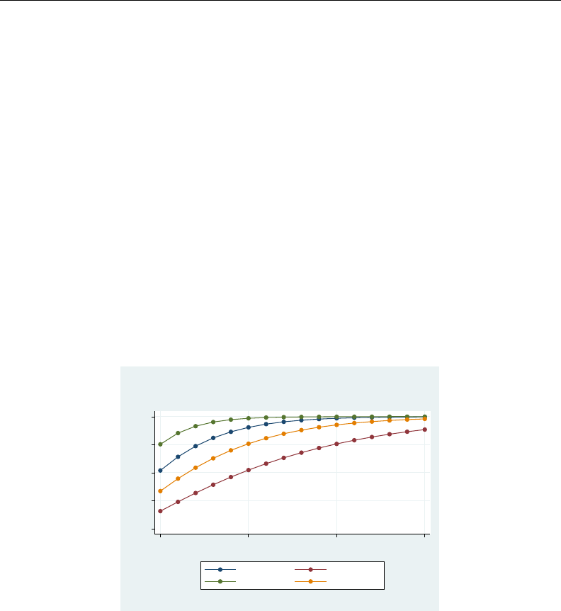
12 [ U ] 1 Read this—it will help
In addition, forecast is particularly easy to use because forecast also provides an intuitive,
interactive control panel to guide you and, if you do something wrong, forecast itself offers
advice on how to fix the problem.
See [TS]forecast.
6. Power and sample size.
The new power command performs power and sample-size analysis. Included are
Comparison of a mean to a reference value
Comparison of a proportion to a reference value
Comparison of a variance to a reference value
Comparison of a correlation to a reference value
Comparison of two independent means
Comparison of two independent proportions
Comparison of two independent variances
Comparison of two independent correlations
Comparison of two paired means
Comparison of two paired proportions
Results can be displayed in customizable tables and graphs.
.2
.4
.6
.8
1
Power (1−β)
10 20 30 40
Sample size (N)
µa=.8, σ=1 µa=.8, σ=1.5
µa=1, σ=1 µa=1, σ=1.5
Parameters: α = .05, µ0 = 0
t test
H0: µ = µ0 versus Ha: µ != µ0
Estimated power
An integrated GUI lets you select your analysis type, input assumptions, and obtain desired results.
Power and sample size is the subject of its own manual. See Stata Power and Sample-Size Reference
Manual; start by seeing [PSS]intro.

[ U ] 1 Read this—it will help 13
7. New and extended panel-data estimators.
Two new random-effects panel-data estimation commands are added:
xtoprobit ordered probit regression
xtologit ordered logistic regression
These new commands allow for cluster–robust standard errors.
The following previously existing random-effects panel-data estimation commands now allow for
cluster–robust standard errors:
xtprobit probit regression
xtlogit logistic regression
xtcloglog complementary log-log regression
xtpoisson Poisson regression
See [XT]xt for a complete list of all of Stata’s panel-data estimators.
8. New commands are provided for calculating effect sizes after estimation in the way behavioral
scientists, and especially psychologists, want to see them. Cohen’s d, Hedges’s g, Glass’s ∆,η2,
and ω2, with confidence intervals, are now provided:
a. New commands esize and esizei calculate effect sizes comparing the difference between
the means of a continuous variable for two groups. See [R]esize.
b. New postestimation command estat esize computes effect sizes for linear models after anova
and regress. See [R]regress postestimation.
9. Project Manager.
The new Project Manager lets you organize your analysis files—your do-files, ado-files, datasets,
raw files, etc. You can have multiple projects, and each can contain hundreds of files, or just a
few.
You can see all the files in a project at a glance, filter on filenames, and click to open, edit, or run.
Projects are portable, meaning that you can pick the whole collection up at once and move it
across computers or share it with colleagues.
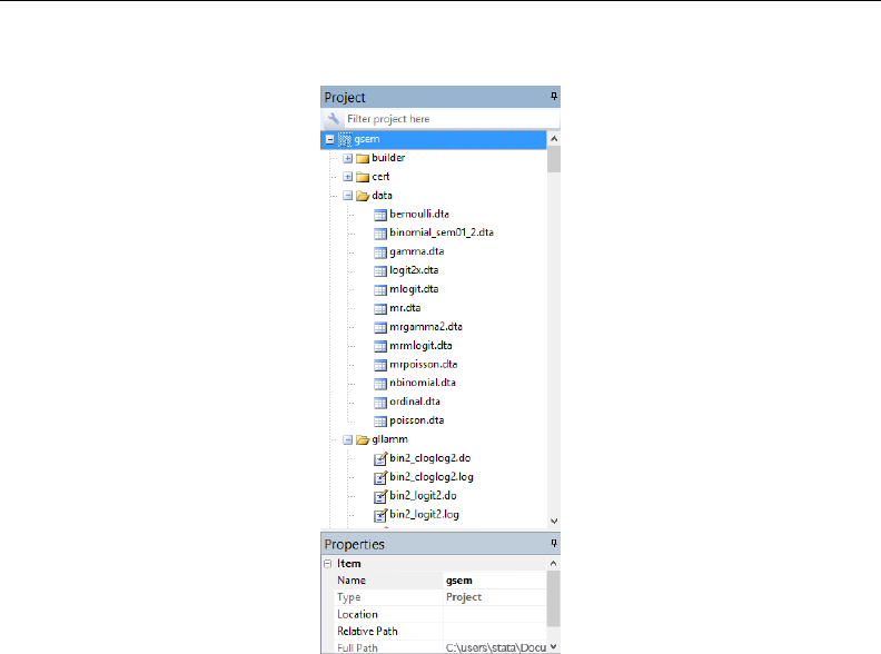
14 [ U ] 1 Read this—it will help
Take a look:
Try it. Get started from the Do-file Editor by selecting File >New >Project . . .
See [P]Project Manager.
10. Java plugins.
You can now call Java methods directly from Stata. You can take advantage of the plethora of
existing Java libraries or write your own Java code. You call Java using Stata’s new javacall
command. See [P]java and see the Java-Stata API specification at http://www.stata.com/java/api/.
Java recently encountered some negative publicity regarding security concerns. That publicity was
about Java and web browsers automatically loading and running Java code from untrusted websites.
It does not apply to Stata’s implementation of Java. Stata’s implementation is about running Java
code already installed on your computer from known and trusted sources.
1.3.2 What’s new that you will want to know
11. You can clear the Results window.
Use the new cls command. See [R]cls.
12. Value labels of factor variables used to label output.
You use variable i.sex, and output now shows male and female in your model rather than 0
and 1if variable sex has a value label. You can control how output looks. See more details below
in [U] 1.3.3 What’s new in statistics (general).

[ U ] 1 Read this—it will help 15
13. Programmers can create Word and Excel files from Stata.
You can add paragraphs, insert images, insert tables, poke into individual cells, and more.
See [M-5]docx*( ) to create Word documents.
See [P]putexcel and [M-5]xl( ) to interact with Excel files.
By the way, Stata could already import and export Excel files; see [D]import excel.
14. Searching is better.
Here’s why:
a. Help >Search... and the search command now default to searching the Internet as well as
Stata’s local keyword database. If you do not want that, type set searchdefault local,
permanently to set Stata 13 to the old default.
b. search without options now displays its results in the Viewer rather than in the Results window.
(If any options are specified, however, results appear in the Results window.)
c. Existing command findit is no longer documented but continues to work. Changes to search
make search into the equivalent of findit.
See [R]search.
15. help now searches when no help is found.
help xyz now invokes search xyz if xyz is not found. See [R]help.
16. Stata now supports secure HTTP (HTTPS) and FTP. You can, for instance, use datasets from sites
using either of the protocols. See [U] 3.6 Updating and adding features from the web.
17. Concerning the Data Editor,
a. noncontiguous column selections are now allowed.
b. encode,decode,destring, and tostring have been added as operations that can be performed
on selected variables.
c. the Delete key can now be used to drop data.
See [GS]6 Using the Data Editor (GSM,GSU, or GSW).
18. Concerning the Do-file Editor,
a. matching braces are highlighted.
b. an adjustable column guide has been added.
c. you can now zoom in and out.
d. you can convert between the different types of end-of-line characters used by Windows and by
Mac and Unix.
See [GS]13 Using the Do-file Editor (GSM,GSU, or GSW).
19. Concerning Stata’s GUI,
a. the Properties window now displays the sorted-by variables.
b. the Jump To menu in the Viewer now allows you to jump to the top of the page.
c. Stata for Windows now supports Windows high-contrast themes.
20. .dta file format has changed.
The file format has changed because of the new strL variables. Stata 13 can, of course, read
old-format datasets. If you need to create datasets in the previous format—used by Stata 11 and
Stata 12—use the saveold command. See [D]save. If you want to know the details of the new
.dta format, type help dta.

16 [ U ] 1 Read this—it will help
21. Official directory ado/updates no longer used.
Official ado-file updates are no longer stored in directory installation-directory/ado/updates/.
Updates are now applied to ado/base directly. Modern operating systems do not approve of
applications such as Stata having multiple files of the same name. The updates process remains
the same.
22. Videos.
Type help videos to list and link to the videos on Stata’s YouTube channel. We provide dozens
of tutorials on Stata’s features.
23. Fast PDF-manual navigation.
There are now links at the top of each manual entry to jump directly to section headings, and on
each page’s header, there is a link to take you to the beginning of the entry.
If you did not know already, clicking on the blue manual reference in the title of a help file jumps
to the PDF documentation.
24. Manuals have color graphs.
If you want to use the same color graph scheme we use in the manuals, type set scheme
s2gcolor. See [G-4]scheme s2.
25. Ten new vignettes.
Scientific history buffs will want to read about the following:
a. Florence Nightingale
b. Florence Nightingale David, a different person from Florence Nightingale
c. Charles William Dunnett
d. Andrew Charles Harvey
e. William Lee Hays
f. Fred Nichols Kerlinger
g. Janet Elizabeth Lane-Claypon
h. martingale
i. Elizabeth L. “Betty” Scott
j. John Snow
The following two items were added during the Stata 12 release:
26. New command icc computes intraclass correlation coefficients for one-way random-effects models,
two-way random-effects models, and two-way mixed-effects models for both individual and average
measurements. Intraclass correlations measure consistency of agreement or absolute agreement.
See [R]icc.
27. New postestimation command estat icc computes intraclass correlations at each nesting level
for nested random-effects models fit by mixed and melogit. See [ME]mixed postestimation and
[ME]melogit postestimation.

[ U ] 1 Read this—it will help 17
1.3.3 What’s new in statistics (general)
Already mentioned as highlights of the release were treatment effects,generalized SEMs,multilevel
mixed-effects models,power and sample size, and panel-data estimators. The following are also new:
28. Concerning sample-selection estimation commands,
a. new estimation command heckoprobit fits the parameters of an ordered probit model with
sample selection. See [R]heckoprobit.
b. existing estimation command heckprob is renamed heckprobit. See [R]heckprobit.
29. Existing estimation command hetprob is renamed hetprobit. See [R]hetprobit.
30. New estimation command ivpoisson fits the parameters of a Poisson regression model with
endogenous regressors. Estimates can be obtained using the GMM or control-function estimators.
See [R]ivpoisson.
31. New command mlexp allows you to specify maximum likelihood models without writing an
evaluator program. You can instead specify an expression representing the log-likelihood function
in much the same way you would with nl,nlsur, or gmm. See [R]mlexp.
32. Concerning fractional polynomials,
a. new prefix command fp: replaces fracpoly for fitting models with fractional polynomial
regressors. You type
. fp ...: estimation command
Results are the same. The new fp command supports more estimation commands, it is easier to
use, and it is more flexible. You can substitute the same fractional polynomial into multiple places
of the estimation command, which is especially useful in multiple-equation models. You may now
use factor-variable notation in the estimation command.
b. fp generate replaces fracgen.
c. fp plot replaces fracplot.
d. fp predict replaces fracpred.
e. commands fracpoly and fracgen are no longer documented but continue to work. Commands
fracplot and fracpred are still documented for use after mfp.
See [R]fp.
33. Concerning quantile-regression estimation commands,
a. existing estimation command qreg now accepts option vce(robust).
b. existing estimation commands qreg,iqreg,sqreg, and bsqreg now allow factor variables
to be used.
See [R]qreg.
34. Syntax and methodology for predict after boxcox have changed. Predicted values are now
calculated using Duan’s smearing method by default. The previous back-transformed predicted-
values estimates are provided if predict’s btransform option is specified and under version
control. See [R]boxcox postestimation.
35. Value labels of factor variables are now used by default to label estimation output. The numeric
values (levels) were previously used and continue to be used if the factor variables are unlabeled.
There are three new display options that may be used with estimation commands affecting how
this works:

18 [ U ] 1 Read this—it will help
a. Option nofvlabel displays factor-variable level values, just as Stata 12 did previously. (You
can set fvlabel off to make nofvlabel the default.)
b. Option fvwrap(#)specifies the number of lines to allow when long value labels must be
wrapped. Labels requiring more than #lines are truncated. fvwrap(1) is the default. You can
change the default by using set fvwrap #.
c. Option fvwrapon() specifies whether value labels that wrap will break at word boundaries.
fvwrapon(word) is the default, meaning to break at word boundaries.
fvwrapon(width) specifies that line breaks may occur arbitrarily so as to maximize use of
available space.
You can change the defaults by using set fvwrapon width or set fvwrapon word.
Current default settings are shown by query and also stored in c(fvlabel),c(fvwrap), and
c(fvwrapon).
See [R]set showbaselevels and [P]creturn.
36. Existing estimation command proportion now uses the logit transform when computing the limits
of the confidence interval. The original behavior of using the normal approximation is preserved
under version control or when the new citype(normal) option is specified. See [R]proportion.
37. Concerning existing command margins,
a. option at() has new suboption generate(), which allows you to specify an expression to
replace the values for any continuous variable in the model. For example, you can compute the
predictive margins at x+1 by typing
. margins, at(x = generate(x+1))
at(generate()) can be combined with contrasts to estimate the effect of giving each subject
an additional amount of x,
. margins, at((asobserved) _all) at(x= generate(x+1)) contrast(at(r._at))
See Estimating treatment effects with margins in [R]margins, contrast.
b. margins automatically uses the tdistribution for computing p-values and confidence intervals
when appropriate, which is after linear regression and ANOVA and whenever degrees of freedom
are posted to e(df r).
The previous default behavior of always using the standard normal distribution for all p-values
and confidence intervals is preserved under version control.
c. new option df(#)specifies that margins is to use the tdistribution when it otherwise would
not.
See [R]margins.
38. nlcom and predictnl now use the standard normal distribution for computing p-values and
confidence intervals. Original behavior was to compute the p-values and CIs based on the t
distribution in some cases. Original behavior is preserved under version control. In addition, if you
want p-values and confidence intervals calculated using the tdistribution, use new option df(#)
to specify the degrees of freedom.
testnl’s calculated test statistic is now χ2rather than Funless you specify the df() option.
See [R]nlcom,[R]predictnl, and [R]testnl.

[ U ] 1 Read this—it will help 19
39. contrast,pwcompare, and lincom have new option df(#)to use the tdistribution in computing
p-values and confidence intervals. For contrast, this option also causes the Wald table to use
the Fdistribution.
See [R]contrast,[R]pwcompare, and [R]lincom.
40. estimates table’s option label is renamed varlabel. Original option label is allowed under
version control. See [R]estimates table.
41. The previously existing sampsi command is no longer documented because it is replaced by the
new power command—a highlight of the release. See [PSS]power.
42. Existing functions normalden(x,µ,σ)and lnnormalden(x,µ,σ)now allow you to omit
argument µor arguments µand σ.µ=0 and σ=1 is assumed. See help normalden(),help
lnnormalden(), and [D]functions.
43. The following new functions are added:
t(df,t)cumulative Student’s tdistribution
invt(df,p)inverse cumulative Student’s tdistribution
ntden(df,np,t)density of noncentral Student’s tdistribution
nt(df,np,t)cumulative noncentral Student’s tdistribution
npnt(df,t,p)noncentrality parameter of noncentral Student’s tdistribution
nttail(df,np,t)right-tailed noncentral Student’s tdistribution
invnttail(df,np,p)inverse of right-tailed noncentral Student’s tdistribution
nF(df1,df2,np,f)cumulative noncentral Fdistribution
npnF(df1,df2,f,p)noncentrality parameter of noncentral Fdistribution
chi2den(df,x)density of χ2distribution
fileread(f)return the contents of a file as a string
filewrite(f,s,r)create or overwrite file with the contents of a string
fileexists(f)check whether a file exists
filereaderror(s)use results returned by fileread() to determine whether an
I/O error occurred
See help functionname() and [D]functions.
1.3.4 What’s new in statistics (SEM)
We have already mentioned a highlight of the release, the new gsem command, for fitting generalized
SEMs. The following are also new:
44. Existing estimation command sem has new option noestimate, which is useful when you are
having convergence problems; you can use it to get the starting values into a Stata matrix (vector)
that you can then modify to use as alternative starting values. See [SEM]intro 12.
45. sem now supports time-series operators on all observed variables. See [SEM]sem.
46. You can now use postestimation command margins after sem. See [SEM]intro 7.
47. sem no longer reports in the estimation output any zero-valued constraints on covariances between
exogenous variables; absence of the covariance indicates the presence of the constraint. Original
behavior is preserved under version control.

20 [ U ] 1 Read this—it will help
48. The new options for controlling display of factor variables with value labels mentioned in [U] 1.3.3
What’s new in statistics (general)—nofvlabel,fvwrap(#), and fvwrapon(word |width)—
work with varname of sem, group(varname).sem itself does not allow factor variables, but the
factor-variable display options nonetheless work with group(varname).
Thus old options wrap() and nolabel are now officially fvwrap() and fvnolabel, although
the old option names continue to work as synonyms. See [SEM]sem reporting options.
49. We now show how to construct path diagrams at the end of each estimation example in the manual.
See [SEM]example 1,[SEM]example 3,. . . .
1.3.5 What’s new in statistics (time series)
We have already mentioned a highlight of the release, the new forecast command. The following
are also new:
50. New command import haver (available with Stata for Windows only) replaces old command
haver.import haver imports economic and financial data from Haver Analytics databases. See
[D]import haver.
51. Existing command tsreport now provides better information about gaps in time-series and panel
datasets, including the length of each gap.
In addition, tsreport will provide information about missing values in variables even where there
are no gaps.
See [TS]tsreport.
Also see item 55 in [U] 1.3.8 What’s new in data management for information on the new
command bcal create.
1.3.6 What’s new in statistics (longitudinal/panel data)
We have already mentioned a highlight of the release, new and extended panel-data estimators.
1.3.7 What’s new in statistics (survival analysis)
52. Shared frailty survival models can no longer be fit when there is delayed entry or there are gaps in
time under observation. Said differently, stcox and streg no longer allow option shared() when
there are delayed entry or gaps. The use of shared frailty models to fit truncated survival data leads to
inconsistent results unless the frailty distribution is independent of the covariates and the truncation
point, which rarely happens in practice. If you have such data and can make the independence
assumption—which is unlikely—estimation can be forced by specifying undocumented option
forceshared. See [ST]stcox and [ST]streg. See help st forceshared for information on the
forceshared option.
53. Output produced by existing commands stset,streset, and cttost more accurately labels
time at risk. What was labeled “total time at risk” is now labeled “total time at risk and under
observation”. See [ST]stset and [ST]cttost.
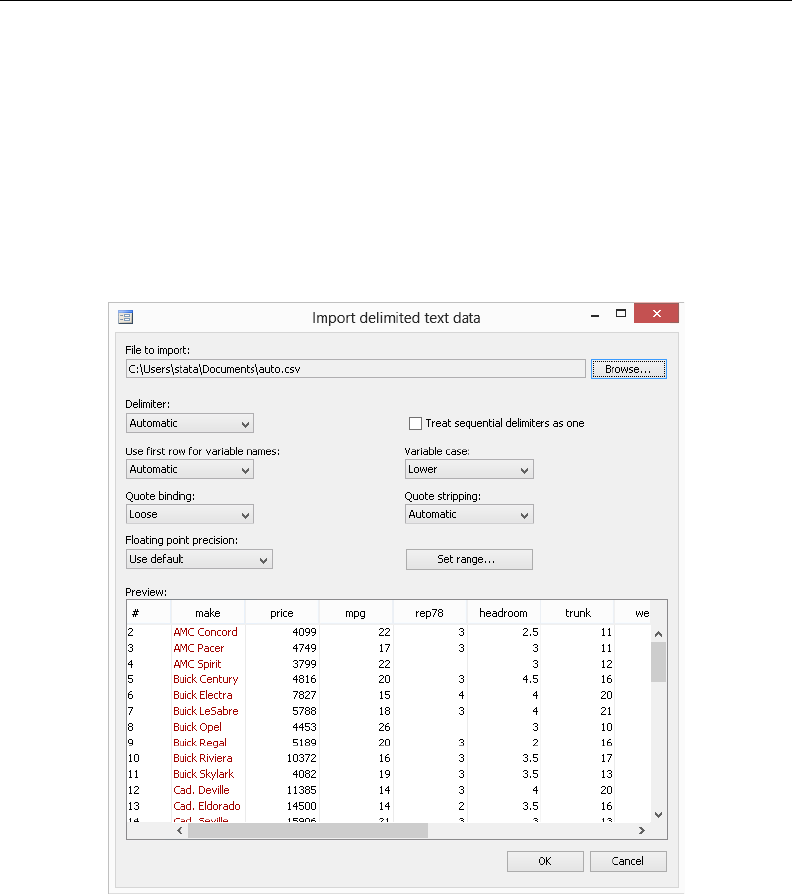
[ U ] 1 Read this—it will help 21
1.3.8 What’s new in data management
We have already mentioned a highlight of the release, long strings/BLOBs.
54. New commands import delimited and export delimited supersede old commands insheet
and outsheet. This is not just a renaming.
import delimited supports several different quoting methods. Some packages, for instance, use
"" in the middle of a string to represent an embedded double quote. Others do not.
import delimited now allows column and row ranges (subsets).
Use import delimited’s GUI to see a preview of the data and how they will be read. You can
also customize the GUI.
Of course, import delimited and export delimited support Stata 13’s new strLs.
See [D]import delimited.
55. existing command bcal has new subcommand create to create a business calendar from the
current dataset automatically. bcal create infers business holidays and closures from gaps in the
data. See [D]bcal.
56. String expressions now support string duplication via multiplication. For example, 3*"abc" eval-
uates to "abcabcabc". See help strdup() or [D]functions.

22 [ U ] 1 Read this—it will help
57. Concerning long strings, that is, strLs,
a. existing command compress has new option nocoalesce in support of the new strL string
storage type. By default, compress coalesces the storage used to store duplicated strL values.
nocoalesce prevents this.
In addition, compress always considers demoting strL variables to str#variables if that
would save memory.
See [D]compress.
b. the output of existing command memory has changed to include information on new string
storage type strL. See [D]memory.
c. the options of existing command ds, such as has() and not(), now understand string to
mean both strL and str#,strL to mean strL, and str# to mean str1,str2,. . . ,str2045.
See [D]ds.
d. existing command type has new option lines(#)to list the first #lines of the file. See
[D]type.
Also see item 50 in [U] 1.3.5 What’s new in statistics (time series) for information on the new
command import haver.
1.3.9 What’s new in Mata
58. Programmers can create Word and Excel files from Stata.
You can add paragraphs, insert images, insert tables, poke into individual cells, and more.
See [M-5]docx*( ) to create Word documents.
See [P]putexcel and [M-5]xl( ) to interact with Excel files.
By the way, Stata could already import and export Excel files; see [D]import excel.
59. New functions in solvenl() allow you to solve arbitrary systems of nonlinear equations. Gauss–
Seidel, damped Gauss–Seidel, Broyden–Powell, and Newton–Raphson techniques are provided.
See [M-5]solvenl( ).
60. The same statistical functions added to Stata have been added to Mata, namely,
Noncentral Student’s t
p=nt(df,np,t)
d=ntden(df,np,t)
q=nttail(df,np,t)
t=invnttail(df,np,q)
np =npnt(df,t,p)
Student’s t
p=t(df,t)
t=invt(df,p)
Noncentral F
p=nF(df1,df2,np,f)
np =npnF(df1,df2,f,p)
χ2
d=chi2den(df,x)
See [M-5]normal( ).

[ U ] 1 Read this—it will help 23
61. New function selectindex() returns a vector of indices for which v[j]6=0. For instance,
if v= (6,0,7,0,8), then selectindex(v)= (1,3,5).selectindex() is useful with logical
expressions, such as x[selectindex(x:>1000)]. See [M-5]select( ).
1.3.10 What’s new in programming
We have already mentioned the Project Manager and Java plugins as highlights of the release. The
following are also new:
62. New command putexcel writes Stata expressions, matrices, and stored results to an Excel file.
Excel 1997/2003 (.xls) files and Excel 2007/2010 (.xlsx) files are supported. See [P]putexcel.
Mata programmers will also be interested in [M-5]xl( ), a class to interact with Excel files.
63. A new set of Mata functions provide the ability to create Word documents. See [M-5]docx*( ).
64. Concerning strLs,
a. strL is now a reserved word.
b. the maximum length of a string in string expressions increases from 244 to 2-billion characters.
See [R]limits.
c. new c(maxstrlvarlen) returns the maximum possible length for strL variables.
d. confirm . . . variable now understands str#to mean any str1,str2,. . . ,str2045
variable; strL to mean strL; and string to mean str#or strL. See [P]confirm.
e. new function fileread(filename ,startpos ,length )returns the contents of filename.
See help fileread() and [D]functions.
f. new function filewrite(filename,s, 1|2 )writes sto the specified filename, optionally
overwriting 1or appending 2. See help filewrite() and [D]functions.
g. new function fileexists(filename)returns 1if the specified filename exists, and returns 0
otherwise.
h. new function filereaderror(s)returns 0or a positive integer, said value having the inter-
pretation of a return code. It is used like this
. generate strL s= fileread(filename) if fileexists(filename)
. assert filereaderror(s)==0
or this
. generate strL s= fileread(filename) if fileexists(filename)
. generate rc = filereaderror(s)
That is, filereaderror(s)is used on the result returned by fileread(filename)to determine
whether an I/O error occurred.
In the example, we only fileread() files that fileexist(). That is not required. If the file
does not exist, that will be detected by filereaderror() as an error. The way we showed
the example, we did not want to read missing files as errors. If we wanted to treat missing files
as errors, we would have coded
. generate strL s= fileread(filename)
. assert filereaderror(s)==0

24 [ U ] 1 Read this—it will help
or
. generate strL s= fileread(filename)
. generate rc = filereaderror(s)
65. New command expr query exp returns in r() the variables used in expression exp. See help
undocumented and see help expr query.
66. The maximum number of elements in a numlist increases from 1,600 to 2,500. See [U] 11.1.8 num-
list.
67. Existing command ereturn post now allows posting of noninteger as well as integer dof()
values.
68. New c(hostname) returns the computer’s hostname. See [P]creturn.
69. New c(maxvlabellen) returns the maximum possible length for a value label.
1.3.11 What’s new, Mac only
In addition to all the above What’s New items, which apply to all platforms, Stata for Mac has
several of its own new features:
70. The Do-file Editor in Stata for Mac has been completely rewritten. It now includes
•code folding
•more robust syntax highlighting that is consistent with highlighting in Windows and Unix
•more color options for customizing its appearance
•the ability to save the syntax-highlighting colors as separate themes
•line ending preservation and normalization, which is useful for working in a mixed platform
environment where do-files are exchanged between Windows and Macs
•text-size zooming without having to change the font or font size
•more drag-and-drop options
•more control over the appearance of printed files
71. The Command window now has the same syntax highlighting as the Do-file Editor.
72. There is a new path control that not only shows the current working directory but also can change
the current working directory and open Stata files without having to use the Open dialog.
73. Mac OS X 10.7 GUI enhancements such as full-screen support and textured backgrounds for
spring-back scrolling are now supported.
74. There is a new interface for saving and managing saved preferences.
75. Applescript is better supported and enables users to directly access Stata macros, scalars, stored
results, and datasets.
76. Stata for Mac is now 64-bit only and allows the application’s file size to be roughly 67% smaller.

[ U ] 1 Read this—it will help 25
1.3.12 What’s more
We have not listed all the changes, but we have listed the important ones.
Stata is continually being updated. Those between-release updates are available for free over the
Internet.
Type update query and follow the instructions.
We hope that you enjoy Stata 13.
1.4 References
Chambers, J. M., W. S. Cleveland, B. Kleiner, and P. A. Tukey. 1983. Graphical Methods for Data Analysis. Belmont,
CA: Wadsworth.
Everitt, B. S., and A. Skrondal. 2010. The Cambridge Dictionary of Statistics. 4th ed. Cambridge: Cambridge
University Press.
Heyde, C. C., and E. Seneta, ed. 2001. Statisticians of the Centuries. New York: Springer.
Johnson, N. L., and S. Kotz, ed. 1997. Leading Personalities in Statistical Sciences: From the Seventeenth Century
to the Present. New York: Wiley.
Upton, G. J. G., and I. T. Cook. 2014. A Dictionary of Statistics. 3rd ed. Oxford: Oxford University Press.

2A brief description of Stata
Stata is a statistical package for managing, analyzing, and graphing data.
Stata is available for a variety of platforms. Stata may be used either as a point-and-click application
or as a command-driven package.
Stata’s GUI provides an easy interface for those new to Stata and for experienced Stata users who
wish to execute a command that they seldom use.
The command language provides a fast way to communicate with Stata and to communicate more
complex ideas.
Here is an extract of a Stata session using the GUI:
(Throughout the Stata manuals, we will refer to various datasets. These datasets are all available from
http://www.stata-press.com/data/r13/. For easy access to them within Stata, type webuse dataset name,
or select File > Example Datasets... and click on Stata 13 manual datasets.)
. webuse lbw
(Hosmer & Lemeshow data)
We select Data > Describe data > Summary statistics and choose to summarize variables low,
age, and smoke, whose names we obtained from the Variables window. We click on OK.
27
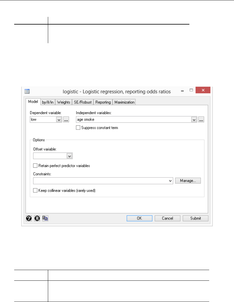
28 [ U ] 2 A brief description of Stata
. summarize low age smoke
Variable Obs Mean Std. Dev. Min Max
low 189 .3121693 .4646093 0 1
age 189 23.2381 5.298678 14 45
smoke 189 .3915344 .4893898 0 1
Stata shows us the command that we could have typed in command mode—summarize low age
smoke—before displaying the results of our request.
Next we fit a logistic regression model of low on age and smoke. We select Statistics > Binary
outcomes > Logistic regression (reporting odds ratios), fill in the fields, and click on OK.
. logistic low age smoke
Logistic regression Number of obs = 189
LR chi2(2) = 7.40
Prob > chi2 = 0.0248
Log likelihood = -113.63815 Pseudo R2 = 0.0315
low Odds Ratio Std. Err. z P>|z| [95% Conf. Interval]
age .9514394 .0304194 -1.56 0.119 .8936482 1.012968
smoke 1.997405 .642777 2.15 0.032 1.063027 3.753081
_cons 1.062798 .8048781 0.08 0.936 .2408901 4.689025
Here is an extract of a Stata session using the command language:
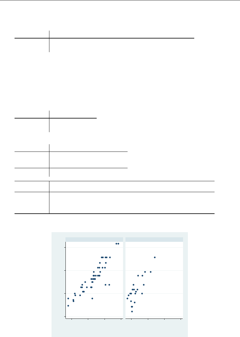
[ U ] 2 A brief description of Stata 29
. use http://www.stata-press.com/data/r13/auto
(1978 Automobile Data)
. summarize mpg weight
Variable Obs Mean Std. Dev. Min Max
mpg 74 21.2973 5.785503 12 41
weight 74 3019.459 777.1936 1760 4840
The user typed summarize mpg weight and Stata responded with a table of summary statistics.
Other commands would produce different results:
. generate gp100m = 100/mpg
. label var gp100m "Gallons per 100 miles"
. format gp100m %5.2f
. correlate gp100m weight
(obs=74)
gp100m weight
gp100m 1.0000
weight 0.8544 1.0000
. regress gp100m weight gear_ratio
Source SS df MS Number of obs = 74
F( 2, 71) = 96.65
Model 87.4543721 2 43.7271861 Prob > F = 0.0000
Residual 32.1218886 71 .452420967 R-squared = 0.7314
Adj R-squared = 0.7238
Total 119.576261 73 1.63803097 Root MSE = .67262
gp100m Coef. Std. Err. t P>|t| [95% Conf. Interval]
weight .0014769 .0001556 9.49 0.000 .0011665 .0017872
gear_ratio .1566091 .2651131 0.59 0.557 -.3720115 .6852297
_cons .0878243 1.198434 0.07 0.942 -2.301786 2.477435
. scatter gp100m weight, by(foreign)
2.00 4.00 6.00 8.00
2,000 3,000 4,000 5,000 2,000 3,000 4,000 5,000
Domestic Foreign
Gallons per 100 miles
Weight (lbs.)
Graphs by Car type
The user-interface model is type a little, get a little, etc., so that the user is always in control.

30 [ U ] 2 A brief description of Stata
Stata’s model for a dataset is that of a table—the rows are the observations and the columns are
the variables:
. list mpg weight gp100m in 1/10
mpg weight gp100m
1. 22 2,930 4.55
2. 17 3,350 5.88
3. 22 2,640 4.55
4. 20 3,250 5.00
5. 15 4,080 6.67
6. 18 3,670 5.56
7. 26 2,230 3.85
8. 20 3,280 5.00
9. 16 3,880 6.25
10. 19 3,400 5.26
Observations are numbered; variables are named.
Stata is fast. That speed is due partly to careful programming, and partly because Stata keeps the
data in memory. Stata’s file model is that of a word processor: a dataset may exist on disk, but the
dataset in memory is a copy. Datasets are loaded into memory, where they are worked on, analyzed,
changed, and then perhaps stored back on disk.
Working on a copy of the data in memory makes Stata safe for interactive use. The only way to
harm the permanent copy of your data on disk is if you explicitly save over it.
Having the data in memory means that the dataset size is limited by the amount of computer
memory. Stata stores the data in memory in an efficient format—you will be surprised how much
data can fit. Nevertheless, if you work with extremely large datasets, you may run into memory
constraints. You will want to learn how to store your data as efficiently as possible; see [D]compress.
2.1 Video example
Tour of the Stata 13 interface
3Resources for learning and using Stata
Contents
3.1 Overview .............................................................. 31
3.2 Stata on the Internet (www.stata.com and other resources) ...................... 32
3.2.1 The Stata website (www.stata.com) ................................. 32
3.2.2 The Stata YouTube Channel ....................................... 33
3.2.3 The Stata Blog—Not Elsewhere Classified ........................... 33
3.2.4 The Stata forum ................................................ 33
3.2.5 Stata on Twitter and Facebook .................................... 33
3.2.6 Other Internet resources on Stata ................................... 33
3.3 Stata Press ............................................................. 33
3.4 The Stata forum ........................................................ 34
3.5 The Stata Journal ....................................................... 34
3.6 Updating and adding features from the web .................................. 35
3.6.1 Official updates ................................................. 35
3.6.2 Unofficial updates ............................................... 35
3.7 Conferences and training ................................................. 36
3.7.1 Conferences and users group meetings .............................. 36
3.7.2 NetCourses .................................................... 36
3.7.3 Public training courses ........................................... 37
3.7.4 On-site training courses .......................................... 37
3.8 Books and other support materials ......................................... 38
3.8.1 For readers ..................................................... 38
3.8.2 For authors .................................................... 38
3.9 Technical support ....................................................... 38
3.9.1 Register your software ........................................... 38
3.9.2 Before contacting technical support ................................. 39
3.9.3 Technical support by email ....................................... 39
3.9.4 Technical support by phone or fax ................................. 39
3.9.5 Comments and suggestions for our technical staff ..................... 39
3.1 Overview
The Getting Started manual, User’s Guide, and Reference manuals are the primary tools for learning
about Stata; however, there are many other sources of information. A few are listed below.
•Stata itself. Stata has a search command that makes it easy search a topic to find and to
execute a Stata command. See [U] 4 Stata’s help and search facilities.
•The Stata website. Visit http://www.stata.com. Much of the site is dedicated to user support;
see [U] 3.2.1 The Stata website (www.stata.com).
•The Stata YouTube Channel. Visit http://www.youtube.com/user/statacorp. The site is regularly
updated with video demonstrations of Stata.
•The Stata Blog, Twitter, and Facebook. Visit http://blog.stata.com/,http://twitter.com/stata, and
http://facebook.com/statacorp. See [U] 3.2.3 The Stata Blog—Not Elsewhere Classified and
[U] 3.2.5 Stata on Twitter and Facebook.
31

32 [ U ] 3 Resources for learning and using Stata
•The Stata Press website. Visit http://www.stata-press.com. This site contains the datasets used
throughout the Stata manuals; see [U] 3.3 Stata Press.
•The Stata forum. An active group of Stata users communicate over an Internet forum; see
[U] 3.4 The Stata forum.
•The Stata Journal and the Stata Technical Bulletin. The Stata Journal contains reviewed papers,
regular columns, book reviews, and other material of interest to researchers applying statistics
in a variety of disciplines. The Stata Technical Bulletin, the predecessor to the Stata Journal,
contains articles and user-written commands. See [U] 3.5 The Stata Journal.
•The Stata software distribution site and other user-provided software distribution sites. Stata
itself can download and install updates and additions. We provide official updates to Stata—type
update query or select Help > Check for Updates. We also provide user-written additions to
Stata and links to other user-provided sites—type net or select Help > SJ and User-written
Programs; see [U] 3.6 Updating and adding features from the web.
•NetCourses. We offer training via the Internet. Details are in [U] 3.7.2 NetCourses.
•Public training courses. We offer in-depth training courses at third-party sites around the United
States. Details are in [U] 3.7.3 Public training courses.
•On-site training courses. We can come to your institution to provide customized training. Details
are in [U] 3.7.4 On-site training courses.
•Books and support materials. Supplementary Stata materials are available; see [U] 3.8 Books
and other support materials.
•Technical support. We provide technical support by email, telephone, and fax; see [U] 3.9 Tech-
nical support.
3.2 Stata on the Internet (www.stata.com and other resources)
3.2.1 The Stata website (www.stata.com)
Point your browser to http://www.stata.com and click on Support. More than half our website is
dedicated to providing support to users.
•The website provides answers to FAQs (frequently asked questions) on Windows, Mac, Unix,
statistics, programming, Internet capabilities, graphics, and data management. These FAQs run
the gamut from “I cannot save/open files” to “What does ‘completely determined’ mean in my
logistic regression output?” Most users will find something of interest.
•The website provides detailed information about NetCourses, along with the current schedule;
see [U] 3.7.2 NetCourses.
•The website provides information about Stata courses and meetings, both in the United States
and elsewhere. See [U] 3.7.1 Conferences and users group meetings,[U] 3.7.3 Public training
courses, and [U] 3.7.4 On-site training courses.
•The website provides an online bookstore for Stata-related books and other supplementary
materials; see [U] 3.8 Books and other support materials.
•The website provides links to information about statistics: other statistical software providers,
book publishers, statistical journals, statistical organizations, and statistical listservers.
•The website provides links to resources for learning Stata at
http://www.stata.com/links/resources.html. Be sure to look at these materials, as many outstand-
ing resources about Stata are listed here.

[ U ] 3 Resources for learning and using Stata 33
In short, the website provides up-to-date information on all support materials and, where possible,
provides the materials themselves. Visit http://www.stata.com if you can.
3.2.2 The Stata YouTube Channel
Visit Stata’s YouTube Channel at http://www.youtube.com/user/statacorp to view video demonstra-
tions on a wide variety of topics ranging from basic data management and graphics to more advanced
statistical analyses, such as ANOVA, regression, and SEM. New demonstrations are regularly added.
3.2.3 The Stata Blog—Not Elsewhere Classified
Stata’s official blog can be found at http://blog.stata.com/ and contains news and advice related
to the use of Stata. The articles appearing in the blog are individually signed and are written by the
same people who develop, support, and sell Stata.
The Stata Blog also has links to other blogs about Stata, written by Stata users around the world.
3.2.4 The Stata forum
Visit Statalist at http://www.statalist.org. Statalist is a forum dedicated to Stata where thousands
of Stata users talk about Stata and statistics. Register and participate, or simply lurk and read the
discussions.
3.2.5 Stata on Twitter and Facebook
StataCorp has an official presence on Twitter and Facebook. You can follow us on Twitter at
http://twitter.com/stata and find us on Facebook at http://facebook.com/statacorp. These are both good
ways to stay up-to-the-minute with the latest Stata information.
3.2.6 Other Internet resources on Stata
Many other people have published information on the Internet about Stata such as tutorials, examples,
and datasets. Visit http://www.stata.com/links/ to explore other Stata and statistics resources on the
Internet.
3.3 Stata Press
Stata Press is the publishing arm of StataCorp LP and publishes books, manuals, and journals
about Stata statistical software and about general statistics topics for professional researchers of all
disciplines.
Point your browser to http://www.stata-press.com. This site is devoted to the publications and
activities of Stata Press.
•Datasets that are used in the Stata Reference manuals and other books published by Stata
Press may be downloaded. Visit http://www.stata-press.com/data/. These datasets can be used
in Stata by simply typing use http://www.stata-press.com/data/r13/dataset name; for
example, type use http://www.stata-press.com/data/r13/auto. You could also type
webuse auto; see [D]webuse.

34 [ U ] 3 Resources for learning and using Stata
•An online catalog of all our books and multimedia products is at
http://www.stata-press.com/catalog.html. We have tried to include enough information, such as
table of contents and preface material, so that you may tell whether the book is appropriate for
you.
•Information about forthcoming publications is posted at
http://www.stata-press.com/forthcoming.html.
3.4 The Stata forum
The Stata forum (Statalist) is an Internet forum, where Stata users discuss Stata and statistics. It
is run and moderated by Stata users and maintained by StataCorp. Many knowledgeable users are
active on the forum, as are the StataCorp technical staff. Anyone may join, and instructions for doing
so can be found at http://www.statalist.org/.
You can browse Statalist without registering, but you need to register to participate in the discussion
or to ask a question.
Statalist has a long history of high-quality discussion dating back to 1994. New-to-Stata members
are welcome.
Before posting a question to Statalist, you will want to read the Statalist FAQ, which can be found
at http://www.statalist.org/forums/help/.
3.5 The Stata Journal
The Stata Journal (SJ) is a printed and electronic journal, published quarterly, containing articles
about statistics, data analysis, teaching methods, and effective use of Stata’s language. The Journal
publishes reviewed papers together with shorter notes and comments, regular columns, tips, book
reviews, and other material of interest to researchers applying statistics in a variety of disciplines.
The Journal is a publication for all Stata users, both novice and experienced, with different levels of
expertise in statistics, research design, data management, graphics, reporting of results, and in Stata,
in particular.
Tables of contents for past issues and abstracts of the articles are available at http://www.stata-
journal.com/archives.html.PDF copies of articles published at least three years ago are available for
free from the Stata Journal website.
We recommend that all users subscribe to the SJ. Visit http://www.stata-journal.com to learn more
about the Stata Journal and to order your subscription.
To obtain any programs associated with articles in the SJ, type
. net from http://www.stata-journal.com/software
or
•Select Help > SJ and User-written Programs
•Click on Stata Journal
The Stata Technical Bulletin
For 10 years, 1991–2001, the Stata Technical Bulletin (STB) served as the means of distributing
new commands and Stata upgrades, both user-written and “official”. After 10 years of continual
publication, the STB evolved into the Stata Journal. The Internet provided an alternative delivery
mechanism for user-written programs, so the emphasis shifted from user-written programs to more

[ U ] 3 Resources for learning and using Stata 35
expository articles. Although the STB is no longer published, many of the programs and articles that
appeared in it are still valuable today. PDF copies of all issues of the STB are available for free at
http://www.stata.com/bookstore/stbj.html. To obtain the programs that were published in the STB, type
. net from http://www.stata.com
. net cd stb
3.6 Updating and adding features from the web
Stata itself can open files on the Internet. Stata understands http, https, and ftp protocols.
First, try this:
. use http://www.stata.com/manual/oddeven, clear
That will load an uninteresting dataset into your computer from our website. If you have a home
page, you can use this feature to share datasets with coworkers. Save a dataset on your home page,
and researchers worldwide can use it. See [R]net.
3.6.1 Official updates
Although we follow no formal schedule for the release of updates, we typically provide updates
to Stata approximately once a month. Installing the updates is easy. Type
. update query
or select Help > Check for Updates. Do not be concerned; nothing will be installed unless and until
you say so. Once you have installed the update, you can type
. help whatsnew
or select Help > What’s New? to find out what has changed. We distribute official updates to fix
bugs and to add new features.
3.6.2 Unofficial updates
There are also “unofficial” updates—additions to Stata written by Stata users, which includes
members of the StataCorp technical staff. Stata is programmable, and even if you never write a Stata
program, you may find these additions useful, some of them spectacularly so. Start by typing
. net from http://www.stata.com
or select Help > SJ and User-written Programs.
Be sure to visit the Statistical Software Components (SSC) archive, which hosts a large collection
of free additions to Stata. The ssc command makes it easy for you to find, install, and uninstall
packages from the SSC archive. Type
. ssc whatsnew
to find out what’s new at the site. If you find something that interests you, type
. ssc describe pkgname
for more information. If you have already installed a package, you can check for and optionally install
updates by typing
. adoupdate pkgname

36 [ U ] 3 Resources for learning and using Stata
To check for and optionally install updates to all the packages you have previously installed, type
. adoupdate all
Periodically, you can type
. news
or select Help > News to display a short message from our website telling you what is newly available.
See [U] 28 Using the Internet to keep up to date.
3.7 Conferences and training
3.7.1 Conferences and users group meetings
StataCorp organizes the annual Stata Conference in the United States. Other conferences and users
group meetings are held in several countries around the world each year.
These meetings provide in-depth presentations from experienced Stata users and experts from
StataCorp. They also provide you with the opportunity to interact directly with the people who
develop Stata and to share your thoughts and ideas with them.
Visit http://www.stata.com/meeting/ for a list of upcoming conferences and meetings.
3.7.2 NetCourses
We offer courses on Stata at both introductory and advanced levels. Courses on software are
typically expensive and time consuming. They are expensive because, in addition to the direct costs
of the course, participants must travel to the course site. Courses over the Internet save everyone time
and money.
We offer courses over the Internet and call them Stata NetCoursesTM.
•What is a NetCourse?
A NetCourse is a course offered through the Stata website that varies in length from 7 to 8
weeks. Everyone with an email address and a web browser can participate.
•How does it work?
Every Friday a lecture is posted on a password-protected website. After reading the lecture
over the weekend or perhaps on Monday, participants then post questions and comments on a
message board. Course leaders typically respond to the questions and comments on the same
day they are posted. Other participants are encouraged to amplify or otherwise respond to the
questions or comments as well. The next lecture is then posted on Friday, and the process
repeats.
•How much of my time does it take?
It depends on the course, but the introductory courses are designed to take roughly 3 hours per
week.
•There are three of us here—can just one of us enroll and then redistribute the NetCourse
materials ourselves?
We ask that you not. NetCourses are priced to cover the substantial time input of the course
leaders. Moreover, enrollment is typically limited to prevent the discussion from becoming
unmanageable. The value of a NetCourse, just like a real course, is the interaction of the
participants, both with each other and with the course leaders.

[ U ] 3 Resources for learning and using Stata 37
•I’ve never taken a course by Internet before. I can see that it might work, but then again,
it might not. How do I know I will benefit?
All Stata NetCourses come with a 30-day satisfaction guarantee. The 30 days begins after the
conclusion of the final lecture.
You can learn more about the current NetCourse offerings by visiting http://www.stata.com/netcourse.
NetCourseNow
A NetCourseNow offers the same material as NetCourses but it allows you to choose the time
and pace of the course, and you have a personal NetCourse instructor.
•What is a NetCourseNow?
A NetCourseNow offers the same material as a NetCourse, but allows you to move at your own
pace and to specify a starting date. With a NetCourseNow, you also have the added benefit of
a personal NetCourse instructor whom you can email directly with questions about lectures and
exercises. You must have an email address and a web browser to participate.
•How does it work?
All course lectures and exercises are posted at once, and you are free to study at your own
pace. You will be provided with the email address of your personal NetCourse instructor to
contact when you have questions.
•How much of my time does it take?
A NetCourseNow allows you to set your own pace. How long the course takes and how much
time you spend per week is up to you.
3.7.3 Public training courses
Public training courses are intensive, in-depth courses taught by StataCorp at third-party sites
around the United States.
•How is a public training course taught?
These are interactive, hands-on sessions. Participants work along with the instructor so that
they can see firsthand how to use Stata. Questions are encouraged.
•Do I need my own computer?
Because the sessions are in computer labs running the latest version of Stata, there is no need
to bring your own computer. Of course, you may bring your own computer if you have a
registered copy of Stata you can use.
•Do I get any notes?
You get a complete set of notes for each class, which includes not only the materials from the
lessons but also all the output from the example commands.
See http://www.stata.com/training/public.html for all course offerings.
3.7.4 On-site training courses
On-site training courses are courses that are tailored to the needs of an institution. StataCorp
personnel can come to your site to teach what you need, whether it be to teach new users or to show
how to use a specialized tool in Stata.
•How is an on-site training course taught?
These are interactive, hands-on sessions, just like our public-training courses. You will need a
computer for each participant.

38 [ U ] 3 Resources for learning and using Stata
•What topics are available?
We offer training in anything and everything related to Stata. You work with us to put together
a curriculum that matches your needs.
•How does licensing work?
We will supply you with the licenses you need for the training session, whether the training
is in a lab or for individuals working on laptops. We will ship the licensing and installation
instructions so that you can have everything up and running before the session starts.
See http://www.stata.com/training/onsite.html for all the details.
3.8 Books and other support materials
3.8.1 For readers
There are books published about Stata, both by us and by others. Visit the Stata bookstore at
http://www.stata.com/bookstore/. For the books that we carry, we include the table of contents and
comments written by a member of our technical staff, explaining why we think this book might
interest you.
3.8.2 For authors
If you have written a book related to Stata and would like us to consider carrying it in our
bookstore, email bookstore@stata.com.
If you are writing a book, join our free Author Support Program. Stata professionals are available
to review your Stata code to ensure that it is efficient and reflects modern usage, production specialists
are available to help format Stata output, and editors and statisticians are available to ensure the
accuracy of Stata-related content. Visit http://www.stata.com/authorsupport/.
If you are thinking about writing a Stata-related book, consider publishing it with Stata Press.
Email submissions@statapress.com.
3.9 Technical support
We are committed to providing superior technical support for Stata software. To assist you as
efficiently as possible, please follow the procedures listed below.
3.9.1 Register your software
You must register your software to be eligible for technical support, updates, special offers, and
other benefits. By registering, you will receive the Stata News, and you may access our support staff
for free with any question that you encounter. You may register your software either electronically
or by mail.
Electronic registration: After installing Stata and successfully entering your License and Activation
Key, your default web browser will open to the online registration form at the Stata website. You
may also manually point your web browser to http://www.stata.com/register/ if you wish to register
your copy of Stata at a later time.
Mail-in registration: Fill in the registration card that came with Stata and mail it to StataCorp.

[ U ] 3 Resources for learning and using Stata 39
3.9.2 Before contacting technical support
Before you spend the time gathering the information our technical support department needs, make
sure that the answer does not already exist in the help files. You can use the help and search
commands to find all the entries in Stata that address a given subject. Be sure to try selecting
Help > Contents. Check the manual for a particular command. There are often examples that address
questions and concerns. Another good source of information is our website. You should keep a
bookmark to our frequently asked questions page (http://www.stata.com/support/faqs/) and check it
occasionally for new information.
If you do need to contact technical support, visit http://www.stata.com/support/tech-support/ for
more information.
3.9.3 Technical support by email
This is the preferred method of asking a technical support question. It has the following advantages:
•You will receive a prompt response from us saying that we have received your question and
that it has been forwarded to Technical Services to answer.
•We can route your question to a specialist for your particular question.
•Questions submitted via email may be answered after normal business hours, or even on
weekends or holidays. Although we cannot promise that this will happen, it may, and your
email inquiry is bound to receive a faster response than leaving a message on Stata’s voicemail.
•If you are receiving an error message or an unexpected result, it is easy to include a log file
that demonstrates the problem.
Please see visit http://www.stata.com/support/tech-support/ for information about contacting tech-
nical support.
3.9.4 Technical support by phone or fax
Our installation support telephone number is 979-696-4600. Please have your serial number handy.
It is also best if you are at your computer when you call. Telephone support is reserved for installation
questions. If your question does not involve installation, the question should be submitted via email
or fax.
Send fax requests to 979-696-4601. If possible, collect the relevant information in a log file and
include the file in your fax.
Please see visit http://www.stata.com/support/tech-support/ for information about contacting tech-
nical support.
3.9.5 Comments and suggestions for our technical staff
By all means, send in your comments and suggestions. Your input is what determines the changes
that occur in Stata between releases, so if we do not hear from you, we may not include your most
desired new feature! Email is preferred, as this provides us with a permanent copy of your request.
When requesting new features, please include any references that you would like us to review should
we develop those new features. Email your suggestions to service@stata.com.

4Stata’s help and search facilities
Contents
4.1 Introduction ............................................................ 41
4.2 Getting started .......................................................... 41
4.3 help: Stata’s help system ................................................. 42
4.4 Accessing PDF manuals from help entries ................................... 43
4.5 Searching .............................................................. 43
4.6 More on search ......................................................... 44
4.7 More on help ........................................................... 45
4.8 search: All the details .................................................... 45
4.8.1 How search works .............................................. 46
4.8.2 Author searches ................................................. 46
4.8.3 Entry ID searches ............................................... 47
4.8.4 FAQ searches ................................................... 47
4.8.5 Return codes ................................................... 48
4.9 net search: Searching net resources ......................................... 48
4.1 Introduction
To access Stata’s help, you will either
1. select Help from the menus, or
2. use the help and search commands.
Regardless of the method you use, results will be shown in the Viewer or Results windows. Blue
text indicates a hypertext link, so you can click to go to related entries.
4.2 Getting started
The first time you use help, try one of the following:
1. select Help > Advice from the menu bar, or
2. type help advice.
Either step will open the help advice help file within a Viewer window; it will be similar to the
following:
41

42 [ U ] 4 Stata’s help and search facilities
The advice file provides you with steps to search Stata to find information on topics and commands
that interest you. The steps show an example of finding all there is to know about “logistic regression”
within Stata.
4.3 help: Stata’s help system
When you
1. Select Help > Stata Command...
Type a command name in the Command edit field
Click on OK, or
2. Type help followed by a command name
you access Stata’s help files. These files provide shortened versions of what is in the printed manuals.
Let’s access the help file for Stata’s ttest command. Do one of the following:
1. Select Help > Stata Command...
Type ttest in the Command edit field
Click on OK, or
2. Type help ttest
Regardless of which you do, the result will be

[ U ] 4 Stata’s help and search facilities 43
The trick is in already knowing that Stata’s command for testing equality of means is ttest and
not, say, meanstest. The solution to that problem is searching.
4.4 Accessing PDF manuals from help entries
Every help file in Stata links to the equivalent manual entry. If you are reading help ttest,
simply click on [R] ttest in the Title section of the help file to go directly to the [R]ttest manual
entry.
We provide recommended settings for your PDF viewer to optimize it for Stata’s documentation at
http://www.stata.com/support/faqs/res/documentation.html.
4.5 Searching
If you do not know the name of the Stata command you are looking for, you can search for it by
keyword,
1. Select Help > Search...
Type keywords in the edit field
Click on OK
2. Type search followed by the keywords

44 [ U ] 4 Stata’s help and search facilities
search matches the keywords you specify to a database and returns matches found in Stata
commands, FAQs at www.stata.com, official blogs, and articles that have appeared in the Stata Journal.
It can also find user-written additions to Stata available over the web.
search does a better job when what you want is based on terms commonly used or when what
you are looking for might not already be installed on your computer.
4.6 More on search
However you access search—command or menu—it does the same thing. You tell search what
you want information about, and it searches for relevant entries. By default, search looks for the
topic across all sources, including the system help, the FAQs at the Stata website, the Stata Journal,
and all Stata-related Internet sources including user-written additions.
search can be used broadly or narrowly. For instance, if you want to perform the
Kolmogorov–Smirnov test for equality of distributions, you could type
. search Kolmogorov-Smirnov test of equality of distributions
[R] ksmirnov . . . . . . Kolmogorov-Smirnov equality of distributions test
(help )
In fact, we did not have to be nearly so complete—typing search Kolmogorov-Smirnov
would have been adequate. Had we specified our request more broadly — looking up equality
of distributions—we would have obtained a longer list that included ksmirnov.
Here are guidelines for using search.
•Capitalization does not matter. Look up Kolmogorov-Smirnov or kolmogorov-smirnov.
•Punctuation does not matter. Look up kolmogorov smirnov.
•Order of words does not matter. Look up smirnov kolmogorov.
•You may abbreviate, but how much depends. Break at syllables. Look up kol smir.search
tends to tolerate a lot of abbreviation; it is better to abbreviate than to misspell.
•The words a, an, and, are, for, into, of, on, to, the, and with are ignored. Use them—look up
equality of distributions—or omit them—look up equality distributions—it
makes no difference.
•search tolerates plurals, especially when they can be formed by adding an s. Even so, it is
better to look up the singular. Look up normal distribution, not normal distributions.
•Specify the search criterion in English, not in computer jargon.
•Use American spellings. Look up color, not colour.
•Use nouns. Do not use -ing words or other verbs. Look up median tests, not testing
medians.
•Use few words. Every word specified further restricts the search. Look up distribution,
and you get one list; look up normal distribution, and the list is a sublist of that.
•Sometimes words have more than one context. The following words can be used to restrict
the context:
a. data, meaning in the context of data management. Order could refer to the order of
data or to order statistics. Look up order data to restrict order to its data management
sense.
b. statistics (abbreviation stat), meaning in the context of statistics.
Look up order statistics to restrict order to the statistical sense.

[ U ] 4 Stata’s help and search facilities 45
c. graph or graphs, meaning in the context of statistical graphics. Look up median
graphs to restrict the list to commands for graphing medians.
d. utility (abbreviation util), meaning in the context of utility commands. The
search command itself is not data management, not statistics, and not graphics; it
is a utility.
e. programs or programming (abbreviation prog), to mean in the context of program-
ming. Look up programming scalar to obtain a sublist of scalars in programming.
search has other features, as well; see [U] 4.8 search: All the details.
4.7 More on help
Both help and search are understanding of some mistakes. For instance, you may abbreviate
some command names. If you type either help regres or help regress, you will bring up the
help file for regress.
When help cannot find the command you are looking for among Stata’s official help files or any
user-written additions you have installed, Stata automatically performs a search. For instance, typing
help ranktest causes Stata to reply with “help for ranktest not found”, and then Stata performs
search ranktest. The search tells you that ranktest is available in the Enhanced routines for
IV/GMM estimation and testing article in Stata Journal, Volume 7, Number 4.
Stata can run into some problems with abbreviations. For instance, Stata has a command with the
inelegant name ksmirnov. You forget and think the command is called ksmir:
. help ksmir
No entries found for search on "ksmir"
A help file for ksmir was not found, so Stata automatically performed a search on the word. The
message indicates that a search of ksmir also produced no results. You should type search followed
by what you are really looking for: search kolmogorov smirnov.
4.8 search: All the details
The search command actually provides a few features that are not available from the Help menu.
The full syntax of the search command is
search word word . . . [,all |local |net author entry exact faq
historical or manual sj ]
where underlining indicates the minimum allowable abbreviation and brackets indicate optional.
all, the default, specifies that the search be performed across both the local keyword database and
the net materials.
local specifies that the search be performed using only Stata’s keyword database.
net specifies that the search be performed across the materials available via Stata’s net command.
Using search word word . . . , net is equivalent to typing net search word word . . .
(without options); see [R]net.
author specifies that the search be performed on the basis of author’s name rather than keywords.
entry specifies that the search be performed on the basis of entry IDs rather than keywords.
exact prevents matching on abbreviations.

46 [ U ] 4 Stata’s help and search facilities
faq limits the search to entries found in the FAQs at http://www.stata.com.
historical adds to the search entries that are of historical interest only. By default, such entries
are not listed. Past entries are classified as historical if they discuss a feature that later became an
official part of Stata. Updates to historical entries will always be found, even if historical is
not specified.
or specifies that an entry be listed if any of the words typed after search are associated with the
entry. The default is to list the entry only if all the words specified are associated with the entry.
manual limits the search to entries in the User’s Guide and all the Reference manuals.
sj limits the search to entries in the Stata Journal and the Stata Technical Bulletin.
4.8.1 How search works
search has a database—files—containing the titles, etc., of every entry in the User’s Guide,
Reference manuals, undocumented help files, NetCourses, Stata Press books, FAQs posted on the
Stata website, videos on StataCorp’s YouTube channel, selected articles on StataCorp’s official blog,
selected user-written FAQs and examples, and the articles in the Stata Journal and in the Stata Technical
Bulletin. In this file is a list of words associated with each entry, called keywords.
When you type search xyz,search reads this file and compares the list of keywords with xyz.
If it finds xyz in the list or a keyword that allows an abbreviation of xyz, it displays the entry.
When you type search xyz abc,search does the same thing but displays an entry only if it
contains both keywords. The order does not matter, so you can search linear regression or
search regression linear.
How many entries search finds depends on how the search database was constructed. We have
included a plethora of keywords under the theory that, for a given request, it is better to list too much
rather than risk listing nothing at all. Still, you are in the position of guessing the keywords. Do you
look up normality test, normality tests, or tests of normality? Normality test would be best, but all
would work. In general, use the singular, and strike the unnecessary words. We provide guidelines
for specifying keywords in [U] 4.6 More on search above.
4.8.2 Author searches
search ordinarily compares the words following search with the keywords for the entry. If you
specify the author option, however, it compares the words with the author’s name. In the search
database, we have filled in author names for Stata Journal and STB articles, Stata Press books,
StataCorp’s official blog, and FAQs.
For instance, in [R]kdensity, you will discover that Isa´
ıas H. Salgado-Ugarte wrote the first version
of Stata’s kdensity command and published it in the STB. Assume that you have read his original
and find the discussion useful. You might now wonder what else he has written in the STB. To find
out, type
. search Salgado-Ugarte, author
(output omitted )
Names like Salgado-Ugarte are confusing to some people. search does not require you specify the
entire name; what you type is compared with each “word” of the name, and, if any part matches,
the entry is listed. The hyphen is a special character, and you can omit it. Thus you can obtain the
same list by looking up Salgado, Ugarte, or Salgado Ugarte without the hyphen.

[ U ] 4 Stata’s help and search facilities 47
Actually, to find all entries written by Salgado-Ugarte, you need to type
. search Salgado-Ugarte, author historical
(output omitted )
Prior inserts in the STB that provide a feature that later was superseded by a built-in feature of Stata
are marked as historical in the search database and, by default, are not listed. The historical option
ensures that all entries are listed.
4.8.3 Entry ID searches
If you specify the entry option, search compares what you have typed with the entry ID. The
entry ID is not the title—it is the reference listed to the left of the title that tells you where to look.
For instance, in
[R] regress . . . . . . . . . . . . . . . . . . . . . . Linear regression
(help )
“[R] regress” is the entry ID. In
GS . . . . . . . . . . . . . . . . . . . . . . . . Getting Started manual
“GS” is the entry ID. In
SJ-6-4 . Testing for cross-sectional dependence in panel-data models
(help if installed) . . . . . . R. E. De Hoyos and V. Sarafidis
Q4/06 SJ 6(4): 482--496
tests for the presence of cross-sectional dependence in
panels with many cross-sectional units and few time-series
observations
“SJ-6-4 st0113” is the entry ID.
search with the entry option searches these entry IDs.
Thus you could generate a table of contents for the Reference manuals by typing
. search [R], entry
(output omitted )
You could generate a table of contents for the 16th issue of the STB by typing
. search STB-16, entry historical
(output omitted )
The historical option here is possibly important. STB-16 was published in November 1993, and
perhaps some of its inserts have been marked as historical.
You could obtain a list of all inserts associated with dm36 by typing
. search dm36, entry historical
(output omitted )
Again, we include the historical option if any of the relevant inserts have been marked historical.
4.8.4 FAQ searches
To search across the FAQs, specify the faq option:
. search logistic regression, faq
(output omitted )

48 [ U ] 4 Stata’s help and search facilities
4.8.5 Return codes
In addition to indexing the entries in the User’s Guide and all the Stata Reference manuals, search
also can be used to look up return codes.
To see information about return code 131, type
. search rc 131
[R] error messages . . . . . . . . . . . . . . . . . . . Return code 131
;
You requested a of a hypothesis that is nonlinear in the
variables. tests only linear hypotheses. Use .
To get a list of all Stata return codes, type
. search rc
(output omitted )
4.9 net search: Searching net resources
When you select Help > Search..., there are two types of searches to choose. The first, which
has been discussed in the previous sections, is to Search documentation and FAQs. The second is
to Search net resources. This feature of Stata searches resources over the Internet.
When you choose Search net resources in the search dialog box and enter keywords in the field,
Stata searches all user-written programs on the Internet, including user-written additions published in
the Stata Journal and the STB. The results are displayed in the Viewer, and you can click to go to
any of the matches found.
Equivalently, you can type net search keywords on the Stata command line to display the results
in the Results window. For the full syntax for using the net search command, see [R]net search.
5Flavors of Stata
Contents
5.1 Platforms .............................................................. 49
5.2 Stata/MP, Stata/SE, Stata/IC, and Small Stata ................................ 49
5.2.1 Determining which version you own ................................ 50
5.2.2 Determining which version is installed .............................. 50
5.3 Size limits of Stata/MP, SE, IC, and Small Stata .............................. 50
5.4 Speed comparison of Stata/MP, SE, IC, and Small Stata ....................... 51
5.5 Feature comparison of Stata/MP, SE, and IC ................................. 52
5.1 Platforms
Stata is available for a variety of computers, including
Stata for Windows, 64-bit x86-64
Stata for Windows, 32-bit x86
Stata for Mac, 64-bit Intel
Stata for Linux, 64-bit x86-64
Stata for Linux, 32-bit x86
Stata for Solaris, 64-bit SPARC
Stata for Solaris, 64-bit x86-64
Which version of Stata you run does not matter—Stata is Stata. You instruct Stata in the same way
and Stata produces the same results, right down to the random-number generator. Even files can be
shared. A dataset created on one computer can be used on any other computer, and the same goes
for graphs, programs, or any file Stata uses or produces. Moving files across platforms is simply a
matter of copying them; no translation is required.
Some computers, however, are faster than others. Some computers have more memory than others.
Computers with more memory, and faster computers, are better.
The list above includes both 64- and 32-bit computers. 64-bit Stata runs faster than 32-bit Stata
and 64-bit Stata will allow processing data in excess of 2 gigabytes, assuming you have enough
memory. 32-bit Stata will run on 64-bit hardware.
When you purchase Stata, you may install it on any of the above platforms. Stata licenses are not
locked to a single operating system.
5.2 Stata/MP, Stata/SE, Stata/IC, and Small Stata
Stata is available in four flavors, although perhaps sizes would be a better word. The flavors are,
from largest to smallest, Stata/MP, Stata/SE, Stata/IC, and Small Stata.
Stata/MP is the multiprocessor version of Stata. It runs on multiple CPUs or on multiple cores,
from 2 to 64. Stata/MP uses however many cores you tell it to use (even one), up to the number
of cores for which you are licensed. Stata/MP is the fastest version of Stata. Even so, all the details
of parallelization are handled internally and you use Stata/MP just like you use any other flavor of
Stata. You can read about how Stata/MP works and see how its speed increases with more cores in
the Stata/MP performance report at http://www.stata.com/statamp/report.pdf.
49

50 [ U ] 5 Flavors of Stata
Stata/SE is like Stata/MP, but for single CPUs. Stata/SE will run on multiple CPUs or multiple-core
computers, but it will use only one CPU or core. SE stands for special edition.
Both Stata/MP and Stata/SE have the same limits and the same capabilities and are intended for
those who work with large datasets. You may have up to 32,767 variables with either. Statistical
models may have up to 11,000 variables.
Stata/IC is standard Stata. Up to 2,047 variables are allowed. Statistical models may have up to
800 variables.
Stata/MP, Stata/SE, and Stata/IC all allow up to 2,147,583,647 observations, assuming you have
enough memory.
Small Stata is intended for students and limited to 99 variables and 1,200 observations.
5.2.1 Determining which version you own
Check your License and Activation Key. Included with every copy of Stata is a License and
Activation Key that contains codes that you will input during installation. This determines which
flavor of Stata you have and for which platform.
Contact us or your distributor if you want to upgrade from one flavor to another. Usually, all you
need is an upgraded License and Activation Key with the appropriate codes. All flavors of Stata are
on the same DVD.
If you purchased one flavor of Stata and want to use a lesser version, you may. You might want to
do this if you had a large computer at work and a smaller one at home. Please remember, however,
that you have only one license (or however many licenses you purchased). You may, both legally and
ethically, install Stata on both computers and then use one or the other, but you should not use them
both simultaneously.
5.2.2 Determining which version is installed
If Stata is already installed, you can find out which Stata you are using by entering Stata as you
normally do and typing about:
. about
Stata/MP 13.0 for Windows (64-bit x86-64)
Revision date
Copyright 1985-2013 StataCorp LP
10-user 32-core Stata network perpetual license:
Serial number: 5013041234
Licensed to: Alan R. Riley
StataCorp
5.3 Size limits of Stata/MP, SE, IC, and Small Stata
Here are some of the different size limits for Stata/MP, Stata/SE, Stata/IC, and Small Stata. See
[R]limits for a longer list.

[ U ] 5 Flavors of Stata 51
Maximum size limits for Stata/MP, Stata/SE, Stata/IC, and Small Stata
Stata/MP and SE Stata/IC Small Stata
Number of observations limited only by memory limited only by memory fixed at 1,200
Number of variables 32,767 2,047 fixed at 99
Width of a dataset 393,192 24,564 800
Maximum #of right-hand-side variables 10,998 798 99
Number of characters in a macro 1,081,511 165,200 13,400
Number of characters in a command 1,081,527 165,216 13,416
Stata/MP and Stata/SE allow more variables, larger models, longer macros, and a longer command
line than Stata/IC. The longer command line and macro length are required because of the greater
number of variables allowed. Larger models means that Stata/MP and Stata/SE can fit statistical
models with more independent variables.
Small Stata is limited. It is intended for student use and often used in undergraduate labs.
5.4 Speed comparison of Stata/MP, SE, IC, and Small Stata
We have written a white paper comparing the performance of Stata/MP with Stata/SE; see
http://www.stata.com/statamp/report.pdf. The white paper includes command-by-command perfor-
mance measurements.
In summary, on a 2-CPU or dual-core computer, Stata/MP will run commands in 71% of the time
required by Stata/SE. There is variation; some commands run in half the time and others are not
sped up at all. Statistical estimation commands run in 59% of the time. Numbers quoted are medians.
Average performance gains are higher because commands that take longer to execute are generally
sped up more.
Stata/MP running on four CPUs runs in 50% (all commands) and 35% (estimation commands) of
the time required by Stata/SE. Both numbers are median measures.
Stata/MP supports up to 64 cores.
Stata/IC is slower than Stata/SE, but those differences emerge only when processing datasets
that are pushing the limits of Stata/IC. Stata/SE has a larger memory footprint and uses that extra
memory for larger look-aside tables to more efficiently process large datasets. The real benefits of
the larger tables become apparent only after exceeding the limits of Stata/IC. Stata/SE was designed
for processing large datasets.
Small Stata is, by comparison with all the above, slow, but given its limits, no one notices.
Small Stata was designed to have a minimal memory footprint, and to achieve that, different logic is
sometimes used. For instance, in Stata’s test command, it must compute the matrix calculation RZR0
(where Z= (X0X)−1). Stata/MP, Stata/SE, and Stata/IC make the calculation in a straightforward
way, which is to form T=RZ and then calculate TR0. This requires temporarily storing the matrix
T. Small Stata, on the other hand, goes into more complicated code to form the result directly — code
that requires temporary storage of only one scalar. This code, in effect, recalculates intermediate
results over and over again, and so it is slower.
The differences are all technical and internal. From the user’s point of view, Stata/MP, Stata/SE,
Stata/IC, and Small Stata work the same way.


6Managing memory
Contents
6.1 Memory-size considerations ............................................... 53
6.2 Compressing data ....................................................... 53
6.3 Setting maxvar ......................................................... 53
6.4 Setting matsize ......................................................... 54
6.5 The memory command ................................................... 54
6.1 Memory-size considerations
Stata works with a copy of data that it loads into memory. Memory allocation is automatic.
Stata automatically sizes itself up and down as your session progresses. Stata obtains memory
from the operating system and draws no distinction between real and virtual memory. Virtual memory
is memory that resides on disk that operating systems supply when physical memory runs short.
Virtual memory is slow but adequate in cases when you have a dataset that is too large to load
into real memory. If you wish to limit the maximum amount of memory Stata can use, you can set
max memory; see [D]memory. If you use the Linux operating system, we strongly suggest you set
max memory; see Serious bug in Linux OS in [D]memory.
6.2 Compressing data
Stata stores data in memory. The compress command reduces the amount of memory required
to store the data without loss of precision or any other disadvantages; see [D]compress. Typing
compress every so often is a good idea.
compress works by examining the values you have stored and changing the data types of variables
when that can be done without loss of precision. For instance, you may have a variable stored as
float but that records only integer values between −127 and 100. compress would change the
storage type of that variable to byte and save 3 bytes per observation. If you had 100 variables like
that, the savings would be 300 bytes per observation, and if you had 3,000,000 observations, the total
savings would be nearly 900 megabytes.
6.3 Setting maxvar
If you get the error message “no room to add more variables”, r(901), do not jump to the conclusion
that you have exceeded Stata’s capacity.
maxvar specifies the maximum number of variables you can use. The default setting depends on
whether you are using Stata/MP, Stata/SE, Stata/IC, or Small Stata. To determine the current setting,
type query memory at the Stata prompt.
If you use Stata/MP or Stata/SE, you can reset this maximum number all the way up to 32,767.
Set maxvar to more than you need—at least 20 more than you need but not too much more than
you need. Figure that each 10,000 variables consumes roughly 0.5 megabytes of memory.
53

54 [ U ] 6 Managing memory
You reset maxvar using the set maxvar command,
set maxvar #, permanently
where 2,048 ≤#≤32,767. You can reset maxvar repeatedly during a session. If you specify the
permanently option, you change maxvar not only for this session but also for future sessions. See
[D]memory.
6.4 Setting matsize
You may issue an estimation command and obtain the error message “matsize too small”, r(908).
Stata uses matrices in making many calculations. matsize specifies the maximum size of those
matrices in terms of (roughly speaking) the number of estimated coefficients. The default value of
matsize is 400. matsize can be set to any value between 10 and 11,000, inclusive. The command
is
set matsize #, permanently
where 10 ≤#≤11,000.
Increasing matsize increases Stata’s memory consumption:
matsize memory use
400 1.254M
800 4.950M
1,600 19.666M
3,200 78.394M
6,400 313.037M
11,000 924.080M
The table above understates the amount of memory Stata will use. The table was derived under
the assumption of one matrix and eleven vectors. If two matrices are required, the numbers above
would be nearly doubled.
If you use a 32-bit computer, you likely will be unable to set matsize to 11,000. A value of 11,000
would require nearly 1 gigabyte per matrix. The total memory consumption most 32-bit operating
systems will grant to Stata is 2 gigabytes, so if you had two matrices, there would be no memory
left for data or for Stata’s code!
You should not set matsize larger than is necessary. Doing so will at best waste memory and at
worst slow Stata down or prevent Stata from having enough memory for other tasks. If you receive
the error message “matsize too small”, increase matsize only as much as is necessary to eliminate
the error message.
6.5 The memory command
The memory command will show you the major components of Stata’s memory footprint.

[ U ] 6 Managing memory 55
You may use
. use http://www.stata-press.com/data/r13/regsmpl
(NLS Women 14-26 in 1968)
. memory
used allocated
data 913,088 33,554,432
strLs 0 0
data & strLs 913,088 33,554,432
data & strLs 913,088 33,554,432
var. names, %fmts, ... 1,793 25,440
overhead 1,064,964 1,065,360
Stata matrices 0 0
ado-files 14,167 14,167
stored results 0 0
Mata matrices 0 0
Mata functions 0 0
usage 1,185,183 1,185,183
other 1,309 1,309
grand total 3,178,200 35,845,891
See [D]memory.

7–more– conditions
Contents
7.1 Description ............................................................ 57
7.2 set more off ............................................................ 57
7.3 The more programming command .......................................... 57
7.1 Description
When you see more at the bottom of the screen,
Press . . . and Stata . . .
letter lor Enter displays the next line
letter qacts as if you pressed Break
Spacebar or any other key displays the next screen
Also, you can press the clear –more– condition button, the button labeled Go with a circle around it.
more is Stata’s way of telling you that it has something more to show you, but showing you
that something more will cause the information on the screen to scroll off.
7.2 set more off
If you type set more off,more conditions will never arise and Stata’s output will scroll by
at full speed.
If you type set more on,more conditions will be restored at the appropriate places.
Programmers: Do-file writers sometimes include set more off in their do-files because they do
not care to interactively watch the output. They want Stata to proceed at full speed because they plan
on making a log of the output that they will review later. Do-filers need not bother to set more on
at the conclusion of their do-file. Stata automatically restores the previous set more when the do-file
(or program) concludes.
7.3 The more programming command
Ado-file programmers need take no special action to have more conditions arise when the
screen is full. Stata handles that automatically.
If, however, you wish to force a more condition early, you can include the more command
in your program. The syntax of more is
more
more takes no arguments.
For more information, see [P]more.
57

8Error messages and return codes
Contents
8.1 Making mistakes ........................................................ 59
8.1.1 Mistakes are forgiven ............................................ 59
8.1.2 Mistakes stop user-written programs and do-files ...................... 59
8.1.3 Advanced programming to tolerate errors ............................ 60
8.2 The return message for obtaining command timings ........................... 60
8.1 Making mistakes
When an error occurs, Stata produces an error message and a return code. For instance,
. list myvar
no variables defined
r(111);
We ask Stata to list the variable named myvar. Because we have no data in memory, Stata responds
with the message “no variables defined” and a line that reads “r(111)”.
The “no variables defined” is called the error message.
The 111 is called the return code. You can click on blue return codes to get a detailed explanation
of the error.
8.1.1 Mistakes are forgiven
After “no variables defined” and r(111), all is forgiven; it is as if the error never occurred.
Typically, the message will be enough to guide you to a solution, but if it is not, the numeric
return codes are documented in [P]error.
8.1.2 Mistakes stop user-written programs and do-files
Whenever an error occurs in a user-written program or do-file, the program or do-file immediately
stops execution and the error message and return code are displayed.
For instance, consider the following do-file:
begin myfile.do
use http://www.stata-press.com/data/r13/auto
decribe
list
end myfile.do
Note the second line—you meant to type describe but typed decribe. Here is what happens when
you execute this do-file by typing do myfile:
. do myfile
. use http://www.stata-press.com/data/r13/auto
(1978 Automobile Data)
59

60 [ U ] 8 Error messages and return codes
. decribe
unrecognized command: decribe
r(199);
end of do-file
r(199);
.
The first error message and return code were caused by the illegal decribe. This then caused the
do-file itself to be aborted; the valid list command was never executed.
8.1.3 Advanced programming to tolerate errors
Errors are not only of the typographical kind; some are substantive. A command that is valid in
one dataset might not be valid in another. Moreover, in advanced programming, errors are sometimes
anticipated: use one dataset if it is there, but use another if you must.
Programmers can access the return code to determine whether an error occurred, which they can
then ignore, or, by examining the return code, code their programs to take the appropriate action.
This is discussed in [P]capture.
You can also prevent do-files from stopping when errors occur by using the do command’s nostop
option.
. do myfile, nostop
8.2 The return message for obtaining command timings
In addition to error messages and return codes, there is something called a return message, which
you normally do not see. Normally, if you typed summarize tempjan, you would see
. use http://www.stata-press.com/data/r13/citytemp
(City Temperature Data)
. summarize tempjan
Variable Obs Mean Std. Dev. Min Max
tempjan 954 35.74895 14.18813 2.2 72.6
If you were to type
. set rmsg on
r; t=0.00 10:21:22
sometime during your session, Stata would display return messages:
. summarize tempjan
Variable Obs Mean Std. Dev. Min Max
tempjan 954 35.74895 14.18813 2.2 72.6
r; t=0.01 10:21:26
The line that reads r; t=0.01 10:21:26 is called the return message.
The r; indicates that Stata successfully completed the command.
The t=0.01 shows the amount of time, in seconds, it took Stata to perform the command (timed
from the point you pressed Enter to the time Stata typed the message). This command took a hundredth
of a second. Stata also shows the time of day with a 24-hour clock. This command completed at
10:21 a.m.

[ U ] 8 Error messages and return codes 61
Stata can run commands stored in files (called do-files) and can log output. Some users find the
detailed return message helpful with do-files. They construct a long program and let it run overnight,
logging the output. They come back the next morning, look at the output, and discover a mistake in
some portion of the job. They can look at the return messages to determine how long it will take to
rerun that portion of the program.
You may set rmsg on whenever you wish.
When you want Stata to stop displaying the detailed return message, type set rmsg off.

9The Break key
Contents
9.1 Making Stata stop what it is doing ......................................... 63
9.2 Side effects of clicking on Break .......................................... 64
9.3 Programming considerations .............................................. 64
9.1 Making Stata stop what it is doing
When you want to make Stata stop what it is doing and return to the Stata dot prompt, you click on
Break:
Stata for Windows: click on the Break button (it is the button with the big red X), or
press Ctrl+Pause/Break
Stata for Mac: click on the Break button or
press Command+.(period)
Stata for Unix(GUI): click on the Break button or
press Ctrl+k
Stata for Unix(console): press Ctrl+cor
press q
Elsewhere in this manual, we describe this action as simply clicking on Break. Break tells Stata to
cancel what it is doing and return control to you as soon as possible.
If you click on Break in response to the input prompt or while you are typing a line, Stata ignores
it, because you are already in control.
If you click on Break while Stata is doing something—creating a new variable, sorting a dataset,
making a graph, etc.—Stata stops what it is doing, undoes it, and issues an input prompt. The state
of the system is the same as if you had never issued the command.
Example 1
You are fitting a logit model, type the command, and, as Stata is working on the problem, realize
that you omitted an important variable:
. logit foreign mpg weight
Iteration 0: log likelihood = -45.03321
Iteration 1: log likelihood = -29.898968
Break
r(1);
.
When you clicked on Break, Stata responded by typing Break and then typing r(1);. Clicking
on Break always results in a return code of 1—that is why return codes are called return codes and
not error codes. The 1 does not indicate an error, but it does indicate that the command did not
complete its task.
63

64 [ U ] 9 The Break key
9.2 Side effects of clicking on Break
In general, there are no side effects of clicking on Break. We said above that Stata undoes what it
is doing so that the state of the system is the same as if you had never issued the command. There
are two exceptions to that statement.
If you are reading data from disk by using import delimited,infile, or infix, whatever data
have already been read will be left behind in memory, the theory being that perhaps you stopped the
process so you could verify that you were reading the right data correctly before sitting through the
whole process. If not, you can always clear.
. infile v1-v9 using workdata
(eof not at end of obs)
(4 observations read)
Break
r(1);
The other exception is sort. You have a large dataset in memory, decide to sort it, and then
change your mind.
. sort price
Break
r(1);
If the dataset was previously sorted by, say, the variable prodid, it is no longer. When you click on
Break in the middle of a sort, Stata marks the data as unsorted.
9.3 Programming considerations
There are basically no programming considerations for handling Break because Stata handles it
all automatically. If you write a program or do-file, execute it, and then click on Break, Stata stops
execution just as it would with an internal command.
Advanced programmers may be concerned about cleaning up after themselves; perhaps they have
generated a temporary variable they intended to drop later or a temporary file they intended to erase
later. If a Stata user clicks on Break, how can you ensure that these temporary variables and files
will be erased?
If you obtain names for such temporary items from Stata’s tempname,tempvar, and tempfile
commands, Stata will automatically erase the temporary items; see [U] 18.7 Temporary objects.
There are instances, however, when a program must commit to executing a group of commands
without interruption, or the user’s data would be left in an intermediate or undefined state. In these
instances, Stata provides a
nobreak {
...
}
construct; see [P]break. Also see [M-5]setbreakintr( ) to read about Break-key processing in Mata.

10 Keyboard use
Contents
10.1 Description ............................................................ 65
10.2 F-keys ................................................................ 65
10.3 Editing keys in Stata ..................................................... 67
10.4 Editing keys in Stata for Unix(console) ..................................... 67
10.5 Editing previous lines in Stata ............................................. 69
10.6 Tab expansion of variable names ........................................... 70
10.1 Description
The keyboard should operate much the way you would expect, with a few additions:
•There are some unexpected keys you can press to obtain previous commands you have typed.
Also, you can click once on a command in the Review window to reload it, or click on it twice
to reload and execute; this feature is discussed in the Getting Started manuals.
•There are a host of command-editing features for Stata for Unix(console) users because their
user interface does not offer such features.
•Regardless of operating system or user interface, if there are F-keys on your keyboard, they
have special meaning and you can change the definitions of the keys.
10.2 F-keys
Windows users: F10 is reserved internally by Windows; you cannot program this key.
By default, Stata defines the F-keys to mean
F-key Definition
F1 help advice;
F2 describe;
F7 save
F8 use
The semicolons at the end of some entries indicate an implied Enter.
Stata provides several methods for obtaining help. To learn about these methods, select Help >
Advice. Or you can just press F1.
describe is the Stata command to report the contents of data loaded into memory. It is explained
in [D]describe. Normally, you type describe and press Enter. You can also press F2.
save is the command to save the data in memory into a file, and use is the command to load
data; see [D]use and [D]save. The syntax of each is the same: save or use followed by a filename.
You can type the commands or you can press F7 or F8 followed by the filename.
You can change the definitions of the F-keys. For instance, the command to list data is list; you
can read about it in [D]list. The syntax is list to list all the data, or list followed by the names
of some variables to list just those variables (there are other possibilities).
65

66 [ U ] 10 Keyboard use
If you wanted F3 to mean list, you could type
. global F3 "list "
In the above, F3 refers to the letter Ffollowed by 3, not the F3 key. Note the capitalization and
spacing of the command.
You type global in lowercase, type F3, and then type "list ". The space at the end of list is
important. In the future, rather than typing list mpg weight, you want to be able to press the F3
key and then type only mpg weight. You put a space in the definition of F3 so that you would not
have to type a space in front of the first variable name after pressing F3.
Now say you wanted F5 to mean list all the data — list followed by Enter. You could define
. global F5 "list;"
Now you would have two ways of listing all the data: press F3, and then press Enter, or press F5.
The semicolon at the end of the definition of F5 will press Enter for you.
If you really want to change the definitions of F3 and F5, you will probably want to change the
definition every time you invoke Stata. One way would be to type the two global commands every
time you invoke Stata. Another way would be to type the two commands into a text file named
profile.do. Stata executes the commands in profile.do every time it is launched if profile.do
is placed in the appropriate directory:
Windows: see [GSW] B.3 Executing commands every time Stata is started
Mac: see [GSM] B.1 Executing commands every time Stata is started
Unix: see [GSU] B.1 Executing commands every time Stata is started
You can use the F-keys any way you desire: they contain a string of characters, and pressing the
F-key is equivalent to typing those characters.
Technical note
[Stata for Unix(console) users.] Sometimes Unix assigns a special meaning to the F-keys, and if
it does, those meanings supersede our meanings. Stata provides a second way to get to the F-keys.
Press Ctrl+F, release the keys, and then press a number from 0through 9. Stata interprets Ctrl+F
plus 1 as equivalent to the F1 key, Ctrl+Fplus 2 as F2, and so on. Ctrl+Fplus 0 means F10. These
keys will work only if they are properly mapped in your termcap or terminfo entry.
Technical note
On some international keyboards, the left single quote is used as an accent character. In this
case, we recommend mapping this character to one of your function keys. In fact, you might find it
convenient to map both the left single quote (‘) and right single quote (’) characters so that they are
next to each other.
Within Stata, open the Do-file Editor. Type the following two lines in the Do-file Editor:
global F4 ‘
global F5 ’
Save the file as profile.do into your Stata directory. If you already have a profile.do file,
append the two lines to your existing profile.do file.

[ U ] 10 Keyboard use 67
Exit Stata and restart it. You should see the startup message
running C:\Program Files\Stata13\profile.do . . .
or some variant of it depending on where your Stata is installed. Press F4 and F5 to verify that they
work.
If you did not see the startup message, you did not save the profile.do in your home folder.
You can, of course, map to any other function keys, but F1,F2,F7, and F8 are already used.
10.3 Editing keys in Stata
Users have available to them the standard editing keys for their operating system. So, Stata should
just edit what you type in the natural way—the Stata Command window is a standard edit window.
Also, you can fetch commands from the Review window into the Command window. Click on a
command in the Review window, and it is loaded into the Command window, where you can edit it.
Alternatively, if you double-click on a line in the Review window, it is loaded and executed.
Another way to get lines from the Review window into the Command window is with the PgUp
and PgDn keys. Press PgUp and Stata loads the last command you typed into the Command window.
Press it again and Stata loads the line before that, and so on. PgDn goes in the opposite direction.
Another editing key that interests users is Esc. This key clears the Command window.
In summary,
Press Result
PgUp Steps back through commands and moves command
from Review window to Command window
PgDn Steps forward through commands and moves command
from Review window to Command window
Esc Clears Command window
10.4 Editing keys in Stata for Unix(console)
Certain keys allow you to edit the line that you are typing. Because Stata supports a variety of
computers and keyboards, the location and the names of the editing keys are not the same for all
Stata users.
Every keyboard has the standard alphabet keys (QWERTY and so on), and every keyboard has a
Ctrl key. Some keyboards have extra keys located to the right, above, or left, with names like PgUp
and PgDn.
Throughout this manual we will refer to Stata’s editing keys using names that appear on nobody’s
keyboard. For instance, PrevLine is one of the Stata editing keys — it retrieves a previous line. Hunt
all you want, but you will not find it on your keyboard. So, where is PrevLine? We have tried to put
it where you would naturally expect it. On keyboards with a key labeled PgUp,PgUp is the PrevLine
key, but on everybody’s keyboard, no matter which version of Unix, brand of keyboard, or anything
else, Ctrl+Ralso means PrevLine.

68 [ U ] 10 Keyboard use
When we say press PrevLine, now you know what we mean: press PgUp or Ctrl+R. The editing
keys are the following:
Name for
editing key Editing key Function
Kill Esc on PCs and Ctrl+UDeletes the line and lets you start over.
Dbs Backspace on PCs and Backspace Backs up and deletes one character.
or Delete on other computers
Lft ←,4on the numeric keypad Moves the cursor left one character
for PCs, and Ctrl+Hwithout deleting any characters.
Rgt →,6on the numeric keypad Moves the cursor forward one character.
for PCs, and Ctrl+L
Up ↑,8on the numeric keypad Moves the cursor up one physical line on a
for PCs, and Ctrl+Oline that takes more than one physical line.
Also see PrevLine.
Dn ↓,2on the numeric keypad Moves the cursor down one physical line on a
for PCs, and Ctrl+Nline that takes more than one physical line.
Also see NextLine.
PrevLine PgUp and Ctrl+RRetrieves a previously typed line. You may
press PrevLine multiple times to step back
through previous commands.
NextLine PgDn and Ctrl+BThe inverse of PrevLine.
Seek Ctrl+Home on PCs and Ctrl+WGoes to the line number specified. Before
pressing Seek, type the line number. For
instance, typing 3and then pressing Seek is
the same as pressing PrevLine three times.
Ins Ins and Ctrl+EToggles insert mode. In insert mode, characters
typed are inserted at the position
of the cursor.
Del Del and Ctrl+DDeletes the character at the position of
the cursor.
Home Home and Ctrl+KMoves the cursor to the start of the line.
End End and Ctrl+PMoves the cursor to the end of the line.
Hack Ctrl+End on PCs, and Ctrl+XHacks off the line at the cursor.
Tab →| on PCs, Tab, and Ctrl+IExpand variable name.
Btab |← on PCs, and Ctrl+GThe inverse of Tab.
Example 1
It is difficult to demonstrate the use of editing keys on paper. You should try each of them.
Nevertheless, here is an example:
. summarize price waht
You typed summarize price waht and then pressed the Lft key (←key or Ctrl+H) three times
to maneuver the cursor back to the aof waht. If you were to press Enter right now, Stata would see
the command summarize price waht, so where the cursor is does not matter when you press Enter.
If you wanted to execute the command summarize price, you could back up one more character
and then press the Hack key. We will assume, however, that you meant to type weight.
If you were now to press the letter eon the keyboard, an ewould appear on the screen to replace
the a, and the cursor would move under the character h. We now have weht. You press Ins, putting
Stata into insert mode, and press iand g. The line now says summarize price weight, which is

[ U ] 10 Keyboard use 69
correct, so you press Enter. We did not have to press Ins before every character we wanted to insert.
The Ins key is a toggle: If we press it again, Stata turns off insert mode, and what we type replaces
what was there. When we press Enter, Stata forgets all about insert mode, so we do not have to
remember from one command to the next whether we are in insert mode.
Technical note
Stata performs its editing magic from the information about your terminal recorded in
/etc/termcap(5) or, under System V, /usr/lib/terminfo(4). If some feature does not appear to
work, the entry for your terminal in the termcap file or terminfo directory is probably incorrect.
Contact your system administrator.
10.5 Editing previous lines in Stata
In addition to what is said below, remember that the Review window also shows the contents of
the review buffer.
One way to retrieve lines is with the PrevLine and NextLine keys. Remember, PrevLine and
NextLine are the names we attach to these keys — there are no such keys on your keyboard. You have
to look back at the previous section to find out which keys correspond to PrevLine and NextLine
on your computer. To save you the effort this time, PrevLine probably corresponds to PgUp and
NextLine probably corresponds to PgDn.
Suppose you wanted to reissue the third line back. You could press PrevLine three times and then
press Enter. If you made a mistake and pressed PrevLine four times, you could press NextLine to
go forward in the buffer. You do not have to count lines because, each time you press PrevLine or
NextLine, the current line is displayed on your monitor. Simply press the key until you find the line
you want.
Another method for reviewing previous lines, #review, is convenient for Unix(console) users.
Example 2
Typing #review by itself causes Stata to list the last five commands you typed. For instance,
. #review
5 list make mpg weight if abs(res)>6
4 list make mpg weight if abs(res)>5
3 tabulate foreign if abs(res)>5
2 regress mpg weight weight2
1 test weight2=0
.
We can see from the listing that the last command typed by the user was test weight2=0. Or, you
may just look at the Review window to see the history of commands you typed.

70 [ U ] 10 Keyboard use
Example 3
Perhaps the command you are looking for is not among the last five commands you typed. You
can tell Stata to go back any number of lines. For instance, typing #review 15 tells Stata to show
you the last 15 lines you typed:
. #review 15
15 replace resmpg=mpg-pred
14 summarize resmpg, detail
13 drop predmpg
12 describe
11 sort foreign
10 by foreign: summarize mpg weight
9 * lines that start with a * are comments.
8 * they go into the review buffer too.
7 summarize resmpg, detail
6 list make mpg weight
5 list make mpg weight if abs(res)>6
4 list make mpg weight if abs(res)>5
3 tabulate foreign if abs(res)>5
2 regress mpg weight weight2
1 test weight2=0
.
If you wanted to resubmit the 10th previous line, you could type 10 and press Seek, or you could
press PrevLine 10 times. No matter which of the above methods you prefer for retrieving lines, you
may edit previous lines by using the editing keys.
10.6 Tab expansion of variable names
Another way to quickly enter a variable name is to take advantage of Stata’s variable name
completion feature. Simply type the first few letters of the variable name in the Command window
and press the Tab key. Stata will automatically type the rest of the variable name for you. If more
than one variable name matches the letters you have typed, Stata will complete as much as it can
and beep at you to let you know that you have typed a nonunique variable abbreviation.
Elements of Stata
11 Language syntax .......................................................... 73
12 Data .................................................................... 107
13 Functions and expressions .................................................. 141
14 Matrix expressions ........................................................ 161
15 Saving and printing output—log files ......................................... 177
16 Do-files ................................................................. 183
17 Ado-files ................................................................ 197
18 Programming Stata ........................................................ 203
19 Immediate commands ...................................................... 257
20 Estimation and postestimation commands ...................................... 261
71
11 Language syntax
Contents
11.1 Overview .............................................................. 73
11.1.1 varlist ......................................................... 74
11.1.2 by varlist: ...................................................... 75
11.1.3 if exp ......................................................... 76
11.1.4 in range ....................................................... 78
11.1.5 =exp .......................................................... 79
11.1.6 weight ........................................................ 79
11.1.7 options ........................................................ 81
11.1.8 numlist ........................................................ 83
11.1.9 datelist ........................................................ 83
11.1.10 Prefix commands ................................................ 84
11.2 Abbreviation rules ....................................................... 85
11.2.1 Command abbreviation ........................................... 86
11.2.2 Option abbreviation .............................................. 86
11.2.3 Variable-name abbreviation ....................................... 87
11.2.4 Abbreviations for programmers .................................... 87
11.3 Naming conventions ..................................................... 88
11.4 varlists ................................................................ 88
11.4.1 Lists of existing variables ......................................... 88
11.4.2 Lists of new variables ............................................ 90
11.4.3 Factor variables ................................................. 91
11.4.3.1 Factor-variable operators ................................ 92
11.4.3.2 Base levels ........................................... 94
11.4.3.3 Setting base levels permanently .......................... 94
11.4.3.4 Selecting levels ....................................... 95
11.4.3.5 Applying operators to a group of variables ................ 96
11.4.3.6 Using factor variables with time-series operators ............ 96
11.4.3.7 Video examples ....................................... 96
11.4.4 Time-series varlists .............................................. 97
11.5 by varlist: construct ..................................................... 99
11.6 Filenaming conventions .................................................. 103
11.6.1 A special note for Mac users ...................................... 104
11.6.2 A special note for Unix users ..................................... 105
11.7 References ............................................................. 105
11.1 Overview
With few exceptions, the basic Stata language syntax is
by varlist:command varlist =exp if exp in range weight ,options
where square brackets distinguish optional qualifiers and options from required ones. In this diagram,
varlist denotes a list of variable names, command denotes a Stata command, exp denotes an algebraic
expression, range denotes an observation range, weight denotes a weighting expression, and options
denotes a list of options.
73

74 [ U ] 11 Language syntax
11.1.1 varlist
Most commands that take a subsequent varlist do not require that you explicitly type one. If no
varlist appears, these commands assume a varlist of all, the Stata shorthand for indicating all the
variables in the dataset. In commands that alter or destroy data, Stata requires that the varlist be
specified explicitly. See [U] 11.4 varlists for a complete description.
Some commands take a varname, rather than a varlist. A varname refers to exactly one variable.
The tabulate command requires a varname; see [R]tabulate oneway.
Example 1
The summarize command lists the mean, standard deviation, and range of the specified variables.
In [R]summarize, we see that the syntax diagram for summarize is
summarize varlist if in weight ,options
Farther down on the manual page is a table summarizing options, but let’s focus on the syntax
diagram itself first. Because everything except the word summarize is enclosed in square brackets, the
simplest form of the command is “summarize”. Typing summarize without arguments is equivalent
to typing summarize all; all the variables in the dataset are summarized. Underlining denotes the
shortest allowed abbreviation, so we could have typed just su; see [U] 11.2 Abbreviation rules.
The table that defines options looks like this:
options Description
Main
detail display additional statistics
meanonly suppress the display; calculate only the mean; programmer’s option
format use variable’s display format
separator(#)draw separator line after every #variables; default is separator(5)
Thus we learn we could also type, for instance, summarize, detail or summarize, detail
format.
As another example, the drop command eliminates variables or observations from a dataset. When
dropping variables, its syntax is
drop varlist
drop has no option table because it has no options.
In fact, nothing is optional. Typing drop by itself would result in the error message “varlist or in
range required”. To drop all the variables in the dataset, we must type drop all.
Even before looking at the syntax diagram, we could have predicted that varlist would be
required—drop is destructive, so Stata requires us to spell out our intent. The syntax diagram
informs us that varlist is required because varlist is not enclosed in square brackets. Because drop
is not underlined, it cannot be abbreviated.

[ U ] 11 Language syntax 75
11.1.2 by varlist:
The by varlist:prefix causes Stata to repeat a command for each subset of the data for which the
values of the variables in varlist are equal. When prefixed with by varlist:, the result of the command
will be the same as if you had formed separate datasets for each group of observations, saved them,
and then gave the command on each dataset separately. The data must already be sorted by varlist,
although by has a sort option; see [U] 11.5 by varlist: construct for more information.
Example 2
Typing summarize marriage rate divorce rate produces a table of the mean, standard
deviation, and range of marriage rate and divorce rate, using all the observations in the data:
. use http://www.stata-press.com/data/r13/census12
(1980 Census data by state)
. summarize marriage_rate divorce_rate
Variable Obs Mean Std. Dev. Min Max
marriage_r~e 50 .0133221 .0188122 .0074654 .1428282
divorce_rate 50 .0056641 .0022473 .0029436 .0172918
Typing by region: summarize marriage rate divorce rate produces one table for each region
of the country:
. sort region
. by region: summarize marriage_rate divorce_rate
-> region = N Cntrl
Variable Obs Mean Std. Dev. Min Max
marriage_r~e 12 .0099121 .0011326 .0087363 .0127394
divorce_rate 12 .0046974 .0011315 .0032817 .0072868
-> region = NE
Variable Obs Mean Std. Dev. Min Max
marriage_r~e 9 .0087811 .001191 .0075757 .0107055
divorce_rate 9 .004207 .0010264 .0029436 .0057071
-> region = South
Variable Obs Mean Std. Dev. Min Max
marriage_r~e 16 .0114654 .0025721 .0074654 .0172704
divorce_rate 16 .005633 .0013355 .0038917 .0080078
-> region = West
Variable Obs Mean Std. Dev. Min Max
marriage_r~e 13 .0218987 .0363775 .0087365 .1428282
divorce_rate 13 .0076037 .0031486 .0046004 .0172918

76 [ U ] 11 Language syntax
The dataset must be sorted on the by variables:
. use http://www.stata-press.com/data/r13/census12
(1980 Census data by state)
. by region: summarize marriage_rate divorce_rate
not sorted
r(5);
. sort region
. by region: summarize marriage_rate divorce_rate
(output appears)
We could also have asked that by sort the data:
. by region, sort: summarize marriage_rate divorce_rate
(output appears)
by varlist:can be used with most Stata commands; we can tell which ones by looking at their
syntax diagrams. For instance, we could obtain the correlations by region, between marriage rate
and divorce rate, by typing by region: correlate marriage rate divorce rate.
Technical note
The varlist in by varlist:may contain up to 32,767 variables with Stata/MP and Stata/SE or 2,047
variables with Stata/IC; these are the maximum allowed in the dataset. For instance, if we had data
on automobiles and wished to obtain means according to market category (market) broken down
by manufacturer (origin), we could type by market origin: summarize. That varlist contains
two variables: market and origin. If the data were not already sorted on market and origin, we
would first type sort market origin.
Technical note
The varlist in by varlist:may contain string variables, numeric variables, or both. In the example
above, region is a string variable, in particular, a str7. The example would have worked, however,
if region were a numeric variable with values 1, 2, 3, and 4, or even 12.2, 16.78, 32.417, and
152.13.
11.1.3 if exp
The if exp qualifier restricts the scope of a command to those observations for which the value
of the expression is true (which is equivalent to the expression being nonzero; see [U] 13 Functions
and expressions).
Example 3
Typing summarize marriage rate divorce rate if region=="West" produces a table for
the western region of the country:

[ U ] 11 Language syntax 77
. summarize marriage_rate divorce_rate if region == "West"
Variable Obs Mean Std. Dev. Min Max
marriage_r~e 13 .0218987 .0363775 .0087365 .1428282
divorce_rate 13 .0076037 .0031486 .0046004 .0172918
The double equal sign in region=="West" is not an error. Stata uses a double equal sign to denote
equality testing and one equal sign to denote assignment; see [U] 13 Functions and expressions.
A command may have at most one if qualifier. If you want the summary for the West re-
stricted to observations with values of marriage rate in excess of 0.015, do not type summarize
marriage rate divorce rate if region=="West" if marriage rate>.015. Instead type
. summarize marriage_rate divorce_rate if region == "West" & marriage_rate > .015
Variable Obs Mean Std. Dev. Min Max
marriage_r~e 1 .1428282 . .1428282 .1428282
divorce_rate 1 .0172918 . .0172918 .0172918
You may not use the word and in place of the symbol “&” to join conditions. To select observations
that meet one condition or another, use the “|” symbol. For instance, summarize marriage rate
divorce rate if region=="West" | marriage rate>.015 summarizes all observations for
which region is West or marriage rate is greater than 0.015.
Example 4
if may be combined with by. Typing by region: summarize marriage rate divorce rate
if marriage rate>.015 produces a set of tables, one for each region, reflecting summary statistics
on marriage rate and divorce rate among observations for which marriage rate exceeds
0.015:
. by region: summarize marriage_rate divorce_rate if marriage_rate > .015
-> region = N Cntrl
Variable Obs Mean Std. Dev. Min Max
marriage_r~e 0
divorce_rate 0
-> region = NE
Variable Obs Mean Std. Dev. Min Max
marriage_r~e 0
divorce_rate 0
-> region = South
Variable Obs Mean Std. Dev. Min Max
marriage_r~e 2 .0163219 .0013414 .0153734 .0172704
divorce_rate 2 .0061813 .0025831 .0043548 .0080078
-> region = West
Variable Obs Mean Std. Dev. Min Max
marriage_r~e 1 .1428282 . .1428282 .1428282
divorce_rate 1 .0172918 . .0172918 .0172918
78 [ U ] 11 Language syntax
The results indicate that there are no states in the Northeast and North Central regions for which
marriage rate exceeds 0.015, whereas there are two such states in the South and one state in the
West.
11.1.4 in range
The in range qualifier restricts the scope of the command to a specific observation range. A range
specification takes the form #1/#2, where #1and #2are positive or negative integers. Negative
integers are understood to mean “from the end of the data”, with −1 referring to the last observation.
The implied first observation must be less than or equal to the implied last observation.
The first and last observations in the dataset may be denoted by fand l(lowercase letter),
respectively. Fis allowed as a synonym for f, and Lis allowed as a synonym for l. A range specifies
absolute observation numbers within a dataset. As a result, the in qualifier may not be used when
the command is preceded by the by varlist:prefix; see [U] 11.5 by varlist: construct.
Example 5
Typing summarize marriage rate divorce rate in 5/25 produces a table based on the
values of marriage rate and divorce rate in observations 5–25:
. summarize marriage_rate divorce_rate in 5/25
Variable Obs Mean Std. Dev. Min Max
marriage_r~e 21 .0096285 .0016892 .0074654 .01293
divorce_rate 21 .0046914 .0012262 .0029436 .0072868
This is, admittedly, a rather odd thing to want to do. It would not be odd, however, if we substituted
list for summarize. If we wanted to see the states with the 10 lowest values of marriage rate,
we could type sort marriage rate followed by list marriage rate in 1/10.
Typing summarize marriage rate divorce rate in f/l is equivalent to typing summarize
marriage rate divorce rate — all observations are summarized.
Example 6
Typing summarize marriage rate divorce rate in 5/25 if region == "South" produces
a table based on the values of the two variables in observations 5–25 for which the value of region
is South:
. summarize marriage_rate divorce_rate in 5/25 if region == "South"
Variable Obs Mean Std. Dev. Min Max
marriage_r~e 4 .0105224 .0027555 .0074654 .01293
divorce_rate 4 .005581 .0012977 .0038917 .0068035
The ordering of the in and if qualifiers is not significant. The command could also have been
specified as summarize marriage rate divorce rate if region == "South" in 5/25.

[ U ] 11 Language syntax 79
Example 7
Negative in ranges can be useful with sort. For instance, we have data on automobiles and wish
to list the five with the highest mileage ratings:
. use http://www.stata-press.com/data/r13/auto
(1978 Automobile Data)
. sort mpg
. list make mpg in -5/l
make mpg
70. Toyota Corolla 31
71. Plym. Champ 34
72. Subaru 35
73. Datsun 210 35
74. VW Diesel 41
11.1.5 =exp
=exp specifies the value to be assigned to a variable and is most often used with generate and
replace. See [U] 13 Functions and expressions for details on expressions and [D]generate for
details on the generate and replace commands.
Example 8
Expression Meaning
generate newvar=oldvar+2 creates a new variable named newvar
equal to oldvar+2
replace oldvar=oldvar+2 changes the contents of the existing variable
oldvar
egen newvar=rank(oldvar) creates newvar containing the ranks of
oldvar (see [D]egen)
11.1.6 weight
weight indicates the weight to be attached to each observation. The syntax of weight is
[weightword=exp]
where you actually type the square brackets and where weightword is one of
weightword Meaning
weight default treatment of weights
fweight or frequency frequency weights
pweight sampling weights
aweight or cellsize analytic weights
iweight importance weights
The underlining indicates the minimum acceptable abbreviation. Thus weight may be abbreviated w
or we, etc.

80 [ U ] 11 Language syntax
Example 9
Before explaining what the different types of weights mean, let’s obtain the population-weighted
mean of a variable called median age from data containing observations on all 50 states of the
United States. The dataset also contains a variable named pop, which is the total population of each
state.
. use http://www.stata-press.com/data/r13/census12
(1980 Census data by state)
. summarize median_age [weight=pop]
(analytic weights assumed)
Variable Obs Weight Mean Std. Dev. Min Max
median_age 50 225907472 30.11047 1.66933 24.2 34.7
In addition to telling us that our dataset contains 50 observations, Stata informs us that the sum of
the weight is 225,907,472, which was the number of people living in the United States as of the
1980 census. The weighted mean is 30.11. We were also informed that Stata assumed that we wanted
“analytic” weights.
weight is each command’s idea of what the “natural” weights are and is one of fweight,pweight,
aweight, or iweight. When you specify the vague weight, the command informs you which kind
it assumes. Not every command supports every kind of weight. A note below the syntax diagram for
a command will tell you which weights the command supports.
Stata understands four kinds of weights:
1. fweights, or frequency weights, indicate duplicated observations. fweights are always integers.
If the fweight associated with an observation is 5, that means there are really 5 such observations,
each identical.
2. pweights, or sampling weights, denote the inverse of the probability that this observation
is included in the sample because of the sampling design. A pweight of 100, for instance,
indicates that this observation is representative of 100 subjects in the underlying population.
The scale of these weights does not matter in terms of estimated parameters and standard
errors, except when estimating totals and computing finite-population corrections with the svy
commands; see [SVY]survey.
3. aweights, or analytic weights, are inversely proportional to the variance of an observation;
that is, the variance of the jth observation is assumed to be σ2/wj, where wjare the weights.
Typically, the observations represent averages, and the weights are the number of elements
that gave rise to the average. For most Stata commands, the recorded scale of aweights is
irrelevant; Stata internally rescales them to sum to N, the number of observations in your data,
when it uses them.
4. iweights, or importance weights, indicate the relative “importance” of the observation. They
have no formal statistical definition; this is a catch-all category. Any command that supports
iweights will define how they are treated. They are usually intended for use by programmers
who want to produce a certain computation.
See [U] 20.23 Weighted estimation for a thorough discussion of weights and their meaning.
Technical note
When you do not specify a weight, the result is equivalent to specifying [fweight=1].

[ U ] 11 Language syntax 81
11.1.7 options
Many commands take command-specific options. These are described along with each command
in the Reference manuals. Options are indicated by typing a comma at the end of the command,
followed by the options you want to use.
Example 10
Typing summarize marriage rate produces a table of the mean, standard deviation, minimum,
and maximum of the variable marriage rate:
. summarize marriage_rate
Variable Obs Mean Std. Dev. Min Max
marriage_r~e 50 .0133221 .0188122 .0074654 .1428282
The syntax diagram for summarize is
summarize varlist if in weight ,options
followed by the option table
options Description
Main
detail display additional statistics
meanonly suppress the display; calculate only the mean; programmer’s option
format use variable’s display format
separator(#)draw separator line after every #variables; default is separator(5)
Thus the options allowed by summarize are detail or meanonly,format, and separator().
The shortest allowed abbreviations for these options are dfor detail,mean for meanonly,ffor
format, and sep() for separator(); see [U] 11.2 Abbreviation rules.
Typing summarize marriage rate, detail produces a table that also includes selected per-
centiles, the four largest and four smallest values, the skewness, and the kurtosis.
. summarize marriage_rate, detail
marriage_rate
Percentiles Smallest
1% .0074654 .0074654
5% .0078956 .0075757
10% .0080043 .0078956 Obs 50
25% .0089399 .0079079 Sum of Wgt. 50
50% .0105669 Mean .0133221
Largest Std. Dev. .0188122
75% .0122899 .0146266
90% .0137832 .0153734 Variance .0003539
95% .0153734 .0172704 Skewness 6.718494
99% .1428282 .1428282 Kurtosis 46.77306
Some commands have options that are required. For instance, the ranksum command requires
the by(groupvar)option, which identifies the grouping variable. A groupvar is a specific kind of
varname. It identifies to which group each observation belongs.

82 [ U ] 11 Language syntax
Technical note
Once you have typed the varlist for the command, you can place options anywhere in the command.
You can type summarize marriage rate divorce rate if region=="West", detail, or you
can type summarize marriage rate divorce rate, detail, if region=="West". You use a
second comma to indicate a return to the command line as opposed to the option list. Leaving out
the comma after the word detail would cause an error because Stata would attempt to interpret the
phrase if region=="West" as an option rather than as part of the command.
You may not type an option in the middle of a varlist. Typing summarize marriage rate,
detail, divorce rate will result in an error.
Options need not be specified contiguously. You may type summarize marriage rate di-
vorce rate, detail, if region=="South", noformat. Both detail and noformat are op-
tions.
Technical note
Most options are toggles—they indicate that something either is or is not to be done. Sometimes
it is difficult to remember which is the default. The following rule applies to all options: if option
is an option, then nooption is an option as well, and vice versa. Thus if we could not remember
whether detail or nodetail were the default for summarize but we knew that we did not want
the detail, we could type summarize, nodetail. Typing the nodetail option is unnecessary, but
Stata will not complain.
Some options take arguments. The Stata kdensity command has an n(#)option that indicates
the number of points at which the density estimate is to be evaluated. When an option takes an
argument, the argument is enclosed in parentheses.
Some options take more than one argument. In such cases, arguments should be separated from
one another by commas. For instance, you might see in a syntax diagram
saving(filename, replace )
Here replace is the (optional) second argument. Lists, such as lists of variables (varlists) and lists
of numbers (numlists), are considered to be one argument. If a syntax diagram reported
powers(numlist)
the list of numbers would be one argument, so the elements would not be separated by commas. You
would type, for instance, powers(1 2 3 4). In fact, Stata will tolerate commas here, so you could
type powers(1,2,3,4).
Some options take string arguments. regress has an eform() option that works this way—for
instance, eform("Exp Beta"). To play it safe, you should type the quotes surrounding the string,
although it is not required. If you do not type the quotes, any sequence of two or more consecutive
blanks will be interpreted as one blank. Thus eform(Exp beta) would be interpreted the same as
eform(Exp beta).

[ U ] 11 Language syntax 83
11.1.8 numlist
Anumlist is a list of numbers. Stata allows certain shorthands to indicate ranges:
Numlist Meaning
2just one number
1 2 3 three numbers
3 2 1 three numbers in reversed order
.5 1 1.5 three different numbers
1 3 -2.17 5.12 four numbers in jumbled order
1/3 three numbers: 1, 2, 3
3/1 the same three numbers in reverse order
5/8 four numbers: 5, 6, 7, 8
-8/-5 four numbers: −8, −7, −6, −5
-5/-8 four numbers: −5, −6, −7, −8
-1/2 four numbers: −1, 0, 1, 2
1 2 to 4 four numbers: 1, 2, 3, 4
4 3 to 1 four numbers: 4, 3, 2, 1
10 15 to 30 five numbers: 10, 15, 20, 25, 30
1 2:4 same as 1 2 to 4
4 3:1 same as 4 3 to 1
10 15:30 same as 10 15 to 30
1(1)3 three numbers: 1, 2, 3
1(2)9 five numbers: 1, 3, 5, 7, 9
1(2)10 the same five numbers, 1, 3, 5, 7, 9
9(-2)1 five numbers: 9, 7, 5, 3, and 1
-1(.5)2.5 the numbers −1, −.5, 0, .5, 1, 1.5, 2, 2.5
1[1]3 same as 1(1)3
1[2]9 same as 1(2)9
1[2]10 same as 1(2)10
9[-2]1 same as 9(−2)1
-1[.5]2.5 same as −1(.5)2.5
1 2 3/5 8(2)12 eight numbers: 1, 2, 3, 4, 5, 8, 10, 12
1,2,3/5,8(2)12 the same eight numbers
1 2 3/5 8 10 to 12 the same eight numbers
1,2,3/5,8,10 to 12 the same eight numbers
1 2 3/5 8 10:12 the same eight numbers
poisson’s constraints() option has syntax constraints(numlist). Thus you could type con-
straints(2 4 to 8),constraints(2(2)8), etc.
11.1.9 datelist
Adatelist is a list of dates or times and is often used with graph options when the variable being
graphed has a date format. For a description of how dates and times are stored and manipulated
in Stata, see [U] 24 Working with dates and times. Calendar dates, also known as %td dates, are
recorded in Stata as the number of days since 01jan1960, so 0 means 01jan1960, 1 means 02jan1960,
and 16,541 means 15apr2005. Similarly, −1 means 31dec1959, −2 means 30dec1959, and −16,541
means 18sep1914. In such a case, a datelist is either a list of dates, as in
15apr1973 17apr1973 20apr1973 23apr1973
or it is a first and last date with an increment between, as in
17apr1973(3)23apr1973
or it is a combination:
15apr1973 17apr1973(3)23apr1973

84 [ U ] 11 Language syntax
Dates specified with spaces, slashes, or commas must be bound in parentheses, as in
(15 apr 1973) (april 17, 1973)(3)(april 23, 1973)
Evenly spaced calendar dates are not especially useful, but with other time units, even spacing
can be useful, such as
1999q1(1)2005q1
when %tq dates are being used. 1999q1(1)2005q1 means every quarter between 1999q1 and 2005q1.
1999q1(4)2005q1 would mean every first quarter.
To interpret a datelist, Stata first looks at the format of the related variable and then uses the
corresponding date-to-numeric translation function. For instance, if the variable has a %td format,
the td() function is used to translate the date; if the variable has a %tq format, the tq() function
is used; and so on. See Conveniently typing SIF values in [D]datetime.
11.1.10 Prefix commands
Stata has a handful of commands that are used to prefix other Stata commands. by varlist:,
discussed in section [U] 11.1.2 by varlist:, is in fact an example of a prefix command. In that section,
we demonstrated by using
by region: summarize marriage rate divorce rate
and later,
by region, sort: summarize marriage rate divorce rate
and although we did not, we could also have demonstrated
by region, sort: summarize marriage rate divorce rate, detail
Each of the above runs the summarize command separately on the data for each region.
by itself follows standard Stata syntax:
by varlist[,options]:. . .
In by region, sort: summarize marriage rate divorce rate, detail,region is by’s varlist
and sort is by’s option, just as marriage rate and divorce rate are summarize’s varlist and
detail is summarize’s option.

[ U ] 11 Language syntax 85
by is not the only prefix command, and the full list of such commands is
Prefix command Description
by run command on subsets of data
statsby same as by, but collect statistics from each run
rolling run command on moving subsets and collect statistics
bootstrap run command on bootstrap samples
jackknife run command on jackknife subsets of data
permute run command on random permutations
simulate run command on manufactured data
svy run command and adjust results for survey sampling
mi estimate run command on multiply imputed data and adjust results for multiple
imputation (MI)
nestreg run command with accumulated blocks of regressors, and
report nested model comparison tests
stepwise run command with stepwise variable inclusion/exclusion
xi run command after expanding factor variables and interactions; for most
commands, using factor variables is preferred to using xi (see
[U] 11.4.3 Factor variables)
fp run command with fractional polynomials of one regressor
mfp run command with multiple fractional polynomial regressors
capture run command and capture its return code
noisily run command and show the output
quietly run command and suppress the output
version run command under specified version
The last group—capture,noisily,quietly, and version—have to do with programming Stata
and, for historical reasons, capture,noisily, and quietly allow you to omit the colon, so one
programmer might code
quietly regress . . .
and another
quietly: regress . . .
All the other prefix commands require the colon. In addition to the corresponding reference manual
entries, you may want to consult Baum (2009) for a richer discussion of prefix commands.
11.2 Abbreviation rules
Stata allows abbreviations. In this manual, we usually avoid abbreviating commands, variable
names, and options to ensure readability:
. summarize myvar, detail
Experienced Stata users, on the other hand, tend to abbreviate the same command as
. sum myv, d
As a general rule, command, option, and variable names may be abbreviated to the shortest string of
characters that uniquely identifies them.

86 [ U ] 11 Language syntax
This rule is violated if the command or option does something that cannot easily be undone; the
command must then be spelled out in its entirety.
Also, a few common commands and options are allowed to have even shorter abbreviations than
the general rule would allow.
The general rule is applied, without exception, to variable names.
11.2.1 Command abbreviation
The shortest allowed abbreviation for a command or option can be determined by looking at the
command’s syntax diagram. This minimal abbreviation is shown by underlining:
regress
rename
replace
rotate
run
If there is no underlining, no abbreviation is allowed. For example, replace may not be abbreviated,
the underlying reason being that replace changes the data.
regress can be abbreviated reg,regr,regre, or regres, or it can be spelled out in its entirety.
Sometimes short abbreviations are also allowed. Commands that begin with the letter dinclude
decode,describe,destring,dir,discard,display,do, and drop, which suggests that
the shortest allowable abbreviation for describe is desc. However, because describe is such a
commonly used command, you may abbreviate it with the single letter d. You may also abbreviate
the list command with the single letter l.
The other exception to the general abbreviation rule is that commands that alter or destroy data
must be spelled out completely. Two commands that begin with the letter d,discard and drop, are
destructive in the sense that, once you give one of these commands, there is no way to undo the
result. Therefore, both must be spelled out.
The final exceptions to the general rule are commands implemented as ado-files. Such commands
may not be abbreviated. Ado-file commands are external, and their names correspond to the names
of disk files.
11.2.2 Option abbreviation
Option abbreviation follows the same logic as command abbreviation: you determine the mini-
mum acceptable abbreviation by examining the command’s syntax diagram. The syntax diagram for
summarize reads, in part,
summarize . . . , detail format
The detail option may be abbreviated d,de,det,. . . ,detail. Similarly, option format may be
abbreviated f,fo,. . . ,format.
The clear and replace options occur with many commands. The clear option indicates that
even though completing this command will result in the loss of all data in memory, and even though
the data in memory have changed since the data were last saved on disk, you want to continue. clear
must be spelled out, as in use newdata, clear.

[ U ] 11 Language syntax 87
The replace option indicates that it is okay to save over an existing dataset. If you type save
mydata and the file mydata.dta already exists, you will receive the message “file mydata.dta already
exists”, and Stata will refuse to overwrite it. To allow Stata to overwrite the dataset, you would type
save mydata, replace.replace may not be abbreviated.
Technical note
replace is a stronger modifier than clear and is one you should think about before using. With
a mistaken clear, you can lose hours of work, but with a mistaken replace, you can lose days of
work.
11.2.3 Variable-name abbreviation
•Variable names may be abbreviated to the shortest string of characters that uniquely identifies them
given the data currently loaded in memory.
If your dataset contained four variables, state,mrgrate,dvcrate, and dthrate, you could
refer to the variable dvcrate as dvcrat,dvcra,dvcr,dvc, or dv. You might type list dv to
list the data on dvcrate. You could not refer to the variable dvcrate as d, however, because
that abbreviation does not distinguish dvcrate from dthrate. If you were to type list d, Stata
would respond with the message “ambiguous abbreviation”. (If you wanted to refer to all variables
that started with the letter d, you could type list d*; see [U] 11.4 varlists.)
•The character ~may be used to mean that “zero or more characters go here”. For instance, r~8
might refer to the variable rep78, or rep1978, or repair1978, or just r8. (The ~character is
similar to the *character in [U] 11.4 varlists, except that it adds the restriction “and only one
variable matches this specification”.)
Above, we said that you could abbreviate variables. You could type dvcr to refer to dvcrate,
but, if there were more than one variable that started with the letters dvcr, you would receive an
error. Typing dvcr is the same as typing dvcr~.
11.2.4 Abbreviations for programmers
Stata has several useful commands and functions to assist programmers with abbreviating and
unabbreviating command names and variable names.
Command/function Description
unab expand and unabbreviate standard variable lists
tsunab expand and unabbreviate variable lists that may contain time-series
operators
fvunab expand and unabbreviate variable lists that may contain time-series
operators or factor variables
unabcmd unabbreviate command name
novarabbrev turn off variable abbreviation
varabbrev turn on variable abbreviation
set varabbrev set whether variable abbreviations are supported
abbrev(s,n)string function that abbreviates sto ncharacters
abbrev(s,n)Mata variant of above that allows sand nto be matrices

88 [ U ] 11 Language syntax
11.3 Naming conventions
A name is a sequence of one to 32 letters (A–Zand a–z), digits (0–9), and underscores ( ).
Programmers: Local macro names can have no more than 31 characters in the name; see
[U] 18.3.1 Local macros.
Stata reserves the following names:
all float n skip
b if N str#
byte in pi strL
coef int pred using
cons long rc with
double
You may not use these reserved names for your variables.
The first character of a name must be a letter or an underscore. We recommend, however, that
you not begin your variable names with an underscore. All of Stata’s built-in variables begin with an
underscore, and we reserve the right to incorporate new variables freely.
Stata respects case; that is, myvar,Myvar, and MYVAR are three distinct names.
All objects in Stata—not just variables—follow this naming convention.
11.4 varlists
Avarlist is a list of variable names. The variable names in a varlist refer either exclusively to new
(not yet created) variables or exclusively to existing variables. A newvarlist always refers exclusively
to new (not yet created) variables. Similarly, a varname refers to one variable, either existing or not
yet created. A newvar always refers to one new variable.
Sometimes a command will refer to a varname in another way, such as “groupvar”. This is still
a varname. The different name for it is used to give you an extra hint about the purpose of that
variable. For example, a groupvar is the name of a variable that defines groups within your data.
11.4.1 Lists of existing variables
In lists of existing variable names, variable names may be repeated.
Example 11
If you type list state mrgrate dvcrate state, the variable state will be listed twice, once
in the leftmost column and again in the rightmost column of the list.
Existing variable names may be abbreviated as described in [U] 11.2 Abbreviation rules. You
may also use “*” to indicate that “zero or more characters go here”. For instance, if you suffix *to a
partial variable name (for example, sta*), you are referring to all variable names that start with that
letter combination. If you prefix *to a letter combination (for example, *rate), you are referring to
all variables that end in that letter combination. If you put *in the middle (for example, m*rate),
you are referring to all variables that begin and end with the specified letters. You may put more than
one *in an abbreviation.

[ U ] 11 Language syntax 89
Example 12
If the variables poplt5,pop5to17, and pop18p are in our dataset, we may type pop* as a
shorthand way to refer to all three variables. For instance, list state pop* lists the variables
state,poplt5,pop5to17, and pop18p.
If we had a dataset with variables inc1990,inc1991,. . . ,inc1999 along with variables
incfarm1990,. . . ,incfarm1999;pop1990,. . . ,pop1999; and ms1990,. . . ,ms1999, then *1995
would be a shorthand way of referring to inc1995,incfarm1995,pop1995, and ms1995. We could
type, for instance, list *1995.
In that same dataset, typing list i*95 would be a shorthand way of listing inc1995 and
incfarm1995.
Typing list i*f*95 would be a shorthand way of listing to incfarm1995.
~is an alternative to *, and really, it means the same thing. The difference is that ~indicates that
if more than one variable matches the specified pattern, Stata will complain rather than substituting
all the variables that match the specification.
Example 13
In the previous example, we could have typed list i~f~95 to list incfarm1995. If, however, our
dataset also included variable infant1995, then list i*f*95 would list both variables and list
i~f~95 would complain that i~f~95 is an ambiguous abbreviation.
You may use ?to specify that one character goes here. Remember, *means zero or more characters
go here, so ?* can be used to mean one or more characters goes here, ??* can be used to mean two
or more characters go here, and so on.
Example 14
In a dataset containing variables rep1,rep2,. . . ,rep78,rep? would refer to rep1,rep2,. . . ,
rep9, and rep?? would refer to rep10,rep11,. . . ,rep78.
You may place a dash (-) between two variable names to specify all the variables stored between
the two listed variables, inclusive. You can determine storage order by using describe; it lists
variables in the order in which they are stored.
Example 15
If the dataset contains the variables state,mrgrate,dvcrate, and dthrate, in that order, typing
list state-dvcrate is equivalent to typing list state mrgrate dvcrate. In both cases, three
variables are listed.

90 [ U ] 11 Language syntax
11.4.2 Lists of new variables
In lists of new variables, no variable names may be repeated or abbreviated.
You may specify a dash (-) between two variable names that have the same letter prefix and that
end in numbers. This form of the dash notation indicates a range of variable names in ascending
numerical order.
For example, typing input v1-v4 is equivalent to typing input v1 v2 v3 v4. Typing infile
state v1-v3 ssn using rawdata is equivalent to typing infile state v1 v2 v3 ssn using
rawdata.
You may specify the storage type before the variable name to force a storage type other than
the default. The numeric storage types are byte,int,long,float (the default), and double. The
string storage types are str#, where #is replaced with an integer between 1 and 2045, inclusive,
representing the maximum length of the string. See [U] 12 Data.
For instance, the list var1 str8 var2 var3 specifies that var1 and var3 be given the default
storage type and that var2 be stored as a str8—a string whose maximum length is eight characters.
The list var1 int var2 var3 specifies that var2 be stored as an int. You may use parentheses
to bind a list of variable names. The list var1 int(var2 var3) specifies that both var2 and var3
be stored as ints. Similarly, the list var1 str20(var2 var3) specifies that both var2 and var3
be stored as str20s. The different storage types are listed in [U] 12.2.2 Numeric storage types and
[U] 12.4 Strings.
Example 16
Typing infile str2 state str10 region v1-v5 using mydata reads the state and region
strings from the file mydata.raw and stores them as str2 and str10, respectively, along with the
variables v1 through v5, which are stored as the default storage type float (unless we have specified
a different default with the set type command).
Typing infile str10(state region) v1-v5 using mydata would achieve almost the same
result, except that the state and region values recorded in the data would both be assigned to str10
variables. (We could then use the compress command to shorten the strings. See [D]compress; it
is well worth reading.)
Technical note
You may append a colon and a value label name to numeric variables. (See [U] 12.6 Dataset,
variable, and value labels for a description of value labels.) For instance, var1 var2:myfmt specifies
that the variable var2 be associated with the value label stored under the name myfmt. This has the
same effect as typing the list var1 var2 and then subsequently giving the command label values
var2 myfmt.
The advantage of specifying the value label association with the colon notation is that value labels
can then be assigned by the current command; see [D]input and [D]infile (free format).

[ U ] 11 Language syntax 91
Example 17
Typing infile int(state:stfmt region:regfmt) v1-v5 using mydata, automatic reads
the state and region data from the file mydata.raw and stores them as ints, along with the variables
v1 through v5, which are stored as the default storage type.
In our previous example, both state and region were strings, so how can strings be stored in a
numeric variable? See [U] 12.6 Dataset, variable, and value labels for the complete answer. The
colon notation specifies the name of the value label, and the automatic option tells Stata to assign
unique numeric codes to all character strings. The numeric code for state, which Stata will make up
on the fly, will be stored in the state variable. The mapping from numeric codes to words will be
stored in the value label named stfmt. Similarly, regions will be assigned numeric codes, which are
stored in region, and the mapping will be stored in regfmt.
If we were to list the data, the state and region variables would look like strings. state,
for instance, would appear to contain things like AL,CA, and WA, but actually it would contain only
numbers like 1, 2, 3, and 4.
11.4.3 Factor variables
Factor variables are extensions of varlists of existing variables. When a command allows factor
variables, in addition to typing variable names from your data, you can type factor variables, which
might look like
i.varname
i.varname#i.varname
i.varname#i.varname#i.varname
i.varname##i.varname
i.varname##i.varname##i.varname
Factor variables create indicator variables from categorical variables and are allowed with most
estimation and postestimation commands, along with a few other commands.
Consider a variable named group that takes on the values 1, 2, and 3. Stata command list allows
factor variables, so we can see how factor variables are expanded by typing
. list group i.group in 1/5
1b. 2. 3.
group group group group
1. 1 0 0 0
2. 1 0 0 0
3. 2 0 1 0
4. 2 0 1 0
5. 3 0 0 1
There are no variables named 1b.group,2.group, and 3.group in our data; there is only the
variable named group. When we type i.group, however, Stata acts as if the variables 1b.group,
2.group, and 3.group exist. 1b.group,2.group, and 3.group are called virtual variables.

92 [ U ] 11 Language syntax
Start at the right of the listing. 3.group is the virtual variable that equals 1 when group =3,
and 0 otherwise. 2.group is the virtual variable that equals 1 when group =2, and 0 otherwise.
1b.group is different. The bis a marker indicating base value. 1b.group is a virtual variable equal
to 0. If the i.group collection was included in a linear regression, virtual variable 1b.group would
drop out from the estimation because it does not vary, and thus the coefficients on 2.group and
3.group would measure the change from group =1. Hence the term base value.
The categorical variable to which factor-variable operators are applied must contain nonnegative
integers.
Technical note
We said above that 3.group equals 1 when group =3 and equals 0 otherwise. We should have
added that 3.group equals missing when group contains missing. To be precise, 3.group equals 1
when group =3, equals system missing (.) when group ≥., and equals 0 otherwise.
Technical note
We said above that when we typed i.group, Stata acts as if the variables 1b.group,2.group,
and 3.group exist, and that might suggest that the act of typing i.group somehow created the
virtual variables. That is not true; the virtual variables always exist.
In fact, i.group is an abbreviation for 1b.group,2.group, and 3.group. In any command that
allows factor variables, you can specify virtual variables. Thus the listing above could equally well
have been produced by typing
. list group 1b.group 2.group 3.group in 1/5
#.varname is defined as equal to 1 when varname =#, equal to system missing (.) when
varname ≥., and equal to 0 otherwise. Thus 4.group is defined even when group takes on only
the values 1, 2, and 3. 4.group would be equal to 0 in all observations. Referring to 4.group would
not produce an error such as “virtual variable not found”.
11.4.3.1 Factor-variable operators
i.group is called a factor variable, although more correctly, we should say that group is a categorical
variable to which factor-variable operators have been applied. There are five factor-variable operators:
Operator Description
i. unary operator to specify indicators
c. unary operator to treat as continuous
o. unary operator to omit a variable or indicator
#binary operator to specify interactions
## binary operator to specify full-factorial interactions
When you type i.group, it forms the indicators for the unique values of group. We will usually
say this more briefly as i.group forms indicators for the levels of group, and sometimes we will
abbreviate the statement even more and say i.group forms indicators for group.

[ U ] 11 Language syntax 93
The c. operator means continuous. We will get to that below.
The o. operator specifies that a continuous variable or an indicator for a level of a categorical
variable should be omitted. For example, o.age means that the continuous variable age should be
omitted, and o2.group means that the indicator for group =2 should be omitted.
#and ##, pronounced cross and factorial cross, are operators for use with pairs of variables.
i.group#i.sex means to form indicators for each combination of the levels of group and sex.
group#sex means the same thing, which is to say that use of #implies the i. prefix.
group#c.age (or i.group#c.age) means the interaction of the levels of group with the continuous
variable age. This amounts to forming i.group and then multiplying each level by age. We
already know that i.group expands to the virtual variables 1b.group,2.group, and 3.group,
so group#c.age results in the collection of variables equal to 1b.group*age,2.group*age, and
3.group*age.1b.group*age will just be zero because 1b.group is zero. 2.group*age will be
age when group =2, and 0 otherwise. 3.group*age will be age when group =3, and 0 otherwise.
In a linear regression of yon age and group#c.age,1b.group*age will be omitted, 2.group*age
will measure the change in the age coefficient for group =2 relative to the base group, and
3.group*age will measure the change for group =3 relative to the base.
Here are some more examples of use of the operators:
Factor specification Result
i.group indicators for levels of group
i.group#i.sex indicators for each combination of levels of group and sex,
a two-way interaction
group#sex same as i.group#i.sex
group#sex#arm indicators for each combination of levels of group,sex, and arm,
a three-way interaction
group##sex same as i.group i.sex group#sex
group##sex##arm same as i.group i.sex i.arm group#sex group#arm sex#arm
group#sex#arm
sex#c.age two variables—age for males and 0 elsewhere, and age for females
and 0 elsewhere; if age is also in the model, one of the two virtual
variables will be treated as a base
sex##c.age same as i.sex age sex#c.age
c.age same as age
c.age#c.age age squared
c.age#c.age#c.age age cubed
Several factor-variable terms are often specified in the same varlist, such as
. regress y i.sex i.group sex#group age sex#c.age
or, equivalently,
. regress y sex##group sex##c.age

94 [ U ] 11 Language syntax
11.4.3.2 Base levels
When we typed i.group,group =1 became the base level. When we do not specify otherwise,
the smallest level becomes the base level.
You can specify the base level of a factor variable by using the ib. operator. The syntax is
Base operatoraDescription
ib#.use #as base, #=value of variable
ib(##). use the #th ordered value as baseb
ib(first). use smallest value as base (default)
ib(last). use largest value as base
ib(freq). use most frequent value as base
ibn. no base level
aThe imay be omitted. For instance, you can type ib2.group or b2.group.
bFor example, ib(#2). means to use the second value as the base.
Thus, if you want to use group =3 as the base, you can type ib3.group. You can type
. regress y i.sex ib3.group sex#ib3.group age sex#c.age
or you can type
. regress y i.sex ib3.group sex#group age sex#c.age
That is, you only have to set the base once. If you specify the base level more than once, it must be
the same base level. You will get an error if you attempt to change base levels in midsentence.
If you type ib3.group, the virtual variables become 1.group,2.group, and b3.group.
Were you to type ib(freq).group, the virtual variables might be b1.group,2.group, and
3.group;1.group,b2.group, and 3.group; or 1.group,2.group, and b3.group, depending on
the most frequent group in the data.
11.4.3.3 Setting base levels permanently
You can permanently set the base level by using the fvset command; see [R]fvset. For example,
. fvset base 3 group
sets the base for group to be 3. The setting is recorded in the data, and if the dataset is resaved, the
base level will be remembered in future sessions.
If you want to set the base group back to the default, type
. fvset base default group
If you want to set the base levels for a group of variables to be the largest value, you can type
. fvset base last group sex arm
See [R]fvset for details.
Base levels can be temporarily overridden by using the ib. operator regardless of whether they
are set explicitly.

[ U ] 11 Language syntax 95
11.4.3.4 Selecting levels
Typing i.group specifies virtual variables b1.group,2.group, and 3.group. Regardless of
whether you type i.group, you can access those virtual variables. You can, for instance, use them
in expressions and if statements:
. list if 3.group
(output omitted )
. generate over_age = cond(3.group, age-21, 0)
Although throughout this section we have been typing #.group such as 3.group as if it is
somehow distinctly different from i.group, the complete, formal syntax is i3.group. You are
allowed to omit the i. The point is that i3.group is just a special case of i.group;i3.group
specifies an indicator for the third level of group, and i.group specifies the indicators for all the
levels of group. Anyway, the above commands could be typed as
. list if i3.group
(output omitted )
. generate over_age = cond(i3.group, age-21, 0)
Similarly, the virtual variables b1.group,2.group, and 3.group more formally would be referred
to as ib1.group,i2.group, and i3.group. You are allowed to omit the leading iwhenever what
appears after is a number or a bfollowed by a base specification.
You can select a range of levels—a range of virtual variables—by using the i(numlist).varname.
This can be useful when specifying the model to be fit using estimation commands. You may not
omit the iwhen specifying a numlist.
Examples Description
i2.cat single indicator for cat =2
2.cat same as i2.cat
i(2 3 4).cat three indicators, cat =2, cat =3, and cat =4; same as
i2.cat i3.cat i4.cat
i(2/4).cat same as i(2 3 4).cat
2.cat#1.sex a single indicator that is 1 when cat =2 and sex =1 and is 0 otherwise
i2.cat#i1.sex same as 2.cat#1.sex
Rather than selecting the levels that should be included, you can specify the levels that should
be omitted by using the o. operator. When you use io(numlist).varname in a command, indicators
for the levels of varname other than those specified in numlist are included. When omitted levels are
specified with the o. operator, the i. operator is implied, and the remaining indicators for the levels
of varname will be included.
Examples Description
io2.cat indicators for levels of cat, omitting the indicator for cat =2
o2.cat same as io2.cat
io(2 3 4).cat indicators for levels of cat, omitting three indicators, cat =2, cat =3, and
cat =4
o(2 3 4).cat same as io(2 3 4).cat
o(2/4).cat same as io(2 3 4).cat
o2.cat#o1.sex indicators for each combination of the levels of cat and sex, omitting the
indicator for cat =2 and sex =1

96 [ U ] 11 Language syntax
11.4.3.5 Applying operators to a group of variables
Factor-variable operators may be applied to groups of variables by using parentheses. You may
type, for instance,
i.(group sex arm)
to mean i.group i.sex i.arm.
In the examples that follow, variables group,sex,arm, and cat are categorical, and variables
age,wt, and bp are continuous:
Examples Expansion
i.(group sex arm) i.group i.sex i.arm
group#(sex arm cat) group#sex group#arm group#cat
group##(sex arm cat) i.group i.sex i.arm i.cat group#sex group#arm
group#cat
group#(c.age c.wt c.bp) group#c.age group#c.wt group#c.bp
group#c.(age wt bp) same as group#(c.age c.wt c.bp)
Parentheses can shorten what you type and make it more readable. For instance,
. regress y i.sex i.group sex#group age sex#c.age c.age#c.age sex#c.age#c.age
is easier to understand when written as
. regress y sex##(group c.age c.age#c.age)
11.4.3.6 Using factor variables with time-series operators
Factor-variable operators may be combined with the L. and F. time-series operators, so you
may specify lags and leads of factor variables in time-series applications. You could type iL.group
or Li.group; the order of the operators does not matter. You could type L.group#L.arm or
L.group#c.age.
Examples include
. regress y b1.sex##(i(2/4).group cL.age cL.age#cL.age)
. regress y 2.arm#(sex#i(2/4)b3.group cL.age)
. regress y 2.arm##cat##(sex##i(2/4)b3.group cL.age#c.age) c.bp
> c.bp#c.bp c.bp#c.bp#c.bp sex##c.bp#c.age
11.4.3.7 Video examples
Introduction to factor variables in Stata, part 1: The basics
Introduction to factor variables in Stata, part 2: Interactions
Introduction to factor variables in Stata, part 3: More interactions

[ U ] 11 Language syntax 97
11.4.4 Time-series varlists
Time-series varlists are a variation on varlists of existing variables. When a command allows a
time-series varlist, you may include time-series operators. For instance, L.gnp refers to the lagged
value of variable gnp. The time-series operators are
Operator Meaning
L. lag xt−1
L2. 2-period lag xt−2
. . .
F. lead xt+1
F2. 2-period lead xt+2
. . .
D. difference xt−xt−1
D2. difference of difference xt−xt−1−(xt−1−xt−2) = xt−2xt−1+xt−2
. . .
S. “seasonal” difference xt−xt−1
S2. lag-2 (seasonal) difference xt−xt−2
. . .
Time-series operators may be repeated and combined. L3.gnp refers to the third lag of variable
gnp. So do LLL.gnp,LL2.gnp, and L2L.gnp.LF.gnp is the same as gnp.DS12.gnp refers to the
one-period difference of the 12-period difference. LDS12.gnp refers to the same concept, lagged
once.
D1. =S1., but D2. 6=S2.,D3. 6=S3., and so on. D2. refers to the difference of the difference.
S2. refers to the two-period difference. If you wanted the difference of the difference of the 12-period
difference of gnp, you would write D2S12.gnp.
Operators may be typed in uppercase or lowercase. Most users would type d2s12.gnp instead of
D2S12.gnp.
You may type operators however you wish; Stata internally converts operators to their canonical
form. If you typed ld2ls12d.gnp, Stata would present the operated variable as L2D3S12.gnp.
In addition to using operator#, Stata understands operator(numlist)to mean a set of operated
variables. For instance, typing L(1/3).gnp in a varlist is the same as typing L.gnp L2.gnp L3.gnp.
The operators can also be applied to a list of variables by enclosing the variables in parentheses; for
example,
. use http://www.stata-press.com/data/r13/gxmpl1
. list year L(1/3).(gnp cpi)
L. L2. L3. L. L2. L3.
year gnp gnp gnp cpi cpi cpi
1. 1989 . . . . . .
2. 1990 5837.9 . . 124 . .
3. 1991 6026.3 5837.9 . 130.7 124 .
4. 1992 6367.4 6026.3 5837.9 136.2 130.7 124
5. 1993 6689.3 6367.4 6026.3 140.3 136.2 130.7
6. 1994 7098.4 6689.3 6367.4 144.5 140.3 136.2
7. 1995 7433.4 7098.4 6689.3 148.2 144.5 140.3
8. 1996 7851.9 7433.4 7098.4 152.4 148.2 144.5

98 [ U ] 11 Language syntax
The parentheses notation may be used with any operator. Typing D(1/3).gnp would return the
first through third differences.
The parentheses notation may be used in operator lists with multiple operators, such as
L(0/3)D2S12.gnp.
Operator lists may include up to one set of parentheses, which may enclose a numlist; see
[U] 11.1.8 numlist.
The time-series operators L. and F. may be combined with factor variables. If we want to lag
the indicator variables for the levels of the factor variable region, we would type iL.region. We
could also say that we are specifying the level indicator variables for the lag of the region variables.
They are equivalent statements.
The numlists and parentheses notation from both factor varlists and time-series oper-
ators may be combined. For example, iL(1/3).region specifies the first three lags of
the level indicators for region. If region has four levels, this is equivalent to typ-
ing i1L1.region i2L1.region i3L1.region i4L1.region i1L2.region i2L2.region
i3L2.region i4L2.region i1L3.region i2L3.region i3L3.region i4L3.region. Pushing
the notation further, i(1/2)L(1/3).(region education) specifies the first three lags of the level
1 and level 2 indicator variables for both the region and education variables.
Technical note
The D. and S. time-series operators may not be combined with factor variables because such
combinations could have two meanings. iD.a could be the level indicators for the difference of the
variable afrom its prior period, or it could be the level indicators differenced between the two periods.
These are generally not the same values, nor even the same number of indicators. Moreover, they are
rarely interesting.
Before you can use time-series operators in varlists, you must set the time variable by using the
tsset command:
. list l.gnp
time variable not set
r(111);
. tsset time
(output omitted )
. list l.gnp
(output omitted )
See [TS]tsset. The time variable must take on integer values. Also, the data must be sorted on the
time variable. tsset handles this, but later you might encounter
. list l.mpg
not sorted
r(5);
Then type sort time or type tsset to reestablish the order.
The time-series operators respect the time variable. L2.gnp refers to gnpt−2, regardless of missing
observations in the dataset. In the following dataset, the observation for 1992 is missing:

[ U ] 11 Language syntax 99
. use http://www.stata-press.com/data/r13/gxmpl2
. list year gnp l2.gnp, separator(0)
L2.
year gnp gnp
1. 1989 5837.9 .
2. 1990 6026.3 .
3. 1991 6367.4 5837.9
4. 1993 7098.4 6367.4 ←note, filled in correctly
5. 1994 7433.4 .
6. 1995 7851.9 7098.4
Operated variables may be used in expressions:
. generate gnplag2 = l2.gnp
(3 missing values generated)
Stata also understands cross-sectional time-series data. If you have cross sections of time series,
you indicate this when you tsset the data:
. tsset country year
See [TS]tsset. In fact, you can type that, or you can type
. xtset country year
xtset is how you set panel data just as tsset is how you set time-series data and here the two
commands do the same thing. Some panel datasets are not cross-sectional time series, however, in
that the second variable is not time, so xtset also allows
. xtset country
See [XT]xtset.
11.5 by varlist: construct
by varlist:command
The by prefix causes command to be repeated for each unique set of values of the variables in the
varlist.varlist may contain numeric, string, or a mixture of numeric and string variables. (varlist may
not contain time-series operators.)
by is an optional prefix to perform a Stata command separately for each group of observations
where the values of the variables in the varlist are the same.
During each iteration, the values of the system variables nand Nare set in relation to the first
observation in the by-group; see [U] 13.7 Explicit subscripting. The in range qualifier cannot be
used with by varlist:because ranges specify absolute rather than relative observation numbers.
Technical note
The inability to combine in and by is not really a constraint because if provides all the functionality
of in and a bit more. If you wanted to perform command for the first three observations in each of
the by-groups, you could type
. by varlist:command if _n<=3

100 [ U ] 11 Language syntax
The results of command would be the same as if you had formed separate datasets for each group
of observations, saved them, used each separately, and issued command.
Example 18
We provide some examples using by in [U] 11.1.2 by varlist: above. We demonstrate the effect
of by on n,N, and explicit subscripting in [U] 13.7 Explicit subscripting.
by requires that the data first be sorted. For instance, if we had data on the average January and
July temperatures in degrees Fahrenheit for 420 cities located in the Northeast and West and wanted
to obtain the averages, by region, across those cities, we might type
. use http://www.stata-press.com/data/r13/citytemp3, clear
(City Temperature Data)
. by region: summarize tempjan tempjuly
not sorted
r(5);
Stata refused to honor our request because the data are not sorted by region. We must either sort
the data by region first (see [D]sort) or specify by’s sort option (which has the same effect):
. by region, sort: summarize tempjan tempjuly
-> region = NE
Variable Obs Mean Std. Dev. Min Max
tempjan 164 27.88537 3.543096 16.6 31.8
tempjuly 164 73.35 2.361203 66.5 76.8
-> region = N Cntrl
Variable Obs Mean Std. Dev. Min Max
tempjan 284 21.69437 5.725392 2.2 32.6
tempjuly 284 73.46725 3.103187 64.5 81.4
-> region = South
Variable Obs Mean Std. Dev. Min Max
tempjan 250 46.1456 10.38646 28.9 68
tempjuly 250 80.9896 2.97537 71 87.4
-> region = West
Variable Obs Mean Std. Dev. Min Max
tempjan 256 46.22539 11.25412 13 72.6
tempjuly 256 72.10859 6.483131 58.1 93.6
Example 19
Using the same data as in the example above, we estimate regressions, by region, of average January
temperature on average July temperature. Both temperatures are specified in degrees Fahrenheit.

[ U ] 11 Language syntax 101
. by region: regress tempjan tempjuly
-> region = NE
Source SS df MS Number of obs = 164
F( 1, 162) = 479.82
Model 1529.74026 1 1529.74026 Prob > F = 0.0000
Residual 516.484453 162 3.18817564 R-squared = 0.7476
Adj R-squared = 0.7460
Total 2046.22471 163 12.5535258 Root MSE = 1.7855
tempjan Coef. Std. Err. t P>|t| [95% Conf. Interval]
tempjuly 1.297424 .0592303 21.90 0.000 1.180461 1.414387
_cons -67.28066 4.346781 -15.48 0.000 -75.86431 -58.697
-> region = N Cntrl
Source SS df MS Number of obs = 284
F( 1, 282) = 115.89
Model 2701.97917 1 2701.97917 Prob > F = 0.0000
Residual 6574.79175 282 23.3148644 R-squared = 0.2913
Adj R-squared = 0.2887
Total 9276.77092 283 32.7801093 Root MSE = 4.8285
tempjan Coef. Std. Err. t P>|t| [95% Conf. Interval]
tempjuly .9957259 .0924944 10.77 0.000 .8136589 1.177793
_cons -51.45888 6.801344 -7.57 0.000 -64.84673 -38.07103
-> region = South
Source SS df MS Number of obs = 250
F( 1, 248) = 95.17
Model 7449.51623 1 7449.51623 Prob > F = 0.0000
Residual 19412.2231 248 78.2750933 R-squared = 0.2773
Adj R-squared = 0.2744
Total 26861.7394 249 107.878471 Root MSE = 8.8473
tempjan Coef. Std. Err. t P>|t| [95% Conf. Interval]
tempjuly 1.83833 .1884392 9.76 0.000 1.467185 2.209475
_cons -102.74 15.27187 -6.73 0.000 -132.8191 -72.66089
-> region = West
Source SS df MS Number of obs = 256
F( 1, 254) = 2.84
Model 357.161728 1 357.161728 Prob > F = 0.0932
Residual 31939.9031 254 125.74765 R-squared = 0.0111
Adj R-squared = 0.0072
Total 32297.0648 255 126.655156 Root MSE = 11.214
tempjan Coef. Std. Err. t P>|t| [95% Conf. Interval]
tempjuly .1825482 .1083166 1.69 0.093 -.0307648 .3958613
_cons 33.0621 7.84194 4.22 0.000 17.61859 48.5056

102 [ U ] 11 Language syntax
The regressions show that a 1-degree increase in the average July temperature in the Northeast
corresponds to a 1.3-degree increase in the average January temperature. In the West, however, it
corresponds to a 0.18-degree increase, which is only marginally significant.
Technical note
by has a second syntax that is especially useful when you want to play it safe:
by varlist1(varlist2): command
This says that Stata is to verify that the data are sorted by varlist1varlist2and then, assuming that
is true, perform command by varlist1. For instance,
. by subject (time): gen finalval = val[_N]
By typing this, we want to create new variable finalval, which contains, in each observation, the
final observed value of val for each subject in the data. The final value will be the last value if,
within subject, the data are sorted by time. The above command verifies that the data are sorted by
subject and time and then, if they are, performs
. by subject: gen finalval = val[_N]
If the data are not sorted properly, an error message will instead be issued. Of course, we could have
just typed
. by subject: gen finalval = val[_N]
after verifying for ourselves that the data were sorted properly, as long as we were careful to look.
by’s second syntax can be used with by’s sort option, so we can also type
. by subject (time), sort: gen finalval = val[_N]
which is equivalent to
. sort subject time
. by subject: gen finalval = val[_N]
See Mitchell (2010, chap. 7) for numerous examples of processing groups using the by: construct.
Also see Cox (2002).

[ U ] 11 Language syntax 103
11.6 Filenaming conventions
Some commands require that you specify a filename. Filenames are specified in the way natural
for your operating system:
Windows Unix Mac
mydata mydata mydata
mydata.dta mydata.dta mydata.dta
c:mydata.dta ~friend/mydata.dta ~friend/mydata.dta
"my data" "my data" "my data"
"my data.dta" "my data.dta" "my data.dta"
myproj\mydata myproj/mydata myproj/mydata
"my project\my data" "my project/my data" "my project/my data"
C:\analysis\data\mydata ~/analysis/data/mydata ~/analysis/data/mydata
"C:\my project\my data" "~/my project/my data" "~/my project/my data"
..\data\mydata ../data/mydata ../data/mydata
"..\my project\my data" "../my project/my data" "../my project/my data"
In most cases, where filename is a file that you are loading, filename may also be a URL. For
instance, we might specify use http://www.stata-press.com/data/r13/nlswork.
Usually (the exceptions being copy,dir,ls,erase,rm, and type), Stata automatically provides
a file extension if you do not supply one. For instance, if you type use mydata, Stata assumes that
you mean use mydata.dta because .dta is the file extension Stata normally uses for data files.
Stata provides 22 default file extensions that are used by various commands:
.ado automatically loaded do-files
.dct text data dictionary
.do do-file
.dta Stata-format dataset
.dtasig datasignature file
.gph graph
.grec Graph Editor recording (text format)
.irf impulse–response function datasets
.log log file in text format
.mata Mata source code
.mlib Mata library
.mmat Mata matrix
.mo Mata object file
.raw text-format data
.smcl log file in SMCL format
.stbcal business calendars
.ster saved estimates
.sthlp help file
.stpr project file
.stptrace parameter-trace file; see [MI] mi ptrace
.stsem SEM Builder file
.sum checksum files to verify network transfers
You do not have to name your data files with the .dta extension—if you type an explicit file
extension, it will override the default. For instance, if your dataset was stored as myfile.dat, you
could type use myfile.dat. If your dataset was stored as simply myfile with no file extension,
you could type the period at the end of the filename to indicate that you are explicitly specifying the
null extension. You would type use myfile. to use this dataset.
All operating systems allow blanks in filenames, and so does Stata. However, if the filename
includes a blank, you must enclose the filename in double quotes. Typing
. save "my data"

104 [ U ] 11 Language syntax
would create the file my data.dta. Typing
. save my data
would be an error.
Technical note
Stata also uses 12 other file extensions. These files are of interest only to advanced programmers
or are for Stata’s internal use. They are
.class class file for object-oriented programming; see [P] class
.dlg dialog resource file
.idlg dialog resource include file
.ihlp help include file
.key search’s keyword database file
.maint maintenance file (for Stata’s internal use only)
.mnu menu file (for Stata’s internal use only)
.pkg user-site package file
.plugin compiled addition (DLL)
.scheme control file for a graph scheme
.style graph style file
.toc user-site description file
11.6.1 A special note for Mac users
Have you seen the notation myfolder/myfile before? This notation is called a path and describes
the location of a file or folder (also called a directory).
You do not have to use this notation if you do not like it. You could instead restrict yourself to using
files only in the current folder. If that turns out to be too restricting, Stata for Mac provides enough
menus and buttons that you can probably get by. You may, however, find the notation convenient. If
you do, here is the rest of the definition.
The character /is called a path delimiter and delimits folder names and filenames in a path. If
the path starts with no path delimiter, the path is relative to the current folder.
For example, the path myfolder/myfile refers to the file myfile in the folder myfolder, which
is contained in the current folder.
The characters .. refer to the folder containing the current folder. Thus ../myfile refers to
myfile in the folder containing the current folder, and ../nextdoor/myfile refers to myfile in
the folder nextdoor in the folder containing the current folder.
If a path starts with a path delimiter, the path is called an absolute path and describes a fixed
location of a file or folder name, regardless of what the current folder is. The leading /in an absolute
path refers to the root directory, which is the main hard drive from which the operating system is
booted. For example, the path /myfolder/myfile refers to the file myfile in the folder myfolder,
which is contained in the main hard drive.
The character ~refers to the user’s home directory. Thus the path ~/myfolder/myfile refers to
myfile in the folder myfolder in the user’s home directory.

[ U ] 11 Language syntax 105
11.6.2 A special note for Unix users
Stata understands ~to mean your home directory. Stata understands this, even if you do not use
csh(1) as your shell.
11.7 References
Baum, C. F. 2009. An Introduction to Stata Programming. College Station, TX: Stata Press.
Cox, N. J. 2002. Speaking Stata: How to move step by: step.Stata Journal 2: 86–102.
. 2009. Stata tip 79: Optional arguments to options.Stata Journal 9: 504.
Kolev, G. I. 2006. Stata tip 31: Scalar or variable? The problem of ambiguous names.Stata Journal 6: 279–280.
Mitchell, M. N. 2010. Data Management Using Stata: A Practical Handbook. College Station, TX: Stata Press.
Ryan, P. 2005. Stata tip 22: Variable name abbreviation.Stata Journal 5: 465–466.

12 Data
Contents
12.1 Data and datasets ....................................................... 107
12.2 Numbers .............................................................. 108
12.2.1 Missing values .................................................. 108
12.2.2 Numeric storage types ........................................... 112
12.3 Dates and times ......................................................... 112
12.4 Strings ................................................................ 113
12.4.1 Overview ...................................................... 113
12.4.2 Strings containing identifying data ................................. 114
12.4.3 Strings containing categorical data ................................. 115
12.4.4 Strings containing numeric data .................................... 115
12.4.5 String literals ................................................... 115
12.4.6 str1–str2045 and str ............................................. 116
12.4.7 strL ........................................................... 116
12.4.8 strL variables and duplicated values ................................ 118
12.4.9 strL variables and binary strings ................................... 118
12.4.10 strL variables and files ........................................... 119
12.4.11 String display formats ............................................ 120
12.4.12 How to see the full contents of a strL or a str# variable ............... 120
12.4.13 Notes for programmers ........................................... 121
12.5 Formats: Controlling how data are displayed ................................. 121
12.5.1 Numeric formats ................................................ 122
12.5.2 European numeric formats ........................................ 125
12.5.3 Date and time formats ........................................... 126
12.5.4 String formats .................................................. 126
12.6 Dataset, variable, and value labels .......................................... 127
12.6.1 Dataset labels .................................................. 127
12.6.2 Variable labels .................................................. 128
12.6.3 Value labels .................................................... 129
12.6.4 Labels in other languages ......................................... 135
12.7 Notes attached to data ................................................... 136
12.8 Characteristics .......................................................... 137
12.9 Data Editor and Variables Manager ......................................... 138
12.10 References ............................................................. 139
12.1 Data and datasets
Data form a rectangular table of numeric and string values in which each row is an observation on
all the variables and each column contains the observations on one variable. Variables are designated
by variable names. Observations are numbered sequentially from 1to N. The following example of
data contains the first five odd and first five even positive integers, along with a string variable:
odd even name
1. 1 2 Bill
2. 3 4 Mary
3. 5 6 Pat
4. 7 8 Roger
5. 9 10 Sean
107

108 [ U ] 12 Data
The observations are numbered 1to 5, and the variables are named odd,even, and name. Observations
are referred to by number, and variables by name.
Adataset is data plus labelings, formats, notes, and characteristics.
All aspects of data and datasets are defined here. Long (2009) offers a long-time Stata user’s hard-
won advice on how to manage data in Stata to promote accurate, replicable research. Mitchell (2010)
provides many examples on data management in Stata.
12.2 Numbers
Anumber may contain a sign, an integer part, a decimal point, a fraction part, an eor E, and a
signed integer exponent. Numbers may not contain commas; for example, the number 1,024 must be
typed as 1024 (or 1024. or 1024.0). The following are examples of valid numbers:
5
-5
5.2
.5
5.2e+2
5.2e-2
Technical note
Stata also allows numbers to be represented in a hexadecimal/binary format, defined as
+|-0.0hzerosi{X|x}-3ff
or +|-1.hhexdigitihhexdigitsi{X|x}{+|-}hhexdigitihhexdigitsi
The lead digit is always 0 or 1; it is 0 only when the number being expressed is zero. A maximum of
13 digits to the right of the hexadecimal point are allowed. The power ranges from -3ff to +3ff. The
number is expressed in hexadecimal (base 16) digits; the number aX+bmeans a×2b. For instance,
1.0X+3 is 23or 8. 1.8X+3 is 12 because 1.816 is 1 +8/16 =1.5 in decimal and the number is thus
1.5 ×23=1.5 ×8=12.
Stata can also display numbers using this format; see [U] 12.5.1 Numeric formats. For example,
. di 1.81x+2
6.015625
. di %21x 6.015625
+1.8100000000000X+002
This hexadecimal format is of special interest to numerical analysts.
12.2.1 Missing values
A number may also take on the special value missing, denoted by a period (.). You specify a
missing value anywhere that you may specify a number. Missing values differ from ordinary numbers
in one respect: any arithmetic operation on a missing value yields a missing value.

[ U ] 12 Data 109
In fact, there are 27 missing values in Stata: ‘.’, the one just discussed, as well as .a,.b,. . . ,
and .z, which are known as extended missing values. The missing value ‘.’ is known as the default
or system missing value. In any case, some people use extended missing values to indicate why
a certain value is unknown—the question was not asked, the person refused to answer, etc. Other
people have no use for extended missing values and just use ‘.’.
Stata’s default or system missing value will be returned when you perform an arithmetic operation
on missing values or when the arithmetic operation is not defined, such as division by zero, or the
logarithm of a nonpositive number.
. display 2/0
.
. list
a
1. .b
2. .
3. .a
4. 3
5. 6
. generate x = a + 1
(3 missing values generated)
. list
a x
1. .b .
2. . .
3. .a .
4. 3 4
5. 6 7
Numeric missing values are represented by “large positive values”. The ordering is
all numbers <.<.a <.b <· · · <.z
Thus the expression
age >60
is true if variable age is greater than 60 or is missing. Similarly,
gender ! = 0
is true if gender is not zero or is missing.
The way to exclude missing values is to ask whether the value is less than ‘.’, and the way to
detect missing values is to ask whether the value is greater than or equal to ‘.’. For instance,
. list if age>60 & age<.
. generate agegt60 = 0 if age<=60
. replace agegt60 = 1 if age>60 & age<.
. generate agegt60 = (age>60) if age<.

110 [ U ] 12 Data
Technical note
Before Stata 8, Stata only had one representation for missing values, the period (.).
To ensure that old programs and do-files continue to work properly, when version is set less
than 8, all missing values are treated as being the same. Thus . == .a == .b == .z, and so ‘exp==.’
and ‘exp!=.’ work just as they previously did.
Example 1
We have data on the income of husbands and wives recorded in the variables hincome and
wincome, respectively. Typing the list command, we see that your data contain
. use http://www.stata-press.com/data/r13/gxmpl3
. list
hincome wincome
1. 32000 0
2. 35000 34000
3. 47000 .b
4. .z 50000
5. .a .
The values of wincome in the third and fifth observations are missing, as distinct from the value of
wincome in the first observation, which is known to be zero.
If we use the generate command to create a new variable, income, that is equal to the sum of
hincome and wincome, three missing values would be produced:
. generate income = hincome + wincome
(3 missing values generated)
. list
hincome wincome income
1. 32000 0 32000
2. 35000 34000 69000
3. 47000 .b .
4. .z 50000 .
5. .a . .
generate produced a warning message that 3 missing values were created, and when we list the
data, we see that 47,000 plus missing yields missing.
[ U ] 12 Data 111
Technical note
Stata stores numeric missing values as the largest 27 numbers allowed by the particular storage
type; see [U] 12.2.2 Numeric storage types. There are two important implications. First, if you sort
on a variable that has missing values, the missing values will be placed last, and the sort order of
any missing values will follow the rule regarding the properties of missing values stated above.
. sort wincome
. list wincome
wincome
1. 0
2. 34000
3. 50000
4. .
5. .b
The second implication concerns relational operators and missing values. Do not forget that a
missing value will be larger than any numeric value.
. list if wincome > 40000
hincome wincome income
3. .z 50000 .
4. .a . .
5. 47000 .b .
Observations 4 and 5 are listed because ‘.’ and ‘.b’ are both missing and thus are greater than
40,000. Relational operators are discussed in detail in [U] 13.2.3 Relational operators.
Example 2
In producing statistical output, Stata ignores observations with missing values. Continuing with the
example above, if we request summary statistics on hincome and wincome by using the summarize
command, we obtain
. summarize hincome wincome
Variable Obs Mean Std. Dev. Min Max
hincome 3 38000 7937.254 32000 47000
wincome 3 28000 25534.29 0 50000
Some commands discard the entire observation (known as casewise deletion) if one of the variables
in the observation is missing. If we use the correlate command to obtain the correlation between
hincome and wincome, for instance, we obtain
. correlate hincome wincome
(obs=2)
hincome wincome
hincome 1.0000
wincome 1.0000 1.0000
The correlation coefficient is calculated over two observations.

112 [ U ] 12 Data
12.2.2 Numeric storage types
Numbers can be stored in one of five variable types: byte,int,long,float (the default), or
double.bytes are, naturally, stored in 1 byte. ints are stored in 2 bytes, longs and floats in 4
bytes, and doubles in 8 bytes. The table below shows the minimum and maximum values for each
storage type.
Closest to 0
Storage type Minimum Maximum without being 0 Bytes
byte −127 100 ±1 1
int −32,767 32,740 ±1 2
long −2,147,483,647 2,147,483,620 ±1 4
float −1.70141173319 ×1038 1.70141173319 ×1038 ±10−38 4
double −8.9884656743 ×10307 +8.9884656743 ×10307 ±10−323 8
Do not confuse the term integer, which is a characteristic of a number, with int, which is a storage
type. For instance, the number 5 is an integer, no matter how it is stored; thus, if you read that an
argument must be an integer, that does not mean that it must be stored as an int.
12.3 Dates and times
Stata has nine date, time, and date-and-time numeric encodings known collectively as %t variables
or values. They are
%tC calendar date and time, adjusted for leap seconds
%tc calendar date and time, ignoring leap seconds
%td calendar date
%tw week
%tm calendar month
%tq financial quarter
%th financial half-year
%ty calendar year
%tb business calendars
All except %ty and %tb are based on 0 =beginning of January 1960. %tc and %tC record the number
of milliseconds since then. %td records the number of days. The others record the numbers of weeks,
months, quarters, or half-years. %ty simply records the year, and %tb records a user-defined business
calendar format.
For a full discussion of working with dates and times, see [U] 24 Working with dates and times.

[ U ] 12 Data 113
12.4 Strings
This section describes the treatment of strings by Stata. The section is divided into the following
subsections:
[U] 12.4.1 Overview
[U] 12.4.2 Strings containing identifying data
[U] 12.4.3 Strings containing categorical data
[U] 12.4.4 Strings containing numeric data
[U] 12.4.5 String literals
[U] 12.4.6 str1–str2045 and str
[U] 12.4.7 strL
[U] 12.4.8 strL variables and duplicated values
[U] 12.4.9 strL variables and binary strings
[U] 12.4.10 strL variables and files
[U] 12.4.11 String display formats
[U] 12.4.12 How to see the full contents of a strL or a str# variable
[U] 12.4.13 Notes for programmers
12.4.1 Overview
A string is a sequence of characters:
Samuel Smith
California
U.K.
Usually—but not always—strings are enclosed in double quotes:
"Samuel Smith"
"California"
"U.K."
Strings typed in quotes are called string literals.
Strings can be stored in Stata datasets in string variables.
. use http://www.stata-press.com/data/r13/auto, clear
(1978 Automobile Data)
. describe make
storage display value
variable name type format label variable label
make str18 %-18s Make and Model
The string-variable storage types are str1,str2,. . . ,str2045, and strL.
Variable make is a str18 variable. It can contain strings of up to 18 characters long. The strings
are not all 18-characters long:
. list make in 1/2
make
1. AMC Concord
2. AMC Pacer

114 [ U ] 12 Data
str18 means that the variable cannot hold a string longer than 18 characters, and even that is an
unimportant detail, because Stata automatically promotes str#variables to be longer when required:
. replace make = "Mercedes Benz Gullwing" in 1
make was str18 now str22
(1 real change made)
Stata provides a suite of string functions, such as strlen(),substr():
. generate len = strlen(make)
. generate str first5 = substr(make, 1,5)
. list make len first5 in 1/2
make len first5
1. Mercedes Benz Gullwing 22 Merce
2. AMC Pacer 9 AMC P
Many Stata commands can use string variables:
. generate str brand = word(make, 1)
. tabulate brand
brand Freq. Percent Cum.
AMC 2 2.70 2.70
Audi 2 2.70 5.41
BMW 1 1.35 6.76
Buick 7 9.46 16.22
Cad. 3 4.05 20.27
Chev. 6 8.11 28.38
Datsun 4 5.41 33.78
Dodge 4 5.41 39.19
Fiat 1 1.35 40.54
Ford 2 2.70 43.24
Honda 2 2.70 45.95
Linc. 3 4.05 50.00
Mazda 1 1.35 51.35
Merc. 6 8.11 59.46
Mercedes 1 1.35 60.81
Olds 7 9.46 70.27
Peugeot 1 1.35 71.62
Plym. 5 6.76 78.38
Pont. 6 8.11 86.49
Renault 1 1.35 87.84
Subaru 1 1.35 89.19
Toyota 3 4.05 93.24
VW 4 5.41 98.65
Volvo 1 1.35 100.00
Total 74 100.00
12.4.2 Strings containing identifying data
String variables often contain identifying information, such as the patient’s name or the name
of the city or state. Such strings are typically listed but are not used directly in statistical analysis,
although the data might be sorted on the string or datasets might be merged on the basis of one or
more string variables.

[ U ] 12 Data 115
12.4.3 Strings containing categorical data
Strings sometimes contain information to be used directly in analysis, such as the patient’s sex,
which might be coded “male” or “female”. Stata shows a decided preference for such information to be
numerically encoded and stored in numeric variables. Stata’s statistical routines treat string variables
as if every observation records a numeric missing value. Stata provides two commands for converting
string variables into numeric codes and back again: encode and decode; see [U] 23.2 Categorical
string variables and [U] 11.4.3 Factor variables.
12.4.4 Strings containing numeric data
If a string variable contains the character representation of a number, say, myvar contains “1”,
“1.2”, and “−5.2”, you can convert the string into a numeric value by using the real() function or
the destring command. For example,
. generate newvar = real(myvar)
If you want to convert a numeric variable to its string representation, you can use the string()
function or the tostring command. For example,
. generate as_str = string(numvar)
See [D]functions and [D]destring.
12.4.5 String literals
A string literal is a sequence of printable characters enclosed in quotes. The quotes are not
considered part of the string; they merely serve to delimit the beginning and end of the string. The
following are examples of string literals:
"Hello, world"
"String"
"string"
" string"
"string "
""
"x/y+3"
"1.2"
All the strings above are distinct. Capitalization matters. Leading and trailing spaces matter. Also
note that "1.2" is a string and not a number because it is enclosed in quotes.
There is never a circumstance in which a string cannot be delimited with quotes, but there are
instances where strings do not have to be delimited by quotes, such as when inputting data. In those
cases, nondelimited strings are stripped of their leading and trailing blanks. Delimited strings are
always accepted as is.
The list above could also be written as
‘"Hello, world"’
‘"String"’
‘"string"’
‘" string"’
‘"string "’
‘""’
‘"x/y+3"’
‘"1.2"’

116 [ U ] 12 Data
‘" and "’ are called compound double quotes.
Use of compound double quotes is how you solve the problem of typing strings that themselves
contain double quotes:
‘"Bob said, "Wow!" and promptly fainted."’
Strings in compound quotes can themselves contain compound quotes:
‘"The compound quotes characters are ‘" and "’"’
12.4.6 str1–str2045 and str
str is something generate understands. We will get to that.
str1–str2045 are known as Stata’s fixed-length string storage types.
They are called that because, in your dataset, if a variable is stored as a str#, then each observation
requires #bytes to store the contents of the variable. You obviously do not want #to be longer than
necessary. Stata’s compress command will shorten str#strings that are unnecessarily long:
. use http://www.stata-press.com/data/r13/auto, clear
(1978 Automobile Data)
. compress
mpg was int now byte
rep78 was int now byte
trunk was int now byte
turn was int now byte
make was str18 now str17
(370 bytes saved)
In [U] 12.4.1 Overview, you saw us use str with generate:
. generate str brand = word(make, 1)
str is something generate understands and tells generate to create a str#variable of the
minimum required length. Although you cannot tell from the output, generate created variable
brand as a str7.
Stata commands automatically promote str#storage types when necessary:
. replace make = "Mercedes Benz Gullwing" in 1
make was str17 now str22
(1 real change made)
In fact, if the string to be stored is longer than 2,045 characters, generate and replace will even
promote to strL.strLs are the subject of the next section.
12.4.7 strL
strL variables can be 0 to 2-billion characters long.
The “L” stands for long, and strL is often pronounced sturl.
strL variables are not required to be longer than 2,045 characters.
str#variables can store strings of up to 2,045 characters, so strL and str#overlap. This overlap
is comparable to the overlap of the numeric types int and float. Any number that can be stored as
an int can be stored as a float, and similarly, any string that can be stored as a str#can be stored
as a strL. The reverse is not true. In addition, strL variables can hold binary strings, whereas str#
variables can only hold ASCII strings. Thus the analogy between str#/strL and int/float is exact.
There will be occasions when you will want to use strL variables in preference to str#variables,
just as there are occasions when you will want to use float variables in preference to int variables.
[ U ] 12 Data 117
strL variables work just like str#variables. Below we repeat what we did in [U] 12.4.1 Overview
using a strL variable:
. use http://www.stata-press.com/data/r13/auto, clear
(1978 Automobile Data)
. generate strL mymake = make
. describe mymake
storage display value
variable name type format label variable label
mymake strL %9s
. list mymake in 1/2
mymake
1. AMC Concord
2. AMC Pacer
We can replace strL values just as we can replace str#values:
. replace mymake = "Mercedes Benz Gullwing" in 1
(1 real change made)
We can use string functions with strL variables just as we can with str#variables:
. generate len = strlen(mymake)
. generate strL first5 = substr(mymake, 1, 5)
. list mymake len first5 in 1/2
mymake len first5
1. Mercedes Benz Gullwing 22 Merce
2. AMC Pacer 9 AMC P
We can even make tabulations:
. generate strL brand = word(mymake, 1)
. tabulate brand
brand Freq. Percent Cum.
AMC 2 2.70 2.70
Audi 2 2.70 5.41
BMW 1 1.35 6.76
(output omitted )
Volvo 1 1.35 100.00
Total 74 100.00
The only limitations are the following:
1. You cannot use strL variables as the matching (key) variables in a match merge of two
datasets.
2. They cannot be used with fillin.
strL variables are stored differently from str#variables. str#variables require #bytes per
observation. strL variables require the actual number of bytes per string per observation, which
means strLs require even less memory than str#when the value being stored is less than #
characters long. Most strLs, however, have an 80-byte overhead per value stored (the exception is
strLs containing empty strings), in which case the overhead is 8 bytes.

118 [ U ] 12 Data
Whether strL or str#requires less memory for storing the same string values depends on the
string values themselves. compress can figure that out:
. compress
mpg was int now byte
rep78 was int now byte
trunk was int now byte
turn was int now byte
len was float now byte
make was str18 now str17
mymake was strL now str22
first5 was strL now str5
brand was strL now str8
(8,244 bytes saved)
compress decided to demote all of our strL variables to str#because that would save memory.
compress, however, never promotes a str#variable to a strL even if that would save memory.
It does not because, as we mentioned, there are a few things you can do with str#variables that
you cannot do with strL variables.
You can use recast to promote str#to strL:
. * variable make is currently str17
. recast strL make
. describe make
storage display value
variable name type format label variable label
make strL %-9s Make and Model
. compress make
make was strL now str17
(3,831 bytes saved)
12.4.8 strL variables and duplicated values
You would never know it, but when strL variables have the same values across observations,
Stata stores only one copy of each value. That is called coalescing and it saves memory.
Stata mostly coalesces strL variables automatically as they are created, but sometimes duplicate
values escape its attention. When you type compress, however, Stata looks for coalescing opportunities.
You might see
. compress x
x is strL now coalesced
(11,301,687 bytes saved)
We recommend that you type compress occasionally when strL variables are present.
12.4.9 strL variables and binary strings
strLs can hold binary strings. A binary string is, technically speaking, any string that contains
binary 0. Here is a silly example:

[ U ] 12 Data 119
. use http://www.stata-press.com/data/r13/auto, clear
(1978 Automobile Data)
. replace make = "a" + char(0) + "b" in 1
make was str18 now strL
(1 real change made)
. list make in 1
make
1. a\0b
list displays binary zeros as \0.
If we did this same experiment with a str#variable and include the nopromote option to prevent
promotion, we would see something different:
. use http://www.stata-press.com/data/r13/auto, clear
(1978 Automobile Data)
. replace make = "a" + char(0) + "b" in 1, nopromote
(1 real change made)
. list make in 1
make
1. a
For str#strings, binary 0indicates the end of the string, and thus the variable really does contain
“a” in the first observation.
str#variables cannot contain binary 0;strL variables can.
compress knows this. If we typed compress in the first example, we would discover that compress
would not demote make to be a str#. It would not because one of the values could not be stored
in a str#variable. This is no different from compress not demoting a float variable to an int
because one of the values is 1.5.
12.4.10 strL variables and files
One of the neat things you can do with strLs is use them to hold the contents of files. We have
data on 10 patients. Some of the data have been coded from doctor notes, and those notes are stored
in notes 2217.xyz,notes 2221.xyz,notes 2222.xyz, and so on. We could do the following:
. generate strL notes = fileread("notes_2217.xyz") in 1
. replace notes = fileread("notes_2221.xyz") in 2
. replace notes = fileread("notes_2222.xyz") in 3
. ...
It would be even easier for us to type
. generate str fname = "notes_" + string(patid) + ".xyz"
. generate strL notes = fileread(fname)
The original files can be re-created from the copies stored in Stata. To re-create all the files, we
could type
. generate len = filewrite(fname, notes)

120 [ U ] 12 Data
If we want to know whether the phrase “Diabetes Mellitus Type 1” appears in the notes and
whether doctors recorded the disease as T1DM, we can type
. generate t2dm = (strpos("notes", "T1DM")) != 0
Of course, that depends on the notes *.xyz files being either ASCII or ASCII-like enough so that
the T1DM would show up as “T1DM”.
Note that strpos() and all of Stata 13’s string functions work with long strings and with binary
strings.
12.4.11 String display formats
The format for strings is %-#s, such as %18s and %-18s.#may be up to 2,045. #indicates
the width of the field. %#sspecifies that the string be displayed right-aligned in the field, and %-#s
specifies that the string is displayed left-aligned.
Stata sets good default formats for str#variables. The default format is %#s, so if a variable is
str18, its default format is %18s.
Stata sets poor default formats for strL variables. Stata uses %9s in all cases. Because strL
variables can be so long, there is no good choice for the format; the question is merely how much
of the string you want to see.
When the format is too short for the length of the string, whether the string is str#or strL,
Stata usually displays #−2 characters of the string and adds two dots at the end. We say “usually”
because a few commands are able to do something better than that.
12.4.12 How to see the full contents of a strL or a str# variable
By default, the list command shows only the first part of long strings, followed by two dots.
How much list shows is determined by the width of your Results window.
list will show the first 2,045 characters of long strings, whether stored as strLs or str#s, if
you add the notrim option:
. list, notrim
(output omitted )
. list mystr, notrim
(output omitted )
. list mystr in 5, notrim
(output omitted )
Another way to display long strings is to use the display command. With display, you can see
the entire contents. To display the fifth observation of the variable mystr, you type
. display _asis mystr[5]
(output omitted )
That one command can produce a lot of output if the string is long, even hundreds of thousands
of pages! Remember that you can press Break to stop the listing.
If you wanted to see the first 5,000 characters of the string, type
. display _asis substr(mystr[5], 1, 5000)
If you really wanted a full listing of a long string, you will want to set more off first:
. set more off
. display _asis mystr[5]
(output omitted )

[ U ] 12 Data 121
Very rarely, a string variable might contain SMCL output. SMCL is Stata’s text markup language.
A variable might contain SMCL if you used fileread() to read a Stata log file into it. In that case,
you can see the text correctly formatted by typing
. display as txt mystr[1]
(output omitted )
To learn more about other features of display, see [R]display.
12.4.13 Notes for programmers
The maximum length of macros is shorter than that of strLs. This means
1. you can use macros in string expressions without fear that results will be truncated.
2. you can enclose expanded macros in quotes—‘"‘macname’"’—to form string literals
without fear of truncation.
3. macros cannot hold binary strings. If you are working with binary strings, use string scalars,
which are also implemented as strLs. See [P]scalar.
4. you should not assume that the result of a string expression will fit into a macro. If you
are sure it will, go ahead and store the result into a macro. If you are not sure, use a string
scalar, which can hold a strL.
5. you should not assume that the contents of a strL variable will fit into a macro. Use string
scalars.
6. in programming, use string scalars just as you would use numeric scalars.
program ...
version 13
...
tempname mystr
...
scalar ‘mystr’ = ...
...
generate ... = ...‘mystr’...
...
end
mystr in the above code is a macro containing a temporary name. Thus ‘mystr’ is a
reference, not an expansion, of the contents of the string scalar.
12.5 Formats: Controlling how data are displayed
Formats describe how a number or string is to be presented. For instance, how is the number
325.24 to be presented? As 325.2, or 325.24, or 325.240, or 3.2524e+02, or 3.25e+02, or some
other way? The display format tells Stata exactly how to present such data. You do not have to
specify display formats because Stata always makes reasonable assumptions about how to display a
variable, but you always have the option.

122 [ U ] 12 Data
12.5.1 Numeric formats
A Stata numeric format is formed by
first type %to indicate the start of the format
then optionally type -if you want the result left-aligned
then optionally type 0if you want to retain leading zeros (1)
then type a number wstating the width of the result
then type .
then type a number dstating the number of digits to follow the decimal point
then type
either efor scientific notation, e.g., 1.00e+03
or ffor fixed format, e.g., 1000.0
or gfor general format; Stata chooses based on the number being displayed
then optionally type cto indicate comma format (not allowed with e)
(1) Specifying 0to mean “include leading zeros” will be honored only with the fformat.
For example,
%9.0g general format, 9 columns wide
sqrt(2) = 1.414214
1,000 = 1000
10,000,000 = 1.00e+07
%9.0gc general format, 9 columns wide, with commas
sqrt(2) = 1.414214
1,000 = 1,000
10,000,000 = 1.00e+07
%9.2f fixed format, 9 columns wide, 2 decimal places
sqrt(2) = 1.41
1,000 = 1000.00
10,000,000 = 10000000.00
%9.2fc fixed format, 9 columns wide, 2 decimal places, with commas
sqrt(2) = 1.41
1,000 = 1,000.00
10,000,000 = 10,000,000.00
%9.2e exponential format, 9 columns wide
sqrt(2) = 1.41e+00
1,000 = 1.00e+03
10,000,000 = 1.00e+07
Stata has three numeric format types: e,f, and g. The formats are denoted by a leading percent
sign (%) followed by the string w.d, where wand dstand for two integers. The first integer, w,
specifies the width of the format. The second integer dspecifies the number of digits that are to
follow the decimal point. dmust be less than w. Finally, a character denotes the format type (e,f,
or g), and to that may optionally be appended a cindicating that commas are to be included in the
result (cis not allowed with e.)
By default, every numeric variable is given a %w.0g format, where wis large enough to display
the largest number of the variable’s type. The %w.0g format is a set of formatting rules that present
the values in as readable a fashion as possible without sacrificing precision. The gformat changes
the number of decimal places displayed whenever it improves the readability of the current value.

[ U ] 12 Data 123
The default formats for each of the numeric variable types are
byte %8.0g
int %8.0g
long %12.0g
float %9.0g
double %10.0g
You can change the format of a variable by using the format varname %fmt command.
In addition to %w.0g, allowed is %w.0gc to display numbers with commas. “One thousand” is
displayed as 1000 in %9.0g format and as 1,000 in %9.0gc format.
In addition to using %w.0g and %w.0gc, you can use %w.dgand %w.dgc,d > 0. For example,
%9.4g and %9.4gc. The 4 means to display approximately four significant digits. For instance, the
number 3.14159265 in %9.4g format is displayed as 3.142, 31.4159265 as 31.42, 314.159265 as 314.2,
and 3141.59265 as 3142. The format is not exactly a significant-digit format because 31415.9265 is
displayed as 31416, not as 3.142e+04.
Under the fformat, values are always displayed with the same number of decimal places, even
if this results in a loss in the displayed precision. Thus the fformat is similar to the C fformat.
Stata’s fformat is also similar to the Fortran Fformat, but, unlike the Fortran Fformat, it switches
to gwhenever a number is too large to be displayed in the specified fformat.
In addition to %w.df, the format %w.dfc can display numbers with commas.
The eformat is similar to the C eand the Fortran Eformat. Every value is displayed as a leading
digit (with a minus sign, if necessary), followed by a decimal point, the specified number of digits,
the letter e, a plus sign or a minus sign, and the power of 10 (modified by the preceding sign) that
multiplies the displayed value. When the eformat is specified, the width must exceed the number of
digits that follow the decimal point by at least seven to accommodate the leading sign and digit, the
decimal point, the e, and the signed power of 10.
Example 3
Below we have a 5-observation dataset with three variables: e fmt,f fmt, and g fmt. All three
variables have the same values stored in them; only the display format varies. describe shows the
display format to the right of the variable type:
. use http://www.stata-press.com/data/r13/format, clear
. describe
Contains data from http://www.stata-press.com/data/r13/format.dta
obs: 5
vars: 3 12 Mar 2013 15:18
size: 60
storage display value
variable name type format label variable label
e_fmt float %9.2e
f_fmt float %10.2f
g_fmt float %9.0g
Sorted by:
The formats for each of these variables were set by typing
. format e_fmt %9.2e
. format f_fmt %10.2f

124 [ U ] 12 Data
It was not necessary to set the format for the g fmt variable because Stata automatically assigned it
the %9.0g format. Nevertheless, we could have typed format g fmt %9.0g if we wished. Listing
the data results in
. list
e_fmt f_fmt g_fmt
1. 2.80e+00 2.80 2.801785
2. 3.96e+06 3962322.50 3962323
3. 4.85e+00 4.85 4.852834
4. -5.60e-06 -0.00 -5.60e-06
5. 6.26e+00 6.26 6.264982
Technical note
The discussion above is incomplete. There is one other format available that will be of interest to
numerical analysts. The %21x format displays base 10 numbers in a hexadecimal (base 16) format.
The number is expressed in hexadecimal (base 16) digits; the number aX+bmeans a×2b. For
example,
. display %21x 1234.75
+1.34b0000000000X+00a
Thus the base 10 number 1,234.75 has a base 16 representation of 1.34bX+0a, meaning
1+3·16−1+ 4 ·16−2+ 11 ·16−3×210
Remember, the hexadecimal–decimal equivalents are
hexadecimal decimal
0 0
1 1
2 2
3 3
4 4
5 5
6 6
7 7
8 8
9 9
a 10
b 11
c 12
d 13
e 14
f 15
See [U] 12.2 Numbers.

[ U ] 12 Data 125
12.5.2 European numeric formats
The three numeric formats e,f, and gwill use ‘,’ to indicate the decimal symbol if you specify
their width and depth as w,drather than w.d. For instance, the format %9,0g will display what Stata
would usually display as 1.5 as 1,5.
If you use the European specification with fc or gc, the “comma” will be presented as a period.
For instance, %9,0gc would display what Stata would usually display as 1,000.5 as 1.000,5.
If this way of presenting numbers appeals to you, consider using Stata’s set dp comma command.
set dp comma tells Stata to interpret nearly all %w.d{g|f|e}formats as %w,d{g|f|e}formats. Most
of Stata is written using a period to represent the decimal symbol, and that means that, even if you
set the appropriate %w,d{g|f|e}format for your data, it will affect only displays of the data. For
instance, if you type summarize to obtain summary statistics or regress to obtain regression results,
the decimal will still be shown as a period.
set dp comma changes that and affects all of Stata. With set dp comma, it does not matter whether
your data are formatted %w.d{g|f|e}or %w,d{g|f|e}. All results will be displayed using a comma
as the decimal character:
. use http://www.stata-press.com/data/r13/auto
(1978 Automobile Data)
. set dp comma
. summarize mpg weight foreign
Variable Obs Mean Std. Dev. Min Max
mpg 74 21,2973 5,785503 12 41
weight 74 3019,459 777,1936 1760 4840
foreign 74 ,2972973 ,4601885 0 1
. regress mpg weight foreign
Source SS df MS Number of obs = 74
F( 2, 71) = 69,75
Model 1619,2877 2 809,643849 Prob > F = 0,0000
Residual 824,171761 71 11,608053 R-squared = 0,6627
Adj R-squared = 0,6532
Total 2443,45946 73 33,4720474 Root MSE = 3,4071
mpg Coef. Std. Err. t P>|t| [95% Conf. Interval]
weight -,0065879 ,0006371 -10,34 0,000 -,0078583 -,0053175
foreign -1,650029 1,075994 -1,53 0,130 -3,7955 ,4954422
_cons 41,6797 2,165547 19,25 0,000 37,36172 45,99768
You can switch the decimal character back to a period by typing set dp period.
Technical note
set dp comma makes drastic changes inside Stata, and we mention this because some older, user-
written programs may not be able to deal with those changes. If you are using an older user-written
program, you might set dp comma and then find that the program does not work and instead presents
some sort of syntax error.
If, using any program, you do get an unanticipated error, try setting dp back to period. See
[D]format for more information.

126 [ U ] 12 Data
Also understand that set dp comma affects how Stata outputs numbers, not how it inputs them.
You must still use the period to indicate the decimal point on all input. Even with set dp comma,
you type
. replace x=1.5 if x==2
12.5.3 Date and time formats
Date and time formats are really a numeric format because Stata stores dates as the number of
milliseconds, days, weeks, months, quarters, half-years, or years from 01jan1960; see [U] 24 Working
with dates and times.
The syntax of the %t format is
first type %to indicate the start of the format
then optionally type -if you want the result left-aligned
then type t
then type character to indicate the units
then optionally type other characters to indicate how the date/time is to be displayed
The letter you type to specify the units is
Cmilliseconds from 01jan1960, adjusted for leap seconds
cmilliseconds from 01jan1960, ignoring leap seconds
ddays from 01jan1960
wweeks from 1960-w1
mcalendar months from jan1960
qquarters from 1960-q1
hhalf years from 1960-h1
There are many codes you can type after that to specify exactly how the date/time is to be displayed, but
usually, you do not. Most users use the default %tc for date/times and %td for dates. See [D]datetime
display formats for details.
12.5.4 String formats
The syntax for a string format is
first type %to indicate the start of the format
then optionally type -if you want the result left-aligned
then type a number indicating the width of the result
then type s
For instance, %10s represents a string format of width 10.
For strw, the default format is %wsor %9s, whichever is wider. For example, a str10 variable
receives a %10s format. Strings are displayed right-justified in the field, unless the minus sign is
coded; %-10s would display the string left-aligned.

[ U ] 12 Data 127
Example 4
Our automobile data contain a string variable called make.
. use http://www.stata-press.com/data/r13/auto
(1978 Automobile Data)
. describe make
storage display value
variable name type format label variable label
make str18 %-18s Make and Model
. list make in 63/67
make
63. Mazda GLC
64. Peugeot 604
65. Renault Le Car
66. Subaru
67. Toyota Celica
These values are left-aligned because make has a display format of %-18s. If we want to right-align
the values, we could change the format:
. format %18s make
. list make in 63/67
make
63. Mazda GLC
64. Peugeot 604
65. Renault Le Car
66. Subaru
67. Toyota Celica
12.6 Dataset, variable, and value labels
Labels are strings used to label elements in Stata, such as labels for datasets, variables, and values.
12.6.1 Dataset labels
Associated with every dataset is an 80-character dataset label, which is initially set to blanks. You
can use the label data "text"command to define the dataset label.
Example 5
We have just entered 1980 state data on marriage rates, divorce rates, and median ages. The
describe command will describe the data in memory:

128 [ U ] 12 Data
. describe
Contains data
obs: 50
vars: 4
size: 1,200
storage display value
variable name type format label variable label
state str8 %9s
median_age float %9.0g
marriage_rate long %12.0g
divorce_rate long %12.0g
Sorted by:
Note: dataset has changed since last saved
describe shows that there are 50 observations on four variables named state,median age,
marriage rate, and divorce rate.state is stored as a str8;median age is stored as a
float; and marriage rate and divorce rate are both stored as longs. Each variable’s display
format (see [U] 12.5 Formats: Controlling how data are displayed) is shown. Finally, the data are
not in any particular sort order, and the dataset has changed since it was last saved on disk.
We can label the data by typing label data "1980 state data". We type this and then type
describe again:
. label data "1980 state data"
. describe
Contains data
obs: 50 1980 state data
vars: 4
size: 1,200
storage display value
variable name type format label variable label
state str8 %9s
median_age float %9.0g
marriage_rate long %12.0g
divorce_rate long %12.0g
Sorted by:
Note: dataset has changed since last saved
The dataset label is displayed by the describe and use commands.
12.6.2 Variable labels
In addition to the name, every variable has associated with it an 80-character variable label. The
variable labels are initially set to blanks. You use the label variable varname "text"command to
define a new variable label.

[ U ] 12 Data 129
Example 6
We have entered data on four variables: state,median age,marriage rate, and di-
vorce rate.describe portrays the data we entered:
. describe
Contains data from states.dta
obs: 50 1980 state data
vars: 4
size: 1,200
storage display value
variable name type format label variable label
state str8 %9s
median_age float %9.0g
marriage_rate long %12.0g
divorce_rate long %12.0g
Sorted by:
Note: dataset has changed since last saved
We can associate labels with the variables by typing
. label variable median_age "Median Age"
. label variable marriage_rate "Marriages per 100,000"
. label variable divorce_rate "Divorces per 100,000"
From then on, the result of describe will be
. describe
Contains data
obs: 50 1980 state data
vars: 4
size: 1,200
storage display value
variable name type format label variable label
state str8 %9s
median_age float %9.0g Median Age
marriage_rate long %12.0g Marriages per 100,000
divorce_rate long %12.0g Divorces per 100,000
Sorted by:
Note: dataset has changed since last saved
Whenever Stata produces output, it will use the variable labels rather than the variable names to
label the results if there is room.
12.6.3 Value labels
Value labels define a correspondence or mapping between numeric data and the words used to
describe what those numeric values represent. Mappings are named and defined by the label define
lblname # "string"#"string". . . command. The maximum length for the lblname is 32 characters.
#must be an integer or an extended missing value (.a,.b,. . . ,.z). The maximum length of string
is 32,000 characters. Named mappings are associated with variables by the label values varname
lblname command.

130 [ U ] 12 Data
Example 7
The definition makes value labels sound more complicated than they are in practice. We create a
dataset on individuals in which we record a person’s sex, coding 0 for males and 1 for females. If
our dataset also contained an employee number and salary, it might resemble the following:
. use http://www.stata-press.com/data/r13/gxmpl4
(2007 Employee data)
. describe
Contains data from http://www.stata-press.com/data/r13/gxmpl4.dta
obs: 7 2007 Employee data
vars: 3 11 Feb 2013 15:31
size: 84
storage display value
variable name type format label variable label
empno float %9.0g Employee number
sex float %9.0g Sex
salary float %8.0fc Annual salary, exclusive of bonus
Sorted by:
. list
empno sex salary
1. 57213 0 34.000
2. 47229 1 37.000
3. 57323 0 34.000
4. 57401 0 34.500
5. 57802 1 37.000
6. 57805 1 34.000
7. 57824 0 32.500
We could create a mapping called sexlabel defining 0 as “Male” and 1 as “Female”, and then
associate that mapping with the variable sex by typing
. label define sexlabel 0 "Male" 1 "Female"
. label values sex sexlabel
From then on, our data would appear as
. describe
Contains data from http://www.stata-press.com/data/r13/gxmpl4.dta
obs: 7 2007 Employee data
vars: 3 11 Feb 2013 15:31
size: 84
storage display value
variable name type format label variable label
empno float %9.0g Employee number
sex float %9.0g sexlabel Sex
salary float %8.0fc Annual salary, exclusive of bonus
Sorted by:
[ U ] 12 Data 131
. list
empno sex salary
1. 57213 Male 34.000
2. 47229 Female 37.000
3. 57323 Male 34.000
4. 57401 Male 34.500
5. 57802 Female 37.000
6. 57805 Female 34.000
7. 57824 Male 32.500
Notice not only that the value label is used to produce words when we list the data but also that the
association of the variable sex with the value label sexlabel is shown by the describe command.
Technical note
Value labels and variables may share the same name. For instance, rather than calling the value
label sexlabel in the example above, we could just as well have named it sex. We would then type
label values sex sex to associate the value label named sex with the variable named sex.
Example 8
Stata’s encode and decode commands provide a convenient way to go from string variables to
numerically coded variables and back again. Let’s pretend that, in the example above, rather than
coding 0 for males and 1 for females, we created a string variable recording either "male" or
"female".
. use http://www.stata-press.com/data/r13/gxmpl5
(2007 Employee data)
. describe
Contains data from http://www.stata-press.com/data/r13/gxmpl5.dta
obs: 7 2007 Employee data
vars: 3 11 Feb 2013 15:37
size: 98
storage display value
variable name type format label variable label
empno float %9.0g Employee number
sex str6 %9s Sex
salary float %8.0fc Annual salary, exclusive of bonus
Sorted by:

132 [ U ] 12 Data
. list
empno sex salary
1. 57213 male 34.000
2. 47229 female 37.000
3. 57323 male 34.000
4. 57401 male 34.500
5. 57802 female 37.000
6. 57805 female 34.000
7. 57824 male 32.500
We now want to create a numerically encoded variable—we will call it gender—from the string
variable. We want to do this, say, because we typed anova salary sex to perform a one-way ANOVA
of salary on sex, and we were told that there were “no observations”. We then remembered that all
Stata’s statistical commands treat string variables as if they contain nothing but missing values. The
statistical commands work only with numerically coded data.
. encode sex, generate(gender)
. describe
Contains data from http://www.stata-press.com/data/r13/gxmpl5.dta
obs: 7 2007 Employee data
vars: 4 11 Feb 2013 15:37
size: 126
storage display value
variable name type format label variable label
empno float %9.0g Employee number
sex str6 %9s Sex
salary float %8.0fc Annual salary, exclusive of bonus
gender long %8.0g gender Sex
Sorted by:
Note: dataset has changed since last saved
encode adds a new long variable called gender to the data and defines a new value label called
gender. The value label gender maps 1 to the string male and 2 to female, so if we were to list
the data, we could not tell the difference between the gender and sex variables. However, they are
different. Stata’s statistical commands know how to deal with gender but do not understand the sex
variable. See [D]encode.
Technical note
Perhaps rather than employee data, our data are on persons undergoing sex-change operations.
There would therefore be two sex variables in our data, sex before the operation and sex after the
operation. Assume that the variables are named presex and postsex. We can associate the same
value label to each variable by typing
. label define sexlabel 0 "Male" 1 "Female"
. label values presex sexlabel
. label values postsex sexlabel

[ U ] 12 Data 133
Technical note
Stata’s input commands (input and infile) can switch from the words in a value label back to
the numeric codes. Remember that encode and decode can translate a string to a numeric mapping
and vice versa, so we can map strings to numeric codes either at the time of input or later.
For example,
. label define sexlabel 0 "Male" 1 "Female"
. input empno sex:sexlabel salary, label
empno sex salary
1. 57213 Male 34000
2. 47229 Female 37000
3. 57323 0 34000
4. 57401 Male 34500
5. 57802 Female 37000
6. 57805 Female 34000
7. 57824 Male 32500
8. end
The label define command defines the value label sexlabel.input empno sex:sexlabel
salary, label tells Stata to input three variables from the keyboard (empno,sex, and salary),
attach the value label sexlabel to the sex variable, and look up any words that are typed in the
value label to try to convert them to numbers. To prove that it works, we list the data that we
recently entered:
. list
empno sex salary
1. 57213 Male 34000
2. 47229 Female 37000
3. 57323 Male 34000
4. 57401 Male 34500
5. 57802 Female 37000
6. 57805 Female 34000
7. 57824 Male 32500
Compare the information we typed for observation 3 with the result listed by Stata. We typed
57323 0 34000. Thus the value of sex in the third observation is 0. When Stata listed the observation,
it indicated the value is Male because we told Stata in our label define command that zero is
equivalent to Male.
Let’s now add one more observation to our data:
. input, label
empno sex salary
8. 67223 FEmale 33000
8. 67223 Female 33000
9. end
At first we typed 67223 FEmale 33000, and Stata responded with “’FEmale’ cannot be read as a
number”. Remember that Stata always respects case, so FEmale is not the same as Female. Stata
prompted us to type the line again, and we did so, this time correctly.

134 [ U ] 12 Data
Technical note
Coupled with the automatic option, Stata not only can go from words to numbers but also can
create the mapping. Let’s input the data again, but this time, rather than typing the data, let’s read
the data from a file. Assume that we have a text file named employee.raw stored on our disk that
contains
57213 Male 34000
47229 Female 37000
57323 Male 34000
57401 Male 34500
57802 Female 37000
57805 Female 34000
57824 Male 32500
The infile command can read these data and create the mapping automatically:
. label list sexlabel
value label sexlabel not found
r(111);
. infile empno sex:sexlabel salary using employee, automatic
(7 observations read)
Our first command, label list sexlabel, is only to prove that we had not previously defined the
value label sexlabel. Stata infiled the data without complaint. We now have
. list
empno sex salary
1. 57213 Male 34000
2. 47229 Female 37000
3. 57323 Male 34000
4. 57401 Male 34500
5. 57802 Female 37000
6. 57805 Female 34000
7. 57824 Male 32500
Of course, sex is just another numeric variable; it does not actually take on the values Male and
Female—it takes on numeric codes that have been automatically mapped to Male and Female. We
can find out what that mapping is by using the label list command:
. label list sexlabel
sexlabel:
1 Male
2 Female
We discover that Stata attached the codes 1 to Male and 2 to Female. Anytime we want to see what
our data really look like, ignoring the value labels, we can use the nolabel option:
[ U ] 12 Data 135
. list, nolabel
empno sex salary
1. 57213 1 34000
2. 47229 2 37000
3. 57323 1 34000
4. 57401 1 34500
5. 57802 2 37000
6. 57805 2 34000
7. 57824 1 32500
12.6.4 Labels in other languages
A dataset can contain labels—data, variable, and value—in up to 100 languages. To discover the
languages available for the dataset in memory, type label language. You will see this
. label language
In this dataset, value and variable labels have been defined in only one
language: default
To create new language: . label language <name>, new
To rename current language: . label language <name>, rename
or something like this:
. label language
Available languages:
de
en
sp
Currently set is: . label language sp
To select different language: . label language <name>
To create new language: . label language <name>, new
To rename current language: . label language <name>, rename

136 [ U ] 12 Data
Right now, the example dataset is set with sp (Spanish) labels:
. describe
Contains data
obs: 74 Autom´oviles, 1978
vars: 12 3 Oct 2012 13:53
size: 3,478
storage display value
variable name type format label variable label
make str18 %-18s Marca y modelo
price int %8.0gc Precio
mpg int %8.0g Consumo de combustible
rep78 int %8.0g Historia de reparaciones
headroom float %6.1f Cabeza adelante
trunk int %8.0g Volumen del maletero
weight int %8.0gc Peso
length int %8.0g Longitud
turn int %8.0g Radio de giro
displacement int %8.0g Cilindrada
gear_ratio float %6.2f Relaci´on de cambio
foreign byte %8.0g Extranjero
Sorted by: foreign
To create labels in more than one language, you set the new language and then define the labels in
the standard way; see [D]label language.
12.7 Notes attached to data
A dataset may contain notes, which are nothing more than little bits of text that you define and
review with the notes command. Typing note, a colon, and the text defines a note:
. note: Send copy to Bob once verified.
You can later display whatever notes you have previously defined by typing notes:
. notes
_dta:
1. Send copy to Bob once verified.
Notes are saved with the data, so once you save your dataset, you can replay this note in the future,
too.

[ U ] 12 Data 137
You can add more notes:
. note: Mary wants a copy, too.
. notes
_dta:
1. Send copy to Bob once verified.
2. Mary wants a copy, too.
The notes you have added so far are attached to the data generically, which is why Stata prefixes
them with dta when it lists them. You can attach notes to variables:
. note state: verify values for Nevada.
. note state: what about the two missing values?
. notes
_dta:
1. Send copy to Bob once verified.
2. Mary wants a copy, too.
state:
1. verify values for Nevada.
2. what about the two missing values?
When you describe your data, you can see whether notes are attached to the dataset or to any
of the variables:
. describe
Contains data from states.dta
obs: 50 1980 state data
vars: 4
size: 1,200 (_dta has notes)
storage display value
variable name type format label variable label
state str8 %9s *
median_age float %9.0g Median Age
marriage_rate long %12.0g Marriages per 100,000
divorce_rate long %12.0g Divorces per 100,000
* indicated variables have notes
Sorted by:
Note: dataset has changed since last saved
See [D]notes for a complete description of this feature.
12.8 Characteristics
Characteristics are an arcane feature of Stata but are of great use to Stata programmers. In fact,
the notes command described above was implemented using characteristics.
The dataset itself and each variable within the dataset have associated with them a set of
characteristics. Characteristics are named and referred to as varname[charname], where varname is
the name of a variable or dta. The characteristics contain text and are stored with the data in the
Stata-format .dta dataset, so they are recalled whenever the data are loaded.
How are characteristics used? The [XT]xt commands need to know the name of the panel variable,
and some of these commands also need to know the name of the time variable. xtset is used to
specify the panel variable and optionally the time variable. Users need xtset their data only once.
Stata then remembers this information, even from a different Stata session. Stata does this with

138 [ U ] 12 Data
characteristics: dta[iis] contains the name of the panel variable and dta[tis] contains the
name of the time variable. When an xt command is issued, the command checks these characteristics
to obtain the panel and time variables’ names. If this information is not found, then the data have
not previously been xtset and an error message is issued. This use of characteristics is hidden from
the user—no mention is made of how the commands remember the identity of the panel variable and
the time variable.
As a Stata user, you need understand only how to set and clear a characteristic for the few commands
that explicitly reveal their use of characteristics. You set a variable varname’s characteristic charname
to xby typing
. char varname[charname]x
You set the data’s characteristic charname to be xby typing
. char _dta[charname]x
You clear a characteristic by typing
. char varname[charname]
where varname is either a variable name or dta. You can clear a characteristic, even if it has never
been set.
The most important feature of characteristics is that Stata remembers them from one session to
the next; they are saved with the data.
Technical note
Programmers will want to know more. A technical description is found in [P]char, but for an
overview, you may refer to varname’s charname characteristic by embedding its name in single quotes
and typing ‘varname[charname]’; see [U] 18.3.13 Referring to characteristics.
You can fetch the names of all characteristics associated with varname by typing
. local macname : char varname[ ]
The maximum length of the contents of a characteristic is 13,400 characters for Small Stata and
67,784 characters for Stata/IC, Stata/SE, and Stata/MP. The association of names with characteristics
is by convention. If you, as a programmer, wish to create new characteristics for use in your ado-files,
do so, but include at least one capital letter in the characteristic name. The current convention reserves
all lowercase names for “official” Stata.
12.9 Data Editor and Variables Manager
We have spent most of this chapter writing about data management performed from Stata’s command
line. However, Stata provides two powerful features in its interface to help you examine and manage
your data: the Data Editor and the Variables Manager.
The Data Editor is a spreadsheet-style data editor that allows you to enter new data, edit existing
data, safely browse your data in a read-only mode, and perform almost any data management task
you desire in a reproducible manner using a graphical interface. To open the Data Editor, select
Data >Data Editor >Data Editor (Edit) or Data >Data Editor >Data Editor (Browse). See
[GS]6 Using the Data Editor (GSM,GSU, or GSW) for a tutorial discussion of the Data Editor. See
[D]edit for technical details.

[ U ] 12 Data 139
The Variables Manager is a tool that lists and allows you to manage all the properties of the
variables in your data. Variable properties include the name, label, storage type, format, value label,
and notes. The Variables Manager allows you to sort and filter your variables, something that you
will find to be very useful if you work with datasets having many variables. The Variables Manager
also can be used to create varlists for the Command window. To open the Variables Manager, select
Data >Variables Manager. See [GS]7 Using the Variables Manager (GSM,GSU, or GSW) for a
tutorial discussion of the Variables Manager.
Both the Data Editor and Variables Manager submit commands to Stata to perform any changes
that you request. This lets you see a log of what changes were made, and it also allows you to work
interactively while still building a list of commands you can execute later to reproduce your analysis.
12.10 References
Cox, N. J. 2006. Stata tip 33: Sweet sixteen: Hexadecimal formats and precision problems.Stata Journal 6: 282–283.
. 2010a. Stata tip 84: Summing missings.Stata Journal 10: 157–159.
. 2010b. Stata tip 85: Looping over nonintegers.Stata Journal 10: 160–163.
Long, J. S. 2009. The Workflow of Data Analysis Using Stata. College Station, TX: Stata Press.
Longest, K. C. 2012. Using Stata for Quantitative Analysis. Thousand Oaks, CA: Sage.
Mitchell, M. N. 2010. Data Management Using Stata: A Practical Handbook. College Station, TX: Stata Press.
Rising, W. R. 2010. Stata tip 86: The missing() function.Stata Journal 10: 303–304.

13 Functions and expressions
Contents
13.1 Overview .............................................................. 141
13.2 Operators .............................................................. 142
13.2.1 Arithmetic operators ............................................. 142
13.2.2 String operators ................................................. 142
13.2.3 Relational operators ............................................. 143
13.2.4 Logical operators ............................................... 144
13.2.5 Order of evaluation, all operators .................................. 145
13.3 Functions .............................................................. 145
13.4 System variables ( variables) .............................................. 146
13.5 Accessing coefficients and standard errors ................................... 147
13.5.1 Single-equation models ........................................... 147
13.5.2 Multiple-equation models ......................................... 147
13.5.3 Factor variables and time-series operators ........................... 148
13.6 Accessing results from Stata commands ..................................... 150
13.7 Explicit subscripting ..................................................... 151
13.7.1 Generating lags and leads ........................................ 151
13.7.2 Subscripting within groups ........................................ 152
13.8 Indicator values for levels of factor variables ................................. 155
13.9 Time-series operators .................................................... 155
13.9.1 Generating lags, leads, and differences .............................. 155
13.9.2 Time-series operators and factor variables ........................... 156
13.9.3 Operators within groups .......................................... 156
13.9.4 Video example .................................................. 157
13.10 Label values ........................................................... 157
13.11 Precision and problems therein ............................................ 158
13.12 References ............................................................. 159
If you have not read [U] 11 Language syntax, please do so before reading this entry.
13.1 Overview
Examples of expressions include
2+2
miles/gallons
myv+2/oth
(myv+2)/oth
ln(income)
age<25 & income>50000
age<25 | income>50000
age==25
name=="M Brown"
fname + " " + lname
substr(name,1,10)
val[ n-1]
L.gnp
141

142 [ U ] 13 Functions and expressions
Expressions like those above are allowed anywhere exp appears in a syntax diagram. One example
is [D]generate:
generate newvar =exp if in
The first exp specifies the contents of the new variable, and the optional second expression restricts
the subsample over which it is to be defined. Another is [R]summarize:
summarize varlist if in
The optional expression restricts the sample over which summary statistics are calculated.
Algebraic and string expressions are specified in a natural way using the standard rules of hierarchy.
You may use parentheses freely to force a different order of evaluation.
Example 1
myv+2/oth is interpreted as myv+(2/oth). If you wanted to change the order of the evaluation,
you could type (myv+2)/oth.
13.2 Operators
Stata has four different classes of operators: arithmetic, string, relational, and logical. Each type
is discussed below.
13.2.1 Arithmetic operators
The arithmetic operators in Stata are +(addition), -(subtraction), *(multiplication), /(division),
^(raise to a power), and the prefix -(negation). Any arithmetic operation on a missing value or an
impossible arithmetic operation (such as division by zero) yields a missing value.
Example 2
The expression -(x+y^(x-y))/(x*y)denotes the formula
−x+yx−y
x·y
and evaluates to missing if xor yis missing or zero.
13.2.2 String operators
The +and *signs are also used as string operators.
+is used for the concatenation of two strings. Stata determines by context whether +means
addition or concatenation. If +appears between two numeric values, Stata adds them. If +appears
between two strings, Stata concatenates them.

[ U ] 13 Functions and expressions 143
Example 3
The expression "this"+"that" results in the string "thisthat", whereas the expression 2+3
results in the number 5. Stata issues the error message “type mismatch” if the arguments on either
side of the +sign are not of the same type. Thus the expression 2+"this" is an error, as is 2+"3".
The expressions on either side of the +can be arbitrarily complex:
substr(string(20+2),1,1) + upper(substr("rf",1+1,1))
The result of the above expression is the string "2F". See [D]functions for a description of the
substr(),string(), and upper() functions.
*is used to duplicate a string 0 or more times. Stata determines by context whether *means
multiplication or string duplication. If *appears between two numeric values, Stata multiplies them.
If *appears between a string and a numeric value, Stata duplicates the string as many times as the
numeric value indicates.
Example 4
The expression "this"*3 results in the string "thisthisthis", whereas the expression 2*3
results in the number 6. Stata issues the error message “type mismatch” if the arguments on either
side of the *sign are both strings. Thus the expression "this"*"that" is an error.
As with string concatenation above, the arguments can be arbitrarily complex.
13.2.3 Relational operators
The relational operators are >(greater than), <(less than), >= (greater than or equal), <= (less than
or equal), == (equal), and != (not equal). Observe that the relational operator for equality is a pair
of equal signs. This convention distinguishes relational equality from the =exp assignment phrase.
Technical note
You may use ~anywhere !would be appropriate to represent the logical operator “not”. Thus the
not-equal operator may also be written as ~=.
Relational expressions are either true or false. Relational operators may be used on either numeric
or string subexpressions; thus, the expression 3>2 is true, as is "zebra">"cat". In the latter case, the
relation merely indicates that "zebra" comes after the word "cat" in the dictionary. All uppercase
letters precede all lowercase letters in Stata’s book, so "cat">"Zebra" is also true.
Missing values may appear in relational expressions. If xwere a numeric variable, the expression
x>=. is true if xis missing and false otherwise. A missing value is greater than any nonmissing
value; see [U] 12.2.1 Missing values.
Example 5
You have data on age and income and wish to list the subset of the data for persons aged 25
years or less. You could type
. list if age<=25

144 [ U ] 13 Functions and expressions
If you wanted to list the subset of data of persons aged exactly 25, you would type
. list if age==25
Note the double equal sign. It would be an error to type list if age=25.
Although it is convenient to think of relational expressions as evaluating to true or false, they
actually evaluate to numbers. A result of true is defined as 1 and false is defined as 0.
Example 6
The definition of true and false makes it easy to create indicator, or dummy, variables. For instance,
generate incgt10k=income>10000
creates a variable that takes on the value 0 when income is less than or equal to $10,000, and 1 when
income is greater than $10,000. Because missing values are greater than all nonmissing values, the
new variable incgt10k will also take on the value 1 when income is missing. It would be safer to
type
generate incgt10k=income>10000 if income<.
Now, observations in which income is missing will also contain missing in incgt10k. See
[U] 25 Working with categorical data and factor variables for more examples.
Technical note
Although you will rarely wish to do so, because arithmetic and relational operators both evaluate
to numbers, there is no reason you cannot mix the two types of operators in one expression. For
instance, (2==2)+1 evaluates to 2, because 2==2 evaluates to 1, and 1+1 is 2.
Relational operators are evaluated after all arithmetic operations. Thus the expression (3>2)+1 is
equal to 2, whereas 3>2+1 is equal to 0. Evaluating relational operators last guarantees the logical
(as opposed to the numeric) interpretation. It should make sense that 3>2+1 is false.
13.2.4 Logical operators
The logical operators are &(and), |(or), and !(not). The logical operators interpret any nonzero
value (including missing) as true and zero as false.
Example 7
If you have data on age and income and wish to list data for persons making more than $50,000
along with persons under the age of 25 making more than $30,000, you could type
list if income>50000 | income>30000 & age<25
The &takes precedence over the |. If you were unsure, however, you could have typed
list if income>50000 | (income>30000 & age<25)

[ U ] 13 Functions and expressions 145
In either case, the statement will also list all observations for which income is missing, because
missing is greater than 50,000.
Technical note
Like relational operators, logical operators return 1 for true and 0 for false. For example, the
expression 5 & . evaluates to 1. Logical operations, except for !, are performed after all arithmetic
and relational operations; the expression 3>2 & 5>4 is interpreted as (3>2) & (5>4) and evaluates
to 1.
13.2.5 Order of evaluation, all operators
The order of evaluation (from first to last) of all operators is !(or ~), ^,-(negation), /,*,-
(subtraction), +,!= (or ~=), >,<,<=,>=,==,&, and |.
13.3 Functions
Stata provides mathematical functions, probability and density functions, matrix functions, string
functions, functions for dealing with dates and time series, and a set of special functions for
programmers. You can find all of these documented in [D]functions. Stata’s matrix programming
language, Mata, provides more functions and those are documented in the Mata Reference Manual
or in the help documentation (type help mata functions).
Functions are merely a set of rules; you supply the function with arguments, and the function
evaluates the arguments according to the rules that define the function. Because functions are essentially
subroutines that evaluate arguments and cause no action on their own, functions must be used in
conjunction with a Stata command. Functions are indicated by the function name, an open parenthesis,
an expression or expressions separated by commas, and a close parenthesis.
For example,
. display sqrt(4)
2
or
. display sqrt(2+2)
2
demonstrates the simplest use of a function. Here we have used the mathematical function, sqrt(),
which takes one number (or expression) as its argument and returns its square root. The function was
used with the Stata command display. If we had simply typed
. sqrt(4)
Stata would have returned the error message
unrecognized command: sqrt
r(199);

146 [ U ] 13 Functions and expressions
Functions can operate on variables, as well. For example, suppose that you wanted to generate a
random variable that has observations drawn from a lognormal distribution. You could type
. set obs 5
obs was 0, now 5
. generate y = runiform()
. replace y = invnormal(y)
(5 real changes made)
. replace y = exp(y)
(5 real changes made)
. list
y
1. .686471
2. 2.380994
3. .2814537
4. 1.215575
5. .2920268
You could have saved yourself some typing by typing just
. generate y = exp(rnormal())
Functions accept expressions as arguments.
All functions are defined over a specified domain and return values within a specified range.
Whenever an argument is outside a function’s domain, the function will return a missing value or
issue an error message, whichever is most appropriate. For example, if you supplied the log()
function with an argument of zero, the log(0) would return a missing value because zero is outside
the natural logarithm function’s domain. If you supplied the log() function with a string argument,
Stata would issue a “type mismatch” error because log() is a numerical function and is undefined
for strings. If you supply an argument that evaluates to a value that is outside the function’s range,
the function will return a missing value. Whenever a function accepts a string as an argument, the
string must be enclosed in double quotes, unless you provide the name of a variable that has a string
storage type.
13.4 System variables ( variables)
Expressions may also contain variables (pronounced “underscore variables”), which are built-in
system variables that are created and updated by Stata. They are called variables because their names
all begin with the underscore character, ‘ ’.
The variables are
[eqno] b[varname](synonym: [eqno] coef[varname]) contains the value (to machine precision)
of the coefficient on varname from the most recently fit model (such as ANOVA, regression, Cox,
logit, probit, and multinomial logit). See [U] 13.5 Accessing coefficients and standard errors
below for a complete description.
cons is always equal to the number 1when used directly and refers to the intercept term when
used indirectly, as in b[ cons].
ncontains the number of the current observation.

[ U ] 13 Functions and expressions 147
Ncontains the total number of observations in the dataset or the number of observations in the
current by() group.
rc contains the value of the return code from the most recent capture command.
[eqno] se[varname]contains the value (to machine precision) of the standard error of the coefficient
on varname from the most recently fit model (such as ANOVA, regression, Cox, logit, probit, and
multinomial logit). See [U] 13.5 Accessing coefficients and standard errors below for a complete
description.
13.5 Accessing coefficients and standard errors
After fitting a model, you can access the coefficients and standard errors and use them in subsequent
expressions. Also see [R]predict (and [U] 20 Estimation and postestimation commands) for an
easier way to obtain predictions, residuals, and the like.
13.5.1 Single-equation models
First, let’s consider estimation methods that yield one estimated equation with a one-to-one
correspondence between coefficients and variables such as logit,ologit,oprobit,probit,
regress, and tobit.b[varname](synonym coef[varname]) contains the coefficient on varname
and se[varname]contains its standard error, and both are recorded to machine precision. Thus
b[age] refers to the calculated coefficient on the age variable after typing, say, regress response
age sex, and se[age] refers to the standard error on the coefficient. b[ cons] refers to the
constant and se[ cons] to its standard error. Thus you might type
. regress response age sex
. generate asif = _b[_cons] + _b[age]*age
13.5.2 Multiple-equation models
The syntax for referring to coefficients and standard errors in multiple-equation models is the same
as in the simple-model case, except that b[ ] and se[ ] are preceded by an equation number in
square brackets. There are, however, many alternatives in how you may type requests. The way that
you are supposed to type requests is
[eqno] b[varname]
[eqno] se[varname]
but you may substitute coef[ ] for b[ ]. In fact, you may omit the b[ ] altogether, and most
Stata users do:
[eqno][varname]
You may also omit the second pair of square brackets:
[eqno]varname
You may retain the b[] or se[] and insert a colon between eqno and varname:
b[eqno:varname]

148 [ U ] 13 Functions and expressions
There are two ways to specify the equation number eqno: either as an absolute equation number or
as an “indirect” equation number. In the absolute form, the number is preceded by a ‘#’ sign. Thus
[#1]displ refers to the coefficient on displ in the first equation (and [#1] se[displ] refers to
its standard error). You can even use this form for simple models, such as regress, if you prefer.
regress estimates one equation, so [#1]displ refers to the coefficient on displ, just as b[displ]
does. Similarly, [#1] se[displ] and se[displ] are equivalent. The logic works both ways—in
the multiple-equation context, b[displ] refers to the coefficient on displ in the first equation
and se[displ] refers to its standard error. b[varname](se[varname]) is just another way of
saying [#1]varname ([#1] se[varname]).
Equations may also be referred to indirectly. [res]displ refers to the coefficient on displ in the
equation named res. Equations are often named after the corresponding dependent variable name if
there is such a concept in the fitted model, so [res]displ might refer to the coefficient on displ
in the equation for variable res.
For multinomial logit (mlogit), multinomial probit (mprobit), and similar commands, equations
are named after the levels of the single dependent categorical variable. In these models, there is one
dependent variable, and there is an equation corresponding to each of the outcomes (values taken
on) recorded in that variable, except for the one that is taken to be the base outcome. [res]displ
would be interpreted as the coefficient on displ in the equation corresponding to the outcome res.
If outcome res is the base outcome, Stata treats [res]displ as zero (and Stata does the same for
[res] se[displ]).
Continuing with the multinomial outcome case: the outcome variable must be numeric. The syntax
[res]displ would be understood only if there were a value label associated with the numeric
outcome variable and res were one of the labels. If your data are not labeled, then you can use the
usual multiple-equation syntax [##]varname and [##] se[varname]to refer to the coefficient and
standard error for variable varname in the #th equation.
For mlogit, if your data are not labeled, you can also use the syntax [#]varname and
[#] se[varname](without the ‘#’) to refer to the coefficient and standard error for varname
in the equation for outcome #.
13.5.3 Factor variables and time-series operators
We refer to time-series–operated variables exactly as we refer to normal variables. We type the name
of the variable, which for time-series–operated variables includes the operators; see [U] 11.4.4 Time-
series varlists. You might type
. regress open L.close LD.volume
. display _b[L.close]
. display _b[LD.volume]
We cannot refer to factor variables such as i.group in expressions. Assuming that i.group has
three levels, i.group represents three virtual indicator variables—1b.group,2.group, and 3.group.
We can refer to the indicator variables in expressions by typing, for example, b[i2.group] or just
b[2.group]. That is to say, we include the operators and the levels of the factor variables when
typing the indicator-variable name. Consider a regression using factor variables:

[ U ] 13 Functions and expressions 149
. use http://www.stata-press.com/data/r13/fvex, clear
(Artificial factor variables’ data)
. regress y i.sex i.group sex#group age sex#c.age
Source SS df MS Number of obs = 3000
F( 7, 2992) = 80.84
Model 221310.507 7 31615.7868 Prob > F = 0.0000
Residual 1170122.5 2992 391.083723 R-squared = 0.1591
Adj R-squared = 0.1571
Total 1391433.01 2999 463.965657 Root MSE = 19.776
y Coef. Std. Err. t P>|t| [95% Conf. Interval]
sex
female 32.29378 3.782064 8.54 0.000 24.87807 39.70949
group
2 9.477077 1.624075 5.84 0.000 6.292659 12.66149
3 18.31292 1.776337 10.31 0.000 14.82995 21.79588
sex#group
female 2 -6.621804 2.021384 -3.28 0.001 -10.58525 -2.658361
female 3 -10.48293 3.209 -3.27 0.001 -16.775 -4.190858
age -.212332 .0538345 -3.94 0.000 -.3178884 -.1067756
sex#c.age
female -.226838 .0745707 -3.04 0.002 -.3730531 -.0806229
_cons 60.48167 2.842955 21.27 0.000 54.90732 66.05601
If we want to use the coefficient for level 2 of group in an expression, we type b[2.group]; for
level 3, we type b[3.group]. To refer to the coefficient of an interaction of two levels of two factor
variables, we specify the interaction operator and the level of each variable. For example, to use the
coefficient for sex =1 (female) and group =2, we type b[1.sex#2.group]. (We determined
that 1 was the level corresponding to female by typing label list.) When one of the variables in
an interaction is continuous, we can either make that explicit, b[1.sex#c.age], or we can leave
off the c.,b[1.sex#age].
Referring to interactions is more challenging than referring to normal variables. It is also more
challenging to refer to coefficients from estimators that use multiple equations. If you find it difficult
to know what to type for a coefficient, replay your estimation results using the coeflegend option.

150 [ U ] 13 Functions and expressions
. regress, coeflegend
Source SS df MS Number of obs = 3000
F( 7, 2992) = 80.84
Model 221310.507 7 31615.7868 Prob > F = 0.0000
Residual 1170122.5 2992 391.083723 R-squared = 0.1591
Adj R-squared = 0.1571
Total 1391433.01 2999 463.965657 Root MSE = 19.776
y Coef. Legend
sex
female 32.29378 _b[1.sex]
group
2 9.477077 _b[2.group]
3 18.31292 _b[3.group]
sex#group
female 2 -6.621804 _b[1.sex#2.group]
female 3 -10.48293 _b[1.sex#3.group]
age -.212332 _b[age]
sex#c.age
female -.226838 _b[1.sex#c.age]
_cons 60.48167 _b[_cons]
The Legend column shows you exactly what to type to refer to any coefficient in the estimation.
If your estimation results have both equations and factor variables, nothing changes from what we
said in [U] 13.5.2 Multiple-equation models above. What you type for varname is just a little more
complicated.
13.6 Accessing results from Stata commands
Most Stata commands—not just estimation commands—store results so that you can access them
in subsequent expressions. You do that by referring to e(name),r(name),s(name), or c(name).
. summarize age
. generate agedev = age-r(mean)
. regress mpg weight
. display "The number of observations used is " e(N)
Most commands are categorized as r-class, meaning that they store results in r(). The returned
results—such as r(mean)—are available immediately following the command, and if you are going
to refer to them, you need to refer to them soon because the next command will probably replace
what is in r().
e-class commands are Stata’s estimation commands—commands that fit models. Results in e()
remain available until the next model is fit.
s-class commands are parsing commands—commands used by programmers to interpret commands
you type. Few commands store anything in s().
There are no c-class commands. c() contains values that are always available, such as
c(current date) (today’s date), c(pwd) (the current directory), c(N) (the number of observations),
and so on. There are many c() values and they are documented in [P]creturn.

[ U ] 13 Functions and expressions 151
Every command of Stata is designated r-class, e-class, or s-class, or, if the command stores nothing,
n-class. r stands for return as in returned results, e stands for estimation as in estimation results, s
stands for string, and, admittedly, this last acronym is weak, n stands for null.
You can find out what is stored where by looking in the Stored results section for the particular
command in the Reference manual. If you know the class of a command—and it is easy enough to
guess—you can also see what is stored by typing return list,ereturn list, or sreturn list:
See [R]stored results and [U] 18.8 Accessing results calculated by other programs.
13.7 Explicit subscripting
Individual observations on variables can be referred to by subscripting the variables. Explicit
subscripts are specified by following a variable name with square brackets that contain an expression.
The result of the subscript expression is truncated to an integer, and the value of the variable for the
indicated observation is returned. If the value of the subscript expression is less than 1or greater
than N, a missing value is returned.
13.7.1 Generating lags and leads
When you type something like
. generate y = x
Stata interprets it as if you typed
. generate y = x[_n]
which means that the first observation of yis to be assigned the value from the first observation of
x, the second observation of yis to be assigned the value from the second observation on x, and so
on. If you instead typed
. generate y = x[1]
you would set each observation of yequal to the first observation on x. If you typed
. generate y = x[2]
you would set each observation of yequal to the second observation on x. If you typed
. generate y = x[0]
Stata would merely copy a missing value into every observation of ybecause observation 0 does not
exist. The same would happen if you typed
. generate y = x[100]
and you had fewer than 100 observations in your data.
When you type the square brackets, you are specifying explicit subscripts. Explicit subscripting
combined with the variable ncan be used to create lagged values on a variable. The lagged value
of a variable xcan be obtained by typing
. generate xlag = x[_n-1]
If you are really interested in lags and leads, you probably have time-series data and would be better
served by using the time-series operators, such as L.x. Time-series operators can be used with varlists
and expressions and they are safer because they account for gaps in the data; see [U] 11.4.4 Time-series
varlists and [U] 13.9 Time-series operators. Even so, it is important that you understand how the
above works.

152 [ U ] 13 Functions and expressions
The built-in underscore variable nis understood by Stata to mean the observation number of the
current observation. That is why
. generate y = x[_n]
results in observation 1 of xbeing copied to observation 1 of yand similarly for the rest of the
observations. Consider
. generate xlag = x[_n-1]
n-1 evaluates to the observation number of the previous observation. For the first observation,
n-1 =0 and therefore xlag[1] is set to missing. For the second observation, n-1 =1 and
xlag[2] is set to the value of x[1], and so on.
Similarly, the lead of xcan be created by
. generate xlead = x[_n+1]
Here the last observation on the new variable xlead will be missing because n+1 will be greater
than N(Nis the total number of observations in the dataset).
13.7.2 Subscripting within groups
When a command is preceded by the by varlist:prefix, subscript expressions and the underscore
variables nand Nare evaluated relative to the subset of the data currently being processed. For
example, consider the following (admittedly not very interesting) data:
. use http://www.stata-press.com/data/r13/gxmpl6
. list
bvar oldvar
1. 1 1.1
2. 1 2.1
3. 1 3.1
4. 2 4.1
5. 2 5.1
To see how n,N, and explicit subscripting work, let’s create three new variables demonstrating
each and then list their values:
. generate small_n = _n
. generate big_n = _N
. generate newvar = oldvar[1]
. list
bvar oldvar small_n big_n newvar
1. 1 1.1 1 5 1.1
2. 1 2.1 2 5 1.1
3. 1 3.1 3 5 1.1
4. 2 4.1 4 5 1.1
5. 2 5.1 5 5 1.1
small n (which is equal to n) goes from 1 to 5, and big n (which is equal to N) is 5. This should
not be surprising; there are 5 observations in the data, and nis supposed to count observations,
whereas Nis the total number. newvar, which we defined as oldvar[1], is 1.1. Indeed, we see
that the first observation on oldvar is 1.1.

[ U ] 13 Functions and expressions 153
Now, let’s repeat those same three steps, only this time preceding each step with the prefix by
bvar:. First, we will drop the old values of small n,big n, and newvar so that we start fresh:
. drop small_n big_n newvar
. by bvar, sort: generate small_n=_n
. by bvar: generate big_n =_N
. by bvar: generate newvar=oldvar[1]
. list
bvar oldvar small_n big_n newvar
1. 1 1.1 1 3 1.1
2. 1 2.1 2 3 1.1
3. 1 3.1 3 3 1.1
4. 2 4.1 1 2 4.1
5. 2 5.1 2 2 4.1
The results are different. Remember that we claimed that nand Nare evaluated relative to the
subset of data in the by-group. Thus small n (n) goes from 1 to 3 for bvar =1 and from 1 to 2
for bvar =2. big n (N) is 3 for the first group and 2 for the second. Finally, newvar (oldvar[1])
is 1.1 and 4.1.
Example 8
You now know enough to do some amazing things.
Suppose that you have data on individual states and you have another variable in your data called
region that divides the states into the four census regions. You have a variable xin your data, and
you want to make a new variable called avgx to include in your regressions. This new variable is to
take on the average value of xfor the region in which the state is located. Thus, for California, you
will have the observation on xand the observation on the average value in the region, avgx. Here is
how:
. by region, sort: generate avgx=sum(x)/_n
. by region: replace avgx=avgx[_N]
First, by region, we generate avgx equal to the running sum of xdivided by the number of
observations so far. The , sort ensures that the data are in region order. We have, in effect, created
the running average of xwithin region. It is the last observation of this running average, the overall
average within the region, that interests us. So, by region, we replace every avgx observation
in a region with the last observation within the region, avgx[ N].
Here is what we will see when we type these commands:
. use http://www.stata-press.com/data/r13/gxmpl7, clear
. by region, sort: generate avgx=sum(x)/_n
. by region: replace avgx=avgx[_N]
(46 real changes made)
In our example, there are no missing observations on x. If there had been, we would have obtained
the wrong answer. When we created the running average, we typed
. by region, sort: generate avgx=sum(x)/_n

154 [ U ] 13 Functions and expressions
The problem is not with the sum() function. When sum() encounters a missing, it adds zero to
the sum. The problem is with n. Let’s assume that the second observation in the first region has
recorded a missing for x. When Stata processes the third observation in that region, it will calculate
the sum of two elements (remember that one is missing) and then divide the sum by 3 when it should
be divided by 2. There is an easy solution:
. by region: generate avgx=sum(x)/sum(x<.)
Rather than divide by n, we divide by the total number of nonmissing observations seen on xso
far, namely, the sum(x<.).
If our goal were simply to obtain the mean, we could have more easily accomplished it by typing
egen avgx=mean(x), by(region); see [D]egen.egen, however, is written in Stata, and the above
is how egen’s mean() function works. The general principles are worth understanding.
Example 9
You have some patient data recording vital signs at various times during an experiment. The
variables include patient, an ID number or name of the patient; time, a variable recording the date
or time or epoch of the vital-sign reading; and vital, a vital sign. You probably have more than
one vital sign, but one is enough to illustrate the concept. Each observation in your data represents
a patient-time combination.
Let’s assume that you have 1,000 patients and, for every observation on the same patient, you
want to create a new variable called orig that records the patient’s initial value of this vital sign.
. use http://www.stata-press.com/data/r13/gxmpl8, clear
. sort patient time
. by patient: generate orig=vital[1]
Observe that vital[1] refers not to the first reading on the first patient but to the first reading on
the current patient, because we are performing the generate command by patient.
Example 10
Let’s do one more example with these patient data. Suppose that we want to create a new dataset
from our patient data that record not only the patient’s identification, the time of the reading of the
first vital sign, and the first vital sign reading itself, but also the time of the reading of the last vital
sign and its value. We want 1 observation per patient. Here’s how:
. sort patient time
. by patient: generate lasttime=time[_N]
. by patient: generate lastvital=vital[_N]
. by patient: drop if _n!=1
See Mitchell (2010, chap. 7) for numerous examples of subscripting and subscripting within groups

[ U ] 13 Functions and expressions 155
13.8 Indicator values for levels of factor variables
Stata’s factor-variable features let us access virtual indicator variables for categorical variables and
their interactions; see [U] 11.4.3 Factor variables and [U] 25 Working with categorical data and
factor variables. We can use those virtual indicator variables in expressions just as though the virtual
variables existed in our data. If you have not read about factor-variable varlists in [U] 11.4.3 Factor
variables, do so now.
If group is a categorical variable taking on the value 1, 2, or 3, consider the expression
. generate group1 = 1.group
We have taken the virtual indicator variable that is 1 when group =1 and 0 when group 6=1
and made it into a real variable—group1. That is strictly true only if group is never missing. If
group can be missing, we need to add that 1.group is missing when group is missing.
These virtual variables extend to interactions. If we also have a variable, sex, that is 0 for males
and 1 for females, then
. generate sex0grp2 = 0.sex#2.group
creates the variable sex0grp2, which is 1when sex =0 and group =2, .(missing) when sex or
group is missing, and 0otherwise.
Virtual indicator variables can be used in any expression, including if expressions.
Technical note
We have been using the shorthand notation for virtual indicators that drops the iprefix. We
have written 2.group rather than i2.group. There are three cases where we cannot drop the i
prefix—when our variable name is e,d, or x. These three letters can be used to construct numbers
such as 1e-3, which can also be typed 1.e-3. If we have a variable named e, are we to interpret
1.e-3 as the number 0.001 or as the virtual indicator variable 1.e with the number 3 subtracted?
Because of longstanding precedent, it is interpreted as the number 0.001. If we want 1.e interpreted
as a virtual indicator, we must include the iprefix—i1.e.
13.9 Time-series operators
Time-series operators allow you to refer to the lag of gnp by typing L.gnp, the second lag by
typing L2.gnp, etc. There are also operators for lead (F), difference D, and seasonal difference S.
Time-series operators can be used with varlists and with expressions. See [U] 11.4.4 Time-series
varlists if you have not read it already. This section has to do with using time-series operators in
expressions such as with generate. You do not have to create new variables; you can use the
time-series operated variables directly.
13.9.1 Generating lags, leads, and differences
In a time-series context, referring to L2.gnp is better than referring to gnp[ n-2] because there
might be missing observations. Pretend that observation 4 contains data for t=25 and observation
5 data for t=27. L2.gnp will still produce correct answers; L2.gnp for observation 5 will be the
value from observation 4 because the time-series operators look at tto find the relevant observation.
The more mechanical gnp[ n-2] just goes 2 observations back, which, here, would not produce the
desired result.

156 [ U ] 13 Functions and expressions
This same idea holds for differences. In our example, D.gnp will produce a missing value in
observation 5 (t=27) because there is no data recorded for t=26, and therefore there is no first
difference for t=27.
Time-series operators can be used with varlists or with expressions, so you can type
. regress val L.gnp r
or
. generate gnplagged = L.gnp
. regress val gnplagged
Before you can type either one, however, you must use the tsset command to tell Stata the identity
of the time variable; see [TS]tsset. Once you have tsset the data, anyplace you see an exp in a
syntax diagram, you may type time series–operated variables, so you can type
. summarize r if F.gnp < gnp
or
. generate grew = 1 if gnp > L.gnp & L.gnp < .
. replace grew = 0 if grew >= . & L.gnp < .
or
. generate grew = (gnp > L.gnp) if L.gnp < .
13.9.2 Time-series operators and factor variables
As with varlists, factor variables may be combined with the L. (lag) and F. (lead) time-series
operators in expressions. We can generate a variable containing the lag of the level 2 indicator of
group (group =2) by typing
. generate lag2group = 2L.group
The operators can be combined anywhere expressions are allowed. We can select observations for
which the lag of the second level of group is 1 by typing if i2L.group.
They can be combined in interactions. We can generate the lag of the interaction of sex =1 with
group =3 by typing
. generate lag1sexX3grp = 1L.sex#2L.group
See [U] 11.4.3 Factor variables and [U] 11.4.4 Time-series varlists for more on factor variables
and time-series operators.
13.9.3 Operators within groups
Stata also understands panel or cross-sectional time-series data. For instance, if you type
. tsset country time
you are declaring that you have time-series data. The time variable is time, and you have time-series
data for separate countries.
Once you have tsset both cross-sectional and time identifiers, you proceed just as you would if
you had a simple time series.
. generate grew = (gnp > L.gnp) if L.gnp < .
would produce correct results. The L. operator will not confuse the observation at the end of one
panel with the beginning of the next.

[ U ] 13 Functions and expressions 157
13.9.4 Video example
Time series, part 3: Time-series operators
13.10 Label values
If you have not read [U] 12.6 Dataset, variable, and value labels, please do so. You may use
labels in an expression in place of the numeric values with which they are associated. To use a label
in this way, type the label in double quotes followed by a colon and the name of the value label.
Example 11
If the value label yesno associates the label yes with 1 and no with 0, then "yes":yesno (said
aloud as the value of yes under yesno) is evaluated as 1. If the double-quoted label is not defined
in the indicated value label, or if the value label itself is not found, a missing value is returned. Thus
the expression "maybe":yesno is evaluated as missing.
. use http://www.stata-press.com/data/r13/gxmpl9, clear
. list
name answer
1. Mikulin no
2. Gaines no
3. Hilbe yes
4. DeLeon no
5. Cain no
6. Wann yes
7. Schroeder no
8. Cox no
9. Bishop no
10. Hardin yes
11. Lancaster yes
12. Poole no
. list if answer=="yes":yesno
name answer
3. Hilbe yes
6. Wann yes
10. Hardin yes
11. Lancaster yes
In the above example, the variable answer is not a string variable; it is a numeric variable that has
the associated value label yesno. Because yesno associates yes with 1 and no with 0, we could
have typed list if answer==1 instead of what we did type. We could not have typed list if
answer=="yes" because answer is not a string variable. If we had, we would have received the
error message “type mismatch”.

158 [ U ] 13 Functions and expressions
13.11 Precision and problems therein
Examine the following short Stata session:
. drop _all
. input x y
x y
1. 1 1.1
2. 2 1.2
3. 3 1.3
4. end
. count if x==1
1
. count if y==1.1
0
. list
x y
1. 1 1.1
2. 2 1.2
3. 3 1.3
We created a dataset containing two variables, xand y. The first observation has xequal to 1 and
yequal to 1.1. When we asked Stata to count the number of times that the variable xtook on the
value 1, we were told that it occurred once. Yet when we asked Stata to count the number of times
ytook on the value 1.1, we were told zero—meaning that it never occurred. What has gone wrong?
When we list the data, we see that the first observation has yequal to 1.1.
Despite appearances, Stata has not made a mistake. Stata stores numbers internally in binary form,
and the number 1.1 has no exact binary representation—that is, there is no finite string of binary
digits that is equal to 1.1.
Technical note
The number 1.1 in binary form is 1.0001100110011 . . . , where the period represents the binary
point. The problem binary computers have with storing numbers like 1/10 is much like the problem
we base-10 users have in precisely writing 1/11, which is 0.0909090909 . . . .
For detailed information about precision on binary computers and how Stata stores binary floating-
point numbers, see Gould (2011a).
The number that appears as 1.1 in the listing above is actually 1.1000000238419, which is off
by roughly 2 parts in 108. Unless we tell Stata otherwise, it stores all numbers as floats, which
are also known as single-precision or 4-byte reals. On the other hand, Stata performs all internal
calculations in double, which is also known as double-precision or 8-byte reals. This is what leads
to the difficulty.
In the above example, we compared the number 1.1, stored as a float, with the number 1.1 stored
as a double. The double-precision representation of 1.1 is more accurate than the single-precision
representation, but it is also different. Those two numbers are not equal.
There are several ways around this problem. The problem with 1.1 apparently not equaling 1.1
would never arise if the storage precision and the precision of the internal calculations were the same.
Thus you could store all your data as doubles. This takes more computer memory, however, and it

[ U ] 13 Functions and expressions 159
is unlikely that your data are really that accurate and the extra digits would meaningfully affect any
calculated result, even if the data were that accurate.
Technical note
This is unlikely to affect any calculated result because Stata performs all internal calculations
in double precision. This is all rather ironic, because the problem would also not arise if we had
designed Stata to use single precision for its internal calculations. Stata would be less accurate, but
the problem would have been completely disguised from the user, making this entry unnecessary.
Another solution is to use the float() function. float(x)rounds xto its float representation.
If we had typed count if y==float(1.1) in the above example, we would have been informed
that there is one such value.
13.12 References
Cox, N. J. 2006. Stata tip 33: Sweet sixteen: Hexadecimal formats and precision problems.Stata Journal 6: 282–283.
. 2011a. Speaking Stata: Compared with . . . .Stata Journal 11: 305–314.
. 2011b. Stata tip 96: Cube roots.Stata Journal 11: 149–154.
Gould, W. W. 2006. Mata Matters: Precision.Stata Journal 6: 550–560.
. 2011a. How to read the %21x format, part 2. The Stata Blog: Not Elsewhere Classified.
http://blog.stata.com/2011/02/10/how-to-read-the-percent-21x-format-part-2/.
. 2011b. Precision (yet again), Part I. The Stata Blog: Not Elsewhere Classified.
http://blog.stata.com/2011/06/17/precision-yet-again-part-i/.
. 2011c. Precision (yet again), Part II. The Stata Blog: Not Elsewhere Classified.
http://blog.stata.com/2011/06/23/precision-yet-again-part-ii/.
. 2012. The penultimate guide to precision. The Stata Blog: Not Elsewhere Classified.
http://blog.stata.com/2012/04/02/the-penultimate-guide-to-precision/.
Linhart, J. M. 2008. Mata Matters: Overflow, underflow and the IEEE floating-point format.Stata Journal 8: 255–268.
Mitchell, M. N. 2010. Data Management Using Stata: A Practical Handbook. College Station, TX: Stata Press.
Weiss, M. 2009. Stata tip 80: Constructing a group variable with specified group sizes.Stata Journal 9: 640–642.
14 Matrix expressions
Contents
14.1 Overview .............................................................. 161
14.1.1 Definition of a matrix ............................................ 161
14.1.2 matsize ........................................................ 162
14.2 Row and column names .................................................. 162
14.2.1 The purpose of row and column names ............................. 163
14.2.2 Two-part names ................................................. 165
14.2.3 Setting row and column names .................................... 168
14.2.4 Obtaining row and column names .................................. 169
14.3 Vectors and scalars ...................................................... 170
14.4 Inputting matrices by hand ................................................ 170
14.5 Accessing matrices created by Stata commands ............................... 171
14.6 Creating matrices by accumulating data ..................................... 172
14.7 Matrix operators ........................................................ 172
14.8 Matrix functions ........................................................ 173
14.9 Subscripting ............................................................ 174
14.10 Using matrices in scalar expressions ........................................ 175
14.11 Reference .............................................................. 176
14.1 Overview
Stata has two matrix programming languages, one that might be called Stata’s older matrix language
and another that is called Mata. Stata’s Mata is the new one, and there is an uneasy relationship
between the two.
Below we discuss Stata’s older language and leave the newer one to another manual—the Mata
Reference Manual ( [M] )—or you can learn about the newer one by typing help mata.
We admit that the newer language is better in almost every way than the older language, but the
older one still has a use because it is the one that Stata truly and deeply understands. Even when
Mata wants to talk to Stata, matrixwise, it is the older language that Mata must use, so you must
learn to use the older language as well as the new.
This is not nearly as difficult, or messy, as you might imagine because Stata’s older language is
remarkably easy to use, and really, there is not much to learn. Just remember that for heavy-duty
programming, it will be worth your time to learn Mata, too.
14.1.1 Definition of a matrix
Stata’s definition of a matrix includes a few details that go beyond the mathematics. To Stata, a
matrix is a named entity containing an r×c(0 < r ≤matsize, 0 < c ≤matsize) rectangular
array of double-precision numbers (including missing values) that is bordered by a row and a column
of names.
161

162 [ U ] 14 Matrix expressions
. matrix list A
A[3,2]
c1 c2
r1 1 2
r2 3 4
r3 5 6
Here we have a 3 ×2 matrix named Acontaining elements 1, 2, 3, 4, 5, and 6. Row 1, column 2
(written A1,2in math and A[1,2] in Stata) contains 2. The columns are named c1 and c2 and the
rows, r1,r2, and r3. These are the default names Stata comes up with when it cannot do better. The
names do not play a role in the mathematics, but they are of great help when it comes to labeling
the output.
The names are operated on just as the numbers are. For instance,
. matrix B=A’*A
. matrix list B
symmetric B[2,2]
c1 c2
c1 35
c2 44 56
We defined B=A0A. The row and column names of Bare the same. Multiplication is defined for
any a×band b×cmatrices, the result being a×c. Thus the row and column names of the result
are the row names of the first matrix and the column names of the second matrix. We formed A0A,
using the transpose of Afor the first matrix—which also interchanged the names—and so obtained
the names shown.
14.1.2 matsize
Matrices are limited to being no larger than matsize ×matsize. The default value of matsize
is 400 for Stata/MP, Stata/SE, and Stata/IC, but you can reset this with the set matsize command;
see [R]matsize.
The maximum value of matsize is 800 for Stata/IC, so matrices are not suitable for holding many
data. This restriction does not prove a limitation because terms that appear in statistical formulas
are of the form (X0WZ)and Stata provides a command, matrix accum, for efficiently forming
such matrices; see [U]14.6 Creating matrices by accumulating data below. The maximum value
of matsize is 11,000 for Stata/MP and Stata/SE, so performing matrix operations directly on many
data is more feasible. The matsize limit does not apply to Mata matrices; see the Mata Reference
Manual.
14.2 Row and column names
Matrix rows and columns always have names. Stata is smart about setting these names when
the matrix is created, and the matrix commands and operators manipulate these names throughout
calculations, so the names typically are set correctly at the conclusion of matrix calculations.
For instance, consider the matrix calculation b= (X0X)−1X0yperformed on real data:
. use http://www.stata-press.com/data/r13/auto
(1978 Automobile Data)
. matrix accum XprimeX = weight foreign
(obs=74)
. matrix vecaccum yprimeX = mpg weight foreign

[ U ] 14 Matrix expressions 163
. matrix b = invsym(XprimeX)*yprimeX’
. matrix list b
b[3,1]
mpg
weight -.00658789
foreign -1.6500291
_cons 41.679702
These names were produced without our ever having given a special command to place the names
on the result. When we formed matrix XprimeX, Stata produced the result
. matrix list XprimeX
symmetric XprimeX[3,3]
weight foreign _cons
weight 7.188e+08
foreign 50950 22
_cons 223440 22 74
matrix accum forms X0Xmatrices from data and sets the row and column names to the variable
names used. The names are correct in the sense that, for instance, the (1,1) element is the sum across
the observations of squares of weight and the (2,1) element is the sum of the product of weight
and foreign.
Similarly, matrix vecaccum forms y0Xmatrices, and it sets the row and column names to the
variable names used, so matrix vecaccum yprimeX = mpg weight foreign resulted in
. matrix list yprimeX
yprimeX[1,3]
weight foreign _cons
mpg 4493720 545 1576
The final step, matrix b = invsym(XprimeX)*yprimeX’, manipulated the names, and, if you think
carefully, you can derive the rules for yourself. invsym() (inversion) is much like transposition, so
row and column names must be swapped. Here, however, the matrix was symmetric, so that amounted
to leaving the names as they were. Multiplication amounts to taking the column names of the first
matrix and the row names of the second. The final result is
. matrix list b
b[3,1]
mpg
weight -.00658789
foreign -1.6500291
_cons 41.679702
and the interpretation is mpg =−0.00659 weight −1.65 foreign +41.68 +e.
Researchers realized long ago that using matrix notation simplifies the description of complex
calculations. What they may not have realized is that, corresponding to each mathematical definition
of a matrix operator, there is a definition of the operator’s effect on the names that can be used to
carry the names forward through long and complex matrix calculations.
14.2.1 The purpose of row and column names
Mostly, matrices in Stata are used in programming estimators, and Stata uses row and column
names to produce pretty output. Say that we wrote code—interactively or in a program—that produced
the following coefficient vector band covariance matrix V:

164 [ U ] 14 Matrix expressions
. matrix list b
b[1,3]
weight displacement _cons
y1 -.00656711 .00528078 40.084522
. matrix list V
symmetric V[3,3]
weight displacement _cons
weight 1.360e-06
displacement -.0000103 .00009741
_cons -.00207455 .01188356 4.0808455
We could now produce standard estimation output by coding two more lines:
. ereturn post b V
. ereturn display
Coef. Std. Err. z P>|z| [95% Conf. Interval]
weight -.0065671 .0011662 -5.63 0.000 -.0088529 -.0042813
displacement .0052808 .0098696 0.54 0.593 -.0140632 .0246248
_cons 40.08452 2.02011 19.84 0.000 36.12518 44.04387
Stata’s ereturn command knew to produce this output because of the row and column names on
the coefficient vector and variance matrix. Moreover, we usually do nothing special in our code that
produces band Vto set the row and column names because, given how matrix names work, they
work themselves out.
Also, sometimes row and column names help us detect programming errors. Assume that we wrote
code to produce matrices band Vbut made a mistake. Sometimes our mistake will result in the wrong
row and column names. Rather than the bvector we previously showed you, we might produce
. matrix list b
b[1,3]
weight c2 _cons
y1 -.00656711 42.23 40.084522
If we posted our estimation results now, Stata would refuse because it can tell by the names that
there is a problem:
. ereturn post b V
name conflict
r(507);
Understand, however, that Stata follows the standard rules of matrix algebra; the names are just along
for the ride. Matrices are summed by position, meaning that a directive to form C=A+Bresults
in C11 =A11 +B11, regardless of the names, and it is not an error to sum matrices with different
names:

[ U ] 14 Matrix expressions 165
. matrix list a
symmetric a[3,3]
c1 c2 c3
mpg 14419
weight 1221120 1.219e+08
_cons 545 50950 22
. matrix list b
symmetric b[3,3]
c1 c2 c3
displacement 3211055
mpg 227102 22249
_cons 12153 1041 52
. matrix c = a + b
. matrix list c
symmetric c[3,3]
c1 c2 c3
displacement 3225474
mpg 1448222 1.219e+08
_cons 12698 51991 74
Matrix row and column names are used to label output; they do not affect how matrix algebra is
performed.
14.2.2 Two-part names
Row and column names have two parts separated by a colon: equation name:opvarname.
In the examples shown so far, the equation name has been blank and the opvarnames have been
simple variable names without factor-variable or time-series operators. A blank equation name is
typical. Run any single-equation model (such as regress,probit, or logistic), and if you fetch
the resulting matrices, you will find that they have row and column names that use only opvarnames.
Those who work with time-series data will find matrices with row and column names of the
form opvarname. For time-series variables, opvarname is the variable name prefixed by a time-series
operator such as L.,D., or L2D.; see [U] 11.4.4 Time-series varlists. For example,

166 [ U ] 14 Matrix expressions
. matrix list example1
symmetric example1[3,3]
L.
rate rate _cons
rate 3.0952534
L.rate .0096504 .00007742
_cons -2.8413483 -.01821928 4.8578916
We obtained this matrix by running a linear regression on rate and L.rate and then fetching the
covariance matrix. Think of the row and column name L.rate no differently from how you think of
rate or, in the previous examples, r1,r2,c1,c2,weight, and foreign.
Those who work with factor variables will also find row and column names of the opvarname
form. For factor variables, opvarname is any factor-variable construct that references a single virtual
indicator variable. For example, 3.group refers to the virtual variable that is 1when group =3 and
is 0otherwise, 1.sex#3.group refers to the virtual variable that is 1when sex =1 and group =3
and is 0otherwise, and 1.sex#c.age refers to the virtual variable that takes on the values of age
when sex =1 and is 0otherwise. For example,
. matrix list example2
symmetric example2[5,5]
0b. 1. 0b.sex# 1.sex#
sex sex c.age c.age _cons
0b.sex 0
1.sex 0 7.7785864
0b.sex#
c.age 0 .08350827 .00231307
1.sex#c.age 0 -.09705697 -1.977e-16 .00223195
_cons 0 -3.2868185 -.08350827 7.688e-15 3.2868185
1.sex#c.age is a row name and column name just like rate or L.rate in the prior example.
For details on factor variables and valid factor-variable constructs see [U] 11.4.3 Factor variables,
[U] 25 Working with categorical data and factor variables,[U] 13.8 Indicator values for levels of
factor variables, and [U] 20.11 Accessing estimated coefficients.
Factor-variable operators may be combined with the time-series operators L. and F., leading to
opvarnames such as 1L.sex (the first lag of the level 1 indicator of sex) and 3L2.group (the second
lag of the level 3 indicator of group).
Equation names are used to label partitioned matrices and, in estimation, occur in the context of
multiple equations. Here is a matrix with equation names and simple (unoperated) opvarnames.
. matrix list example3
symmetric example2[5,5]
mpg: mpg: mpg: mpg: mpg:
foreign displ _cons foreign _cons
mpg:foreign 1.6483972
mpg:displ .004747 .00003876
mpg:_cons -1.4266352 -.00905773 2.4341021
weight:foreign -51.208454 -4.665e-19 15.224135 24997.727
weight:_cons 15.224135 2.077e-17 -15.224135 -7431.7565 7431.7565

[ U ] 14 Matrix expressions 167
Here is an example with equation names and operated variable names:
. matrix list example4
symmetric example3[5,5]
val: val: val: weight: weight:
L.
rate rate _cons foreign _cons
val:rate 2.2947268
val:L.rate .00385216 .0000309
val:_cons -1.4533912 -.0072726 2.2583357
weight:foreign -163.86684 7.796e-17 49.384526 25351.696
weight:_cons 49.384526 -1.566e-16 -49.384526 -7640.237 7640.237
val:L.rate is a column name, just as, in the previous section, c2 and foreign were column names.
Say that this last matrix is the variance matrix produced by a program we wrote and that our
program also produced a coefficient vector, b:
. matrix list b
b[1,5]
val: val: val: weight: weight:
L.
rate rate _cons foreign _cons
y1 4.5366753 -.00316923 20.68421 -1008.7968 3324.7059
Here is the result of posting and displaying the results:
. ereturn post b example4
. ereturn display
Coef. Std. Err. z P>|z| [95% Conf. Interval]
val
rate
4.536675 1.514836 2.995 0.003 1.567652 7.505698
L1 -.0031692 .0055591 -0.570 0.569 -.0140648 .0077264
_cons 20.68421 1.502776 13.764 0.000 17.73882 23.6296
weight
foreign -1008.797 159.2222 -6.336 0.000 -1320.866 -696.7271
_cons 3324.706 87.40845 38.036 0.000 3153.388 3496.023
We have been using matrix list to see the row and column names on our matrices because
matrix list works on all matrices. There is a better way to see the names when we are working
with estimation results because estimation results have the same names on the rows and columns
of the variance matrix, and those same names are also the column names for the coefficient vector.
That better way is the coeflegend display option available on almost every estimation command.
For example,

168 [ U ] 14 Matrix expressions
. sureg (y = sex##group) (distance = d.age il2.sex)
(output omitted )
. sureg, coeflegend
Seemingly unrelated regression
Equation Obs Parms RMSE "R-sq" chi2 P
y 2998 5 20.03657 0.1343 464.08 0.0000
distance 2998 2 181.3797 0.0005 0.92 0.6314
Coef. Legend
y
sex
female 21.59726 _b[y:1.sex]
group
2 11.42832 _b[y:2.group]
3 21.6461 _b[y:3.group]
sex#group
female 2 -4.892653 _b[y:1.sex#2.group]
female 3 -6.220653 _b[y:1.sex#3.group]
_cons 50.5957 _b[y:_cons]
distance
age
D1. .2230927 _b[distance:D.age]
L2.sex
female 1.300898 _b[distance:1L2.sex]
_cons 57.96172 _b[distance:_cons]
We could have used matrix list e(V) or matrix list e(b) to see the names, but the
limited space available to matrix list to write the names would have made the names more
difficult to read. With coeflegend, the names are neatly arrayed in their own Legend column. One
difference between matrix list and the coeflegend option is that coeflegend brackets the names
with b[]. That is because coeflegend’s primary use is to show us how to type coefficients in
expressions and postestimation commands; see [U] 13.5 Accessing coefficients and standard errors
and [U] 20.11 Accessing estimated coefficients. There the b[] is required.
14.2.3 Setting row and column names
You reset row and column names by using the matrix rownames and matrix colnames commands.
Before resetting the names, use matrix list to verify that the names are not set correctly; often,
they already are. When you enter a matrix by hand, however, the row names are unimaginatively set
to r1,r2,. . . , and the column names to c1,c2,. . . .
. matrix a = (1,2,3\4,5,6)
. matrix list a
a[2,3]
c1 c2 c3
r1 1 2 3
r2 4 5 6

[ U ] 14 Matrix expressions 169
Regardless of the current row and column names, matrix rownames and matrix colnames reset
them:
. matrix colnames a = foreign alpha _cons
. matrix rownames a = one two
. matrix list a
a[2,3]
foreign alpha _cons
one 1 2 3
two 4 5 6
You may set the operator as part of the opvarname,
. matrix colnames a = foreign l.rate _cons
. matrix list a
a[2,3]
L.
foreign rate _cons
one 1 2 3
two 4 5 6
The names you specify may be any virtual factor-variable indicators, and those names may include
the base (b.) and omitted (o.) operators,
. matrix colnames b = 0b.sex 2o.arm 1.sex#c.age 1.sex#3.group#2.arm
. matrix list b
b[2,4]
1.sex#
0b. 2o. 1.sex# 3.group#
sex arm c.age 2.arm
one 1 2 3 3
two 5 6 7 8
See [U] 11.4.3 Factor variables for more about factor-variable operators.
You may set equation names:
. matrix colnames a = this:foreign this:l.rate that:_cons
. matrix list a
a[2,3]
this: this: that:
L.
foreign rate _cons
one 1 2 3
two 4 5 6
See [P]matrix rownames for more information.
14.2.4 Obtaining row and column names
matrix list displays the matrix with its row and column names. In a programming context, you
can fetch the row and column names into a macro using
local . . . : rowfullnames matname
local . . . : colfullnames matname
local . . . : rownames matname
local . . . : colnames matname
local . . . : roweq matname
local . . . : coleq matname

170 [ U ] 14 Matrix expressions
rowfullnames and colfullnames return the full names (equation name:opvarnames) listed one
after the other.
rownames and colnames omit the equations and return opvarnames, listed one after the other.
roweq and coleq return the equation names, listed one after the other.
See [P]macro and [P]matrix define for more information.
14.3 Vectors and scalars
Stata does not have vectors as such—they are considered special cases of matrices and are handled
by the matrix command.
Stata does have scalars, although they are not strictly necessary because they, too, could be handled
as special cases. See [P]scalar for a description of scalars.
14.4 Inputting matrices by hand
You input matrices using
matrix input matname = (. . .)
or
matrix matname = (. . .)
In either case, you enter the matrices by row. You separate one element from the next by using
commas (,) and one row from the next by using backslashes (\). If you omit the word input, you
are using the expression parser to input the matrix:
. matrix a = (1,2\3,4)
. matrix list a
a[2,2]
c1 c2
r1 1 2
r2 3 4
This has the advantage that you can use expressions for any of the elements:
. matrix b = (1, 2+3/2 \ cos(_pi), _pi)
. matrix list b
b[2,2]
c1 c2
r1 1 3.5
r2 -1 3.1415927
The disadvantage is that the matrix must be small, say, no more than 50 elements (regardless of the
value of matsize).
matrix input has no such restriction, but you may not use subexpressions for the elements:
. matrix input c = (1,2\3,4)
. matrix input d = (1, 2+3/2 \ cos(_pi), _pi)
invalid syntax
r(198);

[ U ] 14 Matrix expressions 171
Either way, after inputting the matrix, you will probably want to set the row and column names; see
[U]14.2.3 Setting row and column names above.
For small matrices, you may prefer entering them in a dialog box. Launch the dialog box from the
menu Data > Matrices, ado language > Input matrix by hand, or by typing db matrix input.
The dialog box is particularly convenient for small symmetric matrices.
14.5 Accessing matrices created by Stata commands
Some Stata commands—including all estimation commands—leave behind matrices that you can
subsequently use. After executing an estimation command, type ereturn list to see what is available:
. use http://www.stata-press.com/data/r13/auto
(1978 Automobile Data)
. probit foreign mpg weight
(output omitted )
. ereturn list
scalars:
e(rank) = 3
e(N) = 74
e(ic) = 5
e(k) = 3
e(k_eq) = 1
e(k_dv) = 1
e(converged) = 1
e(rc) = 0
e(ll) = -26.84418900579868
e(k_eq_model) = 1
e(ll_0) = -45.03320955699139
e(df_m) = 2
e(chi2) = 36.37804110238542
e(p) = 1.26069126402e-08
e(N_cdf) = 0
e(N_cds) = 0
e(r2_p) = .4039023807124773
macros:
e(cmdline) : "probit foreign mpg weight"
e(cmd) : "probit"
e(estat_cmd) : "probit_estat"
e(predict) : "probit_p"
e(title) : "Probit regression"
e(chi2type) : "LR"
e(opt) : "moptimize"
e(vce) : "oim"
e(user) : "mopt__probit_d2()"
e(ml_method) : "d2"
e(technique) : "nr"
e(which) : "max"
e(depvar) : "foreign"
e(properties) : "b V"

172 [ U ] 14 Matrix expressions
matrices:
e(b) : 1 x 3
e(V) : 3 x 3
e(mns) : 1 x 3
e(rules) : 1 x 4
e(ilog) : 1 x 20
e(gradient) : 1 x 3
functions:
e(sample)
Most estimation commands leave behind e(b) (the coefficient vector) and e(V) (the variance–
covariance matrix of the estimator):
. matrix list e(b)
e(b)[1,3]
foreign: foreign: foreign:
mpg weight _cons
y1 -.10395033 -.00233554 8.275464
You can refer to e(b) and e(V) in any matrix expression:
. matrix myb = e(b)
. matrix list myb
myb[1,3]
foreign: foreign: foreign:
mpg weight _cons
y1 -.10395033 -.00233554 8.275464
. matrix c = e(b)*invsym(e(V))*e(b)’
. matrix list c
symmetric c[1,1]
y1
y1 22.440542
14.6 Creating matrices by accumulating data
In programming estimators, matrices of the form X0X,X0Z,X0WX, and X0WZ often occur,
where Xand Zare data matrices. matrix accum,matrix glsaccum,matrix vecaccum, and
matrix opaccum produce such matrices; see [P]matrix accum.
We recommend that you not load the data into a matrix and use the expression parser directly to
form such matrices, although see [P]matrix mkmat if that is your interest. If that is your interest,
be sure to read the technical note at the end of [P]matrix mkmat. There is much to recommend
learning how to use the matrix accum commands.
14.7 Matrix operators
You can create new matrices or replace existing matrices by typing
matrix matname =matrix expression
For instance,
. matrix A = invsym(R*V*R’)
. matrix IAR = I(rowsof(A)) - A*R
. matrix beta = b*IAR’ + r*A’
. matrix C = -C’
. matrix D = (A, B \ B’, A)
. matrix E = (A+B)*C’
. matrix S = (S+S’)/2

[ U ] 14 Matrix expressions 173
The following operators are provided:
Operator Symbol
Unary operators
negation -
transposition ’
Binary operators
(lowest precedence)
row join \
column join ,
addition +
subtraction -
multiplication *
division by scalar /
Kronecker product #
(highest precedence)
Parentheses may be used to change the order of evaluation.
Note in particular that ,and \are operators; (1,2) creates a 1 ×2 matrix (vector), and (A,B)
creates a rowsof(A) ×colsof(A)+colsof(B) matrix, where rowsof(A) =rowsof(B).(1\2)
creates a 2 ×1 matrix (vector), and (A\B) creates a rowsof(A)+rowsof(B) ×colsof(A) matrix,
where colsof(A) =colsof(B). Thus expressions of the form
matrix R = (A,B)*Vinv*(A,B)’
are allowed.
14.8 Matrix functions
In addition to the functions listed below, see [P]matrix svd for singular value decomposition,
[P]matrix symeigen for eigenvalues and eigenvectors of symmetric matrices, and see [P]matrix
eigenvalues for eigenvalues of nonsymmetric matrices. For a full description of the matrix functions,
see [D]functions.
Matrix functions returning matrices:
cholesky(M) I(n) nullmat(matname)
corr(M) inv(M) sweep(M,i)
diag(v) invsym(M) vec(M)
get(systemname) J(r,c,z) vecdiag(M)
hadamard(M,N) matuniform(r,c)
Matrix functions returning scalars:
colnumb(M,s) el(M,i,j) rownumb(M,s)
colsof(M) issymmetric(M) rowsof(M)
det(M) matmissing(M) trace(M)
diag0cnt(M) mreldif(X,Y)

174 [ U ] 14 Matrix expressions
14.9 Subscripting
1. In matrix and scalar expressions, you may refer to matname[r,c], where rand care scalar
expressions, to obtain one element of matname as a scalar.
Examples:
matrix A = A / A[1,1]
generate newvar = oldvar / A[2,2]
2. In matrix expressions, you may refer to matname[sr,sc], where srand scare string expressions,
to obtain a submatrix with one element. The element returned is based on searching the row and
column names.
Examples:
matrix B = V["price","price"]
generate sdif = dif / sqrt(V["price","price"])
3. In matrix expressions, you may mix these two syntaxes and refer to matname[r,sc]or to
matname[sr,c].
Example:
matrix b = b * R[1,"price"]
4. In matrix expressions, you may use matname[r1..r2,c1..c2]to refer to submatrices; r1,r2,c1,
and c2may be scalar expressions. If r2evaluates to missing, it is taken as referring to the last
row of matname; if c2evaluates to missing, it is taken as referring to the last column of matname.
Thus matname[r1...,c1...] is allowed.
Examples:
matrix S = Z[1..4, 1..4]
matrix R = Z[5..., 5...]
5. In matrix expressions, you may refer to matname[sr1..sr2,sc1..sc2]to refer to submatrices
where sr1,sr2,sc1, and sc2, are string expressions. The matrix returned is based on looking up
the row and column names.
If the string evaluates to an equation name only, all the rows or columns for the equation are
returned.
Examples:
matrix S = Z["price".."weight", "price".."weight"]
matrix L = D["mpg:price".."mpg:weight", "mpg:price".."mpg:weight"]
matrix T1 = C["mpg:", "mpg:"]
matrix T2 = C["mpg:", "price:"]
6. In matrix expressions, any of the above syntaxes may be combined.
Examples:
matrix T1 = C["mpg:", "price:weight".."price:displ"]
matrix T2 = C["mpg:", "price:weight"...]
matrix T3 = C["mpg:price", 2..5]
matrix T4 = C["mpg:price", 2]

[ U ] 14 Matrix expressions 175
7. When defining an element of a matrix, use
matrix matname[i,j] = expression
where iand jare scalar expressions. The matrix matname must already exist.
Example:
matrix A = J(2,2,0)
matrix A[1,2] = sqrt(2)
8. To replace a submatrix within a matrix, use the same syntax. If the expression on the right evaluates
to a scalar or 1 ×1 matrix, the element is replaced. If it evaluates to a matrix, the submatrix with
top-left element at (i, j)is replaced. The matrix matname must already exist.
Example:
matrix A = J(4,4,0)
matrix A[2,2] = C’*C
14.10 Using matrices in scalar expressions
Scalar expressions are documented as exp in the Stata manuals:
generate newvar =exp if exp . . .
replace newvar =exp if exp . . .
regress . . . if exp . . .
if exp {. . . }
while exp {. . . }
Most importantly, scalar expressions occur in generate and replace, in the if exp modifier allowed
on the end of many commands, and in the if and while commands for program control.
You will rarely need to refer to a matrix in any of these situations except when using the if and
while commands.
In any case, you may refer to matrices in any of these situations, but the expression cannot require
evaluation of matrix expressions returning matrices. Thus you could refer to trace(A) but not to
trace(A+B).
It can be difficult to predict when an evaluation of an expression requires evaluating a matrix;
even experienced users can be surprised. If you get the error message “matrix operators that return
matrices not allowed in this context”, r(509), you have encountered such a situation.
The solution is to split the line in two. For instance, you would change
if trace(A+B)==0 {
. . .
}
to
matrix AplusB = A+B
if trace(AplusB)==0 {
. . .
}
or even to
matrix Trace = trace(A+B)
if Trace[1,1]==0 {
. . .
}


15 Saving and printing output—log files
Contents
15.1 Overview .............................................................. 177
15.1.1 Starting and closing logs ......................................... 178
15.1.2 Appending to an existing log ...................................... 180
15.1.3 Suspending and resuming logging .................................. 180
15.2 Placing comments in logs ................................................ 181
15.3 Logging only what you type .............................................. 181
15.4 The log-button alternative ................................................. 182
15.5 Printing logs ........................................................... 182
15.6 Creating multiple log files for simultaneous use .............................. 182
15.1 Overview
Stata can record your session into a file called a log file but does not start a log automatically; you
must tell Stata to record your session. By default, the resulting log file contains what you type and what
Stata produces in response, recorded in a format called Stata Markup and Control Language (SMCL);
see [P]smcl. The file can be printed or converted to plain text for incorporation into documents you
create with your word processor.
To start a log: . log using filename
Your session is now being recorded
in file filename.smcl.
To temporarily stop logging:
Temporarily stop: . log off
Resume: . log on
To stop logging and close the file: . log close
You can now print filename.smcl or type: . translate filename.smcl filename.log
to create filename.log that you can
load into your word processor.
You can also create a PDF of filename.smcl
on Windows or Mac: . translate filename.smcl filename.pdf
Alternative ways to start logging:
append to an existing log: . log using filename, append
replace an existing log: . log using filename, replace
Using the GUI:
To start a log: click on the Log button
To temporarily stop logging: click on the Log button, and choose Suspend
To resume: click on the Log button, and choose Resume
To stop logging and close the file: click on the Log button, and choose Close
To print previous or current log: select File > View..., choose file,
right-click on the Viewer, and select Print
Also, cmdlog will produce logs containing solely what you typed—logs that, although not containing
your results, are sufficient to re-create the session.
To start a command-only log: . cmdlog using filename
To stop logging and close the file: . cmdlog close
To re-create your session: . do filename.txt
177

178 [ U ] 15 Saving and printing output—log files
15.1.1 Starting and closing logs
With great foresight, you begin working in Stata and type log using session (or click on the
Log button) before starting your work:
. log using session
name: <unnamed>
log: C:\example\session.smcl
log type: smcl
opened on: 17 Mar 2013, 12:35:08
. use http://www.stata-press.com/data/r13/census5
(1980 Census data by state)
. tabulate region [freq=pop]
Census
region Freq. Percent Cum.
NE 49,135,283 21.75 21.75
N Cntrl 58,865,670 26.06 47.81
South 74,734,029 33.08 80.89
West 43,172,490 19.11 100.00
Total 225,907,472 100.00
. summarize median_age
Variable Obs Mean Std. Dev. Min Max
median_age 50 29.54 1.693445 24.2 34.7
. log close
name: <unnamed>
log: C:\example\session.smcl
log type: smcl
closed on: 17 Mar 2013, 12:35:38
There is now a file named session.smcl on your disk. If you were to look at it in a text editor or
word processor, you would see something like this:
{smcl}
{com}{sf}{ul off}{txt}{.-}
name: {res}<unnamed>
{txt}log: {res}C:\example\session.smcl
{txt}log type: {res}smcl
{txt}opened on: {res}17 Mar 2013, 12:35:08
{com}. use http://www.stata-press.com/data/r13/census5
{txt}(1980 Census data by state)
{com}. tabulate region [freq=pop]
{txt}Census {c |}
region {c |} Freq. Percent Cum.
{hline 12}{c +}{hline 35}
NE {c |}{res} 49,135,283 21.75 21.75
{txt} N Cntrl {c |}{res} 58,865,670 26.06 47.81
(output omitted )
What you are seeing is SMCL, which Stata understands. Here is the result of typing the file using
Stata’s type command:

[ U ] 15 Saving and printing output—log files 179
. type session.smcl
name: <unnamed>
log: C:\example\session.smcl
log type: smcl
opened on: 17 Mar 2013, 12:35:08
. use http://www.stata-press.com/data/r13/census5
(1980 Census data by state)
. tabulate region [freq=pop]
Census
region Freq. Percent Cum.
NE 49,135,283 21.75 21.75
N Cntrl 58,865,670 26.06 47.81
South 74,734,029 33.08 80.89
West 43,172,490 19.11 100.00
Total 225,907,472 100.00
. summarize median_age
Variable Obs Mean Std. Dev. Min Max
median_age 50 29.54 1.693445 24.2 34.7
. log close
name: <unnamed>
log: C:\example\session.smcl
log type: smcl
closed on: 17 Mar 2013, 12:35:38
.
What you will see is a perfect copy of what you previously saw. If you use Stata to print the file,
you will get a perfect printed copy, too.
SMCL files can be translated to plain text, which is a format more useful for inclusion into a
word processing document. If you type translate filename.smcl filename.log, Stata will translate
filename.smcl to text and store the result in filename.log:
. translate session.smcl session.log
The resulting file session.log looks like this:
-------------------------------------------------------------------------------
name: <unnamed>
log: C:\example\session.smcl
log type: smcl
opened on: 17 Mar 2013, 12:35:08
. use http://www.stata-press.com/data/r13/census5
(1980 Census data by state)
. tabulate region [freq=pop]
Census |
region | Freq. Percent Cum.
------------+-----------------------------------
NE | 49,135,283 21.75 21.75
N Cntrl | 58,865,670 26.06 47.81
South | 74,734,029 33.08 80.89
(output omitted )
When you use translate to create filename.log from filename.smcl,filename.log must not
already exist:

180 [ U ] 15 Saving and printing output—log files
. translate session.smcl session.log
file session.log already exists
r(602);
If the file does already exist and you wish to overwrite the existing copy, you can specify the replace
option:
. translate session.smcl session.log, replace
See [R]translate for more information.
On Windows and Mac, you can also convert your SMCL file to a PDF to share it more easily with
others:
. translate session.smcl session.pdf
See [R]translate for more information.
If you prefer, you can skip the SMCL and create text logs directly, either by specifying that you
want the log in text format,
. log using session, text
or by specifying that the file to be created be a .log file:
. log using session.log
15.1.2 Appending to an existing log
Stata never lets you accidentally write over an existing log file. If you have an existing log file
and you want to continue logging, you have three choices:
•create a new log file
•append the new log onto the existing log file by typing log using logname, append
•replace the existing log file by typing log using logname, replace
For example, if you have an existing log file named session.smcl, you might type
. log using session, append
to append the new log to the end of the existing log file, session.smcl.
15.1.3 Suspending and resuming logging
Once you have started logging your session, you can turn logging on and off. When you turn
logging off, Stata temporarily stops recording your session but leaves the log file open. When you
turn logging back on, Stata continues to record your session, appending the additional record to the
end of the file.
Say that the first time something interesting happens, you type log using results (or click on
Log and open results.smcl). You then retype the command that produced the interesting result (or
double-click on the command in the Review window, or use the PgUp key to retrieve the command;
see [U] 10 Keyboard use). You now have a copy of the interesting result saved in the log file.
You are now reasonably sure that nothing interesting will occur, at least for a while. Rather than
type log close, however, you type log off, or you click on Log and choose Suspend. From now
on, nothing goes into the file. The next time something interesting happens, you type log on (or
click on Log and choose Resume) and reissue the (interesting) command. After that, you type log
off. You keep working like this— toggling the log on and off.

[ U ] 15 Saving and printing output—log files 181
15.2 Placing comments in logs
Stata treats lines starting with a “*” as comments and ignores them. Thus, if you are working
interactively and wish to make a comment, you can type “*” followed by your comment:
. * check that all the spells are completed
.
Stata ignores your comment, but if you have a log going the comment now appears in the file.
Technical note
log can be combined with #review (see [U] 10 Keyboard use) to bail you out when you have
not adequately planned ahead. Say that you have been working in front of your computer, and you
now realize that you have done what you wanted to do. Unfortunately, you are not sure exactly what
it is you have done. Did you make a mistake? Could you reproduce the result? Unfortunately, you
have not been logging your output. Typing #review will allow you to look over what commands
you have issued, and, combined with log, will allow you to make a record. You can also see the
commands that you have issued in the Review window. You can save those commands to a file by
selecting the commands to save, right-clicking on the Review window, and selecting Save Selected....
Type log using filename. Type #review 100. Stata will list the last 100 commands you gave,
or however many it has stored. Because log is making a record, that list will also be stored in the
file. Finally, type log close.
15.3 Logging only what you type
Log files record everything that happens during a session, both what you type and what Stata
produces in response.
Stata can also produce command log files—files that contain only what you type. These files are
perfect for later going back and creating a Stata do-file.
cmdlog creates command log files, and its basic syntax is
cmdlog using filename [, append replace ]creates filename.txt
cmdlog off temporarily suspends command logging
cmdlog on resumes command logging
cmdlog close closes the command log file
See [R]log for all the details.
Command logs are plain text files. If you typed
. cmdlog using session
(cmdlog C:\example\session.txt opened)
. use http://www.stata-press.com/data/r13/census5
(Census Data)
. tabulate region [freq=pop]
(output omitted )
. summarize median_age
(output omitted )
. cmdlog close
(cmdlog C:\example\session.txt closed)

182 [ U ] 15 Saving and printing output—log files
file mycmds.txt would contain
use http://www.stata-press.com/data/r13/census5
tabulate region [freq=pop]
summarize median_age
You can create both kinds of logs—full session logs and command logs—simultaneously, if you
wish. A command log file can later be used as a do-file; see [R]do.
15.4 The log-button alternative
The capabilities of the log command (but not the cmdlog command) are available from Stata’s
GUI interface; just click on the Log button or select Log from the File menu.
You can use the Viewer to view logs, even logs that are in the process of being created. Just select
File > View.... If you are currently logging, the filename to view will already be filled in with the
current log file, and all you need to do is click on OK. Periodically, you can click on the Refresh
button to bring the Viewer up to date.
You can also use the Viewer to view previous logs.
You can access the Viewer by selecting File > View..., or you can use the view command:
. view myoldlog.smcl
15.5 Printing logs
You print logs from the Viewer. Select File > View..., or type view logfilename from the command
line to load the log into the Viewer, and then right-click on the Viewer and select Print.
You can also print logs by other means; see [R]translate.
15.6 Creating multiple log files for simultaneous use
Programmers or advanced users may want to create more than one log file for simultaneous use.
For example, you may want a log file of your whole session but want a separate log file for part of
your session.
You can create multiple logs by using log’s name() option; see [R]log.

16 Do-files
Contents
16.1 Description ............................................................ 183
16.1.1 Version ........................................................ 184
16.1.2 Comments and blank lines in do-files ............................... 185
16.1.3 Long lines in do-files ............................................ 186
16.1.4 Error handling in do-files ......................................... 188
16.1.5 Logging the output of do-files ..................................... 189
16.1.6 Preventing –more– conditions ..................................... 190
16.2 Calling other do-files .................................................... 190
16.3 Creating and running do-files .............................................. 191
16.3.1 Creating and running do-files for Windows .......................... 191
16.3.2 Creating and running do-files for Mac .............................. 191
16.3.3 Creating and running do-files for Unix .............................. 192
16.4 Programming with do-files ................................................ 193
16.4.1 Argument passing ............................................... 193
16.4.2 Suppressing output .............................................. 194
16.5 References ............................................................. 195
16.1 Description
Rather than typing commands at the keyboard, you can create a text file containing commands
and instruct Stata to execute the commands stored in that file. Such files are called do-files because
the command that causes them to be executed is do.
A do-file is a standard text file that is executed by Stata when you type do filename. You can
use any text editor or the built-in Do-file Editor to create do-files; see [GSW] 13 Using the Do-file
Editor—automating Stata. Using do-files rather than typing commands with the keyboard or using
dialog boxes offers several advantages. By writing the steps you take to manage and analyze your
data in the form of a do-file, you can reproduce your work later. Also, writing a do-file makes
the inevitable debugging process much easier. If you decide to change one part of your analysis,
changing the relevant commands in your do-file is much easier than having to start back at square
one, as is often necessary when working interactively. In this chapter, we describe the mechanics of
do-files. Long (2009) cogently argues that do-files should be used in all research projects and offers
an abundance of time-tested advice in how to manage data and statistical analysis.
Example 1
You can use do-files to create a batchlike environment in which you place all the commands you
want to perform in a file and then instruct Stata to do that file. Assume that you use your text editor
or word processor to create a file called myjob.do that contains these three lines:
begin myjob.do
use http://www.stata-press.com/data/r13/census5
tabulate region
summarize marriage_rate divorce_rate median_age if state!="Nevada"
end myjob.do
183

184 [ U ] 16 Do-files
You then enter Stata and instruct Stata to do the file:
. do myjob
. use http://www.stata-press.com/data/r13/census5
(1980 Census data by state)
. tabulate region
Census
region Freq. Percent Cum.
NE 9 18.00 18.00
N Cntrl 12 24.00 42.00
South 16 32.00 74.00
West 13 26.00 100.00
Total 50 100.00
. summarize marriage_rate divorce_rate median_age if state !="Nevada"
Variable Obs Mean Std. Dev. Min Max
marriage_r~e 49 .0106791 .0021746 .0074654 .0172704
divorce_rate 49 .0054268 .0015104 .0029436 .008752
median_age 49 29.52653 1.708286 24.2 34.7
You typed only do myjob to produce this output. Because you did not specify the file extension,
Stata assumed you meant do myjob.do; see [U] 11.6 Filenaming conventions.
16.1.1 Version
We recommend that the first line in your do-file declare the Stata release you used when you wrote
the do-file; myjob.do would read better as
begin myjob.do
version 13
use http://www.stata-press.com/data/r13/census5
tabulate region
summarize marriage_rate divorce_rate median_age if state!="Nevada"
end myjob.do
We admit that we do not always follow our own advice, as you will see many examples in this
manual that do not include the version 13 line.
If you intend to keep the do-file, however, you should include this line because it ensures that your
do-file will continue to work with future versions of Stata. Stata is under continual development, and
sometimes things change in surprising ways.
For instance, in Stata 3.0, a new syntax for specifying the weights was introduced. If you had an
old do-file written for Stata 2.1 that analyzed weighted data and did not have version 2.1 at the
top, you would find that today’s Stata would flag some of the file’s lines as syntax errors. If you had
the version 2.1 line, it would work just as it used to.
Skipping ahead to Stata 10, we introduced xtset and declared that, to use the xt commands, you
must xtset your data first. Previously, you specified options on the end of each xt command that
identified the group and, optionally, the time variables. Despite this change, if you include version 9
or earlier at the top of your do-file, the xt commands will continue to work the old way.
For an overview of versioning and an up-to-date list of the issues that versioning does not address
automatically, see help version.

[ U ] 16 Do-files 185
When running an old do-file that includes a version statement, you need not worry about setting
the version back after it has completed. Stata automatically restores the previous value of version
when the do-file completes.
16.1.2 Comments and blank lines in do-files
You may freely include blank lines in your do-file. In the previous example, the do-file could just
as well have read
begin myjob.do
version 13
use http://www.stata-press.com/data/r13/census5
tabulate region
summarize marriage_rate divorce_rate median_age if state!="Nevada"
end myjob.do
There are four ways to include comments in a do-file.
1. Begin the line with a ‘*’; Stata ignores such lines. *cannot be used within Mata.
2. Place the comment in /* */ delimiters.
3. Place the comment after two forward slashes, that is, //. Everything after the // to the end of
the current line is considered a comment (unless the // is part of http://. . . ).
4. Place the comment after three forward slashes, that is, ///. Everything after the /// to the
end of the current line is considered a comment. However, when you use ///, the next line
joins with the current line. /// lets you split long lines across multiple lines in the do-file.
Technical note
The /* */,//, and /// comment indicators can be used in do-files and ado-files only; you may
not use them interactively. You can, however, use the ‘*’ comment indicator interactively.
myjob.do then might read
begin myjob.do
* a sample analysis job
version 13
use http://www.stata-press.com/data/r13/census5
/* obtain the summary statistics: */
tabulate region
summarize marriage_rate divorce_rate median_age if state!="Nevada"
end myjob.do
or equivalently,
begin myjob.do
// a sample analysis job
version 13
use http://www.stata-press.com/data/r13/census5
// obtain the summary statistics:
tabulate region
summarize marriage_rate divorce_rate median_age if state!="Nevada"
end myjob.do
The style of comment indicator you use is up to you. One advantage of the /* */ method is that it
can be put at the end of lines:

186 [ U ] 16 Do-files
begin myjob.do
* a sample analysis job
version 13
use http://www.stata-press.com/data/r13/census5
tabulate region /* obtain summary statistics */
summarize marriage_rate divorce_rate median_age if state!="Nevada"
end myjob.do
In fact, /* */ can be put anywhere, even in the middle of a line:
begin myjob.do
* a sample analysis job
version 13
use /* confirm this is latest */ http://www.stata-press.com/data/r13/census5
tabulate region /* obtain summary statistics */
summarize marriage_rate divorce_rate median_age if state!="Nevada"
end myjob.do
You can achieve the same results with the // and /// methods:
begin myjob.do
// a sample analysis job
version 13
use http://www.stata-press.com/data/r13/census5
tabulate region // obtain summary statistics
summarize marriage_rate divorce_rate median_age if state!="Nevada"
end myjob.do
or
begin myjob.do
// a sample analysis job
version 13
use /// confirm this is latest
http://www.stata-press.com/data/r13/census5
tabulate region // obtain summary statistics
summarize marriage_rate divorce_rate median_age if state!="Nevada"
end myjob.do
16.1.3 Long lines in do-files
When you use Stata interactively, you press Enter to end a line and tell Stata to execute it. If you
need to type a line that is wider than the screen, you simply do it, letting it wrap or scroll.
You can follow the same procedure in do-files—if your editor or word processor will let you—but
you can do better. You can change the end-of-line delimiter to ‘;’ by using #delimit, you can
comment out the line break by using /* */ comment delimiters, or you can use the /// line-join
indicator.

[ U ] 16 Do-files 187
Example 2
In the following fragment of a do-file, we temporarily change the end-of-line delimiter:
fragment of example.do
use mydata
#delimit ;
summarize weight price displ headroom rep78 length turn gear_ratio
if substr(company,1,4)=="Ford" |
substr(company,1,2)=="GM", detail ;
gen byte ford = substr(company,1,4)=="Ford" ;
#delimit cr
gen byte gm = substr(company,1,2)=="GM"
fragment of example.do
Once we change the line delimiter to semicolon, all lines, even short ones, must end in semicolons.
Stata treats carriage returns as no different from blanks. We can change the delimiter back to carriage
return by typing #delimit cr.
The #delimit command is allowed only in do-files— it is not allowed interactively. You need
not remember to set the delimiter back to carriage return at the end of a do-file because Stata will
reset it automatically.
Example 3
The other way around long lines is to comment out the carriage return by using /* */ comment
brackets or to use the /// line-join indicator. Thus our code fragment could also read
fragment of example.do
use mydata
summarize weight price displ headroom rep78 length turn gear_ratio /*
*/ if substr(company,1,4)=="Ford" | /*
*/ substr(company,1,2)=="GM", detail
gen byte ford = substr(company,1,4)=="Ford"
gen byte gm = substr(company,1,2)=="GM"
fragment of example.do
or
fragment of example.do
use mydata
summarize weight price displ headroom rep78 length turn gear_ratio ///
if substr(company,1,4)=="Ford" | ///
substr(company,1,2)=="GM", detail
gen byte ford = substr(company,1,4)=="Ford"
gen byte gm = substr(company,1,2)=="GM"
fragment of example.do

188 [ U ] 16 Do-files
16.1.4 Error handling in do-files
A do-file stops executing when the end of the file is reached, an exit is executed, or an error
(nonzero return code) occurs. If an error occurs, the remaining commands in the do-file are not
executed.
If you press Break while executing a do-file, Stata responds as though an error has occurred,
stopping the do-file. This happens because the return code is nonzero; see [U] 8 Error messages and
return codes for an explanation of return codes.
Example 4
Here is what happens when we execute a do-file and then press Break:
. do myjob2
. version 13
. use census
(Census data)
. tabulate region
Census
region Freq. Percent Cum.
Break
r(1);
end of do-file
Break
r(1);
.
When we pressed Break, Stata responded by typing Break and showed a return code of 1. Stata
seemingly repeated itself, typing first “end of do-file”, and then Break and the return code of 1
again. Do not worry about the repeated messages. The first message indicates that Stata was stopping
the tabulate because you pressed Break, and the second message indicates that Stata is stopping
the do-file for the same reason.
Example 5
Let’s try our example again, but this time, let’s introduce an error. We change the file myjob2.do
to read
begin myjob2.do
version 13
use censas
tabulate region
summarize marriage_rate divorce_rate median_age if state!="Nevada"
end myjob2.do
To introduce a subtle typographical error, we typed use censas when we meant use census5. We
assume that there is no file called censas.dta, so now we have an error. Here is what happens
when you instruct Stata to do the file:

[ U ] 16 Do-files 189
. do myjob2
. version 13
. use censas
file censas.dta not found
r(601);
end of do-file
r(601);
.
When Stata was told to use censas, it responded with “file censas.dta not found” and a return code
of 601. Stata then typed “end of do-file” and repeated the return code of 601. The repeated message
occurred for the same reason it did when we pressed Break in the previous example. The use resulted
in a return code of 601, so the do-file itself resulted in the same return code. The important thing to
understand is that Stata stopped executing the file because there was an error.
Technical note
We can tell Stata to continue executing the file even if there are errors by typing do filename,
nostop. Here is the result:
. do myjob2, nostop
. version 13
. use censas
file censas.dta not found
r(601);
. tabulate region
no variables defined
r(111);
summarize marriage_rate divorce_rate median_age if state!="Nevada"
no variables defined
r(111);
end of do-file
.
None of the commands worked because the do-file’s first command failed. That is why Stata
ordinarily stops. However, if our file had contained anything that could work, it would have worked.
In general, we do not recommend coding in this manner, as unintended consequences can result when
errors do not stop execution.
16.1.5 Logging the output of do-files
You log the output of do-files just as you would an interactive session; see [U] 15 Saving and
printing output—log files.

190 [ U ] 16 Do-files
Many users include the commands to start and stop the logging in the do-file itself:
begin myjob3.do
version 13
log using myjob3, replace
* a sample analysis job
use census
tabulate region // obtain summary statistics
summarize marriage_rate divorce_rate median_age if state!="Nevada"
log close
end myjob3.do
We chose to open with log using myjob3, replace, the important part being the replace option.
Had we omitted the option, we could not easily rerun our do-file. If myjob3.smcl had already existed
and log was not told that it is okay to replace the file, the do-file would have stopped and instead
reported that “file myjob3.smcl already exists”. We could get around that, of course, by erasing the
log file before running the do-file.
16.1.6 Preventing –more– conditions
Assume that you are running a do-file and logging the output so that you can look at it later. Then
Stata’s feature of pausing every time the screen is full is just an irritation: it means that you have to
sit and watch the do-file run so you can clear the more .
The way around this is to include the line set more off in your do-file. Setting more to off, as
explained in [U] 7 –more– conditions, prevents Stata from ever issuing a more .
16.2 Calling other do-files
Do-files may call other do-files. Say that you wrote makedata.do, which infiles your data,
generates a few variables, and saves step1.dta. Say that you wrote anlstep1.do, which performed
a little analysis on step1.dta. You could then create a third do-file,
begin master.do
version 13
do makedata
do anlstep1
end master.do
and so in effect combine the two do-files.
Do-files may call other do-files, which, in turn, call other do-files, and so on. Stata allows do-files
to be nested 64 deep.
Be not confused: master.do above could call 1,000 do-files one after the other, and still the level
of nesting would be only two.

[ U ] 16 Do-files 191
16.3 Creating and running do-files
16.3.1 Creating and running do-files for Windows
1. You can execute do-files by typing do followed by the filename, as we did above.
2. You can execute do-files by selecting File > Do....
3. You can use the Do-file Editor to compose, save, and execute do-files; see [GSW] 13 Using
the Do-file Editor—automating Stata. To use the Do-file Editor, click on the Do-file Editor
button, or type doedit in the Command window. Stata also has a Project Manager for managing
collections of do-files and other files. See [P]Project Manager.
4. You can double-click on the icon for the do-file to launch Stata and open the do-file in the
Do-file Editor.
5. You can run the do-file in batch mode. See [GSW] B.5 Stata batch mode for details, but the
short explanation is that you open a Window command window and type
C:\data> "C:\Program Files\Stata13\Stata" /s do myjob
or
C:\data> "C:\Program Files\Stata13\Stata" /b do myjob
to run in batch mode, assuming that you have installed Stata in the folder C:\Program
Files\Stata13./b and /s determine the kind of log produced, but put that aside for a
second. When you start Stata in these ways, Stata will run in the background. When the do-file
completes, the Stata icon on the taskbar will flash. You can then click on it to close Stata. If
you want to stop the do-file before it completes, click on the Stata icon on the taskbar, and
Stata will ask you if you want to cancel the job. If you want Stata to exit when the do-file is
complete rather than flashing on the taskbar, also specify /e on the command line.
To log the output, you can start the log before executing the do-file or you can include the log using
and log close in your do-file.
When you run Stata in these ways, Stata takes the following actions:
a. Stata automatically opens a log. If you specified /s, Stata will open a SMCL log; if you
specified /b, Stata will open a plain text log. If your do-file is named xyz.do, the log
will be called xyz.smcl (/s) or xyz.log (/b) in the same directory.
b. If your do-file explicitly opens another log, Stata will save two copies of the output.
c. Stata ignores more conditions and anything else that would cause the do-file to stop
were it running interactively.
16.3.2 Creating and running do-files for Mac
1. You can execute do-files by typing do followed by the filename, as we did above.
2. You can execute do-files by selecting File > Do....
3. You can use the Do-file Editor to compose, save, and execute do-files; see [GSM] 13 Using the
Do-file Editor—automating Stata. Click on the Do-file Editor button, or type doedit in the
Command window. Stata also has a Project Manager for managing collections of do-files and
other files. See [P]Project Manager.
4. You can double-click on the icon for the do-file to open the do-file in the Do-file Editor.

192 [ U ] 16 Do-files
5. Double-clicking on the icon for a do-file named Stata.do will launch Stata if it is not already
running and set the current working directory to the location of the do-file.
6. You can run the do-file in batch mode. See [GSM] B.3 Stata batch mode for details, but the
short explanation is that you open a Terminal window and type
% /Applications/Stata/Stata.app/Contents/MacOS/Stata -s do myjob
or
% /Applications/Stata/Stata.app/Contents/MacOS/Stata -b do myjob
to run in batch mode, assuming that you have installed Stata/IC in the folder
/Applications/Stata.-b and -s determine the kind of log produced, but put that aside for a
second. When you start Stata in these ways, Stata will run in the background. When the do-file
completes, the Stata icon on the Dock will bounce until you put Stata into the foreground. You
can then exit Stata. If you want to stop the do-file before it completes, right-click on the Stata
icon on the Dock, and select Quit.
To log the output, you can start the log before executing the do-file or you can include the log using
and log close in your do-file.
When you run Stata in these ways, Stata takes the following actions:
a. Stata automatically opens a log. If you specified -s, Stata will open a SMCL log; if you
specified -b, Stata will open a plain text log. If your do-file is named xyz.do, the log
will be called xyz.smcl (-s) or xyz.log (-b) in the same directory.
b. If your do-file explicitly opens another log, Stata will save two copies of the output.
c. Stata ignores more conditions and anything else that would cause the do-file to stop
were it running interactively.
16.3.3 Creating and running do-files for Unix
1. You can execute do-files by typing do followed by the filename, as we did above.
2. You can execute do-files by selecting File > Do....
3. You can use the Do-file Editor to compose, save, and execute do-files; see [GSU] 13 Using the
Do-file Editor—automating Stata. Click on the Do-file Editor button, or type doedit in the
Command window. Stata also has a Project Manager for managing collections of do-files and
other files. See [P]Project Manager.
4. At the Unix prompt, you can type
$ xstata do filename
or
$ stata do filename
to launch Stata and run the do-file. When the do-file completes, Stata will prompt you for the
next command just as if you had started Stata the normal way. If you want Stata to exit instead,
include exit, STATA clear as the last line of your do-file.
To log the output, you can start the log before executing the do-file or you can include the log using
and log close in your do-file.

[ U ] 16 Do-files 193
5. At the Unix prompt, you can type
$ stata -s do filename &
or
$ stata -b do filename &
to run the do-file in the background. The above two examples both involve the use of stata, not
xstata. Type stata, even if you usually use the GUI version of Stata, xstata. The examples
differ only in that one specifies the -s option and the other, the -b option, which determines
the kind of log that will be produced. In the above examples, Stata takes the following actions:
a. Stata automatically opens a log. If you specified -s, Stata will open a SMCL log; if you
specified -b, Stata will open a plain text log. If your do-file is named xyz.do, the log
will be called xyz.smcl (-s) or xyz.log (-b) in the current directory (the directory from
which you issued the stata command).
b. If your do-file explicitly opens another log, Stata will save two copies of the output.
c. Stata ignores more conditions and anything else that would cause the do-file to stop
were it running interactively.
To reiterate: one way to run a do-file in the background and obtain a text log is by typing
$ stata -b do myfile &
Another way uses standard redirection:
$ stata < myfile.do > myfile.log &
The first way is slightly more efficient. Either way, Stata knows it is in the background and ignores
more conditions and anything else that would cause the do-file to stop if it were running
interactively. However, if your do-file contains either the #delimit command or the comment
characters (/* at the end of one line and */ at the beginning of the next), the second method will
not work. We recommend that you use the first method: stata -b do myfile &.
The choice between stata -b do myfile & and stata -s do myfile & is more personal. We
prefer obtaining SMCL logs (-s) because they look better when printed, and, in any case, they can
always be converted to text format with translate; see [R]translate.
16.4 Programming with do-files
This is an advanced topic, and we are going to refer to concepts not yet explained; see [U] 18 Pro-
gramming Stata for more information.
16.4.1 Argument passing
Do-files accept arguments, just as Stata programs do; this is described in [U] 18 Programming
Stata and [U] 18.4 Program arguments. In fact, the logic Stata follows when invoking a do-file
is the same as when invoking a program: the local macros are stored, and new ones are defined.
Arguments are stored in the local macros ‘1’,‘2’, and so on. When the do-file completes, the
previous definitions are restored, just as with programs.
Thus, if you wanted your do-file to
1. use a dataset of your choosing,
2. tabulate a variable named region, and
3. summarize variables marriage rate and divorce rate,

194 [ U ] 16 Do-files
you could write the do-file
begin myxmpl.do
use ‘1’
tabulate region
summarize marriage_rate divorce_rate
end myxmpl.do
and you could run this do-file by typing, for instance,
. do myxmpl census
(output omitted )
The first command—use ‘1’—would be interpreted as use census5 because census5 was the
first argument you typed after do myxmpl.
An even better version of the do-file would read
begin myxmpl.do
args dsname
use ‘dsname’
tabulate region
summarize marriage_rate divorce_rate
end myxmpl.do
The args command merely assigns a better name to the argument passed. args dsname does not
verify that what we type following do myxmpl is a filename—we would have to use the syntax
command if we wanted to do that—but substituting ‘dsname’ for ‘1’ does make the code more
readable.
If our program were to receive two arguments, we could refer to them as ‘1’ and ‘2’, or we could
put an ‘args dsname other’ at the top of our do-file and then refer to ‘dsname’ and ‘other’.
To learn more about argument passing, see [U] 18.4 Program arguments.Baum (2009) provides
many examples and tips related to do-files.
16.4.2 Suppressing output
There is an alternative to typing do filename; it is run filename.run works in the same way as
do, except that neither the instructions in the file nor any of the output caused by those instructions
is shown on the screen or in the log file.
For instance, with the above myxmpl.do, typing run myxmpl census5 results in
. run myxmpl census
.
All the instructions were executed, but none of the output was shown.
This is not useful here, but if the do-file contained only the definitions of Stata programs—see
[U] 18 Programming Stata—and you merely wanted to load the programs without seeing the code,
run would be useful.

17 Ado-files
Contents
17.1 Description ............................................................ 197
17.2 What is an ado-file? ..................................................... 197
17.3 How can I tell if a command is built in or an ado-file? ........................ 198
17.4 How can I look at an ado-file? ............................................ 198
17.5 Where does Stata look for ado-files? ....................................... 199
17.5.1 Where is the official ado-directory? ................................ 200
17.5.2 Where is my personal ado-directory? ............................... 200
17.6 How do I install an addition? ............................................. 201
17.7 How do I add my own ado-files? .......................................... 201
17.8 How do I install official updates? .......................................... 201
17.9 How do I install updates to user-written additions? ............................ 202
17.10 Reference .............................................................. 202
17.1 Description
Stata is programmable, and even if you never write a Stata program, Stata’s programmability is
still important. Many of Stata’s features are implemented as Stata programs, and new features are
implemented every day, both by StataCorp and by others.
1. You can obtain additions from the Stata Journal. You subscribe to the printed journal, but the
software additions are available free over the Internet.
2. You can obtain additions from the Stata forum, Statalist, where an active group of users advise
each other on how to use Stata, and often, in the process, trade programs. Visit the Statalist
website, http://www.statalist.org, for instructions on how to participate.
3. The Boston College Statistical Software Components (SSC) archive is a distributed database
making available a large and constantly growing number of Stata programs. You can browse and
search the archive, and you can find links to the archive from http://www.stata.com. Importantly,
Stata knows how to access the archive and other places, as well. You can search for additions
by using Stata’s search, net command; see [R]search. You can immediately install materials
you find with search, net by using the hyperlinks that will be displayed by search in
the Results window or by using the net command. A specialized command, ssc, has several
options available to help you find and install the user-written commands that are available from
this site; see [R]ssc.
4. You can write your own additions to Stata.
This chapter is written for people who want to use ado-files. All users should read it. If you later
decide you want to write ado-files, see [U] 18.11 Ado-files.
17.2 What is an ado-file?
An ado-file defines a Stata command, but not all Stata commands are defined by ado-files.
When you type summarize to obtain summary statistics, you are using a command built into
Stata.
197

198 [ U ] 17 Ado-files
When you type ci to obtain confidence intervals, you are running an ado-file. The results of using
a built-in command or an ado-file are indistinguishable.
An ado-file is a text file that contains a Stata program. When you type a command that Stata does
not know, it looks in certain places for an ado-file of that name. If Stata finds it, Stata loads and
executes it, so it appears to you as if the ado-command is just another command built into Stata.
We just told you that Stata’s ci command is implemented as an ado-file. That means that,
somewhere, there is a file named ci.ado.
Ado-files usually come with help files. When you type help ci (or select Help > Stata Command...,
and type ci), Stata looks for ci.sthlp, just as it looks for ci.ado when you use the ci command.
A help file is also a text file that tells Stata’s help system what to display.
17.3 How can I tell if a command is built in or an ado-file?
You can use the which command to determine whether a file is built in or implemented as an
ado-file. For instance, logistic is an ado-file, and here is what happens when you type which
logistic:
. which logistic
C:\Program Files\Stata13\ado\base\l\logistic.ado
*! version 3.5.1 03feb2012
summarize is a built-in command:
. which summarize
built-in command: summarize
17.4 How can I look at an ado-file?
When you type which followed by an ado-command, Stata reports where the file is stored:
. which logistic
C:\Program Files\Stata13\ado\base\l\logistic.ado
*! version 3.5.1 03feb2012
Ado-files are just text files containing the Stata program, so you can type them or view them in
Stata’s Viewer (or even look at them in your editor or word processor):
. type "C:\Program Files\Stata13\ado\base\l\logistic.ado"
*! version 3.5.1 03feb2012
program define logistic, eclass prop(or svyb svyj svyr swml mi) byable(onecall)
version 6.0, missing
(output omitted )
end
or
. viewsource logistic.ado
(output omitted )

[ U ] 17 Ado-files 199
The type command displays the contents of a file. The viewsource command searches for a file
along the ado directories and displays the file in the Viewer. You can also look at the corresponding
help file in raw form if you wish. If there is a help file, it is stored in the same place as the ado-file:
. type "C:\Program Files\Stata13\ado\base\l\logistic.sthlp", asis
{smcl}
{* *! version 1.3.9 03apr2013}{...}
{viewerdialog logistic "dialog logistic"}{...}
{viewerdialog "svy: logistic" "dialog logistic, message(-svy-)
name(svy_logistic)"}{...}
{vieweralsosee "[R] logistic" "mansection R logistic"}{...}
(output omitted )
or
. viewsource logistic.sthlp
(output omitted )
17.5 Where does Stata look for ado-files?
Stata looks for ado-files in seven places, which can be categorized in three ways:
I. The official ado directory:
1. (BASE), the official directory containing the ado-files shipped with your version of Stata
and any updated ado-files that have been made available since then
II. Your personal ado-directories:
2. (SITE), the directory for ado-files your site might have installed
3. (PLUS), the directory for ado-files you personally might have installed
4. (PERSONAL), the directory for ado-files you might have written
5. (OLDPLACE), the directory where Stata users used to save their personally written ado-files
III. The current directory:
6. (.), the ado-files you have written just this instant or for just this project
The location of these directories varies from computer to computer, but Stata’s sysdir command
will tell you where they are on your computer:
. sysdir
STATA: C:\Program Files\Stata13\
BASE: C:\Program Files\Stata13\ado\base\
SITE: C:\Program Files\Stata13\ado\site\
PLUS: C:\ado\plus\
PERSONAL: C:\ado\personal\
OLDPLACE: C:\ado\

200 [ U ] 17 Ado-files
17.5.1 Where is the official ado-directory?
This is the directory listed as BASE by sysdir:
. sysdir
STATA: C:\Program Files\Stata13\
BASE: C:\Program Files\Stata13\ado\base\
SITE: C:\Program Files\Stata13\ado\site\
PLUS: C:\ado\plus\
PERSONAL: C:\ado\personal\
OLDPLACE: C:\ado\
1. BASE contains the ado-files we originally shipped to you and any updates you might have
installed since then. You can install updates by using the update command or by selecting
Help > Check for Updates; see [U] 17.8 How do I install official updates?.
17.5.2 Where is my personal ado-directory?
These are the directories listed as PERSONAL,PLUS,SITE, and OLDPLACE by sysdir:
. sysdir
STATA: C:\Program Files\Stata13\
BASE: C:\Program Files\Stata13\ado\base\
SITE: C:\Program Files\Stata13\ado\site\
PLUS: C:\ado\plus\
PERSONAL: C:\ado\personal\
OLDPLACE: C:\ado\
1. PERSONAL is for ado-files you have written. Store your private ado-files here; see [U] 17.7 How
do I add my own ado-files?.
2. PLUS is for ado-files you personally installed but did not write. Such ado-files are usually
obtained from the SJ or the SSC archive, but they are sometimes found in other places, too. You
find and install such files by using Stata’s net command, or you can select Help > SJ and
User-written Programs; see [U] 17.6 How do I install an addition?.
3. SITE is really the opposite of a personal ado directory—it is a public directory corresponding
to PLUS. If you are on a networked computer, the site administrator can install ado-files here,
and all Stata users will then be able to use them just as if they all found and installed them
in their PLUS directory for themselves. Site administrators find and install the ado-files just as
you would, using Stata’s net command, but they specify an option when they install something
that tells Stata to write the files into SITE rather than PLUS; see [R]net.
4. OLDPLACE is for old-time Stata users. Prior to Stata 6, all “personal” ado-files, whether personally
written or just personally installed, were written in the same directory—OLDPLACE. So that the
old-time Stata users do not have to go back and rearrange what they have already done, Stata
still looks in OLDPLACE.

[ U ] 17 Ado-files 201
17.6 How do I install an addition?
Additions come in four types:
1. User-written additions, which you might find in the SJ, etc.
2. Updates to user-written additions
See [U] 17.9 How do I install updates to user-written additions?.
3. Ado-files you have written
See [U] 17.7 How do I add my own ado-files? If you have an ado-file obtained from
the Stata forum or a friend, treat it as belonging to this case.
4. Official updates provided by StataCorp
See [U] 17.8 How do I install official updates?.
User-written additions you might find in the Stata Journal (SJ), etc., are obtained over the Internet.
To access them on the Internet,
1. select Help > SJ and User-written Programs, and click on one of the links
or
2. type net from http://www.stata.com.
What to do next will be obvious, but, in case it is not, see [GS]19 Updating and extending
Stata—Internet functionality (GSM,GSU, or GSW). Also see [U] 28 Using the Internet to keep up
to date,[R]net, and [R]adoupdate.
17.7 How do I add my own ado-files?
You write a Stata program (see [U] 18 Programming Stata), store it in a file ending in .ado,
perhaps write a help file, and copy everything to the directory sysdir lists as PERSONAL:
. sysdir
STATA: C:\Program Files\Stata13\
BASE: C:\Program Files\Stata13\ado\base\
SITE: C:\Program Files\Stata13\ado\site\
PLUS: C:\ado\plus\
PERSONAL: C:\ado\personal\
OLDPLACE: C:\ado\
Here we would copy the files to C:\ado\personal.
While you are writing your ado-file, it is sometimes convenient to store the pieces in the current
directory. Do that if you wish; you can move them to your personal ado-directory when the program
is debugged.
17.8 How do I install official updates?
Updates are available over the Internet:
1. select Help > Check for Updates, and then click on http://www.stata.com
or
2. type update query.
What to do next should be obvious, but in case it is not, see [GS]19 Updating and extending
Stata—Internet functionality (GSM,GSU, or GSW). Also see [U] 28 Using the Internet to keep up
to date and [R]net.

202 [ U ] 17 Ado-files
The official updates include bug fixes and new features but do not change the syntax of an existing
command or change the way Stata works.
Once you have installed the updates, you can enter Stata and type help whatsnew (or select
Help > What’s New?) to learn about what has changed.
17.9 How do I install updates to user-written additions?
If you have previously installed user-written additions, you can check for updates to them by
typing adoupate. If updates are available, you can install them by typing adoupdate, update. See
[R]adoupdate.
17.10 Reference
Cox, N. J. 2006. Stata tip 30: May the source be with you.Stata Journal 6: 149–150.
18 Programming Stata
Contents
18.1 Description ............................................................ 204
18.2 Relationship between a program and a do-file ................................ 205
18.3 Macros ................................................................ 208
18.3.1 Local macros ................................................... 208
18.3.2 Global macros .................................................. 209
18.3.3 The difference between local and global macros ...................... 209
18.3.4 Macros and expressions .......................................... 210
18.3.5 Double quotes .................................................. 211
18.3.6 Extended macro functions ........................................ 213
18.3.7 Macro increment and decrement functions ........................... 214
18.3.8 Macro expressions ............................................... 215
18.3.9 Advanced local macro manipulation ................................ 216
18.3.10 Advanced global macro manipulation ............................... 217
18.3.11 Constructing Windows filenames by using macros .................... 218
18.3.12 Accessing system values ......................................... 218
18.3.13 Referring to characteristics ........................................ 219
18.4 Program arguments ...................................................... 219
18.4.1 Named positional arguments ...................................... 221
18.4.2 Incrementing through positional arguments ........................... 223
18.4.3 Using macro shift ............................................... 224
18.4.4 Parsing standard Stata syntax ...................................... 225
18.4.5 Parsing immediate commands ..................................... 227
18.4.6 Parsing nonstandard syntax ....................................... 227
18.5 Scalars and matrices ..................................................... 228
18.6 Temporarily destroying the data in memory .................................. 229
18.7 Temporary objects ....................................................... 229
18.7.1 Temporary variables ............................................. 229
18.7.2 Temporary scalars and matrices .................................... 230
18.7.3 Temporary files ................................................. 230
18.8 Accessing results calculated by other programs ............................... 230
18.9 Accessing results calculated by estimation commands .......................... 234
18.10 Storing results .......................................................... 235
18.10.1 Storing results in r() ............................................. 236
18.10.2 Storing results in e() ............................................. 236
18.10.3 Storing results in s() ............................................. 239
18.11 Ado-files .............................................................. 240
18.11.1 Version ........................................................ 242
18.11.2 Comments and long lines in ado-files ............................... 242
18.11.3 Debugging ado-files ............................................. 242
18.11.4 Local subroutines ............................................... 243
18.11.5 Development of a sample ado-command ............................ 244
18.11.6 Writing system help ............................................. 249
18.11.7 Programming dialog boxes ........................................ 256
18.12 Tools for interacting with programs outside Stata and with other languages ........ 256
18.13 A compendium of useful commands for programmers ......................... 256
18.14 References ............................................................. 256
203

204 [ U ] 18 Programming Stata
Stata programming is an advanced topic. Some Stata users live productive lives without ever
programming Stata. After all, you do not need to know how to program Stata to import data, create
new variables, and fit models. On the other hand, programming Stata is not difficult—at least if the
problem is not difficult—and Stata’s programmability is one of its best features. The real power of
Stata is not revealed until you program it.
Stata has two programming languages. One, known informally as “ado”, is the focus of this chapter.
It is based on Stata’s commands, and you can write scripts and programs to automate reproducible
analyses and to add new features to Stata.
The other language, Mata, is a byte-compiled language with syntax similar to C/C++, but with
extensive matrix capabilities. The two languages can interact with each other. You can call Mata
functions from ado-programs, and you can call ado-programs from Mata functions. You can learn all
about Mata in the Mata Reference Manual.
Stata also has a Project Manager to help you manage large collections of Stata scripts, programs,
and other files. See [P]Project Manager.
If you are uncertain whether to read this chapter, we recommend that you start reading and then
bail out when it gets too arcane for you. You will learn things about Stata that you may find useful
even if you never write a Stata program.
If you want even more, we offer courses over the Internet on Stata programming; see [U] 3.7.2 Net-
Courses.Baum (2009) provides a wealth of practical knowledge related to Stata programming.
18.1 Description
When you type a command that Stata does not recognize, Stata first looks in its memory for a
program of that name. If Stata finds it, Stata executes the program.
There is no Stata command named hello,
. hello
unrecognized command
r(199);
but there could be if you defined a program named hello, and after that, the following might happen
when you typed hello:
. hello
hi there
.
This would happen if, beforehand, you had typed
. program hello
1. display "hi there"
2. end
.
That is how programming works in Stata. A program is defined by
program progname
Stata commands
end
and it is executed by typing progname at Stata’s dot prompt.

[ U ] 18 Programming Stata 205
18.2 Relationship between a program and a do-file
Stata treats programs the same way it treats do-files. Below we will discuss passing arguments,
consuming results from Stata commands, and other topics, but everything we say applies equally to
do-files and programs.
Programs and do-files differ in the following ways:
1. You invoke a do-file by typing do filename. You invoke a program by simply typing the
program’s name.
2. Programs must be defined (loaded) before they are used, whereas all that is required to run a
do-file is that the file exist. There are ways to make programs load automatically, however, so
this difference is of little importance.
3. When you type do filename, Stata displays the commands it is executing and the results. When
you type progname, Stata shows only the results, not the display of the underlying commands.
This is an important difference in outlook: in a do-file, how it does something is as important
as what it does. In a program, the how is no longer important. You might think of a program
as a new feature of Stata.
Let’s now mention some of the similarities:
1. Arguments are passed to programs and do-files in the same way.
2. Programs and do-files both contain Stata commands. Any Stata command you put in a do-file
can be put in a program.
3. Programs may call other programs. Do-files may call other do-files. Programs may call do-files
(this rarely happens), and do-files may call programs (this often happens). Stata allows programs
(and do-files) to be nested up to 64 deep.
Now here is the interesting thing: programs are typically defined in do-files (or in a variant of do-files
called ado-files; we will get to that later).
You can define a program interactively, and that is useful for pedagogical purposes, but in real
applications, you will compose your program in a text editor and store its definition in a do-file.
You have already seen your first program:
program hello
display "hi there"
end
You could type those commands interactively, but if the body of the program were more complicated,
that would be inconvenient. So instead, suppose that you typed the commands into a do-file:
begin hello.do
program hello
display "hi there"
end
end hello.do
Now returning to Stata, you type
. do hello
. program hello
1. display "hi there"
2. end
.
end of do-file

206 [ U ] 18 Programming Stata
Do you see that typing do hello did nothing but load the program? Typing do hello is the same as
typing out the program’s definition because that is all the do-file contains. The do-file was executed,
but the statements in the do-file only defined the program hello; they did not execute it. Now that
the program is loaded, we can execute it interactively:
. hello
hi there
So, that is one way you could use do-files and programs together. If you wanted to create new
commands for interactive use, you could
1. Write the command as a program . . . end in a do-file.
2. do the do-file before you use the new command.
3. Use the new command during the rest of the session.
There are more convenient ways to do this that would automatically load the do-file, but put that
aside. The above method would work.
Another way we could use do-files and programs together is to put the definition of the program
and its execution together into a do-file:
begin hello.do
program hello
display "hi there"
end
hello
end hello.do
Here is what would happen if we executed this do-file:
. do hello
. program hello
1. display "hi there"
2. end
. hello
hi there
.
end of do-file
Do-files and programs are often used in such combinations. Why? Say that program hello is long
and complicated and you have a problem where you need to do it twice. That would be a good reason
to write a program. Moreover, you may wish to carry forth this procedure as a step of your analysis
and, being cautious, do not want to perform this analysis interactively. You never intended program
hello to be used interactively — it was just something you needed in the midst of a do-file—so you
defined the program and used it there.
Anyway, there are many variations on this theme, but few people actually sit in front of Stata and
interactively type program and then compose a program. They instead do that in front of their text
editor. They compose the program in a do-file and then execute the do-file.
There is one other (minor) thing to know: once a program is defined, Stata does not allow you to
redefine it:
. program hello
hello already defined
r(110);

[ U ] 18 Programming Stata 207
Thus, in our most recent do-file that defines and executes hello, we could not rerun it in the same
Stata session:
. do hello
. program hello
hello already defined
r(110);
end of do-file
r(110);
That problem is solved by typing program drop hello before redefining it. We could do that
interactively, or we could modify our do-file:
begin hello.do
program drop hello
program hello
display "hi there"
end
hello
end hello.do
There is a problem with this solution. We can now rerun our do-file, but the first time we tried to
run it in a Stata session, it would fail:
. do hello
. program drop hello
hello not found
r(111);
end of do-file
r(111);
The way around this conundrum is to modify the do-file:
begin hello.do
capture program drop hello
program hello
display "hi there"
end
hello
end hello.do
capture in front of a command makes Stata indifferent to whether the command works; see
[P]capture. In real do-files containing programs, you will often see capture program drop before
the program’s definition.
To learn about the program command itself, see [P]program. It manipulates programs. program
can define programs, drop programs, and show you a directory of programs that you have defined.
A program can contain any Stata command, but certain Stata commands are of special interest to
program writers; see the Programming heading in the subject table of contents in the Glossary and
Index.

208 [ U ] 18 Programming Stata
18.3 Macros
Before we can begin programming, we must discuss macros, which are the variables of Stata
programs.
Amacro is a string of characters, called the macroname, that stands for another string of characters,
called the macro contents.
Macros can be local or global. We will start with local macros because they are the most commonly
used, but nothing really distinguishes one from the other at this stage.
18.3.1 Local macros
Local macro names can be up to 31 (not 32) characters long.
One sets the contents of a local macro with the local command. In fact, we can do this interactively.
We will begin by experimenting with macros in this way to learn about them. If we type
. local shortcut "myvar thisvar thatvar"
then ‘shortcut’ is a synonym for “myvar thisvar thatvar”. Note the single quotes around
shortcut. We said that sentence exactly the way we meant to because
if you type ‘shortcut’,
i.e., left-single-quote shortcut right-single-quote,
Stata hears myvar thisvar thatvar.
To access the contents of the macro, we use a left single quote (located at the upper left on most
keyboards), the macro name, and a right single quote (located under the "on the right side of most
keyboards).
The single quotes bracketing the macroname shortcut are called the macro-substitution characters.
shortcut means shortcut.‘shortcut’ means myvar thisvar thatvar.
So, if you typed
. list ‘shortcut’
the effect would be exactly as if you typed
. list myvar thisvar thatvar
Macros can be used anywhere in Stata. For instance, if we also defined
. local cmd "list"
we could type
. ‘cmd’ ‘shortcut’
to mean list myvar thisvar thatvar.
For another example, consider the definitions
. local prefix "my"
. local suffix "var"
Then
. ‘cmd’ ‘prefix’‘suffix’
would mean list myvar.

[ U ] 18 Programming Stata 209
One other important note is on the way we use left and right single quotes within Stata, which
you will especially deal with when working with macros (see [U] 18.3 Macros). Single quotes (and
double quotes, for that matter) may look different on your keyboard, your monitor, and our printed
documentation, making it difficult to determine which key to press on your keyboard to replicate
what we have shown you.
For the left single quote, we use the grave accent, which occupies a key by itself on most computer
keyboards. On U.S. keyboards, the grave accent is located at the top left, next to the numeral 1. On
some non-U.S. keyboards, the grave accent is produced by a dead key. For example, pressing the
grave accent dead key followed by the letter a would produce `
a; to get the grave accent by itself,
you would press the grave accent dead key followed by a space. This accent mark appears in our
printed documentation as ‘.
For the right single quote, we use the standard single quote, or apostrophe. On U.S. keyboards,
the single quote is located on the same key as the double quote, on the right side of the keyboard
next to the Enter key.
18.3.2 Global macros
Let’s put aside why Stata has two kinds of macros—local and global—and focus right now on
how global macros work.
Global macros can have names that are up to 32 (not 31) characters long. You set the contents of
a global macro by using the global rather than the local command:
. global shortcut "alpha beta"
You obtain the contents of a global macro by prefixing its name with a dollar sign: $shortcut is
equivalent to “alpha beta”.
In the previous section, we defined a local macro named shortcut, which is a different macro.
‘shortcut’ is still “myvar thisvar thatvar”.
Local and global macros may have the same names, but even if they do, they are unrelated and
are still distinguishable.
Global macros are just like local macros except that you set their contents with global rather
than local, and you substitute their contents by prefixing them with a $rather than enclosing them
in ‘’.
18.3.3 The difference between local and global macros
The difference between local and global macros is that local macros are private and global macros
are public.
Say that you have written a program
program myprog
code using local macro alpha
end
The local macro alpha in myprog is private in that no other program can modify or even look at
alpha’s contents. To make this point absolutely clear, assume that your program looks like this:

210 [ U ] 18 Programming Stata
program myprog
code using local macro alpha
mysub
more code using local macro alpha
end
program mysub
code using local macro alpha
end
myprog calls mysub, and both programs use a local macro named alpha. Even so, the local macros
in each program are different. mysub’s alpha macro may contain one thing, but that has nothing to
do with what myprog’s alpha macro contains. Even when mysub begins execution, its alpha macro
is different from myprog’s. It is not that mysub’s inherits myprog’s alpha macro contents but is then
free to change it. It is that myprog’s alpha and mysub’s alpha are entirely different things.
When you write a program using local macros, you need not worry that some other program
has been written using local macros with the same names. Local macros are just that: local to your
program.
Global macros, on the other hand, are available to all programs. If both myprog and mysub use
the global macro beta, they are using the same macro. Whatever the contents of $beta are when
mysub is invoked, those are the contents when mysub begins execution, and, whatever the contents
of $beta are when mysub completes, those are the contents when myprog regains control.
18.3.4 Macros and expressions
From now on, we are going to use local and global macros according to whichever is convenient;
whatever is said about one applies to the other.
Consider the definitions
. local one 2+2
. local two = 2+2
(which we could just as well have illustrated using the global command). In any case, note the
equal sign in the second macro definition and the lack of the equal sign in the first. Formally, the
first should be
. local one "2+2"
but Stata does not mind if we omit the double quotes in the local (global) statement.
local one 2+2 (with or without double quotes) copies the string 2+2 into the macro named one.
local two = 2+2 evaluates the expression 2+2, producing 4, and stores 4in the macro named
two.
That is, you type
local macname contents
if you want to copy contents to macname, and you type
local macname =expression
if you want to evaluate expression and store the result in macname.
In the second form, expression can be numeric or string. 2+2 is a numeric expression. As an
example of a string expression,
. local res = substr("this",1,2) + "at"
stores that in res.

[ U ] 18 Programming Stata 211
Because the expression can be either numeric or string, what is the difference between the following
statements?
. local a "example"
. local b = "example"
Both statements store example in their respective macros. The first does so by a simple copy operation,
whereas the second evaluates the expression "example", which is a string expression because of
the double quotes that, here, evaluates to itself. You could put a more complicated expression to be
evaluated on the right-hand side of the second syntax.
There are some other issues of using macros and expressions that look a little strange to programmers
coming from other languages, at least the first time they see them. Say that the macro ‘i’ contains
5. How would you increment iso that it contains 5 +1=6? The answer is
local i = ‘i’ + 1
Do you see why the single quotes are on the right but not the left? Remember, ‘i’ refers to the
contents of the local macro named i, which, we just said, is 5. Thus, after expansion, the line reads
local i = 5 + 1
which is the desired result.
There is a another way to increment local macros that will be more familiar to some programmers,
especially C programmers:
local ++i
As C programmers would expect, local ++i is more efficient (executes more quickly) than local
i = i+1, but in terms of outcome, it is equivalent. You can decrement a local macro by using
local --i
local --i is equivalent to local i = i-1 but executes more quickly. Finally,
local i++
will not increment the local macro ibut instead redefines the local macro ito contain ++. There is,
however, a context in which i++ (and i--) do work as expected; see [U] 18.3.7 Macro increment
and decrement functions.
18.3.5 Double quotes
Consider another local macro, ‘answ’, which might contain yes or no. In a program that was
supposed to do something different on the basis of answ’s content, you might code
if "‘answ’" == "yes" {
. . .
}
else { . . .
}
Note the odd-looking "‘answ’", and now think about the line after substitution. The line reads
either
if "yes" == "yes" {
or
if "no" == "yes" {

212 [ U ] 18 Programming Stata
either of which is the desired result. Had we omitted the double quotes, the line would have read
if no == "yes" {
(assuming ‘answ’ contains no), and that is not at all the desired result. As the line reads now, no
would not be a string but would be interpreted as a variable in the data.
The key to all this is to think of the line after substitution.
Double quotes are used to enclose strings: "yes","no","my dir\my file","‘answ’" (meaning
that the contents of local macro answ, treated as a string), and so on. Double quotes are used with
macros,
local a "example"
if "‘answ’" == "yes" {
. . .
}
and double quotes are used by many Stata commands:
. regress lnwage age ed if sex=="female"
. gen outa = outcome if drug=="A"
. use "person file"
Do not omit the double quotes just because you are using a “quoted” macro:
. regress lnwage age ed if sex=="‘x’"
. gen outa = outcome if drug=="‘firstdrug’"
. use "‘filename’"
Stata has two sets of double-quote characters, of which "" is one. The other is ‘""’. They both
work the same way:
. regress lnwage age ed if sex==‘"female"’
. gen outa = outcome if drug==‘"A"’
. use ‘"person file"’
No rational user would use ‘""’ (called compound double quotes) instead of "" (called simple double
quotes), but smart programmers do use them:
local a ‘"example"’
if ‘"‘answ’"’ == ‘"yes"’ {
. . .
}
Why is ‘"example"’ better than "example",‘"‘answ’"’ better than "‘answ’", and ‘"yes"’
better than "yes"? The answer is that only ‘"‘answ’"’ is better than "‘answ’";‘"example"’
and ‘"yes"’ are no better—and no worse—than "example" and "yes".
‘"‘answ’"’ is better than "‘answ’" because the macro answ might itself contain (simple or
compound) double quotes. The really great thing about compound double quotes is that they nest.
Say that ‘answ’ contained the string “I "think" so”. Then,
Stata would find if "‘answ’"=="yes"
confusing because it would expand to if "I "think" so"=="yes"
Stata would not find if ‘"‘answ’"’==‘"yes"’
confusing because it would expand to if ‘"I "think" so"’==‘"yes"’

[ U ] 18 Programming Stata 213
Open and close double quote in the simple form look the same; open quote is "and so is close
quote. Open and close double quote in the compound form are distinguishable; open quote is ‘" and
close quote is "’, and so Stata can pair the close with the corresponding open double quote. ‘"I
"think" so"’ is easy for Stata to understand, whereas "I "think" so" is a hopeless mishmash.
(If you disagree, consider what "A"B"C" might mean. Is it the quoted string A"B"C, or is it quoted
string A, followed by B, followed by quoted string C?)
Because Stata can distinguish open from close quotes, even nested compound double quotes are
understandable: ‘"I ‘"think"’ so"’. (What does "A"B"C" mean? Either it means ‘"A‘"B"’C"’
or it means ‘"A"’B‘"C"’.)
Yes, compound double quotes make you think that your vision is stuttering, especially when
combined with the macro substitution ‘’ characters. That is why we rarely use them, even when
writing programs. You do not have to use exclusively one or the other style of quotes. It is perfectly
acceptable to code
local a "example"
if ‘"‘answ’"’ == "yes" {
. . .
}
using compound double quotes where it might be necessary (‘"‘answ’"’) and using simple double
quotes in other places (such as "yes"). It is also acceptable to use simple double quotes around
macros (for example, "‘answ’") if you are certain that the macros themselves do not contain double
quotes or (more likely) if you do not care what happens if they do.
Sometimes careful programmers should use compound double quotes. Later you will learn that
Stata’s syntax command interprets standard Stata syntax and so makes it easy to write programs
that understand things like
. myprog mpg weight if strpos(make,"VW")!=0
syntax works—we are getting ahead of ourselves—by placing the if exp typed by the user in the
local macro if. Thus ‘if’ will contain “if strpos(make,"VW")!=0” here. Now say that you are
at a point in your program where you want to know whether the user specified an if exp. It would
be natural to code
if ‘"‘if’"’ != "" {
// the if exp was specified
. . .
}
else {
// it was not
. . .
}
We used compound double quotes around the macro ‘if’. The local macro ‘if’ might contain
double quotes, so we placed compound double quotes around it.
18.3.6 Extended macro functions
In addition to allowing =exp,local and global provide extended functions. The use of an
extended function is denoted by a colon (:) following the macro name, as in
local lbl : variable label myvar
local filenames : dir "." files "*.dta"
local xi : word ‘i’ of ‘list’

214 [ U ] 18 Programming Stata
Some macro extended functions access a piece of information. In the first example, the variable label
associated with variable myvar will be stored in macro lbl. Other macro extended functions perform
operations to gather the information. In the second example, macro filenames will contain the
names of all the .dta datasets in the current directory. Still other macro extended functions perform
an operation on their arguments and return the result. In the third example, xi will contain the ‘i’th
word (element) of ‘list’. See [P]macro for a list of the macro extended functions.
Another useful source of information is c(), documented in [P]creturn:
local today "‘c(current_date)’"
local curdir "‘c(pwd)’"
local newn = c(N)+1
c() refers to a prerecorded list of values, which may be used directly in expressions or which may
be quoted and the result substituted anywhere. c(current date) returns today’s date in the form
”dd MON yyyy”. Thus the first example stores in macro today that date. c(pwd) returns the current
directory, such as C:\data\proj. Thus the second example stores in macro curdir the current
directory. c(N) returns the number of observations of the data in memory. Thus the third example
stores in macro newn that number, plus one.
Note the use of quotes with c(). We could just as well have coded the first two examples as
local today = c(current_date)
local curdir = c(pwd)
c() is a Stata function in the same sense that sqrt() is a Stata function. Thus we can use c()
directly in expressions. It is a special property of macro expansion, however, that you may use the
c() function inside macro-expansion quotes. The same is not true of sqrt().
In any case, whenever you need a piece of information, whether it be about the dataset or about
the environment, look in [P]macro and [P]creturn. It is likely to be in one place or the other, and
sometimes, it is in both. You can obtain the current directory by using
local curdir = c(pwd)
or by using
local curdir : pwd
When information is in both, it does not matter which source you use.
18.3.7 Macro increment and decrement functions
We mentioned incrementing macros in [U] 18.3.4 Macros and expressions. The construct
command that makes reference to ‘i’
local ++i
occurs so commonly in Stata programs that it is convenient (and faster when executed) to collapse
both lines of code into one and to increment (or decrement) iat the same time that it is referred to.
Stata allows this:

[ U ] 18 Programming Stata 215
while (‘++i’ < 1000) {
. . .
}
while (‘i++’ < 1000) {
. . .
}
while (‘--i’ > 0) {
. . .
}
while (‘i--’ > 0) {
. . .
}
Above we have chosen to illustrate this by using Stata’s while command, but ++ and -- can be used
anyplace in any context, just so long as it is enclosed in macro-substitution quotes.
When the ++ or -- appears before the name, the macro is first incremented or decremented, and
then the result is substituted.
When the ++ or -- appears after the name, the current value of the macro is substituted and then
the macro is incremented or decremented.
Technical note
Do not use the inline ++ or -- operators when a part of the line might not be executed. Consider
if (‘i’==0) local j = ‘k++’
versus
if (‘i’==0) {
local j = ‘k++’
}
The first will not do what you expect because macros are expanded before the line is interpreted.
Thus the first will result in kalways being incremented, whereas the second increments konly when
‘i’==0.
18.3.8 Macro expressions
Typing
command that makes reference to ‘=exp’
is equivalent to
local macroname =exp
command that makes reference to ‘macroname’
although the former runs faster and is easier to type. When you use ‘=exp’within some larger
command, exp is evaluated by Stata’s expression evaluator, and the results are inserted as a literal
string into the larger command. Then the command is executed. For example,
summarize u4
summarize u‘=2+2’
summarize u‘=4*(cos(0)==1)’

216 [ U ] 18 Programming Stata
all do the same thing. exp can be any valid Stata expression and thus may include references to
variables, matrices, scalars, or even other macros. In the last case, just remember to enclose the
submacros in quotes:
replace ‘var’ = ‘group’[‘=‘j’+1’]
Also, typing
command that makes reference to ‘:extended macro function’
is equivalent to
local macroname :extended macro function
command that makes reference to ‘macroname’
Thus one might code
format y ‘:format x’
to assign to variable ythe same format as the variable x.
Technical note
There is another macro expansion operator, .(called dot), which is used in conjunction with
Stata’s class system; see [P]class for more information.
There is also a macro expansion function, macval(), which is for use when expanding a macro—
‘macval(name)’—which confines the macro expansion to the first level of name, thereby suppressing
the expansion of any embedded references to macros within name. Only two or three Stata users have
or will ever need this, but, if you suspect you are one of them, see [P]macro and then see [P]file
for an example.
18.3.9 Advanced local macro manipulation
This section is really an aside to help test your understanding of macro substitution. The tricky
examples illustrated below sometimes occur in real programs.
1. Say that you have macros x1,x2,x3, and so on. Obviously, ‘x1’ refers to the contents of x1,
‘x2’ to the contents of x2, etc. What does ‘x‘i’’ refer to? Suppose that ‘i’ contains 6.
The rule is to expand the inside first:
‘x‘i’’ expands to ‘x6’
‘x6’ expands to the contents of local macro x6
So, there you have a vector of macros.
2. We have already shown adjoining expansions: ‘alpha’‘beta’ expands to myvar if ‘alpha’
contains my and ‘beta’ contains var. What does ‘alpha’‘gamma’‘beta’ expand to when
gamma is undefined?
Stata does not mind if you refer to a nonexistent macro. A nonexistent macro is treated as a macro
with no contents. If local macro gamma does not exist, then
‘gamma’ expands to nothing
It is not an error. Thus ‘alpha’‘gamma’‘beta’ expands to myvar.
3. You clear a local macro by setting its contents to nothing:
local macname
or local macname ""
or local macname = ""

[ U ] 18 Programming Stata 217
18.3.10 Advanced global macro manipulation
Global macros are rarely used, and when they are used, it is typically for communication between
programs. You should never use a global macro where a local macro would suffice.
1. Constructions like $x$i are expanded sequentially. If $x contained this and $i 6, then $x$i
expands to this6. If $x was undefined, then $x$i is just 6because undefined global macros, like
undefined local macros, are treated as containing nothing.
2. You can nest macro expansion by including braces, so if $i contains 6,${x$i} expands to ${x6},
which expands to the contents of $x6 (which would be nothing if $x6 is undefined).
3. You can mix global and local macros. Assume that local macro jcontains 7. Then, ${x‘j’}
expands to the contents of $x7.
4. You also use braces to force the contents of global macros to run up against the succeeding text.
For instance, assume that the macro drive contains “d:”. If drive were a local macro, you could
type
‘drive’myfile.dta
to obtain b:myfile.dta. Because drive is a global macro, however, you must type
${drive}myfile.dta
You could not type
$drive myfile.dta
because that would expand to b: myfile.dta. You could not type
$drivemyfile.dta
because that would expand to .dta.
5. Because Stata uses $to mark global-macro expansion, printing a real $is sometimes tricky.
To display the string $22.15 with the display command, you can type display "\$22.15",
although you can get away with display "$22.15" because Stata is rather smart. Stata would
not be smart about display "$this" if you really wanted to display $this and not the contents
of the macro this. You would have to type display "\$this". Another alternative would be
to use the SMCL code for a dollar sign when you wanted to display it: display "{c S|}this";
see [P]smcl.
6. Real dollar signs can also be placed into the contents of macros, thus postponing substitution.
First, let’s understand what happens when we do not postpone substitution; consider the following
definitions:
global baseset "myvar thatvar"
global bigset "$baseset thisvar"
$bigset is equivalent to “myvar thatvar thisvar”. Now say that we redefine the macro
baseset:
global baseset "myvar thatvar othvar"
The definition of bigset has not changed—it is still equivalent to “myvar thatvar thisvar”.
It has not changed because bigset used the definition of baseset that was current at the time
it was defined. bigset no longer knows that its contents are supposed to have any relation to
baseset.
Instead, let’s assume that we had defined bigset as
global bigset "\$baseset thisvar"

218 [ U ] 18 Programming Stata
at the outset. Then $bigset is equivalent to “$baseset thisvar”, which in turn is equivalent to
“myvar thatvar othvar thisvar”. Because bigset explicitly depends upon baseset, anytime
we change the definition of baseset, we will automatically change the definition of bigset as
well.
18.3.11 Constructing Windows filenames by using macros
Stata uses the \character to tell its parser not to expand macros.
Windows uses the \character as the directory path separator.
Mostly, there is no problem using a \in a filename. However, if you are writing a program that
contains a Windows path in macro path and a filename in fname, do not assemble the final result as
‘path’\‘fname’
because Stata will interpret the \as an instruction to not expand ‘fname’. Instead, assemble the
final result as
‘path’/‘fname’
Stata understands /as a directory separator on all platforms.
18.3.12 Accessing system values
Stata programs often need access to system parameters and settings, such as the value of π, the
current date and time, or the current working directory.
System values are accessed via Stata’s c-class values. The syntax works much the same as if you
were referring to a local macro. For example, a reference to the c-class value for π,‘c(pi)’, will
expand to a literal string containing 3.141592653589793 and could be used to do
. display sqrt(2*‘c(pi)’)
2.5066283
You could also access the current time
. display "‘c(current_time)’"
11:34:57
C-class values are designed to provide one all-encompassing way to access system parameters
and settings, including system directories, system limits, string limits, memory settings, properties
of the data currently in memory, output settings, efficiency settings, network settings, and debugging
settings.
See [P]creturn for a detailed list of what is available. Typing
. creturn list
will give you the list of current settings.

[ U ] 18 Programming Stata 219
18.3.13 Referring to characteristics
Characteristics—see [U] 12.8 Characteristics—are like macros associated with variables. They
have names of the form varname[charname]—such as mpg[comment]—and you quote their names
just as you do macro names to obtain their contents:
To substitute the value of varname[charname], type ‘varname[charname]’
For example, ‘mpg[comment]’
You set the contents using the char command:
char varname[charname][["]text["]]
This is similar to the local and global commands, except that there is no =exp variation. You clear
a characteristic by setting its contents to nothing just as you would with a macro:
Type char varname[charname]
or char varname[charname] ""
What is unique about characteristics is that they are saved with the data, meaning that their contents
survive from one session to the next, and they are associated with variables in the data, so if you ever
drop a variable, the associated characteristics disappear, too. (Also, dta[charname]is associated
with the data but not with any variable in particular.)
All the standard rules apply: characteristics may be referred to by quotation in any context, and the
characteristic’s contents are substituted for the quoted characteristic name. As with macros, referring
to a nonexistent characteristic is not an error; it merely substitutes to nothing.
18.4 Program arguments
When you invoke a program or do-file, what you type following the program or do-file name are
the arguments. For instance, if you have a program called xyz and type
. xyz mpg weight
then mpg and weight are the program’s arguments, mpg being the first argument and weight the
second.
Program arguments are passed to programs via local macros:
Macro Contents
‘0’ what the user typed exactly as the user typed it,
odd spacing, double quotes, and all
‘1’ the first argument (first word of ‘0’)
‘2’ the second argument (second word of ‘0’)
‘3’ the third argument (third word of ‘0’)
. . . . . .
‘*’ the arguments ‘1’,‘2’,‘3’,. . . , listed one after the other
and with one blank in between; similar to but different from ‘0’
because odd spacing and double quotes are removed

220 [ U ] 18 Programming Stata
That is, what the user types is passed to you in three different ways:
1. It is passed in ‘0’ exactly as the user typed it, meaning quotes, odd spacing, and all.
2. It is passed in ‘1’,‘2’,. . . broken out into arguments on the basis of blanks (but with quotes
used to force binding; we will get to that).
3. It is passed in ‘*’ as “‘1’ ‘2’ ‘3’ . . .”, which is a crudely cleaned up version of ‘0’.
You will probably not use all three forms in one program.
We recommend that you ignore ‘*’, at least for receiving arguments; it is included so that old
Stata programs will continue to work.
Operating directly with ‘0’ takes considerable programming sophistication, although Stata’s syntax
command makes interpreting ‘0’ according to standard Stata syntax easy. That will be covered in
[U] 18.4.4 Parsing standard Stata syntax below.
The easiest way to receive arguments, however, is to deal with the positional macros ‘1’,‘2’,
. . . .
At the start of this section, we imagined an xyz program invoked by typing xyz mpg weight.
Then ‘1’ would contain mpg,‘2’ would contain weight, and ‘3’ would contain nothing.
Let’s write a program to report the correlation between two variables. Of course, Stata already
has a command that can do this—correlate—and, in fact, we will implement our program in
terms of correlate. It is silly, but all we want to accomplish right now is to show how Stata passes
arguments to a program.
Here is our program:
program xyz
correlate ‘1’ ‘2’
end
Once the program is defined, we can try it:
. use http://www.stata-press.com/data/r13/auto
(1978 Automobile Data)
. xyz mpg weight
(obs=74)
mpg weight
mpg 1.0000
weight -0.8072 1.0000
See how this works? We typed xyz mpg weight, which invoked our xyz program with ‘1’ being
mpg and ‘2’ being weight. Our program gave the command correlate ‘1’ ‘2’, and that expanded
to correlate mpg weight.
Stylistically, this is not a good example of the use of positional arguments, but realistically, there
is nothing wrong with it. The stylistic problem is that if xyz is really to report the correlation
between two variables, it ought to allow standard Stata syntax, and that is not a difficult thing to do.
Realistically, the program works.
Positional arguments, however, play an important role, even for programmers who care about style.
When we write a subroutine—a program to be called by another program and not intended for direct
human use—we often pass information by using positional arguments.
Stata forms the positional arguments ‘1’,‘2’,. . . by taking what the user typed following the
command (or do-file), parsing it on white space with double quotes used to force binding, and
stripping the quotes. The arguments are formed on the basis of words, but double-quoted strings are
kept together as one argument but with the quotes removed.

[ U ] 18 Programming Stata 221
Let’s create a program to illustrate these concepts. Although we would not normally define programs
interactively, this program is short enough that we will:
. program listargs
1. display "The 1st argument you typed is: ‘1’"
2. display "The 2nd argument you typed is: ‘2’"
3. display "The 3rd argument you typed is: ‘3’"
4. display "The 4th argument you typed is: ‘4’"
5. end
The display command simply types the double-quoted string following it; see [P]display.
Let’s try our program:
. listargs
The 1st argument you typed is:
The 2nd argument you typed is:
The 3rd argument you typed is:
The 4th argument you typed is:
We type listargs, and the result shows us what we already know—we typed nothing after the
word listargs. There are no arguments. Let’s try it again, this time adding this is a test:
. listargs this is a test
The 1st argument you typed is: this
The 2nd argument you typed is: is
The 3rd argument you typed is: a
The 4th argument you typed is: test
We learn that the first argument is ‘this’, the second is ‘is’, and so on. Blanks always separate
arguments. You can, however, override this feature by placing double quotes around what you type:
. listargs "this is a test"
The 1st argument you typed is: this is a test
The 2nd argument you typed is:
The 3rd argument you typed is:
The 4th argument you typed is:
This time we typed only one argument, ‘this is a test’. When we place double quotes around
what we type, Stata interprets whatever we type inside the quotes to be one argument. Here ‘1’
contains ‘this is a test’ (the double quotes were removed).
We can use double quotes more than once:
. listargs "this is" "a test"
The 1st argument you typed is: this is
The 2nd argument you typed is: a test
The 3rd argument you typed is:
The 4th argument you typed is:
The first argument is ‘this is’ and the second argument is ‘a test’.
18.4.1 Named positional arguments
Positional arguments can be named: in your code, you do not have to refer to ‘1’,‘2’,‘3’,
. . . ; you can instead refer to more meaningful names, such as n,a, and b;numb,alpha, and beta;
or whatever else you find convenient. You want to do this because programs coded in terms of ‘1’,
‘2’,. . . are hard to read and therefore are more likely to contain errors.

222 [ U ] 18 Programming Stata
You obtain better-named positional arguments by using the args command:
program progname
args argnames
. . .
end
For instance, if your program received four positional arguments and you wanted to call them varname,
n,oldval, and newval, you would code
program progname
args varname n oldval newval
. . .
end
varname,n,oldval, and newval become new local macros, and args simply copies ‘1’,‘2’,‘3’,
and ‘4’ to them. It does not change ‘1’,‘2’,‘3’, and ‘4’—you can still refer to the numbered
macros if you wish—and it does not verify that your program receives the right number of arguments.
If our example above were invoked with just two arguments, ‘oldval’ and ‘newval’ would contain
nothing. If it were invoked with five arguments, the fifth argument would still be out there, stored in
local macro ‘5’.
Let’s make a command to create a dataset containing nobservations on xranging from ato b.
Such a command would be useful, for instance, if we wanted to graph some complicated mathematical
function and experiment with different ranges. It is convenient if we can type the range of xover
which we wish to make the graph rather than concocting the range by hand. (In fact, Stata already
has such a command—range—but it will be instructive to write our own.)
Before writing this program, we had better know how to proceed, so here is how you could create
a dataset containing nobservations with xranging from ato b:
1. clear
to clear whatever data are in memory.
2. set obs n
to make a dataset of nobservations on no variables; if nwere 100, we would type set obs
100.
3. gen x = ( n-1)/(n-1)*(b-a)+a
because the built-in variable nis 1 in the first observation, 2 in the second, and so on; see
[U] 13.4 System variables ( variables).
So, the first version of our program might read
program rng // arguments are n a b
clear
set obs ‘1’
generate x = (_n-1)/(_N-1)*(‘3’-‘2’)+‘2’
end
The above is just a direct translation of what we just said. ‘1’ corresponds to n,‘2’ corresponds
to a, and ‘3’ corresponds to b. This program, however, would be far more understandable if we
changed it to read
program rng
args n a b
clear
set obs ‘n’
generate x = (_n-1)/(_N-1)*(‘b’-‘a’)+‘a’
end

[ U ] 18 Programming Stata 223
18.4.2 Incrementing through positional arguments
Some programs contain karguments, where kvaries, but it does not much matter because the
same thing is done to each argument. One such program is summarize: type summarize mpg to
obtain summary statistics on mpg, and type summarize mpg weight to obtain first summary statistics
on mpg and then summary statistics on weight.
program . . .
local i = 1
while "‘‘i’’" != "" {
logic stated in terms of ‘‘i’’
local ++i
}
end
Equivalently, if the logic that uses ‘‘i’’ contains only one reference to ‘‘i’’,
program . . .
local i = 1
while "‘‘i’’" != "" {
logic stated in terms of ‘‘i++’’
}
end
Note the tricky construction ‘‘i’’, which then itself is placed in double quotes—"‘‘i’’"—for the
while loop. To understand it, say that icontains 1 or, equivalently, ‘i’ is 1. Then ‘‘i’’ is ‘1’ is
the name of the first variable. "‘‘i’’" is the name of the first variable in quotes. The while asks
if the name of the variable is nothing and, if it is not, executes. Now ‘i’ is 2, and "‘‘i’’" is the
name of the second variable, in quotes. If that name is not "", we continue. If the name is "", we
are done.
Say that you were writing a subroutine that was to receive kvariables, but the code that processes
each variable needs to know (while it is processing) how many variables were passed to the subroutine.
You need first to count the variables (and so derive k) and then, knowing k, pass through the list
again.
program progname
local k = 1 // count the number of arguments
while "‘‘k’’" != "" {
local ++k
}
local --k // k contains one too many
// now pass through again
local i = 1
while ‘i’ <= ‘k’ {
code in terms of ‘‘i’’ and ‘k’
local ++i
}
end
In the above example, we have used while, Stata’s all-purpose looping command. Stata has two
other looping commands, foreach and forvalues, and they sometimes produce code that is more
readable and executes more quickly. We direct you to read [P]foreach and [P]forvalues, but at this
point, there is nothing they can do that while cannot do. Above we coded
local i = 1
while ‘i’ <= ‘k’ {
code in terms of ‘‘i’’ and ‘k’
local ++i
}

224 [ U ] 18 Programming Stata
to produce logic that looped over the values ‘i’ =1 to ‘k’. We could have instead coded
forvalues i = 1(1)‘k’ {
code in terms of ‘‘i’’ and ‘k’
}
Similarly, at the beginning of this subsection, we said that you could use the following code in terms
of while to loop over the arguments received:
program . . .
local i = 1
while "‘‘i’’" != "" {
logic stated in terms of ‘‘i’’
local ++i
}
end
Equivalent to the above would be
program . . .
foreach x of local 0 {
logic stated in terms of ‘x’
}
end
See [P]foreach and [P]forvalues.
You can combine args and incrementing through an unknown number of positional arguments.
Say that you were writing a subroutine that was to receive varname, the name of some variable;
n, which is some sort of count; and at least one and maybe 20 variable names. Perhaps you are to
sum the variables, divide by n, and store the result in the first variable. What the program does is
irrelevant; here is how we could receive the arguments:
program progname
args varname n
local i 3
while "‘‘i’’" != "" {
logic stated in terms of ‘‘i’’
local ++i
}
end
18.4.3 Using macro shift
Another way to code the repeat-the-same-process problem for each argument is
program . . .
while "‘1’" != "" {
logic stated in terms of ‘1’
macro shift
}
end
macro shift shifts ‘1’,‘2’,‘3’,. . . , one to the left: what was ‘1’ disappears, what was ‘2’
becomes ‘1’, what was ‘3’ becomes ‘2’, and so on.
The outside while loop continues the process until macro ‘1’ contains nothing.
macro shift is an older construct that we no longer advocate using. Instead, we recommend
that you use the techniques described in the previous subsection, that is, references to ‘‘i’’ and
foreach/forvalues.

[ U ] 18 Programming Stata 225
There are two reasons we make this recommendation: macro shift destroys the positional macros
‘1’,‘2’, which must then be reset using tokenize should you wish to pass through the argument
list again, and (more importantly) if the number of arguments is large (which in Stata/MP and Stata/SE
is more likely), macro shift can be incredibly slow.
Technical note
macro shift can do one thing that would be difficult to do by other means.
‘*’, the result of listing the contents of the numbered macros one after the other with one blank
between, changes with macro shift. Say that your program received a list of variables and that the
first variable was the dependent variable and the rest were independent variables. You want to save
the first variable name in ‘lhsvar’ and all the rest in ‘rhsvars’. You could code
program progname
local lhsvar "‘1’"
macro shift 1
local rhsvars "‘*’"
. . .
end
Now suppose that one macro contains a list of variables and you want to split the contents of the macro
in two. Perhaps ‘varlist’ is the result of a syntax command (see [U] 18.4.4 Parsing standard
Stata syntax), and you now wish to split ‘varlist’ into ‘lhsvar’ and ‘rhsvars’.tokenize
will reset the numbered macros:
program progname
. . .
tokenize ‘varlist’
local lhsvar "‘1’"
macro shift 1
local rhsvars "‘*’"
. . .
end
18.4.4 Parsing standard Stata syntax
Let’s now switch to ‘0’ from the positional arguments ‘1’,‘2’,. . . .
You can parse ‘0’ (what the user typed) according to standard Stata syntax with one command.
Remember that standard Stata syntax is
by varlist:command varlist =exp using filename if in weight
,options
See [U] 11 Language syntax.
The syntax command parses standard syntax. You code what amounts to the syntax diagram of
your command in your program, and then syntax looks at ‘0’ (it knows to look there) and compares
what the user typed with what you are willing to accept. Then one of two things happens: either
syntax stores the pieces in an easily processable way or, if what the user typed does not match what
you specified, syntax issues the appropriate error message and stops your program.
Consider a program that is to take two or more variable names along with an optional if exp and
in range. The program would read

226 [ U ] 18 Programming Stata
program . . .
syntax varlist(min=2) [if] [in]
. . .
end
You will have to read [P]syntax to learn how to specify the syntactical elements, but the command
is certainly readable, and it will not be long until you are guessing correctly about how to fill it in.
And yes, the square brackets really do indicate optional elements, and you just use them with syntax
in the natural way.
The one syntax command you code encompasses the parsing process. Here, if what the user
typed matches “two or more variables and an optional if and in”, syntax defines new local macros:
‘varlist’ the two or more variable names
‘if’ the if exp specified by the user (or nothing)
‘in’ the in range specified by the user (or nothing)
To see that this works, experiment with the following program:
program tryit
syntax varlist(min=2) [if] [in]
display "varlist now contains |‘varlist’|"
display ‘"if now contains |‘if’|"’
display "in now contains |‘in’|"
end
Below we experiment:
. tryit mpg weight
varlist now contains |mpg weight|
if now contains ||
in now contains ||
. tryit mpg weight displ if foreign==1
varlist now contains |mpg weight displ|
if now contains |if foreign==1|
in now contains ||
. tryit mpg wei in 1/10
varlist now contains |mpg weight|
if now contains ||
in now contains |in 1/10|
. tryit mpg
too few variables specified
r(102);
In our third try we abbreviated the weight variable as wei, yet, after parsing, syntax unabbreviated
the variable for us.
If this program were next going to step through the variables in the varlist, the positional macros
‘1’,‘2’,. . . could be reset by coding
tokenize ‘varlist’
See [P]tokenize.tokenize ‘varlist’ resets ‘1’ to be the first word of ‘varlist’,‘2’ to be
the second word, and so on.

[ U ] 18 Programming Stata 227
18.4.5 Parsing immediate commands
Immediate commands are described in [U] 19 Immediate commands—they take numbers as
arguments. By convention, when you name immediate commands, you should make the last letter
of the name i. Assume that mycmdi takes as arguments two numbers, the first of which must be a
positive integer, and allows the options alpha and beta. The basic structure is
program mycmdi
gettoken n 0 : 0, parse(" ,") /* get first number */
gettoken x 0 : 0, parse(" ,") /* get second number */
confirm integer number ‘n’ /* verify first is integer */
confirm number ‘x’ /* verify second is number */
if ‘n’<=0 error 2001 /* check that n is positive */
place any other checks here
syntax [, Alpha Beta] /* parse remaining syntax */
make calculation and display output
end
See [P]gettoken.
18.4.6 Parsing nonstandard syntax
If you wish to interpret nonstandard syntax and positional arguments are not adequate for you,
you know that you face a formidable programming task. The key to the solution is the gettoken
command.
gettoken can pull one token from the front of a macro according to the parsing characters you
specify and, optionally, define another macro or redefine the initial macro to contain the remaining
(unparsed) characters. That is,
Say that ‘0’ contains “this is what the user typed”
After gettoken,
new macro ‘token’ could contain “this”
and ‘0’ could still contain “this is what the user typed”
or
new macro ‘token’ could contain “this”
and new macro ‘rest’ could contain “ is what the user typed”
and ‘0’ could still contain “this is what the user typed”
or
new macro ‘token’ could contain “this”
and ‘0’ could contain “ is what the user typed”
A simplified syntax of gettoken is
gettoken emname1 emname2:emname3 , parse(pchars) quotes
match(lmacname) bind
where emname1,emname2,emname3, and lmacname are the names of local macros. (Stata provides
a way to work with global macros, but in practice that is seldom necessary; see [P]gettoken.)
gettoken pulls the first token from emname3 and stores it in emname1, and if emname2 is
specified, stores the remaining characters from emname3 in emname2. Any of emname1,emname2,
and emname3 may be the same macro. Typically, gettoken is coded
gettoken emname1 : 0 [,options]
gettoken emname1 0 : 0 [,options]

228 [ U ] 18 Programming Stata
because ‘0’ is the macro containing what the user typed. The first coding is used for token lookahead,
should that be necessary, and the second is used for committing to taking the token.
gettoken’s options are
parse("string") for specifying parsing characters
the default is parse(" "), meaning to parse on white space
it is common to specify parse(‘"" "’), meaning to parse on white space
and double quote
(‘"" "’ is the string double-quote-space in compound double quotes)
quotes to specify that outer double quotes not be stripped
match(lmacname)to bind on parentheses and square brackets
lmacname will be set to contain “(”, “[”, or nothing, depending on
whether emname1 was bound on parentheses or brackets or if match()
turned out to be irrelevant
emname1 will have the outside parentheses or brackets removed
gettoken binds on double quotes whenever a (simple or compound) double quote is encountered
at the beginning of emname3. Specifying parse(‘"" "’) ensures that double-quoted strings are
isolated.
quote specifies that double quotes not be removed from the source in defining the token. For
instance, in parsing “"this is" a test”, the next token is “this is” if quote is not specified and
is “"this is"” if quote is specified.
match() specifies that parentheses and square brackets be matched in defining tokens. The outside
level of parentheses or brackets is stripped. In parsing “(2+3)/2”, the next token is “2+3” if match()
is specified. In practice, match() might be used with expressions, but it is more likely to be used
to isolate bound varlists and time-series varlists.
18.5 Scalars and matrices
In addition to macros, scalars and matrices are provided for programmers; see [U] 14 Matrix
expressions,[P]scalar and [P]matrix.
As far as scalar calculations go, you can use macros or scalars. Remember, macros can hold
numbers. Stata’s scalars are, however, slightly faster and are a little more accurate than macros. The
speed issue is so slight as to be nearly immeasurable. Macros are accurate to a minimum of 12
decimal digits, and scalars are accurate to roughly 16 decimal digits. Which you use makes little
difference except in iterative calculations.
Scalars can hold strings, and, in fact, can hold longer strings than macros can. Scalars can also
hold binary “strings”. See [U] 12.4.13 Notes for programmers.
Stata has a serious matrix programming language called Mata, which is the subject of another
manual. Mata can be used to write subroutines that are called by Stata programs. See the Mata
Reference Manual, and in particular, [M-1]ado.

[ U ] 18 Programming Stata 229
18.6 Temporarily destroying the data in memory
It is sometimes necessary to modify the data in memory to accomplish a particular task. A well-
behaved program, however, ensures that the user’s data are always restored. The preserve command
makes this easy:
code before the data need changing
preserve
code that changes data freely
When you give the preserve command, Stata makes a copy of the user’s data on disk. When
your program terminates—no matter how—Stata restores the data and erases the temporary file; see
[P]preserve.
18.7 Temporary objects
If you write a substantial program, it will invariably require the use of temporary variables in the
data, or temporary scalars, matrices, or files. Temporary objects are necessary while the program is
making its calculations, and once the program completes they are discarded.
Stata provides three commands to create temporary objects: tempvar creates names for variables
in the dataset, tempname creates names for scalars and matrices, and tempfile creates names for
files. All are described in [P]macro, and all have the same syntax:
{tempvar |tempname |tempfile }macname [macname . . .]
The commands create local macros containing names you may use.
18.7.1 Temporary variables
Say that, in making a calculation, you need to add variables sum y and sum z to the data. You
might be tempted to code
. . .
gen sum_y = . . .
gen sum_z = . . .
. . .
but that would be poor because the dataset might already have variables named sum y and sum z
in it and you will have to remember to drop the variables before your program concludes. Better is
. . .
tempvar sum_y
gen ‘sum_y’ = . . .
tempvar sum_z
gen ‘sum_z’ = . . .
. . .
or
. . .
tempvar sum_y sum_z
gen ‘sum_y’ = . . .
gen ‘sum_z’ = . . .
. . .

230 [ U ] 18 Programming Stata
It is not necessary to explicitly drop ‘sum y’ and ‘sum z’ when you are finished, although you
may if you wish. Stata will automatically drop any variables with names assigned by tempvar.
After issuing the tempvar command, you must refer to the names with the enclosing quotes, which
signifies macro expansion. Thus, after typing tempvar sum y—the one case where you do not put
single quotes around the name—refer thereafter to the variable ‘sum y’, with quotes. tempvar does
not create temporary variables. Instead tempvar creates names that may later be used to create new
variables that will be temporary, and tempvar stores that name in the local macro whose name you
provide.
A full description of tempvar can be found in [P]macro.
18.7.2 Temporary scalars and matrices
tempname works just like tempvar. For instance, a piece of your code might read
tempname YXX XXinv
matrix accum ‘YXX’ = price weight mpg
matrix ‘XXinv’ = invsym(‘YXX’[2..., 2...])
tempname b
matrix ‘b’ = ‘XXinv’*‘YXX’[1..., 1]
The above code solves for the coefficients of a regression on price on weight and mpg; see
[U] 14 Matrix expressions and [P]matrix for more information on the matrix commands.
As with temporary variables, temporary scalars and matrices are automatically dropped at the
conclusion of your program.
18.7.3 Temporary files
In cases where you ordinarily might think you need temporary files, you may not because of
Stata’s ability to preserve and automatically restore the data in memory; see [U] 18.6 Temporarily
destroying the data in memory above.
For more complicated programs, Stata does provide temporary files. A code fragment might read
preserve /* save original data */
tempfile males females
keep if sex==1
save "‘males’"
restore, preserve /* get back original data */
keep if sex==0
save "‘females’"
As with temporary variables, scalars, and matrices, it is not necessary to delete the temporary files
when you are through with them; Stata automatically erases them when your program ends.
18.8 Accessing results calculated by other programs
Stata commands that report results also store the results where they can be subsequently used
by other commands or programs. This is documented in the Stored results section of the particular
command in the reference manuals. Commands store results in one of three places:

[ U ] 18 Programming Stata 231
1. r-class commands, such as summarize, store their results in r(); most commands are r-class.
2. e-class commands, such as regress, store their results in e(); e-class commands are Stata’s
model estimation commands.
3. s-class commands (there are no good examples) store their results in s(); this is a rarely used
class that programmers sometimes find useful to help parse input.
Commands that do not store results are called n-class commands. More correctly, these commands
require that you state where the result is to be stored, as in generate newvar =. . . .
Example 1
You wish to write a program to calculate the standard error of the mean, which is given by the
formula ps2/n, where s2is the calculated variance. (You could obtain this statistic by using the ci
command, but we will pretend that is not true.) You look at [R]summarize and learn that the mean
is stored in r(mean), the variance in r(Var), and the number of observations in r(N). With that
knowledge, you write the following program:
program meanse
quietly summarize ‘1’
display " mean = " r(mean)
display "SE of mean = " sqrt(r(Var)/r(N))
end
The result of executing this program is
. meanse mpg
mean = 21.297297
SE of mean = .67255109
If you run an r-class command and type return list or run an e-class command and type
ereturn list, Stata will summarize what was stored:
. use http://www.stata-press.com/data/r13/auto
(1978 Automobile Data)
. regress mpg weight displ
(output omitted )
. ereturn list
scalars:
e(N) = 74
e(df_m) = 2
e(df_r) = 71
e(F) = 66.78504752026517
e(r2) = .6529306984682528
e(rmse) = 3.45606176570828
e(mss) = 1595.409691543724
e(rss) = 848.0497679157351
e(r2_a) = .643154098425105
e(ll) = -195.2397979466294
e(ll_0) = -234.3943376482347
e(rank) = 3

232 [ U ] 18 Programming Stata
macros:
e(cmdline) : "regress mpg weight displ"
e(title) : "Linear regression"
e(marginsok) : "XB default"
e(vce) : "ols"
e(depvar) : "mpg"
e(cmd) : "regress"
e(properties) : "b V"
e(predict) : "regres_p"
e(model) : "ols"
e(estat_cmd) : "regress_estat"
matrices:
e(b) : 1 x 3
e(V) : 3 x 3
functions:
e(sample)
. summarize mpg if foreign
Variable Obs Mean Std. Dev. Min Max
mpg 22 24.77273 6.611187 14 41
. return list
scalars:
r(N) = 22
r(sum_w) = 22
r(mean) = 24.77272727272727
r(Var) = 43.70779220779221
r(sd) = 6.611186898567625
r(min) = 14
r(max) = 41
r(sum) = 545
In the example above, we ran regress followed by summarize. As a result, e(N) records the
number of observations used by regress (equal to 74), and r(N) records the number of observations
used by summarize (equal to 22). r(N) and e(N) are not the same.
If we now ran another r-class command—say, tabulate—the contents of r() would change,
but those in e() would remain unchanged. You might, therefore, think that if we then ran another
e-class command, say, probit, the contents of e() would change, but r() would remain unchanged.
Although it is true that e() results remain in place until the next e-class command is executed, do
not depend on r() remaining unchanged. If an e-class or n-class command were to use an r-class
command as a subroutine, that would cause r() to change. Anyway, most commands are r-class, so
the contents of r() change often.
Technical note
It is, therefore, of great importance that you access results stored in r() immediately after the
command that sets them. If you need the mean and variance of the variable ‘1’ for subsequent
calculation, do not code
summarize ‘1’
. . .
. . . r(mean) . . . r(Var) . . .

[ U ] 18 Programming Stata 233
Instead, code
summarize ‘1’
local mean = r(mean)
local var = r(Var)
. . .
. . . ‘mean’ . . . ‘var’ . . .
or
tempname mean var
summarize ‘1’
scalar ‘mean’ = r(mean)
scalar ‘var’ = r(Var)
. . .
. . . ‘mean’ . . . ‘var’ . . .
Stored results, whether in r() or e(), come in three types: scalars, macros, and matrices. If you
look back at the ereturn list and return list output, you will see that regress stores examples
of all three, whereas summarize stores just scalars. (regress also stores the “function” e(sample),
as do all the other e-class commands; see [U] 20.6 Specifying the estimation subsample.)
Regardless of the type of e(name)or r(name), you can just refer to e(name)or r(name).
That was the rule we gave in [U] 13.6 Accessing results from Stata commands, and that rule
is sufficient for most uses. There is, however, another way to refer to stored results. Rather than
referring to r(name)and e(name), you can embed the reference in macro-substitution characters
‘’ to produce ‘r(name)’ and ‘e(name)’. The result is the same as macro substitution; the stored
result is evaluated, and then the evaluation is substituted:
. display "You can refer to " e(cmd) " or to ‘e(cmd)’"
You can refer to regress or to regress
This means, for instance, that typing ‘e(cmd)’ is the same as typing regress because e(cmd)
contains “regress”:
. ‘e(cmd)’
Source SS df MS Number of obs = 74
F( 2, 71) = 66.79
Model 1595.40969 2 797.704846 Prob > F = 0.0000
(remaining output omitted )
In the ereturn list,e(cmd) was listed as a macro, and when you place a macro’s name in single
quotes, the macro’s contents are substituted, so this is hardly a surprise.
What is surprising is that you can do this with scalar and even matrix stored results. e(N) is a
scalar equal to 74 and may be used as such in any expression such as “display e(mss)/e(N)”
or “local meanss = e(mss)/e(N)”. ‘e(N)’ substitutes to the string “74” and may be used in
any context whatsoever, such as “local val‘e(N)’ = e(N)” (which would create a macro named
val74). The rules for referring to stored results are
1. You may refer to r(name)or e(name)without single quotes in any expression and only in
an expression. (Referring to s-class s(name)without single quotes is not allowed.)
1.1 If name does not exist, missing value (.) is returned; it is not an error to refer to a
nonexistent stored result.
1.2 If name is a scalar, the full double-precision value of name is returned.
1.3 If name is a macro, it is examined to determine whether its contents can be interpreted
as a number. If so, the number is returned; otherwise, the first 80 characters of name are
returned.

234 [ U ] 18 Programming Stata
1.4 If name is a matrix, the full matrix is returned.
2. You may refer to ‘r(name)’,‘e(name)’, or ‘s(name)’—note the presence of quotes
indicating macro substitution—in any context whatsoever.
2.1 If name does not exist, nothing is substituted; it is not an error to refer to a nonexistent
stored result. The resulting line is the same as if you had never typed ‘r(name)’,
‘e(name)’, or ‘s(name)’.
2.2 If name is a scalar, a string representation of the number accurate to no less than 12
digits of precision is substituted.
2.3 If name is a macro, the full contents are substituted.
2.4 If name is a matrix, the word matrix is substituted.
In general, you should refer to scalar and matrix stored results without quotes—r(name)and
e(name)—and to macro stored results with quotes—‘r(name)’,‘e(name)’, and ‘s(name)’—but
it is sometimes convenient to switch. Say that stored result r(example) contains the number of
periods patients are observed, and assume that r(example) was stored as a macro and not as a
scalar. You could still refer to r(example) without the quotes in an expression context and obtain
the expected result. It would have made more sense for you to have stored r(example) as a scalar,
but really it would not matter, and the user would not even have to know how the stored result was
stored.
Switching the other way is sometimes useful, too. Say that stored result r(N) is a scalar that
contains the number of observations used. You now want to use some other command that has an
option n(#)that specifies the number of observations used. You could not type n(r(N)) because
the syntax diagram says that the n() option expects its argument to be a literal number. Instead, you
could type n(‘r(N)’).
18.9 Accessing results calculated by estimation commands
Estimation results are stored in e(), and you access them in the same way you access any stored
result; see [U] 18.8 Accessing results calculated by other programs above. In summary,
1. Estimation commands—regress,logistic, etc.—store results in e().
2. Estimation commands store their name in e(cmd). For instance, regress stores “regress”
and poisson stores “poisson” in e(cmd).
3. Estimation commands store the command they executed in e(cmdline). For instance, if you
typed reg mpg displ, stored in e(cmdline) would be “reg mpg displ”.
4. Estimation commands store the number of observations used in e(N), and they identify the
estimation subsample by setting e(sample). You could type, for instance, summarize if
e(sample) to obtain summary statistics on the observations used by the estimator.
5. Estimation commands store the entire coefficient vector and variance–covariance matrix of the
estimators in e(b) and e(V). These are matrices, and they may be manipulated like any other
matrix:
. matrix list e(b)
e(b)[1,3]
weight displ _cons
y1 -.00656711 .00528078 40.084522

[ U ] 18 Programming Stata 235
. matrix y = e(b)*e(V)*e(b)’
. matrix list y
symmetric y[1,1]
y1
y1 6556.982
6. Estimation commands set b[name]and se[name]as convenient ways to use coefficients
and their standard errors in expressions; see [U] 13.5 Accessing coefficients and standard
errors.
7. Estimation commands may set other e() scalars, macros, or matrices containing more infor-
mation. This is documented in the Stored results section of the particular command in the
command reference.
Example 2
If you are writing a command for use after regress, early in your code you should include the
following:
if "‘e(cmd)’" != "regress" {
error 301
}
This is how you verify that the estimation results that are stored have been set by regress and not
by some other estimation command. Error 301 is Stata’s “last estimates not found” error.
18.10 Storing results
If your program calculates something, it should store the results of the calculation so that other
programs can access them. In this way, your program not only can be used interactively but also can
be used as a subroutine for other commands.
Storing results is easy:
1. On the program line, specify the rclass,eclass, or sclass option according to whether
you intend to return results in r(),e(), or s().
2. Code
return scalar name =exp (same syntax as scalar without the return)
return local name . . . (same syntax as local without the return)
return matrix name matname (moves matname to r(name))
to store results in r().
3. Code
ereturn name =exp (same syntax as scalar without the ereturn)
ereturn local name . . . (same syntax as local without the ereturn)
ereturn matrix name matname (moves matname to e(name))
to store results in e(). You do not store the coefficient vector and variance matrix e(b) and
e(V) in this way; instead you use ereturn post.
4. Code
sreturn local name . . . (same syntax as local without the sreturn)
to store results in s(). (The s-class has only macros.)
A program must be exclusively r-class, e-class, or s-class.

236 [ U ] 18 Programming Stata
18.10.1 Storing results in r()
In [U] 18.8 Accessing results calculated by other programs, we showed an example that reported
the mean and standard error of the mean. A better version would store in r() the results of its
calculations and would read
program meanse, rclass
quietly summarize ‘1’
local mean = r(mean)
local sem = sqrt(r(Var)/r(N))
display " mean = " ‘mean’
display "SE of mean = " ‘sem’
return scalar mean = ‘mean’
return scalar se = ‘sem’
end
Running meanse now sets r(mean) and r(se):
. meanse mpg
mean = 21.297297
SE of mean = .67255109
. return list
scalars:
r(se) = .6725510870764975
r(mean) = 21.2972972972973
In this modification, we added the rclass option to the program statement, and we added two
return commands to the end of the program.
Although we placed the return statements at the end of the program, they may be placed at the
point of calculation if that is more convenient. A more concise version of this program would read
program meanse, rclass
quietly summarize ‘1’
return scalar mean = r(mean)
return scalar se = sqrt(r(Var)/r(N))
display " mean = " return(mean)
display "SE of mean = " return(se)
end
The return() function is just like the r() function, except that return() refers to the results that
this program will return rather than to the stored results that currently are returned (which here are due
to summarize). That is, when you code the return command, the result is not immediately posted
to r(). Rather, Stata holds onto the result in return() until your program concludes, and then it
copies the contents of return() to r(). While your program is active, you may use the return()
function to access results you have already “returned”. (return() works just like r() works after
your program returns, meaning that you may code ‘return()’ to perform macro substitution.)
18.10.2 Storing results in e()
Storing in e() is in most ways similar to saving in r(): you add the eclass option to the
program statement, and then you use ereturn . . . just as you used return . . . to store results.
There are, however, some significant differences:
1. Unlike r(), estimation results are stored in e() the instant you issue an ereturn scalar,
ereturn local, or ereturn matrix command. Estimation results can consume considerable
memory, and Stata does not want to have multiple copies of the results floating around. That
means you must be more organized and post your results at the end of your program.

[ U ] 18 Programming Stata 237
2. In your code when you have your estimates and are ready to begin posting, you will first
clear the previous estimates, set the coefficient vector e(b) and corresponding variance matrix
e(V), and set the estimation-sample function e(sample). How you do this depends on how
you obtained your estimates:
2.1 If you obtained your estimates by using Stata’s likelihood maximizer ml, this is automat-
ically handled for you; skip to step 3.
2.2 If you obtained estimates by “stealing” an existing estimator, e(b),e(V), and e(sample)
already exist, and you will not want to clear them; skip to step 3.
2.3 If you write your own code from start to finish, you use the ereturn post com-
mand; see [P]ereturn. You will code something like “ereturn post ‘b’ ‘V’, esam-
ple(‘touse’)”, where ‘b’ is the name of the coefficient vector, ‘V’ is the name of
the corresponding variance matrix, and ‘touse’ is the name of a variable containing 1
if the observation was used and 0 if it was ignored. ereturn post clears the previous
estimates and moves the coefficient vector, variance matrix, and variable into e(b),e(V),
and e(sample).
2.4 A variation on (2.3) is when you use an existing estimator to produce the estimates but
do not want all the other e() results stored by the estimator. Then you code
tempvar touse
tempname b V
matrix ‘b’ = e(b)
matrix ‘V’ = e(V)
qui gen byte ‘touse’ = e(sample)
ereturn post ‘b’ ‘V’, esample(‘touse’)
3. You now store anything else in e() that you wish by using the ereturn scalar,ereturn
local, or ereturn matrix command.
4. Save e(cmdline) by coding
ereturn local cmdline ‘"‘0’"’
This is not required, but it is considered good style.
5. You code ereturn local cmd "cmdname". Stata does not consider estimation results complete
until this command is posted, and Stata considers the results to be complete when this is posted,
so you must remember to do this and to do this last. If you set e(cmd) too early and the user
pressed Break, Stata would consider your estimates complete when they are not.
Say that you wish to write the estimation command with syntax
myest depvar var1var2[if exp] [in range],optset1 optset2
where optset1 affects how results are displayed and optset2 affects the estimation results themselves.
One important characteristic of estimation commands is that, when typed without arguments, they
redisplay the previous estimation results. The outline is

238 [ U ] 18 Programming Stata
program myest, eclass
local options "optset1"
if replay() {
if "‘e(cmd)’"!="myest" {
error 301 /* last estimates not found */
}
syntax [, ‘options’]
}
else {
syntax varlist [if] [in] [, ‘options’ optset2]
marksample touse
Code contains either this,
tempnames b V
commands for performing estimation
assume produces ‘b’ and ‘V’
ereturn post ‘b’ ‘V’, esample(‘touse’)
ereturn local depvar "‘depv’"
or this,
ml model . . . if ‘touse’ . . .
and regardless, concludes,
perhaps other ereturn commands appear here
ereturn local cmdline ‘"‘0’"’
ereturn local cmd "myest"
}
/* (re)display results ... */
code typically reads
code to output header above coefficient table
ereturn display /* displays coefficient table */
or
ml display /* displays header and coef. table */
end
Here is a list of the commonly stored e() results. Of course, you may create any e() results that
you wish.
e(N) (scalar)
Number of observations.
e(df m) (scalar)
Model degrees of freedom.
e(df r) (scalar)
“Denominator” degrees of freedom if estimates are nonasymptotic.
e(r2 p) (scalar)
Value of the pseudo-R2if it is calculated. (If a “real” R2is calculated as it would be in linear
regression, it is stored in (scalar) e(r2).)
e(F) (scalar)
Test of the model against the constant-only model, if relevant, and if results are nonasymptotic.
e(ll) (scalar)
Log-likelihood value, if relevant.
e(ll 0) (scalar)
Log-likelihood value for constant-only model, if relevant.
e(N clust) (scalar)
Number of clusters, if any.
e(chi2) (scalar)
Test of the model against the constant-only model, if relevant, and if results are asymptotic.

[ U ] 18 Programming Stata 239
e(rank) (scalar)
Rank of e(V).
e(cmd) (macro)
Name of the estimation command.
e(cmdline) (macro)
Command as typed.
e(depvar) (macro)
Names of the dependent variables.
e(wtype) and e(wexp) (macros)
If weighted estimation was performed, e(wtype) contains the weight type (fweight,pweight,
etc.) and e(wexp) contains the weighting expression.
e(title) (macro)
Title in estimation output.
e(clustvar) (macro)
Name of the cluster variable, if any.
e(vcetype) (macro)
Text to appear above standard errors in estimation output; typically Robust,Bootstrap,Jack-
knife, or "".
e(vce) (macro)
vcetype specified in vce().
e(chi2type) (macro)
LR or Wald or other depending on how e(chi2) was performed.
e(properties) (macro)
Typically contains b V.
e(predict) (macro)
Name of the command that predict is to use; if this is blank, predict uses the default predict.
e(b) and e(V) (matrices)
The coefficient vector and corresponding variance matrix. Stored when you coded ereturn post.
e(sample) (function)
This function was defined by ereturn post’s esample() option if you specified it. You specified
a variable containing 1 if you used an observation and 0 otherwise. ereturn post stole the
variable and created e(sample) from it.
18.10.3 Storing results in s()
s() is a strange class because, whereas the other classes allow scalars, macros, and matrices, s()
allows only macros.
s() is seldom used and is for subroutines that you might write to assist in parsing the user’s input
prior to evaluating any user-supplied expressions.
Here is the problem that s() solves: say that you create a nonstandard syntax for some command
so that you have to parse through it yourself. The syntax is so complicated that you want to create
subroutines to take pieces of it and then return information to your main routine. Assume that your
syntax contains expressions that the user might type. Now say that one of the expressions the user
types is, for example, r(mean)/sqrt(r(Var))—perhaps the user is using results left behind by
summarize.

240 [ U ] 18 Programming Stata
If, in your parsing step, you call subroutines that return results in r(), you will wipe out r(mean)
and r(Var) before you ever get around to seeing them, much less evaluating them. So, you must
be careful to leave r() intact until your parsing is complete; you must use no r-class commands,
and any subroutines you write must not touch r(). You must use s-class subroutines because s-class
routines return results in s() rather than r(). S-class provides macros only because that is all you
need to solve parsing problems.
To create an s-class routine, specify the sclass option on the program line and then use sreturn
local to return results.
S-class results are posted to s() at the instant you issue the sreturn() command, so you must
organize your results. Also, s() is never automatically cleared, so occasionally coding sreturn
clear at appropriate points in your code is a good idea. Few programs need s-class subroutines.
18.11 Ado-files
Ado-files were introduced in [U] 17 Ado-files.
When a user types ‘gobbledygook’, Stata first asks itself if gobbledygook is one of its built-in com-
mands. If so, the command is executed. Otherwise, it asks itself if gobbledygook is a defined program.
If so, the program is executed. Otherwise, Stata looks in various directories for gobbledygook.ado.
If there is no such file, the process ends with the “unrecognized command” error.
If Stata finds the file, it quietly issues to itself the command ‘run gobbledygook.ado’ (specifying the
path explicitly). If that runs without error, Stata asks itself again if gobbledygook is a defined program.
If not, Stata issues the “unrecognized command” error. (Here somebody wrote a bad ado-file.) If the
program is defined, as it should be, Stata executes it.
Thus you can arrange for programs you write to be loaded automatically. For instance, if you were
to create hello.ado containing
begin hello.ado
program hello
display "hi there"
end
end hello.ado
and store the file in your current directory or your personal directory (see [U] 17.5.2 Where is my
personal ado-directory?), you could type hello and be greeted by a reassuring
. hello
hi there
You could, at that point, think of hello as just another part of Stata.
There are two places to put your personal ado-files. One is the current directory, and that is a
good choice when the ado-file is unique to a project. You will want to use it only when you are
in that directory. The other place is your personal ado-directory, which is probably something like
C:\ado\personal if you use Windows, ~/ado/personal if you use Unix, and ~/ado/personal
if you use a Mac. We are guessing.
To find your personal ado-directory, enter Stata and type
. personal

[ U ] 18 Programming Stata 241
Technical note
Stata looks in various directories for ado-files, defined by the c-class value c(adopath), which
contains
BASE;SITE;.;PERSONAL;PLUS;OLDPLACE
The words in capital letters are codenames for directories, and the mapping from codenames to
directories can be obtained by typing the sysdir command. Here is what sysdir shows on one
particular Windows computer:
. sysdir
STATA: C:\Program Files\Stata13\
BASE: C:\Program Files\Stata13\ado\base\
SITE: C:\Program Files\Stata13\ado\site\
PLUS: C:\ado\plus\
PERSONAL: C:\ado\personal\
OLDPLACE: C:\ado\
Even if you use Windows, your mapping might be different because it all depends on where you
installed Stata. That is the point of the codenames. They make it possible to refer to directories
according to their logical purposes rather than their physical location.
The c-class value c(adopath) is the search path, so in looking for an ado-file, Stata first looks
in BASE then in SITE, and so on, until it finds the file. Actually, Stata not only looks in BASE
but also takes the first letter of the ado-file it is looking for and looks in the lettered subdirectory.
For files with the extension .style, Stata will look in a subdirectory named style rather than
a lettered subdirectory. Say that Stata was looking for gobbledygook.ado. Stata would look up
BASE (C:\Program Files\Stata13\ado\base in our example) and, if the file were not found
there, it would look in the gsubdirectory of BASE (C:\Program Files\Stata13\ado\base\g)
before looking in SITE, whereupon it would follow the same rules. If Stata were looking for
gobbledygook.style, Stata would look up BASE (C:\Program Files\Stata13\ado\base in our
example) and, if the file were not found there, it would look in the style subdirectory of BASE
(C:\Program Files\Stata13\ado\base\style) before looking in SITE, whereupon it would
follow the same rules.
Why the extra complication? We distribute hundreds of ado-files, help files, and other file types
with Stata, and some operating systems have difficulty dealing with so many files in the same directory.
All operating systems experience at least a performance degradation. To prevent this, the ado-directory
we ship is split 28 ways (letters a–z, underscore, and style). Thus the Stata command ci, which
is implemented as an ado-file, can be found in the subdirectory cof BASE.
If you write ado-files, you can structure your personal ado-directory this way, too, but there is no
reason to do so until you have more than, say, 250 files in one directory.
Technical note
After finding and running gobbledygook.ado, Stata calculates the total size of all programs that it
has automatically loaded. If this exceeds adosize (see [P]sysdir), Stata begins discarding the oldest
automatically loaded programs until the total is less than adosize. Oldest here is measured by the
time last used, not the time loaded. This discarding saves memory and does not affect you, because
any program that was automatically loaded could be automatically loaded again if needed.
It does, however, affect performance. Loading the program takes time, and you will again have to
wait if you use one of the previously loaded-and-discarded programs. Increasing adosize reduces
this possibility, but at the cost of memory. The set adosize command allows you to change this

242 [ U ] 18 Programming Stata
parameter; see [P]sysdir. The default value of adosize is 1,000. A value of 1,000 for adosize
means that up to 1,000 Kcan be allocated to autoloaded programs. Experimentation has shown that
this is a good number—increasing it does not improve performance much.
18.11.1 Version
We recommend that the first line following program in your ado-file declare the Stata release
under which you wrote the program; hello.ado would read better as
begin hello.ado
program hello
version 13
display "hi there"
end
end hello.ado
We introduced the concept of version in [U] 16.1.1 Version. In regular do-files, we recommend that
the version line appear as the first line of the do-file. For ado-files, the line appears after the
program because loading the ado-file is one step and executing the program is another. It is when
Stata executes the program defined in the ado-file that we want to stipulate the interpretation of the
commands.
The inclusion of the version line is of more importance in ado-files than in do-files because
ado-files have longer lives than do-files, so it is more likely that you will use an ado-file with a later
release and ado-files tend to use more of Stata’s features, increasing the probability that any change
to Stata will affect them.
18.11.2 Comments and long lines in ado-files
Comments in ado-files are handled the same way as in do-files: you enclose the text in
/* comment */ brackets, or you begin the line with an asterisk (*), or you interrupt the line
with //; see [U] 16.1.2 Comments and blank lines in do-files.
Logical lines longer than physical lines are also handled as they are in do-files: either you change
the delimiter to a semicolon (;) or you comment out the new line by using /// at the end of the
previous physical line.
18.11.3 Debugging ado-files
Debugging ado-files is a little tricky because it is Stata and not you that controls when the ado-file
is loaded.
Assume that you wanted to change hello to say “Hi, Mary”. You open hello.ado in the Do-file
Editor and change it to read
begin hello.ado
program hello
version 13
display "hi, Mary"
end
end hello.ado

[ U ] 18 Programming Stata 243
After saving it, you try it:
. hello
hi there
Stata ran the old copy of hello—the copy it still has in its memory. Stata wants to be fast about
executing ado-files, so when it loads one, it keeps it around a while—waiting for memory to get
short—before clearing it from its memory. Naturally, Stata can drop hello anytime because it can
always reload it from disk.
You changed the copy on disk, but Stata still has the old copy loaded into memory. You type
discard to tell Stata to forget these automatically loaded things and to force itself to get new copies
of the ado-files from disk:
. discard
. hello
hi, Mary
You had to type discard only because you changed the ado-file while Stata was running. Had you
exited Stata and returned later to use hello, the discard would not have been necessary because
Stata forgets things between sessions anyway.
18.11.4 Local subroutines
An ado-file can contain more than one program, and if it does, the other programs defined in the
ado-file are assumed to be subroutines of the main program. For example,
begin decoy.ado
program decoy
. . .
duck . . .
. . .
end
program duck
. . .
end
end decoy.ado
duck is considered a local subroutine of decoy. Even after decoy.ado was loaded, if you typed
duck, you would be told “unrecognized command”. To emphasize what local means, assume that
you have also written an ado-file named duck.ado:
begin duck.ado
program duck
. . .
end
end duck.ado
Even so, when decoy called duck, it would be the program duck defined in decoy.ado that was
called. To further emphasize what local means, assume that decoy.ado contains

244 [ U ] 18 Programming Stata
begin decoy.ado
program decoy
. . .
manic . . .
. . .
duck . . .
. . .
end
program duck
. . .
end
end decoy.ado
and that manic.ado contained
begin manic.ado
program manic
. . .
duck . . .
. . .
end
end manic.ado
Here is what would happen when you executed decoy:
1. decoy in decoy.ado would begin execution. decoy calls manic.
2. manic in manic.ado would begin execution. manic calls duck.
3. duck in duck.ado (yes) would begin execution. duck would do whatever and return.
4. manic regains control and eventually returns.
5. decoy is back in control. decoy calls duck.
6. duck in decoy.ado would execute, complete, and return.
7. decoy would regain control and return.
When manic called duck, it was the global ado-file duck.ado that was executed, yet when decoy
called duck, it was the local program duck that was executed.
Stata does not find this confusing and neither should you.
18.11.5 Development of a sample ado-command
Below we demonstrate how to create a new Stata command. We will program an influence measure
for use with linear regression. It is an interesting statistic in its own right, but even if you are not
interested in linear regression and influence measures, the focus here is on programming, not on the
particular statistic chosen.
Belsley, Kuh, and Welsch (1980, 24) present a measure of influence in linear regression defined as
Var by(i)
i
Var(byi)
which is the ratio of the variance of the ith fitted value based on regression estimates obtained by
omitting the ith observation to the variance of the ith fitted value estimated from the full dataset.
This ratio is estimated using

[ U ] 18 Programming Stata 245
FVARATIOi≡n−k
n−(k+ 1) 1−d2
i
1−hii (1 −hii)−1
where nis the sample size; kis the number of estimated coefficients; d2
i=e2
i/e0eand eiis the
ith residual; and hii is the ith diagonal element of the hat matrix. The ingredients of this formula
are all available through Stata, so, after estimating the regression parameters, we can easily calculate
FVARATIOi. For instance, we might type
. regress mpg weight displ
. predict hii if e(sample), hat
. predict ei if e(sample), resid
. quietly count if e(sample)
. scalar nreg = r(N)
. gen eTe = sum(ei*ei)
. gen di2 = (ei*ei)/eTe[_N]
. gen FVi = (nreg - 3) / (nreg - 4) * (1 - di2/(1-hii)) / (1-hii)
The number 3 in the formula for FVi represents k, the number of estimated parameters (which is an
intercept plus coefficients on weight and displ), and the number 4 represents k+1.
Technical note
Do you understand why this works? predict can create hii and ei, but the trick is in getting
e0e—the sum of the squared eis. Stata’s sum() function creates a running sum. The first observation
of eTe thus contains e2
1; the second, e2
1+e2
2; the third, e2
1+e2
2+e2
3; and so on. The last observation,
then, contains PN
i=1 e2
i, which is e0e. (We specified if e(sample) on our predict commands to
restrict calculations to the estimation subsample, so hii and eii might have missing values, but that
does not matter because sum() treats missing values as contributing zero to the sum.) We use Stata’s
explicit subscripting feature and then refer to eTe[ N], the last observation. (See [U] 13.3 Functions
and [U] 13.7 Explicit subscripting.) After that, we plug into the formula to obtain the result.
Assuming that we often wanted this influence measure, it would be easier and less prone to error
if we canned this calculation in a program. Our first draft of the program reflects exactly what we
would have typed interactively:
begin fvaratio.ado, version 1
program fvaratio
version 13
predict hii if e(sample), hat
predict ei if e(sample), resid
quietly count if e(sample)
scalar nreg = r(N)
gen eTe = sum(ei*ei)
gen di2 = (ei*ei)/eTe[_N]
gen FVi = (nreg - 3) / (nreg - 4) * (1 - di2/(1-hii)) / (1-hii)
drop hii ei eTe di2
end
end fvaratio.ado, version 1
All we have done is to enter what we would have typed into a file, bracketing it with program
fvaratio and end. Because our command is to be called fvaratio, the file must be named
fvaratio.ado and must be stored in either the current directory or our personal ado-directory (see
[U] 17.5.2 Where is my personal ado-directory?).
Now when we type fvaratio, Stata will be able to find it, load it, and execute it. In addition
to copying the interactive lines into a program, we added the line ‘drop hii . . .’ to eliminate the
working variables we had to create along the way.

246 [ U ] 18 Programming Stata
So, now we can interactively type
. regress mpg weight displ
. fvaratio
and add the new variable FVi to our data.
Our program is not general. It is suitable for use after fitting a regression model on two, and only
two, independent variables because we coded a 3in the formula for k. Stata statistical commands
such as regress store information about the problem and answer in e(). Looking in Stored results in
[R]regress, we find that e(df m) contains the model degrees of freedom, which is k−1, assuming
that the model has an intercept. Also, the sample size of the dataset used in the regression is stored
in e(N), eliminating our need to count the observations and define a scalar containing this count.
Thus the second draft of our program reads
begin fvaratio.ado, version 2
program fvaratio
version 13
predict hii if e(sample), hat
predict ei if e(sample), resid
gen eTe = sum(ei*ei)
gen di2 = (ei*ei)/eTe[_N]
gen FVi = (e(N)-(e(df_m)+1)) / (e(N)-(e(df_m)+2)) * /// changed this
(1 - di2/(1-hii)) / (1-hii) // version
drop hii ei eTe di2
end
end fvaratio.ado, version 2
In the formula for FVi, we substituted (e(df m)+1) for the literal number 3,(e(df m)+2) for the
literal number 4, and e(N) for the sample size.
Back to the substance of our problem, regress also stores the residual sum of squares in e(rss),
so calculating eTe is not really necessary:
begin fvaratio.ado, version 3
program fvaratio
version 13
predict hii if e(sample), hat
predict ei if e(sample), resid
gen di2 = (ei*ei)/e(rss) // changed this version
gen FVi = (e(N)-(e(df_m)+1)) / (e(N)-(e(df_m)+2)) * ///
(1 - di2/(1-hii)) / (1-hii)
drop hii ei di2
end
end fvaratio.ado, version 3
Our program is now shorter and faster, and it is completely general. This program is probably good
enough for most users; if you were implementing this solely for your own occasional use, you could
stop right here. The program does, however, have the following deficiencies:
1. When we use it with data with missing values, the answer is correct, but we see messages
about the number of missing values generated. (These messages appear when the program is
generating the working variables.)
2. We cannot control the name of the variable being produced—it is always called FVi. Moreover,
when FVi already exists (say, from a previous regression), we get an error message that FVi
already exists. We then have to drop the old FVi and type fvaratio again.
3. If we have created any variables named hii,ei, or di2, we also get an error that the variable
already exists, and the program refuses to run.

[ U ] 18 Programming Stata 247
Fixing these problems is not difficult. The fix for problem 1 is easy; we embed the entire program
in a quietly block:
begin fvaratio.ado, version 4
program fvaratio
version 13
quietly { // new this version
predict hii if e(sample), hat
predict ei if e(sample), resid
gen di2 = (ei*ei)/e(rss)
gen FVi = (e(N)-(e(df_m)+1)) / (e(N)-(e(df_m)+2)) * ///
(1 - di2/(1-hii)) / (1-hii)
drop hii ei di2
} // new this version
end
end fvaratio.ado, version 4
The output for the commands between the quietly { and }is now suppressed—the result is the
same as if we had put quietly in front of each command.
Solving problem 2—that the resulting variable is always called FVi—requires use of the syntax
command. Let’s put that off and deal with problem 3—that the working variables have nice names
like hii,ei, and di2, and so prevent users from using those names in their data.
One solution would be to change the nice names to unlikely names. We could change hii to
MyHiiVaR, which would not guarantee the prevention of a conflict but would certainly make it unlikely.
It would also make our program difficult to read, an important consideration should we want to change
it in the future. There is a better solution. Stata’s tempvar command (see [U] 18.7.1 Temporary
variables) places names into local macros that are guaranteed to be unique:
begin fvaratio.ado, version 5
program fvaratio
version 13
tempvar hii ei di2 // new this version
quietly {
predict ‘hii’ if e(sample), hat // changed, as are other lines
predict ‘ei’ if e(sample), resid
gen ‘di2’ = (‘ei’*‘ei’)/e(rss)
gen FVi = (e(N)-(e(df_m)+1)) / (e(N)-(e(df_m)+2)) * ///
(1 - ‘di2’/(1-‘hii’)) / (1-‘hii’)
}
end
end fvaratio.ado, version 5
At the beginning of our program, we declare the temporary variables. (We can do it outside or inside
the quietly—it makes no difference —and we do not have to do it at the beginning or even all at
once; we could declare them as we need them, but at the beginning is prettiest.) When we refer to a
temporary variable, we do not refer directly to it (such as by typing hii); we refer to it indirectly by
typing open and close single quotes around the name (‘hii’). And at the end of our program, we
no longer bother to drop the temporary variables— temporary variables are dropped automatically
by Stata when a program concludes.
Technical note
Why do we type single quotes around the names? tempvar creates local macros containing the
real temporary variable names. hii in our program is now a local macro, and ‘hii’ refers to the
contents of the local macro, which is the variable’s actual name.

248 [ U ] 18 Programming Stata
We now have an excellent program—its only fault is that we cannot specify the name of the new
variable to be created. Here is the solution to that problem:
begin fvaratio.ado, version 6
program fvaratio
version 13
syntax newvarname // new this version
tempvar hii ei di2
quietly {
predict ‘hii’ if e(sample), hat
predict ‘ei’ if e(sample), resid
gen ‘di2’ = (‘ei’*‘ei’)/e(rss)
gen ‘typlist’ ‘varlist’ = /// changed this version
(e(N)-(e(df_m)+1)) / (e(N)-(e(df_m)+2)) * ///
(1 - ‘di2’/(1-‘hii’)) / (1-‘hii’)
}
end
end fvaratio.ado, version 6
It took a change to one line and the addition of another to obtain the solution. This magic all happens
because of syntax (see [U] 18.4.4 Parsing standard Stata syntax above).
‘syntax newvarname’ specifies that one new variable name must be specified (had we typed
‘syntax [newvarname]’, the new varname would have been optional; had we typed ‘syntax
newvarlist’, the user would have been required to specify at least one new variable and allowed
to specify more). In any case, syntax compares what the user types to what is allowed. If what the
user types does not match what we have declared, syntax will issue the appropriate error message
and stop our program. If it does match, our program will continue, and what the user typed will be
broken out and stored in local macros for us. For a newvarname, the new name typed by the user
is placed in the local macro varlist, and the type of the variable (float,double,. . . ) is placed
in typlist (even if the user did not specify a storage type, in which case the type is the current
default storage type).
This is now an excellent program. There are, however, two more improvements we could make.
First, we have demonstrated that, by the use of ‘syntax newvarname’, we can allow the user to
define not only the name of the created variable but also the storage type. However, when it comes
to the creation of intermediate variables, such as ‘hii’ and ‘di2’, it is good programming practice
to keep as much precision as possible. We want our final answer to be precise as possible, regardless
of how we ultimately decide to store it. Any calculation that uses a previously generated variable
would benefit if the previously generated variable were stored in double precision. Below we modify
our program appropriately:
begin fvaratio.ado, version 7
program fvaratio
version 13
syntax newvarname
tempvar hii ei di2
quietly {
predict double ‘hii’ if e(sample), hat // changed, as are
predict double ‘ei’ if e(sample), resid // other lines
gen double ‘di2’ = (‘ei’*‘ei’)/e(rss)
gen ‘typlist’ ‘varlist’ = ///
(e(N)-(e(df_m)+1)) / (e(N)-(e(df_m)+2)) * ///
(1 - ‘di2’/(1-‘hii’)) / (1-‘hii’)
}
end
end fvaratio.ado, version 7

[ U ] 18 Programming Stata 249
As for the second improvement we could make, fvaratio is intended to be used sometime
after regress. How do we know the user is not misusing our program and executing it after, say,
logistic?e(cmd) will tell us the name of the last estimation command; see [U] 18.9 Accessing
results calculated by estimation commands and [U] 18.10.2 Storing results in e() above. We should
change our program to read
begin fvaratio.ado, version 8
program fvaratio
version 13
if "‘e(cmd)’"!="regress" { // new this version
error 301
}
syntax newvarname
tempvar hii ei di2
quietly {
predict double ‘hii’ if e(sample), hat
predict double ‘ei’ if e(sample), resid
gen double ‘di2’ = (‘ei’*‘ei’)/e(rss)
gen ‘typlist’ ‘varlist’ = ///
(e(N)-(e(df_m)+1)) / (e(N)-(e(df_m)+2)) * ///
(1 - ‘di2’/(1-‘hii’)) / (1-‘hii’)
}
end
end fvaratio.ado, version 8
The error command issues one of Stata’s prerecorded error messages and stops our program. Error
301 is “last estimates not found”; see [P]error. (Try typing error 301 at the command line.)
In any case, this is a perfect program.
Technical note
You do not have to go to all the trouble we did to program the FVARATIO measure of influence or
any other statistic that appeals to you. Whereas version 1 was not really an acceptable solution—it
was too specialized—version 2 was acceptable. Version 3 was better, and version 4 better yet, but
the improvements were of less and less importance.
Putting aside the details of Stata’s language, you should understand that final versions of programs
do not just happen—they are the results of drafts that have been refined. How much refinement
depends on how often and who will be using the program. In this sense, the “official” ado-files that
come with Stata are poor examples. They have been subject to substantial refinement because they
will be used by strangers with no knowledge of how the code works. When writing programs for
yourself, you may want to stop refining at an earlier draft.
18.11.6 Writing system help
When you write an ado-file, you should also write a help file to go with it. This file is a standard
text file, named command.sthlp, that you place in the same directory as your ado-file command.ado.
This way, when users type help followed by the name of your new command (or pull down Help),
they will see something better than “help for . . . not found”.
You can obtain examples of help files by examining the .sthlp files in the official ado-directory;
type “sysdir” and look in the lettered subdirectories of the directory defined as BASE:

250 [ U ] 18 Programming Stata
. sysdir
STATA: C:\Program Files\Stata13\
BASE: C:\Program Files\Stata13\ado\base\
SITE: C:\Program Files\Stata13\ado\site\
PLUS: C:\ado\plus\
PERSONAL: C:\ado\personal\
OLDPLACE: C:\ado\
Here you would find examples of .sthlp files in the a,b,. . . subdirectories of C:\Program
Files\Stata13\ado\base.
Help files are physically written on the disk in text format, but their contents are Stata Markup
and Control Language (SMCL). For the most part, you can ignore that. If the file contains a line that
reads
Also see help for the finishup command
it will display in just that way. However, SMCL contains many special directives, so that if the line
in the file were to read
Also see {hi:help} for the {help finishup} command
what would be displayed would be
Also see for the command
and moreover, finishup would appear as a hypertext link, meaning that if users clicked on it, they
would see help on finishup.

[ U ] 18 Programming Stata 251
You can read about the details of SMCL in [P]smcl. The following is a SMCL help file:
begin examplehelpfile.sthlp
{smcl}
{* *! version 1.2.1 07mar2013}{. . .}
{vieweralsosee "[R] help" "help help "}{. . .}
{viewerjumpto "Syntax" "examplehelpfile##syntax"}{. . .}
{viewerjumpto "Description" "examplehelpfile##description"}{. . .}
{viewerjumpto "Options" "examplehelpfile##options"}{. . .}
{viewerjumpto "Remarks" "examplehelpfile##remarks"}{. . .}
{viewerjumpto "Examples" "examplehelpfile##examples"}{. . .}
{title:Title}
{phang}
{bf:whatever} {hline 2} Calculate whatever statistic
{marker syntax}{. . .}
{title:Syntax}
{p 8 17 2}
{cmdab:wh:atever}
[{varlist}]
{ifin}
{weight}
[{cmd:,}
{it:options}]
{synoptset 20 tabbed}{...}
{synopthdr}
{synoptline}
{syntab:Main}
{synopt:{opt d:etail}}display additional statistics{p_end}
{synopt:{opt mean:only}}suppress the display; calculate only the mean;
programmer’s option{p_end}
{synopt:{opt f:ormat}}use variable’s display format{p_end}
{synopt:{opt sep:arator(#)}}draw separator line after every {it:#} variables;
default is {cmd:separator(5)}{p_end}
{synopt:{opth g:enerate(newvar)}}create variable name {it:newvar}{p_end}
{synoptline}
{p2colreset}{...}
{p 4 6 2}
{cmd:by} is allowed; see {manhelp by D}.{p_end}
{p 4 4 2}
{cmd:fweight}s are allowed; see {help weight}.
{marker description}{. . .}
{title:Description}
{pstd}
{cmd:whatever} calculates the whatever statistic for the variables in
{varlist} when the data are not stratified.
{marker options}{. . .}
{title:Options}
{dlgtab:Main}
{phang}
{opt detail} displays detailed output of the calculation.
{phang}
{opt meanonly} restricts the calculation to be based on only the
means. The default is to use a trimmed mean.
252 [ U ] 18 Programming Stata
{phang}
{opt format} requests that the summary statistics be displayed using the display
formats associated with the variables, rather than the default {cmd:g} display
format; see {bf:[U] 12.5 Formats: Controlling how data are displayed}.
{phang}
{opt separator(#)} specifies how often to insert separation lines
into the output. The default is {cmd:separator(5)}, meaning that a
line is drawn after every 5 variables. {cmd:separator(10)} would
draw a line after every 10 variables. {cmd:separator(0)} suppresses
the separation line.
{phang}
{opth generate(newvar)} creates {it:newvar} containing the whatever values.
{marker remarks}{. . .}
{title:Remarks}
{pstd}
For detailed information on the whatever statistic, see {bf:[R] intro}.
{marker examples}{. . .}
{title:Examples}
{phang}{cmd:. whatever mpg weight}{p_end}
{phang}{cmd:. whatever mpg weight, meanonly}{p_end}
end examplehelpfile.sthlp
If you were to select Help > Stata Command, and type examplehelpfile and click on OK, or if
you were to type help examplehelpfile, this is what you would see:
Calculate whatever statistic
[varlist] [if] [in] [weight] [ options]
options description
Main
display additional statistics
suppress the display; calculate only the mean;
programmer’s option
use variable’s display format
#draw separator line after every #variables; default
is
newvar create variable name newvar
is allowed; see .
s are allowed; see .
calculates the whatever statistic for the variables in varlist when
the data are not stratified.
[ U ] 18 Programming Stata 253
Main
displays detailed output of the calculation.
restricts the calculation to be based on only the means.
The default is to use a trimmed mean.
requests that the summary statistics be displayed using the display
formats associated with the variables, rather than the default display
format; see .
#specifies how often to insert separation lines into the output.
The default is , meaning that a line is drawn after every 5
variables. would draw a line after every 10 variables.
suppresses the separation line.
newvar creates newvar containing the whatever values.
For detailed information on the whatever statistic, see .
Users will find it easier to understand your programs if you document them the same way that we
document ours. We offer the following guidelines:
1. The first line must be
{smcl}
This notifies Stata that the help file is in SMCL format.
2. The second line should be
{* *! version #.#.# date}{...}
The *indicates a comment and the {. . .}will suppress the blank line. Whenever you edit the
help file, update the version number and the date found in the comment line.
3. The next several lines denote what will be displayed in the quick access toolbar with the three
pulldown menus: Dialog, Also See, and Jump To.
{vieweralsosee "[R] help" "help help "}{. . .}
{viewerjumpto "Syntax" "examplehelpfile##syntax"}{. . .}
{viewerjumpto "Description" "examplehelpfile##description"}{. . .}
{viewerjumpto "Options" "examplehelpfile##options"}{. . .}
{viewerjumpto "Remarks" "examplehelpfile##remarks"}{. . .}
{viewerjumpto "Examples" "examplehelpfile##examples"}{. . .}
4. Then place the title.
{title:Title}
{phang}
{bf:yourcmd} {hline 2} Your title

254 [ U ] 18 Programming Stata
5. Include two blank lines, and place the Syntax title, syntax diagram, and options table:
{title:Syntax}
{p 8 17 2}
syntax line
{p 8 17 2}
second syntax line, if necessary
{synoptset 20 tabbed}{...}
{synopthdr}
{synoptline}
{syntab:tab}
{synopt:{option}}brief description of option{p end}
{synoptline}
{p2colreset}{...}
{p 4 6 2}
clarifying text, if required
6. Include two blank lines, and place the Description title and text:
{title:Description}
{pstd}
description text
Briefly describe what the command does. Do not burden the user with details yet. Assume that
the user is at the point of asking whether this is what he or she is looking for.
7. If your command allows options, include two blank lines, and place the Options title and
descriptions:
{title:Options}
{phang}
{opt optionname}option description
{pmore}
continued option description, if necessary
{phang}
{opt optionname}second option description
Options should be included in the order in which they appear in the option table. Option
paragraphs are reverse indented, with the option name on the far left, where it is easily spotted.
If an option requires more than one paragraph, subsequent paragraphs are set using {pmore}.
One blank line separates one option from another.
8. Optionally include two blank lines, and place the Remarks title and text:
{title:Remarks}
{pstd}
text
Include whatever long discussion you feel necessary. Stata’s official system help files often omit
this because the discussions appear in the manual. Stata’s official help files for features added
between releases (obtained from the Stata Journal, the Stata website, etc.), however, include
this section because the appropriate Stata Journal may not be as accessible as the manuals.

[ U ] 18 Programming Stata 255
9. Optionally include two blank lines, and place the Examples title and text:
{title:Examples}
{phang}
{cmd:. first example}
{phang}
{cmd:. second example}
Nothing communicates better than providing something beyond theoretical discussion. Examples
rarely need much explanation.
10. Optionally include two blank lines, and place the Author title and text:
{title:Author}
{pstd}
Name, affiliation, etc.
Exercise caution. If you include a telephone number, expect your phone to ring. An email
address may be more appropriate.
11. Optionally include two blank lines, and place the References title and text:
{title:References}
{pstd}
Author. year.
Title. Location: Publisher.
We also warn that it is easy to use too much {hi:highlighting}. Use it sparingly. In text, use
{cmd:. . . }to show what would be shown in typewriter typeface it the documentation were printed
in this manual.
Technical note
Sometimes it is more convenient to describe two or more related commands in the same .sthlp
file. Thus xyz.sthlp might document both the xyz and abc commands. To arrange that typing help
abc displays xyz.sthlp, create the file abc.sthlp, containing
begin abc.sthlp
.h xyz
end abc.sthlp
When a .sthlp file contains one line of the form ‘.h refname’, Stata interprets that as an instruction
to display help for refname.
Technical note
If you write a collection of programs, you need to somehow index the programs so that users
(and you) can find the command they want. We do that with our contents.sthlp entry. You should
create a similar kind of entry. We suggest that you call your private entry user.sthlp in your
personal ado-directory; see [U] 17.5.2 Where is my personal ado-directory?. This way, to review
what you have added, you can type help user.
We suggest that Unix users at large sites also add site.sthlp to the SITE directory (typically
/usr/local/ado, but type sysdir to be sure). Then you can type help site for a list of the
commands available sitewide.

256 [ U ] 18 Programming Stata
18.11.7 Programming dialog boxes
You cannot only write new Stata commands and help files, but you can also create your own
interface, or dialog box, for a command you have written. Stata provides a dialog box programming
language to allow you to create your own dialog boxes. In fact, most of the dialog boxes you see in
Stata’s interface have been created using this language.
This is not for the faint of heart, but if you want to create your own dialog box for a command,
see [P]dialog programming. The manual entry contains all the details on creating and programming
dialog boxes.
18.12 Tools for interacting with programs outside Stata and with other
languages
Advanced programmers may wish to interact Stata with other programs or to call programs or
libraries written in other languages from Stata. Stata supports the following:
Shell out synchronously or asynchronously to another program See [D]shell
Call code in libraries written in C, C++, FORTRAN, etc. See [P]plugin
Call code in libraries written in Java See [P]java
Control Stata—send commands to it and retrieve See [P]automation
results from it—from an external program via OLE Automation
18.13 A compendium of useful commands for programmers
You can use any Stata command in your programs and ado-files. Also, some commands are
intended solely for use by Stata programmers. You should see the section under the Programming
heading in the subject table of contents at the beginning of the Glossary and Index.
Also see the Mata Reference Manual for all the details on the Mata language within Stata.
18.14 References
Baum, C. F. 2009. An Introduction to Stata Programming. College Station, TX: Stata Press.
Belsley, D. A., E. Kuh, and R. E. Welsch. 1980. Regression Diagnostics: Identifying Influential Data and Sources of
Collinearity. New York: Wiley.
Gould, W. W. 2001. Statistical software certification.Stata Journal 1: 29–50.
Herrin, J. 2009. Stata tip 77: (Re)using macros in multiple do-files.Stata Journal 9: 497–498.
19 Immediate commands
Contents
19.1 Overview .............................................................. 257
19.1.1 Examples ...................................................... 258
19.1.2 A list of the immediate commands ................................. 260
19.2 The display command .................................................... 260
19.3 The power command .................................................... 260
19.1 Overview
An immediate command is a command that obtains data not from the data stored in memory but
from numbers typed as arguments. Immediate commands, in effect, turn Stata into a glorified hand
calculator.
There are many instances when you may not have the data, but you do know something about the
data, and what you know is adequate to perform statistical tests. For instance, you do not have to
have individual-level data to obtain the standard error of the mean, and thereby a confidence interval,
if you know the mean, standard deviation, and number of observations. In other instances, you may
actually have the data, and you could enter the data and perform the test, but it would be easier if
you could just ask for the statistic based on a summary. For instance, you flip a coin 10 times, and it
comes up heads twice. You could enter a 10-observation dataset with two ones (standing for heads)
and eight zeros (meaning tails).
Immediate commands are meant to solve those problems. Immediate commands have the following
properties:
1. They never disturb the data in memory. You can perform an immediate calculation as an aside
without changing your data.
2. The syntax for these commands is the same, the command name followed by numbers, which
are the summary statistics from which the statistic is calculated. The numbers are almost always
summary statistics, and the order in which they are specified is in some sense “natural”.
3. Immediate commands all end in the letter i, although the converse is not true. Usually, if there
is an immediate command, there is a nonimmediate form also, that is, a form that works on the
data in memory. For every statistical command in Stata, we have included an immediate form if
it is reasonable to assume that you might know the requisite summary statistics without having
the underlying data and if typing those statistics is not absurdly burdensome.
4. Immediate commands are documented along with their nonimmediate counterparts. Thus, if you
want to obtain a confidence interval, whether it be from summary data with an immediate command
or using the data in memory, use the table of contents or index to discover that [R]ci discusses
confidence intervals. There, you learn that ci calculates confidence intervals by using the data in
memory and that cii does the same with the data specified immediately following the command.
257

258 [ U ] 19 Immediate commands
19.1.1 Examples
Example 1
Let’s take the example of confidence intervals. Professional papers often publish the mean, standard
deviation, and number of observations for variables used in the analysis. Those statistics are sufficient
for calculating a confidence interval. If we know that the mean mileage rating of cars in some sample
is 24, that the standard deviation is 6, and that there are 97 cars in the sample, we can calculate
. cii 97 24 6
Variable Obs Mean Std. Err. [95% Conf. Interval]
97 24 .6092077 22.79073 25.20927
We learn that the mean’s standard error is 0.61 and its 95% confidence interval is [22.8,25.2 ].
To obtain this, we typed cii (the immediate form of the ci command) followed by the number
of observations, the mean, and the standard deviation. We knew the order in which to specify the
numbers because we had read [R]ci.
We could use the immediate form of the ttest command to test the hypothesis that the true mean
is 22:
. ttesti 97 24 6 22
One-sample t test
Obs Mean Std. Err. Std. Dev. [95% Conf. Interval]
x 97 24 .6092077 6 22.79073 25.20927
mean = mean(x) t = 3.2830
Ho: mean = 22 degrees of freedom = 96
Ha: mean < 22 Ha: mean != 22 Ha: mean > 22
Pr(T < t) = 0.9993 Pr(|T| > |t|) = 0.0014 Pr(T > t) = 0.0007
The first three numbers were as we specified in the cii command. ttesti requires a fourth number,
which is the constant against which the mean is being tested; see [R]ttest.
Example 2
We mentioned flipping a coin 10 times and having it come up heads twice. The 99% confidence
interval can also be obtained from ci:
. cii 10 2, level(99)
Binomial Exact
Variable Obs Mean Std. Err. [99% Conf. Interval]
10 .2 .1264911 .0108505 .6482012
In the previous example, we specified cii with three numbers following it; in this example, we
specify 2. Immediate commands often determine what to do by the number of arguments following
the command. With two arguments, ci assumes that we are specifying the number of trials and
successes from a binomial experiment; see [R]ci.

[ U ] 19 Immediate commands 259
The immediate form of the bitest command performs exact hypothesis testing:
. bitesti 10 2 .5
N Observed k Expected k Assumed p Observed p
10 2 5 0.50000 0.20000
Pr(k >= 2) = 0.989258 (one-sided test)
Pr(k <= 2) = 0.054688 (one-sided test)
Pr(k <= 2 or k >= 8) = 0.109375 (two-sided test)
For a full explanation of this output, see [R]bitest.
Example 3
Stata’s tabulate command makes tables and calculates various measures of association. The
immediate form, tabi, does the same, but we specify the contents of the table following the
command:
. tabi 5 10 \ 2 14
col
row 1 2 Total
1 5 10 15
2 2 14 16
Total 7 24 31
Fisher’s exact = 0.220
1-sided Fisher’s exact = 0.170
The tabi command is slightly different from most immediate commands because it uses ‘\’ to
indicate where one row ends and another begins.

260 [ U ] 19 Immediate commands
19.1.2 A list of the immediate commands
Command Reference Description
bitesti [R] bitest Binomial probability test
cci [ST] epitab Tables for epidemiologists
csi
iri
mcci
cii [R] ci Confidence intervals for means, proportions, and counts
esizei [R] esize Effect size based on mean comparison
prtesti [R] prtest Tests of proportions
sdtesti [R] sdtest Variance comparison tests
symmi [R] symmetry Symmetry and marginal homogeneity tests
tabi [R] tabulate twoway Two-way tables of frequencies
ttesti [R] ttest Mean comparison tests
twoway pci [G-2] graph twoway pci Paired-coordinate plot with spikes or lines
twoway pcarrowi [G-2] graph twoway pcarrowi Paired-coordinate plot with arrows
twoway scatteri [G-2] graph twoway scatteri Twoway scatterplot
19.2 The display command
display is not really an immediate command, but it can be used as a hand calculator.
. display 2+5
7
. display sqrt(2+sqrt(3^2-4*2*-2))/(2*3)
.44095855
See [R]display.
19.3 The power command
power is not technically an immediate command because it does not do something on typed
numbers that another command does on the dataset. It does, however, work strictly on numbers you
type on the command line and does not disturb the data in memory.
power performs power and sample-size analysis. See Stata Power and Sample-Size Reference
Manual.
20 Estimation and postestimation commands
Contents
20.1 All estimation commands work the same way ................................ 262
20.2 Standard syntax ......................................................... 264
20.3 Replaying prior results ................................................... 267
20.4 Cataloging estimation results .............................................. 268
20.5 Saving estimation results ................................................. 269
20.6 Specifying the estimation subsample ........................................ 270
20.7 Specifying the width of confidence intervals ................................. 271
20.8 Formatting the coefficient table ............................................ 272
20.9 Obtaining the variance–covariance matrix ................................... 273
20.10 Obtaining predicted values ................................................ 274
20.10.1 Using predict ................................................... 276
20.10.2 Making in-sample predictions ..................................... 277
20.10.3 Making out-of-sample predictions .................................. 277
20.10.4 Obtaining standard errors, tests, and confidence intervals for predictions . . 278
20.11 Accessing estimated coefficients ........................................... 279
20.12 Performing hypothesis tests on the coefficients ............................... 282
20.12.1 Linear tests .................................................... 282
20.12.2 Using test ..................................................... 283
20.12.3 Likelihood-ratio tests ............................................ 284
20.12.4 Nonlinear Wald tests ............................................. 285
20.13 Obtaining linear combinations of coefficients ................................. 286
20.14 Obtaining nonlinear combinations of coefficients .............................. 287
20.15 Obtaining marginal means, adjusted predictions, and predictive margins ........... 289
20.15.1 Obtaining estimated marginal means ................................ 289
20.15.2 Obtaining adjusted predictions ..................................... 292
20.15.3 Obtaining predictive margins ...................................... 294
20.16 Obtaining conditional and average marginal effects ............................ 299
20.16.1 Obtaining conditional marginal effects .............................. 300
20.16.2 Obtaining average marginal effects ................................. 302
20.17 Obtaining pairwise comparisons ........................................... 303
20.18 Obtaining contrasts, tests of interactions, and main effects ...................... 305
20.19 Graphing margins, marginal effects, and contrasts ............................. 307
20.20 Dynamic forecasts and simulations ......................................... 308
20.21 Obtaining robust variance estimates ........................................ 309
20.21.1 Interpreting standard errors ....................................... 311
20.21.2 Correlated errors: Cluster–robust standard errors ...................... 312
20.22 Obtaining scores ........................................................ 314
20.23 Weighted estimation ..................................................... 317
20.23.1 Frequency weights .............................................. 318
20.23.2 Analytic weights ................................................ 319
20.23.3 Sampling weights ............................................... 319
20.23.4 Importance weights .............................................. 321
20.24 A list of postestimation commands ......................................... 322
20.25 References ............................................................. 323
261

262 [ U ] 20 Estimation and postestimation commands
20.1 All estimation commands work the same way
All Stata commands that fit statistical models—commands such as regress,logit,sureg, and
so on—work the same way. Most single-equation estimation commands have the syntax
command varlist if in weight ,options
and most multiple-equation estimation commands have the syntax
command (varlist) (varlist). . . (varlist)if in weight ,options
Adopt a loose definition of single and multiple equation in interpreting this. For instance, heckman is a
two-equation system, mathematically speaking, yet we categorize it, syntactically, with single-equation
commands because most researchers think of it as a linear regression with an adjustment for the
censoring. The important thing is that most estimation commands have one or the other of these two
syntaxes.
In single-equation commands, the first variable in the varlist is the dependent variable, and the
remaining variables are the independent variables, with some exceptions. For instance, mixed allows
special variable prefixes to identify random factors.
Prefix commands may be specified in front of an estimation command to modify what it does.
The syntax is
prefix:command . . .
where the prefix commands are
Prefix command Description Manual entry
by repeat command on subsets of data [D]by
statsby collect results across subsets of data [D]statsby
rolling time-series rolling estimation [TS]rolling
*svy estimation for complex survey data [SVY]svy
*mi estimate multiply imputed data and multiple imputation [MI]mi estimate
*nestreg nested model statistics [R]nestreg
*stepwise stepwise estimation [R]stepwise
*xi interaction expansion [R]xi
*fp fractional polynomials [R]fp
*mfp multiple fractional polynomials [R]mfp
*Available for some but not all estimation commands
Two other prefix commands—bootstrap and jackknife—also work with estimation commands—
see [R]bootstrap and [R]jackknife—but usually it is easier to specify the estimation-command
option vce(bootstrap) or vce(jackknife).
Also, all estimation commands — whether single or multiple equation — share the following features:
1. You can use the standard features of Stata’s syntax— if exp and in range—to specify the
estimation subsample; you do not have to make a special dataset.
2. You can retype the estimation command without arguments to redisplay the most recent estimation
results. For instance, after fitting a model with regress, you can see the estimates again by
typing regress by itself. You do not have to do this immediately—any number of commands
can occur between the estimation and the replaying, and, in fact, you can even replay the last
estimates after the data have changed or you have dropped the data altogether. Stata never
forgets (unless you type discard; see [P]discard).

[ U ] 20 Estimation and postestimation commands 263
3. You can specify the level() option at the time of estimation, or when you redisplay results
if that makes sense, to specify the width of the confidence intervals for the coefficients. The
default is level(95), meaning 95% confidence intervals. You can reset the default with set
level; see [R]level.
4. You can use the postestimation command margins to display model results in terms of marginal
effects (dy/dx or even df(y)/dx), which can be displayed as either derivatives or elasticities;
see [R]margins.
5. You can use the postestimation command margins to obtain tables of estimated marginal
means, adjusted predictions, and predictive margins; see [U] 20.16 Obtaining conditional and
average marginal effects and see [R]margins.
6. You can use the postestimation command pwcompare to obtain pairwise comparisons across levels
of factor variables. You can compare estimated cell means, marginal means, intercepts, marginal
intercepts, slopes, or marginal slopes—collectively called margins. See [U] 20.17 Obtaining
pairwise comparisons,[R]margins, and [R]margins, pwcompare.
7. You can use the postestimation command contrast to obtain contrasts, which is to say,
to compare levels of factor variables and their interactions. This command can also produce
ANOVA-style tests of main effects, interactions effects, simple effects, and nested effects; and
it can be used after most estimation commands. See [U] 20.18 Obtaining contrasts, tests of
interactions, and main effects,[R]contrast, and [R]margins, contrast.
8. You can use the postestimation command marginsplot to graph any of the results produced
by margins, and because margins can replicate any result produced by pwcompare and
contrast, you can graph any result produced by them, too. See [R]marginsplot.
9. You can use the postestimation command estat to obtain common statistics associated with the
model. Which statistics are available are documented in the postestimation section following
the documentation of the estimation command, for instance, in [R]regress postestimation
following [R]regress.
You can always use the postestimation command estat vce to obtain the variance–covariance
matrix of the estimators (VCE), presented as either a correlation matrix or a covariance matrix.
(You can also obtain the estimated coefficients and covariance matrix as vectors and matrices
and manipulate them with Stata’s matrix capabilities; see [U] 14.5 Accessing matrices created
by Stata commands.)
10. You can use the postestimation command predict to obtain predictions, residuals, influence
statistics, and the like, either for the data on which you just estimated or for some other data.
You can use postestimation command predictnl to obtain point estimates, standard errors,
etc., for customized predictions. See [R]predict and [R]predictnl.
11. You can use the postestimation command forecast to perform dynamic and static forecasts,
with optional forecast confidence intervals. This includes the ability to produce forecasts from
multiple estimation commands, even when estimates imply simultaneous systems. An example
of a simultaneous system is when y2 predicts y1 in estimation 1 and y1 predicts y2 in
estimation 2. forecast provides many facilities for creating comparative forecast scenarios.
See [TS]forecast.
12. You can refer to the values of coefficients and standard errors in expressions (such as with
generate) by using standard notation; see [U] 13.5 Accessing coefficients and standard
errors. You can refer in expressions to the values of other estimation-related statistics by using
e(resultname). For instance, all commands define e(N) recording the number of observations
in the estimation subsample. After estimation, type ereturn list to see a list of all that is

264 [ U ] 20 Estimation and postestimation commands
available. See the Stored results section in the estimation command’s documentation for their
definition.
An especially useful e() result is e(sample): it returns 1 if an observation was used in the
estimation and 0 otherwise, so you can add if e(sample) to the end of other commands
to restrict them to the estimation subsample. You could type, for instance, summarize if
e(sample).
13. You can use the postestimation command test to perform tests on the estimated parameters
(Wald tests of linear hypotheses), testnl to perform Wald tests of nonlinear hypotheses, and
lrtest to perform likelihood-ratio tests. You can use the postestimation command lincom
to obtain point estimates and confidence intervals for linear combinations of the estimated
parameters and the postestimation command nlcom to obtain nonlinear combinations.
14. You can specify the coeflegend option at the time of estimation or when you redisplay results
to see how to type your coefficients in postestimation commands such as test and lincom
(see [R]test and [R]lincom) and in expressions.
15. You can use the statsby prefix command (see [D]statsby) to fit models over each category
in a categorical variable and collect the results in a Stata dataset.
16. You can use the postestimation command estimates to store estimation results by name for
later retrieval or for displaying/comparing multiple models by using estimates, or for saving
them in a file; see [R]estimates.
17. You can use the postestimation command estimates to hold estimates, perform other
estimation commands, and then restore the prior estimates. This is of particular interest to
programmers. See [P]estimates.
18. You can use the postestimation command suest to obtain the joint parameter vector and
variance–covariance matrix for coefficients from two different models by using seemingly
unrelated estimation. This is especially useful for testing the equality, say, of coefficients across
models; see [R]suest.
19. You can use the postestimation command hausman to perform Hausman model-specification
tests by using hausman; see [R]hausman.
20. With some exceptions, you can specify the vce(robust) option at the time of estimation to obtain
the Huber/White/robust alternate estimate of variance, or you can specify the vce(cluster
clustvar)option to relax the assumption of independence of the observations. See [R]vce option.
Most estimation commands also allow a vce(vcetype)option to specify other alternative
variance estimators—which ones are allowed are documented with the estimator—and usually
vce(opg),vce(bootstrap), and vce(jackknife) are available.
20.2 Standard syntax
You can combine Stata’s if exp and in range with any estimation command. Estimation commands
also allow by varlist:, where it would be sensible.
Example 1
We have data on 74 automobiles that record the mileage rating (mpg), weight (weight), and
whether the car is domestic or foreign produced (foreign). We can fit a linear regression model of
mpg on weight and the square of weight, using just the foreign-made automobiles, by typing

[ U ] 20 Estimation and postestimation commands 265
. use http://www.stata-press.com/data/r13/auto2
(1978 Automobile Data)
. regress mpg weight c.weight#c.weight if foreign
Source SS df MS Number of obs = 22
F( 2, 19) = 8.31
Model 428.256889 2 214.128444 Prob > F = 0.0026
Residual 489.606747 19 25.7687762 R-squared = 0.4666
Adj R-squared = 0.4104
Total 917.863636 21 43.7077922 Root MSE = 5.0763
mpg Coef. Std. Err. t P>|t| [95% Conf. Interval]
weight -.0132182 .0275711 -0.48 0.637 -.0709252 .0444888
c.weight#
c.weight 5.50e-07 5.41e-06 0.10 0.920 -.0000108 .0000119
_cons 52.33775 34.1539 1.53 0.142 -19.14719 123.8227
We use the factor-variable notation c.weight#c.weight to add the square of weight to our
regression; see [U] 11.4.3 Factor variables.
We can run separate regressions for the domestic and foreign-produced automobiles with the by
varlist:prefix:

266 [ U ] 20 Estimation and postestimation commands
. by foreign: regress mpg weight c.weight#c.weight
-> foreign = Domestic
Source SS df MS Number of obs = 52
F( 2, 49) = 91.64
Model 905.395466 2 452.697733 Prob > F = 0.0000
Residual 242.046842 49 4.93973146 R-squared = 0.7891
Adj R-squared = 0.7804
Total 1147.44231 51 22.4988688 Root MSE = 2.2226
mpg Coef. Std. Err. t P>|t| [95% Conf. Interval]
weight -.0131718 .0032307 -4.08 0.000 -.0196642 -.0066794
c.weight#
c.weight 1.11e-06 4.95e-07 2.25 0.029 1.19e-07 2.11e-06
_cons 50.74551 5.162014 9.83 0.000 40.37205 61.11896
-> foreign = Foreign
Source SS df MS Number of obs = 22
F( 2, 19) = 8.31
Model 428.256889 2 214.128444 Prob > F = 0.0026
Residual 489.606747 19 25.7687762 R-squared = 0.4666
Adj R-squared = 0.4104
Total 917.863636 21 43.7077922 Root MSE = 5.0763
mpg Coef. Std. Err. t P>|t| [95% Conf. Interval]
weight -.0132182 .0275711 -0.48 0.637 -.0709252 .0444888
c.weight#
c.weight 5.50e-07 5.41e-06 0.10 0.920 -.0000108 .0000119
_cons 52.33775 34.1539 1.53 0.142 -19.14719 123.8227
Although all estimation commands allow if exp and in range, only some allow the by varlist:
prefix. For by(), the duration of Stata’s memory is limited: it remembers the last set of estimates
only. This means that, if we were to use any of the other features described below, they would use the
last regression estimated, which right now is mpg on weight and square of weight for the Foreign
subsample.
We can instead collect the statistics from each of the by-groups using the [D]statsby prefix.
. statsby, by(foreign): regress mpg weight c.weight#c.weight
(running regress on estimation sample)
command: regress mpg weight c.weight#c.weight
by: foreign
Statsby groups
12345
..
statsby runs the regression first on Domestic cars then on Foreign cars and saves the coefficients
by overwriting our dataset. Do not worry; if the dataset has not been previously saved, statsby will
refuse to run unless we also specify the clear option.

[ U ] 20 Estimation and postestimation commands 267
Here is what we now have in memory.
. list
foreign _b_weight _stat_2 _b_cons
1. Domestic -.0131718 1.11e-06 50.74551
2. Foreign -.0132182 5.50e-07 52.33775
These are the coefficients from the two regressions above. statsby does not know how to name
the coefficient for c.weight#c.weight so it labels the coefficient with the generic name stat 2.
We can also save the standard errors and other statistics from the regressions; see [D]statsby.
20.3 Replaying prior results
When you type an estimation command without arguments, it redisplays prior results.
Example 2
To perform a regression of mpg on the variables weight and displacement, we could type
. use http://www.stata-press.com/data/r13/auto2, clear
(1978 Automobile Data)
. regress mpg weight displacement
Source SS df MS Number of obs = 74
F( 2, 71) = 66.79
Model 1595.40969 2 797.704846 Prob > F = 0.0000
Residual 848.049768 71 11.9443629 R-squared = 0.6529
Adj R-squared = 0.6432
Total 2443.45946 73 33.4720474 Root MSE = 3.4561
mpg Coef. Std. Err. t P>|t| [95% Conf. Interval]
weight -.0065671 .0011662 -5.63 0.000 -.0088925 -.0042417
displacement .0052808 .0098696 0.54 0.594 -.0143986 .0249602
_cons 40.08452 2.02011 19.84 0.000 36.05654 44.11251
We now go on to do other things, summarizing data, listing observations, performing hypothesis
tests, or anything else. If we decide that we want to see the last set of estimates again, we type the
estimation command without arguments.
. regress
Source SS df MS Number of obs = 74
F( 2, 71) = 66.79
Model 1595.40969 2 797.704846 Prob > F = 0.0000
Residual 848.049768 71 11.9443629 R-squared = 0.6529
Adj R-squared = 0.6432
Total 2443.45946 73 33.4720474 Root MSE = 3.4561
mpg Coef. Std. Err. t P>|t| [95% Conf. Interval]
weight -.0065671 .0011662 -5.63 0.000 -.0088925 -.0042417
displacement .0052808 .0098696 0.54 0.594 -.0143986 .0249602
_cons 40.08452 2.02011 19.84 0.000 36.05654 44.11251

268 [ U ] 20 Estimation and postestimation commands
This feature works with every estimation command, so we could just as well have done it with, say,
stcox or logit.
20.4 Cataloging estimation results
Stata keeps only the results of the most recently fit model in active memory. You can use Stata’s
estimates command, however, to temporarily store estimation results for displaying, comparing,
cross-model testing, etc., during the same session. You can also save estimation results to disk, but
that will be the subject of the next section. You may temporarily store up to 300 sets of estimation
results.
Example 3
Continuing with our automobile data, we fit four models and estimates store them. We fit the
models quietly to keep the output to a minimum.
. quietly regress mpg weight displ
. estimates store r_base
. quietly regress mpg weight displ foreign
. estimates store r_alt
. quietly qreg mpg weight displ
. estimates store q_base
. quietly qreg mpg weight displ foreign
. estimates store q_alt
We saved the four models under the names r base,r alt,q base, and q alt but, if we forget,
we can ask to see a directory of what is stored:
. estimates dir
name command depvar npar title
r_base regress mpg 3
r_alt regress mpg 4
q_base qreg mpg 3
q_alt qreg mpg 4
We can ask that any of the previous models be replayed:
. estimates replay r_base
Model
Source SS df MS Number of obs = 74
F( 2, 71) = 66.79
Model 1595.40969 2 797.704846 Prob > F = 0.0000
Residual 848.049768 71 11.9443629 R-squared = 0.6529
Adj R-squared = 0.6432
Total 2443.45946 73 33.4720474 Root MSE = 3.4561
mpg Coef. Std. Err. t P>|t| [95% Conf. Interval]
weight -.0065671 .0011662 -5.63 0.000 -.0088925 -.0042417
displacement .0052808 .0098696 0.54 0.594 -.0143986 .0249602
_cons 40.08452 2.02011 19.84 0.000 36.05654 44.11251

[ U ] 20 Estimation and postestimation commands 269
Or we can ask to see all the models in a combined table:
. estimates table _all
Variable r_base r_alt q_base q_alt
weight -.00656711 -.00677449 -.00581172 -.00595056
displacement .00528078 .00192865 .0042841 .00018552
foreign -1.6006312 -2.1326005
_cons 40.084522 41.847949 37.559865 39.213348
estimates displayed just the coefficients, but we could ask for other statistics. Finally, we can also
select one of the stored estimates to be made active, meaning things are just as if we had just fit the
model:
. estimates restore r_alt
(results r_alt are active now)
. regress
Source SS df MS Number of obs = 74
F( 3, 70) = 45.88
Model 1619.71935 3 539.906448 Prob > F = 0.0000
Residual 823.740114 70 11.7677159 R-squared = 0.6629
Adj R-squared = 0.6484
Total 2443.45946 73 33.4720474 Root MSE = 3.4304
mpg Coef. Std. Err. t P>|t| [95% Conf. Interval]
weight -.0067745 .0011665 -5.81 0.000 -.0091011 -.0044479
displacement .0019286 .0100701 0.19 0.849 -.0181556 .0220129
foreign -1.600631 1.113648 -1.44 0.155 -3.821732 .6204699
_cons 41.84795 2.350704 17.80 0.000 37.15962 46.53628
You can do a lot more with estimates; see [R]estimates. In particular, estimates makes it
easy to perform cross-model tests, such as the Hausman specification test.
20.5 Saving estimation results
estimates can also save estimation results into a file.
. estimates save alt
file alt.ster saved
That saved the active estimation results, the ones we just estimated or, in our case, the ones we just
restored. Later, even in another Stata session, we could reload our estimates:

270 [ U ] 20 Estimation and postestimation commands
. estimates use alt
. regress
Source SS df MS Number of obs = 74
F( 3, 70) = 45.88
Model 1619.71935 3 539.906448 Prob > F = 0.0000
Residual 823.740114 70 11.7677159 R-squared = 0.6629
Adj R-squared = 0.6484
Total 2443.45946 73 33.4720474 Root MSE = 3.4304
mpg Coef. Std. Err. t P>|t| [95% Conf. Interval]
weight -.0067745 .0011665 -5.81 0.000 -.0091011 -.0044479
displacement .0019286 .0100701 0.19 0.849 -.0181556 .0220129
foreign -1.600631 1.113648 -1.44 0.155 -3.821732 .6204699
_cons 41.84795 2.350704 17.80 0.000 37.15962 46.53628
There is one important difference between storing results in memory and saving them in a file:
e(sample) is lost. We have not discussed e(sample) yet, but it allows us to identify the observations
among those currently in memory that were used in the estimation. For instance, after estimation, we
could type
. summarize mpg weight displ foreign if e(sample)
and see the summary statistics of the relevant data. We could do that after an estimates restore,
too. But we cannot do it after an estimates use. Part of the reason is that we might not even have
the relevant data in memory. Even if we do, however, here is what will happen:
. summarize mpg weight displ foreign if e(sample)
Variable Obs Mean Std. Dev. Min Max
mpg 0
weight 0
displacement 0
foreign 0
Stata will just assume that none of the data in memory played a role in obtaining the estimation
results.
There is more worth knowing. You could, for instance, type estimates describe to see the
command line that produced the estimates. See [R]estimates.
20.6 Specifying the estimation subsample
You specify the estimation subsample—the sample to be used in estimation—by specifying the
if exp and/or in range modifiers with the estimation command.
Once an estimation command has been run or previous estimates restored, Stata remembers the
estimation subsample, and you can use the modifier if e(sample) on the end of other Stata
commands. The term estimation subsample refers to the set of observations used to produce the active
estimation results. That might turn out to be all the observations (as it was in the above example) or
some of the observations:

[ U ] 20 Estimation and postestimation commands 271
. regress mpg weight 5.rep78 if foreign
Source SS df MS Number of obs = 21
F( 2, 18) = 10.21
Model 423.317154 2 211.658577 Prob > F = 0.0011
Residual 372.96856 18 20.7204756 R-squared = 0.5316
Adj R-squared = 0.4796
Total 796.285714 20 39.8142857 Root MSE = 4.552
mpg Coef. Std. Err. t P>|t| [95% Conf. Interval]
weight -.0131402 .0029684 -4.43 0.000 -.0193765 -.0069038
rep78
Excellent 5.052676 2.13492 2.37 0.029 .5673764 9.537977
_cons 52.86088 6.540147 8.08 0.000 39.12054 66.60122
. summarize mpg weight 5.rep78 if e(sample)
Variable Obs Mean Std. Dev. Min Max
mpg 21 25.28571 6.309856 17 41
weight 21 2263.333 364.7099 1760 3170
rep78
Excellent 21 .4285714 .5070926 0 1
Twenty-one observations were used in the above regression and we subsequently obtained the means
for those same 21 observations by typing summarize . . . if e(sample). There are two reasons
observations were dropped: we specified if foreign when we ran the regression, and there were
observations for which 5.rep78 was missing. The reason does not matter; e(sample) is true if the
observation was used and false otherwise.
You can use if e(sample) on the end of any Stata command that allows an if exp.
Here Stata has a shorthand command that produces the same results as summarize . . . if
e(sample):
. estat summarize, label
Estimation sample regress Number of obs = 21
Variable Mean Std. Dev. Min Max Label
mpg 25.28571 6.309856 17 41 Mileage (mpg)
weight 2263.333 364.7099 1760 3170 Weight (lbs.)
rep78 Repair Record 1978
Excellent .4285714 .5070926 0 1
See [R]estat summarize.
20.7 Specifying the width of confidence intervals
You can specify the width of the confidence intervals for the coefficients using the level() option
at estimation or when you play back the results.

272 [ U ] 20 Estimation and postestimation commands
Example 4
To obtain narrower, 90% confidence intervals when we fit the model, we type
. regress mpg weight displ, level(90)
Source SS df MS Number of obs = 74
F( 2, 71) = 66.79
Model 1595.40969 2 797.704846 Prob > F = 0.0000
Residual 848.049768 71 11.9443629 R-squared = 0.6529
Adj R-squared = 0.6432
Total 2443.45946 73 33.4720474 Root MSE = 3.4561
mpg Coef. Std. Err. t P>|t| [90% Conf. Interval]
weight -.0065671 .0011662 -5.63 0.000 -.0085108 -.0046234
displacement .0052808 .0098696 0.54 0.594 -.0111679 .0217294
_cons 40.08452 2.02011 19.84 0.000 36.71781 43.45124
If we subsequently typed regress, without arguments, 95% confidence intervals would be reported.
If we initially fit the model with 95% confidence intervals, we could later type regress, level(90)
to redisplay results with 90% confidence intervals.
Also, we could type set level 90 to make 90% intervals our default; see [R]level.
Stata allows noninteger confidence intervals between 10.00 and 99.99, with a maximum of two
digits following the decimal point. For instance, we could type
. regress mpg weight displ, level(92.5)
Source SS df MS Number of obs = 74
F( 2, 71) = 66.79
Model 1595.40969 2 797.704846 Prob > F = 0.0000
Residual 848.049768 71 11.9443629 R-squared = 0.6529
Adj R-squared = 0.6432
Total 2443.45946 73 33.4720474 Root MSE = 3.4561
mpg Coef. Std. Err. t P>|t| [92.5% Conf. Interval]
weight -.0065671 .0011662 -5.63 0.000 -.0086745 -.0044597
displacement .0052808 .0098696 0.54 0.594 -.0125535 .023115
_cons 40.08452 2.02011 19.84 0.000 36.43419 43.73485
20.8 Formatting the coefficient table
You can change the formatting of the coefficient table with the sformat(),pformat(), and
cformat() options. The sformat() option changes the output format of test statistics; pformat()
changes p-values; and cformat() changes coefficients, standard errors, and confidence limits. We
can reduce the number of decimal places by specifying %f fixed-width formats:

[ U ] 20 Estimation and postestimation commands 273
. regress mpg weight displ, cformat(%6.3f) sformat(%4.1f) pformat(%4.2f)
Source SS df MS Number of obs = 74
F( 2, 71) = 66.79
Model 1595.40969 2 797.704846 Prob > F = 0.0000
Residual 848.049768 71 11.9443629 R-squared = 0.6529
Adj R-squared = 0.6432
Total 2443.45946 73 33.4720474 Root MSE = 3.4561
mpg Coef. Std. Err. t P>|t| [95% Conf. Interval]
weight -0.007 0.001 -5.6 0.00 -0.009 -0.004
displacement 0.005 0.010 0.5 0.59 -0.014 0.025
_cons 40.085 2.020 19.8 0.00 36.057 44.113
The option cformat(%6.3f), for example, fixes a width of six characters with three digits to the
right of the decimal point. For more information on formats, see [U] 12.5.1 Numeric formats.
The formatting options may also be specified when replaying results, so you can try different
formats without refitting the model:
. regress, cformat(%7.4f)
Source SS df MS Number of obs = 74
F( 2, 71) = 66.79
Model 1595.40969 2 797.704846 Prob > F = 0.0000
Residual 848.049768 71 11.9443629 R-squared = 0.6529
Adj R-squared = 0.6432
Total 2443.45946 73 33.4720474 Root MSE = 3.4561
mpg Coef. Std. Err. t P>|t| [95% Conf. Interval]
weight -0.0066 0.0012 -5.63 0.000 -0.0089 -0.0042
displacement 0.0053 0.0099 0.54 0.594 -0.0144 0.0250
_cons 40.0845 2.0201 19.84 0.000 36.0565 44.1125
20.9 Obtaining the variance–covariance matrix
Typing estat vce displays the variance–covariance matrix of the estimators in active memory.
Example 5
In example 2, we typed regress mpg weight displacement. The full variance–covariance
matrix of the estimators can be displayed at any time after estimation:

274 [ U ] 20 Estimation and postestimation commands
. estat vce
Covariance matrix of coefficients of regress model
e(V) weight displace~t _cons
weight 1.360e-06
displacement -.0000103 .00009741
_cons -.00207455 .01188356 4.0808455
Typing estat vce with the corr option presents this matrix as a correlation matrix:
. estat vce, corr
Correlation matrix of coefficients of regress model
e(V) weight displa~t _cons
weight 1.0000
displacement -0.8949 1.0000
_cons -0.8806 0.5960 1.0000
See [R]estat vce.
Also, Stata’s matrix commands understand that e(V) refers to the matrix:
. matrix list e(V)
symmetric e(V)[3,3]
weight displacement _cons
weight 1.360e-06
displacement -.0000103 .00009741
_cons -.00207455 .01188356 4.0808455
. matrix Vinv = invsym(e(V))
. matrix list Vinv
symmetric Vinv[3,3]
weight displacement _cons
weight 60175851
displacement 4081161.2 292709.46
_cons 18706.732 1222.3339 6.1953911
See [U] 14.5 Accessing matrices created by Stata commands.
20.10 Obtaining predicted values
Our discussion below, although cast in terms of predicted values, applies equally to the other statistics
generated by predict; see [R]predict.
When Stata fits a model, whether it is regression or anything else, it internally stores the results,
including the estimated coefficients and the variable names. The predict command allows you to
use that information.
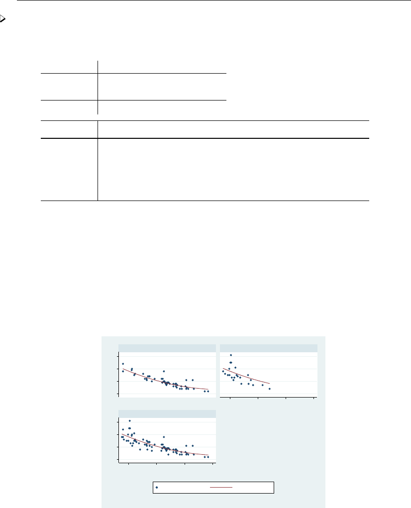
[ U ] 20 Estimation and postestimation commands 275
Example 6
Let’s perform a linear regression of mpg on weight and the square of weight:
. regress mpg weight c.weight#c.weight
Source SS df MS Number of obs = 74
F( 2, 71) = 72.80
Model 1642.52197 2 821.260986 Prob > F = 0.0000
Residual 800.937487 71 11.2808097 R-squared = 0.6722
Adj R-squared = 0.6630
Total 2443.45946 73 33.4720474 Root MSE = 3.3587
mpg Coef. Std. Err. t P>|t| [95% Conf. Interval]
weight -.0141581 .0038835 -3.65 0.001 -.0219016 -.0064145
c.weight#
c.weight 1.32e-06 6.26e-07 2.12 0.038 7.67e-08 2.57e-06
_cons 51.18308 5.767884 8.87 0.000 39.68225 62.68392
After the regression, predict is defined to be
−.0141581weight +1.32 ·10−6weight2+51.18308
(Actually, it is more precise because the coefficients are internally stored at much higher precision than
shown in the output.) Thus we can create a new variable—call it fitted—equal to the prediction
by typing predict fitted and then use scatter to display the fitted and actual values separately
for domestic and foreign automobiles:
. predict fitted
(option xb assumed; fitted values)
. scatter mpg fitted weight, by(foreign, total) c(. l) m(o i) sort
10 20 30 4010 20 30 40
2,000 3,000 4,000 5,000
2,000 3,000 4,000 5,000
Domestic Foreign
Total
Mileage (mpg) Fitted values
Weight (lbs.)
Graphs by Car type
predict can calculate much more than just predicted values. For predict after linear regression,
predict can calculate residuals, standardized residuals, Studentized residuals, influence statistics,
etc. In any case, we specify what is to be calculated via an option, so if we wanted the residuals
stored in new variable r, we would type
. predict r, resid
276 [ U ] 20 Estimation and postestimation commands
The options that may be specified following predict vary according to the estimation command
previously used; the predict options are documented along with the estimation command. For
instance, to discover all the things predict can do following regress, see [R]regress.
20.10.1 Using predict
The use of predict is not limited to linear regression. predict can be used after any estimation
command.
Example 7
You fit a logistic regression model of whether a car is manufactured outside the United States on
the basis of its weight and mileage rating using either the logistic or the logit command; see
[R]logistic and [R]logit. We will use logit.
. use http://www.stata-press.com/data/r13/auto2, clear
. logit foreign weight mpg
Iteration 0: log likelihood = -45.03321
Iteration 1: log likelihood = -29.238536
Iteration 2: log likelihood = -27.244139
Iteration 3: log likelihood = -27.175277
Iteration 4: log likelihood = -27.175156
Iteration 5: log likelihood = -27.175156
Logistic regression Number of obs = 74
LR chi2(2) = 35.72
Prob > chi2 = 0.0000
Log likelihood = -27.175156 Pseudo R2 = 0.3966
foreign Coef. Std. Err. z P>|z| [95% Conf. Interval]
weight -.0039067 .0010116 -3.86 0.000 -.0058894 -.001924
mpg -.1685869 .0919175 -1.83 0.067 -.3487418 .011568
_cons 13.70837 4.518709 3.03 0.002 4.851859 22.56487
After logit,predict without options calculates the probability of a positive outcome (we learned
that by looking at [R]logit). To obtain the predicted probabilities that each car is manufactured outside
the United States, we type
. predict probhat
(option pr assumed; Pr(foreign))
. summarize probhat
Variable Obs Mean Std. Dev. Min Max
probhat 74 .2972973 .3052979 .000729 .8980594
. list make mpg weight foreign probhat in 1/5
make mpg weight foreign probhat
1. AMC Concord 22 2,930 Domestic .1904363
2. AMC Pacer 17 3,350 Domestic .0957767
3. AMC Spirit 22 2,640 Domestic .4220815
4. Buick Century 20 3,250 Domestic .0862625
5. Buick Electra 15 4,080 Domestic .0084948

[ U ] 20 Estimation and postestimation commands 277
20.10.2 Making in-sample predictions
predict does not retrieve a vector of prerecorded values—it calculates the predictions on the
basis of the recorded coefficients and the data currently in memory. In the above examples, when we
typed things like
. predict probhat
predict filled in the prediction everywhere that it could be calculated.
Sometimes we have more data in memory than were used by the estimation command, either
because we explicitly ignored some of the observations by specifying an if exp with the estimation
command or because there are missing values. In such cases, if we want to restrict the calculation to
the estimation subsample, we would do that in the usual way by adding if e(sample) to the end
of the command:
. predict probhat if e(sample)
20.10.3 Making out-of-sample predictions
Because predict makes its calculations on the basis of the recorded coefficients and the data in
memory, predict can do more than calculate predicted values for the data on which the estimation
took place—it can make out-of-sample predictions, as well.
If you fit your model on a subset of the observations, you could then predict the outcome for all
the observations:
. logit foreign weight mpg if rep78 > 3
. predict pall
If you do not specify if e(sample) at the end of the predict command, predict calculates the
predictions for all observations possible.
In fact, because predict works from the active estimation results, you can use predict with
any dataset that contains the necessary variables.
Example 8
Continuing with our previous logit example, assume that we have a second dataset containing
the mpg and weight of a different sample of cars. We have just fit your model and now continue:
. use otherdat, clear
(Different cars)
. predict probhat Stata remembers the previous model
(option pr assumed; Pr(foreign))
. summarize probhat foreign
Variable Obs Mean Std. Dev. Min Max
probhat 12 .2505068 .3187104 .0084948 .8920776
foreign 12 .1666667 .3892495 0 1
278 [ U ] 20 Estimation and postestimation commands
Example 9
There are many ways to obtain out-of-sample predictions. Above, we estimated on one dataset and
then used another. If our first dataset had contained both sets of cars, marked, say, by the variable
difcars being 0 if from the first sample and 1 if from the second, we could type
. logit foreign weight mpg if difcars==0
same output as above appears
. predict probhat
(option pr assumed; Pr(foreign))
. summarize probhat foreign if difcars==1
same output as directly above appears
If we just had a few additional cars, we could even input them after estimation. Assume that
our data once again contain only the first sample of cars, and assume that we are interested in an
additional sample of only two rather than 12 cars; we could type
. use http://www.stata-press.com/data/r13/auto2
(1978 Automobile Data)
. keep make mpg weight foreign
. logit foreign weight mpg
same output as above appears
. input
make mpg weight foreign
75. "Merc. Zephyr" 20 2830 0 we type in our new data
76. "VW Dasher" 23 2160 1
77. end
. predict probhat obtain all the predictions
(option pr assumed; Pr(foreign))
. list in -2/l
make mpg weight foreign probhat
75. Merc. Zephyr 20 2,830 Domestic .3275397
76. VW Dasher 23 2,160 Foreign .8009743
20.10.4 Obtaining standard errors, tests, and confidence intervals for predictions
When you use predict, you create, for each observation in the prediction sample, a statistic that
is a function of the data and the estimated model parameters. You also could have generated your
own customized predictions by using generate. In either case, to get standard errors, Wald tests, and
confidence intervals for your predictions, use predictnl. For example, if we wanted the standard
errors for our predicted probabilities, we could type
. drop probhat
. predictnl probhat = predict(), se(phat_se)
. list in 1/5
make mpg weight foreign probhat phat_se
1. AMC Concord 22 2,930 Domestic .1904363 .0658387
2. AMC Pacer 17 3,350 Domestic .0957767 .0536297
3. AMC Spirit 22 2,640 Domestic .4220815 .0892845
4. Buick Century 20 3,250 Domestic .0862625 .0461928
5. Buick Electra 15 4,080 Domestic .0084948 .0093079

[ U ] 20 Estimation and postestimation commands 279
Comparing this output to our previous listing of the first five predicted probabilities, you will notice
that the output is identical, except that we now have an additional variable, phat se, which contains
the estimated standard error for each predicted probability.
We first had to drop probhat because predictnl will regenerate it. Note also the use of
predict() within predictnl—it specified that we wanted to generate a point estimate (and
standard error) for the default prediction after logit; see [R]predictnl for more details.
20.11 Accessing estimated coefficients
You can access coefficients and standard errors after estimation by referring to b[name]and
se[name]; see [U] 13.5 Accessing coefficients and standard errors.
Example 10
Let’s return to linear regression. We are doing a study of earnings of men and women at a particular
company. In addition to each person’s earnings, we have information on their educational attainment
and tenure with the company. We type the following:
. regress lnearn ed tenure i.female female#(c.ed c.tenure)
(output omitted )
If you are not familiar with the #notation, see [U] 11.4.3 Factor variables.
We now wish to predict everyone’s income as if they were male and then compare these as-if
earnings with the actual earnings:
. generate asif = _b[_cons] + _b[ed]*ed + _b[tenure]*tenure
Example 11
We are analyzing the mileage of automobiles and are using a slightly more sophisticated model
than any we have used so far. As we have previously, we will fit a linear regression model of mpg on
weight and the square of weight, but we also add the interaction of foreign with weight, the car’s
gear ratio (gear ratio), and foreign interacted with gear ratio. We will use factor-variable
notation to create the squared term and the interactions; see [U] 11.4.3 Factor variables.

280 [ U ] 20 Estimation and postestimation commands
. use http://www.stata-press.com/data/r13/auto2, clear
(1978 Automobile Data)
. regress mpg weight c.weight#c.weight i.foreign#c.weight gear_ratio
> i.foreign#c.gear_ratio
Source SS df MS Number of obs = 74
F( 5, 68) = 33.44
Model 1737.05293 5 347.410585 Prob > F = 0.0000
Residual 706.406534 68 10.3883314 R-squared = 0.7109
Adj R-squared = 0.6896
Total 2443.45946 73 33.4720474 Root MSE = 3.2231
mpg Coef. Std. Err. t P>|t| [95% Conf. Interval]
weight -.0118517 .0045136 -2.63 0.011 -.0208584 -.002845
c.weight#
c.weight 9.81e-07 7.04e-07 1.39 0.168 -4.25e-07 2.39e-06
foreign#
c.weight
Foreign -.0032241 .0015577 -2.07 0.042 -.0063326 -.0001157
gear_ratio 1.159741 1.553418 0.75 0.458 -1.940057 4.259539
foreign#
c.gear_ratio
Foreign 1.597462 1.205313 1.33 0.189 -.8077036 4.002627
_cons 44.61644 8.387943 5.32 0.000 27.87856 61.35432
If you are not experienced in both regression technology and automobile technology, you may find it
difficult to interpret this regression. Putting aside issues of statistical significance, we find that mileage
decreases with a car’s weight but increases with the square of weight; decreases even more rapidly
with weight for foreign cars; increases with higher gear ratio; and increases even more rapidly with
higher gear ratio in foreign cars.
Thus do foreign cars yield better or worse gas mileage? Results are mixed. As the foreign cars’
weight increases, they do more poorly in relation to domestic cars, but they do better at higher gear
ratios. One way to compare the results is to predict what mileage foreign cars would have if they
were manufactured domestically. The regression provides all the information necessary for making
that calculation; mileage for domestic cars is estimated to be
−.012 weight +9.81 ·10−7weight2+1.160 gear ratio +44.6
We can use that equation to predict the mileage of foreign cars and then compare it with the true
outcome. The b[ ] function simplifies reference to the estimated coefficients. We can type
. gen asif=_b[weight]*weight + _b[c.weight#c.weight]*c.weight#c.weight +
> _b[gear_ratio]*gear_ratio + _b[_cons]
b[weight] refers to the estimated coefficient on weight,b[c.weight#c.weight] to the estimated
coefficient on c.weight#c.weight, and so on.

[ U ] 20 Estimation and postestimation commands 281
We might now ask how the actual mileage of a Honda compares with the asif prediction:
. list make asif mpg if strpos(make,"Honda")
make asif mpg
61. Honda Accord 26.52597 25
62. Honda Civic 30.62202 28
Notice the way we constructed our if clause to select Hondas. strpos() is the string function that
returns the location in the first string where the second string is found or, if the second string does
not occur in the first, zero. Thus any recorded make that contains the string “Honda” anywhere in it
would be listed; see [D]functions.
We find that both Honda models yield slightly lower gas mileage than the asif domestic car–based
prediction. (We do not endorse this model as a complete model of the determinants of mileage, nor
do we single out the Honda for any special scorn. In fact, please note that the observed values are
within the root mean squared error of the average prediction.)
We might wish to compare the overall average mpg and the asif prediction over all foreign cars
in the data:
. summarize mpg asif if foreign
Variable Obs Mean Std. Dev. Min Max
mpg 22 24.77273 6.611187 14 41
asif 22 26.67124 3.142912 19.70466 30.62202
We find that, on average, foreign cars yield slightly lower mileage than our asif prediction. This
might lead us to ask if any foreign cars do better than the asif prediction:
. list make asif mpg if foreign & mpg>asif, sep(0)
make asif mpg
55. BMW 320i 24.31697 25
57. Datsun 210 28.96818 35
63. Mazda GLC 29.32015 30
66. Subaru 28.85993 35
68. Toyota Corolla 27.01144 31
71. VW Diesel 28.90355 41
We find six such automobiles.

282 [ U ] 20 Estimation and postestimation commands
20.12 Performing hypothesis tests on the coefficients
20.12.1 Linear tests
After estimation, test is used to perform tests of linear hypotheses on the basis of the variance–
covariance matrix of the estimators (Wald tests).
Example 12
(test has many syntaxes and features, so do not use this example as an excuse for not reading
[R]test.) Using the automobile data, we perform the following regression:
. use http://www.stata-press.com/data/r13/auto2, clear
(1978 Automobile Data)
. generate weightsq=weight^2
. regress mpg weight weightsq foreign
Source SS df MS Number of obs = 74
F( 3, 70) = 52.25
Model 1689.15372 3 563.05124 Prob > F = 0.0000
Residual 754.30574 70 10.7757963 R-squared = 0.6913
Adj R-squared = 0.6781
Total 2443.45946 73 33.4720474 Root MSE = 3.2827
mpg Coef. Std. Err. t P>|t| [95% Conf. Interval]
weight -.0165729 .0039692 -4.18 0.000 -.0244892 -.0086567
weightsq 1.59e-06 6.25e-07 2.55 0.013 3.45e-07 2.84e-06
foreign -2.2035 1.059246 -2.08 0.041 -4.3161 -.0909002
_cons 56.53884 6.197383 9.12 0.000 44.17855 68.89913
We can use the test command to calculate the joint significance of weight and weightsq:
. test weight weightsq
( 1) weight = 0
( 2) weightsq = 0
F( 2, 70) = 60.83
Prob > F = 0.0000
We are not limited to testing whether the coefficients are zero. We can test whether the coefficient
on foreign is −2 by typing
. test foreign = -2
( 1) foreign = -2
F( 1, 70) = 0.04
Prob > F = 0.8482
We can even test more complicated hypotheses because test can perform basic algebra. Here is
an absurd hypothesis:
. test 2*(weight+weightsq)=-3*(foreign-(weight-weightsq))
( 1) - weight + 5*weightsq + 3*foreign = 0
F( 1, 70) = 4.31
Prob > F = 0.0416
test simplified the algebra of our hypothesis and then presented the test results. We discover that
the hypothesis may be absurd but we cannot reject it at the 1% or even 4% level. We can also use
test’s accumulate option to combine this test with another test:

[ U ] 20 Estimation and postestimation commands 283
. test foreign+weight=0, accum
( 1) - weight + 5*weightsq + 3*foreign = 0
( 2) weight + foreign = 0
F( 2, 70) = 9.12
Prob > F = 0.0003
There are limitations. test can test only linear hypotheses. If we attempt to test a nonlinear
hypothesis, test will tell us that it is not possible:
. test weight/foreign=0
not possible with test
r(131);
Testing nonlinear hypotheses is discussed in [U] 20.12.4 Nonlinear Wald tests below.
20.12.2 Using test
test bases its results on the estimated variance–covariance matrix of the estimators (that is,
performs a Wald test), so it can be used after any estimation command. For maximum likelihood
estimation, you will have to decide whether you want to perform tests on the basis of the information
matrix instead of constraining the equation, reestimating it, and then calculating the likelihood-ratio
test (see [U] 20.12.3 Likelihood-ratio tests). Because test bases its results on the information matrix,
its results have the same standing as the asymptotic zstatistic presented in the coefficient table.
Example 13
Let’s examine the repair records of the cars in our automobile data as rated by Consumer Reports:
. tabulate rep78 foreign
Repair
Record Car type
1978 Domestic Foreign Total
Poor 2 0 2
Fair 8 0 8
Average 27 3 30
Good 9 9 18
Excellent 2 9 11
Total 48 21 69
The values are coded 1 – 5, corresponding to Poor, Fair, Average, Good, and Excellent. We will fit
this variable by using a maximum-likelihood ordered logit model (the nolog option suppresses the
iteration log, saving us some paper):

284 [ U ] 20 Estimation and postestimation commands
. ologit rep78 price foreign weight weightsq displ, nolog
Ordered logistic regression Number of obs = 69
LR chi2(5) = 33.12
Prob > chi2 = 0.0000
Log likelihood = -77.133082 Pseudo R2 = 0.1767
rep78 Coef. Std. Err. z P>|z| [95% Conf. Interval]
price -.000034 .0001188 -0.29 0.775 -.0002669 .000199
foreign 2.685647 .9320404 2.88 0.004 .8588817 4.512413
weight -.0037447 .0025609 -1.46 0.144 -.0087639 .0012745
weightsq 7.87e-07 4.50e-07 1.75 0.080 -9.43e-08 1.67e-06
displacement -.0108919 .0076805 -1.42 0.156 -.0259455 .0041617
/cut1 -9.417196 4.298202 -17.84152 -.992874
/cut2 -7.581864 4.234091 -15.88053 .7168028
/cut3 -4.82209 4.14768 -12.95139 3.307214
/cut4 -2.793441 4.156221 -10.93948 5.352602
We now wonder whether all our variables other than foreign are jointly significant. We test the
hypothesis just as we would after linear regression:
. test weight weightsq displ price
( 1) [rep78]weight = 0
( 2) [rep78]weightsq = 0
( 3) [rep78]displacement = 0
( 4) [rep78]price = 0
chi2( 4) = 3.63
Prob > chi2 = 0.4590
To compare this with the results performed by a likelihood-ratio test, see [U] 20.12.3 Likelihood-ratio
tests. Here results differ little.
20.12.3 Likelihood-ratio tests
After maximum likelihood estimation, you can obtain likelihood-ratio tests by fitting both the
unconstrained and constrained models, storing the results using estimates store, and then running
lrtest. See [R]lrtest for the full details.
Example 14
In [U] 20.12.2 Using test above, we fit an ordered logit on rep78 and then tested the significance
of all the explanatory variables except foreign.
To obtain the likelihood-ratio test, sometime after fitting the full model, we type estimates store
full model name, where full model name is just a label that we assign to these results.
. ologit rep78 price foreign weight weightsq displ
(output omitted )
. estimates store myfullmodel
This command saves the current model results with the name myfullmodel.

[ U ] 20 Estimation and postestimation commands 285
Next we fit the constrained model. After that, typing ‘lrtest myfullmodel .’ compares the
current model with the model we saved:
. ologit rep78 foreign
Iteration 0: log likelihood = -93.692061
Iteration 1: log likelihood = -79.696089
Iteration 2: log likelihood = -79.034005
Iteration 3: log likelihood = -79.029244
Iteration 4: log likelihood = -79.029243
Ordered logistic regression Number of obs = 69
LR chi2(1) = 29.33
Prob > chi2 = 0.0000
Log likelihood = -79.029243 Pseudo R2 = 0.1565
rep78 Coef. Std. Err. z P>|z| [95% Conf. Interval]
foreign 2.98155 .6203644 4.81 0.000 1.765658 4.197442
/cut1 -3.158382 .7224269 -4.574313 -1.742452
/cut2 -1.362642 .3557343 -2.059868 -.6654154
/cut3 1.232161 .3431227 .5596532 1.90467
/cut4 3.246209 .5556657 2.157124 4.335293
. lrtest myfullmodel .
Likelihood-ratio test LR chi2(4) = 3.79
(Assumption: . nested in myfullmodel) Prob > chi2 = 0.4348
When we tested the same constraint with test (which performed a Wald test), we obtained a χ2of
3.63 and a significance level of 0.4590. We used .(the dot) to specify the results in active memory,
although we also could have stored them with estimates store and referred to them by name
instead. Also, the order in which you specify the two models to lrtest doesn’t matter; lrtest is
smart enough to know the full model from the constrained model.
Two other postestimation commands work in the same way as lrtest, meaning that they accept
names of stored estimation results as their input: hausman for performing Hausman specification
tests and suest for seemingly unrelated estimation. We do not cover these commands here; see
[R]hausman and [R]suest for more details.
20.12.4 Nonlinear Wald tests
testnl can be used to test nonlinear hypotheses about the parameters of the active estimation
results. testnl, like test, bases its results on the variance–covariance matrix of the estimators (that
is, performs a Wald test), so it can be used after any estimation command; see [R]testnl.
Example 15
We fit the model
. regress price mpg weight foreign
(output omitted )

286 [ U ] 20 Estimation and postestimation commands
and then type
. testnl (38*_b[mpg]^2 = _b[foreign]) (_b[mpg]/_b[weight]=4)
(1) 38*_b[mpg]^2 = _b[foreign]
(2) _b[mpg]/_b[weight] = 4
chi2(2) = 0.04
Prob > chi2 = 0.9806
We performed this test on linear regression estimates, but tests of this type could be performed after
any estimation command.
20.13 Obtaining linear combinations of coefficients
lincom computes point estimates, standard errors, tor zstatistics, p-values, and confidence
intervals for a linear combination of coefficients after any estimation command. Results can optionally
be displayed as odds ratios, incidence-rate ratios, or relative-risk ratios.
Example 16
We fit a linear regression:
. use http://www.stata-press.com/data/r13/regress, clear
. regress y x1 x2 x3
Source SS df MS Number of obs = 148
F( 3, 144) = 96.12
Model 3259.3561 3 1086.45203 Prob > F = 0.0000
Residual 1627.56282 144 11.3025196 R-squared = 0.6670
Adj R-squared = 0.6600
Total 4886.91892 147 33.2443464 Root MSE = 3.3619
y Coef. Std. Err. t P>|t| [95% Conf. Interval]
x1 1.457113 1.07461 1.36 0.177 -.666934 3.581161
x2 2.221682 .8610358 2.58 0.011 .5197797 3.923583
x3 -.006139 .0005543 -11.08 0.000 -.0072345 -.0050435
_cons 36.10135 4.382693 8.24 0.000 27.43863 44.76407
Suppose that we want to see the difference of the coefficients of x2 and x1. We type
. lincom x2 - x1
( 1) - x1 + x2 = 0
y Coef. Std. Err. t P>|t| [95% Conf. Interval]
(1) .7645682 .9950282 0.77 0.444 -1.20218 2.731316
lincom is handy for computing the odds ratio of one covariate group relative to another.

[ U ] 20 Estimation and postestimation commands 287
Example 17
We estimate the parameters of a logistic model of low birthweight:
. use http://www.stata-press.com/data/r13/lbw3
(Hosmer & Lemeshow data)
. logit low age lwd i.race smoke ptd ht ui
Iteration 0: log likelihood = -117.336
Iteration 1: log likelihood = -99.3982
Iteration 2: log likelihood = -98.780418
Iteration 3: log likelihood = -98.777998
Iteration 4: log likelihood = -98.777998
Logistic regression Number of obs = 189
LR chi2(8) = 37.12
Prob > chi2 = 0.0000
Log likelihood = -98.777998 Pseudo R2 = 0.1582
low Coef. Std. Err. z P>|z| [95% Conf. Interval]
age -.0464796 .0373888 -1.24 0.214 -.1197603 .0268011
lwd .8420615 .4055338 2.08 0.038 .0472299 1.636893
race
black 1.073456 .5150753 2.08 0.037 .0639273 2.082985
other .815367 .4452979 1.83 0.067 -.0574008 1.688135
smoke .8071996 .404446 2.00 0.046 .0145001 1.599899
ptd 1.281678 .4621157 2.77 0.006 .3759478 2.187408
ht 1.435227 .6482699 2.21 0.027 .1646414 2.705813
ui .6576256 .4666192 1.41 0.159 -.2569313 1.572182
_cons -1.216781 .9556797 -1.27 0.203 -3.089878 .656317
Level 1 of race designates white, level 2 designates black, and level 3 designates other.
If we want to obtain the odds ratio for black smokers relative to white nonsmokers (the reference
group), we type
. lincom 2.race + smoke, or
( 1) [low]2.race + [low]smoke = 0
low Odds Ratio Std. Err. z P>|z| [95% Conf. Interval]
(1) 6.557805 4.744692 2.60 0.009 1.588176 27.07811
lincom computed exp(βrace==2 +βsmoke) = 6.56.
20.14 Obtaining nonlinear combinations of coefficients
lincom is limited to estimating linear combinations of coefficients, for example, 2.race + smoke,
or exponentiated linear combinations, as in the above. For general nonlinear combinations, use nlcom.

288 [ U ] 20 Estimation and postestimation commands
Example 18
Continuing our previous example: suppose that we wanted the ratio of the coefficients (and standard
errors, Wald test, confidence interval, etc.) of blacks and races other than white and black:
. nlcom _b[2.race]/_b[3.race]
_nl_1: _b[2.race]/_b[3.race]
low Coef. Std. Err. z P>|z| [95% Conf. Interval]
_nl_1 1.316531 .7359262 1.79 0.074 -.1258574 2.75892
The Wald test given is that of the null hypothesis that the nonlinear combination is zero versus the
two-sided alternative—this is probably not informative for a ratio. If we would instead like to test
whether this ratio is one, we can rerun nlcom, this time subtracting one from our ratio estimate.
. nlcom _b[2.race]/_b[3.race] - 1
_nl_1: _b[2.race]/_b[3.race] - 1
low Coef. Std. Err. z P>|z| [95% Conf. Interval]
_nl_1 .3165314 .7359262 0.43 0.667 -1.125857 1.75892
We can interpret this as not much evidence that the “ratio minus 1” is different from zero, meaning
that we cannot reject the null hypothesis that the ratio equals one.
When using nlcom, we needed to refer to the model coefficients by their “proper” names, for
example, b[2.race], and not by the shorthand 2.race, such as when using lincom. If we had
typed
. nlcom 2.race/3.race
Stata would have reported an error.
If you have difficulty determining what to type for a coefficient when using lincom or nlcom
replay your results using the coeflegend option. Here are the results for our current estimates,
. logit, coeflegend
Logistic regression Number of obs = 189
LR chi2(8) = 37.12
Prob > chi2 = 0.0000
Log likelihood = -98.777998 Pseudo R2 = 0.1582
low Coef. Legend
age -.0464796 _b[age]
lwd .8420615 _b[lwd]
race
black 1.073456 _b[2.race]
other .815367 _b[3.race]
smoke .8071996 _b[smoke]
ptd 1.281678 _b[ptd]
ht 1.435227 _b[ht]
ui .6576256 _b[ui]
_cons -1.216781 _b[_cons]

[ U ] 20 Estimation and postestimation commands 289
20.15 Obtaining marginal means, adjusted predictions, and predictive
margins
predict uses the current estimation results (the coefficients and the VCE) to estimate the value of
statistics for observations in the data. lincom and nlcom use the current estimation results to estimate
a specific linear or nonlinear expression of the coefficients. The margins command combines aspects
of both and estimates margins of responses.
margins answers the question “What does my model have to say about such-and-such a group or
such-and-such a person”, where such-and-such might be
•my estimation sample or another sample
•a sample with the values of some covariates fixed
•a sample evaluated at each level of a treatment
•a population represented by a complex survey sample
•someone who looks like the fifth person in my sample
•someone who looks like the mean of the covariates in my sample
•someone who looks like the median of the covariates in my sample
•someone who looks like the 25th percentile of the covariates in my sample
•someone who looks like some other function of the covariates in my sample
•a standardized population
•a balanced experimental design
•any combination of the above
•any comparison of the above
margins answers these questions either conditionally on fixed values of all covariates or averaged
over the observations in a sample. It answers these questions about almost any predictions or any
other response that you can calculate as a function of your estimated parameters—linear responses,
probabilities, hazards, survival times, odds ratios, risk differences, etc. It answers these questions in
terms of the response given covariate levels, or in terms of the change in the response for a change
in levels (also known as marginal effects). It answers these questions providing standard errors, test
statistics, and confidence intervals; and those statistics can take the covariates as given or adjust for
sampling, also known as predictive margins and survey statistics.
A margin is a statistic based on a response for a fitted model calculated over a dataset in which
some of or all the covariates are fixed at values different from what they really are.
Margins go by different names in different fields, and they can estimate many interesting statistics
related to a fitted model. We discuss some common uses below; see [R]margins for more applications.
20.15.1 Obtaining estimated marginal means
A classic application of margins is to estimate the expected marginal means from a linear estimator
as though the design for the covariates were balanced—assuming an equal number of observations
for each unique combination of levels for the factor-variable covariates. These means have a long
history in the study of ANOVA and MANOVA but are of limited use with nonexperimental data. For a
discussion, see Obtaining margins as though the data were balanced in [R]margins and example 4
in [R]anova.
Estimated marginal means are also called “least-squares means”.

290 [ U ] 20 Estimation and postestimation commands
Consider an analysis of variance of the change in systolic blood pressure as determined by one of
four drug treatments and adjusting for the patient’s disease (Afifi and Azen 1979).
. use http://www.stata-press.com/data/r13/systolic
(Systolic Blood Pressure Data)
. tabulate drug disease
Patient’s Disease
Drug Used 1 2 3 Total
1 6 4 5 15
2 5 4 6 15
3 3 5 4 12
4 5 6 5 16
Total 19 19 20 58
. anova systolic drug##disease
Number of obs = 58 R-squared = 0.4560
Root MSE = 10.5096 Adj R-squared = 0.3259
Source Partial SS df MS F Prob > F
Model 4259.33851 11 387.212591 3.51 0.0013
drug 2997.47186 3 999.157287 9.05 0.0001
disease 415.873046 2 207.936523 1.88 0.1637
drug#disease 707.266259 6 117.87771 1.07 0.3958
Residual 5080.81667 46 110.452536
Total 9340.15517 57 163.862371
Despite having randomized on drug, we see in the tabulation that our data are not balanced—for
example, 12 patients were administered drug 3, whereas 16 were administered drug 4. The diseases
are also not balanced across drugs. To estimate the marginal mean for each level of drug while treating
the design as though it were balanced, we type
. margins drug, asbalanced
Adjusted predictions Number of obs = 58
Expression : Linear prediction, predict()
at : drug (asbalanced)
disease (asbalanced)
Delta-method
Margin Std. Err. t P>|t| [95% Conf. Interval]
drug
1 25.99444 2.751008 9.45 0.000 20.45695 31.53194
2 26.55556 2.751008 9.65 0.000 21.01806 32.09305
3 9.744444 3.100558 3.14 0.003 3.503344 15.98554
4 13.54444 2.637123 5.14 0.000 8.236191 18.8527
Assuming everyone in the sample were treated with drug 4 and that the diseases were equally
distributed across the drug treatments, the expected mean change in pressure resulting from treatment
with drug 4 is 13.54. Because we are treating the data as balanced, we could also say that 13.54 is
the expected mean change resulting from drug 4 for any sample where an equal number of patients
has each of the three diseases.
If we want an estimate of the mean that uses the distribution of diseases observed in the sample,
we would remove the asbalanced option:

[ U ] 20 Estimation and postestimation commands 291
. margins drug
Predictive margins Number of obs = 58
Expression : Linear prediction, predict()
Delta-method
Margin Std. Err. t P>|t| [95% Conf. Interval]
drug
1 25.89799 2.750533 9.42 0.000 20.36145 31.43452
2 26.41092 2.742762 9.63 0.000 20.89003 31.93181
3 9.722989 3.099185 3.14 0.003 3.484652 15.96132
4 13.55575 2.640602 5.13 0.000 8.24049 18.871
We can now say that a pressure change of 13.56 is expected if everyone in the sample is given
drug 4 and the distribution of diseases is as observed in the sample.
The second set of margins are not usually called estimated marginal means because they do not
impose a balanced design when estimating the mean. They are adjusted predictions that just happen
to be means because the response is linear.
Neither of these values is the average pressure change for those taking drug 4 in our sample
because margins treats everyone in the sample as having taken drug 4. Treating everyone as though
they have taken each drug is what makes the means comparable. We are essentially standardizing on
the values of all the other covariates in our model (in this example, just disease).
To obtain the observed mean for those taking drug 4, we must tell margins to treat drug 4 as its
sample, which we do with the over() option.
. summarize systolic if drug==4
Variable Obs Mean Std. Dev. Min Max
systolic 16 13.5 9.323805 -5 27
. margins, over(drug)
Predictive margins Number of obs = 58
Expression : Linear prediction, predict()
over : drug
Delta-method
Margin Std. Err. t P>|t| [95% Conf. Interval]
drug
1 26.06667 2.713577 9.61 0.000 20.60452 31.52881
2 25.53333 2.713577 9.41 0.000 20.07119 30.99548
3 8.75 3.033872 2.88 0.006 2.643133 14.85687
4 13.5 2.62741 5.14 0.000 8.211298 18.7887
The margin in the last line of the table matches the mean from summarize.
For many questions, we prefer one of the first two estimates of margins to the last one. If we
compare drugs 3 and 4 from the last results, the 8.75 and 13.5 include both the effect from the drug
and the differing distribution of diseases among patients taking drug 3 and drug 4 in our sample.
Our first set of margins, those from margins drug, asbalanced, assumed that for both drug 3 and
drug 4, we had an equal number of patients with each disease. Our second set of margins, those
from margins drug, assumed that for both drug 3 and drug 4, we wanted the observed distribution
of patients from the whole sample. By assuming a common distribution of diseases across the drugs,
our first two sets of margins remove the effect of disease when we compare across drugs.

292 [ U ] 20 Estimation and postestimation commands
20.15.2 Obtaining adjusted predictions
We will use the term adjusted predictions to refer to margins that are evaluated at fixed values for
all covariates. The margins command has a great deal of flexibility in letting you choose what those
fixed values are. Consider a model of high blood pressure as a function of sex, age group, and body
mass index (BMI, a common measure of weight relative to height; variable bmi). We will allow the
effect of age to differ for males and females by interacting the age group and sex variables. We will
also allow the effect of BMI to differ across all combinations of age group and sex by specifying a
full factorial model.

[ U ] 20 Estimation and postestimation commands 293
. use http://www.stata-press.com/data/r13/nhanes2
. logistic highbp sex##agegrp##c.bmi
Logistic regression Number of obs = 10351
LR chi2(23) = 2521.83
Prob > chi2 = 0.0000
Log likelihood = -5789.851 Pseudo R2 = 0.1788
highbp Odds Ratio Std. Err. z P>|z| [95% Conf. Interval]
sex
Female .4012124 .2695666 -1.36 0.174 .107515 1.497199
agegrp
30-39 .8124869 .6162489 -0.27 0.784 .1837399 3.592768
40-49 1.346976 1.101181 0.36 0.716 .2713222 6.687051
50-59 5.415758 4.254136 2.15 0.032 1.161532 25.2515
60-69 16.31623 10.09529 4.51 0.000 4.852423 54.86321
70+ 161.2491 130.7332 6.27 0.000 32.9142 789.9717
sex#agegrp
Female #
30-39 1.441256 1.44721 0.36 0.716 .2013834 10.31475
Female #
40-49 6.29497 6.575021 1.76 0.078 .8126879 48.75998
Female #
50-59 4.377185 4.43183 1.46 0.145 .6016818 31.84366
Female #
60-69 1.790026 1.502447 0.69 0.488 .3454684 9.27492
Female#70+ .1958758 .2165763 -1.47 0.140 .0224297 1.710562
bmi 1.18539 .0221872 9.09 0.000 1.142692 1.229684
sex#c.bmi
Female .9809543 .0250973 -0.75 0.452 .9329775 1.031398
agegrp#c.bmi
30-39 1.021812 .0299468 0.74 0.462 .9647712 1.082225
40-49 1.00982 .0315328 0.31 0.754 .9498702 1.073554
50-59 .979291 .0298836 -0.69 0.493 .9224373 1.039649
60-69 .9413883 .0228342 -2.49 0.013 .8976813 .9872234
70+ .8738056 .0278416 -4.23 0.000 .8209061 .930114
sex#agegrp#
c.bmi
Female #
30-39 1.000676 .0377954 0.02 0.986 .9292736 1.077564
Female #
40-49 .9702656 .0382854 -0.76 0.444 .8980559 1.048281
Female #
50-59 .9852929 .0380345 -0.38 0.701 .9134969 1.062732
Female #
60-69 1.028896 .0330473 0.89 0.375 .9661212 1.09575
Female#70+ 1.12236 .0480541 2.70 0.007 1.032019 1.220609
_cons .0052191 .0024787 -11.07 0.000 .0020575 .0132388

294 [ U ] 20 Estimation and postestimation commands
We can evaluate the probability of having high blood pressure for each age group while holding
the proportion of males and females and the value of bmi to its average by specifying the covariate
agegrp to margins and including the option atmeans:
. margins agegrp, atmeans
Adjusted predictions Number of obs = 10351
Model VCE : OIM
Expression : Pr(highbp), predict()
at : 1.sex = .4748333 (mean)
2.sex = .5251667 (mean)
1.agegrp = .2241329 (mean)
2.agegrp = .1566998 (mean)
3.agegrp = .1228867 (mean)
4.agegrp = .1247222 (mean)
5.agegrp = .2763018 (mean)
6.agegrp = .0952565 (mean)
bmi = 25.5376 (mean)
Delta-method
Margin Std. Err. z P>|z| [95% Conf. Interval]
agegrp
20-29 .1611491 .0091135 17.68 0.000 .1432869 .1790113
30-39 .2487466 .0121649 20.45 0.000 .2249038 .2725893
40-49 .3679695 .0144456 25.47 0.000 .3396567 .3962823
50-59 .5204507 .0146489 35.53 0.000 .4917394 .549162
60-69 .5714605 .0095866 59.61 0.000 .5526711 .5902499
70+ .6637982 .0154566 42.95 0.000 .6335038 .6940927
The header of the table showed us the mean values of each covariate. These are the values at which
the probabilities were evaluated. The mean values for the levels of agegrp appear in the header even
though they were not used. agegrp assumed the values 1, 2, 3, 4, 5, and 6, as shown in the table.
The means of the levels of agegrp are shown because we might have asked for more margins in the
table, for example, margins sex agegrp.
The modeled probability is just below 25% for those under 40 years of age, and then increases
fairly rapidly to 52% in the 50–59 age group. Above age 59, the probability remains under 67%. It is
often easier for nonstatisticians to interpret the statistics computed by margins than the coefficients
of a fitted model.
20.15.3 Obtaining predictive margins
Rather than evaluate the probability of having high blood pressure at one fixed point (the means),
as we did above, we can evaluate the probability at the covariate values for each observation in our
data and average those probabilities. Here is the modeled probability averaged over our sample:
. margins
Predictive margins Number of obs = 10351
Model VCE : OIM
Expression : Pr(highbp), predict()
Delta-method
Margin Std. Err. z P>|z| [95% Conf. Interval]
_cons .4227611 .0042939 98.46 0.000 .4143451 .4311771

[ U ] 20 Estimation and postestimation commands 295
If we fix the level of agegrp to 1, compute the probability for each observation, and then average
those probabilities, the result is the predictive margin for level 1 of agegrp.margins, by default,
computes these margins for each level of each variable specified on the command line. Let’s compute
the predictive margins for agegrp:
. margins agegrp
Predictive margins Number of obs = 10351
Model VCE : OIM
Expression : Pr(highbp), predict()
Delta-method
Margin Std. Err. z P>|z| [95% Conf. Interval]
agegrp
20-29 .2030932 .0087166 23.30 0.000 .1860089 .2201774
30-39 .2829091 .010318 27.42 0.000 .2626862 .3031319
40-49 .3769536 .0128744 29.28 0.000 .3517202 .4021871
50-59 .5153439 .0136201 37.84 0.000 .4886491 .5420387
60-69 .5641065 .009136 61.75 0.000 .5462003 .5820127
70+ .6535679 .0151371 43.18 0.000 .6238997 .683236
One way of looking at predictive margins is that they answer the question “What would the average
response (probability) be in my sample if everyone were in one age group?” Another way of looking
at predictive margins is that they standardize the effect of being in an age group with the distribution
of other covariate values in our sample. The margins above are comparable because only the level of
agegrp is changing across the margins. They represent our sample because all the other covariates
take on their values in the sample when the margins are evaluated.
The predictive margins in this table differ from the adjusted predictions we estimated in
[U] 20.15.2 Obtaining adjusted predictions because the probability is a nonlinear function of
the coefficients in a logistic model; see Example 3: Average response versus response at average in
[R]margins for details.
Our analysis so far has been a bit na¨
ıve. The dataset we are using is from the Second National
Health and Nutrition Examination Survey (NHANES II). It has weights to make it representative of
the population from which it was drawn as well as other survey characteristics—strata and primary
sampling units. The data have already been svyset; see [SVY]svyset. We should take note of these
characteristics and use the svy prefix when fitting our model.
. svy: logistic highbp sex##agegrp##c.bmi
(output omitted )
If we were to repeat the command margins agegrp, we would see that our point estimates differ
only a little, but our standard errors are generally larger.
We are not restricted to margining over a single factor variable. Let’s see if the pattern of high
blood pressure over age groups differs for men and women. We do that by specifying the interaction
of sex and agegrp to margins. We add the vce(unconditional) option to accommodate the
survey design.

296 [ U ] 20 Estimation and postestimation commands
. margins sex#agegrp, vce(unconditional)
Predictive margins Number of obs = 10351
Expression : Pr(highbp), predict()
Linearized
Margin Std. Err. t P>|t| [95% Conf. Interval]
sex#agegrp
Male#20-29 .2931664 .0204899 14.31 0.000 .251377 .3349557
Male#30-39 .3664032 .0241677 15.16 0.000 .3171128 .4156936
Male#40-49 .3945619 .0240343 16.42 0.000 .3455435 .4435802
Male#50-59 .5376423 .0295377 18.20 0.000 .4773997 .5978849
Male#60-69 .5780997 .0224681 25.73 0.000 .5322756 .6239237
Male#70+ .6507023 .0209322 31.09 0.000 .6080109 .6933938
Female #
20-29 .1069761 .0135978 7.87 0.000 .0792432 .1347091
Female #
30-39 .1898006 .0143975 13.18 0.000 .1604367 .2191646
Female #
40-49 .3250246 .0236775 13.73 0.000 .276734 .3733152
Female #
50-59 .4855339 .03364 14.43 0.000 .4169247 .5541431
Female #
60-69 .5441773 .0186243 29.22 0.000 .5061928 .5821618
Female#70+ .6195342 .0275568 22.48 0.000 .5633317 .6757367
Each line in the table corresponds to holding both sex and agegrp to fixed values while using
the observed level of bmi to evaluate the probability and then averaging over the observations in the
sample. To calculate the results in the first line of the table, margins fixed sex =1 and agegrp =1,
evaluated the probability for each observation, and then averaged the probabilities. All of these margins
reflect the observed distribution of bmi in the sample.
The first six lines represent males, and the second six lines represent females. Comparing males
with females for the same age groups, males are almost three times as likely to have high blood
pressure in the first age group (0.293/0.107 =2.7), they are almost twice as likely in the second
age group, and while the relative gap narrows, it is not until above age 70 that the probability for
males drops below the probability for females.
Can the pattern of probabilities be affected by controlling one’s bmi? Let’s reevaluate the proba-
bilities while holding bmi to two levels—20 (which is well within the normal range) and 30 (which
is at the boundary between overweight and obese). We add the option at(bmi=(20 30)) to set bmi
first to 20 and then to 30.

[ U ] 20 Estimation and postestimation commands 297
. margins sex#agegrp, at(bmi=(20 30)) vce(unconditional)
Adjusted predictions Number of obs = 10351
Expression : Pr(highbp), predict()
1._at : bmi = 20
2._at : bmi = 30
Linearized
Margin Std. Err. t P>|t| [95% Conf. Interval]
_at#sex#
agegrp
1 #
Male #
20-29 .1392353 .0217328 6.41 0.000 .094911 .1835596
1 #
Male #
30-39 .1714727 .0241469 7.10 0.000 .1222249 .2207205
1 #
Male #
40-49 .1914061 .0366133 5.23 0.000 .1167329 .2660794
1 #
Male #
50-59 .3380778 .0380474 8.89 0.000 .2604797 .4156759
1 #
Male #
60-69 .4311378 .0371582 11.60 0.000 .3553532 .5069225
1#Male#70+ .6131166 .0521657 11.75 0.000 .506724 .7195092
1 #
Female #
20-29 .0439911 .0061833 7.11 0.000 .0313802 .056602
1 #
Female #
30-39 .075806 .0134771 5.62 0.000 .0483193 .1032926
1 #
Female #
40-49 .1941274 .0231872 8.37 0.000 .1468367 .2414181
1 #
Female #
50-59 .3493224 .0405082 8.62 0.000 .2667055 .4319394
1 #
Female #
60-69 .3897998 .0226443 17.21 0.000 .3436165 .4359831
1 #
Female #
70+ .4599175 .0338926 13.57 0.000 .3907931 .5290419
2 #
Male #
20-29 .4506376 .0370654 12.16 0.000 .3750422 .526233
2 #
Male #
30-39 .569466 .04663 12.21 0.000 .4743635 .6645686
2 #
Male #
40-49 .6042078 .039777 15.19 0.000 .5230821 .6853334
2 #
Male #
50-59 .7268547 .0339618 21.40 0.000 .657589 .7961203
2 #
Male #
60-69 .7131811 .0271145 26.30 0.000 .6578807 .7684816

298 [ U ] 20 Estimation and postestimation commands
2#Male#70+ .6843337 .0357432 19.15 0.000 .611435 .7572323
2 #
Female #
20-29 .1638185 .024609 6.66 0.000 .1136282 .2140088
2 #
Female #
30-39 .3038899 .0271211 11.20 0.000 .2485761 .3592037
2 #
Female #
40-49 .4523337 .0364949 12.39 0.000 .3779019 .5267655
2 #
Female #
50-59 .6132219 .0376898 16.27 0.000 .536353 .6900908
2 #
Female #
60-69 .68786 .0274712 25.04 0.000 .631832 .7438879
2 #
Female #
70+ .7643662 .0343399 22.26 0.000 .6943296 .8344029
That is a lot of margins, but they are in sets of six age groups. The first six margins are men
with a BMI of 20, the second six are women with a BMI of 20, the third six are men with a BMI
of 30, and the last six are women with a BMI of 30. These margins tell a more complete story. The
probability of high blood pressure is much lower for both men and women who maintain a BMI of 20.
More interesting is that the relationship between men and women differs depending on BMI. While
young men who maintain a BMI of 20 are still twice as likely as young women to have high blood
pressure (0.139/0.044)and youngish men are over 50% more likely (0.171/0.076), the gap narrows
substantially for men in the four older groups. The story is worse for those with a BMI of 30. Both
men and women with a high BMI have a substantially increased risk of high blood pressure, with men
ages 50–69 almost 10 percentage points higher than women. Before you dismiss these differences as
caused by the usual attenuation of the logistic curve in the tails, recall that when we fit the model,
we allowed the effect of bmi to be different for each combination of sex and agegrp.
You may have noticed that the header of the prior results says “Adjusted predictions” rather than
“Predictive margins”. That is because our model has only three covariates, and we have fixed the
values of each. margins is no longer averaging over the data, but is instead evaluating the margins
at fixed points that we have requested. It lets us know that by changing the header.
We could post the results of margins and form linear combinations or perform tests about any of
the assertions above; see Example 10: Testing margins—contrasts of margins in [R]margins.
There is much more to know about margins and the margins command. Consider the headings
for the Remarks and examples section of [R]margins:
Introduction
Obtaining margins of responses
Example 1: A simple case after regress
Example 2: A simple case after logistic
Example 3: Average response versus response at average
Example 4: Multiple margins from one command
Example 5: Margins with interaction terms
Example 6: Margins with continuous variables
Example 7: Margins of continuous variables
Example 8: Margins of interactions
Example 9: Decomposing margins
Example 10: Testing margins—contrasts of margins
Example 11: Margins of a specified prediction
Example 12: Margins of a specified expression
Example 13: Margins with multiple outcomes (responses)

[ U ] 20 Estimation and postestimation commands 299
Example 14: Margins with multiple equations
Example 15: Margins evaluated out of sample
Obtaining margins of derivatives of responses (a.k.a. marginal effects)
Do not specify marginlist when you mean over()
Use at() freely, especially with continuous variables
Expressing derivatives as elasticities
Derivatives versus discrete differences
Example 16: Average marginal effect (partial effects)
Example 17: Average marginal effect of all covariates
Example 18: Evaluating marginal effects over the response surface
Obtaining margins with survey data and representative samples
Example 19: Inferences for populations, margins of response
Example 20: Inferences for populations, marginal effects
Example 21: Inferences for populations with svyset data
Standardizing margins
Obtaining margins as though the data were balanced
Balancing using asbalanced
Balancing by standardization
Balancing nonlinear responses
Treating a subset of covariates as balanced
Using fvset design
Balancing in the presence of empty cells
Obtaining margins with nested designs
Introduction
Margins with nested designs as though the data were balanced
Coding of nested designs
Special topics
Requirements for model specification
Estimability of margins
Manipulability of tests
Using margins after the estimates use command
Syntax of at()
Estimation commands that may be used with margins
Glossary
20.16 Obtaining conditional and average marginal effects
Marginal effects measure the change in a response given a change in a covariate, which is to
say that marginal effects are derivatives. As used here, marginal effects can also be the discrete
change in a response as an indicator goes from 0 to 1. Some authors reserve the term marginal
effect for the continuous change and use partial effect for the discrete change. We will not make that
distinction. Regardless, marginal effects are most often used to make it easier to interpret how changes
in covariates affect a nonlinear response from a fitted model—a probability, a censored dependent
variable, a survival time, a hazard, etc.
Marginal effects can either be evaluated at a specified point for all the covariates in our model
(conditional marginal effects) or be evaluated at the observed values of the covariates in a dataset
and then averaged (average marginal effects).
To Stata, marginal effects are just margins whose response happens to be the derivative of another
response. Those interested in marginal effects will be interested in all or most of [R]margins.

300 [ U ] 20 Estimation and postestimation commands
20.16.1 Obtaining conditional marginal effects
We call a marginal effect conditional when we fix the values of all the covariates and then take
the derivative of the response with respect to a covariate. The mean of all covariates is often used as
the fixed point, and this is sometimes called the marginal effect at the means.
Consider a simple probit model of union membership for women as a function of having graduated
from college (collgrad), living in the South (south), tenure on the job (tenure), and the interaction
of south and tenure. We are interested in how being in the South affects union membership. We fit
the model by using an extract from 1988 of the U.S. National Longitudinal Survey of Labor Market
Experience (see [XT]xt).
. use http://www.stata-press.com/data/r13/nlsw88b, clear
(NLSW, 1988 extract)
. probit union i.collgrad i.south tenure south#c.tenure
Iteration 0: log likelihood = -1042.6816
Iteration 1: log likelihood = -997.71809
Iteration 2: log likelihood = -997.60984
Iteration 3: log likelihood = -997.60983
Probit regression Number of obs = 1868
LR chi2(4) = 90.14
Prob > chi2 = 0.0000
Log likelihood = -997.60983 Pseudo R2 = 0.0432
union Coef. Std. Err. z P>|z| [95% Conf. Interval]
collgrad
not grad .2783278 .0726167 3.83 0.000 .1360018 .4206539
1.south -.2534964 .1050552 -2.41 0.016 -.4594008 -.0475921
tenure .0362944 .0068205 5.32 0.000 .0229264 .0496624
south#
c.tenure
1 -.0239785 .0119533 -2.01 0.045 -.0474065 -.0005504
_cons -.8497418 .0664524 -12.79 0.000 -.9799862 -.7194974
Clearly, being located in the South decreases union membership. Using the dydx() and atmeans
options of margins, we can ask how much it decreases membership by evaluating the marginal effect
of being southern at the mean of all covariates:
. margins, dydx(south) atmeans
Conditional marginal effects Number of obs = 1868
Model VCE : OIM
Expression : Pr(union), predict()
dy/dx w.r.t. : 1.south
at : 0.collgrad = .7521413 (mean)
1.collgrad = .2478587 (mean)
0.south = .5744111 (mean)
1.south = .4255889 (mean)
tenure = 6.571065 (mean)
Delta-method
dy/dx Std. Err. z P>|z| [95% Conf. Interval]
1.south -.1236055 .019431 -6.36 0.000 -.1616896 -.0855215
Note: dy/dx for factor levels is the discrete change from the base level.

[ U ] 20 Estimation and postestimation commands 301
At the means of all the covariates, southern women are 12 percentage points less likely to be
members of a union. This marginal effect includes both the direct effect of i.south and the interaction
south#c.tenure.
As margins reports below the table, this change in the response is for the discrete change of
going from not southern (0) to southern (1).
The header of margins tells us where the marginal effect was estimated. This margin fixes tenure
to be 6.6 years. There is nothing special about this point. We could also evaluate the marginal effect
at the median of tenure:
. margins, dydx(south) atmeans at((medians) _continuous)
Conditional marginal effects Number of obs = 1868
Model VCE : OIM
Expression : Pr(union), predict()
dy/dx w.r.t. : 1.south
at : 0.collgrad = .7521413 (mean)
1.collgrad = .2478587 (mean)
0.south = .5744111 (mean)
1.south = .4255889 (mean)
tenure = 4.666667 (median)
Delta-method
dy/dx Std. Err. z P>|z| [95% Conf. Interval]
1.south -.1061338 .0201722 -5.26 0.000 -.1456706 -.066597
Note: dy/dx for factor levels is the discrete change from the base level.
With tenure at its median of 4.67, the marginal effect is about 2 percentage points less than it
was at the mean of 6.6.
When examining conditional marginal effects, it is often useful to evaluate them at a range of values
for the covariates. We can do that by asking both for values of the indicator covariate collgrad and
for a range of values for tenure:

302 [ U ] 20 Estimation and postestimation commands
. margins collgrad, dydx(south) at(tenure=(0(5)25))
Conditional marginal effects Number of obs = 1868
Model VCE : OIM
Expression : Pr(union), predict()
dy/dx w.r.t. : 1.south
1._at : tenure = 0
2._at : tenure = 5
3._at : tenure = 10
4._at : tenure = 15
5._at : tenure = 20
6._at : tenure = 25
Delta-method
dy/dx Std. Err. z P>|z| [95% Conf. Interval]
1.south
_at#collgrad
1#grad -.0627725 .0254161 -2.47 0.014 -.112587 -.0129579
1#not grad -.0791483 .0321151 -2.46 0.014 -.1420928 -.0162038
2#grad -.1031957 .0189184 -5.45 0.000 -.140275 -.0661164
2#not grad -.1256566 .0232385 -5.41 0.000 -.1712031 -.0801101
3#grad -.1496772 .022226 -6.73 0.000 -.1932392 -.1061151
3#not grad -.1760137 .0266874 -6.60 0.000 -.2283202 -.1237073
4#grad -.2008801 .036154 -5.56 0.000 -.2717407 -.1300196
4#not grad -.2282 .0419237 -5.44 0.000 -.310369 -.146031
5#grad -.2549707 .0546355 -4.67 0.000 -.3620543 -.1478872
5#not grad -.2799495 .0613127 -4.57 0.000 -.4001201 -.1597789
6#grad -.3097656 .0747494 -4.14 0.000 -.4562717 -.1632594
6#not grad -.3289702 .0816342 -4.03 0.000 -.4889703 -.1689701
Note: dy/dx for factor levels is the discrete change from the base level.
We now have a more complete picture of the effect that being in the South has on union participation.
For those with no tenure and without a college degree (the first line in the table), being in the South
decreases union participation by only 6 percentage points. For those with 25 years of tenure and with
a college degree (the last line in the table), being in the South decreases participation by almost 33
percentage points. We can read the effect for any combination of tenure and college graduation status
from the other lines in the table.
20.16.2 Obtaining average marginal effects
To compute average marginal effects, the marginal effect is first computed for each observation
in the dataset and then averaged. If the sample over which we compute the average marginal effect
represents a population, then we have estimated the marginal effect for the population.
We continue with our example of labor union participation.
. use http://www.stata-press.com/data/r13/nlsw88b
(NLSW, 1988 extract)
. probit union i.collgrad i.south tenure south#c.tenure
(output omitted )

[ U ] 20 Estimation and postestimation commands 303
To estimate the average marginal effect for each of our regressors, we type
. margins, dydx(*)
Average marginal effects Number of obs = 1868
Model VCE : OIM
Expression : Pr(union), predict()
dy/dx w.r.t. : 1.collgrad 1.south tenure
Delta-method
dy/dx Std. Err. z P>|z| [95% Conf. Interval]
collgrad
not grad .0878847 .0238065 3.69 0.000 .0412248 .1345447
1.south -.126164 .0191504 -6.59 0.000 -.1636981 -.0886299
tenure .0083571 .0016521 5.06 0.000 .005119 .0115951
Note: dy/dx for factor levels is the discrete change from the base level.
For this sample, the average marginal effect is very close to the marginal effect at the mean that
we computed earlier. That is not always true; it depends on the distribution of the other covariates.
The results also tell us that on average, for populations like the one from which our sample was
drawn, union participation increases 0.8 percentage points for every year of tenure on the job. College
graduates are, on average, 8.8 percentage points more likely to participate.
In the examples above, we treated the covariates in the sample as fixed and known. We could have
accounted for the fact that this sample was drawn from a population and the covariates represent just
one sample from that population. We do that by adding the vce(robust) or vce(cluster clustvar)
option when fitting the model and the vce(unconditional) option when estimating the margins;
see Obtaining margins with survey data and representative samples in [R]margins. It makes little
difference in the examples above.
20.17 Obtaining pairwise comparisons
pwcompare performs pairwise comparisons across the levels of factor variables. pwcompare can
compare estimated cell means, marginal means, intercepts, marginal intercepts, slopes, or marginal
slopes—collectively called margins. pwcompare reports comparisons as contrasts (differences) of
margins along with significance tests or confidence intervals for the contrasts. The tests and confidence
intervals can be adjusted for multiple comparisons.
pwcompare is for use after an estimation command in which you have used factor variables in
specifying the model. You could not use pwcompare after typing
. regress yield fertilizer1-fertilizer5
but you could use pwcompare after typing
. regress yield i.fertilizer
Below we fit a linear regression of wheat yield on type of fertilizer, and then we compare the mean
yields for each pair of fertilizers and obtain p-values and confidence intervals adjusted for multiple
comparisons using Tukey’s honestly significant difference.

304 [ U ] 20 Estimation and postestimation commands
. use http://www.stata-press.com/data/r13/yield
(Artificial wheat yield dataset)
. regress yield i.fertilizer
Source SS df MS Number of obs = 200
F( 4, 195) = 5.33
Model 1078.84207 4 269.710517 Prob > F = 0.0004
Residual 9859.55334 195 50.561812 R-squared = 0.0986
Adj R-squared = 0.0801
Total 10938.3954 199 54.9668111 Root MSE = 7.1107
yield Coef. Std. Err. t P>|t| [95% Conf. Interval]
fertilizer
10-08-22 3.62272 1.589997 2.28 0.024 .4869212 6.758518
16-04-08 .4906299 1.589997 0.31 0.758 -2.645169 3.626428
18-24-06 4.922803 1.589997 3.10 0.002 1.787005 8.058602
29-03-04 -1.238328 1.589997 -0.78 0.437 -4.374127 1.89747
_cons 41.36243 1.124298 36.79 0.000 39.14509 43.57977

[ U ] 20 Estimation and postestimation commands 305
. pwcompare fertilizer, effects mcompare(tukey)
Pairwise comparisons of marginal linear predictions
Margins : asbalanced
Number of
Comparisons
fertilizer 10
Tukey Tukey
Contrast Std. Err. t P>|t| [95% Conf. Interval]
fertilizer
10-08-22
vs
10-10-10 3.62272 1.589997 2.28 0.156 -.7552913 8.000731
16-04-08
vs
10-10-10 .4906299 1.589997 0.31 0.998 -3.887381 4.868641
18-24-06
vs
10-10-10 4.922803 1.589997 3.10 0.019 .5447922 9.300815
29-03-04
vs
10-10-10 -1.238328 1.589997 -0.78 0.936 -5.616339 3.139683
16-04-08
vs
10-08-22 -3.13209 1.589997 -1.97 0.285 -7.510101 1.245921
18-24-06
vs
10-08-22 1.300083 1.589997 0.82 0.925 -3.077928 5.678095
29-03-04
vs
10-08-22 -4.861048 1.589997 -3.06 0.021 -9.239059 -.4830368
18-24-06
vs
16-04-08 4.432173 1.589997 2.79 0.046 .0541623 8.810185
29-03-04
vs
16-04-08 -1.728958 1.589997 -1.09 0.813 -6.106969 2.649053
29-03-04
vs
18-24-06 -6.161132 1.589997 -3.87 0.001 -10.53914 -1.78312
See [R]pwcompare and [R]margins, pwcompare.
20.18 Obtaining contrasts, tests of interactions, and main effects
contrast estimates and tests contrasts—comparisons of levels of factor variables. It also performs
joint tests of these contrasts and can produce ANOVA-style tests of main effects, interaction effects,
simple effects, and nested effects. It can be used after most estimation commands.
contrast provides a set of “contrast operators” such as r.,ar., and p.. These operators are
prefixed onto variable names—for example, r.varname—to specify the contrasts to be performed.
The operators can be used with the contrast and margins commands.
Below we fit a regression of cholesterol level on age group category.

306 [ U ] 20 Estimation and postestimation commands
. regress chol i.agegrp
The reported coefficients on i.agegrp will themselves be contrasts, namely, contrasts on the reference
category. After estimation, if we wanted to compare the cell mean of each age group with that of the
previous group, we would perform a reverse-adjacent contrast by typing
. contrast ar.agegrp
That is exactly what we will do:
. use http://www.stata-press.com/data/r13/cholesterol
(Artificial cholesterol data)
. regress chol i.agegrp
Source SS df MS Number of obs = 75
F( 4, 70) = 35.02
Model 14943.3997 4 3735.84993 Prob > F = 0.0000
Residual 7468.21971 70 106.688853 R-squared = 0.6668
Adj R-squared = 0.6477
Total 22411.6194 74 302.859722 Root MSE = 10.329
chol Coef. Std. Err. t P>|t| [95% Conf. Interval]
agegrp
20-29 8.203575 3.771628 2.18 0.033 .6812991 15.72585
30-39 21.54105 3.771628 5.71 0.000 14.01878 29.06333
40-59 30.15067 3.771628 7.99 0.000 22.6284 37.67295
60-79 38.76221 3.771628 10.28 0.000 31.23993 46.28448
_cons 180.5198 2.666944 67.69 0.000 175.2007 185.8388
. contrast ar.agegrp
Contrasts of marginal linear predictions
Margins : asbalanced
df F P>F
agegrp
(20-29 vs 10-19) 1 4.73 0.0330
(30-39 vs 20-29) 1 12.51 0.0007
(40-59 vs 30-39) 1 5.21 0.0255
(60-79 vs 40-59) 1 5.21 0.0255
Joint 4 35.02 0.0000
Denominator 70
Contrast Std. Err. [95% Conf. Interval]
agegrp
(20-29 vs 10-19) 8.203575 3.771628 .6812991 15.72585
(30-39 vs 20-29) 13.33748 3.771628 5.815204 20.85976
(40-59 vs 30-39) 8.60962 3.771628 1.087345 16.1319
(60-79 vs 40-59) 8.611533 3.771628 1.089257 16.13381
We could use orthogonal polynomial contrasts to test whether there is a linear, quadratic, or even
higher-order trend in the estimated cell means.

[ U ] 20 Estimation and postestimation commands 307
. contrast p.agegrp, noeffects
Contrasts of marginal linear predictions
Margins : asbalanced
df F P>F
agegrp
(linear) 1 139.11 0.0000
(quadratic) 1 0.15 0.6962
(cubic) 1 0.37 0.5448
(quartic) 1 0.43 0.5153
Joint 4 35.02 0.0000
Denominator 70
You are not limited to using contrast in one-way models. Had we fit
. regress chol agegrp##race
we could contrast to obtain tests of the main effects and interaction effects.
. contrast agegrp##race
These results would be the same as would be reported by anova. We mention this because you can
use contrast after any estimation command that allows factor variables and works with margins.
You could type
. logistic highbp agegrp##race
. contrast agegrp##race
See [R]contrast and [R]margins, contrast.
20.19 Graphing margins, marginal effects, and contrasts
Using marginsplot, you can graph any of the results produced by margins, and because margins
can replicate any of the results produced by pwcompare and contrast, you can graph any of the
results produced by them, too.
In [U] 20.15.3 Obtaining predictive margins, we did the following:
. use http://www.stata-press.com/data/r13/nhanes2
. svy: logistic highbp sex##agegrp##c.bmi
. margins sex#agegrp, vce(unconditional)
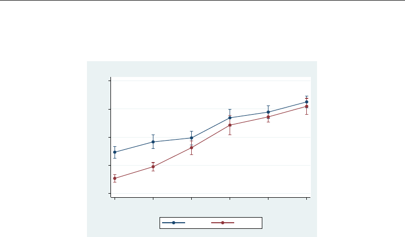
308 [ U ] 20 Estimation and postestimation commands
We can now graph those results by typing
. marginsplot, xdimension(agegrp)
Variables that uniquely identify margins: sex agegrp
0 .2 .4 .6 .8
Pr(Highbp)
20−29 30−39 40−49 50−59 60−69 70+
Age Group
Male Female
Predictive Margins of sex#agegrp with 95% CIs
See [R]marginsplot.Mitchell (2012) shows how to make similar graphs for a variety of predictions
and models.
20.20 Dynamic forecasts and simulations
The forecast suite of commands lets you obtain forecasts from forecast models, collections of
equations that jointly determine the outcomes of one or more endogenous variables. You fit stochastic
equations using estimation commands such as regress or var, then you add those results to your
forecast model. You can also specify identities that define variables in terms of other variables, and
you can also specify exogenous variables whose values are already known or otherwise determined
by factors outside your model. forecast then solves the resulting system of equations to obtain
forecasts.
forecast works with time-series and panel datasets, and you can obtain either dynamic or static
forecasts. Dynamic forecasts use previous periods’ forecast values wherever lags appear in the model’s
equations and thus allow you to obtain forecasts for multiple periods in the future. Static forecasts
use previous periods’ actual values wherever lags appear in the model’s equations, so if you use lags,
you cannot make predictions much beyond the end of the time horizon in your dataset. However,
static forecasts are useful during model development
You can incorporate outside information into your forecasts, and you can specify a future path for
some of the model’s variables and obtain forecasts for the other variables conditional on that path.
These features allow you to produce forecasts under different scenarios, and they allow you to explore
how different policy interventions would affect your forecasts.
forecast also has the capability to produce confidence intervals around the forecasts. You can
have forecast account for the sampling variance of the estimated parameters in the stochastic
equations. There are two ways to account for an additive stochastic error term in the stochastic
equations. You can request either that forecast assume the error terms are normally distributed and
take draws from a random-number generator or that forecast take random samples from the pool
of static-forecast residuals.
See [TS]forecast.

[ U ] 20 Estimation and postestimation commands 309
20.21 Obtaining robust variance estimates
Estimates of variance refer to estimated standard errors or, more completely, the estimated variance–
covariance matrix of the estimators of which the standard errors are a subset, being the square root of
the diagonal elements. Call this matrix the variance. All estimation commands produce an estimate
of variance and, using that, produce confidence intervals and significance tests.
In addition to the conventional estimator of variance, there is another estimator that has been
called by various names because it has been derived independently in different ways by different
authors. Two popular names associated with the calculation are Huber and White, but it is also known
as the sandwich estimator of variance (because of how the calculation formula physically appears)
and the robust estimator of variance (because of claims made about it). Also, this estimator has an
independent and long tradition in the survey literature.
The conventional estimator of variance is derived by starting with a model. Let’s start with the
regression model
yi=xiβ+i, i∼N(0, σ2)
although it is not important for the discussion that we are using regression. Under the model-based
approach, we assume that the model is true and thereby derive an estimator for βand its variance.
The estimator of the standard error of b
βwe develop is based on the assumption that the model is
true in every detail. yiis not exactly equal to xiβ(so that we would only need to solve an equation
to obtain precisely that value of β) because the observed yihas noise iadded to it, the noise is
Gaussian, and it has constant variance. That noise leads to the uncertainty about β, and it is from
the characteristics of that noise that we are able to calculate a sampling distribution for b
β.
The key thought here is that the standard error of b
βarises because of and is valid only because
the model is absolutely, without question, true; we just do not happen to know the particular values of
βand σ2that make the model true. The implication is that, in an infinite-sized sample, the estimator
b
βfor βwould converge to the true value of βand that its variance would go to 0.
Now here is another interpretation of the estimation problem: We are going to fit the model
yi=xib+ei
and, to obtain estimates of b, we are going to use the calculation formula
b
b= (X0X)−1X0y
We have made no claims that the model is true or any claims about eior its distribution. We shifted
our notation from βand ito band eito emphasize this. All we have stated are the physical actions
we intend to carry out on the data. Interestingly, it is possible to calculate a standard error for b
b
here. At least, it is possible if you will agree with us on what the standard error measures are.
We are going to define the standard error as measuring the standard error of the calculated b
bif
we were to repeat the data collection followed by estimation over and over again.
This is a different concept of the standard error from the conventional, model-based ideas, but it
is related. Both measure uncertainty about b(or β). The regression model–based derivation states
from where the variation arises and so can make grander statements about the applicability of the
measured standard error. The weaker second interpretation makes fewer assumptions and so produces
a standard error suitable for one purpose.
There is a subtle difference in interpretation of these identically calculated point estimates. b
βis
the estimate of βunder the assumption that the model is true. b
bis the estimate of b, which is merely
what the estimator would converge to if we collected more and more data.

310 [ U ] 20 Estimation and postestimation commands
Is the estimate of bunbiased? If we mean, “Does b=β?” that depends on whether the model
is true. b
bis, however, an unbiased estimate of b, which admittedly is not saying much.
What if xand eare correlated? Don’t we have a problem then? We may have an interpretation
problem—bmay not measure what we want to measure, namely, β—but we measure b
bto be such
and such and expect, if the experiment and estimation were repeated, that we would observe results
in the range we have reported.
So, we have two different understandings of what the parameters mean and how the variance in
their estimators arises. However, both interpretations must confront the issue of how to make valid
statistical inference about the coefficient estimates when the data do not come from either a simple
random sample or the distribution of (xi, i)is not independent and identically distributed (i.i.d.). In
essence, we need an estimator of the standard errors that is robust to this deviation from the standard
case.
Hence, the name the robust estimate of variance; its associated authors are Huber (1967) and White
(1980,1982) (who developed it independently), although many others have extended its development,
including Gail, Tan, and Piantadosi (1988); Kent (1982); Royall (1986); and Lin and Wei (1989). In the
survey literature, this same estimator has been developed; see Kish and Frankel (1974), Fuller (1975),
and Binder (1983). Most of Stata’s estimation commands can produce this alternative estimate of
variance and do so via the vce(robust) option.
Halbert Lynn White Jr. (1950–2012) was born in Kansas City. After receiving economics degrees
at Princeton and MIT, he taught and researched econometrics at the University of Rochester and,
from 1979, at the University of California in San Diego. He also co-founded an economics and
legal consulting firm known for its rigorous use of econometrics methods. His 1980 paper on
heteroskedasticity introduced the use of robust covariance matrices to economists and passed
16,000 citations in Google Scholar in 2012. His 1982 paper on maximum likelihood estimation
of misspecified models helped develop the now-common use of quasi–maximum likelihood
estimation techniques. Later in his career, he explored the use of neural networks, nonparametric
models, and time-series modeling of financial markets.
Among his many awards and distinctions, White was made a fellow of the American Academy
of Arts and Sciences and the Econometric Society, and he won a fellowship from the John
Simon Guggenheim Memorial Foundation. Had he not died prematurely, many scholars believe
he would have eventually been awarded the Sveriges Riksbank Prize in Economic Sciences in
Memory of Alfred Nobel.
Aside from his academic work, White was an avid jazz musician who played with well-known
jazz trombonist and fellow University of California at San Diego teacher Jimmy Cheatam.
Peter Jost Huber (1934– ) was born in Wohlen (Aargau, Switzerland). He gained mathematics
degrees from ETH Z¨
urich, including a PhD thesis on homotopy theory, and then studied statistics
at Berkeley on postdoctoral fellowships. This visit yielded a celebrated 1964 paper on robust
estimation, and Huber’s later monographs on robust statistics were crucial in directing that field.
Thereafter his career took him back and forth across the Atlantic, with periods at Cornell, ETH
Z¨
urich, Harvard, MIT, and Bayreuth. His work has touched several other major parts of statistics,
theoretical and applied, including regression, exploratory multivariate analysis, large datasets, and
statistical computing. Huber also has a major long-standing interest in Babylonian astronomy.

[ U ] 20 Estimation and postestimation commands 311
20.21.1 Interpreting standard errors
Without vce(robust), we get one measure of variance:
. use http://www.stata-press.com/data/r13/auto7
(1978 Automobile Data)
. regress mpg weight foreign
Source SS df MS Number of obs = 74
F( 2, 71) = 69.75
Model 1619.2877 2 809.643849 Prob > F = 0.0000
Residual 824.171761 71 11.608053 R-squared = 0.6627
Adj R-squared = 0.6532
Total 2443.45946 73 33.4720474 Root MSE = 3.4071
mpg Coef. Std. Err. t P>|t| [95% Conf. Interval]
weight -.0065879 .0006371 -10.34 0.000 -.0078583 -.0053175
foreign -1.650029 1.075994 -1.53 0.130 -3.7955 .4954422
_cons 41.6797 2.165547 19.25 0.000 37.36172 45.99768
With vce(robust), we get another:
. regress mpg weight foreign, vce(robust)
Linear regression Number of obs = 74
F( 2, 71) = 73.81
Prob > F = 0.0000
R-squared = 0.6627
Root MSE = 3.4071
Robust
mpg Coef. Std. Err. t P>|t| [95% Conf. Interval]
weight -.0065879 .0005462 -12.06 0.000 -.007677 -.0054988
foreign -1.650029 1.132566 -1.46 0.150 -3.908301 .6082424
_cons 41.6797 1.797553 23.19 0.000 38.09548 45.26392
Either way, the point estimates are the same. (See [R]regress for an example where specifying
vce(robust) produces strikingly different standard errors.)
How do we interpret these results? Let’s consider the model-based interpretation. Suppose that
yi=xiβ+i,
where (xi, i)are independently and identically distributed (i.i.d.) with variance σ2.For the model-
based interpretation, we also must assume that xiand iare uncorrelated. With these assumptions and
a few technical regularity conditions, our first regression gives us consistent parameter estimates and
standard errors that we can use for valid statistical inference about the coefficients. Now suppose that
we weaken our assumptions so that (xi, i)are independently and—but not necessarily—identically
distributed. Our parameter estimates are still consistent, but the standard errors from the first regression
can no longer be used to make valid inference. We need estimates of the standard errors that are
robust to the fact that the error term is not identically distributed. The standard errors in our second
regression are just what we need. We can use them to make valid statistical inference about our
coefficients, even though our data are not identically distributed.
Now consider a non–model-based interpretation. If our data come from a survey design that ensures
that (xi, ei)are i.i.d., then we can use the nonrobust standard errors for valid statistical inference

312 [ U ] 20 Estimation and postestimation commands
about the population parameters b. For this interpretation, we do not need to assume that xiand ei
are uncorrelated. If they are uncorrelated, the population parameters band the model parameters β
are the same. However, if they are correlated, then the population parameters bthat we are estimating
are not the same as the model-based β.So, what we are estimating is different, but we still need
standard errors that allow us to make valid statistical inference. So, if the process that we used to
collect the data caused (xi, ei)to be independently but not identically distributed, then we need to
use the robust standard errors to make valid statistical inference about the population parameters b.
20.21.2 Correlated errors: Cluster–robust standard errors
The robust estimator of variance has one feature that the conventional estimator does not have:
the ability to relax the assumption of independence of the observations. That is, if you specify the
vce(cluster clustvar)option, it can produce “correct” standard errors (in the measurement sense),
even if the observations are correlated.
For the automobile data, it is difficult to believe that the models of the various manufacturers are
truly independent. Manufacturers, after all, use common technology, engines, and drive trains across
their model lines. The VW Dasher in the above regression has a measured residual of −2.80. Having
been told that, do you really believe that the residual for the VW Rabbit is as likely to be above 0 as
below? (The residual is −2.32.) Similarly, the measured residual for the Chevrolet Malibu is 1.27.
Does that provide information about the expected value of the residual of the Chevrolet Monte Carlo
(which turns out to be 1.53)?
We need to be careful about picking examples from data; we have not told you about the Datsun
210 and 510 (residuals +8.28 and −1.01) or the Cadillac Eldorado and Seville (residuals −1.99 and
+7.58), but you should, at least, question the assumption of independence. It may be believable that the
measured mpg given the weight of one manufacturer’s vehicles is independent of other manufacturers’
vehicles, but it is at least questionable whether a manufacturer’s vehicles are independent of one
another.
In commands with the vce(robust) option, another option—vce(cluster clustvar)—relaxes
the independence assumption and requires only that the observations be independent across the clusters:
. regress mpg weight foreign, vce(cluster manufacturer)
Linear regression Number of obs = 74
F( 2, 22) = 90.93
Prob > F = 0.0000
R-squared = 0.6627
Root MSE = 3.4071
(Std. Err. adjusted for 23 clusters in manufacturer)
Robust
mpg Coef. Std. Err. t P>|t| [95% Conf. Interval]
weight -.0065879 .0005339 -12.34 0.000 -.0076952 -.0054806
foreign -1.650029 1.039033 -1.59 0.127 -3.804852 .5047939
_cons 41.6797 1.844559 22.60 0.000 37.85432 45.50508
It turns out that, in these data, whether or not we specify vce(cluster clustvar)makes little
difference. The VW and Chevrolet examples above were not representative; had they been, the
confidence intervals would have widened. (In the above, manuf is a variable that takes on values
such as “Chev.” or “VW”, recording the manufacturer of the vehicle. This variable was created from
variable make, which contains values such as “Chev. Malibu” or “VW Rabbit”, by extracting the first
word.)

[ U ] 20 Estimation and postestimation commands 313
As a demonstration of how well clustering can work, in [R]regress we fit a random-effects model
with regress, vce(robust) and then compared the results with ordinary least squares and the GLS
random-effects estimator. Here we will simply summarize the results.
We start with a dataset on 4,711 women aged 14–46 years. Subjects appear an average of 6.056
times in the data; there are a total of 28,534 observations. The model we use is log wage on age,
age-squared, and job tenure. The focus of the example is the estimated coefficient on tenure. We
obtain the following results:
Estimator Point estimate Confidence interval
(Inappropriate) least squares .039 [ .038, .041 ]
Robust clusterered .039 [ .036, .042 ]
GLS random effects .026 [ .025, .027 ]
Notice how well the robust clustered estimate does compared with the GLS random-effects model.
We then run a Hausman specification test, obtaining χ2(3) = 336.62, which casts grave doubt on the
assumptions justifying the use of the GLS estimator and hence on the GLS results. At this point, we
will simply quote our comments:
Meanwhile, our robust regression results still stand, as long as we are careful about the
interpretation. The correct interpretation is that, if the data collection were repeated (on
women sampled the same way as in the original sample), and if we were to refit the
model, 95% of the time we would expect the estimated coefficient on tenure to be in the
range [.036,.042 ].
Even with robust regression, we must be careful about going beyond that statement.
Here the Hausman test is probably picking up something that differs within and between
person, which would cast doubt on our robust regression model in terms of interpreting
[.036,.042 ]to contain the rate of return for keeping a job, economywide, for all women,
without exception.
The formula for the robust estimator of variance is
b
V=b
VN
X
j=1
u0
jujb
V
where b
V= (−∂2ln L/∂β2)−1(the conventional estimator of variance) and uj(a row vector) is the
contribution from the jth observation to ∂ln L/∂β.
In the example above, observations are assumed to be independent. Assume for a moment that
the observations denoted by jare not independent but that they can be divided into Mgroups G1,
G2,. . . ,GMthat are independent. The robust estimator of variance is
b
V=b
VM
X
k=1
u(G)0
ku(G)
kb
V
where u(G)
kis the contribution of the kth group to ∂ln L/∂β. That is, application of the robust variance
formula merely involves using a different decomposition of ∂ln L/∂β, namely, u(G)
k,k=1, . . . , M
rather than uj,j=1, . . . , N. Moreover, if the log-likelihood function is additive in the observations
denoted by j
lnL=
N
X
j=1
lnLj

314 [ U ] 20 Estimation and postestimation commands
then uj=∂ln Lj/∂β, so
u(G)
k=X
j∈Gk
uj
That is what the vce(cluster clustvar)option does. (This point was first made in writing by
Rogers [1993], although he considered the point an obvious generalization of Huber [1967] and the
calculation—implemented by Rogers—had appeared in Stata a year earlier.)
Technical note
What is written above is asymptotically correct but ignores a finite-sample adjustment to b
V. For
maximum likelihood estimators, when you specify vce(robust) but not vce(cluster clustvar),
a better estimate of variance is b
V∗={N/(N−1)}b
V. When you also specify the vce(cluster
clustvar)option, this becomes b
V∗={M/(M−1)}b
V.
For linear regression, the finite-sample adjustment is N/(N−k)without vce(cluster clust-
var)— where kis the number of regressors—and {M/(M−1)}{(N−1)/(N−k)}with
vce(cluster clustvar). Also, two data-dependent modifications to the calculation for b
V∗, sug-
gested by MacKinnon and White (1985), are also provided by regress; see [R]regress.Angrist and
Pischke (2009, chap. 8) is devoted to robust covariance matrix estimation and offers practical guid-
ance on the use of vce(robust) and vce(cluster clustvar)in both cross-sectional and panel-data
applications.
20.22 Obtaining scores
Many of the estimation commands that provide the vce(robust) option also provide the ability to
generate equation-level score variables via the predict command. With the score option, predict
returns an important ingredient into the robust variance calculation that is sometimes useful in its
own right. As explained in [U] 20.21 Obtaining robust variance estimates above, ignoring the
finite-sample corrections, the robust estimate of variance is
b
V=b
VN
X
j=1
u0
jujb
V
where b
V= (−∂2ln L/∂β2)−1is the conventional estimator of variance. Let’s consider likelihood
functions that are additive in the observations
lnL=
N
X
j=1
lnLj
then uj=∂ln Lj/∂β. In general, function Ljis a function of xjand β,Lj(β;xj). For many
likelihood functions, however, it is only the linear form xjβthat enters the function. In those cases,
∂lnLj(xjβ)
∂β=∂lnLj(xjβ)
∂(xjβ)
∂(xjβ)
∂β=∂lnLj(xjβ)
∂(xjβ)xj
By writing uj=∂ln Lj(xjβ)/∂(xjβ), this becomes simply ujxj. Thus the formula for the robust
estimate of variance can be rewritten as
b
V=b
VN
X
j=1
u2
jx0
jxjb
V

[ U ] 20 Estimation and postestimation commands 315
We refer to ujas the equation-level score (in the singular), and it is ujthat is returned when you
use predict with the score option. ujis like a residual in that
1. Pjuj=0 and
2. correlation of ujand xj, calculated over j=1, . . . , N, is 0.
In fact, for linear regression, ujis the residual, normalized,
∂lnLj
∂(xjβ)=∂
∂(xjβ)lnf(yj−xjβ)/σ
= (yj−xjβ)/σ
where f() is the standard normal density.
Example 19
probit provides both the vce(robust) option and predict, score. Equation-level scores play
an important role in calculating the robust estimate of variance, but we can use predict, score
regardless of whether we specify vce(robust):
. use http://www.stata-press.com/data/r13/auto2
. probit foreign mpg weight
Iteration 0: log likelihood = -45.03321
Iteration 1: log likelihood = -27.914626
Iteration 2: log likelihood = -26.858074
Iteration 3: log likelihood = -26.844197
Iteration 4: log likelihood = -26.844189
Iteration 5: log likelihood = -26.844189
Probit regression Number of obs = 74
LR chi2(2) = 36.38
Prob > chi2 = 0.0000
Log likelihood = -26.844189 Pseudo R2 = 0.4039
foreign Coef. Std. Err. z P>|z| [95% Conf. Interval]
mpg -.1039503 .0515689 -2.02 0.044 -.2050235 -.0028772
weight -.0023355 .0005661 -4.13 0.000 -.003445 -.0012261
_cons 8.275464 2.554142 3.24 0.001 3.269437 13.28149
. predict double u, score
. summarize u
Variable Obs Mean Std. Dev. Min Max
u 74 -6.66e-14 .5988325 -1.655439 1.660787
. correlate u mpg weight
(obs=74)
u mpg weight
u 1.0000
mpg 0.0000 1.0000
weight -0.0000 -0.8072 1.0000
. list make foreign mpg weight u if abs(u)>1.65
make foreign mpg weight u
24. Ford Fiesta Domestic 28 1,800 -1.6554395
64. Peugeot 604 Foreign 14 3,420 1.6607871

316 [ U ] 20 Estimation and postestimation commands
The light, high-mileage Ford Fiesta is surprisingly domestic, whereas the heavy, low-mileage Peugeot
604 is surprisingly foreign.
Technical note
For some estimation commands, one score is not enough. Consider a likelihood that can be written as
Lj(xjβ1,zjβ2), a function of two linear forms (or linear equations). Then ∂ln Lj/∂βcan be written
(∂ln Lj/∂β1, ∂ln Lj/∂β2). Each of the components can in turn be written as [∂ln Lj/∂(β1x)]x=
u1xand [∂ln Lj/∂(β2z)]z=u2z. There are then two equation-level scores, u1and u2, and, in
general, there could be more.
Stata’s streg, distribution(weibull) command is an example of this: it estimates βand a
shape parameter, lnp, the latter of which can be thought of as a degenerate linear form (lnp)zwith
z=1.predict, scores after this command requires that you specify two new variable names, or
you can specify stub*, which will generate two variables, stub1and stub2; the first will be defined
containing u1—the score associated with β—and the second will be defined containing u2—the
score associated with lnp.
Technical note
Using Stata’s matrix commands—see [P]matrix—we can make the robust variance calculation
for ourselves and then compare it with that made by Stata.
. use http://www.stata-press.com/data/r13/auto2, clear
(1978 Automobile Data)
. quietly probit foreign mpg weight
. predict double u, score
. matrix accum S = mpg weight [iweight=u^2*74/73]
(obs=26.53642547)
. matrix rV = e(V)*S*e(V)
. matrix list rV
symmetric rV[3,3]
foreign: foreign: foreign:
mpg weight _cons
foreign:mpg .00352299
foreign:weight .00002216 2.434e-07
foreign:_cons -.14090346 -.00117031 6.4474174
. quietly probit foreign mpg weight, vce(robust)
. matrix list e(V)
symmetric e(V)[3,3]
foreign: foreign: foreign:
mpg weight _cons
foreign:mpg .00352299
foreign:weight .00002216 2.434e-07
foreign:_cons -.14090346 -.00117031 6.4474174
The results are the same.
There is an important lesson here for programmers. Given the scores, conventional variance estimates
can be easily transformed to robust estimates. If we were writing a new estimation command, it
would not be difficult to include a vce(robust) option.
It is, in fact, easy if we ignore clustering. With clustering, it is more work because the calculation
involves forming sums within clusters. For programmers interested in implementing robust variance
calculations, Stata provides an robust command to ease the task. This is documented in [P]robust.

[ U ] 20 Estimation and postestimation commands 317
To use robust, you first produce conventional results (a vector of coefficients and covariance
matrix) along with a variable containing the scores uj(or variables if the likelihood function has more
than one stub). You then call robust, and it will transform your conventional variance estimate into
the robust estimate. robust will handle the work associated with clustering and the details of the
finite-sample adjustment, and it will even label your output so that the word Robust appears above
the standard error when the results are displayed.
Of course, this is all even easier if you write your commands with Stata’s ml maximum likelihood
optimization, in which case you merely pass the vce(robust) option on to ml.ml will then call
robust itself and do all the work for you.
Technical note
For some estimation commands, predict, score computes parameter-level scores ∂Lj/∂β
instead of equation-level scores ∂Lj/∂xjβ. Those commands are
asclogit
asmprobit
asroprobit
nlogit
stcox
stcrreg
mixed
These models share the characteristic that there are multiple observations per independent event.
In making the robust variance calculation, what are really needed are parameter-level scores
∂Lj/∂β, and so you may be asking yourself why predict, score does not always produce
parameter-level scores. In the usual case we can obtain them from equation-level scores via the chain
rule, and fewer variables are required if we adopt this approach. In the cases above, however, the
likelihood is calculated at the group level and is not split into contributions from the individual
observations. Thus the chain rule cannot be used and we must use the parameter level scores directly.
robust can be tricked into using them if each parameter appears to be in its own equation as a
constant. This requires resetting the row and column stripes on the covariance matrix before robust
is called. The equation names for each row and column must each be unique and the variable names
must all be cons.
20.23 Weighted estimation
[U] 11.1.6 weight introduced the syntax for weights. Stata provides four kinds of weights: fweights,
or frequency weights; pweights, or sampling weights; aweights, or analytic weights; and iweights,
or importance weights. The syntax for using each is the same. Type
. regress y x1 x2
and you obtain unweighted estimates; type
. regress y x1 x2 [pweight=pop]
and you obtain (in this example) pweighted estimation.
The sections below explain how each type of weight is used in estimation.

318 [ U ] 20 Estimation and postestimation commands
20.23.1 Frequency weights
Frequency weights—fweights—are integers and are nothing more than replication counts. The
weight is statistically uninteresting, but from a data processing perspective it is important. Consider
the following data
y x1 x2
22 1 0
22 1 0
22 1 1
23 0 1
23 0 1
23 0 1
and the estimation command
. regress y x1 x2
Equivalent is the following, more compressed data
y x1 x2 pop
22 1 0 2
22 1 1 1
23 0 1 3
and the corresponding estimation command
. regress y x1 x2 [fweight=pop]
When you specify frequency weights, you are treating each observation as one or more real observations.
Technical note
You might occasionally run across a command that does not allow weights at all, especially
among user-written commands. expand (see [D]expand) can be used with such commands to obtain
frequency-weighted results. The expand command duplicates observations so that the data become
self-weighting. Suppose that you want to run the command usercmd, which does something or other,
and you would like to type usercmd y x1 x2 [fw=pop]. Unfortunately, usercmd does not allow
weights. Instead, you type
. expand pop
. usercmd y x1 x2
to obtain your result. Moreover, there is an important principle here: the results of running any
command with frequency weights should be the same as running the command on the unweighted,
expanded data. Unweighted, duplicated data and frequency-weighted data are merely two ways of
recording identical information.

[ U ] 20 Estimation and postestimation commands 319
20.23.2 Analytic weights
Analytic weights—analytic is a term we made up—statistically arise in one particular problem:
linear regression on data that are themselves observed means. That is, think of the model
yi=xiβ+i, i∼N(0, σ2)
and now think about fitting this model on data (yj,xj)that are themselves observed averages. For
instance, a piece of the underlying data for (yi,xi)might be (3,1),(4,2), and (2,2), but you do not
know that. Instead, you have one observation {(3+4+2)/3,(1+2+2)/3}= (3,1.67)and know
only that the (3,1.67)arose as the average of 3 underlying observations. All your data are like that.
regress with aweights is the solution to that problem:
. regress y x [aweight=pop]
There is a history of misusing such weights. A researcher does not have cell-mean data but instead has a
probability-weighted random sample. Long before Stata existed, some researchers were using aweights
to produce estimates from such samples. We will come back to this point in [U] 20.23.3 Sampling
weights below.
Anyway, the statistical problem that aweights resolve can be written as
yi=xiβ+i, i∼N(0, σ2/wi)
where the wiare the analytic weights. The details of the solution are to make linear regression
calculations using the weights as if they were fweights but to normalize them to sum to Nbefore
doing that.
Most commands that allow aweights handle them in this manner. That is, if you specify aweights,
they are
1. normalized to sum to Nand then
2. inserted in the calculation formulas in the same way as fweights.
20.23.3 Sampling weights
Sampling weights—probability weights or pweights—refer to probability-weighted random sam-
ples. Actually, what you specify in [pweight=. . .]is a variable recording the number of subjects in
the full population that the sampled observation in your data represents. That is, an observation that
had probability 1/3 of being included in your sample has pweight 3.
Some researchers have used aweights with this kind of data. If they do, they are probably making
a mistake. Consider the regression model
yi=xiβ+i, i∼N(0, σ2)
Begin by considering the exact nature of the problem of fitting this model on cell-mean data—for
which aweights are the solution: heteroskedasticity arising from the grouping. The error term iis
homoskedastic (meaning that it has constant variance σ2). Say that the first observation in the data
is the mean of 3 underlying observations. Then
y1=x1β+1, i∼N(0, σ2)
y2=x2β+2, i∼N(0, σ2)
y3=x3β+3, i∼N(0, σ2)

320 [ U ] 20 Estimation and postestimation commands
and taking the mean
(y1+y2+y3)/3 = {(x1+x2+x3)/3}β+ (1+2+3)/3
For another observation in the data — which may be the result of summing of a different number of
observations—the variance will be different. Hence, the model for the data is
yj=xjβ+j, j∼N(0, σ2/Nj)
This makes intuitive sense. Consider 2 observations, one recording means over two subjects and the
other means over 100,000 subjects. You would expect the variance of the residual to be less in the
100,000-subject observation; that is, there is more information in the 100,000-subject observation than
in the two-subject observation.
Now instead say that you are fitting the same model, yi=xiβ+i,i∼N(0, σ2), on probability-
weighted data. Each observation in your data is one subject, but the different subjects have different
chances of being included in your sample. Therefore, for each subject in your data
yi=xiβ+i, i∼N(0, σ2)
That is, there is no heteroskedasticity problem. The use of the aweighted estimator cannot be justified
on these grounds.
As a matter of fact, from the argument just given, you do not need to adjust for the weights at
all, although the argument does not justify not making an adjustment. If you do not adjust, you are
holding tightly to the assumed truth of your model. Two issues arise when considering adjustment
for sampling weights:
1. the efficiency of the point estimate b
βof βand
2. the reported standard errors (and, more generally, the variance matrix of b
β).
Efficiency argues in favor of adjustment, and that, by the way, is why many researchers have used
aweights with pweighted data. The adjustment implied by pweights to the point estimates is the
same as the adjustment implied by aweights.
With regard to the second issue, the use of aweights produces incorrect results because it interprets
larger weights as designating more accurately measured points. For pweights, however, the point
is no more accurately measured—it is still just one observation with one residual jand variance
σ2. In [U] 20.21 Obtaining robust variance estimates above, we introduced another estimator of
variance that measures the variation that would be observed if the data collection followed by the
estimation were repeated. Those same formulas provide the solution to pweights, and they have
the added advantage that they are not conditioned on the model’s being true. If we have any hopes
of measuring the variation that would be observed were the data collection followed by estimation
repeated, we must include the probability of the observations being sampled in the calculation.
In Stata, when you type
. regress y x1 x2 [pw=pop]
the results are the same as if you had typed
. regress y x1 x2 [pw=pop], vce(robust)

[ U ] 20 Estimation and postestimation commands 321
That is, specifying pweights implies the vce(robust) option and, hence, the robust variance
calculation (but weighted). In this example, we use regress simply for illustration. The same is
true of probit and all of Stata’s estimation commands. Estimation commands that do not have a
vce(robust) option (there are a few) do not allow pweights.
pweights are adequate for handling random samples where the probability of being sampled varies.
pweights may be all you need. If, however, the observations are not sampled independently but are
sampled in groups—called clusters in the jargon—you should specify the estimator’s vce(cluster
clustvar)option as well:
. regress y x1 x2 [pw=pop], vce(cluster block)
There are two ways of thinking about this:
1. The robust estimator answers the question of which variation would be observed were the data
collection followed by the estimation repeated; if that question is to be answered, the estimator
must account for the clustered nature of how observations are selected. If observations 1 and
2 are in the same cluster, then you cannot select observation 1 without selecting observation 2
(and, by extension, you cannot select observations like 1 without selecting observations like 2).
2. If you prefer, you can think about potential correlations. Observations in the same cluster
may not really be independent—that is an empirical question to be answered by the data.
For instance, if the clusters are neighborhoods, it would not be surprising that the individual
neighbors are similar in their income, their tastes, and their attitudes, and even more similar
than two randomly drawn persons from the area at large with similar characteristics, such as
age and sex.
Either way of thinking leads to the same (robust) estimator of variance.
Sampling weights usually arise from complex sampling designs, which often involve not only
unequal probability sampling and cluster sampling but also stratified sampling. There is a family of
commands in Stata designed to work with the features of complex survey data, and those are the
commands that begin with svy. To fit a linear regression model with stratification, for example, you
would use the svy:regress command.
Non-svy commands that allow pweights and clustering give essentially identical results to the
svy commands. If the sampling design is simple enough that it can be accommodated by the non-svy
command, that is a fine way to perform the analysis. The svy commands differ in that they have
more features, and they do all the little details correctly for real survey data. See [SVY]survey for
a brief discussion of some of the issues involved in the analysis of survey data and a list of all the
differences between the svy and non-svy commands.
Not all model estimation commands in Stata allow pweights. This is often because they are
computationally or statistically difficult to implement.
20.23.4 Importance weights
Stata’s iweights—importance weights—are the emergency exit. These weights are for those who
want to take control and create special effects. For example, programmers have used regress with
iweights to compute iteratively reweighted least-squares solutions for various problems.

322 [ U ] 20 Estimation and postestimation commands
iweights are treated much like aweights, except that they are not normalized. Stata’s iweight
rule is that
1. the weights are not normalized and
2. they are generally inserted into calculation formulas in the same way as fweights. There are
exceptions; see the Methods and formulas for the particular command.
iweights are used mostly by programmers who are often on the way to implementing one of the
other kinds of weights.
20.24 A list of postestimation commands
The following commands can be used after estimation:
[R]contrast contrasts and ANOVA-style joint tests of estimates
[R]estat ic Akaike’s and Schwarz’s Bayesian information criteria (AIC and BIC)
[R]estat summarize summary statistics for the estimation sample
[R]estat vce variance–covariance matrix of the estimators (VCE)
[R]estimates cataloging estimation results
[TS]forecast dynamic forecasts and simulations
[R]hausman Hausman specification test
[R]lincom point estimates, standard errors, testing, and inference for linear
combinations of coefficients
[R]linktest specification link test for single-equation models
[R]lrtest likelihood-ratio test
[R]margins marginal means, predictive margins, and marginal effects
[R]marginsplot graph the results from margins (profile plots, interaction plots, etc.)
[R]nlcom point estimates, standard errors, testing, and inference for generalized
predictions
[R]predict predictions, residuals, influence statistics, and other diagnostic measures
[R]predictnl point estimates, standard errors, testing, and inference for generalized
predictions
[R]pwcompare pairwise comparisons of estimates
[R]suest seemingly unrelated estimation
[R]test Wald tests of simple and composite linear hypotheses
[R]testnl Wald tests of nonlinear hypotheses
Also see [U] 13.5 Accessing coefficients and standard errors for accessing coefficients and standard
errors.
The commands above are general-purpose postestimation commands that can be used after almost
all estimation commands. Many estimation commands provide other estimator-specific postestimation
commands. The full list of postestimation commands available for an estimator can be found in
an entry titled estimator postestimation that immediately follows each estimator’s entry in the
reference manuals.

[ U ] 20 Estimation and postestimation commands 323
20.25 References
Afifi, A. A., and S. P. Azen. 1979. Statistical Analysis: A Computer Oriented Approach. 2nd ed. New York: Academic
Press.
Angrist, J. D., and J.-S. Pischke. 2009. Mostly Harmless Econometrics: An Empiricist’s Companion. Princeton, NJ:
Princeton University Press.
Baum, C. F. 2009. An Introduction to Stata Programming. College Station, TX: Stata Press.
Binder, D. A. 1983. On the variances of asymptotically normal estimators from complex surveys. International
Statistical Review 51: 279–292.
Buja, A., and H. R. K¨
unsch. 2008. A conversation with Peter Huber. Statistical Science 23: 120–135.
Deaton, A. S. 1997. The Analysis of Household Surveys: A Microeconometric Approach to Development Policy.
Baltimore, MD: Johns Hopkins University Press.
Fuller, W. A. 1975. Regression analysis for sample survey. Sankhy¯
a, Series C 37: 117–132.
Gail, M. H., W. Y. Tan, and S. Piantadosi. 1988. Tests for no treatment effect in randomized clinical trials. Biometrika
75: 57–64.
Hampel, F. R. 1992. Introduction to Huber (1964) “Robust estimation of a location parameter”. In Breakthroughs in
Statistics. Volume II: Methodology and Distribution, ed. S. Kotz and N. L. Johnson, 479–491. New York: Springer.
Huber, P. J. 1967. The behavior of maximum likelihood estimates under nonstandard conditions. In Vol. 1 of Proceedings
of the Fifth Berkeley Symposium on Mathematical Statistics and Probability, 221–233. Berkeley: University of
California Press.
. 2011. Data Analysis: What Can be Learned from the Past 50 Years. Hoboken, NJ: Wiley.
Kent, J. T. 1982. Robust properties of likelihood ratio tests. Biometrika 69: 19–27.
Kish, L., and M. R. Frankel. 1974. Inference from complex samples. Journal of the Royal Statistical Society, Series
B36: 1–37.
Lin, D. Y., and L. J. Wei. 1989. The robust inference for the Cox proportional hazards model. Journal of the American
Statistical Association 84: 1074–1078.
Long, J. S., and J. Freese. 2000a. sg145: Scalar measures of fit for regression models.Stata Technical Bulletin 56:
34–40. Reprinted in Stata Technical Bulletin Reprints, vol. 10, pp. 197–205. College Station, TX: Stata Press.
. 2000b. sg152: Listing and interpreting transformed coefficients from certain regression models.Stata Technical
Bulletin 57: 27–34. Reprinted in Stata Technical Bulletin Reprints, vol. 10, pp. 231–240. College Station, TX:
Stata Press.
MacKinnon, J. G., and H. L. White, Jr. 1985. Some heteroskedasticity-consistent covariance matrix estimators with
improved finite sample properties. Journal of Econometrics 29: 305–325.
McAleer, M., and T. P´
erez-Amaral. 2012. Professor Halbert L. White, 1950–2012. Journal of Economic Surveys 26:
551–554.
Mitchell, M. N. 2012. Interpreting and Visualizing Regression Models Using Stata. College Station, TX: Stata Press.
Rogers, W. H. 1993. sg17: Regression standard errors in clustered samples.Stata Technical Bulletin 13: 19–23.
Reprinted in Stata Technical Bulletin Reprints, vol. 3, pp. 88–94. College Station, TX: Stata Press.
Royall, R. M. 1986. Model robust confidence intervals using maximum likelihood estimators. International Statistical
Review 54: 221–226.
Weesie, J. 2000. sg127: Summary statistics for estimation sample.Stata Technical Bulletin 53: 32–35. Reprinted in
Stata Technical Bulletin Reprints, vol. 9, pp. 275–277. College Station, TX: Stata Press.
White, H. L., Jr. 1980. A heteroskedasticity-consistent covariance matrix estimator and a direct test for heteroskedasticity.
Econometrica 48: 817–838.
. 1982. Maximum likelihood estimation of misspecified models. Econometrica 50: 1–25.
Williams, R. 2012. Using the margins command to estimate and interpret adjusted predictions and marginal effects.
Stata Journal 12: 308–331.
Advice
21 Entering and importing data ................................................. 327
22 Combining datasets ........................................................ 337
23 Working with strings ...................................................... 339
24 Working with dates and times ............................................... 343
25 Working with categorical data and factor variables .............................. 351
26 Overview of Stata estimation commands ...................................... 369
27 Commands everyone should know ........................................... 391
28 Using the Internet to keep up to date ......................................... 393
325
21 Entering and importing data
Contents
21.1 Overview .............................................................. 327
21.2 Determining which method to use .......................................... 328
21.2.1 Entering data interactively ........................................ 329
21.2.2 Copying and pasting data ......................................... 329
21.2.2.1 Video example ........................................ 329
21.2.3 If the dataset is in binary format ................................... 329
21.2.4 If the data are simple ............................................ 330
21.2.5 If the dataset is formatted and the formatting is significant ............. 331
21.2.6 If there are no string variables ..................................... 332
21.2.7 If all the string variables are enclosed in quotes ...................... 332
21.2.8 If the undelimited strings have no blanks ............................ 333
21.2.9 If you have EBCDIC data ........................................ 333
21.2.10 If you make it to here ........................................... 334
21.3 If you run out of memory ................................................ 334
21.4 Transfer programs ....................................................... 334
21.4.1 Video example .................................................. 335
21.5 ODBC sources ......................................................... 335
21.6 Reference .............................................................. 335
21.1 Overview
To enter or import data into Stata, you can use
[D]edit and [D]input to enter data from the keyboard
[D]import delimited to read delimited text data
[D]import excel to read Excel files
[D]import sasxport to read datasets in SAS XPORT format
[D]infile (free format) to read unformatted text data
[D]infile (fixed format) or [D]infix (fixed format) to read formatted text data
[D]infile (fixed format) to read EBCDIC data
[D]odbc to read from an ODBC source
[D]import haver to read data in Haver Analytics’ format
[D]xmlsave (where xmluse is documented) to use datasets in XML format
[U] 21.4 Transfer programs to transfer data
Because dataset formats differ, you should familiarize yourself with each method.
[D]infile (fixed format) and [D]infix (fixed format) are two different commands that do the same
thing. Read about both, and then use whichever appeals to you.
Alternatively, edit and input both allow you to enter data from the keyboard. edit opens a
Data Editor, and input allows you to type at the command line.
After you have read this chapter, also see [D]import for more examples of the different commands
to input data.
327

328 [ U ] 21 Entering and importing data
21.2 Determining which method to use
Below are several rules that, when applied sequentially, will direct you to the appropriate method
for entering your data. After the rules is a description of each command, as well as a reference to
the corresponding entry in the Reference manuals.
1. If you have a few data and simply wish to type the data directly into Stata at the keyboard, see
[D]edit—doing so should be easy. Also see [D]input.
2. If your dataset is in binary format or the internal format of some software package, you have
several options:
a. If the data are in a spreadsheet, copy and paste the data into Stata’s Data Editor; see
[D]edit for details.
b. If the data are in an Excel spreadsheet, use import excel to read them; see [D]import
excel.
c. If the data are in SAS XPORT format, use import sasxport to read the data; see
[D]import sasxport.
d. If the data in Haver Analytics’ .dat format (Haver Analytics provides economics and
financial databases), and you are using Stata for Windows, use import haver to read
the data; see [D]import haver.
e. Translate the data into text (also known as character) format by using the other software.
For instance, in most software, you can save data as tab-delimited or comma-separated
text. Then, see [D]import delimited.
f. If the data are located in an ODBC source, which typically includes databases and
spreadsheets, you can use the odbc load command to import the data; see [D]odbc.
Currently odbc is available for Windows, Mac, and Linux versions of Stata.
g. Other software packages are available that will convert non–Stata format data files into
Stata-format files; see [U] 21.4 Transfer programs.
3. If the dataset has one observation per line and the data are tab- or comma separated, use import
delimited; see [D]import delimited. This is the easiest way to read text data.
4. If the dataset is formatted and that formatting information is required to interpret the data, you
can use infile with a dictionary or infix; see [D]infile (fixed format) or [D]infix (fixed
format).
5. If there are no string variables, you can use infile without a dictionary: see [D]infile (free
format).
6. If all the string variables in the data are enclosed in (single or double) quotes, you can use
infile without a dictionary; see [D]infile (free format).
7. If the undelimited string variables have no blanks, you can use infile without a dictionary;
see [D]infile (free format).
8. If the data are in EBCDIC format, see [D]infile (fixed format).
9. If you make it to here, see [D]infile (fixed format) or [D]infix (fixed format).

[ U ] 21 Entering and importing data 329
21.2.1 Entering data interactively
If you have a few data, you can type the data directly into Stata; see [D]edit or [D]input.
Otherwise, we assume that your data are stored on disk.
21.2.2 Copying and pasting data
If your data are in another program and you wish to analyze them with Stata, first see if the
program you are using allows you to copy the data to the clipboard. If it does, do so, and then open
the Data Editor in Stata and select Edit > Paste to paste the data into Stata.
21.2.2.1 Video example
Copy/paste data from Excel into Stata
21.2.3 If the dataset is in binary format
Stata can read text datasets, which is technical jargon for datasets composed of characters—datasets
that can be typed on your screen or printed on your printer. The alternative, binary datasets, can only
sometimes be read by Stata. Binary datasets are popular, and almost every software package has its
own binary format. Stata .dta datasets are an example of a binary format that Stata can read. The
Excel .xls and .xlsx formats are other binary formats that Stata can read. The OpenOffice .ods
format is a binary format that Stata cannot read.
If your dataset is in binary format or in the internal format of another software package that Stata
cannot import, you must translate it into plain text or use some other program for conversion to
Stata format. If this dataset is an Excel .xls or .xlsx file, you can read it by using Stata’s import
excel command; see [D]import excel. If this dataset is located in a database or an ODBC source,
see [U] 21.5 ODBC sources. If the dataset is in SAS XPORT format, you can read it by using Stata’s
import sasxport command; see [D]import sasxport. If the dataset is in Haver Analytics’ .dat
format, you can read it by using Stata’s import haver command; see [D]import haver. If the
dataset is in EBCDIC format, you can read it by using Stata’s infile command; see [D]infile (fixed
format).
Detecting whether data are stored in binary format can be tricky. For instance, many Windows
users wish to read data that have been entered into a word processor—let’s assume Word. Unwittingly,
they have stored the dataset as a Word document. The dataset looks like text to them: When they
look at it in Word, they see readable characters. The dataset seems to even pass the printing test in
that Word can print it. Nevertheless, the dataset is not text; it is stored in an internal Word format,
and the data cannot really pass the printing test because only Word can print it. To read the dataset,
Windows users must use it in Word and then store it as a plain text (.txt) file.
So, how do you know whether your dataset is binary? Here’s a simple test: regardless of the
operating system you use, start Stata and type type followed by the name of the file:
. type myfile.raw
output will appear
You do not have to list the entire file; press Break when you have seen enough.
Do you see things that look like hieroglyphics? If so, the dataset is binary. See [U] 21.4 Transfer
programs below.
If it looks like data, however, the file is (probably) plain text.

330 [ U ] 21 Entering and importing data
Let’s assume that you have a text dataset that you wish to read. The data’s format will determine
the command you need to use. The different formats are discussed in the following sections.
21.2.4 If the data are simple
The easiest way to read text data is with import delimited; see [D]import delimited.
import delimited is smart: it looks at the dataset, determines what it contains, and then reads
it. That is, import delimited is smart given certain restrictions, such as that the dataset has one
observation per line and that the values are tab- or comma separated. import delimited can read
this
begin data1.csv
M,Joe Smith,288,14
M,K Marx,238,12
F,Farber,211,7
end data1.csv
or this (which has variable names on the first line)
begin data2.csv
sex, name, dept, division
M,Joe Smith,288,14
M,K Marx,238,12
F,Farber,211,7
end data2.csv
or this (which has one tab character separating the values):
begin data3.txt
M Joe Smith 288 14
M K Marx 238 12
F Farber 211 7
end data3.txt
This looks odd because of how tabs work; data3.txt could similarly have a variable header, but
import delimited cannot read
begin data4.txt
M Joe Smith 288 14
M K Marx 238 12
F Farber 211 7
end data4.txt
which has spaces rather than tabs.
There is a way to tell data3.txt from data4.txt: Ask Stata to type the data and show the tabs
by typing
. type data3.txt, showtabs
M<T>Joe Smith<T>288<T>14
M<T>K Marx<T>238<T>12
F<T>Farber<T>211<T>7
. type data4.txt, showtabs
M Joe Smith 288 14
M K Marx 238 12
F Farber 211 7

[ U ] 21 Entering and importing data 331
21.2.5 If the dataset is formatted and the formatting is significant
If the dataset is formatted and formatting information is required to interpret the data, see [D]infile
(fixed format) or [D]infix (fixed format).
Using infix or infile with a data dictionary is something new users want to avoid if at all
possible.
The purpose of this section is only to take you to the most complicated of all cases if there is
no alternative. Otherwise, you should wait and see if it is necessary. Do not misinterpret this section
and say, “Ah, my dataset is formatted, so at last I have a solution.”
Just because a dataset is formatted does not mean that you have to exploit the formatting information.
The following dataset is formatted
begin data5.raw
1 27.39 12
2 1.00 4
3 100.10 100
end data5.raw
in that the numbers line up in neat columns, but you do not need to know the information to read it.
Alternatively, consider the same data run together:
begin data6.raw
1 27.39 12
2 1.00 4
3100.10100
end data6.raw
This dataset is formatted, too, and you must know the formatting information to make sense of
“3100.10100”. You must know that variable 2 starts in column 4 and is six characters long to extract
the 100.10. It is datasets like data6.raw that you should be looking for at this stage—datasets that
make sense only if you know the starting and ending columns of data elements. To read data such
as data6.raw, you must use either infix or infile with a data dictionary.
Reading unformatted data is easier. If you need the formatting information to interpret the data,
then you must communicate that information to Stata, which means that you will have to type it.
This is the hardest kind of data to read, but Stata can do it. See [D]infile (fixed format) or [D]infix
(fixed format).
Looking back at data4.raw,
begin data4.raw
M Joe Smith 288 14
M K Marx 238 12
F Farber 211 7
end data4.raw
you may be uncertain whether you have to read it with a data dictionary. If you are uncertain, do
not jump yet.
Finally, here is an obvious example of unformatted data:
begin data7.raw
1 27.39 12
214
3 100.1 100
end data7.raw

332 [ U ] 21 Entering and importing data
Here blanks separate one data element from the next and, in one case, many blanks, although there
is no special meaning attached to more than one blank.
The following sections discuss datasets that are unformatted or formatted in a way that do not
require a data dictionary.
21.2.6 If there are no string variables
If there are no string variables, see [D]infile (free format).
Although the dataset data7.raw is unformatted, it can still be read using infile without a
dictionary. This is not the case with data4.raw because this dataset contains undelimited string
variables with embedded blanks.
Technical note
Some Stata users prefer to read data with a data dictionary, even when we suggest differently,
as above. They like the convenience of the data dictionary—they can sit in front of an editor and
carefully compose the list of variables and attach variable labels rather than having to type the variable
list (correctly) on the Stata command line. However, they can create a do-file containing the infile
statement and thus have all the advantages of a data dictionary without some of the (extremely
technical) disadvantages of data dictionaries.
Nevertheless, we do tend to agree with such users —we, too, prefer data dictionaries. Our recom-
mendations, however, are designed to work in all cases. If the dataset is unformatted and contains no
string variables, it can always be read without a data dictionary, whereas only sometimes can it be
read with a data dictionary.
The distinction is that infile without a data dictionary performs stream I/O, whereas with a data
dictionary it performs record I/O. The difference is intentional—it guarantees that you will be able to
read your data into Stata somehow. Some datasets require stream I/O, others require record I/O, and
still others can be read either way. Recommendations 1 – 5 identify datasets that either require stream
I/O or can be read either way.
We are now left with datasets that contain at least one string variable.
21.2.7 If all the string variables are enclosed in quotes
If all the string variables in the data are enclosed in (single or double) quotes, see [D]infile (free
format).
See [U] 23 Working with strings for a formal definition of strings, but as a quick guide, a string
variable is a variable that takes on values like “bob” or “joe”, as opposed to numeric variables that
take on values like 1, 27.5, and –17.393. Undelimited strings — strings not enclosed in quotes —can
be difficult to read.
Here is an example including delimited string variables:
begin data8.raw
"M" "Joe Smith" 288 14
"M" "K Marx" 238 12
"F" "Farber" 211 7
end data8.raw

[ U ] 21 Entering and importing data 333
or
begin data8.raw, alternative format
"M" "Joe Smith" 288 14
"M" "K Marx" 238 12
"F" "Farber" 211 7
end data8.raw, alternative format
Both of these are merely variations on data4.raw except that the strings are enclosed in quotes.
Here infile without a dictionary can be used to read the data.
Here is another version of data4.raw without delimiters or even formatting:
begin data9.raw
M Joe Smith 288 14
M K Marx 238 12
F Farber 211 7
end data9.raw
What makes these data difficult? Blanks sometimes separate values and sometimes are nothing more
than a blank within a string. For instance, you cannot tell whether Farber has first initial F with
missing sex or is instead female with a missing first initial.
Fortunately, such data rarely happen. Either the strings are delimited, as we showed in data8.raw,
or the data are in columns, as in data4.raw.
21.2.8 If the undelimited strings have no blanks
There is a case in which uncolumnized, undelimited strings cause no confusion — when they contain
no blanks. For instance, if our data contained only last names,
begin data10.raw
Smith 288 14
Marx 238 12
Farber 211 7
end data10.raw
Stata could read it without a data dictionary. Caution: the last names must contain no blanks—no
Van Owen’s or von Beethoven’s.
If the undelimited string variables have no blanks, see [D]infile (free format).
21.2.9 If you have EBCDIC data
You may rarely encounter data from a mainframe that is encoded in extended binary coded decimal
interchange code (EBCDIC). EBCDIC is used on some IBM mainframe operating systems.
If you have EBCDIC data, you should have information on that data specifying where each field
begins and ends and what type of data is in that field. You can read EBCDIC data in the same way
that you read fixed-format ASCII data, using infile (see [D]infile (fixed format). You create a data
dictionary that tells Stata which columns to read for each field, and you merely specify the ebcdic
option with the infile command to read the data.
Alternatively, you can convert an EBCDIC file to an ASCII file with the filefilter command.
See [D]filefilter.

334 [ U ] 21 Entering and importing data
21.2.10 If you make it to here
If you make it to here, see [D]infile (fixed format) or [D]infix (fixed format).
Remember data4.raw?
begin data4.raw
M Joe Smith 288 14
M K Marx 238 12
F Farber 211 7
end data4.raw
It can be read using either infile with a dictionary or infix.
21.3 If you run out of memory
You may need to tweak a setting; see [U] 6 Managing memory and [D]memory.
You can also try to conserve memory.
When you read the data, did you specify variable types? Stata can store integers more compactly
than floats and small integers more compactly than large integers; see [U] 12 Data.
If that is not sufficient, you will have to resort to reading the data in pieces. Both infile and
infix allow you to specify an in range modifier, and, here the range is interpreted as the observation
range to read. Thus, infile . . . in 1/100 would read observations 1–100 of your data and stop.
infile . . . in 101/200 would read observations 101–200. The end of the range may be specified
as larger than the actual number of observations in the data. If the dataset contained only 150
observations, infile . . . in 101/200 would read observations 101–150.
Another way of reading the data in pieces is to specify the if exp modifier. Say that your data
contained an equal number of males and females, coded as the variable sex (which you will read)
being 0 or 1, respectively. You could type infile . . . if sex==0 to read the males. infile will
read an observation, determine if sex is zero, and if not, throw the observation away. You could read
just the females by typing infile . . . if sex==1.
If the dataset is really big, perhaps you need only a random sample of the data — you never intended
to analyze the entire dataset. Because infile and infix allow if exp, you could type infile
. . . if runiform()<.1.runiform() is the uniformly distributed random-number generator; see
[D]functions. This method would read an approximate 10% sample of the data. If you are serious
about using random samples, do not forget to set the seed before using runiform(); see [R]set seed.
The final approach is to read all the observations but only some of the variables. When reading
data without a data dictionary, you can specify skip for variables, indicating that the variable is to
be skipped. When reading with a data dictionary or using infix, you can specify the actual columns
to read, skipping any columns you wish to ignore.
If you are using import excel, you can read a subset of an Excel worksheet by using the
cellrange() option. See [D]import excel.
21.4 Transfer programs
To import data from, say, Access, you can save the data as a text file and then read it into Stata
according to the rules above, read it via an ODBC source, or purchase a program to translate the
dataset from the Access format to Stata’s format.

[ U ] 21 Entering and importing data 335
One such program is Stat/Transfer, which is available for Windows, Mac OS X, and Unix. It reads
and writes data in a variety of formats, including Microsoft Access, dBASE, Epi Info, Excel, FoxPro,
GAUSS,JMP,LIMDEP,MATLAB, MineSet, Minitab, Mplus, ODBC, Paradox, Quattro Pro, S-Plus, SAS,
SPSS, Statistica, SYSTAT, and, of course, Stata.
Stat/Transfer, available from... is manufactured by...
StataCorp Circle Systems
4905 Lakeway Drive 1001 Fourth Avenue, Suite 3200
College Station, Texas 77845 Seattle, Washington 98154
Telephone: 979-696-4600 Telephone: 206-682-3783
Fax: 979-696-4601 Fax: 206-508-9030
http://www.stata.com/products/stat-transfer/ http://stattransfer.com/
21.4.1 Video example
Converting data to Stata with Stat/Transfer
21.5 ODBC sources
If your dataset is located in a network database or shared spreadsheet, you may be able to import
your data via ODBC. Open Database Connectivity (ODBC) is a standard for exchanging data between
programs. Stata supports the ODBC standard for importing data via the odbc command and can read
from any ODBC source on your computer.
This process requires a data source, such as a database located on a network. To use the odbc
command to import data from a database requires that the database first be set up as an ODBC source on
the same machine that is running Stata. The database itself does not have to be on the same machine,
just the definition of that database as the ODBC source. On a Windows machine, an ODBC source is
added via a Control Panel called “Data Sources”. Also, typing odbc list from Stata displays all the
ODBC sources that are provided by the computer.
If the database is functioning and the appropriate data source has been set up on the same machine
as Stata, one call using odbc load is all that is needed to import data. For a more thorough description
of this process, see [D]odbc.
21.6 Reference
Swagel, P. L. 1994. os14: A program to format raw data files.Stata Technical Bulletin 20: 10–12. Reprinted in Stata
Technical Bulletin Reprints, vol. 4, pp. 80–82. College Station, TX: Stata Press.

22 Combining datasets
You have two datasets that you wish to combine. Below, we will draw a dataset as a box where,
in the box, the variables go across and the observations go down.
See [D]append if you want to combine datasets vertically:
A+B=
A
B
append adds observations to the existing variables. That is an oversimplification because append
does not require that the datasets have the same variables. append is appropriate, for instance, when
you have data on hospital patients and then receive data on more patients.
See [D]merge if you want to combine datasets horizontally:
A+B=A B
merge adds variables to the existing observations. That is an oversimplification because merge does
not require that the datasets have the same observations. merge is appropriate, for instance, when
you have data on survey respondents and then receive data on part 2 of the questionnaire.
See [D]joinby when you want to combine datasets horizontally but form all pairwise combinations
within group:
A×B=A B
joinby is similar to merge but forms all combinations of the observations where it makes sense.
joinby would be appropriate, for instance, where A contained data on parents and B contained data
on their children. joinby familyid would form a dataset of each parent joined with each of his or
her children.
337

338 [ U ] 22 Combining datasets
Also see [D]cross for a less frequently used command that forms every pairwise combination of
two datasets.
See Mitchell (2010, chap. 6) for more information on combining datasets in Stata.
22.1 References
Golbe, D. L. 2010. Stata tip 83: Merging multilingual datasets.Stata Journal 10: 152–156.
Gould, W. W. 2011a. Merging data, part 1: Merges gone bad. The Stata Blog: Not Elsewhere Classified.
http://blog.stata.com/2011/04/18/merging-data-part-1-merges-gone-bad/.
. 2011b. Merging data, part 2: Multiple-key merges. The Stata Blog: Not Elsewhere Classified.
http://blog.stata.com/2011/05/27/merging-data-part-2-multiple-key-merges/.
Mitchell, M. N. 2010. Data Management Using Stata: A Practical Handbook. College Station, TX: Stata Press.
23 Working with strings
Contents
23.1 Description ............................................................ 339
23.2 Categorical string variables ............................................... 339
23.3 Mistaken string variables ................................................. 340
23.4 Complex strings ........................................................ 341
23.5 Reference .............................................................. 342
Please read [U] 12 Data before reading this entry.
23.1 Description
The word string is shorthand for a string of characters. “Male” and “Female”, “yes” and “no”,
and “R. Smith” and “P. Jones” are examples of strings. The alternative to strings is numbers—0, 1,
2, 5.7, and so on. Variables containing strings—called string variables—occur in data for a variety
of reasons. Four of these reasons are listed below.
A variable might contain strings because it is an identifying variable. Employee names in a payroll
file, patient names in a hospital file, and city names in a city data file are all examples of this. This
is a proper use of string variables.
A variable might contain strings because it records categorical information. “Male” and “Female”
and “yes” and “no” are examples of such use, but this is not an appropriate use of string variables.
It is not appropriate because the same information could be coded numerically, and, if it were, it
would take less memory to store the data and the data would be more useful. We will explain how
to convert categorical strings to categorical numbers below.
Also, a variable might contain strings because of a mistake. For example, the variable contains
things like 1, 5, 8.2, but because of an error in reading the data, the data were mistakenly put into a
string variable. We will explain how to fix such mistakes.
Finally, a variable might contain strings because the data simply could not be coerced into being
stored numerically. “15 Jan 1992”, “1/15/92”, and “1A73” are examples of such use. We will explain
how to deal with such complexities.
23.2 Categorical string variables
A variable might contain strings because it records categorical information.
Suppose that you have read in a dataset that contains a variable called sex, recorded as “male”
and “female”, yet when you attempt to run a linear regression, the following message is displayed:
. use http://www.stata-press.com/data/r13/hbp2
. regress hbp sex
no observations
r(2000);
There are no observations because regress, along with most of Stata’s “analytic” commands, cannot
deal with string variables. Commands want to see numbers, and when they do not, they treat the
variable as if it contained numeric missing values. Despite this limitation, it is possible to obtain
tables:
339

340 [ U ] 23 Working with strings
. encode sex, gen(gender)
. regress hbp gender
Source SS df MS Number of obs = 1128
F( 1, 1126) = 14.04
Model .644485682 1 .644485682 Prob > F = 0.0002
Residual 51.6737767 1126 .045891454 R-squared = 0.0123
Adj R-squared = 0.0114
Total 52.3182624 1127 .046422593 Root MSE = .21422
hbp Coef. Std. Err. t P>|t| [95% Conf. Interval]
gender .0491501 .0131155 3.75 0.000 .0234166 .0748837
_cons -.0306744 .0221353 -1.39 0.166 -.0741054 .0127566
The magic here is to convert the string variable sex into a numeric variable called gender with an
associated value label, a trick accomplished by encode; see [U] 12.6.3 Value labels and [D]encode.
23.3 Mistaken string variables
A variable might contain strings because of a mistake.
Suppose that you have numeric data in a variable called x, but because of a mistake, xwas made
a string variable when you read the data. When you list the variable, it looks fine:
. list x
x
1. 2
2. 2.5
3. 17
(output omitted )
Yet, when you attempt to obtain summary statistics on x,
. summarize x
Variable Obs Mean Std. Dev. Min Max
x 0
If this happens to you, type describe to confirm that xis stored as a string:
. describe
Contains data
obs: 10
vars: 3
size: 160
storage display value
variable name type format label variable label
x str4 %9s
y float %9.0g
z float %9.0g
Sorted by:
xis stored as a str4.

[ U ] 23 Working with strings 341
The problem is that summarize does not know how to calculate the mean of string variables—how
to calculate the mean of “Joe” plus “Bill” plus “Roger”—even when the string variable contains what
could be numbers. By using the destring command ([D]destring), the variable mistakenly stored
as a str4 can be converted to a numeric variable.
. destring x, replace
. summarize x
Variable Obs Mean Std. Dev. Min Max
newx 10 1.76 .8071899 .7 3
An alternative to using the destring command is to use generate with the real() function;
see [D]functions.
23.4 Complex strings
A variable might contain strings because the data simply could not be coerced into being stored
numerically.
A complex string is a string that contains more than one piece of information. Complex strings may
be very long and may contain binary information. Stata can store strings up to 2-billion characters
long and can store strings containing binary information, including binary 0 (\0). You can read more
about this in [U] 12.4 Strings. The most common example of a complex string, however, is a date:
“15 Jan 1992” contains three pieces of information—a day, a month, and a year. If your complex
strings are dates or times, see [U] 24 Working with dates and times.
Although Stata has functions for dealing with dates, you will have to deal with other complex
strings yourself. Assume that you have data that include part numbers:
. list partno
partno
1. 5A2713
2. 2B1311
3. 8D2712
(output omitted )
The first digit of the part number is a division number, and the character that follows identifies the
plant at which the part was manufactured. The next three digits represent the major part number and
the last digit is a modifier indicating the color. This complex variable can be decomposed using the
substr() and real() functions described in [D]functions:
. gen byte div = real(substr(partno,1,1))
. gen str1 plant = substr(partno,2,1)
. gen int part = real(substr(partno,3,3))
. gen byte color = real(substr(partno,6,1))
We use the substr() function to extract pieces of the string and use the real() function, when
appropriate, to translate the piece into a number.
For an extended discussion of numeric and string data types and how to convert from one kind to
another, see Cox (2002).

24 Working with dates and times
Contents
24.1 Overview .............................................................. 343
24.2 Inputting dates and times ................................................. 345
24.3 Displaying dates and times ............................................... 348
24.4 Typing dates and times (datetime literals) .................................... 349
24.5 Extracting components of dates and times ................................... 349
24.6 Converting between date and time values .................................... 349
24.7 Business dates and calendars .............................................. 350
24.8 References ............................................................. 350
24.1 Overview
Full documentation on Stata’s date and time capabilities—including documentation on relevant
functions and display formats—can be found in [D]datetime.
Stata can work with dates such as 21nov2006, with times such as 13:42:02.213, and with dates
and times such as 21nov2006 13:42:02.213. You can write these dates and times however you wish,
such as 11/21/2006, November 21, 2006, and 1:42 p.m.
Stata stores dates, times, and dates and times as integers such as −4,102, 0, 82, 4,227, and
1,479,735,745,213. It works like this:
1. You begin with the datetime variables in your data however they are recorded, such as 21nov2006
or 11/21/2006 or November 21, 2006, or 13:42:02.213 or 1:42 p.m. The original values are
usually best stored in string variables.
2. Using functions we will describe below, you translate the original into the integers that Stata
understands and store those values in a new variable.
3. You specify the appropriate display format for the new variable so that, rather than displaying
as the integer values that they are, they display in a way you can read them such as 21nov2006
or 11/21/2006 or November 21, 2006, or 13:42:02.213 or 1:42 p.m.
The numeric encoding that Stata uses is centered on the first millisecond of 01jan1960, that is,
01jan1960 00:00:00.000. That datetime is assigned integer value 0.
Integer value 1 is the millisecond after that: 01jan1960 00:00:00.001.
Integer value −1 is the millisecond before that: 31dec1959 23:59:59.999.
By that logic, 21nov2006 13:42:02.213 is integer value 1,479,735,722,213 or, at least, it is if
we ignore the leap seconds that have been inserted to keep clocks in alignment with astronomical
observation. If we account for leap seconds, 21nov2006 13:42:02.213 would be 23 seconds later,
namely, 1,479,735,745,213. Stata can work either way.
Obtaining the number of milliseconds associated with a datetime is easy because Stata pro-
vides functions that translate things like 21nov2006 13:42:02.213 (written however you wish) to
1,479,735,722,213 or 1,479,735,745,213.
Just remember, Stata records datetime values as the number of milliseconds since the first millisecond
of 01jan1960.
343

344 [ U ] 24 Working with dates and times
Stata records pure time values (clock times independent of date) the same way. Rather than thinking
of the numeric value as the number of milliseconds since 01jan1960, however, think of it as the
number of milliseconds since the beginning of the day. For instance, at 2 p.m. every day, the airplane
takes off from Houston for London. The numeric value associated with 2 p.m. is 50,400,000 because
there are that many milliseconds between the beginning of the day (00:00:00.000) and 2 p.m.
The advantage of thinking this way is that you can add dates and times. What is the datetime value
for when the plane takes off on 21nov2006? Well, 21nov2006 00:00:00.000 is 1,479,686,400,000
(ignoring leap seconds), and 1,479,686,400,000 +50,400,000 is 1,479,736,800,000.
Subtracting datetime values is useful, too. How many hours are there between 21jan1952 7:23
a.m. and 21nov2006 3:14 p.m.? Answer: (1,479,741,240,000 −(−250,706,220,000))/3,600,000 =
480,679.85 hours.
Variables that record the number of milliseconds since 01jan1960 and ignore leap seconds are
called %tc variables.
Variables that record the number of milliseconds since 01jan1960 and account for leap seconds
are called %tC variables.
Stata has seven other kinds of %t variables.
In many applications, calendar dates by themselves are sufficient. The applicant was hired on
15jan2006, for instance. You could use a %tc variable to record that value, assigning some arbitrary
time that you would ignore, but it is better and easier to use a %td variable. In %td variables, 0 still
corresponds to 01jan1960, but a unit change now represents an entire day rather than a millisecond.
The value 1 represents 02jan1960. The value −1 represents 31dec1959. When you subtract %td
variables, you obtain the number of days between dates.
In a financial application, you might use %tq variables. In %tq, 0 represents the first quarter of
1960, 1 represents the second quarter, and −1 represents the last quarter of 1959. When you subtract
%tq variables, you obtain the number of quarters between dates.
Stata understands nine %t formats:
Format Base Units Comment
%tc 01jan1960 milliseconds ignores leap seconds
%tC 01jan1960 milliseconds accounts for leap seconds
%td 01jan1960 days calendar date format
%tw 1960-w1 weeks 52nd week may have more than 7 days
%tm jan1960 months calendar month format
%tq 1960-q1 quarters financial quarter
%th 1960-h1 half-years 1 half-year = 2 quarters
%ty 0A.D year 1960 means year 1960
%tb – days user defined
All formats except %ty and %tb are based on the beginning of January 1960. The value 0 means the
first millisecond, day, week, month, quarter, or half-year of 1960, depending on format. The value 1
is the millisecond, day, week, month, quarter, or half-year after that. The value −1 is the millisecond,
day, week, month, quarter, or half-year before that.
Stata’s %ty format records years as numeric values and it codes them the natural way: rather than
0 meaning 1960, 1960 means 1960, and so 2006 also means 2006.

[ U ] 24 Working with dates and times 345
24.2 Inputting dates and times
Dates and time variables are best read as strings. You then use one of the string-to-numeric
conversion functions to convert the string to an appropriate %t value:
Format String-to-numeric conversion function
%tc clock(string,mask)
%tC Clock(string,mask)
%td date(string,mask)
%tw weekly(string,mask)
%tm monthly(string,mask)
%tq quarterly(string,mask)
%th halfyearly(string,mask)
%ty yearly(string,mask)
The full documentation of these functions can be found in [D]datetime translation.
In the above table, string is the string variable to be translated, and mask specifies the order in
which the components of the date and/or time appear in string. For instance, the mask in %td function
date() is made up of the letters M,D, and Y.
date(string, "DMY") specifies string contains dates in the order of day, month, year. With that
specification, date() can translate 21nov2006, 21 November 2006, 21-11-2006, 21112006, and other
strings that contain dates in the order day, month, year.
date(string, "MDY") specifies string contains dates in the order of month, day, year. With that
specification, date() can translate November 21, 2006, 11/21/2006, 11212006, and other strings that
contain dates in the order month, day, year.
You can specify a two-digit prefix in front of Yto handle two-digit years. date(string, "MD19Y")
specifies string contains dates in the order of month, day, and year, and that if the year contains
only two digits, it is to be prefixed with 19. With that specification, date() could not only translate
November 21, 2006, 11/21/2006, and 11212006, but also Feb. 15 ’98, 2/15/98, and 21598. (There
is another way to deal with two-digit years so that 98 becomes 1998 while 06 becomes 2006; it
involves specifying an optional third argument. See Working with two-digit years in [D]datetime
translation.)
Let’s consider some %td data. We have the following raw-data file:
begin bdays.raw
Bill 21 Jan 1952 22
May 11 Jul 1948 18
Sam 12 Nov 1960 25
Kay 9 Aug 1975 16
end bdays.raw
We could read these data by typing
. infix str name 1-5 str bday 7-17 x 20-21 using bdays
(4 observations read)
We read the date not as three separate variables but as one variable. Variable bday contains the entire
date:

346 [ U ] 24 Working with dates and times
. list
name bday x
1. Bill 21 Jan 1952 22
2. May 11 Jul 1948 18
3. Sam 12 Nov 1960 25
4. Kay 9 Aug 1975 16
The data look fine, but if we set about using them, we would quickly discover there is not much we
could do with variable bday. Variable bday looks like a date, but it is just a string. We need to turn
bday into a %t variable that Stata understands:
. gen birthday = date(bday, "DMY")
. list
name bday x birthday
1. Bill 21 Jan 1952 22 -2902
2. May 11 Jul 1948 18 -4191
3. Sam 12 Nov 1960 25 316
4. Kay 9 Aug 1975 16 5699
New variable birthday is a %td variable. The problem now is that, whereas the new variable is
perfectly understandable to Stata, it is not understandable to us. Naturally enough, a %td variable
needs a %td format:
. format birthday %td
. list
name bday x birthday
1. Bill 21 Jan 1952 22 21jan1952
2. May 11 Jul 1948 18 11jul1948
3. Sam 12 Nov 1960 25 12nov1960
4. Kay 9 Aug 1975 16 09aug1975
Using our new %td variable, we can create a variable recording how old each of these subjects
was on 01jan2000:
. gen age2000 = (td(1jan2000)-birthday)/365.25
. list
name bday x birthday age2000
1. Bill 21 Jan 1952 22 21jan1952 47.94524
2. May 11 Jul 1948 18 11jul1948 51.47433
3. Sam 12 Nov 1960 25 12nov1960 39.13484
4. Kay 9 Aug 1975 16 09aug1975 24.39699
td() is a function that makes it easy to type %td dates. There are also functions tc(),tC(),tw(),
tm(),tq(), and th() for the other %t formats; see [D]datetime.

[ U ] 24 Working with dates and times 347
Let’s consider one more example. We have the following data:
. use http://www.stata-press.com/data/r13/datexmpl2
. list
id timestamp action
1. 1001 Tue Nov 14 08:59:43 CST 2006 15
2. 1002 Wed Nov 15 07:36:49 CST 2006 15
3. 1003 Wed Nov 15 09:21:07 CST 2006 11
4. 1002 Wed Nov 15 14:57:36 CST 2006 16
5. 1005 Thu Nov 16 08:22:53 CST 2006 12
6. 1001 Thu Nov 16 08:36:44 CST 2006 16
Variable timestamp is a string which we want to convert to a %tc variable. From the table above,
we know we will use function clock(). The mask in clock() uses the letters D,M,Y, and h,m,s,
which specify the order of the day, month, year and hours, minutes, seconds. timestamp contains
more than that and so cannot directly be converted using clock(). First, we must create a variable
that clock() understands:
. gen str ts = substr(timestamp, 5, 15) + " " + substr(timestamp, 25, 4)
. list ts
ts
1. Nov 14 08:59:43 2006
2. Nov 15 07:36:49 2006
3. Nov 15 09:21:07 2006
4. Nov 15 14:57:36 2006
5. Nov 16 08:22:53 2006
6. Nov 16 08:36:44 2006
New variable ts can be translated using clock(ts, "MD hms Y")."MD hms Y" specifies that the
order of the components in ts is month, day, hours, minutes, seconds, and year. There is no meaning
to the spaces; we could just as well have specified clock(ts, "MDhmsY"). You can specify spaces
when they help to make what you type more readable.
Because %tc values can be so large, whenever you use the function clock(), you must store the
results in a double, as we do below:
. gen double dt = clock(ts, "MD hms Y")
. list id dt action
id dt action
1. 1001 1.479e+12 15
2. 1002 1.479e+12 15
3. 1003 1.479e+12 11
4. 1002 1.479e+12 16
5. 1005 1.479e+12 12
6. 1001 1.479e+12 16
Don’t panic. New variable dt contains numeric values, and large ones, which is why it was so
important that we stored the values as doubles. That output above just shows us what a %tc variable

348 [ U ] 24 Working with dates and times
looks like with default formatting. If we wanted to see the numeric values better, we could change dt
to have a %20.0gc format. We would then see that the first value is 1,479,113,983,000, the second
1,479,195,409,000, and so on. We will not do that. Instead, we will put a %tc format on our %tc
variable:
. format dt %tc
. list id dt action
id dt action
1. 1001 14nov2006 08:59:43 15
2. 1002 15nov2006 07:36:49 15
3. 1003 15nov2006 09:21:07 11
4. 1002 15nov2006 14:57:36 16
5. 1005 16nov2006 08:22:53 12
6. 1001 16nov2006 08:36:44 16
Variable dt is a variable we can use. Say we wanted to know how many hours it had been since the
previous action:
. sort dt
. gen hours = hours(dt - dt[_n-1])
(1 missing value generated)
. format hours %9.2f
. list id dt action hours
id dt action hours
1. 1001 14nov2006 08:59:43 15 .
2. 1002 15nov2006 07:36:49 15 22.62
3. 1003 15nov2006 09:21:07 11 1.74
4. 1002 15nov2006 14:57:36 16 5.61
5. 1005 16nov2006 08:22:53 12 17.42
6. 1001 16nov2006 08:36:44 16 0.23
We subtracted the previous value of dt from dt, which results in the number of milliseconds. Converting
milliseconds to hours is easy enough: we just have to divide by 60 ×60 ×1,000 =3,600,000. It
is easy to forget or mistype that constant, so we used Stata’s hours() function, which converts
milliseconds to hours. hours(), and other useful functions, are documented in [D]datetime.
24.3 Displaying dates and times
A%td variable should have a %td format, a %tc variable should have a %tc format, and so on for
all the other %t variable–format pairs. You do that by typing format varname %td,format varname
%tc, etc.
Formats %tc,%tC,%td,%tw,%tm,%tq,%th, and %ty are called the default %t formats. By
specifying codes following them, you can control how the variable is to be displayed.
In the previous example, we started with a string variable that contained a time stamp and looked
like “Tue Nov 14 08:59:43 CST 2006”. After creating a %tc variable from it, and putting the default
%tc format on it, our datetimes looked like “14nov2006 08:59:43”. Below we specify a %tc format
that makes our new variable look just like the original:

[ U ] 24 Working with dates and times 349
. format dt %tcDay_Mon_DD_HH:MM:SS_!C!S!T_CCYY
. list id dt action hours
id dt action hours
1. 1001 Tue Nov 14 08:59:43 CST 2006 15 .
2. 1002 Wed Nov 15 07:36:49 CST 2006 15 22.62
3. 1003 Wed Nov 15 09:21:07 CST 2006 11 1.74
4. 1002 Wed Nov 15 14:57:36 CST 2006 16 5.61
5. 1005 Thu Nov 16 08:22:53 CST 2006 12 17.42
6. 1001 Thu Nov 16 08:36:44 CST 2006 16 0.23
%t display formats are documented in [D]datetime display formats.
24.4 Typing dates and times (datetime literals)
You will sometimes need to type dates and times in expressions. When we needed to calculate
the age of subjects as of 01jan2000 in a previous example, for instance, we typed,
. gen age2000 = (td(1jan2000)-birthday)/365.25
although we could just as well have typed,
. gen age2000 = (14610-birthday)/365.25
because 14,610 is the %td value of 01jan2000. Typing td(1jan2000) is easier and less error-prone.
Similarly, if we needed 10:55 a.m. on 01jan1960 as a %tc value, rather than typing 39,300,000, we
could type tc(01jan1960 10:55). See Conveniently typing SIF values in [D]datetime for details.
24.5 Extracting components of dates and times
Once you have a %t variable, you can use the extraction functions to obtain components of the
variable. For instance, the following functions are appropriate for use with %td variables:
year(date)returns four-digit year; e.g., 1980, 2002
month(date)returns month; 1, 2, . . . , 12
day(date)returns day within month; 1, 2, . . . , 31
halfyear(date)returns the half of year; 1 or 2
quarter(date)returns quarter of year; 1, 2, 3, or 4
week(date)returns week of year; 1, 2, . . . , 52
dow(date)returns day of week; 0, 1, . . . , 6; 0 = Sunday
doy(date)returns day of year; 1, 2, . . . , 366
There are other functions useful with other %t variables. See Extracting time-of-day components from
SIFs and Extracting date components from SIFs in [D]datetime.
24.6 Converting between date and time values
You can convert between %t values. For instance, the cofd() function converts a %td value
to a %tc value. cofd() of 17,126 (21nov2006) returns 1,479,686,400,000 (21nov2006 00:00:00).
Function dofc() of 1,479,736,920,000 (21nov2006 14:02) returns 17,126 (21nov2006).
There are other functions for converting between other %t values; see SIF-to-SIF conversion in
[D]datetime.

350 [ U ] 24 Working with dates and times
24.7 Business dates and calendars
In addition to the built-in date types above, such as %tc and %td, Stata provides a type you can
define, denoted as %tb and called business dates and calendars.
A business calendar is like an ordinary calendar with some dates crossed out. The crossed-out
dates correspond to the dates on which the business is closed:
November 2011
Su Mo Tu We Th Fr Sa
1 2 3 4 X
X 7 8 9 10 11 X
X 14 15 16 17 18 19
X 21 22 23 X 25 X
X 28 29 30
With respect to a business date, yesterday is the last day the business was open, and tomorrow is
the next day the business will be open.
Consider date =25nov2011. If date is a regular (%td) date variable,
yesterday =date −1 = 24nov2011
tomorrow =date + 1 = 26nov2011
If date is a business (%tb) date variable,
yesterday =date −1 = 23nov2011
tomorrow =date + 1 = 28nov2011
That is important because variables containing dates are often used with Stata’s lag and lead
operators; see [U] 13.9 Time-series operators. If variable trading date is an ordinary %td vari-
able, then L.trading date really is yesterday and F.trading date really is tomorrow. But if
trading date has an appropriately defined %tb format, L.trading date is the previous trading
date and F.trading date is the next trading date.
You can use bcal create to create a business calendar based on the current dataset. Alternatively,
you can create a file named calname.stbcal, such as nyse.stbcal. After that, Stata deeply
understands the new format %tbnyse. For more information, see [D]datetime business calendars.
Business dates work just like regular dates, it is just that some dates are crossed out.
24.8 References
Cox, N. J. 2006. Speaking Stata: Time of day.Stata Journal 6: 124–137.
. 2010. Stata tip 68: Week assumptions.Stata Journal 10: 682–685.
. 2012. Stata tip 111: More on working with weeks.Stata Journal 12: 565–569.
Samuels, S. J., and N. J. Cox. 2012. Stata tip 105: Daily dates with missing days.Stata Journal 12: 159–161.
25 Working with categorical data and factor variables
Contents
25.1 Continuous, categorical, and indicator variables ............................... 351
25.1.1 Converting continuous variables to indicator variables ................. 352
25.1.2 Converting continuous variables to categorical variables ................ 352
25.2 Estimation with factor variables ............................................ 354
25.2.1 Including factor variables ......................................... 355
25.2.2 Specifying base levels ............................................ 356
25.2.3 Setting base levels permanently .................................... 357
25.2.4 Testing significance of a main effect ................................ 358
25.2.5 Specifying indicator (dummy) variables as factor variables .............. 358
25.2.6 Including interactions ............................................ 359
25.2.7 Testing significance of interactions ................................. 361
25.2.8 Including factorial specifications ................................... 361
25.2.9 Including squared terms and polynomials ............................ 362
25.2.10 Including interactions with continuous variables ...................... 362
25.2.11 Parentheses binding .............................................. 364
25.2.12 Including indicators for single levels ................................ 365
25.2.13 Including subgroups of levels ..................................... 367
25.2.14 Combining factor variables and time-series operators .................. 367
25.2.15 Treatment of empty cells ......................................... 367
25.1 Continuous, categorical, and indicator variables
Although to Stata a variable is a variable, it is helpful to distinguish among three conceptual types:
•Acontinuous variable measures something. Such a variable might measure a person’s age, height,
or weight; a city’s population or land area; or a company’s revenues or costs.
•Acategorical variable identifies a group to which the thing belongs. You could categorize persons
according to their race or ethnicity, cities according to their geographic location, or companies
according to their industry. Sometimes, categorical variables are stored as strings.
•An indicator variable denotes whether something is true. For example, is a person a veteran, does
a city have a mass transit system, or is a company profitable?
Indicator variables are a special case of categorical variables. Consider a variable that records a
person’s sex. Examined one way, it is a categorical variable. A categorical variable identifies the
group to which a thing belongs, and here the thing is a person and the basis for categorization is
anatomy. Looked at another way, however, it is an indicator variable. It indicates whether the person
is female.
We can use the same logic on any categorical variable that divides the data into two groups. It is
a categorical variable because it identifies whether an observation is a member of this or that group;
it is an indicator variable because it denotes the truth value of the statement “the observation is in
this group”.
All indicator variables are categorical variables, but the opposite is not true. A categorical variable
might divide the data into more than two groups. For clarity, let’s reserve the term categorical variable
351

352 [ U ] 25 Working with categorical data and factor variables
for variables that divide the data into more than two groups, and let’s use the term indicator variable
for categorical variables that divide the data into exactly two groups.
Stata can convert continuous variables to categorical and indicator variables and categorical variables
to indicator variables.
25.1.1 Converting continuous variables to indicator variables
Stata treats logical expressions as taking on the values true or false, which it identifies with the
numbers 1 and 0; see [U] 13 Functions and expressions. For instance, if you have a continuous
variable measuring a person’s age and you wish to create an indicator variable denoting persons aged
21 and over, you could type
. generate age21p = age>=21
The variable age21p takes on the value 1 for persons aged 21 and over and 0 for persons under 21.
Because age21p can take on only 0 or 1, it would be more economical to store the variable as a
byte. Thus it would be better to type
. generate byte age21p = age>=21
This solution has a problem. The value of age21 is set to 1 for all persons whose age is missing
because Stata defines missing to be larger than all other numbers. In our data, we might have no
such missing ages, but it still would be safer to type
. generate byte age21p = age>=21 if age<.
That way, persons whose age is missing would also have a missing age21p.
Technical note
Put aside missing values and consider the following alternative to generate age21p = age>=21
that may have occurred to you:
. generate age21p = 1 if age>=21
That does not produce the desired result. This statement makes age21p 1 (true) for all persons aged
21 and above but makes age21p missing for everyone else.
If you followed this second approach, you would have to combine it with
. replace age21p = 0 if age<21
25.1.2 Converting continuous variables to categorical variables
Suppose that you wish to categorize persons into four groups on the basis of their age. You want
a variable to denote whether a person is 21 or under, between 22 and 38, between 39 and 64, or
65 and above. Although most people would label these categories 1, 2, 3, and 4, there is really no
reason to restrict ourselves to such a meaningless numbering scheme. Let’s call this new variable
agecat and make it so that it takes on the topmost value for each group. Thus persons in the first
group will be identified with an agecat of 21, persons in the second with 38, persons in the third
with 64, and persons in the last (drawing a number out of the air) with 75. Here is a way to create
the variable that will work, but it is not the best method for doing so:

[ U ] 25 Working with categorical data and factor variables 353
. use http://www.stata-press.com/data/r13/agexmpl
. generate byte agecat=21 if age<=21
(176 missing values generated)
. replace agecat=38 if age>21 & age<=38
(148 real changes made)
. replace agecat=64 if age>38 & age<=64
(24 real changes made)
. replace agecat=75 if age>64 & age<.
(4 real changes made)
We created the categorical variable according to the definition by using the generate and replace
commands. The only thing that deserves comment is the opening generate. We (wisely) told Stata
to generate the new variable agecat as a byte, thus conserving memory.
We can create the same result with one command using the recode() function:
. use http://www.stata-press.com/data/r13/agexmpl, clear
. generate byte agecat=recode(age,21,38,64,75)
recode() takes three or more arguments. It examines the first argument (here age) against the
remaining arguments in the list. It returns the first element in the list that is greater than or equal to
the first argument or, failing that, the last argument in the list. Thus, for each observation, recode()
asked if age was less than or equal to 21. If so, the value is 21. If not, is it less than or equal to 38?
If so, the value is 38. If not, is it less than or equal to 64? If so, the value is 64. If not, the value is
75.
Most researchers typically make tables of categorical variables, so we will tabulate the result:
. tabulate agecat
agecat Freq. Percent Cum.
21 28 13.73 13.73
38 148 72.55 86.27
64 24 11.76 98.04
75 4 1.96 100.00
Total 204 100.00
There is another way to convert continuous variables into categorical variables, and it is even more
automated: autocode() works like recode(), except that all you tell the function is the range and
the total number of cells that you want that range broken into:
. use http://www.stata-press.com/data/r13/agexmpl, clear
. generate agecat=autocode(age,4,18,65)
. tabulate agecat
agecat Freq. Percent Cum.
29.75 82 40.20 40.20
41.5 96 47.06 87.25
53.25 16 7.84 95.10
65 10 4.90 100.00
Total 204 100.00
In one instruction, we told Stata to break age into four evenly spaced categories from 18 to 65.
When we tabulate agecat, we see the result. In particular, we see that the breakpoints of the
four categories are 29.75, 41.5, 53.25, and 65. The first category contains everyone aged 29.75 years
or less; the second category contains persons over 29.75 who are 41.5 years old or less; the third
category contains persons over 41.5 who are 53.25 years old or less; and the last category contains
all persons over 53.25.

354 [ U ] 25 Working with categorical data and factor variables
Technical note
We chose the range 18–65 arbitrarily. Although you cannot tell from the table above, there are
persons in this dataset who are under 18, and there are persons over 65. Those persons are counted
in the first and last cells, but we have not divided the age range in the data evenly. We could split
the full age range into four categories by obtaining the overall minimum and maximum ages (by
typing summarize) and substituting the overall minimum and maximum for the 18 and 65 in the
autocode() function:
. use http://www.stata-press.com/data/r13/agexmpl, clear
. summarize age
Variable Obs Mean Std. Dev. Min Max
age 204 31.57353 10.28986 2 66
. generate agecat2=autocode(age,4,2,66)
We could also sort the data into ascending order of age and tell Stata to construct four categories
over the range age[1] (the minimum) to age[ N] (the maximum):
. use http://www.stata-press.com/data/r13/agexmpl, clear
. sort age
. generate agecat2=autocode(age,4,age[1],age[_N])
. tabulate agecat2
agecat2 Freq. Percent Cum.
18 10 4.90 4.90
34 138 67.65 72.55
50 41 20.10 92.65
66 15 7.35 100.00
Total 204 100.00
25.2 Estimation with factor variables
Stata handles categorical variables as factor variables; see [U] 11.4.3 Factor variables. Categorical
variables refer to the variables in your data that take on categorical values, variables such as sex,
group, and region. Factor variables refer to Stata’s treatment of categorical variables. Factor variables
create indicator variables for the levels (categories) of categorical variables and, optionally, for their
interactions.
In what follows, the word level means the value that a categorical variable takes on. The variable
sex might take on levels 0 and 1, with 0 representing male and 1 representing female. We could say
that sex is a two-level factor variable.
The regressors created by factor variables are called indicators or, more explicitly, virtual indicator
variables. They are called virtual because the machinery for factor variables seldom creates new
variables in your dataset, even though the indicators will appear just as if they were variables in your
estimation results.
To be used as a factor variable, a categorical variable must take on nonnegative integer values. If
you have variables with negative values, recode them; see [D]recode. If you have string variables,
you can use egen’s group() function to recode them,
. egen newcatvar= group(mystringcatvar)

[ U ] 25 Working with categorical data and factor variables 355
If you also specify the label option, egen will create a value label for the numeric code it
produces so that your output will be subsequently more readable:
. egen newcatvar= group(mystringcatvar), label
Alternatively, you can use encode to convert string categorical variables to numeric ones:
. encode mystringcatvar, generate(newcatvar)
egen group(), label and encode do the same thing. We tend to use egen group(), label.
See [D]egen and [D]encode.
In the unlikely event that you have a noninteger categorical variable, use the egen solution. More
likely, however, is that you need to read [U] 25.1.2 Converting continuous variables to categorical
variables.
Technical note
If you should ever need to create your own indicator variables from a string or numeric variable—and
it is difficult to imagine why you would—type
. tabulate var, gen(newstub)
Typing that will create indicator variables named newstub1,newstub2,. . . ; see [R]tabulate oneway.
We will be using linear regression in the examples that follow just because it is so easy to explain
and to interpret. We could, however, just as well have used logistic regression, Heckman selectivity,
or even Cox proportional-hazards regression with shared frailties. Stata’s factor-variable features work
with nearly every estimation command.
25.2.1 Including factor variables
The fundamental building block of factor variables is the treatment of each factor variable as if
it represented a collection of indicators, with one indicator for each level of the variable. To treat a
variable as a factor variable, you add i. in front of the variable’s name:

356 [ U ] 25 Working with categorical data and factor variables
. use http://www.stata-press.com/data/r13/fvex, clear
(Artificial factor variables’ data)
. regress y i.group age
Source SS df MS Number of obs = 3000
F( 3, 2996) = 31.67
Model 42767.8126 3 14255.9375 Prob > F = 0.0000
Residual 1348665.19 2996 450.155272 R-squared = 0.0307
Adj R-squared = 0.0298
Total 1391433.01 2999 463.965657 Root MSE = 21.217
y Coef. Std. Err. t P>|t| [95% Conf. Interval]
group
2 -2.395169 .9497756 -2.52 0.012 -4.257447 -.5328905
3 .2966833 1.200423 0.25 0.805 -2.057054 2.65042
age -.318005 .039939 -7.96 0.000 -.3963157 -.2396943
_cons 83.2149 1.963939 42.37 0.000 79.3641 87.06571
In these data, variable group takes on the values 1, 2, and 3.
Because we typed
. regress y i.group age
rather than
. regress y group age
instead of fitting the regression as a continuous function of group’s values, regress fit the regression
on indicators for each level of group included as a separate covariate. In the left column of the
coefficient table in the output, the numbers 2 and 3 identify the coefficients that correspond to the
values of 2 and 3 of the group variable. Using the more precise terminology of [U] 11.4.3 Factor
variables, the coefficients reported for 2 and 3 are the coefficients for virtual variables 2.group and
3.group, the indicator variables for group =2 and group =3.
If group took on the values 2, 10, 11, and 125 rather than 1, 2, and 3, then we would see 2,
10, 11, and 125 below group in the table, corresponding to virtual variables 2.group,10.group,
11.group, and 125.group.
We can use as many sets of indicators as we need in a varlist. Thus we can type
. regress y i.group i.sex i.arm ...
25.2.2 Specifying base levels
In the above results, group =1 was used as the base level and regress omitted reporting that
fact in the output. Somehow, you are just supposed to know that, and usually you do. We can see
base levels identified explicitly, however, if we specify the baselevels option, either at the time we
estimate the model or, as we do now, when we replay results:

[ U ] 25 Working with categorical data and factor variables 357
. regress, baselevels
Source SS df MS Number of obs = 3000
F( 3, 2996) = 31.67
Model 42767.8126 3 14255.9375 Prob > F = 0.0000
Residual 1348665.19 2996 450.155272 R-squared = 0.0307
Adj R-squared = 0.0298
Total 1391433.01 2999 463.965657 Root MSE = 21.217
y Coef. Std. Err. t P>|t| [95% Conf. Interval]
group
1 0 (base)
2 -2.395169 .9497756 -2.52 0.012 -4.257447 -.5328905
3 .2966833 1.200423 0.25 0.805 -2.057054 2.65042
age -.318005 .039939 -7.96 0.000 -.3963157 -.2396943
_cons 83.2149 1.963939 42.37 0.000 79.3641 87.06571
The smallest value of the factor variable is used as the base by default. Using the notation explained
in [U] 11.4.3.2 Base levels, we can request another base level, such as group =2, by typing
. regress y ib2.group age
or, such as the largest value of group,
. regress y ib(last).group age
Changing the base does not fundamentally alter the estimates in the sense that predictions from
the model would be identical no matter which base levels we use. Changing the base does change
the interpretation of coefficients. In the regression output above, the reported coefficients measure the
differences from group =1. Group 2 differs from group 1 by −2.4, and that difference is significant
at the 5% level. Group 3 is not significantly different from group 1.
If we fit the above using group =3 as the base,
. regress y ib3.group age
(output omitted )
the coefficients on group =1 and group =2 would be −0.297 and −2.692. Note that the difference
between group 2 and group 1 would still be −2.692 −(−0.296) = −2.4. Results may look different,
but when looked at correctly, they are the same. Similarly, the significance of group =2 would now
be 0.805 rather than 0.012, but that is because what is being tested is different. In the output above,
the test against 0 is a test of whether group 2 differs from group 1. In the output that we omit, the
test is whether group 2 differs from group 3. If, after running the ib3.group specification, we were
to type
. test 2.group = 1.group
we would obtain the same 0.012 result. Similarly, after running the shown result, if we typed test
3.group = 1.group, we would obtain 0.805.
25.2.3 Setting base levels permanently
As explained directly above, you can temporarily change the base level by using the ib. operator;
also see [U] 11.4.3.2 Base levels. You can change the base level permanently by using the fvset
command; see [U] 11.4.3.3 Setting base levels permanently.

358 [ U ] 25 Working with categorical data and factor variables
25.2.4 Testing significance of a main effect
In the example we have been using,
. use http://www.stata-press.com/data/r13/fvex
. regress y i.group age
many disciplines refer to the coefficients on the set of indicators for i.group as a main effect.
Because we have no interactions, the main effect of i.group refers to the effect of the levels of
group taken as a whole. We can test the significance of the indicators by using contrast (see
[R]contrast):
. contrast group
Contrasts of marginal linear predictions
Margins : asbalanced
df F P>F
group 2 4.89 0.0076
Denominator 2996
When we specify the name of a factor variable used in the previous estimation command in the
contrast command, it will perform a joint test on the effects of that variable. Here we are testing
whether the coefficients for the group indicators are jointly zero. We reject the hypothesis.
25.2.5 Specifying indicator (dummy) variables as factor variables
We are using the model
. use http://www.stata-press.com/data/r13/fvex
. regress y i.group age
We are going to add sex to our model. Variable sex is a 0/1 variable in our data, a type of
variable we call an indicator variable and which many people call a dummy variable. We could type
. regress y sex i.group age
but we are going to type
. regress y i.sex i.group age
It is better to include indicator variables as factor variables, which is to say, to include indicator
variables with the i. prefix.
You will obtain the same estimation results either way, but by specifying i.sex rather than sex,
you will communicate to postestimation commands that care that sex is not a continuous variable,
and that will save you typing later should you use one of those postestimation commands. margins
(see [R]margins) is an example of a postestimation command that cares.
Below we type regress y i.sex i.group age, and we will specify the baselevels option
just to make explicit how regress is interpreting our request. Ordinarily, we would not specify the
baselevels option.

[ U ] 25 Working with categorical data and factor variables 359
. regress y i.sex i.group age, baselevels
Source SS df MS Number of obs = 3000
F( 4, 2995) = 136.51
Model 214569.509 4 53642.3772 Prob > F = 0.0000
Residual 1176863.5 2995 392.942737 R-squared = 0.1542
Adj R-squared = 0.1531
Total 1391433.01 2999 463.965657 Root MSE = 19.823
y Coef. Std. Err. t P>|t| [95% Conf. Interval]
sex
male 0 (base)
female 18.44069 .8819175 20.91 0.000 16.71146 20.16991
group
1 0 (base)
2 5.178636 .9584485 5.40 0.000 3.299352 7.057919
3 13.45907 1.286127 10.46 0.000 10.93729 15.98085
age -.3298831 .0373191 -8.84 0.000 -.4030567 -.2567094
_cons 68.63586 1.962901 34.97 0.000 64.78709 72.48463
As with all factor variables, by default the first level of sex serves as its base, so the coefficient
18.4 measures the increase in yfor sex =1 as compared with sex =0. In these data, sex =1
represents females and sex =0 represents males.
Notice that in the above output male and female were displayed rather than 0 and 1. The variable
sex has the value label sexlab associated with it, so Stata used the value label in its output.
Stata has three options, nofvlabel,fvwrap(#), and fvwrapon(word |width), that control how
factor-variable value labels are displayed; see [R]estimation options.
25.2.6 Including interactions
We are using the model
. use http://www.stata-press.com/data/r13/fvex
. regress y i.sex i.group age
If we are not certain that the levels of group have the same effect for females as they do for
males, we should add to our model interactions for each combination of the levels in sex and group.
We would need to add indicators for
sex =male and group =1
sex =male and group =2
sex =male and group =3
sex =female and group =1
sex =female and group =2
sex =female and group =3
Doing this would allow each combination of sex and group to have a different effect on y.
Interactions like those listed above are produced using the #operator. We could type
. regress y i.sex i.group i.sex#i.group age

360 [ U ] 25 Working with categorical data and factor variables
The #operator assumes that the variables on either side of it are factor variables, so we can omit
the i. prefixes and obtain the same result by typing
. regress y i.sex i.group sex#group age
We must continue to specify the prefix on the main effects i.sex and i.group, however.
In the output below, we add the allbaselevels option to that. The allbaselevels option is
much like baselevels, except allbaselevels lists base levels in interactions as well as in main
effects. Specifying allbaselevels will make the output easier to understand the first time, and after
that, you will probably never specify it again.
. regress y i.sex i.group sex#group age, allbaselevels
Source SS df MS Number of obs = 3000
F( 6, 2993) = 92.52
Model 217691.706 6 36281.9511 Prob > F = 0.0000
Residual 1173741.3 2993 392.162145 R-squared = 0.1565
Adj R-squared = 0.1548
Total 1391433.01 2999 463.965657 Root MSE = 19.803
y Coef. Std. Err. t P>|t| [95% Conf. Interval]
sex
male 0 (base)
female 21.71794 1.490858 14.57 0.000 18.79473 24.64115
group
1 0 (base)
2 8.420661 1.588696 5.30 0.000 5.305615 11.53571
3 16.47226 1.6724 9.85 0.000 13.19309 19.75143
sex#group
male#1 0 (base)
male#2 0 (base)
male#3 0 (base)
female#1 0 (base)
female#2 -4.658322 1.918195 -2.43 0.015 -8.419436 -.8972081
female#3 -6.736936 2.967391 -2.27 0.023 -12.55527 -.9186038
age -.3305546 .0373032 -8.86 0.000 -.4036972 -.2574121
_cons 65.97765 2.198032 30.02 0.000 61.66784 70.28745
Look at the sex#group term in the output. There are six combinations of sex and group, just
as we expected. That four of the cells are labeled base and that only two extra coefficients were
estimated should not surprise us, at least after we think about it. There are 3 ×2sex#age groups,
and thus 3 ×2=6 means to be estimated, and we indeed estimated six coefficients, including a
constant, plus a seventh for continuous variable age. Now look at which combinations were treated
as base. Treated as base were all combinations that were the base of sex, plus all combinations that
were the base of group. The combination of sex =0 (male) and group =1 was omitted for both
reasons, and the other combinations were omitted for one or the other reason.
We entered a two-way interaction between sex and group. If we believed that the effects of
sex#group were themselves dependent on the treatment arm of an experiment, we would want the
three-way interaction, which we could obtain by typing sex#group#arm. Stata allows up to eight-way
interactions among factor variables and another eight-ways of interaction among continuous covariates.

[ U ] 25 Working with categorical data and factor variables 361
Technical note
The virtual variables associated with the interaction terms have the names 1.sex#2.group and
1.sex#3.group.
25.2.7 Testing significance of interactions
We are using the model
. use http://www.stata-press.com/data/r13/fvex
. regress y i.sex i.group sex#group age
We can test the overall significance of the sex#group interaction by typing
. contrast sex#group
Contrasts of marginal linear predictions
Margins : asbalanced
df F P>F
sex#group 2 3.98 0.0188
Denominator 2993
We can type the interaction term to be tested—sex#group—in the same way as we typed it to
include it in the regression. The interaction is significant beyond the 5% level. That is not surprising
because both interaction indicators were significant in the regression.
25.2.8 Including factorial specifications
We have the model
. use http://www.stata-press.com/data/r13/fvex
. regress y i.sex i.group sex#group age
The above model is called a factorial specification with respect to sex and group because sex
and group appear by themselves and an interaction. Were it not for age being included in the model,
we could call this model a full-factorial specification. In any case, Stata provides a shorthand for
factorial specifications. We could fit the model above by typing
. regress y sex##group age
When you type A##B, Stata takes that to mean A B A#B.
When you type A##B##C, Stata takes that to mean A B C A#B A#C B#C A#B#C.
And so on. Up to eight-way interactions are allowed.
The ## notation is just a shorthand. Estimation results are unchanged. This time we will not
specify the allbaselevels option:

362 [ U ] 25 Working with categorical data and factor variables
. regress y sex##group age
Source SS df MS Number of obs = 3000
F( 6, 2993) = 92.52
Model 217691.706 6 36281.9511 Prob > F = 0.0000
Residual 1173741.3 2993 392.162145 R-squared = 0.1565
Adj R-squared = 0.1548
Total 1391433.01 2999 463.965657 Root MSE = 19.803
y Coef. Std. Err. t P>|t| [95% Conf. Interval]
sex
female 21.71794 1.490858 14.57 0.000 18.79473 24.64115
group
2 8.420661 1.588696 5.30 0.000 5.305615 11.53571
3 16.47226 1.6724 9.85 0.000 13.19309 19.75143
sex#group
female#2 -4.658322 1.918195 -2.43 0.015 -8.419436 -.8972081
female#3 -6.736936 2.967391 -2.27 0.023 -12.55527 -.9186038
age -.3305546 .0373032 -8.86 0.000 -.4036972 -.2574121
_cons 65.97765 2.198032 30.02 0.000 61.66784 70.28745
25.2.9 Including squared terms and polynomials
#may be used to interact continuous variables if you specify the c. indicator in front of them.
The command
. regress y age c.age#c.age
fits yas a quadratic function of age. Similarly,
. regress y age c.age#c.age c.age#c.age#c.age
fits a third-order polynomial.
Using the #operator is preferable to generating squared and cubed variables of age because when #
is used, Stata understands the relationship between age and c.age#c.age and c.age#c.age#c.age.
Postestimation commands can take advantage of this to produce smarter answers; see, for example,
Requirements for model specification in [R]margins.
25.2.10 Including interactions with continuous variables
#and ## may be used to create interactions of categorical variables with continuous variables if
the continuous variables are prefixed with c., such as sex#c.age in
. regress y i.sex age sex#c.age
. regress y sex##c.age
. regress y i.sex sex#c.age
The result of fitting the first of these models (equivalent to the second) is shown below. We include
allbaselevels to make results more understandable the first time you see them.

[ U ] 25 Working with categorical data and factor variables 363
. regress y i.sex age sex#c.age, allbaselevels
Source SS df MS Number of obs = 3000
F( 3, 2996) = 139.91
Model 170983.675 3 56994.5583 Prob > F = 0.0000
Residual 1220449.33 2996 407.35959 R-squared = 0.1229
Adj R-squared = 0.1220
Total 1391433.01 2999 463.965657 Root MSE = 20.183
y Coef. Std. Err. t P>|t| [95% Conf. Interval]
sex
male 0 (base)
female 14.92308 2.789012 5.35 0.000 9.454508 20.39165
age -.4929608 .0480944 -10.25 0.000 -.5872622 -.3986595
sex#c.age
male 0 (base)
female -.0224116 .0674167 -0.33 0.740 -.1545994 .1097762
_cons 82.36936 1.812958 45.43 0.000 78.8146 85.92413
The coefficient on the interaction (−0.022) is the difference in the slope of age for females
(sex =1) as compared with the slope for males. It is far from significant at any reasonable level, so
we cannot distinguish the two slopes.
A different but equivalent parameterization of this model would be to omit the main effect of age,
the result of which would be that we would estimate the separate slope coefficients of age for males
and females:
. regress y i.sex sex#c.age
Source SS df MS Number of obs = 3000
F( 3, 2996) = 139.91
Model 170983.675 3 56994.5583 Prob > F = 0.0000
Residual 1220449.33 2996 407.35959 R-squared = 0.1229
Adj R-squared = 0.1220
Total 1391433.01 2999 463.965657 Root MSE = 20.183
y Coef. Std. Err. t P>|t| [95% Conf. Interval]
sex
female 14.92308 2.789012 5.35 0.000 9.454508 20.39165
sex#c.age
male -.4929608 .0480944 -10.25 0.000 -.5872622 -.3986595
female -.5153724 .0472435 -10.91 0.000 -.6080054 -.4227395
_cons 82.36936 1.812958 45.43 0.000 78.8146 85.92413
It is now easier to see the slopes themselves, although the test of the equality of the slopes no longer
appears in the output. We can obtain the comparison of slopes by using the lincom postestimation
command:

364 [ U ] 25 Working with categorical data and factor variables
. lincom 1.sex#c.age - 0.sex#c.age
( 1) - 0b.sex#c.age + 1.sex#c.age = 0
y Coef. Std. Err. t P>|t| [95% Conf. Interval]
(1) -.0224116 .0674167 -0.33 0.740 -.1545994 .1097762
As noted earlier, it can be difficult at first to know how to refer to individual parameters when
you need to type them on postestimation commands. The solution is to replay your estimation results
specifying the coeflegend option:
. regress, coeflegend
Source SS df MS Number of obs = 3000
F( 3, 2996) = 139.91
Model 170983.675 3 56994.5583 Prob > F = 0.0000
Residual 1220449.33 2996 407.35959 R-squared = 0.1229
Adj R-squared = 0.1220
Total 1391433.01 2999 463.965657 Root MSE = 20.183
y Coef. Legend
sex
female 14.92308 _b[1.sex]
sex#c.age
male -.4929608 _b[0b.sex#c.age]
female -.5153724 _b[1.sex#c.age]
_cons 82.36936 _b[_cons]
The legend suggests that we type
. lincom _b[1.sex#c.age] - _b[0b.sex#c.age]
instead of lincom 1.sex#c.age - 0.sex#c.age. That is, the legend suggests that we bracket terms
in b[] and explicitly recognize base levels. The latter does not matter. Concerning bracketing, some
commands allow you to omit brackets, and others do not. All commands will allow bracketing, which
is why the legend suggests it.
25.2.11 Parentheses binding
Factor-variable operators can be applied to groups of variables if those variables are bound in
parentheses. For instance, you can type
. regress y sex##(group c.age c.age#c.age)
rather than
. regress y i.sex i.group sex#group age sex#c.age c.age#c.age sex#c.age#c.age
Parentheses may be nested. The parenthetically bound notation does not let you specify anything
you could not specify without it, but it can save typing and, as importantly, make what you type
more understandable. Consider
. regress y i.sex i.group sex#group age sex#c.age c.age#c.age sex#c.age#c.age
. regress y sex##(group c.age c.age#c.age)
The second specification is shorter and easier to read. We can see that all the covariates have
different parameters for males and females.

[ U ] 25 Working with categorical data and factor variables 365
25.2.12 Including indicators for single levels
Consider the following regression of statewide marriage rates (marriages per 100,000) on the
median age in the state of the United States:
. use http://www.stata-press.com/data/r13/censusfv
(1980 Census data by state)
. regress marriagert medage
Source SS df MS Number of obs = 50
F( 1, 48) = 0.00
Model 148.944706 1 148.944706 Prob > F = 0.9949
Residual 173402855 48 3612559.48 R-squared = 0.0000
Adj R-squared = -0.0208
Total 173403004 49 3538836.82 Root MSE = 1900.7
marriagert Coef. Std. Err. t P>|t| [95% Conf. Interval]
medage 1.029541 160.3387 0.01 0.995 -321.3531 323.4122
_cons 1301.307 4744.027 0.27 0.785 -8237.199 10839.81
There appears to be no effect of median age. We know, however, that couples from around the
country flock to Nevada to be married in Las Vegas, which biases our results. We would like to add
a single indicator for the state of Nevada. We describe our data, see the value label for state is st,
and then type label list st to discover the label for Nevada. We find it is 30; thus we can now
type
. regress marriagert medage i30.state
Source SS df MS Number of obs = 50
F( 2, 47) = 2311.15
Model 171657575 2 85828787.6 Prob > F = 0.0000
Residual 1745428.85 47 37136.784 R-squared = 0.9899
Adj R-squared = 0.9895
Total 173403004 49 3538836.82 Root MSE = 192.71
marriagert Coef. Std. Err. t P>|t| [95% Conf. Interval]
medage -61.23095 16.2825 -3.76 0.000 -93.98711 -28.47479
state
Nevada 13255.81 194.9742 67.99 0.000 12863.57 13648.05
_cons 2875.366 481.5533 5.97 0.000 1906.606 3844.126
These results are more reasonable.
There is a subtlety to specifying individual levels. Let’s add another indicator, this time for
California. The following will not produce the desired results, and we specify the baselevels option
to help you understand the issue. First, however, here is the result:

366 [ U ] 25 Working with categorical data and factor variables
. regress marriagert medage i5.state i30.state, baselevels
Source SS df MS Number of obs = 50
F( 2, 47) = 2311.15
Model 171657575 2 85828787.6 Prob > F = 0.0000
Residual 1745428.85 47 37136.784 R-squared = 0.9899
Adj R-squared = 0.9895
Total 173403004 49 3538836.82 Root MSE = 192.71
marriagert Coef. Std. Err. t P>|t| [95% Conf. Interval]
medage -61.23095 16.2825 -3.76 0.000 -93.98711 -28.47479
state
California 0 (base)
Nevada 13255.81 194.9742 67.99 0.000 12863.57 13648.05
_cons 2875.366 481.5533 5.97 0.000 1906.606 3844.126
Look at the result for state. Rather than obtaining a coefficient for 5.state as we expected,
Stata instead chose to omit it as the base category.
Stata considers all the individual specifiers for a factor variable together as being related. In our
command, we specified that we wanted i5.state and i30.state by typing
. regress marriagert medage i5.state i30.state
and Stata put that together as “include state, levels 5 and 30”. Then Stata applied its standard logic
for dealing with factor variables: treat the smallest level as the base category.
To achieve the desired result, we need to tell Stata that we want no base, which we do by typing
the “base none” (bn) modifier:
. regress marriagert medage i5bn.state i30.state
We need to specify bn only once, and it does not matter where we specify it. We could type
. regress marriagert medage i5.state i30bn.state
and we would obtain the same result. We can specify bn more than once:
. regress marriagert medage i5bn.state i30bn.state
The result of typing any one of these commands is
. regress marriagert medage i5bn.state i30.state, baselevels
Source SS df MS Number of obs = 50
F( 3, 46) = 1529.59
Model 171681987 3 57227328.9 Prob > F = 0.0000
Residual 1721017.33 46 37413.4203 R-squared = 0.9901
Adj R-squared = 0.9894
Total 173403004 49 3538836.82 Root MSE = 193.43
marriagert Coef. Std. Err. t P>|t| [95% Conf. Interval]
medage -60.80985 16.35134 -3.72 0.001 -93.7234 -27.8963
state
California -157.9413 195.5294 -0.81 0.423 -551.5214 235.6389
Nevada 13252.3 195.7472 67.70 0.000 12858.28 13646.32
_cons 2866.156 483.478 5.93 0.000 1892.965 3839.346

[ U ] 25 Working with categorical data and factor variables 367
25.2.13 Including subgroups of levels
We just typed
. regress marriagert medage i5bn.state i30.state
You can specify specific levels by using numlists. We could have typed
. regress marriagert medage i(5 30)bn.state
There may be a tendency to think of i(5 30)bn.state as specifying something extra to be added
to the regression. In the example above, it is just that. But consider
. regress y i.arm i.agegroup arm#i(3/4)bn.agegroup
The goal may be to restrict the interaction term just to levels 3 and 4 of agegroup, but the effect
will be to restrict agegroup to levels 3 and 4 throughout, which includes the term i.agegroup.
Try the example for yourself:
. use http://www.stata-press.com/data/r13/fvex
. regress y i.arm i.agegroup arm#i(3/4)bn.agegroup
If you really wanted to restrict the interaction term arm#agegroup to levels 3 and 4 of agegroup,
while leaving i.agegroup to include all the levels, you need to fool Stata:
. generate agegrp = agegroup
. regress y i.arm i.agegroup arm#i(3/4)bn.agegrp
In the above, we use agegroup for the main effect, but agegrp in the interaction.
25.2.14 Combining factor variables and time-series operators
You can combine factor-variable operators with the time-series operators L. and F. to lag and
lead factor variables. Terms like iL.group (or Li.group), cL.age#cL.age (or Lc.age#Lc.age),
and F.arm#L.group are all legal as long as the data are tsset or xtset. See [U] 11.4.3.6 Using
factor variables with time-series operators.
25.2.15 Treatment of empty cells
Consider the following data:
. use http://www.stata-press.com/data/r13/estimability, clear
(margins estimability)
. table sex group
group
sex 1 2 3 4 5
male 2 9 27 8 2
female 9 9 3
In these data, there are no observations for sex =female and group =4, and for sex =female
and group =5. Here is what happens when you use these data to fit an interacted model:

368 [ U ] 25 Working with categorical data and factor variables
. regress y sex##group
note: 1.sex#4.group identifies no observations in the sample
note: 1.sex#5.group identifies no observations in the sample
Source SS df MS Number of obs = 69
F( 7, 61) = 4.88
Model 839.550121 7 119.935732 Prob > F = 0.0002
Residual 1500.65278 61 24.6008652 R-squared = 0.3588
Adj R-squared = 0.2852
Total 2340.2029 68 34.4147485 Root MSE = 4.9599
y Coef. Std. Err. t P>|t| [95% Conf. Interval]
sex
female -5.666667 3.877352 -1.46 0.149 -13.41991 2.086579
group
2 -13.55556 3.877352 -3.50 0.001 -21.3088 -5.80231
3 -13 3.634773 -3.58 0.001 -20.26818 -5.731822
4 -12.875 3.921166 -3.28 0.002 -20.71586 -5.034145
5 -11 4.959926 -2.22 0.030 -20.91798 -1.082015
sex#group
female#2 12.11111 4.527772 2.67 0.010 3.057271 21.16495
female#3 10 4.913786 2.04 0.046 .1742775 19.82572
female#4 0 (empty)
female#5 0 (empty)
_cons 32 3.507197 9.12 0.000 24.98693 39.01307
Stata reports that the results for sex =female and group =4 and for sex =female and
group =5 are empty; no coefficients can be estimated. The notes refer to 1.sex#4.group and
1.sex#5.group because level 1 corresponds to female.
Empty cells are of no concern when fitting models and interpreting results. If, however, you
subsequently perform tests or form linear or nonlinear combinations involving any of the coefficients
in the interaction, you should be aware that those tests or combinations may depend on how you
parameterized your model. See Estimability of margins in [R]margins.
26 Overview of Stata estimation commands
Contents
26.1 Introduction ............................................................ 369
26.2 Means, proportions, and related statistics .................................... 370
26.3 Linear regression with simple error structures ................................ 370
26.4 Structural equation modeling (SEM) ........................................ 372
26.5 ANOVA, ANCOVA, MANOVA, and MANCOVA ............................. 373
26.6 Generalized linear models ................................................ 373
26.7 Binary-outcome qualitative dependent-variable models ......................... 374
26.8 ROC analysis ........................................................... 375
26.9 Conditional logistic regression ............................................. 376
26.10 Multiple-outcome qualitative dependent-variable models ........................ 376
26.11 Count dependent-variable models .......................................... 377
26.12 Exact estimators ........................................................ 377
26.13 Linear regression with heteroskedastic errors ................................. 378
26.14 Stochastic frontier models ................................................ 378
26.15 Regression with systems of equations ....................................... 379
26.16 Models with endogenous sample selection ................................... 379
26.17 Models with time-series data .............................................. 379
26.18 Panel-data models ....................................................... 381
26.18.1 Linear regression with panel data .................................. 381
26.18.2 Censored linear regression with panel data ........................... 382
26.18.3 Generalized linear models with panel data ........................... 382
26.18.4 Qualitative dependent-variable models with panel data ................. 383
26.18.5 Count dependent-variable models with panel data ..................... 383
26.18.6 Random-coefficients model with panel data .......................... 383
26.19 Multilevel mixed-effects models ........................................... 383
26.20 Survival-time (failure-time) models ......................................... 385
26.21 Treatment-effect models .................................................. 385
26.22 Generalized method of moments (GMM) .................................... 386
26.23 Estimation with correlated errors ........................................... 386
26.24 Survey data ............................................................ 387
26.25 Multiple imputation ..................................................... 387
26.26 Multivariate and cluster analysis ........................................... 388
26.27 Pharmacokinetic data .................................................... 389
26.28 Specification search tools ................................................. 389
26.29 Power and sample-size analysis ............................................ 389
26.30 Obtaining new estimation commands ....................................... 390
26.31 References ............................................................. 390
26.1 Introduction
Estimation commands fit models such as linear regression and probit. Stata has many such
commands, so it is easy to overlook a few. Some of these commands differ greatly from each other,
others are gentle variations on a theme, and still others are equivalent to each other.
369

370 [ U ] 26 Overview of Stata estimation commands
Estimation commands share features that this chapter will not discuss; see [U] 20 Estimation and
postestimation commands. Especially see [U] 20.21 Obtaining robust variance estimates, which
discusses an alternative calculation for the estimated variance matrix (and hence standard errors) that
many of Stata’s estimation commands provide, and [U] 20.12 Performing hypothesis tests on the
coefficients.
Here, however, this chapter will put aside all of that — and all issues of syntax — and deal solely
with matching commands to their statistical concepts. This chapter will not cross-reference specific
commands. To find the details on a particular command, look up its name in the index.
26.2 Means, proportions, and related statistics
This group of estimation commands computes summary statistics rather than fitting regression
models. However, being estimation commands, they share the features discussed in [U] 20 Estimation
and postestimation commands, such as allowing the use of postestimation commands.
mean,proportion,ratio, and total provide estimates of population means, proportions, ratios,
and totals, respectively. Each of these commands allows for obtaining separate estimates within
subpopulations, groups defined by a separate categorical variable. In addition, mean,proportion,
and ratio can report statistics adjusted by direct standardization.
pwmean provides another option for computing means of one variable for each level of one or
more categorical variables. In addition, pwmean computes all pairwise differences in these means
along with the corresponding tests and confidence intervals, which can optionally be adjusted for to
account for multiple comparisons.
26.3 Linear regression with simple error structures
Consider models of the form
yj=xjβ+j
for a continuous yvariable. In this category, estimation is restricted to when σ2
is constant across
observations j. The model is called the linear regression model, and the estimator is often called the
(ordinary) least-squares (OLS) estimator.
regress is Stata’s linear regression command. (regress produces the robust estimate of variance
as well as the conventional estimate, and regress has a collection of commands that can be run
after it to explore the nature of the fit.)
Also, the following commands will do linear regressions, as does regress, but offer special
features:
1. ivregress fits models in which some of the regressors are endogenous, using either instrumental
variables or generalized method of moments (GMM) estimators.
2. areg fits models yj=xjβ+djγ+j, where djis a mutually exclusive and exhaustive dummy
variable set. areg obtains estimates of β(and associated statistics) without ever forming dj,
meaning that it also does not report the estimated γ. If your interest is in fitting fixed-effects
models, Stata has a better command—xtreg—discussed in [U] 26.18.1 Linear regression with
panel data. Most users who find areg appealing will probably want to use xtreg because
it provides more useful summary and test statistics. areg duplicates the output that regress
would produce if you were to generate all the dummy variables. This means, for instance, that
the reported R2includes the effect of γ.

[ U ] 26 Overview of Stata estimation commands 371
3. boxcox obtains maximum likelihood estimates of the coefficients and the Box – Cox transform
parameters in a model of the form
y(θ)
i=β0+β1x(λ)
i1+β2x(λ)
i2+· · · +βkx(λ)
ik +γ1zi1+γ2zi2+· · · +γlzil +i
where ∼N(0, σ2). Here the yis subject to a Box–Cox transform with parameter θ. Each of
the x1, x2, . . . , xkis transformed by a Box–Cox transform with parameter λ. The z1, z2, . . . , zl
are independent variables that are not transformed. In addition to the general form specified
above, boxcox can fit three other versions of this model defined by the restrictions λ=θ,
λ=1,and θ=1.
4. tobit allows estimation of linear regression models when yihas been subject to left-censoring,
right-censoring, or both. Say that yiis not observed if yi<1,000, but for those observations,
it is known that yi<1,000. tobit fits such models.
ivtobit does the same but allows for endogenous regressors.
5. intreg (interval regression) is a generalization of tobit. In addition to allowing open-ended
intervals, intreg allows closed intervals. Rather than observing yj, it is assumed that y0jand
y1jare observed, where y0j≤yj≤y1j. Survey data might report that a subject’s monthly
income was in the range $1,500–$2,500. intreg allows such data to be used to fit a regression
model. intreg allows y0j=y1jand so can reproduce results reported by regress.intreg
allows y0jto be −∞ and y1jto be +∞and so can reproduce results reported by tobit.
6. truncreg fits the regression model when the sample is drawn from a restricted part of the
population and so is similar to tobit, except that here the independent variables are not
observed. Under the normality assumption for the whole population, the error terms in the
truncated regression model have a truncated-normal distribution.
7. cnsreg allows you to place linear constraints on the coefficients.
8. eivreg adjusts estimates for errors in variables.
9. nl provides the nonlinear least-squares estimator of yj=f(xj,β) + j.
10. rreg fits robust regression models, which are not to be confused with regression with robust
standard errors. Robust standard errors are discussed in [U] 20.21 Obtaining robust vari-
ance estimates. Robust regression concerns point estimates more than standard errors, and it
implements a data-dependent method for downweighting outliers.
11. qreg produces quantile regression estimates, a variation that is not linear regression at all but
is an estimator of yj=xjβ+j. In the basic form of this model, sometimes called median
regression, xjβmeasures not the predicted mean of yjconditional on xj, but its median. As
such, qreg is of most interest when jdoes not have constant variance. qreg allows you to
specify the quantile, so you can produce linear estimates for the predicted 1st, 2nd, . . . , 99th
percentile.
Another command, bsqreg, is identical to qreg but presents bootstrap standard errors.
The sqreg command estimates multiple quantiles simultaneously; standard errors are obtained
via the bootstrap.
The iqreg command estimates the difference between two quantiles; standard errors are obtained
via the bootstrap.
12. vwls (variance-weighted least squares) produces estimates of yj=xjβ+j, where the variance
of jis calculated from group data or is known a priori. vwls is therefore of most interest to
categorical-data analysts and physical scientists.

372 [ U ] 26 Overview of Stata estimation commands
26.4 Structural equation modeling (SEM)
SEM stands for structural equation modeling. The sem and gsem commands fit SEM.
sem fits standard linear SEMs. gsem fits what we call generalized SEMs, generalized to allow for
generalized linear responses and multilevel modeling.
Generalized linear means binary responses such as probit and logit, count responses such as Poisson
and negative binomial, categorical responses such as multinomial logit, and ordered responses such
as ordered probit, ordered logit, and more. Generalized linear includes linear responses.
Multilevel modeling allows for nested effects such as patient within doctor and patients within
doctor within hospital and crossed effects such as occupation and industry.
Let’s start with sem.sem can fit models ranging from linear regression to measurement models to
simultaneous equations, including confirmatory factor analysis (CFA) models, correlated uniqueness
models, latent growth models, and multiple indicators and multiple causes (MIMIC) models. You can
obtain standardized or unstandardized results, direct and indirect effects, goodness-of-fit statistics,
modification indices, scores tests, Wald tests, linear and nonlinear tests of estimated parameters, and
linear and nonlinear combinations of estimated parameters with confidence intervals. You can perform
estimation across groups with easy model specification and easy-to-use tests for group invariance.
All this may be done using raw or summary statistics data. In addition, sem optionally can use full
information maximum-likelihood (FIML) estimation to handle observations containing missing values.
gsem extends the types of models that can be fit. Responses may be continuous, ordinal, count, or
categorical, and gsem allows for multilevel modeling. Latent variables can be included at any level.
This allows for fitting models with random intercepts and random slopes. These random effects may
be nested or crossed.
There is considerable overlap in the capabilities of sem and gsem. Whenever there is overlap, sem
is faster and sometimes easier to use.
The generalized response variables allowed by gsem permit fitting measurement models with
different types of responses, latent growth models with different types of responses, and so on.
gsem can also fit item–response theory (IRT) models, multilevel CFA models, multilevel mixed-effects
models, and multilevel structural equation models.
Where appropriate, results can be reported in exponentiated form to provide odds ratios, incidence-
rate ratios, and relative-risk ratios. You can also obtain predictions, likelihood-ratio tests, Wald tests,
predictive margins, contrasts, and pairwise comparisons.
Whether fitting a model with sem or gsem, you can specify your model by typing the command
or by using the SEM Builder to draw path diagrams.
For those of you unfamiliar with SEM, it is worth your time to learn about it if you ever fit linear
regressions, logistic regressions, ordered logit regressions, ordered probit regressions, Poisson regres-
sions, seemingly unrelated regressions, multivariate regressions, simultaneous systems, measurement
error models, selection models, endogenous treatment-effects models, and multilevel mixed-effects
models, or if you are interested in generalized method of moments.
sem and gsem can be used to fit many models that can be fit by other Stata commands. The
advantage of using sem and gsem is in the extensions that they can provide. They allow for introduction
of latent variables to account for measurement error, simultaneous equations with different types of
responses, multilevel versions of popular models such as selection models, and more.
See the [SEM]Stata Structural Equation Modeling Reference Manual; in particular, see [SEM]intro 5.

[ U ] 26 Overview of Stata estimation commands 373
26.5 ANOVA, ANCOVA, MANOVA, and MANCOVA
ANOVA and ANCOVA are related to linear regression, but we classify them separately. The related
Stata commands are anova,oneway, and loneway. The manova command provides MANOVA and
MANCOVA (multivariate ANOVA and ANCOVA).
anova fits ANOVA and ANCOVA models, one-way and up—including two-way factorial, three-way
factorial, etc.—and fits nested and mixed-design models and repeated-measures models.
oneway fits one-way ANOVA models. It is quicker at producing estimates than anova, although
anova is so fast that this probably does not matter. The important difference is that oneway can
report multiple-comparison tests.
loneway is an alternative to oneway. The results are numerically the same, but loneway can deal
with more levels (limited only by dataset size; oneway is limited to 376 levels and anova to 798, but
for anova to reach 798 requires a lot of memory), and loneway reports some additional statistics,
such as the intraclass correlation.
manova fits MANOVA and MANCOVA models, one-way and up—including two-way factorial,
three-way factorial, etc.—and it fits nested and mixed-design models.
26.6 Generalized linear models
The generalized linear model is
g{E(yj)}=xjβ, yj∼F
where g() is called the link function and Fis a member of the exponential family, both of which
you specify before estimation. glm fits this model.
The GLM framework encompasses a surprising array of models known by other names, including
linear regression, Poisson regression, exponential regression, and others. Stata provides dedicated
estimation commands for many of these. Stata has, for instance, regress for linear regression,
poisson for Poisson regression, and streg for exponential regression, and that is not all of the
overlap.
glm by default uses maximum likelihood estimation and alternatively estimates via iterated
reweighted least squares (IRLS) when the irls option is specified. For each family, F, there is
a corresponding link function, g(), called the canonical link, for which IRLS estimation produces
results identical to maximum likelihood estimation. You can, however, match families and link func-
tions as you wish, and, when you match a family to a link function other than the canonical link,
you obtain a different but valid estimator of the standard errors of the regression coefficients. The
estimator you obtain is asymptotically equivalent to the maximum likelihood estimator, which, in
small samples, produces slightly different results.
For example, the canonical link for the binomial family is logit. glm, irls with that combination
produces results identical to the maximum-likelihood logit (and logistic) command. The binomial
family with the probit link produces the probit model, but probit is not the canonical link here. Hence,
glm, irls produces standard error estimates that differ slightly from those produced by Stata’s
maximum-likelihood probit command.
Many researchers feel that the maximum-likelihood standard errors are preferable to IRLS estimates
(when they are not identical), but they would have a difficult time justifying that feeling. Maximum
likelihood probit is an estimator with (solely) asymptotic properties; glm, irls with the binomial
family and probit link is an estimator with (solely) asymptotic properties, and in finite samples, the
standard errors differ a little.

374 [ U ] 26 Overview of Stata estimation commands
Still, we recommend that you use Stata’s dedicated estimators whenever possible. IRLS — the
theory—and glm, irls—the command—are all encompassing in their generality, meaning that
they rarely use the right jargon or provide things in the way you wish they would. The narrower
commands, such as logit,probit, and poisson, focus on the issue at hand and are invariably
more convenient.
glm is useful when you want to match a family to a link function that is not provided elsewhere.
glm also offers several estimators of the variance–covariance matrix that are consistent, even when
the errors are heteroskedastic or autocorrelated. Another advantage of a glm version of a model
over a model-specific version is that many of these VCE estimators are available only for the glm
implementation. You can also obtain the ML–based estimates of the VCE from glm.
26.7 Binary-outcome qualitative dependent-variable models
There are many ways to write these models, one of which is
Pr(yj6= 0) = F(xjβ)
where Fis some cumulative distribution. Two popular choices for F() are the normal and logistic, and
the models are called the probit and logit (or logistic regression) models. A third is the complementary
log–log function; maximum likelihood estimates are obtained by Stata’s cloglog command.
The two parent commands for the maximum likelihood estimator of probit and logit are probit
and logit, although logit has a sibling, logistic, that provides the same estimates but displays
results in a slightly different way. There is also an exact logistic estimator; see [U] 26.12 Exact
estimators.
Do not read anything into the names logit and logistic. Logit and logistic have two interchanged
definitions in two scientific camps. In the medical sciences, logit means the minimum χ2estimator,
and logistic means maximum likelihood. In the social sciences, it is the other way around. From our
experience, it appears that neither reads the other’s literature, because both talk (and write books)
asserting that logit means one thing and logistic the other. Our solution is to provide both logit
and logistic, which do the same thing, so that each camp can latch on to the maximum likelihood
command under the name each expects.
There are two slight differences between logit and logistic.logit reports estimates in the
coefficient metric, whereas logistic reports exponentiated coefficients— odds ratios. This is in
accordance with the expectations of each camp and makes no substantial difference. The other
difference is that logistic has a family of postlogistic commands that you can run to explore the
nature of the fit. Actually, that is not exactly true because all the commands for use after logistic
can also be used after logit.
If you have not already selected logit or logistic as your favorite, we recommend that you
try logistic. Logistic regression (logit) models are more easily interpreted in the odds-ratio metric.
In addition to logit and logistic, Stata provides glogit,blogit, and binreg commands.
blogit is the maximum likelihood estimator (the same as logit or logistic) but applied on
data organized in a different way. Rather than having individual observations, your data are organized
so that each observation records the number of observed successes and failures.
glogit is the weighted-regression, grouped-data estimator.
binreg can be used to model either individual-level or grouped data in an application of the
generalized linear model. The family is assumed to be binomial, and each link provides a distinct
parameter interpretation. Also, binreg offers several options for setting the link function according
to the desired biostatistical interpretation. The available links and interpretation options are

[ U ] 26 Overview of Stata estimation commands 375
Option Implied link Parameter
or logit Odds ratios = exp(β)
rr log Risk ratios = exp(β)
hr log complement Health ratios = exp(β)
rd identity Risk differences = β
Related to logit, the skewed logit estimator scobit adds a power to the logit link function and is
estimated by Stata’s scobit command.
Turning to probit, you have two choices: probit and ivprobit.probit fits a maximum-likelihood
probit model. ivprobit fits a probit model where one or more of the regressors are endogenously
determined.
Stata also provides bprobit and gprobit. The bprobit command is a maximum likelihood
estimator—equivalent to probit —but works with data organized in the different way outlined above.
gprobit is the weighted-regression, grouped-data estimator.
Continuing with probit: hetprobit fits heteroskedastic probit models. In these models, the variance
of the error term is parameterized.
heckprobit fits probit models with sample selection.
Also, Stata’s biprobit command fits bivariate probit models, meaning two correlated outcomes.
biprobit also fits partial-observability models in which only the outcomes (0,0)and (1,1)are
observed.
26.8 ROC analysis
ROC stands for receiver operating characteristics. ROC deals with specificity and sensitivity, the
number of false positives and undetected true positives of a diagnostic test. The term ROC dates back
to the early days of radar when there was a knob on the radar receiver labeled “ROC”. If you turned the
knob one way, the receiver became more sensitive, which meant it was more likely to show airplanes
that really were there and, simultaneously, more likely to show returns where there were no airplanes
(false positives). If you turned the knob the other way, you suppressed many of the false positives,
but unfortunately, also suppressed the weak returns from real airplanes (undetected positives). These
days, in the statistical applications we imagine, one does not turn a knob but instead chooses a value
of the diagnostic test, above which is declared to be a positive, and below which, a negative.
ROC analysis is applied to binary outcomes such as those appropriate for probit or logistic regression.
After fitting a model, one can obtain predicted probabilities of a positive outcome. One chooses a
value, above which the predicted probability is declared a positive and below which, a negative.
ROC analysis is about modeling the tradeoff of sensitivity and specificity as the threshold value is
chosen.
Stata’s suite for ROC analysis consists of six commands: roctab,roccomp,rocfit,rocgold,
rocreg, and rocregplot.
roctab provides nonparametric estimation of the ROC curve and produces Bamber and Hanley
confidence intervals for the area under the curve.
roccomp provides tests of equality of ROC areas. It can estimate nonparametric and parametric
binormal ROC curves.
rocfit fits maximum likelihood models for a single classifier, an indicator of the latent binormal
variable for the true status.

376 [ U ] 26 Overview of Stata estimation commands
rocgold performs tests of equality of ROC area against a “gold standard” ROC curve and can
adjust significance levels for multiple tests across classifiers via ˇ
Sid´
ak’s method.
rocreg performs ROC regression; it can adjust both sensitivity and specificity for prognostic factors
such as age and gender; it is by far the most general of all the ROC commands.
rocregplot graphs ROC curves as modeled by rocreg.ROC curves may be drawn across covariate
values, across classifiers, and across both.
See [R]roc.
26.9 Conditional logistic regression
clogit is Stata’s conditional logistic regression estimator. In this model, observations are assumed
to be partitioned into groups, and a predetermined number of events occur in each group. The model
measures the risk of the event according to the observation’s covariates, xj. The model is used in
matched case–control studies (clogit allows 1 :1, 1 :k, and m:kmatching) and is used in natural
experiments whenever observations can be grouped into pools in which a fixed number of events
occur. clogit is also used to fix logistic regression with fixed group effects.
26.10 Multiple-outcome qualitative dependent-variable models
For more than two outcomes, Stata provides ordered logit, ordered probit, rank-ordered logit,
multinomial logistic regression, multinomial probit regression, McFadden’s choice model (conditional
fixed-effects logistic regression), and nested logistic regression.
oprobit and ologit provide maximum-likelihood ordered probit and logit. These are general-
izations of probit and logit models known as the proportional odds model and are used when the
outcomes have a natural ordering from low to high. The idea is that there is an unmeasured zj=xjβ,
and the probability that the kth outcome is observed is Pr(ck−1< zj< ck), where c0=−∞,
ck= +∞, and c1,. . . ,ck−1along with βare estimated from the data.
heckoprobit fits ordered probit models with sample selection.
rologit fits the rank-ordered logit model for rankings. This model is also known as the Plackett–
Luce model, the exploded logit model, and choice-based conjoint analysis.
asroprobit fits the probit model for rankings, a more flexible estimator than rologit because
asroprobit allows covariances among the rankings. asroprobit is also similar to asmprobit
(below), which is used for outcomes that have no natural ordering. The as in the name signifies that
asroprobit also allows alternative-specific regressors—variables that have different coefficients for
each alternative.
slogit fits the stereotype logit model for data that are not truly ordered, as data are for ologit,
but for which you are not sure that it is unordered, in which case mlogit would be appropriate.
mlogit fits maximum-likelihood multinomial logistic models, also known as polytomous logistic
regression. It is intended for use when the outcomes have no natural ordering and you know only
the characteristics of the outcome chosen (and, perhaps, the chooser).
asclogit fits McFadden’s choice model, also known as conditional logistic regression. In the
context denoted by the name McFadden’s choice model, the model is used when the outcomes have
no natural ordering, just as multinomial logistic regression, but the characteristics of the outcomes
chosen and not chosen are known (along with, perhaps, the characteristics of the chooser).

[ U ] 26 Overview of Stata estimation commands 377
In the context denoted by the name conditional logistic regression—mentioned above—subjects
are members of pools, and one or more are chosen, typically to be infected by some disease or to
have some other unfortunate event befall them. Thus the characteristics of the chosen and not chosen
are known, and the issue of the characteristics of the chooser never arises. Either way, it is the same
model.
In their choice-model interpretations, mlogit and clogit assume that the odds ratios are inde-
pendent of other alternatives, known as the independence of irrelevant alternatives (IIA) assumption.
This assumption is often rejected by the data and the nested logit model relaxes this assumption.
nlogit is also popular for fitting the random utility choice model.
asmprobit is for use with outcomes that have no natural ordering and with regressors that are
alternative specific. It is weakly related to mlogit. Unlike mlogit,asmprobit does not assume the
IIA.
mprobit is also for use with outcomes that have no natural ordering but with models that do not
have alternative-specific regressors.
26.11 Count dependent-variable models
These models concern dependent variables that count the number of occurrences of an event. In
this category, we include Poisson and negative binomial regression. For the Poisson model,
E(count) = Ejexp(xjβ)
where Ejis the exposure time. poisson fits this model; see [R]poisson. There is also an exact
Poisson estimator; see [U] 26.12 Exact estimators.ivpoisson fits a Poisson model where one or
more of the regressors are endogenously determined. It can also be used for modeling nonnegative
continuous outcomes instead of counts. See [R]ivpoisson
Negative binomial regression refers to estimating with data that are a mixture of Poisson counts.
One derivation of the negative binomial model is that individual units follow a Poisson regression
model but there is an omitted variable that follows a gamma distribution with parameter α. Negative
binomial regression estimates βand α.nbreg fits such models. A variation on this, unique to Stata,
allows you to model α.gnbreg fits those models. See [R]nbreg.
Truncation refers to count models in which the outcome count variable is observed only above a
certain threshold. In truncated data, the threshold is typically zero. Commands tpoisson and tnbreg
fit such models; see [R]tpoisson and [R]tnbreg.
Zero inflation refers to count models in which the number of zero counts is more than would
be expected in the regular model. The excess zeros are explained by a preliminary probit or logit
process. If the preliminary process produces a positive outcome, the usual counting process occurs,
and otherwise the count is zero. Thus whenever the preliminary process produces a negative outcome,
excess zeros are produced. The zip and zinb commands fit such models; see [R]zip and [R]zinb.
26.12 Exact estimators
Exact estimators refer to models which, rather than being estimated by asymptotic formulas, are
estimated by enumerating the conditional distribution of the sufficient statistics and then computing
the maximum likelihood estimate using that distribution. Standard errors cannot be estimated, but
confidence intervals can be and are obtained from the enumerations.
exlogistic fits logistic models of binary data in this way.

378 [ U ] 26 Overview of Stata estimation commands
expoisson fits Poisson models of count data in this way.
In small samples, exact estimates have better coverage than the asymptotic estimates, and exact
estimates are the only way to obtain estimates, tests, and confidence intervals of covariates that
perfectly predict the observed outcome.
26.13 Linear regression with heteroskedastic errors
We now consider the model yj=xjβ+j, where the variance of jis nonconstant.
First, regress can fit such models if you specify the vce(robust) option. What Stata calls
robust is also known as the White correction for heteroskedasticity.
For scientists who have data where the variance of jis known a priori, vwls is the command.
vwls produces estimates for the model given each observation’s variance, which is recorded in a
variable in the data.
If you wish to model the heteroskedasticity on covariates, use the het() option of the arch
command. Although arch is written primarily to analyze time-series data, it can be used with cross-
sectional data. Before using arch with cross-sectional data, set the data as time series, by typing gen
faketime = n and then typing tsset faketime.
Finally, qreg performs quantile regression, which in the presence of heteroskedasticity is most
of interest. Median regression (one of qreg’s capabilities) is an estimator of yj=xjβ+jwhen
jis heteroskedastic. Even more useful, you can fit models of other quantiles and so model the
heteroskedasticity. Also see the sqreg and iqreg commands; sqreg estimates multiple quantiles
simultaneously. iqreg estimates differences in quantiles.
26.14 Stochastic frontier models
frontier fits stochastic production or cost frontier models on cross-sectional data. The model
can be expressed as
yi=xiβ+vi−sui
where
s=n1for production functions
−1for cost functions
uiis a nonnegative disturbance standing for technical inefficiency in the production function or
cost inefficiency in the cost function. Although the idiosyncratic error term viis assumed to have
a normal distribution, the inefficiency term is assumed to be one of the three distributions: half-
normal, exponential, or truncated-normal. Also, when the nonnegative component of the disturbance
is assumed to be either half-normal or exponential, frontier can fit models in which the error
components are heteroskedastic conditional on a set of covariates. When the nonnegative component
of the disturbance is assumed to be from a truncated-normal distribution, frontier can also fit a
conditional mean model, where the mean of the truncated-normal distribution is modeled as a linear
function of a set of covariates.
For panel-data stochastic frontier models, see [U] 26.18.1 Linear regression with panel data.

[ U ] 26 Overview of Stata estimation commands 379
26.15 Regression with systems of equations
For systems of equations with endogenous covariates, use the three-stage least-squares (3SLS)
estimator reg3. The reg3 command can produce constrained and unconstrained estimates.
When we have correlated errors across equations but no endogenous right-hand-side variables,
y1j=x1jβ+1j
y2j=x2jβ+2j
.
.
.
ymj =xmj β+mj
where k·and l·are correlated with correlation ρkl, a quantity to be estimated from the data. This
is called Zellner’s seemingly unrelated regressions, and sureg fits such models. When x1j=x2j=
· · · =xmj , the model is known as multivariate regression, and the corresponding command is mvreg.
The equations need not be linear; if they are not linear, use nlsur.
26.16 Models with endogenous sample selection
What has become known as the Heckman model refers to linear regression in the presence of
sample selection: yj=xjβ+jis not observed unless some event occurs that itself has probability
pj=F(zjγ+νj), where and νmight be correlated and zjand xjmay contain variables in
common.
heckman fits such models by maximum likelihood or Heckman’s original two-step procedure.
This model has recently been generalized to replace the linear regression equation with another
probit equation, and that model is fit by heckprobit.heckoprobit fits an ordered probit model in
the presence of sample selection.
Another important case of endogenous sample selection is the endogenous treatment-effects model,
which considers the effect of an endogenously determined binary treatment variable on an outcome.
etregress fits an endogenous treatment-effects model by using a linear model for the outcome.
etregress uses either a two-step consistent estimator or full maximum likelihood. etpoisson fits
an endogenous treatment-effects model by using a nonlinear (exponential) model for the outcome.
etpoisson uses a likelihood estimator and can be used for modeling counts.
26.17 Models with time-series data
ARIMA refers to models with autoregressive integrated moving-average processes, and Stata’s arima
command fits models with ARIMA disturbances via the Kalman filter and maximum likelihood. These
models may be fit with or without covariates. arima also fits ARMA models. See [TS]arima.
ARFIMA stands for autoregressive fractionally integrated moving average and handles long-memory
processes. ARFIMA generalizes the ARMA and ARIMA models. ARMA models assume short memory;
after a shock, the process reverts to its trend relatively quickly. ARIMA models assume shocks are
permanent and memory never fades. ARFIMA provides a middle ground in the length of the process’s
memory. The arfima command fits ARFIMA models. In addition to one-step and dynamic forecasts,
arfima can predict fractionally integrated series. See [TS]arfima.

380 [ U ] 26 Overview of Stata estimation commands
UCM stands for unobserved components model and decomposes a time series into trend, seasonal,
cyclic, and idiosyncratic components after controlling for optional exogenous variables. UCM provides
a flexible and formal approach to smoothing and decomposition problems. The ucm command fits
UCM models. See [TS]ucm.
Relatedly, band-pass and high-pass filters are also used to decompose a time series into trend
and cyclic components, even though the tsfilter commands are not estimation commands; see
[TS]tsfilter. Provided are Baxter–King, Butterworth, Christiano–Fitzgerald, and Hodrick–Prescott
filters.
Concerning ARIMA,ARFIMA, and UCM, the estimated parameters are sometimes more easily
interpreted in terms of the implied spectral density. psdensity transforms results; see [TS]psdensity.
Stata’s prais command performs regression with AR(1) disturbances using the Prais–Winsten
or Cochrane–Orcutt transformation. Both two-step and iterative solutions are available, as well as a
version of the Hildreth–Lu search procedure. See [TS]prais.
newey produces linear regression estimates with the Newey–West variance estimates that are robust
to heteroskedasticity and autocorrelation of specified order. See [TS]newey.
Stata provides estimators for ARCH,GARCH, univariate, and multivariate models. These models
are for time-varying volatility. ARCH models allow for conditional heteroskedasticity by including
lagged variances. GARCH models also include lagged second moments of the innovations (errors).
ARCH stands for autoregressive conditional heteroskedasticity. GARCH stands for generalized ARCH.
arch fits univariate ARCH and GARCH models, and the command provides many popular extensions,
including multiplicative conditional heteroskedasticity. Errors may be normal or Student’s tor may
follow a generalized error distribution. Robust standard errors are optionally provided. See [TS]arch.
mgarch fits multivariate ARCH and GARCH models, including the diagonal vech model and the
constant, dynamic, and varying conditional correlation models. Errors may be multivariate normal or
multivariate Student’s t. Robust standard errors are optionally provided. See [TS]mgarch.
Stata provides VAR,SVAR, and VEC estimators for modeling multivariate time series. VAR and
SVAR deal with stationary series, and SVAR places additional constraints on the VAR model that
identifies the impulse–response functions. VEC is for cointegrating VAR models. VAR stands for vector
autoregression. SVAR stands for structural VAR.VEC stands for vector error-correction model.
var fits VAR models, svar fits SVAR models, and vec fits VEC models. These commands share many
of the same features for specification testing, forecasting, and parameter interpretation; see [TS]var
intro for both var and svar,[TS]vec intro for vec, and [TS]irf for all three impulse–response
functions and forecast-error variance decomposition. For lag-order selection, residual analysis, and
Granger causality tests, see [TS]var intro (for var and svar) and [TS]vec intro.
sspace estimates the parameters of multivariate state-space models using the Kalman filter. The
state-space representation of time-series models is extremely flexible and can be used to estimate
the parameters of many different models, including vector autoregressive moving-average (VARMA)
models, dynamic-factor (DF) models, and structural time-series (STS) models. It can also solve some
stochastic dynamic-programming problems. See [TS]sspace.
dfactor estimates the parameters of dynamic-factor models. These flexible models for multivariate
time series provide for a vector-autoregressive structure in both observed outcomes and in unobserved
factors. They also allow exogenous covariates for observed outcomes or unobserved factors. See
[TS]dfactor.

[ U ] 26 Overview of Stata estimation commands 381
26.18 Panel-data models
26.18.1 Linear regression with panel data
This section could just as well be called “linear regression with complex error structures”. Commands
in this class begin with the letters xt.
xtreg fits models of the form
yit =xitβ+νi+it
xtreg can produce the between-regression estimator, the within-regression (fixed effects) estimator,
or the GLS random-effects (matrix-weighted average of between and within results) estimator. It can
also produce the maximum-likelihood random-effects estimator.
xtregar can produce the within estimator and a GLS random-effects estimator when the it are
assumed to follow an AR(1) process.
xtivreg contains the between-2SLS estimator, the within-2SLS estimator, the first-differenced-2SLS
estimator, and two GLS random-effects-2SLS estimators to handle cases in which some of the covariates
are endogenous.
xtabond is for use with dynamic panel-data models (models in which there are lagged dependent
variables) and can produce the one-step, one-step robust, and two-step Arellano–Bond estimators.
xtabond can handle predetermined covariates, and it reports both the Sargan and autocorrelation tests
derived by Arellano and Bond.
xtdpdsys is an extension of xtabond and produces estimates with smaller bias when the coefficients
of the AR process are large. xtpdsys is also more efficient than xtabond. Whereas xtabond uses
moment conditions based on the differenced errors, xtpdsys uses moment conditions based on both
the differenced errors and their levels.
xtdpd is an extension of xtdpdsys and can be used to estimate the parameters of a broader class
of dynamic panel-data models. xtdpd can be used to fit models with serially correlated idiosyncratic
errors, whereas xtdpdsys and xtabond assume no serial correlation. Or xtdpd can be used with
models where the structure of the predetermined variables is more complicated than that assumed by
xtdpdsys or xtabond.
xtgls produces generalized least-squares estimates for models of the form
yit =xitβ+it
where you may specify the variance structure of it. If you specify that it is independent for all iand
t,xtgls produces the same results as regress up to a small-sample degrees-of-freedom correction
applied by regress but not by xtgls.
You may choose among three variance structures concerning iand three concerning t, producing
a total of nine different models. Assumptions concerning ideal with heteroskedasticity and cross-
sectional correlation. Assumptions concerning tdeal with autocorrelation and, more specifically, AR(1)
serial correlation.
Alternative methods report the OLS coefficients and a version of the GLS variance–covariance
estimator. xtpcse produces panel-corrected standard error (PCSE) estimates for linear cross-sectional
time-series models, where the parameters are estimated by OLS or Prais–Winsten regression. When
you are computing the standard errors and the variance–covariance estimates, the disturbances are,
by default, assumed to be heteroskedastic and contemporaneously correlated across panels.

382 [ U ] 26 Overview of Stata estimation commands
In the jargon of GLS, the random-effects model fit by xtreg has exchangeable correlation
within i—xtgls does not model this particular correlation structure. xtgee, however, does.
xtgee fits population-averaged models, and it optionally provides robust estimates of variance.
Moreover, xtgee allows other correlation structures. One that is of particular interest to those with
many data goes by the name unstructured. The within-panel correlations are simply estimated in an
unconstrained way. [U] 26.18.3 Generalized linear models with panel data will discuss this estimator
further because it is not restricted to linear regression models.
xthtaylor uses instrumental variables estimators to estimate the parameters of panel-data random-
effects models of the form
yit =X1itβ1+X2itβ2+Z1iδ1+Z2iδ2+ui+eit
The individual effects uiare correlated with the explanatory variables X2it and Z2ibut are uncorrelated
with X1it and Z1i, where Z1and Z2are constant within panel.
xtfrontier fits stochastic production or cost frontier models for panel data. You may choose from
a time-invariant model or a time-varying decay model. In both models, the nonnegative inefficiency
term is assumed to have a truncated-normal distribution. In the time-invariant model, the inefficiency
term is constant within panels. In the time-varying decay model, the inefficiency term is modeled as
a truncated-normal random variable multiplied by a specific function of time. In both models, the
idiosyncratic error term is assumed to have a normal distribution. The only panel-specific effect is
the random inefficiency term.
See [U] 26.19 Multilevel mixed-effects models for a generalization of xtreg that allows for
multiple levels of panels, random coefficients, and variance-component estimation in general.
26.18.2 Censored linear regression with panel data
xttobit fits random-effects tobit models and generalizes that to observation-specific censoring.
xtintreg performs random-effects interval regression and generalizes that to observation-specific
censoring. Interval regression, in addition to allowing open-ended intervals, also allows closed intervals.
26.18.3 Generalized linear models with panel data
[U] 26.6 Generalized linear models above discussed the model
g{E(yj)}=xjβ, yj∼F(1)
where g() is the link function and Fis a member of the exponential family, both of which you
specify before estimation.
There are two ways to extend the generalized linear model to panel data. They are the generalized
linear mixed model (GLMM) and generalized estimation equations (GEE).
GEE uses a working correlation structure to model within-panel correlation. GEEs may be fit with
the xtgee command; see [XT]xtgee.
For generalized linear models with multilevel data, including panel data, see [U] 26.19 Multilevel
mixed-effects models.

[ U ] 26 Overview of Stata estimation commands 383
26.18.4 Qualitative dependent-variable models with panel data
xtprobit fits random-effects probit regression via maximum likelihood. It also fits population-
averaged models via GEE. This last is nothing more than xtgee with the binomial family, probit link,
and exchangeable error structure.
xtlogit fits random-effects logistic regression models via maximum likelihood. It also fits
conditional fixed-effects models via maximum likelihood. Finally, as with xtprobit, it fits population-
averaged models via GEE.
xtcloglog estimates random-effects complementary log-log regression via maximum likelihood.
It also fits population-averaged models via GEE.
xtologit and xtoprobit are multiple-outcome models. xtologit fits a random-effects ordered
logistic model, and xtoprobit fits a random-effects ordered probit model.
These models are generalizable to multilevel data; see [U] 26.19 Multilevel mixed-effects models.
26.18.5 Count dependent-variable models with panel data
xtpoisson fits two different random-effects Poisson regression models via maximum likelihood.
The two distributions for the random effect are gamma and normal. It also fits conditional fixed-effects
models, and it fits population-averaged models via GEE. This last is nothing more than xtgee with
the Poisson family, log link, and exchangeable error structure.
xtnbreg fits random-effects negative binomial regression models via maximum likelihood (the
distribution of the random effects is assumed to be beta). It also fits conditional fixed-effects models,
and it fits population-averaged models via GEE.
These models are generalizable to multilevel data; see [U] 26.19 Multilevel mixed-effects models.
26.18.6 Random-coefficients model with panel data
xtrc fits Swamy’s random-coefficients linear regression model. In this model, rather than only
the intercept varying across groups, all the coefficients are allowed to vary. xtrc is a special case of
mixed.
26.19 Multilevel mixed-effects models
In multilevel data, observations—subjects, for want of a better word—can be divided into groups
that have something in common. Perhaps the subjects are students, and the groups attended the same
high school, or they are patients who were treated at the same hospital, or they are tractors that
were manufactured at the same factory. Whatever it is they have in common, it may be reasonable
to assume that the shared attribute affects the outcome being modeled.
With regard to students and high school, perhaps you are modeling later success in life. Some
high schools are better (or worse) than others, so it would not be unreasonable to assume that the
identity of the high school had an effect. With regard to patients and hospital, the argument is much
the same if the outcome is subsequent health: some hospitals are better (or worse) than others, at
least with respect to particular health problems. With regard to tractors and factory, it would hardly
be surprising if tractors from some factories were more reliable than tractors from other factories.
Described above is two-level data. The first level is the student, patient, or tractor, and the second
level is the high school, hospital, or factory. Observations are said to be nested within groups: students
within a high school, patients within a hospital, or tractors within a factory.

384 [ U ] 26 Overview of Stata estimation commands
Even though the effect on outcome is not directly observed, one can control for the effect if one
is willing to assume that the effect is the same for all observations within a group and that, across
groups, the effect is a random draw from a statistical distribution that is uncorrelated with the overall
residual of the model and other group effects.
We have just described multilevel models.
A more complicated scenario might have three levels: students nested within teachers within a
high school, patients nested within doctors within a hospital, or tractors nested within an assembly
line within a factory.
An alternative to three-level hierarchical data is crossed data. We have workers and their occupation
and the industry in which they work.
In any case, multilevel data arise in a variety of situations. One possible way of analyzing such
data is simply to ignore the multilevel aspect of the data. If you do that, and assuming that the ignored
effect is uncorrelated with the residual, you will still obtain unbiased coefficients, although standard
errors produced by standard methods will be incorrect. Many estimation commands in Stata provide
cluster–robust standard errors to get around that problem.
You can obtain more efficient parameter estimates, however, if you use an estimator that explicitly
accounts for the multilevel nature of the data. And if you want to perform comparisons across groups,
you must use such estimators.
Stata provides a suite of multilevel estimation commands. The estimation commands are the
following:
Command Outcome variable Equivalent to
mixed continuous linear regression
meprobit binary probit regression
melogit binary logistic regression
meqrlogit binary logistic regression 1
mecloglog binary complementary log-log regression
meoprobit ordered categorical ordered probit regression
meologit ordered categorical ordered logistic regression
mepoisson count Poisson regression
meqrpoisson count Poisson regression 1
menbreg count negative binomial regression
meglm various generalized linear models
1meqrlogit and meqrpoisson use QR decomposition to produce results. They exist for
historical reasons but can be useful for estimation on the boundary of the parameter space.
Results are numerically equivalent to melogit and mepoisson in other cases.
The above estimators provide random intercepts and random coefficients and allow constraints
to be placed on coefficients and on variance components. (The QR decomposition estimators do not
allow constraints.)
See the [ME]Stata Multilevel Mixed-Effects Reference Manual; in particular, see [ME]me.

[ U ] 26 Overview of Stata estimation commands 385
26.20 Survival-time (failure-time) models
Commands are provided to fit Cox proportional-hazards models, competing-risks regression, and
several parametric survival models including exponential, Weibull, Gompertz, lognormal, loglogistic,
and generalized gamma; see [ST]stcox,[ST]stcrreg, and [ST]streg. The commands for Cox and
parametric regressions, stcox and streg, are appropriate for single- or multiple-failure-per-subject
data. The command for competing-risks regression, stcrreg, is appropriate only for single-failure data.
Conventional, robust, bootstrap, and jackknife standard errors are available with all three commands,
with the exception that for stcrreg, robust standard errors are the conventional standard errors.
Both the Cox model and the parametric models (as fit using Stata) allow for two additional
generalizations. First, the models may be modified to allow for latent random effects, or frailties.
Second, the models may be stratified in that the baseline hazard function may vary completely over
a set of strata. The parametric models also allow for the modeling of ancillary parameters.
Competing-risks regression, as fit using Stata, is a useful alternative to Cox regression for datasets
where more than one type of failure occurs, in other words, for data where failure events compete
with one another. In such situations, competing-risks regression allows you to easily assess covariate
effects on the incidence of the failure type of interest without having to make strong assumptions
concerning the independence of failure types.
stcox,stcrreg, and streg require that the data be stset so that the proper response variables
may be established. After you stset the data, the time/censoring response is taken as understood,
and you need only supply the regressors (and other options) to stcox,stcrreg, and streg. With
stcrreg, one required option deals with specifying which events compete with the failure event of
interest that was previously stset.
26.21 Treatment-effect models
teffects estimates treatment effects from observational data.
A treatment effect is the change in an outcome caused by an individual getting one treatment
instead of another. We can estimate average treatment effects, but not individual-level treatment effects,
because we only observe each individual getting one or another treatment.
teffects uses methods that specify what the individual-level outcomes would be for each treatment
level, even though only one of them can be realized. This approach is known as the potential-outcome
framework.
It is not appropriate to use teffects when a treatment is endogenously determined (the potential
outcomes are not conditionally independent). When the treatment is endogenous, an endogenous
treatment-effects model can be used to estimate the average treatment effect. These models consider
the effect of an endogenously determined binary treatment variable on the outcome. etregress fits
an endogenous treatment-effects model by using a linear model for the outcome. etpoisson fits an
endogenous treatment-effects model by using nonlinear (exponential) model for the outcome.
Suppose we want to use observational data to learn about the effect of exercise on blood pressure.
The potential-outcome framework provides the structure to estimate what would be the average effect
of everyone exercising instead of everyone not exercising, an effect known as average treatment effect
(ATE). Similarly, we can estimate the average effect, among those who exercise, of exercising instead
of not exercising, which is known as the average treatment effect on the treated (ATET). Finally, we
could estimate the average blood pressure that would be obtained if everyone exercised or if no one
exercised, parameters known as potential-outcome means (POMs).
teffects can estimate the ATE, the ATET, and the POMs. The estimators implemented in teffects
impose the structure of the potential-outcome framework on the data in different ways.

386 [ U ] 26 Overview of Stata estimation commands
•Regression-adjustment estimators use models for the potential outcomes.
•Inverse-probability-weighted estimators use models for treatment assignment.
•Augmented inverse-probability-weighted estimators and inverse-probability-weighted regression-
adjustment estimators use models for the potential outcomes and for treatment assignment. These
estimators have the double-robust property; they correctly estimate the treatment effect even if
only one of the two models is correctly specified.
•Nearest-neighbor matching (NNM) and propensity-score matching (PSM) estimators compare the
outcomes of individuals who are similar as possible except that one gets the treatment and the
other does not. NNM uses a nonparametric similarity measure, while PSM uses estimated treatment
probabilities to measure similarity.
etregress and etpoisson can be used to estimate the ATE and the ATET.etregress uses either
a two-step consistent estimator or full maximum likelihood. etpoisson uses a maximum likelihood
estimator. See [TE]etregress and [TE]etpoisson.
See [TE]teffects intro or [TE]teffects intro advanced for a simple or an advanced introduction.
teffects can estimate treatment effects from multivalued treatments; see [TE]teffects multivalued.
For examples and details, see [TE]teffects aipw,[TE]teffects ipw,[TE]teffects ipwra,[TE]teffects
nnmatch,[TE]teffects psmatch, or [TE]teffects ra.
26.22 Generalized method of moments (GMM)
gmm fits models using generalized method of moments (GMM). With the interactive version of the
command, you enter your moment equations directly into the dialog box or command line using
substitutable expressions just like with nl or nlsur. The moment-evaluator program version gives
you greater flexibility in exchange for increased complexity; with this version, you write a program
that calculates the moments based on a vector of parameters passed to it.
gmm can fit both single- and multiple-equation models, and you can combine moment conditions of
the form E{ziui(β)}=0, where ziis a vector of instruments and ui(β)is often an additive regression
error term, as well as more general moment conditions of the form E{hi(zi;β)}=0. In the former
case, you specify the expression for ui(β)and use the instruments() and xtinstruments()
options to specify zi. In the latter case, you specify the expression for hi(zi;β); because that
expression incorporates your instruments, you do not use the instruments() or xtinstruments()
option.
gmm supports cross-sectional, time-series, and panel data. You can request weight matrices and VCEs
that are suitable for independent and identically distributed errors, that are suitable for heteroskedastic
errors, that are appropriate for clustered observations, or that are heteroskedasticity- and autocorrelation-
consistent (HAC). For HAC weight matrices and VCEs, gmm lets you specify the bandwidth or request
an automatic bandwidth selection algorithm.
26.23 Estimation with correlated errors
By correlated errors, we mean that observations are grouped, and that within group, the observations
might be correlated but, across groups, they are uncorrelated. regress with the vce(cluster
clustvar)option can produce “correct” estimates, that is, inefficient estimates with correct standard
errors and lots of robustness; see [U] 20.21 Obtaining robust variance estimates. Obviously, if you
know the correlation structure (and are not mistaken), you can do better, so xtreg and xtgls are
also of interest here; we discuss them in [U] 26.18.1 Linear regression with panel data.
Estimation in the presence of autocorrelated errors is discussed in [U] 26.17 Models with time-series
data.

[ U ] 26 Overview of Stata estimation commands 387
26.24 Survey data
Stata’s svy command fits statistical models for complex survey data. svy is a prefix command,
so to obtain linear regression, you type
. svy: regress . . .
or to obtain probit regression, you type
. svy: probit . . .
but first you must type a svyset command to define the survey design characteristics. Prefix svy
works with many estimation commands, and everything is documented together in the Stata Survey
Data Reference Manual.
svy supports the following variance-estimation methods:
•Taylor-series linearization
•Bootstrap
•Balanced repeated replication (BRR)
•Jackknife
•Successive difference replication (SDR)
See [SVY]variance estimation for details.
svy supports the following survey design characteristics:
•With- and without- replacement sampling
•Sampling weights
•Stratification
•Poststratification
•Clustering
•Multiple stages of clustering without replacement
•BRR and jackknife replication weights
See [SVY]svyset for details.
Subpopulation estimation is available for all estimation commands.
Tabulations and summary statistics are also available, including means, proportions, ratios, and
totals over multiple subpopulations, and direct standardization of means, proportions, and ratios.
See [SVY]survey.
26.25 Multiple imputation
Multiple imputation (MI) is a statistical technique for estimation in the presence of missing data.
If you fit the parameters of yon x1,x2, and x3using any of the other Stata estimation commands,
parameters are fit on the data for which y,x1,x2, and x3contain no missing values. This process
is known as listwise or casewise deletion because observations for which any of y,x1,x2, or x3
contain missing values are ignored or, said differently, deleted from consideration. MI is a technique to
recover the information in those ignored observations when the missing values are missing at random
(MAR) or missing completely at random (MCAR). Data are MAR if the probability that a value is
missing may depend on observed data but not on unobserved data. Data are MCAR if the probability
of missingness is not even a function of the observed data.

388 [ U ] 26 Overview of Stata estimation commands
MI is named for the imputations it produces to replace the missing values in the data. MI does not
just form replacement values for the missing data, it produces multiple replacements. The purpose is
not to create replacement values as close as possible to the true ones, but to handle missing data in
a way resulting in valid statistical inference.
There are three steps in an MI analysis. First, one forms Mimputations for each missing value
in the data. Second, one fits the model of interest separately on each of the Mresulting datasets.
Finally, one combines those Mestimation results into the desired single result.
The mi command does this for you. It can be used with most of Stata’s estimation commands,
including survey, survival, and panel and multilevel models. See [MI]intro.
26.26 Multivariate and cluster analysis
Most of Stata’s multivariate capabilities are to be found in the Multivariate Statistics Reference Manual,
although there are some exceptions.
1. mvreg fits multivariate regressions.
2. manova fits MANOVA and MANCOVA models, one-way and up—including two-way factorial, three-
way factorial, etc.—and it fits nested and mixed-design models. Also see [U] 26.5 ANOVA,
ANCOVA, MANOVA, and MANCOVA above.
3. canon estimates canonical correlations and their corresponding loadings. Canonical correlation
attempts to describe the relationship between two sets of variables.
4. pca extracts principal components and reports eigenvalues and loadings. Some people consider
principal components a descriptive tool—in which case standard errors as well as coefficients are
relevant—and others look at it as a dimension-reduction technique.
5. factor fits factor models and provides principal factors, principal-component factors, iterated
principal-component factors, and maximum-likelihood solutions. Factor analysis is concerned with
finding few common factors b
zk,k=1, . . . , q that linearly reconstruct the original variables yi,
i=1, . . . , L.
6. tetrachoric, in conjunction with pca or factor, allows you to perform PCA or factor analysis
on binary data.
7. rotate provides a wide variety of orthogonal and oblique rotations after factor and pca.
Rotations are often used to produce more interpretable results.
8. procrustes performs Procrustes analysis, one of the standard methods of multidimensional scaling.
It can perform orthogonal or oblique rotations, as well as translation and dilation.
9. mds performs metric and nonmetric multidimensional scaling for dissimilarity between observations
with respect to a set of variables. A wide variety of dissimilarity measures are available and, in
fact, are the same as those for cluster.
10. ca performs correspondence analysis, an exploratory multivariate technique for analyzing cross-
tabulations and the relationship between rows and columns.
11. mca performs multiple correspondence analysis (MCA) and joint correspondence analysis (JCA).
12. mvtest performs tests of multivariate normality along with tests of means, covariances, and
correlations.
13. cluster provides cluster analysis; both hierarchical and partition clustering methods are available.
Strictly speaking, cluster analysis does not fall into the category of statistical estimation. Rather, it
is a set of techniques for exploratory data analysis. Stata’s cluster environment has many different
similarity and dissimilarity measures for continuous and binary data.

[ U ] 26 Overview of Stata estimation commands 389
14. discrim and candisc perform discriminant analysis. candisc performs linear discriminant
analysis (LDA). discrim also performs LDA, and it performs quadratic discriminant analysis
(QDA), kth nearest neighbor (KNN), and logistic discriminant analysis. The two commands differ
in default output. discrim shows the classification summary, candisc shows the canonical linear
discriminant functions, and both will produce either.
26.27 Pharmacokinetic data
There are four estimation commands for analyzing pharmacokinetic data. See [R]pk for an overview
of the pk system.
1. pkexamine calculates pharmacokinetic measures from time-and-concentration subject-level data.
pkexamine computes and displays the maximum measured concentration, the time at the maximum
measured concentration, the time of the last measurement, the elimination time, the half-life, and
the area under the concentration–time curve (AUC).
2. pksumm obtains the first four moments from the empirical distribution of each pharmacokinetic
measurement and tests the null hypothesis that the distribution of that measurement is normally
distributed.
3. pkcross analyzes data from a crossover design experiment. When one is analyzing pharmaceutical
trial data, if the treatment, carryover, and sequence variables are known, the omnibus test for
separability of the treatment and carryover effects is calculated.
4. pkequiv performs bioequivalence testing for two treatments. By default, pkequiv calculates a
standard confidence interval symmetric about the difference between the two treatment means.
pkequiv also calculates confidence intervals symmetric about zero and intervals based on Fieller’s
theorem. Also, pkequiv can perform interval hypothesis tests for bioequivalence.
26.28 Specification search tools
There are three other commands that are not really estimation commands but are combined with
estimation commands to assist in specification searches: stepwise,fp, and mfp.
stepwise, one of Stata’s prefix commands, provides stepwise estimation. You can use the stepwise
prefix with some, but not all, estimation commands. See [R]stepwise for a list of estimation commands
that are supported.
fp and mfp are commands to assist you in performing fractional-polynomial functional specification
searches.
26.29 Power and sample-size analysis
Power and sample-size (PSS) analysis is performed during the planning stage of a study. The main
goal of PSS analysis is to provide an estimate of the sample size needed to successfully achieve the
research objective of a study.
For example, suppose that we want to design a study to evaluate a new drug for lowering blood
pressure. We want to test whether the mean blood pressure of the experimental group, which will
receive the new drug, is the same as the mean blood pressure of the control group, which will receive
the old drug. The post-hoc analysis will use a two-sample ttest to test the difference between the
two means. How many subjects do we need to enroll in our study to detect a difference between
means that is of clinical importance? PSS analysis can answer this question.

390 [ U ] 26 Overview of Stata estimation commands
PSS analysis can also answer other questions that may arise during the planning stage of a study.
For example, what is the power of a test given an available sample size, and how likely is it to
detect an effect of interest given limited study resources? The answers to these questions may help
reduce the cost of a study by preventing an overpowered study or may avoid wasting resources on
an underpowered study.
See [PSS]intro for more information about PSS analysis.
The power command performs PSS analysis. It provides PSS analysis for comparison of means,
variances, proportions, and correlations. One-sample, two-sample, and paired analyses are supported.
power provides both tabular output and graphical output, or power curves; see [PSS]power, table
and [PSS]power, graph for details.
See [PSS]power for a full list of supported methods and the description of the command.
You can work with power commands either interactively or via a convenient point-and-click
interface; see [PSS]GUI for details.
26.30 Obtaining new estimation commands
This chapter has discussed all the official estimation commands included in Stata 13. Users may
have written their own estimation commands that they are willing to share. Type search estimation,
ssc new, and ssc hot to discover more estimation commands; see [R]ssc.
And, of course, you can always write your own commands; see [R]ml.
26.31 References
Gould, W. W. 2000. sg124: Interpreting logistic regression in all its forms.Stata Technical Bulletin 53: 19–29.
Reprinted in Stata Technical Bulletin Reprints, vol. 9, pp. 257–270. College Station, TX: Stata Press.
. 2011. Use poisson rather than regress; tell a friend. The Stata Blog: Not Elsewhere Classified.
http://blog.stata.com/2011/08/22/use-poisson-rather-than-regress-tell-a-friend/.
27 Commands everyone should know
Contents
27.1 41 commands .......................................................... 391
27.2 The by construct ........................................................ 392
27.1 41 commands
Putting aside the statistical commands that might particularly interest you, here are 41 commands
that everyone should know:
Getting help [U] 4 Stata’s help and search facilities
help,net search,
search
Keeping Stata up to date
ado,net,update [U] 28 Using the Internet to keep up to date
adoupdate [R]adoupdate
Operating system interface
pwd,cd [D]cd
Using and saving data from disk
save [D]save
use [D]use
append,merge [U] 22 Combining datasets
compress [D]compress
Inputting data into Stata [U] 21 Entering and importing data
import [D]import
edit [D]edit
Basic data reporting
describe [D]describe
codebook [D]codebook
list [D]list
browse [D]edit
count [D]count
inspect [D]inspect
table [R]table
tabulate [R]tabulate oneway and [R]tabulate twoway
summarize [R]summarize
391

392 [ U ] 27 Commands everyone should know
Data manipulation [U] 13 Functions and expressions
generate,replace [D]generate
egen [D]egen
rename [D]rename,[D]rename group
clear [D]clear
drop,keep [D]drop
sort [D]sort
encode,decode [D]encode
order [D]order
by [U] 11.5 by varlist: construct
reshape [D]reshape
Keeping track of your work
log [U] 15 Saving and printing output—log files
notes [D]notes
Convenience
display [R]display
27.2 The by construct
If you do not understand the by varlist:construct, n, and N, and their interaction, and if you
process data where observations are related, you are missing out on something. See
[U] 13.7 Explicit subscripting
[U] 11.5 by varlist: construct
Say that you have a dataset with multiple observations per person, and you want the average value
of each person’s blood pressure (bp) for the day. You could
. egen avgbp = mean(bp), by(person)
but you could also
. by person, sort: gen avgbp = sum(bp)/_N
. by person: replace avgbp = avgbp[_N]
Yes, typing two commands is more work than typing just one, but understanding the two-command
construct is the key to generating more complicated things that no one ever thought about adding to
egen.
Say that your dataset also contains time recording when each observation was made. If you want
to add the total time the person is under observation (last time minus first time) to each observation,
type
. by person (time), sort: gen ttl = time[_N]-time[1]
Or, suppose you want to add how long it has been since the person was last observed to each
observation:
. by person (time), sort: gen howlong = time - time[_n-1]
If instead you wanted how long it would be until the next observation, type
. by person (time), sort: gen whennext = time[_n+1] - time
by varlist:,n, and Nare often the solution to difficult calculations.
28 Using the Internet to keep up to date
Contents
28.1 Overview .............................................................. 393
28.2 Sharing datasets (and other files) ........................................... 394
28.3 Official updates ......................................................... 394
28.3.1 Frequently asked questions about updating ........................... 394
28.4 Downloading and managing additions by users ............................... 395
28.4.1 Downloading files ............................................... 395
28.4.2 Managing files .................................................. 396
28.4.3 Finding files to download ......................................... 397
28.4.4 Updating additions by users ....................................... 398
28.4.5 Video example .................................................. 398
28.5 Making your own download site ........................................... 398
28.1 Overview
Stata can read files over the Internet. Just to prove that to yourself, type the following:
. use http://www.stata.com/manual/chapter28, clear
You have just reached out and gotten a dataset from our website. The dataset is not in HTML format, nor
does this have anything to do with your browser. We just copied the Stata data file chapter28.dta
onto our server, and now people all over the world can use it. If you have a website, you can do the
same thing. It is a convenient way to share datasets with colleagues.
Now type the following:
. update query
We promise that nothing bad will happen. update will read a short file from www.stata.com that
will allow Stata to report whether your copy of Stata is up to date. Is your copy up to date? Now
you know. If it is not, we will show you how to update it—it is no harder than typing update.
Now type the following:
. net from http://www.stata.com
That will go to www.stata.com and tell you what is available from our user-download site. The
material there is not official, but it is useful. More useful is to type
. search kernel regression, net
or equivalently,
. net search kernel regression
That will search the entire web for additions to Stata having to do with kernel regression, whether
the additions are from the Stata Journal,Stata Technical Bulletin, Statalist, archive sites, or private
user sites.
393

394 [ U ] 28 Using the Internet to keep up to date
To summarize: Stata can read files over the Internet:
1. You can share datasets, do-files, etc., with colleagues all over the world. This requires no special
expertise, but you do need to have a website.
2. You can update Stata; it is free and easy.
3. You can find and add new features to Stata; it is also free and easy.
Finally, you can create a site to distribute new features for Stata.
28.2 Sharing datasets (and other files)
There is just nothing to it: you copy the file as-is (in binary) onto the server and then let your
colleagues know the file is there. This works for .dta files, .do files, .ado files, and, in fact, all
files.
On the receiving end, you can use the file (if it is a .dta dataset) or you can copy it:
. use http://www.stata.com/manual/chapter28, clear
. copy http://www.stata.com/manual/chapter28.dta mycopy.dta
Stata includes a copy-file command and it works over the Internet just as use does; see [D]copy.
28.3 Official updates
Although we follow no formal schedule for the release of updates, we typically provide updates
to Stata approximately once a month. You do not have to update that often, although we recommend
that you do. There are two ways to check whether your copy of Stata is up to date:
select or type
Help > Check for Updates . update query
After that if an update is available, you should
click on or type
Install available updates . update all
After you have updated your Stata, to find out what has changed
select or type
Help > What’s New? . help whatsnew
28.3.1 Frequently asked questions about updating
1. Could something go wrong and make my Stata become unusable?
No. The updates are copied to a temporary place on your computer, Stata examines them
to make sure they are complete before copying them to the official place. Thus either the
updates are installed or they are not.
2. I do not have access to the Internet from within Stata. Is there a way to update Stata manually?
Yes. Open your web browser to http://www.stata.com/support/updates/ and follow the
instructions on that page.

[ U ] 28 Using the Internet to keep up to date 395
28.4 Downloading and managing additions by users
Try the following:
select
Help > SJ and User-written Programs
or type
. net from http://www.stata.com
and click on one of the links.
28.4.1 Downloading files
We are not the only ones developing additions to Stata. Stata is supported by a large and highly
competent user community. An important part of this is the Stata Journal (SJ) and the Stata Technical
Bulletin (STB). The Stata Journal is a refereed, quarterly journal containing articles of interest
to Stata users. For more details and subscription information, visit the Stata Journal website at
http://www.stata-journal.com.
The Stata Journal is a printed and electronic journal with corresponding software. If you want the
journal, you must subscribe, but the software is available for free; see the instructions below.
The predecessor to the Stata Journal was the Stata Technical Bulletin (STB). The STB was also
a printed and electronic journal with corresponding software. Individual STB issues are available for
free at http://www.stata.com/bookstore/individual-stata-technical-bulletin-issues/. The STB software is
available for free; see the instructions below.
Installing software from the Stata Journal
1. From within Stata, select Help > SJ and User-written Programs.
2. Click on Stata Journal.
3. Click on sj2-2.
4. Click on st0001 1.
5. Click on click here to install.
or
1. Type . net from http://www.stata-journal.com/software
2. Type . net cd sj2-2
3. Type . net describe st0001 1
4. Type . net install st0001 1
The above could be shortened to
. net from http://www.stata-journal.com/software/sj2-2
. net describe st0001_1
. net install st0001_1
You could also type
. net sj 2-2
. net describe st0001_1
. net install st0001_1

396 [ U ] 28 Using the Internet to keep up to date
Installing software from the STB
1. From within Stata, select Help > SJ and User-written Programs.
2. Click on STB.
3. Click on stb58.
4. Click on sg84 3.
5. Click on click here to install.
or
1. Type . net from http://www.stata.com
2. Type . net cd stb
3. Type . net cd stb58
4. Type . net describe sg84 3
5. Type . net install sg84 3
The above could be shortened to
. net from http://www.stata.com/stb/stb58
. net describe sg84_3
. net install sg84_3
28.4.2 Managing files
You now have the concord command, because we just downloaded and installed it. Convince
yourself of this by typing
. help concord
and you might try it out, too. Let’s now list the additions you have installed—that is probably just
concord—and then get rid of concord.
In command mode, you can type
. ado dir
[1] package sg84_3 from http://www.stata.com/stb/stb58
STB-58 sg84_3. Concordance correlation coefficient: minor corrections
If you had more additions installed, they would be listed. Now knowing that you have sg84 3 installed,
you can obtain a more thorough description by typing
[ U ] 28 Using the Internet to keep up to date 397
. ado describe sg84_3
[1] package from http://www.stata.com/stb/stb58
STB-58 sg84_3. Concordance correlation coefficient: minor corrections
STB insert by Thomas J. Steichen, RJRT
Nicholas J. Cox, University of Durham, UK
Support: steicht@rjrt.com, n.j.cox@durham.ac.uk
After installation, see help
c/concord.ado
c/concord.sthlp
5 Oct 2002
You can erase sg84 3 by typing
. ado uninstall sg84_3
package from http://www.stata.com/stb/stb58
You can do all of this from the point-and-click interface, too. Pull down Help and select SJ and
User-written Programs and then click on List. From there, you can click on sg84 3 to see the
detailed description of the package and from there you can click on click here to uninstall if you
want to erase it.
For more information on the ado command and the corresponding menu, see [R]net.
28.4.3 Finding files to download
There are two ways to find useful files to download. One is simply to thumb through sites. That
is inefficient but entertaining. If you want to do that,
1. Select Help > SJ and User-written Programs.
2. Click on Other Locations.
3. Click on links.
What you are doing is starting at our download site and then working out from there. We maintain
a list of other sites and those sites will have more links. You can do this from command mode, too:
. net from http://www.stata.com
. net cd links
The efficient way to find files is to search; that is, use Stata’s search command:
. search concordance correlation
Equivalently, you could select Help > Search.... Either way, you will learn about sg84 3 and you
can even click to install it.

398 [ U ] 28 Using the Internet to keep up to date
28.4.4 Updating additions by users
After you have installed some user-written features, you should periodically check whether any
updates or bug fixes are available for those commands. You can do this with the adoupdate command.
Simply type adoupdate to see if any updates are available, and if they are, type adoupdate, update
to obtain the updates. See [R]adoupdate for more details.
28.4.5 Video example
How to download and install user-written commands in Stata
28.5 Making your own download site
There are two reasons you may wish to create your own download site:
1. You have datasets and the like, you want to share them with colleagues, and you want to make
it easier for colleagues to download the files.
2. You have written Stata programs, etc., that you wish to share with the Stata user community.
Before you create your own download site, you may wish to submit a command you have written
to the Statistical Software Components (SSC) archive. The SSC archive contains the largest repository
of user-written Stata software on the web. Stata has a command (see [R]ssc) that makes it easy to
find and install packages from the SSC.
For information about submitting a command you have written to the SSC, see
http://repec.org/bocode/s/sscsubmit.html.
If you do wish to create your own download site, making one is easy; the full instructions are
found in [R]net.
At the beginning of this chapter, we pretended that you had a dataset you wanted to share with
colleagues. We said you just had to copy the dataset onto your server and then let your colleagues
know the dataset is there.
Let’s now pretend that you had two datasets, ds1.dta and ds2.dta, and you wanted your
colleagues to be able to learn about and fetch the datasets by using the net command or by pulling
down Help and selecting SJ and User-written Programs.
First, you would copy the datasets to your home page just as before. Then you would create three
more files, one to describe your site named stata.toc and two more to describe each “package”
you want to provide:
begin stata.toc
v 3
d My name and affiliation (or whatever other title I choose)
d Datasets for the PAR study
p ds1 The base dataset
p ds2 The detail dataset
end stata.toc

[ U ] 28 Using the Internet to keep up to date 399
begin ds1.pkg
v 3
d ds1. The base dataset
d My name or whatever else I wanted to put
d This dataset contains the baseline values for ...
d Distribution-Date: 26sep2011
p ds1.dta
end ds1.pkg
begin ds2.pkg
v 3
d ds1. The detail dataset
d My name or whatever else I wanted to put
d This dataset contains the follow-up information ...
d Distribution-Date: 26sep2011
p ds2.dta
end ds2.pkg
The Distribution-Date line in the description should be changed whenever you change your
package. This line is used by adoupdate to determine if a user who has installed your package needs
to update it.
Here is what users would see when they went to your site:
. net from http://www.myuni.edu/hande/~aparker
http://www.myuni.edu/hande/~aparker
My name and whatever else I wanted to put
Datasets for the PAR study
PACKAGES you could -net describe-:
ds1 The base dataset
ds2 The detail dataset
. net describe ds1
package ds1 from http://www.myuni.edu/hande/~aparker
TITLE
ds1. The base dataset
DESCRIPTION/AUTHOR(S)
My name and whatever else I wanted to put
This dataset contains the baseline values for ...
Distribution-Date: 26sep2011
ANCILLARY FILES (type net get ds1)
ds1.dta
. net get ds1
checking ds1 consistency and verifying not already installed...
copying into current directory...
copying ds1.dta
ancillary files successfully copied.
.
See [R]net.

Subject and author index
This is the subject and author index for the User’s Guide.
You may also want to consult the combined subject index
(and the combined author index) in the Glossary and
Index.
Symbols
!(not), see logical operators
!= (not equal), see relational operators
&(and), see logical operators
*abbreviation character, see abbreviations
-abbreviation character, see abbreviations
<(less than), see relational operators
<= (less than or equal), see relational operators
== (equality), see relational operators
>(greater than), see relational operators
>= (greater than or equal), see relational operators
?abbreviation characters, see abbreviations
|(or), see logical operators
~(not), see logical operators
~abbreviation character, see abbreviations
~= (not equal), see relational operators
A
.a,.b,. . . ,.z,see missing values
abbreviations, [U] 11.1.1 varlist,[U] 11.2 Abbreviation
rules,[U] 11.4 varlists
aborting command execution, [U] 9 The Break key,
[U] 10 Keyboard use
Access, Microsoft, reading data from, [U] 21.4 Transfer
programs
addition operator, see arithmetic operators
.ado file, [U] 11.6 Filenaming conventions
ado-files, [U] 3.5 The Stata Journal,[U] 17 Ado-files,
[U] 18.11 Ado-files
downloading, see files, downloading
installing, [U] 17.6 How do I install an addition?
location, [U] 17.5 Where does Stata look for ado-
files?
long lines, [U] 18.11.2 Comments and long lines in
ado-files
official, [U] 28 Using the Internet to keep up to
date
adopath command, [U] 17.5 Where does Stata look
for ado-files?
adosize,set subcommand, [U] 18.11 Ado-files
Afifi, A. A., [U] 20.25 References
algebraic expressions, functions, and operators,
[U] 13 Functions and expressions
all,[U] 11.1.1 varlist
alphanumeric variables, see string variables
analytic weight, [U] 11.1.6 weight,
[U] 20.23.2 Analytic weights
and operator, [U] 13.2.4 Logical operators
Angrist, J. D., [U] 20.25 References
append command, [U] 22 Combining datasets
appending data, [U] 22 Combining datasets
arithmetic operators, [U] 13.2.1 Arithmetic operators
Author Support Program, [U] 3.8.2 For authors
auto.dta,[U] 1.2.2 Example datasets
autocode() function, [U] 25.1.2 Converting
continuous variables to categorical variables
[aweight=exp]modifier, [U] 11.1.6 weight,
[U] 20.23.2 Analytic weights
Azen, S. P., [U] 20.25 References
B
b[],[U] 13.5 Accessing coefficients and standard
errors
BASE directory, [U] 17.5 Where does Stata look for
ado-files?
base level, [U] 11.4.3 Factor variables
Baum, C. F., [U] 11.7 References,[U] 16.5 References,
[U] 18.14 References,[U] 20.25 References
Belsley, D. A., [U] 18.14 References
Binder, D. A., [U] 20.25 References
biyearly() function, [U] 25 Working with
categorical data and factor variables
blog, see Stata Blog
Break key, [U] 9 The Break key,[U] 16.1.4 Error
handling in do-files
built-in variables, [U] 11.3 Naming conventions,
[U] 13.4 System variables ( variables)
Buja, A., [U] 20.25 References
business calendars, [U] 24.7 Business dates and
calendars
by varlist:prefix, [U] 11.5 by varlist: construct,
[U] 13.7 Explicit subscripting,[U] 27.2 The
by construct
by-groups, [U] 11.5 by varlist: construct
byte (storage type), [U] 12.2.2 Numeric storage types
C
categorical variables, [U] 25.1.2 Converting continuous
variables to categorical variables
Chambers, J. M., [U] 1.4 References
char command, [U] 12.8 Characteristics
character data, see string variables
characteristics, [U] 12.8 Characteristics,
[U] 18.3.6 Extended macro functions,
[U] 18.3.13 Referring to characteristics
clear option, [U] 11.2 Abbreviation rules
Cleveland, W. S., [U] 1.4 References
cluster analysis, [U] 26.26 Multivariate and cluster
analysis
cmdlog command, [U] 15 Saving and printing
output—log files
coef[],[U] 13.5 Accessing coefficients and
standard errors
coefficients (from estimation),
accessing, [U] 13.5 Accessing coefficients and
standard errors
401

402 Subject and author index
coefficients (from estimation), continued
estimated linear combinations, see linear
combinations of estimators
columns of matrix, names of, [U] 14.2 Row and
column names
combining datasets, [U] 22 Combining datasets
command
arguments, [U] 18.4 Program arguments
parsing, [U] 18.4 Program arguments
timings, [U] 8 Error messages and return codes
commands,
abbreviating, [U] 11.2 Abbreviation rules
aborting, [U] 9 The Break key,[U] 10 Keyboard
use
editing and repeating, [U] 10 Keyboard use
immediate, [U] 19 Immediate commands
comments in programs, do-files, etc.,
[U] 16.1.2 Comments and blank lines in do-
files,[U] 18.11.2 Comments and long lines in
ado-files
concatenating strings, [U] 13.2.2 String operators
confidence interval, [U] 20.7 Specifying the width of
confidence intervals
contrast command, [U] 20.18 Obtaining contrasts,
tests of interactions, and main effects
contrasts, [U] 20.18 Obtaining contrasts, tests of
interactions, and main effects
graphing, [U] 20.19 Graphing margins, marginal
effects, and contrasts
Cook, I. T., [U] 1.4 References
count data, estimation, [U] 26.11 Count dependent-
variable models
courses about Stata, [U] 3.7.2 NetCourses
Cox, N. J., [U] 11.7 References,[U] 12.10 References,
[U] 13.12 References,[U] 17.10 Reference,
[U] 23.5 Reference,[U] 24.8 References
D
data,
appending, see appending data
characteristics of, see characteristics
combining, see combining datasets
experimental, see experimental data
exporting, see exporting data
importing, see importing data
inputting, see reading data from disk
labeling, see labeling data
large, dealing with, see memory
missing values, see missing values
observational, see observational data
reading, see reading data from disk
strings, see string variables
survey, see survey data
data entry, see reading data from disk
data types, [U] 12 Data
database, reading data from other software,
[U] 21.4 Transfer programs
datasets, example, [U] 1.2.2 Example datasets
date,
displaying, [U] 12.5.3 Date and time formats,
[U] 24.3 Displaying dates and times
formats, [U] 12.5.3 Date and time formats,
[U] 24.3 Displaying dates and times
functions, [U] 24.5 Extracting components of dates
and times
inputting, [U] 24.2 Inputting dates and times
variables, [U] 24 Working with dates and times
datelist, [U] 11.1.9 datelist
day() function, [U] 24.5 Extracting components of
dates and times
dBASE, reading data from, [U] 21.4 Transfer
programs
.dct file, [U] 11.6 Filenaming conventions
Deaton, A. S., [U] 20.25 References
describe command, [U] 12.6 Dataset, variable, and
value labels
difference of estimated coefficients, see linear
combinations of estimators
difference operator, [U] 11.4.4 Time-series varlists
digits, controlling the number displayed,
[U] 12.5 Formats: Controlling how data are
displayed
directories, [U] 11.6 Filenaming conventions,
[U] 18.3.11 Constructing Windows filenames
by using macros
location of ado-files, [U] 17.5 Where does Stata
look for ado-files?
discard command, [U] 18.11.3 Debugging ado-files
display command, [U] 19.1.2 A list of the immediate
commands
display formats, [U] 12.5 Formats: Controlling how
data are displayed,[U] 24.3 Displaying dates
and times
displaying long strings, see string variables, long
division operator, see arithmetic operators
do command, [U] 16 Do-files
.do file, [U] 11.6 Filenaming conventions
documentation, [U] 1 Read this—it will help
keyword search on, [U] 4 Stata’s help and search
facilities
do-files, [U] 16 Do-files,[U] 18.2 Relationship
between a program and a do-file
long lines, [U] 18.11.2 Comments and long lines in
ado-files
double (storage type), [U] 12.2.2 Numeric storage
types
double-precision floating point number,
[U] 12.2.2 Numeric storage types
dow() function, [U] 24.5 Extracting components of
dates and times
.dta file, [U] 11.6 Filenaming conventions
.dtasig file, [U] 11.6 Filenaming conventions
dummy variables, see indicators
dynamic forecast, [U] 20.20 Dynamic forecasts and
simulations

Subject and author index 403
E
e() stored results, [U] 18.8 Accessing
results calculated by other programs,
[U] 18.9 Accessing results calculated by
estimation commands,[U] 18.10.2 Storing
results in e()
EBCDIC files, [U] 21.2.9 If you have EBCDIC data
e-class command, [U] 18.8 Accessing results calculated
by other programs
editing
commands, [U] 10 Keyboard use
output, [U] 15 Saving and printing output—log
files
encode command, [U] 23.2 Categorical string
variables
entering data, see reading data from disk
equality operator, [U] 13.2.3 Relational operators
equation names of matrix, [U] 14.2 Row and column
names
error
handling, [U] 16.1.4 Error handling in do-files
messages and return codes, [U] 4.8.5 Return codes,
[U] 8 Error messages and return codes,also
see error handling
estimate linear combinations of coefficients, see linear
combinations of estimators
estimation commands, [U] 18.9 Accessing results
calculated by estimation commands,
[U] 26 Overview of Stata estimation commands
estimators,
covariance matrix of, [U] 20.9 Obtaining the
variance–covariance matrix
linear combinations, [U] 20.13 Obtaining linear
combinations of coefficients
Everitt, B. S., [U] 1.4 References
exact statistics, [U] 26.12 Exact estimators
example datasets, [U] 1.2.2 Example datasets
Excel, [U] 21 Entering and importing data
exit command, [U] 16.1.4 Error handling in do-files
=exp,[U] 11 Language syntax
experimental data, [U] 12 Data,[U] 20 Estimation and
postestimation commands,[U] 26.4 Structural
equation modeling (SEM),[U] 26.19 Multilevel
mixed-effects models,[U] 26.20 Survival-time
(failure-time) models
exponential notation, [U] 12.2 Numbers
exporting data, [U] 21.4 Transfer programs
expressions, [U] 13 Functions and expressions
F
Facebook, see Stata on Facebook
factor variables, [U] 11.4.3 Factor variables,
[U] 13.8 Indicator values for levels of factor
variables,[U] 14.2.2 Two-part names,
[U] 20.11 Accessing estimated coefficients,
[U] 25 Working with categorical data and
factor variables
factorial, [U] 11.4.3 Factor variables
failure-time model, see survival analysis
FAQs, [U] 3.2.1 The Stata website (www.stata.com)
search, [U] 4.8.4 FAQ searches
files,
downloading, [U] 28 Using the Internet to keep up
to date
exporting, see exporting data
extensions, [U] 11.6 Filenaming conventions
importing, see importing data
names, [U] 11.6 Filenaming conventions,
[U] 18.3.11 Constructing Windows filenames
by using macros
F-keys, [U] 10 Keyboard use
float,[U] 13.11 Precision and problems therein
float (storage type), [U] 12.2.2 Numeric storage
types
float() function, [U] 13.11 Precision and problems
therein
%fmts,[U] 12.5 Formats: Controlling how data are
displayed
forecast, econometric model, [U] 20.20 Dynamic
forecasts and simulations
formats, [U] 12.5 Formats: Controlling how data are
displayed,[U] 20.8 Formatting the coefficient
table,[U] 24.3 Displaying dates and times
formatted data, reading, see importing data
forum, [U] 3.2.4 The Stata forum,[U] 3.4 The Stata
forum
FoxPro, reading data from, [U] 21.4 Transfer programs
Frankel, M. R., [U] 20.25 References
Freese, J., [U] 20.25 References
frequency weight, [U] 11.1.6 weight,
[U] 20.23.1 Frequency weights
[frequency=exp]modifier, [U] 11.1.6 weight,
[U] 20.23.1 Frequency weights
frontier model, see stochastic frontier model
full factorial, [U] 11.4.3 Factor variables
Fuller, W. A., [U] 20.25 References
functions, [U] 13.3 Functions
date, [U] 24.5 Extracting components of dates and
times
matrix, [U] 14.8 Matrix functions
[fweight=exp]modifier, [U] 11.1.6 weight,
[U] 20.23.1 Frequency weights
G
Gail, M. H., [U] 20.25 References
Gauss, reading data from, [U] 21.4 Transfer programs
generalized
linear models, [U] 26.6 Generalized linear models,
[U] 26.18.3 Generalized linear models with
panel data
method of moments, [U] 26.22 Generalized method
of moments (GMM)
getting started, [U] 1 Read this—it will help
Getting Started with Stata manuals, [U] 1.1 Getting
Started with Stata

404 Subject and author index
keyword search of, [U] 4 Stata’s help and search
facilities
GLM, see generalized linear models
global command, [U] 18.3.2 Global macros,
[U] 18.3.10 Advanced global macro
manipulation
GMM, see generalized method of moments
Golbe, D. L., [U] 22.1 References
Gould, W. W., [U] 13.12 References,
[U] 18.14 References,[U] 22.1 References,
[U] 26.31 References
.gph file, [U] 11.6 Filenaming conventions
graphical user interface, examples of, [U] 2 A brief
description of Stata
graphs,
contrasts, see subentry margins
margins, [U] 20.19 Graphing margins, marginal
effects, and contrasts
greater than (or equal) operator, [U] 13.2.3 Relational
operators
.grec file, [U] 11.6 Filenaming conventions
groupvar,[U] 11.4 varlists
GUI, see graphical user interface, examples of
H
Hampel, F. R., [U] 20.25 References
help command, [U] 4 Stata’s help and search
facilities,[U] 7 –more– conditions
writing your own, [U] 18.11.6 Writing system help
help — I don’t know what to do, [U] 3 Resources for
learning and using Stata
Herrin, J., [U] 18.14 References
heteroskedastic errors, see linear regression with
heteroskedastic errors
Heyde, C. C., [U] 1.4 References
hierarchical model, [U] 26.19 Multilevel mixed-effects
models
http://www.stata.com, [U] 3.2.1 The Stata website
(www.stata.com)
Huber, P. J., [U] 20.25 References
hypertext help, [U] 4 Stata’s help and search facilities,
[U] 18.11.6 Writing system help
I
if exp,[U] 11 Language syntax
immediate commands, [U] 18.4.5 Parsing immediate
commands,[U] 19 Immediate commands
importance weight, [U] 11.1.6 weight,
[U] 20.23.4 Importance weights
importing data, [U] 21 Entering and importing data,
[U] 21.4 Transfer programs
in range modifier, [U] 11 Language syntax
index search, [U] 4 Stata’s help and search facilities
indicators, [U] 11.4.3 Factor variables
Informix, reading data from, [U] 21.4 Transfer
programs
inputting data from a file, see reading data from disk
installation
of official updates, [U] 28 Using the Internet to
keep up to date
of SJ and STB, [U] 3.6 Updating and adding
features from the web,[U] 17.6 How do I
install an addition?
int (storage type), [U] 12.2.2 Numeric storage types
interaction, [U] 11.4.3 Factor variables,
[U] 13.5.3 Factor variables and time-series
operators,[U] 20.18 Obtaining contrasts,
tests of interactions, and main effects,
[U] 25.2 Estimation with factor variables
Internet,
installation of updates from, [U] 28 Using the
Internet to keep up to date
Stata, [U] 3.2.1 The Stata website (www.stata.com)
Stata Journal, [U] 3.5 The Stata Journal
Stata Press, [U] 3.3 Stata Press
interrupting command execution, [U] 10 Keyboard use
.irf file, [U] 11.6 Filenaming conventions
[iweight=exp]modifier, [U] 11.1.6 weight,
[U] 20.23.4 Importance weights
J
Johnson, N. L., [U] 1.4 References
joinby command, [U] 22 Combining datasets
joining datasets, see combining datasets
K
Kent, J. T., [U] 20.25 References
keyboard
entry, [U] 10 Keyboard use
search, [U] 4 Stata’s help and search facilities
Kish, L., [U] 20.25 References
Kleiner, B., [U] 1.4 References
Kolev, G. I., [U] 11.7 References
Kotz, S., [U] 1.4 References
Kuh, E., [U] 18.14 References
K¨
unsch, H. R., [U] 20.25 References
L
label command, [U] 12.6 Dataset, variable, and value
labels
label values, [U] 12.6 Dataset, variable, and value
labels,[U] 13.10 Label values
labeling data, [U] 12.6 Dataset, variable, and value
labels
labeling data in other languages, [U] 12.6.4 Labels in
other languages
lag operator, [U] 11.4.4 Time-series varlists
lagged values, [U] 11.4.4 Time-series varlists,
[U] 13 Functions and expressions,
[U] 13.7 Explicit subscripting,
[U] 13.9.1 Generating lags, leads, and
differences
language syntax, [U] 11 Language syntax

Subject and author index 405
lead
operator, [U] 11.4.4 Time-series varlists
values, see lagged values
least-squares means, [U] 20.15.1 Obtaining estimated
marginal means
less than (or equal) operator, [U] 13.2.3 Relational
operators
levels, [U] 11.4.3 Factor variables
likelihood-ratio test, [U] 20.12.3 Likelihood-ratio tests
limits, [U] 6 Managing memory
Lin, D. Y., [U] 20.25 References
linear combinations of estimators, [U] 20.13 Obtaining
linear combinations of coefficients
linear regression, also see generalized linear models,
also see panel data,also see random-coefficients
model
conditional, [U] 26.9 Conditional logistic regression
with heteroskedastic errors, [U] 26.13 Linear
regression with heteroskedastic errors
with simple error structures, [U] 26.3 Linear
regression with simple error structures
lines, long, in do-files and ado-files,
[U] 18.11.2 Comments and long lines in ado-
files
Linhart, J. M., [U] 13.12 References
listing strings, [U] 12.4.12 How to see the full contents
of a strL or a str# variable
loading data, see reading data from disk
local command, [U] 18.3.1 Local macros,
[U] 18.3.9 Advanced local macro manipulation
log command, [U] 15 Saving and printing output—
log files,[U] 16.1.2 Comments and blank lines
in do-files
.log file, [U] 11.6 Filenaming conventions
log files, see log command
logical operators, [U] 13.2.4 Logical operators
long lines in ado-files and
do-files, [U] 18.11.2 Comments and long lines
in ado-files
long strings, see string variables, long
long (storage type), [U] 12.2.2 Numeric storage types
Long, J. S., [U] 12.10 References,[U] 16.5 References,
[U] 20.25 References
Longest, K. C., [U] 12.10 References
longitudinal data, see panel data
Lotus 1-2-3, reading data from, see spreadsheets
M
Mac,
keyboard use, [U] 10 Keyboard use
specifying filenames, [U] 11.6 Filenaming
conventions
MacKinnon, J. G., [U] 20.25 References
macros, [U] 18.3 Macros
marginal
effects, [U] 20.15 Obtaining marginal means,
adjusted predictions, and predictive margins,
[U] 20.19 Graphing margins, marginal effects,
and contrasts
means, [U] 20.15 Obtaining marginal means,
adjusted predictions, and predictive margins
margins command, [U] 20.15 Obtaining marginal
means, adjusted predictions, and predictive
margins
marginsplot command, [U] 20.19 Graphing margins,
marginal effects, and contrasts
.mata source code file, [U] 11.6 Filenaming
conventions
mathematical functions and expressions,
[U] 13.3 Functions
Matlab, reading data from, [U] 21.4 Transfer programs
matrices, [U] 14 Matrix expressions
input, [U] 14.4 Inputting matrices by hand
operators such as addition, [U] 14.7 Matrix
operators
row and column names, [U] 14.2 Row and column
names
subscripting, [U] 14.9 Subscripting
matsize command, [U] 14 Matrix expressions
maximum
number of variables and observations,
[U] 6 Managing memory
size of dataset, [U] 6 Managing memory
McAleer, M., [U] 20.25 References
memory, [U] 6 Managing memory
memory command, [U] 6 Managing memory
merge command, [U] 22 Combining datasets
merging data, see combining datasets
messages and return codes, see error messages and
return codes
Microsoft
Access, reading data from, [U] 21.4 Transfer
programs
Windows, see Windows
missing values, [U] 12.2.1 Missing values,
[U] 13 Functions and expressions
Mitchell, M. N., [U] 11.7 References,
[U] 12.10 References,[U] 13.12 References,
[U] 20.25 References,[U] 22.1 References
Miura, H., [U] 14.11 Reference
mixed model, [U] 26.19 Multilevel mixed-effects
models
.mlib library file, [U] 11.6 Filenaming conventions
.mmat matrix file, [U] 11.6 Filenaming conventions
.mo object code file, [U] 11.6 Filenaming conventions
month() function, [U] 24.5 Extracting components of
dates and times
more command and parameter, [U] 7 –more–
conditions,[U] 16.1.6 Preventing –more–
conditions
multilevel model, [U] 26.19 Multilevel mixed-effects
models
multiple imputation, [U] 26.25 Multiple imputation

406 Subject and author index
multiplication operator, see arithmetic operators
multivariate analysis, [U] 26.26 Multivariate and
cluster analysis
N
nand Nbuilt-in variables, [U] 13.4 System variables
( variables),[U] 13.7 Explicit subscripting
names, [U] 11.3 Naming conventions
negation operator, see arithmetic operators
NetCourseNow, [U] 3.7.2 NetCourses
NetCourses, [U] 3.7.2 NetCourses
newsletter, [U] 3 Resources for learning and using
Stata
Not Elsewhere Classified, see Stata Blog
not equal operator, [U] 13.2.3 Relational operators
not operator, [U] 13.2.4 Logical operators
number to string conversion, see string functions
numbers, [U] 12.2 Numbers
numeric list, [U] 11.1.8 numlist
numerical precision, [U] 13.11 Precision and problems
therein
numlist command, [U] 11.1.8 numlist
O
observational data, [U] 12 Data,[U] 20 Estimation and
postestimation commands,[U] 26.4 Structural
equation modeling (SEM),[U] 26.17 Models
with time-series data,[U] 26.18 Panel-data
models,[U] 26.19 Multilevel mixed-effects
models,[U] 26.20 Survival-time (failure-time)
models,[U] 26.21 Treatment-effect models,
[U] 26.24 Survey data,[U] 26.26 Multivariate
and cluster analysis
observations,
built-in counter variable, [U] 11.3 Naming
conventions
maximum number of, [U] 6 Managing memory
ODBC data source, reading data from,
[U] 21.4 Transfer programs,[U] 21.5 ODBC
sources
OLDPLACE directory, [U] 17.5 Where does Stata look
for ado-files?
online help, [U] 7 –more– conditions
operator, [U] 13.2 Operators
difference, [U] 11.4.4 Time-series varlists
lag, [U] 11.4.4 Time-series varlists
lead, [U] 11.4.4 Time-series varlists
order of evaluation, [U] 13.2.5 Order of evaluation,
all operators
seasonal lag, [U] 11.4.4 Time-series varlists
options, [U] 11 Language syntax
or operator, [U] 13.2.4 Logical operators
Oracle, reading data from, [U] 21.4 Transfer programs
out-of-sample predictions, [U] 20.10.3 Making out-of-
sample predictions
output, printing, [U] 15 Saving and printing output—
log files
P
pairwise comparisons, [U] 20.17 Obtaining pairwise
comparisons
panel data, [U] 26.18 Panel-data models
Paradox, reading data from, [U] 21.4 Transfer
programs
parsing, [U] 18.4 Program arguments
partitioning memory, [U] 6 Managing memory
paths, [U] 11.6 Filenaming conventions
PERSONAL directory, [U] 17.5 Where does Stata look
for ado-files?
pharmacokinetic data, [U] 26.27 Pharmacokinetic data
pi built-in variable, [U] 11.3 Naming conventions
pi, value of, [U] 11.3 Naming conventions,
[U] 13.4 System variables ( variables)
Piantadosi, S., [U] 20.25 References
Pischke, J.-S., [U] 20.25 References
platforms for which Stata is available,
[U] 5.1 Platforms
PLUS directory, [U] 17.5 Where does Stata look for
ado-files?
power, [U] 19.3 The power command,
[U] 26.29 Power and sample-size analysis
power, raise to, function, see arithmetic operators
precision, [U] 13.11 Precision and problems therein
predict command, [U] 20.10 Obtaining predicted
values
predictive margins, [U] 20.15 Obtaining marginal
means, adjusted predictions, and predictive
margins
prefix command, [U] 11.1.10 Prefix commands
printing, logs (output), [U] 15 Saving and printing
output—log files
probability weight, see sampling weight
pwcompare command, [U] 20.17 Obtaining pairwise
comparisons
[pweight=exp]modifier, [U] 11.1.6 weight,
[U] 20.23.3 Sampling weights
P´
erez-Amaral, T., [U] 20.25 References
Q
qualitative dependent variables, [U] 26.7 Binary-
outcome qualitative dependent-variable
models,[U] 26.10 Multiple-outcome
qualitative dependent-variable models,
[U] 26.18.4 Qualitative dependent-variable
models with panel data
Quattro Pro, reading data from, [U] 21.4 Transfer
programs
quitting Stata, see exit command
quotes
to delimit strings, [U] 18.3.5 Double quotes
to expand macros, [U] 18.3.1 Local macros

Subject and author index 407
R
r() stored results, [U] 18.8 Accessing
results calculated by other programs,
[U] 18.10.1 Storing results in r()
raise to a power function, [U] 13.2.1 Arithmetic
operators
random sample, [U] 21.3 If you run out of memory
random-coefficients model, [U] 26.18.6 Random-
coefficients model with panel data
raw data, [U] 12 Data
.raw file, [U] 11.6 Filenaming conventions
rc (return codes), see error messages and return codes
rc built-in variable, [U] 13.4 System variables
( variables)
r-class command, [U] 18.8 Accessing results calculated
by other programs
reading data from disk, [U] 21 Entering and importing
data,[U] 21.4 Transfer programs
receiver operating characteristic analysis, [U] 26.8 ROC
analysis
recode() function, [U] 25.1.2 Converting continuous
variables to categorical variables
record I/O versus stream I/O, [U] 21 Entering and
importing data
recording sessions, [U] 15 Saving and printing
output—log files
regression (in generic sense), see estimation commands
accessing coefficients and standard errors,
[U] 13.5 Accessing coefficients and standard
errors
relational operators, [U] 13.2.3 Relational operators
repeating and editing commands, [U] 10 Keyboard use
replace option, [U] 11.2 Abbreviation rules
reserved names, [U] 11.3 Naming conventions
return codes, see error messages and return codes
#review command, [U] 10 Keyboard use,
[U] 15 Saving and printing output—log files
Rising, W. R., [U] 12.10 References
rmsg,[U] 8 Error messages and return codes
ROC, see receiver operating characteristic analysis
Rogers, W. H., [U] 20.25 References
roundoff error, [U] 13.11 Precision and problems
therein
Royall, R. M., [U] 20.25 References
run command, [U] 16 Do-files
Ryan, P., [U] 11.7 References
S
s() stored results, [U] 18.8 Accessing
results calculated by other programs,
[U] 18.10.3 Storing results in s()
sample size, [U] 26.29 Power and sample-size analysis
sample, random, see random sample
sampling weight, [U] 11.1.6 weight,
[U] 20.23.3 Sampling weights,also see survey
data
Samuels, S. J., [U] 24.8 References
SAS, reading data from, [U] 21.4 Transfer programs
saved results, see stored results
scientific notation, [U] 12.2 Numbers
s-class command, [U] 18.8 Accessing results calculated
by other programs
scores, obtaining, [U] 20.22 Obtaining scores
se[],[U] 13.5 Accessing coefficients and standard
errors
search command, [U] 4 Stata’s help and search
facilities
seasonal lag operator, [U] 11.4.4 Time-series varlists
SEM, see structural equation modeling
Seneta, E., [U] 1.4 References
sensitivity, see receiver operating characteristic analysis
session, recording, [U] 15 Saving and printing
output—log files
set adosize command, [U] 18.11 Ado-files
significance level, [U] 20.7 Specifying the width of
confidence intervals
simulation, [U] 20.20 Dynamic forecasts and
simulations
single-precision floating point number,
[U] 12.2.2 Numeric storage types
SITE directory, [U] 17.5 Where does Stata look for
ado-files?
Skrondal, A., [U] 1.4 References
Small Stata, [U] 5 Flavors of Stata
.smcl file, [U] 11.6 Filenaming conventions
sort order for strings, [U] 13.2.3 Relational operators
specificity, see receiver operating characteristic analysis
S-Plus, reading data from, [U] 21.4 Transfer programs
spreadsheets, transferring
from Stata, [U] 21.4 Transfer programs
into Stata, [U] 21 Entering and importing data,
[U] 21.4 Transfer programs
SPSS, reading data from, [U] 21.4 Transfer programs
standard errors, accessing, [U] 13.5 Accessing
coefficients and standard errors
Stat/Transfer, [U] 21.4 Transfer programs
Stata
Blog, [U] 3.2.3 The Stata Blog—Not Elsewhere
Classified
conference, [U] 3.7.1 Conferences and users group
meetings
description, [U] 2 A brief description of Stata
documentation, [U] 1 Read this—it will help
example datasets, [U] 1.2.2 Example datasets
exiting, see exit command
for Mac, see Mac
for Unix, see Unix
for Windows, see Windows
forum, [U] 3.2.4 The Stata forum,[U] 3.4 The
Stata forum
limits, [U] 5 Flavors of Stata
NetCourseNow, [U] 3.7.2 NetCourses
NetCourses, [U] 3.7.2 NetCourses
on Facebook, [U] 3.2.5 Stata on Twitter and
Facebook

408 Subject and author index
Stata, continued
on Twitter, [U] 3.2.5 Stata on Twitter and
Facebook
platforms, [U] 5.1 Platforms
Press, [U] 3.3 Stata Press
Small, see Small Stata
Stata/IC, see Stata/IC
Stata/MP, see Stata/MP
Stata/SE, see Stata/SE
supplementary material, [U] 3 Resources for
learning and using Stata
support, [U] 3 Resources for learning and using
Stata
training, [U] 3.7 Conferences and training
updates, see updates to Stata
users group meeting, [U] 3.7.1 Conferences and
users group meetings
website, [U] 3.2.1 The Stata website
(www.stata.com)
YouTube Channel, [U] 3.2.2 The Stata YouTube
Channel
Stata Journal and Stata Technical Bulletin,[U] 3.5 The
Stata Journal
installation of, [U] 17.6 How do I install an
addition?
keyword search of, [U] 4 Stata’s help and search
facilities
Stata News,[U] 3 Resources for learning and using
Stata
Stata Technical Bulletin Reprints,[U] 3.5 The Stata
Journal
Stata/IC, [U] 5 Flavors of Stata
Stata/MP, [U] 5 Flavors of Stata
Stata/SE, [U] 5 Flavors of Stata
Statalist, [U] 3.2.4 The Stata forum,[U] 3.4 The Stata
forum
STB, see Stata Journal and Stata Technical Bulletin
.stbcal file, [U] 11.6 Filenaming conventions
.ster file, [U] 11.6 Filenaming conventions
.sthlp file, [U] 4 Stata’s help and search
facilities,[U] 11.6 Filenaming conventions,
[U] 18.11.6 Writing system help
stochastic frontier model, [U] 26.14 Stochastic frontier
models
stopping command execution, [U] 10 Keyboard use
storage types, [U] 11.4 varlists,[U] 12.2.2 Numeric
storage types,[U] 12.4 Strings
stored results, [U] 18.8 Accessing results calculated
by other programs,[U] 18.9 Accessing
results calculated by estimation commands,
[U] 18.10 Storing results
.stpr file, [U] 11.6 Filenaming conventions
.stptrace file, [U] 11.6 Filenaming conventions
str#,[U] 12.4 Strings
stream I/O versus record I/O, [U] 21 Entering and
importing data
string functions, [U] 12.4 Strings,[U] 23 Working with
strings
string variables, [U] 12.4 Strings,[U] 23 Working with
strings
inputting, [U] 21 Entering and importing data
long, [U] 12.4.12 How to see the full contents of a
strL or a str# variable,also see strL
sort order, [U] 13.2.3 Relational operators
strL,[U] 12.4 Strings
displaying, [U] 12.4.12 How to see the full contents
of a strL or a str# variable
structural equation modeling, [U] 26.4 Structural
equation modeling (SEM)
.stsem file, [U] 11.6 Filenaming conventions
subdirectories, [U] 11.6 Filenaming conventions
subscripts in expressions, [U] 13.7 Explicit
subscripting
subtraction operator, see arithmetic operators
.sum file, [U] 11.6 Filenaming conventions
support of Stata, [U] 3 Resources for learning and
using Stata
survey data, [U] 26.24 Survey data
survival analysis, [U] 26.20 Survival-time (failure-
time) models
survival-time data, see survival analysis
Swagel, P. L., [U] 21.6 Reference
Sybase, reading data from, [U] 21.4 Transfer programs
syntax of Stata’s language, [U] 11 Language syntax
sysdir command, [U] 17.5 Where does Stata look for
ado-files?
Systat, reading data from, [U] 21.4 Transfer programs
system estimators, [U] 26.15 Regression with systems
of equations,also see generalized method of
moments
system variables, [U] 13.4 System variables
(variables)
T
tab expansion of variable names, [U] 10.6 Tab
expansion of variable names
tables, printing, [U] 15 Saving and printing output—
log files
Tan, W. Y., [U] 20.25 References
technical support, [U] 3.9 Technical support
temporary
names, [U] 18.7.2 Temporary scalars and matrices
variables, [U] 18.7.1 Temporary variables
termcap(5), [U] 10 Keyboard use
terminfo(4), [U] 10 Keyboard use
test command, [U] 20.12 Performing hypothesis tests
on the coefficients
time-series
estimation, [U] 26.17 Models with time-series data
operators, [U] 13.9 Time-series operators
varlists, [U] 11.4.4 Time-series varlists
training, [U] 3.7 Conferences and training
transferring data
from Stata, [U] 21.4 Transfer programs
into Stata, [U] 21 Entering and importing data,
[U] 21.4 Transfer programs

Subject and author index 409
treatment-effect models, [U] 26.21 Treatment-effect
models
Tukey, P. A., [U] 1.4 References
tutorials, [U] 1.2.2 Example datasets
Twitter, see Stata on Twitter
U
underlining in syntax diagram, [U] 11 Language syntax
underscore variables, [U] 13.4 System variables
( variables)
Unix,
keyboard use, [U] 10 Keyboard use
specifying filenames, [U] 11.6 Filenaming
conventions
updates to Stata, [U] 3.5 The Stata Journal,
[U] 3.6 Updating and adding features from the
web,[U] 17.6 How do I install an addition?,
[U] 28 Using the Internet to keep up to date
Upton, G. J. G., [U] 1.4 References
V
value labels, [U] 12.6.3 Value labels,[U] 13.10 Label
values
variable
labels, [U] 11.4 varlists,[U] 12.6.2 Variable labels
lists, see varlist
types, [U] 11.4 varlists,[U] 12.2.2 Numeric storage
types,[U] 12.4 Strings
variables,[U] 11.3 Naming conventions,
[U] 13.4 System variables ( variables)
variables,
characteristics of, [U] 12.8 Characteristics
dummy, see indicators
in dataset, maximum number of, [U] 6 Managing
memory
naming, [U] 11.2 Abbreviation rules,
[U] 11.3 Naming conventions
storage types, see storage types
string, see string variables
system, see system variables
tab expansion of, [U] 10.6 Tab expansion of
variable names
variance–covariance matrix of estimators,
[U] 20.9 Obtaining the variance–covariance
matrix
varlist,[U] 11 Language syntax,[U] 11.4 varlists
existing, [U] 11.4.1 Lists of existing variables
new, [U] 11.4.2 Lists of new variables
time series, [U] 11.4.4 Time-series varlists
version command, [U] 16.1.1 Version,
[U] 18.11.1 Version
version control, see version command
videos, see Stata YouTube Channel
vignette, [U] 1.2.7 Vignette
W
Wald test, [U] 20.12 Performing hypothesis tests on
the coefficients,[U] 20.12.4 Nonlinear Wald
tests
website,
stata.com, [U] 3.2.1 The Stata website
(www.stata.com)
stata-press.com, [U] 3.3 Stata Press
Weesie, J., [U] 20.25 References
Wei, L. J., [U] 20.25 References
[weight=exp]modifier, [U] 11.1.6 weight,
[U] 20.23 Weighted estimation
weighted data, [U] 11.1.6 weight,[U] 20.23 Weighted
estimation,also see survey data
Weiss, M., [U] 13.12 References
Welsch, R. E., [U] 18.14 References
which command,[U] 17.3 How can I tell if a
command is built in or an ado-file?
White, H., [U] 20.21 Obtaining robust variance
estimates
White, H. L., Jr., [U] 20.25 References
Williams, R., [U] 20.25 References
Windows,
filenames, [U] 18.3.11 Constructing Windows
filenames by using macros
keyboard use, [U] 10 Keyboard use
specifying filenames, [U] 11.6 Filenaming
conventions
www.stata.com website, [U] 3.2.1 The Stata website
(www.stata.com)
www.stata-press.com website, [U] 3.3 Stata Press
Y
year() function, [U] 24.5 Extracting components of
dates and times
YouTube Channel, see Stata YouTube Channel
