Systemverilog For Verification A Guide To Learning The Bench Language Features
User Manual:
Open the PDF directly: View PDF ![]() .
.
Page Count: 499 [warning: Documents this large are best viewed by clicking the View PDF Link!]
- 001Download PDF (417.5 KB)front-matter
- 002Download PDF (859.0 KB)fulltext
- Chapter 1: Verification Guidelines
- 1.1 The Verification Process
- 1.2 The Verification Methodology Manual
- 1.3 Basic Testbench Functionality
- 1.4 Directed Testing
- 1.5 Methodology Basics
- 1.6 Constrained-Random Stimulus
- 1.7 What Should You Randomize?
- 1.8 Functional Coverage
- 1.9 Testbench Components
- 1.10 Layered Testbench
- 1.11 Building a Layered Testbench
- 1.12 Simulation Environment Phases
- 1.13 Maximum Code Reuse
- 1.14 Testbench Performance
- 1.15 Conclusion
- 1.16 Exercises
- Chapter 1: Verification Guidelines
- 003Download PDF (1.2 MB)fulltext
- Chapter 2: Data Types
- 2.1 Built-In Data Types
- 2.2 Fixed-Size Arrays
- 2.2.1 Declaring and initializing fixed-size arrays
- 2.2.2 The Array Literal
- 2.2.3 Basic array operations — for and foreach
- 2.2.4 Basic array operations – copy and compare
- 2.2.5 Bit and Array Subscripts, Together at last
- 2.2.6 Packed arrays
- 2.2.7 Packed Array Examples
- 2.2.8 Choosing between packed and unpacked arrays
- 2.3 Dynamic Arrays
- 2.4 Queues
- 2.5 Associative Arrays
- 2.6 Array Methods
- 2.7 Choosing a Storage Type
- 2.8 Creating New Types with typedef
- 2.9 Creating User-Defined Structures
- 2.10 Packages
- 2.11 Type Conversion
- 2.12 Streaming operators
- 2.13 Enumerated Types
- 2.14 Constants
- 2.15 Strings
- 2.16 Expression Width
- 2.17 Conclusion
- 2.18 Exercises
- Chapter 2: Data Types
- 004Download PDF (526.4 KB)fulltext
- 005Download PDF (1.2 MB)fulltext
- Chapter 4: Connecting the Testbench and Design
- 4.1 Separating the Testbench and Design
- 4.2 The Interface Construct
- 4.2.1 Using an interface to simplify connections
- 4.2.2 Connecting interfaces and ports
- 4.2.3 Grouping signals in an interface using modports
- 4.2.4 Using modports with a bus design
- 4.2.5 Creating an interface monitor
- 4.2.6 Interface trade-offs
- 4.2.7 More information and examples
- 4.2.8 Logic vs. wire in an interface
- 4.3 Stimulus Timing
- 4.4 Interface Driving and Sampling
- 4.5 Program Block Considerations
- 4.6 Connecting It All Together
- 4.7 Top-Level Scope
- 4.8 Program–Module Interactions
- 4.9 SystemVerilog Assertions
- 4.10 The Four-Port ATM Router
- 4.11 The Ref Port Direction
- 4.12 Conclusion
- 4.13 Exercises
- Chapter 4: Connecting the Testbench and Design
- 006Download PDF (1.2 MB)fulltext
- Chapter 5: Basic OOP
- 5.1 Introduction
- 5.2 Think of Nouns, not Verbs
- 5.3 Your First Class
- 5.4 Where to Define a Class
- 5.5 OOP Terminology
- 5.6 Creating New Objects
- 5.7 Object Deallocation
- 5.8 Using Objects
- 5.9 Class Methods
- 5.10 Defining Methods Outside of the Class
- 5.11 Static Variables vs. Global Variables
- 5.12 Scoping Rules
- 5.13 Using One Class Inside Another
- 5.14 Understanding Dynamic Objects
- 5.15 Copying Objects
- 5.16 Public vs. Local
- 5.17 Straying Off Course
- 5.18 Building a Testbench
- 5.19 Conclusion
- 5.20 Exercises
- Chapter 5: Basic OOP
- 007Download PDF (1.5 MB)fulltext
- Chapter 6: Randomization
- 6.1 Introduction
- 6.2 What to Randomize
- 6.3 Randomization in SystemVerilog
- 6.4 Constraint Details
- 6.5 Solution Probabilities
- 6.6 Controlling Multiple Constraint Blocks
- 6.7 Valid Constraints
- 6.8 In-line Constraints
- 6.9 The pre_randomize and post_randomize Functions
- 6.10 Random Number Functions
- 6.11 Constraints Tips and Techniques
- 6.11.1 Constraints with Variables
- 6.11.2 Using Nonrandom Values
- 6.11.3 Checking Values Using Constraints
- 6.11.4 Randomizing Individual Variables
- 6.11.5 Turn Constraints Off and On
- 6.11.6 Specifying a Constraint in a Test Using In-Line Constraints
- 6.11.7 Specifying a Constraint in a Test with External Constraints
- 6.11.8 Extending a Class
- 6.12 Common Randomization Problems
- 6.13 Iterative and Array Constraints
- 6.14 Atomic Stimulus Generation vs. Scenario Generation
- 6.15 Random Control
- 6.16 Random Number Generators
- 6.17 Random Device Configuration
- 6.18 Conclusion
- 6.19 Exercises
- Chapter 6: Randomization
- 008Download PDF (1.4 MB)fulltext
- Chapter 7: Threads and Interprocess Communication
- 7.1 Working with Threads
- 7.2 Disabling Threads
- 7.3 Interprocess Communication
- 7.4 Events
- 7.5 Semaphores
- 7.6 Mailboxes
- 7.6.1 Mailbox in a Testbench
- 7.6.2 Bounded Mailboxes
- 7.6.3 Unsynchronized Threads Communicating with a Mailbox
- 7.6.4 Synchronized Threads Using a Bounded Mailbox and a Peek
- 7.6.5 Synchronized Threads Using a Mailbox and Event
- 7.6.6 Synchronized Threads Using Two Mailboxes
- 7.6.7 Other Synchronization Techniques
- 7.7 Building a Testbench with Threads and IPC
- 7.8 Conclusion
- 7.9 Exercises
- Chapter 7: Threads and Interprocess Communication
- 009Download PDF (1.5 MB)fulltext
- Chapter 8: Advanced OOP and Testbench Guidelines
- 8.1 Introduction to Inheritance
- 8.2 Blueprint Pattern
- 8.3 Downcasting and Virtual Methods
- 8.4 Composition, Inheritance, and Alternatives
- 8.5 Copying an Object
- 8.6 Abstract Classes and Pure Virtual Methods
- 8.7 Callbacks
- 8.8 Parameterized Classes
- 8.9 Static and Singleton Classes
- 8.10 Creating a Test Registry
- 8.11 Conclusion
- 8.12 Exercises
- Chapter 8: Advanced OOP and Testbench Guidelines
- 010Download PDF (986.5 KB)fulltext
- Chapter 9: Functional Coverage
- 9.1 Gathering Coverage Data
- 9.2 Coverage Types
- 9.3 Functional Coverage Strategies
- 9.4 Simple Functional Coverage Example
- 9.5 Anatomy of a Cover Group
- 9.6 Triggering a Cover Group
- 9.7 Data Sampling
- 9.7.1 Individual Bins and Total Coverage
- 9.7.2 Creating Bins Automatically
- 9.7.3 Limiting the Number of Automatic Bins Created
- 9.7.4 Sampling Expressions
- 9.7.5 User-Defined Bins Find a Bug
- 9.7.6 Naming the Cover Point Bins
- 9.7.7 Conditional Coverage
- 9.7.8 Creating Bins for Enumerated Types
- 9.7.9 Transition Coverage
- 9.7.10 Wildcard States and Transitions
- 9.7.11 Ignoring Values
- 9.7.12 Illegal Bins
- 9.7.13 State Machine Coverage
- 9.8 Cross Coverage
- 9.9 Generic Cover Groups
- 9.10 Coverage Options
- 9.11 Analyzing Coverage Data
- 9.12 Measuring Coverage Statistics During Simulation
- 9.13 Conclusion
- 9.14 Exercises
- Chapter 9: Functional Coverage
- 011Download PDF (824.0 KB)fulltext
- 012Download PDF (1.2 MB)fulltext
- 013Download PDF (917.4 KB)fulltext
- Chapter 12: Interfacing with C/C++
- 014Download PDF (94.5 KB)back-matter
SystemVerilog for Verifi cation

Chris Spear ● Greg Tumbush
SystemVerilog
for Verifi cation
A Guide to Learning the Testbench
Language Features
Third Edition
Chris Spear
Synopsys, Inc.
Marlborough, MA, USA
Greg Tumbush
University of Colorado, Colorado Springs
Colorado Springs, CO, USA
ISBN 978-1-4614-0714-0 e-ISBN 978-1-4614-0715-7
DOI 10.1007/978-1-4614-0715-7
Springer New York Dordrecht Heidelberg London
Library of Congress Control Number: 2011945681
© Springer Science+Business Media, LLC 2012
All rights reserved. This work may not be translated or copied in whole or in part without the written
permission of the publisher (Springer Science+Business Media, LLC, 233 Spring Street, New York,
NY 10013, USA), except for brief excerpts in connection with reviews or scholarly analysis. Use in
connection with any form of information storage and retrieval, electronic adaptation, computer software,
or by similar or dissimilar methodology now known or hereafter developed is forbidden.
The use in this publication of trade names, trademarks, service marks, and similar terms, even if they are
not identifi ed as such, is not to be taken as an expression of opinion as to whether or not they are subject
to proprietary rights.
Printed on acid-free paper
Springer is part of Springer Science+Business Media (www.springer.com)
This book is dedicated to my wife Laura, who
takes care of everything, my daughter Allie,
long may you travel, my son Tyler, welcome
back, and all the mice.
– Chris Spear
This book is dedicated to my wife Carolye,
who shrugged off my “I need to work on the
book” requests with a patient smile, and to
my toddler son Lucca who was always
available for play time.
– Greg Tumbush
vii
What is this Book About?
This book should be the fi rst one you read to learn the SystemVerilog verifi cation
language constructs. It describes how the language works and includes many exam-
ples on how to build a basic coverage-driven, constrained-random, layered test-
bench using Object-Oriented Programming (OOP). The book has many guidelines
on building testbenches, to help you understand how and why to use classes,
randomization, and functional coverage. Once you have learned the language, pick
up some of the methodology books listed in the References section for more infor-
mation on building a testbench.
Who Should Read this Book?
If you create testbenches, you need this book. If you have only written tests using
Verilog or VHDL and want to learn SystemVerilog, this book shows you how to
move up to the new language features. Vera and Specman users can learn how one
language can be used for both design and verifi cation. You may have tried to read
the SystemVerilog Language Reference Manual but found it loaded with syntax
but no guidelines on which construct to choose.
Chris originally wrote this book because, like many of his customers, he spent
much of his career using procedural languages such as C and Verilog to write tests,
and had to relearn everything when OOP verifi cation languages came along. He made
all the typical mistakes, and wrote this book so you won’t have to repeat them.
Before reading this book, you should be comfortable with Verilog-1995. You do
not need to know about Verilog-2001 or SystemVerilog design constructs, or
SystemVerilog Assertions in order to understand the concepts in this book.
Preface
viii Preface
What is New in the Third Edition?
This new edition of SystemVerilog for Verifi cation has many improvements over the
fi rst two editions, written in 2006 and 2008, respectively.
Our universities need to train future engineers in the art of verifi cation. This •
edition is suitable for the academic environment, with exercise questions at the
end of each chapter to test your understanding.
Qualifi ed instructors should visit • http://extras.springer.com for additional mate-
rials such as slides, tests, homework problems, solutions, and a sample syllabus
suitable for a semester-long course.
The 2009 version of the IEEE 1800 SystemVerilog Language Reference Manual •
(LRM) has many changes, both large and small. This book tries to include the
latest relevant information.
Accellera created UVM (Universal Verifi cation Methodology) with ideas from •
VMM (Verifi cation Methodology Manual), OVM (Open Verifi cation
Methodology), eRM (e Reuse Methodology), and other methodologies. Many of
the examples in this book are based on VMM because its explicit calling of phases
is easier to understand if you are new to verifi cation. New examples are provided
that show UVM concepts such as the test registry and confi guration database.
When looking for a specifi c topic, engineers read books backwards, starting with •
the index, so we boosted the number of entries.
Lastly, a big thanks to all the readers who spotted mistakes in the previous •
editions, from poor grammar to code that was obviously written on the morning
after an 18-hour fl ight from Asia to Boston, or, even worse, changing a diaper.
This edition has been checked and reviewed many times over, but once again,
all mistakes are ours.
Why was SystemVerilog Created?
In the late 1990s, the Verilog Hardware Description Language (HDL) became the
most widely used language for describing hardware for simulation and synthesis.
However, the fi rst two versions standardized by the IEEE (1364-1995 and 1364-
2001) had only simple constructs for creating tests. As design sizes outgrew the
verifi cation capabilities of the language, commercial Hardware Verifi cation
Languages (HVLs) such as OpenVera and e were created. Companies that did not
want to pay for these tools instead spent hundreds of man-years creating their own
custom tools.
This productivity crisis, along with a similar one on the design side, led to the
creation of Accellera, a consortium of EDA companies and users who wanted to
create the next generation of Verilog. The donation of the OpenVera language
formed the basis for the HVL features of SystemVerilog. Accellera’s goal was met
ix
Preface
in November 2005 with the adoption of the IEEE standard 1800-2005 for
SystemVerilog, IEEE (2005). In December 2009, the latest Verilog LRM, 1364-
2005, was merged with the aforementioned 2005 SystemVerilog standard to create
the IEEE standard 1800-2009 for SystemVerilog. Merging these two standards into
a single one means there is now one language, SystemVerilog, for both design and
verifi cation.
Importance of a Unifi ed Language
Verifi cation is generally viewed as a fundamentally different activity from design.
This split has led to the development of narrowly focused languages for verifi cation
and to the bifurcation of engineers into two largely independent disciplines. This
specialization has created substantial bottlenecks in terms of communication
between the two groups. SystemVerilog addresses this issue with its capabilities for
both camps. Neither team has to give up any capabilities it needs to be successful,
but the unifi cation of both syntax and semantics of design and verifi cation tools
improves communication. For example, while a design engineer may not be able to
write an object-oriented testbench environment, it is fairly straightforward to read
such a test and understand what is happening, enabling both the design and verifi ca-
tion engineers to work together to identify and fi x problems. Likewise, a designer
understands the inner workings of his or her block, and is the best person to write
assertions about it, but a verifi cation engineer may have a broader view needed to
create assertions between blocks.
Another advantage of including the design, testbench, and assertion constructs in
a single language is that the testbench has easy access to all parts of the environment
without requiring a specialized Application Programming Interface (API). The
value of an HVL is its ability to create high-level, fl exible tests, not its loop con-
structs or declaration style. SystemVerilog is based on the Verilog, VHDL, and
C/C++ constructs that engineers have used for decades.
Importance of Methodology
There is a difference between learning the syntax of a language and learning how to
use a tool. This book focuses on techniques for verifi cation using constrained-
random tests that use functional coverage to measure progress and direct the verifi -
cation. As the chapters unfold, language and methodology features are shown side
by side. For more on methodology, see Bergeron et al. (2006).
The most valuable benefi t of SystemVerilog is that it allows the user to construct
reliable, repeatable verifi cation environments, in a consistent syntax, that can be
used across multiple projects.
xPreface
Overview of the Book
The SystemVerilog language includes features for design, verifi cation, assertions,
and more. This book focuses on the constructs used to verify a design. There are
many ways to solve a problem using SystemVerilog. This book explains the trade-
offs between alternative solutions.
Chapter 1, Verifi cation Guidelines , presents verifi cation techniques to serve as
a foundation for learning and using the SystemVerilog language. These guidelines
emphasize coverage-driven random testing in a layered testbench environment.
Chapter 2, Data Types , covers the new SystemVerilog data types such as arrays,
structures, enumerated types, and packed arrays and structures.
Chapter 3, Procedural Statements and Routines , shows the new procedural
statements and improvements for tasks and functions.
Chapter 4, Connecting the Testbench and Design , shows the new SystemVerilog
verifi cation constructs, such as program blocks, interfaces, and clocking blocks, and
how they are used to build your testbench and connect it to the design under test.
Chapter 5, Basic OOP , is an introduction to Object-Oriented Programming,
explaining how to build classes, construct objects, and use handles.
Chapter 6, Randomization , shows you how to use SystemVerilog’s constrained-
random stimulus generation, including many techniques and examples.
Chapter 7, Threads and Interprocess Communication , shows how to create
multiple threads in your testbench, use interprocess communication to exchange
data between these threads and synchronize them.
Chapter 8, Advanced OOP and Testbench Guidelines , shows how to build a
layered testbench with OOP so that the components can be shared by all tests.
Chapter 9, Functional Coverage , explains the different types of coverage and
how you can use functional coverage to measure your progress as you follow a
verifi cation plan.
Chapter 10, Advanced Interfaces , shows how to use virtual interfaces to sim-
plify your testbench code, connect to multiple design confi gurations, and create
interfaces with procedural code so your testbench and design can work at a higher
level of abstraction.
Chapter 11, A Complete SystemVerilog Testbench , shows a constrained ran-
dom testbench using the guidelines shown in Chapter 8. Several tests are shown to
demonstrate how you can easily extend the behavior of a testbench without editing
the original code, which always carries risk of introducing new bugs.
Chapter 12, Interfacing with C / C++ , describes how to connect your C or
C++ Code to SystemVerilog using the Direct Programming Interface.
xi
Preface
Icons used in this book
Table i.1 Book icons
The compass shows verifi cation methodology to guide
your usage of SystemVerilog testbench features.
The bug shows common coding mistakes such as
syntax errors, logic problems, or threading issues.
About the Authors
Chris Spear has been working in the ASIC design and verifi cation fi eld for 30
years. He started his career with Digital Equipment Corporation (DEC) as a CAD
Engineer on DECsim, connecting the fi rst Zycad box ever sold, and then a hard-
ware Verifi cation engineer for the VAX 8600, and a hardware behavioral simula-
tion accelerator. He then moved on to Cadence where he was an Application
Engineer for Verilog-XL, followed a a stint at Viewlogic. Chris is currently
employed at Synopsys Inc. as a Verifi cation Consultant, a title he created a dozen
years ago. He has authored the fi rst and second editions of SystemVerilog for
Verifi cation. Chris earned a BSEE from Cornell University in 1981. In his spare
time, Chris enjoys road biking in the mountains and traveling with his wife.
Greg Tumbush has been designing and verifying ASICs and FPGAs for 13
years. After working as a researcher in the Air Force Research Labs (AFRL) he
moved to beautiful Colorado to work with Astek Corp as a Lead ASIC Design
Engineer. He then began a 6 year career with Starkey Labs, AMI Semiconductor,
and ON Semiconductor where he was an early adopter of SystemC and
SystemVerilog. In 2008, Greg left ON Semiconductor to form Tumbush
Enterprises, where he has been consulting clients in the areas of design, verifi ca-
tion, and backend to ensure fi rst pass success. He is also a 1/2 time Instructor at
the University of Colorado, Colorado Springs where he teaches senior and gradu-
ate level digital design and verifi cation courses. He has numerous publications
which can be viewed at
www.tumbush.com . Greg earned a PhD from the
University of Cincinnati in 1998.
xii Preface
Final comments
If you would like more information on SystemVerilog and Verifi cation, you can fi nd
many resources at:
http://chris.spear.net/systemverilog . This site
has the source code for many of the examples in this book. Academics who want to
use this book in their classes can access slides, tests, homework problems, solutions,
and a sample syllabus at http://extras.springer.com .
Most of the code samples in the book were verifi ed with Synopsys’ Chronologic
VCS, Mentor’s QuestaSim, and Cadence Incisive. Any errors were caused by Chris’
evil twin, Skippy. If you think you have found a mistake in this book, please check
his web site for the Errata page. If you are the fi rst to fi nd a technical mistake in a
chapter, we will send you a free, autographed book. Please include “SystemVerilog”
in the subject line of your email.
Chris Spear
Greg Tumbush
xiii
We thank all the people who spent countless hours helping us learn SystemVerilog
and reviewing the book that you now hold in your hands. We especially would like
to thank all the people at Synopsys and Cadence for their help. Thanks to Mentor
Graphics for supplying Questa licenses through the Questa Vanguard program, and
to Tim Plyant at Cadence who checked hundreds of examples for us.
A big thanks to Mark Azadpour, Mark Barrett, Shalom Bresticker, James Chang,
Benjamin Chin, Cliff Cummings, Al Czamara, Chris Felton, Greg Mann, Ronald
Mehler, Holger Meiners, Don Mills, Mike Mintz, Brad Pierce, Tim Plyant, Stuart
Sutherland, Thomas Tessier, and Jay Tyer, plus Professor Brent Nelson and his
students who reviewed some very rough drafts and inspired many improvements.
However, the mistakes are all ours!
Janick Bergeron provided inspiration, innumerable verifi cation techniques, and
top-quality reviews. Without his guidance, this book would not exist.
The following people pointed out mistakes in the second edition, and made
valuable suggestions on areas where the book could be improved: Alok Agrawal,
Ching-Chi Chang, Cliff Cummings, Ed D’Avignon, Xiaobin Chu, Jaikumar Devaraj,
Cory Dearing, Tony Hsu, Dave Hamilton, Ken Imboden, Brian Jensen,
Jim Kann, John Keen, Amirtha Kasturi, Devendra Kumar, John Mcandrew,
Chet Nibby, Eric Ohana, Simon Peter, Duc Pham, Hani Poly, Robert Qi, Ranbir
Rana, Dan Shupe, Alex Seibulescu, Neill Shepherd, Daniel Wei, Randy Wetzel,
Jeff Yang, Dan Yingling and Hualong Zhao.
Lastly, a big thanks to Jay Mcinerney for his brash pronoun usage.
All trademarks and copyrights are the property of their respective owners. If you
can’t take a joke, don’t sue us.
Acknowledgments
xv
1 Verifi cation Guidelines ........................................................................... 1
1.1 The Verifi cation Process ................................................................ 2
1.1.1 Testing at Different Levels ............................................... 3
1.1.2 The Verifi cation Plan ........................................................ 4
1.2 The Verifi cation Methodology Manual .......................................... 4
1.3 Basic Testbench Functionality ....................................................... 5
1.4 Directed Testing ............................................................................. 5
1.5 Methodology Basics ...................................................................... 6
1.6 Constrained-Random Stimulus ...................................................... 8
1.7 What Should You Randomize? ...................................................... 9
1.7.1 Device and Environment Confi guration ........................... 9
1.7.2 Input Data ......................................................................... 10
1.7.3 Protocol Exceptions, Errors, and Violations .................... 10
1.7.4 Delays and Synchronization ............................................. 11
1.7.5 Parallel Random Testing .................................................. 11
1.8 Functional Coverage ...................................................................... 12
1.8.1 Feedback from Functional Coverage to Stimulus ............ 12
1.9 Testbench Components .................................................................. 13
1.10 Layered Testbench ......................................................................... 14
1.10.1 A Flat Testbench .............................................................. 14
1.10.2 The Signal and Command Layers .................................... 17
1.10.3 The Functional Layer ....................................................... 17
1.10.4 The Scenario Layer .......................................................... 18
1.10.5 The Test Layer and Functional Coverage ........................ 18
1.11 Building a Layered Testbench ........................................................ 19
1.11.1 Creating a Simple Driver .................................................. 20
1.12 Simulation Environment Phases ..................................................... 20
1.13 Maximum Code Reuse ................................................................... 21
1.14 Testbench Performance .................................................................. 22
1.15 Conclusion...................................................................................... 22
1.16 Exercises ........................................................................................ 23
Contents
xvi Contents
2 Data Types ............................................................................................... 25
2.1 Built-In Data Types ........................................................................ 25
2.1.1 The Logic Type .............................................................. 26
2.1.2 2-State Data Types ........................................................... 26
2.2 Fixed-Size Arrays .......................................................................... 27
2.2.1 Declaring and Initializing Fixed-Size Arrays .................. 28
2.2.2 The Array Literal.............................................................. 29
2.2.3 Basic Array Operations — for and Foreach ................. 30
2.2.4 Basic Array Operations – Copy and Compare ................. 32
2.2.5 Bit and Array Subscripts, Together at Last ...................... 32
2.2.6 Packed Arrays .................................................................. 33
2.2.7 Packed Array Examples ................................................... 33
2.2.8 Choosing Between Packed and Unpacked Arrays ........... 34
2.3 Dynamic Arrays ............................................................................. 35
2.4 Queues ........................................................................................... 36
2.5 Associative Arrays ......................................................................... 38
2.6 Array Methods ............................................................................... 41
2.6.1 Array Reduction Methods ................................................ 41
2.6.2 Array Locator Methods .................................................... 42
2.6.3 Array Sorting and Ordering ............................................. 44
2.6.4 Building a Scoreboard with Array Locator Methods ....... 45
2.7 Choosing a Storage Type ............................................................... 46
2.7.1 Flexibility ......................................................................... 46
2.7.2 Memory Usage ................................................................. 46
2.7.3 Speed ................................................................................ 47
2.7.4 Data Access ...................................................................... 47
2.7.5 Choosing the Best Data Structure .................................... 48
2.8 Creating New Types with typedef .......................................... 48
2.9 Creating User-Defi ned Structures .................................................. 50
2.9.1 Creating a Struct and a New Type ............................... 50
2.9.2 Initializing a Structure ...................................................... 51
2.9.3 Making a Union of Several Types .................................... 51
2.9.4 Packed Structures ............................................................. 52
2.9.5 Choosing Between Packed and Unpacked Structures ...... 52
2.10 Packages ......................................................................................... 53
2.11 Type Conversion ............................................................................. 54
2.11.1 The Static Cast ................................................................. 54
2.11.2 The Dynamic Cast ............................................................ 55
2.12 Streaming Operators....................................................................... 55
2.13 Enumerated Types .......................................................................... 57
2.13.1 Defi ning Enumerated Values ............................................ 58
2.13.2 Routines for Enumerated Types ....................................... 59
2.13.3 Converting to and from Enumerated Types...................... 60
xvii
Contents
2.14 Constants ........................................................................................ 61
2.15 Strings ............................................................................................ 61
2.16 Expression Width ........................................................................... 62
2.17 Conclusion...................................................................................... 63
2.18 Exercises ........................................................................................ 64
3 Procedural Statements and Routines .................................................... 69
3.1 Procedural Statements .................................................................... 69
3.2 Tasks, Functions, and Void Functions ............................................ 71
3.3 Task and Function Overview .......................................................... 72
3.3.1 Routine Begin…End Removed ........................................ 72
3.4 Routine Arguments ........................................................................ 72
3.4.1 C-style Routine Arguments ................................................ 72
3.4.2 Argument Direction ........................................................... 73
3.4.3 Advanced Argument Types ................................................ 73
3.4.4 Default Value for an Argument .......................................... 75
3.4.5 Passing Arguments by Name ............................................. 76
3.4.6 Common Coding Errors ..................................................... 77
3.5 Returning from a Routine............................................................... 78
3.5.1 The Return Statement ......................................................... 78
3.5.2 Returning an Array from a Function .................................. 78
3.6 Local Data Storage ......................................................................... 79
3.6.1 Automatic Storage .............................................................. 80
3.6.2 Variable Initialization ......................................................... 80
3.7 Time Values .................................................................................... 81
3.7.1 Time Units and Precision ................................................... 81
3.7.2 Time Literals ...................................................................... 82
3.7.3 Time and Variables ............................................................. 82
3.7.4 $time vs. $realtime ............................................................. 83
3.8 Conclusion...................................................................................... 83
3.9 Exercises ........................................................................................ 83
4 Connecting the Testbench and Design .................................................. 87
4.1 Separating the Testbench and Design ............................................ 88
4.1.1 Communication Between the Testbench and DUT ............ 88
4.1.2 Communication with Ports ................................................. 89
4.2 The Interface Construct .................................................................. 90
4.2.1 Using an Interface to Simplify Connections ...................... 91
4.2.2 Connecting Interfaces and Ports ......................................... 93
4.2.3 Grouping Signals in an Interface Using Modports ............ 94
4.2.4 Using Modports with a Bus Design ................................... 95
4.2.5 Creating an Interface Monitor ............................................ 95
4.2.6 Interface Trade-Offs ........................................................... 96
4.2.7 More Information and Examples ....................................... 97
4.2.8 Logic vs. Wire in an Interface ............................................ 97
xviii Contents
4.3 Stimulus Timing ............................................................................. 98
4.3.1 Controlling Timing of Synchronous Signals
with a Clocking Block ...................................................... 98
4.3.2 Timing Problems in Verilog ............................................. 99
4.3.3 Testbench – Design Race Condition ................................ 100
4.3.4 The Program Block and Timing Regions ......................... 101
4.3.5 Specifying Delays Between the Design and Testbench ... 103
4.4 Interface Driving and Sampling ..................................................... 104
4.4.1 Interface Synchronization ................................................ 104
4.4.2 Interface Signal Sample ................................................... 105
4.4.3 Interface Signal Drive ...................................................... 106
4.4.4 Driving Interface Signals Through a Clocking Block ...... 106
4.4.5 Bidirectional Signals in the Interface ............................... 108
4.4.6 Specifying Delays in Clocking Blocks ............................ 109
4.5 Program Block Considerations ...................................................... 110
4.5.1 The End of Simulation ..................................................... 110
4.5.2 Why are
Always Blocks not Allowed
in a Program? ................................................................... 111
4.5.3 The Clock Generator ........................................................ 111
4.6 Connecting It All Together ............................................................. 112
4.6.1 An Interface in a Port List Must Be Connected ............... 113
4.7 Top-Level Scope ............................................................................. 114
4.8 Program–Module Interactions ........................................................ 115
4.9 SystemVerilog Assertions .............................................................. 116
4.9.1 Immediate Assertions ....................................................... 116
4.9.2 Customizing the Assertion Actions .................................. 117
4.9.3 Concurrent Assertions ...................................................... 118
4.9.4 Exploring Assertions ........................................................ 118
4.10 The Four-Port ATM Router ............................................................ 119
4.10.1 ATM Router with Ports .................................................... 119
4.10.2 ATM Top-Level Module with Ports ................................. 120
4.10.3 Using Interfaces to Simplify Connections ....................... 123
4.10.4 ATM Interfaces ................................................................. 124
4.10.5 ATM Router Model Using an Interface ........................... 124
4.10.6 ATM Top Level Module with Interfaces .......................... 125
4.10.7 ATM Testbench with Interface ......................................... 125
4.11 The Ref Port Direction ................................................................... 126
4.12 Conclusion...................................................................................... 127
4.13 Exercises ........................................................................................ 128
5 Basic OOP ................................................................................................ 131
5.1 Introduction .................................................................................... 131
5.2 Think of Nouns, not Verbs ............................................................. 132
5.3 Your First Class .............................................................................. 133
5.4 Where to Defi ne a Class ................................................................. 133
5.5 OOP Terminology .......................................................................... 134
xix
Contents
5.6 Creating New Objects .................................................................... 135
5.6.1 Handles and Constructing Objects ................................... 135
5.6.2 Custom Constructor ......................................................... 136
5.6.3 Separating the Declaration and Construction ................... 137
5.6.4 The Difference Between New() and New[]...................... 138
5.6.5 Getting a Handle on Objects ............................................ 138
5.7 Object Deallocation ........................................................................ 139
5.8 Using Objects ................................................................................. 140
5.9 Class Methods ................................................................................ 141
5.10 Defi ning Methods Outside of the Class ......................................... 142
5.11 Static Variables vs. Global Variables ............................................. 143
5.11.1 A Simple Static Variable .................................................. 143
5.11.2 Accessing Static Variables Through the Class Name ...... 144
5.11.3 Initializing Static Variables .............................................. 145
5.11.4 Static Methods .................................................................. 145
5.12 Scoping Rules................................................................................. 146
5.12.1 What is
This? ................................................................ 148
5.13 Using One Class Inside Another .................................................... 149
5.13.1 How Big or Small Should My Class Be? ......................... 151
5.13.2 Compilation Order Issue .................................................. 151
5.14 Understanding Dynamic Objects ................................................... 152
5.14.1 Passing Objects and Handles to Methods ........................ 152
5.14.2 Modifying a Handle in a Task .......................................... 153
5.14.3 Modifying Objects in Flight ............................................. 154
5.14.4 Arrays of Handles ............................................................ 155
5.15 Copying Objects ............................................................................. 156
5.15.1 Copying an Object with the New Operator ....................... 156
5.15.2 Writing Your Own Simple Copy Function ....................... 158
5.15.3 Writing a Deep Copy Function ........................................ 159
5.15.4 Packing Objects to and from Arrays Using
Streaming Operators......................................................... 161
5.16 Public vs. Local .............................................................................. 162
5.17 Straying Off Course ....................................................................... 163
5.18 Building a Testbench ...................................................................... 163
5.19 Conclusion...................................................................................... 164
5.20 Exercises ........................................................................................ 165
6 Randomization ........................................................................................ 169
6.1 Introduction .................................................................................... 169
6.2 What to Randomize ........................................................................ 170
6.2.1 Device Confi guration ....................................................... 170
6.2.2 Environment Confi guration .............................................. 171
6.2.3 Primary Input Data ........................................................... 171
6.2.4 Encapsulated Input Data .................................................. 171
6.2.5 Protocol Exceptions, Errors, and Violations .................... 172
6.2.6 Delays ............................................................................... 172
xx Contents
6.3 Randomization in SystemVerilog ................................................... 172
6.3.1 Simple Class with Random Variables .............................. 173
6.3.2 Checking the Result from Randomization ....................... 174
6.3.3 The Constraint Solver ...................................................... 175
6.3.4 What can be Randomized? ............................................... 175
6.4 Constraint Details ........................................................................... 175
6.4.1 Constraint Introduction .................................................... 176
6.4.2 Simple Expressions .......................................................... 176
6.4.3 Equivalence Expressions .................................................. 177
6.4.4 Weighted Distributions ..................................................... 177
6.4.5 Set Membership and the Inside Operator ......................... 179
6.4.6 Using an Array in a Set .................................................... 180
6.4.7 Bidirectional Constraints .................................................. 183
6.4.8 Implication Constraints .................................................... 184
6.4.9 Equivalence Operator ....................................................... 186
6.5 Solution Probabilities ..................................................................... 186
6.5.1 Unconstrained .................................................................. 187
6.5.2 Implication ....................................................................... 187
6.5.3 Implication and Bidirectional Constraints ....................... 188
6.5.4 Guiding Distribution with Solve…Before ..................... 189
6.6 Controlling Multiple Constraint Blocks ......................................... 191
6.7 Valid Constraints ............................................................................ 192
6.8 In-Line Constraints......................................................................... 192
6.9 The pre_randomize and post_randomize Functions ............ 193
6.9.1 Building a Bathtub Distribution ....................................... 193
6.9.2 Note on Void Functions .................................................... 195
6.10 Random Number Functions ........................................................... 195
6.11 Constraints Tips and Techniques .................................................... 196
6.11.1 Constraints with Variables................................................ 196
6.11.2 Using Nonrandom Values ................................................ 197
6.11.3 Checking Values Using Constraints ................................. 198
6.11.4 Randomizing Individual Variables ................................... 198
6.11.5 Turn Constraints Off and On ............................................ 198
6.11.6 Specifying a Constraint in a Test Using In-Line
Constraints........................................................................ 199
6.11.7 Specifying a Constraint in a Test with External
Constraints........................................................................ 199
6.11.8 Extending a Class ............................................................. 200
6.12 Common Randomization Problems ............................................... 200
6.12.1 Use Signed Variables with Care ....................................... 201
6.12.2 Solver Performance Tips .................................................. 202
6.12.3 Choose the Right Arithmetic Operator to Boost
Effi ciency ......................................................................... 202
6.13 Iterative and Array Constraints ...................................................... 203
6.13.1 Array Size......................................................................... 203
6.13.2 Sum of Elements .............................................................. 203
xxi
Contents
6.13.3 Issues with Array Constraints .......................................... 205
6.13.4 Constraining Individual Array and Queue Elements ....... 207
6.13.5 Generating an Array of Unique Values ............................ 208
6.13.6 Randomizing an Array of Handles ................................... 211
6.14 Atomic Stimulus Generation vs. Scenario Generation .................. 211
6.14.1 An Atomic Generator with History .................................. 212
6.14.2 Random Array of Objects ................................................ 212
6.14.3 Combining Sequences ...................................................... 213
6.14.4 Randsequence ................................................................... 213
6.15 Random Control ............................................................................. 215
6.15.1 Introduction to
randcase ................................................ 215
6.15.2 Building a Decision Tree with randcase ....................... 216
6.16 Random Number Generators.......................................................... 217
6.16.1 Pseudorandom Number Generators ................................. 217
6.16.2 Random Stability — Multiple Generators ....................... 217
6.16.3 Random Stability and Hierarchical Seeding .................... 219
6.17 Random Device Confi guration ....................................................... 220
6.18 Conclusion...................................................................................... 223
6.19 Exercises ........................................................................................ 224
7 Threads and Interprocess Communication .......................................... 229
7.1 Working with Threads .................................................................... 230
7.1.1 Using fork…join and begin…end................................. 231
7.1.2 Spawning Threads with fork…join_none ..................... 232
7.1.3 Synchronizing Threads with fork…join_any ............... 233
7.1.4 Creating Threads in a Class.............................................. 234
7.1.5 Dynamic Threads ............................................................. 235
7.1.6 Automatic Variables in Threads ....................................... 236
7.1.7 Waiting for all Spawned Threads ..................................... 238
7.1.8 Sharing Variables Across Threads ................................... 239
7.2 Disabling Threads .......................................................................... 240
7.2.1 Disabling a Single Thread ................................................ 241
7.2.2 Disabling Multiple Threads.............................................. 241
7.2.3 Disable a Task that was Called Multiple Times ............... 243
7.3 Interprocess Communication ......................................................... 244
7.4 Events ............................................................................................. 244
7.4.1 Blocking on the Edge of an Event .................................... 245
7.4.2 Waiting for an Event Trigger ............................................ 245
7.4.3 Using Events in a Loop .................................................... 246
7.4.4 Passing Events .................................................................. 247
7.4.5 Waiting for Multiple Events ............................................. 248
7.5 Semaphores .................................................................................... 250
7.5.1 Semaphore Operations ..................................................... 251
7.5.2 Semaphores with Multiple Keys ...................................... 252
xxii Contents
7.6 Mailboxes......................................................................................... 252
7.6.1 Mailbox in a Testbench ........................................................ 255
7.6.2 Bounded Mailboxes ............................................................. 256
7.6.3 Unsynchronized Threads Communicating
with a Mailbox ..................................................................... 257
7.6.4 Synchronized Threads Using a Bounded Mailbox
and a Peek ............................................................................ 259
7.6.5 Synchronized Threads Using a Mailbox and Event............. 261
7.6.6 Synchronized Threads Using Two Mailboxes ..................... 262
7.6.7 Other Synchronization Techniques ...................................... 264
7.7 Building a Testbench with Threads and IPC ................................... 264
7.7.1 Basic Transactor .................................................................. 265
7.7.2 Confi guration Class ............................................................. 266
7.7.3 Environment Class ............................................................... 266
7.7.4 Test Program ........................................................................ 267
7.8 Conclusion ....................................................................................... 268
7.9 Exercises .......................................................................................... 269
8 Advanced OOP and Testbench Guidelines ........................................... 273
8.1 Introduction to Inheritance .............................................................. 274
8.1.1 Basic Transaction ................................................................. 275
8.1.2 Extending the
Transaction Class ..................................... 275
8.1.3 More OOP Terminology ...................................................... 277
8.1.4 Constructors in Extended Classes ........................................ 277
8.1.5 Driver Class ......................................................................... 278
8.1.6 Simple Generator Class ....................................................... 279
8.2 Blueprint Pattern .............................................................................. 280
8.2.1 The Environment Class ..................................................... 281
8.2.2 A Simple Testbench ............................................................. 282
8.2.3 Using the Extended Transaction Class ........................... 283
8.2.4 Changing Random Constraints with an Extended
Class ..................................................................................... 283
8.3 Downcasting and Virtual Methods .................................................. 284
8.3.1 Downcasting with $cast .................................................... 284
8.3.2 Virtual Methods ................................................................... 286
8.3.3 Signatures and Polymorphism ............................................. 288
8.3.4 Constructors are Never Virtual ............................................ 288
8.4 Composition, Inheritance, and Alternatives..................................... 288
8.4.1 Deciding Between Composition and Inheritance ................ 288
8.4.2 Problems with Composition ................................................ 289
8.4.3 Problems with Inheritance ................................................... 291
8.4.4 A Real-World Alternative .................................................... 292
8.5 Copying an Object ........................................................................... 293
8.5.1 Specifying a Destination for Copy ...................................... 294
8.6 Abstract Classes and Pure Virtual Methods ..................................... 295
xxiii
Contents
8.7 Callbacks ........................................................................................ 297
8.7.1 Creating a Callback .......................................................... 298
8.7.2 Using a Callback to Inject Disturbances .......................... 299
8.7.3 A Quick Introduction to Scoreboards .............................. 300
8.7.4 Connecting to the Scoreboard with a Callback ................ 300
8.7.5 Using a Callback to Debug a Transactor .......................... 302
8.8 Parameterized Classes .................................................................... 302
8.8.1 A Simple Stack ................................................................. 302
8.8.2 Sharing Parameterized Classes ........................................ 305
8.8.3 Parameterized Class Suggestions ..................................... 305
8.9 Static and Singleton Classes........................................................... 306
8.9.1 Dynamic Class to Print Messages .................................... 306
8.9.2 Singleton Class to Print Messages ................................... 307
8.9.3 Confi guration Database with Static Parameterized
Class ................................................................................. 308
8.10 Creating a Test Registry ................................................................. 311
8.10.1 Test registry with Static Methods ..................................... 311
8.10.2 Test Registry with a Proxy Class...................................... 313
8.10.3 UVM Factory Build ......................................................... 319
8.11 Conclusion...................................................................................... 319
8.12 Exercises ........................................................................................ 320
9 Functional Coverage ............................................................................... 323
9.1 Gathering Coverage Data ............................................................... 324
9.2 Coverage Types .............................................................................. 326
9.2.1 Code Coverage ................................................................. 326
9.2.2 Functional Coverage ........................................................ 327
9.2.3 Bug Rate ........................................................................... 327
9.2.4 Assertion Coverage .......................................................... 328
9.3 Functional Coverage Strategies ...................................................... 328
9.3.1 Gather Information, not Data ........................................... 328
9.3.2 Only Measure What you are Going to Use ...................... 329
9.3.3 Measuring Completeness ................................................. 329
9.4 Simple Functional Coverage Example ........................................... 330
9.5 Anatomy of a Cover Group ............................................................ 333
9.5.1 Defi ning a Cover Group in a Class................................... 334
9.6 Triggering a Cover Group .............................................................. 335
9.6.1 Sampling Using a Callback .............................................. 335
9.6.2 Cover Group with a User Defi ned Sample
Argument List .................................................................. 336
9.6.3 Cover Group with an Event Trigger ................................. 337
9.6.4 Triggering on a System Verilog Assertion ....................... 337
9.7 Data Sampling ................................................................................ 338
9.7.1 Individual Bins and Total Coverage ................................. 338
9.7.2 Creating Bins Automatically ............................................ 339
xxiv Contents
9.7.3 Limiting the Number of Automatic Bins Created ............ 339
9.7.4 Sampling Expressions ...................................................... 340
9.7.5 User-Defi ned Bins Find a Bug ......................................... 341
9.7.6 Naming the Cover Point Bins........................................... 342
9.7.7 Conditional Coverage ....................................................... 344
9.7.8 Creating Bins for Enumerated Types ............................... 345
9.7.9 Transition Coverage ......................................................... 345
9.7.10 Wildcard States and Transitions ....................................... 346
9.7.11 Ignoring Values ................................................................ 346
9.7.12 Illegal Bins ....................................................................... 347
9.7.13 State Machine Coverage................................................... 347
9.8 Cross Coverage .............................................................................. 348
9.8.1 Basic Cross Coverage Example ....................................... 348
9.8.2 Labeling Cross Coverage Bins ......................................... 349
9.8.3 Excluding Cross Coverage Bins ....................................... 351
9.8.4 Excluding Cover Points from the Total
Coverage Metric ............................................................... 351
9.8.5 Merging Data from Multiple Domains ............................ 352
9.8.6 Cross Coverage Alternatives ............................................ 352
9.9 Generic Cover Groups .................................................................... 354
9.9.1 Pass Cover Group Arguments by Value ........................... 354
9.9.2 Pass Cover Group Arguments by Reference .................... 355
9.10 Coverage Options ........................................................................... 355
9.10.1 Per-Instance Coverage ...................................................... 355
9.10.2 Cover Group Comment .................................................... 356
9.10.3 Coverage Threshold ......................................................... 357
9.10.4 Printing the Empty Bins ................................................... 357
9.10.5 Coverage Goal .................................................................. 357
9.11 Analyzing Coverage Data .............................................................. 358
9.12 Measuring Coverage Statistics During Simulation ........................ 359
9.13 Conclusion...................................................................................... 360
9.14 Exercises ........................................................................................ 360
10 Advanced Interfaces ............................................................................... 363
10.1 Virtual Interfaces with the ATM Router ......................................... 364
10.1.1 The Testbench with Just Physical Interfaces .................... 364
10.1.2 Testbench with Virtual Interfaces ..................................... 366
10.1.3 Connecting the Testbench to an Interface
in Port List ........................................................................ 369
10.1.4 Connecting the Test to an Interface with an XMR ........... 370
10.2 Connecting to Multiple Design Confi gurations ............................. 372
10.2.1 A Mesh Design ................................................................. 372
10.2.2 Using
Typedefs with Virtual Interfaces ......................... 375
10.2.3 Passing Virtual Interface Array Using a Port ................... 376
10.3 Parameterized Interfaces and Virtual Interfaces ............................. 377
xxv
Contents
10.4 Procedural Code in an Interface ..................................................... 379
10.4.1 Interface with Parallel Protocol ........................................ 380
10.4.2 Interface with Serial Protocol ........................................... 380
10.4.3 Limitations of Interface Code .......................................... 381
10.5 Conclusion...................................................................................... 382
10.6 Exercises ........................................................................................ 382
11 A Complete SystemVerilog Testbench ................................................... 385
11.1 Design Blocks ................................................................................ 385
11.2 Testbench Blocks ........................................................................... 390
11.3 Alternate Tests ................................................................................ 411
11.3.1 Your First Test - Just One Cell ......................................... 411
11.3.2 Randomly Drop Cells ....................................................... 412
11.4 Conclusion...................................................................................... 413
11.5 Exercises ........................................................................................ 414
12 Interfacing with C/C++ .......................................................................... 415
12.1 Passing Simple Values .................................................................... 416
12.1.1 Passing Integer and Real Values....................................... 416
12.1.2 The Import Declaration .................................................... 416
12.1.3 Argument Directions ........................................................ 417
12.1.4 Argument Types ............................................................... 418
12.1.5 Importing a Math Library Routine ................................... 419
12.2 Connecting to a Simple C Routine ................................................. 419
12.2.1 A Counter with Static Storage.......................................... 420
12.2.2 The Chandle Data Type .................................................... 421
12.2.3 Representation of Packed Values ..................................... 423
12.2.4 4-State Values ................................................................... 424
12.2.5 Converting from 2-State to 4-State .................................. 426
12.3 Connecting to C++ ......................................................................... 427
12.3.1 The Counter in C++ ......................................................... 427
12.3.2 Static Methods .................................................................. 428
12.3.3 Communicating with a Transaction Level
C++ Model ....................................................................... 428
12.4 Simple Array Sharing ..................................................................... 432
12.4.1 Single Dimension Arrays - 2-State .................................. 432
12.4.2 Single Dimension Arrays - 4-State .................................. 433
12.5 Open arrays .................................................................................... 434
12.5.1 Basic Open Array ............................................................. 434
12.5.2 Open Array Methods ........................................................ 435
12.5.3 Passing Unsized Open Arrays .......................................... 435
12.5.4 Packed Open Arrays in DPI ............................................. 436
12.6 Sharing Composite Types............................................................... 437
12.6.1 Passing Structures Between SystemVerilog and C .......... 438
12.6.2 Passing Strings Between SystemVerilog and C ............... 439
xxvi Contents
12.7 Pure and Context Imported Methods ........................................... 440
12.8 Communicating from C to SystemVerilog .................................. 441
12.8.1 A simple Exported Function .......................................... 441
12.8.2 C function Calling SystemVerilog Function .................. 442
12.8.3 C Task Calling SystemVerilog Task ............................... 444
12.8.4 Calling Methods in Objects ............................................ 446
12.8.5 The Meaning of Context ................................................ 449
12.8.6 Setting the Scope for an Imported Routine .................... 450
12.9 Connecting Other Languages ...................................................... 452
12.10 Conclusion ................................................................................... 453
12.11 Exercises ...................................................................................... 453
References ........................................................................................................ 455
Index ................................................................................................................. 457
xxvii
Fig. 1.1 Directed test progress over time ..................................................... 6
Fig. 1.2 Directed test coverage .................................................................... 6
Fig. 1.3 Constrained-random test progress over time vs.
directed testing ............................................................................... 7
Fig. 1.4 Constrained-random test coverage ................................................. 8
Fig. 1.5 Coverage convergence .................................................................... 8
Fig. 1.6 Test progress with and without feedback ....................................... 12
Fig. 1.7 The testbench — design environment ............................................ 13
Fig. 1.8 Testbench components ................................................................... 14
Fig. 1.9 Signal and command layers ........................................................... 17
Fig. 1.10 Testbench with functional layer added ........................................... 17
Fig. 1.11 Testbench with scenario layer added .............................................. 18
Fig. 1.12 Full testbench with all layers.......................................................... 19
Fig. 1.13 Connections for the driver .............................................................. 20
Fig. 2.1 Unpacked array storage .................................................................. 29
Fig. 2.2 Packed array layout ........................................................................ 33
Fig. 2.3 Packed array bit layout ................................................................... 34
Fig. 2.4 Associative array ............................................................................ 39
Fig. 4.1 The testbench – design environment .............................................. 87
Fig. 4.2 Testbench – Arbiter without interfaces .......................................... 89
Fig. 4.3 An interface straddles two modules ............................................... 91
Fig. 4.4 Main regions inside a SystemVerilog time step ............................. 102
Fig. 4.5 A clocking block synchronizes the DUT and testbench ................ 104
Fig. 4.6 Sampling a synchronous interface ................................................. 106
Fig. 4.7 Driving a synchronous interface .................................................... 108
Fig. 4.8 Testbench – ATM router diagram without interfaces ..................... 119
Fig. 4.9 Testbench - router diagram with interfaces .................................... 123
Fig. 5.1 Handles and objects after allocating multiple objects .................... 138
Fig. 5.2 Static variables in a class ................................................................ 144
List of Figures
xxviii List of Figures
Fig. 5.3 Contained objects Sample 5.22 ...................................................... 149
Fig. 5.4 Handles and objects across methods .............................................. 152
Fig. 5.5 Objects and handles before copy with the new operator ................ 157
Fig. 5.6 Objects and handles after copy with the new operator ................... 158
Fig. 5.7 Both src and dst objects refer to a single statistics object
and see updated startT value .......................................................... 158
Fig. 5.8 Objects and handles after deep copy .............................................. 160
Fig. 5.9 Layered testbench........................................................................... 163
Fig. 6.1 Building a bathtub distribution ....................................................... 194
Fig. 6.2 Random strobe waveforms ............................................................. 204
Fig. 6.3 Sharing a single random generator ................................................. 218
Fig. 6.4 First generator uses additional values ............................................ 218
Fig. 6.5 Separate random generators per object .......................................... 219
Fig. 7.1 Testbench environment blocks ....................................................... 230
Fig. 7.2 Fork…join blocks ......................................................................... 230
Fig. 7.3 Fork…join block .......................................................................... 231
Fig. 7.4 Fork…join block diagram ............................................................ 242
Fig. 7.5 A mailbox connecting two transactors ........................................... 252
Fig. 7.6 A mailbox with multiple handles to one object ............................. 254
Fig. 7.7 A mailbox with multiple handles to multiple objects .................... 254
Fig. 7.8 Layered testbench with environment ............................................. 265
Fig. 8.1 Simplifi ed layered testbench .......................................................... 274
Fig. 8.2 Base Transaction class diagram .............................................. 275
Fig. 8.3 Extended Transaction class diagram ...................................... 276
Fig. 8.4 Blueprint pattern generator ............................................................ 280
Fig. 8.5 Blueprint generator with new pattern ............................................. 280
Fig. 8.6 Simplifi ed extended transaction ..................................................... 285
Fig. 8.7 Multiple inheritance problem ......................................................... 292
Fig. 8.8 Callback fl ow.................................................................................. 297
Fig. 9.1 Coverage convergence .................................................................... 324
Fig. 9.2 Coverage fl ow................................................................................. 325
Fig. 9.3 Bug rate during a project ................................................................ 327
Fig. 9.4 Coverage comparison ..................................................................... 330
Fig. 9.5 Uneven probability for packet length ............................................. 358
Fig. 9.6 Even probability for packet length with solve…before .............. 359
Fig. 10.1 Router and testbench with interfaces ............................................. 366
Fig. 11.1 The testbench — design environment ............................................ 386
Fig. 11.2 Block diagram for the squat design ................................................ 386
Fig. 12.1 Storage of a 40-bit 2-state variable ................................................ 424
Fig. 12.2 Storage of a 40-bit 4-state variable ................................................ 425
xxix
Table 2.1 ALU Opcodes .............................................................................. 67
Table 4.1 Primary SystemVerilog scheduling regions ................................. 102
Table 4.2 AHB Signal Description .............................................................. 128
Table 6.1 Solutions for bidirectional constraint .......................................... 184
Table 6.2 Implication operator truth table ................................................... 184
Table 6.3 Equivalence operator truth table .................................................. 186
Table 6.4 Solutions for Unconstrained class ...................................... 187
Table 6.5 Solutions for Imp1 class .............................................................. 188
Table 6.6 Solutions for Imp2 class .............................................................. 189
Table 6.7 Solutions for solve x before y constraint ............................ 190
Table 6.8 Solutions for solve y before x constraint ............................ 190
Table 6.9 Solution probabilities ................................................................... 225
Table 8.1 Comparing inheritance to composition ....................................... 289
Table 12.1 Data types mapping between SystemVerilog and C .................... 418
Table 12.2 4-state bit encoding ...................................................................... 424
Table 12.3 Open array query functions ......................................................... 435
Table 12.4 Open array locator functions ....................................................... 435
List of Tables
xxxi
Sample 1.1 Driving the APB pins ............................................................... 15
Sample 1.2 A task to drive the APB pins .................................................... 16
Sample 1.3 Low-level Verilog test .............................................................. 16
Sample 1.4 Basic transactor code ................................................................ 20
Sample 2.1 Using the logic type .................................................................. 26
Sample 2.2 Signed data types ...................................................................... 27
Sample 2.3 Checking for 4-state values ...................................................... 27
Sample 2.4 Declaring fi xed-size arrays ....................................................... 28
Sample 2.5 Calculating the address width for a memory ............................ 28
Sample 2.6 Declaring and using multi-dimensional arrays ......................... 28
Sample 2.7 Unpacked array declarations .................................................... 29
Sample 2.8 Initializing an array .................................................................. 29
Sample 2.9 Printing with %p print specifi er ............................................... 30
Sample 2.10 Using arrays with for- and foreach loops .......................... 30
Sample 2.11 Initialize and step through a multi-dimensional array .............. 30
Sample 2.12 Output from printing multi-dimensional array values .............. 31
Sample 2.13 Printing a multi-dimensional array ........................................... 31
Sample 2.14 Output from printing multi-dimensional array values .............. 31
Sample 2.15 Array copy and compare operations ......................................... 32
Sample 2.16 Using word and bit subscripts together .................................... 33
Sample 2.17 Packed array declaration and usage .......................................... 33
Sample 2.18 Declaration for a mixed packed/unpacked array ...................... 34
Sample 2.19 Using dynamic arrays ............................................................... 35
Sample 2.20 Using a dynamic array for an uncounted list ............................ 36
Sample 2.21 Multi-dimensional dynamic array ............................................ 36
Sample 2.22 Queue methods ......................................................................... 37
Sample 2.23 Queue operations ...................................................................... 38
Sample 2.24 Declaring, initializing, and using associative arrays ................ 39
Sample 2.25 Using an associative array with a string index ......................... 40
Sample 2.26 Initializing and printing associative arrays ............................... 41
List of Samples
xxxii List of Samples
Sample 2.27 Array reduction operations ....................................................... 41
Sample 2.28 Picking a random element from an associative array ............... 42
Sample 2.29 Array locator methods: min, max, unique............................... 42
Sample 2.30 Array locator methods: fi nd ...................................................... 43
Sample 2.31 Declaring the iterator argument ................................................ 43
Sample 2.32 Array locator methods .............................................................. 43
Sample 2.33 Creating the sum of an array of single bits ............................... 44
Sample 2.34 Sorting an array ........................................................................ 44
Sample 2.35 Sorting an array of structures ................................................... 45
Sample 2.36 A scoreboard with array methods ............................................. 45
Sample 2.37 User-defi ned type-macro in Verilog ......................................... 49
Sample 2.38 User-defi ned type in SystemVerilog ......................................... 49
Sample 2.39 Defi nition of uint ...................................................................... 49
Sample 2.40 User-defi ned array type ............................................................ 50
Sample 2.41 User-defi ned associative array index ........................................ 50
Sample 2.42 Creating a single pixel type ...................................................... 50
Sample 2.43 The pixel struct ..................................................................... 51
Sample 2.44 Initializing a struct .................................................................... 51
Sample 2.45 Using typedef to create a union ................................................ 52
Sample 2.46 Packed structure ........................................................................ 52
Sample 2.47 Package for ABC bus................................................................ 53
Sample 2.48 Importing packages .................................................................. 53
Sample 2.49 Importing selected symbols from a package ............................ 54
Sample 2.50 Converting between int and real with static cast ...................... 55
Sample 2.51 Basic streaming operator .......................................................... 55
Sample 2.52 Converting between queues with streaming operator ............... 56
Sample 2.53 Converting between a structure and an array
with streaming operators .......................................................... 57
Sample 2.54 A simple enumerated type, not recommended ......................... 57
Sample 2.55 Enumerated types, recommended style .................................... 58
Sample 2.56 Specifying enumerated values .................................................. 58
Sample 2.57 Incorrectly specifying enumerated values ................................ 59
Sample 2.58 Correctly specifying enumerated values ................................... 59
Sample 2.59 Stepping through all enumerated members .............................. 60
Sample 2.60 Assignments between integers and enumerated types .............. 60
Sample 2.61 Declaring a const variable ...................................................... 61
Sample 2.62 String methods .......................................................................... 62
Sample 2.63 Expression width depends on context ...................................... 63
Sample 3.1 New procedural statements and operators ................................ 70
Sample 3.2 Using break and continue while reading a fi le .................... 70
Sample 3.3 Case-inside statement with ranges ............................................ 71
Sample 3.4 Void function for debug ............................................................ 71
Sample 3.5 Ignoring a function’s return value ............................................ 71
Sample 3.6 Simple task without begin…end .............................................. 72
xxxiii
List of Samples
Sample 3.7 Verilog-1995 routine arguments ............................................... 72
Sample 3.8 C-style routine arguments ......................................................... 73
Sample 3.9 Verbose Verilog-style routine arguments .................................. 73
Sample 3.10 Routine arguments with sticky types ........................................ 73
Sample 3.11 Passing arrays using ref and const ....................................... 74
Sample 3.12 Using ref across threads .......................................................... 75
Sample 3.13 Function with default argument values ..................................... 76
Sample 3.14 Using default argument values ................................................. 76
Sample 3.15 Binding arguments by name ..................................................... 77
Sample 3.16 Original task header .................................................................. 77
Sample 3.17 Task header with additional array argument ............................. 77
Sample 3.18 Task header with additional array argument ............................. 77
Sample 3.19 Return in a task ......................................................................... 78
Sample 3.20 Return in a function .................................................................. 78
Sample 3.21 Returning an array from a function with a typedef .................. 79
Sample 3.22 Passing an array to a function as a ref argument ...................... 79
Sample 3.23 Specifying automatic storage in program blocks ..................... 80
Sample 3.24 Static initialization bug ............................................................. 81
Sample 3.25 Static initialization fi x: use automatic ................................... 81
Sample 3.26 Static initialization fi x: break apart declaration
and initialization ....................................................................... 81
Sample 3.27 Time literals and $timeformat .............................................. 82
Sample 3.28 Time variables and rounding .................................................... 83
Sample 4.1 Arbiter model using ports ......................................................... 89
Sample 4.2 Testbench module using ports .................................................. 90
Sample 4.3 Top-level module with ports ..................................................... 90
Sample 4.4 Simple interface for arbiter ....................................................... 91
Sample 4.5 Arbiter using a simple interface................................................ 92
Sample 4.6 Testbench using a simple arbiter interface ............................... 92
Sample 4.7 Top module with a simple arbiter interface .............................. 92
Sample 4.8 Bad test module includes interface ........................................... 93
Sample 4.9 Connecting an interface to a module that uses ports ................ 93
Sample 4.10 Interface with modports ............................................................ 94
Sample 4.11 Arbiter model with interface using modports ........................... 94
Sample 4.12 Testbench with interface using modports ................................. 94
Sample 4.13 Top level module with modports .............................................. 95
Sample 4.14 Arbiter monitor with interface using modports ........................ 96
Sample 4.15 Driving logic and wires in an interface..................................... 97
Sample 4.16 Interface with a clocking block ................................................ 99
Sample 4.17 Race condition between testbench and design ......................... 101
Sample 4.18 Testbench using interface with clocking block ......................... 103
Sample 4.19 Signal synchronization ............................................................. 105
Sample 4.20 Synchronous interface sample and drive from module ............ 105
Sample 4.21 Testbench using interface with clocking block ......................... 106
xxxiv List of Samples
Sample 4.22 Interface signal drive ................................................................ 107
Sample 4.23 Driving a synchronous interface ............................................... 107
Sample 4.24 Interface signal drive ................................................................ 108
Sample 4.25 Bidirectional signals in a program and interface ...................... 109
Sample 4.26 Clocking block with default statement ..................................... 109
Sample 4.27 Clocking block with delays on individual signals .................... 110
Sample 4.28 A fi nal block ............................................................................ 110
Sample 4.29 Bad clock generator in program block ..................................... 111
Sample 4.30 Good clock generator in module .............................................. 112
Sample 4.31 Top module with implicit port connections .............................. 112
Sample 4.32 Module with just port connections ........................................... 113
Sample 4.33 Module with an interface .......................................................... 113
Sample 4.34 Top module connecting DUT and interface.............................. 113
Sample 4.35 Top-level scope for arbiter design ............................................ 114
Sample 4.36 Cross-module references with $root ...................................... 115
Sample 4.37 Checking a signal with an if-statement ................................... 116
Sample 4.38 Simple immediate assertion ...................................................... 116
Sample 4.39 Error from failed immediate assertion ...................................... 116
Sample 4.40 Creating a custom error message in an immediate
assertion .................................................................................... 117
Sample 4.41 Error from failed immediate assertion ...................................... 117
Sample 4.42 Creating a custom error message .............................................. 118
Sample 4.43 Concurrent assertion to check for X/Z ..................................... 118
Sample 4.44 ATM router model header with ports ....................................... 120
Sample 4.45 Top-level module without an interface ..................................... 121
Sample 4.46 Verilog-1995 testbench using ports .......................................... 122
Sample 4.47 Rx interface with modports and clocking block ....................... 124
Sample 4.48 Tx interface with modports and clocking block ....................... 124
Sample 4.49 ATM router model with interface using modports ................... 125
Sample 4.50 Top-level module with interface ............................................... 125
Sample 4.51 Testbench using an interface with a clocking block ................. 126
Sample 4.52 Ref ports ................................................................................... 127
Sample 5.1 Simple transaction class ........................................................... 133
Sample 5.2 Class in a package .................................................................... 134
Sample 5.3 Importing a package in a program ............................................ 134
Sample 5.4 Declaring and using a handle ................................................... 136
Sample 5.5 Simple user-defi ned new() function .......................................... 136
Sample 5.6 A new() function with arguments ............................................. 137
Sample 5.7 Calling the right new() function ............................................... 137
Sample 5.8 Allocating multiple objects ....................................................... 138
Sample 5.9 Creating multiple objects .......................................................... 139
Sample 5.10 Using variables and routines in an object ................................. 140
Sample 5.11 Routines in the class ................................................................. 141
Sample 5.12 Out-of-block method declarations ............................................ 142
xxxv
List of Samples
Sample 5.13 Out-of-body method missing class name ................................. 143
Sample 5.14 Class with a static variable ....................................................... 144
Sample 5.15 The class scope resolution operator .......................................... 145
Sample 5.16 Static storage for a handle ........................................................ 145
Sample 5.17 Static method displays static variable ....................................... 146
Sample 5.18 Name scope .............................................................................. 147
Sample 5.19 Class uses wrong variable ......................................................... 148
Sample 5.20 Move class into package to fi nd bug ......................................... 148
Sample 5.21 Using this to refer to class variable ........................................ 149
Sample 5.22 Statistics class declaration ................................................. 150
Sample 5.23 Encapsulating the Statistics class ...................................... 150
Sample 5.24 Using a typedef class statement ........................................ 152
Sample 5.25 Passing objects .......................................................................... 153
Sample 5.26 Bad transaction creator task, missing ref on handle ............... 154
Sample 5.27 Good transaction creator task with ref on handle ..................... 154
Sample 5.28 Bad generator creates only one object ...................................... 155
Sample 5.29 Good generator creates many objects ....................................... 155
Sample 5.30 Using an array of handles ......................................................... 156
Sample 5.31 Copying a simple class with new .............................................. 156
Sample 5.32 Copying a complex class with new operator ....................... 157
Sample 5.33 Simple class with copy function .............................................. 158
Sample 5.34 Using a copy function .............................................................. 159
Sample 5.35 Complex class with deep copy function ................................... 159
Sample 5.36 Statistics class declaration ................................................. 160
Sample 5.37 Copying a complex class with new operator ....................... 160
Sample 5.38 Transaction class with pack and unpack functions ................... 161
Sample 5.39 Using the pack and unpack functions ....................................... 162
Sample 5.40 Basic Transactor ....................................................................... 164
Sample 6.1 Simple random class ................................................................. 173
Sample 6.2 Randomization check macro and example ............................... 174
Sample 6.3 Constraint without random variables ........................................ 175
Sample 6.4 Constrained-random class ........................................................ 176
Sample 6.5 Bad ordering constraint ............................................................ 177
Sample 6.6 Result from incorrect ordering constraint ................................. 177
Sample 6.7 Constrain variables to be in a fi xed order ................................. 177
Sample 6.8 Weighted random distribution with dist ................................. 178
Sample 6.9 Dynamically changing distribution weights ............................. 179
Sample 6.10 Random sets of values .............................................................. 179
Sample 6.11 Inverted random set constraint .................................................. 180
Sample 6.12 Random set constraint for an array ........................................... 180
Sample 6.13 Equivalent set of constraints ..................................................... 180
Sample 6.14 Choose any value except those in an array ............................... 180
Sample 6.15 Printing a histogram ................................................................. 181
Sample 6.16 Histogram for inside constraint ................................................ 181
xxxvi List of Samples
Sample 6.17 Class to choose from an array of possible values ..................... 181
Sample 6.18 Choosing from an array of values ............................................. 182
Sample 6.19 Using randc to choose array values in random order ............... 182
Sample 6.20 Testbench for randc choosing array values
in random order ........................................................................ 183
Sample 6.21 Bidirectional constraints ........................................................... 183
Sample 6.22 Constraint block with implication operator .............................. 184
Sample 6.23 Implication operator ................................................................. 185
Sample 6.24 Constraint block with if implication operator .......................... 185
Sample 6.25 Constraint block with if-else operator ...................................... 185
Sample 6.26 Constraint block with multiple if-else operator ........................ 186
Sample 6.27 Equivalence constraint .............................................................. 186
Sample 6.28 Class Unconstrained ............................................................ 187
Sample 6.29 Class with implication constraint ............................................. 188
Sample 6.30 Class with implication constraint and additional
constraint .................................................................................. 189
Sample 6.31 Class with implication and solve…before ............................ 189
Sample 6.32 Using constraint_mode ....................................................... 191
Sample 6.33 Checking write length with a valid constraint .......................... 192
Sample 6.34 The randomize() with statement............................. 193
Sample 6.35 Building a bathtub distribution ................................................. 194
Sample 6.36 $urandom range usage .............................................................. 195
Sample 6.37 Constraint with a variable bound .............................................. 196
Sample 6.38 dist constraint with variable weights ..................................... 196
Sample 6.39 rand_mode disables randomization of variables ..................... 197
Sample 6.40 Randomizing a subset of variables in a class ........................... 198
Sample 6.41 Class with an external constraint .............................................. 199
Sample 6.42 Program defi ning an external constraint ................................... 200
Sample 6.43 Signed variables cause randomization problems ...................... 201
Sample 6.44 Randomizing unsigned 32-bit variables ................................... 201
Sample 6.45 Randomizing unsigned 8-bit variables ..................................... 201
Sample 6.46 Expensive constraint with mod and unsized variable ............... 202
Sample 6.47 Effi cient constraint with bit extract .......................................... 202
Sample 6.48 Constraining dynamic array size .............................................. 203
Sample 6.49 Random strobe pattern class ..................................................... 204
Sample 6.50 First attempt at sum constraint: bad_sum1 .............................. 205
Sample 6.51 Program to try constraint with array sum ................................. 205
Sample 6.52 Output from bad_sum1 ............................................................ 205
Sample 6.53 Second attempt at sum constraint: bad_sum2 .......................... 206
Sample 6.54 Output from bad_sum2 ............................................................ 206
Sample 6.55 Third attempt at sum constraint: bad_sum3............................. 206
Sample 6.56 Output from bad_sum3 ............................................................ 206
Sample 6.57 Fourth attempt at sum constraint: bad_sum4 .......................... 207
Sample 6.58 Output from bad_sum4 ............................................................ 207
Sample 6.59 Simple foreach constraint: good_sum5 ................................... 207
xxxvii
List of Samples
Sample 6.60 Output from good_sum5 .......................................................... 207
Sample 6.61 Creating ascending array values with foreach ....................... 208
Sample 6.62 Creating unique array values with foreach ............................ 208
Sample 6.63 Creating unique array values with a randc helper class ............ 209
Sample 6.64 Unique value generator ............................................................. 209
Sample 6.65 Class to generate a random array of unique values .................. 210
Sample 6.66 Using the UniqueArray class ................................................. 210
Sample 6.67 Constructing elements in a random array class ........................ 211
Sample 6.68 Simple random sequence with ascending values ...................... 213
Sample 6.69 Command generator using randsequence ............................. 214
Sample 6.70 Random control with randcase and $urandom_range ........ 215
Sample 6.71 Equivalent constrained class ..................................................... 215
Sample 6.72 Creating a decision tree with randcase .................................. 216
Sample 6.73 Simple pseudorandom number generator ................................. 217
Sample 6.74 Test code before modifi cation ................................................... 219
Sample 6.75 Test code after modifi cation ..................................................... 220
Sample 6.76 Ethernet switch confi guration class .......................................... 221
Sample 6.77 Building environment with random confi guration ................... 221
Sample 6.78 Simple test using random confi guration ................................... 222
Sample 6.79 Simple test that overrides random confi guration ...................... 223
Sample 7.1 Interaction of begin…end and fork…join ............................. 231
Sample 7.2 Output from begin…end and fork…join ............................... 232
Sample 7.3 Fork…join_none code ........................................................... 232
Sample 7.4 Fork…join_none output ......................................................... 233
Sample 7.5 Fork…join_any code.............................................................. 233
Sample 7.6 Output from fork…join_any ................................................. 234
Sample 7.7 Generator / Driver class with a run task ................................... 234
Sample 7.8 Dynamic thread creation ........................................................... 235
Sample 7.9 Bad fork…join_none inside a loop ....................................... 236
Sample 7.10 Execution of bad fork…join_none inside a loop .................. 237
Sample 7.11 Automatic variables in a fork…join_none ............................ 237
Sample 7.12 Steps in executing automatic variable code .............................. 238
Sample 7.13 Automatic variables in a fork…join_none ............................ 238
Sample 7.14 Using wait fork to wait for child threads ............................. 239
Sample 7.15 Bug using shared program variable .......................................... 240
Sample 7.16 Disabling a thread ..................................................................... 241
Sample 7.17 Limiting the scope of a disable fork ......................................... 242
Sample 7.18 Using disable label to stop threads ....................................... 243
Sample 7.19 Using disable label to stop a task .......................................... 243
Sample 7.20 Blocking on an event in Verilog ............................................... 245
Sample 7.21 Output from blocking on an event ............................................ 245
Sample 7.22 Waiting for an event .................................................................. 246
Sample 7.23 Output from waiting for an event ............................................. 246
Sample 7.24 Waiting on event causes a zero delay loop ............................... 247
xxxviii List of Samples
Sample 7.25 Waiting for an edge on an event ............................................... 247
Sample 7.26 Passing an event into a constructor ........................................... 248
Sample 7.27 Waiting for multiple threads with wait fork ............................. 249
Sample 7.28 Waiting for multiple threads by counting triggers .................... 249
Sample 7.29 Waiting for multiple threads using a thread count .................... 250
Sample 7.30 Semaphores controlling access to hardware resource .............. 251
Sample 7.31 Mailbox declarations ................................................................ 253
Sample 7.32 Bad generator creates only one object ...................................... 253
Sample 7.33 Good generator creates many objects ....................................... 254
Sample 7.34 Good driver receives transactions from mailbox ...................... 254
Sample 7.35 Exchanging objects using a mailbox: the Generator class ....... 255
Sample 7.36 Bounded mailbox ...................................................................... 256
Sample 7.37 Output from bounded mailbox ................................................. 257
Sample 7.38 Producer–consumer without synchronization .......................... 258
Sample 7.39 Producer–consumer without synchronization output ............... 259
Sample 7.40 Producer–consumer synchronized with bounded mailbox ....... 260
Sample 7.41 Output from producer–consumer with bounded mailbox ........ 260
Sample 7.42 Producer–consumer synchronized with an event ..................... 261
Sample 7.43 Output from producer–consumer with event ............................ 262
Sample 7.44 Producer–consumer synchronized with a mailbox ................... 263
Sample 7.45 Output from producer–consumer with mailbox ....................... 264
Sample 7.46 Basic Transactor ....................................................................... 265
Sample 7.47 Confi guration class ................................................................... 266
Sample 7.48 Environment class ..................................................................... 266
Sample 7.49 Basic test program .................................................................... 268
Sample 8.1 Base Transaction class ..................................................... 275
Sample 8.2 Extended Transaction class ............................................... 276
Sample 8.3 Constructor with arguments in an extended class..................... 277
Sample 8.4 Driver class ............................................................................... 278
Sample 8.5 Bad generator class ................................................................... 279
Sample 8.6 Generator class using blueprint pattern .................................... 281
Sample 8.7 Environment class ............................................................... 282
Sample 8.8 Simple test program using environment defaults ..................... 282
Sample 8.9 Injecting an extended transaction into testbench ...................... 283
Sample 8.10 Adding a constraint with inheritance ........................................ 284
Sample 8.11 Base and extended class ........................................................... 285
Sample 8.12 Copying extended handle to base handle ................................. 285
Sample 8.13 Copying a base handle to an extended handle .......................... 286
Sample 8.14 Using $cast to copy handles.................................................. 286
Sample 8.15 Transaction and BadTr classes ........................................ 287
Sample 8.16 Calling class methods ............................................................... 287
Sample 8.17 Building an Ethernet frame with composition .......................... 290
Sample 8.18 Building an Ethernet frame with inheritance ............................ 291
Sample 8.19 Building a fl at Ethernet frame .................................................. 292
xxxix
List of Samples
Sample 8.20 Base transaction class with a virtual copy function ................ 293
Sample 8.21 Extended transaction class with virtual copy method ............. 293
Sample 8.22 Base transaction class with copy function .............................. 294
Sample 8.23 Extended transaction class with new copy function ............... 294
Sample 8.24 Abstract class with pure virtual methods .................................. 295
Sample 8.25 Transaction class extends abstract class ................................... 296
Sample 8.26 Base callback class ................................................................... 298
Sample 8.27 Driver class with callbacks ....................................................... 298
Sample 8.28 Test using a callback for error injection ................................... 299
Sample 8.29 Simple scoreboard for atomic transactions ............................... 300
Sample 8.30 Test using callback for scoreboard ........................................... 301
Sample 8.31 Stack using the int type ............................................................. 302
Sample 8.32 Parameterized class for a stack ................................................. 303
Sample 8.33 Creating the parameterized stack class ..................................... 303
Sample 8.34 Parameterized generator class using blueprint pattern ............. 304
Sample 8.35 Simple testbench using parameterized generator class ............ 304
Sample 8.36 Common base class for parameterized generator class ............ 305
Sample 8.37 Dynamic print class with static variables ................................. 306
Sample 8.38 Transactor class with dynamic print object .............................. 307
Sample 8.39 Static print class ........................................................................ 307
Sample 8.40 Transactor class with static print class...................................... 308
Sample 8.41 Confi guration database with global methods ........................... 309
Sample 8.42 Confi guration database with parameterized class ..................... 309
Sample 8.43 Confi guration database with static parameterized class ........... 310
Sample 8.44 Testbench for confi guration database ....................................... 310
Sample 8.45 Base test class ........................................................................... 311
Sample 8.46 Test registry class ...................................................................... 312
Sample 8.47 Simple test in a class ................................................................. 312
Sample 8.48 Program block for test classes .................................................. 313
Sample 8.49 Test class that puts a bad transaction in the generator .............. 313
Sample 8.50 Common SVM base class ......................................................... 314
Sample 8.51 Component class ....................................................................... 315
Sample 8.52 Common base class for proxy class .......................................... 315
Sample 8.53 Parameterized proxy class ........................................................ 316
Sample 8.54 Factory class ............................................................................. 317
Sample 8.55 Base test class and registration macro ...................................... 318
Sample 8.56 Test program ............................................................................. 318
Sample 8.57 UVM factory build example ..................................................... 319
Sample 9.1 Incomplete D-fl ip fl op model missing a path ........................... 326
Sample 9.2 Functional coverage of a simple object .................................... 331
Sample 9.3 Coverage report for a simple object ......................................... 332
Sample 9.4 Coverage report for a simple object, 100% coverage ............... 332
Sample 9.5 Functional coverage inside a class ............................................ 334
Sample 9.6 Test using functional coverage callback ................................... 336
xl List of Samples
Sample 9.7 Callback for functional coverage .............................................. 336
Sample 9.8 Defi ning an argument list to the sample method ...................... 337
Sample 9.9 Cover group with a trigger ........................................................ 337
Sample 9.10 Module with SystemVerilog Assertion ..................................... 338
Sample 9.11 Triggering a cover group with an SVA ..................................... 338
Sample 9.12 Using auto_bin_max set to 2 ................................................. 339
Sample 9.13 Report with auto_bin_max set to 2 ........................................ 340
Sample 9.14 Using auto_bin_max for all cover points .............................. 340
Sample 9.15 Using an expression in a cover point ........................................ 340
Sample 9.16 Defi ning bins for transaction length ......................................... 341
Sample 9.17 Coverage report for transaction length ..................................... 342
Sample 9.18 Specifying bin names ............................................................... 343
Sample 9.19 Report showing bin names ....................................................... 343
Sample 9.20 Specifying ranges with $ .......................................................... 344
Sample 9.21 Conditional coverage — disable during reset ........................... 344
Sample 9.22 Using stop and start functions ............................................ 344
Sample 9.23 Functional coverage for an enumerated type ............................ 345
Sample 9.24 Coverage report with enumerated types ................................... 345
Sample 9.25 Specifying transitions for a cover point .................................... 345
Sample 9.26 Wildcard bins for a cover point ................................................ 346
Sample 9.27 Cover point with ignore_bins ................................................... 346
Sample 9.28 Cover point with auto bin max and ignore bins............ 347
Sample 9.29 Cover point with illegal_bins ............................................ 347
Sample 9.30 Basic cross coverage ................................................................. 348
Sample 9.31 Coverage summary report for basic cross coverage ................. 349
Sample 9.32 Specifying cross coverage bin names ....................................... 350
Sample 9.33 Cross coverage report with labeled bins ................................... 350
Sample 9.34 Excluding bins from cross coverage ......................................... 351
Sample 9.35 Specifying cross coverage weight ............................................ 352
Sample 9.36 Cross coverage with bin names ................................................ 353
Sample 9.37 Cross coverage with binsof .................................................... 353
Sample 9.38 Mimicking cross coverage with concatenation ........................ 354
Sample 9.39 Covergroup with simple argument ........................................... 354
Sample 9.40 Pass-by-reference ...................................................................... 355
Sample 9.41 Specifying per-instance coverage ............................................. 356
Sample 9.42 Specifying comments for a cover group ................................... 356
Sample 9.43 Specifying comments for a cover group instance ..................... 356
Sample 9.44 Report all bins including empty ones ....................................... 357
Sample 9.45 Specifying the coverage goal .................................................... 358
Sample 9.46 Original class for packet length ................................................ 358
Sample 9.47 solve…before constraint for packet length ........................... 359
Sample 10.1 Rx interface with clocking block .............................................. 364
Sample 10.2 Tx interface with clocking block .............................................. 364
Sample 10.3 Testbench using physical interfaces ......................................... 365
xli
List of Samples
Sample 10.4 Top level module with array of interfaces .............................. 366
Sample 10.5 Testbench using virtual interfaces .......................................... 367
Sample 10.6 Testbench using virtual interfaces .......................................... 367
Sample 10.7 Monitor class using virtual interfaces .................................... 368
Sample 10.8 Test harness using an interface in the port list ........................ 369
Sample 10.9 Test with an interface in the port list ...................................... 370
Sample 10.10 Top module with a second interface in the test’s port list ...... 370
Sample 10.11 Test with two interfaces in the port list .................................. 370
Sample 10.12 Test with virtual interface and XMR ...................................... 370
Sample 10.13 Test harness without interfaces in the port list ....................... 371
Sample 10.14 Test harness with a second interface ...................................... 371
Sample 10.15 Test with two virtual interfaces and XMRs ............................ 371
Sample 10.16 Interface for 8-bit counter ....................................................... 372
Sample 10.17 Counter model using X if interface ..................................... 373
Sample 10.18 Top-level module with an array of virtual interfaces ............. 373
Sample 10.19 Counter testbench using virtual interfaces ............................. 374
Sample 10.20 Driver class using virtual interfaces ................................... 375
Sample 10.21 Interface with a typedef .......................................................... 375
Sample 10.22 Testbench using a typedef for virtual interfaces ..................... 376
Sample 10.23 Driver using a typedef for virtual interfaces ...................... 376
Sample 10.24 Testbench using an array of virtual interfaces ........................ 376
Sample 10.25 Testbench passing virtual interfaces with a port .................... 377
Sample 10.26 Parameterized counter model using X_if interface .............. 378
Sample 10.27 Parameterized interface for 8-bit counter ............................... 378
Sample 10.28 Parameterized top-level module with an array
of virtual interfaces ................................................................. 378
Sample 10.29 Parameterized counter testbench using virtual interfaces ...... 379
Sample 10.30 Driver class using virtual interfaces ................................... 379
Sample 10.31 Interface with tasks for parallel protocol ................................ 380
Sample 10.32 Interface with tasks for serial protocol ................................... 381
Sample 11.1 Top level module .................................................................... 387
Sample 11.2 Testbench program ................................................................. 388
Sample 11.3 CPU Management Interface ................................................... 388
Sample 11.4 Utopia interface ...................................................................... 389
Sample 11.5 Environment class header ....................................................... 390
Sample 11.6 Environment class methods .................................................... 391
Sample 11.7 Callback class connects driver and scoreboard ...................... 394
Sample 11.8 Callback class connects monitor and scoreboard ................... 394
Sample 11.9 Callback class connects the monitor and coverage ................ 395
Sample 11.10 Environment confi guration class ............................................ 396
Sample 11.11 Cell confi guration type ........................................................... 396
Sample 11.12 Confi guration class methods .................................................. 397
Sample 11.13 UNI cell format ...................................................................... 397
Sample 11.14 NNI cell format ...................................................................... 397
xlii List of Samples
Sample 11.15 ATMCellType ......................................................................... 398
Sample 11.16 UNI_cell defi nition ................................................................. 398
Sample 11.17 UNI_cell methods................................................................... 399
Sample 11.18 UNI_generator class ............................................................... 402
Sample 11.19 driver class .............................................................................. 402
Sample 11.20 Driver callback class ............................................................... 405
Sample 11.21 Monitor callback class ............................................................ 405
Sample 11.22 The Monitor class ................................................................... 405
Sample 11.23 The Scoreboard class .............................................................. 407
Sample 11.24 Functional coverage class ....................................................... 409
Sample 11.25 The CPU_driver class ............................................................. 410
Sample 11.26 Test with one cell .................................................................... 412
Sample 11.27 Test that drops cells using driver callback .............................. 413
Sample 12.1 SystemVerilog code calling C factorial routine ...................... 416
Sample 12.2 C factorial function ................................................................. 416
Sample 12.3 Changing the name of an imported function .......................... 417
Sample 12.4 Argument directions ............................................................... 418
Sample 12.5 C factorial routine with const argument ................................. 418
Sample 12.6 Importing a C math function .................................................. 419
Sample 12.7 Counter routine using a static variable ................................... 420
Sample 12.8 Testbench for an 7-bit counter with static storage .................. 421
Sample 12.9 Counter routine using instance storage .................................. 422
Sample 12.10 Testbench for an 7-bit counter with per-instance storage ....... 423
Sample 12.11 Testbench for counter that checks for Z or X values .............. 425
Sample 12.12 Counter routine that checks for Z and X values ..................... 426
Sample 12.13 Counter class .......................................................................... 427
Sample 12.14 Static methods and linkage ..................................................... 428
Sample 12.15 C++ counter communicating with methods ........................... 429
Sample 12.16 Static wrapper for C++ transaction level counter ................... 430
Sample 12.17 Testbench for C++ model using methods ............................... 431
Sample 12.18 C routine to compute Fibonacci series ................................... 432
Sample 12.19 Testbench for Fibonacci routine ............................................. 433
Sample 12.20 C routine to compute Fibonacci series with 4-state array ...... 433
Sample 12.21 Testbench for Fibonacci routine with 4-state array ................ 433
Sample 12.22 Testbench code calling a C routine with an open array .......... 434
Sample 12.23 C code using a basic open array ............................................. 434
Sample 12.24 Testbench calling C code with multi-dimensional
open array ............................................................................... 436
Sample 12.25 C code with multi-dimensional open array ............................ 436
Sample 12.26 Testbench for packed open arrays .......................................... 437
Sample 12.27 C code using packed open arrays ........................................... 437
Sample 12.28 C code to share a structure ..................................................... 438
Sample 12.29 Testbench for sharing structure .............................................. 439
Sample 12.30 Returning a string from C ....................................................... 440
xliii
List of Samples
Sample 12.31 Returning a string from a heap in C ....................................... 440
Sample 12.32 Importing a pure function ....................................................... 441
Sample 12.33 Imported context tasks ............................................................ 441
Sample 12.34 Exporting a SystemVerilog function ...................................... 442
Sample 12.35 Calling an exported SystemVerilog function from C ............. 442
Sample 12.36 Output from simple export ..................................................... 442
Sample 12.37 C code to read simple command fi le and call exported
function ................................................................................... 443
Sample 12.38 SystemVerilog module for simple memory model ................. 443
Sample 12.39 Command fi le for simple memory model .............................. 444
Sample 12.40 SystemVerilog module for memory model with exported
tasks ........................................................................................ 444
Sample 12.41 C code to read command fi le and call exported function ....... 445
Sample 12.42 Command fi le for simple memory model .............................. 446
Sample 12.43 Command fi le for exported methods with OOP
memories ................................................................................ 446
Sample 12.44 SystemVerilog module with memory model class ................. 447
Sample 12.45 C code to call exported tasks with OOP memory .................. 448
Sample 12.46 Second module for simple export example ............................ 449
Sample 12.47 Output from simple example with two modules .................... 449
Sample 12.48 C code getting and setting context ......................................... 450
Sample 12.49 Modules calling methods that get and set context .................. 451
Sample 12.50 Output from svSetScope code ................................................ 451
Sample 12.51 SystemVerilog code calling C wrapper for Perl ..................... 452
Sample 12.52 C wrapper for Perl script ........................................................ 452
Sample 12.53 Perl script called from C and SystemVerilog ......................... 452
Sample 12.54 VCS command line to run Perl script ..................................... 453
1
C. Spear and G. Tumbush, SystemVerilog for Verifi cation: A Guide to Learning
the Testbench Language Features, DOI 10.1007/978-1-4614-0715-7_1,
© Springer Science+Business Media, LLC 2012
Some believed we lacked the programming language
to describe your perfect world …
( The Matrix, 1999 )
Imagine that you are given the job of building a house for someone. Where should
you begin? Do you start by choosing doors and windows, picking out paint and
carpet colors, or selecting bathroom fi xtures? Of course not! First you must consider
how the owners will use the space, and their budget, so you can decide what type of
house to build. Questions you should consider are: Do they enjoy cooking and want
a high-end kitchen, or will they prefer watching movies in their home theater room
and eating takeout pizza? Do they want a home offi ce or an extra bedroom? Or does
their budget limit them to a more modest house?
Before you start to learn details of the SystemVerilog language, you need to
understand how you plan to verify your particular design and how this infl uences
the testbench structure. Just as all houses have kitchens, bedrooms, and bathrooms,
all testbenches share some common structure of stimulus generation and response
checking. This chapter introduces a set of guidelines and coding styles for designing
and constructing a testbench that meets your particular needs. These techniques use
some of the same concepts that are shown in the Verifi cation Methodology Manual
for SystemVerilog (VMM), Bergeron et al. (2006), but without the base classes.
Other methodologies such as UVM and OVM share the same concepts.
The most important principle you can learn as a verifi cation engineer is: “Bugs
are good.” Don’t shy away from fi nding the next bug, do not hesitate to ring a bell
each time you uncover one, and furthermore, always keep track of the details
of each bug found. The entire project team assumes there are bugs in the design, so
each bug found before tape-out is one fewer that ends up in the customer’s hands.
At each stage in the design cycle such as specifi cation, coding, synthesis, manufac-
turing, the cost of fi xing a bug goes up by a factor of 10, so fi nd those bugs early and
often. You need to be as devious as possible, twisting and torturing the design to
Chapter 1
Verifi cation Guidelines
21 Verifi cation Guidelines
extract all possible bugs now, while they are still easy to fi x. Don’t let the designers
steal all the glory — without your craft and cunning, the design might never work!
This book assumes you already know the Verilog language and want to learn the
System Verilog Hardware Verifi cation Language (HVL). Some of the typical fea-
tures of an HVL that distinguish it from a Hardware Description Language such as
Verilog or VHDL are:
Constrained-random stimulus generation •
Functional coverage •
Higher-level structures, especially Object-Oriented Programming, and transaction-•
level modeling
Multi-threading and interprocess communication (IPC) •
Support for HDL types such as Verilog’s 4-state values •
Tight integration with event-simulator for control of the design •
There are many other useful features, but these allow you to create testbenches
at a higher level of abstraction than you are able to achieve with an HDL or a
programming language such as C.
1.1 The Verifi cation Process
What is the goal of verifi cation? If you answered, “Finding bugs,” you are only
partly correct. The goal of hardware design is to create a device that performs a
particular task, such as a DVD player, network router, or radar signal processor,
based on a design specifi cation. Your purpose as a verifi cation engineer is to make
sure the device can accomplish that task successfully — that is, the design is an
accurate representation of the specifi cation. Bugs are what you get when there is a
discrepancy. The behavior of the device when used outside of its original purpose is
not your responsibility, although you want to know where those boundaries lie.
The process of verifi cation parallels the design creation process. A designer reads
the hardware specifi cation for a block, interprets the human language description,
and creates the corresponding logic in a machine-readable form, usually RTL code.
To do this, he or she needs to understand the input format, the transformation func-
tion, and the format of the output. There is always ambiguity in this interpretation,
perhaps because of ambiguities in the original document, missing details, or con-
fl icting descriptions. As a verifi cation engineer, you must also read the hardware
specifi cation, create the verifi cation plan, and then follow it to build tests showing
the RTL code correctly implements the features. Therefore, as a verifi cation engi-
neer, not only do you have to understand the design and its intent, but also, you have
to consider all the corner test cases that the designer might not have thought about.
By having more than one person perform the same interpretation, you have
added redundancy to the design process. As the verifi cation engineer, your job is
to read the same hardware specifi cations and make an independent assessment of
what they mean. Your tests then exercise the RTL to show that it matches your
interpretation.
3
1.1 The Verifi cation Process
1.1.1 Testing at Different Levels
What types of bugs are lurking in the design? The easiest ones to detect are at the
block level, in modules created by a single person. Did the ALU correctly add two
numbers? Did every bus transaction successfully complete? Did all the packets make
it through a portion of a network switch? It is almost trivial to write directed tests to
fi nd these bugs, as they are contained entirely within one block of the design.
After the block level, the next place to look for discrepancies is at boundaries
between blocks. This is known as the integration phase. Interesting problems arise
when two or more designers read the same description yet have different interpreta-
tions. For a given protocol, what signals change and when? The fi rst designer builds
a bus driver with one view of the specifi cation, while a second builds a receiver with
a slightly different view. Your job is to fi nd the disputed areas of logic and maybe
even help reconcile these two different views.
To simulate a single design block, you need to create tests that generate stimuli
from all the surrounding blocks — a diffi cult chore. The benefi t is that these low-
level simulations run very fast. However, you may fi nd bugs in both the design and
testbench, as the latter requires a great deal of code to provide stimuli from the
missing blocks. As you start to integrate design blocks, they can stimulate each
other, reducing your workload. These multiple block simulations may uncover more
bugs, but they also run slower. Analyzing the behavior to determine the root cause
of a bug is more time consuming at higher levels.
At the highest level of the Design Under Test (DUT), the entire system is tested,
but the simulation performance is greatly reduced. Your tests should strive to have
all blocks performing interesting activities concurrently. All I/O ports are active,
processors are crunching data, and caches are being refi lled. With all this action,
data alignment and timing bugs are sure to occur.
At this level you are able to run sophisticated tests that have the DUT executing
multiple operations concurrently so that as many blocks as possible are active. What
happens if an MP3 player is playing music and the user tries to download new music
from the host computer? Then, during the download, the user presses several of the
buttons on the player? You know that when the real device is being used, someone
is going to do all this, so why not try it out before it is built? This testing makes the
difference between a product that is seen as easy to use and one that repeatedly
locks up.
Once you have verifi ed that the DUT performs its designated functions correctly,
you need to see how it operates when there are errors. Can the design handle a par-
tial transaction, or one with corrupted data or control fi elds? Just trying to enumer-
ate all the possible problems is diffi cult, not to mention determining how the design
should recover from them. Error injection and handling can be the most challenging
part of verifi cation.
As you move to system-level verifi cation, the challenges also move to a higher
level. At the block level, you can show that individual cells fl ow through the blocks
of an ATM router correctly, but at the system level you might have to consider what
41 Verifi cation Guidelines
happens if there are streams of different priority. Which cell should be chosen next
is not always obvious at the highest level. You may have to analyze the statistics
from thousands of cells to see if the aggregate behavior is correct.
One last point: you can never prove there are no bugs left, so you need to con-
stantly come up with new verifi cation tactics.
1.1.2 The Verifi cation Plan
The verifi cation plan is derived from the hardware specifi cation and contains a
description of what features need to be exercised and the techniques to be used. These
steps may include directed or random testing, assertions, HW/SW co-verifi cation,
emulation, formal proofs, and use of verifi cation IP. For a more complete discussion
on verifi cation see Bergeron (2006).
1.2 The Verifi cation Methodology Manual
The book in your hands draws upon the VMM that has its roots in a methodology
developed by Janick Bergeron and others at Qualis Design. They started with
industry-standard practices and refi ned them based on their experience on many
projects. VMM’s techniques were originally developed for use with the OpenVera
language and were extended in 2005 for SystemVerilog. VMM and its predecessor,
the Reference Verifi cation Methodology (RVM) for Vera, have been used success-
fully to verify a wide range of hardware designs, from networking devices to pro-
cessors. Newer methodologies such as OVM and UVM use many similar ideas.
This book is based on many of the same concepts as all these methodologies,
though greatly simplifi ed.
This book serves as a user guide for the SystemVerilog language. It describes
many language constructs and provides guidelines for choosing the ones best suited
to your needs. If you are new to verifi cation, have little experience with Object-
Oriented Programming (OOP), or are unfamiliar with constrained-random tests
(CRT), this book can show you the right path to choose. Once you are familiar with
them, you will fi nd UVM and VMM to be an easy step up.
So why doesn’t this book teach you UVM or VMM? Like any advanced tool,
these methodologies were designed for use by an experienced user, and excel on
diffi cult problems. Are you in charge of verifying a 100 million-gate design with
many communication protocols, complex error handling, and a library of IP? If so,
UVM or VMM are the right tools for the job. However, if you are working on smaller
modules with a single protocol, you may not need such a robust methodology. Just
remember that your block is part of a larger system; UVM- or VMM-compliant code
is reusable both during a project and on later designs. The cost of verifi cation goes
beyond your immediate project.
5
1.4 Directed Testing
The UVM and VMM have a set of base classes for data and environment, utilities
for managing log fi les and interprocess communication, and much more. This book
is an introduction to SystemVerilog and shows the techniques and tricks that go into
these classes and utilities, giving you insight into their construction.
1.3 Basic Testbench Functionality
The purpose of a testbench is to determine the correctness of the DUT. This is
accomplished by the following steps.
Generate stimulus •
Apply stimulus to the DUT •
Capture the response •
Check for correctness •
Measure progress against the overall verifi cation goals •
Some steps are accomplished automatically by the testbench, while others are
manually determined by you. The methodology you choose determines how the
preceding steps are carried out.
1.4 Directed Testing
Traditionally, when faced with the task of verifying the correctness of a design, you
probably used directed tests. Using this approach, you look at the hardware specifi -
cation and write a verifi cation plan with a list of tests, each of which concentrated
on a set of related features. Armed with this plan, you write stimulus vectors that
exercise these features in the DUT. You then simulate the DUT with these vectors
and manually review the resulting log fi les and waveforms to make sure the design
does what you expect. Once the test works correctly, you check it off in the verifi ca-
tion plan and move to the next one.
This incremental approach makes steady progress, which is always popular with
managers who want to see a project making headway. It also produces almost imme-
diate results, since little infrastructure is needed when you are guiding the creation
of every stimulus vector. Given ample time and staffi ng, directed testing is suffi cient
to verify many designs.
Figure 1.1 shows how directed tests incrementally cover the features in the veri-
fi cation plan. Each test is targeted at a very specifi c set of design elements. If you
had enough time, you could write all the tests needed for 100% coverage of the
entire verifi cation plan.
What if you do not have the necessary time or resources to carry out the directed
testing approach? As you can see, while you may always be making forward prog-
ress, the slope remains the same. When the design complexity doubles, it takes
twice as long to complete or requires twice as many people to implement it.
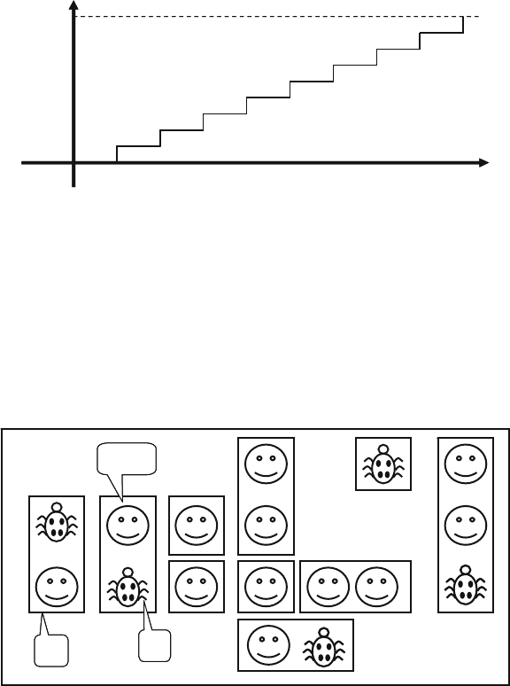
61 Verifi cation Guidelines
Neither of these situations is desirable. You need a methodology that fi nds bugs
faster in order to reach the goal of 100% coverage. Brute force does not work; if
you tried to verify every combination of inputs for a 32-bit adder, your simulations
would still be running years after the project should have shipped.
Figure 1.2 shows the total design space and features that are covered by directed
test cases. In this space there are many features, some of which have bugs. You need
to write tests that cover all the features and fi nd the bugs.
Test
Feature
Bug
TestTest
Feature
Bug
Feature
Bug
Fig. 1.2 Directed test coverage
Time
Coverage
100%
Fig. 1.1 Directed test progress over time
1.5 Methodology Basics
This book uses the following principles.
Constrained-random stimulus •
Functional coverage •
Layered testbench using transactors •
Common testbench for all tests •
Test case-specifi c code kept separate from testbench •
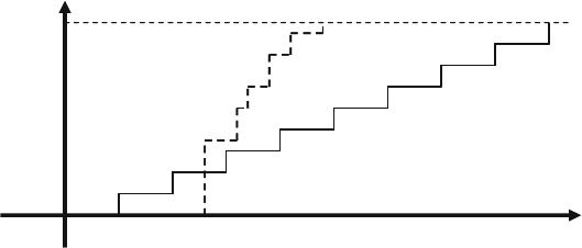
7
1.5 Methodology Basics
All these principles are related. Random stimulus is crucial for exercising
complex designs. A directed test fi nds the bugs you expect to be in the design,
whereas a random test can fi nd bugs you never anticipated. When using random
stimuli, you need functional coverage to measure verifi cation progress. Furthermore,
once you start using automatically generated stimuli, you need an automated way
to predict the results — generally a scoreboard or reference model. Building the
testbench infrastructure, including self-prediction, takes a signifi cant amount of
work. A layered testbench helps you control the complexity by breaking the prob-
lem into manageable pieces. Transactors provide a useful pattern for building these
pieces. With appropriate planning, you can build a testbench infrastructure that can
be shared by all tests and does not have to be continually modifi ed. You just need
to leave “hooks” where the tests can perform certain actions such as shaping
the stimulus and injecting disturbances. Conversely, code specifi c to a single test
must be kept separate from the testbench to prevent it from complicating the
infrastructure.
Building this style of testbench takes longer than a traditional directed
testbench — especially the self-checking portions. As a result, there may be a
signifi cant delay before the fi rst test can be run. This gap can cause a manager to
panic, so make this effort part of your schedule. In Fig.
1.3 , you can see the initial
delay before the fi rst random test runs.
Time
Coverage
100%
Random
Test Directed
Test
Fig. 1.3 Constrained-random test progress over time vs. directed testing
While this up-front work may seem daunting, the payback is high. Every random
test you create shares this common testbench, as opposed to directed tests where
each is written from scratch. Each random test contains a few dozen lines of code to
constrain the stimulus in a certain direction and cause any desired exceptions, such
as creating a protocol violation. The result is that your single constrained-random
testbench is now fi nding bugs faster than the many directed ones.
As the rate of discovery begins to drop off, you can create new random con-
straints to explore new areas. The last few bugs may only be found with directed
tests, but the vast majority of bugs will be found with random tests. If you create a
random testbench, you can always constrain it to created directed tests, but a directed
testbench can never be turned into a true random testbench.
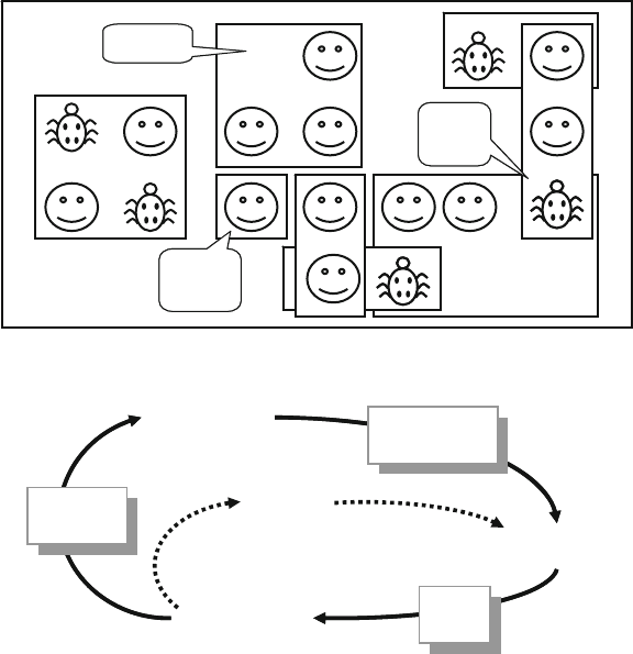
81 Verifi cation Guidelines
1.6 Constrained-Random Stimulus
Although you want the simulator to generate the stimulus, you don’t want totally
random values. You use the SystemVerilog language to describe the format of the
stimulus (“address is 32-bits; opcode is ADD, SUB or STORE; length < 32 bytes”),
and the simulator picks values that meet the constraints. Constraining the random
values to become relevant stimuli is covered in Chapter 6 . These values are sent into
the design, and are also sent into a high-level model that predicts what the result
should be. The design’s actual output is compared with the predicted output.
Figure 1.4 shows the coverage for constrained-random tests over the total design
space. First, notice that a random test often covers a wider space than a directed one.
This extra coverage may overlap other tests, or may explore new areas that you did
not anticipate. If these new areas fi nd a bug, you are in luck! If the new area is not
legal, you need to write more constraints to keep random generation from creating
illegal design functionality. Lastly, you may still have to write a few directed tests to
fi nd cases not covered by any other constrained-random tests.
Figure 1.5 shows the paths to achieve complete coverage. Start at the upper
left with basic constrained-random tests. Run them with many different seeds.
New area
?
Test
overlap
??
Directed
testcase
New area
?
Test
overlap
??
Directed
testcase
Fig. 1.4 Constrained-random test coverage
Constrained
random tests
Functional
Coverage
Many runs,
different seeds
Many runs,
different seeds
Identify
holes
Identify
holes
Add
constraints
Add
constraints
Minimal code
modifications
Directed
testcase
Many runs,
different seeds
Many runs,
different seeds
Identify
holes
Identify
holes
Add
constraints
Add
constraints
Directed
Fig. 1.5 Coverage convergence
9
1.7 What Should You Randomize?
When you look at the functional coverage reports, fi nd the holes where there are
gaps in the coverage. Then you make minimal code changes, perhaps by using new
constraints, or by injecting errors or delays into the DUT. Spend most of your time
in this outer loop, writing directed tests for only the few features that are very
unlikely to be reached by random tests.
1.7 What Should You Randomize?
When you think of randomizing the stimulus to a design, you might fi rst pick
the data fi elds. These values are is the easiest to create — just call $random () . The
problem is that this choice gives a very low payback in terms of bugs found. The
primary types of bugs found with random data are data path errors, perhaps with
bit-level mistakes. You need to fi nd bugs in the control logic, source of the most
devious problems.
Think broadly about all design inputs, such as the following.
Device confi guration •
Environment confi guration •
Input data •
Protocol exceptions •
Errors and violations •
Delays •
These are discussed in sections 1.7.1 through 1.7.4 .
1.7.1 Device and Environment Confi guration
What is the most common reason why bugs are missed during testing of the RTL
design? Not enough different confi gurations are tried. Most tests just use the design
as it comes out of reset, or apply a fi xed set of initialization vectors to put it into a
known state. This is like testing a PC’s operating system right after it has been
installed, but without any of the applications installed. Of course the performance is
fi ne and there aren’t any crashes.
In a real world environment, the DUT’s confi guration becomes more random the
longer it is in use. For example, I helped a company verify a time-division multi-
plexor switch that had 2000 input channels and 12 output channels. The verifi cation
engineer said, “These channels could be mapped to various confi gurations on the
other side. Each input could be used as a single channel, or further divided into
multiple channels. The tricky part is that although a few standard ways of breaking
it down are used most of the time, any combination of breakdowns is legal, leaving
a huge set of possible customer confi gurations.”
To test this device, the engineer had to write several dozen lines of directed test-
bench code to confi gure each channel. As a result, she was never able to try confi gura-
tions with more than a handful of channels. Together, we wrote a testbench that
10 1 Verifi cation Guidelines
randomized the parameters for a single channel and then put this in a loop to confi gure
all the switch’s channels. Now she had confi dence that her tests would uncover
confi guration-related bugs that would have been missed before.
In the real world, your device operates in an environment containing other compo-
nents. When you are verifying the DUT, it is connected to a testbench that mimics this
environment. You should randomize the entire environment confi guration, including
the length of the simulation, number of devices, and how they are confi gured.
Of course you need to create constraints to make sure the confi guration is legal.
In another Synopsys customer example, a company created an I/O switch chip
that connected multiple PCI buses to an internal memory bus. At the start of simula-
tion they randomly chose the number of PCI buses (1–4), the number of devices on
each bus (1–8), and the parameters for each device (master or slave, CSR addresses,
etc.). They kept track of the tested combinations using functional coverage so that
they could be sure that they had covered almost every possible one.
Other environment parameters include test length, error injection rates, and delay
modes. See Bergeron (2006) for more examples.
1.7.2 Input Data
When you read about random stimulus, you probably thought of taking a transac-
tion such as a bus write or ATM cell and fi lling the data fi elds with random values.
Actually, this approach is fairly straightforward as long as you carefully prepare
your transaction classes as shown in Chapters 5 and 8 . You need to anticipate any
layered protocols and error injection, plus scoreboarding and functional coverage.
1.7.3 Protocol Exceptions, Errors, and Violations
There are few things more frustrating than when a device such as a PC or cell phone
locks up. Many times, the only cure is to shut it down and restart. Chances are that
deep inside the product there is a piece of logic that experienced some sort of error
condition from which it could not recover and thus prevented the device from work-
ing correctly.
How can you prevent this from happening to the hardware you are building? If
something can go wrong in the real hardware, you should try to simulate it. Look at
all the errors that can occur. What happens if a bus transaction does not complete?
If an invalid operation is encountered? Does the design specifi cation state that two
signals are mutually exclusive? Drive them both and make sure the device continues
to operate properly.
Just as you are trying to provoke the hardware with ill-formed commands,
you should also try to catch these occurrences. For example, recall those mutually
11
1.7 What Should You Randomize?
exclusive signals. You should add checker code to look for these violations. Your
code should at least print a warning message when this occurs, and preferably gen-
erate an error and wind down the test. It is frustrating to spend hours tracking back
through code trying to fi nd the root of a malfunction, especially when you could
have caught it close to the source with a simple assertion. See Vijayaraghavan
[2005] for more guidelines on writing assertions in your testbench and design code.
Just make sure that you can disable the code that stops simulation on error so that
you can easily test error handling.
1.7.4 Delays and Synchronization
How fast should your testbench send in stimulus? You should pick random delays
to help catch protocol bugs. A test with the shortest delays is easy to write, but won’t
create all possible stimulus combinations. Subtle bugs around boundary conditions
are often revealed when realistic delays are chosen.
A block may function correctly for all possible permutations of stimulus from a
single interface, but subtle errors may occur when transactions are fl owing into
multiple inputs. Try to coordinate the various drivers so they can communicate at
different timing rates. What if the inputs arrive at the fastest possible rate, but the
output is being throttled back to a slower rate? What if stimulus arrives at multiple
inputs concurrently? What if it is staggered with different delays? Use functional
coverage, which will be discussed in Chapter 9 , to measure what combinations have
been randomly generated.
1.7.5 Parallel Random Testing
How should you run the tests? A directed test has a testbench that produces a unique
set of stimulus and response vectors. To change the stimulus, you need to change the
test. A random test consists of the testbench code plus a random seed. If you run the
same test 50 times, each time with a unique seed, you will get 50 different sets of
stimuli. Running with multiple seeds broadens the coverage of your test and lever-
ages your work.
You need to choose a unique seed for each simulation. Some people use the time
of day, but that can still cause duplicates. What if you are using a batch queuing
system across a CPU farm and tell it to start 10 jobs at midnight? Multiple jobs
could start at the same time but on different computers, and will thus get the same
random seed and run the same stimulus. You should blend in the processor name to
the seed. If your CPU farm includes multiprocessor machines, you could have two
jobs start running at midnight with the same seed, so you should also throw in the
process ID. Now all jobs get unique seeds.
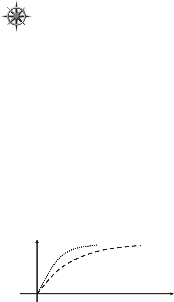
12 1 Verifi cation Guidelines
You need to plan how to organize your fi les to handle multiple
simulations. Each job creates a set of output fi les, such as log fi les
and functional coverage data. You can run each job in a different
directory, or you can try to give a unique name to each fi le. The easiest
approach is to append the random seed value to the directory name.
1.8 Functional Coverage
Sections 1.6 and 1.7 showed how to create stimuli that can randomly walk through
the entire space of possible inputs. With this approach, your testbench visits some
areas often, but takes too long to reach all possible states. Unreachable states will
never be visited, even given unlimited simulation time. You need to measure what
has been verifi ed in order to check off items in your verifi cation plan.
The process of measuring and using functional coverage consists of several
steps. First, you add code to the testbench to monitor the stimulus going into the
device, and its reaction and response, to determine what functionality has been
exercised. Run several simulations, each with a different seed. Next, merge the
results from these simulations into a report. Lastly, you need to analyze the results
and determine how to create new stimulus to reach untested conditions and logic.
Chapter 9 describes functional coverage in SystemVerilog.
1.8.1 Feedback from Functional Coverage to Stimulus
A random test evolves using feedback. The initial test can be run with many differ-
ent seeds, thus creating many unique input sequences. Eventually the test, even with
a new seed, is less likely to generate stimulus that reaches areas of the design space.
As the functional coverage asymptotically approaches its limit, you need to change
the test to fi nd new approaches to reach uncovered areas of the design. This is
known as “coverage-driven verifi cation” and is shown in Fig. 1.6 .
Time
Coverage
100%
Without
feedback
With
feedback
Fig. 1.6 Test progress with and without feedback
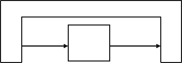
13
1.9 Testbench Components
What if your testbench were smart enough to do this for you? In a previous job,
I wrote a test that generated every bus transaction for a processor and additionally
fi red every bus terminator (Success, Parity Error, Retry) in every cycle. This was
before HVLs, so I wrote a long set of directed tests and spent days lining up the
terminator code to fi re at just the right cycles. After much hand analysis I declared
success — 100% coverage. Then the processor’s timing changed slightly! Now
I had to reanalyze the test and change the stimuli.
A more productive testing strategy uses random transactions and terminators.
The longer you run it, the higher the coverage. As a bonus, the test can be made
fl exible enough to create valid stimuli even if the design’s timing changed. You can
accomplish this by adding a feedback loop that looks at the stimulus created so far
(generated all write cycles yet?) and then change the constraint weights (drop write
weight to zero). This improvement would greatly reduce the time needed to get to
full coverage, with little manual intervention.
This is not a typical situation however, because of the trivial feedback from func-
tional coverage to the stimulus. In a real design, how should you change the stimu-
lus to reach a desired design state? This requires deep knowledge of the design and
powerful formal techniques. There are no easy answers, so dynamic feedback is
rarely used for constrained-random stimulus. Instead, you need to manually analyze
the functional coverage reports and alter your random constraints.
Feedback is used in formal analysis tools such as Magellan (Synopsys 2003).
It analyzes a design to fi nd all the unique, reachable states. It then runs a short simu-
lation to see how many states were visited. Lastly, it searches from the state machine
to the design inputs to calculate the stimulus needed to reach any remaining states
and then Magellan applies this to the DUT.
1.9 Testbench Components
In simulation, the testbench wraps around the DUT, just as a hardware tester con-
nects to a physical chip, as shown in Fig. 1.7 . Both the testbench and tester provide
stimulus and capture responses. The difference between them is that your testbench
needs to work over a wide range of levels of abstraction, creating transactions and
sequences, which are eventually transformed into bit vectors. A tester just works at
the bit level.
Testbench
Design
Under
Test
inputs outputs
Fig. 1.7 The testbench — design environment
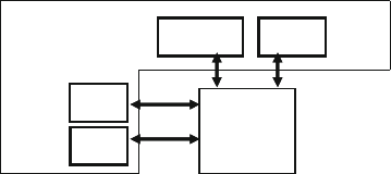
14 1 Verifi cation Guidelines
What goes into that testbench block? It is comprised of many Bus Functional
Models (BFM), which you can think of as testbench components — to the DUT
they look like real components, but they are part of the testbench, not the RTL
design. If the real device connects to AMBA, USB, PCI, and SPI buses, you have to
build equivalent components in your testbench that can generate stimulus and check
the response, as shown in Fig.
1.8 . These are not detailed, synthesizable models, but
instead highlevel transactors that obey the protocol, and execute more quickly. On
the other hand, if you are prototyping using FPGAs or emulation, the BFMs do need
to be synthesizable.
Testbench AMBA
SPI
Design
Under
Test
PCI
USB
Fig. 1.8 Testbench components
1.10 Layered Testbench
A key concept for any modern verifi cation methodology is the layered testbench.
Although this process may seem to make the testbench more complex, it actually
helps to make your task easier by dividing the code into smaller pieces that can be
developed separately. Don’t try to write a single routine that can randomly generate
all types of stimuli, both legal and illegal, plus inject errors with a multi-layer
protocol. The routine quickly becomes complex and unmaintainable. In addition, a
layered approach allows reuse and encapsulation of Verifi cation IP (VIP) which are
OOP concepts.
1.10.1 A Flat Testbench
When you fi rst learned Verilog and started writing tests, they probably looked like
the low-level code in Sample 1.1 , which does a simplifi ed APB (AMBA Peripheral
Bus) Write. (VHDL users may have written similar code).
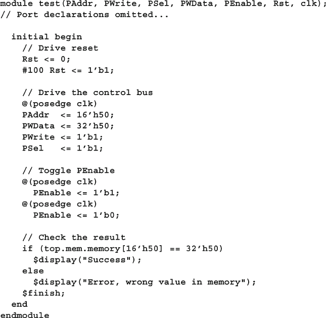
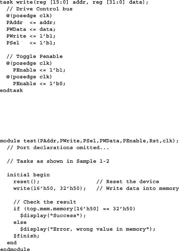
16 1 Verifi cation Guidelines
By taking the common actions (such as reset, bus reads and writes) and putting
them in a routine, you became more effi cient and made fewer mistakes. This cre-
ation of the physical and command layers is the fi rst step to a layered testbench.
Now your testbench became simpler, as shown in Sample 1.3
Sample 1.2 A task to drive the APB pins
Sample 1.3 Low-level Verilog test
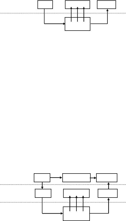
17
1.10 Layered Testbench
1.10.2 The Signal and Command Layers
Figure 1.9 shows the lower layers of a testbench.
DUT
AssertionsDriver Monitor
Command
Signal
Fig. 1.9 Signal and command layers
DUT
AssertionsDriver Monitor
Scoreboard CheckerAgent
Functional
Signal
Command
Agent
Fig. 1.10 Testbench with functional layer added
At the bottom is the signal layer that contains the design under test and the sig-
nals that connect it to the testbench.
The next higher level is the command layer. The DUT’s inputs are driven by the
driver that runs single commands, such as bus read or write. The DUT’s output
drives the monitor that takes signal transitions and groups them together into com-
mands. Assertions also cross the command/signal layer, as they look at individual
signals and also changes across an entire command.
1.10.3 The Functional Layer
Figure 1.10 shows the testbench with the functional layer added, which feeds down
into the command layer. The agent block (called the transactor in the VMM) receives
higher-level transactions such as DMA read or write and breaks them into individ-
ual commands or transactions. These commands are also sent to the scoreboard that
predicts the results of the transaction. The checker compares the commands from
the monitor with those in the scoreboard.
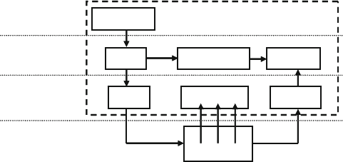
18 1 Verifi cation Guidelines
1.10.4 The Scenario Layer
The functional layer is driven by the generator in the scenario layer, as shown in
Fig.
1.11 . What is a scenario? Remember that your job as a verifi cation engineer is
to make sure that this device accomplishes its intended task. An example device is
an MP3 player that can concurrently play music from its storage, download new
music from a host, and respond to input from the user, such as adjusting the vol-
ume and track controls. Each of these operations is a scenario. Downloading a
music fi le takes several steps, such as control register reads and writes to set up the
operation, multiple DMA writes to transfer the song, and then another group of
reads and writes. The scenario layer of your testbench orchestrates all these steps
with constrained-random values for parameters such as track size and memory
location.
DUT
Assertions
Driver Monitor
Scoreboard Checker
Generator Environment
Agent
Scenario
Signal
Command
Functional Agent
Fig. 1.11 Testbench with scenario layer added
The blocks in the testbench environment (inside the dashed line of Fig. 1.11 ) are
written at the beginning of development. During the project they may evolve and
you may add functionality, but these blocks should not change for individual tests.
This is done by leaving “hooks” in the code so that a test can change the behavior
of these blocks without having to rewrite them. You create these hooks with factory
patterns (Section 8.2) and callbacks (Section 8.7).
1.10.5 The Test Layer and Functional Coverage
You are now at the top of the testbench, in the test layer, as shown in Fig. 1.12 .
Design bugs that occur between DUT blocks are harder to fi nd as they involve mul-
tiple people reading and interpreting multiple specifi cations.
This top-level test is the conductor: he does not play any musical instrument, but
instead guides the efforts of others. The test contains the constraints to create the
stimulus.
Functional coverage measures the progress of all tests in fulfi lling the verifi ca-
tion plan requirements. The functional coverage code changes through the project
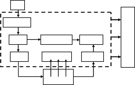
19
1.11 Building a Layered Testbench
as the various criteria complete. This code is constantly being modifi ed and thus it
is not part of the environment.
You can create a directed test in a constrained-random environment. Simply
insert a section of directed test code into the middle of a random sequence, or put
the two pieces of code in parallel. The directed code performs the work you want,
but the random “background noise” may cause a bug to become visible, perhaps in
a block that you never considered.
DUT
AssertionsDriver Monitor
Test
Scoreboard Checker
Generator
Functional Coverage
Environment
AgentAgent
Fig. 1.12 Full testbench with all layers
Do you need all these layers in your testbench? The answer depends on what
your DUT looks like. A complicated design requires a sophisticated testbench. You
always need the test layer. For a simple design, the scenario layer may be so simple
that you can merge it with the agent. When estimating the effort to test a design,
don’t count the number of gates; count the number of designers. Every time you add
another person to the team, you increase the chance of different interpretations of
the specifi cations. Typical hardware teams need more than two verifi cation engi-
neers for every designer.
You may need more layers. If your DUT has several protocol layers, each should
get its own layer in the testbench environment. For example, if you have TCP traffi c
that is wrapped in IP and sent in Ethernet packets, consider using three separate lay-
ers for generation and checking. Better yet, use existing verifi cation components.
One last note about Fig. 1.12 . It shows some of the possible connections between
blocks, but your testbench may have a different set. The test may need to reach
down to the driver layer to force physical errors. What has been described here is
just guidelines — let your needs guide what you create.
1.11 Building a Layered Testbench
Now it is time to take the preceding fi gures and learn how to map the components
into SystemVerilog constructs.
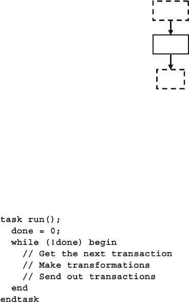
20 1 Verifi cation Guidelines
The driver shown in Fig. 1.13 receives commands from the agent. The driver
may inject errors or add delays. It then breaks the command down into individual
signal changes such as bus requests and handshakes. The general term for such a
testbench block is a “transactor,” which, at its core, is a loop. Sample code for a
transactor is shown in Sample 1.4 .
1.11.1 Creating a Simple Driver
First, take a closer look at one of the blocks, the driver.
Sample 1.4 Basic transactor code
DUT
Driver
Agent
Fig. 1.13 Connections for the driver
Chapter 5 presents basic OOP and how to create an object that includes the rou-
tines and data for a transactor. Another example of a transactor is the agent. It might
break apart a complex transaction such as a DMA read into multiple bus commands.
Also in Chapter 5 , you will see how to build an object that contains the data and
routines that make up a command. These objects are sent between transactors using
SystemVerilog mailboxes. In Chapter 7 , you will learn about many ways to exchange
data between the different layers and to synchronize the transactors.
1.12 Simulation Environment Phases
Up until now you have been learning what parts make up the environment. When do
these parts execute? You want to clearly defi ne the phases to coordinate the test-
bench so that all the code for a project works together. The three primary phases are
Build, Run, and Wrap-up. Each is divided into smaller steps. These three are a sub-
set of the many phases of the UVM and VMM.
21
1.13 Maximum Code Reuse
The Build phase is divided into the following steps:
• Generate confi guration : Randomize the confi guration of the DUT and the sur-
rounding environment.
• Build environment : Allocate and connect the testbench components based on the
confi guration. A testbench component is one that only exists in the testbench, as
opposed to physical components in the design that are built with RTL code. For
example, if the confi guration chose three bus drivers, the testbench would allo-
cate and initialize them in this step.
• Reset the DUT .
• Confi gure the DUT : Based on generated confi guration from the fi rst step, load
the DUT command registers.
The Run phase is where the test actually runs. It has the following steps:
• Start environment : Run the testbench components such as BFMs and stimulus
generators.
• Run the test : Start the test and then wait for it to complete. It is easy to tell when
a directed test has completed, but doing so can be complex for a random test. You
can use the testbench layers as a guide. Starting from the top, wait for a layer to
drain all the inputs from the previous layer (if any), wait for the current layer
to become idle, and then wait for the next lower layer. You should also use time-
out checkers to ensure that the DUT or testbench does not lock up.
The Wrap-up phase has two steps:
• Sweep : After the lowest layer completes, you need to wait for the fi nal transac-
tions to drain out of the DUT.
• Report : Once the DUT is idle, sweep the testbench for lost data. Sometimes the
scoreboard holds transactions that never came out, perhaps because they were
dropped by the DUT. Armed with this information, you can create the fi nal report
on whether the test passed or failed. If it failed, be sure to delete any functional
coverage results, as they may not be correct.
As shown in Fig.
1.12 , the test starts the environment, which, in turn, runs each of
the steps. More details can be found in Chapter 8 .
1.13 Maximum Code Reuse
To verify a complex device with hundreds of features, you have to write hundreds
of directed tests. If you use constrained-random stimulus, you would write fewer
tests. Instead, the real work is put into constructing the testbench, which contains all
the lower testbench layers: scenario, functional, command, and signal. This test-
bench code is used by all the tests, so it remains generic.
These guidelines appear to recommend an overly complicated testbench, but
remember that every line that you put into a testbench can eliminate a line in every
single test. If you know you will be creating a few dozen tests, there is a high pay-
22 1 Verifi cation Guidelines
back in making a more sophisticated testbench. Keep this in mind when you read
Chapter 8 .
1.14 Testbench Performance
If this is the fi rst time you have seen this methodology, you probably have some
qualms about how it works compared to directed testing. A common objection is
testbench performance. A directed test often simulates in a few seconds, whereas
constrained-random tests will wander around through the state space for minutes or
even hours. The problem with this argument is that it ignores a real verifi cation
bottleneck: the time required by you to create a test. You may be able to hand-craft
a directed test in a day and debug it and manually verify the results by hand in
another day or two. The actual simulation run time is dwarfed by the amount of time
that you personally invested.
There are several steps to creating a constrained-random test. The fi rst and most
signifi cant step is building the layered testbench, including the self-checking por-
tion. The benefi t of this work is shared by all tests, so it is well worth the effort. The
second step is creating the stimulus specifi c to a goal in the verifi cation plan. You
may be crafting random constraints, or devious ways of injecting errors or protocol
violations. Building one of these may take more time than making several directed
tests, but the payoff will be much higher. A constrained-random test that tries thou-
sands of different protocol variations is worth more than the handful of directed
tests that could have been created in the same amount of time.
The third step in constrained-random testing is functional coverage. This task
starts with the creation of a strong verifi cation plan with clear goals that can be easily
measured. Next you need to create the SystemVerilog code that adds instrumentation
to the environment and gathers the data. Finally, it is essential that you analyze the
results to determine if you have met the goals, and, if not, how you should modify
the tests.
1.15 Conclusion
The continuous growth in complexity of electronic designs requires a modern, sys-
tematic, and automated approach to creating testbenches. The cost of fi xing a bug
grows by tenfold as a project moves from each step of specifi cation to RTL coding,
gate synthesis, fabrication, and fi nally into the user’s hands. Directed tests only test
one feature at a time and cannot create the complex stimulus and confi gurations that
the device would be subjected to in the real world. To produce robust designs, you
must use constrained-random stimulus combined with functional coverage to create
the widest possible range of stimuli.
23
1.16 Exercises
1.16 Exercises
1. Write a verifi cation plan for an Arithmetic Logic Unit (ALU) with:
Asynchronous active high input reset •
Input clock •
4-bit signed inputs, A and B •
5-bit signed output C that is registered on the positive edge of input clock. •
4 opcodes•
Add: A + B –
Sub: A − B –
Bit-wise invert: A –
Reduction Or: B –
2. What are the advantages and disadvantages to testing at the block level? Why?
3. What are the advantages and disadvantages to testing at the system level? Why?
4. What are the advantages and disadvantages to directed testing? Why?
5. What are the advantages and disadvantages to constrained random testing? Why?
25
C. Spear and G. Tumbush, SystemVerilog for Verifi cation: A Guide to Learning
the Testbench Language Features, DOI 10.1007/978-1-4614-0715-7_2,
© Springer Science+Business Media, LLC 2012
SystemVerilog offers many improved data structures compared with Verilog. Some
of these were created for designers but are also useful for testbenches. In this chapter
you will learn about the data structures most useful for verifi cation.
System Verilog introduces new data types with the following benefi ts.
Two-state: better performance, reduced memory usage •
Queues, dynamic and associative arrays: reduced memory usage, built-in support •
for searching and sorting
Classes and structures: support for abstract data structures •
Unions and packed structures: allow multiple views of the same data •
Strings: built-in string support •
Enumerated types: code is easier to write and understand •
2.1 Built-In Data Types
Verilog-1995 has two basic data types: variables and nets, both which hold 4-state
values: 0, 1, Z, and X. RTL code uses variables to store combinational and sequen-
tial values. Variables can be unsigned single or multi-bit ( reg [7:0] m ), signed
32-bit variables ( integer ), unsigned 64-bit variables ( time ), and fl oating point
numbers ( real ). Variables can be grouped together into arrays that have a fi xed
size. A net is used to connect parts of a design such as gate primitives and module
instances. Nets come in many fl avors, but most designers use scalar and vector
wires to connect together the ports of design blocks. Lastly, all storage is static,
meaning that all variables are alive for the entire simulation and routines cannot use
a stack to hold arguments and local values. Verilog-2001 allows you to switch
between static and dynamic storage, such as stacks.
SystemVerilog adds many new data types to help both hardware designers and
verifi cation engineers.
Chapter 2
Data Types
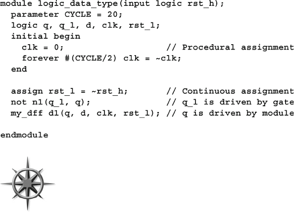
26 2 Data Types
2.1.1 The Logic Type
The one thing in Verilog that always leaves new users scratching their heads is the
difference between a
reg and a wire . When driving a port, which should you use?
How about when you are connecting blocks? SystemVerilog improves the classic
reg data type so that it can be driven by continuous assignments, gates, and mod-
ules, in addition to being a variable. It is given the synonym logic as some people
new to Verilog thought that reg declared a digital register, and not a signal. A logic
signal can be used anywhere a net is used, except that a logic variable cannot
be driven by multiple structural drivers, such as when you are modeling a bidirec-
tional bus. In this case, the variable needs to be a net type such as wire so that
SystemVerilog can resolve the multiple values to determine the fi nal value.
Sample 2.1 shows the SystemVerilog logic type.
Sample 2.1 Using the logic type
You can use the logic type to fi nd netlist bugs as this type can
only have a single driver. Rather than trying to choose between
reg and wire , declare all your signals as logic , and you’ll get a
compilation error if it has multiple drivers. Of course, any signal
that you do want to have multiple drivers, such as a bidirectional
bus, should be declared with a net type such as wire or tri .
2.1.2 2-State Data Types
SystemVerilog introduces several 2-state data types to improve simulator perfor-
mance and reduce memory usage, compared to variables declared as 4-state types.
The simplest type is the bit , which is always unsigned. There are four signed 2-state
types: byte, shortint, int , and longint . as shown in Sample 2.2 .
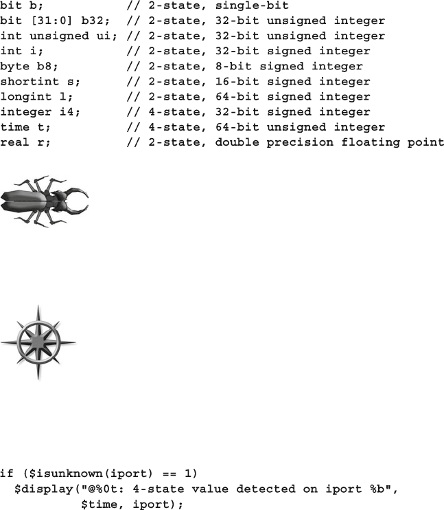
27
2.2 Fixed-Size Arrays
Sample 2.2 Signed data types
Sample 2.3 Checking for 4-state values
You might be tempted to use types such as byte to replace more
verbose declarations such as logic [7:0] . Hardware design-
ers should be careful as these new types are signed variables, so
a byte variable can only count up to 127, not the 255 you may
expect. (It has the range −128 to +127.) You could use byte unsigned, but that is
more verbose than just bit [7:0] . Signed variables can also cause unexpected
results with randomization, as discussed in Chapter 6 .
Be careful connecting 2-state variables to the design under test,
especially its outputs. If the hardware tries to drive an X or Z, these
values are converted to a 2-state value, and your testbench code
may never know. Don’t try to remember if they are converted to
0 or 1; instead, always check for propagation of unknown values.
Use the $isunknown() operator that returns 1 if any bit of the expression is X or Z,
as shown in Sample 2.3 .
The format %0t and the argument $time print the current simulation time, for-
matted as specifi ed with the $timeformat() routine. Time values are explored in
more detail in Section 3.7.
2.2 Fixed-Size Arrays
SystemVerilog offers several fl avors of arrays beyond the single-dimension, fi xed-
size Verilog-1995 arrays. Additionally, many new features have been added to sup-
port these data types.
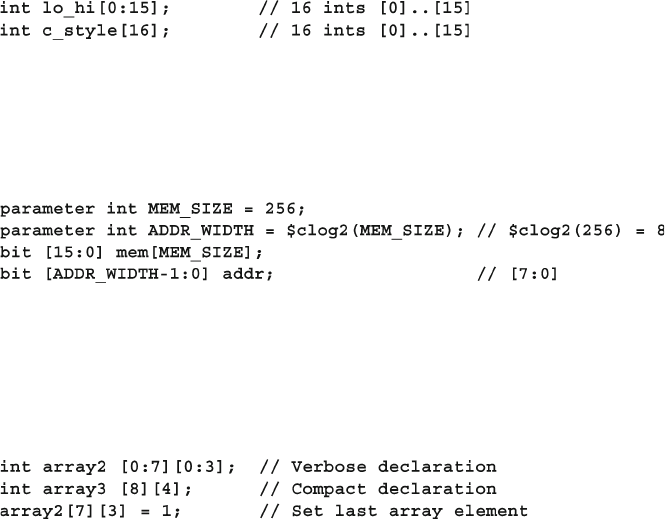
28 2 Data Types
2.2.1 Declaring and Initializing Fixed-Size Arrays
Verilog requires that the low and high array limits must be given in the declaration.
Since almost all arrays use a low index of 0, SystemVerilog lets you use the shortcut
of just giving the array size, which is similar to C’s style, as shown in Sample
2.4 .
Sample 2.6 Declaring and using multi-dimensional arrays
Sample 2.5 Calculating the address width for a memory
Sample 2.4 Declaring fi xed-size arrays
How can you compute the number of bits needed to address a given array size?
SystemVerilog has the $clog2() function that calculates the ceiling of log base 2,
as shown in Sample 2.5 .
You can create multi-dimensional fi xed-size arrays by specifying the dimensions
after the variable name. Sample 2.6 creates several two-dimensional arrays of inte-
gers, 8 entries by 4, and sets the last entry to 1. Multi-dimensional arrays were
introduced in Verilog-2001, but the compact declaration style is new.
If your code accidently tries to read from an out-of-bounds address, System-
Verilog will return the default value for the array element type. That just means
that an array of 4-state types, such as logic , will return X’s, whereas an array of
2-state types, such as int or bit , will return 0. This applies for all array types –
fi xed, dynamic, associative, or queue, and also if your address has an X or Z. An
undriven net is Z.
Many SystemVerilog simulators store each element on a 32-bit word boundary.
So a byte, shortint , and int are all stored in a single word, whereas a longint
is stored in two words.
An unpacked array, such as the one shown in Sample 2.7 , stores the values in the
lower portion of the word, whereas the upper bits are unused. The array of bytes,
b_unpack , is stored in three words, as shown in Fig. 2.1 .
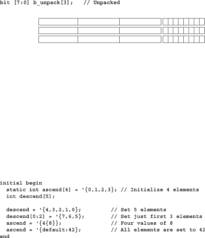
29
2.2 Fixed-Size Arrays
Sample 2.7 Unpacked array declarations
b_unpack[1]
234567
Unused space
b_unpack[2]
b_unpack[0] 01
01234567
01234567
Fig. 2.1 Unpacked array storage
Packed arrays are explained in Section 2.2.6 .
Simulators generally store 4-state types such as logic and integer in two or
more consecutive words, using twice the storage as 2-state variables.
2.2.2 The Array Literal
Sample 2.8 shows how to initialize an array using an array literal, which is an apos-
trophe followed by the values in curly braces. (This is not the accent grave used for
compiler directives and macros.) You can set some or all elements at once. You can
replicate values by putting a count before the curly braces.
Sample 2.8 Initializing an array
Notice that in Sample 2.8 , the declaration of the array ascend includes an initial
value. The 2009 LRM states that these variables must be declared either in a static
block, or have the
static keyword. Since this book recommends always declaring
your test modules and programs as automatic , you need to add the static key-
word to a declaration plus initialization when it is inside an initial block.
A great new feature in the 2009 LRM is printing with the %p format specifi er.
This prints an assignment pattern that is equivalent to the data object’s value. You can
print any data type in SystemVerilog including arrays, structures, classes, and more.
Sample
2.9 shows how to print an array with the %p format specifi er.
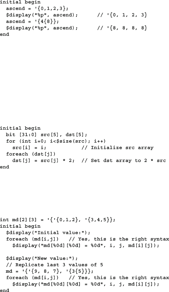
30 2 Data Types
2.2.3 Basic Array Operations — for and Foreach
The most common way to manipulate an array is with a for or foreach loop. In
Sample 2.10 , the variable i is declared local to the for loop. The SystemVerilog
function $size returns the size of the array. In the foreach loop, you specify the
array name and an index in square brackets, and SystemVerilog automatically steps
through all the elements of the array. The index variable is automatically declared
for you and is local to the loop.
Sample 2.10 Using arrays with for- and foreach loops
Sample 2.11 Initialize and step through a multi-dimensional array
Sample 2.9 Printing with %p print specifi e r
Note that in Sample 2.11 , the syntax of the foreach loop for multi-dimensional
arrays may not be what you expected. Instead of listing each subscript in separate
square brackets, [i][j] , they are combined with a comma: [i,j] .
The output from Sample 2.11 is shown in Sample 2.12 .
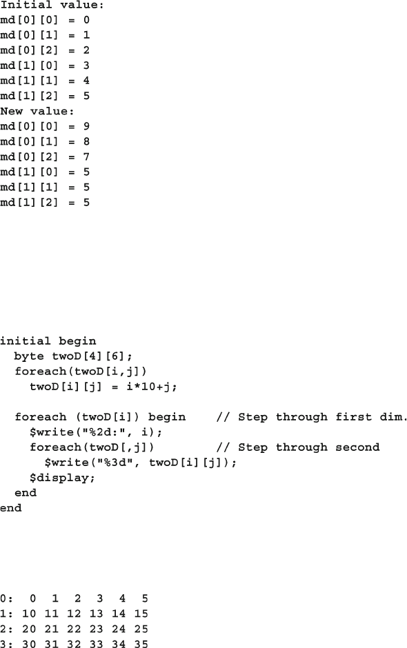
31
2.2 Fixed-Size Arrays
You can omit some dimensions in the foreach loop if you don’t need to step
through all of them. Sample 2.13 prints a two-dimensional array in a rectangle.
It steps through the fi rst dimension in the outer loop, and then through the second
dimension in the inner loop.
Sample 2.12 Output from printing multi-dimensional array values
Sample 2.13 Printing a multi-dimensional array
Sample 2.13 produces the output shown in Sample 2.14 .
Sample 2.14 Output from printing multi-dimensional array values
Lastly, a foreach loop iterates using the ranges in the original declaration. The
array f[5] is equivalent to f[0:4] , and a foreach (f[i]) is equivalent to for
(int i=0;i<=4; i++ ). With the array rev[6:2] , the statement foreach(rev[i] ) is
equivalent to for(int i=6; i>=2; i-- ).
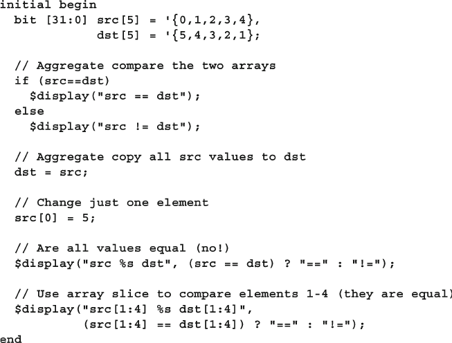
32 2 Data Types
2.2.4 Basic Array Operations – Copy and Compare
You can perform aggregate compare and copy of arrays without loops. (An aggregate
operation works on the entire array as opposed to working on just an individual
element.) Comparisons are limited to just equality and inequality. Sample
2.15 shows
several examples of compares. The ? : conditional operator is a mini if-else state-
ment. In Sample 2.15 , it is used to choose between two strings. The fi nal compare
uses an array slice, src[1:4] , which creates a temporary array with 4 elements.
Sample 2.15 Array copy and compare operations
A copy between fi xed arrays of different sizes causes a compile error. You can
not perform aggregate arithmetic such as addition or subtraction on arrays, for
example, a = b + c . Instead, use foreach loops. For logical operations such as xor ,
you have to either use a loop or use packed arrays as described in Section 2.2.6 .
2.2.5 Bit and Array Subscripts, Together at Last
A common annoyance in Verilog-1995 is that you cannot use array and bit sub-
scripts together. Verilog-2001 removes this restriction for fi xed-size arrays. Sample
2.16 prints the fi rst array element (binary 101), its lowest bit (1), and the next two
higher bits (binary 10).
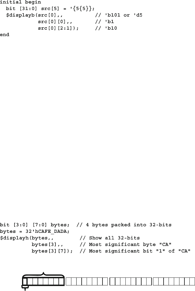
33
2.2 Fixed-Size Arrays
Although this change is not new to SystemVerilog, many users may not
know about this useful improvement in Verilog-2001. FYI - a double comma in a
$display statement inserts a space.
2.2.6 Packed Arrays
For some data types, you may want both to access the entire value and also to divide
it into smaller elements. For example, you may have a 32-bit register that sometimes
you want to treat as four 8-bit values and at other times as a single, unsigned value.
A SystemVerilog packed array is treated as both an array and a single value. It is
stored as a contiguous set of bits with no unused space, unlike an unpacked array.
2.2.7 Packed Array Examples
The packed bit and array dimensions are specifi ed as part of the type, before the
variable name. These dimensions must be specifi ed in the [msb:lsb] format, not
[size] . Sample 2.17 shows the variable bytes , a packed array of four bytes that
are stored in a single 32-bit word as shown in Fig. 2.2 .
Sample 2.16 Using word and bit subscripts together
Sample 2.17 Packed array declaration and usage
b
ytes 01234567
bytes[3]
012345670123456701234567
bytes[3][7]
Fig. 2.2 Packed array layout
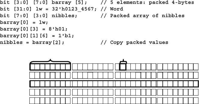
34 2 Data Types
You can mix packed and unpacked dimensions. You may want to make an array
that represents a memory that can be accessed as bits, bytes, or longwords. Sample
2.18 shows barray , an unpacked array of fi ve packed elements, each four bytes
wide, which are stored in memory as shown in Fig.
2.3 .
Sample 2.18 Declaration for a mixed packed/unpacked array
barray[0][3] barray[0][1][6]
b
array[1] 01234567012345670123456701234567
b
array[0] 01234567012345670123456701234567
barray[2] 01234567012345670123456701234567
barray[3] 01234567012345670123456701234567
b
array[4] 01234567012345670123456701234567
Fig. 2.3 Packed array bit layout
With a single subscript, you get a word of data, barray[0] .With two subscripts,
you get a byte of data, barray[0][3] . With three subscripts, you can access a
single bit, barray[0][1][6] . Because one dimension is specifi ed after the name,
barray[5] , that dimension is unpacked, so you must always give at least one
subscript.
The last line of Sample 2.18 copies between two packed arrays. Since the under-
lying values are just bits, you can copy even if the arrays have different dimensions.
2.2.8 Choosing Between Packed and Unpacked Arrays
Which should you choose — a packed or an unpacked array? A packed array is
handy if you need to convert to and from scalars. For example, you might need to
reference a memory as a byte or as a word. The barray in Fig. 2.3 can handle this
requirement. Any array type can be packed, including dynamic arrays, queues and
associative arrays, which are explained in Sections 2.3 , 2.4 , and 2.5 .
If you need to wait for a change in an array, you have to use a packed array.
Perhaps your testbench might need to wake up when a memory changes value, so
you want to use the @ operator. This is only legal with scalar values and packed
arrays. In Sample 2.18 you can block on the variables lw or barray[0] , but not the
entire array barray unless you expand it: @(barray[0] or barray[1] or
barray[2] or barray[3] or barray[4]) .
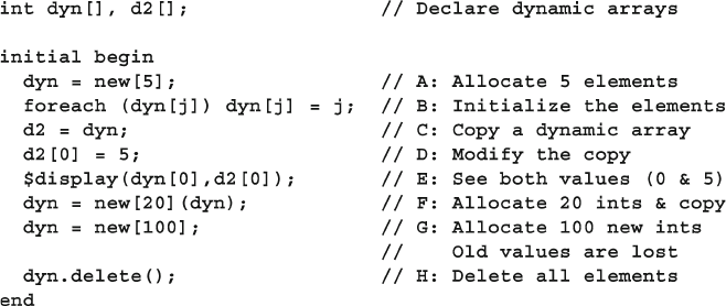
35
2.3 Dynamic Arrays
2.3 Dynamic Arrays
The basic Verilog array type shown so far is known as a fi xed-size array, as its size
is set at compile time. What if you do not know the size of the array until run time?
For example, you may want generate a random number of transactions at the start
of simulation. If you stored the transactions in a fi xed-size array, it would have to be
large enough to hold the maximum number of transactions, but would typically hold
far fewer, thus wasting memory. SystemVerilog provides a dynamic array that can
be allocated and resized during simulation so your simulation consumes a minimal
amount of memory.
A dynamic array is declared with empty word subscripts
[] . This means that you
do not specify the array size at compile time; instead, give it at run time. The array is
initially empty, so you must call the new[] constructor to allocate space, passing in
the number of entries in the square brackets. If you pass an array name to the new[]
constructor, the values are copied into the new elements, as shown in Sample 2.19 .
Sample 2.19 Using dynamic arrays
In Sample 2.19 , Line A calls new[5] to allocate 5 array elements. The dynamic
array dyn now holds 5 int’s . Line B sets the value of each element of the array to
its index value. Line C allocates another array and copies the contents of dyn into
it. Lines D and E show that the arrays dyn and d2 are separate. Line F allocates 20
new elements, and copies the existing 5 elements of dyn to the beginning of the
array. Then the old 5-element dyn array is deallocated. The result is that dyn points
to a 20-element array. The last call to new[] allocates 100 elements, but the existing
values are not copied. The old 20-element array is deallocated. Finally, line H
deletes the dyn array.
The $size function returns the size of a fi xed or dynamic array. Dynamic arrays
have several built-in routines, such as delete and size .
If you want to declare a constant array of values but do not want to bother counting
the number of elements, use a dynamic array with an array literal. In Sample 2.20
there are 9 mask elements of 8-bits each. You should let SystemVerilog count them,
rather than making a fi xed-size array and accidently choosing the wrong array size.
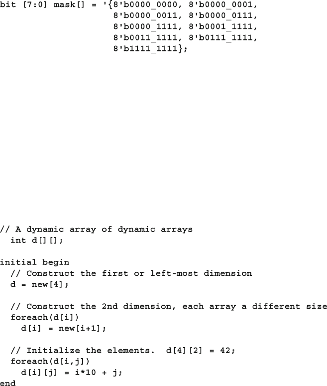
36 2 Data Types
You can make assignments between fi xed-size and dynamic arrays as long as
they have the same base type such as int . You can assign a dynamic array to a fi xed
array as long as they have the same number of elements.
When you copy a fi xed-size array to a dynamic array, SystemVerilog calls the
new[] constructor to allocate space, and then copies the values.
You can have multi-dimensional dynamic arrays, so long as you are careful when
constructing the sub-arrays. Remember, a multi-dimensional array in SystemVerilog
can be thought of as an array of other arrays. First you need to construct the left-
most dimension. Then construct the sub-arrays. In Sample 2.21 , each sub-array has
a different size.
Sample 2.20 Using a dynamic array for an uncounted list
Sample 2.21 Multi-dimensional dynamic array
2.4 Queues
SystemVerilog introduces a new data type, the queue, which combines the best of a
linked list and array. Like a linked list, you can add or remove elements anywhere
in a queue, without the performance hit of a dynamic array that has to allocate a new
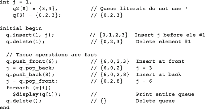
37
2.4 Queues
array and copy the entire contents. Like an array, you can directly access any ele-
ment with an index, without linked list’s overhead of stepping through the preced-
ing elements.
A queue is declared with word subscripts containing a dollar sign:
[$] . The ele-
ments of a queue are numbered from 0 to $. Sample 2.22 shows how you can add
and remove values from a queue using methods. Note that queue literals only have
curly braces, and are missing the initial apostrophe of array literals.
The SystemVerilog queue is similar to the Standard Template Library’s deque
data type. You create a queue by adding elements. SystemVerilog typically allocates
extra space so you can quickly insert additional elements. If you add enough ele-
ments that the queue runs out of that extra space, SystemVerilog automatically allo-
cates more. As a result, you can grow and shrink a queue without the performance
penalty of a dynamic array, and SystemVerilog keeps track of the free space for you.
Note that you never call the new[] constructor for a queue.
Sample 2.22 Queue methods
The LRM does not allow inserting a queue in another queue using the above
methods, though some simulators permit this.
You can use word subscripts and concatenation instead of methods. As a short-
cut, if you put a $ on the left side of a range, such as [$:2] , the $ stands for the
minimum value, [0:2] . A $ on the right side, as in [1:$] , stands for the maximum
value, [1:2] , in fi rst line of the initial block of Sample 2.23 .
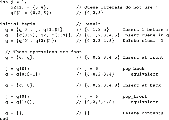
38 2 Data Types
The queue elements are stored in contiguous locations, so it is effi cient to push
and pop elements from the front and back. This takes a fi xed amount of time no
matter how large the queue. Adding and deleting elements in the middle of a queue
requires shifting the existing data to make room. The time to do this grows linearly
with the size of the queue.
You can copy the contents of a fi xed or dynamic array into a queue.
2.5 Associative Arrays
Dynamic arrays are good if you want to occasionally create a big array, but what if
you want something really large? Perhaps you are modeling a processor that has a
multi-gigabyte address range. During a typical test, the processor may only touch a
few hundred or thousand memory locations containing executable code and data, so
allocating and initializing gigabytes of storage is wasteful.
SystemVerilog offers associative arrays that store entries in a sparse matrix. This
means that while you can address a very large address space, SystemVerilog only
allocates memory for an element when you write to it. In the following picture, the
associative array holds the values 0:3, 42, 1000, 4521, and 200,000. The memory
used to store these is far less than would be needed to store a fi xed or dynamic array
with 200,000 entries, as shown in Figure 2.4 .
Sample 2.23 Queue operations
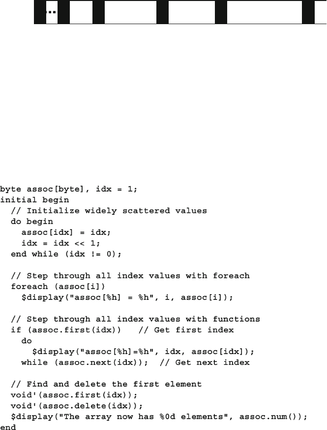
39
2.5 Associative Arrays
An associative array can be stored by the simulator as a tree or hash table. This
additional overhead is acceptable when you need to store arrays with widely sepa-
rated index values, such as packets indexed with 32-bit addresses or 64-bit data
values. An associative array is declared with a data type in square brackets, such as
[ int ]. or [ Packet ]. Sample 2.24 shows declaring, initializing, printing, and step-
ping through an associative array.
Sample 2.24 Declaring, initializing, and using associative arrays
data
0…..3 42 1000 4521 200,000
index
Fig. 2.4 Associative array
Sample 2.24 has the associative array, assoc, with very scattered elements: 1, 2,
4, 8, 16, etc. A simple for loop cannot step through them; you need to use a foreach
loop. If you want fi ner control, you can use the fi rst and next functions in a
do…while loop. These functions modify the index argument, and return 0 or 1
depending on whether any elements are left in the array. You can fi nd the number of
elements in an associative array with the num or size functions.
Associative arrays can also be addressed with a string index, similar to Perl’s
hash arrays. Sample 2.25 reads a fi le with strings and builds the associative array
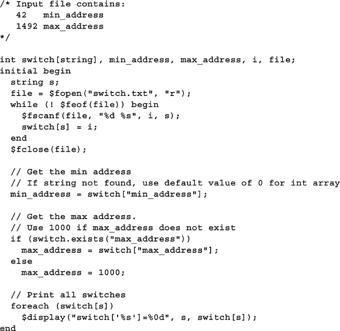
40 2 Data Types
switch so you can quickly map from a string value to a number. Strings are
explained in more detail in Section 2.15 .
If you try to read an element of an associative array that has not been written,
SystemVerilog returns the default value for the array base type, such as 0 for 2-state
types such as
bit or int , or X for 4-state types such as logic . The simulator may
also give a warning message. You can use the function exists() to check if an
element has been allocated, as shown in Sample 2.25 .
Sample 2.25 Using an associative array with a string index
You can initialize an associative array with the array literal with index:element
pairs as shown in Sample 2.26 . When you print the array with %p , the elements are
displayed in the same format.
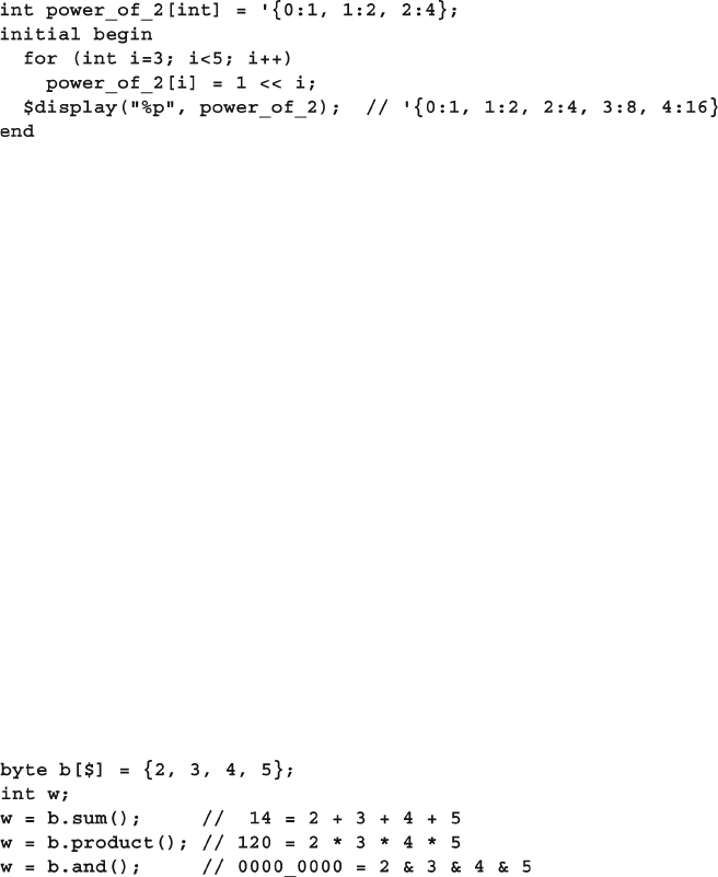
41
2.6 Array Methods
You can also declare an associative array with wildcard subscripts, as in wild[*].
However, this style is not recommended as you are allowing an index of almost any
data type. One of the many resulting problems is with foreach –loops: what type is
the variable j in foreach(wild[j] )? Integer, string, bit, or logic?
2.6 Array Methods
There are many array methods that you can use on any unpacked array types: fi xed,
dynamic, queue, and associative. These routines can be as simple as giving the cur-
rent array size or as complex as sorting the elements. The parentheses are optional
if there are no arguments.
2.6.1 Array Reduction Methods
A basic array reduction method takes an array and reduces it to a single value, as
shown in Sample 2.27 . You can calculate the sum, product, or perform a logical
operation on all the elements.
Sample 2.26 Initializing and printing associative arrays
Sample 2.27 Array reduction operations
Other array reduction methods are or , and xor .
SystemVerilog does not have a method specifi cally for choosing a random ele-
ment from an array, so use the index $urandom_range(array.size()−1) for
queues and dynamic arrays, and $urandom_range($size(array)−1) for fi xed
arrays, queues, dynamic and associative arrays. See Section 6.10 for more informa-
tion on $urandom_range .
If you need to choose a random element from an associative array, you need to step
through the elements one by one as there is no one-line way to access the N th element.
Sample 2.28 shows how to choose a random element from an associative array
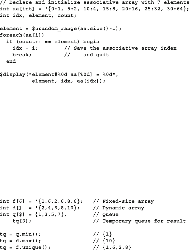
42 2 Data Types
indexed by integers by fi rst picking a random number, then stepping through the array.
If the array was indexed by a string, just change the type of idx to string .
Sample 2.29 Array locator methods: min, max, unique
Sample 2.28 Picking a random element from an associative array
2.6.2 Array Locator Methods
What is the largest value in an array? Does an array contain a certain value? The
array locator methods fi nd data in an unpacked array. At fi rst you may wonder why
these return a queue of values. After all, there is only one maximum value in an
array. However, SystemVerilog needs a queue for the case when you ask for a value
from an empty queue or dynamic array.
Sample 2.29 shows the array locator methods: min and max functions fi nd the
smallest and largest elements in an array. These methods also work for associative
arrays. The unique method returns a queue of the unique values from the array —
duplicate values are not included.
You could search through an array using a foreach loop, but SystemVerilog can
do this in one operation with a locator method. The with expression tells
SystemVerilog how to perform the search, as shown in Sample 2.30 . These methods
return an empty queue if the value you are searching for does not exist in the array.
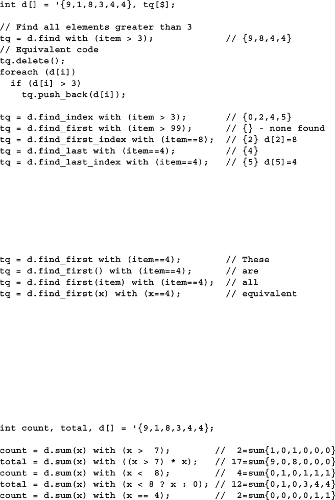
43
2.6 Array Methods
In a with clause, the name item is called the iterator argument and represents a
single element of the array. You can specify your own name by putting it in the argu-
ment list of the array method as shown in Sample 2.31 .
Sample 2.30 Array locator methods: fi n d
Sample 2.31 Declaring the iterator argument
Sample 2.32 Array locator methods
Sample 2.32 shows various ways to total up a subset of the values in the array.
The fi rst line compares the item with 7. This relational returns a 1 (true) or 0 (false)
so the calculation is a sum of the array {1,0,1,0,0,0}. The second multiplies the bool-
ean result with the array element being tested. So the total is the sum of {9,0,8,0,0,0},
which is 17. The third calculates the total of elements less than 8. The fourth total is
computed using the ? : conditional operator. The last counts the number of 4’s.
When you combine an array reduction such as sum using the with clause, the
results may surprise you. In Sample 2.32 , the sum operator totals the number of
44 2 Data Types
times that the expression is true. For the fi rst statement in Sample 2.32 , there are two
array elements that are greater than 7 (9 and 8) so count is set to 2.
The array locator methods that return an index, such as fi nd_
index , return a queue of type int , not integer . Your code
may not compile if you use the wrong queue type with these
statements.
Be careful of SystemVerilog’s rules for the width of operations.
Normally, if you were to add a set of single bit values, SystemVer-
ilog would make the calculations with enough precision not to
lose any bits. But the sum method uses the width of the array. So,
if you add the values of a single-bit array, the result is a single bit, which is probably
not what you expected. The solution is to use a with expression as shown in
Sample 2.33 .
Sample 2.34 Sorting an array
Sample 2.33 Creating the sum of an array of single bits
2.6.3 Array Sorting and Ordering
SystemVerilog has several methods for changing the order of elements in an array.
You can sort the elements, reverse their order, or shuffl e the order as shown in
Sample 2.34 . Notice that these change the original array, unlike the array locator
methods in Section
2.6.2 , which create a queue to hold the results.
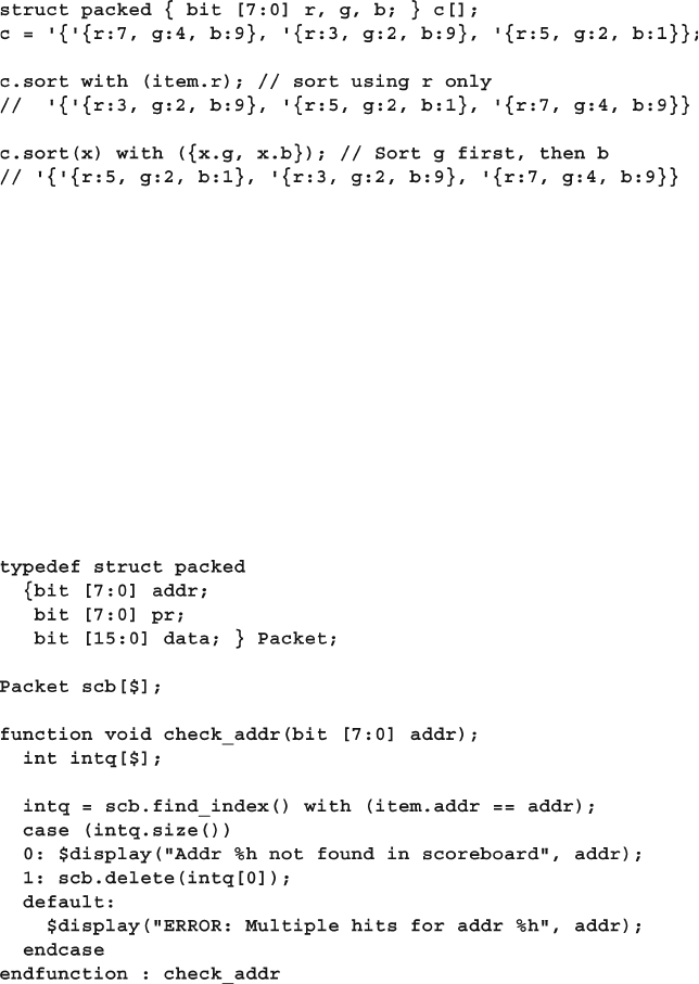
45
2.6 Array Methods
The reverse and shuffl e methods have no with -clause, so they work on the
entire array. Sample 2.35 shows how to sort a structure by sub-fi elds. Structures and
packed structures are explained in Section 2.9 .
Sample 2.35 Sorting an array of structures
Sample 2.36 A scoreboard with array methods
Only fi xed and dynamic arrays, plus queues can be sorted, reversed, or shuffl ed.
Associative arrays can not be reordered.
2.6.4 Building a Scoreboard with Array Locator Methods
The array locator methods can be used to build a scoreboard. Sample 2.36 defi nes
the Packet structure, then creates a scoreboard made from a queue of these struc-
tures. Section 2.8 describes how to create structures with typedef .
46 2 Data Types
The check_addr() function in Sample 2.36 looks up an address in the score-
board. The fi nd_index() method returns an int queue. If the queue is empty
(size==0), no match was found. If the queue has one member (size==1), a single
match was found, which the
check_addr() function deletes. If the queue has mul-
tiple members (size > 1), there are multiple packets in the scoreboard whose address
matching the requested one.
A better choice for storing packet information is a class, which is described in
Chapter 5 . You can read more about structures in Section 2.9 .
2.7 Choosing a Storage Type
Here are some guidelines for choosing the right storage type based on fl exibility,
memory usage, speed, and sorting. These are just rules of thumb, and results may
vary between simulators.
2.7.1 Flexibility
Use a fi xed-size or dynamic array if it is accessed with consecutive positive integer
indices: 0, 1, 2, 3… Choose a fi xed-size array if the array size is known at compile
time, or choose a dynamic array if the size is not known until run time. For example,
variable-size packets can easily be stored in a dynamic array. If you are writing
routines to manipulate arrays, consider using just dynamic arrays, as one routine
can work with any size dynamic array as long as the element types match: int,
string , etc. Likewise, you can pass a queue of any size into a routine as long as the
element type matches the queue argument. Associative arrays can also be passed
regardless of size. However, a routine with a fi xed-size array argument only accepts
arrays of the specifi ed length.
Choose associative arrays for nonstandard indices such as widely separated val-
ues because of random values or addresses. Associative arrays can also be used to
model content-addressable memories.
Queues are a good way to store values when the number of elements grows and
shrinks a lot during simulation, such as a scoreboard that holds expected values.
2.7.2 Memory Usage
If you want to reduce the simulation memory usage, use 2-state elements. You
should choose data sizes that are multiples of 32 bits to avoid wasted space.
Simulators usually store anything smaller in a 32-bit word. For example, an array of
1024 bytes wastes ¾ of the memory if the simulator puts each element in a 32-bit
word. Packed arrays can also help conserve memory.
47
2.7 Choosing a Storage Type
For arrays that hold up to a thousand elements, the type of array that you choose
does not make a big difference in memory usage (unless there are many instances of
these arrays). For arrays with a thousand to a million active elements, fi xed-size and
dynamic arrays are the most memory effi cient. You may want to reconsider your
algorithms if you need arrays with more than a million active elements.
Queues are slightly less effi cient to access than fi xed-size or dynamic arrays
because of additional pointers. However, if your data set grows and shrinks often,
and you store it in a dynamic memory, you will have to manually call
new[] to
allocate memory and copy. This is an expensive operation and would wipe out any
gains from using a dynamic memory.
Modeling memories larger than a few megabytes should be done with an associa-
tive array. Note that each element in an associative array can take several times more
memory than a fi xed-size or dynamic memory because of pointer overhead.
2.7.3 Speed
Choose your array type based on how many times it is accessed per clock cycle. For
only a few reads and writes, you could use any type, as the overhead is minor com-
pared with the DUT. As you use an array more often, its size and type matters.
Fixed-size and dynamic arrays are stored in contiguous memory, so any element
can be found in the same amount of time, regardless of array size.
Queues have almost the same access time as a fi xed-size or dynamic array for
reads and writes. The fi rst and last elements can be pushed and popped with almost
no overhead. Inserting or removing elements in the middle requires many elements
to be shifted up or down to make room. If you need to insert new elements into a
large queue, your testbench may slow down, so consider changing how you store
new elements.
When reading and writing associative arrays, the simulator must search for the
element in memory. The LRM does not specify how this is done, but popular ways
are hash tables and trees. These require more computation than other arrays, and
therefore associative arrays are the slowest.
2.7.4 Data Access
Since SystemVerilog can sort any single-dimension array (fi xed-size, dynamic, and
associative arrays plus queues), you should pick the array type based on how often
the values are added to it. If the values are received all at once, choose a fi xed-size
or dynamic array so that you only have to allocate the array once. If the data slowly
dribbles in, choose a queue, as adding new elements to the head or tail is very
effi cient.
If you have unique and noncontiguous values, such as ¢ {1, 10, 11, 50} , you
can store them in an associative array by using them as an index. Using the routines
48 2 Data Types
fi rst, next , and prev , you can search an associative array for a value and fi nd
successive values. Lists are doubly linked, so you can fi nd values both larger and
smaller than the current value. Both of these support removing a value. However,
the associative array is much faster in accessing any given element given an index.
For example, you can use an associative array of bits to hold expected 32-bit
values. When the value is created, write to that location. When you need to see if a
given value has been written, use the
exists function. When done with an element,
use delete to remove it from the associative array.
2.7.5 Choosing the Best Data Structure
Here are some suggestions on choosing a data structure.
• Network packets . Properties: fi xed size, accessed sequentially. Use a fi xed-size or
dynamic array for fi xed- or variable-size packets.
• Scoreboard of expected values . Properties: array size not known until run time,
accessed by value, and a constantly changing size. In general, use a queue, as you
are continually adding and deleting elements during simulation. If you can give
every transaction a fi xed ID, such as 1, 2, 3, …, you could use this as an index
into the queue. If your transaction is fi lled with random values, you can just push
them into a queue and search for unique values. If the scoreboard may have hun-
dreds of elements and you are often inserting and deleting them from the middle,
an associative array may be faster. If you model your transactions as objects, the
scoreboard can be a queue of handles. See Chapter 5 for more information of
classes.
• Sorted structures . Use a queue if the data comes out in a predictable order or an
associative array if the order is unspecifi ed. If the scoreboard never needs to be
searched, just store the expected values in a mailbox as shown in Section 7.6.
• Modeling very large memories, greater than a million entries . If you do not need
every location, use an associative array as a sparse memory. If you do plan on
accessing every location, try a different approach where you do not need so much
live data. Be sure to use 2-state values packed into 32-bits to conserve simulation
memory.
• Command names or opcodes from a fi le . Property: translate a string to a fi xed
value. Read string from a fi le, and then look up the commands or opcodes in an
associative array using the command as a string index.
2.8 Creating New Types with typedef
You can create new types using the typedef statement. For example, you may have
an ALU that can be confi gured at compile time to use 8, 16, 24, or 32-bit operands.
In Verilog you would defi ne a macro for the operand width and another for the type
as shown in Sample
2.37 .
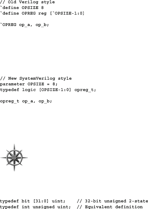
49
2.8 Creating New Types with typedef
You are not really creating a new type; you are just performing text substitution.
In SystemVerilog you create a new type as shown in Sample 2.38 . This book uses
the convention that user-defi ned types use the suffi x “ _t ” except for the basic uint .
Sample 2.37 User-defi ned type-macro in Verilog
Sample 2.39 Defi nition of uint
Sample 2.38 User-defi ned type in SystemVerilog
In general, SystemVerilog lets you copy between these basic types with no warning,
either extending or truncating values if there is a width mismatch.
Note that parameter and typedef statements can be put in a package so they
can be shared across the design and testbench, as shown in Section 2.10 .
One of the most useful types you can create is an unsigned, 2-state,
32-bit integer as shown in Sample 2.39 . Most values in a testbench are
positive integers such as fi eld length or number of transactions
received, and so having a signed integer can cause problems. Put the
defi nition of uint in a package of common defi nitions so it can be
used anywhere.
The syntax for defi ning a new array type is not obvious. You need to put the array
subscripts on the new name. Sample 2.40 creates a new type, fi xed_array5_t ,
a fi xed array with 5 elements. It then declares an array of this type and initializes it.
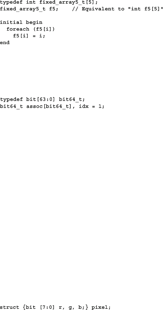
50 2 Data Types
A good use for a user defi ned type is an associative array, which must be declared
with an index that is a simple type. You could change Sample 2.24 to use 64 bit
values by changing the fi rst line as shown in Sample 2.41 .
Sample 2.40 User-defi ned array type
Sample 2.42 Creating a single pixel type
Sample 2.41 User-defi ned associative array index
2.9 Creating User-Defi ned Structures
One of the biggest limitations of Verilog is the lack of data structures. In SystemVer-
ilog you can create a structure using the struct statement, similar to what is avail-
able in C. However, a struct has just a subset of the functionality of a class, so use
a class instead for your testbenches, as shown in Chapter 5 . Just as a Verilog module
combines both data (signals) and code (always/initial blocks plus routines), a class
combines data and routines to make an entity that can be easily debugged and
reused. A struct just groups data fi elds together. Without the code that manipu-
lates the data, you are only creating half of the solution.
Since a struct is just a collection of data, it can be synthesized. If you want to
model a complex data type, such as a pixel, in your design code, put it in a struct .
This can also be passed through module ports. Eventually, when you want to gener-
ate constrained random data, look to classes.
2.9.1 Creating a Struct and a New Type
You can combine several variables into a structure. Sample 2.42 creates a structure
called pixel that has three unsigned bytes for red, green, and blue.
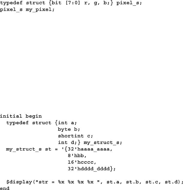
51
2.9 Creating User-Defi ned Structures
The problem with the preceding declaration is that it creates a single pixel of this
type. To be able to share pixels using ports and routines, you should create a new
type instead, as shown in Sample 2.43 .
Sample 2.43 The pixel struct
Sample 2.44 Initializing a struct
Use the suffi x “ _s ” when declaring a struct . This makes it easier to spot user-
defi ned types, simplifying the process of sharing and reusing code.
2.9.2 Initializing a Structure
You can assign multiple values to a struct just like an array, either in the declaration
or in a procedural assignment. Just surround the values with an apostrophe and
braces, as shown in Sample 2.44 .
2.9.3 Making a Union of Several Types
In hardware, the interpretation of a set of bits in a register may depend on the value
of other bits. For example, a processor instruction may have many layouts based on
the opcode. Immediate-mode operands might store a literal value in the operand
fi eld. This value may be decoded differently for integer instructions than for fl oating
point instructions. Sample 2.45 stores both the unsigned bit vector b and the integer i
in the same location.
52 2 Data Types
Use the suffi x “ _u ” when declaring a union.
Unions are useful when you frequently need to read and write a
register in several different formats. However, don’t go overboard,
especially just to save memory. Unions may help squeeze a few
bytes out of a structure, but at the expense of having to create and
maintain a more complicated data structure. Instead, make a class
with a discriminant variable, as shown in Section 8.4.4. This “kind”
variable indicates which type of transaction you have, and thus which fi elds to read,
write, and randomize. If you just need an array of values, plus all the bits, use a
packed array as described Section in 2.2.6
2.9.4 Packed Structures
SystemVerilog allows you more control in how bits are laid out in memory by using
packed structures. A packed structure is stored as a contiguous set of bits with no
unused space. The struct for a pixel in Sample 2.43 has three values, so it is stored
in three longwords, even though it only needs three bytes. You can specify that it
should be packed into the smallest possible space with the packed keyword, as
shown in Sample 2.46 .
Sample 2.45 Using typedef to create a union
Sample 2.46 Packed structure
Packed structures are used when the underlying bits represent a numerical value or
when you are trying to reduce memory usage. For example, you could pack together
several bit-fi elds to make a single register. Or you might pack together the opcode and
operand fi elds to make a value that contains an entire processor instruction.
2.9.5 Choosing Between Packed and Unpacked Structures
When you are trying to choose between packed and unpacked structures, consider
how the structure is most commonly used and the alignment of the elements. If you
plan on making aggregate operations on the structure, such as copying the entire
structure, a packed structure is more effi cient. However, if your code accesses
the individual members more than the entire structure, use an unpacked structure.
The difference in performance is greater if the elements are not aligned on byte
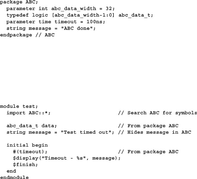
53
2.10 Packages
boundaries, have sizes that don’t match the typical byte, or have word instructions
used by processors. Reading and writing elements with odd sizes in a packed struc-
ture requires expensive shift and mask operations.
2.10 Packages
At the start of a project, you need to create new types and parameters. For example,
if your processor communicates with your company’s ABC bus, your testbench
needs to defi ne ABC data types, and parameters to specify the bus width and timing.
Another project may want to use these types, plus those for the XYZ bus.
You could create separate fi les for each bus and use the 'include statement to
bring in the fi les during compilation. But then every name associated with each bus
must be unique, even those that are internal variables, never intended to be visible.
How can you organize these types to avoid name confl icts?
The SystemVerilog package allows you to share declarations among modules,
packages, plus programs and interface, which are described in Chapter 4 . Sample
2.47 shows the package for the ABC bus.
Sample 2.48 Importing packages
Sample 2.47 Package for ABC bus
You import symbols from a package with the import statement. The compiler only
looks in imported packages when a symbol is not defi ned in the usual search path. In
Sample 2.48 , the fi rst import statement makes the symbols abc_data_width,
abc_data_t , and timeout visible if there is no local variable with the same name.
The variable message in ABC is hidden by the one in the module.
54 2 Data Types
If you really want to see the message variable in ABC, use ABC:: message .
You can import specifi c symbols from a package with the scope operator, ::.
Sample 2.49 imports all the symbols from ABC, plus just the timeout variable
from XYZ.
Sample 2.49 Importing selected symbols from a package
Packages can only see symbols defi ned inside themselves, or packages that they
import. You can not have hierarchical references to symbols such as signals, rou-
tines, or modules from outside the package. Think of a package as being completely
standalone, able to plug in where needed, with no outside dependencies.
A package can contain routines, plus classes, as shown in Section 5.4.
2.11 Type Conversion
SystemVerilog has several rules to ensure that expressions are evaluated with little
or no loss of accuracy. For example, if you add two 8-bit values, the addition is done
with 9-bit precision to avoid overfl ow. Multiply two 8-bit values, and SystemVerilog
calculates a 16-bit result.
The proliferation of data types in SystemVerilog means that you may need to
convert between them. If the layout of the bits between the source and destination
variables are the same, such as an integer and enumerated type, cast between the
two values. If the bit layouts differ, such as an array of bytes and words, use the
streaming operators to rearrange the bits as described in Section 2.12 .
2.11.1 The Static Cast
The static cast operation converts between two types with no checking of values.
You specify the destination type, an apostrophe, and the expression to be converted
as shown in Sample 2.50 . Note that Verilog has always implicitly converted between
types such as integer and real, and also between different width vectors.
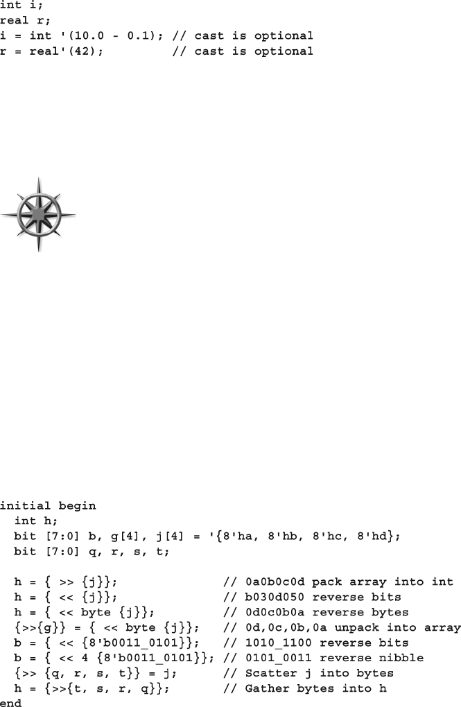
55
2.12 Streaming Operators
2.11.2 The Dynamic Cast
The dynamic cast, $cast , allows you to check for out-of-bounds values. See Section
2.13.3 for an explanation and example with enumerated types.
Use a static cast when you want SystemVerilog to use a type with
more precision, like when using the sum method for a single bit
array. Use the dynamic cast when converting from a type with a
larger number of values than the destination, such as int to an enu-
merated variable.
2.12 Streaming Operators
When used on the right side of an assignment, the streaming operators << and >>
take an expression, structure, or array, and packs it into a stream of bits. The >>
operator streams data from left to right while << streams from right to left, as shown
in Sample 2.51 . You can also give a slice size, used to break up the source before
being streamed. You can not assign the bit stream result directly to an unpacked
array. Instead, use the streaming operators on the left side of an assignment to
unpack the bit stream into an unpacked array.
Sample 2.51 Basic streaming operator
Sample 2.50 Converting between int and real with static cast
56 2 Data Types
You could do the same operations with many concatenation operators, {}, but
the streaming operators are more compact and easier to read.
If you need to pack or unpack arrays, use the streaming operator to convert
between arrays of different element sizes. For instance, you can convert an array of
bytes to an array of words. You can use fi xed size arrays, dynamic arrays, and
queues. Sample
2.52 converts between queues, but would also work with dynamic
arrays. Array elements are automatically allocated as needed.
Sample 2.52 Converting between queues with streaming operator
A common mistake when streaming between arrays is mis-
matched array subscripts. The word subscript [ 256 ] in an array
declaration is equivalent to [ 0:255 ], not [ 255:0 ]. Since many
arrays are declared with the word subscripts [ high:low ],
streaming them to an array with the subscript [ size ] would result in the elements
ending up in reverse order. Likewise, streaming an unpacked array declared as bit
[ 7:0 ] src[255:0] to the packed array declared as bit [ 7:0 ] [ 255:0 ] dst will
scramble the order of values. The correct declaration for a packed array of bytes is
bit [255:0] [7:0] dst .
You can also use the streaming operator to pack and unpack structures, such as
an ATM cell, into an array of bytes. In Sample 2.53 a structure is streamed into a
dynamic array of bytes, then the byte array is streamed back into the structure.
57
2.13 Enumerated Types
2.13 Enumerated Types
An enumerated type allows you to create a set of related but unique constants such
as states in a state machine or opcodes. In classic Verilog, you had to use text mac-
ros. Their global scope is too broad, and their value might not be visible in the
debugger. An enumeration creates a strongly typed variable that is limited to a set of
specifi ed names. For example, the names ADD, MOVE, or ROTW make your code
easier to write and maintain than if you had used literals such as 8 ' h01 or macros.
A weaker alternative for defi ning constants is a parameter. These are fi ne for indi-
vidual values, but an enumerated type automatically gives a unique value to every
name in the list.
The simplest enumerated type declaration contains a list of constant names and
one or more variables as shown in Sample 2.54 . This creates an anonymous enumer-
ated type, but it cannot be used for any other variables than the ones in this
declaration.
Sample 2.53 Converting between a structure and an array with streaming operators
Sample 2.54 A simple enumerated type, not recommended
58 2 Data Types
Use the suffi x “ _e ” when declaring an enumerated type name.
2.13.1 Defi ning Enumerated Values
The actual values default to int starting at 0 and then increase. You can choose your
own enumerated values. The code in Sample 2.56 uses the default value of 0 for
INIT , then 2 for DECODE , and 3 for IDLE .
Sample 2.55 Enumerated types, recommended style
Sample 2.56 Specifying enumerated values
Enumerated constants, such as INIT in Sample 2.56 , follow the same scoping
rules as variables. Consequently, if you use the same name in several enumerated
types (such as INIT in different state machines), they have to be declared in differ-
ent scopes such as modules, program blocks, packages, routines, or classes.
It is recommended to create a named enumerated type so you can declare
multiple variables of the same type, especially if these are used as routine argu-
ments or module ports. You fi rst create the enumerated type, and then the vari-
ables of this type, as shown in Sample 2.55 . You can get the string representation
of an enumerated variable with the built-in function name() .
59
2.13 Enumerated Types
An enumerated type is stored as int unless you specify other-
wise. Be careful when assigning values to enumerated constants,
as the default value of an int is 0. In Sample 2.57 , position is
initialized to 0, which is not a legal
ordinal_e variable. This
behavior is not a tool bug – it is how the language is specifi ed. So always specify an
enumerated constant with the value of 0, as shown in Sample 2.58 , just to catch the
testbench error.
Sample 2.57 Incorrectly specifying enumerated values
Sample 2.58 Correctly specifying enumerated values
2.13.2 Routines for Enumerated Types
SystemVerilog provides several functions for stepping through enumerated types.
• fi rst () returns the fi rst member of the enumeration.
• last() returns the last member of the enumeration.
• next() returns the next element of the enumeration.
• next (N) returns the N th next element.
• prev () returns the previous element of the enumeration.
• prev(N) returns the N th previous element.
The functions next and prev wrap around when they reach the beginning or end
of the enumeration.
Note that there is no clean way to write a for loop that steps through all members
of an enumerated type if you use an enumerated loop variable. You get the starting
member with fi rst function and the next member with next. A for loop ends when
the loop variable is outside the defi ned bounds, but the next function always returns
a value inside the enumeration. If you use the test current!= current.last() ,
the loop ends before using the last value. If you use current<=current. last () , you
get an infi nite loop, as next never gives you a value that is greater than the fi nal
value. This is similar to trying to make a for loop that steps through the values 0..3
with an index declared as bit [1:0] . The loop never exits! You can get around this
limitation by either using an integer variable in the loop, or incrementing the
enumerated variable, but both of these solutions can give illegal values if your
enumerated values are not contigious, such as 1, 2, 3, 5, 8.
You can use a do…while loop to step through all the values, checking when the
value wraps around, as shown in Sample 2.59 .
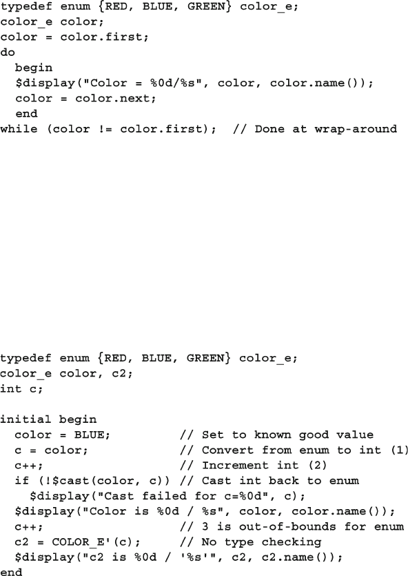
60 2 Data Types
2.13.3 Converting to and from Enumerated Types
The default type for an enumerated type is int (2-state). You can take the value of an
enumerated variable and assign it to a non-enumerated variable such as an int with
a simple assignment. SystemVerilog does not, however, let you store an integer value
in an enum without explicitly changing the type. Instead, it requires you to explicitly
cast the value to make you realize that you could be writing an out-of-bounds value.
Sample 2.59 Stepping through all enumerated members
Sample 2.60 Assignments between integers and enumerated types
When called as a function as shown in Sample 2.60 , $cast() tried to assign
the right value to the left variable. If the assignment succeeds, $cast() returns 1.
If the assignment fails because of an out-of-bounds value, no assignment is made
and the function returns 0. If you use $cast() as a task and the operation fails,
SystemVerilog prints an error.
You can also cast the value using the type ' (val) as shown in the example, but
this does not do any type checking, so the result may be out-of-bounds. For example,
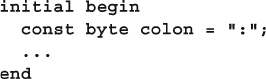
61
2.15 Strings
after the static cast in Sample 2.60 , c2 has an out-of-bounds value. You should avoid
this style of casting with enumerated types.
2.14 Constants
There are several types of constants in SystemVerilog. The classic Verilog way to
create a constant is with a text macro. On the plus side, macros have global scope
and can be used for bit fi eld defi nitions and type defi nitions. On the negative side,
macros are global, so that they can cause confl icts if you just need a local constant.
Lastly, a macro requires the ` character so that it is recognized and expanded by the
compiler.
A Verilog parameter was loosely typed and was limited in scope to a single
module. Verilog-2001 added typed parameters, but their limited scope kept param-
eters from being widely used. In SystemVerilog, parameters can be declared in a
package so they can be used across multiple modules. This approach can replace
most Verilog macros that were just being used as constants.
SystemVerilog also supports the const modifi er that allows you to make a vari-
able that can be initialized in the declaration but not written by procedural code.
Sample 2.61 Declaring a const variable
In Sample 2.61 , the value of colon is initialized at run time, when the initial
block is entered. In the next chapter, Sample 3.11 shows a const routine argument.
2.15 Strings
If you have ever tried to use a Verilog reg variable to hold a string of characters,
your suffering is over. The SystemVerilog string type holds variable-length
strings. An individual character is of type byte . The elements of a string of length
N are numbered 0 to N -1. Note that, unlike C, there is no null character at the end of
a string, and any attempt to use the character “\0” is ignored. Memory for strings is
dynamically allocated, so you do not have to worry about running out of space to
store the string.
Sample 2.62 shows various string operations. The function getc ( N ) returns the
byte at location N , while toupper returns an upper-case copy of the string and
tolower returns a lowercase copy. The curly braces {} are used for concatenation.
The task putc ( M , C ) writes a byte C into a string at location M , that must be between 0
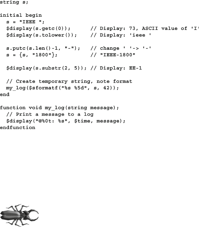
62 2 Data Types
and the length as given by len . The substr(start,end) function extracts
characters from location start to end .
Sample 2.62 String methods
Note how useful dynamic strings can be. In other languages such as C, you have
to keep making temporary strings to hold the result from a function. In Sample 2.62 ,
the $sformatf function is used instead of $sformat , from Verilog-2001. This new
function returns a formatted temporary string that, as shown above, can be passed
directly to another routine. This saves you from having to declare a temporary string
and passing it between the formatting statement and the routine call. The undocu-
mented function $psprintf has the same functionality as $sformatf , but is not in
the LRM, even though most vendors support this non-standard system function.
There are two ways to compare strings, but they behave differ-
ently. The equality operator, s1==s2 , returns 1 if the strings are
identical, and 0 if they are not. The string comparison function,
s1.compare(s2) , returns 1 if s1 is greater than s2, 0 if they are
equal, and −1 if s1 is less than s2. While this matches the ANSI C strcmp() behav-
ior, it may not be what you expect.
2.16 Expression Width
A prime source for unexpected behavior in Verilog has been the width of expres-
sions. Sample 2.63 adds 1+1 using four different styles. Addition A uses two 1-bit
variables, so with this precision 1+1=0. Addition B uses 8-bit precision because
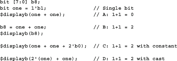
63
2.17 Conclusion
there is an 8-bit variable on the left side of the assignment. In this case, 1+1=2.
Addition C uses a dummy constant to force SystemVerilog to use 2-bit precision.
Lastly, in addition D, the fi rst value is cast to be a 2-bit value with the cast operator,
so 1+1=2.
Sample 2.63 Expression width depends on context
There are several tricks you can use to avoid this problem. First, avoid situations
where the overfl ow is lost, as in addition A. Use a temporary, such as b8 , with the
desired width. Or, you can add another value to force the minimum precision, such
as 2 ' b0 . Lastly, in SystemVerilog, you can cast one of the variables to the desired
precision.
2.17 Conclusion
SystemVerilog provides many new data types and structures so that you can create
high-level testbenches without having to worry about the bit-level representation.
Queues work well for creating scoreboards for which you constantly need to add
and remove data. Dynamic arrays allow you to choose the array size at run time for
maximum testbench fl exibility. Associative arrays are used for sparse memories and
some scoreboards with a single index. Enumerated types make your code easier to
read and write by creating groups of named constants.
Don’t go off and create a procedural testbench with just these constructs. Explore
the OOP capabilities of SystemVerilog in Chapter 5 to learn how to design code at
an even higher level of abstraction, thus creating robust and reusable code.
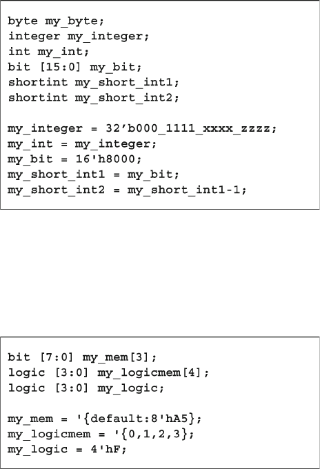
64 2 Data Types
2.18 Exercises
1. Given the following code sample:
a. What is the range of values my_byte can take?
b. What is the value of my_int in hex?
c. What is the value of my_bit in decimal?
d. What is the value of my_short_int1 in decimal?
e. What is the value of my_short_int2 in decimal?
2. Given the following code sample:
Evaluate the following statements in the given order and give the result for
each assignment
a . my_mem[2] = my_logicmem[4] ;
b . my_logic = my_logicmem[4] ;
c . my_logicmem[3] = my_mem[3] ;
d . my_mem[3] = my_logic ;
e . my_logic = my_logicmem[1] ;
f . my_logic = my_mem[1] ;
g . my_logic = my_logicmem[my_logicmem[41] ;
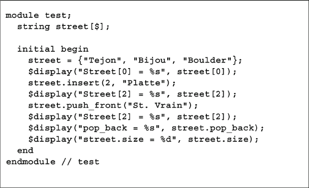
65
2.18 Exercises
3. Write the SystemVerilog code to:
a. Declare a 2-state array, my_array , that holds four 12-bit values
b. Initialize my_array so that:
* my_array[0] = 12 ' h012
* my_array[1] = 12 ' h345
* my_array[2] = 12 ' h678
* my_array[3] = 12 ' h9AB
c. Traverse my_array and print out bits [5:4] of each 12-bit element
* With a for loop
* With a foreach loop
4. Declare a 5 by 31 multi-dimensional unpacked array, my_array1 . Each element
of the unpacked array holds a 4-state value.
a. Which of the following assignment statements are legal and not out of bounds?
* my_array1[4][30] = 1 ' b1 ;
* my_array1[29][4] = 1 ' b1 ;
* my_array1[4] = 32 ' b1 ;
b . D r a w my_array1 after the legal assignments complete.
5. Declare a 5 by 31 multi-dimensional packed array, my_array2 . Each element of
the packed array holds a 2-state value.
a. Which of the following assignment statements are legal and not out of bounds?
* my_array2[4][30] = 1 ' b1 ;
* my_array2[29][4] = 1 ' b1 ;
* my_array2[3] = 32 ' b1 ;
b . D r a w my_array2 after the assignment statements complete.
6. Given the following code, determine what will be displayed.

66 2 Data Types
7. Write code for the following problems.
a. Create memory using an associative array for a processor with a word width of
24 bits and an address space of 2
20 words. Assume the PC starts at address 0 at
reset. Program space starts at 0´400. The ISR is at the maximum address.
b. Fill the memory with the following instructions:
* 24 ' hA50400; // Jump to location 0´400 for the main code
* 24 ' h123456; // Instruction 1 located at location 0´400
* 24 ' h789ABC; // Instruction 2 located at location 0´401
* 24 ' h0F1E2D; // ISR = Return from interrupt
c. Print out the elements and the number of elements in the array.
8. Create the SystemVerilog code for the following requirements
a. Create a 3-byte queue and initialize it with 2, −1, and 127
b. Print out the sum of the queue in the decimal radix
c. Print out the min and max values in the queue
d. Sort all values in the queue and print out the resulting queue
e. Print out the index of any negative values in the queue
f. Print out the positive values in the queue
g. Reverse sort all values in the queue and print out the resulting queue
9 . D e fi ne a user defi ned 7-bit type and encapsulate the fi elds of the following
packet in a structure using your new type. Lastly, assign the header to 7 ' h5A.
header datacmd crc
076131420
21
27
10. Create the SystemVerilog code for the following requirements
a. Create a user-defi ned type, nibble, of 4 bits
b. Create a real variable, r, and initialize it to 4.33
c. Create a short int variable, i_pack
d. Create an unpacked array, k, containing 4 elements of your user defi ned type
nibble and initialize it to 4 ' h0, 4 ' hF, 4 ' hE, and 4 ' hD
e. Print out k
f. Stream k into i_pack right to left on a bit basis and print it out
g. Stream k into i_pack right to left on a nibble basis and print it out
h. Type convert real r into a nibble, assign it to k[0], and print out k

67
2.18 Exercises
11. An ALU has the opcodes shown in Table 2.1 .
Write a testbench that performs the following tasks.
a. Create an enumerated type of the opcodes:
opcode_e
b. Create a variable, opcode , of type opcode_e
c. Loop through all the values of variable opcode every 10ns
d. Instantiate an ALU with one 2-bit input opcode
Table 2.1 ALU Opcodes
Opcode Encoding
Add: A + B 2 ' b00
Sub: A − B 2 ' b01
Bit-wise invert: A 2 ' b10
Reduction Or: B 2 ' b11
69
C. Spear and G. Tumbush, SystemVerilog for Verifi cation: A Guide to Learning
the Testbench Language Features, DOI 10.1007/978-1-4614-0715-7_3,
© Springer Science+Business Media, LLC 2012
As you verify your design, you need to write a great deal of code, most of which is in
tasks and functions. SystemVerilog introduces many incremental improvements to
make this easier by making the language look more like C, especially around argu-
ment passing. If you have a background in software engineering, these additions
should be very familiar.
3.1 Procedural Statements
SystemVerilog adopts many operators and statements from C and C++. You can
declare a loop variable inside a for loop that then restricts the scope of the loop
variable and can prevent some coding bugs. The new auto-increment ++ and auto-
decrement −− operators are available in both pre- and post-forms. The compound
assignments, +=, −=, ˆ=, and many more make your code tighter. If you have a label
on a begin or fork statement, you can put the same label on the matching end or
join statement. This makes it easier to match the start and fi nish of a block. You can
also put a label on other SystemVerilog end statements such as endmodule, end-
task, endfunction , and others that you will learn in this book. Sample 3.1 demon-
strates some of the new constructs.
Chapter 3
Procedural Statements and Routines
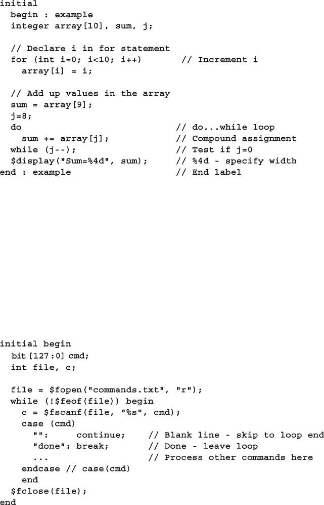
70 3 Procedural Statements and Routines
Two new statements help with loops. First, if you are in a loop, but want to skip
over the rest of the statements and do the next iteration, use continue . If you want
to leave the loop immediately, use break .
The compound assignment in Sample 3.1 is equivalent to sum = sum + array[j] ;
The loop in Sample 3.2 reads commands from a fi le using the fi le I/O system tasks
that are part of Verilog-2001. If the command is just a blank line, the code does a
continue , skipping any further processing of the command. If the command is
“ done ,” the code does a break to terminate the loop.
Sample 3.1 New procedural statements and operators
Sample 3.2 Using break and continue while reading a fi l e
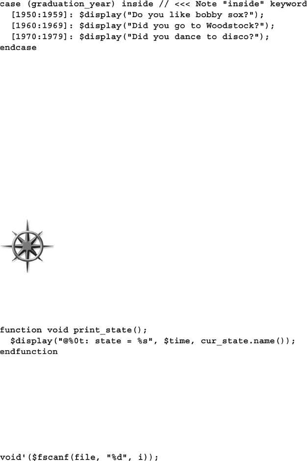
71
3.2 Tasks, Functions, and Void Functions
SystemVerilog expands the case statement so that you no longer have to give
every possible value, but can instead give a range values as shown in Sample 3.3 . This
is a version of the inside operator shown more in more detail in Section 6.4.5.
Sample 3.4 Void function for debug
Sample 3.3 Case-inside statement with ranges
3.2 Tasks, Functions, and Void Functions
Verilog makes a very clear differentiation between tasks and functions. The most
important difference is that a task can consume time whereas a function cannot.
A function cannot have a delay, #100 , a blocking statement such as @(posedge
clock) or wait (ready) , or call a task. Additionally, a Verilog function must
return a value and the value must be used, as in an assignment statement.
SystemVerilog relaxes this rule a little in that a function can call a task, but only in
a thread spawned with the fork… join_none statement, which is described in
Section 7.1.
If you have a SystemVerilog task that does not consume time, you
should make it a void function , which is a function that does not
return a value. Now it can be called from any task or function. For
maximum fl exibility, any debug routine should be a void function
rather than a task so that it can be called from any task or function.
Sample 3.4 prints values from a state machine.
In SystemVerilog, if you want to call a function and ignore its return value, cast the
result to void , as shown in Sample 3.5 . Some simulators, such as VCS, allow you to
ignore the return value without using the void syntax. The LRM says this should be
a warning.
Sample 3.5 Ignoring a function’s return value
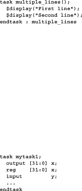
72 3 Procedural Statements and Routines
3.3 Task and Function Overview
SystemVerilog makes several small improvements to tasks and functions to make
them look more like C or C++ routines. In general, a routine defi nition or call with no
arguments does not need the empty parentheses (). This book includes them for added
clarity.
3.3.1 Routine Begin…End Removed
The fi rst improvement you may notice in SystemVerilog routines is that begin…end
blocks are optional, while Verilog-1995 required them on all but single-line routines.
The task / endtask and function / endfunction keywords are enough to
defi ne the routine boundaries, as shown in Sample 3.6 .
Sample 3.6 Simple task without begin…end
Sample 3.7 Verilog-1995 routine arguments
3.4 Routine Arguments
Many of the SystemVerilog improvements for routines make it easier to declare argu-
ments and expand the ways you can pass values to and from a routine.
3.4.1 C-style Routine Arguments
SystemVerilog and Verilog-2001 allow you to declare task and function arguments
more cleanly and with less repetition. The following Verilog task requires you to
declare some arguments twice: once for the direction, and once for the type, as shown
in Sample 3.7 .
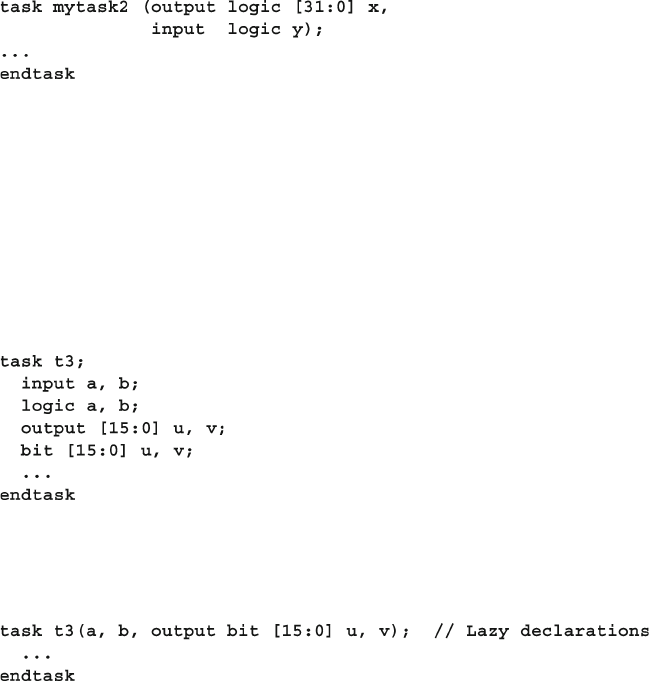
73
3.4 Routine Arguments
With SystemVerilog, you can use the less verbose C-style, shown in Sample 3.8 .
Note that you should use the universal input type of logic .
Sample 3.8 C-style routine arguments
3.4.2 Argument Direction
You can take even more shortcuts with declaring routine arguments. The direction
and type default to “input logic” and are sticky, so you don’t have to repeat these for
similar arguments. Sample 3.9 shows a routine header written using the Verilog-1995
style and SystemVerilog data types.
Sample 3.9 Verbose Verilog-style routine arguments
You could rewrite this as shown in Sample 3.10 .
Sample 3.10 Routine arguments with sticky types
The arguments a and b are input logic, 1-bit wide. The arguments u and v are
16-bit output bit types. Now that you know this, don’t depend on the defaults, as your
code will be infested with subtle and hard to fi nd bugs, as explained in Section 3.4.6 .
Always declare the type and direction for every routine argument.
3.4.3 Advanced Argument Types
Verilog had a simple way to handle arguments: an input or inout was copied to a
local variable at the start of the routine, whereas an output or inout was copied
when the routine exited. No memories could be passed into a Verilog routine, only
scalars.
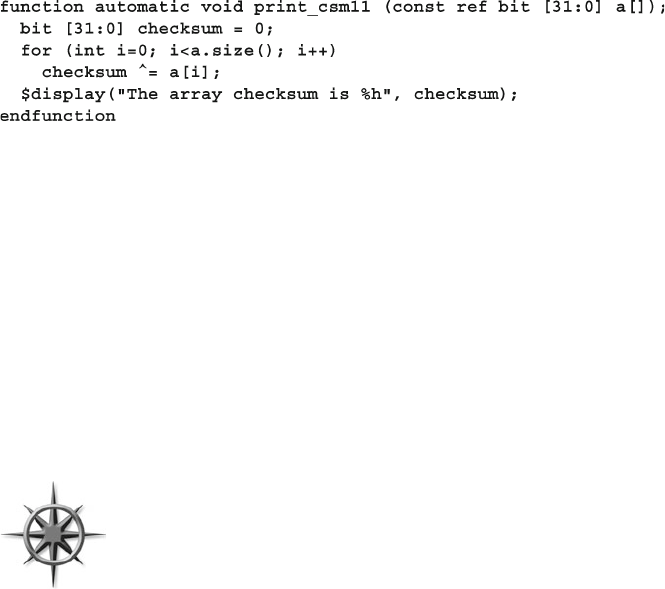
74 3 Procedural Statements and Routines
In SystemVerilog, you can specify that an argument is passed by reference, rather
than copying its value. This argument type, ref , has several benefi ts over input,
output , and inout . First, you can now pass an array into a routine, here one that
prints the checksum.
Sample 3.11 Passing arrays using ref and const
The = compound assignment in Sample 3.11 is a shorthand way of writing the
statement: checksum = checksum ^ a[i];
SystemVerilog allows you to pass array arguments without the ref direction, but
the array is copied onto the stack, an expensive operation for all but the smallest
arrays.
The SystemVerilog LRM states that ref arguments can only be used in routines
with automatic storage. If you specify the automatic attribute for programs and
module, all the routines inside are automatic. See Section 3.6 for more details on
storage.
Sample 3.11 also shows the const modifi er. As a result, the array a points to the
array in the routine call, but the contents of the array cannot be modifi ed. If you try to
change the contents, the compiler prints an error.
Always use ref when passing arrays to a routine for best perfor-
mance. If you don’t want the routine to change the array values, use
the const ref type, which causes the compiler to check that your
routine does not modify the array.
The second benefi t of ref arguments is that a task can modify a variable and is
instantly seen by the calling function. This is useful when you have several threads
executing concurrently and want a simple way to pass information. See Chapter 7 for
more details on using fork-join .
In Sample 3.12 , the thread2 block in the initial block can access the data from
memory as soon as enable is asserted, even though the bus_read task does
not return until the bus transaction completes, which could be several cycles later.
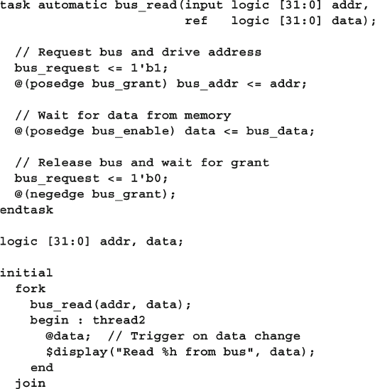
75
3.4 Routine Arguments
The data argument is passed as ref , and as a result, the @data statement triggers as
soon as data changes in the task. If you had declared data as output , the @data
statement would not trigger until the end of the bus transaction.
3.4.4 Default Value for an Argument
As your testbench grows in sophistication, you may want to add additional controls
to your code but not break existing code. For the function in Sample
3.11 , you might
want to print a checksum of just the middle values of the array. However, you don’t
want to go back and rewrite every call to add extra arguments. In SystemVerilog you
can specify a default value that is used if you leave out an argument in the call.
Sample
3.13 adds low and high arguments to the print_csm function so you can
print a checksum of a range of values.
Sample 3.12 Using ref across threads
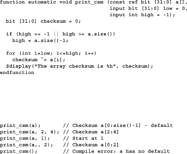
76 3 Procedural Statements and Routines
You can call this function in the following ways, as shown in Sample 3.14 . Note
that the fi rst call is compatible with both versions of the print_csm routine.
Sample 3.13 Function with default argument values
Sample 3.14 Using default argument values
Using a default value of −1 (or any out-of-range value) is a good way to see if the
call specifi ed a value.
A Verilog for loop always executes the initialization ( int i=low ), and test
( i<=high ) before starting the loop. Thus, if you accidently passed a low value that
was larger than high or the array size, the for loop would never execute the body.
3.4.5 Passing Arguments by Name
You may have noticed in the SystemVerilog LRM that the arguments to a task or func-
tion are sometimes called “ports,” just like the connections for a module. If you have
a task or function with many arguments, some with default values, and you only want
to set a few of those arguments, you can specify a subset by specifying the name of
the routine argument with a port-like syntax, as shown in Sample 3.15 .
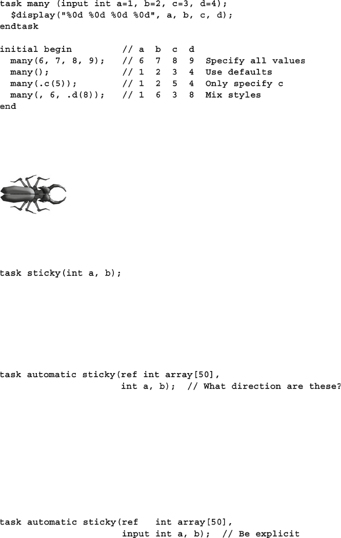
77
3.4 Routine Arguments
3.4.6 Common Coding Errors
The most common coding mistake that you are likely to make
with a routine is forgetting that the argument type is sticky with
respect to the previous argument, and that the default type for the
fi rst argument is a single-bit input. Start with the simple task
header in Sample 3.16 .
Sample 3.15 Binding arguments by name
Sample 3.16 Original task header
The two arguments are input integers. As you are writing the task, you realize that
you need access to an array, so you add a new array argument, and use the ref type
so it does not have to be copied. Your routine header now looks like Sample 3.17 .
Sample 3.17 Task header with additional array argument
What argument types are a and b? They take the direction of the previous argu-
ment that is a ref . Using ref for a simple variable such as an int is not usually
needed, but you would not get even a warning from the compiler, and thus would not
realize that you were using the wrong direction.
If any argument to your routine is something other than the default input type,
specify the direction for all arguments as shown in Sample 3.18 .
Sample 3.18 Task header with additional array argument
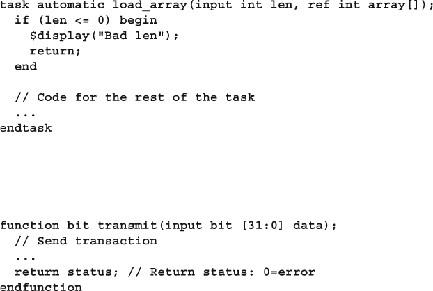
78 3 Procedural Statements and Routines
3.5 Returning from a Routine
Verilog had a primitive way to end a routine; after you executed the last statement in
a routine, it returned to the calling code. In addition, a function returned a value by
assigning that value to a variable with the same name as the function.
3.5.1 The Return Statement
SystemVerilog adds the return statement to make it easier for you to control the
fl ow in your routines. The task in Sample 3.19 needs to return early because of error
checking. Otherwise, it would have to put the rest of the task in an else clause,
which would cause more indentation and be more diffi cult to read.
Sample 3.19 Return in a task
Sample 3.20 Return in a function
The return statement in Sample 3.20 can simplify your functions.
3.5.2 Returning an Array from a Function
Verilog routines could only return a simple value such as a bit, integer, or vector. If
you wanted to compute and return an array, there was no simple way. In System
Verilog, a function can return an array, using several techniques.
The fi rst way is to defi ne a type for the array, and then use that in the function
declaration. Sample 3.21 uses the array type from Sample 2.40, and creates an func-
tion to initialize the array.
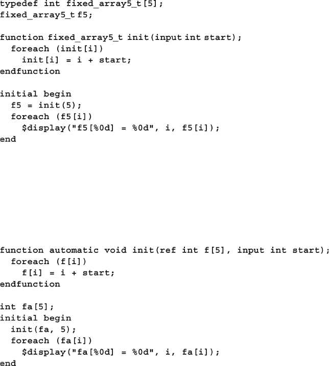
79
3.6 Local Data Storage
One problem with the preceding code is that the function init creates an array,
which is copied into the array f5. If the array was large, this could be a large perfor-
mance problem.
The alternative is to pass the routine by reference. The easiest way is to pass the
array into the function as a ref argument, as shown in Sample 3.22 .
Sample 3.21 Returning an array from a function with a typedef
Sample 3.22 Passing an array to a function as a ref argument
The last way for a function to return an array is to wrap the array inside of a class,
and return a handle to an object. Chapter 5 describes classes, objects, and handles.
3.6 Local Data Storage
When Verilog was created in the 1980s, it was tightly tied to describing hardware. As
a result, all objects in the language were statically allocated. In particular, routine
arguments and local variables were stored in a fi xed location, rather than pushing
them on a stack like other programming languages. Why try to model dynamic code
such as a recursive routine when there is no way to build this in silicon? However,
software engineers verifying the designs, who were used to the behavior of stack-
based languages such as C, were bitten by these subtle bugs, and were thus limited in
their ability to create complex testbenches with libraries of routines.
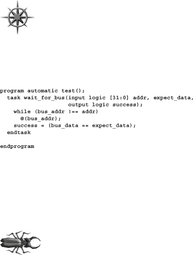
80 3 Procedural Statements and Routines
3.6.1 Automatic Storage
In Verilog-1995, if you tried to call a task from multiple places in your testbench, the
local variables shared common, static storage, and so the different threads stepped on
each other’s values. In Verilog-2001 you can specify that tasks, functions, and mod-
ules use automatic storage, which causes the simulator to use the stack for local
variables.
In SystemVerilog, routines still use static storage by default, for both
modules and program blocks. You should always make program
blocks (and their routines) use automatic storage by putting the
automatic keyword in the program statement. In Chapter 4 you
will learn about program blocks that hold the testbench code.
Section 7.1.6 shows how automatic storage helps when you are cre-
ating multiple threads.
Sample 3.23 shows a task to monitor when data are written into memory.
Sample 3.23 Specifying automatic storage in program blocks
You can call this task multiple times concurrently, as the addr and expect_data
arguments are stored separately for each call. Without the automatic modifi er, if you
called wait_f or_bus a second time while the fi rst was still waiting, the second call
would overwrite the two arguments.
3.6.2 Variable Initialization
A similar problem occurs when you try to initialize a local vari-
able in a declaration, as it is actually initialized before the start of
simulation. The general solution is to avoid initializing a variable
in a declaration to anything other than a constant. Use a separate
assignment statement to give you better control over when initial-
ization is done.
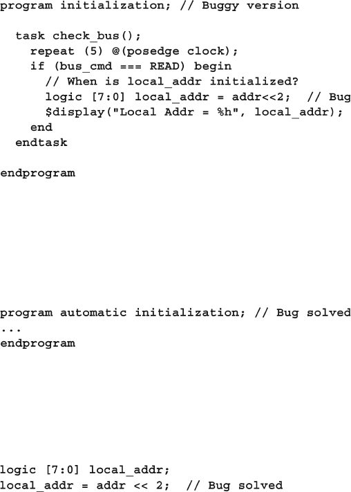
81
3.7 Time Values
The task in Sample 3.24 looks at the bus after fi ve cycles and then creates a local
variable and attempts to initialize it to the current value of the address bus.
Sample 3.24 Static initialization bug
Sample 3.25 Static initialization fi x: use automatic
The bug is that the variable local_addr is statically allocated, so it is actually ini-
tialized at the start of simulation, not when the begin…end block is entered. Once
again, the solution is to declare the program as automatic as shown in Sample 3.25 .
Additionally, you can avoid this by never initializing a variable in the declaration,
but this is harder to remember, especially for C programmers. Sample 3.26 show the
recommended style of separating the declaration and initialization.
Sample 3.26 Static initialization fi x: break apart declaration and initialization
3.7 Time Values
SystemVerilog has several new constructs to allow you to unambiguously specify
time values in your system.
3.7.1 Time Units and Precision
When you rely on the ` timescale compiler directive, you must compile the fi les in
the proper order to be sure all the delays use the proper scale and precision. One way
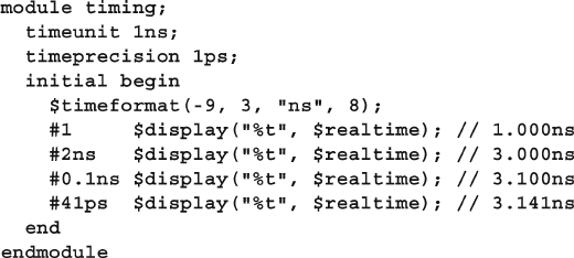
82 3 Procedural Statements and Routines
avoiding this compilation ordering problem is to require that every fi le that starts
with a ` timescale compiler directive should end with one that resets it back to a
company-specifi c default such as 1ns/1ns.
The timeunit and timeprecision declarations eliminate this ambiguity by
precisely specifying the values for every module. Sample 3.27 shows these declara-
tions. Note that if you use these instead of `
timescale , you must put them in every
module that has a delay. See the LRM for more on these declarations.
3.7.2 Time Literals
SystemVerilog allows you to unambiguously specify a time value plus units. Your
code can use delays such as 0.1ns or 20ps . Just remember to use timeunit and
timeprecision or ` timescale . You can make your code even more time aware by
using the classic Verilog $timeformat(), $time , and $realtime system tasks.
The four arguments to $timeformat are the scaling factor (−9 for nanoseconds, −12
for picoseconds), the number of digits to the right of the decimal point, a string to
print after the time value, and the minimum fi eld width.
Sample 3.27 shows various delays and the result from printing the time when it is
formatted by $timeformat() and the %t specifi er.
Sample 3.27 Time literals and $timeformat
3.7.3 Time and Variables
You can store time values in variables and use them in calculations and delays. The
values are scaled and rounded according to the current time scale and precision.
Variables of type time cannot hold fractional delays as they are just 64-bit integers,
so delays will be rounded. You should use realtime variables if this is a problem.
Sample 3.28 shows how realtime variables are rounded when used as a delay.
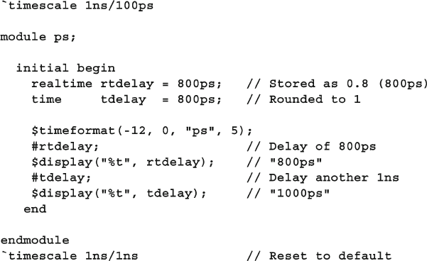
83
3.9 Exercises
3.7.4 $time vs. $realtime
The system task $time returns an integer scaled to the time unit of the current mod-
ule, but missing any fractional units, while $realtime returns a real number with
the complete time value, including fractions. This book uses $time in the examples
for brevity, but your testbenches may need to use $realtime .
3.8 Conclusion
The new SystemVerilog procedural constructs and task/function features make it
easier for you to create testbenches by making the language look more like other
programming languages such as C/C++. As a bonus, SystemVerilog has additional
HDL constructs such as timing controls, simple thread control, and 4-state logic.
3.9 Exercises
1. Create the SystemVerilog code with the following requirements:
a. Create a 512 element integer array
b. Create a 9-bit address variable to index into the array
c. Initialize the last location in the array to 5
d. Call a task, my_task() , and pass the array and the address
Sample 3.28 Time variables and rounding
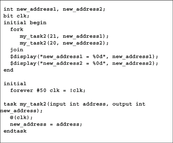
84 3 Procedural Statements and Routines
e. Create my_task() that takes two inputs: a constant 512-element integer array
passed by reference, and a 9-bit address. The task calls a function, print_
int() , and passes the array element indexed by the address, pre-decrementing
the address.
f. Create print_int() that prints out the simulation time and the value of the
input. The function has no return value.
2. For the following SystemVerilog code, what is displayed if the task
my_task2()
is automatic?
3. For the same SystemVerilog code in Exercise 2, what is displayed if the task my_
task2() is not automatic?
4. Create the SystemVerilog code to specify that the time should be printed in ps
(picoseconds), display 2 digits to the right of the decimal point, and use as few
characters as possible
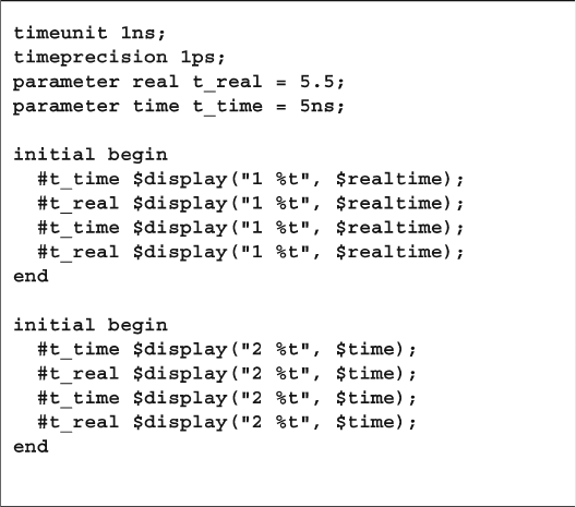
85
3.9 Exercises
5. Using the formatting system task from Exercise 4, what is displayed by the
following code?
87
C. Spear and G. Tumbush, SystemVerilog for Verifi cation: A Guide to Learning
the Testbench Language Features, DOI 10.1007/978-1-4614-0715-7_4,
© Springer Science+Business Media, LLC 2012
There are several steps needed to verify a design: generate stimulus, capture
responses, determine correctness, and measure progress. However, fi rst you need
the proper testbench, connected to the design, as shown in Fig. 4.1 .
Your testbench wraps around the design, sending in stimulus and capturing the
design’s response. The testbench forms the “real world” around the design, mimick-
ing the entire environment. For example, a processor model needs to connect to
various buses and devices, which are modeled in the testbench as bus functional
models. A networking device connects to multiple input and output data streams that
are modeled based on standard protocols. A video chip connects to buses that send
in commands, and then forms images that are written into memory models. The key
concept is that the testbench simulates everything not in the design under test.
Your testbench needs a higher-level way to communicate with the design than
Verilog’s ports and the error-prone pages of connections. You need a robust way to
describe the timing so that synchronous signals are always driven and sampled at
the correct time and all interactions are free of the race conditions so common to
Verilog models.
Chapter 4
Connecting the Testbench and Design
Testbench
Design
Under
Test
inputs outputs
Fig. 4.1 The testbench – design environment
88 4 Connecting the Testbench and Design
4.1 Separating the Testbench and Design
In an ideal world, all projects have two separate groups: one to create the design and
one to verify it. In the real world, limited budgets may require you to wear both hats.
Each team has its own set of specialized skills, such as creating synthesizable RTL
code, or fi guring out new ways to fi nd bugs in the design. These two groups each
read the original design specifi cation and make their own interpretations. The
designer has to create code that meets that specifi cation, whereas your job as the
verifi cation engineer is to create scenarios where the design does not match its
description.
Likewise, your testbench code is in a separate block from design code. In classic
Verilog, each goes in a separate module. However, using a module to hold the test-
bench often causes timing problems around driving and sampling, so SystemVerilog
introduces the program block to separate the testbench, both logically and tempo-
rally. For more details, see Section
4.3 .
As designs grow in complexity, the connections between the blocks increase.
Two RTL blocks may share dozens of signals, which must be listed in the correct
order for them to communicate properly. One mismatched or misplaced connection
and the design will not work. You can reduce errors by using the connect-by-name
syntax, but this more than doubles your typing burden. If it is a subtle error, such as
swapping pins that only toggle occasionally, you may not notice the problem for
some time. Worse yet is when you add a new signal between two blocks. You have
to edit not only the blocks to add the new port but also the higher-level modules that
wire up the devices. Again, one wrong connection at any level and the design stops
working. Or worse, the system only fails intermittently!
The solution is the interface, the SystemVerilog construct that represents a bun-
dle of wires. Additionally, you can specify timing, signal direction, and even add
functional code. An interface is instantiated like a module but is connected to ports
like a signal.
4.1.1 Communication Between the Testbench and DUT
The next few sections show a testbench connected to an arbiter, using individual
signals and again using interfaces. Figure 4.2 is a diagram of the top level design
including a testbench, arbiter, clock generator, and the signals that connect them.
This DUT (Design Under Test) is a trivial design, so you can concentrate on the
SystemVerilog concepts and not get bogged down in the design. At the end of the
chapter, an ATM router is shown.
89
4.1 Separating the Testbench and Design
4.1.2 Communication with Ports
The following code shows the steps needed to connect an RTL block to a testbench.
First is the header for the arbiter model, shown in Sample 4.1 . This uses the
Verilog-2001 style port declarations where the type and direction are in the header.
Some code has been left out for clarity.
As discussed in Section 2.1.1, SystemVerilog has expanded the classic reg type
so that you can use it like a wire to connect blocks. In recognition of its new capa-
bilities, the reg type has the new name of logic . The only place where you cannot
use a logic variable is a net with multiple structural drivers, where you must use a
net such as wire .
Arbiter
Testbench
clk
grant[1:0]
request[1:0]
rst
Fig. 4.2 Testbench – Arbiter without interfaces
Sample 4.1 Arbiter model using ports
The testbench in Sample 4.2 is kept in a module to separate it from the design.
Typically, it connects to the design with ports.
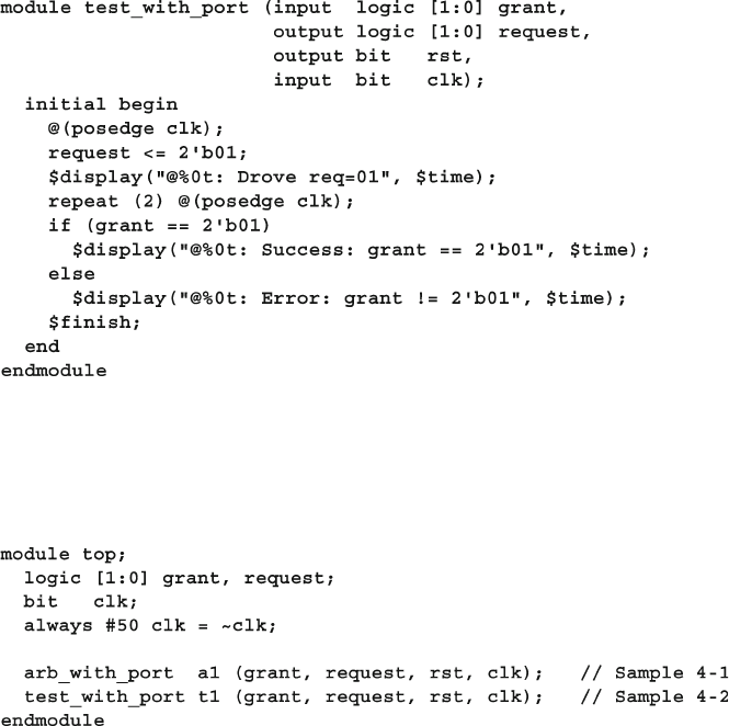
90 4 Connecting the Testbench and Design
In Sample 4.3 , the modules are simple, but real designs with hundreds of pins
require pages of signal and port declarations. All these connections can be error
prone. As a signal moves through several layers of hierarchy, it has to be declared
and connected over and over. Worst of all, if you just want to add a new signal, it
has to be declared and connected in multiple fi les. SystemVerilog interfaces can
help in each of these cases.
4.2 The Interface Construct
Designs have become so complex that even the communication between blocks may
need to be separated out into separate entities. To model this, SystemVerilog uses
the interface construct that you can think of as an intelligent bundle of wires. It con-
The top module connects the testbench and DUT, and includes a simple clock
generator.
Sample 4.2 Testbench module using ports
Sample 4.3 Top-level module with ports
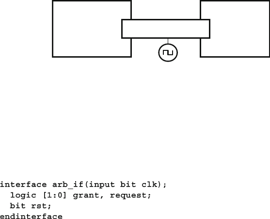
91
4.2 The Interface Construct
tains the connectivity, synchronization, and optionally, the functionality of the com-
munication between two or more blocks and, optionally, error checking. They
connect design blocks and/or testbenches.
Design-level interfaces are covered in Sutherland (2006). This book concentrates
on interfaces that connect design blocks and testbenches.
4.2.1 Using an Interface to Simplify Connections
The fi rst improvement to the arbiter example is to bundle the wires together into an
interface. Figure 4.3 shows the testbench and arbiter, communicating using an inter-
face. Note how the interface extends into the two blocks, representing the drivers
and receivers that are functionally part of both the test and the DUT. The clock can
be part of the interface or a separate port.
Testbench ArbiterInterfaceInterface
Fig. 4.3 An interface straddles two modules
The simplest interface is just a bundle of bidirectional signals as shown in Sample 4.4 .
Use the logic data type so you can drive the signals from procedural statements.
Sample 4.4 Simple interface for arbiter
Sample 4.5 is the device under test, the arbiter, that uses an interface instead of
ports.
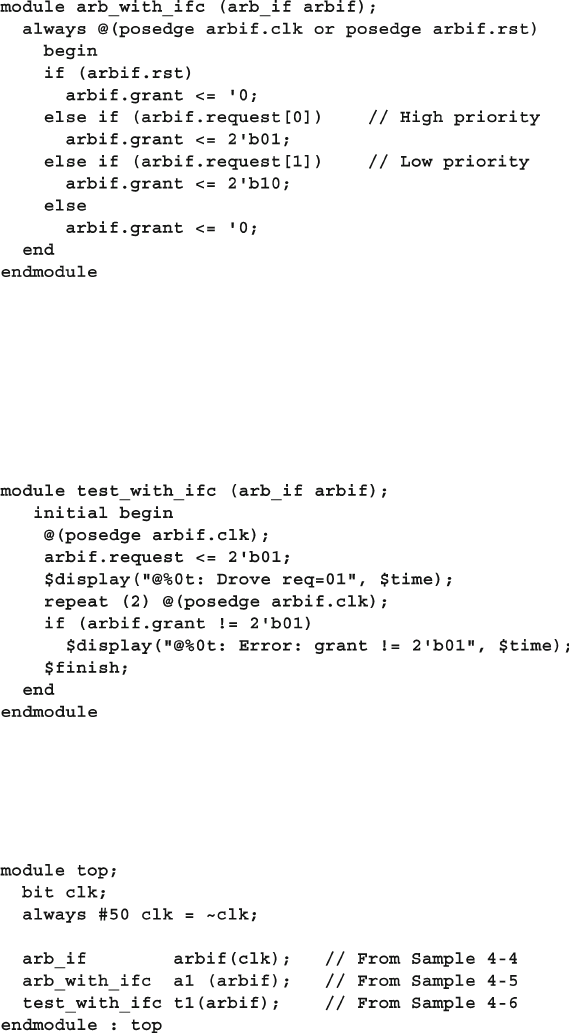
92 4 Connecting the Testbench and Design
Sample 4.6 shows the testbench. You refer to a signal in an interface by making
a hierarchical reference using the instance name: arbif.request . Interface sig-
nals should always be driven using nonblocking assignments. This is explained in
more detail in Section 4.4.3 and 4.4.4 .
Sample 4.6 Testbench using a simple arbiter interface
Sample 4.5 Arbiter using a simple interface
All these blocks are instantiated and connected in the top module as shown in
Sample 4.7 .
Sample 4.7 Top module with a simple arbiter interface
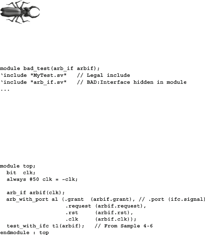
93
4.2 The Interface Construct
You can see an immediate benefi t, even on this small device: the connections
become cleaner and less prone to mistakes. If you wanted to put a new signal in an
interface, you would just have to add it to the interface defi nition and the modules
that actually used it. You would not have to change any module such as
top that just
passes the interface through. This language feature greatly reduces the chance for
wiring errors.
This book only shows interfaces with a single clock that is connected to a genera-
tor at the top level. If your interface requires multiple clocks, treat them like the
other signals inside the interface, and connect the interface to a clock generator. You
are more productive if you work at a high level and treat the interface as a cycle
based construct. The next level up is transaction-based, which is beyond typical
RTL code.
Make sure you declare your interfaces outside of modules and
program blocks. If you forget, expect all sorts of trouble. Some
compilers may not support defi ning an interface inside a mod-
ule. If allowed, the interface would be local to the module and
thus not visible to the rest of the design. Sample 4.8 shows the common mistake of
including the interface defi nition right after other include statements.
Sample 4.8 Bad test module includes interface
Sample 4.9 Connecting an interface to a module that uses ports
4.2.2 Connecting Interfaces and Ports
If you have a Verilog-2001 legacy design with ports that cannot be changed to use an
interface, you can just connect the interface’s signals to the individual ports. Sample 4.9
connects the original arbiter from Sample 4.1 to the interface in Sample 4.4 .
94 4 Connecting the Testbench and Design
4.2.3 Grouping Signals in an Interface Using Modports
Sample 4.5 uses a point-to-point connection scheme with no signal directions in the
interface. The original modules using ports had this information that the compiler
uses to check for wiring mistakes. The
modport construct in an interface lets you
group signals and specify directions. The MONITOR modport in Sample 4.10 allows
you to connect a monitor module to the interface.
Sample 4.10 Interface with modports
Sample 4.11 shows the arbiter model and testbench, with the modport in their
port connection list. Note that you put the modport name, DUT or TEST , after the
interface name, arb_if . Other than the modport name, these are identical to the
previous examples.
Sample 4.12 Testbench with interface using modports
Sample 4.11 Arbiter model with interface using modports
Even though the code didn’t change much (except that the interface grew larger),
this interface more accurately represents the real design, especially the signal
direction.
There are two ways to use these modport names in your design. You can specify
them in the modules that connect to the interface signals. In this case, the top
model does not change from Sample 4.7 , except for the module names. This book
95
4.2 The Interface Construct
recommends this style, as the modport is an implementation detail that should not
clutter the top level module.
The alternative is to specify the modport when you instantiate the module as
shown in Sample
4.13 .
Sample 4.13 Top level module with modports
With this style, you have the fl exibility to instantiate a module more than once,
with each instance connected to a different modport, that is, a different subset of
interface signals. For example, a byte-wide RAM model could connect to one of
four slots on a 32-bit bus. In this case, you would need to specify the modport when
you instantiate the module, not in the module itself.
Note that modports are defi ned in the interface, and specifi ed in the module port
list, but never in the signal name. The name arb_if.TEST.grant is illegal!
4.2.4 Using Modports with a Bus Design
Not every signal needs to go in every modport. Consider a CPU – memory bus mod-
eled with an interface. The CPU is the bus master and drives a subset of the signals,
such as request, command , and address . The memory is a slave and receives
those signals and drives ready . Both master and slave drive data . The bus arbiter
only looks at request and grant , and ignores all other signals. So your interface
would have three modports for master, slave, and arbiter, plus an optional monitor
modport.
4.2.5 Creating an Interface Monitor
You can create a bus monitor using the MONITOR modport. Sample 4.14 shows a
trivial monitor for the arbiter. For a real bus, you could decode the commands and
print the status: completed, failed, etc.
96 4 Connecting the Testbench and Design
4.2.6 Interface Trade-Offs
An interface cannot contain module instances, only instances of other interfaces.
There are trade-offs in using interfaces with modports as compared with traditional
ports connected with signals.
The advantages to using an interface are as follows.
An interface is ideal for design reuse. When two blocks communicate with a •
specifi ed protocol using more than two signals, consider using an interface. If
groups of signals are repeated over and over, as in a networking switch, you
should additionally use virtual interfaces, as described in Chapter 10 .
The interface takes the jumble of signals that you declare over and over in every •
module or program and puts it in a central location, reducing the possibility of
misconnecting signals.
To add a new signal, you just have to declare it once in the interface, not in •
higher-level modules, once again reducing errors.
Modports allow a module to easily tap a subset of signals from an interface. You •
can specify signal direction for additional checking.
The disadvantages of using an interface are as follows.
For point-to-point connections, interfaces with modports are almost as verbose •
as using ports with lists of signals. Interfaces have the advantage that all the
declarations are still in one central location, reducing the chance for making an
error.
You must now use the interface name in addition to the signal name, possibly •
making the modules more verbose, but more readable for debugging.
If you are connecting two design blocks with a unique protocol that will not be •
reused, interfaces may be more work than just wiring together the ports.
Sample 4.14 Arbiter monitor with interface using modports
97
4.2 The Interface Construct
It is diffi cult to connect two different interfaces. A new interface ( • bus_if ) may
contain all the signals of an existing one ( arb_if ), plus new signals (address,
data, etc.). You may have to break out the individual signals and drive them
appropriately.
4.2.7 More Information and Examples
The SystemVerilog LRM specifi es many other ways for you to use interfaces. See
Sutherland (2006) for more examples of using interfaces for design.
4.2.8 Logic vs. Wire in an Interface
This book recommends declaring the signals in your interface as logic while the
VMM has a rule that says to use a wire . The difference is ease-of-use vs.
reusability.
If your testbench drives an asynchronous signal in an interface with a procedural
assignment, the signal must be a logic type. A wire can only be driven with a
continuous assignment statement. Signals in a clocking block are always synchro-
nous and can be declared as logic or wire . Sample 4.15 shows how the logic
signal can be driven directly, whereas the wire requires additional code.
Sample 4.15 Driving logic and wires in an interface
Another reason to use logic for interface signals is that the compiler will give
an error if you unintentionally use multiple structural drivers.
The VMM takes a more long-term approach. Take the case where you have cre-
ated test code that works well on the current project and is later used in a new
design.
98 4 Connecting the Testbench and Design
What if your interface with all its logic signals is connected such that now a
signal has multiple structural drivers? The engineers will have to change that
logic
to a
wire , and, if the signal does not go through a clocking block, change the pro-
cedural assignment statements. Now there are two versions of the interface, and
existing tests must be modifi ed before they can be reused. Rewriting good code
goes against the VMM principles.
4.3 Stimulus Timing
The timing between the testbench and the design must be carefully orchestrated.
At a cycle level, you need to drive and receive the synchronous signals at the proper
time in relation to the clock. Drive too late or sample too early, and your testbench
is off a cycle. Even within a single time slot (for example, everything that happens
at time 100ns), mixing design and testbench events can cause a race condition, such
as when a signal is both read and written at the same time. Do you read the old
value, or the one just written? In Verilog, nonblocking assignments help when a test
module drives the DUT, but the test could not always be sure it sampled the last
value driven by the design. SystemVerilog has several constructs to help you control
the timing of the communication.
4.3.1 Controlling Timing of Synchronous Signals
with a Clocking Block
An interface should contain a clocking block to specify the timing of synchronous
signals relative to the clocks. Clocking blocks are mainly used by testbenches but
also allow you to create abstract synchronous models. Signals in a clocking block
are driven or sampled synchronously, ensuring that your testbench interacts with the
signals at the right time. Synthesis tools do not support clocking blocks, so your
RTL code can not take advantage of them. The chief benefi t of clocking blocks is
that you can put all the detailed timing information in here, and not clutter your
testbench.
An interface can contain multiple clocking blocks, one per clock domain, as there
is a single clock expression in each block. Typical clock expressions are @(posedge
clk) for a single edge clock and @(clk) for a DDR (double data rate) clock.
You can specify a clock skew in the clocking block using the default statement,
but the default behavior is that input signals are sampled just before the design exe-
cutes, and the outputs are driven back into the design during the current time slot. The
next section provides more details on the timing between the design and testbench.
Once you have defi ned a clocking block, your testbench can wait for the clocking
expression with @arbif.cb rather than having to spell out the exact clock and
edge. Now if you change the clock or edge in the clocking block, you do not have
to change your testbench.
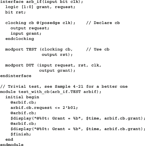
99
4.3 Stimulus Timing
Sample 4.16 is similar to Sample 4.10 except that the TEST modport now treats
request and grant as synchronous signals. The clocking block cb declares that
the signals are active on the positive edge of the clock. The signal directions are
relative to the
modport where they are used. So request is a synchronous output
in the TEST modport, and grant is an synchronous input. The signal rst is asyn-
chronous in the TEST modport.
Sample 4.16 Interface with a clocking block
4.3.2 Timing Problems in Verilog
Your testbench needs to be separate from the design, not just logically but also tem-
porally. Consider how a hardware tester interacts with a chip for synchronous sig-
nals. In a real hardware design, the DUT’s storage elements latch their inputs from
the tester at the active clock edge. These values propagate through the storage ele-
ment outputs, and then the logic clouds to the inputs of the next storage element. The
time from the input of the fi rst storage to the next must be less than a clock cycle.
100 4 Connecting the Testbench and Design
So a hardware tester needs to drive the chip’s inputs at the clock edge, and read the
outputs just before the following edge.
A testbench has to mimic this tester behavior. It should drive on or after the
active clock edge, and should sample as late as possible as allowed by the protocol
timing specifi cation, just before the active clock edge.
If the DUT and testbench are made of Verilog modules only, this outcome is
nearly impossible to achieve. If the testbench drives the DUT at the clock edge,
there could be race conditions. What if the clock propagates to some DUT inputs
before the testbench stimulus, but is a little later to other inputs? From the outside,
the clock edges all arrive at the same simulation time, but in the design, some inputs
get the value driven during the last cycle, whereas other inputs get values from the
current cycle.
One way around this problem is to add small delays to the system, such as #0.
This forces the thread of Verilog code to stop and be rescheduled after all other
code. Invariably though, a large design has several sections that all want to execute
last. Whose #0 wins out? It could vary from run to run and be unpredictable between
simulators. Multiple threads using #0 delays cause indeterministic behavior. Avoid
using #0 as it will make your code unstable and not portable.
The next solution is to use a larger delay, #1. RTL code has no timing, other than
clock edges, so one time unit after the clock, the logic has settled. However, what if
one module uses a time precision of 1ns, whereas another used a resolution of just
10ps? Does that #1 mean 1ns, 10ps, or something else? You want to drive as soon
as possible after the clock cycle with the active clock edge, but not during that time,
and before anything else can happen. Worse yet, your DUT may contain a mix of
RTL code with no delays and gate code with delays. Just as you should avoid using
#0, stay away from #1 delays to fi x timing problems. See Cummings (2000) and
other papers by him for additional guidelines.
4.3.3 Testbench – Design Race Condition
Sample 4.17 shows a potential race condition between the testbench and design.
The race condition occurs when the test drives the start signal and then the other
ports. The memory is waiting on the start signal and could wake up immediately,
whereas the write signal still has its old value, while addr and data have new
values. This behavior is perfectly legal according to the LRM. You could delay all
these signals slightly by using nonblocking assignments, as recommended by
Cummings (2000), but remember that the testbench and the design are both using
these assignments. It is still possible to get a race condition between the testbench
and design.
Sampling the design outputs has a similar problem. You want to grab the values
at the last possible moment, just before the active clock edge. Perhaps you know the
next clock edge is at 100ns. You can’t sample right at the clock edge at 100ns, as
some design values may have already changed. You should sample at Tsetup just
before the clock edge.
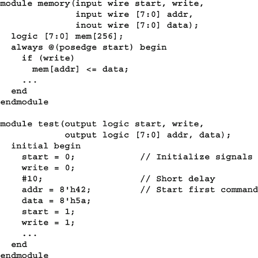
101
4.3 Stimulus Timing
4.3.4 The Program Block and Timing Regions
The root of the problem is the mixing of design and testbench events during the
same time slot, though even in pure RTL the same problem can happen. Good cod-
ing guidelines such as proper use of nonblocking assignments can reduce these race
conditions, but improperly coded assignments have the habit of creeping in. What if
there were a way you could separate these events temporally, just as you separated
the code? At 100ns, your testbench could sample the design outputs before the clock
has had a chance to change and any design activity has occurred. By defi nition,
these values would be the last possible ones from the previous time slot. Then, after
all the design events are done, your testbench would start.
How does SystemVerilog know to schedule the testbench events separately from
the design events? In SystemVerilog, your testbench code is in a program block,
which is similar to a module in that it can contain code and variables and be instanti-
ated in other modules. However, a program cannot have any hierarchy such as
instances of modules, interfaces, or other programs.
A new region of the time slot was introduced in SystemVerilog as shown in Fig.
4.4 . In Verilog, most events are executed in the Active region. There are dozens of
other regions for nonblocking assignments, PLI execution, etc., but they can be
Sample 4.17 Race condition between testbench and design
102 4 Connecting the Testbench and Design
Sample 4.18 shows part of the testbench code for the arbiter. Note that the state-
ment @arbif.cb waits for the active edge of the clocking block, @(posedge
clk) , as shown in Sample 4.16 . This sample shows that your testbench code is
ignored for the purposes of this book. See Table
4.1 , the LRM, and Cummings
(2006) for more details on the SystemVerilog event regions.
First to execute during a time slot is the Active region, where design events run.
These include your traditional RTL and gate code plus the clock generator. The
second region is the Observed region, where SystemVerilog Assertions are evalu-
ated. Following that is the Reactive region where the testbench code in a program
executes. Note that time does not strictly fl ow forwards — events in the Observed
and Reactive regions can trigger further design events in the Active region in the
current cycle. Last is the Postponed region, which samples signals at the end of the
time slot, in the readonly period, after design activity has completed.
To next
time slot
From previous
time slot
Active
(design)
Observed
(assertions)
Reactive
(testbench)
Loop back
if more events
Postponed
(sample)
Active
(design)
Observed
(assertions)
Reactive
(testbench)
Postponed
(sample)
Fig. 4.4 Main regions inside
a SystemVerilog time step
Table 4.1 Primary SystemVerilog scheduling regions
Name Activity
Active Simulation of design code in modules
Observed Evaluation of SystemVerilog Assertions
Reactive Execution of testbench code in programs
Postponed Sampling design signals for testbench input
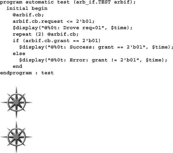
103
4.3 Stimulus Timing
Sample 4.18 Testbench using interface with clocking block
Your test should be contained in a single program. You should use
OOP to build a dynamic, hierarchical testbench from objects instead
of modules. A simulation may have multiple program blocks if you
are using code from other people or combining several tests.
As discussed in Section 3.6.1, you should always declare your pro-
gram block as automatic so that it behaves more like the routines
in stack-based languages you may have worked with, such as C.
Note that not all vendors regard program blocks equally. See Rich (2009) for an
alternate opinion.
4.3.5 Specifying Delays Between the Design and Testbench
The default timing of the clocking block is to sample inputs with a skew of #1step
and to drive the outputs with a delay of #0. The 1step delay specifi es that signals
are sampled in the Postponed region of the previous time slot, before any design
activity. So you get the output values just before the clock changes. The testbench
outputs are synchronous by virtue of the clocking block, so they fl ow directly into the
design. The program block, running in the Reactive region, generates the stimulus
written at a slightly higher level of abstraction, using cycle-by-cycle timing instead
of worrying about individual clock edges.
Section 4.4 explains more about the driving and sampling of interface signals.
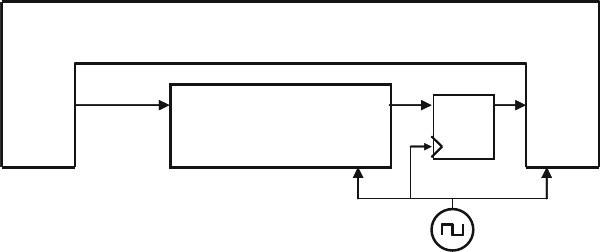
104 4 Connecting the Testbench and Design
that is applied to the DUT, which is then evaluated in the Active region during the
same time slot. The DUT evaluates its logic and drives its outputs, which are the
inputs to the testbench through the clocking blocks. These are then sampled in
the Postponed region and the cycle repeats. If you have a design background, you can
remember this by imagining that the clocking block inserts a synchronizer between
the design and testbench, as shown in Fig.
4.5 . With proper use of program and
clocking blocks, race conditions between the testbench and DUT can be all but
eliminated.
Design
Under Test
Testbench
out
test
out
clk
test
in
in
dq
Fig. 4.5 A clocking block synchronizes the DUT and testbench
4.4 Interface Driving and Sampling
Your testbench needs to drive and sample signals from the design, primarily through
interfaces with clocking blocks. The next section uses the arbiter interface from
Sample 4.16 and the top-level module from Sample 4.9 .
Asynchronous signals such as rst pass through the interface with no delays. The
signals in the clocking block get synchronized as shown in the sections below.
4.4.1 Interface Synchronization
You can use the Verilog @ and wait constructs to synchronize the signals in a test-
bench. Sample 4.19 shows the various constructs.
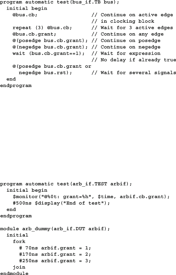
105
4.4 Interface Driving and Sampling
The waveforms in Fig. 4.6 show that in the program, arbif.cb.grant gets the
value from just before the clock edge. When the interface input changes right at a
clock edge, such as 250ns, the value does not propagate to the testbench until the
next cycle, which starts at 350ns.
Sample 4.20 Synchronous interface sample and drive from module
Sample 4.19 Signal synchronization
4.4.2 Interface Signal Sample
When you read a signal from a clocking block, you get the value sampled from just
before the last clock edge, i.e., from the Postponed region. Sample 4.20 shows a
program block that reads the synchronous grant signal from the DUT. The arb
module drives grant to 1 & 2 in the middle of the 100ns cycle, and then to 3 exactly
at the clock edge. This code is for illustration only and is not real, synthesizable
RTL.
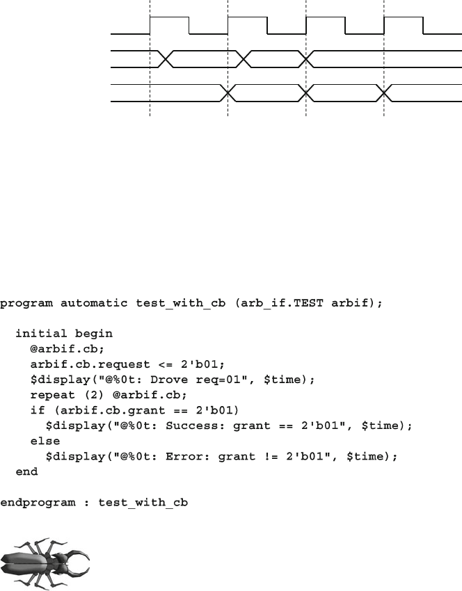
106 4 Connecting the Testbench and Design
4.4.3 Interface Signal Drive
Sample 4.21 has an abbreviated version of the arbiter test program, which uses the
arbiter interface defi ned in Sample 4.16 .
Sample 4.21 Testbench using interface with clocking block
clk
DUT arb.grant
TEST arbif.cb.grant
132X
32X 1
150ns 250ns 350ns50ns
Fig. 4.6 Sampling a synchronous interface
When using modports with clocking blocks, a synchronous
interface signal such as request must be prefi xed with both the
interface name, arbif , and the clocking block name, cb . So in
Sample 4.21 , arbif.cb.request is legal, but arbif.
request is not. This is the most common coding mistake with interfaces and clock-
ing blocks.
4.4.4 Driving Interface Signals Through a Clocking Block
You should always drive interface signals in a clocking block with a synchronous
drive using a nonblocking assignment. This is because the design signal does not
change immediately after your assignment – remember that your testbench executes
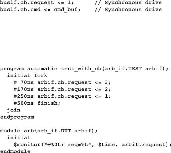
107
4.4 Interface Driving and Sampling
in the Reactive region while design code is in the Active region. If your testbench
drives arbif.cb.request at 100ns, the same time as arbif.cb (which is
@(posedge clk) according to the clocking block), request changes in the design
at 100ns. However, if your testbench tries to drive
arbif.cb.request at time
101ns, between clock edges, the change does not propagate until the next clock
edge. In this way, your drives are always synchronous. In Sample
4.20 , arbif.
grant is driven by a module and can use a blocking assignment.
If the testbench drives the synchronous interface signal at the active edge of the
clock, as shown in Sample 4.22 , the value propagates immediately to the design.
This is because the default output delay is #0 for a clocking block. If the testbench
drives the output just after the active edge, the value is not seen in the design until
the next active edge of the clock.
Sample 4.23 Driving a synchronous interface
Sample 4.22 Interface signal drive
Sample 4.23 shows what happens if you drive a synchronous interface signal at
various points during a clock cycle. This uses the interface from Sample 4.16 and
the top module and clock generator from Sample 4.9 .
Note that in Fig. 4.7 , the value 3, driven in the middle of the fi rst cycle, is seen
by the DUT at the start of the second cycle. The value 2 is driven in the middle of
the second cycle. It is never seen by the DUT as the testbench drives a 1 at the end
of the second cycle.
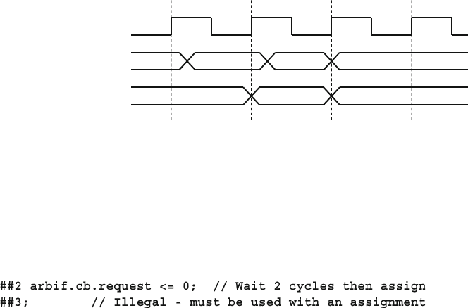
108 4 Connecting the Testbench and Design
Driving clocking block signals asynchronously can lead to dropped values.
Instead, drive at the clock edge by using a cycle delay prefi x on your drives as
shown in Sample 4.24 .
clk
TEST arb.cb.request
DUT arbif.request
312X
1X 3
150ns 250ns 350ns50ns
1
Fig. 4.7 Driving a synchronous interface
Sample 4.24 Interface signal drive
If you want to wait for two clock cycles before driving a signal, you can either
use “ repeat (2) @arbif.cb ;” or use the cycle delay ##2 . This latter delay only
works as a prefi x to a drive of a signal in a clocking block, as it needs to know which
clock to use for the delay.
The cycle delay of ##0 in an assignment that drives the value immediately if the
clock was asserted in this time slot, according to the clocking block. If the clock was
not just asserted, the signal is driven at the next active edge of the clock. The cycle
delay of ##1 always waits for the next active edge of the clock, even if the clock was
asserted in the current time slot.
The naked cycle delay statement ##3 ; works if you have a default clocking block
for your program or module. This book only recommends putting a clocking block in
an interface and not creating a default clocking block. You should always be specifi c
about which clock is being referenced.
4.4.5 Bidirectional Signals in the Interface
In Verilog-1995, if you want to drive a bidirectional signal such as a port from
procedural code, you need a continuous assignment to connect the reg to the wire .
In SystemVerilog, synchronous bidirectional signals in interfaces are easier to use
as the continuous assignment is added for you, as shown in Sample 4.25 . When you
write to the net from a program, SystemVerilog actually writes to a temporary vari-
able that drives the net. Your program reads directly from the wire, seeing the value
that is resolved from all the drivers. Design code in a module still uses the classic
register plus continuous assignment statement.
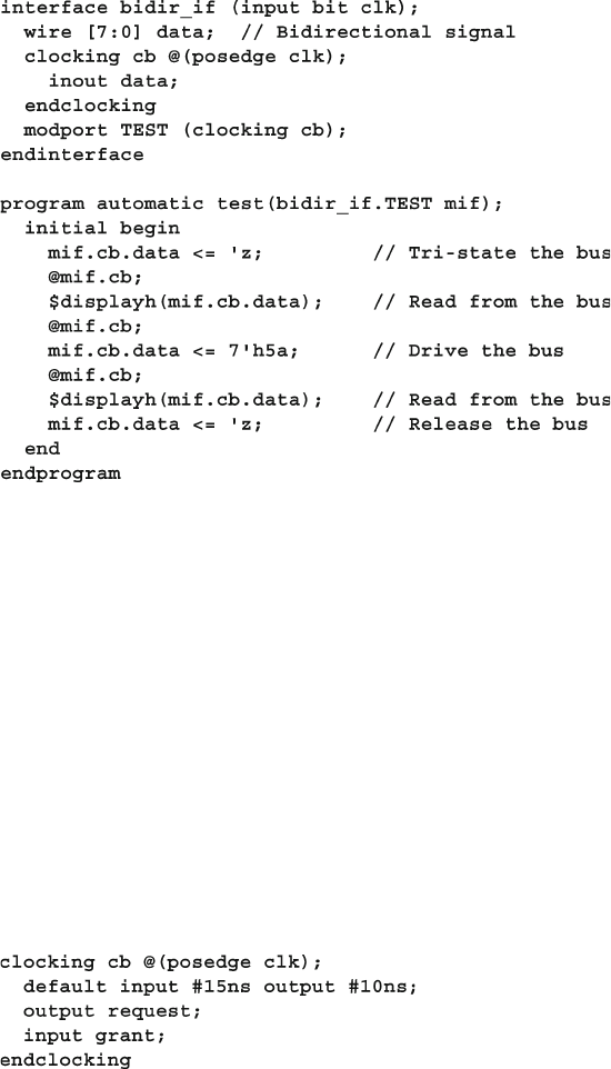
109
4.4 Interface Driving and Sampling
The SystemVerilog LRM is not clear on driving an asynchronous bidirectional
signal using an interface. Two possible solutions are to use a cross-module reference
and continuous assignment or to use a virtual interface as shown in Chapter 10 .
4.4.6 Specifying Delays in Clocking Blocks
A clocking block ensures that your signals are driven and sampled at the specifi ed
clock edge. You can skew these times with either a default statement, or by speci-
fying the delays for individual signals. This can be useful when simulating netlists
with real delays. Sample 4.26 shows a clocking block with a default statement that
has the skews for all signals. In this example, the inputs are sampled 15ns before the
posedge of the clock and the outputs are driven 10ns after the posedge of the clock.
Sample 4.26 Clocking block with default statement
Sample 4.25 Bidirectional signals in a program and interface
Sample 4.27 shows the equivalent clocking block, but with the delays specifi ed
on the individual signals.
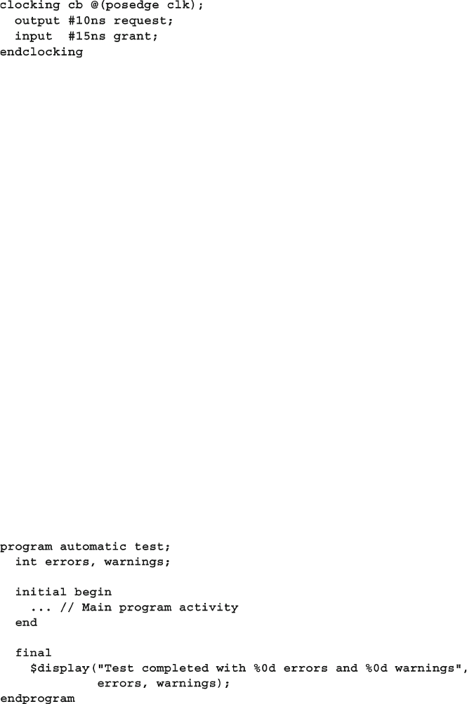
110 4 Connecting the Testbench and Design
4.5 Program Block Considerations
4.5.1 The End of Simulation
In Verilog, simulation continues while there are scheduled events, or until a $fi nish
is executed. SystemVerilog adds an additional way to end simulation. A program
block is treated as if it contains a test. If there is only a single program, simulation
ends when you complete the last statement in every initial block in the program,
as this is considered the end of the test. Simulation ends even if there are threads
still running in the program or modules. As a result, you don’t have to shut down
every monitor and driver when a test is done.
If there are several program blocks, simulation ends when the last program com-
pletes. This way simulation ends when the last test completes. You can terminate
any program block early by executing $exit . Of course you can still explicitly call
$fi nish to end simulation, but this might cause issues if you have multiple
programs.
However, simulation is not yet over. A module or program can have a fi nal
block that contains code to be run just before the simulator terminates, as shown in
Sample 4.28 . This is a great place to perform clean up work such as closing fi les,
and printing a report of the number of errors and warnings encountered. You cannot
schedule any events, or have any delays in a fi nal block that could cause time to
elapse. You do not have to worry about freeing any memory that was allocated as
this will be done automatically.
Sample 4.27 Clocking block with delays on individual signals
Sample 4.28 A fi nal block
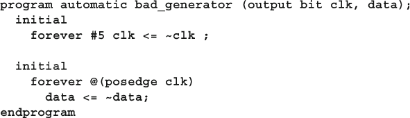
111
4.5 Program Block Considerations
4.5.2 Why are Always Blocks not Allowed in a Program?
In SystemVerilog you can put initial blocks in a program, but not always blocks.
This may seem odd if you are used to Verilog modules, but there are several reasons
SystemVerilog programs are closer to a program in C, with one (or more) entry
points, than Verilog’s many small blocks of concurrently executing hardware. In a
design, an always block might trigger on every positive edge of a clock from the
start of simulation. In contrast, a testbench has the steps of initialization, stimulate
and respond to the design, and then wrap up simulation. An always block that runs
continuously would not work.
When the last initial block completes in the program, simulation implicitly
ends just as if you had executed $fi nish . If you had an always block, it would run
for ever, so you would have to explicitly call $exit to signal that the program com-
pleted. But don’t despair. If you really need an always block, you can use initial
forever to accomplish the same thing.
4.5.3 The Clock Generator
Now that you have seen the program block, you may wonder if the clock generator
should be in a module. The clock is more closely tied to the design than the test-
bench, and so the clock generator should remain in a module. The generator should
be instantiated at the same level as the DUT so it can drive both the DUT and test-
bench As you refi ne the design, you create clock trees, and you have to carefully
control the skews as the clocks enter the system and propagate through the blocks.
The testbench is much less picky. It just wants a clock edge to know when to
drive and sample signals. Functional verifi cation is concerned with providing the
right values at the right cycle, not with fractional nanosecond delays and relative
clock skews.
The program block is not the place to put a clock generator. Sample 4.29 tries to
put the generator in a program block but just causes a race condition. The clk and
data signals both propagate from the Reactive region to the design in the Active
region and could cause a race condition depending on which one arrived fi rst.
Sample 4.29 Bad clock generator in program block
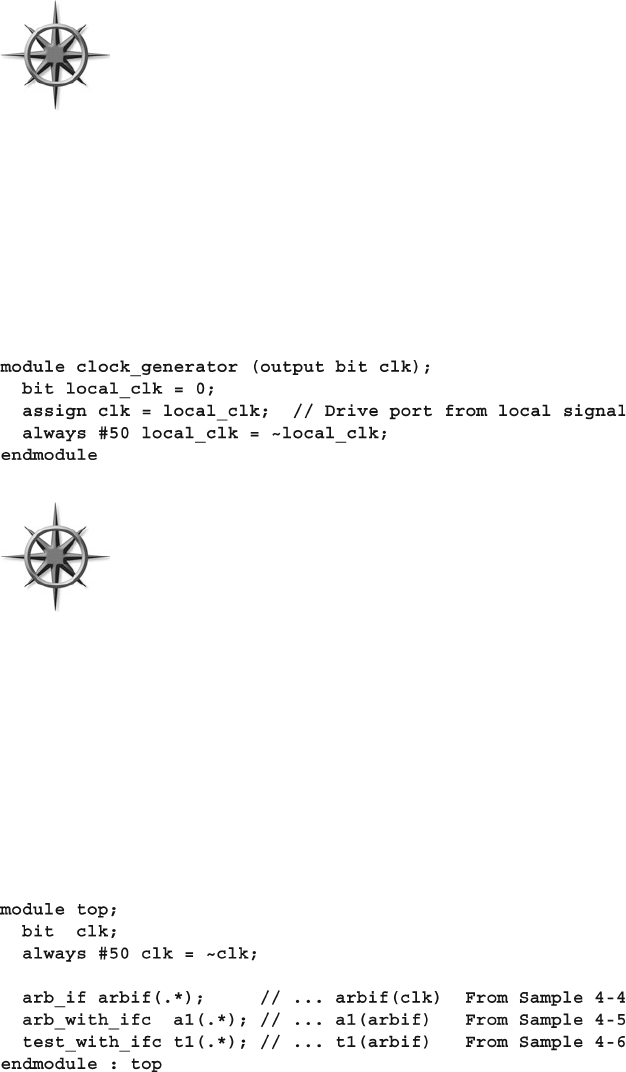
112 4 Connecting the Testbench and Design
Avoid race conditions by always putting the clock generator in a
module. If you want to randomize the generator’s properties, create
a class with random variables for skew, frequency, and other char-
acteristics, as shown in Chapter 6 . You can use this class in the
generator module, or in the testbench.
Sample 4.30 shows a good clock generator in a module. It deliberately avoids an
edge at time 0 to prevent race conditions. All clock edges are generated with a
blocking assignment to trigger events during the Active region. If you must generate
a clock edge at time 0, use a nonblocking assignment to set the initial value so all
clock sensitive logic such as always blocks will have started before the clock
changes value.
Sample 4.30 Good clock generator in module
Lastly, don’t try to verify the low-level timing with functional veri-
fi cation. The testbenches described in this book check the behavior
of the DUT but not the timing, which is better done with a static
timing analysis tool. Your testbenches should be fl exible enough to
be compatible with gate-level simulations run with back-annotated
timing.
4.6 Connecting It All Together
Now you have a design described in a module, a testbench in a program block, and
interfaces that connect them together. Sample 4.31 has the top-level module that
instantiates and connects all the pieces.
Sample 4.31 Top module with implicit port connections
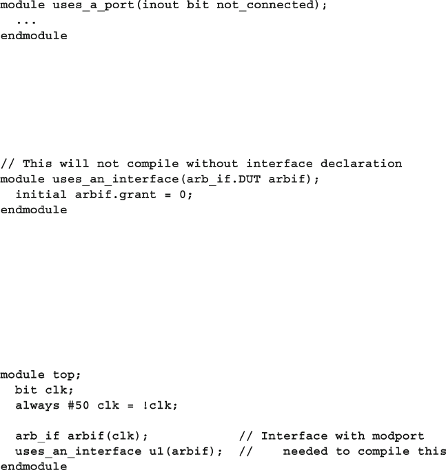
113
4.6 Connecting It All Together
This is almost identical to Sample 4.7 . It uses a shortcut notation.* (implicit port
connection) that automatically connects module instance ports to signals at the cur-
rent level if they have the same name and data type.
4.6.1 An Interface in a Port List Must Be Connected
The SystemVerilog compiler won’t let you compile a single module or program that
uses an interface in the port list. Why not? After all, a module or program with ports
made of individual signals can be compiled without being instantiated, as shown in
Sample 4.32 .
Sample 4.33 Module with an interface
Sample 4.34 Top module connecting DUT and interface
Sample 4.32 Module with just port connections
The compiler creates wires and connects them to the dangling signals. However,
a module or program with an interface in its port list must be connected to an
instance of the interface.
For Sample 4.33 , the compiler is not able to build even a simple interface. If you
have modports or a program block using clocking blocks in an interface, the com-
piler has an even more diffi cult time. Even if you are just looking to wring out
syntax bugs, you must complete the connections. This can be done as shown in
Sample 4.34 .
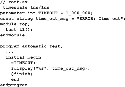
114 4 Connecting the Testbench and Design
4.7 Top-Level Scope
Sometimes you need to create things in your simulation that are outside of a
program or module so that they are seen by all blocks. In Verilog, only macros
extend across module boundaries, and so are used for creating global constants.
SystemVerilog introduces the compilation unit , that is a group of source fi les
that are compiled together. The scope outside the boundaries of any
module,
macromodule, interface, program, package , or primitive is known as the
compilation-unit scope , also referred to as $unit . Anything such as a parameter
defi ned in this scope is similar to a global because it can be seen by all lower-level
blocks. However, it is not truly global as the parameter cannot be seen during
compilation of other fi les.
This leads to some confusion. Some simulators compile all the SystemVerilog
code together, so $unit is global. Other simulators and synthesis tools compile a
single module or group of modules at a time, so $unit may be just the contents of
one or a few fi les. As a result, $unit is not portable. Packages allow you to have
code outside of a program or module while eliminating the requirement of compil-
ing all the modules at the same time.
This book calls the scope outside blocks the “top-level scope.” You can defi ne
variables, parameters, data types and even routines in this space. Sample 4.35
declares a top-level parameter, TIMEOUT , that can be used anywhere in the hierar-
chy. This example also has a const string that holds an error message. You can
declare top-level constants either way.
Sample 4.35 Top-level scope for arbiter design
The instance name $root allows you to unambiguously refer to names in the
system, starting with the top-level scope. In this respect, $root is similar to “/” in
the Unix fi le system. For tools such as VCS that compile all fi les at once, $root
and $unit are equivalent. The name $root also solves an old Verilog problem.
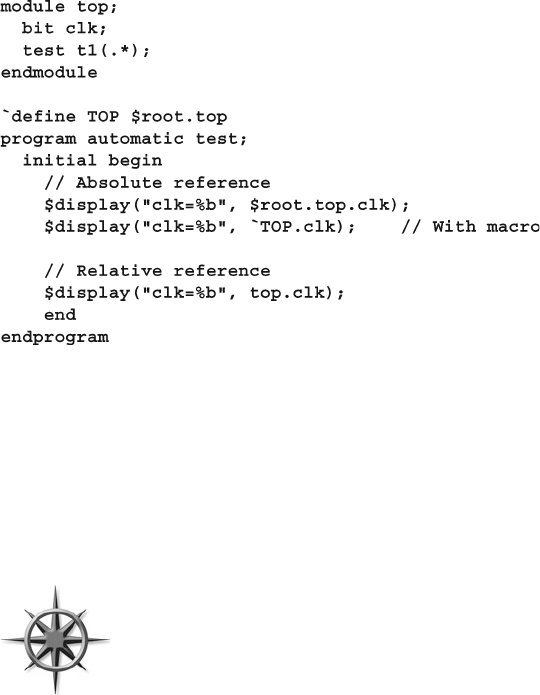
115
4.8 Program–Module Interactions
When your code refers to a name in another module, such as i1.var , the compiler
fi rst looks in the local scope, then looks up to the next higher scope, and so on until
it reaches the top. You may have wanted to use i1.var in the top module, but an
instance named i1 in an intermediate scope may have sidetracked the search, giving
you the wrong variable. You use $root to make unambiguous cross module refer-
ences by specifying the absolute path.
Sample 4.36 shows a program that is instantiated in the module top that is
implicitly instantiated in the top-level scope. The program can use a relative or
absolute reference to the clk signal in the module. You can use a macro to hold the
hierarchical path so that when the path changes, you only have to change one piece
of code. The LRM does not allow modules to be explicitly instantiated in the top-
level scope.
Sample 4.36 Cross-module references with $root
4.8 Program–Module Interactions
The program block can read and write all signals in modules, and can call routines
in modules, but a module has no visibility into a program. This is because your test-
bench needs to see and control the design, but the design should not depend on
anything in the testbench.
A program can call a routine in a module to perform various
actions. The routine can set values on internal signals, also known
as “backdoor load.” Next, because the current SystemVerilog stan-
dard does not defi ne how to force signals from a program block,
you need to write a task in the design to do the force, and then call
it from the program.
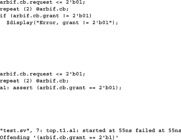
116 4 Connecting the Testbench and Design
Lastly, it is a good practice for your testbench to use a function to get information
from the DUT. Reading signal values can work most of the time, but if the design
code changes, your testbench may interpret the values incorrectly. A function in the
module can encapsulate the communication between the two and make it easier for
your testbench to stay synchronized with the design. Chapter 10 shows how to
embed functions and SystemVerilog Assertions in an interface.
4.9 SystemVerilog Assertions
You can create temporal assertions about signals in your design to check their
behavior and temporal relationship with SystemVerilog Assertions (SVA). The sim-
ulator keeps track of what assertions have triggered, so you can gather functional
coverage data on them.
4.9.1 Immediate Assertions
An immediate assertion checks if an expression is true when the statement is exe-
cuted. Your testbench procedural code can check the values of design signals and
testbench variables and take action if there is a problem. For example, if you have
asserted the bus request, you expect that grant will be asserted two cycles later. You
could use an if -statement as shown in Sample 4.37 .
Sample 4.39 Error from failed immediate assertion
Sample 4.37 Checking a signal with an if-statement
Sample 4.38 Simple immediate assertion
An assertion is more compact than an if -statement. However, note that the logic
is reversed compared to the if -statement above. You want the expression inside the
parentheses to be true; otherwise, print an error as shown in Sample 4.38 .
If the grant signal is asserted correctly, the test continues. If the signal does not
have the expected value, the simulator produces a message similar Sample 4.39 .
117
4.9 SystemVerilog Assertions
This says that on line 7 of the fi le test.sv , the assertion top.t1.a1 started at
55ns to check the signal arbif.cb.grant , but failed immediately. The label a1
should be unique so that you can quickly locate the failing assertion.
You may be tempted to use the full SystemVerilog Assertion syntax
to check an elaborate sequence over a range of time, but use care as
they can be hard to debug. Assertions are declarative code, and exe-
cute very differently than the surrounding procedural code. In just a
few lines of assertions, you can verify temporal relations; the equiv-
alent procedural code would be more complicated and verbose, but easier for the next
person to understand when they have to read your code.
If you are a VHDL programmer, you may be tempted at this
point to start sprinkling immediate assertions across your code.
Resist the temptation! Your code will work correctly for weeks
or months until someone decides to improve simulation perfor-
mance by disabling assertions. The simulator will no longer execute the expression
in the assertion. If the expression has a side effect such as incrementing a value or
calling a function, it will no longer occur.
4.9.2 Customizing the Assertion Actions
An immediate assertion has optional then- and else-clauses. If you want to augment
the default message, you can add your own as shown in Sample 4.40 .
Sample 4.40 Creating a custom error message in an immediate assertion
If grant does not have the expected value, you’ll see an error message similar to
Sample 4.41 .
Sample 4.41 Error from failed immediate assertion
SystemVerilog has four functions to print messages: $info, $warning, $error ,
and $fatal . These are allowed only inside an assertion, not in procedural code,
though future versions of SystemVerilog may allow this.
You can use the then-clause to record when an assertion completed success-
fully as shown in Sample 4.42 .
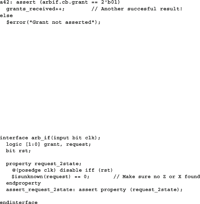
118 4 Connecting the Testbench and Design
4.9.3 Concurrent Assertions
The other type of assertion is the concurrent assertion that you can think of as a small
model that runs continuously, checking the values of signals for the entire simulation.
These are instantiated similarly to other design blocks and are active for the entire
simulation. You need to specify a sampling clock in the assertion. Sample 4.43 has
a small assertion to check that the arbiter request signal does not have X or Z values
except during reset. This code is placed outside of procedural blocks such as initial
and always . Sample 4.43 is for illustration only. See one of the books listed below
for a more information.
Sample 4.42 Creating a custom error message
Sample 4.43 Concurrent assertion to check for X/Z
4.9.4 Exploring Assertions
There are many other uses for assertions. For example, you can put assertions in an
interface. Now your interface not only transmits signal values but also checks the
protocol.
This Section has provided a brief introduction to SystemVerilog Assertions. For
more information, see Vijayaraghhavan and Ramanathan (2005) and Haque et al.
(2007).
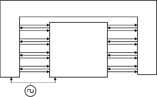
119
4.10 The Four-Port ATM Router
4.10 The Four-Port ATM Router
The arbiter example is a good introduction to interfaces, but real designs have more
than a single input and output. This section discusses a four-port ATM (Asynchronous
Transfer Mode) router, shown in Fig.
4.8 .
4x4
ATM
router
Testbench
Tx0
Tx1
Tx2
Tx3
Rx0
Rx1
Rx2
Rx3
Fig. 4.8 Testbench – ATM router diagram without interfaces
4.10.1 ATM Router with Ports
The following code fragments show the tangle of wires you would have to endure to
connect an RTL block to a testbench. First is the header for the ATM router model.
This uses the Verilog-1995 style port declarations, where the type and direction are
separate from the header.
The actual code for the router in Sample 4.44 is crowded out by nearly a page of
port declarations.
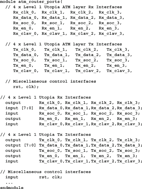
120 4 Connecting the Testbench and Design
So what sort of synthesizable code goes in the “…” at the end of Sample 4.44 ?
See Sutherland (2006) for more information and examples of using interfaces in
modules and other SystemVerilog design constructs.
4.10.2 ATM Top-Level Module with Ports
Sample 4.45 contains the top-level module.
Sample 4.44 ATM router model header with ports
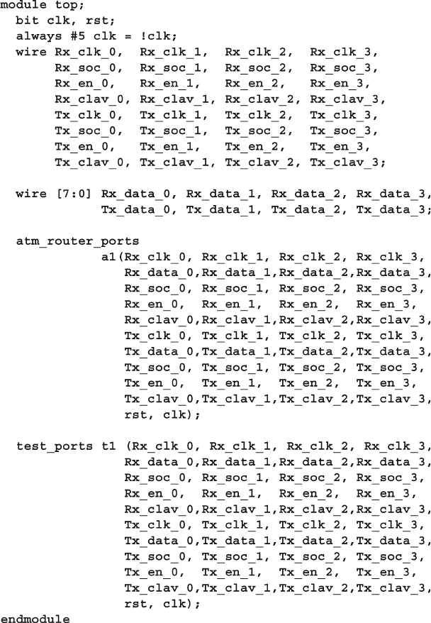
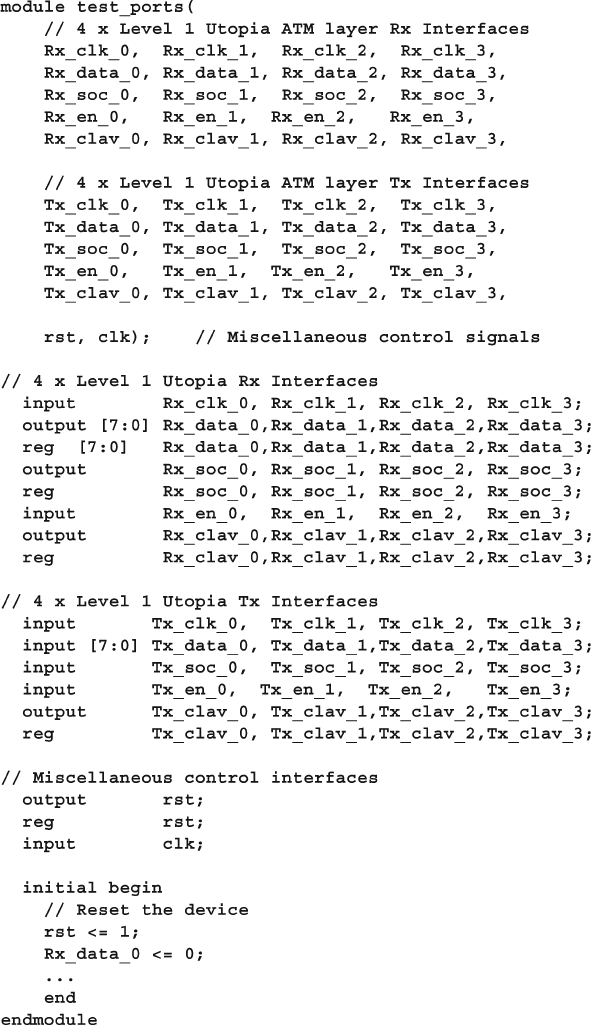
122 4 Connecting the Testbench and Design
Sample 4.46 Verilog-1995 testbench using ports
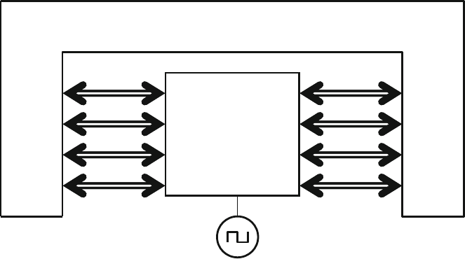
123
4.10 The Four-Port ATM Router
You just saw three pages of code, and it was all just connectivity — no testbench,
no design! Interfaces provide a better way to organize all this information and elimi-
nate the repetitive parts that are so error prone.
4.10.3 Using Interfaces to Simplify Connections
Figure 4.9 shows the ATM router connected to the testbench, with the signals
grouped into interfaces.
4x4 ATM
router
Testbench
Rx Tx
Fig. 4.9 Testbench - router diagram with interfaces
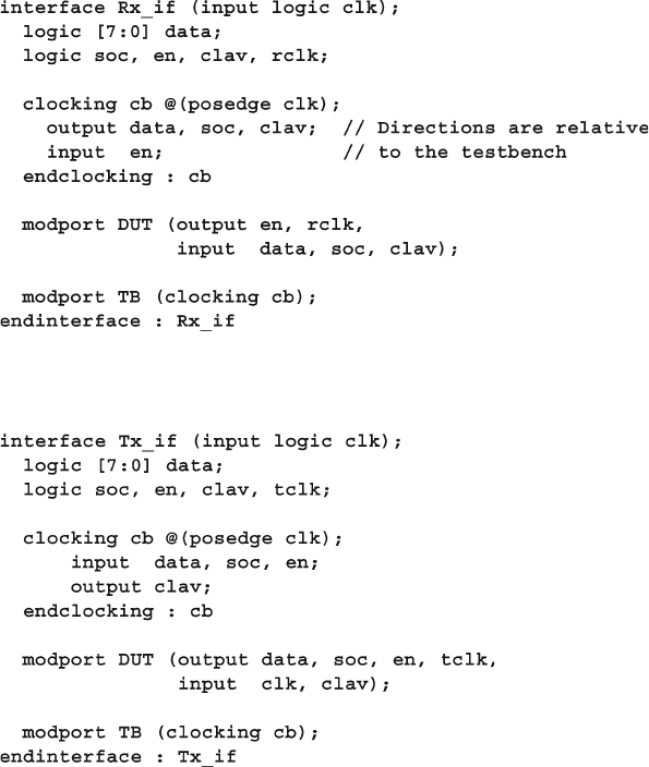
124 4 Connecting the Testbench and Design
4.10.5 ATM Router Model Using an Interface
Sample 4.49 contains the ATM router model and testbench, which need to specify
the modport in their port connection list. Note that you put the modport name after
the interface name, Rx_if .
Sample 4.48 Tx interface with modports and clocking block
Sample 4.47 Rx interface with modports and clocking block
4.10.4 ATM Interfaces
Sample 4.47 and 4.48 show the Rx and Tx interfaces with modports and clocking
blocks.
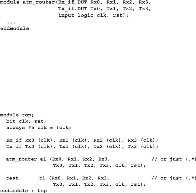
125
4.10 The Four-Port ATM Router
4.10.7 ATM Testbench with Interface
Sample 4.51 shows the part of the testbench that captures cells coming in from the
TX port of the router. Note that the interface names are hard-coded, so you have to
duplicate the same code four times for the 4´4 ATM router. For example, only the
task receive_cell0 is shown, and the fi nal code would also have receive_
cell1, receive_cell2 , and receive_cell30 . Chapter 10 shows how to sim-
plify the code by using virtual interfaces.
Sample 4.49 ATM router model with interface using modports
4.10.6 ATM Top Level Module with Interfaces
The top module, shown in Sample 4.50 , has shrunk considerably, along with the
chances of making a mistake.
Sample 4.50 Top-level module with interface
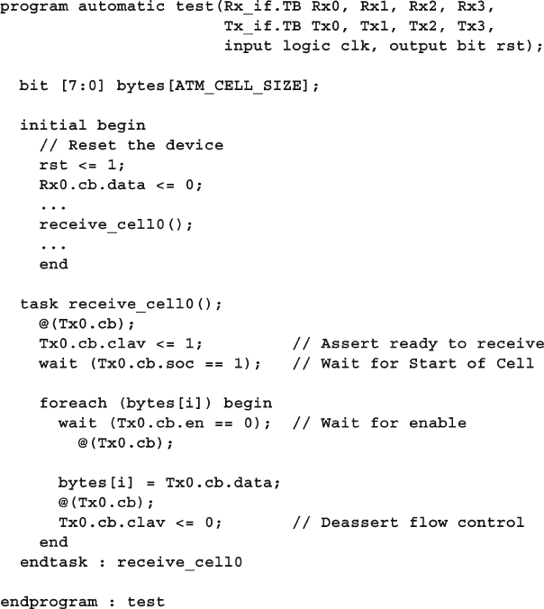
126 4 Connecting the Testbench and Design
4.11 The Ref Port Direction
SystemVerilog introduces a new port direction for connecting modules: ref . You
should be familiar with the input, output , and inout directions. The last is for
modeling bidirectional connections. If you drive a signal with multiple inout ports,
SystemVerilog will calculate the value of the signal by combining the values of all
drivers, taking in to account driver strengths and Z values.
A ref port is a different beast. It is essentially a way to make two names that
both reference the same variable. There is only one storage location, but multiple
aliases. Ref ports can only connect to variables, not signals. See Section 3.4.3 for
information on the ref direction for routine arguments.
Sample 4.51 Testbench using an interface with a clocking block
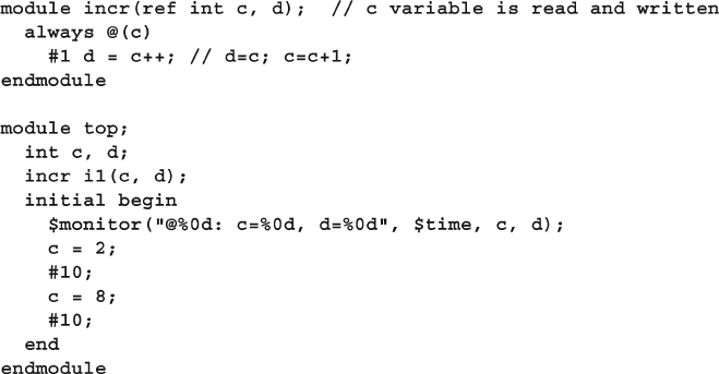
127
4.12 Conclusion
In Sample 4.52 , the incr module has two ref ports, c and d . These two variables
share storage with the c and d variables in the top module. When top changes the
value of c , it is seen immediately by incr . Then incr increments c and the result
is seen back in the
top module. If the port c was declared as inout , you would
have had to build tristate drivers such as continuous assignment statements, and
make sure you properly drove an enable signal and Z values. Don’t consider
ref
ports as a convenient replacement for inout ports as only the latter are supported
for synthesis.
Sample 4.52 Ref ports
4.12 Conclusion
In this chapter you have learned how to use SystemVerilog’s interfaces to organize
the communication between design blocks and your testbench. With this design
construct, you can replace dozens of signal connections with a single interface,
making your code easier to maintain and improve, and reducing the number of wir-
ing mistakes.
SystemVerilog also introduces the program block to hold your testbench and to
reduce race conditions between the device under test and the testbench. With a
clocking block in an interface, your testbenches will drive and sample design sig-
nals correctly relative to the clock.
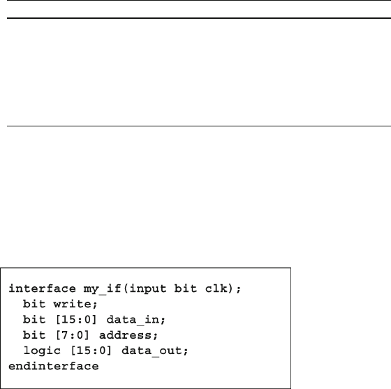
128 4 Connecting the Testbench and Design
4.13 Exercises
1. Design an interface and testbench for the ARM Advanced High-performance
Bus (AHB). You are provided a bus master as verifi cation IP that can initiate
AHB transactions. You are testing a slave design. The testbench instantiates the
interface, slave, and master. Your interface will display an error if the transaction
type is not IDLE or NONSEQ on the negative edge of HCLK. The AHB signals
are described in Table
4.2 .
Table 4.2 AHB Signal Description
Signal Width Direction Description
HCLK 1 Output Clock
HADDR 21 Output Address
HWRITE 1 Output Write fl ag: 1=write, 0=read
HTRANS 2 Output Transaction type:
2 ¢ b00=IDLE, 2 ¢ b10=NONSEQ
HWDATA 8 Output Write data
HRDATA 8 Input Read data
2. For the following interface, add the following code.
a. A clocking block that is sensitive to the negative edge of the clock, and all I/O
that are synchronous to the clock.
b. A modport for the testbench called master , and a modport for the DUT called
slave
c. Use the clocking block in the I/O list for the master modport.
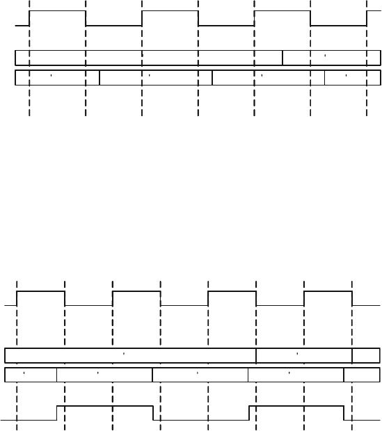
129
4.13 Exercises
3. For the clocking block in Exercise 2, fi ll in the data_in and data_out signals
in the following timing diagram.
reg_bus/clk
reg_bus/data_in
reg_bus/data_out
reg_bus/cb/data_in
reg_bus/cb/data_out
reg_bus/cb/write
reg_bus/write
16 h0000 16 h0001
16 h0000 16 h0001 16 h0002 16 h0003
2
4
test/reg_bus/clk
test/reg_bus/data_in
test/reg_bus/data_out 16 h0000 16 h0001
reg_bus/cb/data_in 16 h0000 16 h0001 16 h0002 16 h0003
reg_bus/cb/data_out
4. Modify the clocking block in Exercise 2 to have:
a. output skew of 25ns for output write and address
b. input skew of 15ns
c. restrict data_in to only change on the positive edge of the clock
5. For the clocking block in Exercise 4, fi ll in the following timing diagram, assuming
a clock period of 100ns.
131
C. Spear and G. Tumbush, SystemVerilog for Verifi cation: A Guide to Learning
the Testbench Language Features, DOI 10.1007/978-1-4614-0715-7_5,
© Springer Science+Business Media, LLC 2012
5.1 Introduction
With procedural programming languages such as Verilog and C, there is a strong
division between data structures and the code that uses them. The declarations and
types of data are often in a different fi le than the algorithms that manipulate them.
As a result, it can be diffi cult to understand the functionality of a program, as the
two halves are separate.
Verilog users have it even worse than C users, as there are no structures in Verilog,
only bit vectors and arrays. If you wanted to store information about a bus transac-
tion, you would need multiple arrays: one for the address, one for the data, one for
the command, and more. Information about transaction N is spread across all the
arrays. Your code to create, transmit, and receive transactions is in a module that
may or may not be actually connected to the bus. Worst of all, the arrays are all
static, so if your testbench only allocated 100 array entries, and the current test
needed 101, you would have to edit the source code to change the size and recom-
pile. As a result, the arrays are sized to hold the greatest conceivable number of
transactions, but during a normal test, most of that memory is wasted.
Object-Oriented Programming (OOP) lets you create complex data types and tie
them together with the routines that work with them. You can create testbenches and
system-level models at a more abstract level by calling routines to perform an action
rather than toggling bits. When you work with transactions instead of signal transi-
tions, you are working at a higher level, and your code is more easily written and
understood. As a bonus, your testbench is decoupled from the design details,
making it more robust and easier to maintain and reuse on future projects.
Chapter 5
Basic OOP
132 5 Basic OOP
If you already are familiar with OOP, skim this chapter, as SystemVerilog
follows OOP guidelines fairly closely. Be sure to read Section 5.18 to learn how
to build a testbench. Chapter 8 presents advanced OOP concepts such as inheri-
tance and more testbench techniques; it should be read by everyone.
5.2 Think of Nouns, not Verbs
Grouping data and code together helps you in creating and maintaining large test-
benches. How should data and code be brought together? You can start by thinking
of how you would perform the testbench’s job.
The goal of a testbench is to apply stimulus to a design and then check the result
to see if it is correct. The data that fl ows into and out of the design is grouped
together into transactions such as bus cycles, opcodes, packets, or data samples. The
best way to organize the testbench is around the transactions, and the operations that
you perform on them. In OOP, the transaction is the focus of your testbench.
You can think of an analogy between cars and testbenches. Early cars required
detailed knowledge about their internals (nouns) to operate. You had to advance or
retard the spark, open and close the choke, keep an eye on the engine speed and be
aware of the traction of the tires if you drove on a slippery surface such as a wet
road. Today your interactions with the car are at a high level. When you get into a
car, you perform discrete actions (verbs), such as starting, moving forward, turning,
stopping, and listening to music while you drive. If you want to start a car, just turn
the key in the ignition, and you are done. Get the car moving by pressing the gas
pedal; stop it with the brakes. Are you driving on snow? Don’t worry: the anti-lock
brakes help you stop safely and in a straight line. You don’t have to think about the
low level details.
Your testbench should be structured the same way. Traditional testbenches were
oriented around the operations that had to happen: create a transaction, transmit it,
receive it, check it, and make a report. Instead, you should think about the structure
of the testbench, and what each part does. The generator creates transactions and
passes them to the next level. The driver talks with the design that responds with
transactions that are received by a monitor. The scoreboard checks these against the
expected data. You should divide your testbench into blocks, and then defi ne how
they communicate. This chapter shows many examples of these components.
How do you represent these blocks in SystemVerilog? A class may describe a
data-centric block such as a bus transaction, network packet, or CPU instruction. Or
a class might represent a control block such as a driver or scoreboard. Either way, a
class encapsulates the data together with the routines that manipulate it. The details
of how the class implements actions such as data generation or checking is hidden
from the outside, making the class more reusable.
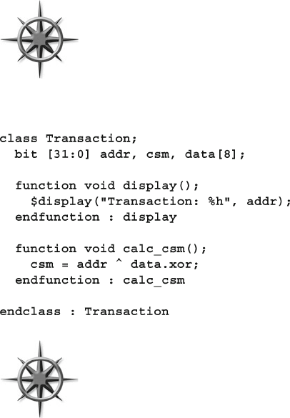
133
5.4 Where to Defi ne a Class
5.3 Your First Class
Sample 5.1 shows a class for a generic transaction. It contains an address, a check-
sum, and an array of data values. There are two routines in the
Transaction class:
one that displays the address, and another that computes a checksum of the data.
To make it easier to match the beginning and end of a named block,
you can put a label on the end of it. In Sample 5.1 these end labels
may look redundant, but in complex code, with many nested blocks,
the labels help you fi nd the mate for a simple end, endtask,
endfunction , or endclass .
Sample 5.1 Simple transaction class
Every company has its own naming style. This book uses the follow-
ing convention: Class names start with a capital letter and avoid
using underscores, as in Transaction or Packet . Constants are all
upper case, as in CELL_SIZE , and variables are lower case, as in
count or opcode . You are free to use whatever style you want.
5.4 Where to Defi ne a Class
You can defi ne and use classes in SystemVerilog in a program, module, package ,
or outside of any of these.
When you start a project, you might store a single class per fi le. When the num-
ber of fi les gets too large, you can group a set of related classes and type defi nitions
into a SystemVerilog package as shown in Sample 5.2 . For instance, you might
group together all USB3 transactions and BFMs into a single package . Now you
can compile the package separately from the rest of the system. Unrelated classes,
such as those for other transactions, scoreboards, or different protocols, should
remain in separate fi les.
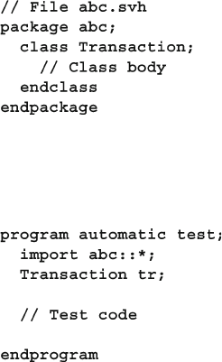
134 5 Basic OOP
Code samples in this book leave out the packages to keep the text more compact.
Sample 5.3 Importing a package in a program
Sample 5.2 Class in a package
5.5 OOP Terminology
What separates you, an OOP novice, from an expert? The fi rst thing is the words
you use. You already know some OOP concepts from working with Verilog. Here
are some OOP terms, defi nitions, and rough equivalents in Verilog 2001.
Class – a basic building block containing routines and variables. The analogue in •
Verilog is a module.
Object – an instance of a class. In Verilog, you need to instantiate a module to use it. •
Handle – a pointer to an object. In Verilog, you use the name of an instance when •
you refer to signals, and routines from outside the module. A handle is like the
address of the object, but stored in a pointer that can only refer to one type.
A handle is similar to a reference in other OOP languages.
Property – a variable that holds data. In Verilog, this is a signal such as a register •
or wire.
Method – the procedural code that manipulates variables, contained in tasks and •
functions. Verilog modules have tasks and functions plus initial and always
blocks.
Prototype – the header of a routine that shows the name, type, and argument list •
plus return type. The body of the routine contains the executable code. See
Section 5.10 for more on prototypes and out-of-body experiences.
Sample 5.3 shows how to import a package into a program.
135
5.6 Creating New Objects
This book uses the more traditional terms from Verilog of “variable” and “routine”
when discussing non-OOP code, and “property” and “method” for classes.
In Verilog you build complex designs by creating modules and instantiating them
hierarchically. In OOP you create classes and construct them (creating objects) to
create a similar hierarchy. Modules are instantiated during compilation while classes
are constructed at run time.
Here is an analogy to explain these OOP terms. Think of a class as the blueprint for
a house. This plan describes the structure of the house, but you cannot live in a blue-
print; you need to build the physical house. An object is the actual house. Just as one
set of blueprints can be used to build a whole subdivision of houses, a single class can
be used to build many objects. The house address is like a handle in that it uniquely
identifi es your house. Inside your house you have things such as lights (on or off),
with switches to control them. A class has variables that hold values, and routines that
control the values. A class for the house might have many lights. A single call to
turn_on_porch_light() sets the light variable ON in a single house.
5.6 Creating New Objects
Both Verilog and OOP have the concept of instantiation, but there are some differ-
ences in the details. A Verilog module, such as a counter, is instantiated when you
compile your design. A SystemVerilog class, such as a network packet, is instanti-
ated during simulation, when needed by the testbench. Verilog instances are static,
as the hardware does not change during simulation; only signal values change.
SystemVerilog stimulus objects are constantly being created and used to drive the
DUT and check the results. Later, the objects may be freed so their memory can be
used by new ones. Back to the house analogy: the address is normally static, unless
your house burns down, causing you to construct a new one. Garbage collection at
home is not automatic, especially if you have teenagers.
The analogy between OOP and Verilog has a few other exceptions. The top-level
Verilog module is implicitly instantiated. However, a SystemVerilog class must be
instantiated before it can be used. Next, a Verilog instance name only refers to a
single instance, whereas a SystemVerilog handle can refer to many objects, though
only one at a time.
5.6.1 Handles and Constructing Objects
In Sample 5.4 , tr is a handle that points to an object of type Transaction . For
brevity, you can just say tr is a Transaction handle.
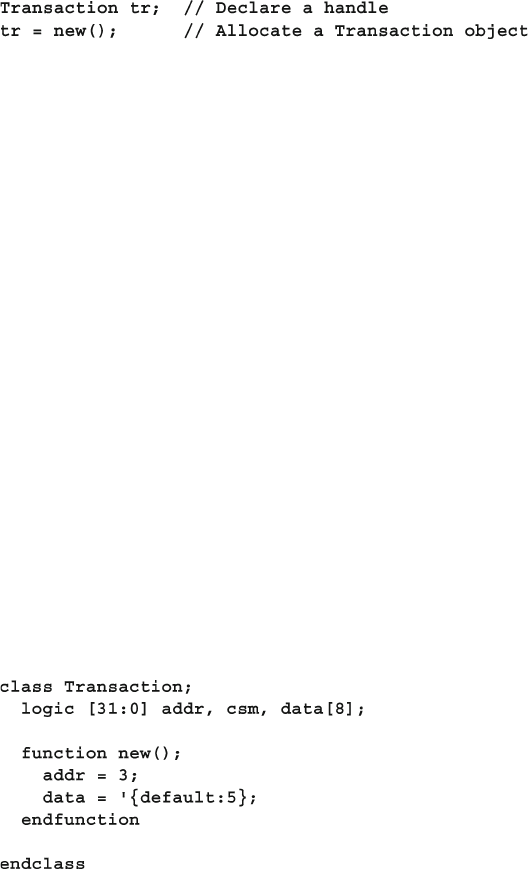
136 5 Basic OOP
When you declare the handle tr , it is initialized to the special value null .
On the next line, call the new() function to construct the Transaction object.
This special new function allocates space for the Transaction , initializes the
variables to their default value (0 for 2-state variables and X for 4-state ones), and
returns the address where the object is stored. For example, the Transaction class
has two 32-bit registers ( addr and csm ) and an array with eight values (data), for a
total of 10 longwords, or 40 bytes. So when you call new , SystemVerilog allocates
at least 40 bytes of storage. If you have used C, this step is similar to calling the
malloc function. Note that SystemVerilog requires additional memory for 4-state
variables and housekeeping information such as the object’s type.
This process is called instantiation as you are making an instance of the class.
The new function is sometimes called the constructor, as it builds the object, just as
your carpenter constructs a house from wood and nails. For every class, SystemVerilog
creates a default new function to allocate and initialize an object.
5.6.2 Custom Constructor
You can defi ne your own new() function to set your own values. Note that you must
not give a return value type as the constructor is a special function and automatically
returns a handle to an object of the same type as the class.
Sample 5.5 Simple user-defi ned new() function
Sample 5.4 Declaring and using a handle
In Sample 5.5 , fi rst SystemVerilog allocates the space for the object automati-
cally. Next it sets addr and data to fi xed values but leaves csm at its default value
of X. You can use arguments with default values to make a more fl exible constructor,
as shown in Sample 5.6 . Now you can specify the value for addr and data when
you call the constructor, or use the default values.
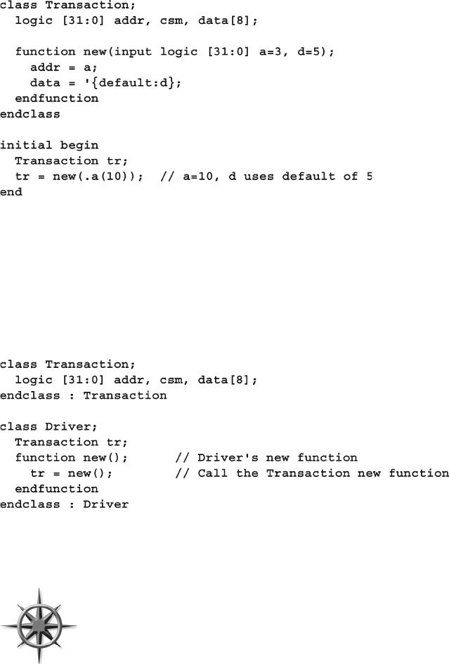
137
5.6 Creating New Objects
How does SystemVerilog know which new() function to call? It looks at the type
of the handle on the left side of the assignment. In Sample 5.7 , the call to new inside
the Driver constructor calls the new() function for Transaction , even though
the one for Driver is closer. Since tr is a Transaction handle, SystemVerilog
does the right thing and creates an object of type Transaction .
Sample 5.6 A new() function with arguments
Sample 5.7 Calling the right new() function
5.6.3 Separating the Declaration and Construction
You should avoid declaring a handle and calling the constructor,
new , all in one statement. While this is legal syntax and less verbose,
it can create ordering problems, as the constructor is called before
the fi rst procedural statement. You might need to initialize objects in
a certain order, but if you call new() in the declaration, you won’t
have the same control. Additionally, if you forget to use automatic storage, the
constructor is called at the start of simulation, not when the block is entered.
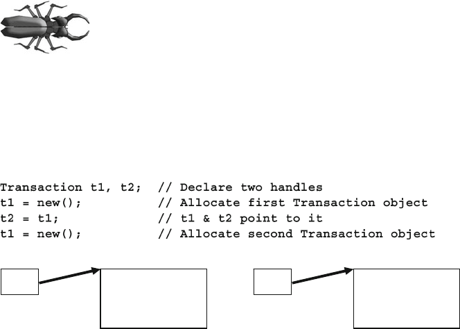
138 5 Basic OOP
5.6.4 The Difference Between New() and New[]
You may have noticed that this new() function looks a lot like the new[] operator
described in Section 2.3, used to set the size of dynamic arrays. They both allocate
memory and initialize values. The big difference is that the
new() function is called
to construct a single object, whereas the new[] operator is building an array with
multiple elements. new() can take arguments for setting object values, whereas
new[] only takes a single value for the number of elements in the array. Just remem-
ber that the new with square brackets [] is for arrays, while the one with paren-
theses () is for classes, which usually contain methods.
5.6.5 Getting a Handle on Objects
New OOP users often confuse an object with its handle. The two
are very distinct. You declare a handle and construct an object.
Over the course of a simulation, a handle can point to many
objects. This is the dynamic nature of OOP and SystemVerilog.
Don’t get the handle confused with the object.
In Sample 5.8 , t1 fi rst points to one object, then another. Fig. 5.1 shows the
resulting handles and objects.
Sample 5.8 Allocating multiple objects
First
Transaction
object
t2
Second
Transaction
object
t1 t2t1
Fig. 5.1 Handles and objects after allocating multiple objects
Why would you want to create objects dynamically? During a simulation you
may need to create hundreds or thousands of transactions. SystemVerilog lets you
create objects automatically, when you need them. In Verilog, you would have to
use a fi xed-size array large enough to hold the maximum number of transactions.
Note that this dynamic creation of objects is different from anything else offered
before in the Verilog language. An instance of a Verilog module and its name are
bound together statically during compilation. Even with automatic variables, which
come and go during simulation, the name and storage are always tied together.
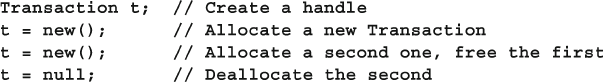
139
5.7 Object Deallocation
An analogy for handles is people who are attending a conference. Each person is
similar to an object. When you arrive, a badge is “constructed” by writing your
name on it. This badge is a handle that can be used by the organizers to keep track
of each person. When you take a seat for the lecture, space is allocated. You may
have multiple badges for attendee, presenter, or organizer. When you leave the con-
ference, your badge may be reused by writing a new name on it, just as a handle can
point to different objects through assignment. Lastly, if you lose your badge and
there is nothing to identify you, you will be asked to leave. The space you take, your
seat, is reclaimed for use by someone else.
5.7 Object Deallocation
Now you know how to create an object — but how do you get rid of it? For example,
your testbench creates and sends thousands of transactions, such as packets, instruc-
tions, frames, interrupts, etc. into your DUT. Once you know the transaction has
completed successfully, you don’t need to keep it around. You should reclaim the
memory; otherwise, a long simulation might run out of memory.
Garbage collection is the process of automatically freeing objects that are no
longer referenced. One way SystemVerilog can tell if an object is no longer being
used is by keeping track of the number of handles that point to it. When the last
handle no longer references an object, SystemVerilog releases the memory for it.
(The actual algorithm to fi nd unused objects varies between simulators. This section
describes reference counting, which is the easiest to understand).
Sample 5.9 Creating multiple objects
The second line in Sample 5.9 calls new() to construct an object and store the
address in the handle t. The next call to new() constructs a second object and stores
its address in t , overwriting the previous value. Since there are no handles pointing
to the fi rst object, SystemVerilog can deallocate it. The object may be deleted imme-
diately, or after a short wait. The last line explicitly clears the handle so that now the
second object can be deallocated.
If you are familiar with C++, these concepts of objects and handles are familiar,
but there are some important differences. A SystemVerilog handle can only point to
objects of one type, so they are called “type-safe.” In C, a typical void pointer is only
an address in memory, and you can set it to any value or modify it with operators
such as pre-increment. You cannot be sure that a pointer is valid. A C++ typed pointer
is much safer, but you may be tempted by C’s fl exibility. SystemVerilog does not
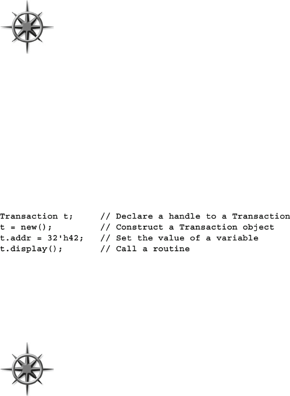
140 5 Basic OOP
allow any modifi cation of a handle or using a handle of one type to refer to an object
of another type. (SystemVerilog’s OOP specifi cation is closer to Java than C++).
Since SystemVerilog garbage collects an object when no more handles refer to it,
you can be sure your code always uses valid handles. In C / C++, a pointer can refer
to an object that no longer exists. Garbage collection in those languages is manual, so
your code can suffer from “memory leaks” when you forget to deallocate objects.
SystemVerilog cannot garbage collect an object that is still refer-
enced somewhere by a handle. For example, if you keep objects in
a linked list, SystemVerilog cannot deallocate the objects until you
manually clear all handles by setting them to null . If an object
contains a routine that forks off a thread, the object is not deallo-
cated while the thread is running. Likewise, any objects that are
used by a spawned thread may not be deallocated until the thread terminates. See
Chapter 7 for more information on threads.
5.8 Using Objects
Now that you have allocated an object, how do you use it? Going back to the Verilog
module analogy, you can refer to variables and routines in an object with the “.”
notation, as shown in Sample 5.10 .
Sample 5.10 Using variables and routines in an object
In strict OOP, the only access to variables in an object should be through accessor
functions such as get() and put() . This is because accessing variables directly
limits your ability to change the underlying implementation in the future. If a better
(or simply different) algorithm comes along in the future, you may not be able to
adopt it because you would also need to modify all of the references to the variables.
The problem with this methodology is that it was written for large
software applications with lifetimes of a decade or more. With dozens
of programmers making modifi cations, stability is paramount.
However, you are creating a testbench, where the goal is maximum
control of all variables to generate the widest range of stimulus values.
One of the ways to accomplish this is with constrained-random stimu-
lus generation, which cannot be done if a variable is hidden behind a screen of meth-
ods. While the
get() and put() methods are fi ne for compilers, GUIs, and APIs,
you should stick with public variables that can be directly accessed anywhere in
your testbench.
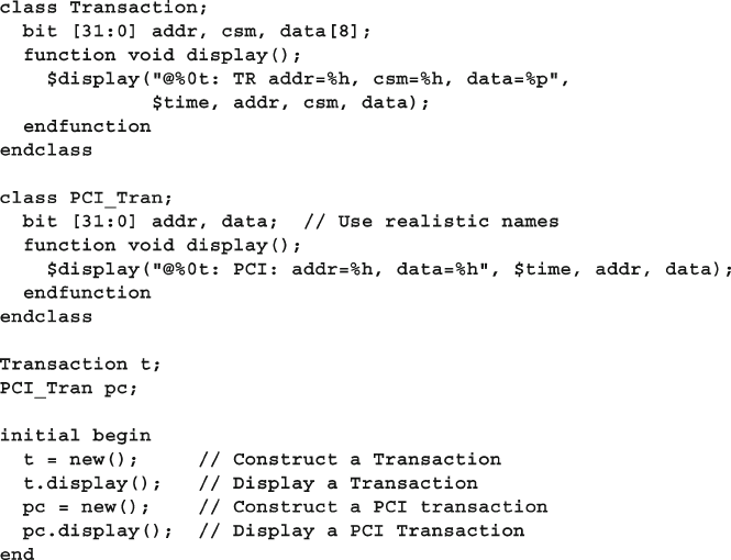
141
5.9 Class Methods
The exception to this rule is for verifi cation IP that is created and maintained by
a group such as a company that has no direct relationship to the end user. For exam-
ple, if you purchase a PCI transactor from another company, they will restrict access
to the internals, forcing you to treat it as a black box. The developer must give you
enough methods to generate both good transactions and inject all fl avors of errors.
5.9 Class Methods
A method in a class is just a task or function defi ned inside the scope of the class.
Sample 5.11 defi nes display() methods for the Transaction and PCI_Tran .
SystemVerilog calls the correct one, based on the handle type.
Sample 5.11 Routines in the class
A method in a class uses automatic storage by default, so you don’t have to worry
about remembering the automatic modifi er.
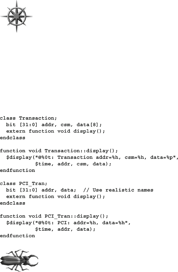
142 5 Basic OOP
5.10 Defi ning Methods Outside of the Class
A good rule of thumb is you should limit a piece of code to one
“page” or screen in your favorite editor to keep it understandable.
You may be familiar with this rule for routines, but it also applies
to classes. If you can see everything in a class on the screen at one
time, it is easier to understand.
However, if each method takes a page, how can the whole class fi t on a page? In
SystemVerilog you can break a method into the prototype (method name and argu-
ments) inside the class, and the body (the procedural code) that goes after the class.
Here is how you create out-of-block declarations. Copy the fi rst line of the
method, with the name and arguments, and add the
extern keyword at the begin-
ning. Now take the entire method and move it after the class body, and add the class
name and two colons (:: the scope operator) before the method name. The above
classes could be defi ned as shown in Sample 5.12 .
Sample 5.12 Out-of-block method declarations
A common coding mistake is when the prototype does not match
the out-of-body. SystemVerilog requires that the prototype be
identical to the out-of-block method declaration, except for the
class name and scope operator, ::. The prototype can have qual-
ifi ers such as local, protected , or virtual , but not the out-of-body. If any
arguments have default values, they must be given in the prototype, but they are
optional in the out-of-body.
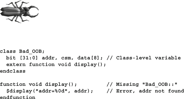
143
5.11 Static Variables vs. Global Variables
Another common mistake is to leave out the class name when you
declare the method outside of the class. As a result, it is defi ned at
the next higher scope (probably the program or package scope),
and the compiler gives an error when the task tries to access class-
level variables and methods. This is shown in Sample
5.13 .
Sample 5.13 Out-of-body method missing class name
5.11 Static Variables vs. Global Variables
Every object has its own local variables that are not shared with any other object. If
you have two Transaction objects, each has its own addr, csm , and data variables.
Sometimes though, you need a variable that is shared by all objects of a certain type.
For example, you might want to keep a running count of the number of transactions
that have been created. Without OOP, you would probably create a global variable.
Then you would have a global variable that is used by one small piece of code, but
is visible to the entire testbench. This “pollutes” the global name space and makes
variables visible to everyone, even if you want to keep them local.
5.11.1 A Simple Static Variable
In SystemVerilog you can create a static variable inside a class. This variable is
shared amongst all instances of the class, but its scope is limited to the class. In
Sample 5.14 , the static variable count holds the number of objects created so far. It
is initialized to 0 in the declaration because there are no transactions at the begin-
ning of the simulation. Each time a new object is constructed, it is tagged with a
unique value, and count is incremented.
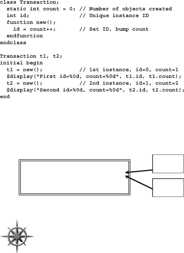
144 5 Basic OOP
In Sample 5.14 , there is only one copy of the static variable count , regardless of
how many Transaction objects are created. You can think that count is stored
with the class and not the object. The variable id is not static, so every Transaction
has its own copy, as shown in Fig. 5.2 . Now you don’t need to make a global vari-
able for the count.
class Transaction;
static int count = 0;
int id;
endclass
id: 0
count
id: 1
count
Fig. 5.2 Static variables in a class
Sample 5.14 Class with a static variable
Using the ID fi eld is a good way to track objects as they fl ow
through a design. When debugging a testbench, you often need a
unique value. SystemVerilog does not let you print the address of
an object, but you can make an ID fi eld. Whenever you are tempted
to make a global variable, consider making a class-level static vari-
able. A class should be self-contained, with as few outside refer-
ences as possible.
5.11.2 Accessing Static Variables Through the Class Name
Sample 5.14 showed how you can reference a static variable using a handle. You
don’t need a handle; you could use the class name followed by ::, the class scope
resolution operator, shown in Sample 5.15.
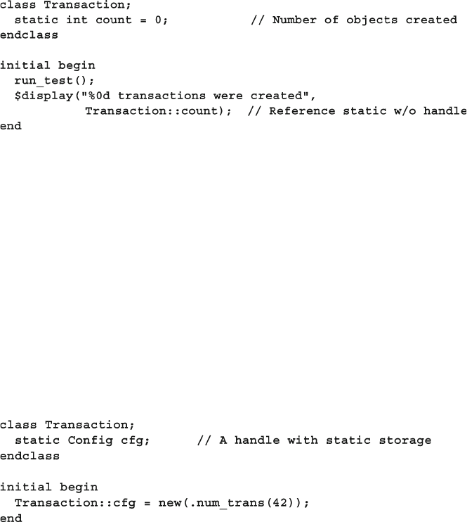
145
5.11 Static Variables vs. Global Variables
5.11.4 Static Methods
As you employ more static variables, the code to manipulate them may grow into a full
fl edged routine. In SystemVerilog you can create a static method inside a class that can
read and write static variables, even before the fi rst instance has been created.
Sample 5.17 has a simple static function to display the values of the static variables.
SystemVerilog does not allow a static method to read or write non-static variables,
such as id . You can understand this restriction based on the code below. When the
function display_statics is called at the end of the example, no Transaction
objects have been constructed, so no storage has been created for id variables.
Sample 5.15 The class scope resolution operator
Sample 5.16 Static storage for a handle
5.11.3 Initializing Static Variables
A static variable is usually initialized in the declaration. You can’t easily initialize it
in the class constructor, as this is called for every single new object. You would need
another static variable to act as a fl ag, indicating whether the original variable had
been initialized. If you have a more elaborate initialization, you could use an initial
block. Make sure static variables are initialized before the fi rst object is constructed.
Another use for a static variable is when every instance of a class needs informa-
tion from a single object. For example, a transaction class may refer to a confi gura-
tion object that has the number of transactions. If you have a non-static handle in the
Transaction class, every object will have its own copy, wasting space. Sample
5.16 shows how to use a static variable instead.
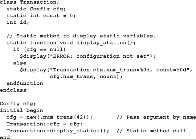
146 5 Basic OOP
5.12 Scoping Rules
When writing your testbench, you need to create and refer to many variables.
SystemVerilog follows the same basic rules as Verilog, with a few helpful
improvements.
A scope is a block of code such as a module, program, task, function, class, or
begin/end block. The for and foreach loops automatically create a block so
that an index variable can be declared or created local to the scope of the loop.
You can only defi ne new variables in a block. New in SystemVerilog is the abil-
ity to declare a variable in an unnamed begin-end block.
A name can be relative to the current scope or absolute starting with $root . For
a relative name, SystemVerilog looks up the list of scopes until it fi nds a match. If
you want to be unambiguous, use $root at the start of a name. Variables can not be
declared in $root , that is, outside of any module, program or package.
Sample 5.18 uses the same name in several scopes. Note that in actual code, you
would use more meaningful names! The name limit is used for a global variable,
a program variable, a class variable, a function variable, and a local variable in an
initial block. The latter is in an unnamed block, so the label created is tool depen-
dent, along with the signal’s hierarchical name.
Sample 5.17 Static method displays static variable
147
5.12 Scoping Rules
For testbenches, you can declare variables in the program or in the initial
block. If a variable is only used inside a single initial block, such as a counter,
you should declare it there to avoid possible name confl icts with other blocks. Note
that if you declare a variable in an unnamed block, such as the initial in Sample
5.18 , there is no hierarchical name that works consistently across all tools.
Declare your classes outside of any program or module in a
package . This approach can be shared by all the testbenches, and
you can declare temporary variables at the innermost possible
level. This style also eliminates a common bug that happens when
you forget to declare a variable inside a class. SystemVerilog looks
for that variable in higher scopes.
If a block uses an undeclared variable, and another variable with
that name happens to be declared in the program block, the class
uses it instead, with no warning. In Sample 5.19 , the function
Bad::display did not declare the loop variable i , so SystemVer-
ilog uses the program level i instead. Calling the function changes the value of
test.i , probably not what you want!
Sample 5.18 Name scope
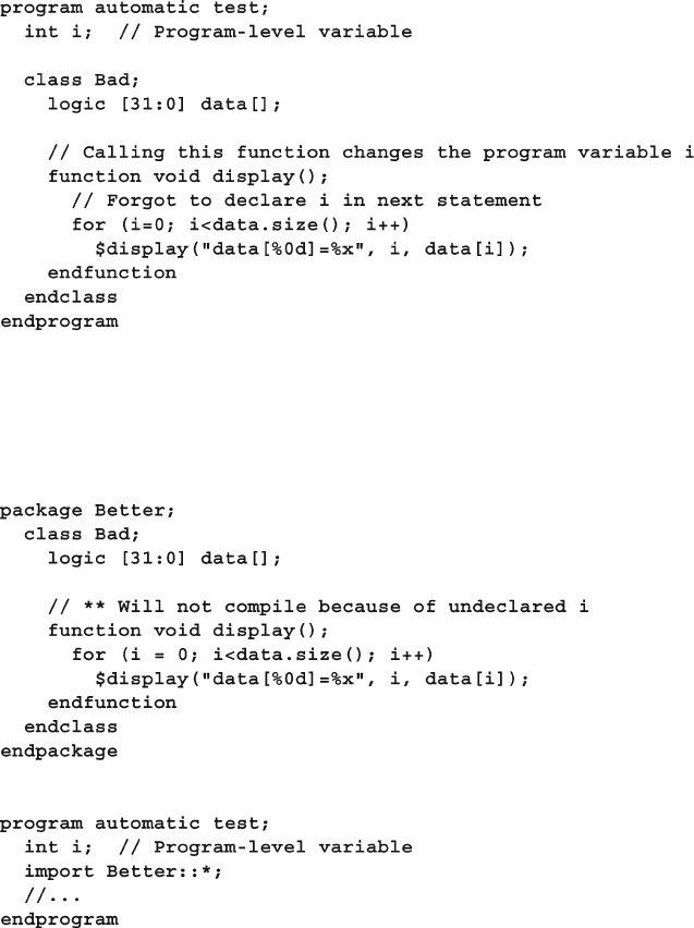
148 5 Basic OOP
If you move the class into a package, the class cannot see the program-level
variables, and thus won’t use them unintentionally as shown in Sample 5.20 .
Sample 5.19 Class uses wrong variable
Sample 5.20 Move class into package to fi nd bug
5.12.1 What is This?
When you use a variable name, SystemVerilog looks in the current scope for it, and
then in the parent scopes until the variable is found. This is the same algorithm
used by Verilog. What if you are deep inside a class and want to unambiguously
refer to a class-level object? This style code is most commonly used in constructors,
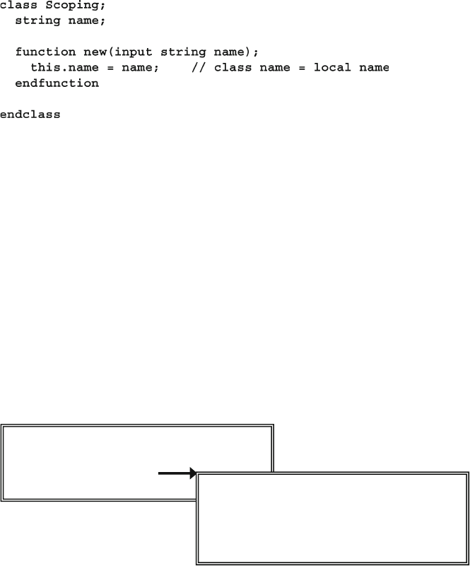
149
5.13 Using One Class Inside Another
where the programmer uses the same name for a class variable and an argument.
In Sample 5.21 , the keyword “ this ” removes the ambiguity to let SystemVerilog
know that you are assigning the local variable, name , to the class variable, name .
class Transaction;
bit [31:0] addr, crc, data[8];
Statistics stats;
endclass
endclass
class Statistics;
time startT, stopT;
static int ntrans= 0;
static time total_elapsed_time;
Fig. 5.3 Contained objects Sample 5.22
Sample 5.21 Using this to refer to class variable
Some people think this argument naming style makes the code easier to read;
others think it is a shortcut by a lazy programmer.
5.13 Using One Class Inside Another
A class can contain an instance of another class, using a handle to an object. This is
just like Verilog’s concept of instantiating a module inside another module to build
up the design hierarchy. A common reason for using containment are code reuse and
controlling complexity. For example, every one of your transactions may have a
statistics block, including timestamps indicating when the transaction started and
ended transmission, and information about all transactions, as shown in Fig. 5.3 and
Sample 5.22 .
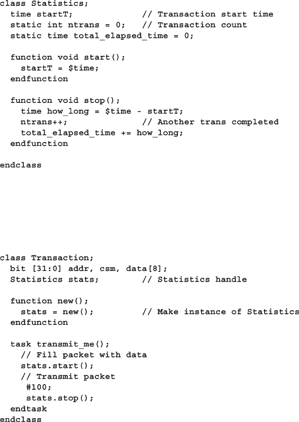
150 5 Basic OOP
Now you can use the Statistics class inside another class such as a transaction as
can been seen in Sample 5.23 .
Sample 5.23 Encapsulating the Statistics class
Sample 5.22 Statistics class declaration
The outermost class, Transaction , can refer to things in the Statistics class
using the usual hierarchical syntax, such as stats.startT .
Remember to instantiate the object; otherwise, the handle stats is null and the
call to start fails. This is best done in the constructor of the outer class,
Transaction .

151
5.13 Using One Class Inside Another
As your classes become larger, they may become hard to manage. When your
variable declarations and method prototypes grow larger than a page, you should
see if there is a logical grouping of items in the class so that it can be split into
several smaller ones.
This is also a potential sign that it’s time to refactor your code, i.e., split it into
several smaller, related classes. See Chapter 8 for more details on class inheritance.
Look at what you’re trying to do in the class. Is there something you could move
into one or more base classes, i.e., decompose a single class into a class hierarchy?
A classic indication is similar code appearing at various places in the class. You
need to factor that code out into a function in the current class, one of the current
class’s parent classes, or both.
5.13.1 How Big or Small Should My Class Be?
Just as you may want to split up classes that are too big, you should
also have a lower limit on how small a class should be. A class with
just one or two members makes the code harder to understand as it
adds an extra layer of hierarchy and forces you to constantly jump
back and forth between the parent class and all the children to
understand what it does. In addition, look at how often it is used. If a small class is
only instantiated once, you might want to merge it into the parent class.
One Synopsys customer put each transaction variable into its own class for fi ne
control of randomization. The transaction had a separate object for the address,
checksum, data, etc. In the end, this approach only made the class hierarchy more
complex. On the next project they fl attened the hierarchy.
See Section 8.4 for more ideas on partitioning classes.
5.13.2 Compilation Order Issue
Sometimes you need to compile a class that includes another class that is not yet
defi ned. The declaration of the handle causes an error, as the compiler does not
recognize the new type. Declare the class name with a typedef statement, as shown
in Sample 5.24 .
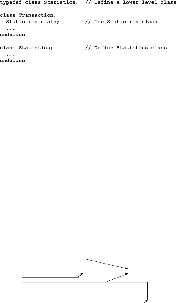
152 5 Basic OOP
5.14 Understanding Dynamic Objects
In a statically allocated language such as Verilog, every signal has a unique variable
associated with it. For example, there may be a wire called grant , the integer
count , and a module instance i1 . In OOP, there is not the same one-to-one corre-
spondence. There can be many objects, but only a few named handles. A testbench
may allocate a thousand transaction objects during a simulation, but may only have
a few handles to manipulate them. This situation takes some getting used to if you
have only written Verilog code.
In reality, there is a handle pointing to every active object. Some handles may be
stored in arrays or queues, or in another object, like a linked list. For objects stored
in a mailbox, the handle is in an internal SystemVerilog structure. See Section 7.6
for more information on mailboxes. Remember that as soon as you assign a new
value to the last handle pointing to an object, that object can be garbage collected.
5.14.1 Passing Objects and Handles to Methods
What happens when you pass an object into a method? Perhaps the method only
needs to read the values in the object, such as transmit above. Or, your method
may modify the object, like a method to create a packet. Either way, when you call
the method, you pass a handle to the object, not the object itself.
Sample 5.24 Using a typedef class statement
Transaction
task generator;
Transaction t;
t = new;
transmit(t);
endtask
task transmit(input Transaction t);
…
endtask
Fig. 5.4 Handles and objects across methods
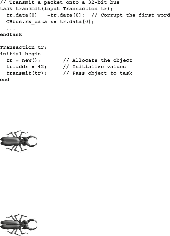
153
5.14 Understanding Dynamic Objects
In Fig. 5.4 , the generator task has just called transmit . There are two
handles, generator.t and transmit.t , that both refer to the same object.
When you call a method, if you pass a scalar variable such as a handle into a ref
argument, SystemVerilog passes the address of the variable so the method can mod-
ify it. If you don’t use
ref , SystemVerilog copies the scalar’s value into the argu-
ment variable, so any change to the argument in the method does not affect the
original value.
Sample 5.25 Passing objects
In Sample 5.25 , the initial block allocates a Transaction object and calls the
transmit task with the handle that points to the object. Using this handle, trans-
mit can read and write values in the object. However, if transmit tries to modify
the handle, the result won’t be seen in the initial block, as the t argument was not
declared as ref .
A method can modify an object, even if the handle argument
does not have a ref modifi er. This frequently causes confusion
for new users, as they mix up the handle with the object. As
shown above, transmit can modify data[0] in the object
without changing the value of t . If you don’t want an object modifi ed in a method,
pass a copy of it so that the original object is untouched. See Section 5.15 for more
on copying objects.
5.14.2 Modifying a Handle in a Task
A common coding mistake is to forget to use ref on method
arguments that you want to modify, especially handles. In
Sample 5.26 , the argument tr is not declared as ref , so any
change to it is not be seen by the calling code. The argument tr
has the default direction of input .
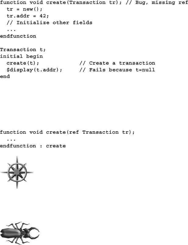
154 5 Basic OOP
Sample 5.26 Bad transaction creator task, missing ref on handle
Even though create modifi ed the argument tr , the handle t in the calling
block remains null . You need to declare the argument tr as ref as can be seen in
Sample 5.27 .
Sample 5.27 Good transaction creator task with ref on handle
If a method is only going to modify the properties of the object, the
method should declare the handle as an input argument. If a method
is going to modify the handle, for example to make it point to a new
object, the method must declare the handle as a ref argument.
5.14.3 Modifying Objects in Flight
A very common mistake is forgetting to create a new object for
each transaction in the testbench. In Sample 5.28 , the generate_
bad task creates a Transaction object with random values, and
transmits it into the design over several cycles.
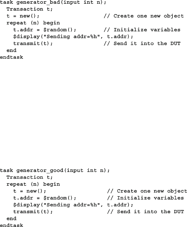
155
5.14 Understanding Dynamic Objects
What are the symptoms of this mistake? The code above creates only one
Transaction , so every time through the loop, generator_bad changes the object
at the same time it is being transmitted. When you run this, the $display shows
many addr values, but all transmitted Transaction objects have the same value
of addr . The bug becomes visible when transmit spawns off a thread that takes
several cycles to send the transaction, and so the values in the object are re-randomized
in the middle of transmission. If your transmit task makes a copy of the object,
you can recycle the same object over and over. This bug can also happen with
mailboxes as shown in Sample 7.32
To avoid this bug, you need to create a new Transaction during each pass
through the loop as seen in Sample 5.29 .
Sample 5.29 Good generator creates many objects
Sample 5.28 Bad generator creates only one object
5.14.4 Arrays of Handles
As you write testbenches, you need to be able to store and reference many objects.
You can make arrays of handles, each of which refers to an object. Sample 5.30
shows storing ten bus transaction handles in an array.
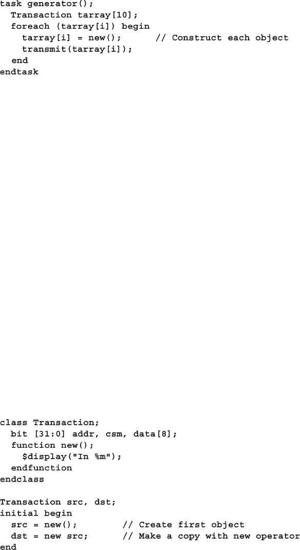
156 5 Basic OOP
The array tarray is made of handles, not objects. So you need to construct each
object in the array before using it, just as you would for a normal handle. There is
no way to call new on an entire array of handles.
There is no such thing as an “array of objects”, though you may use this term as
a shorthand for an array of handles that points to objects. Keep in mind that some
handles may be set to null , or that multiple handles could point to a single object.
5.15 Copying Objects
You may want to make a copy of an object to keep a method from modifying the origi-
nal, or in a generator to preserve the constraints. You can either use the simple, built-in
copy available with new operator or you can write your own for more complex classes.
See Section 8.2 for more reasons why you should make a copy method.
5.15.1 Copying an Object with the New Operator
Copying an object with the new operator is easy and reliable as shown in Sample
5.31 . Memory for the new object is allocated and all variables from the existing
object are copied. However any new() function that you may have defi ned is not
called.
Sample 5.30 Using an array of handles
Sample 5.31 Copying a simple class with new
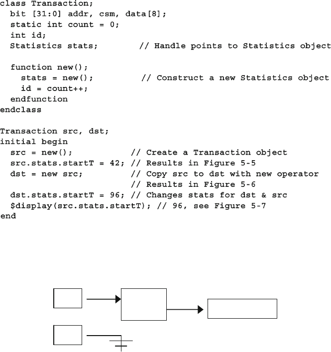
157
5.15 Copying Objects
This is a shallow copy, similar to a photocopy of the original, blindly transcribing
values from source to destination. If the class contains a handle to another class,
only the handle’s value is copied by the new operator, not a full copy of the lower
level object. In Sample
5.32 , the Transaction class contains a handle to the
Statistics class, originally shown in Sample 5.22 .
Sample 5.32 Copying a complex class with new operator
id=0
stats
dst
src
startT=42
Fig. 5.5 Objects and handles before copy with the new operator
The initial block creates the fi rst Transaction object and modifi es a variable in
the contained object stats as shown in Fig. 5.5 .
When you use the new operator to make a copy, the Transaction object is
copied, but not the Statistics one. This is because the new operator does not call
your own new() function. Instead, the values of variables and handles are copied.
So now both Transaction objects have the same id as shown in Fig. 5.6 .
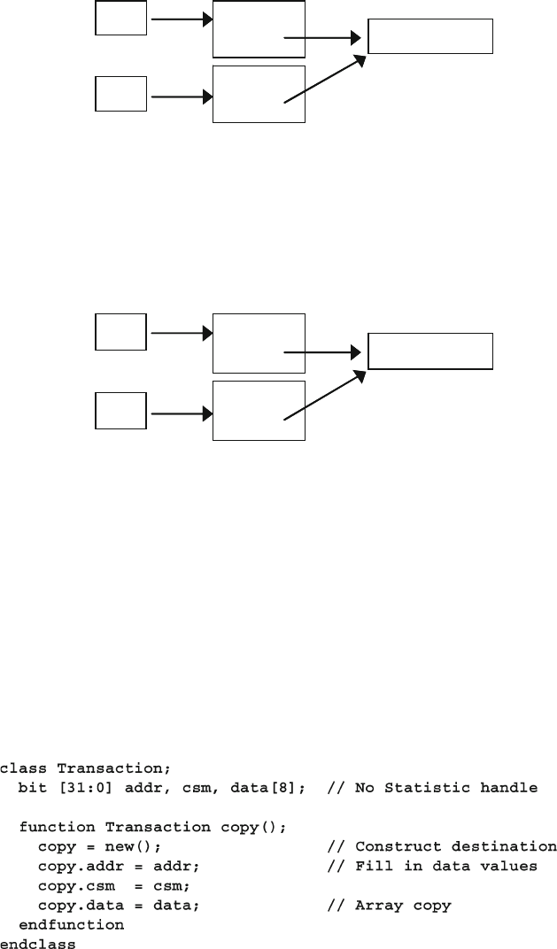
158 5 Basic OOP
Worse yet, both Transaction objects point to the same Statistics object so
modifying startT with the src handle affects what is seen with the dst handle as
you can see in Figure 5.7 .
id=0
stats
dst
src
startT=42
id=0
stats
Fig. 5.6 Objects and handles after copy with the new operator
id=0
stats
dst
src
startT=96
id=0
stats
Fig. 5.7 Both src and dst objects refer to a single statistics object and see updated startT value
Sample 5.33 Simple class with copy function
5.15.2 Writing Your Own Simple Copy Function
If you have a simple class that does not contain any references to other classes, writing
a copy function is easy as you can see in Samples 5.33 and 5.34 . Instead of calling
the new() function and copying each individual variable, the copy function could
have instead used the new operator, but then it would need to replicate any processing
done in new() , such as setting the id .
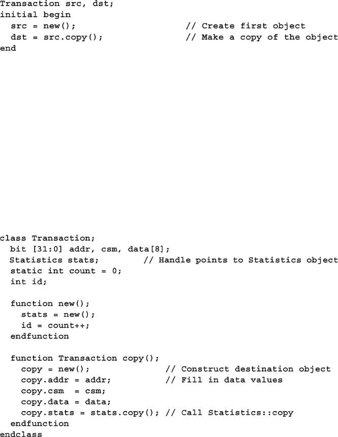
159
5.15 Copying Objects
5.15.3 Writing a Deep Copy Function
For nontrivial classes, you should always create your own copy function as seen in
Sample 5.35 . You can make it a deep copy by calling the copy functions of all the
contained objects. Your own copy function makes sure all your user fi elds (such as
id ) remain consistent. The downside of making your own copy function is that you
need to keep it up to date as you add new variables – forget one and you could spend
hours debugging to fi nd the missing value.
Sample 5.34 Using a copy function
Sample 5.35 Complex class with deep copy function
The new() constructor is called by copy so every object gets a unique id . Add
a copy() method for the Statistics class as shown in Sample 5.36 , and every
other class in the hierarchy.
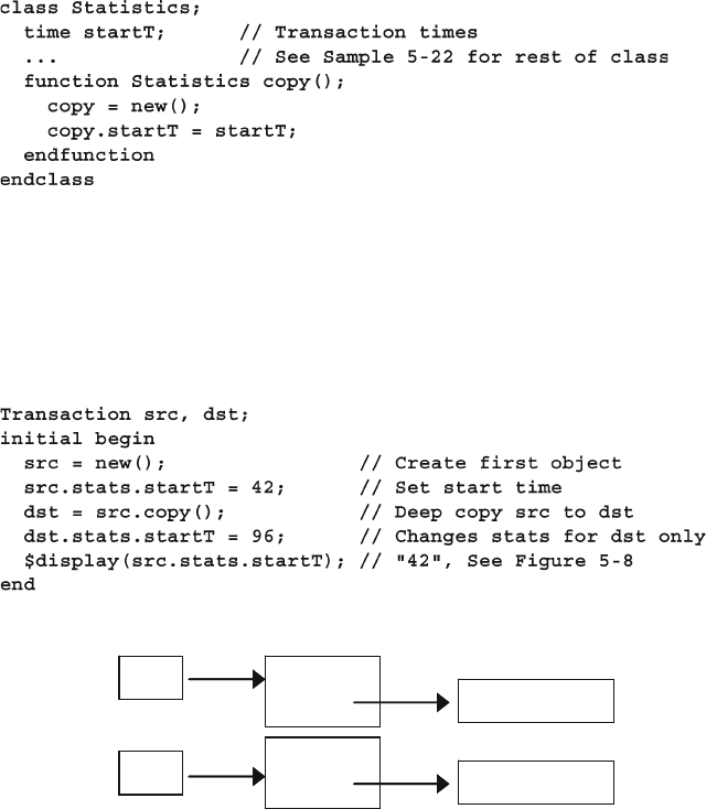
160 5 Basic OOP
The good news is that the UVM data macros create the copy function automati-
cally, so you are spared from having to write them by hand. Manually creating these
is very error prone, especially when you add new variables.
Sample 5.37 Copying a complex class with new operator
id=0
stats
dst
src
startT=96
id=1
stats
startT=42
Fig. 5.8 Objects and handles after deep copy
Sample 5.36 Statistics class declaration
Now when you make a copy of the Transaction object, it will have its own
Statistics object as shown in Sample 5.37 .
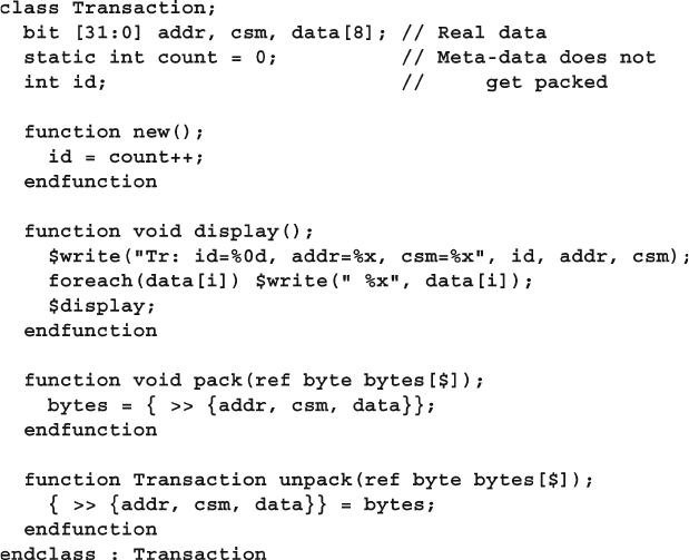
161
5.15 Copying Objects
Sample 5.38 Transaction class with pack and unpack functions
5.15.4 Packing Objects to and from Arrays Using
Streaming Operators
Some protocols, such as ATM, transmit control and data values one byte at a time.
Before you send out a transaction, you need to pack together the variables in the
object to a byte array. Likewise, after receiving a string of bytes, you need to unpack
them back into a transaction object. For both of these functions, use the streaming
operators, as shown in Section 2.12.
You can’t just stream the entire object as this would gather all properties,
including both data and also meta-data such as timestamps and self-checking
information that you may not want packed. You need to write your own pack
function like the one in Samples 5.38 and 5.39 that only uses the properties that
you choose.
More good news - the UVM data macros create the pack and unpack methods.
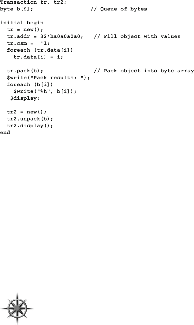
162 5 Basic OOP
5.16 Public vs. Local
The core concept of OOP is encapsulating data and related methods into a class.
Variables are kept local to the class by default to keep one class from poking around
inside another. A class provides a set of accessor methods to access and modify the
data. This would also allow you to change the implementation without needing to
let the users of the class know. For instance, a graphics package could change its
internal representation from Cartesian coordinates to polar as long as the user inter-
face (accessor methods) have the same functionality.
Consider the Transaction class that has a payload and a checksum so that the
hardware can detect errors. In conventional OOP, you would make a method to set
the payload also set the checksum so they would stay synchronized. Thus your
objects would always be fi lled with correct values.
However, testbenches are not like other programs, such as a web browser or word
processor. A testbench needs to create errors. You want to have a bad checksum so
you can test how the hardware reacts to errors.
OOP languages such as C++ and Java allow you to specify the visibility of vari-
ables and methods. By default, everything in a class is local unless labeled otherwise.
In SystemVerilog, everything is public unless labeled local or
protected . You should stick with this default so you have the
greatest control over the operation of the DUT, which is more
important than long-term software stability. For example, making
the checksum visible allows you to easily inject errors into the
Sample 5.39 Using the pack and unpack functions
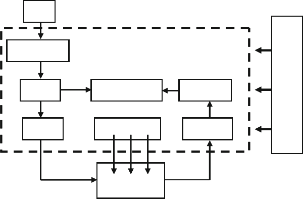
163
5.18 Building a Testbench
DUT. If the checksum was local, you would have to write extra code to bypass the
data-hiding mechanisms, resulting in a larger and more complex testbench.
5.17 Straying Off Course
As a new OOP student, you may be tempted to skip the extra thought needed to
group items into a class, and just store data in a few variables. Avoid the temptation!
A basic DUT monitor samples several values from an interface. Don’t just store them
in some integers and pass them to the next stage. This saves you a few minutes at
fi rst, but eventually you need to group these values together to form a complete trans-
action. Several of these transactions may need to be grouped to create a higher-level
transaction such as a DMA transfer. Instead, immediately put those interface values
into a transaction class. Now you can store related information (port number, receive
time) along with the data, and easily pass this object to the rest of your testbench.
5.18 Building a Testbench
Now that you have seen the basics of OOP, you can see how to create a layered test-
bench from a set of classes. Figure 5.9 is the diagram from Chapter 1 . Obviously,
the transactions fl owing between the blocks are objects, but each block is also
modeled with a class.
DUT
AssertionsDriver Monitor
Test
Scoreboard Checker
Generator
Functional Coverage
Environment
Agent
Fig. 5.9 Layered testbench
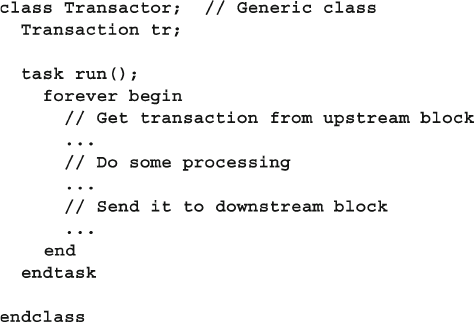
164 5 Basic OOP
How do you exchange transactions between blocks? With procedural code you
could have one object call the next, or you could use a data structure such as a FIFO
to hold transactions in fl ight between blocks. In Chapter 7 , you will learn how to use
mailboxes, which are FIFOs with the ability to stall a thread until a new value is
added.
5.19 Conclusion
Using Object-Oriented Programming is a big step, especially if your fi rst computer
language was Verilog. The payoff is that your testbenches are more modular and
thus easier to develop, debug, and reuse.
Sample 5.40 Basic Transactor
The Generator, Agent, Driver, Monitor, Checker , and Scoreboard are
all classes, modeled as transactors (described below). They are instantiated inside
the Environment class. For simplicity, the test is at the top of the hierarchy, as is the
program that instantiates the Environment class. The Functional coverage defi ni-
tions can be put inside or outside the Environment class. See Section 1.10 for a
description of the layered verifi cation environment and its components.
A transactor is made of a simple loop that receives a transaction object from a
previous block, makes some transformations, and sends it to the following one as
you can see in Sample
5.40 . Some, such as the Generator , have no upstream
block, so this transactor constructs and randomizes every transaction, while others,
such as the Driver , receive a transaction and send it into the DUT as signal
transitions.
165
5.20 Exercises
Have patience — your fi rst OOP testbench may look more like Verilog with a
few classes added. As you get the hang of this new way of thinking, you begin to
create and manipulate classes for both transactions and the transactors in the test-
bench that manipulate them.
In Chapter 8 you will learn more OOP techniques so your test can change
the behavior of the underlying testbench without having to change any of the exist-
ing code.
5.20 Exercises
1. Create a class called MemTrans that contains the following members, then con-
struct a MemTrans object in an initial block.
a. An 8-bit data_in of logic type
b. A 4-bit address of logic type
c. A void function called print that prints out the value of data_in and address
2. Using the MemTrans class from Exercise 1, create a custom constructor, the new
function, so that data_in and address are both initialized to 0.
3. Using the MemTrans class from Exercise 1, create a custom constructor so that
data_in and address are both initialized to 0 but can also be initialized through
arguments passed into the constructor. In addition, write a program to perform
the following tasks.
a. Create two new MemTrans objects.
b. Initialize address to 2 in the fi rst object, passing arguments by name.
c. Initialize data_in to 3 and address to 4 in the second object, passing argu-
ments by name.
4. Modify the solution from Exercise 3 to perform the following tasks.
a. After construction, set the address of the fi rst object to 4’hF.
b. Use the print function to print out the values of data_in and address for
the two objects.
c. Explicitly deallocate the 2nd object.
5. Using the solution from Exercise 4, create a static variable last_address that
holds the initial value of the address variable from the most recently created
object, as set in the constructor. After allocating objects of class MemTrans (done
in Exercise 4) print out the current value of last_address .
6. Using the solution from Exercise 5, create a static method called print_last_
address that prints out the value of the static variable last_address . After
allocating objects of class MemTrans , call the method print_last_address
to print out the value of last_address .
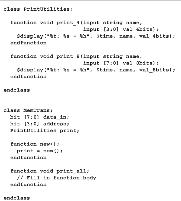
166 5 Basic OOP
7. Given the following code, complete the function print_all in class MemTrans
to print out data_in and address using the class PrintUtilities .
Demonstrate using the function print_all .
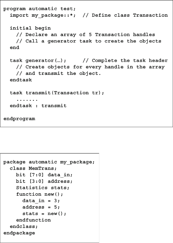
167
5.20 Exercises
8. Complete the following code where indicated by the comments starting with //.
9. For the following class, create a copy function and demonstrate its use. Assume
the Statistics class has its own copy function.
169
C. Spear and G. Tumbush, SystemVerilog for Verifi cation: A Guide to Learning
the Testbench Language Features, DOI 10.1007/978-1-4614-0715-7_6,
© Springer Science+Business Media, LLC 2012
6.1 Introduction
As designs grow larger, it becomes more diffi cult to create a complete set of stimuli
needed to check their functionality. You can write a directed testcase to check a
certain set of features, but you cannot write enough directed testcases when the
number of features keeps doubling on each project. Worse yet, the interactions
between all these features are the source for the most devious bugs and are the least
likely to be caught by going through a laundry list of features.
The solution is to create test cases automatically using constrained-random tests
(CRT). A directed test fi nds the bugs you think are there, but a CRT fi nds bugs you
never thought about, by using random stimulus. You restrict the test scenarios to
those that are both valid and of interest by using constraints.
Creating the environment for a CRT takes more work than creating one for
directed tests. A simple directed test just applies stimulus, and then you manually
check the result. These results are captured as a golden log fi le and compared with
future simulations to see whether the test passes or fails. A CRT requires an environ-
ment to predict the result, using a reference model, transfer function, or other tech-
niques, plus functional coverage to measure the effectiveness of the stimulus.
However, once this environment is in place, you can run hundreds of tests without
having to hand-check the results, thereby improving your productivity. This trade-
off of test-authoring time (your work) for CPU time (machine work) is what makes
CRT so valuable.
A CRT is made of two parts: the test code that uses a stream of random values to
create input to the DUT, and a seed to the pseudo-random number generator (PRNG),
shown in Section 6.16.1 at the end of this chapter. You can make a CRT behave dif-
ferently just by using a new seed. This feature allows you to leverage each test so
each is the functional equivalent of many directed tests, just by changing seeds. You
are able to create more equivalent tests using these techniques than with directed
testing.
Chapter 6
Randomization
170 6 Randomization
You may feel that these random tests are like throwing darts. How do you know
when you have covered all aspects of the design? The stimulus space is too large to
generate every possible input, so you need to generate a useful subset. In Chapter 9
you will learn how to measure verifi cation progress by using functional coverage.
There are many ways to use randomization, and this chapter gives many exam-
ples. It highlights the most useful techniques, but choose what works best for you.
6.2 What to Randomize
When you think of randomizing the stimulus to a design, the fi rst thing you may
think of are the data fi elds. These are the easiest to create – just call $random . The
problem is that this approach has a very low payback in terms of bugs found: you
only fi nd data-path bugs, perhaps with bit-level mistakes. The test is still inherently
directed. The challenging bugs are in the control logic. As a result, you need
to randomize all decision points in your DUT. Everywhere control paths diverge,
randomization increases the probability that you’ll take a different path in each
test case.
You need to think broadly about all design input such as the following items.
Device confi guration •
Environment confi guration •
Primary input data •
Encapsulated input data •
Protocol exceptions •
Delays •
Transaction status •
Errors and violations •
6.2.1 Device Confi guration
What is the most common reason why bugs are missed during testing of the RTL
design? Not enough different confi gurations have been tried! Most tests just use the
design as it comes out of reset, or apply a fi xed set of initialization vectors to put it
into a known state. This is like testing a PC’s operating system right after it has been
installed, and without any applications; of course the performance is fi ne, and there
are no crashes.
Over time, in a real world environment, the DUT’s confi guration becomes more
and more random. In a real world example, a verifi cation engineer had to verify a
timedivision multiplexor switch that had 600 input channels and 12 output chan-
nels. When the device was installed in the end-customer’s system, channels would
be allocated and deallocated over and over. At any point in time, there was little
171
6.2 What to Randomize
correlation between adjacent channels. In other words, the confi guration would
seem random.
To test this device, the verifi cation engineer had to write several dozen lines of
Tcl code to confi gure each channel. As a result, she was never able to try confi gura-
tions with more than a handful of channels enabled. Using a CRT methodology, she
wrote a testbench that randomized the parameters for a single channel, and then put
this in a loop to confi gure the whole device. Now she had confi dence that her tests
would uncover bugs that previously would have been missed.
6.2.2 Environment Confi guration
The device that you are designing operates in an environment containing other
devices. When you are verifying the DUT, it is connected to a testbench that mimics
this environment. You should randomize the entire environment, including the num-
ber of objects and how they are confi gured.
Another company was creating a PCI switch that connected multiple buses to an
internal memory bus. At the start of simulation the customer used randomization to
choose the number of PCI buses (1–4), the number of devices on each bus (1–8),
and the parameters for each device (master or slave, CSR addresses, etc.). Even
though there were many possible combinations, this company knew all had been
covered.
6.2.3 Primary Input Data
This is what you probably thought of fi rst when you read about random stimulus:
take a transaction such as a bus write or ATM cell and fi ll it with some random
values. How hard can that be? Actually it is fairly straightforward as long as you
carefully prepare your transaction classes. You should anticipate any layered proto-
cols and error injection.
6.2.4 Encapsulated Input Data
Many devices process multiple layers of stimulus. For example, a device may create
TCP traffi c that is then encoded in the IP protocol, and fi nally sent out inside
Ethernet packets. Each level has its own control fi elds that can be randomized to try
new combinations. So you are randomizing the data and the layers that surround it.
You need to write constraints that create valid control fi elds but that also allow
injecting errors.
172 6 Randomization
6.2.5 Protocol Exceptions, Errors, and Violations
Anything that can go wrong, will, eventually. The most challenging part of design
and verifi cation is how to handle errors in the system. You need to anticipate all the
cases where things can go wrong, inject them into the system, and make sure the
design handles them gracefully, without locking up or going into an illegal state.
A good verifi cation engineer tests the behavior of the design to the edge of the func-
tional specifi cation and sometimes even beyond.
When two devices communicate, what happens if the transfer stops partway
through? Can your testbench simulate these breaks? If there are error detection and
correction fi elds, you must make sure all combinations are tried.
The random component of these errors is that your testbench should be able to
send functionally correct stimuli and then, with the fl ip of a confi guration bit, start
injecting random types of errors at random intervals.
6.2.6 Delays
Many communication protocols specify ranges of delays. The bus grant comes one
to three cycles after request. Data from the memory is valid in the fourth to tenth bus
cycle. However, many directed tests, optimized for the fastest simulation, use the
shortest latency, except for that one test that only tries various delays. Your test-
bench should always use random, legal delays during every test to try to fi nd that
(hopefully) one combination that exposes a design bug.
Below the cycle level, some designs are sensitive to clock jitter. By sliding the
clock edges back and forth by small amounts, you can make sure your design is not
overly sensitive to small changes in the clock cycle.
The clock generator should be in a module outside the testbench so that it creates
events in the Active region along with other design events. However, the generator
should have parameters such as frequency and offset that can be set by the testbench
during the confi guration phase.
Note that the methodology described in this book is for fi nding functional
errors, not timing errors. Your constrained random testbench should not purpose-
fully violate setup and hold and hold requirements. These are better validated using
timing analysis tools.
6.3 Randomization in SystemVerilog
The random stimulus generation in SystemVerilog is most useful when used with
OOP. You fi rst create a class to hold a group of related random variables, and then
have the random-solver fi ll them with random values. You can create constraints to
limit the random values to legal values, or to test specifi c features.
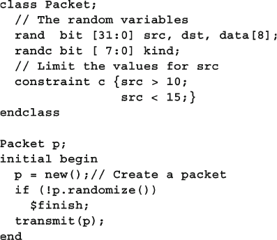
173
6.3 Randomization in SystemVerilog
You can randomize individual variables, but this case is the least interesting. True
constrained-random stimuli is created at the transaction level, not one value at a time.
6.3.1 Simple Class with Random Variables
Sample 6.1 shows a packet class with random variables and constraints, plus test-
bench code that constructs and randomizes a packet.
Sample 6.1 Simple random class
This class has four random variables. The fi rst three use the rand modifi er, so
that every time you randomize the class, the variables are assigned a value. Think of
rolling dice where each roll could be a new value or repeat the current one. The
kind variable is randc , which means random cyclic, so that the random solver
does not repeat a random value until every possible value has been assigned. Think
of dealing cards from a deck where you deal out every card in the deck in random
order, then shuffl e the deck, and deal out the cards in a different order. Note that the
cyclic pattern is for a single variable. A randc array with fi ve elements has fi ve dif-
ferent patterns, like fi ve decks of cards, dealt in parallel. Simulators are only required
to implement randc variables up to 8 bits wide with 256 different values, but most
support much larger ranges.
A constraint is just a set of relational expressions that must be true for the chosen
value of the variables. In this example, the src variable must be greater than 10 and
less than 15. Note that the constraint expression is grouped using curly braces: {}.
This is because this code is declarative, not procedural, which uses begin…end .
The randomize function returns 0 if a problem is found with the constraints.
The code checks the result and stops simulation with $fi nish if there is a problem.
Alternatively, you might want to call a special routine to end simulation, after doing
some housekeeping chores like printing a summary report. The rest of the book uses
a macro instead of this extra code.
174 6 Randomization
You should not randomize an object in the class constructor. Your
test may need to turn constraints on or off, change weights, or even
add new constraints before randomization. The constructor is for
initializing the object’s variables, and if you called
randomize at
this early stage, you might end up throwing away the results.
Variables in your classes should be random and public. This gives
your test the most control over the DUT’s stimulus and control.
You can disable randomization of a variable, as shown in Section
6.11.2 . If you forget to make a variable random, you must edit
the environment, which you want to avoid. The exception is that
confi guration variables such as weights and limits should not be
random in transaction classes as their values are chosen at the start of simulation and
do not change.
6.3.2 Checking the Result from Randomization
The randomize function assigns random values to any variable in
the class that has been labeled as rand or randc , and also makes
sure that all active constraints are obeyed. Randomization can fail
if your code has confl icting constraints (see next section), so you
should always check the status. If you don’t check, the variables
may get unexpected values, causing your simulation to fail.
The remaining code samples in this book employ the macro in Sample 6.2 to check
for the result of randomization. If you adopt this style, you can easily add code to give
meaningful error messages and gracefully wind down simulation. The macro shows
off several coding tricks, including wrapping the generated code in a do…while state-
ment so it can be used like a normal statement terminated with a semicolon, including
in an if-else statement, something that VMM log macros did right, but not OVM.
Sample 6.2 Randomization check macro and example
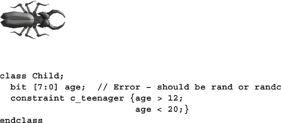
175
6.4 Constraint Details
6.3.3 The Constraint Solver
The process of solving constraint expressions is handled by the SystemVerilog
constraint solver. The solver chooses values that satisfy the constraints. The values
come from SystemVerilog’s PRNG, that is started with an initial seed. If you give a
SystemVerilog simulator the same seed and the same testbench, it should always
produce the same results. Note that changing the tool version or switches such as
debug level can change results. See the exercises at the end of this chapter to see
how to specify the initial seed.
The solver is specifi c to the simulation vendor, and a constrained-random test
may not give the same results when run on different simulators, or even on different
versions of the same tool. The SystemVerilog standard specifi es the meaning of the
expressions, and the legal values that are created, but does not detail the precise
order in which the solver should operate. See Section
6.16 for more details on ran-
dom number generators.
6.3.4 What can be Randomized?
SystemVerilog allows you to randomize integral variables, that is, variables that
contain a simple set of bits. This includes 2-state and 4-state types, though random-
ization only generates 2-state values. You can have integers, bit vectors, etc. You
cannot have a random string, or refer to a handle in a constraint. Randomizing real
variables is not yet defi ned in the LRM.
6.4 Constraint Details
Useful stimulus is more than just random values — there are relationships between
the variables. Otherwise, it may take too long to generate interesting stimulus val-
ues, or the stimulus might contain illegal values. You defi ne these interactions in
SystemVerilog using constraint blocks that contain one or more constraint expres-
sions. SystemVerilog chooses random values so that the expressions are true.
At least one variable in each expression should be random, either
rand or randc . The following class fails when randomized,
unless age happens to be in the right range. The solution is to
add the modifi er rand or randc before age.
Sample 6.3 Constraint without random variables
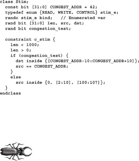
176 6 Randomization
The randomize function tries to assign new values to random variables and to
make sure all constraints are satisfi ed. In Sample 6.3 , since there are no random vari-
ables, randomize just checks the value of age to see if it is in the bounds specifi ed
by the constraint
c_teenager . Unless the variable falls in the range of 13:19, ran-
domize fails. While you can use a constraint to check that a non-random variable has
a valid value, use an
assert or if -statement instead. It is much easier to debug your
procedural checker code than read through an error message from the random solver.
6.4.1 Constraint Introduction
Sample 6.4 shows a simple class with random variables and constraints. The spe-
cifi c constructs are explained in the following sections. Notice that in constraint
blocks, you use curly braces, { }, to group together multiple expressions. The
begin…end keywords are for procedural code.
Sample 6.4 Constrained-random class
6.4.2 Simple Expressions
Sample 6.4 showed a constraint block with several expressions. The fi rst two control
the values for the len variable. As you can see, a variable can be used in multiple
expressions.
There should be a maximum of only one operator in an expres-
sion, such as <, <=, ==, >=, or >. Sample 6.5 shows a
SystemVerilog gotcha in that it incorrectly tries to generate three
variables in a fi xed order.
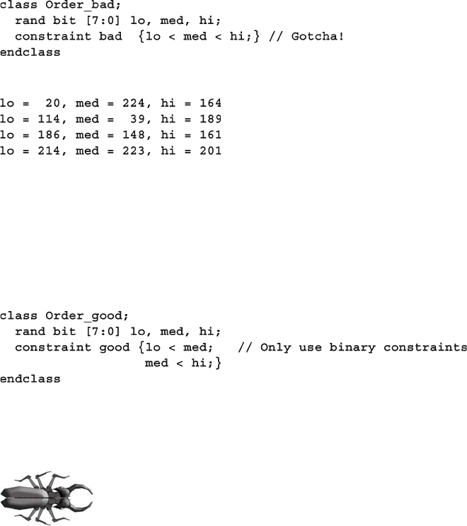
177
6.4 Constraint Details
Sample 6.6 shows the results, which are not what was intended. The constraint
bad in Sample 6.5 is broken down into multiple binary relational expressions, going
from left to right: (( lo < med ) < hi ). First, the expression ( lo < med ) is evaluated,
which gives 0 or 1. Then hi is constrained to be greater than the result. The variables
lo and med are randomized but not constrained. The correct constraint is shown in
Sample 6.7 . For more examples, see Sutherland (2007).
Sample 6.5 Bad ordering constraint
Sample 6.7 Constrain variables to be in a fi xed order
Sample 6.6 Result from incorrect ordering constraint
6.4.3 Equivalence Expressions
The most common mistake with constraints is trying to make
an assignment in a constraint block, which can only contain
expressions. Instead, use the equivalence operator to set a ran-
dom variable to a value, e.g., len==42 . You can build complex
relationships between one or more random variables: len == (header.addr_
mode * 4 + payload.size()) .
6.4.4 Weighted Distributions
A bug in the DUT may be found with constrained random stimulus if you apply
enough patterns. However, it may take a long time for a particular corner case to be
generated. When reviewing functional coverage result, see if corner cases are being
generated. If not, you can use a weighted distribution to skew the stimulus in a
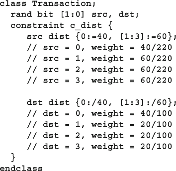
178 6 Randomization
particular direction, and thus accelerate fi nding bugs. The dist operator allows you
to create weighted distributions so that some values are chosen more often than
others.
The dist operator takes a list of values and weights, separated by the : = or
the : / operator. The values and weights can be constants or variables. The values
can be a single value or a range such as [lo:hi] . The weights are not percentages
and do not have to add up to 100. The : = operator specifi es that the weight is the
same for every specifi ed value in the range, whereas the : / operator specifi es that
the weight is to be equally divided between all the values.
Sample 6.8 Weighted random distribution with dist
In Sample 6.8 , src gets the value 0, 1, 2, or 3. The weight of 0 is 40, whereas, 1,
2, and 3 each have the weight of 60, for a total of 220. The probability of choosing
0 is 40/220, and the probability of choosing 1, 2, or 3 is 60/220 each.
Next, dst gets the value 0, 1, 2, or 3. The weight of 0 is 40, whereas 1, 2, and 3
share a total weight of 60, for a total of 100. The probability of choosing 0 is 40/100,
and the probability of choosing 1, 2, or 3 is only 20/100 each.
Once again, the values and weights can be constants or variables. You can use
variable weights to change distributions on the fl y or even to eliminate choices by
setting the weight to zero, as shown in Sample 6.9 .
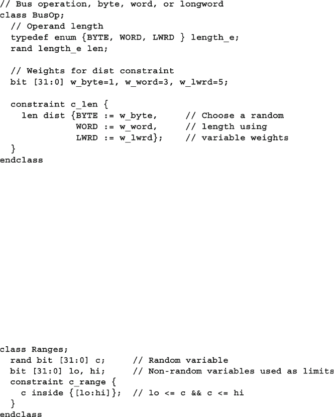
179
6.4 Constraint Details
In Sample 6.9 , the len enumerated variable has three values. With the default
weighting values, longword lengths are chosen more often, as w_lwrd has the larg-
est value. Don’t worry, you can change the weights on the fl y during simulation to
get a different distribution.
6.4.5 Set Membership and the Inside Operator
You can create sets of values with the inside operator. The SystemVerilog solver
chooses between the values in the set with equal probability, unless you have other
constraints on the variable. As always, you can use variables in the sets.
Sample 6.9 Dynamically changing distribution weights
Sample 6.10 Random sets of values
In Sample 6.10 , SystemVerilog uses the values for lo and hi to determine the
range of possible values. You can use the variables as parameters for your con-
straints so that the testbench can alter the behavior of the stimulus generator without
rewriting the constraints. Note that if lo > hi , an empty set is formed, and the con-
straint fails.
If you want any value, as long as it is not inside a set, invert the constraint with
the NOT operator: ! as shown in Sample 6.11 .
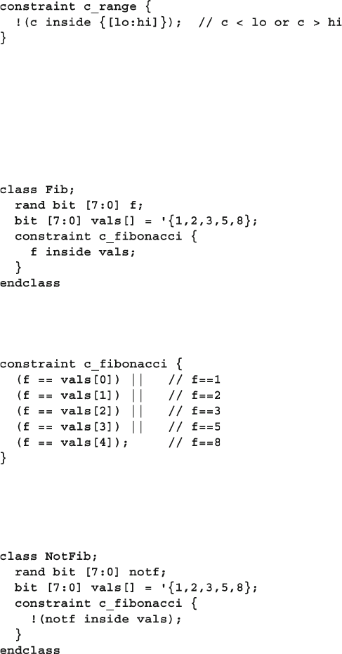
180 6 Randomization
6.4.6 Using an Array in a Set
Sample 6.12 shows how you can choose from a set of values by storing them in an
array.
Sample 6.11 Inverted random set constraint
Sample 6.12 Random set constraint for an array
This is expanded into the constraints in Sample 6.13 .
Sample 6.13 Equivalent set of constraints
Likewise, you can use the NOT operator to tell SystemVerilog to choose any
value except those in an array as shown in Sample 6.14 .
Sample 6.14 Choose any value except those in an array
Always make sure your constraints work as you expect. You could create func-
tional coverage groups and generate reports, or print a histogram of values with the
code in Sample 6.15 , with the output in Sample 6.16 .
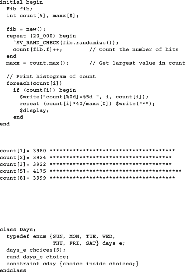
181
6.4 Constraint Details
Samples 6.17 and 6.18 choose a day of the week from a list of enumerated val-
ues. You can change the list of choices on the fl y. If you make choice a randc
variable, the simulator tries every possible value before repeating.
Sample 6.15 Printing a histogram
Sample 6.16 Histogram for inside constraint
Sample 6.17 Class to choose from an array of possible values
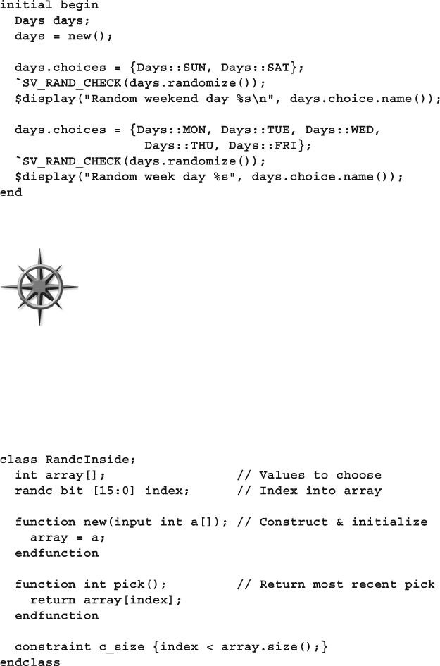
182 6 Randomization
The name function returns a string with the name of an enumerated value.
If you want to dynamically add or remove values from a set, think
twice before using the inside operator because of its perfor-
mance. Perhaps you have a set of values that you want to choose
just once. You could use inside to choose values from a queue,
and delete them to slowly shrink the queue. This requires the solver
to solve N constraints, where N is the number of elements left in
the queue. Instead, use a randc variable that is an index into an array of choices as
shown in Samples 6.19 and 6.20 . Choosing a randc value takes a short, constant
time, whereas solving a large number of constraints is more expensive, especially if
your array has more than a few dozen elements.
Sample 6.18 Choosing from an array of values
Sample 6.19 Using randc to choose array values in random order
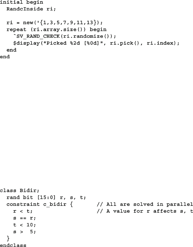
183
6.4 Constraint Details
Note that constraints and routines can be mixed in any order.
6.4.7 Bidirectional Constraints
By now you may have realized that constraint blocks are not procedural code, exe-
cuting from top to bottom. They are declarative code, all active at the same time. If
you constrain a variable with the inside operator with the set [10:50] and have
another expression that constrains the variable to be greater than 20, SystemVerilog
solves both constraints simultaneously and only chooses values between 21 and 50.
SystemVerilog constraints are solved bidirectionally, which means that the con-
straints on all random variables are solved concurrently. Adding or removing a con-
straint on any one variable affects the value chosen for all variables that are related
directly or indirectly. Consider the constraint in Sample 6.21 .
Sample 6.20 Testbench for randc choosing array values in random order
Sample 6.21 Bidirectional constraints
The SystemVerilog solver looks at all four constraints simultaneously. The variable
r has to be less than t , which has to be less than 10. However, r is also constrained
to be equal to s, which is greater than 5. Even though there is no direct constraint on
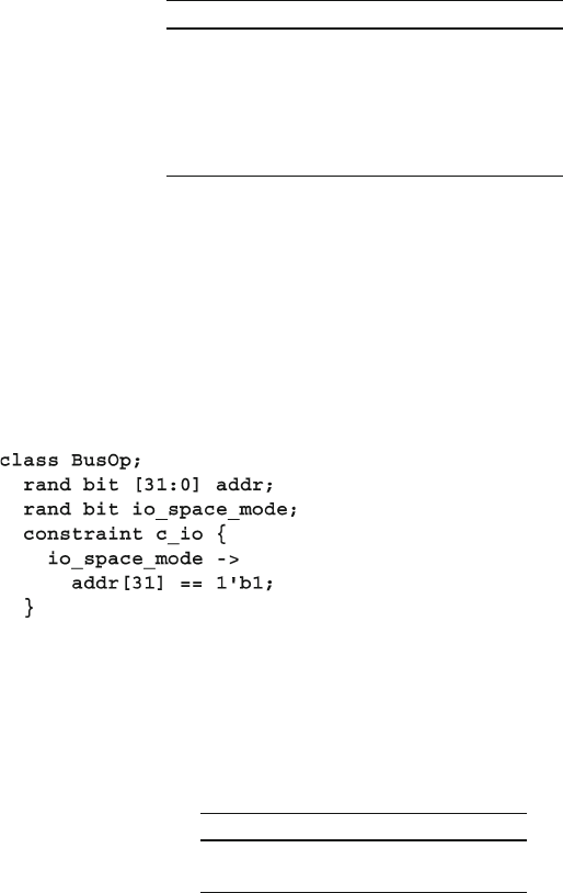
184 6 Randomization
6.4.8 Implication Constraints
Normally, all constraint expressions are active in a block. What if you want to have
an expression active only some of the time? Set the highest address, but only for IO
space mode. SystemVerilog supports two implication operators, -> and if .
Table 6.1 Solutions for bidirectional constraint
Solution r s t
A 6 6 7
B 6 6 8
C 6 6 9
D 7 7 8
E 7 7 9
F 8 8 9
Sample 6.22 Constraint block with implication operator
The expression A->B is equivalent to the expression (! A || B ). When the impli-
cation operator appears in a constraint, the solver picks values for A and B so the
expression is true. Truth Table 6.2 shows the value of the expression for the logical
values of A and B .
Table 6.2 Implication operator truth table
A -> B B = false B = true
A=false true true
A=true false true
the lower value of t , the constraint on s restricts the choices. Table 6.1 shows the
possible values for these three variables.
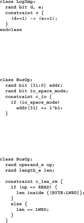
185
6.4 Constraint Details
When A is true, B must be true, but when A is false, B can be true or false. Note
that this is a partly bidirectional constraint, but that A->B does not imply that B->A .
The two expressions produce different results.
In Sample
6.23 , when d==1 , the variable e must be 1, but when e==1, d can be
0 or 1.
Sample 6.24 Constraint block with if implication operator
Sample 6.23 Implication operator
If you add the constraint { e==0; }, the variable d must be 0; But if you add a
constraint { e==1; } the values of d are not constrained, it can still be 0 or 1.
Sample 6.24 shows how Sample 6.22 could be written with an if implication
constraint.
The if-else operator is a great way to choose between multiple expressions.
For example, the bus defi ned in Sample 6.9 might support byte, word, and longword
reads, but only longword writes if written like Sample 6.25 .
Sample 6.25 Constraint block with if-else operator
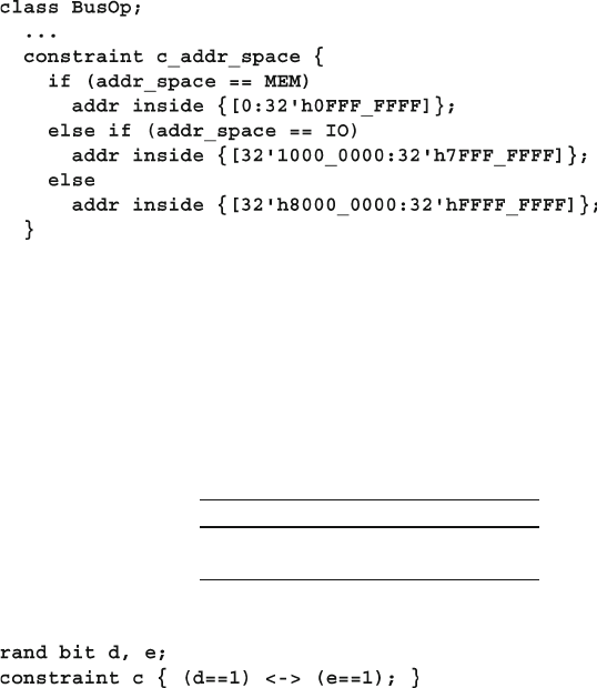
186 6 Randomization
The constraint if (A) B else C ; is equivalent to the two constraints ( A && B ); and
( !A && C );. Sample 6.26 shows how you can chain together multiple choices.
Sample 6.26 Constraint block with multiple if-else operator
6.4.9 Equivalence Operator
The equivalence operator <-> is bidirectional. A<−>B is defi ned as ((A->B) &&
(B->A)). Table 6.3 is the truth table for the logical values of A and B as constrained
in Sample
6.27 .
Table 6.3 Equivalence operator truth table
A <-> B B=false B=true
A=false true false
A=true false true
When d is true, e must also be true, and when d is false, e must also be false. So this
operator is the same as a logical XNOR. If you start with the constraint d<−>e , and add
a constraint such as d==1, e is set to 1 by the solver. The constraint d<−>e and e==0
cause d to be set to 0 by the solver. If your class has all three of the constraints,
d<−>e, d==1 , and e==0 , the solver will not be able to choose values for d and e .
6.5 Solution Probabilities
Whenever you deal with random values, you need to understand the probability
of the outcome. SystemVerilog does not guarantee the exact solution found by
the random constraint solver, but you can infl uence the distribution. Any time you
Sample 6.27 Equivalence constraint
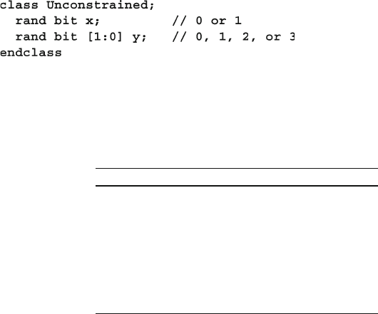
187
6.5 Solution Probabilities
work with random numbers, you have to look at thousands or millions of values to
average out the noise. Some simulators, such as Synopsys VCS, have multiple solv-
ers to allow you to trade memory usage vs. performance. The distributions will vary
between different simulators. The tables were generated with Synopsys VCS
2011.03.
6.5.1 Unconstrained
Start with two random variables in a class with no constraints as shown in Sample
6.28 .
Sample 6.28 Class Unconstrained
Table 6.4 shows the eight possible solutions. Since there are no constraints, each
has the same probability. You have to run thousands of randomizations to see the
actual results approach the listed probabilities.
Table 6.4 Solutions for Unconstrained class
Solution x y Probability
A 0 0 1/8
B 0 1 1/8
C 0 2 1/8
D 0 3 1/8
E 1 0 1/8
F 1 1 1/8
G 1 2 1/8
H 1 3 1/8
6.5.2 Implication
In Sample 6.29 , the value of y depends on the value of x. This is indicated with the
implication operator in the following constraint. This example and the rest in this
section also behave in the way same with the if implication operator.
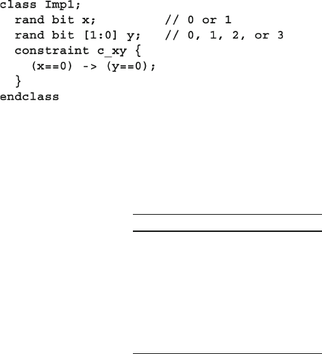
188 6 Randomization
Table 6.5 shows the possible solutions and probability. You can see that the ran-
dom solver recognizes that there are eight combinations of x and y, but all the solu-
tions where x==0 (solutions A–D) have been merged together.
Table 6.5 Solutions for Imp1 class
Solution x y Probability
A 0 0 1/2
B 0 1 0
C 0 2 0
D 0 3 0
E 1 0 1/8
F 1 1 1/8
G 1 2 1/8
H 1 3 1/8
Sample 6.29 Class with implication constraint
6.5.3 Implication and Bidirectional Constraints
Note that the implication operator says that when x==0, y is forced to 0, but when
y==0 , there is no constraint on x. However, implication is bidirectional in that if y
were forced to a nonzero value, x would have to be 1. Sample 6.30 has the constraint
y>0 , so x can never be 0 and Table 6.6 shows the solutions.
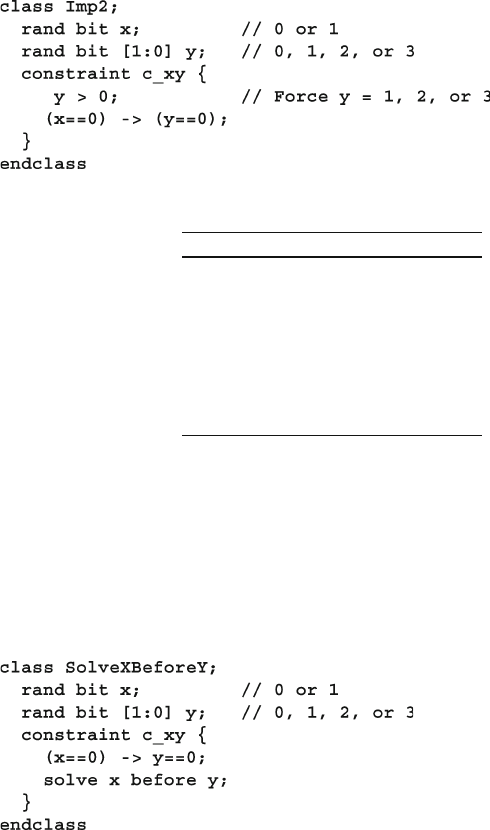
189
6.5 Solution Probabilities
6.5.4 Guiding Distribution with Solve…Before
You can guide the SystemVerilog solver using the “ solve…before ” constraint as
seen in Sample 6.31 .
Table 6.6 Solutions for Imp2 class
Solution x y Probability
A 0 0 0
B 0 1 0
C 0 2 0
D 0 3 0
E 1 0 0
F 1 1 1/3
G 1 2 1/3
H 1 3 1/3
Sample 6.30 Class with implication constraint and additional constraint
Sample 6.31 Class with implication and solve…before
190 6 Randomization
The solve…before constraint does not change the solution space, just the prob-
ability of the results. The solver chooses values of x (0, 1) with equal probability.
In 1000 calls to randomize , x is 0 about 500 times, and 1 about 500 times. When
x is 0, y must be 0. When x is 1, y can be 0, 1, 2, or 3 with equal probability as
shown in Table 6.7 .
Table 6.7 Solutions for solve x before y
constraint
Solution x y Probability
A 0 0 1/2
B 0 1 0
C 0 2 0
D 0 3 0
E 1 0 1/8
F 1 1 1/8
G 1 2 1/8
H 1 3 1/8
If you use the constraint solve y before x , you get a very different distribu-
tion as shown in Table 6.8 .
Table 6.8 Solutions for solve y before x
constraint
Solution x y Probability
A 0 0 1/8
B 0 1 0
C 0 2 0
D 0 3 0
E 1 0 1/8
F 1 1 1/4
G 1 2 1/4
H 1 3 1/4
Only use solve…before if you are dissatisfi ed with how often
some values occur. Excessive use can slow the constraint solver
and make your constraints diffi cult for others to understand.
For the simple class in Sample 6.31 , the equivalence operator, <->, gives the same
solution as the implication operator ->. Try adding additional constraints and plot
the results for your favorite simulator.
191
6.6 Controlling Multiple Constraint Blocks
6.6 Controlling Multiple Constraint Blocks
A class can contain multiple constraint blocks. One block might ensure you have a
valid transaction, as described in Section
6.7 , but you might need to disable this
when testing the DUT’s error handling. Or you might want to have a separate con-
straint for each test. Perhaps one constraint would restrict the data length to create
small transactions (great for testing congestion), whereas another would make long
transactions.
You can turn constraints on and off with the constraint_mode function. You can
control a single constraint with handle. constraint. constraint_mode (arg) .
To control all constraints in an object, use handle. constraint_mode (arg) , as
shown in Sample 6.32 . When the argument for constraint_mode is 0, the con-
straint is turned off, and when it is 1, the constraint is turned on.
Sample 6.32 Using constraint_mode
While many small constraints may give you more fl exibility, the process of turn-
ing them on and off is more complex. For example, when you turn off all constraints
that create data, you are also disabling all the ones that check the data’s validity.
If you just want to make a random variable non-random, use rand_mode as
described in Section 6.11.2 .
192 6 Randomization
6.7 Valid Constraints
A good randomization technique is to create several constraints to ensure the
correctness of your random stimulus, known as “valid constraints.” In Sample
6.33 , a bus read-modify-write command is only allowed for a longword data
length.
Sample 6.33 Checking write length with a valid constraint
Now you know the bus transaction obeys the rule. Later, if you want to violate
the rule, use constraint_mode to turn off this one constraint. You can turn these
off with constraint_mode when you want to generate errors. For example, what
if a packet has a zero-length payload? You should have a naming convention to
make these constraints stand out, such as using the prefi x valid as shown above.
6.8 In-Line Constraints
As you write more tests, you can end up with many constraints. They can interact
with each other in unexpected ways, and the extra code to enable and disable them
adds to the test complexity. Additionally, constantly adding and editing constraints
to a class could cause problems in a team environment.
Many tests only randomize objects at one place in the code. SystemVerilog
allows you to add an extra constraint using randomize with . This is equivalent to
adding an extra constraint to any existing ones in effect. Sample 6.34 shows a base
class with constraints, then two randomize with statements.
193
6.9 The
pre _ randomize and Post _ Randomize Functions
The extra constraints are added to the existing ones in effect. Use constraint_
mode if you need to disable a confl icting constraint. Note that inside the with{}
statement, SystemVerilog uses the scope of the class. That is why Sample 6.34 used
just addr , not t.addr .
A common mistake is to surround your in-line constraints with
parenthesis instead of curly braces {}. Just remember that con-
straint blocks use curly braces, so your in-line constraint must
use them too. Braces are for declarative code.
6.9 The pre_randomize and post_randomize Functions
Sometimes you need to perform an action immediately before every randomize
call or immediately afterwards. For example, you may want to set some nonrandom
class variables (such as limits or weights) before randomization starts, or you may
need to calculate the error correction bits for random data. SystemVerilog lets you
do this with two functions, pre_randomize and post_randomize that are cre-
ated automatically in any class with random variables.
6.9.1 Building a Bathtub Distribution
For some applications, you want a nonlinear random distribution. For instance,
small and large packets are more likely to fi nd a design bug such as buffer overfl ow
Sample 6.34 The randomize() with statement
194 6 Randomization
than medium-sized packets. So you want a bathtub shaped distribution; high on
both ends, and low in the middle. You could build an elaborate
dist constraint, but
it might require lots of tweaking to get the shape you want. Verilog has several func-
tions for nonlinear distribution, such as
$dist_exponential , but none for a bath-
tub. The graph in Fig. 6.1 shows how you can combine two exponential curves to
make a bathtub curve. The pre_randomize method in Sample 6.35 calculates a
point on an exponential curve, then randomly chooses to put this on the left curve,
or right. As you pick points on either the left and right curves, you gradually build a
distribution of the combined values.
Left
Exponential
Right
Exponential
Sum is a
bathtub
Probability
Values WIDTH
0
Fig. 6.1 Building a bathtub distribution
Sample 6.35 Building a bathtub distribution
Every time this object is randomized, the variable value gets updated. Across
many randomizations, you will see the desired nonlinear distribution. Since the
variable is calculated procedurally, not through the random constraint solver, it does
not need the rand modifi er.
See Sample 6.64 for another example of post_randomize .
195
6.10 Random Number Functions
6.9.2 Note on Void Functions
The functions pre_randomize and post_randomize can only
call other functions, not tasks that could possibly consume time.
You cannot have a delay in the middle of a call to
randomize .
When you are debugging a randomization problem, you can call
your display routines if you planned ahead and made them void
functions.
Chapter 8 describes advanced OOP concepts including extended classes and virtual
methods. The pre_randomize and post_randomize functions are not virtual and
so they are called based on the type of the handle, not the object. Additionally, if your
extended class’s pre_randomize or post_randomize need functionality in the
base class’s pre_randomize and post_randomize functions, they should call
these methods using the super prefi x, as in super.pre_randomize .
6.10 Random Number Functions
You can use all the Verilog-1995 distribution functions, plus several that are new for
SystemVerilog. Consult a statistics book for more details on the “dist” functions.
Some of the useful functions include the following.
• $random — Flat distribution, returning signed 32-bit random
• $urandom — Flat distribution, returning unsigned 32-bit random
• $urandom_range — Flat distribution over a range
• $dist_exponential — Exponential decay, as shown in Fig. 6.1
• $dist_normal — Bell-shaped distribution
• $dist_poisson — Bell-shaped distribution
• $dist_uniform — Flat distribution
The $urandom_range function takes two arguments, an optional low value, and
a high value as shown in Sample 6.36 .
Sample 6.36 $urandom range usage
196 6 Randomization
6.11 Constraints Tips and Techniques
How can you create constrained-random tests that can be easily modifi ed? There are
several tricks you can use. The most general technique is to use OOP to extend the
original class as described in sections
6.11.8 and 8.2.4 but this requires more plan-
ning. So fi rst learn some simple techniques, but keep your mind open to other ways.
6.11.1 Constraints with Variables
Most constraint examples in this book use constants to make them more readable.
In Sample 6.37 , length is randomized over a range that uses a variable for the
upper bound.
Sample 6.37 Constraint with a variable bound
By default, this class creates random lengths between 1 and 100, but by changing
the variable max_length , you can vary the upper limit.
You can use variables in the dist constraint to turn on and off values and ranges.
In Sample 6.38 , each bus command has a different weight variable.
Sample 6.38 dist constraint with variable weights
By default, this constraint produces each command with equal probability. If you
want to have a greater number of READ8 commands, increase the read8_wt weight
variable. Most importantly, you can turn off generation of a command by dropping
its weight to 0.
197
6.11 Constraints Tips and Techniques
6.11.2 Using Nonrandom Values
If you have a set of constraints that produces stimulus that is almost what you want,
but not quite, you could call
randomize , and then set a variable to the value you
want — you don’t have to use the random value. However, your stimulus values
may not be correct according to the constraints you created to check validity.
If there are just a few random variables that you want to override, use the rand_
mode function to make them nonrandom. When you call this method with the argu-
ment 0 for a random variable, the rand or randc qualifi er is disabled and the
variable’s value is no longer changed by the random solver, but the value is still
checked in if it appears in a constraint. Setting the random mode to 1 turns the quali-
fi er back on so the variable can changed by the solver.
Sample 6.39 rand_mode disables randomization of variables
In Sample 6.39 , the packet size is stored in the random variable length . The
fi rst half of the test randomizes both the length variable and the contents of the
payload dynamic array. The second half calls rand_mode to make length a non-
random variable, sets it to 42, then calls randomize . The constraint sets the pay-
load size at the constant 42, but the array is still fi lled with random values.
198 6 Randomization
6.11.3 Checking Values Using Constraints
If you randomize an object and then modify some variables, you can check that the
object is still valid by checking if all constraints are still obeyed. Call
handle.
randomize(null) and SystemVerilog treats all variables as nonrandom (“state
variables”) and just ensures that all constraints are satisfi ed, i.e all expressions are
true. If any constraints are not satisfi ed, the randomize function returns 0.
6.11.4 Randomizing Individual Variables
Suppose you want to randomize a few variables inside a class. You can call ran-
domize with the subset of variables. Only those variables passed in the argument
list will be randomized; the rest will be treated as state variables and not random-
ized. All constraints remain in effect. In Sample 6.40 , the fi rst call to randomize
only changes the values of two rand variables med and hi . The second call only
changes the value of med , whereas hi retains its previous value. Surprisingly, you
can pass a non-random variable, as shown in the last call, and low is given a random
value, as long as it obeys the constraint.
Sample 6.40 Randomizing a subset of variables in a class
This trick of only randomizing a subset of the variables is not commonly used in
real testbenches as you are restricting the randomness of your stimulus. You want
your testbench to explore the full range of legal values, not just a few corners.
6.11.5 Turn Constraints Off and On
Sections 6.6 and 6.7 discuss valid constraints and constraint_mode . Turning off
individual constraints is fi ne for error generation, but should be used in moderation.
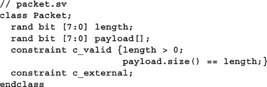
199
6.11 Constraints Tips and Techniques
6.11.6 Specifying a Constraint in a Test Using In-Line
Constraints
If you keep adding constraints to a class, it becomes hard to manage and control.
Soon, everyone is checking out the same fi le from your source control system. Many
times a constraint is only used by a single test, so why have it visible to every test?
One way to localize the effects of a constraint is to use in-line constraints, random-
ize with , shown in Section 6.8 . This works well if your new constraint is additive
to the default constraints. If you follow the recommendations in Section 6.7 to cre-
ate “valid constraints”, you can quickly constrain valid sequences. For error injec-
tion, you can disable any constraint that confl icts with what you are trying to do.
A test that injects a particular fl avor of corrupted data would fi rst turn off the par-
ticular validity constraint that checks for that error.
There are several tradeoffs with using in-line constraints. The fi rst is that now
your constraints are in multiple locations which can make it more diffi cult to under-
stand all the active constraints. If you add a new constraint to the original class, it
may confl ict with the in-line constraint. The second is that it can be very hard for
you to reuse an in-line constraint across multiple tests. By defi nition, an in-line
constraint only exists in one piece of code. You could put it in a routine in a separate
fi le and then call it as needed. At that point it has become nearly the same as an
external constraint.
6.11.7 Specifying a Constraint in a Test with External
Constraints
The body of a constraint does not have to be defi ned within the class, just as a rou-
tine body can be defi ned externally, as shown in Section 5.10 . Your data class could
be defi ned in one fi le, with one empty constraint. Then each test could defi ne its own
version of this constraint to generate its own fl avors of stimulus as shown in Samples
6.41 and 6.42 .
Sample 6.41 Class with an external constraint
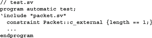
200 6 Randomization
External constraints have several advantages over in-line constraints. They can
be put in a fi le and thus reused between tests. An external constraint applies to all
instances of the class, whereas an in-line constraint only affects the single call to
randomize . Consequently, an external constraint provides a primitive way to
change a class without having to learn advanced OOP techniques. Keep in mind that
with this technique, you can only add constraints, not alter existing ones, and you
need to defi ne the external constraint prototype in the original class.
Like in-line constraints, external constraints can cause problems, as the con-
straints are spread across multiple fi les. The LRM requires external constraints to be
defi ned in the same scope as the original class. A class defi ned in a package must
have its external constraint also defi ned in the same package, limiting its usefulness.
That is why Sample 6.42 includes the class defi nition rather than using a package.
A fi nal consideration is what happens when the body for an external constraint is
never defi ned. The SystemVerilog LRM does not currently specify what should
happen in this case. Before you build a testbench with many external constraints,
fi nd out how your simulator handles missing defi nitions. Is this an error that pre-
vents simulation, just a warning, or no message at all?
6.11.8 Extending a Class
In Chapter 8 , you will learn how to extend a class. With this technique, you can take
a testbench that uses a given class, and swap in an extended class that has additional
or redefi ned constraints, routines, and variables. See Sample 8.10 for a typical test-
bench. Note that if you defi ne a constraint in an extended class with the same name
as one in the base class, the extended constraint replaces the base one.
Learning OOP techniques requires a little more study, but the fl exibility of this
new approach repays with great rewards.
6.12 Common Randomization Problems
You may be comfortable with procedural code, but writing constraints and under-
standing random distributions requires a new way of thinking. Here are some issues
you may encounter when trying to create random stimulus.
Sample 6.42 Program defi ning an external constraint
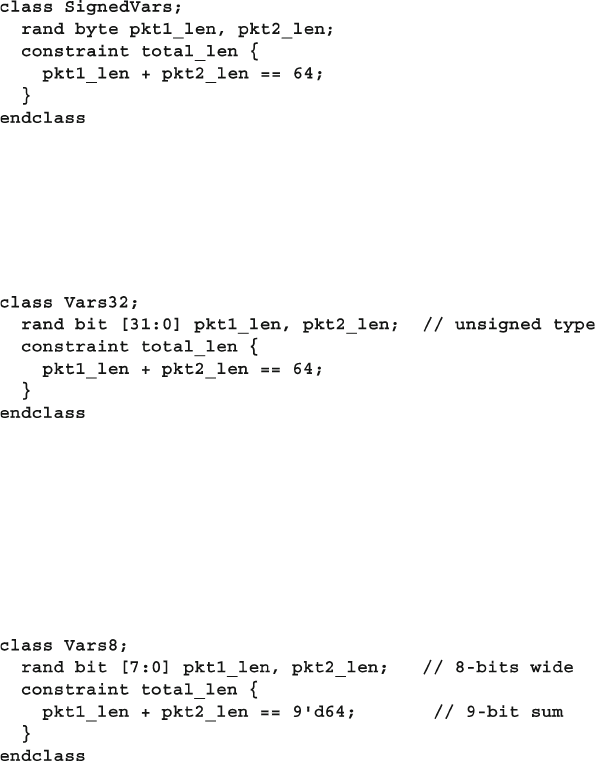
201
6.12 Common Randomization Problems
6.12.1 Use Signed Variables with Care
When creating a testbench, you may be tempted to use the int, byte , or other
signed types for counters and other simple variables. Don’t use them in random
constraints unless you really want signed values. What values are produced when
the class in Sample
6.43 is randomized? It has two random variables and wants to
make the sum of them 64.
Sample 6.43 Signed variables cause randomization problems
Obviously, you could get pairs of values such as (32, 32) and (2, 62). Additionally,
you could see (−63, 127), as this is a legitimate solution of the equation, even though
it may not be what you wanted. To avoid meaningless values such as negative
lengths, use only unsigned random variables, as shown in Sample 6.44 .
Sample 6.44 Randomizing unsigned 32-bit variables
Even this version causes problems, as large values of pkt1_len and pkt2_len ,
such as 32'h80000040 and 32'h80000000 , wrap around when added together
and give 32'd64 or 32'h40 . You might think of adding another pair of constraints
to restrict the values of these two variables, but the best approach is to make them
only as wide as needed, and to avoid using 32-bit variables in constraints. In Sample
6.45 , the sum of two 8-bit variables is compared to a 9-bit value.
Sample 6.45 Randomizing unsigned 8-bit variables
202 6 Randomization
6.12.2 Solver Performance Tips
Each constraint solver has its strengths and weaknesses but there are some guide-
lines that you can follow to improve the speed of your simulations with constrained
random variables. Tools are always being improved, so check with your vendor for
more specifi c information.
If you just need to fi ll an array with raw data, don’t use the solver as it has some
overhead choosing values, even for a variable that has no constraints. Don’t declare
these arrays as rand, instead calculate the values in pre_randomize with $urandom
or $urandom_range . These functions calculate a value up to 100 times faster than the
solver, which is important when you need a 1000 values quickly. Generally, the larger
the array, the less important are the individual values, and the less likely that there
is a need to use a solver. Even if you need a non-uniform range of values, or there is
a simple relationship between values, you might be able to employ an if statement.
6.12.3 Choose the Right Arithmetic Operator to Boost Effi ciency
Simple arithmetic operators such as addition and subtraction, bit
extracts, and shifts are handled very effi ciently by the solver in a
constraint. However, multiplication, division, and modulo are
very expensive with 32-bit values. Remember that any constant
without an explicit size, such as 42, is treated as a 32-bit value,
32'd42 .
If you want to generate random addresses that are near a page boundary, where a
page is 4096 bytes, you could write the following code, but the solver may take a
long time to fi nd suitable values for addr if you use the constraint in Sample 6.46 .
Sample 6.46 Expensive constraint with mod and unsized variable
Many constants in hardware are powers of 2, so take advantage of this with a bit
extraction rather than division and modulo. Only constrain the bits that matter, not
the upper bits. Likewise, multiplication by a power of two can be replaced by a shift.
Note that some constraint solvers make these optimizations automatically Sample
6.47 replaces the MOD operator with a bit extract.
Sample 6.47 Effi cient constraint with bit extract
203
6.13 Iterative and Array Constraints
6.13 Iterative and Array Constraints
The constraints presented so far allow you to specify limits on single variables.
What if you want to randomize an array? The
foreach constraint and several array
functions let you shape the distribution of the values.
Using the foreach constraint creates many constraints that can
slow down simulation. A good solver can quickly solve hundreds
of constraints but may slow down with thousands. Especially slow
are nested foreach constraints, as they produce N
2 constraints for
an array of size N. See Section 6.13.5 for an algorithm that used
randc variables instead of nested foreach .
6.13.1 Array Size
The easiest array constraint to understand is the size function. In Sample 6.48 , you
are specifying the number of elements in a dynamic array or queue.
Sample 6.48 Constraining dynamic array size
Using the inside constraint lets you set a lower and upper boundary on the
array size. In many cases you may not want an empty array, that is, size==0 .
Remember to specify an upper limit; otherwise, you can end up with thousands or
millions of elements, which can cause the random solver to take an excessive
amount of time.
6.13.2 Sum of Elements
You can send a random array of data into a design, but you can also use it to control
the fl ow. Perhaps you have an interface that has to transfer four data words.
The words can be sent consecutively or over many cycles. A strobe signal tells when
the data signal is valid. Figure 6.2 shows some legal strobe patterns, sending four
values over ten cycles.
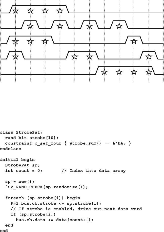
204 6 Randomization
You can create these patterns using a random array as shown in Sample 6.49 .
Constrain it to have four bits enabled out of the entire range using the sum function.
Fig. 6.2 Random strobe waveforms
Sample 6.49 Random strobe pattern class
As you remember from Chapter 2 , the sum of an array of single-bit elements
would normally be a single bit, e.g., 0 or 1. Sample 6.49 compares strobe.sum to
a 4-bit value (4'h4), so the sum is calculated with 4-bit precision. The example uses
4-bit precision to store the maximum number of elements, which is 10.
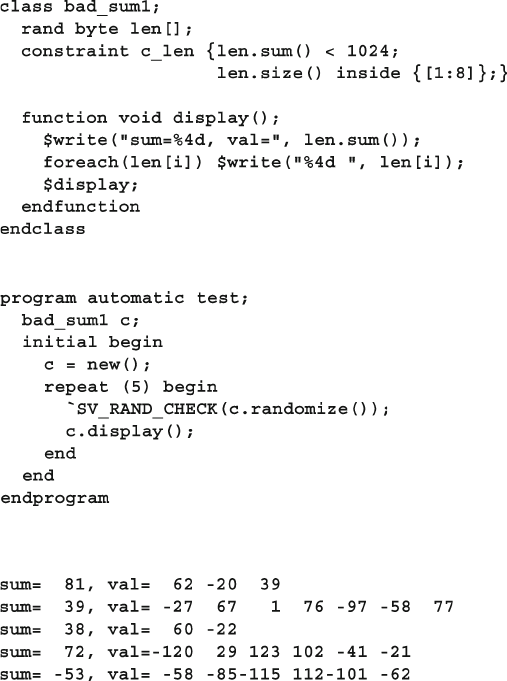
205
6.13 Iterative and Array Constraints
6.13.3 Issues with Array Constraints
The sum function looks simple but can cause several problems because of Verilog’s
arithmetic rules. The following is a simple problem that one of the authors experi-
enced creating constrained random stimulus. You want to generate from one to eight
transactions, such that the total length of all of them is less than 1024 bytes. Sample
6.50 shows a fi rst attempt, 6.51 has the test program, and 6.52 shows the output. The
len fi eld is a byte in the original transaction.
Sample 6.50 First attempt at sum constraint: bad_sum1
Sample 6.51 Program to try constraint with array sum
Sample 6.52 Output from bad_sum1
This generates some smaller lengths, but the sum is sometimes negative and is
always less than 127 — defi nitely not what you wanted! Sample 6.53 shows another
attempt, but this time replace the byte data type with an unsigned fi eld. The display
function is unchanged. Sample 6.54 shows the output.
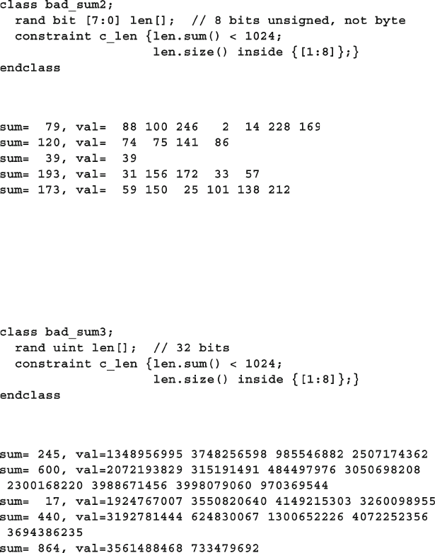
206 6 Randomization
Sample 6.53 has a subtle problem. The sum of all transaction lengths is always
less than 256, even though you constrained the array sum to be less than 1024. The
problem here is that in Verilog, the sum of many 8-bit values is computed using an
8-bit result. Sample 6.55 bumps the len fi eld up to 32 bits using the uint type from
Section 2.8 .
Sample 6.54 Output from bad_sum2
Sample 6.53 Second attempt at sum constraint: bad_sum2
Sample 6.55 Third attempt at sum constraint: bad_sum3
Sample 6.56 Output from bad_sum3
Wow – what happened here in Sample 6.56 ? This is similar to the signed problem
in Section 6.12.1 , in that the sum of two very large numbers can wrap around to a
small number. You need to limit the size based on the comparison in the constraint.
Samples 6.57 and 6.58 show the next attempt and result.
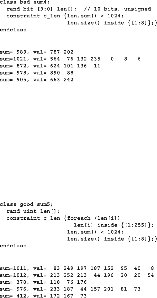
207
6.13 Iterative and Array Constraints
This does not work either as the individual len fi elds are more than 8 bits, so the
len values are often greater than 255. You need to specify that each len fi eld is
between 1 and 255, but use a 10-bit fi eld so they sum correctly. This requires con-
straining every element of the array, as shown in the following section.
6.13.4 Constraining Individual Array and Queue Elements
SystemVerilog lets you constrain individual elements of an array using foreach .
While you might be able to write constraints for a fi xed-size array by listing every
element, the foreach style is more compact. The only practical way to constrain a
dynamic array or queue is with foreach as shown in Samples 6.59 and 6.60 .
Sample 6.58 Output from bad_sum4
Sample 6.59 Simple foreach constraint: good_sum5
Sample 6.57 Fourth attempt at sum constraint: bad_sum4
Sample 6.60 Output from good_sum5
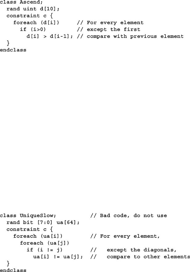
208 6 Randomization
The addition of the constraint for individual elements fi xed the example. Note
that the len array can be 10 or more bits wide, but must be unsigned.
You can specify constraints between array elements as long as you are careful
about the endpoints. The class in Sample
6.61 creates an ascending list of values by
comparing each element to the previous, except for the fi rst.
Sample 6.61 Creating ascending array values with foreach
Sample 6.62 Creating unique array values with foreach
How complex can these constraints become? Constraints have been written to
solve Einstein’s problem (a logic puzzle with fi ve people, each with fi ve separate
attributes), the Eight Queens problem (place eight queens on a chess board so that
none can capture each other), and even Sudoku.
6.13.5 Generating an Array of Unique Values
How can you create an array of random unique values? If your array has N ele-
ments, and the element values range from 0..N-1, you can simply use the array
shuffl e function as described in Section 2.6.3 .
What if the range of values is greater than the number of array elements? If you
try to make a randc array, each array element will be randomized independently, so
you are almost certain to get repeated values.
You may be tempted to use a constraint solver to compare every element with
every other with nested foreach loops as shown in Sample 6.62 . This creates over
4000 individual constraints, which could slow down simulation.

209
6.13 Iterative and Array Constraints
Instead, you should use procedural code as shown in Sample 6.63 with a helper
class containing a randc variable so that you can randomize the same variable over
and over.
Sample 6.64 Unique value generator
Sample 6.63 Creating unique array values with a randc helper class
Samples 6.64 and 6.65 give a more general solution. For example, you may need
to assign ID numbers to N bus drivers, which are in the range of 0 to MAX-1 where
MAX >=N.
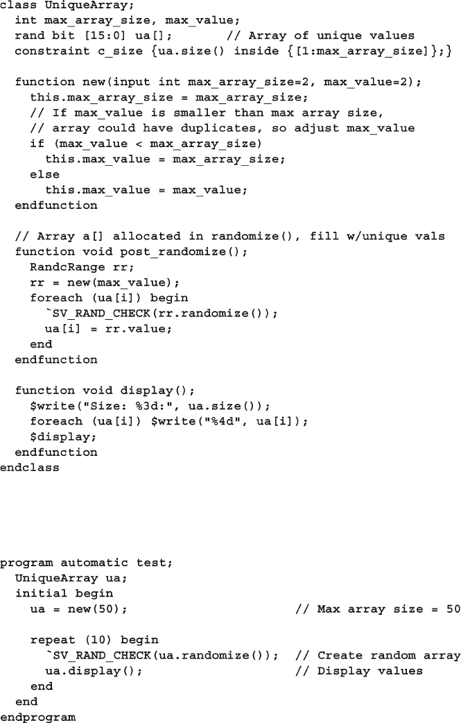

211
6.14 Atomic Stimulus Generation vs. Scenario Generation
6.13.6 Randomizing an Array of Handles
If you need to create multiple random objects, you might create a random array of
handles. Unlike an array of integers, you need to allocate all the elements before
randomization as the random solver never constructs objects. If you have a dynamic
array, allocate the maximum number of elements you may need, and then use a
constraint to resize the array as shown in Sample
6.67 . A dynamic array of handles can
remain the same size or shrink during randomization, but it can never increase in size.
Sample 6.67 Constructing elements in a random array class
The above code works well for a single array randomization. If you need to repeatedly
randomize the same array over and over, allocate the array and construct the elements
in pre_randomize . See Section 5.14.4 for more on arrays of handles.
6.14 Atomic Stimulus Generation vs. Scenario Generation
Up until now, you have seen atomic random transactions. You have learned how to
make a single random bus transaction, a single network packet, or a single processor
instruction. This is a good start, however your job is to verify that the design works
212 6 Randomization
with real-world stimuli. A bus may have long sequences of transactions such as
DMA transfers or cache fi lls. Network traffi c consists of extended sequences of
packets as you simultaneously read e-mail, browse a web page, and download music
from the net, all in parallel. Processors have deep pipelines that are fi lled with the
code for routine calls,
for loops, and interrupt handlers. Generating transactions
one at a time is unlikely to mimic any of these scenarios.
6.14.1 An Atomic Generator with History
The easiest way to create a stream of related transactions is to have an atomic gen-
erator base some of its random values on ones from previous transactions. The class
might constrain a bus transaction to repeat the previous command, such as a write,
80% of the time, and also use the previous destination address plus an increment.
You can use the post_randomize function to make a copy of the generated trans-
action for use by the next call to randomize .
This scheme works well for smaller cases but gets into trouble when you need
information about the entire sequence ahead of time. A DUT may need to know the
length of a sequence of network transactions before it starts.
6.14.2 Random Array of Objects
If you want to generate stimulus for a complex, multi-level protocol, you could
build up a combination of code and arrays of random objects. The UVM and VMM
both allow you to generate random sequences through a sophisticated set of classes
and macros. This section shows a simplifi ed random sequence.
One way to generate random sequences is to randomize an entire array of objects.
You can create constraints that refer to the previous and next objects in the array,
and the SystemVerilog solver solves all constraints simultaneously. Since the entire
sequence is generated at once, you can then extract information such as the total
number of transactions or a checksum of all data values before the fi rst transaction
is sent. Alternatively, you can build a sequence for a DMA transfer that is con-
strained to be exactly 1024 bytes, and let the solver pick the right number of transac-
tions to reach that goal.
Sample 6.68 shows a simple sequence of transactions, each one with a destina-
tion address that is greater than the one before. It builds on the array constraint
shown in Sample 6.61 .
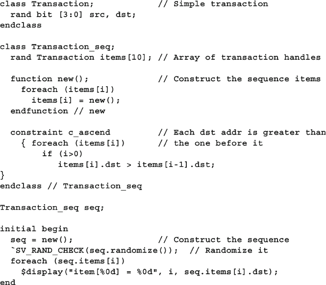
213
6.14 Atomic Stimulus Generation vs. Scenario Generation
6.14.3 Combining Sequences
You can combine multiple sequences together to make a more realistic fl ow of
transactions. For example, for a network device, you could make one sequence that
resembles downloading e-mail, a second that is viewing a web page, and a third that
is entering single characters into web-based form.The techniques to combine these
fl ows is beyond the scope of this book, but you can learn more from the VMM, as
described in Bergeron, et al. (2005).
6.14.4 Randsequence
You may fi nd it challenging to write random constraints as they don’t execute
sequentially like procedural statements. An alternative way to create random
sequences is to describe the grammar of a protocol with a declarative style using a
syntax similar to BNF (Backus-Naur Form) and random weighted case statements.
Sample 6.68 Simple random sequence with ascending values
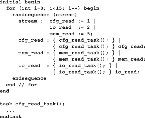
214 6 Randomization
SystemVerilog’s randsequence construct resembles the algorithmic code that you
have traditionally used but can still be challenging.
Sample 6.69 generates a sequence called stream . A stream can be either cfg_
read, io_read , or mem_read . The random sequence engine randomly picks one.
The cfg_read label has a weight of 1, io_read has twice the weight and so is
twice as likely to be chosen as
cfg_read . The label mem_read is most likely to be
chosen, with a weight of 5.
Sample 6.69 Command generator using randsequence
A cfg_read can be either a single call to cfg_read_task , or a call to the task
followed by another cfg_read . As a result, the task is always called at least once,
and possibly many times.
One big advantage of randsequence is that it is procedural code and you can
debug it by stepping though the execution, or adding $display statements. When
you call randomize for an object, it either all works or all fails, but you can’t see
the steps taken to get to a result.
There are several problems with using randsequence . The code to generate the
sequence is separate and a very different style from the classes with data and con-
straints used by the sequence. So if you use both randomize and randsequence ,
you have to master two different forms of randomization. More seriously, if you
want to modify a sequence, perhaps to add a new branch or action, you have to
modify the original sequence code. You can’t just make an extension. As you will
see in Chapter 8 , you can extend a class to add new code, data, and constraints with-
out having to edit the original class.
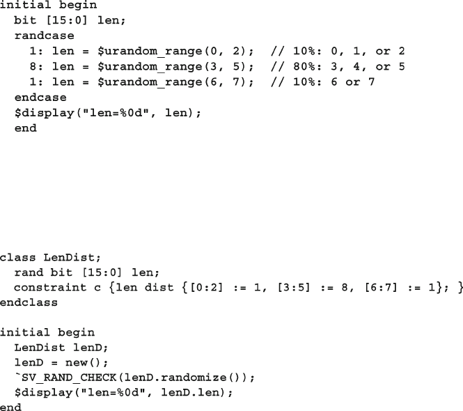
215
6.15 Random Control
6.15 Random Control
At this point you may be thinking that this process is a great way to create long
streams of random input into your design. Or you may think that this is a lot of work
if all you want to do is occasionally to make a random decision in your code. You may
prefer a set of procedural statements that you can step through using a debugger.
6.15.1 Introduction to randcase
You can use randcase to make a weighted choice between several actions, without
having to create a class and instance. Sample 6.70 chooses one of the three branches
based on the weight. SystemVerilog adds up the weights (1+8+1 = 10), chooses a
value in this range, and then picks the appropriate branch. The branches are not
order dependent, the weights can be variables, and they do not have to add up to
100%. The function $urandom_range is described in Section 6.10 .
Sample 6.70 Random control with randcase and $urandom_range
You can write Sample 6.70 using a class and the randomize function. For this
small case, the OOP version in Sample 6.71 is a little larger. However, if this were
part of a larger class, the constraint would be more compact than the equivalent
randcase statement.
Sample 6.71 Equivalent constrained class
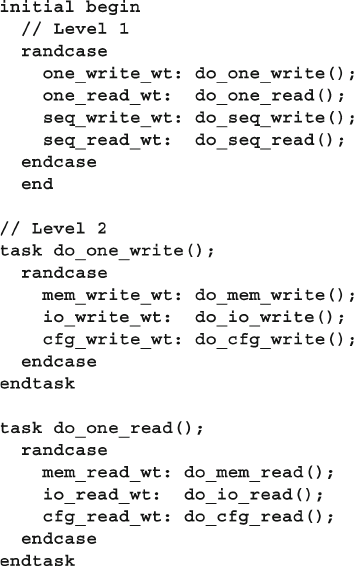
216 6 Randomization
Code using randcase is more diffi cult to override and modify than random
constraints. The only way to modify the random results is to rewrite the code or use
variable weights.
Be careful using
randcase , as it does not leave any tracks behind. For example,
you could use it to decide whether or not to inject an error in a transaction. The
problem is that the downstream transactors and scoreboard need to know of this
choice. The best way to inform them would be to use a variable in the transaction or
environment. However, if you are going to create a variable that is part of these
classes, you could have made it a random variable and used constraints to change its
behavior in different tests.
6.15.2 Building a Decision Tree with randcase
You can use the randcase statement to create a decision tree. Sample 6.72 has just
two levels of procedural code, but you can see how it can be extended to use more.
Sample 6.72 Creating a decision tree with randcase
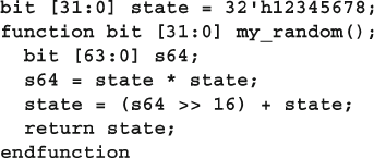
217
6.16 Random Number Generators
6.16 Random Number Generators
How random is SystemVerilog? On the one hand, your testbench depends on an
uncorrelated stream of random values to create stimulus patterns that go beyond any
directed test. On the other hand, you need to repeat the patterns over and over during
debug of a particular test, even if the design and testbench make minor changes.
6.16.1 Pseudorandom Number Generators
Verilog uses a simple PRNG that you could access with the $random function. The
generator has an internal state that you can set by providing a seed to $random . All
IEEE-1364-compliant Verilog simulators use the same algorithm to calculate
values.
Sample 6.73 shows a simple PRNG, not the one used by SystemVerilog. The
PRNG has a 32-bit state. To calculate the next random value, square the state to
produce a 64-bit value, take the middle 32 bits, then add the original value.
Sample 6.73 Simple pseudorandom number generator
You can see how this simple code produces a stream of values that seem random,
but can be repeated by using the same seed value. SystemVerilog calls its own
PRNG to generate a new value for randomize and randcase .
6.16.2 Random Stability — Multiple Generators
Verilog has a single PRNG that is used for the entire simulation. What would hap-
pen if SystemVerilog kept this approach? Testbenches often have several stimulus
generators running in parallel, creating data for the design under test. If two streams
share the same PRNG, they each get a subset of the random values.
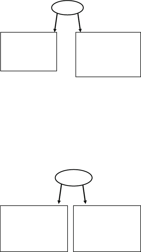
218 6 Randomization
In Fig. 6.3 , there are two stimulus generators and a single PRNG producing
values a, b, c , etc. Gen2 has two random objects, so during every cycle, it uses
twice as many random values as Gen1.
A problem can occur when one of the classes changes as shown in Fig. 6.4 . Gen1
gets an additional random variable, and so consumes two random values every time
it is called. This approach changes the values used not only by Gen1, but also by
Gen2.
class Gen1;
Transaction tr;
forever @(int1.cb)
tr.randomize()
endclass
class Gen2;
Transaction tr1, tr2;
forever @(int2.cb)
tr1.randomize();
tr2.randomize();
endclass
a
d
g
b,c
e,f
h,i
PRNG
PRNG
Fig. 6.3 Sharing a single random generator
PRNG
class Gen1;
Transaction tra, trb;
forever @(int1.cb)
tra.randomize();
trb.randomize();
endclass
class Gen2;
Transaction tr1, tr2;
forever @(int2.cb)
tr1.randomize();
tr2.randomize();
endclass
a,b
e,f
i,j
c,d
g,h
k,l
PRNG
Fig. 6.4 First generator uses additional values
In SystemVerilog, there is a separate PRNG for every object and thread. Figure 6.5
shows how changes to one object don’t affect the random values seen by others.
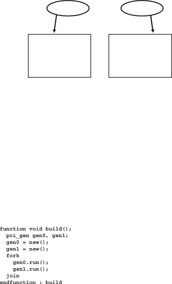
219
6.16 Random Number Generators
6.16.3 Random Stability and Hierarchical Seeding
In SystemVerilog, every object and thread has its own PRNG and unique seed.
When a new object or thread is started, its PRNG is seeded from its parent’s PRNG.
Thus a single seed specifi ed at the start of simulation can create many streams of
random stimulus, each distinct.
When you are debugging a testbench, you add, delete, and move code. Even with
random stability, your changes may cause the testbench to generate different ran-
dom values. This can be very frustrating if you are in the middle of debugging a
DUT failure, and the testbench no longer creates the same stimulus. You can mini-
mize the effect of code modifi cations by adding any new objects or threads after
existing ones. Sample 6.74 shows a routine from testbench that constructs objects,
and runs them in parallel threads.
class Gen1;
Transaction tra, trb;
forever @(int1.cb)
tra.randomize();
trb.randomize();
endclass
class Gen2;
Transaction tr1, tr2;
forever @(int2.cb)
tr1.randomize();
tr2.randomize();
endclass
a,b
c,d
e,f
m,n
o,p
q,r
PRNG 1 PRNG 2
Fig. 6.5 Separate random generators per object
Sample 6.74 Test code before modifi cation
Sample 6.75 adds a new generator, and runs it in a new thread. The new object is
constructed after the existing ones, and the new thread is spawned after the old ones.
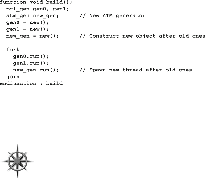
220 6 Randomization
As new code is added, you may not be able to keep the random streams the same as
the old ones, but you might be able to postpone any side effects from these changes.
6.17 Random Device Confi guration
An important part of your DUT to test is the confi guration of both
the internal DUT settings and the system that surrounds it. As
described in Section 6.2.1 , your tests should randomize the environ-
ment so that you can be confi dent it has been tested in as many
modes as possible.
Sample 6.76 shows a random testbench confi guration that can be modifi ed as needed
at the test level. The EthCfg class describes the confi guration for a 4-port Ethernet
switch. It is instantiated in an environment class, which in turn is used in the test.
The test overrides one of the confi guration values, enabling all 4 ports.
Sample 6.75 Test code after modifi cation
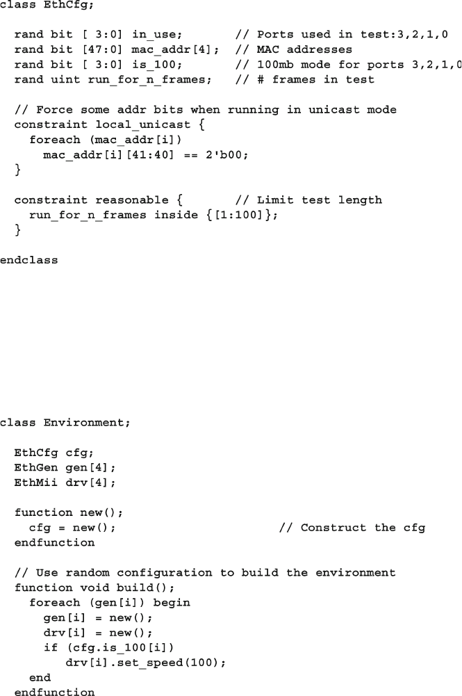
221
6.17 Random Device Confi guration
The confi guration class is used in the Environment class during several phases.
The confi guration is constructed in the Environment constructor, but not random-
ized until the gen_cfg phase as shown in Sample 6.77 . This allows you to turn
constraints on and off before randomize is called. Afterwards, you can override
the generated values before the build phase creates the virtual components around
the DUT. (The classes such as EthGen and EthMii are not shown).
Sample 6.76 Ethernet switch confi guration class
Sample 6.77 Building environment with random confi guration
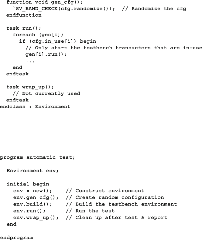
222 6 Randomization
Now you have all the components to build a test, which is described in a program
block. The test in Sample 6.78 instantiates the environment class and then runs each
step.
Sample 6.78 Simple test using random confi guration
You may want to override the random confi guration, perhaps to reach a corner
case. The test in Sample 6.79 randomizes the confi guration class and then enables
all the ports.
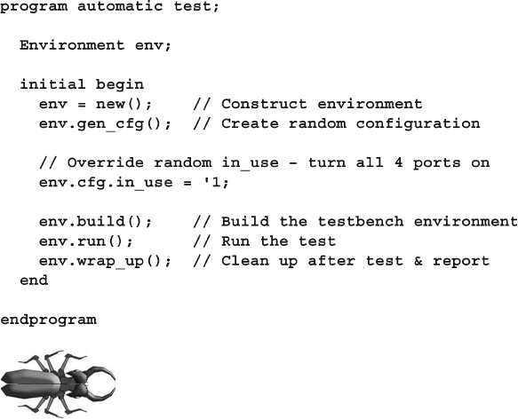
223
6.18 Conclusion
Notice how in Sample 6.77 all generators were constructed, but
only a few were run, depending on the random confi guration.
If you only constructed the generators that are in-use, you would
have to surround any reference to gen [i] with a test of in_
use [i] , otherwise your testbench would crash when it tried to
refer to the non-existent generator. The extra memory taken up by these generators
that are not used is a small price to pay for a more stable testbench.
6.18 Conclusion
Constrained-random tests are the only practical way to generate the stimulus needed
to verify a complex design. SystemVerilog offers many ways to create a random
stimulus and this chapter presents many of the alternatives.
A test needs to be fl exible, allowing you either to use the values generated by
default or to constrain or override the values so that you can reach your goals.
Always plan ahead when creating your testbench by leaving suffi cient “hooks” so
that you can steer the testbench from the test without modifying existing code.
Sample 6.79 Simple test that overrides random confi guration
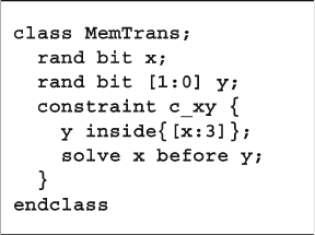
224 6 Randomization
6.19 Exercises
1. Write the SystemVerilog code for the following items.
a. Create a class Exercise1 containing two random variables, 8-bit data and
4-bit address . Create a constraint block that keeps address to 3 or 4.
b. In an initial block, construct an Exercise1 object and randomize it.
Check the status from randomization.
2. Modify the solution for Exercise 1 to create a new class Exercise2 so that:
a . data is always equal to 5
b. The probability of address==0 is 10%
c. The probability of address being between [1:14] is 80%
d. The probability of address==15 is 10%
3. Using the solution to either Exercise 1 or 2, demonstrate its usage by generating
20 new data and address values and check for success from the constraint
solver.
4. Create a testbench that randomizes the Exercise2 class 1000 times.
a. Count the number of times each address value occurs and print the results in
a histogram. Do you see an exact 10% / 80% / 10% distribution? Why or why
not?
b. Run the simulation with 3 different random seeds, creating histograms, and
then comment on the results. Here is how to run a simulation with the seed 42.
VCS: > simv +ntb_random_seed=42
IUS: > irun exercise4.sv −svseed 42
Questa: > vsim −sv_seed 42
5. For the code in Sample 6.4 , describe the constraints on the len, dst , and src
variables.
6. Complete Table 6.9 below for the following constraints.
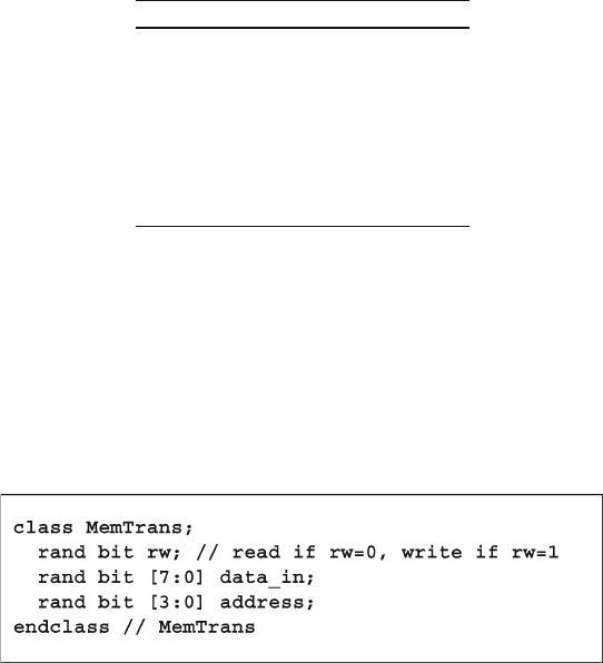
225
6.19 Exercises
7. For the following class, create:
a. A constraint that limits read transaction addresses to the range 0 to 7,
inclusive.
b. Write behavioral code to turn off the above constraint. Construct and ran-
domize a MemTrans object with an in-line constraint that limits read trans-
action addresses to the range 0 to 8, inclusive. Test that the in-line constraint
is working.
Table 6.9 Solution probabilities
Solution x y Probability
A 0 0
B 0 1
C 0 2
D 0 3
E 1 0
F 1 1
G 1 2
H 1 3
8. Create a class for a graphics image that is 10x10 pixels. The value for each
pixel can be randomized to black or white. Randomly generate an image that is,
on average, 20% white. Print the image and report the number of pixels of each
type.
9. Create a class, StimData , containing an array of integer samples. Randomize
the size and contents of the array, constraining the size to be between 1 and
1000. Test the constraint by generating 20 transactions and reporting the size.
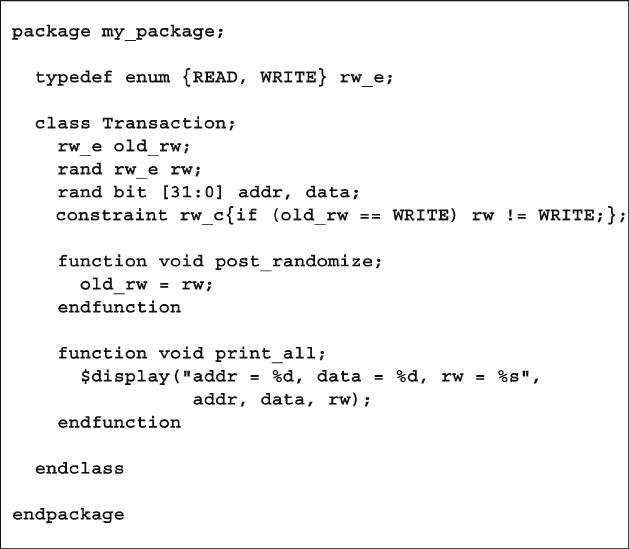
226 6 Randomization
10. Expand the Transaction class below so back-to-back transactions of the
same type do not have the same address. Test the constraint by generating 20
transactions.
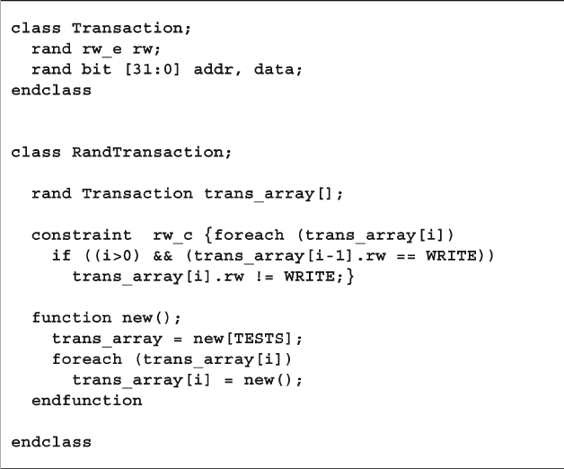
227
6.19 Exercises
11. Expand the RandTransaction class below so back-to-back transactions of
the same type do not have the same address. Test the constraint by generating
20 transactions.

229
C. Spear and G. Tumbush, SystemVerilog for Verifi cation: A Guide to Learning
the Testbench Language Features, DOI 10.1007/978-1-4614-0715-7_7,
© Springer Science+Business Media, LLC 2012
In real hardware, the sequential logic is activated on clock edges, whereas combina-
tional logic is constantly changing when any inputs change. All this parallel activity is
simulated in Verilog RTL using initial and always blocks, plus the occasional gate
and continuous assignment statement. To stimulate and check these blocks, your test-
bench uses many threads of execution, all running in parallel. Most blocks in your
testbench environment are modeled with a transactor and run in their own thread.
The SystemVerilog scheduler is the traffi c cop that chooses which thread runs
next. You can use the techniques in this chapter to control the threads and thus your
testbench.
Each of these threads communicates with its neighbors. In Fig. 7.1 , the generator
passes the stimulus to the agent. The environment class needs to know when the
generator completes and then tell the rest of the testbench threads to terminate. This
is done with interprocess communication (IPC) constructs such as the standard
Verilog events, event control and wait statements, and the SystemVerilog mail-
boxes and semaphores.
1
Chapter 7
Threads and Interprocess Communication
1 The SystemVerilog LRM uses “thread” and “process” interchangeably. The term “process” is
most commonly associated with Unix processes, in which each contains a program running in its
own memory space. Threads are lightweight processes that may share common code and memory,
and consume far fewer resources than a typical process. This book uses the term “thread.” However,
“interprocess communication” is such a common term that it is used in this book.
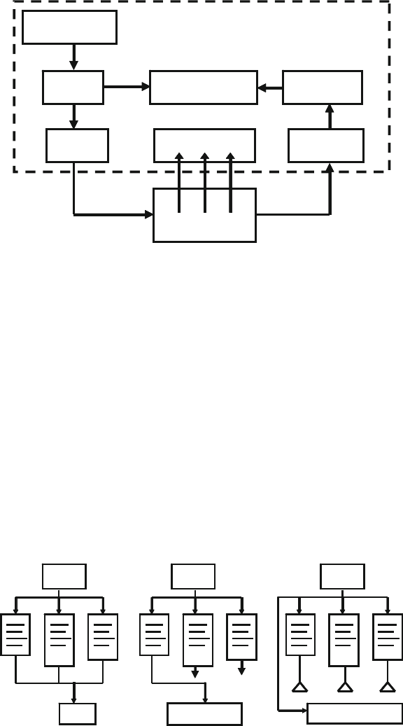
230 7 Threads and Interprocess Communication
7.1 Working with Threads
While all the thread constructs can be used in both modules and program blocks,
your testbenches belong in program blocks. As a result, your code always starts with
initial blocks that start executing at time 0. You cannot put an always block in
a program. However, you can easily get around this by using a forever loop in an
initial block.
Classic Verilog has two ways of grouping statements — with a begin…end or
fork…join . Statements in a begin…end run sequentially, whereas those in a
fork…join execute in parallel. The latter is very limited in that all statements
inside the fork…join have to fi nish before the rest of the block can continue. As a
result, it is rare for Verilog testbenches to use this feature.
SystemVerilog introduces two new ways to create threads — with the fork…
join_none and fork…join_any statements, shown in Fig. 7.2 .
Agent
DUT
Assertions
Driver Monitor
Scoreboard Checker
Generator
Environment
Agent
Fig. 7.1 Testbench environment blocks
join_any join_none
join
forkfork fork
Fig. 7.2 Fork…join blocks
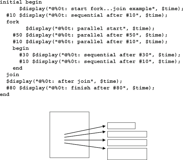
231
7.1 Working with Threads
Your testbench communicates, synchronizes, and controls these threads with
existing constructs such as events, @ event control, the wait and disable state-
ments, plus new language elements such as semaphores and mailboxes.
7.1.1 Using fork…join and begin…end
Sample 7.1 has a fork…join parallel block with an enclosed begin…end sequen-
tial block, and shows the difference between the two.
Sample 7.1 Interaction of begin…end and fork…join
initial
$display
#10 $display
fork
.
join
$display
#80 $display
$display
#30 $display
#10 $display
#50 $display
#10 $display
Parent
Child
threads
Fig. 7.3 Fork…join block
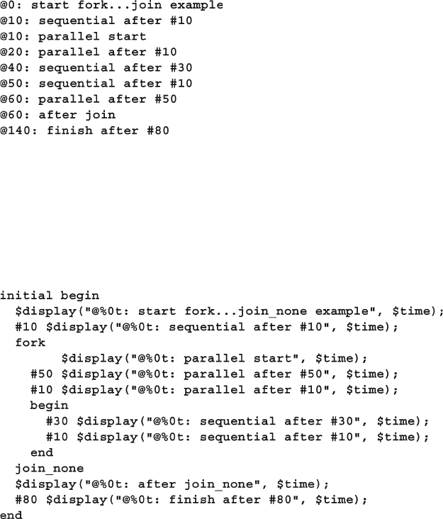
232 7 Threads and Interprocess Communication
In the output below, the code in the fork…join executes in parallel, so statements
with shorter delays execute before those with longer delays. As shown in Sample 7.2 ,
the fork…join completes after the last statement, which starts with #50 .
Sample 7.2 Output from begin…end and fork…join
7.1.2 Spawning Threads with fork…join_none
A fork…join_none block schedules each statement in the block, but execution
continues in the parent thread. Sample 7.3 is identical to Sample 7.1 except that the
join has been converted to join_none .
Sample 7.3 Fork…join_none code
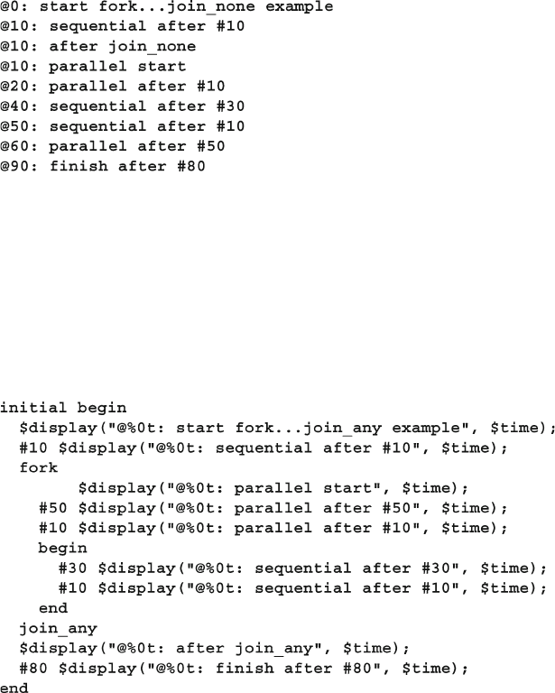
233
7.1 Working with Threads
The diagram for this block is similar to Fig. 7.3 . Note that the statement after the
join_none block in Sample 7.4 executes before any statement inside the fork…
join_none .
Sample 7.5 Fork…join_any code
Sample 7.4 Fork…join_none output
7.1.3 Synchronizing Threads with fork…join_any
A fork…join_any block schedules each statement in the block. Then, when the
fi rst statement completes, execution continues in the parent thread. All other remain-
ing threads continue. Sample 7.5 is identical to the previous examples, except that
the join has been converted to join_any .
Note in Sample 7.6 , the statement $display(“after join_any”) completes
after the fi rst statement in the parallel block.
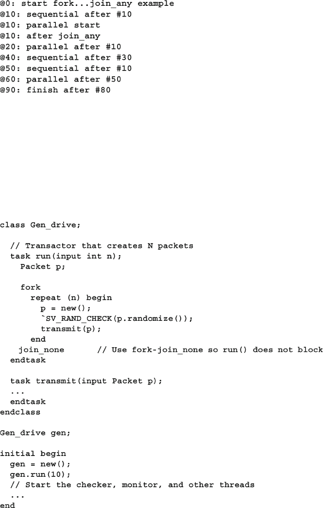
234 7 Threads and Interprocess Communication
7.1.4 Creating Threads in a Class
You can use a fork…join_none to start a thread, such as the code for a random
transactor generator. Sample 7.7 shows a generator / driver class with a run task
that creates N packets. The full testbench has classes for the driver, monitor, checker,
and more, all with transactors that need to run in parallel.
Sample 7.6 Output from fork…join_any
Sample 7.7 Generator / Driver class with a run task
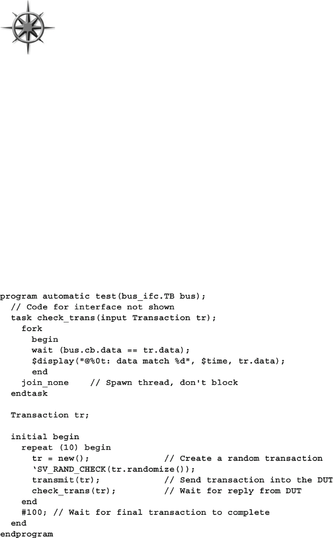
235
7.1 Working with Threads
There are several points to note with Sample 7.7 . First, the trans-
actor is not started in the new() function. The constructor should
just initialize values, not start any threads. Separating the con-
structor from the code that does the real work allows you to change
any variables before you start executing the code in the object.
This allows you to inject errors, modify the defaults, and alter the
behavior of the object. Next, the
run task starts a thread in a fork…join_none
block. The thread is a part of the transactor and should be spawned there, not in the
parent class.
7.1.5 Dynamic Threads
Verilog’s threads are very predictable. You can read the source code and count the
initial, always , and fork…join blocks to know how many threads were in a
module. On the other hand, SystemVerilog lets you create threads dynamically, and
does not require you to wait for them to fi nish.
In Sample 7.8 , the testbench generates random transactions and sends them to a
DUT that stores them for some predetermined time, and then returns them. The
testbench has to wait for the transaction to complete, but does not want to stop the
generator.
Sample 7.8 Dynamic thread creation
236 7 Threads and Interprocess Communication
When the check_trans task is called, it spawns off a thread to watch the bus
for the matching transaction data. During a normal simulation, many of these threads
run concurrently. In this simple example, the thread just prints a message, but you
could add more elaborate controls.
7.1.6 Automatic Variables in Threads
A common but subtle bug occurs when you have a loop that
spawns threads and you don’t save variable values before the
next iteration. Sample 7.8 only works in a program or module
with automatic storage. If check_trans used static storage,
each thread would share the same variable tr , so later calls
would overwrite the value set by earlier ones. Likewise, if the example had the
fork…join_none inside the repeat loop, it would try to match incoming transac-
tions using tr , but its value would change the next time through the loop. Always
use automatic variables to hold values in concurrent threads.
Sample 7.9 has a fork…join_none inside a for loop. SystemVerilog schedules
the threads inside a fork…join_none but they are not executed until after the
original code blocks, here because of the #0 delay. So Sample 7.9 prints “ 3 3 3 ”
which are the values of the index variable j when the loop terminates.
Sample 7.9 Bad fork…join_none inside a loop
237
7.1 Working with Threads
The #0 delay blocks the current thread and reschedules it to start later during the
current time slot. In Sample 7.10 , the delay makes the current thread run after the
threads spawned in the fork…join_none statement. This delay is useful for block-
ing a thread, but you should be careful, as excessive use causes race conditions and
unexpected results.
You should use automatic variables inside a fork…join statement to save a
copy of a variable as shown in Sample 7.11 .
Sample 7.10 Execution of bad fork…join_none inside a loop
Sample 7.11 Automatic variables in a fork…join_none
The fork…join_none block is split into two parts, declarations and procedural
code. The automatic variable declaration with initialization runs in the thread inside
the for loop. During each loop, a copy of k is created and set to the current value
of j. Then the body of the fork…join_none ($write) is scheduled, including a
copy of k . After the loop fi nishes, #0 blocks the current thread, so the three threads
run, printing the value of their copy of k . When the threads complete, and there is
nothing else left during the current time-slot region, SystemVerilog advances to the
next statement and the $display executes.
238 7 Threads and Interprocess Communication
Sample 7.12 traces the code and variables from Sample 7.11 . The three copies of
the automatic variable k are called k0, k1 , and k2 for this sample.
Sample 7.12 Steps in executing automatic variable code
Another way to write Sample 7.11 is to declare the automatic variable outside of
the fork…join_none . Sample 7.13 works inside a program with automatic storage.
Sample 7.13 Automatic variables in a fork…join_none
7.1.7 Waiting for all Spawned Threads
In SystemVerilog, when all the initial blocks in the program are done, the simu-
lator exits. Sample 7.14 shows how you can spawn many threads, which might still
be running. Use the wait fork statement to wait for all child threads.
239
7.1 Working with Threads
7.1.8 Sharing Variables Across Threads
Inside a class’s routines, you can use local variables, class variables,
or variables defi ned in the program. If you forget to declare a
variable, SystemVerilog looks up the higher scopes until it fi nds
a match. This can cause subtle bugs if two parts of the code are
unintentionally sharing the same variable, perhaps because you forgot to declare it
in the innermost scope.
For example, if you like to use the index variable, i, be careful that two different
threads of your testbench don’t concurrently modify this variable by each using it in
a for loop. Or you may forget to declare a local variable in a class, such as Buggy ,
shown below. If your program block declares a global i, the class just uses the
global instead of the local that you intended. You might not even notice this unless
two parts of the program try to modify the shared variable at the same time.
Sample 7.14 Using wait fork to wait for child threads
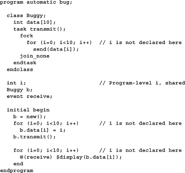
240 7 Threads and Interprocess Communication
The solution is to declare all your variables in the smallest scope that encloses all
uses of the variable. In Sample 7.15 , declare index variables inside the for loops,
not at the program or class level. Better yet, use the foreach statement whenever
possible.
7.2 Disabling Threads
Just as you need to create threads in the testbench, you also need to stop them. The
Verilog disable statement works on SystemVerilog threads. The following sec-
tions show how you can asynchronously disable threads. This can cause unexpected
behavior, so you should watch out for side effects when a thread is stopped mid-
stream. You may, instead, want to design your algorithm to check for interrupts at
stable points, then gracefully give up its resources.
Sample 7.15 Bug using shared program variable
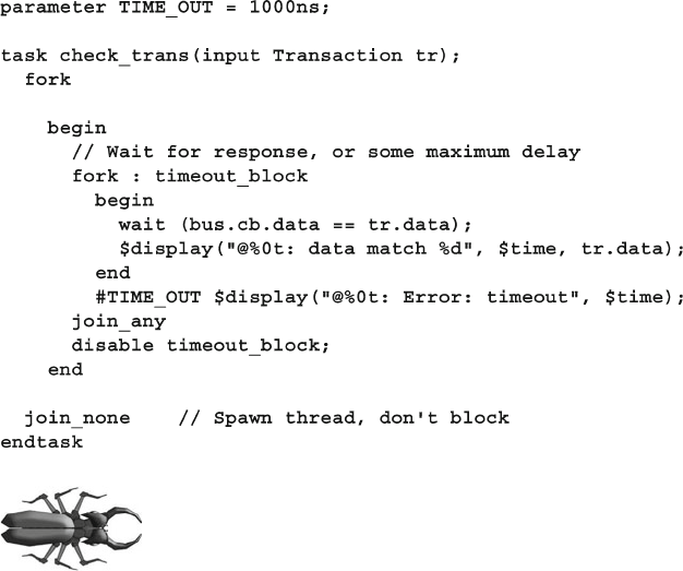
241
7.2 Disabling Threads
7.2.1 Disabling a Single Thread
Here is the check_trans task, this time using a fork…join_any plus a disable
to create a watch with a time-out. In this case, you are disabling a labelled block, to
precisely specify what to stop.
The outermost
fork…join_none is identical to Sample 7.8 . This version imple-
ments a time-out with two threads inside a fork…join_any so that the simple wait
statement is executed in parallel with a delayed $display . If the correct bus data
comes back quickly enough, the wait construct completes, the join_any executes,
and then the disable kills off the remaining thread. However, if the bus data does
not get the right value before the TIME_OUT delay completes, the error message is
printed, the join_any executes, and the disable kills the thread with the wait .
Sample 7.16 Disabling a thread
Watch out, as you might unintentionally stop too many threads
with disable label. This statement stops every process execut-
ing the labeled block, as might occur if you have multiple driver
or monitor objects running in parallel. If your code only has one
instance, disable label is a safe way to stop a thread.
7.2.2 Disabling Multiple Threads
Sample 7.16 used the classic Verilog disable statement to stop the threads in a
named block. SystemVerilog introduces the
disable fork statement so you can
stop all child threads that have been spawned from the current thread.
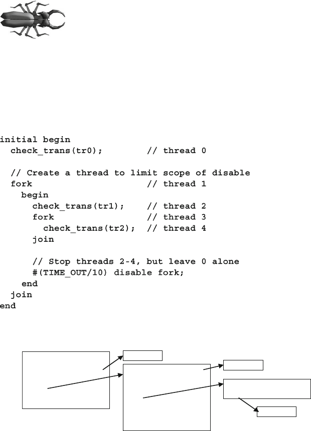
242 7 Threads and Interprocess Communication
Watch out, as you might unintentionally stop too many threads
with disable fork , such as those created from surrounding
task calls. You should always surround the target code with
a
fork…join to limit the scope of a disable fork
statement.
The next few samples use the check_trans task from Sample 7.16 . You can just
think of this task as doing a #TIME_OUT . Sample 7.17 has an additional begin…end
block inside the fork…join to make the statements sequential.
Sample 7.17 Limiting the scope of a disable fork
Fig. 7.4 shows a diagram of the spawned threads.
initial begin
check_trans(tr0)
fork
...
join
end
thread 1
check_trans(tr1)
fork
...
join
#TIME_OUT/2
disable fork
thread 0
thread 2
thread 3
check_trans(tr2)
thread 4
Fig. 7.4 Fork…join block diagram
The code calls check_trans that starts thread 0. Next a fork…join creates
thread 1. Inside this thread, one is spawned by the check_trans task and one by
the innermost fork…join , which spawns thread 4 by calling the task. After a delay,
a disable fork stops and all the child threads, 2-4. Thread 0 is outside the fork…
join block that has the disable , so it is unaffected.
Sample 7.18 is the more robust version of Sample 7.17 , with disable with a
label that explicitly names the threads that you want to stop.
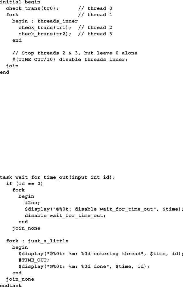
243
7.2 Disabling Threads
7.2.3 Disable a Task that was Called Multiple Times
Be careful when you disable a block from inside that block - you might end up stopping
more than you expected. As expected, if you disable a task from inside the task, it is like
a return statement, but it also kills all threads started by the task. Additionally, a single
disable label terminates all threads using that code, not just the current one.
In Sample 7.19 , the wait_for_time_out task is called three times, spawning
three threads. Then, thread 0 also disables the task after #2ns. When you run this code,
you will see the three threads starting, but none fi nishes, because of the disable in
thread 0 stops all three threads, not just one. If this task was inside a driver class that
was instantiated multiple times, a disable label in one could stop all the blocks.
Sample 7.19 Using disable label to stop a task
Sample 7.18 Using disable label to stop threads
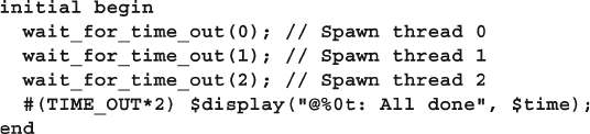
244 7 Threads and Interprocess Communication
7.3 Interprocess Communication
All these threads in your testbench need to synchronize and exchange data. At the
most basic level, one thread waits for another, such as the environment object wait-
ing for the generator to complete. Multiple threads might try to access a single
resource such as bus in the DUT, so the testbench needs to ensure that one and only
one thread is granted access. At the highest level, threads need to exchange data
such as transaction objects that are passed from the generator to the agent. All of
this data exchange and control synchronization is called interprocess communica-
tion (IPC), which is implemented in SystemVerilog with events, semaphores, and
mailboxes. These are described in the remainder of this chapter.
There are generally three parts to IPC: a producer that creates the information, a
consumer that accepts the information, and the channel that carries the information.
The producer and consumer are in separate threads.
7.4 Events
A Verilog event synchronizes threads. It is similar to a phone, where one person
waits for a call from another person. In Verilog a thread waits for an event with the
@ operator. This operator is edge sensitive, so it always blocks, waiting for the event
to change. Another thread triggers the event with the -> operator, unblocking the
fi rst thread.
System Verilog enhances the Verilog event in several ways. An event is now a
handle to a synchronization object that can be passed around to routines. This fea-
ture allows you to share events across objects without having to make the events
global. The most common way is to pass the event into the constructor for an
object.
There is always the possibility of a race condition in Verilog where one thread
blocks on an event at the same time another triggers it. If the triggering thread exe-
cutes before the blocking thread, the trigger is missed. SystemVerilog introduces the
triggered status that lets you check whether an event has been triggered, includ-
ing during the current time-slot. A thread can wait on this function instead of block-
ing with the @ operator.
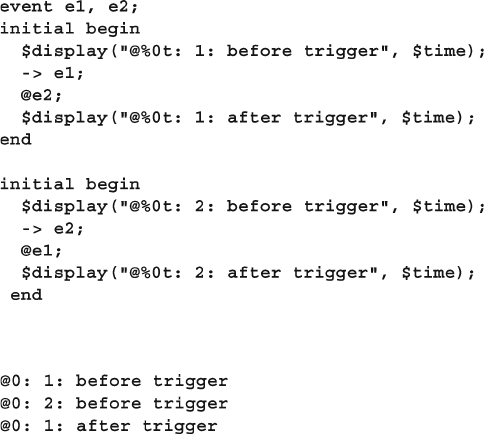
245
7.4 Events
7.4.1 Blocking on the Edge of an Event
When you run Sample 7.20 , one initial block starts, triggers its event, and then
blocks on the other event, as shown in the output in Sample
7.21 . The second block
starts, triggers its event (waking up the fi rst), and then blocks on the fi rst event.
However, the second thread locks up because it missed the fi rst event, as it is a zero-
width pulse.
Sample 7.21 Output from blocking on an event
Sample 7.20 Blocking on an event in Verilog
7.4.2 Waiting for an Event Trigger
Instead of the edge-sensitive block @e1 , use the level-sensitive wait(e1.trig-
gered) . This does not block if the event has been triggered during this time step.
Otherwise, it waits until the event is triggered.
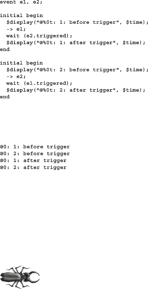
246 7 Threads and Interprocess Communication
When you run Sample 7.22 , one initial block starts, triggers its event, and then
blocks on the other event. The second block starts, triggers its event (waking up the
fi rst) and then blocks on the fi rst event, producing the output in Sample 7.23 .
Sample 7.22 Waiting for an event
Sample 7.23 Output from waiting for an event
Several of these samples have race conditions and may not execute exactly the
same on every simulator. For example, the output in Sample 7.23 assumes that when
the second block triggers e2, execution jumps back to the fi rst block. It would also
be legal for the second block to trigger e2, wait on e1, and display a message before
control is returned back to the fi rst block.
7.4.3 Using Events in a Loop
You can synchronize two threads with an event, but use caution.
If you use wait ( handshake.triggered ) in a loop, be sure to
advance the time before waiting again. Otherwise your code will
go into a zero delay loop as the wait continues over and over
again on a single event trigger. Sample 7.24 incorrectly uses a
level-sensitive blocking statement for notifi cation that a transaction is ready.
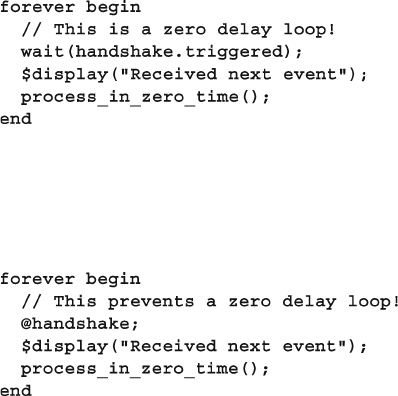
247
7.4 Events
Just as you learned to always put a delay inside an always block you need to put
a delay in a transaction process loop. The edge-sensitive delay statement in Sample
7.25 continues once and only once per event trigger.
Sample 7.25 Waiting for an edge on an event
Sample 7.24 Waiting on event causes a zero delay loop
You should avoid events if you need to send multiple notifi cations in a single
time slot, and look at other IPC methods with built-in queuing such as semaphores
and mailboxes, discussed later in this chapter.
7.4.4 Passing Events
As described above, an event in SystemVerilog can be passed as an argument to a
routine. In Sample 7.26 , an event is used by a transactor to signal when it has
completed.
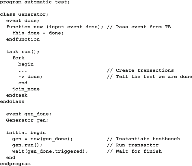
248 7 Threads and Interprocess Communication
7.4.5 Waiting for Multiple Events
In Sample 7.26 , you had a single generator that fi red a single event. What if your
testbench environment class must wait for multiple child processes to fi nish, such as
N generators? The easiest way is to use wait fork , that waits for all child pro-
cesses to end. The problem is that this also waits for all the transactors, drivers, and
any other threads that were spawned by the environment. You need to be more
selective. You still want to use events to synchronize between the parent and child
threads.
You could use a for loop in the parent to wait for each event, but that would only
work if thread 0 fi nished before thread 1, which fi nished before thread 2, etc. If the
threads fi nish out of order, you could be waiting for an event that triggered many
cycles ago.
The solution is to make a new thread and then spawn children from there that
each block on an event for each generator, as shown in Sample 7.27 . Now you can
do a wait fork because you are being more selective.
Sample 7.26 Passing an event into a constructor
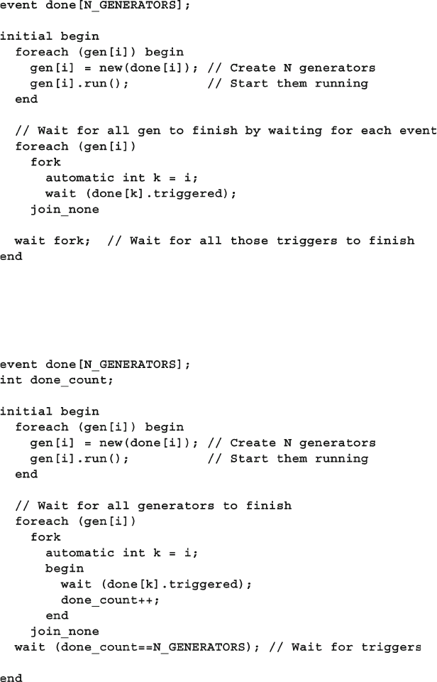
249
7.4 Events
Another way to solve this problem is to keep track of the number of events that
have triggered, as shown in Sample 7.28 .
Sample 7.27 Waiting for multiple threads with wait fork
Sample 7.28 Waiting for multiple threads by counting triggers
That was slightly less complicated. Why not get rid of all the events and just wait
on a count of the number of running generators? This count can be a static variable
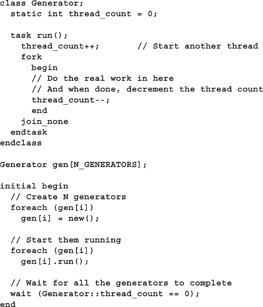
250 7 Threads and Interprocess Communication
in the Generator class. Note that most of the thread manipulation code has been
replaced with a single wait construct. The last block in Sample 7.29 waits for the
count using the class scope resolution operator, ::. You could have used any handle,
such as
gen[0] , but that would be less direct.
Sample 7.29 Waiting for multiple threads using a thread count
7.5 Semaphores
A semaphore allows you to control access to a resource. Imagine that you and your
spouse share a car. Obviously, only one person can drive it at a time. You can man-
age this situation by agreeing that whoever has the key can drive it. When you are
done with the car, you give up the car so that the other person can use it. The key is
the semaphore that makes sure only one person has access to the car. In operating
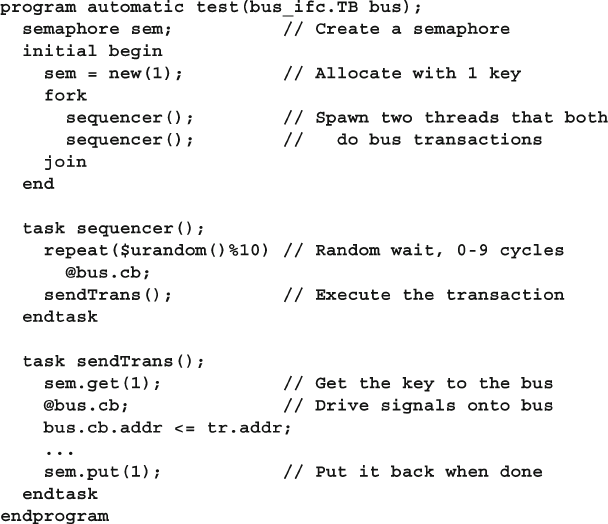
251
7.5 Semaphores
system terminology, this is known as “mutually exclusive access,” so a semaphore
is known as a “mutex” and is used to control access to a resource.
Semaphores can be used in a testbench when you have a resource, such as a bus,
that may have multiple requestors from inside the testbench but, as part of the physi-
cal design, can only have one driver. In SystemVerilog, a thread that requests a key
when one is not available always blocks. Multiple blocking threads are queued in
FIFO order.
7.5.1 Semaphore Operations
There are three basic operations for a semaphore. You create a semaphore with one
or more keys using the new method, get one or more keys with the blocking task
get() , and return one or more keys with put() . If you want to try to get a sema-
phore, but not block, use the try_get() function. If keys are available, try_get()
obtains them and returns 1. If there are not suffi cient keys, it just returns a 0. Sample
7.30 shows how to control access to a resource with a semaphore.
Sample 7.30 Semaphores controlling access to hardware resource
252 7 Threads and Interprocess Communication
7.5.2 Semaphores with Multiple Keys
There are two things you should watch out for with semaphores. First, you can put
more keys back than you took out. Suddenly you may have two keys but only one car!
Secondly, be careful if your testbench needs to get and put multiple keys. Perhaps you
have one key left, and a thread requests two, causing it to block. Now a second thread
requests a single semaphore – what should happen? In SystemVerilog the second
request,
get(1) , sneaks ahead of the earlier get(2) , bypassing the FIFO ordering.
If you are mixing different sized requests, you can always write your own class.
That way you can be very clear on who gets priority.
7.6 Mailboxes
How do you pass information between two threads? Perhaps your generator needs to
create many transactions and pass them to a driver. You might be tempted to just have
the generator thread call a task in the driver. If you do that, the generator needs to know
the hierarchical path to the driver task, making your code less reusable. Additionally,
this style forces the generator to run at the same speed as the driver, that can cause
synchronization problems if one generator needs to control multiple drivers.
Think of your generator and driver as transactors that are autonomous
objects that communicate through a channel. Each object gets a trans-
action from an upstream object (or creates it, as in the case of a gen-
erator), does some processing, and then passes it to a downstream
object. The channel must allow its driver and receiver to operate asyn-
chronously. You may be tempted to just use a shared array or queue, but it can be
diffi cult to create threads that read, write, and blocks safely.
The solution is a SystemVerilog mailbox. From a hardware point of view, the easiest
way to think about a mailbox is that it is just a FIFO, with a source and sink. The
source puts data into the mailbox, and the sink gets values from the mailbox.
Mailboxes can have a maximum size or can be unlimited. When the source thread
tries to put a value into a sized mailbox that is full, that thread blocks until the value
is removed. Likewise, if a sink threads tries to remove a value from a mailbox that
is empty, that thread blocks until a value is put into the mailbox.
Figure 7.5 shows a mailbox connecting a generator and driver.
generator driver
mailbox
Fig. 7.5 A mailbox connecting two transactors
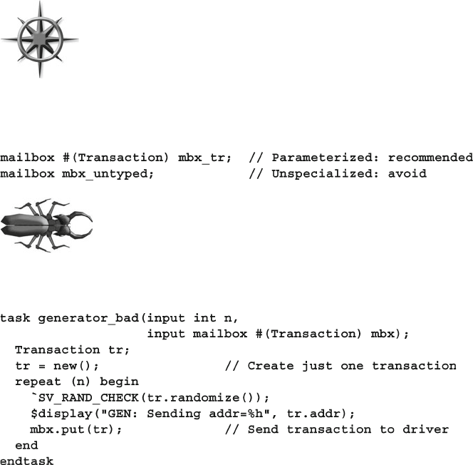
253
7.6 Mailboxes
A mailbox is an object and thus has to be instantiated by calling the new func-
tion. This takes an optional size argument to limit the number of entries in the
mailbox. If the size is 0 or not specifi ed, the mailbox is unbounded and can hold an
unlimited number of entries.
You put data into a mailbox with the
put() task, and remove it with the blocking
get() task. A put() blocks if the mailbox is full, and get() blocks if the mailbox
is empty. Use try_put() if you want to see if the mailbox is full. and try_get()
to see if it is empty. The peek() task gets a copy of the data in the mailbox but does
not remove it.
The data is a single value, such as an integer, or logic of any size or
a handle. A mailbox never contains objects, only references to
them. By default, a mailbox does not have a type, so you could put
any mix of data into it. Don’t do it! Enforce one data type per mail-
box by sticking with parameterized mailboxes as shown in Sample
7.31 to catch type mismatches at compile time.
Sample 7.31 Mailbox declarations
A classic mailbox bug, shown in Sample 7.32 , is a loop that ran-
domizes objects and puts them in a mailbox, but the object is
only constructed once, outside the loop. Since there is only one
object, it is randomized over and over.
Sample 7.32 Bad generator creates only one object
Figure 7.6 shows all the handles pointing to a single object. A mailbox only
holds handles, not objects, so you end up with a mailbox containing multiple han-
dles that all point to the single object. The code that gets the handles from the mail-
box just sees the last set of random values.
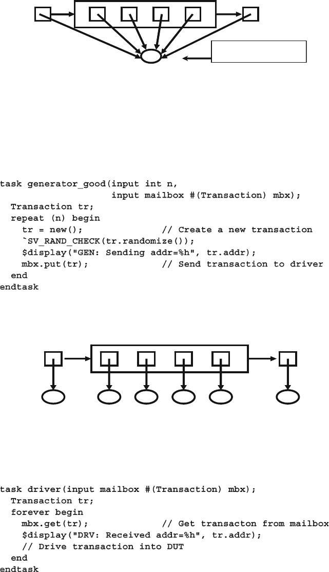
254 7 Threads and Interprocess Communication
The solution, shown in Sample 7.33 , is to make sure your loop has all three steps
of constructing the object, randomizing it, and putting it in the mailbox. This bug is
so common that it is also mentioned in Section 5.14.3.
All handles refer
to the same object
Fig. 7.6 A mailbox with multiple handles to one object
Sample 7.33 Good generator creates many objects
The result, shown in Fig. 7.7 , is that every handle points to a unique object. This
type of generator is known as the Blueprint Pattern and described in Section 8.2.
Fig. 7.7 A mailbox with multiple handles to multiple objects
Sample 7.34 Good driver receives transactions from mailbox
Sample 7.34 shows the driver that waits for transactions from the generator.
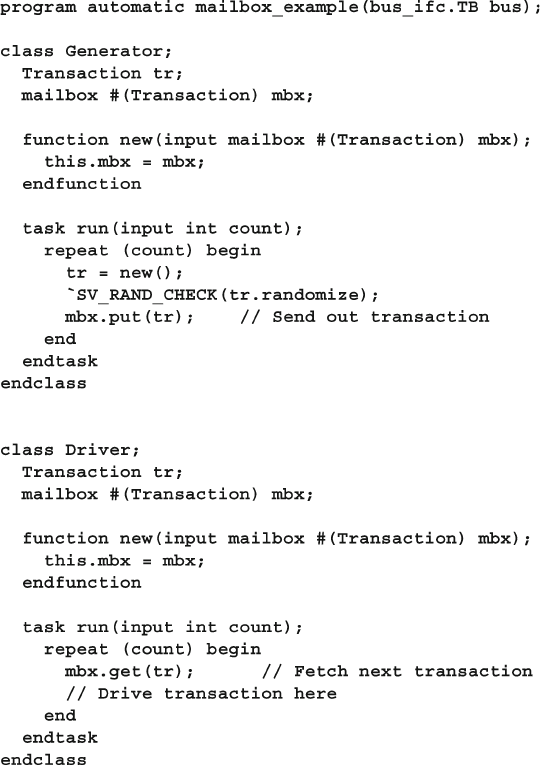
255
7.6 Mailboxes
If you don’t want your code to block when accessing the mailbox, use the try_
get() and try_peek() functions. If they are successful, they return a nonzero
value; otherwise, they return 0. These are more reliable than the
num() function, as
the number of entries can change between when you measure it and when you next
access the mailbox.
7.6.1 Mailbox in a Testbench
Sample 7.35 shows a program with a Generator and Driver exchanging transactions
using a mailbox.
Sample 7.35 Exchanging objects using a mailbox: the Generator class
256 7 Threads and Interprocess Communication
7.6.2 Bounded Mailboxes
By default, mailboxes are similar to an unlimited FIFO — a producer can put any
number of objects into a mailbox before the consumer gets the objects out. However,
you may want the two threads to operate in lockstep so that the producer blocks
until the consumer is done with the object.
You can specify a maximum size for the mailbox when you construct it. The
default mailbox size is 0 which creates an unbounded mailbox. Any size greater
than 0 creates a bounded mailbox. If you attempt to put more objects than this limit,
put() blocks until you get an object from the mailbox, creating a vacancy.
Sample 7.36 Bounded mailbox
257
7.6 Mailboxes
Sample 7.36 creates the smallest possible mailbox, which can hold a single message.
The Producer thread tries to put three messages (integers) in the mailbox, and the
Consumer thread slowly gets messages every 1ns. As Sample 7.37 shows, the fi rst
put() succeeds, then the Producer tries put(2) which blocks. The Consumer
wakes up, gets a message 1 from the mailbox, so now the Producer can fi nish put-
ting the message 2.
Sample 7.37 Output from bounded mailbox
The bounded mailbox acts as a buffer between the two processes. You can see how
the Producer generates the next value before the Consumer reads the current value.
7.6.3 Unsynchronized Threads Communicating with a Mailbox
In many cases, two threads that are connected by a mailbox should
run in lockstep, so that the producer does not get ahead of the con-
sumer. The benefi t of this approach is that your entire chain of stimu-
lus generation now runs in lock step. The highest level generator
only completes when the last low level transaction completes trans-
mission. Now your testbench can tell precisely when all stimulus has
been sent. In another example, if your generator gets ahead of the driver, and you are
gathering functional coverage on the generator, you might record that some transac-
tions were tested, even if the test stopped prematurely. So even though a mailbox
allows you to decouple the two sides, you may still want to keep them synchronized.
If you want two threads to run in lockstep, you need a handshake in addition to the
mailbox. In Sample 7.38 the Producer and Consumer are now classes that exchange
258 7 Threads and Interprocess Communication
integers using a mailbox, with no explicit synchronization between the two objects.
As a result, as shown in Sample
7.39 , the producer runs to completion before the
consumer even starts.
Sample 7.38 Producer–consumer without synchronization
The above sample holds the mailbox in a global variable to make the code more
compact. In real code, you should pass the mailbox into the class through the con-
structor and save a reference to it in a class-level variable.
259
7.6 Mailboxes
Sample 7.38 has no synchronization so the Producer puts all three integers into
the mailbox before the Consumer can get the fi rst one. This is because a thread
continues running until there is a blocking statement, and the Producer has none.
The Consumer thread blocks on the fi rst call to
mbx.get .
Sample 7.39 Producer–consumer without synchronization output
This example has a race condition, so on some simulators the consumer could
activate earlier. The result is still the same as the values are determined by the pro-
ducer, not by how quickly the consumer sees them.
7.6.4 Synchronized Threads Using a Bounded Mailbox
and a Peek
In a synchronized testbench, the Producer and Consumer operate in lock step. This
way, you can tell when the input stimuli is complete by waiting for any of the
threads. If the threads operate unsynchronized, you need to add extra code to detect
when the last transaction is applied to the DUT.
To synchronize two threads, the Producer creates and puts a transaction into a
mailbox, then blocks until the Consumer fi nishes with it. This is done by having the
Consumer remove the transaction from the mailbox only when it is fi nally done
with it, not when the transaction is fi rst detected.
Sample 7.40 show the fi rst attempt to synchronize two threads, this time with a
bounded mailbox. The Consumer uses the built-in mailbox method peek() to look
at the data in the mailbox without removing. When the Consumer is done process-
ing the data, it removes the data with get() . This frees up the Producer to generate
a new value. If the Consumer loop started with a get() instead of the peek() , the
transaction would be immediately removed from the mailbox, so the Producer could
wake up before the Consumer fi nished with the transaction. Sample 7.41 has the
output from this code.
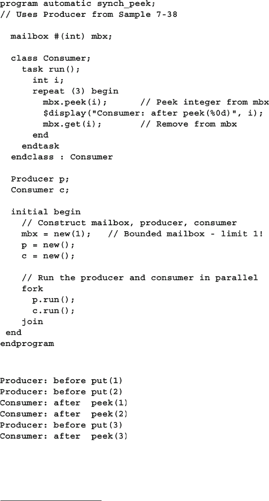
260 7 Threads and Interprocess Communication
You can see that the Producer and Consumer are in lockstep, but the Producer is
still one transaction ahead of the Consumer. This is because a bounded mailbox
with size=1 only blocks when you try to do a put of the second transaction.
2
Sample 7.41 Output from producer–consumer with bounded mailbox
Sample 7.40 Producer–consumer synchronized with bounded mailbox
2 This behavior is different from the VMM channel. If you set a channel’s full level to 1, the very fi rst
call to put() places the transaction in the channel, but does not return until the transaction is removed.
261
7.6 Mailboxes
7.6.5 Synchronized Threads Using a Mailbox and Event
You may want the two threads to use a handshake so that the Producer never gets ahead
of the Consumer. The Consumer already blocks, waiting for the Producer using a mail-
box. The Producer needs to block, waiting for the Consumer to fi nish the transaction.
Do this by adding a blocking statement to the Producer such as an event, a semaphore,
or a second mailbox. Sample
7.42 uses an event to block the Producer after it puts data
in the mailbox. The Consumer triggers the event after it consumes the data.
If you use wait ( handshake.triggered ) in a loop, be sure to
advance the time before waiting again, as previously shown in
Section 7.4.3 . This wait blocks only once in a given time slot, so
you need move into another. Sample 7.42 uses the edge-sensitive
blocking statement @handshake instead to ensure that the
Producer stops after sending the transaction. The edge-sensitive statement works
multiple times in a time slot but may have ordering problems if the trigger and block
happen in the same time slot.
Sample 7.42 Producer–consumer synchronized with an event

262 7 Threads and Interprocess Communication
Now the Producer does not advance until the Consumer triggers the event, as
shown in Sample 7.43 .
Sample 7.43 Output from producer–consumer with event
You can see that the Producer and Consumer are successfully running in lockstep by
the fact that the Producer never produces a new value until after the old one is read.
7.6.6 Synchronized Threads Using Two Mailboxes
Another way to synchronize the two threads is to use a second mailbox that sends a
completion message back to the Producer, as shown in Sample 7.44 .
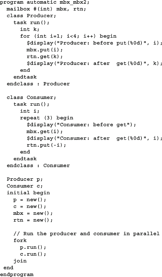
263
7.6 Mailboxes
The return message in the rtn mailbox is just a negative version of the original
integer. You could use any value, but this one can be checked against the original for
debugging purposes.
Sample 7.44 Producer–consumer synchronized with a mailbox
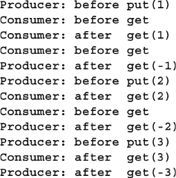
264 7 Threads and Interprocess Communication
You can see from Sample 7.45 that the Producer and Consumer are successfully
running in lockstep.
7.6.7 Other Synchronization Techniques
You can also complete the handshake by blocking on a variable or a semaphore. An
event is the simplest construct, followed by blocking on a variable. A semaphore is
comparable to using a second mailbox, but no information is exchanged. SystemVer-
ilog’s bounded mailbox just does not work as well as these other techniques as there
is no way to block the producer when it puts the fi rst transaction in. Sample 7.41
shows that the Producer is always one transaction ahead of the Consumer.
7.7 Building a Testbench with Threads and IPC
Way back in Section 1.10 you learned about layered testbenches. Figure 7.8 shows
the relationship between the different parts. Now that you know how to use threads
and IPC, you can construct a basic testbench with transactors.
Sample 7.45 Output from producer–consumer with mailbox
265
7.7 Building a Testbench with Threads and IPC
7.7.1 Basic Transactor
Sample 7.46 is the Agent class that sits between the Generator and the Driver.
Agent
DUT
Assertions
Driver Monitor
Scoreboard Checker
Generator Environment
Agent
Scenario
Signal
Command
Functional
Fig. 7.8 Layered testbench with environment
Sample 7.46 Basic Transactor
266 7 Threads and Interprocess Communication
7.7.2 Confi guration Class
The confi guration class allows you to randomize the confi guration of your system
for every simulation. Sample
7.47 has just one variable and a basic constraint.
Sample 7.47 Confi guration class
7.7.3 Environment Class
The Environment class, shown as a dashed line in Fig. 7.8 , holds the Generator,
Agent, Driver, Monitor, Checker, Scoreboard, and Confi g objects, and the mail-
boxes between them. Sample 7.48 shows a basic Environment class.
Sample 7.48 Environment class
267
7.7 Building a Testbench with Threads and IPC
Chapter 8 shows more details on how to build these classes.
7.7.4 Test Program
Sample 7.49 shows the main test, which is in a program block. As discussed in
Section 4.3.4, you can also put a test in a module, but at a slight increase in the
chances of race conditions.
268 7 Threads and Interprocess Communication
7.8 Conclusion
Your design is modeled as many independent blocks running in parallel, so your
testbench must also generate multiple stimulus streams and check the responses
using parallel threads. These are organized into a layered testbench, orchestrated by
the toplevel environment. SystemVerilog introduces powerful constructs such as
fork…join_none and fork…join_any for dynamically creating new threads, in
addition to the standard fork…join . These threads communicate and synchronize
using events, semaphores, mailboxes, and the classic @ event control and wait
statements. Lastly, the disable command is used to terminate threads.
These threads and the related control constructs complement the dynamic nature
of OOP. As objects are created and destroyed, they can run in independent threads,
allowing you to build a powerful and fl exible testbench environment.
Sample 7.49 Basic test program
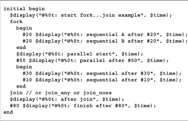
269
7.9 Exercises
7.9 Exercises
1. For the following code determine the order and time of execution for each state-
ment if a
join or join_none or join_any is used. Hint: the order and time of
execution between the fork and join/join_none/join_any is the same,
only the order and execution time of the statements after the join are different.
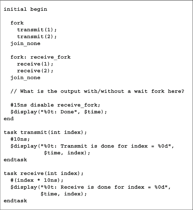
270 7 Threads and Interprocess Communication
2. For the following code what would the output be with and without a wait fork
inserted in the indicated location?
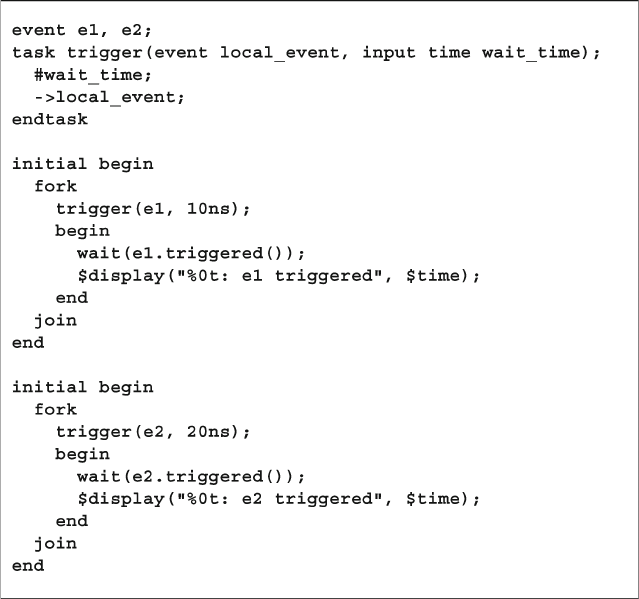
271
7.9 Exercises
3. What would be displayed with the following code? Assume that the events and
task trigger is declared inside a program declared as automatic.
4. Create a task called wait10 that for 10 tries will wait for 10ns and then check
for 1 semaphore key to be available. When the key is available, quit the loop and
print out the time.
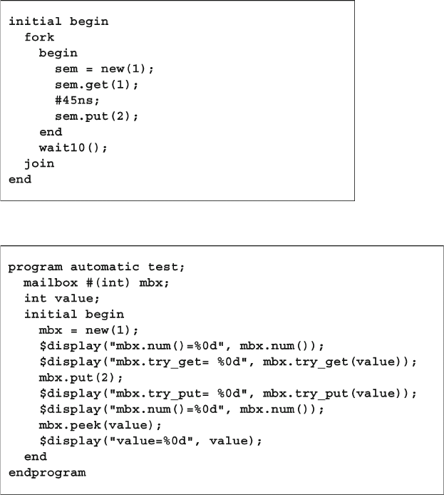
272 7 Threads and Interprocess Communication
5. What would be displayed with the following code that calls the task from Exercise 4?
6. What would be displayed with the following code?
7. Look at Fig. 7.8 “Layered testbench with environment” on page 265 and create
the Monitor class. You can make the following assumptions.
a. The Monitor class has knowledge of class OutputTrans with member vari-
ables out1 and out2 .
b. The DUT and Monitor are connected with an interface called my_bus , with
signals out1 and out2 .
c. The interface my_bus has a clocking block, cb .
d. On every active clock edge, the Monitor class will sample the DUT outputs,
out1 and out2 , assign them to an object of type OutputTrans , and place
the object in a mailbox.
273
C. Spear and G. Tumbush, SystemVerilog for Verifi cation: A Guide to Learning
the Testbench Language Features, DOI 10.1007/978-1-4614-0715-7_8,
© Springer Science+Business Media, LLC 2012
How would you create a complex class for a bus transaction that also performs error
injection and has random delays? The fi rst approach is to put everything in a large,
fl at class. This approach is simple to build, easy to understand (all the code is right
there in one class) but can be slow to develop and debug. Additionally, such a large
class is a maintenance burden, as anyone who wants to make a new transaction
behavior has to edit the same fi le. Just as you would never create a complex RTL
design using just one Verilog module, you should break classes down into smaller,
reusable blocks.
Another approach is composition. As you learned in Chapter 5 , you can instan-
tiate one class inside another, just as you instantiate modules inside another, build-
ing up a hierarchical testbench. You write and debug your classes from the top
down or bottom up, always looking for natural partitions when deciding what vari-
ables and method go into the various classes. A pixel could be partitioned into its
color and coordinate. A packet might be divided into header and payload. You
might break an instruction into opcode and operands. See Section 8.4 for guidelines
on partitioning.
Sometimes it is diffi cult to divide the functionality into separate parts. Consider
injecting errors during a bus transaction. When you write the original class for the
transaction, you may not think of all the possible error cases. Ideally, you would like
to make a class for a good transaction, and later add different error injectors.
The transaction has data fi elds and an error-checking checksum fi eld generated from
the data. One form of error injection is corruption of the checksum fi eld. If you use
composition, you need separate classes for good transactions and error transactions.
Testbench code that used good objects would have to be rewritten to process the
new error objects. What you need is a class that resembles the original class but adds
a few new variables and methods. This result is accomplished through inheritance.
Chapter 8
Advanced OOP and Testbench Guidelines
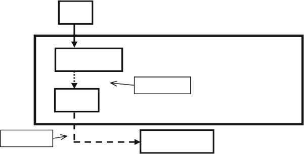
274 8 Advanced OOP and Testbench Guidelines
Inheritance allows a new class to be extended from an existing one by adding
new variables and methods. The original class is known as the base class. Since the
new class extends the capability of the base class, it is called the extended class.
Inheritance provides reusability by overlaying features, such as error injection, on
an existing class, without modifying that class.
A real power of OOP is that it gives you the ability to take an existing class,
such as a transaction, and selectively update parts of its behavior by replacing
methods, but without having to change the surrounding infrastructure. All your
original tests that depend on the base class keep working, and you can now create
new tests with the extended class. With some planning, you can create a testbench
solid enough to send basic transactions, but able to accommodate any extensions
needed by the test.
Note that this chapter goes into a wide range of advanced OOP topics, many of
which you won’t need when learning SystemVerilog. Feel free to skip the later sec-
tions for now, and save them for when you are digging into the internals of UVM
and VMM.
8.1 Introduction to Inheritance
Figure 8.1 shows a simple testbench. The test controls the generator. The generator
creates transactions, randomizes them, and sends them to the driver along the dotted
line. The driver breaks down the transaction into pin wiggles and sends it into the
DUT along the dashed line. The rest of the testbench is left out.
Fig. 8.1 Simplifi ed layered testbench
DUT
Driver
Test
Environment
Generator
transactions
pin wiggles
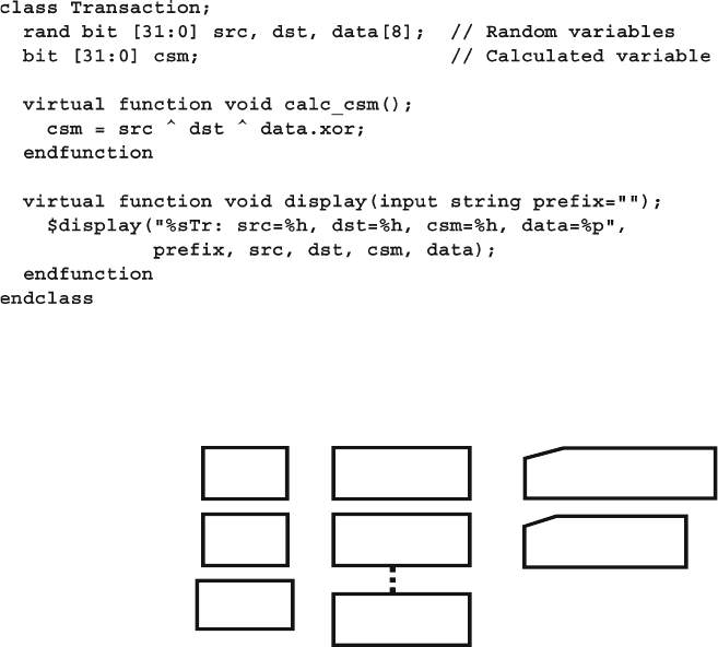
275
8.1 Introduction to Inheritance
8.1.1 Basic Transaction
The basic transaction class in Sample 8.1 has variables for the source and destina-
tion addresses, eight data words, and a checksum for error checking, plus methods
for displaying the contents and calculating the checksum. The
calc_csm function
is tagged as virtual so that it can be redefi ned if needed, as shown in the next sec-
tion. Virtual methods are explained in more detail later in this chapter in Section
8.3.2 . The class is simple enough that it uses the default SystemVerilog constructor
that allocates memory and initializes variables to their default value.
Sample 8.1 Base Transaction class
Normally calculating the checksum would be done in post_randomize(), but in
this example it has been separated from the randomization to show how to inject errors.
Figure 8.2 shows a diagram for the class with both the variables and methods.
8.1.2 Extending the Transaction Class
Suppose you have a testbench that sends good transactions through the DUT and
now you want to inject errors. If you follow the guidelines from Chapter 1 , you
would want to make as few code changes as possible to your existing testbench.
So how can you reuse the existing Transaction class? Take the existing class and
Fig. 8.2 Base Transaction class diagram
Transaction src data[0]
dst
csm data[7]
display()
data[1]
calc_csm()
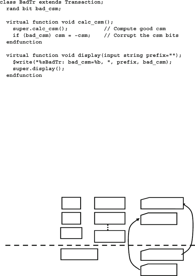
276 8 Advanced OOP and Testbench Guidelines
extend it to create a new class. This is done by declaring a new class, BadTr , as an
extension of the current class. Transaction is the base class, and BadTr is the
extended class. The code is shown in Sample
8.2 and in a diagram in Fig. 8.3 .
Sample 8.2 Extended Transaction class
Note that in Sample 8.2 , the variable csm is does not need a hierarchical identi-
fi er. The BadTr class can see all the variables from the original Transaction plus
its own variables such as bad_csm , as shown in Fig. 8.3 . The calc_csm function
in the extended class calls calc_csm in the base class using the super prefi x. You
can call a single level up, but going across multiple levels such as super.super.
new is not allowed in SystemVerilog. This style, that reaches across multiple levels,
would violate the rules of encapsulation by reaching across multiple boundaries.
The original display method printed a single line, starting with the prefi x. So
the extended display method prints the prefi x, class name, and bad_csm with
$write so the result is still on a single line.
Fig. 8.3 Extended Transaction class diagram
bad_csm
BadTr calc_csm()
Transaction src data[0]
dst
csm
display()
data[1]
display()
data[7]
calc_csm()
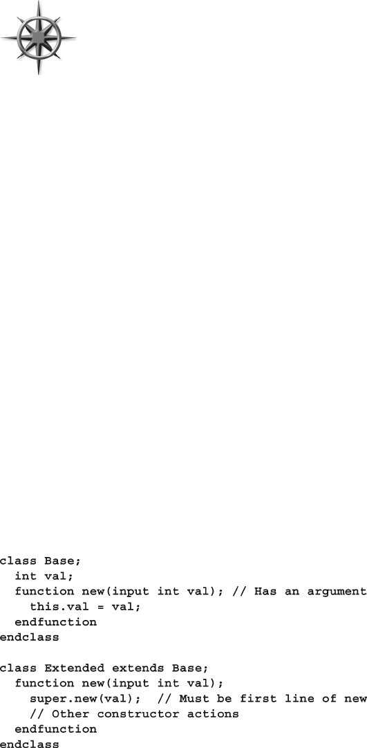
277
8.1 Introduction to Inheritance
Always declare methods inside a class as virtual so that they can be
redefi ned in an extended class. This applies to all tasks and func-
tions except the new function, which is called when the object is
constructed, so there is no way to extend it. SystemVerilog always
calls the new function based on the handle’s type. Virtual methods
are described fully in Section 8.3.2 .
8.1.3 More OOP Terminology
Here is a quick glossary of terms. As explained in Chapter 5 , the OOP term for a
variable in a class is “property,” and a task or function is called a “method.” A base
class is one that is not derived from any other class. When you extend a class, the
original class (such as Transaction ) is called the parent class or superclass. The
extended class ( BadTr ) is also known as the derived or subclass. The “prototype”
for a method is just the fi rst line that shows the argument list and return type, if
any. The prototype is used when you move the body of the method outside the
class, but is needed to describe how the method communicates, as shown in
Section 5.10.
8.1.4 Constructors in Extended Classes
When you start extending classes, there is one rule about constructors ( new func-
tions) to keep in mind. If your base class constructor has any arguments, the
extended class must have a constructor and must call the base’s constructor on its
fi rst line. In Sample 8.3 , since Base::new has an argument, Extended::new
must call it.
Sample 8.3 Constructor with arguments in an extended class
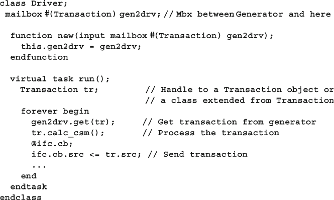
278 8 Advanced OOP and Testbench Guidelines
8.1.5 Driver Class
The driver class in Sample 8.4 receives transactions from the generator and drives
them into the DUT.
Sample 8.4 Driver class
This class receives Transaction objects from the generator though the mailbox
gen2drv, breaks them down into signal changes in the interface to stimulate the
DUT. What happens if your generator instead sends a BadTr object into the class?
OOP rules say that if you have a handle of the base type ( Transaction ), it can also
point to an object of an extended type ( BadTr ). The handle tr can only reference
things in the base class such as the variables src, dst, csm , and data , and the
method calc_csm . So you can send BadTr objects into the driver without changing
the Driver class.
See Chapter 10 and 11 for examples of fully functional drivers with advanced
features such as virtual interfaces and callbacks.
When the driver calls tr.calc_csm , which one will be called, the one in
Transaction or BadTr? Since calc_csm was declared as a virtual method in the
base class in Sample 8.1 , SystemVerilog chooses the proper method based on the
type of object stored in tr . If the object is of type Transaction , SystemVerilog
calls the task Transaction::calc_csm . If it is of type BadTr , SystemVerilog calls
the function BadTr::calc_csm .
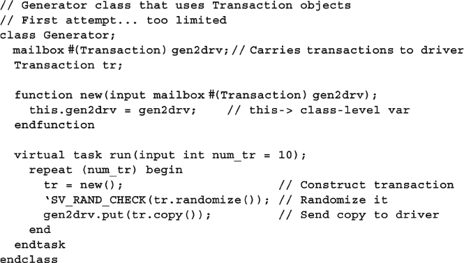
279
8.1 Introduction to Inheritance
8.1.6 Simple Generator Class
The generator in Sample 8.5 for this testbench creates a random transaction and puts
it in the mailbox to the driver. The following (bad) example shows how you might
create the class from what you have learned so far. Note that this avoids a very com-
mon testbench bug by constructing a new transaction object every pass through the
loop instead of just once outside. This bug is discussed in more detail in Section 7.6
on mailboxes.
Sample 8.5 Bad generator class
There is a big limitation with this generator. The run task constructs a transac-
tion and immediately randomizes it. This means that the transaction uses whatever
constraints are turned on by default. The only way you can change this would be to
edit the Transaction class, which goes against the verifi cation guidelines pre-
sented in this book. Worse yet, the generator only uses Transaction objects —
there is no way to use an extended object such as BadTr . The fi x is to separate the
construction of tr from its randomization as shown below in Section 8.2 .
As you build data-oriented classes such as network and bus transactions, you
will see that they have common properties ( id ) and methods ( display ). Control-
oriented classes such as the Generator and Driver classes also have a common
structure. You can enforce this by making both of these classes extensions of a
base Transactor class, with virtual methods for run , and wrap_up . Both the
UVM and VMM has an extensive set of base classes for transactors, data, and
much more.
280 8 Advanced OOP and Testbench Guidelines
8.2 Blueprint Pattern
A useful OOP technique is the “blueprint pattern.” If you have a
machine to make signs, you don’t need to know the shape of every
possible sign in advance. You just need a stamping machine and
then change the die to cut different shapes. Likewise, when you
want to build a transactor generator, you don’t have to know how to
build every type of transaction; you just need to be able to stamp
new ones that are similar to a given transaction.
Instead of constructing and then immediately using an object, as in Sample
8.5 ,
construct a blueprint object (the cutting die), and then modify its constraints with
constraint_mode , or even replace it with an extended object, as shown in Fig. 8.4 .
Now when you randomize this blueprint, it will have the random values that you want.
Make a copy of this object and send the copy to the downstream transactor.
Generator
Blueprint
Blueprint
(from test)
(from test)
Copy
Copy
Generated
Generated
stream
stream
Generator
Blueprint
Blueprint
(from test)
(from test)
Copy
Copy
Generated
Generated
stream
stream
Fig. 8.4 Blueprint pattern
generator
Generator
Blueprint
Blueprint
(from test)
(from test)
Copy
Copy
Generated
Generated
stream
stream
Generator
Blueprint
Blueprint
(from test)
(from test)
Copy
Copy
Generated
Generated
stream
stream
Fig. 8.5 Blueprint generator
with new pattern
The beauty of this technique is that if you change the blueprint object, your gen-
erator creates an object of a different type. Using the sign analogy, you change the
cutting die from a square to a triangle to make Yield signs, as shown in Fig. 8.5 .
The blueprint is the “hook” that allows you to change the behavior of the genera-
tor class without having to change its code. You need to make a copy method that
can make a copy of the blueprint to transmit, so that the original blueprint object is
kept around for the next pass through the loop.
Sample 8.6 shows the generator class using the blueprint pattern. The important
thing to notice is that the blueprint object is constructed in one place (the new function)
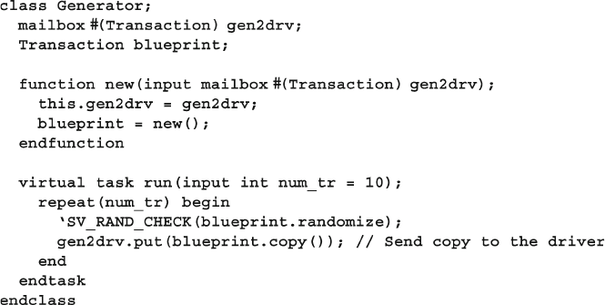
281
8.2 Blueprint Pattern
and used in another (the run task). Previous coding guidelines in this book said to
separate the declaration and construction; similarly, you need to separate the con-
struction and randomization of the blueprint object.
The copy method, which makes a duplicate of an object by copying its variables
into a new object, is discussed in Sections 5.15 and 8.5 . For now, remember that you
must add it to the Transaction and BadTr classes. Sample 8.34 on page 304
shows an advanced generator using templates.
This generator constructs a new transaction every time the blueprint is random-
ized. This coding style prevents the classic OOP mailbox bug, as the mailbox will
store handles to multiple unique objects, not that same single object.
Another advantage of randomizing the blueprint object over and over is that
randc variables work correctly. The bad generator in Sample 8.5 constructed new
objects every pass through the loop. Every object with a randc variable maintains
a history of previous values generated for the variable. Every time you construct a
new object, that history is lost, and the bad generator creates objects with separate
randc variables. In Sample 8.6 , only the blueprint object is randomized, so the
randc history is maintained.
Section 8.2.3 shows how to change the blueprint.
8.2.1 The Environment Class
Chapter 1 discussed the three phases of execution: Build, Run, and Wrap-up. Sample
8.7 shows the environment class that instantiates all the testbench components, and
runs these three phases. Also notice how the mailbox gen2drv carries transactions
from the generator to the driver, and so is passed into the constructor for each.
Sample 8.6 Generator class using blueprint pattern
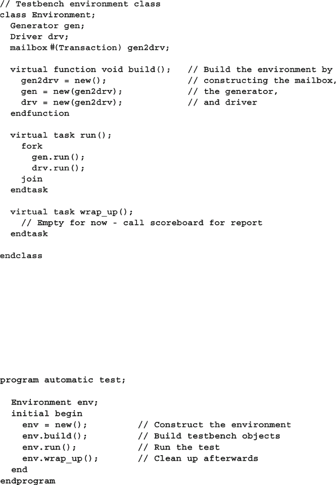
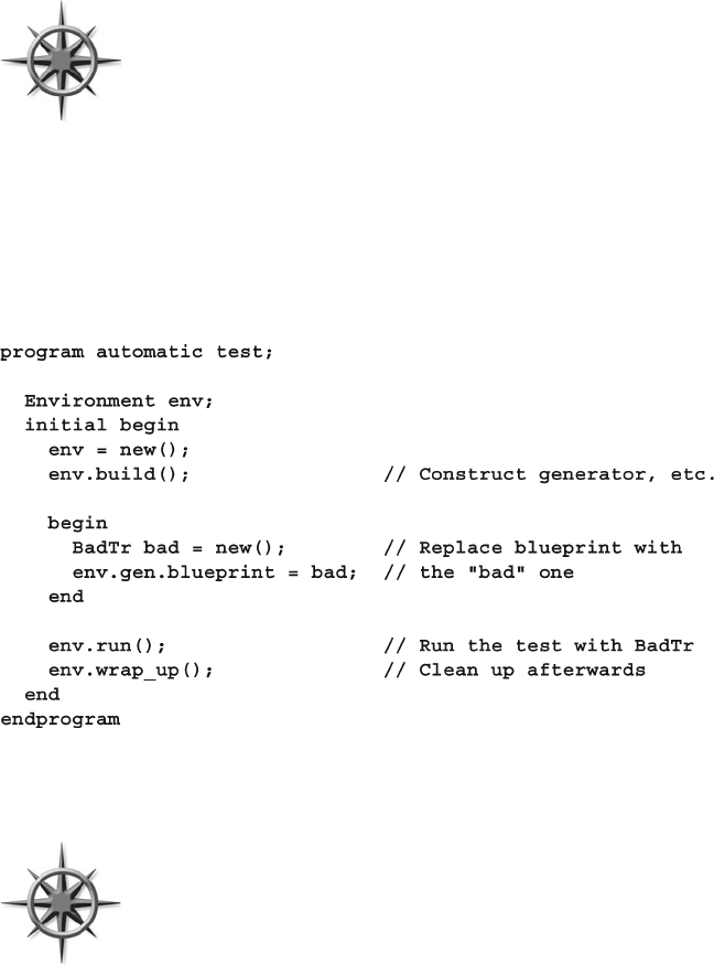
283
8.2 Blueprint Pattern
8.2.3 Using the Extended Transaction Class
To inject an error, you need to change the blueprint object from a
Transaction object to a BadTr . You do this between the build
and run phases in the environment. The top-level testbench in
Sample 8.9 runs each phase of the environment and changes the
blueprint. Note how all the references to BadTr are in this one fi le,
so you don’t have to change the Environment or Generator
classes. You want to restrict the scope of where BadTr can be used, so a standalone
begin…end block is used in the middle of the initial block. This makes a visu-
ally distinctive block of code. You can take a shortcut and construct the extended
class in the declaration.
Sample 8.9 Injecting an extended transaction into testbench
8.2.4 Changing Random Constraints with an Extended Class
In Chapter 6 you learned how to generate constrained random data.
Most of your tests are going to need to further constrain the data,
which is best done with inheritance. In Sample 8.10 , the original
Transaction class is extended to include a new constraint that keeps
the destination address in the range of +/−100 of the source address.
Sample 8.10 replaces the generator’s blueprint with an extended object that has an
additional constraint. As you will learn later in this chapter, the Nearby class should
have a copy method, but hold on for a few sections.
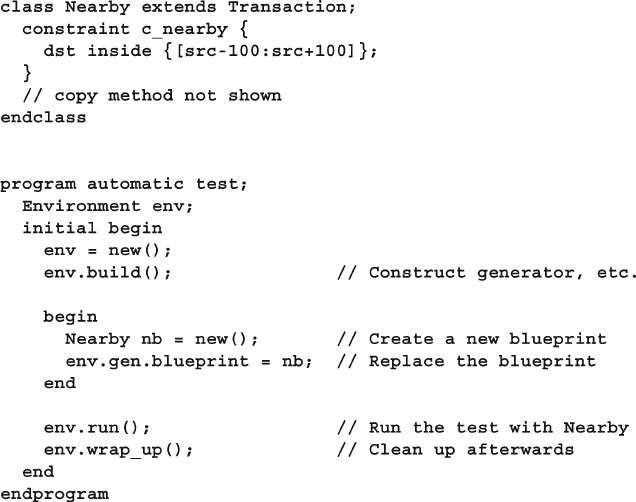
284 8 Advanced OOP and Testbench Guidelines
Note that if you defi ne a constraint in an extended class with the same name as
one in the base class, the extended constraint replaces the base one. This allows you
to change the behavior of existing constraints.
8.3 Downcasting and Virtual Methods
As you start to use inheritance to extend the functionality of classes, you need a few
OOP techniques to control the objects and their functionality. In particular, a handle
can refer to an object for a certain class, or any extended class. So what happens
when a base handle points to an extended object? What happens when you call a
method that exists in both the base and extended classes? This section explains what
happens using several examples.
8.3.1 Downcasting with $cast
Downcasting or conversion is the act of casting a base class handle to point to an
object that is a class extended from that base type. Consider the base and extended
classes in Sample 8.11 and Fig. 8.6 .
Sample 8.10 Adding a constraint with inheritance
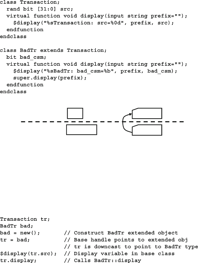
285
8.3 Downcasting and Virtual Methods
You can assign an extended handle to a base handle, and no special code is
needed, as shown in Sample 8.12 . When a class is extended, all the base class vari-
ables and methods are included, so src is in the extended object. The assignment to
tr is permitted, as any reference using the base handle tr is valid, such as tr.src
and tr.display .
Sample 8.11 Base and extended class
src
Transaction
bad_csm
BadTr display()
display()
Fig. 8.6 Simplifi ed extended transaction
Sample 8.12 Copying extended handle to base handle
What if you try going in the opposite direction, copying a handle to a base object
into an extended handle, as shown in Sample 8.13 ? This fails because the base
object is missing properties that only exist in the extended class, such as bad_csm .
The SystemVerilog compiler does a static check of the handle types and will not
compile the second line.
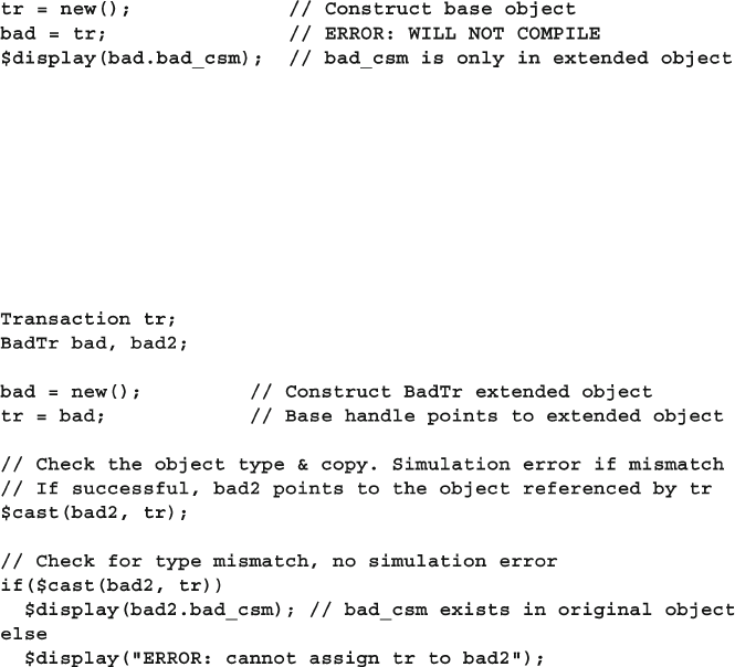
286 8 Advanced OOP and Testbench Guidelines
It is not always illegal to assign a base handle to an extended handle, but you
must always use $cast . The assignment is allowed when the base handle points to
an extended object. The $cast method checks the type of object referenced by the
handles, not just the handle. If the source object is the same type as the destination,
or a class extended from the destination’s class, you can copy the address of the
extended object from the base handle, tr , into the extended handle, bad2 .
Sample 8.13 Copying a base handle to an extended handle
Sample 8.14 Using $cast to copy handles
When you use $cast as a task, SystemVerilog checks the type of the source
object at run time and gives an error if it is not compatible with the destination.
When you use $cast as a function, SystemVerilog still checks the type, but no
longer prints an error if there is a mismatch. The $cast function returns zero when
the types are incompatible, and one for compatible types.
As an alternative to the if statement in Sample 8.14 , you could use something
like the SV_RAND_CHECK macro from Section 6.3.2. You should not use an immedi-
ate assert statement as the assertion expression is not evaluated if you disable
assertions, which means the $cast and bad2 assignment will never execute.
8.3.2 Virtual Methods
By now you should be comfortable using handles with extended classes. What hap-
pens if you try to call a method using one of these handles? Sample 8.15 and 8.16
show base and extended classes and code that calls methods inside these classes.
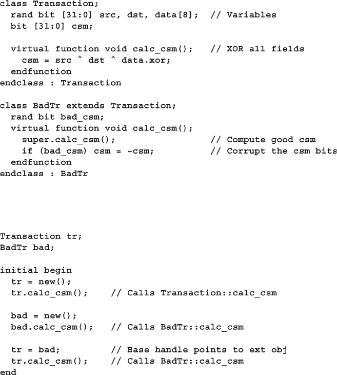
287
8.3 Downcasting and Virtual Methods
Sample 8.16 contains a block of code that uses handles of different types.
Sample 8.15 Transaction and BadTr classes
Sample 8.16 Calling class methods
To decide which virtual method to call, SystemVerilog uses the object’s type, not
the handle’s type. In the last statement of Sample 8.16 , tr points to an extended
object ( BadTr ) and so BadTr::calc_csm is called.
If you leave out the virtual modifi er on Transaction::calc_csm ,
SystemVerilog checks the type of the handle
tr (Transaction) , not the object.
That last statement in Sample 8.16 calls Transaction::calc_csm – probably not
what you wanted.
The OOP term for multiple methods sharing a common name is “polymorphism.”
It solves a problem similar to what computer architects faced when trying to make
a processor that could address a large address space but had only a small amount of
physical memory. They created the concept of virtual memory, where the code and
288 8 Advanced OOP and Testbench Guidelines
data for a program could reside in memory or on a disk. At compile time, the program
didn’t know where its parts resided — that was all taken care of by the hardware
plus operating system at run time. A virtual address could be mapped to some RAM
chips, or the swap fi le on the disk. Programmers no longer needed to worry about
this virtual memory mapping when they wrote code — they just knew that the
processor would fi nd the code and data at run time. See also Denning (2005).
8.3.3 Signatures and Polymorphism
There is a downside to using virtual methods: once you defi ne one, all extended
classes that defi ne the same method must use the same “signature,” i.e., the same
number and type of arguments, plus return value, if any. You cannot add or remove
an argument in an extended virtual method. This means you need to plan ahead.
There is a good reason that SystemVerilog and other OOP languages require that
a virtual method must have the same signature as the one in the parent (or grandpar-
ent). If you were able to add an additional argument, or turn a task into a function,
polymorphism would no longer work. Your code needs to be able to call a virtual
method with the assurance that a method in a extended class will have the same
interface.
8.3.4 Constructors are Never Virtual
When you call a virtual method, SystemVerilog checks the type of the object to
decide if it should call the method in the base class or the extended. Now you can
see why a constructor can not be virtual. When you call it, there is no object whose
type can be checked. The object only exists after the constructor call starts.
8.4 Composition, Inheritance, and Alternatives
As you build up your testbench, you have to decide how to group related variables
and methods together into classes. In Chapter 5 you learned how to build basic
classes and include one class inside another. Previously in this chapter, you saw the
basics of inheritance. This section shows you how to decide between the two styles,
and also shows an alternative.
8.4.1 Deciding Between Composition and Inheritance
How should you tie together two related classes? Composition uses a “has-a” rela-
tionship. A packet has a header and a body. Inheritance uses an “is-a” relationship.

289
8.4 Composition, Inheritance, and Alternatives
A BadTr is a Transaction , just with more information. Table 8.1 is a quick guide,
with more detail below.
Table 8.1 Comparing inheritance to composition
Question
Inheritance
(is-a relationship)
Composition
(has-a relationship)
1. Do you need to group multiple extended classes
together? (SystemVerilog does not support
multiple inheritance)
No Yes
2. Does the higher-level class represent objects at a
similar level of abstraction?
Yes No
3. Is the lower-level information always present or
required?
Yes No
4. Does the additional data need to remain attached
to the original class while it is being processed
by pre-existing code?
Yes No
1. Are there several small classes that you want to combine into a larger class? For
example, you may have a data class and header class and now want to make a
packet class. SystemVerilog does not support multiple inheritance, where one
class extends from several classes at once. Instead you have to use composition.
Alternatively, you could extend one of the classes to be the new class, and manu-
ally add the information from the others.
2. In Sample 8.15 , the Transaction and BadTr classes are both bus transactions
created in a generator and driven into the DUT, so inheritance makes sense.
3. The lower-level information such as src, dst , and data must always be present
for the Driver to send a transaction.
4. In Sample 8.15 , the new BadTr class has a new fi eld bad_csm and the extended
calc_csm function. The Generator class just transmits a transaction and does
not care about the additional information. If you use composition to create the
error bus transaction, the Generator class would have to be rewritten to handle
the new type.
If two objects seem to be related by both “is-a” and “has-a,” you may need to
break them down into smaller components.
8.4.2 Problems with Composition
The classical OOP approach to building a class hierarchy partitions functionality
into small blocks that are easy to understand. However, testbenches are not standard
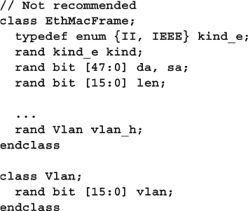
290 8 Advanced OOP and Testbench Guidelines
software development projects, as was discussed in Section 5.16 on public vs. local
attributes. Concepts such as information hiding (using local variables) confl ict with
building a testbench that needs maximum visibility and controllability. Similarly,
dividing a transaction into smaller pieces may cause more problems than it solves.
When you are creating a class to represent a transaction, you may want to parti-
tion it to keep the code more manageable. For example, you may have an Ethernet
MAC frame and your testbench uses two fl avors, normal (II) and Virtual LAN
(VLAN). Using composition, you could create a basic cell EthMacFrame with all the
common fi elds such as da and sa and a discriminant variable, kind , to indicate the
type as shown in Sample 8.17 . There is a second class to hold the VLAN informa-
tion, which is included in EthMacFrame .
Sample 8.17 Building an Ethernet frame with composition
There are several problems with composition. First, it adds an extra layer of
hierarchy, so you are constantly having to add an extra name to every reference. The
VLAN information is called eth_h.vlan_h.vlan . If you start adding more lay-
ers, the hierarchical names become a burden.
A more subtle issue occurs when you want to instantiate and randomize
the hierarchy of classes. What does the EthMacFrame constructor create? Since
kind is random, you don’t know whether to construct a Vlan object when new
is called. When you randomize the class, the constraints set variables in both the
EthMacFrame and Vlan objects based on the random kind fi eld. You have a cir-
cular dependency in that randomization only works on objects that have been
instantiated, but you can’t instantiate these objects until kind has been chosen.
The only solution to the construction and randomization problems is to always
instantiate all objects in EthMacFrame::new . However, if you are always using all
alternatives, why divide the Ethernet cell into two different classes?
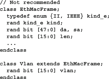
291
8.4 Composition, Inheritance, and Alternatives
8.4.3 Problems with Inheritance
Inheritance can solve some of these issues. Variables in the extended classes can be
referenced without the extra hierarchy as in
eth_h.vlan . You don’t need a dis-
criminant, but you may fi nd it easier to have one variable to test rather than doing
type-checking as shown in Sample 8.18 .
Sample 8.18 Building an Ethernet frame with inheritance
On the downside, a set of classes that use inheritance always requires more effort
to design, build, and debug than a set of classes without inheritance. Your code must
use $cast whenever you have an assignment from a base handle to an extended
handle. Building a set of virtual methods can be challenging, as they all have to have
the same signature. If you need an extra argument, you need to go back and edit the
entire set, and possibly the method calls too.
There are also problems with randomization. How do you make a constraint that
randomly chooses between the two kinds of frame and sets the proper variables?
You can’t put a constraint in EthMacFrame that references the vlan fi eld.
The fi nal issue is with multiple inheritance. In Fig. 8.7 , you can see how the
VLAN frame is extended from a normal MAC frame. The problem is that these dif-
ferent standards reconverged. SystemVerilog does not support multiple inheritance,
so you could not create the VLAN / Snap / Control frame through inheritance.
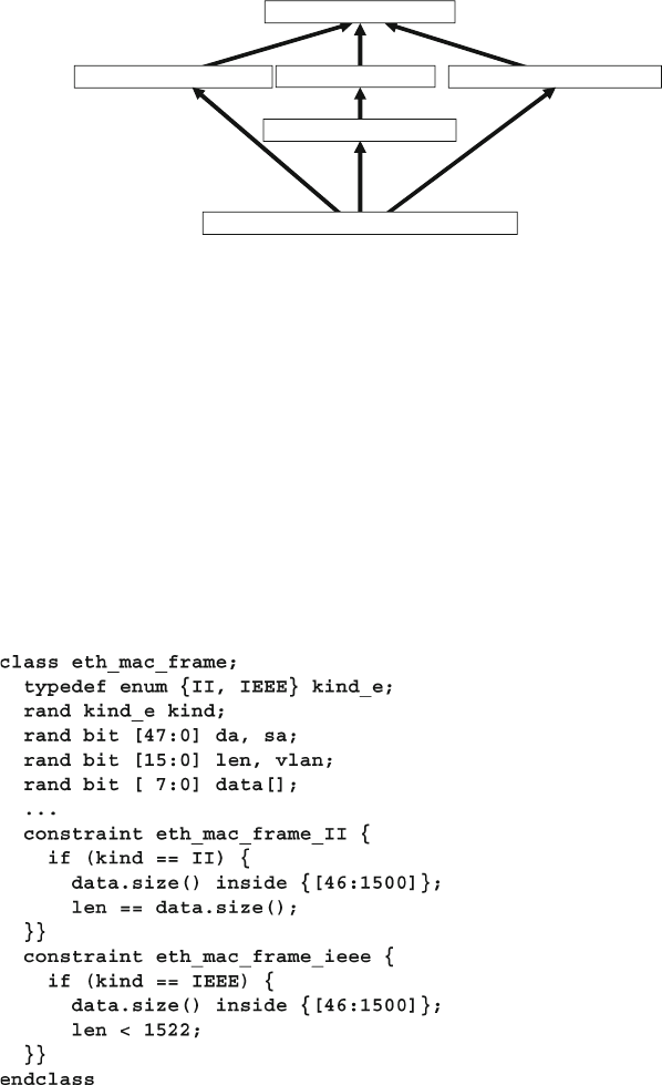
292 8 Advanced OOP and Testbench Guidelines
8.4.4 A Real-World Alternative
If composition leads to large hierarchies, but inheritance requires extra code and
planning to deal with all the different classes, and both have diffi cult construction
and randomization, what can you do? You can instead make a single, fl at class that
has all the variables and methods. This approach leads to a very large class, but it
handles all the variants cleanly. You have to use the discriminant variable often to
tell which variables are valid, as shown in Sample 8.19 . It contains several condi-
tional constraints, which apply in different cases, depending on the value of kind .
Ethernet MAC Frame
Ethernet II Frame
Ethernet VLAN Frame Ethernet Control Frame
Ethernet Snap Frame
Ethernet VLAN Snap Control Frame
Fig. 8.7 Multiple inheritance problem
Sample 8.19 Building a fl at Ethernet frame
Regardless of how you build your classes, defi ne the typical behavior and con-
straints in the class, and then use inheritance to inject new behavior at the test level.
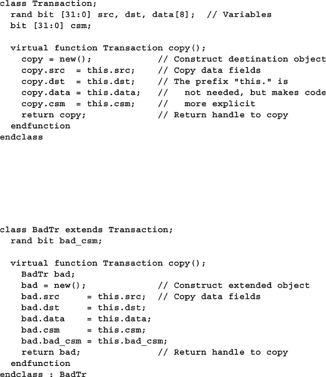
293
8.5 Copying an Object
8.5 Copying an Object
In Sample 8.6 , the generator fi rst randomized, and then copied the blueprint to make
a new transaction. Take a closer look at the
copy function in Sample 8.20 . Also see
Section 5.15 for more examples of copy functions.
Sample 8.20 Base transaction class with a virtual copy function
When you extend the Transaction class to make the class BadTr , the copy
function still has to return a Transaction object. This is because the extended
virtual function must match the base Transaction::copy , including all argu-
ments and return type, as shown in Sample 8.21
Sample 8.21 Extended transaction class with virtual copy method
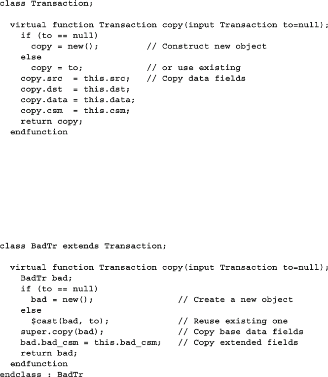
294 8 Advanced OOP and Testbench Guidelines
8.5.1 Specifying a Destination for Copy
The previous copy methods always constructed a new object. An improvement for
copy is to specify the location where the copy should be put. This technique is useful
when you want to reuse an existing object, and not allocate a new one.
Sample 8.22 Base transaction class with copy function
The only difference is the additional argument to specify the destination, and the
code to test that a destination object was passed to this method. If nothing was
passed (the default), construct a new object, or else use the existing one.
Since you have added a new argument to a virtual method in the base class, you
will have to add it to the same method in the extended classes, such as BadTr .
Sample 8.23 Extended transaction class with new copy function
Notice how BadTr::copy only needs to copy the fi elds in the extended class
and can use the base class method, Transaction::copy to copy its own fi elds.
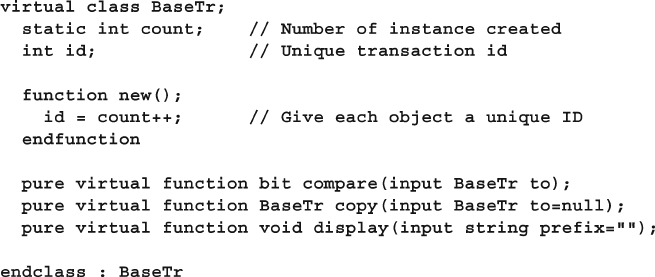
295
8.6 Abstract Classes and Pure Virtual Methods
8.6 Abstract Classes and Pure Virtual Methods
By now you have seen classes with methods to perform common operations such as
copying and displaying. One goal of verifi cation is to create code that can be shared
across multiple projects. If your company standardizes on a common set of classes
and methods, it is easier to reuse code between projects.
OOP languages such as SystemVerilog have two constructs to allow you to build
a shareable base class. The fi rst is an abstract class, which is a class that can be
extended, but not instantiated directly. It is defi ned with the
virtual keyword. The
second is a pure virtual method, which is a prototype without a body. A class
extended from an abstract class can only be instantiated if all pure virtual methods
have bodies. The pure keyword specifi es that a method declaration is a prototype,
and not just an empty virtual method. A pure method has no endfunction or end-
task . Lastly, pure virtual methods can only be declared in an abstract class. An
abstract class can contain pure virtual methods, virtual methods with and without a
body, and non-virtual methods. Note that if you defi ne a virtual method without a
body, i.e. no code inside, you can call it but it just immediately returns.
Sample 8.24 shows an abstract class, BaseTr , which is a base class for transac-
tions. It starts with a some useful properties such as id and count . The constructor
makes sure every instance has a unique ID. Next are pure virtual methods to com-
pare, copy, and display the object.
Sample 8.24 Abstract class with pure virtual methods
You can declare handles of type BaseTr , but you cannot construct objects of this
type. You need to extend the class and provide implementations for all the pure
virtual methods.
296 8 Advanced OOP and Testbench Guidelines
Sample 8.25 shows the defi nition of the Transaction class, which has been
extended from
BaseTr . Since Transaction has bodies for all the pure virtual
methods extended from
BaseTr , you can construct objects of this type in your
testbench.
Sample 8.25 Transaction class extends abstract class
Abstract classes and pure virtual methods let you build testbenches that have a
common look and feel. This allows any engineer to read your code and quickly
understand the structure.

297
8.7 Callbacks
8.7 Callbacks
One of the main guidelines of this book is to create a single verifi cation environ-
ment that you can use for all tests with no changes. The key requirement is that this
testbench must provide a “hook” where the test program can inject new code with-
out modifying the original classes. Your driver may want to do the following.
Inject errors •
Drop the transaction •
Delay the transaction •
Synchronize this transaction with others •
Put the transaction in the scoreboard •
Gather functional coverage data •
Rather than try to anticipate every possible error, delay, or disturbance in the fl ow
of transactions, the driver just needs to “call back” a method that is defi ned in the
top-level test. The beauty of this technique is that the callback method can be defi ned
differently in every test. As a result, the test can add new functionality to the driver
using callbacks, without editing the
Driver class. For some drastic behaviors such
as dropping a transaction, you need to code this in the class ahead of time, but this is
a known pattern. The reason why the transaction is dropped is left to the callback.
task Driver::run;
forever begin
...
<pre_callback>
transmit(tr);
<post_callback>
...
end
endtask
task pre_callback;
...
endtask
task post_callback;
...
endtask
Fig. 8.8 Callback fl o w
In Fig. 8.8 , the Driver::run task loops forever with a call to a transmit task.
Before sending the transaction, run calls the pre-transmit callback, if any. After
sending the transaction, it calls the post-callback task, if any. By default, there are
no callbacks, so run just calls transmit .
You could make Driver::run a virtual method and then override its behavior
in an extended class, perhaps MyDriver::run . The drawback to this is that you
might have to duplicate all the original method’s code in the new method if you are
298 8 Advanced OOP and Testbench Guidelines
injecting new behavior. Now if you made a change in the base class, you would
have to remember to propagate it to all the extended classes. Additionally, you can
inject a callback without modifying the code that constructed the original object.
8.7.1 Creating a Callback
A callback task is created in the top-level test and called from the driver, the lowest
level of the environment. However, the driver does not have to have any knowledge
of the test – it just has to use a generic class that the test can extend. The driver in
Sample 8.27 uses a queue to hold the callback objects, which allows you to add
multiple objects. The base callback class in Sample 8.26 is an abstract class that
must be extended before being used. Your callback is a task so it can have delays.
Sample 8.26 Base callback class
Sample 8.27 Driver class with callbacks
299
8.7 Callbacks
Note that while Driver_cbs is an abstract class, pre_tx and post_tx are not
pure virtual methods. This is because a typical callback uses only one of them. If a
class has even one pure virtual method without an implementation, OOP rules won’t
allow you to instantiate it.
Callbacks are part of both VMM and UVM. This callback technique is not related
to Verilog PLI callbacks or SVA callbacks.
8.7.2 Using a Callback to Inject Disturbances
A common use for a callback is to inject some disturbance such as causing an error
or delay. The testbench in Sample 8.28 randomly drops packets using a callback
object. Callbacks can also be used to send data to the scoreboard or to gather func-
tional coverage values. Note that you can put callback objects in the queue with the
push_back() or push_front() depending on the order in which you want these
to be called. For example, you probably want the scoreboard called after any tasks
that may delay, corrupt, or drop a transaction. You should only gather coverage after
a transaction has been successfully transmitted.
Sample 8.28 Test using a callback for error injection
300 8 Advanced OOP and Testbench Guidelines
8.7.3 A Quick Introduction to Scoreboards
The design of your scoreboard depends on the design under test. A DUT that processes
atomic transactions such as packets may have a scoreboard that contains a trans-
form function to turn the input transactions into expected values, a memory to hold
these values, and a compare method. A processor design needs a reference model to
predict the expected output, and the comparison between expected and actual values
may happen at the end of simulation.
Sample 8.29 shows a simple scoreboard that stores transactions in a queue of
expected values. The fi rst method saves an expected transaction, and the second
tries to fi nd an expected transaction that matches an actual one that was received by
the testbench. Note that when you search through a queue, you can get 0 matches
(transaction not found), 1 match (ideal case) or multiple matches (you need to do a
more sophisticated match).
Sample 8.29 Simple scoreboard for atomic transactions
8.7.4 Connecting to the Scoreboard with a Callback
The testbench in Sample 8.30 creates its own extension of the driver’s callback class
and adds a reference to the driver’s callback queue. Note that the scoreboard call-
back needs a handle to the scoreboard so it can call the method to save the expected
transaction. This example does not show the monitor side, which will need its own
callback to send the actual transaction to the scoreboard for comparison.
301
8.7 Callbacks
The VMM recommends that you use callbacks for scoreboards and functional
coverage. The monitor transactor can use a callback to compare received transac-
tions with expected ones. The monitor callback is also the perfect place to gather
functional coverage on transactions that are actually sent by the DUT.
You may have thought of putting the scoreboard or functional coverage group in
a transactor, and connect it to the testbench using a mailbox. This is a poor solution
for several reasons. These testbench components are almost always passive and
asynchronous, so they only wake up when the testbench has data for them, plus they
never pass information to a downstream transactor. Thus a transactor that has to
monitor multiple mailboxes concurrently is an overly complex solution. Additionally,
you may sample data from several points in your testbench, but a transactor is
designed for a single source. Instead, put methods in your scoreboard and coverage
classes to gather data, and connect them to the testbench with callbacks.
Sample 8.30 Test using callback for scoreboard
302 8 Advanced OOP and Testbench Guidelines
The UVM recommends a TLM analysis port for connecting monitors / drivers to
scoreboards and functional coverage. A description of this construct is beyond the
scope of this book, but you can think of it as a mailbox with an optional consumer.
8.7.5 Using a Callback to Debug a Transactor
If a transactor with callbacks is not working as expected, you can add a debug call-
back. You can start by adding a callback to display the transaction. If there are mul-
tiple instances of the transactor, create a unique identifi er for each. Put debug code
before and after the other callbacks to locate the one that is causing the problem.
Even for debug, you want to avoid making changes to the testbench environment.
8.8 Parameterized Classes
As you become more comfortable with classes, you may notice that a class, such as
a stack or generator, only works on a single data type. This section shows how you
can defi ne a single parameterized class that works with multiple data types.
8.8.1 A Simple Stack
A common data structure is a stack, which has push and pop methods to store and
retrieve data. Sample 8.31 shows a simple stack that works with the int data type.
Sample 8.31 Stack using the int type
303
8.8 Parameterized Classes
The problem with this class is that it only works with integers. If you want to
make a stack for real numbers, you would have to copy the class, and change the
data type from int to real . This quickly leads to a proliferation of classes, which
can become a maintenance problem if you ever want to add new operations such as
traversing or printing the stack contents.
In SystemVerilog you can add a data type parameter to a class and then specify a
type when you declare handles to that class. This is similar to, but more powerful
than, a parameterized module, where you can specify a value such as bus width
when it is instantiated. SystemVerilog’s parameterized classes are similar to tem-
plates in C++.
Sample 8.32 is a parameterized class for a stack. Notice how the type T is defi ned
on the fi rst line with a default type of int .
Sample 8.32 Parameterized class for a stack
The step of specifying values to a parameterized class is called specialization.
Sample 8.33 declares a handle to the stack class with a real data type.
Sample 8.33 Creating the parameterized stack class
Generators are a great example of a class that can be parameterized. Once you
have defi ned the class for one, the same structure works for any data type. Sample
8.34 takes the atomic generator from Sample 8.6 and adds a parameter so you can
304 8 Advanced OOP and Testbench Guidelines
generate any random object. The generator should be part of a package of verifi cation
classes. It needs to specify a the default type, so it uses BaseTr from Sample 8.24
as this abstract class should also be part of the verifi cation package.
Sample 8.34 Parameterized generator class using blueprint pattern
Using the Transaction class from Sample 8.25 and the generator in Sample 8.34 ,
you can build a simple testbench like in Sample 8.35 . It starts the generator and prints
the fi rst fi ve transactions, using the mailbox synchronization shown in Sample 7.40.
Sample 8.35 Simple testbench using parameterized generator class
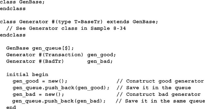
305
8.8 Parameterized Classes
8.8.2 Sharing Parameterized Classes
When you specialize a parameterized class, as in the real stack in Sample 8.33 , you
are creating a new data type, with no OOP relationship to any other specialization. For
example, you can not use
$cast() to convert between a stack of real variables and
one of integers. For that, you need a common base class as shown in Sample 8.36 .
Sample 8.36 Common base class for parameterized generator class
Upcoming sections show more examples of parameterized classes.
8.8.3 Parameterized Class Suggestions
When creating parameterized classes, you should start with a non-parameterized
class, debug it thoroughly, and then add parameters. This separation reduces your
debug effort.
A common set of virtual methods in your transaction class help you when creat-
ing parameterized classes. The Generator class uses the copy method, knowing
that it always has the same signature. Likewise, the display method allows you to
easily debug transactions as they fl ow through your testbench components.
The system functions $typename() and $bits() are helpful when your class
needs to know the name and width of the parameter. The $typename(T) function
returns the name of the parameter type such as int, real , or the class name for a
handle. The $bits() function returns the width of the parameter. For complex
types such as structures and arrays, it returns the number of bits required to hold an
expression as a bit stream. The UVM transaction print methods use this function to
get the fi elds to line up correctly.
Macros are an alternative to parameterized classes. For example, you could defi ne
a macro for the generator and pass it the transaction data type. Macros are harder to
debug than parameterized classes, unless your compiler outputs the expanded code.
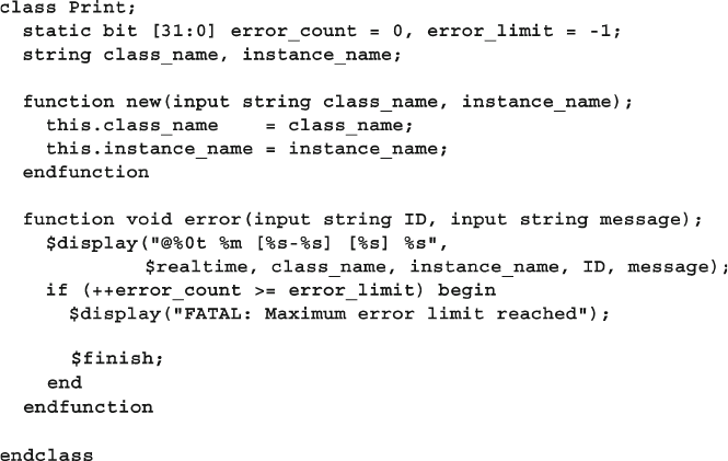
306 8 Advanced OOP and Testbench Guidelines
If you need to defi ne several related classes that all share the same transaction
type, you could use parameterized classes or a single large macro. In the end, how
you defi ne your classes is not as important as what goes into them.
8.9 Static and Singleton Classes
This section and the next show advanced OOP concepts that are used extensively in
the UVM and VMM. You could try to understand UVM’s factory mechanism by
reading the source code with its many methods, but this section should save you
several days of experimentation with a greatly simplifi ed example. This chapter
shows several alternatives so you can understand why the UVM did not pick a more
simple alternative.
One of the goals of OOP is to eliminate global variables and methods as the
resulting code is hard to maintain and reuse. Their names exist in the global name
space, potentially causing name space collisions. Does packet_count refer to
TCP/IP packets or some other protocol? Instead, put a variable called count in the
Packet class to avoid any ambiguity.
8.9.1 Dynamic Class to Print Messages
Sometimes, however, you really need globals. For example, all verifi cation method-
ologies provide a print service so you can fi lter messages and count errors. If you try
to build such a class with what you have learned so far, it might look something like
Sample 8.37 .
Sample 8.37 Dynamic print class with static variables
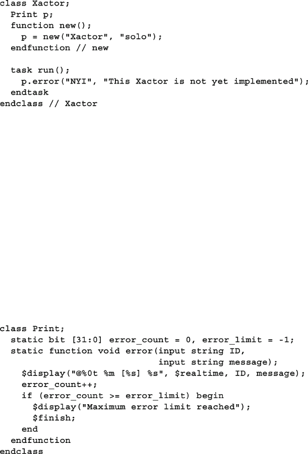
307
8.9 Static and Singleton Classes
This is a greatly simplifi ed version of the VMM log class. The VMM code allows
you to fi lter messages by the class and instance names, and many other features.
Sample 8.38 has a class that prints an error message with the Print class from
Sample
8.37 .
Sample 8.38 Transactor class with dynamic print object
The biggest limitation for the Print class is that every component in your test-
bench needs to instantiate it. The simple Print class above has a small footprint,
but a realistic one, like VMM’s, could have many strings and arrays, consuming a
signifi cant amount of memory. This overhead, when added to a transactor class
might not be signifi cant, but could overwhelm a small transaction class, such as an
ATM cell, which only has 53 bytes.
8.9.2 Singleton Class to Print Messages
An alternative to constructing all these print objects is to not construct any. As you
saw in section 5.11.4, you could declare the methods in the Print class to be static.
These methods can only reference static variables, as shown in Sample 8.39 .
Sample 8.39 Static print class
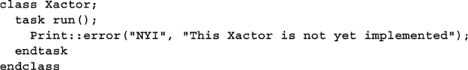
308 8 Advanced OOP and Testbench Guidelines
Now that the class is static, you can no longer have per-instance information such as
the parent class’s name and instance. Any fi ltering has to be based on other criteria.
Sample 8.40 Transactor class with static print class
Sample 8.40 shows the call to the error() method using the Print class name.
This style of class is known as a singleton class, as there is only one copy, the one
allocated at elaboration time with the static variables.
As your static classes, such as the one in Sample 8.39 , grow larger, you have to
label everything with the static keyword, a small annoyance. Next, the class is
allocated before simulation time, even if you never use it. Additionally, there is no
handle to this class, so you can not pass it around your testbench. The alternative to
a static class is a singleton class (or singleton pattern) with a single instance, which
is a non-static class that is only constructed once. They are more diffi cult to create
initially, but they can simplify your program’s architecture. Many of the UVM’s
classes are singletons.
The singleton pattern is implemented by creating a class with a method that cre-
ates a new instance of the class if one does not exist. If an instance already exists, it
simply returns a handle to that object. To make sure that the object cannot be instan-
tiated any other way, you must make the constructor protected . Don’t make it
local , because an extended class might need to access the constructor.
8.9.3 Confi guration Database with Static Parameterized Class
Another good use for static classes in verifi cation is a database of confi guration
parameters. At the start of simulation you randomize the confi guration of your sys-
tem. In a small system, you can simply store these in a single class or hierarchy of
classes and pass them around the testbench as needed. At some point though, this
becomes too complicated as handles are passed up and down the hierarchy. Instead,
create a global database of parameters, indexed by a name, that you can access any-
where in the testbench. UVM 1.0 introduced this concept, which is the basis for the
following set of examples. This code has a single string index into the database,
while a real database such as UVM’s could have a property name, instance name, and
other values. You could concatenate these to create a more complex index string.
One issue with a database is that you need to store values of different types, such
as bit vectors, integers, real numbers, enumerated values, string, class handles, virtual
interfaces, and more in a single database. While you could fi nd a few common types
such as bit vectors and a common base class, there are some type such as virtual
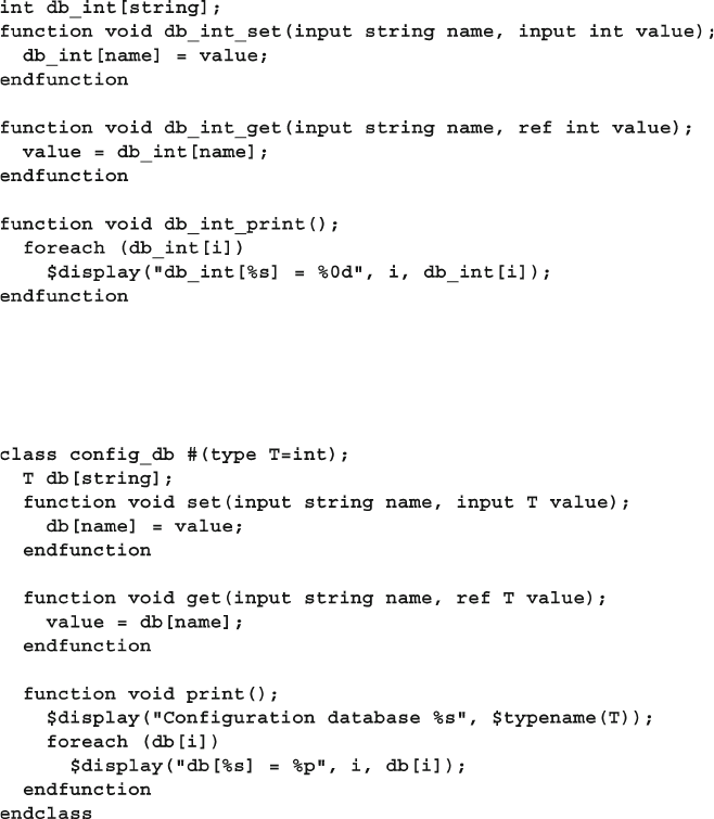
309
8.9 Static and Singleton Classes
interfaces that are unique, so there is no easy way to store them in a common database.
Earlier versions of OVM and UVM recommended creating a class wrapper around
virtual interfaces, but this required extra coding and was a common source of bugs.
What if you made a different database for each data type? You could use an asso-
ciative array indexed by the parameter name. A real database might also have an
instance name, but for this simple example, you can just concatenate all the names
together to make a single index. Sample
8.41 shows the code for an integer database
made from global methods.
Sample 8.41 Confi guration database with global methods
You can generalize this into a parameterized class with the concepts from Section
8.8 , as shown in Sample 8.42 .
Sample 8.42 Confi guration database with parameterized class
You can now construct objects for an integer database, a real database, etc. The
fi nal problem is that each instance of the database is local to the scope where this
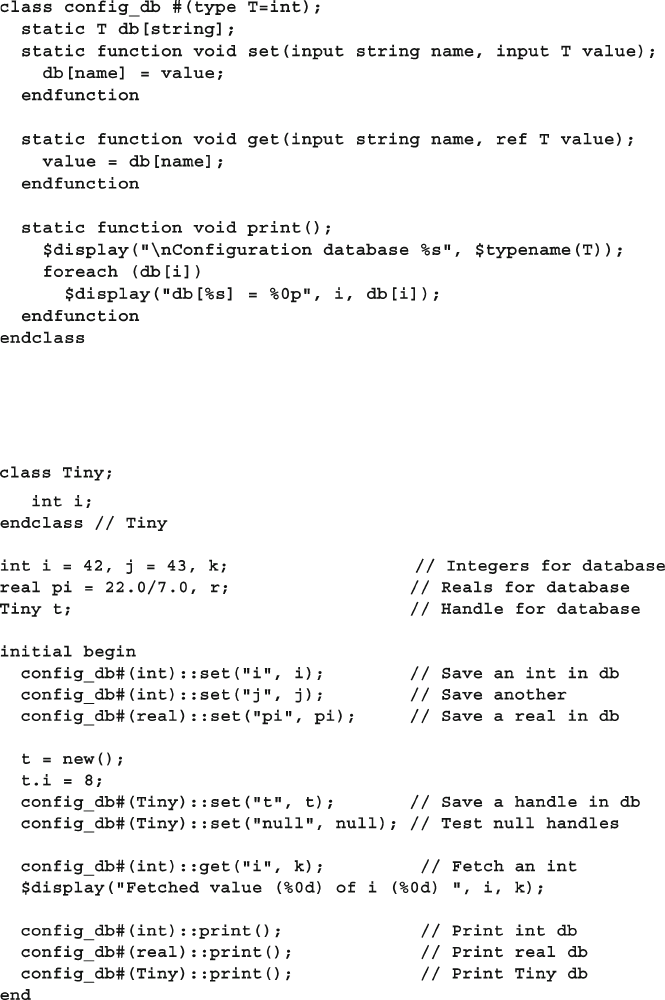
310 8 Advanced OOP and Testbench Guidelines
class is instantiated. The solution shown in Sample 8.43 is to go global and make
this a static class, that is a class with static properties and methods.
Sample 8.43 Confi guration database with static parameterized class
You can test the above code with Sample 8.44 and see how the parameterized
class creates a new database for each type.
Sample 8.44 Testbench for confi guration database
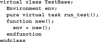
311
8.10 Creating a Test Registry
With singletons implemented as single instances instead of static class members,
you can initialize the singleton lazily, creating it only when it is needed.
The UVM database allows wildcards and other regular expressions, which
requires a more complex lookup scheme than associative arrays.
8.10 Creating a Test Registry
In a real design, compiling your test and DUT takes a signifi cant amount of time.
If you want to run 100 tests, each in a separate program block, you need to recom-
pile before each test, 100 times in all. This is a waste of CPU time as most of the
code has not changed. If you make 100 program blocks, each with a single test,
and connect all these programs in the model, you then need a way to disable all
but one program block. The best solution is to include all tests and testbenches
inside one program block, compile this once with the DUT. This section shows
how you can select one test per run with a Verilog command line switch.
8.10.1 Test registry with Static Methods
Earlier examples in this book have a program that contains one test. For this new
approach, each test is a separate class, all which are in a single program block, either
imported from a package or included at compile time. The test classes are con-
structed, registered in a test registry, and then, at run time, you can choose the
desired test at runtime. This follows an early VMM style.
First you need a base test class that your tests can extend from. Sample 8.45
shows an abstract class that contains a handle for the Environment class and a pure
virtual task that is a placeholder for the method that contains your test code.
Sample 8.45 Base test class
The core of the test registry class is an associative array of handles to all the tests,
indexed by the test name. The TestRegistry class, shown in Sample 8.46 , is a
static class with only static variables and methods, and is never constructed. The
get_test() method reads the Verilog command line argument to determine which
test to execute.
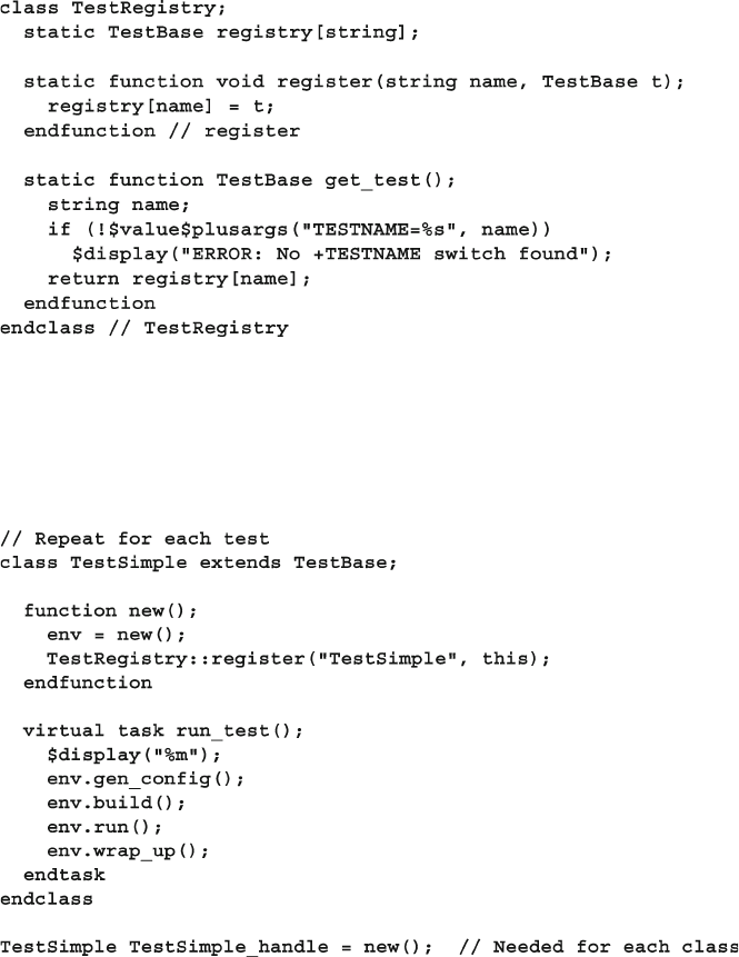
312 8 Advanced OOP and Testbench Guidelines
Sample 8.47 show how you can extend TestBase to create a simple test that
runs all the environment phases. The last line of the example is a declaration that
calls the constructor, which also registers the test. All the test objects are constructed,
but only one is run.
Sample 8.46 Test registry class
Sample 8.47 Simple test in a class
The program in Sample 8.48 now just asks the test registry for a test object and
runs it. The test classes can be declared in a package and imported, or declared
inside or outside the program block.
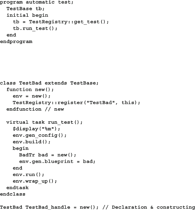
313
8.10 Creating a Test Registry
Sample 8.49 shows how you can create a test class that injects new behavior by
changing the generator’s blueprint to create bad transactions.
Sample 8.48 Program block for test classes
Sample 8.49 Test class that puts a bad transaction in the generator
This short example allows you to compile many tests into a single simulation
executable and choose your test at runtime, saving many recompiles. This pattern is
fi ne when you are starting out with a handful of tests, but the next section shows
more powerful approach.
8.10.2 Test Registry with a Proxy Class
The previous section’s test registry works well for smaller test environments, but
has several limitations for real projects. First, you need to remember to con-
struct every test class, otherwise the registry can not locate it. Second, every test
gets constructed at the start of simulation, even though only one is actually run.
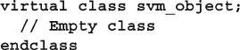
314 8 Advanced OOP and Testbench Guidelines
When verifying a large design, there could be hundreds of tests, so constructing all
of them wastes valuable simulation time and memory.
Consider this analogy. When you are looking to buy a car, you can go to a dealer
to see the choices. If there are only a few variants, white or black, with or without
sunroof, the dealer can stock one of each model with little overhead. This is what you
saw in the previous section, where the test registry had an object of each test type.
What if there are many different models, each in one of a dozen colors, with vari-
ants such as radios, sunroofs, air conditioning, sports packages, and engines? The
dealer could never have one of each type on his lot as there are hundreds of combi-
nations. Instead he would show you a catalog with all the choices. You pick the
options that you want, and the factory builds one to your specifi cation. Likewise, the
test registry can have a lot of small classes, each which knows how to build a com-
plete test. The small class has low overhead, so even a thousand objects would not
consume much memory. Now when you want to run test N, imagine fl ipping through
the catalog (test registry) until you fi nd a picture of your test, and you then tell the
factory to build an object of that type.
The test registry needs a table (analogous to the above catalog) that goes from
test names to objects. In section
8.10.1 , this table is an associative array of TestBase
handles, indexed by a string, shown in Sample 8.46 . What if instead, you had a
parameterized class whose only job is to construct a test? The UVM uses a design
pattern called a proxy class whose only role is to build the actual desired class. The
proxy class is lightweight in that it only contains a few properties and methods, and
thus consumes little memory or CPU time. It acts like the picture in the car dealer’s
catalog, holding a representation of what you can build.
The next few code samples show how the UVM class factory works. Because the
code in this book is a simplifi ed version of the real UVM classes, the name has been
changed to SVM, SystemVerilog Methodology, so that you won’t confuse it with
the real thing. Hopefully you will fi nd this explanation of a simple factory easier to
understand than trying to read the UVM source code.
First is Sample 8.50 which has the common base class from which everything
else is built. It is a abstract class because you should never construct an object of this
type, only classes extended from this one.
Sample 8.50 Common SVM base class
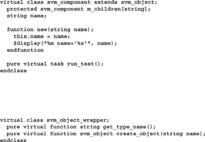
315
8.10 Creating a Test Registry
Now defi ne svm_object_wrapper , the abstract common base class for the
proxy class as shown in Sample 8.52 . It has pure virtual methods to return the name
of the class type, and create an object of this type.
Sample 8.51 Component class
Sample 8.52 Common base class for proxy class
Now for the crucial class, svm_component_registry shown in Sample 8.53 .
This is a lightweight class that can be constructed with little overhead. It is param-
eterized with the test class type and name. Once you have an instance of this class,
your testbench can construct the actual test class at any time, using the create_
object method. This is a singleton class as you only need one copy to create an
instance of the test class. At the start of simulation, the static handle me is initialized
by calling the get() method that constructs the fi rst instance if needed.
Next is the component class in Sample
8.51 . In the UVM, a component is a time-
consuming object that forms the testbench hierarchy, similar to a VMM transactor.
In this simplifi ed example, the hierarchical parent handle has been removed.
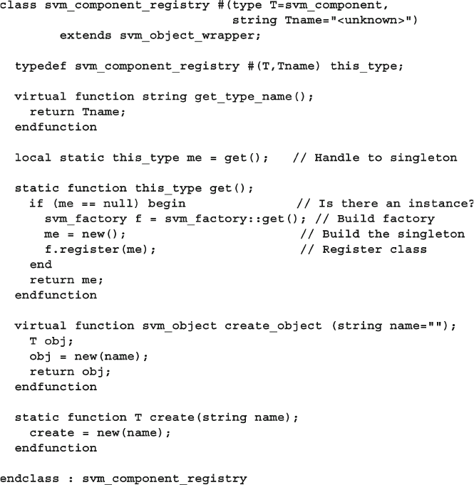
316 8 Advanced OOP and Testbench Guidelines
The last major class is svm_factory , which, at its core, is just a singleton class
that holds the array, m_type_names , to go from test case name to the proxy class
that creates an instance of the test class. Also in this class in Sample 8.54 is the
get_test method that reads the test name from the simulation run command line
and constructs an instance of the test class. Unlike Sample 8.46 , you even get a little
self checking.
Sample 8.53 Parameterized proxy class
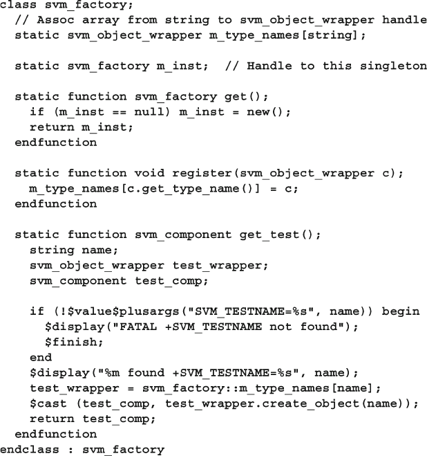
317
8.10 Creating a Test Registry
Lastly is a base test class, extended from svm_component shown in Sample 8.55 .
It uses the macro svm_component_utils to defi ne a new data type, type_id , that
points to the proxy class. The macro stringifi es the token T that holds the class name,
and turns it into a string containing the value of T with the syntax: `" T `".
Sample 8.54 Factory class
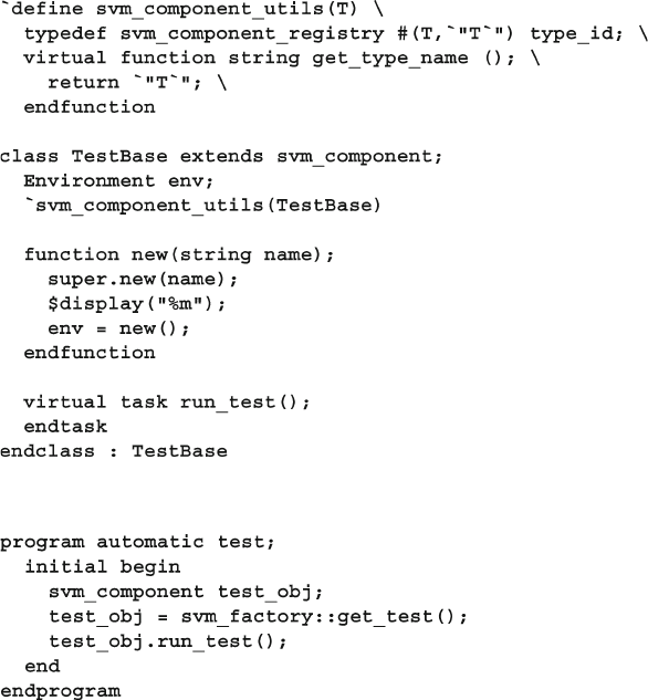
318 8 Advanced OOP and Testbench Guidelines
Sample 8.55 Base test class and registration macro
Here are the steps that happen when you start a simulation with the command line
switch +SVM_TESTNAME=TestBase .
With the macro • svm_component_utils , the class TestBase defi nes the type
type_id based on the class svm_component_registry , with the parameters
TestBase and " TestBase ". Because this is a new type, the simulator initial-
izes the static variable svm_component_registry::me by calling the get
method that instantiates the class. This instance is registered in the factory. What
does all this mean? There is now an object that can construct the TestBase
class, and you can get to it through the factory.
Simulation now starts and the factory’s • get_test method reads the test name
from the command line. This string is used an index into the registry to get a
handle to the proxy object. This object’s create_object method constructs an
instance of the TestBase object.
Sample 8.56 Test program

319
8.11 Conclusion
The program calls the test object’s • run_test method, which calls the steps for
the specifi c class. Now the TestBase class in Sample 8.55 does not do anything
interesting, but add a call to svm_component_utils macro to the test classes
in Sample
8.47 and Sample 8.49 and you can run tests.
Now you can see the basic UVM fl ow to start tests. The registry contains a list of
proxy classes that can construct test objects.
8.10.3 UVM Factory Build
The UVM factory can also construct objects for any class in the testbench with the
create method in Sample 8.53 . Sample 8.57 show how to build a driver.
Sample 8.57 UVM factory build example
The above code calls the static method create to construct an object of type
driver. In UVM, the second argument points to the parent of the component being
created.
The UVM factory allows you to override the component so that when you build
a component, you get an extended one instead.
You may have noticed a change in terminology. In classic OOP, you “construct”
a class by calling the new method, based on the handle type and assigning the
address to the handle on the left side of the assignment statement. With the UVM
factory pattern, you “build” an object by calling the static create method. This
could make an object of the same type as the handle, or an extended type.
8.11 Conclusion
The software concept of inheritance, where new functionality is added to an exist-
ing class, parallels the hardware practice of extending the design’s features for each
generation, while still maintaining backwards compatibility.
For example, you can upgrade your PC by adding a larger capacity disk. As long
as it uses the same interface as the old one, you do not have to replace any other part
of the system, yet the overall functionality is improved.
Likewise, you can create a new test by “upgrading” the existing driver class to
inject errors. If you use an existing callback in the driver, you do not have to change
any of the testbench infrastructure.
You need to plan ahead if you want use these OOP techniques. By using virtual
methods and providing suffi cient callback points, your test can modify the behavior
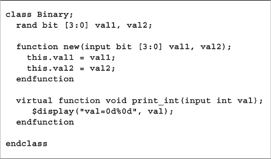
320 8 Advanced OOP and Testbench Guidelines
of the testbench without changing its code. The result is a robust testbench that does
not need to anticipate every type of disturbance (error-injection, delays, synchroni-
zation) that you may want as long as you leave a hook where the test can inject its
own behavior.
The testbench is more complex than what you have previously constructed, but
there is a payback in that the tests become smaller and easier to write. The testbench
does the hard work of sending stimulus and checking responses, so the test only has
to make small tweaks to cause specialized behavior. An extra few lines of testbench
code might replace code that would have to be repeated in every single test.
Lastly, OOP techniques improve your productivity by allowing you to reuse
classes. For example, a parameterized class for a stack that operates on any other
class, rather than a single type, saves you from having to create duplicate code.
8.12 Exercises
1. Given the following class, create a method in an extended class ExtBinary that
multiplies val1 and val2 and returns an integer.
2. Starting with the solution to Exercise 1, use the ExtBinary class to initialize
val1=15, val2=8 , and print out the multiplied value.
3. Starting with the solution to Exercise 1, create an extended class Exercise3
that constrains
val1 and val2 to be less than 10.
4. Starting with the solution to Exercise 3, use the Exercise3 class to randomize
val1 and val2 , and print out the multiplied value.
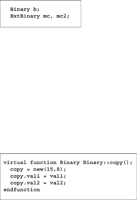
321
8.12 Exercises
5. Given the class in Exercise 1, and the following declarations, and an extended
class ExtBinary , what will handles mc, mc2 , and b point to after executing
each code snippet a-d, or will a compile error occur?
a . mc = new(15,8);
b = mc;
b . b = new(15, 8);
mc = b;
c . mc = new(15, 8);
b = mc;
mc2 = b;
d . mc = new(15, 8);
b = mc;
if($cast(mc2, b))
$display(“Success”);
else
$display(“Error: cannot assign”);
6. Given the classes Binary and Ext Binary in Exercise 1 and the following
copy function for class Binary , create the function Ext Binary::copy .
7. From the solution to Exercise 6, use the copy function to copy the object pointed
to by the extended class handle mc to the extended class handle mc2.
8. Using code Sample 8.26 to Sample 8.28 in Section 8.7.1 and 8.7.2 of the text,
add the ability to randomly delay a transaction between 0 and 100ns.
9. Create a class that can compare any data type using the case equality operators,
=== and !== . It contains a compare function that returns a 1 if the two values
match, 0 otherwise. By default it compares two 4-bit data types.
10. Using the solution from Exercise 9, use the comparator class to compare two
4-bit values, expected_4bit and actual_4bit . Next, compare two values
of type color_t, expected_color and actual_color . Increment an error
counter if an error occurs.
323
C. Spear and G. Tumbush, SystemVerilog for Verifi cation: A Guide to Learning
the Testbench Language Features, DOI 10.1007/978-1-4614-0715-7_9,
© Springer Science+Business Media, LLC 2012
As designs become more complex, the only effective way to verify them effectively
is with constrained-random testing (CRT). This approach elevates you above the
tedium of writing individual directed tests, one for each feature in the design.
However, if your testbench is taking a random walk through the space of all design
states, how do you know if you have reached your destination? Even directed tests
should be double checked with functional coverage. Over the life of a project, small
changes in the DUT’s timing or functionality can subtly alter the results from a
directed test, so it no longer verifi es the same features. Whether you are using ran-
dom or directed stimulus, you can gauge progress using coverage.
Functional coverage is a measure of which design features have been exercised by the
tests. Start with the design specifi cation and create a verifi cation plan with a detailed list
of what to test and how. For example, if your design connects to a bus, your tests need to
exercise all the possible interactions between the design and bus, including relevant
design states, delays, and error modes. The verifi cation plan is a map to show you where
to go. For more information on creating a verifi cation plan, see Bergeron (2006).
In many complex systems, you may never achieve 100% coverage as schedules
don’t allow you to reach every possible corner case. After all, you didn’t have time
to write directed tests to get suffi cient coverage, and even CRT is limited by the time
it takes you to create and debug test cases, and analyze the results.
Figure 9.1 shows the feedback loop to analyze the coverage results and decide on
which actions to take in order to converge on 100% coverage. Your fi rst choice is to
run existing tests with more seeds; the second is to build new constraints. Only
resort to creating directed tests if absolutely necessary.
Back when you exclusively wrote directed tests, the verifi cation planning was
limited. If the design specifi cation listed 100 features, all you had to do was write
100 tests. Coverage was implicit in the tests — the “register move” test moved all
combinations of registers back and forth. Measuring progress was easy: if you had
completed 50 tests, you were halfway done. This chapter uses “explicit” and
“implicit” to describe how coverage is specifi ed. Explicit coverage is described
Chapter 9
Functional Coverage
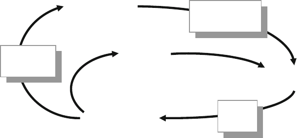
324 9 Functional Coverage
directly in the test environment using SystemVerilog features. Implicit coverage is
implied by a test — when the “register move” directed test passes, you have hopefully
covered all register transactions.
With CRT, you are freed from hand crafting every line of input stimulus, but now
you need to write code that tracks the effectiveness of the test with respect to the veri-
fi cation plan. You are still more productive, as you are working at a higher level of
abstraction. You have moved from tweaking individual bits to describing the interest-
ing design states. Reaching for 100% functional coverage forces you to think more
about what you want to observe and how you can direct the design into those states.
9.1 Gathering Coverage Data
You can run the same random testbench over and over, simply by changing the
random seed to generate new stimulus. Each individual simulation generates a data-
base of functional coverage information, the trail of footprints from the random
walk. You can then merge all this information together to measure your overall
progress using functional coverage as shown in Figure 9.2 .
You then analyze the coverage data to decide how to modify your tests. If the
coverage levels are steadily growing, you may just need to run existing tests with
new random seeds, or even just run longer tests. If the coverage growth has started
to slow, you can add additional constraints to generate more “interesting” stimuli.
When you reach a plateau, some parts of the design are not being exercised, so you
need to create more tests. Lastly, when your functional coverage values near 100%,
check the bug rate. If bugs are still being found, you may not be measuring true
coverage for some areas of your design. Don’t be in too big of a rush to reach 100%
coverage, which just shows that you looked for bugs in all the usual places. While
you are trying to verify your design, take many random walks through the stimulus
space; this can create many unanticipated combinations, as shown in van der Schoot
(2007).
Fig. 9.1 Coverage convergence
Constrained
random tests
Functional
Coverage
Many runs,
different seeds
Many runs,
different seeds
Identify
holes
Identify
holes
Add
constraints
Add
constraints
Minimal code
modifications
Directed
testcase
Many runs,
different seeds
Many runs,
different seeds
Identify
holes
Identify
holes
Add
constraints
Add
constraints
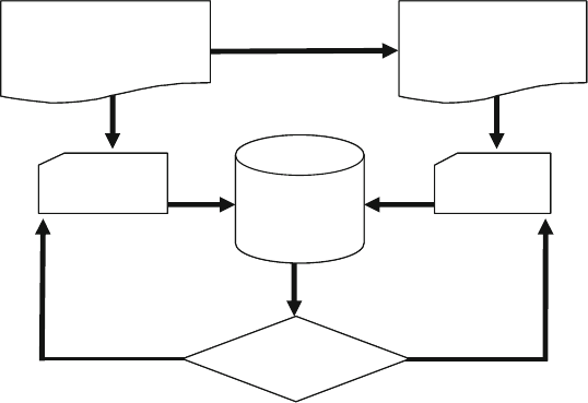
325
9.1 Gathering Coverage Data
Each simulation vendor has its own format for storing coverage data and as well
as its own analysis tools. You need to perform the following actions with those tools.
• Run a test with multiple seeds. For a given set of constraints and coverage
groups, compile the testbench and design into a single executable. Now you need
to run this constraint set over and over with different random seeds. You can use
the Unix system clock as a seed, but be careful, as your batch system may start
multiple jobs simultaneously. These jobs may run on different servers or may
start on a single server with multiple processors. So combine all these values to
make a truly unique seeds. The seed must be saved with the simulation and cov-
erage results for repeatability.
• Check for pass/fail. Functional coverage information is only valid for a success-
ful simulation. When a simulation fails because there is a design bug, the cover-
age information must be discarded. The coverage data measures how many items
in the verifi cation plan are complete, and this plan is based on the design specifi -
cation. If the design does not match the specifi cation, the coverage values are
useless. Some verifi cation teams periodically measure all functional coverage
from scratch so that it refl ects the current state of the design.
• Analyze coverage across multiple runs. You need to measure how successful
each constraint set is, over time. If you are not yet getting 100% coverage for the
areas that are targeted by the constraints, but the amount is still growing, run more
seeds. If the coverage level has plateaued, with no recent progress, it is time to
modify the constraints. Only if you think that reaching the last few test cases for
one particular section may take too long for constrained-random simulation should
you consider writing a directed test. Even then, continue to use random stimulus
for the other sections of the design, in case this “background noise” fi nds a bug.
Fig. 9.2 Coverage fl o w
Design
Specification
Verification
Plan
Coverage
Database
seYoN
Debug
Coverage
Analysis
Design Tests
Pass?
Design
Specification
Verification
Plan
Coverage
Database
seYoN
Design Tests
Pass?
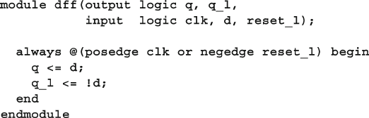
326 9 Functional Coverage
9.2 Coverage Types
Coverage is a generic term for measuring progress to complete design verifi cation.
Your simulations slowly paint the canvas of the design, as you try to cover all of the
legal combinations. The coverage tools gather information during a simulation and
then post-process it to produce a coverage report. You can use this report to look for
coverage holes and then modify existing tests or create new ones to fi ll the holes.
This iterative process continues until you are satisfi ed with the coverage level.
9.2.1 Code Coverage
The easiest way to measure verifi cation progress is with code coverage. Here you
are measuring how many lines of code have been executed (line coverage), which
paths through the code and expressions have been executed (path coverage),
which single-bit variables have had the values 0 or 1 (toggle coverage), and which
states and transitions in a state machine have been visited (FSM coverage). You
don’t have to write any extra HDL code. The tool instruments your design automati-
cally by analyzing the source code and adding hidden code to gather statistics. You
then run all your tests, and the code coverage tool creates a database.
Most simulators include a code coverage tool. A post-processing tool converts
the database into a readable form. The end result is a measure of how much your
tests exercise the design code. Note that you are primarily concerned with analyzing
the design code, not the testbench. Untested design code could conceal a hardware
bug, or may be just redundant code.
Code coverage measures how thoroughly your tests exercised the “implementation”
of the design specifi cation, but not the verifi cation plan. Just because your tests have
reached 100% code coverage, your job is not done. What if you made a mistake that
your test didn’t catch? Worse yet, what if your implementation is missing a feature?
The module in Sample 9.1 is for a D-fl ip fl op. Can you see the mistake?
Sample 9.1 Incomplete D-fl ip fl op model missing a path
The reset logic was accidently left out. A code coverage tool would report that
every line had been exercised, yet the model was not implemented correctly. Go
back to the functional specifi cation that describes reset behavior and make sure your
verifi cation plan includes a requirement to verify this. Then gather functional cover-
age information on the design during reset.
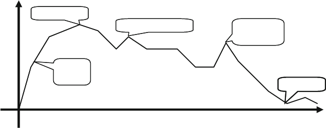
327
9.2 Coverage Types
9.2.2 Functional Coverage
The goal of verifi cation is to ensure that a design behaves correctly in its real envi-
ronment, be that an MP3 player, network router, or cell phone. The design specifi ca-
tion details how the device should operate, whereas the verifi cation plan lists how
that functionality is to be stimulated, verifi ed, and measured. When you gather mea-
surements on what functions were covered, you are performing “design” coverage.
For example, the verifi cation plan for a D-fl ip fl op would mention not only its data
storage but also how it resets to a known state. Until your test checks both these
design features, you will not have 100% functional coverage.
Functional coverage is tied to the design intent and is sometimes called “specifi -
cation coverage,” while code coverage measures how well you have tested the RTL
code and is known as, “implementation coverage.” These are two very different
metrics. Consider what happens if a block of code is missing from the design. Code
coverage cannot catch this mistake and could report that you have executed 100%
of the lines, but functional coverage will show that the functionality does not exist.
9.2.3 Bug Rate
An indirect way to measure coverage is to look at the rate at which fresh bugs are found,
show in the graph in Fig. 9.3 . You should keep track of how many bugs you found each
week, over the life of a project. At the start, you may fi nd many bugs through inspection
as you create the testbench. As you read the design spec, you may fi nd inconsistencies,
which hopefully are fi xed before the RTL is written. Once the testbench is up and run-
ning, a torrent of bugs is found as you check each module in the system. The bug rate
drops, hopefully to zero, as the design nears tape-out. However, you are not yet done.
Every time the rate sags, it is time to fi nd different ways to create corner cases.
Bugs/week
Time
Tape-out
Integration
New DUT code
Design
review
New verif.
engineer
Fig. 9.3 Bug rate during a project
The bug rate can vary per week based on many factors such as project phases,
recent design changes, blocks being integrated, personnel changes, and even vaca-
tion schedules. Unexpected changes in the rate could signal a potential problem.
328 9 Functional Coverage
As shown in Fig. 9.3 , it is not uncommon to keep fi nding bugs even after tape-out,
and even after the design ships to customers.
9.2.4 Assertion Coverage
Assertions are pieces of declarative code that check the relationships between design
signals, either once or over a period of time. These can be simulated along with the
design and testbench, or proven by formal tools. Sometimes you can write the
equivalent check using SystemVerilog procedural code, but many assertions are
more easily expressed using SystemVerilog Assertions (SVA).
Assertions can have local variables and perform simple data checking. If you need
to check a more complex protocol, such as determining whether a packet success-
fully went through a router, procedural code is often better suited for the job. There
is a large overlap between sequences that are coded procedurally or using SVA. See
Vijayaraghavan and Ramanadhan (2005), Cohen et al. (2005), and Chapters 3 and 7
in the VMM book, Bergeron et al. (2006) for more information on SVA.
The most familiar assertions look for errors such as two signals that should be
mutually exclusive or a request that was never followed by a grant. These error
checks should stop the simulation as soon as they detect a problem. Assertions can
also check arbitration algorithms, FIFOs, and other hardware. These are coded with
the assert property statement.
Some assertions might look for interesting signal values or design states, such as a
successful bus transaction. These are coded with the cover property statement.
You can measure how often these assertions are triggered during a test by using asser-
tion coverage. A cover property observes sequences of signals, whereas a cover group
(described below) samples data values and transactions during the simulation. These
two constructs overlap in that a cover group can trigger when a sequence completes.
Additionally, a sequence can collect information that can be used by a cover group.
9.3 Functional Coverage Strategies
Before you write the fi rst line of test code, you need to anticipate what are the key
design features, corner cases, and possible failure modes. This is how you write
your verifi cation plan. Don’t think in terms of data values only; instead, think about
what information is encoded in the design. The plan should spell out the signifi cant
design states.
9.3.1 Gather Information, not Data
A classic example is a FIFO. How can you be sure you have thoroughly tested a
1K FIFO memory? You could measure the values in the read and write indices,
329
9.3 Functional Coverage Strategies
but there are over a million possible combinations. Even if you were able to simulate
that many cycles, you would not want to read the coverage report.
At a more abstract level, a FIFO can hold from 0 to N–1 possible values. So what
if you just compare the read and write indices to measure how full or empty the
FIFO is? You would still have 1K coverage values. If your testbench pushed 100
entries into the FIFO, then pushed in 100 more, do you really need to know if the
FIFO ever had 150 values? Not as long as you can successfully read out all values.
The corner cases for a FIFO are Full and Empty. If you can make the FIFO go from
Empty (the state after reset) through Full and back down to Empty, you have covered
all the levels in between. Other interesting states involve the indices as they pass
between all 1’s and all 0’s. A coverage report for these cases is easy to understand.
You may have noticed that the interesting states are independent of the FIFO
size. Once again, look at the information, not the data values.
Design signals with a large range (more than a few dozen possible values) should
be broken down into smaller ranges, plus corner cases. For example, your DUT may
have a 32-bit address bus, but you certainly don’t need to collect 4 billion samples.
Check for natural divisions such as memory and IO space. For a counter, pick a few
interesting values, and always try to rollover counter values from all 1’s back to 0.
9.3.2 Only Measure What you are Going to Use
Gathering functional coverage data can be expensive, so only measure what you will
analyze and use to improve your tests. Your simulations may run slower as the simu-
lator monitors signals for functional coverage, but this approach has lower overhead
than gathering waveform traces and measuring code coverage. Once a simulation
completes, the database is saved to disk. With multiple testcases and multiple seeds,
you can fi ll disk drives with functional coverage data and reports. But if you never
look at the fi nal coverage reports, don’t perform the initial measurements.
There are several ways to control cover data: at compilation, instantiation, or
triggering. You could use switches provided by the simulation vendor, conditional
compilation, or suppression of the gathering of coverage data. The last of these is
less desirable because the post-processing report is fi lled with sections with 0%
coverage, making it harder to fi nd the few enabled ones.
9.3.3 Measuring Completeness
Like your kids in the backseat on a family vacation, your manager constantly asks
you, “Are we there yet?” How can you tell if you have fully tested a design? You
need to look at all coverage measurements and consider the bug rate to see if you
have reached your destination.
At the start of a project, both code and functional coverage are low. As you
develop tests, run them over and over with different random seeds until you no lon-
ger see increasing values of functional coverage. Create additional constraints and
330 9 Functional Coverage
What if the functional coverage is high but the code coverage is low as shown in
the upper left of Figure 9.4 ? Your tests are not exercising the full design, perhaps
from an inadequate verifi cation plan. It may be time to go back to the hardware
specifi cations and update your verifi cation plan. Then you need to add more func-
tional coverage points to locate untested functionality.
A more diffi cult situation is high code coverage but low functional coverage.
Even though your testbench is giving the design a good workout, you are unable to
put it in all the interesting states. First, see if the design implements all the specifi ed
functionality. If it is there, but your tests can’t reach it, you might need a formal veri-
fi cation tool that can extract the design’s states and create appropriate stimulus.
The goal is both high code and functional coverage. However, don’t plan your
vacation yet. What is the trend of the bug rate? Are signifi cant bugs still popping up?
Worse yet, are they being found deliberately, or did your testbench happen to
stumble across a particular combination of states that no one had anticipated? On
the other hand, a low bug rate may mean that your existing strategies have run out
of steam, and you should look into different approaches. Try different approaches
such as new combinations of design blocks and error generators.
9.4 Simple Functional Coverage Example
To measure functional coverage, you begin with the verifi cation plan and write an
executable version of it for simulation. In your System Verilog testbench, sample
the values of variables and expressions. These sample locations are known as cover
points. Multiple cover points that are sampled at the same time (such as when a
transaction completes) are placed together in a cover group.
Sample 9.2 has a transaction that comes in eight fl avors. The testbench generates
the dst variable randomly, and the verifi cation plan requires that every value be tried.
Functional Coverage
Code Coverage
Start of
project
Need more FC
points, including
corner cases
High
Low
Low High
Is design complete?
Perhaps try
formal tools
Good coverage:
check bug rate
Fig. 9.4 Coverage comparison
tests to explore new areas. Save test/seed combinations that give high coverage, so
that you can use them in regression testing.
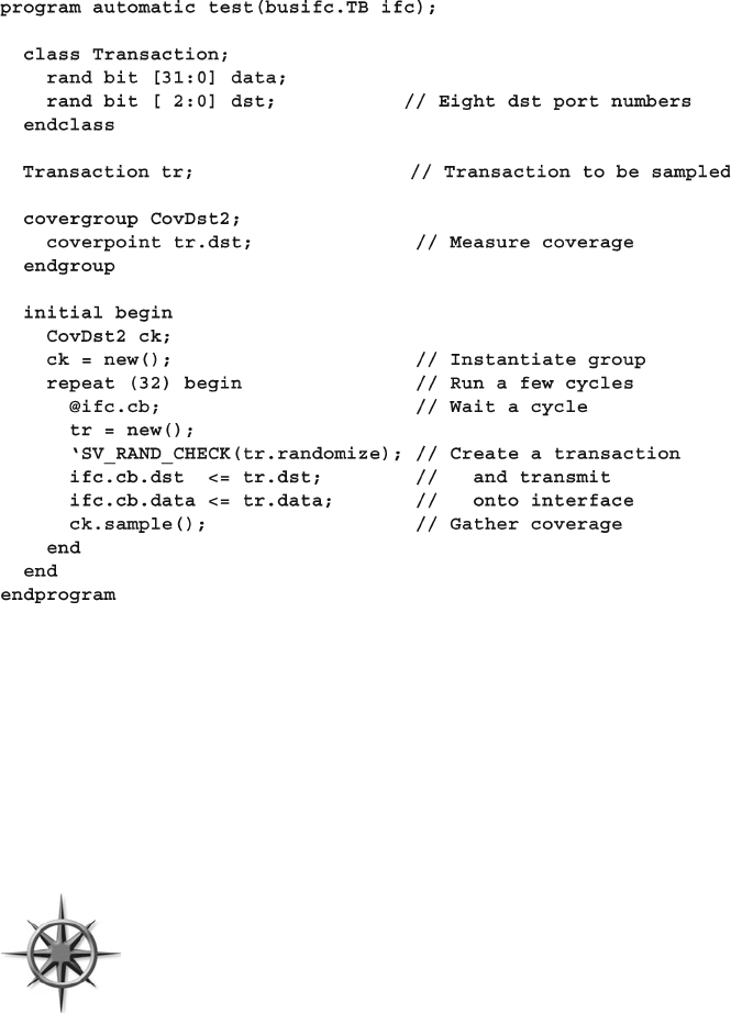
331
9.4 Simple Functional Coverage Example
Sample 9.2 creates a random transaction and drives it out to an interface. The
testbench samples the value of the dst fi eld using the CovDst2 cover group. Eight
possible values, 32 random transactions — did your testbench generate them all?
Samples 9.3 and 9.4 have part of a coverage report from VCS. Because of random-
ization, every simulator will give different results.
As you can see, the testbench generated dst values of 1, 2, 3, 4, 5, 6, and 7, but
never generated a 0. The at least column specifi es how many hits are needed
before a bin is considered covered. See Section 9.10.3 for the at_least option.
To improve your functional coverage, the easiest strategies are to run
more simulation cycles, or to try new random seeds. For Sample
9.2 , the very next random transaction (#33) has a dst value of 0, giv-
ing 100% coverage. Or, if you started simulation with a different
seed, you may reach 100% in fewer transactions, for this trivial
case. On a real design, you may see a plateau in coverage, with most
coverage points getting hit more and more, but a few stubborn points that are never
hit, no matter how long you run, regardless of seed values. In this case, you probably
have to try a new strategy, as the testbench is not creating the proper stimulus. The
most important part of any coverage report are the points with 0 hits.
Sample 9.2 Functional coverage of a simple object
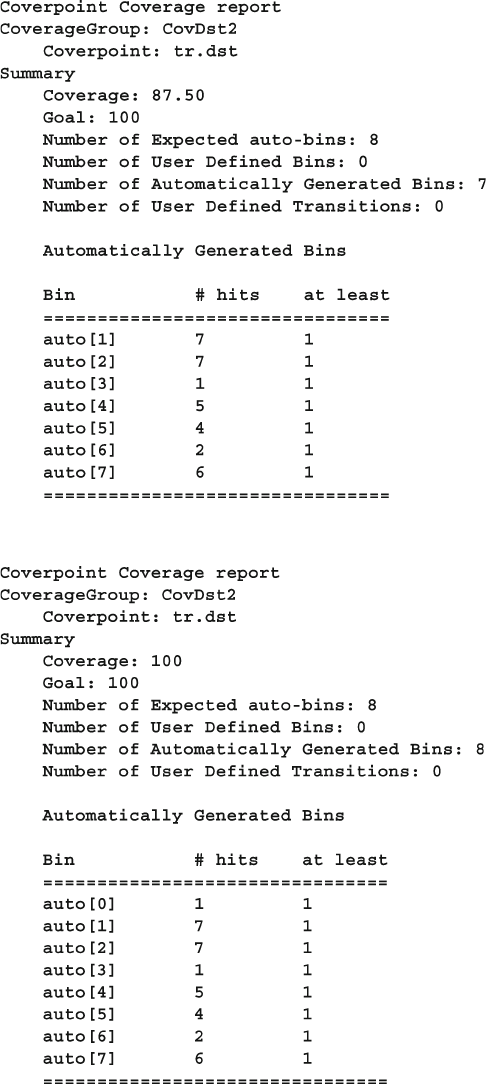
332 9 Functional Coverage
Sample 9.4 Coverage report for a simple object, 100% coverage
Sample 9.3 Coverage report for a simple object

333
9.5 Anatomy of a Cover Group
This book gives a rough explanation of how coverage is calculated. The LRM
has a very detailed explanation of coverage computation across four pages, with
more details across an entire chapter. Consult it for the most accurate details.
9.5 Anatomy of a Cover Group
A cover group is similar to a class — you defi ne it once and then instantiate it one
or more times. It contains cover points, options, formal arguments, and an optional
trigger. A cover group encompasses one or more data points, all of which are sam-
pled at the same time.
You should create very clear cover group names that explicitly indicate what you
are measuring and, if possible, reference to the verifi cation plan. The name Parity_
Errors_In_Hexaword_Cache_Fills may seem verbose, but when you are try-
ing to read a coverage report that has dozens of cover groups, you will appreciate
the extra detail. You can also use the comment option for additional descriptive
information, as shown in Section 9.9.2 .
A cover group can be defi ned in a class or at the program or module level. It can
sample any visible variable such as program/module variables, signals from an
interface, or any signal in the design (using a hierarchical reference). A cover group
inside a class can sample variables in that class, as well as data values from embed-
ded objects.
Don’t defi ne the cover group in a data class, such as a transaction,
as doing so can cause additional overhead when gathering cover-
age data. Imagine you are trying to track how many beers were
consumed by patrons in a pub. Would you try to follow every bottle
as it fl owed from the loading dock, over the bar, and into each per-
son? No, instead you could just have each patron check off the type and number of
beers consumed, as shown in van der Schoot (2006).
In SystemVerilog, you should defi ne cover groups at the appropriate level of abstrac-
tion. This level can be at the boundary between your testbench and the design, in the
transactors that read and write data, in the environment confi guration class, or wher-
ever is needed. The sampling of any transaction must wait until it is actually received
by the DUT. If you inject an error in the middle of a transaction, causing it to be
aborted in transmission, you need to change how you treat it for functional cover-
age. You need to use a different cover point that has been created just for error
handling.
A class can contain multiple cover groups. This approach allows you to have
separate groups that can be enabled and disabled as needed. Additionally, each
group may have a separate trigger, allowing you to gather data from many
sources.
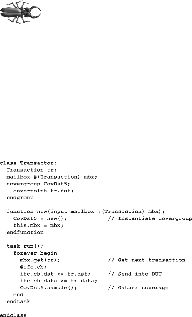
334 9 Functional Coverage
A cover group must be instantiated for it to collect data. If you
forget, no error message about null handles is printed at run
time, but the coverage report will not contain any mention of the
cover group. This rule applies for cover groups defi ned either
inside or outside of classes.
9.5.1 Defi ning a Cover Group in a Class
A cover group can be defi ned in a program, module, or class. In all cases, you must
explicitly instantiate it to start sampling. If the cover group is defi ned in a class, it is
known as an embedded covergroup. In this case, you do not make a separate name
when you construct it; just use the original cover group name. You must construct
an embedded covergroup in the class’s constructor, as opposed to a non-embedded
cover group that can be constructed at any time.
Sample 9.5 is very similar to the fi rst example of this chapter except that it
embeds a cover group in a transactor class, and thus does not need a separate instance
name.
Sample 9.5 Functional coverage inside a class
335
9.6 Triggering a Cover Group
9.6 Triggering a Cover Group
The two major parts of functional coverage are the sampled data values and the time
when they are sampled. When new values are ready (such as when a transaction has
completed), your testbench triggers the cover group. This can be done directly
with the
sample function, as shown in Sample 9.5 , or by using a coverage event
in the covergroup defi nition. The coverage event can use a @ to block on signals
or events.
Use sample if you want to explicitly trigger coverage from procedural code, if
there is no existing signal or event that tells when to sample, or if there are multiple
instances of a cover group that trigger separately.
Use the coverage event in the covergroup declaration if you want to tap into
existing events or signals to trigger coverage.
9.6.1 Sampling Using a Callback
One of the better ways to integrate functional coverage into your testbench is to use
callbacks, as originally shown in Section 8.7. This technique allows you to build a
fl exible testbench without restricting when coverage is collected. You can decide
for every point in the verifi cation plan where and when values are sampled. And if
you need an extra “hook” in the environment for a callback, you can always add
one in an unobtrusive manner, as a callback only “fi res” during simulations when
the test registers a callback object. You can create many separate callbacks for each
cover group, with little overhead. As explained in Section 8.7.4, callbacks are
superior to using a mailbox to connect the testbench to the coverage objects. You
might need multiple mailboxes to collect transactions from different points in your
testbench. A mailbox requires a transactor to receive transactions, and multiple
mailboxes cause you to juggle multiple threads. Instead of an active transactor, use
a passive callback.
Sample 8.26 – 8.28 shows a driver class that has two callback points, before and
after the transaction is transmitted. Sample 8.26 shows the base callback class, and
Sample 8.28 has a test with an extended callback class that sends data to a score-
board. Make your own extension, Driver_cbs_coverage , of the base callback
class, Driver_cbs , to call the sample task for your cover group in post_tx . Push
an instance of the coverage callback class into the driver’s callback queue, and your
coverage code triggers the cover group at the right time. Samples
9.6 and 9.7 defi ne
and use the callback Driver_cbs_coverage .
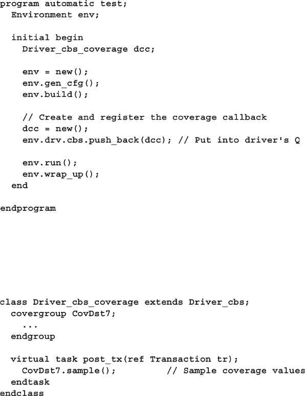
336 9 Functional Coverage
Sample 9.6 Test using functional coverage callback
Sample 9.7 Callback for functional coverage
The UVM recommends gathering coverage by monitoring the DUT and sending
transactions to a coverage component through an analysis port, similar to a mailbox.
9.6.2 Cover Group with a User Defi ned Sample Argument List
In Sample 9.5 , the cover group samples a variable in transaction object that is
defi ned inside the class. If your cover group is defi ned outside of a class, you can
pass variables through the sample method by defi ning your own argument list.
Now you can sample variables from anywhere in the testbench.
In Sample 9.8 , the cover group is expanded to also cover the low data bit. The last
statement of the run method passes the destination address and also the confi gura-
tion variable for high speed mode.
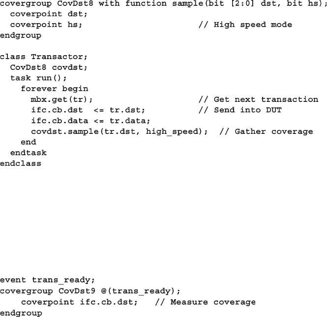
337
9.6 Triggering a Cover Group
9.6.3 Cover Group with an Event Trigger
In Sample 9.9 , the cover group CovDst9 is sampled when the testbench triggers the
trans_ready event .
Sample 9.8 Defi ning an argument list to the sample method
Sample 9.9 Cover group with a trigger
The advantage of using an event over calling the sample method directly is that
you may be able to use an existing event such as one triggered by an assertion, as
shown in Sample 9.11 .
9.6.4 Triggering on a System Verilog Assertion
If you already have an SVA that looks for useful events like a complete transaction,
you can add an event trigger to wake up the cover group as shown in 9.10 .
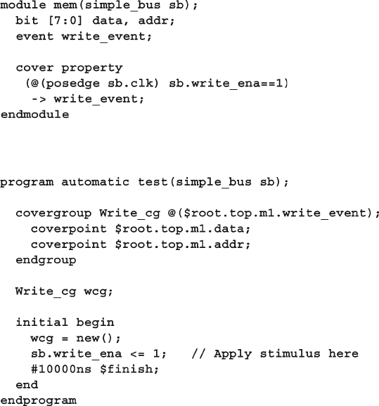
338 9 Functional Coverage
9.7 Data Sampling
How is coverage information gathered? When you specify a variable or expression
in a cover point, SystemVerilog creates a number of “bins” to record how many
times each value has been seen. These bins are the basic units of measurement for
functional coverage. If you sample a one-bit variable, a maximum of two bins are
created. You can imagine that System Verilog drops a token in one or the other bin
every time the cover group is triggered. At the end of each simulation, a database is
created with all bins that have a token in them. You then run an analysis tool that
reads all databases and generates a report with the coverage for each part of the
design and for the total coverage.
9.7.1 Individual Bins and Total Coverage
To calculate the coverage for a point, you fi rst have to determine the total number of
possible values, also known as the domain. There may be one value per bin or multiple
Sample 9.10 Module with SystemVerilog Assertion
Sample 9.11 Triggering a cover group with an SVA
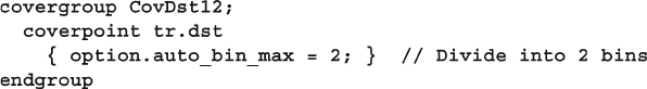
339
9.7 Data Sampling
values. Coverage is the number of sampled values divided by the number of bins in
the domain.
A cover point that is a 3-bit variable has the domain 0:7 and is normally divided
into eight bins. If, during simulation, values belonging to seven bins are sampled,
the report will show 7/8 or 87.5% coverage for this point. All these points are com-
bined to show the coverage for the entire group, and then all the groups are com-
bined to give a coverage percentage for all the simulation databases.
This is the status for a single simulation. You need to track coverage over time.
Look for trends so you can see where to run more simulations or add new con-
straints or tests. Now you can better predict when verifi cation of the design will be
completed.
9.7.2 Creating Bins Automatically
As you saw in the report in Sample 9.3 , System Verilog automatically creates bins for
cover points. It looks at the domain of the sampled expression to determine the range
of possible values. For an expression that is N bits wide, there are 2
N possible values.
For the 3-bit variable dst , there are 8 possible values. The range of an enumerated
type is shown in Section 9.6.8 . The domain for enumerated data types is the number
of named values. You can also explicitly defi ne bins as shown in Section 9.6.5 .
9.7.3 Limiting the Number of Automatic Bins Created
The cover group option auto_bin_max specifi es the maximum number of bins to
automatically create, with a default of 64 bins. If the domain of values in the cover
point variable or expression is greater than this option, System Verilog divides the
range into auto_bin_max bins. For example, a 16-bit variable has 65,536 possible
values, so each of the 64 bins covers 1024 values.
In reality, you may fi nd this approach impractical, as it is very diffi cult to fi nd the
needle of missing coverage in a haystack of auto-generated bins. Lower this limit to
8 or 16, or better yet, explicitly defi ne the bins as shown in Section 9.6.5 .
Sample 9.12 takes the chapter’s fi rst example and adds a cover point option that
sets auto_bin_max to two bins. The sampled variable is still dst , which is three
bits wide, for a domain of eight possible values. The fi rst bin holds the lower half of
the range, 0–3, and the other hold the upper values, 4–7.
Sample 9.12 Using auto_bin_max set to 2
340 9 Functional Coverage
The coverage report from VCS shows the two bins. This simulation achieved
100% coverage because the eight dst values were mapped to two bins. Since both
bins have sampled values, your coverage is 100% as shown in Sample 9.13 .
Sample 9.13 Report with auto_bin_max set to 2
Sample 9.12 used auto_bin_max as an option for the cover point only. You can
also use it as an option for the entire group as shown in Sample 9.14 .
Sample 9.14 Using auto_bin_max for all cover points
9.7.4 Sampling Expressions
You can sample expressions, but always check the coverage report to be sure you
are getting the values you expect. You may have to adjust the width of the computed
expression, as shown in Section 2.16. For example, sampling a 3-bit header length
(0:7) plus a 4-bit payload length (0:15) creates only 2
4 or 16 bins, which may not be
enough if your transactions can actually be from 0 to 22 bytes long.
Sample 9.15 Using an expression in a cover point
341
9.7 Data Sampling
Sample 9.15 has a cover group that samples the total packet length. The cover
point has a label to make it easier to read the coverage report. Also, the expression
has an additional dummy constant so that the transaction length is computed with
5-bit precision, for a maximum of 32 auto-generated bins.
A long run with random packets showed that the
len16 had 100% coverage, but
this is across only 16 bins. (The cover point only has 16 bins as the sum of a 3-bit
and 4-bit value is only 4-bits in Verilog.) The cover point
len32 had 72% coverage
across 32 bins. (The addition of a 5-bit value to the expression for bin32 results in
a 5-bit result.) Neither of these cover points are correct, as the maximum length has
a domain of 0:22 (0+0:7+15). The auto-generated bins just don’t work, as the maxi-
mum length is not a power of 2. You need a way to precisely defi ne bins.
9.7.5 User-Defi ned Bins Find a Bug
Automatically generated bins are okay for anonymous data values, such as counter
values, addresses, or values that are a power of 2. For other values, you should
explicitly name the bins to improve accuracy and ease coverage report analysis.
System Verilog automatically creates bin names for enumerated types, but for other
variables you need to give names to the interesting states. The easiest way to specify
bins is with the [] syntax, as shown in Sample 9.16 .
Sample 9.16 Defi ning bins for transaction length
After sampling many random transactions, the group has 95.83% coverage.
A quick look at the report in Sample 9.17 shows the problem — the length of 23 (17
hex) was never seen. The longest header is 7, and the longest payload is 15, for a
total of 22, not 23! If you change to the bins declaration to use 0:22, the coverage
jumps to 100%. The user-defi ned bins found a bug in the test.
342 9 Functional Coverage
9.7.6 Naming the Cover Point Bins
Sample 9.18 samples a 4-bit variable, kind , that has 16 possible values. The fi rst
bin is called zero and counts the number of times that kind is 0 when sampled. The
next four values, 1–3 and 5, are all grouped into a single bin, lo . The upper eight
values, 8–15, are kept in separate bins, hi_8, hi_9, hi_a, hi_b, hi_c, hi_d,
hi_e , and hi_f . Note how $ in the hi bin expression is used as a shorthand nota-
tion for the largest value for the sampled variable. Lastly, misc holds all values that
were not previously chosen: 4, 6, and 7.
Sample 9.17 Coverage report for transaction length
343
9.7 Data Sampling
Note that the additional information about the coverpoint is grouped using
curly braces: {}. This is because the bin specifi cation is declarative code, not pro-
cedural code that would be grouped with begin…end . Lastly, the fi nal curly brace
is NOT followed by a semicolon, just as an end never is.
Now you can easily see in Sample 9.19 which bins have no hits — hi_8 in this case.
Sample 9.18 Specifying bin names
Sample 9.19 Report showing bin names
When you defi ne the bins, you are restricting the values used for coverage to
those that are interesting to you. SystemVerilog no longer automatically creates
bins, and it ignores values that do not fall into a predefi ned bin. More importantly,
only the bins you create are used to calculate functional coverage. You get 100%
coverage only as long as you get a hit in every specifi ed bin.
Values that do not fall into any specifi ed bin are ignored. This rule
is useful if the sampled value, such as transaction length, is not a
power of 2. If you are specifying bins, you can use the default bin
specifi er to catch values that you may have forgotten. However, the
LRM says that default bins are not used in coverage calculation.
In Sample 9.18 , the range for hi uses a dollar sign ($) on the right side to specify
the upper value. This is a very useful shortcut - now you can let the compiler calculate
344 9 Functional Coverage
the limits for a range. You can use the dollar sign on the left side of a range to
specify the lower limit. In Sample 9.20 , the $ in the range for bin neg represents the
negative number furthest from zero: 32¢h8000_0000, or -2,147,483,648, whereas
the $ in bin
pos represents the largest signed positive value, 32’h7FFF_FFFF, or
2,147,483,647.
Sample 9.20 Specifying ranges with $
9.7.7 Conditional Coverage
You can use the iff keyword to add a condition to a cover point. The most common
reason for doing so is to turn off coverage during reset so that stray triggers are
ignored. Sample 9.21 gathers only values of dst when rst is 0, where rst is
active-high.
Sample 9.21 Conditional coverage — disable during reset
Alternately, you can use the start and stop functions to control individual
instances of cover groups as shown in Sample 9.22 .
Sample 9.22 Using stop and start functions
345
9.7 Data Sampling
9.7.8 Creating Bins for Enumerated Types
For enumerated types, SystemVerilog creates a bin for each value as you can see in
Sample
9.23 .
Sample 9.23 Functional coverage for an enumerated type
Here is part of the coverage report from VCS, Sample 9.24 showing the bins for
the enumerated types.
Sample 9.24 Coverage report with enumerated types
If you want to group multiple values into a single bin, you have to defi ne your
own bins. Any bins outside the enumerated values are ignored unless you defi ne a
bin with the default specifi er. When you gather coverage on enumerated types,
auto_bin_max does not apply.
9.7.9 Transition Coverage
You can specify state transitions for a cover point. In this way, you can tell not only
what interesting values were seen but also the sequences. For example, you can
check if dst ever went from 0 to 1, 2, or 3 as shown in Sample 9.25 .
Sample 9.25 Specifying transitions for a cover point
You can quickly specify multiple transitions using ranges. The expression (1, 2
=> 3, 4) creates the four transitions (1=>3), (1=>4), (2=>3) , and (2=>4) .
You can specify transitions of any length. Note that you have to sample once for
each state in the transition. So (0 => 1 => 2) is different from (0 => 1 => 1 => 2)

346 9 Functional Coverage
or (0 => 1 => 1 => 1 => 2) . If you need to repeat values, as in the last
sequence, you can use the shorthand form:
(0 => 1[*3] => 2) . To repeat the
value 1 for 3, 4, or 5 times, use
1[*3:5] .
9.7.10 Wildcard States and Transitions
You use the wildcard keyword to create multiple states and transitions. Any X, Z,
or ? in the expression is treated as a wildcard for 0 or 1. Sample 9.26 creates a cover
point with a bin for even values and one for odd.
Sample 9.26 Wildcard bins for a cover point
9.7.11 Ignoring Values
With some cover points, you never get all possible values. For instance, a 3-bit vari-
able may be used to store just six values, 0–5. If you use automatic bin creation, you
never get beyond 75% coverage. There are two ways to solve this problem. You can
explicitly defi ne the bins that you want to cover as shown in Section 9.6.5 .
Alternatively, you can let SystemVerilog automatically create bins, and then use
ignore_bins to tell which values to exclude from functional coverage calculation like
in Sample 9.27 .
Sample 9.27 Cover point with ignore_bins
The original range of low_ports_0_5 , a three-bit variable is 0:7. The ignore_
bins excludes the last two bins, which reduces the range to 0:5. So total coverage
for this group is the number of bins with samples, divided by the total number of
bins, which is 5 in this case.
347
9.7 Data Sampling
If you defi ne bins either explicitly or by using the auto_bin_max option, and
then ignore them, the ignored bins do not contribute to the calculation of coverage.
In Sample 9.28 , four bins are initially created using the auto_bin_max option: 0:1,
2:3, 4:5, and 6:7. However, then the uppermost bin is eliminated by ignore_bins ,
so in the end only three bins are created. This cover point can have coverage of 0%,
33%, 66%, or 100%.
9.7.12 Illegal Bins
Some sampled values not only should be ignored, but also should cause an error if
they are seen. This is best done in the testbench’s monitor code, but can also be done
by labeling a bin with illegal_bins as shown in Sample 9.29 . Use this to catch
states that were missed by the test’s error checking. This also double-checks the
accuracy of your bin creation: if an illegal value is found by the cover group, it is a
problem either with the testbench or with your bin defi nitions.
Sample 9.28 Cover point with auto bin max and ignore bins
Sample 9.29 Cover point with illegal_bins
9.7.13 State Machine Coverage
You should have noticed that if a cover group is used on a state machine, you can
use bins to list the specifi c states, and transitions for the arcs. However, this does not
mean you should use SystemVerilog’s functional coverage to measure state machine
coverage. You would have to extract the states and arcs manually. Even if you did
this correctly the fi rst time, you might miss future changes to the design code.
Instead, use a code coverage tool that extracts the state register, states, and arcs
automatically, saving you from possible mistakes.
However, an automatic tool extracts the information exactly as coded, mistakes
and all. You may want to monitor small, critical state machines manually using
functional coverage.
348 9 Functional Coverage
9.8 Cross Coverage
A cover point records the observed values of a single variable or expression. You
may want to know not only what bus transactions occurred but also what errors hap-
pened during those transactions, and their source and destination. For this you need
cross coverage that measures what values were seen for two or more cover points at
the same time. Note that when you measure cross coverage of a variable with N
values, and of another with M values, SystemVerilog needs N ´ M cross bins to store
all the combinations.
9.8.1 Basic Cross Coverage Example
Previous examples have measured coverage of the transaction kind, and destination
port number, but what about the two combined? Did you try every kind of transac-
tion into every port? The cross construct in SystemVerilog records the combined
values of two or more cover points in a group. The cross statement takes only
cover points or a simple variable name. If you want to use expressions, hierarchical
names or variables in an object such as handle.variable , you must fi rst specify
the expression in a coverpoint with a label and then use the label in the cross
statement.
Sample 9.30 creates cover points for tr.kind and tr.dst . Then the two points
are crossed to show all combinations. SystemVerilog creates a total of 128 (8 ´ 16)
bins. Be careful: even a simple cross can result in a very large number of bins.
Sample 9.30 Basic cross coverage
A random testbench created 56 transactions and produced the coverage report in
Sample 9.31 . Note that even though all possible kind and dst values were gener-
ated, only 1/3 of the cross combinations were seen. This is a very typical result.
Also note that the total coverage for the group is the cross coverage plus the cover-
age for kind and dst .
349
9.8 Cross Coverage
9.8.2 Labeling Cross Coverage Bins
If you want more readable cross coverage bin names, you can label the individual cover
point bins as demonstrated in Sample 9.32 , and SystemVerilog will use these names
when creating the cross bins.
Sample 9.31 Coverage summary report for basic cross coverage
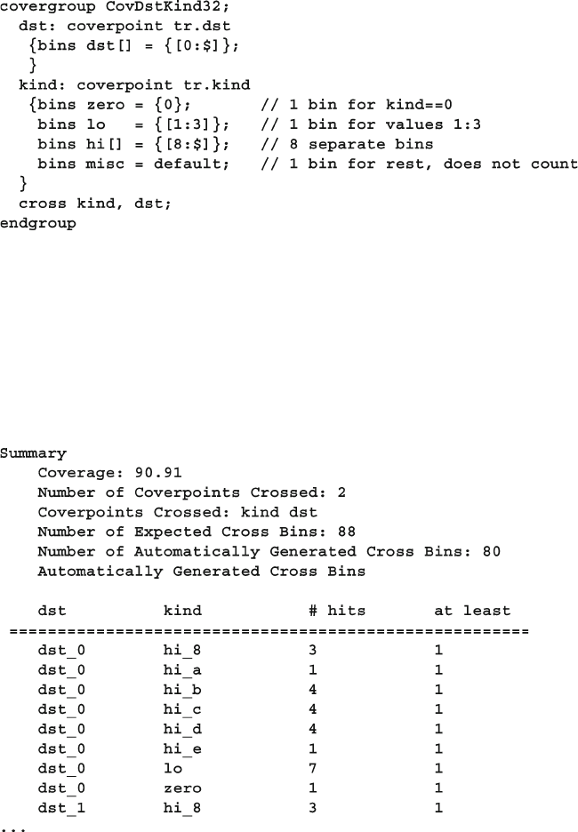
350 9 Functional Coverage
If you defi ne bins that contain multiple values, the coverage statistics change. In the
report below, the number of bins has dropped from 128 to 80. This is because kind
has 10 bins: zero, lo, hi_8, hi_9, 9hi_a, hi_b, hi_c, hi_d, hi_e , and hi_f.
Remember that the misc bin, which defi ned its values with default , does not add
to the coverage total. The percentage of coverage jumped from 87.5% to 90.91%
as shown in Sample 9.33 because any single value in the lo bin, such as 2, allows
that bin to be marked as covered, even if the other values, 1 or 3, are not seen.
Sample 9.33 Cross coverage report with labeled bins
Sample 9.32 Specifying cross coverage bin names
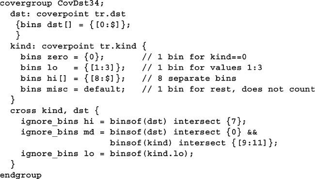
351
9.8 Cross Coverage
9.8.3 Excluding Cross Coverage Bins
To reduce the number of bins, use ignore_bins . With cross coverage, you specify
the cover point with
binsof and the set of values with intersect so that a single
ignore_bins construct can sweep out many individual bins.
Sample 9.34 Excluding bins from cross coverage
The fi rst ignore_bins in Sample 9.34 just excludes bins where dst is 7 and any
value of kind . Since kind is a 4-bit value, this statement excludes 12 bins, as misc’s
values of 4–7 don’t count because of the default . The second ignore_bins is more
selective, ignoring bins where dst is 0 and kind is 9, 10, or 11, for a total of 3 bins.
The ignore_bins can use the bins defi ned in the individual cover points. The
ignore_bins lo uses bin names to exclude kind.lo that is 1, 2, or 3. The bins
must be names defi ned at compile time, such as zero and lo . The bins hi_8, hi_9,
hi_a,… hi_f , and any automatically generated bins do not have names that can be
used at compile time in other statements such as ignore_bins ; these names are
created at run time or during the report generation.
Note that binsof uses parentheses () while intersect specifi es a range and
therefore uses curly braces {}.
9.8.4 Excluding Cover Points from the Total Coverage Metric
The total coverage for a group is based on all simple cover points and cross coverage.
If you are only sampling a variable or expression in a coverpoint to be used in a
cross statement, you should set its weight to 0 so that it does not contribute to the
total coverage.
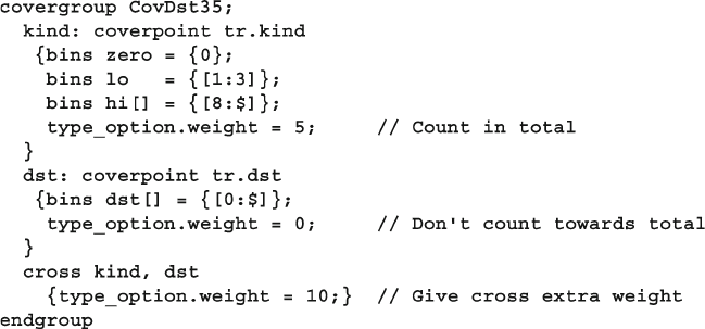
352 9 Functional Coverage
There are two types of options: those that are specifi c to an instance of a cover-
group and those that specify an option for the covergroup type as a whole. The
instance specifi c options are like local variables and are specifi ed with the option
keyword, as in option.auto_bin_max=2 from Sample 9.12 . The alternatives are
specifi ed with the type_option keyword and are tied to the cover group, like static
variables in a class. In Sample 9.35 , type_option.weight applies to all instances
of this group. The LRM has a detailed explanation of the difference, and this book
shows the most common options and their usage.
9.8.5 Merging Data from Multiple Domains
One problem with cross coverage is that you may need to sample values from dif-
ferent timing domains. You might want to know if your processor ever received an
interrupt in the middle of a cache fi ll. The interrupt hardware is separate from and
may use different clocks than the cache hardware, making it diffi cult to know when
to trigger the cover group. On the other hand, you want to make sure you have tested
this case, as a previous design had a bug of this very sort.
The solution is to create a timing domain separate from the cache or interrupt
hardware. Make copies of the signals into temporary variables and then sample
them in a new coverage group that measures the cross coverage.
9.8.6 Cross Coverage Alternatives
As your cross coverage defi nition becomes more elaborate, you may spend consid-
erable time specifying which bins should be used and which should be ignored. You
may have two random bits, a and b with three interesting states, {a==0, b==0},
{a==1, b==0} , and {b==1} .
Sample 9.35 Specifying cross coverage weight
353
9.8 Cross Coverage
Sample 9.36 shows how you can name bins in the cover points and then gather
cross coverage using those bins.
Sample 9.36 Cross coverage with bin names
Sample 9.37 gathers the same cross coverage, but now uses binsof to specify
the cross coverage values.
Sample 9.37 Cross coverage with binsof
Alternatively, you can make a cover point that samples a concatenation of values.
Then you only have to defi ne bins using the less complex cover point syntax.
354 9 Functional Coverage
Use the style in Sample 9.36 if you already have bins defi ned for the individual
cover points and want to use them to build the cross coverage bins. Use Sample 9.37
if you need to build cross coverage bins but have no pre-defi ned cover point bins.
Use Sample 9.38 if you want the tersest format.
9.9 Generic Cover Groups
As you start writing cover groups, you will fi nd that some are very similar to one
another. SystemVerilog allows you to create a generic cover group so that you can
specify a few unique details when you instantiate it.
9.9.1 Pass Cover Group Arguments by Value
Sample 9.39 shows a cover group that uses an argument to split the range into two
halves. Just pass the midpoint value to the cover groups’ new function.
Sample 9.38 Mimicking cross coverage with concatenation
Sample 9.39 Covergroup with simple argument
355
9.10 Coverage Options
Like a task or function, the arguments to a cover group have a
sticky direction. In Sample 9.40 , if you forgot the input direc-
tion, the mid argument will have the direction ref . The example
would not compile because you cannot pass a constant (4 or 2)
into a ref argument.
9.10 Coverage Options
You can specify additional information in the cover group using options. There are
two fl avors of options: instance options that apply to a specifi c cover group instance
and type options that apply to all instances of the cover group, and are analogous to
static data members of classes. Options can be placed in the cover group so that they
apply to all cover points in the group, or they can be put inside a single cover point
for fi ner control. You have already seen the auto_bin_max and weight options.
Here are several more.
9.10.1 Per-Instance Coverage
If your testbench instantiates a coverage group multiple times, by default System-
Verilog groups together all the coverage data from all the instances. However, if you
9.9.2 Pass Cover Group Arguments by Reference
You can specify a variable to be sampled with pass-by-reference. Here you want the
cover group to sample the value during the entire simulation, not just to use the
value when the constructor is called.
Sample 9.40 Pass-by-reference
356 9 Functional Coverage
have several generators, each creating very different streams of transactions, you
will need to see separate reports. For example, one generator may be creating long
transactions while another makes short ones. The cover group in Sample 9.41 can
be instantiated in each separate generator. It keeps track of coverage for each
instance, and has a unique comment string with the hierarchical path to the cover
group instance.
Sample 9.42 Specifying comments for a cover group
Sample 9.43 Specifying comments for a cover group instance
Sample 9.41 Specifying per-instance coverage
The per-instance option can only be given in the cover group, not in the cover
point or cross point.
9.10.2 Cover Group Comment
You can add a comment into coverage reports to make them easier to analyze.
A comment could be as simple as the section number from the verifi cation plan to
tags used by a report parser to automatically extract relevant information from the
sea of data. If you have a cover group that is only instantiated once, use the type_
option as shown in Sample 9.42 .
However, if you have multiple instances, you can give each a separate comment,
as long as you also use the per-instance option as shown in Sample 9.43 .
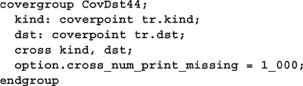
357
9.10 Coverage Options
9.10.3 Coverage Threshold
You may not have suffi cient visibility into the design to gather robust coverage
information. Suppose you are verifying that a DMA state machine can handle bus
errors. You don’t have access to its current state, but you know the range of cycles
that are needed for a transfer. So if you repeatedly cause errors during that range,
you have probably covered all the states. So you could set
option.at_least to 8
or more to specify that after 8 hits on a bin, you are confi dent that you have exer-
cised that combination.
If you defi ne option.at_least at the cover group level, it applies to all cover
points. If you defi ne it inside a point, it only applies to that single point.
However, as Sample 9.2 showed, even after 32 attempts, the random kind vari-
able still did not hit all possible values. So only use at_least if there is no direct
way to measure coverage, like when the testbench can not probe the DUT details.
9.10.4 Printing the Empty Bins
By default, the coverage report shows only the bins with samples. Your job is to verify
all that is listed in the verifi cation plan, so you are actually more interested in the bins
without samples. Use the option cross_num_print_missing to tell the simulation
and report tools to show you all bins, especially the ones with no hits. Set it to a
large value, as shown in Sample 9.44 , but no larger than you are willing to read.
Sample 9.44 Report all bins including empty ones
9.10.5 Coverage Goal
The goal for a cover group or point is the level at which the group or point is
considered fully covered. The default is 100% coverage. If you set this level below
100% like in Sample 9.45 , you are requesting less than complete coverage, which is
probably not desirable. This option affects only the coverage report.
358 9 Functional Coverage
9.11 Analyzing Coverage Data
In general, assume you need more seeds and fewer constraints. After all, it is easier
to run more tests than to construct new constraints. If you are not careful, new con-
straints can easily restrict the search space.
If your cover point has only zero or one sample, your constraints are probably
not targeting these areas at all. You need to add constraints that “pull” the solver
into new areas. In Sample 9.16 , the transaction length had an uneven distribution.
Sample 9.46 shows the full class. This situation is similar to the distribution seen
when you roll two dice and look at the total value.
Sample 9.45 Specifying the coverage goal
Sample 9.46 Original class for packet length
The problem with this class is that len is not evenly weighted. Look in the cov-
erage report and note how the low and high values are rarely hit. Figure 9.5 is a
graph of the values from the report.
0
20
40
60
80
100
120
140
160
0 5 10 15 20 25
Count
Packet length
Fig. 9.5 Uneven probability for packet length
359
9.12 Measuring Coverage Statistics During Simulation
If you want to make the total length be evenly distributed, use a solve…before
constraint as shown in Sample 9.47 and plotted in Fig. 9.6 .
Sample 9.47 solve…before constraint for packet length
0
20
40
60
80
100
120
0 5 10 15 20 25
Count
Packet length
Fig. 9.6 Even probability for packet length with solve…before
The normal alternative to solve…before is the dist constraint. However, this
does not work, as len is also being constrained by the sum of the two lengths.
9.12 Measuring Coverage Statistics During Simulation
You can query the level of functional coverage on the fl y during simulation. This
allows you to check whether you have reached your coverage goals, and possibly to
control a random test.
At the global level, you can get the total coverage of all cover groups with
$get_coverage , which returns a real number between 0. and 100. This system
task looks across all cover groups.
You can narrow down your measurements with the get_coverage() and get_
inst_coverage() methods. The fi rst function works with both cover group names
and instances to give coverage across all instances of a cover group, for example
CoverGroup::get_coverage() or cgInst.get_coverage() . The second
function returns coverage for a specifi c cover group instance, for example cgInst.
get_inst_coverage() . You need to specify option.per_instance=1 if you
want to gather per-instance coverage.
360 9 Functional Coverage
The most practical use for these functions is to monitor coverage over a long test.
If the coverage level does not advance after a given number of transactions or cycles,
the test should stop. Hopefully, another seed or test will increase the coverage.
While it would be nice to have a test that can perform some sophisticated actions
based on functional coverage results, it is very hard to write this sort of test. Each
test + random seed pair may uncover new functionality, but it may take many runs
to reach a goal. If a test fi nds that it has not reached 100% coverage, what should it
do? Run for more cycles? How many more? Should it change the stimulus being
generated? How can you correlate a change in the input with the level of functional
coverage? The one reliable thing to change is the random seed, which you should
only do once per simulation. Otherwise, how can you reproduce a design bug if the
stimulus depends on multiple random seeds?
You can query the functional coverage statistics if you want to create your own
coverage database. Verifi cation teams have built their own SQL databases that are
fed functional coverage data from simulation. This setup allows them greater con-
trol over the data, but requires a lot of work outside of creating tests.
Some formal verifi cation tools can extract the state of a design and then create
input stimulus to reach all possible states. Don’t try to duplicate this in your
testbench!
9.13 Conclusion
When you switch from writing directed tests, hand-crafting every bit of stimulus, to
constrained-random testing, you might worry that the tests are no longer under your
command. By measuring coverage, especially functional coverage, you regain con-
trol by knowing what features have been tested.
Using functional coverage requires a detailed verifi cation plan and much time
creating the cover groups, analyzing the results, and modifying tests to create the
proper stimulus. This may seem like a lot of work, but is less effort than would be
required to write the equivalent directed tests. Additionally, the time spent in gather-
ing coverage helps you better track your progress in verifying your design.
9.14 Exercises
1. For the class below, write a covergroup to collect coverage on the test plan
requirement, “All ALU opcodes must be tested.” Assume the opcodes are valid
on the positive edge of signal clk .
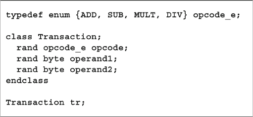
361
9.14 Exercises
2. Expand the solution to Exercise 1 to cover the test plan requirement, “Operand1
shall take on the values maximum negative (−128), zero, and maximum positive
(127).” Defi ne a coverage bin for each of these values as well as a default bin.
Label the coverpoint operand1_cp .
3. Expand the solution to Exercise 2 to cover the following test plan requirements:
a. “The opcode shall take on the values ADD or SUB” (hint: this is 1 coverage
bin).
b. “The opcode shall take on the values ADD followed by SUB” (hint: this is a
second coverage bin).
Label the coverpoint opcode_cp .
4. Expand the solution to Exercise 3 to cover the test plan requirement, “Opcode
must not equal DIV” (hint: report an error using illegal_bins ).
5. Expand the solution to Exercise 4 to collect coverage on the test plan requirement,
“The opcode shall take on the values ADD or SUB when operand1 is maximum
negative or maximum positive value.” Weight the cross coverage by 5.
6. Assuming that your covergroup is called Covcode and the instantiation name of
the covergroup is ck , expand Exercise 4 to:
a. Display the coverage of coverpoint operand1_cp referenced by the instan-
tiation name.
b. Display the coverage of coverpoint opcode_cp referenced by the covergroup
name.
363
C. Spear and G. Tumbush, SystemVerilog for Verifi cation: A Guide to Learning
the Testbench Language Features, DOI 10.1007/978-1-4614-0715-7_10,
© Springer Science+Business Media, LLC 2012
In Chapter 4 you learned how to connect the design and testbench with interfaces.
These physical interfaces represent real signals, similar to the wires that connected
ports in Verilog-1995. A testbench uses these interfaces by statically connecting to
them through ports. However, for many designs, the testbench needs to connect
dynamically to the design.
For example, in a network switch, a single driver class may connect to many
interfaces, one for each input channel of the DUT. You wouldn’t want to write a
unique driver for each channel — instead you want to write a generic driver, instan-
tiate it N times, and have it connect to each of the N physical interfaces. You can do
this in SystemVerilog by using a virtual interface, which is merely a handle or
pointer to a physical interface. A better name for a virtual interface would be a “ref
interface.”
You may need to write a testbench that attaches to several different confi gura-
tions of your design. In another example, a chip may have multiple confi gurations.
In one, the pins might drive a USB bus, whereas in another the same pins may drive
an I2C serial bus. Once again, you can use a virtual interface so you can decide at
run time which drivers to run in your testbench.
A SystemVerilog interface is more than just signals — you can put executable
code inside. This might include routines to read and write to the interface, initial and
always blocks that run code inside the interface, and assertions to constantly check
the status of the signals. However, do not put testbench code in an interface. Program
blocks have been created expressly for building a testbench, including scheduling
their execution in the Reactive region, as described in the SystemVerilog LRM.
Chapter 10
Advanced Interfaces
364 10 Advanced Interfaces
10.1 Virtual Interfaces with the ATM Router
The most common use for a virtual interface is to allow objects in a testbench to
refer to items in a replicated interface using a generic handle rather than the actual
name. Virtual interfaces are the only mechanism that can bridge the dynamic world
of objects with the static world of modules and interfaces.
10.1.1 The Testbench with Just Physical Interfaces
Chapter 4 showed how to build an interface to connect a 4x4 ATM router to a test-
bench. Sample 10.1 and 10.2 show the ATM interfaces for the receive and transmit
directions.
Sample 10.1 Rx interface with clocking block
Sample 10.2 Tx interface with clocking block
365
10.1 Virtual Interfaces with the ATM Router
These interfaces can be used in a program block shown in Sample 10.3 . This
procedural code is hard coded with interface names such as Rx0 and Tx0 . Note that
in these examples, the top module does not pass a clock to the testbench; instead the
tests synchronize with clocking blocks in the interfaces, thus allowing you to work
at a higher level of abstraction.
Sample 10.3 Testbench using physical interfaces
Figure 10.1 shows the testbench communicating with the design through virtual
interfaces.
366 10 Advanced Interfaces
The top level module must connect an array of interfaces to work with the
testbench in Sample 10.6 . The module in Sample 10.4 instantiates an array of inter-
faces, and passes this array to the testbench. Since the DUT was written with four
RX and four TX interfaces, you need to pass the individual interface array elements
into the DUT instance.
Sample 10.4 Top level module with array of interfaces
4x4 ATM
router
Testbench
Rx Tx m0
m2
m3
m1
d0
d2
d3
d1
top
Fig. 10.1 Router and testbench with interfaces
10.1.2 Testbench with Virtual Interfaces
A good OOP technique is to create a class that uses a handle to reference an object,
rather than a hard-coded object name. In this case, you can make a single Driver
class and a single Monitor class, have them operate on a handle to the data, and then
pass in the handle at run time.
367
10.1 Virtual Interfaces with the ATM Router
The program block in Sample 10.5 is still passed the 4 Rx and 4 Tx interfaces
as ports, as in Sample 10.3 , but it creates an array of virtual interfaces, vRx and vTx .
These can now be passed into the constructors for the drivers and monitors.
Sample 10.6 Testbench using virtual interfaces
Sample 10.5 Testbench using virtual interfaces
You can also skip the virtual interface array variables, and make an array in the
port list. These interfaces are passed to the constructors as shown in Sample 10.6 .
The task monitor::receive_cell in Sample 10.7 is similar to the task
receive_cell0 in Sample 10.3 , except it uses the virtual interface name Tx
instead of the physical interface Tx0 .
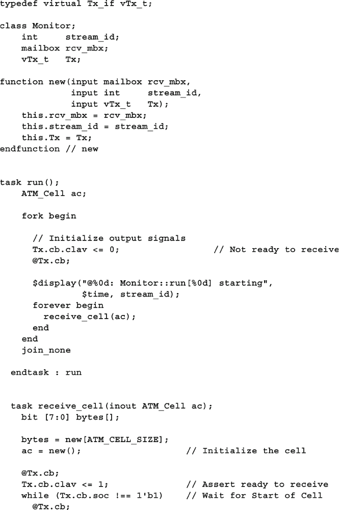
368 10 Advanced Interfaces
Sample 10.7 Monitor class using virtual interfaces
369
10.1 Virtual Interfaces with the ATM Router
A common mistake when creating a testbench is to leave off the
modport name from a virtual interface declaration. The program in
Sample 10.5 declares Tx_if.TB Tx0 in the port list, so it can only
assign Tx0 to a virtual interface declared with the TB modport. See
the declaration of the virtual interface Tx in Sample 10.7 .
10.1.3 Connecting the Testbench to an Interface in Port List
This book shows tests that connect to the DUT with interfaces in the port list. This
style is comfortable to Verilog users who have always connected modules using
signals in ports. Sample 10.8 is the top level module, also known as a test harness,
which connects the DUT and test using an interface in the port list.
Sample 10.8 Test harness using an interface in the port list
Sample 10.9 shows the program block with an interface in the port list.
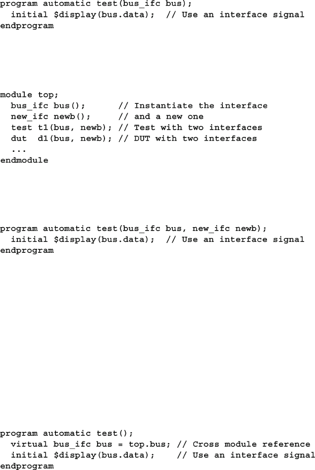
370 10 Advanced Interfaces
What happens if you add a new interface to your design? The test harness in
Sample 10.10 declares the new bus and puts it in the port lists.
Sample 10.11 Test with two interfaces in the port list
Sample 10.9 Test with an interface in the port list
Sample 10.10 Top module with a second interface in the test’s port list
Now you have to change the test in Sample 10.9 to include another interface in
the port list, giving the test in Sample 10.11 .
Adding a new interface to your design means you need to edit all existing tests
so they can plug into the test harness. How can you avoid this extra work? Avoid
port connections!
10.1.4 Connecting the Test to an Interface with an XMR
Your test needs to connect to the physical interface in the harness, so use a cross
module reference (XMR) and a virtual interface in the program block as shown in
Sample 10.12 . You must use a virtual interface so you can assign it the physical
interface in the top level module.
Sample 10.12 Test with virtual interface and XMR
The program connects to the test harness shown in Sample 10.13 .
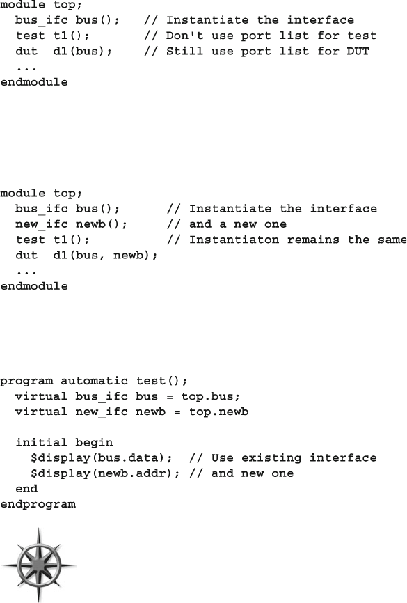
371
10.1 Virtual Interfaces with the ATM Router
This approach is recommended by methodologies such as the VMM to make
your test code more reusable. If you add a new interface to your design, as shown in
Sample 10.14 , the test harness changes, but existing tests don’t have to change.
Sample 10.13 Test harness without interfaces in the port list
Sample 10.14 Test harness with a second interface
The harness in Sample 10.14 works with the test in Sample 10.12 that does not
know about the new interface, as well as the test in Sample 10.15 that does.
Sample 10.15 Test with two virtual interfaces and XMRs
Some methodologies have a rule that makes the connection between
tests and harnesses slightly more complicated than with traditional
ports, but means you won’t have to modify existing tests, even if
the design changes. The examples in this book use the simple style
of interfaces in the port lists, but you should decide if test reuse is
important enough to change your coding style.
372 10 Advanced Interfaces
10.2 Connecting to Multiple Design Confi gurations
A common challenge to verifying a design is that it may have several confi gura-
tions. You could make a separate testbench for each confi guration, but this could
lead to a combinatorial explosion as you explore every alternative. Instead, you can
use virtual interfaces to dynamically connect to the optional interfaces.
10.2.1 A Mesh Design
Sample 10.16 is built of a simple replicated component, an 8-bit counter. This
resembles a DUT that has a device such as a network chip or processor that is
instantiated repeatedly in a mesh confi guration. The key idea is that the top-level
module creates an array of interfaces and counters. Now the testbench can connect
its array of virtual interfaces to the physical ones.
Sample 10.16 shows the code for the counter’s interface, X_if . If the code
printed the signal values with a $monitor, they would display when any signal
changed. Instead, the always block waits until the clocking block changes, then
prints the values of the signals at the end of the time slot with $strobe . The result
is you are now working at a higher level of abstraction, seeing the values cycle by
cycle instead of the individual events.
Sample 10.16 Interface for 8-bit counter
The simple counter is shown in Sample 10.17 .
373
10.2 Connecting to Multiple Design Confi gurations
The top-level module in Sample 10.18 uses a generate statement to instantiate
NUM_XI interfaces and counters, but only one testbench.
Sample 10.17 Counter model using X_if interface
Sample 10.18 Top-level module with an array of virtual interfaces
In Sample 10.19 , the key line in the testbench is where the local virtual inter-
face array, vxi , is assigned to point to the array of physical interfaces in the top
module, top.xi . (Note that this example takes some shortcuts compared to the
374 10 Advanced Interfaces
recommendations in Chapter 8 . To simplify Sample 10.18 , the environment class
has been merged with the test, whereas the generator, agent, and driver layers have
been compressed into the driver.)
The testbench assumes there is at least one counter and thus at least one X inter-
face. If your design could have zero counters, you would have to use a dynamic array
to hold the virtual interfaces, as a fi xed-size array cannot have a size of zero. The
actual number of interfaces is passed as a parameter from the top-level module.
Sample 10.19 Counter testbench using virtual interfaces
Of course in this simple example, you could just pass the interface directly into
the Driver’s constructor, rather than make a separate variable.
In Sample 10.20 , the Driver class uses a single virtual interface to drive and
sample signals from the counter.
375
10.2 Connecting to Multiple Design Confi gurations
10.2.2 Using Typedefs with Virtual Interfaces
You can reduce the amount of typing, and ensure you always use the correct mod-
port by replacing “ virtual X_if.TB ” with a typedef , as shown in Sample 10.21
through 10.23 , of the interface, testbench, and driver.
Sample 10.20 Driver class using virtual interfaces
Sample 10.21 Interface with a typedef
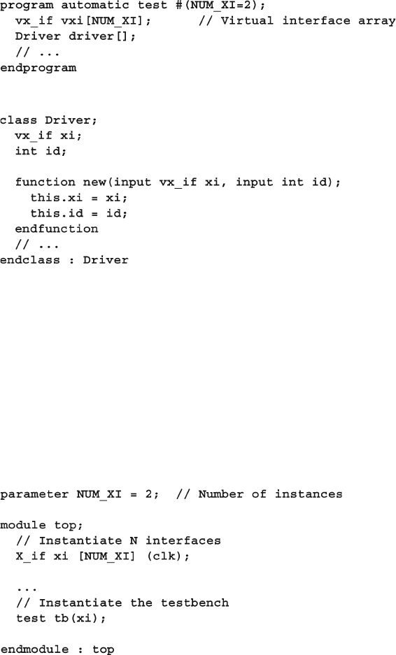
376 10 Advanced Interfaces
10.2.3 Passing Virtual Interface Array Using a Port
The previous examples passed the array of virtual interfaces using a cross module
reference (XMR). An alternative is to pass the array in a port. Since the array in the
top module is static and so only needs to be referenced once, the XMR style makes
more sense than using a port that normally is used to pass changing values.
Sample 10.24 uses a global parameter to defi ne the number of X interfaces. Here
is a snippet of the top module.
Sample 10.22 Testbench using a typedef for virtual interfaces
Sample 10.23 Driver using a typedef for virtual interfaces
Sample 10.24 Testbench using an array of virtual interfaces
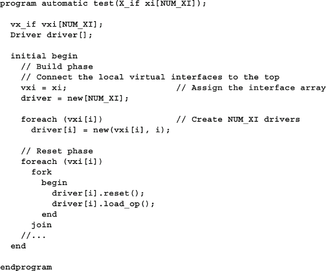
377
10.3 Parameterized Interfaces and Virtual Interfaces
The testbench that uses the virtual interfaces is shown in Sample 10.25 . It creates
an array of virtual interfaces so that it can pass them into the constructor for the
driver class, or just pass the interface directly from the port.
Sample 10.25 Testbench passing virtual interfaces with a port
10.3 Parameterized Interfaces and Virtual Interfaces
The example in Section 10.2 shows an 8-bit counter and matching busses. What if
you want to vary the counter’s width? Verilog-1995 allows you to parameterize
modules, and System Verilog extends this concept with parameterized interfaces
and virtual interfaces.
First, update the counter, originally shown in Sample 10.17 with parameters.
This only requires changing the fi rst few lines. Sample 10.26 now passes the num-
ber of interfaces in as a parameter too.
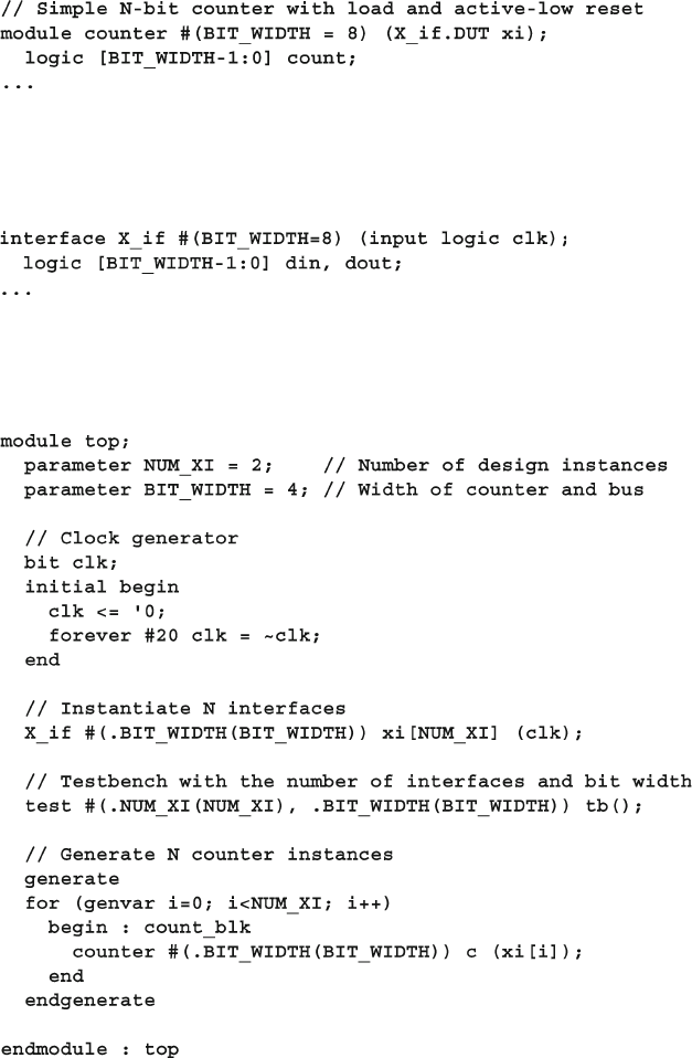
378 10 Advanced Interfaces
Sample 10.27 Parameterized interface for 8-bit counter
Sample 10.28 Parameterized top-level module with an array of virtual interfaces
Sample 10.26 Parameterized counter model using X_if interface
Next, Sample 10.27 adds the bit width parameter to the interface in Sample 10.16 .
Sample 10.28 shows the parameter being passed into the testbench.
Lastly are the testbench module and
Driver class are shown in Samples 10.29
and 10.30 . These have virtual interfaces that must be parameterized. The syntax for
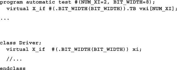
379
10.4 Procedural Code in an Interface
this is a little tricky, especially when you have a modport. First, the testbench,
updated from Sample 10.19 . Notice how the parameter goes between the type name
and the modport.
Sample 10.30 Driver class using virtual interfaces
Sample 10.29 Parameterized counter testbench using virtual interfaces
10.4 Procedural Code in an Interface
Just as a class contains both variables and routines, an interface can contain code
such as routines, assertions, and initial and always blocks. Recall that an inter-
face includes the signals and functionality of the communication between two
blocks. So the interface block for a bus can contain the signals and also routines to
perform commands such as a read or write. The inner workings of these routines are
hidden from the external blocks, allowing you to defer the actual implementation.
Access to these routines is controlled using the modport statement, just as with
signals. A task or function is imported into a modport so that it is then visible to
any block that uses the modport .
These routines can be used by both the design and the testbench. This approach
ensures that both are using the same protocol, eliminating a common source of test-
bench bugs. However, not all synthesis tools can handle routines in an interface.
A problem with sharing code between the design and testbench is that the inde-
pendence between the design and verifi cation teams is lost. If only one person
implements the interface protocol for both parts, who checks it?
You can verify a protocol with assertions in an interface. An assertion can check
for illegal combinations, such as protocol violations and unknown values. These can
display state information and stop simulation immediately so that you can easily
debug the problem. An assertion can also fi re when good transactions occur.
Functional coverage code uses this type of assertion to trigger the gathering of cov-
erage information.
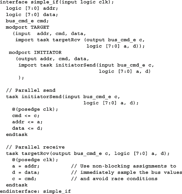
380 10 Advanced Interfaces
10.4.1 Interface with Parallel Protocol
When creating your system, you may not know whether to choose a parallel or
serial protocol. The interface in Sample
10.31 has two tasks, initiatorSend
and targetRcv , that send a transaction between two blocks using the interface
signals. It sends the address and data in parallel across two 8-bit buses.
Sample 10.31 Interface with tasks for parallel protocol
10.4.2 Interface with Serial Protocol
The interface in Sample 10.32 implements a serial interface for sending and receiv-
ing the address and data values. It has the same interface and routine names as
Sample 10.31 , so you can swap between the two without having to change any
design or testbench code.
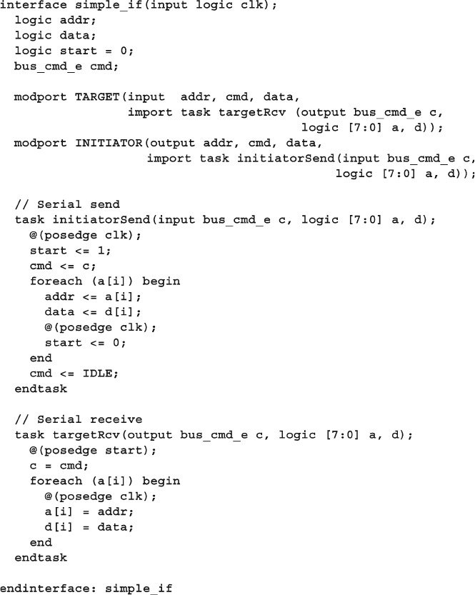
381
10.4 Procedural Code in an Interface
10.4.3 Limitations of Interface Code
Tasks in interfaces are fi ne for RTL, where the functionality is strictly defi ned.
However, these tasks are a poor choice for any type of verifi cation IP. Interfaces and
their code cannot be extended, overloaded, or dynamically instantiated based on
confi guration. An interface cannot have private data. Any code for verifi cation needs
Sample 10.32 Interface with tasks for serial protocol
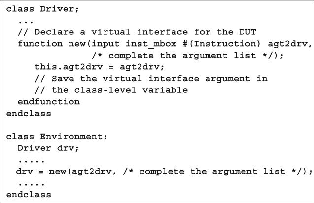
382 10 Advanced Interfaces
maximum fl exibility and confi gurability, and so should go in classes that run in a
program block.
10.5 Conclusion
The interface construct in SystemVerilog provides a powerful technique to group
together the connectivity, timing, and functionality for the communication between
blocks. In this chapter you saw how you can create a single testbench that connects
to many different design confi gurations containing multiple interfaces. Your signal
layer code can connect to a variable number of physical interfaces at run time with
virtual interfaces. Additionally, an interface can have routines that drive the signals
and assertions to check the protocol, but put the test in a program block, not an
interface.
In many ways, an interface can resemble a class with pointers, encapsulation,
and abstraction. This lets you create an interface to model your system at a higher
level than Verilog’s traditional ports and wires. Just remember to keep the testbench
in the program block.
10.6 Exercises
1. Complete the following code, as indicated by the comments.
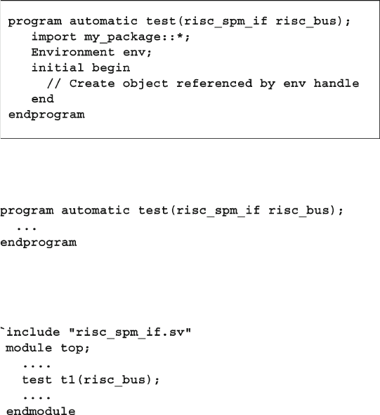
383
10.6 Exercises
2. Using the solution to Exercise 1, complete the following code as indicated by the
comments.
3. Modify the following program declaration to use cross module references (XMR).
Assume the top module that contains the interface is named
top .
Modify the following instantiation of program test to use cross module
references (XMR).
4. Expand the solution to Exercise 3 to create NUM_RISC_BUS environments and
create NUM_RISC_BUS interfaces.
5. Expand the solution to Exercise 3 to use a typedef for the virtual interface.
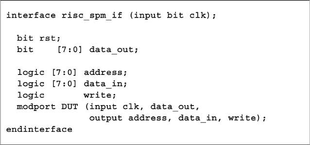
384 10 Advanced Interfaces
6. Modify the following interface to use a parameter, ADDRESS_WIDTH . By default
the addressing space supports 256 words.
385
C. Spear and G. Tumbush, SystemVerilog for Verifi cation: A Guide to Learning
the Testbench Language Features, DOI 10.1007/978-1-4614-0715-7_11,
© Springer Science+Business Media, LLC 2012
This chapter applies the many concepts you have learned about SystemVerilog
features to verify a design. The testbench creates constrained random stimulus, and
gathers functional coverage. It is structured according to the guidelines from Chapter 8
so you can inject new behavior without modifying the lower-level blocks.
The design is an ATM switch that was shown in Sutherland [2006], who based
his SystemVerilog description on an example from Janick Bergeron’s Verifi cation
Guild. Sutherland took the original Verilog design and used SystemVerilog design
features to create a switch that can be confi gured from 4×4 to 16×16. The testbench
in the original example creates ATM cells using $urandom , overwrites certain fi elds
with ID values, sends them through the device, then checks that the same values
were received.
The entire example, with the testbench and ATM switch, is available for
download at http://chris.spear.net/systemverilog . This chapter shows
just the testbench code.
11.1 Design Blocks
The overall connection between the design and testbench, shown in Fig. 11.1 ,
follows the pattern shown in Chapter 4 .
Chapter 11
A Complete SystemVerilog Testbench
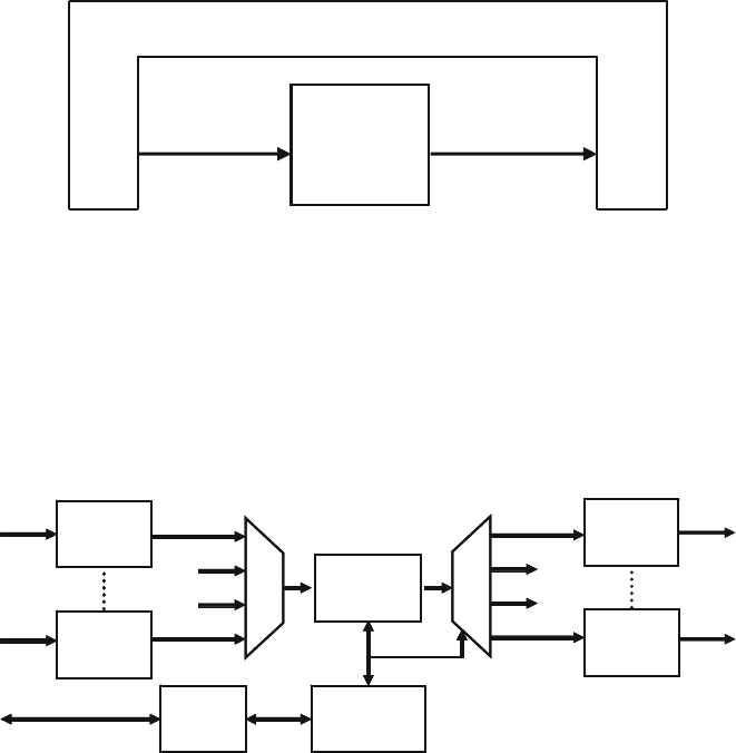
386 11 A Complete SystemVerilog Testbench
The top level of the design is called squat , as shown in Fig. 11.2 . The module
has 1..N Utopia Rx interfaces that are sending UNI formatted cells. Inside the
DUT, cells are stored, converted to NNI format, and forwarded to the Tx interfaces.
The forwarding is done according to a lookup table that is addressed with the VPI fi eld
of the incoming cell. The table is programmed through the management interface.
The top level module in Sample 11.1 defi nes arrays of interfaces for the Rx and
Tx ports.
Fig. 11.1 The testbench — design environment
Testbench
Design
Under
Test
inputs outputs
Fig. 11.2 Block diagram for the squat design
Rx
Utopia
Rx
Utopia
Rewrite
Cell
Tx
Utopia
Tx
Utopia
Register
File
Mgmt
I/F
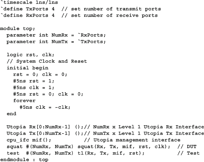
387
11.1 Design Blocks
The testbench program in Sample 11.2 passes the interfaces and signals through
the port list. See Section 10.1.4 for a discussion on ports vs. cross module refer-
ences. The actual testbench code is in the Environment class. The program steps
through the phases of the environment. In order to work at a higher level of abstrac-
tion, the testbench only uses clocking blocks in the interfaces to synchronize with
the DUT, not low level clocks.
Sample 11.1 Top level module
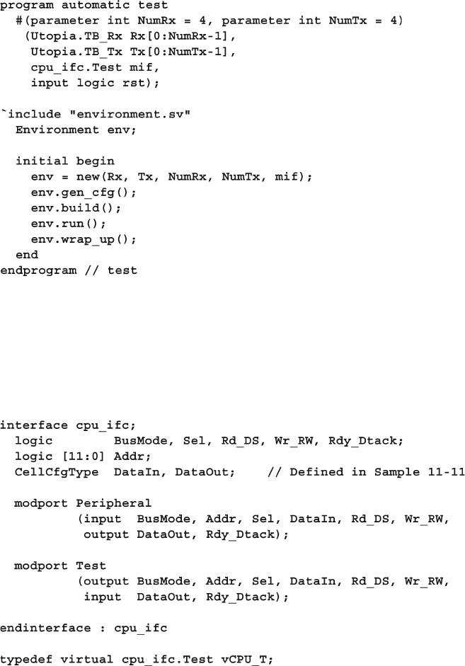
388 11 A Complete SystemVerilog Testbench
The testbench loads control information into the ATM switch through the
Management interface, also known as the CPU interface, shown in Sample 11.3 .
In this chapter’s examples, the interface is only used to load the lookup table that
maps VPI to forwarding masks.
Sample 11.2 Testbench program
Sample 11.3 CPU Management Interface
Sample 11.4 shows the Utopia interface, which is used by the testbench to
communicate with the squat design by transmitting and receiving ATM cells.
The interface has clocking blocks for the transmit and receive paths, and modports
for the design and testbench connections to the interface.
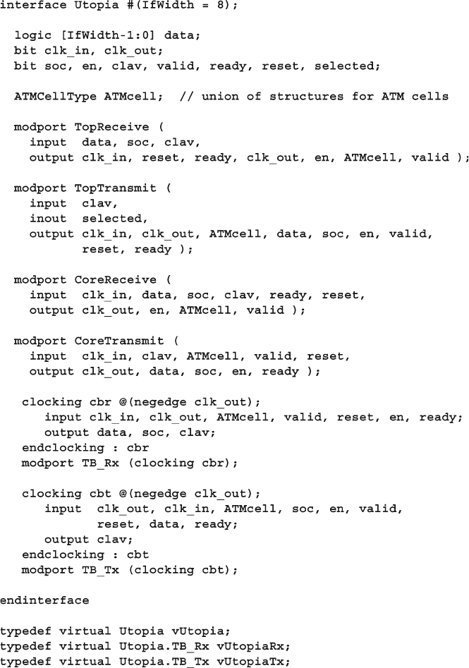
389
11.1 Design Blocks
Sample 11.4 Utopia interface
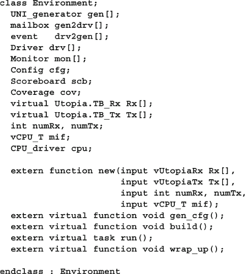
390 11 A Complete SystemVerilog Testbench
11.2 Testbench Blocks
The environment class, as shown in Section 8.2.1 , is the scaffolding that supports
the testbench structure. Inside this class lies the blocks of your layered testbench,
such as generators, drivers, monitors, and scoreboard. The environment also con-
trols the sequencing of the four testbench steps: generate a random confi guration,
build the testbench environment, run the test and wait for it to complete, and a wrap-
up phase to shut down the system and generate reports. Sample
11.5 shows the ATM
environment class. It uses the virtual interface vCPU_T defi ned in Sample 11.3 .
Sample 11.5 Environment class header
With the $test$plusargs() system task, the Environment class constructor
in Sample 11.6 looks for the VCS switch +ntb_random_seed , which sets the
random seed for the simulation. The system task $value$plusargs() extracts
the value from the switch. Your simulator may have a different way to set the seed.
It is important to print the seed in the log fi le so that if the test fails, you can run it
again with the same value.
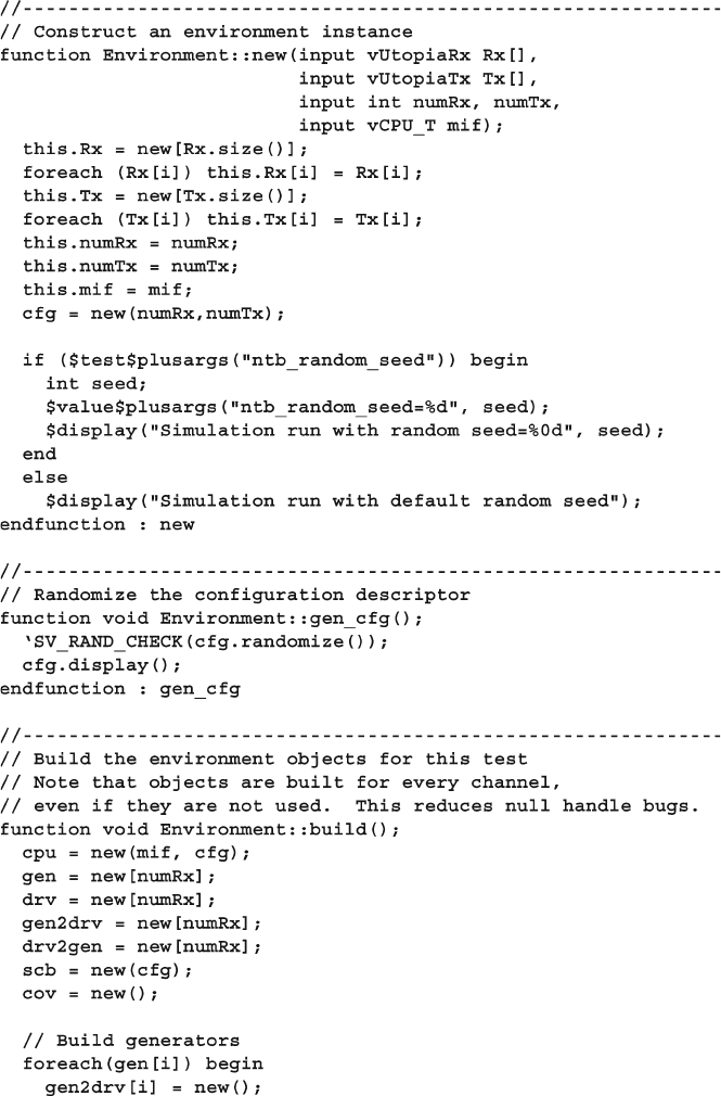
391
11.2 Testbench Blocks
Sample 11.6 Environment class methods
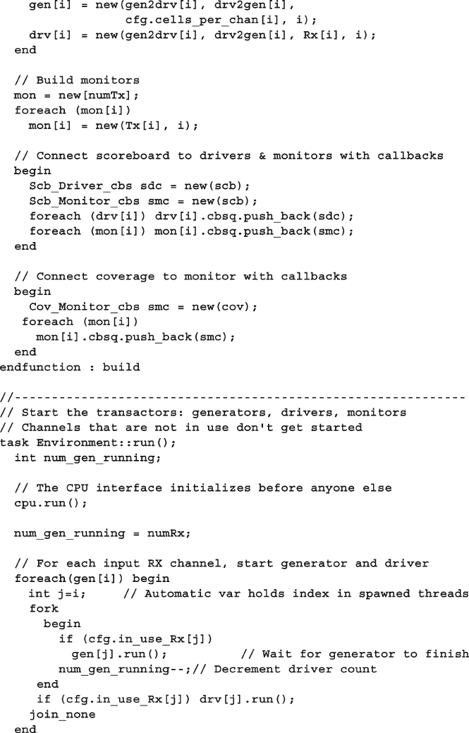
392 11 A Complete SystemVerilog Testbench
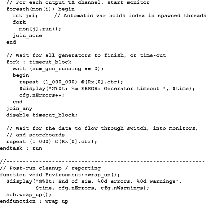
393
11.2 Testbench Blocks
The method Environment::build in Sample 11.6 connects the scoreboard to
the driver and monitor with the callback class, which is shown in Sample 11.7 ,
Scb_Driver_cbs . This class sends the expected values to the scoreboard. The
base driver callback class, Driver_cbs , is shown in Sample 11.20 .
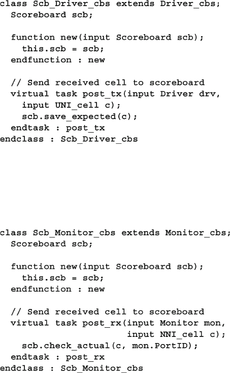
394 11 A Complete SystemVerilog Testbench
The callback class in Sample 11.8 , Scb_Monitor_cbs , connects the monitor
with the scoreboard. The base monitor callback class, Monitor_cbs , is shown in
Sample 11.21 .
Sample 11.7 Callback class connects driver and scoreboard
Sample 11.8 Callback class connects monitor and scoreboard
The environment connects the monitor to the coverage class with the fi nal
callback class, Cov_Monitor_cbs , shown in Sample 11.9 .
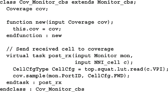
395
11.2 Testbench Blocks
The random confi guration class header is shown in Sample 11.10 . It starts with
nCells , a random value for the total number of cells that fl ow through the system.
The constraint c_nCells_valid ensures that the number of cells is valid by being
greater than zero, whereas c_nCells_reasonable limits the test to a reasonable
size, 1000 cells. You can disable or override this if you want longer tests.
Next is a dynamic bit array, in_use_Rx , to specify which Rx channels into the
switch are active. This is used in Sample 11.6 in the run method so that only active
channels run.
The array cells_per_chan is used to randomly divide the total number of cells
across the active channels. The constraint zero_unused_channels sets the num-
ber of cells to zero for inactive channels. To help the solver, the active channel mask
is solved before dividing up the cells between channels. Otherwise, a channel would
be inactive only if the number of cells assigned to it was zero, which is very
unlikely.
Sample 11.9 Callback class connects the monitor and coverage
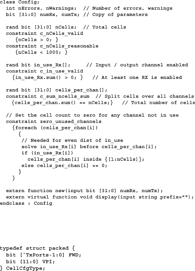
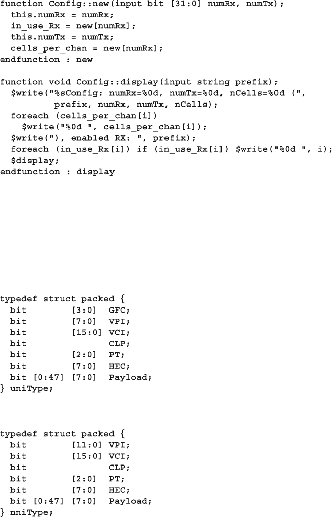
397
11.2 Testbench Blocks
The ATM switch accepts UNI formatted cells and sends out NNI formatted cells.
These cells are sent through both an OOP testbench and a structural design, so they
are defi ned using typedef . The major difference between the two formats is that
the UNI’s GFC and VPI fi eld are merged into the NNI’s VPI. The defi nitions in
Sample 11.13 through 11.15 are from Sutherland [2006].
Sample 11.12 Confi guration class methods
Sample 11.13 UNI cell format
Sample 11.14 NNI cell format
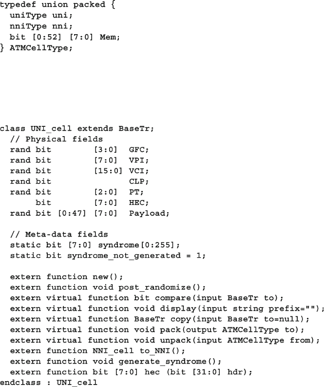
398 11 A Complete SystemVerilog Testbench
The UNI and NNI cells are merged with a byte memory to form a universal type,
shown in Sample 11.15 .
Sample 11.15 ATMCellType
The testbench generates constrained random ATM cells, shown in Sample 11.16,
that are extended from the BaseTr class, defi ned in Sample 8.24.
Sample 11.16 UNI_cell defi nition
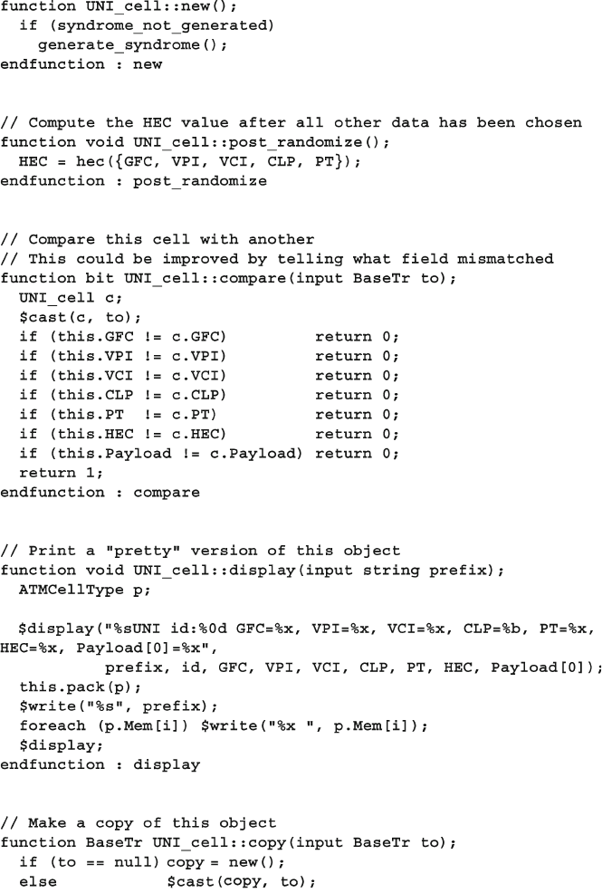
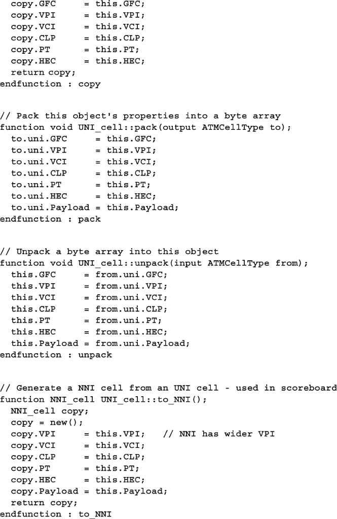
400 11 A Complete SystemVerilog Testbench

401
11.2 Testbench Blocks
The NNI_cell class is almost identical to UNI_cell , except that it does not
have a GFC fi eld, or a method to convert to a UNI_cell .
Sample 11.18 shows the UNI cells random atomic generator, as originally shown
in Section 8.2. The generator randomizes the blueprint instance of the UNI cell, and
then sends out a copy of the cell to the driver.
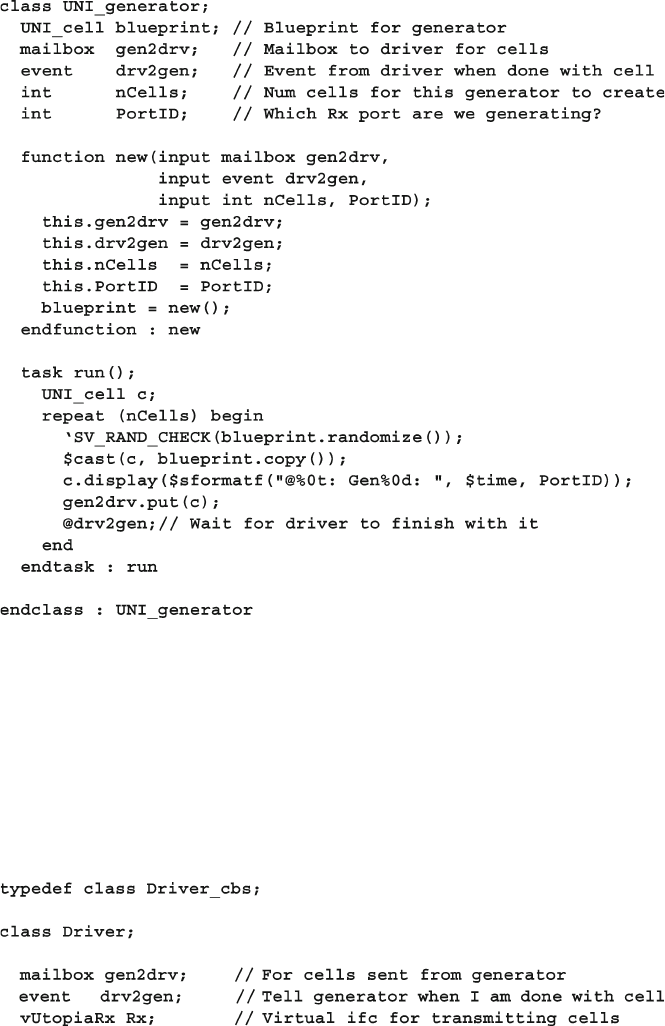
402 11 A Complete SystemVerilog Testbench
Sample 11.19 shows the Driver class that sends UNI cells into the ATM switch.
This class uses the driver callbacks in Sample 11.20 . Note that there is a circular
relationship here. The Driver class has a queue of Driver_cbs objects, and the
pre_tx() and post_tx() methods in Driver_cbs are passed Driver objects.
When you compile the two classes, you may need either typedef class Driver ;
before the Driver_cbs class defi nition, or typedef class Driver_cbs ; before
the Driver class defi nition.
Sample 11.19 driver class
Sample 11.18 UNI_generator class
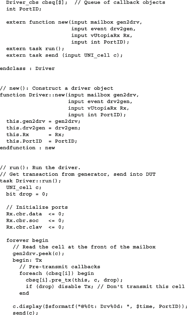
403
11.2 Testbench Blocks
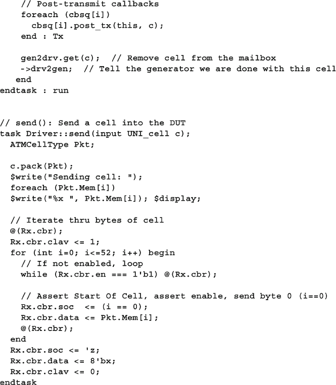
404 11 A Complete SystemVerilog Testbench
Sample 11.20 shows the driver callback class which has simple callbacks that are
called before & after a cell is transmitted. This class has empty tasks, which are used
by default. A test case can extend this class to inject new behavior in the driver
without having to change any code in the driver
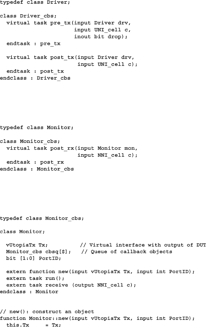
405
11.2 Testbench Blocks
The Monitor class in Sample 11.21 has a very simple callback, with just one
task that is called after a cell is received.
Sample 11.21 Monitor callback class
Sample 11.20 Driver callback class
Sample 11.22 The Monitor class
Sample 11.22 shows the Monitor class. Like the Driver class, this uses a
typedef to break the circular compile dependency with Monitor_cbs .
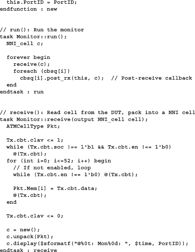
406 11 A Complete SystemVerilog Testbench
The scoreboard in Sample 11.23 gets expected cells from the driver through the
function save_expected , and the cells actually received by the monitor with the
function check_actual . The function save_expected() is called from the call-
back Scb_Driver_cbs::post_tx() , shown in Sample 11.7 . The function
check_actual () is called from Scb_Monitor_cbs::post_rx() in Sample 11.8 .
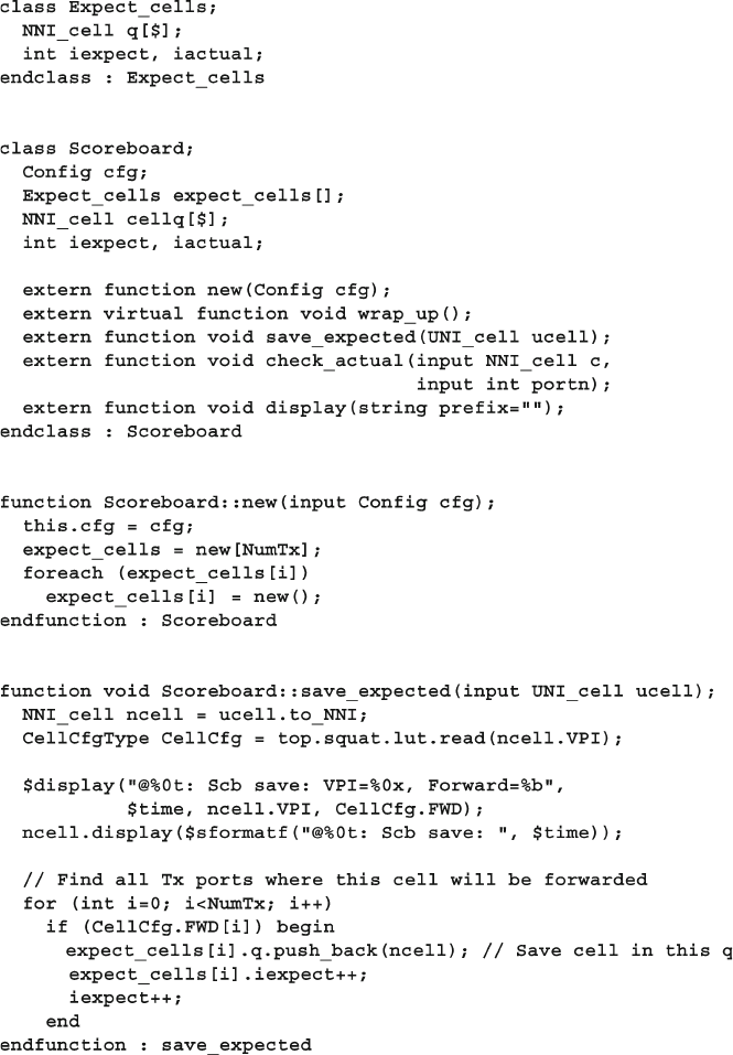
407
11.2 Testbench Blocks
Sample 11.23 The Scoreboard class
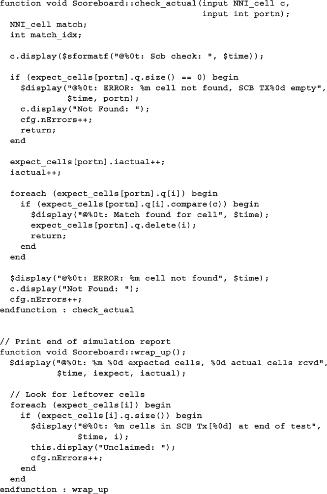
408 11 A Complete SystemVerilog Testbench
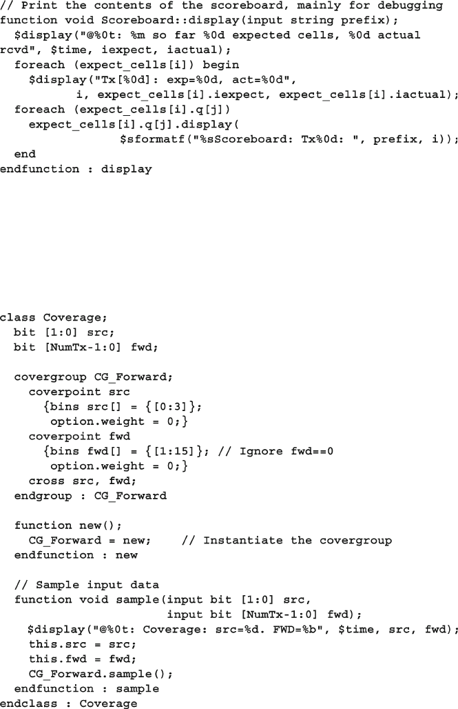
409
11.2 Testbench Blocks
Sample 11.24 shows the class used to gather functional coverage. Since the cov-
erage only looks at data in a single class, the cover group is defi ned and instantiated
inside the Coverage class. The data values are read by the class’s sample() method,
then the cover group’s sample() method is called to record the values.
Sample 11.24 Functional coverage class
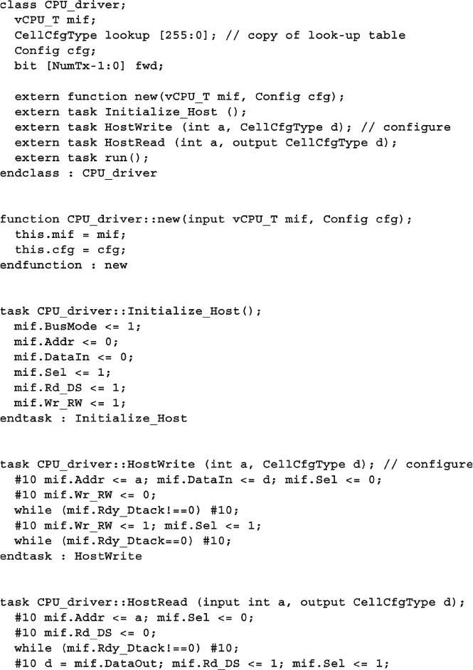
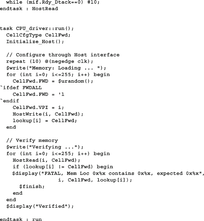
411
11.3 Alternate Tests
11.3 Alternate Tests
The simplest test program is shown in Sample 11.2 and runs with very few con-
straints. During verifi cation, you will be creating many tests, depending on the
major functionality to be tested. Each test can then be run with different seeds.
11.3.1 Your First Test - Just One Cell
The fi rst test you run should probably have just one cell, such as the test in Sample
11.26 . You can add a new constraint to the Confi g class by extending it, and then
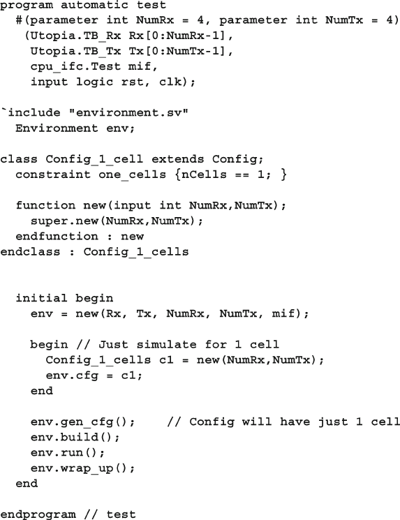
412 11 A Complete SystemVerilog Testbench
injecting a new object into the environment before randomization. Once this test
works, you can try two cells, then rewrite the constraint on the number of cells to
run longer sequences.
Sample 11.26 Test with one cell
11.3.2 Randomly Drop Cells
The next test you may run creates errors by occasionally dropping cells, as shown
in Sample 11.27 . You need to make a callback for the driver that sets the drop bit.
Then, in the test, inject this new functionality after the driver class has been con-
structed during the build phase.
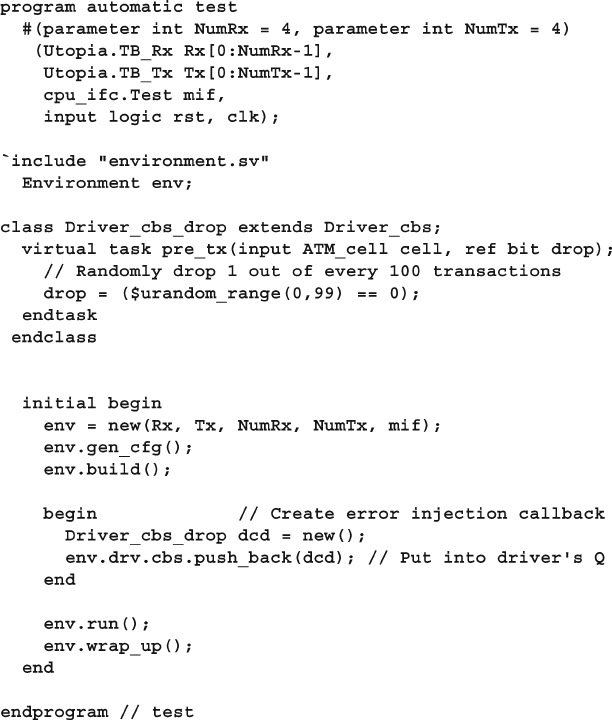
413
11.4 Conclusion
11.4 Conclusion
This chapter shows how you can build a layered testbench, following the guidelines
in this book. You can then create new tests by just modifying a single fi le and inject-
ing new behavior, utilizing the hooks such as callbacks and multiple environment
phases.
The testbench was able to get to 100% functional coverage of the ATM switch,
at least for the basic cover group. You can use this example to explore more about
SystemVerilog testbenches.
Sample 11.27 Test that drops cells using driver callback
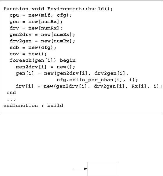
414 11 A Complete SystemVerilog Testbench
11.5 Exercises
1. In Sample 11.2 , why is clk not passed into the port list of program test ?
2. In Sample 11.6 , could numRx be substituted for Rx.size() ? Why or why not?
3. For the following code snippet from Sample 11.6 , explain what is being created
for each statement.
4. In Sample 11.9 , what coverage object does the handle cov point to?
5. In Sample 11.17 , the function UNI_cell::copy assumes that the handle to the
object UNI_cell points to an object of class UNI_cell as depicted in the following
drawing. Draw what object the handle dst points to for the following function calls.
UNI_cell
handle
a . copy() ;
b . copy(handle) ;
6. In Sample 11.18 , why are the $cast () required?
7. In Sample 11.19 and 11.20 , why are the typedef declaration needed?
8. In Sample 11.19 , why is peek() used fi rst and then later a get() ?
9. In Sample 11.23 , is the error message “ …cell not found… ” in the function
check_actual printed every time it are called? Why or why not?
10. Why do classes Environment, Scoreboard , and CPU_driver all defi ne a
handle to class Confi g ? Are 3 objects of class Confi g created?
415
C. Spear and G. Tumbush, SystemVerilog for Verifi cation: A Guide to Learning
the Testbench Language Features, DOI 10.1007/978-1-4614-0715-7_12,
© Springer Science+Business Media, LLC 2012
In Verilog, you can communicate with C routines using the Programming Language
Interface. With the three generations of the PLI: TF (Task / Function), ACC (Access),
and VPI (Verifi cation Procedural Interface), you can create delay calculators, con-
nect and synchronize multiple simulators, and add debug tools such as waveform
displays. However the PLI’s greatest strength is also its greatest weakness. If you
just want to connect a simple C routine using the PLI, you need to write dozens
of lines of code, and understand many different concepts such as synchronizing
with multiple simulation phases, call frames, and instance pointers. Additionally,
the PLI adds overhead to your simulation as it copies data between the Verilog and
C domains, in order to protect Verilog data structures from corruption.
SystemVerilog introduces the Direct Programming Interface (DPI), an easier
way to interface with C, C++, or any other foreign language. Once you declare or
“import” the C routine with the import statement, you can call it as if it were
any SystemVerilog routine. Additionally, your C code can call SystemVerilog
routines. With the DPI you can connect C code that reads stimulus, contains a
ref erence model, or just extends SystemVerilog with new functionality. Currently
SystemVerilog only supports an interface to the C language. C++ code has to be
wrapped to look like C.
If you have a SystemC model that does not consume time, and that you want
to connect to SystemVerilog, you can use the DPI. SystemC models with time-
consuming methods are best connected with the utilities built into your favorite
simulator.
The fi rst half of this chapter is data-centric and shows how you can pass different
data types between SystemVerilog and C. The second half is control centric, show-
ing how you can pass control back and forth between SystemVerilog and C. While
the actual C code is trivial, with the factorial function, the Fibonacci series, and
counters, they are easy to understand so you can quickly substitute your own code.
Chapter 12
Interfacing with C/C++
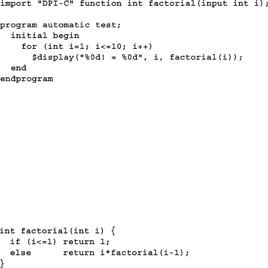
416 12 Interfacing with C/C++
12.1 Passing Simple Values
The fi rst few examples in this chapter show you how to pass integral values between
SystemVerilog and C, and the mechanics of how to declare routines and their argu-
ments on both sides. Later sections show how to pass arrays and structures.
12.1.1 Passing Integer and Real Values
The most basic data type that you can pass between SystemVerilog and C is an int ,
the 2-state, 32-bit type. Sample 12.1 shows the SystemVerilog code that calls a C
factorial routine, shown in Sample 12.2 .
Sample 12.1 SystemVerilog code calling C factorial routine
Sample 12.2 C factorial function
The import statement declares that a SystemVerilog routine factorial is
implemented in a foreign language such as C. The modifi er " DPI-C " specifi es that
this is a Direct Programing Interface routine, and the rest of the statement describes
the routine arguments.
Sample 12.1 passes 32-bit signed values using the SystemVerilog int data type
that maps directly to the C int type. The SystemVerilog int is always 32 bits,
whereas the width of an int in C is operating system dependent. The C function in
Sample 12.2 takes an integer as an input and so the DPI passes the argument by
value.
12.1.2 The Import Declaration
The import declaration defi nes the prototype of the C task or function, but using
SystemVerilog types. A C function with a return value is mapped to a SystemVerilog
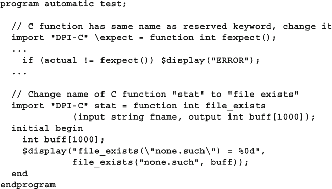
417
12.1 Passing Simple Values
function. A void C function can be mapped to a SystemVerilog task or void function.
If the name of the imported C function confl icts with a SystemVerilog name, you can
import the function with a new name. In Sample 12.3 , the C function expect is
mapped to the SystemVerilog name
fexpect , as the name expect is a reserved
keyword in SystemVerilog. The name expect becomes a global symbol, used to link
with the C code, whereas
fexpect is a local SystemVerilog symbol. In the second
half of the example, the C function stat is given a new name in SystemVerilog,
fi le_exists . SystemVerilog does not support overloading a routine, for example by
importing expect once with a real argument and once with an int .
Sample 12.3 Changing the name of an imported function
You can import routines anywhere in your SystemVerilog code where you can
declare a routine including inside programs, modules, interfaces, packages, and $unit ,
the compilation-unit space. The imported routine will be local to the declaration
space in which it is declared. If you need to call an imported routine in several loca-
tions in your code, put the import statement in a package which you import where
it is needed. Any changes to the import statements are localized to the package.
12.1.3 Argument Directions
Imported C routines can have zero or more arguments. By default the argument
direction is input (data goes from SystemVerilog to C), but can also be output
and inout . The direction ref is not supported. A function can return a simple value
such as an integer or real number, or have no return value if you make it void .
Sample 12.4 shows how to specify argument directions.
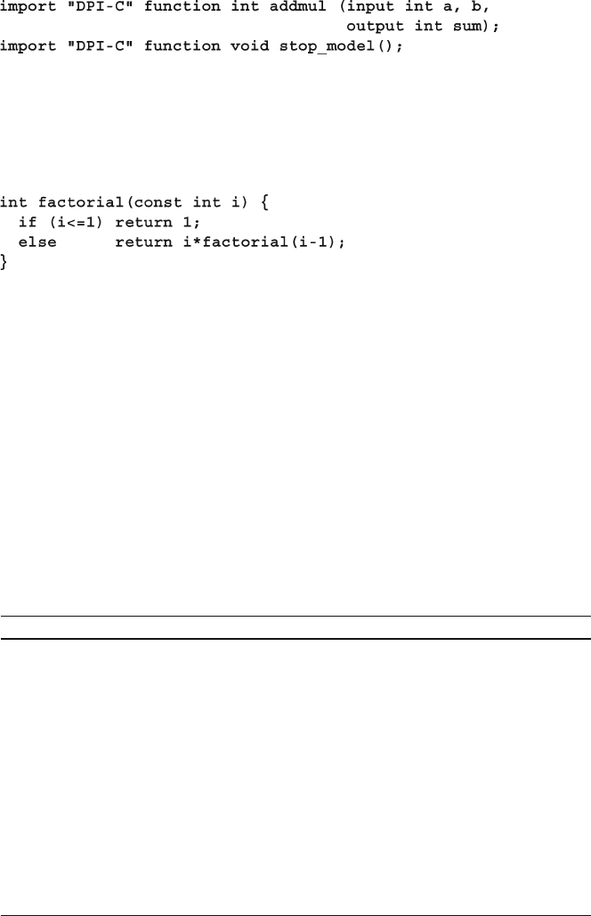
418 12 Interfacing with C/C++
Table 12.1 Data types mapping between SystemVerilog and C
SystemVerilog C (input ) C (output )
byte char char*
shortint short int short int*
int int int*
longint long long int long int*
shortreal fl oat fl oat*
real double double*
string const char* char**
string [N] const char** char**
bit svBit or unsigned char svBit* or unsigned char*
logic, reg svLogic or unsigned char svLogic* or unsigned char*
bit[N:0] const svBitVecVal* svBitVecVal*
reg[N:0] logic[N:0] const svLogicVecVal* svLogicVecVal*
unsized array[] const svOpenArrayHandle svOpenArrayHandle
chandle const void* void*
Sample 12.4 Argument directions
You can reduce the chances of bugs in your C code by declaring any input argu-
ments as const as shown in Sample 12.5 so the C compiler will give an error for
any write to an input.
Sample 12.5 C factorial routine with const argument
12.1.4 Argument Types
Each variable that is passed through the DPI has two matching defi nitions: one for
the SystemVerilog side, and one for the C side. It is your responsibility to use com-
patible types. The SystemVerilog simulator cannot compare the types as it is unable
to read the C code. (The VCS compiler produces vc_hdrs.h and Questa creates
incl.h with the C header for any routine that you have imported. You can use this
fi le as a guide to matching the types.)
Table 12.1 shows the data type mapping between SystemVerilog and the inputs
and outputs of C routines. The C structures are defi ned in the include fi le svdpi.h .
Arrays mapping is discussed in Section 12.4 and 12.5 , and structures are discussed
in Section 12.6 .
419
12.2 Connecting to a Simple C Routine
Note that some mappings are not exact. For example, a bit in
SystemVerilog maps to svBit in C, which ultimately maps to
unsigned char in the svdpi.h include fi le. As a result, you
could write illegal values into the upper bits.
The LRM limits imported function results “small values”, which include:
void, byte,
shortint, int, longint, real, shortreal, chandle , and string , plus single
bit values of type bit and logic . A function cannot return a vector such as bit
[6:0] as this would require returning a pointer to a svBitVecVal structure.
12.1.5 Importing a Math Library Routine
Sample 12.6 shows how you can call many functions in the C math library directly,
without a C wrapper, thereby reducing the amount of code that you need to write.
The Verilog real type maps to a C double .
Sample 12.6 Importing a C math function
12.2 Connecting to a Simple C Routine
Your C code might contain a simulation model, such as a processor, that is instan-
tiated side by side with Verilog models. Or your code could be a reference model
that is compared to a Verilog model at the transaction or cycle level. Many exam-
ples in this chapter show an 7-bit counter written in C or C++. Though very simple,
the counter has the same parts as a complex model, with inputs, outputs, storage
of internal values between calls, and the need to support multiple instances. The
counter is 7 bits to show what happens when a hardware type does not match a
C type.
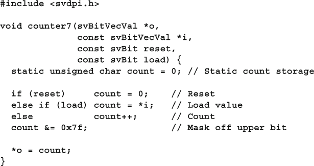
420 12 Interfacing with C/C++
12.2.1 A Counter with Static Storage
Sample 12.7 is the C code for an 7-bit counter. The count is stored in a static variable,
as you might do if you wrote the model before thinking about simulation.
Sample 12.7 Counter routine using a static variable
The reset and load signals are 2-state single bit signals, and so they are passed
as svBit which reduces to unsigned char . Your code could declare the value
either way, but play it safe by using the SystemVerilog DPI types. The input i is
2-state, and 7 bits wide, and is passed as svBitVecVal . Notice that it is passed as
a const pointer, which means the underlying value can change, but you cannot
change the value of the pointer, such as making it point to another value. Likewise,
the reset and load inputs are also marked as const . In this example, the 7-bit
counter value is stored in a char , so you have to mask off the upper bit.
The fi le svdpi.h contains the defi nitions for SystemVerilog DPI structures and
methods. The C code examples in the rest of this chapter leave off the #include
statements, unless they are important to the discussion.
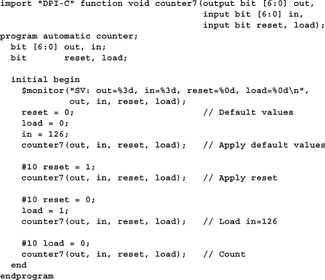
421
12.2 Connecting to a Simple C Routine
12.2.2 The Chandle Data Type
The chandle data type allows you to store a C or C++ pointer in your SystemVerilog
code. A chandle variable is wide enough to hold a pointer on the machine where
the code was compiled, i.e. 32- or 64-bits. The counter in Sample 12.7 works well
as long as it is the only one in the design. You could wrap the counter7 calls from
Sample 12.8 in a module, and instantiate multiple copies in a design. However,
since the counter value is stored in a C static, every instance shares a single value.
If you need more than one instance of a module that calls C code, the C code needs
to store its variables somewhere other than in static variables. A better way is to
allocate storage, and pass a handle to it, along with the input and output signal
values. Sample 12.9 shows a counter that stores the 7-bit count in the structure c7 .
This is overkill for a simple counter, but if you are creating a model for a larger
device, you can build from this example.
Sample 12.8 Testbench for an 7-bit counter with static storage
Sample 12.8 shows a SystemVerilog program that imports and calls the C function
for the 7-bit counter.
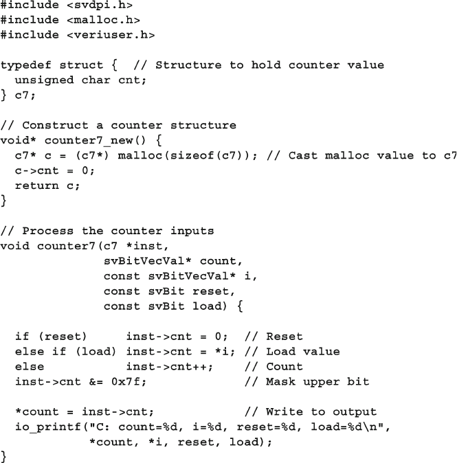
422 12 Interfacing with C/C++
The routine counter7_new constructs the counter instance. This returns a
chandle that must be passed into future calls to counter7 . The counter value is
stored in a struct of type c7 . The function counter7_new calls malloc to allocate
the struct, and casts the result into a local pointer c .
The C code uses the PLI task io_printf to display debug messages. The
routine is helpful when you are debugging C and SystemVerilog code side-by-side
as it writes to the same outputs, including log files, as $display , including
the simulator’s log fi le. The routine is defi ned in veriuser.h .
The testbench for this counter in Sample 12.10 differs from the static one in
several ways. First, the counter must be constructed before it can be used. Next, the
counter is called on a clock edge, rather than calling it in-line with the stimulus. For
simplicity, the counter is invoked when the clock goes high, and stimulus is applied
when the clock goes low, to avoid any race conditions.
Sample 12.9 Counter routine using instance storage
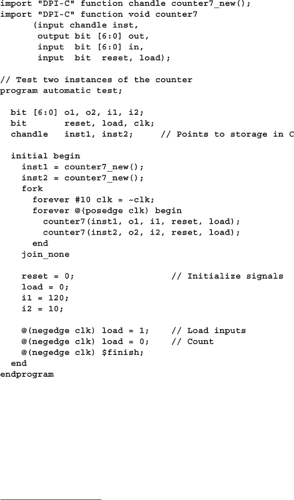
423
12.2 Connecting to a Simple C Routine
12.2.3 Representation of Packed Values
The string " DPI-C "
1 specifi es that you are using the canonical representation of
packed values. This representation stores a SystemVerilog variable as a C array of
one or more elements. A 2-state variable is stored using the type svBitVecVal .
A 2-state array is stored with multiple elements of this type.
Sample 12.10 Testbench for an 7-bit counter with per-instance storage
1 Early versions of the LRM used “DPI” but this is now obsolete and should not be used.
424 12 Interfacing with C/C++
For performance reasons. the SystemVerilog simulator may not mask the
upper bits after calling a DPI routine, and so the SystemVerilog variable could be
corrupted. Make sure your C code treats these values properly.
If you need to convert between bits and words, use the macro SV_PACKED_
DATA_NELEMS . For example, to convert 40 bits to two 32-bit words (as seen in
Fig. 12.1 ), use SV_PACKED_DATA_NELEMS(40) .
12.2.4 4-State Values
Each 4-state bit in SystemVerilog is stored in the simulator using two bits known as
aval and bval , as shown in Table 12.2
39:32Unused
31:0
Fig. 12.1 Storage of a 40-bit 2-state variable
Table 12.2 4-state bit encoding
4-state value bval aval
0 0 0
1 0 1
Z 1 0
X 1 1
A single bit 4-state variable, such as logic f , is stored in an unsigned byte, with
the aval bit stored in the least signifi cant bit, and the bval in the next higher bit.
So the value 1'b0 is seen as 0x0 in C, 1'b1 is 0x1, 1'bz is 0x2, and 1'bx is 0x3.
A 4-state vector such as logic [31:0] lword is stored using pairs of 32 bits,
svLogicVecVal , which contains the aval and bval bits as shown in Figure 12.2 .
The 32-bit variable lword is stored in a single svLogicVecVal . Variables wider
than 32-bits are stored in multiple svLogicVecVal elements, with the fi rst ele-
ment contains the 32 least signifi cant bits, the next element contains the next 32
bits, up to the most signifi cant bits. A 40-bit logic variable is stored as one
svLogicVecVal for the least signifi cant 32 bits, and a second for the upper 8 bits
(Fig. 12.2 ). The unused 24-bits in this upper value are undetermined, and you are
responsible for masking or extending the sign bit, as needed. The svLogicVecVal
type is equivalent to s_vpi_vecval , which is used to represent 4-state types such
as logic in the VPI.
425
12.2 Connecting to a Simple C Routine
Beware of arguments declared without bit subscripts or those
declared with a single bit. An argument declared as input
logic a is stored in an unsigned char . The argument input
logic [0:0] b is svLogicVecVal , even though it contains
only a single bit.
Sample 12.11 shows the import statements for a 4-state counter. The only difference
from Sample 12.10 is that the bit types are now logic .
bval 39:32Unused
bval 31:0
aval 31:0
aval 39:32Unused
Fig. 12.2 Storage of a 40-bit 4-state variable
Sample 12.11 Testbench for counter that checks for Z or X values
The counter previously shown in Sample 12.9 assumes all the inputs are 2-state.
Sample 12.12 extends this code to check for Z and X values on reset, load , and i .
The actual count is still kept as a 2-state value.
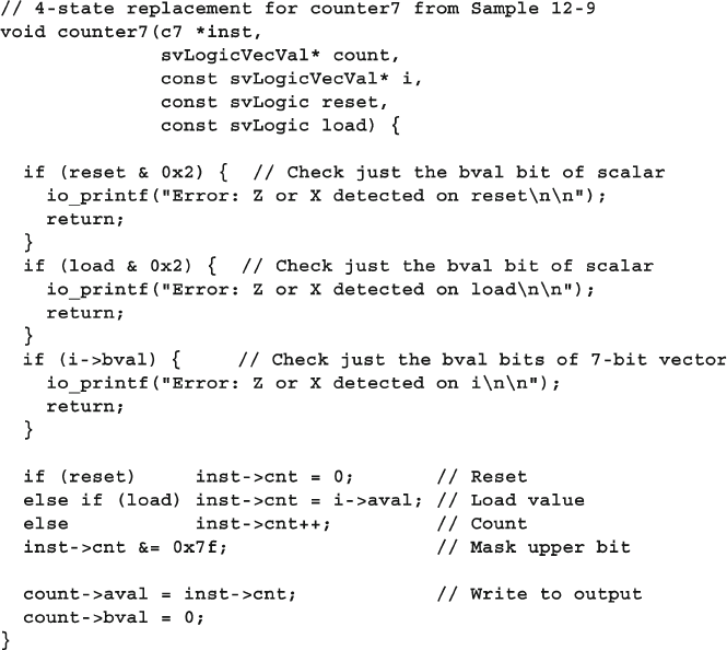
426 12 Interfacing with C/C++
If you want to force the simulation to terminate cleanly because of a condi-
tion found in an imported routine, you can call the VPI routine vpi_
control(vpiFinish, 0) . This routine and constant are defi ned in the include fi le
vpi_user.h . The value vpiFinish tells the simulator to execute a $fi nish after
your imported routine returns.
12.2.5 Converting from 2-State to 4-State
If you have a DPI application that works with 2-state types and you want to convert
it to work with 4-state types, follow the following guidelines.
On the SystemVerilog side, change the import declaration from using 2-state
types such as bit and int to 4-state types such as logic and integer . Make sure
you are using 4-state variables in the function call.
On the C side, switch the argument declarations from svBitVecVal to svLog-
icVecVal . Any reference to the arguments will have to use the . aval suffi x to
Sample 12.12 Counter routine that checks for Z and X values
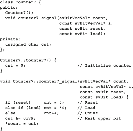
427
12.3 Connecting to C++
correctly access the data. When you read from a 4-state variable, check the bval
bits to see if there are any Z or X values. When you write to a 4-state variable, clear
the bval bits unless you need to write Z or X values.
12.3 Connecting to C++
You can use the DPI to connect routines written in C or C++ to SystemVerilog.
There are several ways your C++ code can communicate using the DPI, depending
on your model’s level of abstraction.
12.3.1 The Counter in C++
Sample 12.13 shows a C++ class for the 7-bit counter, with 2-state inputs. It con-
nects to the SystemVerilog testbench in Sample 12.10 and the C++ wrapper code in
Sample 12.14 .
Sample 12.13 Counter class
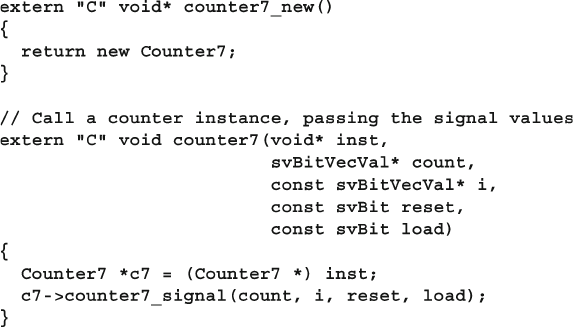
428 12 Interfacing with C/C++
12.3.2 Static Methods
The DPI can only call a C or C++ function that is known at link time. As a result,
your SystemVerilog code cannot call a C++ routine in an object as the object does
not exist when the linker runs.
So what if you need to call a method in a C++ class? The solution, as shown in
Sample
12.14 , is to create a function with a fi xed address, that then can communi-
cate with the C++ dynamic objects and methods. The fi rst routine, counter7_new ,
constructs an object for the counter and returns a handle to the object. The second
static routine, counter7 , calls the C++ method that performs the counter logic,
using the object handle.
Sample 12.14 Static methods and linkage
The extern “C” code tells the C++ compiler that the external information
sent to the linker should use C calling conventions and not perform name mangling.
You can put this before each routine that is called by SystemVerilog, or put extern
"C" { ... } around a set of methods.
From the testbench point of view, the C++ counter looks the same as the counter
that stored the value in per-instance storage, shown in Sample 12.9 , so you can use
the same testbench, Sample 12.10 , for both.
12.3.3 Communicating with a Transaction Level C++ Model
The previous C / C++ code examples were low-level models that communicated with
the SystemVerilog at the signal level. This is not effi cient; for example the counter is
called every clock cycle, even if the data or control inputs have not changed. When
you create models for complex devices such as processors and networking devices,
communicate with them at the transaction level for faster simulations.
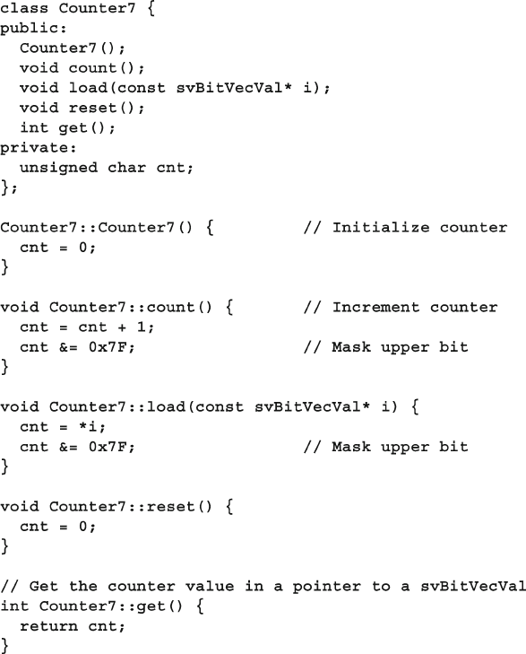
429
12.3 Connecting to C++
The C++ counter model in Sample 12.15 has a transaction-level interface,
communicating with methods instead of signals and a clock.
Sample 12.15 C++ counter communicating with methods
The dynamic C++ methods such as reset, load , and count are wrapped in
static methods that use the object handle, passed from SystemVerilog, as shown in
Sample
12.16 .
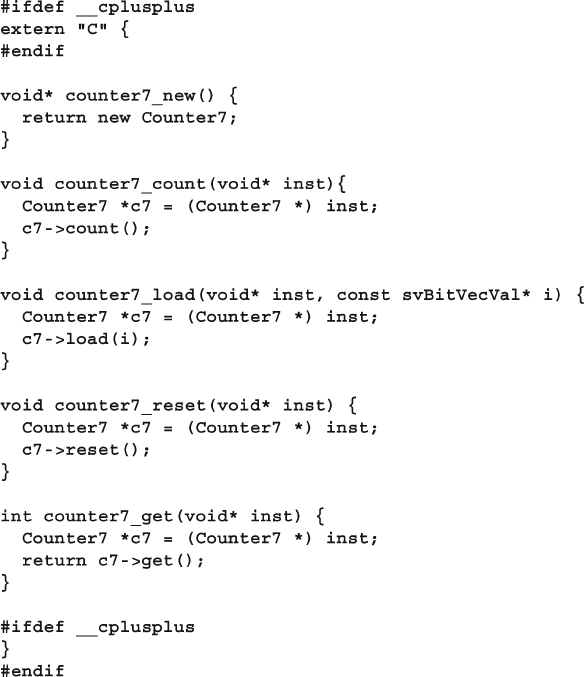
430 12 Interfacing with C/C++
The OOP interface for the transaction level counter is carried up to the testbench.
Sample 12.17 has the SystemVerilog import statements and a class to wrap the C++
object. This allows you to hide the C++ handle inside the class.
Note that the counter7_get() function returns an int (32-bit, signed) rather
than bit [6:0] , as the latter would require returning a pointer to a svBitVecVal , as
shown in Table 12.1 . An imported function can not return a pointer. It can only return
a value of type void, byte, shortint, int, longint, real, shortreal,
chandle , and string , plus single bit values of type bit and logic .
Sample 12.16 Static wrapper for C++ transaction level counter
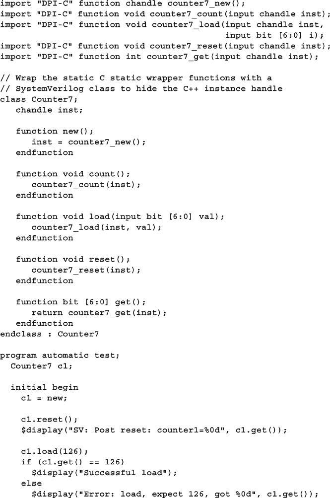
431
12.3 Connecting to C++
Sample 12.17 Testbench for C++ model using methods
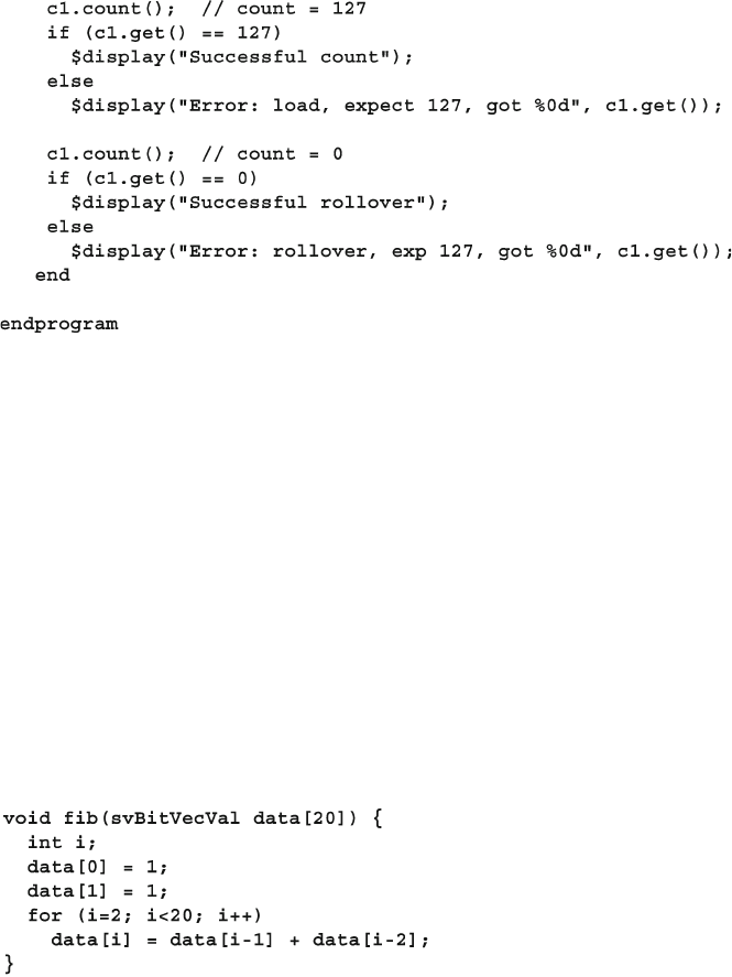
432 12 Interfacing with C/C++
12.4 Simple Array Sharing
So far you have seen examples of passing scalar and vectors between SystemVerilog
and C. A typical C model might read an array of values, perform some computation,
and return another array with the results.
12.4.1 Single Dimension Arrays - 2-State
Sample 12.18 shows a routine that computes the fi rst 20 values in the Fibonacci
series. It is called by the SystemVerilog code in Sample 12.19 .
Sample 12.18 C routine to compute Fibonacci series
Note that in C, you could have alternatively declared the argument as a pointer,
* data or an array, data[20] . In this example, they are interchangeable.
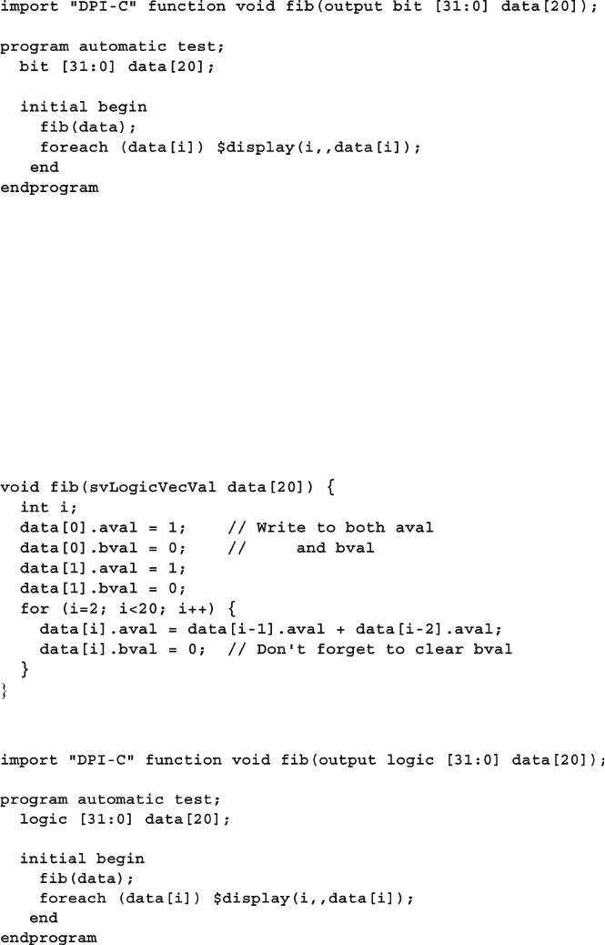
433
12.4 Simple Array Sharing
Notice that the array of Fibonacci values is allocated and stored in SystemVerilog,
even though it is calculated in C. There is no way to allocate an array in C and refer-
ence it in SystemVerilog.
12.4.2 Single Dimension Arrays - 4-State
Sample 12.20 shows the Fibonacci C routine for a 4-state array with the testbench
in Sample 12.21 .
Sample 12.19 Testbench for Fibonacci routine
Sample 12.20 C routine to compute Fibonacci series with 4-state array
Sample 12.21 Testbench for Fibonacci routine with 4-state array
Section 12.2.5 describes how to convert a 2-state application to 4-state.
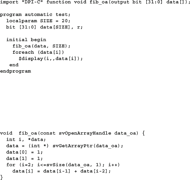
434 12 Interfacing with C/C++
12.5 Open arrays
When sharing arrays between SystemVerilog and C, you have two options. For the
fastest simulations, you can reverse-engineer the layout of the elements in System-
Verilog, and write your C code to use this mapping. This approach is fragile,
meaning that you will have to rewrite and debug your C code if any of the array
sizes change. A more robust approach is to use “open arrays”, and their associated
SystemVerilog routines to manipulate them. These allow you to write generic C
routines that can operate on any size array.
12.5.1 Basic Open Array
Sample 12.22 and 12.23 show how to pass a simple array between SystemVerilog
and C with open arrays. Use the empty square brackets [] in the SystemVerilog
import statement to specify that you are passing an open array.
Sample 12.22 Testbench code calling a C routine with an open array
Your C code references the open array with a handle of type svOpenArray-
Handle . This points to a structure with information about the array such as the
declared word range. You can locate the actual array elements with calls such as
svGetArrayPtr . Note that svSize() is an open array query method, as described
in the next section.
Sample 12.23 C code using a basic open array

435
12.5 Open arrays
12.5.2 Open Array Methods
There are many DPI methods to access their contents and ranges, as defi ned in
svdpi.h . These only work with open array handles declared as svOpenArray-
Handle , not with pointers such as svBitVecVal or svLogicVecVal . The
methods in Table 12.3 give you information about the size of an open array.
Table 12.4 Open array locator functions
Function Returns pointer to :
void *svGetArrayPtr(h) storage for the entire array
void *svGetArrElemPtr(h, i1, ...) an element in the array
void *svGetArrElemPtr1(h, i1) an element in a 1-D array
void *svGetArrElemPtr2(h, i1, i2) an element in a 2-D array
void *svGetArrElemPtr3(h, i1, i2, i3) an element in a 3-D array
Table 12.3 Open array query functions
function Description
int svLeft(h, d) Left bound for dimension d
int svRight(h, d) Right bound for dimension d
int svLow(h, d) Low bound for dimension d
int svHigh(h, d) High bound for dimension d
int svIncrement(h, d) If left >= right, 1, else −1
int svSize(h, d) Number of elements in dimension d: svHigh−svLow+1
int svDimensions(h) Number of dimensions in open array
int svSizeOfArray(h) Total size of array in bytes
In Table 12.3 , the variable h is a svOpenArrayHandle and d is an int . The
dimensions are numbered starting with d=1 .
The functions in Table 12.4 return the locations of the C storage for the entire
array or a single element.
12.5.3 Passing Unsized Open Arrays
Sample 12.24 calls C code with a 2-dimensional array. The C code uses the svLow
and svHigh methods to fi nd the array ranges, which, in this example, don’t follow
the usual 0..size-1.
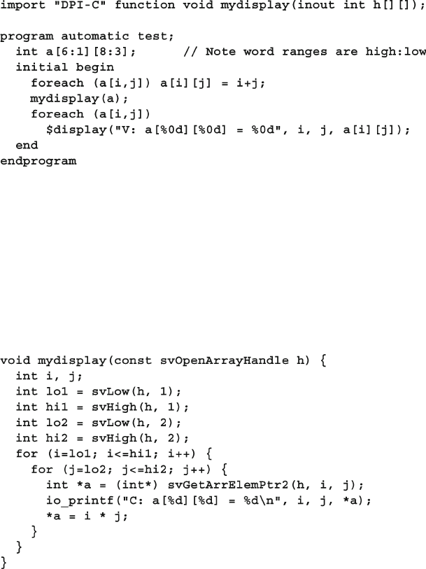
436 12 Interfacing with C/C++
This calls the C code in Sample 12.25 that reads the array using the open array
methods. The routine svLow(handle, dimension) returns the lowest index
number for the specifi ed dimension. So svLow(h,1) returns 1 for the array declared
with the range [6:1]. Likewise, svHigh(h, 1) returns 6. You should use svLow
and svHigh with C for loops.
The methods svLeft and svRight return the left and right index from the array
declaration, 6 and 1 respectively for the range [6:1]. At the center of Sample 12.25 , the
call svGetArrElemPtr2 returns a pointer to an element in a two dimensional array.
Sample 12.24 Testbench calling C code with multi-dimensional open array
Sample 12.25 C code with multi-dimensional open array
12.5.4 Packed Open Arrays in DPI
An open array in the DPI is treated as having a single packed dimension and one or
more unpacked dimensions. You can pass an array with multiple packed dimen-
sions, as long as they pack into an element that is the same size as a single element
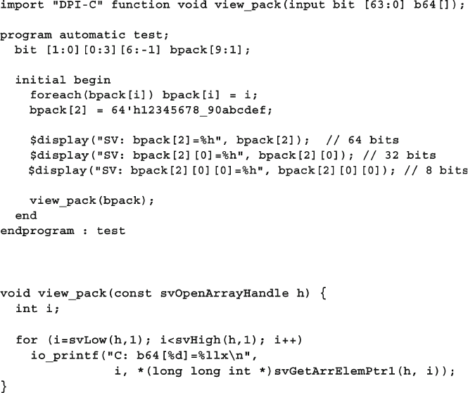
437
12.6 Sharing Composite Types
Notice that the C code in Sample 12.27 prints a 64-bit value using % llx , and
casts the result from svGetArrayElemPtr1 to long long int .
12.6 Sharing Composite Types
By this point you may wonder how to pass objects between SystemVerilog and C.
The layout of class properties does not match between the two languages, so you
cannot share objects directly. Instead, you must create similar structures on each
Sample 12.27 C code using packed open arrays
Sample 12.26 Testbench for packed open arrays
of the formal argument. For example, if you have the formal argument bit[63:0]
b64[] in the import statement, you could pass in the actual argument bit [1:0]
[0:3][6:−1] bpack [9:1] . Sample 12.26 shows the SystemVerilog code with
packed open arrays.
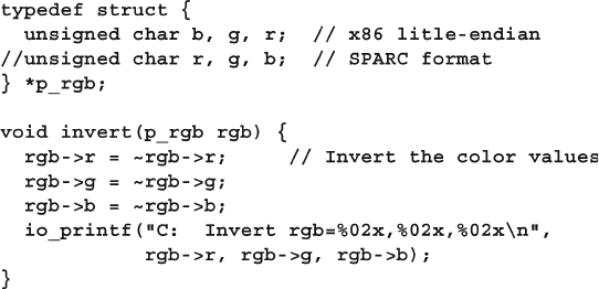
438 12 Interfacing with C/C++
side, plus pack and unpack methods to convert between the two formats. Once you
have all this in place, you can share composite types.
12.6.1 Passing Structures Between SystemVerilog and C
The following example shares a simple structure for a pixel made of three bytes
packed into a word. Sample 12.28 shows the C structure. Notice that C treats a char
as signed variable, which can give you unexpected results, so the structure marks
the char as unsigned. The bytes are in reverse order from the SystemVerilog because
this code was written for a Intel x86 processor that is little-endian, which means that
the least signifi cant byte is stored at a lower address than the most signifi cant. A Sun
SPARC is big endian, so the bytes are stored in the same order as in SystemVerilog:
r, g, b .
Sample 12.28 C code to share a structure
The SystemVerilog testbench in Sample 12.29 has a packed struct that holds a
single pixel, and class to encapsulate the pixel operations. The RGB_T struct is
packed so SystemVerilog will store the bytes in consecutive locations. Without the
packed modifi er, each 8-bit value would be stored in a separate word.
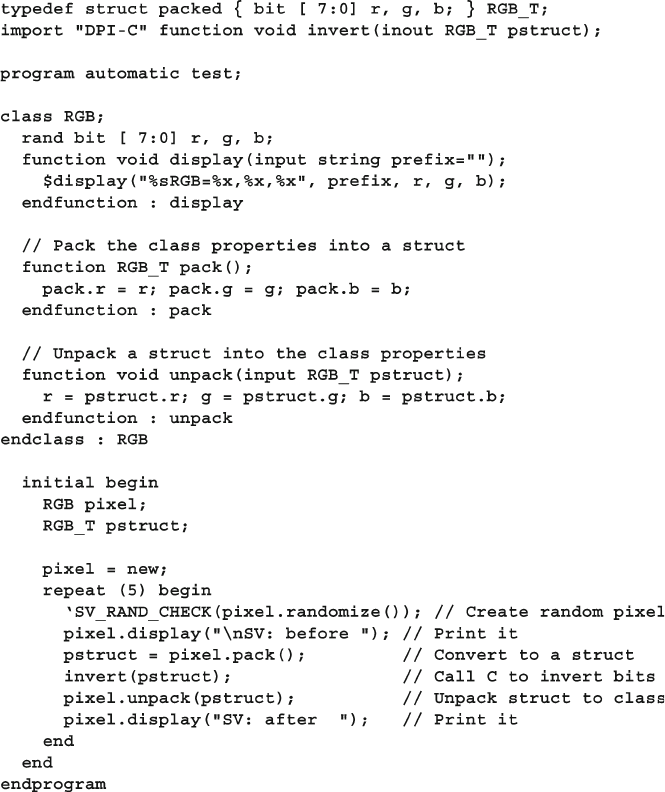
439
12.6 Sharing Composite Types
12.6.2 Passing Strings Between SystemVerilog and C
Using the DPI, you can pass strings from C back to SystemVerilog. You might need
to pass a string for the symbolic value of a structure, or get a string representing the
internal state of your C code for debug.
The easiest way to pass a string from C to SystemVerilog is for your C function
to return a pointer to a static string as shown in Sample 12.30 . The string must be
Sample 12.29 Testbench for sharing structure
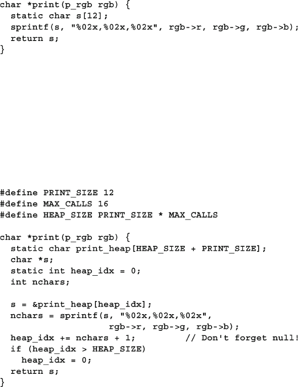
440 12 Interfacing with C/C++
declared as static in C, and not as a local string. Non-static variables are stored
on the stack and are reclaimed when the function returns.
Sample 12.30 Returning a string from C
A danger with static storage is that multiple concurrent calls could end up
sharing storage. For example, a SystemVerilog $display statement that is printing
several pixels might call the above print routine multiple times. Depending on
how the SystemVerilog compiler orders these calls, later calls to print() could
overwrite results from earlier calls, unless the SystemVerilog compiler makes a
copy of the string. Note that a call to an imported routine can never be interrupted
by the SystemVerilog scheduler. Sample 12.31 stores the strings in a heap to support
concurrent calls.
Sample 12.31 Returning a string from a heap in C
12.7 Pure and Context Imported Methods
Imported methods are classifi ed as pure, context , or generic. A pure function
calculates its output strictly based on its inputs, with no outside interactions.
Specifi cally, a pure function does not access any global or static variables, perform
any fi le operations, or interact with anything outside the function such as the operating
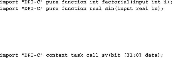
441
12.8 Communicating from C to SystemVerilog
system, processes, shared memory, sockets, etc. The SystemVerilog compiler may
optimize away calls to a
pure function if the result is not needed, or replace the call
with the results from a previous call with the same arguments. The
factorial
function in Sample
12.5 , and the sin function in 12.6 are both pure functions as
their result is only based on their inputs. Sample 12.32 shows how to import a pure
function.
Sample 12.32 Importing a pure function
Sample 12.33 Imported context tasks
An imported routine may need to know the context of where it is called so it can
call a PLI TF, ACC, or VPI methods, or a SystemVerilog task that has been exported.
Use the context attribute for these methods as shown in Sample 12.33 .
An imported routine may use global storage, so it is not pure , but might not have
any PLI references, so it does not need the overhead of a context routine.
Sutherland (2004) uses the term “generic” for these methods as the SystemVerilog
LRM does not have a specifi c name. By default, an imported routine is generic, as
are many of the examples in this chapter.
There is overhead invoking a context imported routine as the simulator needs
to record the calling context, so only declare a routine as context if needed. On the
other hand, if a generic imported routine calls an exported task or a PLI routine that
accesses SystemVerilog data objects, the simulator could crash.
A context-aware PLI routine is one that needs to know where it was called from
so that it can access information relative to that location.
12.8 Communicating from C to SystemVerilog
The examples so far have shown you how to call C code from your SystemVerilog
models. The DPI also allows you to call SystemVerilog routines from C code. The
SystemVerilog routine can be a simple task to record the result from an operation
in C, or a time-consuming task representing part of a hardware model.
12.8.1 A simple Exported Function
Sample 12.34 shows a module that imports a context function, and exports a System-
Verilog function.
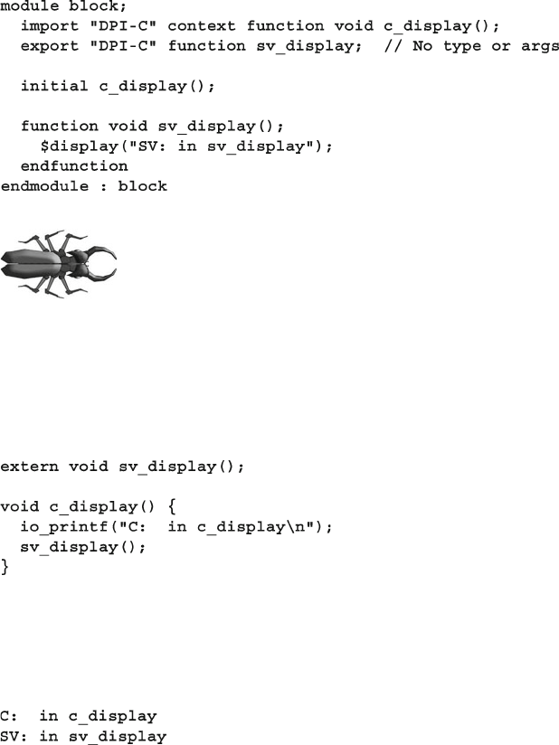
442 12 Interfacing with C/C++
The export declaration in Sample 12.34 looks naked because
the LRM forbids putting a return value declaration or any argu-
ments. You can’t even give the usual empty parentheses. This
information in the export declaration would duplicate the
information in the function declaration at the end of the module and could thus
become out of sync if you ever changed the function.
Sample 12.35 shows the C code that calls the exported function.
Sample 12.34 Exporting a SystemVerilog function
Sample 12.36 Output from simple export
Sample 12.35 Calling an exported SystemVerilog function from C
This example prints the line from the C code, followed by the $display output
from the SystemVerilog, as shown in Sample 12.36 .
12.8.2 C function Calling SystemVerilog Function
While the majority of your testbench should be in SystemVerilog, you may have
legacy testbenches in C or other languages, or applications that you want to reuse.
This section creates a SystemVerilog memory model that is stimulated by C code
that reads transactions from an external fi le.
The fi rst version of the memory model, shown in Sample 12.38 and 12.37 ,
is coded with just functions, so everything runs in zero time. The C code in
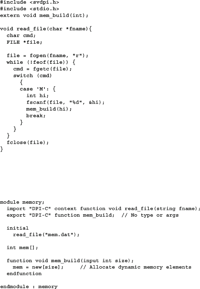
443
12.8 Communicating from C to SystemVerilog
Sample 12.37 opens the fi le, reads a command, and calls the exported function.
Error checking has been removed for compactness.
Sample 12.37 C code to read simple command fi le and call exported function
The SystemVerilog code calls the C task read_fi le which opens a fi le. The only
command in the fi le sets the memory size, so the C code calls an exported
function.
Sample 12.38 SystemVerilog module for simple memory model
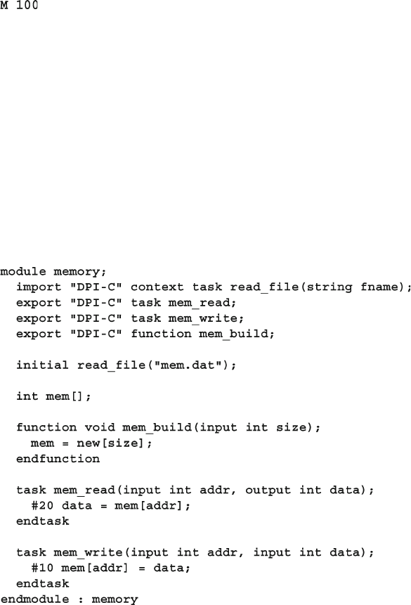
444 12 Interfacing with C/C++
Notice that in Sample 12.38 , the export statement does not have any arguments
as this information is already in the function declaration.
The command fi le is trivial, with one command to construct a memory with 100
elements as shown in Sample
12.39 .
Sample 12.39 Command fi le for simple memory model
12.8.3 C Task Calling SystemVerilog Task
A real memory model has operations such as read and write that consume time, and
thus must be modeled with tasks.
Sample 12.40 shows the SystemVerilog code for the second version of the memory
model. It has several improvements compared to Sample 12.38 . There are two new
tasks, mem_read and mem_write , which respectively take 20ns and 10ns to com-
plete. The imported routine read_fi le is now a SystemVerilog task as it is calling
other tasks that consume time. The import statement now specifi es that read_fi le is
a context task, as the simulator needs to create a separate stack when it is called.
Sample 12.40 SystemVerilog module for memory model with exported tasks
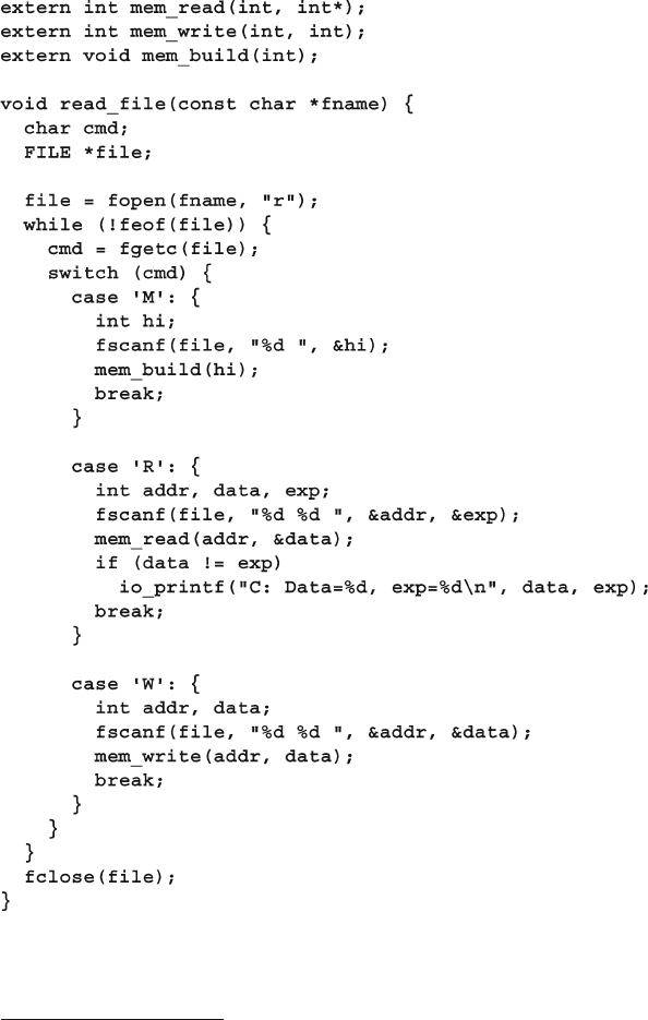
445
12.8 Communicating from C to SystemVerilog
The C code in Sample 12.41 primarily expands the case statement that
decodes commands and calls the exported tasks, which are declared as extern
int according to the LRM.
2
Sample 12.41 C code to read command fi le and call exported function
The command fi le in Sample 12.42 has new commands that write two locations,
and then reads back one of them, and includes the expected value.
2 VCS declared exported tasks as void functions in C.
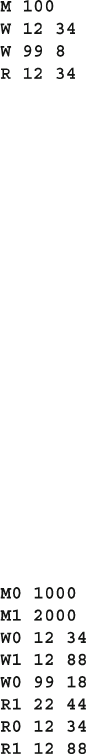
446 12 Interfacing with C/C++
12.8.4 Calling Methods in Objects
You can export SystemVerilog methods, except for those defi ned inside a class. This
restriction is similar to the restriction of importing static C methods, as shown in
Section 12.3.2 as objects do not exist when SystemVerilog elaborates your code.
The solution is to pass a reference to the object between the SystemVerilog and C
code. However, unlike a C pointer, a SystemVerilog handle cannot be passed through
the DPI. You can instead have an array of handles, and pass the array index between
the two languages.
The following examples build on the previous versions of the memory. The
SystemVerilog code in Sample 12.44 has a class that encapsulates the memory. Now
you can have multiple memories, each in a separate object. The command fi le in
Sample 12.43 creates two memories, M0, and M1. Then it performs several writes
to initialized locations in both memories, and lastly tries to read back the values.
Notice that location 12 is used for both memories.
Sample 12.42 Command fi le for simple memory model
Sample 12.43 Command fi le for exported methods with OOP memories
The SystemVerilog code in Sample 12.44 constructs a new object for every M
command in the fi le. The exported function mem_build calls the Memory construc-
tor. It then stores the handle to the Memory object in a SystemVerilog queue, and
returns the queue index, idx , to the C code as shown in Sample 12.45 . The handles
are stored in a queue so you can dynamically add new memories. The exported tasks
mem_read and mem_write now have an additional argument, the index of the
memory handle in the queue.
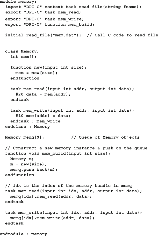
447
12.8 Communicating from C to SystemVerilog
Sample 12.44 SystemVerilog module with memory model class
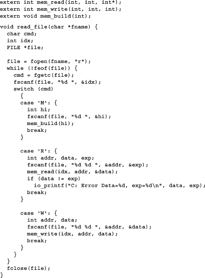
448 12 Interfacing with C/C++
Sample 12.45 C code to call exported tasks with OOP memory
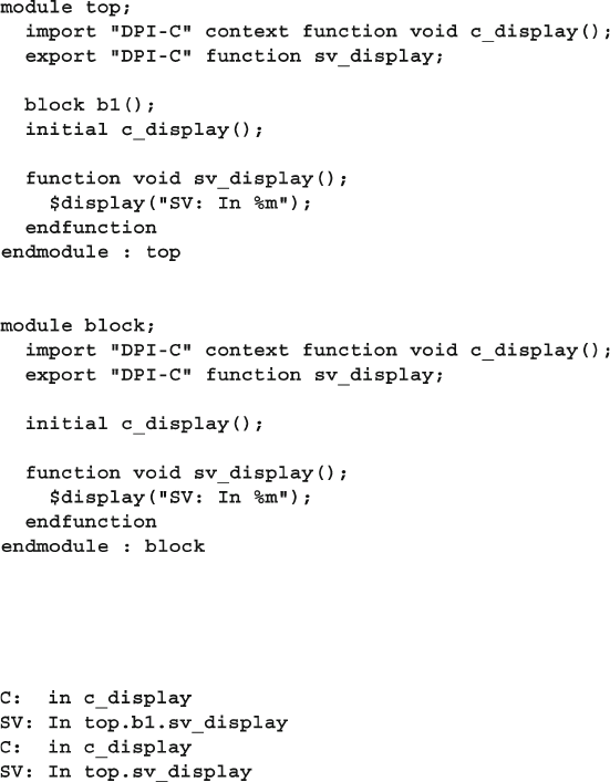
449
12.8 Communicating from C to SystemVerilog
12.8.5 The Meaning of Context
The context of an imported routine is the location where it was defi ned, such as
$unit , module, program, or package scope, just like a normal SystemVerilog
routine. If you import a routine in two different scopes, the corresponding C code
executes in the context of where the import statement occurred. This is similar to
defi ning a SystemVerilog run() task in each of two separate modules. Each task
accesses variables in its own module, with no ambiguity.
Sample 12.46 shows that if you add a second module to Sample 12.34 that
imports the same C code and exports its own function, the C routine will call different
SystemVerilog methods, depending on the context of the import and export
statements.
Sample 12.46 Second module for simple export example
Sample 12.47 Output from simple example with two modules
The output in Sample 12.47 shows that one C routine calls two separate
SystemVerilog methods, depending on where the C routine was called.
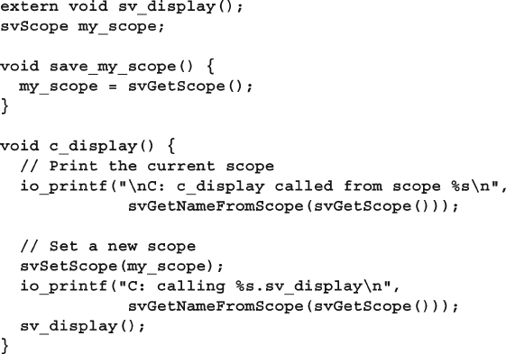
450 12 Interfacing with C/C++
12.8.6 Setting the Scope for an Imported Routine
Just as your SystemVerilog code can call a routine in the local scope, an imported C
routine can call a routine outside its default context. Use the routine
svGetScope to
get a handle to the current scope, and then use that handle in a call to svGetScope
to make the C code think it is inside another context. Sample 12.48 shows the C code
for two methods. The fi rst, save_my_scope( ) , saves the scope of where it was
called from the SystemVerilog side. The second routine, c_display() , sets its
scope to the saved one, prints a message, then calls your function, sv_display() .
Sample 12.48 C code getting and setting context
The C code calls svGetNameFromScope() that returns a string of the current
scope. The scope is printed twice, once with the scope where the C code was fi rst
called from, and again with the scope that was previously saved. The routine
svGetScopeFromName() takes a string with a SystemVerilog scope and returns a
pointer to a svScope handle that can be used with svSetScope() .
In the SystemVerilog code in Sample 12.49 , the fi rst module, block , calls a C
routine that saves the context. When the module top calls c_display() , the
routine sets scope back to block , and so it calls the sv_display() routine in
the block module, not the top module.
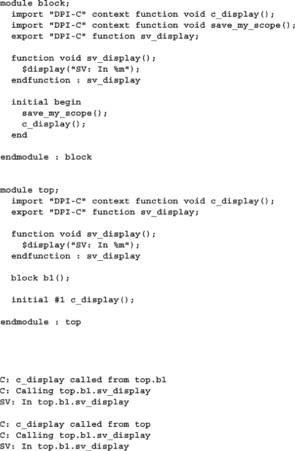
451
12.8 Communicating from C to SystemVerilog
This produces the output shown in Sample 12.50 .
Sample 12.49 Modules calling methods that get and set context
Sample 12.50 Output from svSetScope code
You could use this concept of scope to allow a C model to know where it was
instantiated from, and differentiate each instance. For example, a memory model
may be instantiated several times, and needs to allocate unique storage for every
instance.
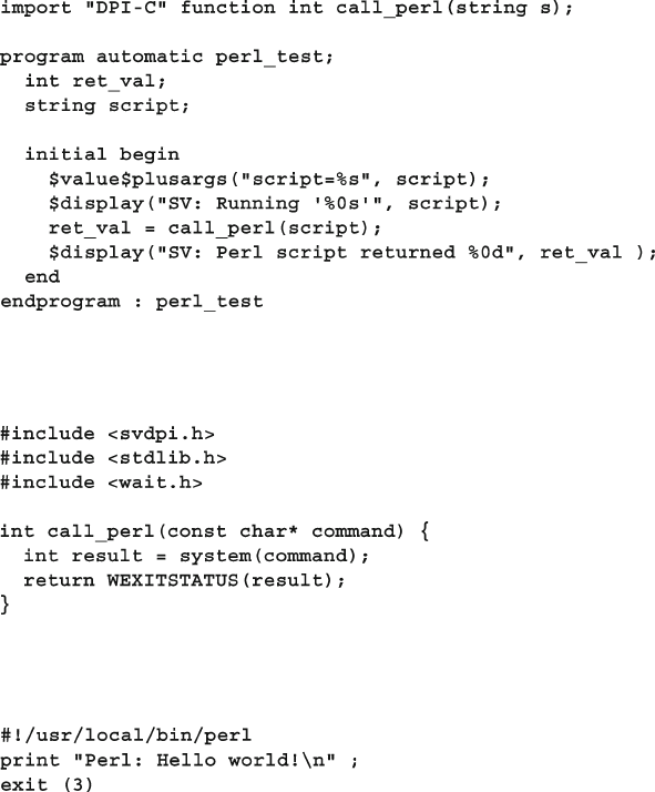
452 12 Interfacing with C/C++
12.9 Connecting Other Languages
This chapter has shown the DPI working with C and C++. With a little work, you
can connect other languages. The easiest way is to call the Verilog
$system() task.
If you need the return value from the command, use the Unix system() function
and the WEXITSTATUS macro. The SystemVerilog code in Sample 12.51 calls a
C wrapper for system() .
Sample 12.51 SystemVerilog code calling C wrapper for Perl
Sample 12.52 is the C wrapper that calls system () and translates the return value.
Sample 12.52 C wrapper for Perl script
Sample 12.53 is a Perl script that prints a message and returns a value.
Sample 12.53 Perl script called from C and SystemVerilog
Now you can run the Unix command in Sample 12.54 to run the simulation and
call the hello.pl script.

453
12.11 Exercises
12.10 Conclusion
The Direct Programing Interface allows you to call C routines as if they are just
another SystemVerilog routine, passing SystemVerilog types directly into C. This
has less overhead than the PLI, which builds argument lists, and always has to keep
track of the calling context, not to mention the complexity of having up to four
C routines for every system task.
Additionally, with the DPI, your C code can call SystemVerilog routines, allowing
external applications to control simulation. With the PLI you would need trigger
variables and more argument lists, and you have to worry about subtle bugs from
multiple calls to time-consuming tasks.
The most difficult part of the DPI is mapping SystemVerilog types to C,
especially if you have structures and classes that are shared between the two
languages. If you can master this problem, you can connect almost any application
to SystemVerilog.
12.11 Exercises
1. Create a C function, shift_c , that has two input arguments: a 32-bit unsigned
input value i and an integer for the shift amount n . The input i is shifted n
places. When n is positive, values are shifted left, when n is negative, shifted
right, and when n is 0, no shift is performed. The function returns the shifted
value. Create a SystemVerilog module that calls the C function and tests each
feature. Provide the output.
2. Expand Exercise 1 to add a third argument to shift_c , a load fl ag ld . When ld
is true, i is shifted by n places and then loaded into an internal 32-bit register.
When ld is false, the register is shifted n places. The function returns the value
of the register after these operations. Create a SystemVerilog module that calls
the C function and tests each feature. Provide the output.
3. Expand Exercise 2 to create multiple instances of the
shift_c function. Each
instance in C needs a unique identifi er, so use the address where the internal
register is stored. Print this address along with the arguments when the function
shift_c is called. Instantiate the function twice, and call each instance twice.
Provide the output.
Sample 12.54 VCS command line to run Perl script
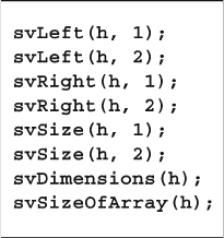
454 12 Interfacing with C/C++
4. Expand the C code from Exercise 3 to display the total number of times the
shift_c function has been called, even if the function is instantiated more
than once.
5. Expand Exercise 4 to provide the ability to initialize the stored value at
instantiation.
6. Expand Exercise 5 to encapsulate the shift_c function in a class.
7. For the code in Sample 12.24 and 12.25 , what is returned by the following open
array methods?
8. Modify Exercise 1 so that instead of shifting the value in C, the function calls
an exported SystemVerilog void function named shift_sv that does the
shifting.
9. Expand Exercise 8 to call the SystemVerilog function shift_sv for two differ-
ent SystemVerilog objects as demonstrated in Section 12.8.4 of the text. Assume
the SystemVerilog function shift_build has been exported to the C code.
10. Expand Exercise 8 to:
a. Create a SystemVerilog class Shift containing the function shift_sv that
stores the result in a class-level variable, and a shift_print function that
displays the stored result.
b . D e fi ne and export SystemVerilog function shift_build .
c. Support the creation of multiple Shift objects with the handles to these
objects stored in a queue.
d. Create a testbench that constructs multiple Shift objects. Demonstrate that
each object holds a separate result after performing calculations.
455
Bergeron, Janick. Writing Testbenches Using SystemVerilog . Norwell, MA: Springer, 2006
Bergeron, Janick, Cerny, Eduard, Hunter, Alan, and Nightingale, Andrew. Verifi cation Methodology
Manual for SystemVerilog . Norwell, MA: Springer, 2006
Cohen, Ben, Venkataramanan, Srinivasan, and Kumari, Ajeetha. SystemVerilog Assertions
Handbook for Formal and Dynamic Verifi cation : VhdlCohen Publishing 2005
Cummings, Cliff. Nonblocking Assignments in Verilog Synthesis, Coding Styles That Kill!
Synopsys User Group, San Jose, CA, 2000
Cummings, Cliff, Salz, Arturo. SystemVerilog Event Regions, Race Avoidance & Guidelines ,
Synopsys User Group, Boston, CA, 2006
Denning, Peter. The Locality Principle , Communications of the ACM, 48(7), July 2005,
pp. 19–24
Haque, Faisal, Michelson, Jonathan. The Art of Verifi cation with SystemVerilog Assertions .
Verifi cation Central 2006
IEEE IEEE Standard for SystemVerilog — Unifi ed Hardware Design, Specifi cation, and Verifi cation
Language . New York: IEEE 2009 (a.k.a. SystemVerilog Language Reference Manual,
or LRM.)
IEEE IEEE Standard Verilog Hardware Design, Description Language . New York: IEEE 2001
Rich, Dave Are SystemVerilog Program Blocks Needed? http://blogs.men-tor.com/verifi cationhorizons/
blog/2009/05/07/programblocks/ 2009
Sutherland, Stuart. Integrating SystemC Models with Verilog and SystemVerilog Using the
SystemVerilog Direct Programing Interface . Synopsys User Group Europe, 2004
Sutherland, Stuart, Davidmann, Simon, Flake, Peter, and Moorby, Phil. System-Verilog for Design: A
Guide to Using SystemVerilog for Hardware Design and Modeling . Norwell, MA: Springer, 2006
Sutherland, Stuart, Mills, Don. Verilog and SystemVerilog Gotchas . Norwell, MA: Springer, 2007
Synopsys, Inc., Hybrid RTL Formal Verifi cation Ensures Early Detection of Corner-Case Bugs ,
http://synopsys.com/products/magellan/magellan_wp.html , 2003
van der Schoot, Hans, and Bergeron, Janick Transaction-Level Functional Coverage in
SystemVerilog . San Jose, CA: DVCon, February 2006
Vijayaraghavan, Srikanth, and Ramanathan, Meyyappan. A Practical Guide for SystemVerilog
Assertions . Norwell, MA: Springer, 2005
Wachowski Andy, and Wachowski Larry. The Matrix . Hollywood, CA: Warner Brothers
Studios, 1999
References
C. Spear and G. Tumbush, SystemVerilog for Verifi cation: A Guide to Learning
the Testbench Language Features, DOI 10.1007/978-1-4614-0715-7,
© Springer Science+Business Media, LLC 2012
457
! , 179
-- , 69
## cycle delay , 108, 204, 375
$ , 37, 343–344
$bits , 305
$cast , 55, 60, 284, 286, 291, 305
$clog2 , 28
$dist_exponential , 195
$dist_normal , 195
$dist_poisson , 195
$dist_uniform , 195
$error , 117
$exit , 110–111
$fatal , 117
$fclose , 70
$feof , 40, 70
$finish , 110–111, 426
$fopen , 40, 70
$fscanf , 40, 70–71
$get_coverage , 359
$info , 117
$isunknown , 27, 118
$monitor , 372
$psprintf , 62
$random , 195, 217
$realtime , 82–83
$root , 115
$sformat , 62
$sformatf , 62
$size , 30, 35, 41
$strobe , 372
$system , 452
$test$plusargs , 390–391
$time , 27, 82–83
$timeformat , 27, 82–83
$typename , 305, 310
$unit , 114, 417, 449
$urandom , 195, 202, 251
$urandom_range , 41, 194, 195, 202, 215
$value$plusargs , 311, 390–391, 452
$warning , 117
%0t , 27
%p , 29–30, 41, 309
%t , 82
++ , 69
+= , 69–70
+ntb_random_seed , 224, 390
:: , 54, 142, 144, 250
<< , 55
<-> , 186, 190
-= , 69
-> , 184, 188–189, 192
-> , 190
>> , 55–57, 161
? : operator , 32, 43
[$] , 37
[] , 35
^= , 69, 74, 76
__FILE__ , 174
__LINE__ , 174
`define , 49
‘include , 53, 93
‘SV_RAND_CHECK , 174
Numerics
2-state types , 27, 416, 420, 423, 426
4-state types , 27, 424–426
A
Abstract class , 295–296, 298–299, 311,
314, 315
Accellera , viii
Accessor methods , 162
Active region , 101–103, 106, 112
Agent , 17, 163
AHB , 128
Always block , 230
Index
458 Index
Always block in programs , 111
and method , 41
Anonymous enumerated type , 57
API see Application Programming
Interface (API)
Application Programming Interface (API) , ix
Arguments
default value , 75–76
sticky , 73
task and function , 72
type , 73
Array
assignment , 37
associative , 38–42, 47
compare , 32
constraint , 203
copy , 32
dynamic , 35–36, 38, 46, 47
fixed-size , 28, 36, 38, 46, 47
handle , 155
literal , 29, 35, 37, 40
locator methods , 42
methods , 41
multi-dimensional , 28, 30–31, 36, 436
open , 435–436
packed , 33–34
queue , 36, 38, 46, 47
reduction methods , 41
slice , 32
unpacked , 29, 34
Assertion
concurrent , 118
coverage , 328
immediate , 116–117, 286
in an interface , 379
Assignment pattern , 29
Associative array , 38–42, 47, 50
at_least option , 331, 357
ATM router , 119–121, 123–125
Atomic stimulus generation , 211
auto_bin_max , 339–340, 347, 355
Automatic , 74, 80–81, 103, 137, 138, 141, 237
in threads , 236
Aval , 426, 428
B
Backdoor load , 115
Base class , 276–277
BaseTr class , 295, 304–305
Begin…end , 72, 230
optional in tasks and functions , 72
Bergeron, Janick , xiii, 4, 387, 455
BFM see Bus Functional Model (BFM)
Bus Functional Model (BFM) , 13
Bidirectional constraint, see Constraint
bidirectional
Bidirectional signal , 108
Binsof , 351, 353
Bit data type , 27, 421, 432
Bit streaming see Streaming operator
Blueprint pattern , 279
BNF see Backus-Naur Form (BNF)
Backus-Naur Form (BNF) , 213
Bounded mailbox , 256–257
Break , 70
Bval , 424, 426
Byte data type , 27, 418, 430
C
calc_csm method , 275–276, 287
Callback
coverage , 335
creation , 298
inject distrubance , 297
scoreboard , 300
usage , 299
Case , 71
Cast , 54, 60, 63, 71
function return value , 71
Cerny, Eduard , 455
Chandle data type , 419, 421–423, 430
Char , 419
Checker , 17, 163
Class , 132, 134
Class constructor , 136
Class scope resolution operator , 144, 250
Clock generator , 111–112
Clocking block , 98–99, 103, 108, 109, 123,
124, 365
Cohen, Ben , 455
Command layer , 17
Comment
covergroup , 356
Comment option , 333, 356
Compilation unit , 113
Composition , 273, 288, 290, 292
Compound assignment , 69–70, 74
Concatenation
bits , 56
string , 61
Concurrent assertion , 118
Conditional operator , 32, 43
Config class , 266
Configuration database , 308
Const , 76
Const type , 61, 74, 114, 176
459
Index
Constrained , 7
Constraint
array , 203
bidirectional , 184, 188
block , 173
dist , 178–179, 196, 359
implication , 188
in extended class , 284
inside , 176, 179, 183, 202, 203
solve…before , 190–191, 359, 396
constraint_mode , 191–193, 280
Constructor , 136–137, 277, 295
Consumer , 244
Containment , 149
Context , 444
Continue , 70
Copy
deep , 159
method , 159–160, 280, 293, 294
object , 156, 293
shallow , 158
Coverage event , 335
Covergroup
comment , 356
embedded , 334
generic , 354–355
option , 355
sample , 331, 335–337
trigger , 335
Coverpoint , 330, 334, 337, 340, 343, 351,
353, 358
Cross coverage , 348–354
Cross module reference , 114, 370, 376
cross_num_print_missing option , 357
CRT see constrained-random test (CRT)
Constrained-Random Test (CRT) , 4, 7–8, 169,
196, 323
Cummings, Cliff , xiii, 100, 102, 455
Cyclic random , 173
D
Data type
bit , 26–27
byte , 26–27
chandle , 419, 421–423, 430
int , 27
integer , 25
logic , 26
longint , 27
real , 25
reg , 25–26
shortint , 27
time , 25
wire , 26
Deallocation , 139
DDR see Double data rate (DDR)
Decrement , 69
Default clocking block , 108
Default coverage value , 343, 345, 350–351
Default statement , 98
Default value , 75–76
Delete method , 35, 37, 39, 48
Derived class , 277
Design pattern , 314
Design Under Test (DUT) , 3, 88
Direct Programming Interface (DPI) , 415–454
Disable , 231, 240–243
Disable fork , 241–242
Disable label , 242–243
Display method , 141–142, 275, 276, 285
Dist constraint , 178, 179, 196, 359
do…while , 39, 59, 70, 174
Domain , 338–339
Double data rate (DDR) clock , 98
Double data type , 418–419
Double precision floating point , 28
Downcasting , 284
DPI see Direct Programming Interface (DPI)
DPI-C , 416, 423
Driver , 17, 163
Driver class , 375, 379
DUT see Design Under Test (DUT)
Dynamic array , 35–36, 38, 46, 47
Dynamic cast, see $cast
Dynamic threads , 235
E
e Reuse Methodology (eRM) , viii
Embedded covergroup , 334
Enum , 57–60
Enumerated types, see enum
Enumerated values , 58
Enumeration , 57
Environment , 18, 163
Environment class , 163
Equivalence operator , 186, 190
eRM see e Reuse Methodology (eRM)
Event , 244–249, 264
Event triggered , 244–249, 261
Exists , 40, 48
Expression width , 62
Extended class , 276–277
Extern, see External routine declaration
External constraint , 199–200
External routine declaration , 142–143,
266, 296
460 Index
F
Fabs routine , 417
File I/O , 70
File_exists method , 417
Final block , 110
Find_first method , 43
Find_index method , 43–45
Find_last method , 43
Find_last_index method , 43
First , 39
First method , 39, 47, 59–60
Fixed-size array , 28, 35, 38, 46, 47
Float data type , 418
for loop , 30, 39, 59, 69, 197
Force design signals , 115
foreach constraint , 203, 207–209, 396
foreach loop , 30–31, 35, 37, 40
Fork…join , 230–231
Fork…join_any , 230, 233
Fork…join_none , 230, 232, 234, 235, 237,
238
Four-state types, see 4-state types
Function , 71
arguments , 72
Functional coverage , 18, 455
using callbacks , 301
Functional layer , 17
G
Garbage collection , 139–140
Generator , 18, 163
Generator class , 234, 248, 250, 255, 279, 281,
304, 305
Get method , 251–254, 261, 263, 265
get_coverage , 359
get_inst_coverage , 359
Getc method , 61–62
Goal option , 358
H
Handle , 134–135, 139
array , 155
Haque, Faisal , 455
Hardware Description Language (HDL) , 2, 83
Hardware Verification Language (HVL) , viii,
2, 13
HDL see Hardware Description Language
(HDL)
Histogram , 180
Hook , 280, 297
HVL see Hardware Verification Language
(HVL)
I
IEEE 1800, see LRM
If constraint , 185–186
Iff , 118, 344
Ignore_bins , 346–347, 351
Illegal_bins , 347
Immediate assertion , 116–117, 286
Implication , 184
Implication operator , 184, 190
Implicit port connection , 112
Import , 53, 418–419
Incl.h , 418
Increment , 69
Inheritance , 274, 288
Initial , 29
Initialization in declaration , 80
In-line constraint , 199
Inout
argument type , 73
port type , 126
Input
argument type , 73
port type , 126
Insert queue , 37
Inside , 71, 176, 180
Inside constraint , 176, 179, 183, 202, 203
Instance , 136
Instantiation , 136
Int data type , 27, 418, 419, 430
Integer data type , 25, 27, 51
Interface , 91, 97, 113, 369
connecting to port , 93
procedural code , 379
virtual , 363–364, 366, 368, 370, 379
Interprocess , 2
Interprocess communication (IPC) , 229,
244, 264
Intersect , 351, 353
io_printf , 422, 436
IPC see Interprocess Communication (IPC)
Iterator argument , 43
L
Language Reference Manual (LRM) , vii–viii,
47, 76, 100, 102, 109, 175, 200,
229, 333, 352, 363
Last method , 59
Local , 162, 302, 303, 308
Logic , 49, 91
Logic data type , 26, 27, 97, 419, 430
Long long int , 437
Longint data type , 26, 418, 419, 430
LRM see Language Reference Manual (LRM)
461
Index
M
Macro , 48
Macromodule , 114
Magellan , 455
Mailbox , 252, 257, 262–264
bounded , 256, 257
unbounded , 256
Makes Jack a dull boy
Malloc , 136, 422
Max method , 42
Method , 134, 277
virtual , 286–288, 293, 294
Min method , 42
Modport , 94, 123
Module , 133
Monitor , 17, 163
Multi-dimensional array , 28, 30–31, 36, 436
N
Name function , 182
Name method , 57
New
constructor , 136–137
copying objects , 156
New function , 137
New[] operator , 35, 138
Next method , 39, 48, 59
Nonblocking assignment , 92, 98, 100,
101, 106
Null , 136, 139, 140, 198
Num method , 39, 255
O
Object , 134, 135
copy , 156, 293
deallocation , 139
Object-Oriented Programming
(OOP) , vii, 131, 132, 273
analogy badge , 139
analogy car , 132
analogy house , 135
terminology , 134, 277
Observed region , 102
OOP, see Object-Oriented
Programming (OOP)
Open array , 434
Open array, see array open
Open Verification Methodology
(OVM) , viii, 4, 309
OpenVera , viii
Option , 352
at_least , 331, 357
auto_bin_max , 339, 340, 347, 355
comment , 333, 356
cross_num_print_missing , 357
goal , 358
per_instance , 356, 359
weight , 351–353, 355
Output
argument type , 73
port type , 126
OVM, see Open Verification Methodology
(OVM)
P
Pack
method , 160, 161, 438–439
operation , 55
Package , 49, 53, 61, 114, 133, 146, 200
Packed array , 33–34
Packed structure , 52
Parameter , 49, 61, 114
Parameterized
class , 302
interface , 377
mailbox , 253
module , 377
virtual interface , 377–379
Parent class , 277
Peek method , 253
Per_instance option , 356, 359
Perl hash array , 39
Physical interfaces , 363
PLI , 415, 422
Plyant, Tim
a good guy
Polymorphism , 287–288
Pop_back method , 37
Pop_front method , 37
Port
connecting to interface , 93
Post_randomize , 193–195, 210, 212
Post-decrement , 69
Post-increment , 69
Postponed region , 102–105
Pre_randomize , 193–195, 202
Pre-decrement , 69
Pre-increment , 69
Prev method , 47, 59
Primitive , 114
Print class , 306
Pseudo-random number generator
(PRNG) , 175, 217, 219
Process , 229
Producer , 244
462 Index
Product method , 41
Program , 80, 103, 114, 133, 146, 238,
267–268
Program blocks
single vs. multiple , 103
Property , 136, 277
Protected , 308
Prototype , 134, 277, 295
Proxy class , 314–315
PRNG see Pseudo-random number
generator(PRNG)
Public , 162
Pure
imported method , 440–441
virtual method , 295–296, 299, 311
virtual methods , 315
Push_back method , 43, 299
Push_front , 37
Push_front method , 37, 299
Put method , 251, 253, 254, 257–258, 261,
263, 265
Putc method , 62
Q
Queue , 36, 38, 46–47
literal , 37–38
R
Ramanathan, Meyyappan , 455
Rand , 173
Rand_mode , 191, 197
Randc , 173, 182, 203, 208, 281
Randcase , 215–216
Random seed , 11–12, 170, 175, 217,
219, 224
Random stability , 217, 219
Randomize function , 173, 176
Randomize() with , 192–193, 199
Randomize(null) , 198
Reactive region , 102–103, 106
Real data type , 25, 27, 175,
418, 430
Realtime data type , 82–83
Ref
argument type , 76, 418–419
port type , 126
Reg data type , 25–26
Regions
scheduling , 101, 102
Return , 78
Reverse method , 45
Rich, Dave , 455
Routine arguments , 72
Run method , 279, 281–282
RVM , 4
S
S_vpi_vecval , 424
Sample method , 331, 335–337
Scenario generation , 211–212
Scenario layer , 18
Scheduling region , 101
Scheduling regions , 102
Scope operator , 54, 142
Scoreboard , 18, 45–46, 163, 297,
300–301
using callbacks , 297
seed, see Random seed
Semaphore , 250–252, 264
Shortint data type , 29, 418, 430
Shortreal data type , 418, 430
Shuffle method , 45
Signal layer , 17
Signature , 288
Signed data types , 27
Sine function , 441
Singleton class , 306, 308, 315
Size function , 203
Size method , 35, 39
Solve…before, see Constraint solve…before
Sort method , 45
Sparse matrix , 38
Specialization , 303, 305
Start method , 344
Stat method , 417
State variables , 198
Static , 29
cast , 54
class , 306, 311
method , 145, 311
storage , 80
variable , 143–146, 311
Stop method , 344
Streaming operator , 55–56, 160–161
String concatenation , 61
String data type , 61–62, 419, 430
Stringify , 174, 317
Struct , 50–53, 57
Subclass , 277
Substr method , 62
Sum , 55
Sum method , 41, 43–44, 204–207, 396
Superclass , 277
Sutherland, Stuart , 385
SV_PACKED_DATA_NELEMS , 424
463
Index
SV_RAND_CHECK , 174, 286
SVA , 118, 328, 338
SvBit , 419–420, 422, 427–428
SvBitVecVal , 419–420, 423, 426, 435
SvDimension , 435
Svdpi.h , 418, 420, 422, 435
SvGetArrayElemPtr1 , 437
SvGetArrayPtr , 434, 435
SvGetArrElemPtr , 435
SvGetArrElemPtr1 , 435
SvGetArrElemPtr2 , 435–436
SvGetArrElemPtr3 , 435
SvGetNameFromScope , 450
SvGetScope , 450
SvGetScopeFromName , 450
SvHigh , 435–436
SvIncrement , 435
SvLeft , 435–436
SvLogic , 418, 426
SvLogicVecVal , 419, 424–426, 435
SvLow , 435–436
SVM , 314
SvOpenArrayHandle , 434, 435
SvRight , 435–436
SvScope , 450
-Svseed , 224
SvSetScope , 450
SvSize , 435
SvSizeOfArray , 435
Synchronous drive , 106
System() , 452
SystemC , 415
SystemVerilog, see LRM
SystemVerilog Assertion, see SVA
SystemVerilog Methodology , 314
T
Task , 71
Arguments , 72
Template, see Parameterized class
Test class , 311
Test layer , 18
The Matrix , 1
This , 148–149
Thread , 229, 232–236, 238–240
Time data type , 25, 27, 82
Time literals , 82
Time step , 102
Timeprecision , 82
Timescale , 81–83, 114
Timeunit , 82
TLM analysis port , 302
Tolower method , 61
Toupper method , 61–62
Transactor , 163–164
Transition coverage , 345–346
Tri data type , 26
Triggered , 246
Triggered method , 244–249, 261
Try_get method , 251, 255
Try_put method , 253
Two-state types, see 2-State types
Type conversion , 54
Type_option , 352
Typedef , 48–49
array , 50, 79
associative array index , 50
class , 152
enum , 58
struct , 51–52, 57
union , 52
virtual interface , 375
U
Uint user-defined type , 49, 206
Unbounded mailbox , 256
Union , 51–52
Unique method , 42
Universal Verification Methodology (UVM) ,
viii, 4–5, 20, 160, 212, 279, 299,
305, 309, 314, 336
Unpack
method , 160–161, 438–439
operation , 55
Unpacked array , 29, 33–34
Unsigned , 27, 49, 195, 201, 208
Unsized array, see array open
User defined type, see typedef
UVM see Universal Verification Methodology
(UVM)
V
Van der Schoot, Hans , 455
Vc_hdrs.h , 418
Verification IP, see VIP
Verification Methodology Manual for
SystemVerilog, see VMM
Verification Procedural Interface,
see VPI
Verilog-1995 , vii–viii, 25, 28, 32, 72–73, 80,
119, 195, 363, 377
Verilog-2001 , vii–viii, 26, 28, 32, 33, 61, 62,
70, 72, 80, 89, 93
Veriuser.h , 422
Vijayaraghavan, Srikanth , 455
464 Index
VIP , 14
Virtual
class, see Abstract class interface , 309,
363–379
memory , 287
method , 279, 286–288, 293–295
VMM , viii, 4–5, 17, 20, 97, 212–213, 279,
299, 307, 314, 328, 371
Void
data type , 71, 419, 430
function , 71, 195
VPI , 415, 424, 426
Vpi_control , 426
VpiFinish , 426
W
Wait , 231, 235, 241, 245–250, 268
Wait fork , 238–239, 248
Weight option , 351–353,
355
Wildcard , 346, 354
Wire data type , 26, 97
With , 42–44
Wrap_up method , 282
X
XMR , 370–371, 376
Xor method , 41
