Electronic Controls Design E51-0386-40 Super MOLE® Gold 2 User Manual ECD M O L E MAP Users Help System 3 0 6
Electronic Controls Design Inc Super MOLE® Gold 2 ECD M O L E MAP Users Help System 3 0 6
Contents
- 1. User Manual part 1 of 3
- 2. User Manual part 2 of 3
- 3. User Manual part 3 of 3
User Manual part 2 of 3
12) Select the Finish command button to complete the wizard and display the new
calculation data in the selected template cell.
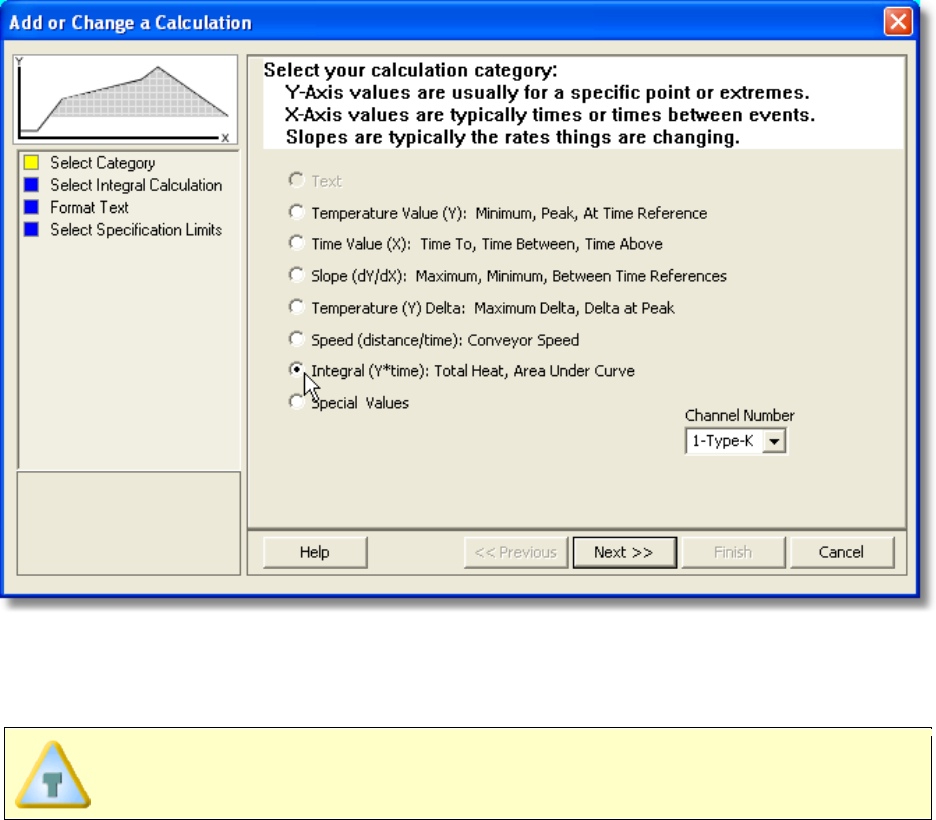
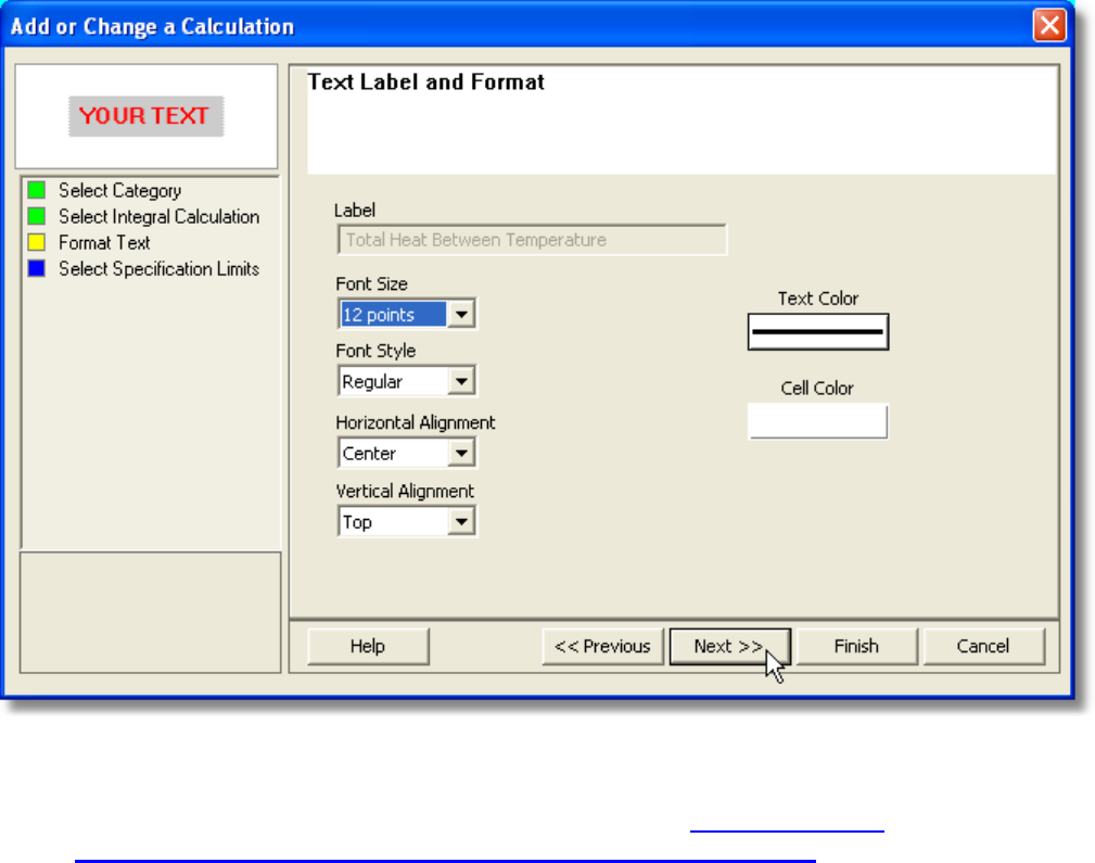
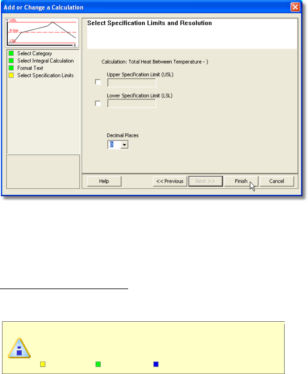
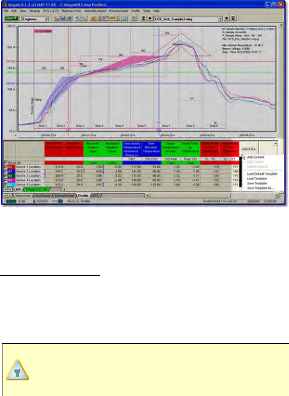
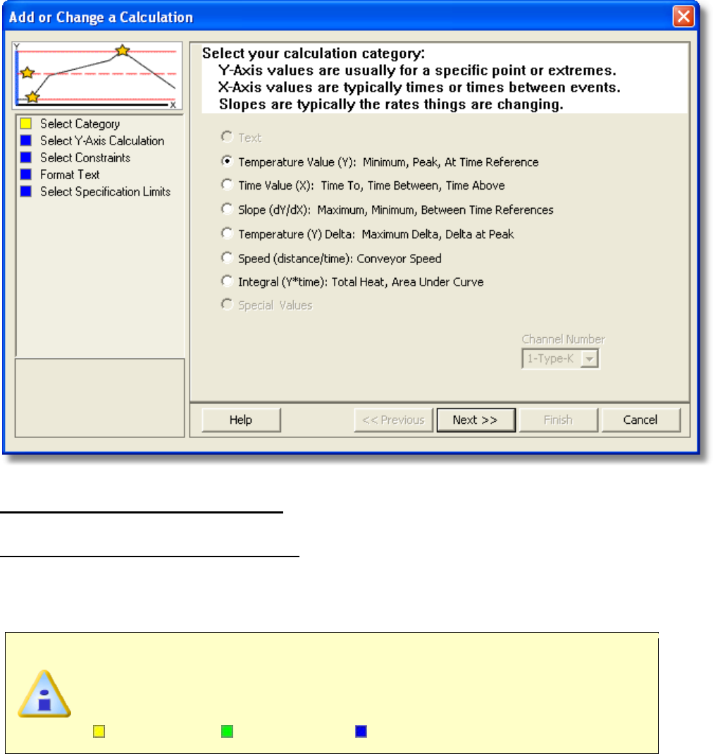
5.4.3.2.1.6. Integral (Y*time)
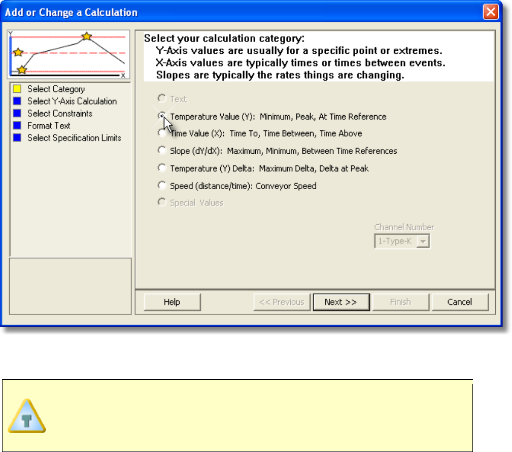
To add or edit Speed (distance/time) content:
1) Right-click a template cell and a shortcut menu appears.
2) Select Add Content or Edit Content from the shortcut menu and the Add or
Change a Calculation wizard appears.
When navigating through the wizard, the step list on the left uses a color key
to inform the user of the current step, steps that have been completed and
remaining steps.
Current Completed Remaining
3) Click Intergral (Y*time) and which channel to derive the data from
4) Select the Next command button.
5) Enter the Lower value to define the base of the integral calculation and an Upper
value to define maximum value to include in the integral.
To not rest
rict the maximum value of the integral, a very large value can be set
for the Upper value.

6) Select the Next command button.
7) Select desired text formatting options.
8) Select the Next command button.
9) Select Specification Limits and Units. If these values are violated colored bars will
appear in the formatted template cell. Refer to topic Software>Page
Tabs>Spreadsheet>Template>Specification Limit Indicators for more
information.
10) Select the Finish command button to complete the wizard and display the new
calculation data in the selected template cell.
5.4.3.2.1.7. Special Value
To add or edit Special Value content:
1) Right-click a template cell and a shortcut menu appears.
2) Select Add Content or Edit Content from the shortcut menu and the Add or
Change a Calculation wizard appears.
When navigating through the wizard, the step list on the left uses a color key
to inform the user of the current step, steps that have been completed and
remaining steps.
Current Completed Remaining
3) Click Special Value.
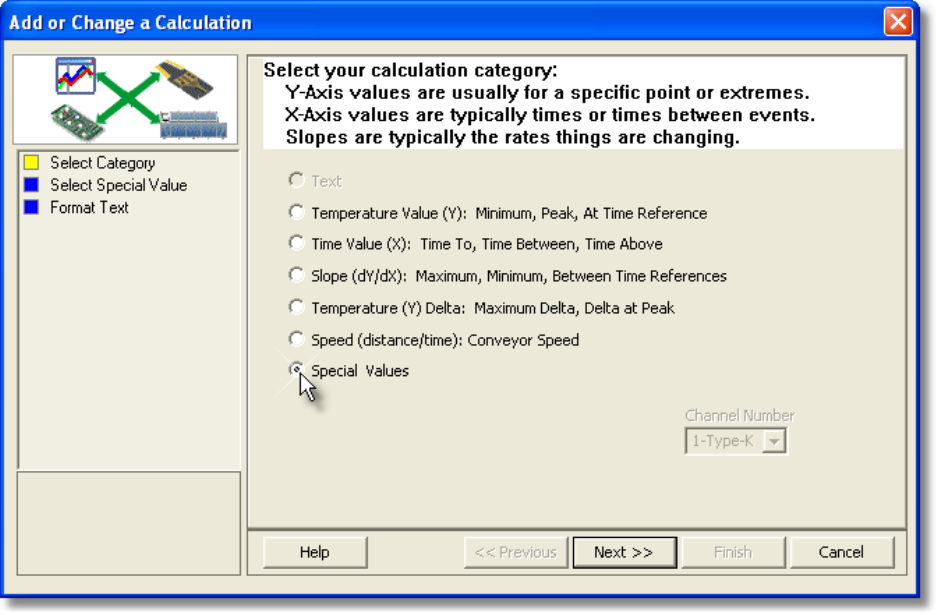
4) Select the Next command button.
5) Select a Special Value type.
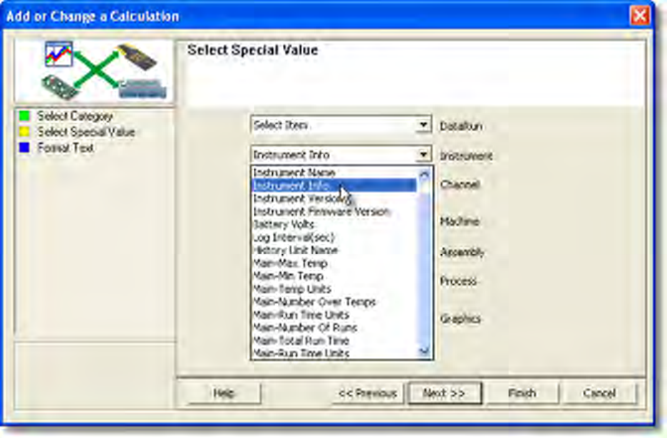
6) Select the Next command button.
7) Select desired text formatting options.
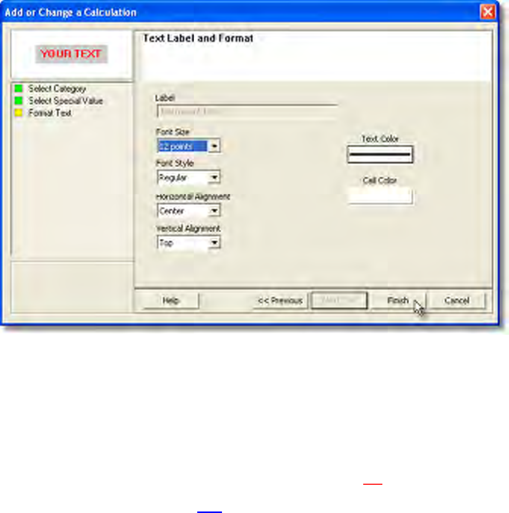
8) Select the Finish command button to complete the wizard and display the new
calculation data in the selected template parameter column.
5.4.3.2.2. Specification Limit Indicators
Each Parameter displayed on the Spreadsheet Page Tab can have both Lower and
Upper specifications applied. If a specification limit is violated, the software displays a red
or blue indicator on the left edge of the Data Table cell.
If a USL has been exceeded, that parameter indicator will appear in red (indicating it is
above the specification limit). If a parameter is less than the user specified LSL, that
parameter indicator will be appear in blue (indicating below the specification limit).
Refer to topic Software>Page Tabs>Spreadsheet>Template>Add & Edit
Content for information on how to apply LSL and USL values.
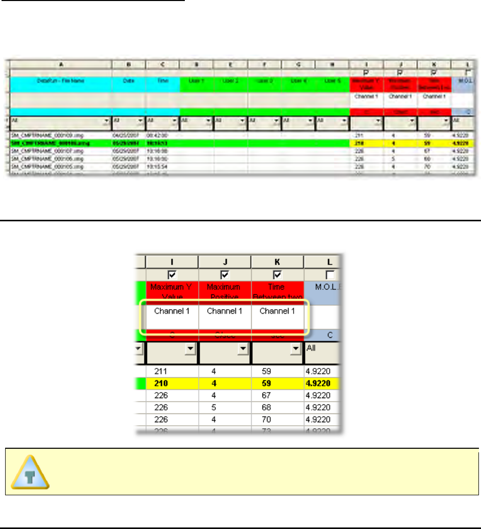
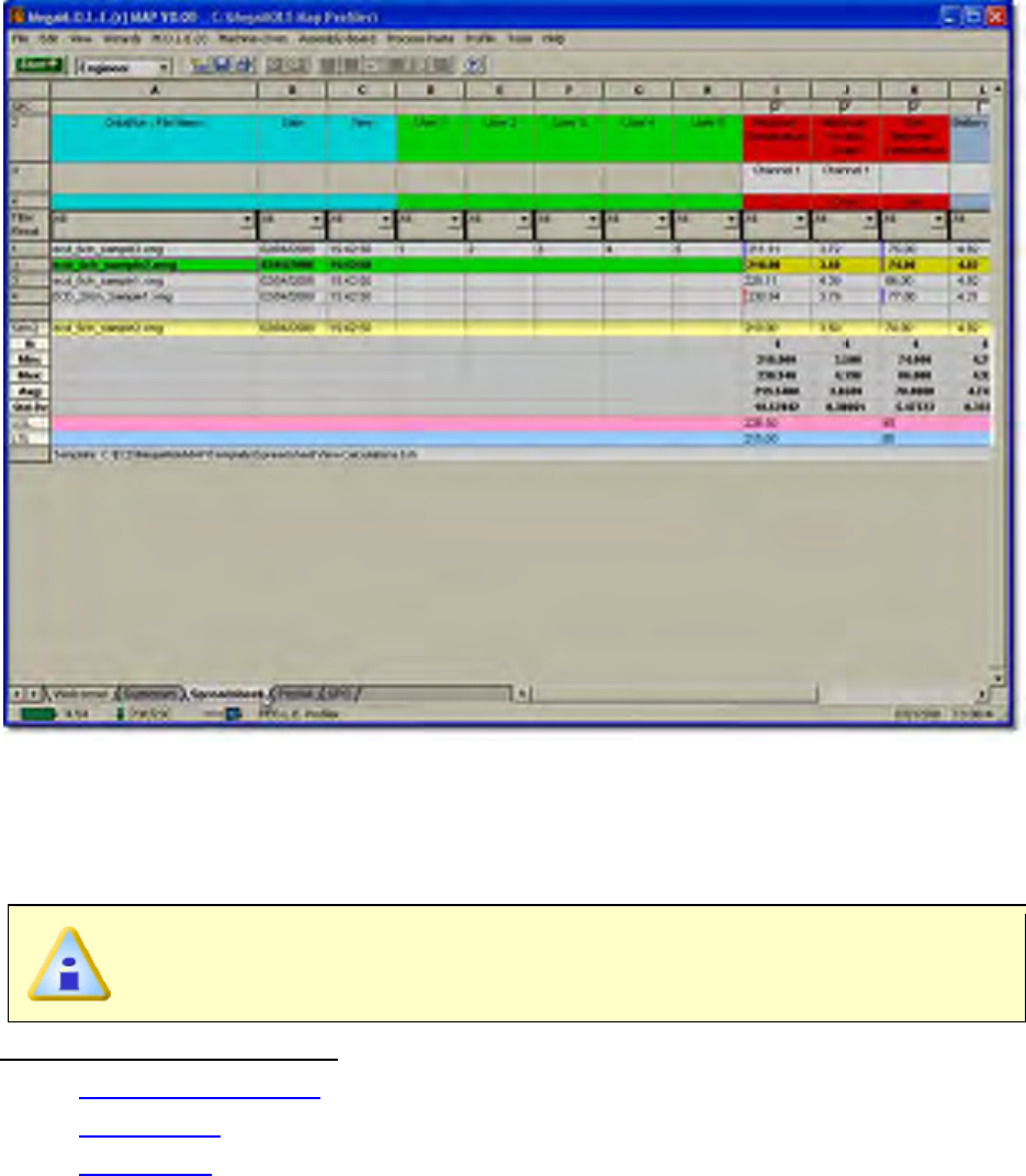
5.4.3.3. Parameters
When parameters are displayed on the Spreadsheet template, they include header,
labels and unit cells. These parameters can be color coded with the associated
Parameter Labels so they can be easily identified together.
The width of each column can be adjusted to be larger or smaller by placing
the mouse pointer over a split line dividing the columns and sliding it to the
desired width.
Parameter Headers
The software includes two default parameter headers that display data run and user
defined information. All headers displayed to the right of those display the description of
the parameter.
When editing or adding parameters, the software does not allow the default
parameter description to be modified.
Data Run Parameter Group:
This group contains file information associated with the run such as; date and time, (of
profile) and the data file tag.
User Defined Parameter Group:
These parameter columns can be used to enter text to help identify the row with unique
information about that run (i.e. shift, operator, line number, part number). This information
will also appear in the Tool Status box on the Profile worksheet.
Parameter Labels
The Parameter Labels display details associated with the displayed parameters.
For example, in the Maximum Y Value parameter, the label is Channel 1.
Parameter Units
The Parameter Units are the units of measurement for the displayed parameter.
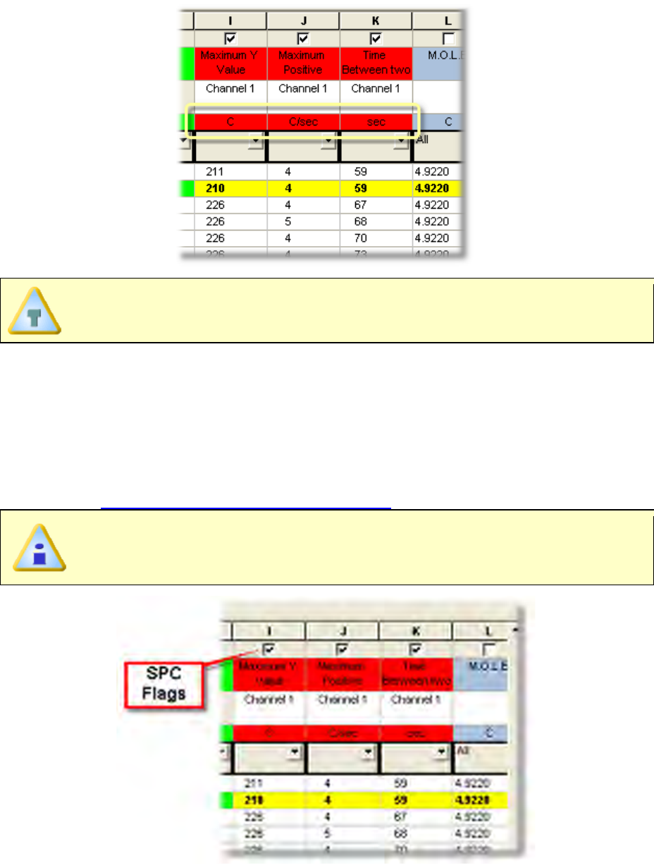
For example, in the Maximum Positive Slope parameter, the parameter unit
is °C/sec.
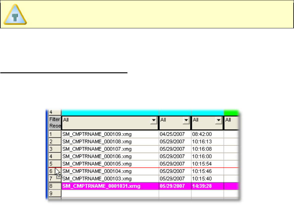
5.4.3.4. SPC Flags
SPC Flags allow the user to flag parameters so they are displayed on the SPC Page Tab.
For each Parameter listed after the User defined Parameters, there is an SPC Flag. To
display the parameter data in an X-Bar and R-Chart format, select the desired SPC Flag.
Refer to topic Software>Page Tabs>SPC Page Tab for more information.
This is available when in Engineer Mode.
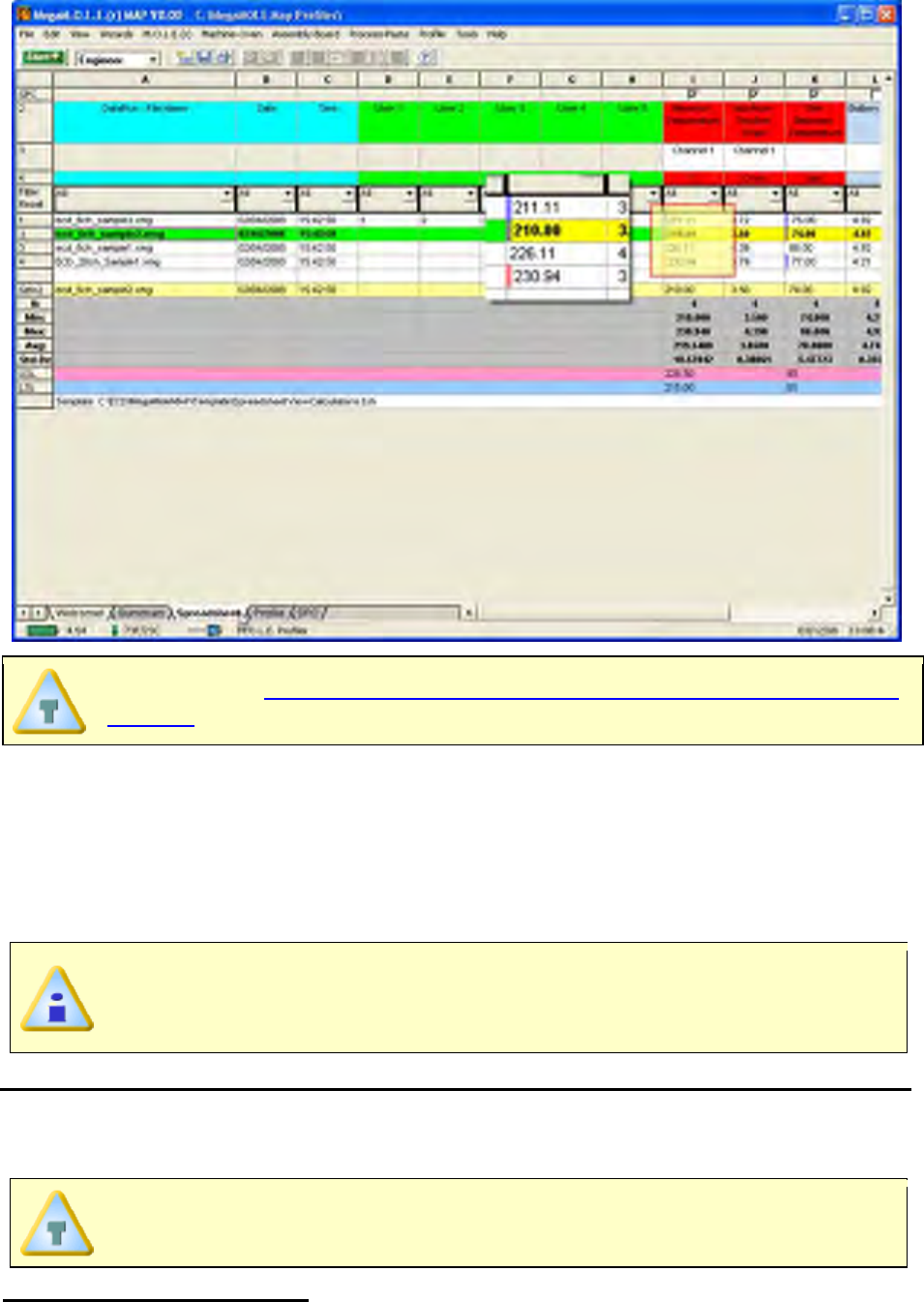
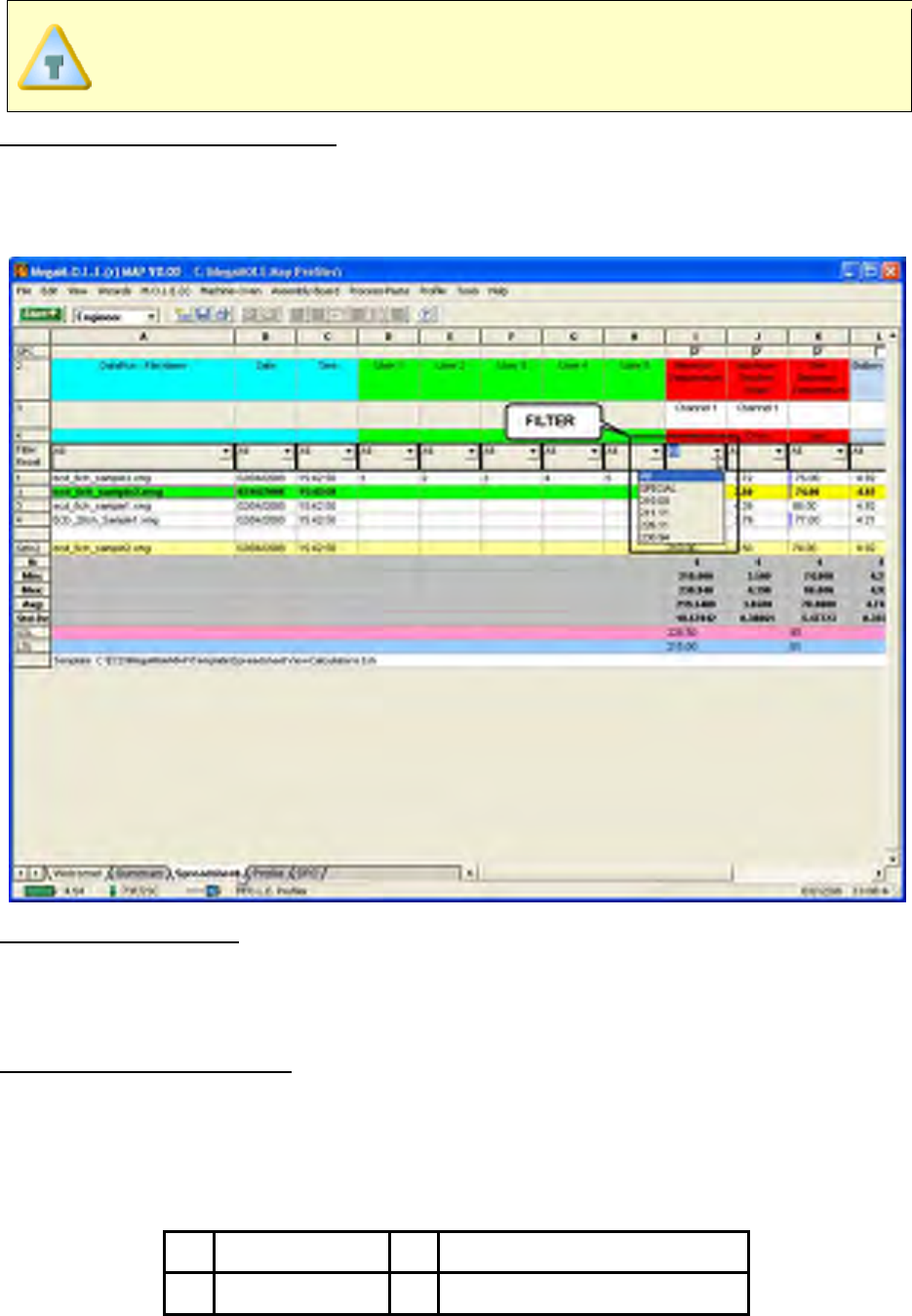
5.4.3.5. Data Run Rows
All of the data runs in the open working directory are listed on the Spreadsheet Page Tab
as individual rows. The first data run uploaded or imported into the directory is on the
bottom and the most recent data run is on the top.
When any data run row is selected, all of the cells in the entire row are highlighted in
purple and blue. The purple cells indicate that the cells can be modified and the blue cells
indicate the data cannot be modified.
When any individual data cell in a data run row is selected, all of the cells in the entire row
are highlighted in green and yellow. The green cells indicate that the cells can be modified
and the yellow cells indicate the data cannot be modified.
When a data run row is selected, the data for that row will also be displayed in the Sel=
row located at the bottom of the data run rows. This row allows the user to easily compare
the selected data row to the statistics calculations located below the selected run row.
Selected rows and columns can be “copied” by pressing keys [CTRL +
C] and then “pasted” [Ctrl + V] into other applications.
The data run rows can also be moved into any order desired. This is useful when the user
wants to place similar data runs together.
To change the order of the data run:
1) Select the number cell of a data run row with the mouse pointer. The row will then
become highlighted in purple and blue.
2) Drag the row and drop it to a desired location.
5.4.3.6. Filters
There are Filters for each parameter label that user can filter specific data out.
Filtering more than one column at a time acts as a Logical AND
Function. All conditions of all set filters must be met for data row(s) to
remain visible.
How to use the Filter function:
1) Click the Filter button to reveal the unique data as populated in that column under
that particular parameter label.
2) Select a desired data value to filter, or the two standard filters All and Special.
To use the All option:
1) Select All to reset the filter for that column and view all of the data run rows that
meet the other column filters.
To use the Special option:
1) Select Special to select data run rows within a range of values. There are multiple
options to select information to filter by clicking the appropriate relational operators
option button. The user can either select data from a populated list or type it in the
text box on the top of the column.
=
equal to
>=
greater than or equal to
>
greater than
<=
less than or equal to
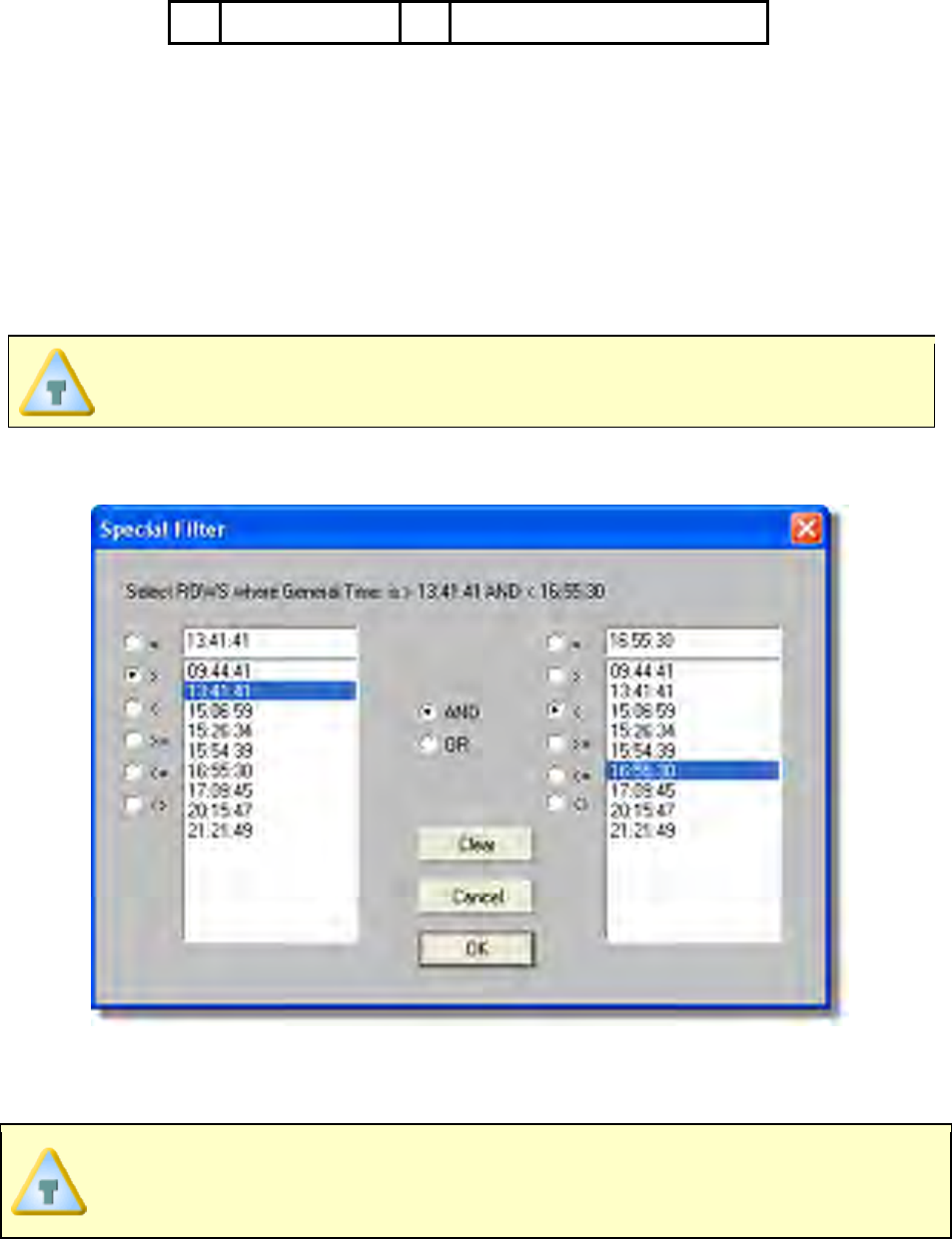
<
less than
<>
Not equal to
2) Select a data filter by:
• Clicking the greater than relational operator option button beside the left data
column.
• Click a parameter value from the list or type it in the text box.
• Click the AND logical operator option button.
• Click the less than relational operator option button beside the right data column.
• Click a parameter value from the list or type it in the text box.
The Clear command button can be selected at any time to clear the
selections and the new values can be selected.
3) Click the OK command button to accept the selected data filters or Cancel to
return to the Spreadsheet Page Tab without executing the filter request.
In this example, the data filtered would be all times between, but not including 13:41:41
and 16:55:30.
When the data is filtered, the column header and the Filter Reset button
are highlighted in RED. To reset the data run rows to display the entire
set of collected data, click the red Filter Reset button.
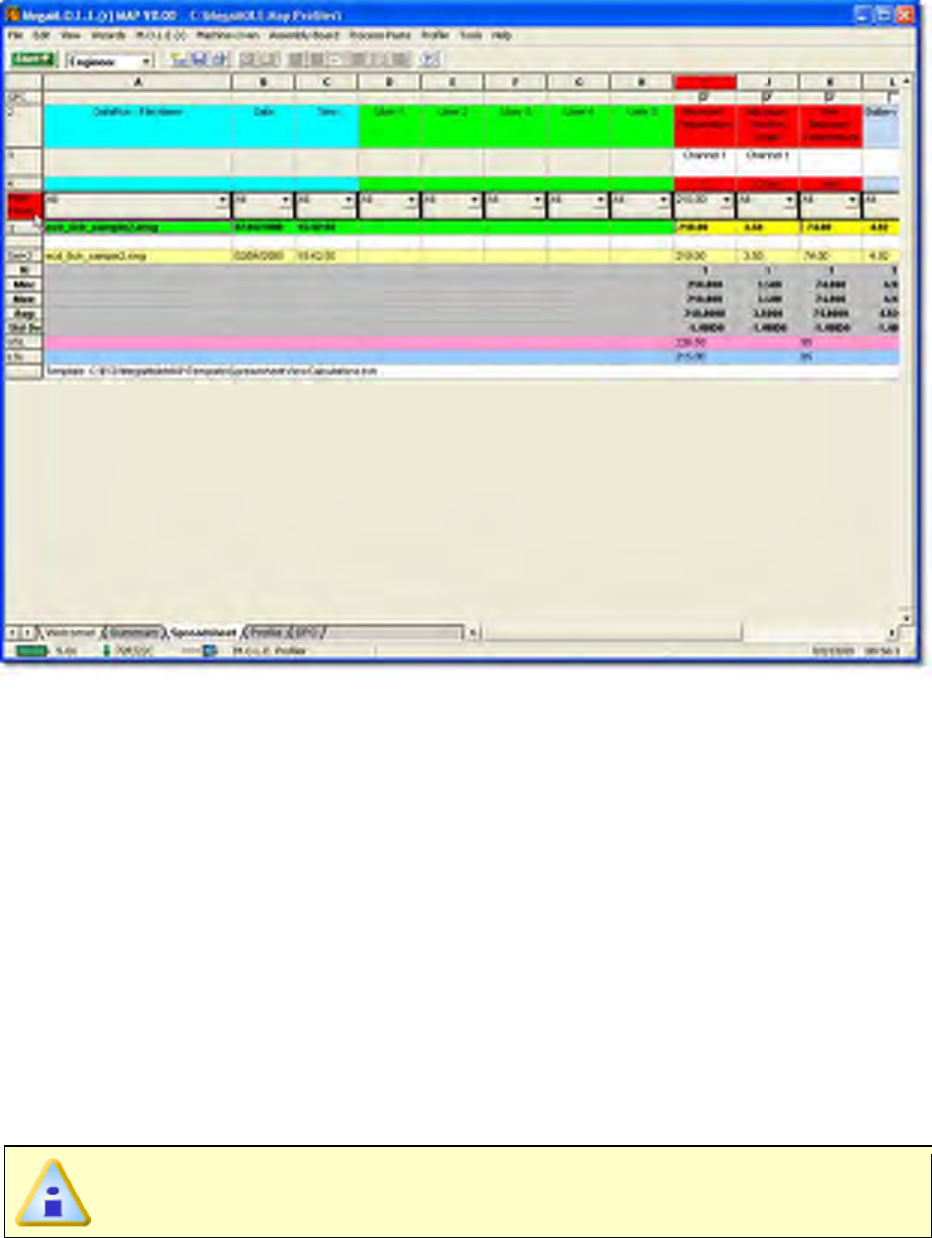
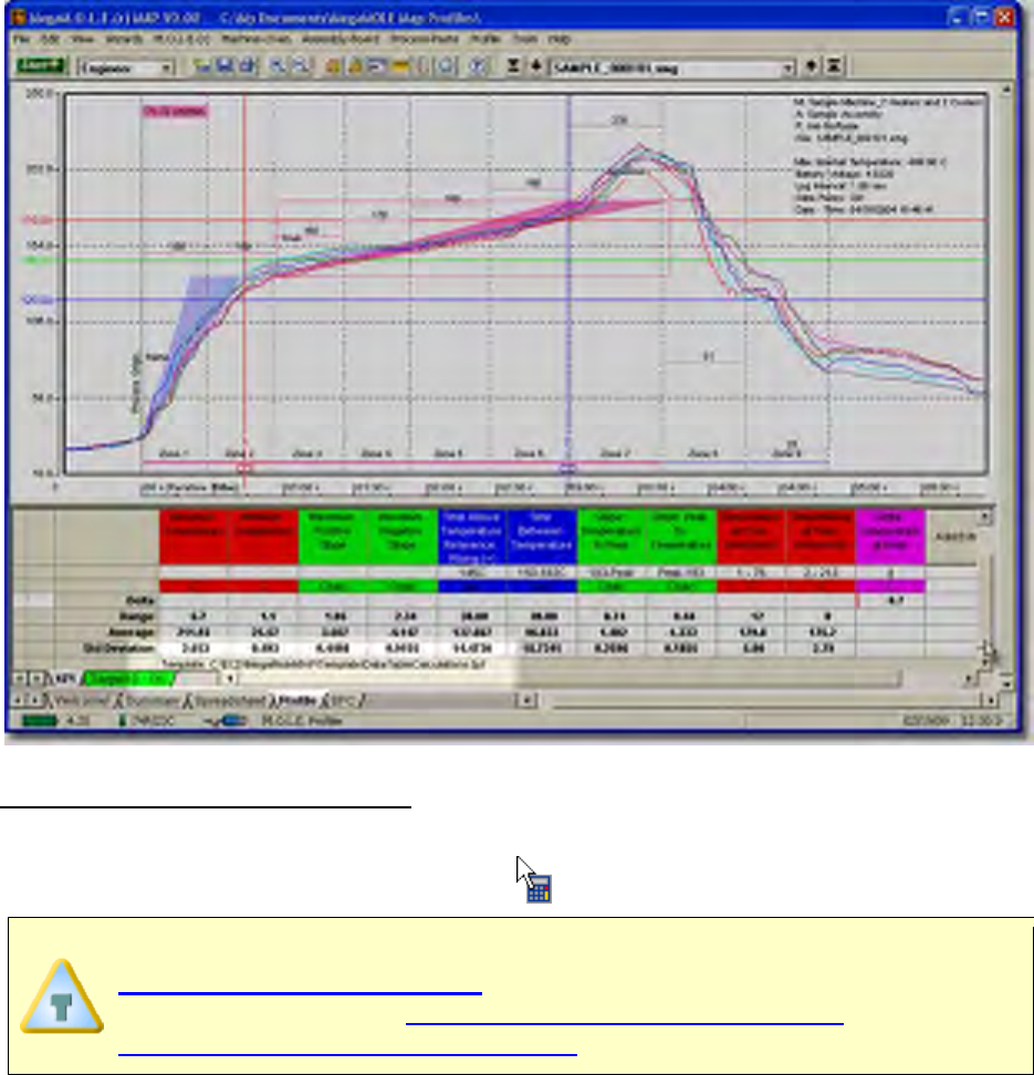
5.4.3.7. Statistics
There are shaded rows located on the bottom of the Spreadsheet worksheet, which are
the combined calculations for all the data runs that are currently being viewed in the
Spreadsheet worksheet display. The following information is the definitions for each
Statistics row:
• N = Number of samples included in the calculations
• Min. = The lowest value in the parameter column.
• Max. = The highest value the parameter column.
• Avg = The average of all values in the parameter column.
• Std. Dev. = The standard deviation of the values in that column.
• USL = Upper Specification limit set for that parameter using the Calculation wizard.
• LSL = Lower Specification limit set for that parameter using the Calculation wizard.
The USL and LSL statistics will only be displayed if there is values set for that
parameter
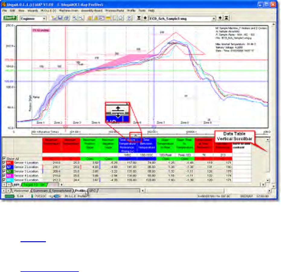
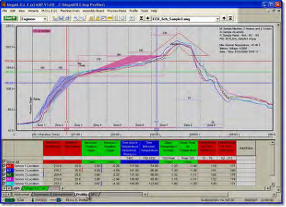
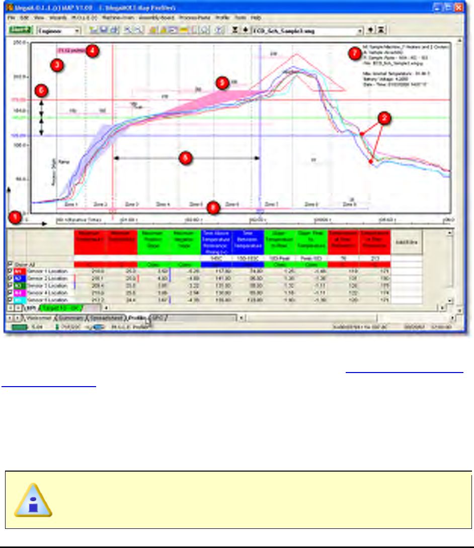
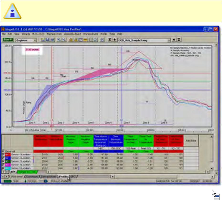
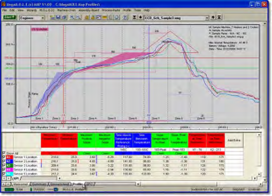
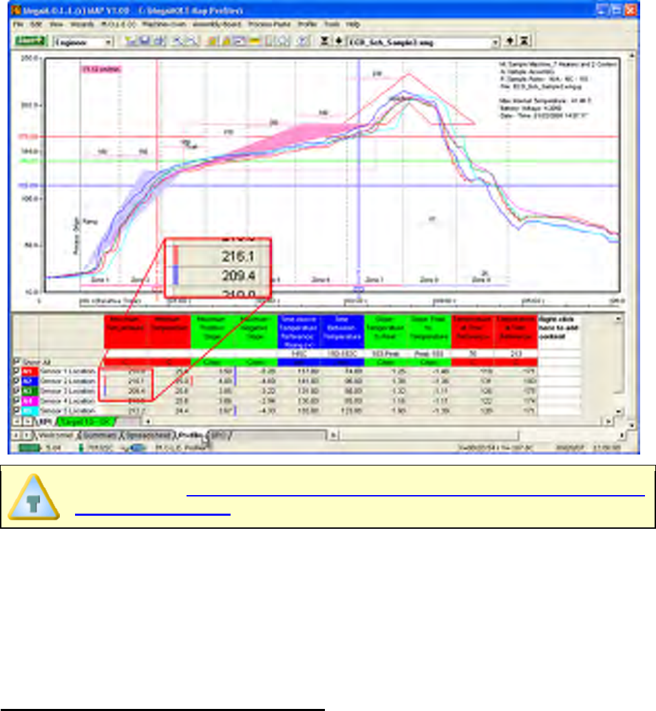
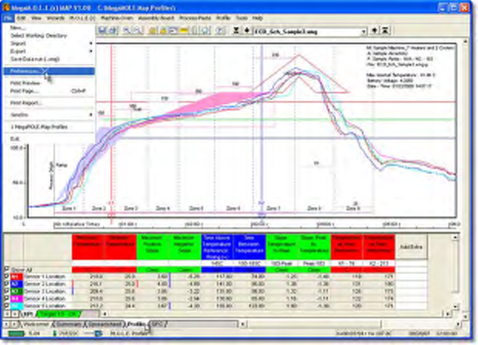
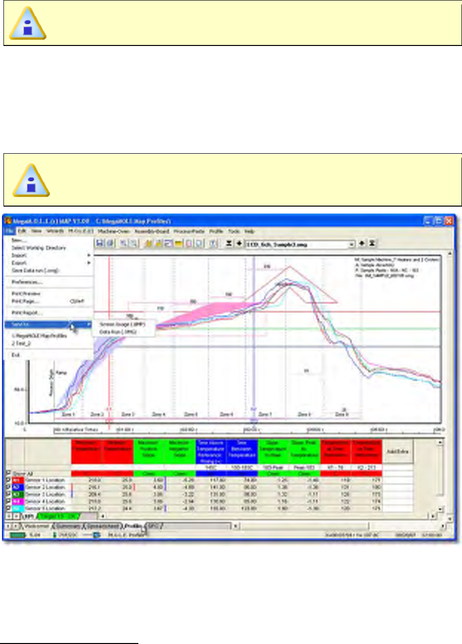
5.4.4. Profile Page Tab
The Profile worksheet is where a selected data run is represented graphically. The
software allows the user to analyze the data and to compute statistics based on the data.
This is available in both Engineer & Verify Modes.
Profile worksheet features:
Menus and Toolbar
Data Graph
Data Table
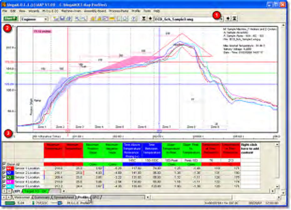
The Profile Page Tab is divided into two panes, the Data Graph and Data Table. Using the
pane split bar, these panes can be moved vertically so the user can display more of the
Data Graph or Data Table. The Data Table also includes a vertical scroll bar so the user
can view more Data Table without moving the pane split bar.
5.4.4.1. Menus & Toolbar
• Menus:
File, Edit, Wizards, M.O.L.E.®, Machine-Oven, Assembly-Board, Process-Paste,
Profile, Tools and Help.
• Toolbar Buttons:
Engineer Mode - Start, Open Working Directory, Save, Print, Magnify, 100%,
Slope, Peak Difference, Overlay, Measure, Notes, Prediction, Help, First (data run
of the data set), Back (to previous data run), Forward (to the next data run), and
Last (data run of the data set).
Verify Mode - Start, Open Working Directory, Save, Print, Notes, Help, First (data
run of the data set), Back (to previous data run), Forward (to the next data run),
and Last (data run of the data set).
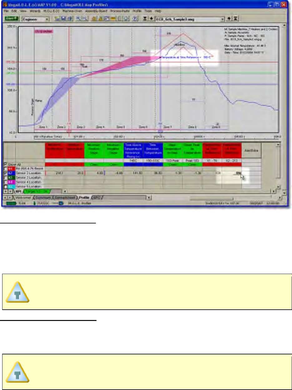
5.4.4.2. The Data Graph
The Data Graph is a display that shows the data collected from the data run overlaid on a
graph. The user can analyze and highlight various process features with the tools listed
below.
The features associated with the Data Graph can be used when in Engineer
mode. They can only be viewed when in Verify mode.
Data Graph features:
Time & Temperature Scales
Data Plots
Process Origin
Conveyor Speed Indicator
Time Reference Lines
Temperature Reference Lines
Map Data
Machine Zones and Zone Sizes
Machine Zone Temperatures
The Data Graph features are described in the sections that follow. Some of these features
are also controlled using the appropriate menu options. Refer to Software>Menu and
Tool Commands for more information.
5.4.4.2.1. Time (X) & Temperature (Y) Scales
The Data Graph displays both Time (X) and Temperature (Y) scales.
According to the type of sensor that is associated with the displayed profile,
the Temperature (Y) scale may display different a type of scale other than
Temperature .
Time (X) Scale:
The horizontal Time (X) scale displays values data points collected. The user can select
four different types of Time (X) scales. The scales are:
• Point: The data points collected from the Process-Origin.
• Time-Relative: Time measured from the Process-Origin
• Time-Absolute: Time of day
• Distance: Distance from the Process Origin (Meters, Centimeters, Feet or
Inches).
The Distance scale will not be accurate until an accurate conveyor speed is
set.
Relative Time Scale
Distance Scale
Points Scale
Absolute Time Scale
Temperature (Y) Scale:
The vertical Temperature (Y) scale displays the scale of the measured temperature.
Lower values are at the bottom and higher values at the top.
The Temperature (Y) scale includes temperature labels on the left side of the graph.
These temperatures divide the vertical scale up to four equal parts and are automatically
scaled to fit the current Temperature (Y) scale limits. These units can be displayed in
Celsius or Fahrenheit.
The amount of displayed Temperature (Y) grid lines can be changed on the
Profile tab of the Preferences dialog box. Refer to topic
Software>Menus>File>Preferences>Profile for more information.
Autoscaling:
The software includes a powerful Autoscaling option to automatically scale the Data
Graph so the data will always be visible and easy to work with.
The software automatically selects a range of values for the Temperature (Y) scale to
ensure that all the data fits on the screen. The user can change the range of temperature
values displayed by using the Manual mode. Refer to topic
Software>Menus>Profile>Temperature (Y) Scale for more information.
When the Magnify tool is used the Temperature (Y) scale will automatically
scale to the temperatures viewed in the magnified window.
The software provides different methods to view Time (X) and Temperature (Y) values of
any location on the Data Graph.
To view Time (X) & Temperature (Y) values:
• The Time (X)/Temp (Y) Readout in the Status bar continuously displays both Time
(X) and Temperature (Y) values at the location of the mouse pointer. Details of this
feature are described in topic Software>Menus>View>Status Bar.
• The Time (X) value at the position of a Time (X) Ref line is displayed in the Data
Table if a Temperature value at Time Reference calculation is loaded in the Data
Table template.
5.4.4.2.2. Data Plots
The Data Plots in the Data Graph represent the data for each of the sensors connected to
the M.O.L.E. Profiler. Each sensor is represented by a different color that corresponds to
the color of its sensor location description in the Data Table.
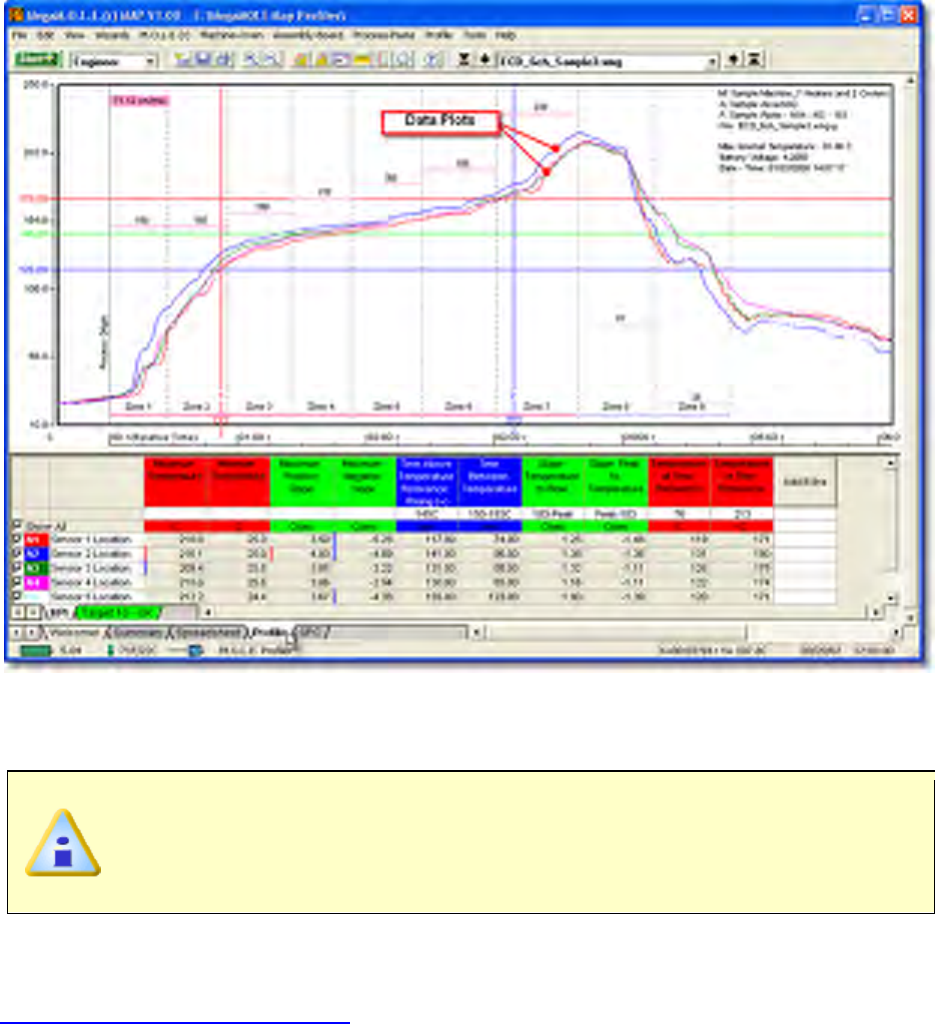
A Data Plot in the Data Graph can be suppressed or restored at any time by clicking the
channel check box with the corresponding sensor description in the Data Table. This
allows the user to view any combination of the Data Plots or individually.
When two or more Data Plots overlap the same values, the Data Plots
overwrite each other. For example, if the Data Plot that represents the sensor
connected to channel 5 and channel 1 have the same value, the channel 5
Data Plot will only appear unless the user suppresses it.
When printing a Data Graph in black and white, suppressing one or more Data Plots is
useful for clearing a view of a Data Plot that is obscured by others near it. The Notes tool
can also be used to help identify each Data Plot. Refer to topic
Software>Menus>Tools>Notes for more information.
5.4.4.2.3. Process Origin
The Process Origin is a gray vertical line at the left edge of the Data Graph that indicates
where the assembly process starts. When Points or Distance units are being used for the
Time (X) values, the Time (X) values to the left of the Process Origin are displayed as
negative and those to the right as positive in the Time (X)/Temp (Y) Readout.
To move the Process Origin:
1) Position the mouse pointer over the Process Origin.
2) When the mouse pointer becomes a , click and hold the left mouse button to
drag it left or right releasing the mouse button when the Time (X) Reference line is
at the desired location.
The X/Y Readout in the Status Bar indicates the true position of the Process Origin while
it is being moving. After the mouse button is released, the X-Readout changes to zero at
the Process Origin and displays negative numbers for X when the mouse pointer is
moved to the left of the Process Origin.
Reference line values are automatically adjusted when the Process
Origin is moved.
To display the distance of a conveyor process along the X-axis, adjust the Process Origin
to the data point that was recorded at the start of the conveyor process. Now set the
conveyor speed in the Oven Configure dialog box located in the Profile menu.
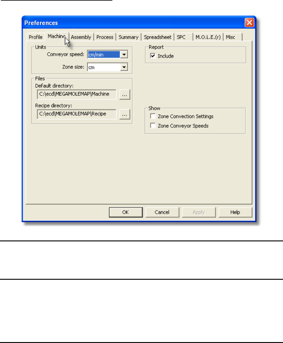
5.4.4.2.4. Conveyor Speed Indicator
Located at the top of the Process Origin, there is a Conveyor Speed Indicator that
displays the speed of the machine conveyor specified in the selected machine recipe.
Refer to topic Software>Menus>Machine>Set Machine Information.
Conveyor Speed can not be set or viewed after the Data Graph has been
magnified.
When the mouse pointer is placed over the conveyor speed indicator, it becomes a .
This informs the user that they can double-click the indicator to quickly change the
conveyor speed in the machine recipe.
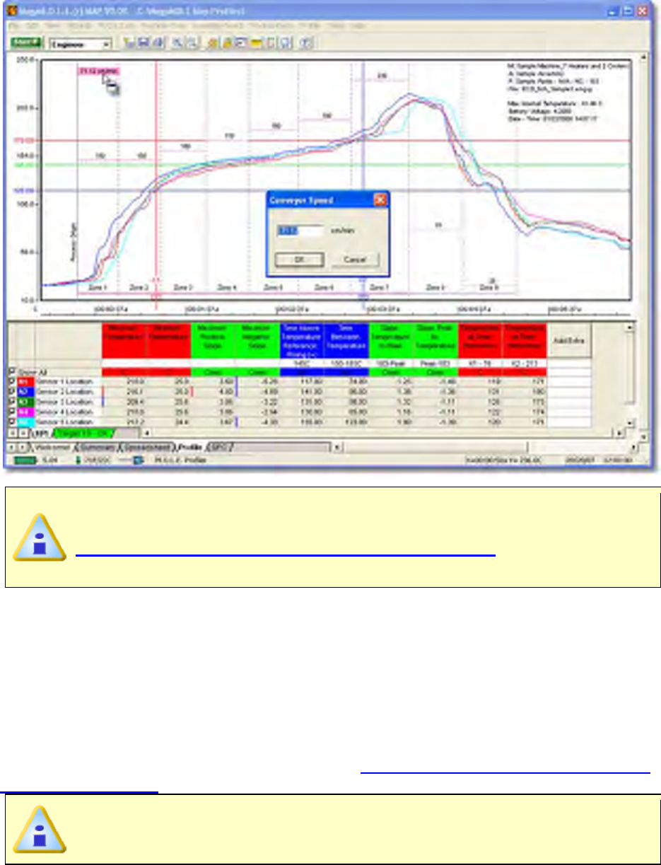
By changing the conveyor speed from the indicator, the user is modifying the
selected machine recipe. This recipe can also be edited using the
Software>Menus>Machine>Set Machine Information command on the
Machine-Oven menu.
5.4.4.2.5. Time (X) Reference Lines
Time (X) Reference lines are colored vertical lines that indicate the Temperature (Y)
values at the intersection of a Data Plot with each line. The values in the Temperature
value at Time Reference Data Table column(s) indicate the Temperature (Y) values at
the intersection of a Data Plot with an Time (X) Reference line. The Time (Y) Reference
lines can be added to the Data Graph using the Software>Menus>Profile>Add Time
(X) Reference Lines command in the Profile menu.
The Time (X) value at the position of a Time (X) Reference line will only be
displayed in the Data Table if a Temperature value at Time Reference
calculation is loaded in the Data Table template.
5.4.4.2.6. Temperature (Y) Reference Lines
Temperature (Y) Reference lines are colored horizontal lines that are positioned within
the Temperature (Y) scale in the graph. Temperature (Y) Reference lines can be added to
the Data Graph using the Software>Menus>Profile>Set Temperature (Y) Reference
Lines command in the Profile menu.
5.4.4.2.7. MAP Data
MAP data is the Machine model, Assembly number and Process name data associated
with the displayed data run. This data is located in the upper right corner of the Data
Graph along with the data run filename. This data can be specified when creating or
modifying the Machine, Assembly and Process information
The user can turn the MAP data ON or OFF using the Show on Profile
commands located on the Machine, Assembly and Process menus.
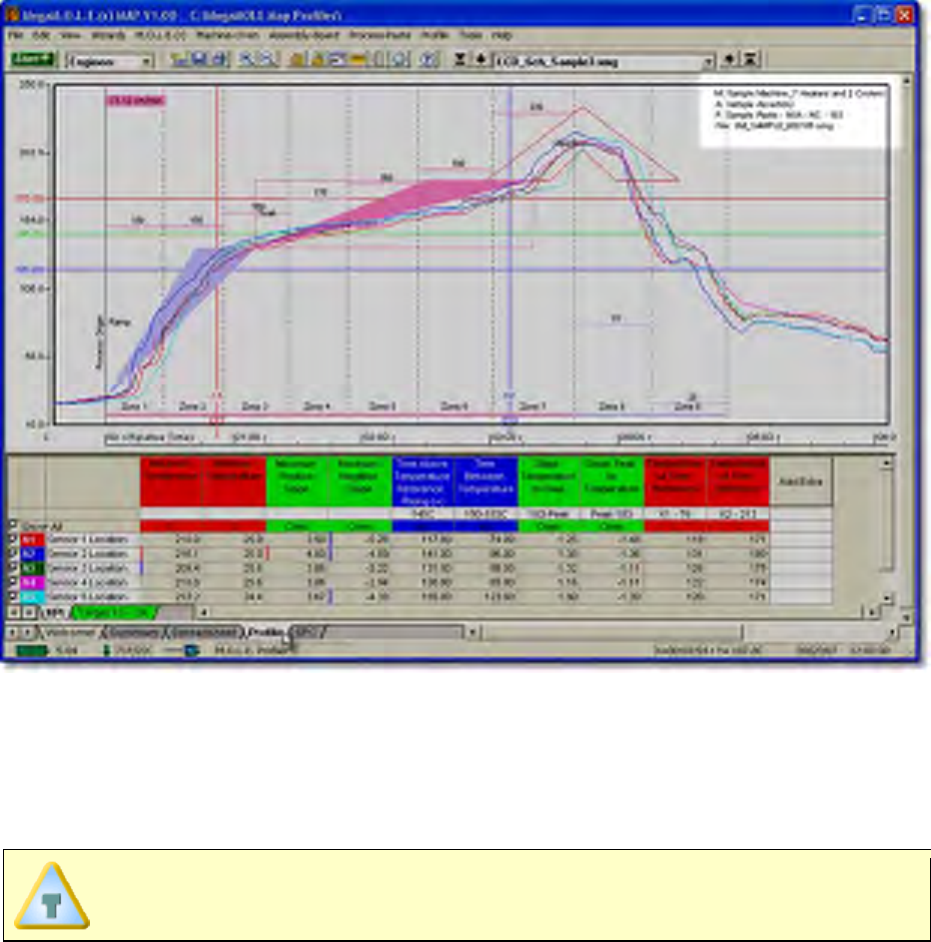
5.4.4.2.8. M.O.L.E. Status
M.O.L.E. status information displays the Max internal temperature, Battery Voltage and
the data run Date - Time at the time the data run was performed. This information is
located in the upper right corner of the Data Graph below with the MAP Data.
The user can turn the M.O.L.E. status information ON or OFF using the Show
on Profile commands located on the M.O.L.E. and Profile menus.
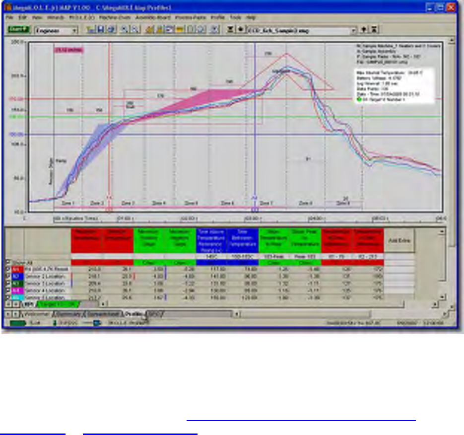
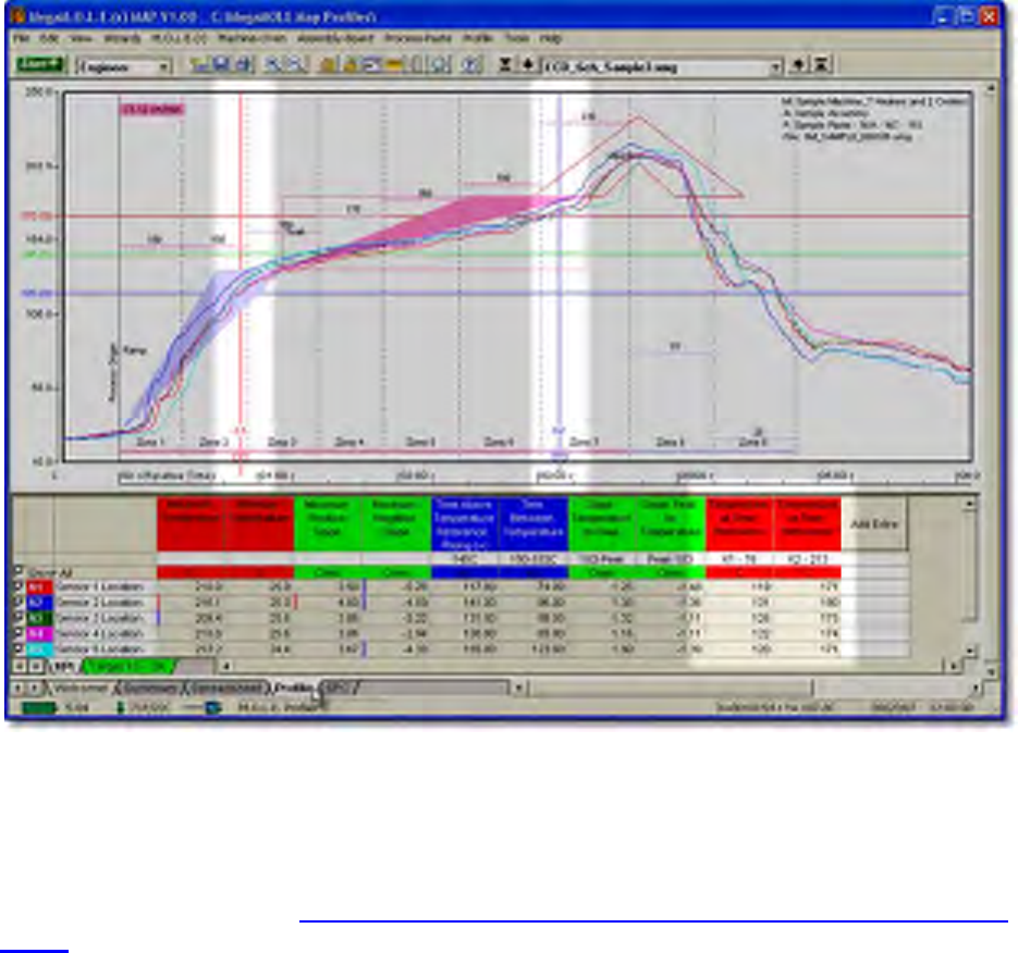
5.4.4.2.9. Machine Zones
The Time (X) scale can be divided into zones that represent the machine zones in a
process defined in units of length or time. Zones can be specified editing or creating a
new machine model. Refer to topic Software>Menus>Machine>Set Machine
Information or Create new Machine for more information.
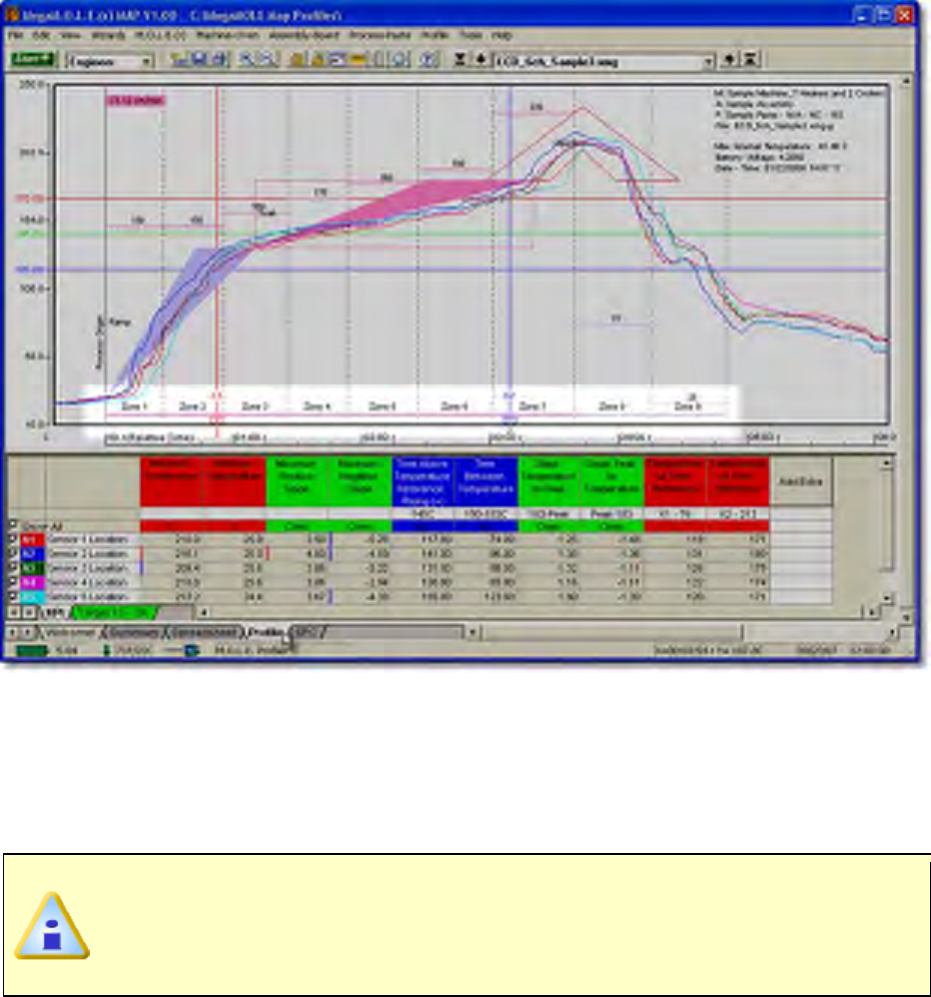
To display defined zones along the Time (X) scale, select the Show on Profile command
on the Machine menu. When zones are displayed, they appear as Magenta and Blue
colored lines along the bottom of the data graph and as dotted vertical lines that extend
top to bottom. The Magenta zones indicate heating and Blue zones indicate cooling. The
first zone begins at the Process Origin. When the Process Origin is moved, the zones
move with it.
When importing SMG SPC (.MDM) files, the machine zones remain the same
zone colors as specified in the original (.MDM) file. If the user edits the
imported machine zones, or applies a defined machine to the data run the
zone colors will be updated Magenta and Blue.
5.4.4.2.10. Machine Zone Temperatures
For each defined zone, two zone temperatures can be established using the Set
Machine Recipe command on the Machine menu. These temperatures might be upper
and lower boundaries for the acceptable range of values in that zone or they might
represent the settings of upper and lower heating elements in a process.
Zone Temperature Lines appear in the Data Graph as colored bars at the temperature set
for each zone. (Zone Temperatures can be displayed only after zone sizes are defined).
Upper Zone Temperature Lines appear in the Data graph as solid colored bars and the
lower Zone Temperature Lines are dashed.
5.4.4.3. KPI Data Table
The KPI Data Table includes various user configured parameter values. Each column
after the Sensor Locations allows the user to define parameters using the Template
commands. Each row in the Data Table represents the channel sensor data from the
M.O.L.E. Profiler.
This is available when in Engineer Mode.
KPI Data Table features:
Sensor Locations
Channel Check Boxes
Data Table Template
Value Pop-up
Specification Limit Indicators
5.4.4.3.1. Data Table Template
The Data Table is built using a template file (*.TPF) overlaid on a cell grid. Columns to the
right of the Channel check boxes and Sensor Locations allow the user to define
parameters using the Template commands.
The Data Table template is automatically loaded every time the software is
started and is used as the default template for every downloaded data run.
This template file is specified on the Profile Page Tab of the Preferences
dialog box. Refer to topic Software>Menus>File>Preferences>Profile for
more information.
For reference, the file name for the loaded template appears in the lower left corner of the
template grid.
To display Template commands:
1) Move the mouse pointer over a column header.
2) When the mouse pointer becomes a , right-click and a shortcut menu appears.
Template commands can also be accessed on the View menu. Refer to topic
Software>Menus>View Menu for more information. To add or edit a
calculation refer to topic Software>Page Tabs>Profile>Data
Table>Template>Add & Edit Content for more information.
5.4.4.3.1.1. Add & Edit Content Wizard
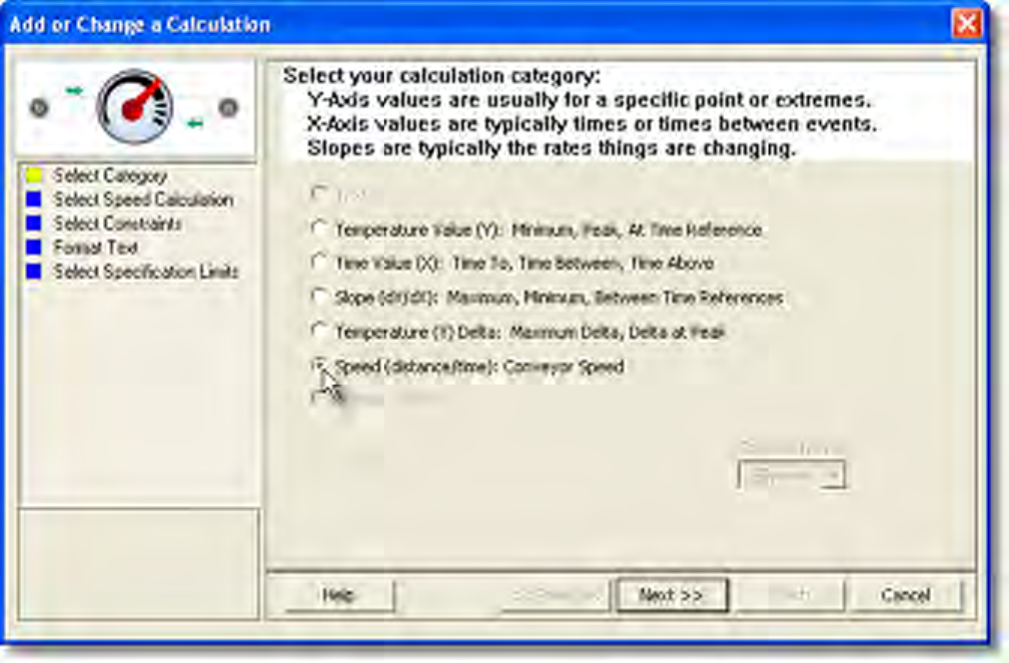
To add or edit template content, the software includes a wizard to guide the user through
the related content options. The Data Table template allows six different calculation
categories to be displayed.
Add & Edit Content wizards:
Temperature Value (Y)
Time Value (X)
Slope (dX/dY)
Temperature (Y) Delta
Speed (distance/time)
Integral (Y*time)
This wizard contains all the related steps to add or edit content to the template.
It is recommended to process all steps in order but the software allows you to
navigate forward and backward setting options individually. When the
minimum options have been selected, Finish command button will become
active.
5.4.4.3.1.1.1. Temperature Value (Y)
To add or edit Y-Axis Values content:
1) Right-click a template cell and a shortcut menu appears.
2) Select Add Content or Edit Content from the shortcut menu and the Add or
Change a Calculation wizard appears.
When navigating through the wizard, the step list on the left uses a color key
to inform the user of the current step, steps that have been completed and
remaining steps.
Current Completed Remaining
3) Click Temperature Values (Y).
4) Select the Next command button.
5) Select a Temperature (Y) Axis Value.
If Temperature at Time Reference calculation is selected, the software
requires the user to select an established Time (X) Reference line. If one is not
established the software automatically creates one on the Profile Page Tab
Data Graph.
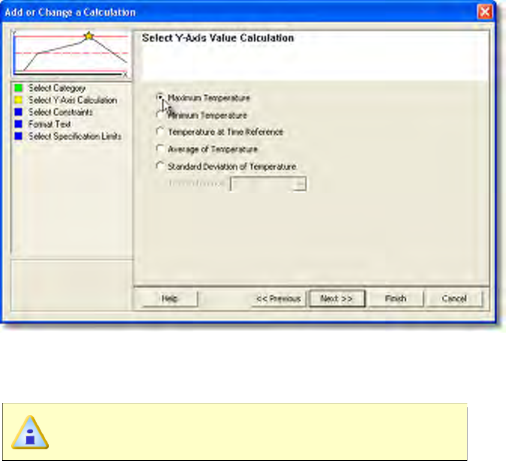
6) Select the Next command button.
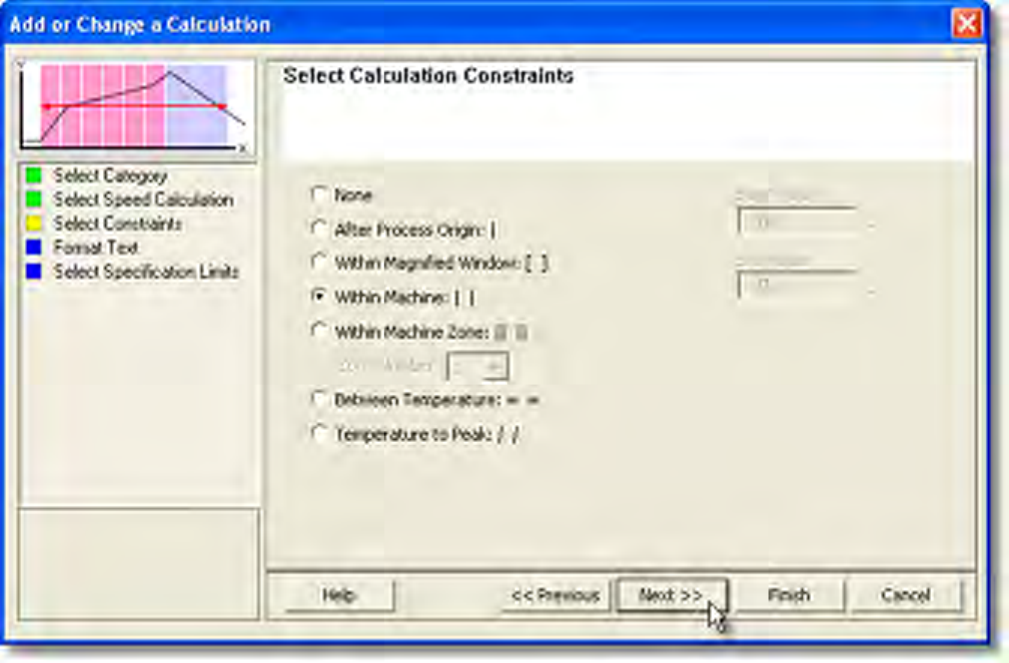
7) Select the calculation constraints. These options are the specified area on the
Time (X) Axis where the values are to be extracted from. When a constraint is
applied, the constraint symbol appears in the header of the calculation.
If the Within Magnified Window constraint is selected and the Magnify tool is
used to zoom in on a portion of the Data Graph, the Data Table displays the
statistics for those values within the magnified window.

8) Select the Next command button.
9) Select desired text formatting options.
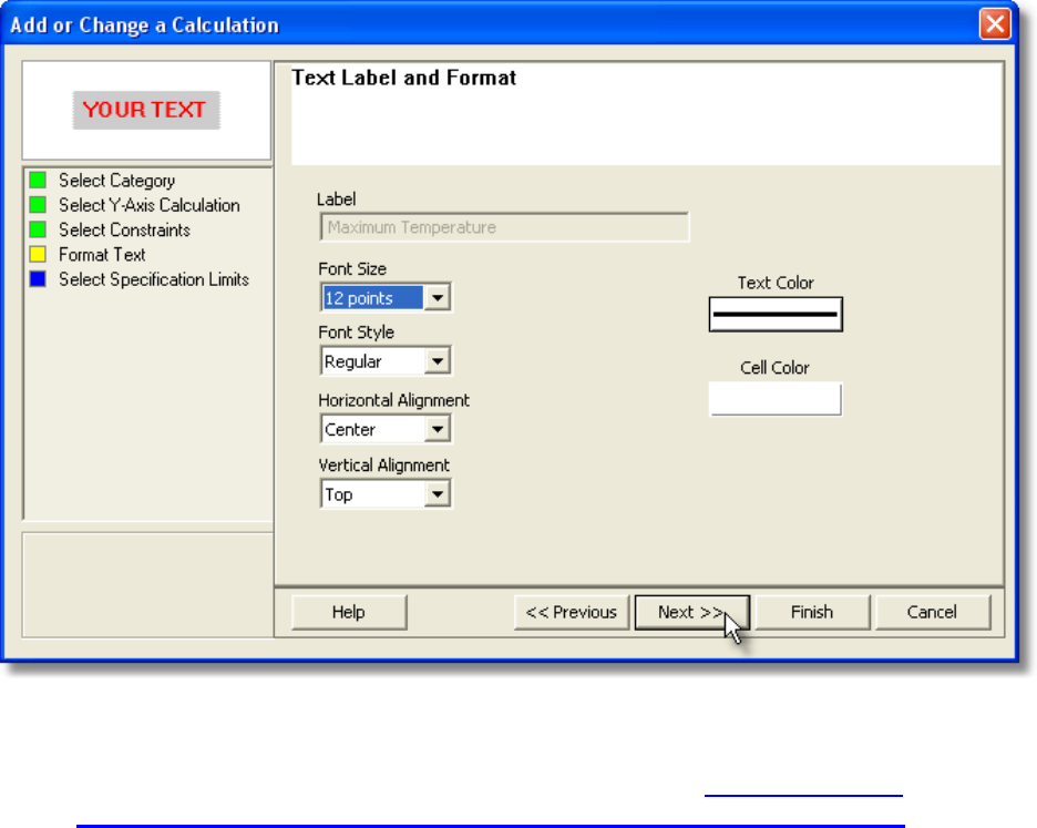
10) Select the Next command button.
11) Select Specification Limits and Units. If these values are violated colored bars will
appear in the formatted template cell. Refer to topic Software>Page
Tabs>Profile>Data Table>Template>Specification Limit Indicators for more
information.

12) Select the Finish command button to complete the wizard and display the new
calculation data in the selected template column.
5.4.4.3.1.1.2. Time Value (X)
To add or edit X-Axis Values content:
1) Right-click a template cell and a shortcut menu appears.
2) Select Add Content or Edit Content from the shortcut menu and the Add or
Change a Calculation wizard appears.
When navigating through the wizard, the step list on the left uses a color key
to inform the user of the current step, steps that have been completed and
remaining steps.
Current Completed Remaining
3) Click Time Value (X).
4) Select the Next command button.
5) Select a Time (X) Axis Value.
If any Temperature Reference (Y) calculation is selected, the software
requires a Temperature (Y) Reference Line to be established. Refer to topic
Software>Menus>Profile>Add Temperature (Y) Reference Lines.
6) Select the Next command button.
7) Select the calculation constraints. These options are the specified area on the
Time (X) Axis where the values are to be extracted from. When a constraint is
applied, the constraint symbol appears in the header of the calculation.
If the Within Magnified Window constraint is selected and the Magnify tool is
used to zoom in on a portion of the Data Graph, the Data Table displays the
statistics for those values within the magnified window.
8) Select the Next command button.
9) Select desired text formatting options.

10) Select the Next command button.
11) Select Specification Limits and Units. If these values are violated colored bars will
appear in the formatted template cell. Refer to topic Software>Page
Tabs>Profile>Data Table>Template>Specification Limit Indicators for more
information.
12) Select the Finish command button to complete the wizard and display the new
calculation data in the selected template column.
5.4.4.3.1.1.3. Slope (dX/dY)
To add or edit Slope Value content:
1) Right-click a template cell and a shortcut menu appears.
2) Select Add Content or Edit Content from the shortcut menu and the Add or
Change a Calculation wizard appears.
When navigating through the wizard, the step list on the left uses a color key
to inform the user of the current step, steps that have been completed and
remaining steps.
Current Completed Remaining
3) Click Slope (dX/dY).
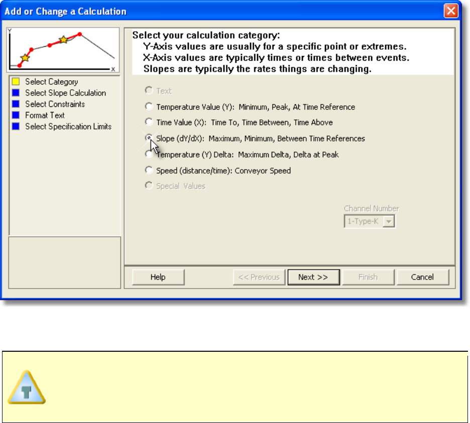
4) Select the Next command button.
5) Select a Slope Value.
If Slope Between Time References calculation is selected, the software
requires the user to select an established Time (X) Reference line. If one is not
established the software automatically creates one on the Profile Page Tab
Data Graph.
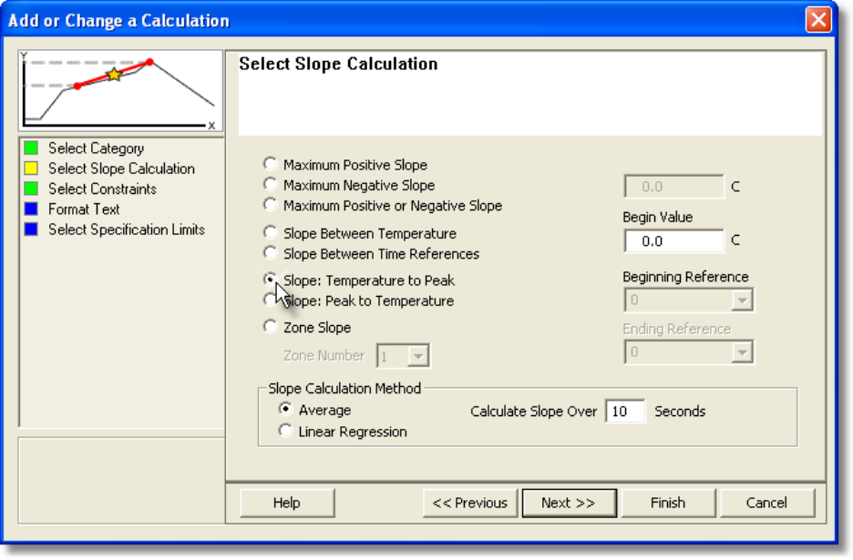
6) Select the Next command button.
7) Select the calculation constraints. These options are the specified area on the
Time (X) Axis where the values are to be extracted from. When a constraint is
applied, the constraint symbol appears in the header of the calculation.

8) Select the Next command button.
9) Select desired text formatting options.
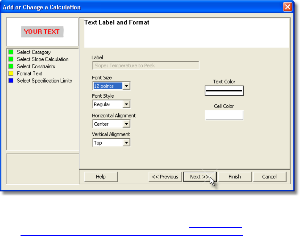
10) Select the Next command button.
11) Select Specification Limits and Units. If these values are violated colored bars will
appear in the formatted template cell. Refer to topic Software>Page
Tabs>Profile>Data Table>Template>Specification Limit Indicators for more
information.

12) Select the Finish command button to complete the wizard and display the new
calculation data in the selected template column.
5.4.4.3.1.1.4. Temperature (Y) Delta
To add or edit Temperature (Y) Delta content:
1) Right-click a template cell and a shortcut menu appears.
2) Select Add Content or Edit Content from the shortcut menu and the Add or
Change a Calculation wizard appears.
When navigating through the wizard, the step list on the left uses a color key
to inform the user of the current step, steps that have been completed and
remaining steps.
Current Completed Remaining
3) Click Temperature (Y) Delta and which channel to derive the data from.
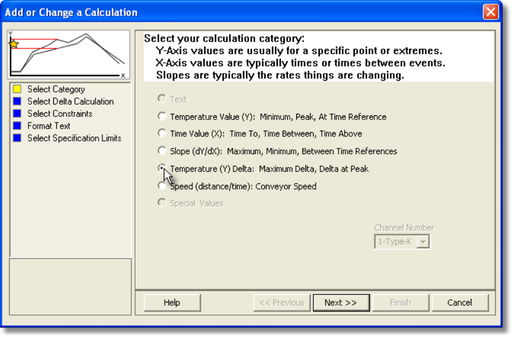
4) Select the Next command button.
5) Select a Y-Axis value delta calculation and which channels to you wish to be
included in this calculation.
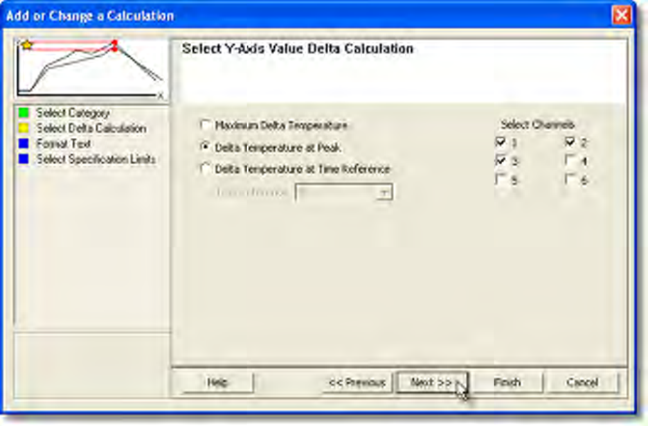
6) Select the Next command button.
7) Select desired text formatting options.
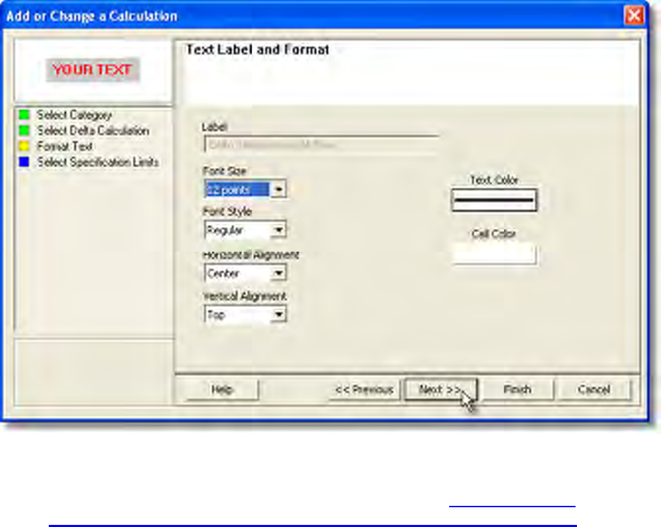
8) Select the Next command button.
9) Select Specification Limits and Units. If these values are violated colored bars will
appear in the formatted template cell. Refer to topic Software>Page
Tabs>Profile>Data Table>Template>Specification Limit Indicators for more
information.
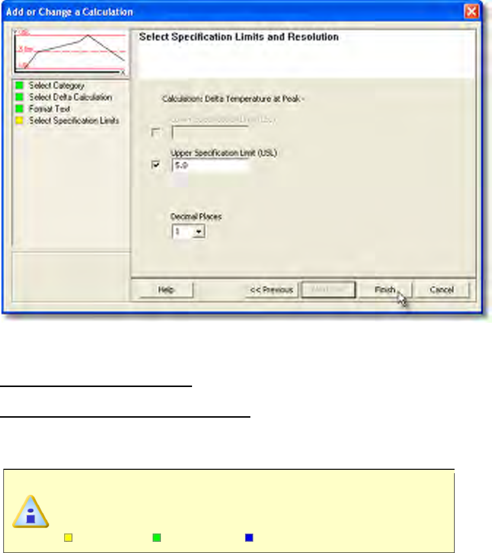
10) Select the Finish command button to complete the wizard and display the new
calculation data in the selected template cell.
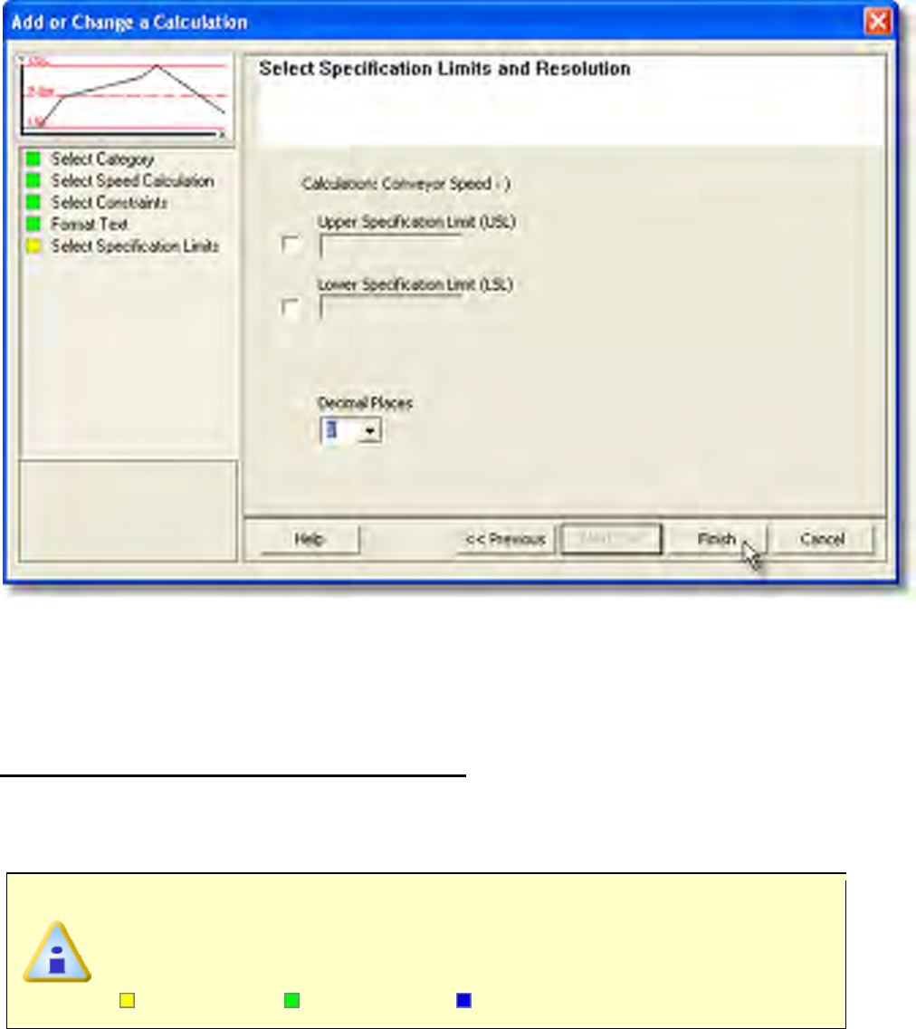
5.4.4.3.1.1.5. Speed (distance/time)
To add or edit Speed (distance/time) content:
1) Right-click a template cell and a shortcut menu appears.
2) Select Add Content or Edit Content from the shortcut menu and the Add or
Change a Calculation wizard appears.
When navigating through the wizard, the step list on the left uses a color key
to inform the user of the current step, steps that have been completed and
remaining steps.
Current Completed Remaining
3) Click Speed (distance/time).
4) Select the Next command button.
5) Select the two conveyor speed sensors and the distance between them.
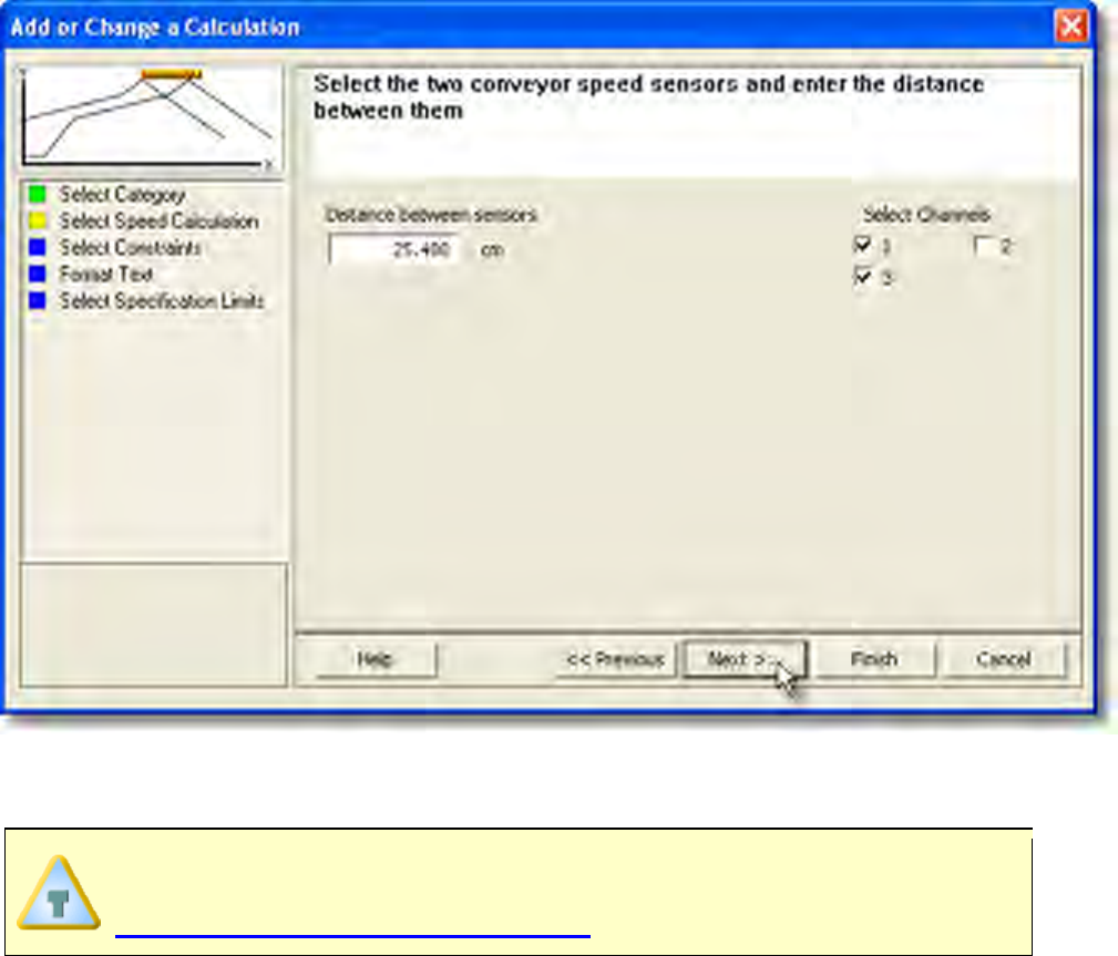
6) Select the Next command button.
7) Select a Time (X) Axis Value.
If any Temperature Reference (Y) calculation is selected, the software
requires a Temperature (Y) Reference Line to be established. Refer to topic
Add Temperature (Y) Reference Lines.
8) Select the Next command button.
9) Select desired text formatting options.
10) Select the Next command button.
11) Select Specification Limits and Units. If these values are violated colored bars will
appear in the formatted template cell. Refer to topic Software>Page
Tabs>Summary>Template>Specification Limit Indicators for more
information.

12) Select the Finish command button to complete the wizard and display the new
calculation data in the selected template cell.
5.4.4.3.1.1.6. Integral (Y*time)
To add or edit Speed (distance/time) content:
1) Right-click a template cell and a shortcut menu appears.
2) Select Add Content or Edit Content from the shortcut menu and the Add or
Change a Calculation wizard appears.
When navigating through the wizard, the step list on the left uses a color key
to inform the user of the current step, steps that have been completed and
remaining steps.
Current Completed Remaining
3) Click Intergral (Y*time).
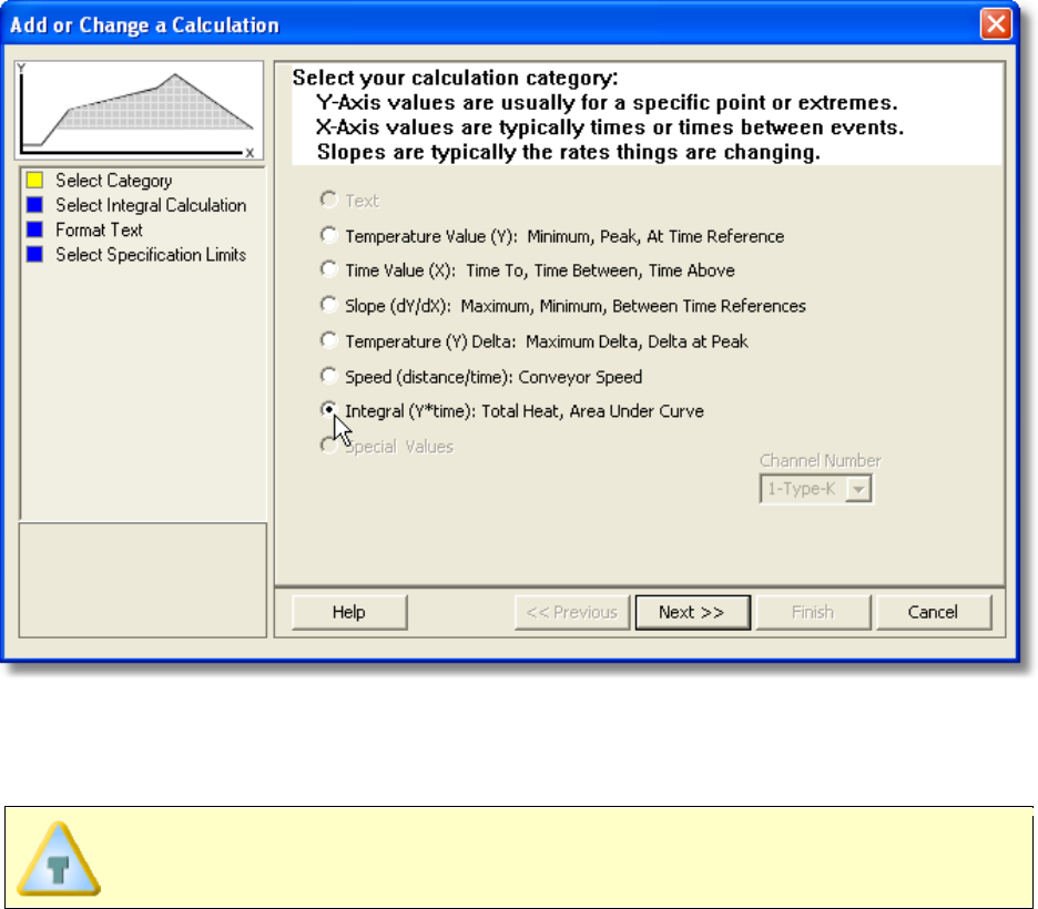
4) Select the Next command button.
5) Enter the Lower value to define the base of the integral calculation and an Upper
value to define maximum value to include in the integral.
To not restrict the maximum value of the integral, a very large value can be set
for the Upper value.
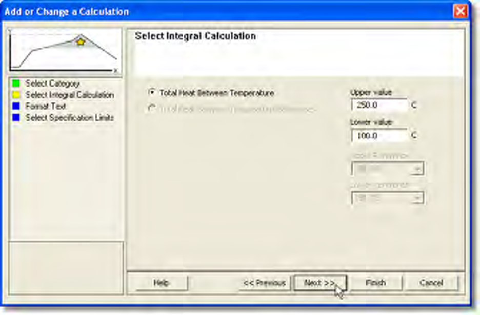
6) Select the Next command button.
7) Select desired text formatting options.
8) Select the Next command button.
9) Select Specification Limits and Units. If these values are violated colored bars will
appear in the formatted template cell. Refer to topic Software>Page
Tabs>Profile>Data Table>Template>Specification Limit Indicators for more
information.
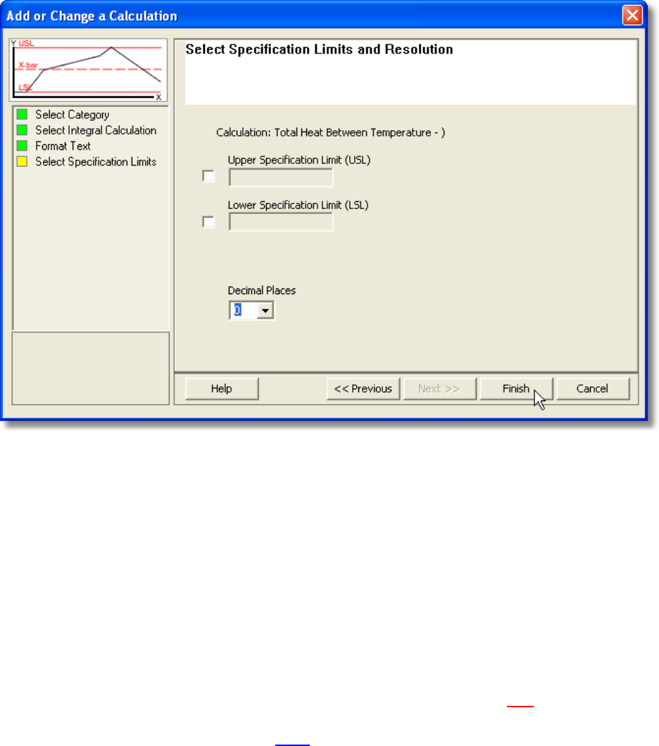
10) Select the Finish command button to complete the wizard and display the new
calculation data in the selected template cell.
5.4.4.3.1.2. Specification Limit Indicators
Each Parameter displayed on the Data Tab can have both Lower and Upper
specifications applied. If a specification limit is violated, the software displays a red or blue
indicator on the left edge of the Data Table cell.
If a USL has been exceeded, that parameter indicator will appear in red (indicating it is
above the specification limit). If a parameter is less than the user specified LSL, that
parameter indicator will be appear in blue (indicating below the specification limit).
Refer to topic Software>Page Tabs>Profile>Data Table>Template>Add &
Edit Content Wizard for information on how to apply LSL and USL values.
5.4.4.3.2. Sensor Location Description
The user can use the Sensor Location cells in the Data Table to describe the location
where each sensor is connected to the test product. The color and description indicates
which Data Plot on the Data Graph it represents.
To change a Sensor location description:
1) Click a Sensor Location cell and type the desired name and press the [enter] key.
The Sensor Location description can also be accessed by using the Set
Assembly Information command in the Assembly menu.
When the user places the mouse pointer over a Sensor Location Description,
that channel on the Data Graph profile will be become bolder so the user can
easily identify it.
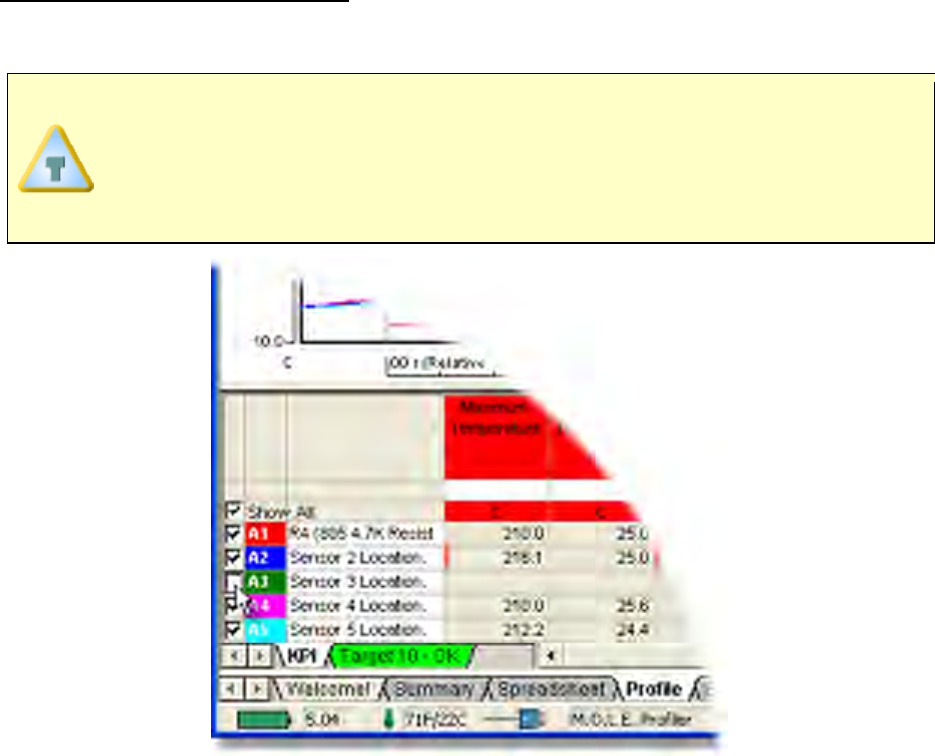
5.4.4.3.3. Channel Check Boxes
The Channel check boxes control whether the associated Data Plot is displayed on the
Data Graph and whether the data for that channel are included in the data table
calculations.
To turn a Data Plot ON or OFF:
1) Click the channel check box beside a Sensor location description to turn it “ON” or
“OFF”.
The user can click the Show All
check box to turn all channels “ON” or “OFF”.
This is helpful when a data run has a large amount of channels and they want
to view a smaller amount. To achieve this, click the Show All check box to turn
all channels “OFF”. Then click the desired channel check boxes to turn them
“ON”
5.4.4.3.4. Value Pop-up
Each value in the Data Table can be displayed as a Value Pop-up. A Value Pop-up is
graphically illustrated on the Data Graph showing how and where that value was
extracted from the profile.
To display a Value Pop-up:
1) Select the Profile Page Tab view.
2) Move the mouse pointer and hover over a desired value cell in the Data Table.
That value will be displayed on the Data Graph where that value was extracted. To
display more than one value pop-up at one time, left-click on each desired value
cell.
To print Value Pop-ups displayed on the Data Graph, they must be displayed
using selection method. Value Pop-
ups displayed using the hover method will
not print.
To remove a Value Pop-up:
1) Using the mouse pointer, select the object on the Data Graph by clicking it once.
The object trackers will then become bold indicating that it has been selected.
2) Press the [Delete] key on the keyboard to remove the object.
Additional methods to remove value pop-ups are, left-click on each value cell
displayed or press the [ESC] key to remove them all at one time. Also,
selecting a different page tab refreshes the Data Graph.
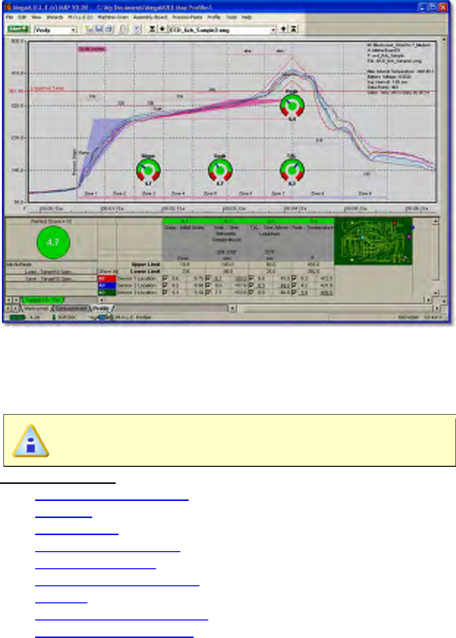
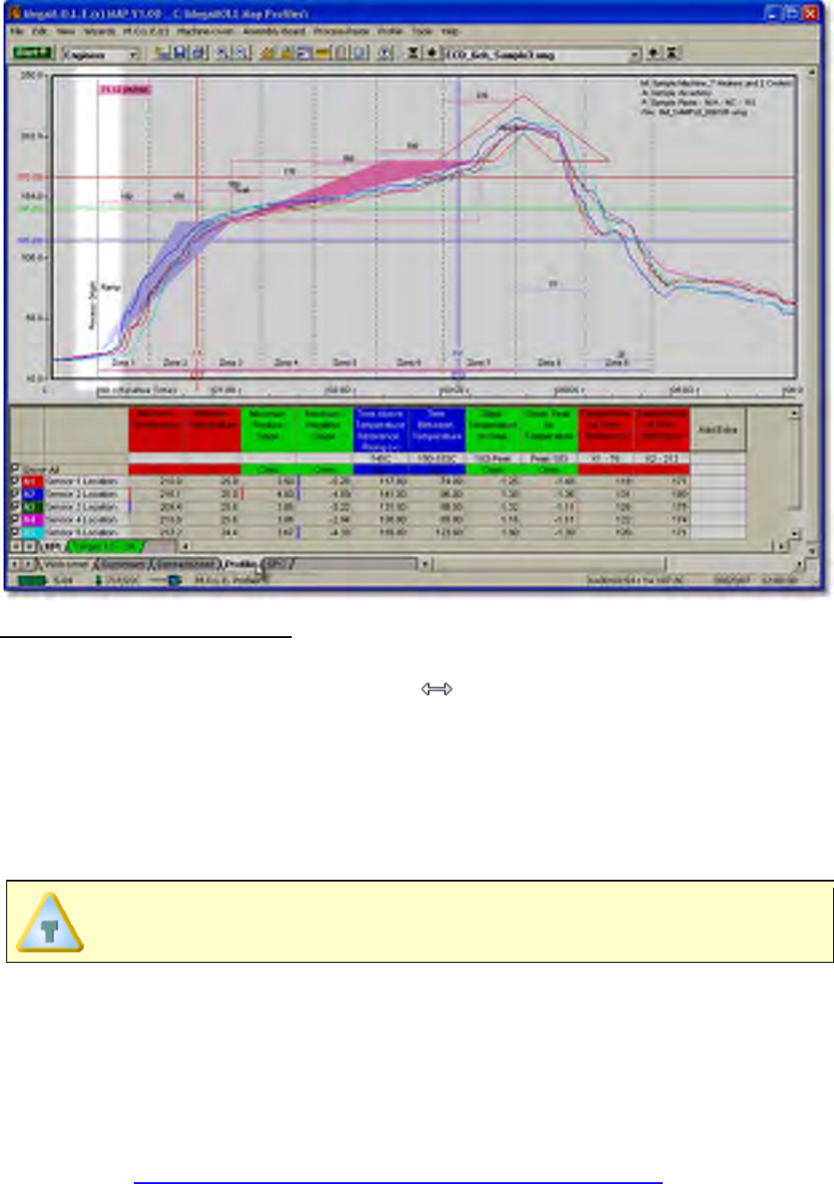
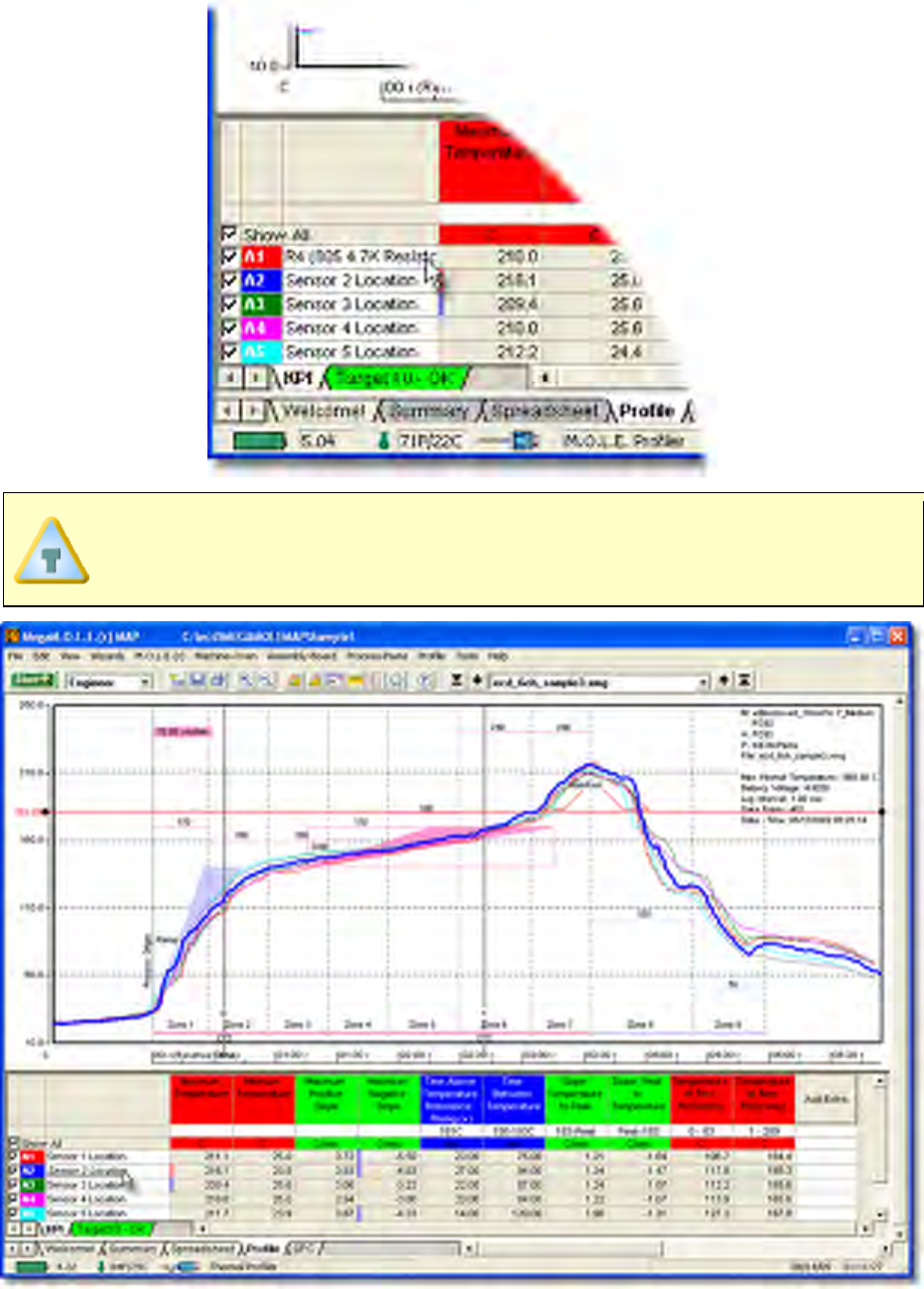
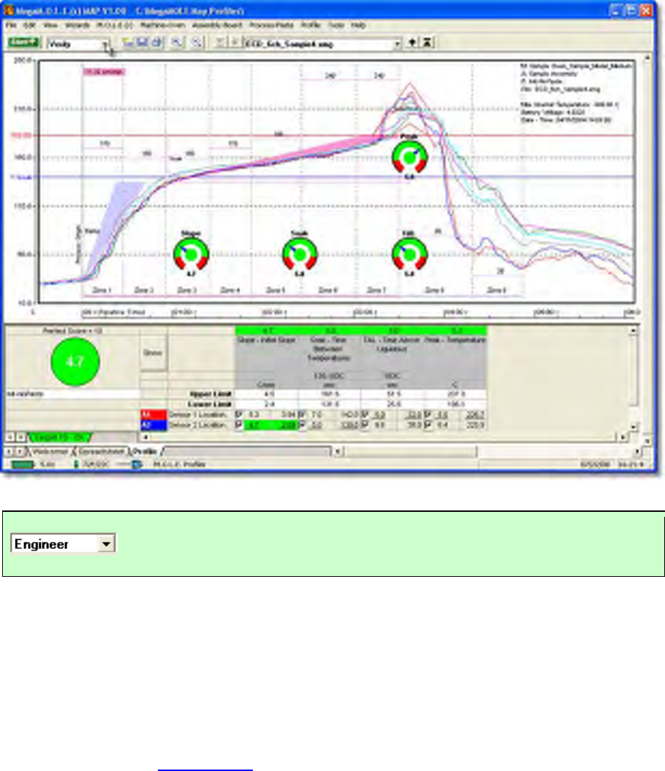
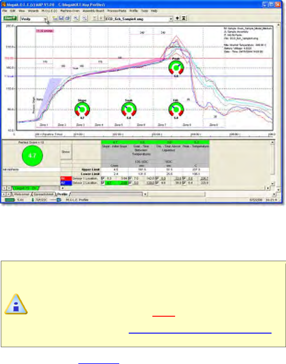
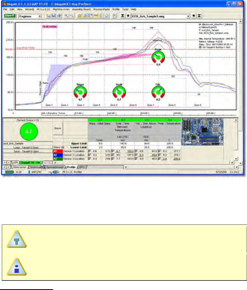
5.4.4.4. Target 10-OK
Target 10-OK is a simple yet powerful way to achieve the pursuit of the perfect profile.
The user specifies requirements for the profile initial slope, soak, TAL (time above
liquidous), peak parameter and the channels that these requirements are to be applied.
Then the software automatically calculates a single go/no-go number.
A Target 10 specification is created using the Create Target 10 Specification workflow
wizard. Refer to topic Menus>Wizards Menu>Create Target 10 Specification for more
information.
The features associated with Target 10-OK can only be used when in
Engineer mode. They can only be viewed when in Verify mode.
Target 10-OK feature allows the user to answer the following questions:
1) How do I specify a good profile?
• Answer: Based on the selected process specification and specification limits, the
user can set the four process parameters (Initial slope, Soak, TAL & Peak).
2) How do I know I have a good profile?
• Answer: Based on the specified settings, the active individual parameter indicators
(Slope, Soak, TAL & Peak) display the normalized values. Once Target 10-OK
numbers are calculated, they reduce the evaluation of the displayed data run
profile to a single number. This number appears in a two state (Red-Green)
indicator with the worst condition number appearing in the Final Indicator symbol.
A score of less than 0.0 is bad, 0.0-5.0 is good, 5.1-9.9 better and 10.0 being the
perfect score.
3) How can I improve the profile?
• Answer: Using the Prediction Tool, the user can change zone temperature values
or the conveyor speed and adjust the outcome toward a perfect 10.0.
Target 10-OK features:
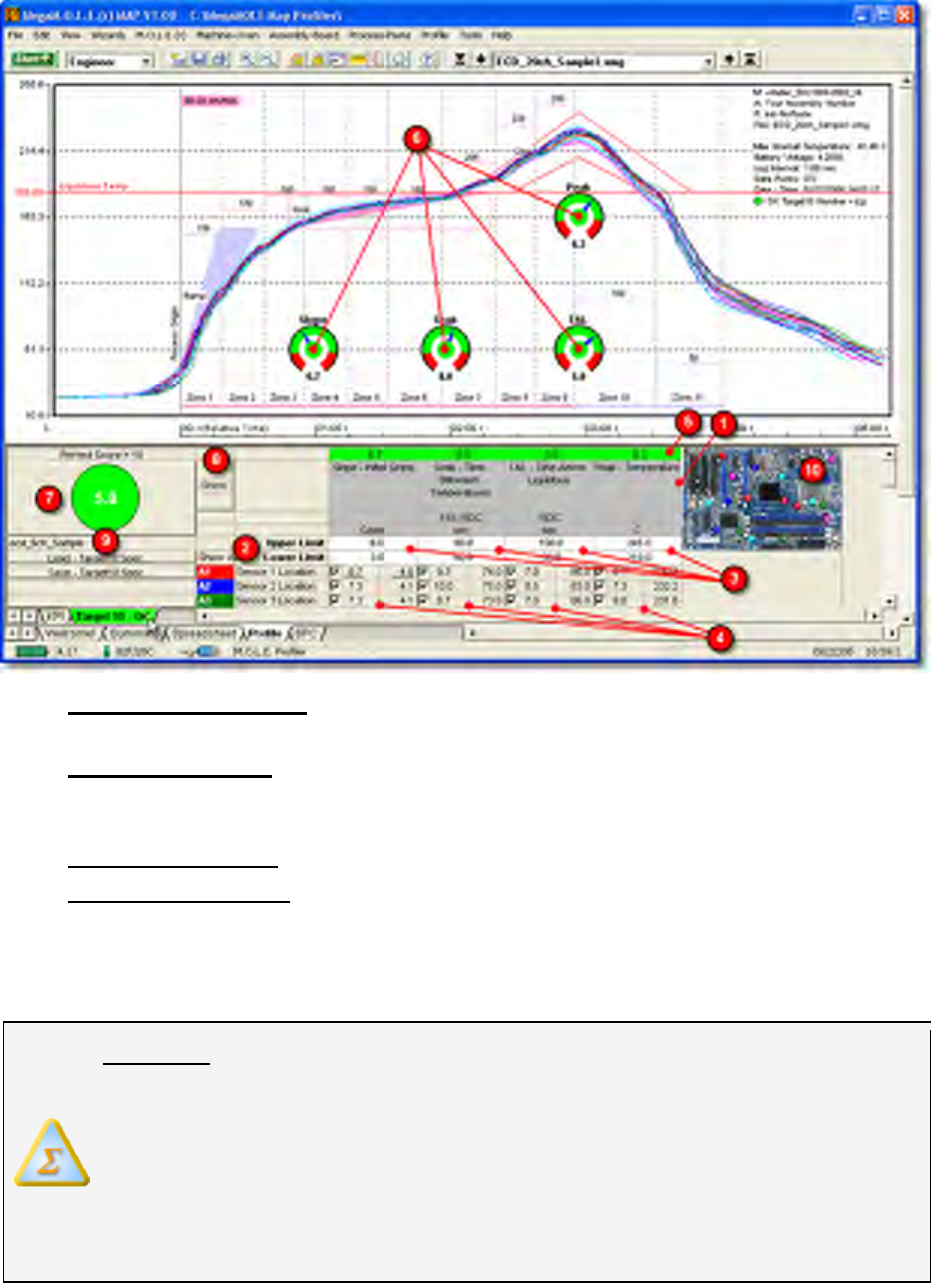
Process Parameters: Initial slope, Soak, TAL & Peak parameters derived from
the associated paste for the currently selected data run.
Limit Adjustment: Upper and lower specification limits from the selected process
for each parameter. The user can adjust these as needed to meet their
requirements.
Parameter Values: Actual values derived from the current data run.
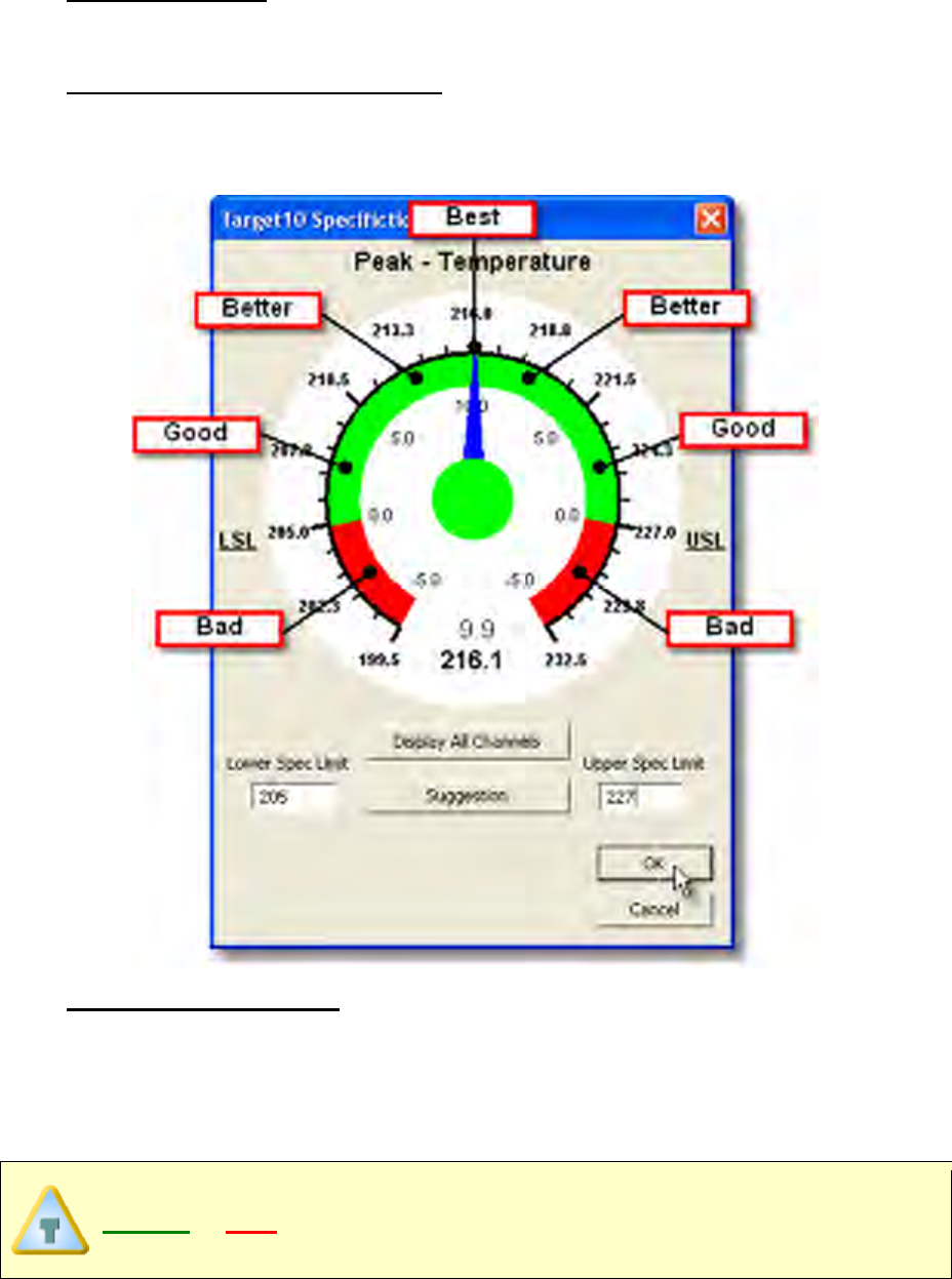
Normalized Values: Parameter values in the data run converted to a single
number based on a 0-10 scale. The software takes the parameter value then
determines where it is in respect to the upper and lower specification limits. If the
actual parameter value is in the exact center of the specification limits the
normalized value will be a perfect 10.0.
Example: The Peak Temperature has an upper limit of 240.0°C and a lower
limit of 195.0°C. The software subtracts the upper limit (240.0°C) from the
lower limit (195.0°C) equaling (45°C). Then the software creates a 0-10 scale
by dividing the 45°C by 20 equaling a scale of 1 point for every 2.25°C.
If the actual parameter value for channel 1 is 210.0°C. The software then
determine where that value lands on the 0-10 scale. In this case it is 15°C
higher than the lower limit so the software divides the 15°C by the scale value
of 2.25°C which equals at 6.7 on the scale.
Worst Condition: Once all of the Target 10-OK numbers are calculated into
normalized values, the software reduces the evaluation of the displayed data run
profile to a single worst condition number for each process parameter.
Individual Parameter Indicators: These are individual visual indicators of the
worst condition number for each process parameter. The user can click these
indicators to launch the detail dialog box where they can visually analyze the worst
condition number for each channel.
Final Indicator Symbol: This is a two state (Red-Green) indicator that displays
the worst condition number out of the four process parameters. This indicator can
also be displayed on the data graph for easy identification in an manufacturing
environment. To display click the Final Indicator Symbol to toggle the data graph.
To restore the Individual Parameter Indicators select the symbol again or
single-click anywhere within the data graph.
The Target 10-OK tab also indicates the go/no-go state by appearing in
GREEN or RED. This is useful when the user is viewing the KPI tab so they
can immediately know the Target 10-OK status of the displayed data run.
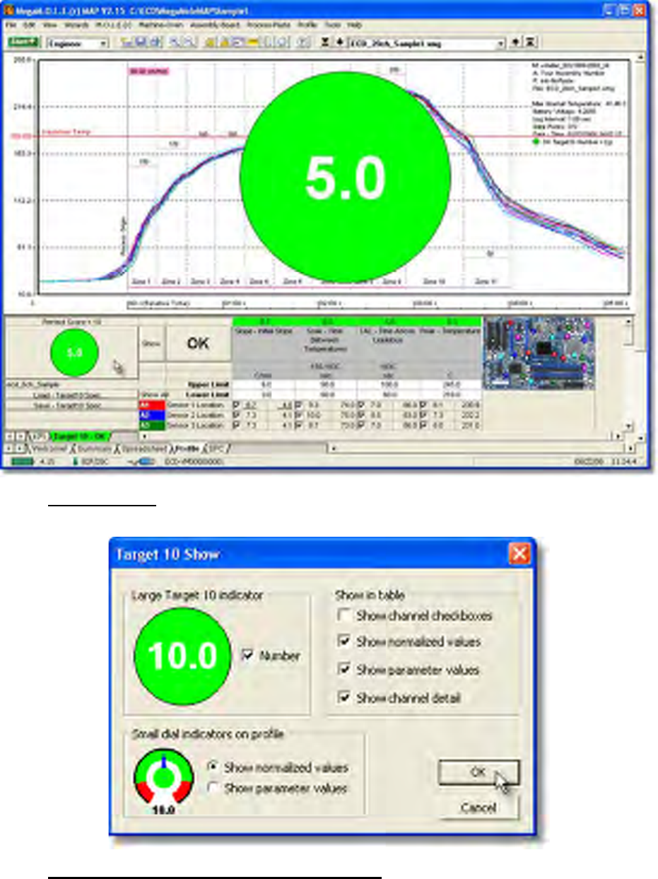
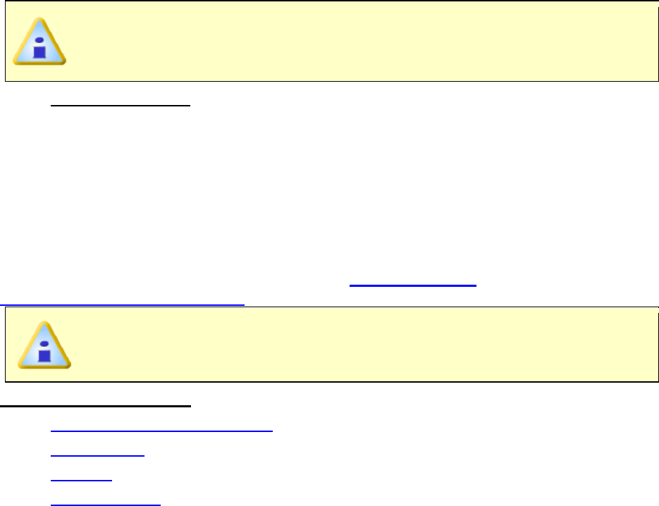
Show button: The user can select this button to display or hide various Target
10-OK features.
Target 10 Specification File Management: This area includes Load and Save
Target 10 buttons to load and save Target 10 specification files (*.T10). The Load
button is used to load a saved Target 10 specification file which is displayed on the
Data Graph. This typically is used to determine if different Target 10 specification
may be a better match with the currently displayed data run. The Save button is
used to save a Target 10 specification if any adjustments have been made, or
creating a new one based off of an existing Target 10 specification.
If a different Target 10 specification is saved with a data run, it does not affect
the original Target 10 specification associated with the data run when using
the OK button on the MEGAM.O.L.E.® or V-M.O.L.E.® profilers.
Assembly Image: This is a thumbnail image of the assembly product associated
with the currently displayed data run. To view the sensor locations, right-click over
the image and select the Enlarge command. When in Engineer mode the user
has the ability to set the sensor locations. When in Verify mode, the sensor
locations can only be viewed.
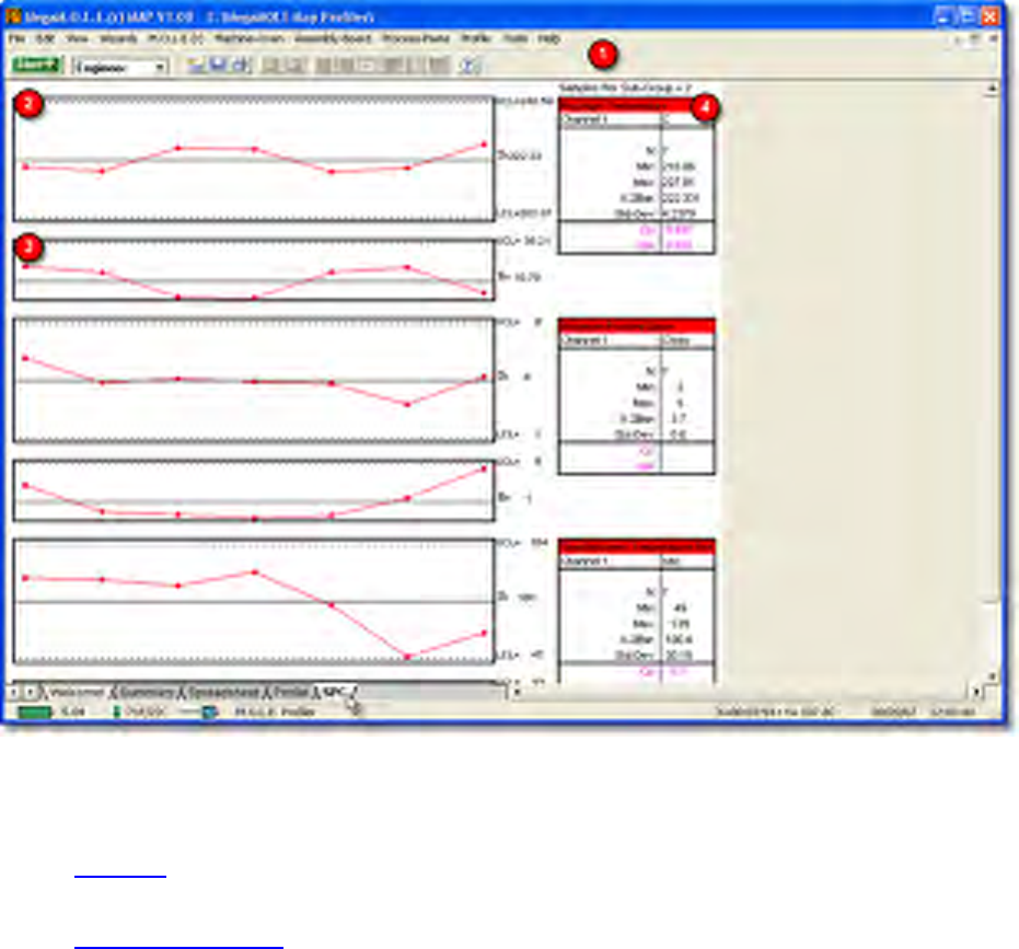
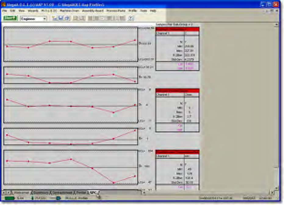
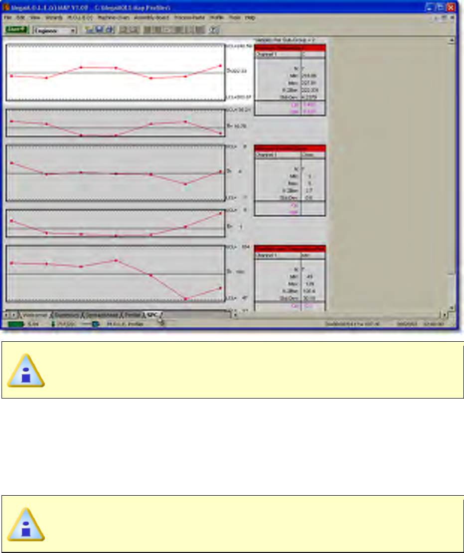
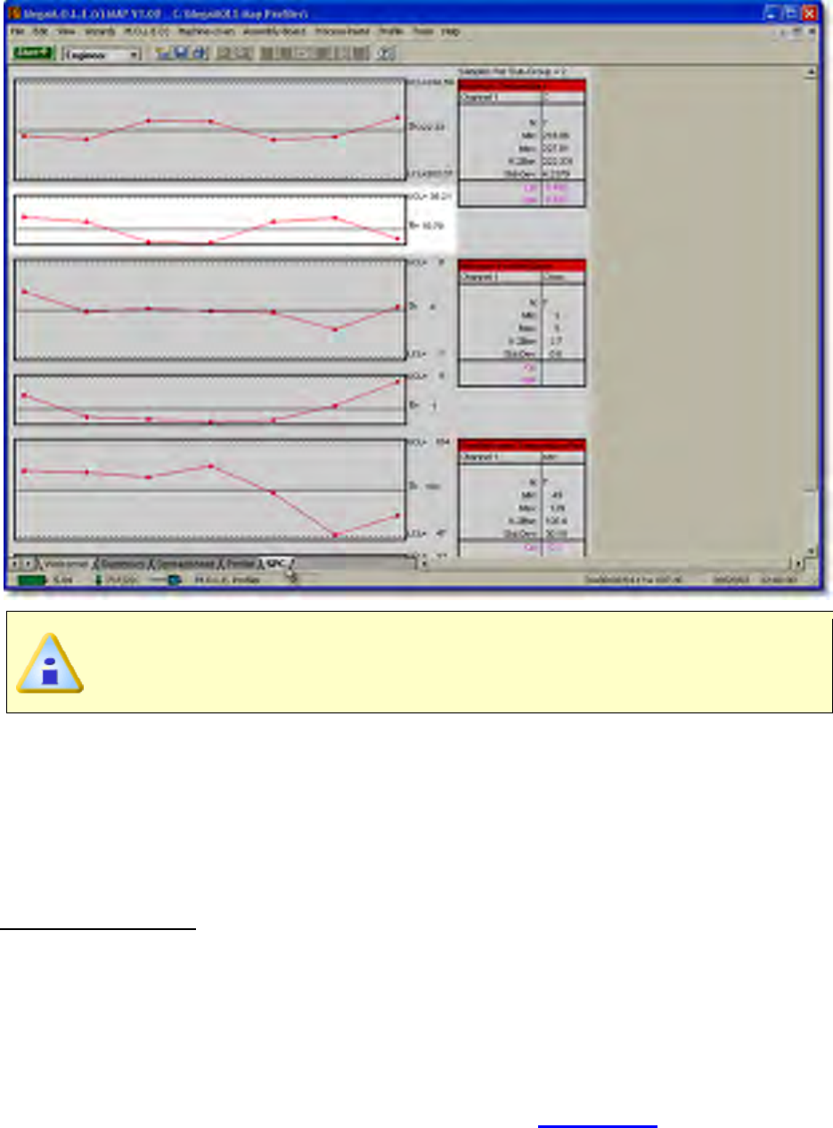
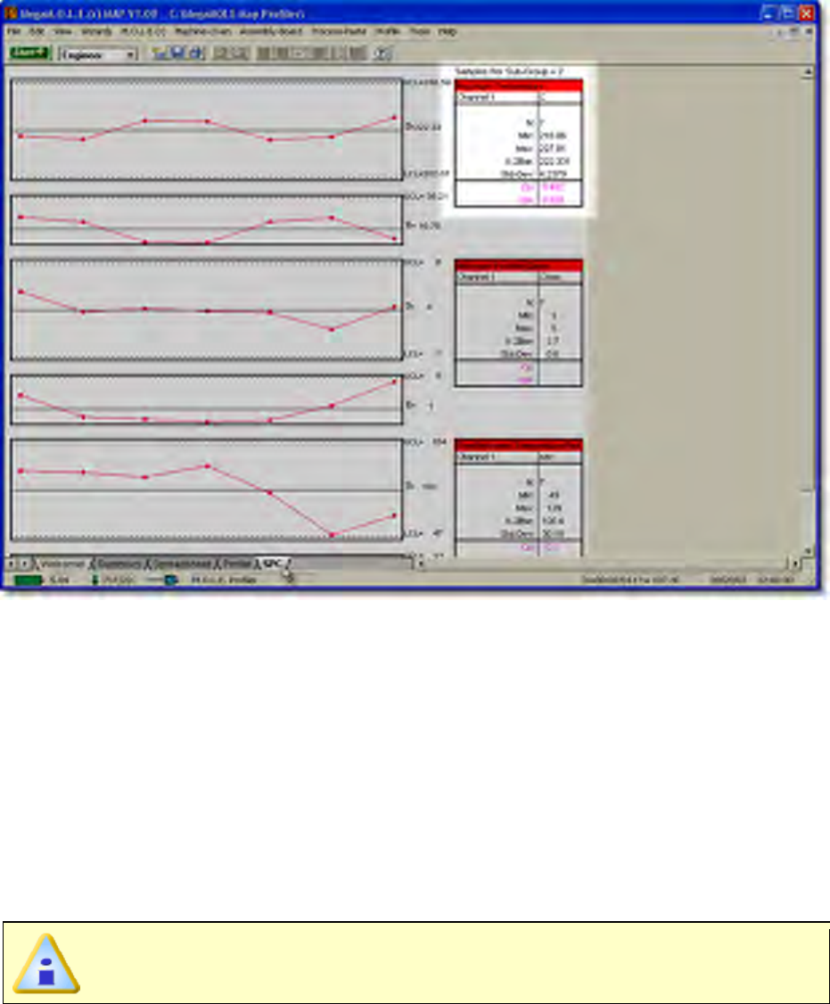
5.4.5. SPC Page Tab
The SPC Page Tab displays the specified parameters flagged on the Spreadsheet Page
Tab in SPC X-Bar and R charts. Refer to topic Software>Page
Tabs>Spreadsheet>SPC Flags for more information.
This is available when in Engineer Mode.
SPC Page Tab features:
Menus and Toolbar buttons
X-Bar Chart
R Chart
Statistics box
5.4.5.1. Menus & Toolbar
• Menus: File, Edit, Wizards, M.O.L.E.®, Machine-Oven, Assembly-Board,
Process-Paste, Profile, Tools and Help.
• Toolbar buttons:
Engineer Mode - Start, Open Working Directory, Save, Print, and Help.
Verify Mode - Tab not available.
5.4.5.2. X-Bar Chart
The X-Bar Chart is the graphical chart produced from samples of a flagged parameter on
the Spreadsheet Page Tab. The chart uses a rolling average of 2 through 6 sample
points. The user can specify the sample points on the SPC Page Tab of the Preferences
dialog box. The X-bar is the average of the data samples and the UCL and LCL are
calculated using a formula based on the Range data.
The calculation numbers vary depending on the data in the Spreadsheet Page
Tab. Using the filter function or the hide command allows the user to select the
specific data runs to include on the SPC chart.
5.4.5.3. R Chart
The R Chart is the graphical chart produced from samples of a flagged parameter on the
Spreadsheet Page Tab. The R-Bar is the averages of the range samples.
If the Sub-Group size on the SPC Page Tab of the Preferences dialog box is
set to 1, the R chart becomes a moving range (mR) chart. The moving range is
the difference between a specified X value and the one preceding it.
The calculation numbers vary depending on the data in the Spreadsheet Page
Tab. Using the filter function or the hide command allows the user to select the
specific data runs to include on the SPC chart.
5.4.5.4. Statistics Box
The Statistics Box reflects the current SPC data from the selected, sorted and filtered
data set parameter.
Statistics box data:
• N = Number of subgroups.
• Min. = The lowest data point on the graph.
• Max. = The highest data point on the graph.
• X-2 bar = The current X-Bar Bar calculation.
• Std. Dev.= The Standard Deviation of the selected parameter.
• Cp; Cpk = Process capability indeces (Refer to Appendix B for more
information).
5.5. Menu and Tool Commands
5.5.1. File Menu
This section explains how to use all of the Menu and Toolbar button commands. Each of
the following sections will list all of the commands specific to each of the menus.
Commands in the File menu are used to manipulate and configure data run files.
The dimmed menu commands are used in other page tabs.
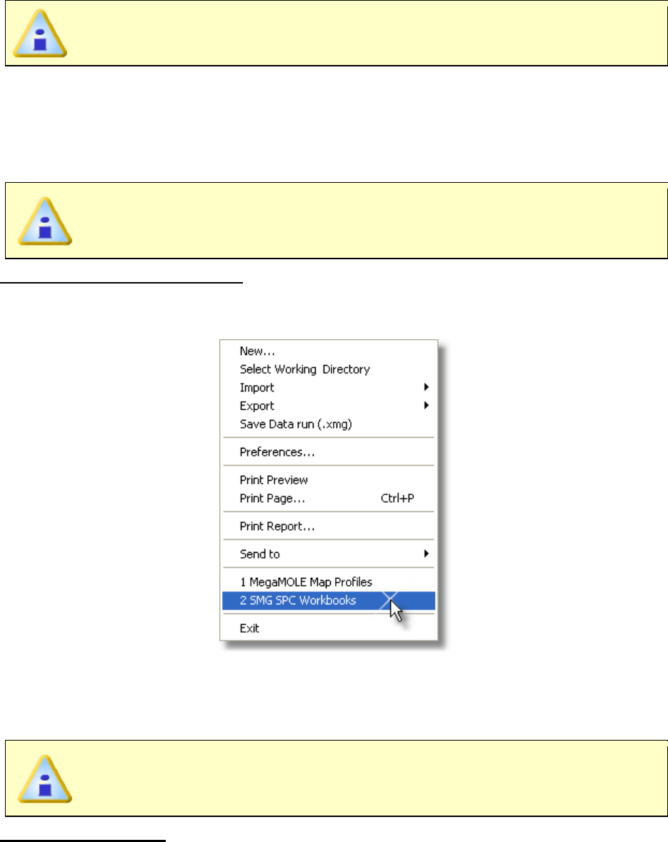
5.5.1.1. New (Start)
The New (Start) command is a blank state starting point where users can choose from
five different MEGAM.O.L.E.® MAP workflows. A MAP workflow is a wizard of steps
based on which option is selected which help guide a user.
The dimmed workfows are associated with the Verify mode and can only be
used when in Engineer mode.
Engineer Mode
Verify Mode
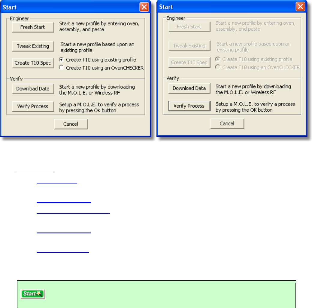
Workflows:
• Fresh Start: Start a new profile (data run) by entering Machine (oven), Assembly
(board) and Process (Paste) information.
• Tweak Existing: Start a new profile (data run) based on an existing profile.
• Create Target 10 File: Create a Target 10 Specification using an existing profile
(data run) or OvenCHECKER™.
• Download Data: Start a new profile (data run) by downloading the M.O.L.E.
Profiler.
• Verify Process: Setup a M.O.L.E. Profiler to verify a process by presetting the OK
button.
The New (Start) command can be accessed on the Toolbar and Get Started dialog box.
New (Start) button.
5.5.1.2. Open Working Directory
The M.O.L.E.® MAP software is a data run manager. The software does not store data
run files (.XMG) it allows the user to save them in a directory of their choice. This can be
useful to store data runs in different directories based on customer, shift or machine type.
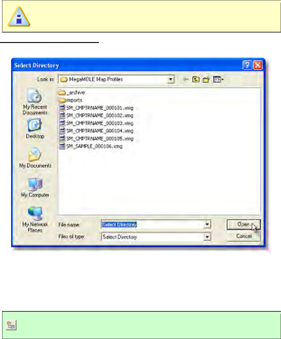
This is available in both Engineer & Verify Modes.
To open a working directory:
1) On the File menu, click Open Working Directory.
2) Navigate to the location where the data run files (.XMG) are located.
3) Click the Open command button to select the directory or Cancel to quit the
command.
This command can be accessed on the Toolbar.
Open Working Directory button
5.5.1.3. Import
The Import command imports existing SMG/SMFW (.MDM) and M.O.L.E.® MAP (.XMG)
files into the current working directory. When importing SMG/SMFW files, this process
automatically converts the profile, configured machine data, process documentation then
saves it in the new (.XMG) file format.
The import command also imports Text (.TXT) files. The values in these files must be
either comma or tab separated values. This process automatically converts the data then
saves it in the new (.XMG) file format.
This is available when in Engineer Mode.
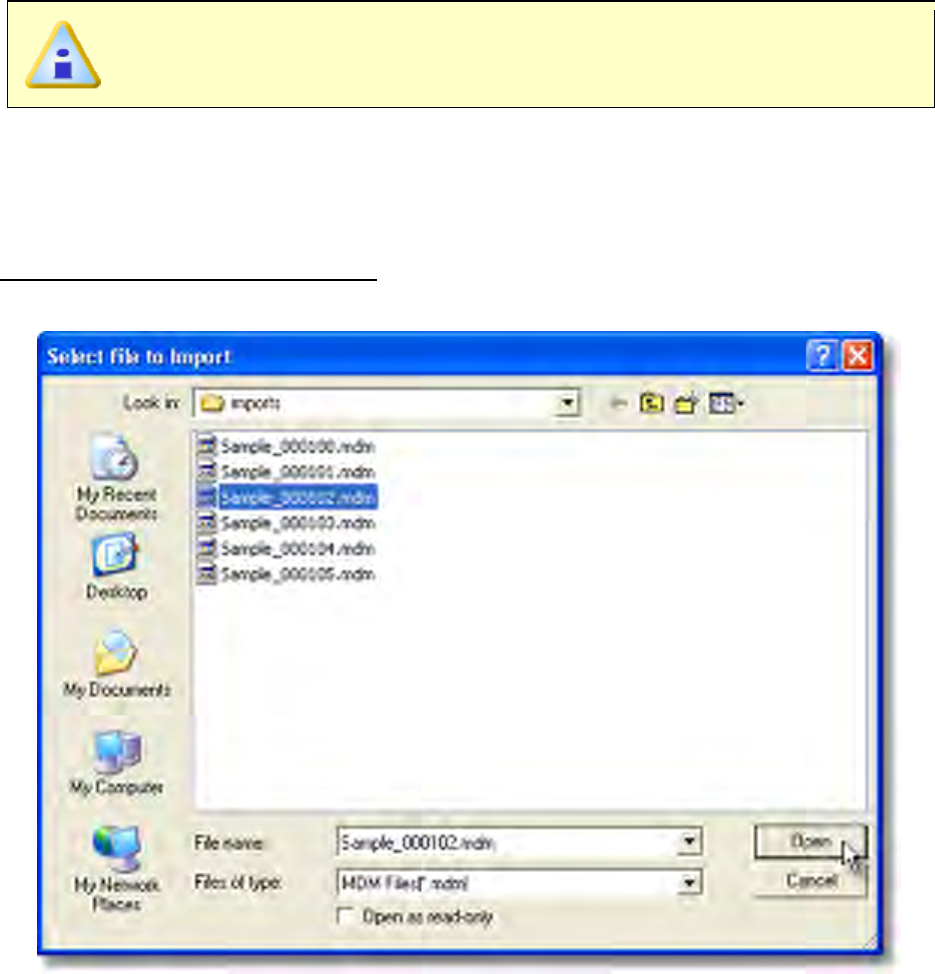
5.5.1.3.1. SMG SPC (.mdm)
To import SMG SPC (.mdm) files:
1) On the File menu, point to Import and then select SMG-SPC (.mdm).
2) Navigate to the file folder where the file(s) to import are located.
3) Select the file to import.
You can import several files at one time. For consecutive files, click the first file
in the list, press and hold down the SHIFT key, and then click the last file in the
list. For files that are not consecutive,
press and hold down the CTRL key, and
then click each file that you want to import.
4) Click the Open command button to import or Cancel to quit the command.
The .MDM is automatically converted to a (.XMG) file and saved in the current open
working directory.
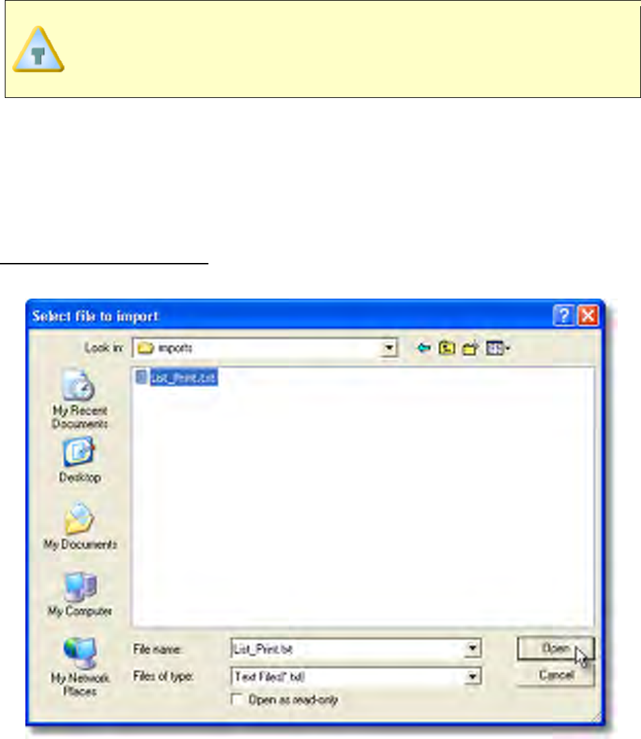
5.5.1.3.2. TEXT (.txt)
To import Text (.TXT) files:
1) On the File menu, point to Import and then select TEXT (.txt).
2) Navigate to the file folder where the file(s) to import are located.
3) Select the file to import.
4) Click the Open command button to import and the Data Import Formatter dialog
box appears.
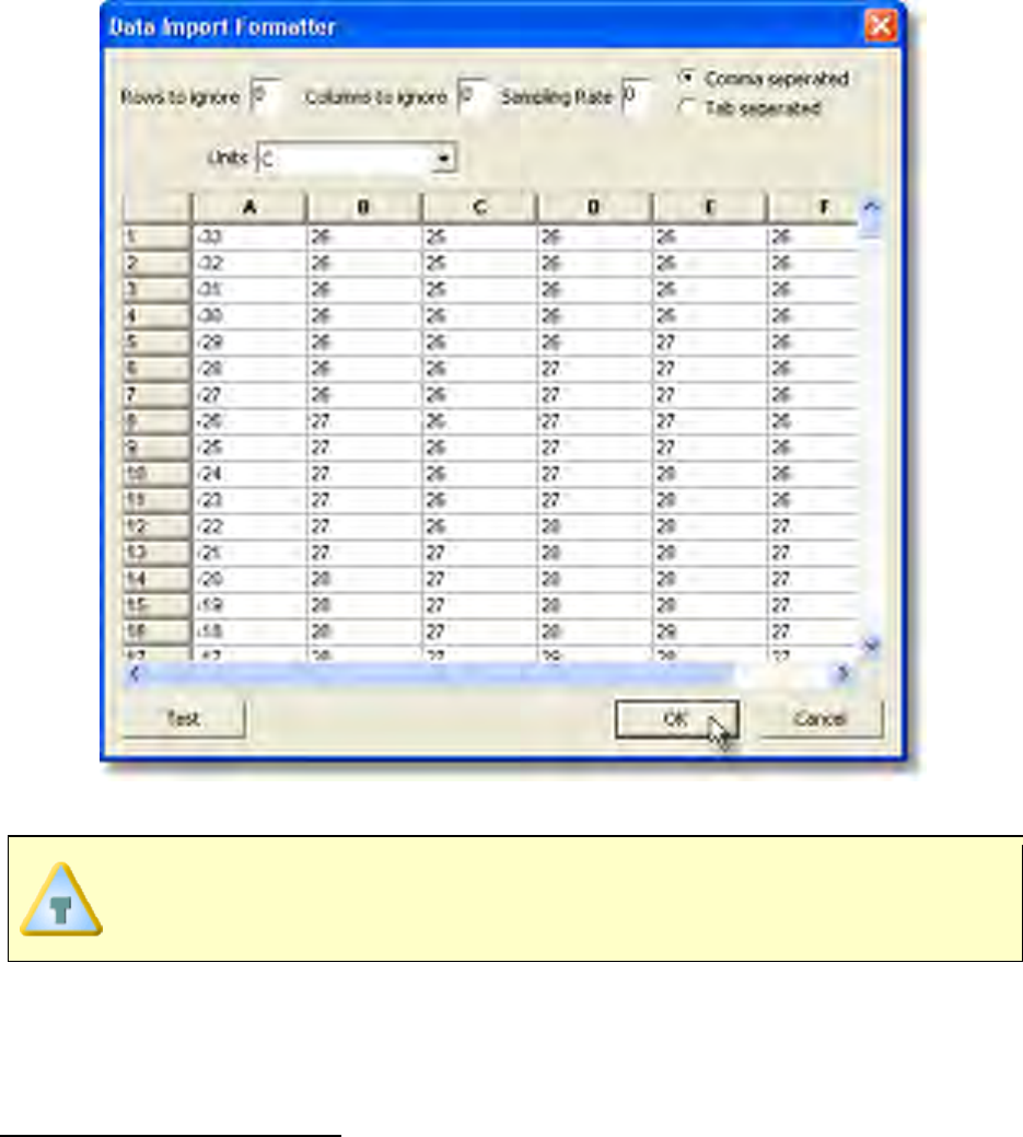
5) Select from the formatter options.
If the user is not sure if the Text file values are comma or tab separated, the
Test command button can be used to test the format to display the data in
columns and rows.
6) Click the OK command button to import or Cancel to stop.
5.5.1.3.3. MAP (.xmg)
To import MAP (.xmg) files:
1) On the File menu, point to Import and then select MAP (.xmg).
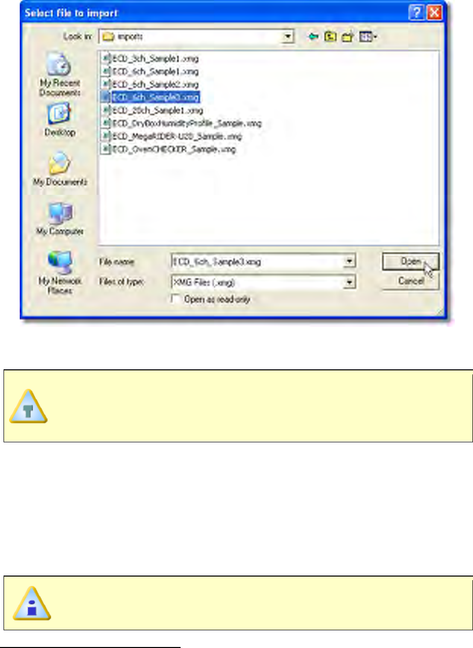
2) Navigate to the file folder where the file(s) to import are located.
3) Select the file to import.
You can import several files at one time. For consecutive files, click the first file
in the list, press and hold down the SHIFT key, and then click the last file in the
list. For files that are not consecutive, press and hold down the CTRL key, and
then click each file that you want to import.
4) Click the Open command button to import or Cancel to quit the command.
The .XMG is automatically saved in the current open working directory.
5.5.1.4. Export
The Export command exports a data run into Microsoft Excel. This process automatically
launches Excel and inserts the selected data run information. The user can then save it as
an Excel file format.
This is available when in Engineer Mode.
To export data run information:
1) On the File menu, point to Export and then select Excel.
The data run information is automatically converted to the Microsoft® Excel file format.
5.5.1.5. Save Data Run
The Save Data Run command saves the any changes made to the selected data run.
If the user selects a different page tab or exits the software, any changes
made to the selected data run will automatically be saved.
This is available when in Engineer Mode.
To save the current data run:
1) On the File menu, click Save Data Run and the currently selected data run will be
saved.
This command can be accessed on the Toolbar.
Save Data Run button
5.5.1.6. Preferences
The Preferences command allows access to property sheet that includes custom setup
tasks and global settings for the software.
This is available when in Engineer Mode.
The Preferences property sheet includes various tabs associated with the each
individual Page Tab and the MAP menus.
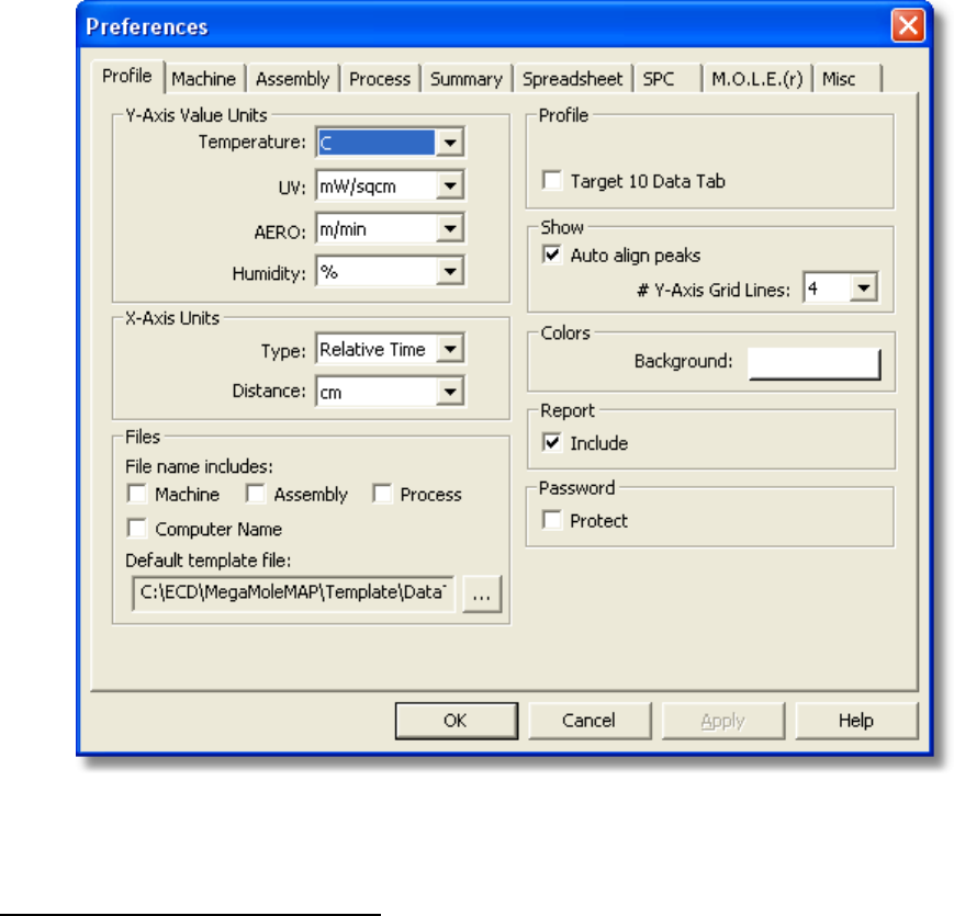
5.5.1.6.1. Profile
To access profile preferences:
1) On the File menu, click Preferences, and then click the Profile tab.
Y-Axis Units
Temperature units can be globally set for the Y-Axis. The software also allows the user to
set units for optional sensors such as, UV, AERO, and Humidity.
This command does not set the units reported by the M.O.L.E. profiler. It
applies only to the software.
X-Axis Units
Time units and measurement type can be globally set for the X-Axis.
The user can select from the following scales:
• Point: the data points collected from the Process-Origin.
• Time-Relative: Time measured from the Process-Origin
• Time-Absolute: Time of day
• Distance: Distance from the Process Origin (Meters, Centimeters, Feet or
Inches).
Files
The user can decide how to set the default file name when saving a data run profile
(.XMG) and the default Data Table template they wish to use.
When saving a data run file, the software includes options to add the set Machine,
Assembly, Process, Computer Name and Date-Time.
Once the default filename is set, the (.XMG) file will be incremented
automatically to avoid that file from being overwritten.
If a user creates a new Data Table template, it can save using the template commands. If
the new template is to be used as the default, the new one can be specified in this text
box. The new template will now be loaded every time the program is started.
Profile
The user can decide if they want to include Recipe Values in the Data Graph when using
the Autoscale command and display the Target 10-OK tab in the Data Table.
Refer to topics Profile>Set Temperature (Y) Scale and Software>Page
Tabs>Profile>Target 10 for more information.
Show
The user can select the default Auto align Peak temperature method and select the
amount of Y-Axis gridlines to display on the Data Graph
When Auto align Peaks is selected, the software automatically aligns the Time (X) axis
maximum peak values for each Data Plot so the results can be easily compared during
analysis.
Colors
The software allows the user to change the background color of the Data Graph with
colors from the Windows default pallet.
Report
Select the corresponding check box to include the Profile Page Tab when printing in
Report format.
Password
Select the corresponding check box to password protect the Profile Page Tab and
preferences. If password protection has been selected, a dialog box appears prompting
the user to enter the current password. The software will then need to be restarted to
apply password protection settings.
If the default password has not been changed, the current password is
Admin. Refer to topic
Software>Menus>File>Preferences>Misc>Passwords for more
information.
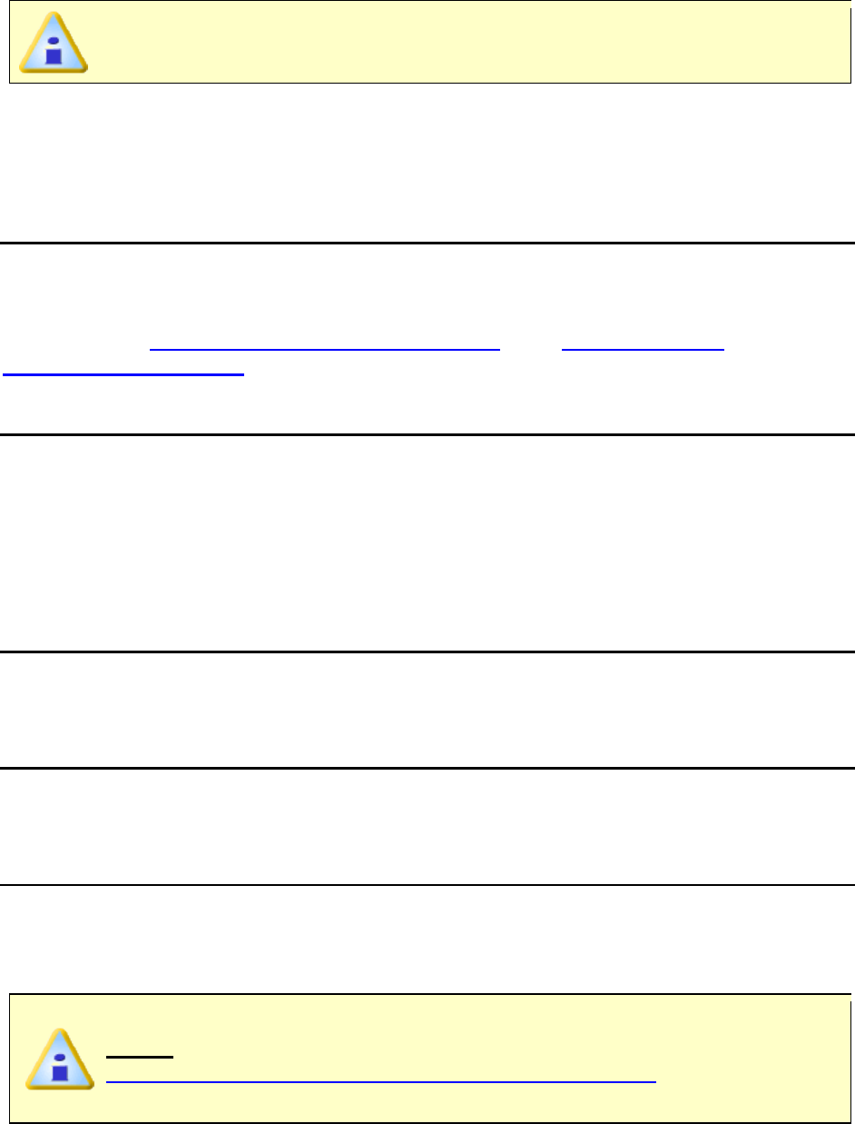
5.5.1.6.2. Machine
To access machine preferences:
1) On the File menu, click Preferences, and then click the Machine tab.
Units
The user can set the machine conveyor speed and zone size units. These units will be
used as the default when setting machine information.
Files
As the user creates Machine (.OVS) & Recipe (.XMR) files, they are saved to the
specified default working directories.
Changing the directory locations may be useful when the user would like to share them on
a network drive.
Report
Select the corresponding check box to include the Machine and Recipe settings when
printing in Report format.
Show
Select the corresponding check box to display the Zone Convection Settings and/or Zone
Conveyor Speeds in the Set Machine Information dialog box. Having these options
displayed is useful when the user wishes to have the ability to set the convection
temperature and/or speed of the machine conveyor for each zone.
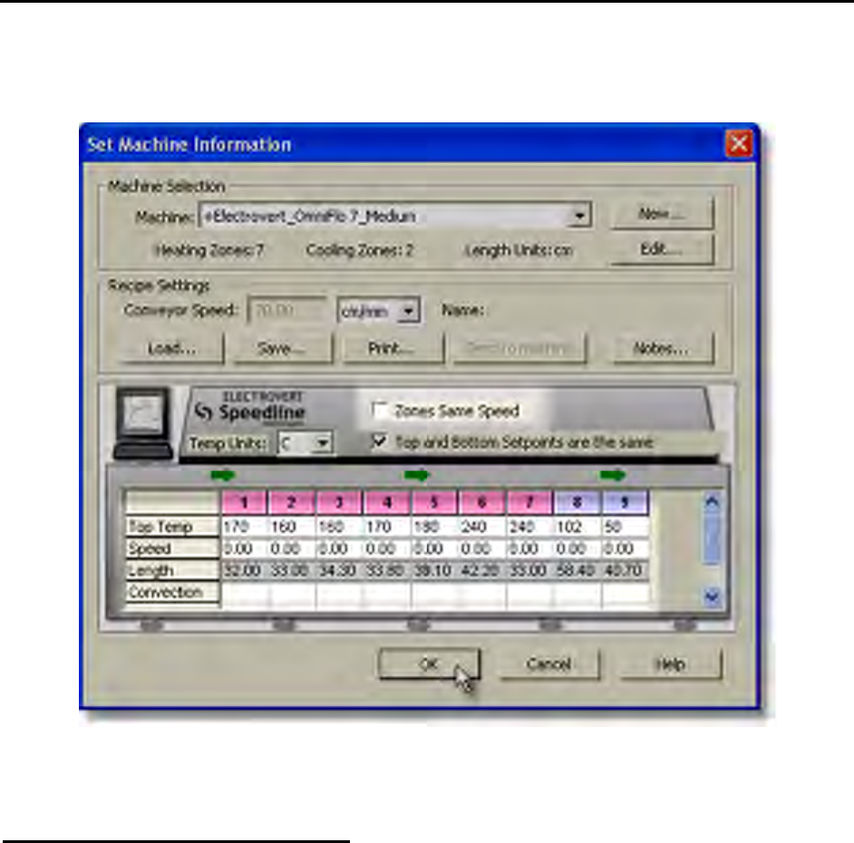
5.5.1.6.3. Assembly
To access assembly preferences:
1) On the File menu, click Preferences, and then click the Assembly tab.
Units
The user can set the board size and component location units. These units will be used as
the default when setting assembly information.
Files
As the user collects assembly board image files, they can be saved to the specified
default working directory. When setting assembly information the user can select a
product image. The software automatically starts in the directory specified as the default.
Changing the directory location may be useful when the user would like to share the
images on a network drive.
Report
Select the corresponding check box to include the Assembly settings when printing in
Report format.
5.5.1.6.4. Process
To access process preferences:
1) On the File menu, click Preferences, and then click the Process tab.
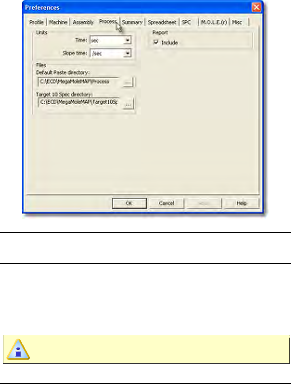
Units
The user can set the Time and Slope time process parameters extracted from a data run.
Files
The user can change the location where they store the paste database and Target 10
Specs files to a specified default working directory of their choice. Included with the
software is a Paste database file (paste1.psp). As the user creates process recipes the
software creates an extension paste file (user1.psp) which is combined with the default
paste1.psp file.
Changing the directory location may be useful when the user would like to share the paste
database on a network drive.
If the paste1.psp file is moved to a different location, the user1.psp file must
also be copied to the new location.
Report
Select the corresponding check box to include the Process settings when printing in
Report format.
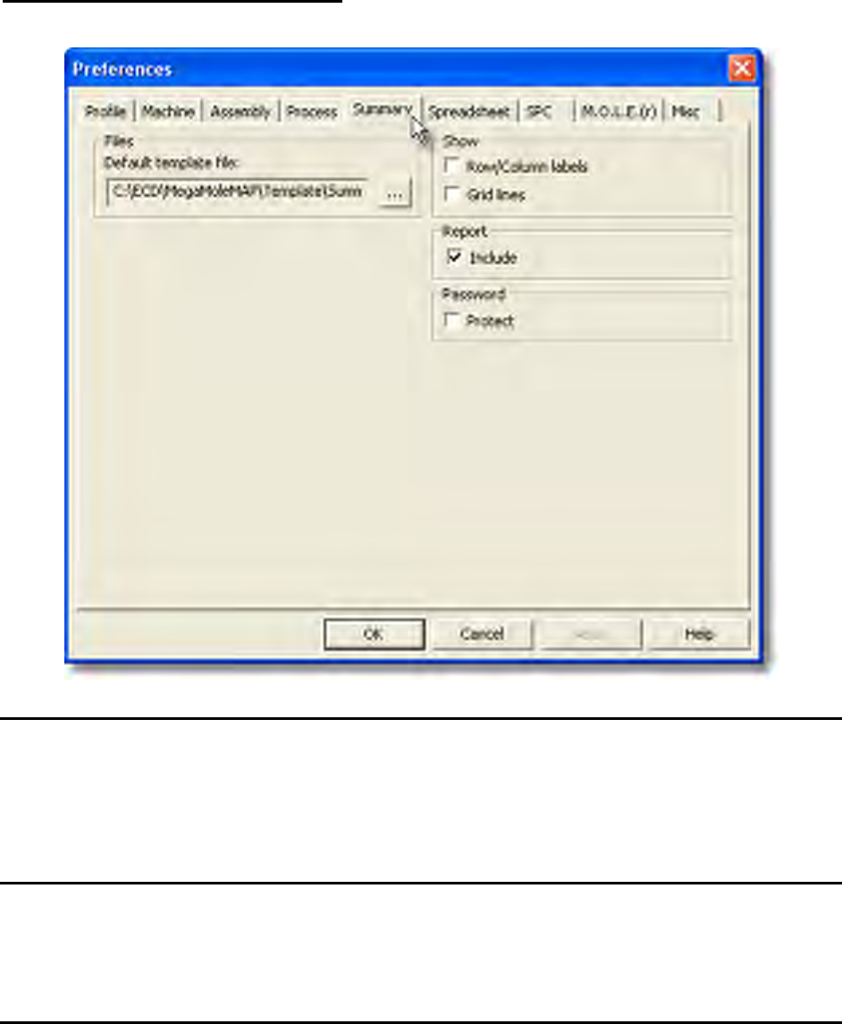
5.5.1.6.5. Summary
To access summary preferences:
1) On the File menu, click Preferences, and then click the Summary tab.
Files
The user can decide which default Summary template they wish to use. If a user creates
a new Summary template, it can save using the template commands. If the new template
is to be used as the default, the new one can be specified in this text box. The specified
template will now be loaded every time the program is started.
Show
The Summary Page Tab is built with cells that are organized into columns and rows. The
software allows the user to show and hide the cell Row/Column labels and Grid lines.
Selecting the corresponding check boxes to show or hide the labels and cells.
Report
Select the corresponding check box to include the Summary Page Tab when printing in
Report format.
Password
Select the corresponding check box to password protect the Summary Page Tab and
preferences. If password protection has been selected, a dialog box appears prompting
the user to enter the current password. The software will then need to be restarted to
apply password protection settings.
If the default password has not been changed, the current password is
Admin. Refer to topic
Software>Menus>File>Preferences>Misc>Passwords for more
information.
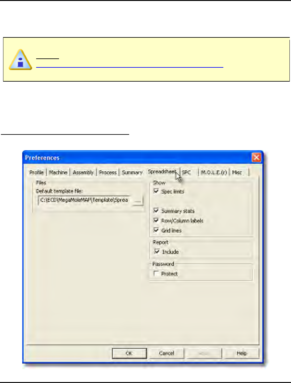
5.5.1.6.6. Spreadsheet
To access spreadsheet preferences:
1) On the File menu, click Preferences, and then click the Spreadsheet tab.
Files
The user can decide which default Spreadsheet template they wish to use. If a user
creates a new Spreadsheet template, it can save using the template commands. If the
new template is to be used as the default, the new one can be specified in this text box.
The specified template will now be loaded every time the program is started.
Show
The Spreadsheet Page Tab is built with cells that are organized into columns and rows.
The software allows the user to show and hide the cell Row/Column labels and Grid lines.
Selecting the corresponding check boxes to show or hide the labels and cells.
Report
Select the corresponding check box to include the Spreadsheet Page Tab when printing
in Report format.
Password
Select the corresponding check box to password protect the Spreadsheet Page Tab and
preferences. If password protection has been selected, a dialog box appears prompting
the user to enter the current password. The software will then need to be restarted to
apply password protection settings.
If the default password has not been changed, the current password is
Admin. Refer to topic
Software>Menus>File>Preferences>Misc>Passwords for more
information.
5.5.1.6.7. SPC
To access profile preferences:
1) On the File menu, click Preferences, and then click the SPC tab.
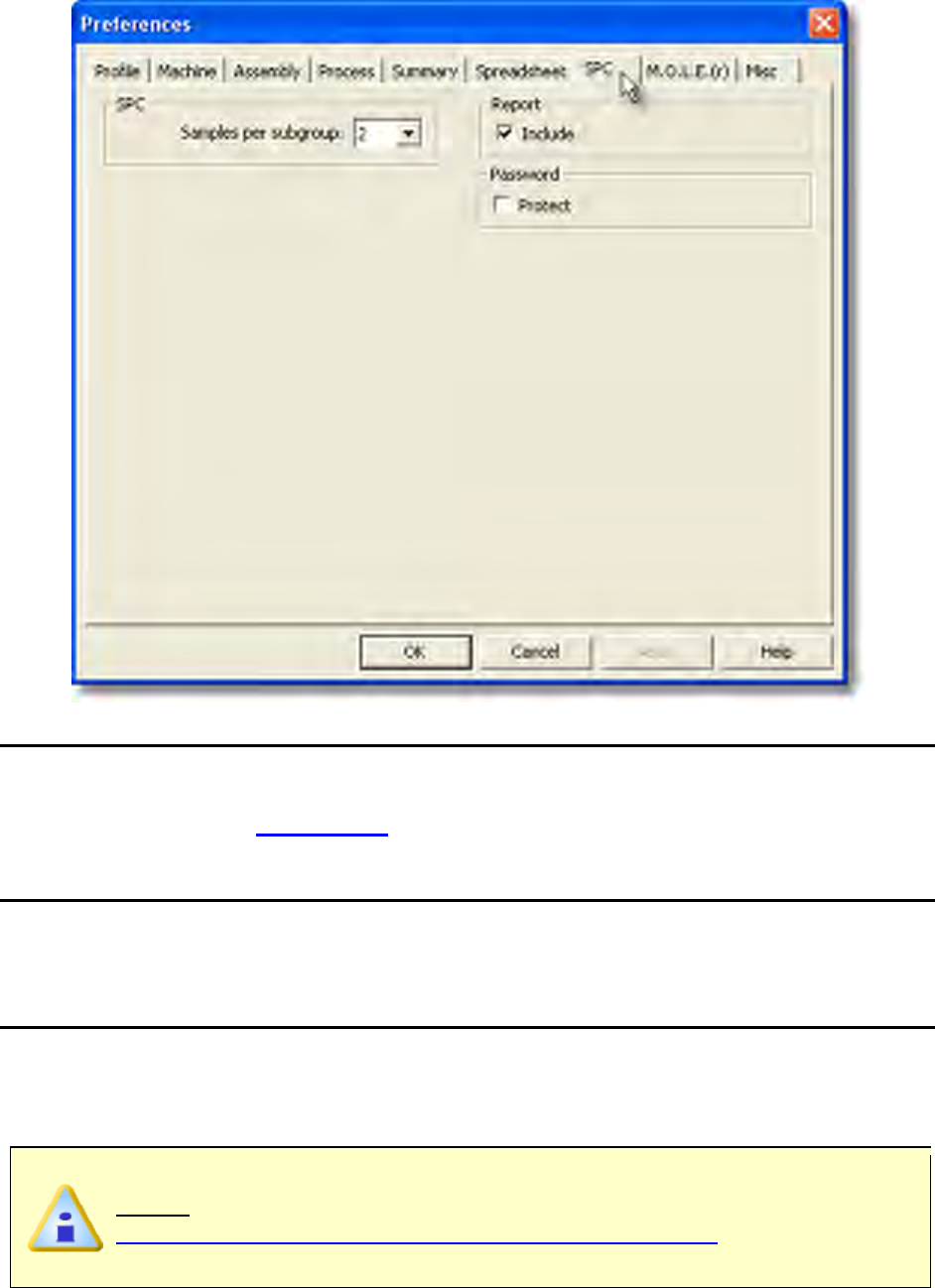
SPC
The software utilizes the standard Moving Average/Moving Range Charting technique
with a subgroup size of 2-6. The user can specify the samples per subgroup using the
drop-down list. Refer to Appendix B for more information.
Report
Select the corresponding check box to include the SPC Page Tab when printing in Report
format.
Password
Select the corresponding check box to password protect the SPC Page Tab and
preferences. If password protection has been selected, a dialog box appears prompting
the user to enter the current password. The software will then need to be restarted to
apply password protection settings.
If the default password has not been changed, the current password is
Admin. Refer to topic
Software>Menus>File>Preferences>Misc>Passwords for more
information.
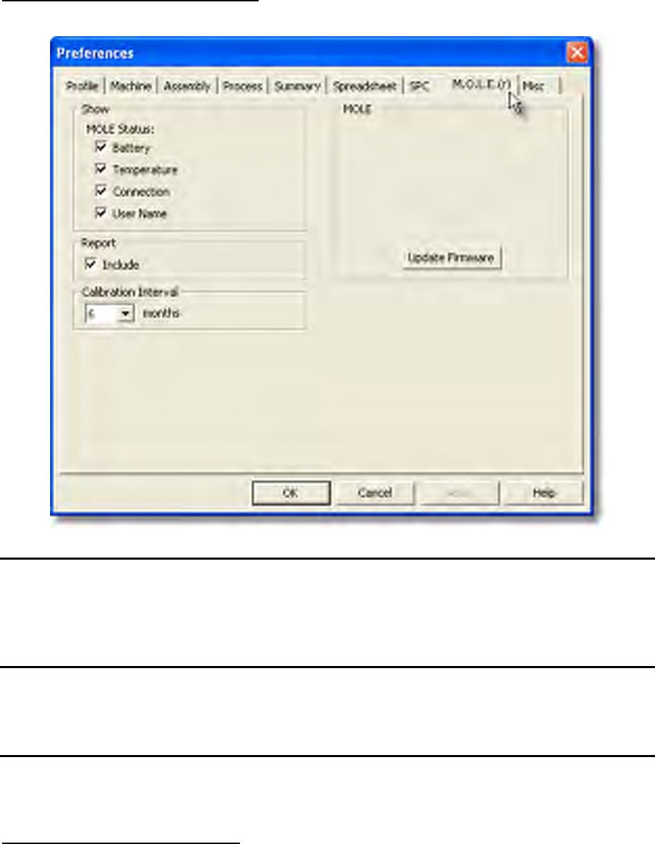
5.5.1.6.8. M.O.L.E.(r)
To access M.O.L.E. preferences:
1) On the File menu, click Preferences, and then click the M.O.L.E.(r) tab.
Show
The Status bar located on the bottom of the software display can show the status of the
M.O.L.E. Profiler Power Pack battery, Internal operating temperature, connected COM
port. Select the corresponding check box to display these status indicators.
Report
Select the corresponding check box to include the M.O.L.E. information when printing in
Report format.
Calibration Interval
When reporting the instrument status, the software can inform the user when the
M.O.L.E. Profiler calibration has expired.
To set the calibration interval:
1) On the File menu, click Preferences, and then click the M.O.L.E.(r) tab.
2) In the Calibration Interval section, select 6 or 12 months from the drop down
box.
3) Select the Apply or OK command button to save.
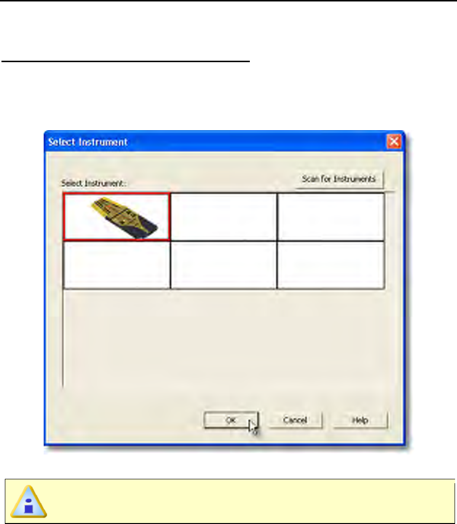
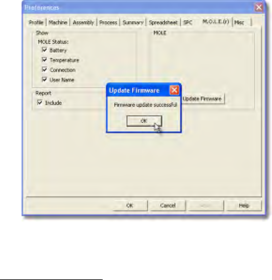
Update Firmware
If a new version of the MEGAM.O.L.E.® Profiler firmware is released by ECD, the user
can use the Update Firmware wizard to upgrade to the newest version.
To update MEGAM.O.L.E.® Profiler firmware:
1) On the File menu, click Preferences, and then click the M.O.L.E.(r) tab.
2) In the MOLE section, click the Update Firmware command button and the
software automatically scans for a selected instrument. If there is no instrument
selected, the Select Instrument dialog box appears.
3) Select the OK command button.
Updating the MEGAM.O.L.E.® Profiler firmware erases any stored data runs.
Make sure they have been downloaded prior to completing this process.
4) Click the Yes command button to proceed with the update or No to cancel.
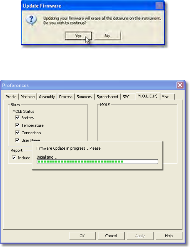
5) Navigate to the file folder where the firmware file *.BIN is located.
6) Select the firmware file.
7) Click the Open command button to start updating the firmware.
8) When the update firmware process is complete, select the OK command button.
5.5.1.6.9. Misc
To access misc preferences:
1) On the File menu, click Preferences, and then click the Misc tab.
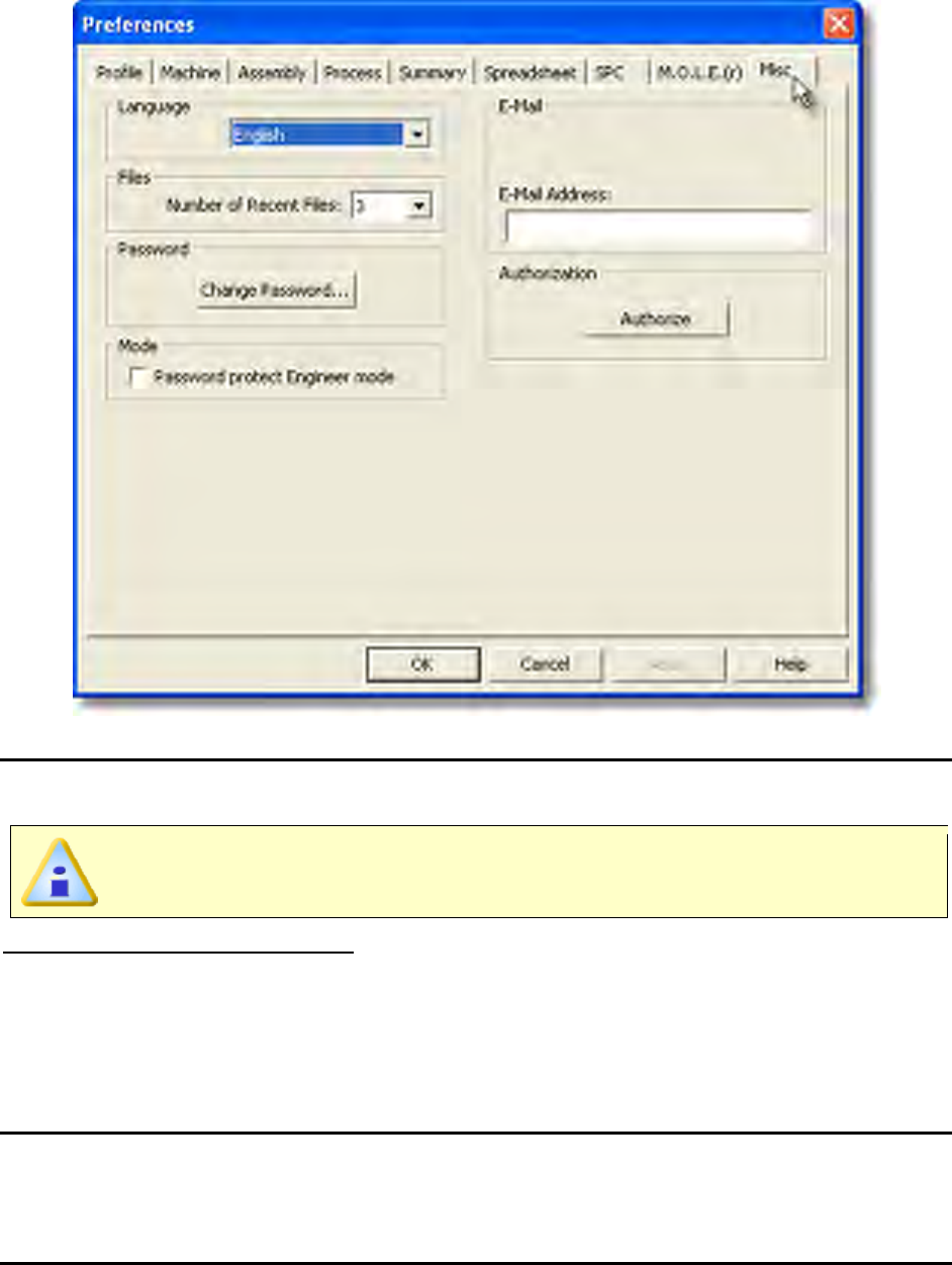
Language
This is where the user can change all of the menus and commands to a different
language.
If the language is changed it will require the software to be restarted.
To select a different language:
1) On the File menu, click Preferences, and then click the Misc tab.
2) Select a desired language from the Language drop-down box.
3) Restart the software program.
Files
The most recently open working directories are displayed at the bottom of the File menu.
The user can select how many recent directories to display.
Password
The software has a global password protection feature that uses case-sensitive text for
securing access to a Page Tab, associated preference tab and Engineer mode. When
password protection is used for tabs, the Page Tab will be highlighted in yellow and the
user will not be able to access the protected worksheet without proper password
privileges. When protecting the Engineer mode, the user will not have access to engineer
mode features.
If there are password protected features, data will not be affected when uploading from
the M.O.L.E. profiler.
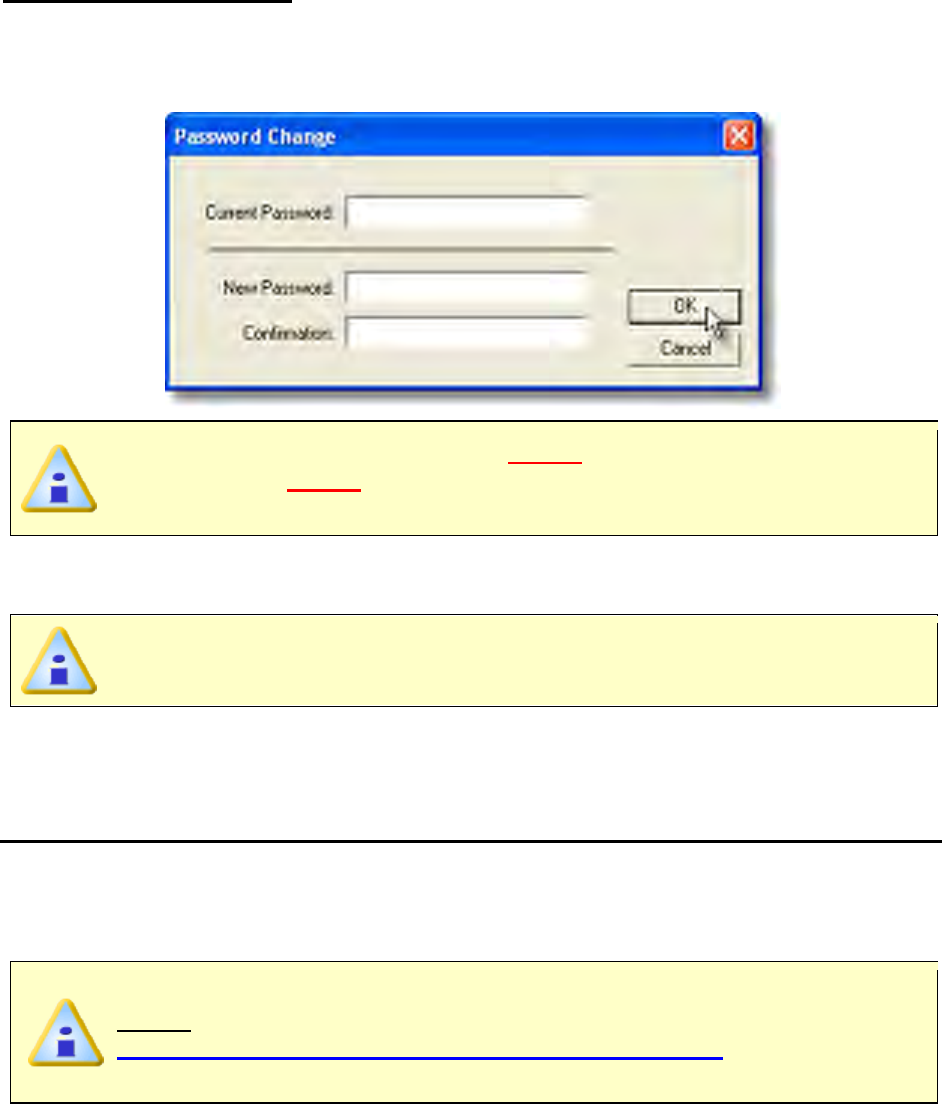
To change the password:
1) On the File menu, click Preferences, and then click the Profile tab.
2) In the Password section, click the Change Password command button and the
Password Change dialog box appears.
The software has a default password Admin
. When the password is changed
for the first time, Admin will need to be entered in the Current Password text
box.
3) Enter current password in the Current Password text box.
4) Enter a new password in the New Password text box.
The software only accepts passwords with a minimum of 4 characters.
5) Enter the new password again in the Confirmation text box and then click the OK
command button to accept or Cancel to not change the password.
Mode
Select the corresponding check box to password protect the Engineer Mode. If password
protection has been selected, a dialog box appears prompting the user to enter the
current password. The software will then need to be restarted to apply password
protection settings.
If the default password has not been changed, the current password is
Admin. Refer to topic
Software>Menus>File>Preferences>Misc>Passwords for more
information.
Email
The user can send or save a Screen image (.BMP) or Data Run (.XMG) to an email
recipient. The user can set a default email address to have the software automatically
populate the Email recipient text box when using the Send to command.
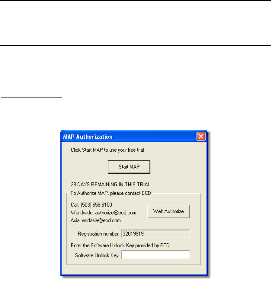
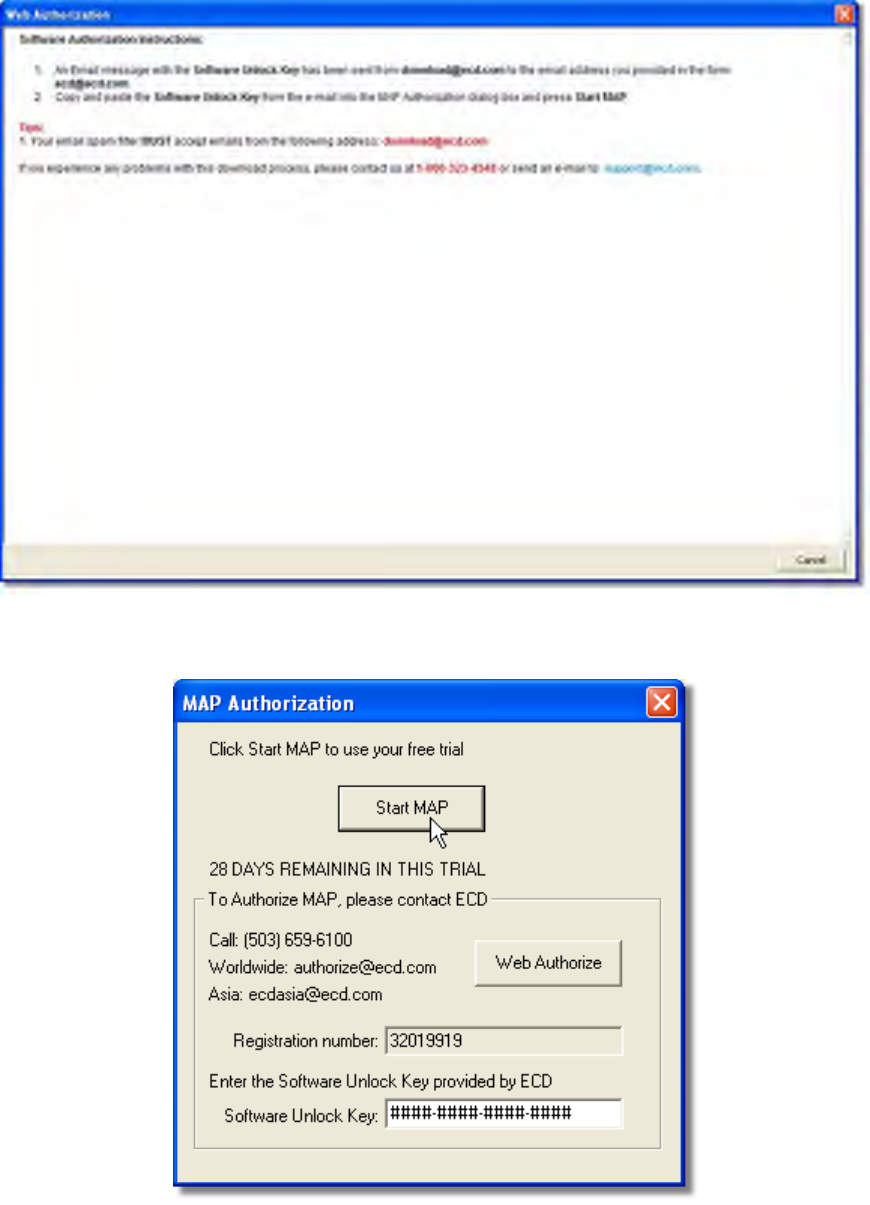
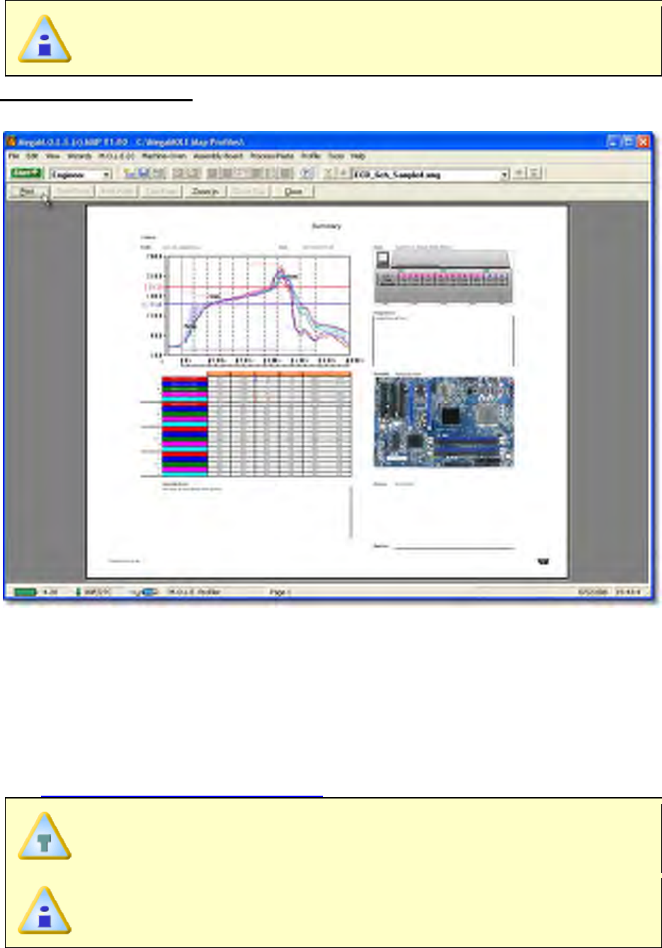
Authorization
The software is a fully functional 30-day trial version that can be authorized at any time.
Once the trial period is over, the user cannot access the software until it is authorized.
A Software Unlock Key can be obtained via the web or using the contact information
supplied on the dialog box, contact ECD.
To Web Authorize:
1) On the File menu, click Preferences, and then click the Misc tab.
2) In the Authorization section, click the Authorize command button and the
Authorization dialog box appears.
3) Enter the required information on the M.O.L.E.® MAP Software Authorization
form.
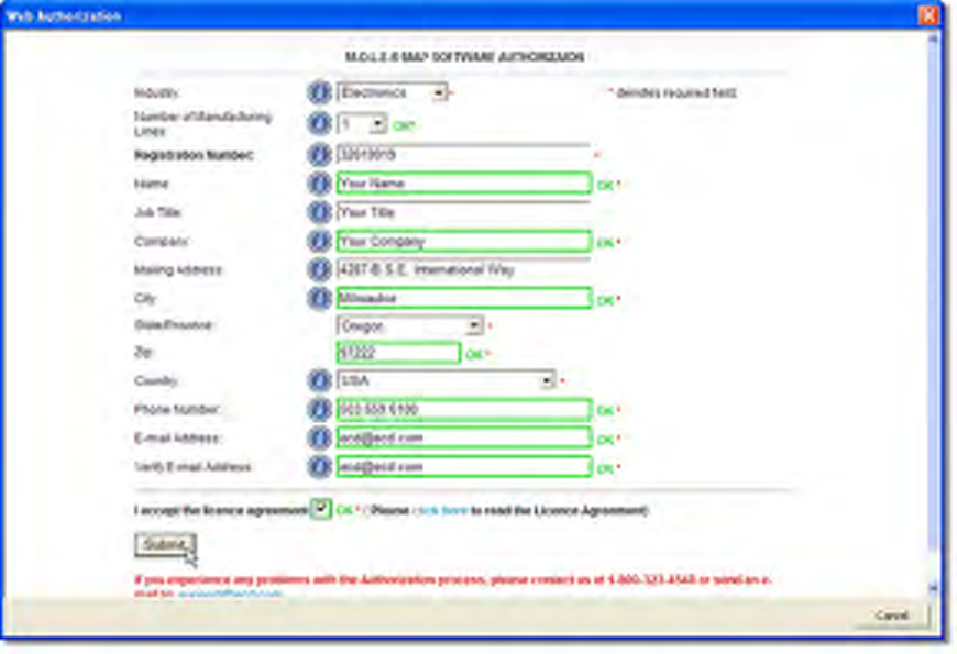
4) When finished select the Submit button. A confirmation screen appears indicating
that the Software Unlock Key has been sent to the email address provided in the
form.
5) Enter the 16-digit Software Unlock Key and then the Start MAP command button
to complete the software Authorization.
5.5.1.7. Print Preview
The Print Preview command shows a preview of the page(s) to be printed. This command
is useful when confirming print options.
This is available in both Engineer & Verify Modes.
To view a print preview:
1) On the File menu, click Print Preview.
2) Use the buttons on the toolbar to look over the page or make adjustments before
printing.
5.5.1.8. Print
The Print command allows all of the individual Page Tabs and MAP information to be
printed in a report format. The default Page Tabs in addition to MAP information to be
included when printing can also be configured on the associated Preference tab. Refer to
topic Software>Menus>File>Preferences for more information.
The options that appear on the Print dialog box will depend on the type of
printer and the installed printer driver.
This is available when in Engineer Mode.
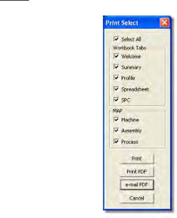
To print:
1) On the File menu, click Print.
2) Select desired print options.
• Print: Hardcopy print of selected Tabs and/or MAP information.
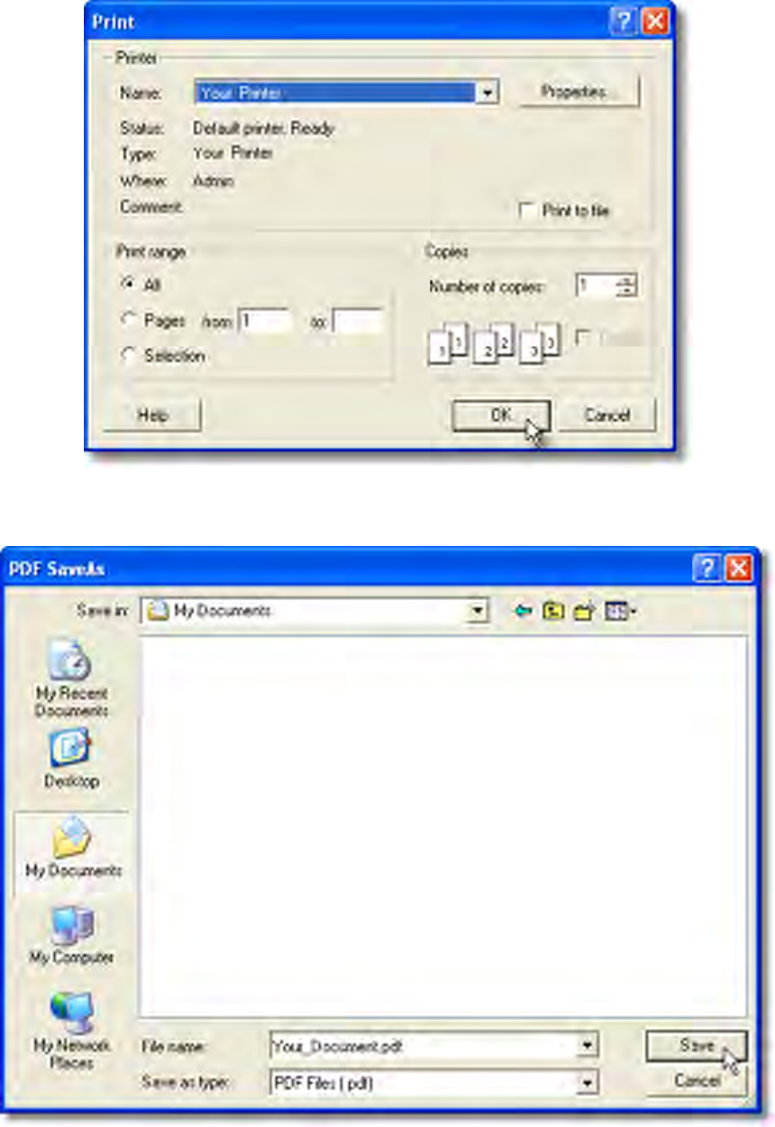
• Print PDF: Print a .PDF file of selected Tabs and/or MAP information using the
MAP PDF Printer.
• e-mail PDF: Sends a .PDF file of selected Tabs and/or MAP information using
the users default email program.
Until the e-
mail is sent or the user cancels this process, the software will not be
able to be accessed.
5.5.1.9. Send to
The Send to commands let the user send or save a Screen image (.BMP) or Data Run
(.XMG) to an email recipient or file folder. This command is useful when the user would
like to share profile data with other locations or when troubleshooting problems.
This is available in both Engineer & Verify Modes.
5.5.1.9.1. Screen Image
To send a screen image:
1) Launch an email program (i.e. Outlook, Firefox, Endora).
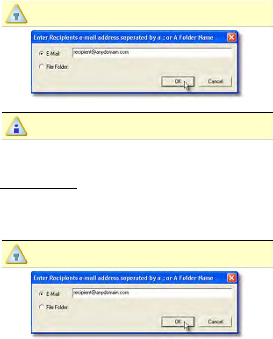
2) On the File menu, point to Send to Mail Recipients then select Screen Image to
capture a bitmap (.BMP) image of the displayed Page Tab screen.
3) In the Send to dialog box select Email or File Folder.
4) Enter an email address or navigate to a file folder.
When sending a file to multiple recipients, all email addresses must be
separated by a semicolon (;).
5) Click the OK command button to finish or Cancel to quit the command.
When sending files, the email program may display an message dialog that
informs the user that it is sending the email.
5.5.1.9.2. Data Run
To send a data run file:
1) Launch an email program (i.e. Outlook, Firefox, Endora).
2) On the File menu, point to Send to Mail Recipients then select Data Run to send
or save the currently selected data run (.XMG).
3) In the Send to dialog box select Email or File Folder.
4) Enter an email address or navigate to a file folder.
When sending a file to multiple recipients, all email addresses must be
separated by a semicolon (;).
5) Click the OK command button to finish or Cancel to quit the command.
When sending files, the email program may display an message dialog that
informs the user that it is sending the email.
5.5.1.10. Recent Working Directory
The most recently open working directories are displayed at the bottom of the File menu.
This is available in both Engineer & Verify Modes.
To select a working directory:
1) On the File menu, click the name of the desired directory or press the appropriate
number beside it.
5.5.1.11. Exit
The Exit command closes the software program.
When exiting the software, any changes made to the currently selected data
run will automatically be saved.
To exit the program:
1) On the File menu, click Exit to quit the program.
5.5.2. Edit Menu
The Edit menu commands enable the user manage the data run set displayed on the
Spreadsheet to so the most beneficial data is assembled in the working directory.
This is available in both Engineer & Verify Modes.
5.5.2.1. Copy
To copy data:
1) Select the Spreadsheet Page Tab.
2) Highlight a Spreadsheet data run row or individual cell.
3) On the Edit menu, click Copy to copy the data in the selected Spreadsheet cells
for pasting into other user definable cells or different programs.
This command can also be used by pressing the shortcut keys [CTRL +C].
5.5.2.2. Paste
To paste data:

1) Select the Spreadsheet Page Tab.
2) Highlight a user definable cell.
User definable cells have label headers of User 1-5 and are colored green.
3) On the Edit menu, click Paste, to paste the data in the selected Spreadsheet cells.
This command can also be used by pressing the shortcut keys [CTRL +V].
5.5.2.3. Rename Data Run
Since the software is a data run manager, the user can rename the data run files
displayed on the Spreadsheet Page Tab.
To rename a data run:
1) Select the Spreadsheet Page Tab.
2) Highlight a Spreadsheet data run.
3) On the Edit menu, click Rename Data Run and the software prompts the user to
specify a new data run file name.
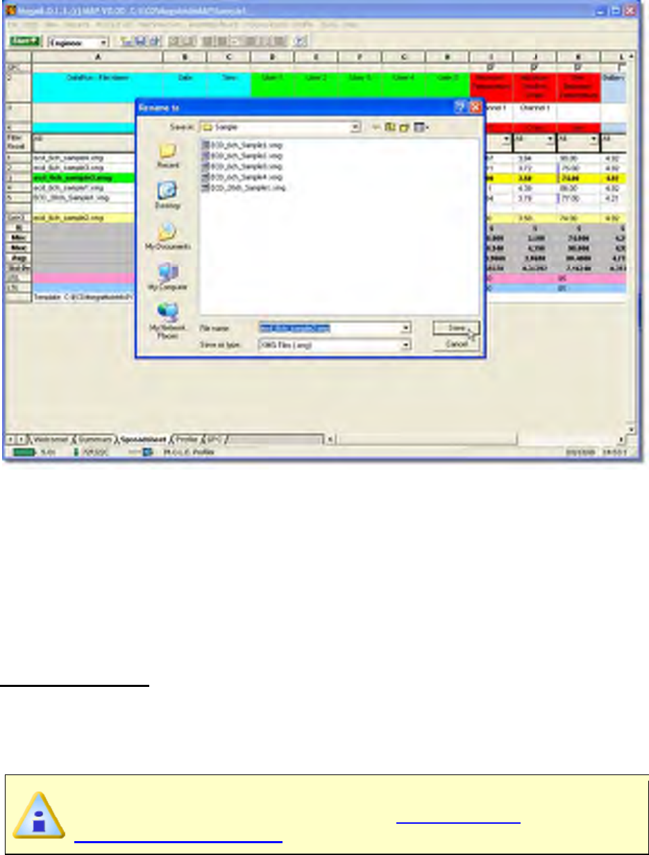
4) Rename the data run file.
5) Click the Save command button to rename the file or Cancel to quit the command.
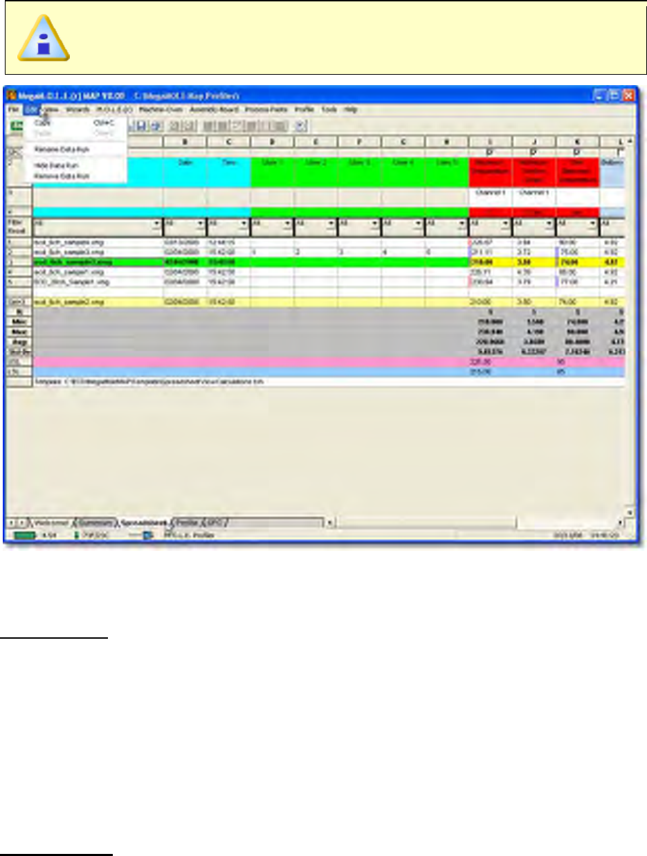
5.5.2.4. Hide Data Run
The Hide Data Run excludes a data run row without eliminating it completely from the
working directory. This command is similar to the filter function, and is helpful when data
runs may not be beneficial to the data run set statistics.
To hide a data run:
1) On the Edit menu, click Hide Row.
The data run is now excluded from the data run set without eliminating it completely from
the working directory.
To restore hidden data set row(s) click the Red Filter Reset button located on
the Spreadsheet Page Tab. Refer to topic Software>Page
Tabs>Spreadsheet>Filtersfor more information.
5.5.2.5. Remove Data Run
Since the software is a data run manager, the user can remove data runs open working
directory displayed on the Spreadsheet Page Tab.
When a data run is removed the software automatically creates a backup
(.BAK) file of the removed data run. To restore, navigate to the working
directory, rename the (*.BAK) file extension to the M.O.L.E.® MAP software
(.XMG) file extension.
To remove a data run:
1) On the Edit menu, click Remove Data Run to remove a data run that is not
wanted. This command is helpful when data has been collected and the user feels
it is not beneficial to the data run set or is corrupted.
If more than one data run needs to be removed from the open working
directory, it is recommended that the Microsoft® file management tools are
used.
5.5.3. View Menu
The View menu commands enable the user to manipulate which areas are viewed on the
standard Page Tabs and Templates.
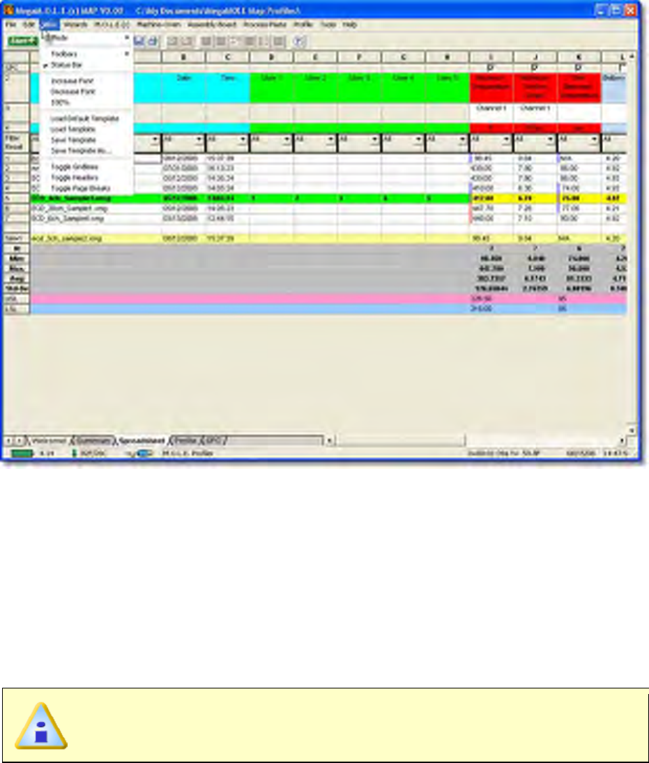
5.5.3.1. Mode
Modes are a set of page tabs, menus, toolbars, and shortcuts that are grouped and
organized so that the user can work in a specific task-oriented environment.
When you use a mode, only the menus, toolbars, and shortcut commands that are
relevant to it are displayed. The software has two Modes; Verify and Engineer. Engineer
mode contains all of the M.O.L.E.® MAP software features and functions. When
switching from Engineer to Verify mode, the amount of page tabs and toolbar items
decrease leaving the user with the tools best suited to perform verify tasks.
This is available in both Engineer & Verify Modes.
To switch modes:
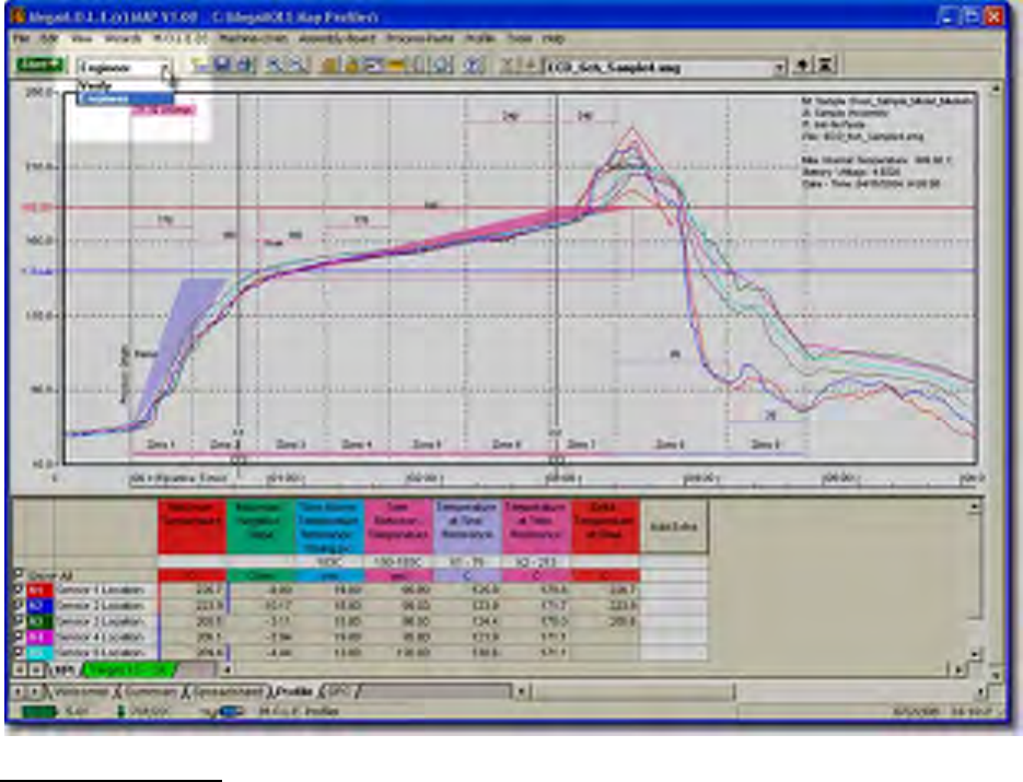
1) On the View menu, point to Modes then select the desired mode to switch to.
Modes can be accessed on the Toolbar by using the modes drop down box..
Mode drop down box
5.5.3.1.1. Verify
The full featured M.O.L.E.® MAP software, includes a simplified operating mode that
provides customers what they need for everyday profile verification.
For a complete outline of page tabs, menus, toolbars, and shortcuts associated with the
Verify mode, refer to Appendix C.
5.5.3.1.2. Engineer
Engineer mode contains all of the M.O.L.E.® MAP software features and functions.
These options are typically used so a process Engineer can set up a M.O.L.E. Profiler for
a data run, MAP information and Target-10 verification specifications.
The Engineer mode has a password protection feature that uses
case-
sensitive text for securing access to it. When password protection is used,
a user will not have access to engineer mode features without proper password
privileges.
The software has a default password Admin. If you would like to change it use
the Change Password... feature located on the Misc tab of the Preferences
property sheet. Refer to topic Software>Menus>File>Preferences>Misc for
more information.
For a complete outline of page tabs, menus, toolbars, and shortcuts associated with the
Engineer mode, refer to Appendix C.
5.5.3.2. Toolbars
By default, the Standard and Navigate toolbars appear docked on a single row, showing
the toolbar buttons that are used most often. When there is a check mark beside the
toolbar command it indicates that that it is displayed.
The toolbars can be moved to other edges of the program window. To move,
drag docked toolbar until the toolbar snaps into place on the desired edge.
This is available in both Engineer & Verify Modes.
To hide a toolbar:
1) On the View menu, point to Toolbar then select the desired toolbar to display or
hide.
5.5.3.3. Status Bar
By default, the Status bar appears along the bottom of the program window. When there
is a check mark beside the toolbar command it indicates that that it is displayed.
This is available in both Engineer & Verify Modes.
To display the status bar:
1) On the View menu, click Status bar to display or hide the Status bar.
5.5.3.4. Increase Font
The Increase Font command has the capability to zoom the current Page Tab in multiple
times.
This is available in both Engineer & Verify Modes.
To Increase Font:
1) On the View menu, click Increase Font to make the current Page Tab view larger.
When the maximum Increase Font level has been reached the command will be
dimmed.
The Increase Font command can be accessed on all Page Tabs excluding the
Profile Page Tab.
5.5.3.5. Decrease Font
The Decrease Font command has the capability to zoom the current Page Tab out
multiple times.
This is available in both Engineer & Verify Modes.
To Decrease Font:
1) On the View menu, click Decrease Font to make the current Page Tab view
smaller. When the maximum Decrease Font level has been reached the
command will be dimmed.
The Decrease Font command can be accessed on all Page Tabs excluding
the Profile Page Tab.
5.5.3.6. 100%
The Zoom 100% command restores the current Page Tab to the default view level.
This is available when in Engineer Mode.
To zoom 100%:
1) On the View menu, click 100% to restore current Page Tab view to the default.
The 100% command can be accessed on all Page Tabs excluding the Profile
Page Tab.
5.5.3.7. Load Default Template
Template data calculations are highly customizable. When a user has changed one, the
user can use the Load Default Template to discard all modifications and restore the
default template specified in Software>Menus>File>Preferences.
Templates are automatically loaded every time the software is started and is
used as the default template for every downloaded data run. Template files
are specified on the Preferences property sheet. Refer to topic
Software>Menus>File>Preferences for more information.
This is available when in Engineer Mode.
To load a default template:
1) On the View menu, click Load Default Template to load the default template.
This command can also be accessed by right-clicking over a template.
5.5.3.8. Load Template
Since the software allows the user to create different templates use the Load Template
command to apply a template file to any data run in the working directory.
This is available when in Engineer Mode.
To load a template:
1) On the View menu, click Load Template.
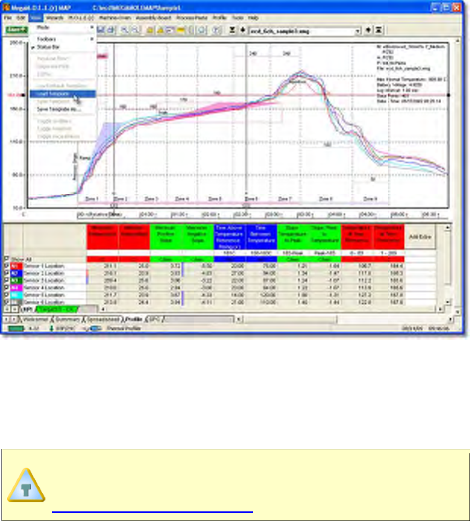
2) Navigate to the location where the template files are located. Depending on which
page tab you are viewing, the software only displays the template file type for that
tab.
• Summary Template File (*.TSU)
• Spreadsheet Template File (*.TSH)
• Data Table Template File (*.TPF)
When loading templates the software opens to the default Templates folder of
the M.O.L.E.®
MAP Software file structure. You can change this setting using
the Preferences property sheet. Refer to topic
Software>Menus>File>Preferences for more information.
3) Click the Open command button to select the template file or Cancel to quit the
command.
4) After the template file has been selected, the software prompts the user to decide if
they would like to set the selected template file as the new default template which
is applied to all future data runs downloaded from a M.O.L.E. Profiler.
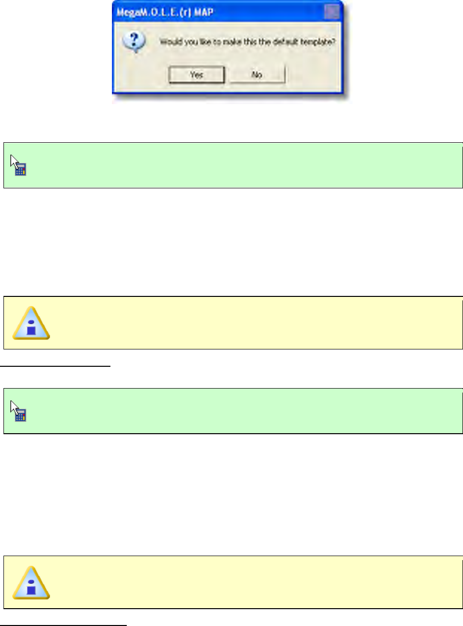
5) Click the Yes command button to use at the new default template for No to apply it
to the current data run only keeping the current default template.
This command can also be accessed by right-clicking over a template.
5.5.3.9. Save Template
When a template data calculation has been changed or a new one has been added, the
user can save the calculations to the template saved with the currently displayed data
run.
This is available when in Engineer Mode.
To save a template:
1) On the View menu, click Save Template to save the displayed data run template.
This command can also be accessed by right-clicking over a template data
calculation.
5.5.3.10. Save Template As...
When a template data calculation has been changed or a new one has been added, the
user can save the calculations to a new template file. This is useful when the user would
like to customize a template leaving the default template the same. The user can apply
this new template to other data run files by using the Load Template command.
This is available when in Engineer Mode.
To save a template as:
1) On the View menu, click Save Template As and the Save Data Calculation
Template dialog box appears.
2) Specify a new file name.
3) Click the Save command button to save the new template file or Cancel to quit the
command.
This command can also be accessed by right-clicking over a template.
5.5.3.11. Toggle Gridlines
The Summary and Spreadsheet Page Tabs are built with cells that are organized into
columns and rows. The software allows the user to show and hide the cell gridlines as
needed. This command is particularly helpful when customizing the Summary Page Tab
template.
This is available when in Engineer Mode.
To toggle gridlines:
1) On the View menu, click Toggle Gridlines to show or hide cell gridlines.
This command can also be accessed by right-clicking over the Summary or
Spreadsheet templates.
5.5.3.12. Toggle Headers
The Summary and Spreadsheet Page Tabs are built with cells that are organized into
columns and rows. These columns and rows include row headings which are numbers
that appear on the left of each row, and column headings which are the letters that appear
at the top of each column.
This is available when in Engineer Mode.
To toggle headers:
1) On the View menu, click Toggle Headers to show or hide column and row
headers.
This command can also be accessed by right-clicking over the Summary or
Spreadsheet templates.
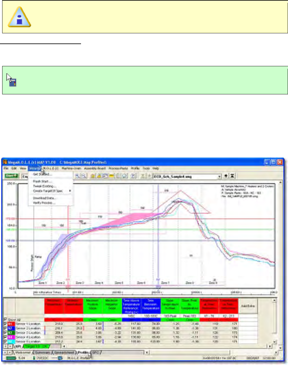
5.5.3.13. Toggle Page Breaks
As data calculations get added to the Spreadsheet Page Tab, it may increase the amount
of pages when printing. The software includes a preview of where page breaks occur.
This is available when in Engineer Mode.
To toggle page breaks:
1) On the View menu, click Toggle Page Breaks to show or hide the page break
lines.
This command can also be accessed by right-clicking over the Spreadsheet
template.
5.5.4. Wizards Menu
M.O.L.E.® MAP software wizards help guide the user through the most common
multi-step tasks.
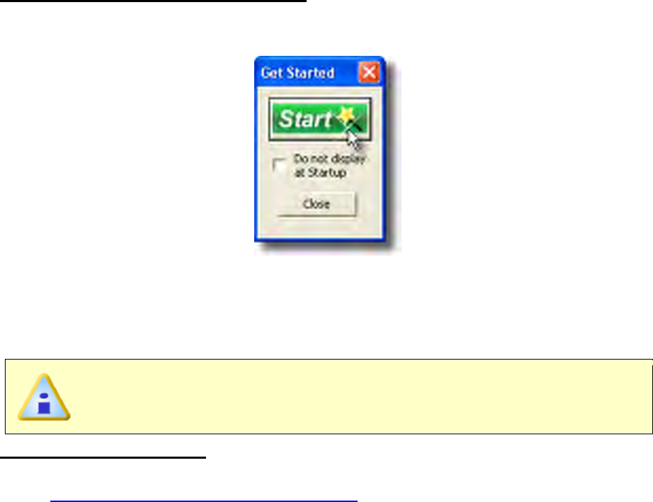
5.5.4.1. Get Started
This command activates the Get Started dialog box for access to the New (Start)
command.
To activate the Get Started dialog box:
1) On the Wizards menu, click Get Started and a dialog box appears with the New
(Start) command button.
5.5.4.2. Fresh Start
The Fresh Start workflow is a wizard that starts a new profile (data run) by entering
Machine (oven), Assembly (board) and Process (Paste) information.
This is available when in Engineer Mode.
The Fresh Start workflow:
1) Connect the M.O.L.E. Profiler to the computer. Refer to
Basics>Setup>Communications Setup for more information.
2) On the File menu, cllick New. A message box appears with the five workflow
wizard options.
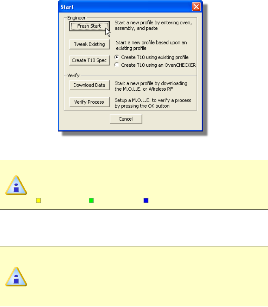
3) On the Start dialog box, click the Fresh Start command button and the workflow
wizard appears.
When navigating through the wizard, the step list on the left uses a color key
to inform the user of the current step, steps that have been completed and
remaining steps.
Current Completed Remaining
4) Select the desired instrument from the dialog box to make active. If a M.O.L.E.
Profiler has already been selected during a different process, the software
automatically selects the M.O.L.E. Profiler connected to the COM port previously
used.
If the software does not detect a M.O.L.E. Profiler, using the communication
cable connect it to the computer and click the Scan for Instruments
command button to search again. M.O.L.E.® MAP software allows multiple
instruments to be connected to a computer at one time. Selecting the Scan for
Instruments command button will detect all instruments and display them in
the dialog box. If no instrument is detected the software displays all of the
Demonstration thermal profilers to select from.
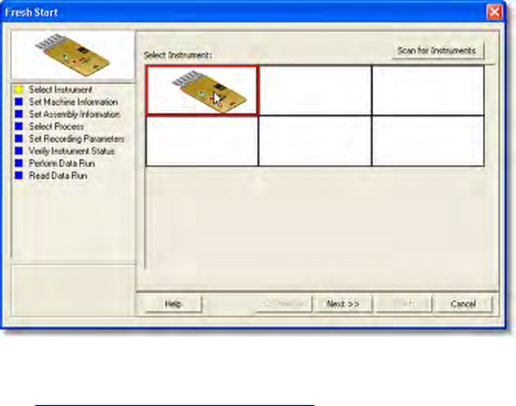
5) Click the Next command button.
6) Select a machine from the Machine drop down list. If the machine does not appear
in the list click the New command button to create a new machine. Refer to topic
Software>Menus>Machine>Create new Machine for more information.
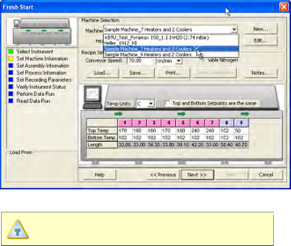
7) Set the machine recipe settings such as Conveyor Speed, Zone Temperatures
and Temperature units.
The software includes features to save and load machine recipe setting files.
These files are helpful to quickly load machine information and to ensure they
are always the same.
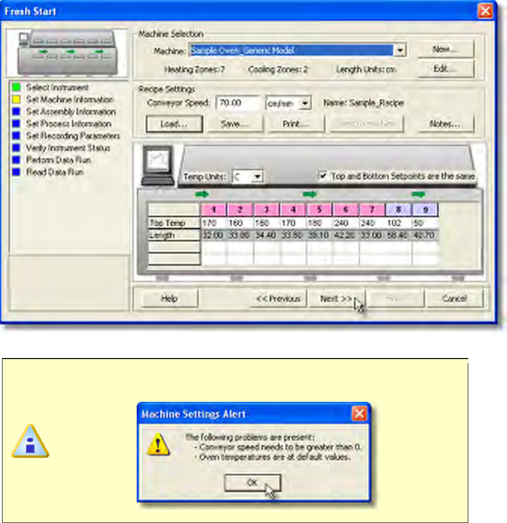
8) Click the Next command button.
If no value is specified for the conveyor speed or the default oven temperature
values, the software will remind the user to set them.
9) Set the assembly information such as part number, board size, sensor locations
and a product image.
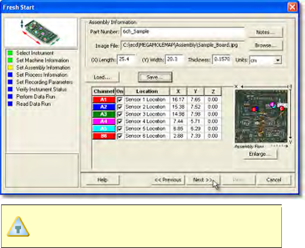
If the user specifies a product image, clicking the Enlarge command button
displays the Set Sensor Locations dialog box where the user can specify the
locations of each sensor. To move sensor locations, drag the sensor markers
to the approximate location where the sensors are attached.
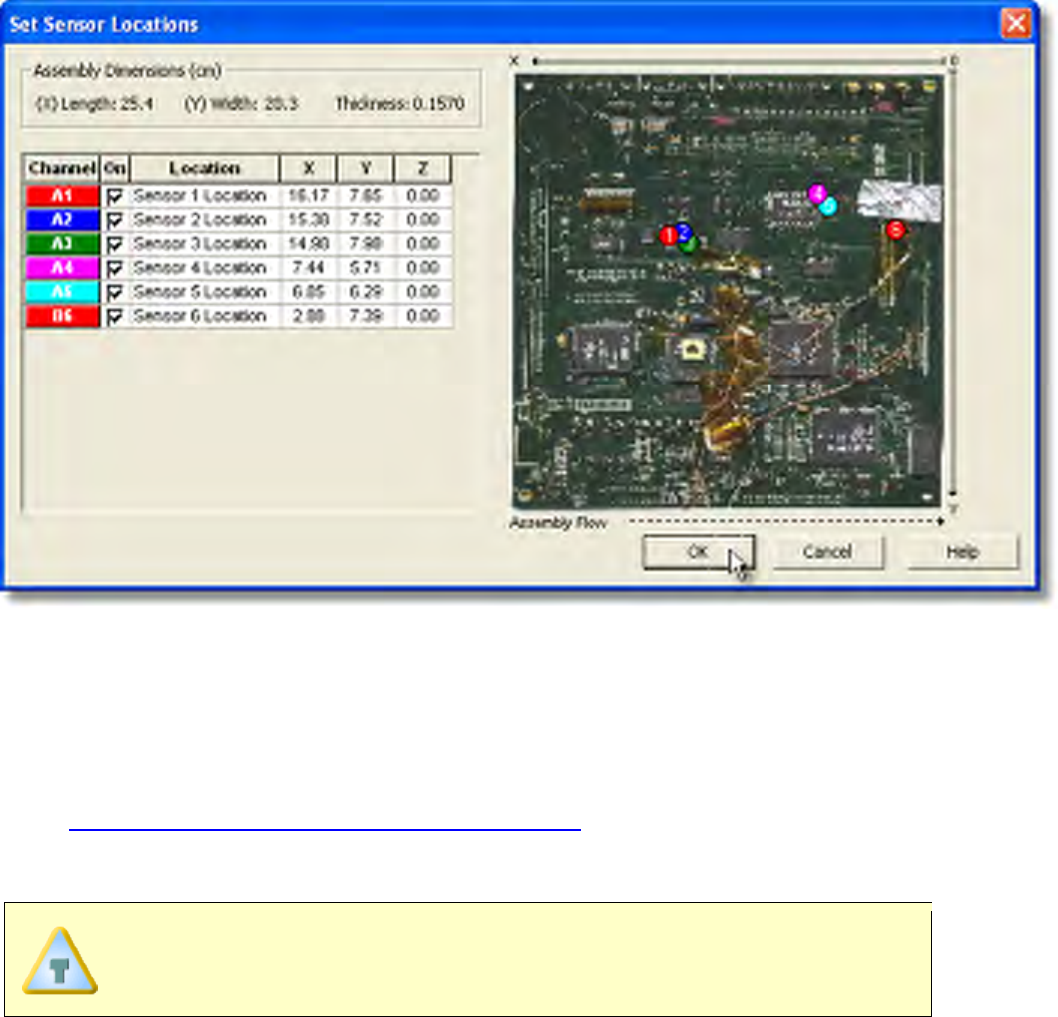
10) When finished, click the OK command button to accept or Cancel to return without
making any changes.
11) Click the Next command button.
12) Select your process specification. Select a Paste from the database or previously
created Target 10 Specification. If your Paste does not appear in the database
list click the New command button to create a new one. Refer to topic
Software>Menus>Process>Create new Paste for more information.
13) Choose the Profile Type (Ramp-Soak-Spike or Ramp-to-Spike).
Ramp-Soak-Spike profile types are the only type allowed to be edited.
When the user selects a paste from the database, they can use the radio
buttons below the drop down box to filter and display only the user created
pastes from paste database.
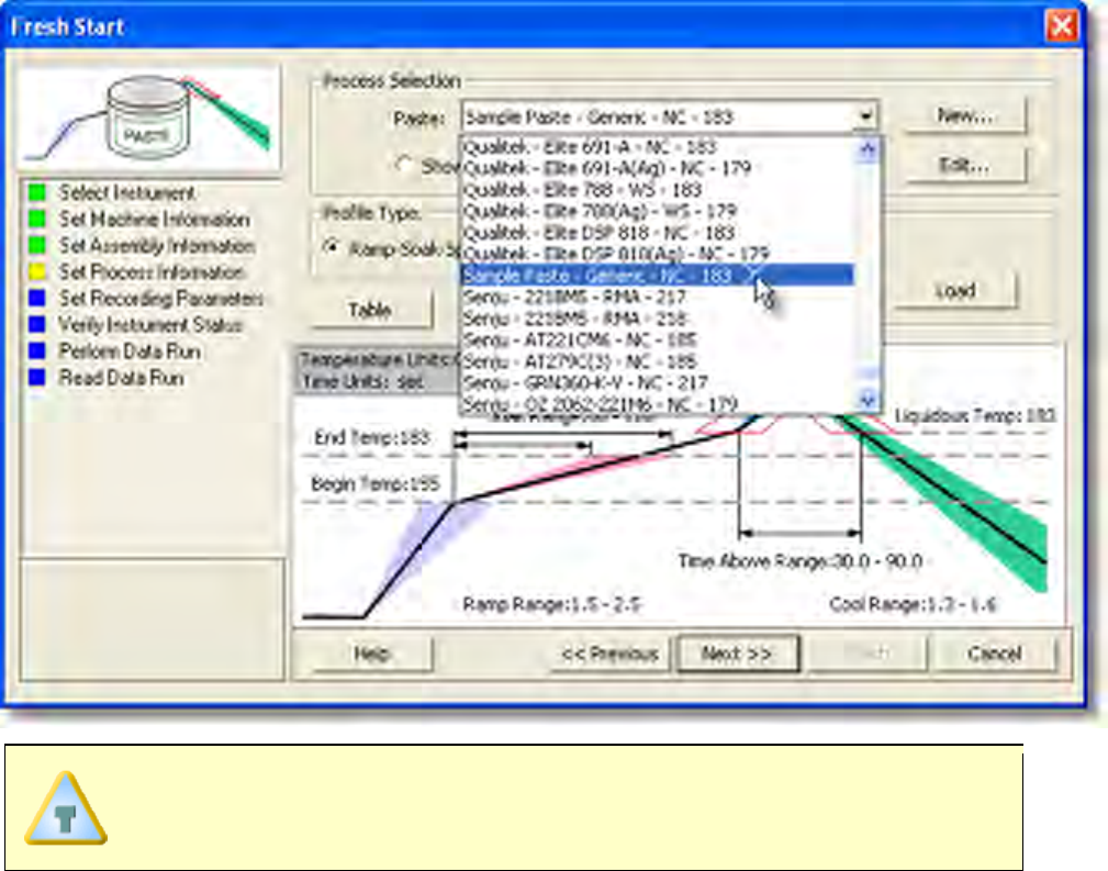
Once a paste is selected the specifications are displayed on the graph. The
software also allows paste specification data to be viewed in a table view by
clicking the Table command button.
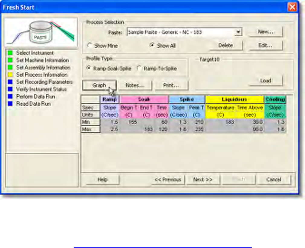
14) Click the Next command button
15) Set Recording Parameters such as the instrument name, recording interval, start
parameters and stop parameters. This step is where the user can also turn a
sensor channel ON or OFF, set the sensor location description and sensor type.
Refer to section Software>Menus>MOLE>Set Recording Parameters for
detailed information for each setting.
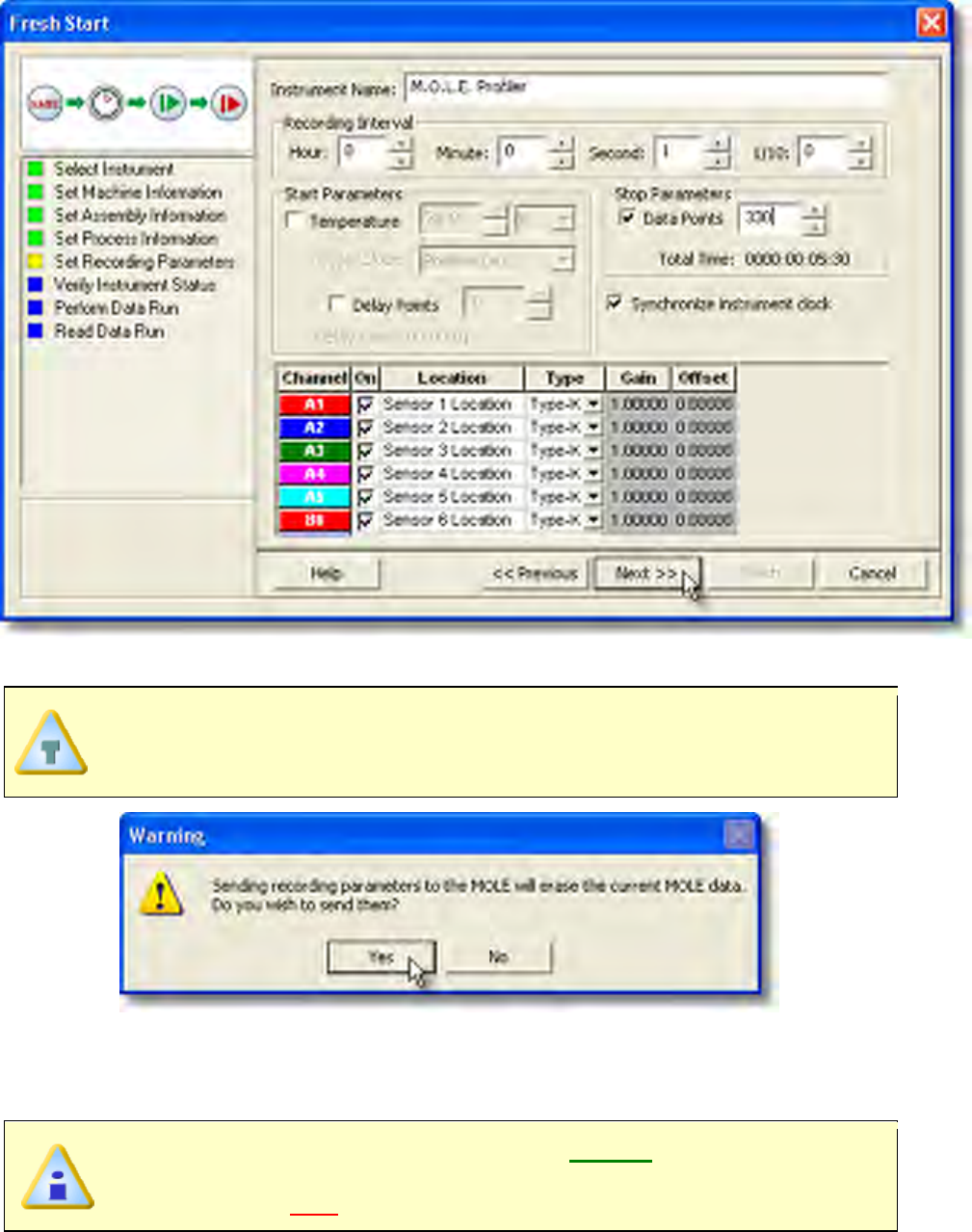
16) Click the Next command button.
If the currently selected M.O.L.E. Profiler is a SuperM.O.L.E.® Gold, sending
recording parameters will erase the data currently stored in the M.O.L.E.
Profiler. The software will warn the user with a message box.
17) Verify the instrument status. This dialog box displays the health of the M.O.L.E.
Profiler such as battery charge, internal temperature, thermocouple temperatures.
If everything is OK, the dialog box displays a GREEN sign. If there are any
items that may prevent the user from collecting good data, they are
highlighted and a RED sign is displayed.
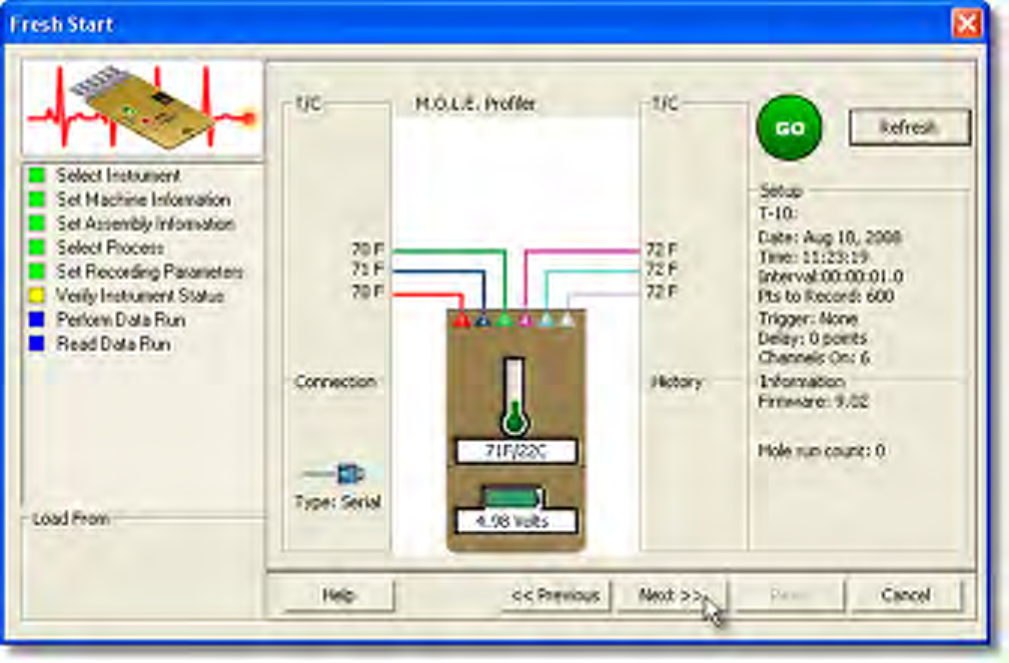
18) Click the Next command button.
19) Review the oven settings and click the Next command button to continue.
20) Pass the thermally protected M.O.L.E. Profiler and test product through the
process. Refer to topic Basics>Operation>Step 2 - Data Collection for more
information.
If the M.O.L.E. Profiler already contains a data run or if the selected M.O.L.E.
Profiler is wireless RF, click the Next command button to proceed to the next
step.
21) Select the desired data run and then click the Finish command button to complete
the wizard and read the data run from the M.O.L.E. Profiler.
If the user has selected to use a Wireless RF option, select Start real-time
RF on the top of the data run list and then the Finish command button to
display the RF Control dialog.
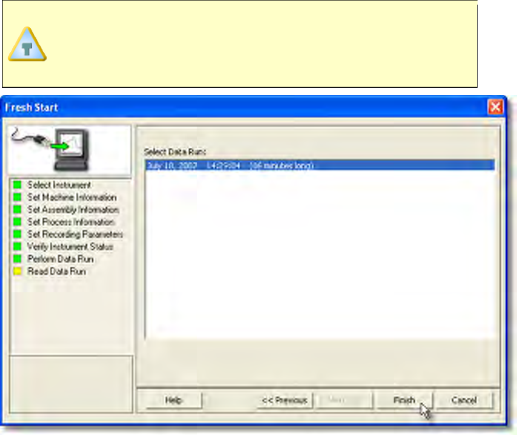
This step of the wizard allows the user to remove a selected data run from the
M.O.L.E. Profiler by either selecting the Delete After Reading check box or
selecting the Delete command button and removing it before downloading.
This feature is not available for the SuperM.O.L.E.® Gold Thermal Profiler as it
does not have the ability to store more than one data run.
• Prior to reading the data run, the software prompts the user to select the sensor
type for the active channels. When finished select the OK command button to
proceed.

22) When the data run has been downloaded, the software prompts the user to specify
a new file name (*.XMG).
When saving a data run (*.XMG) to a different file directory other than the
current Working directory, the software automatically sets the new file
directory as the current Working Directory. This process does not delete any
data run files in the previously set Working directory and can be quickly
accessed using the Recent Working Directory command on the File menu.
I
23) When finished, click the Save command button.
24) The software then prompts the user if they want to enter Prediction mode. Entering
prediction mode enables the user to change a zone temperature value or the
conveyor speed and predict the outcome of that change. Refer to topic
Software>Menus>Tools>Prediction for more information.
25) Click the Predict command button to enter Prediction mode or Done to complete
the process .
5.5.4.3. Tweak Existing
The Tweak Existing workflow is a wizard that starts a new profile (data run) using the
established Machine (oven), Assembly (board) and Process (Paste) information from an
existing profile.
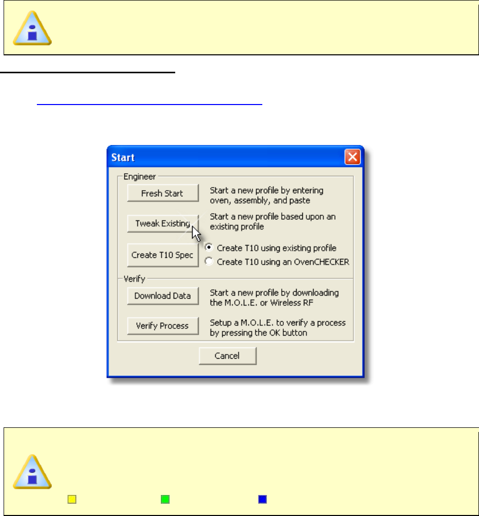
This is available when in Engineer Mode.
The Tweak Existing workflow:
1) Connect the M.O.L.E. Profiler to the computer. Refer to
Basics>Setup>Communications Setup for more information.
2) On the File menu, click New. A message box appears with the five workflow
wizard options.
3) On the Start dialog box, click the Tweak Existing command button and the
workflow wizard appears.
When
navigating through the wizard, the step list on the left uses a color key
to inform the user of the current step, steps that have been completed and
remaining steps.
Current Completed Remaining
4) Select an existing data run. The software lists the data runs from the currently open
working directory and and automatically highlights the currently selected data run
on the Spreadsheet page tab. The user can select any data run displayed on the
list.
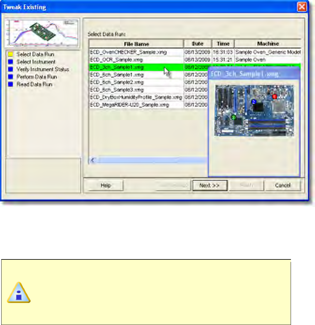
5) Click the Next command button.
6) Select the desired instrument from the dialog box to make active. If a M.O.L.E.
Profiler has already been selected during a different process, the software
automatically selects the M.O.L.E. Profiler connected to the COM port previously
used.
If the software does not detect a M.O.L.E. Profiler, using the communication
cable connect it to the computer and click the Scan for Instruments
command button to search again. M.O.L.E.® MAP software allows multiple
instruments to be connected to a computer at one time. Selecting the Scan for
Instruments command button will detect all instruments and display them in
the dialog box. If no instrument is detected the software displays all of the
Demonstration thermal profilers to select from.
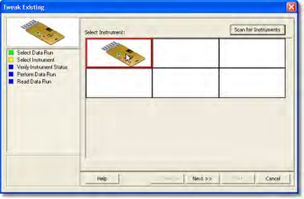
7) Click the Next command button.
8) Verify the instrument status. This dialog box displays the health of the M.O.L.E.
Profiler such as battery charge, internal temperature, thermocouple temperatures.
If the user selects the Show Critical command button the dialog box will only
display items that will prevent the user from completing a successful data run.
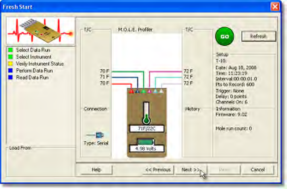
9) Click the Next command button.
10) Review the oven settings and click the Next command button to continue..
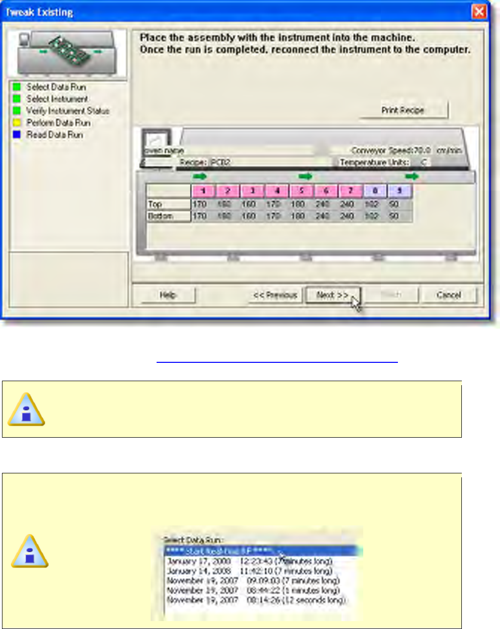
11)Pass the thermally protected M.O.L.E. Profiler and test product through the
process. Refer to topic Basics>Operation>Step 2 - Data Collection for more
information.
If the M.O.L.E. Profiler already contains a data run or if the the selected
M.O.L.E. Profiler is wireless RF, click the Next command button to proceed to
the next step.
12) Select the desired data run and then click the Finish command button to complete
the wizard and read the data run from the M.O.L.E. Profiler.
If the user has selected to use a Wireless RF option, select Start real-time
RF on the top of the data run list and then the Finish command button to
display the RF Control dialog.
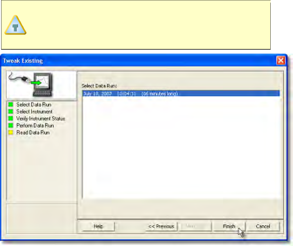
This step of the wizard allows the user to remove a selected data run from the
M.O.L.E. Profiler by either selecting the Delete After Reading check box or
selecting the Delete command button and removing it before downloading.
This feature is not available for the SuperM.O.L.E.® Gold Thermal Profiler as it
does not have the ability to store more than one data run.
• Prior to reading the data run, the software prompts the user to select the sensor
type for the active channels. When finished select the OK command button to
proceed.

13) When the data run has been downloaded, the software prompts the user to specify
a new file name (*.XMG).
When saving a data run (*.XMG) to a different file directory other than the
current Working directory, the software automatically sets the new file
directory as the current Working Directory. This process does not delete any
data run files in the previously set Working directory and can be quickly
accessed using the Recent Working Directory command on the File menu.
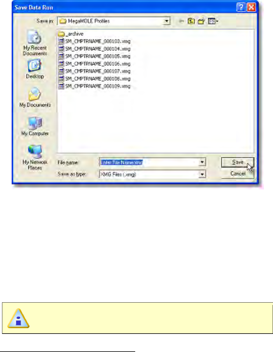
I
14) When finished, click the Save command button to complete the process.
5.5.4.4. Create Target 10 Specification
The Create Target 10 Specification is a wizard that helps the user create a Target 10
Specification using an existing profile (data run) or OvenCHECKER™. The Target 10
specification can then be used to verify a process or machine performance.
5.5.4.4.1. Existing Profile
The Create Target 10 Specification - Existing Profile is a wizard that helps the user
create a specification from an existing data run profile to be used when verifying a
process.
This is available when in Engineer Mode.
Create Target 10 Specification workflow:
1) On the File menu, click New. A message box appears with the five workflow
wizard options.
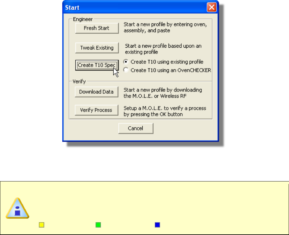
2) On the Start dialog box, click the Create T10 using an existing profile option,
then click the Create T-10 Spec command button and the workflow wizard
appears.
When navigating through the wizard, the step list on the left uses a color key
to inform the user of the current step, steps that have been completed and
remaining steps.
Current Completed Remaining
3) Select the instrument type that will be used to verify the process.
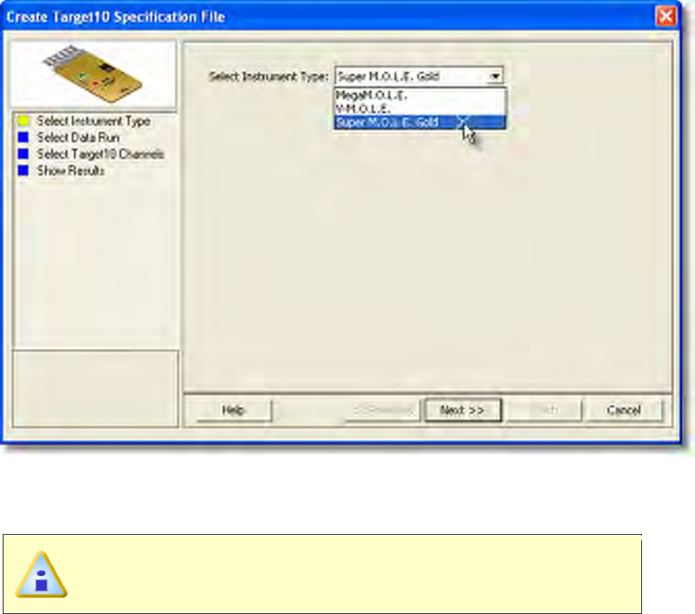
4) Click the Next command button.
5) Select a data run. This is the data run that is known to be good and the user wishes
to confirm the process is reproducing faithfully using the verify process.
If the selected data run was created using a recording interval other than 1.0
second, the Slope calculation will not be included in the Target10
Specification.
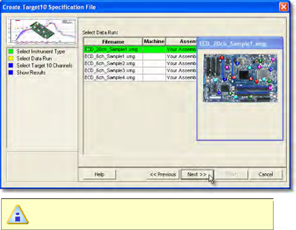
This list displays the data runs from the currently open working directory.
6) Click the Next command button.
7) Map the desired channels from selected data run to channels of the M.O.L.E.
Profiler. These typically are the most important channels that best represent the
process being verified.
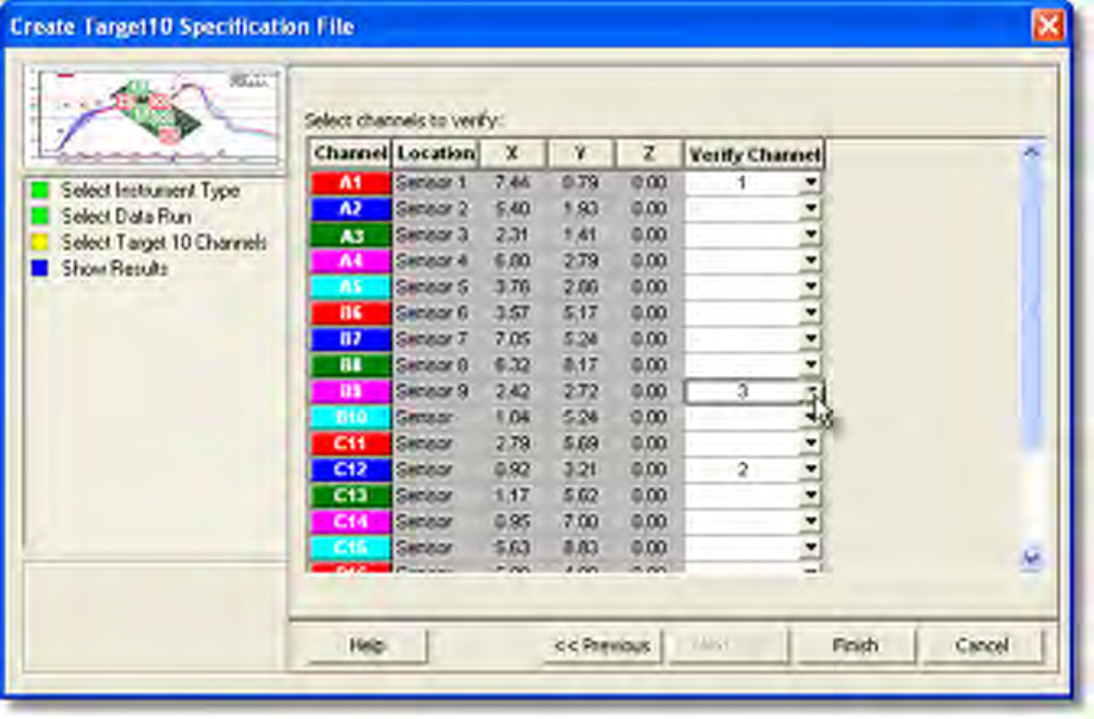
8) Click the Next command button.
9) Once the channels are mapped, review the results of the Target 10 specification.
The user can then decide if they wish to send these to the M.O.L.E. profiler or
make final modifications to the Slope, Soak, Time Above and/or Peak parameter.
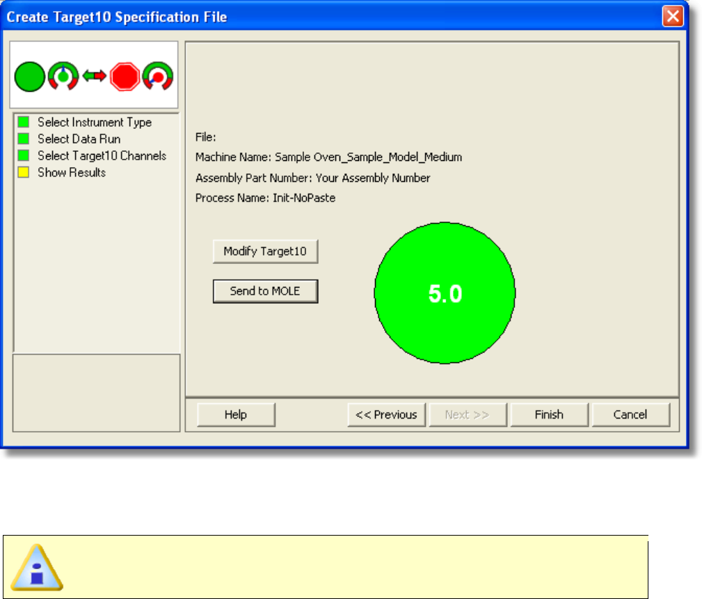
10) If the user decides to make modifications, click the Modify Target10 command
button and the the Target 10-OK tab is displayed. Make the desired modifications
to the Slope, Soak, Time Above and/or Peak parameter specifications.
If any of the parameter specifications are changed the OK button will inform
the user by displaying (OKModified).
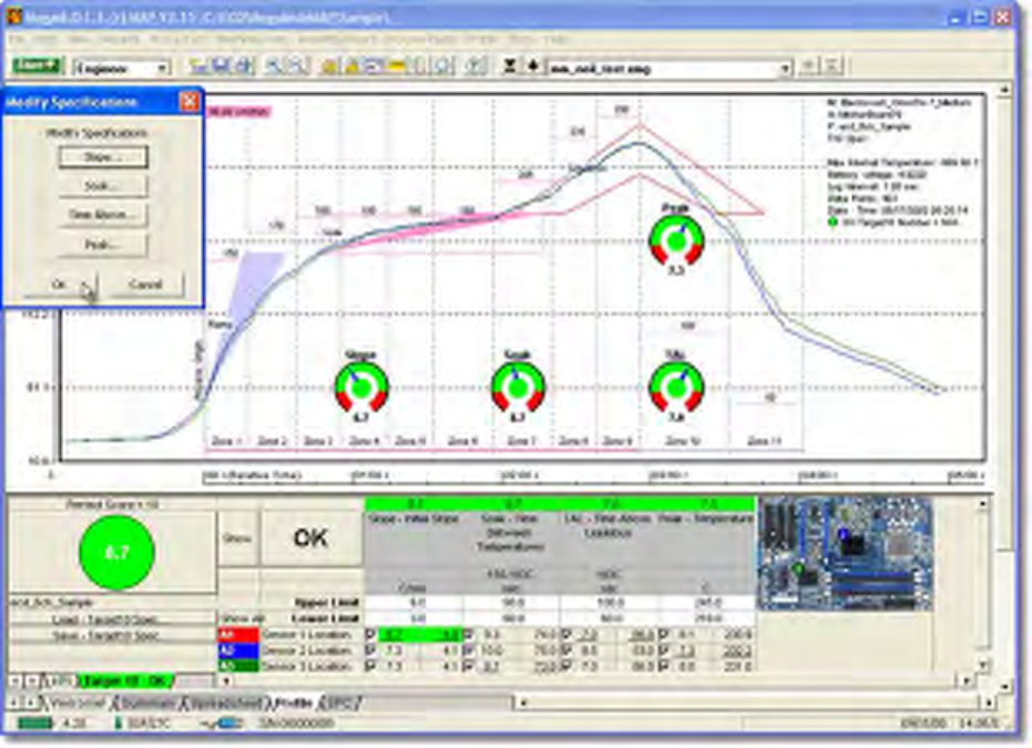
11) Click the OK command button to accept the modified specifications or Cancel to
discard them and return to the workflow wizard.
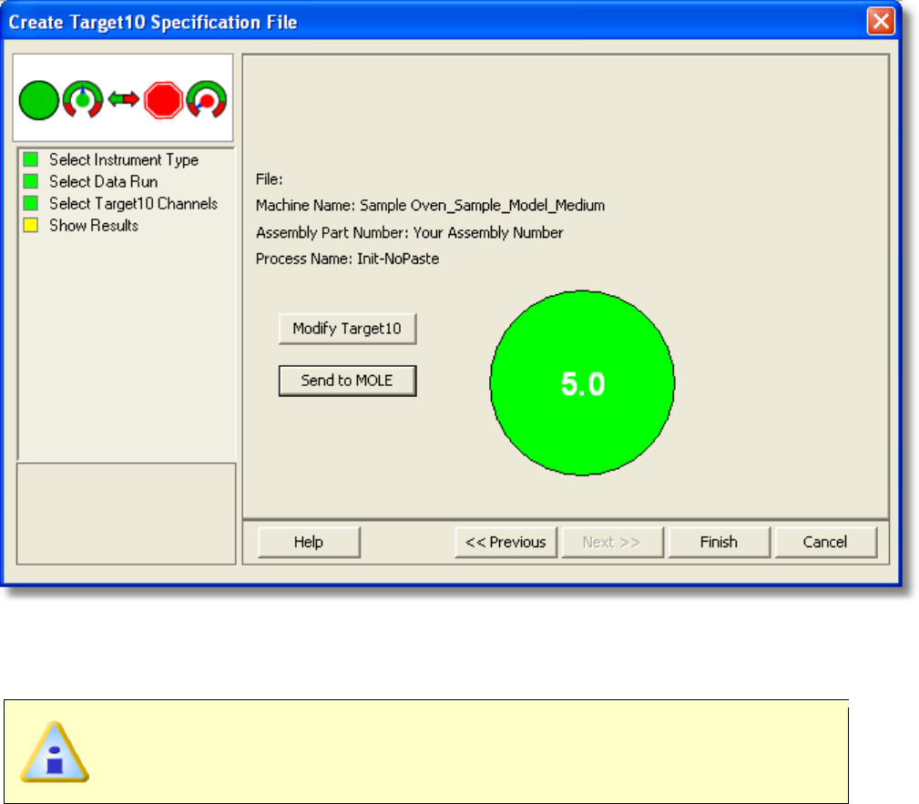
12) If the user either decides to send the Target10 to the M.O.L.E. profiler or complete
the wizard by clicking the Finish command button, the software prompts the user
to save the Target 10 file (*.T10).
Only the MEGAM.O.L.E.® and V-M.O.L.E.® can have the Target 10 sent to
them. When using the SuperM.O.L.E.®
Gold the Target 10 will only be able to
be saved as a file.
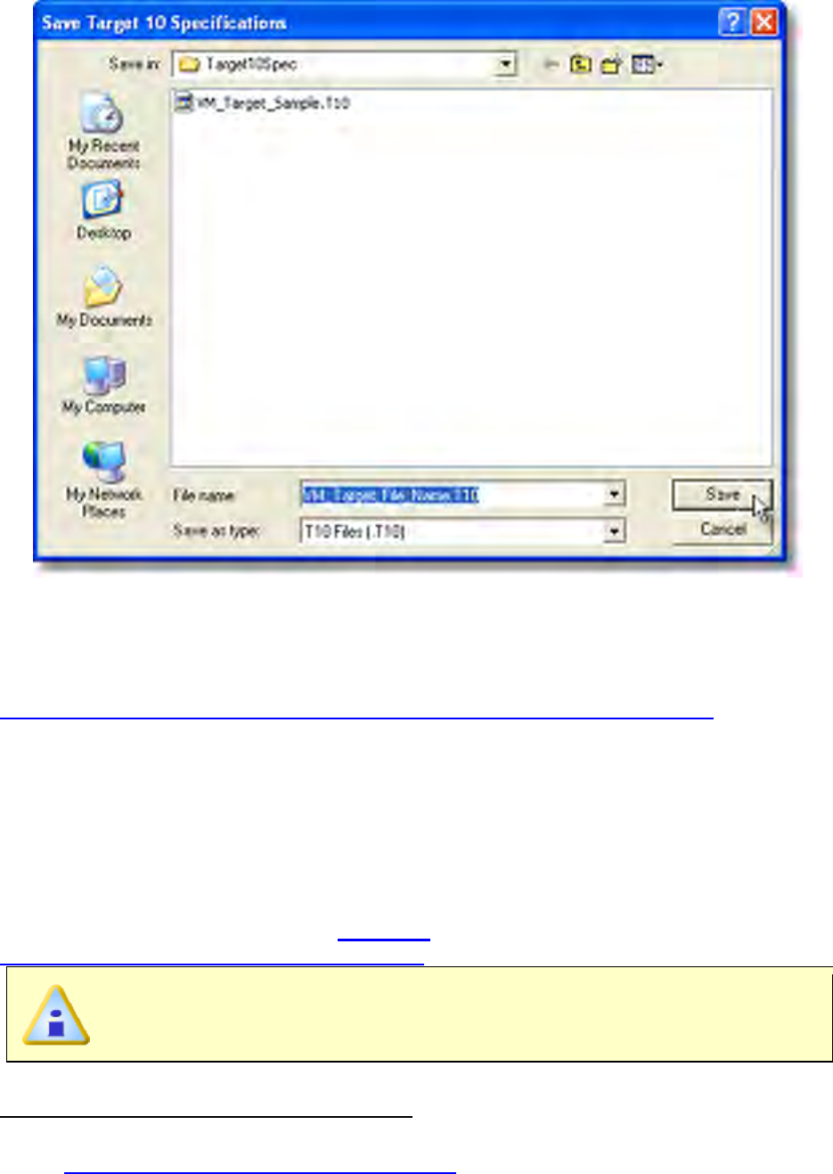
13) When finished naming the file, click the Save command button to complete the
workflow wizard.
This Target 10 Specification can now be used when Verifying a process. Refer to topic
Menus and Tool Commands>File Menu>Wizards Menu>Verify Process for more
information.
5.5.4.4.2. OvenCHECKER
The Create Target 10 Specification - OvenCHECKER is a wizard that helps the user
create a Target 10 Specification using an OvenCHECKER™ data run that can be used to
verify that your machine performance is the same in the future. To use this wizard, it
requires the OvenCHECKER™ Oven Verification System which is powered by the
V-M.O.L.E.® profiler. Refer to topic Optional
Accessories>Products>OvenCHECKER™ for more information.
This is available when in Engineer Mode.
Create Target 10 Specification workflow:
1) Connect the M.O.L.E. Profiler to the computer. Refer to
Basics>Setup>Communications Setup for more information.
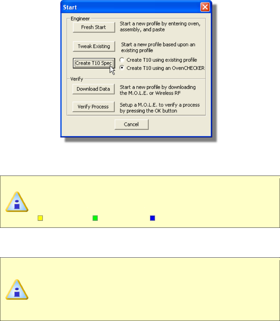
2) On the File menu, cllick New. A message box appears with the five workflow
wizard options.
3) On the Start dialog box, click the Create T10 using an OvenCHECKER option,
then click the Create T-10 Spec command button and the workflow wizard
appears.
When
navigating through the wizard, the step list on the left uses a color key
to inform the user of the current step, steps that have been completed and
remaining steps.
Current Completed Remaining
4) Select the desired instrument from the dialog box to make active. If a V-M.O.L.E.®
Profiler has already been selected during a different process, the software
automatically selects the COM port previously used.
If the software does not detect a M.O.L.E. Profiler, using the communication
cable connect it to the computer and click the Scan for Instruments
command button to search again. M.O.L.E.® MAP software allows multiple
instruments to be connected to a computer at one time. Selecting the Scan for
Instruments command button will detect all instruments and display them in
the dialog box. If no instrument is detected the software displays all of the
Demonstration thermal profilers to select from.
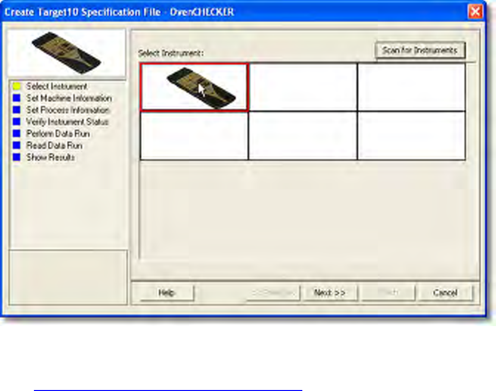
5) Click the Next command button.
6) Select a machine from the Machine drop down list. If the machine does not appear
in the list click the New command button to create a new machine. Refer to topic
Software>Menus>Machine>Create new Machine for more information.
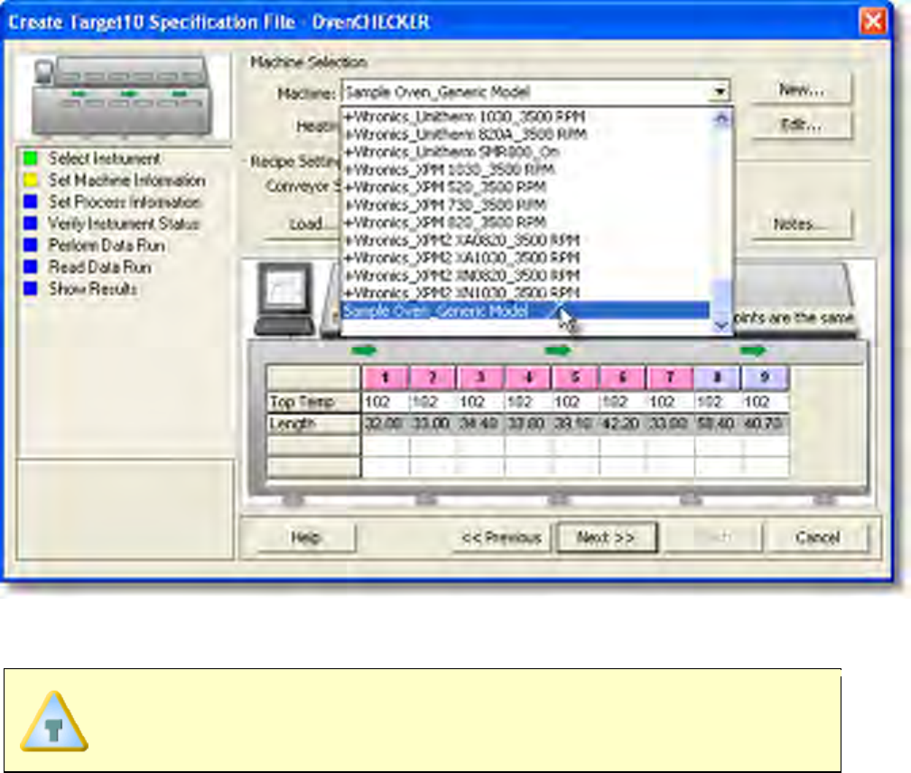
7) Set the machine recipe settings such as Conveyor Speed, Zone Temperatures
and Temperature units.
The software includes features to save and load machine recipe setting files.
These files are helpful to quickly load machine information and to ensure they
are always the same.
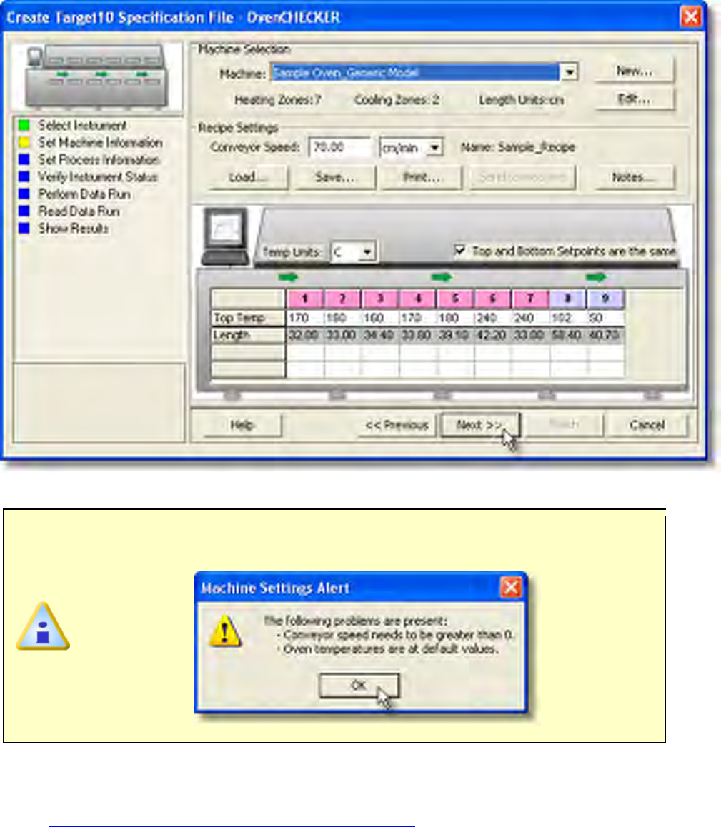
8) Click the Next command button.
If no value is specified for the conveyor speed or the default oven temperature
values, the software will remind the user to set them.
9) Select your process specification by selecting a Paste from the database or
previously created Target 10 Specification. If your Paste does not appear in the
database list click the New command button to create a new one. Refer to topic
Software>Menus>Process>Create new Paste for more information.
The OvenCHECKER™ uses the begin temp, end temp and liquidous temp to
measure the initial slope, soak, TAL (time above liquidous), peak parameters from
the selected Paste or Target 10 Specification. Then based on the range of the
parameters taken from the 3 OvenCHECKER™ sensors, automatically calculates
the USL (Upper Specification Limits) and LSL (Lower Specification Limits).
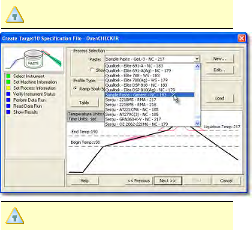
When the user selects a paste from the database, they can use the radio
buttons below the drop down box to filter and display only the user created
pastes from paste database.
If the user decides to use a previously created Target 10 Specification,
selecting the Load command button displays a list of Target 10
Specification Files (*.T10).
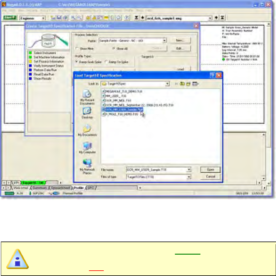
10) After selecting a process specification, click the Next command button.
11) Verify the instrument status. This dialog box displays the health of the
V-M.O.L.E.® Profiler such as battery charge, internal temperature, thermocouple
temperatures.
If everything is OK, the dialog box displays a GREEN sign. If there are any
items that may prevent the user from collecting good data, they are
highlighted and a RED sign is displayed.
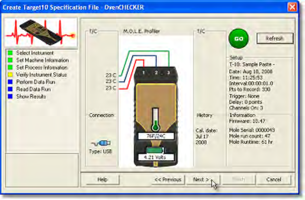
12) Click the Next command button.
13) Review the machine settings and click the Next command button to continue.
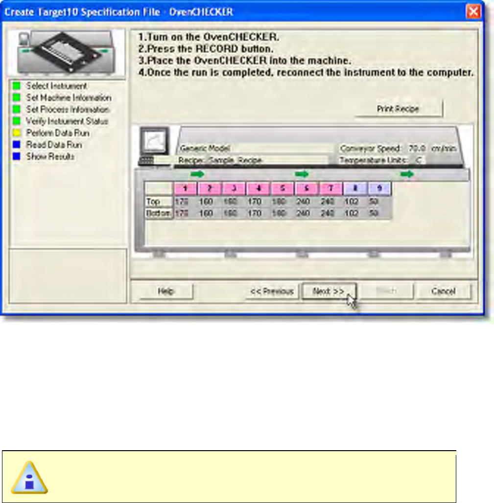
14) After the oven stabilizes, turn the V-M.O.L.E.® Profiler on and press the record
button.
15) Pass the OvenCHECKER™ through the machine.
16) Once the OvenCHECKER™ has been retrieved from the machine and the
V-M.O.L.E.® Profiler has been stopped, disconnect the V-M.O.L.E.® Profiler from
the OvenCHECKER™ and place it near the computer. Since you are creating a
new Target 10 Specification, the OK button on the V-M.O.L.E.® does not need to
be pressed at this time as contains an old Target 10 Specification.
If the V-M.O.L.E.® Profiler already contains an previously recorded
OvenCHECKER™ data run, a new data run does not need to be performed.
17) Select the desired OvenCHECKER™ data run and then click the Read command
button to read the data run from the V-M.O.L.E.® Profiler.
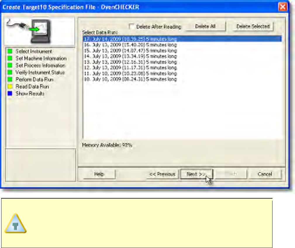
This step of the wizard allows the user to remove a selected data run from the
M.O.L.E. Profiler by either selecting the Delete After Reading check box or
selecting the Delete command button and removing it before downloading.
This feature is not available for the SuperM.O.L.E.® Gold Thermal Profiler as it
does not have the ability to store more than one data run.
18) Once the OvenCHECKER™ data run is downloaded, review the calculated results
of the Target 10 specification. The user can then decide if they wish to accept
these or make final modifications to the Slope, Soak, Time Above and/or Peak
parameter.
If the user decides to make modifications, click the Modify Target10 command
button and the the Target 10-OK tab is displayed. Make the desired
modifications to the Slope, Soak, Time Above and/or Peak parameter
specifications. If any of the parameter specifications are changed the OK
button will inform the user by displaying (OKModified).
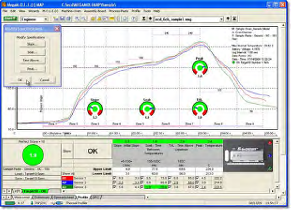
19) Click the OK command button on the Modify Specifications pallet to accept the
specifications or Cancel to discard them and return to the workflow wizard.
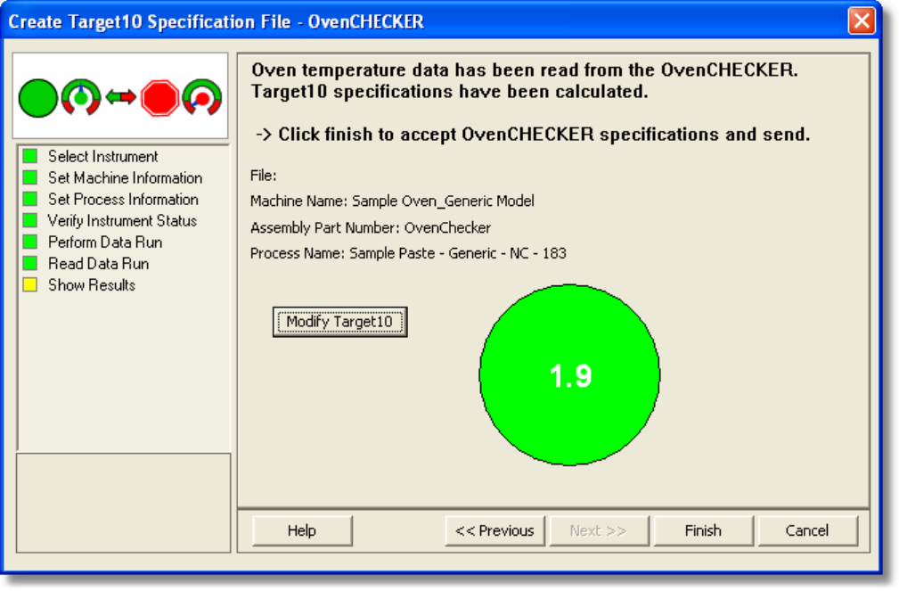
20) Click the Finish command button and the software prompts the user to save the
Target 10 Specification file (*.T10).
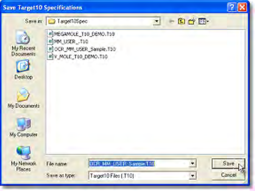
21) When finished naming the file, click the Save command button to complete the
workflow wizard. This step saves both the Target 10 Specification file (*.T10) and
the downloaded data run (.XMG) and is displayed on the Target10-OK tab.
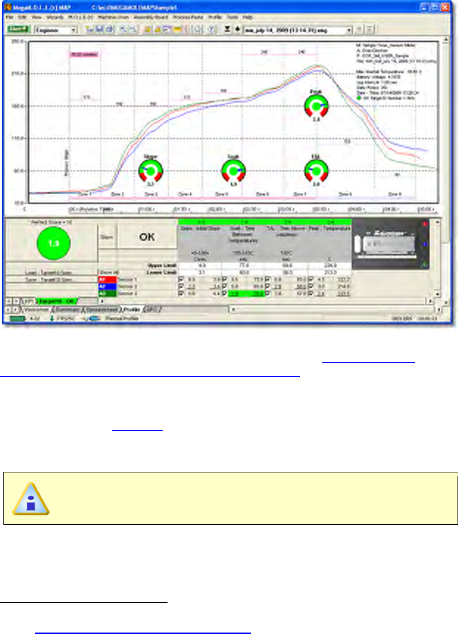
This OvenCHECKER™ Target 10 Specification can now be used to verify that your
machine performance is the same in the future. Refer to topic Menus and Tool
Commands>File Menu>Wizards Menu>Verify Process for more information.
5.5.4.5. Download Data
The Download Data workflow is a wizard that starts a new profile (data run) by
downloading a file from the M.O.L.E. Profiler. Once the data run is downloaded, the user
can then choose to apply Machine (Oven), Assembly (Board) and Process (Paste)
information.
This is available in both Engineer & Verify Modes.
5.5.4.5.1. Workflow
The Download Data workflow:
1) Connect the M.O.L.E. Profiler to the computer. Refer to
Basics>Setup>Communications Setup for more information.
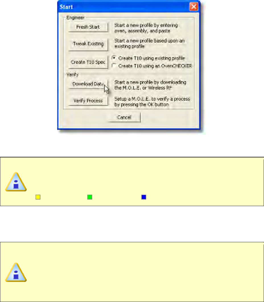
2) On the File menu, click New. A message box appears with the five workflow
wizard options.
3) On the Start dialog box, click the Download Data command button and the
workflow wizard appears.
When navigating through the wizard, the step list on the left uses a color key
to inform the user of the current step, steps that have been completed and
remaining steps.
Current Completed Remaining
4) Select the desired instrument from the dialog box to make active. If a M.O.L.E.
Profiler has already been selected during a different process, the software
automatically selects the M.O.L.E. Profiler connected to the COM port previously
used.
If the software does not detect a M.O.L.E. Profiler, using the communication
cable connect it to the computer and click the Scan for Instruments
command button to search again. M.O.L.E.® MAP software allows multiple
instruments to be connected to a computer at one time. Selecting the Scan for
Instruments command button will detect all instruments and display them in
the dialog box. If no instrument is detected the software displays all of the
Demonstration thermal profilers to select from.
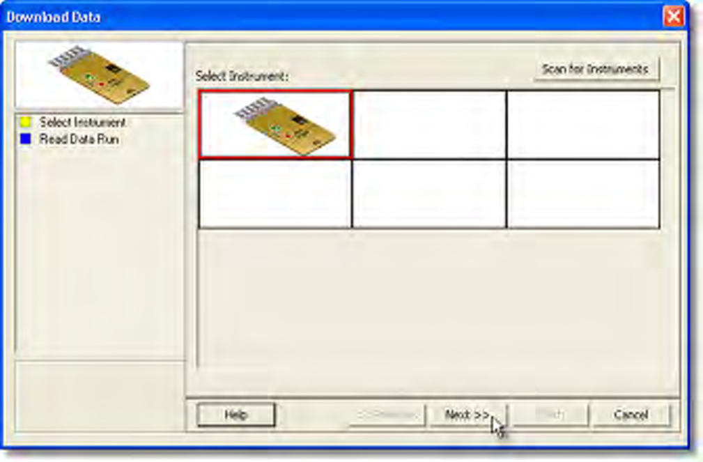
5) Click the Next command button.
6) Select the desired data run and then click the Finish command button to complete
the wizard and read the data run from the M.O.L.E. Profiler.
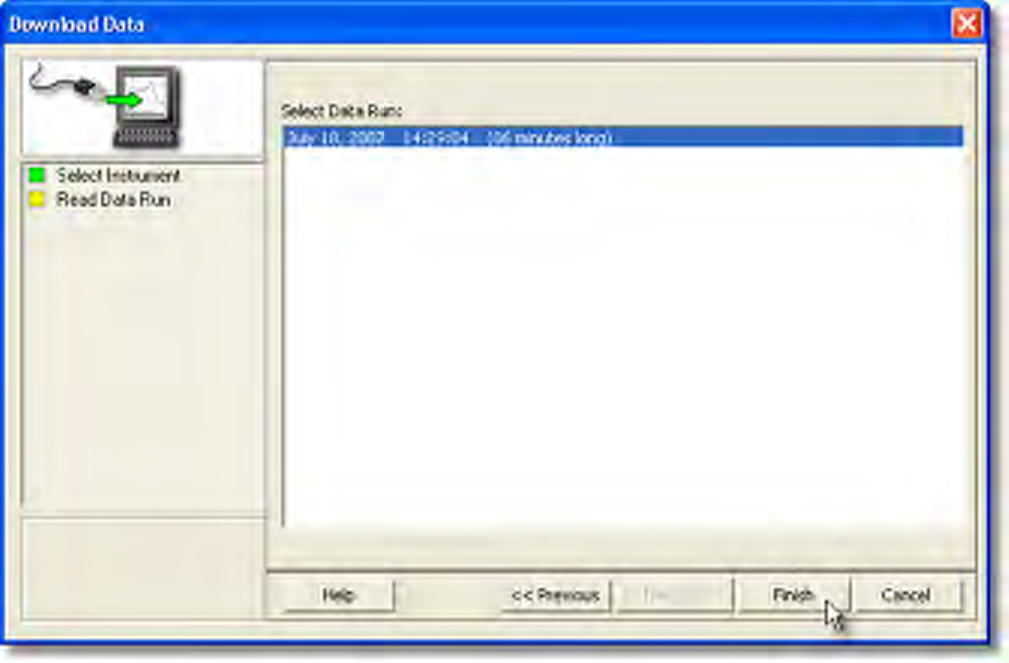
• Prior to reading the data run, the software prompts the user to select the sensor
type for the active channels. When finished select the OK command button to
proceed.
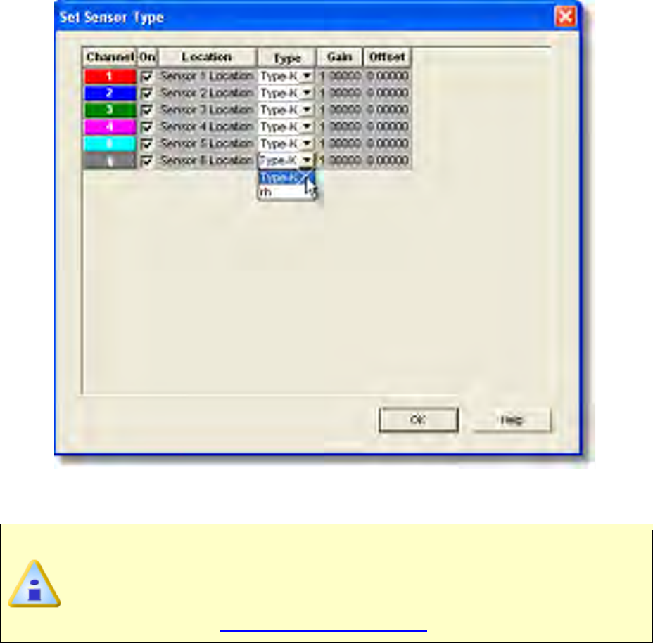
8) When the data run has been downloaded, the software prompts the user to specify
a file name (*.XMG).
When saving a data run (*.XMG) to a different file directory other than the
current Working directory, the software automatically sets the new file
directory as the current Working Directory. This process does not delete any
data run files in the previously set Working directory and can be quickly
accessed using the Recent Working Directory command on the File menu.
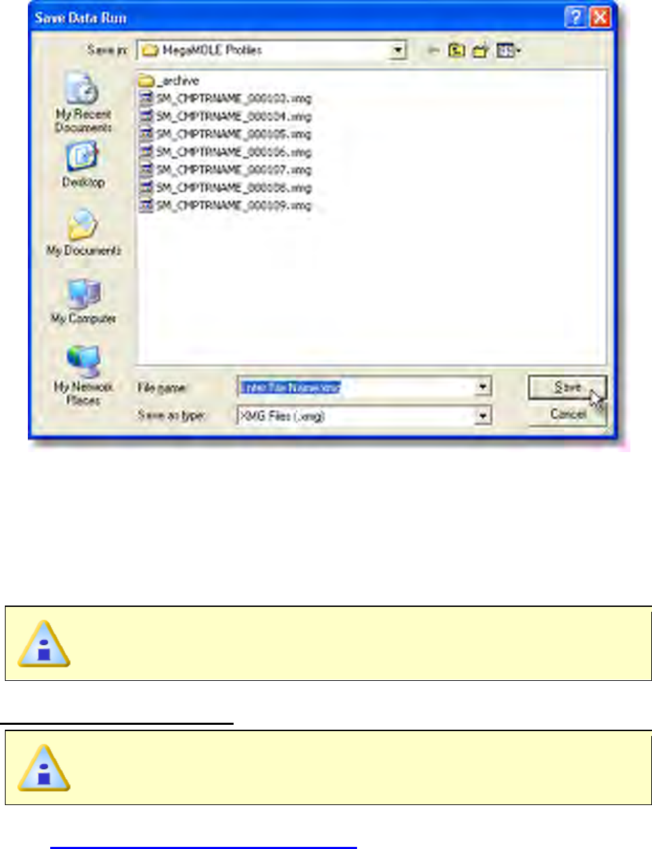
I
9) When finished, click the Save command button to complete the process.
5.5.4.6. Verify Process
The Verify Process workflow is a wizard that configures a M.O.L.E. Profiler or
OvenCHECKER™ to verify a process or machine performance using a Target 10
Specification file (*.T10).
This is available in both Engineer & Verify Modes.
The Verify Process workflow:
The verify process can only be performed using a MEGAM.O.L.E.® or
V-M.O.L.E.® Profiler.
1) Connect the M.O.L.E. Profiler to the computer. Refer to
Basics>Setup>Communications Setup for more information.
2) On the File menu, click New. The Start dialog box appears with the five workflow
wizard options.
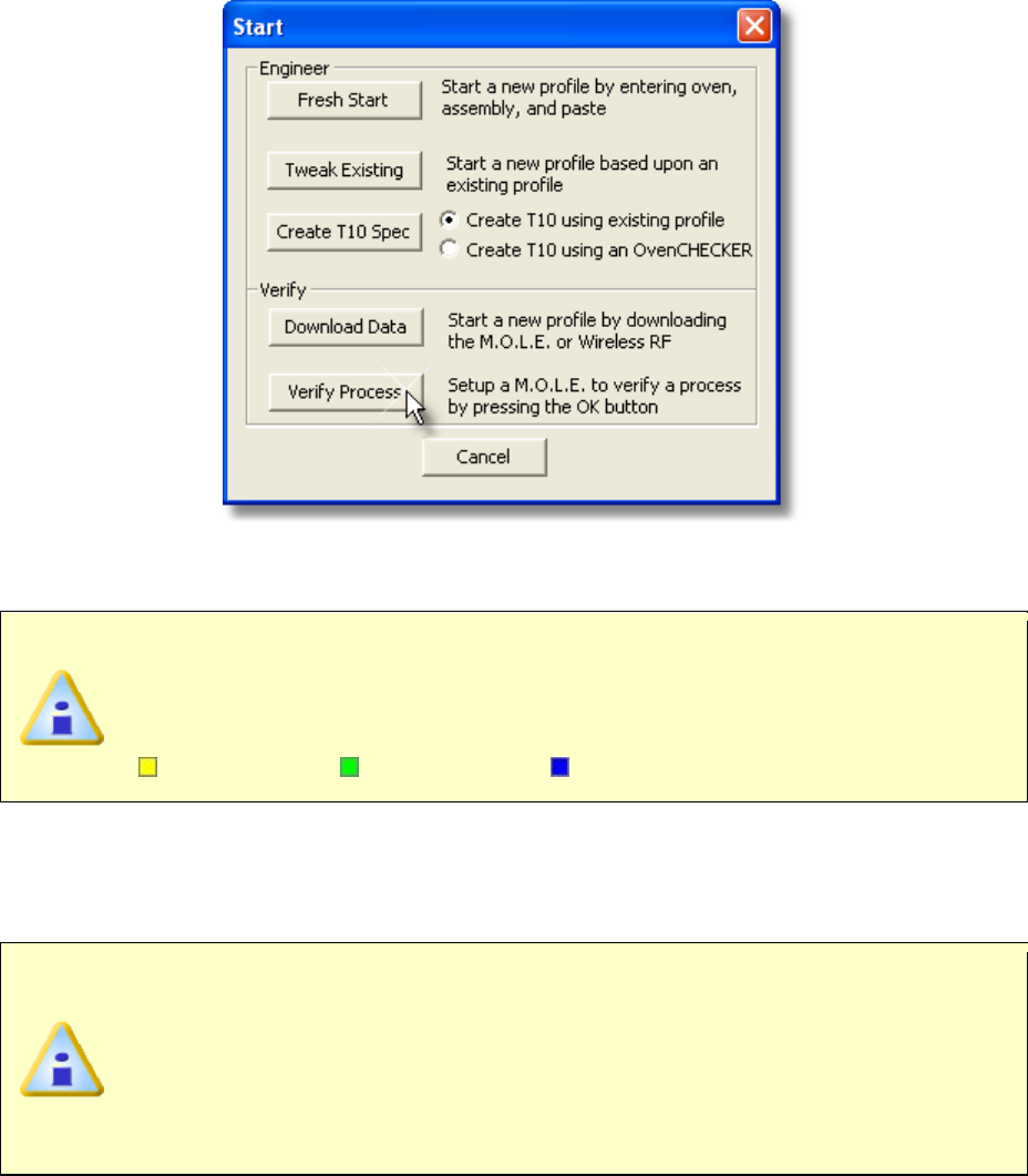
3) On the Start dialog box, click the Verify Process command button and the
workflow wizard appears.
When
navigating through the wizard, the step list on the left uses a color key
to inform the user of the current step, steps that have been completed and
remaining steps.
Current
Completed
Remaining
4) Select the desired instrument from the dialog box to choose the M.O.L.E. Profiler.
If a M.O.L.E. Profiler has already been selected during a different process, the
software automatically selects the M.O.L.E. Profiler connected to the COM port
previously used.
If the software does not detect a M.O.L.E. Profiler, using the communication
cable connect it to the computer and click the Scan for Instruments
command button to search again. M.O.L.E.® MAP software allows multiple
instruments to be connected to a computer at one time. Selecting the Scan for
Instruments command button will detect all instruments and display them in
the dialog box. If no instrument is detected the software displays all of the
Demonstration thermal profilers to select from.
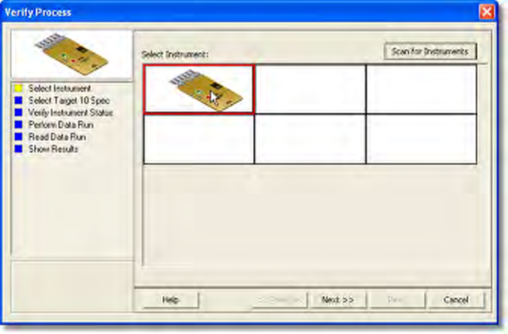
5) Click the Next command button.
6) Select a Target 10 file from the list to verify. When placing the mouse cursor over a
file on the list, a thumbnail image appears to help properly identify the assembly
associated with it.
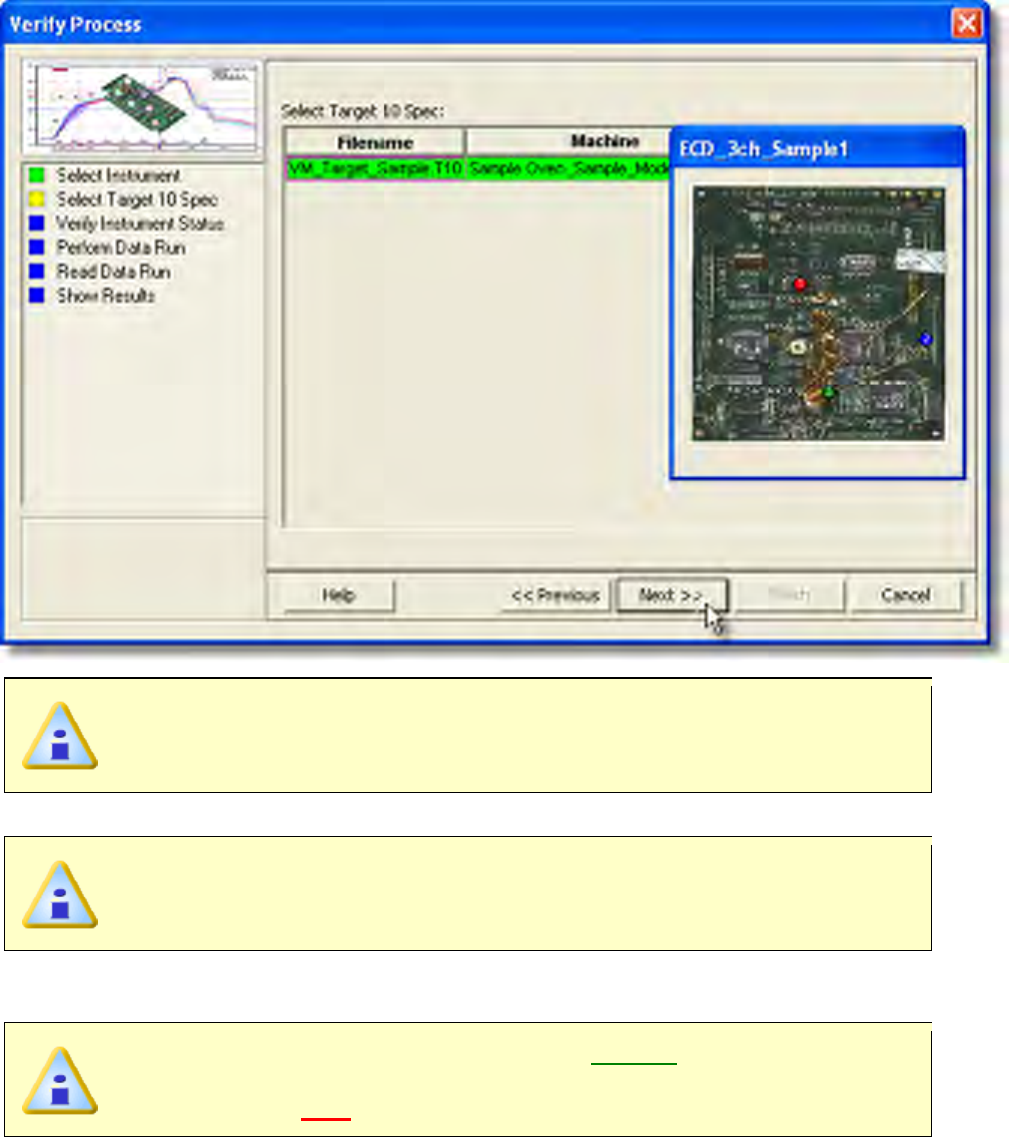
When selecting a Target 10 file to verify, the software displays files located in
the \ECD\MegaMoleMAP\Target10Spec\ directory that are associated with
the currently selected instrument.
7) Click the Next command button.
When selecting a Target 10 file, the software extracts the MAP data from it
and sends it to the M.O.L.E. Profiler. The process will overwrite any
configurations and Target 10 specs currently stored in the M.O.L.E. Profiler.
8) Verify the instrument status. This dialog box displays the health of the M.O.L.E.
Profiler such as battery charge, internal temperature, thermocouple temperatures.
If everything is OK, the dialog box displays a GREEN sign. If there are any
items that may prevent the user from collecting good data, they are
highlighted and a RED sign is displayed.
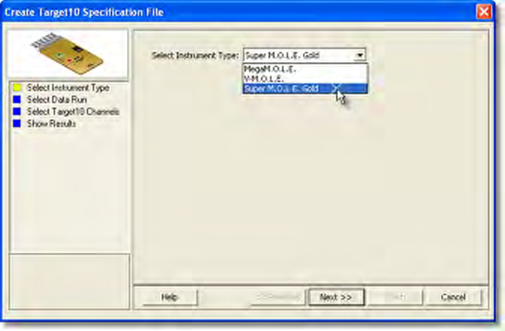
9) Click the Next command button.
10) Review the machine settings and click the Next command button to continue.
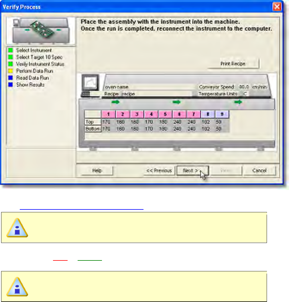
11) Pass M.O.L.E. Profiler and test product through the process. Refer to topic
Basics>Verify>Step 2 - Verify Process for more information.
If the selected M.O.L.E. Profiler is wireless RF, click the Next command
button to proceed to the Step 14.
12) Press the OK button on the M.O.L.E. Profiler and wait for the GO or NO-GO
indication (RED or GREEN). By pressing the OK button, the M.O.L.E. Profiler
analyzes the most recent data run to verify the Target 10 Specifications.
Only the MEGAM.O.L.E.® and V-M.O.L.E.® are equipped with the OK button.
When using the SuperM.O.L.E.® Gold please skip the previous step.
13) Connect the M.O.L.E. Profiler to the computer and click the Next command button.
14) Select the desired data run and then click the Next command button to read the
data run from the M.O.L.E. Profiler.
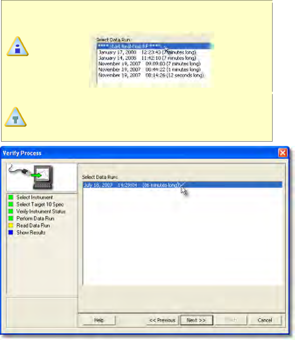
If the user has selected to use a Wireless RF option, select Start real-time
RF on the top of the data run list and then the Finish command button to
display the RF Control dialog.
This step of the wizard allows the user to remove a selected data run from the
M.O.L.E. Profiler by either selecting the Delete After Reading check box or
selecting the Delete command button and removing it before downloading.
This feature is not available for the SuperM.O.L.E.® Gold Thermal Profiler as it
does not have the ability to store more than one data run.
• Prior to reading the data run, the software prompts the user to select the sensor
type for the active channels. When finished select the OK command button to
proceed.

15) When the data run has been downloaded, the software prompts the user to save
the verification data run file (.XMG).
When saving a data run (*.XMG) to a different file directory other than the
current Working directory, the software automatically sets the new file
directory as the current Working Directory. This process does not delete any
data run files in the previously set Working directory and can be quickly
accessed using the Recent Working Directory command on the File menu.
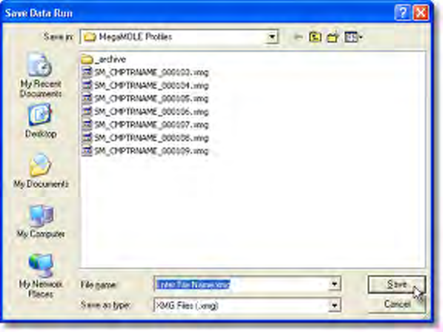
I
16) Once the file is saved, the software returns to the workflow wizard and displays the
Target 10-OK results.
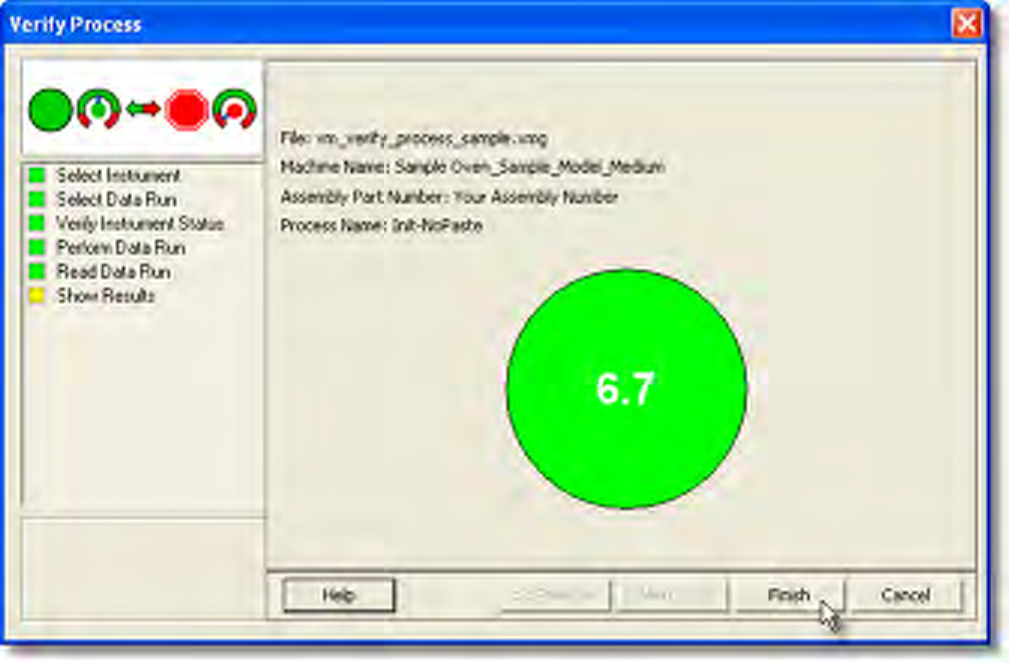
17)Analyze the data by selecting the Target10-OK tab on the Profile Tab.
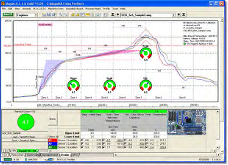
5.5.5. M.O.L.E. Menu
The M.O.L.E. menu commands configure a M.O.L.E. Profiler for collecting process data.
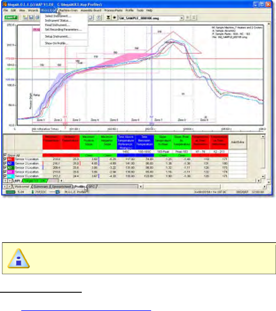
5.5.5.1. Select Instrument
The Select Instrument command allows the user to select an available M.O.L.E. Profiler
to make active so it can interface with the software.
This is available in both Engineer & Verify Modes.
To select an instrument:
1) Connect the M.O.L.E. Profiler to the computer. Refer to
Basics>Setup>Communications Setup for more information.
2) On the M.O.L.E. menu, click the Select Instrument command.
3) Select the desired instrument from the dialog box. If there are none displayed, click
the Scan for Instruments command button to detect all available instruments.
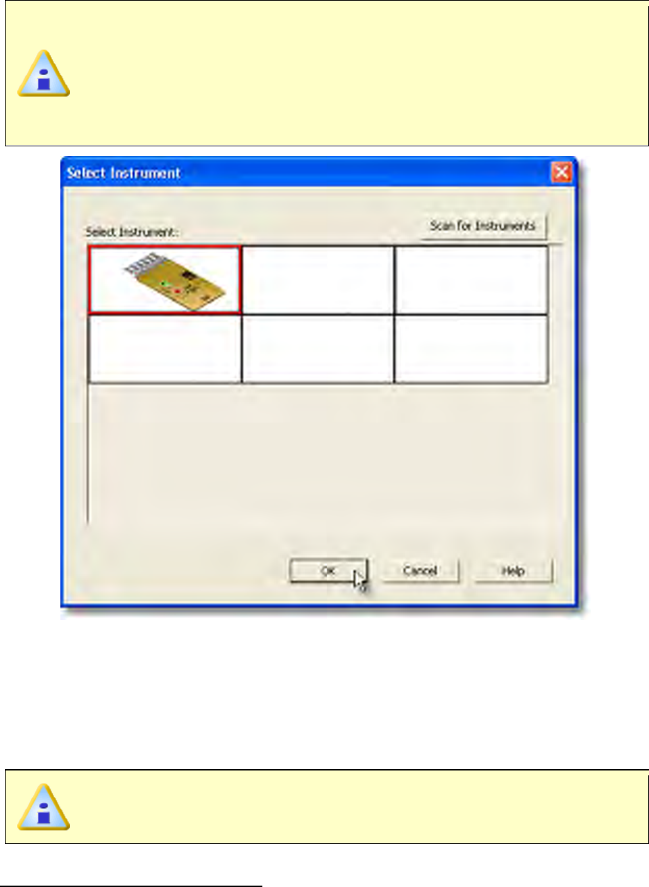
If the software does not detect a M.O.L.E. Profiler, using the communication
cable connect it to the computer and click the Scan for Instruments
command button to search again. M.O.L.E.® MAP software allows multiple
instruments to be connected to a computer at one time. Selecting the Scan for
Instruments command button will detect all instruments and display them in
the dialog box. If no instrument is detected the software displays all of the
Demonstration thermal profilers to select from.
4) Click the OK command button to accept or Cancel to quit the command.
5.5.5.2. Instrument Status
This command displays the health of the M.O.L.E. Profiler such as battery charge,
internal temperature, thermocouple temperatures. This command also allows the user to
display items that will prevent the user from completing a successful data run.
This is available in both Engineer & Verify Modes.
To display the instrument status:
1) On the M.O.L.E. menu, click Instrument Status and the dialog box appears.
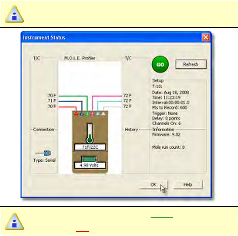
If an instrument is not currently connected to the computer, the default
Demonstration MEGAM.O.L.E.® profiler will be displayed.
If everything is OK, the dialog box displays a GREEN sign. If there are any
items that may prevent the user from collecting good data, they are
highlighted and a RED sign is displayed.
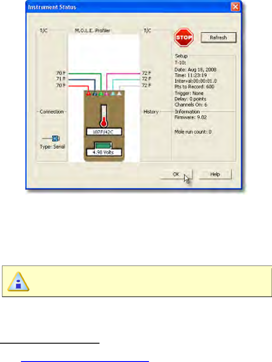
2) Click the OK command button to close the dialog box.
5.5.5.3. Read Instrument
The Download Data workflow is a wizard that downloads a recorded thermal profile (data
run) from the M.O.L.E. Profiler or starts logging wireless real-time data. Once the data run
is downloaded, the user can then choose to apply Machine (Oven), Assembly (Board)
and Process (Paste) information.
This is available in both Engineer & Verify Modes.
5.5.5.3.1. USB Communication
The Download Data workflow:
1) Connect the M.O.L.E. Profiler to the computer. Refer to
Basics>Setup>Communications Setup for more information.
2) On the M.O.L.E. menu, click Read Instrument.
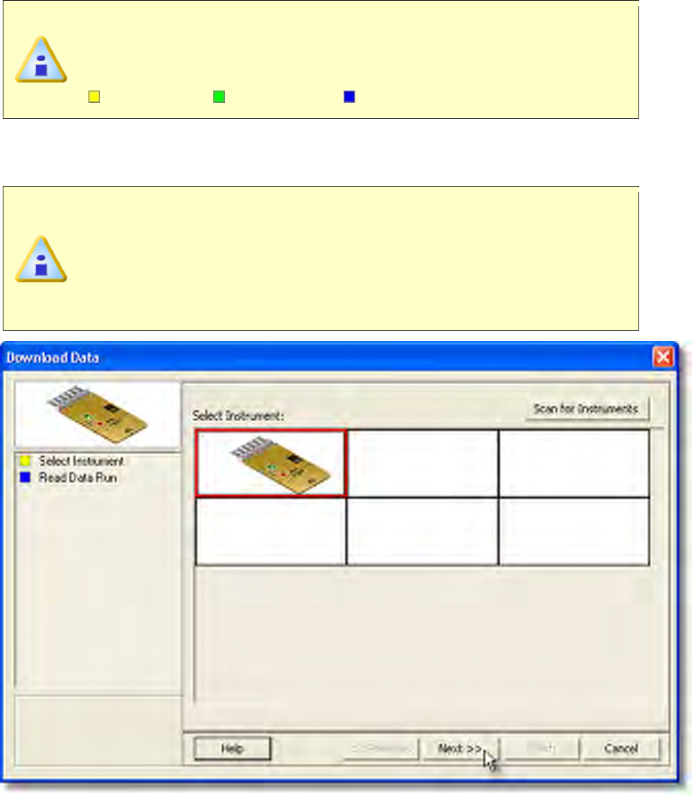
When navigating through the wizard, the step list on the left uses a color key
to inform the user of the current step, steps that have been completed and
remaining steps.
Current Completed Remaining
3) Select the desired instrument from the dialog box to make active. If there are none
displayed, click the Scan for Instruments command button to detect all available
instruments.
If the software does not detect a M.O.L.E. Profiler, using the communication
cable connect it to the computer and click the Scan for Instruments
command button to search again. M.O.L.E.® MAP software allows multiple
instruments to be connected to a computer at one time. Selecting the Scan for
Instruments command button will detect all instruments and display them in
the dialog box. If no instrument is detected the software displays all of the
Demonstration thermal profilers to select from.
4) Click the Next command button.
5) Select the desired data run and then click the Finish command button to complete
the wizard and read the data run from the M.O.L.E. Profiler.
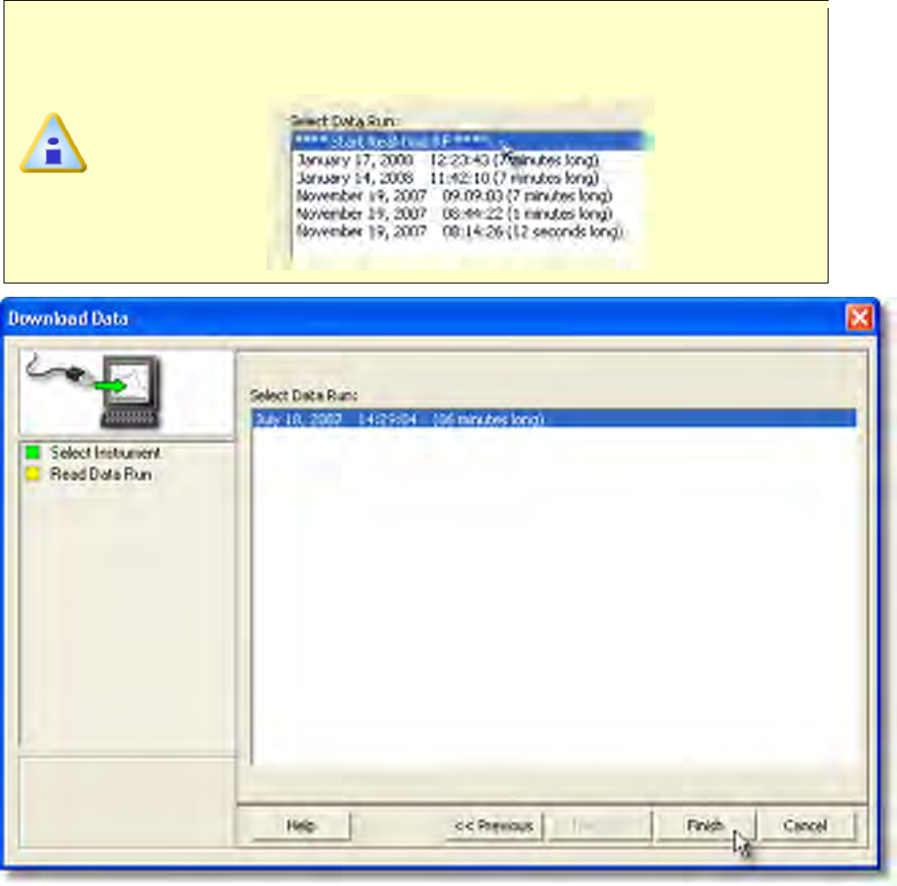
If the user has selected to use a Wireless RF option, select Start real-time
RF on the top of the data run list and then the Finish command button to
display the RF Control dialog.
• Prior to reading the data run, the software prompts the user to select the sensor
type for the active channels. When finished select the OK command button to
proceed.
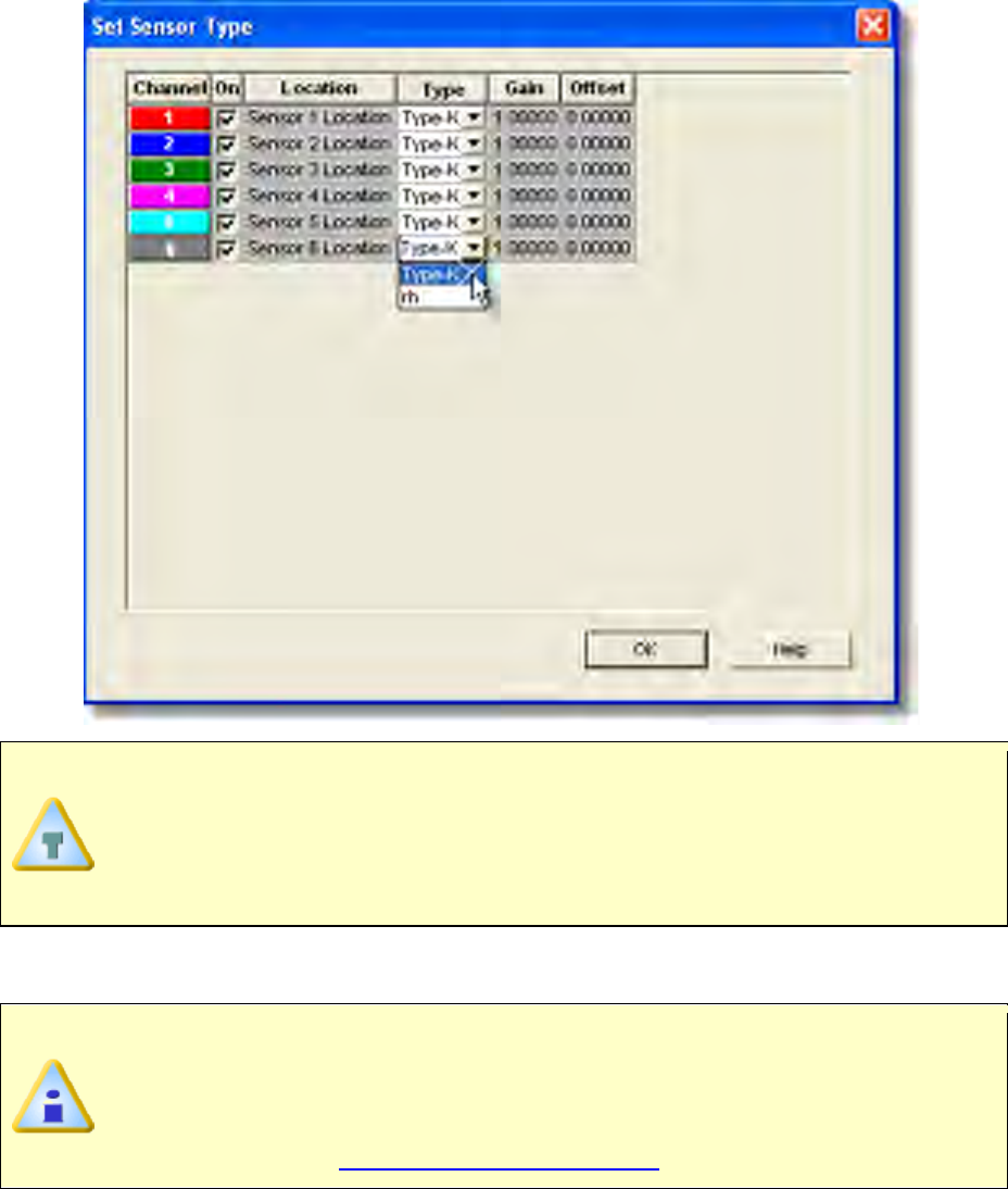
This step of the wizard allows the user to remove a selected data run from the
M.O.L.E. Profiler by either selecting the Delete After Reading check box or
selecting the Delete command button and removing it before downloading.
This feature is not available for the SuperM.O.L.E.® Gold Thermal Profiler as it
does not have the ability to store more than one data run.
6) When the data run has been downloaded, the software prompts the user to specify
a file name (*.XMG).
When saving a data run (*.XMG) to a different file directory other than the
current Working directory, the software automatically sets the new file
directory as the current Working Directory. This process does not delete any
data run files in the previously set Working directory and can be quickly
accessed using the Recent Working Directory command on the File menu.
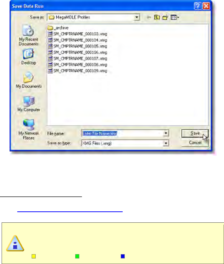
I
7) When finished, click the Save command button to complete the process.
5.5.5.3.2. Wireless RF Communication
The Download Data workflow:
1) Connect the M.O.L.E. Profiler to the computer. Refer to
Basics>Setup>Communications Setup for more information.
2) On the M.O.L.E. menu, click Read Instrument.
When navigating through the wizard, the step list on the left uses a color key
to inform the user of the current step, steps that have been completed and
remaining steps.
Current Completed Remaining
3) Select the desired instrument from the dialog box to make active. If a M.O.L.E.
Profiler has already been selected during a different process, the software
automatically selects the M.O.L.E. Profiler connected to the COM Port previously
used.
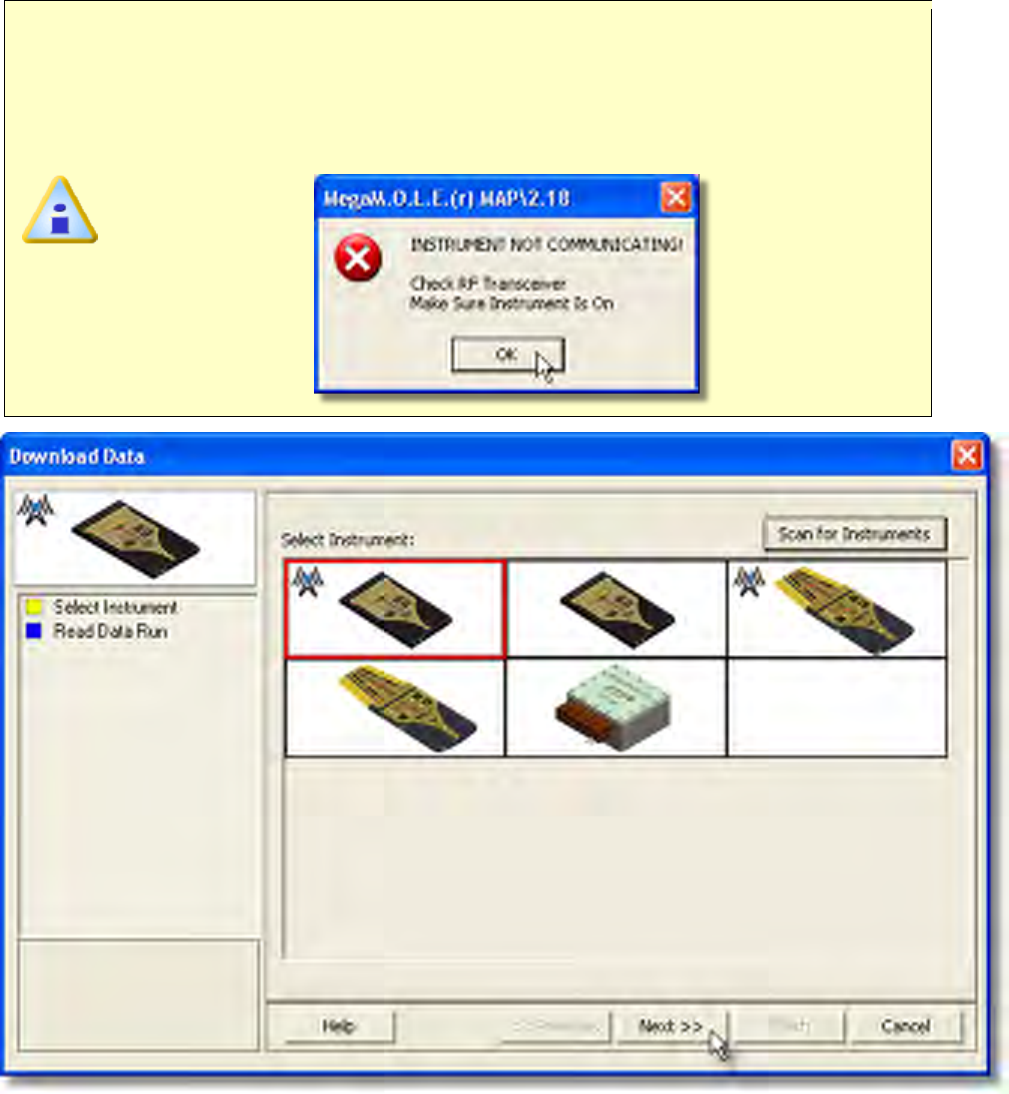
If the software does not detect a M.O.L.E. Profiler, make sure it is ON and/or
connected to the computer and click the Scan for Instruments command
button to search. M.O.L.E.® MAP software allows multiple instruments to be
connected to a computer at one time. Selecting the Scan for Instruments
command button will detect all instruments and display them in the list. If no
instrument is detected, the software displays a warning message.
4) Click the Next command button.
5) Select Start Real-time RF on data run list then select the Finish command button
to complete the wizard and display the RF Control dialog box.
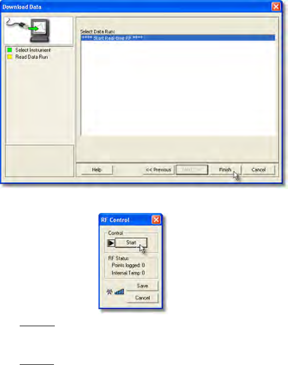
6) Once the RF Control dialog is displayed, it includes the following command
buttons and information:
Start/Stop:
• Starts logging real-time data and is displayed on the Data Graph.
• Once the Start command button is selected it automatically changes to a Stop
command button which Stops the M.O.L.E. Profiler logging real-time data.
RF Status:
• Points logged: Indicates number of data points received.