Electronic Controls Design E51-0386-40 Super MOLE® Gold 2 User Manual ECD M O L E MAP Users Help System 3 0 6
Electronic Controls Design Inc Super MOLE® Gold 2 ECD M O L E MAP Users Help System 3 0 6
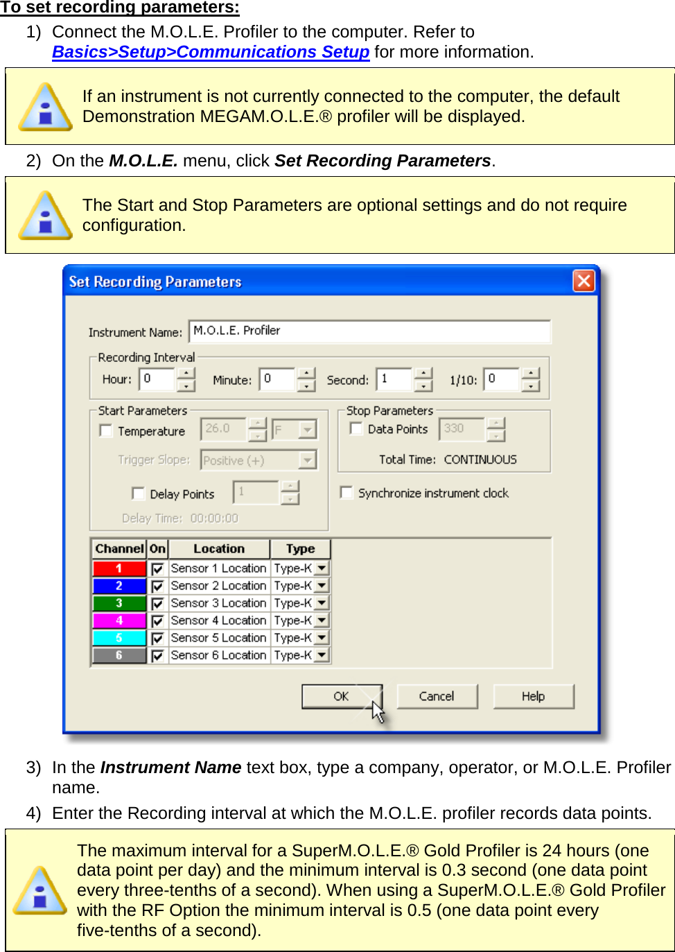
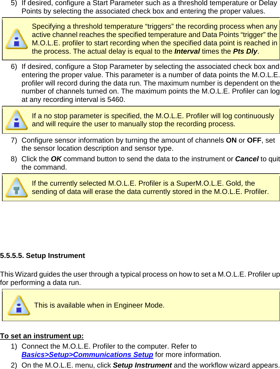
Contents
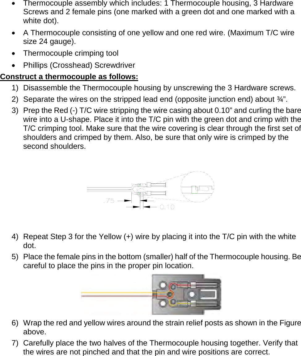
- 1. User Manual part 1 of 3
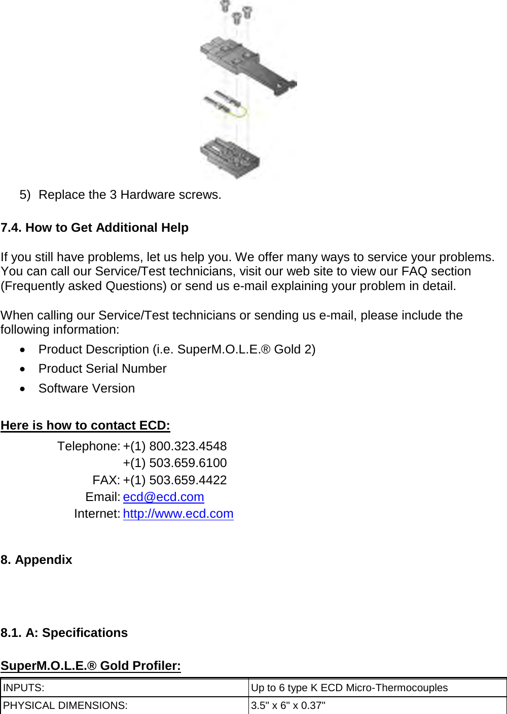
- 2. User Manual part 2 of 3
- 3. User Manual part 3 of 3
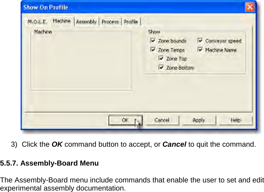
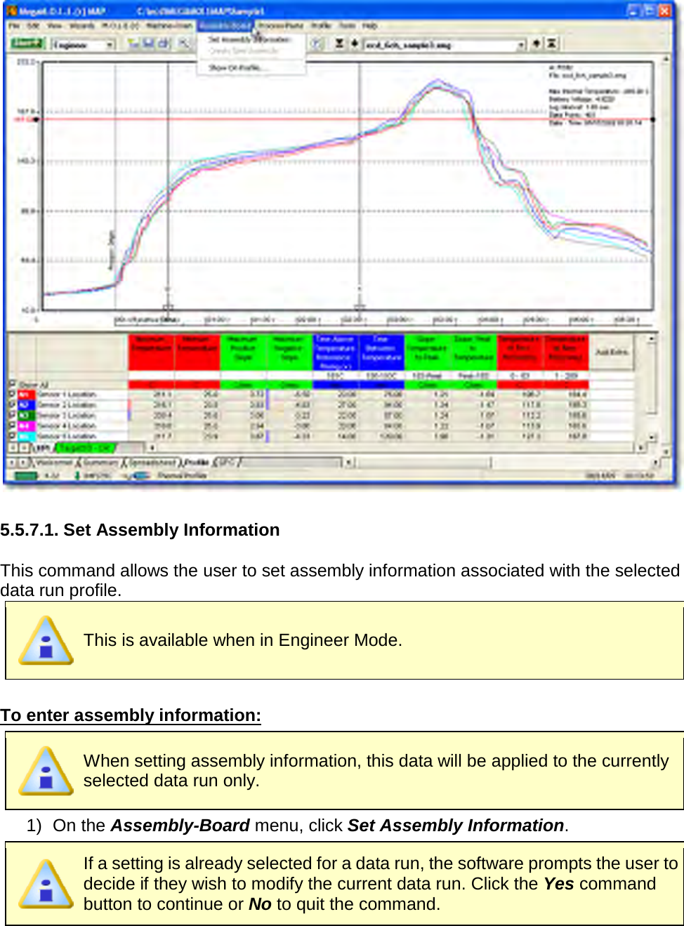
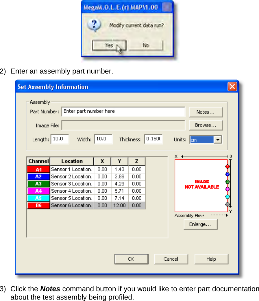
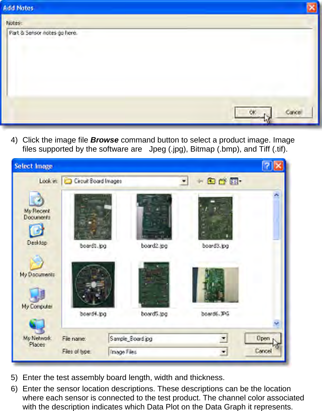
User Manual part 3 of 3
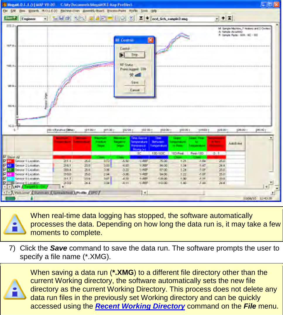
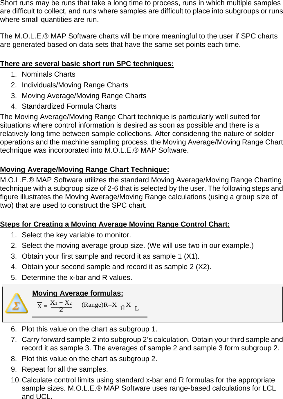
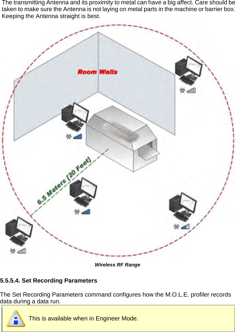
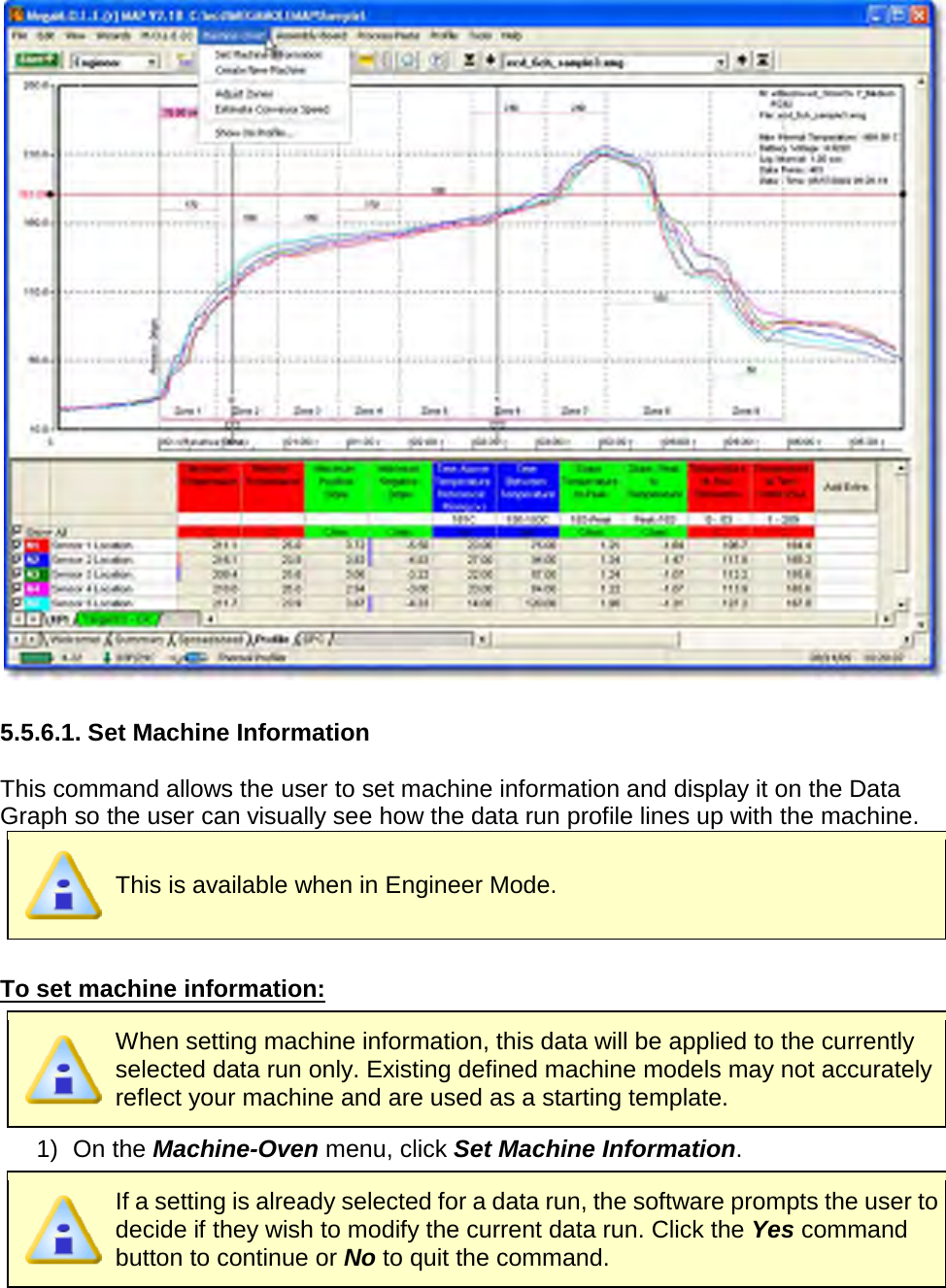
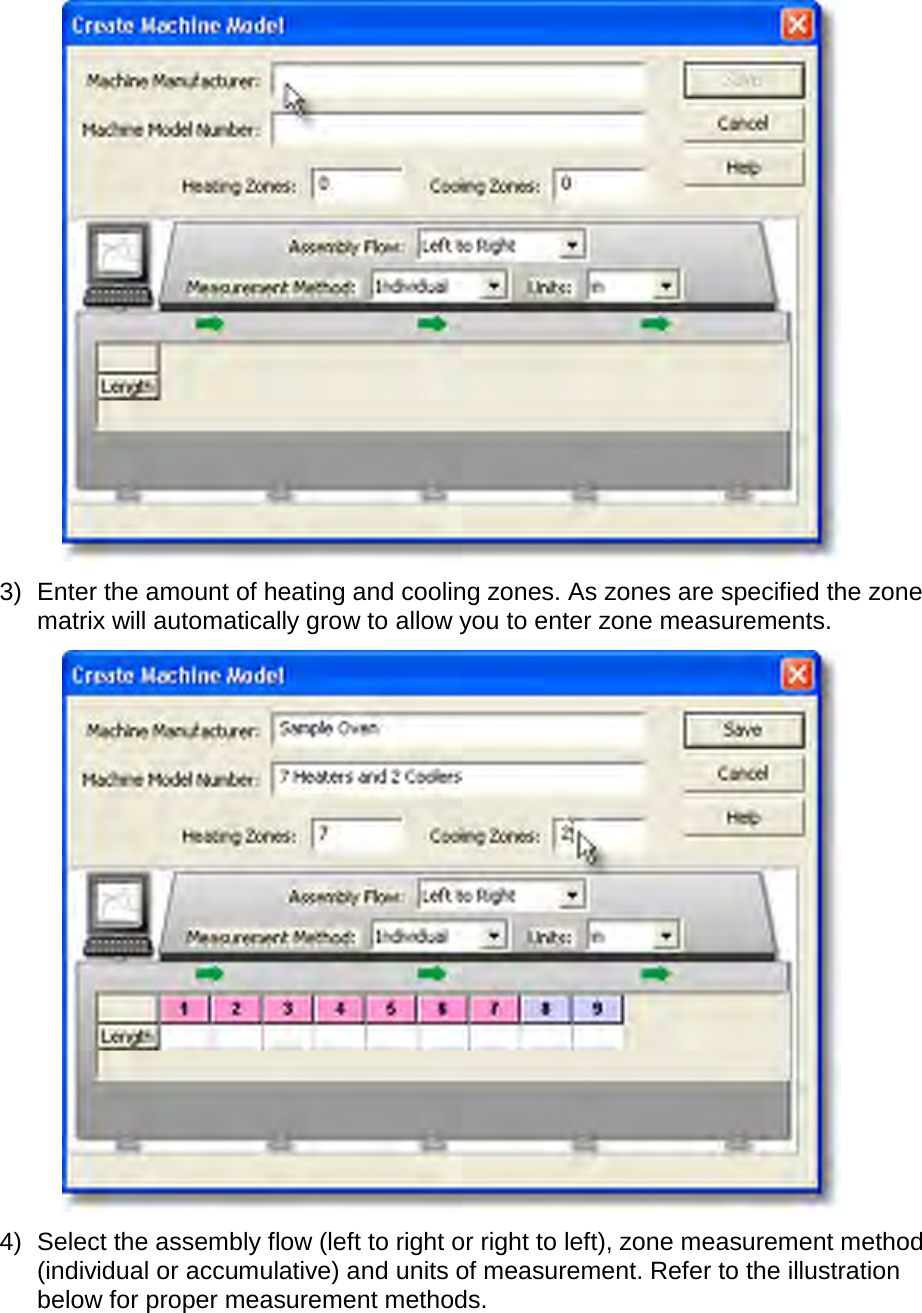
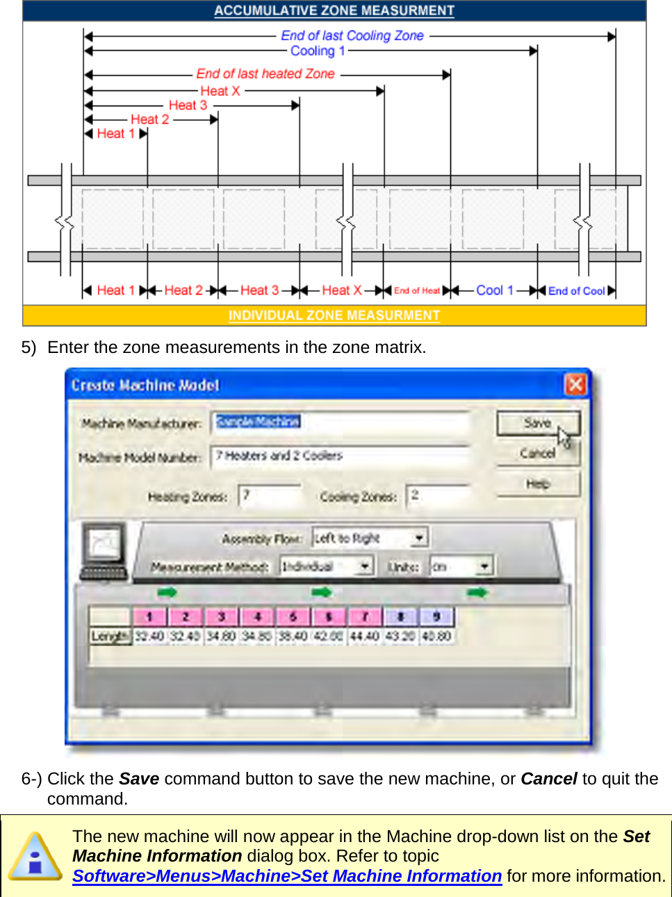
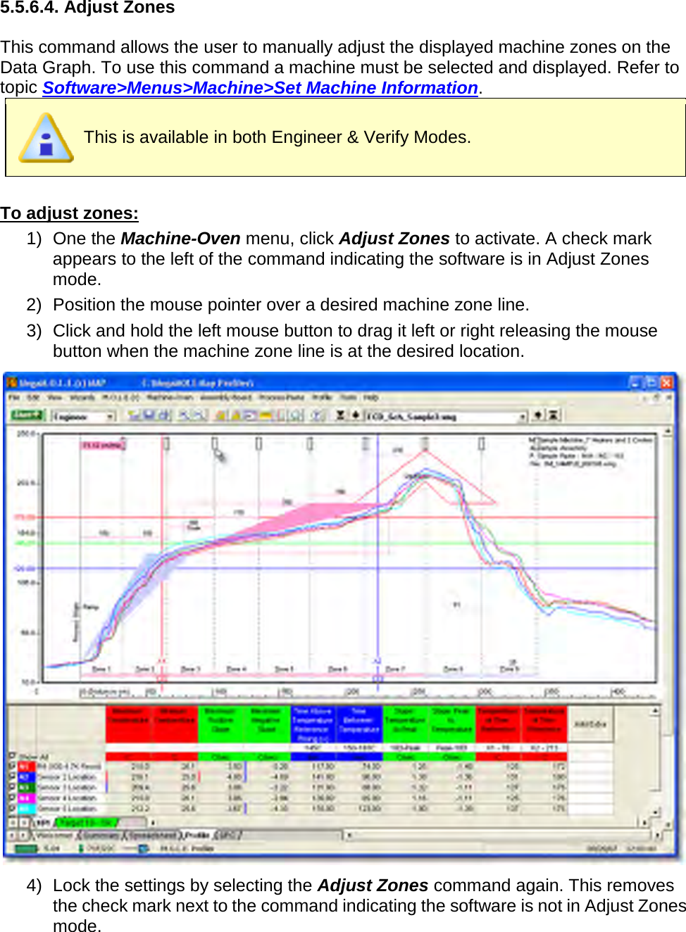
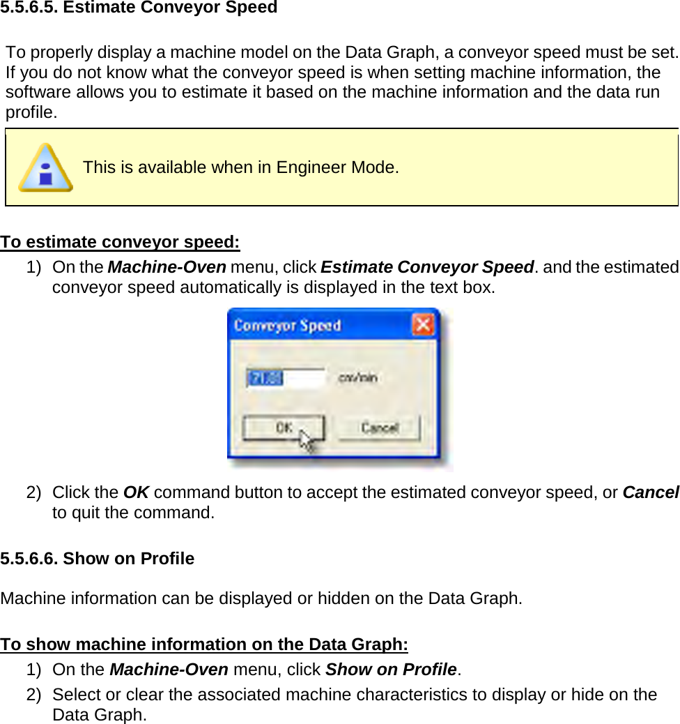
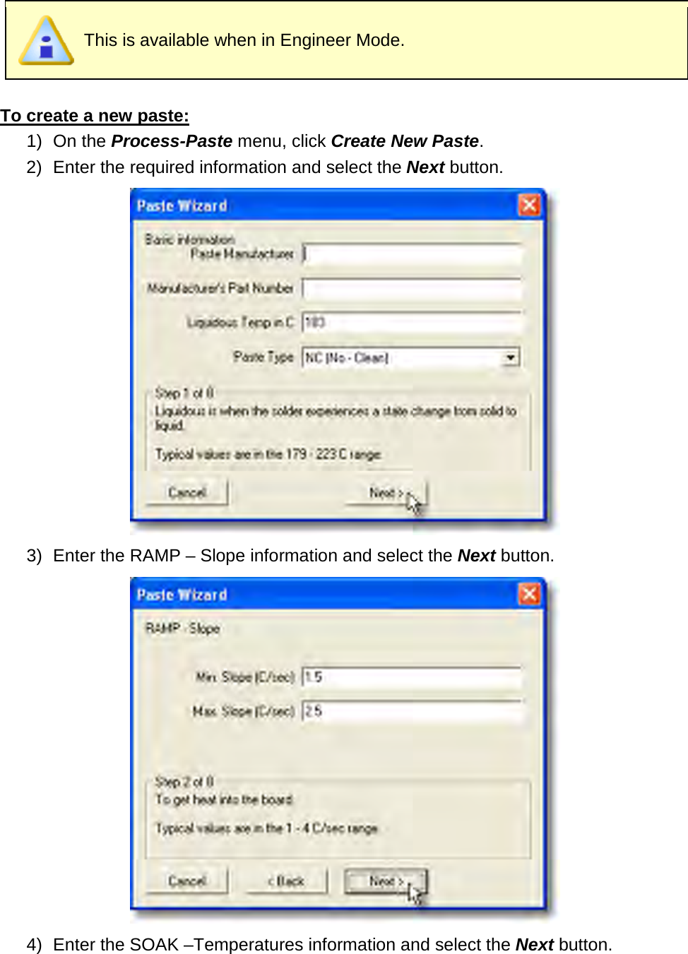
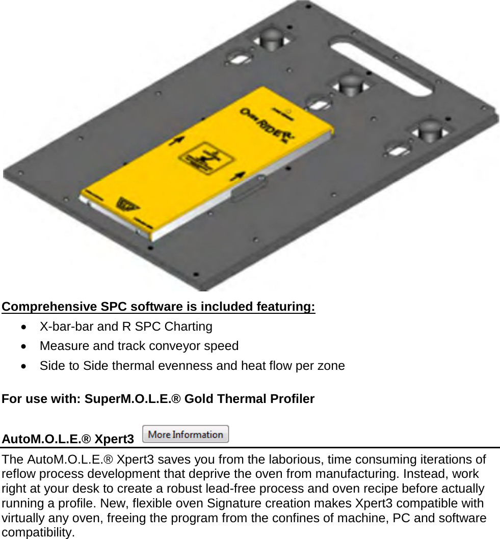
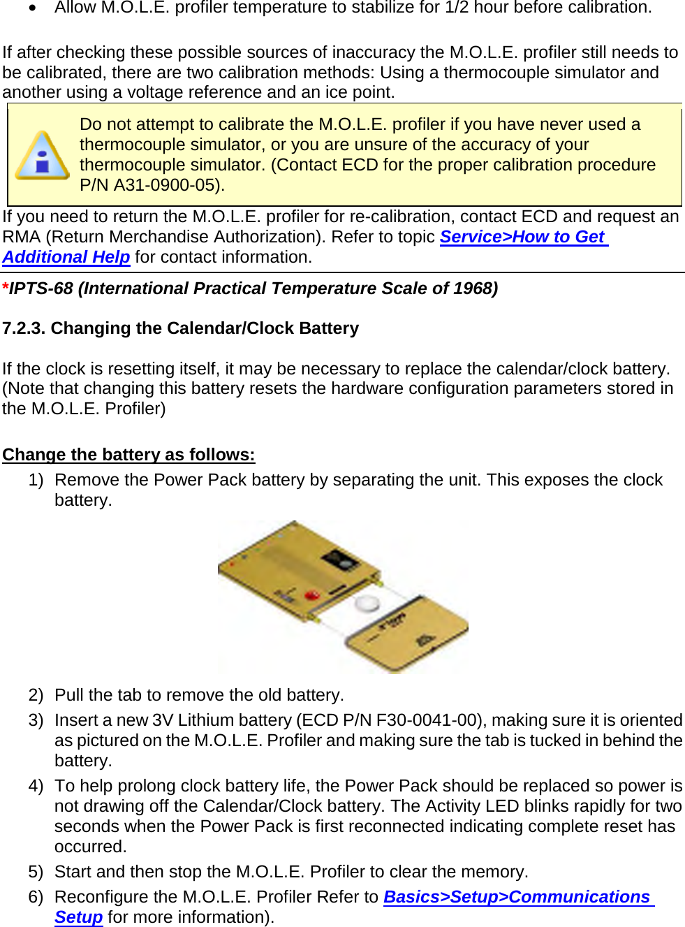
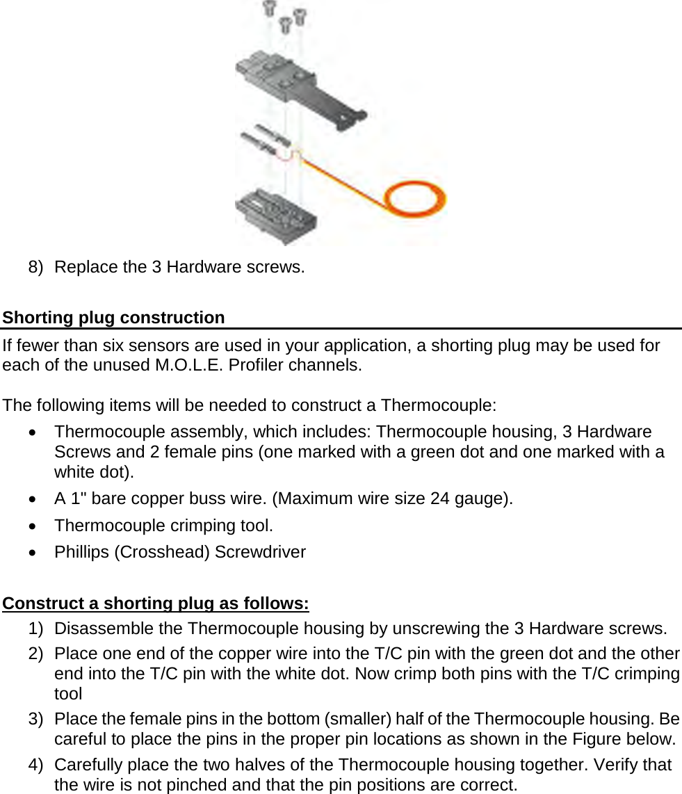
![8) When finished, click the Save command button to complete the process. When using the PTP® VP-8, the PTP® TX power must be turned OFF after saving the data run by removing the On/Off Male Plug connector from the Female On/Off Power connector. Wireless RF communication tips (MEGAM.O.L.E.® & SuperM.O.L.E.® Gold 2): RF signals come and go as either the M.O.L.E. Profiler moves through the oven or the Transceiver is moved around like FM radio static as you drive in your car. Moving a few inches in any direction can turn a low signal strength to high signal strength. This gets worse as the Transceiver gets further from the M.O.L.E. Profiler, to a point where no position works. When setting up the Wireless RF system, the transceiver should be placed as close to the machine as practical. A standard USB extension cable can be used to move the Transceiver closer to the machine or up and away from metal or other interference objects. Typically if the Transceiver is 3 meters [10 feet] away from the M.O.L.E. Profiler in a machine any location in the room, reception should be fine. Reception is also often a bit better when the Transceiver is perpendicular to the direction of travel through the machine. Metal objects such as carts, walls, or other equipment in the room will impede transmission.](https://usermanual.wiki/Electronic-Controls-Design/E51-0386-40.User-Manual-part-3-of-3/User-Guide-1481867-Page-3.png)
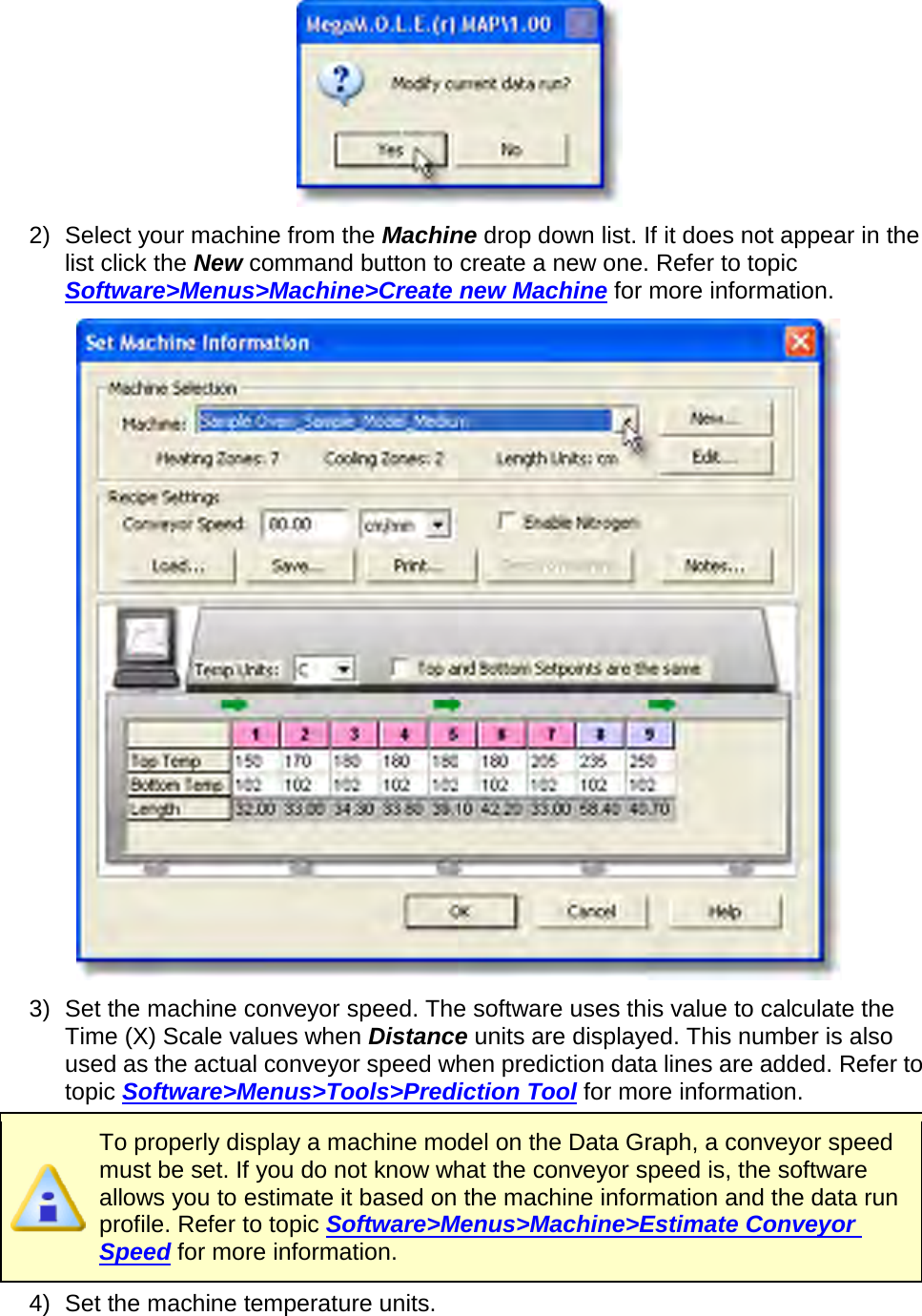
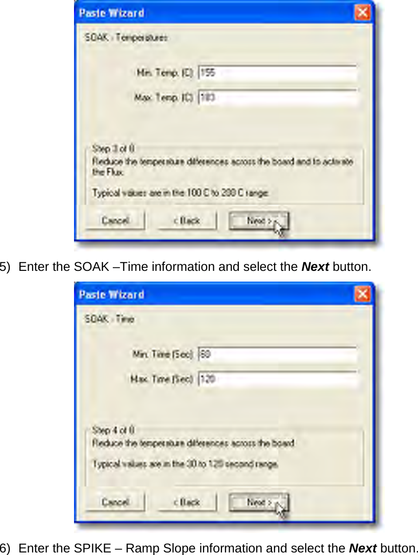
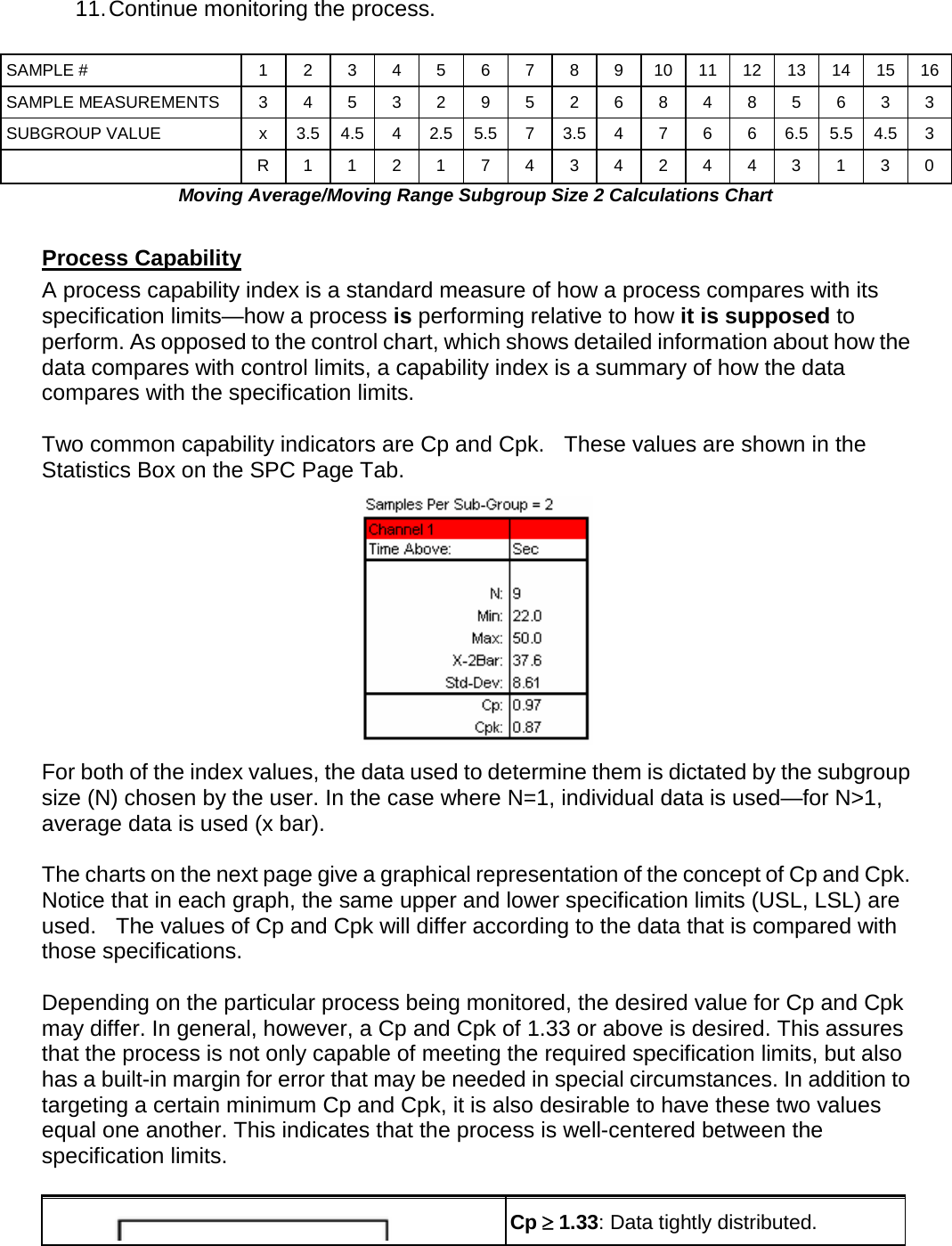
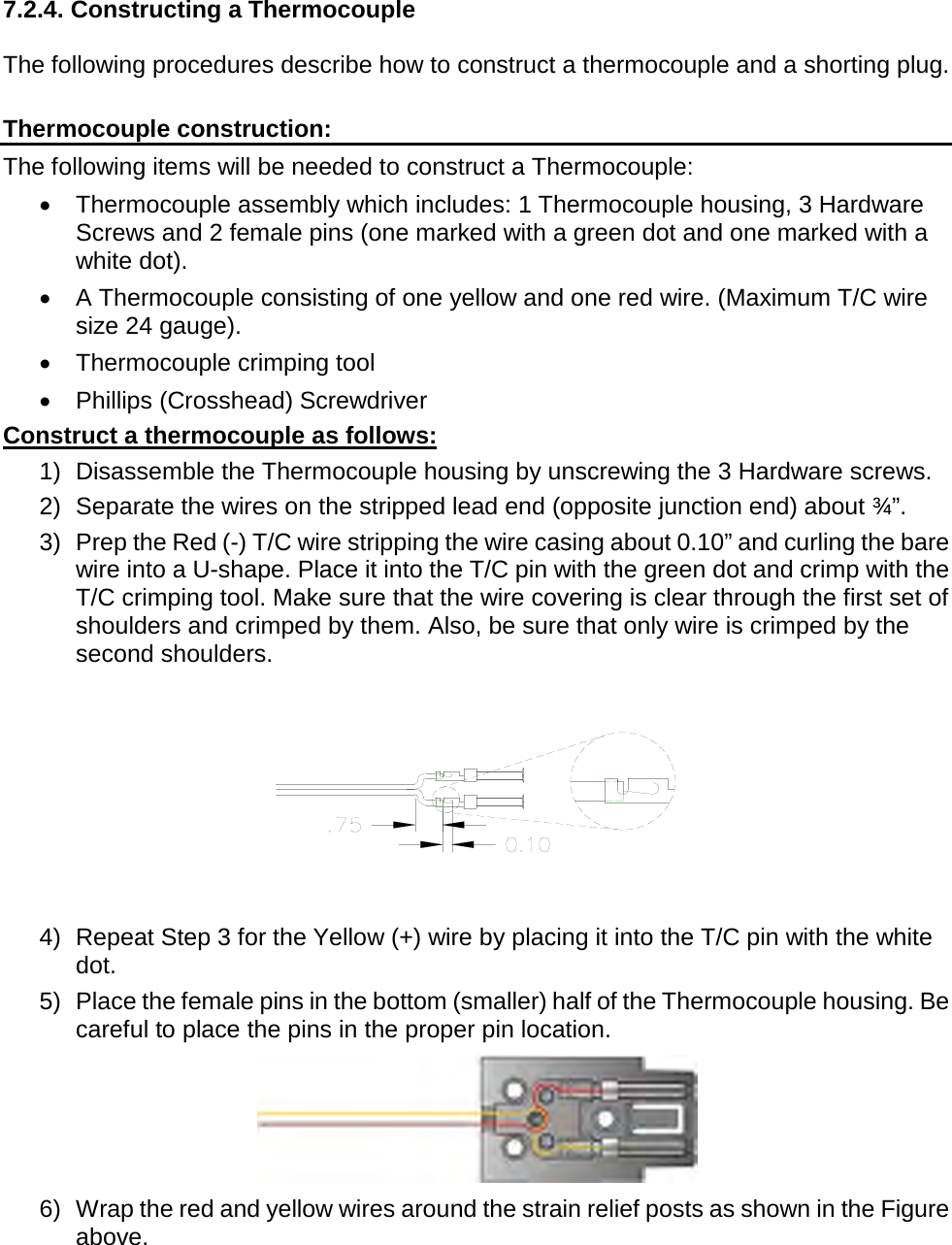
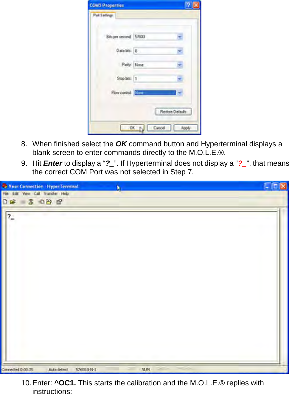
![To remove a slope line from the Data Graph: 1) Using the mouse pointer, select the object on the Data Graph by clicking it once. The object trackers will then become bold indicating that it has been selected. 2) Press the [Delete] key on the keyboard to remove the object.](https://usermanual.wiki/Electronic-Controls-Design/E51-0386-40.User-Manual-part-3-of-3/User-Guide-1481867-Page-50.png)
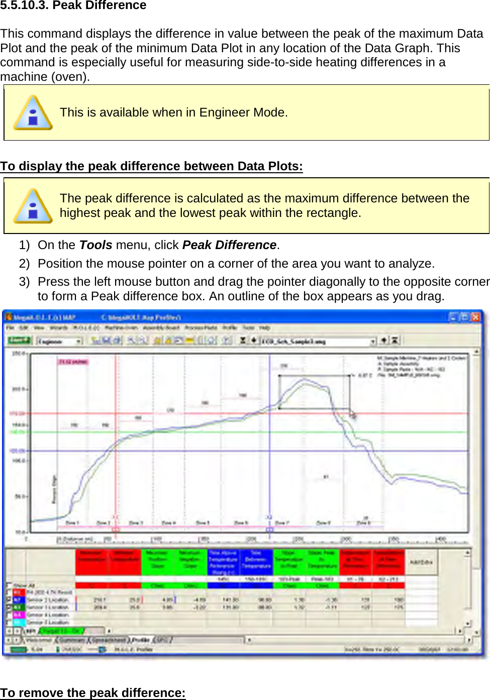
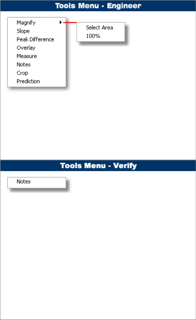
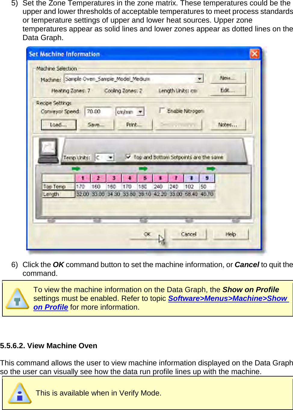
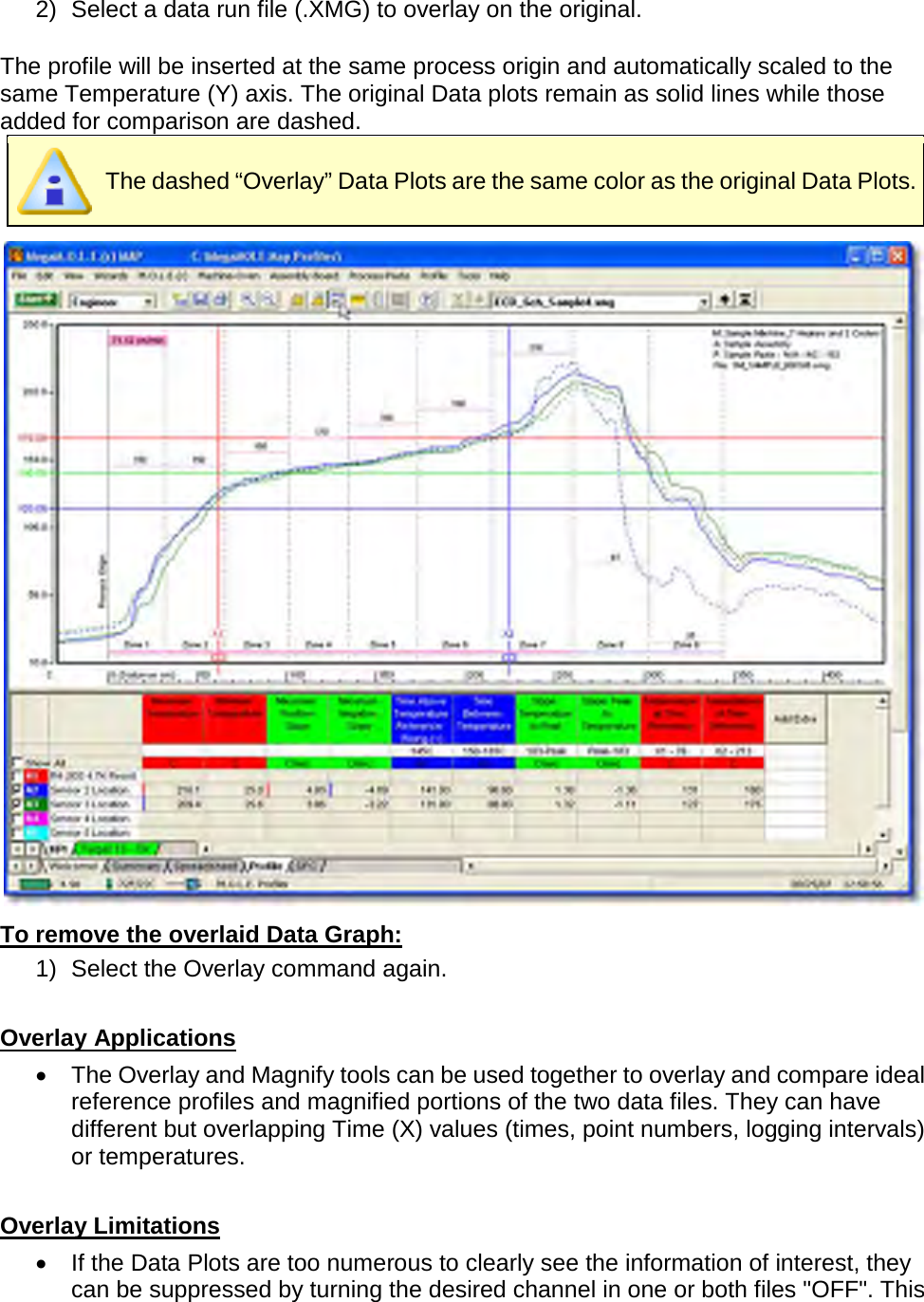
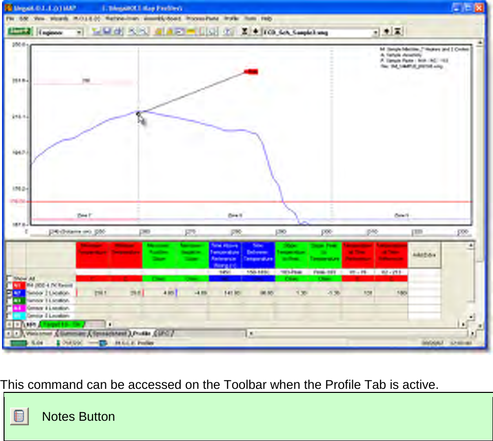
![1) Using the mouse pointer, select the object on the Data Graph by clicking it once. The object trackers will then become bold indicating that it has been selected. 2) Press the [Delete] key on the keyboard to remove the object. This command can be accessed on the Toolbar when the Profile Tab is active. Peak Difference Button 5.5.10.4. Overlay The Overlay tool displays a second data run profile over the currently displayed profile on the Data Graph for comparison. This is available when in Engineer Mode. To overlay two Profiles: 1) On the Tools menu, click Overlay. A list box of data run files (.XMG) in the currently open working directory appears.](https://usermanual.wiki/Electronic-Controls-Design/E51-0386-40.User-Manual-part-3-of-3/User-Guide-1481867-Page-53.png)
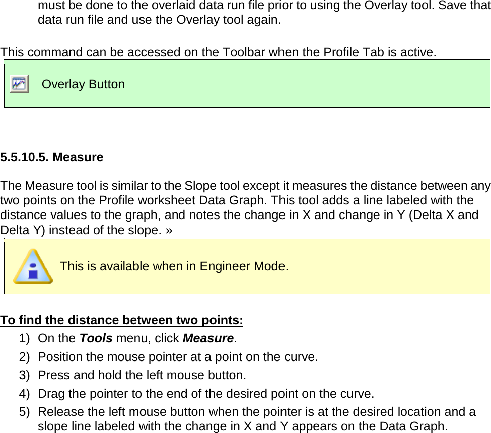
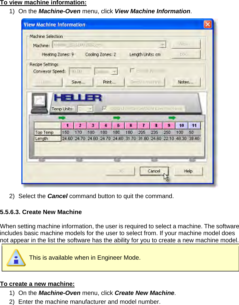
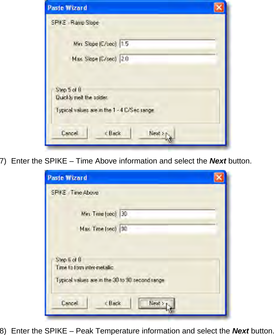
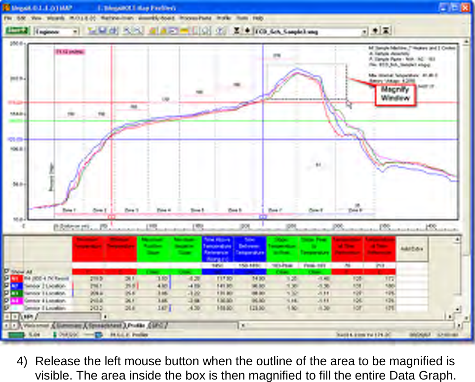
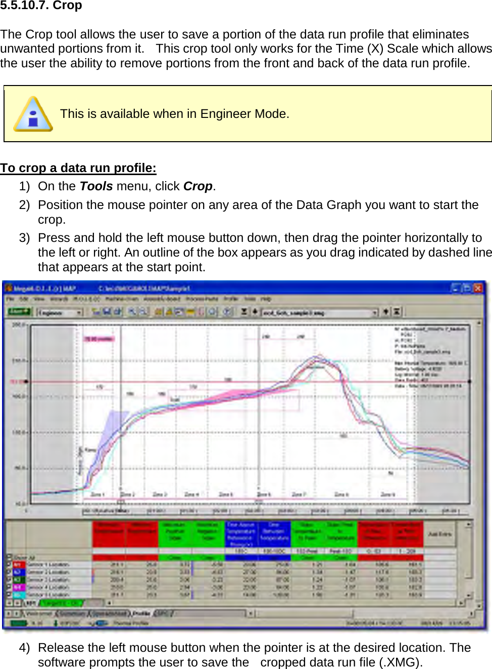
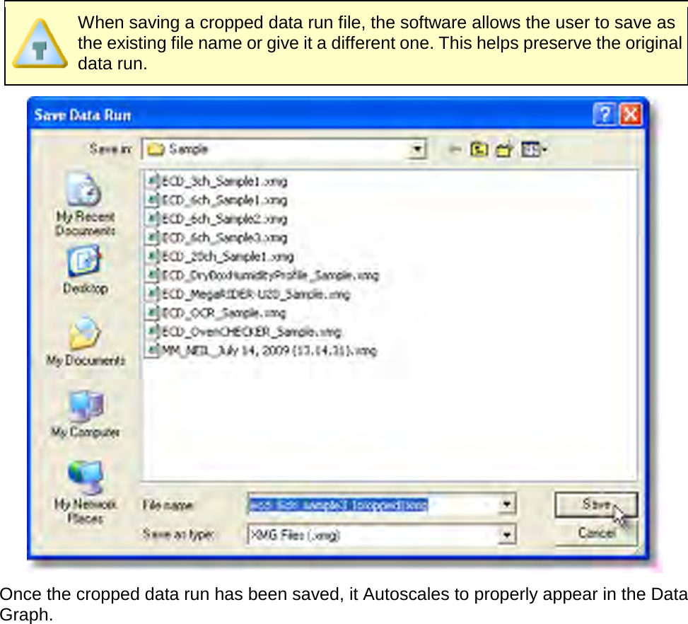
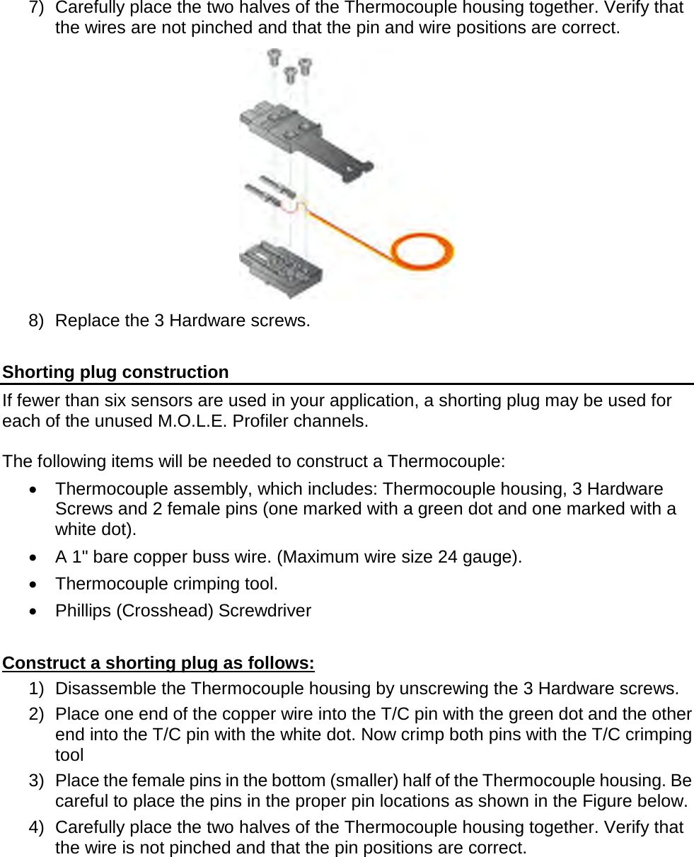
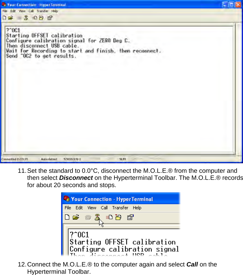
![To obtain more accurate distances: 1) Magnify a portion of the Data Graph using the Magnify tool and repeat this procedure. To remove the annotated distance: 1) Using the mouse pointer, select the object on the Data Graph by clicking it once. The object trackers will then become bold indicating that it has been selected. 2) Press the [Delete] key on the keyboard to remove the object.](https://usermanual.wiki/Electronic-Controls-Design/E51-0386-40.User-Manual-part-3-of-3/User-Guide-1481867-Page-56.png)
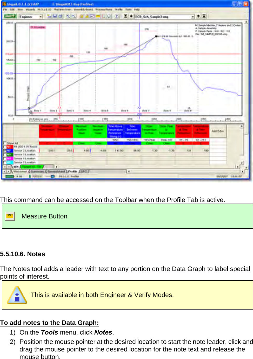
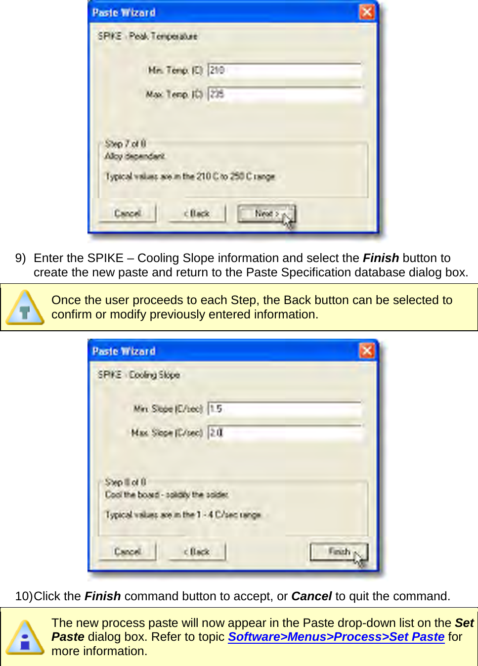
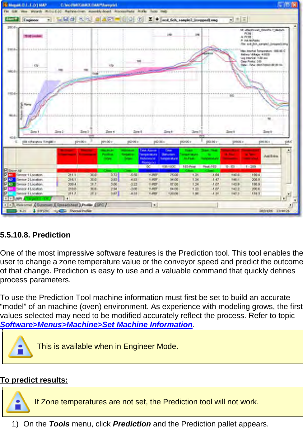
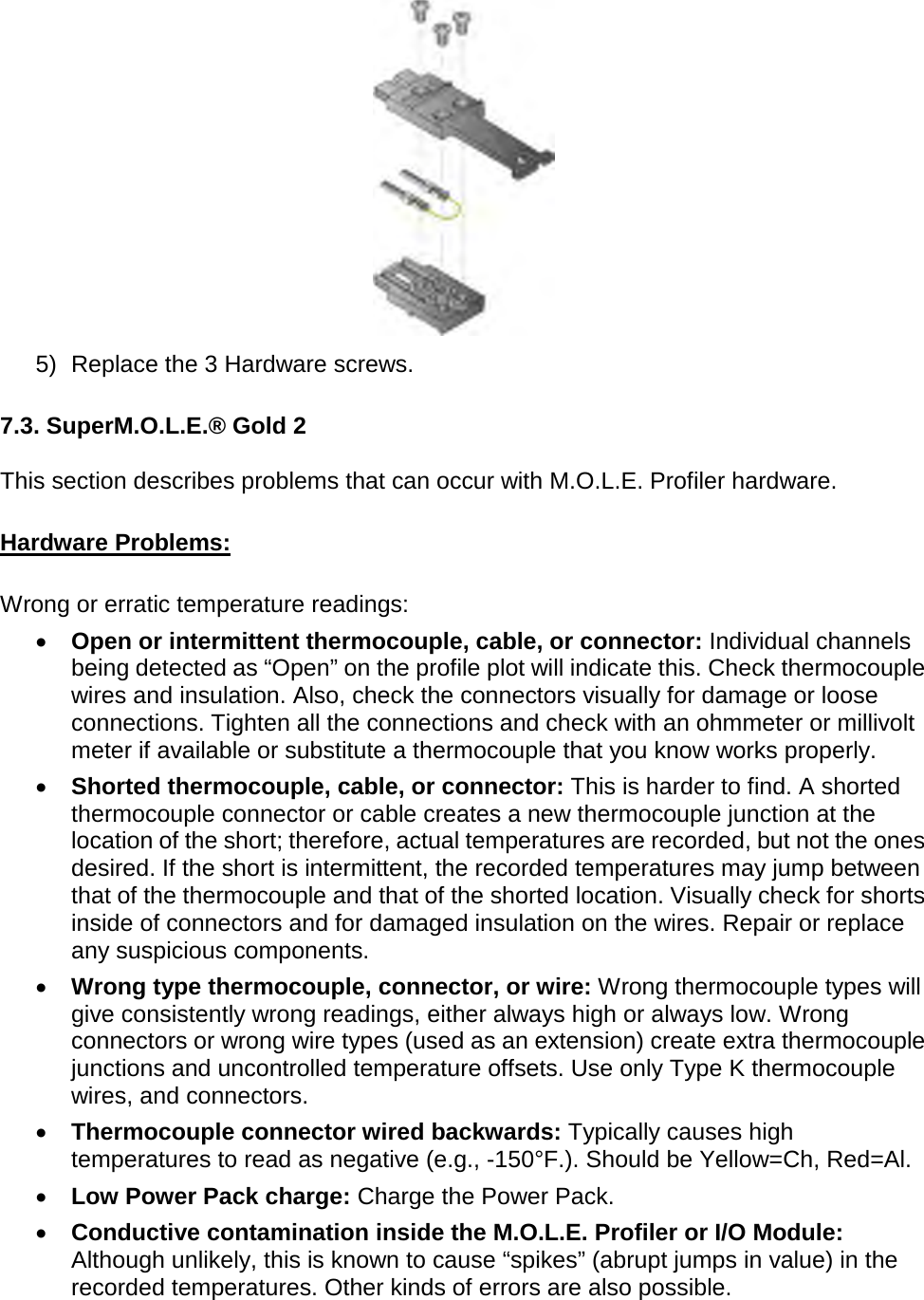
![3) A dialog box appears allowing the user to enter a note by typing it in the text box. There also are options to customize the color and font size. 4) Click the OK command button or Cancel to quit the command. To move notes: 1) Select a note leader, click and drag the mouse pointer to the desired location for the note and release the mouse button. To remove notes: 1) Using the mouse pointer, select the object on the Data Graph by clicking it once. The object trackers will then become bold indicating that it has been selected. 2) Press the [Delete] key on the keyboard to remove the object.](https://usermanual.wiki/Electronic-Controls-Design/E51-0386-40.User-Manual-part-3-of-3/User-Guide-1481867-Page-58.png)
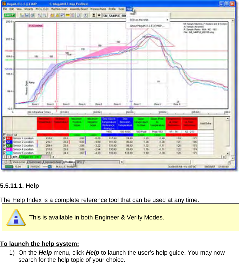
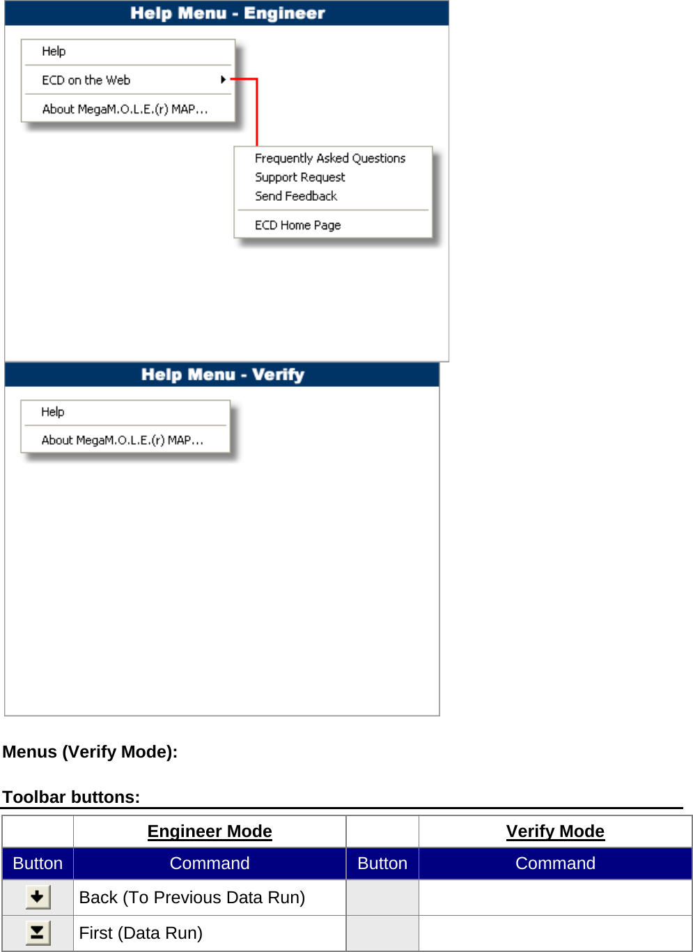
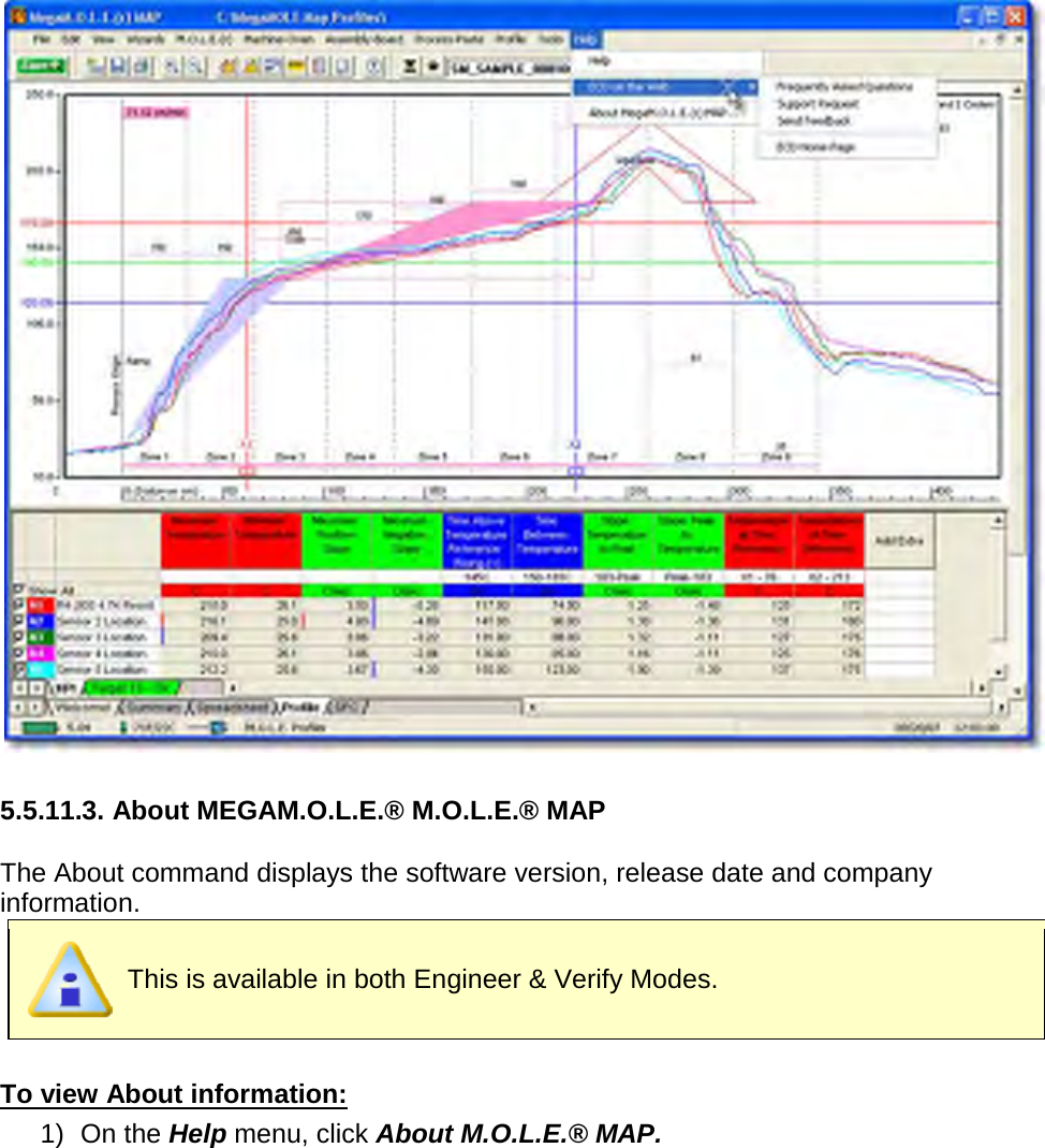
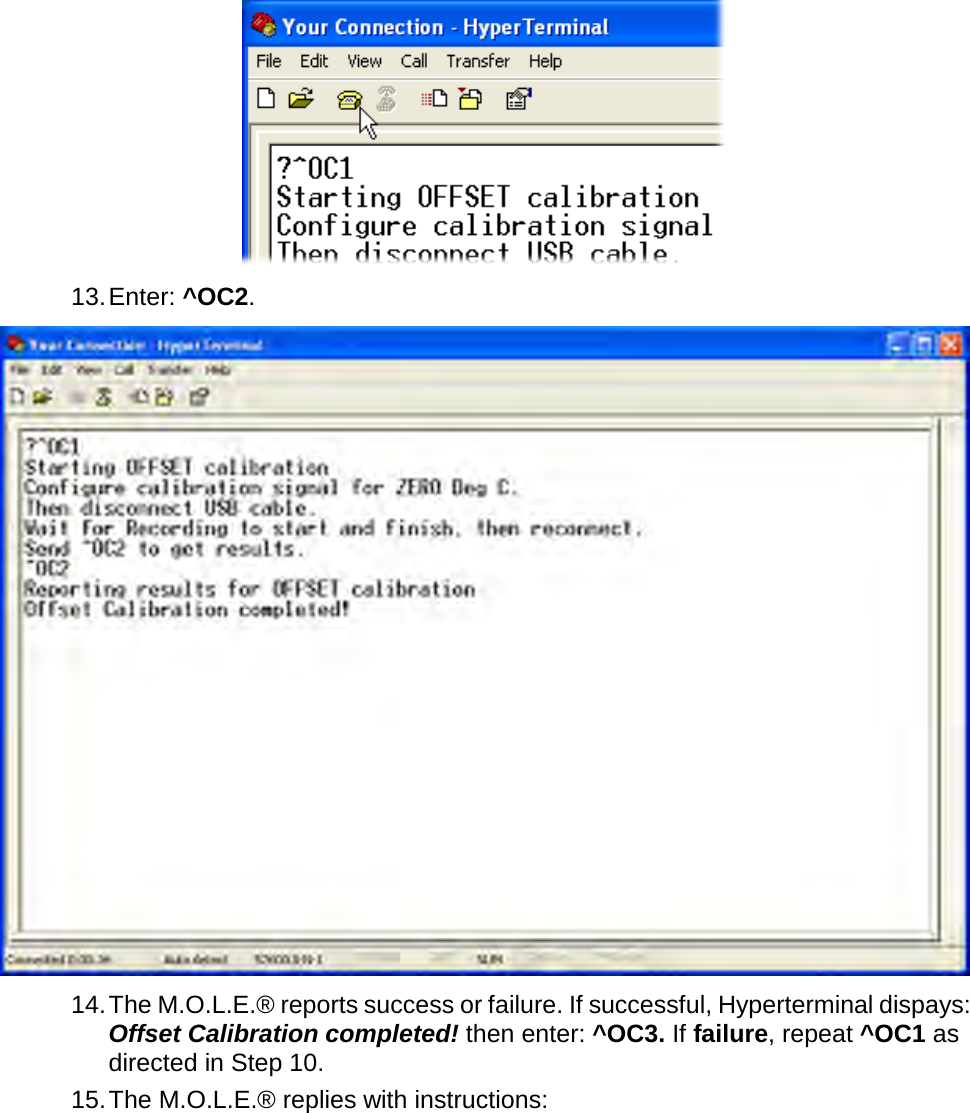
![This command can be accessed on the Toolbar and can also be used by pressing the shortcut key [F1]. Help Button 5.5.11.2. ECD on the Web You can access more help by using ECD web commands. Let us help you by using the linked commands to the ECD Web site. This is available when in Engineer Mode.](https://usermanual.wiki/Electronic-Controls-Design/E51-0386-40.User-Manual-part-3-of-3/User-Guide-1481867-Page-68.png)
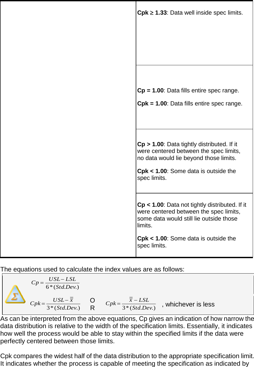
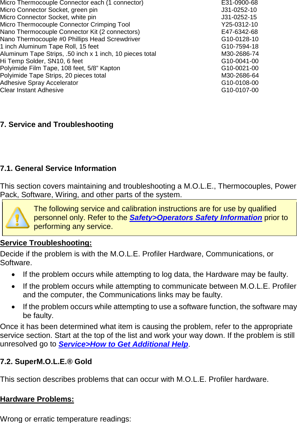
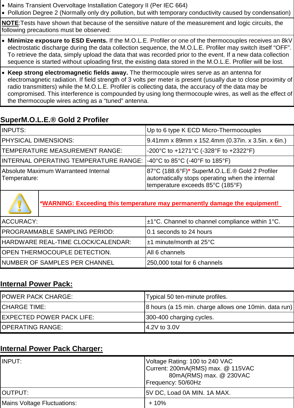
![For use with: SuperM.O.L.E.® Gold Thermal Profiler 6.4. Thermocouples & Other Thermocouples for SuperM.O.L.E.® Gold: (Micro Connector, Type K): Insulation Qty Color Wire AWG Length Max. Temp. Part Number Glass 6 Color-Indexed 36 [.005”/.127mm] 3ft/915mm 900F/482C E44-0944-85 Glass 6 Color-Indexed 30 [.010”/.254mm] 3ft/915mm 900F/482C E44-0944-81 Glass 6 Brown 36 [.005”/.127mm] 3ft/915mm 900F/482C E43-0900-85 Glass 6 Brown 30 [.010”/.254mm] 3ft/915mm 900F/482C E43-0900-89 Glass 6 Brown 40 [.003”/.076mm] 3ft/915mm 900F/482C E47-0900-83 PFA 6 Color-Indexed 36 [.005”/.127mm] 3ft/915mm 500F/260C E43-0900-65 PFA 6 Color-Indexed 30 [.010”/.254mm] 3ft/915mm 500F/260C E43-0900-61 PFA 6 Color-Indexed 30 [.010”/.254mm] 12ft/3658mm 500F/260C E44-2253-71 PFA 6 Transparent 36 [.005”/.127mm] 3ft/915mm 500F/260C E31-0900-65 PFA 6 Transparent 30 [.010”/.254mm] 3ft/915mm 500F/260C E31-0900-61](https://usermanual.wiki/Electronic-Controls-Design/E51-0386-40.User-Manual-part-3-of-3/User-Guide-1481867-Page-77.png)
![PFA 6 Transparent 30 [.010”/.254mm] 6ft/1829mm 500F/260C E31-0900-62 PFA 6 Transparent 36 [.005”/.127mm] 7ft/2134mm 500F/260C E31-0900-66 PFA 6 Transparent 30 [.010”/.254mm] 7ft/2134mm 500F/260C E31-0900-71 SSOB 6 - 24 [.021”/ .533mm] 3ft/915mm 900F/482C E31-0900-86 SSOB 6 - 24 [.021”/ .533mm] 6ft/1829mm 900F/482C E31-0900-87 Thermocouple Adaptors & Extension Cables: Part Number Glass 6-Channel Thermocouple Adapter Set [Mini-Micro] 900F/482C E44-0944-64 PFA 6-Channel Thermocouple Adapter Set [Mini-Micro] 500F/260C E31-0900-64 Glass 6-Channel K-Type Extension [Mini-Mini], 15ft/ 4572mm 900F/482C E42-6672-64 Glass 6-Channel K-Type Extension [Mini-Mini], 20ft/ 6096mm 900F/482C E42-6672-74 Thermocouples for V-M.O.L.E. ® (Miniature Connector, Type K): Insulation Qty Color Wire AWG Length Max. Temp. Part Number Glass 6 Color-Indexed 36 [.005”/.127mm] 3ft/915mm 900F/482C E47-0248-65 Glass 6 Color-Indexed 30 [.010”/.254mm] 3ft/915mm 900F/482C E47-0248-61 PFA 6 Color-Indexed 36 [.005”/.127mm] 3ft/915mm 500F/260C E43-0216-65 PFA 6 Color-Indexed 30 [.010”/.254mm] 3ft/915mm 500F/260C E43-0216-61 PFA 5 Transparent 36 [.005”/.127mm] 3ft/915mm 500F/260C Y15-0216-05 PFA 5 Transparent 30 [.010”/.254mm] 3ft/915mm 500F/260C Y15-0216-10 PFA 5 Transparent 36 [.005”/.127mm] 7ft/2134mm 500F/260C E29-0180-65 Glass 3 Brown 36 [.005”/.127mm] 3ft/915mm 900F/482C E48-0509-63 Glass 3 Brown 30 [.010”/.254mm] 3ft/915mm 900F/482C E48-0509-61 Glass 3 Red/Green/Blue 36 [.005”/.127mm] 3ft/915mm 900F/482C E48-0509-73 Glass 3 Red/Green/Blue 30 [.010”/.254mm] 3ft/915mm 900F/482C E48-0509-71 PFA 3 Red/Green/Blue 36 [.005”/.127mm] 3ft/915mm 500F/260C E48-0509-83 PFA 3 Red/Green/Blue 30 [.010”/.254mm 3ft/915mm 500F/260C E48-0509-81 Glass 1 Brown 30 [.010”/.254mm] 3ft/915mm 900F/482C Y15-0224-20 Glass 1 Brown 30 [.010”/.254mm] 15ft/ 4572mm 900F/482C Y15-0224-30 Glass 1 Brown 30 [.010”/.254mm] 20ft/ 6096mm 900F/482C Y15-0224-40 Thermocouples for MEGAM.O.L.E.® (Nano Connector, Type K): Part Number MEGAM.O.L.E.® 20 Thermocouple Kit E47-6342-34 Includes: 4 Sets of 5 Glass Color-Indexed 36-gauge [.005”/.127mm], 3ft 900F/482C, Aluminum and Kapton Tape Strips, High Temp Solder & Organizer Sleeves Insulation Qty Color Wire AWG Length Max. Temp. Part Number Glass 5 Color-Indexed 36 [.005”/.127mm] 3ft/915mm 900F/482C E47-6342-85 [For channel banks A & C] Glass 5 Color-Indexed 36 [.005”/.127mm] 3ft/915mm 900F/482C E47-6342-75](https://usermanual.wiki/Electronic-Controls-Design/E51-0386-40.User-Manual-part-3-of-3/User-Guide-1481867-Page-78.png)
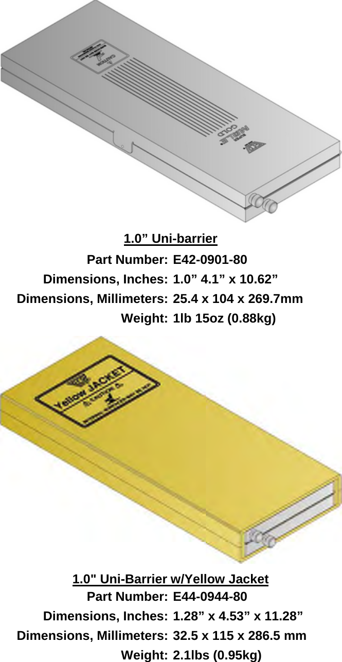
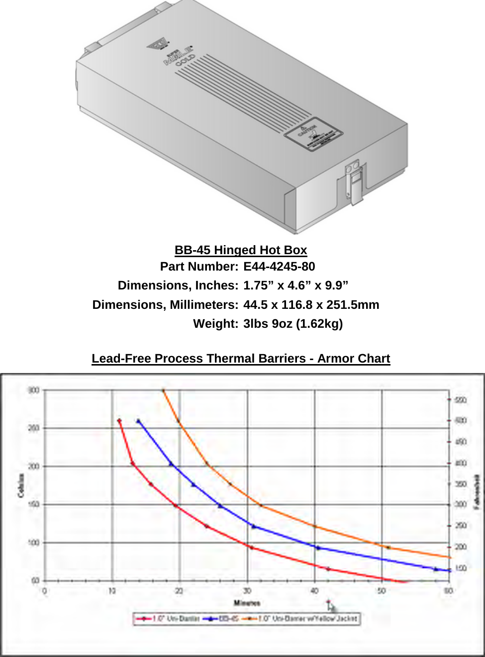
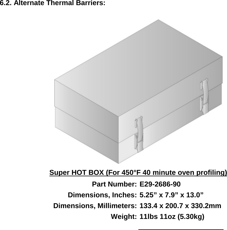
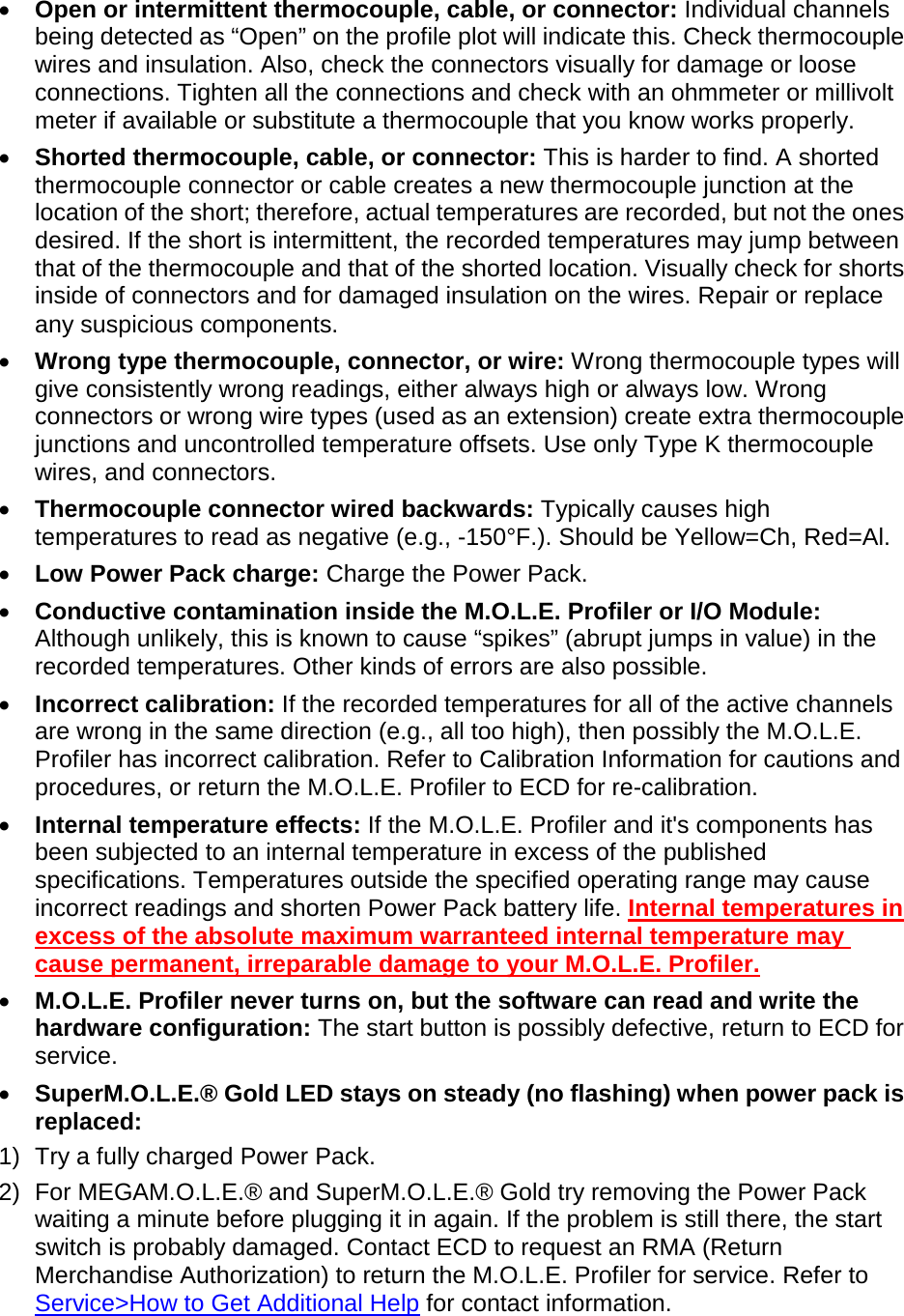
![[For channel banks B & D] Glass 1 Red 36 [.005”/.127mm 3ft/915mm 900F/482C Y15-6342-15 Glass 1 Blue 36 [.005”/.127mm 3ft/915mm 900F/482C Y15-6342-25 Glass 1 Green 36 [.005”/.127mm 3ft/915mm 900F/482C Y15-6342-35 Glass 1 Violet 36 [.005”/.127mm 3ft/915mm 900F/482C Y15-6342-45 Glass 1 Light Blue 36 [.005”/.127mm 3ft/915mm 900F/482C Y15-6342-55 Thermal Protective Enclosures for SuperM.O.L.E.® Gold, SuperM.O.L.E.® Gold 2 & RF Option: Dimensions Part Number 1” Uni-Barrier 1.0 x 4.2 x 10.5” E42-0901-80 Yellow Jacket [for Uni-Barrier or 1” Super Survivor] 1.28 x 4.52 x 11.27” E44-7435-80 1” Uni-Barrier with Yellow Jacket 1.28 x 4.52 x 11.27” E44-0944-80 SuperM.O.L.E. Boot 1.3 x 5.2 x 9.7” M30-0200-70 BB-45 1.75 x 4.6 x 9.9” E44-4245-80 Super Hot Box 5.25 x 7.9 x 13.0” E29-2686-90 Thermal Protective Enclosures for MEGAM.O.L.E.® & V-M.O.L.E.®: Dimensions Part Number M.O.L.E. Thermal Barrier (stainless steel) E47-6342-80 M.O.L.E. Yellow Jacket Thermal Barrier Cover E47-6342-70 Accessories and Value Added Options SuperM.O.L.E.® Gold, SuperM.O.L.E.® Gold 2: Part Number Lead-Free Upgrade Kit-Hardware that makes your Gold Lead-Free Compatible E44-0944-05 For those with an older version of the SuperM.O.L.E. Gold profiling kit. Includes: 1” Uni-Barrier, Yellow Jacket and 5 & 10-mil sets of color indexed glass thermocouples Xpert Desktop Download/Charging Station E40-2875-52 Power Pack Charger, 110V E31-0900-25 Power Pack Charger, 220V E31-0900-21 SuperM.O.L.E. Gold Rechargeable Power Pack - RoHS Compliant E45-7647-30 SuperM.O.L.E. Gold Calendar/Clock Battery F30-0041-00 SuperM.O.L.E. Gold Pogo Pin [for RF and Xpert dock charging use] J01-6016-00 SuperM.O.L.E. Gold to PC Interface Cable Y20-2848-04 USB/RS-232 Serial Adapter Y23-7782-10 VaporWATCH Humidity Sensor E44-7423-00 MEGAM.O.L.E. MAP Software (includes CD & Quick Ref Guide) E47-6342-32 Extended M.O.L.E. warranty; 1 year, includes 1 calibration A10-0900-00 Accessories and Value Added Options MEGAM.O.L.E.® & V-M.O.L.E.®: Part Number MEGAM.O.L.E. Rechargeable Power Pack Battery E47-6342-30 MEGAM.O.L.E. 20 nano-mini 20-channel adapter E47-6342-74 MEGAM.O.L.E./V-M.O.L.E. PC USB 2.0 Cable E47-6342-10 MEGAM.O.L.E./V-M.O.L.E. Battery Charger E47-6342-20 MEGAM.O.L.E. MAP Software (includes CD & Quick Ref Guide) E47-6342-32 Extended M.O.L.E. warranty; 1 year, includes 1 calibration A10-0900-00 Miscellaneous Accessories: Micro Connector Thermocouple Organizer w/screw lock M45-0900-60 Micro Thermocouple Connector Set (6 connectors) E31-0900-60](https://usermanual.wiki/Electronic-Controls-Design/E51-0386-40.User-Manual-part-3-of-3/User-Guide-1481867-Page-79.png)
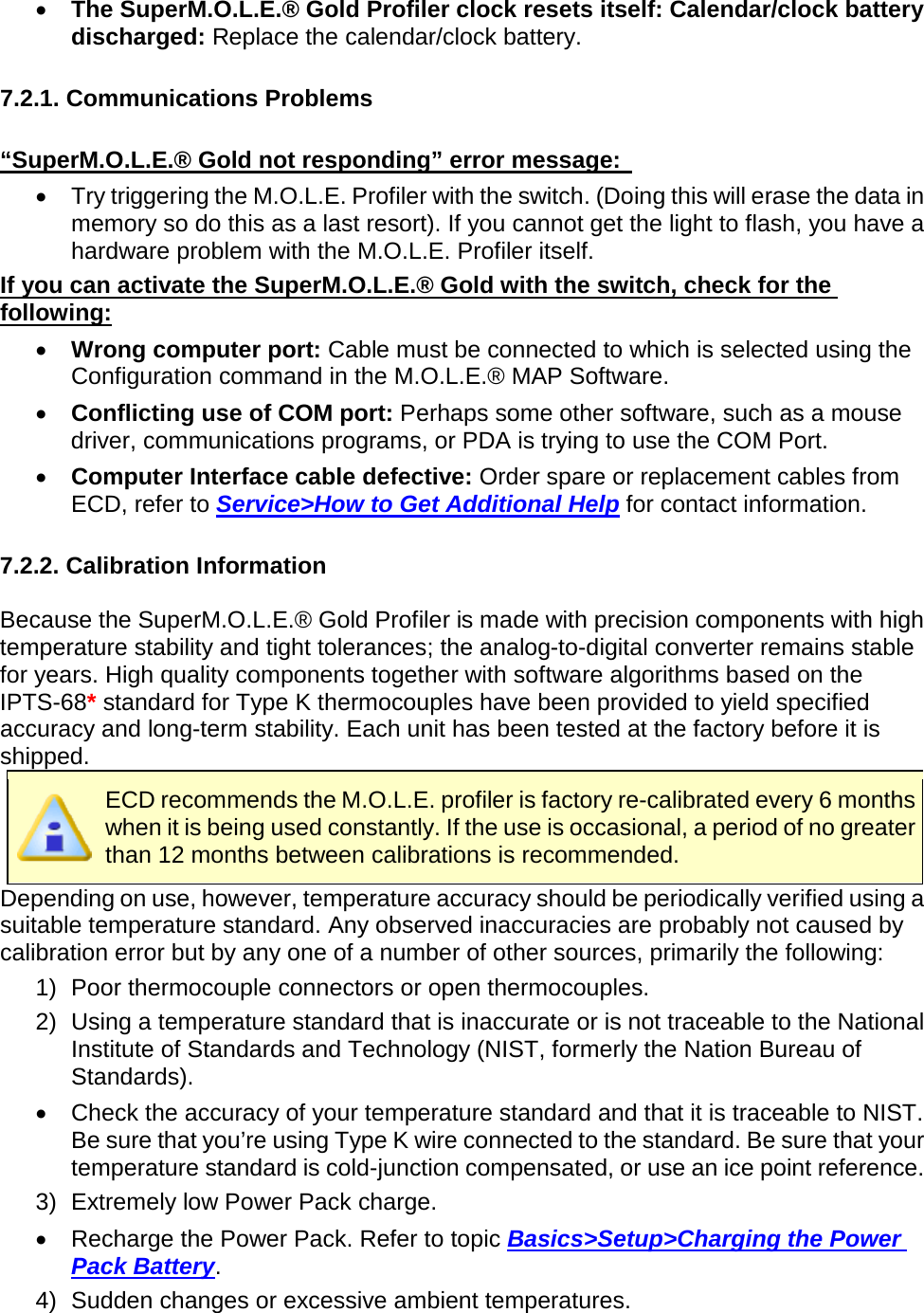
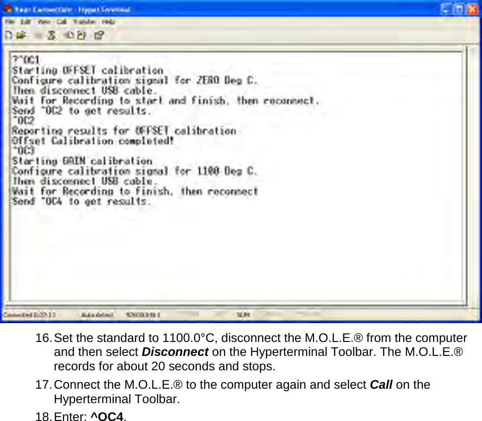
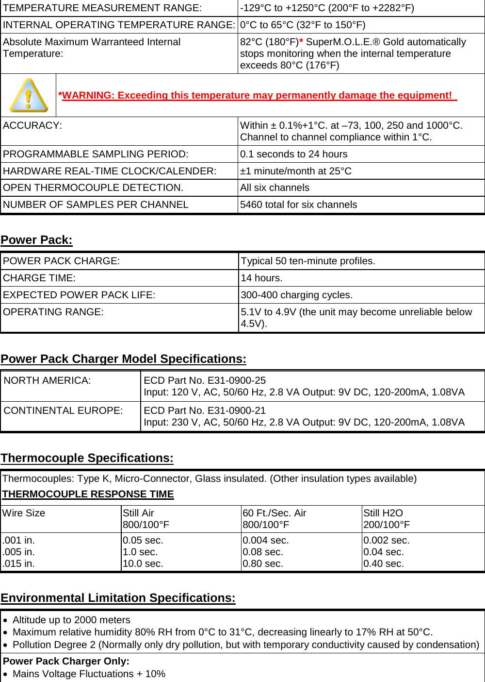
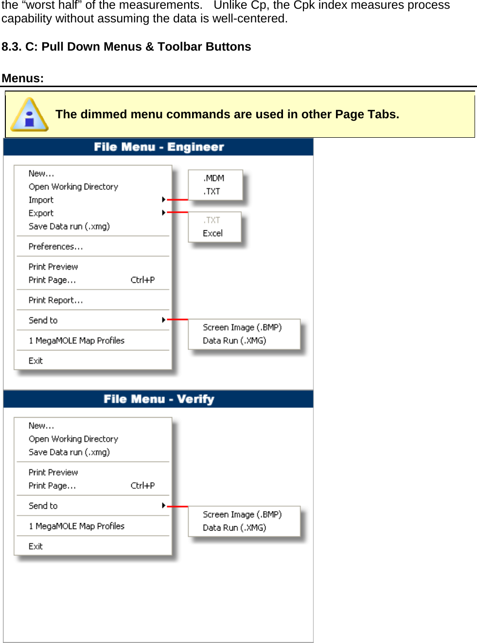
![Wireless RF Option: This equipment has been tested and found to comply with the limits for a Class A digital device, pursuant to Part 15 of the FCC Rules. These limits are designed to provide reasonable protection against harmful interference in a residential installation. This equipment generates, uses and can radiate radio frequency energy and, if not installed and used in accordance with the instructions, may cause harmful interference to radio communications. However, there is no guarantee that interference will not occur in a particular installation. If this equipment does cause harmful interference to radio or television reception, which can be determined by turning the equipment off and on, the user is encouraged to try to correct the interference by one or more of the following measures: • Reorient or relocate the receiving antenna. • Increase the separation between the equipment and receiver. • Connect the equipment into an outlet on a circuit different from that to which the receiver is connected. • Consult the dealer or an experienced radio/TV technician for help. SuperM.O.L.E.® Gold 2 Radio: Type: IEEE 802.15.4 ZigBee™ two way Frequency: 2.45 gHz Power: 1mW (0dbm) Range: 6.5 meters (20ft)* Wireless Antenna: Temperature: 250ºC (500ºF) Exposed Material: Teflon insulation Connector: MMCX Right Angle USB Transceiver: Type: IEEE 802.15.4 ZigBee™ two way Antenna: Internal fractal chip * The range of the SuperM.O.L.E.® Gold 2 RF system varies with the RF environment. Under ideal conditions, the range may be 6.5 meters [20 feet] and in some situations it may only be a few meters. Refer to topic Basics>Wireless RF Option Setup Thermocouple Specifications: Thermocouples: Type K, Mini-Connector, Glass insulated. (Other insulation types available.) THERMOCOUPLE RESPONSE TIME Wire Size Still Air 800/100°F 60 Ft./Sec. Air 800/100°F Still H2O 200/100°F .005 in. 1.0 sec. 0.08 sec. 0.04 sec. Environmental Limitation Specifications: SuperM.O.L.E.® Gold 2 Profiler: • Maximum relative humidity 80% RH from 0°C to 31°C, decreasing linearly to 17% RH at 50°C. • Pollution Degree 2 (Normally only dry pollution, but with temporary conductivity caused by condensation) Power Pack Charger: • Temperature: (Operation) 0 to +45°C (32 to 113°F) • Temperature: (Non-Operation) -20 to +75°C (-4 to 167°F) • Humidity: (Operation) 20 to 90% NOTE:Tests have shown that because of the sensitive nature of the measurement and logic circuits, the](https://usermanual.wiki/Electronic-Controls-Design/E51-0386-40.User-Manual-part-3-of-3/User-Guide-1481867-Page-109.png)