FineTurbo_User_manual User Manual FINETurbo
2013-12-19
: Ensight Usermanual-Fineturbo UserManual-FINETurbo Numeca Misc
Open the PDF directly: View PDF ![]() .
.
Page Count: 351 [warning: Documents this large are best viewed by clicking the View PDF Link!]
- CHAPTER 1: Getting Started
- CHAPTER 2: Graphical User Interface
- 2-1 Overview
- 2-2 Project Selection
- 2-3 Main Menu Bar
- 2-4 Icon Bar
- 2-5 Computation Management
- 2-6 Graphical Area Management
- 2-7 Profile Management
- CHAPTER 3: Fluid Model
- CHAPTER 4: Flow Model
- 4-1 Overview
- 4-2 Mathematical Model
- 4-2.1 Euler
- 4-2.2 Laminar Navier-Stokes
- 4-2.3 Turbulent Navier-Stokes
- 4-2.4 Expert Parameters for Turbulence Modelling
- 4-2.5 Best Practice for Turbulence Modelling
- 4-2.5.1 Introduction to Turbulence
- 4-2.5.2 First Step: Choosing a Turbulence Model.
- 4-2.5.3 Second Step: Generating an Appropriate Grid.
- 4-2.5.4 Defining Initial & Boundary Conditions
- 4-2.5.5 Setting Expert Parameters to Procure Convergence
- a) Cut-off (Clipping) of Minimum k Value
- b) Minimizing Artificial Dissipation in the Boundary Layer
- c) Wall Function for the k-e Turbulence Model
- d) Full Multigrid k-e / Baldwin-Lomax & v2-f / Baldwin-Lomax Switch
- e) Cut-off (clipping) of Maximum Turbulence Production/Destruction Value
- f) Cut-off (clipping) of Maximum Turbulent Viscosity Ratio (mt /m)
- 4-2.6 Laminar-Transition Model
- 4-2.7 Gravity Forces
- 4-2.8 Low Speed Flow (Preconditioning)
- 4-3 Characteristic & Reference Values
- CHAPTER 5: Boundary Conditions
- 5-1 Overview
- 5-2 Boundary Conditions in the FINE™/Turbo GUI
- 5-3 Expert Parameters
- 5-3.1 Imposing Velocity Angles of Relative Flow
- 5-3.2 Inlet Mass Flow Boundary Condition
- 5-3.3 Outlet Mass Flow Boundary Condition
- 5-3.4 Outlet Averaged Mach Number Boundary Condition
- 5-3.5 Control of backflows
- 5-3.6 Torque and Force
- 5-3.7 Euler or Navier-Stokes Wall for Viscous Flow
- 5-3.8 Pressure Condition at Solid Wall
- 5-4 Best Practice for Imposing Boundary Conditions
- CHAPTER 6: Numerical Scheme
- 6-1 Overview
- 6-2 Numerical Model
- 6-3 Time Configuration
- 6-3.1 Interface for Unsteady Computation
- 6-3.2 Expert Parameters for Unsteady Computations
- 6-3.3 Best Practice on Time Accurate Computations
- CHAPTER 7: Physical Models
- 7-1 Overview
- 7-2 Fluid-Particle Interaction
- 7-3 Fluid-Structure
- 7-4 Passive Tracers
- 7-5 Porous Media Model
- 7-6 Cavitation Model
- CHAPTER 8: Dedicated Turbomachinery Models
- 8-1 Overview
- 8-2 Rotating Blocks
- 8-3 Rotor/Stator Interaction
- 8-4 Harmonic Method
- 8-5 Clocking
- 8-6 Cooling/Bleed
- 8-6.1 Introduction
- 8-6.2 Cooling/Bleed Model in the FINE™/Turbo GUI
- 8-6.3 Expert Parameters
- 8-6.4 Cooling/Bleed Data File: ’.cooling-holes’
- 8-6.4.1 Injection file format
- a) The header
- b) Multiple injector format
- c) Injector name
- d) Injection geometry Type
- e) Injection physical Type
- f) Locations patches
- g) Location patch index
- h) Anchor point location
- i) Cooling direction (not for Bleed)
- j) Anchor point location and cooling direction (for points type only)
- k) Mass flow
- l) Number of holes on a line
- m) Cooling/Bleed size
- n) Physical Properties
- 8-6.4.2 Examples
- 8-6.4.1 Injection file format
- 8-7 Rigid Motion
- 8-8 Aeroacoustics
- 8-9 Laminar-Transition Model
- 8-10 Performance Curve
- 8-11 SubProject Management
- CHAPTER 9: Initial Solution
- CHAPTER 10: Output
- CHAPTER 11: Task Manager
- 11-1 Overview
- 11-2 Getting Started
- 11-3 The Task Manager Interface
- 11-4 Parallel Computations
- 11-5 Task Management in Batch
- 11-5.1 Launch IGG™ in Batch
- 11-5.2 Launch AutoGrid™ in Batch
- 11-5.3 Launch FINE™ in Batch
- 11-5.3.1 How to Launch FINE™ on UNIX
- a) Create a ".run" file
- b) Set-up a parallel computation using MPI
- c) Set-up a parallel computation using SGE
- d) Set-up a parallel computation using PBS
- e) Set-up a parallel computation using LSF
- f) Set-up a parallel partitioned computation using MPI
- g) Set-up a parallel partitioned computation using SGE
- h) Set-up a parallel partitioned computation using PBS
- i) Set-up a parallel partitioned computation using LSF
- 11-5.3.2 How to Launch FINE™ on Windows
- 11-5.3.1 How to Launch FINE™ on UNIX
- 11-5.4 Launch the flow solver in Sequential Mode in Batch
- 11-5.5 Launch the flow solver in Parallel Mode in Batch
- 11-5.5.1 How to Launch the flow solver in Parallel using MPI on UNIX
- 11-5.5.2 How to Launch the flow solver in Parallel using MPI on Windows
- 11-5.5.3 How to Launch the flow solver in Parallel using SGE on UNIX
- 11-5.5.4 How to Launch the flow solver in Parallel using PBS on UNIX
- 11-5.5.5 How to Launch the flow solver in Parallel using LSF on UNIX
- 11-5.6 Launch CFView™ in Batch
- 11-6 Limitations
- CHAPTER 12: Computation Steering & Monitoring
- APPENDIX A: File Formats
- A-1 Overview
- A-2 Files Produced by IGG™
- A-3 Files Produced by the FINE™/Turbo GUI
- A-4 Files Produced by the FINE™/Turbo solver
- A-4.1 The Binary Solution File: ’project_computation.cgns’
- A-4.2 The Global Solution File: ’project_computation.mf’
- A-4.3 The Global Solution File: ’project_computation.xmf’
- A-4.4 The Residual File: ’project_computation.res’
- A-4.5 The LOG File: ’project_computation.log’
- A-4.6 The STD file: ’project_computation.std’
- A-4.7 The Wall File: ’project_computation.wall’
- A-4.8 The AQSI File: ’project_computation.aqsi’
- A-4.9 The ADF File: ’project.adf’
- A-4.10 The Plot3D Files
- A-4.11 The Meridional File: ’project_computation.me.cfv’
- A-5 Files Used as Data Profile
- A-6 Resource Files
- APPENDIX B: List of Expert Parameters
- APPENDIX C: Characteristics of Thermodynamic Tables
- APPENDIX D: TabGen

NUMERICAL MECHANICS APPLICATIONS
User Manual
FINE™/Turbo v8.10
Flow Integrated Environment
- November 2012 -

NUMERICAL MECHANICS APPLICATIONS
User Manual
FINE™/Turbo v8.10
Documentation v8.10c
NUMECA International
Chaussée de la Hulpe, 189
1170 Brussels
Belgium
Tel: +32 2 647.83.11
Fax: +32 2 647.93.98
Web: http://www.numeca.com

Contents
FINE™/Turbo iii
CHAPTER 1: Getting Started 1-1
1-1 Overview 1-1
1-2 Introduction 1-1
Components 1-1
Multi-Tasking 1-2
Project Management 1-2
1-3 How To Use This Manual 1-4
Outline 1-4
Conventions 1-4
1-4 First Time Use 1-5
Basic Installation 1-5
Expert Graphics Options 1-5
1-5 How to start the FINE™/Turbo Interface 1-6
1-6 Required Licenses 1-7
Standard FINE™/Turbo License 1-7
Additional Licenses 1-7
CHAPTER 2: Graphical User Interface 2-1
2-1 Overview 2-1
2-2 Project Selection 2-2
Create New Project 2-2
Open Existing Project 2-4
Grid Units & Project Configuration 2-4
2-3 Main Menu Bar 2-6
File Menu 2-6
Mesh Menu 2-9
Solver Menu 2-11
Modules Menu 2-12
2-4 Icon Bar 2-12
File Buttons 2-12
Grid Selection Bar 2-13
Solver Buttons 2-14
Module Buttons 2-14
User Mode 2-14
2-5 Computation Management 2-14
2-6 Graphical Area Management 2-15
Configuration Management 2-15
Parameters Management 2-16
View Area 2-16
Mesh Information 2-18
Parameters Area 2-18
Graphics Area 2-19
Viewing Buttons 2-19
2-7 Profile Management 2-22

Contents
iv FINE™/Turbo
CHAPTER 3: Fluid Model 3-1
3-1 Overview 3-1
3-2 The Fluid Model in the FINE™/Turbo GUI 3-2
Properties of Fluid Used in the Project 3-2
List of Fluids 3-2
Add Fluid 3-3
Delete Fluid from List 3-9
Edit Fluid 3-9
Show Fluid Properties 3-10
Filters 3-10
Import Fluid Database 3-10
Expert Parameters 3-10
CHAPTER 4: Flow Model 4-1
4-1 Overview 4-1
4-2 Mathematical Model 4-2
Euler 4-2
Laminar Navier-Stokes 4-2
Turbulent Navier-Stokes 4-2
Expert Parameters for Turbulence Modelling 4-4
Best Practice for Turbulence Modelling 4-9
Laminar-Transition Model 4-19
Gravity Forces 4-21
Low Speed Flow (Preconditioning) 4-22
4-3 Characteristic & Reference Values 4-22
Reynolds Number Related Information 4-22
Reference Values 4-23
CHAPTER 5: Boundary Conditions 5-1
5-1 Overview 5-1
5-2 Boundary Conditions in the FINE™/Turbo GUI 5-1
Inlet Condition 5-4
Outlet Condition 5-7
Periodic Condition 5-11
Solid Wall Boundary Condition 5-12
External Condition (Far-field) 5-16
5-3 Expert Parameters 5-17
Imposing Velocity Angles of Relative Flow 5-17
Inlet Mass Flow Boundary Condition 5-17
Outlet Mass Flow Boundary Condition 5-17
Outlet Averaged Mach Number Boundary Condition 5-18
Control of backflows 5-18
Torque and Force 5-18
Euler or Navier-Stokes Wall for Viscous Flow 5-18
Pressure Condition at Solid Wall 5-19
5-4 Best Practice for Imposing Boundary Conditions 5-19

Contents
FINE™/Turbo v
Compressible Flows 5-19
Incompressible or Low Speed Flow 5-20
Special Parameters (for Turbomachinery) 5-20
CHAPTER 6: Numerical Scheme 6-1
6-1 Overview 6-1
6-2 Numerical Model 6-1
Introduction 6-1
Numerical Model in the FINE™/Turbo GUI 6-2
Expert Parameters 6-5
6-3 Time Configuration 6-10
Interface for Unsteady Computation 6-10
Expert Parameters for Unsteady Computations 6-13
Best Practice on Time Accurate Computations 6-14
CHAPTER 7:Physical Models 7-1
7-1 Overview 7-1
7-2 Fluid-Particle Interaction 7-1
Introduction 7-1
Fluid-Particle Interaction in the FINE™/Turbo GUI 7-3
Specific Output 7-7
Expert Parameters 7-8
7-3 Fluid-Structure 7-9
Thermal 7-9
Mechanical 7-13
7-4 Passive Tracers 7-23
Boundary Conditions 7-23
Initial Solution 7-23
Outputs 7-24
7-5 Porous Media Model 7-24
Porous Media Model in the FINE™/Turbo GUI 7-24
Experts Parameters 7-24
7-6 Cavitation Model 7-25
Cavitation Model in the FINE™/Turbo GUI 7-25
Experts Parameters 7-25
CHAPTER 8:Dedicated Turbomachinery Models 8-1
8-1 Overview 8-1
8-2 Rotating Blocks 8-1
8-3 Rotor/Stator Interaction 8-4
Rotor/Stator Interfaces in the FINE™/Turbo GUI 8-4
How to Set-up a Simulation with Rotor/Stator Interfaces? 8-6
8-4 Harmonic Method 8-19
Introduction 8-19
Interface & Best Practice for Harmonic Computations 8-20
Expert Parameters 8-27

Contents
vi FINE™/Turbo
8-5 Clocking 8-30
Introduction 8-30
Interface Settings 8-31
8-6 Cooling/Bleed 8-33
Introduction 8-33
Cooling/Bleed Model in the FINE™/Turbo GUI 8-34
Expert Parameters 8-54
Cooling/Bleed Data File: ’.cooling-holes’ 8-54
8-7 Rigid Motion 8-59
8-8 Aeroacoustics 8-59
Aeroacoustics in the FINE™/Turbo GUI 8-60
Expert Parameters for Aeroacoustics 8-62
8-9 Laminar-Transition Model 8-63
Introduction 8-63
Transition Model in the FINE™/Turbo GUI 8-63
Expert Parameters 8-65
8-10 Performance Curve 8-66
Introduction 8-66
Performance Curve in the FINE™/Turbo GUI 8-66
8-11 SubProject Management 8-69
Introduction 8-69
Set-up of SubProjects in FINE™/Turbo 8-70
CHAPTER 9: Initial Solution 9-1
9-1 Overview 9-1
9-2 Block Dependent Initial Solution 9-1
How to Define a Block Dependent Initial Solution 9-2
Examples for the use of Block Dependent Initial Solution 9-2
9-3 Initial Solution Defined by Constant Values 9-3
9-4 Initial Solution from File 9-3
General Restart Procedure 9-3
Restart in Unsteady Computations 9-5
Expert Parameters for an Initial Solution from File 9-5
9-5 Initial Solution for Turbomachinery 9-5
Methodology 9-6
Grouping & Parameters 9-7
Expert Parameters 9-8
9-6 Throughflow-oriented Initial Solution 9-8
CHAPTER 10:Output 10-1
10-1 Overview 10-1
10-2 Output in FINE™/Turbo 10-2
Computed Variables 10-2
Surface Averaged Variables 10-8
Azimuthal Averaged Variables 10-10
Template manager 10-11
ANSYS 10-13

Contents
FINE™/Turbo vii
Global Performance Output 10-19
Plot3D Formatted Output 10-22
10-3 Expert Parameters 10-22
Azimuthal Averaged Variables 10-22
Global Performance Output 10-23
Solid Data Output 10-24
CHAPTER 11:Task Manager 11-1
11-1 Overview 11-1
11-2 Getting Started 11-1
PVM Daemons 11-1
Multiple FINE™/Turbo Sessions 11-2
Machine Connections 11-2
Remote Copy Features on UNIX/LINUX 11-4
Remote Copy Features on Windows 11-4
11-3 The Task Manager Interface 11-5
Hosts Definition 11-5
Tasks Definition 11-6
11-4 Parallel Computations 11-17
Introduction 11-17
Management of Inter-Block Communication 11-19
How to Run a Parallel Computation 11-19
Use an External OpenMPI Library on LINUX/UNIX 11-20
Troubleshooting 11-21
Limitations 11-22
11-5 Task Management in Batch 11-22
Launch IGG™ in Batch 11-22
Launch AutoGrid™ in Batch 11-23
Launch FINE™ in Batch 11-24
Launch the flow solver in Sequential Mode in Batch 11-30
Launch the flow solver in Parallel Mode in Batch 11-31
Launch CFView™ in Batch 11-43
11-6 Limitations 11-45
CHAPTER 12:Computation Steering & Monitoring 12-1
12-1 Overview 12-1
12-2 Control Variables 12-1
Control Variables in the FINE™/Turbo GUI 12-1
Expert Parameters 12-2
12-3 Convergence History 12-3
Convergence History in the FINE™/Turbo GUI 12-3
Expert Parameters 12-10
12-4 MonitorTurbo 12-10
Introduction 12-10
The MonitorTurbo GUI 12-11
12-5 Best Practice for Computation Monitoring 12-14
Introduction 12-14

Contents
viii FINE™/Turbo
Convergence History 12-14
MonitorTurbo 12-16
Analysis of Residuals 12-16
APPENDIX A:File Formats A-1
A-1 Overview A-1
A-2 Files Produced by IGG™ A-1
The Identification File: ’project.igg’ A-2
The Binary File: ’project.cgns’ A-2
The Geometry File: ’project.geom’ A-2
The Boundary Condition File: ’project.bcs’ A-2
The Configuration File: ’project.config’ A-2
A-3 Files Produced by the FINE™/Turbo GUI A-2
The Project File: ’project.iec’ A-2
The Computation File: ’project_computation.run’ A-3
A-4 Files Produced by the FINE™/Turbo solver A-3
The Binary Solution File: ’project_computation.cgns’ A-3
The Global Solution File: ’project_computation.mf’ A-7
The Global Solution File: ’project_computation.xmf’ A-7
The Residual File: ’project_computation.res’ A-8
The LOG File: ’project_computation.log’ A-9
The STD file: ’project_computation.std’ A-10
The Wall File: ’project_computation.wall’ A-10
The AQSI File: ’project_computation.aqsi’ A-10
The ADF File: ’project.adf’ A-10
The Plot3D Files A-10
The Meridional File: ’project_computation.me.cfv’ A-11
A-5 Files Used as Data Profile A-11
Boundary Conditions Data A-12
Fluid Properties A-14
Solid Properties A-14
A-6 Resource Files A-15
Boundary Conditions Resource File: ’euranus_bc.def’ A-15
Fluids Database File: ’euranus.flb’ A-15
Units Systems Resource File: ’euranus.uni’ A-15
APPENDIX B:List of Expert Parameters B-1
B-1 Overview B-1
B-2 List of Integer Expert Parameters B-1
B-3 List of Float Expert Parameters B-3
APPENDIX C:Characteristics of Thermodynamic Tables C-1
C-1 Overview C-1
C-2 Main Characteristics for Water (Steam) C-1
C-3 Main Characteristics for R134a C-2


Contents
xFINE™/Turbo

FINE™/Turbo 1-1
CHAPTER 1: Getting Started
1-1 Overview
Welcome to the FINE™/Turbo User Manual, a presentation of NUMECA’s Flow INtegrated Envi-
ronment for computations on structured meshes. This chapter presents the basic concepts of
FINE™/Turbo and shows how to get started with the program by describing:
•what FINE™/Turbo does and how it operates,
•how to use this guide,
•how to start the FINE™/turbo interface.
1-2 Introduction
1-2.1 Components
The resolution of Computational Fluid Dynamics (CFD) problems involves three main steps:
•spatial discretization of the flow domain,
•flow computation,
•visualization of the results.
To perform these steps NUMECA has developed three software systems. The first one, IGG™, is
an Interactive Geometry modeller and Grid generation system for multiblock structured grids. The
second software system, the FINE™/turbo solver, is a state of the art 3D multiblock flow solver
able to simulate Euler or Navier-Stokes (laminar or turbulent) flows. The third one, CFView™, is a
highly interactive Computational Field Visualization system.
These three software systems have been integrated in a unique and user friendly Graphical User
Interface (GUI), called FINE™/Turbo, allowing the achievement of complete simulations of 3D
internal and external flows from the grid generation to the visualization, without any file manipula-
tion, through the concept of project. Moreover, multi-tasking capabilities are incorporated, allowing
the simultaneous treatment of multiple projects.

Getting Started Introduction
1-2 FINE™/Turbo
1-2.2 Multi-Tasking
FINE™/Turbo has the particularity of integrating the concept of multi-tasking. This means that the
user can manage a complete project in the FINE™/Turbo interface; making the grid using IGG™,
running the computation with the FINE™/Turbo solver and visualizing the results with CFView™.
Furthermore, the user has the possibility to start, stop and control multiple computations. Please
note that the flow simulation can be time consuming, therefore the possibility of running computa-
tions in background has been implemented. See Chapter 11 for more detail on how to manage mul-
tiple tasks through the interface or in background.
1-2.3 Project Management
To manage complete flow analyses, FINE™/Turbo integrates the concept of project. A project
involves grid generation, flow computation and visualization tasks. The results of each of these
tasks are stored in different files that are automatically created, managed and modified within
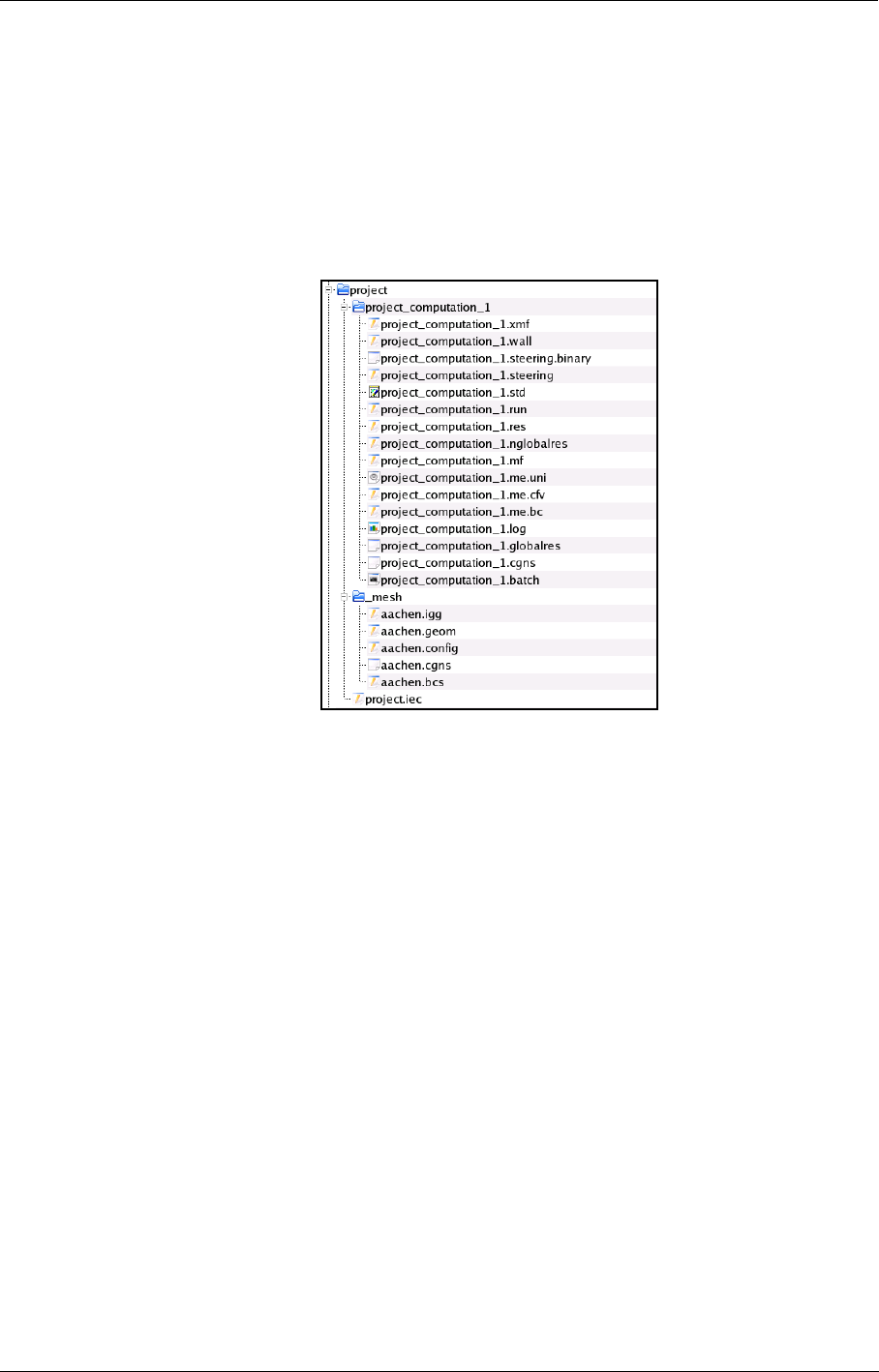
FINE™/Turbo:
•The grid files: The grid generation process, IGG™, creates files containing the representation
of the geometry and the grid related to the project. The definition of the types of boundary con-
ditions is also done during this process. The five files that contain the information about the
mesh have the extensions ".igg", ".geom", ".bcs", ".config" and ".cgns".
•The project file: The project file is created by FINE™/Turbo. It has the extension ".iec" and
contains the input parameters needed for the flow computations.
•The result files: FINE™/Turbo creates a new subdirectory for each computation where it
stores the following files:
—a file with extension ".run" containing all computation input parameters used by the solver
and by CFView™,
—a ".cgns" file that contains the solution and that is used for restarting the solver,
—a ".res" file used by the Monitor to visualize the residual history (see Chapter 12),
—two files used to visualize the convergence history in the Steering with extensions ".steer-
ing" and ".steering.binary" (see Chapter 12).
—two files with extensions ".mf" and ".wall" that contain global solution parameters.
—a ".xmf" file that stores the information contained in the ".mf" file in XML format.
—two files with extensions ".std" and ".log" that contain information on the flow computation
process.
—a ".batch" file used to launch the computation in batch (see Chapter 11).
•The CFView™ visualization files: In addition to the ".run" file, the flow solver creates a
series of files, which can be read by CFView™. These files have different extensions. For
example in case of turbomachinery flow problem, the solver will create a file for the azimuthal
averaged results with extension ".me.cfv".
Through the interface, the user can modify all the information stored in the files associated to the
project.
When creating a new project a new directory is made, e.g. "/project". In this directory the project
file is stored "/project/project.iec" and a directory is created called "/project/_mesh". In this direc-
tory the grid files used for the computations can be stored. It is however also possible to select a
grid that is located in another directory.
Only one mesh file should be used for all computations in a project. If computations
need to be done on another mesh file it is advised to duplicate the project (see section 2-
Introduction Getting Started
FINE™/Turbo 1-3
3.1.4) or to create a new project (see section 2-3.1.1) for those computations.
The special characters, such as ü, ë and ê et al., are not allowed in the path name.
Off line files on Windows operation system are not supported.
The length of the path name should be less than 256.
FIGURE 1.2.3-1 Example of file management for a FINE™/Turbo project
Both the absolute and relative path names are used in ".iec" and ".run" files for the mesh and initial
solution files. When moving the project from one location to another location in the local machine
or between different machines (the same or different OS), the use of the relative pathnames allows
the user to:
•open the graphical user interface and (re)start calculation without the need to (re)link the mesh
and pathnames,
•open a solution file within CFView™ without the need to open the graphical user interface,
•start calculations in batch mode without the need to open the graphical user interface and
(re)link the mesh and pathnames.
The limitations on the use of relative pathnames are as follows:
•All files (mesh and computations) related to a given project must be located in hard-coded sub-
directories (e.g. _mesh).
•Keywords related to relative path in ".iec" and ".run" files are only vaild if the concerned files
are at the same level of the project file ".iec" or in subdirectories.
•Both the project and the directory in which it is included must have the same name. They can’t
be renamed.
•When duplicating or moving the project, the user must be able to copy either the entire project
(mesh files and computations with existing solutions), or a partial project (mesh files and com-
putations, restricted to ".run" files)

Getting Started How To Use This Manual
1-4 FINE™/Turbo
•Relative path is not compatible with FINE™/Design3D.
1-3 How To Use This Manual
1-3.1 Outline
This manual consists of five distinct parts:
•Chapters 1 and 2: introduction and description of the interface,
•Chapters 3 to 10: computation definition,
•Chapter 11: task management,
•Chapter 12: monitoring capabilities,
•Appendix A: used file formats,
•Appendix B: list of supported non-interfaced expert parameters,
•Appendix C: characteristics of steam tables.
At first time use of FINE™/Turbo it is recommended to read this first chapter carefully and cer-
tainly section 1-4 to section 1-6. Chapter 2 gives a general overview of the FINE™/Turbo interface
and the way to manage a project. For every computation the input parameters can be defined as
described in the Chapters 3 to 10. Chapter 11 gives an overview of how to run computations using
the Task Manager or using a script. Chapter 12 finally describes the available tools to monitor the
progress on a computation.
In Chapters 3 to 10, the expert user finds a section describing advanced options that are available in
expert user mode. Additionally Appendix B provides a list with all supported expert parameters on
the page Computation Steering/Control Variables in expert user mode. For each parameter a ref-
erence is given to the section in the manual where it is described.
The use of non-supported parameters is at own risk and will not guarantee correct
results.
1-3.2 Conventions
Some conventions are used to ease information access throughout this guide:
•Commands to type are in italics.
•Keys to press are in italics and surrounded by <> (e.g.: press <Ctrl>).
•Names of menu or sub-menu items are in bold.
•Names of buttons that appear in dialog boxes are in italics.
•Numbered sentences are steps to follow to complete a task. Sentences that follow a step and are
preceded with a dot (•) are substeps; they describe in detail how to accomplish the step.
The hand indicates an important note
The pair of scissors indicates a keyboard short cut.

First Time Use Getting Started
FINE™/Turbo 1-5
A light bulb in the margin indicates a section with a description of expert parameters.
1-4 First Time Use
1-4.1 Basic Installation
When using FINE™/Turbo for the first time it is important to verify that FINE™/Turbo is properly
installed according to the installation note. The installation note provided with the installation soft-
ware should be read carefully and the following points are specifically important:
•Hardware and operating system requirements should be verified to see whether the chosen
machine is supported.
•Installation of FINE™/Turbo according to the described procedure in a directory chosen by the
user and referenced in the installation note as ‘NUMECA_INSTALLATION_DIRECTORY’.
•A license should be requested that allows for the use of FINE™/Turbo and the desired compo-
nent and modules (see section 1-6 for all available licenses). The license should be installed
according to the described procedure in the installation note.
•Each user willing to use FINE™/Turbo or any other NUMECA software must perform a user
configuration as described in the installation note.
When these points are checked the software can be started as described in the installation note or
section 1-5 of this user manual.
1-4.2 Expert Graphics Options
a) Graphics Driver
The graphics area of the FINE™/Turbo interface uses by default an OPENGL driver that takes
advantage of the available graphics card. When the activation of OPENGL is causing problems,
FINE™/Turbo uses an X11 driver (on UNIX) or MSW driver (for Windows) instead.
It is possible to explicitly change the driver used by FINE™/Turbo in the following ways:
On UNIX:
in csh, tcsh or bash shell:
setenv NI_DRIVER X11
in korn shell:
NI_DRIVER=X11
export NI_DRIVER
The selection will take effect at the next session.
On Windows:
•Log in as Administrator.
•Launch regedit from the Start/Run menu.
•Go to the HKEY_LOCAL_MACHINE/SOFTWARE/NUMECA International/Fine# register.
•Modify the DRIVER entry to either OPENGL or MSW.

Getting Started How to start the FINE™/Turbo Interface
1-6 FINE™/Turbo
The selection will take effect at the next session.
b) Background Color
The background color of the graphics area can be changed by setting the environment variable
NI_IGG_REVERSEVIDEO on UNIX/LINUX platforms or IGG_REVERSEVIDEO on Windows
platforms. Set the variable to ’ON’ to have a black background and set it to ’OFF’ to have a white
background. The variable can be manually specified through the following commands:
On UNIX:
in csh, tcsh or bash shell:
setenv NI_IGG_REVERSEVIDEO ON
in korn shell:
NI_IGG_REVERSEVIDEO=ON
export NI_IGG_REVERSEVIDEO
The selection will take effect at the next session.
On Windows:
•Log in as Administrator.
•Launch System Properties from the Start/Settings/Control Panel/System menu.
•Go in the Environment Variables.
•Modify or add the IGG_REVERSEVIDEO entry to either ON or OFF.
The selection will take effect at the next session.
1-5 How to start the FINE™/Turbo Interface
In order to run FINE™/Turbo, the following command should be executed:
On UNIX and LINUX platforms type: fine -print <Enter>
When multiple versions of FINE™/Turbo are installed the installation note should be
consulted for advice on how to start FINE™/Turbo in a multi-version environment.
On Windows click on the FINE™/Turbo icon in Start/Programs/NUMECA software/fine#.
Alternatively FINE™/Turbo can be launched from a dos shell by typing:
<NUMECA_INSTALLATION_DIRECTORY>\fine#\bin\fine <Enter>
where NUMECA_INSTALLATION_DIRECTORY is the directory indicated in section 1-4.1 and #
is the number corresponding to the version to be used.

Required Licenses Getting Started
FINE™/Turbo 1-7
1-6 Required Licenses
1-6.1 Standard FINE™/Turbo License
The standard license for FINE™/Turbo allows for the use of all basic features of FINE™/Turbo
including:
•IGG™ (see separate IGG™ manual),
•AutoGrid™ (see separate AutoGrid™ manuals),
•CFView™ (see separate CFView™ manual),
•Task Manager (see Chapter 11),
•Monitor (see Chapter 12).
1-6.2 Additional Licenses
Within FINE™/Turbo the following features are available that require a separate license:
•parallel computations (see Chapter 11),
•treatment of unsteady rotor-stator interfaces (see Chapter 8),
•harmonic method (see Chapter 8),
•transition (see Chapter 4 and Chapter 8),
•fluid-particle interaction (see Chapter 7),
•passive tracers (see Chapter 7),
•conjugate heat transfer (see Chapter 7),
•thermodynamic tables (see Chapter 3),
•cooling/bleed flow (see Chapter 8),
•ANSYS outputs (see Chapter 10),
•SubProject module (see Chapter 8),
•porous media (see Chapter 7),
•cavitation module (see Chapter 7).
•MpCCI Coupling (Chapter 7)
•Modal Coupling (Chapter 7)
•Mesh Deformation (Chapter 7)
•Aeroacoustics (Chapter 8)
•CPU Booster (Chapter 6)
Next to FINE™/Turbo other products are available that require a separate license:
•FINE™/Design 3D (3D inverse design, see separate user manual).

Getting Started Required Licenses
1-8 FINE™/Turbo
FINE™/Turbo 2-1
CHAPTER 2: Graphical User
Interface
2-1 Overview
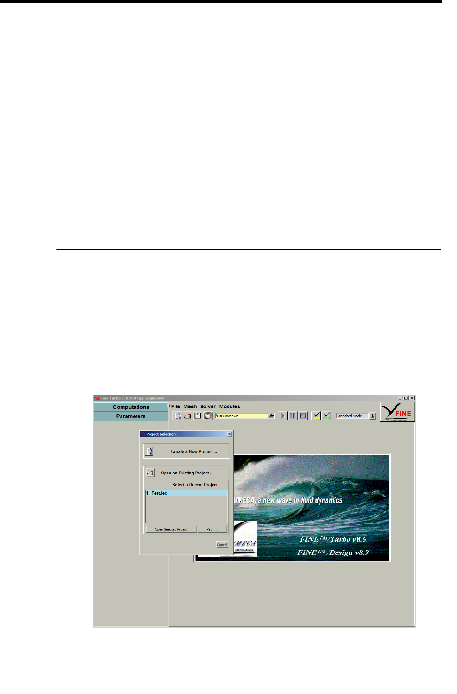
When launching FINE™/Turbo as described in Chapter 1 the interface appears in its default layout
as shown in Figure 2.1.0-1. An overview of the complete layout of the FINE™/Turbo interface is
shown on the next page in Figure 2.1.0-2. In the next sections the items in this interface are
described in more detail.
Together with the FINE™/Turbo interface a Project Selection window is opened, which allows to
create a new project or to open an existing project. See section 2-2 for a description of this window.
To define a profile through the FINE™/Turbo interface a Profile Manager is included. The Profile
Manager is described in more detail in section 2-7.
FIGURE 2.1.0-1 Default FINE™/Turbo Interface
Graphical User Interface Project Selection
2-2 FINE™/Turbo
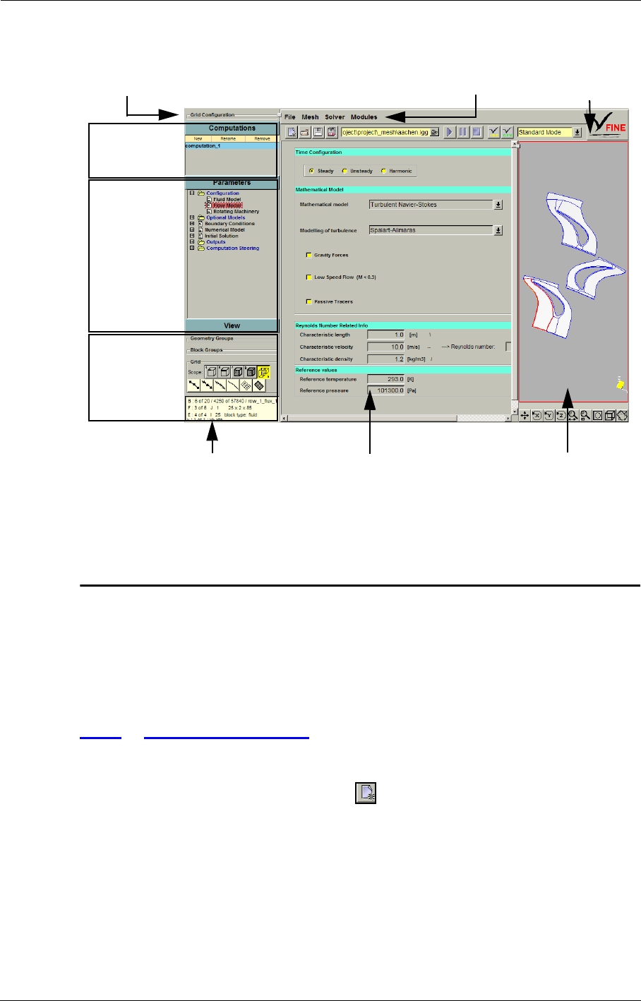
FIGURE 2.1.0-2 Complete overview of the FINE™/Turbo interface
2-2 Project Selection
When the FINE™/Turbo interface is started the Project Selection window is appearing together
with the interface. This window allows to create a new project or to open an existing one as
described in the next sections. After use of this window it is closed. To open a project or to create a
new one without the Project Selection window is also possible using the File menu.
2-2.1 Create New Project
To create a new project when launching the FINE™/Turbo interface:
1. click on the Create a New Project... icon ( ) in the Project Selection dialog box. A File
Chooser will appear, which allows to select a name and location for the new project.
The layout of the File Chooser depends on the used operating system but a typical layout is shown
in Figure 2.2.1-3. The Directories list allows to browse through the available directory structure to
the project directory. Then the Files list can be used to select the file name. In the case a file needs
to be opened an existing file should be selected in the list of available files. In the case a new file
needs to be created the user can type a new file name with the appropriate extension. In the List
Files of Type bar the default file type is set by default to list only the files of the required type.
Main menu bar Icon bar
Computations
Parameters
button
Graphics area Parameters area
Mesh information
View
button
button
Grid Configuration (under license)
Project Selection Graphical User Interface
FINE™/Turbo 2-3
FIGURE 2.2.1-3 Typical layout of a File Chooser window
2. In the Directories text box on UNIX a name can be typed or the browser under the text box may
be used to browse to an appropriate location. On Windows, the browser under the Save in text
box is used to browse to an appropriate location.
3. Once the location is defined type on UNIX and on Windows a new name in the text box under
respectively Files and File name, for example "project.iec" (it is not strictly necessary to add the
extension ".iec", FINE™/Turbo will automatically create a project file with this extension).
4. Click on OK (on UNIX) or Save (on Windows) to accept the selected name and location of the
new project.
A new directory is automatically created with the chosen name as illustrated in figure below indi-
cated by point (1). All the files related to the project are stored in this new directory. The most
important of them is the project file with the extension ".iec", which contains all the project settings
(Figure 2.2.1-4 - (2)). Inside the project directory FINE™/Turbo creates automatically a subdirec-
tory "_mesh" (Figure 2.2.1-4 - (3)).
FIGURE 2.2.1-4 Directories managed through FINE™/Turbo
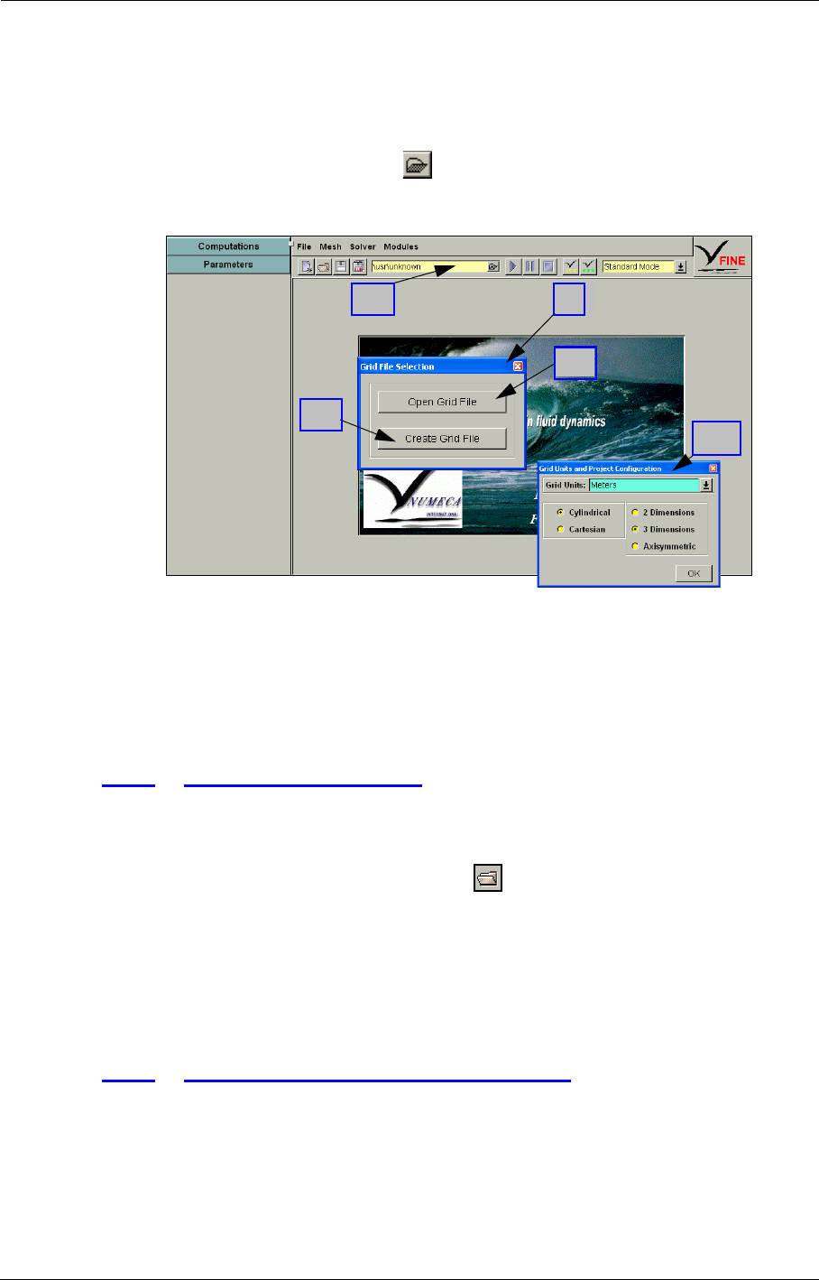
5. A Grid File Selection window (Figure 2.2.1-5) appears to assign a grid to the new project. There
are three possibilities:
•To open an existing grid click on Open Grid File (Figure 2.2.1-5 - 1.1). A File Chooser allows
to browse to the grid file with extension ".igg". Select the grid file and press OK to accept the
selected mesh. A window appears to define the Grid Units and Project Configuration
(Figure 2.2.1-5 - 1.2). Set the parameters in this window as described in section 2-2.3 and click
OK to accept.
(1) project directory
(2)
(3)
automatically created
"_mesh" directory
(4) computation directory
Graphical User Interface Project Selection
2-4 FINE™/Turbo
•If the grid to be used in the project is not yet created use Create Grid File to start IGG™
(Figure 2.2.1-5 - 2.1). Create a mesh in IGG™ or AutoGrid™ (Modules/AutoGrid4 - Mod-
ules/AutoGrid5) and save the mesh in the directory "_mesh" of the new project. Click on
Modules/Fine Turbo and confirm "yes" to return to the FINE™/Turbo project. Select the cre-
ated mesh with the pull down menu (Figure 2.2.1-5 - 2.2) in the icon bar. A window will
appear to define the Grid Units and Project Configuration. Set the parameters in this window
as described in section 2-2.3 and click OK to accept.
FIGURE 2.2.1-5 Grid File Selection window.
•When using the AutoBlade™ or FINE™/Design 3D modules it is not necessary to select a
grid. In that case close the Grid File Selection window (Figure 2.2.1-5 - 3) and select Mod-
ules/AutoBlade or Modules/Design 3D menu to use these modules.
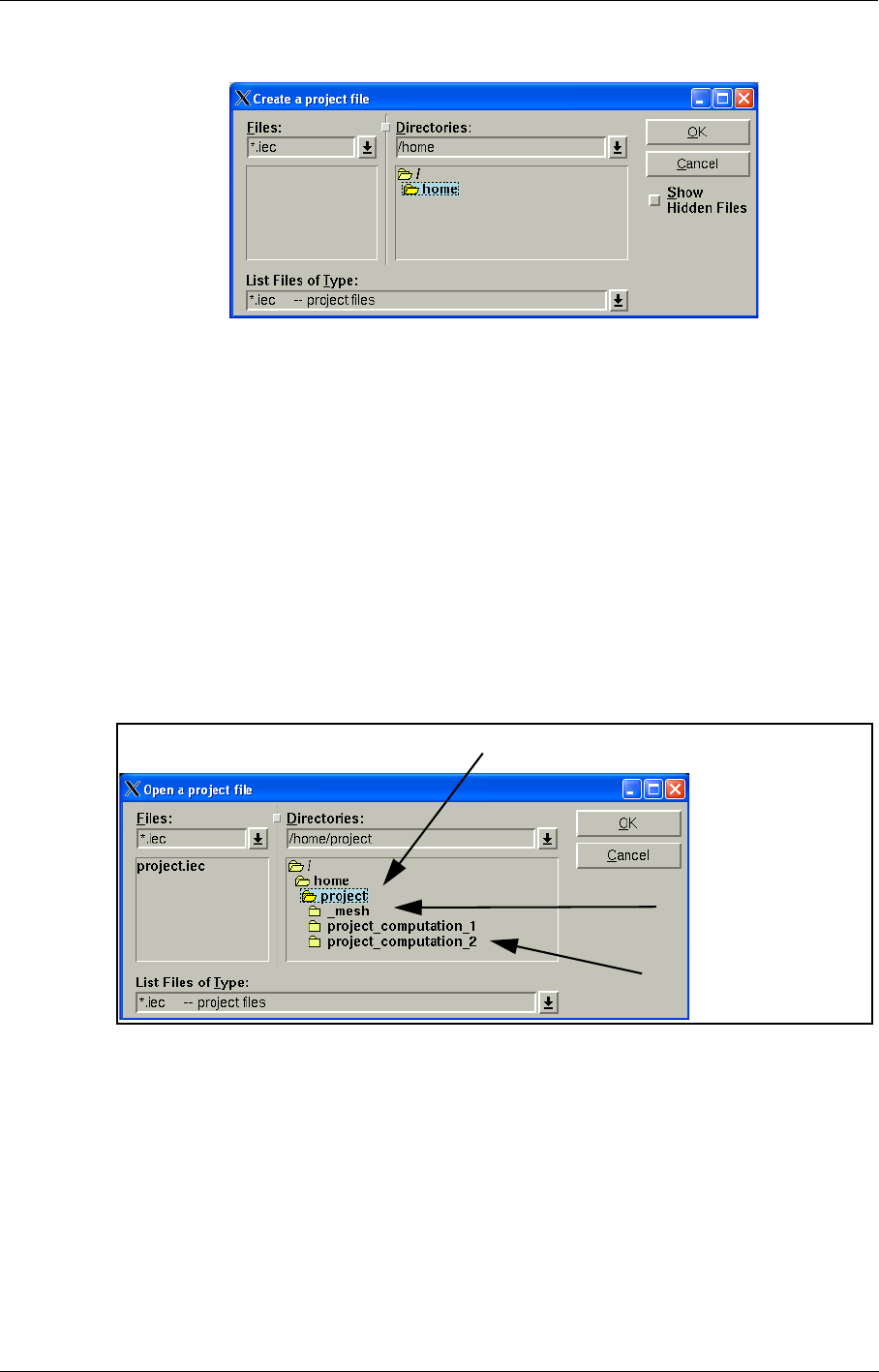
2-2.2 Open Existing Project
To open an existing project the two following possibilities are available in the Project Selection
window:
•Click on the icon Open an Existing Project... (). A File Chooser will appear that allows to
browse to the location of the existing project. Automatically the filter in the File Chooser is set
to display only the files with extension ".iec", the default extension for a project file.
•Select the project to open in the list of Recent Projects, which contains the five most recently
used project files. If a project no longer exists it will be removed from the list when selected.
To view the full path of the selected project click on Path... To open the selected project click
on Open Selected Project.
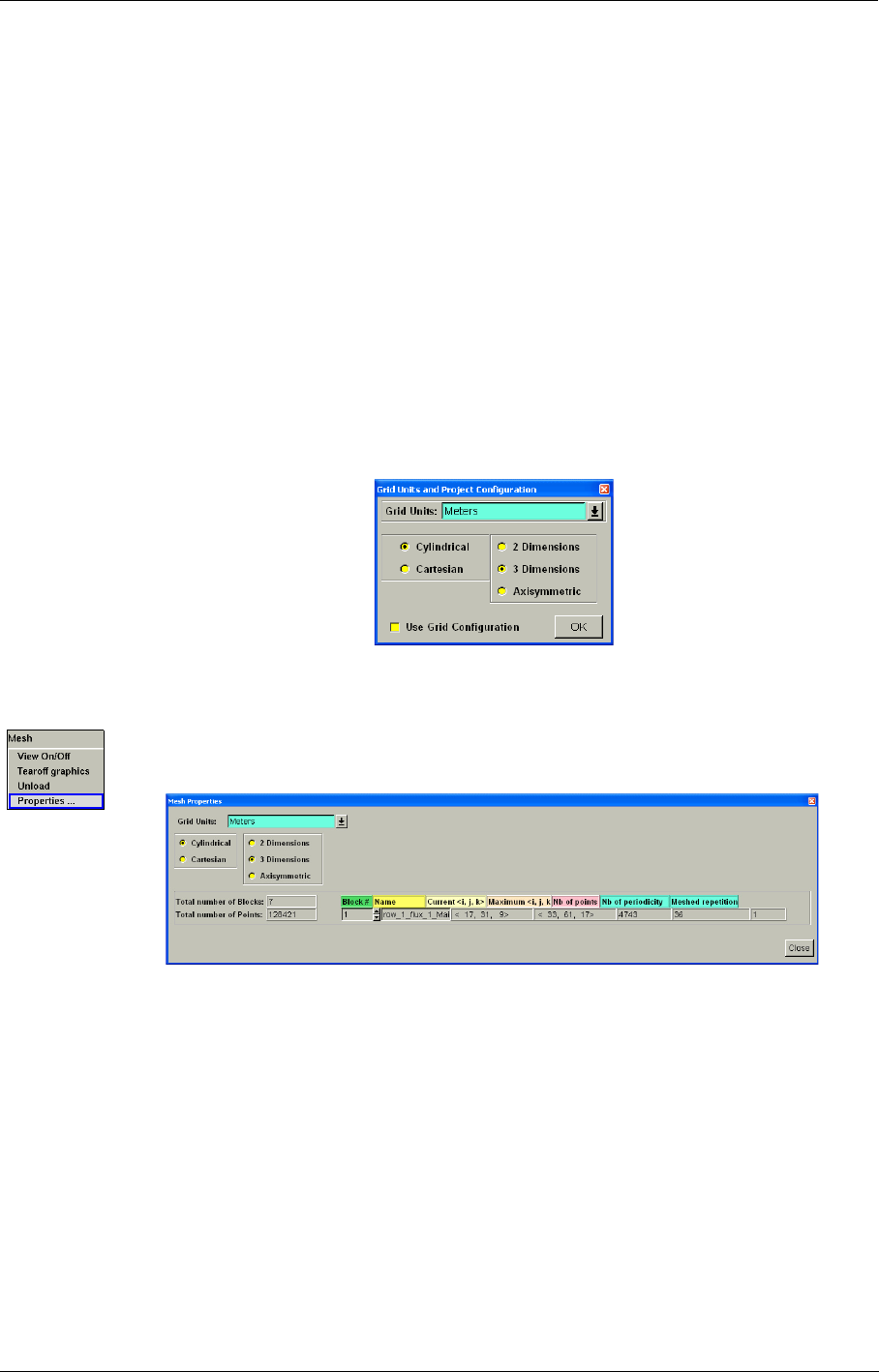
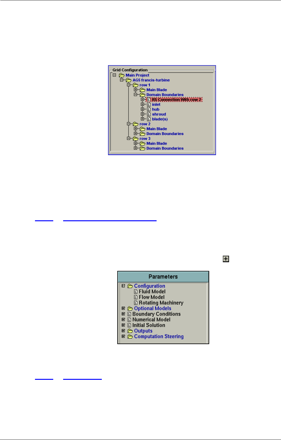
2-2.3 Grid Units & Project Configuration
The Grid Units and Project Configuration window shows some properties of the selected mesh
when linking the mesh to the project:
•Grid Units: the user specifies the grid units when importing a mesh. The user may define a
different scale factor to convert the units of the mesh to meters. The scale factor is for instance
0.01 when the grid is in centimeters.
1.1
1.2
2.1
2.2 3
Project Selection Graphical User Interface
FINE™/Turbo 2-5
•Space Configuration: allows the user to specify whether the mesh is cylindrical or Cartesian
and the dimensionality of the mesh. In case the mesh is axisymmetric the axis of symmetry
should be defined.
If a 2D project is created by selecting Cartesian and 2 Dimensions, the mesh must have
K direction and Z direction perpendicular to the surface.
Some options in FINE™/Turbo are linked to the used mesh configuration. For example,
the Cartesian mesh is not compatible with some TURBO features (Rotating Blocks, Azi-
muthal averaged output, ...). The user should select an appropriate coordinate system
according to the applications.
•Use Grid Configuration: This option is only available with a special license feature (Sub-
Projects). The user can choose whether or not to use the automatic grouping based on the grid
configuration file (.config). More information on the automatic grouping can be found in
Chapter 8. This choice can only be made when loading the mesh for the first time, it cannot be
changed afterwards.
FIGURE 2.2.3-6 Grid Units & Project Configuration window
The mesh properties are always accessible after linking the mesh to the project through
the menu Mesh/Properties...

Graphical User Interface Main Menu Bar
2-6 FINE™/Turbo
2-3 Main Menu Bar
2-3.1 File Menu
2-3.1.1 New Project
The menu item File/New allows to create a new FINE™/Turbo project. When clicking on File/New
a File Chooser window appears. Browse in the Directory list to the directory in which to create a
new project directory (in the example of Figure 2.2.1-4 the directory "/home" was selected). Give a
new name for the project in the File list, for example "project.iec" and click on OK to create the
new project.
When starting a new project a new directory is automatically (Figure 2.2.1-4) created with the cho-
sen name (1). All the files related to the project are stored in this new directory. The most important
of them is the project file with the extension ".iec", which contains all the project settings (2). Inside
the project directory FINE™/Turbo creates automatically a subdirectory "_mesh" (3). As all the
computations of the project must have the same mesh it is advised to store the mesh in this specially
dedicated directory. Each time the user creates a new computation, a subdirectory is added (4). The
output files generated by the flow solver will be written in the subdirectory of the running computa-
tion.
After the new project is created a Grid File Selection window (Figure 2.2.1-5) appears to assign a
grid to the new project. There are two possibilities:
•To open an existing grid click on Open Grid File. A File Chooser allows to browse to the grid
file with extension .igg. Select the grid file and press OK to accept the selected mesh. A win-
dow appears to define the Grid Units and Project Configuration. Set the parameters in this
window as described in section 2-2.3 and click OK to accept.
•If the grid to be used in the project was not yet created use Create Grid File to start IGG™.
Create a mesh in IGG™ or AutoGrid™ (Modules/AutoGrid4 - Modules/AutoGrid5) and
save the mesh in the directory "_mesh" of the new project. Click on Modules/Fine Turbo and
confirm "yes" to return to the FINE™/Turbo project. Select the created mesh with the pull
down menu in the icon bar. A window will appear to define Grid Units and Project Configura-
tion. Set the parameters in this window as described in section 2-2.3 and click OK to accept.
If the name of an already existing project is specified, this project file will be overwrit-
ten. All other files and subdirectories will remain the same as before.
By default, no IGG™ file is associated with the new project and it is indicated "usr/
unknown" in the place of the grid file name. The procedure to link a mesh file to the
project is explained in section 2-4.2.
2-3.1.2 Open Project
There are two ways to open an existing project file:
a) Use File/Open Menu
1. Click on File/Open.
2. A File Chooser window appears.
3. Browse through the directory structure to find the project file to open. This file has normally the
".iec" extension. If this is not the case, the file filter in the input box named 'List Files of Type',
has to be modified.
Main Menu Bar Graphical User Interface
FINE™/Turbo 2-7
4. Select the project file.
5. Click on the file name and press the OK button.
The opened project becomes the active project. All subsequent actions will be applied to this
project.
b) Select File From the List of Files in File Menu.
The File menu lists the names of the five most recent projects that have already been opened. Click
on a project name from this menu to open this project.
FINE™/Turbo will check the write permission of the project directory and the project file and will
issue a warning if the project or directory is read only. In both cases the project can be modified, but
the changes will not be saved.
Only one project can be active. Opening a second project will save and close the first
one.
An attempt to open a no longer existing project will remove its name from the list in the
File menu.
2-3.1.3 Save Project
The File/Save menu item stores the project file (with extension ".iec") on disk. The project file is
automatically saved when the flow solver is started and can be saved when FINE™/Turbo is closed
or when another project is opened.
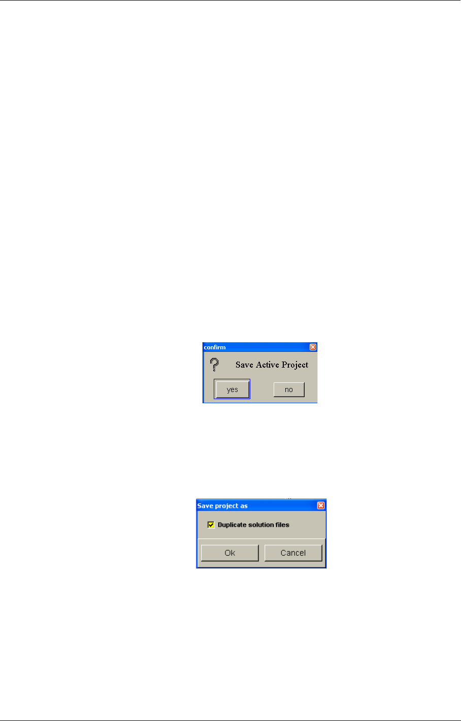
2-3.1.4 Save As Project
File/Save As is used to store the active project on disk under different name. A File Chooser opens
to specify the new directory and name of the project. When this is done a dialog box asks whether
to save all the results files associated with the project. If deactivated, only the project file (with the
extension ".iec") will be saved in the new location.
2-3.1.5 Save Run Files
File/Save Run Files is used to store all the information needed for the flow solver in the ".run" file
of the active computation (highlighted in blue in the Computations list). This menu is mainly use-
ful when the Task Manager is used (see Chapter 11 for a detailed description of the Task Manager).
Together with the ".run" file, a ".batch" (UNIX) or ".bat" (Windows) file is saved. This
file can be used to launch the computation in batch mode, without the need of opening
Graphical User Interface Main Menu Bar
2-8 FINE™/Turbo
the interface. More information on how to use this ".batch" file can be found in
Chapter 11.
If more than one computation is selected in the Computations list, then all parameters in
the Parameters area will be assigned to all selected (active) computations. This may be
dangerous if the parameters for the currently opened information page are not the same
for all the selected computations. To avoid this it is recommended to select only one
computation at a time.
The ".run" file is automatically updated (or created if not existing) when starting a com-
putation through the main menu (Solver/Start...).
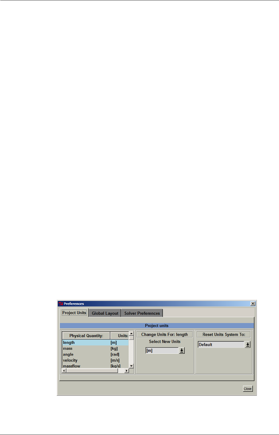
2-3.1.6 Preferences
When clicking on File/Preferences... the Preferences window appears and gives access to some
project specific and global settings:
a) Project Units
In this section the user can change the units system of the project. The units can be changed inde-
pendently for a selected physical quantity or for all of them at the same time. To change the units
for one specific quantity select the quantity in the list (see (1) in Figure 2.3.1-7). Then select the
unit under Select New Units (2). To change the units for all physical quantities at the same time use
the box Reset Units System To (3).
The default system proposed by NUMECA is the standard SI system except for the unit for the
rotational speed, which is [RPM].
When the user changes the units, all the numerical values corresponding to the selected physical
quantity are multiplied automatically by the appropriate conversion factor. The numerical values
are stored into the project file ".iec" in the same units as they appear in the interface (e.g. the rota-
tion speed is in [RPM]), but in the ".run" file, which is used by the flow solver, the numerical values
are always stored in SI units (e.g the rotation speed is in [rad/s]). The results can be visualized with
the flow visualization system CFView™ in the units specified in FINE™/Turbo.The change of the
units can be done at any stage of the creation of the project.
User-defined units can be defined through a text file "euranus.uni". Please contact our local support
office for more information.
FIGURE 2.3.1-7 Project Units in the Preferences Window
(1)
(2) (3)
Main Menu Bar Graphical User Interface
FINE™/Turbo 2-9
b) Global Layout
In this section, the user may specify project independent preferences for the layout of the interface.
More specifically the user may activate or deactivate the balloon help (Show Balloon Help), which
gives short explanation of the buttons when the mouse pointer is positioned over them. By default
balloon help is activated. Deactivation of the balloon help will only be effective for the current ses-
sion of FINE™/Turbo. When FINE™/Turbo is closed and launched again the balloon help will
always be active by default.
Furthermore, the section allows the user to control the Number of curves that can be plotted in the
Convergence History page of the Task Manager. By default the parameter is set to 10 meaning that
only 9 curves can be plotted in the steering (more details in Chapter 12).
c) Solver Preferences
In this section, the user may select the calculation accuracy for the flow solver. Single and double
precision modes of the FINE™/Turbo solver are available. For most cases, the single precision
solver (much less demanding in memory consumption) will be sufficiently accurate and should be
considered as the default option. However, some special cases, such as very long thin pipe and con-
jugate heat transfer problems, may benefit from the double precision solver.
One of the most important criteriums to choose the double precision solver is the maximum dimen-
sion of the domain and its positioning in the 3D field. If the ratio is bigger than roughly
1e-6, the double precision solver should be considered. Where is the local cell size and is
the local coordinate value.
After selecting single or double precision solver, the value will be used as default value for new
projects.
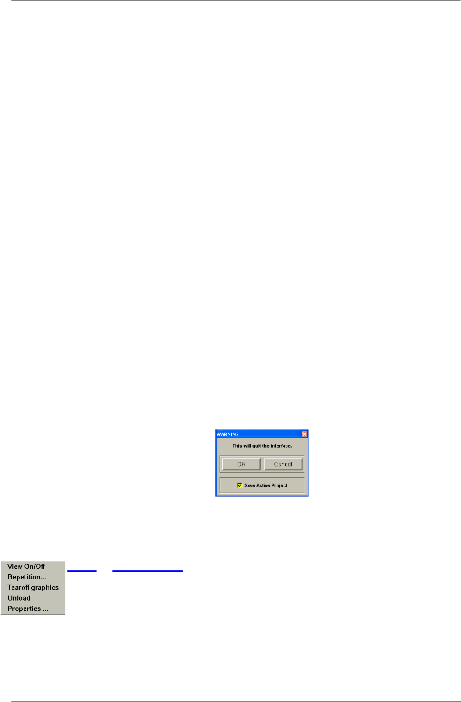
2-3.1.7 Quit
Select the File/Quit menu item to quit the FINE™/Turbo integrated environment after confirmation
from the user. The active project will be saved automatically by default (Save Active Project acti-
vated).
Note that this action will not stop the running calculations. A FINE TaskManager window will
remain open for each running computation. Closing the FINE TaskManager window(s) will kill the
running calculation(s) after confirmation from the user.
2-3.2 Mesh Menu
2-3.2.1 View On/Off
This toggle menu is used to visualize the grid in FINE™/Turbo GUI. It may take few seconds to
load the mesh file for the first time. The parameters area will be overlapped by the graphic window,
and the small control button on the upper - left corner of the graphic window can be used to resize
the graphics area in order to visualize simultaneously the parameters and the mesh (see section 2-
Δxx
local
⁄
Δx
xlocal
Graphical User Interface Main Menu Bar
2-10 FINE™/Turbo
6.6). Once the mesh is opened, the same menu item Mesh/View On/Off will hide it. Note that the
mesh will stay in the memory and the following use of the menu will visualize it much faster than
the first time.
When the mesh is loaded the following items appear in the FINE™/Turbo interface:
• the View subpad (see section 2-6.3 for more details),
•the mesh information area (see section 2-6.4 for more details),
•the graphics area will appear in the FINE™/Turbo interface (see section 2-6.6 for more
details),
•the Viewing buttons will appear on the bottom of the graphics area. Their function is described
in section 2-6.7).
The graphics area and the Viewing buttons will disappear when the mesh is hidden (Mesh/View
On/Off). All the tools will disappear when the mesh is unloaded (Mesh/Unload).
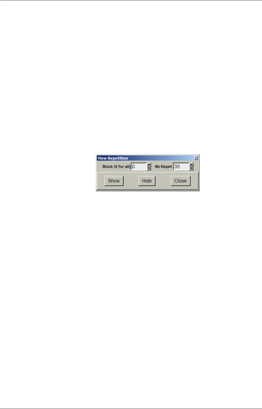
2-3.2.2 Repetition
This menu opens the following dialog box to control the repetition of the blocks when the mesh is
visualized:
For each block, the number of repetition desired can be set in the Nb Repet entry. The repetition of
all blocks can be displayed or hidden respectively by pressing the Show or Hide button.
2-3.2.3 Tearoff graphics
This menu transfers the graphics area and its control buttons into a separate window. Closing this
window will display the graphics area back in the main FINE™/Turbo window.
This feature is only available on UNIX systems.
2-3.2.4 Unload
Mesh/Unload clears the mesh from the memory of the computer.
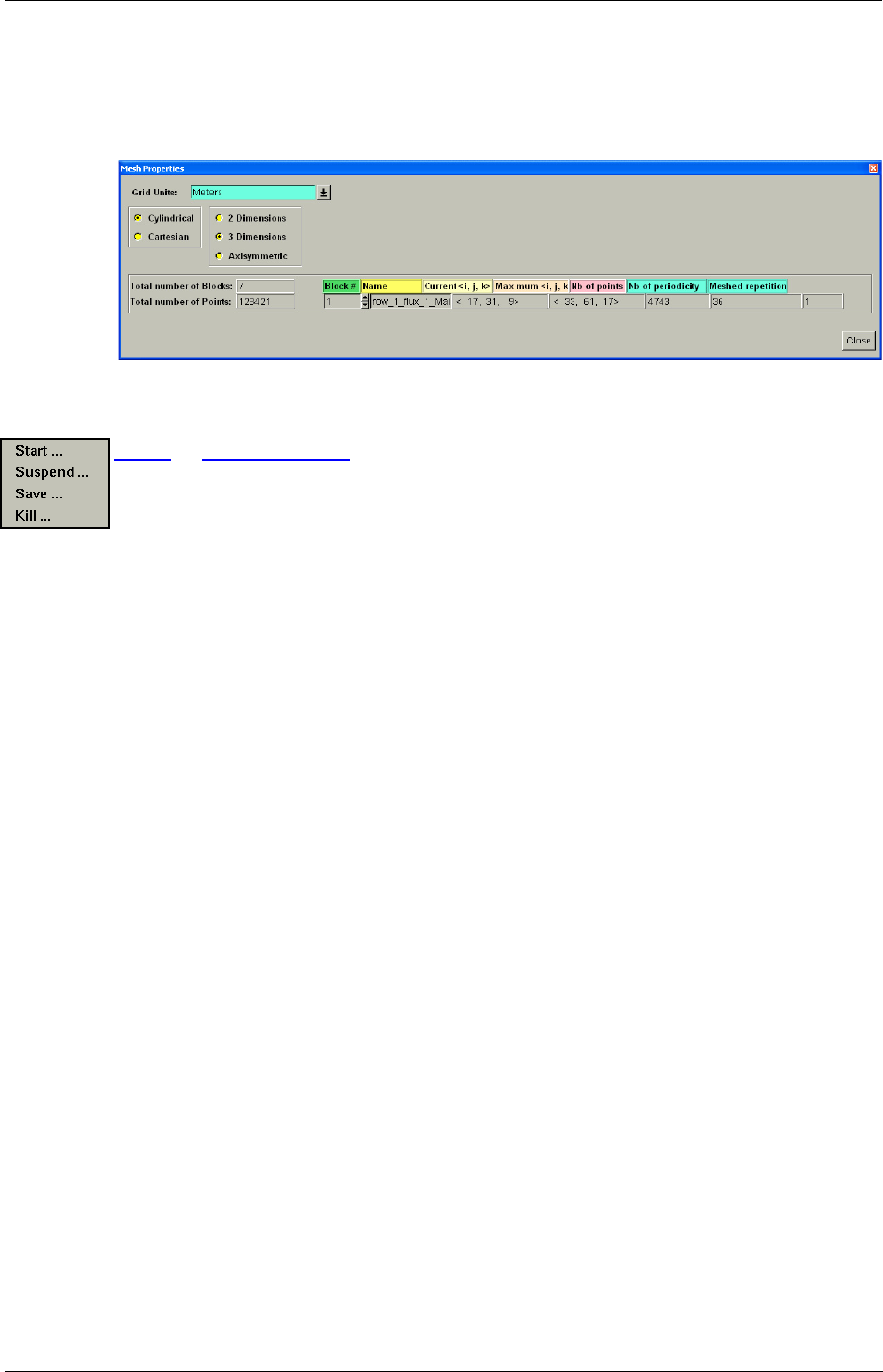
2-3.2.5 Properties
Clicking on Mesh/Properties... opens a dialog box that displays global information about the
mesh:
•Grid Units: the user specifies the grid units when importing a mesh. When importing a mesh
the Grid Units and Project Configuration window appears, which allows the user to check the
mesh units (see section 2-2.3). The chosen units can be verified and, if necessary, changed.
•Space Configuration: allows the user to verify whether the mesh is cylindrical or Cartesian
and the dimensionality of the mesh. When importing a mesh the Grid Units and Project Con-
figuration window allows the user to check these properties. Those chosen properties can be
verified and, if necessary, changed.
•The total number of blocks and the total number of points are automatically detected from the
mesh.
Main Menu Bar Graphical User Interface
FINE™/Turbo 2-11
•For each block: the current (depending on the current grid level) and maximum number of
points in each I, J and K directions, and the total number of points are automatically detected
from the mesh.
FIGURE 2.3.2-8 Mesh Properties dialog box
2-3.3 Solver Menu
This menu gives access to the FINE™/Turbo solver, which is a powerful 3D code dedicated to
Navier-Stokes or Euler computations. The FINE™/Turbo solver uses the computational parameters
and boundary conditions set through the FINE™/Turbo GUI and can be fully controlled both from
the FINE™/Turbo Solver Menu and from the Task Manager (see Chapter 11).
In this section, the information is given on how to start, suspend, interrupt and restart the flow
solver. All these actions may be simply performed by using the pull down menu appearing when the
button Solver of the Menu bar is clicked.
2-3.3.1 Start Flow Solver
To start the flow solver, select the menu item Solver/Start....
It is not recommended to start the flow solver before setting the physical boundary conditions and
the computational parameters.
Using the Start item to run the flow solver on active computation implies that the result file pro-
duced by a previous calculations on that computation will be overwritten with the new result val-
ues. It also implies that the initial solution will be created from the values set in the Initial Solution
page.
To restart a computation from an existing solution the solver should be also started using
the Solver/Start... menu. On the Initial Solution page the initial solution has to be spec-
ified from an existing file (".run"). Chapter 9 describes the several available ways to
define an initial solution.
2-3.3.2 Save
To save an intermediate solution while the flow solver is running click on Solver/Save....
2-3.3.3 Stop Flow Solver
There are two different ways to stop the flow solver:
•Solver/Suspend... interrupts the flow computation after the next iteration. This means that the
flow solver stops the computation at the end of the next finest grid iteration and outputs the
current state of the solution (solution files and CFView™ files) exactly as if the computation
was finished. This operation may take from few seconds to few minutes depending on the
Graphical User Interface Icon Bar
2-12 FINE™/Turbo
number of grid points in the mesh. Indeed, if the finest grid is not yet reached, the flow solver
continues the full multigrid stage and stops only after completion of the first iteration on the
finest grid.
•Solver/Kill... allows to stop immediately the computation for the active project. In this case no
output is created and the only solution left is the last one that was output during the run. This
may become a dangerous choice if asked during the output of the solution. The output is then
ruined and all the computation time is lost. To avoid this, it is better to use Solver/Suspend...
or to kill the computation some iterations after the writing operations.
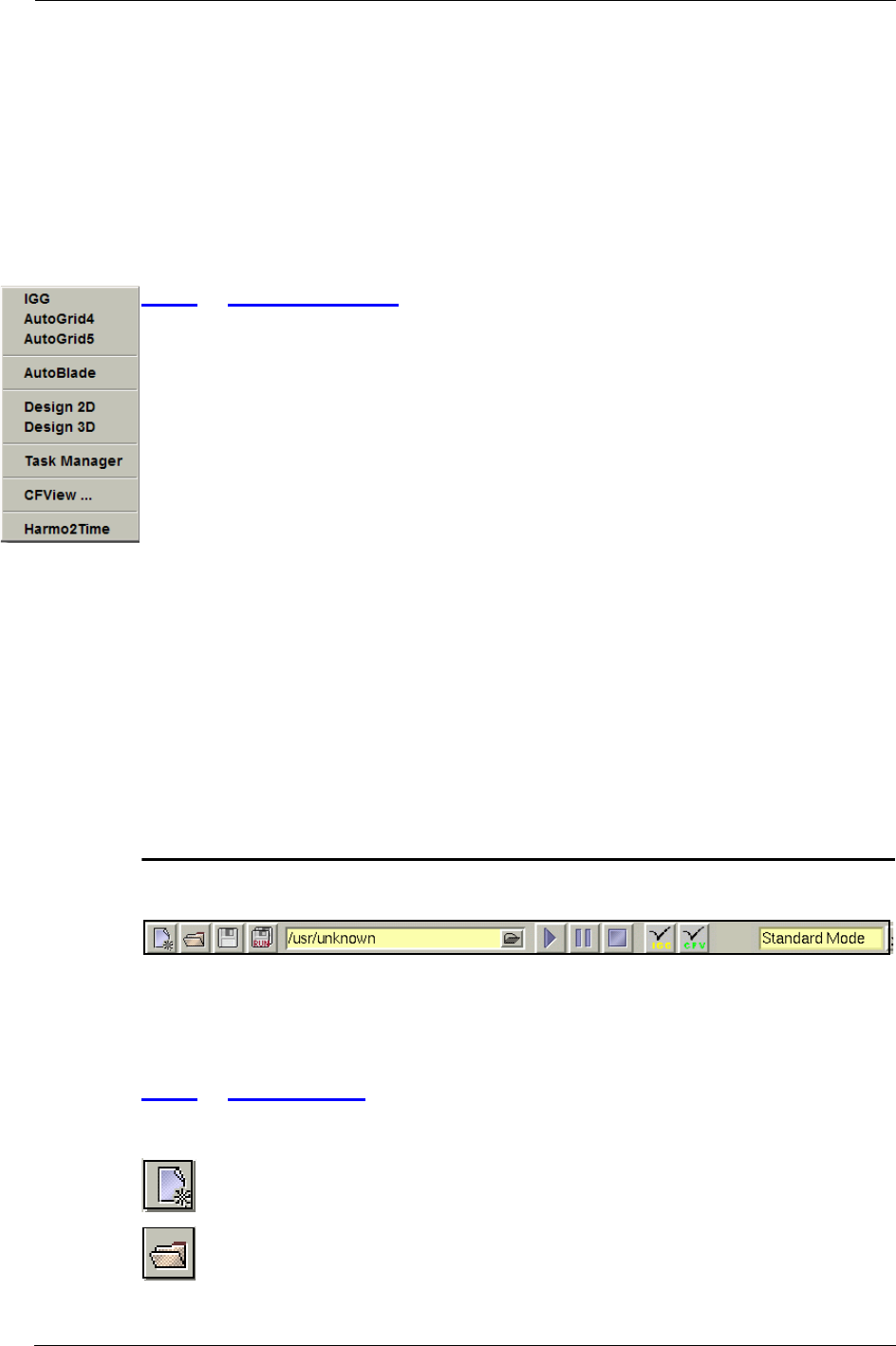
2-3.4 Modules Menu
Clicking on the menu item Modules shows a pull down menu with the available modules. The first
four items are related to geometry and mesh definition:
•IGG™ is the interactive geometry modeller and grid generator,
•AutoGrid™ 4 & AutoGrid™ 5 are the automated grid generators for turbomachinery.
•AutoBlade™ is the parametric blade modeller,
Furthermore a design module is available:
•Design3D is a product for three-dimensional blade analysis and optimization.
The Task Manager is accessible with Modules/Task Manager. For more detailed information on
the Task Manager consult Chapter 11.
To start the flow visualization from FINE™/Turbo, click on the Modules/CFView ... and confirm
to start a CFView™ session. Wait until the layout of CFView™ appears on the screen. CFView™
automatically loads the visualization file associated with the active computation. To visualize inter-
mediate results of a computation, wait until the flow solver has written output. For more informa-
tion about the flow visualization system, please refer to the CFView™ User Manual.
Finally, the Harmo2Time module launches a reconstruction tool that will generate unsteady flow
simulation results from existing harmonic flow simulation results, for more details, see Chapter 8-4.
2-4 Icon Bar
The icon bar contains several buttons that provide a shortcut for menu items in the main menu bar.
Also the icon bar contains a File Chooser to indicate the mesh linked to the project and a pull down
menu to choose between Standard Mode and Expert Mode.
2-4.1 File Buttons
The four buttons on the left of the icon bar are shortcuts for items of the File menu:
The New Project icon is a shortcut for the menu item File/New.
The Open Project icon is a shortcut for the menu item File/Open.
Icon Bar Graphical User Interface
FINE™/Turbo 2-13
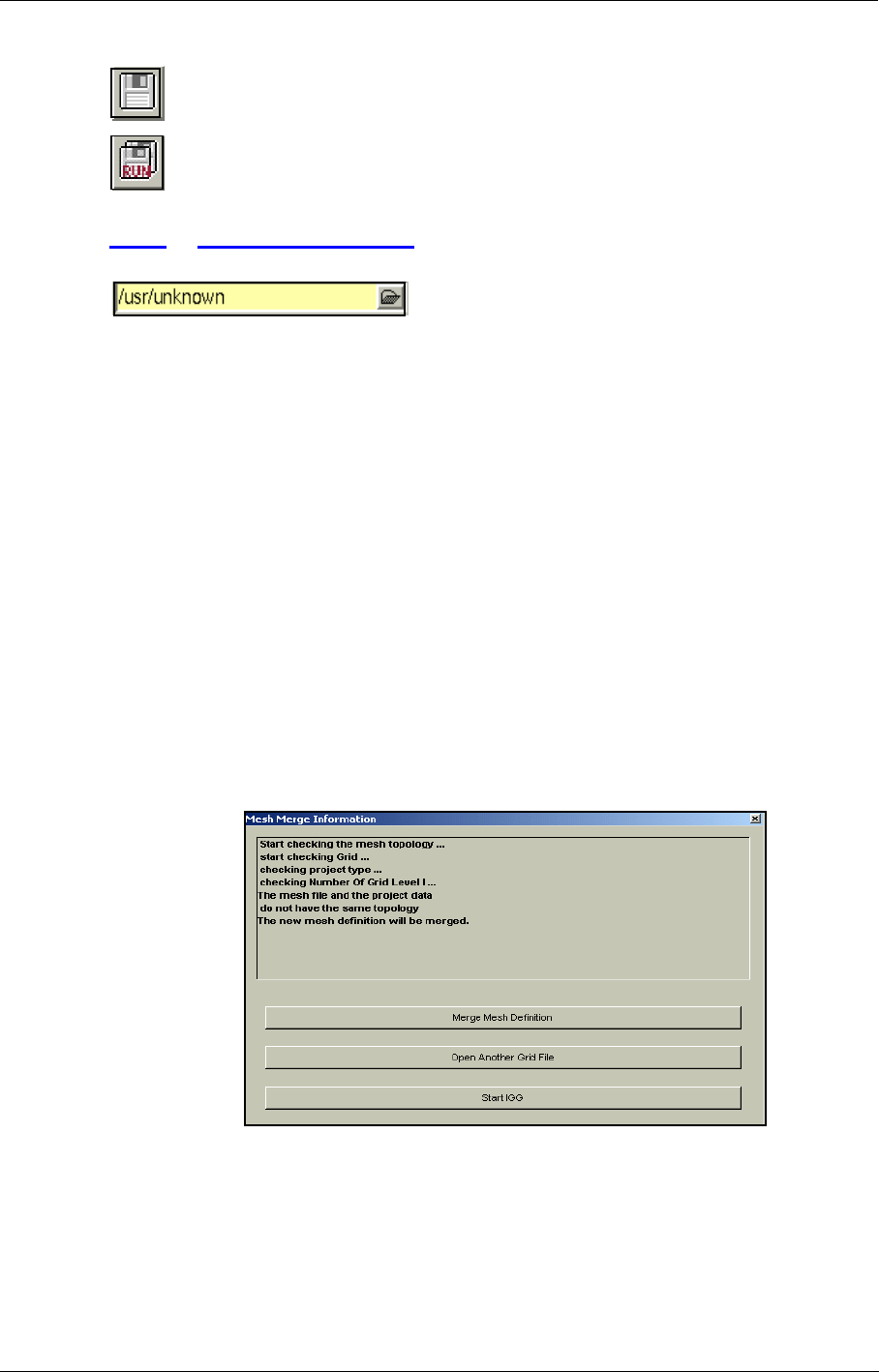
The Save Project icon is a shortcut for the menu item File/Save.
The Save RUN Files icon is a shortcut for the menu item File/Save Run Files.
2-4.2 Grid Selection Bar
By clicking on the icon on the right of the bar a File
Chooser is opened, which allows to select the grid file
(with extension ".igg") of the mesh to use for the project.
To select a grid not only the grid file with extension ".igg" needs to be present but at least
the files with extensions ".igg", ".geom", ".bcs" and ".cgns" need to be available in the
same directory with the same name as for the chosen mesh.
If a mesh has already been linked to the current project and another mesh is opened, FINE™/Turbo
will check the topological data in the project and compare it against the data in the mesh file. If the
topological data is not equal, a new dialog box (Figure 2.4.2-9) will open. This dialog box informs
the user that a merge of the topologies is necessary and will also show at which item the first differ-
ence was detected.
The three following possibilities are available:
•Merge Mesh Definition will merge the project and mesh data. For example, if a new block has
been added to the mesh. The existing project parameters have been kept for the old blocks, and
the default parameters have been set for the new block.
•Open Another Grid File will open a File Chooser allowing to browse to the a new grid file
with extension ".igg". Select the grid file and press OK to accept the selected mesh. Then the
dialog box Mesh Merge Information will appear.
•Start IGG will load automatically the new mesh into IGG™, where it can be modified.
FIGURE 2.4.2-9 Merge Topology dialog box
The merge process may also occur when opening an existing project, or when switching between
IGG™ and FINE™/Turbo, because the check of the topology is performed each time when a
project is read.
Graphical User Interface Computation Management
2-14 FINE™/Turbo
In case the mesh file no longer exists, or is not accessible, an appropriate warning will pop-up when
opening the project. In this case it will not be possible to start the flow solver, so the user needs to
locate the mesh by means of the File Chooser button on the right of the Grid Selection bar.
Once the grid file is selected and its topology is checked, the Grid Units and Project Configuration
window appears. This window allows to check the properties of the mesh and to modify them if
necessary. See section 2-2.3 for more details on this window.
2-4.3 Solver Buttons
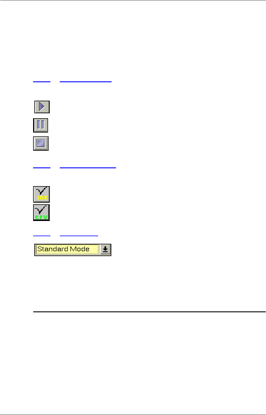
Three buttons allow to start, suspend and kill the active computation:
The Start Flow Solver icon is a shortcut for the menu item Solver/Start....
The Suspend Flow Solver icon is a shortcut for the menu item Solver/Suspend....
The Kill Flow Solver icon is a shortcut for the menu item Solver/Kill....
2-4.4 Module Buttons
Two buttons allow to start the pre- and post-processor:
The Start IGG icon is a shortcut for the menu item Modules/IGG.
The Start CFView icon is a shortcut for the menu item Modules/CFView.
2-4.5 User Mode
By clicking on the arrow at the right the user may select the user
mode. For most projects the available parameters in Standard
Mode are sufficient. When selecting Expert Mode, parameters
area included additional parameters. These expert parameters may be useful in some more complex
projects. The next chapters contain sections in which the expert parameters are described for the
advanced user.
2-5 Computation Management
When selecting the Computations subpanel at the top left of the interface a list of all the computa-
tions in the project is shown. The active computation is highlighted in blue and the corresponding
parameters are shown in the "parameters area". All the project parameters of the computation can
be controlled separately by selecting (from this list) the computation on which all the user modifica-
tions are applied.
When selecting multiple computations, the parameters of the active page in the "parame-
ters area" are copied from the first selected computation to all other computations.
Graphical Area Management Graphical User Interface
FINE™/Turbo 2-15
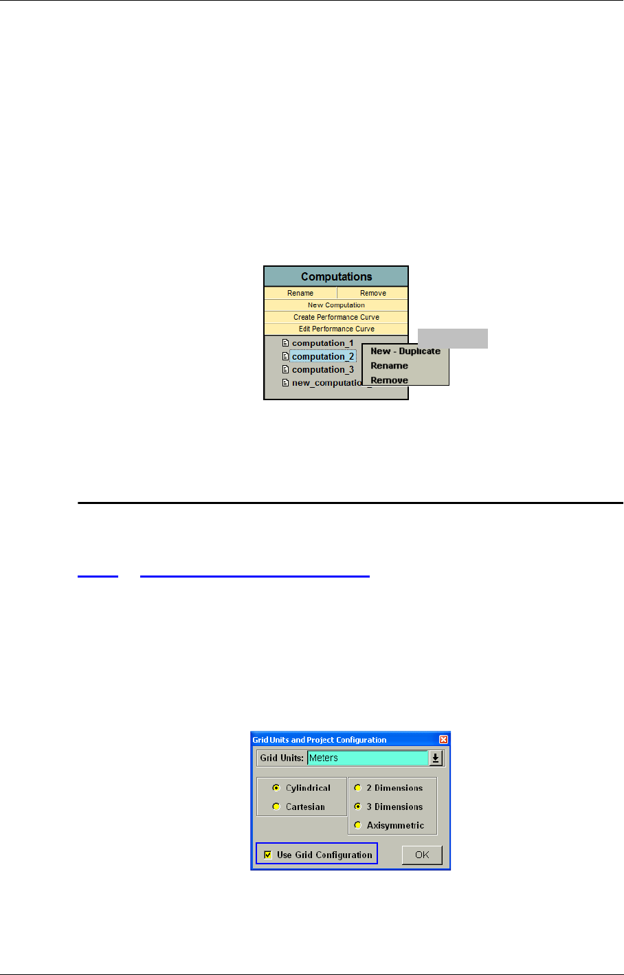
With the buttons New Computation and Remove computations can be created or removed. When
clicking on New Computation the active computation (highlighted in blue) is copied and the new
computation has the same name as the original with the prefix "new_" as shown in the example
below. In this example "computation_2" was the active computation at the moment of pressing the
button New Computation. A new computation is created called "new_computation_2" that has the
same project parameters as "computation_2". To rename the active computation click on Rename,
type the new name and press <Enter>. These options are also available when click-right on the
active computation.
Two buttons Create Performance Curve and Edit Performance Curve are dedicated to the creation
and management of the performance curve for turbomachinary. More details can be found in
Chapter 8-10.
FIGURE 2.5.0-10 Computations subpanel
2-6 Graphical Area Management
2-6.1 Configuration Management
When creating a mesh within AutoGrid™ or IGG™, the multiblock data structure can become very
complex. A database, named Grid Configuration, is created automatically at the end of the mesh
generation, saved together with the project into a file ".config" (more details can be found in the
IGG™ or AutoGrid™ User Manuals).
To access the grid configuration menu in FINE™/Turbo, the Use Grid Configuration option has to
be activated when linking the mesh for the first time, see section 2-2.3. This option is only available
through a special license feature (SubProjects).
FIGURE 2.6.1-11 Use Grid Configuration
Right-Click
Graphical User Interface Graphical Area Management
2-16 FINE™/Turbo
The grid configuration describes (as presented in the figure below) the mesh structure of the project
as a tree through which the user can access the domain structure. The structure is defined as a set of
fluid and solid domains interconnected together through domain interfaces. Each domain contains a
set of subdomains and a set of interfaces. Each domain interface contains a type of boundary condi-
tion, a type of free boundary condition and the possible connected domain reference.
FIGURE 2.6.1-12 Grid Configuration control
This data structure is very useful. It can be used to reduce the time needed to analyse and visualize
the mesh of a project, to setup the boundary conditions within FINE™/Turbo and to create sub-
projects starting from the main project (see Chapter 8 for more details).
2-6.2 Parameters Management
The Parameters subpanel on the left, below the Computations subpanel, is presenting a directory
structure allowing the user to go through the available pages of the project definition. The "parame-
ters area" shows the parameters corresponding to the selected page in the parameters list.
To see the pages in a directory double click on the name or click on the sign in front of the name.
FIGURE 2.6.2-13 Parameters subpanel
2-6.3 View Area
When the mesh is loaded with Mesh/View On/Off, a subpanel is shown in the list on the left: the
View subpanel. By default the View subpanel is opened. It consists of three pages and controls the
viewing operations on the geometry and the grid. The two first pages show the created geometry
Graphical Area Management Graphical User Interface
FINE™/Turbo 2-17
and/or block groups of the mesh and allow to create new groups. This possibility is only useful in
the FINE™/Turbo GUI for visualization purposes (for example, to show only some blocks of the
mesh to get a clearer picture in the case of a complex configuration).
FIGURE 2.6.3-14 View subpanel
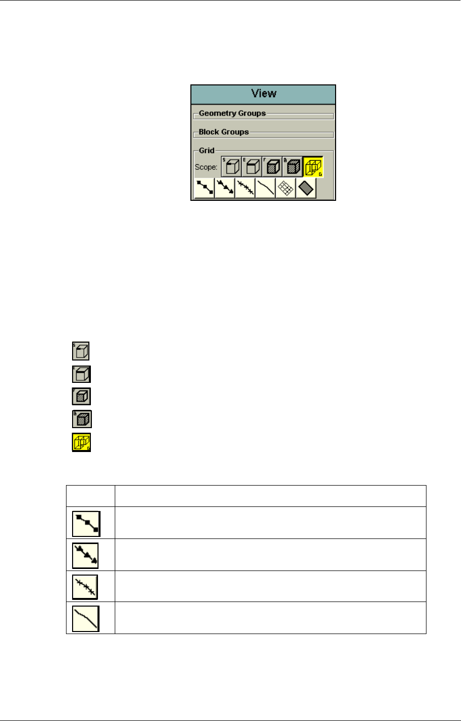
The third page provides visualization commands on the grid. It consists of two rows: a row of but-
tons and a row of icons.
The row of buttons is used to determine the viewing scope, that is the grid scope on which the view-
ing commands provided by the icons of the second row will apply. There are five modes determin-
ing the scope, each one being represented by a button: Segment, Edge, Face, Block, Grid. Only
one mode is active at a time and the current mode is highlighted in yellow. Simply click-left on a
button to select the desired mode.
•: in Segment mode, a viewing operation applies to the active segment only.
•: in Edge mode, a viewing operation applies to the active edge only.
•: in Face mode, a viewing operation applies to the active face only.
•: in Block mode, a viewing operation applies to the active block only.
•: in Grid mode, a viewing operation applies to all the blocks of the grid.
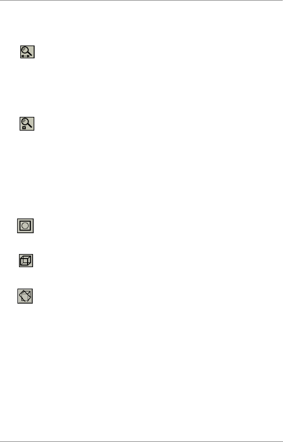
The icons of the second row and their related commands are listed in the following table:
Icon Command
Toggles vertices.
Toggles fixed points.
Toggles segment grid points.
Toggles edges.
Graphical User Interface Graphical Area Management
2-18 FINE™/Turbo
The display of vertices should be avoided since it allows to modify interactively in the
graphics area the location of the vertices and therefore alter the mesh. The graphics area
is for display purposes only and any modification on the mesh in the graphics area will
not be saved in the mesh files and therefore not used by the flow solver.
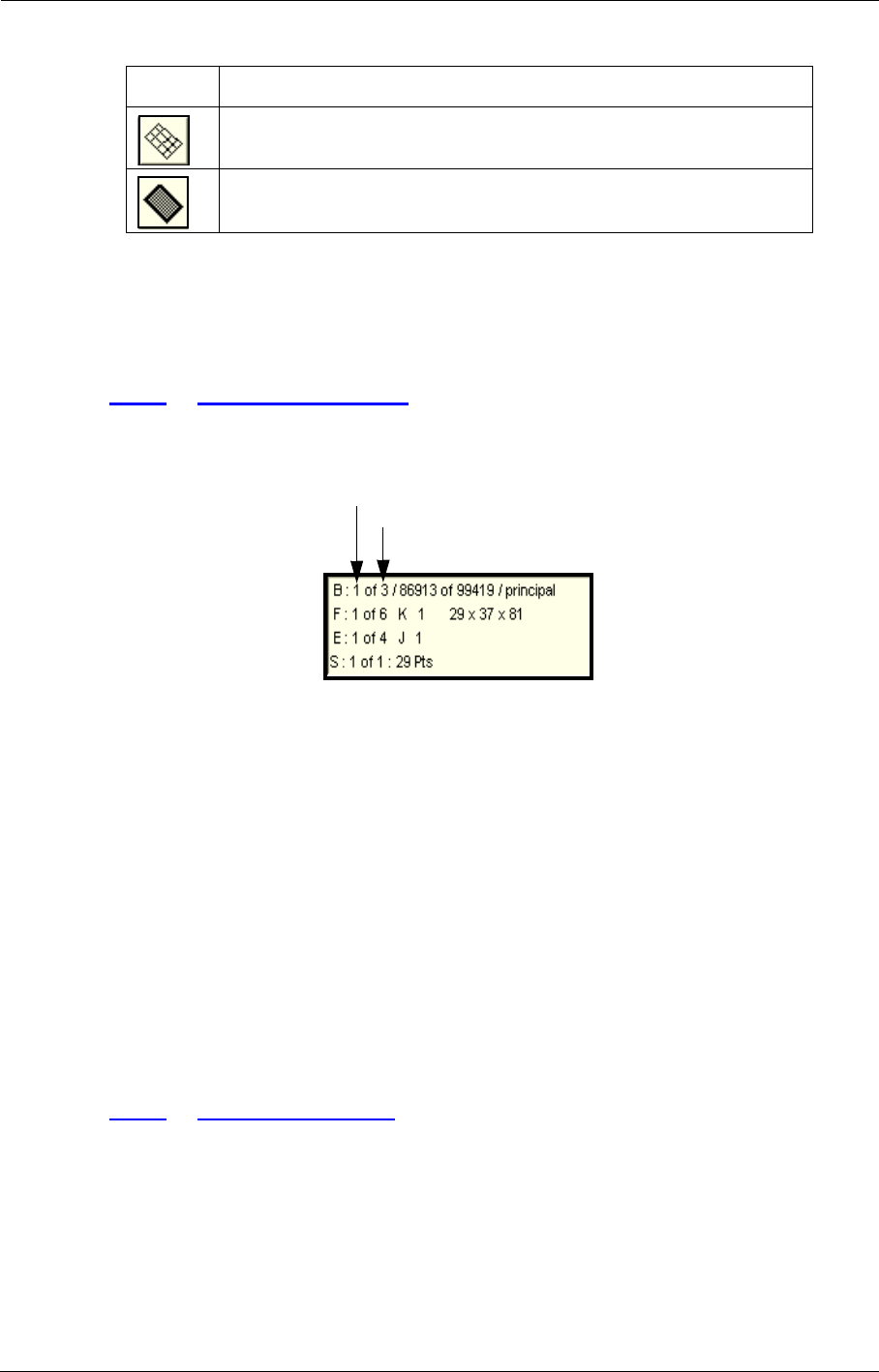
2-6.4 Mesh Information
When the mesh is loaded also the Mesh Information area is shown containing the following infor-
mation for the selected section of the mesh:
FIGURE 2.6.4-15 Mesh Information area
•Active Block, Face, Edge and Segment indices.
•Number of grid blocks, active block faces, active face edges, active edge segments.
•Block:
—Number of active block points.
—Number of grid points.
—Name of the block.
—Number of points in each block direction.
•Face: constant direction and the corresponding index.
•Edge: constant direction according to the active face and the corresponding index.
•Segment: number of points on the segment.
2-6.5 Parameters Area
The Parameters area displays a page containing the parameters related to the selected item of the
parameters list. Depending on the selected User Mode the available expert parameters will be dis-
played.
Toggles face grid.
Toggles shading.
Icon Command
Active block, face, edge and segment indices
Number of blocks, faces, edges and segments
for the active topology
Graphical Area Management Graphical User Interface
FINE™/Turbo 2-19
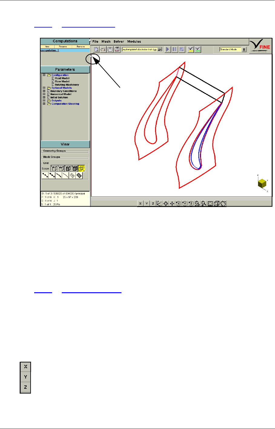
2-6.6 Graphics Area
button to resize
Graphics area
FIGURE 2.6.6-16 Resizing of Graphics Area
The graphics area shows the mesh of the open project. The graphics area appears and disappears
when clicking on Mesh/View On/Off. When the graphics area appears it is covering the parameters
area. Use the button on the left boundary of the graphics area to reduce its size and to display the
parameters area. The Grid page, in the View subpanel on the left, and the viewing buttons can be
used to influence the visualization of the mesh. The View subpanel is described in section 2-6.3 and
the viewing buttons area are described below.
2-6.7 Viewing Buttons
The viewing buttons are used to perform viewing manipulations on the active view, such as scroll-
ing, zooming and rotating. The manipulations use the left, middle and right buttons of the mouse in
different ways. The sub-sections below describe the function associated with each mouse button for
each viewing button.
For systems that only accept a mouse with two buttons, the middle mouse button can be
emulated for viewing options by holding the <Ctrl> key with the left mouse button.
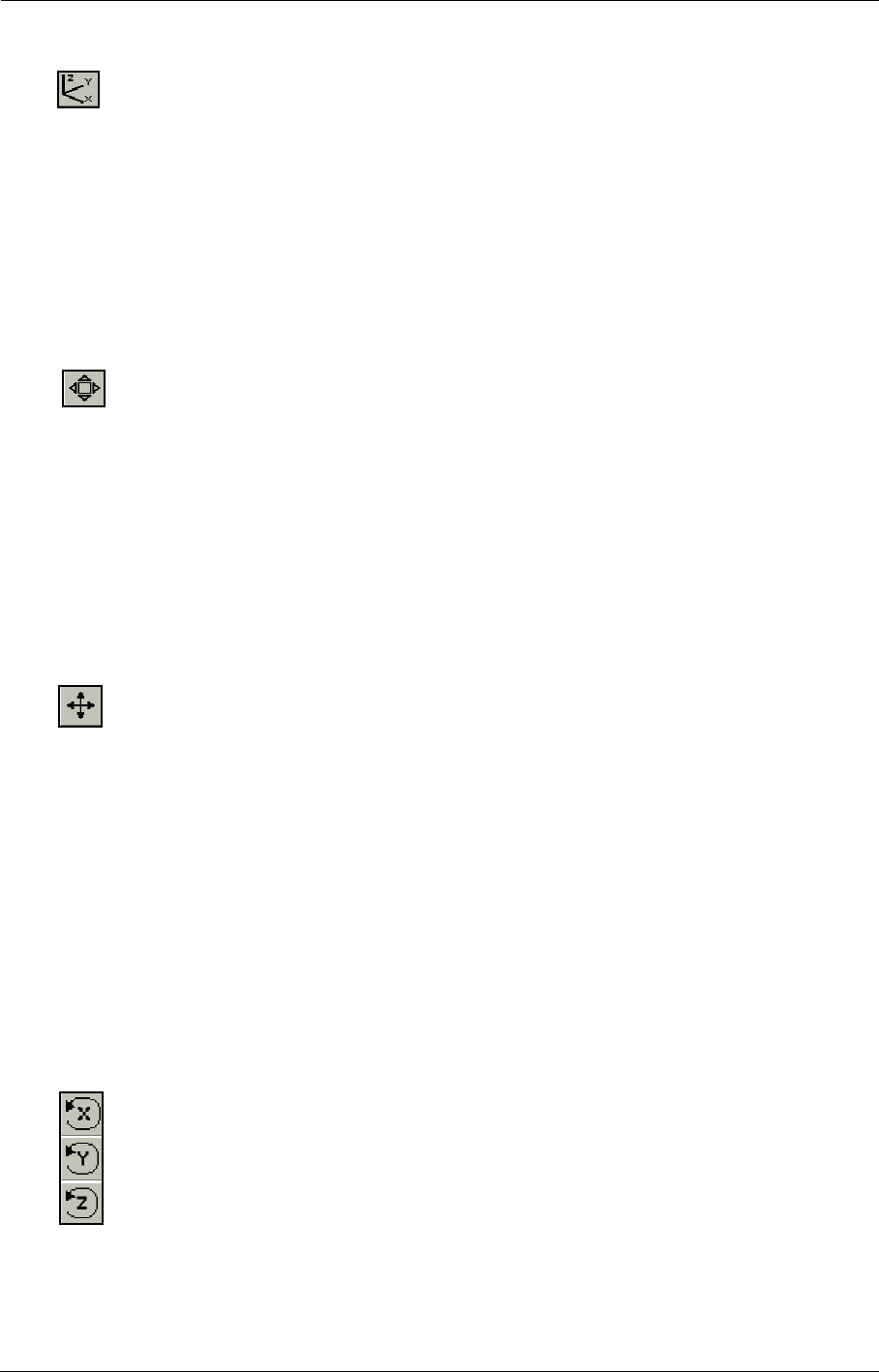
2-6.7.1 X, Y, and Z Projection Buttons
These buttons allow to view the graphics objects on X, Y or Z projection plane. Press the left mouse
button to project the view on an X, Y or Z constant plane. If the same button is pressed more than
one time, the horizontal axis changes direction at each click.
Graphical User Interface Graphical Area Management
2-20 FINE™/Turbo
2-6.7.2 Coordinate Axes
The coordinate axes button acts as a toggle to display different types of coordinate axes on the
active view using the following mouse buttons:
•Left: press to turn on/off the display of symbolic coordinate axis at the lower right corner of the
view.
•Middle: press to turn on/off the display of scaled coordinate axis for the active view. The axis
surrounds all objects in the view and may not be visible when the view is zoomed in.
•Right: press to turn on/off the display of IJK axis at the origin of the active block (in Block
Viewing Scope) or of all the blocks (in Grid Viewing Scope). For more informations about the
viewing scope, see section 2-6.3.
2-6.7.3 Scrolling
This button is used to translate the contents of active view within the plane of graphics window in
the direction specified by the user. Following functions can be performed with the mouse buttons:
•Left: press and drag the left mouse button to indicate the translation direction. The translation
is proportional to the mouse displacement. Release the button when finished. The translation
magnitude is automatically calculated by measuring the distance between the initial clicked
point and the current position of the cursor.
•Middle: press and drag the middle mouse button to indicate the translation direction. The
translation is continuous in the indicated direction. Release the button when finished. The
translation speed is automatically calculated by measuring the distance between the initial
clicked point and the current position of the cursor.
2-6.7.4 3D Viewing Button
This button allows to perform viewing operations directly in the graphics area. Allowed operations
are 3D rotation, scrolling and zooming.
After having selected the option, move the mouse to the active view, then:
•Press and drag the left mouse button to perform a 3D rotation
•Press and drag the middle mouse button to perform a translation
•Press and drag the middle mouse button while holding the <Shift> key or use the mouse wheel
to perform a zoom
•To select the centre of rotation, hold the <Shift> key and press the left mouse button on a
geometry curve, a vertex or a surface (even if this one is visualized with a wireframe model).
The centre of rotation is always located in the centre of the screen. So, when changing it, the
model is moved according to its new value.
The 3D viewing tool is also accessible with the <F1> key.
2-6.7.5 Rotate About X, Y or Z Axis
The rotation buttons are used to rotate graphical objects on the active view around the X, Y or Z
axis. The rotations are always performed around the centre of the active view. Following functions
can be performed with the mouse buttons:
•Left: press and drag the left mouse button to the left or to the right. A clockwise or counter-
clockwise rotation will be performed, proportional to the mouse displacement. Release the
button when finished.
Graphical Area Management Graphical User Interface
FINE™/Turbo 2-21
•Middle: press and drag the middle mouse button to the left or to the right. A continuous rota-
tion will be performed, clockwise or counter-clockwise. Release the button when finished.
2-6.7.6 Zoom In/Out
This button is used for zooming operations on the active view. Zooming is always performed
around the centre of the view. Following functions can be performed with the mouse buttons:
•Left: press and drag the left mouse button to the left or to the right. A zoom in - zoom out will
be performed, proportional to the mouse displacement. Release the button when finished.
•Middle: press and drag the middle mouse button to the left or to the right. A continuous zoom
in - zoom out will be performed. Release the button when finished.
2-6.7.7 Region Zoom
This button allows to specify a rectangular area of the active view that will be fitted to the view
dimensions. After having selected the button:
1. Move the mouse to the active view.
2. Press and drag the left mouse button to select the rectangular region.
3. Release the button to perform the zoom operation.
These operations can be repeated several times to perform more zooming.
Press <q> or click the right mouse button to quit the option.
The region zoom is also accessible with the <F2> key.
2-6.7.8 Fit Button
The fit button is used to fit the content of the view to the view limits without changing the current
orientation of the camera (which can be interpreted as the user's eyes).
2-6.7.9 Original Button
The original button is used to fit the content of the view and to change back to the default orienta-
tion of the camera.
2-6.7.10 Cutting Plane
This option displays a movable plane that cuts the geometry and the blocks of the mesh. The plane
is symbolically represented by four boundaries and its normal, and is by default semi-transparent.
After having selected the button:
•Press and drag the left mouse button to rotate the plane
•Press and drag the middle mouse button to translate the plane
•Press < x >, < y > or < z > to align the plane normal along the X, Y or Z axis
•Press <n> to revert the plane normal
•Press < t > to toggle the transparency of the plane (to make it semi-transparent or fully trans-
parent). It is highly advised to deactivate the plane transparency when using X11 driver to
increase the execution speed.
Graphical User Interface Profile Management
2-22 FINE™/Turbo
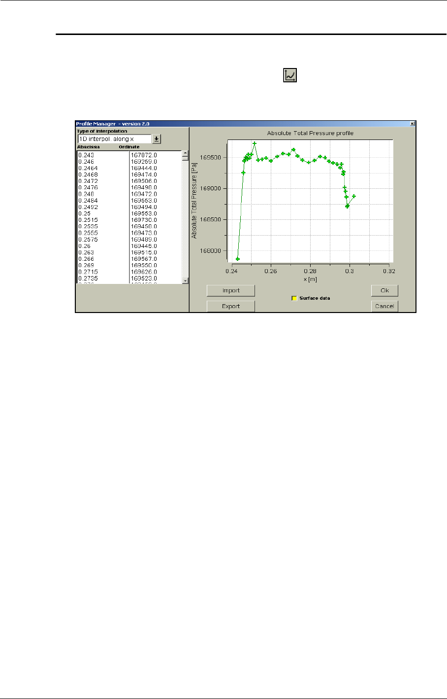
2-7 Profile Management
When a law is defined by a profile clicking on the button right next to the pull down menu will
invoke a Profile Manager window.
FIGURE 2.7.0-17 Profile Manager for boundary conditions parameters
The Profile Manager is used to interactively define and edit profiles for both fluids and boundary
conditions parameters. The user simply enters the corresponding coordinates in the two columns on
the left. The graph is updated after each coordinate (after each pressing of <Enter> key).
The button Import may be used if the profile exists already as a file on the disk. The Export button
is used to store the current data in the profile manager as a file (for example to share profiles
between different projects and users).
The option Surface data allows the user to impose a 2D profile. The formats of the profile files are
explained in Appendix A where all file formats used by FINE™/Turbo and the flow solver are
detailed.
If the mouse cursor is placed over a point in the graph window, this point is highlighted and the cor-
responding coordinates on the left will be also highlighted, giving the user the possibility to verify
the profile.
The button OK will store the profile values and return back to the main FINE™/Turbo window.
When imposing profiles, a zero extrapolation is applied for point located outside the
defined range of the profile. E.g. if the density profile is given for a pressure between 10
bar and 100 bar, the density at 1 bar will be the one imposed at 10 bar.

FINE™/Turbo 3-1
CHAPTER 3: Fluid Model
3-1 Overview
Every FINE™/Turbo project selects a fluid and its properties, defined by:
1. Using the fluid defined in the project file of which the properties are shown on the fluid selec-
tion page (see section 3-2.1), or
2. selecting a fluid from the fluid database included in the release that contains a set of pre-defined
fluids (see section 3-2.2), or
3. creating a new fluid (see section 3-2.3).
In the next section the interface is described in detail, including advises for use of the fluid defini-
tions. The theoretical background for the different fluid models is described in the theoretical man-
ual.
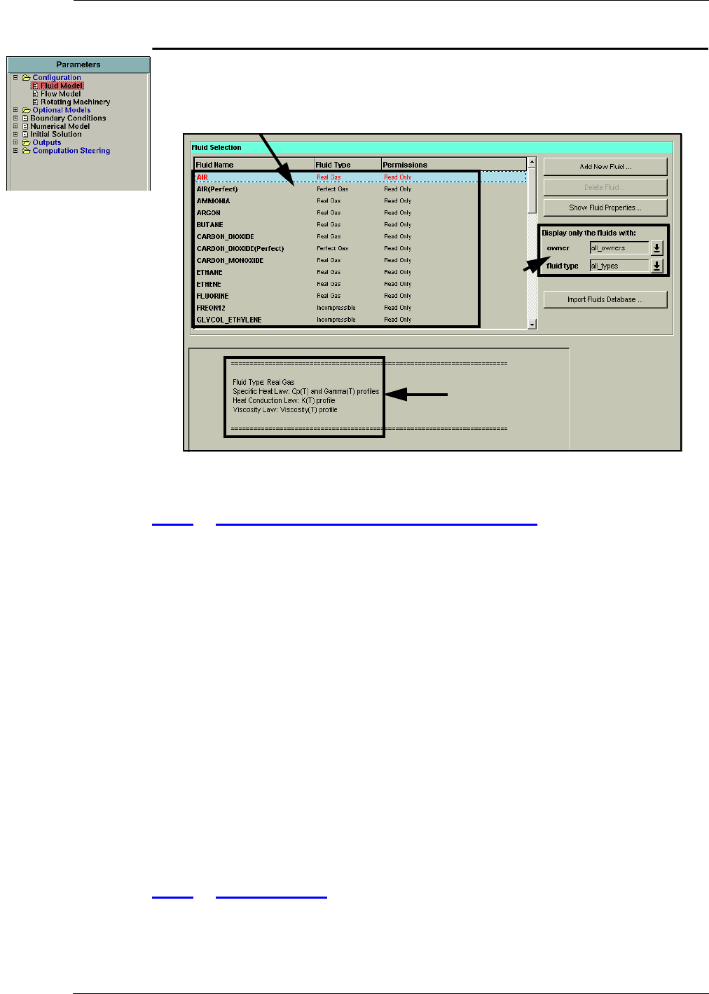
Fluid Model The Fluid Model in the FINE™/Turbo GUI
3-2 FINE™/Turbo
3-2 The Fluid Model in the FINE™/Turbo GUI
FIGURE 3.2.0-1 Fluid Selection page
3-2.1 Properties of Fluid Used in the Project
Every FINE™/Turbo project contains a fluid with the corresponding properties that are displayed in
the interface (see Figure 3.2.0-1). When a new project is created, the default fluid is a perfect gas,
pre-defined by FINE™/Turbo. When an existing project is opened, the used fluid is defined by the
properties as defined in the project file ".iec".
The first listed fluid property is the fluid type. Four fluid types are available:
•perfect gas,
•real gas,
•incompressible gas or liquid,
•condensable fluid.
For more details on each of these types, please see Chapter 2 in the theoretical manual. For the first
three fluid types, the properties can be defined through the interface as described in section 3-2.3.
To add a condensable fluid to the list of fluids proposed by default, please use TabGen to generate
the appropriate tables.
To modify the properties of the fluid used, a fluid can be selected from the list of pre-defined fluids
(section 3-2.2) or a new fluid may be defined (where the new fluid is based on the current one, see
section 3-2.3 for more detail).
3-2.2 List of Fluids
The list of fluids (see Figure 3.2.0-1) contains pre-defined fluids in a database. For each fluid the
fluid type and the permissions are defined.
list of properties
list of pre-defined fluids
filters
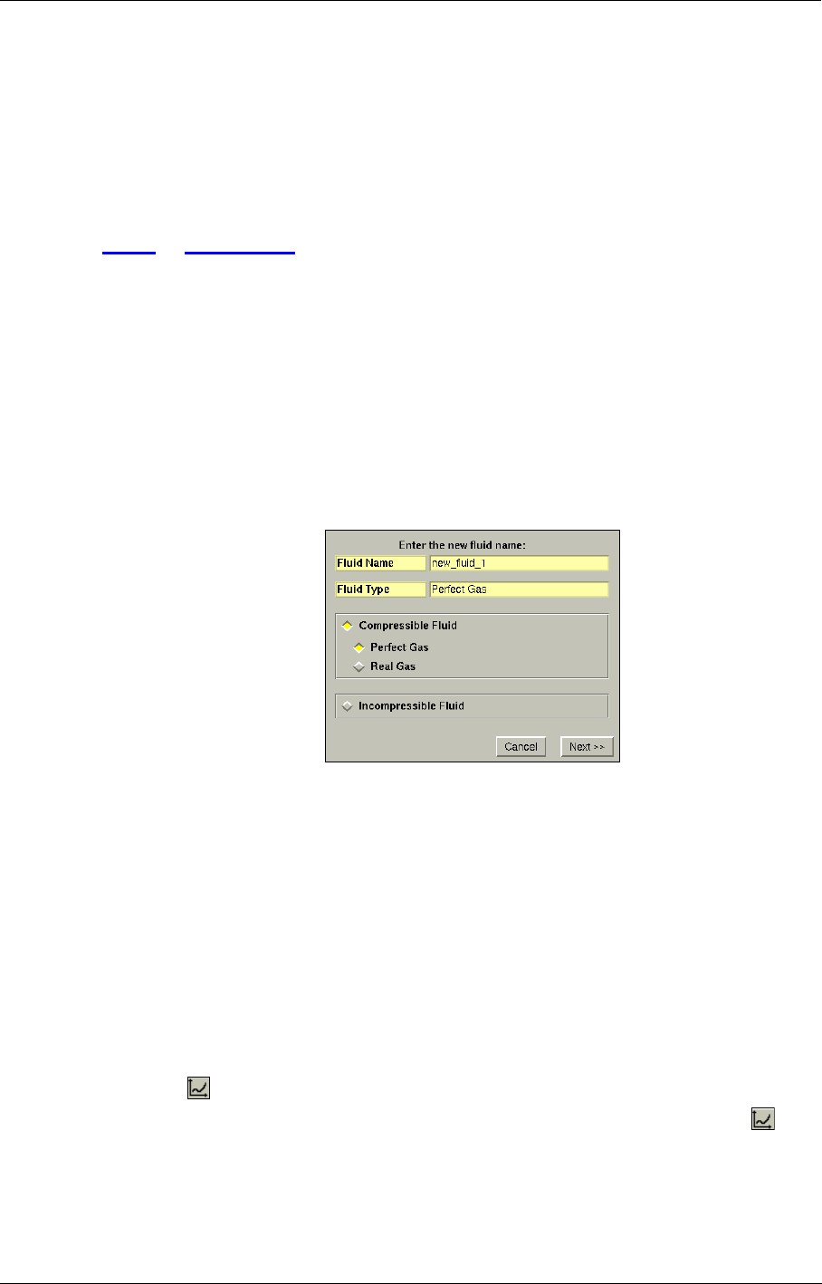
The Fluid Model in the FINE™/Turbo GUI Fluid Model
FINE™/Turbo 3-3
Every fluid is associated with the user who created it and can be modified or removed only by its
owner (the owner has Read Write Delete permissions). All other users will only have Read Only
permissions.
If the user selects a fluid from the list, the selection will be highlighted and the properties are dis-
played in the information box below the fluid list. Those fluid properties will be saved in the project
file ".iec" as soon as the project is saved.
3-2.3 Add Fluid
To add a fluid to the database click on the Add New Fluid... button. A new fluid is then created with
the current properties as shown in the list of properties. A wizard will appear allowing the user to
modify those properties.
On the first page of this wizard the user can enter the name and the type of the new fluid. The name
should be entered by moving the mouse to the text box for the Fluid Name and to type the name on
the keyboard. By default a name is proposed like "new_fluid_1". The fluid type can be entered by
selecting the appropriate check boxes. First make a choice for a compressible or incompressible
fluid. For a compressible fluid select a perfect gas or a real gas. The fluid type corresponding to the
selected checkboxes is shown in the text box for the Fluid Type. To cancel the modifications to the
fluid definition and close the wizard click on the Cancel button.
FIGURE 3.2.3-2 Fluid Wizard
Once the fluid name and type are correctly set, click on Next>> to go to the next page of the wiz-
ard. On this page the following properties have to be defined:
•Specific Heat Law,
•Heat Conduction Law,
•Viscosity Law,
•Density Law (for an incompressible fluid only).
The possible values to enter for these laws depend on the selected fluid type as described in the next
paragraphs. In the case a law is defined by a constant value, type the value in the corresponding dia-
log box. In the case a law is defined by a profile, the Profile Manager can be opened by clicking on
the button ( ) right next to the pull down menu (see section 3-2.3.6 for more detail). In the case a
law is defined by a formula, the Formula Editor can be opened by clicking on the button ( ) right
next to the pull down menu (see section 3-2.3.5).
Information linked to fluid creation is stored in the fluid database only when closing the
FINE™/Turbo interface. As a consequence, this information will not be available to
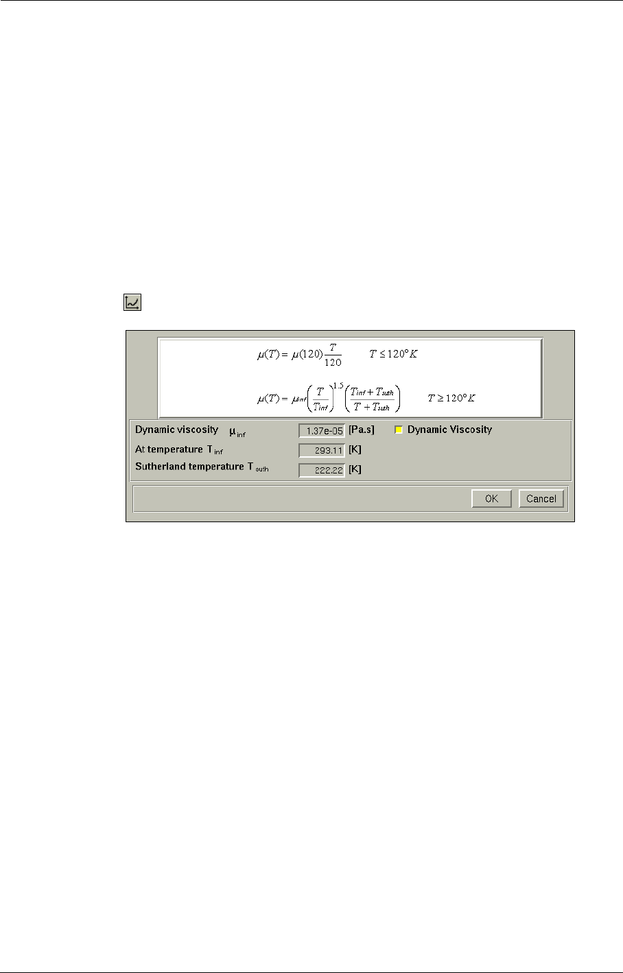
Fluid Model The Fluid Model in the FINE™/Turbo GUI
3-4 FINE™/Turbo
other users as long as this operation is not completed.
3-2.3.1 Definition of a Perfect Gas
For the definition of a perfect gas the user has to specify:
•The specific heat at constant pressure. For a perfect gas only a constant is allowed.
•The constant specific heat ratio ( ) characteristic of the fluid.
•The heat conductivity which may be constant, defined by a polynomial or a profile in tempera-
ture or specified through a constant Prandtl number.
•The viscosity law which may be constant, temperature dependent or specified by the Sutherland
law. In case the viscosity depends on the temperature the user can specify the law through a pol-
ynomial or as a profile through the Profile Manager. Furthermore, when the viscosity law is
defined by the Sutherland law, the Sutherland parameters are accessible by clicking on the but-
ton ( ) right next to the pull down menu.
FIGURE 3.2.3-3 Sutherland Law Parameters
The default law uses the dynamic viscosity but the user can specify the kinematic viscosity if
required.
3-2.3.2 Definition of a Real Gas
A real gas is defined by laws for the dependence of and/or gamma with the temperature and/or
gas constant r.
By default when adding a new fluid, the recommended specific heat law consists on imposing
with the temperature and the gas constant r.
The user can either define a profile, using the Profile Manager, or impose a polynomial approxima-
tion using the Formula Editor. In this last case, the polynomials take the following form:
(3-1)
(3-2)
where the coefficients are chosen by the user
and set in the dialog box for and g respectively. In the definition of real gas properties, lower and
upper bounds of temperature variations [Tmin-Tmax] allowed in the domain must be provided.
cp
cpcv
⁄
cp
cp
cpT() A0T3– A1T2– A2T1– A3A+4T1A5T2A6T3
+++ ++=
γT() B0T3– B1T2– B2T1– B3B+4T1B5T2B6T3
+++ ++=
A0A1A2A3A4A5A6B0B1B2B3B4B5and B6
,,,,,,,,,,,,
cp
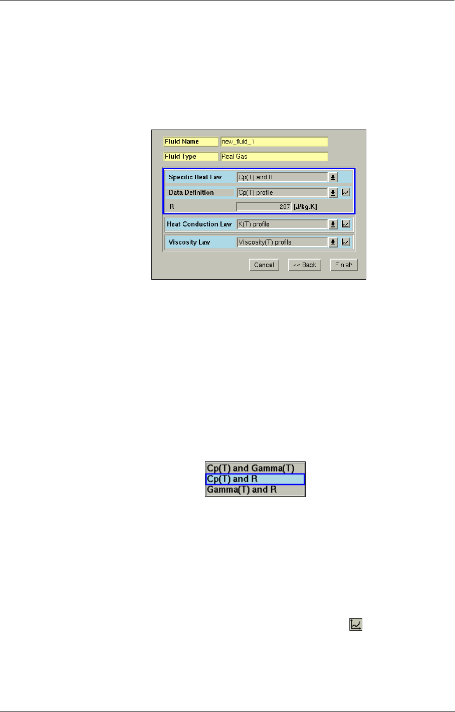
The Fluid Model in the FINE™/Turbo GUI Fluid Model
FINE™/Turbo 3-5
Depending on the local temperature during the iterative process, the physical properties will then be
able to vary according to the laws defined in the fluid database. Note that it is necessary to cover the
whole temperature range occurring in the system otherwise some inaccuracy in the results might be
introduced. In addition, the local temperature may not fit at some occasion in the prescribed range;
this is especially true during the transient. If so, as indicated by the formula editor (section 3-2.3.5),
the physical properties are kept constant, at a value that corresponds to the lower/upper bound
allowed by the range.
FIGURE 3.2.3-4 New Fluid Definition - Real Gas
For the default definition of a real gas, the user has to specify:
•The gas constant r and the specific heat at constant pressure , which depend on the tempera-
ture through a polynomial or a profile. In both cases, the user has to specify the temperature
range over which the specific heat is defined. Furthermore there are alternative modelling meth-
ods for a real gas that consists on:
—involving a compressibility factor and two laws defining the dependence of and gamma
with the temperature.
—constant r model with gamma dependent on the temperature and calculated from r and
gamma.
For the pre-defined fluids, the value of is defined as a function of the temperature
through a profile. These profiles have been computed for a constant pressure 100,000Pa.
•The heat conductivity, which can be constant, defined by a polynomial or a profile in tempera-
ture or specified through a constant Prandtl number.
•The viscosity law, which can be constant, dependent on temperature or specified by the Suther-
land law. In case the viscosity depends on the temperature the user can specify the law through a
polynomial or as profile. Furthermore, when the viscosity law is defined by the Sutherland law,
the Sutherland parameters are accessible by clicking on the button ( ) right next to the pull
down menu. The default law uses the dynamic viscosity but the user can specify the kinematic
viscosity if required, see Figure 3.2.3-3.
cp
cp
cp
cp

Fluid Model The Fluid Model in the FINE™/Turbo GUI
3-6 FINE™/Turbo
Compared to a perfect gas computation ( and g constant), the real gas option results in an
increase of about 25% of the CPU time. Real gas calculations are usually robust enough to avoid
any use of a preliminary run with averaged physical properties. However, convergence difficulties
may arise during the convergence process (say the first 100-200 iterations) if either the allowed
temperature range is too large or if the properties are expected to vary significantly in the allowed
temperature range. At these occasions, it is often useful to make an equivalent perfect gas computa-
tion, with average properties, in order to remove any temperature dependency and ease the conver-
gence process.
3-2.3.3 Definition of a Liquid
For the definition of a liquid two models are available:
•a ’pure’ liquid with constant density,
•a barotropic liquid for which the density varies with pressure.
Depending on the type of liquid the user has to specify:
•The specific heat at constant pressure. For liquids only a constant is allowed.
•The heat conductivity, which can be constant, defined by a polynomial or a profile in tempera-
ture or specified through a constant Prandtl number.
•The viscosity law, which can be constant, dependent on temperature or specified by the Suther-
land law. In case the viscosity depends on the temperature the user can specify the law through a
polynomial or as profile. Furthermore, when the viscosity law is defined by the Sutherland law,
the Sutherland parameters are accessible by clicking on the button ( ) right next to the pull
down menu. The default law concerned the dynamic viscosity but the user can specify the kine-
matic if required, see Figure 3.2.3-3.
•The density law, which can be pressure dependent (using a polynomial law or as a profile
through the Profile Manager) or following the Boussinesq law. In this latter case the density is
constant and the Boussinesq coefficients are taken into account only if the button Gravity
Forces (Flow Model page) is activated. These coefficients are used in source terms of the
momentum equation and the energy equation in order to model the gravitational effect (i.e. nat-
ural convection) although the density is assumed to be strictly constant.
For liquids, the reference temperature and pressure must lie in the expected range of the
static temperature and pressure of the flow field. The reference pressure and temperature
are defined on the Flow Model page (Eq. 4-19).
3-2.3.4 Definition of a Condensable Fluid
The aim of the condensable fluid module is modelling the real thermodynamic properties of the
fluid by means of interpolation of the variables from dedicated tables.
A generation tool TabGen for the condensable tables is provided in FINE™/Turbo. The
details can be found in Appendix D.
The module can be used for a single-phase fluid of which the properties are too complex to be
treated with a perfect or real gas model. It can also be used in order to treat thermodynamic condi-
tions that are close to the saturation line. Note that the model can be used on the liquid or on the
vapour side of the saturation curve. In case the thermodynamic state lies inside the two-phase
region a homogeneous equilibrium two-phase mixture of vapour and liquid is considered. However
the hypothesis of an equilibrium mixture is not valid if the dryness (wetness) fraction exceeds 20%.
cp
cp

The Fluid Model in the FINE™/Turbo GUI Fluid Model
FINE™/Turbo 3-7
The module can not be used above these fractions, as it completely ignores evaporation-condensa-
tion phenomena.
The approach that has been adopted in the FINE™/Turbo solver consists of using a series of ther-
modynamic tables, one table being required each time a thermodynamic variable must be deduced
from two other ones. This implies the creation of many tables as an input, but presents the advan-
tage that no iterative inversion of the tables is done in the solver, with as a consequence a very small
additional CPU time.
By default, two sets of thermodynamic tables are provided in the standard FINE™/Turbo package:
Refrigerant R134a and Water-Steam tables. The other thermodynamic tables can be generated
using TabGen by the user or provided by NUMECA, upon request.
In order to use a condensable gas as a fluid model, the user has to copy the provided tables in a user-
defined subdirectory called "/tables_fluidname/". The location of this subdirectory is platform
dependent:
•On Unix/Linux systems:
"/NUMECA_INSTALLATION_DIRECTORY/fine#/COMMON/thermodynamic_tables/"
•On Windows systems:
"/NUMECA_INSTALLATION_DIRECTORY/Fine#/bin/thermodynamic_tables/"
The subdirectory has to be created before launching FINE™/Turbo. When the subdirectory is exist-
ing, the condensable gas is recognized by FINE™/Turbo and the fluid will appear in the list with
respectively Fluid Name and Fluid Type as "Condensable__fluidname" and "Condensable Fluid".
The condensable fluid option is not compatible with the use of cooling/bleed module
and/or upwind schemes for space discretization.
a) Selection of the Viscosity, Conductivity, and Specific Heat
The viscosity and conductivity can be specified in two-dimensional tables. If it is not the case the
other laws can be used (constant, polynomial expression or user profiles).
Since the complete integration of the condensable fluid module in the user interface is not yet fin-
ished, the selection of these laws is no longer available as soon as a condensable fluid is chosen.
The way to select these laws is the following:
1. create a perfect gas,
2. enter the desired properties for the viscosity and conductivity,
3. save the corresponding computation,
4. change the fluid type by selecting the condensable fluid.
The same procedure applies to the specific heat at constant pressure, that is used in order to derive
the turbulent conductivity from the turbulent viscosity.
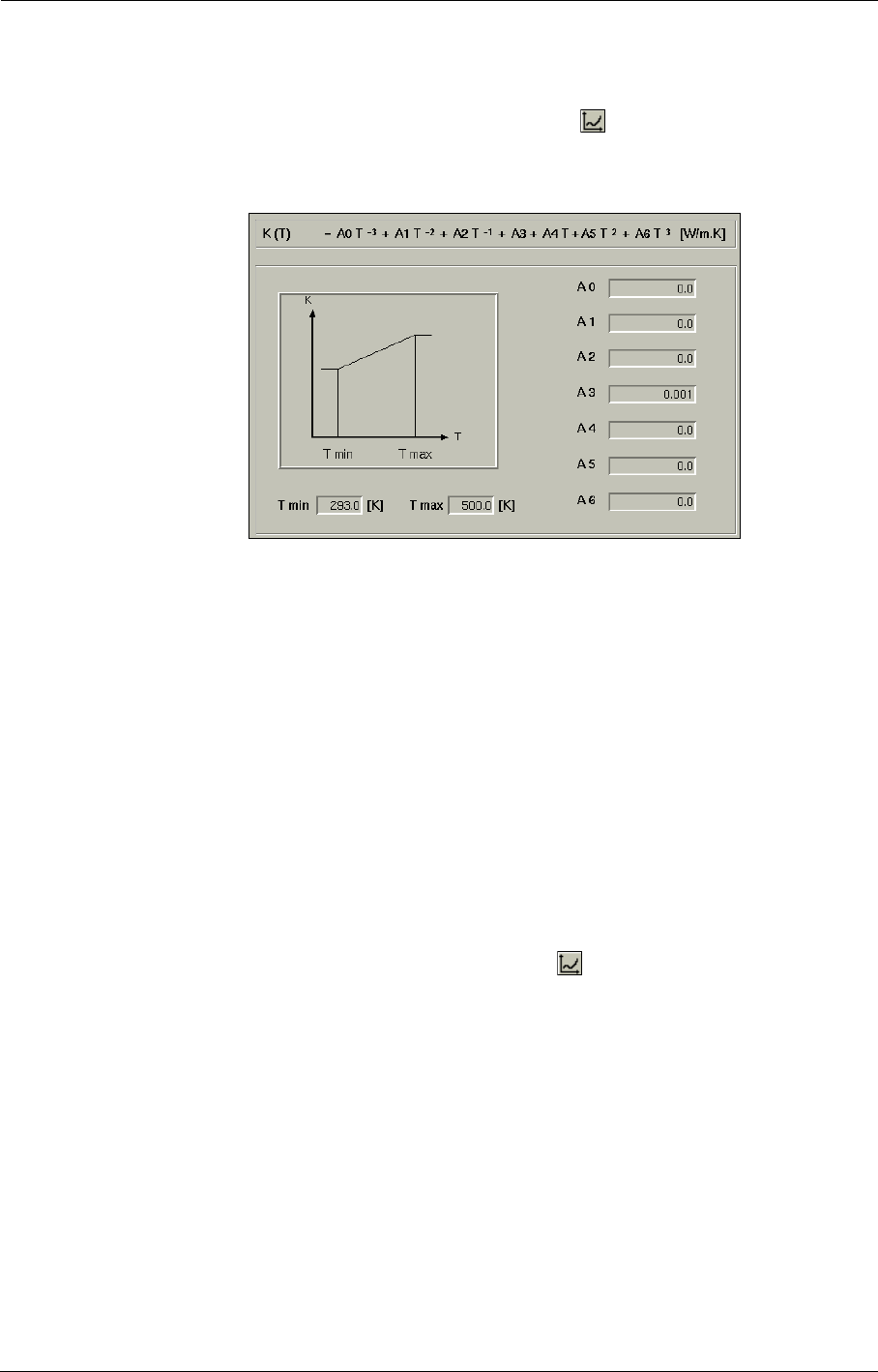
Fluid Model The Fluid Model in the FINE™/Turbo GUI
3-8 FINE™/Turbo
3-2.3.5 Formula Editor
When a law is defined by a formula clicking on the button ( ) right next to the pull down menu
will invoke a formula editor. When a law is defined by a formula clicking on the button right next to
the pull down menu will invoke the Formula Editor.
FIGURE 3.2.3-5 The Formula Editor for polynomials in the fluid properties
The Formula Editor is used to define polynomial values for the fluid properties. The user has to
define the seven coefficients of the polynomial according to the displayed formula on the top, and
also the lower and upper limits of the temperature range, in which the polynomial function is
defined. Press <Enter> after each entry to validate the input. Values outside of the specified temper-
ature range, will be considered constant and equal to the minimum or maximum value (as shown in
the graph in Figure 3.2.3-5).
If a fluid with "Read Only" permissions contains formulas they may be visualized by
means of the Show Fluid Properties... button that opens the Formula Editor window, but
they can not be modified - a message will warn the user that the selected fluid can not be
modified.
3-2.3.6 Profile Manager
When a law is defined by a profile clicking on the button ( ) next to the pull down menu will start
the Profile Manager.
The Profile Manager is used to interactively define and edit profiles for both fluid and boundary
condition parameters. To input a profile, the user has to enter the corresponding coordinates in the
two columns on the left. The graph is updated after each coordinate entry (after pressing the
<Enter> key).
The button Import can be used to import a profile, which is already existing as a data file on the
disk. The Export button is used to store the current data in the profile manager as a data file (for
example to share profiles between different projects and users). The format of the profile files is
explained in detail in Appendix A.
If the mouse cursor is placed over a point in the graph window, this point is highlighted and the cor-
responding coordinates on the left will be also highlighted, giving the user the possibility to verify
the profile.
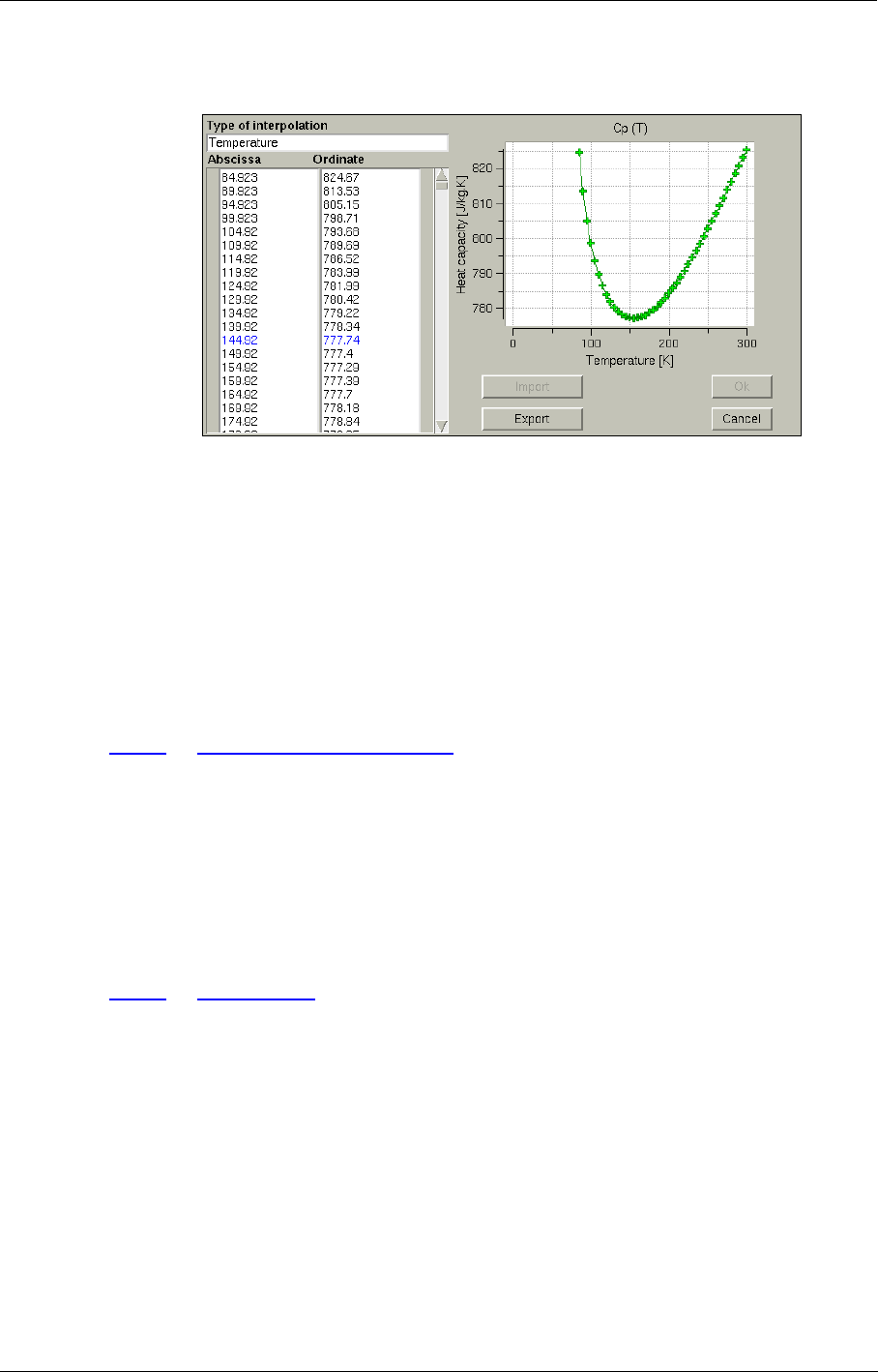
The Fluid Model in the FINE™/Turbo GUI Fluid Model
FINE™/Turbo 3-9
The button OK will store the profile values into the fluid definition.
FIGURE 3.2.3-6 Profile Manager for fluid parameters
If a fluid with "Read Only" permissions contains profiles they may be visualized by
means of the Show Fluid Properties... button that opens the Profile Manager window,
but they can not be modified - a message will warn the user that the selected fluid can not
be modified.
Only uniform distributions should be entered in the Profile Manager. Non-uniform distri-
butions will be converted to a uniform distribution by the FINE™/Turbo solver.
3-2.4 Delete Fluid from List
When the user has the permission to delete a fluid, the button Delete Fluid... allows to remove the
selected fluid from the list of available fluids.
Information linked to fluid removal is stored in the fluid database only when closing the
FINE™/Turbo interface. As a consequence, this information will not be available to
other users until this operation is completed. A message will however warn users that the
fluid properties have been modified (up to removal in the present situation) by the owner.
3-2.5 Edit Fluid
When the user has the write permission for a fluid, the properties of the selected fluid can be modi-
fied by clicking on Edit Fluid.... A wizard will appear allowing to modify the name, the type and
the laws defining the selected fluid. The two pages of this wizard and the laws to define are
described in detail in section 3-2.3.
Information linked to fluid edition is stored in the fluid database only when closing the
FINE™/Turbo interface. As a consequence, this information will not be available to
other users until this operation is completed. A message will however warn users that the
fluid properties have been modified by the owner.

Fluid Model The Fluid Model in the FINE™/Turbo GUI
3-10 FINE™/Turbo
3-2.6 Show Fluid Properties
When the user does not have the write permission (Read Only) for a fluid the Show Fluid Proper-
ties... button opens the wizard with the properties of the fluid. In this case it is not possible to mod-
ify any of the properties in the wizard but the user has access to visualize the properties including
the defined profiles and formulae.
3-2.7 Filters
On the Fluid Model page two filters are available to display only a limited amount of fluids out of
the complete list of fluids. Select the owner(s) and fluid type(s) to display from the pull down
menus to limit the list of fluids.
Please notice that under Windows™ the fluid database is not owner-oriented. The data-
base is stored locally and user defined fluids are accessible with full permissions to all
Windows users.
The filters are used only to browse the fluid list and not to change the current fluid asso-
ciated to the active computation except if selected in the list by left-click on it.
3-2.8 Import Fluid Database
When the user has is own fluid database, the Import Fluids Database... enables to load a user
defined database through a File Chooser window to select the ".flb" file containing the properties of
all the fluids.
When loading an existing project and opening the Fluid Model page, please notice that
FINE™/Turbo is automatically checking if the fluid is existing or not in the fluid data-
base. If the fluid name is existing but the properties are different, a comparison window
will invite the user to select the fluid to use (the default fluid in the database or the fluid
defined in the project). If the fluid is not existing in the fluid database, no fluid will be
selected but the fluid parameters defined in the project will be kept.
3-2.9 Expert Parameters
In this section, the expert parameters which can be used in the definition of the fluid type can be
found. This is only a summary to know directly the expert parameters related to the definition of a
fluid.
All expert parameters related to fluid definition are available in Expert Mode in the Control Vari-
ables page. For these expert parameters the default values only have to be changed in case the user
has specific wishes concerning the fluid modelling.
PRT(real): Allows to define the turbulent Prandtl number (default value = 1.0).
CLIPCG(integer): The thermodynamic tables are generated in a given range of thermodynamic
variables. When the thermodynamic variables are not in the given range, the
expert parmeter CLIPCG can be used to control the computing method of the
dependent thermodynamic variable.
0 (default): the dependent thermodynamic variable is extrapolated from the
interior field.
1: a clipping value will be used for the dependent thermodynamic variable.
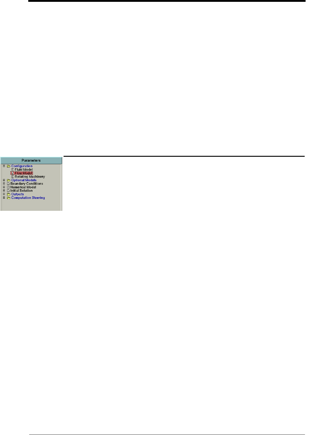
FINE™/Turbo 4-1
CHAPTER 4: Flow Model
4-1 Overview
The Flow Model page, as displayed in Figure 4.1.0-1, can be used in order to specify several char-
acteristics of the flow:
•the time configuration to define time dependence of the equations to solve,
•the mathematical model to:
—choose between viscous and non-viscous flow,
—choose between laminar and turbulent flow,
—activate gravity,
—activate pre-conditioning for low speed flow
•the characteristic scales defining the Reynolds number of the flow,
•the reference values of the temperature and pressure in the flow.
This chapter is organised in the following way:
•section 4-2 describes the interface and best practice for the definition of the mathematical
model and especially the available turbulence models,
•section 4-3 provides details on the Reynolds number related information and reference values.
The interface and best practice for unsteady computations will be described in Chapter 6,
The interface and best practice for harmonic method will be described in Chapter 8,
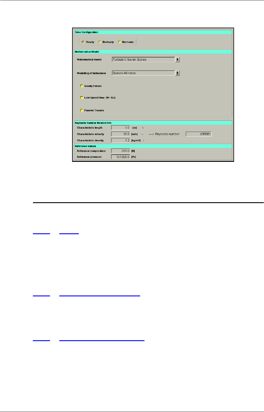
Flow Model Mathematical Model
4-2 FINE™/Turbo
FIGURE 4.1.0-1 Flow Model page.
4-2 Mathematical Model
4-2.1 Euler
When selecting Euler on the Flow Model page an inviscid calculation will be performed. In such a
case all solid walls are considered as Euler walls and the (non-zero) velocity is tangential to the
wall.
Since the Reynolds number has no meaning for Euler calculations this number is not displayed
when Euler flow is selected.
4-2.2 Laminar Navier-Stokes
When selecting Laminar Navier-Stokes equations the only effect is on the thermodynamic prop-
erty of the flow. The viscosity will be the laminar kinematic viscosity and thus does not contain any
turbulent component.
4-2.3 Turbulent Navier-Stokes
When selecting Turbulent Navier-Stokes equations, turbulence is taken into account depending on
the chosen turbulence model. In FINE™/Turbo, several turbulence models are available:
•Algebraic model (0-equation):
—Baldwin-Lomax
•1-equation model:
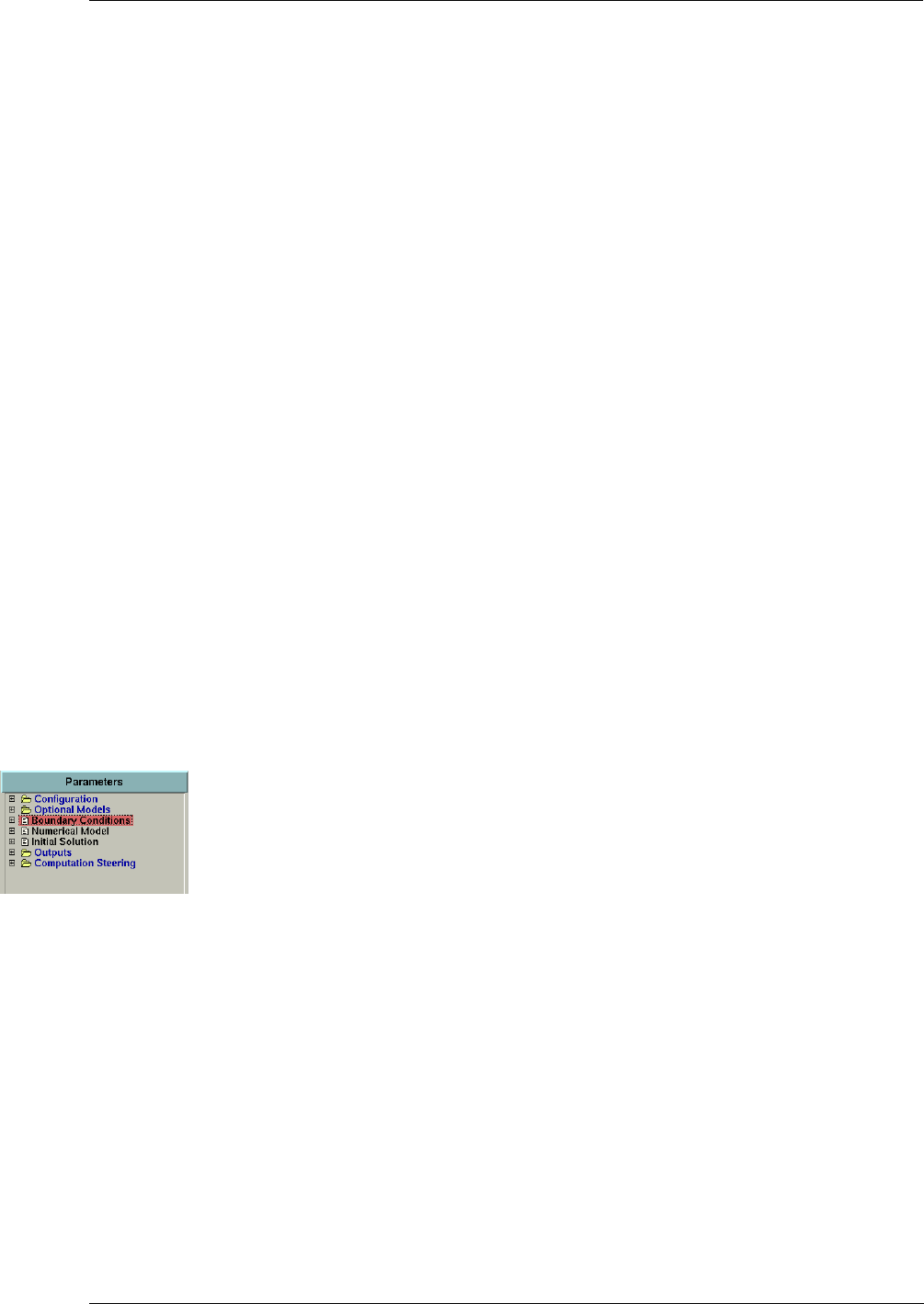
Mathematical Model Flow Model
FINE™/Turbo 4-3
—Spalart-Allmaras
—Spalart-Allmaras (Extended Wall Function)
—SARC, see Chapter 4-2.4.2
—SARC (Extended Wall Function), see Chapter 4-2.4.2
•2-equation models:
—k-ε (Extended wall function)
—k-ε (Standard wall function), see Chapter 4-2.4.2
—k-ε (Low Re Yang-Shih)
—k-ε (Low Re Chien)
—k-ε (Low Re Launder-Sharma)
—Shear Stress Transport (SST)
—SST (Extended wall function)
—EARSM
—EARSM (Extended wall function)
—k-ω (Wilcox)
•4-equation model:
—v2-f (code friendly)
For the Baldwin-Lomax model, algebraic formula is used to compute the turbulent data and conse-
quently no additional input is needed. For all the 1/2/4 equation(s) models, additional equation(s)
are solved and consequently suitable initial and boundary conditions must be defined in the inter-
face.
The DES (Detached Eddy Simulations) model has been implemented in FINE™/Turbo. For more
information, please contact your local support office.
In the following sections, the parameters related to the turbulence models are described.
a) Boundary Condition
Inlet
•Spalart-Allmaras: the value of the turbulent viscosity must be defined. It might be constant or
varying in space and time. The user can specify the time or spatial variation through the profile
manager.
•k-ε models: the values of the turbulent quantities (k and ε) must be defined. They might be
constant or varying in space and time. The user can specify the time or spatial variations
through the profile manager.
•k-ω, SST and EARSM models: the values of the turbulent quantities (k and ε) must be defined.
They might be constant or varying in space and time. The user can specify the time or spatial
variations through the profile manager. The value for ω is determined according to:
, with β*=0.09 (4-1)
•v2-f model: the values of the turbulent quantities (k and ε) must be defined. They might be
constant or varying in space and time. The user can specify the time or spatial variations
through the profile manager. The value of v2 is deduced by assuming an isotropic turbulence.
ωε
β∗k
---------
=
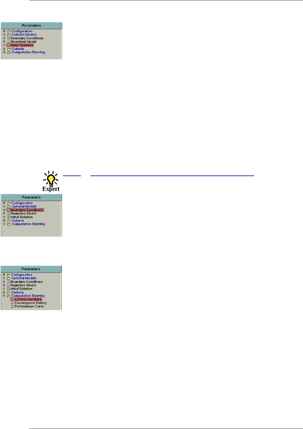
Flow Model Mathematical Model
4-4 FINE™/Turbo
b) Initial Condition
•Spalart-Allmaras: a constant initial value of the turbulent viscosity is defined through the
expert parameter NUTFRE on the Control Variables page under the Expert Mode.
•k-ε models: the initial values of the turbulent quantities (k and ε) are specified by the user if a
constant or initial solution for turbomachinery is chosen.
•k-ω, SST and EARSM models: the initial values of the turbulent quantities (k and ε) are speci-
fied by the user if a constant or initial solution for turbomachinery is chosen. The value for ω is
determined according to Eq. 4-1.
•v2-f model: the initial values of the turbulent quantities (k and ε) are specified by the user if a
constant or initial solution for turbomachinery is chosen. The value of v2 is deduced assuming
an isotropic turbulence.
It is not recommended to use a previously computed solution with different turbulence
model. For k-ε models, the Chien and the Launder-Sharma models belong to the same
family (zero value of ε at the wall) while the standard and Yang-Shih model belong to a
second family (non zero value of ε at the wall). Launching a restart from a previously
computed solution is only allowed as long as the user sticks to the same family.
4-2.4 Expert Parameters for Turbulence Modelling
4-2.4.1 Interfaced Expert Parameters
In expert mode additional parameters related to turbulence modelling are available when using the
turbulence models with extended wall functions. For these turbulence models the wall type can be
defined as smooth or rough:
•For a smooth solid wall (default) only the Von Karman constant and Bo have to be specified (κ
and B).
•When selecting a rough solid wall two additional parameters have to be specified: the equiva-
lent roughness height and the zero-displacement plane (k0 and d0).
4-2.4.2 Non-interfaced Expert Parameters
All non-interfaced expert parameters related to the turbulence models are accessible on the Control
Variables page by selecting the Expert Mode.
Calculation of the wall distances
All turbulence models need to compute the wall distances everywhere in the computed domain. It is
a rather time consuming process so that they are saved in the ".cgns" mesh file at the beginning of
the first computation. These values will be read and used for the next computations. If the mesh file
is modified or saved again, they are erased and will be computed again.
Different important expert parameter are used in the calculation of the wall distance. The default
values are generally sufficient and they have to be changed only if a problem arises.
NREPET(integer): allows to take into account the periodicity of the computed domain. At each
point of the domain, the closest wall is not always in the computed domain if
periodic boundary conditions are used. Consequently the domain is repeated
beyond the periodic boundaries to compute correctly the wall distance (default
value =1).

Mathematical Model Flow Model
FINE™/Turbo 4-5
NSUBM(integer): is the maximum number of subdomains a domain is split into. Its value is suffi-
ciently high and it must be changed only if an error message informs the user to
increase it (default value = 1000).
NTUPTC(integer): is the number of patches whose sub-patches will be searched. In a very com-
plex geometry, the value of this parameter can be increased if the calculation of
the wall distances fail (default value = 100).
The computed wall distances should be removed from the mesh first before relaunch-
ing a computation with a different value of NTUPTC. To remove the computed wall dis-
tances, you should open your mesh in IGG™ and simply save it again.
RTOL(real): maximum angle allowed between two normals of a patch (default value = 1.8).
When the value of IDISTN is 1, the value of RTOL has to be set as the default
value (1.8).
When problems occur during the wall distance calculation (wall distance not equal to
0 on the wall), it is recommended to increase the value of NTUPTC (and to reduce RTOL
if the wall distance gradient is not smooth). Please keep in mind that increasing this
value will slow down the computing of the wall distances.
IDISTN(integer): algorithm for wall distance calculation:
0 : old algorithm
1: new algorithm
2 (default): review of new algrithm (advised for 64 bits platforms)
Limiters for all of the turbulence models
MAVRES(real): denoted here . This parameter limits the variation of the turbulence variables
for each Runge-Kutta stage. Denoting the new value of or as , the fol-
lowing restrictions are imposed when MAVRES > 0:
(4-2)
(4-3)
where EPS is an expert parameter with a small value, default 1E-28, also used
to avoid possible divisions by zero.
The restriction defined in Eq. 4-3 is not applied to the turbulent dissipation rate
(ε) when this tends to increase, in order to avoid excessive values of the turbu-
lent viscosity.
If MAVRES = 0, only the restriction defined in Eq. 4-2 is applied (avoiding
negative values)
If MAVRES < 0, the restriction is:
(4-4)
ζ
k
ε
qn+1
qn+1 max qn+1 EPS,ζqn
,()=
qn+1 min qn+1 2ζ–()qn
,()=
qn1+ qn
–1ζ+()qn1+ qn
–()
1qn1+ qn
–
qn
--------------------------
+
---------------------------------------------
=

Flow Model Mathematical Model
4-6 FINE™/Turbo
MAVREM(real): a similar system is applied to the multigrid corrections with the expert parame-
ter MAVREM, denoted below as :
If MAVREM > 0:
If MAVREM = 0: restriction to positive values
If MAVREM < 0:
MUCLIP(real): controls the maximum allowable value for the ratio MUT/MU in the flow field
but not on boundary conditions (default value = 5000).
KEGRID(integer): allows the use of a particular full multigrid strategy. The Baldwin-Lomax
model is used on the coarse grids during the full multigrid stage and the k, ε, v2
and f initial solution is obtained from the Baldwin-Lomax model solution. This
parameter is not used for the Spalart-Allmaras model.
KEGRID corresponds to the last grid level on which the algebraic model is
used. For example, if the computation is done with 4 levels of multigrid and
KEGRID is equal to 2, the Baldwin-Lomax model is used on the 333 (or level
4), 222 (or level 3) and 111 (or level 2) and the k-ε computation is initiated
when transferring to the finest grid. If KEGRID is set to 3, the k-ε computation
will be initiated when transferring to 222. If KEGRID is greater than the
number of multigrid levels, the computation will be started on the coarsest level
with k-ε.
Baldwin-Lomax
IATFRZ(integer): control the interaction of the model with the multigrid system
0: apply the turbulence model on all grid levels,
1: freeze turbulence on coarser grids (default),
2: freeze turbulence on all grids (see ITFRZ and RESFRZ).
ITFRZ(integer): freeze the turbulent viscosity field if the fine grid iteration exceeds ITFRZ
(default value = 1000000).
RESFRZ(integer): freeze the turbulent viscosity field if the fine grid residual is lower than RES-
FRZ (default value = -12).
Spalart-Allmaras
NUTFRE(real): constant to initialize the turbulent viscosity field (default value = 0.0003).
ITURRC(integer): the Spalart-Allmaras turbulence model with/without extended wall function
does not take the rotation and curvature effects into account. Modifications
have been brought in order to consider these effects. The modified Spalart-All-
maras model is marked as SARC model.
0(default): use the Spalart-Allmaras model, which does not take the rotation/
curvature effects into account.
2: use the SARC model, which takes the rotation/curvature effects into account.
ζ
qn1+ qn
–1ζ–()qn
<
qn1+ qn
–1ζ+()qn1+ qn
–()
1qn1+ qn
–
qn
--------------------------
+
---------------------------------------------
=

Mathematical Model Flow Model
FINE™/Turbo 4-7
k-ε models
CMU(real): constant for the k-ε model (default value = 0.09).
CE1(real): constant for the k-ε model (default value = 1.44 automatically set to 1.35 for
the Chien k-ε model).
CE2(real): constant for the k-ε model (default value = 1.92 automatically set to 1.8 for the
Chien k-ε model).
SIGK(real): constant for the k-ε model (default value = 1.).
SIGE(real): constant for the k-ε model (default value = 1.3).
PRT(real): constant for the k-ε model - the turbulent Prandtl Number (default value = 1.).
INEWKE(integer):allows the user to activate the k-ε (Standard wall function) model when the k-ε
(Extended wall function) model is selected in the interface:
0: activate the the k-ε (Standard wall function) model.
10 (default): use the k-ε (Extended wall function) model.
LTM AX(real): maximum turbulent length scale (default = 1.E+6),
-1: control of turbulent length scale with automatic clipping.
IYAP(integer): 1: applies the Yap’s modification to control the turbulent length scale.
0 (default): The value of the expert parameter LTMAX must be the default
value.
TEDAMP(real): parameter to improve the robustness of the k-ε models (default value = -1),
> 0: a minimum of TEDAMP multiplication factor of the clipping value
(EKCLIP) is used for in the factor ; a minimum of TEDAMP multipli-
cation factor of the clipping value (EPCLIP) is used for to compute the tur-
bulent viscosity,
<= 0: the minimum values used for and correspond to the expert parameter
EPS,
PRCLIP(real): sets an upper bound for the ratio between production and dissipation (default
value = 50).
LIPROD(integer): corresponds to a linearization of the production term (default = 1) when strain
rate is large (i.e. impinging flow) and PRCLIP has no effect anymore on the
flow field.
EKCLIP(real): clipping value for the turbulent kinetic energy k (default value = 1.E-5).
EPCLIP(real): clipping value for the turbulent dissipation rate ε (default value = 1E-5).
IUPWTE(integer): uses an upwind scheme for the convection of k-ε instead of a centre scheme
(default = 1).
IKENC(integer): solves the k-ε equations with a non-conservative approach (default = 1).
IKELED(integer): (= 1) activates the LED scalar scheme for k-ε instead of the standard central
scheme (default = 0).
IOPTKE(integer): optimized implementation for k-ε (Yang-Shih, Wall function, Lauder Sharma)
(default = 1).
k
1T⁄
ε
k
ε

Flow Model Mathematical Model
4-8 FINE™/Turbo
All the above mentioned limiters are very important for the robustness of k-ε compu-
tations. With the exception of the length scale LTMAX all limiters are given appropriate
defaults and it is not recommend to modify them.
v2-f model
CMUV2F(real): constant for the v2-f model (default value = 0.22),
C1F(real): constant for the v2-f model (default value = 1.4),
C2F(real): constant for the v2-f model (default value = 0.3),
CL(real): constant for the v2-f model (default value = 0.23),
CET(real): constant for the v2-f model (default value = 70.0),
CE2V2F(real): constant for the v2-f model (default value = 1.9),
SIGE(real): constant for the v2-f model (default value = 1.3),
SIGK(real): constant for the v2-f model (default value = 1),
EKCLIP(real): clipping value for the turbulent kinetic energy k (default value = 1.E-5),
EPCLIP(real): clipping value for the turbulent dissipation rate ε (default value = 1E-5),
k-ω (Wilcox)
The parameters for the k-ω (Wilcox) model are hard coded. The user cannot modify the default val-
ues.
Shear Stress Transport (SST)
GAM1(real): constant for the SST model (default value = 0.5532),
GAM2(real): constant for the SST model (default value = 0.4403),
BETA1(real): constant for the SST model (default value = 0.075),
BETA2(real): constant for the SST model (default value = 0.0828),
SICK1(real): constant for the SST model (default value = 0.85),
SICK2(real): constant for the SST model (default value = 1.0),
SIGO1(real): constant for the SST model (default value = 0.5),
SIGO2(real): constant for the SST model (default value = 0.856),
A1SST(real): constant for the SST model (default value = 0.31),
BETSST(real): constant for the SST model (default value = 0.09).
EARSM
GAM1(real): constant for the EARSM model (default value = 0.5532),
GAM2(real): constant for the EARSM model (default value = 0.4403),
BETA1(real): constant for the EARSM model (default value = 0.075),

Mathematical Model Flow Model
FINE™/Turbo 4-9
BETA2(real): constant for the EARSM model (default value = 0.0828),
SICK1(real): constant for the EARSM model (default value = 0.5),
SICK2(real): constant for the EARSM model (default value = 1.0),
SIGO1(real): constant for the EARSM model (default value = 0.5),
SIGO2(real): constant for the EARSM model (default value = 0.856),
A1SST(real): constant for the EARSM model (default value = 1.245),
BETSST(real): constant for the EARSM model (default value = 0.09).
4-2.5 Best Practice for Turbulence Modelling
4-2.5.1 Introduction to Turbulence
Turbulence can be defined as the appearance of non-deterministic fluctuations of all variables
(velocity u', pressure p', etc...) around mean values. Turbulence is generated above a critical Rey-
nolds number that may range in values from 400 to 2000 depending on the specific case. In 95% of
industrial applications the critical Reynolds number falls above that range. That is why it is in gen-
eral necessary to predict adequately the turbulence effects on the flow-field behaviour.
To model turbulent flow in a satisfactory way, four steps should be performed:
•choosing a turbulence model,
•generating an appropriate grid,
•defining initial and boundary conditions,
•if necessary, setting expert parameters to procure convergence.
4-2.5.2 First Step: Choosing a Turbulence Model.
A turbulence model is chosen based on the specific application. Table 4-1 states the most appropri-
ate turbulence models to use for different types of flows. Although these are the "most appropriate"
this does not mean that certain turbulence models cannot be used for the flow types listed, but just
that they are "less appropriate".
According to the method accounting for viscous effects close to the wall, the turbulence models can
be divided into two types: high Reynolds number turbulence models and low Reynolds number tur-
bulence models. Please note that here "high Reynolds number" and "low Reynolds number" refer to
the local turbulent Reynolds number formed by the turbulent fluctuation , turbulent
length scale and kinematic viscosity . The high Reynolds number turbulence models assume
that the flow near the wall behaves like a fully developed turbulent boundary layer and prescribe
boundary conditions by employing wall functions. The viscous sublayer will not be resolved. In
FINE™/Turbo, both standard wall function and extended wall function are available, see the theo-
retical manual for the detailed information. The low Reynolds number turbulence models resolve
the entire boundary layer, including the viscous sublayer where the viscous diffusion is much larger
that the turbulent one. Thus, sufficiently fine grid should be used inside the boundary layer so that
the sharp gradients can be resolved.
Relu'lν⁄=
u'
l
ν

Flow Model Mathematical Model
4-10 FINE™/Turbo
TABLE 4-1 Recommended turbulence models for different flow types
Three main kinds of turbulence models exist:
•algebraic models (e.g. Baldwin-Lomax),
•one-equation models (e.g. Spalart-Allmaras),
•two (four)-equation models (k-ε, k-ω and v2-f).
When quick turbulence calculations are required, for example, in design-cycle analysis, it is recom-
mended that the Baldwin-Lomax model is used due to its high numerical stability and low compu-
tational expense. To simulate more precisely the turbulent quantities with also a good rate of
convergence the Spalart-Allmaras model should be preferred.
Another model often used in design is the "standard" k-ε model. This model employs an empiri-
cally based logarithmic function to represent the near-wall physics and requires a lower grid resolu-
tion in this region as a result. One drawback of this treatment is that the logarithmic function does
not apply for separated flows, although the NUMECA extended wall function will still work. If it is
expected that a significant amount of separation will have to be predicted, one of the low-Reynolds
number turbulence models would be more appropriate. All of the listed turbulence models employ
constant turbulent Prandtl numbers which is somewhat of a restriction when performing heat trans-
fer calculations. However, experience has shown quite successful prediction of heat transfer coeffi-
cients when using low Reynolds models.
The Shear Stress Transport (SST) k-ω turbulence model is another most utilized two-equation
model. This model, which combines the advantages of the Wilcox k-ω model and the k-ε model,
has higher accuracy in the separation flow predictions. The user is recommended to use the SST k-
ω model in predicting the onset and the amount of separations under adverse pressure gradient con-
ditions.
The EARSM (Explicit Algebraic Reynolds Stress Model) model is a non linear eddy viscosity 2-
equation model. EARSM is much less demanding than RSM from the computational standpoint
and, at the same time, is capable of reproducing some important features of turbulence (e.g. its ani-
High-Re: Low-Re:
Turbulence Models Spalart-Allmaras (Extended Wall
Function);
SARC (Extended Wall Function);
k-ε (Extended wall function);
k-ε (Standard wall function);
SST (Extended wall function)
EARSM (Extended wall function);
Baldwin-Lomax;
Spalart-Allmaras;
Spalart-Allmaras (Extended Wall
Function);
SARC;
SARC (Extended Wall Function);
k-ε (Extended wall function);
k-ε (Low Re Yang-Shih);
k-ε (Low Re Chien);
k-ε (Low Re Launder-Sharma);
Shear Stress Transport (SST);
SST (Extended wall function);
EARSM;
EARSM (Extended wall function);
k-ω (Wilcox);
v2-f (code friendly)
Most Appropriate
Flows
Quasi-2D;
Weak pressure gradient;
Quick design-cycle calculations
3D;
Strong pressure gradient;
Moderate curvature;
Separating flows

Mathematical Model Flow Model
FINE™/Turbo 4-11
sotropy in the normal stresses), which are beyond the capabilities of linear eddy viscosity turbu-
lence models. The user is recommended to use the EARSM model when strong anisotropy exists in
the computational domain.
The v2-f turbulence model was developed to eliminate the need to the damping functions that used
by the low-Reynolds k-ε turbulence models. Through several years of fundamental research, v2-f
turbulence model has been proven to have better behavior in predicting wall induced phenomena
such as heat transfer and flow separation than the other low-Reynolds turbulence models. The user
is suggested to use this model in heat transfer applications.
The v2-f turbulence model has not been extended to some specific modules: Rotor/
Stator interfaces, Full Non-Matching connections and Cooling/Bleed module.
4-2.5.3 Second Step: Generating an Appropriate Grid.
a) Cell Size
When calculating turbulence quantities it is important to place the first grid node off the wall within
a certain range (ywall). This can be done for the blade and the endwalls (hub and shroud) independ-
ently. When doing computations including viscosity (Navier-Stokes equations) the boundary layer
near a solid wall presents high gradients. To properly capture those high gradients in a numerical
simulation it is important to have a sufficient amount of grid points inside the boundary layer. When
Euler computations are performed no boundary layer exists and therefore the cell size near solid
walls is of less importance.
To estimate an appropriate cell size ywall for Navier-Stokes simulations including turbulence, the
local Reynolds number based on the wall variable y+ is computed. The value of y+ associated with
the first node off the wall will be referred to here as y1+:
y1+(4-5)
where uτ is the friction velocity:
(4-6)
Note that the value of ywall depends on the value of y1+.
ρuτywall
μ
---------------------
=
uτ
τwall
ρ
----------- 1
2
---Vref
()
2Cf
==
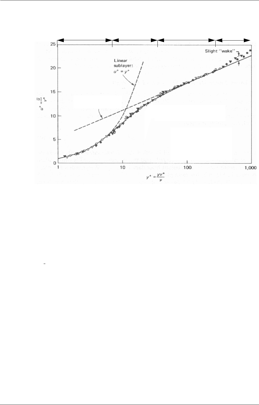
Flow Model Mathematical Model
4-12 FINE™/Turbo
Note that the sublayer extends up to y+=5 but 10 is an acceptable approximation for
design calculations.
Note: The variable v* displayed in the figure is uτ.
Picture from White, F.M., Viscous Fluid Flow, McGraw Hill, 1991.
FIGURE 4.2.5-2 Boundary layer profiles
In Figure 4.2.5-2 it is represented the evolution of u+ against y+ from the measurements of Lind-
gren(1965) with:
u+=/
Low-Re models resolve the viscous sublayer and are well suited for y1+ values less than 10 whereas
high-Re models apply analytical functions to the log-layer and are appropriate to y1+ values ranging
from 20 to 50, even more (depending on the extension of the buffer layer for the considered flow).
When the extended wall function is used, it is strongly advised to locate the first inner node either in
the viscous sublayer (y1+<5) or in the log layer (y1+>20).
Moreover one can notice that the logarithmic function does not apply for separated flow. So
whether it is expected that a significant amount of separation will have to be predicted, one of the
low-Reynolds number turbulence models would be more appropriate.
Recommendations are given in the table below for ranges of y1+ specific to the different types of
models.
logarithmic law
Data of Lindgren (1965)
viscous sub-layer buffer layer log layer
Separating flow
defect layer
u
uτ

Mathematical Model Flow Model
FINE™/Turbo 4-13
TABLE 4-1 Appropriate y1+ values for available turbulence models
One way to estimate ywall as a function of a desired y1+ value is to use a truncated series solution of
the Blasius equation:
y1+... (4-7)
Note that the reference velocity, Vref, can be taken from an average at the inlet. For instance, if the
mass flow is known the value can be calculated using density and the cross-sectional area of the
inlet. If the mass flow is not known the reference velocity may be calculated from the inlet total
pressure and an estimated static pressure using isentropic relations. The reference length, Lref,
should be based on a typical length scale since an estimation of boundary layer thickness is implied
in this calculation. For instance, in the case of a turbomachinery simulation one could use the dis-
tance between hub and shroud curves that exist upstream of the first row of blades. This is approxi-
mate, of course, as the thickness of the boundary layers will vary widely within the computational
domain. Fortunately it is only necessary to place y1+ within a range and not at a specific value.
Another method of estimating ywall is to apply the 1/7th velocity profile. In this case the skin fric-
tion coefficient Cf is related to the Reynolds number:
(4-8)
where Rex should be based on average streamwise values of Vref and Lref as discussed above. Since
uτ is based on Cf it may be calculated based on Eq. 4-6, and ywall may then be calculated from
Eq. 4-5. Note that either method is not exact but they will yield results that are quite close to each
other. In fact, it can be instructive to calculate ywall using both methods as a check. Since only one
wall distance is being calculated, the particular flow being studied should be kept in mind. For
instance if it is a diffusing flow Cf, and hence y1+, can be expected to drop. Since a certain range is
desired (e.g., 20< y1+<50 for high-Re Standard k- ε) the user may choose to base the calculation of
wall distance on an average of that range (e.g., 40).
High-Re: Low-Re:
Turbulence Models Spalart-Allmaras (Extended Wall
Function);
SARC (Extended Wall Function);
k-ε (Extended wall function);
k-ε (Standard wall function);
SST (Extended wall function)
EARSM (Extended wall function);
Baldwin-Lomax;
Spalart-Allmaras;
Spalart-Allmaras (Extended Wall
Function);
SARC;
SARC (Extended Wall Function);
k-ε (Extended wall function);
k-ε (Low Re Yang-Shih);
k-ε (Low Re Chien);
k-ε (Low Re Launder-Sharma);
Shear Stress Transport (SST);
SST (Extended wall function);
EARSM;
EARSM (Extended wall function);
k-ω (Wilcox);
v2-f (code friendly)
y1+20-50 <10
ywall 6Vref
ν
---------
78/– Lref
2
---------
18/
=
Cf
0.027
Rex
17/
--------------
=

Flow Model Mathematical Model
4-14 FINE™/Turbo
b) Things to Look Out For
Previous recommendations should provide reasonable estimates but it is always wise to plot y+
once a solution has finished. Spot checks should be made to ensure that most y1+ values fall within
the desired range. For instance it is useful to plot y+ contours over the first layer of nodes from a
given wall (available in solid data output, see section 10-2.1.5). There are some special cases where
such checks do not strictly apply. For instance, skin friction approaches zero at points of separation
so it is expected that y1+ will be low in such regions. It is generally recommended that turbomachin-
ery blade tip clearances are meshed with uniform spanwise node distributions. In such cases, the
y1+ values will tend to be higher within the gap than elsewhere in the computational domain near-
wall regions. This should not raise concern as the tip clearance flow consists of thoroughly sheared
vortical fluid that undergoes significant acceleration and is therefore quite different than a standard
boundary layer. It is expected that the skin friction will be high in this region due to the accelera-
tion.
c) General Advice
•What grid resolution is adequate?
The resolution method employed in the FINE™/Turbo solver requires approximately 9 nodes
across a free shear-layer and approximately 15 across a boundary layer to provide grid-independent
results for turbulent flows. If wall functions are used the boundary layer only requires approxi-
mately 9 nodes.
Of course the flow field under study will realistically consist of shear layers of which the width var-
ies substantially throughout the flow field. The user must therefore decide what is important to cap-
ture and what is not. For instance, in the design-cycle analysis of a compressor with a volute it
would probably be acceptable to choose a fully-developed boundary layer. The number of nodes
across the diameter would therefore be approximately 29. However, it would be wise to select a
number like 33 to maintain a large number of multi-grid levels. The selection of nodes in the
streamwise direction should be governed by what resolution adequately represents the studied
geometry. Regions of concentrated high gradients, such as airfoil leading or trailing edges or any
geometrical corners should contain a relatively high clustering of nodes.
•What determines the grid quality?
After the various grid resolution concerns are addressed, the level of skewness must be analysed.
Providing clustering in a curved geometry can often lead to internal angles of grids cells of 10o. It is
important to minimize the number of cells containing such low angles as the calculation of fluxes
can become significantly erroneous under such conditions. More information concerning how to
check the quality of a grid can be found in the IGG™ or AutoGrid™ manual. If the adjustment of
node numbers and clustering does not reduce the level of skewness, local smoothing should be
applied. The expansion ratio, or the ratio of adjacent cell sizes, should also be checked. It is partic-
ularly important to keep this value within an absolute range of about 1.0-1.6 in regions of high gra-
dients, such as boundary layers, free shear-layers and shocks. If it is evident that adjacent cells are
different in size by factors significantly greater than two, the clustering in this region should be
reduced or the number of nodes should be increased.
d) Verification of y1+
By following these instructions it should be possible to generate a grid of reasonable quality for tur-
bulent flows. It is recommended however, that the user checks values of y1+ after approximately
one hundred iterations on the fine grid to ensure the proper range has been specified. At the same
time, it can be useful to plot contours of residuals (continuity, momentum, energy and turbulence)

Mathematical Model Flow Model
FINE™/Turbo 4-15
over selective planes. If the level of skewness is too high, this will be indicated by local peaks in
residuals that are orders of magnitude greater than the rest of the flow field. If a multi-block grid is
used, the residual levels in each block can be compared in the Monitor.
4-2.5.4 Defining Initial & Boundary Conditions
Turbulence is commonly modelled by emulating molecular diffusion with a so-called "eddy-viscos-
ity" (μT). A standard method for determining μT is based on turbulent-eddy length and time scales
that are modelled through turbulence kinetic energy (k) and dissipation (e.g. ε) equations. It is
important to note that the level of turbulence quantities (i.e. turbulence intensity, μT, k, ε) specified
at the inlet boundary can have a strong effect on the flow-field prediction for quantities like the total
pressure, velocity profiles, flow angles, total temperature etc. Since the measurement of turbulence
is rarely conducted in a design and test environment, the designer faces the problem of setting these
quantities without knowing the correct values.
a) Spalart-Allmaras Model
When the Spalart-Allmaras model is selected, the kinematic turbulent viscosity
ν
t (m2/s) has to be
specified. The kinematic turbulent viscosity ratio is extremely sensitive to the type of application/
configuration. Therefore, if the user has any indication of the actual level of turbulence in the case
configuration, the user should use it. If no information is available on the order of magnitude of the
kinematic turbulent viscosity ratio, estimates can be made based on the following assumptions that:
•For internal flows (e.g. turbomachinery): = 1 to 5.
•For external flows (e.g. vehicle aerodynamics): .
b) k-
ε
, k-
ω
, EARSM and v2-f Models
When the k-ε, k-ω and v2-f models are selected, the boundary values of k and ε have to be specified.
If no information is available on the turbulence properties of the flow, estimates can be made based
on the following formulations.
b.1) Estimation of k
The value of the turbulent kinetic energy k can be derived from the turbulence intensity Tu or from
the wall shear stress.
—From the turbulence intensity: The turbulence intensity Tu can be expressed against the
streamwise fluctuating velocity u' and the streamwise velocity Uref:
(4-9)
For internal flows the value of Tu is about 5% and for external flows it is reduced to 1%. With
these considerations k can be calculated in considering an isotropic turbulence:
(4-10)
—From the wall shear stress: If the wall shear stress is known, the user can use the wall func-
tions defined for the fully turbulent flow:
νt
ν
----
νt
ν
---- 1=
Tu
u'2
Uref
----------
=
k3
2
---u'2
2
=

Flow Model Mathematical Model
4-16 FINE™/Turbo
(4-11)
This value of k could be used as an initial value and also for the inlet boundary condition.
b.2) Estimation of
ε
The value of the turbulent dissipation can be specified through one of the following rules:
—Specify the ratio of the turbulent viscosity to the laminar viscosity:
(4-12)
For internal flows (such as turbomachinery flow), typical values are .
For external flows (in aerodynamics computations), typical values are .
—Specify the turbulent length scale (only for internal flows):
A typical values is . where DH is the hydraulic diameter of the inlet section
(4-13)
—Derive ε from the asymptotic turbulent kinetic equation:
In a free uniform flow the turbulent kinetic energy equation reduces to
(4-14)
This relation can be used to specify the value of the turbulent dissipation in the following way:
(4-15)
where u is the inlet velocity, Δk the decay of the turbulent kinetic energy over a length L. For
example, in a turbomachine, L is the maximum geometric length and Δk could be set to 10% of
the inlet value of k.
Using this method, the user must make sure that the value of the turbulent viscosity obtained
from these values of k and ε is not too big or too small. i.e. . If this condition is not
satisfied, it is advised to scale down or up the value of k inlet or the Δk and compute again the
turbulent dissipation
—Specify the wall shear stress:
If the wall shear stress is known, the user can use the wall functions defined for the fully turbu-
lent flow.
(4-16)
If there is an initial solution file containing and , the and values of this file are used to
initialize the fields.
k
τ
wall
ρ
Cμ
-----------
=
εCμ
μ
μt
---- ρrefk2
μ
--------------
=
μtμ⁄ 50=
μtμ⁄ 1=
l0.1DH
=
εcμ
3
4
---
k
3
2
---
l
----------
=
uk∂
x∂
----- ε–=
εu–Δk
L
------
=
1μt
μ
---- 1000<<
ετwall ρ⁄()
3
2
---
l
-------------------------
=
k
ε
k
ε

Mathematical Model Flow Model
FINE™/Turbo 4-17
The values of the inlet boundary conditions for the and can also be used to set the initial and
fields. However, to reduce the possibility of oscillations in skin friction due to non-physical rela-
minarisation during convergence, it is recommended to insure ≈ 0.1 .
Either of the above methods can be applied for setting the boundary conditions in tur-
bomachine applications. However, if the given values of k and ε lead to the damping of
the turbulence shortly after the inlet section, we suggest to apply Eq. 4-15 and select an
inlet values of k such that the ratio of the turbulent viscosity to the laminar viscosity
equals 50.
In some cases a cross-check between Eq. 4-12 and Eq. 4-14 may result in very differ-
ent values for ε. In such a case it is recommended to re-evaluate k and ε in the following
manner:
1. Use relation Eq. 4-15:
(4-17)
This relation expresses that k0 (k at the inlet) is expected to be decreased by about 10% over a
length ΔL that is characteristic to the size of the domain.
2. Use relation Eq. 4-12. In this relation Cμ=0.09 and represents the dynamic laminar viscosity
of the fluid.
3. Combine the relations of the two previous steps to remove ε0, leading to:
(4-18)
4. Using either relation Eq. 4-12 or Eq. 4-15 then easily leads to an estimation of ε0.
4-2.5.5 Setting Expert Parameters to Procure Convergence
Several expert parameters may be set to procure convergence.
a) Cut-off (Clipping) of Minimum k Value
The float parameter EKCLIP controls the minimum allowable value of k. This is done to prevent
non-physical laminarisation and remove the possibility of negative values being calculated during
numerical transients. Setting this value to a reasonable level has been shown to significantly
increase the convergence rate.
EKCLIP(real): clipping k to about 1% of inlet value maintains minimum residual turbulence in
the domain.
b) Minimizing Artificial Dissipation in the Boundary Layer
An alternative treatment of the dissipation terms in the k and ε equations has been introduced to
overcome difficulties related to turbulence decay in boundary layers observed in some specific test
cases. Currently, the dissipation terms are scaled with the spectral radius of the equations and are
further damped in an exponential manner across the boundary layer. The major drawback of this
formulation is that it introduces an excessive amount of artificial dissipation into the boundary
layer, leading to non-physical relaminarisation problems. A different implementation, based on the
L.E.D. (Local Extrema Diminishing) version of the Jameson-Schmidt-Turkel treatment introduces
better monotonicity properties of the k and ε equations.
k
ε
k
ε
ε
εinlet
εu–Δk
ΔL
-------u0.1k
ΔL
----------
==
μ
k0
0.1U
ΔL
------------μt
μ
---- ν
Cμ
------
=

Flow Model Mathematical Model
4-18 FINE™/Turbo
IKELED(integer): 0 (default): Dissipation scaled with spectral radius.
1: Less diffusive L.E.D. scheme activated.
c) Wall Function for the k-ε Turbulence Model
INEWKE(integer):0: Wall function applies for first node off the wall at y+ =20-50, Launder &
Spalding.
10 (default): Mesh-independent formulation of the wall function.
d) Full Multigrid k-ε / Baldwin-Lomax & v2-f / Baldwin-Lomax Switch
KEGRID = 2(default) Grid 222 - Baldwin Lomax,
Grid 111 - Baldwin Lomax,
Grid 000 - k-ε or v2-f Model.
KEGRID = 3: Grid 222 - Baldwin Lomax,
Grid 111 - k-ε or v2-f Model,
Grid 000 - k-ε or v2-f Model.
Example: k-ε run on the finest grid level (000) with 3 levels of grid (222, 111 & 000) in the multi-
grid procedure. The Baldwin-Lomax model remains active on levels 222 and 111 before k-ε is auto-
matically switched on when the finest grid is reached. This is controlled through the expert parame-
ter KEGRID whose value is set to 2 by default, meaning that the Baldwin Lomax model is used up
to the second level of grid. The μt / μ field computed using the Baldwin-Lomax model is then trans-
ferred to the finest mesh and used to calculate initial k and ε values. The use of a KEGRID value
higher than the number of grid levels available enables the k and ε equations to be solved on all grid
levels.
A similar procedure can be followed when a calculation on 111 mesh is first desired. Providing
KEGRID is set to 2 (default value), the Baldwin-Lomax is then active on level 222 before the k-ε
model is automatically switched on when the finest grid level (111 in this case) is reached. How-
ever, the question then arises when a restart procedure on the 000 level is required. How to restart
on 000 while transferring strictly the k and ε fields already computed on 111? By default, since
KEGRID=2, the solution computed on 111 is seen as a Baldwin-Lomax solution. The k and ε fields
are then reset using the classical procedure while the other variable fields (density, velocity and
energy) are transferred adequately. To overcome this difficulty, KEGRID must again be set to a
value higher than the number of grids. This procedure results in a much better initialisation of k and
ε, thus preventing some relaminarisation while enhancing convergence.
e) Cut-off (clipping) of Maximum Turbulence Production/Destruction Value
The float parameter PRCLIP controls the maximum allowable value of turbulence production/
destruction (=production/density*dissipation in k-ε model). Limiting this to a finite value enhances
the convergence rate by removing the possibility of unbounded turbulence spikes occurring during
the numerical transient. However, care must be taken to apply a reasonable limit. Recommended
values are:
PRCLIP (real): For most flows: 50 (default),
In turbulent diffusion dominated flows (e.g., seals): 200.
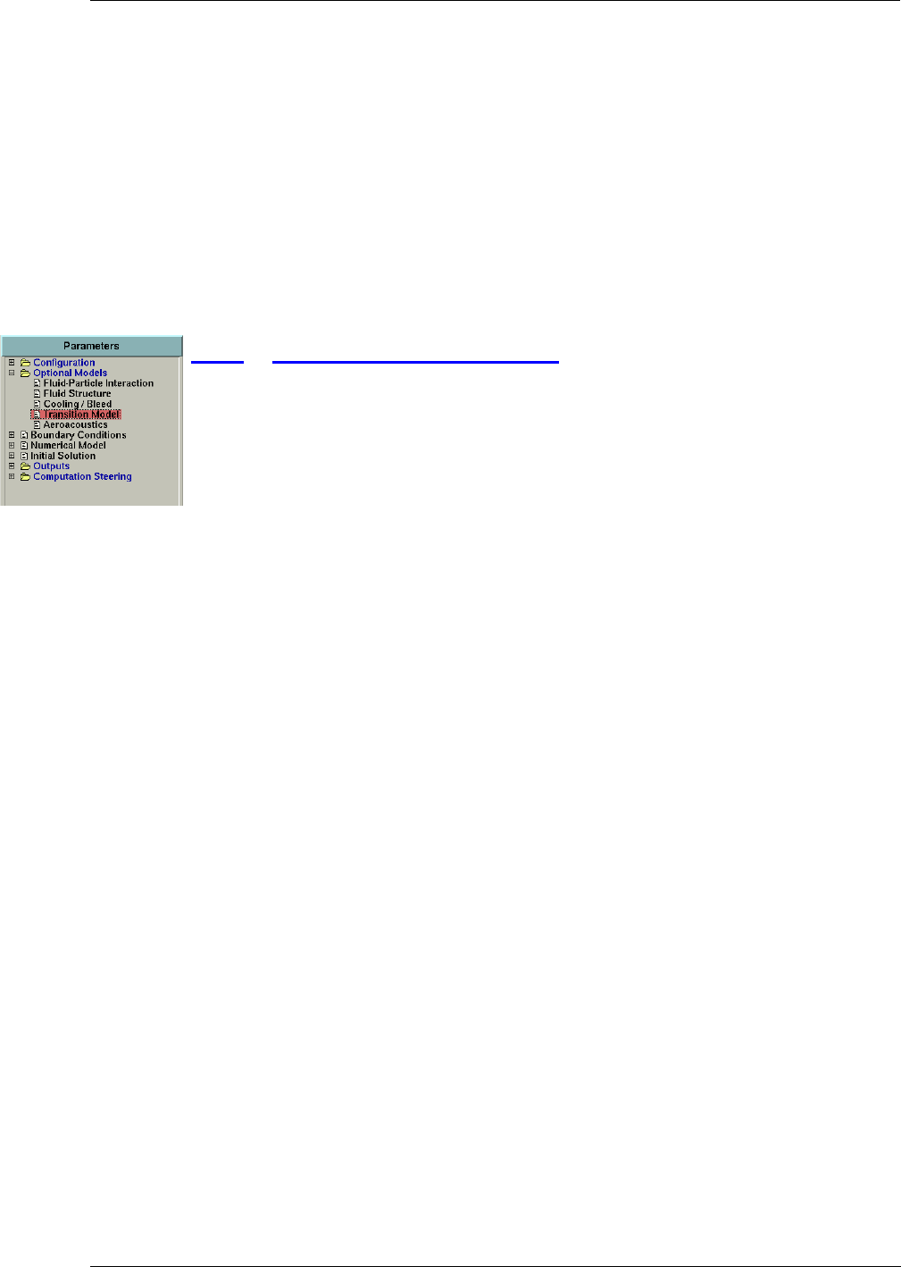
Mathematical Model Flow Model
FINE™/Turbo 4-19
f) Cut-off (clipping) of Maximum Turbulent Viscosity Ratio (
μ
t /
μ
)
The float parameter MUCLIP controls the maximum allowable value of the turbulent viscosity ratio
μt/μ. Limiting this to a finite value enhances the convergence rate by removing the possibility of
unbounded spikes occurring during the numerical transient. At the end of the computation however,
the value of μt/μ should not be clipped anymore. During the convergence process, the user can
check the output of the computation to see if the maximum value for the turbulence ratio has been
reached. If this is the case, the output will contain a line: "MUT/MU CLIPPED FOR # CELLS".
MUCLIP can then be put to a higher value, to increase the limit. However, care must be taken to
apply reasonable limits. Recommended values are:
MUCLIP (real): For most flows: 5000 (default). It can be increased if necessary.
4-2.6 Laminar-Transition Model
4-2.6.1 Introduction
The boundary layer which develops on the surface of a solid body starts as a laminar layer but
becomes turbulent over a relatively short distance known as the transition region. This Laminar-
Turbulent transition is a complex and not yet fully understood phenomenon. Among the numerous
parameters that affect the transition one can list: the free stream turbulence intensity, the pressure
gradient, the Reynolds number, and the surface curvature.
Furthermore, predicting the onset of turbulence is a critical component of many engineering flows.
It can have a tremendous impact on the overall drag, heat transfer, and performances especially for
low-Reynolds number applications. However, most of the turbulent models fail to predict the
transition location.
Therefore, a laminar-transition model is proposed in the FINE™/Turbo solver in order to take into
account the effect of the laminar-turbulent transition. The following four choices are possible in the
Transition Model page under Optional Models:
—Fully Turbulent
—Fully Laminar
—Forced Transition
—Abu-Ghannam and Shaw (AGS) Model
The present transition model can be used only with the low Reynolds number Spalart-Allmaras,
Yang-Shih k-epsilon, Wilcox k-omega and SST turbulence models.
The transition model in FINE™/Turbo is mainly devoted to turbomachinery applications using
AutoGrid™ mesh. Both the pressure and suction sides of the blade need to be set with the transition
model. Chapter 8-9 describes the interface for the transition model. More information on the
transition model can be seen in Chapter 3-8 in the theoretical manual.
However, the transition model in FINE™/Turbo is also available for the other cases, such as flat
plate, wings and hydrofoils, etc. In the next section a best practice will be given to describe how to
model transition on non-turbomachinery cases.
4-2.6.2 How to model transition on non-turbomachinery cases
Use of the transition model is restricted to the pressure and suction sides of the turbomachinery
blade using AutoGrid™ mesh. Modeling transition on non-turbomachinery cases can therefore only
be performed by considering the object to be a pseudo "blade" and modifying the mesh files manu-
ally. The limitation on the mesh of non-turbomachinery cases is:
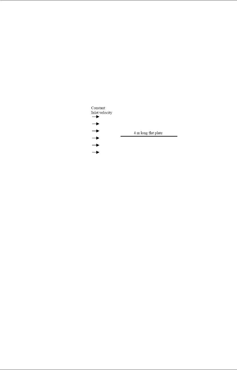
Flow Model Mathematical Model
4-20 FINE™/Turbo
•The mesh topology should be similar to a Autogrid™ mesh topology (with at least a proper
mesh in spanwise direction).
•The transition is along a pseudo "blade", so the user has to add the "blade" definition in the
mesh files manually.
Example: Mesh for modeling transition on a flat plate
Considering transition flow over a flat plate (Figure 4.2.6-3). The computational domain corre-
sponds to an external flow with a constant velocity blowing towards the flat plate.
Note that for the flat plate case the user has to consider the two faces of the plate since the transition
model needs a pressure side and a suction side.
FIGURE 4.2.6-3 Computational domain for a flat plate
In order to be compatible with the transition model, a 3D mesh should be used for this case with a
correct orientation: i perpendicular to the flat plate with i=1 on the flat plate and with j and k along
the plate: k in streamwise direction and j perpendicular to main flow direction.
The .bcs file of the mesh should be modified in order to include the turbomachinery blade defini-
tion. At the end of the .bcs file the line "NUMBER_OF_BLADES 0" should be modified: the "0"
should be change in a "1" as the flat plate will be considered as one blade (of zero thickness).
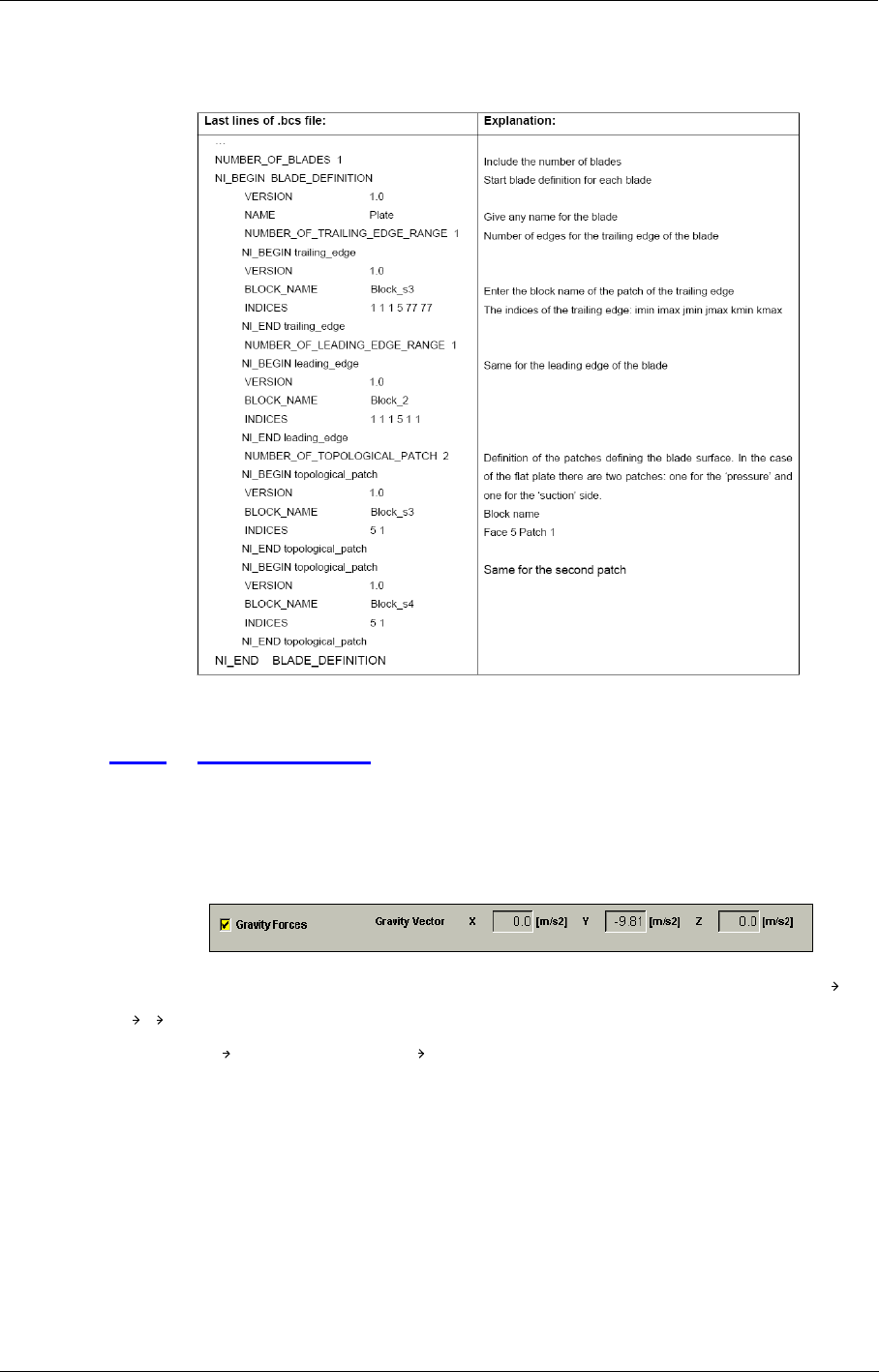
Mathematical Model Flow Model
FINE™/Turbo 4-21
Next lines need to be added as shown here:
4-2.7 Gravity Forces
When gravity should be taken into account the box Gravity Forces should be checked. If gravity is
activated, three input dialog boxes appear to define the Gravity Vector. The default gravity vector
is defined as: (gx, gy, gz)=(0,-9.81,0) [m/s2], representing the gravity on Earth where the y-axis is
oriented normal to the ground.
When the gravity is taken into account in the Navier-Stokes equations, the source terms and
are respectively introduced in the momentum and energy conservation equations where ρ
is the density, the gravity vector and the velocity vector.
If the fluid is a liquid, the density is constant and there is no influence of the pressure or temperature
on the flow by interaction with the gravity. To simulate these interactions, one can use the Boussin-
esq approximation in the gravity source terms. With this approximation, the density is developed in
the first order of the MacLaurin series. It becomes:
(4-19)
with α the compressibility and β the dilatation coefficients specified in the fluid properties.
ρg
ρgv⋅()
g
v
ρρ
ref 1αpp
ref
–()β–TT
ref
–()+()=

Flow Model Characteristic & Reference Values
4-22 FINE™/Turbo
This variation of the density is only applied to the gravity source term (Boussinesq approximation).
Otherwise, the density is kept constant in the conservation equations. The value of is the char-
acteristic density specified in the Configuration/Flow Model page. and are the reference
values in the Configuration/Flow Model page.
When the gravity is taken into account, a reference pressure must be specified at a ref-
erence altitude to add the hydrostatic pressure in the initial pressure field. The reference
pressure is the reference value in the Configuration/Flow Model page. The reference
altitude is specified in the expert parameter IREFPT in meter [m].
4-2.8 Low Speed Flow (Preconditioning)
This option appears in the Flow Model page only if the fluid type is compressible.
Preconditioning is automatically used for incompressible fluids.
In the low Mach number regime, time-marching algorithms designed for compressible flows show
a pronounced lack of efficiency. When the magnitude of the flow velocity becomes small in com-
parison with the acoustic speeds, time marching compressible codes converge very slowly.
Two low speed preconditioners, Hakimi and Merkle preconditioners, have been implemented in the
FINE™/Turbo solver in order to provide fast convergence characteristics and accurate solutions as
the Mach number approaches zero:
•The Hakimi preconditioner is of sufficient generality and can treat any type of fluids and
flows. Efficient convergence rates and accurate solution can be obtained for Mach numbers
from M=0.1 to M=10-6, Reynolds numbers from Re=106 to 10-6 and aspect ratios from 1 to
2000.
•Compared with the Hakimi preconditioner, the Merkle preconditioner has the advantage that it
is not only effcient at all Mach number but also at all Reynolds and Strouhal numbers. With the
Merkle preconditioner, the user can perform a fast and accurate computation of supersonic
flows with regions at very low speed. Moreover the Merkle preconditioner doesn't require any
user inputs.
Merkle preconditioning is not compatible with:
•barotropic fluids
•unsteady mode
•cavitation model
For the detailed parameter settings, please refer to section 6-2.2.4.
4-3 Characteristic & Reference Values
4-3.1 Reynolds Number Related Information
The user has to specify some characteristic values (length, velocity and density). These values are
used to calculate the Reynolds Number (only plotted when the kinematic viscosity is constant) that
provides a useful information to choose the suitable model (section 4-2.5). These characteristic val-
ues can be used for other purposes as well.
ρref
pref
Tref
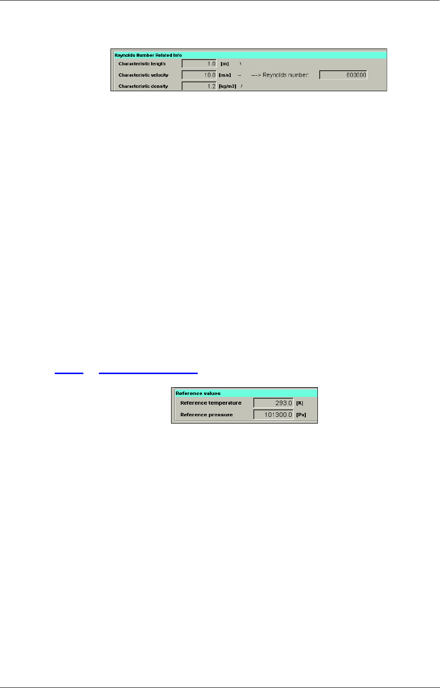
Characteristic & Reference Values Flow Model
FINE™/Turbo 4-23
The characteristic length is used:
—in the outlet boundary condition for which the mass flow is imposed with pressure adapta-
tion,
—in the computation of CP1 and CP3 for cylindrical cases.
—in the transition model, to set the free stream turbulent intensity.
The characteristic velocity is used:
—in the preconditioning method to compute the parameter β,
—in the computation of the solid data Cf (normalized by ).
The characteristic velocity should be set to the highest value in the flow domain.
The characteristic density is used:
— in the Boussinesq approximation for incompressible fluid (Eq. 4-19),
— in the computation of the solid data Cf (normalized by ),
—in the evaluation of the Reynolds number only when the dynamic viscosity of the fluid is
specified in the Sutherland law on the Fluid Model page.
4-3.2 Reference Values
The reference values have been introduced for preconditioning, to define a gauge pressure and a
gauge total energy.
A value of Reference temperature Tref of the order of magnitude of the expected tem-
perature field will reduce the machine round-off errors influence on the temperature
field.
The value of Reference pressure Pref fixes the absolute level of the pressure in the
field. This value is used in the equation of state for a compressible fluid and in the sec-
ond order artificial dissipation term. A value of Pref close to the real pressure level is
therefore recommended.
These reference values also have some additional uses which are described hereafter:
—in the Boussinesq approximation for incompressible fluid (Eq. 4-19),
—in the outlet boundary condition for which the mass flow is imposed with pressure adapta-
tion,
ρrefUref
22⁄()
ρrefUref
22⁄()

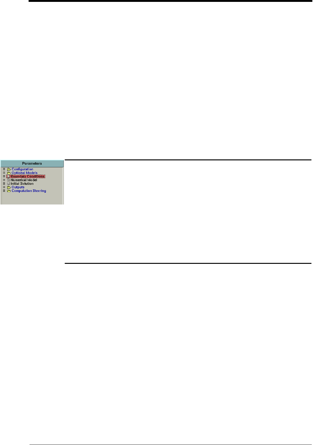
FINE™/Turbo 5-1
CHAPTER 5: Boundary Conditions
5-1 Overview
During the IGG™ grid generation process, the user has to define the type of boundary condition to
be imposed along all boundaries. The parameters associated with these boundary condition types
can be fully defined using the Boundary Conditions page.
This chapter gives a description of the boundary conditions, available in the Boundary Conditions
page. In section 5-2, the page is described. For expert use, section 5-3 gives an overview of the
available expert parameters. In section 5-4, some advice is provided on the combinations of bound-
ary conditions to use.
5-2 Boundary Conditions in the FINE™/Turbo
GUI
When selecting the Boundary Conditions page the "parameters area" appears as shown in
Figure 5.2.0-1. Five tabs are available, depending on the boundary condition types defined in the
mesh. There are currently five types of boundary conditions available in the FINE™/Turbo solver:
inlet, outlet, periodic (connection with or without rotational or translational periodicity), solid walls
and external (far-field). Each of those is described in the next sections.
Note that the connecting (matching (CON) and non-matching (NMB)) boundary con-
ditions (without periodicity) do not appear in this menu, because they do not require any
input from the user. Only the "periodic" conditions (PER & PERNM) appear in the Peri-
odic tab page.
Note that the full non matching and periodic full non matching connections defined
within IGG™ (refer to IGG™ User Manual for details on limitations) are appearing in
the Solid tab page.
A common particularity of the five boundary conditions pages is their subdivision into two areas.
The left area contains always a list of the different patches that are of the boundary condition type
of the selected tab page. A patch can be identified either by the name of the block face to which it
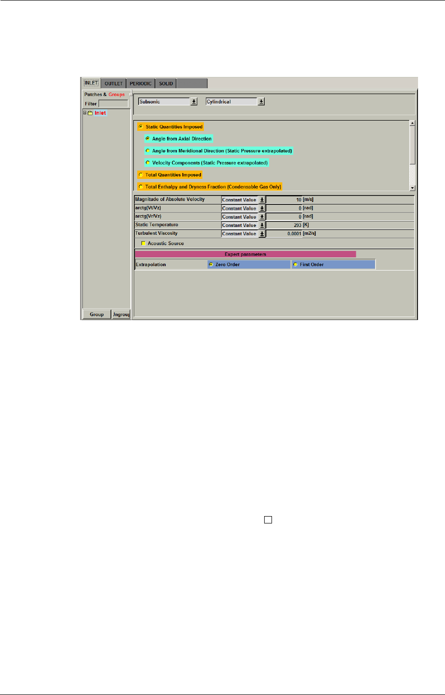
Boundary Conditions Boundary Conditions in the FINE™/Turbo GUI
5-2 FINE™/Turbo
belongs and by its number, or by the numbers of the block and face and by its local index on the
face (if no name is provided in IGG™). The right area is the area where the boundary condition
parameters are specified for the selected patch(es).
FIGURE 5.2.0-1 Boundary Conditions page
One or several patches may be selected in the left area by simply clicking on them. Clicking on a
patch unselects the currently selected patch(es). It is possible to select several patches situated one
after another in the list by clicking on the first one and holding the left mouse button while selecting
the next. To select a group of patches that are not situated one after another in the list, the user
should click on each of them while simultaneously holding the <Ctrl> key pressed.
Several patches can be grouped by selecting them and clicking on the Group button. A dialog box
will appear asking for a group name. The name of the group will appear in red color in the list of
patches to indicate that this is a group of patches. Every change in the parameters when a group is
selected applies to all patches in the group. The Ungroup button removes the group and its patches
are displayed individually in the list.
The Ungroup button is active only when at least one group is selected.
Clicking with the left mouse button on the plus sign + left of a group name in the list will display
the patches included in this group.
If some of the patches have been given names in IGG™, these names will appear in
FINE™/Turbo. If the patches have been grouped in IGG™, by giving the same name to
many patches, they will appear ungrouped in FINE™/Turbo (with block, face and patch
number shown after the name) to avoid contradiction between grouping in IGG™ and
FINE™/Turbo. Ungroup button will toggle the IGG™ name of the selected patch(es)
with the default FINE™/Turbo name (block, face and patch number).
If the Use Grid Configuration option is activated when linking the mesh for the first
time (see section 2-2.3), a default grouping by row is proposed by FINE™/Turbo. For
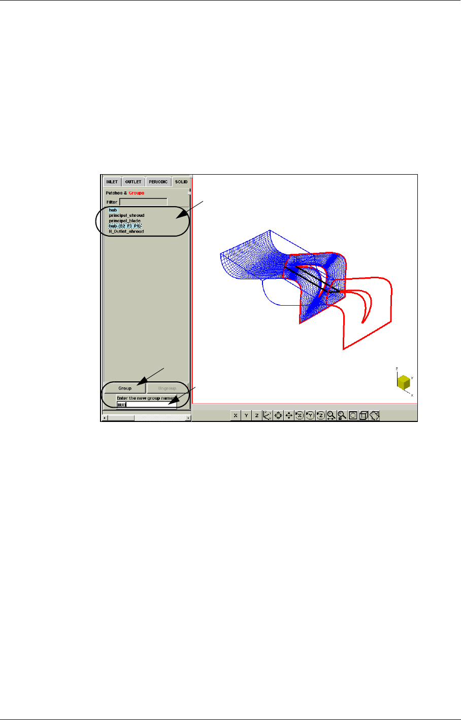
Boundary Conditions in the FINE™/Turbo GUI Boundary Conditions
FINE™/Turbo 5-3
the solid boundaries, the rotation speed specified in IGG™ or AutoGrid™ is automati-
cally transferred to FINE™/Turbo. This limits the user input to a strict minimum. This
automatic grouping cannot be modified by the user.
If the graphics area with the mesh topology of the project is opened (Mesh/View On/Off menu), all
the selected patches and/or groups will be highlighted. A click with the right mouse button over a
selected patch will select all the patches and groups in the list that have the same parameters.
If the user selects several patches that have different parameters, a warning dialog box will appear.
When clicking on OK all parameters will be set equal to the ones of the first patch. Selecting Cancel
instead will cancel the selection.
FIGURE 5.2.0-2 Two patches will be grouped into a group called HUB.
The right area of all the notebook boundary condition pages is created in a generic way by means of
a resource file, where all the boundary condition parameters are described altogether with their
default values.
Some boundary conditions are only available for an incompressible, compressible or
condensable gases. FINE™/Turbo will automatically disable the boundary conditions
that are not available, depending on the type of fluid selected in the Fluid Model page.
Also the type of boundary conditions are adjusted according to the selection for Carte-
sian or cylindrical boundary conditions.
The five pages associated to each of the five types of boundary conditions are described in detail in
the following sections.
(1)
(2)
(3)
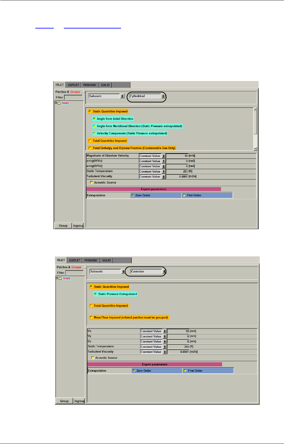
Boundary Conditions Boundary Conditions in the FINE™/Turbo GUI
5-4 FINE™/Turbo
5-2.1 Inlet Condition
5-2.1.1 Available Types
The inlet boundary condition page is customized according to the configuration of the project (Car-
tesian or cylindrical) as shown in the following two figures. The user has the freedom to access both
types of configuration in the Boundary Conditions page independently of the mesh properties.
FIGURE 5.2.1-3 Subsonic inlet boundary conditions page for cylindrical problems.
FIGURE 5.2.1-4 Subsonic inlet boundary conditions page for Cartesian problems.

Boundary Conditions in the FINE™/Turbo GUI Boundary Conditions
FINE™/Turbo 5-5
The upper part of the inlet boundary condition page allows the user to select the type of inlet condi-
tion to apply to the selected patches through a series of toggle buttons. There are two categories of
inlet conditions: conditions applicable to Subsonic inlets and conditions applicable to Supersonic
inlets.
Note that to determine whether an inlet (or an outlet) boundary is subsonic or super-
sonic, the velocity component normal to the boundary should be considered.
Total quantities imposed condition applicable to supersonic inlets is not compatible
with condensable fluid.
For each inlet condition type, the lower part of the page is adapted in order to provide input boxes
only for the physical variables that are required to fully determine the boundary condition. These
variables are for instance: the pressure and temperature (static or total), the velocity components,
the velocity magnitude, the velocity angles (specified in radians), or the mass flow. In case of a sim-
ulation using a k-ε, k-ω or v2-f turbulence model, the inlet values of the parameters k and ε are also
required. A turbulent viscosity entry appears in case the Spalart-Allmaras turbulence model is used.
For the inlet boundary conditions:
•The velocity components are defined in the Cartesian or cylindrical coordinate system,
depending on the selected type
•The pressure and the temperature values to specify can be the static or the total values
•For rotating configurations, the specified values are the absolute quantities
•A special condition is available, for which the values can be entered in the upstream rotational
frame of reference
Six major types of inlet boundary conditions can be identified:
•velocity components and the static temperature
•total pressure, total temperature and the flow direction
Total quantities imposed boundary conditions with V-extrapolated is incompatible
with a model which streamwise direction is in negative Z.
•total enthalpy, dryness fraction and the flow angles (only for condensable fluid)
It should be mentioned that the use of this boundary condition requires the presence of
the saturation table ("PSA.atab") of the fluid in the corresponding subfolder.
The boundary condition is based on the dryness fraction (X), whose value is bounded
between 0 and 1. The inlet thermodynamic must be either saturated or be located inside
the biphasic zone. The validity of the condensable fluid model is limited to gases with
small fraction of liquid (X > 0.9) or reversely to liquids with small fraction of gas (X <
0.1).
•mass flow, static temperature and the flow direction (see the next paragraph for detail on cou-
pling with the outlet)
The mass flow imposed in the GUI will be used for the whole inlet. For example, if
the user has a rotational periodicity of 40, the mass flow for only one passage will be the
mass flow specified in the GUI divided by 40.
•distributions of the flow variables for the non-linear harmonic method. For more detail, please
refer to Chapter 8-4.2.2.
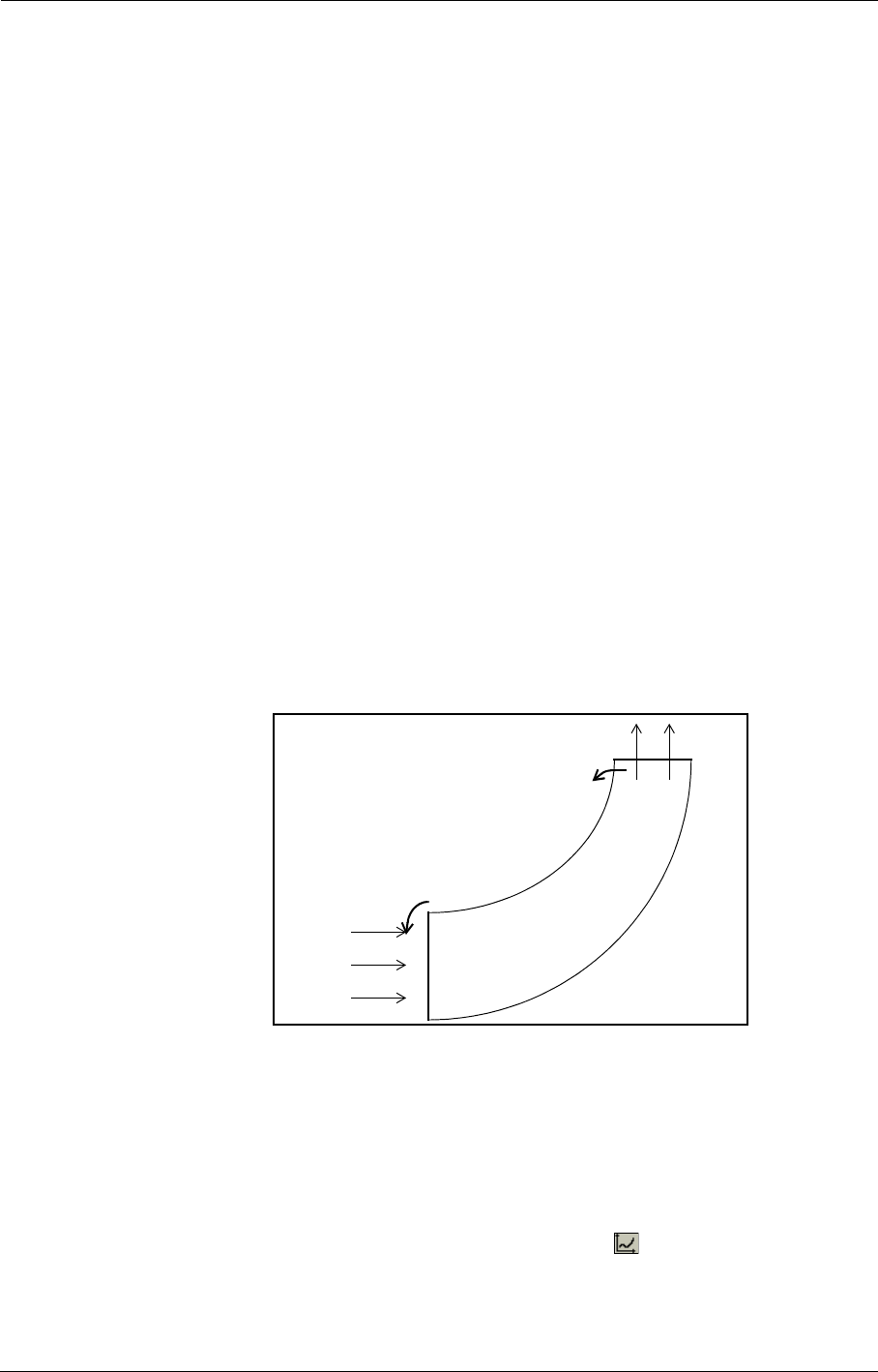
Boundary Conditions Boundary Conditions in the FINE™/Turbo GUI
5-6 FINE™/Turbo
•conditions set from a rotor-stator interface (SubProjects only, see Chapter 8-11)
Inlet boundary condition Velocity normal to inlet is not compatible with the following
expert parameter value:
•INITRB=0
•IMASFL=1
•INMFTT=1
Moving grid is not compatible with relative velocity normal to inlet when using mass
flow imposed.
5-2.1.2 Coupling Temperature with Outlet
When the mass flow is imposed at an inlet patch, the temperature may be chosen to be coupled to an
outlet patch. The coupling is performed through the static temperature. Only in that case, the aver-
age temperature Taverage is computed at the specified outlet and imposed at the inlet as Tinlet = Taver-
age + ΔT (see Figure 5.2.1-5). The quantity ΔT is a constant temperature difference (>=0 or <0)
specified by the user. This is done in FINE™/Turbo by choosing Mass Flow Imposed as boundary
condition type for the subsonic inlet in cylindrical configuration and clicking on the Coupling
Temperature With Outlet button. A pull-down menu allows to select which patch of the outlet
must be involved in the coupling. The value to be entered in the static temperature box is ΔT.
This option is only working if both inlet and coupled outlet patch have the mass flow
imposed as a boundary condition.
FIGURE 5.2.1-5 Meridional view of the "Coupling with Outlet ID" functionality
5-2.1.3 Imposing Variables as an Interpolation Profile
Each variable can be defined as constant or as an interpolation profile of the variable. The imposed
boundary condition may be variable in space (one or two dimensions) and/or in time (in case of an
unsteady calculation).
To visualize and/or edit the profile data press the small button ( ) on the right side of the label
"profile data". This button opens the Profile Manager with the existing profile. See section 2-7 for a
Taverage + ΔT
Taverage
Outlet
Inlet
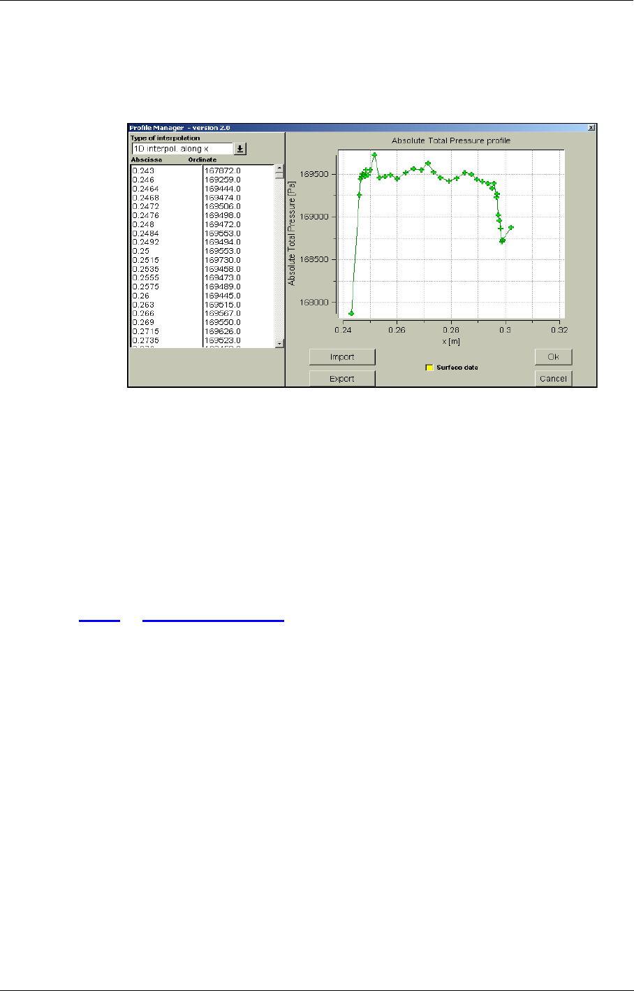
Boundary Conditions in the FINE™/Turbo GUI Boundary Conditions
FINE™/Turbo 5-7
detailed description of the Profile Manager. It offers the possibility to modify or to create a data
profile interactively. Click on the OK button to set the new profile to the selected patch(es).
FIGURE 5.2.1-6 The Profile Manager
The option Surface data toggles 1D and 2D editing modes. It can be used to change the dimension
of an existing profile. 2D profiles are displayed as a "cloud of points". Selecting a point will display
the f(x,y) value in blue in the corresponding column of the Profile Manager. More details on the
required file format are available in Appendix A.
If a quantity is defined as a function without the definition of a valid profile a warning
message will appear when saving the project or opening a new page or tab page. In such
a case a default constant value is used in the computation.
5-2.2 Outlet Condition
For a supersonic outlet all variables are extrapolated. An outlet is considered as supersonic on the
basis of the normal velocity direction to the boundary.
Five types of subsonic outlet boundary condition are available, as shown in Figure 5.2.2-7. These
five different boundary conditions are described in the following paragraphs.
An option for treatment of Backflow Control can be activated in the case of radial diffusers outlet.
The purpose of this option is to control the total temperature distribution along the exit section. In
case the flow partially re-enters the domain through the boundary, the total temperature of the enter-
ing flow is controlled so that the entering and outgoing flows globally have the same total tempera-
ture.
Backflow Control is only compatible with compressible fluid. When condensable or
incompressible fluids are used, it is suggested to use the expert parameter BCKFLO to
control backflow at outlet, see Chapter 5-3.5 for more detail.
Backflow Control is applied separately on each outlet patch when an uniform static
pressure is imposed (it is applied to a group of patches if averaged static pressure and
mass flow are imposed).
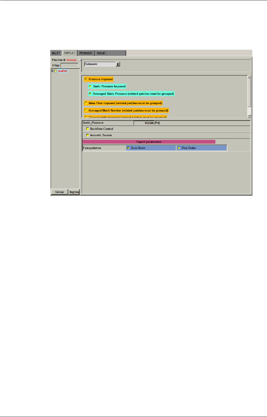
Boundary Conditions Boundary Conditions in the FINE™/Turbo GUI
5-8 FINE™/Turbo
Backflow Control is not available for the outlet boundary conditions where static
pressure is imposed with radial equilibrium.
FIGURE 5.2.2-7 Outlet boundary conditions page.
5-2.2.1 Pressure Imposed
There are three different methods to impose the pressure at the outlet:
•Static Pressure Imposed: the static pressure is imposed on the boundary, the static tempera-
ture and the absolute velocity components are extrapolated. As described for the inlet condi-
tions, the static pressure can be constant or defined as a data profile.
•Averaged Static Pressure: if imposing an uniform static pressure at the outlet is not an appro-
priate approximation of the physical pressure distribution at the outlet, an averaged static pres-
sure may be used. In this case only an averaged value for the static pressure is imposed while
the pressure profile (around this average) is extrapolated from the interior field.
The outlet patches have to be grouped in one group to use this boundary condition.
•Radial Equilibrium: This boundary condition is applicable only to cylindrical problems. It is
adapted for a patch in which the mesh lines in the circumferential direction have a constant
radius. The outlet static pressure is then imposed on the given radius and the integration of the
radial equilibrium law along the spanwise direction permits to calculate the hub-to-shroud pro-
file of the static pressure. Please note that the given radius should be between hub and shroud.
Otherwise the outlet static pressure will be imposed on the corresponding extreme radius of
the outlet instead of the given radius. A constant static pressure is imposed along the circum-
ferential direction.
This boundary condition is only valid on surfaces with mesh lines at constant radius.
This boundary condition is not compatible with the radius r=0.

Boundary Conditions in the FINE™/Turbo GUI Boundary Conditions
FINE™/Turbo 5-9
The pressure imposed at the outlet, can be constant or as a function of space and/or time. To define
a profile as a function of space and/or time click on the profile button ( ) right next to the input
text box. The Profile Manager will appear as described in section 5-2.1.3.
5-2.2.2 Mass Flow Imposed
When imposing the mass flow at the outlet, the related patches must be grouped. This permits to
have several groups of patches, each of the groups constituting an outlet through which the mass
flow can be controlled.
Two different techniques are available to impose the mass flow:
•Velocity Scaling: the pressure is extrapolated and the velocity vector is scaled to respect the
mass flow. This technique is only valid for subsonic flows, and is not recommended in case of
significant back flows along the exit boundary.
•Pressure Adaptation: this boundary condition is identical to the ’Static Pressure Imposed’
or ’Radial Equilibrium’ boundary conditions, except from the fact that the exit pressure is
automatically modified during the resolution process so that after convergence, the prescribed
mass flow is obtained.
The pressure asked in addition to the imposed mass flow with both options is only used to create the
initial solution and for the full-multigrid process, during which a uniform static pressure outlet con-
dition is used.
When using the mass flow imposed outlet boundary condition and restarting a compu-
tation from a file, only one group of patches can be used in the initial solution page and
the reset convergence history has to be deactivated
The outlet patches have to be grouped in one group to use this boundary condition.
The mass flow imposed in the GUI will be used for the whole outlet. For example, if
the user has a rotational periodicity of 40, the mass flow for only one passage will be the
mass flow specified in the GUI divided by 40.
5-2.2.3 Averaged Mach Number
When imposing the averaged Mach number at the outlet, the user must group all the related patches
for each outlet. This permits to have several groups of patches, each of the groups constituting an
outlet through which the averaged Mach number can be controlled.
Two options are available:
•Absolute Mach Number with Pressure adaptation: the absolute Mach number is imposed at
the outlet boundary. The exit pressure is automatically modified during the resolution process
so that after convergence, the prescribed absolute Mach number is obtained.
•Relative Mach Number with Pressure adaptation: the relative Mach number is imposed at
the outlet boundary. The exit pressure is automatically modified during the resolution process
so that after convergence, the prescribed relative Mach number is obtained.
The initial pressure asked in addition to the imposed Mach number is used in the full multigrid ini-
tialisation. This value is also used for the turbomachinery initial solution.
During the pressure adaptation process, the exit pressure can be imposed in different ways:
•Constant Profile: this boundary condition is identical to the ’Static Pressure Imposed’
boundary condition.
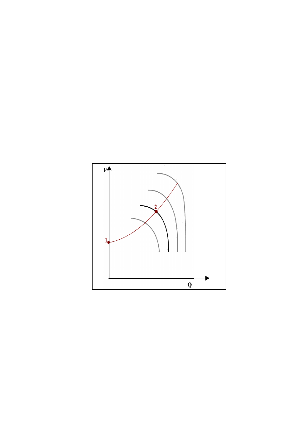
Boundary Conditions Boundary Conditions in the FINE™/Turbo GUI
5-10 FINE™/Turbo
•Radial Equilibrium: this boundary condition is identical to the ’Radial Equilibrium’ bound-
ary condition.
•Extrapolated Profile: this boundary condition is identical to the ’Averaged Static Pressure’
boundary condition.
The averaged Mach number boundary condition at outlet is not compatible with
incompressible fluid.
5-2.2.4 Characteristic Imposed
This boundary condition has been implemented to increase the robustness in the frame of a design
process and is only available when using a perfect or real gas in the Fluid Model page.
Figure 5.2.2-8 shows as an illustration performance curves for a centrifugal compressor. Near chok-
ing conditions the mass flow stays almost constant with a variation of the pressure. Therefore, it is
recommended in this region, to impose the static pressure at the outlet. Near stall however, the pres-
sure varies only slightly with varying mass flow. Therefore, it is recommended in this region of the
performance curve, to impose the mass flow at the outlet instead of the static pressure.
FIGURE 5.2.2-8 Example of performance curves for centrifugal compressor
In a design process, with a variation of the geometry, it is not always known in advance where in the
performance curve the computations are performed. Therefore it is not always possible to choose
the appropriate boundary condition at the outlet for the complete design process.
To overcome this problem this boundary condition allows to impose a relation between the mass
flow and the pressure at the outlet. It is no longer needed to choose between imposing pressure
when working around the chocking part and imposing mass flow when working close to the stall
limit.
The user has to impose a very simple characteristic line defined through 3 parameters: a target out-
let mass flow and a target outlet pressure (at point 2 in Figure 5.2.2-8) and the pressure at zero mass
flow (point 1 in Figure 5.2.2-8). Based on these three parameters, a simple parabolic curve is gener-
ated. This curve is then used to apply the boundary condition allowing to impose a relation between
the mass flow and the pressure at the outlet.
(static pressure)
(mass flow)
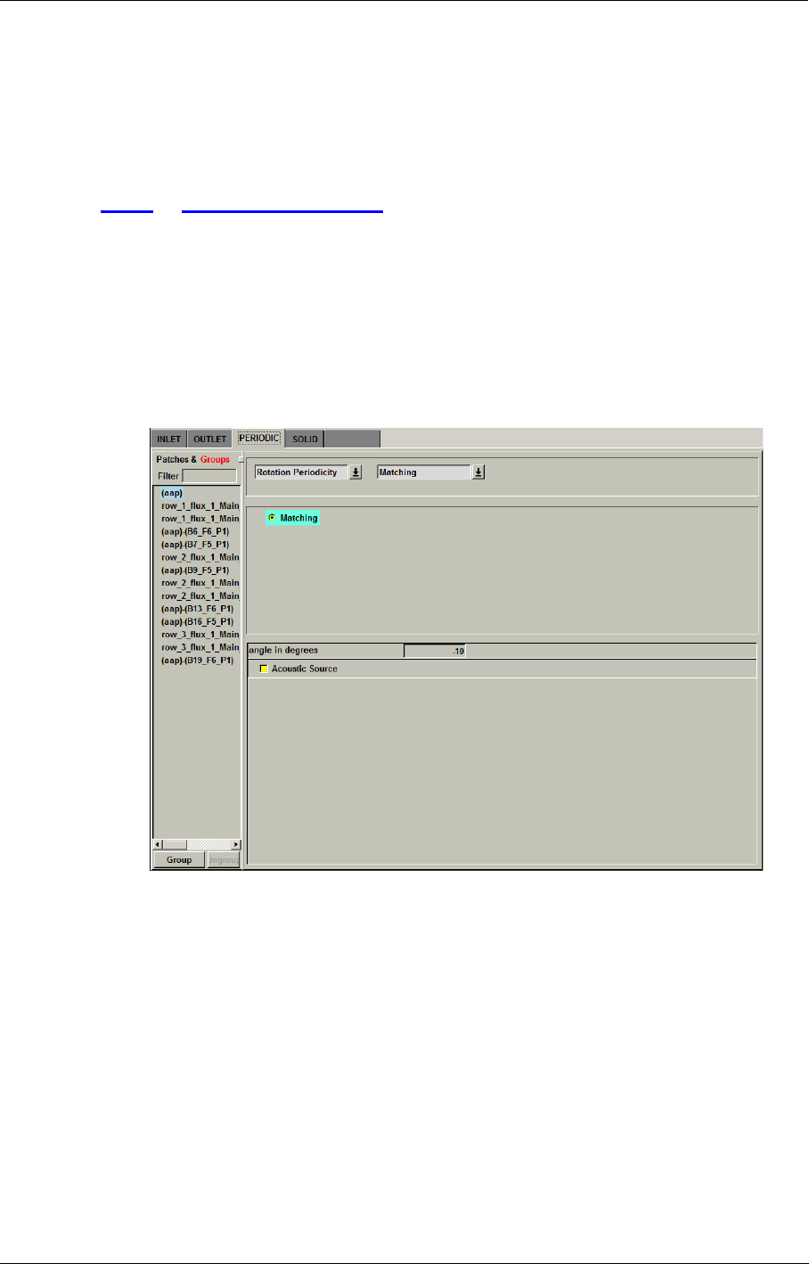
Boundary Conditions in the FINE™/Turbo GUI Boundary Conditions
FINE™/Turbo 5-11
5-2.2.5 From Rotor/Stator
The outlet boundary condition From Rotor/Stator can only be used in the frame of the SubProject
module. This boundary condition is set automatically, no user intervention is required. For more
details, see Chapter 8-11.
5-2.3 Periodic Condition
One important feature of the IGG™ mesh generator concerns the automatic establishment of all
connecting and periodic boundary conditions. The corresponding information is transmitted to the
FINE™/Turbo interface, with the advantage that the user does not need to specify any input con-
cerning these boundary conditions.
Normally no user input is required on this page. The only periodic boundary condition cases for
which a user input is required are those in which some of the boundary conditions have to be
applied with a periodicity angle that differs from the global periodicity angle of the block.
FIGURE 5.2.3-9 Periodic boundary condition page.
In case some input is required this section explains how to define the periodic conditions using the
PERIODIC tab page.
The type of periodicity connection between the patches (Matching or Non Matching) can be
entered. A connection is Matching if the numbers of mesh points along the connected patches are
identical, and if all the corresponding points along these patches coincide (PER type within
IGG™). The Non Matching connection (PERNM type within IGG™) requires the use of an inter-
polation process to establish the connection, whereas a matching one consists of a single communi-
cation of the flow variables. The interpolation used for non matching periodic boundaries consists
on a linear interpolation from the four nearest cells.
Some additional characteristics need to be given to fully determine the periodic boundary condi-
tion:

Boundary Conditions Boundary Conditions in the FINE™/Turbo GUI
5-12 FINE™/Turbo
•For Cartesian (rectangular) problems, the user has to specify the translation vector defining the
periodicity. The positive translation vector goes from the current patch to the periodicity
patches.
•For cylindrical problems, the user has to specify the rotation angle in degrees. The rotation
angle is calculated from the connected patch to the current patch, according to the rule of the
right handed system.
5-2.4 Solid Wall Boundary Condition
The solid wall boundary condition page is customized essentially according to the type of calcula-
tion (inviscid or viscous).
For Euler cases (i.e. inviscid), no parameter is requested for the wall boundary conditions. For
Navier-Stokes cases, the box at the top of the page allows to set both velocity and thermal condi-
tions. The type of boundary conditions determines the way the velocity and thermal conditions are
defined for the solid boundary.
5-2.4.1 Cylindrical Boundary Condition
a) Area Defined Rotation Speed
The wall rotation velocity can be constant or area defined (see Figure 5.2.4-10). The area defined
option allows to attribute a specific rotation velocity to a rectangular zone in the meridional plane
independently of the grid structure.
When the area defined option is selected, a small picture defining the parameters is displayed (the z
axis is the rotation axis, the r axis is the radial axis). The rotation velocity is set to outside the
domain and to inside the domain.
The specified range must be a valid range for the used geometry. For example, for an
axial machine the limits for rotation of the hub can be defined by setting the lower and
higher axial limit to appropriate values. In such a case it is important to set the radial lim-
its such that they include the full solid (hub) patch.
ω1
ω2

Boundary Conditions in the FINE™/Turbo GUI Boundary Conditions
FINE™/Turbo 5-13
FIGURE 5.2.4-10 Solid boundary conditions page in case of a cylindrical boundary condition
b) Thermal Condition
Four options are available for the thermal condition:
•Adiabatic
•Imposed Heat Flux (in W/m2)
A positive heat flux indicates that the direction of the heat flux is from the solid wall to the
fluid.
•Imposed Temperature (isothermal)
•Imposed heat transfer coefficient (W/K/m2)
,
where is the local heat flux, the local temperature at the wall and the refer-
ence temperature inputted by the user.
The imposed heat flux, temperature or heat transfer coefficient can be constant on the patch or
defined as a profile. Use the pull down menu to change Constant Value to for example fct(space).
Click on the profile button to launch the Profile Manager as described insection 5-2.1.3.
5-2.4.2 Cartesian Boundary Conditions
The user can define a translation or a rotation velocity vector. In the latter case, the coordinates of
the rotation centre are requested. The thermal conditions are similar to those for cylindrical flows.
hqw
Tref Twall
–()
---------------------------------
=
qw
Twall
Tref

Boundary Conditions Boundary Conditions in the FINE™/Turbo GUI
5-14 FINE™/Turbo
5-2.4.3 Force and Torque
Below the box, a Compute force and torque option is provided that permits to include the selected
patches in the calculation of the global solid boundary characteristics.
The contribution of patches included in a full non-matching connection will not be
taken into account for the computation of the force and torque. Those patches will how-
ever appear as solid in the boundary condition page.
For a cylindrical project (as defined in Mesh/Properties) in an internal flow (the expert parameter
IINT set to 1 as by default):
—the axial thrust, i.e. the projection of the global force on the rotation axis,
—the torque, i.e. the couple exerted by the global force, calculated at (0,0,0).
These quantities are often calculated on the rotating walls. They are calculated from the pressure
and the velocity fields on the walls. The axial thrust is computed as:
.(5-1)
The computed force is the one from fluid on solid. The force is considered as positive
when in the direction of the z-axis.
The projection of the torque along a given direction , i.e. the couple exerted by the global force
along the rotation axis:
(5-2)
In all other cases the force and torque are computed as:
—the lift,
—the drag,
—the moment calculated at (0,0,0) by default.
The direction of the forces and torque as well as the location of the point for the moment can be
determined with the expert parameters IDCLP, IDCDP, IDCMP and IXMP (see section 5-3).
When using an area defined rotation speed, the expert parameter TORRO can be used to compute
the force and torque on the complete patch, or on the rotating part only (see section 5-3).
Within the FINE™/Turbo solver it is possible to calculate and to store the partial torque in the cor-
responding ".wall" file of the computation through the use of the expert parameter IFRCTO within
the FINE™/Turbo GUI.
The partial torque is the torque computed for each layer on the whole blade. When IFRCTO is set to
2 (1 or 3), the torque is defined on each J-direction (I-direction or K-direction) layer (i.e. when
using AutoGrid™ meshes, J-direction corresponds to the spanwise direction).
Fn
z
⋅
S
z
rF×
S
z⋅
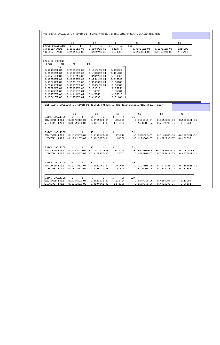
Boundary Conditions in the FINE™/Turbo GUI Boundary Conditions
FINE™/Turbo 5-15
FIGURE 5.2.4-11 File ".wall" when computing partial torque along the blade
Finally, the resulting ".wall" will contain, in addition of the global torque and force on the selected
blade, the partial torque for each layer along the J-direction of the blade as presented in
Figure 5.2.4-11.
The force and torque computed on the selected surface(s) and included in ".wall" file
are based on the full 360 degrees, so taking into account the periodicity when the blocks
concerned are presenting a periodicity.
5-2.4.4 Properties of Solid for Turbulence
In addition, when turbulence models with extended wall function are used, the user has to specify
the type of wall ("Smooth" or "Rough") and the following constants: the Von Karman constant κ
and the B constant. If the wall type is rough, the equivalent roughness height k0 and the height of
the zero displacement plane d0 are also required. A description of these constants is provided in the
theoretical manual.
Two methods considering the wall function for roughness is implemented. With the old method
(default, IROUGH=0), the constant B has to be computed after obtaining the value of y+. And the
value of B will also correct y+. The user has to iterate this procedure and converge to the desired
IFRCTO = 0
IFRCTO = 2
Total Torque and Force on Suction Side
Partial Torque and Force on Suction Side
• 56 = 56 sublayers in J-direction (spanwise)
• column 1: %span corresponding to the layer
• column 2: Fx on the sublayer
• column 3: Fy on the sublayer
• column 4: Fz on the sublayer
Total Torque and Force on Suction Side
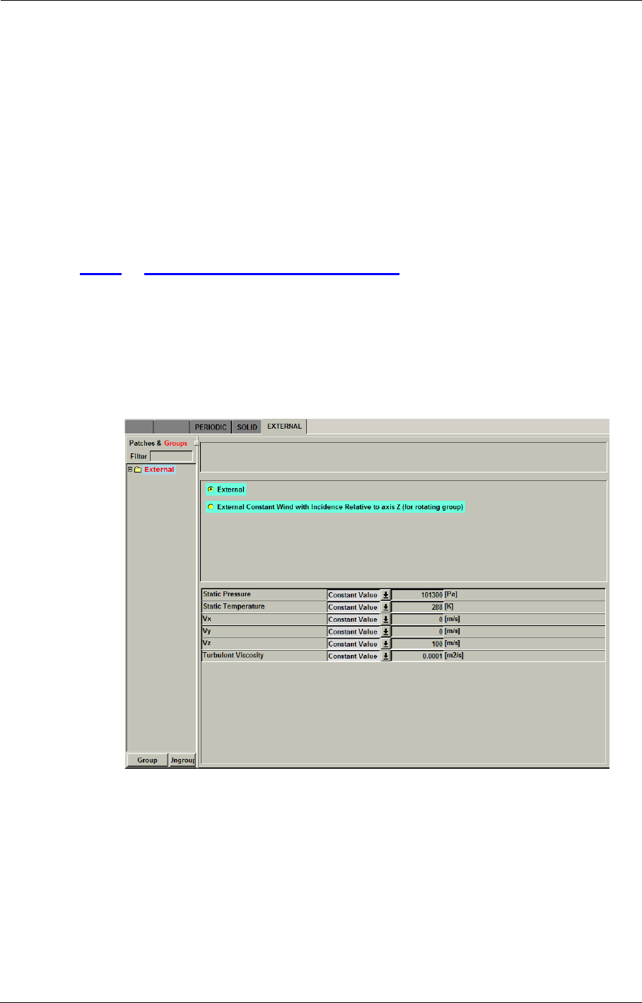
Boundary Conditions Boundary Conditions in the FINE™/Turbo GUI
5-16 FINE™/Turbo
value of B. This is not straighforward and a new approach has been introduced in the flow solver in
order to simplify the computations with roughness. To use the new method, the user has to set the
expert parameter IROUGH to 1.
When a rough wall is specified, if IROUGH=0, the distance from the wall to the cell-
centre of the first inner cell should be bigger than k0 + d0; if IROUGH=1, the distance
from the wall to the cell-centre of the first inner cell should be bigger than ks + d0. In
general, the first inner cell should be located within the fully turbulent layer.
The application field of the ’law of the wall’ imposes restrictions on the grid. The user is strongly
advised to check the conformity of this grid with these conditions (see section 4-2).
5-2.5 External Condition (Far-field)
The external boundary condition is provided to treat the far-field boundaries when dealing with
external flow computations (the expert parameter IINT=0). An example is given in Figure 5.2.5-12.
This type of boundary condition determines whether the flow is locally entering or leaving the flow
domain and uses the theory of the Riemann invariants to act consequently on the appropriate varia-
bles. Depending on the chosen turbulence model, five or seven input boxes are provided to specify
the free-stream values of the variables to be used in the boundary condition formulation.
FIGURE 5.2.5-12 External (far-field) boundary conditions page.
Use an external condition rather than an inlet condition for cases for which it is not
known if the flow enters or leaves the domain.
Condensable gases are not compatible with external boundary condition.
The boundary condition External Constant Wind with Incidence Relative to Axis
Z is only compatible with NLH.

Expert Parameters Boundary Conditions
FINE™/Turbo 5-17
5-3 Expert Parameters
5-3.1 Imposing Velocity Angles of Relative Flow
In case of a stator calculation it may be convenient to impose the velocity angles of the relative flow
at the exit of the upstream rotor. In case of rotors, the user may also prefer to impose relative bound-
ary conditions. This procedure is only available when total conditions and flow angles are imposed.
In addition to that the extrapolation of Vz must be selected. Note also that both flow angles and
total conditions are then treated in the relative mode.
The following parameters have to be defined:
INLREL(integer): allows to specify relative angles for the cylindrical inlet boundary conditions
with
= 0 (default):total quantities imposed,
= 1: inlet for a stator (extrapolation of the axial velocity only). The expert
parameter OMGINL has also to be specified,
= 2: inlet for a rotor.
ANGREL(real): data use with the expert parameter INLREL (for stator only). This variable con-
tains three values:
•1st real: relaxation angle (in degrees),
•2nd real: distance (%) from hub where the absolute flow angle is extrapo-
lated,
•3rd real: distance (%) from shroud where the absolute flow angle is extrapo-
lated.
5-3.2 Inlet Mass Flow Boundary Condition
IMASFL(integer): expert parameter specially dedicated to radial inlets. The mass flow is extrapo-
lated instead of the velocity for the cylindrical inlet boundary conditions with
imposed total quantities:
= 0 (default): treatment inactive, the velocity is extrapolated,
=1: option activated, extrapolation of the mass-flow.
INMFTT(integer): specify static temperature or total temperature when using mass flow imposed
inlet BC,
= 0 (default): static temperature is specified.
=1: total temperature is specified.
5-3.3 Outlet Mass Flow Boundary Condition
RELAXP(real): is the under-relaxation for the outlet boundary condition where the mass flow is
imposed with the exit pressure adaptation (default value = 1.).
VELSCA(real): is the maximum value allowed for the velocity scaling (outlet boundary condi-
tion with mass flow imposed by scaling velocity) (default value = 2.)

Boundary Conditions Expert Parameters
5-18 FINE™/Turbo
5-3.4 Outlet Averaged Mach Number Boundary Condition
RELAXP(real): is the under-relaxation for the outlet boundary condition where the averaged
Mach number is imposed with the exit pressure adaptation (default value = 1.).
5-3.5 Control of backflows
BCKFLO(integer): defines whether an Euler wall boundary condition is used at all outlet cells
where back flow is detected:
= 0 (default): don’t use the control of backflow,
= 1: use an Euler wall boundary condition at all cells where backflow is
detected.
BCKFLU(integer): defines whether the backflow control at inlet is activated or not. The use of
BCKFLU is limited to turbomachinery cases meshed with AutoGrid4™/
AutoGrid5™.
= 0 (default): don’t use the control of backflow at inlet
= 1: use the control of backflow at inlet, based on pitchwise averaging of the
solution.
5-3.6 Torque and Force
IDCDP(real): if cylindrical project (as defined in Mesh/Properties) and IINT=1: direction
(x,y,z) of axial thrust,
in all other cases: direction (x,y,z) of drag.
IDCLP(real): direction (x,y,z) for lift (not used if cylindrical project and IINT=1),
IDCMP(real): direction (x,y,z) for moment,
IFRCTO(integer): calculate and to store the partial torque in the corresponding ".wall" file. More
detail in Chapter 5-2.4.3.
IXMP(real): coordinate (x,y,z) of the point around which the moment has to be calculated.
The coordinates are expressed in meters.
TORRO(integer): = 0 (default): Compute force and torque on the complete patch
= 1: Compute force and torque only on the part of the patch which is defined
through an area defined rotation (the part corresponding to ω2).
IMUWAL(integer):if set to 1, the ".wall" file will be saved at each iteration on the finest grid level
(current grid level specified in the Numerical Model page) when performing a
steady simulation. The corresponding .wall file (_iter#.wall) will be saved in
the computation directory.
5-3.7 Euler or Navier-Stokes Wall for Viscous Flow
If the flow type selected is laminar or turbulent Navier-Stokes, it is possible in Expert Mode to
choose between an Euler wall (zero normal velocity) and a Navier-Stokes wall (no-slip condition).
Further details on the numerical treatment of the walls are provided in the theoretical manual. Note
that the default (active in Standard Mode) is a Navier-Stokes wall.

Best Practice for Imposing Boundary Conditions Boundary Conditions
FINE™/Turbo 5-19
5-3.8 Pressure Condition at Solid Wall
When the interface is in Expert Mode, two toggle buttons are provided to select the type of pres-
sure condition at the wall: extrapolated or computed from the normal momentum equation. The
default (active in Standard Mode) is the extrapolation of the pressure.
5-4 Best Practice for Imposing Boundary
Conditions
The quality of the flow simulation depends primarily on the quality of the grid and the imposed
boundary conditions. In this section the most adapted boundary conditions are proposed according
to the type of studied flow.
In case a calculation is diverging, it is strongly recommended to check by post
processing of the solution (in CFView™), that the appropriate boundary conditions have
been imposed.
5-4.1 Compressible Flows
For compressible flows it is recommended that the inlet boundary condition fixes the absolute total
quantities (pressure, temperature) and the flow angles and that the outlet boundary condition fixes
the static pressure (exit pressure). This exit pressure can be imposed as:
•a constant value along the exit,
•an average value at the exit,
•the pressure at mid-span for radial equilibrium (only for an axial outlet).
The static pressure at the exit of the domain is rarely constant. It is thus advised to impose the pres-
sure as an average value or as a initialization data for radial equilibrium.
Even if this value of pressure is known, for numerical reasons it is possible that the computed mass-
flow differs from the expected one. It is thus necessary to modify the exit pressure repeatedly until
obtaining the accurate mass-flow. This procedure can be numerically expensive especially if the
calculations are carried out on a fine grid.
A solution to overcome this drawback is to impose the mass-flow at the outlet. This can be done in
two ways:
•Velocity Scaling: for a low subsonic outlet (Mach number lower than 0.4) this condition fixes
the mass-flow at a given control surface by scaling the vectors on this surface. This is not as
robust as to impose the exit pressure and is not recommended in case significant backflows are
detected along the exit. If this is the case, the next option is better suited.
•Pressure Adaptation: in this case, an automatic procedure introduces a variation of the
imposed exit pressure at each iteration of the calculation. The pressure is then iteratively
updated in order to reach at convergence the imposed mass-flow. This is not as robust as to
impose the exit pressure, but is more robust than the velocity scaling option.
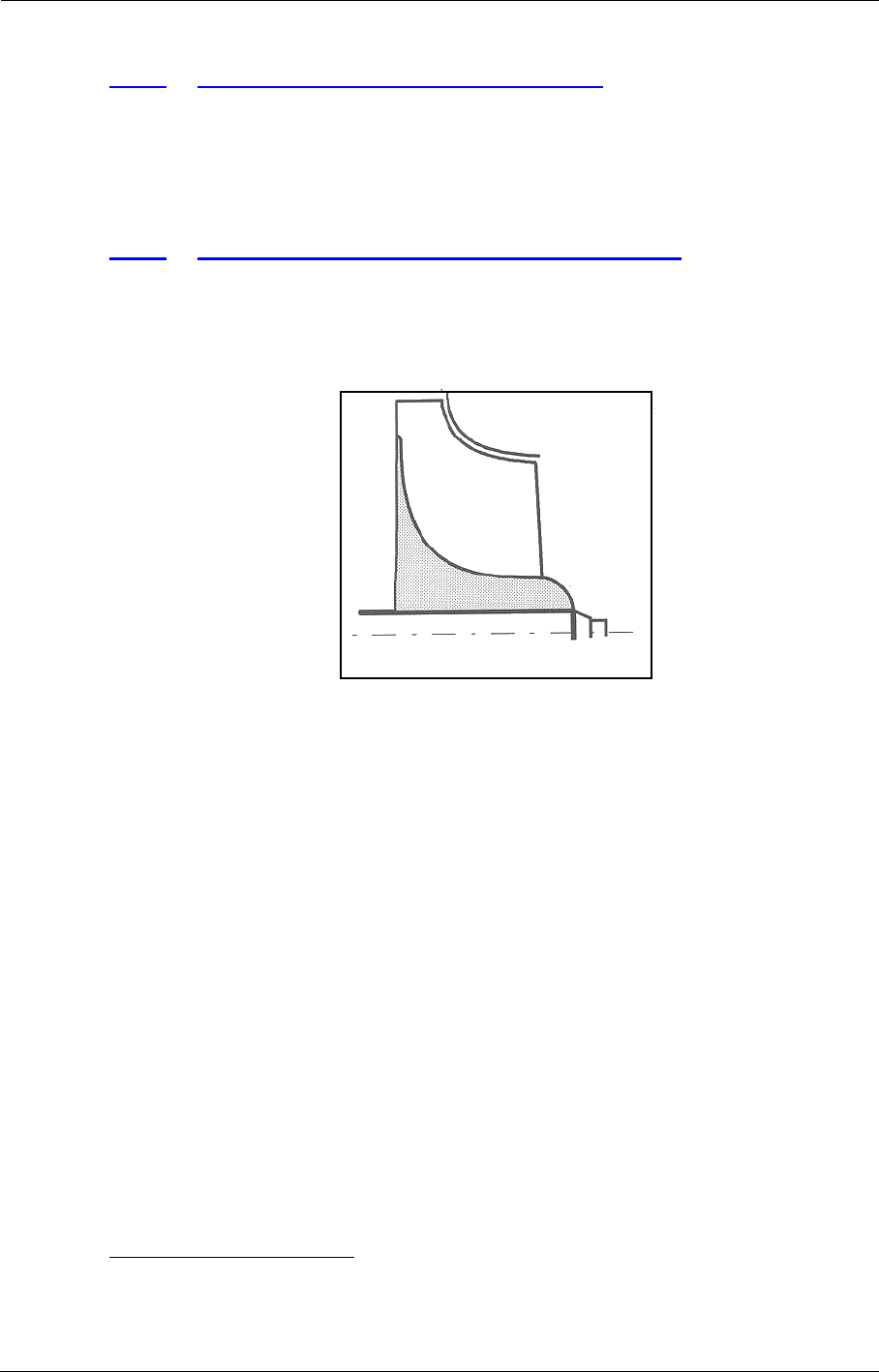
Boundary Conditions Best Practice for Imposing Boundary Conditions
5-20 FINE™/Turbo
5-4.2 Incompressible or Low Speed Flow
For incompressible or low speed flows it is recommended to impose the mass-flow and the static
temperature at the inlet and a static pressure at the exit. This couple of inlet-outlet conditions has a
stabilizing effect on calculations and is also well adapted to provide initial solutions for multi-stage
calculations.
5-4.3 Special Parameters (for Turbomachinery)
In case of flow separation at the outlet of radial diffusers it is recommended to use the backflow
treatment option. This option can be activated by activating Backflow Control in the FINE™/
Turbo GUI on the Boundary Conditions page under the OUTLET tab page.
FIGURE 5.4.3-13 Example of case with strongly varying radius in the inlet1
When end-walls in the inlet regions are strongly varying in radius (e.g. centripetal turbines as in
Figure 5.4.3-13) or in case of highly tangential inlet flow angles it is advised to use the IMASFL
expert parameter (in the list of expert parameters on the Control Variables page in Expert Mode).
This option is adapted when the inlet boundary conditions fixes the absolute total quantities (pres-
sure, temperature) and is only valid for non-preconditioned computations. When it is activated, the
mass-flow is extrapolated instead of the velocity.
Inlet patches have to be grouped in one group to use the extrapolation of mass flow
boundary condition.
1. Picture from D. Japikse, N.C. Balines, Introduction to Turbomachinery, Concept ETI Inc. and Oxford Uni-
versity Press, 1994.
Radial turbine

FINE™/Turbo 6-1
CHAPTER 6: Numerical Scheme
6-1 Overview
This chapter describes the interface and settings that can be used to specify the numerical parame-
ters and the time configuration for the simulations:
•Numerical Model defines the numerical aspects of the computations
•Time Configuration defines the time dependence of the equations to solve.
This chapter is organised as follows:
•section 6-2 describes the interface and settings for the definition of the numerical model,
•section 6-3 describes the interface and best practice for unsteady computations.
6-2 Numerical Model
6-2.1 Introduction
To define numerical parameters of the computation, the Numerical Model page allows to define
several aspects of the computation:
•the CFL number,
•the multigrid parameters,
•preconditioning parameters (if applicable).
These parameters are described in the next section.
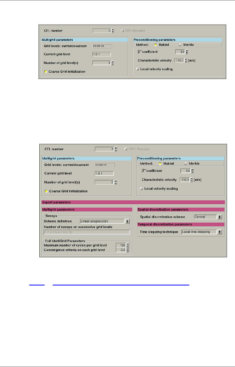
Numerical Scheme Numerical Model
6-2 FINE™/Turbo
FIGURE 6.2.1-1 Numerical model interface
In expert user mode (Expert Mode) additional parameters are available as shown in Figure 6.2.1-2:
additional multigrid parameters and unsteady parameters. These interfaced expert parameters are
described in section 6-2.3. Also the non-interfaced expert parameters are described in this section.
More theoretical information on the available parameters related to the numerical model (spatial
and temporal discretizations) is provided in Chapter 5-2 in the theoretical manual.
FIGURE 6.2.1-2 Numerical Model page in expert mode
6-2.2 Numerical Model in the FINE™/Turbo GUI
6-2.2.1 CFL Number
This box allows to tune the CFL (Courant-Friedrich-Levy) number to be employed in the compu-
tation. This number globally scales the time-step sizes used for the time-marching scheme of the
flow solver. A higher value of the CFL number results in a faster convergence, but will lead to
divergence if the stability limit is exceeded.

Numerical Model Numerical Scheme
FINE™/Turbo 6-3
6-2.2.2 CPU Booster
FINE™/Turbo includes an innovative breakthrough in convergence acceleration. Based on
enhanced implicitness, it leads to a drastic reduction in computational time with respect to the cur-
rent advanced technologies in FINE™/Turbo. If the user activates the option CPU Booster, the
default value of the CFL number will be 1000.
The CPU Booster is available only in case of perfect gas or real gas without precondi-
tioning.
The CPU Booster is not recommended when modelling low speed flows without pre-
conditioning
For the turbulence simulations, the CPU Booster is compatible only with the 0-equa-
tion and 1-equation turbulence models.
The CPU Booster is not compatible with the phase-lagged and NLH simulations.
When simulating flow with real gas, the results obtained with CPU Booster may be
less accurate if either the allowed temperature range is too large or if the properties are
expected to vary significantly in the allowed temperature range. In this case, the results
obtained with CPU booster could be different from a computation run without CPU
booster.
6-2.2.3 Multigrid Parameters
In the left part of the Numerical Model page, three boxes are visible. The first one is an informa-
tion box, named Grid levels: current/coarsest. It indicates for each of the i, j and k directions the
currently selected grid level and the number of the coarsest grid level available in the corresponding
direction. The second box of the Numerical Model page is an input box that allows to define the
Current grid level for each of the i, j and k directions.
•The coarsest grid level depends on the number of times the grid can be coarsened, along each of
the (i,j,k) directions. For example, if the grid has 17*33*33 points in the i, j, k directions, it has
respectively 16*32*32 cells. The i direction (16 cells) can thus be divided 4 times by 2, while
the others can be divided 5 times by 2. The following grid levels are then available:
0 0 0 17*33*33 (18,513 points)
1 1 1 9*17*17 (2,601 points)
2 2 2 5*9*9 (405 points)
3 3 3 3*5*5 (75 points)
4 4 4 2*3*3 (18 points)
4 5 5 2*2*2 (8 points)
The coarsest grid level available is then 4 along i and 5 along j and k.
•The current grid level is the finest grid level (for each of the i, j and k directions) on which the
computation will take place. The selected levels should be in the range between 0 and the coars-
est grid level available for each of the i, j and k directions. Referring to the example given just
above, the user can do a first run on level 3 3 3 to validate the computational parameters and
then switch to level 1 1 1 or 0 0 0 for a finer solution. It gives a high flexibility to the system
since with one grid, the user can run simulations on several sub-meshes.
All combinations between the i, j and k grid levels, in the specified range, are possible
such as 2 3 1 or 0 3 2...etc. It is however not recommended to use such hybrid levels (e.g.
010 or 211) since it deforms the mesh in a preferential direction and thus possibly

Numerical Scheme Numerical Model
6-4 FINE™/Turbo
increasing the aspect ratio. Consequently, the quality of the resulting mesh can be
decreased.
Press <Enter> after each modification to validate the new specified levels.
The use of multigrid is highly recommended in order to ensure fast convergence of the flow solver.
The mesh used to discretise the space can have multiple grid levels in each direction of the compu-
tational domain i, j and k. These levels are numbered from 0 (finest grid) to N (coarsest grid).
The grid level (N) available in one direction (I, J, or K) is the smallest grid among all
patches on that particular direction (I, J, or K).
The third box, named Number of grid level(s), permits to significantly accelerate the convergence
to steady state if several grid levels are available: the flow calculation is performed simultaneously
on all the grid levels. This technique is referred to as the multigrid strategy. This number should be
chosen as high as possible, and deduced from the information displayed on the available grid level
and the grid level on which the computation will be performed (Current Grid Level).
Finally, the option Coarse Grid Initialization enables, before calculating the flow on the mesh
contained in the IGG™ files, to perform a preliminary flow calculations on a coarser mesh auto-
matically created by the flow solver by coarsening the initial one. This provides a rapid estimation
of the flow. This technique is referred to Full Multigrid.
6-2.2.4 Preconditioning Parameters
This box allows the user to choose the Hakimi or Merkle preconditioners. The parameters are only
available when an incompressible fluid is selected on the Fluid Model page or when the Low
Speed Flow (M<0.3) option is activated on the Flow Model page.
The upwind spatial scheme (Numerical Model page) is not available if the precondi-
tioning option is chosen.
a) Hakimi Preconditioning
When choosing Hakimi preconditioning, extra parameters have to be defined. The variables that the
user controls are reference pressure , reference temperature , β coefficient and charac-
teristic velocity .
and are accessible through the Flow Model page.
The default value of β∗ is 3. Based on our experience with the presented low speed preconditioner
the parameter β∗ can be taken of order unity for inviscid flow computations. For viscous computa-
tions associated with Reynolds numbers greater than about Re=1000, a constant value β∗ of order
unity is also adequate. If convergence difficulties are encountered at the very beginning of a compu-
tation, it is recommended to increase the value of the parameter β∗. Remember however that a too
large value of β∗ will introduce excessive artificial dissipation into the solution. For lower Reynolds
number the parameter β∗ has to vary in order to preserve numerical stability and a good convergence
rate. The parameter β∗ should increase as the Reynolds number decreases and may vary over several
orders of magnitude (see Figure 6.2.2-3).
With low Reynolds number, β∗ has to be increased. But this increases the dissipation
and therefore alters the precision of the solution.
Pref
Tref
β∗
Uref
Pref
Tref
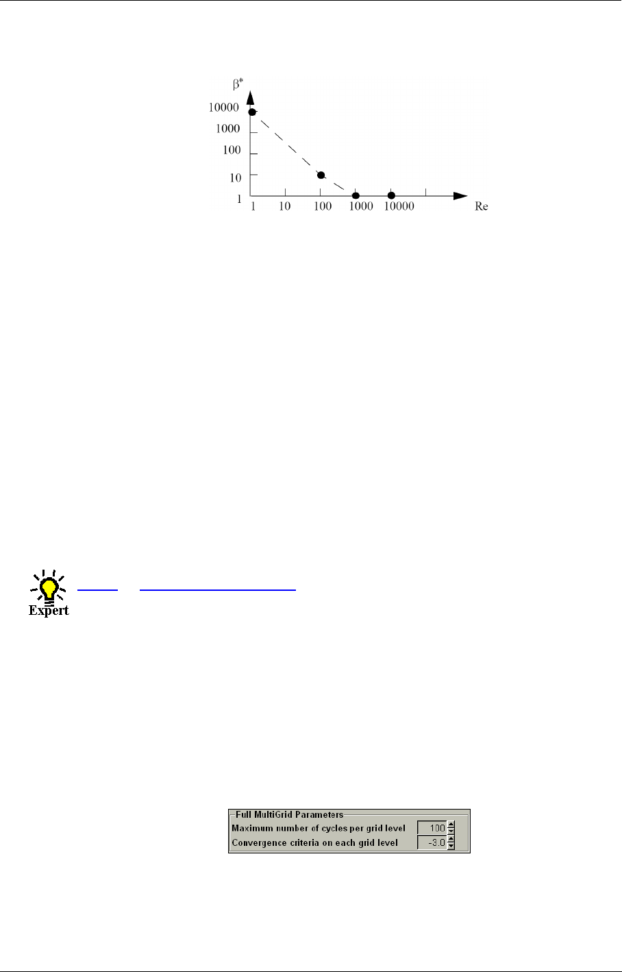
Numerical Model Numerical Scheme
FINE™/Turbo 6-5
FIGURE 6.2.2-3 Typical variation of the preconditioning parameter with Reynolds
number
is representative of the maximum velocity in the flow field. For example, in external flows,
Uref could be taken as the free stream velocity whereas in internal flows it could be taken as the
maximum inlet velocity. Note, for the user’s convenience, the constant Uref is always equal to the
reference velocity specified in the Flow Model page, which means that one of them (Uref/reference
velocity in the Flow Model page) is changed, the other one will be changed automatically.
The choice of Uref has an influence on the convergence.
Another expert parameter ALPHAP (α) is accessible in the Control Variables page under Expert
Mode. According to several computations accomplished with the central scheme, good conver-
gence rates were obtained for values of α lying in the range [-1,1]. So far the best value is found to
be α=-1.
b) Merkle Preconditioning
When choosing the Merkle preconditioner, no extra inputs are required.
6-2.3 Expert Parameters
6-2.3.1 Interfaced Expert Parameters
a) Multigrid Strategy
If the option Coarse Grid Initialization is activated, the computation starts on the coarsest grid
level and includes a finer grid level each time one of the two following criteria is satisfied:
•The maximum number of cycles to be performed on each grid level is reached. This parameter
is specified through the input box in the Full MultiGrid Parameters area as the Maximum
number of cycles per grid level.
•The residual on the current grid level has dropped a certain order of magnitude as indicated by
the Convergence criteria on each grid level in the Full MultiGrid Parameters area.
For the Convergence criteria on each grid level, both the RMS and maximum resid-
uals are checked when passing from one grid level to the next one in full multigrid ini-
tialization. The flow solver jumps to the next grid level when both criteria has decreased
β∗
Uref
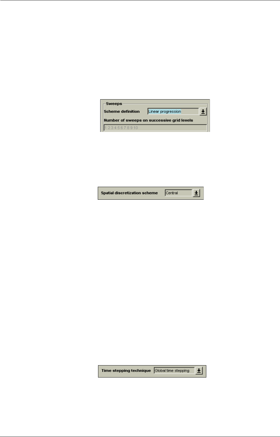
Numerical Scheme Numerical Model
6-6 FINE™/Turbo
e.g. 3 orders of magnitude.
•An additional input box permits to select the number of sweeps to be performed on the coarse
grid levels through the input box Number of sweeps on successive grid levels. The amount of
sweeps is the amount of times the Runge-Kutta operator is applied. In the default configuration
of the solver called Linear progression, the number of sweeps on each level equals the level
number (2 sweeps on second level,...). It has been observed in many cases that the convergence
rate may be significantly improved by performing a higher number of sweeps on the coarsest
levels. Recommended sets of values are proposed in the Sweeps area through the parameter
Scheme definition: for instance (1,2,16) in case of 3 grid levels. However, it is should be noted
that more sweeps have as a consequence more time required for an iteration.
b) Spatial Discretization
Two types of spatial discretization are available:
•central scheme (default) and
•upwind scheme.
A new way of calculating the artificial dissipation based on the primitive variables can be accessed
by switch expert parameter IARTVS to 2 when a central scheme is chosen. Such a new way can
limit or remove strong overshoot in temperature in the vicinity of holes when running blade cooling
configurations with the source term approach.
This method is restricted to non-preconditioned perfect gas and real gas implementa-
tions. And it is not applicable with NLH method.
If an upwind discretization is chosen, an input box appears in a Spatial discretization parameters
area to specify the order of accuracy of the desired upwind scheme: first or second order. See sec-
tion for more detail on those different schemes.
Condensable and preconditioned fluids are not compatible with the use of upwind
schemes for space discretization.
c) Temporal Discretization
The temporal discretization scheme used for the computation is an explicit multi-stage Runge-Kutta
scheme. In the interface, the time stepping technique should be selected between Local time step-
ping (default) and Global time stepping. See section for more detailed information on the tempo-
ral discretization. In general the default scheme is recommended.
If the computation is an unsteady computation, unsteady parameters box appears. Please refer to
chapter section 6-3.1 for a description of those unsteady parameters.

Numerical Model Numerical Scheme
FINE™/Turbo 6-7
6-2.3.2 Non-interfaced Expert Parameters
Additional parameters related to the numerical model are available in the list on the Control Varia-
bles page in Expert Mode.
a) Multigrid
IMGDIR(integer): Indicates if coarsening will be applied in the specified I, J or K direction (three
values):
1 1 1 (default): coarsening applied in all directions
0 0 0: no coarsening applied in all directions
1 1 0: coarsening applied only on I and J directions
IPROLO(integer): Indicates the order of the prolongation within the multigrid approach. The
default value is depending on the selected fluid type and turbulence model.
0: piecewise constant prolongation,
1: linear prolongation with damping,
-1: linear prolongation without damping,
2: linear prolongation except at boundaries(-2).
When used with a preconditioned formulation, this damping option is somewhat use-
less and can be damaging. FINE™/Turbo therefore sets it to off when preconditioning is
used.
When used with k-ε turbulence model and preconditioning, the linear prolongation
with damping is recommended.
IRESTR(integer): Gives the order of the restriction operator of the multigrid.
= 0 (default): corresponds to linear restriction,
= 1: to quadratic restriction.
MGRSTR(integer):Applies only for multigrid and fixes the type of multigrid cycle. MGRSTR=1:
V-cycle; MGRSTR=2: W-cycle; MGRSTR=3: F-cycle; MGRSTR=4: V-cycle
in sawtooth; MGRSTR=5: W-cycle in sawtooth; MGRSTR=6: F-cycle in saw-
tooth. Default: MGRSTR=1.
MGSIMP(integer):Applies only for multigrid. If MGSIMP>1 a simplification will be used on
coarser levels. If MGSIMP=1 a more dissipative scheme is used on coarser
meshes, i.e. first-order upwind (if 2nd order upwind scheme is used) or central
scheme with increased 4th order dissipation on solid walls (if central scheme is
used). If MGSIMP=2, in addition to the simplification for MGSIMP=1, viscous
and source terms (of turbulence) are neglected on coarser levels. No simplifica-
tion for MGSIMP=0. Default: MGSIMP=1
RSMPAR(real): Residual smoothing parameter σ*/σ. A value less or equal to zero means no
residual smoothing.
SMCOR(real): Only used in case of multigrid. SMCOR has the same meaning as RSMPAR but
applies to the interpolated multigrid corrections instead of the residuals.
SMCOR indicates whether interpolated corrections should be smoothed or not.
The default value for SMCOR is 0.
b) Spatial Discretization
IFACE(integer): = 1(default): Cell face gradients are used for the viscous fluxes,

Numerical Scheme Numerical Model
6-8 FINE™/Turbo
= 0: cell corner gradients.
IWAVVI(integer): Only used if IFACE=0. If IWAVVI=0 the cell face gradients are obtained by
arithmetic averaging of the cell corner gradients. If IWAVVI=1 a weighted
averaging is used instead, taking the cell volumes into account.
IWAVCO(integer): If IWAVCO=0 a variable averaging is performed. If IWAVCO=2 a flux averag-
ing is used instead.
c) Central Discretization
CDIDTE(real): Constant used in the exponential damping factor that is used in the numerical
dissipation for k and ε, both if central or upwind schemes are used. The default
value for CDIDTE is 100
EXPMAR(real): Exponent in the multi-dimensional scaling model of Martinelli of the dissipa-
tion used in central schemes. Default EXPMAR=0.5 i.e. multi-dimensional
scaling not used.
IARTV2(integer): Defines whether the second order artificial dissipation switch should be based
on both pressure and temperature gradients (parameter IARTV2=1) or on pres-
sure gradients only (IARTV2=0). In the default configuration, only pressure
gradients are taken into account. Both pressure and temperature gradients
(IARTV2=1) can only be taken into account for compressible cases.
VIS2(real): Coefficient κ(2) for 2nd order dissipation in the central scheme (default
VIS2=1.0).
VIS2KE(real): Used only for k-ε turbulence model. Coefficient κ(2) for 2nd order dissipation
in the central scheme, as applied to the k and ε equations. Default VIS2KE=1.0
VIS2SW(integer): This parameter switches off all second order dissipation for incompressible flu-
ids (when set to the default: VIS2SW=1). Second order dissipation is intended
for stabilization of the shocks but there are no shocks in incompressible flows.
Therefore the default is to switch off all second order dissipation for incom-
pressible fluids. Sometimes it may be stabilizing to use some second order dis-
sipation. In that case set this parameter to zero.
VIS4(real): Coefficient κ(4) for 4th order dissipation in the central scheme. Default
VIS4=0.1
VIS4KE(real): Used only for k-ε turbulence model. Coefficient κ(4) for 4th order dissipation in
the central scheme, as applied to the k and ε equations. Default VIS4KE=0.1
VISNUL(integer): Eliminates 2nd order dissipation fluxes along the physical boundaries (central
scheme). Default VISNUL=1. If VISNUL=0, the procedure is not applied.
d) Upwind Discretization
ENTRFX(real): Entropy coefficients. The first value is the entropy fix coefficient applied to the
linear field, the second value is applied to the non-linear field. ENTRFX<1.
means a constant value, ENTRFX>1. means scaled with the spectral radius
through a factor ENTRFX-1.
IRATIO(integer): Vector of two values, that indicate which effective ratio is to be used. The first
value applies to the linear field, the second to the non-linear field.
IRATIO is only active for second-order upwind schemes.

Numerical Model Numerical Scheme
FINE™/Turbo 6-9
IROEAV(integer): =1 indicates that Roe averages are to be used to calculate cell face data. If
IROEAV=0 (default), arithmetic averaging will be used.
e) Time Discretization
IBOTH(integer): used in combination with ISWV. The latter parameter indicates whether the dis-
sipation terms are recalculated or not in the different Runge-Kutta stages.
IBOTH=0 means that the dissipation term only contains the physical, viscous
dissipation; IBOTH=1 means that it also contains the artificial/upwind dissipa-
tion. The default value = 2 means that the dissipation term contains only the
artificial dissipation. The physical dissipation is computed once per time step.
IRKCO(real): Runge-Kutta coefficients. One for each stage, the first one for the first stage,
the second one for the 2nd stage and so on.
The default values that are used when nothing is set in IRKCO are:
1st order upwind - Van Leer:
4stage .0833 .2069 .4265 1.
5stage .0533 .1263 .2375 .4414 1.
2nd order upwind - Van Leer:
4stage .1084 .2602 .5052 1.
5stage .0695 .1602 .2898 .5060 1.
central scheme - Jameson:
4stage .25 .3333 .5 1.
5 stage .25 .1666 .375 .5 1.
both central and upwind - Eliasson:
4stage .125 .306 .587 1.
5stage .0814 .191 .342 .574 1.
NSTAGE(integer): number of stages for the explicit Runge-Kutta scheme. In practice, 4 or 5 stage
schemes are mostly used.
= 4: ISWV = 1 1 0 ...(ISWV can be modified afterwards independently)
= 5: ISWV = 1 0 1 0 1 0 ...(ISWV can be modified afterwards independently)
IRSMCH(integer): specifies the type of residual/correction smoothing.
= 1: standard version
= 2 (default only if Hakimi preconditioning): Radespiel & Rossow
= 3 (default): Zhu, time step dependent coefficients
= 4: Swanson & Turkel viscous
= 5: Vatsa. On meshes without high aspect ratio.
ISWV(real): governs the recalculation of the dissipative residual in the different Runge-
Kutta stages. A value α between 0 and 1 is allowed. Zero means no recalcula-
tion of dissipative residual (latest available value will be used); 1 means recal-
culation. For intermediate values, a weighted averaging of the latest dissipation
residual and of the preceding one is applied with the weight α and (1-α) respec-
tively. E.g. for a 5-stage scheme: ISWV = 1 0 1 0 1, means that the dissipative
residual is calculated in 1st,3rd and 5th stage only. ISWV is used in combina-
tion with IBOTH.
RSMPAR(real): residual smoothing parameter σ*/σ. A value less or equal to zero means no
residual smoothing. Default value = 2.
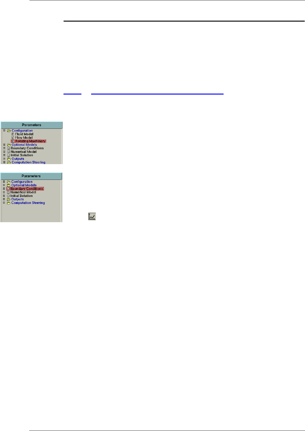
Numerical Scheme Time Configuration
6-10 FINE™/Turbo
6-3 Time Configuration
To perform time independent computations it is sufficient to select Steady. In case time dependence
needs to be included in the simulation Unsteady or Harmonic should be selected which gives
access to additional parameters respectively for unsteady flow simulation. All parameters in the
FINE™/Turbo interface related to Unsteady computations are described in the following section.
The parameters related to Harmonic computations are described in section 8-4.
6-3.1 Interface for Unsteady Computation
When selecting Unsteady time configuration in the Flow Model page the following additional
parameters become accessible in the FINE™/Turbo interface:
a) Rotating Machinery
On the Rotating Machinery page, under the Rotor-Stator tab, the Domain Scaling rotor/stator
interaction is activated. Furthermore, the Phase Lagged capability can be activated on the top of
the page. When activated, the Phase Lagged rotor/stator interaction will be applied.
b) Time Dependent Boundary Conditions
On the Boundary Conditions page the boundary conditions at inlet and outlet may be defined as a
function of time. To define a time dependent boundary condition go to the Boundary Conditions
page and change the default (Constant Value) with the pull down menu to:
•fct(time) to define a constant value in space but varying in time. Click on the profile data but-
ton ( ) to activate the Profile Manager.
•fct(space-time) to define a space and time dependent variation of the boundary condition
value. In this case a one-dimensional space profile has to be defined. The time profile to
impose is a scaling factor that is applied to the space profile. This means that the profile in
space is only varying in time with a certain scaling factor.
Another way to define an inlet/outlet unsteady boundary condition is to set an absolute rotational
speed to the boundary condition by activating Rotating Boundary_Condition and specifying the
rotational speed in Rotational Speed Unsteady respectively under the INLET and OUTLET tabs,
and to set the periodicity of the signal entered in FINE™/Turbo through the expert parameter
NPERBC.
The FINE™/Turbo solver allows only one rotation speed (combined with a zero rota-
tion speed) when performing an unsteady simulation using the Domain Scaling method
or Phase lagged method.
The inlet/outlet unsteady boundary condition circumferential profile has to be
imposed on a range covering the initial blade passage location and the blade passage
location after one period of the signal.
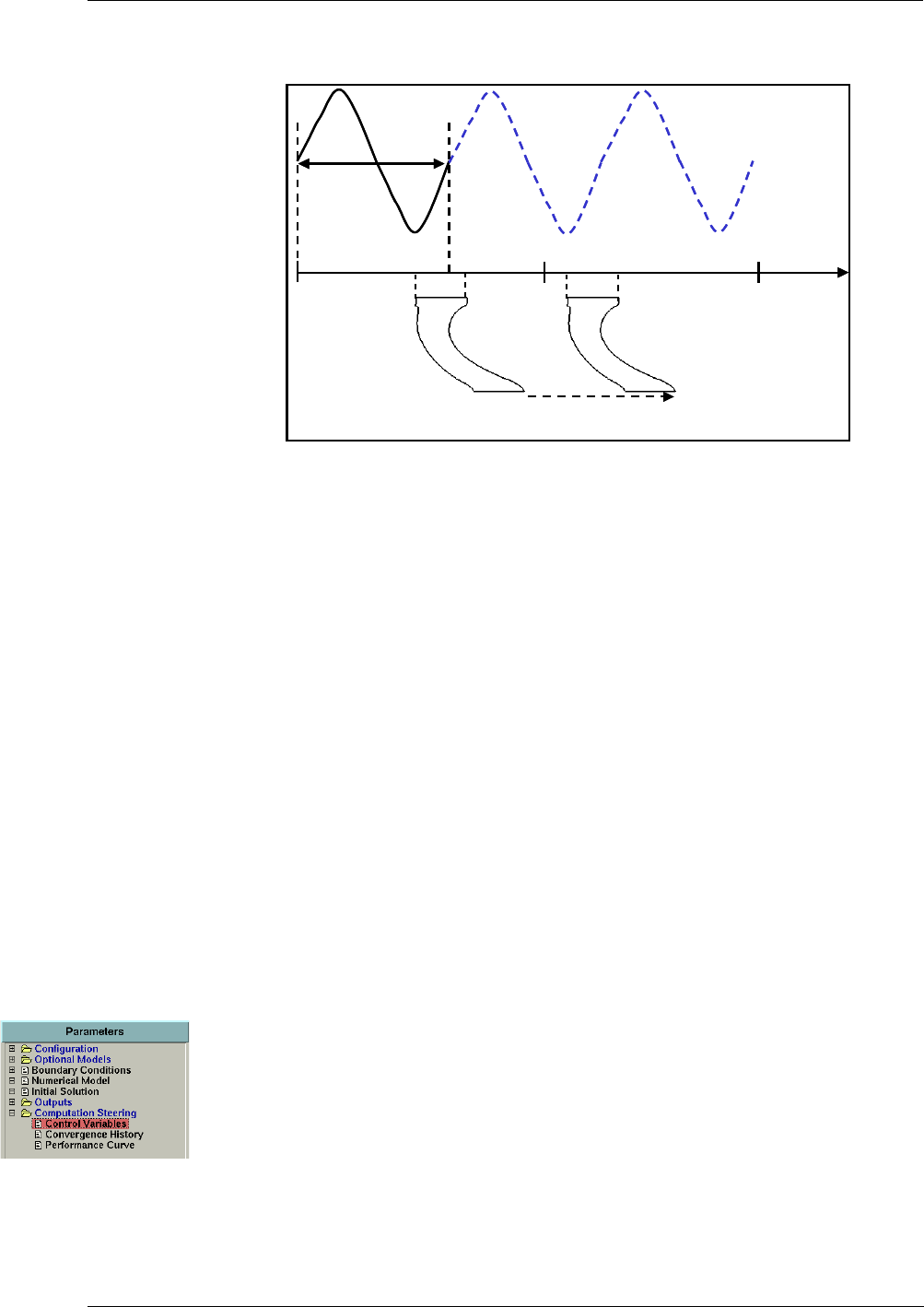
Time Configuration Numerical Scheme
FINE™/Turbo 6-11
Example:
FIGURE 6.3.1-4 Circumferential signal
The blade channel is initially (t0) located at θ1,θ2 and will after one period of the signal (T) be
located at θ3,θ4. Τhe circumferential signal has thus to be imposed from at least θ1 to θ4.
When Rotating Boundary Condition is activated, the time step is no longer specified by the phys-
ical time step in the FINE™/Turbo interface in the Computation Steering/Control Variables
page. Instead the time step is imposed by defining the Number Of Angular Positions.
c) Phase Lagged
When activating Rotating Boundary Condition in the Boundary Conditions page to rotate the
reference system of the boundary condition at the inlet and/or outlet, the period of the boundary
condition should be compared to the blade passing period. In the case of a single blade row calcula-
tion with the period of the varying inlet or outlet boundary conditions different from the blade pass-
ing period, the Phase Lagged option should be activated in the Rotating Machinery page and the
periodicity of the signal entered in FINE™/Turbo has to be specified through the expert parameter
NPERBC.
The current implementation of the phase-lagged boundary conditions only allows
matching and full non matching periodic boundary conditions. This option can be used
with non matching periodic boundary conditions (PERNMB) if they are automatically
transformed into full non matching boundary by setting the expert parameter IFNMB to
1.
d) Control Variables
On the Computation Steering/Control Variables page the following parameters appear when
selecting an unsteady time configuration non-turbomachine:
•Physical Time Step: in general cases the user specifies the magnitude of the physical time step
in seconds. This time step is constant through the whole calculation. In cases of turbomachin-
ery applications where Rotor/Stator interfaces are detected or Rotating Boundary Condition
activated, the Number Of Angular Positions is requested instead of the time step as
described in section 6-3.3.4.
v2.2
θ
02π
π
t0
T
t0+T
v2.2
θ
02π
π
t0
T
t0+T
θ1 θ2 θ3 θ4

Numerical Scheme Time Configuration
6-12 FINE™/Turbo
•Number Of Physical Time Steps: to define the number of time steps to perform. In cases of
turbomachinery applications where Rotor/Stator interfaces are detected or Rotating Bound-
ary Condition activated, the Number of Periods can also be specified.
•Save Solution Every: allows to save the solution after a constant number of time steps. By
default the output files will be overwritten, every time the solution is saved. In order to keep
the successive unsteady solutions, the multiple output (Multiple Files) option has to be acti-
vated.
•Include Time Averaged Solution in Output: When activated the time averaged solution will
be saved in a "_tav.cfv" file. This option is only available when Rotor/Stator interfaces are
detected or the Rotating Boundary Condition is activated.
The option Include Time Averaged Solution in Output is not available when the
phase lagged approach is used. A tool has been provided, which allows the user to com-
pute the time averaged solution for the phase lagged computation. For more information,
refer to Chapter 6-3.3.6.
•Outputs For Visualization:
—At end only and Intermediate Restart Files: One File: During the computation, one set of
output files is saved1 for a possible restart of the unsteady computation. Output files for vis-
ualization in CFView™ are only available at the end of the computation. No second order
restart possible.
—At end only and Intermediate Restart Files: Multiple Files: During the computation, mul-
tiple sets of output files are saved1 for restart of the unsteady computation. Output files for
visualization in CFView™ are only saved at the end of the computation. This option allows
a second order restart (see paragraph e).
—Intermediate and One Output File: One set of output files is saved2 for restart of the
unsteady computation and visualization in CFView™ during the computation. No second
order restart possible.
—Intermediate and Multiple Files: Multiple sets of output files are saved2 for restart of the
unsteady computation. and visualization in CFView™ during the computation. This option
allows a second order restart (see paragraph e). This combination has to be chosen to be able
to make an animation of the saved time steps in CFView™.
•Number Of Steady Iterations: the number of iterations to initialize the unsteady computa-
tion. Such initialisation is performed with the steady state algorithm, using fixed geometry and
mesh as well as constant inlet/outlet boundary conditions. In case this initialisation procedure
is used the steady state iterations can even be proceeded by a full multigrid process allowing a
rapid initialisation of the flow.
•Save Steady Solution Every: the number of iterations at which the solution of steady initiali-
sation is saved
By default only one output file is created. For the generation of multiple output files,
the Multiple Files option has to be selected.
1. The solution is saved every x time steps as specified in Save Solution Every ... time steps
2. The solution is saved every x time steps as specified in Save Solution Every ... time steps
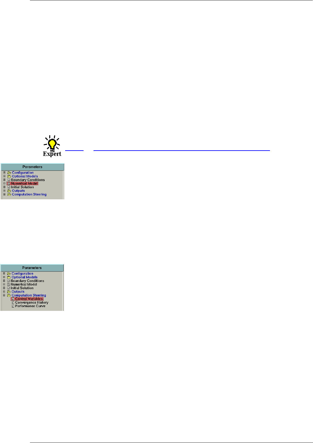
Time Configuration Numerical Scheme
FINE™/Turbo 6-13
e) Second Order Accurate in Time
The FINE™/Turbo solver performs second order accurate simulations in time. In order to allow a
second order restart it is necessary to select Multiple Files in the Computation Steering/Control
Variables page. When Multiple Files option is selected, in unsteady calculations the ".cfv" and
".cgns" are saved at the requested time steps and only a part of the ".cgns" file is saved for the pre-
vious time step. When requesting a restart of an unsteady computation the FINE™/Turbo solver
will automatically find this second solution file to use. If this file is not found, a first order scheme
is used for the first time step.
Note that only a limited output is saved when selecting Multiple Files with Output
For Visualization/At end only. If a solution is requested every x time steps, only solu-
tion files with extension ".cgns" are written every x time steps instead of a full set of
solution files. This limited output still allows to restart from this solution (see section 12-
2). The full set of solution files will be written at the end of the computation.
6-3.2 Expert Parameters for Unsteady Computations
6-3.2.1 Numerical Model in Expert User Mode
On the Numerical Model page, two new parameters appear in the user expert mode when selecting
the Dual time stepping technique. They are the control variables for the inner iterations. For each
physical time step a certain amount of iterations is performed in pseudo time leading to a converged
solution independent of the pseudo time.
•Convergence criteria of the inner iterations (orders of magnitude of reduction). The inner
iterations are stopped if the reduction of the residuals reaches the specified value.
•Maximum number of inner iterations: it allows to define the maximum number of iterations
to perform for each time step. In general the default of 100 iterations per time step is sufficient.
The inner iteration process is automatically stopped after this maximum number of iterations if
the convergence criteria has not been satisfied before.
6-3.2.2 List of Non-interfaced Expert Parameters
The following expert parameter related to unsteady computations are accessible on the Control
Variables page by selecting the Expert Mode.
ICYOUT(integer): can be equal to 0 or 1 (default):
0: name of output changes with suffix _t#iter,
1(default): each solution is overwritten every cycle.
IFNMB(integer): can be equal to 0 (default) or 1:
0 (default): to keep all PERNM or NMB boundaries,
1: to transform all PERNM boundaries into periodic full non matching ones or
all NMB boundaries into full non matching ones.
NPERBC(integer): can be equal to 1 (default) or integer value:
1 (default): when the inlet/outlet unsteady boundary condition is a rotating cir-
cumferential profile (activating Rotating Boundary Condition and specifying
the rotational speed in Rotational Speed Unsteady respectively under the
INLET and OUTLET tabs) and the boundary condition is entered in the
FINE™/Turbo interface for the full range [0,2π].

Numerical Scheme Time Configuration
6-14 FINE™/Turbo
N: when the inlet/outlet unsteady boundary condition is a rotating circumferen-
tial profile (activating Rotating Boundary Condition and specifying the rota-
tional speed in Rotational Speed Unsteady respectively under the INLET and
OUTLET tabs) and the boundary condition is entered in the FINE™/Turbo
interface for part of the range [0,2π/N] covering one or multiple periods of the
signal.
RELPHL(real): 0.5 (default) if necessary, under-relaxation factor can be applied on Periodic
and R/S boundary conditions by reducing the two values of the expert parame-
ter for respectively the periodic and the R/S boundary conditions.
6-3.3 Best Practice on Time Accurate Computations
To perform time accurate computations, general advice is provided in this section. For advice on
how to perform a time accurate turbomachinery calculation including rotor/stator interactions see
section 8-3.2.3.
6-3.3.1 General Project Set-up for Time Accurate Computations
1. Create a new project,
2. Select the fluid to use in the Fluid Model page,
3. Select Unsteady time configuration in the Flow Model page and set all the other parameters on
this page in the same way as for a steady computations as detailed in section 4-2 and section 4-
3.
4. On the Rotating Machinery page set all the parameters (Phase Lagged option) in the same
way as for a steady computation as described in Chapter 8.
5. Set the steady or unsteady boundary conditions. For more detail on time dependent boundary
conditions and phase lagged approach see section 6-3.3.2.
6. Concerning the initial solution for unsteady computations there are three possibilities:
—to start from a steady solution,
—to start from an unsteady solution,
—to use constant values, initial solution for turbomachinery or throughflow as an initial guess
with or without steady state initialisation.
For more detail on these initialisation procedures see section 6-3.3.3.
7. All outputs available in steady mode are also available in unsteady mode (see Chapter 10).
8. On the Control Variables page set:
—the physical time step or number of angular position (see section 6-3.3.4) and the number of
time steps or periods,
—the amount of output files (see section 6-3.3.5),
—amount of iterations in steady state initialisation (see section 6-3.3.3).
6-3.3.2 Time Dependent Boundary Conditions
Unsteadiness can be generated by means of time varying inlet/outlet boundary conditions. Two dif-
ferent situations can be encountered:
1. The time variation is imposed as an amplitude factor of the space variation,
2. The time variation is imposed by rotating the inlet and/or outlet boundary condition. The abso-
lute rotation speed of the boundary condition(s) is imposed in the Boundary Conditions page.

Time Configuration Numerical Scheme
FINE™/Turbo 6-15
Depending on the periodicity of the boundary condition the phase lagged approach needs to be
used:
1. The circumferential distribution of the imposed inlet/outlet conditions has the same period as
the blade row. The calculation of such time-dependent flow does not require to activate the
Phase Lagged approach.
2. The period of the time varying inlet/outlet boundary condition is different from the blade pass-
ing period. The calculation of such time-dependent flow requires to activate the Phase Lagged
approach at the top of the Rotating Machinery page.
A circumferential profile must be entered in the FINE™/Turbo interface for the full
range [0,2π] and NPERBC = 1 or for part of the range [0,2π/N] covering one or multiple
periods of the signal and NPERBC = N. The profile should be based on θ, z-θ or r-θ. The
profile is rotating at the speed, specified in the Boundary Conditions page (Rotational
Speed Unsteady).
It is important that the inlet/outlet unsteady boundary condition circumferential profile
is imposed on a range covering the initial blade passage location and the blade passage
location after one period of the signal (see Figure 6.3.1-4).
6-3.3.3 Initialisation Procedure
a) Start From Steady Solution
In most cases, it is first required to perform a preliminary steady state computation. The objective
might be to ensure that the problem naturally depicts the unsteady behaviour and/or to get an ade-
quate guess solution before going towards time accurate calculations depicting periodic behaviours.
The steady state initialisation may be done in a separate computation, performed in steady mode
using the time-marching approach based on a local time stepping, which is proposed by default.
The time accurate calculation is then started using this solution as an initial solution. To set up the
time accurate calculation in this case follow the steps 1 to 8 as detailed in section 6-3.3.1. In step 6
select in the Initial Solution page from file and select the solution of the steady computation. In
step 8 (section 6-3.3.1) it is also possible to select additional steady state initialisation in the Con-
trol Variables page (see paragraph c).
b) Start From Time Accurate Solution
It is possible to start from a previously performed time accurate solution. For general information
about starting from an initial solution see section 9-4.
In order to allow to do a second order accurate restart it is necessary that Multiple Files option is
selected in the Control Variables page in the Output Files parameters. When the option is acti-
vated in unsteady calculations the ".cfv" and ".cgns" files are saved at the requested time steps and
only a part of the ".cgns" file is saved for the previous time step. When requesting a restart of an
unsteady computation the FINE™/Turbo solver will automatically find this second solution file to
use. If this file is not found, a first order scheme is used for the first time step.
c) Steady State Initialisation in Unsteady Computation
The steady state initialisation is automatically performed before starting the time accurate computa-
tion (that means within the same computation). To perform a steady state initialisation in an
unsteady computation, the number of iterations has to be entered in Steady Initialisation parame-
ters on the Control Variables page.

Numerical Scheme Time Configuration
6-16 FINE™/Turbo
6-3.3.4 Physical Time Step
The physical time step should be entered on the Control Variables page. The time step to choose
depends on the expected frequency of the flow phenomena to capture. In general it is recommended
to compute at least 10 to 20 time steps per period.
When working with the Domain Scaling method, using a Number Of Angular Positions of 10
points per blade passage is giving a coarse but reasonable result. To have a more accurate (but more
CPU consuming) result choose 20 to 30 points per passage (see Chapter 8-3.2.3 for more details).
When working with the Phase Lagged method, the Number Of Angular Positions is the number
of time iterations per 2π (see Chapter 8-3.2.4 for more details).
The following examples show the settings of Number Of Angular Positions and Number Of
Time Steps when using an unsteady inlet boundary condition.
Example 1: single blade row calculation involving phase-lagged boundary conditions
When working with a N1 blades turbomachine and a periodic signal at inlet presenting a periodicity
of N2 and plotted on [0,2π/N2] range.
•Number Of Angular Positions = i x N1 where i is an integer imposed so that (i x N1) is
around 30.
•Number Of Time Steps = j x (Number Of Angular Positions) where j is the number of full
revolutions. Usually j is set to 20.
•NPERBC = period of the signal (N2)
(Number Of Angular Positions)x(NPERBC) corresponds to the number of time steps per full rev-
olution (2π)
Example 2: complete row calculation involving sliding boundary conditions
When working with a N1 blades turbomachine and a periodic signal at inlet presenting a period of
N2 and plotted on [0,2π] range.
•Number Of Angular Positions = i x N1 x N2 where i is an integer so that (i x N1) and (i x
N2) are around 30.
•Number Of Time Steps = j x (Number Of Angular Positions) where j is the number of full
revolutions. Usually j is set to 20.
•NPERBC = 1
(Number Of Angular Positions)x(NPERBC) corresponds to the number of time steps per full rev-
olution (2π)
6-3.3.5 Amount of Output
By default only one set of output files is created, which is periodically overwritten. Activate Multi-
ple Files in the Control Variables page to create a set of output files for each time step that an out-
put will occur (this depends on the Save solution Every entry available in the Control Variables
page).
".cgns" files will be generated. The files are automatically renamed accordingly to the
time step computed using the suffix "_t#." that is thus determining the #th physical time
step. The corresponding ".cfv" files can be read in CFView™ only if in addition of the
Multiple Files the Intermediate option has been selected in the Output For Visualiza-

Time Configuration Numerical Scheme
FINE™/Turbo 6-17
tion option. Note that the ".run" and ".cgns" files (without "_t#." suffix) are linked to the
initial state of calculation.
6-3.3.6 Time Averaged Solution
For domain scaling simulations, the user can get a time averaged solution by activating the option
Include Time Averaged Solution in Output on the interface. But for phase lagged simulations,
this is not the case. A tool plg2harmo is provided in the FINE™/Turbo package. Using plg2harmo,
the user can compute a time averaged solution from the solutions obtained by the phase lagged sim-
ulation or the domain scaling simulation.
The tool plg2harmo can only be launched from the shell.
On Linux:
plg2harmo<version> project-path/project-name.run
On Windows:
Installation path\bin\plg2harmo.exe project-path/project-name.run (for 32bits OS)
Installation path\bin64\plg2harmox86_64.exe project-path/project-name.run (for 64bits OS)
Then two new files "project-name_ft0.run" and "project-name_ft0.cgns" will be generated. The two
files include the time averaged solution. The user can load these files into CFView™ for post-
processing.
If the periodicity of the different rows is different, the number of the solution files
must be larger than the smallest periodicity.
The treatment of solid data is not allowed.
The calculation of time-averaged velocities for a computation with an inlet or outlet
distortion set as boundary condition is not allowed.

Numerical Scheme Time Configuration
6-18 FINE™/Turbo

FINE™/Turbo 7-1
CHAPTER 7: Physical Models
7-1 Overview
FINE™/Turbo contains the following physical models:
•Fluid-Particle Interaction to model solid particles in the flow.
•Fluid-Structure to model the fluid structure interaction.
•Passive Tracers allows to introduce species that are entrained by the flow, without influencing
its properties.
•Porous Media Model to model the flow in porous media
•Cavitation Model to model cavitating flow
Each of these models requires a special license feature. If the model is not accessible due to a miss-
ing license it is displayed in grey. Please contact our local sales or support office for more informa-
tion about the possibility to obtain a license.
7-2 Fluid-Particle Interaction
7-2.1 Introduction
Particle-laden flows cover a large class of two-phase flows, such as droplets or solid particles in a
gas or liquid flow, or bubbles in liquids. One phase is assumed to be continuous and occupies the
majority of the flow. It is called the "carrier" phase. Another phase, whose volume fraction is rela-
tively small (usually less than 10-2), exists as a number of separate elements or particles. It is called
the "dispersed" phase.
In this section 7-2 an overview is given of the fluid particle interaction module incorporated in
FINE™/Turbo GUI:
•7-2.2 describes the main functionalities of the module and the way to proceed in the FINE™/
Turbo interface.

Physical Models Fluid-Particle Interaction
7-2 FINE™/Turbo
7-2.1.1 Lagrangian Approach
A Lagrangian approach is used here, whereby the trajectories of individual groups of particles are
calculated as transported by the velocity field of the carrier phase, including the effect of drag and
other forces. The calculations of the carrier flow and of the particles can be fully coupled, the fully
coupling approach implying that the calculation of the particles trajectories is followed by a second
flow calculation, taking into account the presence of the particles in the flow (the interphase forces
are introduced as source terms in the flow calculation). The sequence consisting of a flow calcula-
tion and of the particle traces tracking can be repeated several times until no changes are observed
in the results (usually 3 to 10 times).
In the present Lagrangian model, the motion of the particles is only influenced by their own inertia
and by the flow, i.e. the local aerodynamic or hydrodynamic forces. Interactions between the parti-
cles are currently not considered. This implies the hypothesis of a dilute flow. On the contrary in a
dense flow, particle motion is governed by their direct interaction, which implies more complex
models, such as the Eulerian ones, in which both phases are modelled as continuous phases.
Particle-laden flows are found in many industrial applications such as cyclone separators, pneu-
matic transport of powder, droplet and coal combustion system, spray drying and cooling or sand-
blasting. In all cases, the flow consists of a continuous phase - also named carrier flow - and a
dispersed phase in the form of solid particles, liquid droplets or gas bubbles. In general, the motions
of the carrier flow and of the dispersed phase are interdependent.
In the lagrangian approach, the physical particle cloud is represented by a finite number of compu-
tational particles. The continuous phase (fluid) is treated as a continuum using a boundary-control-
led method whereas the dispersed phase (particles) is treated as a number of separate particles. The
particles are successively tracked as a single probe particle through the flow field using a Lagrang-
ian formulation.
In the case of laminar flows, each particle will follow a unique deterministic trajectory. In the case
of turbulent flows however, particles will have their own random path due to interactions with the
fluctuating turbulent velocity field. This feature is taken into account in the FINE™/Turbo solver
through a stochastic treatment. This approach consists of employing a sampling technique based on
a Gaussian probability density function to introduce the random nature of the turbulent velocity
field. The particle diffusion due to turbulence can therefore be modelled without introducing artifi-
cial diffusion properties of the cloud.
According to the distribution and contents of the particles, an averaging procedure provides phase
coupling source terms to be added into the Eulerian carrier phase conservation equations. The two-
way coupling can be achieved through global iterations.
7-2.1.2 Algorithm
The hypothesis of a dilute mixture permits to have a very simple sequential calculation of the trajec-
tories of the different particles injected through the inlet sections.
The algorithm considers successively the different inlet patches. The user specifies the number of
trajectories per cell. The origins can be located at a given point chosen by the user, or equally dis-
tributed throughout the cell.
The algorithm proceeds cell by cell, the time step being calculated so that several time steps are per-
formed in each mesh cell. The procedure starts at a cell of an inlet boundary and stops when a
boundary is reached.
Each time step consists of:
•the calculation of the force on the particle.
•the integration to find the new velocity and position.
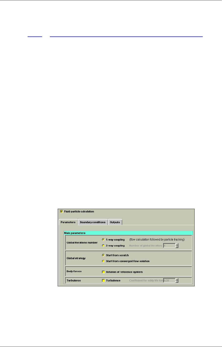
Fluid-Particle Interaction Physical Models
FINE™/Turbo 7-3
•the determination of the cell in which the particle is located.
7-2.2 Fluid-Particle Interaction in the FINE™/Turbo GUI
To access the parameters select the Fluid-Particle Interaction page under the Optional Models.
In the parameters section click on Fluid-particle calculation to activate this model (see
Figure 7.2.2-1). The user enters not only the main features of the numerical simulations but also the
characteristics (i.e. processes to be taken into account) of the interphase force between the fluid and
the particles.
7-2.2.1 Parameters
The top window allows to choose the degree of influence of the particles on the flow. The calcula-
tion of the carrier flow and of the particles can be fully (2-way coupling) or weakly (1-way cou-
pling) coupled:
•in the 1-way coupling approach the flow calculation (ignoring the influence of the particles on
the flow field) is followed by a calculation of the trajectories of particles. In this case, there is
no influence of the particles on the flow.
•in the 2-way coupling approach the calculation of the trajectories of particles is followed by a
second flow calculation, taking into account the presence of the particles in the flow (the inter-
phase forces are introduced as source terms in the flow calculation). The sequence can be
repeated several times (by entering the Number of global iterations) until no changes are
observed in the results (usually 3 to 10 times).
Concerning the simulation itself, the user can choose the Global strategy:
•Start from scratch: to start the flow calculations and then pursue with the particle tracking
simulation. In this particular case, the criterion for the carrier flow calculations convergence is
the one set on the Control Variables page (set to -6 by default).
•Start from converged flow solution: to proceed directly with the Lagrangian coupling from a
previous converged flow calculation.
FIGURE 7.2.2-1 Parameters page of the lagrangian fluid-particle interaction model.
The usual way to proceed is:
1. perform a pure flow study without activating the Fluid-Particle Interaction model in a computa-
tion.

Physical Models Fluid-Particle Interaction
7-4 FINE™/Turbo
2. while this computation is active in the list of Computations subpanel on the top left of the inter-
face create a new project by clicking on the New button.
3. in this new computation activate the Lagrangian Fluid-particle calculation and perform a com-
putation with Lagrangian coupling. The particles encounter several forces: the friction force, i.e.
the resultant of the pressure and viscous stress in the carrier phase over the particle surface, as
well as potential inertia and gravity forces. The user is free to introduce the Gravity Forces
through the vectorial components of the acceleration of gravity on the Flow Model page. An
inertial force due to the rotation of the system of reference can also be included. If some of the
blocks are rotating the option Body forces/Rotation of reference system should systematically
be activated. In this case the reference rotation velocity is the one specified on the Rotating
Machinery page.
4. while moving through a turbulent flow, each particle faces a sequence of random turbulent
eddies that result in a lack of accuracy in particle velocity and position. This process is taken
into account using a stochastic treatment when activating Turbulence. The treatment is availa-
ble when the k-ε turbulence model is assumed for the carrier flow simulation. In this case a
Coefficient for eddy life time has to be imposed.
The turbulence is only taken into account for the k-ε turbulence models and for the v2-
f turbulence model. It is not compatible with the Spalart-Allmaras and SST turbulence
models. In the particular case of the Baldwin-Lomax model, turbulence does not have a
direct influence on the particles trajectories.
7-2.2.2 Boundary Conditions
All boundary conditions available for the carrier flow solver are also accepted by the particle track-
ing algorithm. The only boundary conditions requiring user’s input are: inlet and solid boundary.
The boundary conditions are imposed by selecting a patch on which to fix the condition. The user
has to confirm the entered values by clicking on the Apply to selection button (Figure 7.2.2-2). In
the list of patches it is not possible to group patches but multiple patches can be selected at the same
time to apply the same boundary conditions to all of them. To select multiple patches hold the
<Ctrl> key while selecting them.
a) Inlet Boundary
The user can enter a number of classes of particles, each class representing a different type of parti-
cles. For each class the inlet boundary conditions have to be specified. The displayed boundary con-
ditions are the one for the class specified in the bar as indicated (a) in Figure 7.2.2-2. To select
another class use the scroll buttons on both sides of this bar. The purpose of this is to be able to sim-
ulate the presence of different types of particles in the same patch.
Note however that multiple classes are of interest for fully couples calculations only, by allowing
the flow calculation to account for the presence of different particle types. In the case of a weak
coupling strategy it is recommended to create one computation per particle class, because only one
particle class can be visualized in CFView™. The expert parameter (in Expert Mode on the Con-
trol Variables page) CLASID permits to specify which particle class must be included in the
CFView™ output.
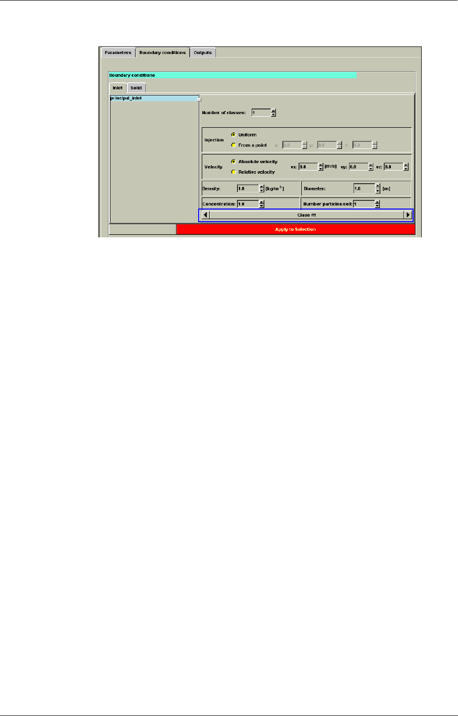
Fluid-Particle Interaction Physical Models
FINE™/Turbo 7-5
FIGURE 7.2.2-2 Inlet boundary conditions for the fluid-particle interaction model
The inlet boundary conditions are the following:
•spatial distribution of the injection points: uniform over the chosen patch or located at a chosen
point of coordinates (x,y,z).
•inlet velocity of the particles (absolute or relative frame of reference). The velocity is always
considered in the same relative frame of reference as the one of the block in which the inlet
particle is located. The relative velocities here defined as the difference between the particle
and the flow velocity (a zero relative velocity is therefore very commonly used) whereas the
absolute velocity boundary conditions is used when the velocity of the particle is well known
and different from the velocity of the flow. Note that only the Cartesian coordinate system is
available.
•density and mean diameter of the particles.
•particle concentration (number of particles/m3).
•number of particles per cell should be seen as the number of trajectories per cell.
The use of multiple trajectories per cell permits to ensure a more uniform covering of the inlet (and
hence of the computational domain) by the particles. This is only of interest in the case of fully cou-
pled calculations where it is important to ensure that the source terms are correctly evaluated in all
mesh cells. The use of multiple trajectories does not modify the number of particles entering the
domain. Each trajectory must be seen as an ensemble of particles. It is also very often referred to as
a computational particle.
In the case of full coupling, the number of particles per cell should be statistically large enough to
provide accurate averaging of the dispersed phase parameters. Therefore it is recommended in this
case to have a high number of particles per cell. This increases the computational time required for
the particle tracking process, but gives rise to a smoother distribution of the particles in the domain.
In the case of a weak (1-way) coupling, only one particle per cell is usually enough to provide a suf-
ficiently detailed description of the particles distribution in the field.
b) Solid Wall Boundary
The solid wall boundary condition requires an additional input data, which is the reflection ratio. If
the ratio is zero, all the particles remain stuck on the wall, whereas if it is 1.0, all particles are
(a)
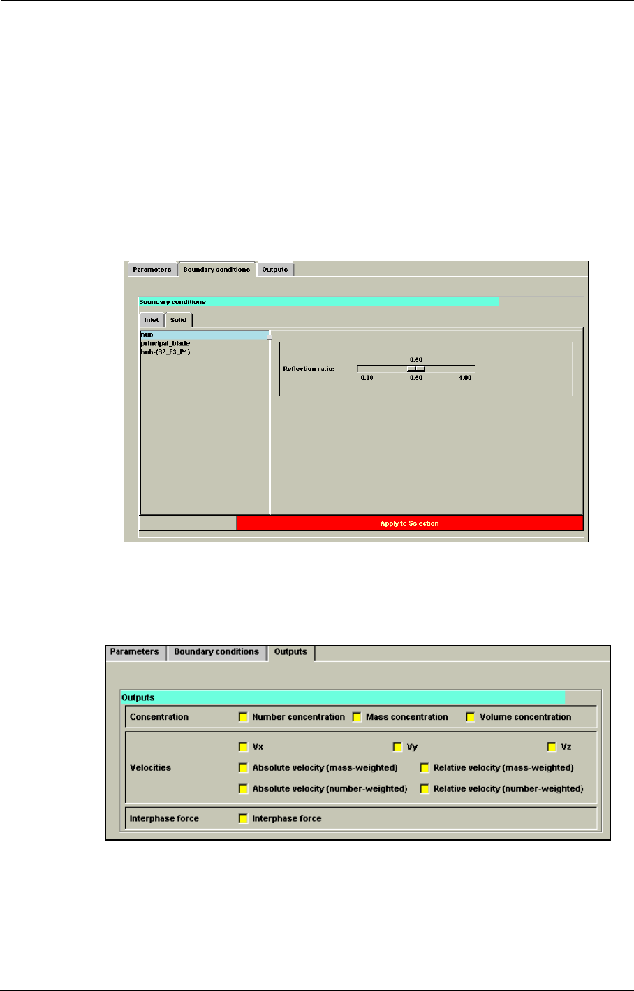
Physical Models Fluid-Particle Interaction
7-6 FINE™/Turbo
reflected, without any loss of mass or energy. The user can choose the reflection ratio by clicking on
the corresponding button while moving the mouse (Figure 7.2.2-3).
Two reflection modes are available and can be selected by the expert parameter IBOUND:
•In the default mode (IBOUND = 1) the particle loses a fraction of its mass and hence of its
kinetic energy at each wall hit. After several wall hits, the size of the particles becomes very
small, and the tracking stops (once the diameter has reached a given ratio of the initial one,
specified by the expert parameter DIAMR).
•In the other mode (IBOUND = 2) the velocity of the particle is reduced, with an unchanged
mass. The particle is stopped as soon as the velocity becomes too small (also specified by the
parameter DIAMR).
FIGURE 7.2.2-3 Solid boundary conditions for the fluid-particle interaction model
7-2.2.3 Outputs
FIGURE 7.2.2-4 Outputs of the fluid-particle interaction model
The following quantities are calculated by the solver:

Fluid-Particle Interaction Physical Models
FINE™/Turbo 7-7
•the number concentration where Ni is the number of particles of class i in the cell
of volume Ω,
•the mass concentration (mass of particles per cell volume) where
is the density of the particle of class i and volume ,
•the volume concentration (volume of particles per cell volume),
•the components of the mass weighted absolute velocity vector ( , , )
,
•the weighted mass and weighted absolute or relative velocity vectors number,
•the components of the interphase force .
The solver automatically writes an output file (".tr" and ".tr.sum") containing the particle traces that
is read by the CFView™ post processing software.
7-2.3 Specific Output
This section describes the specific outputs generated by the Lagrangian module.
7-2.3.1 Field Quantities (’.cgns’)
The solver automatically includes in the CFView™ output (".cgns") of the project the field quanti-
ties that have been specified by the user under the Outputs tab in the Fluid-Particle Interaction
page. These quantities can be scalars or vectors, and are the following:
•Vectors
Mass-weighted relative velocity (1)
Number-weighted relative velocity (2)
Mass-weighted absolute velocity (3)
Number-weighted absolute velocity (4)
Interphase force vector (5)
•Scalars
Number concentration (51)
Mass of particles per cell volume (52)
Volume of particles per cell volume (53)
Presence (1) or absence (0) of particles in cells (54)
Vx: x-component of mass-weighted velocity vector (55)
Vy: y-component of mass-weighted velocity vector (56)
Vz: z-component of mass-weighted velocity vector (57)
Fx: x-component of interphase force (58)
Fy: y-component of interphase force (59)
Fz: z-component of interphase force (60)
Ni
i
Ω⁄
ρipartNiΩipart
i
Ω⁄
ρipart
Ωipart
NiΩipart
i
Ω⁄
vx
vy
vz
vxvxiρipartΩipartNi
i
=ρipartΩipartNi
i
⁄
FF
iNi
i
Ω⁄=
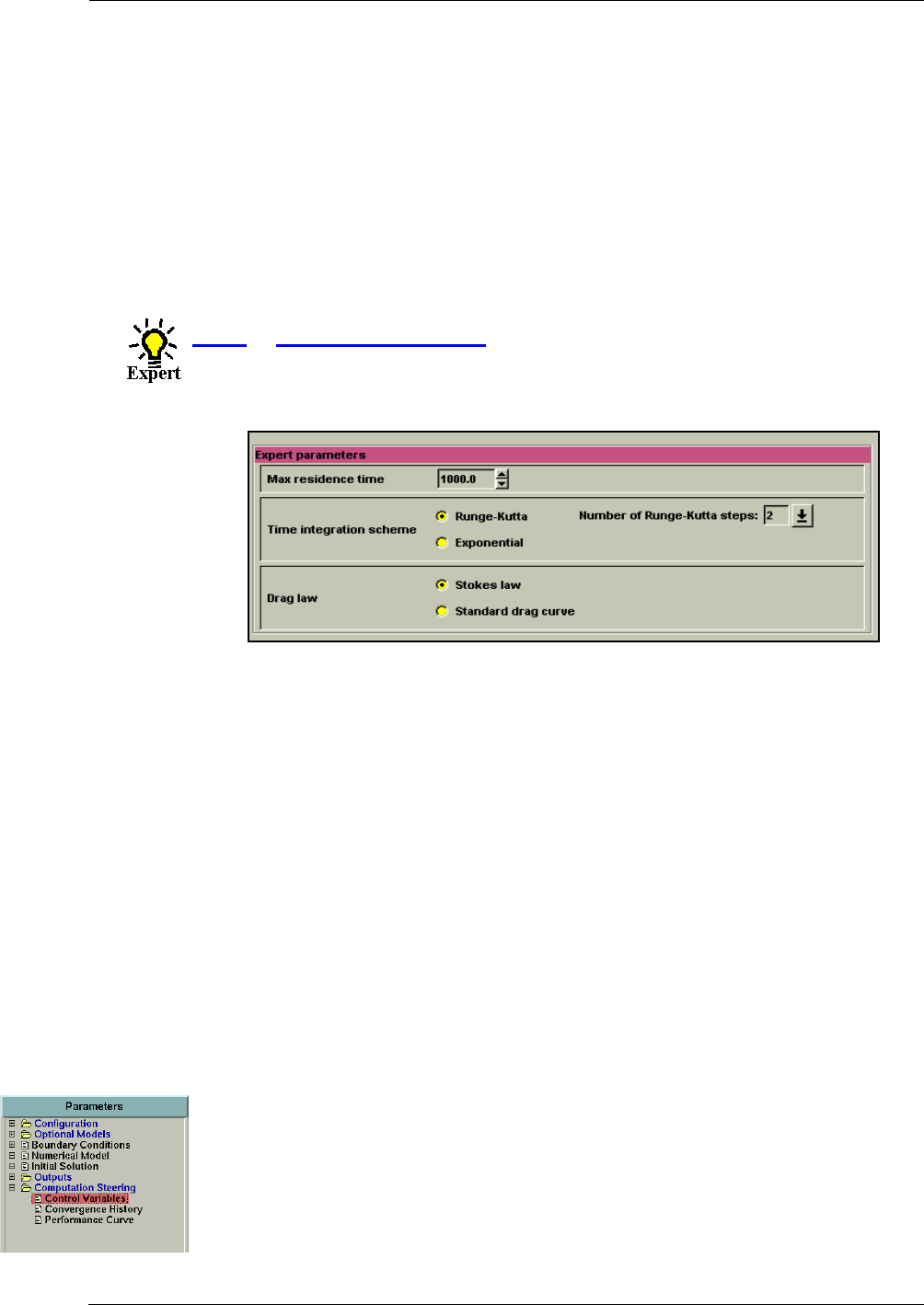
Physical Models Fluid-Particle Interaction
7-8 FINE™/Turbo
7-2.3.2 Particles Traces (’.tr’)
The solver also creates an specific lagrangian output file (".tr"), containing the trajectories of the all
the particles. This file is automatically transmitted to CFView™, which allows for the visualization
of the trajectories.
7-2.3.3 Summary File (’.tr.sum’)
In addition to the previous outputs, a summary file (".tr.sum") is automatically written by the solver,
giving for each injection patch the particles numbers and mass flows through the inlet/outlet bound-
aries, and the number of particles that remain stuck on the walls.
7-2.4 Expert Parameters
Other parameters appear in the Expert Mode of the Fluid-Particle Interaction page under the
Parameters tab:
•The maximum residence time (TMAX in corresponding ".run" file), which is the time limita-
tion for particle residence in the flow. It may be used either to prevent particle stopping or to
avoid an infinite loop, having for instance a particle captured in a separation bubble. After the
time has expired, the particle disappears.
•The governing equations for particles in a carrier flow consist of a set of non-linear ordinary
equations. Two methods are provided to integrate this equations with respect to time (that can
be selected in expert mode):
—The Runge-Kutta scheme, in which the transfer to the next time level is fulfilled through a
finite number of intermediate steps. A two-stage and a four-stage option (NRKS in corre-
sponding ".run" file) are available. This scheme is limited to big particles.
—The exponential scheme that lies on a semi-analytical method. This scheme is particularly
suitable for small particles.
•The Drag force is in general the only considered part of the interphase force. It corresponds to
the force on a particle moving in a still fluid at constant velocity (or using the particle refer-
ence system, a fixed particle in a uniform laminar flow). At extremely low Reynolds numbers
(Rep << 1 i.e. at low relative velocities), it is expressed through the Stokes formula. For higher
Reynolds numbers, an optional standard curve fit may be chosen. The choice between the two
types of forces can be made in expert mode.
Other parameters have a standard value, which may be modified only on rare occasions. They are
accessible in the Expert Mode of the Computation Steering/Control Variables page:
CLASID (integer): selection of class for CFView™ output
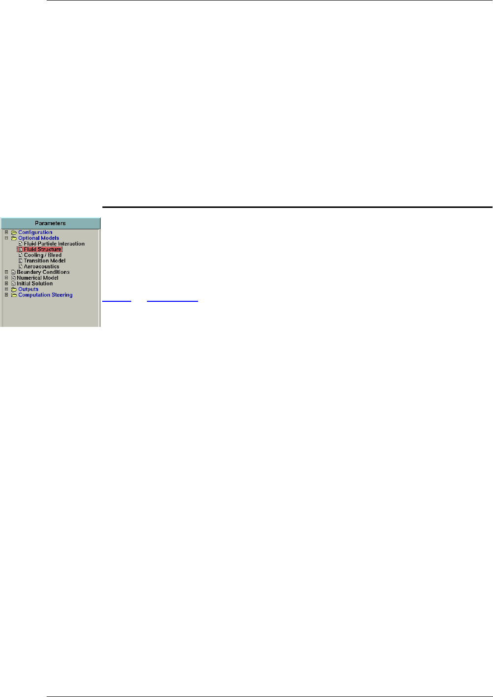
Fluid-Structure Physical Models
FINE™/Turbo 7-9
LMAX (integer): the maximum number of segments along a trajectory may be used to avoid an
infinite loop in the case of an oscillatory movement for instance.
DDIMAX (real): tolerance factor to establish that a particle has left a cell (default=1.E-4).
I2DLAG (integer): simplification for 2D problems (0 if 3D, 1 if 2D).
DIAMR (real): diameter ratio under which the particle tracking process stops (default value:
0.1).
KOUTPT (integer):enables to write the ASCII ".tr.out" file containing the output of the trajectories
(default value: 0). Please contact our local support office to have more details
on this file.
7-3 Fluid-Structure
Multi-physics problems, including Fluid-Structure Interaction (FSI), are becoming more important
for industrial applications. FINE™/Turbo has integrated several modules, which allows the user to
perform multi-physics simulations, including thermal and mechanical simulations.
7-3.1 Thermal
7-3.1.1 Conjugate Heat Transfer
a) Introduction
The conjugate heat transfer model allows the simulation of the thermal coupling between a fluid flow
and the surrounding solid bodies, i.e. the simultaneous calculation of the flow and of the temperature
distribution within the solid bodies.
The model has been validated for steady state applications. It assumes that some of the blocks of the
multiblock mesh are "solid", whereas the other ones are "fluid". The connections between the solid
and fluid blocks become "thermal connections" along which the fluid-solid coupling is performed.
Conjugate heat transfer is not compatible with Euler simulations.
b) Conjugate Heat Transfer in the FINE™/Turbo GUI
The Conjugate Heat Transfer model can be activated from the Optional Models / Fluid Structure
page under the Thermal tab. When opening the Conjugate Heat Transfer page it looks like
Figure 7.3.1-5. All blocks in the mesh are listed on the left of the page and all of them are by default
set as "fluid".
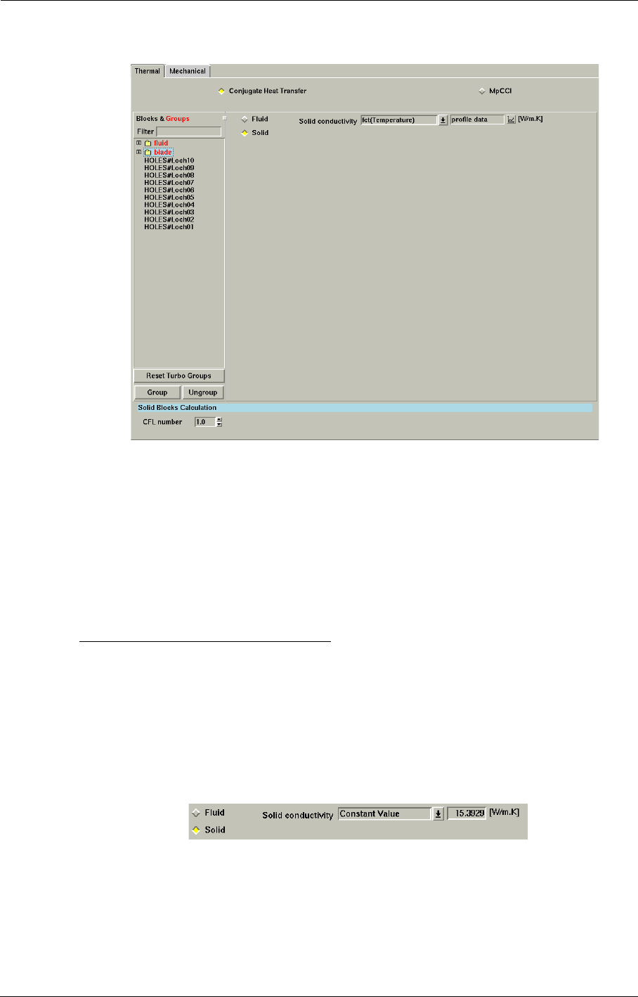
Physical Models Fluid-Structure
7-10 FINE™/Turbo
FIGURE 7.3.1-5 Conjugate Heat Transfer page
The only action required from the user to set up a computation involving the Conjugate Heat Trans-
fer model can be decomposed in three steps:
1. determine the "solid" and "fluid" blocks.
2. set the global parameters.
3. define the thermal connections.
Those steps are described in the following paragraphs in more detail.
b.1) Step 1: Determine Solid & Fluid Blocks
The use of the Conjugate Heat Transfer model requires the generation of a multi-block mesh, the
"solid" and "fluid" parts of the domain being discretised with separate blocks.
Once the mesh is generated, the first step consists in pointing the "fluid" and the "solid" blocks via
the FINE™/Turbo user interface. In the default configuration of the solver all blocks are of Fluid
type, so that the Conjugate Heat Transfer page does not need to be entered for a classical flow
calculation. The transfer of some of the blocks from "fluid" to "solid" is performed by selecting
those blocks on the left part of the window and by selecting the option Solid.
For each solid block the thermal conductivity has to be specified (in W/m/K). The specified con-
ductivity can be a constant or a profile, seeing Appendix A-5.3 on how to define a profile. The
specified value has to be larger than 0.
When the automatic grouping based on the Grid Configuration is used, the blocks
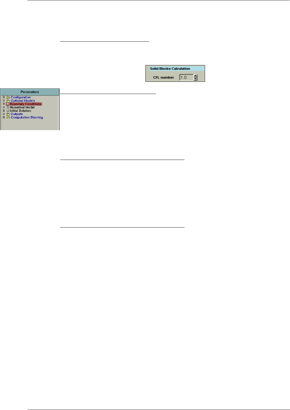
Fluid-Structure Physical Models
FINE™/Turbo 7-11
put as solid during the mesh generation, will automatically be set to solid in the FINE™/
Turbo GUI.
b.2) Step 2: Setting Global Parameters
The only global parameter is the CFL number used for the time integration of the conduction
equation. It can be different from the one used for the fluid. The default value is 1.0.
b.3) Step 3: Setting Thermal Connections
Once some blocks of the multi-block mesh are set as "solid" blocks, the connections between solid
and fluid blocks become "thermal connections". These connections are solid wall boundary condi-
tions with a particular thermal condition, along which the imposed temperature profile is iteratively
recalculated in order to ensure a correct coupling.
These patches appear in the list of patches in the tab page Solid in the Boundary Conditions page.
Although the thermal aspect is fully controlled by the coupling procedure, the kinematic boundary
condition must be specified by the user (rotation speed in [RPM]).
Type of Connections Between Solid and Fluid Blocks
Two types of thermal connections are allowed:
•matching connections (one patch on each side),
•full non-matching connections (one patch or one group of patches on each side). The connec-
tion algorithm is implemented in a general way, allowing on both sides a grouping of solid and
fluid patches. This is useful for instance in order to facilitate the coupling of a turbine block
with holes with the external flow. One single connection can be built, with on the inner side a
group of patches including the blade surface and the outer face of the holes.
Type of Connections Between Solid and Solid Blocks
Three types of thermal connections are allowed:
•matching connections (one patch on each side),
•Periodic connections (PER),
•full non-matching connections (one patch or one group of patches on each side). The connec-
tion algorithm is implemented in a general way, allowing on both sides a grouping of solid and
solid patches.
7-3.1.2 MpCCI Coupling
a) Introduction
For multi-physics problems, many commercial codes, such as FINE™/Turbo and Abaqus etc., can
be used to solve only one aspect of the physical problem. One way to perform the multi-physics
simulations is to use two or more dedicated codes coupled through the exchange of data.
MpCCI (Mesh-based parallel Code Coupling Interface) is a coupling interface developed by the
Fraunhofer Institute (SCAI) and used to perform multi-physics simulations. It consists in a server,
which handles physical quantities exchanges between two or more heterogeneous solvers (for
example a Computational Fluid Dynamics solver and a solid mechanics solver).
FINE™/Turbo includes a MpCCI code adapter in order to solve the thermal coupling problems.
The adapter takes in charge all communication processes with the MpCCI coupling server. About
the settings in MpCCI, please refer to the MpCCI manual.
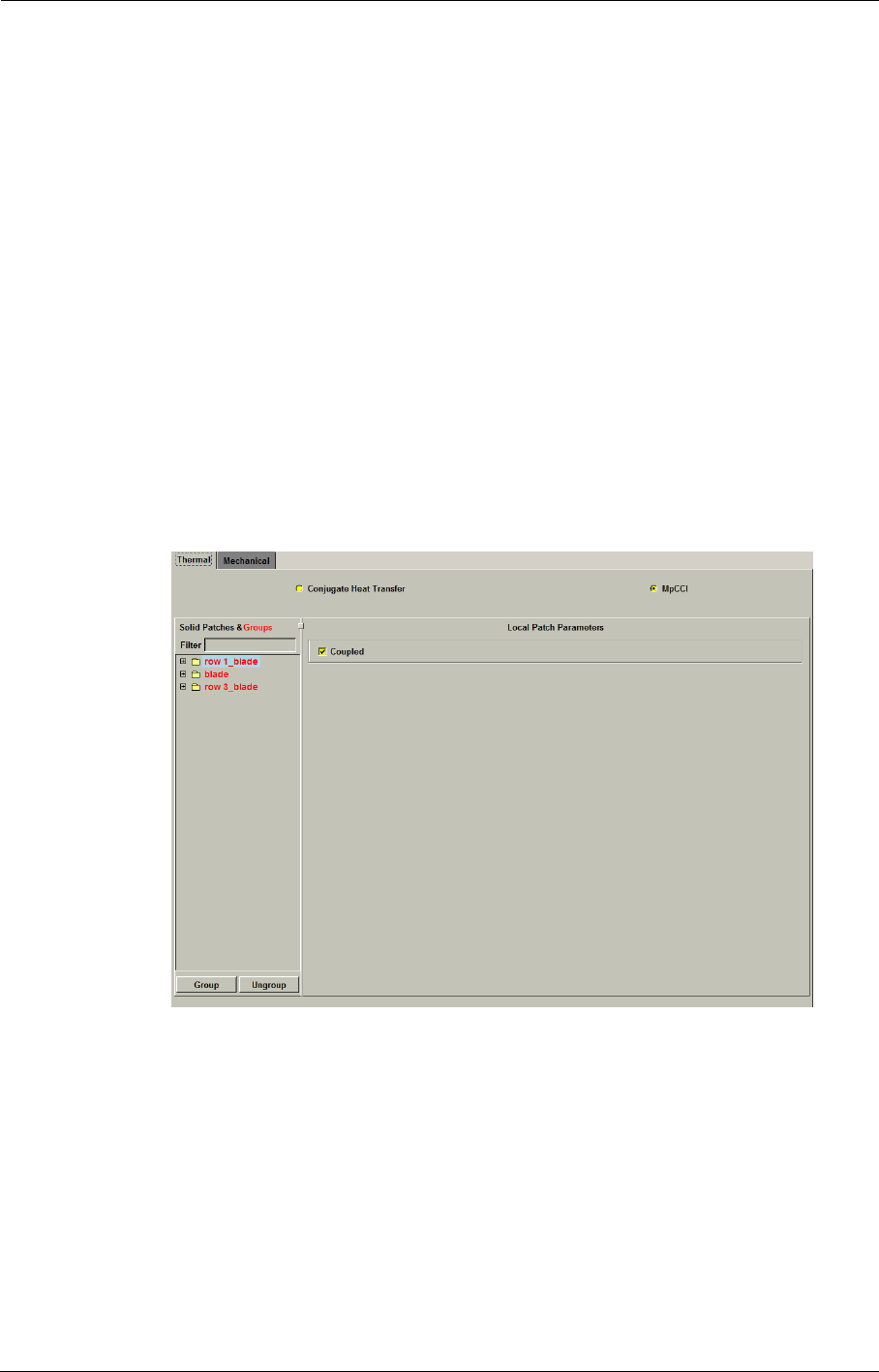
Physical Models Fluid-Structure
7-12 FINE™/Turbo
The limitations on coupling with MpCCI are as follows:
•Wall heat flux exchange is not compatible with FNMB and condensable fluids.
•Not compatible with coarse grid initialization and steady initialization.
•Not compatible with NLH.
Simulations coupling with MpCCI is available on the following platforms: AIX5.3
64bits, Linux 64bits and Windows 32/64bits.
MpCCI v4 is supported
b) Thermal Coupling with MpCCI
In order to perform a thermal coupling simulation, the user has to select the option MpCCI on the
Optional Models/ Flow Structure page under the tab Thermal. All solid patches and groups in the
mesh are listed on the left of the page, see Figure 7.3.1-6. The user has to select the coupled sur-
faces and mark them as "Coupled".
The coupled patches must be set as Temperature Imposed on the Boundary Conditions / Solid
page. The imposed temperature will be the initial value.
FIGURE 7.3.1-6 The thermal coupling with MpCCI
c) Expert Parameters
The expert parameters related to the thermal coupling with MpCCI:
ITCPL(integer): defines the number of iterations between each exchange with the coupled code
for steady computation.
CPLREL(real): relaxation factor for received temperature. This parameter can be useful for
steady calculation by reducing it to less than one if computation diverges. For
unsteady computation, it should not be modified.
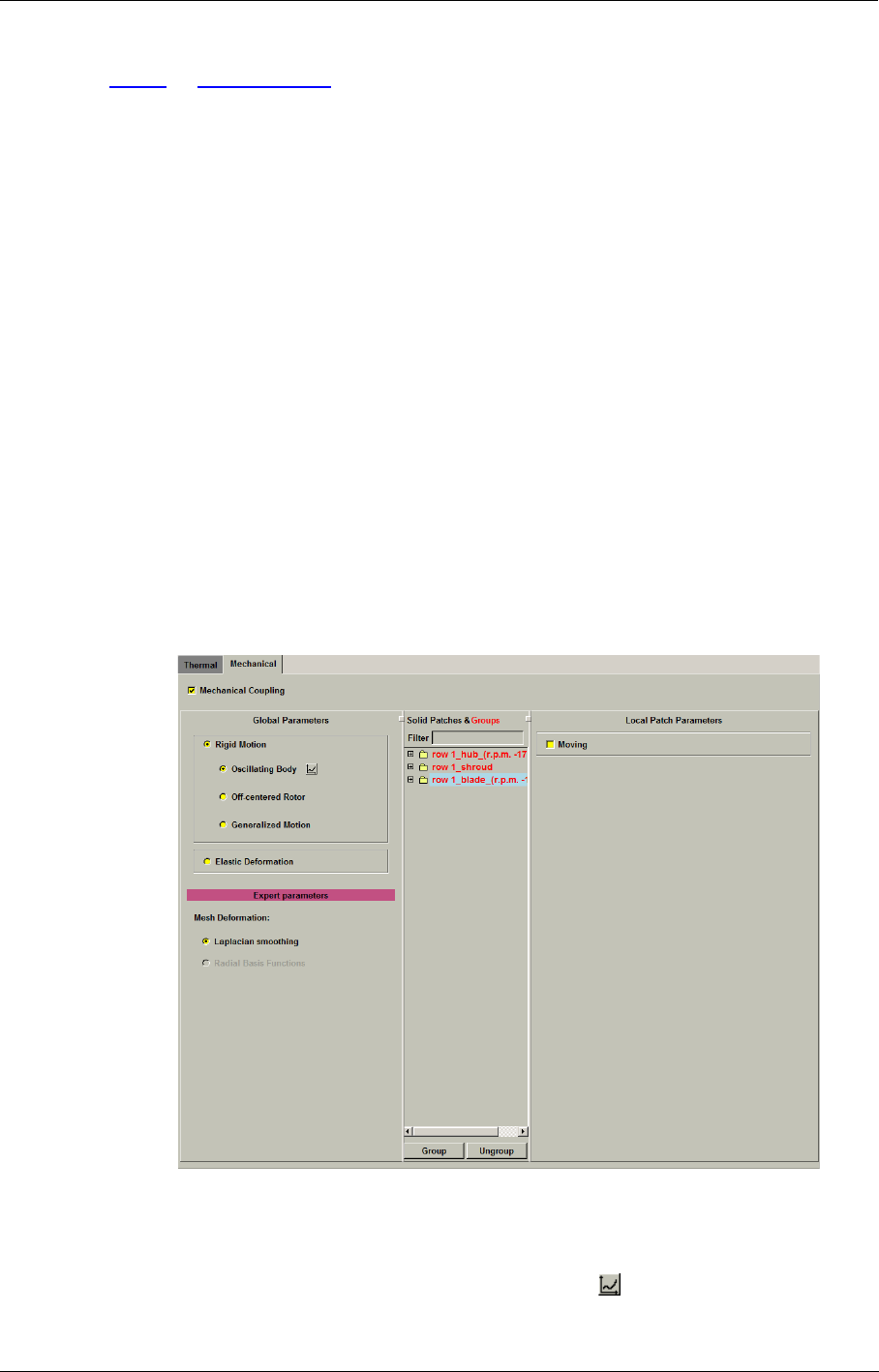
Fluid-Structure Physical Models
FINE™/Turbo 7-13
7-3.2 Mechanical
7-3.2.1 Rigid Motion
a) Introduction
The predefined Rigid Motion model allows to simulate the flow in a domain where the solid bound-
ary can move. The computation will be unsteady if the boundary is moving in time and steady if the
movement is constant in the relative frame of reference. This functionality is compatible with all
the existing fluid models and turbulence models.
For the mesh deformation, the user can only select the Laplacian smoothing method (in Expert
mode). For more information on the Laplacian smoothing and its limitations, please refer to
Chapter 7-3.2.4.
The main solver limitations with respect to the rigid motion model are as follows:
•Not compatible with spatial upwind scheme;
•Not compatible with NLH.
b) Rigid Motion in the FINE™/Turbo GUI
The Rigid Motion model can be activated from the Optional Models / Fluid Structure page under
the Mechanical tab. After activating the Mechanical Coupling, the Rigid Motion page will appear.
It looks like Figure 7.3.2-7.
FIGURE 7.3.2-7 The Rigid Motion page
Firstly, the user needs to select the type of motion. Depending on this choice, all the parameters
describing the motion law can be set by clicking on the button .
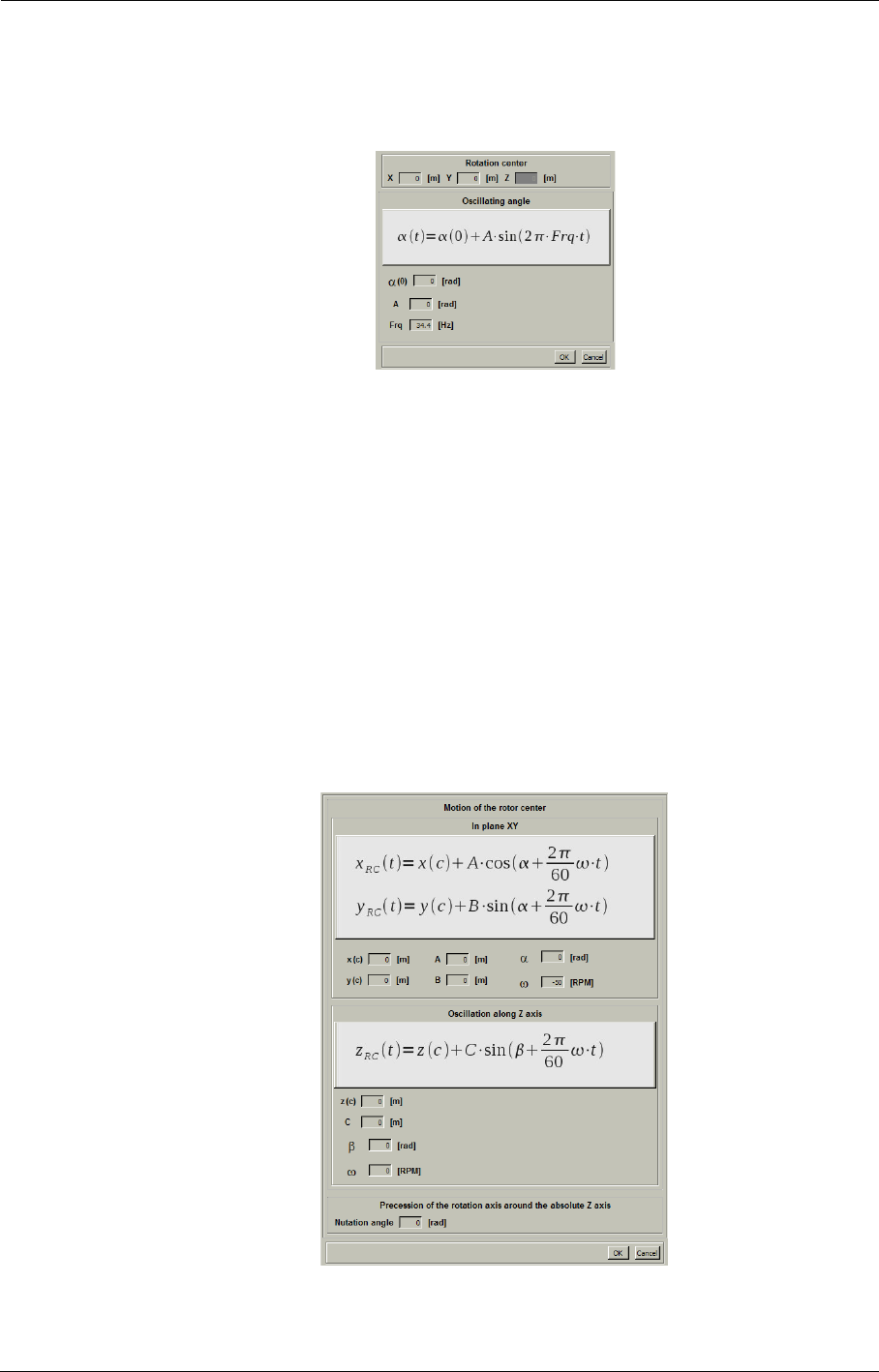
Physical Models Fluid-Structure
7-14 FINE™/Turbo
Three kinds of motion are available:
•Oscillating Body: oscillation of a solid body about Z axis at a reference point.
FIGURE 7.3.2-8 The parameters for Oscillating Body
To define the motion, the user has to input the location of the rotation center (x,y) and the
parameters describing the oscillations angle:
The rotation axis is always Z for the oscillating body.
Average angle;
Amplitude of the oscillations;
Frq Frequency of the oscillations.
Then the oscillating angle is computed by .
•Off-centered Rotor: three kinds of basic motion for off-centered rotor can be simulated.
These three basic motions can be combined to define more complex motions.
FIGURE 7.3.2-9 The parameters for Off-entered Rotor
α0()
A
αt() α0() A2πFrq t⋅⋅()sin+=

Fluid-Structure Physical Models
FINE™/Turbo 7-15
The rotation axis is always Z for the off-centered rotor.
—Motion of the rotor center around Z axis (in XY plane). To describe the motion, the user has
to input the following parameters:
x(c), y(c) Location of the rotation center in XY plane;
A Amplitude of the oscillations along X axis;
B Amplitude of the oscillations along Y axis;
α Angle at t = 0 in XY plane;
ω Frequency of oscillations in XY plane;
The location of the rotating axis of the rotor is obtained by:
—Oscillation of the rotor center along Z axis. To describe the motion, the user has to input the
following parameters:
z(c) Location of the oscillation center in Z axis;
C Amplitude of the oscillations along Z axis;
β Angle at t = 0 along Z axis;
ω Frequency of oscillations along Z axis.
The location of the rotating axis of the rotor is obtained by:
—Precession of the rotation axis around the absolute Z axis. Slanting the rotation axis allows
more complex predefined motions. It is particularly interesting for precessions with a con-
stant nutation angle. In this particular case, the rotation axis describes a cone. The Nutation
Angle has to be inputed, which is defined in the plane OXZ at the initial time (t = 0).
•Generalized Motion: the motion is specified by an external file. The user has to input the
location of the rotation center (x,y,z) in the original mesh domain.
FIGURE 7.3.2-10 The parameters for Generalized Motion
In the external file, the motion has to be specified with 7 data for each time step:
(Time, Δx,Δy,Δz,Δα,Δβ,Δγ)
where Time: the simulated time;
Δx: the displacement along X axis;
Δy: the displacement along Y axis;
Δz: the displacement along Z axis;
Δα: the rotation angle around X axis;
xRC t() xc() Aα2πωt60⁄+()cos+=
yRC t() yc() Bα2πωt60⁄+()sin+=
zRC t() zc() Cβ2πωt60⁄+()cos+=
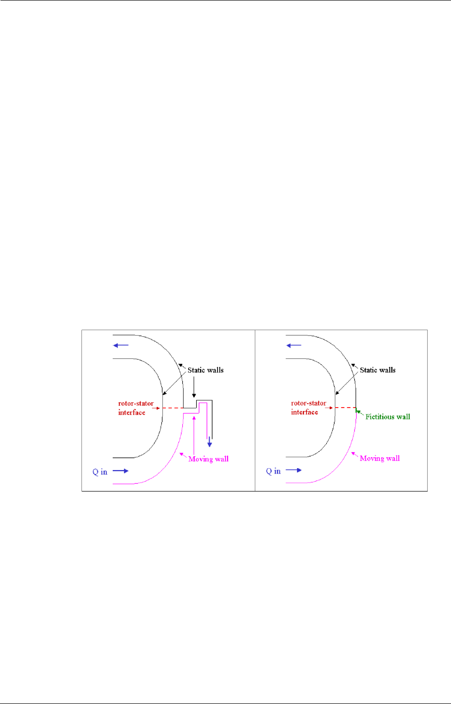
Physical Models Fluid-Structure
7-16 FINE™/Turbo
Δβ: the rotation angle around Y axis;
Δγ: the rotation angle around Z axis.
All displacements and rotations must be specified in the absolute frame of reference.
Consequently, the file must contain N+1 lines with N the number of time steps of the unsteady
computation. The first line in the file is used to initialize the deformed mesh. For a restart com-
putation, the previous time steps must be kept in the file and the total number of lines is Npre-
vious+N+1. The external file must be located in the computation directory with the name
“projectname_computationname.evol_pos”.
All solid patches and groups in the mesh are listed on the middle of the page, see Figure 7.3.2-7.
After choosing the type of motion, the user has to select the moving surfaces and mark them as
"Moving".
c) Adaptive Wall
The geometry simplifications imply sometimes that a moving wall is connected to a static wall. In
reality, it is not possible and such simplifications must be avoided. For the computation, it is possi-
ble to consider an adaptive wall to fill the gap between moving and static walls, as shown in
Figure 7.3.2-11. Adaptive wall is compatible only with the laplacian smoothing. The boundary ver-
tices belonging to solid surface can move in order to have a better mesh quality. The displacement
normal to the wall is zero for these vertices.
FIGURE 7.3.2-11 Case with a simplified geometry where a moving wall is connected to a
static wall
The limitations on the adaptive wall are:
•the adaptive wall must be located between a moving wall and a solid wall or a R-S interface;
•the size of the adaptive wall must be large enough to take the imposed movements;
•the subdivision of patches must keep the multigrid levels.
To define an adaptive wall (fictitious wall), the user has to define the corresponding parts of wall in
IGG™ as separated solid patches. These separated solid patches must be grouped and named as
“Adaptative_wall” in the Boundary Conditions / SOLID page.
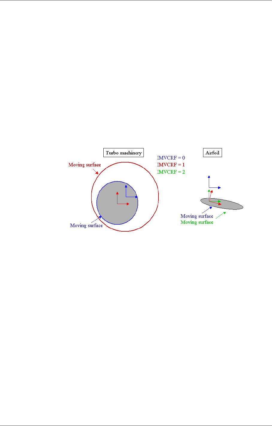
Fluid-Structure Physical Models
FINE™/Turbo 7-17
d) Expert Parameters
The following expert parameters are related to the rigid motion module:
IMVCRF(integer): The application of the mesh deformation is depending on the coordinate sys-
tem. For example, for the off-centered motion, the displacement will be applied
to the "Moving" walls specified by the user on the FINE™/Turbo GUI if the
standard frame is used. Otherwise, the displacement will be used to the "sta-
tionary" walls if the relative frame attached to the solid body is used. The rela-
tive frame of reference can be defined by the expert parameter IMVCRF.
0(default): the standard rotating frame is used.
1: the relative frame attached to the solid body is used.
2: the relative frame is defined only by the translation of the body. This is used
only for oscillating body in external flow.
FIGURE 7.3.2-12 Moving surfaces depending on the value set to IMVCRF
7-3.2.2 MpCCI Coupling
a) Introduction
In addition to performing a thermal coupling simulation with MpCCI (see Chapter 7-3.1.2), the user
can also perform a mechanical coupling, or both thermal and mechanical coupling simulation.
When performing the mechanical coupling simulation with MpCCI, the FINE™/Turbo solver com-
putes the flow around the structure and transfers the computed quantities to the structural solver.
The displacements are therefore computed and transferred back to the FINE™/Turbo solver, which
deforms the mesh. Then, the process is repeated until a steady state solution (steady mode) or the
last physical time step (unsteady mode) is reached.
For the mesh deformation, the user can select the Laplacian smoothing method or the Radial Basis
Functions method (in Expert mode). For more information on the mesh deformation methods and
its limitations, please refer to Chapter 7-3.2.4.
The limitations on the mechanical coupling with MpCCI are as follows:
•Wall forces exchange is not compatible with FNMB and condensable fluids.
•Not compatible with coarse grid initialization and steady initialization.
•No compatible with NLH.
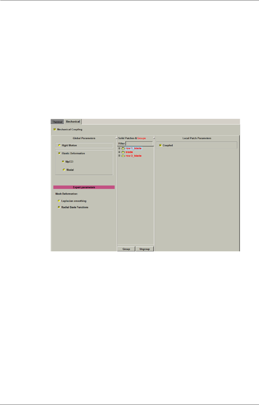
Physical Models Fluid-Structure
7-18 FINE™/Turbo
Simulations coupling with MpCCI is available on the following platforms: AIX5.3
64bits, Linux 64bits and Windows 32/64bits.
MpCCI v4 is supported
b) Mechanical Coupling with MpCCI
The mechanical coupling with MpCCI can be activated from the Optional Models / Fluid Struc-
ture page under the Mechanical tab. After selecting Mechanical Coupling and then Elastic Defor-
mation, the mechanical coupling with MpCCI page will appear. It looks like Figure 7.3.2-13.
All solid patches and groups in the mesh are listed on the middle of the page. The user has to select
the coupled surfaces and mark them as "Coupled".
FIGURE 7.3.2-13 The mechanical coupling with MpCCI
c) Expert Parameters
The expert parameters related to the mechanical coupling with MpCCI:
ITCPL(integer): defines the number of iterations between each exchange with the coupled code
for steady computation.
7-3.2.3 Modal Coupling
a) Introduction
FINE™/Turbo includes a modal coupling module in order to perform Fluid-Structure Interaction
(FSI) simulations. For this kind of coupling simulation, a structure code is used to compute the
modal shapes and the eigen frequencies of the structure. With these information the FINE™/Turbo
flow solver will consider the interaction between the flow and structure and compute the deforma-
tion of the structure by solving the modal equations.
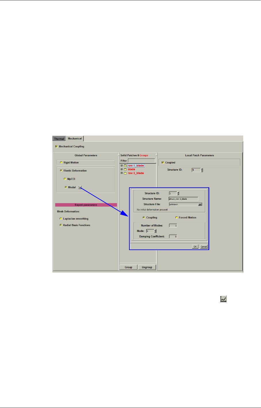
Fluid-Structure Physical Models
FINE™/Turbo 7-19
For the mesh deformation, the user can select the Laplacian smoothing method or the Radial Basis
Functions method (in Expert mode). For more information on the mesh deformation methods and
its limitations, please refer to Chapter 7-3.2.4.
The limitations on modal coupling are as follows:
•For unsteady computation, the time step should be less than one third of the period of the high-
est mode to avoid divergence.
•Structure file containing mode shape definition must be written in SI units.
•Modal coupling requires elastic mesh deformation. It involves all limitations linked to the
mesh deformation methods.
b) The Modal Coupling in the FINE™/Turbo GUI
The modal coupling can be activated from the Optional Models / Fluid Structure page under the
Mechanical tab, see Figure 7.3.2-14.
FIGURE 7.3.2-14 The mechanical coupling with Modal
The parameters related to modal coupling can be set by clicking on the button . The FINE™/
Turbo flow solver can model several structures. The user has to specify a Structure ID and Struc-
ture Name for each structure and set the corresponding parameters.
Modal properties (eigen frequencies and modes shapes) are needed by the flow solver in order to
compute the elastic deformation of the structures. These properties can be computed by a CSM
code or measured experimentally. As modal resolution is a linear method, an initial deformation can
be specified. This is useful to take into account non-linear effects independent of fluid load, such as
centrifugal effect.
A Structure File including these properties and the initial deformation (if any) must be imposed for
each structure. The structure file must be written in ASCII format. First this file includes the
number of dimensions of the structure, the number of modes, the number of structure nodes at
which the modes are defined and a flag to specify if an initial deformation is specified. After that
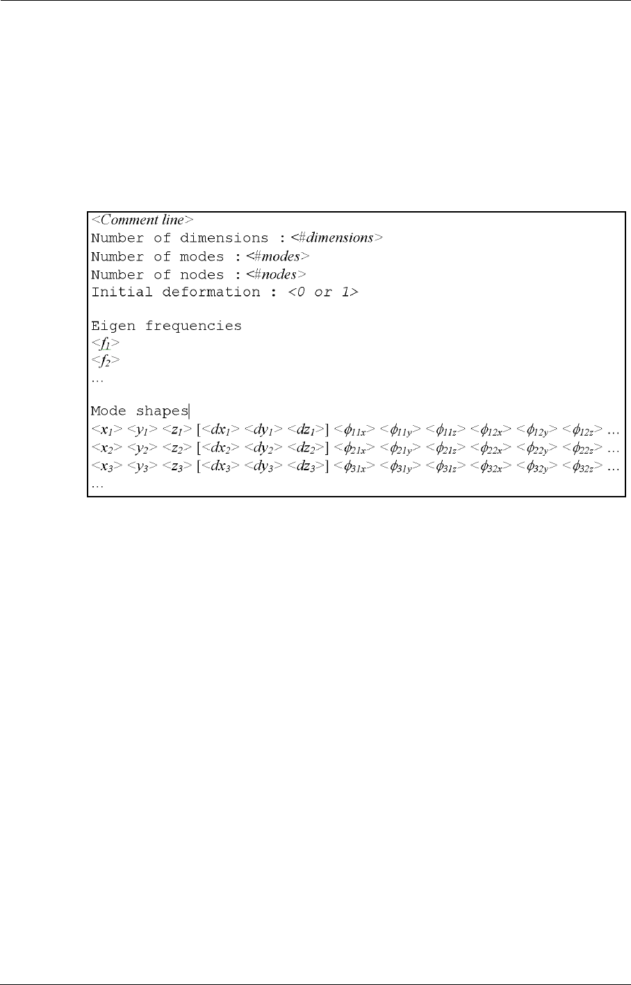
Physical Models Fluid-Structure
7-20 FINE™/Turbo
the eigen frequencies are listed in increasing order. The frequencies have to be written in Hz.
Finally the initial deformation and the mode shape information are written node by node. For each
node one line contains the three (or two for 2D computation) coordinates, the initial deformation (if
the parameter Initial deformation is set to 1) and the components of each mode sorted in increasing
frequency order. Coordinates and mode shapes have to be written in SI unit system. For mode shape
the conversion factor is the inverse of the square root of mass conversion factor.
Mode shape must be scaled for a generalized mass equal to 1.
FIGURE 7.3.2-15 The format of structure file
Two kinds of method computing the displacement of the structure are available: Coupled and
Forced Motion. In both methods, the user needs to specify the Number of Modes. The number of
used modes must be less than or equal to the number of modes defined in the structure file.
If the coupled method is selected, a Damping Coefficient needs to be specified for each mode
used. These damping coefficients will be used to solve the modal equations and compute the defor-
mation of the structures. If the forced motion is selected, the Generalized Displacement needs to
be specified for each mode used. The generalized displacement can be a constant value (steady or
unsteady mode) or a time profile (unsteady mode). These generalized displacements will be used to
compute the deformation of the structures directly. For more information on how to compute the
deformation of the structures, please refer to the theoretical manual.
After setting the modal parameters, the user has to specify the boundaries corresponding to the
structure surfaces. All solid patches and groups in the fluid mesh are listed on the middle of the
page. The user has to select the coupled surfaces, mark them as Coupled and specify the corre-
sponding Structure ID.
With the modal approach, a new output file is generated with the extension ".generalized_motion".
This file has the following format:
•for steady computation: the iteration number, for each mode and each structure defined in
the interface, where is the generalized displacement.
q
q

Fluid-Structure Physical Models
FINE™/Turbo 7-21
•for unsteady computation: the time step, , , for each mode and each structure defined
in the interface, where is the generalized displacement.
7-3.2.4 Mesh deformation methods
Mesh deformation plays a crucial role in the analysis of multi-physics problems that involve mov-
ing bodies and domain with dynamic boundaries. For example, in Fluid-Structure Interaction (FSI),
the fluid mesh has to be deformed at each time step according to the displacements computed by the
structural solver at the interface of the fluid domain and solid domain.
In FINE™/Turbo, two kinds of mesh deformation methods are available: Laplacian smoothing and
Radial Basis Functions. The user can select them in expert mode when Mechanical coupling is
activated, see Figure 7.3.2-7.
For all computations with mesh deformation, a ".globalforce_unsteady" file is generated, which
contains the evolution of the load on solid surfaces. The ".globalforce_unsteady" file has the
following format:
•for steady computation: <iteration_number> <Force_X> <Force_Y> <Force_Z> <Torque_X>
<Torque_Y> <Torque_Z> <Force_X> <Force_Y> <Force_Z> <Torque_X> <Torque_Y>
<Torque_Z>
•for unsteady computation: <time_step> <Force_X> <Force_Y> <Force_Z> <Torque_X>
<Torque_Y> <Torque_Z> <Force_X> <Force_Y> <Force_Z> <Torque_X> <Torque_Y>
<Torque_Z>
The first set of <Force_X> <Force_Y> <Force_Z> <Torque_X> <Torque_Y> <Torque_Z> is for
the surfaces for which the option Compute force and torque has been activated in the Boundary
Conditions page under SOLID tab. The second one is for the other solid surfaces.
a) Laplacian Smoothing
The Laplacian smoothing method assumes that the mesh deformation caused by a moving solid
wall boundary is small enough so that the mesh topology is not modified and the mesh can be
smoothed without generating negative cells. This assumption of small displacements on the moving
solid boundary allows to keep the same mesh topology and generate the new mesh with a Laplacian
smoothing of these displacements inside the domain. The smoothing of displacements is carried out
only to groups where a surface is moving.
The main limitations for the groups of blocks where the mesh is deformed are as follows:
•no FNMB connection;
•no SNG boundary conditions;
•no rotor-stator interface with deformation;
•rotor-stator interface can not be located between moving walls;
b) Radial Basis Functions
The Laplacian smoothing works only when the mesh deformation is very small. When performing a
MpCCI or modal mechanical coupling simulation, the structure deformation may be very large. In
this case, the mesh deformation method using Radial Basis Function (RBF) can be used. The RBF
method gives deformed meshes keeping very good quality even for large deformation. For more
information on the RBF method, please refer to the theoretical manual.
The main limitations for the RBF mesh deformation method are as follows:
q
dq
dt
------
d2q
dt2
--------
q

Physical Models Fluid-Structure
7-22 FINE™/Turbo
•The mesh deformation method using RBF is not compatible with:
—FNMB connections,
—SNG boundary condition,
—Upwind scheme,
—Rigid body motion,
—Adaptive wall.
•The number of boundary nodes is limited to 46000 per blade row. Please note that memory
cost can become quite huge when the number of boundary nodes increases.
c) Expert Parameters
IMOVWD(integer):When mesh deformation exists, the wall distance used for turbulent flow may
change. In this case, the user can set the expert parameter IMOVWD to 1 to
compute the wall distance at each time step.
0(default): compute the wall distance only once.
1: compute the wall distance at each time step.
The expert parameters related to Laplacian smoothing:
IMVCYL(integer): The smoothing can be applied to the displacement field in cartesian coordinates
or in cylindrical coordinates. The best choice is depending on the geometry of
the case.
0(default): applied in cartesian coordinate.
1: applied in cylindrical coordinate.
FCTNIT (real): Multiplicative factor for the number of smoothing iteration. The number of iter-
ation (N) for the full multigrid initialization on grid level G is based on the
maximum number of points in each direction in all blocks:
N (on grid level G) = FCTNIT*(G+1)*MAX(NI, NJ, NK)
If the deformed mesh has negative volumes, the user can increase this expert
parameter.
MVRELF (real): Relaxation factor of the iterative process (default = 0.9). A mesh with high
aspect ratio and skewed cells requires lower value (0.45). If the iterative proc-
ess of the mesh deformation is unstable, MVRELF must be decreased (<0.5).
IMVWEI (integer):Select the smoothing method for the moving mesh:
0 (default): Linear smoothing of displacements;
1: Weighted smoothing of displacements based on the cell volume in the no-
deformed mesh. The weighted smoothing allows to restrict the smoothing of
the small volume cells in order to preserve the quality of the mesh. The smaller
cells are more rigid than bigger cells.
MVDIFF (real): Relaxation factor for the weighted elliptical smoothing of displacements.
The expert parameters related to mesh deformation module (RBF):
MOVRBF(integer):Choice of RBF function.
1: Wendland C2 function,
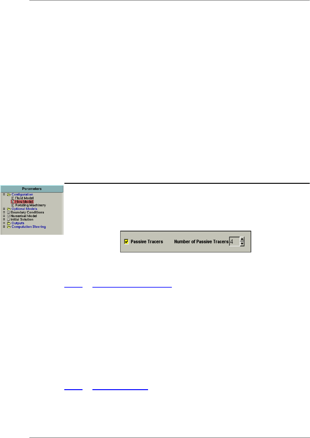
Passive Tracers Physical Models
FINE™/Turbo 7-23
2(default): TPS function.
MOVRAD(real): Support radius for Wendland C2 function or scale factor for TPS function.
ISVMAT(integer): Choice of the solving method for system of equations.
0: don’t use inverse matrix,
1(default): compute, save and use inverse matrix,
2: use inverse matrix that has already been computed and saved.
ICOARS(integer): Controls the coarsening level of the boundaries. It only affects the mesh defor-
mation step. This parameter is an array of two dimensions, corresponding to
coarsening level for moving boundaries and fixed boundaries. The first number
is the grid level (relative to the grid level of the computation) of moving bound-
ary nodes used for the deformation. The second number is the grid level for the
fixed boundary (solid, inlet, outlet, periodic,...) nodes. If the grid level is set to
0, all the nodes of the surface are taken into account. If it is set to one, only the
nodes of the surface belonging to the first coarser grid are used. Hence the
number of boundary nodes is reduced by four for the surface.
7-4 Passive Tracers
Selecting the Passive Tracer option in the Configuration / Flow Model page allows the user to
introduce, into the computations, species that are passive with regards to the carrier fluid. This
means that the carrier fluid ignores the tracer and is only defined by its own properties.
•The passive tracers are not allowed to react with each other.
7-4.1 Boundary Conditions
There are currently two types of boundary conditions available in the FINE™/Turbo solver for pas-
sive tracers: inlet and external (far field).
The inlet condition is set through the specification of the species mass fractions where
with ns, the total number of species. The external condition requires the same input data.
For passive tracers, species concentrations are entered and are independent from each
other. There is no limitation on the sum of the concentrations.
7-4.2 Initial Solution
For each species, the initial value of the mass fraction at the initial stage is required. Initial condi-
tions are uniform over the domain for each species.
ρsρ⁄
ρρ
s
s1=
ns
=

Physical Models Porous Media Model
7-24 FINE™/Turbo
For passive tracers, species concentrations are entered and are independent from each
other. There is no limitation on the sum of the concentrations
7-4.3 Outputs
For each species, the FINE™/Turbo solver will compute automatically the species concentration
for each tracer.
7-5 Porous Media Model
A porous medium is a solid permeated by an interconnected network of pores filled with a fluid.
Usually both the solid matrix and the pore network are assumed to be continuous, so as to form two
interpenetrating continua such as in a sponge. Many natural substances such as rocks and soils, and
man made materials such as foams and ceramics can be considered as porous media. When simulat-
ing the flow in porous media the user has to use a porous media model because the geometry is too
complex to resolve with a grid.
The porous media model in FINE™/Turbo allows the user to simulate the flow in porous media. In
FINE™/Turbo, the user needs to set which grid block will be treated as a porous medium. And the
user has to specify the parameters for each block.
In the next sections the following information is given on the Porous Media Model:
•7-5.2 gives a summary of the available expert parameters related to the Porous Media Model.
7-5.1 Porous Media Model in the FINE™/Turbo GUI
There is no access of Porous Media Model through the graphical user interface. The user has to
activate this model and set all the parameters through the Expert Parameters, as describing in the
following part.
7-5.2 Experts Parameters
IPORME (integer):Control if activate the porous media module or not:
0: module is deactivated (default)
1: module is activated
IDOMPO (integer):Porous media domain number (no more than 50 domains).
IDIRPO (real): Imposed direction for each specified porous block (if 0 0 0, no direction is
imposed).
IMODPO (integer):Select the models available to model the pressure drop through the porous
media:
1: Darcy or Ergun law
2: Integral law
LPORME (real): Porous medium thickness (L), used only if IMODPO = 2.

Cavitation Model Physical Models
FINE™/Turbo 7-25
EPORME (real): Porosity ( ), used only if IMODPO = 1, is defined as the volume fraction of
the voids from the solid matrix
KPORME (real): Constant C in the models.
APORME (real): the specific surface area A in the Ergun or Darcy model and in
the integral model.
NPORME (real): Exponent n, used only if IMODPO = 2.
ITHEPO (integer): Control if activate the thermal source term in the porous media or not:
0 (default): Activate the thermal source term
1: Deactivate the thermal source term
HPORME (real): Heat transfer coefficient for porous media.
SPORME (real): Volumetric exchange surface.
TPORME (real): Skin temperature.
7-6 Cavitation Model
Cavitation is a dynamic process of formation of bubbles inside the liquid, their growth and subse-
quent collapse. It appears where the pressure of the liquid falls below its vapor pressure. Such cavi-
tation often occurs in pumps, nozzles, injectors and marine etc. Cavitation is an abnormal condition
that can result in loss of efficiency, increase of the noise level and structural damage.
The development of the cavitation phenomena is related to the cavitation number . Cavitation
develops with decreasing the cavitation number. More details can be referred to the theoretical
manual.
In the next sections the following information is given on the Cavitation Model:
•7-6.2 gives a summary of the available expert parameters related to the Cavitation model.
7-6.1 Cavitation Model in the FINE™/Turbo GUI
There is no access of Cavitation Model through the graphical user interface. The user has to activate
this model and set all the parameters through Expert Parameters, as describing in the following
part.
7-6.2 Experts Parameters
IMITRA (integer): control the activation of the cavitation model
0: model is inactive (default)
2: model is active
Parameters related to the definition of the fluid:
PVAPS (real): vapor pressure [Pa] (default = 2000, cold water)
RHOL (real): density in liquid phase [kg/m3] (default = 1000, cold water).
ε
Atotal A⁄passage
σ

Physical Models Cavitation Model
7-26 FINE™/Turbo
RHOV (real): density in vapor phase [kg/m3] (default = 1, cold water).
AMIN (real): related to the maximum slope of the barotropic law (default = 50, cold water).
where cmin is the celerity of sound in the homogeneous liquid-vapor mixture.
Parameters related to the numerical scheme:
VIS2SW (integer): 1: second order pressure switch is de-active (default)
0: second order pressure switch is active (suggested for incompressible flows)
RSMPAR (real): 1: residual smoothing is active (default)
0: residual smoothing is de-active (suggested for incompressible flows)
VA P L A X (real): under relaxation coefficient for pressure. This parameter will be activated
when and/or static pressure drops during run.
Amin
ρLρV
–
2
------------------ cmin
2
=
ρρ
V
=
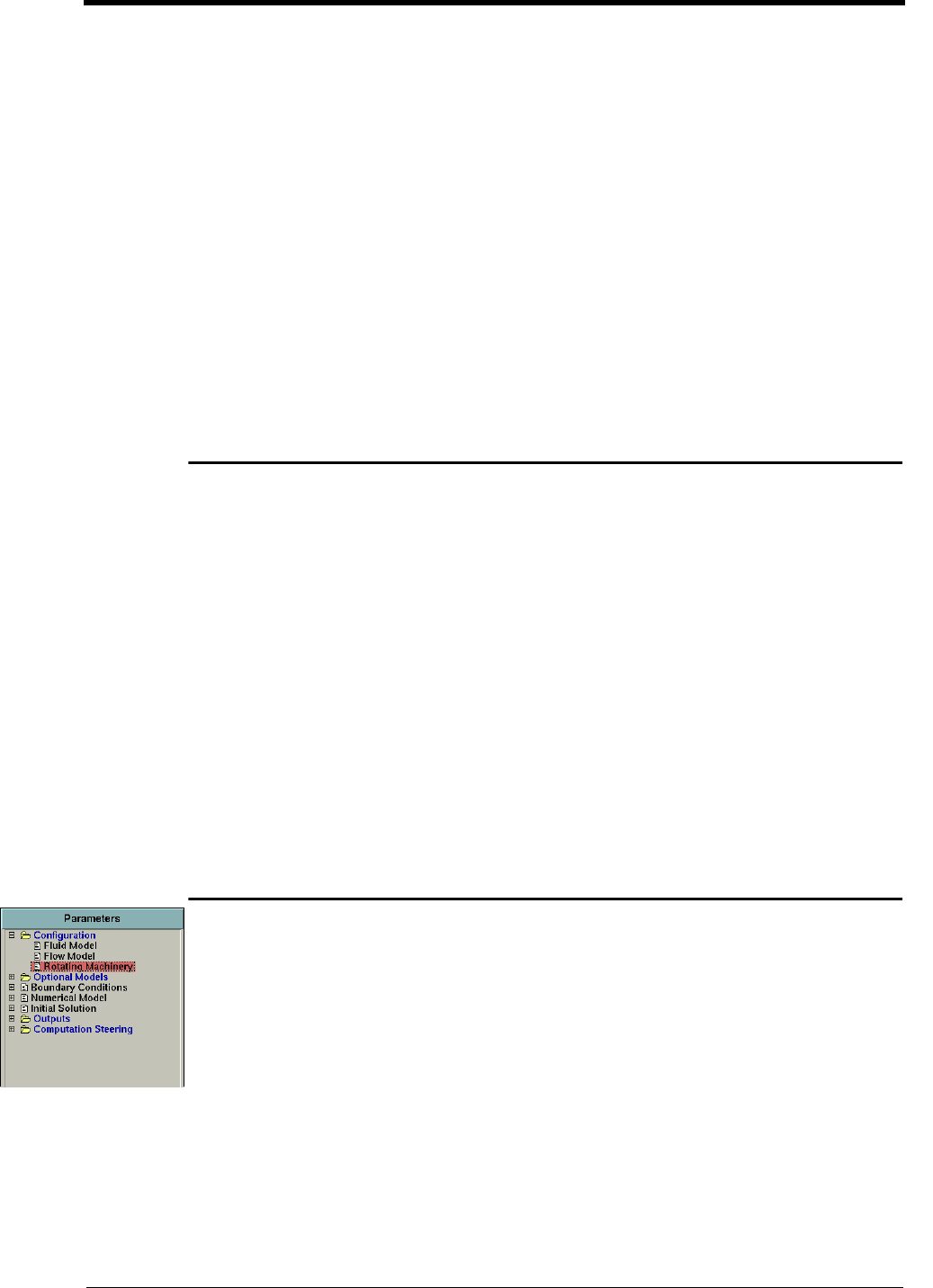
FINE™/Turbo 8-1
CHAPTER 8: Dedicated
Turbomachinery
Models
8-1 Overview
The following models and modules in FINE™/Turbo are dedicated to turbomachinery applications:
•Rotating Blocks defines the typical information concerning cylindrical cases for each block.
•Rotor/Stator Interaction defines the properties of each rotor/stator interface.
•Harmonic Method allows to perform unsteady simulation using Harmonic method.
•Clocking allows to consider the effect of clocking in multistage turbomachinery case.
•Cooling/Bleed models cooling holes or bleed.
•Rigid Motion models the flow where the solid walls can move.
•Aeroacoustics models acoustic noise based on harmonic computation.
•Laminar-Transition Model models the flow transition.
•Performance Curve allows to perform an off-designed analysis for turbomachinery.
•SubProject Management allows the partial treatment of multistage turbomachinery projects
8-2 Rotating Blocks
The Rotating Blocks tab gives access to the definition of the typical information for each block as
shown in Figure 8.2.0-1. This tab is only accessible when the mesh is cylindrical (see Mesh/Prop-
erties... to see whether the mesh is cylindrical or Cartesian).
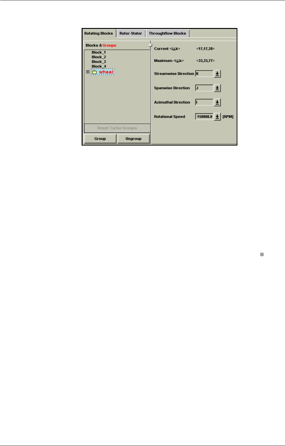
Dedicated Turbomachinery Models Rotating Blocks
8-2 FINE™/Turbo
FIGURE 8.2.0-1 Rotating Blocks on Rotating Machinery Page
When selecting the Rotating Blocks tab the page appears as shown in Figure 8.2.0-1. On the left a
list of all blocks is displayed. If the mesh has been made with AutoGrid™, a default grouping per
row is proposed. It is also possible to manually group the blocks that have the same properties:
1. Clicking on a block de-selects the currently selected block(s). It is possible to select several con-
secutive blocks in the list by clicking on the first one and holding the left mouse button while
selecting the next. To select a group of blocks which are not situated next to each other, click on
each of them while keeping the <Ctrl> key pressed.
2. Click on the Group button. A text box will appear just below the Group button. Place the cursor
in the text box and type the name of the group and press <Enter>. The name of the group will
appear on the list of blocks in red with a plus sign on the left of the name. To see the blocks that
are included in a certain group double click on the name of the group or click on the symbol
in front of the name.
3. To remove a group of blocks select the group and click on the Ungroup button. The group will
be removed and the blocks that were in this group will be listed again in the list as separate
blocks.
4. The Reset Turbo Groups button allows to reset the default grouping proposed by AutoGrid™.
On the right of the list with blocks, the information for the selected block or group of blocks is
given. If multiple blocks are selected the information is only displayed for the first selected block.
For each block the current and maximum number of nodes in the three grid directions is shown.
Four items need to be defined by the user: the streamwise direction, the spanwise direction, the azi-
muthal direction and the rotational speed:
—The streamwise, spanwise and azimuthal directions allow to determine the block orientation.
Please note that if AutoGrid™ is used for the grid generation, the streamwise direction is
automatically taken as being the k-direction, the spanwise direction as the j-direction and the
azimuthal direction as the i-direction.
The block orientation has an impact when using the radial equilibrium outlet (span-
wise direction used), when performing an azimuthal or surface averaging (respectively
spanwise and streamwise direction used).

Rotating Blocks Dedicated Turbomachinery Models
FINE™/Turbo 8-3
—The FINE™/Turbo solver solves the equations in a relative frame of reference. This implies
that the mesh blocks surrounding rotating blades rotate with the blades and should therefore
be set as "rotating" in this page. The Rotational Speed of the block has to be given in Revo-
lutions Per Minute (RPM). A positive value for the rotation speed indicates a rotation in pos-
itive θ-direction with θ positive according to a right handed coordinate system. In
Figure 8.2.0-2 this is illustrated for the case where the z-axis is the axis of rotation which is
automatically the case for a mesh created with AutoGrid™.
FIGURE 8.2.0-2 Positive rotation speed
Although the governing equations for rotating systems are usually formulated in the
relative system and solved for the relative velocity components, the formulation retained
for ship propeller applications, ventilators or wind turbine are often expressed in the rel-
ative frame of reference for the absolute velocity components. The two formulations
should lead to the same flow solution. However, experience shows that the solution can
be different, especially in the far field region. For propeller problems, the formulation
based on relative velocities has the disadvantage that the far field relative velocity can
reach high values. This induces an excess of artificial dissipation leading to a non-physi-
cal rotational flow in the far field region, this dissipation being based on the computed
variables. In FINE™/Turbo, the governing equations for rotating systems can be solved
for the relative velocity components or for the absolute velocity components, which is
controled by setting the expert parameter IVELSY to 1 or 0.
The different computations in a project can not have different configuration settings. If
any of the settings in this area are changed, the modifications will be taken into account
for all (active and non-active) computations.
The rotation axis should be the z-axis in order to be compatible with the FINE™/
Turbo solver.
Only one rotation speed different than 0 is allowed when performing an unsteady sim-
ulation using the Domain Scaling method or Phase lagged method.

Dedicated Turbomachinery Models Rotor/Stator Interaction
8-4 FINE™/Turbo
8-3 Rotor/Stator Interaction
8-3.1 Rotor/Stator Interfaces in the FINE™/Turbo GUI
The Rotor-Stator tab gives access to the definition of the rotor/stator interfaces as shown in
Figure 8.3.1-3. This tab is only accessible when the mesh contains rotor/stator interfaces. Rotor/sta-
tor interfaces are defined in IGG™ as ROT boundary condition. Consult the IGG™ User Manual
for more detailed information on how to define this boundary condition.
The rotor/stator patches should not include regions where R=0.
On the left, the list of patches is displayed which are defined as part of a rotor/stator interface in
IGG™ (boundary condition type: ROT). It is possible to display only a limited amount of patches
by using the Filter. Type in the text box the part of the name that is common to all patches to dis-
play and press <Enter>. All patches containing in the name the entered text will be displayed. Note
that the filter is case insensitive.
If the mesh has been made with AutoGrid™, a default grouping is proposed. It is possible to group
patches that have the same definition by selecting them in the list and clicking on the Group button.
A text box will appear below this button which allows to enter a name for the group. The group will
be displayed in red in the list of patches. Double click on the group name to see which patches are
in the group. To select multiple patches select them while keeping the <Ctrl> key pressed. To
remove the group simply select the group from the list and click on Ungroup. The patches in the
selected group will be put back into the list of patches and the group name will be removed from the
list.
In some special cases where the mesh is made by AutoGrid5™ (e.g. bypass configura-
tion), the upstream and/or downstream patches can not be grouped automatically. In this
case, the user has to pay attention to the rotor/stator interface definition to see if the mesh
constraints are ensured.
Multiple rotor/stator interfaces can be treated in one single project. Each rotor/stator interface is
indicated by an ID Number and each of them may contain an arbitrary number of Upstream and
Downstream patches. For each patch in the list, the ID number of the corresponding rotor/stator
interface has to be provided by the user. Also it should be specified whether the patch is located in
the upstream or downstream side of the interface. It should be mentioned that no hypothesis is made
on the direction of the flow through the interface, except when the transition module (see section 8-
9) or the stage-by-stage analysis (see section 10-3.2) is used. The purpose of the upstream and
downstream denominations is only to establish the two groups of patches belonging to respectively
the rotor and the stator side.
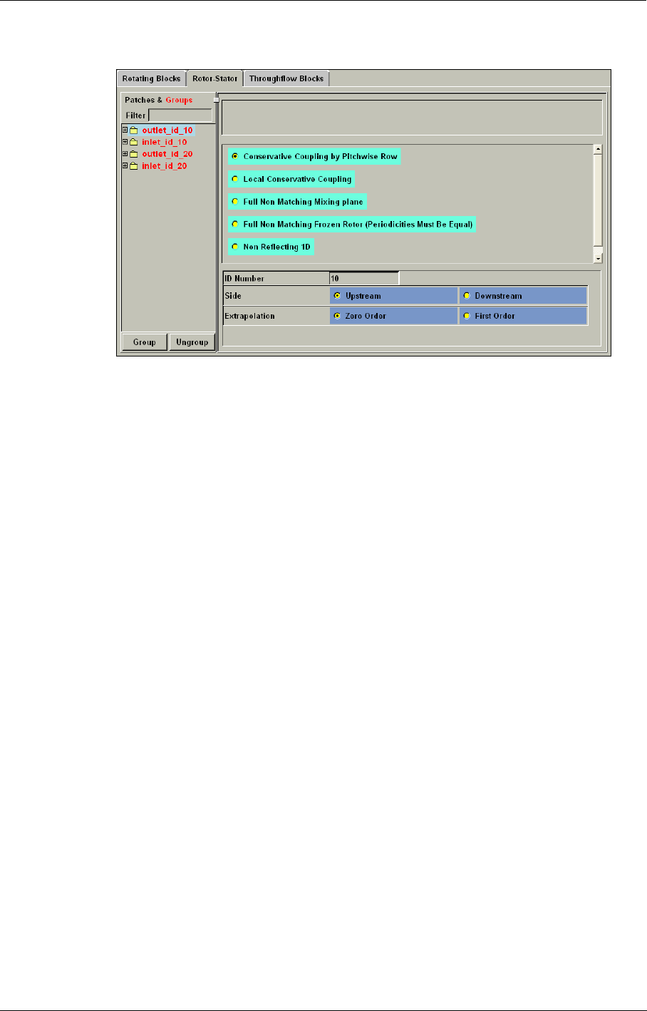
Rotor/Stator Interaction Dedicated Turbomachinery Models
FINE™/Turbo 8-5
FIGURE 8.3.1-3 Rotor-Stator interface definition in steady mode
In addition to the ID number and the upstream/downstream side specifications the user has to select
also:
•the order of Extrapolation (zero or first order). Zero order extrapolation (default) is used in
most cases and usually provides satisfactory results. First order extrapolation may be useful in
case of important flow gradients in the direction normal to the interface together with a rela-
tively coarse mesh.
•one of the six available steady state techniques (for steady state applications only):
The type of several rotor-stator interfaces can be changed simultaneously by selecting
one rotor-stator interface, hold the <Shift> button and left-click on the desired type of
rotor-stator interface. All other settings, such as the ID Number, will be kept.
—1. The Conservative Coupling by Pitchwise Rows approach is recommended due to its
capability to provide an exact conservation of mass flow, momentum and energy through the
interface. This approach adopts the same coupling procedure for all the nodes along the cir-
cumferential direction, even if the local flow direction is different from the averaged one.
This technique offers the advantage of being able to guarantee a strict conservation of mass,
momentum and energy through the interface. Moreover it shows to be very robust and is
therefore used by default.
—2. The Local Conservative Coupling approach is only recommended for the rotor/stator
interface between an impeller and a volute. Experience has shown that in cases, where sig-
nificant flow variations are observed in the circumferential direction (as for instance in the
case of rotor-volute interactions), it is more stable to base the flux decomposition on the
local flow direction as it is done in the Local Conservative Coupling technique. Small con-
servation errors can be observed with this technique, which is therefore only used for special
configurations.
—3. The Full Non Matching Mixing plane approach is respecting an exact conservation of
mass flow, momentum and energy through the interface as the Conservative Coupling by
Pitchwise Rows but has less constraints on the interface geometry.

Dedicated Turbomachinery Models Rotor/Stator Interaction
8-6 FINE™/Turbo
—4. The Full Non Matching Frozen Rotor approach is considering the rotor/stator interface
as a perfect connection and is neglecting the rotor movement in the connecting algorithm. In
this approach, the periodicities between rotor stator must be equal.
—5. The Non Reflecting 1D approach is based upon a characteristic analysis of the linearized
Euler equations. The characteristic variables are imposed on each side of the rotor/stator
interface. Such a treatment is recommended when wave reflection is observed at the inter-
face, which can occur when the interface is close to the blade.
—6. The Non Reflecting 2D approach is the extension of the Non Reflecting 1D approach.
The Non Reflecting 2D approach is also based upon a characteristic analysis of the linear-
ized Euler equations. The characteristic variables are imposed on each side of the rotor/sta-
tor interface. The Non Reflecting 2D approach will produce a better representation of the
shock wave crossing a R/S interface.
The Non Reflecting 1D/2D approach can not be used when the flow perpendicular to
the rotor/stator interface is supersonic.
The use of the Non Reflecting 1D/2D approach is limited to steady simulations with-
out preconditioning.
The Non Reflecting 1D/2D approach is only compatible with perfect gas or real gas.
8-3.2 How to Set-up a Simulation with Rotor/Stator Interfaces?
Five different approaches are available in FINE™/Turbo to simulate the interaction between rotat-
ing and non-rotating blocks:
Steady state:
•Mixing plane approach: a pitchwise averaging of the flow solution is performed at the rotor/
stator interface and the exchange of information at the interface depends on the local direction
of the flow. See section 8-3.2.1 for more detail on how to use this approach.
•Frozen rotor: a steady simulation of one specific position of the rotor with respect to the sta-
tor. For more information on how to set up a project according to this method see section 8-
3.2.2.
Unsteady:
•Domain scaling method: unsteady simulation in which the mesh periodicities are constrained
to be identical on both sides of the interface. See section 8-3.2.3 for more detail on how to use
this approach.
•Phase lagged method: unsteady simulation in which the mesh periodicities are not con-
strained to be identical on both sides of the interface. See section 8-3.2.4 for more detail on
how to use this approach.
•Harmonic method: like the phase-lagged method, this method only needs one inter-blade
channel per blade row. No special requirement on the periodicities is required. The interaction
between two adjacent blade rows is modelled by computing the time harmonics of the fluctuat-
ing part of the unsteady flow along the two sides of the rotor/stator interface as well as the
time-averaged flow. The values are calculated with respect to the matching of the unsteady
flow on both sides of the interface and are treated locally by a non-reflective treatment. A mix-
ing-plane approach is applied to the eddy-viscosity if the Spalart-Allmaras model is used. See
section 8-3.2.5 for more detail on how to use this approach.
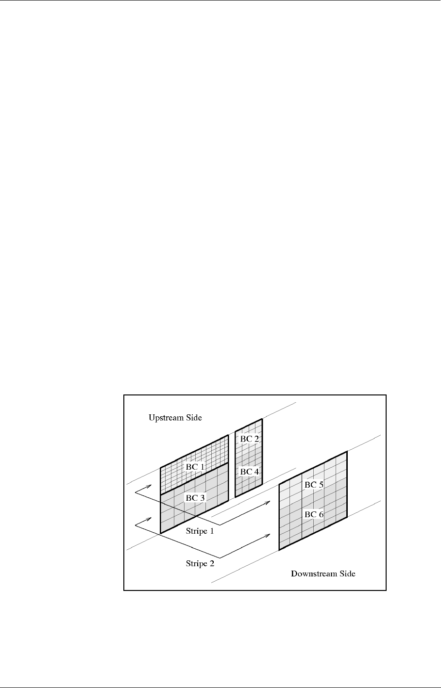
Rotor/Stator Interaction Dedicated Turbomachinery Models
FINE™/Turbo 8-7
8-3.2.1 Mixing Plane Approach
In the mixing plane approach the flow solution at the rotor/stator interface is azimuthally averaged
and the exchange of information at the interface depends on the local direction of the flow. In this
section it is described how to use this approach in FINE™/Turbo.
a) Geometrical Constraints
The default mixing plane method (Local Conservative Coupling and Conservative Coupling by
Pitchwise Rows) used in FINE™/Turbo imposes the following geometrical constraints:
•The patches on both sides of the rotor/stator interface must cover the same range in spanwise
direction,
•The meshes need not to match in the spanwise direction, but the azimuthal mesh lines on the
boundary must be circular arcs.
An illustration of these constraints is given in Figure 8.3.2-4. Consisting of two stripes, the depicted
configuration provides a complete description of the capabilities. The upstream side of the quasi-
steady interface consists of three blocks, represented by the bold frames and the surface meshes,
while a single block is assumed for the downstream side. A gap may exist between two blocks, e.g.,
if the mixing plane coincides with the exit plane of a blade row having a blunt trailing edge. The
grid points distribution are different for each of the boundary patches involved, but the pitchwise
grid lines have constant radius and the pitchwise line along which two patches of the same side join
(e.g., BC 1 and BC 3) exists as an inner grid line on all other boundaries. In the example, the inter-
face is thus decomposed into two stripes, stripe 1, consisting of BC 1 and BC 2 on the upstream side
and BC 5 on the downstream side, and stripe 2, consisting of BC 3 and BC 4 on the upstream side
and BC 6 on the downstream side.
In special configurations such as rotor-volute interaction it is preferable to use Local
Conservative Coupling.
.
FIGURE 8.3.2-4 Example of stripe configuration

Dedicated Turbomachinery Models Rotor/Stator Interaction
8-8 FINE™/Turbo
The full non matching mixing plane method (Full Non Matching Mixing plane, Non Reflecting
1D and Non Reflecting 2D) removes the geometrical constraints imposed in the default mixing
plane method. This technique is based on the full non-matching algorithm and has clear advantages:
an exact conservation of the mass flow, momentum and energy is guaranteed.
The remaining geometrical constraints for the full non matching mixing plane method are:
•The rotor/stator patches belonging to a given interface should lie on the same common
axisymmetric surface.
•The hub and the shroud lines are assumed to be located on a circular arc, and each extremity of
the hub and shroud lines should coincide with one corner of one of the patches. The periodic
boundaries between the adjacient blades must be defined by continuous lines with edges con-
nected by their corners. For a 360-degree mesh, a similar continuous spanwise line (defined by
interconnected edges) must be used in the connection algorithm.
•All patches constituting a rotor/stator interface should form a filled closed surface with no gap.
•the rotor/stator patches should be fully included in the rotor/stator interface: contrary to the full
non matching algorithm, which includes an automatic detection of the connection zone, and in
which the patches can then be partially connected, the rotor/stator module assumes that the
patches are fully connected.
b) Mesh Constraints
Only one blade passage needs to be meshed for both the rotor and the stator, regardless of their
respective periodicities. The boundary condition type must be set to "ROT" in IGG™ for all grid
patches belonging to a rotor/stator interface.
c) FINE™/Turbo Settings
1. The mixing plane approach is a steady simulation technique which requires to set the Time
Configuration to Steady on the Flow Model page.
2. The patches that have boundary condition type "ROT" in the mesh are listed in FINE™/Turbo
on the Rotating Machinery page under the Rotor-Stator tab. The user has to specify for each
of these patches:
•an ID Number that identifies the rotor/stator interface (useful for multistage configurations).
•a switch to indicate if the patch is belonging to the Upstream or Downstream part of the
rotor/stator interface.
•the order of Extrapolation (zero or first order).
•the boundary condition:
—Conservative Coupling by Pitchwise Rows,
—Local Conservative Coupling,
—Full Non Matching Mixing plane,
—Non Reflecting 1D.
—Non Reflecting 2D.
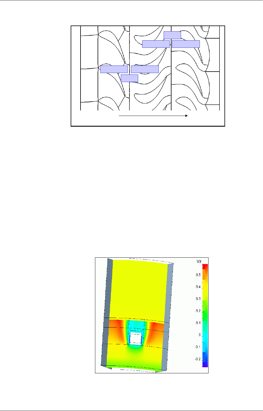
Rotor/Stator Interaction Dedicated Turbomachinery Models
FINE™/Turbo 8-9
FIGURE 8.3.2-5 Aachen Turbine: Upstream/Downstream and ID number identification
d) Illustrative Example
To illustrate the mixing plane approach the flow around a cube is considered as shown in
Figure 8.3.2-6. The flow is entering the domain at the bottom of the figure. The upstream portion of
the domain is the 'rotor' with a cube fixed on it. The second part is a 'stator'. Due to the pitchwise
averaging process one can see that the vortex occurring slightly downstream the 'trailing edge' of
the cube is spread when entering in the 'stator' component. If the rotational speed of the cube is
high, this approximation is acceptable since one can consider that the stator "sees" a more statisti-
cally averaged flow. If the rotational speed is low, this approximation is essentially invalid and thus
another method should be considered.
In some cases, i.e. in low pressure ratio compressors or turbines, the losses at the
rotor/stator interfaces are in the order of magnitude of the overall gain in the machine. In
such cases, it is recommended to use an unsteady approach and more specifically the har-
monic approach (section 8-3.2.5)
FIGURE 8.3.2-6 Flow around a cube: Mixing Plane approach
Flow Direction
ID = 1
ID = 2
Downstream
DownstreamUpstream
Upstream
Flow Direction
ID = 1
ID = 2
Downstream
DownstreamUpstream
Upstream

Dedicated Turbomachinery Models Rotor/Stator Interaction
8-10 FINE™/Turbo
e) Expert Parameters
This section provides a summary of the expert parameters related to mixing plane approach.
CFFNMB(integer):0 (default): old implementation for FNMB connection
1: new implementation with connection factor of cell area between image mesh
and actual mesh.
NQSTDY(integer): gives the possibility to the user to update the rotor-stator boundary conditions
every NQSTDY iterations. If the parameter NQSTDY is set to zero (default),
the update is done at every Runge-Kutta step. This is an under-relaxation tech-
nique that is rarely used.
Before the mixing process, an under-relaxation technique can be applied on the
averaged variables to stabilize the calculation:
RQSTDY(real): This is another under-relaxation technique that allows to limit the changes in
the variables from one iteration to the next. This technique is used in special
cases where stability problems are encountered.
1 (default): no relaxation
0 to 1: under-relaxation
IRSMRG(integer): This parameter is used only for the Conservative Coupling by Pitchwise
Rows method and the Local Conservative Coupling method in parallel simu-
lations. It is linked to memory allocation for merging of spanwise distribution.
The allocation will be based on the value of IRSMRG multiples the maximum
number of points in different distributions.
RSROL(real): This parameter is the tolerance used for the Full Non Matching Plane algorithm
(default value 1.8). This parameter should be smaller than the ratio of the first
inner cell distance to the hub-to-shroud distance.
NH2DNR(integer): sets the number of harmonics used for DFT and inverse DFT when using the
non-reflecting 2D Rotor/Stator interface. The default value is 3.
LOCCOR(integer) In some particular cases, a problem of mass flow conservation through a non
reflecting 1D or 2D rotor-stator interface can arise. This can be improved by
deactivating the local enthalpy correction through the expert parameter LOC-
COR.
0: local enthalpy correction deactivated
1 (default): local enthalpy correction activated
8-3.2.2 Frozen Rotor
The basic idea at the origin of the frozen rotor technique consists of neglecting the rotor movement
in the connecting algorithm.
The governing equations are solved for the rotor in a rotating frame of reference, including Coriolis
and centrifugal forces; whereas, the equations for the stator are solved in a absolute reference
frame. The two components are literally connected, and hence a rotor-stator approximation is not
required, rather the continuity of velocity components and pressure is imposed. As a result, the final
steady solution will be depending on the relative position of the rotor and the stator. Unsteady 'his-
tory effect' (such as shedding separated zones) are neglected.
It is usually well accepted that the frozen rotor approach is an appropriate solution for the treatment
of rotor-volute interactions, where pitchwise variations of the flow cannot be neglected. However, it

Rotor/Stator Interaction Dedicated Turbomachinery Models
FINE™/Turbo 8-11
requires the meshing of the complete impeller (all passages). Another drawback is that the flow
solution depends on the rotor position, relative to the stator.
a) Mesh Constraints
Exactly as for the domain scaling approach a constraint must be satisfied on the mesh periodicity.
The pitchwise distance must be the same for both sides of the rotor/stator and coincident (no gap
allowed between rotor and stator components in the pitchwise direction). For each different position
of the rotor with respect to the stator a new mesh will have to be created in IGG™ and a new steady
calculation has to be performed.
b) FINE™/Turbo Settings
There are three ways to run a frozen rotor calculation:
1. To mesh all blade rows completely and to use matching connections (CON) in IGG™ for the
patches at the interface of the rotor and the stator. The blocks of the rotor should be made rotat-
ing, as well as the boundary conditions. A steady calculation can be run for this configuration. A
non matching (NMB) connection can not be used in this case: even though the computation
might run the result would not be correct. This was previously the only way to perform frozen
rotor calculations in FINE™/Turbo. This approach is no longer used as the constraint on match-
ing connections is too restrictive.
Only CON matching connections are allowed in this first method.
2. To create a mesh covering the same pitchwise distance on both sides of the interface and to
impose Full Non Matching Frozen Rotor in the Rotating Machinery page under the Rotor-
Stator tab. Furthermore the user has to specify for each of these patches the ID and the
upstream/downstream location as described in section c) at step 2. Therefore, the boundary con-
dition type must be set to "ROT" in IGG™ for all grid patches belonging to a rotor/stator inter-
face.
3. When starting an unsteady computation by imposing iterations as a steady initialization in the
Control Variables page, the frozen rotor technique is used during the steady iterations.
Note that for example for an impeller-volute computation the complete impeller
would need to be meshed in all three cases since the periodicity of the volute is 1.
c) Illustrative Example
Results obtained from frozen rotor calculations usually look similar to unsteady ones. A more
detailed analysis shows that the approximation introduced in the connection algorithm induces a
deviation of the wake when passing through the interface.
As an illustration the frozen rotor method is compared to the sliding mesh approach for the Aachen
Turbine in Figure 8.3.2-7 and Figure 8.3.2-8.
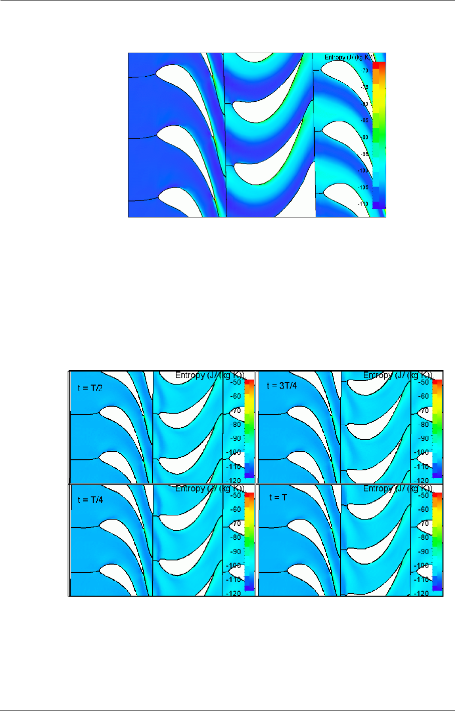
Dedicated Turbomachinery Models Rotor/Stator Interaction
8-12 FINE™/Turbo
FIGURE 8.3.2-7 Aachen Turbine: Frozen Rotor approach
8-3.2.3 Domain Scaling Method
The Domain Scaling Method is an unsteady simulation technique for rotor/stator interfaces. The
effect of displacement due to rotation is taken into account. At each time step, the rotor is set at its
correct position and equations are solved for that particular time step for the whole computation
domain. The final solution is therefore a succession of instantaneous solutions for each increment
of the rotor position.
FIGURE 8.3.2-8 Aachen Turbine: Domain Scaling (Sliding Mesh) approach

Rotor/Stator Interaction Dedicated Turbomachinery Models
FINE™/Turbo 8-13
a) Mesh Constraints
The boundary condition type must be set to "ROT" in IGG™ for all grid patches belonging to a
rotor/stator interface. The blade passages of each blade row to include in the mesh should cover the
same pitch distance (have the same periodicity). If the periodicity of the rotor and the stator is not
the same this can be solved in three different ways:
•modelling a higher number of blade passages on each side to find a common periodicity,
•scaling the geometry (with the scaling being as close to 1 as possible). The common way to
scale the geometry is to modify the number of blades during the mesh generation process. The
time frequencies are resolved with an error that is proportional to the scaling coefficient.
•using the phase lagged approach explained in section 8-3.2.4 or the nonlinear harmonic
method in section 8-3.2.5.
Apart from this constraint on the periodicity, there is no constraint on the patches and mesh nodes
configurations.
b) FINE™/Turbo Settings
1. Domain Scaling Method is an unsteady simulation technique so the Time Configuration in the
Flow Model page should be set to Unsteady.
2. By default, in the Rotating Machinery page under Rotor-Stator tab page, the Domain Scaling
approach is selected. The user has to specify for each of these patches the ID and the upstream/
downstream location as described in section c) at step 2. Therefore, the boundary condition type
must be set to "ROT" in IGG™ for all grid patches belonging to a rotor/stator interface.
3. The initialization process can be performed in two ways:
•A steady state initialization is performed in a separate computation with Steady as Time Con-
figuration. It is suggested to model all rotor/stator interfaces in this case using frozen rotor
approach. The unsteady domain scaling computation is using the result of this steady computa-
tion as initial solution. See Chapter 9 for more information on how to start a computation from
an initial solution file.
•The steady state initialization is automatically performed before starting the time accurate
computation (that means within the same computation), switching to Unsteady as Time Con-
figuration in the Flow Model page and selecting in the interface an appropriate Number of
Steady Iterations in the Steady Initialization parameters on the Control Variables page.
4. The Number Of Angular Positions is defined in the Control Variables page. When working
with the Domain Scaling method, using a Number Of Angular Positions of 10 points per blade
passage is giving a coarse but reasonable result. To have a more accurate (but more CPU con-
suming) result choose 20 to 30 points per blade passage.
5. The Number Of Time Steps is defined in the Control Variables page. In general, it is recom-
mended to repeat the period at least 20 times. Usually after 20 periods, the flow becomes peri-
odic.
For example, considering a 1-1/2 turbine with the blade number of 43, 64 and 16. The user can
generate a scaled multi-row mesh including 8 stator passages, 12 rotor passages and 3 stator
passages with a common periodicity of 5. In this case the user needs at least 10 time steps for
each rotor passage and that is really a coarse result. So the minimum Number of Angular Posi-
tions is 120. Usually, 20 periods are needed to reach periodic flow. The user will have to set the
Number Of Time Steps to 2400.
6. For more info on the Outputs Files available in the Control Variables page, see section 6-3.1.
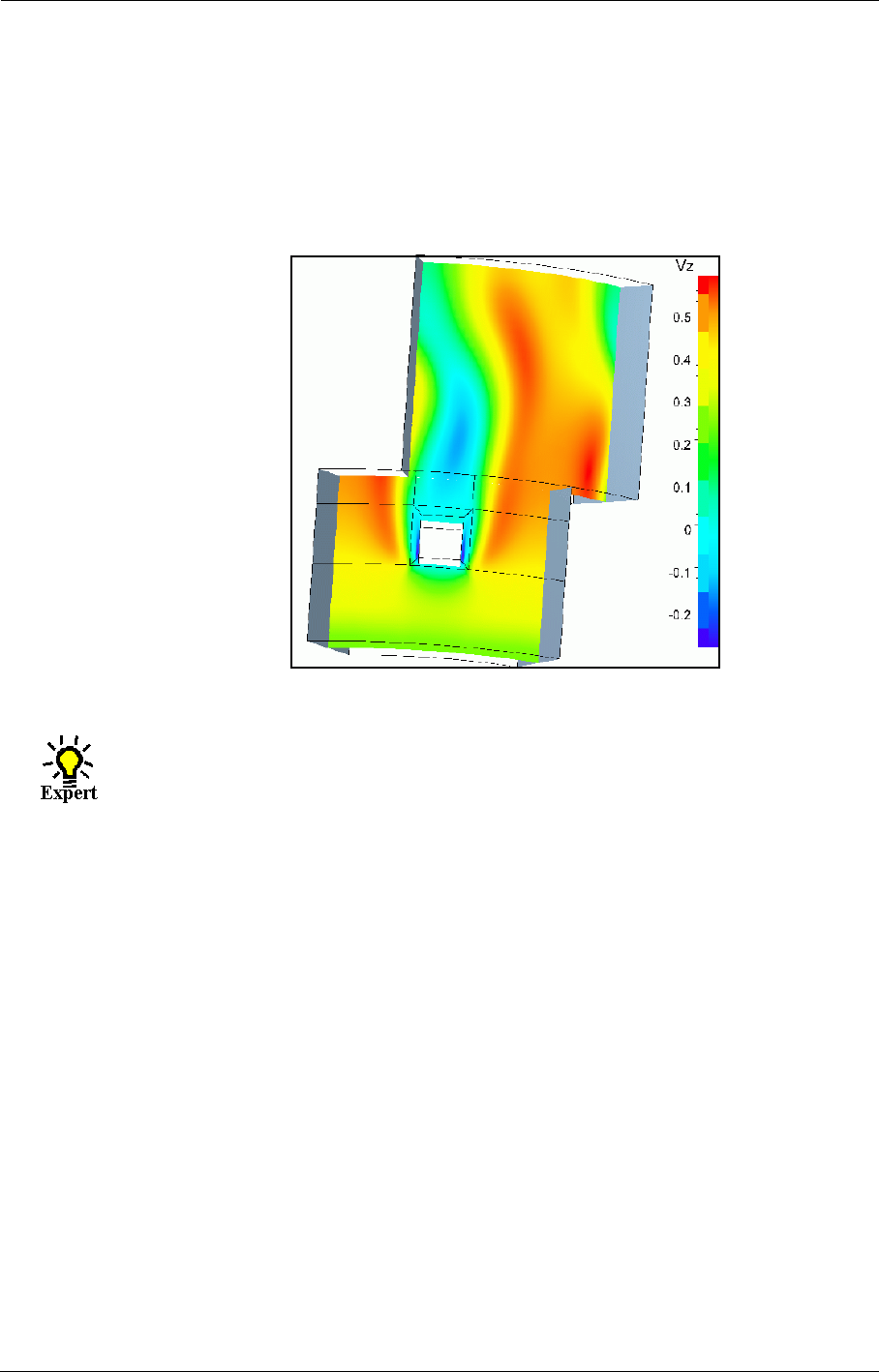
Dedicated Turbomachinery Models Rotor/Stator Interaction
8-14 FINE™/Turbo
c) Illustrative Example
For the example case of the flow around a cube where the flow is entering the domain at the bottom
of Figure 8.3.2-9. The upstream portion of the domain is the 'rotor' with a cube fixed on it. The sec-
ond part is a 'stator'. With the domain scaling approach, one can observe a strong vortex shed into
the stator passage, leading to a correct physical simulation of the unsteady phenomenon (at the
expense of much higher CPU time compared to mixing plane approach).
FIGURE 8.3.2-9 Flow around a cube: Domain Scaling method
d) Expert Parameters
The following expert parameters can be used with an unsteady computation using domain scaling
method:
Parameter for Saving/Reading of FNMB data of rotor-stator interface:
IFRSFI(integer) 0: FNMB data computed but not saved
1: FNMB data computed and results saved in .adf file.
2 (default): FNMB data computed and results saved if the .adf file is not exist-
ing. Results read from .adf file otherwise.
ICYOUT(integer): 1 is used in combination with Multiple Files option to avoid overwriting of the
output files at each blade passage.
8-3.2.4 Phase Lagged Method
The Phase Lagged Method is an unsteady simulation technique for rotor/stator interfaces. The
effect of displacement due to rotation is taken into account. At each time step, the rotor is set at its
correct position and equations are solved for that particular time step for the whole computation
domain. The final solution is therefore a succession of instantaneous solutions for each increment
of the rotor position.
This method is allowing the user to reduce the CPU time needed for computing an unsteady simula-
tion of a turbomachinery stage (rotor-stator interaction). This capability has been implemented as
an additional functionality into the release FINE™/Turbo.

Rotor/Stator Interaction Dedicated Turbomachinery Models
FINE™/Turbo 8-15
If a phase lagged computation should be used as an initial solution for another compu-
tation, the .res and the .bpl files must be manually copied to the new computation direc-
tory.
The phase lagged method is only allowed for one stage computations (stator-rotor).
For multi-stage computations, such as a 1-1/2 stage computation (stator-rotor-stator), it is
only possible if the number of both stators is the same.
a) Mesh Constraints
The only constraints is that the boundary condition type must be set to "ROT" in IGG™ for all grid
patches belonging to a rotor/stator interface.
It is recommended to have an overlapping region in the circumferential direction
between the channel(s) of the rotor and the channel(s) of the stator.
b) FINE™/Turbo Settings
1. The Phase Lagged Method is an unsteady simulation technique so the Time Configuration in
the Flow Model page should be set to Unsteady.
2. At the top of the Rotating Machinery page, the Phase Lagged option has to be activated and
under Rotor-Stator tab, the Phase Lagged approach is selected automatically. However the
user has to specify for each of these patches the ID and the upstream/downstream location as
described in section c) at step 2. Therefore, the boundary condition type must be set to "ROT" in
IGG™ for all grid patches belonging to a rotor/stator interface.
3. The initialization process can be performed in two ways:
•A steady state initialization is performed in a separate computation with Steady as Time Con-
figuration. The unsteady phase-lagged computation is using the result of this steady computa-
tion as initial solution. See Chapter 9 for more information on how to start a computation from
an initial solution file.
•The steady state initialization is automatically performed before starting the time accurate
computation (that means within the same computation), switching to Unsteady as Time Con-
figuration in the Flow Model page and selecting in the interface an appropriate Number of
Steady Iterations in the Steady Initialization parameters on the Control Variables page.
4. The Number Of Angular Positions defined in the Control Variables page is the number of
time steps per full revolution (2π) of the rotor. In theory, the number of time steps per full rota-
tion has to be a multiple of the number of blades in the rotor (Nbrotor) and number of blades in
the stator (Nbstator).
Number Of Angular Positions = i x Nbrotor x Nbstator
The two periods of blade passing frequencies are respectively (ixNbrotorxΔt) and
(ixNbstatorxΔt). Since the number of time steps per passage is usually imposed around
40, the value of i should be adjusted so that (ixNbrotor) and (ixNbstator) are both close to
this number. By experience, if the number of time steps per passage is lower than 30 the
solution starts to be deteriorated.
5. The Number Of Time Steps in the Control Variable page is defined as:
Number Of Time Steps = j x (Number Of Angular Positions)/min(Nbrotor,Nbstator)
During the calculation, it is recommended to repeat the longer period at least 15 to 20

Dedicated Turbomachinery Models Rotor/Stator Interaction
8-16 FINE™/Turbo
times (j evolves from 15 to 20). By experience, usually after 20 times (j=20), the flow
becomes periodic. There is thus no need to make many full rotations and sometimes even
one full rotation.
6. For more info on the Outputs Files available in the Control Variables page, see section 6-3.1.
By default, the Phase Lagged method computes the viscous fluxes at the rotor/stator
interface by extrapolation from dummy cell values, set from same side inner cells.
c) Output
When a simulation using the phase lagged method is performed, the output includes only one chan-
nel for each blade row. FINE™/Turbo provides a tool repetition, which allows the user to generate
3 channels for each blade row for post-processing. This tool can only be launched from the shell.
On Linux:
repetition project-path/project-name.run
On Windows:
Installation path\bin\repetition.exe project-path/project-name.run
Then a new .run file "project-name_rep.run" and the corresponding .cgns files "project-
name_rep_t##.cgns" will be generated. The user can load these files into CFView™ for post-
processing.
d) Expert Parameters
The following expert parameters can be used with an unsteady computation using phase lagged
method:
ICYOUT(integer): 1 is used in combination with Multiple Files option to avoid overwriting of the
output files at each blade passage.
RELPHL(real): 0.5 (default) if necessary, under-relaxation factor can be applied on Periodic
and R/S boundary conditions by reducing the two values of the expert parame-
ter for respectively the periodic and the R/S boundary conditions.
8-3.2.5 Harmonic Method
The harmonic method provides unsteady flow results with considerably less constraints than the
domain scaling and phase-lagged methods. More information on Harmonic method can be seen in
section 8-4.
a) Mesh Constraints
Like the phase-lagged approach, it is necessary to set the grid patches of a rotor/stator interface to
the boundary condition type "ROT".
No specific azimuthal position of the blade channels is requested by the harmonic method, but it is
recommended to have an overlapping region in the circumferential direction between the rotor and
the stator channel. This is only for post-processing purposes. Visualization of the flow across the
interface is much clearer.
Mesh resolution in the tangential direction:
The harmonic method is based on the spatial Fourier decomposition of the time-averaged flow and
the harmonics in the tangential direction.

Rotor/Stator Interaction Dedicated Turbomachinery Models
FINE™/Turbo 8-17
It is suggested to guarantee at least 30 grid nodes in the azimuthal direction to represent in space the
first harmonic (or fundamental) of a periodic disturbance at the inlet/outlet of a row. Then, the
number of nodes in the tangential direction of the row channel should be at least 30 times the
number of blades of the adjacent blade row generating this harmonic divided by the number of the
blades of the row. The narrower the adjacent blade row channels, the more refined the channel
should be.
It is assumed that the amplitude of the subharmonics decreases very quickly. The constraint can
thus be relaxed for the other harmonics. In general, at least 30 grid notes for the first harmonic and
15 for the other harmonics are suggested.
For example, for a stator/rotor/stator configuration, where the number of blades in the rotor and sta-
tors are Nbrotor, Nbstator 1 and Nbstator 2 and NH is the number of harmonics:
Number of Points in Azimuthal Direction in stator 1:
30 x if(NH=1)
15 x x NH if(NH>1)
Number of Points in Azimuthal Direction in rotor:
max(30 x , 30 x ) if(NH=1)
max(15 x x NH, 15 x x NH) if(NH>1)
Number of Points in Azimuthal Direction in stator 2:
30 x if(NH=1)
15 x x NH if(NH>1)
b) FINE™/Turbo Settings
1. The harmonic method is a hybrid method. Unsteady flow results are obtained by the solving of
pseudo-steady transport equations like in steady flow simulation. These pseudo-steady transport
equations are solved for the time-averaged flow and for the harmonics of the periodic unsteady
disturbances about the time-averaged flow. The Time Configuration in the Flow Model page
should be set to Harmonic.
2. Under the Rotor-Stator tab of the Rotating Machinery page, the type of rotor/stator treatment
is automatically selected. The full non-matching technique is used like in a mixing-plane simu-
lation. However, the mixing-plane method is used only for the time-averaged Spalart-Allmaras
eddy-viscosity. In particular, it includes a part of the deterministic stress that appears because of
the time-averaging of the advective fluxes of the eddy-viscosity transport equation. All the other
Nbrotor
Nbstator1
---------------------
Nbrotor
Nbstator1
---------------------
Nbstator1
Nbrotor
---------------------
Nbstator2
Nbrotor
---------------------
Nbstator1
Nbrotor
---------------------
Nbstator2
Nbrotor
---------------------
Nbrotor
Nbstator2
---------------------
Nbrotor
Nbstator2
---------------------
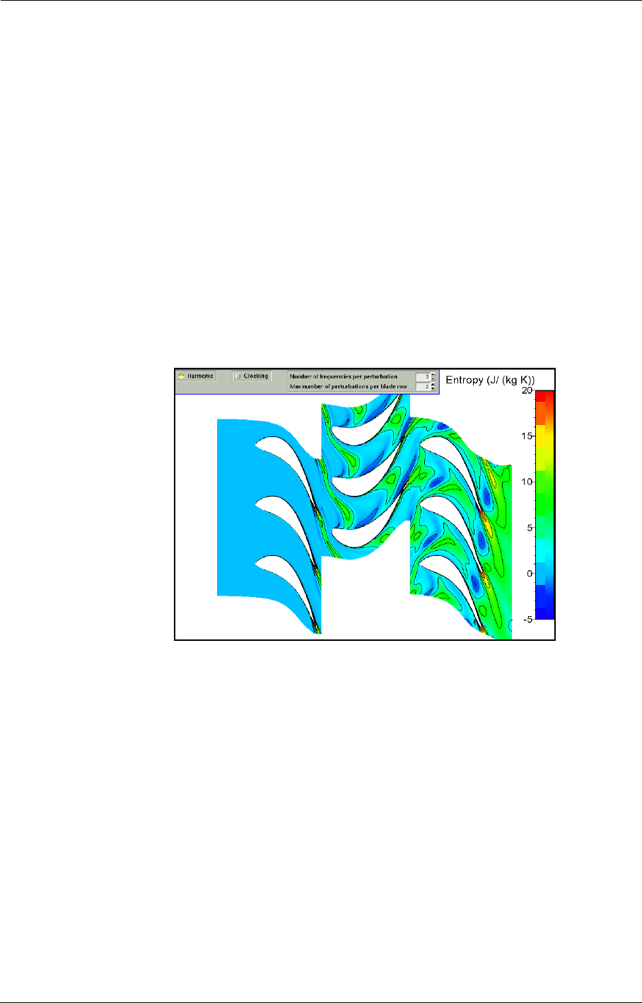
Dedicated Turbomachinery Models Rotor/Stator Interaction
8-18 FINE™/Turbo
flow variables are treated by a connection algorithm based on the spatial Fourier decomposition
of the time-averaged flow and the harmonics. The user has to specify for each of the patches the
ID and the upstream/downstream location as described in section c) at step 2.
3. The initialization should be performed using a solution in steady state. The user can perform a
separate computation (initial solution) for which the Time Configuration is set to Steady. For
this computation, it is suggested to model the rotor/stator interface using the Non Reflecting 1D
treatment. The result of this computation is used as the initial solution for the harmonic run. See
Chapter 9 for more information on how to start a computation from an initial solution file. The
user can also impose an appropriate Number of Steady Iterations in the Computation steer-
ing / Control Variables page. In this case, a steady computation will be performed until the
Number of Steady Iterations in the fine mesh. Then the NLH computation will be initialized
using the steady solution and be launched.
NLH does not work when the rotor-stator interface is connecting two stators.
c) Illustrative Example
Results obtained from harmonic calculations using three harmonics.
FIGURE 8.3.2-10 Aachen Turbine: entropy at 50% spanwise
8-3.2.6 Control the flux of Eddy viscosity
For the Spalart-Allmaras turbulence model, the flux at the Rotor/Stator is computed using the pitch
averaged eddy viscosity. Such a procedure can leads to a build-up of turbulence for multistage
machineries. The eddy viscosity is not destroyed in the free stream. Very high level of eddy viscos-
ity is often found in the last stages for multi-stage calculations. Such a high level of eddy viscosity
can impact on the predicted efficiency of the machinery.
Two methods can be used to reduce the eddy viscosity at a Rotor/Stator interface when using the
Spalart-Allmaras model:
•Control the flux of eddy viscosity at all rotor/Stator interfaces by using the minimum eddy vis-
cosity over the pitch (IMINRS set to unity)
•Control the flux of eddy viscosity at all rotor/Stator interfaces by multiplying the flux by a fac-
tor (FACTRS set lower than unity)

Harmonic Method Dedicated Turbomachinery Models
FINE™/Turbo 8-19
Because both the expert parameters are global, the limitation of the eddy viscosity at Rotor/Stator
interfaces is activated for all Rotor/Stator interfaces of the project. Both methods cannot be com-
bined. If the two parameters are changed only IMINRS will be activated.
The methods reducing the eddy viscosity are restricted to the following Rotor/Stator interfaces:
•Conservative coupling
•Local conservative coupling
•Full non matching mixing plane
•Non reflecting 1D
•Full non matching (non Reflecting) for NLH calculations
8-4 Harmonic Method
8-4.1 Introduction
An attractive feature of FINE™/Turbo is the computation of unsteady flows using the so-called
nonlinear harmonic method (NLH). This approach, introduced by He and Ning (1998), can be con-
sidered as a hybrid method that conjugates the advantages of classical steady state and full unsteady
calculations: it provides an approximate unsteady solution at affordable calculation costs.
The main idea is that the flow perturbations that make the flow unsteady are written about a time-
averaged value of the flow and are Fourier decomposed in time. Casting the unsteady Navier-
Stokes system into the frequency domain, transport equations are obtained for each time frequency.
The user controls the accuracy of the unsteady solution through the order of the Fourier series.
Alongside the solving of the time-averaged flow steady-state equations, each frequency requires the
solving of two additional sets of conservation equations (for the real and imaginary parts of each
harmonic). The method is made nonlinear by the injection of the so-called deterministic stresses,
resulting from all the solved frequencies, into the time-averaged flow solver. Because of the trans-
position to the frequency domain, only one blade channel is required like a steady flow simulation.
The presented method also features an improved treatment that enhances the flow continuity across
the rotor/stator interface by a reconstruction of the harmonics and the time-averaged flow on both
sides of the interface. A non-reflective treatment is applied as well at each interface.
The limitations for the NLH simulations are:
•The nonlinear harmonic method can only be used for turbomachinery applications.
•The Number of frequencies per perturbation and Max number of perturbations per
blade row can not be larger than 10. And the product of them can not be larger than 20.
•The flow perpendicular to the inlet (INL), outlet (OUT), external boundary (EXT) and rotor/
stator interface (ROT) has to be subsonic.
•The number of frequencies per perturbation in a row is the same all over the multistage
machine.
•When using thermodynamic tables as fluid, NLH is not compatible with preconditioning and
inlet distortion.
•When simulating Cooling injectors with NLH, the injected mass flow is assumed constant.
About the mesh constraint for NLH simulations, please refer to Chapter 8-3.2.5.
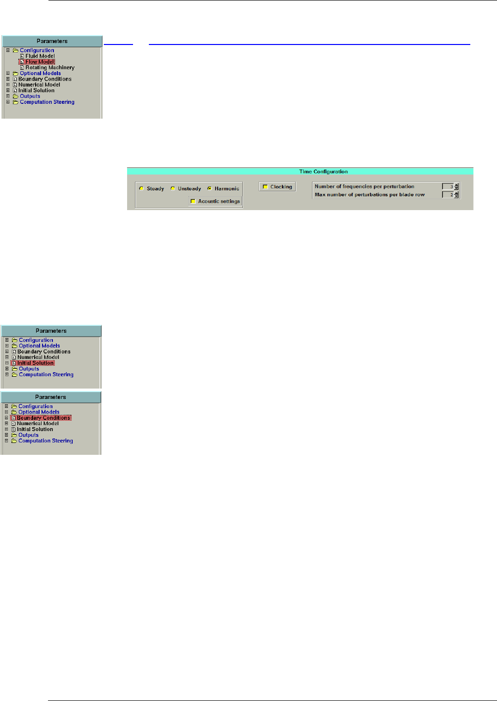
Dedicated Turbomachinery Models Harmonic Method
8-20 FINE™/Turbo
8-4.2 Interface & Best Practice for Harmonic Computations
When activating Harmonic in the Flow Model page, two boxes appear:
•Number of frequencies per perturbation (number of harmonics: NBHAR): it represents the
number of time harmonics per periodic perturbation modelled in a row. Default value: 3.
•Max number of perturbations per blade row: the highest number of blade passing frequen-
cies that a blade row is subjected to (NPERT). Default value: 2. For the particular stator/rotor/
stator configuration, where the stators have the same number of blades, this parameter is equal
to 1.
FIGURE 8.4.2-11 Harmonic parameters
When Harmonic is checked, the turbulence model is by default set to Spalart-Allmaras. The other
turbulence model that can be selected is Baldwin-Lomax. Euler flow.The Laminar flow can also
be selected.
The other harmonic method parameters in the FINE™/Turbo GUI can be found at the following
menus:
8-4.2.1 Initial Solution
It is recommended to set the initial solution as the result of a previous steady flow simulation. This
improves the rate of convergence to the values of the amplitudes of the disturbance frequencies.
8-4.2.2 Boundary conditions
For one stage or multi-stage computations, different boundary conditions can be specified for the
NLH method. These boundary conditions are non-reflective at the far inlet and far outlet. They are
based on 1D non-reflective treatment that computes the flow variables on the boundary as a result-
ing combination of incoming and outgoing characteristics. The flow at the far inlet and far outlet is
assumed to be the time-averaged without the deterministic stress terms.
Under the tab INLET of the Boundary Conditions page, a dedicated boundary condition, Static
Quantities Distributions for Harmonic Calculation, allows FINE™/Turbo to perform NLH
computations with distortion at inlet. For this kind of computations, the FINE™/Turbo solver per-
forms a spatial Fourier decomposition of the inlet distortion. The extracted spatial harmonics are
transformed into time harmonics in the frame of the domain that is subject to the relative motion of
the distortion. This inlet boundary condition can be considered as a simplified Rotor-Stator inter-
face. But the computation only takes into account the effect of the fictitious upstream row (inlet dis-
tortion) on the downstream row(s). With inlet distortion, it is possible to simulate the flow in only
one row by using the NLH method.
The inlet distortion must be specified by using profile. These profiles are the azimuthal distribu-
tions of the five flow variables ( , , , and ). Each distribution is for a constant radius or a
constant axial position. The imposed profile must range from 0 to 2π and must be periodic over the
azimuthal length. Currently, only r-θ or θ-z profile is allowed. The profile should be given at sta-
tions of constant θ for increasing r or z. Also θ must be increasing going from one station to the
next in the file. Please refer to Appendix A-5 for more detail of the file format. The option PERIO-
DICITY is used to scale the inputted profile in θ direction.
vr
vt
vz
ρ
p

Harmonic Method Dedicated Turbomachinery Models
FINE™/Turbo 8-21
Under the tab EXTERNAL of the Boundary Conditions page, the user can specify external
boundary conditions for NLH computations:
•When using the boundary condition External, the flow at the external boundaries must be
axial ( and ) if the external boundaries are attached to the rotating domain.
•If the external boundaries are attached to the rotating domain and the flow at the external
boundaries is non-axial, the boundary condition External Constant Wind with Incidence
Relative to Axis Z should be used. This boundary condition allows to simulate the flow result-
ing from a constant wind with incidence applied on the external boundaries. The incidence
means that and/or are not equal to 0. In the cylindrical framework, the velocity compo-
nents write as:
(8-1)
So, the incidence can be considered as a distortion on the external boundaries with the perio-
dicity of 1. The same treatment method for inlet distortion is used to treat the incidence on the
external boundaries in the flow solver. Note, the pseudo-steady solution in the NLH method
represents the time-averaged solution over one passage. As a result, in the cylindrical frame-
work, the incidence can not be represented since it is not periodic over one blade passage. To
check the effect of the incidence, unsteady solution must be reconstructed.
The boundary condition External Constant Wind with Incidence Relative to Axis
Z is exclusively for external boundaries attached to rotating domains.
8-4.2.3 Outputs
The Harmonics tab allows to activate specific outputs from the harmonic method and the recon-
struction in time.
vx0=
vy0=
vx
vy
vtv–xθ() vyθ()cos+sin=
vrvxθ() vyθ()sin+cos=
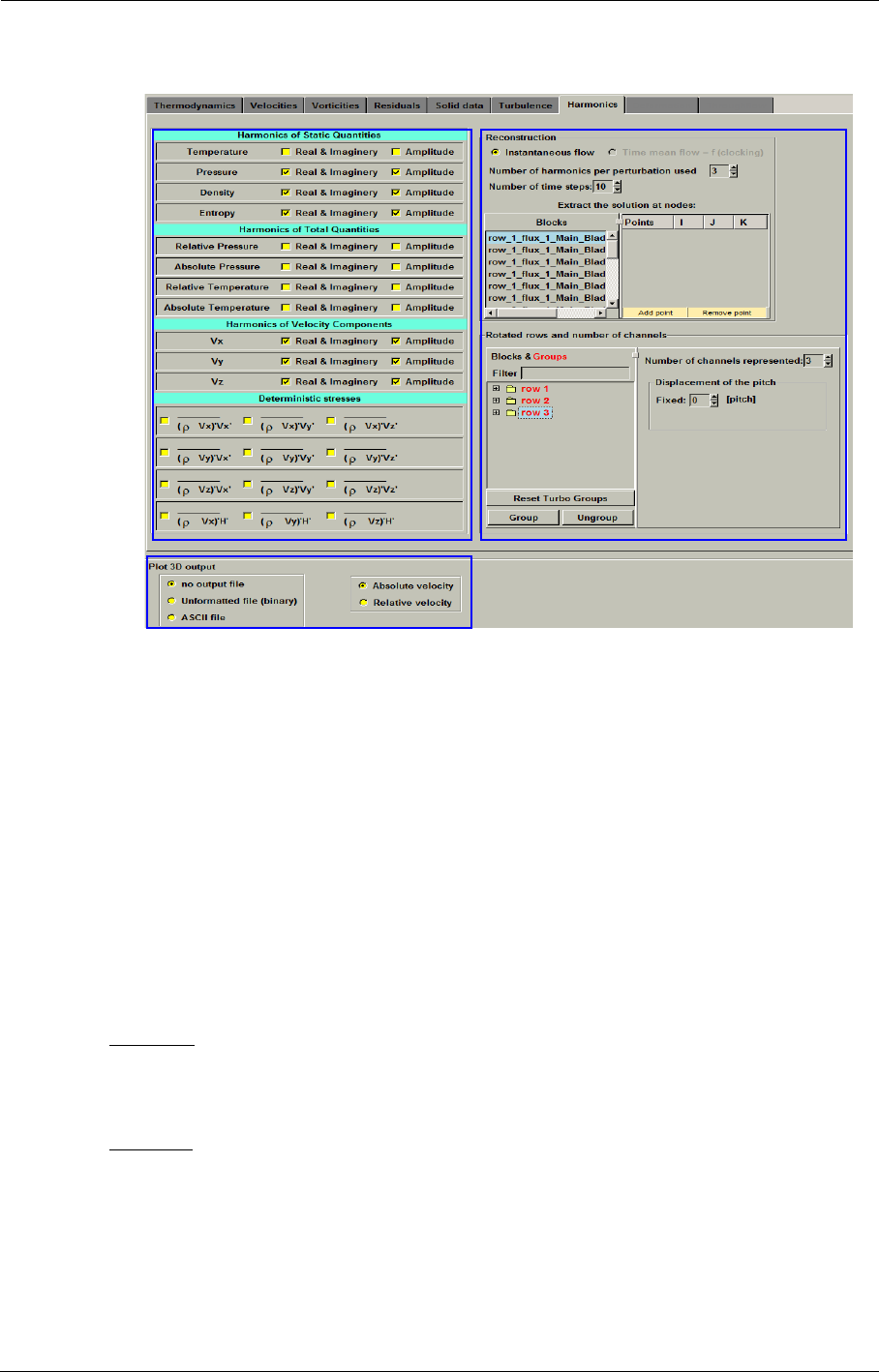
Dedicated Turbomachinery Models Harmonic Method
8-22 FINE™/Turbo
FIGURE 8.4.2-12 Harmonic outputs
a) Harmonic variables output
In the Harmonics page of the Outputs/Computed Variables page, a first group is visible and cor-
responds to the harmonic variables:
•Static quantities: Temperature, Pressure, Density and Entropy
•Total quantities: Relative Pressure, Absolute Pressure, Relative Temperature and Absolute
Temperature.
•Velocity components: , ,
If a box is checked, the Real & Imaginary parts and/or the norm (Amplitude) of the complex
amplitude of the harmonics of the variable, can be stored in the output ".cgns" file. The number of
harmonics is the maximum, over the whole flow field, of the total number of harmonics per group
(blade row), which is equal to (NPERT)x(NBHAR), both set in the Flow Model page.
Example 1: if the Pressure box is checked, there will be 6 harmonics of pressure fluctuation per
row in the output solution file for NBHAR=3 and NPERT=2. This means 6 (for real) + 6 (for imag-
inary) + 6 (for norm) = 18 additional flow variables in the ".cgns" file, if the real and imaginary
parts are selected as well as the norm.
Example 2: For a igv/rotor/ogv configuration, NPERT is set to 2 and NBHAR is set to 4 by the user.
There are thus 8 (2x4) harmonics H1, H2, H3, H4, H5, H6, H7, H8 in the output.
•In igv row: only one perturbation is generated, induced by the downstream rotor. The perturba-
tion is modelled by its first NBHAR=4 harmonics: H1-H2-H3-H4. No second perturbation
exists, so H5, H6, H7, H8 are set to zero.
•In rotor row: two perturbations are generated. If the first perturbation is the one originating
from the row upstream then:
vx
vy
vz

Harmonic Method Dedicated Turbomachinery Models
FINE™/Turbo 8-23
H1-H2-H3-H4: first 4 harmonics of the periodic disturbance induced by the igv,
H5-H6-H7-H8: first 4 harmonics of the periodic disturbance induced by the ogv.
•In ogv row: one perturbation is modelled, the first 4 orders being solved. H1-H2-H3-H4: first 4
harmonics of the periodic disturbance induced by the rotor. H5-H6-H7-H8: zero.
In this case, selecting only the amplitude of the Pressure fluctuation for the output gives 8 addi-
tional flow variables in the ".cgns" file.
If the relative/absolute total pressure or/and the relative/absolute total temperature
time means are selected, then their harmonics will be automatically stored in the ".cgns"
file, and vice-versa.
A second group proposes the selection of the deterministic stresses.
If a stress is selected, each of its contribution per harmonic will be stored in the output ".cgns" file,
that is 8 different values in example 2 presented above.
Information about frequency output for harmonics can be found in the .std file for
each group. Each group indicates a blade row.
b) Plot3D output
The Harmo2Time executable checks the .run file of the computation to process. If the plot3d out-
put of the solver is switched on, the Harmo2Time executable will also produce unsteady plot3d out-
put in addition to the .cgns output.
As for the FINE™/Turbo solver, there are different options to the plot3d output:
•The user can choose between ASCII and binary (formatted) output.
•The user can choose to compute the plot3d output to be in relative or absolute frame of refer-
ence.
The format of the plot3d output is the same as the FINE™/Turbo solver’s (see section 10-2.7).
This output is only valid with IVELSY=1, which is also the only accessible option for
the Harmo2Time executable.
This plot3d output is limited to the perfect gas model.
c) Reconstruction in Time
The executable Harmo2Time for reconstructing a harmonic solution in time, is available in the
Modules menu. It can be also launched from the command line:
On UNIX/LINUX:
ρVx'()Vx'ρVx'()Vy'ρVx'()Vz',,
ρVy'()Vx'ρVy'()Vy'ρVy'()Vz',,
ρVz'()Vx'ρVz'()Vy'ρVz'()Vz',,
ρVx'()H'ρVy'()H'ρVz'()H',,

Dedicated Turbomachinery Models Harmonic Method
8-24 FINE™/Turbo
harmo2time<version> /full path/computation.run On UNIX/LINUX
On 32bits WINDOWS:
<NUMECA_dir>\fine<version>\bin\harmo2time.exe \full path\computation.run
On 64bits WINDOWS:
<NUMECA_dir>\fine<version>\bin64\harmo2timex86_64.exe \full path\computation.run
Harmo2Time generates a run file named "_unst.run" presenting the same format as for the result of
an unsteady flow simulation.
In the Harmonics tab of the Outputs/Computed Variables page, an extra control is available for
the unsteady reconstruction, see Figure 8.4.2-12. The following parameters are only used for the
Harmo2Time module and can thus be modified after the harmonic computation has finished:
For the standard harmonic simulation (no clocking), the user can only reconstruct the
unsteady flow.
•Number of harmonics per perturbation used: The number of harmonics per perturbation
that the user wants to keep for the reconstruction. By default, this parameter is set to the value
of the Number of frequencies per perturbation that was chosen by the user in the Flow
Model page. The number of harmonics per perturbation, used for the reconstruction in time,
can be lower or equal to the value set in the Flow Model page.
•Number of time steps: The number of instantaneous solutions per maximum blade passing
period. By default, 10 instantaneous solutions ("_unst_t#.cgns" files) are generated whose time
span extends over the maximum blade passing period of the multistage turbomachine.
•Extract the solution in time at nodes: Offers the possibility to select different grid nodes in
the mesh blocks at which the flow time evolution will be calculated. The program of recon-
struction will generate one data file per grid node (_unst_P#.dat) that will include the evolu-
tion in time of the flow variables (density, pressure, velocity and also the eddy viscosity for a
turbulent flow).
In the frame of Rotated rows and number of channels, the user can specify the following param-
eters for every Block or Group for the reconstruction in time.
•Number of channels represented: The number of repetitions of the channels that the user
wants to use in the post-processing.
•Displacement of the pitch: The user can specify a rotation of the blade row as a multiple of
the pitch of the blade row. The inputted number must be an integer. For example, 2 [pitch] will
rotate a blade row by twice 360deg/N where N is the periodicity of the blade row.
By default, Harmo2Time automatically reconstructs the unsteady solutions for the following quan-
tities, whatever the selected quantities in the Outputs / Computed Variables page are.
•Static Pressure
•Static Temperature
•Density
•Relative Velocity (Wxyz)
When modelling turbulence, the turbulent viscosity (μt/μ) is outputted by Harmo2Time. Please
note, the turbulent viscosity is computed by using the time-mean solutions and assumed undis-
turbed by the unsteady fluctuations.
In addition, Harmo2Time will also reconstruct the unsteady solutions for the following quantities,
in case that the corresponding quantities are selected for output in the Outputs / Computed Varia-
bles page.
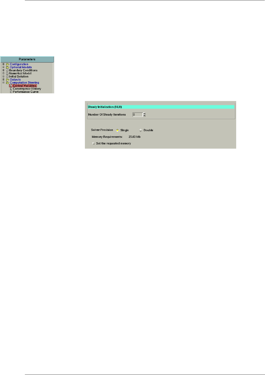
Harmonic Method Dedicated Turbomachinery Models
FINE™/Turbo 8-25
•Absolute Total Pressure
•Relative Total Pressure
•Absolute Total Temperature
•Relative Total Temperature
8-4.2.4 Control Variables
In the Computation Steering / Control Variables page, the user can impose an Number of Steady
Iterations. In this case, a steady computation will be performed until the Number of Steady Itera-
tions in the fine mesh. Then the NLH computation will be initialized using the steady solution and
be launched.
NLH computations need more CPU time and memory, in comparison with a steady mixing-plane
method, due to the additional transport equations associated with each harmonic. If N harmonics of
a perturbation are to be modelled, then there are 10N transport equations to be solved (5 for the real
part and 5 for the imaginary part of the complex amplitude of each harmonic). The CPU time
required by harmonic method is:
with (8-2)
where is the CPU time required by the steady computation and is the number of
the equations in the steady computation (5 for Euler, Laminar and turbulent flow with the 0-equa-
tion turbulence models; 6 for the turbulent flow with the 1-equation turbulence models). is the
cost ratio between the harmonic computation and the steady computation. For example, for a 3-har-
monic simulation (N=3) and using the Spalart-Allmaras model ( =6), the CPU time is there-
fore 6 times that of a steady simulation.
The memory cost follows the same rule as Eq. 8-2.
For the simulation of the multi-row flow through b1, ... ,bB bladerows, the cost ratio is approximated
as:
(8-3)
where is the number of the grid nodes in the bladerow b1, B is the number of the blade-
rows. As an approximation, the number of nodes can be assumed to be the same in the bladerows.
The number of harmonics to be solved is N in the first bladerow and N in the last bladerow because
only one perturbation is solved, generated from the downstream b2 and the upstream bB-1. The inte-
rior bladerows are subject to two perturbations, one generated from the upstream blade passing
(wakes) and one generated from the downstream blade passing (potential effect). Therefore, 2N
harmonics are solved in these bladerows. The estimated resulting CPU and memory cost ratios are:
CPUNLH CPUsteadyCRN
=
CRN110N
Nsteady
-----------------
+=
CPUsteady
Nsteady
CRN
Nsteady
CRharmo
Nnodes b1
,CostNb
1
() ... Nnodes bB
,CostNb
B
()
++
Nnodes b1
, ... Nnodes bB
,
++
-------------------------------------------------------------------------------------------------------------------
=
Nnodes b1
,
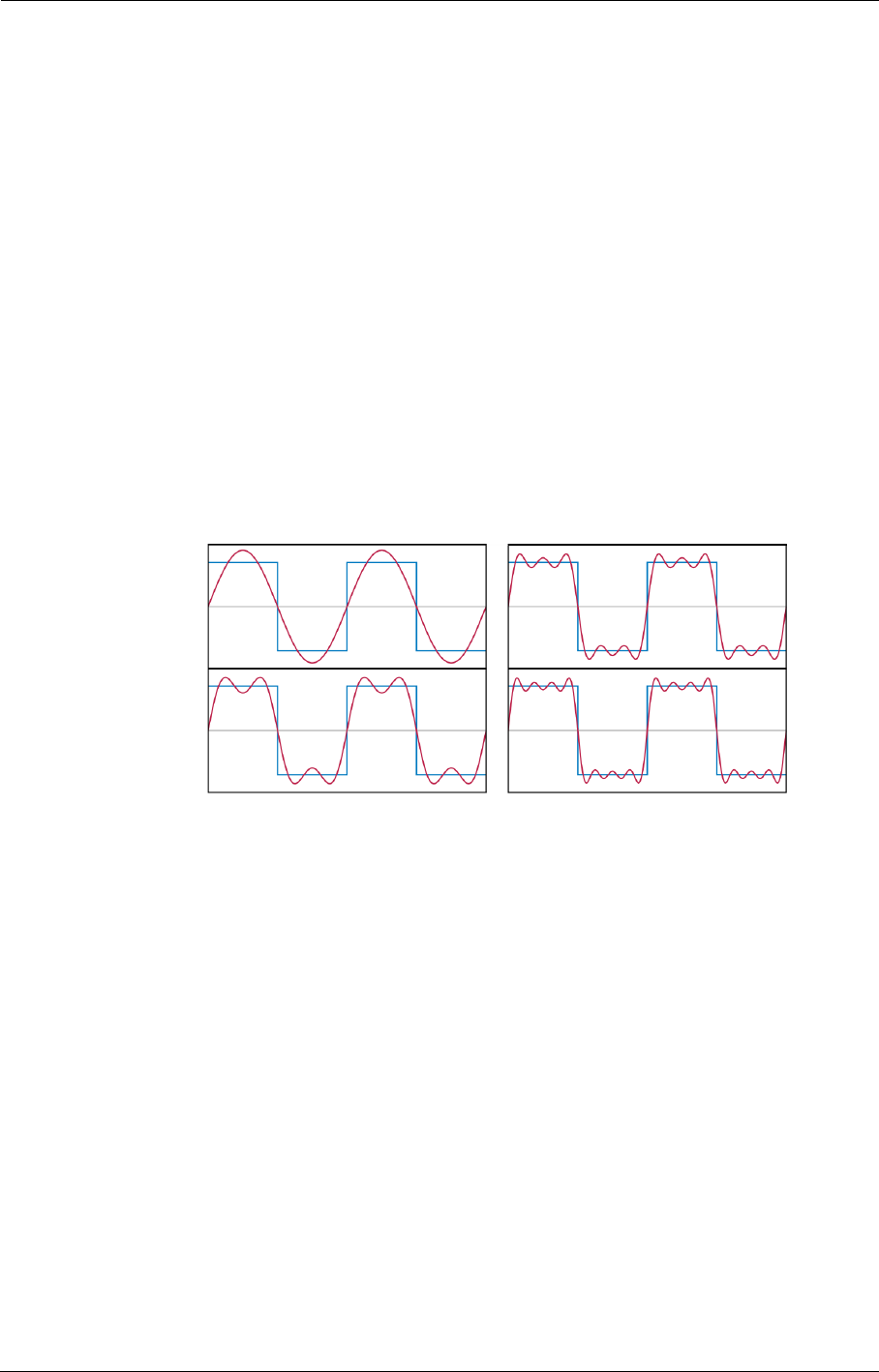
Dedicated Turbomachinery Models Harmonic Method
8-26 FINE™/Turbo
(8-4)
8-4.2.5 Troubleshooting in Rotor/Stator Interface
Sometimes, the user may find that there is a quite large discontinuity in the variable field (such as
entropy) over the rotor-stator interface, even when the number of harmonics per perturbation is 4 or
more. This situation often appears if there exists a strong wake or shock wave at one side of the
rotor-stator interface.
Within the NLH method, the conservative variable is decomposed into a time-averaged value and a
sum of periodic perturbations, which in turn are decomposed into N harmonics. In some special
cases, the perturbation can not be accurately reconstructed by using the decomposed harmonics.
The error is depending on the number of the harmonics that we used.
Figure 8.4.2-13 shows how a square wave signal is captured by using a Fourier series (harmonics)
and what the influence of the number of harmonics used is. Please refer to http://en.wikipedia.org/
wiki/Fourier_series for more information. As you can see, the square wave is reproduced better
with an increasing number of harmonics. However, it is impossible to reproduce the vertical line in
the signal. This can only be reached if the number of harmonics is infinite.
FIGURE 8.4.2-13 The first four Fourier series approximations for a square wave
As an example, Figure 8.4.2-14 shows the contours of the entropy at a constant r surface in a contra
rotating propeller. In this case, there is a strong peak in entropy at the upstream side of the rotor-sta-
tor interface due to the wake of the front blade. This is almost a Dirac signal. To capture such a
Dirac with Fourier series (that is what non-linear harmonics computations do) is indeed very diffi-
cult. As you can see, the signal is captured better when increasing the number of harmonics. This is
in agreement with the theory: increasing the number of harmonics will increase the accuracy, but
with increasing computation costs.
CRharmo
2CostNB2–()Cost2N
+
B
-------------------------------------------------------------
=
1h
2h
3h
4h
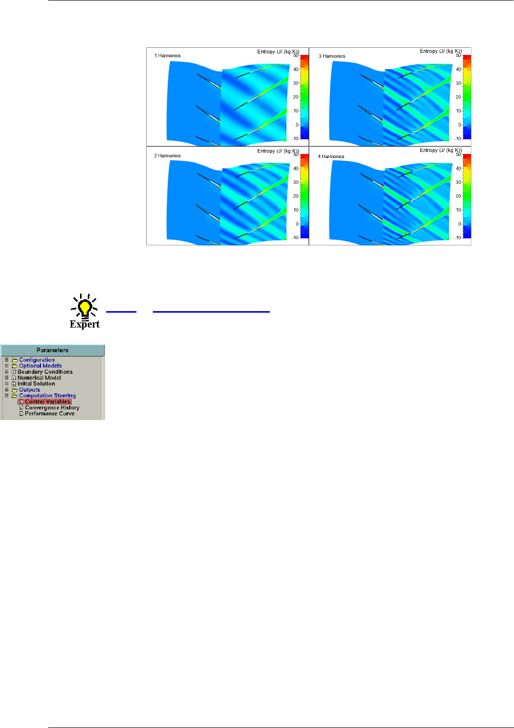
Harmonic Method Dedicated Turbomachinery Models
FINE™/Turbo 8-27
FIGURE 8.4.2-14 The contours of the entropy at a constant r surface for a Contra-rotating
propeller
8-4.3 Expert Parameters
8-4.3.1 Expert Parameters for the Flow Solver
The following expert parameter related to the NLH simulation are accessible on the Control Varia-
bles page by selecting the Expert Mode.
HARTCL (integer):When using the Cooling/Bleed model with NLH, the time averaged variables
in the cooling/bleed are computed by taking into account the deterministic
stresses and the harmonic variables are computed by applying the non reflect-
ing treatment. Adding the stresses implies that the harmonic values are already
known but their computations with the non reflective treatment need the values
of the time averaged variables. This is not a problem for the bleed as the time
averaged values are extrapolated from the first inner cells. For the injectors,
some assumptions are used for the computations of stresses. The main assump-
tion is that the injected mass flow is constant with time. Moreover, the expert
parameter HARTCL is used to impose the fluctuations of temperature or total
temperature (according to the specified characteristics of the cooling).
0 (default): Harmonics of the temperature or total temperature are imposed to 0
in the injectors.
1: Harmonics of the temperature or total temperature are not imposed. Only the
time averaged value is imposed.
IFABCW (integer):On the wall, the velocity components, the pressure and the temperature in the
dummy cell are computed by extrapolating the value on the wall and in the first
inner cell. The corresponding density is computed in the dummy cell. The cool-
ing will introduce high temperature gradient on the wall. The high temperature
gradient may lead to unphysical temperature in the dummy cell and conse-
quently unphysical density in the dummy cell. The expert parameter IFABCW
allows to compute the density by extrapolating the density on the wall and in
the first inner cell. The extrapolation is used not only for the time averaged val-
ues but also for the harmonic values.

Dedicated Turbomachinery Models Harmonic Method
8-28 FINE™/Turbo
0 (default): the density in the dummy cell is computed from the extrapolated
pressure and temperature in the dummy cell.
1: the density in the dummy cell is computed by extrapolating the density on
the wall and in the first inner cell.
IDECOU (integer):Controls if considering the deterministic stress terms when solving the time-
averaged equations. The deterministic stress terms are intrinsic to the nonlinear
harmonic method and are responsible for the improvement of the time-aver-
aged flow compared to simple linearization methods. In some cases, the deter-
ministic stress terms are so high that convergence problem may appear. To
reach the convergence, the deterministic stress terms can be removed from the
time-averaged equations. An result is thus obtained for the time-averaged flow
with less accuracy because the nonlinear term is removed.
0 (default): the deterministic stress terms are considered when solving the time-
averaged equations.
1: the deterministic stress terms will be removed when solving the time-aver-
aged equations.
HAVMOD (integer):In some computations, one can notice a strong gradient of the harmonic of the
pressure. To control such a gradient, the flow solver uses a harmonic pressure
sensor as it is done for the time-averaged solution. The time-averaged pressure
sensor is:
0 (default): no harmonic pressure switch.
1: using the following pressure sensor:
where is a constant controlled by the expert parameter HARAV2 (default
value 0.01). The second term of the denominator is to keep the denominator
different from zero and is chosen to be a percentage of the time-averaged static
pressure. The pressure sensor will be activated when harmonic pressure gradi-
ent is very strong.
2: using the following pressure sensor:
The pressure sensor will be activated when harmonic or time-averaged pressure
gradients are very strong.
3: using the following pressure sensor:
TDECOU (integer):Controls if considering the high order derivative when computing the thermo-
dynamic variables by using thermodynamic tables:
0 (default): High order derivative is considered for thermodynamic variables.
1: High order derivative is not considered for thermodynamic variables.
psw pi1– 2pi
–pi1+
+
pi1– 2pipi1+
++
---------------------------------------------- 1
2
---p
˜i1– 2p
˜i
–p
˜i1+
+
pi1– 2pipi1+
++
----------------------------------------------
+=
psw1
p
˜i1– 2p
˜i
–p
˜i1+
+
1a2
–()p
˜i1– 2p
˜i
–p
˜i1+
+()a2pi1– 2pipi1+
++()+
---------------------------------------------------------------------------------------------------------------------------------------------------
=
a2
psw2max psw p,sw1
()=
psw3max psw p
˜i1– 2p
˜i
–p
˜i1+
+
a2pi1– 2pipi1+
++()
---------------------------------------------------------------
,
=

Harmonic Method Dedicated Turbomachinery Models
FINE™/Turbo 8-29
When the expert parameter IDECOU=1, the expert parameter TDECOU will be set to
1 automatically, which means that high order derivative will not be considered for ther-
modynamic variables and the deterministic stress terms will not be considered when
solving the time-averaged equations.
8-4.3.2 Expert Parameters for Reconstruction in Time
The following expert parameter related to the reconstruction in time of a harmonic computation are
accessible on the Control Variables page by selecting the Expert Mode.
By default, Harmo2Time reconstructs an unsteady solution from the harmonic result by using all
the harmonics or the first N harmonics, where N is the Number of harmonics per perturbation
used inputted in the Outputs / Computed Variables page under the Harmonics tab.
Harmo2Time can also partially reconstruct an unsteady solution by using certain harmonic(s)
specified by the user. For example, the user can reconstruct an unsteady solution that includes only
the contribution of the first and/or the second harmonic(s) of per perturbation.
To perform a partial reconstruction, the user has to specify the Rows/Groups, where the unsteady
solution will be partially reconstructed, through the expert parameter NHGALL. A maximum of 2
Rows/Groups can be selected at the same time. Then the user needs to specify the harmonic(s)
through the expert parameters NHSUB and/or NHSUB2 for the Row1/Group1 and/or Row2/
Group2, respectively.
NHGALL(integer):List of switches for the Groups. There are 20 parameters for the expert parame-
ter NHGALL, which is corresponding to the Group index in the project (up to
20 Groups). The user can find the information of the Groups in the .std file in
the project directory. For each switch:
0: the reconstruction in the corresponding Group will be partial. Only the spec-
ified harmonic(s) will be taken into account.
1 (default): the reconstruction in the corresponding Group will be full. The the
first N harmonics will be taken into account, where N is the Number of har-
monics per perturbation used inputted by the user.
NHSUB(integer): List of switches for the harmonics in the first specified Group. There are 20
parameters for the expert parameter NHSUB, which is corresponding to the
harmonic index per perturbation (up to 20). The numbers of the harmonics are
listed in the .std file in the project directory. For each switch:
0: the corresponding harmonic will not be considered when reconstructing.
1 (default): the corresponding harmonic will be considered when reconstruct-
ing.
For example, setting the second and the fourth values of the list to 1 means that
the reconstructed unsteadiness is from the harmonics #2 and #4.
NHSUB2(integer): List of switches for the harmonics in the second specified Group (if available).
The setting of this parameter is the same with NHSUB.
IGETBK(integer): switch for display mode of the rotating blade channel. When the rotor (visual-
ized with multiple pitches) arrives at the position that is 1 period further away,
it goes back to the original position. To make the rotor continue to move to the
end of the reconstruction period before going back to the initial starting posi-
tion, the user can set the expert parameter IGETBK to 2.

Dedicated Turbomachinery Models Clocking
8-30 FINE™/Turbo
1(default): The following blade channel is represented in the reconstruction
after displacement over more than one pitch
2: The same blade channel(s) are represented on the whole period of recon-
struction.
NBPPER(integer): controls the number of the blade passing periods built by Harmo2time. The
user can modify it, such as a lowest common multiple of periods for all signals,
in order to have a periodic signal.
INDEXT(integer): defines an output range of time steps when reconstructing a harmonic solution
in time. The parameter INDEXT is an array of two dimensions, corresponding
to the first index t1 and the second index t2. If , all the time steps over
NBPPER periods are outputted. If , the imposed time steps are outputted.
PERVAR(integer): controls the output of Harmo2time.
0 (default): output the quantity (the time averaged value + perturbation)
1: only output the perturbation of the quantity
IUNSMF(integer): allows to output unsteady ".mf" file at each time step by Harmo2time. The
outputted ".mf" file has the same format with the one generated by the flow
solver (see Chapter 10-2.6).
0 (default): does not output unsteady ".mf" file
1: output unsteady ".mf" file at each time step
The following limitations exist when using IUNSMF=1:
•Axial thrust, torque and power are assumed constant, and have the same values as
in the steady ".mf" file.
•Specific heat and specific heat ratio for real gas and incompressible fluid are
assumed constant, and have the same values as in the steady ".mf" file.
•Mach number for real gas is calculated by using time-averaged speed of sound.
•Cooling and bleed mass flow are assumed constant, and have the same values as in
the steady ".mf" file.
•IWRIT larger than 2 is not supported.
•OUTTYP equal 1 is not supported.
8-5 Clocking
8-5.1 Introduction
The NLH method deals mainly with rotor/stator interaction. The approach couples and solves the
time-averaged flow and the perturbations. In particular, the time-mean flow is modified by the
deterministic stress that is a product of the unsteadiness. Thus, the time-mean solution in a row is
influenced by the unsteadiness brought about by a rotating upstream row; by relative rotation this
flow disturbs the flow in a downstream row again. The upstream row has an influence on the down-
stream row via the time-mean flow in the central row but it is indirect. No rotor/rotor and/or stator/
stator effects are taken into account. Thus, the clocking effects cannot be modelled
t10=
t10>
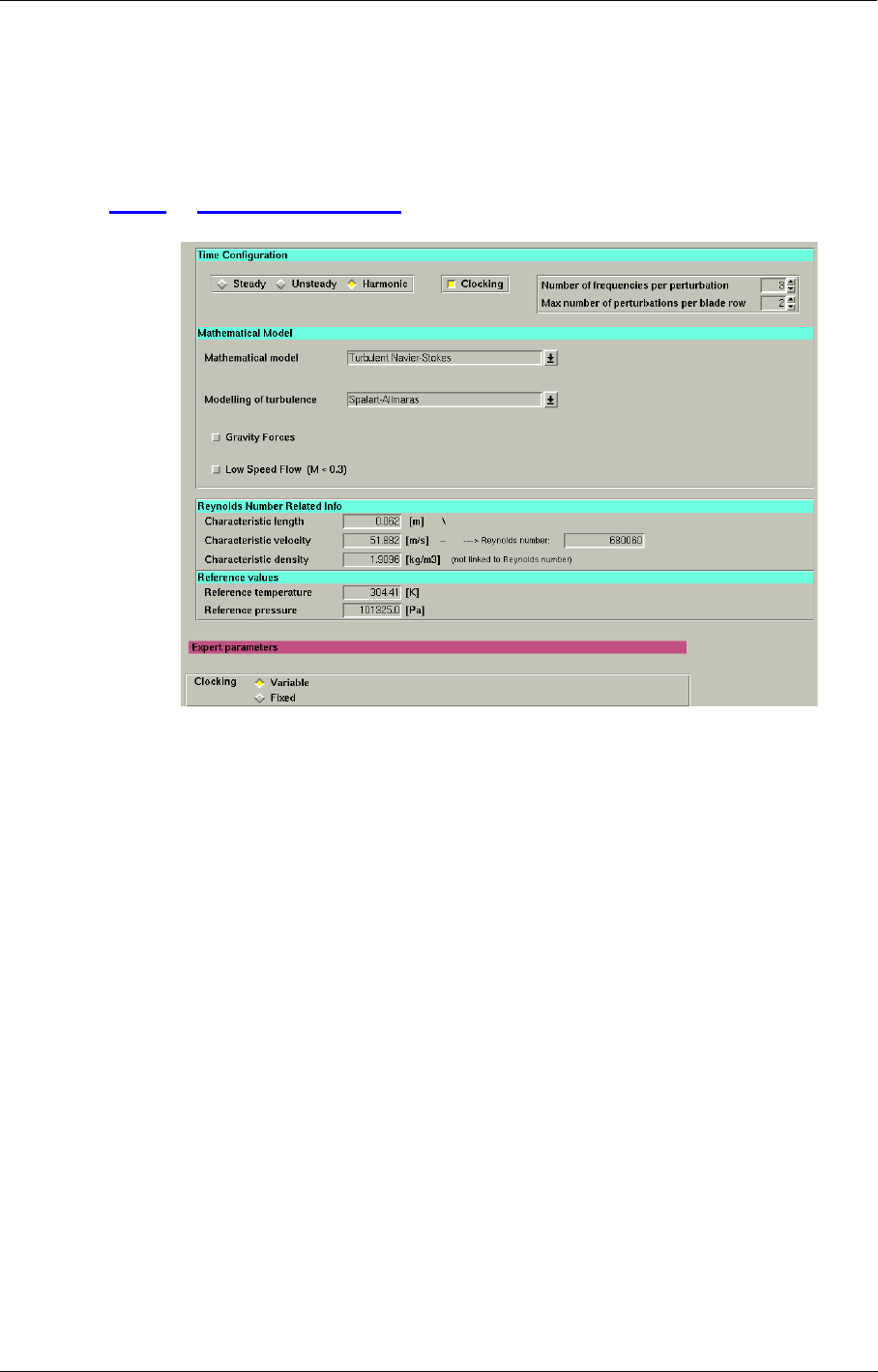
Clocking Dedicated Turbomachinery Models
FINE™/Turbo 8-31
The present Clocking model allows the user to simulate the clocking effects between consecutive
rotors or stators. The range of influence is 1.5 stage upstream or downstream: for a multistage
machine row1/row2/row3/row4/row5 the following clocking interactions are modelled: row1-
row3; row3-row5, row2-row4. The clocking between row5 and row1 is not modelled.
8-5.2 Interface Settings
FIGURE 8.5.2-15 Clocking settings
The Clocking model can be switched on/off through the radio button Clocking on the Flow model
page. When the Clocking model is switch on, a radio button switch appears in the expert parame-
ters frame (visible only in Expert mode) to control the fixed or variable clocking.
Variab le : From this simulation, the user can reconstruct the unsteady flow for all the positions of
the rows. For instance, one stator can be moved relatively to another stator and the unsteady flow
can be reconstructed for each relative position. This simulation takes the effect of a rotor (respec-
tively stator) onto the subsequent rotor (respectively stator) into account. In the post-processing the
time-mean flow can be represented for all the different positions of one stator (or rotor) relatively to
the subsequent stator (or rotor).
Fixed: Same as "Var iable" but with the difference that the stator (or rotor) can’t be moved in the
post-processing. The effects from one stator onto the other stator are also taken into account but
only for the position given in the input mesh. So it is like the standard harmonic but with the differ-
ence that the effects of stator1 onto stator2 are taken into account. In the post-processing the user
can only reconstruct the unsteady flow.
When Clocking is activated, the parameter Max number of perturbations per blade
row includes the clocking perturbations. For example, for the row1/row2/row3 configu-
ration, this parameter is equal to 2. However, for the row1/row2/row3/row4/row5 config-
uration, this parameter should be equal to 4.
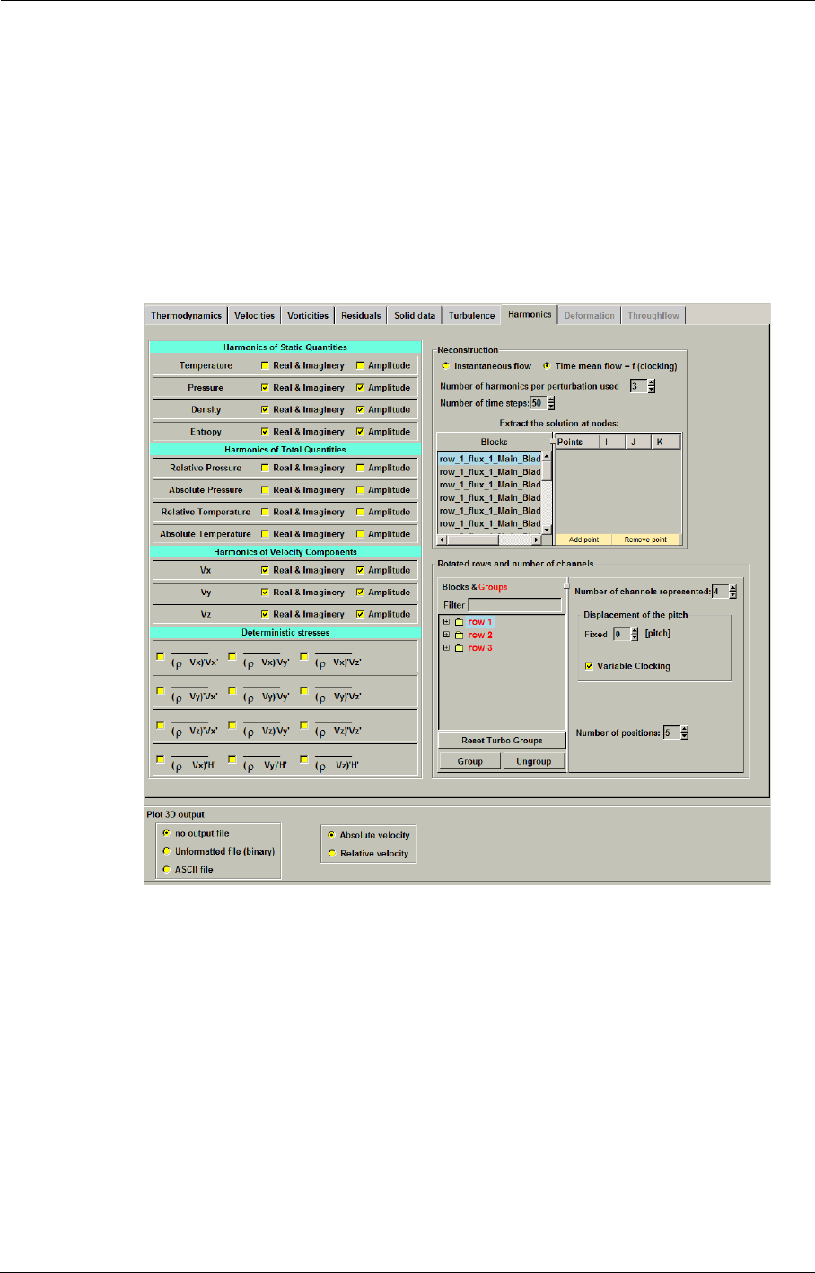
Dedicated Turbomachinery Models Clocking
8-32 FINE™/Turbo
8-5.2.1 Reconstruction in Time
The program Harmo2Time for reconstructing a harmonic solution in time or in space, is also avail-
able for clocking simulations. All the settings in the Harmonics tab of the Computed Variables
page are the same as describing in Chapter 8-4.2.3, except the following settings that are special or
dedicated to clocking simulations.
In the Harmonics tab of the Computed Variables page (seen in Figure 8.5.2-16), the user has two
possibilities for reconstruction in time when the harmonic result simulates the clocking effects.
FIGURE 8.5.2-16 Harmonic outputs in case of clocking considered
•Instantaneous flow: Reconstruct unsteady flow like the standard harmonic output.
For each blade row, the user can change its relative clocking position by specify the Displace-
ment of the pitch in the frame of Rotated rows and number of channels. The inputted
number can be a real number. For example, 0.5 [pitch] will rotate the blade row by a half of a
pitch (360deg/N where N is the periodicity of the blade row).
•Time mean flow = f(clocking): Reconstruct time-mean flow varying with the position of the
selected blade row or distortion.
For each blade row, the user can change its relative clocking position by specify the Displace-
ment of the pitch in the frame of Rotated rows and number of channels. The inputted number
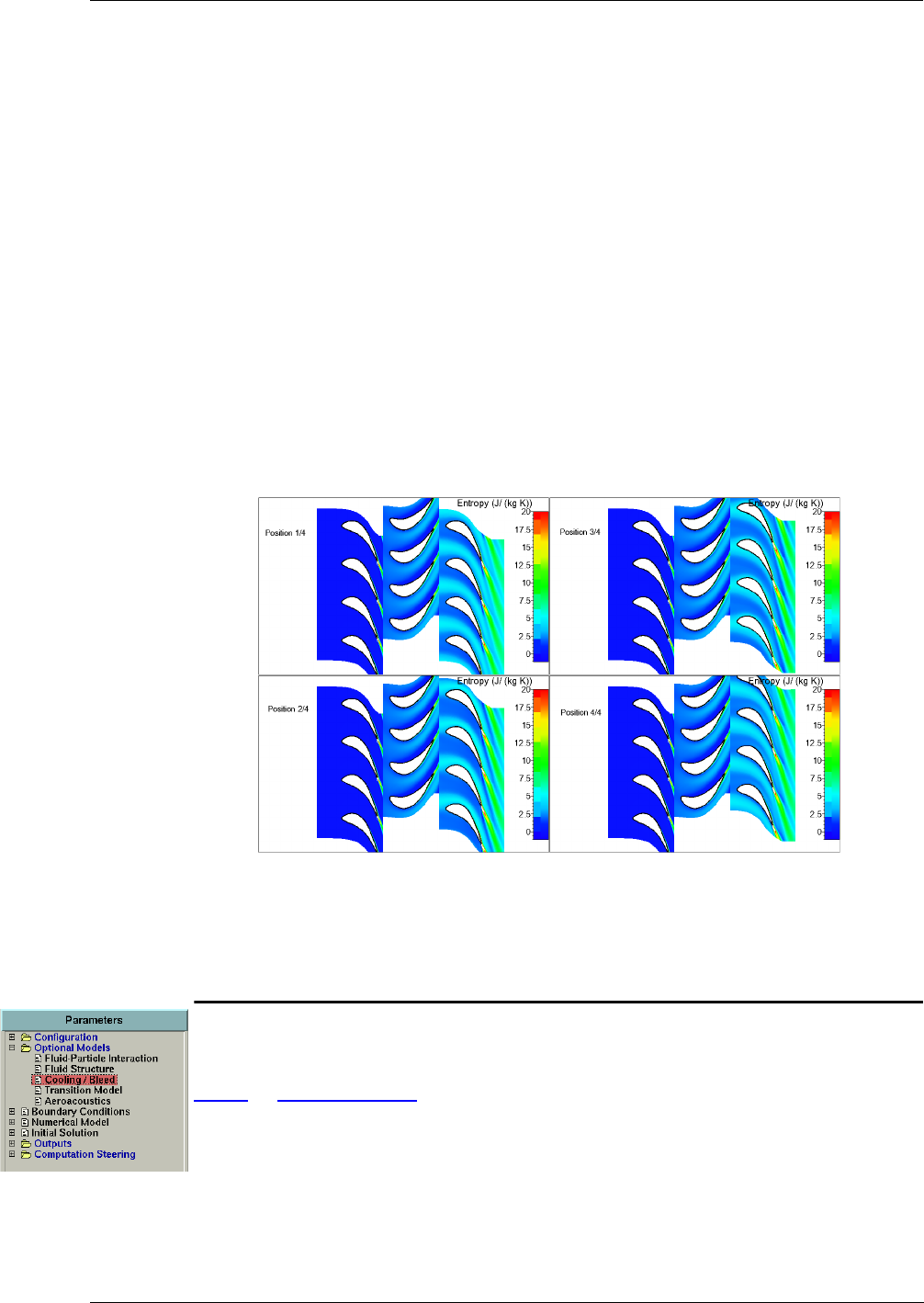
Cooling/Bleed Dedicated Turbomachinery Models
FINE™/Turbo 8-33
can be a real number. For example, 0.5 [pitch] will rotate the blade row by a half of a pitch
(360deg/N where N is the periodicity of the blade row).
The option Variable Clocking must be activated for one of all rows or the inlet distortion. By
default, the option Variable Clocking is activated for the first row in the Blocks&Groups list.
The parameter Number of positions, which appears if Variable Clocking is activated, is used to
set the number of clocking positions over the 100% pitch displacement.
When launching Harmo2Time, the time-mean flow will be reconstructed for each clocking
position of the selected blade row. As an illustration of the reconstruction of time mean flow =
f(clocking), the Aachen turbine case is shown in Figure 8.5.2-17. In this case, the row3 is set
as Variable Clocking and the Number of positions is set to 4. The time mean flow is recon-
structed at four clocking positions of the row3.
The option Time mean flow = f(clocking) is only available for a variable clocking
simulation.
If the button Variable Clocking is switched on for a block or group, then it is switched
off for all the other blocks or groups.
FIGURE 8.5.2-17 Reconstructed time mean flow varying with the different clocking positions
of the row3 in the Aachen turbine case
8-6 Cooling/Bleed
8-6.1 Introduction
The Cooling/Bleed model allows both the simulation of cooling flows injected through solid walls
into the flow or bleed flows where mass flow leaves the main flow through solid wall.
The adopted technique makes use of additional sources of mass, momentum and energy located at
given points or along given lines of the solid walls and does not require the meshing of the cooling
flow injection channels. The objective of this model is not to describe the details of the cooling flow

Dedicated Turbomachinery Models Cooling/Bleed
8-34 FINE™/Turbo
itself but rather to consider its effect on the main flow. The major hypothesis of the model is that the
injection/bleed surface is smaller than the local cell surface.
In the next sections the following information is given on the Cooling/Bleed model:
•section 8-6.2 describes how to set up a project involving the Cooling/Bleed model under the
FINE™/Turbo user environment.
•section 8-6.3 gives a summary of the available expert parameters related to cooling or bleed
flow.
•section 8-6.4 provides the format of the Cooling/Bleed input data file.
8-6.2 Cooling/Bleed Model in the FINE™/Turbo GUI
The Cooling/Bleed model can be directly activated from the FINE™/Turbo interface by opening
the Cooling/Bleed page under Optional Models. The layout of the page is shown in Figure 8.6.2-
18.
The list box on the top of the page (a) displays all the injectors (Cooling or Bleed) imported or
added by the user. The buttons below the list (b) enable to Preview, Add, Edit, Remove, Import
(more details on data file in section 8-6.4) injectors or Export injectors definitions to a file. The list
box (c) gives the informations of total cooling/bleed mass flow. Clicking with the left mouse button
on a selected injector will display its corresponding parameters in the lower part of the page (d).
Clicking with the right mouse button on a selected injector will display a popup menu enabling to
add/edit/remove the injector.
The button Spreading of the hole on the top of the page can be used to control the location and
spreading of the injector. When Spreading of the hole is switched off, the old algorithm of the cool-
ing/bleed model will be used. A hole will be included in one cell only, even when the diameter of
the hole exceeds the cell width. The hole center is the closest cell face center to the defined point.
When Spreading of the hole is switched on, the new algorithm will be used. The position of the hole
and slot is computed exactly. All cells included in the definition of the hole and slot will be used.
And the hole or slot can spread over a patch border to another patch.
The spreading of injector can only cross one border between patches.
The spreading of injector is not implemented to cross a periodic boundary.
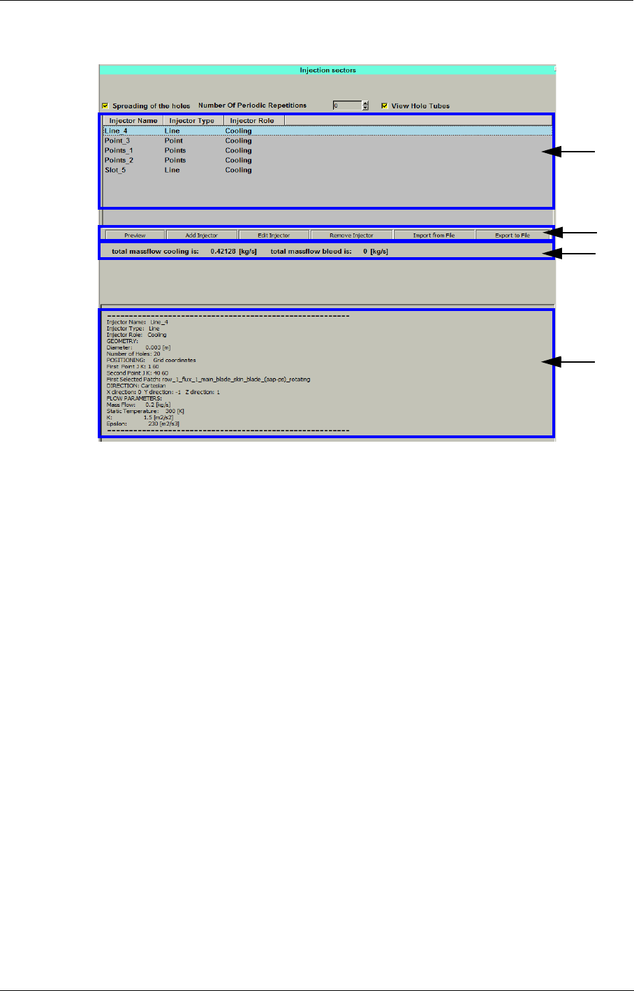
Cooling/Bleed Dedicated Turbomachinery Models
FINE™/Turbo 8-35
FIGURE 8.6.2-18 Cooling/Bleed page in FINE™/Turbo
For the Points type of holes, two additional options are available: Number Of Periodic Repetitions
and View Hole Tubes. If the mesh in the project is generated by AutoGrid5 and includes multiple
blade passages in one row, the user may create or input the Points type of holes in one blade pas-
sage, then set the Number Of Periodic Repetitions to cover all the blade passages. The button View
Hole Tubes is used to show the hole as a tube.
When the user defines holes in AutoGrid5 template but does not mesh them, the hole
line file or the geomTurbo file created by AutoGrid5 can be directly imported as a Points
type of data file to define the injector. The system automatically selects all the patches
related for each holes definition. To use this function, the grid configuration has to be
activated when setting the information of the mesh.
8-6.2.1 Injector Sector Wizard
When adding an injector (Add Injector button), for each injection the following parameters need to
be specified through a wizard:
•injector name,
•injector role: Cooling or Bleed,
•injector solid patches location,
•definition of the geometry,
•position of the injector,
•flow parameters.
(a)
(d)
(b)
(c)
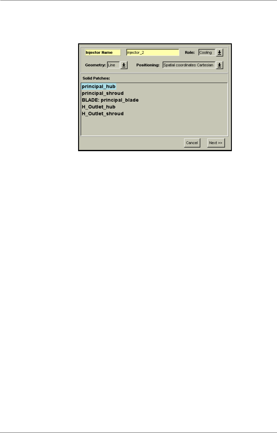
Dedicated Turbomachinery Models Cooling/Bleed
8-36 FINE™/Turbo
On the first page of this wizard the user can enter the name, the role, the solid patches, the geometry
definition and the type of positioning of the injector.
FIGURE 8.6.2-19 Injection Sector Wizard
a) Injection Sector Name
The name should be entered by moving the mouse to the text box for the Injector Name and to
type the name on the keyboard. By default a name is proposed like "injector_1".
It is strongly recommended to use only standard english letters, arabic numerals and
underscore "_" symbol when naming an injection sector. Non-standard characters may
not be recognized or may be misinterpreted when using the project on other computers.
b) Injection Sector Role
The role of the injector should be entered: Cooling if the flow is injected through solid walls into the
main flow or Bleed if part of the mass flow leaves the main flow through solid walls.
c) Injection Sector Geometry
Three types of injection sectors can be defined through the interface: point, line or slot.
•the Point type corresponds to a single cooling hole.
•the Line type stands for a series of cooling holes regularly distributed along a line with the
same geometrical and flow properties.
•a hub or shroud Slot is a continuous line of holes placed at constant radius and axial position
(typically used on the hub or shroud surface of a turbomachine). Slots are only defined along
axisymmetric surfaces.
In case a slot (or a line) should traverse several patches (as for instance in a HOH
mesh configuration) all the patches should be selected and one single slot should be cre-
ated.
•For the Points type, the location of the cooling holes can be defined with a list of points
defined by the user. The definition of the holes will no longer be related to the topology of the
mesh, but to the geometrical entities including hub, shroud and blades.
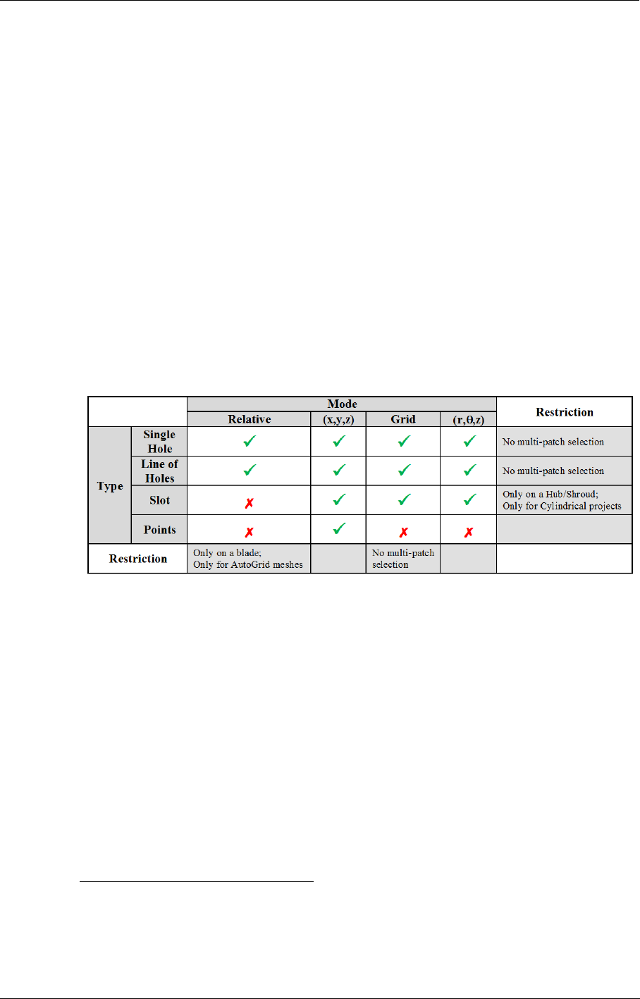
Cooling/Bleed Dedicated Turbomachinery Models
FINE™/Turbo 8-37
d) Injection Sector Positioning
Four modes are available to place the holes:
•Relative mode: this mode is used for blade walls and is valid for AutoGrid™ meshes only. In
this case, the spanwise and streamwise positions of the hole (or of the 2 extremities in the case
of a line of holes) are specified.
•Space Cartesian mode: the user specifies the (X,Y,Z) Cartesian coordinates of the hole or of
the 2 extremities for a line. For a slot the user enters the radius and the Z-coordinate of one
point of the slot.
•Space Cylindrical mode: the user specifies the (R,θ,Z) cylindrical coordinates of the hole or
of the 2 extremities for a line. For a slot the user enters the radius and the Z-coordinate of one
point of the slot.
•Grid mode: the user specifies the (I,J,K) indices of the hole or of the 2 extremities of a line of
holes.
The injection sectors of type Slot cannot be presented in relative coordinates.
The combination of injector geometry and positioning can be summarized as follows:
FIGURE 8.6.2-20 Injector sector geometry/positioning combination & restriction
To cancel the modifications to the injector definition and close the wizard click on the Cancel but-
ton.
Once the injector sector role, type and mode are correctly set, click on Next>> to go to the next
page of the wizard. On this page, depending of the role, type and mode of injector, the flow param-
eters and geometry/positioning parameters have to be defined in the second page of the wizard.
When defining a cooling or bleed using the Cartesian or cylindrical coordinates, no
procedure is implemented to check if the specified direction is correct.
e) Injection Sector Geometry/Positioning Parameters
As presented in Figure 8.6.2-20, 12 combinations are available. As the transformation from cylin-
drical to Cartesian coordinates is obvious, only 9 combinations will be described in more detail.
e.1) Relative positioning for a single hole
The user specifies the diameter of the hole in case of a single hole. Each hole is circular. The diam-
eter of the hole is used to calculate the outgoing velocity.
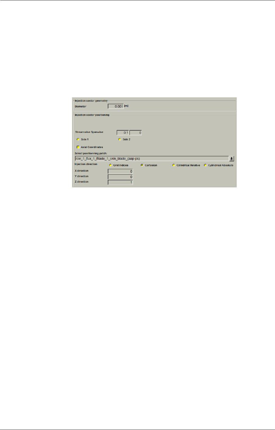
Dedicated Turbomachinery Models Cooling/Bleed
8-38 FINE™/Turbo
As for the old algorithm, the holes are located by means of a spanwise and a streamwise relative
position. The algorithm can be applied to H, I or O-meshes generated by AutoGrid™. For O-
meshes the blade surface is divided in two different sub-patches (one for the pressure side and one
for the suction side). Therefore, the user has to select on which side of the blade (Side1/Side2) the
injection will be located. A button has been added in the interface in order to select the side. This
button is active only for O-meshes.
Only AutoGrid™ provided with FINE™/Turbo 6.1-1 (and later versions) can be used
to generate the mesh and this relative positioning is only available for blade surfaces.
FIGURE 8.6.2-21 Geometry parameters for relative positioning of a hole
The location is defined as a fraction of the arc length from hub to shroud and from the leading edge
to the trailing edge. Spanwise and streamwise coordinates are computed for each cell vertex. The
closest point found in this relative coordinate frame is the one that is concerned by the injection.
An option has been set-up in order to use the axial chord (Axial Coordinates option) instead of the
arc length (only available for axial machines).
The relative positioning does not accept meshes with a blunt at the leading edge
A pop-down manu Select positioning patch is added in the interface. The user has to choose the
patch that the hole will be positioned.
Finally, three ways to impose the injection direction are proposed through the interface: Cartesian,
cylindrical or grid indices. For injection direction specified in Cylindrical coordinates two options
are available: it can be defined in the relative frame of reference or in the absolute frame of refer-
ence.
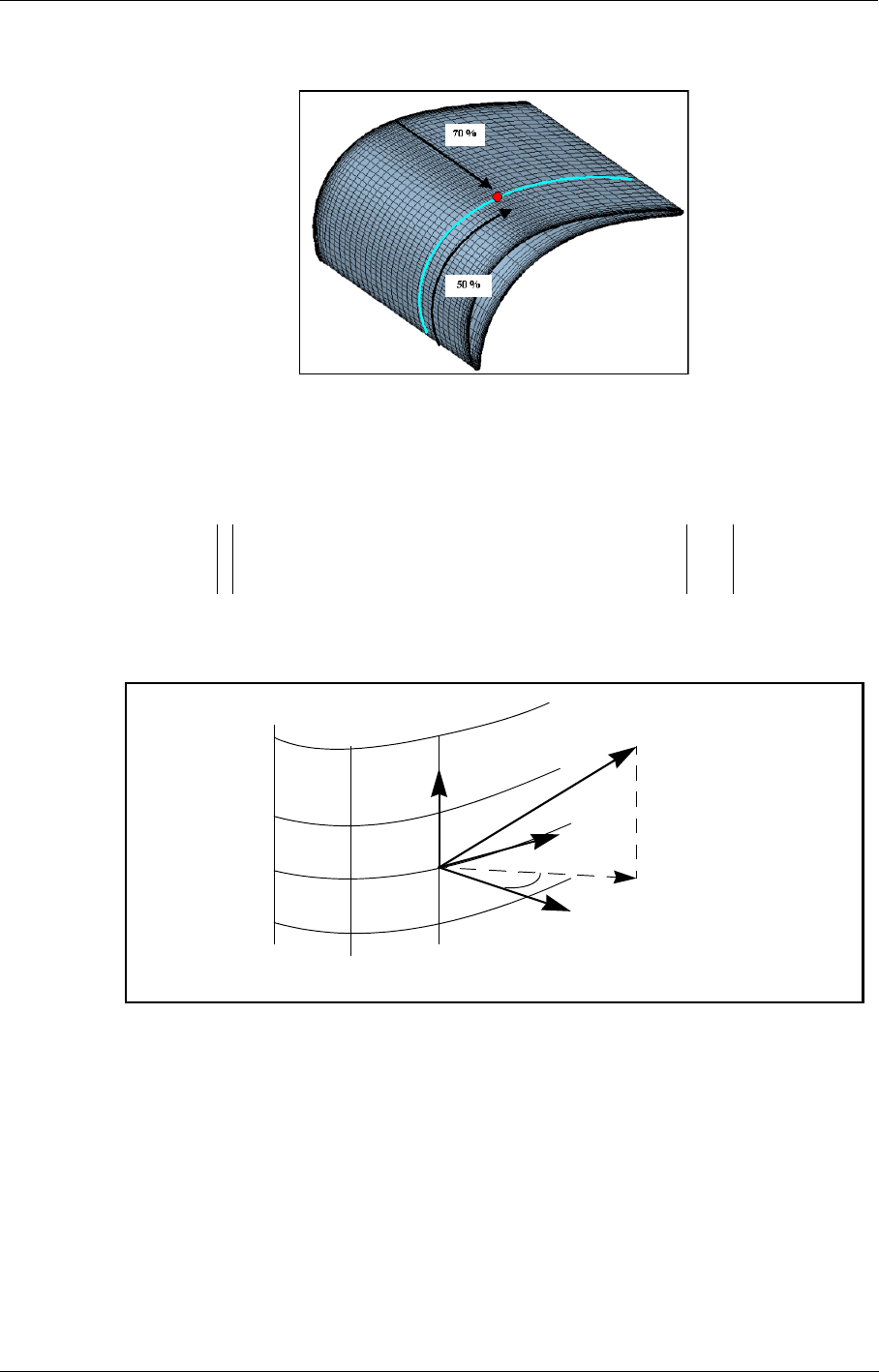
Cooling/Bleed Dedicated Turbomachinery Models
FINE™/Turbo 8-39
FIGURE 8.6.2-22 . Relative positioning of a hole at 70% spanwise and 50% streamwise.
When Grid Indices is selected, the injection direction is provided by the user through 2 angles
expressed in degrees (depending of the units selected in the menu File/Preferences). Each angle is
measured with respect to the local normal and one of the 2 grid line directions tangent to the wall.
In case of an = ct surface, the angles are measured with respect to the grid lines respec-
tively. Figure 8.6.2-23 illustrates the definition of angle βk for an I = cst surface.
FIGURE 8.6.2-23 Angle definition in the cooling flow page of the FINE™ GUI
Each angle is defined as:
(8-5)
For example, in order to make the velocity direction oriented along the normal, the two angles
should be set equal to 0. A 90 degrees angle is not allowed as it will induce a velocity vector tan-
gent to the corresponding grid line direction, with zero mass flow.
I
J
K
JK,()
KI,()
IJ,()
J
n
V
βk
I=constant surface
K
βk is the angle of the velocity projection in the (K,n) plane with respect to the normal n
to the surface.
βijk,,
Vijk,,
Vn
-------------
atan=
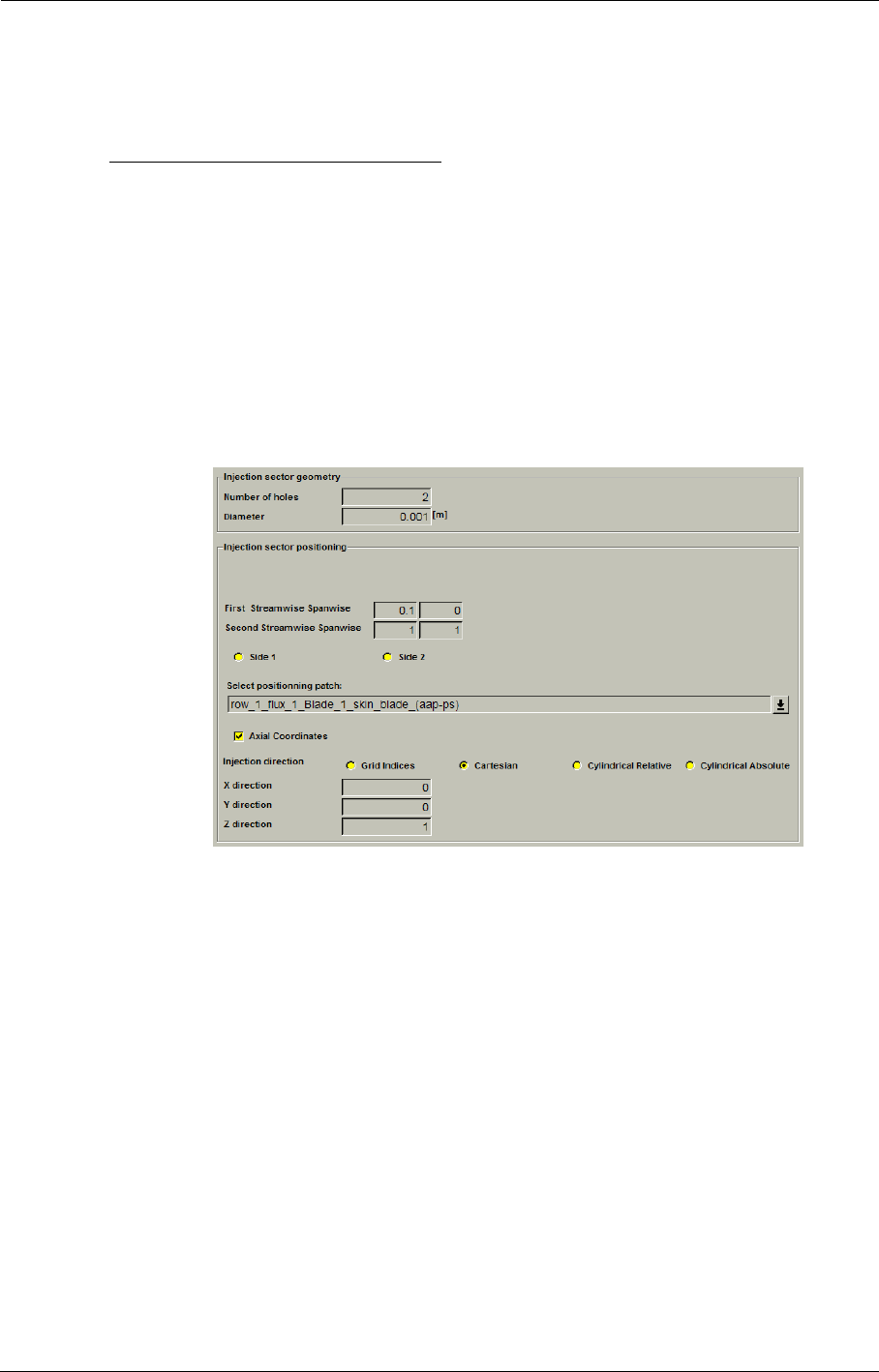
Dedicated Turbomachinery Models Cooling/Bleed
8-40 FINE™/Turbo
For holes located on the blade walls and when the mesh is generated with AutoGrid™, the K- and
J- lines are the two tangent directions along the blade wall, respectively oriented in the streamwise
and spanwise directions.
e.2) Relative positioning for a line of holes
The user specifies the diameter of the hole in case of a line of holes. Furthermore, the number of
holes has to be specified and will be uniformly distributed on the line. Each hole is circular. The
diameter of the hole is used to calculate the outgoing velocity.
As for the old algorithm, the line of holes is defined by two points (holes) that are located by means
of a spanwise and a streamwise relative position. The algorithm can be applied to H, I or O-meshes
generated by AutoGrid™. For O-mesh the blade surface is divided in two different sub-patches
(one for the pressure side and one for the suction side). Therefore, the user has to select on which
side of the blade (Side1/Side2) the injection will be located. A button has been added in the inter-
face in order to select the side. This button is active only for O-meshes.
For each point of the line the algorithm works as for the single hole positioning.
FIGURE 8.6.2-24 Geometry parameters for relative positioning of a line of holes
Only AutoGrid™ provided with FINE™/Turbo 6.1-1 (and later versions) can be used
to generate the mesh and this relative positioning is only available for blade surfaces.
The location is defined as a fraction of the arc length from hub to shroud and from the leading edge
to the trailing edge. Spanwise and streamwise coordinates are computed for each cell vertex. The
closest point found in this relative coordinate frame is the one that is concerned by the injection.
A pop-down manu Select positioning patch is added in the interface. The user has to choose the
patch that the hole will be positioned. And an option has been set-up in order to use the axial chord
(Axial Coordinates option) instead of the arc length (only available for axial machines).
The relative positioning does not accept meshes with a blunt at the leading edge
Finally, three ways to impose the injection direction are proposed through the interface: Cartesian,
cylindrical or grid indices. When Grid Indices is selected, refer to the end of section e.1) for more
details. For injection direction specified in Cylindrical coordinates two options are available: it can
be defined in the relative frame of reference or in the absolute frame of reference.
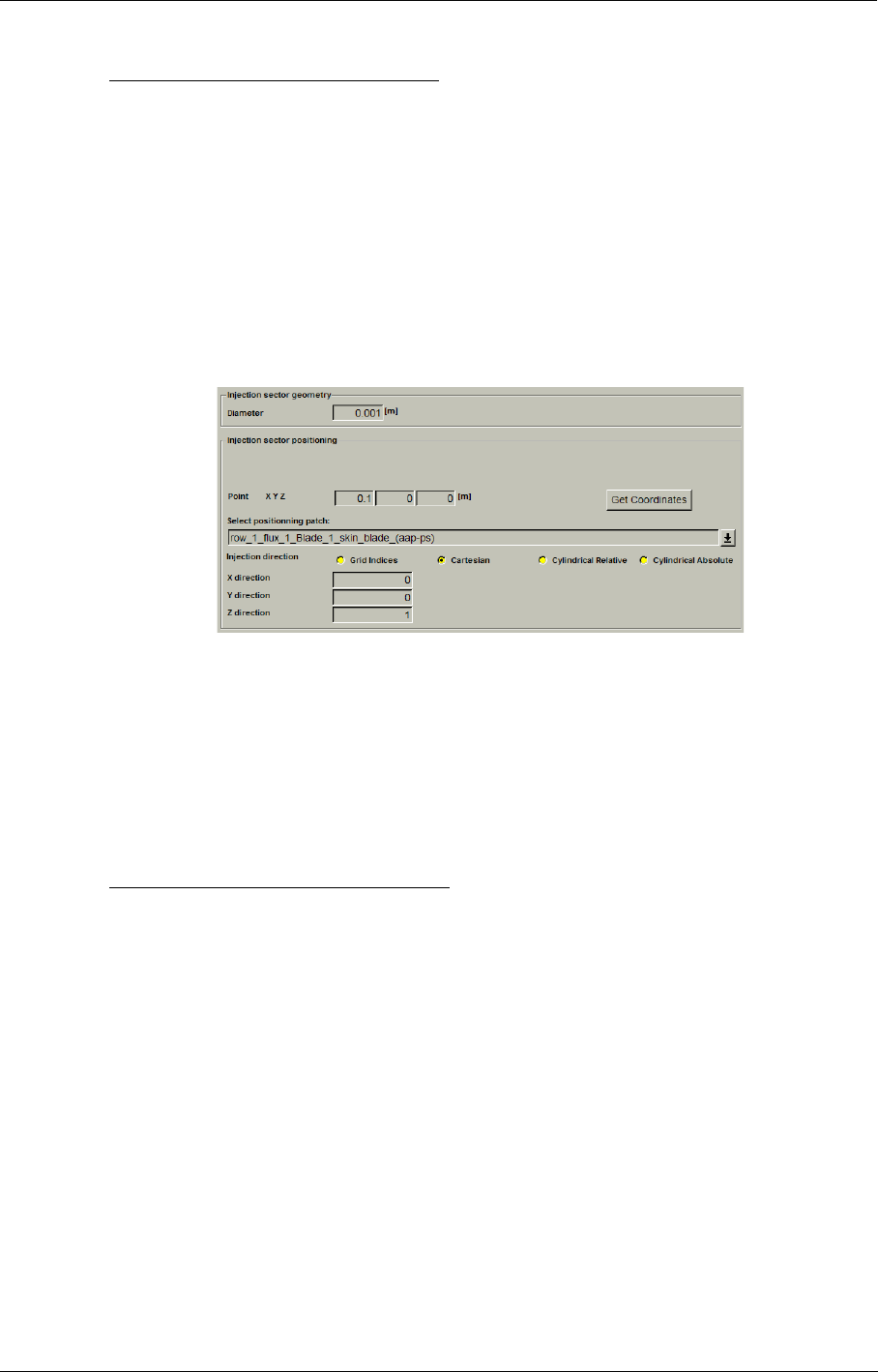
Cooling/Bleed Dedicated Turbomachinery Models
FINE™/Turbo 8-41
e.3) Cartesian positioning for a single hole
The user specifies the diameter of the hole in case of a single hole. Each hole is circular. The diam-
eter of the hole is used to calculate the outgoing velocity.
As for the old algorithm, the holes are located by means of the (X,Y,Z) Cartesian coordinates.
For a single hole, the cell that is concerned by the injection is the closest cell face cen-
tre to the defined point. In case of repetition, the point is automatically transferred to the
meshed patch
Furthermore, in order to ease the capture of the right coordinates, the button Get Coordinates ena-
bles the user to interactively select the point in the mesh view after opening the mesh through the
menu Mesh/View On/Off or Mesh/Tearoff graphics (only available on UNIX).
FIGURE 8.6.2-25 Geometry parameters for space Cartesian positioning of a hole
A pop-down manu Select positioning patch is added in the interface. The user has to choose the
patch that the hole will be positioned.
Finally, three ways to impose the injection direction are proposed through the interface: Cartesian,
cylindrical or grid indices. When Grid Indices is selected, refer to the end of section e.1) for more
details. For injection direction specified in Cylindrical coordinates two options are available: it can
be defined in the relative frame of reference or in the absolute frame of reference.
e.4) Cartesian positioning for a line of holes
The user specifies the diameter of the hole in case of a line of holes. Furthermore, the number of
holes has to be specified. Each hole is circular. The diameter of the hole is used to calculate the out-
going velocity.
As for the old algorithm, the line of holes is defined by two points (holes) that are located by means
of the (X,Y,Z) Cartesian coordinates.
For the two points defining the line, the cells that are concerned by the injection are
the closest cell face centre to the defined point. In case of a repetition, the point is auto-
matically transferred to the meshed patch
Furthermore, in order to ease the capture of the right coordinates, the button Get Coordinates ena-
bles the user to interactively select the point in the mesh view after opening the mesh through the
menu Mesh/View On/Off or Mesh/Tearoff graphics (only available on UNIX).
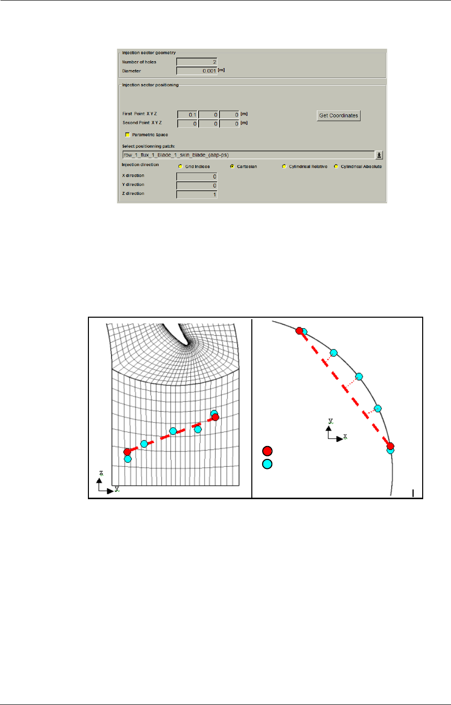
Dedicated Turbomachinery Models Cooling/Bleed
8-42 FINE™/Turbo
FIGURE 8.6.2-26 Geometry parameters for space Cartesian positioning of a line of holes
A line is drawn from those two points (this line does not necessarily follow the surface of the patch,
see Figure 8.6.2-27). The segment is then uniformly divided into N-1 sub-segments (where N is the
number of holes on this line). Each N-2 limits of the sub-segment is then projected on the patch (the
closest cell face centre is found). Those are the cells where the injection will be applied. They are
not necessarily uniformly distributed on the patch.
FIGURE 8.6.2-27 Construction of a line of holes on a turbine hub
For a mesh with a high clustering, or for a high number of points on the line, several
projected points could end on the same cell. This is taken into account in the algorithm.
The mass flow injected is then multiplied by the relevant factor. Therefore, one should be
aware that the number of cells that are highlighted in the interface should not strictly
match the number of holes on the line
On the contrary for a mesh with a relatively poor spatial discretization, the location of the cell face
centres where the injection will be applied will not be strictly on a line. A limitation of this algo-
rithm is that the line does not necessarily follow the patch surface. Therefore, defining a line of
holes at the hub of a gap (upper surface of a rotor blade) could produce the problem presented on
the left side of Figure 8.6.2-28. The same problem can arise generally on a convex surface. In order
points defined by user
points at cell face centre
where injection will be applied
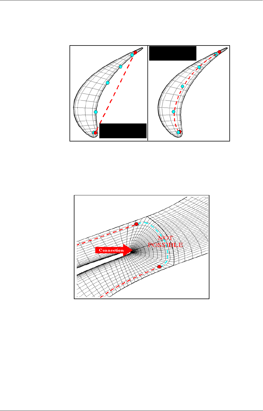
Cooling/Bleed Dedicated Turbomachinery Models
FINE™/Turbo 8-43
to solve this problem, the user can define a line of holes following a parametric surface defined by
the grid lines by activating Parametric Space. Therefore, a line of holes on a convex surface could
be more easily defined (right side of Figure 8.6.2-28)..
FIGURE 8.6.2-28 Definition of a line of holes without or within the parametric space
One limitation of this option is that a line of holes cannot cross a connection. For
instance defining a line of holes (in the parametric space) close to the trailing edge of a O
mesh will produce the result sketched bellow.
FIGURE 8.6.2-29 Definition of a line of holes in the parametric space.
without
Parametric Space
within
Parametric Space
POSSIBLE
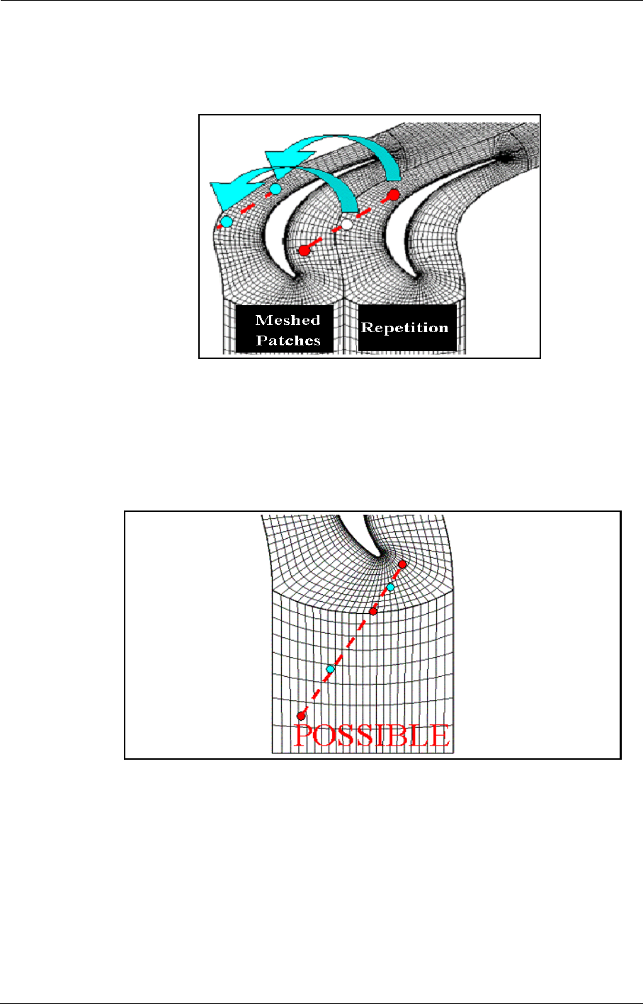
Dedicated Turbomachinery Models Cooling/Bleed
8-44 FINE™/Turbo
For turbomachinery configuration with periodic conditions, points could be located either on the
meshed passage or on one of its repetitions. Therefore, the injections are automatically transferred
to the meshed patch.
FIGURE 8.6.2-30 Two methods to respect repetition for a line of 3 holes.
In case of multi-patch selection the algorithm described above is applied independently for each
patch. Therefore, a direct definition of a line of holes crossing several patches is not possible. In this
case it is recommended to define as many lines as necessary (see figure below). In order to over-
come this problem the multi-patch selection has been restricted to the slots defined by Cartesian or
cylindrical coordinates.
FIGURE 8.6.2-31 Example of definition of a line of 5 holes with multi-patch selection.
A pop-down manu Select positioning patch is added in the interface. The user has to choose the
patch that the hole will be positioned.
Finally, three ways to impose the injection direction are proposed through the interface: Cartesian,
cylindrical or grid indices. When Grid Indices is selected, refer to the end of section e.1) for more
details. For injection direction specified in Cylindrical coordinates two options are available: it can
be defined in the relative frame of reference or in the absolute frame of reference.
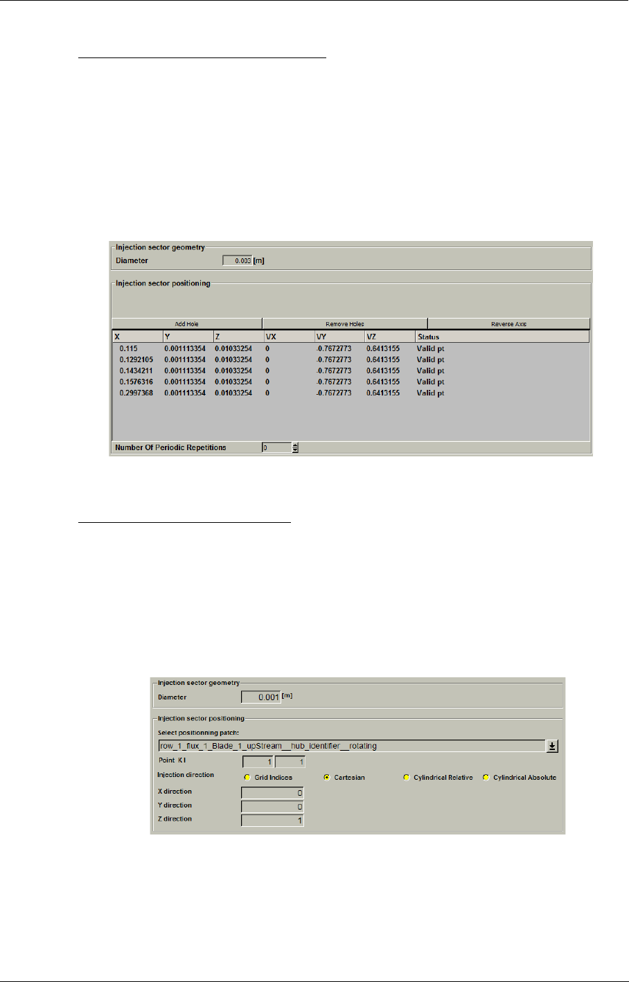
Cooling/Bleed Dedicated Turbomachinery Models
FINE™/Turbo 8-45
e.5) Cartesian positioning for Points of holes
The user specifies the diameter of the hole in case of points of holes. Each hole is circular. The
diameter of the hole is used to calculate the outgoing velocity.
For the points type of holes, the positioning patches are not required any more. The user inputs the
center coordinates and the injection direction for each hole by means of the (X,Y,Z) Cartesian coor-
dinates. The button Add Hole allows to add a hole in the list. A double click will be necessary to
access the input of the center coordinates and the injection direction of the hole. The button Remove
Holes allows to remove the selected holes. Another button Reverse Axis will reverse the injection
direction for all the selected holes.
FIGURE 8.6.2-32 Geometry parameters for space Cartesian positioning of points of holes
e.6) Grid positioning for a single hole
The user specifies the diameter of the hole in case of a single hole. Each hole is circular. The diam-
eter of the hole is used to calculate the outgoing velocity.
The grid positioning used in the FINE™/Turbo solver depends on the grid indices of the centre of
the cell faces. It is different from the grid indices used in IGG™ and in CFView™. The grid indices
are directly used by the flow solver in order to introduce the flow of mass, momentum and energy at
this cell face.
FIGURE 8.6.2-33 Geometry Parameters for Grid positioning of a hole
A pop-down manu Select positioning patch is added in the interface. The user has to choose the
patch that the hole will be positioned.
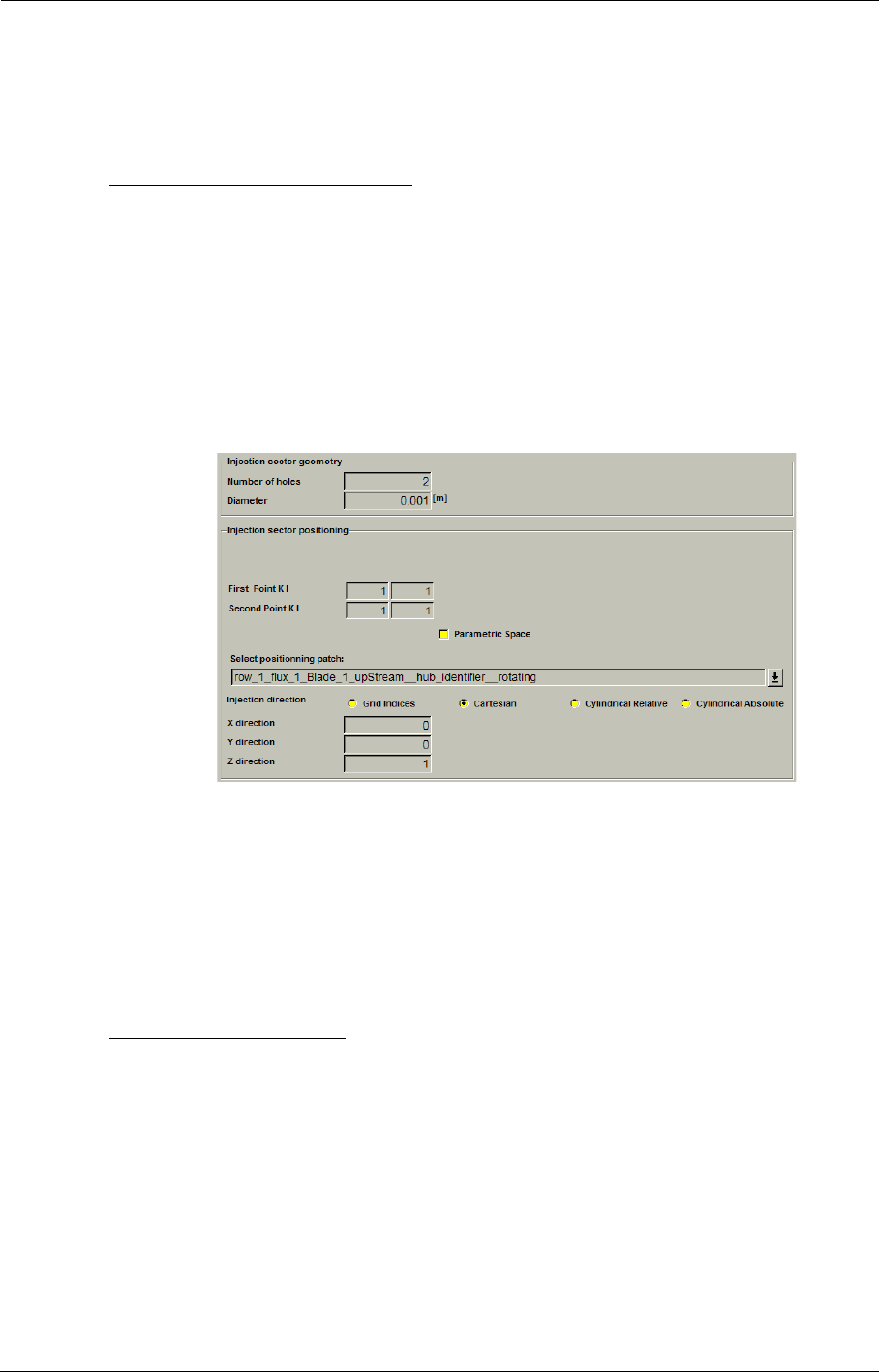
Dedicated Turbomachinery Models Cooling/Bleed
8-46 FINE™/Turbo
Finally, three ways to impose the injection direction are proposed through the interface: Cartesian,
cylindrical or grid indices. When Grid Indices is selected, refer to the end of section e.1) for more
details. For injection direction specified in Cylindrical coordinates two options are available: it can
be defined in the relative frame of reference or in the absolute frame of reference.
e.7) Grid positioning for a line of holes
The user specifies the diameter of the hole in case of a line of holes. Furthermore, the number of
holes has to be specified. Each hole is circular. The diameter of the hole is used to calculate the out-
going velocity.
From the two cell face centres defined in the interface, two geometrical points are defined by their
(x,y,z) coordinates. Then, a line is constructed in the same way as for the Cartesian positioning (sec-
tion e.4). In this case there is no problem of repetition because the two extremities of the line are
located on the meshed patch.
Furthermore, concerning the Parametric Space option, refer to section e.4) on page 7-24 for more
details.
FIGURE 8.6.2-34 Geometry parameters for Grid positioning of a line of holes
A pop-down manu Select positioning patch is added in the interface. The user has to choose the
patch that the hole will be positioned.
Finally, three ways to impose the injection direction are proposed through the interface: Cartesian,
cylindrical or grid indices. When Grid Indices is selected, refer to the end of section e.1) for more
details. For injection direction specified in Cylindrical coordinates two options are available: it can
be defined in the relative frame of reference or in the absolute frame of reference.
e.8) Grid positioning for a slot
The user specifies the width of the slot. The width of the slot is used to calculate the outgoing veloc-
ity.
From the grid indices a geometrical point is defined. Then the slot is defined in the same way as for
the Cylindrical positioning (section e.9).
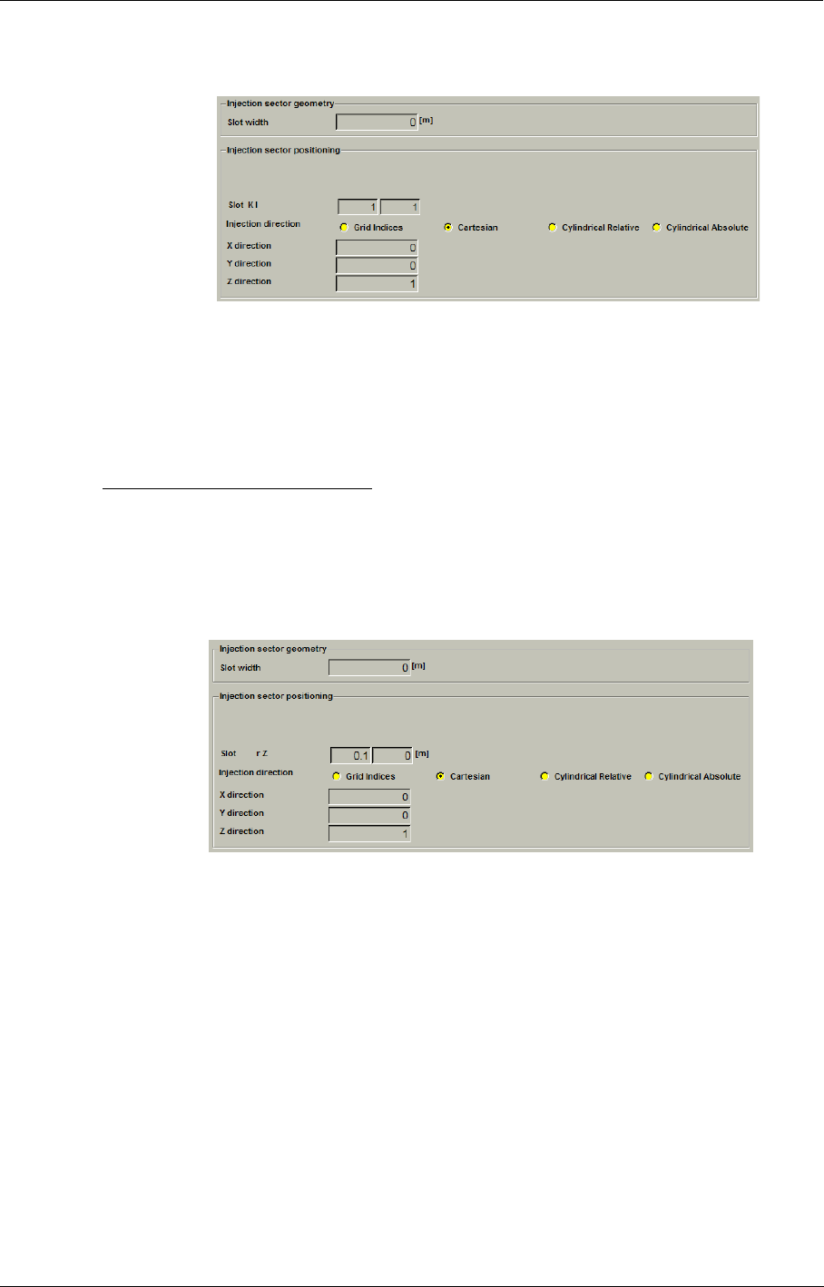
Cooling/Bleed Dedicated Turbomachinery Models
FINE™/Turbo 8-47
FIGURE 8.6.2-35 Geometry Parameters for Grid positioning of a slot
Finally, three ways to impose the injection direction are proposed through the interface: Cartesian,
cylindrical or grid indices. When Grid Indices is selected, refer to the end of section e.1) for more
details. For injection direction specified in Cylindrical coordinates two options are available: it can
be defined in the relative frame of reference or in the absolute frame of reference.
e.9) Cylindrical positioning for a slot
The user has to specify the width of the slot. The width of the slot is used to calculate the outgoing
velocity.
The multi-patch selection has been restricted to the slots defined by Cartesian or cylin-
drical coordinates.
FIGURE 8.6.2-36 Geometry parameters for space Cylindrical positioning of a slot
For the positioning of the slot, the radius and z values are asked to the user. The closest cell face of
the patch to this point is found. The radius and axial position of this cell face centre becomes the
slot position in the (r,z) plane. It should be noted that this slot position is not identical to the initial
user input. For most axial machines the radius can be easily identified by calculating the closest
point on the patch. In this case only the axial position of the slot is required in the interface. For
radial machines, or for axial machines with complex vein geometry, the two components of the
original point are required (Figure 8.6.2-37).
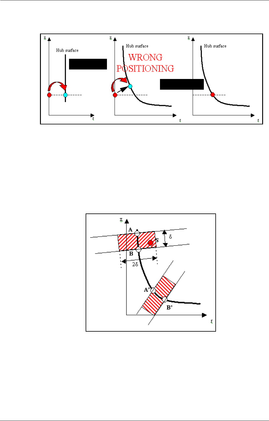
Dedicated Turbomachinery Models Cooling/Bleed
8-48 FINE™/Turbo
FIGURE 8.6.2-37 Examples of slot positioning
The algorithm that defines the cell faces that are concerned by this slot is illustrated in Figure 8.6.2-
38. For each cell face of the patch, the two extremities in the (r,z) plane of this polygon (A,B and
A’,B’) are identified (i.e., the two vertices with the maximum distance in this plane). They define
the limits of the cell face in the (r,z) plane. If those two points are called A,B for cell 1 and A’,B’ for
cell 2, and S is the slot location specified by the user in the (r,z) plane through FINE™/Turbo, as
presented on Figure 8.6.2-38, S is only included in the domain of cell 1 limited by A,B in the (r,z)
plane, therefore, the cell 1 is the only cell concerned by the slot S.
FIGURE 8.6.2-38 Identification of the cells concerned by the slot S in the (r,z) plane. δ is the
distance between A and B.
On the contrary, S is not inside the domain defined by A',B'. Thus, the cell 2 will not be concerned
by the slot.
For O-meshes with small cells close to leading or trailing edges, this algorithm could
leads to missing cells. This problem is due to a (r,z) position specified by the user in
Axial Machine
Radial Machine
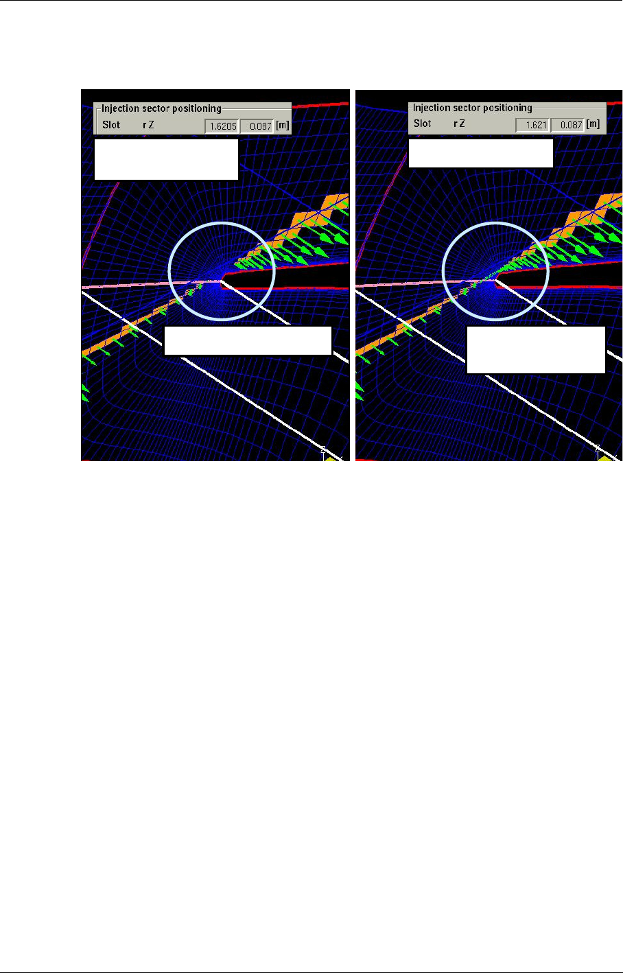
Cooling/Bleed Dedicated Turbomachinery Models
FINE™/Turbo 8-49
FINE™/Turbo for the slot that is not precise enough.
FIGURE 8.6.2-39 Definition of a slot for a O-mesh
Furthermore, in order to ease the capture of the right coordinates, the button Get Coordinates ena-
bles the user to interactively select the point in the mesh view after opening the mesh through the
menu Mesh/View On/Off or Mesh/Tearoff graphics (only available on UNIX).
Finally, three ways to impose the injection direction are proposed through the interface: Cartesian,
cylindrical or grid indices. When Grid Indices is selected, refer to the end of section e.1) for more
details. For injection direction specified in Cylindrical coordinates two options are available: it can
be defined in the relative frame of reference or in the absolute frame of reference.
f) Flow Parameters
The user may specify the Mass flow or Mass flow relative to inlet. The specified mass flow is
actually the total mass flow through all the blades and through all the holes in the case of a line of
holes. Thus the mass flow through one hole is the specified mass flow divided by the number of
blades and the number of holes. The mass flow is often responsible for initialization troubles as it
might be too high. The FINE™/Turbo interface allows a tuning of the specified mass flow through
an expert parameter. This is described in section 8-6.3.
For cooling flow the mass flow specified in FINE™/Turbo will be considered as posi-
tive. The mass flow is considered as negative for bleed flow.
When Mass flow relative to inlet is selected, a new pop-down menu appears. The user has to
choose an inlet patch (or group). The cooling/bleed mass flow is specified as a percentage value of
the inlet mass flow.
In case the user changes the inlet grouping in the Boundary Conditions page, a warn-
points are missing points are
represented
not precise enough
value
exact value
points are missing points are
represented
not precise enough
value
exact value
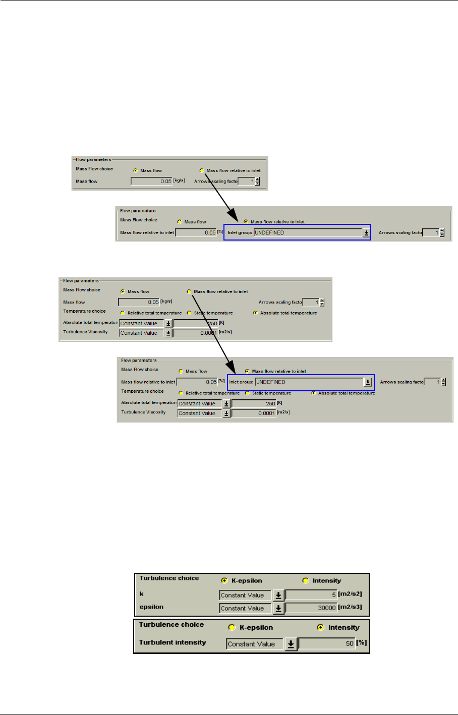
Dedicated Turbomachinery Models Cooling/Bleed
8-50 FINE™/Turbo
ing box will appear if the patch/group that links to the injectors is changed. It is strongly
advised to verify the patches in the injectors definitions after performing inlet group/
ungroup in the Boundary Conditions page.
Since the injected flow is relative to an inlet mass flow, the injected flow can strongly
varies with iterations when Mass flow relative to inlet is selected. This can lead to
unstable behaviour if the injected flow is important with respect to the inlet mass flow. In
that case it should be recommended to start from a previously converged solution.
FIGURE 8.6.2-40 Flow parameters for Bleed
FIGURE 8.6.2-41 Flow parameters for Cooling
Furthermore, the Arrows scaling factor parameter enables the user to control the shape of the
arrows representing the injection direction after opening the mesh through the menu Mesh/View
On/Off or Mesh/Tearoff graphics (only available on UNIX).
For cooling additional parameters have to be defined:
•static or total temperature in absolute or relative frame of reference.
•turbulent kinetic energy and dissipation or turbulent intensity for the k-ε model.
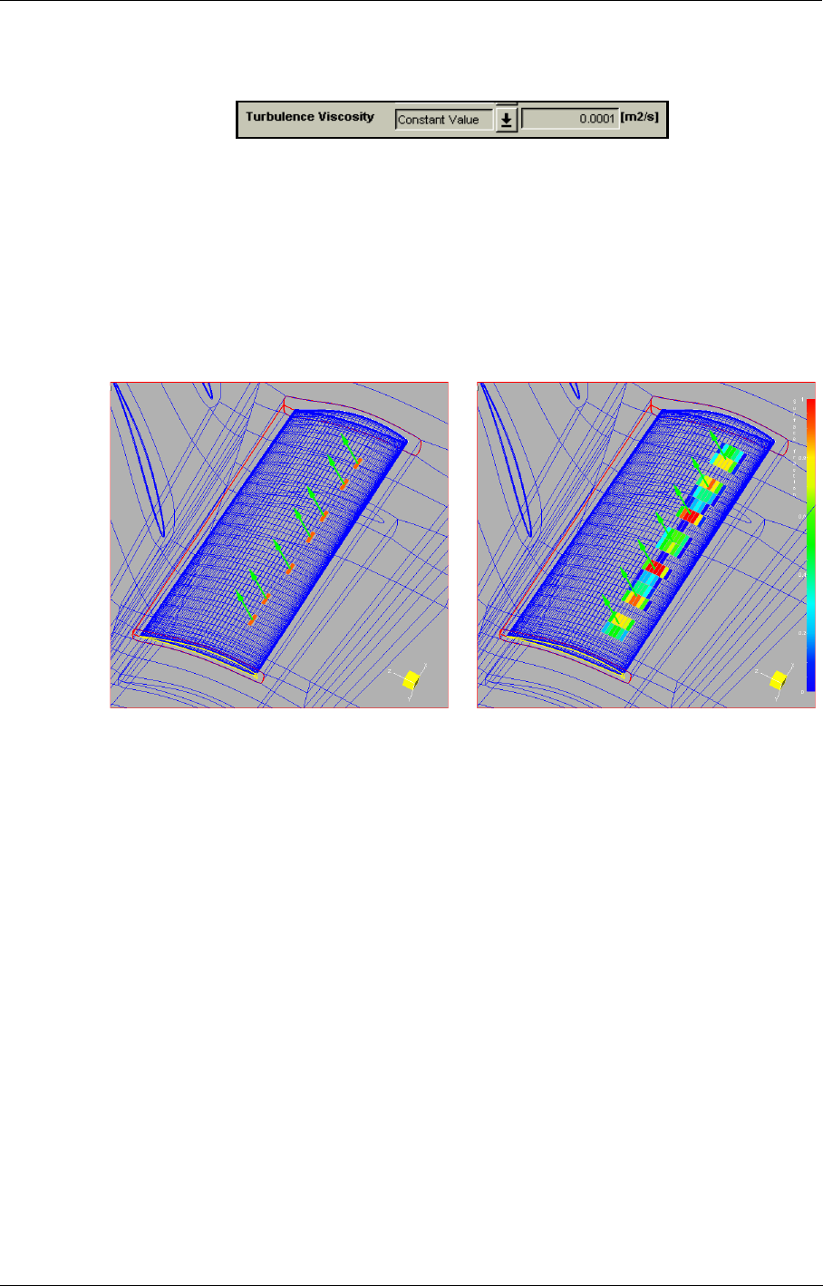
Cooling/Bleed Dedicated Turbomachinery Models
FINE™/Turbo 8-51
•kinematic turbulent viscosity for the Spalart-Allmaras model.
The detail of mass flow through each injector and the maximum Mach number in the
injector has been added in the .mf file. The user can verify whether his/her data is accept-
able.
8-6.2.2 Preview/Preview&Check Injector Sector
When adding an injection sector into FINE™/Turbo, the location (cell face are highlighted) and the
direction of the injection can be visualized. In order to be able to visualize, the user has to load the
mesh through the menu Mesh/View On/Off or Mesh/Tearoff graphics (only available on UNIX).
FIGURE 8.6.2-42 Injection sector visualization within FINE™/Turbo
The parameters area will then be overlapped by the graphic window, and the small control button
on the upper - left corner of the graphic window can be used to resize the graphics area in order to
visualize simultaneously the parameters and the mesh (see Chapter 2-6.6).
Select the injectors and Click-left on the Preview button, a vector will be shown at each hole center
if a line or a single hole is selected. If a slot is selected, the vectors are shown at the center line of
the slot and there is a vector for each cell crossed by that line.
When the Spreading of the holes is switched on, the color contour of the surface fraction is repre-
sented on the mesh of the wall (see section FIGURE 8.6.2-42). This quantity corresponds to the sur-
face fraction of each cell that is "touched" by a hole.The color contour varies from blue to red as the
fraction goes from 0 to 1. But if holes are overlapping in a cell, causing the cell fraction to exceed 1,
the cell will be displayed in white.
If the injection direction is imposed in cylindrical, whatever the reference frame
selected (absolute or relative), the arrows representing the injection direction is displayed
as for the cylindrical relative frame of reference.
When a Points type of holes is selected, the button Preview will be changed to Preview&check.
After the mesh is loaded, the holes location can be visualized and checked by pressing Pre-
Switch off Spreading of the holes Switch on Spreading of the holes
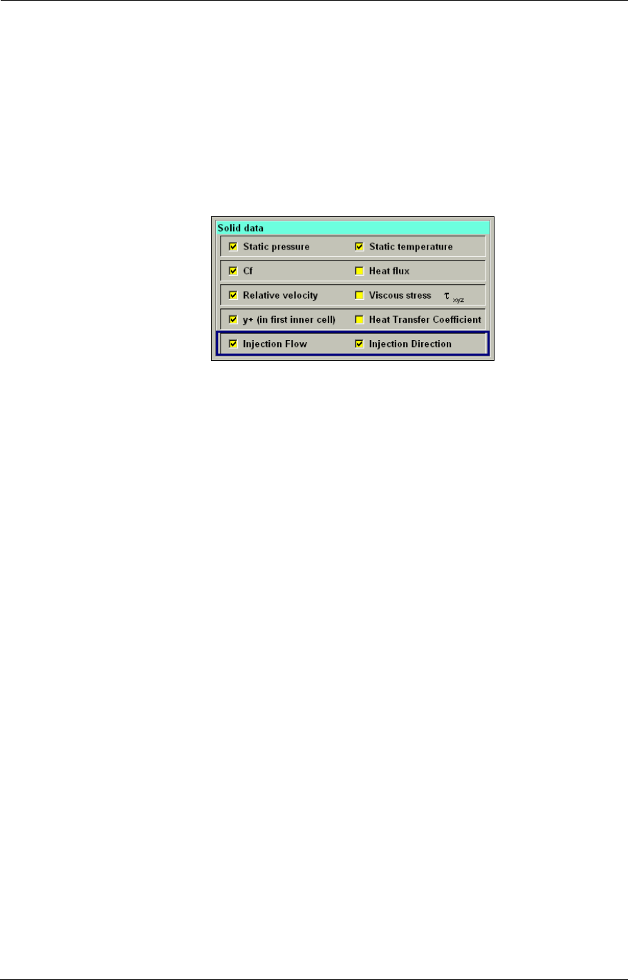
Dedicated Turbomachinery Models Cooling/Bleed
8-52 FINE™/Turbo
view&check. The selected holes in the list are highlighted. If a hole location is wrong, the GUI
prompts the user to remove it. If not, the wrong one is tagged as invalid in the list and displayed in
red.
Furthermore, new outputs have been added into FINE™/Turbo on the Outputs/Computed Varia-
bles page under the tab Solid data in order to enable the visualisation in CFView™ of the injected
flow (in [kg/s]) and the injection direction (normalized [0 1]). The scale of the Injection Direction
vector is normalised by the ratio of the surface of the injector relative to the cell surface. For exam-
ple, 1 means that the cell is entirely covered by the injector and 0 means that there is no injector in
this cell. .
FIGURE 8.6.2-43 Injector sector outputs for CFView™
Within CFView™, the injection direction is always visualized in a relative frame of
reference.
8-6.2.3 Multiple edit and copy of the injectors
By selecting many injectors, the user can modify their parameters at the same time. The user can
also copy injectors from one blade to another blade and use the Repetition display of the mesh in
order to verify the continuity of injectors lines.
a) Multiple select and edit
In the case of multiple selection, the buttons Add injector, Edit injector and Remove injector change
their names to Duplicate injectors, Edit injectors and Remove injectors (a). The information area in
the lower part of the page (b) displays the number and the sum of cooling and bleed mass flow of
selected injectors. Clicking with the right mouse button on the selected injectors will display a
popup menu as shown in section FIGURE 8.6.2-44 (c), which enables to add/edit/remove the injec-
tors or select all injectors through the position or role of the injectors.
Loading the mesh through the menu Mesh/View On/Off or Mesh/Tearoff graphics (only on
UNIX), then selecting the injectors and Clicking-left on the Preview button will simultaneously dis-
play the selected injectors in the graphic view.
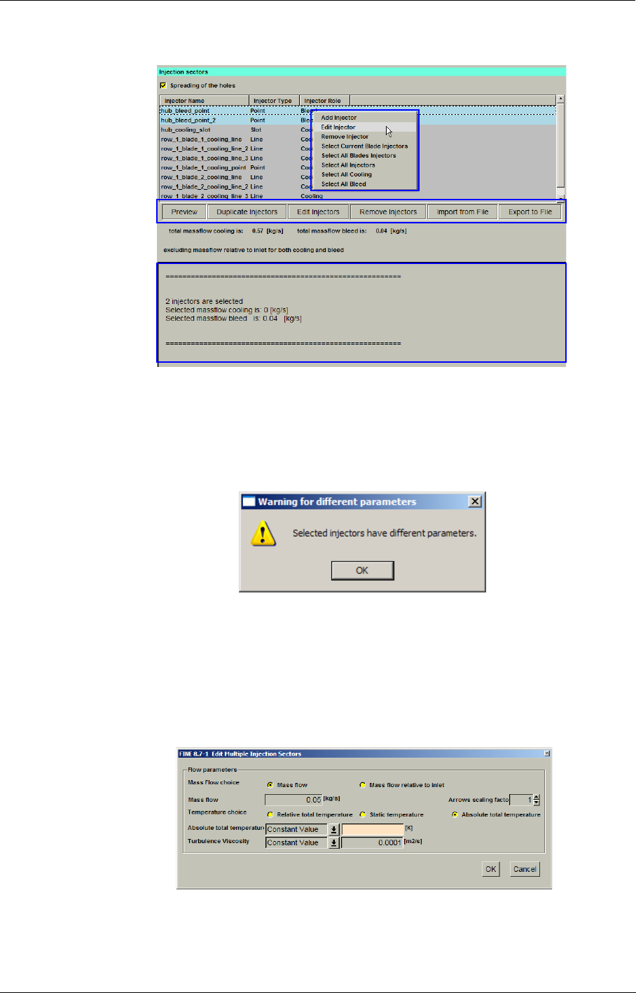
Cooling/Bleed Dedicated Turbomachinery Models
FINE™/Turbo 8-53
FIGURE 8.6.2-44 Cooling/bleed page for multiple selection of the injectors
Multiple edit can only be used to modify the physical parameters. And it is allowed only for injec-
tors of the same type. A check is performed when the Edit injectors button is pressed and a warning
is displayed in case the selection contains injectors of different parameters:
Edit of multiple injectors is possible only for injectors of the same type (cooling or
bleed).
Confirm the warning, a Edit Multiple Injection Sectors dialog box is given as shown in section FIG-
URE 8.6.2-45. The users can modify the flow parameters in this dialog box. The empty entries are
displayed for the quantities that have different values in the selected injectors. The empty entries
and choice buttons have different background color in order to be easily noticed by users.
FIGURE 8.6.2-45 Multiple edit for selected injectors
(A)
(B)
(C)
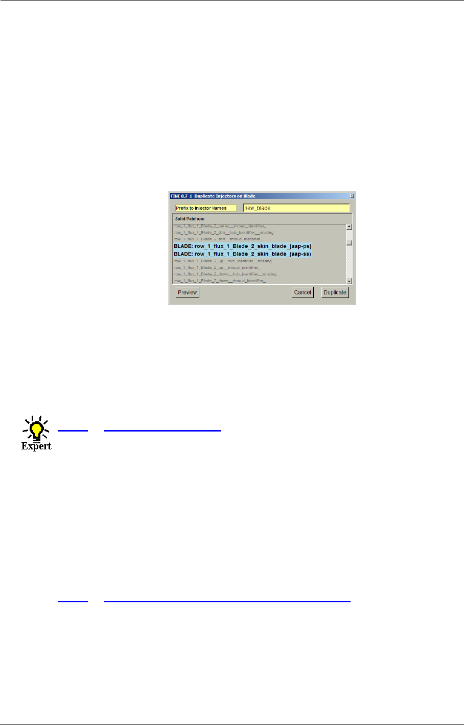
Dedicated Turbomachinery Models Cooling/Bleed
8-54 FINE™/Turbo
In order to see the different values in the selection for a parameter, the user has to click in the empty
entry and press the line down arrow key. A list box will be displayed below the empty entry, which
contains all the values of the parameter in the selectors. The user may click on one of these values
and it will be shown in the entry.
The button OK will store all parameters except those of the empty entries. The button Cancel closes
the Edit dialog box without saving any of the values.
b) Copy and Paste
When multiple injectors are selected, the selected injectors can be copied from one blade to another.
In order to copy injectors, the user has to select multiple injectors, then click-left on the Duplicate
Injectors button. A Wizard page will be displayed first:
The blades on which the selected injectors are located are highlighted with green color. The user
has to specify the new blade on which the injectors will be copied and a prefix to be added to the
names of the new injectors. The selected injectors will be copied to the selected blade if there are
not injectors at the specified position on the chosen blade and there are not injectors with the speci-
fied new name (prefix+selected_injector_name).
Copy of injectors is possible only for injector defined on Relative on Blades.
8-6.3 Expert Parameters
COOLRT (real): in case some difficulties appear at the beginning of the simulation. The robust-
ness can be improved by reducing the imposed cooling/bleed mass flow with
the expert parameter COOLRT. The value of COOLRT (less than 1) corre-
sponds to a constant factor applied to all imposed cooling/bleed mass flow dur-
ing the computation. The user should make successive computations by
progressively increasing this parameter (up to 1) in case of robustness prob-
lems.
MAXNBS (integer):the maximum allowed number of injection sectors is controlled through the
expert parameter MAXNBS (the default value is 50). If the input file contains a
higher number of sectors the parameter should be modified.
8-6.4 Cooling/Bleed Data File: ’.cooling-holes’
A parser is used to find the data in this file, using keywords to locate the position of the data in the
file. The advantage of this technique is that the data do not have to be positioned at a given line in
the file, but only have to be followed by the appropriate keyword (the keywords can be written with
capitals or not).
The user specifies a series of 'injection sectors' in the file. An injection sector is either
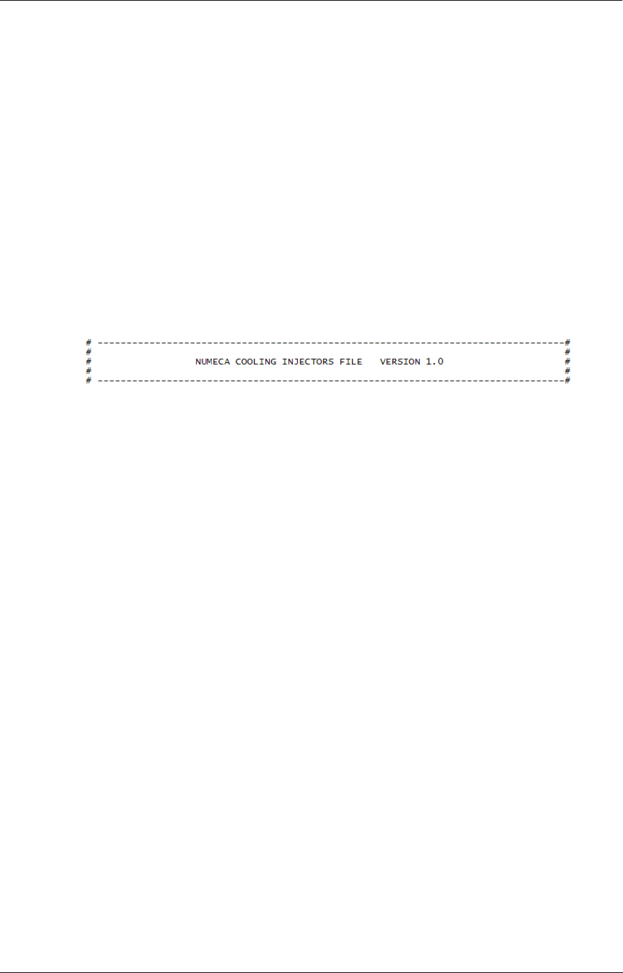
Cooling/Bleed Dedicated Turbomachinery Models
FINE™/Turbo 8-55
—a single cooling hole
—a series of distributed cooling holes along a line (all holes having the same geometrical and
flow properties)
—a hub or shroud slot (continuous line of holes along a constant radius and axial position line)
—a points type of cooling holes
Each injection sector should respectively start and end with the keywords
8-6.4.1 Injection file format
This section describes the format and the keywords used to define any kinds of cooling/bleed. A
easy way to have an example of the file format for a specific type of cooling/bleed is to define a
cooling/bleed in FINE™/Turbo and export it into a file using the menu Export to file.
a) The header
The header of the file contains the injector file version to ensure future backward compatibility. The
current version is 1.0.
b) Multiple injector format
Each file can contain multiple injector definitions. Each injector must be delimited as following:
NI_BEGIN injector
<injector definition>
NI_END injector
NI_BEGIN injector
<injector definition>
NI_END injector
c) Injector name
NAME <injector name>
d) Injection geometry Type
Three types of injectors can be defined: point, slot and line. In addition, the line can be straight or
parametric (defined in the parametric space of the mesh patch).
GEOMETRY_TYPE point
GEOMETRY_TYPE straight line
GEOMETRY_TYPE parametric line
GEOMETRY_TYPE slot
GEOMETRY_TYPE points
e) Injection physical Type
Two types of injectors can be defined through the interface: Bleed and Cooling

Dedicated Turbomachinery Models Cooling/Bleed
8-56 FINE™/Turbo
PHYSICAL_TYPE Cooling
PHYSICAL_TYPE Bleed
f) Locations patches
The cooling/bleed must currently be defined on mesh patches identified by their indices.
LOCATION_PATCH_INDICES <b1> <f1> <p1>
LOCATION_PATCH_INDICES <b2> <f2> <p2>
where bi, fi and pi are the block, face and patch indices.
If the type is points, the user needs to specify the name of the location group instead of specifying
patches. The flow solver computes automatically the positioning patches. The flow solver intersects
the patches definition with the axis of the hole and chooses the closest one as the positioning patch.
If the loaded mesh is generated by AutoGrid5, the following keywords can be identified:
LOCATION_GROUP <row name>
LOCATION_GROUP <blade(s)> or <hub> or <shroud>
The <row name> and <blade(s)> is used for holes defined on the blades. The <row name> and
<hub> is used for holes defined on the hub. The <row name> and <shroud> is used for holes
defined on the shroud.
g) Location patch index
The point and slot are defined with one anchor point, the line with two anchor point. The point must
be defined on one of the location patch specified by its position in the list of the location patch.
POSITION_PATCH_INDEX_1 <location patch index>
h) Anchor point location
The anchor point can be defined using 4 types of coordinates:
•Patch coordinates: parametric normalized arc length along I and J direction of the mesh patch
STREAM_SPAN_POSITION_ON_BLADE_1 s(i) s(j) 0
STREAM_SPAN_POSITION_ON_BLADE_2 s(i) s(j) 0 #for line only
AXIAL_COORDINATES <0 or 1>
SIDE <0 or 1> #only for old AG4 mesh
•Cartesian coordinates X,Y,Z
XYZ1 <x1> <y1> <z1>
XYZ2 <x2> <y2> <z2> #for line only
•Cylindrical Relative R, theta and Z
RTHZ1 <r1> <theta1> <z1> # for slot, only r and z are important
RTHZ2 <r2> <theta2> <z2> # for line only
•Grid Coordinates: I, J indices on the mesh patch
IJ1 <i1> < j1>
IJ2 <i2> < j2> #for line only

Cooling/Bleed Dedicated Turbomachinery Models
FINE™/Turbo 8-57
i) Cooling direction (not for Bleed)
The injection direction can be defined in:
•Grid Angles: angles along the I, J cst lines of the mesh
IJ_ANGLES <beta1> <beta2> #radians
•Injection vector in cartesian coordinates
VXYZ <vx> <vy> <vz>
•Injection vector in cylindrical relative coordinates
RELATIVE_VRTHZ <vr> <vtheta> <vz>
•Injection vector in cylindrical absolute coordinates
ABSOLUTE_VRTHZ <vr> <vtheta> <vz>
j) Anchor point location and cooling direction (for points type only)
For the points type of holes, the anchor point location and the injection direction have to be defined
in one line in cartesian coordinates:
SINGLE_HOLE <x1> <y1> <z1><vx> <vy> <vz>
k) Mass flow
The mass flow can be imposed using the following modes:
•Absolute value:
MASS_FLOW <kg/s>
•Percentage of the inlet mass flow:
MASS_FLOW_RELATIVE_TO_INLET <inlet group> <kg/s>
l) Number of holes on a line
NUMBER_OF_HOLES <n>
m) Cooling/Bleed size
DIAMETER <d> #for point, line or points type only
WIDTH <w> #for slot only
n) Physical Properties
Temperature:
RELATIVE_TEMPERATURE <t> or
STATIC_TEMPERATURE <t> or
ABSOLUTE_TEMPERATURE <t>
Turbulent data:
TURBULENT_VISCOSITY <u> #for Spalart-Allmaras model only
TURBULENT_KE <k> <epsilon> or
TURBULENT_INTENSITY <i> #for k-ε model
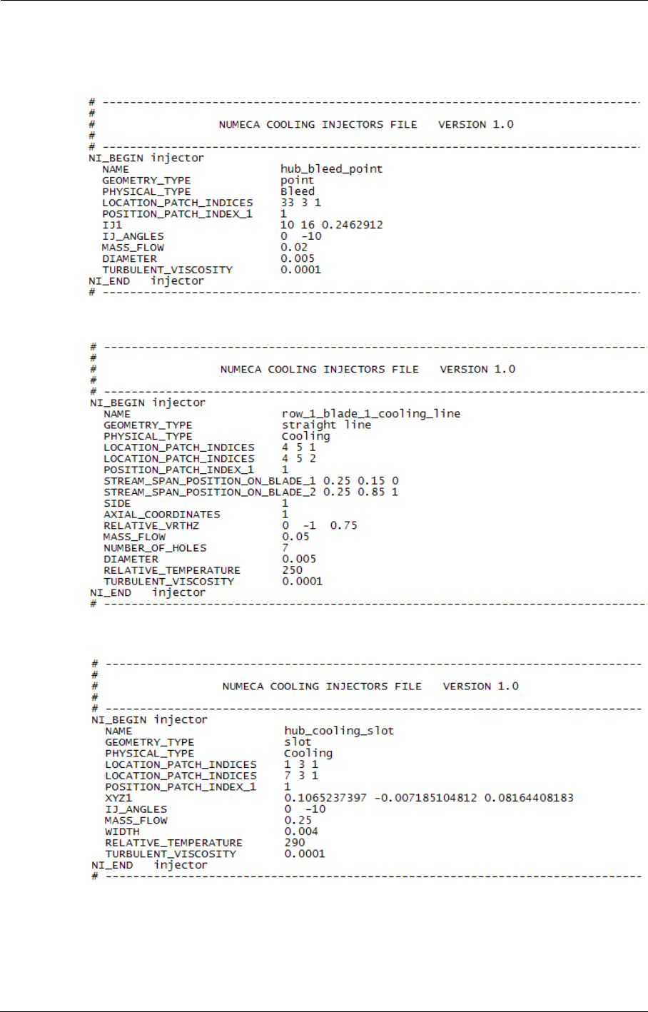
Dedicated Turbomachinery Models Cooling/Bleed
8-58 FINE™/Turbo
8-6.4.2 Examples
Example 1 - Bleed Flow through a Hole defined in Grid Coordinates mode
Example 2 - Cooling Flow through a Line holes defined in Patch Coordinates mode
Example 3 - Cooling Flow through a Slot defined in Cartesian Coordinates mode
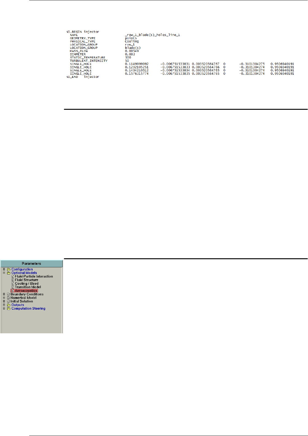
Rigid Motion Dedicated Turbomachinery Models
FINE™/Turbo 8-59
Example 4 - Cooling Flow through the points type of holes
8-7 Rigid Motion
The rigid motion module allows computations in a domain where the solid boundary can move.
Chapter 7-3.2.1 describes the interface and use of the rigid motion module in FINE™/Turbo.
The rigid motion module can be also used in turbomachinery with the rotor/stator interface. The
rotor-stator can be considered only if the interface is located between two stationary solid wall so
that this is not deformed. When the rotor-stator interface is directly connected to a moving surface,
an “adaptative wall” can be considered between the static wall and the moving surface. If the
rotating wall is connected to the static wall by a fictitious wall (simplification of geometry), this
fictitious wall becomes deformable and it can be treated when it belongs to a group named
“Adaptative_wall”.
The main limitations on the rigid motion module with rotor/stator interfaces are as follows:
•no rotor-stator interface with deformation;
•no rotor-stator interface without deformation but located between moving walls;
8-8 Aeroacoustics
Acoustic noise, particularly in the aeronautical field, is of increasing importance in technological
development. The noise emitted by aircraft engines is mainly due to the fan. Sound waves are created
by the rotor and its interactions with the rectifier. In the single-flow turbojet or low bypass ratio
supersonic flight, the jet is the main sound source. Manufacturers must be able to predict the noise
to design quieter engines.
FINE™/Turbo has integrated an Aeroacoustics module, which allows the user to predict the acoustic
response around a turbomachinery component. The method is based on the Ffowcs Williams and
Hawkings (FW-H) equation and its integral solutions (Formulation 1A of Farassat), which replaces
a distributed flow interacting with the surfaces by monopole, dipole, and quadrupole sources
radiating in an undisturbed medium. As first step, only monopole and dipoles sources will be
considered in the current solver. The acoustic signal at the observer is directly computed by
evaluating the surface integrals on the specified surfaces by the user.
Time-accurate solutions of the flow-field variables (CFD sources) are required to evaluate the
surface integrals. Currently, the solutions are coming from the NLH computation. Before launching
the FW-H solver, the user has to launch the flow solver firstly and get a converged solution.
The limitations in the Aeroacoustics module are:
•The flow is subsonic;
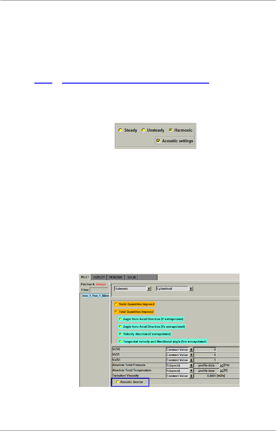
Dedicated Turbomachinery Models Aeroacoustics
8-60 FINE™/Turbo
•The sound is propagated into free space;
•The backward interaction of the acoustic waves on the fluid is neglected;
•The flow viscosity contribution to the noise is neglected.
•No parallel computation ability.
In the next sections, the detailed information on the Aeroacoustics module will be given:
8-8.1 Aeroacoustics in the FINE™/Turbo GUI
In order to access the Aeroacoustics module, the user needs to select the button Acoustic settings in
the Flow Model page, see Figure 8.8.1-46. This button is visible only in case of Harmonic project
configuration. Then the Aeroacoustics page can be accessed under the Optional Models page.
FIGURE 8.8.1-46 The Acoustic settings in the Flow Model page
The user must activate the option Acoustic settings before launching the FINE™/
Turbo flow solver. Otherwise the FW-H solver can not be started.
If a NLH computation was performed by using the FINE™/Turbo flow solver before
v8.9, the user can load the project in FINE™/Turbo v8.9, activate the option Acoustic
settings and restart the computation with zero iteration. Then the FW-H solver can be
started.
In addition, after the button Acoustic settings in the Flow Model page is activated, a tag Acoustic
Source will appear on all the boundary condition pages, see Figure 8.8.1-47. This button allows the
user to select any boundary as an acoustic source (see Chapter 8-8.1.1 to know what can be defined
as an acoustic source).
FIGURE 8.8.1-47 The Acoustic Source option on the Boundary Conditions page
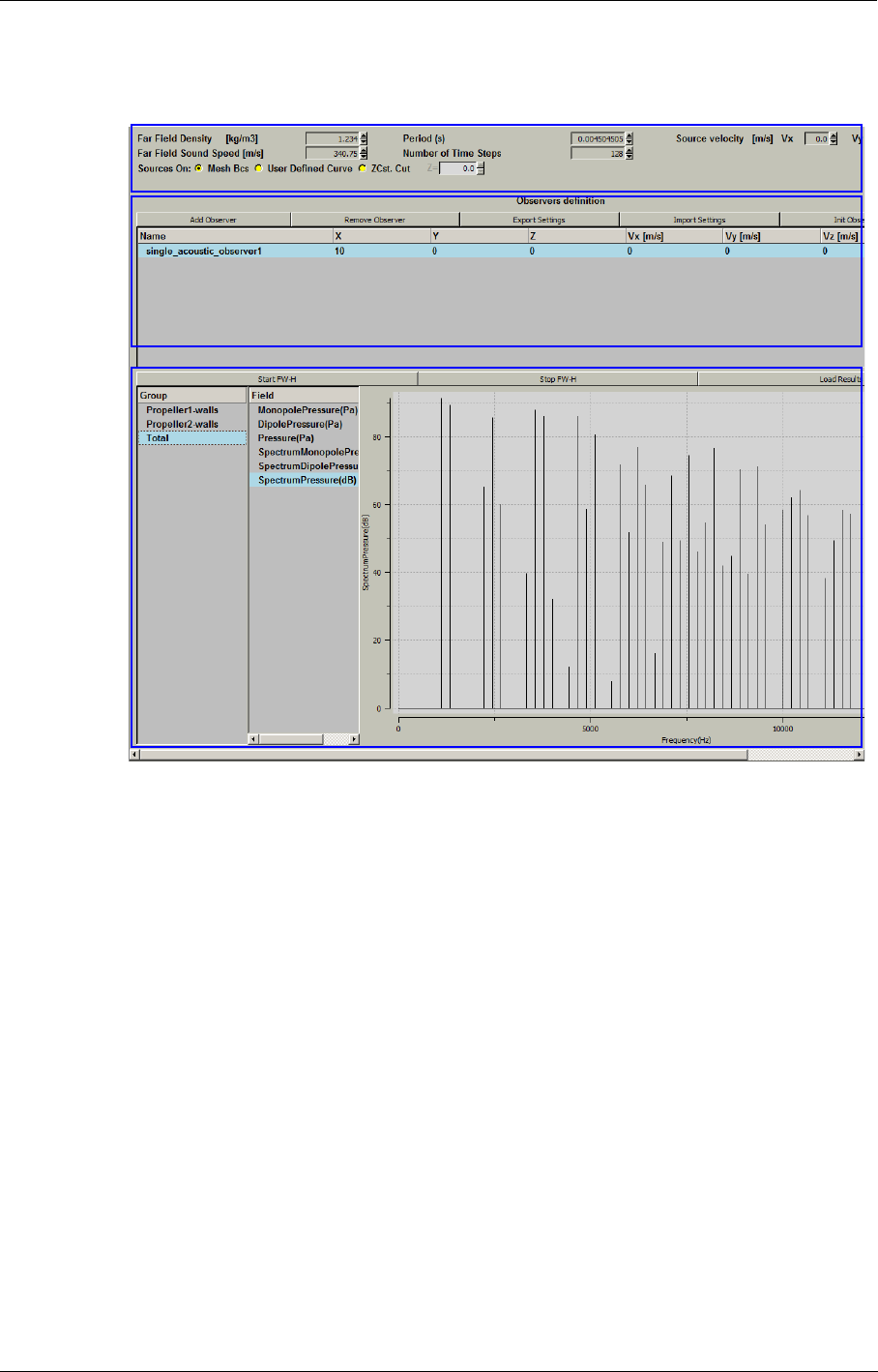
Aeroacoustics Dedicated Turbomachinery Models
FINE™/Turbo 8-61
The GUI for the Aeroacoustics module is shown in Figure 8.8.1-48.
FIGURE 8.8.1-48 Aeroacoustics GUI
The Aeroacoustics page is divided into 3 sections:
8-8.1.1 The global parameters
These parameters are needed by the FW-H solver:
•Far Field Density: the mean density between the source and the observer [kg/m3].
•Far Field Sound Speed: the mean sound speed between the source and the observer [m/s].
•Period: for which the acoustic response must be computed [s].
•Number of Time Steps.
•Sources on: specifies the location of the acoustic source surfaces. The sources are defined as a
cloud of points on a surface with some CFD fields (pressure harmonics, density harmonics,
etc.). Two kinds of sources can be used: solid sources and permeable sources. In FINE™/
Turbo, the user can define the sources on:
—Mesh Bcs: the boundaries of the domain that are meshed and solved by the user. All the
boundaries existing in the Boundary Condition page can be selected as the acoustic source
surface.
(A)
(B)
(C)

Dedicated Turbomachinery Models Aeroacoustics
8-62 FINE™/Turbo
—User Defined Curve: the source can be coming from an external permeable curve defined in
AutoGrid5. A surface of revolution will be created by using the external permeable curve.
Please refer to the AutoGrid5 manual for more information on how to create the permeable
curve.
—ZCst. Cut: the user may specify a constant Z value. Then a cut plane will be created on the
specified Z.
•Source velocity [m/s]: the constant translational velocity imposed to the sources.
8-8.1.2 The observer definition
The button Add Observer can be used to create a new observer. If an observer is selected when add-
ing a new observer, the new observer is a copy of the selected observer. The button Remove Observ-
ers is used to remove all the selected observers from the list. Once the observer has been created,
the user is able to modify its name, its location and its velocity by double clicking on the observer.
Please note, there should be at least one defined observer. Otherwise it is not possible
to launch the FW-H solver.
When multiple observers exist in the list, the user is able to impose the same velocity components
to all observers at once. If selecting one observer and right-clicking on it, a menu will appear and
allow the user to "Set Vx/Vy/Vz of selected to all observers". If selecting several observers and
right-clicking on them, a menu will appear and allow the user to "Set Vx/Vy/Vz of first selected to
all observers".
The buttons Import Settings and Export Settings are used to load or save all the parameters in this
page from/to a file.
8-8.1.3 Launch Solver and Post-processing
When the button Start FW-H is pressed, a new task is created and launched through the task man-
ager. This task calls the FW-H solver with the run file as input. The task manager shows the
progress status of the computation. The button Stop FW-H may be used to kill the running task.
After the FW-H solver has finished the task, the button Load Results can be used to read the .fwh
files and updates the available groups and field lists for selection. Multiple observers and groups
can be selected for visualisation.
8-8.2 Expert Parameters for Aeroacoustics
In the Expert mode, the additional parameters can be specified for the acoustic source surface.
when the sources on Zcst. Cut is selected, the user may select Orientation, which is used to deter-
mine the orientation of the permeable FW-H surface.
The user may change the following settings for the FW-H solver:
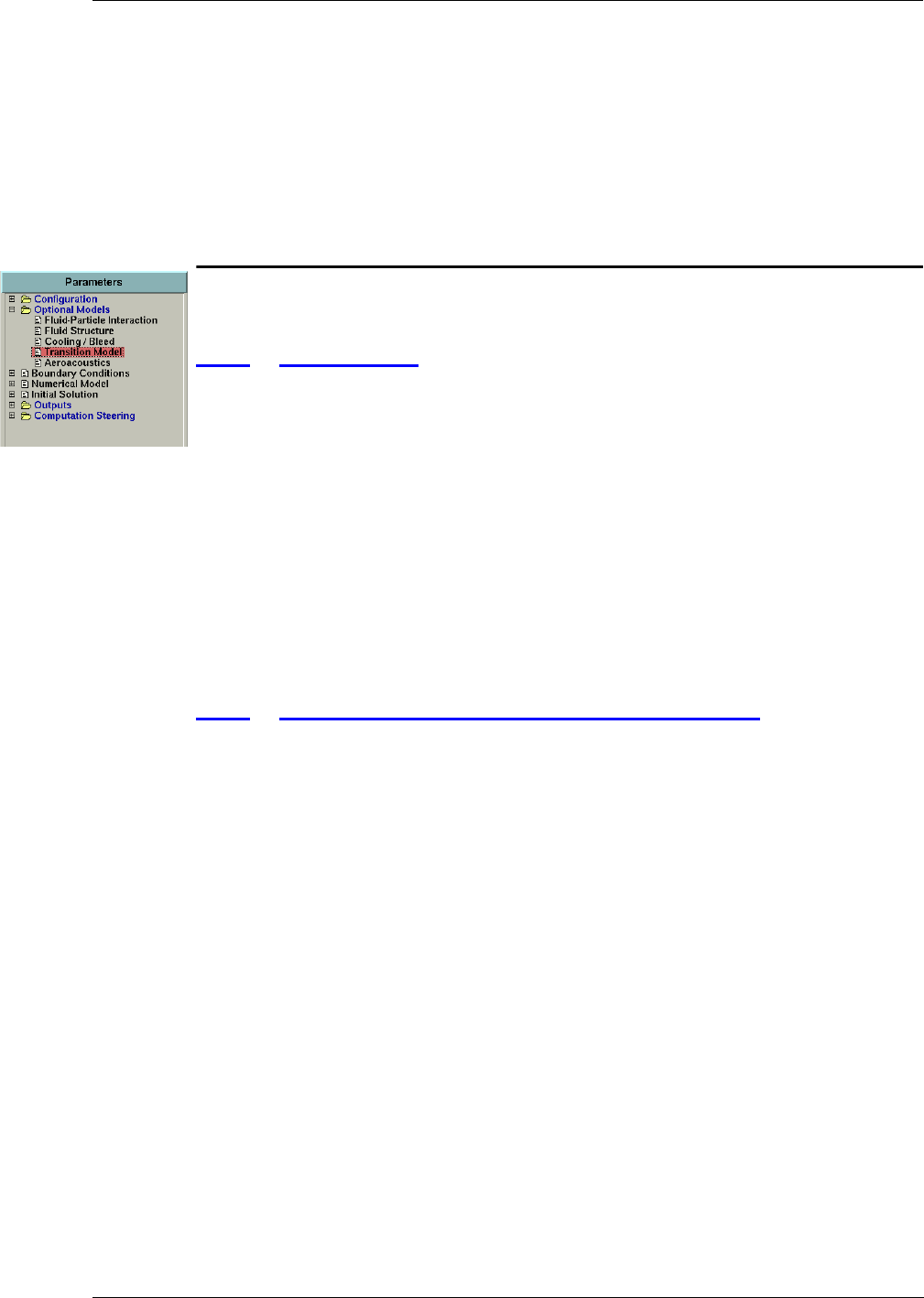
Laminar-Transition Model Dedicated Turbomachinery Models
FINE™/Turbo 8-63
•Number of harmonics: Number of harmonics used in acoustic computations (e.g. if it is set to
0, the mean CFD fields are used as input to the FW-H solver).
•Far Field pressure: the mean pressure between the source and the observer
•Epsilon Newton-Raphson: Level of accuracy that the Newton iterative solver has to reach
before stopping the iterations. This iterative solver is used to evaluate the retarded time.
8-9 Laminar-Transition Model
8-9.1 Introduction
The FINE™/Turbo solver allows the user to perform a laminar-transition simulation in order to take
into account the transition onset at a certain chord distance on a blade pressure and suction sides. The
transition location (transition line in 3D) should be imposed either through a user input or via a
separate guess. These transition terms are activated only when the transition module is used. When
it is not used, the fully turbulent version of the Spalart-Allmaras and Yang-Shih k-epsilon turbulence
model remains unchanged.
In the next sections the following information is given on the Transition Model:
•section 8-9.2 describes how to set up a project involving the Transition Model under the
FINE™/Turbo user environment.
•section 8-9.3 gives a summary of the available expert parameters related to the Transition
model.section
8-9.2 Transition Model in the FINE™/Turbo GUI
The Transition Model can be directly activated from the FINE™/Turbo GUI by opening the Tran-
sition Model page under Optional Models. The layout of the page is shown in Figure 8.9.2-49.
A list of all the blades appears in the left box and the remaining area is divided into two boxes for
suction and pressure side, respectively. Four choices are possible:
—Fully Turbulent
—Fully Laminar
—Forced Transition
—Abu-Ghannam and Shaw (AGS) Model
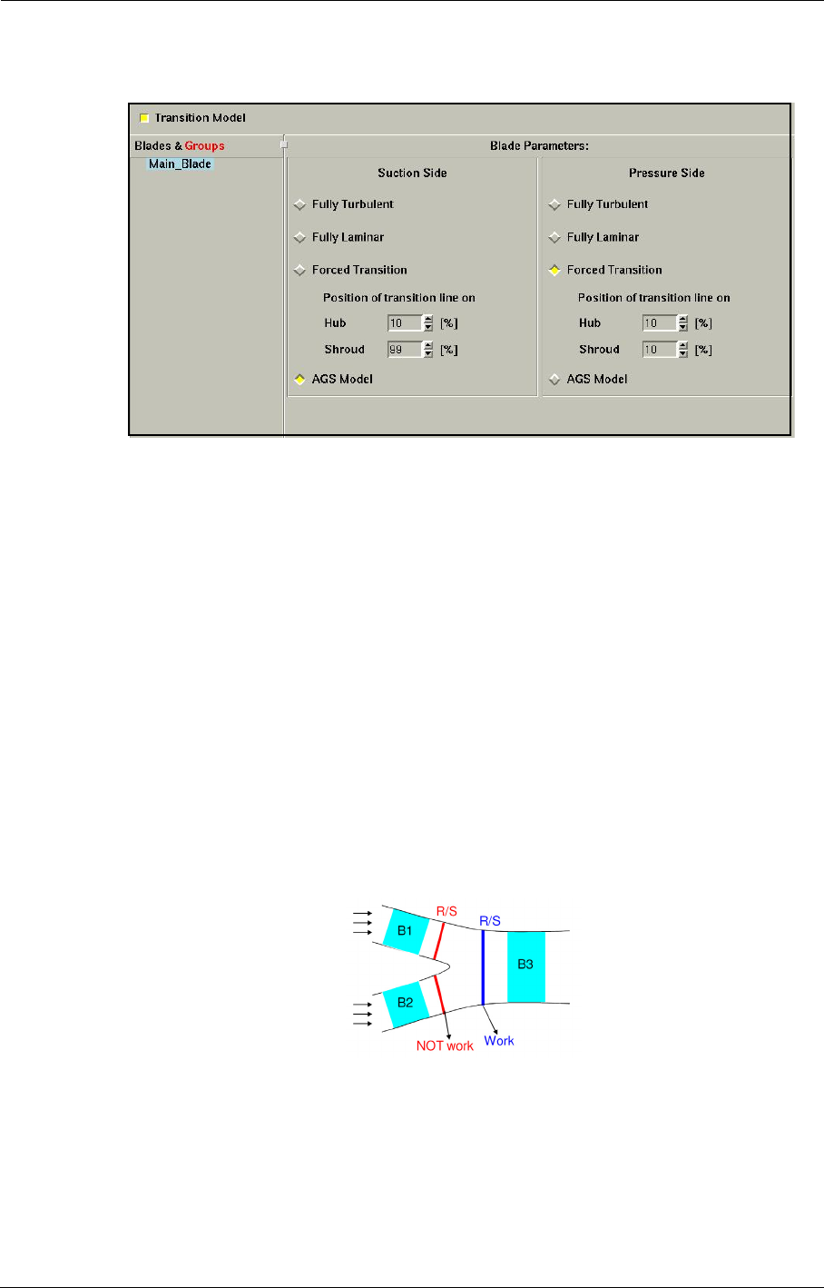
Dedicated Turbomachinery Models Laminar-Transition Model
8-64 FINE™/Turbo
FIGURE 8.9.2-49 Transition Model page in FINE™/Turbo
Furthermore, for Forced Transition, the user has to specify the position of the transition lines on
each side of each blade. It is based on the relative stream-wise position and it is defined as a line on
the blade pressure and/or suction sides from hub to shroud. The user specifies two anchor points
through which a straight line will be built by the solver. It should be noted that only blades are
transitional while wall ends are fully turbulent.
The transition model is only available for the Spalart-Allmaras, Yang-Shih k-ε, k-ω
and SST models using AutoGrid™ mesh.
Rotor/Stator interfaces should be correctly oriented (from upstream to downstream)
and solid walls of the blades should be adiabatic.
For the Abu-Ghannam and Shaw model: only one upstream R/S interface of each
blade is allowed. Furthermore, there are no restrictions on the number of inlets. For
example, the transition model will not work for the Blade3 if positioning the R/S inter-
face to the location indicated by the red lines, as shown in Figure 8.9.2-50.
FIGURE 8.9.2-50 Only one upstream R/S interface directly linked to the blade is allowed
The transition location imposed by the user through the Forced Transition option and
by the AGS Model is only appearing if it has been defined in a turbulent boundary layer.
The AGS model only works for transition from laminar to turbulent boundary layers
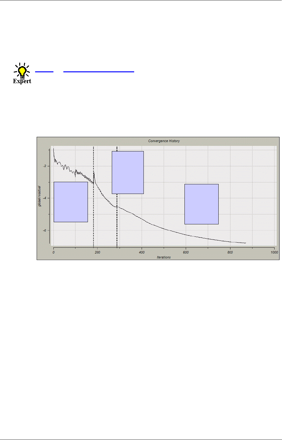
Laminar-Transition Model Dedicated Turbomachinery Models
FINE™/Turbo 8-65
but not to detached turbulent boundary layers. When detached flow is present, you’ll
need to use a forced transition at a certain location.
The intermittency is available on the Outputs/Computed Variables page under the tab Solid data
to visualize the intermittency on solid patches in CFView™.
8-9.3 Expert Parameters
INITRA (integer): control the number of multigrid iterations (default = 100) performed in fully
turbulent after the coarse grid initialization process. Thereafter, the blade pres-
sure side and suction side are identified and the transition line is defined. The
computation pursue for the remaining iterations in transitional mode. The tran-
sition line derived from the Abu-Ghannam and Shaw model is computed at
each iteration.
For starting or restarting a computation in transitional mode from a previous solution
(fully turbulent or in transitional mode) the expert parameter INITRA should be set to 0
(otherwise iterations will be performed in fully turbulent mode).
INTERI (integer): control the type of intermittency distribution (0:binary or 1: from Dhawan and
Narasimah) (default = 0).
INTERL (integer): control the type of location used for forced transition (0: base on arc length or
1: based on axial chord) (default = 0).
FTURBT (real): control the proportion close to the trailing edge that is fully turbulent (default =
0.95).
FTRAST (real): prevents the transition to start in an area defined from the leading edge of the
mesh. The value set is a percentage of the chord upstream of which the transi-
tion is not allowed (by default 0.05: 5%).
KETRAN (Integer):control the terms multiplied by intermittency in the equations of turbulence
model (default=1)
1: transition is activated for production of k
2: transition is activated for production and dissipation of k
Full
MultiGrid
Coarse Grid
Initialization
Transition
Model
MultiGrid
Fully
Turbulent
MultiGrid
Initialization
INITRA
Full
MultiGrid
Coarse Grid
Initialization
Transition
Model
MultiGrid
Fully
Turbulent
MultiGrid
Initialization
INITRA

Dedicated Turbomachinery Models Performance Curve
8-66 FINE™/Turbo
3: transition is activated for production of k and epsilon
BLFACT (real): factor multiplying boundary layer momentum thickness to define distance from
the blade on which the transition model is applied (default=5).
ITRWKI (integer):switches on the wake induced transition model. When activated (ITRWKI set
to 1), the free stream turbulence intensity (defined at the inlet or at the rotor/sta-
tor interface) and the turbulence intensity from the boundary layer edge are
used to define the transition region. When this parameter is not checked, only
the free stream turbulence intensity is used.
8-10 Performance Curve
8-10.1 Introduction
Performance curve is a graphical representation showing the characteristics of a rotating tur-
bomachinary at various operating conditions. For example, the performance curve for a compressor
would include rotor speed for various inlet and outlet pressures versus gas flow rate adjusted for
temperature, density, viscosity, head, and other factors.
The FINE™/Turbo environment provides a dedicated module to create and manage the perform-
ance curve computation in an automatic way. The user imposes the number of the operating points
and the boundary condition. FINE™/Turbo will automatically set-up the computations of the oper-
ating points and give the performance curve.
The next sections will describe the way to set-up and manage the performance curve computation in
more detail.
8-10.2 Performance Curve in the FINE™/Turbo GUI
8-10.2.1 Create and Edit Performance Curve
Before creating a performance curve computation, the user has to create a starting point computa-
tion, such as an operating point at design condition. Then the user needs to set the parameters and
launch the flow solver until obtaining a converged solution. This starting point computation will be
used as the design point to create and set the performance curve computation.
To create a performance curve computation, first select the starting point computation, then click on
the button Create Performance Curve on the Computations subpanel.
A performance curve definition window will appear, see Figure 8.10.2-51.
Here several parameters need to be inputted:
•Rotation Speed: impose the rotation speed for the rotating part in the project.
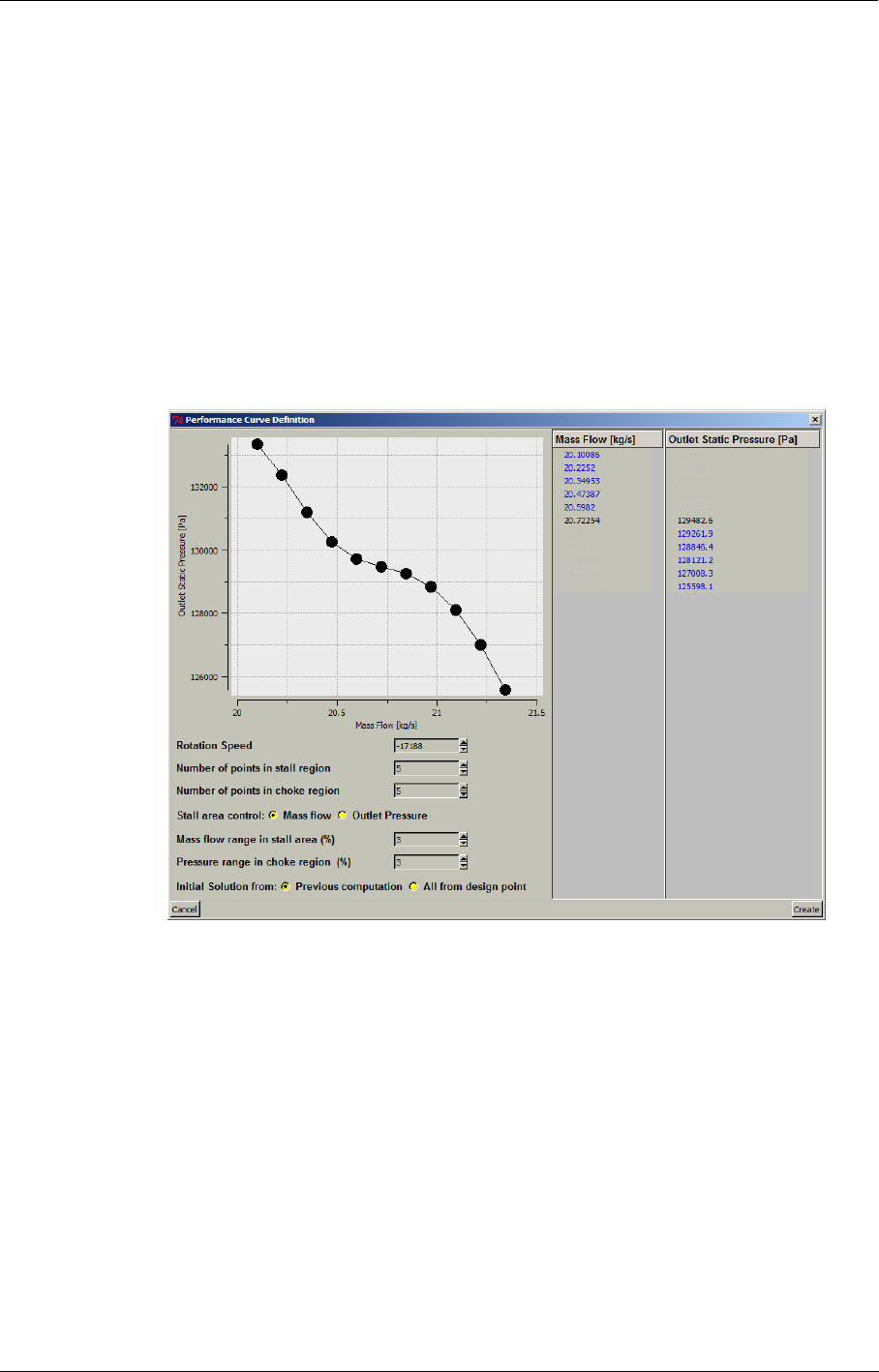
Performance Curve Dedicated Turbomachinery Models
FINE™/Turbo 8-67
•Number of points in stall region: impose the number of the operating points in stall region.
•Number of points in choke region: impose the number of the operating points in choke
region.
•Stall area control: select the type of the outlet boundary condition. The user can specify the
outlet boundary condition with only pressure imposed in both stall and choke regions, or com-
bining mass flow imposed in stall region and pressure imposed in choke region.
•Pressure/Mass flow range in stall region: specify the varying range (%) of the pressure/mass
flow rate at outlet in stall region.
•pressure range in choke region: specify the varying range (%) of the pressure at outlet in
choke region.
•Initial Solution from: by default, the initial solution will be set as a restart from the previous
operating point, except for the design point.
FIGURE 8.10.2-51 Create a performance curve
After clicking on the button Create, multiple sub-computations will be automatically created with
the parameters that the user inputs.
The present implementation is dedicated to compressor.
After its creation, the performance curve may be edited to change the number of points and / or the
mass flow or pressure range. To edit a performance curve, just select the name of the performance
curve and click on the button Edit Performance Curve.
The parameters of each of the automatically generated sub-computations may be separately modi-
fied. The flow solver may be separately started for each sub-computation.
As usual, the sub-computation can be operated through the button New Computation, Rename and
Remove. When a performance curve item is selected in the computations browser, the action will be
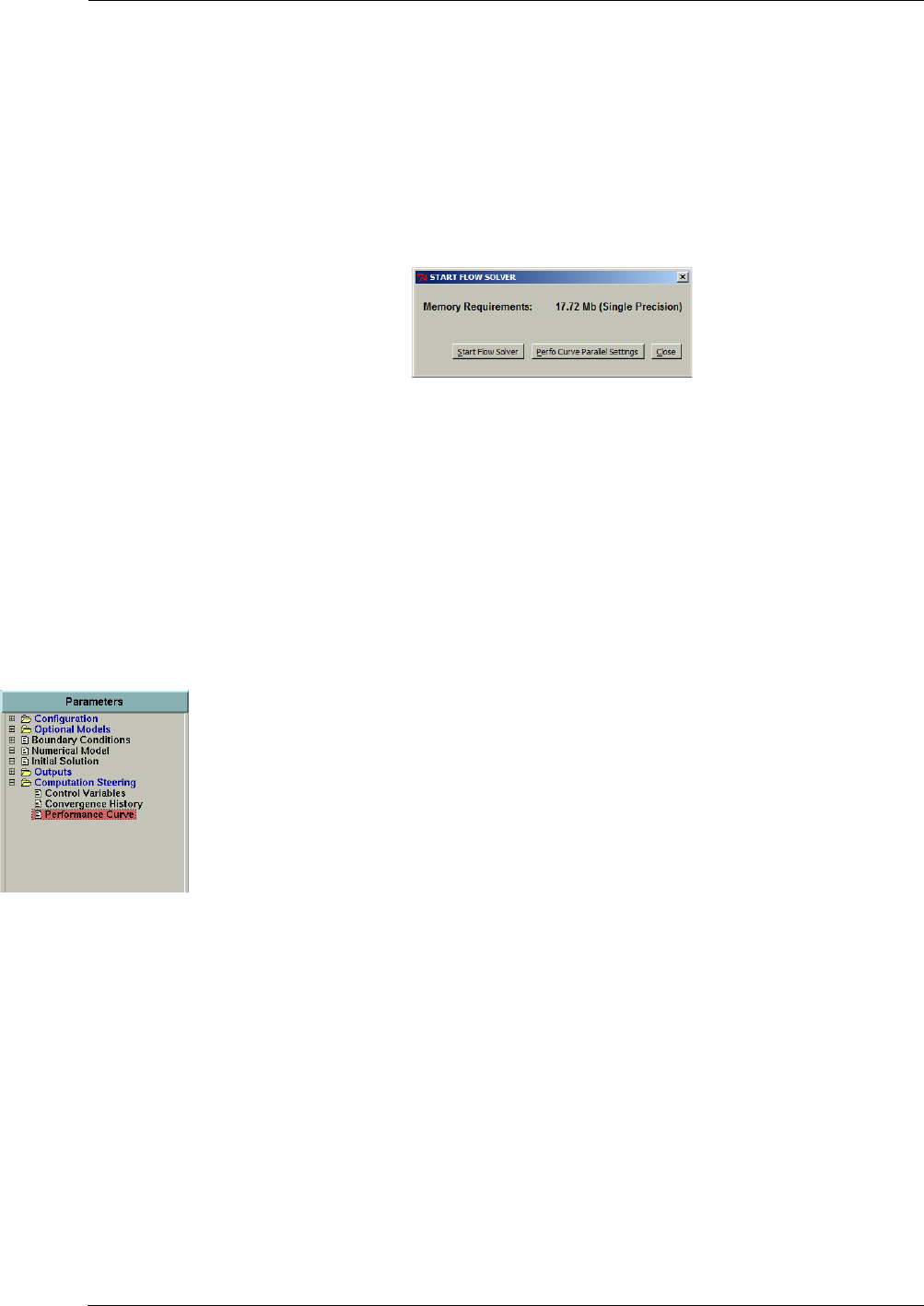
Dedicated Turbomachinery Models Performance Curve
8-68 FINE™/Turbo
applied to all of the subcomputations. The user may change some parameters simultaneously for all
computations.
8-10.2.2 Launch the flow Solver
The performance curve computation can be launched in serial model or in parallel mode. When
selecting a performance curve item and clicking on the button Start Flow Solver, a window will
appear, see Figure 8.10.2-52.
FIGURE 8.10.2-52 Launch the flow solver for performance curve computation
Selecting Start Flow Solver will launch all the sub-computations in serial mode. Selecting Perfo
Curve Parallel Settings, FINE™/Turbo will automatically switch to TaskManager module and cre-
ate a new task with many subtasks for all the sub-computations. A Parallel settings window will
appear. The user can set the number of process and other parallel settings, which is applied to all
subtasks.
If a performance curve has been started and afterwards killed or suspended, the user may choose
Continue from the Solver menu in order to continue computations from the first not finished sub-
computation. The Continue option may also be used in case that the user adds new sub-computa-
tions to the existing performance curve in order to compute only the new sub-computations.
8-10.2.3 Output
The performance curve outputs are available in a separate page, see Figure 8.10.2-53. Both pressure
ratio and efficiency can be plotted. The user can also input the experimental data for comparison or
export the results. If select Export to file, a data file with the name <Performance curve
name>_pressureratio_efficiency.dat will be automatically created in the project folder. The option
User Axis Limit can be used to specify the range of the abscissa and ordinate.
The file format used to imput the experimental data is:
•Line 1: Three strings defining the name of the variables.
•The next lines contain the variable values of each point.
Example 1:
Mass Flow Pressure Ratio Efficiency
10.3443179130554 1.30143475532532 0.839340686798096
10.5739312171936 1.29300808906555 0.844243705272675
10.8034386634827 1.28314805030823 0.847144782543182
11.0327978134155 1.27196598052979 0.848022699356079
11.2620959281921 1.25955402851105 0.846824049949646
......
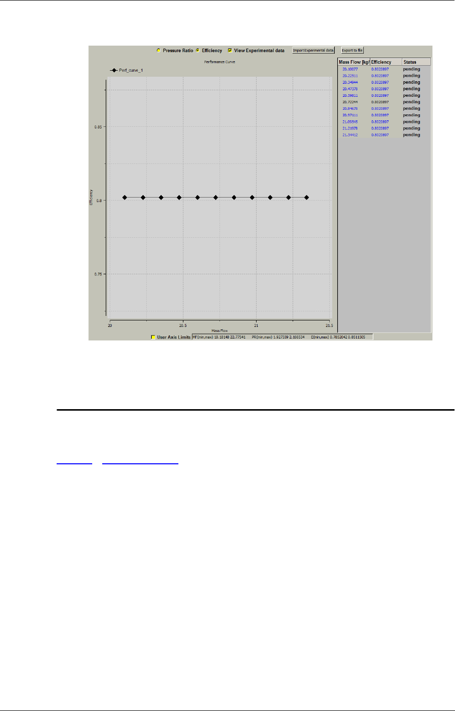
SubProject Management Dedicated Turbomachinery Models
FINE™/Turbo 8-69
FIGURE 8.10.2-53 Performance curve output
8-11 SubProject Management
8-11.1 Introduction
The FINE™/Turbo environment allows the partial treatment of multistage turbomachinery projects.
Turbomachinery applications can be naturally decomposed into several domains, e.g. rotor, stator...
This natural decomposition can also be performed in FINE™/Turbo, by means of a so-called Sub-
Project.
After performing a first computation on the full turbomachine (Main Project), the user can create
SubProjects, containing only part of the machine. This allows a fast and easy optimization of the
geometry of each row. Afterwards, the results obtained on part of the machine can be merged
together again with the full turbomachine.
The access to the SubProject module requires a special license feature. Please contact our local
sales or support office for more information about how to obtain a license.
The next sections will describe the way to set-up and control the SubProjects in more detail.
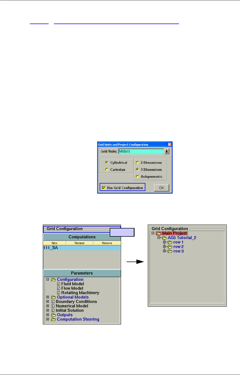
Dedicated Turbomachinery Models SubProject Management
8-70 FINE™/Turbo
8-11.2 Set-up of SubProjects in FINE™/Turbo
8-11.2.1 Grid Requirements
The SubProject module is available for projects of which the mesh has been created with IGG™ or
AutoGrid™. Following requirements have to be respected when generating the mesh:
•Butterfly blocks in IGG™ is not compatible with sub-project management.
•All rotor-stator interfaces have to be defined in the absolute way. This can be defined in the
rotor-stator properties dialog box in AutoGrid™.
•The final mesh has to be saved in the _mesh directory of the main project.
8-11.2.2 Create SubProjects
Once the mesh of the main project has been created, the main project has to be set-up in the
FINE™/Turbo GUI. After creating the project and when the mesh is loaded for the first time, the
user has to activate Use Grid Configuration in the Grid Units and Project Configuration dialog
box, see Figure 8.11.2-54. When the mesh is loaded, the Grid Configuration subpad will appear in
the interface, see Figure 8.11.2-55.
FIGURE 8.11.2-54 Use Grid Configuration
FIGURE 8.11.2-55 Grid Configuration Subpad in the FINE™/Turbo GUI
Left-Click
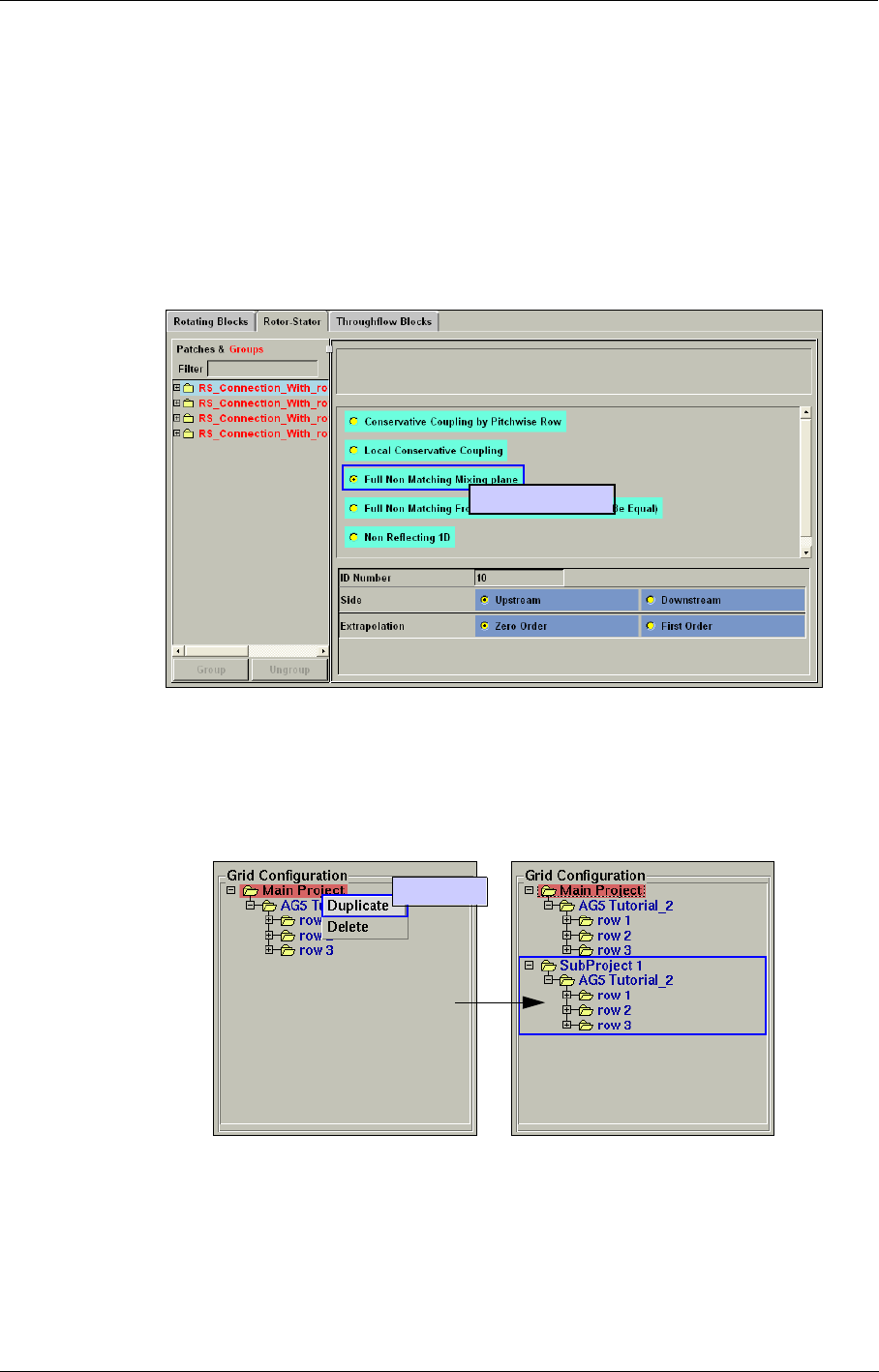
SubProject Management Dedicated Turbomachinery Models
FINE™/Turbo 8-71
Before creating a SubProject, the main project has to be executed first. The final solution of the
main project will be used as the initial solution for the SubProjects. Therefore the main project
should be run until satisfactory convergence is reached.
In the main project, all rotor-stator interfaces have to be defined as Full Non Match-
ing Mixing Plane. The type of several rotor-stator interfaces can be changed simultane-
ously by selecting one rotor-stator interface, hold the <Shift> button and left-click on the
desired type of rotor-stator interface, see Figure 8.11.2-56. All settings, such as the ID
Number, will be kept.
FIGURE 8.11.2-56 Rotor-Stator Interface Settings
After completion of the main project, a SubProject can be created in the following way:
•Go to the Grid Configuration subpad.
•Right-click on Main Project and select Duplicate. A new SubProject is created.
FIGURE 8.11.2-57 Create SubProject
•By left-clicking and holding the <Ctrl> button, several rows of the newly created SubProject
can be selected.
•Right-click allows to delete the selected rows from the SubProject, see Figure 8.11.2-58.
<Shift> - Left-Click
Right-Click
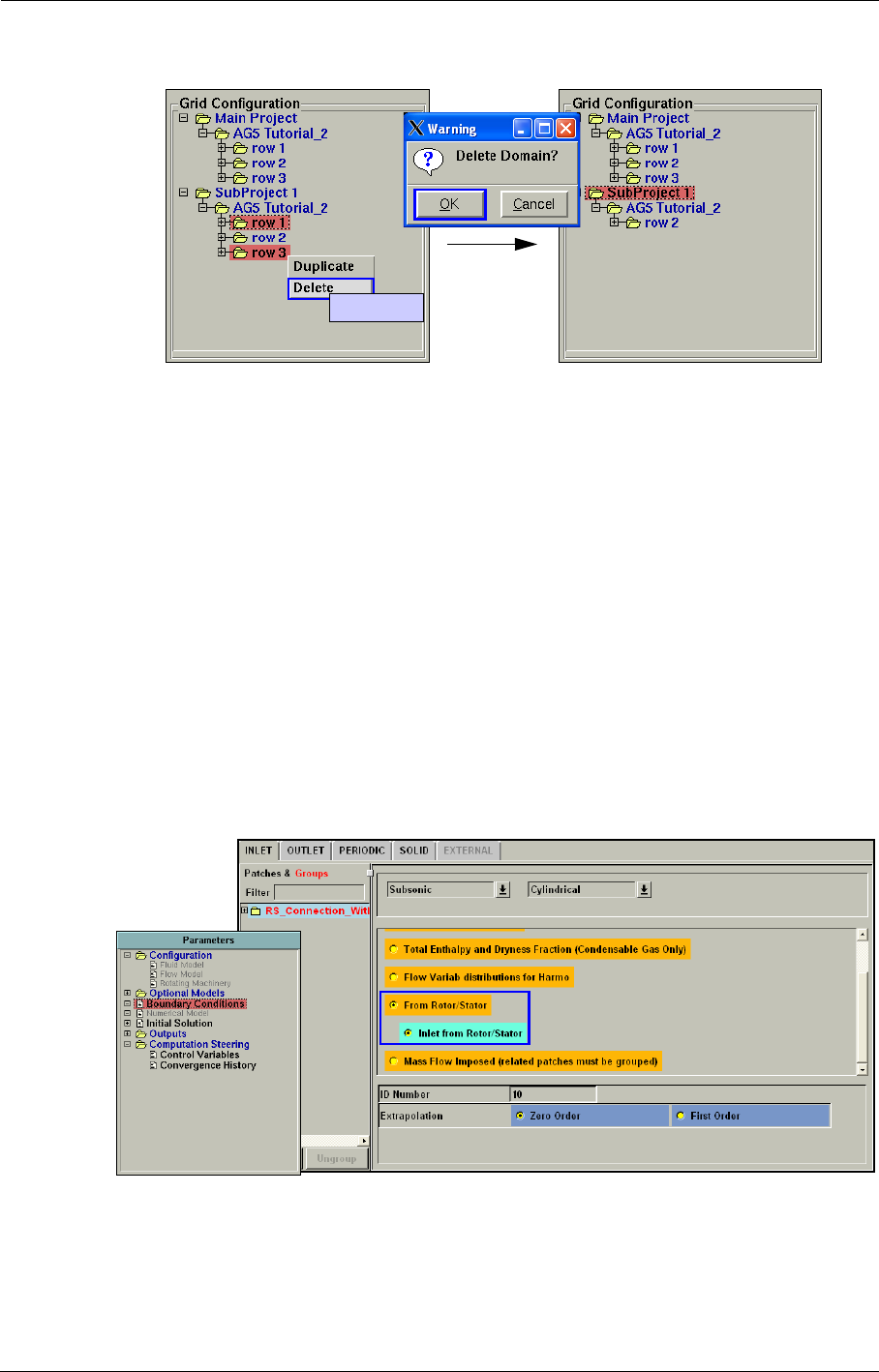
Dedicated Turbomachinery Models SubProject Management
8-72 FINE™/Turbo
FIGURE 8.11.2-58 Delete Rows from SubProject
The settings for the SubProject are copied from the main project and adjusted if necessary.
•Boundary Conditions: Settings for in- and outlet are automatically changed if necessary. A
special boundary condition From Rotor/Stator has been created. This will transfer the quanti-
ties from the rotor-stator of the main project as in- and/or outlet condition.
The From Rotor/Stator boundary condition is only available for SubProjects and is
set by the FINE™/Turbo GUI automatically. These settings should not be modified by
the user.
•Initial Solution: The initial solution is set automatically to From File. The solution of the main
project will be used as an initial solution.
•Control Variables: The settings are identical to the main project.
Settings that are changed manually by the user when a SubProject is selected, e.g.
number of iterations, will be transferred to the main project.
FIGURE 8.11.2-59 Boundary Conditions for SubProject
The SubProject can be executed in the same way as the main project. The computation will con-
tinue until the maximum number of iterations is reached or the convergence criteria is satisfied.
Right-Click
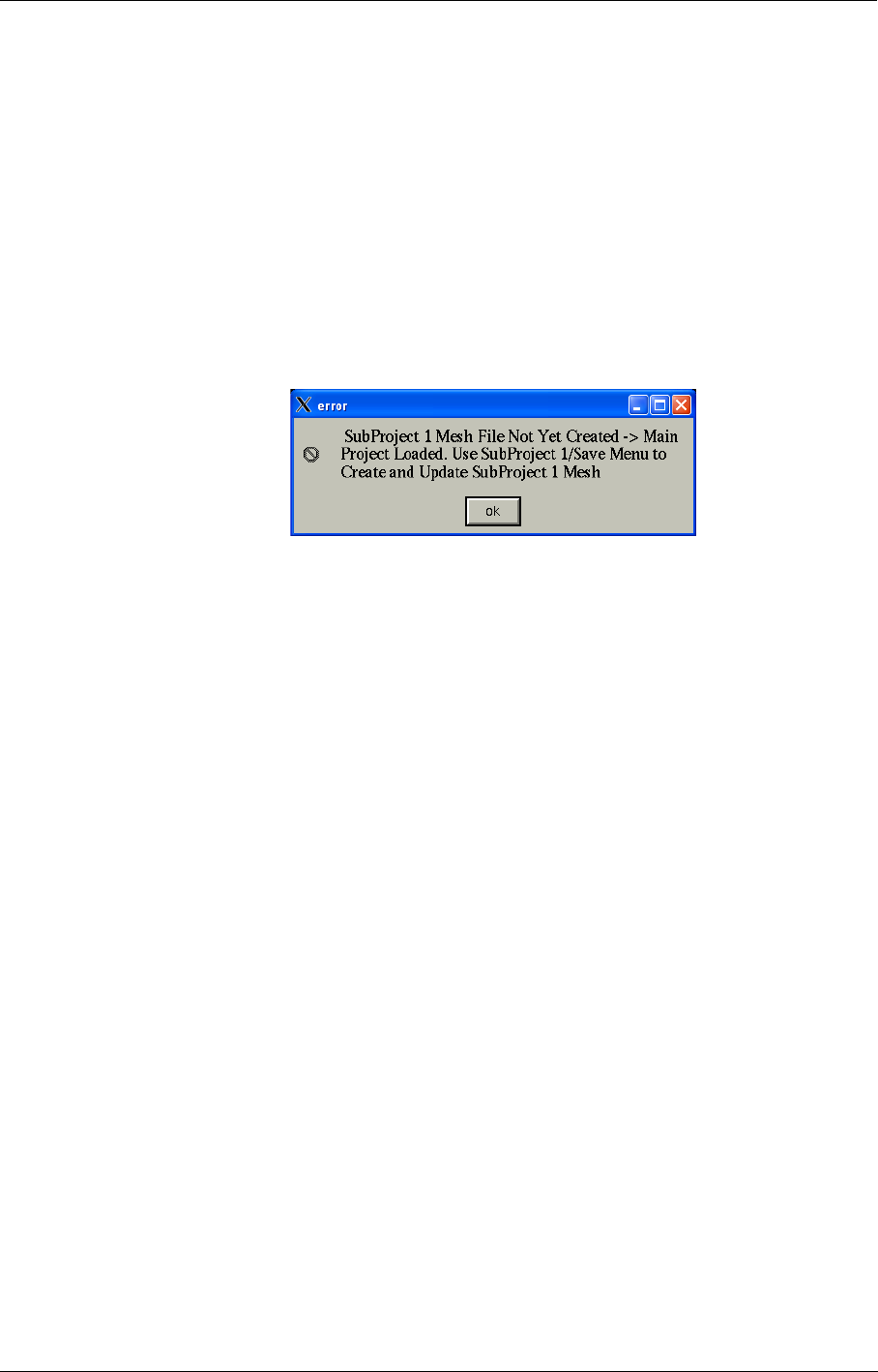
SubProject Management Dedicated Turbomachinery Models
FINE™/Turbo 8-73
8-11.2.3 Modify & Merge SubProjects
The SubProject module allows the user to change the geometry of the subproject. A computation
can be done on the changed geometry, before inserting it back in the main project.
a) Modify Geometry
The geometry can be modified in following way:
•Select the SubProject which contains the row of which the geometry needs to be changed
•Switch to AutoGrid™ by using the Modules menu.
If the mesh of the subproject has not been created yet, a warning message will appear
informing the user that the mesh of the main project will be loaded.
•Before being able to modify the geometry of the SubProject, the mesh of the SubProject has to
be saved separately. More information on this subject, can be found in the Grid Configura-
tion section of the AutoGrid™ user manual.
Only the geometry of the subproject can be modified. The topology of the mesh and
the number of grid points have to be kept equal to the main project.
•After generating and saving the mesh of the SubProject, switch back to the FINE™/Turbo
GUI by using the Modules menu. AutoGrid™ automatically saves the mesh of the SubProject
in a separate folder in the _mesh directory. More details can be found in section 8-11.2.4.
•The mesh of the SubProject will be automatically linked to the computation.
The computation of the modified SubProject can be launched in the exact same way as the main
project.
b) Merge SubProjects
When the computation of the SubProject is finished successfully, the modified geometry can be
transferred to the main project. This is done by means of a merge process. The rows of which the
geometry was modified in the SubProject, will replace those rows in the main project. Following
procedure has to be followed:
•Select the main project from the Grid Configuration subpad and switch to AutoGrid™.
•Execute the Merge process in AutoGrid™, more information can be found in the Grid Con-
figuration section of the AutoGrid™ user manual. When the merge process is completed,
switch back to the FINE™/Turbo GUI. AutoGrid™ automatically saves the mesh of the
merged project in a separate folder in the _mesh directory. More details can be found in section
8-11.2.4.
•The merged project is now available from the Grid Configuration subpad in FINE™/Turbo.
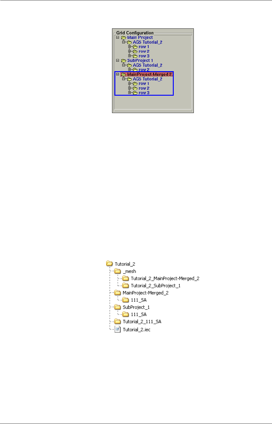
Dedicated Turbomachinery Models SubProject Management
8-74 FINE™/Turbo
FIGURE 8.11.2-60 Merged Project in Grid Configuration Subpad
The merged project will behave in the same way as a SubProject. The computation settings are
transferred from the main project, and adapted automatically if necessary.
8-11.2.4 File Structure
The files generated by the SubProject module are stored in following way (Figure 8.11.2-61):
•The mesh of the main project is stored in the _mesh directory, located in the project directory.
•The computations of the main project are stored in the project directory, with name
<project_name>_<computation_name>
•The mesh of a SubProject is stored in a separate folder in the _mesh directory, with name
<project_name>_<subproject_name>
•The results of the computations of a SubProject are stored separately for every SubProject in
the project directory. The name of the directory is equal to <subproject_name>. In every Sub-
Project directory, the results of each computation are saved separately.
FIGURE 8.11.2-61 SubProject File Structure
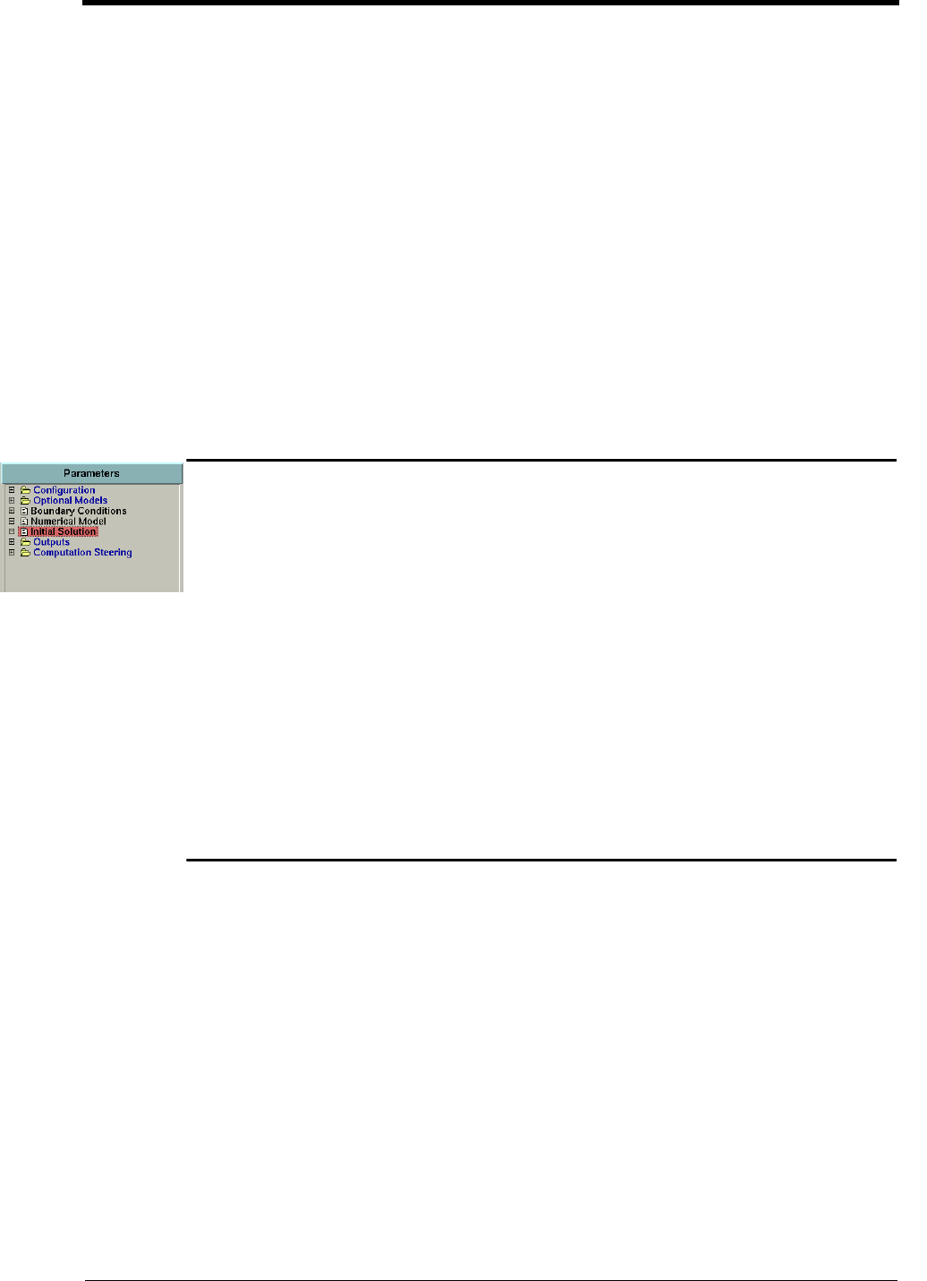
FINE™/Turbo 9-1
CHAPTER 9: Initial Solution
9-1 Overview
FINE™/Turbo provides the possibility to start a computation from an initial solution. The follow-
ing initial solution types are available:
•constant values,
•from file,
•for turbomachinery,
•from throughflow.
Each of these types is described in the next sections.
FINE™/Turbo allows to define a different initial solution type for each block or group of blocks.
Such a block dependent initial solution provides more flexibility in the restart of previously com-
puted solutions. The next section describes how to set up a block dependent solution.
9-2 Block Dependent Initial Solution
This procedure permits to initiate the calculation of some of the blocks with the results of a previ-
ous calculation, whereas the other blocks are started from a uniform flow. Another possibility is to
initiate one new calculation with the results of several previous calculations. This is for instance the
case if a multistage turbomachinery calculation is preceded by the calculation of the separate
stages.
The flow solver can start from files resulting from calculations performed on different grid levels.
Only the grid levels that are used in the multigrid cycle are considered here. For instance, a compu-
tation of a three-stage turbine can start from three solutions for each stage, each one on a different
grid level.
Furthermore, the full multigrid cycle is automatically removed when at least one file is provided on
the finest grid level.
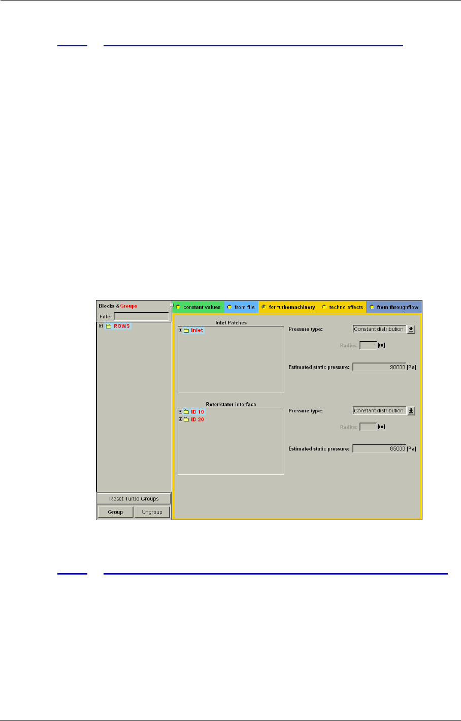
Initial Solution Block Dependent Initial Solution
9-2 FINE™/Turbo
9-2.1 How to Define a Block Dependent Initial Solution
The Initial Solution page is divided in two parts. On the left, a tree displays the structure of the
groups of blocks. On the right, five ratio buttons allow the user to choose the type of initial solution:
constant values, restart from a solution file, turbomachinery oriented, technological effect (AutoG-
rid™ effects) or restart from a throughflow file. At the bottom three buttons allow to modify the
group(s). It is possible to create new groups of blocks in the same way as for the groups of patches
on the boundary conditions page (see section 5-2). Different initial solutions can be assigned to
these groups of blocks. The Reset Turbo Groups button allows to retrieve the default grouping pro-
posed by AutoGrid™.
Two defaults are available depending on the mesh and the application type:
•The first one is dedicated to turbomachinery applications, meshed by AutoGrid™. The Tur-
bomachinery groups are automatically detected and proposed in the interface. These groups
are defined by the different rows (group named "ROWS") and the technological effects. The
static pressure has to be specified at the main inlet and at the rotor-stator interfaces. If the user
modifies the groups, clicking on the button Reset Turbo Groups can restore the default tur-
bomachinery grouping.
•The second default is general. All the blocks are grouped in one group named "MESH" and
constant values are selected. In the constant values page, the toggle option Cylindrical is set
on.
FIGURE 9.2.1-1 Initial Solution default settings when loading AutoGrid™ mesh
9-2.2 Examples for the use of Block Dependent Initial Solution
The block dependent initial solution is helpful in many industrial cases. The following are two sce-
narios in which this capability is very useful:
1. A solution has been calculated for a turbine including 10 stages. A new stage is added. Now the
turbine has 11 stages. The designer does not want to begin a computation from scratch for the
turbine with 11 stages. He can take advantage of the solution that has been found for the 10 first
stages. The new computation will contain one group with the 10 stages and one group with the
last stage. The first group will be assigned to a from file initial solution and the second group
can be assigned to another type of initial solution.

Initial Solution Defined by Constant Values Initial Solution
FINE™/Turbo 9-3
2. A turbine includes 10 stages. Even with the turbomachinery-oriented initial solution, the code
does not succeed to converge properly. The designer could split the turbine in several parts and
calculate the solution for each of these parts. Then a global project is created. In the Initial
Solution page, a from file initial solution is assigned to each part of the project. The computa-
tion will have a far better chance to succeed.
9-3 Initial Solution Defined by Constant Values
When selecting constant values on the Initial Solutions page, the user can modify the physical
values used for the initial solution on the page. The physical values are uniformly used as initial
solution all over the selected group of blocks, except on the boundaries. The variables for which ini-
tial values need to be specified are the static pressure, the static temperature, the velocity compo-
nents and the turbulence-based variables k and ε, if a k-ε, k-ω or v2-f turbulence model is used.
Note that the velocity components specified by the user are the Cartesian (cylindrical) ones for a
Cartesian (cylindrical) case.
Flow Direction: the lower part of the page allows for a further control of the initial field. First, for
both Cartesian and cylindrical projects, the velocity direction can be fitted along the I, J or K mesh
lines. The reverse option determines whether the velocity vectors will point in the I (J or K) increas-
ing or decreasing direction. By default, no specific velocity direction is set and the input box is set
to None.
Velocity Fitting: for the cylindrical projects only, an option for the fitting method can be chosen.
The first option fits , the meridional velocity (defined as ), and uses to set the
azimuthal absolute velocity. The second option fits (default), the relative velocity, to the mesh
lines.
Pressure Field: for the cylindrical projects only, it is also possible to act on the initial pressure
field. To this end, two options are available: constant pressure field (default) and a radial equilib-
rium pressure gradient. In a rotational machinery for instance, a radial equilibrium pressure gradient
is often closer to the physics than a constant field. The radial equilibrium factor allows to adjust the
influence of the pressure gradient (its default value is 1.0).
9-4 Initial Solution from File
9-4.1 General Restart Procedure
To continue on the result of a previous computation the user must simply select the solution. Click-
ing on the Open Browser button will open a File Chooser window to select the ".run" (or ".cgns")
file of a computation.
To restart from a solution the computation definition file with extension ".run" is not
sufficient. It is required that the solution file with extension ".cgns" is present, which
contains all the saved and requested quantities.
An initial solution from file can be used only for computations that have the same
vm
vmvr
2vz
2
+=
vθ
w
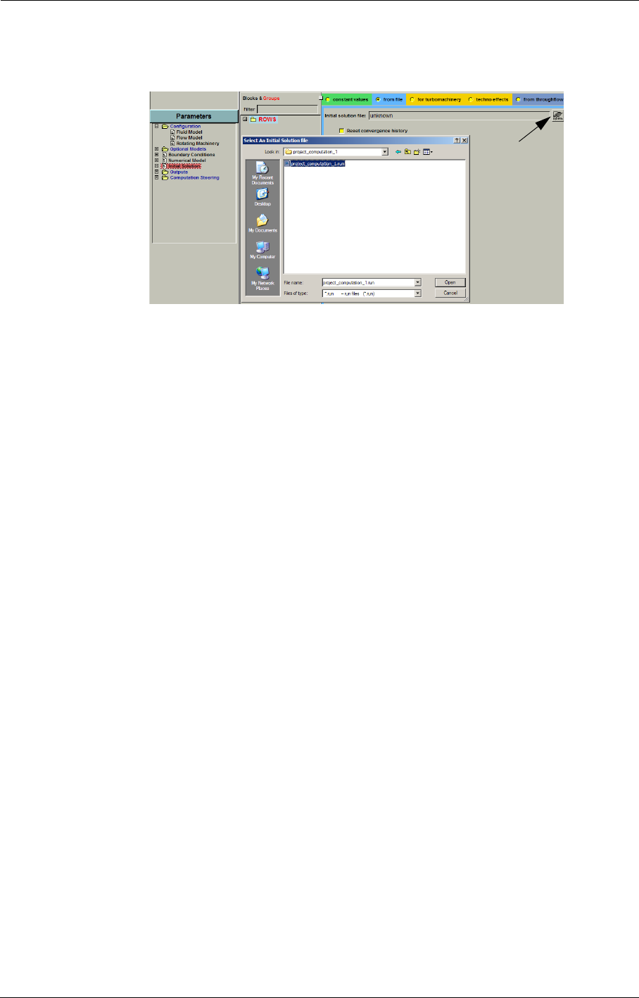
Initial Solution Initial Solution from File
9-4 FINE™/Turbo
topology: same blocks and same grid points distribution.
FIGURE 9.4.1-2 Restarting from a file
The option Reset convergence history can be activated. When activating this option the ".res" file,
which contains all the residuals from the previous computation, will be erased. The new residuals
will be calculated with respect to the first iteration of the new computation. If the from file solution
is already very close to the exact solution, the normalized residuals will decrease slowly, because
the starting state is already a good approximation of the solution.
By default, the option Reset convergence history is deactivated. In this case, the new residuals are
appended to the ".res" file and are calculated with respect to the first iteration of the old computa-
tion. In order to keep the convergence history, the following limitations must be satisfied:
•All the blocks in the Initial Solution page must be grouped in only one group. If several
groups of blocks exist, the option is disabled and automatically the convergence history is
reset.
•If the ".run" and ".cgns" files (initial solution) do not belong to the active computation, the
".res" file located in the initial solution folder must be copied to the active computation folder.
Otherwise, the option Reset convergence history is activated automatically.
For example, perform the following steps: (1) Compute a solution; (2) Create a new computa-
tion; (3) In this new computation, select a from file initial solution and choose the computed
solution in step (1). The Reset convergence history option will be activated automatically,
even though the new computation will start from a previous solution. If the user wants to keep
the convergence history in the new computation, the user has to copy the ".res" file from the
old computation directory to the new computation directory and to rename it with the name of
the new computation.
•If the ".run" and ".cgns" files (initial solution) do not belong to the active computation, the
".steering" and ".steering.binary" files located in the initial solution folder should be copied to
the active computation folder. Otherwise, the convergence history of the global residual before
restart will be lost. Note, the user must close the FINE™/Turbo interface before copying the
".steering" and ".steering.binary" files.
As the initial pressure and temperature fields are block dependent, discontinuities in
these quantities can be present at block connections. The flow solver could have difficul-
ties to converge in such a case. Therefore boundary conditions should be carefully
checked in order to avoid any large discontinuities at block connections.
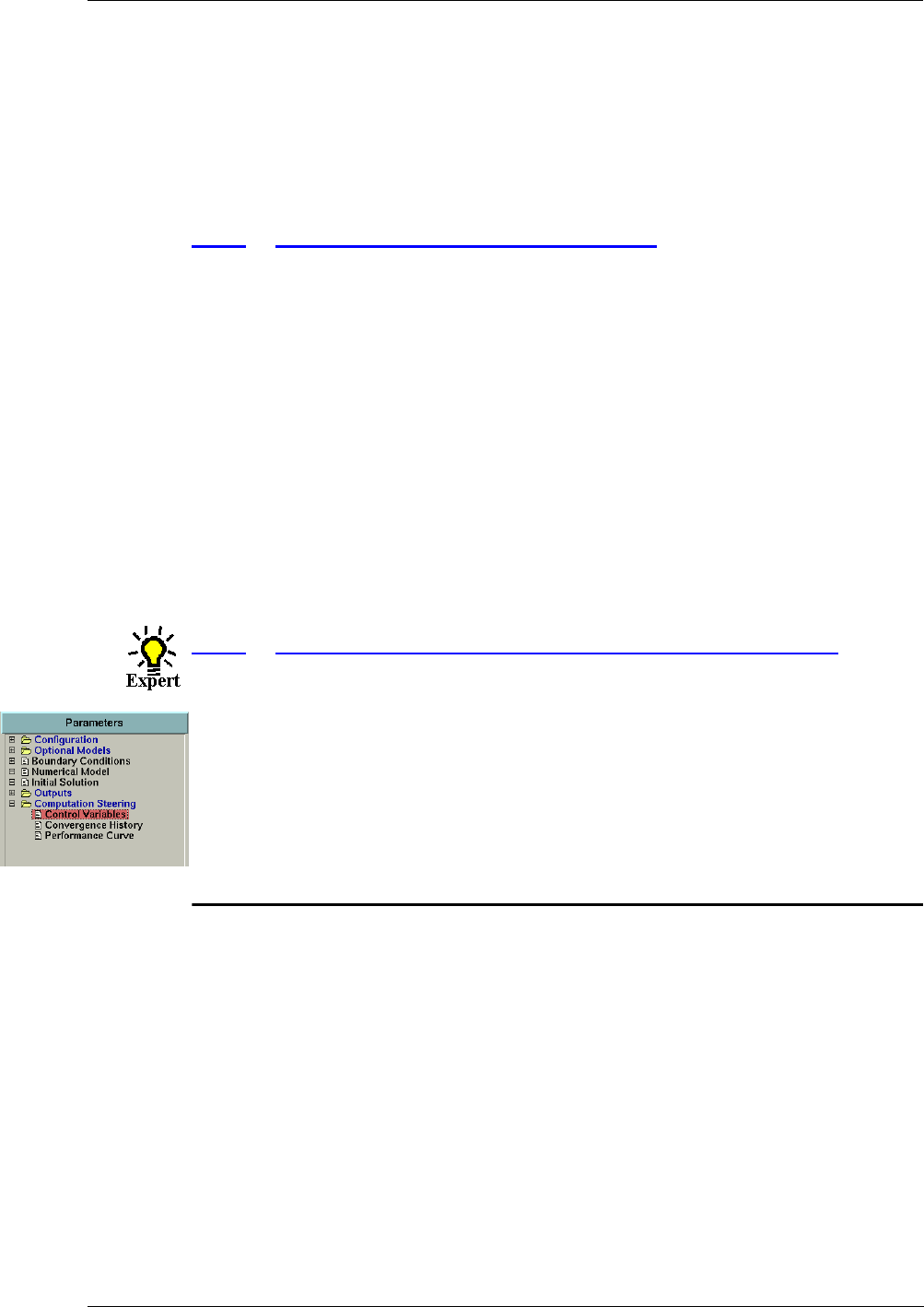
Initial Solution for Turbomachinery Initial Solution
FINE™/Turbo 9-5
The flow solver can start from files resulting from calculations performed on different grid levels.
Only the grid levels that are used in the multigrid cycle are considered here. For instance, a compu-
tation of a three-stage turbine on 0/0/0 with 3 grid levels can start from three solutions for each
stage, each one on a different grid level (0/0/0, 1/1/1, and 2/2/2). Furthermore, the full multigrid
cycle is automatically removed by the flow solver when at least one file is provided on the finest
grid level.
9-4.2 Restart in Unsteady Computations
To allow a second order restart for unsteady computations, it is necessary to set in the Control Var-
iables page Multiple Files in the Output Files. This parameter allows to have multiple output files:
for each saved time step also the solution of the previous time step is saved.
To perform a second order restart for an unsteady computation, select from file in the Initial Solu-
tion page. Using the File Chooser select the solution file with extension ".cgns" at a certain time
step "ti" ("_ti.cgns"). The FINE™/Turbo solver will automatically find the solution of the previous
time step if present ("_ti-1.cgns"). If the FINE™/Turbo solver can not find the solution of the previ-
ous time step a message will appear in the Task Manager to indicate that a first order restart will be
performed.
Note, in order to perform a second order restart for an unsteady computation, the
option Reset convergence history MUST be deactivated. Otherwise only a first order
restart will be applied automatically. Please refer to Chapter 9-4.1 on how to deactivate
the option Reset convergence history.
9-4.3 Expert Parameters for an Initial Solution from File
There is no current limitation to start a k-ε, k-ω or v2-f computation from a Baldwin-Lomax solu-
tion. In this case, the turbulent quantities are estimated from the friction velocity if the expert
parameter INIKE is set to 2 (default value) or from the turbulent viscosity field μt if INIKE = 1. In
the latter case, the turbulent viscosity is initialized or read from file depending on the value of the
expert parameter IMTFIL (default value IMTFIL = 0 to initialized μt or IMTFIL = 2 to read μt from
file).
9-5 Initial Solution for Turbomachinery
The initial solution for turbomachinery is dedicated to the cylindrical rotating machinery. This type
of initial solution respects the inlet and outlet boundary conditions and assumes a constant rothalpy
along axisymmetric stream surfaces. In addition, the velocity field is automatically aligned with the
blade passage.
The initial solution for turbomachinery is not available when imposing supersonic
inlet boundary condition.
The initial solution for turbomachinery is not available for bypass configuration. In a
bypass configuration, the flow solver considers the minimum outlet pressure found on
the both outlets in order to set the initial solution for turbomachinery. This can lead to a
bad initial solution and a crash of the flow solver in few iterations.
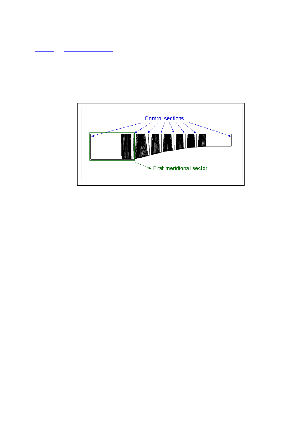
Initial Solution Initial Solution for Turbomachinery
9-6 FINE™/Turbo
2D profiles are not supported when using the initial solution for turbomachinery.
9-5.1 Methodology
The initial solution for turbomachinery is computed on the 2D meridional view divided into differ-
ent parts named "meridional sectors". The control sections of the meridional mesh in AutoGrid™
that correspond to the inlets, outlets and rotor-stator interfaces define these meridional sectors as
showed in Figure 9.5.1-3.
FIGURE 9.5.1-3 Additional data necessary for computing initial solution
The conservation of mass and rothalpy is applied on the streamlines of each meridional sector. Then
the initial solution computed in the meridional view is interpolated in the 3D mesh.
Such initial solution ’for turbomachinery’ can also be used for the blocks defining technological
effects. For example the axisymmetric elements such as seal leakages that are not included in the
general meridional view can be treated easily. If the cell centre is not located in the meridional view,
the pressure will be the pressure in the closest cell of the meridional mesh (idem for the tempera-
ture). The components of the velocity will be set to zero. This special treatment can be applied as
well to the blocks included in 3D effects located in the main passage (cooling holes, …). Selecting
the page techno effects uses this initial solution.
Modifying afterwards the AutoGrid™ mesh in IGG™ can lead to a mismanagement
of the blocks grouping. If some blocks are added, they are not included in the turboma-
chinery group, which is detected automatically by the interface. So they will not be taken
into account in the initial solution ’for turbomachinery’. If some blocks are removed or
renamed, the initial solution ’for turbomachinery’ will be stopped.
When using a mesh created by AutoGrid™ 4, the axisymmetric stream surfaces are
defined by the grid surfaces and the initial solution is applied on each block. For this the
grid topology, orientation (I,J,K) and the type of down- and upstream boundary condi-
tions are taken into account.
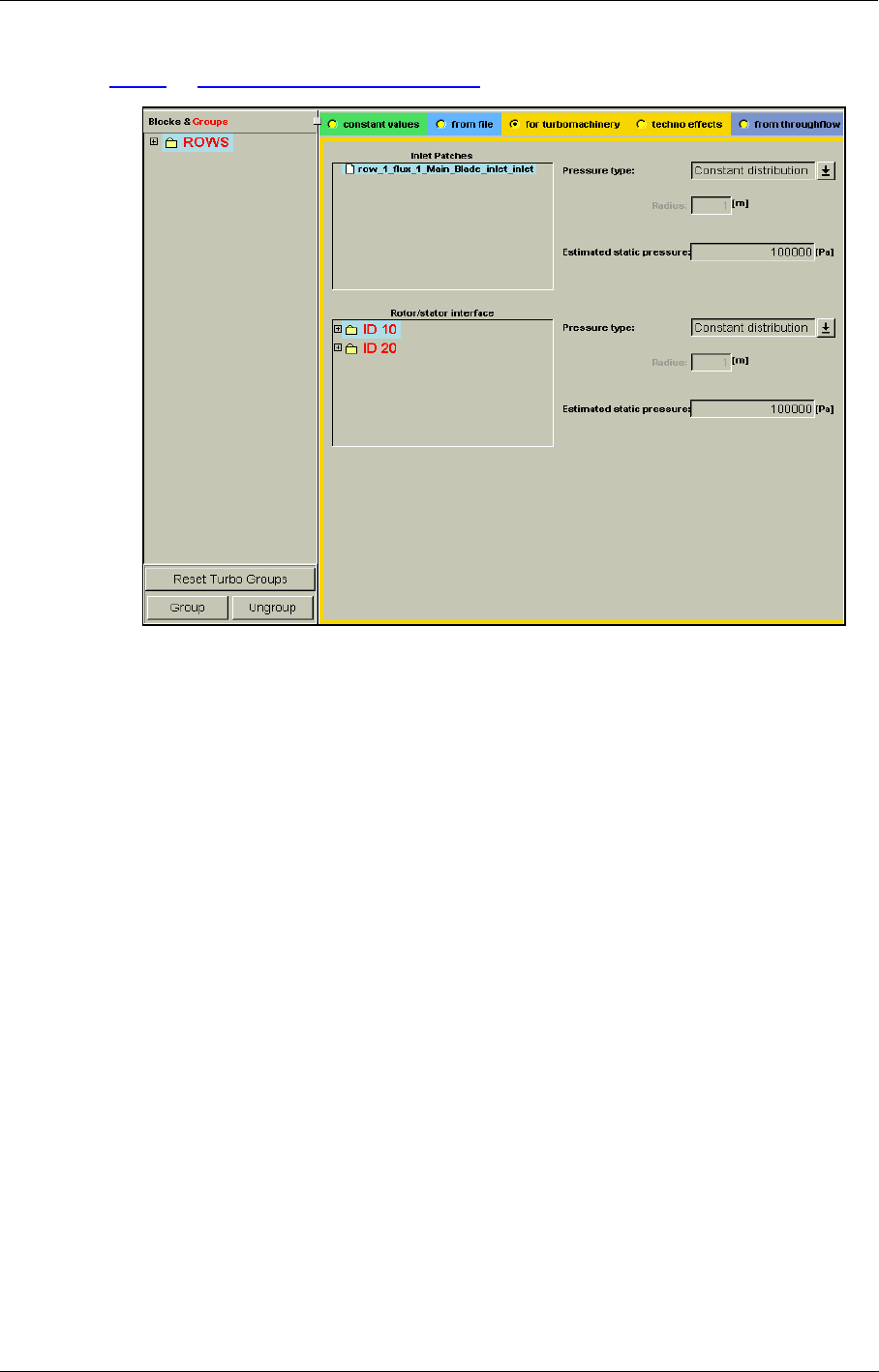
Initial Solution for Turbomachinery Initial Solution
FINE™/Turbo 9-7
9-5.2 Grouping & Parameters
FIGURE 9.5.2-4 Example of Turbomachinery-oriented initial solution
The turbomachinery-oriented page displays two major panels: one for the inlet patches and one for
the Rotor/Stator interfaces (see Figure 9.5.2-4). On the left of each panel, a tree shows by default
the AutoGrid™ grouping. If no patch name has been given in IGG™, the default name will be a
concatenation of the name of the block, the index of the face and the index of the patch.
The Inlet Patches grouping displayed in this initial solution page is identical to the grouping cre-
ated under the INLET tab of the Boundary Conditions page. Similarly, the Rotor/stator Inter-
face grouping displayed in the Initial Solution page is based on the ID given in the Rotor-Stator
tab of the Rotating Machinery page. These groups of patches cannot be modified in the Initial
Solution page. If these groups of patches need to be edited, the user must go back to the Boundary
Conditions or Rotating Machinery pages.
An input dialog box is provided per group of patches in order to select the type of static pressure
specification: constant distribution or radial equilibrium. One or two input boxes are provided per
group of patches in order to define the static pressure value to be used and, if radial equilibrium is
chosen, the radius (in meters [m]) on which this radial equilibrium will be based.
Provided that a k-ε, k-ω or v2-f turbulence model is selected, a third panel is displayed that requires
the initial values for the turbulent kinetic energy ( ) and the turbulent dissipation rate ( ). For
advice on the initial values to choose for and see section 4-2.5.4.
An inlet patch has to be defined among the blocks for which a ’for turbomachinery’
initial solution has been chosen. If there is no inlet patch for the selected group of blocks,
a warning message is displayed in the FINE™/Turbo interface asking the user either to
edit the group or to change the type of initial solution.
k
ε
k
ε

Initial Solution Throughflow-oriented Initial Solution
9-8 FINE™/Turbo
9-5.3 Expert Parameters
Some indispensable data are not available in previous versions so that the new initial solution ’for
turbomachinery’ cannot be applied directly to old projects. Consequently the previous initial solu-
tion ’for turbomachinery’ is kept and applied again if the mesh file does not contain the necessary
data (meridional mesh with the location and the values of the metallic angles of the leading and
trailing edges in the ".bcs" file). The methodology used for the initial solution ’for turbomachin-
ery’ is controlled by the expert parameter INITRB. By default the value is set to 2 in order to use
the method for meshes created with AutoGrid™. If FINE™/Turbo detects that a mesh created with
AutoGrid™ 4 is loaded, the value is automatically set to 0. In this case the old methodology is used.
9-6 Throughflow-oriented Initial Solution
This type of initial solution, of interest in turbomachinery calculations, allows to get an initial field
on the basis of an axisymmetric throughflow solution. The initial solution is defined through an
external file created by the user. The file contains 2D data in the format described hereafter. The
solver will use this data to generate an initial throughflow-oriented solution.
The solver will create a virtual mesh based on the hub and shroud definitions, forcing points on the
data points. Two additional stations will be created, at the inlet and outlet, respectively. The inlet
data are extrapolated from the first streamwise station while the outlet data come from the last sta-
tion. It is therefore recommended that the inlet and outlet boundaries of the mesh lie outside the
meridional domain covered by the throughflow data.
The meridional velocity is based on the mesh direction.
9-6.1 File Format
The file will include three parts, that must be separated by a blank line:
•solution definition,
•hub definition,
•shroud definition,
Once it is created, the file is selected in the FINE™/Turbo interface through a File Chooser click on
the Open Browser button in the Initial Solution/from throughflow page.
9-6.1.1 Solution Definition
The first part of the file contains the values of the flow variables throughout a meridional structured
mesh covering the entire machine. For each node of the meridional mesh, the (R,Z) coordinates are
specified together with the pressure, temperature and velocity components.
An axial case is taken as an example:
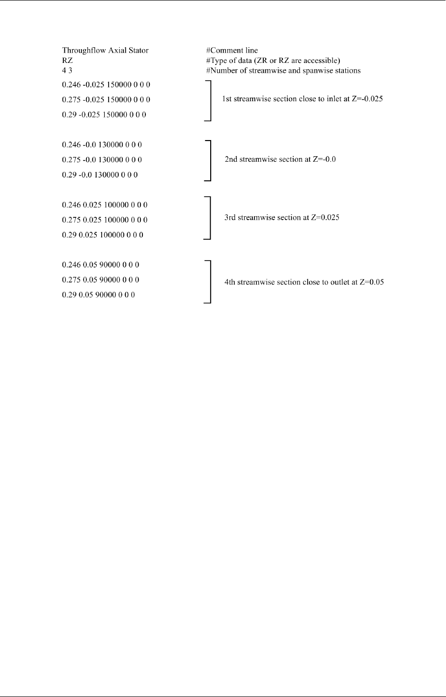
Throughflow-oriented Initial Solution Initial Solution
FINE™/Turbo 9-9
There are 4 streamwise stations in this example (Z=-0.025, Z=0.0, Z=0.025 and Z=0.05), each with
3 points in spanwise direction (R direction). The point order in a spanwise and streamwise station
goes respectively from hub to shroud and from inlet to outlet.
Each data line is made of the two (R,Z) coordinates (in m), the static pressure, the static temperature
, the meridional velocity and the tangential velocity. The unit for grid coordinates remain alwyas in
[m], the units for the other variables are dependent on the settings in the menu File/Preferences.
9-6.1.2 Hub Definition
The hub definition uses the same format as for AutoGrid™. The first line must be HUB. The sec-
ond line specifies the type of coordinate (ZR or RZ) and the third line the number of hub points.
The next lines correspond to the hub coordinates.
Taking again the example of the case above:
HUB
RZ #Type of data (ZR or RZ are accessible)
2 #Number of points on hub
0.245 -0.02 #Point coordinates (in m)
0.245 0.051
The hub is described in increasing Z coordinate from -0.02 to 0.051. The first column contains the
R coordinate for each of the two points on the hub.
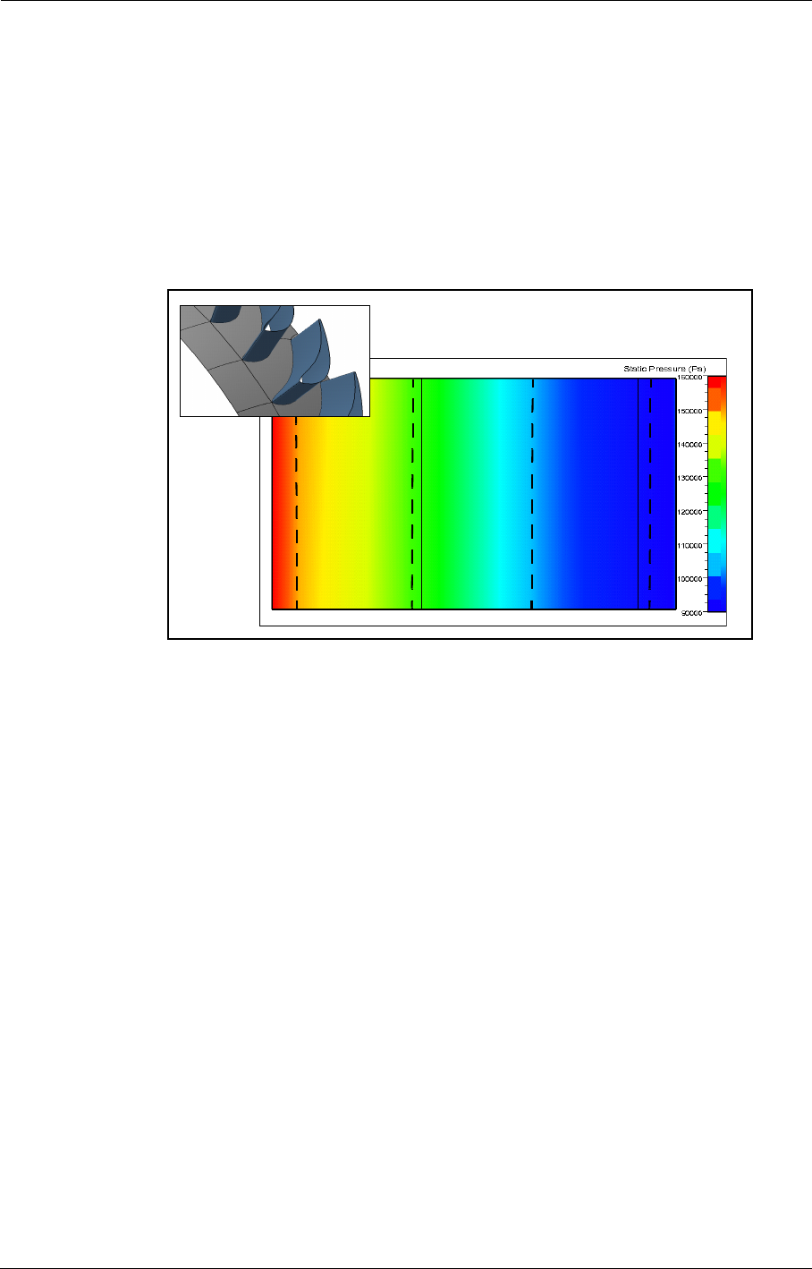
Initial Solution Throughflow-oriented Initial Solution
9-10 FINE™/Turbo
9-6.1.3 Shroud Definition
The shroud definition is similar to the hub definition, except for the first line that will be replaced
by SHROUD and the points coordinates.
SHROUD
RZ #Type of data (ZR or RZ are accessible)
2 #Number of points on hub
0.3 -0.02 #Point coordinates (in m)
0.3 0.051
FIGURE 9.6.1-1 Throughflow-oriented initial solution
Meridional Average View
3D View
INLET OUTLET
BLADE
1st streamwise
section
4th streamwise
section
2nd streamwise
section
3rd streamwise
section
HUB
SHROUD

FINE™/Turbo 10-1
CHAPTER 10:Output
10-1 Overview
With the flow solver in the FINE™/Turbo environment the user has the possibility to specify the
content of the output generated by the solver. The output does not only contain the flow variables
for which the equations are solved (density, pressure, velocity components, temperature), but also
other variables such as total conditions, the Mach number, customized velocity projections, etc...
Furthermore CFView™ allows to calculate derived quantities, which permits to limit the memory
size of the output and to avoid re-launching the flow solver in case one quantity of interest is not
available. With this functionality the user can find the compromise between an acceptable memory
size for the output and the ease of having all flow quantities of interest immediately available for
visualization.
In the next sections the way to control the output from the flow solver is described in more detail:
•field quantities: calculated at all the mesh nodes (see section 10-2.1),
•solid data: calculated along the solid wall boundaries (see section 10-2.1.5),
•customized averaged data:
—the evolution of some averaged quantities can be provided along the streamwise direction as
described in section 10-2.2,
—for turbomachinery applications, a pitchwise averaged output can be created for visualiza-
tion as described in section 10-2.3,
•global performance output (see section 10-2.6),
•additional output for the ANSYS code, a widely used finite element code for structural analy-
sis (see section 10-2.5.1).
The global performance output is written in an ASCII file with the extension ".mf". All other out-
puts, generated by the solver, are written in one single ".cgns" file, compatible with the CFView™
visualisation software. It is also possible to request for the output to be written in Plot3D format, as
described in section 10-2.7.
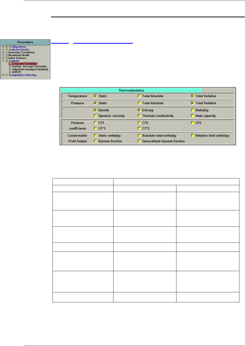
Output Output in FINE™/Turbo
10-2 FINE™/Turbo
10-2 Output in FINE™/Turbo
10-2.1 Computed Variables
Using the Outputs/Computed Variables page, the user can choose which physical variables have
to be included in the output generated by the flow solver, see Figure 10.2.1-1 to Figure 10.2.1-6. All
the selected variables will then be automatically available when launching CFView™ in order to
visualize the results.
10-2.1.1 Thermodynamics
FIGURE 10.2.1-1 Thermodynamics computed variables page (for cylindrical projects)
Table 10-1 and Table 10-2 give the formulae used to calculate the thermodynamic quantities.
Cartesian and cylindrical cases
Quantity Incompressible Perfect gas
Static temperature
Total temperature
Relative total temperature
Static pressure
Total pressure
Relative total pressure
Density
TABLE 10-1 Thermodynamics quantities generated by the FINE™/Turbo solver
Tstat
Tstat
Pstat
ρrgas
-------------
=
Ttot Tstat
v2
2cp
-------- k
cp
-----
++=
Ttot Tstat
v2
2cp
-------- k
cp
-----
++=
Ttot
rTstat
w2
2cp
-------- k
cp
-----
++=
Ttot
rTstat
w2
2cp
-------- k
cp
-----
++=
Pstat
Pstat
Ptot Pstat ρv2
2
-----ρk++=
Ptot Pstat
Ttot
Tstat
-----------
γ
γ1–
-----------
=
Ptot
rPstat ρw2
2
------ ρk++=
Ptot
rPstat
Ttot
r
Tstat
-----------
γ
γ1–
-----------
=
ρ
ρ

Output in FINE™/Turbo Output
FINE™/Turbo 10-3
The heat capacities cp and cv are function of the temperature for real gas, while they are constant in
case of perfect gas. When real gas is used, the total pressure and total temperature are computed by
the following equations:
Furthermore five definitions of the pressure coefficient are available for internal flow (inlet and out-
let boundary conditions available): CP1, CP*1, CP2, CP*2, CP3:
—,
—,
—,
—,
—.
where Xinlet corresponds to the mean value of the variable X on the inlet, and where Uref is defined
as:
• RLEN in cylindrical cases, with RLEN, the reference length given in the Flow Model page,
and ω, the rotational speed (defined block per block),
Cylindrical cases only
Incompressible Perfect gas
Entropy
Rothalpy
Dynamic viscosity
Thermal conductivity
Heat capacity
Gamma -
ω is the angular rotation speed and r, the distance from the rotation axis
The term k only exists when the two or four equation turbulence models are applied.
TABLE 10-2 Thermodynamic quantities generated by the flow solver in cylindrical cases
sc
p
Tstat
Tstatinlet
---------------------ln=
sc
v
Pstat Pstatinlet
⁄()
ρρ
inlet
⁄()
γ
------------------------------------------ln=
Ic
pTstat
Pstat
ρ
----------- w2ω2r2
–
2
------------------------ k++ +=
Ic
pTstat
w2ω2r2
–
2
------------------------ k++=
μ
μ
κ
κ
cp
cp
γ
cpT()Td
Tref
T
v2
2
-----k++ cpT()Td
Tref
Tt
=
Pt
p
-----
ln cpT()
rT()T
-------------- Td
T
Tt
=
CP12PPt
inlet
–()
ρinletUref
2
--------------------------------
=
CP∗1Ptinlet Pt–
Ptinlet
--------------------------
=
CP22PP
inlet
–()
ρinletwinlet
2
------------------------------
=
CP∗22Ptinlet Pt–()
ρinletwinlet
2
----------------------------------
=
CP32PP
inlet
–()
ρU2
------------------------------
=
ω

Output Output in FINE™/Turbo
10-4 FINE™/Turbo
•UENTR (Cartesian case) to be specified in the expert parameters list of the Control Variables
page.
When the reference velocity Uref is set to 0, the value of CP1 and CP3 are undefined
and set to 0.
Finally, when a condensable fluid is selected in the Fluid Model page, new quantities at the bottom
of the page will appear. Those variables are defined using the thermodynamic tables defining the
condensable fluid (see section 3-2.3.4 for more details).
When the condensable fluid option is used, 6 flow variables are stored at all mesh cell centers
instead of 5 for a perfect gas or liquid. These variables are the following: density, velocity compo-
nents, static pressure and total energy ( ). The static and total enthalpy can easily be
derived using:
•static enthalpy .
•absolute total enthalpy .
•relative total enthalpy .
The dryness fraction permits to evaluate the location of the local thermodynamic state with respect
to the saturation curve. For each value of the pressure an interpolation from the saturation table
("PSA.atab") permits to determine the saturated liquid (ρl) and gas (ρv) values of the density. The
dryness fraction is then computed by:
•dryness fraction .
The generalised dryness fraction directly results from the above expression whereas the standard
dryness fraction is bounded in the [0,1] interval.
The presence of the saturation table ("PSA.atab") is required in order to calculate the
dryness fraction, although this table is not required by the solver itself (unless an inlet
boundary condition based on dryness fraction X is used).
10-2.1.2 Velocities
FIGURE 10.2.1-2 Velocities computed variables page (for cylindrical projects)
ρEρev2
2
-----
+
=
he
p
ρ
---
+
=
Hahv2
2
-----
+
=
Hrhw2
2
------
+
=
Xρρ
l
–()ρ
v
ρvρl
–()ρ
------------------------
=
Output in FINE™/Turbo Output
FINE™/Turbo 10-5
The velocity quantities that can be selected are described below.
Both for Cartesian and cylindrical cases:
•Absolute velocities: , , , , .
•Velocity projections: , , , , , , , , .
with , surface vector of the i surface,
.
•Absolute Mach Number, only for compressible fluids:
.
For cylindrical projects only:
•Absolute velocities in the rotating frame: , , :
,
,
.
•Relative velocities: , , , , :
,
.
•Relative velocity projections: , , , , , , , , .
with , surface vector of the i surface,
.
•Relative Mach Number:
.
10-2.1.3 Vorticities
FIGURE 10.2.1-3 Vorticities computed variables page
vx
vy
vz
v
v
vi
vj
vk
vi
vj
vk
vis
vjs
vks
viv
·
Si
⋅()Si
=
Si
vis viv
·Si
⋅()Si
–=
Mabs vγPstat
ρ
--------------
⁄=
vr
vθ
vm
vrvxθvyθsin+cos=
vθvyθcos vxθsin–=
vmvr
2vz
2
+=
wx
wy
wθ
w
w
wvωr×–=
wθwyθcos wxθsin–=
wi
wj
wk
wi
wj
wk
wis
wjs
wks
wiw
·Si
⋅()Si
=
Si
wis wiw
·Si
⋅()Si
–=
Mrel wγPstat
ρ
--------------
⁄=
Output Output in FINE™/Turbo
10-6 FINE™/Turbo
The vorticity is calculated according to the following expression:
,
where is the gradient operator. From the above expression, ζx, ζy, ζz, ζxyz, and ζ are available.
10-2.1.4 Residuals
FIGURE 10.2.1-4 Residuals computed variables page
The residuals are computed in FINE™/Turbo by a flux balance (the sum of the fluxes on all the
faces of each cell). The absolute value |RES| resulting from the flux balance is written as output for
each cell. The residuals for the following quantities can be selected:
•density
ρ
,
•energy E,
•velocity component ,
•velocity component ,
•velocity component ,
•turbulent kinetic energy k, for the k-ε, k-ω and v2-f turbulence models,
•turbulent energy dissipation rate ε, for the k-ε and v2-f turbulence models.
10-2.1.5 Solid Data
FIGURE 10.2.1-5 Solid data computed variables page
The solid wall data refer to quantities that are estimated at the solid boundaries:
•static pressure at walls (see section 10-2.1.1)
•static temperature at walls (see section 10-2.1.1)
ζ∇v×=
∇
wx
wy
wz
Output in FINE™/Turbo Output
FINE™/Turbo 10-7
•normalized tangential component of the viscous stress at walls, where is the
viscous stress, V is the reference velocity and ρ is the reference density defined in Flow Model
page.
•heat flux at walls in general and for the turbulent models with extended wall
function
•relative velocity at walls (see section 10-2.1.2)
•viscous stress at walls
•y+ (in first inner cell): , where y is the normal distance from the walls to the first
inner cell center and is the wall friction velocity.
•heat transfer coefficient:
,
in which is the local heat flux, the local temperature at the wall and the refer-
ence temperature for convection. is controlled by the expert parameter HTCDEF (avail-
able in the expert parameters list of the Control Variables page). When setting HTCDEF to 1
(default), is equal to the absolute averaged total temperature at the inlet. When setting
HTCDEF to 2, is equal to the reference temperature defined in the Configuration /
Flow Model page.
•Injection flow (see Chapter 8-6.2.2)
•Injection direction (see Chapter 8-6.2.2)
10-2.1.6 Turbulence
FIGURE 10.2.1-6 Turbulence computed variables page.
The following quantities can be stored:
•y+ (3D field)
,
•wall distance (i.e. closest distance to the wall: ywall),
•turbulent viscosity (μt/μ),
•production of kinetic energy (Production),
•turbulent kinetic energy k, for the k-ε, k-ω and v2-f turbulence models,
Cf
τ
ρV22⁄
----------------
=
τ
qwκDT
Dn
--------
⋅=
qwρcpuτTτ
=
τxyz
y+yuτ
ν
--------
=
uτ
hqw
Twall Tbulk
–()
------------------------------------
=
qw
Twall
Tbulk
Tbulk
Tbulk
Tbulk
yρywalluw
μ
----------------------
=+
Output Output in FINE™/Turbo
10-8 FINE™/Turbo
•turbulent energy dissipation rate ε, for the k-ε and v2-f turbulence models,
•specific dissipation ω, for the k-ω turbulence models.
10-2.1.7 Harmonic
For the output specific for harmonic computations see section 8-4.2.
10-2.1.8 Deformation
FIGURE 10.2.1-7 Deformation computed variables page
These output variables are only accessed when the mechanical coupling module is activated.
The scalar variables Dx, Dy and Dz is the mesh deformation in X, Y and Z direction, respectively.
The variable Dxyz is the mesh deformation vector.
Mesh deformation output is not available when the mesh deformation is calculated in
the cylindrical coordinates (IMVCYL=1).
10-2.2 Surface Averaged Variables
This option is customised for turbomachinery applications and displays in a Cartesian plot the evo-
lution of surface-averaged variables along the streamwise direction. The user has to select the
blocks along the streamwise direction. A surface averaging is performed on the grid surfaces per-
pendicular to the streamwise direction. The plot is created by a computation on each block.
The Surface Averaged Variables page is modified according to the type of project as defined in
the Mesh/Properties... menu. For a Cylindrical project the page is shown in Figure 10.2.2-8. In
this case the streamwise direction (by default K) is defined on the Rotating Machinery page of the
FINE™/Turbo interface. The blocks to be included in the averaging, can be selected from the list of
blocks by left-clicking on them. Selected blocks appear highlighted. This selection acts as a toggle
where clicking ones on a block name selects the block and clicking a second time deselects the
block. To select multiple blocks it is sufficient to left-click on each of them.
The variables available for averaging are listed on this page and a averaging method can be selected
for each variable independently. The turbulent quantities k and ε only appear for selection if a k-ε,
k-ω or v2-f turbulence model is selected.
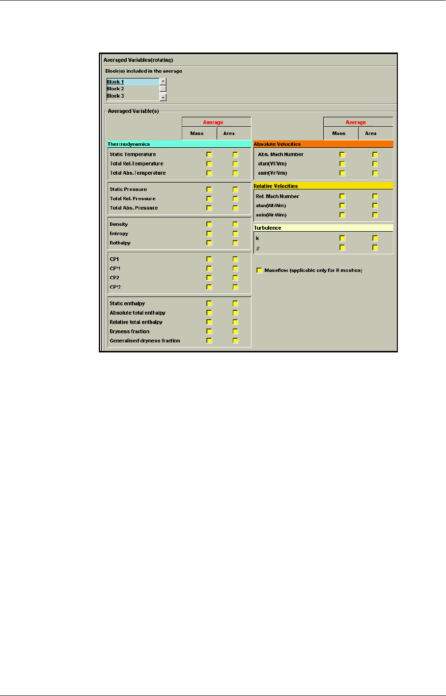
Output in FINE™/Turbo Output
FINE™/Turbo 10-9
FIGURE 10.2.2-8 Surface averaged variables page for a Cylindrical project
Since the integration is performed on mesh surfaces, some differences could appear.
For example, if the geometry contains a splitter, two curves will be generated in the Car-
tesian plot. A sum of these curves has to be performed to see the evolution of the quan-
tity in streamwise direction of one channel.
Since the surface averaging is performed on grid surfaces this option is only suitable
for HI-topology meshes, without a skin block.
For Cartesian projects as defined in the Mesh/Properties... menu the Surface Averaged Varia-
bles page is displayed as shown in Figure 10.2.2-9. In this case the streamwise direction needs to be
selected directly in this page by selecting to average on surfaces of constant index (in the example
of Figure 10.2.2-9 surfaces of constant K). The blocks to include in the averaging need to be
selected in the same way as for a cylindrical case as described before. Contrary to a cylindrical
project, in this case no relative quantities are available.
Like for a cylindrical project the surface averaged evolution of the quantities is shown
for each block separately.
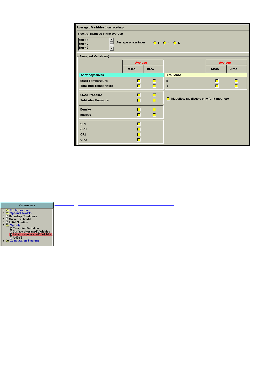
Output Output in FINE™/Turbo
10-10 FINE™/Turbo
FIGURE 10.2.2-9 Surface averaged variables page for a Cartesian projects
After selecting such averaged variables, they are available through the menu Quan-
tity/Plot Data within CFView™, which is automatically plotting the averaged variable
along the selected streamwise direction on each I, J or K constant surface.
10-2.3 Azimuthal Averaged Variables
The FINE™/Turbo environment provides the user with a specific turbomachinery output, i.e. the
two-dimensional meridional view of the circumferentially-averaged results. Note that this function-
ality is also available in CFView™.
Using the Azimuthal Averaged Variables page, the user can choose which physical variables have
to be included in the pitchwise-averaged output generated by the flow solver. This page is therefore
only accessible if the project is of the cylindrical type. The azimuthal averaging of the variables is
calculated at the end of the computation. The results will be displayed as a 2D case in CFView™.
The name of the file from which CFView™ can read which variables have been averaged in the azi-
muthal direction has the extension ".me.cfv".
The choice is left to the user to apply Mass or Area averaging, and to merge the averaging patches
into one patch or not. This last option (Merging of meridional patches) simplifies the meridional
view but the patches are merged in increasing order one after another, which is not suitable for all
mesh topologies. All the patches of the project that will be merged should be matching in spanwise
direction.
If Surface of revolution mesh (Autogrid) option is activated, a specific algorithm will be applied
to enhance azimuthal averaging of the solution performed on revolution surfaces.
The "parameters area" is divided into five ’notebook pages’ which can be selected by clicking on
one of the five corresponding tabs: Thermodynamics, Velocities, Vorticities, Residuals and Tur-
bulence in the same way as for the control variables.
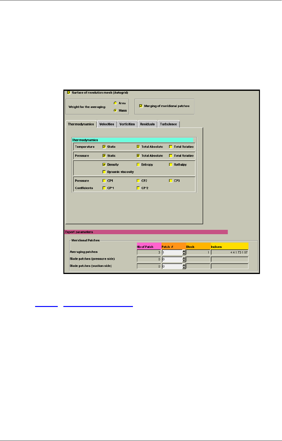
Output in FINE™/Turbo Output
FINE™/Turbo 10-11
Figure 10.2.3-10 shows an example of the corresponding information page for thermodynamics
variables. Other pages are similar to those described in section 10-2.1.
At the bottom of Figure 10.2.3-10 in Expert Mode the user can define the meridional patches for
azimuthal averaging. See section 10-3.1 for more detail on this possibility. By default meridional
averaging patches are set.
Automatic setting of the meridional averaging patches only works if no manual action
has been performed (like renaming of some patches).
FIGURE 10.2.3-10 The thermodynamics azimuthal averaged variables page
10-2.4 Template manager
A new button “Template manager ... “ was added on the top of each of the three output pages in
FINE (Computed variables, Surface averaged variables, and Azimuthal averaged variables). This
button invoke a pop-up window:
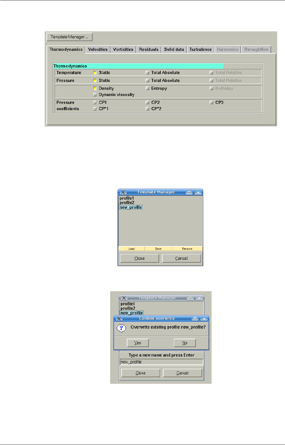
Output Output in FINE™/Turbo
10-12 FINE™/Turbo
This new windows is the same for each of the three pages and it lets the user to Load, Save and
Remove stored output selections. Double click on a profile name also loads the selected profile. The
button Cancel close the window and the page will return to the its state before launching the tem-
plate manager. This gives the user the possibility to browse the existing profiles without loosing his
current outputs selection. To create a new outputs profile the user should click on “Save”. A new
entry appears, asking for the name of the new profile:
When Enter is pressed, Fine checks if the entered name already exists:
The current outputs selection (the values of all check buttons in all tabs) in the current page is
stored in this new profile.
The button “Remove” deletes selected profile.
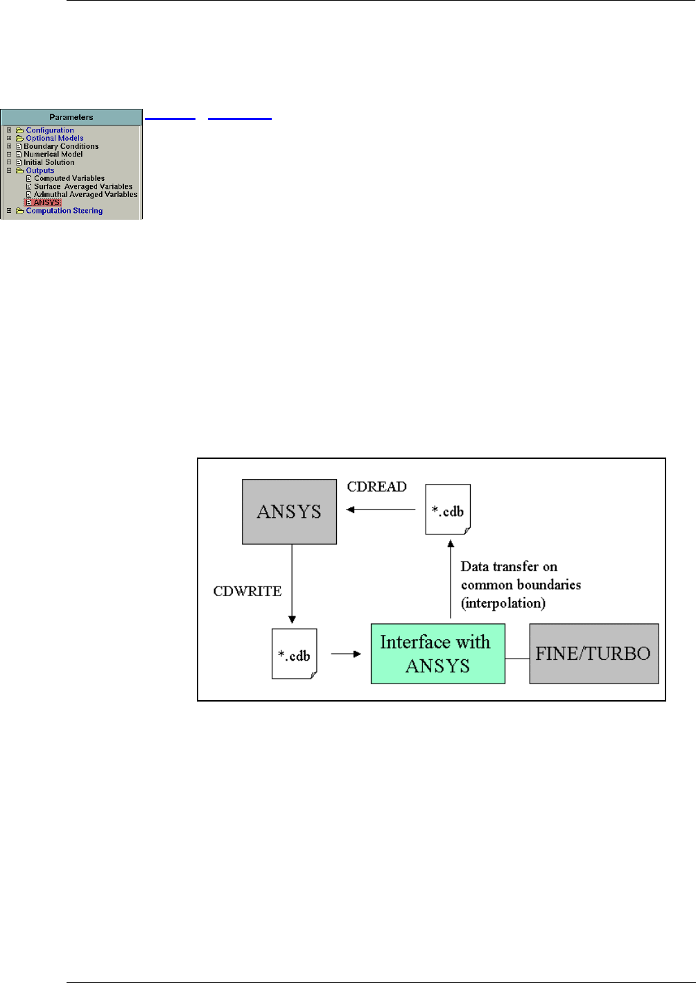
Output in FINE™/Turbo Output
FINE™/Turbo 10-13
The profiles are stored in text format in the file .numeca/fine_output.def and are independent from
projects. Different users may exchange their profiles by means of this file.
10-2.5 ANSYS
The FINE™/Turbo environment provides the user with a specific ANSYS output. The objective is
to export results of the CFD computation on solid surfaces (nodes and elements) into ANSYS as a
boundary condition for the finite element model. This approach is called FEM loading method for
loading the CFD results on a Finite Element Model. The transferred results on the interface fluid-
structure can be the pressure field for a structural analysis and the temperature field or the heat
fluxes for a thermal analysis in the structure.
The FEM approach needs to have the finite element mesh of ANSYS. If this mesh
does not exist before the CFD computation, it is impossible to create directly a file that
can be imported in ANSYS to apply the suitable boundary condition. Consequently the
best way to manage the interface between FINE™/Turbo and ANSYS can be a new post-
processing tool. The post-processing tool is needed with the specification of the ANSYS
mesh, the common surfaces where the data must be interpolated and the type of bound-
ary condition on each surface. The transfer will be carried out through the ANSYS file
saved with the command CDWRITE ("project_ANSYS.cdb") in ANSYS. This file will
be modified and read again in ANSYS to impose the CFD results as boundary conditions
(see Figure 11.2.4-10).
FIGURE 10.2.5-11 Data transfer of CFD results into the ANSYS project
10-2.5.1 ANSYS Pre-Processing
Before completing the Outputs/ANSYS pages, the user must create the file "project_ANSYS.cdb"
with the command CDWRITE in ANSYS. Furthermore before the save in ANSYS, some opera-
tions are needed to allow the identification of the common surface between the fluid model and the
structural model. The ANSYS project must be completely defined with a special treatment for
the surface loads that will be replaced by the interpolated CFD results. On each common sur-
face, a coded constant value is specified. The default coded values are given in the Table 10-3 for
the different types of boundary condition. The value is incremented by one for each different sur-

Output Output in FINE™/Turbo
10-14 FINE™/Turbo
face so that for example the pressure imposed on the first surface is set to 1000001 and it is set to
1000002 on the second,...
TABLE 10-3 Default code for different type of boundary condition imposed from CFD
results
The coded value can be modified in order to avoid confusion with physical values.
Note that the surface must be relatively flat or smooth (without sharp angle) so that the
six surfaces define a cube. Moreover a surface closed on itself, like a cylinder or a blade
must be divided into two parts if the conservative interpolation type is required.
The heat transfer coefficient can be computed only for non-adiabatic solid patches.
The correct physical bulk temperature must be specified on the surfaces with convection.
It must be constant for each surface.
If the coded values have been prescribed by using the solid model, the solid model has
not to be saved in the original ".cdb" input file (see the options for achieve file).
The ansys importation does not support a time profile of a quantity.
Validation tests are performed with ANSYS release v8.0. Please refer to ANSYS user
manual for more details on the ".cdb" file format
10-2.5.2 Global Parameters
The user can complete the Outputs/ANSYS pages when the file "project_ANSYS.cdb" has been
created (refer to section 11-2.4.1 for more details).
Firstly, the user needs to specify under the tab Global Parameters in Boundary Conditions
(Figure 10.2.5-12 - (1)) the coded constant value used in the file "project_ANSYS.cdb". The default
coded values are given in the Table 10-3 for the different types of boundary condition. Furthermore,
the user has to specify the required units of the data for each type of boundary condition. The units
will be specified next to the coded value.
Then, the user needs to load the file "project_ANSYS.cdb" (Figure 10.2.5-12 - (2)) created in
ANSYS (refer to section 10-2.5.1 for more details) in Input File.
The data transfer between the CFD mesh and the structural mesh is possible if the common
geometries are matching. It is possible that this condition is not fulfilled and the causes can be
diverse:
•Units: a first difference can come from the units of the meshes. Consequently the units used in
the ANSYS mesh must be specified in ANSYS Mesh Units. The conversion Factor will be
deduced automatically (Figure 10.2.5-12 - (3)).
•Reference system: the second cause of mismatching is the use of different coordinate systems
(Figure 10.2.5-12 - (3)). For example, the original geometry can be rotated for the CFD model
so that the axial direction corresponds to the Z axis. The necessary conversion of coordinates
Boundary Condition Code
Pressure field 1000001
Temperature field 2000001
Heat transfer coefficient 3000001
Heat flux 4000001
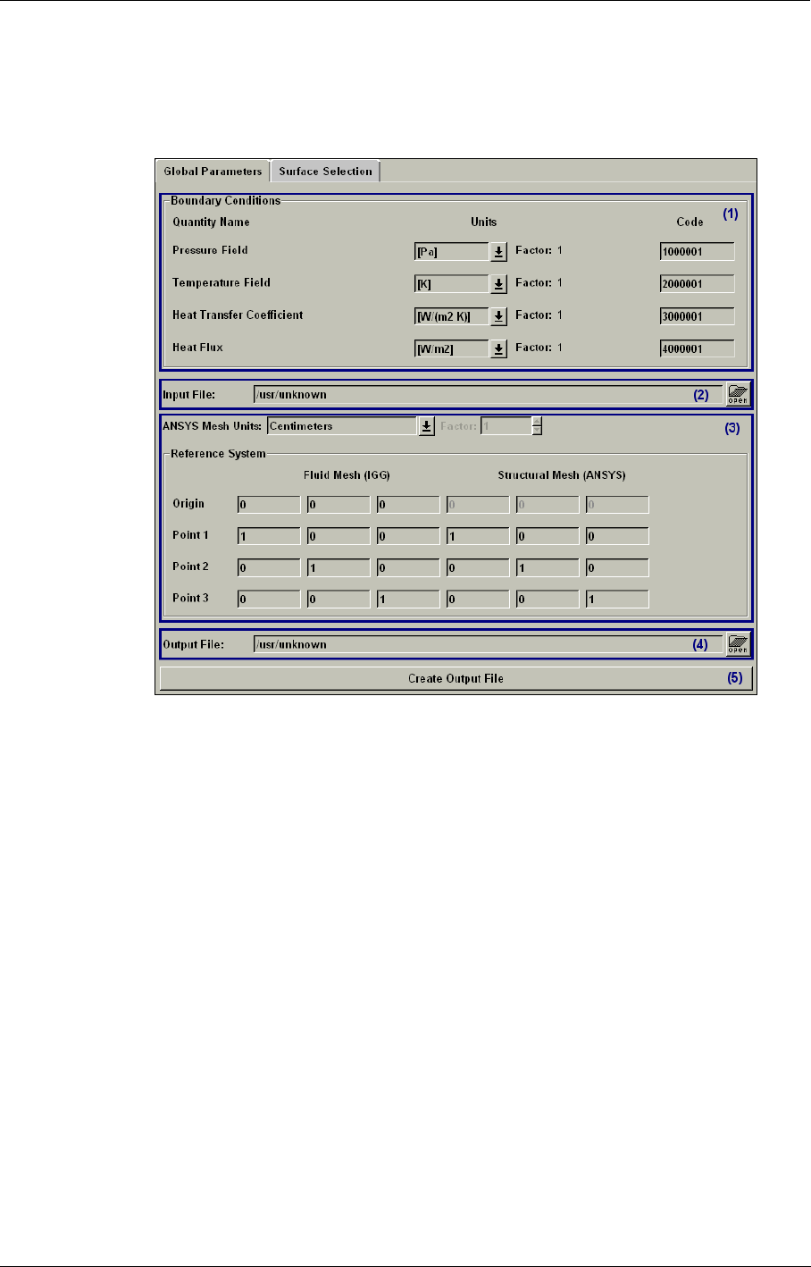
Output in FINE™/Turbo Output
FINE™/Turbo 10-15
will be done through the specification of the position of the coordinate center of the ANSYS
mesh in the coordinate system of the CFD mesh and the specification of the location of three
common points in both meshes in Reference System.
FIGURE 10.2.5-12 General Parameters of ANSYS outputs
Note that these points cannot be located on a line or a plane including the zero point
(not linearly dependent). The coordinates are specified in their respective units.
The origin of the ANSYS mesh should be at (0,0,0).
Finally in Output File, the user specifies the new output file "project_CFD.cdb" (Figure 10.2.5-12
- (4)) containing the transferred CFD results on the solid boundaries coded in ANSYS (refer to sec-
tion 10-2.5.1 for more details).
In order to create the new output file, the user has to complete the page under the Surface Selection
tab before clicking on the Create Output File button (Figure 10.2.5-12 - (5)).
10-2.5.3 Surface Selection
After completion of the page under Global Parameters tab page, the user has to complete the Sur-
face Selection page (refer to section 10-2.5.2 for more details) before creating the ANSYS output
file (Create Output File button).
When the ANSYS input file is read in Input File, the common surfaces on which the data must be
transferred are identified in the ANSYS mesh. The FINE™/Turbo interface lists each surface with
the corresponding coded value (Figure 10.2.5-13 - (1)).
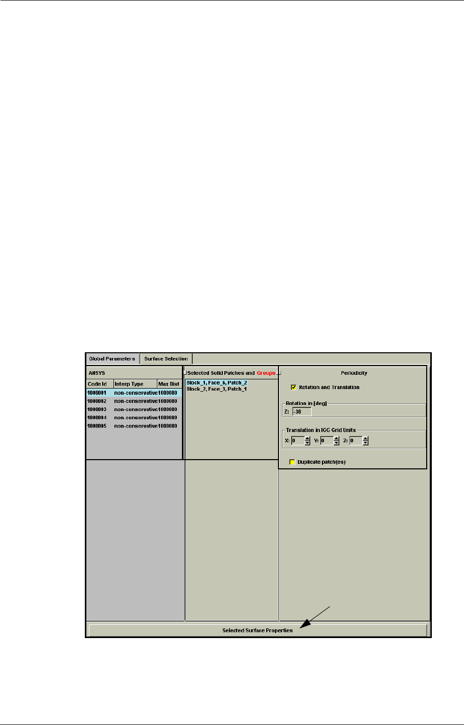
Output Output in FINE™/Turbo
10-16 FINE™/Turbo
When reading the ANSYS input file for the first time, automatically a new file with the extension
".ANSYSgeom" is created in the active computation directory. This file contains the geometry of
the related ANSYS surfaces and allows accelerating the next operations.
By clicking on Selected Surface Properties button (Figure 10.2.5-13 - (2)), a new window
(Figure 10.2.5-14) allows the user to specify the solid patches from which the data will be interpo-
lated. Following interpolation parameters can also be defined: interpolation type (Interp Type) and
the allowed maximal distance (Max Dist).
Two different interpolation types (Interp Type) are proposed: a conservative and a non-conserva-
tive. The suitable interpolation scheme is dependent on the type of boundary conditions. The spatial
field of pressure or temperature can be interpolated from cell faces to nodes whereas a conservative
transfer of the heat fluxes can be preferred.
Note that in the non-conservative approach, the local normal of the fluid mesh is used
for the projection of the ANSYS surface on the corresponding IGG™ solid patches.
Whereas an averaged local normal of the ANSYS mesh is used for the projection in the
conservative approach. If the geometry of the common surfaces does not match exactly
between the IGG™ mesh and the ANSYS mesh (e.g. if the fillet is not modeled in the
fluid mesh), the result depends on the way to define the surfaces in ANSYS, the selection
of the IGG™ solid patches from which the interpolation is performed and the choice of
the interpolation type. A slight discontinuity can appear in the interpolated field. In case
the fillet is not modeled, the different ways to project the ANSYS surface on the IGG™
solid patches imply that the conservative approach can fail if the ANSYS surfaces are
not approximately divided in the fillet where its normal intersects the edge separating the
IGG™ solid patches (blade and hub or shroud).
FIGURE 10.2.5-13 Surface Selection of ANSYS outputs
(2)
(1) (3)
(4)
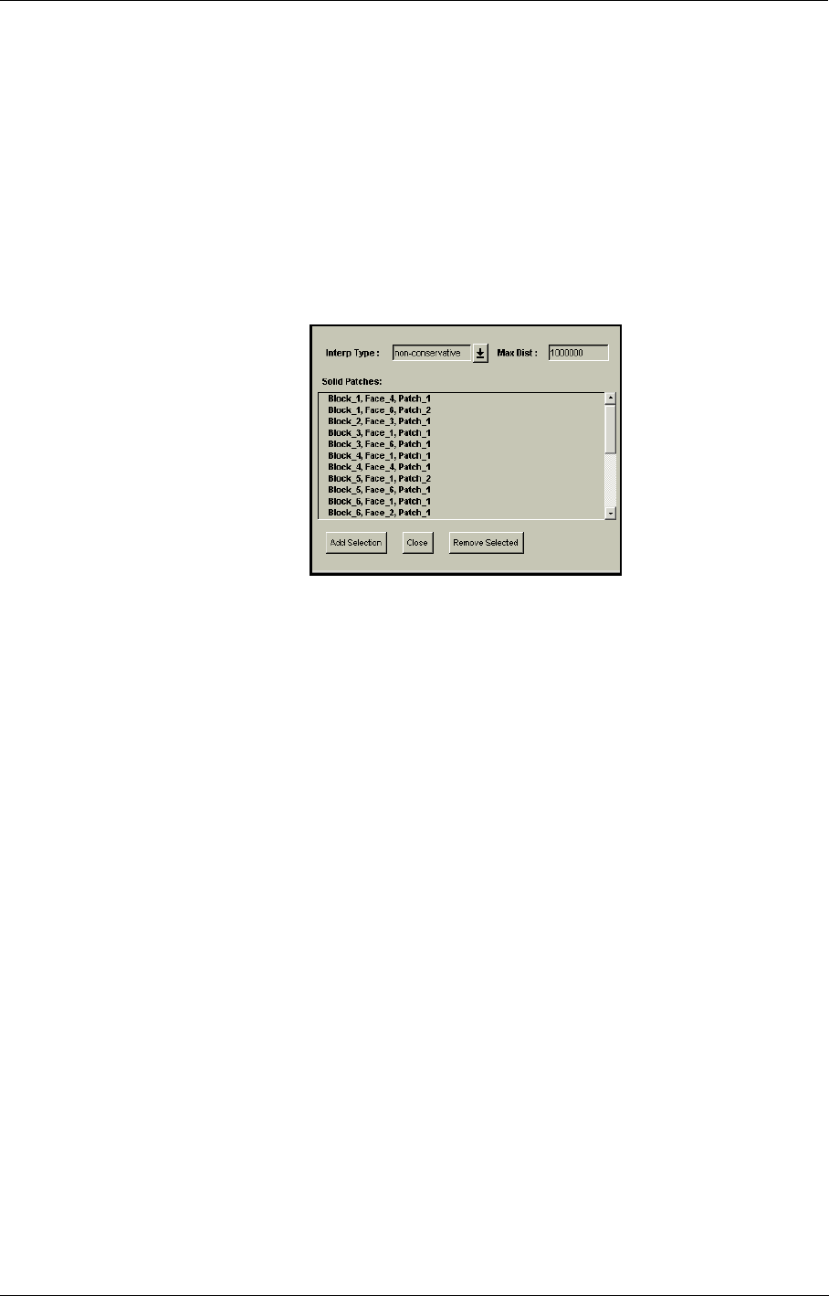
Output in FINE™/Turbo Output
FINE™/Turbo 10-17
The CFD results are read from the ".cgns" file of the active computation. The non-
conservative approach needs to save the solid data on the IGG™ solid patches. For the
conservative approach, only the solid data Heat Flux is required for the computation of
the heat transfer coefficient.
An allowed maximal distance (Max Dist) can be used to control the interpolation process by ensur-
ing that it is performed in the nearest element of the selected solid CFD patches.
The maximum distance of the ANSYS output on the surface selection page, is always
expressed in meters (independent from the mesh units or project preferences)
FIGURE 10.2.5-14 Add solid patches to ANSYS surface
Then, the user specifies the solid CFD patches in the list of Solid Patches by <Ctrl> or <Shift> and
left-click. To add or remove solid patches linked to the highlighted ANSYS surface, the buttons
Add Selection and Remove Selected are used respectively. When the solid patches are well selected,
the window has to be closed (Close) and the patches will appear in the list Selected Solid Patches
and Groups (Figure 10.2.5-13 - (3)).
A visualization of the active ANSYS surface and of the selected solid patches can help the user in
the selection process after opening the mesh through the menu Mesh/View On/Off or Mesh/
Tearoff graphics (only available on UNIX). Moreover, the visualization allows checking that the
surfaces (ANSYS and IGG™ solid patches) are matching. A modification of the ANSYS mesh unit
or reference system is directly taken into account in the visualization when the user refreshes the
view by clicking again on any ANSYS surface.
To ensure a complete data transfer, the selected IGG™ solid patches have to com-
pletely overlap the ANSYS surface.
The area of the selected IGG™ solid patches can be larger than the area of the ANSYS
surface.
Since the IGG™ solid patches defining a periodic structure can be divided (Figure 10.2.5-15), a
periodic shift can be required to match the common ANSYS surface. This shift must be specified
for each solid patch, highlighted in Selected Solid Patches and Groups list, in Periodicity by acti-
vating Rotation and Translation (Figure 10.2.5-13 - (4)). The rotation and translation shifts are
respectively specified in degrees and IGG™ mesh units.
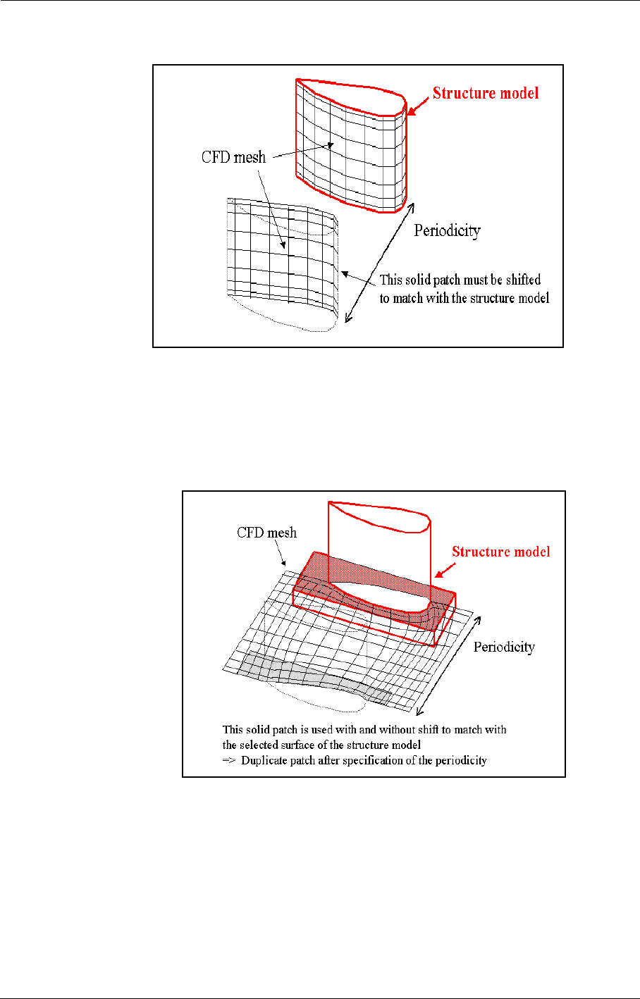
Output Output in FINE™/Turbo
10-18 FINE™/Turbo
FIGURE 10.2.5-15 Mesh differences IGG™ vs. ANSYS
Moreover one ANSYS surface can be covered by a group of solid patches and by the same group
which is rotated (or translated). Consequently, a duplication of the periodic solid patches is possible
by activating Duplicate patch(es) after applying a Rotation and Translation to the highlighted
solid patch (Figure 10.2.5-13 - (4)).
FIGURE 10.2.5-16 Duplicate Option Utility
Finally, the new output file can be created by clicking on the Create Output File button
(Figure 10.2.5-12 - (5)).

Output in FINE™/Turbo Output
FINE™/Turbo 10-19
10-2.5.4 Import Results in ANSYS
The new output file "project_CFD.cdb" (Figure 10.2.5-12 - (4)) containing the transferred CFD
results on the solid boundaries coded in ANSYS is now available. When reading this file in ANSYS
with the command CDREAD, following rules need to be respected:
•Only the FE model (file ".cdb") has to be imported.
•If the coded values have been prescribed by using the solid model, the solid model has not to
be saved in the original ".cdb" input file (see the options for achieve file). If the solid model is
saved, conflicting values are set on the fluid-structure boundaries and the initial coded values
will be kept. Moreover these artificial boundary conditions have to be removed in the ANSYS
project before importing the modified archive file with the suitable boundary conditions. If
they are not removed, the coded values will replace the transferred values.
10-2.6 Global Performance Output
The main results for global performance are summed up in a file with extension ".mf". Inlet and
outlet averaged quantities, pressure ratios and efficiency are computed and stored in this file. The
".mf" file also provides global averages at each rotor/stator interface. When there are multiple inlets
or outlets with different periodicities, only one "number of blades" is reported in the .mf file, but
there will be a minus (-) sign before that number to indicate that there are also other inlets or outlets
with different periodicities than reported. All the variables in .mf file are mass averaged, except that
the static pressure is area averaged.
If the project does not involve any of inlet/outlet or interfaces (e.g. for external flow), the ".mf" file
is empty.
The user can select which and what kind of information is stored using expert parameters as
described in section 10-3.2.
10-2.6.1 Flow Angle
The relative and absolute flow angles are derived from the averaged velocity components:
(10-1)
(10-2)
10-2.6.2 Global Performance
Global performance data, available in the ".mf" file, are calculated using the results at the inlet and
outlet boundaries of the computational domain (index 1 and 2 refer to the inlet and outlet sections
respectively).
A row-by-row and/or stage-by-stage analysis can be performed by using the expert parameter
RBRSBS. The additional performances stored in the ".mf" file are: the mass flow in and out, the
static and total pressure ratio, the static and total temperature ratio and the isentropic and polytropic
efficiency (see section 10-3.2).
a) Global Performance Output for Incompressible Fluid
The outputted global performance is depending on the type of the fluid. In case of incompressible
fluid, the following data will be written:
αarc vθ
vm
-----
tan=βarc wθ
vm
------
tan=cylindrical
αarc vy
vx
----
tan=βarc wy
wx
------
tan=Cartesian

Output Output in FINE™/Turbo
10-20 FINE™/Turbo
•Static pressure rise:
•Absolute total pressure rise:
•Static Head:
•Absolute total Head:
•Static temperature rise:
•Absolute total temperature rise:
•Efficiency
For turbomachinery cases with a rotor, the expressions proposed in Table 10-4 are used. Several
efficiency definitions are available, selected through the expert parameter EFFDEF (default: 1).
Expressions involving the Torque in Table 10-4 are computed only if the user acti-
vates the option Compute force and torque in the Boundary Conditions page devoted
to solid surfaces.
For non rotating projects (pure stator), the following expression is used to define the efficiency:
(10-3)
b) Global Performance Output for Compressible Fluid
In case of compressible fluid, the following data will be written:
•Static pressure ratio:
•Absolute total pressure ratio:
•Static temperature ratio:
•Absolute total temperature ratio:
•Isentropic efficiency
•Polytropic efficiency (only in case of perfect gas)
EFFDEF Pumps Turbines
1
2
3
4
TABLE 10-4 Efficiency definitions for liquids (incompressible flows)
p2p1
–
pt2pt1
–
p2p1
–()ρg⁄
pt2pt1
–()ρg⁄
T2T1
–
Tt2Tt1
–
pt2>pt1
pt2<pt1
ηΔptm
·
ρω Torque⋅
-------------------------------
=
ηρω Torque⋅
Δptm
·
-------------------------------
=
ηΔpm
·
ρω Torque⋅
-------------------------------
=
ηρω Torque⋅
Δpm
·
-------------------------------
=
ηΔpt
ρωΔ rvθ
()
------------------------
=
ηρωΔ rvθ
()
Δpt
------------------------
=
ηΔpt
ρcpΔTt
-----------------
=
ηρcpΔTt
Δpt
-----------------
=
ηpt2p2
–
pt1p2
–
------------------
=
p2p1
⁄
pt2pt1
⁄
T2T1
⁄
Tt2Tt1
⁄

Output in FINE™/Turbo Output
FINE™/Turbo 10-21
For turbomachinery cases with a rotor, the expressions proposed in Table 10-5 are used for perfect
gas. Several efficiency definitions are available, selected through the expert parameter EFFDEF
(default: 1).
For turbomachinery cases with a rotor, the expressions proposed in Table 10-6 are used for real gas.
The definitions in Table 10-6 correspond to real gas when the specific heat law is defined by a con-
stant r and or γ evolving with the temperature. The value of is obtained from the tempera-
ture by using the isentropic relation: .
For non rotating projects (pure stator), the expression is the same with Eq. 10-3.
10-2.6.3 Solid Boundary Characteristics
This part of the file gives the characteristics of the quantities that are estimated at the solid bounda-
ries. Those quantities are computed from the global force exerted by the
flow at a given point. This force can be estimated from the pressure and velocity fields at each
point. The calculated quantities for an internal configuration are:
EFFDEF Compressors Turbines
1
2
3
TABLE 10-5 Isentropic and polytropic efficiency definitions for perfect gases
Compressors Turbines
TABLE 10-6 Isentropic efficiency definition for real gases with ct r
pt2>pt1
pt2<pt1
ηis
pt2
pt1
------
γ1–
γ
-----------
1–
Tt2
Tt1
-------1–
-----------------------------
=
ηpol
R
cp
----
pt2
pt1
------
ln
Tt2
Tt1
-------
ln
------------------
⋅=
ηis
1Tt2
Tt1
-------
–
1pt2
pt1
------
γ1–
γ
-----------
–
-----------------------------
=
ηpol
cp
R
----
Tt2
Tt1
-------
ln
pt2
pt1
------
ln
------------------
⋅=
ηis
p2
pt1
------
γ1–
γ
-----------
1–
Tt2
Tt1
-------1–
-----------------------------
=
ηpol
R
cp
----
p2
pt1
------
ln
Tt2
Tt1
-------
ln
------------------
⋅=
ηis
1Tt2
Tt1
-------
–
1p2
pt1
------
γ1–
γ
-----------
–
-----------------------------
=
ηpol
cp
R
----
Tt2
Tt1
-------
ln
p2
pt1
------
ln
------------------
⋅=
ηis
p2
p1
-----
γ1–
γ
-----------
1–
T2
T1
----- 1–
----------------------------
=
ηpol
R
cp
----
p2
p1
-----
ln
T2
T1
-----
ln
-----------------
⋅=
ηis
1T2
T1
-----
–
1p2
p1
-----
γ1–
γ
-----------
–
----------------------------
=
ηpol
cp
R
----
T2
T1
-----
ln
p2
p1
-----
ln
-----------------
⋅=
cp
h02
is
T02
is
cp
T0
----- T0
d
1
2is
r
P0
------P0
d
1
2is
=
pt2>pt1
pt2<pt1
ηis
ht02,
is ht01,
–
ht02,ht01,
–
---------------------------
=
ηis
ht01,ht02,
–
ht02,
is ht01,
–
---------------------------
=
FF
pressure Fviscous
+=

Output Expert Parameters
10-22 FINE™/Turbo
•Axial thrust, i.e. the projection of the global force on the rotation axis: .
•The projection of the torque along a given direction , i.e. the couple exerted by the global
force along direction . This direction is given through the expert parameter
IDCMP, the default value of which is (0,0,1).
•Power, defined as the product of the torque and the angular velocity.
The power cannot be computed for a counter-rotating turbomachine (i.e. two rotors
presenting the same rotation speed amplitude but not the same direction of rotation).
10-2.7 Plot3D Formatted Output
On the Computed Variables page it is possible to select Plot3D output to be created according to
the file format described in Appendix A. The user may select between an ASCII format or Fortran
unformatted format.
When selecting the Unformatted file (binary) option, use the corresponding option
in CFView™ to open the file: click on the File Format... button in the menu File/Open
Plot3D Project... and select Unformatted. Do not select Binary format. In CFView™
the user needs to select also low endian or big endian formats. On PC platforms (Win-
dows and LINUX) select binary low endian and on all other platforms select binary big
endian (more details in CFView™ User Manual).
When using the Non-Linear Harmonic method, the plot3d output is limited to the grid
file and the quantities (density, momentum and total energy). All other quantities (except
turbulence data) can be derived from this output.
10-3 Expert Parameters
10-3.1 Azimuthal Averaged Variables
In expert mode the user may specify on the bottom of the Azimuthal Averaged Variables page the
Averaging patches of the 3D mesh used to define the mesh surface that will be projected onto the
meridional plane in order to support the azimuthal averaged variables. A default selection is auto-
matically presented for AutoGrid™ meshes. Four input boxes are provided to enter the number of
patches, the index of the patch being defined, the block number and six indices to define the patch.
For instance, the six indices: 1 1 1 65 1 129, define a patch of a given block corresponding to a face
I = 1 and for J =1 to 65 and K=1 to 129.
The same system is used to define blade patches that will simply be projected in the meridional
plane to visualize the variables on the blade pressure side or suction side.
The indices must be defined on the finest mesh.
MERMAR(real): Safety margin for azimuthal averaged CFView™ solution. The mesh is shrunk
with a factor of 1 - MERMAR.
Fn
z
⋅
S
z
rF×
S
z⋅
z

Expert Parameters Output
FINE™/Turbo 10-23
1st entry = axial safety margin
2nd entry = radial safety margin
The purpose of these two margins is to avoid points near the boundaries for which the azimuthal
averaging can not be performed. In general the azimuthal averaging is performed by taking a point
on the defined patch and to average the values for points in azimuthal direction starting from this
point. If there is not a sufficient amount of points in azimuthal direction the average is not com-
puted for that point and therefore the value for this point is not represented in CFView™. To avoid
such ’blank’ points near the edges of the patches it may be necessary to take a certain margin from
the edges of the patches.
The default values for the safety margins are appropriate for meshes on surfaces of revolution. If
the mesh is not a mesh on surfaces of revolution, higher margins may be required. See the theoreti-
cal manual for more detailed information on the methods available for azimuthal averaging and the
use of these margins.
Use of the 3rd and 4th entry is not supported.
10-3.2 Global Performance Output
To influence the type of output written in the file with extension ".mf" the following expert param-
eters can be used:
EFFDEF(integer): Efficiency definition for projects with at least one rotating block:
1 (default): total to total,
2: total to static,
3: static to static.
OUTTYP(integer): Select the type of output:
0 (default): torque and drag,
1: heat flux and energy,
IINT(integer): Type of flow:
0: external flow,
1 (defalut): internal flow.
For external cases the following output can be monitored in the Convergence history page:
•Drag, projection of the global force in a chosen direction: .
•Lift, projection of the global force in a chosen direction, generally perpendicular to that used
for the Drag: .
•Momentum, projection of the torque in a chosen direction: .
In the above equations, S is the surface of the selected patch(es). are normalized vectors
used for the Drag, Lift and Momentum and defined through the expert parameters IDCDP, IDCLP
and IDCMP. Their default value is (0., 0., 1.). r is the distance from the reference point IXMP
(default value: 0., 0., 0.). The parameters mentioned here can be changed in the Control Variables
page in Expert Mode.
Fn
1
⋅
S
Fn
2
⋅
S
rF×
S
n3
⋅
n1n2n3
,,

Output Expert Parameters
10-24 FINE™/Turbo
IWRIT(integer): Add some additional output on all block faces such as mass flow through these
faces:
0 (default): deactivated,
1: mass flow through rotor/stator interfaces,
3: summarizes the mass flow through different boundary types (SOL, ROT,
INL,...),
4: mass flow through all block faces.
RBRSBS(integer): Analyze the performances of every single element (row) and/or stage of a
multi-stage machine. The additional output is available in the ".mf" file. Please
note that the row-by-row and stage-by-stage analysis are not compatible with
by-pass configurations.
0 (default): no extra analysis
1: row-by-row analysis
2: stage-by-stage analysis (stage = stator + rotor)
3: row-by-row and stage-by-stage analysis (stage = stator + rotor)
-2: stage-by-stage analysis (stage = rotor + stator)
-3: row-by-row and stage-by-stage analysis (stage = rotor + stator)
IDCDP(real): This parameter gives the direction (i.e. 3 values) on which the body force has to
be projected to give the axial thrust or the drag component. E.g. 1,0,0 means
that the drag is the x-component of the body force.
IDCLP(real): For flows around bodies this parameter gives the direction (i.e. 3 values) on
which the body force has to be projected to give the lift component. E.g. 1,0,0
means that the lift is the x-component of the body force. For internal (IINT=1)
cylindrical cases this parameter is not used.
IDCMP(real): This parameter gives the direction (i.e. 3 values) on which the moment vector
on the body has to be projected to give the moment. E.g. 1,0,0 means that the
moment is the x-component of the moment vector.
IXMP(real): Specifies the x,y,z coordinate of the point around which the moment has to be
calculated. The coordinates are expressed in meters.
IUNIMF(integer): When a units system is chosen in FINE™/Turbo, the .mf file can be written
using this units system or using the SI system (except that angles are always
explained in degree).
0 (default): the .mf file is written using the SI system.
1: the .mf is written using the units system chosen in FINE™/Turbo GUI.
10-3.3 Solid Data Output
ICGP3D(integer): When solid wall data is outputted (see Chapter 10-2.1.5), the grid coordinates
of the solid patch(es) can be written in the .cgns file or not.
0 (default): don’t write the coordinates of the solid patch(es) in the .cgns file.
1: write the coordinates of the solid patch(es) in the .cgns file.

Expert Parameters Output
FINE™/Turbo 10-25

Output Expert Parameters
10-26 FINE™/Turbo

FINE™/Turbo 11-1
CHAPTER 11:Task Manager
11-1 Overview
Using the Solver menu in FINE™/Turbo, computations can be started, suspended or killed. For
basic task management these menu items are sufficient.
The Task Manager provides more advanced features for the management of (multiple) tasks. It
allows to manage tasks on different machines on a network, to define parallel computations or to
delay tasks to a given date and time.
Before using the Task Manager for the first time it is important to read the next section first. This
section provides important information for getting started with the Task Manager. Read this section
carefully to fully benefit of the capabilities of the Task Manager.
From FINE™/Turbo the Task Manager can be accessed through the Modules/Task Manager menu
item.
In section 11-3 the Task Manager interface is described in detail including a description of all capa-
bilities. The current limitations of the Task Manager are listed in section section 11-6.
To manage tasks through the use of scripts is also possible and has the benefit that it is not neces-
sary to stay logged in on the machine on which the tasks are launched. See section 11-5 for more
detail on the scripts to use to launch NUMECA software.
11-2 Getting Started
11-2.1 PVM Daemons
The Task Manager is based on the PVM library. It allows FINE™/Turbo to control processes and
communication between processes on all the machines available by the user. PVM works with a
virtual machine managed through a pvm daemon. In this section the way PVM daemons are work-
ing and its limitations under Windows are described.

Task Manager Getting Started
11-2 FINE™/Turbo
11-2.1.1 What PVM Daemons Do
If a user starts the FINE™/Turbo interface on a given computer where no PVM daemon is running,
FINE™/Turbo will start the process pvmd on this machine that becomes the virtual machine server
for the user. When adding a host in the Task Manager (on the Hosts definition page) a pvmd is
started on the remote computer that is added to the virtual machine. If after that the user logs on the
second computer and starts the FINE™/Turbo interface this second computer belongs also to the
virtual machine whose server is the first pvmd started.
If after that the user logs on a third computer on which no pvmd is running and starts the FINE™/
Turbo interface, FINE™/Turbo will start a pvmd that becomes the server of a new virtual machine.
When trying to add a host belonging the first virtual machine (containing the two first computers), a
warning message will be shown that it is not possible to connect to the virtual machine because a
pvmd is already running.
If the user wants to have the three computers in the same virtual machine, one of the virtual
machines must be shut down (on the Hosts definition page) and add the corresponding computers
from the second one.
11-2.1.2 Limitation under Windows
On windows only one pvmd can run and hence, only one single user can connect to the virtual
machine. If another user wants to use the NUMECA software on the PC as server (FINE™/Turbo)
or as client (EuranusTurbo), the first one needs to shut down the pvm daemons on this machine. To
shut down go to the Hosts definition page and click on Shutdown button. This will close the inter-
face and it will remove all the pvm daemons on the machine. Remove the files pvml.<userID> and
pvmd.<userID> from the directory defined by the PVM_TMP (by default C:\tmp).
11-2.2 Multiple FINE™/Turbo Sessions
During a FINE™/Turbo session all the tasks defined by the user are stored in the tasks file in the
NUMECA tmp directory. This is the .numeca/tmp directory in the home directory of the user. On
UNIX the home directory corresponds to the HOME environment variable. This is also true on
Windows if this variable is defined and, if it is not the case, it is set to the concatenation of HOME-
DRIVE and HOMEPATH environment variables.
When FINE™/Turbo is started more than once at the same time, a warning indicates to the user that
FINE™/Turbo is already running and can enter in conflicts with the other FINE™/Turbo sessions.
The user can define tasks in both interfaces but the task definitions saved when exiting FINE™/
Turbo will be overwritten by the other sessions. Therefore, it is not advised to open multiple
FINE™/Turbo sessions when the Task Manager is used.
11-2.3 Machine Connections
The Task Manager allows the user to control processes on all the machines connected to the net-
work. The rsh command is used by the PVM library to access the machines. Before using the
Task Manager, the following actions must be done:
1. On Windows platforms the Numeca RSH Daemon has to be started. The user is referred to the
installation note for more details.
2. Modify the .rhosts file in the home directory (on UNIX) or the rhosts.txt file in C:\WINDOWS
(on Windows) in all the machines which can be used by the Task Manager. i.e.: if the machines
machine1 and machine2 will be used by the users tasks from machine_master, the file in
machine1 and machine2 must be modified as follows:
line1: machine_master <login1>

Getting Started Task Manager
FINE™/Turbo 11-3
where machine_master is the host name. login1 is optional. If the login on machine_master
is different from login1, the user in machine_master will be asked to supply a password
when connecting to machine1 and machine2.
The rhosts file needs to be ended by a blank line.
The file permission must be set to ’rw’ (on UNIX: chmod 600 ~/.rhosts).
3. Test the rsh command on the desired machine: an external check that the .rhosts file is set cor-
rectly is to enter the following command line:
% rsh remote_host ls <Enter> when the remote host is UNIX or rsh remote_host dir
<Enter> when the remote host is on Windows.
where remote_host is the name of the machine to connect to. If the login on the remote host
is not the same, ensure that the .rhosts file contains the line:
remote_host local_login
and in this case the command line is:
% rsh remote_host -l local_login ls when the remote host is UNIX or rsh remote_host -l
local_login dir <Enter> when the remote host is on Windows.
If the rhosts file is set up correctly, a listing of the files is shown on the remote host.
On Windows, the rsh.exe executable is located in
<NUMECA_INSTALLATION_DIRECTORY>/fine#/bin/
The ssh command can be used instead of the rsh command on UNIX. To use this com-
mand, the user has to define an environment variable NI_RSHCMD in the shell before start-
ing FINE by typing the following:
•for csh or tcsh:
setenv NI_RSHCMD ssh
•for bash or ksh:
export NI_RSHCMD = ssh
Of course the settings of the NI_RSHCMD can be added to the ".cshrc", ".tcshrc", ".bashrc"
or ".profile" file of the user.
Due to a limitation of the PVM library, FINE™/Turbo can not be connected to a
machine where FINE™/Turbo has already been started. When PVM tries to establish the
connection, it detects that a server FINE™/Turbo is already running and/or pvm daemons
are still running and finally refuses the connection with a warning. To solve this problem, the
PVM daemons must be stopped on the machine on which FINE™/Turbo must be connected:
1. Log on the machine where the connection must be established.
2. Start FINE™/Turbo and open the Task Manager through Modules/Task Manager and
use the button Shutdown of the page Hosts definition. The button Shutdown can be used
to switch off all the PVM daemons of all the machines connected to FINE™/Turbo. This
action will stop all the daemons on all the machines connected, kill all the tasks and
finally exit FINE™/Turbo.
3. On UNIX: remove all the /tmp/pvmd.<userID> and /tmp/pvml.<userID> files. On Win-
dows these files should be removed from the directory defined by PVM_TMP (by default
this directory is C:\tmp).
4. Repeat this operation for all the machines on which the problems appear.
The script cleanpvmd located in <NUMECA_INSTALLATION_DIRECTORY>/fine#/

Task Manager Getting Started
11-4 FINE™/Turbo
COMMON/, provided with the NUMECA software, will automatically perform steps 2
and 3 on all machines listed in the .rhosts file. This script is only available for UNIX
platforms. Performing the script cleanpvmd will kill all the PVM daemons on every com-
puter in the .rhosts file. This means that it will also kill the running computation that are
connected to these PVM daemons.
5. If PVM still has a problem to get the connection, it will print an error message either to
the screen, or in the log file /tmp/pvml.<userID> (on UNIX) or in the directory defined by
the environment variable PVM_TMP (by default C:\tmp) in the log file called:
pvml.<userID>. Please send this log file to our local support office.
All these operations apply to the users daemons and users files. Multiple users can use
the Task Manager simultaneously. No interaction appears between PVM daemons and
PVM log files of different users.
On Windows, when the user stops the pvmd on a remote host (using Remove Host but-
ton on the Hosts definition page) and immediately tries to restart it (using the Add
Host... button), a message will appear stating that it is not possible to connect. This prob-
lem does not occur in general since there is no need to remove a host and add it immedi-
ately after. When it occurs the only solution is to wait until the host is available again
(after 5 to 10 minutes). More details are available in the installation note.
From time to time, when a user tries to connect on a remote host, an error message can
appear very briefly: "Can not connect to RSH Port!!!" This may happen on Windows
connecting to a host, disconnecting, and trying to reconnect again to the same host. There
is a socket release time parameter which keeps the connection for some time.
11-2.4 Remote Copy Features on UNIX/LINUX
All the tasks defined by the user are associated with files used or created by the NUMECA’s soft-
ware. When the files are not visible from the machine on which the task must be launched (i.e. the
files are on the local disk of the host where FINE™/Turbo is running), the user can use the remote
copy feature proposed in the Task Manager. All the files needed by the tasks will be transferred into
a directory (specified by the user) of the remote machine and at the end all the created or modified
files are transferred back to the host machine from which the task has been launched. By default,
the available remote directories are "/tmp". The user can also specify any other directory, as long as
it is visible from the remote host and has writing permissions. This feature uses the rcp UNIX com-
mand. Before using the remote copy feature, it is advised to first check if the rcp command works
correctly between the machines:
—First try the rsh command (see section 11-2.3).
—Type the command: touch test;rcp -p -r test destination_machine:/tmp/test. If no error is
returned by the system, the remote copy works between the local host and the
destination_machine. Errors may appear if the .cshrc file contains an stty command. In order
to be able to use the remote copy feature, remove all the stty commands from the .cshrc file.
—If the login on the local host is different from the login on the remote host, type the com-
mand: touch test;rcp -p -r test remote_login@destination_machine:/tmp/test.
11-2.5 Remote Copy Features on Windows
As files located on the local disk are not visible from a UNIX machine, this feature is proposed to
be able to launch tasks on remote UNIX platforms. The principle is the same as the one described in
the previous section: local files are copied in the remote directory specified by the user, then the
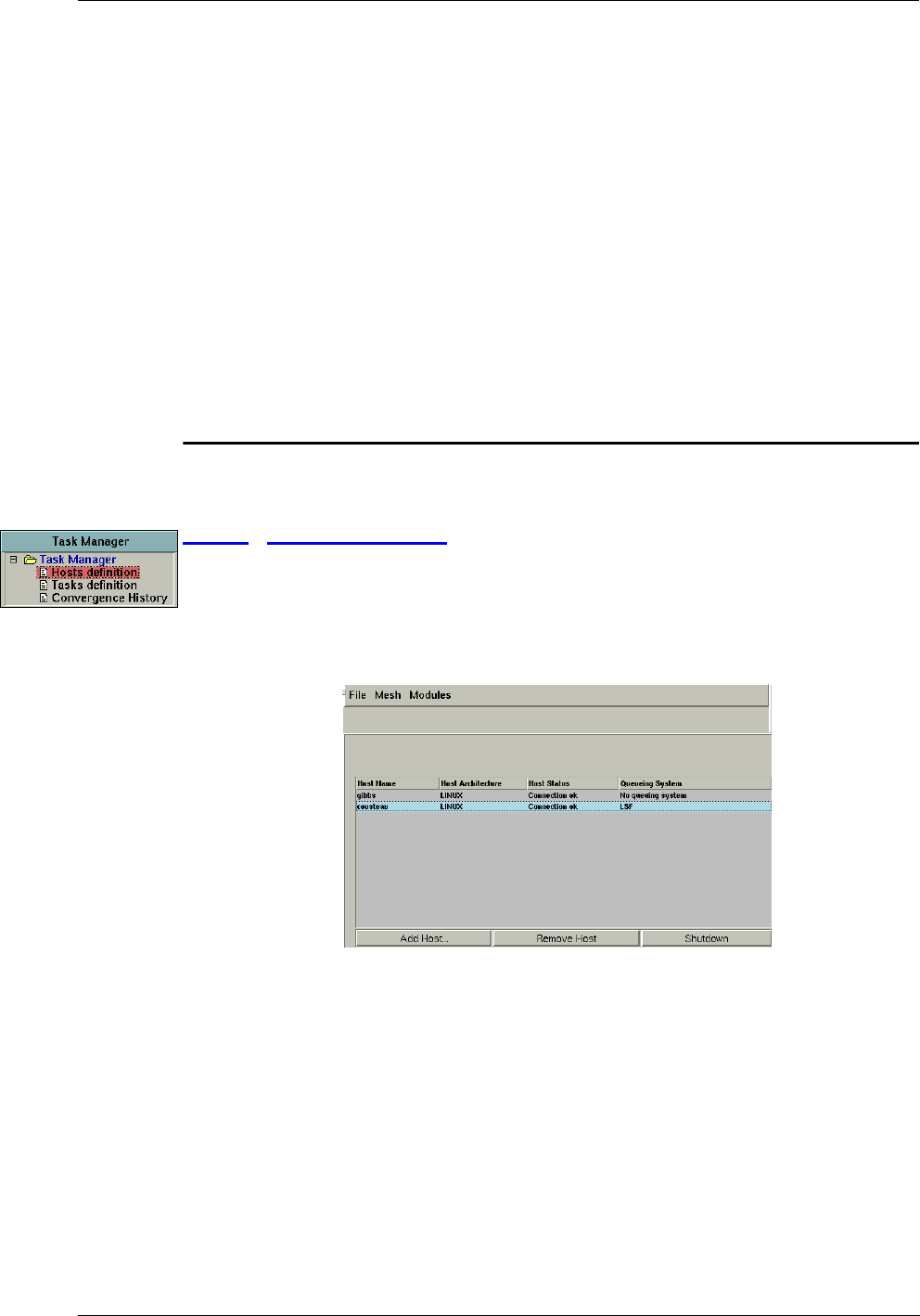
The Task Manager Interface Task Manager
FINE™/Turbo 11-5
task starts. When it terminates, all results files are transferred in the original directory. This feature
uses the rcp.exe Windows command. Before using the remote copy feature, it is advised to first
check if this command works properly:
—First try the rsh.exe command (see section 11-2.3).
—Create a file test, then type the command: rcp -b test destination_machine:/tmp/test. If no
error is returned by the system, the remote copy works between the local host and the
destination_machine. Errors may appear if the .cshrc file contains an stty command. In order
to be able to use the remote copy feature, remove all the stty commands from the .cshrc file.
—If the login on Windows is different from the login on the remote host, type the command:
rcp -b test destination_machine.remote_login:/tmp/test
rcp.exe is provided with FINE™/Turbo and is located in the same directory as rsh.exe.
11-3 The Task Manager Interface
11-3.1 Hosts Definition
The Hosts definition page shows the host name, the operating system, the connection status and the
queuing system supported by FINE™/Turbo if any. For an explanation of the virtual machine see
section 11-2.1.1. If the connection is not OK, it means that the corresponding computer is not in the
virtual machine anymore. This may occur for example if the computer has been rebooted.
FIGURE 11.3.1-1 Hosts definition page
11-3.1.1 Add Host
When the user clicks on the Add Host... button, the interface asks for a host name and a login name.
The login name is optional. It is needed only if the login of the user on the local and remote host are
different.
When the user accepts (Accept), the host name appears in the host list, with type of operating sys-
tem and its connection status. At this point, the host is in the virtual machine, and is ready to receive
a task.
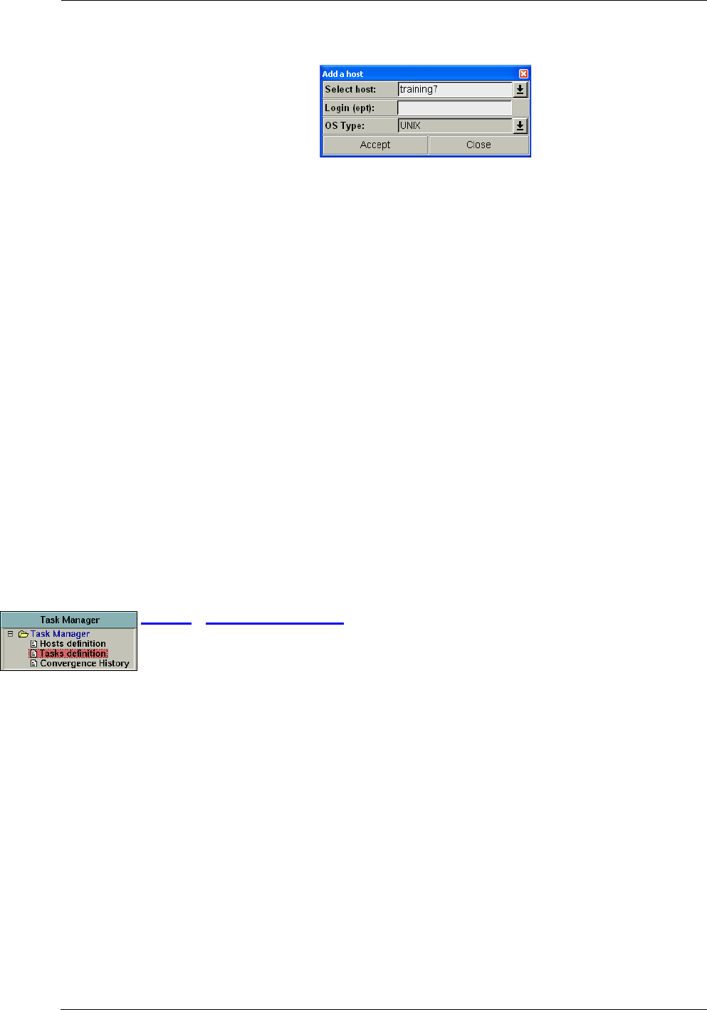
Task Manager The Task Manager Interface
11-6 FINE™/Turbo
FIGURE 11.3.1-2 Add a Host
If the connection can not be established, check for more detail in section 11-2.1, sec-
tion 11-2.3 and section 11-2.4.
The reason that the Task Manager freezes can be because FINE™/Turbo has been
launched in background using an additional & symbol behind the command line. You
can unfreeze the Task Manager with the <fg> command.
It is impossible to add a host on Fedora 3 and Windows Vista operating systems.
11-3.1.2 Remove Host
When the user clicks on the Remove Host button, the selected host is removed from the list, and is
not in the virtual machine anymore. This operation is not allowed when a task is running on the
host, to be removed, or when the selected host is the local one.
11-3.1.3 Shutdown
When the user clicks on the Shutdown button, all hosts in the virtual machine are removed. FINE™/
Turbo exits and the virtual machine halts. All running tasks are killed. This option is useful when
the user wants to change the machine on which FINE™/Turbo is running. See section 11-2.1.1 for
more detail on virtual machines and when to change this.
11-3.2 Tasks Definition
A task is a collection of subtasks, where a subtask is one of the programs with its arguments (".run"
file for the FINE™/Turbo and FINE™/Design3D solver, template ".trb", geometry ".geomTurbo"
and mesh ".igg" files for AutoGrid™ and macro file ".py" and ".run" file for CFView™). The dif-
ferent subtasks of a given task can be run simultaneously if the output of one subtask is not needed
by other ones (for example: several CFView™ subtasks with different macro ".py" files or several
the FINE™/Turbo solver subtasks with different ".run" files started on different computer). If the
output of one subtask is needed by other ones, they must be run sequentially. For example: AutoG-
rid™ generates the mesh that is used for starting an the FINE™/Turbo solver computation whose
output is used for starting CFView™.
11-3.2.1 Task List
In this section, the user can visualize the defined tasks and their status. To create a task, just click on
New Task button. The defaults task name can be modified by clicking on Rename Task button. The
selected task can be removed by clicking on Remove Task button.
After a subtask is defined, the Save button can be used to save all necessary files to start a parallel
computation in batch mode. When a queuing system is used, a set of default templates is available
in order to submit the job to the queue. New templates can also be created by the user.
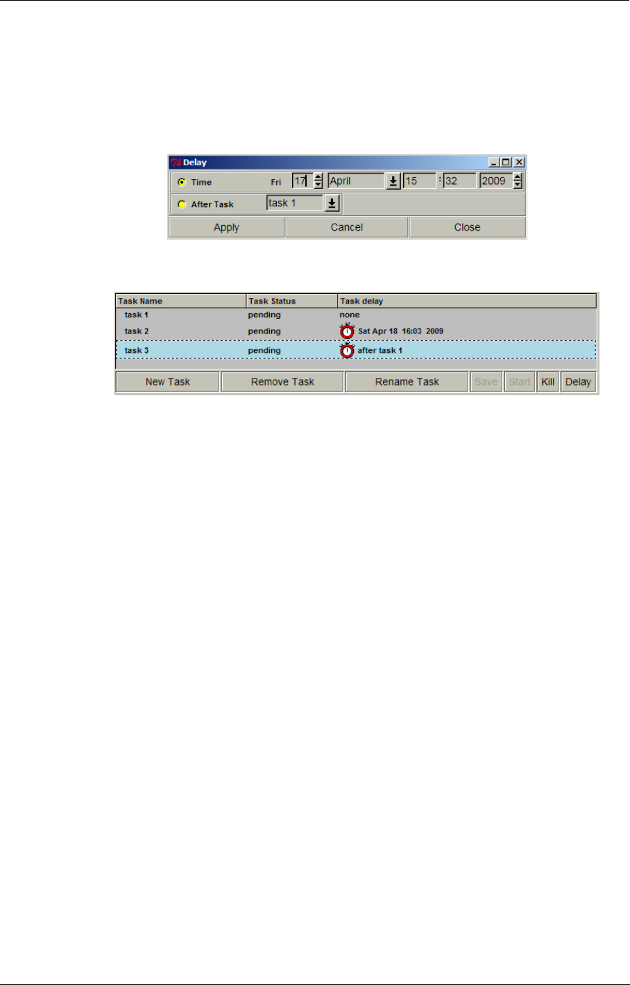
The Task Manager Interface Task Manager
FINE™/Turbo 11-7
Once a task is created and defined (see following section), it can be started or stopped just by click-
ing respectively on the Start or Stop button.
The user can delay the start of a computation by clicking on Delay button. A dialog box will appear
where the user can set a task that will be launched at the specified date and time or after another
specified task has finished. The delayed task can be disabled using the button Cancel.
When the user validates the data, a little watch in the task list indicates that the task is scheduled:
FIGURE 11.3.2-3 Task List with Delay window to start a task at a later moment
When setting a task that will be launched after another specified task has finished, the
reference task should not be a computation launch from the FINE™/Turbo GUI. Other-
wise the delayed task will not start.
11-3.2.2 Task Definition
In this section the subtasks of the selected task are listed. A subtask is defined by its type (FINE™/
Turbo solver, AutoGrid™, CFView™ or Design3D), its status and the host on which they are
launched. To add a subtask click on the New button in Task Definition area. Select the executable
name (FINE™/Turbo solver, AutoGrid™, CFView™ or Design3D) and the host on which the proc-
ess should be started, from the two available lists. The host name list contains the hosts that are in
the virtual machine. They are set in the Host definition page.
11-3.2.3 Subtask Arguments
a) Definition of Input & Output
Once a subtask is created, input and/or output files must be defined in the Subtask Arguments &
characteristics section:
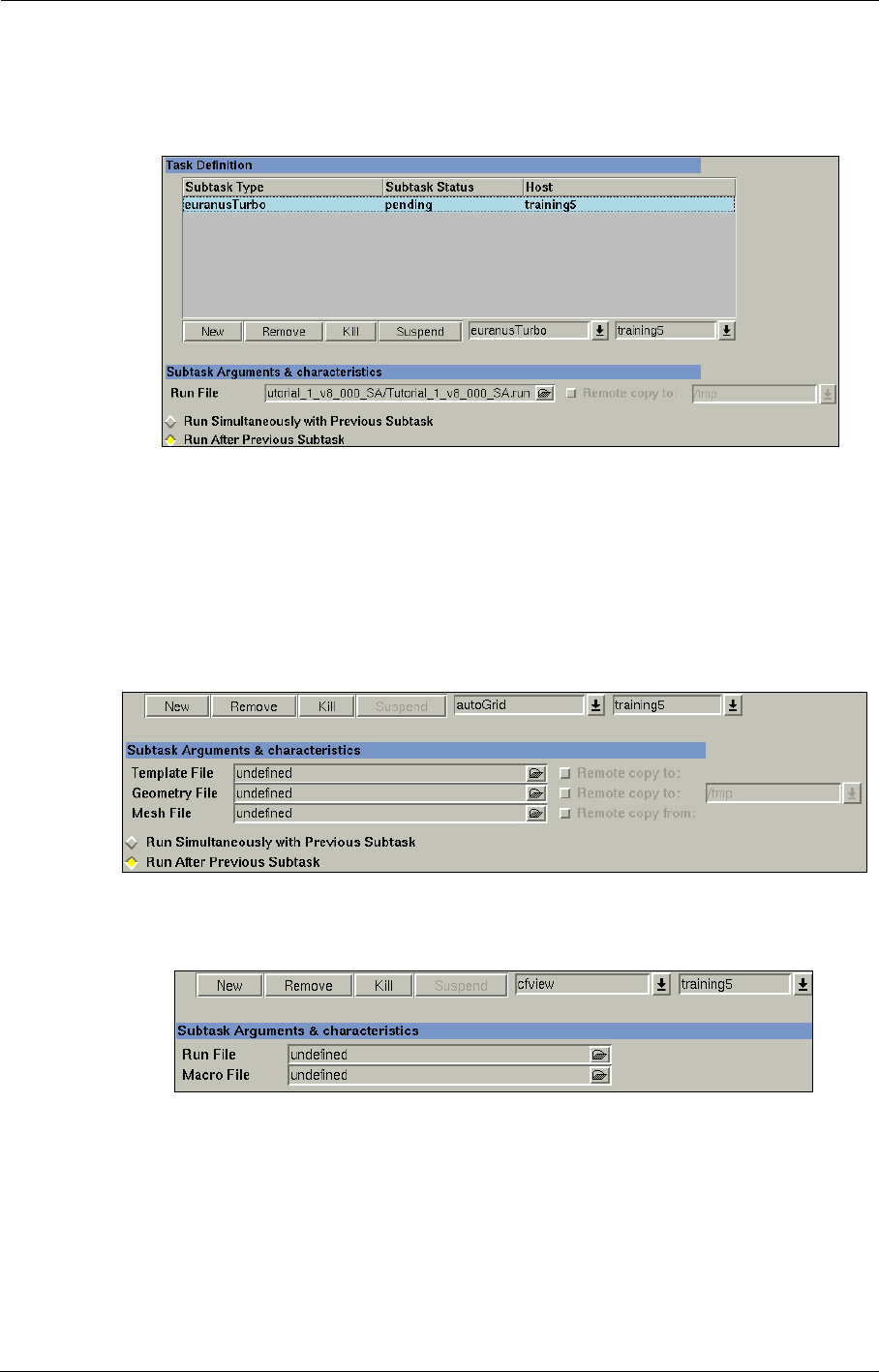
Task Manager The Task Manager Interface
11-8 FINE™/Turbo
—The FINE™/Turbo solver and the FINE™/Design3D solver require one argument file: the
name of the ".run" file. This files is created using the menu File/Save Run Files in the
FINE™/Turbo GUI and FINE™/Design3D GUI.
—The mesh generation system AutoGrid™ requires three files as arguments: the ".trb" file, the
".geomTurbo" file and as output the grid file ".igg" (see the AutoGrid™ User Manual for
more details)
When working on a remote host, the process still requires a valid display. On Win-
dows platforms, it is not possible to transfer the display, therefore the mesh generation
has to be executed locally. On Linux platforms, the command <xhost +> has to be exe-
cuted on the local machine.
—The flow visualization system CFView™ requires two files: the ".run" file and a macro file
".py" (see CFView™ User Manual for more details)
When working on a remote host, the process still requires a valid display. On Win-
dows platforms, it is not possible to transfer the display, therefore the flow postprocess-
ing has to be executed locally. On Linux platforms, the command <xhost +> has to be
executed on the local machine.
The run file is automatically opened by CFView™ before starting the macro. The macro file
may open other ".run" files to perform flow comparisons (see CFView™ User Manual for
more information about the macro ".py" file).
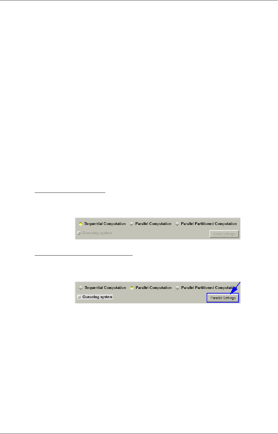
The Task Manager Interface Task Manager
FINE™/Turbo 11-9
b) Simultaneous or Sequential Mode
Moreover, a process can be executed simultaneously with the other subtasks (by selecting Run
Simultaneously with Previous Subtask) or sequentially (by selecting Run After Previous Sub-
task). In sequential mode, the process waits until the previous subtask is finished before starting the
next one. This is only available for AutoGrid™, Design3D and the FINE™/Turbo solver subtasks.
Only a certain amount of tasks can be performed at the same time depending on the available
licenses. The subtasks related to postprocessing with CFView™ are always executed in sequential
mode.
c) Remote Copy
The Remote copy to option allows the user to specify that the files are not visible from the remote
machine and must be transferred. This is only available for AutoGrid™, Design3D and the
FINE™/Turbo solver.
d) Launching Mode
The FINE™/Turbo solver has an integrated multiprocessor machine concept, which allows the user
to launch the flow solver in serial mode or parallel mode. FINE™/Turbo provides two parallel ver-
sions of the flow solver: Parallel Computation relies on the existing block structure and Parallel
Partitioned Computation allows to automatically split the mesh in order to run the computation
on a massively parallel environment, see Chapter 11-4 for more information.
d.1) Sequential Computation
By default, the FINE™/Turbo solver will be launched in serial mode. Nothing is needed to set a
sequential computation.
d.2) Parallel Computation - MPI system
The option Parallel Computation can be selected to specify that the parallel version of the flow
solver has to be used for this computation.
The button Parallel Settings gives access to the dialog box used to set up a parallel computation.
When the dialog box is opened, the block list displays all the blocks of the mesh. The user can
define new processes on all the available machines. Additionally, the load balancing can be defined
manually or automatically (by using the Automatic Load Balancing button).
The parallel processing can only be used on multiprocessor machine (shared memory
mode) or on machines with the same operating systems (homogenous distributed mem-
ory mode)
See section 11-4 for more detailed information on parallel computations.
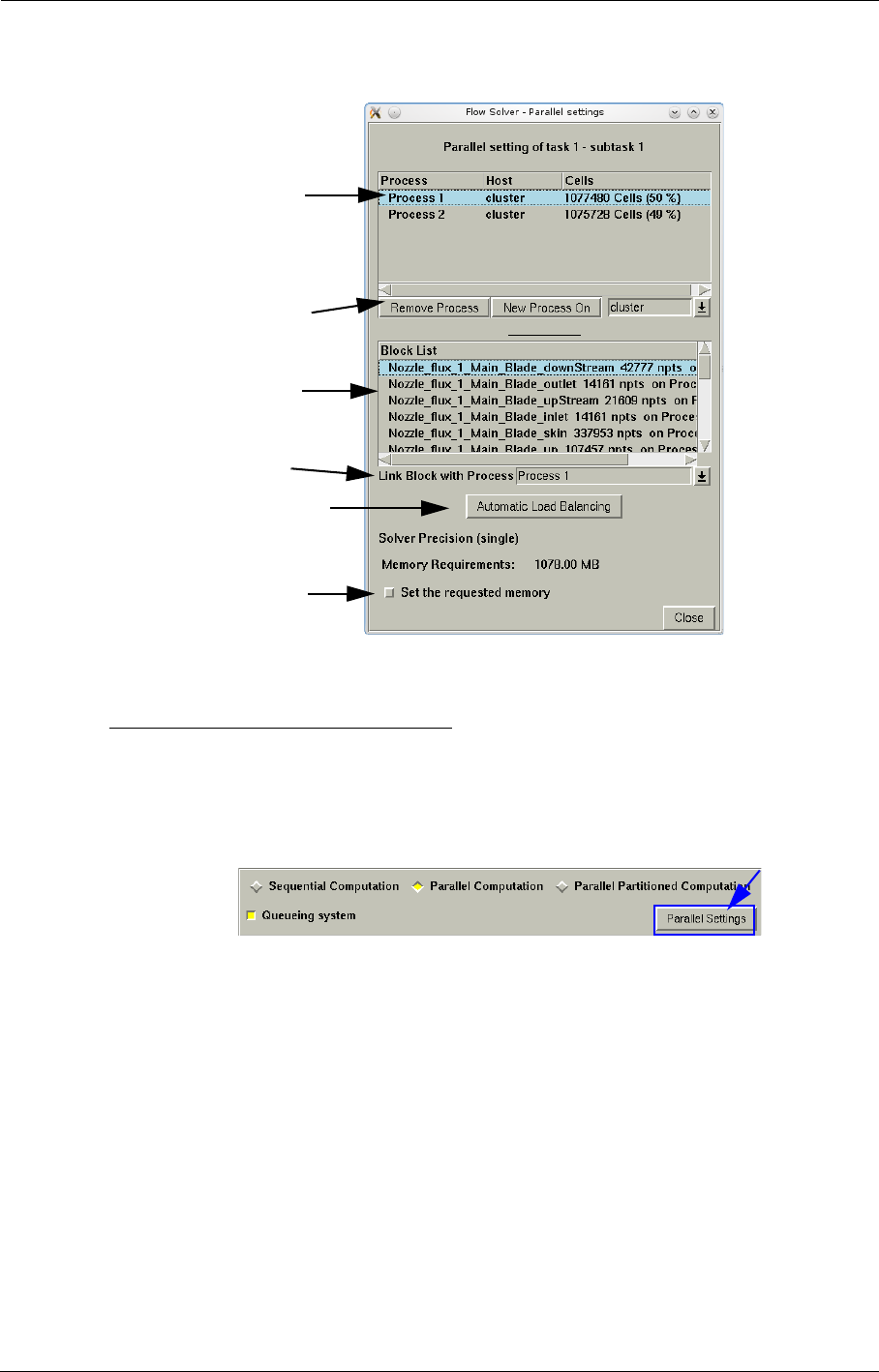
Task Manager The Task Manager Interface
11-10 FINE™/Turbo
FIGURE 11.3.2-4 Parallel settings - load balancing
d.3) Parallel Computation - Queuing system
Within the Task Manager, the parallel computation can also be set-up on the Sun Grid Engine batch
system (SGE), the Portable Batch System (PBS) or the Load Sharing Facility (LSF).
When setting a parallel computation on a queuing system, the option Parallel Computation has to
be selected and the button Queuing system has to be activated.
The button Parallel Settings gives access to the dialog box used to set up a parallel computation on
a queuing system.
After the dialog box is opened, the block list displays all the blocks of the mesh, see Figure 11.3.2-
5. When a queuing system is used, the number of processors and the system environment have to be
specified. Depending on the number of processors, the load balancing can be defined automatically
(by using the Automatic Load Balancing button) or manually.
Processes list with the
load balancing of the cells
Buttons used to remove
or add new processes
on the specified machine
List of the block in the
associated mesh
Button used to link the
selected block with a
process
Default block distribution
Button used to allocate
more memory
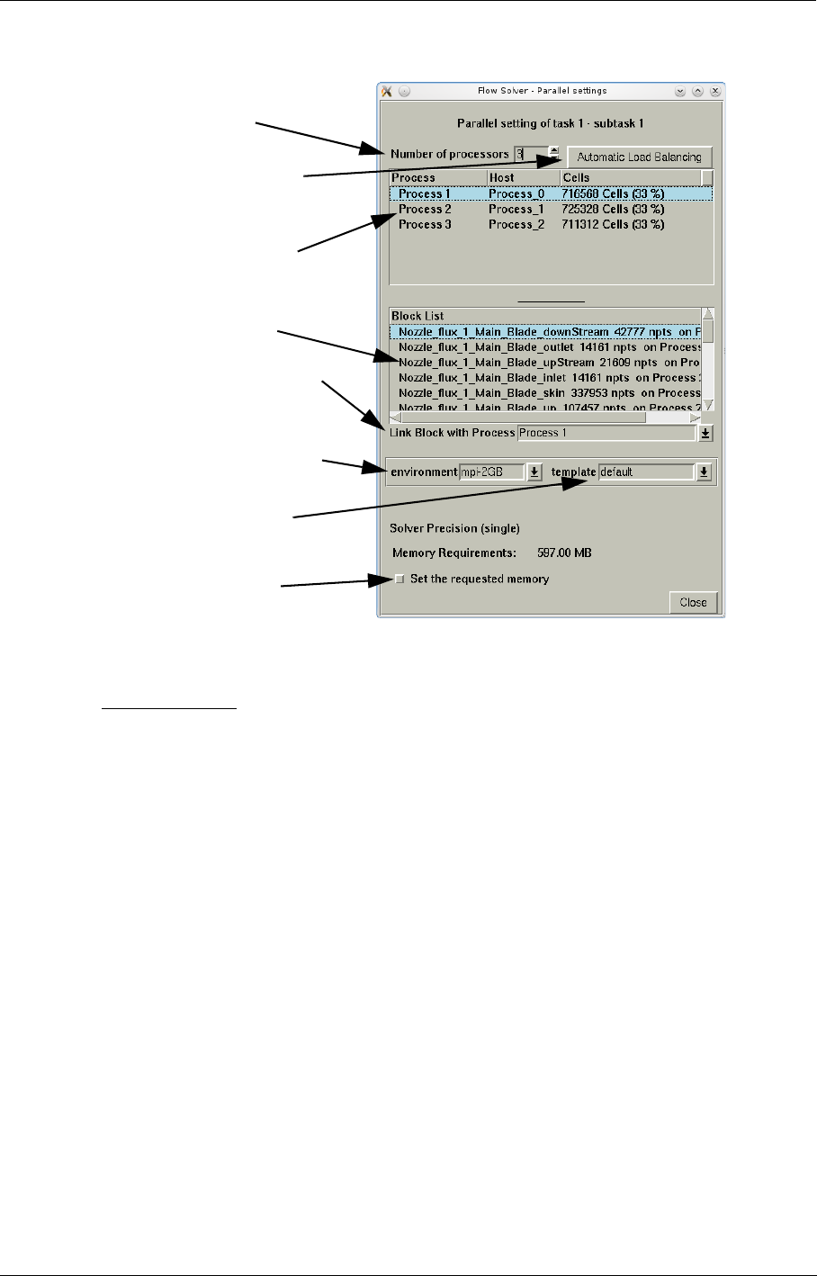
The Task Manager Interface Task Manager
FINE™/Turbo 11-11
FIGURE 11.3.2-5 Parallel settings - load balancing for SGE/PBS/LSF
d.3.1) SGE system
The SGE system includes the possibility to add a SGE type host and to define arguments needed to
launch the computation within the Task Manager.
Host Definition
In the page Hosts definition the user needs to add the host. When adding the host, automatic
checks are performed:
1. it will detect if the "sge_qmaster" or "sge_execd" is running on the platform. If not, it means that
the platform does not have SGE capabilities.
2. it will detect all parallel environments defined in SGE.
3. it will detect all parallel environments, that the user is allowed to use. If no parallel environment
could be accessed by the user, his login should be added to the user list by the SGE administra-
tor.
When all checks are successful, the SGE capability of the added host is activated and the user can
see if the host added is a SGE platform within the Task Manager GUI (Figure 11.3.1-1).
Task Definition
If the user selects a SGE platform when launching an FINE™/Turbo solver task in parallel, the
Task Definition page gives access to the MPI or SGE system. When the SGE system is used, the
task can be defined as shown in Figure 11.3.2-5.
The user can change the block distribution but not the process host names since the
Impose the number
List of the block in the
associated mesh
Button used to link the
selected block with a process
Default block distribution
Button used to allocate
more memory
of processors
Processes list with the
load balancing of the cells
SGE/PBS/LSF environment
SGE/PBS/LSF template

Task Manager The Task Manager Interface
11-12 FINE™/Turbo
SGE system only asks for a number of processors.
See section 11-4 for more detailed information on parallel computations.
Process Management
Once the process is starting, the ".run" file is modified automatically, depending on the number of
processors used. A script file (".sge") is also created at the same time as the ".p4pg" file, when using
MPI system.
The name of the SGE job is limited to 8 characters and the following format is thus
chosen "comp####" where #### stands for any number depending of the number of SGE
jobs already running under the same environment.
Because the FINE™/Turbo solver has not been launched using the PVM daemon, there is no com-
munication with the Task Manager. To test if a computation is running, the "qstat" command with
the job-ID number of the SGE job is used.
To suspend the SGE job, the user can use the Suspend function of the Task Manager. It will create
automatically a ".stop" file in the running computation directory that will enable the FINE™/Turbo
solver to suspend after saving the solution at the next iteration or after the full multigrid initializa-
tion.
To kill the SGE job, the user can use the Kill function. The Task Manager will then use the SGE’s
function "qdel" to kill the computation without saving the solution.
To kill the FINE™/Turbo solver properly, the SGE’s "execd parameters" variable
should be set to "NOTIFY_KILL=TERM" and the "notify time" variable of nodes
should be set to a sufficient value to allow the FINE™/Turbo solver to exit properly (e.g.
120 seconds). In general, this variable should be set to a value higher than the time
required for 1 iteration. We advise the user to ask the SGE administrator to check these
variables.
d.3.2) PBS system
The PBS system includes the possibility to add a PBS type host and to define the arguments needed
to launch the computation within the Task Manager.
Host Definition
In the page Hosts definition the user needs to add the host. When adding the host, automatic
checks are performed:
1. it will detect if the process "pbs_mom" is running on the platform. If not, it means that the plat-
form does not have PBS capabilities.
2. it will detect all defined PBS environments.
When all checks are successful, the PBS capability of the added host is activated and the user can
see if the host added is a PBS platform within the Task Manager GUI (Figure 11.3.1-1).
Task Definition
If the user selects a PBS platform when launching an FINE™/Turbo solver task in parallel, the Task
Definition page gives access to the MPI or PBS system. When the PBS system is used, the task can
be defined as shown in Figure 11.3.2-5.
The user can change the block distribution but not the process host names since the
PBS system only asks for a number of processors.
Process Management

The Task Manager Interface Task Manager
FINE™/Turbo 11-13
Once the process is starting, the ".run" file is modified automatically, depending on the number of
processors used. A script file (".pbs") is also created at the same time as the ".p4pg" file, when
using MPI system.
The name of the PBS job is limited to 8 characters and the following format is thus
chosen "comp####" where #### stands for any number depending of the number of PBS
jobs already running under the same environment.
Because the FINE™/Turbo solver has not been launched using the PVM daemon, there is no com-
munication with the Task Manager. To test if a computation is running, the "qstat" command with
the job-ID number of the PBS job is used.
To suspend the PBS job, the user can use the Suspend function of the Task Manager. It will create
automatically a ".stop" file in the running computation directory that will enable the FINE™/Turbo
solver to suspend after saving the solution at the next iteration or after the full multigrid initializa-
tion.
To kill the PBS job, the user can use the Kill function. The Task Manager will then use the PBS’s
function "qdel" to kill the computation without saving the solution.
To kill the FINE™/Turbo solver properly, the PBS variable "kill_delay" should be set
to a sufficiently high value to allow the FINE™/Turbo solver to exit properly (e.g. 120
seconds). In general, this variable should be set to a value higher than the time required
for 1 iteration. We advise the user to ask the PBS administrator to check this variable.
d.3.3) LSF system
The LSF system includes the possibility to add a LSF type host and to define the arguments needed
to launch the computation within the Task Manager.
Host Definition
In the page Hosts definition the user needs to add the host. When adding the host, automatic
checks are performed:
1. it will detect if the process "sbatchd" is running on the platform. If not, it means that the plat-
form does not have LSF capabilities.
2. it will detect all defined LSF environments.
When all checks are successful, the LSF capability of the added host is activated and the user can
see if the host added is a LSF platform within the Task Manager GUI (Figure 11.3.1-1).
Task Definition
If the user selects a LSF platform when launching an FINE™/Turbo solver task in parallel, the Task
Definition page gives access to the MPI or LSF system. When the LSF system is used, the task can
be defined as shown in Figure 11.3.2-5.
The user can change the block distribution but not the process host names since the
LSF system only asks for a number of processors.
Process Management
Once the process is starting, the ".run" file is modified automatically, depending on the number of
processors used. A script file (".lsf") is also created at the same time as the ".p4pg" file, when using
MPI system.
The name of the LSF job is limited to 8 characters and the following format is thus
chosen "comp####" where #### stands for any number depending of the number of LSF
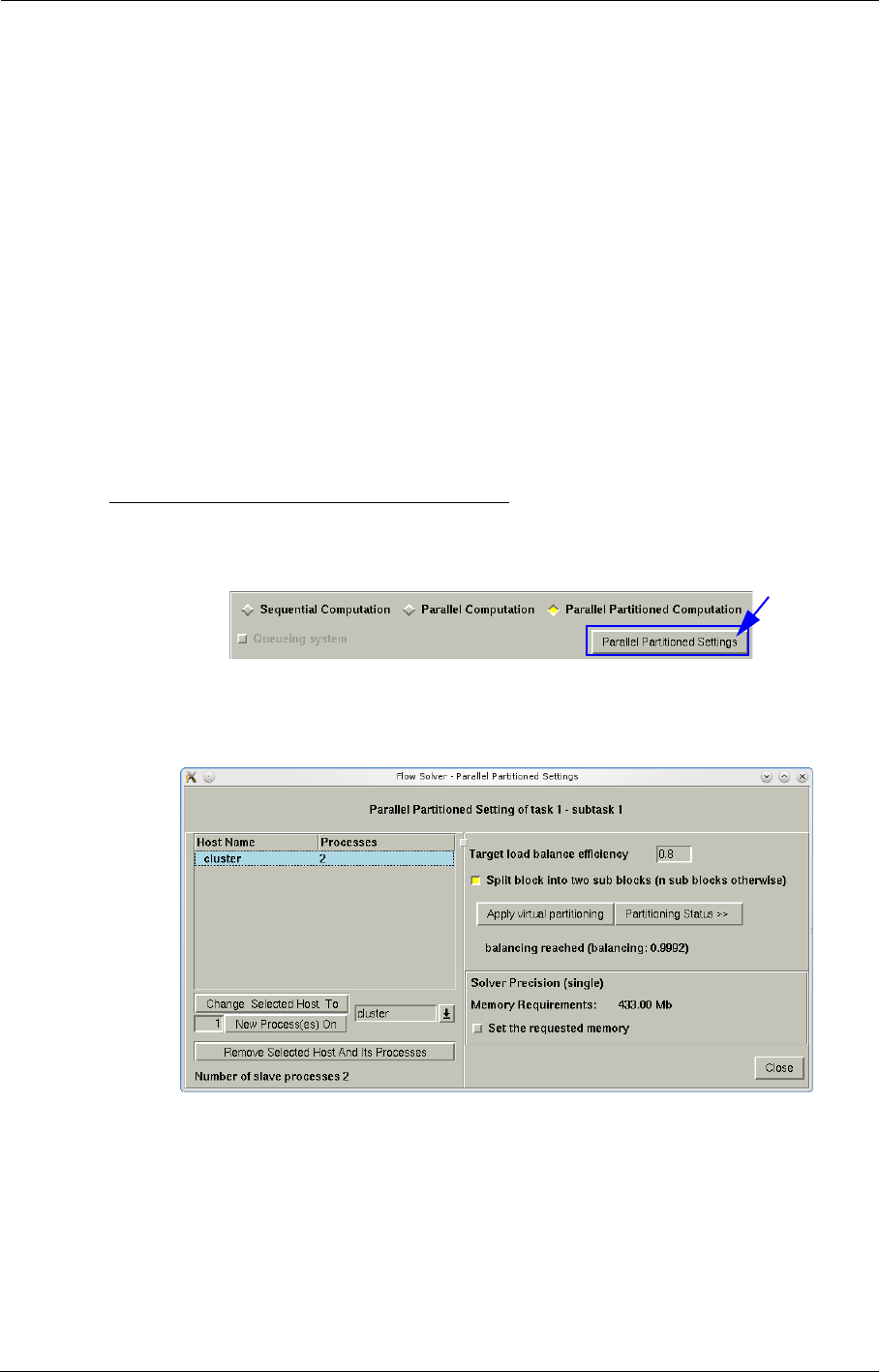
Task Manager The Task Manager Interface
11-14 FINE™/Turbo
jobs already running under the same environment.
Because the FINE™/Turbo solver has not been launched using the PVM daemon, there is no com-
munication with the Task Manager. To test if a computation is running, the "bjobs" command with
the job-ID number of the LSF job is used.
To suspend the LSF job, the user can use the Suspend function of the Task Manager. It will create
automatically a ".stop" file in the running computation directory that will enable the FINE™/Turbo
solver to suspend after saving the solution at the next iteration or after the full multigrid initializa-
tion.
To kill the LSF job, the user can use the Kill function. The Task Manager will then use the LSF’s
function "bkill" to kill the computation without saving the solution.
To kill the FINE™/Turbo solver properly, the LSF variable
"JOB_TERMINATE_INTERVAL" should be set to a sufficiently high value to allow the
FINE™/Turbo solver to exit properly (e.g. 120 seconds). In general, this variable should
be set to a value higher than the time required for 1 iteration. We advise the user to ask
the LSF administrator to check this variable.
d.4) Parallel Partitioned Computation - MPI system
The option Parallel Partitioned Computation can be selected to specify that the parallel parti-
tioned version of the flow solver has to be used for this computation.
The button Parallel Partitioned Settings gives access to the dialog box used to set up a parallel par-
titioned computation.
FIGURE 11.3.2-6 Parallel partitioned settings
For parallel partitioned computation, the mesh will be automatically partitioned. What the user
needs to do is to define the hosts with the number of processes and to specify the parameters used to
split and partition the mesh.
On the left side of the parallel partitioned settings dialog, the hosts can be added or removed. The
list shows all the defined hosts and its processes. The button New Process(es) on allows to add the

The Task Manager Interface Task Manager
FINE™/Turbo 11-15
specified number of processes (left of the button) on the selected host (right of the button) to the
host list. The button Remove Selected Host And Its Processes allows to remove the selected host
from the list.
For the partition, the user needs to specify the Target load balance efficiency, which is a real
between [0,1]. More the target load balance efficiency is close to 1, more the workload, the commu-
nications,... will be properly balanced over the processes but more sub blocks will compose the par-
tition. In order to keep the computational efficiency, the maximum number of blocks per process is
limited to 8 in the parallel partitioned computation. So, if the user specify a large target load balance
efficiency, a partition will be proposed even if it does not raise the expected balancing. If the option
Split block into two subblocks (n subblocks otherwise) is activated, the block will be split into
two subblocks when splitting. Otherwise the block will be split into n subblocks (depending on the
case).
After setting the parameters, click-left on the button Apply Virtual Partitioning to launch the sym-
bolic partitioning and balancing algorithm. The status of the partitioning algorithm can be checked
by clicking on the button Partitioning Status>>.
The parallel processing can only be used on multiprocessor machine (shared memory
mode) or on machines with the same operating systems (homogenous distributed mem-
ory mode)
See section 11-4 for more detailed information on parallel partitioned computations.
d.5) User-defined Templates on Queuing Systems
If the option Queuing system in the Task Definition page is activated, the user needs to select a
template in the Parallel settings dialog box in order to submit the computation to the queue. By
default, a set of templates is available for the supported queuing systems SGE, PBS and LSF (with
corresponding extension .sge, .pbs or .lsf).
The user can also create a new template to customize the settings: queuing system environment,
OpenMPI, etc. In order to use an user-defined template, the user has to:
•name the new template using the extension .sge, .pbs or .lsf, corresponding to the queuing sys-
tem,
•copy the template to the queuing templates folder:
—On Unix/Linux systems:
"NUMECA_INSTALLATION_DIRECTORY/fine#/COMMON/queuing_templates/"
—On Windows systems:
"NUMECA_INSTALLATION_DIRECTORY\Fine#\bin\queuing_templates\"
It is strongly suggested to create a new template based on the existing templates. All the existing
templates can be found in the queuing templates folder mentioned above. Figure 11.3.2-7 shows the
contents of the default SGE template launching the single precision solver. Based on this template,
the user can customize the SGE environment, the OpenMPI settings and the command launching
the computation. Please refer to Chapter 11-5.5.3 to Chapter 11-5.5.5 for the detailed explanation of
the template contents.
The user must obey the following rules when creating a new template:
•Any line beginning with # (except #!, #$, #PBS and #BSUB) is a comment.
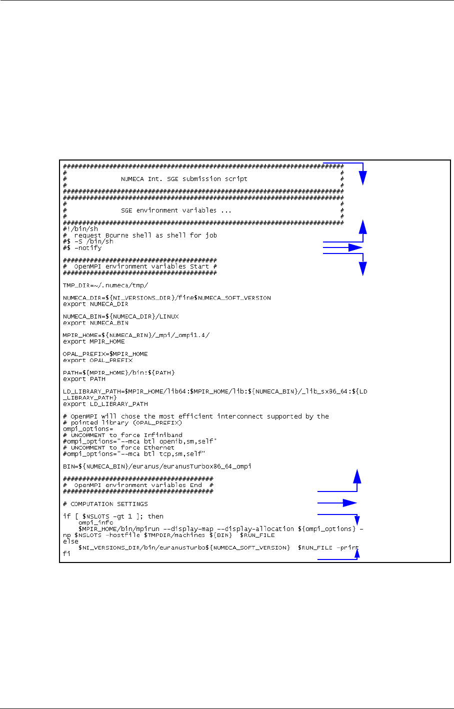
Task Manager The Task Manager Interface
11-16 FINE™/Turbo
•The first blank line MUST be placed after the section defining queuing system environment
and before the section defining the OpenMPI settings. Here, TaskManager will define the
queuing system environment variables (number of processors, name of the computation, etc.)
and the NUMECA variables (NI_VERSION_DIR and NUMECA_SOFT_VERSION),
depending on the user-settings in TaskManager.
•The comment line "# COMPUTATION SETTINGS" MUST be kept and placed before the
command launching the flow solver. Here, TaskManager will define the computation settings
(variables RUN_FILE, STEERING1 and STEERING2), which are used in the command
launching the flow solver.
FIGURE 11.3.2-7 The default template launching the single precision solver for SGE
(default.sge)
The first blank line
Define SGE environment
Variables
Define OpenMPI variables
Comment line where
computation setting
will be defined
Command launching the
flow solver
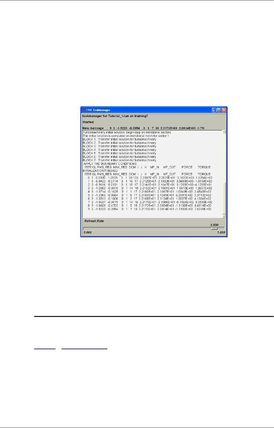
Parallel Computations Task Manager
FINE™/Turbo 11-17
e) Message Window
When a task is started, a Task Manager process is launched to take care about the task management:
process communication, automatic launching of the sequential and parallel subtasks. A message
window linked to the Task Manager is opened. In this window the user can follow the evolution of
the status of all the subtasks of the current task. In case the flow solver is launched, the iterations
are also displayed in this window as shown in Figure 11.3.2-8.
At the bottom of the Task Manager window a Refresh Rate can be chosen. This rate determines how
frequently the Task Manager window is updated. A higher refresh rate will update the information
in the window more frequently but will use more of the available CPU.
FIGURE 11.3.2-8 Task Manager information window
If the user quits FINE™/Turbo, all the message windows will stay open and the tasks
will continue. Closing a message window will immediately kill all the subtasks of the
corresponding task.
11-4 Parallel Computations
11-4.1 Introduction
Parallel computations can be defined through the FINE™/Turbo interface as described in section
11-3.2.3. Parallel processing relies on the distribution of independent tasks among several proces-
sors using communication protocols to transfer data from one processor to another whenever this is
necessary. This induces of course an acceleration of the computation itself but it also offers the pos-
sibility to perform large computations, that would not fit on a single processor.
The parallel version uses MPI (Message Passing Interface) libraries. MPI was chosen among other
tools such as PVM or Open MP for its high communication performances (high bandwidth, low
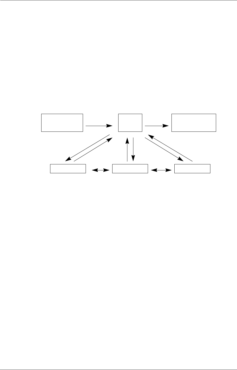
Task Manager Parallel Computations
11-18 FINE™/Turbo
latencies). Although Open MP has better performance on shared memory configurations, i.e. on a
given computer with single global memory and several processors, it is not designed for distributed
memory configurations (several computers with their own memory).
The parallel version is implemented for UNIX, LINUX and Windows platforms (see Installation
Notes for more details on the way to establish connections between platforms). By default, FINE™/
Turbo uses the MPICH/MPICH2 libraries on Windows operating systems and the OpenMPI librar-
ies v1.4 on LINUX/UNIX operating systems.
The present MPI implementation is based on a host/slaves approach. One host process is dedicated
to input/output management. The host reads the mesh and input files, sends the data to the computa-
tion processes (the slaves), receives the computation results from the slave processes and writes the
output files. Figure 11.4.1-9 shows the task distribution on a 4 processor (1 host + 3 slaves) config-
uration. Note that the host/slaves implementation will be replaced progressively as parallel MPI
input/output functionalities are now available.
FIGURE 11.4.1-9 Tasks in a parallel computation
FINE™/Turbo provides two kinds of parallel computation mode: Parallel Computation and Parallel
Partitioned Computation, see section 11-3.2.3 for the interface to set Parallel Computation and Par-
allel Partitioned Computation.
11-4.1.1 Parallel Computation
For parallel computation, the parallel processing relies on the block structure of the mesh. Each
process is assigned a given number of blocks. As a consequence, the number of processors cannot
exceed the number of blocks in the mesh. Boundary data are exchanged between processors each
time an update of the flow solution is required.
11-4.1.2 Parallel Partitioned Computation
The objective of Parallel Partitioned Computation is to improve the capabilities of FINE™/Turbo in
a massively parallel environment, allowing the user to most effectively utilize the computational
resources (large clusters especially). The current parallel partitioned computation version of the
flow solver allows to efficiently use upwards of 1000 compute cores for a single analysis.
The parallel partitioned computation version of the flow solver integrates automatic pre- and post-
processing modules. The pre-processing module is used to automatically split the original mesh and
partition the mesh depending on the user defined Target load balance efficiency and the number of
processes, see section 11-3.2.3. The post-processing module is used to output the result based on
the original mesh instead of on the thousands of split blocks.
Input data
base Host Output data
base
process 1 process 2 process 3
reading writing
boundary conditions boundary conditions

Parallel Computations Task Manager
FINE™/Turbo 11-19
The parallel partitioned computation is not compatible with the following modules:
•transition module
•cooling holes (except the type Points)
•R/S interface: Conservative Coupling by Pitchwise Row / Local Conservative Coupling
•FNMB connecting fluid and solid blocks
•phase lagged method
•2D or axi-symmetric projects
•Lagrangian module
•Turbo machinery initial solution linked to AG4 mesh (expert parameter INITRB set to 0)
•Moving grid module
11-4.2 Management of Inter-Block Communication
The block structure of the solver allows to distribute blocks across processors or computers (in case
of a cluster). Each processor will handle an integer number of blocks. The treatment of the bound-
ary condition will be replaced by a message passing between the processors or remote computers.
Communication optimization
The parallel version of the flow solver is optimized in order to minimize duplicated data as well as
the number and the volume of exchanged messages. A significant improvement of the code per-
formance was obtained by grouping small messages into larger buffers: the information contained
in small messages is usually shared by a large number of blocks, leading to frequent messages of
that type. This is the case for block edges data that are exchanged several times during each itera-
tion. Significant latency times are induced by these communication processes and message group-
ing highly reduces the number of such messages.
Large message limitation
Very large messages are usually exchanged during initialization and at the end of the computation
between the nodes and the host. These also need to be avoided as they can cause important memory
needs and eventually lead to system failure. Messages are split into buffers of maximum size
MXBFSZ (see section 11-4.3) in order to avoid excessive MPI memory requests.
11-4.3 How to Run a Parallel Computation
Configuring a parallel run using the FINE™/Turbo interface is described in section 11-3.2.3.
Memory allocation
Memory allocation is performed as follows:
•The integer data structure is duplicated for all processes. Since the integer data structure size is
about a tenth of the real data structure, this does not lead to high memory overload when the
number of processes is less than 10.
•The real memory allocation is performed for each process. It should be set to the minimal
amount of memory necessary to hold the data structure on the process that has most grid
points. When the load is well balanced, the real memory overload is due to face and edge data
structures. These data need indeed to be duplicated when two processors are involved in the
same block connection.
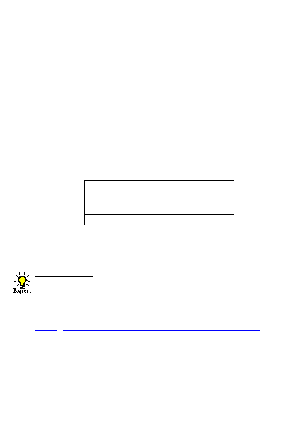
Task Manager Parallel Computations
11-20 FINE™/Turbo
The total memory need Mtotal for a parallel computation involving n ( ) processors can be esti-
mated as:
where Mreal and Minteger are the real and integer memory needed for the same computation in
sequential mode.
From a practical point of view, the user does not specify the total memory needed but the integer
and real memory required per processor. This can be estimated as for the real mem-
ory and Minteger for the integer memory.
When doing a parallel calculation, the estimated real memory displayed by FINE™/
Turbo on the Control Variables page, shall not be followed but the formula shown
above will be respected.
The following table states the total memory needed for a parallel computation using respectively 4
and 6 and 8 processors. The values of Mreal and Minteger are set to 10 Mb and 1 Mb respectively.
The equivalent memory request on a single processor is thus 11Mb.
In the present implementation, the presence of the host processor increases the global memory
request. It also reduces the overall speed-up of the computation as it is mainly dedicated to I/O
management and no computation is affected to it. Future versions of the FINE™/Turbo solver will
optimize this aspect by removing gradually the need of a host processor.
Message size limitation
During initialization and final steps, large messages are usually exchanged between the nodes and
the host process. In order to avoid any system failure, messages are split into buffers of maximum
size. This size is set to 100000 by default but the user can eventually tune this value through the
expert parameter MXBFSZ.
11-4.4 Use an External OpenMPI Library on LINUX/UNIX
By default, FINE™/Turbo uses the OpenMPI library v1.4 on LINUX/UNIX operation systems.
FINE™/Turbo also allows to use an external OpenMPI library, which may be a tuned, customized
or hardware specific OpenMPI library. In order to use an external library, the user has to re-define
the runtime environment, which can be done in two ways:
•create a file ".default_mpi’" under the folder <NUMECA_INSTALLATION_DIRECTORY>/
fine#/_mpi/, where # is the FINE™/Turbo version. Then edit the file ".default_mpi" and spec-
ify the external OpenMPI library in the file ".default_mpi" (here the external library is located
in /tmp/libs/OpenMPI/ompi1.4):
—for csh or tcsh:
setenv NI_MPI_DEFAULT ompi
nM
total (Mb) Parallel overhead (Mb)
4209
6 20.4 9.4
8 21.7 10.7
TABLE 11-1 Parallel memory request
n2≥
Mtotal Mreal 1.2 n
n1–
------------Minteger n⋅+⋅⋅=
Mreal
n
--------------- 1.2⋅

Parallel Computations Task Manager
FINE™/Turbo 11-21
setenv NUMECA_MPI_DIR /tmp/libs/OpenMPI/ompi1.4
—for bash or ksh:
export NI_MPI_DEFAULT=ompi
export NUMECA_MPI_DIR=/tmp/libs/OpenMPI/ompi1.4
In this way, the FINE™/Turbo flow solver will use the specified external library when launch-
ing computations.
•create a file "default_mpi’" under the folder $HOME/.numeca/, where $HOME is the home
directory of the user account. Then edit the file "default_mpi" and specify the external
OpenMPI library in the file "default_mpi" (here the external library is located in /tmp/libs/
OpenMPI/ompi1.4):
—for csh or tcsh:
setenv NI_MPI_DEFAULT ompi
setenv NUMECA_MPI_DIR /tmp/libs/OpenMPI/ompi1.4
—for bash or ksh:
export NI_MPI_DEFAULT=ompi
export NUMECA_MPI_DIR=/tmp/libs/OpenMPI/ompi1.4
In this way, all the NUMECA flow solvers running in this user account will use the specified
external library.
11-4.5 Troubleshooting
Sometimes the parallel computations using MPI can not be started and displays the error message
"p2_3150: p4_error: alloc_p4_mes failed: 0" in the std file. This may be coming from the insuffi-
cient default value of the environment variable P4_GLOBMEMSIZE of your linux system. In that
case the user can increase the value in the shell before starting FINE by typing the following:
•for csh or tcsh:
setenv P4_GLOBMEMSIZE 50000000
•for bash or ksh:
export P4_GLOBMEMSIZE=50000000
Sometimes the parallel computations using MPI might hang or crash at unpredictable iteration that
displays the error message "net_recv_failed for fd" in the std file. The user can increase the value of
the environment variable P4_SOCKBUFSIZE before starting FINE in order to reduce the amount
of occurrences of this problem. Set this variable in the shell by typing the following:
•for csh or tcsh:
setenv P4_SOCKBUFSIZE 1024000
•for bash or ksh:
export P4_SOCKBUFSIZE=1024000
Of course the settings of the P4_GLOBMEMSIZE and P4_SOCKBUFSIZE can be added to the
".cshrc", ".tcshrc", ".bashrc" or ".profile" file of the user. If the user launch the computation in batch
mode or on a cluster by using a script, this variable can be also modified in the launch script before
launching the computation. Please notice that you need to stop or kill all pvm daemons to make sure
that this change is taken into account. This can be done as follows:
•Rebooting your machine if possible, or
•In the Task Manager/Host Definition to click on Shutdown to clean the pvm, or
•To kill the pvm by typing in the shell kill -9 id_pvmd3.
By killing the pvm or performing a shutdown all the processes (including other soft-

Task Manager Task Management in Batch
11-22 FINE™/Turbo
ware that is using PVM) will be stopped.
If the computation is interrupted for the other unknown reason, more detailed information is pro-
vided in the ".std" and ".log" computation files. These files contain all relevant information, includ-
ing MPI error messages and can be sent to our local support office.
11-4.6 Limitations
•The distributed memory mode is restricted to homogeneous (i.e. with the same operating sys-
tem) clusters.
•The blank space is not allowed in the path name.
11-5 Task Management in Batch
This section provides the necessary information to launch NUMECA software from a shell, without
using the IGG™, AutoGrid™, FINE™/Turbo or CFView™ interfaces.
Every time the ".run" file of a FINE™/Turbo computation is saved, a script file is automatically
created. On UNIX systems, the name of this file has the extension ".batch". On Windows the exten-
sion is ".bat". Such files contain text lines with the commands to launch the software with the
appropriate command arguments. To launch a task from a shell simply execute the automatically
generated file by typing its name in a shell.
In the next sections the available commands to launch NUMECA software are described in more
detail.
The capability to launch in batch is currently not supported for the FINE™/Turbo
solver in parallel mode on PC.
11-5.1 Launch IGG™ in Batch
11-5.1.1 How to Launch IGG™ on UNIX
To launch IGG™ without use of the interface the commands to perform must be written in a macro
script file. To create such a file:
1. Create a script file ".py". For more details on the commands that can be included in such a script
file see the IGG™ manual.
2. Launch the macro script in a shell by typing:
"igg <script_path>/script.py -batch -niversion <version>"
The command line to start the grid generator IGG™ contains its name, the full path of the script
".py" file (<script_path>) to launch and the IGG™ release (<version>) that will be used. The "-
batch" option avoids the display of the IGG™ graphical user interface.
When launched in batch, IGG™ does not open the graphical user interface but an
access to the display of the machine on which the process is launched, is still required.

Task Management in Batch Task Manager
FINE™/Turbo 11-23
11-5.1.2 How to Launch IGG™ on Windows
1. Create script file ".py". For more detailed information on the commands to include in a macro
script see the IGG™ manual.
2. Launch the macro script ".py" by typing in a DOS-shell:
"<IGG_path>\igg.exe -script <script_path>\script.py -batch"
The command line to start the grid generator IGG™ contains the full path name of the igg.exe exe-
cutable (<IGG_path>) and the full path of the script ".py" file (<script_path>) to launch. The "-
script" & "-batch" options respectively permit to launch the script and to avoid to display the IGG™
graphical user interface. The igg.exe executable can be found in:
"<NUMECA_install_dir>\Fine#\bin\"
When launched in batch, IGG™ does not open the graphical user interface but an
access to the display of the machine on which the process is launched, is still required.
Remarks:
•The full path of the executable (igg.exe) has to be specified.
•The full path of the script has to be specified.
•There can be a segmentation fault at exit (due to an uncontrollable "opengl" problem). It is
possible to avoid this message, by adding the option "-driver msw".
11-5.2 Launch AutoGrid™ in Batch
11-5.2.1 How to Launch AutoGrid™ 4 on UNIX
1. Create a template and geometry file (".trb" and ".geomTurbo") using the AutoGrid™ 4 inter-
face.
2. Start AutoGrid™ to create a mesh from these files by typing in a shell:
"igg -batch -autoGrid <path>/test.trb <path>/test.geomTurbo \\
<path>/test.igg -niversion <version>"
The command line to start the grid generator AutoGrid™ 4 contains its name, the full path of the
template and geometry file (<path>), the full path of the mesh that will be saved and the IGG™
version that will be used. The "-batch" option avoids the display of the IGG™ graphical user inter-
face.
When launched in batch, IGG™ does not open the graphical user interface but an
access to the display of the machine on which the process is launched, is still required.
11-5.2.2 How to Launch AutoGrid™ on UNIX
1. Create a template and geometry files (".trb" and ".geomTurbo") using the AutoGrid™ interface.
2. Start AutoGrid™ to create a mesh from these files by typing in a shell:
"igg -batch -autogrid5 -trb <path>/test.trb -geomTurbo <path>/test.geomTurbo \\
-mesh <path>/test.igg -niversion <version>"
The command line to start the grid generator AutoGrid™ contains its name, the full path of the tem-
plate and geometry file (<path>), the full path of the mesh that will be saved and the IGG™ ver-
sion that will be used. The "-batch" option avoids the display of the IGG™ graphical user interface.
When launched in batch, IGG™ does not open the graphical user interface but an
access to the display of the machine on which the process is launched, is still required.

Task Manager Task Management in Batch
11-24 FINE™/Turbo
11-5.2.3 How to Launch AutoGrid™ 4 on Windows
1. Create a template and geometry files (".trb" and ".geomTurbo") using the AutoGrid™ 4 inter-
face.
2. Start AutoGrid™ 4 to create a mesh from these files by typing in a DOS-shell:
"<IGG_path>\igg.exe -batch -autoGrid <path>\template.trb \\
<path>\template.geomTurbo <path>\mesh.igg"
The command line to start the grid generator AutoGrid™ 4 contains the full path of the igg.exe exe-
cutable (<IGG_path>), the full path of the template and geometry file (<path>) and the full path of
the mesh that will be saved. The "-batch" option avoids the display of the IGG™ graphical user
interface. The igg.exe executable can be found in: "<NUMECA_install_dir>\Fine#\bin\"
When launched in batch, IGG™ does not open the graphical user interface but an
access to the display of the machine on which the process is launched, is still required.
11-5.2.4 How to Launch AutoGrid™ on Windows
1. Create a template and geometry files (".trb" and ".geomTurbo") using the AutoGrid™ interface.
2. Start AutoGrid™ to create a mesh from these files by typing in a DOS-shell:
"<IGG_path>\igg.exe -batch -autogrid5 -trb <path>\template.trb\\
-geomTurbo <path>/template.geomTurbo -mesh <path>/mesh.igg"
The command line to start the grid generator AutoGrid™ contains the full path of the igg.exe exe-
cutable (<IGG_path>), the full path of the template and geometry file (<path>) and the full path of
the mesh that will be saved. The "-batch" option avoids the display of the IGG™ graphical user
interface. The igg.exe executable can be found in: "<NUMECA_install_dir>\Fine#\bin\"
When launched in batch, IGG™ does not open the graphical user interface but an
access to the display of the machine on which the process is launched, is still required.
11-5.3 Launch FINE™ in Batch
The user has the possibility to set-up a computation, without opening the FINE™/Turbo interface,
through the finebatch program. In batch mode, FINE™/Turbo will create a computation file (.run)
from an existing project (.iec) and mesh (.igg) file. This method can be used to set-up sequential or
parallel computations.
If the geometry or mesh topology has been changed, it is strongly advised to use
FINE™/Turbo interface to set-up the computation. When a new/modified mesh is linked
with an existing project file, an automatic merge will be performed. This merge will reset
the physical parameters to their default values for the modified parts of the mesh. If for
example blocks have been added, the rotation speed, solid conductivity and initial solu-
tion of these blocks will be set to the default values.
The user must have read/write permissions in the project directory.
11-5.3.1 How to Launch FINE™ on UNIX
a) Create a ".run" file
To link a new mesh to an existing project and create the corresponding ".run" file, the finebatch pro-
gram can be launched with following command:

Task Management in Batch Task Manager
FINE™/Turbo 11-25
"fine -niversion <version> -batch <project_path>/project.iec <mesh_path>/mesh.igg \\
<output_path>/output.run <install_path>/fine<version>/COMMON \\
<computation_index>"
or
"fine -niversion <version> -batch <project_path>/project.iec <mesh_path>/mesh.igg \\
<output_path>/output.run <computation_index>"
or
"fine<version> -batch <project_path>/project.iec <mesh_path>/mesh.igg\\
<output_path>/output.run <computation_index>"
In the command line, the version of FINE™/Turbo (<version>) needs to be specified, together with
the -batch option. The -batch option requires following arguments:
•Full path of the input project file (.iec)
•Full path of the input mesh file (.igg)
•Full path of the output computation file (.run)
•Full path of the euranus.def file. This is an optional argument, if no value is specified the
COMMON path of the specified version will be used.
•Index of the computation in the project file. This is an optional argument, if no value is speci-
fied the first computation will be used.
b) Set-up a parallel computation using MPI
To set-up a parallel computation using MPI, the finebatch program can be launched with following
command:
"fine -niversion <version> -batch -parallel <project_path>/computation/computa-
tion.run <nr_of_machines> <machine_name> <nr_of_processors> -print"
or
"fine<version> -batch -parallel <project_path>/computation/computation.run
<nr_of_machines> <machine_name> <nr_of_processors> -print"
In the command line, the version of FINE™/Turbo (<version>) needs to be specified, together with
the -batch and the -parallel option. The -print option is used to print the output to the screen. The -
batch -parallel option require following arguments:
•Full path of the input computation file (.run)
•Number of machines to be used for the parallel computation
•Machine name and the number of processors to use on that machine. If <nr_of_machines> =
N, the machine name and the number of processors have to be repeated N times. e.g. Parallel
computation using 2 machines and 3 processors on each machine:
"fine87_1 -batch -parallel /user/computation/computation.run 2 machine_1 3 machine_2 3"
By default, the distribution of blocks per processor is performed automatically. This automatic dis-
tribution can be modified by adding "-interactive" to the command line. An automatic distribution
will then be proposed, which can be modified by the user.
The output of the program contains 3 files:
•Modified computation file (.run)
•Script file to launch the computation, see section 11-5.5.1 for more details
•Host definition file (.p4pg), see section 11-5.5.1 for more details

Task Manager Task Management in Batch
11-26 FINE™/Turbo
When generating the parallel computation files, the p4pg file generated uses the local
machine as master process and the machines specified in the argument as computing
processes
c) Set-up a parallel computation using SGE
To set-up a parallel computation using the SGE system, the finebatch program can be launched with
following command:
"fine -niversion <version> -batch -sge <project_path>/computation/computation.run\\
<sge_environment> <nr_of_processors> <template_name> -print"
or
"fine <version> -batch -sge <project_path>/computation/computation.run\\
<sge_environment> <nr_of_processors> <template_name> -print"
In the command line, the version of FINE™/Turbo (<version>) needs to be specified, together with
the -batch and the -sge option. The -print option is used to print the output to the screen. The -batch
-sge option require following arguments:
•Full path of the input computation file (.run)
•SGE environment to be used for the parallel computation
•Number of processors to be used for the parallel computation
•Name of template file generated by the user. (It is optional. Finebatch will use the default tem-
plate file by default.)
The distribution of blocks per processor is performed automatically.
The output of the program contains 2 files:
•Modified computation file (.run)
•SGE script file (.sge) to launch the computation, see section 11-5.5.3 for more details
d) Set-up a parallel computation using PBS
To set-up a parallel computation using the PBS system, the finebatch program can be launched with
following command:
"fine -niversion <version> -batch -pbs <project_path>/computation/computation.run\\
<pbs_environment> <nr_of_processors> <template_name> -print"
or
"fine <version> -batch -pbs <project_path>/computation/computation.run\\
<pbs_environment> <nr_of_processors> <template_name> -print"
In the command line, the version of FINE™/Turbo (<version>) needs to be specified, together with
the -batch and the -pbs option. The -print option is used to print the output to the screen. The -batch
-pbs option require following arguments:
•Full path of the input computation file (.run)
•PBS environment to be used for the parallel computation
•Number of processors to be used for the parallel computation
•Name of template file generated by the user. (It is optional. Finebatch will use the default tem-
plate file by default.)
The distribution of blocks per processor is performed automatically.
The output of the program contains 2 files:

Task Management in Batch Task Manager
FINE™/Turbo 11-27
•Modified computation file (.run)
•PBS script file (.pbs) to launch the computation, see section 11-5.5.4 for more details
e) Set-up a parallel computation using LSF
To set-up a parallel computation using the LSF system, the finebatch program can be launched with
following command:
"fine -niversion <version> -batch -lsf <project_path>/computation/computation.run\\
<lsf_environment> <nr_of_processors> <template_name> -print"
or
"fine <version> -batch -lsf <project_path>/computation/computation.run\\
<lsf_environment> <nr_of_processors> <template_name> -print"
In the command line, the version of FINE™/Turbo (<version>) needs to be specified, together with
the -batch and the -lsf option. The -print option is used to print the output to the screen. The -batch -
lsf option require following arguments:
•Full path of the input computation file (.run)
•LSF environment to be used for the parallel computation
•Number of processors to be used for the parallel computation
•Name of template file generated by the user. (It is optional. Finebatch will use the default tem-
plate file by default.)
The distribution of blocks per processor is performed automatically.
The output of the program contains 2 files:
•Modified computation file (.run)
•LSF script file (.lsf) to launch the computation, see section 11-5.5.5 for more details
f) Set-up a parallel partitioned computation using MPI
To set-up a parallel partitioned computation using MPI, the finebatch program can be launched with
following command:
"fine -niversion <version> -batch -partition <balancing> -parallel <project_path>/com-
putation/computation.run <nr_of_machines> <machine_name> <nr_of_processors> -
print"
or
"fine<version> -batch -partition <balancing> -parallel <project_path>/computation/com-
putation.run <nr_of_machines> <machine_name> <nr_of_processors> -print"
In the command line, the version of FINE™/Turbo (<version>) needs to be specified, together with
the -batch, -partition <balancing> and the -parallel option, where <balancing> is the specified Tar-
get laod balance coefficient. The -print option is used to print the output to the screen. The -batch -
partition -parallel option require following arguments:
•Full path of the input computation file (.run)
•Number of machines to be used for the parallel computation
•Machine name and the number of processors to use on that machine. If <nr_of_machines> =
N, the machine name and the number of processors have to be repeated N times. e.g. Parallel
computation using 2 machines and 3 processors on each machine:
"fine87_1 -batch -parallel /user/computation/computation.run 2 machine_1 3 machine_2 3"

Task Manager Task Management in Batch
11-28 FINE™/Turbo
By default, the distribution of blocks per processor is performed automatically. This automatic dis-
tribution can be modified by adding "-interactive" to the command line. An automatic distribution
will then be proposed, which can be modified by the user.
The output of the program contains 3 files:
•Modified computation file (.run)
•Script file to launch the computation, see section 11-5.5.1 for more details
•Host definition file (.p4pg), see section 11-5.5.1 for more details
When generating the parallel partitioned computation files, the p4pg file generated
uses the local machine as master process and the machines specified in the argument as
computing processes
g) Set-up a parallel partitioned computation using SGE
To set-up a parallel partitioned computation using the SGE system, the finebatch program can be
launched with following command:
"fine -niversion <version> -batch -partition <balancing> -sge <project_path>/computa-
tion/computation.run <sge_environment> <nr_of_processors> <template_name> -print"
or
"fine <version> -batch -partition <balancing> -sge <project_path>/computation/compu-
tation.run <sge_environment> <nr_of_processors> <template_name> -print"
In the command line, the version of FINE™/Turbo (<version>) needs to be specified, together with
the -batch, -partition <balancing> and the -sge option, where <balancing> is the specified Target
laod balance coefficient. The -print option is used to print the output to the screen. The -batch -par-
tition -sge option require following arguments:
•Full path of the input computation file (.run)
•SGE environment to be used for the parallel computation
•Number of processors to be used for the parallel computation
•Name of template file generated by the user. (It is optional. Finebatch will use the default tem-
plate file by default.)
The distribution of blocks per processor is performed automatically.
The output of the program contains 2 files:
•Modified computation file (.run)
•SGE script file (.sge) to launch the computation, see section 11-5.5.3 for more details
h) Set-up a parallel partitioned computation using PBS
To set-up a parallel partitioned computation using the PBS system, the finebatch program can be
launched with following command:
"fine -niversion <version> -batch -partition <balancing> -pbs <project_path>/computa-
tion/computation.run <pbs_environment> <nr_of_processors> <template_name> -print"
or
"fine <version> -batch -partition <balancing> -pbs <project_path>/computation/compu-
tation.run <pbs_environment> <nr_of_processors> <template_name> -print"
In the command line, the version of FINE™/Turbo (<version>) needs to be specified, together with
the -batch, -partition <balancing> and the -pbs option, where <balancing> is the specified Target

Task Management in Batch Task Manager
FINE™/Turbo 11-29
laod balance coefficient. The -print option is used to print the output to the screen. The -batch -par-
tition -pbs option require following arguments:
•Full path of the input computation file (.run)
•PBS environment to be used for the parallel computation
•Number of processors to be used for the parallel computation
•Name of template file generated by the user. (It is optional. Finebatch will use the default tem-
plate file by default.)
The distribution of blocks per processor is performed automatically.
The output of the program contains 2 files:
•Modified computation file (.run)
•PBS script file (.pbs) to launch the computation, see section 11-5.5.4 for more details
i) Set-up a parallel partitioned computation using LSF
To set-up a parallel partitioned computation using the LSF system, the finebatch program can be
launched with following command:
"fine -niversion <version> -batch -partition <balancing> -lsf <project_path>/computa-
tion/computation.run <lsf_environment> <nr_of_processors> <template_name> -print"
or
"fine <version> -batch -partition <balancing> -lsf <project_path>/computation/computa-
tion.run <lsf_environment> <nr_of_processors> <template_name> -print"
In the command line, the version of FINE™/Turbo (<version>) needs to be specified, together with
the -batch, -partition <balancing> and the -lsf option, where <balancing> is the specified Target
laod balance coefficient. The -print option is used to print the output to the screen. The -batch -par-
tition -lsf option require following arguments:
•Full path of the input computation file (.run)
•LSF environment to be used for the parallel computation
•Number of processors to be used for the parallel computation
•Name of template file generated by the user. (It is optional. Finebatch will use the default tem-
plate file by default.)
The distribution of blocks per processor is performed automatically.
The output of the program contains 2 files:
•Modified computation file (.run)
•LSF script file (.lsf) to launch the computation, see section 11-5.5.5 for more details
11-5.3.2 How to Launch FINE™ on Windows
It is not possible to set-up parallel computations on Windows with the finebatch pro-
gram.
a) Set-up a sequential computation
To link a new mesh to an existing project and create the corresponding ".run" file, the finebatch pro-
gram can be launched with following command:
"<finebatch_path>\finebatch.exe <project_path>/project.iec <mesh_path>/mesh.igg\\
<output_path>/output.run <install_path>/fine<version>/bin <computation_index>"

Task Manager Task Management in Batch
11-30 FINE™/Turbo
The command line to start the finebatch program contains the full path of the finebatch.exe execut-
able (<finebatch_path>), and following arguments:
•Full path of the input project file (.iec)
•Full path of the input mesh file (.igg)
•Full path of the output computation file (.run)
•Full path of the euranus.def file. This is an optional argument, if no value is specified the bin
path of the specified version will be used.
•Index of the computation in the project file. This is an optional argument, if no value is speci-
fied the first computation will be used.
The finebatch.exe executable can be found in: "<NUMECA_install_dir>\Fine#\bin\"
11-5.4 Launch the flow solver in Sequential Mode in Batch
11-5.4.1 How to Launch the flow solver in Sequential mode on
UNIX
1. Create a script file (for example, with the name "batch.sh"). Such a script file (e.g. "batch.sh")
must be created with permission for execution, to launch a series of computations. An example
of a "batch.sh" file for a series of sequential computations on UNIX:
#! /bin/csh
euranusTurbo <project_path>/computation_1/computation_1.run -niversion <version> \\
-seq
euranusTurbo <project_path>/computation_2/computation_2.run -niversion <version> \\
-seq
or
#! /bin/csh
euranusTurbo<version> <project_path>/computation_1/computation_1.run -seq
euranusTurbo<version> <project_path>/computation_2/computation_2.run -seq
The script is started in a C-shell, which is obtained by the first line: "#! /bin/csh". The command
line, to start the FINE™/Turbo solver, contains its name, the full path of the ".run" file to launch
(<project_path>), the FINE™/Turbo release that will be used (<version>) and the sequential
mode selection.
2. Set Permission for execution for the script file "batch.sh" by typing the command:
"chmod 755 batch.sh".
3. Create an input file (".run") for each computation. To create those files through the FINE™/
Turbo interface, click on the File/Save Run Files menu in order to save the ".run" file of the
activated computation, after opening the corresponding project.
4. Launch the script "batch.sh" by typing: "./batch.sh".
When saving the ".run" file of the computation (File/Save Run Files), a script
"computation_name.batch" is automatically created in the corresponding computation
subfolder. This script enables the user to launch the same computation in batch.
To suspend the batch job, the user can create a ".stop" file with the same computation
name in the running computation directory, which will enable the FINE™/Turbo solver
to suspend after saving the solution at the next iteration or after the full multigrid initiali-
zation.

Task Management in Batch Task Manager
FINE™/Turbo 11-31
11-5.4.2 How to Launch the flow solver in Sequential under
Windows
1. Create script file ".bat". An example of ".bat" file for a series of sequential computations on
Windows:
For 32 bits OS:
"<NUMECA_install_dir>\Fine<version>\bin\euranus.exe <project_path>\computa-
tion\computation.run" -seq
For 64 bits OS:
"<NUMECA_install_dir>\Fine<version>\bin64\euranusx86_64.exe <project_path>\com-
putation\computation.run" -seq
The command line, to start the FINE™/Turbo solver, contains the full path of the flow solver
executable, the full path of the ".run" file to launch and the sequential mode selection.
2. Set permission for execution of the ".bat" file.
3. Create an input file (".run") for each computation. To create those files through the FINE™/
Turbo interface, click on the File/Save Run Files menu in order to save the ".run" file of the
activated computation, after opening the corresponding project.
4. Launch the script ".bat" by typing the script file name: "batch.bat" in a shell or double click on
the ".bat" file from the Windows Explorer.
When saving the ".run" file of the computation (File/Save Run Files), a script
"computation_name.bat" is automatically created in the corresponding computation sub-
folder. This script enables the user to launch the same computation in batch.
To suspend the batch job, the user can create a ".stop" file with the same computation
name in the running computation directory, which will enable the FINE™/Turbo solver
to suspend after saving the solution at the next iteration or after the full multigrid initiali-
zation.
11-5.5 Launch the flow solver in Parallel Mode in Batch
11-5.5.1 How to Launch the flow solver in Parallel using MPI on
UNIX
1. Create a script file "batch.sh" with permission for execution. An example of a "batch.sh" file for
a parallel computation on UNIX:
#! /bin/csh
euranusTurbo_parallel<version> -mca=btl=openib,sm,self <project_path>/computation/
computation.run -p4pg <project_path>/computation/computation.p4pg
The script is started in a C-shell, which is obtained by the first line: "#! /bin/csh". The command
line, to start the FINE™/Turbo solver in parallel, contains the name and the release to use
(<version>), the OpenMPI options that configures the used OpenMPI library or runs the runt-
ime tools, the full path of the ".run" file to launch (<project_path>) and the full path of the file
".p4pg" containing the definition of the machines that will be used to launch the computation in
parallel.

Task Manager Task Management in Batch
11-32 FINE™/Turbo
The name of the executable is different from the one for sequential computations.
The OpenMPI options can be used to configure OpenMPI. In general, all the MCA options
described in http://www.open-mpi.org/faq/?category=tuning#setting-mca-params can be
imposed in the script.
Please note, when the OpenMPI options are following the NUMECA executable
euranusTurbo_parallel<version>, the spaces in the original MCA parameters MUST
be replaced by "=".
If OpenMPI is built with the support of CPU affinity, it is possible to configure this feature
through the script by adding the option -rf=<rankfile>, with a rankfile written like described in
http://www.open-mpi.org/faq/?category=tuning#using-paffinity.
The OpenMPI options can also be used to call the runtime tools that permit to scan the host
machine, get runtime information, etc. For example, the following options can be added in the
command line to obtain the corresponding information:
-param=btl=openib to run ompi_info --param btl openib;
-param=btl=all to run ompi_info --param btl all;
-param=mpi=all to run ompi_info --param mpi all;
-param=all=all to run ompi_info --param all all;
etc.
All the runtime information is written in a hidden file located in the working directory, with the
extension .rtm (.rtm<rank> in case of parallel computation).
2. Create hosts definition file ".p4pg". A file needs to be created to define the hosts (e.g. "compu-
tation.p4pg"). This file specifies the machine information regarding the various processes. An
example of a "computation.p4pg" file:
Example 1:
hostname1 4 euranusTurbo<version>
hostname2 2 euranusTurbo<version>
where master host on hostname1 and 4 processes on hostname1; 2 processes on hostname2.
Example 2:
hostname1 0 euranusTurbo<version>
hostname2 2 euranusTurbo<version>
where master host on hostname1 and 0 process on hostname1; 2 processes on hostname2.
For each machine, a line must be added consisting of the machine name (the machine host-
name), the number of processes to run on the machine, the name of the executable and the
FINE™/Turbo release:
"hostname <nr_processes> euranusTurbo<version>"
If additional machines are to be used, subsequent lines are required for each one. If the number
of processors is set to 0 for the first machine (first line of the ".p4pg" file), only the master host
process will run on that machine while the nodes will run on the next machines declared in the
following lines.
The first machine (hostname) specified in the ".p4pg" file has to be the one, on which

Task Management in Batch Task Manager
FINE™/Turbo 11-33
the script will be launched.
The total number of processes defined in the ".p4pg" file should be equal to the
number of nodes running.
3. Set permission for execution "batch.sh" by using the command: "chmod 755 batch.sh"
The input file ".run" to launch the computation has to be created. The parallel settings of the com-
putational file (".run") are managed by the Task Manager. Therefore before launching the parallel
computation script, the following steps must be performed through the FINE™/Turbo interface:
4. Create computational file (".run") by activating the corresponding computation and clicking on
the File/Save Run Files menu in the interface.
5. To set the final parallel settings:
—create a task in the Task Manager,
—define the parallel settings of the FINE™/Turbo solver subtask (parallel computation),
—Save the task through the Task Manager by clicking on Save button.
These operations are mandatory in order to have all the parallel settings correctly imposed in the
computation file (".run"). They can also be performed in batch, with the finebatch command,
see section 11-5.3.1.
6. Launch the script "batch.sh" by typing the script file name: "./batch.sh".
When saving the ".run" file of the computation (File/Save Run Files) and clicking the
save button (Modules/Task Manager), a script ".batch" and a ".p4pg" file are automati-
cally created in the corresponding computation subfolder. These files enable the user to
launch the same parallel computation in batch.
To suspend the batch job, the user can create a ".stop" file with the same computation
name in the running computation directory, which will enable the FINE™/Turbo solver
to suspend after saving the solution at the next iteration or after the full multigrid initiali-
zation.
11-5.5.2 How to Launch the flow solver in Parallel using MPI on
Windows
1. Create a script file "batch.bat" with permission for execution. An example of a "batch.bat" file
for a parallel computation on Windows:
For 32 bits OS:
"<NUMECA_install_dir>\Fine<version>\bin\mpirun.exe <project_path>\computa-
tion\computation.p4pg <project_path>\computation\computation.run"
The command line, to start the FINE™/Turbo solver in parallel, contains the full path to the
script that enables parallel computations (mpirun.exe), the full path of the ".run" file to launch
(<project_path>) and the full path of the ".p4pg" file containing the definition of the machines
that will be used to launch the computation in parallel.
For 64 bits OS:
"<NUMECA_install_dir>\Fine<version>\bin64\mpiexec.exe -n # -machinefile
<project_path>\computation\computation.machines <NUMECA_install_dir>\Fine<ver-
sion>\bin64\euranusx86_64.exe <project_path>\computation\computation.run"

Task Manager Task Management in Batch
11-34 FINE™/Turbo
The command line, to start the FINE™/Turbo solver in parallel, contains the full path to the
script that enables parallel computations (mpiexec.exe), the number of the processors, the full
path of the ".machines" file containing the definition of the machines that will be used to launch
the computation in parallel, the full path to the flow solver (euranusx86_64.exe) and the full
path of the ".run" file to launch.
2. Create hosts definition file ".p4pg" or ".machines". A file needs to be created to define the hosts
(e.g. "computation.p4pg"). This file specifies the machine information regarding the various
processes.
An example of a "computation.p4pg" file only for 32 bits OS:
hostname1 5 <NUMECA_install_dir>\Fine<version>\bin\euranus.exe
hostname2 2 <NUMECA_install_dir>\Fine<version>\bin\euranus.exe
where master host on hostname1 and 4 processes on hostname1; 2 processes on hostname2.
For each machine, a line must be added consisting of the machine name (the machine host-
name), the number of processes to run on the machine and the full path of the FINE™/Turbo
solver executable. If the number of processors is set to 1 for the first machine (first line of the
".p4pg" file), only the master host process will run on that machine while the nodes will run on
the next machines declared in the following lines.
An example of a "computation.machines" file only for 64 bits OS:
hostname1:5
hostname2:2
where master host on hostname1 and 4 processes on hostname1; 2 processes on hostname2.
For each machine, a line must be added consisting of the machine name (the machine hostname)
and the number of processes to run on the machine. If the number of processors is set to 1 for
the first machine (first line of the ".machines" file), only the master host process will run on that
machine while the nodes will run on the next machines declared in the following lines.
The first machine (hostname) specified in the ".p4pg" or ".machines" file has to be the
one, on which the script will be launched.
The total number of processes defined in the ".p4pg" or ".machines" file should be
equal to the number of nodes running.
3. Set permission for execution "batch.bat"
The input file ".run" to launch the computation has to be created. The parallel settings of the com-
putational file (".run") are managed by the Task Manager. Therefore before launching the parallel
computation script, the following steps must be performed through the FINE™/Turbo interface:
4. Create computational file (".run") by activating the corresponding computation and clicking on
the File/Save Run Files menu in the interface.
5. To set the final parallel settings:
—create a task in the Task Manager,
—define the parallel settings of the FINE™/Turbo solver subtask (parallel computation),
—Save the task through the Task Manager by clicking on Save button.

Task Management in Batch Task Manager
FINE™/Turbo 11-35
These operations are mandatory in order to have all the parallel settings correctly imposed in the
computation file (".run").
6. Launch the script ".bat" by typing the script file name: "batch.bat" in a DOS-shell or double
click on the ".bat" file from the Windows Explorer.
When saving the ".run" file of the computation (File/Save Run Files) and clicking the
save button (Modules/Task Manager), a script ".bat" and a ".p4pg" file are automati-
cally created in the corresponding computation subfolder. These files enable the user to
launch the same parallel computation in batch.
To suspend the batch job, the user can create a ".stop" file with the same computation
name in the running computation directory, which will enable the FINE™/Turbo solver
to suspend after saving the solution at the next iteration or after the full multigrid initiali-
zation.
11-5.5.3 How to Launch the flow solver in Parallel using SGE on
UNIX
1. Create a script file "batch.sge" with permission for execution. An example of a "batch.sge" file
for a parallel computation on UNIX:
#!/bin/sh
#$ -S /bin/sh
#$ -notify
#$ -pe mvapich 4
#$ -N ahmed
#$ -o /tmp/ahmed/ahmed_computation_1/ahmed_computation_1.std -j y
NI_VERSIONS_DIR=/home/fine<version>
export NI_VERSIONS_DIR
NUMECA_SOFT_VERSION=<version>
export NUMECA_SOFT_VERSION
TMP_DIR=~/.numeca/tmp/
NUMECA_DIR=${NI_VERSIONS_DIR}/fine$NUMECA_SOFT_VERSION
export NUMECA_DIR
NUMECA_BIN=${NUMECA_DIR}/LINUX
export NUMECA_BIN
MPIR_HOME=${NUMECA_BIN}/_mpi/_ompi1.4/
export MPIR_HOME
OPAL_PREFIX=$MPIR_HOME
export OPAL_PREFIX
PATH=${MPIR_HOME}/bin:${PATH}
export PATH
LD_LIBRARY_PATH=$MPIR_HOME/lib64:$MPIR_HOME/lib:${NUMECA_BIN}/ \\
_lib_sx86_64:${LD_LIBRARY_PATH}
export LD_LIBRARY_PATH
ompi_options=
BIN=${NUMECA_BIN}/euranus/euranusTurbox86_64_ompi

Task Manager Task Management in Batch
11-36 FINE™/Turbo
RUN_FILE=/tmp/ahmed/ahmed_computation_1/ahmed_computation_1.run
STEERING_FILE=/tmp/ahmed/ahmed_computation_1/ahmed_computation_1.steering
ompi_info
$MPIR_HOME/bin/mpirun --display-map --display-allocation ${ompi_options} -np \\
$NSLOTS -hostfile $TMPDIR/machines ${BIN} $RUN_FILE -steering $STEERING_FILE
where:
#$ -S /bin/sh requires Bourne shell to be used by SGE for job submission and hence, only the
".profile" file of the user is executed if exists on each computation host. There is nothing spe-
cific to NUMECA software that must be written in the ".profile" file.
#$ -notify gives a delay between the send of the SIGKILL signal and SIGUSR2 signal. The
delay is defined in the SGE interface.
#$ -pe mvapich 4 requests 4 slots (processors) to the SGE system for executing the job using the
mvapich parallel environment. This must correspond to NTASK +1 where NTASK is the
number of computation processes (partitions) in the ".run" file, the "+1" being the host process
that manages inputs/outputs.
#$ -N ahmed is the name of the job given to SGE and that will be seen when monitoring the job
with the graphical monitoring utility qmon (Job Control button) or with the qstat SGE com-
mand. SGE has a limitation of 8 characters for the job name.
#$ -o /tmp/ahmed/ahmed_computation_1/ahmed_computation_1.std -j y tells SGE system that
the standard output has to be redirected in the ".std" in the computation directory, the option "-j
y" indicates that the standard error is redirected into the same file.
NI_VERSIONS_DIR=/home/fine<version>
export NI_VERSIONS_DIR
NUMECA_SOFT_VERSION=<version>
export NUMECA_SOFT_VERSION
specifies the installation directory (e.g. /home/fine810_2) and version (e.g. 810_2) of FINE™/
Turbo.
MPIR_HOME=${NUMECA_BIN}/_mpi/_ompi1.4/
export MPIR_HOME
OPAL_PREFIX=$MPIR_HOME
export OPAL_PREFIX
PATH=${MPIR_HOME}/bin:${PATH}
export PATH
LD_LIBRARY_PATH=$MPIR_HOME/lib64:$MPIR_HOME/lib:${NUMECA_BIN}/ \\
_lib_sx86_64:${LD_LIBRARY_PATH}
export LD_LIBRARY_PATH
are the environment variables indicating respectively the OpenMPI directory (FINE™/Turbo
allows to use an external OpenMPI library, which may be a tuned, customized or hardware spe-
cific OpenMPI libraries.) and the library directories that are used in the command launching the
flow solver.
ompi_options= specifies the OpenMPI options. If nothing is specified, OpenMPI will choose
the most efficient parameters supported by the pointed library (OPAL_PREFIX). In general, all
the MCA options described in http://www.open-mpi.org/faq/?category=tuning#setting-mca-
params can be imposed in the script.

Task Management in Batch Task Manager
FINE™/Turbo 11-37
ompi_info provides detailed information about the OpenMPI installation. It can be useful for at
least three common scenarios: 1) Checking local configuration and seeing how OpenMPI was
installed. 2) Submitting bug reports / help requests to the OpenMPI community. 3) Seeing a list
of installed OpenMPI plugins and querying what MCA parameters they support. Refer to http://
www.open-mpi.org/doc/v1.4/man1/ompi_info.1.php for more details.
Independently of OpenMPI, the following commands can be used in the sge script:
ldd -v $NUMECA_BIN/euranus/euranusTurbox86_64_ompi to check which runtime
environment is loaded before launching the flow solver.
/lib64/libc.so.* or /lib/libc.so.* to get the version of the libc.
etc.
$MPIR_HOME/bin/mpirun --display-map --display-allocation ${ompi_options} -np \\
$NSLOTS -hostfile $TMPDIR/machines ${BIN} $RUN_FILE -steering $STEERING_FILE
is the command to launch the parallel computation. --display-map --display-allocation is the
OpenMPI options that are used to display the process map before launching the job and the allo-
cation being used by this job. $NSLOTS is the number of slots (processors) that have been allo-
cated by SGE for the job. $TMPDIR is generated by SGE for providing the machines file used
by the mpirun script. ${BIN} is the single precision solver compiled with the OpenMPI library.
$RUN_FILE -steering $STEERING_FILE are the arguments to the flow solver.
For sequential runs, the line "#$ -pe mvapich 4" must be removed and the final com-
mand must be: ${BIN} $RUN_FILE -steering $STEERING_FILE -seq
Some options should be avoided in the script, such as "-sync yes" that prevents the
TaskManager from detecting that a computation has finished.
2. Set permission for execution "batch.sge" by using the command: "chmod 755 batch.sge"
Create input files ".run" to launch the computation. The parallel settings of the computational file
(".run") are managed by the Task Manager. Therefore before launching the parallel computation
script, the following steps must be performed through the FINE™/Turbo interface:
3. Create computational file (".run") by activating the corresponding computation and clicking on
the Project/Save Run Files menu in the interface.
4. To set the final parallel settings:
—create a task in the Task Manager,
—define the parallel settings of the FINE™/Turbo solver subtask (parallel computation),
—Save the task through the Task Manager by clicking on Save button.
These operations are mandatory in order to have all the parallel settings correctly imposed in the
computation file (".run"). They can also be performed in batch, with the finebatch command,
see section 11-5.3.1.
5. Launch the script "batch.sge" by typing the script file name: "./batch.sge".
When saving the ".run" file of the computation (File/Save Run Files) and clicking the
save button (Modules/Task Manager), a script ".sge" is automatically created in the
corresponding computation subfolder that enables the user to launch the same computa-
tion in batch and in parallel.
To suspend the batch job, the user can create a ".stop" file with the same computation
name in the running computation directory, which will enable the FINE™/Turbo solver

Task Manager Task Management in Batch
11-38 FINE™/Turbo
to suspend after saving the solution at the next iteration or after the full multigrid initiali-
zation.
11-5.5.4 How to Launch the flow solver in Parallel using PBS on
UNIX
1. Create a script file "batch.pbs" with permission for execution. An example of a "batch.pbs" file
for a parallel computation on UNIX:
#!/bin/sh
#PBS -r n
#PBS -o /tmp/ahmed/ahmed_computation_1/ahmed_computation_1.std -j oe
#PBS -N ahmed
#PBS -q workq -lselect=3:ncpus=1
NPROCS=`wc -l < $PBS_NODEFILE`
NI_VERSIONS_DIR=/home/fine<version>
export NI_VERSIONS_DIR
NUMECA_SOFT_VERSION=<version>
export NUMECA_SOFT_VERSION
TMP_DIR=~/.numeca/tmp/
NUMECA_DIR=${NI_VERSIONS_DIR}/fine$NUMECA_SOFT_VERSION
export NUMECA_DIR
NUMECA_BIN=${NUMECA_DIR}/LINUX
export NUMECA_BIN
MPIR_HOME=${NUMECA_BIN}/_mpi/_ompi1.4/
export MPIR_HOME
OPAL_PREFIX=$MPIR_HOME
export OPAL_PREFIX
PATH=${MPIR_HOME}/bin:${PATH}
export PATH
LD_LIBRARY_PATH=$MPIR_HOME/lib64:$MPIR_HOME/lib:${NUMECA_BIN}/ \\
_lib_sx86_64:${LD_LIBRARY_PATH}
export LD_LIBRARY_PATH
ompi_options=
BIN=${NUMECA_BIN}/euranus/euranusTurbox86_64_ompi
RUN_FILE=/tmp/ahmed/ahmed_computation_1/ahmed_computation_1.run
STEERING_FILE=/tmp/ahmed/ahmed_computation_1/ahmed_computation_1.steering
ompi_info
$OPAL_PREFIX/bin/mpirun --display-map --display-allocation ${ompi_options} -v -np \\
$NPROCS -machinefile $PBS_NODEFILE ${BIN} $RUN_FILE -steering \\
$STEERING_FILE
where:
All lines beginning with #PBS are PBS commands.

Task Management in Batch Task Manager
FINE™/Turbo 11-39
#! /bin/sh requires Bourne shell to be used by PBS for job submission and hence, only the .pro-
file file of the user is executed if exists on each computation host. There is nothing specific to
Numeca software that must be written in the .profile file.
#PBS -r n specifies that the job is not rerunnable. That means that the job cannot be stopped and
put back again in the waiting queue.
#PBS -o /tmp/ahmed/ahmed_computation_1/ahmed_computation_1.std -j oe tells the PBS
system that the standard output has to be redirected in the ".std" in the computation directory,
the option "-j oe" indicates that the standard error is also redirected into the same file.
#PBS -N ahmed is the name of the job given to PBS and that will be seen when monitoring the
job with qstat PBS command. PBS has a limitation of 8 characters for the job name.
#PBS -q workq -lselect=3:ncpus=1 requests 3 slots (processors) to the PBS system for execut-
ing the job using the workq queue. This must correspond to NTASK +1 where NTASK is the
number of computation processes in the ".run" file, the "+1" being the host process that manages
inputs/outputs.
NPROCS=`wc -l < $PBS_NODEFILE` The NPROCS variable contains the total number of
processors allocated for the computation and will be used by the mpirun executable.
NI_VERSIONS_DIR=/home/fine<version>
export NI_VERSIONS_DIR
NUMECA_SOFT_VERSION=<version>
export NUMECA_SOFT_VERSION
specifies the installation directory (e.g. /home/fine810_2) and version (e.g. 810_2) of FINE™/
Turbo.
MPIR_HOME=${NUMECA_BIN}/_mpi/_ompi1.4/
export MPIR_HOME
OPAL_PREFIX=$MPIR_HOME
export OPAL_PREFIX
PATH=${MPIR_HOME}/bin:${PATH}
export PATH
LD_LIBRARY_PATH=$MPIR_HOME/lib64:$MPIR_HOME/lib:${NUMECA_BIN}/ \\
_lib_sx86_64:${LD_LIBRARY_PATH}
export LD_LIBRARY_PATH
are the environment variables indicating respectively the OpenMPI directory (FINE™/Turbo
allows to use an external OpenMPI library, which may be a tuned, customized or hardware spe-
cific OpenMPI libraries.) and the library directories that are used in the command launching the
flow solver.
ompi_options= specifies the OpenMPI options. If nothing is specified, OpenMPI will choose
the most efficient parameters supported by the pointed library (OPAL_PREFIX). In general, all
the MCA options described in http://www.open-mpi.org/faq/?category=tuning#setting-mca-
params can be imposed in the script.
ompi_info provides detailed information about the OpenMPI installation. It can be useful for at
least three common scenarios: 1) Checking local configuration and seeing how OpenMPI was
installed. 2) Submitting bug reports / help requests to the OpenMPI community. 3) Seeing a list
of installed OpenMPI plugins and querying what MCA parameters they support. Refer to http://
www.open-mpi.org/doc/v1.4/man1/ompi_info.1.php for more details.
Independently of OpenMPI, the following commands can be used in the pbs script:
ldd -v $NUMECA_BIN/euranus/euranusTurbox86_64_ompi to check which runtime
environment is loaded before launching the flow solver.

Task Manager Task Management in Batch
11-40 FINE™/Turbo
/lib64/libc.so.* or /lib/libc.so.* to get the version of the libc.
etc.
OPAL_PREFIX=$NUMECA_DIR/LINUX/_mpi/_ompi1.4
export OPAL_PREFIX
LD_LIBRARY_PATH=$OPAL_PREFIX/lib64:$OPAL_PREFIX/lib:$NUMECA_DIR/LIN\\
UX/ _lib_sx86_64:${LD_LIBRARY_PATH}
export LD_LIBRARY_PATH
are the environment variables indicating respectively the OpenMPI directory (FINE™/Turbo
allows to use an external OpenMPI library, which may be a tuned, customized or hardware spe-
cific OpenMPI libraries.) and the library directories that are used in the following command:
$OPAL_PREFIX/bin/mpirun --display-map --display-allocation ${ompi_options} -v -np \\
$NPROCS -machinefile $PBS_NODEFILE ${BIN} $RUN_FILE -steering \\
$STEERING_FILE
is the command to launch the parallel computation. --display-map --display-allocation is the
OpenMPI options that are used to display the process map before launching the job and the allo-
cation being used by this job. $PBS_NODEFILE is generated by PBS for providing the
machines file used by the mpirun script. ${BIN} is the single precision solver compiled with the
OpenMPI library. $RUN_FILE -steering $STEERING_FILE are the arguments to the flow
solver.
2. Create computational file (".run") by activating the corresponding computation and clicking on
the File/Save Run Files menu in the interface.
3. To set the final parallel settings:
—create a task in the Task Manager,
—define the parallel settings of the FINE™/Turbo solver subtask (parallel computation),
—Save the task through the Task Manager by clicking on the Save button.
These operations are mandatory in order to have all the parallel settings correctly imposed in the
computation file (".run"). They can also be performed in batch, with the finebatch command,
see section 11-5.3.1.
4. Submit the PBS script to the queue by using the command line: "qsub batch.pbs".
When saving the ".run" file of the computation (File/Save Run Files) and clicking the
save button (Modules/Task Manager), a script ".pbs" is automatically created in the
corresponding computation subfolder that enables the user to launch the same computa-
tion in batch and in parallel.
To suspend the batch job, the user can create a ".stop" file with the same computation
name in the running computation directory, which will enable the FINE™/Turbo solver
to suspend after saving the solution at the next iteration or after the full multigrid initiali-
zation.
11-5.5.5 How to Launch the flow solver in Parallel using LSF on
UNIX
1. Create a script file "batch.lsf" with permission for execution. An example of a "batch.lsf" file
for a parallel computation on UNIX:
#BSUB -L /bin/sh
#BSUB -J comp1875
#BSUB -q priority -n 3

Task Management in Batch Task Manager
FINE™/Turbo 11-41
#BSUB -oo /tmp/ahmed/ahmed_computation_1/ahmed_computation_1.std -eo \\
/tmp/ahmed/ahmed_computation_1/ahmed_computation_1.std
NI_VERSIONS_DIR=/home/fine<version>
export NI_VERSIONS_DIR
NUMECA_SOFT_VERSION=<version>
export NUMECA_SOFT_VERSION
TMP_DIR=~/.numeca/tmp/
NUMECA_DIR=${NI_VERSIONS_DIR}/fine$NUMECA_SOFT_VERSION
export NUMECA_DIR
NUMECA_BIN=${NUMECA_DIR}/LINUX
export NUMECA_BIN
MPIR_HOME=${NUMECA_BIN}/_mpi/_ompi1.4/
export MPIR_HOME
OPAL_PREFIX=$MPIR_HOME
export OPAL_PREFIX
PATH=${MPIR_HOME}/bin:${PATH}
export PATH
LD_LIBRARY_PATH=$MPIR_HOME/lib64:$MPIR_HOME/lib:${NUMECA_BIN}/ \\
_lib_sx86_64:${LD_LIBRARY_PATH}
export LD_LIBRARY_PATH
ompi_options=
BIN=${NUMECA_BIN}/euranus/euranusTurbox86_64_ompi
RUN_FILE=/tmp/ahmed/ahmed_computation_1/ahmed_computation_1.run
STEERING_FILE=/tmp/ahmed/ahmed_computation_1/ahmed_computation_1.steering
computation_file=`basename $RUN_FILE`
directory_name=`dirname $RUN_FILE`
MACHINE_FILE=`echo ${directory_name}/${computation_file}.machine_file`
rm -f $MACHINE_FILE
TOTAL_NUM_PROC=0
FLAG=""
HOST=""
nb_host=0
for TOKEN in $LSB_MCPU_HOSTS
do
if [ "$FLAG" == "" ] ; then
HOST="$TOKEN"
FLAG="1"
host_list[$nb_host]=$host
nb_host=`expr$nb_host+1`
else
TOTAL_NUM_PROC='expr ${TOTAL_NUM_PROC} + ${TOKEN}'
echo 'expr "$HOST" : '\([^\.]*\).*'`:$TOKEN >> $MACHINE_FILE
FLAG=""
fi
done
ompi_info

Task Manager Task Management in Batch
11-42 FINE™/Turbo
$OPAL_PREFIX/bin/mpirun --display-map --display-allocation ${ompi_options} -np \\
$TOTAL_NUM_PROC -hostfile $TMPDIR/machines ${BIN} $RUN_FILE -steering \\
$STEERING_FILE
where:
All lines beginning with #BSUB are LSF commands.
#BSUB -L /bin/sh requires Bourne shell to be used by LSF for job submission and hence, only
the .profile file of the user is executed if exists on each computation host. There is nothing spe-
cific to Numeca software that must be written in the .profile file.
#BSUB -J comp1875 is the name of the job given to LSF. LSF has a limitation of 8 characters
for the job name.
#BSUB -q priority -n 3 sets the queue on which the computation will run (here the queue name
is priority) and the number of processors (here 3 processors).
#BSUB -oo /tmp/ahmed/ahmed_computation_1/ahmed_computation_1.std -eo \\
/tmp/ahmed/ahmed_computation_1/ahmed_computation_1.std tells the LSF system that the
standard and error output has to be redirected in the ".std" in the computation directory.
NI_VERSIONS_DIR=/home/fine<version>
export NI_VERSIONS_DIR
NUMECA_SOFT_VERSION=<version>
export NUMECA_SOFT_VERSION
specifies the installation directory (e.g. /home/fine810_2) and version (e.g. 810_2) of FINE™/
Turbo.
MPIR_HOME=${NUMECA_BIN}/_mpi/_ompi1.4/
export MPIR_HOME
OPAL_PREFIX=$MPIR_HOME
export OPAL_PREFIX
PATH=${MPIR_HOME}/bin:${PATH}
export PATH
LD_LIBRARY_PATH=$MPIR_HOME/lib64:$MPIR_HOME/lib:${NUMECA_BIN}/ \\
_lib_sx86_64:${LD_LIBRARY_PATH}
export LD_LIBRARY_PATH
are the environment variables indicating respectively the OpenMPI directory (FINE™/Turbo
allows to use an external OpenMPI library, which may be a tuned, customized or hardware spe-
cific OpenMPI libraries.) and the library directories that are used in the command launching the
flow solver.
ompi_options= specifies the OpenMPI options. If nothing is specified, OpenMPI will choose
the most efficient parameters supported by the pointed library (OPAL_PREFIX). In general, all
the MCA options described in http://www.open-mpi.org/faq/?category=tuning#setting-mca-
params can be imposed in the script.
Then the script uses the LSF environment LSB_MCPU_HOSTS to create a machine file, which
will be used by the command launching the flow solver.
ompi_info provides detailed information about the OpenMPI installation. It can be useful for at
least three common scenarios: 1) Checking local configuration and seeing how OpenMPI was
installed. 2) Submitting bug reports / help requests to the OpenMPI community. 3) Seeing a list
of installed OpenMPI plugins and querying what MCA parameters they support. Refer to http://
www.open-mpi.org/doc/v1.4/man1/ompi_info.1.php for more details.

Task Management in Batch Task Manager
FINE™/Turbo 11-43
Independently of OpenMPI, the following commands can be used in the lsf script:
ldd -v $NUMECA_BIN/euranus/euranusTurbox86_64_ompi to check which runtime
environment is loaded before launching the flow solver.
/lib64/libc.so.* or /lib/libc.so.* to get the version of the libc.
etc.
$OPAL_PREFIX/bin/mpirun --display-map --display-allocation ${ompi_options} -np \\
$TOTAL_NUM_PROC -machinefile $MACHINE_FILE ${BIN} $RUN_FILE -steering \\
$STEERING_FILE
is the command to launch the parallel computation. --display-map --display-allocation is the
OpenMPI options that are used to display the process map before launching the job and the allo-
cation being used by this job. ${BIN} is the single precision solver compiled with the OpenMPI
library. $RUN_FILE -steering $STEERING_FILE are the arguments to the flow solver.
2. Create computational file (".run") by activating the corresponding computation and clicking on
the File/Save Run Files menu in the interface.
3. To set the final parallel settings:
—create a task in the Task Manager,
—define the parallel settings of the FINE™/Turbo solver subtask (parallel computation),
—Save the task through the Task Manager by clicking on Save button.
These operations are mandatory in order to have all the parallel settings correctly imposed in the
computation file (".run"). They can also be performed in batch, with the finebatch command,
see section 11-5.3.1.
4. Submit the LSF script to the queue by using the command line: "bsub < batch.lsf".
When saving the ".run" file of the computation (File/Save Run Files) and clicking the
save button (Modules/Task Manager), a script ".lsf" is automatically created in the cor-
responding computation subfolder that enables the user to launch the same computation
in batch and in parallel.
To suspend the batch job, the user can create a ".stop" file with the same computation
name in the running computation directory, which will enable the FINE™/Turbo solver
to suspend after saving the solution at the next iteration or after the full multigrid initiali-
zation.
11-5.6 Launch CFView™ in Batch
11-5.6.1 How to Launch CFView™ on UNIX
1. Create a macro file ".py". For more details see the CFView™ for more detailed information on
the format of a macro file and the commands that can be included in a macro file.
2. Launch the macro ".py" by typing:
"cfview -macro <macro_path>/macro.py -batch -niversion <version>"
The command line to start CFView™ contains its name, the full path of the macro ".py" file
(<macro_path>) to launch and the CFView™ release that will be used (<version>). The "-batch"
option avoids the display of the CFView™ graphical user interface.
When launched in batch, CFView™ does not open the graphical user interface but an
access to the display of the machine on which the process is launched, is still required.

Task Manager Task Management in Batch
11-44 FINE™/Turbo
11-5.6.2 How to Launch CFView™ on Windows
1. Create a macro file ".py". For more details see the CFView™ for more detailed information on
the format of a macro file and the commands that can be included in a macro file.
2. Launch the macro ".py" by typing:
"<cfview_path>\cfview.exe -macro <macro_path>\macro.py -batch"
The command line to start CFView™ contains the full path name of the cfview.exe executable
(<cfview_path>) and the full path of the macro ".py" file (<macrp_path>) to launch. The "-macro"
& "-batch" options respectively permit to launch the macro and to avoid to display the CFView™
graphical user interface. The cfview.exe executable can be found in:
"<NUMECA_install_dir>\Fine#\bin\"
When launched in batch, CFView™ does not open the graphical user interface but an
access to the display of the machine on which the process is launched, is still required.
11-5.6.3 Command Line Arguments
The command cfview may be followed by a set of command line arguments. Those command line
arguments allow to override some system defaults (used driver, display, double-buffering and
update abort options) or to specify files to be loaded immediately (project, macro, defaults settings,
macro module). The supported command line arguments are:
-help prints a summary of the command line arguments,
-version prints the CFView™ version number,
-date prints the CFView™ version date,
-defaults <file name> starts CFView™ with the default settings from the specified file,
-project <file name> starts CFView™ and opens immediately the specified project,
-macro <file name> starts CFView™ and execute the specified macro script,
-macromodule <file name> starts CFView™ and load the specified macro module,
-display <display name> starts CFView™ on the specified display device,
-doublebuffering on (off) activates (disables) double buffering,
-updateabort on (off) activates (disable) update aborting (see the CFView™ manual for more
detail on this option),
-driver <driver name> starts CFView™ with the specified graphics accelerator,
-reversevideo on (off) starts CFView™ with black (white) background color (see the CFView™
manual for more detail on this option),
-facedisplacement <n> starts CFView™ with the specified face displacement (see the CFView™
manual for more detail on this option),
-loaddata all (none, ask) when opening a project the quantities fields are loaded in the computed
memory (are not loaded, a specific dialog box is raised where the user choose the field variables to
be loaded). The defaults is to load all field quantities. (see the CFView™ manual for a description
of the data management facility and of the associated dialog box),
-nob2b on: starts CFView™ and allows to avoid the hub and shroud projections process when
loading a turbomachinery solution file,

Limitations Task Manager
FINE™/Turbo 11-45
-batch on (off) starts CFView™ without graphical user interface. This mode can be used in combi-
nation with the -macro command line option in order to perform the execution of a macro script
without user interaction,
-hoops_relinquish_memory off this option disables the hoops garbage collection feature that is
activated when CFView™ is idle during a long period of time.
11-6 Limitations
The task manager have some limitations due to the current PVM and MPI libraries:
•The remote copy works only if there is enough disk space on the remote machine. Currently, no
check is performed to identify the available disk space and the flow solver crashes with "undi-
fined reason".
•Parallel computation with distributed memory are only available on homogenous UNIX/Win-
dows platforms.
•When a user launches FINE™/Turbo on different machines, the connection between these
machines is not allowed as described in section 11-2.1.1.

Task Manager Limitations
11-46 FINE™/Turbo

FINE™/Turbo 12-1
CHAPTER 12:Computation Steering
& Monitoring
12-1 Overview
This chapter is completely dedicated to the monitoring tools available in FINE™/Turbo to monitor
the global solution during and after a computation. The Computation Steering pages and the addi-
tional tool MonitorTurbo are described:
•Computation Steering/Control Variables page is described in section 12-2.
•Computation Steering/Convergence History and Task Manager/Convergence History, see
section 12-3.
•MonitorTurbo, see section 12-4.
•In section 12-5, advice is provided on how to use the monitoring tools in analysing the
progress of a computation.
12-2 Control Variables
12-2.1 Control Variables in the FINE™/Turbo GUI
The Computation Steering/Control Variables page, seeing Figure 12.2.1-1, allows to define
some global parameters for the selected computation:
•the Maximum Number Of Iterations on the finest grid level (i.e. not including the iterations
performed during the coarse grid initialization process).
•the Convergence Criteria corresponding to the (negative) number of orders of magnitude the
norm of the residuals must decrease before stopping the calculation. If this criterion is not
reached the calculation proceeds until the maximum number of iterations is performed.
•the frequency for saving output (Save Solution Every): every x iterations the solver saves the
flow solution and creates the output files to be read in CFView™ (where x is the number of
iterations defined in the FINE™/Turbo interface).
•when the option Minimum output is selected the full solution is only saved at the last itera-
tion.
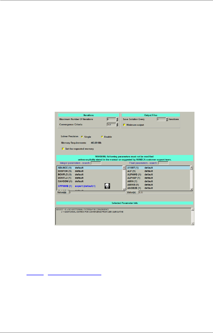
Computation Steering & Monitoring Control Variables
12-2 FINE™/Turbo
•the Solver Precision: single or double. For most cases, the single precision solver (much less
demanding in memory consumption) will be sufficiently accurate. However, some certain
types of problem, such as very long thin pipe and conjugate heat transfer problems, may bene-
fit from the double precision solver.
•the Memory Requirements for the computation. By default an estimate is given for the
required memory. Depending on the parameters defining the computation, additional memory
may be needed. For example, more memory is required when full non-matching connections
or a k-ε turbulence model is used. Also the amount of selected output may require more mem-
ory. To allocate more memory for the computation activate the option Set the requested
memory. This will allow to define the amount of memory in Mb used for reals and integers.
The maximum memory that the flow solver can use is about 8 Gb.
For unsteady computations the Control Variables page is updated to give access to
additional parameters as described in section 6-3.1 and section 6-3.3.
FIGURE 12.2.1-1 The Control Variables page
In expert mode, this page contains two lists of expert parameters. Only the expert parameters that
are described in the manual are supported. Use of the other parameters is not recommended. For a
summary of all supported expert parameters see Appendix B.
12-2.2 Expert Parameters
MNGDBL(integer):The geometrical data (Wall distances and FNMB data) are usually computed
one time and stored in the files linked to the project (or the mesh). It is possible
that some data are corrupted by a lack of precision. This is obvious for the wall
distance computation in single precision when the difference of the absolute
coordinates needs more than 8 significant digits. In the flow solver, the wall
distances are computed and stored (.cgns file) in the specified precision for real.

Convergence History Computation Steering & Monitoring
FINE™/Turbo 12-3
However, the FNMB data is always computed in the double precision and
stored (.adf file) in the specified precision for real. So the FNMB data is less
sensitive to the selected solver precision than the wall distances.
The expert parameter MNGDBL is used to manage the reading or the computa-
tion of the wall distances and FNMB data when using the double precision
solver:
0: Read all stored values.
1(default): Compute the wall distances again if they are stored in the single
precision.
2: Compute the wall distances and FNMB data again if they are stored in the
single precision.
12-3 Convergence History
12-3.1 Convergence History in the FINE™/Turbo GUI
The Computation Steering/Convergence History or Task Manager/Convergence History page
allows the user to define quantities to be followed during the convergence process of the FINE™/
Turbo solver. This page is divided in 5 areas as shown in Figure 12.3.1-2:
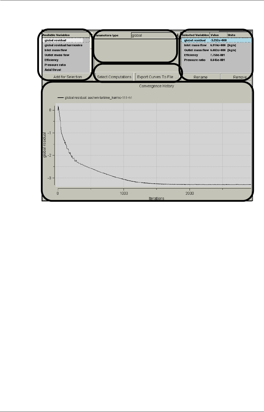
Computation Steering & Monitoring Convergence History
12-4 FINE™/Turbo
FIGURE 12.3.1-2 The five areas of the Convergence History page
1. The steering files selection (Select Computations) and the curves export (Export Curves To
File...) options, are only available through the Task Manager/Convergence History page.
2. The available variables (Available Variables).
3. The parameters (Parameters type).
4. The selected variables (Selected Variables).
5. The graphics view (Convergence History).
When the FINE™/Turbo solver is invoked, a communication is automatically established with
FINE™/Turbo allowing the user to monitor the selected quantities. Two representations of the
quantities are currently available: the convergence curves displayed in the area 5 and the quantity
value at the last iteration in the area 4. All these data are stored in files with extension ".steering"
and ".steering.binary". These files are created and managed automatically by FINE™/Turbo
If the communication between the flow solver and FINE™/Turbo is interrupted (i.e.:
network problem), parts of the convergence curves can be lost.
The FINE™/Turbo solver allows to read and write the steering files in batch mode. The name of the
".steering" file is given through the arguments of the solver ("-steering computation_name.steer-
ing"). The solver reads the "steering" file when reading the ".run" file. The solver will also read the
".steering.binary" file if the ".run" is a restart.
The FINE™/Turbo GUI can not be launched when the steering in batch mode is used,
otherwise the GUI may overwrite the steering data.
(2) (3) (4)
(5)
(1)
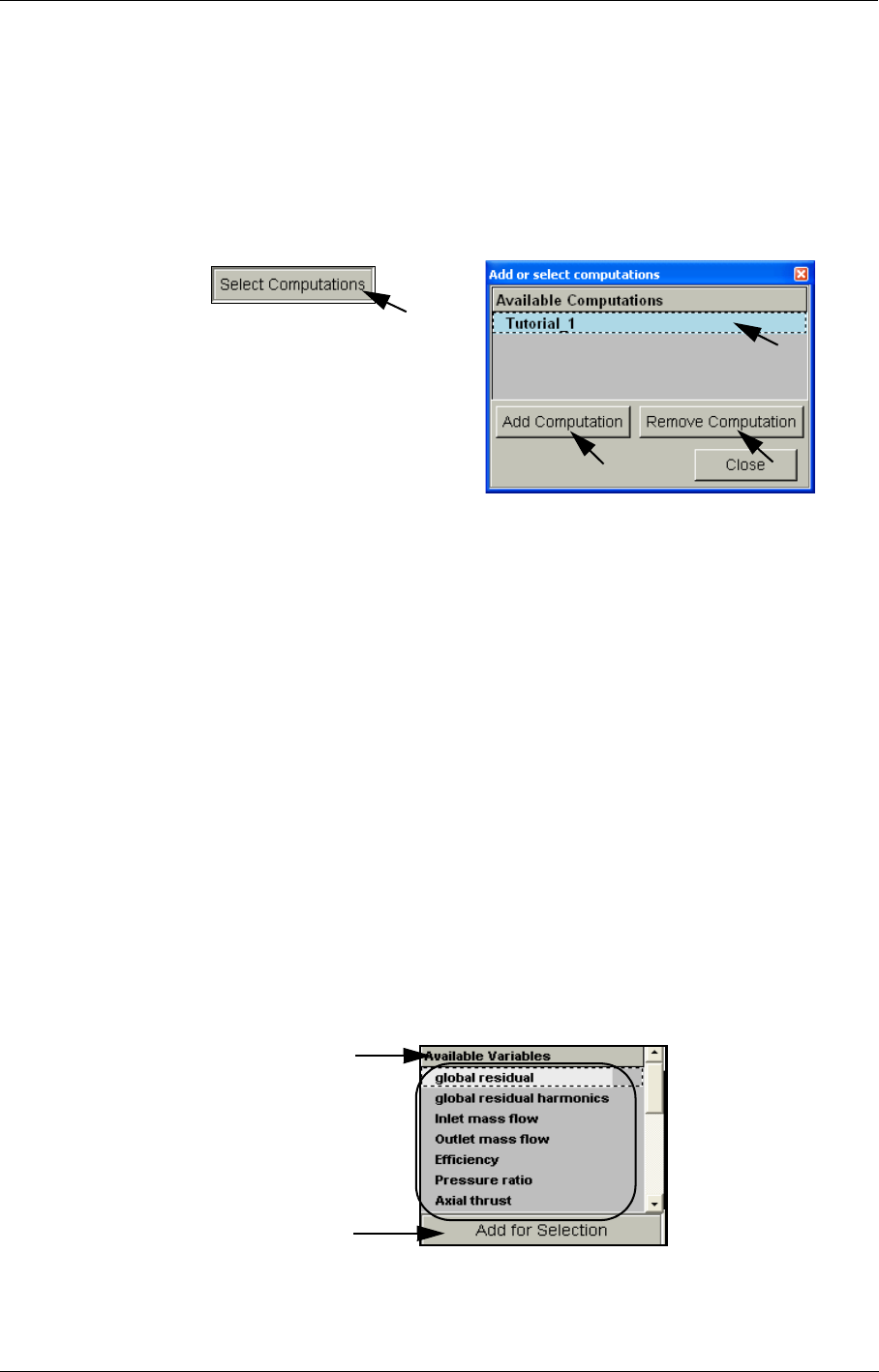
Convergence History Computation Steering & Monitoring
FINE™/Turbo 12-5
12-3.1.1 Steering Files Selection & Curves Export
Different modes exist for the selection of the current steering results stored in the steering files:
1. When a project is opened, the active computation steering file is automatically selected and
appears in the Add or select computations window (a) appearing when clicking on Select Com-
putations button. Each time a new computation is selected, the associated steering file is auto-
matically loaded and becomes the active one.
FIGURE 12.3.1-3 Steering files selection area
2. All the steering files already loaded can be selected by <Ctrl>-left click and <Shift>-left click in
the list of available computations.
3. The file can also be loaded manually using the Add Computation button (c). A file chooser
prompts the user to select the file.
4. The Remove Computation button (d), allows the user to remove the selected computation from
the memory (the file is not removed from the disk and remains available for selection).
5. Additionally, when a task is started, the steering file of the active computation is automatically
loaded and becomes available in the list of computations (b).
The Export Curves To File... button enables the user to save all the curves plotted in the Graphics
View in an ASCII file ".cvh".
12-3.1.2 Available Quantities Selection
The available quantities selected by default depend on the type of computation. For example, when
launching a turbomachinery computation, the global residual, the inlet and outlet mass flow, the
efficiency, the pressure ratio, the axial thrust and the Torque are computed during the convergence
process. The Available Quantities list (b) allows the user to select and add (c) new quantities to the
computed list, see Figure 12.3.1-4.
.
FIGURE 12.3.1-4 Available quantities selection area
(b)
(c)
(a)
(d)
(a)
(c)
(b)
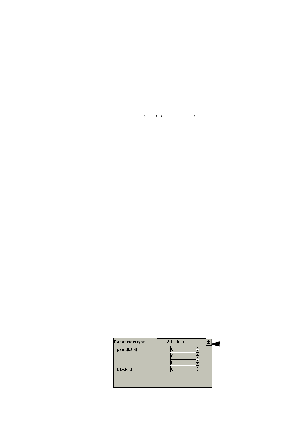
Computation Steering & Monitoring Convergence History
12-6 FINE™/Turbo
All the quantities can be added before or during the computation.
When a quantity has been added, it appears in the selection list and becomes the selected quantity. If
the flow solver is running, the value and the convergence curve of the new quantities is displayed
after a few seconds. The convergence curve begins at the iteration corresponding to the moment
when the new quantity has been added in the Selected Variables list.
When a quantity is added for selection it appears in the selection list with a number behind the
name. This number is only added to avoid to have two times the same variable name in the list. This
is especially necessary when, for example, the static pressure is monitored at two different points in
the domain.
FINE™/Turbo allows the user to monitor the evolution of force (force X, Y, Z), torque (torque X, Y,
Z) and aerodynamic power (defined by , where is the velocity of the wall defor-
mation) on more than one set of solid patches. To access this function, the user has to set the expert
parameter SOLSTE to 1. These quantities are associated to only one parameter: the patch/group
name on which the quantity will be monitored. The patch/group name can be a name either in the
Boundary Conditions page under the tab SOLID or in the Optional Models/Fluid Structure page
under the tab Mechanical. If the patch/group name specified by the user can not be found, the steer-
ing output will be set to zero.
Only the patch/group of patches on which the option "compute force and torque" is
activated may be selected.
The force and torque outputs are computed for one blade only. The periodicity of the
blade is not used.
Monitoring aerodynamic power is restricted to MpCCI and modal computations.
12-3.1.3 New Quantity Parameters Definition
When a new quantity has been added, it becomes available for selection in the Selected Variables
list (area 4 in Figure 12.3.1-2). The user can select the way the flow solver computes the quantity
through the parameter type area (area 2 in Figure 12.3.1-2). Several types of parameters can be cho-
sen through the parameter type list box ((a) in Figure 12.3.1-5).
The available types of parameters that can be defined to compute the selected quantities:
1. global: the computed variable is averaged over all the domain.
2. local 3d grid point: the user specify the grid point indices (I,J,K) and the block index (block id)
where the quantity must be computed.
FIGURE 12.3.1-5 Parameter type definition
pn τn+()vwSd
S
vw
(a)
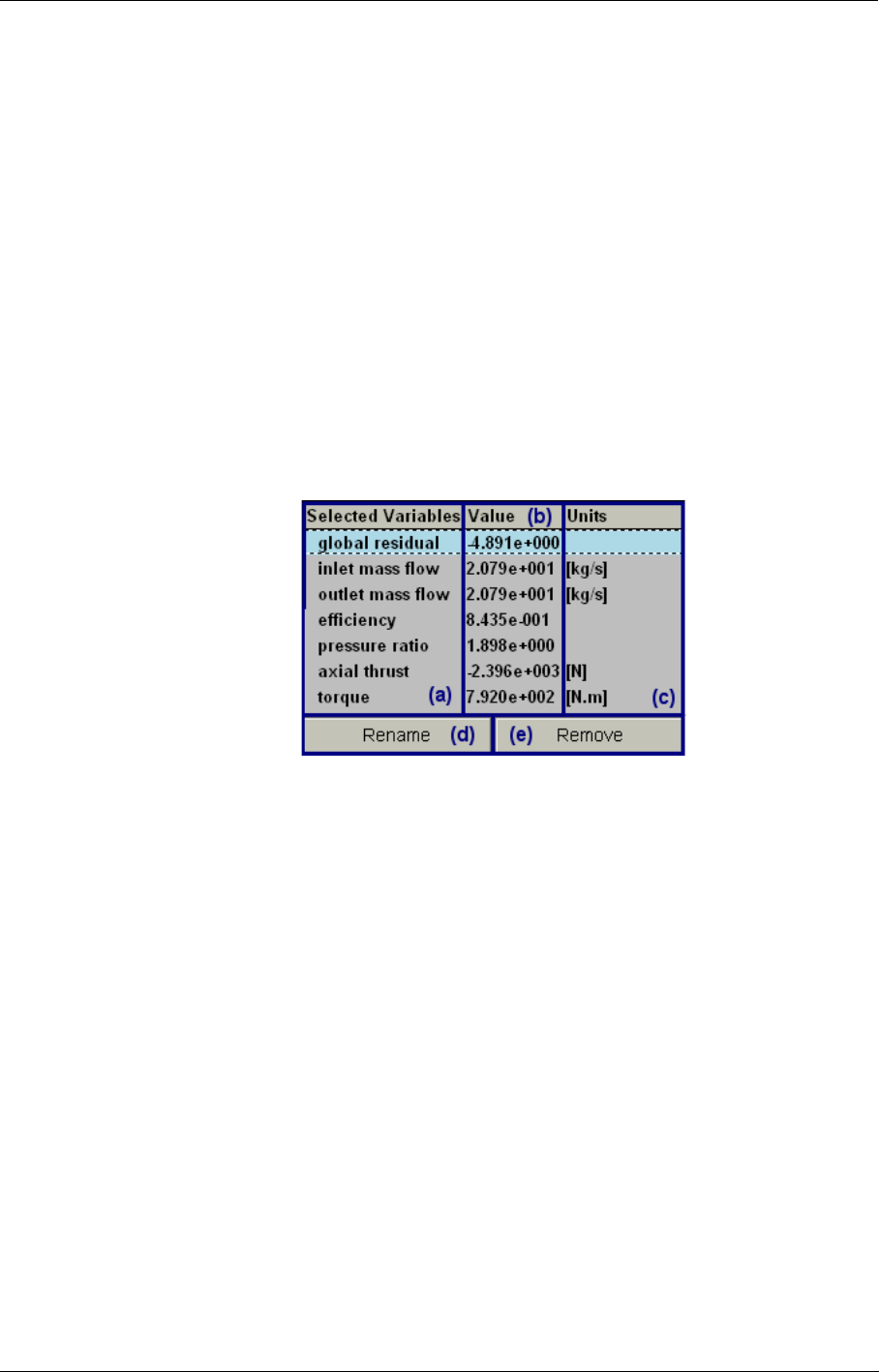
Convergence History Computation Steering & Monitoring
FINE™/Turbo 12-7
Care should be taken when using the steering of a parameter on a local 3d grid point. It
should be carried out in the following way:
—select the parameter (relative velocity u, static pressure...).
—add it for selection. It becomes available for the selected variables.
—set the block id and the I,J,K indices of the grid point on which the evolution
of the selected parameter will be visualized.
All modifications (I,J,K indices...) can also be performed (and modified) during the
computation.
12-3.1.4 Quantity Selection Area
When a quantity has been added, it becomes available for selection in the Selected Variables list.
The list is divided in 3 columns as shown in Figure 12.3.1-6: the variable name (a) which can be
changed using the button rename (d), the quantity value (b) which displays the last computed value
and the units (c) of the variable. The button remove (e) is used to remove the first selected variable.
FIGURE 12.3.1-6 Selected variables area
When a quantity is not yet computed, the value indicated is undefined.
Selecting a quantity will show its history in the graphics view as described in the next paragraph. To
select multiple quantities click on them (with the left mouse button) in the list while holding the
<Ctrl> or <Shift> key. To select quantities that are next to each other in the list simply click on the
first one and keep the mouse button pressed while moving to the last variable.
12-3.1.5 Definition of Global Residual
The residuals are computed by the FINE™/Turbo solver as the imbalance in the linearised system
of discrete equation (the sum of the imbalance of the discrete equation (residual R(U)) in each cell):
.(12-1)
The root mean square of the residuals is computed with the following formula:
,(12-2)
and the maximum of the residuals in the same way:
RES R U()
=
RMSRES RMS RES
cellvolume
-----------------------------
log=
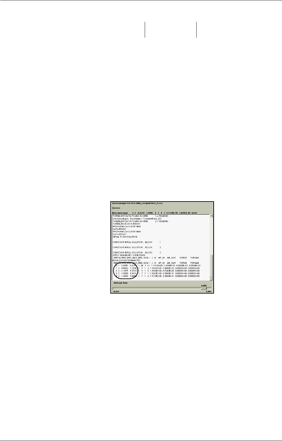
Computation Steering & Monitoring Convergence History
12-8 FINE™/Turbo
,(12-3)
with log the logarithm to the base ten.
On the Computation Steering/Convergence History or Task Manager/Convergence History
page, the global root mean square of the residuals normalized by its value at the first iteration is
shown. These values are stored in the files with extension ".steering" and ".steering.binary".
When working with harmonic method, a global residual called ’global residual har-
monics’ will be available in addition of the ’global residual’. The ’Global residual’ is
linked to the time averaged solution while the ’global residual harmonics’ is linked to
the time fluctuations.
Additionally the global residuals are shown in numerical values in the Task Manager window (3rd
column). The RMS value listed in the Task Manager window is the global root mean square nor-
malized by its value at the first iteration: RMSRES-(RMSRES)it=1. The maximum value (4th col-
umn) is the maximum residual at a certain iteration normalized by the RMS residual at the first
iteration: MAXRES-(RMSRES)it=1.
The values of the global residuals depend on the used initial solution. If the initial
solution is already quite close to the final solution, the obtained residual values are not as
low as they would have been when the initial solution is far from the final solution.
FIGURE 12.3.1-7 Task Manager window
12-3.1.6 The Graphics View
The convergence history of the selected curves are displayed inside the graphics view.
In the Computation Steering/Convergence History page, the color of the curves is different (up
to 8 selected quantities). The automatic chosen curves colors are also used for the displayed value
(a). Additionally, the error between the two first selected quantities is also indicated (b). This is
especially important for checking the difference between the mass flow at inlet and outlet
(Figure 12.3.1-8).
MAXRES MAX RES
cellvolume
-----------------------------
log=
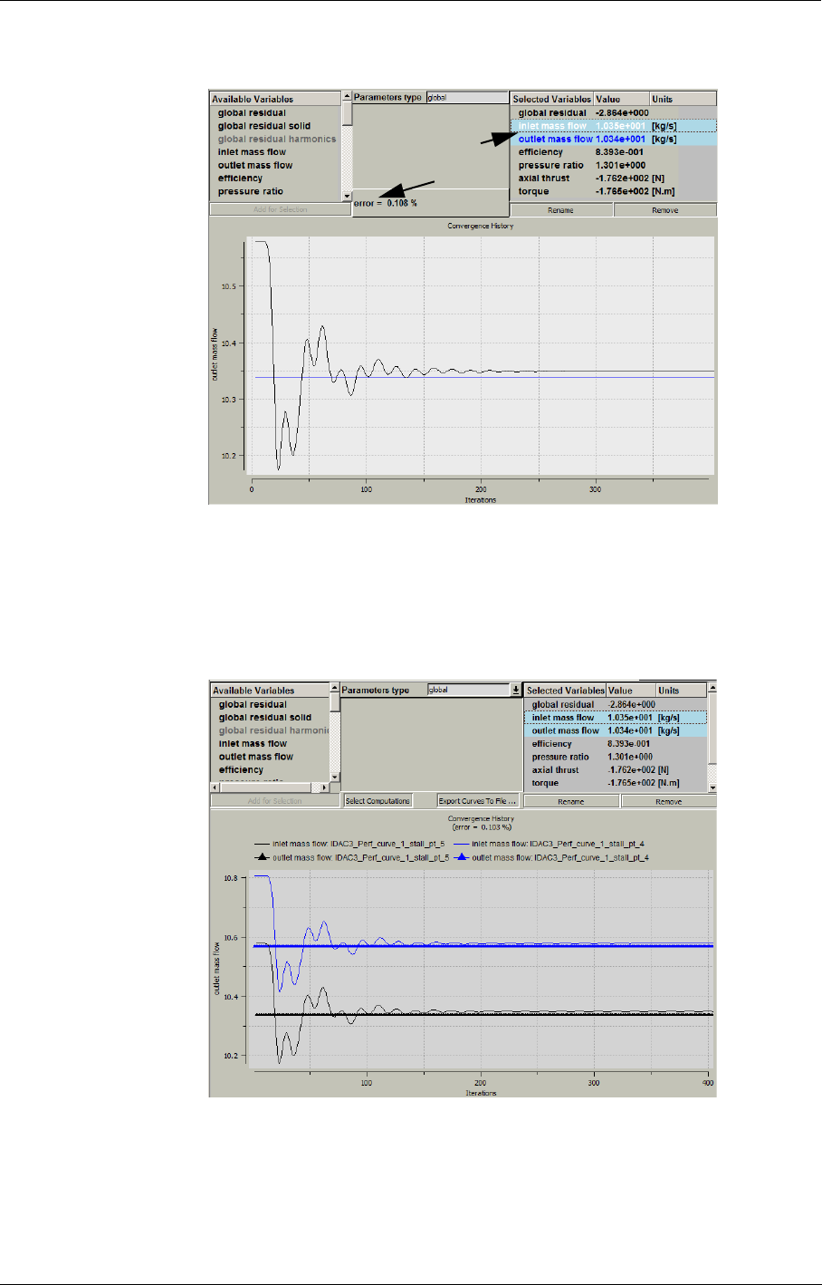
Convergence History Computation Steering & Monitoring
FINE™/Turbo 12-9
FIGURE 12.3.1-8 Graphics view area in Computation Steering/Convergence History page
In the Task Manager/Convergence History page, the color of the curves is the same (but with dif-
ferent markers) if related to the same computation. The color is different for each curve if related to
different computations (up to 9 selected quantities controlled by the user if necessary - File/Prefer-
ences menu, see section 2-3.1.6).
FIGURE 12.3.1-9Graphics view area in Task Manager/Convergence History page
(b)
(a)

Computation Steering & Monitoring MonitorTurbo
12-10 FINE™/Turbo
12-3.2 Expert Parameters
NRRES(integer): controls which variable will be applied for the global risidual:
1 (default): density,
2: ,
3: ,
4: ,
5: energy,
6: the turbulent working variable if Spalart-Allmaras model or k if k-ε mod-
els,
7: ε if k-ε models or ω if k-ω models.
NBLRES(integer): In some cases, especially for unsteady simulations, the .res may be very large.
The expert parameter NBLRES allows the user to output only limited informa-
tion in this file.
-1: output only the global residual
0 (default): output information for all blocks.
N (>0): output information for the first N blocks. For example, NBLRES=10,
outputs only the information for the first 10 blocks.
IASTWL(integer): In each iteration, the force and torque are outputted before multigrid correction
in the .steering and .res files. However, the force and torque are outputted after
multigrid correction in the .mf, .wall and .cgns files. If the convergence is not
fully reached, the force and torque may be different in these files. The expert
parameter IASTWL allows to output the force and torque after multigrid cor-
rection in all files.
0 (default): output the force and torque before multigrid correction in the .steer-
ing and .res files but after multigrid correction in the .mf, .wall and .cgns files.
1: output the force and torque after multigrid correction in all files.
12-4 MonitorTurbo
12-4.1 Introduction
The MonitorTurbo can be launched independently from FINE™/Turbo in order to facilitate the
batch mode control. It is a separate graphic control window in which the user can visually monitor
the convergence history of one or several computations (Convergence history). This section
describes the functionalities of the convergence history display.
On UNIX and LINUX platforms type: monitorTurbo -niversion <version> -print <Enter>
When multiple versions of FINE™/Turbo are installed the installation note should be
consulted for advice on how to start the MonitorTurbo in a multi-version environment.
wx
wy
wz
ν
˜
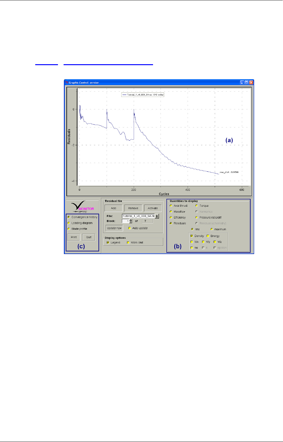
MonitorTurbo Computation Steering & Monitoring
FINE™/Turbo 12-11
On Windows click on the Monitor icon in Start/Programs/NUMECA software/fine#. Alterna-
tively FINE™/Turbo can be launched from a dos shell by typing:
<NUMECA_INSTALLATION_DIRECTORY>\fine#\bin\monitor <Enter>
12-4.2 The MonitorTurbo GUI
FIGURE 12.4.2-10 The monitorTurbo window
The MonitorTurbo allows multi-process analyses. Therefore, the convergence histories of multiple
(running) projects can be visualized at the same time. It is also possible to compare the convergence
history associated with different computational parameters for the same project.
The monitored variables are displayed as a x-y graph in the upper part of the window (a). The x-
axis represents the number of multigrid cycles or work units (see section d) and section A-4.3)
achieved by the flow solver. The y-axis is a logarithmic axis representing the power of ten of the
residual values. The user can choose the residual of any of the equations solved and some global
parameters using the buttons visible in the lower right part of the graphic control window (b) as
shown in Figure 12.4.2-10.
The lower part of the graphic control window contains four boxes. The small box (c) located on the
left side contains a Print button (which allows to save the current graph as a postscript file) and a
Quit button (which allows to close the MonitorTurbo window). The two other boxes are described
in the next sections.
The convergence history of a computation using the v2-f turbulence model, cannot be
loaded in the MonitorTurbo application.

Computation Steering & Monitoring MonitorTurbo
12-12 FINE™/Turbo
12-4.2.1 The Residual File Box
Three buttons are provided in this box to Add, Remove or Activate residual files through a file
chooser. The residual files describe the iteration process of previous or current computations. For
internal flow, they contain the history of the axial thrust, mass flow, torque, efficiency, pressure
ratio (lift, drag and momentum coefficients for external flow), the residuals of five (seven or six if
respectively the k-ε, k-ω or the Spalart-Allmaras turbulence model is used) physical variables and
the harmonic variables (density, Vx, Vy, Vz, pressure).
The activation of a part of the residual files ".res" has the effect of deactivating the other loaded
residual files. When a residual file is deactivated, its associated convergence history is not dis-
played. The selective activation of residual files allows thus to display only the convergence histo-
ries of some of the loaded residual files ".res".
The input boxes File and Block, visible just below the three buttons Add, Remove and Activate,
allow to select for which file and block the choice of the monitored variables performed in the
Quantities to display menu should be applied.
12-4.2.2 Quantities to Display
a) Residuals
Buttons are provided to select the type of residuals: rms or maximum as shown in Figure 12.4.2-10
on the right. The residuals relative to all transport equations of the problem are available: these are
the continuity, the momentum, the energy, and eventually the turbulent kinetic energy k and the tur-
bulent dissipation ε (if the turbulent computation is using a k-ε or v2-f model, e.g. not for Baldwin
Lomax), and the turbulent kinematic viscosity nu (if the Spalart-Allmaras model is used).
While the Computation Steering/Convergence history or Task Manager/Convergence History
page displays only the global residual, the MonitorTurbo gives the RMS and maximum values per
block. Computation of the RMSRES and MAXRES values is done according to Eq. 12-1 to Eq. 12-3.
The values shown in the MonitorTurbo for the RMS are normalized by the value of RMSRES at the
first iteration: RMSRES-(RMSRES)it=1. The values shown for the maximum residuals are normal-
ized by the maximum residual at the first iteration: MAXRES-(MAXRES)it=1.
Since the RMS and maximum residuals are normalized differently it may occur that
the RMS value shown in the MonitorTurbo is higher than the maximum residual.
b) Global Quantities
Several buttons are provided to visualize the additional global quantities available under the envi-
ronment FINE™/Turbo:
•Internal flow problems (expert parameter IINT=1): The axial thrust, the (inlet and outlet) mass
flows, torque, pressure ratio, and efficiency.
•External flow problems (expert parameter IINT=0): The drag, the lift and the momentum coeffi-
cients. The user has to specify the axis that has to be taken into account for these global quanti-
ties as described in section 10-3.
If several computations are performed at the same time, the curves associated with the different
projects are drawn in different colors. The buttons of the present box act only on the curves of the
file and block selected through the File and Block menu.
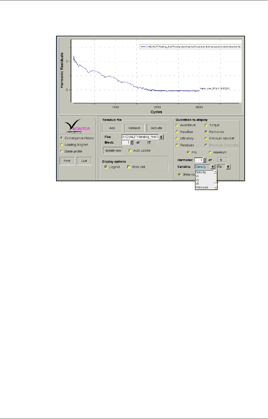
MonitorTurbo Computation Steering & Monitoring
FINE™/Turbo 12-13
c) Harmonic Quantities
FIGURE 12.4.2-11 The monitorTurbo window - Harmonic quantities
Several buttons are provided to visualize the real and imaginary part of the harmonic quantities
available in the FINE™/Turbo environment: Density, Vx, Vy, Vz and Pressure.
If several computations are performed at the same time, the curves associated with the different
projects are drawn in different colors. The buttons of the present box act only on the curves of the
file and block selected through the File and Block menu.
The option Show curve allows to plot the curve in the MonitorTurbo window.
d) Display Options
The Legend option is used to display which files are currently activated. In addition, if the mass
flow button is activated, the relative errors between the inlet and the outlet are indicated.
The Work Unit option is provided to set the type of unit used on the horizontal axis in the Monitor-
Turbo window: multigrid cycles or work units. If the Cycles option is chosen (the Work Unit
option will be deactivated), the abscissa will show the number of iterations. The Work Unit option
will adapt the values on the horizontal axis with respect to the grid levels (if 3 grid levels are used,
one iteration on 222 and 111 is taking respectively 1/64s and 1/8s considering that one iteration on
000 is taking 1s.
The Update now button updates the graph for the active residual file and the selected block.
The Auto update option can be switched on to follow the iteration processes automatically. It is
however a rather time-consuming option and this button is not active by default.
e) Zooming Option
This option allows to interactively zoom in and out:

Computation Steering & Monitoring Best Practice for Computation Monitoring
12-14 FINE™/Turbo
1. In the drawing window, press the left mouse button to initiate a zooming operation,
2. Then drag the mouse to the left or to the right to zoom in, the zooming window number is dis-
played on the screen,
3. Click again on the left button when finished,
4. To zoom out, click on the right button of the mouse.
12-5 Best Practice for Computation Monitoring
12-5.1 Introduction
Several tools are available in the FINE™/Turbo package to follow the evolution of a calculation:
•the Convergence History page available in FINE™/Turbo and in the Task Manager module,
which allows to follow the evolution of a calculation easily and to globally compare the evolu-
tion of multiple computations.
•Another useful tool is the MonitorTurbo to compare per equation and per block, the evolution
of multiple computations.
•CFView™ to enter even into more detail.
Each of them has its own specific features, but they are very complementary. This section describes
how to use those tools to monitor a computation. For a detailed description on the use of CFView™
see the CFView™ User Manual.
When a computation has just been launched for the first time, and initialization steps have been
properly passed, the solver writes a first solution file. In fact it is not yet a solution but only the
result of the initialization. Still this first output is interesting to check if all boundaries conditions
have been set correctly. Especially think to have a look at the rotating elements of the machine, the
profiles of velocities at inlet and at outlet. This operation aims to detect a user mistake, which could
cause a loss of time, like for example, a forgotten patch. To check this first output use CFView™.
To check the rotating part of the machine, select the rotating walls (hub or shroud for rotating walls)
using the menu item Geometry/Select Surfaces and select for the quantity the velocity. Using the
Representation menu the velocity will be displayed on the selected patches and this will be the
rotation speed everywhere.
12-5.2 Convergence History
The global residual on the Convergence History page allows to see quickly whether or not the
computation is iterating properly. The residuals should go down first on the coarser grid levels of
the Full Multigrid strategy as shown in Figure 12.5.2-12. See Chapter 6 for more details on Full
Multigrid. When going to a finer grid level the global residual increases suddenly to decrease
immediately after. When the computation reaches the finest grid, the curve of the global residual
should normally decrease gradually. In general a fall of 3 orders with a stabilization of this curve is
considered as a good convergence. But it is important to check if other global quantities like mass
flow, efficiency, pressure ratio are also stabilized and to compare the differences between mass flow
at inlet and outlet (in general a difference of less than 5% is acceptable).
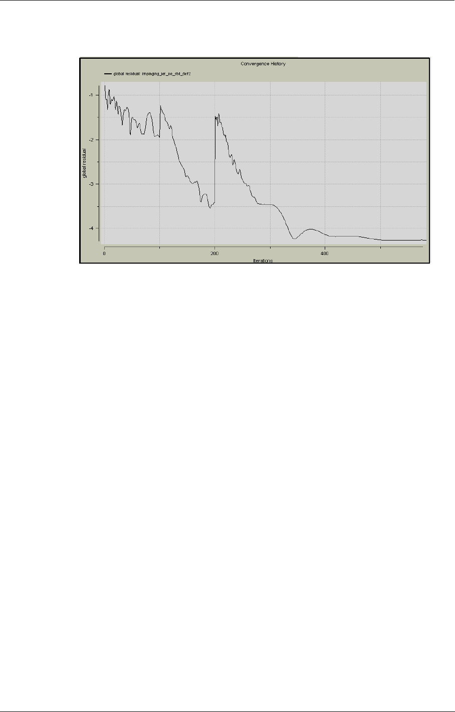
Best Practice for Computation Monitoring Computation Steering & Monitoring
FINE™/Turbo 12-15
FIGURE 12.5.2-12 Example of convergence history for global residuals
Additionally for a deeper analysis, FINE/Turbo has given the user ability to investigate the conver-
gence history of the local flow field, which can be accessed by the following methods:
•Add local 3d grid point in the Convergence History page (see Chapter 12-3.1.3)
•Add "ControlPoints" through the external file
In the second method, the characteristic quantities can be track from iteration to iteration by so
called "ControlPoints". The location of these control points is specified in I,J,K coordinates through
an external data file with extension ".ControlPoints" and the same base name as the other computa-
tion files. The user has to put this input file in the computation directory.
After the computation is started, the FINE™/Turbo solver will create a separate output file for
every point defined in the ".ControlPoints" file. These output files have the extension ".P#.DAT"
and can be found in the computation directory, where # stands for the serial number of the control
point in the input file.
The format of the input and output files is given in the following parts.
•Contents of the input file (.ControlPoints):
Line 1: Number of control points
Line 2: Block Nr. I-Location J-Location K-Location (control point 1)
Line 3: Block Nr. I-Location J-Location K-Location (control point 2)
......
Example
3
5 17 33 21
2 10 15 18
7 33 45 11
Control points in the input file can not be located on block boundary.
Every line has to be ended by a <return> carriage.

Computation Steering & Monitoring Best Practice for Computation Monitoring
12-16 FINE™/Turbo
The maximum number of control points that user can define is limited to 180.
•Contents of the output file (.P#.DAT), for each line:
Iteration number (steady) or Time step (unsteady)
Density
Relative Cartesian Velocity (Vx, Vy, Vz)
Pressure
Nu~ (for Spalart-Allmaras model only)
k and ε (for k-ε model only)
Temperature (for perfect gas with preconditioning only)
12-5.3 MonitorTurbo
The MonitorTurbo follows the same quantities as the Convergence History, but its main interest is
to offer the possibility to follow the convergence block by block. Thus, one can localize problems
and, if necessary, modify the mesh in the region associated to the block, or change a boundary con-
dition.
Finally, coming back to the Task Manager, it is possible to get a deeper control, locally, by adding
control points (local 3d grid point). These points allow to track in important parts of the domain,
the speed, the pressure and turbulent quantities, which sometimes could be a requested information.
In the case of steady computations, the values associated to these points should converge to a con-
stant value.
One additional advice is to use CFView™ during the computation with intermediate and non-con-
verged solutions. When having convergence problems for example CFView™ may be used to look
for the zones were the residuals have too high values compared to other regions or an incorrect tur-
bulence field. To know in which block(s) the residuals start to increase first in case of divergence
problem, the MonitorTurbo may already give a first indication. Combining the information from
the MonitorTurbo and CFView™ allows to find the cause of convergence problems in the computa-
tions.
12-5.4 Analysis of Residuals
In some cases it may occur that the MonitorTurbo shows high RMS and maximum values of the
residuals in a certain block while CFView™ shows high residuals in a different block. This differ-
ence between the two tools is caused by the different ways of representing the residuals. In
CFView™ the absolute values of the residuals resulting from the flux balance are directly plotted
for each cell. In CFView™ the residuals are not scaled with the cell volumes and no normalization
with values at the first iteration is applied. This explains why some high maximum residuals in
scaled mode can be invisible in CFView™ because they occur in small cells. Also the fact that the
residuals are computed on the cell centers in the solver and shown in CFView™ on the cell corners
may lead to some, minor, interpolation differences.

FINE™/Turbo A-1
APPENDIX A:File Formats
A-1 Overview
This Appendix describes the files used by FINE™/Turbo and the flow solver. It is divided in two
parts. The first one gives the file format information needed to use FINE™/Turbo, while the second
one describes the format of the files used and produced by the FINE™/Turbo solver. As FINE™/
Turbo is intended to handle the file treatment for the user, knowing the exact format of all the files
used in a simulation process is not required. This appendix is therefore written for advanced users
only.
In the following description, it is assumed that all the files are related to a generic project called
'project'. The chapter is divided in five sections:
•files produced by IGG™,
•files produced and used by FINE™/Turbo,
•files produced and used by the FINE™/Turbo solver,
•files used as data profile,
•resource files used to control the layout and which contain default values and reference infor-
mation.
To simplify the notations, it is assumed that the related mesh has a topology of one block.
A-2 Files Produced by IGG™
This section describes the files produced by the grid generator IGG™ and used by FINE™/Turbo:
•the identification file "project.igg",
•the binary file "project.cgns",
•the boundary conditions file "project.bcs",
•the geometry file "project.geom",
•the configuration file "project.config".

File Formats Files Produced by the FINE™/Turbo GUI
A-2 FINE™/Turbo
A-2.1 The Identification File: ’project.igg’
This file contains all the mesh geometric and topologic information. It is used by FINE™/Turbo to
identify the mesh topology. A complete description of this file is given in the IGG™ User Manual.
A-2.2 The Binary File: ’project.cgns’
When the mesh is created and saved in IGG™, the binary file "project.cgns" containing the grid
point coordinates is created. Later on, the solver will store the wall distances used for the different
turbulence models in the same file.
A-2.3 The Geometry File: ’project.geom’
When the mesh is created and saved in IGG™, the geometry file "project.geom" containing the
whole geometry (curves, surfaces and Cartesian points) is created.
A-2.4 The Boundary Condition File: ’project.bcs’
As described in Chapter 5, the settings of the boundary condition type have to be set inside IGG™
while the physical boundary condition parameters are set in FINE™/Turbo. The settings of IGG™
are stored in the file "project.bcs". This files is used by FINE™/Turbo to initialize the boundary
condition types for each patch. They are updated each time the boundary condition type is changed
inside IGG™.
A-2.5 The Configuration File: ’project.config’
This file contains all the mesh patches and boundary conditions. It is used by FINE™/Turbo for the
SubProject management. It is also used to automatically create groups to set-up the boundary con-
ditions. A description of this file is given in the IGG™ User Manual.
A-3 Files Produced by the FINE™/Turbo GUI
This section describes the files produced and used by FINE™/Turbo (or used by the flow solver
launched from FINE™/Turbo). Please note that FINE™/Turbo acts as a file manager between dif-
ferent software systems. Therefore, it is important that the read, write and execute permissions are
set properly for all the files and directories used by FINE™/Turbo.
Manual modification of these files is not supported since it may corrupt the file or pro-
vide incorrect results. Such a modification should only be done on explicit advice of our
local support office.
A-3.1 The Project File: ’project.iec’
This file contains all the information related to the project. It is used by FINE™/Turbo to save and
recover all the user settings. This file is subdivided into several blocks. Each block contains data
and/or other blocks. The beginning of the blocks is identified by the key word NI_BEGIN and by a
name and the end of the block is identified by the key word NI_END and by the name of the block.

Files Produced by the FINE™/Turbo solver File Formats
FINE™/Turbo A-3
a) File Header
The file always has the following header containing the version number and the project type:
NUMECA_PROJECT_FILE VERSION 8.2
PROJECT_TYPE STRUCTURED
After the header, 3 new lines are used to store the name of the files linked to the project:
GRID_FILE /usr/_turnkey_tutorials/_rotor37/rotor37/_mesh/rotor37.igg
TRB_FILE /usr/_turnkey_tutorials/_rotor37/rotor37/rotor37.trb
GEOMETRY_FILE /usr/_turnkey_tutorials/_rotor37/rotor37.geomTurbo
These are respectively the mesh, the template and the geometry files. The template and the geome-
try files are not used by FINE™/Turbo and are only there for backward compatibility reasons.
b) The Computation Block
The project file contains the settings of all the computations defined by the user. Each computation
block is identified by the following keywords:
NI_BEGIN computation
...
NI_END computation
The computation block contains the following subblocks:
•The Solver Parameters Section block containing all the parameters of the flow solver.
•The Initial Solution & Boundary Condition Section block containing the initial solution and
the boundary conditions.
•The Grid Parameters Section block containing the topology of the mesh.
•The Fluid Properties Section block containing the fluid properties.
A-3.2 The Computation File: ’project_computation.run’
When the solver is started, FINE™/Turbo creates a new directory using the name of the active com-
putation. A computational file (".run" extension) containing the settings of the active computation
is saved into this new directory. This file is used as input by the flow solver and by the flow visual-
ization system CFView™.
The menu File/Save Run Files enables to save the ".run" file without starting the flow
solver.
A-4 Files Produced by the FINE™/Turbo solver
This section describes the files produced and used by the FINE™/Turbo solver. The flow solver
uses most of the files described above and produces the following files:
A-4.1 The Binary Solution File: ’project_computation.cgns’
The FINE™/Turbo flow solver writes a ".cgns" file (binary) at the end of the simulation and also
during intermediate savings, depending on the user input. It writes several bases, which are
described hereafter according to their name. This "cgns" file contains information that is necessary
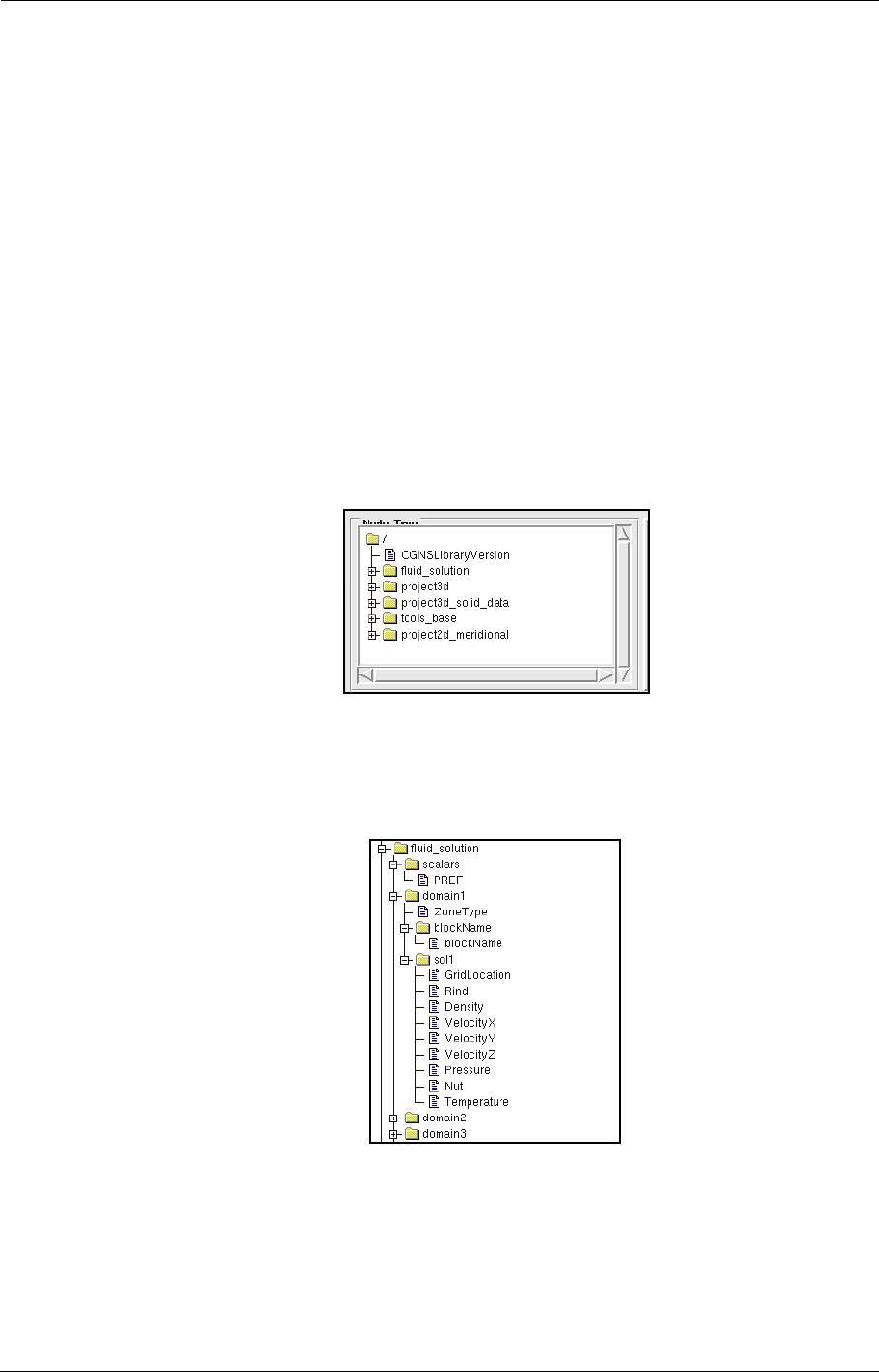
File Formats Files Produced by the FINE™/Turbo solver
A-4 FINE™/Turbo
to restart a simulation from the solution previously obtained, together with information read by
CFView™. The first base, fluid_solution, is mandatory. The other bases are optional and not always
present.
Each string written in the ".cgns" file is limited to 32 characters.
•fluid_solution. This base contains all the information necessary to restart a simulation from
the solution already saved. Only this base is written during intermediate savings and when the
option Minimum output is selected in the Computation Steering/Control Variables page.
•project3d. This base contains all the 3D fields that have been selected as output for CFView™
in the Outputs/Computed Variables page.
•project3d_solid_data. This base contains all the solid data that have been selected as output
for CFView™ in the Outputs/Computed Variables page under the tab Solid data.
•Project2d_meridional. This base contains all the meridional averaging data that have been
selected as output for CFView™ in the Outputs/Azimuthal Averaged Variables page.
•tools_base. This base contains information for post processing and some other information for
CFView™. This information is for internal use in the FINE™/Turbo chain only.
FIGURE A.4.1-1 The structure of the .cgns file
A-4.1.1 Fluid_solution
FIGURE A.4.1-2 The fluid_solution base
This base contains all the information necessary to restart a simulation from the solution already
computed. It contains all the basic flow variables (density, velocity, pressure, temperature, turbulent
quantities, harmonic variables, etc…) for each control volume of the computational domain and for
the dummy cells (two rows of dummy cells are added on each side of the block in order to ensure a
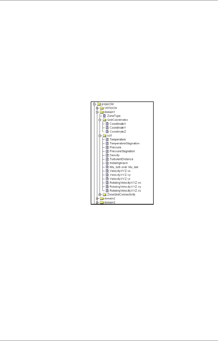
Files Produced by the FINE™/Turbo solver File Formats
FINE™/Turbo A-5
proper block connectivity). These variables are located at cell center, i.e. at the exact location where
they are computed. It should be mentioned that the mesh is not included in this base.
The first input of the base is a zone called scalars including the reference pressure (this reference
pressure is set to zero for non-preconditioned simulations).
Then the base includes a series of zones for each domain. The name of each zone is “domain#”, #
being the block index in the grid generator. The original block name can be found in the user
defined data “blockName”. The node “sol1” contains all the 3D tables with the cell centered final
solution of the simulation. It should be noted that the gauge pressure is stored. The gauge pressure
is based on the reference pressure already stored in the fluid_solution base. Furthermore, only the
solution on the finest grid level of the computation is stored in this base.
A-4.1.2 Project3d
FIGURE A.4.1-3 The project3d base
This base contains all the 3D fields that have been selected as output for CFView™ in the Outputs/
Computed Variables page. It includes a series of zones for each domain. The name of the zone is
similar to the one of the base fluid_solution. For each block, the 3D grid is stored together with the
variables that have been selected in the interface. Each zone contains the (x,y,z) coordinates and all
the 3D variables for each vertex of the computational domain. These variables are located at cell
corners, i.e. they are derived from an interpolation of the variables at cell center. Furthermore, a
node zoneGridConnectivity is also stored in order to be able to connect blocks together (mandatory
for CFView™). If a Non-Linear-Harmonic simulation is performed, a user defined data called Har-
monicData is also created in order to store real information related to harmonic simulations (for
instance frequencies and inter-blade phase angles of the harmonics).
Only the solution on the finest grid level of the computation is stored in this base. If an intermediate
saving is done during full-multigrid procedure, the data is prolongated onto the finest grid level of
the computation.
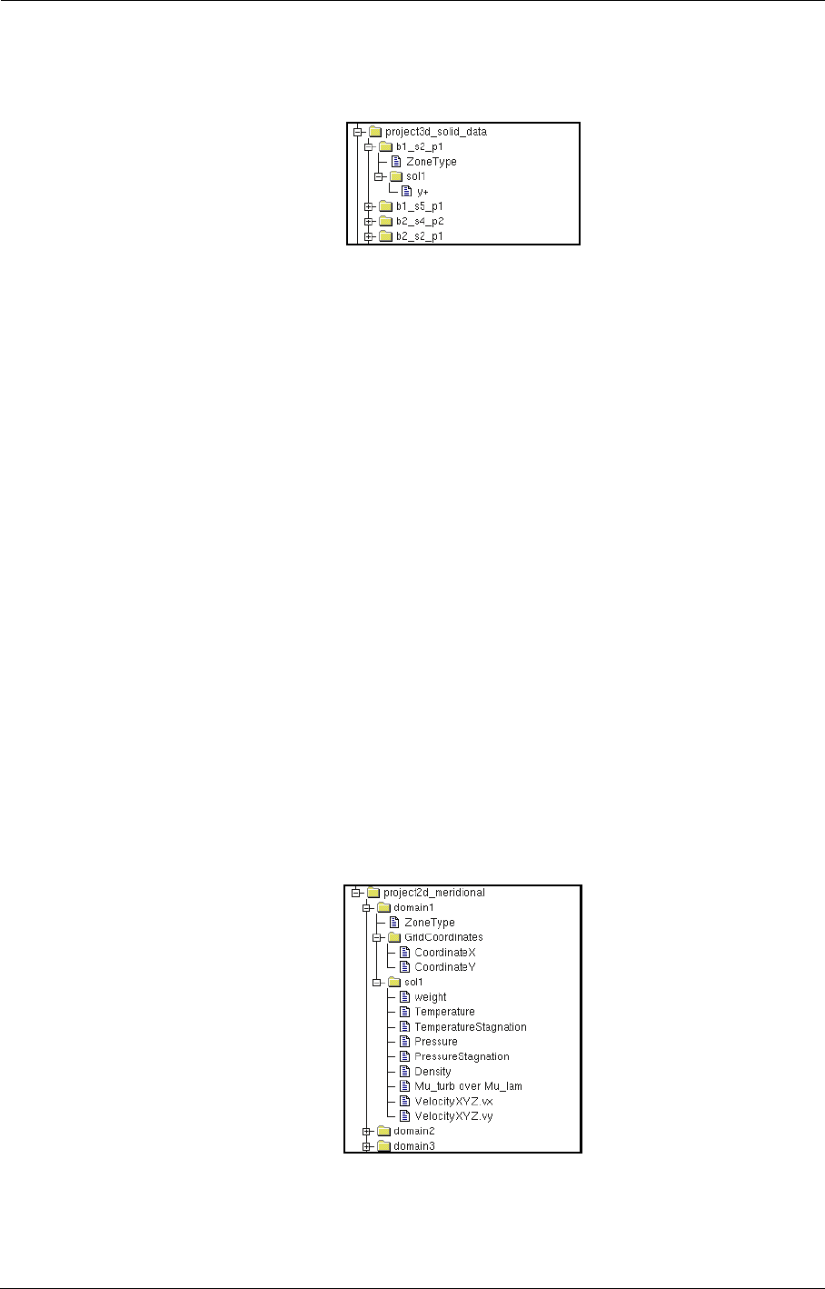
File Formats Files Produced by the FINE™/Turbo solver
A-6 FINE™/Turbo
A-4.1.3 Project3d_solid_data
FIGURE A.4.1-4 The project3d_solid_data base
This base contains all the solid data that have been selected as output for CFView™ in the Outputs/
Computed Variables page under the tab Solid data. By default, the grid coordinates on the faces
are not stored in this base (ICGP3D=0, see Chapter 10-3.3 for more details). In this case, the grid
coordinates can be derived from the coordinates in the project3D base.
This base includes a series of zones for each solid face. The name of the zone is set according to the
following procedure. The name is bI_sJ_pK, where letters b, s, p stand for block, surface, and
patch, respectively. The indices I, J, and K are block, surface, patch numbers, respectively. In order
to define the J index the following method is used:
•Face Imin: J=1
•Face Jmin: J=2
•Face Kmin: J=3
•Face Kmax: J=4
•Face Jmax: J=5
•Face Imax: J=6
Each zone contains all the solid data for each vertex of the solid patches. These variables are
located at cell corners.
Only the solution on the finest grid level of the computation is stored in this base. If an intermediate
saving is done during full-multigrid procedure, the data is prolongated onto the finest grid level of
the computation.
A-4.1.4 Project2d_meridional
FIGURE A.4.1-5 The project2d_meridional base

Files Produced by the FINE™/Turbo solver File Formats
FINE™/Turbo A-7
This base contains all the meridional averaging data that have been selected as output for
CFView™ in the Outputs/Azimuthal Averaged Variables page.
The structure of this base is similar to the one of the project3D except that data are stored in a 2D
structure. The number of zones in this base corresponds to the number of patches selected in the
Outputs/Azimuthal Averaged Variables page in FINE™/Turbo. Each zone is named “domain#”,
# being the index of the patch in the list of selected patches.
Only the solution on the finest grid level of the computation is stored in this base. If an intermediate
saving is done during full-multigrid procedure (coarse grid initialization), the data is prolongated
onto the finest grid level of the computation.
A-4.1.5 The Size of the ".cgns" File
The size of the ".cgns" file can be estimated based on the used flow models and the number of the
outputted variables. Assuming the size of the solid data and the meridional averaging data is small
(compare with 3D field) and can be neglected, the size of the ".cgns" file per million points can be
estimated as:
MB/million points (A-1)
where is the number of the saved variables for turbulence models (1 for 0-equation and 1-equa-
tion models, 2 for 2-equation models, 4 for 4-equation model); is the number of the outputted
3D fields selected in the Outputs / Computed Variables page.
In case of NLH simulations, the size of the ".cgns" file per million points can be estimated as:
MB/million points (A-2)
where is the number of frequencies per perturbation; is the number of perturbation per
blade row.
The actual size of the ".cgns" file will be slightly bigger than the estimated value above due to the
existing of the solid data and the meridional averaging data.
A-4.2 The Global Solution File: ’project_computation.mf’
This ASCII file contains averaged quantities over the inlet, outlet and rotor-stator sections. It is gen-
erated only if both inlet and outlet boundary conditions are present (section 10-2.6).
A-4.3 The Global Solution File: ’project_computation.xmf’
All data stored in ".mf" file are also stored in an XML database (".xmf" file). XML is a markup lan-
guage for text documents. Data are included in XML documents as strings of text and are sur-
rounded by text markup that describes the data. The main interest of XML is his flexibility. The
user’s parser will still work without any change even if data are modified in the ".xmf" file.
XML elements used in this database are as follows:
1. Station element
Station elements contain data at a given position (inlet, rotor/stator interface or outlet)
Data written in mf file in section <GLOBAL RESULTS AT INLET AND OUTLET> are now split
into two parts. These data are stored in two "Station" elements called "inlet" and "outlet".
Sizecgns 46 Nt
+()43 No
+()+=
Nt
No
Sizecgns 46 Nt6NHNP
++()43 No
+()+=
NH
NP

File Formats Files Produced by the FINE™/Turbo solver
A-8 FINE™/Turbo
Data written in mf file in section <GLOBAL RESULTS AT ROTOR/STATOR INTERFACE ID *>
are now stored in a "Station" element.
Station elements have one attribute "name".
2. Row element
Data written in mf file in section <GLOBAL RESULTS FOR ROW *> are now stored in a "Row"
element. In "Row" elements, two "Reference" elements are added, they refer to relative inlet and
outlet of the row.
Row elements have one attribute "name".
3. Stage element
Data written in mf file in section < GLOBAL RESULTS FOR STAGE *> are now stored in a
"Stage" element. In "Stage" elements, two "Reference" elements are added, they refer to rotor+sta-
tor or stator+rotor constituting the stage according to expert parameter "RBRSBS" value.
Stage elements have one attribute "name".
4. Reference elements
Reference elements have three attributes "name", "type" and "value". Reference elements refer to
elements defined previously. Attribute "type" can be "station" or "row" according to the elements
referred. Attribute "value" is the name of station or the row referred.
5. Other elements
Elements MeshData, FluidProperties, WeightFactorsFor Averaging, GeometricalData, Velocity,
Condition, MassFlow and Performance contain same data as mf sections.
A-4.4 The Residual File: ’project_computation.res’
This file contains the residual values for all blocks for each iteration of a computation as described
in Chapter 12-4.2.2. It is continuously updated during the computation. It is used by the Monitor-
Turbo to visualize the convergence history.
The format of this file is the following:
•line 1: Version line.
•line 2: Number of blocks.
•line 3: 3D or 2D.
•line 4: NO-K-EPS or K-EPS or SPL-ALM.
•line 5: Number of chemistry species (not used, for backward compatibility only).
•line 6: Number of harmonics and their name
•line 7: STEADY or UNSTEADY.
•line 8: TURBO (not used, for backward compatibility reasons only).
• For iteration i=1 to itmax
Iteration number, Total iteration number (for unsteady computations only), Work unit, CPU
time, Physical time (for unsteady computations only), Lift, Drag, Torque, Qmax, Tmax,
Mass flow in and out.
For block j = 1 to n:
First the maximum and then the RMS residual is given for the density ρ, the 3 momen-
tum components (ρvx, ρvy, ρvz), the energy e, the turbulent variables k, ε (for k-ε model
only) and υ (for S-A model only).
You might expect that after the first line for each iteration, you have one line for each
block. But this is not the case. When looping over all the blocks, the values are written to

Files Produced by the FINE™/Turbo solver File Formats
FINE™/Turbo A-9
the .res file in columns of 10. So all the values for one block cover more than one line.
Where:
Iteration number = the number of iterations. For unsteady computations it includes the number of
iterations performed in stationary mode to initialize the unsteady computation.
Total iteration number = the total number of iterations including the dual-time step sub-iterations
and the initial stationary iterations.
Work unit: for single grid computations, one work unit is equal to one iteration, while in multigrid,
the work unit corresponds to the computing effort of the multigrid run to the single grid run. For 3D
cases it is computed as follow: WU = 1 + n2(1/2)3 + n3(1/2)6 +...
While for 2D: WU = 1 + n2(1/2)2 + n3(1/2)4 +...
where nx is the number of iteration done on the xth multigrid level
RMS is the root mean square of the residual, defined by (see section 12-4.2.2).
Physical time = the physical time step.
Lift, Drag and Torqu e are scalar values corresponding respectively to the projection of the force
vector along a lift direction (IDCLP), a drag direction (IDCDP) and a torque direction (IDCMP).
These directions are controlled by the real expert parameters "IDCLP", "IDCDP", "IDCMP" in
FINE™/Turbo (on the Computation Steering/Control Variables page in Expert Mode) as
described in section 10-2.6 and section 10-3.2.
For internal flows (expert parameter IINT=1):
•Qmax = efficiency between inlet and outlet,
•Tmax = total pressure ratio between inlet and outlet.
For external flows (expert parameter IINT=0):
•Qmax = maximum heat flux on surface = k*Grad T*n,
•Tmax = maximum static temperature.
Mass flow in/out = total mass flow for both inlet and outlet boundaries. When no inlet or outlet is
present in the computation, the corresponding mass flow is set to zero.
Finally, the ".res" file is given with the CPU time included. For sequential computation, the CPU
time is the total CPU time at each iteration which includes the CPU time of previous iterations. For
parallel computations the wall clock time will be given instead of the CPU time.
A-4.5 The LOG File: ’project_computation.log’
This ASCII file contains all the information related to the current computation. It contains a sum-
mary of the computation variable as well as warnings and error messages. If the flow solver
encounters a problem, the latter is described in the ".log" file. This file is for support purposes only.
When a problem appears please send this file together with a detailed problem description to our
local support office.
ΣRes2
n
---------------------

File Formats Files Produced by the FINE™/Turbo solver
A-10 FINE™/Turbo
A-4.6 The STD file: ’project_computation.std’
This ASCII file contains all the information related to the current computation. It contains the
whole content of the Task Manager window as well as warnings and error messages. If the flow
solver encounters a problem, the latter is described in the ".std" file. This file is for support pur-
poses only. When a problem appears please send this file together with a detailed problem descrip-
tion to our local support office.
A-4.7 The Wall File: ’project_computation.wall’
This self-explained ASCII file gives information about forces and torques on the patches for which
the Compute force and torque option is activated on the Boundary Conditions page in the Solid
tab (see section 5-2.4).
A-4.8 The AQSI File: ’project_computation.aqsi’
This ASCII temporary file is created and read by the code to ensure a smooth restart in the presence
of quasi-steady rotor-stator interfaces.
A-4.9 The ADF File: ’project.adf’
This file contains the FNMB data and is saved in mesh directory. This file is created once and read
afterwards by the code to ensure a faster start-up of following computations. The creation/reading
of the FNMB data of R-S interfaces in this file can be controlled separately through the expert
parameter IFNSFI. The creation/reading of all other FNMB data can be controlled through another
expert parameter IFNMFI.
A-4.10 The Plot3D Files
The Plot3D output module of the FINE™/Turbo solver creates 4 files.
•The "project_computation.g" file contains the grid data.
•The "project_computation.q" file contains the conservative variables.
•The "project_computation.f" file contains additional variables.
•The "project_computation.name" file contains the names of the additional variables.
The first 3 files can be written in ASCII or binary format, the binary format being the Fortran unfor-
matted format. The ".name" file is always written in ASCII.
When the Unformatted file (binary) FORTRAN format is selected in FINE™/Turbo:
the user has to make sure that the file format is also correctly defined in CFView™.
When opening the Plot3D project in CFView™ through the menu File/Open Plot3D
Project..., click on the File Format... button and select Unformatted. Do not select
Binary as it corresponds to binary files generated by C programs. Once this is done, the
user also needs to check the binary low endian or binary big endian format on the
same page. On PC platforms (Windows or LINUX) make sure to use binary low endian
format whereas binary big endian is mandatory on all other platforms.
1. The "project_computation.g" file format:
•Line1: number of blocks,

Files Used as Data Profile File Formats
FINE™/Turbo A-11
•Line2: the 3 dimensions of each block,
•for each block, the coordinates of the mesh points.
2. The "project_computation.q" file format:
•Line1: number of blocks,
•Line2: the 3 dimensions of each block,
•for each block:
the free stream mach number, the flow angle, the Reynolds number and the time,
the 5 conservative unknowns: density, the 3 momentum components and energy.
3. The "project_computation.f" file format:
•Line1: number of blocks,
•Line2: for each block, the 3 dimensions and the number of additional variables selected by the
user,
•for each block: the additional flow variables.
4. The "project_computation.name" file format:
This file contains the names of the additional variables stored in the ".f" file, one name per line. If
the quantity is a vector, it will be written on 3 different lines like in the following example:
Velocity-X
Velocity-Y
Velocity-Z
A-4.11 The Meridional File: ’project_computation.me.cfv’
This ASCII file contains data required for the visualization of the meridional averaged output under
CFView™. It is created whenever the user specifies variables in the Outputs/Azimuthal Averaged
Variables page of the FINE™/Turbo interface.
A-5 Files Used as Data Profile
This section describes the files created by the user and used as input data for the boundary condi-
tions and for the fluid model. Once these files are read by the interface, they are imported in the
".iec" file described in section A-3. The flow solver does not read these files, it retrieves the profiles
from the computation definition file with extension ".run". Profiles may also be specified by enter-
ing the coordinates directly into the profile viewer, as described in section 2-7.
The imported values will be interpreted in the current project units. These values
would change (in the database) if the user changes the corresponding units. Therefore all
values will be converted for the FINE™/Turbo solver in SI system units (in radians for
the angles).
The values for 1D profiles should be given in increasing order of the abscissa. For example, when
entering a profile of temperature as a function of R, FINE™/Turbo checks whether the two first

File Formats Files Used as Data Profile
A-12 FINE™/Turbo
points are in increasing order. If this is not the case, the profile will be inverted automatically in
order to ensure compatibility with the flow solver. The next time the Profile Manager () is
opened, the profile will be shown in increasing order, contrary to what was initially entered.
For 2D profiles there is no such constraint except for profiles as a function of r-θ. A profile as a
function of r-θ must be structured. The profiles must be given at stations of constant θ for increas-
ing r. Also θ must be increasing going from one station to the next in the file.
The minimum difference between two θ positions should be greater than 1E-4 radian.
A-5.1 Boundary Conditions Data
When defining the inlet (or outlet) boundary condition parameters, the user has the option of speci-
fying one or several input files containing each a data profile. These profiles are used to compute by
interpolation the corresponding physical variables at the inlet (or outlet).
The file containing the profile must be created by the user and its name must possess the ".p" exten-
sion. The values of the physical variable stored in this file can come from any source: experiments,
previous computations, etc.
The format used to create this file contains:
•Line 1: Two strings defining the name of the coordinate axes.
•Line 2: Type of interpolation and number of points of the profile curve.
The types are: 0 for data given at each cell centre
1,2,3,4 and 5 for 1D interpolation respectively along x, y, z, r and θ.
51 for 2D interpolation along x and y.
52 for 2D interpolation along x and z.
53 for 2D interpolation along y and z.
54 for 2D interpolation along r and θ.
55 for 2D interpolation along r and z.
56 for 2D interpolation along θ and z.
The theta angle is defined as θ = arctg (y/x). The θ profile should cover the patch
geometry, so it may take negative values. For unsteady calculations with profile rotation
the θ profile must be given form 0 to 2π (see section 6-3.3.2).
•The next lines contain the coordinate(s) of each point with the associated physical value.
Example 1:
r pressure
4 5
0.5 101000
0.6 102000
0.6 103000
0.7 102000
0.8 101000
This example is related to the interpolation of the pressure along the radius. There are 5 point coor-
dinates in the file. This is a space profile.

Files Used as Data Profile File Formats
FINE™/Turbo A-13
FINE™/Turbo uses the same file formats to import space, time, and space and time profiles. Thus if
there is only one profile in the file, it will be interpreted as a space profile, if a second profile exists,
FINE™/Turbo will recognize it as a time profile. Following is an example of a space and time pro-
file:
Example 2:
R Pt
4 6
.3 95600.13
.251765 98913.46
.248412 100909.6
.24445 101527.6
.240182 101740.4
.23622 101811.4
1 10
.216713 101811.4
.210922 101872.1
.205435 101872.1
.199644 101872.1
.195682 101872.1
.191414 101872.1
.187452 101872.1
.18349 101740.4
.179222 99946.98
.1 99946.98
The two profiles are separated by an empty line. If this file is imported with the profile viewer
invoked as fct(space) - only the first part will be taken into account. If fct(time) is specified - only
the second part will be read by the flow solver. Both profiles will be imported if fct(space-time) is
specified for the variable type.
Example 3:
x Pt
1 0
1 3
0 1500
0.05 2000
0.1 2500
If only input the time profile, the user has to define an empty space profine with 0 point and then
input the time profile in the file. The type of the time profile is set to 1.
If there are less coordinates supplied than the number of points specified, FINE™/Turbo will put
zero for the missing coordinates.

File Formats Files Used as Data Profile
A-14 FINE™/Turbo
A-5.2 Fluid Properties
Fluid properties like Cp or Gamma or the viscosity can be inputted in the solver as constant but can
also be inputted as variables in function of the temperature.
The format used is the following:
•Line 1: Comment line.
•Line 2: Contains two integers:
—the first number is the type of interpolation: 11 for Temperature and 12 for Pressure (baro-
tropic profiles only),
—the second one defines the number of points on the profile curve.
•The next lines list the data of each point: temperature and the fluid property.
Example 1:
T Mu
11 5
270 6e-5
275 3e-5
280 2e-5
290 1.5e-5
300 0.9e-5
It is recommended to cover the whole temperature range of the considered problem.
The format for the Cp and Gamma profiles is slightly different because the two profiles are speci-
fied in the same file (with extension ".heat_capacity"). It is as shown in the example below:
Example 2:
T Cp
11 4
295 1004.9
298 1005.3
301 1010.8
318 1011.0
11 3
296 1.31
298 1.34
303 1.36
The first set of points is for the Cp profile, the second is for the Gamma profile as functions of the
temperature.
A-5.3 Solid Properties
Solid properties heat conductivity can be inputted in the solver as constant but can also be inputted
as variables in function of the temperature.
The format used is the following:
•Line 1: Comment line.

Resource Files File Formats
FINE™/Turbo A-15
•Line 2: Contains two integers:
—the first number is the type of interpolation: 11 for Temperature,
—the second one defines the number of points on the profile curve.
•The next lines list the data of each point: temperature and the fluid property.
Example 1:
T k
11 5
300.0 12.8638
350.0 13.8726
400.0 14.8814
450.0 15.8902
500.0 16.899
It is recommended to cover the whole temperature range of the considered problem.
A-6 Resource Files
All the resource files are located in the same directory, which is ~/COMMON under UNIX and
~\bin under Windows. It is not possible to start FINE™/Turbo if any of these files is missing.
A-6.1 Boundary Conditions Resource File: ’euranus_bc.def’
This file contains the default values for all parameters of the available boundary conditions. The
same file is also used to create the graphical layout of the page Boundary Conditions in FINE™/
Turbo. FINE™/Turbo only reads from this file so this file is not modified while using FINE™/
Turbo.
A-6.2 Fluids Database File: ’euranus.flb’
This file contains all the data relative to the fluids created by the users in the page Configuration/
Fluid Model. This file is overwritten each time a user quits FINE™/Turbo after modifying the flu-
ids database (add, remove, or modify a fluid). All the users should have read and write permissions
for this file. It is not recommended to modify this file manually.
A-6.3 Units Systems Resource File: ’euranus.uni’
This file contains the conversion factors for all physical quantities used in FINE™/Turbo for all
possible combinations between existing systems of units. To add a new units system the user should
add the corresponding conversion factors following the existing format shown in the extract below:
...
# new units can be added by respecting the format
# for UNITS NAMES AND CONVERSION FACTORS
# NOTE: VALUE_UNITS_NAME value should NOT begin with capital letter !
# -----------------------------------------------------------------------

File Formats Resource Files
A-16 FINE™/Turbo
# -----------------------------------------------------------------------
# these are the names of the systems
# used to change all the quantities at the same time
DEFAULT_SYSTEM SI
DEFAULT_SYSTEM Default
DEFAULT_SYSTEM British 1
DEFAULT_SYSTEM British 2
# -----------------------------------------------------------------------
# -----------------------------------------------------------------------
# this is the system that will be taken as default
# when creating a new project
NEW_PROJECT_DEFAULT_SYSTEM Default
# -----------------------------------------------------------------------
# --------------------- UNITS NAMES AND CONVERSION FACTORS ---------------
NI_BEGIN UNITS_RECORD
NUMBER_OF_SYSTEMS 4
VALUE_UNITS_NAME length
UNITS_NAME 1 [m]
CONV_FACTOR 1 2 1.
CONV_FACTOR 1 3 3.280839895
CONV_FACTOR 1 4 39.37007874
UNITS_NAME 2 [m]
CONV_FACTOR 2 1 1.
CONV_FACTOR 2 3 3.280839895
CONV_FACTOR 2 4 39.37007874
UNITS_NAME 3 [ft]
CONV_FACTOR 3 1 0.3048
CONV_FACTOR 3 2 0.3048
CONV_FACTOR 3 4 12.
UNITS_NAME 4 [in]
CONV_FACTOR 4 1 0.0254
CONV_FACTOR 4 2 0.0254
CONV_FACTOR 4 3 0.08333333333
NI_END UNITS_RECORD

Resource Files File Formats
FINE™/Turbo A-17
NI_BEGIN UNITS_RECORD
NUMBER_OF_SYSTEMS 4
VALUE_UNITS_NAME mass
UNITS_NAME 1 [kg]
CONV_FACTOR 1 2 1.
CONV_FACTOR 1 3 0.06852176586
CONV_FACTOR 1 4 0.005710147155
UNITS_NAME 2 [kg]
CONV_FACTOR 2 1 1.
CONV_FACTOR 2 3 0.06852176586
CONV_FACTOR 2 4 0.005710147155
UNITS_NAME 3 [lbf s2/ft]
CONV_FACTOR 3 1 14.59390294
CONV_FACTOR 3 2 14.59390294
CONV_FACTOR 3 4 0.08333333333
UNITS_NAME 4 [lbf s2/in]
CONV_FACTOR 4 1 175.1268352
CONV_FACTOR 4 2 175.1268352
CONV_FACTOR 4 3 12.
NI_END UNITS_RECORD
......
If, for example, a new system is added on the fifth position, the user should supply the factors to
convert the physical quantities from all the existing systems (1, 2, 3, and 4) to the fifth, and back
from the fifth to all the others as shown below:
NI_BEGIN UNITS_RECORD
NUMBER_OF_SYSTEMS 5
VALUE_UNITS_NAME length
UNITS_NAME 1 [m]
CONV_FACTOR 1 2 1.
CONV_FACTOR 1 3 3.280839895
CONV_FACTOR 1 4 39.37007874
CONV_FACTOR 1 5 new_factor_value_from_1_to_5
UNITS_NAME 2 [m]
CONV_FACTOR 2 1 1.
CONV_FACTOR 2 3 3.280839895
CONV_FACTOR 2 4 39.37007874
CONV_FACTOR 2 5 new_factor_value_from_2_to_5
UNITS_NAME 3 [ft]
CONV_FACTOR 3 1 0.3048
CONV_FACTOR 3 2 0.3048
CONV_FACTOR 3 4 12.
CONV_FACTOR 3 5 new_factor_value_from_3_to_5

File Formats Resource Files
A-18 FINE™/Turbo
UNITS_NAME 4 [in]
CONV_FACTOR 4 1 0.0254
CONV_FACTOR 4 2 0.0254
CONV_FACTOR 4 3 0.08333333333
CONV_FACTOR 4 5 new_factor_value_from_4_to_5
UNITS_NAME 5 [new_units_name]
CONV_FACTOR 5 1 new_factor_value_from_5_to_1
CONV_FACTOR 5 2 new_factor_value_from_5_to_2
CONV_FACTOR 5 3 new_factor_value_from_5_to_3
CONV_FACTOR 5 4 new_factor_value_from_5_to_4
NI_END UNITS_RECORD
The default units system can be changed by modifying the line
NEW_PROJECT_DEFAULT_SYSTEM Default
with the name of the desired system.
The first (SI) and the second (default) systems are identical except for the rotational
speed units (RPM vs. radian).

FINE™/Turbo B-1
APPENDIX B:List of Expert
Parameters
B-1 Overview
On the Control Variables page under Expert Mode a list of non-interfaced expert parameters is
available. As stated in the interface these parameters should not be used unless explicitly stated in
this manual. This chapter contains a list of all non-interfaced expert parameters that are described in
this manual. For each parameter a reference is given to the corresponding section. If more informa-
tion is desired on another parameters please contact our local support office.
B-2 List of Integer Expert Parameters
BCKFLO: control of backflow at outlet section 5-3.5
BCKFLU: control of backflow at inlet section 5-3.5
CLASID: class of particles for CFView™ output section 7-2.4
CLIPCG: the computing method of the thermodynamic tables section 3-2.9
EFFDEF: efficiency definition section 10-3.2
HTCDEF: definition of heat transfer coefficient section 10-2.1
I2DLAG: simplification of Lagrangian module section 7-2.4
IARTV2: type of computing of VIS2 section 6-2.3.2
IATFRZ: mutligrid parameter for Baldwin Lomax section 4-2.4
IASTWL: control output of force and torque section 12-3.2
IBOTH: time discretization section 6-2.3.2
ICGP3D: output grid coordinates for solid patches section 10-3.3
IBOUND: reflection treatment of particles on solid wall section 7-2.2
IDISTN: wall distance algorithm section 4-2.4
IFACE: spatial discretization section 6-2.3.2
IFNMB: transform PERNM boundaries in FNMB section 6-3.2.2
IFNMFI: reading/writing full non-matching data from file section A-4.9
IFRCTO: activate partial torque output section 5-2.4
IFRSFI: reading/writing FNMB rotor-stator data from file section 8-3.2.4
IINT: internal or external flow section 10-3.2
IKELED: activation of LED scalar scheme for k-εsection 4-2.4
IKENC: non-conservative approach for k-εsection 4-2.4
IMASFL: mass flow extrapolation at inlet instead of velocity section 5-3.2

List of Expert Parameters List of Integer Expert Parameters
B-2 FINE™/Turbo
IMGDIR: coarsening direction section 6-2.3.2
IMTFIL: initial solution for k-εsection 9-4.3
INEWKE: definition of high Reynolds k-ε model section 4-2.4
INIKE: initial solution for k-εsection 9-4.3
INITRA: transition initialisation section 8-9.3
INITRB: initial solution for turbomachinery section 9-5.3
INLREL: relative angles for the cylindrical inlet section 5-3.1
INMFTT: temperature used for inlet mass flow BC section 5-3.2
INTERI: type of intermittency distribution section 8-9.3
INTERL: type of location used for forced transition section 8-9.3
IOPTKE: optimized implementation for k-εsection 4-2.4
IPROLO: multigrid prolongation order section 6-2.3.2
IRATIO: spatial upwind discretization section 6-2.3.2
IRESTR: multigrid restriction order section 6-2.3.2
IROEAV: upwind discretization section 6-2.3.2
IRSMCH: residual smoothing section 6-2.3.2
ITFRZ: freezing of turbulent viscosity section 4-2.4
ITRWKI: wake induced transition through AGS model section 8-9.3
IUNIMF: units used in the .mf file section 10-3.2
IUPWTE: upwind discretization for turbulence equations section 4-2.4
IVELSY: relative frame of reference section 8-4.2
IWAVCO: spatial discretization averaging section 6-2.3.2
IWAVVI: spatial discretization section 6-2.3.2
IWRIT: writing of global performance data section 10-3.2
IYAP: Yap’s modification for turbulent length scale section 4-2.4
KEGRID: switch from Baldwin-Lomax to k-ε model section 4-2.4
KETRAN: transition control in Yang-Shih k-ε model section 8-9.3
KOUTPT: particles trajectories output section 7-2.4
LIPROD: linear production term section 4-2.4
LMAX: maximum number of segments in Lagrangian module section 7-2.4
MAXNBS: maximum number of injection sectors section 8-6.3
MGRSTR: multigrid strategy section 6-2.3.2
MGSIMP: multigrid strategy section 6-2.3.2
MXBFSZ: maximum buffer size section 11-4.3
NBLRES: control output in .res file section 12-3.2
NPERBC: inlet/outlet signal periodicity section 6-3.2
NQSTDY: update rotor-stator boundary condition section 8-3.2.1
NREPET: calculation of the wall distance section 4-2.4
NRRES: select variable for global residual section 12-3.2
NSTAGE: number of stages for the explicit Runge-Kutta scheme section 6-2.3.2
NSUBM: number of subdomains in calculation of wall distance section 4-2.4
NTUPTC: number of patches in calculation of wall distance section 4-2.4
OUTTYP: select type of output section 10-3.2
RBRSBS: select type of performance analysis section 10-3.2
TORRO: area defined computation of force and torque section 5-3.6
VIS2SW: second order dissipation for incompressible fluid section 6-2.3.2
VISNUL: central discretization section 6-2.3.2

List of Float Expert Parameters List of Expert Parameters
FINE™/Turbo B-3
B-3 List of Float Expert Parameters
ALPHAP: preconditioning parameter section 6-2.2.4
ANGREL: relative angles for the inlet boundary conditions section 5-3.1
BLFACT: factor of defining distance from the blade section 8-9.3
C1F: constant for v2-f model section 4-2.4
C2F: constant for v2-f model section 4-2.4
CDIDTE: central discretization section 6-2.3.2
CE1: constant for k-ε model section 4-2.4
CE2: constant for k-ε model section 4-2.4
CE2V2F: constant for v2-f model section 4-2.4
CET: constant for v2-f model section 4-2.4
CL: constant for v2-f model section 4-2.4
CMU: constant for k-ε model section 4-2.4
CMUV2F: constant for v2-f model section 4-2.4
COOLRT: reduction of mass flow in cooling holes section 8-6.3
DDIMAX: tolerance factor for Lagrangian module section 7-2.4
DIAMR: diameter ratio for Lagrangian module section 7-2.4
EKCLIP: clipping value for turbulent kinetic energy section 4-2.4
ENTRFX: upwind discretization section 6-2.3.2
EPCLIP: clipping value for turbulent kinetic dissipation section 4-2.4
EPS: minimum value for reals section 4-2.4.2
EXPMAR: central discretization section 6-2.3.2
FTRAST: forbid transition before FTRAST*chord with AGS model section 8-9.3
FTURBT: proportion close to the trailing edge that is fully turbulent section 8-9.3
IDCDP: direction of drag or axial thrust section 10-3.2
IDCLP: direction of lift section 10-3.2
IDCMP: direction of moment or torque section 10-3.2
IREFPT: reference altitude in gravity force section 4-2.7
IRKCO: Runge-Kutta coefficients section 6-2.3.2
ISWV: Runge-Kutta dissipative residuals section 6-2.3.2
IXMP: definition of point for moment or torque section 10-3.2
LTMAX: maximum turbulent length scale section 4-2.4
MAVREM: control of multigrid correction for k and εsection 4-2.4
MAVRES: update control of k and εsection 4-2.4
MERMAR: azimuthal averaged output section 10-3.1
MUCLIP: clipping value for Mut/Mu section 4-2.4
NUTFRE: initial value of turbulent viscosity for Spalart Allmaras section 4-2.4
OMGINL: rotating boundary condition section 5-3.1
PRCLIP: turbulence parameter section 4-2.4
PRT: turbulent Prandtl number section 3-2.9
RELAXP: under-relaxation for mass flow imposed at outlet section 5-3.3
RELPHL: relaxation factor for Phase-Lagged section 6-3.2
RESFRZ: freeze turbulent viscosity field section 4-2.4
RQSTDY: mixing plane under-relaxation section 8-3.2.1
RSMPAR: residual smoothing parameter section 6-2.3.2
RTOL: maximum angle for normals in calculation wall distance section 4-2.4
SIGE: constant for k-ε and v2-f model section 4-2.4
SIGK: constant for k-ε and v2-f model section 4-2.4
SMCOR: residual smoothing section 6-2.3.2
TEDAMP: damping for k-ε model section 4-2.4

List of Expert Parameters List of Float Expert Parameters
B-4 FINE™/Turbo
UENTR: thermodynamic output variables section 10-2.1
VELSCA: maximum value allowed for velocity scaling section 5-3
VIS2: central discretization section 6-2.3.2
VIS2KE: central discretization section 6-2.3.2
VIS4: central discretization section 6-2.3.2
VIS4KE: central discretization section 6-2.3.2

FINE™/Turbo C-1
APPENDIX C:Characteristics of
Thermodynamic Tables
C-1 Overview
As described in section section 3-2.3.4, the Condensable Fluid module aims at modelling the real
thermodynamic properties of a given fluid by means of interpolation of the variables from dedi-
cated tables.
The approach that has been adopted in the FINE™/Turbo solver consists of using a series of ther-
modynamic tables, one table being required each time a thermodynamic variable must be deduced
from two other ones. This implies the creation of many tables as input, but presents the advantage
that no iterative inversion of the tables is done in the solver, with as a consequence a very small
additional CPU time.
By default, the Water (Steam) and R134a tables are included in the FINE™/Turbo installation pack-
age. Both tables are generated by TabGen. Information related to
•the range of variation of admissible values for thermodynamic variables
•the discretization of the grid
•the nature of the interpolation algorithm selected
•the size of the table
is discussed here below for the available thermodynamic tables.
C-2 Main Characteristics for Water (Steam)
Water (steam) tables come in the form of 13 tables, described as follows:
DHS: interpolates density as a function of entropy and static or total enthalpy
DPT: interpolates density as a function of static pressure and temperature
EPT: interpolates internal energy as a function of pressure and static temperature
HSP: interpolates static or total enthalpy as a function of entropy and static or total pres-
sure
KER: interpolates thermal conductivity as a function of internal energy and density
MER: interpolates dynamic viscosity as a function of internal energy and density
PER: interpolates static pressure as a function of internal energy and density

Characteristics of Thermodynamic Tables Main Characteristics for R134a
C-2 FINE™/Turbo
PHS: interpolates static or total pressure as a function of entropy and static or total
enthalpy
PSA: defines the saturation line
RHP: interpolates density as a function of total enthalpy/total pressure or relative enthalpy/
relative pressure
SHP: interpolates entropy as a function of total enthalpy/total pressure or relative
enthalpy/relative pressure
TER: interpolates static temperature as a function of internal energy and density
THP: interpolates static temperature as a function of total enthalpy/total pressure or rela-
tive enthalpy/relative pressure
The Water (Steam) tables are generated by using the equation of state FEQ (the IAPWS Formula-
tion 1995). The range of admissible variations for the thermodynamic variables is:
•Pressure [ Pa, Pa],
•temperature [273.16K, 1350K].
Table C-1 lists the discretization size of the grid, the interpolation algorithm and the size of the
table.
C-3 Main Characteristics for R134a
The tables for the refrigerant R134a come in the form of 13 tables, described as follows:
DHS: interpolates density as a function of entropy and static or total enthalpy
DPT: interpolates density as a function of static pressure and temperature
EPT: interpolates internal energy as a function of pressure and static temperature
HSP: interpolates static or total enthalpy as a function of entropy and static or total pres-
sure
Tables Grid Interpolation Size [Mb]
DHS 300 x 300 bi-cubic 30.5
DPT 300 x 300 bi-cubic 30.5
EPT 300 x 300 bi-cubic 30.5
HSP 300 x 300 bi-cubic 30.5
KER 300 x 300 bi-cubic 30.5
MER 300 x 300 bi-cubic 30.5
RER 300 x 300 bi-cubic 30.5
PHS 300 x 300 bi-cubic 30.5
PSA 200 cubic 0.1
RHP 300 x 300 bi-cubic 30.5
SHP 300 x 300 bi-cubic 30.5
TER 300 x 300 bi-cubic 30.5
THP 300 x 300 bi-cubic 30.5
TABLE C-1. Main characteristics of water (steam) thermodynamic tables
110
3
×
6.2 108
×

Main Characteristics for R134a Characteristics of Thermodynamic Tables
FINE™/Turbo C-3
KER: interpolates thermal conductivity as a function of internal energy and density
MER: interpolatesdynamic viscosity as a function of internal energy and density
PER: interpolates static pressure as a function of internal energy and density
PHS: interpolates static or total pressure as a function of entropy and static or total
enthalpy
PSA: defines the saturation line
RHP: interpolates density as a function of total enthalpy/total pressure or relative enthalpy/
relative pressure
SHP: interpolates entropy as a function of total enthalpy/total pressure or relative
enthalpy/relative pressure
TER: interpolates static temperature as a function of internal energy and density
THP: interpolates static temperature as a function of total enthalpy/total pressure or rela-
tive enthalpy/relative pressure
The R134a tables are generated by using the equation of state BWR. The range of admissible varia-
tions for the thermodynamic variables is:
•Pressure [ Pa, Pa],
•temperature [169.85K, 600K].
Table C-2 lists the discretization size of the grid, the interpolation algorithm and the size of the
table.
Tables Grid Interpolation Size [Mb]
DHS 301 x 301 bi-cubic 30.7
DPT 301 x 301 bi-linear 8
EPT 301 x 301 bi-linear 8
HSP 301 x 301 bi-cubic 30.7
KER 301 x 301 bi-cubic 30.7
MER 301 x 301 bi-cubic 30.7
RER 301 x 301 bi-cubic 30.7
PHS 301 x 301 bi-cubic 30.7
PSA 300 cubic 0.2
RHP 301 x 301 bi-cubic 30.7
SHP 301 x 301 bi-cubic 30.7
TER 301 x 301 bi-cubic 30.7
THP 301 x 301 bi-cubic 30.7
TABLE C-2. Main characteristics of the R134a thermodynamic tables
510
3
×
510
7
×

Characteristics of Thermodynamic Tables Main Characteristics for R134a
C-4 FINE™/Turbo

FINE™/Turbo D-1
APPENDIX D:TabGen
D-1 Overview
Currently, FINE™/Turbo offers several modelizations of fluid properties, including incompressible
fluid, perfect gas, real gas and condensable fluid. The use of condensable fluid is done by means of
pre-processed thermodynamic tables that are loaded at the beginning of a CFD simulation and
looked-up during run time. Depending on the type of the simulation (pre-conditioning or non-pre-
conditioning) and the type of the boundary conditions, a different set of tables is used.
The objective of TabGen is to manage the generation of these thermodynamic tables. For the given
user input parameters, such as the name of the fluid, the equation-of-state used, the type of tables
generated (e.g. temperature-pressure PT, energy-density ER,…), the dimension of each of the
tables, etc, this tool calculates the thermodynamic state at each grid point and writes the resulting
table files in a special format. The engine of this tool is the source code of REFPROP v8.0 from
NIST (http://www.nist.gov/srd/nist23.htm).
In order to run TabGen, the following command should be executed:
On UNIX and LINUX platforms type: tabgen -niversion <version> -print <Enter>
On Windows click on the TabGen icon in Start/Programs/NUMECA software/fine<version>.
Alternatively TabGen can be launched from a dos shell by typing:
<NUMECA_INSTALLATION_DIRECTORY>\fine<version>\bin\TabGen <Enter>
where NUMECA_INSTALLATION_DIRECTORY is the directory indicated in section 1-4.1 and #
is the number corresponding to the version to be used.
TabGen expects an uniform phase of different components. It does not take into
account the fact that one of the components changes phase at a different conditions than
the others. For instance, if considering a mixture of water and alcohol, the alcohol will
evaporate first if increasing the temperature at the same pressure.
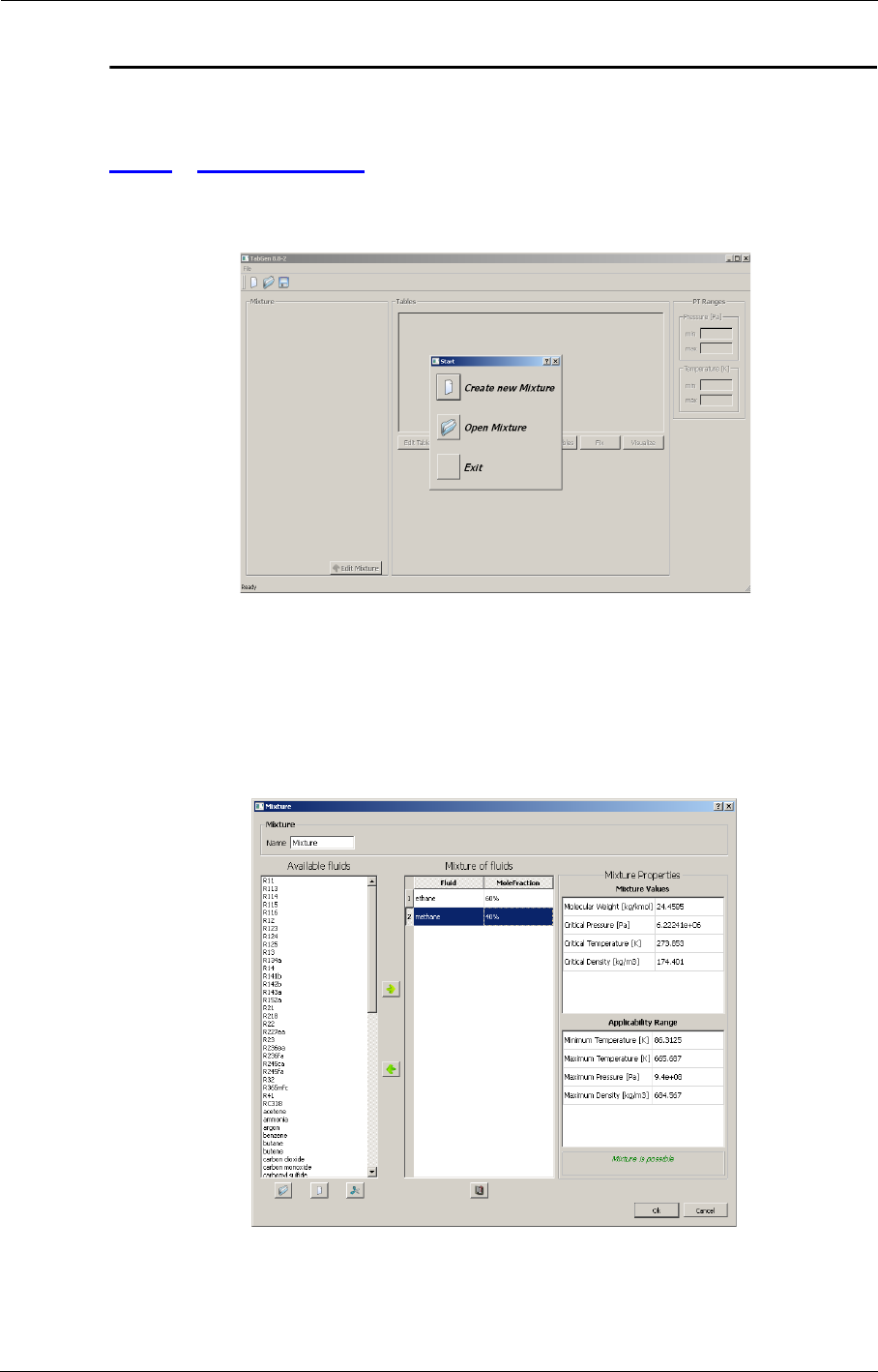
TabGe n Graphical User Interface
D-2 FINE™/Turbo
D-2 Graphical User Interface
D-2.1 Start Program
When starting the program, a Start window (Figure D.2.1-1) allows the user to create a new mix-
ture, load an existing one or exit TabGen.
FIGURE D.2.1-1 Start window of TabGen
D-2.1.1 Create New Mixture
The creation of a new mixture is possible by clicking on the button Create New Mixture in the Start
window. Then a Mixture window will appear, as seen in Figure D.2.1-2. The user can modify the
name of the mixture, which will be displayed in the top of the main window.
FIGURE D.2.1-2 Create new mixture
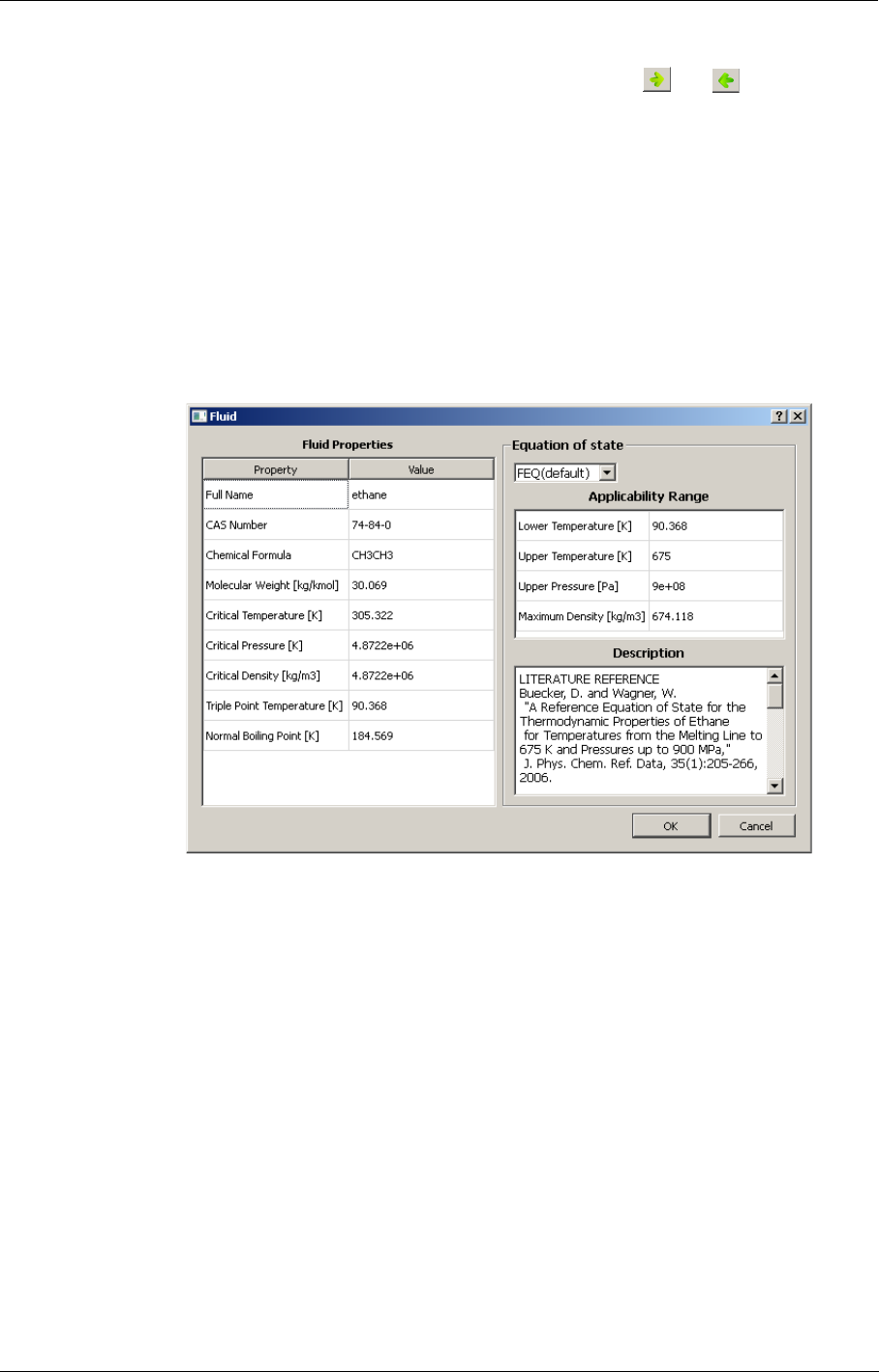
Graphical User Interface TabGen
FINE™/Turbo D-3
In the section Available Fluids, several fluids can be selected. The and buttons are used
to transfer the selected fluids to and from the mixture. Multi-selection is also possible to ease the
process. Three buttons at the bottom of the window allows the user to load directory with fluids,
load one fluid or unload a fluid.
After adding fluids to the mixture, the user needs to set the molar fraction for each fluid of the mix-
ture. The sum of mixture component should be 100%. In order to change molar fraction, a double
click on the dedicated fluid is needed.
For each fluid in the mixture, the user is able to see its properties and to choose its equation of state.
In order to do it the user needs to select the fluid inside the mixture and click on the button See
Fluid Properties at the bottom of the Mixture of fluids section. A new window will be opened, as
seen in Figure D.2.1-3. Inside there are general properties of the fluid and a combo box with cur-
rently selected equation of state. Just below the application ranges and description related to the
selected equation are shown.
FIGURE D.2.1-3 The properties of the selected fluid
For every user action, the current state of the mixture is displayed at the bottom of the Mixture
Properties section. If the mixture is not possible for any reasons, this issue is written inside this
field. When the mixture is possible the mixture values and application ranges are displayed.
After setting all the parameters and clicking on the button Ok, the main window of TabGen will
appear.
D-2.1.2 Open Mixture
The user can open an existing mixture by clicking on the Open Mixture button in the Start window.
Then a Load Mixture window will appear that allows the user to browse to the location of the exist-
ing mixture. The filter in the Load Mixture window is automatically set to display only the files
with extension ".xml", the default extension for a mixture file. After opening the existing mixture,
the main window of TabGen will appear.
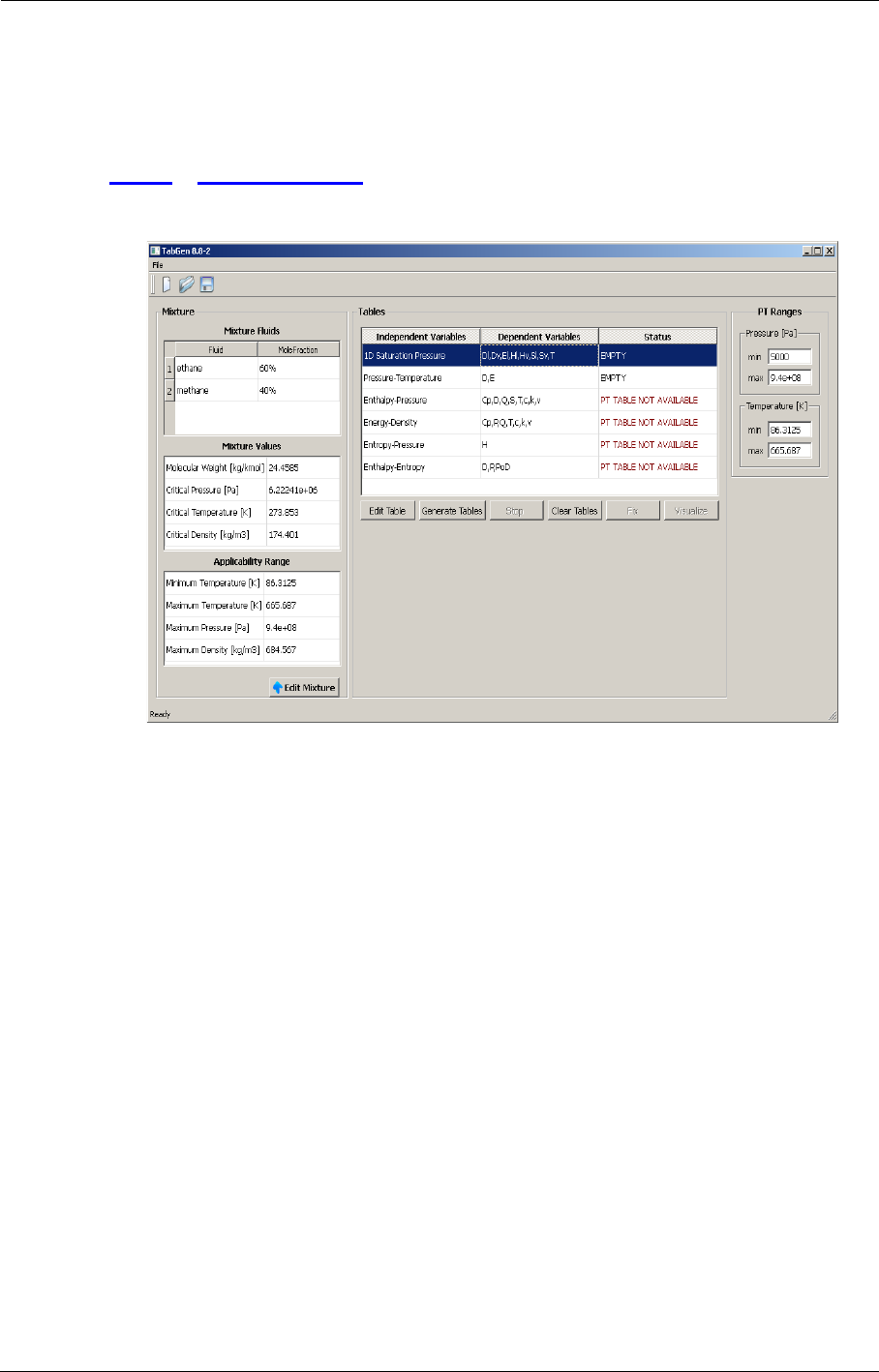
TabGe n Graphical User Interface
D-4 FINE™/Turbo
D-2.1.3 Exit
Clicking on the button Exit will exit TabGen.
D-2.2 Main Window
FIGURE D.2.2-4 Main window of TabGen
In the left part of the main window, the current mixture information is displayed: Mixture Fluids,
Mixture Values and Applicability Ranges. Just at the bottom of this information part, the Edit Mix-
ture button allows the user to go back to edit the mixture.
The central part of the main window is dedicated to the list of tables available. Several actions can
be applied on all the available thermodynamic tables using the bottom buttons. The actions are
applied for the selected table(s) within the list. The actions are adapted (enabled/disabled/trans-
formed) according to the current selection(s) of the table(s) as well as the table's status.
The central part is subdivided in three columns: Independent Variable (or table type), Dependent
Variables, Status:
•Independent Variables are fixed and cannot be changed.
•Dependent Variables are editable (see edit tables section below).
•Status reflects the current status of the table.
The status of the table can be:
•EMPTY if nothing is generated on disk
•GENERATED if generated on disk according to the specified parameters
•MISMATCH if the current definition of the table does not correspond to the table generated
on disk
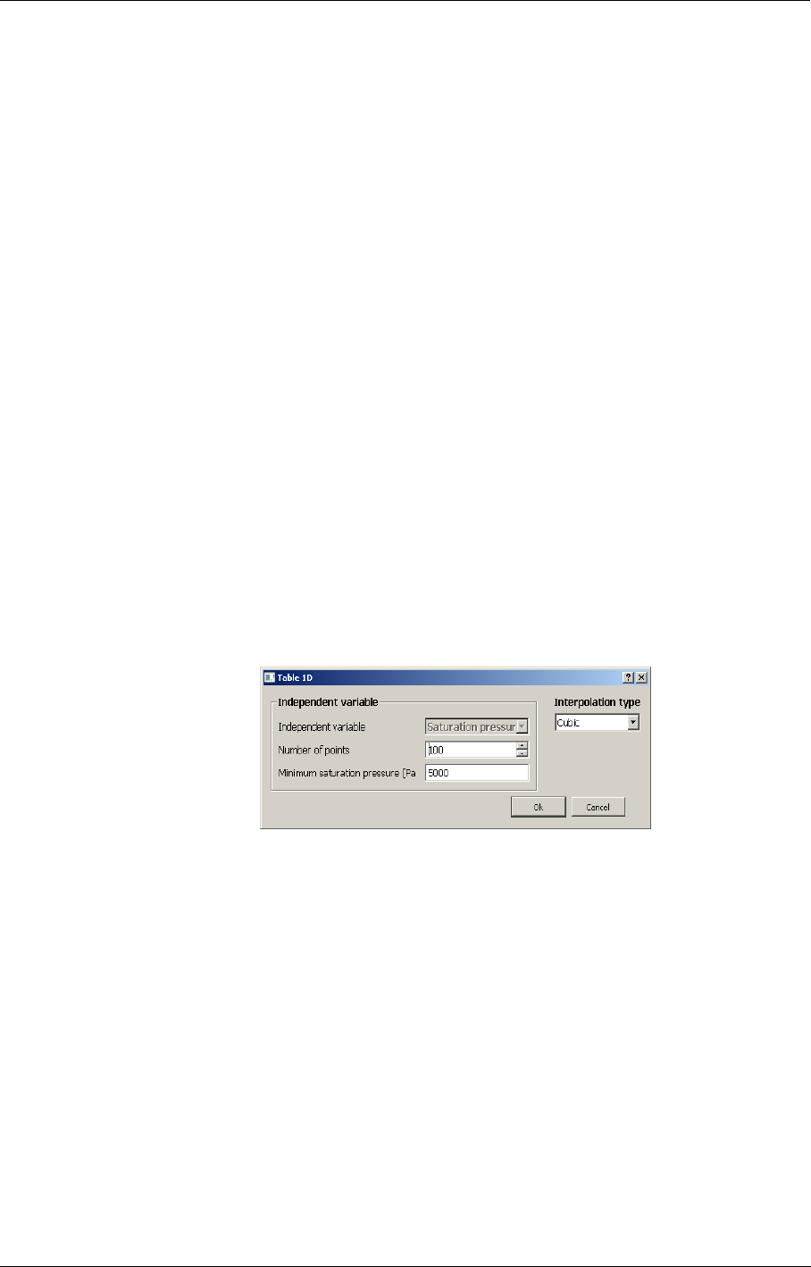
Graphical User Interface TabGen
FINE™/Turbo D-5
•PT TABLE NOT AVAILABLE if the table PT is not generated. Any table cannot be gener-
ated unless the PT table is GENERATED since all 2D Tables depends on the PT table. Thus, if
the PT table is not generated, all other 2D Tables are not available for generation (but available
for editing and clearing).
If the saturation table is not generated or mismatched when the user selects to generate
the PT table, the saturation table will be generated automatically before starting the PT
table generation.
In the right part of the main window, the PT ranges which are defined by default based on the mix-
ture applicability ranges is displayed. The user is allowed to define the Pressure-Temperature
ranges for the generation of the tables.
The user can in principle use the recommended range or a more restricted one (to have
a finer grid in the range it will be really used). However, the user will NOT be allowed to
go beyond the applicability range.
D-2.2.1 Edit Table
When selecting one non-generated table, the user is able to edit its definition by clicking on the Edit
button. It will open a new window related to the type of the table.
a) Edit 1D Saturation Table
For 1D Table there is no dependent variables selection. When generating it, all dependent variables
are selected: Temperature (T), Density_liq (Dl), Density_vap (Dv), Enthalpy_liq (Hl),
Enthalpy_vap (Hv), Entropy_liq (Sl), Entropy_vap (Sv), Energy_liq (El), Energy_vap (Ev).
Linear or Cubic interpolation types can be chosen.
FIGURE D.2.2-5 Edit 1D saturation table
b) Edit PT Table
The user is able to select dependent variables for this table. Temperature and pressure dependent
variables are disabled because they are already independent ones. Bilinear or bicubic interpolation
type can be chosen.
To go to the expert mode the user needs to click on the Expert button.
In the Pressure-Temperature tables, a physical discontinuity exists since the saturation is a single
line. And therefore, a sudden jump physically exists from the liquid to the gas phase. In order to
avoid a non-physical interpolation between the two states, a preferential phase can be used with the
following possibilities:
•NONE
•GAS
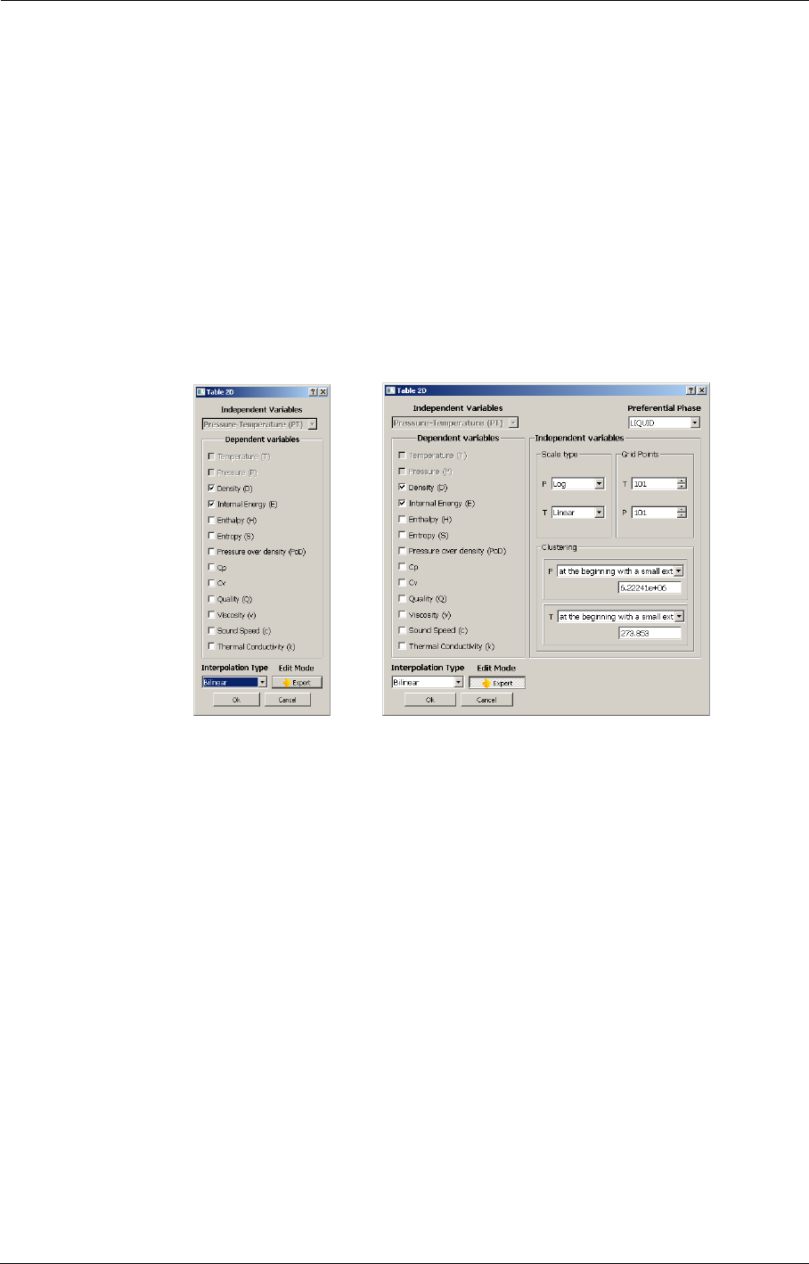
TabGe n Graphical User Interface
D-6 FINE™/Turbo
•LIQUID
In the Independent variables section, the user can select the scale type of the first and second inde-
pendent variable directions. The scale can be either linear or logarithmic. The user can also specify
the number of grid points in each independent variable direction. a default value 101x101 is given.
In the clustering section, The type of clustering in the first and second independent variable direc-
tion can be set. Different grid clustering options are available:
•none
•at the beginning
•at the beginning with a small extension
•at the end
•at the end with a small extension
FIGURE D.2.2-6 Edit PT table
c) Edit 2D Tables
In the normal mode the edit table 2D window is the same as the PT table edition.
In the expert mode, the user can accept the ranges automatically defined from the PT ranges in the
main window or define them by deactivating the option Obtain from PT. It activates the ranges
below and the user is free to impose their own ranges for independent values.
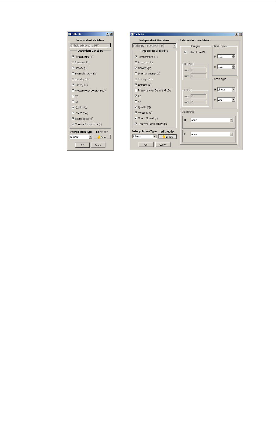
Graphical User Interface TabGen
FINE™/Turbo D-7
FIGURE D.2.2-7 Edit 2D tables
D-2.2.2 Generate Tables
To start a generation process for one or several selected tables, the user clicks on the Generate
Tables button. If the generation action is not allowed for at least one of the selected tables, the Gen-
erate Tables button is disabled. The same rule is applied for the other action buttons. If there are
more than one selected tables and the generation is allowed for all of them, clicking on the button
Generate Tables will open a submenu just below the button where the user can choose between
sequential generation or parallel generation of these tables.
If several tables are selected, launching sequential generation disables the Generate
Tables button for any other tables till the end of this generation, while parallel generation
leaves the possibility to generate tables which are not generated at the moment.
If only one table is selected, clicking on the button Generate Tables will automatically
launch this table generation like a parallel one.
In the case of parallel generation the tasks are really independent, so, they will share
the RAM memory and other resources (and the generation process for complex mixtures
will require a lot of resources).
If the user selection includes the PT table and a parallel generation is started, then, first of all, the
PT table will be generated sequentially and afterwards all selected tables will be generated in paral-
lel.
During the generation process in the status column the progress bar appears to show the generation
progress for the corresponding table. The user is able to stop the generation by clicking on the Stop
button. In the case of sequential generation it will stop all the current generation processes. In the
case of parallel generation, it will stop the generation only for the selected table(s).
When generating a table the user can edit neither the current mixture nor the PT ranges. The user
can not create new mixture or load another mixture too (all these fields are disabled).
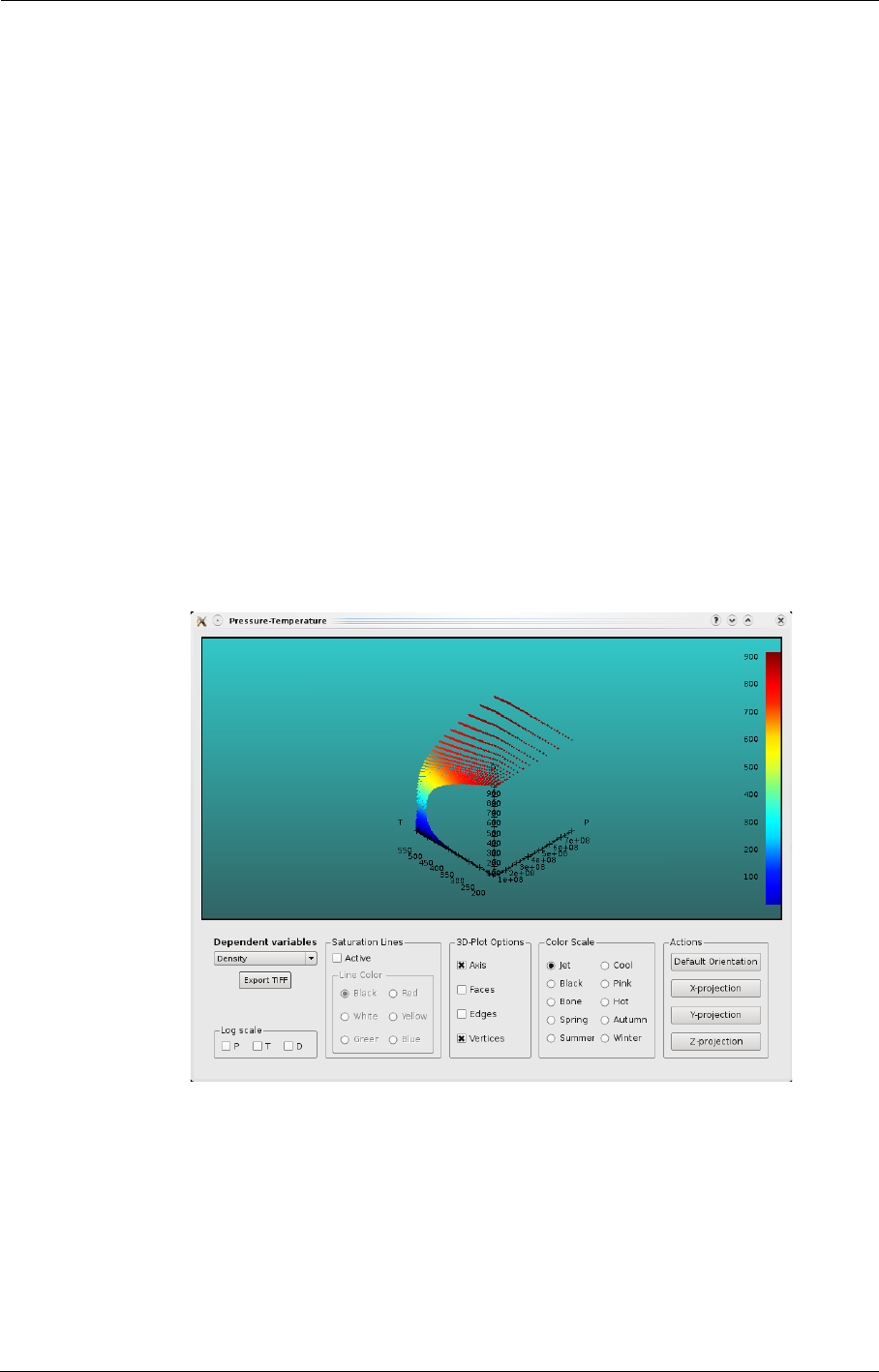
TabGe n Graphical User Interface
D-8 FINE™/Turbo
D-2.2.3 Stop
The user can click on the Stop button to stop the generation of the tables.
D-2.2.4 Clear Tables
The button Clear Tables is used to remove the selected table/tables that have been generated in the
list.
D-2.2.5 Mismatch Status / Fix
MISMATCH status for the table appears when its definition inside the interface differs from the
generated and saved on disk definition. The table acquires the MISMATCH status when the defini-
tion (Edit Table button) of the generated table is changed.
Even with the MISMATCH status, the tables can be regenerated with new definitions (the previous
tables are then lost).
The user can also select the MISMATCH table and click on Fix button. In this case the table defini-
tion is restored based on the table saved on disk. The Fix button works for multi-selection if all the
selected tables are presenting a MISMATCH status.
D-2.2.6 Visualization
FIGURE D.2.2-8 Visualization of the selected table
If the single selected table is generated, the Visualize button is activated and allows to plot the 3D
surface corresponding to the selected generated table.
In the bottom part of the window, the view can be customized thanks to the following items:
•dependent variable surface to visualize
•logarithmic scales for any axis

Launch TabGen in Batch Mode TabGen
FINE™/Turbo D-9
•saturation lines
•colormap
•viewing buttons
In order to rotate the plot, press the mouse left button on the 3D scene and move the mouse while it
is pressed. Zoom can be performed using the mouse wheel. Translation of the surface inside the
view plane can be made by analogy to rotation holding <Ctrl> button.
It is also possible to print the current view by pressing the Export TIFF button.
D-3 Launch TabGen in Batch Mode
In order to execute the table generation in batch mode, the XML project file should exist before.
One or several tables can be generated in one execution depending on the arguments that are given
to the execution file. The keywords of the different table types are as follows:
•SAT : saturation table. The saturation pressure is the independent variable
•PT : tables that have pressure-temperature as independent variables (e.g. EPT.atab)
•HP : tables that have enthalpy-pressure as independent variables (e.g. THP.atab)
•ER : tables that have energy-density as independent variables (e.g. TER.atab)
•SP: tables that have entropy-pressure as independent variables (e.g. HSP.atab)
•HS : tables that have enthalpy-entropy as independent variables (e.g. THS.atab)
Then, the command to generate the tables is:
On Linux:
tabgen <XML File> <List of keywords of the tables types separated by spaces>
On Windows:
Installation path\bin\tabgen.exe <XML File> <List of keywords of the tables types separated by
spaces>
Example: tabgen r114.xml SAT PT HP ER SP
In order to remove the tables, the similar command with the keyword <clear> at the end should be
typed.
Example: tabgen r114.xml SAT PT HP ER SP clear
It should be noticed that the generation of HP, ER SP and HS requires the previous generation of the
PT table. Actually, in the generation of the PT tables, a file containing the ranges of the variables is
written. This file is called “ranges.dat” and contains the maximum and minimum values of temper-
ature, pressure, enthalpy, energy, entropy and density.

TabGe n Launch TabGen in Batch Mode
D-10 FINE™/Turbo

Index
INDEX
FINE™/Turbo i
A
Add Fluid 3-3
Aeroacoustic 8-59
ANSYS
Fillet 10-16
Outputs 10-13
Visualization 10-17
AutoBlade 2-4, 2-12
AutoGrid 2-4, 2-6, 2-12
Batch 11-23
Axial Thrust 5-14, 10-22
Azimuthal Averaged Output 10-10
B
Background Color 1-6
Barotropic Liquid, see Fluid, Barotropic Liquid
Batch
AutoGrid 11-23
CFView™ 11-43
FINE™ 11-24
IGG™ 11-22
Bleed Flow
Theory 8-54
Bleed flow
Data file 8-55
Flow Parameters 8-49
Outputs 8-52
Positioning 8-37
Visualization 8-51
Wizard 8-35
Block
Conjugate Heat Transfer 7-10
Boundary Conditions 5-1
Compute Force and Torque 5-14
External 5-16
Full Non Matching 5-1
Group 5-2
Lagrangian Module 7-4–7-6
Passive Tracers 7-23
Periodic 5-11
Turbulence 4-3
Unsteady 6-10, 6-14
Boussinesq 4-23
C
CFL Number 6-2, 7-11
CFView™ 1-1, 2-12
Batch 11-43
CGNS A-3
Characteristic Values, see Reference Values
Condensable fluid
Outputs 10-4
Condensable Fluid, see Fluid, Condensable
Conductivity 3-4–3-6
Config
Grid Configuration 2-15
Conjugate Heat Transfer 7-9–7-11
Block Types 7-10
CFL Number 7-11
Thermal Connections 7-11
Control Variables 12-1
Unsteady 6-11
Convention 1-4
Convergence History 9-4, 12-3
Cooling Flow
Theory 8-54
Cooling flow 8-33
Bleed flow 8-33
Data file 8-55
Flow Parameters 8-49
Outputs 8-52
Positioning 8-37
Visualization 8-51
Wizard 8-35
CPU Booster 6-3
Create
Grid File 2-4
Project 2-2, 2-6
Run File 2-7
D
Delete Fluid 3-9
Design 3D 2-4, 2-12
Discretization
Spatial 6-6
Temporal 6-6
Drag 5-14
Drag Coefficient 10-23
Driver 1-5
Duplicate Active Project 2-7
E
Edit Fluid 3-9
Efficiency 10-19
Euler 4-2
Expert Mode 2-14

INDEX
Index
ii FINE™/Turbo
Expert Parameters B-1
External Boundary Condition 5-16
F
File
Management 1-2
Menu 2-6
New 2-12
Open 2-12
Save 2-13
Save Run File 2-13
File Format A-1
Fillet 10-16
Finebatch 11-24
Fluid
Add 3-3
Condensable 3-6, ??–3-7
Delete 3-9
Edit 3-9
Interface 3-2
Liquid 3-6
List 3-2
Models 3-1–3-10
Perfect Gas 3-4
Real Gas 3-4
Fluid-Particle Interaction. See Lagrangian Module.
Fluid-Structure Interaction 7-9
Force 5-14
Forced Transition 8-64
Formula Editor 3-8
Full Non Matching 5-1
FW-H 8-59
G
Gas Constant 3-5
Global Layout 2-9
Global Performance 10-19, A-7
Graphics 1-5
Graphics Area 2-19
Gravity 3-6, 4-21
Grid
Configuration 2-15
Create Grid File 2-4
Units 2-4, 2-10
Group
Block Rotation 8-2
Boundary Conditions 5-2
Rotor/Stator 8-4
H
Hand Symbol 1-4
Harmo2Time 2-12, 8-23
Harmonic 8-16, 8-19
Reconstruction in Time 8-22
Harmonic Global Residual 12-8
Host Definition 11-5
I
Icon Bar 2-12
IGG™ 1-1, 1-2, 2-4, 2-6, 2-12
Batch 11-22
Initial Solution 9-1–9-10
Block Dependent 9-1–9-3
Coarse Grid 6-4
Constant Values 9-3
From File 9-3–9-5
Initial Grouping 9-6
Reset Convergence History 9-4
Throughflow 9-8–9-10
Turbomachinery 9-5–9-7
Turbulence 4-4
Unsteady 9-5
Initialization
Full Multigrid Strategy 9-1
Unsteady 6-12
Installation 1-5
Interface 1-6
General Description of FINE™ Interface 2-1–2-22
L
Lagrangian Module
Boundary Conditions 7-4–7-6
Global Strategy 7-3
Outputs 7-6
Particle Traces 7-8
Laminar 4-2
Layout 2-9
License 1-7
Lift 5-14
Lift Coefficient 10-23
Light Bulb 1-5
Liquid, see Fluid, Liquid
Low Speed Flow 7-23
LSF 11-40
M
Mach Number

Index
INDEX
FINE™/Turbo iii
Absolute 10-5
Relative 10-5
Mathematical Model 4-1, 4-2
Menu
File 2-6
Menu Bar 2-6
Mesh 2-9
Modules 2-12
Solver 2-11
Merge
Merge Mesh Topology 2-13
Patch For Azimuthal View 10-10
Mesh
Information 2-18
Properties 2-10
Selection 2-13
Toggles 2-17
View 2-9, 2-19–2-21
View Area 2-16, 2-18
Modal Coupling 7-18
Modules 2-12
Moment 5-14
Momentum 10-23
Monitor
Convergence History 12-14
Display 12-13
Harmonic 12-13
Quantities 12-5
Residual File Box 12-12
Solution 12-1–12-16
Steering File 12-5
Zoom 12-13
MonitorTurbo 12-10
Moving Mesh 7-13
Adaptive Wall 7-16
Generalized Motion 7-15
Off-centered Rotor 7-14
Oscillating Body 7-14
Moving Mesh (Rigid Motion) 7-13
MpCCI Coupling 7-17
Thermal Coupling 7-12
MSW Driver 1-5
Multigrid 6-3
Strategy 6-5
N
New Project 2-6
Numerical Model 6-1
O
Open
Project 2-4, 2-6
OPENGL Driver 1-5
Outputs 10-1–??
.mf File 10-19, 10-23
3D Quantity 10-2–10-8
ANSYS 10-13
Azimuthal Averaged 10-10, 10-22
Condensable Fluid 10-4
Efficiency 10-19
Global Performance 10-19
Lagrangian Module 7-6
Particle Traces 7-8
Plot3D 10-22
Residuals 10-6
Solid Data 10-6
Surface Averaged 10-9
Turbulence 10-7
Velocity 10-5
Vorticity 10-5
P
Pair of Scissors 1-4
Parallel Computation 11-19, 11-31
LSF 11-40
MPI 11-31, 11-33
PBS 11-38
SGE 11-35
Parameters Area 2-2
Particles 7-1
Passive Tracers 7-23
Initial Solution 7-24
mass fractions 7-23
PBS 11-38
Perfect Gas, see Fluid, Perfect Gas
Performance 10-19, A-7
Performance Curve 8-66
Create 8-66
Edit 8-66
Output 8-68
Parallel computation 8-68
Periodic Boundaries 5-11
Phase Lagged 6-11
plg2harmo 6-17
Plot3D 10-22, A-10
Preconditioning 7-23
Hakimi 6-4

INDEX
Index
iv FINE™/Turbo
Merkle 6-4
Parameters 6-4
Preferences 2-8
Profile Manager 2-22, 3-3–3-8
File Formats A-11
Project
Configuration 2-4
Create 2-2
Duplicate 2-7
Management 1-2
New 2-6
Open 2-4, 2-6
Save 2-7
Save As 2-7
Units 2-8
Properties
Fluid 3-1
Mesh 2-10
PVM
Daemons 11-1–11-5
Q
Queuing template
Default template 11-6
User-defined template 11-15
Quit 2-9
R
R134a C-2
Real Gas, see Fluid, Real Gas
Reconstruction in Time 8-22, 8-23
Reference
Density 4-23
Length 4-23
Pressure 3-6, 6-4
Reference Values 4-22
Temperature 3-6, 6-4
Velocity 4-23
Relative path 1-3
repetition 8-16
Residual 10-6, 12-7, A-8
Restart
Unsteady 6-13
Reynolds Number 4-22
Rotate View 2-20
Rotation
Blocks 8-2–8-3
Rotor/Stator
Domain Scaling 8-12–8-14
Frozen Rotor 8-10–8-12
Initial Solution 9-7
Interface 8-4–8-5
Mixing Plane Coupling 8-7–8-9
Phase Lagged 8-14
Steady 8-7–8-9, 8-10–8-12
Unsteady 8-12–8-14
Run File 1-2, 2-7
S
Save
Project 2-7
Second Order Restart 6-13
SGE 11-35
SI System 2-8
Solid Data 10-6
Solver
Menu 2-11
Save 2-11
Start 2-11
Stop 2-11
Suspend 2-11
Solver Preferences 2-9
Standard Mode 2-14
Stator
Rotor/Stator Interface. See Rotor/Stator.
Steady
Rotor/Stator 8-7–8-9, 8-10–8-12
SubProject 8-69
Create 8-70
File Structure 8-74
Grid Requirements 8-70
Merge 8-73
Modify 8-73
Surface Averaged Output 10-8
T
TabGen D-1
Task Definition 11-6
Taskmanager 11-1–11-45
Add Host 11-5
Host Definition 11-5
Limitations 11-45
PVM 11-1–11-5
Remove Host 11-6
Scripts 11-22–11-45
Shutdown 11-6

Index
INDEX
FINE™/Turbo v
Subtask 11-7–11-17
Task Definition 11-6–11-17
Tear-off Graphics 2-10
Thermal Connections 7-11
Thermodynamic Tables C-1
Throughflow
Initial Solution 9-8–9-10
Time Configuration 6-10
Time Step
Global 6-6
Local 6-6
Torque 5-14, 10-22
Tracers 7-23
Transition Model 4-19, 8-63
Forced Transition 8-64
Turbulence
Boundary Conditions 4-3
Initial Solution 4-4
Output 10-7
Turbulence Models
k-epsilon 4-15
Spalart-Allmaras 4-15
U
Units
Grid 2-4, 2-10
Project 2-8
Unload Mesh 2-10
Unsteady 6-10
Boundary Conditions 6-10, 6-14
Control Variables 6-11
Create 6-14
Harmonic 8-16, 8-19
Initial Solution 9-5
Initialization 6-15
Phase Lagged 6-11
Rotor/Stator 8-12–8-14
Rotor/Stator Phase Lagged 8-14
Second Order in Time 6-13
User Mode 2-14
V
Velocity
Absolute 10-5
Friction 4-11
Projections 10-5
Reference 4-23
Relative 10-5
Relative Projections 10-5
View Area 2-16, 2-18
View Manipulation 2-19
View On/Off 2-9, 2-16
Vorticity 10-5
W
Water (Steam) C-1
Work Unit A-9
X
X11 Driver 1-5
Z
Zoom In/Out/Region 2-21
