The Idiot's Guide To Statistics Jr., Ph.D., Robert A. Donnelly Statistics, 2nd Edition Alpha (
User Manual: Pdf
Open the PDF directly: View PDF ![]() .
.
Page Count: 421 [warning: Documents this large are best viewed by clicking the View PDF Link!]
- Cover Page
- Title Page
- Dedication Page & Copyright Page
- Contents at a Glance
- Contents
- Foreword
- Introduction
- Part One: The Basics
- Chapter One: Let’s Get Started
- Chapter Two: Data, Data Everywhere and Not a Drop to Drink
- The Importance of Data
- The Sources of Data—Where Does All This Stuff Come From?
- Direct Observation—I’ll Be Watching You
- Experiments—Who’s in Control?
- Surveys—Is That Your Final Answer?
- Types of Data
- Types of Measurement Scales—a Weighty Topic
- Nominal Level of Measurement
- Ordinal Level of Measurement
- Interval Level of Measurement
- Ratio Level of Measurement
- Computers to the Rescue
- The Role of Computers in Statistics
- Installing the Data Analysis Add-In
- Your Turn
- Chapter Three: Displaying Descriptive Statistics
- Frequency Distributions
- Constructing a Frequency Distribution
- (A Distant) Relative Frequency Distribution
- Cumulative Frequency Distribution
- Graphing a Frequency Distribution—the Histogram
- Letting Excel Do Our Dirty Work
- Statistical Flower Power—the Stem and Leaf Display
- Charting Your Course
- What’s Your Favorite Pie Chart?
- Bar Charts
- Line Charts
- Your Turn
- Chapter Four: Calculating Descriptive Statistics: Measures of Central Tendency (Mean, Median, and Mode)
- Chapter Five: Calculating Descriptive Statistics: Measures of Dispersion
- Range
- Variance
- Using the Raw Score Method (When Grilling)
- The Variance of a Population
- Standard Deviation
- Calculating the Standard Deviation of Grouped Data
- The Empirical Rule: Working the Standard Deviation
- Chebyshev’s Theorem
- Measures of Relative Position
- Quartiles
- Interquartile Range
- Using Excel to Calculate Measures of Dispersion
- Your Turn
- Part Two: Probability Topics
- Chapter Six: Introduction to Probability
- Chapter Seven: More Probability Stuff
- Chapter Eight: Counting Principles and Probability Distributions
- Counting Principles
- The Fundamental Counting Principle
- Permutations
- Combinations
- Using Excel to Calculate Permutations and Combinations
- Probability Distributions
- Random Variables
- Discrete Probability Distributions
- Rules for Discrete Probability Distributions
- The Mean of a Discrete Probability Distribution
- The Variance and Standard Deviation of a Discrete Probability Distribution
- Your Turn
- Chapter Nine: The Binomial Probability Distribution
- Chapter Ten: The Poisson Probability Distribution
- Chapter Eleven: The Normal Probability Distribution
- Characteristics of the Normal Probability Distribution
- Calculating Probabilities for the Normal Distribution
- Calculating the Standard Z-Score
- Using the Standard Normal Table
- The Empirical Rule Revisited
- Calculating Normal Probabilities Using Excel
- Using the Normal Distribution as an Approximation to the Binomial Distribution
- Your Turn
- Part Three: Inferential Statistics
- Chapter Twelve: Sampling
- Chapter Thirteen: Sampling Distributions
- What Is a Sampling Distribution?
- Sampling Distribution of the Mean
- The Central Limit Theorem
- Standard Error of the Mean
- Why Does the Central Limit Theorem Work?
- Putting the Central Limit Theorem to Work
- Sampling Distribution of the Proportion
- Calculating the Sample Proportion
- Calculating the Standard Error of the Proportion
- Your Turn
- Chapter Fourteen: Confidence Intervals
- Confidence Intervals for the Mean with Large Samples
- Estimators
- Confidence Levels
- Beware of the Interpretation of Confidence Interval!
- The Effect of Changing Confidence Levels
- The Effect of Changing Sample Size
- Determining Sample Size for the Mean
- Calculating a Confidence Interval When σ Is Unknown
- Using Excel’s CONFIDENCE Function
- Confidence Intervals for the Mean with Small Samples
- When σ Is Known
- When σ Is Unknown
- Confidence Intervals for the Proportion with Large Samples
- Calculating the Confidence Interval for the Proportion
- Determining Sample Size for the Proportion
- Your Turn
- Chapter Fifteen: Introduction to Hypothesis Testing
- Hypothesis Testing—the Basics
- The Null and Alternative Hypothesis
- Stating the Null and Alternative Hypothesis
- Two-Tail Hypothesis Test
- One-Tail Hypothesis Test
- Type I and Type II Errors
- Example of a Two-Tail Hypothesis Test
- Using the Scale of the Original Variable
- Using the Standardized Normal Scale
- Example of a One-Tail Hypothesis Test
- Your Turn
- Chapter Sixteen: Hypothesis Testing with One Sample
- Hypothesis Testing for the Mean with Large Samples
- When Sigma Is Known
- When Sigma Is Unknown
- The Role of Alpha in Hypothesis Testing
- Introducing the p-Value
- The p-Value for a One-Tail Test
- The p-Value for a Two-Tail Test
- Hypothesis Testing for the Mean with Small Samples
- When Sigma Is Known
- When Sigma Is Unknown
- Using Excel’s TINV Function
- Hypothesis Testing for the Proportion with Large Samples
- One-Tail Hypothesis Test for the Proportion
- Two-Tail Hypothesis Test for the Proportion
- Your Turn
- Chapter Seventeen: Hypothesis Testing with Two Samples
- The Concept of Testing Two Populations
- Sampling Distribution for the Difference in Means
- Testing for Differences Between Means with Large Sample Sizes
- Testing a Difference Other Than Zero
- Testing for Differences Between Means with Small Sample Sizes and Unknown Sigma
- Equal Population Standard Deviations
- Unequal Population Standard Deviations
- Letting Excel Do the Grunt Work
- Testing for Differences Between Means with Dependent Samples
- Testing for Differences Between Proportions with Independent Samples
- Your Turn
- Part Four: Advanced Inferential Statistics
- Chapter Eighteen: The Chi-Square Probability Distribution
- Review of Data Measurement Scales
- The Chi-Square Goodness-of-Fit Test
- Stating the Null and Alternative Hypothesis
- Observed Versus Expected Frequencies
- Calculating the Chi-Square Statistic
- Determining the Critical Chi-Square Score
- Using Excel’s CHIINV Function
- Characteristics of a Chi-Square Distribution
- A Goodness-of-Fit Test with the Binomial Distribution
- Chi-Square Test for Independence
- Your Turn
- Chapter Nineteen: Analysis of Variance
- One-Way Analysis of Variance
- Completely Randomized ANOVA
- Partitioning the Sum of Squares
- Determining the Calculated F-Statistic
- Determining the Critical F-Statistic
- Using Excel to Perform One-Way ANOVA
- Pairwise Comparisons
- Completely Randomized Block ANOVA
- Partitioning the Sum of Squares
- Determining the Calculated F-Statistic
- To Block or Not to Block, That Is the Question
- Your Turn
- Chapter Twenty: Correlation and Simple Regression
- Independent Versus Dependent Variables
- Correlation
- Correlation Coefficient
- Testing the Significance of the Correlation Coefficient
- Using Excel to Calculate Correlation Coefficients
- Simple Regression
- The Least Squares Method
- Confidence Interval for the Regression Line
- Testing the Slope of the Regression Line
- The Coefficient of Determination
- Using Excel for Simple Regression
- A Simple Regression Example with Negative Correlation
- Assumptions for Simple Regression
- Simple Versus Multiple Regression
- Your Turn
- Chapter Eighteen: The Chi-Square Probability Distribution
- Appendix A: Solutions to "Your Turn"
- Appendix B: Statistical Tables
- Appendix C: Glossary
- Index
- Dear Reader
- About the Author

by Robert A. Donnelly, Jr., Ph.D.
ASQ]\R3RWbW]\
A member of Penguin Group (USA) Inc.
AbObWabWQa
To my wife, Debbie, who supported and encouraged me every step of the way.
I could not have done this without you, babe.
/:>6/0==9A
Published by the Penguin Group
Penguin Group (USA) Inc., 375 Hudson Street, New York, New York 10014, U.S.A.
Penguin Group (Canada), 10 Alcorn Avenue, Toronto, Ontario, Canada M4V 3B2 (a division of Pearson Penguin
Canada Inc.)
Penguin Books Ltd, 80 Strand, London WC2R 0RL, England
Penguin Ireland, 25 St Stephen’s Green, Dublin 2, Ireland (a division of Penguin Books Ltd)
Penguin Group (Australia), 250 Camberwell Road, Camberwell, Victoria 3124, Australia (a division of Pearson
Australia Group Pty Ltd)
Penguin Books India Pvt Ltd, 11 Community Centre, Panchsheel Park, New Delhi—110 017, India
Penguin Group (NZ), cnr Airborne and Rosedale Roads, Albany, Auckland 1310, New Zealand (a division of
Pearson New Zealand Ltd)
Penguin Books (South Africa) (Pty) Ltd, 24 Sturdee Avenue, Rosebank, Johannesburg 2196, South Africa
Penguin Books Ltd, Registered Offices: 80 Strand, London WC2R 0RL, England
1]^g`WUVb %Pg@]PS`b/2]\\SZZg8`
All rights reserved. No part of this book shall be reproduced, stored in a retrieval system, or transmitted by any
means, electronic, mechanical, photocopying, recording, or otherwise, without written permission from the pub-
lisher. No patent liability is assumed with respect to the use of the information contained herein. Although every
precaution has been taken in the preparation of this book, the publisher and author assume no responsibility for
errors or omissions. Neither is any liability assumed for damages resulting from the use of information contained
herein. For information, address Alpha Books, 800 East 96th Street, Indianapolis, IN 46240.
THE COMPLETE IDIOT’S GUIDE TO and Design are registered trademarks of Penguin Group (USA) Inc.
Library of Congress Catalog Card Number: 2006938600
Interpretation of the printing code: The rightmost number of the first series of numbers is the year of the book’s
printing; the rightmost number of the second series of numbers is the number of the book’s printing. For example,
a printing code of 07-1 shows that the first printing occurred in 2007.
Note: This publication contains the opinions and ideas of its author. It is intended to provide helpful and informa-
tive material on the subject matter covered. It is sold with the understanding that the author and publisher are not
engaged in rendering professional services in the book. If the reader requires personal assistance or advice, a com-
petent professional should be consulted.
The author and publisher specifically disclaim any responsibility for any liability, loss, or risk, personal or other-
wise, which is incurred as a consequence, directly or indirectly, of the use and application of any of the contents of
this book.
Publisher: Marie Butler-Knight
Editorial Director: Mike Sanders
Managing Editor: Billy Fields
Acquisitions Editor: Tom Stevens
Development Editor: Michael Thomas
Production Editor: Kayla Dugger
Copy Editor: Nancy Wagner
Cartoonist: Chris Eliopoulos
Cover Designer: Bill Thomas
Book Designer: Trina Wurst
Indexer: Angie Bess
Layout: Chad Dressler
Proofreader: Aaron Black
ISBN : 1-4295-1390-X
1]\bS\baObO5ZO\QS
>O`b( BVS0OaWQa
1 Let’s Get Started 3
Statistics plays a vital role in today’s society by providing the
foundation for sound decisions.
2 Data, Data Everywhere and Not a Drop to Drink 15
All statistical analysis begins with the proper selection of the
source, type, and measurement scale of the data.
3 Displaying Descriptive Statistics 29
A vast array of methods display data and information effec-
tively, such as frequency distributions, histograms, pie charts,
and bar charts.
4 Calculating Descriptive Statistics: Measures of
Central Tendency (Mean, Median, and Mode) 47
Using the mean, median, or mode is an effective way to sum-
marize many pieces of data.
5 Calculating Descriptive Statistics: Measures
of Dispersion 61
The standard deviation, range, and quartiles reveal valuable
information about the variability of the data.
>O`b ( >`]POPWZWbgB]^WQa %'
6 Introduction to Probability 81
Basic probability theory, such as the intersection and union of
events, provides important groundwork for statistical concepts.
7 More Probability Stuff 93
Calculate the probability of winning your tennis match given
that you had a short warm-up period.
8 Counting Principles and Probability Distributions 105
Determine your odds at winning a state lottery drawing or
your chances of drawing a five-card flush in poker.
9 The Binomial Probability Distribution 121
Calculate the probability of correctly guessing the answer of 6
out of 12 multiple-choice questions when each question has five
choices.

BVS1][^ZSbS7RW]ba5cWRSb]AbObWabWQaASQ]\R3RWbW]\
Wd
10 The Poisson Probability Distribution 131
Determine the probability that you will receive at least 3
spam e-mails tomorrow given that you average 2.5 such
e-mails per day.
11 The Normal Probability Distribution 145
Determine probabilities of events that follow this symmetrical,
bell-shaped distribution.
>O`b!( 7\TS`S\bWOZAbObWabWQa $!
12 Sampling 165
Discover how to choose between simple random, systematic,
cluster, and stratified sampling for statistical analysis.
13 Sampling Distributions 177
The central limit theorem tells us that sample means follow
the normal probability distribution as long as the sample size
is large enough.
14 Confidence Intervals 195
A confidence interval is a range of values used to estimate a
population parameter.
15 Introduction to Hypothesis Testing 213
A hypothesis test enables us to investigate an assumption about
a population parameter using a sample.
16 Hypothesis Testing with One Sample 227
This procedure focuses on testing a statement concerning a
single population.
17 Hypothesis Testing with Two Samples 249
Use this test to see whether that new golf instructional video
will really lower your scores.
>O`b"( /RdO\QSR7\TS`S\bWOZAbObWabWQa %
18 The Chi-Square Probability Distribution 273
This procedure enables us to test the independence of two cat-
egorical variables.
19 Analysis of Variance 289
Learn how to test the difference between more than two popu-
lation means.
20 Correlation and Simple Regression 309
Determine the strength and direction of the linear relationship
between an independent and dependent variable.

1]\bS\ba
>O`b( BVS0OaWQa
:SbÂa5SbAbO`bSR !
Where Is This Stuff Used? ............................................................4
Who Thought of This Stuff? ........................................................5
Early Pioneers ..............................................................................5
More Recent Famous People ..........................................................6
The Field of Statistics Today .........................................................6
Descriptive Statistics—the Minor League ......................................7
Inferential Statistics—the Major League .......................................8
Ethics and Statistics—It’s a Dangerous World Out There.........10
Your Turn......................................................................................12
2ObO2ObO3dS`geVS`SO\R<]bO2`]^b]2`W\Y #
The Importance of Data ..............................................................16
The Sources of Data—Where Does All This Stuff Come
From?..........................................................................................17
Direct Observation—I’ll Be Watching You...................................19
Experiments—Who’s in Control? ................................................19
Surveys—Is That Your Final Answer? ........................................20
Types of Data................................................................................20
Types of Measurement Scales—a Weighty Topic .......................21
Nominal Level of Measurement ..................................................21
Ordinal Level of Measurement....................................................21
Interval Level of Measurement ...................................................22
Ratio Level of Measurement........................................................22
Computers to the Rescue.............................................................23
The Role of Computers in Statistics .............................................23
Installing the Data Analysis Add-In............................................24
Your Turn......................................................................................26
! 2Wa^ZOgW\U2SaQ`W^bWdSAbObWabWQa '
Frequency Distributions ..............................................................30
Constructing a Frequency Distribution ........................................31
(A Distant) Relative Frequency Distribution ...............................32
Cumulative Frequency Distribution ............................................33
Graphing a Frequency Distribution—the Histogram...................34
Letting Excel Do Our Dirty Work ..............................................34

BVS1][^ZSbS7RW]ba5cWRSb]AbObWabWQaASQ]\R3RWbW]\
dWWW
Statistical Flower Power—the Stem and Leaf Display...............37
Charting Your Course ..................................................................39
What’s Your Favorite Pie Chart? ................................................39
Bar Charts .................................................................................41
Line Charts ................................................................................43
Your Turn......................................................................................44
" 1OZQcZObW\U2SaQ`W^bWdSAbObWabWQa(;SOac`Sa]T1S\b`OZBS\RS\Qg
;SO\;SRWO\O\R;]RS "%
Measures of Central Tendency ....................................................48
Mean..........................................................................................48
Weighted Mean ..........................................................................50
Mean of Grouped Data from a Frequency Distribution................51
Median.......................................................................................54
Mode..........................................................................................55
How Does One Choose?...............................................................56
Using Excel to Calculate Central Tendency ...............................56
Your Turn......................................................................................58
# 1OZQcZObW\U2SaQ`W^bWdSAbObWabWQa(;SOac`Sa]T2Wa^S`aW]\ $
Range ............................................................................................62
Variance ........................................................................................63
Using the Raw Score Method (When Grilling)............................64
The Variance of a Population ......................................................65
Standard Deviation.......................................................................67
Calculating the Standard Deviation of Grouped Data ...............67
The Empirical Rule: Working the Standard Deviation..............69
Chebyshev’s Theorem ..................................................................71
Measures of Relative Position......................................................73
Quartiles ....................................................................................73
Interquartile Range ....................................................................74
Using Excel to Calculate Measures of Dispersion......................75
Your Turn......................................................................................76
>O`b ( >`]POPWZWbgB]^WQa %'
$ 7\b`]RcQbW]\b]>`]POPWZWbg &
What Is Probability? ....................................................................82
Classical Probability ....................................................................82

1]\bS\ba Wf
Empirical Probability..................................................................83
Subjective Probability..................................................................85
Basic Properties of Probability ....................................................86
The Intersection of Events ..........................................................87
The Union of Events: A Marriage Made in Heaven ..................88
Your Turn......................................................................................89
% ;]`S>`]POPWZWbgAbcTT '!
Conditional Probability................................................................94
Independent Versus Dependent Events ......................................96
Multiplication Rule of Probabilities ............................................97
Mutually Exclusive Events ...........................................................98
Addition Rule of Probabilities .....................................................99
Summarizing Our Findings .......................................................101
Bayes’ Theorem..........................................................................102
Your Turn....................................................................................103
& 1]c\bW\U>`W\QW^ZSaO\R>`]POPWZWbg2Wab`WPcbW]\a #
Counting Principles ...................................................................106
The Fundamental Counting Principle .......................................106
Permutations ............................................................................107
Combinations............................................................................109
Using Excel to Calculate Permutations and Combinations..........111
Probability Distributions............................................................112
Random Variables ....................................................................112
Discrete Probability Distributions ..............................................113
Rules for Discrete Probability Distributions................................115
The Mean of a Discrete Probability Distribution........................115
The Variance and Standard Deviation of a Discrete
Probability Distribution ..........................................................116
Your Turn....................................................................................118
' BVS0W\][WOZ>`]POPWZWbg2Wab`WPcbW]\
Characteristics of a Binomial Experiment.................................122
The Binomial Probability Distribution.....................................123
Binomial Probability Tables.......................................................126
Using Excel to Calculate Binomial Probabilities......................127
The Mean and Standard Deviation for the Binomial
Distribution ..............................................................................129
Your Turn....................................................................................129

BVS1][^ZSbS7RW]ba5cWRSb]AbObWabWQaASQ]\R3RWbW]\
f
BVS>]Waa]\>`]POPWZWbg2Wab`WPcbW]\ !
Characteristics of a Poisson Process..........................................132
The Poisson Probability Distribution .......................................133
Poisson Probability Tables .........................................................136
Using Excel to Calculate Poisson Probabilities ........................139
Using the Poisson Distribution as an Approximation to
the Binomial Distribution........................................................140
Your Turn....................................................................................142
BVS<]`[OZ>`]POPWZWbg2Wab`WPcbW]\ "#
Characteristics of the Normal Probability Distribution...........146
Calculating Probabilities for the Normal Distribution ............148
Calculating the Standard Z-Score .............................................148
Using the Standard Normal Table.............................................150
The Empirical Rule Revisited....................................................155
Calculating Normal Probabilities Using Excel ...........................156
Using the Normal Distribution as an Approximation to
the Binomial Distribution........................................................157
Your Turn....................................................................................161
>O`b!( 7\TS`S\bWOZAbObWabWQa $!
AO[^ZW\U $#
Why Sample?..............................................................................166
Random Sampling ......................................................................167
Simple Random Sampling.........................................................168
Systematic Sampling.................................................................170
Cluster Sampling......................................................................171
Stratified Sampling ..................................................................172
Sampling Errors .........................................................................173
Examples of Poor Sampling Techniques ...................................174
Your Turn....................................................................................176
! AO[^ZW\U2Wab`WPcbW]\a %%
What Is a Sampling Distribution?.............................................177
Sampling Distribution of the Mean...........................................178
The Central Limit Theorem .....................................................182
Standard Error of the Mean ......................................................185

1]\bS\ba fW
Why Does the Central Limit Theorem Work?........................186
Putting the Central Limit Theorem to Work ..........................188
Sampling Distribution of the Proportion..................................190
Calculating the Sample Proportion............................................190
Calculating the Standard Error of the Proportion......................192
Your Turn....................................................................................193
" 1]\TWRS\QS7\bS`dOZa '#
Confidence Intervals for the Mean with Large Samples ..........196
Estimators ................................................................................196
Confidence Levels......................................................................197
Beware of the Interpretation of Confidence Interval! ..................199
The Effect of Changing Confidence Levels .................................200
The Effect of Changing Sample Size .........................................201
Determining Sample Size for the Mean ....................................202
Calculating a Confidence Interval When X Is Unknown ............202
Using Excel’s CONFIDENCE Function ...................................203
Confidence Intervals for the Mean with Small Samples...........204
When X Is Known ....................................................................204
When X Is Unknown ................................................................205
Confidence Intervals for the Proportion with Large
Samples.....................................................................................208
Calculating the Confidence Interval for the Proportion...............209
Determining Sample Size for the Proportion.............................210
Your Turn....................................................................................211
# 7\b`]RcQbW]\b]6g^]bVSaWaBSabW\U !
Hypothesis Testing—the Basics.................................................214
The Null and Alternative Hypothesis ........................................215
Stating the Null and Alternative Hypothesis .............................216
Two-Tail Hypothesis Test...........................................................217
One-Tail Hypothesis Test...........................................................218
Type I and Type II Errors..........................................................219
Example of a Two-Tail Hypothesis Test....................................220
Using the Scale of the Original Variable....................................221
Using the Standardized Normal Scale.......................................222
Example of a One-Tail Hypothesis Test....................................223
Your Turn....................................................................................225

BVS1][^ZSbS7RW]ba5cWRSb]AbObWabWQaASQ]\R3RWbW]\
fWW
$ 6g^]bVSaWaBSabW\UeWbV=\SAO[^ZS %
Hypothesis Testing for the Mean with Large Samples.............228
When Sigma Is Known.............................................................228
When Sigma Is Unknown.........................................................229
The Role of Alpha in Hypothesis Testing.................................231
Introducing the p-Value .............................................................233
The p-Value for a One-Tail Test................................................233
The p-Value for a Two-Tail Test................................................234
Hypothesis Testing for the Mean with Small Samples .............236
When Sigma Is Known.............................................................236
When Sigma Is Unknown.........................................................237
Using Excel’s TINV Function ...................................................241
Hypothesis Testing for the Proportion with Large Samples....242
One-Tail Hypothesis Test for the Proportion...............................243
Two-Tail Hypothesis Test for the Proportion...............................245
Your Turn....................................................................................246
% 6g^]bVSaWaBSabW\UeWbVBe]AO[^ZSa "'
The Concept of Testing Two Populations ................................250
Sampling Distribution for the Difference in Means.................250
Testing for Differences Between Means with Large
Sample Sizes .............................................................................252
Testing a Difference Other Than Zero.....................................255
Testing for Differences Between Means with Small
Sample Sizes and Unknown Sigma .........................................256
Equal Population Standard Deviations......................................257
Unequal Population Standard Deviations..................................260
Letting Excel Do the Grunt Work............................................261
Testing for Differences Between Means with Dependent
Samples.....................................................................................263
Testing for Differences Between Proportions with
Independent Samples ...............................................................265
Your Turn....................................................................................269
>O`b"( /RdO\QSR7\TS`S\bWOZAbObWabWQa %
& BVS1VWA_cO`S>`]POPWZWbg2Wab`WPcbW]\ %!
Review of Data Measurement Scales.........................................274
The Chi-Square Goodness-of-Fit Test .....................................274
Stating the Null and Alternative Hypothesis .............................276

1]\bS\ba fWWW
Observed Versus Expected Frequencies .......................................276
Calculating the Chi-Square Statistic .........................................277
Determining the Critical Chi-Square Score...............................277
Using Excel’s CHIINV Function...............................................279
Characteristics of a Chi-Square Distribution............................279
A Goodness-of-Fit Test with the Binomial Distribution..........280
Chi-Square Test for Independence............................................282
Your Turn....................................................................................286
' /\OZgaWa]TDO`WO\QS &'
One-Way Analysis of Variance ..................................................290
Completely Randomized ANOVA ............................................291
Partitioning the Sum of Squares ...............................................292
Determining the Calculated F-Statistic .....................................295
Determining the Critical F-Statistic .........................................296
Using Excel to Perform One-Way ANOVA.............................298
Pairwise Comparisons ................................................................299
Completely Randomized Block ANOVA..................................301
Partitioning the Sum of Squares ...............................................302
Determining the Calculated F-Statistic .....................................303
To Block or Not to Block, That Is the Question...........................304
Your Turn....................................................................................305
1]``SZObW]\O\RAW[^ZS@SU`SaaW]\ !'
Independent Versus Dependent Variables.................................310
Correlation .................................................................................311
Correlation Coefficient ..............................................................312
Testing the Significance of the Correlation Coefficient ................314
Using Excel to Calculate Correlation Coefficients.......................315
Simple Regression .....................................................................316
The Least Squares Method........................................................317
Confidence Interval for the Regression Line ...............................321
Testing the Slope of the Regression Line .....................................323
The Coefficient of Determination ..............................................324
Using Excel for Simple Regression.............................................325
A Simple Regression Example with Negative Correlation ..........326
Assumptions for Simple Regression ............................................330
Simple Versus Multiple Regression.............................................330
Your Turn....................................................................................331
4]`Se]`R
Statistics, statistics everywhere, but not a single word can we understand! Actually,
understanding statistics is a critically important skill that we all need to have in this
day and age. Every day, we are inundated with data about politics, sports, business,
the stock market, health issues, financial matters, and many other topics. Most of us
don’t pay much attention to most of the statistics we hear, but more importantly, most
of us don’t really understand how to make sense of the numbers, ratios, and percent-
ages with which we are constantly barraged. In order to obtain the truth behind the
numbers, we must be able to ascertain what the data is really saying to us. We need to
determine whether the data is biased in a particular direction or whether the true, bal-
anced picture is correctly represented in the numbers. That is the reason for reading
this book.
Statistics, as a field, is usually not the most popular topic or course in school. In fact,
many people will go to great lengths to avoid having to take a statistics course. Many
people think of it as a math course or something that is very quantitative, and that
scares them away. Others, who get past the math, do not have the patience to search
for what the numbers are actually saying. And still others don’t believe that statistics
can ever be used in a legitimate manner to point to the truth. But whether it is about
significant trends in the population, average salary and unemployment rates, or simi-
larities and differences across stock prices, statistics are an extremely important input
to many decisions that we face daily. And understanding how to generate the statistics
and interpret them relating to your particular decision can make all the difference
between a good decision and a poor one.
For example, suppose that you are trying to sell your house and you need to set a sell-
ing price for it. The mean selling price of houses in your area is $250,000, so you set
your price at $265,000. Perhaps $250,000 is the price roughly in the middle of several
house prices that have ranged from $200,000 to $270,000, so you are in the ball-
park. However, a mean of $250,000 could also occur with house prices of $175,000,
$150,000, $145,000, $100,000, and $780,000. One high price out of five causes the
mean to increase dramatically, so you have potentially priced yourself out of most of
the market. For this reason, it is important to understand what the term “mean” really
represents.
Another compelling reason to understand statistics is that we are living in a quality-
driven society. Everything nowadays is related to “improving quality,” a “quality job,”
or “quality improvement processes.” Companies are striving for higher quality in their
products and employees and are using such programs as “continuous improvement”
and “six-sigma” to achieve and measure this quality. Even the ordinary consumer has
heard these terms and needs to understand them in order to be an educated customer
or client. Here again, an understanding of statistics can help you make wise choices
related to purchasing behavior.
So as we move from the information age to the knowledge age, it is becoming increas-
ingly important for us to at least understand, if not generate and use, statistics. In
this book, Bob Donnelly has done a wonderful job of presenting statistics so that you
can improve your ability to look at and comprehend the data you run across every
day. Bob’s many years of teaching statistics at all levels have provided the basis for his
phenomenal ability to explain difficult statistical concepts clearly. Even the most unso-
phisticated reader will soon understand the subtleties and power of telling the truth
with statistics!
Christine T. Kydd
2003 Delaware Professor of the Year
Associate Professor of Business Administration and Director of Undergraduate
Programs
University of Delaware
7\b`]RcQbW]\
Statistics. Why does this single word terrify so many of today’s students? The mere
mention of this word in the classroom causes a glassy-eyed, deer-in-the-headlights
reaction across a sea of faces. In one form or another, the topic of statistics has been
torturing innocent students for hundreds of years. You would think the word statistics
had been derived from the Latin words sta, meaning “Why” and tistica, meaning “Do I
have to take this %#!$@*% class?” But it really doesn’t have to be this way. The term
“stat” needn’t be a four-letter word in the minds of our students.
As you read this paragraph, you’re probably wondering what this book can do for
you. Well, it’s written by a person (that’s me) who (a) clearly remembers being in your
shoes as a student (even if it was in the last century), (b) sympathizes with your current
dilemma (I can feel your pain), and (c) has learned a thing or two over many years of
teaching (those many hours of tutorials were not for naught). The result of this expe-
rience has allowed me to discover ways to walk you through many of the concepts that
traditionally frustrate students. Armed with the tools that you will gain from the many
examples and numerous problems explained in detail, this task will not be as daunting
as it first appears.
Unfortunately, fancy terms such as inferential statistics, analysis of variance, and
hypothesis testing are enough to send many running for the hills. My goal has been
to show that these complicated terms are really used to describe ordinary, straight-
forward concepts. By applying many of the techniques to everyday (and sometimes
humorous) examples, I have attempted to show that not only is statistics a topic that
anyone can master, but it can also actually make sense and be helpful in numerous
situations.
To further help those in need, I have established a companion website for this book at
www.stat-guide.com. Here you will find additional problems with solutions and links
to other useful websites. If you have any feedback you would like to provide about this
book, please send me an e-mail via this website.
So hold on to your hats, we’re about to take a wild ride into the realm of numbers,
inequalities, and, oh yes, don’t forget all those Greek symbols! You will see equations
that look like the Chinese alphabet at first glance, but can, in fact, be simplified into
plain English. The step-by-step description of each problem will help you break down
the process into manageable pieces. As you work the example problems on your own,
you will gain confidence and success in your abilities to put numbers to work to pro-
vide usable information. And, guess what, that is sometimes how statisticians are born!

BVS1][^ZSbS7RW]ba5cWRSb]AbObWabWQaASQ]\R3RWbW]\
fdWWW
6]eBVWa0]]Y7a=`UO\WhSR
The book is organized into four parts:
In Part 1, “The Basics,” we start from the very beginning without any assump-
tions of prior knowledge. After a brief history lesson to warm you up, we dive into
the world of data and learn about the different types of data and the variety of mea-
surement scales that we can use. We also cover how to display data graphically, both
manually and with the help of Microsoft Excel. We wrap up Part 1 with learning how
to calculate descriptive statistics of a sample, such as the mean and standard deviation.
In Part 2, “Probability Topics,” we introduce the scary world of probability theory.
Once again, I assume you have no prior knowledge of this topic (or if you did, I
assume you buried it in the deep recesses of your brain, hoping to never uncover it).
An important topic in this section is learning how to count the number of events,
which can really improve your poker skills. After easing you into the basics, we gently
slide into probability distributions, such as the normal and binomial. Once you master
these, we have set the stage for Part 3.
In Part 3, “Inferential Statistics,” we start off learning about sampling procedures
and the way samples behave statistically. When these concepts are understood, we
start acting like real statisticians by making estimates of populations using confidence
intervals. By this time, your own mother wouldn’t recognize you! We’ll top Part 3 off
with a procedure that’s near and dear to every statistician’s heart—hypothesis testing.
With this tool, you can do things like make bold comparisons between the male and
female population. I’ll leave that one to you.
In Part 4, “Advanced Inferential Statistics,” we build on earlier topics and explore
analysis of variance, a popular method to compare more than two populations to each
other. We will also learn about the chi-square tests, which enable us to determine
whether two variables are dependent. And last but not least, we’ll discover how simple
regression (which, by the way, is not so simple or else it wouldn’t be the last topic in
the book) describes the strength and direction of the relationship between two vari-
ables. When you’re done with these topics, your friends won’t believe the words they
hear coming from your mouth.
fWf
3fb`Oa
Throughout this book, you will come across various sidebars that provide a helping
hand when things seem to get a little tough. Many are based on my experience as a
teacher with the concepts that I have found to cause students the most difficulty.
7\b`]RcQbW]\
These are definitions of sta-
tistical jargon explained in a
nonthreatening manner, which
will help to clarify important
concepts. You’ll find that their
bark is often far worse than
their bite.
In these sidebars I will give you
insights that I find interesting
(and hopefully you will, too!)
about the current topic. Statistics
is full of little-known facts that
can help relieve the intensity of
the topic at hand.
Random Thoughts
These are tips and insights
that I have accumulated over
the years of helping students
master a particular topic. The
goal here is to have that light
bulb in the brain go off, result-
ing in the feeling of “I got it!”
Bob’s Basics
These are warnings of
potential pitfalls lying in
wait for an unsuspecting student
to fall into. By taking note of
these, you’ll avoid the same
traps that have ensnarled many
of your predecessors.
Wrong Number
/QY\]eZSRU[S\ba
There are many people whom I am indebted to for helping me with this project. I’d
like to thank Jessica Faust for her guidance and expertise to get me on track in the
beginning, Mike Sanders for going easy on me with his initial feedback, and Nancy
Lewis, for her valuable opinions during the writing process. I’d also like to thank Mike
Thomas and Nancy Wagner for their helpful suggestions with the second edition.
To my colleague and friend, Dr. Patricia Buhler, who introduced me to the publish-
ing industry, convinced me to take on this project, and encouraged me throughout the
writing process. This all started with you, Pat.

BVS1][^ZSbS7RW]ba5cWRSb]AbObWabWQaASQ]\R3RWbW]\
ff
To my in-laws, Lindsay and Marge, who never failed to ask me what chapter I was
writing, which motivated me to stay on schedule. Your commitment to each other is a
true inspiration for all of us.
To my boss of 10 years at Goldey-Beacom College, Joyce Jones, who rearranged my
teaching schedule to accommodate my deadlines. Life at GBC will never be the same
after you retire, Joyce. I am really going to miss you. Thank you for your constant
support over the years. You have been a great boss and a true friend.
To my friend, Jerry Collarini, who provided many recommendations for changes that
appear in this second edition.
To my students who make teaching a pleasure. The lessons that I have leaned over the
years about teaching were invaluable to me as I wrote this book. Without all of you, I
would never have had the opportunity to be an author.
To my children, Christin, Brian, and John, and my stepchildren, Katie, Sam, and Jeff,
for your interest in this book and your willingness to let me use your antics as exam-
ples in many of the chapters.
And most importantly, to my wife, Debbie, who made this a team effort with all the
hours she spent contributing ideas, proofreading manuscripts, editing figures, and giv-
ing up family time to help me stay on schedule. Deb’s excitement over my opportunity
to write this book gave me the courage to accept this challenge. Deb was also the
inspiration for many of the examples used in the book, allowing me to share experi-
ences from our wonderful life together. Thank you for your love and your patience
with me while writing this book.
B`ORS[O`Ya
All terms mentioned in this book that are known to be or are suspected of being
trademarks or service marks have been appropriately capitalized. Alpha Books and
Penguin Group (USA) Inc. cannot attest to the accuracy of this information. Use of a
term in this book should not be regarded as affecting the validity of any trademark or
service mark.

1
>O`b
The key to successfully mastering statistics is to have a solid foundation of
the basics. To get a firm grasp of the more advanced topics, you need to be
well grounded in the concepts presented in this part. After a quick history
lesson, these chapters focus on data, the starting point for any method in
statistics. You might be surprised with how much there really is to learn
about data and all of its properties. We will examine the different types of
data, how it is collected, how it is displayed, and how it is used to calculate
things called the mean and standard deviation.
BVS0OaWQa


1
1VO^bS`
:SbÂa5SbAbO`bSR
7\BVWa1VO^bS`
UThe purpose of statistics—what’s in it for you?
UThe history of statistics—where did this stuff come from?
UBrief overview of the field of statistics
UThe ethical side of statistics
How many times have you asked yourself why you even need to learn
statistics? Well, you’re not alone. All too often students find themselves
drowning in a mathematical swamp of theories and concepts and never get
a chance to see the “big picture” before going under. My goal in this chap-
ter is to provide you with that broader perspective and convince you that
statistics is a very useful tool in our current society. In other words, here
comes your life preserver. Grab on!
In today’s technologically advanced world, we are surrounded by a barrage
of data and information from sources trying to convince us to buy some-
thing or simply persuade us to agree with their point of view. When we
hear on TV that a politician is leading in the polls and in small print see +
or − 4 percent, do we know what that means? When a new product is rec-
ommended by 4 out of 5 doctors, do we question the validity of the claim?
(For instance, were the doctors paid for their endorsement?) Statistics can
>O`b( BVS0OaWQa"
have a powerful influence on our feelings, our opinions, and our decisions that we
make in life. Getting a handle on this widely used tool is a good thing for all of us.
EVS`S7aBVWaAbcTTCaSR-
The Funk and Wagnalls Dictionary defines statistics as “the science that deals with the
collection, tabulation, and systematic classification of quantitative data, especially as
a basis for inference and induction.” Now that’s a mouthful! In simpler terms, I view
statistics as a way to convert numbers into useful information so that good decisions
can be made.
These decisions can affect our lives in many ways. For instance, countless medical
studies have been performed to determine the effectiveness of new drugs. Statistics
form the basis of making an objective decision as to whether this new drug is actu-
ally an improvement over current treatments. The results of statistical studies and the
manner in which these results are presented often dictate government policies.
Today’s corporations are making major business
decisions based on statistical analysis. In the 1980s,
Marriott conducted an extensive survey with poten-
tial customers on their attitudes about current hotel
offerings. After analyzing the data, the company
launched Courtyard by Marriott, which has been a
huge success.
The federal government heavily relies on the national
census that is conducted every 10 years to determine
funding levels for all the various parts of the country.
The statistical analysis performed on this census data
has far-reaching implications for many ongoing pro-
grams at the state and federal levels.
The entire sports industry is completely dependent
on the field of statistics. Can you even imagine base-
ball, football, or basketball without all the statistical analysis that surrounds them?
You would never know who the top players are, who is currently hot, and who is in a
slump. But then, without statistics, how could the players negotiate those outrageous
salaries? Hmmm, maybe I’m onto something here.
My point here is to make you aware of the fact that we are surrounded by statistics in
our society and that our world would be very different if this wasn’t the case. Statistics
is a useful, and sometimes even critical, tool in our everyday life.
Not interpreting statistical
information properly can
lead to disaster. Coca-Cola per-
formed a major consumer study
in 1985 and, based on the
results, decided to reformulate
Coke, its flagship drink. After a
huge public outcry, Coca-Cola
had to backtrack and bring
the original formulation back to
market. What a mess!
Wrong Number
1VO^bS`( :SbÂa5SbAbO`bSR #
EV]BV]cUVb]TBVWaAbcTT-
The field of statistics has been evolving for a very long time. Population surveys
appear to be the primary motivation for the historical development of statistics as we
know it today. In fact, according to the Bible, Moses conducted a census more than
3,000 years ago. The very word “statistics” comes from the Latin word status, which
means “state.” This etymological connection reflects the earliest focus of statistics on
measuring things such as the number of (taxable) subjects in a kingdom (or state) or
the number of subjects to send off to invade neighboring kingdoms.
3O`Zg>W]\SS`a
European mathematicians provided the basic foundation for the field of statistics.
In 1532, Sir William Petty provided the first accounts of the number of deaths in
London on a weekly basis. So began the insurance companies’ morbid fascination with
death statistics.
During the 1600s, Swiss mathematician James Bernoulli is credited with calculat-
ing the probability of a sequence of events, otherwise known as “independent trials.”
This term is an unfortunate choice of words, as many students over the generations
have struggled with this concept and felt like they were on “trial” themselves. You
might remember dealing with the problem of calculating (or trying desperately to
calculate) the probability of 7 “heads” in 10 coin tosses in a math class. You can thank
Mr. Bernoulli for providing you with a way to solve this type of problem. Chapter 9
explores Bernoulli trials in loving detail, and with a little practice you’ll get off with a
light sentence.
Later, during the 1700s, English mathemati-
cian Thomas Bayes developed probability
concepts that have also been very useful
to the field of statistics. Bayes used the
probability of known events of the past to
predict probabilities of the future. This con-
cept of inference is widely used in statistical
techniques today. Chapter 7 covers one of
his particular contributions, appropriately
known as Bayes’ theorem.
The term inference refers to
a key concept in statistics in
which we draw a conclusion
from available evidence.

>O`b( BVS0OaWQa$
;]`S@SQS\b4O[]ca>S]^ZS
But it wasn’t until the early twentieth century that statistics began to develop into the
field that we know it as today, when William Gossett developed the famous “t-test”
using the Student’s t-distribution while working at the Guinness brewery in Dublin,
Ireland. We will raise our glasses to Mr. Gossett as we investigate his efforts in
Chapter 14.
W. Edwards Deming has been credited with merging the science of statistics with the
field of quality control in manufacturing environments. Dr. Deming spent consider-
able time in Japan during the 1950s and 1960s promoting the concept of statistical
quality for businesses. This technique relies on control charts to monitor a process
and the use of statistics to determine whether the process is operating satisfactorily.
During the 1970s, the Japanese auto industry gained major market share in this coun-
try due mainly to superior quality. That’s the power of statistics!
Dr. Deming’s philosophy has been condensed to what is known as Deming’s 14
points. This list has proven to be invaluable for organizations seeking ways to use
statistics to make their processes more efficient. Through Dr. Deming’s efforts, statistics
has found a significant role in the business world. Check out his book The Deming
Management Method (Perigee, 1988) for more information.
Random Thoughts
BVS4WSZR]TAbObWabWQaB]ROg
The science of statistics has evolved into two basic categories known as descriptive sta-
tistics and inferential statistics. Because descriptive statistics is generally simpler, it can
be thought of as the “minor league” of the field; whereas inferential statistics, being
more challenging, can be considered the “major league” of the two.
The purpose of descriptive statistics is to summarize or display data so we can quickly
obtain an overview. Inferential statistics allows us to make claims or conclusions about
a population based on a sample of data from that population. A population represents
all possible outcomes or measurements of interest. A sample is a subset of a popula-
tion.

1VO^bS`( :SbÂa5SbAbO`bSR %
Today, computers and software play a dominant role in our use of statistics. Current
desktop computers have the capability of processing and analyzing huge amounts of
data and information. Specialized software such as SAS and SPSS allows you to conve-
niently perform all sorts of complicated statistical techniques without breaking a sweat.
In this book, I will show you how to perform many statistical techniques using
Microsoft Excel, a spreadsheet software package that’s readily available on most desk-
top computers (also included in the Microsoft Office software suite). Excel has many
easy-to-use statistics features that can save you time and energy. If this paragraph
causes your blood pressure to elevate (hey, wait a minute, nobody told me this was a
computer book!), have no fear. Feel free to just skip over these sections; subsequent
material in this book does not depend on this information. I promise it will not be on
the final exam.
2SaQ`W^bWdSAbObWabWQa¾bVS;W\]`:SOUcS
The main focus of descriptive statistics is to summarize and display data. Descriptive
statistics plays an important role today because of the vast amount of data readily
available at our fingertips. With a basic computer and an Internet connection, we can
access volumes of data in no time at all. Being able to accurately summarize all of this
data to get a look at the “big picture,” either graphically or numerically, is the job of
descriptive statistics.
There are many examples of descriptive statistics, but the most common is the aver-
age. As an example, let’s say I would like to get a perspective on the average attention
span of my Labrador retriever by using flash cards. I time each incident with a stop-
watch and write it down on my clipboard. The following table lists our results, mea-
sured in seconds:
Observation Seconds
14
28
35
410
52
64
77
812
97

>O`b( BVS0OaWQa&
Using descriptive statistics, I can calculate the average attention span, as follows:
48510247127
966
.seconds
Descriptive statistics can also involve displaying the data graphically, as shown in
Figure 1.1. What a good dog!
0
2
4
6
8
10
12
14
123456789
Observation
Seconds
4WUc`S
Attention span graph.
We will delve into descriptive statistics in more detail in Chapters 3 and 4. But until
then, we’re ready to move up to the big leagues—inferential statistics.
7\TS`S\bWOZAbObWabWQa¾bVS;OX]`:SOUcS
As important as descriptive statistics is to us number crunchers, we really get excited
about inferential statistics. This category covers a large variety of techniques that
allow us to make actual claims about a population based on a sample of data. Suppose,
for instance, that I am interested in discovering in general who has the longer atten-
tion span, Labrador retrievers or, let’s say, teenage boys. (Based on personal observa-
tions, I suspect I know the answer to this, but I’ll keep it to myself.) Now, it’s not
possible to measure the attention span of every teenager and every dog, so the next
best thing is to take a sample of each and measure them.
At this point, I need to explain the difference between a population and a sample.
We use the term “population” in statistics to represent all possible measurements or
outcomes that are of interest to us in a particular study. The term “sample” refers to
a portion of the population that is representative of the population from which it was
selected.
1VO^bS`( :SbÂa5SbAbO`bSR '
In this example, the population is all teenage boys and all Labrador retrievers. I need
to select a sample of teenagers and a sample of dogs that represent their respective
populations. Based on the results of my samples, I can infer the average attention span
of each population and determine which is longer.
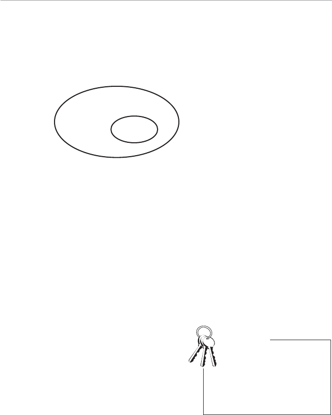
Figure 1.2 shows the relationship between a population and a sample.
The following are other examples of inferential statistics:
UBased on a recent sample, I am 95 percent certain that the average age of my
customers is between 32 and 35 years old.
UThe average salary for male employees in a particular job category across the
country was higher than the female employees’ salary, based on a random survey.
In each case, the findings were based on a sample from a larger population and were
used to make an inference on that entire population.
The basic difference between descriptive and inferential statistics is that descriptive
statistics reports only on the observations at hand and nothing more. Inferential statis-
tics makes a statement about a population based solely on results from a sample taken
from that population.
I must tell you at this point that inferen-
tial statistics is the area of this field that
students find the most challenging. To be
able to make statements based on samples,
you need to use mathematical models that
involve probability theory. Now don’t panic.
Take a deep breath and count to 10 slowly.
That’s better. I realize that this is often the
stumbling block for many, so I have devoted
plenty of pages to that nasty “p” word.
4WUc`S
The relationship between a
population and a sample.
Population
Sample
A good understanding of
probability concepts is an
essential stepping-stone for
properly digesting statistics.
Part 2 of this book covers prob-
ability.
Bob’s Basics
>O`b( BVS0OaWQa
3bVWQaO\RAbObWabWQa¾7bÂaO2O\US`]caE]`ZR=cbBVS`S
People often use statistics when attempting to persuade you to their point of view.
Because they are motivated to convince you to purchase something from them or sim-
ply to support them, this motivation can lead to the misuse of statistics in several ways.
One of the most common misuses is choosing a sample that ensures results consistent
with the desired outcome, rather than choosing a sample representative of the popula-
tion of interest. This is known as having a biased sample.
Suppose, for instance, that I’m an upstanding politi-
cian whose only concern is the best interest of my
constituents and I want to propose that Congress
establish a national golf holiday. During this honored
day, all government and business offices would be
closed so that we could all run out to chase a little
white ball into a hole that’s way too small, with sticks
purposely designed by the evil golf companies to
make this task impossible. Sounds like fun to me!
Somehow, I would need to demonstrate that the aver-
age level-headed American is in favor of this. Here is
where the genius part of my plan lies: rather than survey the general American public,
I pass out my survey form only at golf courses. But wait … it only gets better. I design
the survey to look like the following:
We would like to propose a national golf holiday, on which everybody gets the
day off from work and plays golf all day. (This means you would not need per-
mission from your spouse.) Are you in favor of this proposal?
A. Yes, most definitely.
B. Sure, why not?
C. No, I would rather spend the entire day at work.
P.S. If you choose C, we will permanently revoke all your golfing privileges
everywhere in the country for the rest of your life. We are dead serious.
I can now honestly report back to Congress that the respondents of my survey were
overwhelmingly in favor of this new holiday. And from what we know about Congress,
they’d probably believe me.
Abiased sample is a sample
that does not represent the
intended population and can
lead to distorted findings.
Biased sampling can occur
either intentionally or uninten-
tionally.
1VO^bS`( :SbÂa5SbAbO`bSR
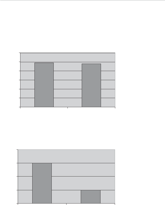
Another way to misuse statistics is to make differences seem greater than they actually
are by graphically presenting the data in a deceptive manner. Now that I have golf on
my brain, let me use my golf scores to demonstrate this point. Let’s say, hypotheti-
cally speaking of course, that my average golf score during the month of May was 98.
After taking some lessons in June, my average score in July dropped to 96. (For you
nongolfers, lower is better.) The graph in Figure 1.3 shows that this improvement was
nothing to write home about.
0
20
40
60
80
100
120
May July
Month
Average Golf Score
95
96
97
98
99
May July
Month
Average Golf Score
However, to avoid feeling like I wasted my money on lessons, I can present the differ-
ence between May and July on a different scale, as in Figure 1.4.
4WUc`S!
This graph shows the actual
difference between May and
July.
4WUc`S"
This graph exaggerates the
difference between May and
July.

>O`b( BVS0OaWQa
By changing the scale of the graph, it appears that I really made progress on my golf
game—when in reality, little progress was made. Oh well, back to the drawing board.
Many of the polls we see on the Internet represent another potential misuse of statis-
tics. Many websites encourage visitors to vote on a question of the day. The results of
these informal polls are unreliable simply because those collecting the data have no
control over who responds or how many times they respond. As stated earlier, a valid
statistical study depends on selecting a sample representative from the population of
interest. This is not possible when any person surfing the Internet can participate in
the poll. Even though most of these polls state that the results are not scientific, it’s
still a natural human tendency to be influenced by the results we see.
The lesson here is that we are all consumers of statistics. We are constantly sur-
rounded by information provided by someone who is trying to influence us or gain
our support. By having a basic understanding about the field of statistics, we increase
the likelihood that we can ward off those evil spirits in their attempts to distort the
truth. In Chapter 2, we’ll begin our journey to achieve this goal … oh, and to help
you pass your statistics course.
G]c`Bc`\
Identify each of the following statistics as either descriptive or inferential.
1. Seventy-three percent of Asian American households in the United States own a
computer.
2. Households with children under the age of 18 are more likely to have access to
the Internet (62 percent) than family households with no children (53 percent).
3. Hank Aaron hit 755 career home runs.
4. The average SAT score for incoming freshman at a local college was 950.
5. On a recent poll, 67 percent of Americans had a favorable opinion of the
President of the United States.
You can find additional sample problems on my website: www.stat-guide.com.

1VO^bS`( :SbÂa5SbAbO`bSR !
BVS:SOabG]c<SSRb]9\]e
UStatistics is a vital tool that provides organizations with the necessary informa-
tion to make good decisions.
UThe field of statistics evolved from the early work of European mathematicians
during the seventeenth century.
UDescriptive statistics focuses on the summary or display of data so we can quickly
obtain an overview.
UInferential statistics allows us to make claims or conclusions about a population
based on a sample of data from that population.
UWe are all consumers of statistics and need to be aware of the potential misuses
that can occur in this field.

2
1VO^bS`
2ObO2ObO3dS`geVS`SO\R
<]bO2`]^b]2`W\Y
7\BVWa1VO^bS`
UThe difference between data and information
UWhere does data come from?
UWhat kinds of data can we use?
UDifferent ways of measuring data
USetting up Excel for statistical analysis
Data is the basic foundation for the field of statistics. The validity of any
statistical study hinges on the validity of the data from the beginning of the
process. Many things can come into question, such as the accuracy of the
data or the source of the data. Without the proper foundation, your efforts
to provide a sound analysis will come tumbling down.
The issues surrounding data can be surprisingly complex. After all, aren’t
we just talking about numbers here? What could go wrong? Well, plenty
can. Because data can be classified in several ways, we need to recognize the
difference between quantitative and qualitative data and how each is used.

>O`b( BVS0OaWQa$
Data also can be measured in many ways. The data measurement choice we make at
the start of the study will determine what kind of statistical techniques we can apply.
BVS7[^]`bO\QS]T2ObO
Data is simply defined as the value assigned to a specific observation or measurement.
If I’m collecting data on my wife’s snoring behavior, I can do so in different ways. I
can measure how many times Debbie snores over a 10-minute period. I can measure
the length of each snore in seconds. I could also measure how loud each snore is with
a descriptive phrase, like “That one sounded like a bear just waking up from hiberna-
tion” or “Wow! That one sounded like an Alaskan seal calling for its young.” (How a
sound like that can come from a person who can fit into a pair of size 2 jeans and still
be able to breathe I’ll never know.)
In each case, I’m recording data on the same event in a different form. In the first
case, I’m measuring a frequency or number of occurrences. In the second instance,
I’m measuring duration or length in time. And the final attempt measures the event by
describing volume using words rather than numbers. Each of these cases just shows a
different way to use data.
If you haven’t noticed yet, statistics people like to use all sorts of jargon, and here are a
couple more terms. Data that is used to describe something of interest about a popula-
tion is called a parameter. However, if the data is describing a sample from that popula-
tion, we refer to it as a statistic. For instance, let’s say that the population of interest is
my wife’s three-year-old preschool class and my measurement of interest is how many
times the little urchins use the bathroom in a day (according to Debbie, much more
than should be physically possible).
If we average the number of trips per child, this figure would be considered a parame-
ter because the entire population was measured. However, if we want to make a state-
ment about the average number of bathroom trips per day per three-year-old in the
country, then Debbie’s class could be our sample. We can consider the average that we
observe from her class a statistic if we assume it could be used to estimate all three-
year-olds in the country.
Data is the building blocks of all statistical studies. You can hire the most expensive,
well-known statisticians and provide them with the latest computer hardware and
software available, but if the data you provide them is inaccurate or not relevant to the
study, the final results will be worthless.

1VO^bS` ( 2ObO2ObO3dS`geVS`SO\R<]bO2`]^b]2`W\Y %
However, data all by its lonesome is not all that useful. By definition, data is just the
raw facts and figures that pertain to a measurement of interest. Information, on the
other hand, is derived from the facts for the purpose of making decisions. One of the
major reasons to use statistics is to transform data into information. For example, the
table that follows shows monthly sales data for a small retail store.
Data is the value assigned to an observation or a measurement and is the building
blocks to statistical analysis. The plural form is data and the singular form is datum,
referring to an individual observation or measurement.
Data that describes a characteristic about a population is known as a param-
eter. Data that describes a characteristic about a sample is known as a statistic.
Information is data that is transformed into useful facts that can be used for a specific
purpose, such as making a decision.
;]\bVZgAOZSa2ObO
Month Sales ($)
January 15,178
February 14,293
March 13,492
April 12,287
May 11,321
Using statistical analysis, we can generate information that may be of interest, such
as “Wake up! You are doing something very wrong. At this rate, you will be out of
business by early next year.” Based on this valuable information, we can make some
important decisions about how to avoid this impending disaster.
BVSA]c`QSa]T2ObO¾EVS`S2]Sa/ZZBVWaAbcTT1][S
4`][-
We classify the sources of data into two broad categories: primary and secondary.
Secondary data is data that somebody else has collected and made available for others
to use. The U.S. government loves to collect and publish all sorts of interesting data,
just in case anyone should need it. The Department of Commerce handles census
>O`b( BVS0OaWQa&
data, and the Department of Labor collects mountains of, you guessed it, labor statis-
tics. The Department of the Interior provides all sorts of data about U.S. resources.
For instance, did you know there are 250 species of squirrels in this country? If you
don’t believe me, go to www.npwrc.usgs.gov/resource/distr/mammals/mammals/
_squirrel.htm and you can become the local “squirrel” expert.
The Canadian government has a great system for
providing statistical data to the public. Rather than
each department in the government being responsible
for collecting and disbursing data as in the United
States, Canada has a national statistical agency known
as Statistics Canada (www.statcan.ca/start.html). It’s
like one-stop shopping for the statistician. It’s a won-
derful website that makes research of Canadian facts
a pleasure.
The main drawback of using secondary data is that you have no control over how the
data was collected. It’s a natural human tendency to believe anything that’s in print
(you believe me, don’t you?), and sometimes that requires a leap of faith. The advan-
tage to secondary data is that it’s cheap (sometimes free) and it’s available now. That’s
called instant gratification.
Primary data, on the other hand, is data collected by the person who eventually uses
this data. It can be expensive to acquire, but the main advantage is that it’s your data
and you have nobody else to blame but yourself if you make a mess of it.
When collecting primary data, you want to ensure that the results will not be biased
by the manner in which it is collected. You can obtain primary data in many ways,
such as direct observation, surveys, and experiments.
Primary data is data that you
have collected for your own
use. Secondary data is data
collected by someone else that
you are “borrowing.”
The Internet has also become a rich source of data for statistics published by vari-
ous industries. If you can muddle your way through the 63,278 sites that come back
from the typical Internet search engine, you might find something useful. I once found
a Japanese study on the effect of fluoride on toad embryos (www.fluoride-journal.
com/_1971.htm). Before this discovery, I was completely oblivious to the fact that
toads even had teeth, much less a cavity problem. I can’t wait to impress my friends at
the next neighborhood dinner party.
Random Thoughts

1VO^bS` ( 2ObO2ObO3dS`geVS`SO\R<]bO2`]^b]2`W\Y '
2W`SQb=PaS`dObW]\¾7ÂZZ0SEObQVW\UG]c
Most often, this method focuses on gathering data while the subjects of interest are
in their natural environment, oblivious to what is going on around them. Examples of
these studies would be observing wild animals stalking their prey in the forest or teen-
agers at the mall on Friday night (or is that the same example?). The advantage of this
method is that the subjects will unlikely be influenced by the data collection.
Focus groups are a direct observational technique where the subjects are aware that
data is being collected. Businesses use focus groups to gather information in a group
setting controlled by a moderator. The subjects are usually paid for their time and are
asked to comment on specific topics.
3f^S`W[S\ba¾EV]ÂaW\1]\b`]Z-
This method is more direct than observation because the subjects will participate in
an experiment designed to determine the effectiveness of a treatment. An example of
a treatment could be the use of a new medical drug. Two groups would be established.
The first is the experimental group who receive the new drug, and the second is the
control group who think they are getting the new drug but are in fact getting no
medication. The reactions from each group are measured and compared to determine
whether the new drug was effective.
The claims that the experimental studies are attempting to verify need to be clear
and specific. I just recently read about an herb called ginkgo biloba. According to this
article, people who make money selling funny-sounding herbs claim ginkgo biloba will
keep your mind sharp as you age. Sounds like something everyone would want. Now
let’s see, where was I? As stated, this claim might prove difficult to verify. How do you
define “keeping your mind sharp”? And then, how do you measure sharpness of mind?
These are some of the challenges that statistical experiments face.
The benefit of experiments is that they allow the statistician to control factors that
could influence the results, such as gender, age, and education of the participants. The
concern about collecting data through experiments is that the response of the subjects
might be influenced by the fact that they are participating in a study. The design of
experiments for a statistical study is a very complex topic and goes beyond the scope
of this book.
>O`b( BVS0OaWQa
Ac`dSga¾7aBVObG]c`4W\OZ/\aeS`-
This technique of data collection involves directly asking the subject a series of ques-
tions. The questionnaire needs to be carefully designed to avoid any bias (see Chapter
1) or confusion for those participating. Concerns also exist about the influence the
survey will have on the participant’s responses. Some participants respond in a way
they feel the survey would like them to. This is very similar to the manner in which
hostages bond with their captors. The survey can be administered by e-mail, snail-
mail, or telephone. It’s the telephone survey that I’m most fond of, especially when I
get the call just as I’m sitting down to dinner, getting into the shower, or finally mak-
ing some progress on the chapter I’m writing.
Research has shown that the manner in which the questions are asked can affect
the responses a person provides on a questionnaire. A question posed in a posi-
tive tone will tend to invoke a more positive response and vice versa. A good
strategy is to test your questionnaire with a small group of people before releasing it to
the general public.
Bob’s Basics
Whatever method you employ, your primary concern should always be that the sam-
ple is representative of the population in which you are interested.
Bg^Sa]T2ObO
Another way to classify data is by one of two types: quantitative or qualitative.
UQuantitative data uses numerical values to describe something of interest. An
example is Debbie’s age, which I have been forced by a legally bound document
to never, never, never reveal anywhere in this book, not even if it’s buried in an
appendix as an answer to an obscure question. (Hint: See page 167.)
UQualitative data uses descriptive terms to measure or classify something of inter-
est. One example of qualitative data is the name of a respondent in a survey and
his or her level of education. The next section covers qualitative data in more
detail.

1VO^bS` ( 2ObO2ObO3dS`geVS`SO\R<]bO2`]^b]2`W\Y
Bg^Sa]T;SOac`S[S\bAQOZSa¾OESWUVbgB]^WQ
Who would have thought of so many ways to look at data? The final way to classify
data is by the way it is measured. This distinction is critical because it affects which
statistical techniques we can use in our analysis of the data. Measurement classification
can be made in several levels.
<][W\OZ:SdSZ]T;SOac`S[S\b
Anominal level of measurement deals strictly with qualitative data. Observations are
simply assigned to predetermined categories. One example is gender of the respon-
dent, with the categories being male and female. Another example is data indicating
the type of dog, if any, owned by families in a neighborhood. The categories for this
data are the various dog types (black Lab, terrier, stupid mangy mutt that keeps me
awake by barking all night at the moon). This data type does not allow us to perform
any mathematical operations, such as adding or multiplying. We also cannot rank-
order this list in any way from highest to lowest (although I would put black Lab at
the top). This type is considered the lowest level of data and, as a result, is the most
restrictive when choosing a statistical technique to use for the analysis.
You can use numbers at the nominal level of measurement. Even in this case, the
rules of the nominal scale still remain. An example would be zip codes or telephone
numbers, which can’t be added or placed in a meaningful order of greater than or less
than. Even though the data appears to be numbers, it’s handled just like qualitative
data.
=`RW\OZ:SdSZ]T;SOac`S[S\b
On the food chain of data, ordinal is the next level up. It has all the properties of
nominal data with the added feature that we can rank-order the values from highest
to lowest. An example is if you were to have a lawnmower race. Let’s say the finishing
order was Scott, Tom, and Bob. We still can’t perform mathematical operations on
this data, but we can say that Scott’s lawnmower was faster than Bob’s. However, we
cannot say how much faster. Ordinal data does not allow us to make measurements
between the categories and to say, for instance, that Scott’s lawnmower is twice as
good as Bob’s (it’s not).
Ordinal data can be either qualitative or quantitative. An example of quantitative data
is rating movies with 1, 2, 3, or 4 stars. However, we still may not claim that a 4-star
movie is 4 times as good as a 1-star movie.
>O`b( BVS0OaWQa
7\bS`dOZ:SdSZ]T;SOac`S[S\b
Moving up the scale of data, we find ourselves at the interval level, which is strictly
quantitative data. Now we can get to work with the mathematical operations of
addition and subtraction when comparing values. For this data, we can measure the
difference between the different categories with actual numbers and also provide
meaningful information. Temperature measurement in degrees Fahrenheit is a com-
mon example here. For instance, 70 degrees is 5 degrees warmer than 65 degrees.
However, multiplication and division can’t be performed on this data. Why not?
Simply because we cannot argue that 100 degrees is twice as warm as 50 degrees.
@ObW]:SdSZ]T;SOac`S[S\b
The king of data types is the ratio level. This is as good as it gets as far as data is con-
cerned. Now we can perform all four mathematical operations to compare values with
absolutely no feelings of guilt. Examples of this type of data are age, weight, height,
and salary. Ratio data has all the features of interval data with the added benefit of
a true 0 point. The term “true zero point” means that a 0 data value indicates the
absence of the object being measured. For instance, 0 salary indicates the absence of
any salary.
With a true 0 point, we can use the rules of multi-
plication and division to compare data values. This
allows us to say that a person who is 6 feet in height
is twice as tall as a 3-foot person or that a 20-year-
old person is half the age of a 40 year old.
The distinction between interval and ratio data is a
fine line. To help identify the proper scale, use the
“twice as much” rule. If the phrase “twice as much”
accurately describes the relationship between two
values that differ by a multiple of 2, then the data can
be considered ratio level.
There are endless examples of ratio data. Let’s look
at measuring typing speed in words per minute. I
happen to be a handicapped, two-finger, hunt-and-peck typist who has tried those
darned typing programs more than once and just can’t get it. I can type maybe 20
words a minute on a good day. My 15-year-old son, John, on the other hand, is one of
those show-offs who types while he’s not even looking and can still type 60 words a min-
ute. Because we can correctly say that John types three times faster than me, typing
speed is an example of ratio data.
Interval data does not
have a true 0 point. For
example, 0 degrees Fahrenheit
does not represent the absence
of temperature, even though it
may feel like it. To help explain
this, try baking a cake at twice
the recommended temperature
in half the recommended time.
Yuck!
Wrong Number

1VO^bS` ( 2ObO2ObO3dS`geVS`SO\R<]bO2`]^b]2`W\Y !
Figure 2.1 summarizes the different data scales and how they relate to one another. As
we explore different statistical techniques later in this book, we will revisit these dif-
ferent measurement scales. You will discover that specific techniques require certain
types of data.
4WUc`S
Summary of data measure-
ment scales.
Types of Data
Qualitative
Nominal Ordinal
Quantitative
Interval Ratio
1][^cbS`ab]bVS@SaQcS
As mentioned in Chapter 1, we will explore the use of Excel in solving some of the
statistics problems in this book. If you have no interest in using Excel in this man-
ner, just skip this section. I promise you won’t hurt my feelings. The purpose of this
last section is to talk about the use of computers with statistics in general and then to
make sure your computer is ready to follow us along.
BVS@]ZS]T1][^cbS`aW\AbObWabWQa
When I was a youthful engineering undergraduate student during the 1970s, the
words “personal computer” had no meaning. I performed calculations on a clever gad-
get fondly known as a “slide rule.” For those of you who weren’t even alive during this
time period, I’ve included a picture of one in Figure 2.2.
4WUc`S
Slide rule circa 1975.
(Courtesy of www.hpmuseum.org)
As you can see, this device looks like a ruler on steroids. It can perform all sorts of
mathematical calculations but is far from being user friendly. During my freshman
year in college, I purchased my first handheld calculator, a Texas Instrument model
that could only perform the basic math functions. It was the approximate size of a cash
register.

>O`b( BVS0OaWQa "
At this point, the only serious statistical analysis was being performed on mainframe
computers by people with high levels of programming skill. These people were
somewhat “different” from the rest of us. Fortunately, we have advanced from the
Dark Ages and now have awesome, user-friendly computing power at our fingertips.
Powerful programs such as SAS, SPSS, Minitab, and Excel are readily accessible to
those of us who don’t know a lick of computer programming and allow us to perform
some of the most sophisticated statistical analysis known to humankind.
Parts of this book will demonstrate how to solve some of the statistical techniques
using Microsoft Excel. Choosing to skip these parts will not interfere with your grasp
of topics in subsequent chapters. This is simply optional material to expose you to
statistical analysis on the computer. I also assume you already have a basic working
knowledge of how to use Excel.
7\abOZZW\UbVS2ObO/\OZgaWa/RR7\
Our first task is to check whether Excel’s data analysis tools are available on your com-
puter. Open the Excel program and left-click with your mouse on the Tools menu as
shown in Figure 2.3. From this point on in the book, I’ll use the term “click” to mean
click the left button on your mouse.
4WUc`S !
Excel’s Tools menu.
Notice in the figure that the highlighted item is Data Analysis, which may or may
not show up under your Tools menu. If Data Analysis does appear under your Tools
menu, skip the rest of this paragraph and the next two and proceed to the following
paragraph that begins with “Click on Data Analysis …”
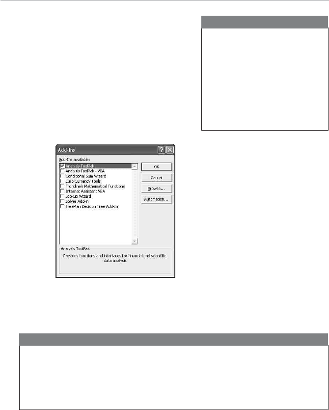
1VO^bS` ( 2ObO2ObO3dS`geVS`SO\R<]bO2`]^b]2`W\Y #
If Data Analysis does not appear under the
Tools menu, you need to add it to the menu. To
do so, click on Add-Ins under the same Tools
menu. If you don’t see Add-Ins under this menu
at first, expand the menu items by clicking on
the downward arrow at the bottom of the Tools
menu list. After clicking on Add-Ins, you should
see the dialog box in Figure 2.4.
If your Tools menu looks differ-
ent from the one in Figure 2.3,
it might be because all of your
available menu items are not
currently visible. To make all the
menu items visible, click on the
Expand symbol at the bottom of
the list (the double-downward-
pointing arrows).
Random Thoughts
4WUc`S "
Excel’s Add-Ins dialog box.
This dialog box provides a list of available add-ins for you to use. Click on the empty
box for Analysis ToolPak, which places a check mark in it, and then click OK. Now
click on the Tools menu again; Data Analysis will now appear in the list.
Don’t panic if you receive the following message: “Microsoft Excel can’t run this add-
in. This feature is not currently installed. Would you like to install it now?” If you want
to install the Analysis ToolPak, you might need to have your original Microsoft Office
CD close by. Click the Yes button and follow any further instructions. Then, the Data
Analysis option will become available on the Tools menu.
Random Thoughts

>O`b( BVS0OaWQa $
Click on Data Analysis under the Tools menu to open the dialog box shown in
Figure 2.5.
4WUc`S #
Excel’s Data Analysis dialog
box.
Your Excel program is now ready to perform all sorts of statistical magic for you as we
explore various techniques throughout this book. At this point, you can click Cancel
and close out Excel. Each time you open Excel in the future, the Data Analysis option
will be available under the Tools menu.
G]c`Bc`\
Classify the following data as nominal, ordinal, interval, or ratio. Explain your choice.
1. Average monthly temperature in degrees Fahrenheit for the city of Wilmington
throughout the year
2. Average monthly rainfall in inches for the city of Wilmington throughout the
year
3. Education level of survey respondents
Level Number of Respondents
High school 168
Bachelor’s degree 784
Master’s degree 212
4. Marital status of survey respondents
Status Number of Respondents
Single 28
Married 189
Divorced 62
5. Age of the respondents in the survey
6. Gender of the respondents in the survey

1VO^bS` ( 2ObO2ObO3dS`geVS`SO\R<]bO2`]^b]2`W\Y %
7. The year in which the respondent was born
8. The voting intentions of the respondents in the survey classified as Republican,
Democrat, or Undecided
9. The race of the respondents in the survey classified as White, African American,
Asian, or Other
10. Performance rating of employees classified as Above Expectations, Meets
Expectations, or Below Expectations
11. The uniform number of each member on a sports team
12. A list of the graduating high school seniors by class rank
13. Final exam scores for my statistics class on a scale of 0 to 100
14. The state in which the respondents in a survey reside
BVS:SOabG]c<SSRb]9\]e
UData serves as the building blocks for all statistical analysis.
UWe classify data as either quantitative or qualitative.
UNominal data is assigned to categories with no mathematical comparisons
between observations.
UOrdinal data has all the properties of nominal data with the additional capability
of arranging the observations in order.
UInterval data has all the properties of ordinal data with the additional capability
of calculating meaningful differences between the observations.
URatio data has all the properties of interval data with the additional capability of
expressing one observation as a multiple of another.

3
1VO^bS`
2Wa^ZOgW\U2SaQ`W^bWdS
AbObWabWQa
7\BVWa1VO^bS`
UHow to construct a frequency distribution
UHow to graph a frequency distribution with a histogram
UHow to construct a stem and leaf display
UThe usefulness of pie, bar, and line charts
UUsing Excel’s Chart Wizard to construct charts
Having explained the various types of data that exist for statistical analysis
in Chapter 2, here we will explore the different ways in which we can pres-
ent data. In its basic form, making sense of the patterns in the data can be
very difficult because our human brains are not very efficient at processing
long lists of raw numbers. We do a much better job of absorbing data when
it is presented in summarized form through tables and graphs.
In the next several sections, we will examine many ways to present data so
that it will be more useful to the person performing the analysis. Through
these techniques, we are able to get a better overview of what the data is
telling us. And believe me, there is plenty of data out there with some very
interesting stories to tell. Stay tuned.
>O`b( BVS0OaWQa!
4`S_cS\Qg2Wab`WPcbW]\a
One of the most common ways to graphically describe data is through the use of fre-
quency distributions. The best way to describe a frequency distribution is to start with
an example.
Ever since I was a young boy, I have been a devoted
fan of the Pittsburgh Pirates Major League Baseball
team. Why I still root for these guys, I’ll never know,
because they have not had a winning season since
1992. Anyway, below is a table of the batting averages
of individual Pirates at the end of the 2005 season. I
have not attached names with these averages in order
to protect their identities.
Pittsburgh Pirates Final Batting Averages for the 2005 Season
.306 .257 .272 .291 .260 .273 .268 .251 .242
.255 .264 .221 .258 .341 .257 .222 .269 .241
.158 .113 .106 .119 .182 .143 .143 .192 .261
Source: www.espn.com
It is difficult to grasp what a tough year these guys had by just looking at this data in
this table format. Transforming this data into the frequency distribution shown here
makes this fact more obvious.
Batting Average Number of Players
.000 to .049 0
.050 to .099 0
.100 to .149 5
.150 to .199 3
.200 to .249 4
.250 to .299 13
.300 to .349 2
As you can see, a frequency distribution is simply a table that organizes the number of
data values into intervals. In this example, the intervals are the batting average ranges
in the first column of the table. The number of data values is the number of players
Afrequency distribution is a
table that shows the number of
data observations that fall into
specific intervals.

1VO^bS`!( 2Wa^ZOgW\U2SaQ`W^bWdSAbObWabWQa !
who fall into each interval shown in the second column. Well, there’s always next sea-
son to look forward to.
The intervals in a frequency distribution are officially known as classes, and the num-
ber of observations in each class is known as class frequencies. Now let’s learn how to
arrange these classes.
1]\ab`cQbW\UO4`S_cS\Qg2Wab`WPcbW]\
You need to make some important decisions when constructing a frequency distribu-
tion. To illustrate these decisions, let’s use another example, something many of us can
relate to—cell phones! My son John and I are on one of those “family share plans,”
which means he gets all the peak minutes and I get to use my phone between the
hours of 3 A.M. and 6 A.M. every other Saturday. The following table represents the
number of calls each day during the month of May on John’s account.
Calls per Day
312 1 1
391 4 2
6 4 9 13 15
255 2 7
301 2 7
186 9 4
Source: A very confusing phone bill that requires a Ph.D. in metaphysical telecommunications to understand.
Using this data, I have constructed the following frequency distribution.
4`S_cS\Qg2Wab`WPcbW]\
Calls per Day Number of Days
0–2 12
3–5 8
6–8 5
9–11 3
12–14 1
15–17 1
>O`b( BVS0OaWQa!
When arranging these classes, I followed these rules:
1. From classes of equal size. I chose 3 data values to be in each class for this dis-
tribution. An example of a class is 0–2, which includes the number of days when
John made 0, 1, or 2 calls.
2. Make classes mutually exclusive, or in other words, prevent classes from overlap-
ping. For instance, I wouldn’t want 2 classes to be 3–5 and 5–7 because 5 calls
would be in 2 different classes.
3. Try to have no fewer than 5 classes and no more than 15 classes. Too few or too
many classes tend to hide the true characteristics of the frequency distribution.
4. Avoid open-ended classes, if possible (for instance, a highest class of 15–over).
5. Include all data values from the original table
in a class. In other words, the classes should be
exhaustive.
Too few or too many classes will obscure patterns in
a frequency distribution. Consider the extreme case
where there are so many classes that no class has
more than one observation. The other extreme is
where there is only one class with all the observations
residing in that class. This would be a pretty useless
frequency distribution!
/2WabO\b@SZObWdS4`S_cS\Qg2Wab`WPcbW]\
Another way to display frequency data is by using the relative frequency distribution.
Rather than display the number of observations in each class, this method calculates
the percentage of observations in each class by dividing the frequency of each class by
the total number of observations. I can display John’s data as a relative frequency dis-
tribution, as I do in the following table.
Classes are considered mutu-
ally exclusive when observa-
tions can only fall into one
class. For example, the gender
classes “male” and “female”
are mutually exclusive because
a person cannot belong to both
classes.
Relative frequency distributions display the percentage of observations of each class
relative to the total number of observations.
1VO^bS`!( 2Wa^ZOgW\U2SaQ`W^bWdSAbObWabWQa !!
@SZObWdS4`S_cS\Qg2Wab`WPcbW]\
Calls per Day Number of Days Percentage
0–2 12 12/30 = 0.40
3–5 8 8/30 = 0.27
6–8 5 5/30 = 0.17
9–11 3 3/30 = 0.10
12–14 1 1/30 = 0.03
15–17 1 1/30 = 0.03
Total = 30 Total = 1.00
According to this distribution, John uses his phone 3 to 5 times 27 percent of the days
during a month.
The total percentage in a relative frequency distribution should be 100 percent or very
close (within 1 percent, because of rounding errors).
1c[cZObWdS4`S_cS\Qg2Wab`WPcbW]\
This “kissing cousin” of the relative frequency
distribution simply totals the percentages of
each class as you move down the column. (Get
it? Cousin, relative? Sorry, I couldn’t help
myself!) This provides you with the percentage
of observations that are less than or equal to
the class of interest. The resulting cumulative
frequency distribution is shown here.
1c[cZObWdS4`S_cS\Qg2Wab`WPcbW]\
Calls per Day No. of Days Percentage Cumulative Percentage
0–2 12 12/30 = 0.40 0.40
3–5 8 8/30 = 0.27 0.67
6–8 5 5/30 = 0.17 0.84
9–11 3 3/30 = 0.10 0.94
12–14 1 1/30 = 0.03 0.97
15–17 1 1/30 = 0.03 1.00
Total = 30 Total = 1.00
Cumulative frequency distribu-
tions indicate the percentage of
observations that are less than
or equal to the current class.
>O`b( BVS0OaWQa!"
The value 0.67 in the fourth column is the result of adding 0.40 to 0.27. According to
this table, John used his phone 8 times or less on 84 percent of the days in the month.
If designed properly, frequency distribution is an excellent way to tease good informa-
tion out of stubborn data. Now, let’s deal with how to display the distribution graphi-
cally.
5`O^VW\UO4`S_cS\Qg2Wab`WPcbW]\¾bVS6Wab]U`O[
Ahistogram is simply a bar graph showing the number of observations in each class as
the height of each bar. Figure 3.1 shows the histogram for John’s phone calls.
4WUc`S!
A histogram of John’s phone
calls.
0
2
4
6
8
10
12
14
0-2 3-5 6-8 9-11 12-14 15-17
Calls per Day
Number of Observations
:SbbW\U3fQSZ2]=c`2W`bgE]`Y
Excel will actually construct a frequency distribution for us and plot the histogram.
How nice!
1. The first thing we need to do is open Excel to a blank sheet and enter our data
in Column A starting in Cell A1 (use the data from the earlier table).
Ahistogram is a bar graph showing the number of observations in each class as the
height of each bar.
This graph gives us a good visual of John’s calling habits. At least the highest class on
the graph is the 0 to 2 calls per day. Things could be worse.
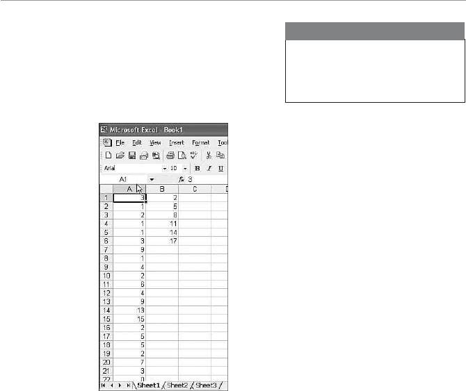
1VO^bS`!( 2Wa^ZOgW\U2SaQ`W^bWdSAbObWabWQa !#
2. Next enter the upper limits to each class
in Column B starting in Cell B1. For
example, in the class 0–2, the upper limit
would be 2. Figure 3.2 shows what the
spreadsheet should look like.
For some bizarre reason, Excel
refers to classes as bins. Go
figure.
Random Thoughts
3. Go to the Tools menu at the top of the Excel window and select Data Analysis.
(Refer to the section “Installing the Data Analysis Add-in” from Chapter 2 if you
don’t see the Data Analysis command on the Tools menu.)
4. Select the Histogram option from the list of Analysis Tools (see Figure 3.3) and
click the OK button.
4WUc`S!
Raw data for the frequency
distribution.
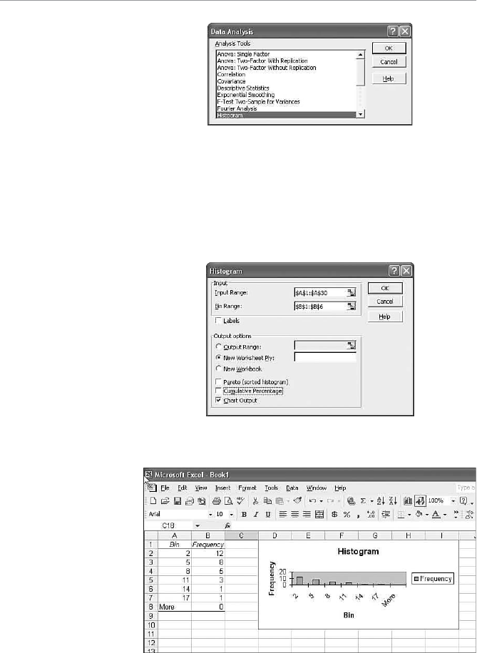
>O`b( BVS0OaWQa!$
5. In the Histogram dialog box (as shown in Figure 3.4), click in the Input Range
list box, and then click in the worksheet to select cells A1 through A30 (the 30
original data values). Then, click in the Bin Range list box and click in the work-
sheet to select cells B1 through B6 (the upper limits for the 6 classes).
6. Click the New Worksheet Ply option button and the Chart Output check box
(see Figure 3.4).
4WUc`S!!
Data Analysis dialog box.
4WUc`S!"
Histogram dialog box.
7. Click OK to generate the frequency distribution and histogram (see Figure 3.5).
4WUc`S!#
Frequency distribution and
histogram.
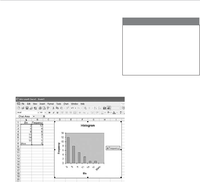
1VO^bS`!( 2Wa^ZOgW\U2SaQ`W^bWdSAbObWabWQa !%
Notice that Excel has generated the frequency
distribution for us in columns A and B. Cool!
The problem here is that the histogram looks
like an elephant sat on it. Click on the chart to
select it, and then click on the bottom border
to drag the bottom of the chart down lower,
expanding the histogram to look like Figure 3.6.
Frequency distributions and histograms are
convenient ways to get an accurate picture of
what your data is trying to tell you. It sounds
like my data is telling me to “get more monthly
minutes on your cell phone plan.” Wonderful.
I prefer using Chart Wizard to
display the histogram because I
think the graph looks better than
when I use the Data Analysis
tool. The Chart Wizard allows
me more control over the final
appearance.
Random Thoughts
4WUc`S!$
Final histogram.
AbObWabWQOZ4Z]eS`>]eS`¾bVSAbS[O\R:SOT2Wa^ZOg
The stem and leaf display is another graphical technique you can use to display your
data. A statistician named John Tukey originated the idea during the 1970s. The major
benefit of this approach is that all the original data points are visible on the display.
To demonstrate this method, I will use my son Brian’s golf scores for his last 24
rounds, shown in the following table. Normally, Brian would only report his better
scores, but we statisticians must be unbiased and accurate.
>O`b( BVS0OaWQa!&
Brian’s Golf Scores
81 86 78 80 81 82 92 90
79 83 84 95 85 88 80 78
84 79 80 83 79 87 84 80
Figure 3.7 shows the stem and leaf display for these scores.
4WUc`S!%
Stem and leaf display. 7
8
9
Stem and Leaf Display
88999
00001123344445678
025
The “stem” in the display is the first column of numbers, which represents the first
digit of the golf scores. The “leaf” in the display is the second digit of the golf scores,
with 1 digit for each score. Because there were 5 scores in the 70s, there are 5 digits to
the right of 7.
If we choose to, we can break this display down fur-
ther by adding more stems. Figure 3.8 shows this
approach.
Here, the stem labeled 7 (5) stores all the scores
between 75 and 79. The stem 8 (0) stores all the
scores between 80 and 84. After examining this dis-
play, I can see a pattern that’s not as obvious when
looking at Figure 3.7: Brian usually scores in the low
80s.
You can find an excellent source of information about
stem and leaf displays at the Statistics Canada website
at www.statcan.ca/english/edu/power/ch8/plots.htm.
The stem and leaf display
splits the data values into stems
(the first digit in the value) and
leaves (the remaining digits in
the value). By listing all of the
leaves to the right of each stem,
we can graphically describe
how the data is distributed.

1VO^bS`!( 2Wa^ZOgW\U2SaQ`W^bWdSAbObWabWQa !'
1VO`bW\UG]c`1]c`aS
Charts are yet another efficient way to summarize and display patterns in a set of data,
so let me demonstrate different types of charts that help us “tell it like it is.”
EVObÂaG]c`4Od]`WbS>WS1VO`b-
Pie charts are commonly used to describe data from relative frequency distributions.
This type of chart is simply a circle divided into portions whose area is equal to the
relative frequency distribution. To illustrate the use of pie charts, let’s say some anony-
mous statistics professor submitted the following final grade distribution.
4W\OZAbObWabWQa5`ORSa
Grade Number of Students Relative Frequency
A 9 9/30 = 0.30
B13 13/30 = 0.43
C 6 6/30 = 0.20
D 2 2/30 = 0.07
Total = 30 Total = 1.00
We can illustrate this relative frequency distribution by using the pie chart in Figure
3.9. This chart was done using Excel’s Chart Wizard.
4WUc`S!&
A more detailed stem and leaf
display.
7 (5)
8 (0)
8 (5)
9 (0)
9 (5)
More Detailed Stem and Leaf Display
88999
000011233444
5678
02
5
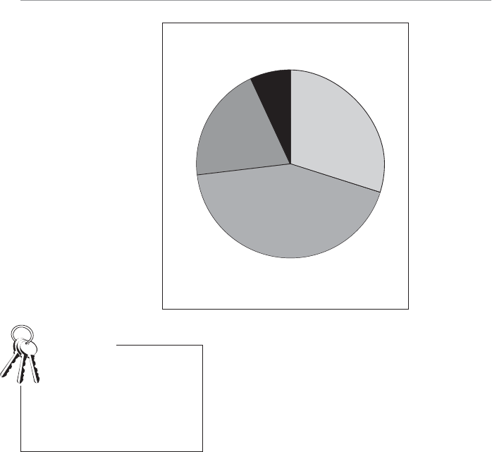
>O`b( BVS0OaWQa"
As you can see, the pie chart approach is much easier
on the eye when compared to looking at data from
a table. This person must be a pretty good statistics
teacher!
To construct a pie chart by hand, you first need to
calculate the center angle for each slice in the pie,
which is illustrated in Figure 3.10.
You determine the center angle of each slice by mul-
tiplying the relative frequency of the class by 360 (which is the number of degrees in a
circle). These results are shown in the following table.
4WUc`S!'
Pie chart illustrating a grade
distribution.
A
30%
B
43%
C
20%
D
7%
Pie charts are an excellent
way to colorfully present data
from a relative frequency
distribution. If you cannot use
colors, use patterns and textures
to display pie charts.
Bob’s Basics

1VO^bS`!( 2Wa^ZOgW\U2SaQ`W^bWdSAbObWabWQa "
1S\bS`/\UZST]`>WS1VO`b1]\ab`cQbW]\
Grade Relative Frequency Central Angle
A9/30 = 0.30 0.30 * 360 = 108 degrees
B13/30 = 0.43 0.43 * 360 = 155 degrees
C6/30 = 0.20 0.20 * 360 = 72 degrees
D2/30 = 0.07 0.07 * 360 = 25 degrees
Total = 1.00
By using a device to measure angles, such as a protractor, you can now divide your pie
chart into slices of the appropriate size. This assumes, of course, you’ve mastered the
art of drawing circles.
0O`1VO`ba
Bar charts are a useful graphical tool when you are plotting individual data values next
to each other. To demonstrate this type of chart (see Figure 3.11), we’ll use the data
from the following table, which represents the monthly credit card balances for an
unnamed spouse of an unnamed person writing a statistics book. (Boy, I’m going to be
in big trouble when she sees this.)
4WUc`S!
The center angle of a pie
chart slice.
Center
Angle
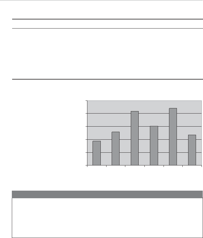
>O`b( BVS0OaWQa"
/\]\g[]ca1`SRWb1O`R0OZO\QSa
Month Balance ($)
1 375
2 514
3 834
4 603
5 882
6 468
Source: An unnamed filing cabinet.
4WUc`S!
Bar chart for somebody’s
credit card balances.
0
200
400
600
800
1000
123456
Month
Credit Card Balance ($)
By now you may have just said to yourself, “Hey, wait one minute! Haven’t I seen this
somewhere before?” By “this” I hope you’re referring to the type of chart rather than
my wife’s credit card statements. The histogram that we visited earlier in the chapter
is actually a special type of bar chart that plots frequencies rather than actual data
values.
Random Thoughts
I’m sure your inquisitive mind is now screaming with the question “How do I choose
between a pie chart and a bar chart?” If your objective is to compare the relative size
of each class to one another, use a pie chart. Bar charts are more useful when you want
to highlight the actual data values.
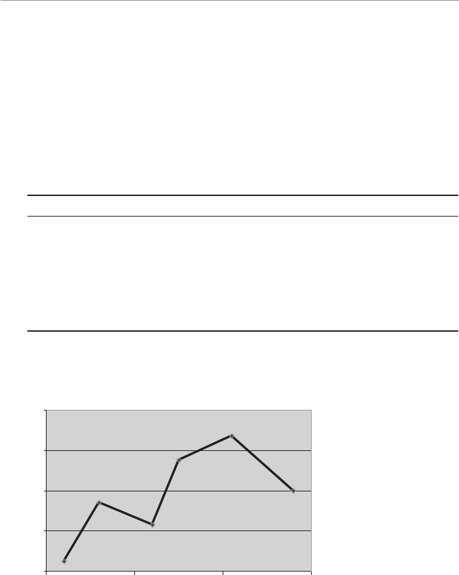
1VO^bS`!( 2Wa^ZOgW\U2SaQ`W^bWdSAbObWabWQa "!
:W\S1VO`ba
The last graphical tool discussed here is a line chart (sometimes called a line graph),
which is used to help identify patterns between two sets of data. To illustrate the use
of line charts, we’ll use a favorite topic of mine: teenagers and showers.
Our current resident teenagers seem to have a costly compulsion to take very long, very
hot showers, and sometimes more than once a day. As I lie awake at night listening to
the constant stream of hot water, all I can envision are dollar bills flowing down the
drain. So I have tabulated some data, which shows the number of showers the cleanest
kids on the block have taken in each of the recent months with the corresponding util-
ity bill. Notice that at these rates we average more than one shower per day.
Month Number of Showers Utility Bill
1 72 $225
2 91 $287
3 98 $260
4 82 $243
5 76 $254
6 85 $275
To see whether there is any pattern between the number of showers and the utility
bill, we can plot the pairs of data for each month on a line chart, which is shown in
Figure 3.12.
220
240
260
280
300
70 80 90 100
Number of Showers
Monthly Utility Bill ($)
4WUc`S!
A line chart for the number
of showers and the utility bill.

>O`b( BVS0OaWQa""
I have chosen to place the number of showers on the x-axis (horizontal) of the chart
and the utility bills on the y-axis (vertical) of the chart. Because the line connecting
the data points seems to have an overall upward trend, my suspicions hold true. It
seems the more showers our waterlogged darlings take, the higher the utility bill.
Line charts prove very useful when you are interested in exploring patterns between
two different types of data. They are also helpful when you have many data points and
want to show all of them on one graph.
Now that you have mastered the art of displaying descriptive statistics, you are ready
to move on to calculating them in the next chapter.
G]c`Bc`\
1. The following table represents the exam grades from 36 students from a certain
class that I might have taught. Construct a frequency distribution with 9 classes
ranging from 56 to 100.
Exam Scores
60 95 75 84 85 74
81 99 89 58 66 98
99 82 62 86 85 99
79 88 98 72 72 72
75 91 86 81 96 86
78 79 83 85 92 68
2. Construct a histogram using the solution from Problem 1.
3. Construct a relative and a cumulative frequency distribution from the data in
Problem 1.
4. Construct a pie chart from the solution to Problem 1.
5. Construct a stem and leaf diagram from the data in Problem 1 using one stem
for the scores in the 50s, 60s, 70s, 80s, and 90s.
6. Construct a stem and leaf diagram from the data in Problem 1 using two stems
for the scores in the 50s, 60s, 70s, 80s, and 90s.

1VO^bS`!( 2Wa^ZOgW\U2SaQ`W^bWdSAbObWabWQa "#
BVS:SOabG]c<SSRb]9\]e
UFrequency distributions are an efficient way to summarize data by counting the
number of observations in various groupings.
UHistograms provide a graphical overview of data from frequency distributions.
UStem and leaf displays not only provide a graphical display of the data’s distribu-
tion, but they also contain the actual data values of interest.
UPie, bar, and line charts are effective ways to present data in different graphical
forms.

4
1VO^bS`
1OZQcZObW\U2SaQ`W^bWdS
AbObWabWQa(;SOac`Sa]T
1S\b`OZBS\RS\Qg;SO\
;SRWO\O\R;]RS
7\BVWa1VO^bS`
UUnderstanding central tendency
UCalculating a mean, weighted mean, median, and mode of a sample
and population
UCalculating the mean of a frequency distribution
UUsing Excel to calculate central tendency
The emphasis in Chapter 3 was to demonstrate ways to display our data
graphically so that our brain cells could quickly absorb the big picture.
With that task behind us, we can now proceed to the next step—
summarizing our data numerically. This chapter allows us to throw around
some really cool words like “median” and “mode” and, when
we’re through, you’ll actually know what they mean!
>O`b( BVS0OaWQa"&
As mentioned in Chapter 1, descriptive statistics form the foundation for practically all
statistical analysis. If these are not calculated with loving care, our final analysis could
be misleading. And as everybody knows, statisticians never want to be misleading.
So this chapter focuses on how to calculate descriptive statistics manually and, if you
choose, how to verify these results with our good friend Excel.
This is the first chapter that uses mathematical formulas that have all those funny-
looking Greek symbols that can make you break out into a cold sweat. But have no
fear. We will slay these demons one by one through careful explanation and, in the
end, victory will be ours. Onward!
;SOac`Sa]T1S\b`OZBS\RS\Qg
There exist two broad categories of descriptive statistics that are commonly used. The
first, measures of central tendency, describes the center point of our data set with a single
value. It’s a valuable tool to help us summarize many pieces of data with one number.
The second category, measures of dispersion, is the topic of Chapter 5. But let’s explore
the many ways to measure the central tendency of our data.
The mean or average is the most common measure of central tendency and is calcu-
lated by adding all the values in our data set and then dividing this result by the num-
ber of observations.
Measures of central tendency describe the center point of a data set with a single
value. Measures of dispersion describe how far individual data values have strayed
from the mean.
;SO\
The most common measure of central tendency is the mean or average, which we cal-
culate by adding all the values in our data set and then dividing this result by the num-
ber of observations. The mathematical formula for the mean differs slightly depending
on whether you’re referring to the sample mean or the population mean. The formula
for the sample mean is as follows:
x
x
n
i
i
n
¤
1

1VO^bS`"( 1OZQcZObW\U2SaQ`W^bWdSAbObWabWQa(;SOac`Sa]T1S\b`OZBS\RS\Qg;SO\;SRWO\O\R;]RS "'
where:
x = the sample mean
xi = the values in the sample (x1 = the first data value, x2 = the second data value,
and so on)
xi
i
n
¤
1
= the sum of all the data values in the sample
n = the number of data values in the sample
Don’t panic when you see the symbol
xi
i
n
¤
1
, which means “the sum of xi for
i = 1 to n.” If our data sample contains the values 5, 8, and 2, then n = 3,
x1 = 5, x2 = 8, and x3 = 2, resulting in the expression:
xxxx
i
i
n
¤
112 3
58215
Bob’s Basics
The formula for the population mean is as follows:
M
¤x
N
i
i
n
1
where:
M
= the population mean (pronounced mu, as in “I hope you find this amusing”)
¤xi
i
n
1
= the sum of all the data values in the population
N = the number of data values in the population
To demonstrate calculating measures of central tendency, let’s use the following exam-
ple. As in many teenage households, video games are a common form of entertain-
ment in our family room. Brian and John love to challenge me with a game and then
clean my clock before I can ask “Which team is mine?” I suspected John of sticking
me with the “bad” controller because it felt like a 10-second delay between pushing
a button and the game responding. (Turns out the delay was really between my brain
and my fingers.) Anyway, the following data set represents the number of hours each
week that video games are played in our household.

>O`b( BVS0OaWQa#
374954 61747
Because this data represents a sample, we will calculate the sample mean:
s
x
n
i
i
n
¤
137495461747
10 66.hours
It looks like I need some serious practice time to catch up to these guys.
ESWUVbSR;SO\
When we calculated the mean number of hours in the previous example, we gave each
data value the same weight in the calculation as the other values. A weighted mean
refers to a mean that needs to go on a diet. Just kidding; I was checking to see whether
you were paying attention. A weighted mean allows you to assign more weight to cer-
tain values and less weight to others. For example, let’s say your statistics grade this
semester will be based on a combination of your final exam score, a homework score,
and a final project, each weighted according to the following table.
Type Score Weight (Percent)
Exam 94 50
Project 89 35
Homework 83 15
We can calculate your final grade using the following formula for a weighted average.
Note that here we are dividing by the sum of the weights rather than by the number
of data values.
x
wx
w
ii
i
n
i
i
n
¤
¤
1
1
The symbol
wx
ii
i
n
¤
1
means “the sum of w times x.” Each pair of w and x is first
multiplied together, and these results are then summed.
Bob’s Basics

1VO^bS`"( 1OZQcZObW\U2SaQ`W^bWdSAbObWabWQa(;SOac`Sa]T1S\b`OZBS\RS\Qg;SO\;SRWO\O\R;]RS #
where:
wi = the weight for each data value xi
wi
i
n
¤
1
= the sum of the weights
The previous equation can be set up in the following table to demonstrate the proce-
dure.
Type Score Weight Weight × Score
ix
iwi(wixi)
Exam 1 94 0.50 47.0
Project 2 89 0.35 31.2
Homework 3 83 0.15 12.4
wi
i
¤10
1
3
.
wx
ii
i
¤90 6
1
3
.
We can obtain the same result by plugging the numbers directly in to the formula for
a weighted average:
x
0 50 94 0 35 89 0 15 83
050 035
...
..
015
47 0 31 2 121 4
10 90 6
.
.. .
..
Congratulations. You earned an A!
The weights in a weighted average do not need to add to 1 as in the previous example.
Let’s say I want a weighted average of my two most recent golf scores, 90 and 100,
and I want 90 to have twice the weight as 100 in my average. I would calculate this by:
x
2 90 1 100
21 93 3.
By giving more weight to my lower score, the result is lower than the true average of
95. In this case, I think I’ll go with the weighted average.
;SO\]T5`]c^SR2ObOT`][O4`S_cS\Qg2Wab`WPcbW]\
Here’s some great news to get excited about! You can actually calculate the mean
of grouped data from a frequency distribution. Recall the data set from Chapter 3
regarding John’s cell phone calls per day shown in the following table.

>O`b( BVS0OaWQa#
Calls per Day
312 1 1
391 4 2
6 4 9 13 15
255 2 7
301 2 7
186 9 4
The following table shows this data as a frequency distribution with the calls per day
as the class.
4`S_cS\Qg2Wab`WPcbW]\
Calls per Day Number of Days
0–2 12
3–5 8
6–8 5
9–11 3
12–14 1
15–17 1
To calculate the mean of this distribution, we first need to determine the midpoint of
each class using the following method:
Class Midpoint = Lower Value Upper Value
2
For instance, the class midpoint for the last class would be as follows:
Class Midpoint =
15 17
216
We can use the following table to assist in the calculations.

1VO^bS`"( 1OZQcZObW\U2SaQ`W^bWdSAbObWabWQa(;SOac`Sa]T1S\b`OZBS\RS\Qg;SO\;SRWO\O\R;]RS #!
Class Midpoint (x) Frequency (f)
0–2 1 12
3–5 4 8
6–8 7 5
9–11 10 3
12–14 13 1
15–17 16 1
After we have determined the midpoint for each class, we can calculate the mean of
the frequency distribution using the following equation—which is basically a weighted
average formula:
x
fx
f
ii
i
n
i
i
n
¤
¤
1
1
where:
xi = the midpoint for each class for i = 1 to n
fi = the number of observations (frequency) of each class for i = 1 to n
n = the number of classes in the distribution
We determine the mean of this frequency distribution as follows:
x
12 1 8 4 5 7 3 10 1 13 1 116
1285311 46
. calls
According to the mean of this frequency distribution, John averages 4.6 calls per day
on his cell phone.
The mean of a frequency distribution where data is grouped into classes is only
an approximation to the mean of the original data set from which it was derived.
This is true because we make the assumption that the original data values are at the
midpoint of each class, which is not necessarily the case. The true mean of the 30
original data values in the cell phone example is only 4.5 calls per day rather than
4.6.
Wrong Number

>O`b( BVS0OaWQa#"
If the classes in the frequency distribution are a single value rather than an interval,
calculate the mean by treating the distribution as a weighted mean. For example, let’s
say the following table represents the number of days that a hardware store experi-
enced various daily demands for a particular hammer during the past 65 days of busi-
ness.
Daily Demand (x) Number of Days ( f)
010
115
212
318
4 6
5 4
Total = 65
For instance, there were 15 days in the past 65 days that the store experienced demand
for one hammer. What is the average daily demand during the past 65 days?
x
fx
f
ii
i
n
i
i
n
¤
¤
1
1
x
10 0 15 1 12 2 18 3 6 4 4
5
10 1
5
12 18 6
4
x
137
65 21. hammers per day
Now that we have become experts in every conceivable method for calculating a
mean, we are ready to move on to the other cool methods of measuring central ten-
dency.
;SRWO\
Another way to measure central tendency is by finding the median. The median is the
value in the data set for which half the observations are higher and half the observa-
tions are lower. We find the median by arranging the data values in ascending order
and identifying the halfway point.
1VO^bS`"( 1OZQcZObW\U2SaQ`W^bWdSAbObWabWQa(;SOac`Sa]T1S\b`OZBS\RS\Qg;SO\;SRWO\O\R;]RS ##
Using our example with the video games, we rearrange our data set in ascending
order:
34445677917
Because we have an even number of data
points (10), the median is the average of the
two center points. In this case, that will be
the values 5 and 6, resulting in a median of
5.5 hours of video games per week. Notice
that there are four data values to the left (3,
4, 4, and 4) of these center points and four
data values to the right (7, 7, 9, and 17).
To illustrate the median for a data set with
an odd number of values, let’s remove 17
from the video games data and repeat our
analysis.
344456779
In this instance, we only have one center point, which is the value 5. Therefore, the
median for this data set is 5 hours of video games per week. Again, there are four data
values to the left and right of this center point.
;]RS
The last measure of central tendency on my mind is the mode, which is simply the
observation in the data set that occurs the most frequently.
To illustrate the mode for a data set, let’s again use the original video game data.
34445677917
The mode is 4 hours per week because this
value occurs three times in the data set.
That wraps up all the different ways to measure
central tendency of our data set. However, one
question is screaming to be answered, and that
is …
The median is a measure of
central tendency that represents
the value in the data set for
which half the observations are
higher and half the observations
are lower. When there is an
even number of data points, the
median will be the average of
the two center points.
There can be more than one
mode of a data set if more than
one value occurs the most fre-
quent number of times.
Random Thoughts

>O`b( BVS0OaWQa#$
6]e2]Sa=\S1V]]aS-
I bet you never thought you would have so many choices of measuring central ten-
dency! It’s kind of like being in an ice cream store in front of 30 flavors. If you think
all the data in your data set is relevant, then the mean is your best choice. This mea-
surement is affected by both the number and magnitude of your values. However, very
small or very large values can have a significant impact on the mean, especially if the
size of the sample is small. If this is a concern, perhaps you should consider using the
median. The median is not as sensitive to a very large or small value.
Consider the following data set from the original video game example:
34445677917
The number 17 is rather large when compared to the rest of the data. The mean of
this sample was 6.6, whereas the median was 5.5. If you think 17 is not a typical value
that you would expect in this data set, the median would be your best choice for cen-
tral tendency.
The poor lonely mode has limited applications. It is primarily used to describe data
at the nominal scale—that is, data that is grouped in descriptive categories such as
gender. If 60 percent of our survey respondents were male, then the mode of our data
would be male.
CaW\U3fQSZb]1OZQcZObS1S\b`OZBS\RS\Qg
Excel will kindly calculate the mean, median, and mode for you all at once with a few
mouse clicks. Let’s demonstrate this using the data set from the video game example.
1. To begin, open a blank Excel worksheet and enter the video game data (Figure
4.1).
2. Click on the Tools menu at the top of the spreadsheet (between Format and
Data) and select Data Analysis. (See the section “Installing the Data Analysis
Add-in” in Chapter 2 for more details on this step if you don’t see the Data
Analysis command.) After selecting Data Analysis, you should see the dialog box
shown in Figure 4.2.
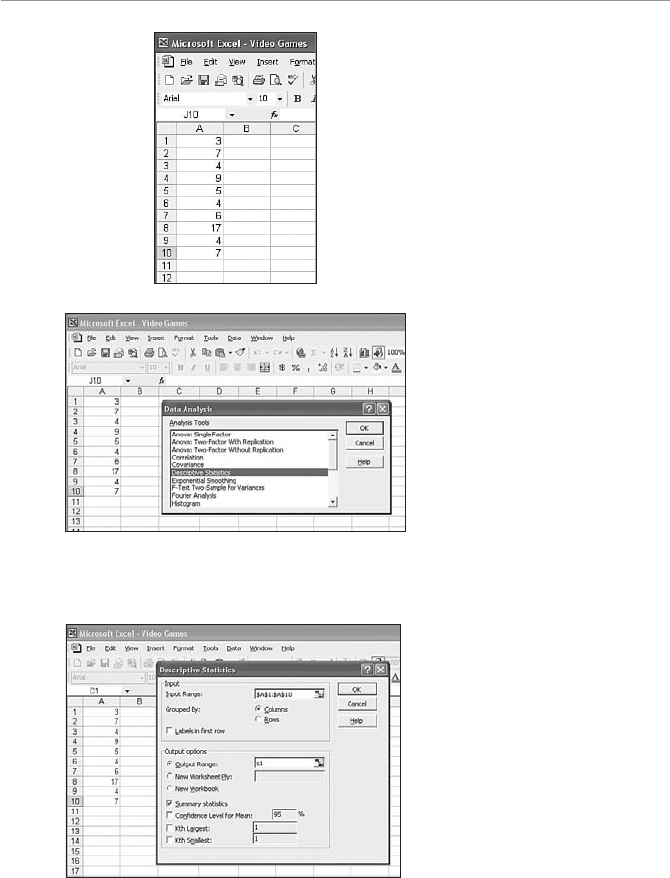
1VO^bS`"( 1OZQcZObW\U2SaQ`W^bWdSAbObWabWQa(;SOac`Sa]T1S\b`OZBS\RS\Qg;SO\;SRWO\O\R;]RS #%
3. Select Descriptive Statistics and click OK. The following dialog box will appear
(Figure 4.3).
4WUc`S"
Enter data from the video
game example.
4WUc`S"
Data Analysis dialog box.
4WUc`S"!
Descriptive Statistics dialog
box.
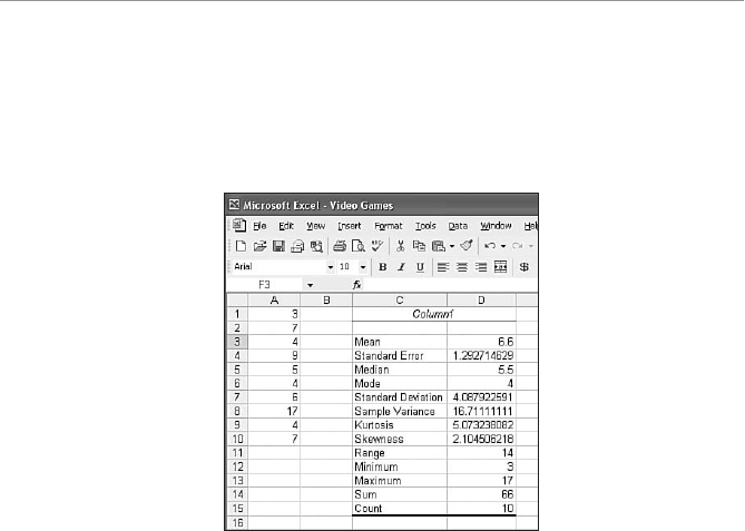
>O`b( BVS0OaWQa#&
4. For the Input Range, select cells A1 through A10, select the Output Range
option, and select cell C1. Then choose the Summary statistics check box and
click OK.
5. After you expand columns C and D slightly to see all the figures, your spread-
sheet should look like Figure 4.4.
4WUc`S""
Measures of central tendency
for the video game example.
As you can see, the mean is 6.6 hours, the median is 5.5 hours, and the mode is 4.0
hours. Piece of cake!
G]c`Bc`\
1. Calculate the mean, median, and mode for the following data set: 20, 15, 24, 10,
8, 19, 24, 12, 21, 6.
2. Calculate the mean, median, and mode for the following data set: 84, 82, 90, 77,
75, 77, 82, 86, 82.
3. Calculate the mean, median, and mode for the following data set: 36, 27, 50, 42,
27, 36, 25, 40, 29, 15.
4. Calculate the mean, median, and mode for the following data set: 8, 11, 6, 2, 11,
6, 5, 6, 10.

1VO^bS`"( 1OZQcZObW\U2SaQ`W^bWdSAbObWabWQa(;SOac`Sa]T1S\b`OZBS\RS\Qg;SO\;SRWO\O\R;]RS #'
5. A company counted the number of their employees in each of the following age
classes. According to this distribution, what is the average age of the employees
in the company?
Age Range Number of Employees
20–24 8
25–29 37
30–34 25
35–39 48
40–44 27
45–49 10
6. Calculate the weighted mean of the following values with the corresponding
weights.
Value Weight
118 3
125 2
107 1
7. A company counted the number of employees at each level of years of service in
the following table. What is the average number of years of service in this com-
pany?
Years of Service Number of Employees
1 5
2 7
310
4 8
512
6 3

>O`b( BVS0OaWQa$
BVS:SOabG]c<SSRb]9\]e
UCalculate the mean of a data set by summing all the values and dividing this
result by the number of values.
UThe median of a data set is the midpoint of the set if the values are arranged in
ascending or descending order.
UThe median is the single center value from the data set if there is an odd number
of values in the set. The median is the average of the two center values if the
number of values in the set is even.
UThe mode of a data set is the value that appears most often in the set. There can
be more than one mode in a data set.

5
1VO^bS`
1OZQcZObW\U2SaQ`W^bWdS
AbObWabWQa(;SOac`Sa]T
2Wa^S`aW]\
7\BVWa1VO^bS`
UCalculating the range of a sample
UCalculating the variance and standard deviation of a sample and popu-
lation
UUsing the empirical rule and Chebyshev’s theorem to predict the dis-
tribution of data values
UUsing measures of relative position to identify outlier data values
UUsing Excel to calculate measures of dispersion
In Chapter 4, we calculated measures of central tendency by summarizing
our data set into a single value. But in doing so, we lost information that
could be useful. For the video game example, if the only information I pro-
vided you was that the mean of my sample was 6.6 hours, you would not
know whether all the values were between 6 and 7 hours or whether the
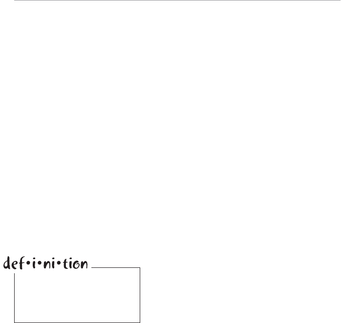
>O`b( BVS0OaWQa$
values varied between 1 and 12 hours. As you will see later, this distinction can be very
important.
To address this issue, we rely on the second major category of descriptive statistics,
measures of dispersion, which describes how far the individual data values have strayed
from the mean. So let’s look at the different ways we can measure dispersion.
@O\US
The range is the simplest measure of dispersion and is calculated by finding the differ-
ence between the highest value and the lowest value in the data set. To demonstrate
how to calculate the range, I’ll use the following example.
One of Debbie’s special qualities is that she is a dedicated grill–a-holic when it comes
to barbequing in the backyard. Recently, we needed to purchase a new grill since our
old one mysteriously caught fire one night when I was at school teaching. The cause
of the fire was labeled “suspicious” after Debbie saw this event as a wonderful oppor-
tunity to “upgrade.” My idea of the perfect grill is one you dump charcoal in, add
one can of lighter fluid to, toss in a match, and run for your life. The best part about
this kind of grill is that it has about four parts to assemble, which is something I can
easily put together in 3 or 4 weeks. Within minutes of arriving at the store, I felt a
stabbing pain in my chest upon finding my wife in an animated conversation with a
total stranger about a grill for the “serious barbeque
person” complete with three burners, electronic igni-
tion, back-up propane tank, 300 horsepower, and
front disc brakes. This thing could barbeque a pig
on a spit faster than I could say “oink.” I’d have bet-
ter luck assembling a car from scratch. As protection
from future acts of arson, I purchased a life insurance
policy for our new family member.
Anyway, the following data set represents the number of meals each month that
Debbie cranks up on the turbo-charged grill:
798114
The range of this sample would be:
Range = 11 – 4 = 7 meals
Obtain the range of a sample
by subtracting the smallest
measurement from the largest
measurement.
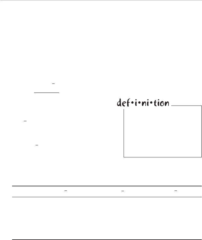
1VO^bS`#( 1OZQcZObW\U2SaQ`W^bWdSAbObWabWQa(;SOac`Sa]T2Wa^S`aW]\ $!
The range is a “quick-and-dirty” way to get a feel for the spread of the data set.
However, the limitation is that it only relies on two data points to describe the varia-
tion in the sample. No other values between the highest and lowest points are part of
the range calculation.
DO`WO\QS
One of the most common measurements of dispersion in statistics is the variance,
which summarizes the squared deviation of each data value from the mean. The for-
mula for the sample variance is:
s
xx
n
i
i
n
2
2
1
1
¤
where:
s2 = the variance of the sample
x
= the sample mean
n = the size of the sample (the number
of data values)
xx
i
= the deviation from the mean
for each value in the data set
The first step in calculating the variance is to determine the mean of the data set,
which in the grilling example is 7.8 meals per month. The rest of the calculations can
be facilitated by the following table.
xix
xx
i
xx
i
2
7 7.8 -0.8 0.64
9 7.8 1.2 1.44
8 7.8 0.2 0.04
11 7.8 3.2 10.24
4 7.8 -3.8 14.44
The variance is a measure of
dispersion that describes the
relative distance between the
data points in the set and the
mean of the data set. This mea-
sure is widely used in inferential
statistics.

>O`b( BVS0OaWQa$"
xx
i
i
¤2
1
5
26 80.
The final sample variance calculation becomes this:
s226 8
51 67
..
For those of us who like to do things in one step, we can also do the entire variance
calculation in the following equation:
s2
222 2
778 978 878 1178 47
... ... .
8
51 67
2
CaW\UbVS@OeAQ]`S;SbV]REVS\5`WZZW\U
A more efficient way to calculate the variance of a data set is known as the raw score
method. Even though at first glance this equation may look more imposing, its bark
is much worse than its bite. Check it out and decide for yourself what works best for
you.
s
x
x
n
n
i
i
ni
i
n
2
2
1
1
2
1
¥
§
¦´
¶
µ
¤¤
where:
xi
i
n2
1
¤ = the sum of each data value after it has been squared
xi
i
n
¤
¥
§
¦´
¶
µ
1
2
= the square of the sum of all the data values
Okay, don’t have heart failure just yet. Let me lay this out in the following table to
prove to you there are fewer calculations than with the previous method.
xix2
i
7 49
9 81
8 64
11 121
4 16
1VO^bS`#( 1OZQcZObW\U2SaQ`W^bWdSAbObWabWQa(;SOac`Sa]T2Wa^S`aW]\ $#
xi
i
n
¤
1
39 xi
i
n2
1
331
¤
xi
i
n
¤
¥
§
¦´
¶
µ
1
2
2
39 1521
s2331 1521
5
4
s2331 304 2
467
..
As you can see, the results are the same
regardless of the method used. The benefits
of the raw score method become more obvi-
ous as the size of the sample (n) gets larger.
BVSDO`WO\QS]TO>]^cZObW]\
So far, we have discussed the variance in the context of samples. The good news is
the variance of a population is calculated in the same manner as the sample variance.
The bad news is I need to introduce another funny-looking Greek symbol: sigma. The
equation for the variance of a population is as follows:
S
M
21
2
¤x
N
i
i
n
where:
S
2 = the variance of the population
(pronounced “sigma squared”)
xi= the measurement of each item in
the population
R = the population mean
N = the size of the population
If you are calculating the vari-
ance by hand, my advice is
to do your fingers and cal-
culator battery a favor and use
the raw score method.
Bob’s Basics
Notice that the denomina-
tor for the population vari-
ance equation is N, whereas
the denominator for the sample
variance is n– 1.
Wrong Number

>O`b( BVS0OaWQa$$
The raw score version of this equation is:
S
2
2
1
1
2
¥
§
¦´
¶
µ
¤¤
x
x
N
N
i
i
Ni
i
N
Even though this procedure is identical to the sample variance, let me demonstrate
with another example. Let’s say I am considering my statistics class as my population
and the following ages are the measurement of interest. (Can you guess which one is
me? My age adds a little spice to the variance.)
21 23 28 47 20 19 25 23
I’ll use the raw score method for this calculation with the population size (N) equal to
8. (I’d love to see a class this size.)
xix2
i
21 441
23 529
28 784
47 2209
20 400
19 361
25 625
23 529
xi
i
n
¤
1
206 xi
i
n2
1
5878
¤
xi
i
n
¤
¥
§
¦´
¶
µ
1
2
2
206 42436
S
25878 42436
8
8
S
25878 5304 5
871 7
..
Thanks to the old guy in the class, the population variance is 71.7.
1VO^bS`#( 1OZQcZObW\U2SaQ`W^bWdSAbObWabWQa(;SOac`Sa]T2Wa^S`aW]\ $%
AbO\RO`R2SdWObW]\
This method is pretty straightforward. The standard deviation is simply the square root
of the variance. Just as with the variance, there is a standard deviation for both the
sample and population, as shown in the following equations.
Sample standard deviation:
ss
xx
n
i
i
n
¤
2
2
1
1
Population standard deviation:
SS
M
¤
2
2
1
x
N
i
i
N
To calculate the standard deviation, you must first calculate the variance and then take
the square root of the result. Recall from the previous sections that the variance from
my sample of the number of meals Debbie grilled per month was 6.7. The standard
deviation of this sample is as follows:
ss
267 26..
meals
Also recall the variance for the age of my class was 71.7. The standard deviation of the
age of this population is as follows:
SS
271 7 8 5..
years
The standard deviation is actually a more useful measure than the variance because
the standard deviation is in the units of the original data set. In comparison, the units
of the variance for the grill example would be 6.7 “meals squared,” and the units of
the variance for the age example would be 71.7 “years squared.” I don’t know about
you, but I’m not too thrilled having my age reported as 2,209 squared years. I’ll take
the standard deviation over the variance any day.
1OZQcZObW\UbVSAbO\RO`R2SdWObW]\]T5`]c^SR2ObO
The following equation shows how to calculate the standard deviation of grouped data
in a frequency distribution.
Astandard deviation is the
square root of a variance.

>O`b( BVS0OaWQa$&
s
xxf
n
i
i
m
i
¤()
2
1
1
where:
fi = the number of data values in each frequency class
m = the number of classes
n = fi
i
m
¤
1 = the total number of values in the data set
The following table is a frequency distribution that represents the number of times
each child in Debbie’s 3-year-old preschool class needs a “potty break” in a day.
Number of Potty Breaks per Day ( xi) Number of Children ( fi)
21
34
412
58
65
In this example, m = 5 and n = 30. From Chapter 4, we know the mean of this fre-
quency distribution is this:
x
fx
f
ii
i
m
i
i
m
¤
¤
1
1
x
12 43 124 85 56
1412
85 44. times per child per day
1VO^bS`#( 1OZQcZObW\U2SaQ`W^bWdSAbObWabWQa(;SOac`Sa]T2Wa^S`aW]\ $'
The following table summarizes the standard deviation calculations.
xifixxx
i
2
xx
i
2
xxf
ii
2
2 1 4.4 -2.4 5.76 5.76
3 4 4.4 -1.4 1.96 7.84
4 12 4.4 -0.4 0.16 1.92
5 8 4.4 0.6 0.36 2.88
6 5 4.4 1.6 2.56 12.80
xxf
ii
i
m
¤2
1
31 20.
s
xxf
n
i
i
m
i
¤() ...
2
1
1
31 20
30 1 108 104 times per child per day
The potty break frequency distribution has a mean of 4.4 times per child per day and
a standard deviation of 1.04 times per child per day. The frequency of these potty
breaks must keep Debbie very busy.
BVS3[^W`WQOZ@cZS(E]`YW\UbVSAbO\RO`R2SdWObW]\
The values of many large data sets tend to cluster around the mean or median so
that the data distribution in the histogram resembles a bell-shape, symmetrical curve.
When this is the case, the empirical rule (sounds like a decree from the emperor) tells
us that approximately 68 percent of the data
values will be within one standard deviation
from the mean.
For example, suppose that the average exam
score for my large statistics class is 88 points
and the standard deviation is 4.0 points and
that the distribution of grades is bell-shape
around the mean, as shown in Figure 5.1.
Because one standard deviation above the
mean would be 92 (88 + 4) and one standard
deviation below the mean would be 84 (88
– 4), the empirical rule tells me that approxi-
mately 68 percent of the exam scores will fall
between 84 and 92 points.
According to the empirical rule,
if a distribution follows a bell-
shape—a symmetrical curve
centered around the mean—we
would expect approximately
68, 95, and 99.7 percent of
the values to fall within one,
two, and three standard devia-
tions around the mean respec-
tively.
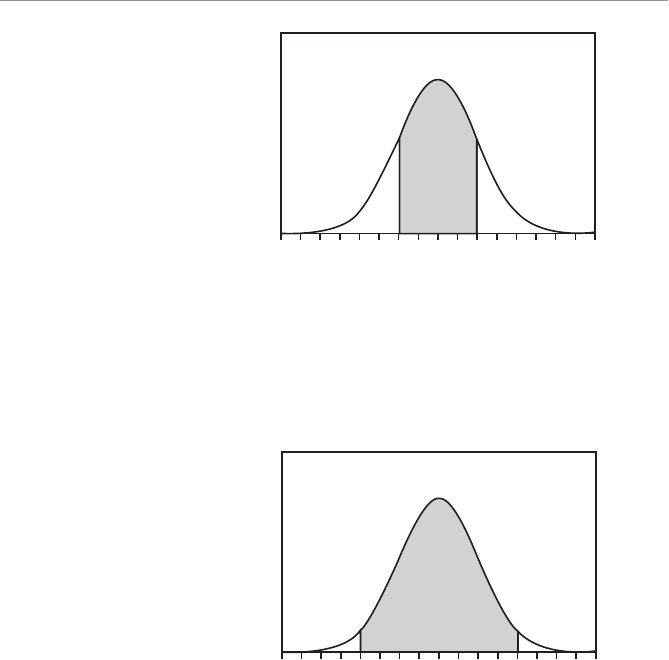
>O`b( BVS0OaWQa%
The empirical rule also states that approximately 95 percent of the data values will fall
within two standard deviations from the mean. In our example, two standard devia-
tions equal 8.0 points (2 * 4.0). Two standard deviations above the mean would be a
score of 96 (88 + 8), and two standard deviations below the mean would be 80 (88
– 8). According to Figure 5.2, approximately 95 percent of the exam scores will be
between 80 and 96 points.
72 76 80 84 88 92 96 100 104
68%
Exam Scores
Number of Students
72 76 80 84 88 92 96 100 104
95%
Exam Scores
Number of Students
4WUc`S#
One standard deviation
around the mean.
4WUc`S#
Two standard deviations
around the mean.
Taking this one final step, the empirical rule states that, under these conditions,
approximately 99.7 percent of the data values will fall within three standard deviations
from the mean. According to Figure 5.3, virtually all the test scores should fall within
plus or minus 12 points (3 * 4.0) from the mean of 88. In this case, I would expect all
the exam scores to be between 76 and 100.
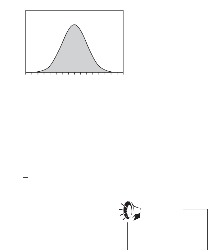
1VO^bS`#( 1OZQcZObW\U2SaQ`W^bWdSAbObWabWQa(;SOac`Sa]T2Wa^S`aW]\ %
In general, we can use the following equation to express the range of values within k
standard deviations around the mean:
MS
pk
We will revisit the empirical rule concept in subsequent chapters.
1VSPgaVSdÂaBVS]`S[
Chebyshev’s theorem is a mathematical rule similar to the empirical rule except that
it applies to any distribution rather than just bell-shape, symmetrical distributions.
Chebyshev’s theorem states that for any number k greater than 1, at least
11100
2
¥
§
¦´
¶
µs
kpercent of the values will fall within k standard deviations from the
mean. Using this equation, we can state the following:
UAt least 75 percent of the data values
will fall within two standard deviations
from the mean by setting k = 2 into
Chebyshev’s equation.
UAt least 88.9 percent of the data values
will fall within three standard devia-
tions from the mean by setting k = 3
into the equation.
72 76 80 84 88 92 96 100 104
99.7%
Exam Scores
Number of Students
4WUc`S#!
Three standard deviations
around the mean.
Chebyshev’s theorem can
be applied to any distribu-
tion of data but can only be
stated for values of k that are
greater than 1.
Wrong Number
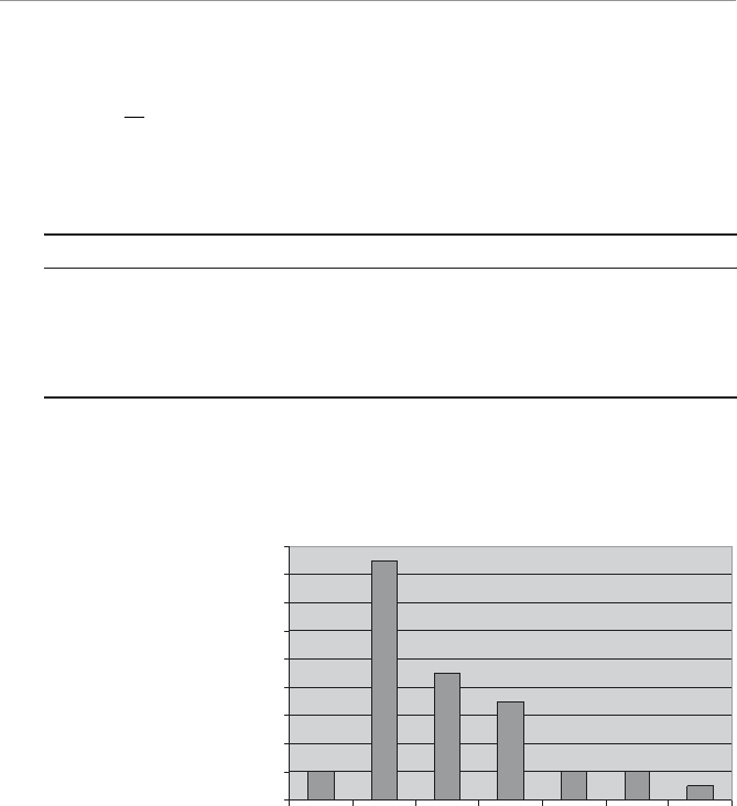
>O`b( BVS0OaWQa%
UAt least 93.7 percent of the data values will fall within four standard deviations
from the mean by setting k = 4 into the equation. This last example is shown as:
11
4100 93 7
2
¥
§
¦´
¶
µs.
Let’s check out Chebyshev’s theorem to see whether it really works. The follow-
ing table shows the number of home runs hit by the top 40 players in Major League
Baseball during the 2002 season.
Number of Home Runs from Top 40 Players in 2002
57 52 49 46 43 42 42 41 39 39
38 38 37 37 35 34 34 34 33 33
33 32 31 31 31 30 30 30 29 29
29 29 29 28 28 28 28 28 27 27
Source: www.espn.com.
The following histogram shows that this distribution is neither bell-shape nor sym-
metrical, so we cannot apply the empirical rule (see Figure 5.4) but will need to use
Chebyshev’s theorem.
%%
4WUc`S#"
Home run histogram for
2002 season.
0
2
4
6
8
10
12
14
16
18
23-27 28-32 33-37 38-42 43-47 48-52 53-57
Home Runs
Number of Players

1VO^bS`#( 1OZQcZObW\U2SaQ`W^bWdSAbObWabWQa(;SOac`Sa]T2Wa^S`aW]\ %!
The mean for this distribution is 34.7 home runs, and the standard deviation is 7.2
home runs. The following table summarizes various intervals around the mean with
the percentage of values within those intervals.
k
M
S
MS
k
MS
kChebyshev’s Actual
Percentage Percentage
2 34.7 7.2 49.1 20.3 75.0% 95.0%
3 34.7 7.2 56.3 13.1 88.9% 97.5%
4 34.7 7.2 63.5 5.9 93.7% 100.0%
This table supports Chebyshev’s theorem, which predicts that at least 75 percent of
the values will fall within two standard deviations from the mean. From the data set,
we can observe that 95 percent actually fall between 20.3 and 49.1 home runs (38 out
of 40). The same explanation holds true for three and four standard deviations around
the mean.
;SOac`Sa]T@SZObWdS>]aWbW]\
Another way of looking at dispersion of data is through measures of relative posi-
tion, which describe the percentage of the data below a certain point. This technique
includes quartile and interquartile measurements.
?cO`bWZSa
Quartiles divide the data set into four equal
segments after it has been arranged in
ascending order. Approximately 25 percent
of the data points will fall below the first
quartile, Q1. Approximately 50 percent of the
data points will fall below the second quartile,
Q2. And, you guessed it, 75 percent should
fall below the third quartile, Q3.To demon-
strate how to identify Q1, Q2, and Q3, let’s
use the following data set.
9531014612714
Quartiles measure the relative
position of the data values by
dividing the data set into four
equal segments.

>O`b( BVS0OaWQa%"
Step 1: Arrange your data in ascending order.
3567910121414
Step 2: Find the median of the data set. This is Q2.
35679 10121414
Q2 = 9
Step 3: Find the median of the lower half of the data set (in parenthesis). This is Q1.
(3567)9 10121414
Q1 = 5.5
Q2 = 9
Step 4: Find the median of the upper half of the data set (in parenthesis). This is Q3.
35679 (10 12 14 14)
Q1 = 5.5
Q2 = 9
Q3 = 13
7\bS`_cO`bWZS@O\US
When you have established the quartiles, you can easily calculate the interquartile
range (IQR); the IQR measures the spread of the center half of our data set. It is sim-
ply the difference between the third and first quartiles, as follows:
IQR = Q3 – Q1
The interquartile range is used to identify outliers,
which are the “black sheep” of our data set. These are
extreme values whose accuracy is questioned and can
cause unwanted distortions in statistical results. Any
values that are more than:
Q3 + 1.5IQR
The interquartile range mea-
sures the spread of the center
half of the data set and identi-
fies outliers, which are extreme
values that you should discard
before analysis.

1VO^bS`#( 1OZQcZObW\U2SaQ`W^bWdSAbObWabWQa(;SOac`Sa]T2Wa^S`aW]\ %#
or less than:
Q1 – 1.5IQR
should be discarded. Let’s use the following data set to determine if any nasty outliers
exist:
10 42 45 46 51 52 58 73
Since there are eight data values, Q1will be the median of the first four values (the
midpoint between the second and third values).
Q1
42 45
243
5
.
Likewise, Q3 will be the median of the last four values (the midpoint between the sixth
and seventh values).
Q2
52 58
256
IRQ Q Q
31
56 43 5 12 5..
Any values greater than
QIRQ
315 56 15 125 7475
....
or less than
QIRQ
11 5 43 5 1 5 12 5 24 75
.....
would be considered an outlier. Therefore, the value 10 would be an outlier in this
data set.
Now that we have worked our fingers to the bones calculating all this stuff, let’s see
how Excel makes it look so easy.
CaW\U3fQSZb]1OZQcZObS;SOac`Sa]T2Wa^S`aW]\
Excel enables you to conveniently calculate the range, variance, and standard deviation
of a sample using the Data Analysis selection under the Tools menu. Use the exact
same steps to calculate these measures as those used to calculate measures of central
tendency shown in Chapter 4. Repeating those steps (see the section “Using Excel to
Calculate Central Tendency”) with the grilling example from this chapter will produce
Figure 5.5.
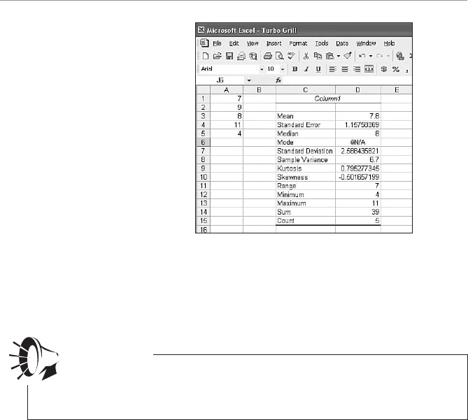
>O`b( BVS0OaWQa%$
As you can see from Figure 5.5, the sample range equals 7 meals, the sample variance
equals 6.7, and the standard deviation equals 2.6 meals. Also note that this data set has
no mode since no value appears more than once.
This wraps up our discussion on the different ways to describe measures of dispersion.
4WUc`S##
Measures of dispersion for the
turbo grill example.
The values for variance and standard deviation reported by Excel are for a
sample. If your data set represents a population, you need to recalculate the
results using N in the denominator rather than n– 1.
Wrong Number
G]c`Bc`\
1. Calculate the variance, standard deviation, and the range for the following
sample data set: 20, 15, 24, 10, 8, 19, 24.
2. Calculate the variance, standard deviation, and the range for the following
population data set: 84, 82, 90, 77, 75, 77, 82, 86, 82.
3. Calculate the variance, standard deviation, and the range for the following
sample data set: 36, 27, 50, 42, 27, 36, 25, 40.
4. Calculate the quartiles and the cutoffs for the outliers for the following data set:
8, 11, 6, 2, 11, 6, 5, 6, 10, 15.
5. A company counted the number of their employees in each of the age classes as
follows. According to this distribution, what is the standard deviation for the age

1VO^bS`#( 1OZQcZObW\U2SaQ`W^bWdSAbObWabWQa(;SOac`Sa]T2Wa^S`aW]\ %%
of the employees in the company?
Age Range Number of Employees
20–24 8
25–29 37
30–34 25
35–39 48
40–44 27
45–49 10
6. A company counted the number of employees at each level of years of service in
the table that follows. What is the standard deviation for the number of years of
service in this company?
Years of Service Number of Employees
15
27
310
48
512
63
7. A data set that follows a bell-shape and symmetrical distribution has a mean
equal to 75 and a standard deviation equal to 10. What range of values centered
around the mean would represent 95 percent of the data points?
8. A data set that is not bell-shape and symmetrical has a mean equal to 50 and a
standard deviation equal to 6. What is the minimum percent of values that would
fall between 38 and 62?

>O`b( BVS0OaWQa%&
BVS:SOabG]c<SSRb]9\]e
UThe range of a data set is the difference between the largest value and smallest
value.
UThe variance of a data set summarizes the squared deviation of each data value
from the mean.
UThe standard deviation of a data set is the square root of the variance and is
expressed in the same units as the original data values.
UThe empirical rule states that if a distribution follows a bell-shape, a symmetri-
cal curve centered around the mean, we would expect approximately 68, 95, and
99.7 percent of the values to fall within one, two, and three standard deviations
around the mean, respectively.
UThe interquartile range measures the spread of the center half of the data set and
identifies outliers, which are extreme values that you should discard before analy-
sis.

2
>O`b
The connection between descriptive and inferential statistics is based on
probability concepts. I know the topic of probability theory scares the living
daylights out of many students, but it is a very important topic in the world
of statistics. The topic of probability acts as a critical link between descrip-
tive and inferential statistics. Without a firm grasp of probability concepts,
inferential statistics will seem like a foreign language. Because of this, Part
2 is designed to help you over this hurdle.
>`]POPWZWbgB]^WQa


6
1VO^bS`
7\b`]RcQbW]\b]>`]POPWZWbg
7\BVWa1VO^bS`
UDistinguish between classical, empirical, and subjective probability
UUse frequency distributions to calculate probability
UExamine the basic properties of probability
UDemonstrate the intersection and union of simple events using a Venn
diagram
As we leave the happy world of descriptive statistics, you may feel like
you’re ready to take on the challenge of inferential statistics. But before
we enter that realm, we need to arm ourselves with probability theory.
Accurately predicting the probability that an event will occur has wide-
spread applications. For instance, the gaming industry uses probability
theory to set odds for lotteries, card games, and sporting events.
The focus of this chapter is to start with the basics of probability, after
which we will gently proceed to more complex concepts in Chapters 7 and
8. We’ll discuss different types of probabilities and how to calculate the
probability of simple events. We’ll rely on data from frequency distribu-
tions to examine the likelihood of a combination of simple events. So pull
up a chair and let’s roll those dice!

>O`b ( >`]POPWZWbgB]^WQa&
EVOb7a>`]POPWZWbg-
Probability concepts surround most of our daily lives. When I see that the weather
forecast shows an 80 percent chance of rain tomorrow and I want to play golf or that
my beloved Pittsburgh Pirates have only won 40 percent of their games this year
(which they also did last year and the year before that), there is a 65 percent chance I
will get moody.
In simple terms, probability is the likelihood of a particular event like rain or winning
a ballgame. But before we go any further, we need to tackle some new “stat jargon.”
The following terms are widely used when talking about probability:
UExperiment. The process of measuring or observing an activity for the purpose
of collecting data. An example is rolling a pair of dice.
UOutcome. A particular result of an experiment. An example is rolling a pair of
threes with the dice.
USample space. All the possible outcomes of the experiment. The sample space
for our experiment is the numbers {2, 3, 4, 5, 6, 7, 8, 9, 10, 11, and 12}. Statistics
people like to put {} around the sample space values because they think it looks
cool.
UEvent. One or more outcomes that are of interest for the experiment and which
is/are a subset of the sample space. An example is rolling a total of 2, 3, 4, or 5
with two dice.
To properly define probability, we need to consider which type of probability we are
referring to.
1ZOaaWQOZ>`]POPWZWbg
Classical probability refers to a situation when we know the number of possible out-
comes of the event of interest and can calculate the probability of that event with the
following equation:
P[A] = Number of possible outcomes in which Event A occurs
Total number of possible outcomes in the sample space
where:
P[A] = the probability that Event A will occur
1VO^bS`$( 7\b`]RcQbW]\b]>`]POPWZWbg &!
For example, if Event A = rolling a total of 2, 3, 4, or 5 with two dice, we need to
define the sample space for this experiment, which is shown in the following table.
{1,1} {2,1} {3,1} {4,1) {5,1} {6,1}
{1,2} {2,2} {3,2} {4,2} {5,2} {6,2}
{1,3} {2,3} {3,3} {4,3} {5,3} {6,3}
{1,4} {2,4} {3,4} {4,4} {5,4} {6,4}
{1,5} {2,5} {3,5} {4,5} {5,5} {6,5}
{1,6} {2,6} {3,6} {4,6} {5,6} {6,6}
There are 36 total outcomes for this experi-
ment, each with the same chance of occur-
ring. I have underlined the outcomes that
correspond to Event A. There is a total of
10 of them. Therefore:
P[A] = 10
36
= 0.28
To use classical probability, you need to
understand the underlying process so you
can determine the number of outcomes asso-
ciated with the event. You also need to be able to count the total number of possible
outcomes in the sample space. As you will see next, this may not always be possible.
3[^W`WQOZ>`]POPWZWbg
When we don’t know enough about the underlying process to determine the number
of outcomes associated with an event, we rely on empirical probability. This type of
probability observes the number of occurrences of an event through an experiment
and calculates the probability from a relative frequency distribution. Therefore:
P[A] = Frequency in which Event A occurs
Total number of observations
Classical probability requires
that you know the number of
outcomes that pertain to a par-
ticular event of interest. You also
need to know the total number
of possible outcomes in the
sample space.
>O`b ( >`]POPWZWbgB]^WQa&"
One example of empirical probability is to answer the
age-old question “What is the probability that John
will get out of bed in the morning for school after his
first wake-up call?” Because I cannot begin to under-
stand the underlying process of why a teenager will
resist getting out of bed before 2 P.M., I need to rely
on empirical probability. The following table indi-
cates the number of wake-up calls John required over
the past 20 school days.
John’s Wake-Up Calls (Previous 20 School Days)
2433124331
4233132434
We can summarize this data with a relative frequency distribution.
@SZObWdS4`S_cS\Qg2Wab`WPcbW]\T]`8]V\ÂaEOYSC^1OZZa
Number of Wake-Up Calls Number of Observations Percentage
13
3/20 = 0.15
24
4/20 = 0.20
38
8/20 = 0.40
45
5/20 = 0.25
Total = 20
Based on these observations, if Event A = John getting out of bed on the first wake-up
call, then P[A] = 0.15.
Using the previous table, we can also examine the probability of other events. Let’s
say Event B = John requiring more than 2 wake-up calls to get out of bed; then P[B] =
0.40 + 0.25 = 0.65. That boy needs to go to bed earlier on school nights!
Empirical probability requires
that you count the frequency
that an event occurs through an
experiment and calculate the
probability from the relative fre-
quency distribution.
1VO^bS`$( 7\b`]RcQbW]\b]>`]POPWZWbg &#
If I choose to run another 20-day experiment of John’s waking behavior, I would
most likely see different results than those in the previous table. However, if I were to
observe 100 days of this data, the relative frequencies would approach the true or clas-
sical probabilities of the underlying process. This pattern is known as the law of large
numbers.
To demonstrate the law of large numbers,
let’s say I flip a coin three times and each
time the result is heads. For this experiment,
the empirical probability for the event heads
is 100 percent. However, if I were to flip the
coin 100 times, I would expect the empirical
probability of this experiment to be much
closer to the classical probability of 50 per-
cent.
AcPXSQbWdS>`]POPWZWbg
We use subjective probability when classical and empirical probabilities are not avail-
able. Under these circumstances, we rely on experience and intuition to estimate the
probabilities.
Examples where we would apply subjective probability are “What is the probability
that my son Brian will ask to borrow my new car, which happens to have a 6-speed
manual transmission, for his junior prom?” (97 percent) or “What is the probability
that my new car will come back with all 6 gears in proper working order?” (18 per-
cent). I based these probabilities on my personal observations after returning from a
The probability that you will win a typical state lottery, where you correctly choose
6 out of 50 numbers, is approximately 0.00000006, or 1 out of 16 million. This
is calculated using classical probability. Compare this to the probability that you will
be struck by lightning once during your lifetime, which is 0.0003 or 1 out of 3,000
(source: www.nws.noaa). This is an empirical probability determined by the number
of times people have been struck by lightning in the past. According to these statistics,
you are more than 5,000 times more likely to be struck by lightning than win the lot-
tery! In spite of this, Debbie still makes me go buy a ticket when there’s a big jackpot,
even during a thunder storm.
Random Thoughts
The law of large numbers states
that when an experiment is con-
ducted a large number of times,
the empirical probabilities of
the process will converge to the
classical probabilities.
>O`b ( >`]POPWZWbgB]^WQa&$
“practice run” where I heard noises from my poor transmission that chilled me to the
bone and to this day haunt me in my sleep. I need to use subjective probability in this
situation because my car would never survive several of these “experiments.”
0OaWQ>`]^S`bWSa]T>`]POPWZWbg
Our next step is to review the “rules and regulations” that govern probability theory.
The basic ones are as follows:
UIf P[A] = 1, then Event A must occur with certainty. An example is Event A =
Debbie buying a pair of shoes this month.
UIf P[A] = 0, then Event A will not occur with certainty. An example is Event A =
Bob will eventually finish the basement project that he started three years ago.
UThe probability of Event A must be between 0 and 1.
UThe sum of all the probabilities for the events in the sample space must be equal
to 1. For example, if the experiment is flipping a coin with Event A = heads and
Event B = tails, then A and B represent the entire sample space. We also know
that P[A] + P[B] = 0.5 + 0.5 = 1.
UThe complement to Event A is defined as all the outcomes in the sample space
that are not part of Event A and is denoted as A’. Using this definition, we can
state the following: P[A] + P[A’] = 1 or P[A] = 1 – P[A’].
For example, if the experiment is rolling a single six-sided die, the sample space is
shown in Figure 6.1.
4WUc`S$
Sample space for a single die
experiment.

1VO^bS`$( 7\b`]RcQbW]\b]>`]POPWZWbg &%
If we say that Event A = rolling a 1, then Event A’ = rolling a 2, 3, 4, 5, or 6.
Therefore:
P[A] = 1
6
= 0.167
P[A’] = 1 – 0.167 = 0.833
Up to this point, all our examples would be considered cases of simple probability,
which is defined as the probability of a single event. Now we’ll expand this concept to
more than one event.
BVS7\bS`aSQbW]\]T3dS\ba
Sometimes we are interested in the probability of a combination of events rather than
just a simple event. To demonstrate this technique, I will use the following example.
Now that my children are older and living away from home, I cherish those moments
when the phone rings and I see one of their numbers appear on my caller ID.
Experience has taught me that I can categorize these calls as either “crisis,” involving
such things as a computer, a car, an ATM card, or a cell phone; or “noncrisis,” when
they call just to see if I’m alive and well enough to help with their next crisis.
The following table, called a contingency table, categorizes the last 50 phone calls by
child and type of call.
1]\bW\US\QgBOPZST]`>V]\S1OZZa
Child Crisis Non-Crisis Totals
Christin 14 6 20
Brian 10 4 14
John 4 12 16
Total 28 22 50
Contingency tables show the actual or relative frequency of two types of data at the
same time. In this case, the data types are child and type of call.
>O`b ( >`]POPWZWbgB]^WQa&&
I’ll assume that this past pattern of calls will hold true in the near future. We’ll define
Events A and B as follows:
UEvent A = the next phone call will come from Christin.
UEvent B = the next phone call will involve a crisis.
We can use the contingency table to calculate the simple probability that the next
phone call will come from Christin as follows:
P[A] = 20
50
= 0.40
The probability that the next phone call will involve a crisis would be as follows:
P[B] = 28
50
= 0.56
What about the probability that the next phone call
will come from Christin and will involve a crisis?
This event is known as the intersection of Events A
and B and is described by AB. The number of
phone calls from our contingency table that meet
both criteria is 14, so:
P[A and B] = P[
AB
] = 14
50
= 0.28
This explains why I hold my breath as I pick up the
phone!
The probability of the intersection of two events is
known as a joint probability.
BVSC\W]\]T3dS\ba(/;O``WOUS;ORSW\6SOdS\
The union of Events A and B represents all the instances where either Event A or
Event B or both occur and is denoted as AB
. Using our previous example, the fol-
lowing table shows the four combinations that include either a call from Christin or a
crisis phone call.
Acontingency table indicates
the number of observations
that are classified according to
two variables. The intersection
of Events A and B represents
the number of instances where
Events A and B occur at the
same time (that is, the same
phone call is both from Christin
and a crisis). The probability of
the intersection of two events is
known as a joint probability.
1VO^bS`$( 7\b`]RcQbW]\b]>`]POPWZWbg &'
Child Type of Call Number of Calls
Christin Crisis 14
Christin Noncrisis 6
Brian Crisis 10
John Crisis 4
Total = 34
Therefore, the probability that the next phone call is either from Christin or is a
crisis is as follows:
P[A and B] = P[AB
] = 34
50
= 0.68
The union of Events A and B represents the number of instances where either Event A
or B occur (that is, the number of calls that were either from Christin or were a crisis).
G]c`Bc`\
1. Define each of the following as classi-
cal, empirical, or subjective probabil-
ity.
a. The probability that the baseball
player Derek Jeter will get a hit
during his next at bat.
b. The probability of drawing an Ace
from a deck of cards.
c. The probability that I will shoot
lower than a 90 during my next round of golf.
d. The probability of winning the next state lottery drawing.
e. The probability that the drive belt for my riding lawnmower will break this
summer (it did).
f. The probability that I will finish writing this book before my deadline.
The probability of the inter-
section of two events can
never be more than the
probability of the union of two
events. If your calculations don’t
agree with this, go back and
check for a mistake!
Bob’s Basics

>O`b ( >`]POPWZWbgB]^WQa'
2. Identify whether each of the following are valid probabilities.
a. 65 percent
b. 1.9
c. 110 percent
d. –4.2
e. 0.75
f. 0
3. A survey of 125 families asked whether the household had Internet access. Each
family was classified by race. The contingency table is shown here.
Race Internet No Internet Total
Caucasian 15 22 37
Asian American 23 18 41
African American 14 33 47
Total 52 73 125
A family from the survey is randomly selected. We define:
Event A: The selected family has an Internet connection in its home.
Event B: The selected family is Asian American.
a. Determine the probability that the selected family has an Internet connection.
b. Determine the probability that the selected family is Asian American.
c. Determine the probability that the selected family has an Internet connection
and is Asian American.
d. Determine the probability that the selected family has an Internet connection
or is Asian American.
4. Using the “crisis” and “noncrisis” phone call example, we define:
Event A: The next phone call will come from Brian.
Event B: The next phone call will be a “noncrisis.”

1VO^bS`$( 7\b`]RcQbW]\b]>`]POPWZWbg '
a. Determine the probability that the next phone call will be from Brian and be a
“noncrisis.”
b. Determine the probability that the next phone call will be from Brian or be a
“noncrisis.”
BVS:SOabG]c<SSRb]9\]e
UClassical probability requires knowledge of the underlying process in order to
count the number of possible outcomes of the event of interest.
UEmpirical probability relies on historical data from a frequency distribution to
calculate the likelihood that an event will occur.
UThe law of large numbers states that when an experiment is conducted a large
number of times, the empirical probabilities of the process will converge to the
classical probabilities.
UThe intersection of Events A and B represents the number of instances where
Events A and B occur at the same time.
UThe union of Events A and B represents the number of instances where either
Event A or B occur.

7
1VO^bS`
;]`S>`]POPWZWbgAbcTT
7\BVWa1VO^bS`
UCalculating conditional probabilities
UThe distinction between independent and dependent events
UUsing the multiplication rule of probability
UDefining mutually exclusive events
UUsing the addition rule of probability
UUsing the Bayes’ theorem to calculate conditional probabilities
Now that we have arrived at the second of three basic probability chap-
ters, we’re ready for some new challenges. We need to take the probability
concepts that you’ve mastered from Chapter 6 and put them to work on
the next step up the ladder. Don’t worry if you’re afraid of heights like I
am—just keep looking up!
This chapter deals with the topic of manipulating the probability of dif-
ferent events in various ways. As new information about events becomes
available, we can revise the old information and make it more useful. This
revised information can sometimes lead to surprising results—as you’ll soon
see.

>O`b ( >`]POPWZWbgB]^WQa'"
1]\RWbW]\OZ>`]POPWZWbg
We define conditional probability as the probability of Event A knowing that Event B
has already occurred. To demonstrate this concept, consider this example.
Debbie is an avid tennis player, and we enjoy playing matches against each other.
We do, however, have one difference of opinion on the court. Debbie likes to have
a nice long warm-up session at the start, where we hit the ball back and forth and
back and forth and back and forth. All during this time, a little voice in my head is
saying, “Who’s winning?” and “What’s the score?” My ideal warm-up is to bend at
the waist to tie my sneakers and to adjust my shorts. Each tennis match becomes a
test of my manhood and the “warm-up” has nothing to do with “the thrill of victory
and the agony of defeat.” I can’t help it; it must be a guy thing that has been passed
down through thousands of years of conditioning. Debbie tells me that when we rush
through the warm-up, she doesn’t play as well. “Poppycock!” I say, and I’ll prove it.
The following table shows the outcomes of our last 20 matches, along with the type of
warm-up before we started keeping score.
1]\bW\US\QgBOPZST]`bVSBS\\Wa3fO[^ZS
Warm-Up Time Debbie Wins (A) Bob Wins (A’) Total
Less than 10 min (B) 4 9 13
10 min or more (B’) 5 2 7
Total 9 11 20
The events of interest are …
UEvent A = Debbie wins the tennis match.
UEvent B = the warm-up time is less than 10 minutes.
UEvent A’ = Bob wins the tennis match.
UEvent B’ = the warm-up time is 10 minutes or more.
1VO^bS`%( ;]`S>`]POPWZWbgAbcTT '#
Without any additional information, the simple probability of each of these events is
as follows:
P[A]
9
20 045.
P[B]
13
20 065.
P[A’]
11
20 055.P[B’]
7
20 035.
As if these probabilities don’t have enough names already, I have one more for you.
These are also known as prior probabilities because they are derived only from infor-
mation that is currently available.
You might wonder, “What other information
is he talking about?” Well, suppose I know
that we had a warm-up period of less than
10 minutes. Knowing this piece of info, what
is the probability that Debbie will win the
match? This is the conditional probability
of Event A given that Event B has occurred.
Looking at the previous table, we can see
that Event B has occurred 13 times. Because
Debbie has won 4 of those matches (A), the
probability of A given B is calculated as follows:
P[A/B]
4
13 031.
Debbie won’t be happy to see that probability.
We can also calculate the probability that Debbie will win, given that the warm-up
is 10 minutes or longer (otherwise known as an eternity). According to the previous
table, these marathon warm-ups occurred 7 times, with Debbie winning 5 of these
matches. Therefore:
P[A/B’]
5
7071.
This one looks bad for Bob. I might have to hide this chapter from my live-in proof-
reader.
Simple or prior probabilities
are always based on the total
number of observations. In
the previous example, it is 20
matches.
>O`b ( >`]POPWZWbgB]^WQa'$
Once again, I bring to you more “stat jargon.”
Conditional probabilities are also known as posterior
probabilities (I’ll resist using a butt joke here), which
are considered revisions of prior probabilities using
additional information. For example, the prior prob-
ability of Debbie winning is P[A] = 0.45. However,
with the additional information that the warm-up
was 10 minutes or longer, we revise the probability of
Debbie winning to P[A/B’] = 0.71.
Conditional probabilities are very useful for deter-
mining the probabilities of compound events as you
will see in the following sections.
7\RS^S\RS\bDS`aca2S^S\RS\b3dS\ba
Events A and B are said to be independent of each other if the occurrence of Event B
has no effect on the probability of Event A. Using conditional probability, Events A
and B are independent of one another if:
P[A/B] = P[A]
If Events A and B are not independent of one another, then they are said to be depen-
dent events.
In the tennis example, Events A and B are dependent because the probability of
Debbie winning depends on whether the warm-up is more or less than 10 minutes.
We can also demonstrate this by observing that:
P[A]
9
20 045. and P[A/B]
4
13 031.
These probabilities tell us that overall, Debbie wins 45 percent of the matches.
However, when there is a short warm-up, she only wins 31 percent of the time.
Because these probabilities are not equal, Events A and B are dependent.
An example of 2 independent events is the outcome of rolling two dice:
UEvent A: Roll the number 4 on the first of two dice.
UEvent B: Roll the number 6 on the second of two dice.
Conditional probability is
defined as the probability of
Event A knowing that Event
B has already occurred.
Conditional probabilities are
also known as posterior prob-
abilities.
1VO^bS`%( ;]`S>`]POPWZWbgAbcTT '%
For these events, the simple probabilities are
as follows:
P[A]
1
60 167.and P[B]
1
60 167.
Even if we know that the first die rolled a 4,
the probability of the second die being a 6 is
not affected because dice, for the most part,
are pretty dim-witted and are not very aware
of what is going on around them. Knowing
this, we can say the following:
P[B/A] P[B]
1
60 167.
Therefore, Events A and B are independent of one another.
;cZbW^ZWQObW]\@cZS]T>`]POPWZWbWSa
We use the multiplication rule of probabilities to calculate the joint probability of two
events. In other words, we are calculating the probability of these events occurring at
the same time. Chapter 6 referred to this as the intersection of two events. For two
independent events, the multiplication rule states the following:
P[A and B] = P[A] × P[B]
Recall from Chapter 6 that P[A and B] is also known as the joint probability of Events
A and B.
For example, we can use the multiplication rule to calculate the joint probability of
rolling “snake eyes” with a pair of dice. We define the events as follows:
UEvent A: Roll a 1 on the first die.
UEvent B: Roll a 1 on the second die.
Because these events are clearly independent, we can calculate the probability they will
occur simultaneously:
P[A and B] ¥
§
¦´
¶
µ¥
§
¦´
¶
µ
1
6
1
6
1
36
Events A and B are said to be
independent of each other if
the occurrence of Event B has
no effect on the probability of
Event A. If Events A and B are
not independent of one another,
then they are said to be depen-
dent events.
>O`b ( >`]POPWZWbgB]^WQa'&
If the two events are dependent, things start to heat
up and the multiplication rule becomes:
P[A and B] = P[A/B] × P[B]
To demonstrate the multiplication rule with depen-
dent events, let’s go back to the tennis court and
calculate P[A and B], the probability that Debbie will
win and that the warm-up is less than 10 minutes
(from my earlier results):
P[B] = 0.65 and P[A/B] = 0.31
P[A and B] = (0.65) (0.31)
P[A and B] = 0.20
We can confirm this result by checking the origi-
nal contingency table, where we see that out of 20
matches, Debbie won 4 times with a warm-up of less
than 10 minutes. Therefore:
P[A and B]
4
20 020.
Maybe Debbie has a valid complaint after all. I won-
der whether she ever gets tired of being right!
;cbcOZZg3fQZcaWdS3dS\ba
Two events are considered to be mutually exclusive if they cannot occur at the same
time during the experiment. For example, suppose my experiment is to roll a single
die and my events of interest are as follows:
UEvent A: Roll a 1.
UEvent B: Roll a 2.
Because there is no way for both of these events
to occur simultaneously, they are considered to be
mutually exclusive.
Events that can occur at the same time are, you
guessed it, not mutually exclusive. In our tennis
For dependent events, the mul-
tiplication rule states that P[A
and B] = P[A/B] × P[B]. If the
events are independent, the
multiplication rule simplifies to
P[A and B] = P[A] × P[B].
We can rearrange the mul-
tiplication rule algebraically
and use it to calculate the
conditional probability of Event
A, given that Event B has
occurred, with the following
equation:
P[A/B] P[
A
an
d
B]
P[B]
Bob’s Basics
Two events are considered to
be mutually exclusive if they
cannot occur at the same time
during the experiment.
1VO^bS`%( ;]`S>`]POPWZWbgAbcTT ''
example, Events A and B are not mutually exclusive because (a) Debbie can win the
match and (b) the warm-up can be less than 10 minutes in the same experiment.
/RRWbW]\@cZS]T>`]POPWZWbWSa
We use the addition rule of probabilities to calculate the probability of the union of
events—that is, the probability that either Event A or Event B will occur. For two
events that are mutually exclusive, the addi-
tion rule states the following:
P[A or B] = P[A] + P[B]
As an example, for the single-die experiment
with mutually exclusive events:
UEvent A: Roll a 1.
UEvent B: Roll a 2.
The simple probabilities are as follows:
P[A]
1
60 167.and P[B]
1
60 167.
The probability that either a 1 or a 2 will be rolled is as follows:
P[A or B] = P[A] + P[B]
P[A or B] = 0.167 + 0.167
P[A or B] = 0.334
For events that are not mutually exclusive, the addition rule states the following:
P[A or B] = P[A} + P[B] – P[A and B]
Going back to the tennis court, where …
UEvent A = Debbie wins the tennis match.
UEvent B = The warm-up time is less than 10 minutes.
Recall that:
P[A] = 0.45 and P[B] = 0.65
P[A and B] = 0.20
For mutually exclusive events,
the addition rule states that
P[A or B] = P[A] + P[B]. If the
events are not mutually exclu-
sive, the addition rule becomes
P[A or B] = P[A] + P[B] – P[A
and B].
>O`b ( >`]POPWZWbgB]^WQa
Therefore, the probability that Debbie will either win the match or the warm-up will
be less than 10 minutes is as follows:
P[A or B] = P[A] + P[B] – P[A and B]
P[A or B] = 0.45 + 0.65 – 0.20
P[A or B] = 0.90
The logic behind subtracting P[A and B] in the addition rule is to avoid double count-
ing. We can demonstrate this in the following table, which converts the frequency
distribution to a relative frequency distribution.
@SZObWdS4`S_cS\Qg2Wab`WPcbW]\T]`BS\\Wa;ObQVSa
Warm-Up Time Debbie Wins Bob Wins Total
Less than 10 4/20 = 0.20 9/20 = 0.45 13/20 = 0.65
10 or more 5/20 = 0.25 2/20 = 0.10 7/20 = 0.35
Total 9/20 = 0.45 11/20 = 0.55 20/20 = 1.00
The union of Events A and B can be displayed using Figure 7.1.
Warm-Up Time
Less than 10 Min
10 Min or More
Totals
Deb Wins
0.20
0.25
0.45
Bob Wins
0.45
0.10
0.55
Totals
0.65
0.35
1.00
The Union of Events A and B
4WUc`S%
The union of Events A and
B.
The probability of Debbie winning the match (Event
A) is represented by the box in the first column. The
probability of having a warm-up of less than 10 min-
utes (Event B) is represented by the box in the first
row. If we add P[A] + P[B], which would be the col-
umn plus the row in Figure 7.3, we are double count-
ing P[A and B] = 0.20 and therefore need to subtract
this in the addition rule for events that are not mutu-
ally exclusive.
When converting frequencies
to relative frequencies in a
contingency table, always
divide each number in the table
by the total number of observa-
tions. In the previous example,
that is 20 matches.
Bob’s Basics
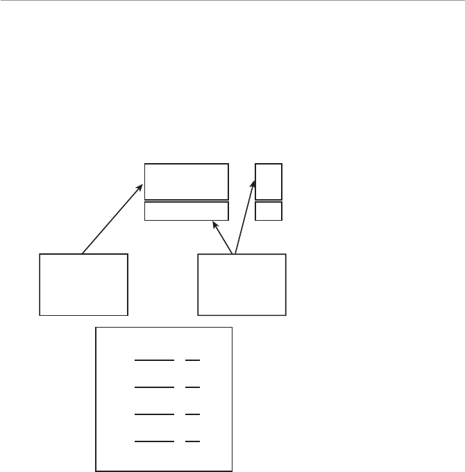
1VO^bS`%( ;]`S>`]POPWZWbgAbcTT
Ac[[O`WhW\U=c`4W\RW\Ua
Before moving on, let’s step back and take a look at what we’ve done so far. Figure 7.2
shows the simple, joint, and conditional probabilities in the relative frequency distri-
bution for our tennis matches.
4WUc`S%
Summary of probabilities for
the tennis example.
Summary of Probabilities for Tennis Example
Warm-Up Time
Less than 10 Min (B)
10 Min or More (B')
Totals
Deb Wins
(A)
0.20
0.25
0.45
Bob Wins
(A')
0.45
0.10
0.55
Totals
0.65
0.35
1.00
p[A and B] = 0.20
p[A' and B] = 0.45
p[A and B'] = 0.25
p[A' and B'] = 0.10
Joint Probabilities
Conditional Probabilities
p[A ] = 0.45
p[A'] = 0.55
p[B] = 0.65
p[B'] = 0.35
Simple Probabilities
P[A/B] P[A and B]
P[B]
0.20
0.65 0.31
===
P[A'/B] P[A' and B]
P[B]
0.45
0.65 0.69
===
P[A/B'] P[A and B']
P[B']
0.25
0.35 0.71
===
P[A'/B'] P[A' and B']
P[B']
0.10
0.35 0.29
===
Note that:
UEvent A’ = Bob wins the match.
UEvent B’ = The warm-up is 10 minutes or more.
These conditional probabilities have revealed my secret to success on the court. The
probability of my winning after a short warm-up, P[A’/B], is 0.69; whereas the prob-
ability of my winning after a longer warm-up, P[A’/B’], is 0.29. I knew I should have
picked another example for this chapter.

>O`b ( >`]POPWZWbgB]^WQa
0OgSaÂBVS]`S[
Thomas Bayes (1701–1761) developed a mathematical rule that deals with calculating
P[B/A] from information about P[A/B]. Bayes’ theorem states the following:
P[B/A] P[B]P[A/B]
(P[B]P[A/B])+(P[B’]P[A/B’]
))
where:
P[B’] = the probability of the complement of Event B
P[A/B’] = the probability of Event A, given that the complement to Event B has
occurred
Now that looks like a mouthful, but applying it in our tennis example will clear things
up. With Bayes’ theorem, we can calculate P[B/A], which is the probability that the
warm-up was less than 10 minutes, given that Debbie won the match. Using the val-
ues from the previous figure:
P[B/A]
065 031
065 031 035 071
..
.. ..
P[B/A]
020
020 025 044
.
...
Knowing that Debbie won the match, we can say
there is a 44 percent chance that the warm-up was
less than 10 minutes.
We can confirm this result by looking at the original
contingency table. Because Debbie won 9 matches
and from those, 4 had a warm-up of less than 10
minutes:
P[B/A]
4
9044.
Ta da! Please hold your applause until the end of the
book.
Not only was Thomas Bayes
a prominent mathematician,
but he was also a published
Presbyterian minister who used
mathematics to study religion.
Random Thoughts

1VO^bS`%( ;]`S>`]POPWZWbgAbcTT !
G]c`Bc`\
A political telephone survey of 260 people asked whether they were in favor or not in
favor of a proposed law. Each person was identified as Republican or Democrat. The
following contingency table shows the results.
Party In Favor Not in Favor Total
Republican 98 54 152
Democrat 79 29 108
Total 177 83 260
A person from the survey is selected at random. We define:
UEvent A: The person selected is in favor of the new law.
UEvent B: The person selected is a Republican.
1. Determine the probability that the selected person is in favor of the new law.
2. Determine the probability that the selected person is a Republican.
3. Determine the probability that the selected person is not in favor of the new law.
4. Determine the probability that the selected person is a Democrat.
5. Determine the probability that the selected person is in favor of the new law
given that the person is a Republican.
6. Determine the probability that the selected person is not in favor of the new law
given that the person is a Republican.
7. Determine the probability that the selected person is in favor of the new law
given that the person is a Democrat.
8. Determine the probability that the selected person is in favor of the new law and
that the person is a Republican.
9. Determine the probability that the selected person is in favor of the new law and
that the person is a Democrat.
10. Determine the probability that the selected person is in favor of the new law or
that the person is a Republican.

>O`b ( >`]POPWZWbgB]^WQa"
11. Determine the probability that the selected person is in favor of the new law or
that the person is a Democrat.
12. Using Bayes’ theorem, calculate the probability that the selected person was a
Republican, given that the person was in favor of the new law.
BVS:SOabG]c<SSRb]9\]e
UWe define conditional probability as the probability of Event A knowing that
Event B has already occurred.
UWe can say Events A and B are independent of each other if the occurrence of
Event B has no effect on the probability of Event A. If Events A and B are not
independent of one another, then they are said to be dependent events.
UFor dependent events, the multiplication rule states that
P[A and B] = P[A/B] P[B]. If the events are independent, the multiplication rule
simplifies to P[A and B] = P[A] P[B].
UWe consider two events to be mutually exclusive if they cannot occur at the same
time during the experiment.
UFor mutually exclusive events, the addition rule states that
P[A or B] = P[A] + P[B]. If the events are not mutually exclusive, the addition
rule becomes P[A or B] = P[A] + P[B] – P[A and B].
UBayes’ theorem deals with calculating P[B/A] from information about P[A/B]
using the following formula:
P[B/A] P[B]P[A/B]
(P[B]P[A/B]) (P[B’]P[A/B’]
))

8
1VO^bS`
1]c\bW\U>`W\QW^ZSaO\R
>`]POPWZWbg2Wab`WPcbW]\a
7\BVWa1VO^bS`
UUsing the fundamental counting principle
UDistinguishing between permutations and combinations
UDefining a random variable and probability distribution
UCalculating the mean and variance of a discrete probability distribu-
tion
Well, we’ve finally arrived at our third and last chapter on general probabil-
ity concepts. This chapter sets the stage for the last three chapters in Part
2, which will focus on specific types of probability distributions. Before you
know it, we’ll be knee deep with inferential statistics.
This chapter will also teach you how to count. This type of counting, how-
ever, goes far beyond what you’ve seen on Sesame Street. Counting events is
an important step in calculating probabilities and must be done with care.
>O`b ( >`]POPWZWbgB]^WQa$
1]c\bW\U>`W\QW^ZSa
To use classical probability, which we introduced way back in Chapter 6, we need
to be able to count the number of events of interest along with the total number of
events that are possible in the sample space. For simple events, like rolling a single die,
the number of possible outcomes (six) is obvious. But for more complex events, like a
state lottery drawing, we need to rely on techniques known as counting principles to
arrive at the correct answer, so let’s look at these techniques.
BVS4c\RO[S\bOZ1]c\bW\U>`W\QW^ZS
After a tough round of golf on a hot afternoon, Brian, John, and I decide to revive our
spirits at the ice cream store on the way home. There I’m overwhelmed with deciding
between four flavors and three toppings to indulge in.
How many different combinations of ice cream and
toppings am I faced with? The fundamental counting
principle comes to my rescue by telling me that if one
event (my ice cream choice) can occur in m ways and
a second event (my topping choice) can occur in n
ways, the total number of ways both events can occur
together is mn ways. In my case, I have mn com-
binations of flavors and toppings in which to blow my
diet. (I’ll leave that topic for another chapter.)
Now I can extend this principle to more than two
events. In addition to flavors and toppings, I have
another tempting choice between a small and large
serving. That leaves me with the mind-boggling decision of 432 24 combinations,
which are summarized in the table that follows my list of options.
Ice Cream Flavors Toppings Size
CH = Death by Chocolate HF = Hot Fudge LG = Large
VA = Vanilla BS = Butterscotch SM = Small
ST = Strawberry SP = Sprinkles
CF = Coffee
According to the fundamental
counting principle, if one event
can occur in mways and a
second event can occur in n
ways, the total number of ways
both events can occur together
is m• n ways. And we can
extend this principle to more
than two events.

1VO^bS`&( 1]c\bW\U>`W\QW^ZSaO\R>`]POPWZWbg2Wab`WPcbW]\a %
List of Combinations (Flavor-Topping-Size)
CH-HF-LG VA-HF-LG ST-HF-LG CF-HF-LG
CH-HF-SM VA-HF-SM ST-HF-SM CF-HF-SM
CH-BS-LG VA-BS-LG ST-BS-LG CF-BS-LG
CH-BS-SM VA-BS-SM ST-BS-SM CF-BS-SM
CH-SP-LG VA-SP-LG ST-SP-LG CF-SP-LG
CH-SP-SM VA-SP-SM ST-SP-SM CF-SP-SM
Can you guess which choice a certain chocolate-loving author made?
Another demonstration of the fundamental counting principle is to calculate the num-
ber of unique combinations for a state’s automobile license plates. Suppose the state
plates have three letters followed by four numbers. The number zero and the letter O
are not eligible because their resemblance may cause confusion. Because we have 25
possible letters and 9 possible numbers, the total number of unique combinations is as
follows:
First Second Third First Second Third Fourth
Letter Letter Letter Number Number Number Number
25 25 25 9 9 9 9
25 × 25 × 25 × 9 × 9 × 9 × 9 = 102,515,625!
That’s 102,515,625 possible combinations!
>S`[cbObW]\a
Permutations are the number of different ways in which objects can be arranged in
order. In a permutation, each item appears only once. The number of permutations of
n distinct objects is n! (expressed as n factorial) and is defined as follows:
nnn n n!( )( )( ) 1234321
>O`b ( >`]POPWZWbgB]^WQa&
By definition, 0! = 1. For instance, 6 654321 720! . As an example, there are
six permutations for the numbers 1, 2, and 3, as shown here:
123 132 213 231 312 321
Because: 33216!
Before the beginning of a professional basketball
game, the starting 5 players are announced one at a
time. How many different ways can we arrange the
order that the players are announced? The number
of permutations is:
55 4 3 2 1 120!
.
Suppose we want to select only some of the objects in
the group. The number of permutations of n objects
taken r at a time can be found as follows:
nn
nr
P!
()!
r
Permutations are the number of
different ways in which objects
can be arranged in order. The
number of permutations of n
objects taken r at a time can
be found by
nn
nr
P!
()!
r
.
It’s easier to calculate the number of permutations using this formula:
nn
nr nn n n rP!
()! ()( )( )
r 12 1
.
This works because every value in the denominator (the bottom of the fraction) will
cancel out with many values in the numerator (the top of the fraction).
Bob’s Basics
Using our basketball example again, if there are 12 players on the team, how many
different ways can any five players on the team be announced to start the game? In
this case, because n = 12 and r = 5, the number of permutations is as follows:
12 5 12
12 5
121110987654321
7
P!
()!
654321
12 5 12
12 5 12 11 10 9 8 95 040P!
()! ,
I’m sure glad it’s not my job to decide who gets announced first.
1VO^bS`&( 1]c\bW\U>`W\QW^ZSaO\R>`]POPWZWbg2Wab`WPcbW]\a '
Sometimes the order of events is not of consequence, and we’ll discuss those cases in
the next section.
1][PW\ObW]\a
Combinations are similar to permutations,
except that the order of the objects is not
important. The number of combinations of
n objects taken r at a time can be found as
follows:
nCn
nrr
r!
()!!
For example, in poker, five cards are selected
randomly from a deck of 52 cards. How
many five-card combinations exist?
52 5 52
52 5 5
52 51 50 49 48
54321 2C
!
()!! ,,,598 960
How many five-card permutations exist?
52 5 52
52 5 52 51 50 49 48 311 875 200P
!
()! ,,
Combinations are the number
of different ways in which
objects can be arranged with-
out regard to order. The number
of combinations of n objects
taken r at a time can be found
by nCn
nrr
r!
()!!
.
It’s easier to calculate the number of combinations using the same logic as the per-
mutation formula and this formula:
n
Cn
nrr
nn n n r
r
r
!
()!!
()( )( )
!
12 1
Bob’s Basics
There are more five-card permutations because the following two poker hands would
be considered two different permutations but be counted as only one combination
because they are the same cards only in different order.
>O`b ( >`]POPWZWbgB]^WQa
Hand 1 Hand 2
Ace of Spades Ace of Spades
Queen of Hearts Ten of Spades
Ten of Spades Queen of Hearts
Ten of Diamonds Ten of Diamonds
Three of Clubs Three of Clubs
Now that we know the total number of five-card combinations from a 52-card deck,
we can calculate the probability of a flush, which is any five cards that are all the same
suit (spades, clubs, hearts, or diamonds). For you poker veterans, I am including a
royal flush and a straight flush in this calculation. First, we need to count the number
of five-card flushes of one suit, let’s say diamonds. Because there are 13 diamonds in
the deck, the number of combinations of these 13 diamonds, taken five at a time, is as
follows:
13 5 13
13 5 5
13 12 11 10 9
54321 1C
!
()!! ,2287
Because there are four suits in the deck, the total number of five-card flushes from
any suit is 1287 4 5 148,. Therefore, the probability of being dealt a flush, including
royal and straight, in a five-card hand is:
P[Flush]
5 148
2 598 960 0 002
,
,, .
or roughly twice in 1,000 hands of poker. Ready to deal?
What about the probability of being dealt a hand
with two pairs of any suit? There are 13 2 78C dif-
ferent two-pair combinations in the deck. Each pair
can have 42 6C different combinations of the four
suits. There are 52 – 6 = 44 possible cards left for the
fifth card in the hand. The number of two-pair hands
would then be:
78 6 6 44 123 552 ,
Therefore, the probability of being dealt two pair is
P[Two-pair]
123 552
2 598 960 0 0475
,
,, .
An alternate notation for nCr
is r
n
¥
§
¦´
¶
µ, which you may
come across in other textbooks.
Statisticians just love to have
different notations for the same
concept!
Bob’s Basics

1VO^bS`&( 1]c\bW\U>`W\QW^ZSaO\R>`]POPWZWbg2Wab`WPcbW]\a
Combinations are also useful for calculating the probability of winning a state lottery
drawing. A typical lottery game requires you to pick six numbers out of a possible 49.
Because the order of the numbers does not matter, we use the combination rather
than the permutation formula. The number of six-number combinations from a pool
of 49 numbers is this:
49 6 49
49 6 6
49 48 47 46 45 44
6543
C
!
()!! 221 13 983 816
,,
Because there are nearly 14 million different six-number combinations, the probability
that your combination is the winner is as follows:
P[Winning a 6/49 Lottery]
1
13 983 816 0 000
,, .000007
Probability does not have a memory. The same six numbers selected in last
week’s lottery drawing have the exact same probability of being chosen again in
this week’s lottery. That’s because the two drawings are independent events and have
absolutely no influence on each other. Therefore, choosing a lottery number because
it has not been selected recently does not increase your odds of winning. Sorry if I
ruined your favorite strategy!
Wrong Number
With those chances of winning the lottery, you better not quit your day job just yet.
CaW\U3fQSZb]1OZQcZObS>S`[cbObW]\aO\R1][PW\ObW]\a
Here’s something that’s pretty cool—rather than deal with all those nasty factorial cal-
culations, we can let Excel figure out the number of permutations or combinations for
us. The functions are:
=PERMUT(n, r)
=COMBIN(n, r)
For example, if we type =PERMUT(12,5) into Excel, the result will be 95,040. Be
sure to try this and give your poor calculator a rest!

>O`b ( >`]POPWZWbgB]^WQa
As we wrap up the topic of counting principles, many of you may be surprised at how
complicated it can be to count events. But this is an important concept in statistics
that we will revisit in Chapter 9.
>`]POPWZWbg2Wab`WPcbW]\a
Now let’s introduce you to probability distributions and prepare you for the last three
chapters of Part 2. However, first we need to discuss the topic of random variables,
which will lay the groundwork for specific probability distributions in Chapters 9, 10,
and 11.
@O\R][DO`WOPZSa
In Chapter 6, we talked about conducting experiments to acquire data. Examples of
experiments could be rolling dice or counting the number of times next month that
I can’t find something in the house and need to ask Debbie to help me. “She who
knows where all things are” has this mystical ability to make these items suddenly
appear before my very eyes after I have given up looking. Debbie then proceeds to
give me a pitiful look that says, “You would never survive a single day in this world
without me,” which sadly I’d have to agree with.
The outcomes of these experiments are considered
random variables. By definition, these outcomes are
not known before the experiment. For example, I
can’t predict with certainty the number of times next
month I’ll need Debbie’s help finding something.
Once the outcome has occurred, I can determine the
value of the random variable. For instance, if I ask
Debbie to help me four times next month, the value
of that random variable is four.
The odds of winning the state lottery drawing are so astronomically low, it’s hard to
really fathom them. Using the 6/49 lottery example, if I bought one ticket every day
of the year, I can expect to win once every 38,312 years. To give this some perspec-
tive, 38,000 years ago, people were living in caves during the Stone Age. I’m not
sure I want to wait that long, no matter how much money I win.
Random Thoughts
Arandom variable is an out-
come that takes on a numerical
value as a result of an experi-
ment. The value of the random
variable, which is not known
with certainty before the experi-
ment, is often denoted by x.
1VO^bS`&( 1]c\bW\U>`W\QW^ZSaO\R>`]POPWZWbg2Wab`WPcbW]\a !
All random variables are not created equal. The first type are known as continuous ran-
dom variables, which are the result of a measurement on a continuous number scale.
For example, each morning when I take a deep breath and step on the bathroom scale
to weigh myself (taking a deep breath and holding it somehow makes me feel lighter),
I’m looking down in shock and disbelief at a continuous random variable. (Maybe I
should have chosen the small Death by Chocolate serving.) Examples of values for
continuous random variables of this sort could be 180, 181.5, 183.2, and so on. (I’ll
stop there.) Because this is a continuous variable, my morning weight could take on an
unlimited number of possible values, which is a very disconcerting thought.
The second type of random variable is discrete. Discrete random variables are the
result of counting outcomes rather than measuring them. Discrete random variables
can only take on a certain number of integer
values within an interval. An example of a
discrete random variable would be my golf
score for my next round because this value is
arrived at by counting my total strokes over
18 holes of play. Obviously, this value needs
to be an integer, such as 94, because there
is no way to count a partial stroke (even
though there are times my golf swing feels
like one).
We will discuss continuous random variables
in more detail in Chapter 11. But here and
in Chapters 9 and 10 we will focus solely on
discrete random variables.
2WaQ`SbS>`]POPWZWbg2Wab`WPcbW]\a
A listing of all the possible outcomes of an experiment for a discrete random variable
along with the relative frequency or probability of each outcome is called a discrete
probability distribution. To illustrate this concept, I’ll use this example.
My oldest daughter, Christin, was a very accomplished competitive swimmer between
the ages of 7 and 13, but her talent certainly didn’t come from my side of the family.
One day, I mustered the courage to ask Christin to teach me how to swim the but-
terfly stroke. My form was best described as “a beached whale having seizures.” The
lifeguards banned me from ever attempting this stroke again, claiming it too closely
resembled a person who was drowning. Somehow, in spite of this gene pool (Get it?
Swimming pool, gene pool?), Christin could not only swim, but she also could swim
fast.
A random variable is continu-
ous if it can assume any numeri-
cal value within an interval
as a result of measuring the
outcome of an experiment. A
random variable is discrete if it
is limited to assuming only spe-
cific integer values as a result
of counting the outcome of an
experiment.
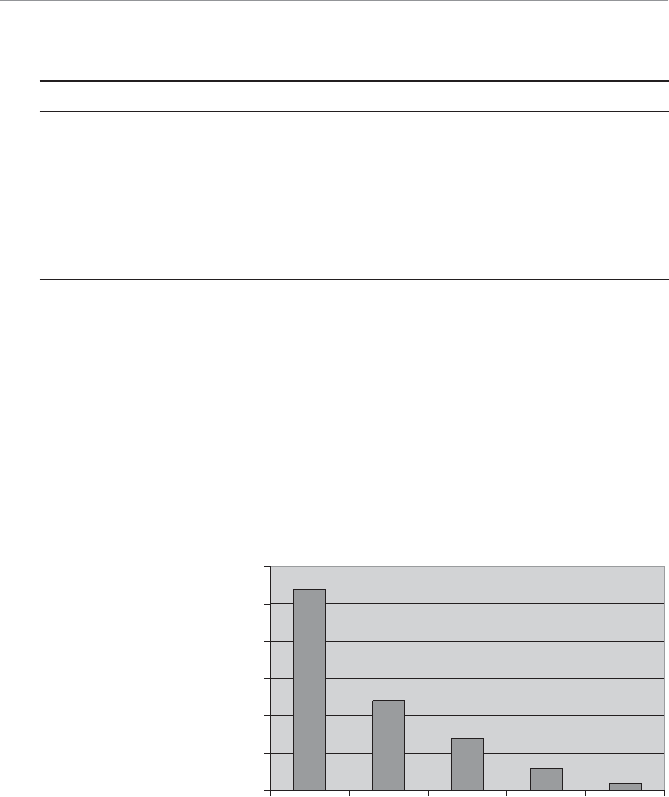
>O`b ( >`]POPWZWbgB]^WQa"
The following table is a relative frequency distribution showing the number of first-,
second-, third-, fourth-, and fifth-place finishes Christin earned during 50 races.
Place Number of Races Relative Frequency (Probability)
127
27/50 = 0.54
212
12/50 = 0.24
37
7
/50 = 0.14
43
3/50 = 0.06
51
1/50 = 0.02
Total = 50 Total = 1.00
If we define the random variable x = the place Christin finished in a race, the previous
table would be the discrete probability distribution for the variable x. From this table,
we can state the probability that Christin will finish first as follows:
P[x = 1] = 0.54
Or we can state the probability that Christin will finish either first or second as fol-
lows:
P[x = 1 or x = 2] = 0.54 + 0.24 = 0.78
Figure 8.1 shows the discrete probability distribution for x graphically.
0
0.1
0.2
0.3
0.4
0.5
0.6
12345
Place
Probability
4WUc`S&
The discrete probability dis-
tribution for Christin’s races.

1VO^bS`&( 1]c\bW\U>`W\QW^ZSaO\R>`]POPWZWbg2Wab`WPcbW]\a #
@cZSaT]`2WaQ`SbS>`]POPWZWbg2Wab`WPcbW]\a
Any discrete probability distribution needs to meet the following requirements:
UEach outcome in the distribution needs to be mutually exclusive—that is, the
value of the random variable cannot fall into more than one of the frequency
distribution classes. For example, it is not possible for Christin to take first and
second place in the same race.
UThe probability of each outcome, P[x], must be between 0 and 1; that is,
01bbP[x] for all values of x. In the previous example, P[x30
14].
, which
falls between 0 and 1.
UThe sum of the probabilities for all the outcomes in the distribution needs to add
up to 1; that is, P[xi
i
n
]
¤1
1
. In the swimming example, the sum of the Relative
Frequency (Probability) column in the previous table adds up to 1.
BVS;SO\]TO2WaQ`SbS>`]POPWZWbg2Wab`WPcbW]\
The mean of a discrete probability distribution is simply a weighted average (discussed
in Chapter 4) calculated using the following formula:
M
¤xx
i
i
n
i
P
1
[]
where:
M
= the mean of the discrete probability distribution
xi = the value of the random variable for the ith outcome
P[xi] = the probability that the ith outcome will occur
n = the number of outcomes in the distribution
The table that follows revisits Christin’s swimming probability distribution.
Place xiProbability P[xi]
1 0.54
20.24
30.14
4 0.06
5 0.02
>O`b ( >`]POPWZWbgB]^WQa$
The mean of this discrete probability distribution is as follows:
M
M
¤xx
i
i
n
i
P
1
1054 2024 3014
[]
...
4 0 06 5 0 02
178
..
.
M
This mean is telling us that Christin’s average finish for a race is 1.78 place! How does
she do that? Obviously, this will never be the result of any one particular race. Rather,
it represents the average finish of many races. The mean of a discrete probability dis-
tribution does not have to equal one of the values of the random variable (1, 2, 3, 4, or
5 in this case).
Another term for describing the mean of a probabil-
ity distribution is the expected value, E[x]. Therefore:
Ex x x
i
i
n
i
[] [ ]
¤
M
P
1
Didn’t I say statisticians love all sorts of notation to
describe the same concept?
BVSDO`WO\QSO\RAbO\RO`R2SdWObW]\]TO2WaQ`SbS>`]POPWZWbg2Wab`WPcbW]\
Just when you thought it was safe to get back into the water, along comes another
variance! Well, if you’ve seen one variance calculation, you’ve seen them all. You can
calculate the variance for a discrete probability distribution as follows:
SM
22
1
¤()[]xx
i
i
n
i
P
where:
S
2 = the variance of the discrete probability distribution
As before, the standard deviation of the distribution is as follows:
SS
2
To demonstrate the use of these equations, we’ll rely on Christin’s swimming distribu-
tion. The calculations are summarized in the following table.
An expected value is the mean
of a probability distribution.

1VO^bS`&( 1]c\bW\U>`W\QW^ZSaO\R>`]POPWZWbg2Wab`WPcbW]\a %
x
i
P[xi]
M
xi
M
()xi
M
2
()]xx
ii
M
2P[
1 0.54 1.78 -0.78 0.608 0.328
2 0.24 1.78 0.22 0.048 0.012
3 0.14 1.78 1.22 1.488 0.208
4 0.06 1.78 2.22 4.928 0.296
5 0.02 1.78 3.22 10.368 0.208
SM
22
1
1 052
¤()].xx
i
i
n
i
P[
The standard deviation of this distribution is:
SS
21 052 1 026..
A more efficient way to calculate the variance of a discrete probability distribution is:
SM
22
1
2
¥
§
¦´
¶
µ
¤xx
i
i
n
i
P[ ]
The following table summarizes these calculations using Christin’s swimming exam-
ple.
xiP[xi]xi
2xx
ii
2P[ ]
1 0.54 1 0.54
20.24 4 0.96
3 0.14 9 1.26
4 0.06 16 0.96
5 0.02 25 0.50
xx
i
i
n
i
2
1
422
¤P[ ] .
SM
22
1
2
¥
§
¦´
¶
µ
¤xx
i
i
n
i
P[ ]
S
22
4 22 1 78 1 052 .(.).
As you can see, the result is the same, but with less effort!

>O`b ( >`]POPWZWbgB]^WQa&
G]c`Bc`\
1. A restaurant has a menu with three appetizers, eight entrées, four desserts, and
three drinks. How many different meals can you order?
2. A multiple-choice test has 10 questions, with each question having four choices.
What is the probability that a student, who randomly answers each question, will
answer each question correctly?
3. The NBA teams with the 13 worst records at the end of the season participate in
a lottery to determine the order in which they will draft new players for the next
season. How many different arrangements exist for the drafting order for these
13 teams?
4. In a race with eight swimmers, how many ways can swimmers finish first, second,
and third?
5. How many different ways can 10 new movies be ranked first and second by a
movie critic?
6. A combination lock has a total of 40 numbers and will unlock with the proper
three-number sequence. How many possible combinations exist?
7. I would like to select three paperback books from a list of 12 books to take on
vacation. How many different sets of three books can I choose?
8. A panel of 12 jurors needs to be selected from a group of 50 people. How many
different juries can be selected?
9. A survey of 450 families was conducted to find how many cats were owned by
each respondent. The following table summarizes the results.
Number of Cats Number of Families
0 137
1 160
2 112
331
410
Develop a probability distribution for this data and calculate the mean, variance,
and standard deviation.
10. What is the probability of being dealt a full house (three-of-a-kind and a pair) in
five-card poker?

1VO^bS`&( 1]c\bW\U>`W\QW^ZSaO\R>`]POPWZWbg2Wab`WPcbW]\a '
BVS:SOabG]c<SSRb]9\]e
UThe fundamental counting principle states that if one event can occur in m ways
and a second event can occur in n ways, the total number of ways both events
can occur together is mn ways. We can extend this principle to more than two
events.
UPermutations are the number of different ways in which objects can be arranged
in order. Combinations are the number of different ways in which objects can be
arranged when order is of no importance.
UA probability distribution is a listing of all the possible outcomes of an experi-
ment along with the relative frequency or probability of each outcome.
UA random variable is an outcome that takes on a numerical value as a result of an
experiment. The value is not known with certainty before the experiment.
UA random variable is continuous if it can assume any numerical value within an
interval as a result of measuring the outcome of an experiment. A random vari-
able is discrete if it is limited to assuming only specific integer values as a result
of counting the outcome of an experiment.
UYou find the mean of a discrete probability distribution as follows:
M
¤xx
i
i
n
i
P
1
[]
.
UYou find the variance of a discrete probability distribution as follows:
SM
22
1
¤()[]xx
i
i
n
i
P.

9
1VO^bS`
BVS0W\][WOZ>`]POPWZWbg
2Wab`WPcbW]\
7\BVWa1VO^bS`
UDescribe the characteristics of a binomial experiment
UCalculate the probabilities for a binomial distribution
UFind probabilities using a binomial table
UFind binomial probabilities using Excel
UCalculate the mean and standard deviation of a binomial distribution
Our discussion of discrete probability distributions so far has been limited
to general distributions based on historical data that has been previously
collected. However, some theoretical probability distributions are based on
a mathematical formula rather than historical data. We will address the first
of these, the binomial probability distribution, in this chapter.
In many types of problems we are interested in the probability of an event
occurring several times. A classical example that has been torturing students
for many years is “What is the chance of getting 7 heads when tossing a
coin 10 times?” By the time you finish this chapter, answering this question
will be a piece of cake!

>O`b ( >`]POPWZWbgB]^WQa
1VO`OQbS`WabWQa]TO0W\][WOZ3f^S`W[S\b
If you remember, in Chapter 6 we defined experimenting as the process of measuring
or observing an activity for the purpose of collecting data. Let’s say our experiment
of interest involves a certain professional basketball player shooting free throws. Each
free throw would be considered a trial for the experiment. For this particular experi-
ment, we have only two possible outcomes for each trial; either the free throw goes in
the basket (a success) or it doesn’t (a failure). Because we can have only two possible
outcomes for each trial, this is known as a binomial experiment.
Let’s say that our player of interest is Michael
Jordan, who historically has made 80 percent of his
free throws. So the probability of success, p, of any
given free throw is 0.80. Because there are only two
outcomes possible, the probability of failure for any
given free throw, q, is 0.20. For a binomial experi-
ment, the values of p and q must be the same for
every trial in the experiment. Because only two out-
comes are allowed in a binomial experiment, pq1
always holds true.
Finally, a binomial experiment requires that each trial
is independent of any other trial. In other words, the
probability of the second free throw being success-
ful is not affected by whether the first free throw was
successful. Other examples of binomial experiments
include the following:
U Testing whether a part is defective after it has
been manufactured
U Observing the number of correct responses in a
multiple-choice exam
U Counting the number of American households
that have an Internet connection
Now that we have defined the ground rules for bino-
mial experiments, we are ready to graduate to calcu-
lating binomial probabilities.
Abinomial experiment has the
following characteristics: (1) the
experiment consists of a fixed
number of trials denoted by n;
(2) each trial has only two pos-
sible outcomes, a success or
a failure; (3) the probability of
success and the probability of
failure are constant throughout
the experiment; (4) each trial is
independent of any other trial in
the experiment.
Binomial experiments are also
known as Bernoulli process,
named after Swiss mathemati-
cian James Bernoulli, who lived
during the 1600s. Repeating a
Bernoulli process several times
is referred to as Bernoulli trials,
a concept that has been haunt-
ing students for hundreds of
years!
Random Thoughts
1VO^bS`'( BVS0W\][WOZ>`]POPWZWbg2Wab`WPcbW]\ !
BVS0W\][WOZ>`]POPWZWbg2Wab`WPcbW]\
The binomial probability distribution allows us to calculate the probability of a spe-
cific number of successes for a certain number of trials. Therefore, the random vari-
able for this distribution would be the number of successes that were observed. To
demonstrate a binomial distribution, I will use the following example.
Debbie has trained our dog, Kaylee, to do an incredible trick. First thing every morn-
ing after she lets the dog out the back door, Kaylee runs like greased lightning around
the house, down our rather long driveway, grabs our newspaper, and races to the back
door, where she dutifully deposits it on the step. In return for this vital chore for our
household, she gets two cups of dry dog food in a plastic bowl. Amazing, you say. But
you’ve only heard half of it. Somehow, in the tiny recesses of Kaylee’s doggy brain,
she has worked out the remarkable deduction that “two breakfasts are better than
one” and at every opportunity goes on a neighborhood hunt for more newspapers to
deposit on our back step. Once she dragged an entire phone book back, thinking maybe
this would earn her a bonus. We have failed miserably trying to train Kaylee to return
these papers—apparently tiny doggy brains don’t work in reverse.
So my job on many afternoons is to care-
fully return the stolen merchandise, hoping
my neighbors fail to notice the dog slobber
on their three-day-old paper. Anyway, let’s
say on any particular day there is a 30 per-
cent probability that Kaylee will bring back
one stolen paper and a 70 percent chance
that she won’t. We will assume that she will
not bring back more than one paper a day.
This scenario represents a binominal experi-
ment, with each day being a Bernoulli trial with
p030.
(the probability of a “suc-
cess”) and q07
0. (the probability of a “failure”). We can calculate the probability of
r successes in n trials using the binomial distribution, as follows:
P[rn n
nrr
pq
rnr
,] !
()!!
With this equation, we can calculate the probability that Kaylee will bring back three
papers over the next five days.
P[3, ] !
()!!
..55
53303 07
353
Remember from Chapter 8
that n
nrr C
n
!
()!! r
, which
represents the number of com-
binations of n objects taken r at
a time.
Bob’s Basics
>O`b ( >`]POPWZWbgB]^WQa "
P[3, ] . . .5120
26 0 027 0 49 0 1323
¥
§
¦´
¶
µ
There is a 13 percent chance that the neighborhood
paper bandit will strike 3 times during the next 5
days. We can also calculate the probability that she
will round up zero, one, two, four, or five papers over
the next five days.
For r= 0:
P[0, ] !
()!!
..55
50003 07
050
P[0, ] . .5120
120 1 1 0 1681 0 1681
¥
§
¦´
¶
µ
For r = 1:
P[1, ] !
()!!
..55
51103 07
151
P[1, ] . . .5120
24 1 0 3 0 2401 0 3601
¥
§
¦´
¶
µ
For r = 2:
P[2, ] !
()!!
..55
52203 07
252
P[2, ] . . .5120
62 0 09 0 343 0 3087
¥
§
¦´
¶
µ
For r= 4:
P[4, ] !
()!!
..55
54403 07
454
P[4, ] . . .5120
124 0 0081 0 7 0 0283
¥
§
¦´
¶
µ
For r = 5:
P[5, ] !
()!!
..55
55503 07
555
Remember from Chapter 8,
0! = 1. Also x0 = 1 for any
value of x.
Bob’s Basics
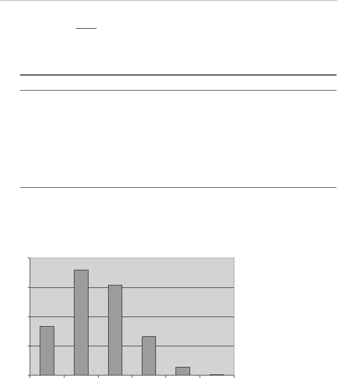
1VO^bS`'( BVS0W\][WOZ>`]POPWZWbg2Wab`WPcbW]\ #
P[5, ] . .5120
1 120 0 0024 1 0 0024
¥
§
¦´
¶
µ
The following table summarizes all the previous probabilities.
r P[r,5]
0 0.1681
1 0.3601
2 0.3087
3 0.1323
4 0.0283
5 0.0024
Total = 1.0
This table represents the binomial probability distribution for rsuccesses in five trials
with the probability of success equal to 0.30. Notice that the sum of all the probabili-
ties equals 1, which is a requirement for all probability distributions. Figure 9.1 shows
this probability distribution as a histogram.
0
0.1
0.2
0.3
0.4
012345
Number of Successes
Probability
4WUc`S'
Binomial probability
distribution.

>O`b ( >`]POPWZWbgB]^WQa $
From this figure, we can see that the most likely number of papers that Kaylee will
show up with over 5 days is 1.
Finally, we can calculate the probability of multiple events for this distribution. For
instance, the probability that Kaylee will steal at least three papers over the next five
days is this:
P[ P[3,5] P[4,5] P[5,5]rr 3]
P[rr 3 0 1323 0 0283 0 0024 0 163]... .
Also, the probability that Kaylee will take no more than one paper over the next five
days is this:
P[ P[0,5] P[1,5]rb 1]
P[rb
1 0 1681 0 3601 0 5285]. . .
Our neighbors will be thrilled to see these figures!
0W\][WOZ>`]POPWZWbgBOPZSa
As the number of trials increases in a binomial experiment, calculating probabilities
using the previous formula will really drain the batteries in your calculator and pos-
sibly even your brain. An easier way to arrive at these probabilities is to use a binomial
probability table, which I have conveniently provided in Appendix B of this book.
Below is an excerpt from this appendix, with the probabilities from our previous
example underlined.
The probability table is organized by values of n, the total number of trials. The num-
ber of successes, r, are the rows of each section, whereas the probability of success, p,
are the columns. Notice that the sum of each block of probabilities for a particular
value of p adds to 1.0.

1VO^bS`'( BVS0W\][WOZ>`]POPWZWbg2Wab`WPcbW]\ %
DOZcSa]T]
nr0.1 0.2 0.3 0.4 0.5 0.6 0.7 0.8 0.9
4 0 0.6561 0.4096 0.2401 0.1296 0.0625 0.0256 0.0081 0.0016 0.0001
1 0.2916 0.4096 0.4116 0.3456 0.2500 0.1536 0.0756 0.0256 0.0036
2 0.0486 0.1536 0.2646 0.3456 0.3750 0.3456 0.2646 0.1536 0.0486
3 0.0036 0.0256 0.0756 0.1536 0.2500 0.3456 0.4116 0.4096 0.2916
4 0.0001 0.0016 0.0081 0.0256 0.0625 0.1296 0.2401 0.4096 0.6561
5 0 0.5905 0.3277 0.1681 0.0778 0.0313 0.0102 0.0024 0.0003 0.0000
1 0.3280 0.4096 0.3601 0.2592 0.1563 0.0768 0.0284 0.0064 0.0005
2 0.0729 0.2048 0.3087 0.3456 0.3125 0.2304 0.1323 0.0512 0.0081
3 0.0081 0.0512 0.1323 0.2304 0.3125 0.3456 0.3087 0.2048 0.0729
4 0.0005 0.0064 0.0283 0.0768 0.1563 0.2592 0.3601 0.4096 0.3281
5 0.0000 0.0003 0.0024 0.0102 0.0313 0.0778 0.1681 0.3277 0.5905
One limitation of using binomial tables is that you are restricted to using only the
values of p that are shown in the table. For instance, the previous table would not be
useful for p03
5..Other statistics books may contain binomial tables that are more
extensive than the one in Appendix B.
CaW\U3fQSZb]1OZQcZObS0W\][WOZ>`]POPWZWbWSa
A convenient way to calculate binomial probabilities is to rely on our friend Excel,
with its BINOMDIST function. This built-in function has the following characteris-
tics:
BINOMDIST(r, n, p, cumulative)
where:
cumulative = FALSE if you want the probability of exactly r successes
cumulative = TRUE if you want the probability of r or fewer successes
For instance, Figure 9.2 shows the BINOMDIST function being used to calculate the
probability that Kaylee will bring back exactly two papers during the next five days.
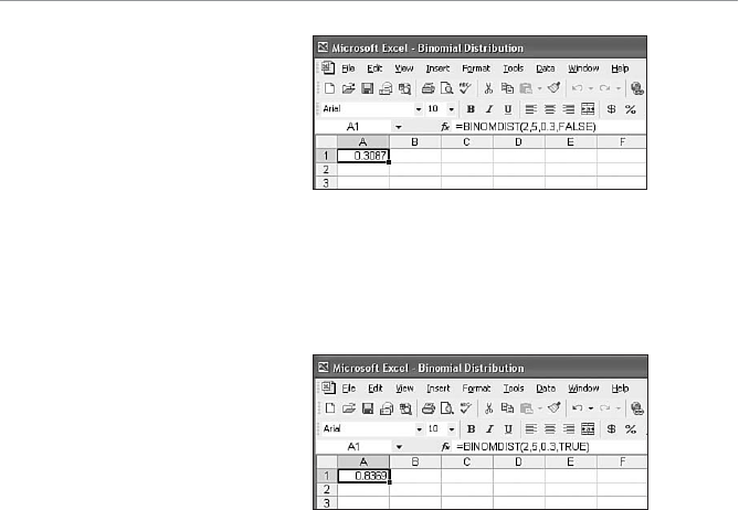
>O`b ( >`]POPWZWbgB]^WQa &
Cell A1 contains the Excel formula =BINOMDIST(2,5,0.3,FALSE) with the result
being 0.3087.
Excel will also calculate the probability that Kaylee will bring back no more than two
papers over the next five days, as shown in Figure 9.3.
4WUc`S'
BINOMDIST function in
Excel for exactly r successes.
4WUc`S'!
BINOMDIST function in
Excel for no more than r
successes.
Cell A1 contains the Excel formula =BINOMDIST(2,5,0.3,TRUE) with the result
being 0.8369, which is the same as this:
P[ P[0,5] P[1,5] P[2,5]rb 2]
P[rb 2 0 1681 0 3601 0 3087 0 8369]... .
In other words, there is more than an 83 percent chance Kaylee will show up at our
back door with 0, 1, or 2 papers that don’t belong to us during the next 5 days. That
dog sure does keep me busy!
One benefit of using Excel to determine binomial probabilities is that you are
not limited to the values of p shown in the binomial table in Appendix B. Excel’s
BINOMDIST function allows you to use any value between 0 and 1 for p.

1VO^bS`'( BVS0W\][WOZ>`]POPWZWbg2Wab`WPcbW]\ '
BVS;SO\O\RAbO\RO`R2SdWObW]\T]`bVS0W\][WOZ
2Wab`WPcbW]\
You can calculate the mean for a binomial probability distribution by using the follow-
ing equation:
M
np
where:
n = the number of trials
p = the probability of a success
For Kaylee’s example, the mean of the distribution is as follows:
M
np ()(.) .503 15papers
In other words, Kaylee brings back, on average, 1.5 papers every 5 days.
You can calculate the standard deviation for a binomial probability distribution using
the following equation:
S
npq
where:
q = the probability of a failure
For our example, the standard deviation of the distribution is as follows:
S
npq ()(.)(.) .5 0 3 0 7 1 02 papers
Well, that about covers the binomial probability distribution discussion. Don’t be too
sad, though; you’ll see this again in future chapters.
G]c`Bc`\
1. What is the probability of seeing exactly 7 heads after tossing a coin 10 times?
2. Goldey-Beacom College accepts 75 percent of applications that are submitted
for entrance. What is the probability that they will accept exactly three of the
next six applications?

>O`b ( >`]POPWZWbgB]^WQa!
3. Michael Jordan makes 80 percent of his free throws. What is the probability that
he will make at least six of his next eight free-throw attempts?
4. A student randomly guesses at a 12-question, multiple-choice test where each
question has 5 choices. What is the probability that the student will correctly
answer exactly six questions?
5. Historical records show that 5 percent of people who visit a particular website
purchase something. What is the probability that no more than two people out
of the next seven will purchase something?
6. During the 2005 Major League Baseball season, Derrek Lee had a 0.335 batting
average. Construct a binomial probability distribution for the number of suc-
cesses (hits) for four official at bats during this season.
7. Sixty percent of a particular college population are female students. What is the
probability that a class of 10 students has exactly 4 female students?
BVS:SOabG]c<SSRb]9\]e
UA binomial experiment has only two possible outcomes for each trial.
UFor a binomial experiment, the probability of success and failure is constant.
UEach trial of a binomial experiment is independent of any other trial in the
experiment.
UThe probability of r successes in n trials using the binomial distribution is as
follows:
P[rn n
nrr
pq
rnr
,] !
()!!
UCalculate the mean for a binomial probability distribution by using the equation
M
np .
UCalculate the standard deviation for a binomial probability distribution by using
the equation
S
npq .

10
1VO^bS`
BVS>]Waa]\>`]POPWZWbg
2Wab`WPcbW]\
7\BVWa1VO^bS`
UDescribe the characteristics of a Poisson process
UCalculate probabilities using the Poisson equation
UUse the Poisson probability tables
UUse Excel to calculate Poisson probabilities
UUse the Poisson equation to approximate the binomial equation
Now that we have mastered the binomial probability distribution, we are
ready to move on to the next discrete theoretical distribution, the Poisson.
This probability distribution is named after Simeon Poisson, a French
mathematician who developed the distribution during the early 1800s.
The Poisson distribution is useful for calculating the probability that a cer-
tain number of events will occur over a specific period of time. We could
use this distribution to determine the likelihood that 10 customers will walk
into a store during the next hour or that 2 car accidents will occur at a busy
intersection this month. So let’s grab some crêpes and croissants and learn
about some French math.

>O`b ( >`]POPWZWbgB]^WQa!
1VO`OQbS`WabWQa]TO>]Waa]\>`]QSaa
In Chapter 9, we defined a binomial experiment, otherwise known as a Bernoulli
process, as counting the number of successes over a specific number of trials. The
result of each trial is either a success or a failure. A Poisson process counts the number
of occurrences of an event over a period of time, area, distance, or any other type of
measurement.
Rather than being limited to only two outcomes, the Poisson process can have any
number of outcomes over the unit of measurement. For instance, the number of cus-
tomers who walk into our local convenience store during the next hour could be zero,
one, two, three, or so on. The random variable for the Poisson distribution would be
the actual number of occurrences—in this case, the number of customers arriving dur-
ing the next hour.
The mean for a Poisson distribution is the average number of occurrences that would
be expected over the unit of measurement. For a Poisson process, the mean has to
be the same for each interval of measurement. For instance, if the average number of
customers walking into the store each hour is 11, this average needs to apply to every
one-hour increment.
The last characteristic of a Poisson process is that the number of occurrences during
one interval is independent of the number of occurrences in other intervals. In other
words, if six customers walk into the store during the first hour of business, this would
have no effect on the number of customers arriving during the second hour.
APoisson process has the following characteristics: (1) the experiment consists of
counting the number of occurrences of an event over a period of time, area, distance,
or any other type of measurement; (2) the mean of the Poisson distribution has to be
the same for each interval of measurement; (3) the number of occurrences during one
interval is independent of the number of occurrences in any other interval.
Examples of random variables that may follow a Poisson probability distribution
include the following:
UThe number of cars that arrive at a tollbooth over a specific period of time
UThe number of typographical errors found in a manuscript

1VO^bS`( BVS>]Waa]\>`]POPWZWbg2Wab`WPcbW]\ !!
UThe number of students who are absent in my Monday-morning statistics class
UThe number of professional football players who are placed on the injured list
each week
Now that you understand the basics of a Poisson process, let’s move into probability
calculations.
BVS>]Waa]\>`]POPWZWbg2Wab`WPcbW]\
If a random variable follows a pattern consistent with a Poisson probability distribu-
tion, we can calculate the probability of a certain number of occurrences over a given
interval. To make this calculation, we need to know the average number of occur-
rences for the event over this interval. To demonstrate the use of the Poisson prob-
ability distribution, I’ll use this example.
The following story is true, but the names have not been changed because nobody in
this story is innocent. Not that any of the previous stories have been false, but this one
is “really” true. Each year, Brian, John, and I make a golf pilgrimage to Myrtle Beach,
South Carolina. On our last night one particular year, we were browsing through a
golf store. Brian somehow convinced me to purchase a used, fancy, brand-name golf
club that he swore he absolutely had to have in order to reach his full potential as a
golfer. Even used, this club cost more than any I had purchased new, but teenagers
have this special talent that allows them to disregard any rational adult logic when
their minds are made up.
Early the following morning, we packed our bags, checked out of the hotel, and drove
to our final round of golf, which I had cleverly planned to be along our route back
home. On the first tee, Brian pulled out his new, used prize possession and proceeded
to hit a “duck hook,” which is a golfer’s term for a ball that goes very short and very
left, often into a bunch of trees never to be seen again. I smiled nervously at Brian and
tried to convince myself that he’d be fine on the next hole. After hitting duck hooks
on holes two, three, and four, I found myself physically restraining Brian from throw-
ing his new, used prized possession into the lake.
After our round was over, I drove back to Myrtle Beach to return the club, adding an
hour to what would have been a 10-hour car ride. (I just hope Brian remembers times
like these when I’m a frail old man drooling away in a retirement home.) At the golf
store, the woman cheerfully said she would take the club back, but I needed to show
her … the receipt. Now I vaguely remembered putting the receipt someplace “special”
just in case I would need it, but after packing, checking out, and playing golf, I would
>O`b ( >`]POPWZWbgB]^WQa!"
have had a better chance of discovering a cure for cancer than remembering where I
had put that piece of paper.
Not being one to give up easily, I marched back to the car and started unpacking
everything. After a short while, during which time I had spread out my dirty under-
wear and socks all over their parking lot, the same woman walked out to tell me the
store would gladly refund my money without the receipt if I would just pack up my
things and put them back in the car.
I discovered a very powerful technique here that I am going to pass along to you. Just
consider this a bonus for using my book. Whenever I can’t find a receipt when I need
to return something, I simply take along some dirty clothes in a suitcase and reenact
my Myrtle Beach scenario right in front of the store. It works like a charm.
Anyway, let’s assume that the number of tee shots that Brian normally hits that actu-
ally land in the fairway during a round of golf is five. The fairway is the area of short
grass where the people who have designed this nerve-wracking game intended your
tee shot to land. We will also assume that the actual number of fairways that Brian
“hits” during one round follows the Poisson distribution.
How do I know that the actual number of fairways that Brian “hits” during one
round follows the Poisson distribution? At this point, I really don’t know for sure.
What I would need to do to verify this claim is record the number of fairways hit over
several rounds and then perform a “Goodness of Fit” test to decide whether the data
fits the pattern of a Poisson distribution. I promise you that we will perform this test in
Chapter 18, so please be patient.
Wrong Number
We can now use the Poisson probability distribution to calculate the probability that
Brian will hit xnumber of fairways during his next round, as follows:
P[xe
x
x
]!
M
M
where:
x = the number of occurrences of interest over the interval
M
= the mean number of occurrences over the interval
e = the mathematical constant 2.71828
1VO^bS`( BVS>]Waa]\>`]POPWZWbg2Wab`WPcbW]\ !#
P[x] the probability of exactly x occurrences over the interval
We can now calculate the probability that
Brian will hit exactly seven fairways during
his next round. With
M
5, the equation
becomes this:
P[7]
5 2 71838
7
75
.
!
P[7]
78125 0 006738
7654321 0 1044
..
In other words, Brian has slightly more
than a 10 percent chance of hitting exactly
seven fairways.
We can also calculate the cumulative prob-
ability that Brian will hit no more than two
fairways using the following equations:
P[ P[ 0] P[ 1] P[ 2]xxx
xb 2]
P[ 0]x
5 2 71838
0
1 0 006738
100
05
.
!
..0067
P[ 1]x
5 2 71838
1
5 0 006738
100
15
.
!
..3337
P[ 2]x
5 2 71838
2
25 0 006738
21
25
.
!
.00 0842.
P[xb 2 0 0067 0 0337 0 0842 0 1246]....
There is a 12.46 percent chance that Brian will hit no more than two fairways during
his next round.
In the previous example, the mean of the Poisson distribution happened to be an
integer (5). However, this doesn’t have to always be the case. Suppose the number
of absent students for my Monday-morning statistics follows a Poisson distribution,
with the average being 2.4 students. The probability that there will be three students
absent next Monday is as follows.
Some statistics books use
the symbol Q, pronounced
lambda, to denote the mean
of a Poisson probability distribu-
tion. However, regardless of
the notation, it’s still the same
equation.
Bob’s Basics
Remember from Chapter 8,
0! = 1. Also x0 = 1 for any
value of x.
Bob’s Basics

>O`b ( >`]POPWZWbgB]^WQa!$
P[ 3]x
2 4 2 71838
3
324
..
!
.
P[ 3]x
13 824 0 090718
321 0 2090
.. .
Looks like I need to start taking roll on Mondays!
There’s one more cool feature of the Poisson distribution: the variance of the distribu-
tion is the same as the mean. In other words:
S
M
2
This means that there are no nasty variance calculations like the ones we dealt with in
previous chapters for this distribution.
>]Waa]\>`]POPWZWbgBOPZSa
Just like the binomial distribution, the Poisson probability distribution has a table
that allows you to look up the probabilities for certain mean values. You can find the
Poisson distribution table in Appendix B of this book. The following is an excerpt
from this appendix with the probabilities from our Myrtle Beach example underlined.
DOZcSa]T
M
x3.2 3.4 3.6 3.8 4.0 4.2 4.4 4.6 4.8 5.0
0 0.0408 0.0334 0.0273 0.0224 0.0183 0.0150 0.0123 0.0101 0.0082 0.0067
1 0.1304 0.1135 0.0984 0.0850 0.0733 0.0630 0.0540 0.0462 0.0395 0.0337
2 0.2087 0.1929 0.1771 0.1615 0.1465 0.1323 0.1188 0.1063 0.0948 0.0842
3 0.2226 0.2186 0.2125 0.2046 0.1954 0.1852 0.1743 0.1631 0.1517 0.1404
4 0.1781 0.1858 0.1912 0.1944 0.1954 0.1944 0.1917 0.1875 0.1820 0.1755
5 0.1140 0.1264 0.1377 0.1477 0.1563 0.1633 0.1687 0.1725 0.1747 0.1755
6 0.0608 0.0716 0.0826 0.0936 0.1042 0.1143 0.1237 0.1323 0.1398 0.1462
7 0.0278 0.0348 0.0425 0.0508 0.0595 0.0686 0.0778 0.0869 0.0959 0.1044
8 0.0111 0.0148 0.0191 0.0241 0.0298 0.0360 0.0428 0.0500 0.0575 0.0653
9 0.0040 0.0056 0.0076 0.0102 0.0132 0.0168 0.0209 0.0255 0.0307 0.0363
10 0.0013 0.0019 0.0028 0.0039 0.0053 0.0071 0.0092 0.0118 0.0147 0.0181
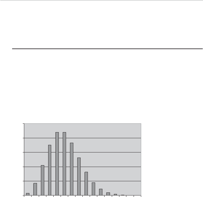
1VO^bS`( BVS>]Waa]\>`]POPWZWbg2Wab`WPcbW]\ !%
11 0.0004 0.0006 0.0009 0.0013 0.0019 0.0027 0.0037 0.0049 0.0064 0.0082
12 0.0001 0.0002 0.0003 0.0004 0.0006 0.0009 0.0013 0.0019 0.0026 0.0034
13 0.0000 0.0000 0.0001 0.0001 0.0002 0.0003 0.0005 0.0007 0.0009 0.0013
14 0.0000 0.0000 0.0000 0.0000 0.0001 0.0001 0.0001 0.0002 0.0003 0.0005
15 0.0000 0.0000 0.0000 0.0000 0.0000 0.0000 0.0000 0.0001 0.0001 0.0002
The probability table is organized by values of R, the average number of occurrences.
Notice that the sum of each block of probabilities for a particular value of R adds to 1.
As with the binomial tables, one limitation of using the Poisson tables is that you are
restricted to using only the values of R that are shown in the table. For instance, the
previous table would not be useful for R = 0.45. However, other statistics books might
contain Poisson tables that are more extensive than the one in Appendix B.
The Poisson distribution for R = 5 is shown graphically in the following histogram.
The probabilities in Figure 10.1 are taken from the last column in the previous table.
0
0.04
0.08
0.12
0.16
0.2
02468
10 12 14
Number of Occurrences
Probability
4WUc`S
Poisson probability
distribution.
Note that the most likely number of occurrences for this distribution is four and five.
Here’s another example. Let’s assume that the number of car accidents each month
at a busy intersection that I pass on my way to work follows the Poisson distribution
with a mean of 1.8 accidents per month. What is the probability that three or more
accidents will occur next month? You can express this as:
P[ P[ P P[ Pxxxxxr d3345]][]][]

>O`b ( >`]POPWZWbgB]^WQa!&
Technically, with a Poisson distribution, there is no upper limit to the number of
occurrences during the interval. You’ll notice from the Poisson tables that the prob-
ability of a large number of occurrences is practically zero. Because we cannot add all
the probabilities of an infinite number of occurrences (if you can, you’re a much better
statistician than I am!), we need to take 1 minus the complement of P[xr3] or:
P[ Pxxr
31 3][]
because:
P[ P[ P[ P[ Pxx
xx x d 0123 10]]]][].
Therefore, to find the probability of three or more accidents, we’ll use the following:
P[ P[ P[ P[xx
x
xr
31012]]]]
Using the probabilities underlined in the following Poisson table (I seem to have mis-
placed my calculator), we have this:
DOZcSa]TR
x1.1 1.2 1.3 1.4 1.5 1.6 1.7 1.8 1.9 2.0
0 0.3329 0.3012 0.2725 0.2466 0.2231 0.2019 0.1827 0.1653 0.1496 0.1353
1 0.3662 0.3614 0.3543 0.3452 0.3347 0.3230 0.3106 0.2975 0.2842 0.2707
2 0.2014 0.2169 0.2303 0.2417 0.2510 0.2584 0.2640 0.2678 0.2700 0.2707
3 0.0738 0.0867 0.0998 0.1128 0.1255 0.1378 0.1496 0.1607 0.1710 0.1804
4 0.0203 0.0260 0.0324 0.0395 0.0471 0.0551 0.0636 0.0723 0.0812 0.0902
5 0.0045 0.0062 0.0084 0.0111 0.0141 0.0176 0.0216 0.0260 0.0309 0.0361
6 0.0008 0.0012 0.0018 0.0026 0.0035 0.0047 0.0061 0.0078 0.0098 0.0120
7 0.0001 0.0002 0.0003 0.0005 0.0008 0.0011 0.0015 0.0020 0.0027 0.0034
8 0.0000 0.0000 0.0001 0.0001 0.0001 0.0002 0.0003 0.0005 0.0006 0.0009
9 0.0000 0.0000 0.0000 0.0000 0.0000 0.0000 0.0001 0.0001 0.0001 0.0002
P[xr
3 1 0 1653 0 2975 0 2678]. . .
P[xr 3 1 0 7306 0 2694]. .
There is almost a 27 percent chance that three or more accidents will occur in this
intersection next month. Looks like I better find a safer way to work!
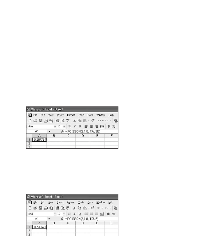
1VO^bS`( BVS>]Waa]\>`]POPWZWbg2Wab`WPcbW]\ !'
CaW\U3fQSZb]1OZQcZObS>]Waa]\>`]POPWZWbWSa
You can also conveniently calculate Poisson probabilities using Excel. The built-in
POISSON function has the following characteristics:
POISSON(x,R, cumulative)
where:
cumulative = FALSE if you want the probability of exactly xoccurrences
cumulative = TRUE if you want the probability of x or fewer occurrences
For instance, Figure 10.2 shows the POISSON function being used to calculate the
probability that there will be exactly two accidents in the intersection next month.
4WUc`S
POISSON function in Excel
for exactly x occurrences.
Cell A1 contains the Excel formula =POISSON(2,1.8,FALSE) with the result being
0.2678. This probability is underlined in the previous table.
Excel will also calculate the cumulative probability that there will be no more than
two accidents in the intersection, as shown in Figure 10.3.
4WUc`S!
POISSON function in Excel
for no more than x occur-
rences.
Cell A1 contains the Excel formula =POISSON(2,1.8,TRUE) with the result being
0.7306, a probability that we saw in the last calculation and which is also the sum of
the underlined probabilities in the previous table.
>O`b ( >`]POPWZWbgB]^WQa"
One benefit of using Excel to determine Poisson probabilities is that you are not lim-
ited to the values of R shown in the Poisson table in Appendix B. Excel’s POISSON
function allows you to use any value for R.
CaW\UbVS>]Waa]\2Wab`WPcbW]\OaO\/^^`]fW[ObW]\b]
bVS0W\][WOZ2Wab`WPcbW]\
I don’t know about you, but when I have two ways to do something, I like to choose
the one that’s less work. If you don’t agree with me, feel free to skip this material. If
you do, read on!
We can use the Poisson distribution to calculate binomial probabilities under the fol-
lowing conditions:
UWhen the number of trials, n, is greater than or equal to 20 and …
UWhen the probability of a success, p, is less than or equal to 0.05 …
The Poisson formula would look like this:
P[xnp e
x
xnp
]!
where:
n = the number of trials
p = the probability of a success
You might be asking yourself at this moment just why
you would want to do this. The answer is because
the Poisson formula has fewer computations than the
binomial formula and, under the stated conditions,
the distributions are very close to one another.
Just in case you are from Missouri (the “Show Me”
state), I’ll demonstrate this point with an example.
Suppose there are 20 traffic lights in my town and
each has a 3 percent chance of not working properly
(a success) on any given day. What is the probability
that exactly 1 of the 20 lights will not work today?
This is a binomial experiment with n = 20, r = 1, and p = 0.03. From Chapter 9, we
know that the binomial probability is this:
If you need to calculate bino-
mial probabilities with the
number of trials, n, greater
than or equal to 20 and the
probability of a success, p, less
than or equal to 0.05, you can
use the equation for the Poisson
distribution to approximate the
binomial probabilities.
Bob’s Basics

1VO^bS`( BVS>]Waa]\>`]POPWZWbg2Wab`WPcbW]\ "
P[rn n
nrr
pq
rnr
,] !
()!!
P[1, ] !
()!!
..20 20
20 1 1 003 097
1201
P[1, ] . . .20 20 0 03 0 560613 0 3364
The Poisson approximation is as follows:
P[xnp e
x
xnp
]!
Because np ()
(.) .20 0 03 0 6 :
P[1 06
1
106
].
!
.
e
P[1 0 6 0 548812 0 3293].. .
Even if you’re from Missouri, I think you would have to agree that the Poisson cal-
culation is easier and the two results are very close. But if you need further proof …
Figures 10.4 and 10.5 show the histogram for each distribution for this example.
4WUc`S"
The binomial probability
distribution with n = 20,
p = 0.03.

>O`b ( >`]POPWZWbgB]^WQa"
Even to a skeptic, these two distributions look very much alike. So my advice to you is
to use the Poisson equation if you’re faced with calculating binomial probabilities with
nr20 and pb00
5..
This concludes our discussion of discrete probability distributions. I hope you’ve had
as much fun with these as I’ve had!
G]c`Bc`\
1. The number of rainy days per month at a particular town follows a Poisson dis-
tribution with a mean value of six days. What is the probability that it will rain
four days next month?
2. The number of customers arriving at a particular store follows a Poisson distri-
bution with a mean value of 7.5 customers per hour. What is the probability that
five customers will arrive during the next hour?
3. The number of pieces of mail that I receive daily follows a Poisson distribution
with a mean value of 4.2 per day. What is the probability that I will receive more
than two pieces of mail tomorrow?
4. The number of employees who call in sick on Monday follows a Poisson distri-
bution with a mean value of 3.6. What is the probability that no more than three
employees will call in sick next Monday?
4WUc`S#
The Poisson probability distri-
bution with the mean = 0.6.

1VO^bS`( BVS>]Waa]\>`]POPWZWbg2Wab`WPcbW]\ "!
5. The number of spam e-mails that I receive each day follows a Poisson distribu-
tion with a mean value of 2.5. What is the probability that I will receive exactly
one spam e-mail tomorrow?
6. Historical records show that 5 percent of people who visit a particular website
purchase something. What is the probability that exactly 2 people out of the next
25 will purchase something? Use the Poisson distribution to estimate this bino-
mial probability.
7. The number of times that Debbie proves me wrong each month follows a
Poisson distribution with a mean of 2.5 times. What is the probability that “she
who is never wrong” will fail to prove me wrong next month?
BVS:SOabG]c<SSRb]9\]e
UA Poisson process counts the number of occurrences of an event over a period of
time, area, distance, or any other type of measurement.
UThe mean for a Poisson distribution is the average number of occurrences that
would be expected over the unit of measurement and has to be the same for each
interval of measurement.
UThe number of occurrences during one interval of a Poisson process is indepen-
dent of the number of occurrences in other intervals.
UIf x is a Poisson random variable, the probability of x occurrences over the
interval of measurement is P[xe
x
x
]!
M
M
.
UIf the number of binomial trials is greater than or equal to 20 and the probability
of a success is less than or equal to 0.05, you can use the equation for the Poisson
distribution to approximate the binomial probabilities.

11
1VO^bS`
BVS<]`[OZ>`]POPWZWbg
2Wab`WPcbW]\
7\BVWa1VO^bS`
UExamining the properties of a normal probability distribution
UUsing the standard normal table to calculate probabilities of a normal
random variable
UUsing Excel to calculate normal probabilities
UUsing the normal distribution as an approximation to the binomial
distribution
Now let’s take on a new challenge, continuous random variables and a
continuous probability distribution known as the normal distribution.
Remember that in Chapter 8 we defined a continuous random variable as
one that can assume any numerical value within an interval as a result of
measuring the outcome of an experiment. Some examples of continuous
random variables are weight, distance, speed, or time.
The normal distribution is a statistician’s workhorse. This distribution is
the foundation for many types of inferential statistics that we rely on today.
We will continue to refer to this distribution through many of the remain-
ing chapters in this book.
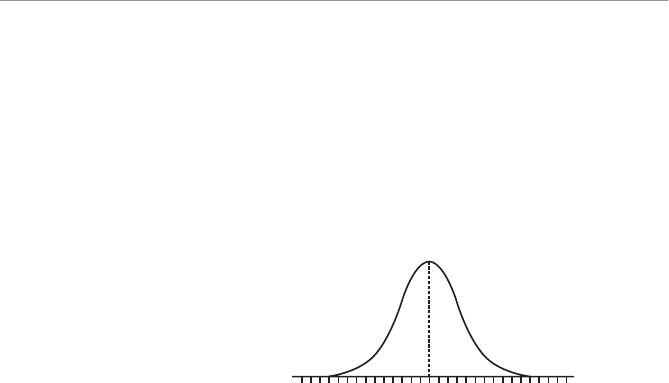
>O`b ( >`]POPWZWbgB]^WQa"$
1VO`OQbS`WabWQa]TbVS<]`[OZ>`]POPWZWbg2Wab`WPcbW]\
A continuous random variable that follows the normal probability distribution has
several distinctive features. Let’s say the monthly rainfall in inches for a particular city
follows the normal distribution with an average of 3.5 inches and a standard devia-
tion of 0.8 inches. The probability distribution for such a random variable is shown in
Figure 11.1.
4WUc`S
Normal distribution with
a mean = 3.5, standard
deviation = 0.8.
Normal Probability Distribution
Mean = 3.5, Standard Deviation = 0.8
0.0 1.0 2.0 3.0 4.0 5.0 6.0 7.0
From this figure, we can make the following observations about the normal distribu-
tion:
UThe mean, median, and mode are the same value—in this case, 3.5 inches.
UThe distribution is bell-shaped and symmetrical around the mean.
UThe total area under the curve is equal to 1.
UThe left and right sides of the normal probability distribution extend indefinitely,
never quite touching the horizontal axis.
The standard deviation plays an important role in the shape of the curve. Looking
at the previous figure, we can see that nearly all the monthly rainfall measurements
would fall between 1.0 and 6.0 inches. Now look at Figure 11.2, which shows the nor-
mal distribution with the same mean of 3.5 inches, but with a standard deviation of
only 0.5 inches.

1VO^bS`( BVS<]`[OZ>`]POPWZWbg2Wab`WPcbW]\ "%
Here you see a curve that’s much tighter
around the mean. Almost all the rainfall
measurements will be between 2.0 and 5.0
inches per month.
Figure 11.3 shows the impact of changing
the mean of the distribution to 5.0 inches,
leaving the standard deviation at 0.8 inches.
4WUc`S
Normal distribution with
a mean = 3.5, standard
deviation = 0.5.
Normal Probability Distribution
Mean = 3.5, Standard Deviation = 0.5
0.0 1.0 2.0 3.0 4.0 5.0 6.0 7.0
A smaller standard deviation
results in a “skinnier” curve
that’s tighter and taller around
the mean. A larger X (standard
deviation) makes for a “fatter”
curve that’s more spread out
and not as tall.
Bob’s Basics
Normal Probability Distribution
Mean = 5.0
,
Standard Deviation = 0.8
0.0 1.0 2.0 3.0 4.0 5.0 6.0 7.0
4WUc`S!
Normal distribution with
a mean = 5.0, standard
deviation = 0.8.
In each of the previous figures, the characteristics of the normal probability distribu-
tion hold true. In each case, the values of R—the mean—and X—the standard
deviation—completely describe the shape of the distribution.

>O`b ( >`]POPWZWbgB]^WQa"&
The probability function for the normal distribution has a particularly mean personal-
ity (that pun was surely intended) and is shown as follows:
fx e x
[] //
¨
ª·
¹
1
2
12 2
SP
MS
I promise you this will be the last you’ll see of this beast. Fortunately, we have other
methods for calculating probabilities for this distribution that are more civilized and
which we will discuss in the next section.
1OZQcZObW\U>`]POPWZWbWSaT]`bVS<]`[OZ2Wab`WPcbW]\
There are a couple of approaches to calculate probabilities for a normal random vari-
able. The following example demonstrates how this is done.
One morning a few days ago, Debbie called me on my cell phone while I was out
running errands and spoke the two words that I had feared hearing for the past year.
“They’re back,” she said. “Okay,” I replied somberly, and then hung up the phone and
headed straight toward the hardware store. My manhood was once again being chal-
lenged, and I’d be darned if I was going to take this lying down. This was war, and I
was coming home fully prepared for battle! I am referring to, of course, my annual
struggle with the most vile, the most dastardly, the most hungry creature that God has
ever placed on this planet … the Japanese beetle.
By the time I returned home from the hardware store, half of our beautiful plum tree
looked like Swiss cheese. I quickly counterattacked with a vengeance, spraying the
most potent chemicals money could buy. In the end, after the toxic spray cleared, I
stood alone, master of my domain.
Alright, let’s say that the amount of toxic spray I use each year follows a normal dis-
tribution with a mean of 60 ounces and a standard deviation of 5 ounces. This means
that each year I do battle with these demons, the most likely amount of spray I’ll use
is 60 ounces, but it will vary year to year. The probability of other amounts above and
below 60 ounces will drop off according to the bell-shaped curve. Armed with this
information, we are now ready to determine probabilities of various usages each year.
1OZQcZObW\UbVSAbO\RO`RHAQ]`S
Because the total area under a normal distribution curve equals 1 and the curve is
symmetrical, we can say the probability that I will use 60 ounces or more of spray
is 50 percent, as is the probability that I will use 60 ounces or less. This is shown in
Figure 11.4.
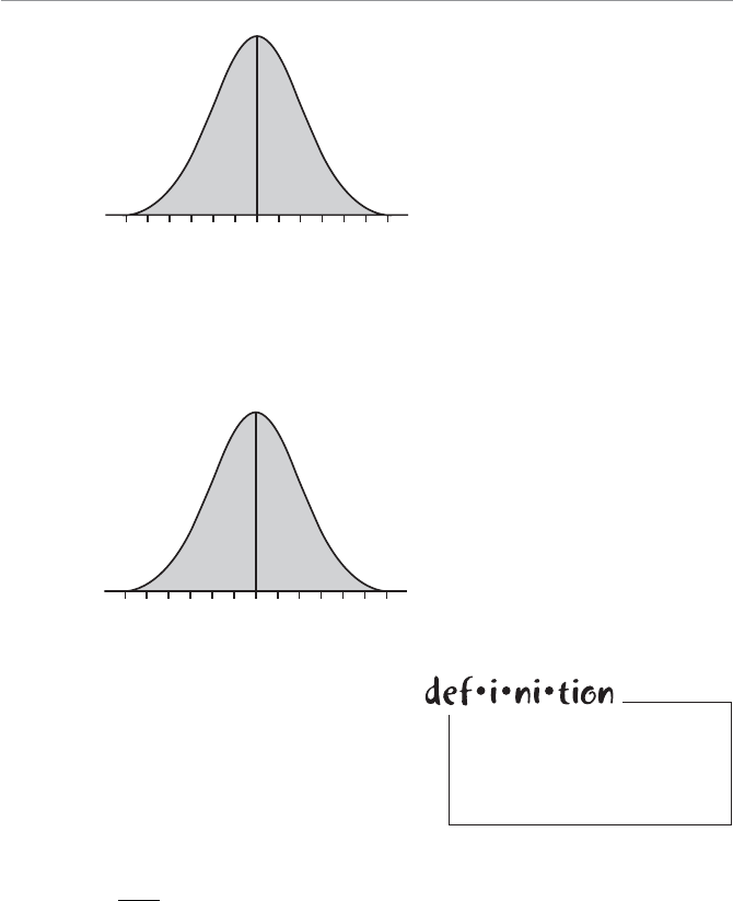
1VO^bS`( BVS<]`[OZ>`]POPWZWbg2Wab`WPcbW]\ "'
How would you calculate the probability that I would use 64.3 ounces of spray or less
next year? I’m glad you asked. For this task, we need to define the standard normal
distribution, which is a normal distribution with R" and X", and is shown in Figure
11.5.
4WUc`S"
Normal distribution with
a mean = 60, standard
deviation = 5.0.
Ounces of Toxic Spray
45
50% 50%
50 55 60 65 70 75
= 60
= 5
4WUc`S#
Standard normal distribution
with a mean = 0, standard
deviation = 1.0.
Number of Standard Deviations
50% 50%
0
=0
=1
This standard normal distribution is the
basis for all normal probability calculations,
and I’ll use it throughout this chapter.
My next step is to determine how many
standard deviations the value 64.3 is from
the mean of 60 and show this value on the
standard normal distribution curve. We do
this using the following formula:
zx
M
S
The standard normal distribu-
tion is a normal distribution with
a mean equal to 0 and a stan-
dard deviation equal to 1.0.

>O`b ( >`]POPWZWbgB]^WQa#
where:
x" the normally distributed random variable of interest
R" the mean of the normal distribution
X" the standard deviation of the normal distribution
z" the number of standard deviations between x and R, otherwise known as the
standard z-score.
For the current example, the standard z-score is as follows:
z64 3
64 3 60
5086
.
..
Now I know that 64.3 is 0.86 standard deviations away from 60 in my distribution.
CaW\UbVSAbO\RO`R<]`[OZBOPZS
Now that I have my standard z-score, I can use the following table to determine the
probability that I will use 64.3 ounces of toxic spray or less next year. This table is an
excerpt from Appendix B and shows the area of the standard normal curve up to and
including certain values of z. Because z = 0.86 in this example, we go to the 0.8 row
and the 0.06 column to find a value of 0.8051, which is underlined.
ASQ]\RRWUWb]TH
z0.00 0.01 0.02 0.03 0.04 0.05 0.06 0.07 0.08 0.09
0.0 0.5000 0.5040 0.5080 0.5120 0.5160 0.5199 0.5239 0.5279 0.5319 0.5359
0.1 0.5398 0.5438 0.5478 0.5517 0.5557 0.5596 0.5636 0.5675 0.5714 0.5753
0.2 0.5793 0.5832 0.5871 0.5910 0.5948 0.5987 0.6026 0.6064 0.6103 0.6141
0.3 0.6179 0.6217 0.6255 0.6293 0.6331 0.6368 0.6406 0.6443 0.6480 0.6517
0.4 0.6554 0.6591 0.6628 0.6664 0.6700 0.6736 0.6772 0.6808 0.6844 0.6879
0.5 0.6915 0.6950 0.6985 0.7019 0.7054 0.7088 0.7123 0.7157 0.7190 0.7224
0.6 0.7257 0.7291 0.7324 0.7357 0.7389 0.7422 0.7454 0.7486 0.7517 0.7549
0.7 0.7580 0.7611 0.7642 0.7673 0.7704 0.7734 0.7764 0.7794 0.7823 0.7852
0.8 0.7881 0.7910 0.7939 0.7967 0.7995 0.8023 0.8051 0.8078 0.8106 0.8133
0.9 0.8159 0.8186 0.8212 0.8238 0.8264 0.8289 0.8315 0.8340 0.8365 0.8389
1.0 0.8413 0.8438 0.8461 0.8485 0.8508 0.8531 0.8554 0.8577 0.8599 0.8621

1VO^bS`( BVS<]`[OZ>`]POPWZWbg2Wab`WPcbW]\ #
This area is shown graphically in Figure 11.6.
4WUc`S$
The shaded area represents
the probability that z will be
less than or equal to 0.86.
Number of Standard Deviations
0.8051
0 0.86
= 1
= 0
The probability that the standard z-score will be less than or equal to 0.86 is 80.51
percent. Because:
P[ P[zxb
b0 86 64 3 0 8051.] .] .
There is an 80.51 percent chance I will use 64.3 ounces of spray or less next year
against those evil Japanese beetles. This can be seen in Figure 11.7.
4WUc`S%
The shaded area represents
the probability that x will
be less than or equal to
64.3 ounces.
Ounces of Toxic Spray
0.8051
60 64.3
= 60
= 5
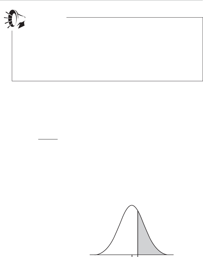
>O`b ( >`]POPWZWbgB]^WQa#
What about the probability that I will use more than 62.5 ounces of spray next year?
Because the standard normal table only has probabilities that are less than or equal to
the z-scores, we need to look at the complement to this event.
PP[.
] [.]xx
b62 5 1 62 5
The z-score now becomes this:
z62.5
62 5 60
5050
..
According to our normal table:
P[ . ] .zb050 0 6915
But we want:
P[ . ] . .z
0 50 1 0 6915 0 3085
This probability is shown graphically in Figure 11.8.
With continuous random variables, we cannot determine the probability of using
exactly 64.3 ounces of spray because this would be an infinitely small probabil-
ity. This is because I can use an infinite amount of quantities in any given year. One
year, I could use 61.757 ounces and another year, 53.472 ounces. That’s why with
continuous random variables we can only calculate the probabilities of certain inter-
vals, like less than 64.3 ounces or between 50.5 and 58.1 ounces. Compare this
to discrete random variables from previous chapters. Because there were only a finite
number of values for these variables, we could calculate the probability of exactly x
occurrences or r successes.
Wrong Number
Number of Standard Deviations
0.3085
0.50
= 0
= 1
4WUc`S&
The shaded area represents
the probability that z will
be more than 0.50.
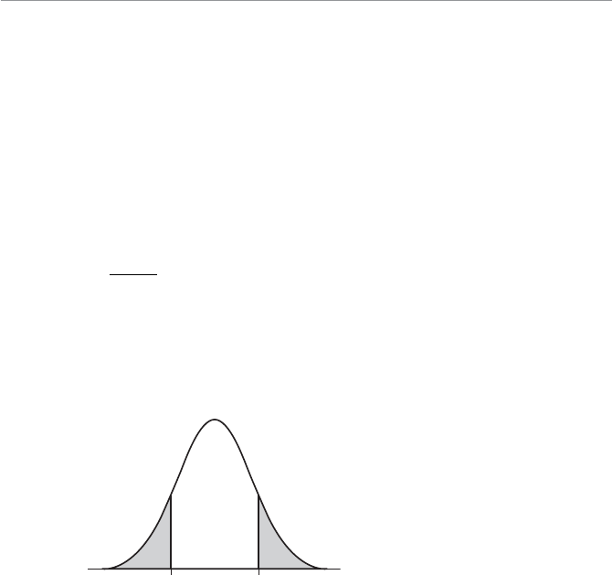
1VO^bS`( BVS<]`[OZ>`]POPWZWbg2Wab`WPcbW]\ #!
Because:
P[ P[zx
0 50 62 5 0 3085.] .] .
There is a 30.85 percent chance that I will use more than 62.5 ounces of toxic spray.
Beetles beware!
What about the probability that I will use more than 54 ounces of spray? Again, I
need the complement, which would be this:
PP[[] ]xx
b54 1 54
The z-score becomes this:
z54
54 60
5120.
The negative score indicates that we are to the left of the distribution mean. Notice
that the standard normal table only shows positive z values. But this is no problem
because the distribution is symmetric. Figure 11.9 shows that the shaded area to the
left of –1.2 standard deviations from the mean is the same as the shaded area to the
right of +1.2 standard deviations from the mean.
4WUc`S'
The shaded areas are equal.
Number of Standard Deviations
1.2-1.2
0.11510.1151
We can determine the area to the right of +1.2 standard deviations as follows:
PP[.
] [.] . .zz b 1 2 1 1 2 1 0 8849 0 1151
Therefore, the area to the left of –1.2 standard deviations from the mean is also
0.1151. We now can calculate the area to the right of –1.2 standard deviations from
the mean.
PP[.
] [.] . .zz b 1 2 1 1 2 1 0 1151 0 8849
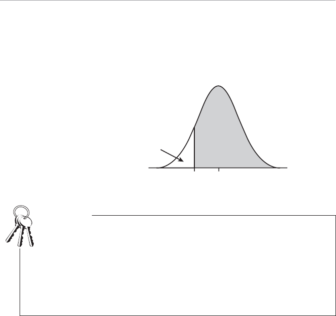
>O`b ( >`]POPWZWbgB]^WQa#"
Because:
PP[[] .
].xz54 1 2 0 8849
There is an 88.49 percent chance I will use more than 54 ounces of spray. This prob-
ability is shown graphically in Figure 11.10.
4WUc`S
The shaded area is the prob-
ability that x will be more
than 54 ounces.
= 60
= 5
Ounces of Toxic Spray
6054
0.1151
0.8849
Finally, let’s look at the probability that I will use between 54 and 62.5 ounces of spray
next year. This probability is shown graphically in Figure 11.11.
A shortcut to the previous example would be to recognize the following:
PP[.]
[.]zz b120 120
P[ . ] .z 1 20 0 8849
In general, you can use the following two relationships for any value a when dealing
with negative z-scores:
PP[]
[]za za b
PP[][]za zab b1
Bob’s Basics
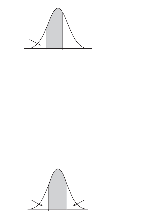
1VO^bS`( BVS<]`[OZ>`]POPWZWbg2Wab`WPcbW]\ ##
We know from previous examples that the area to the left of 54 ounces is 0.1151 and
that the area to the right of 62.5 ounces is 0.3085. Because the total area under the
curve is 1:
P[ . ] . . .54 62 5 1 0 1151 0 3085 0 5764bb x
There is a 57.64 percent chance that I will use between 54 and 62.5 ounces of spray
next year. I can’t wait.
BVS3[^W`WQOZ@cZS@SdWaWbSR
Remember way back in Chapter 5 we discussed the empirical rule, which stated that if
a distribution follows a bell-shaped, symmetrical curve centered around the mean, we
would expect approximately 68, 95, and 99.7 percent of the values to fall within 1.0,
2.0, and 3.0 standard deviations around the mean respectively. I’m glad to inform you
that we now have the ability to demonstrate these results.
The shaded area in Figure 11.12 shows the percentage of observations that we would
expect to fall within 1.0 standard deviation of the mean.
4WUc`S
The shaded area is the prob-
ability that x will be between
54 and 62.5 ounces.
= 60
= 5
Ounces of Toxic Spray
60 62.554
0.1151
0.5764
0.3085
Number of Standard Deviations
1-1
0.1587 0.1587
0.6826
4WUc`S
The shaded area is the prob-
ability that x will be between
–1.0 and +1.0 standard
deviation from the mean.
>O`b ( >`]POPWZWbgB]^WQa#$
Where did 68 percent come from? We can look in the normal table to get the prob-
ability that an observation will be less than one standard deviation from the mean.
P[ . ] .zb 10 0 8413
Therefore, the area to the right of +1.0 standard deviations is this:
P[ . ] . .z 10 1 0 8413 0 1587
By symmetry, the area to the left of –1.0 standard deviations is also 0.1587. That
leaves the area between –1.0 and +1.0 as this:
P[ . . ] . . .b
b 10 1 0 1 0 1587 0 1587 0 6826z
The same logic is used to demonstrate the probabilities of 2.0 and 3.0 standard devia-
tions from the mean. I’ll leave those for you to try.
1OZQcZObW\U<]`[OZ>`]POPWZWbWSaCaW\U3fQSZ
Once again we can rely on Excel to do some of the grunt work for us. The first built-
in function is NORMDIST, which has the following characteristics:
NORMDIST(x, mean, standard dev, cumulative)
where:
cumulative = FALSE if you want the probability mass function (we don’t)
cumulative = TRUE if you want the cumulative probability (we do)
For instance, Figure 11.13 shows the NORMDIST
function being used to calculate the probability that I
will use less than 64.3 ounces of spray on those nasty
beetles next year.
Cell A1 contains the Excel formula =NORMDIST
(64.3,60,5,TRUE) with the result being 0.8051. This
probability is underlined in the previous table.
Excel also has a cool function called NORMSINV,
which has the following characteristics:
NORMSINV(probability)
Don’t be alarmed if the val-
ues that are returned using
the NORMDIST function
in Excel are slightly different
than those found in Table 3
in Appendix B. This is due to
rounding differences that are
small enough to be ignored.
Bob’s Basics
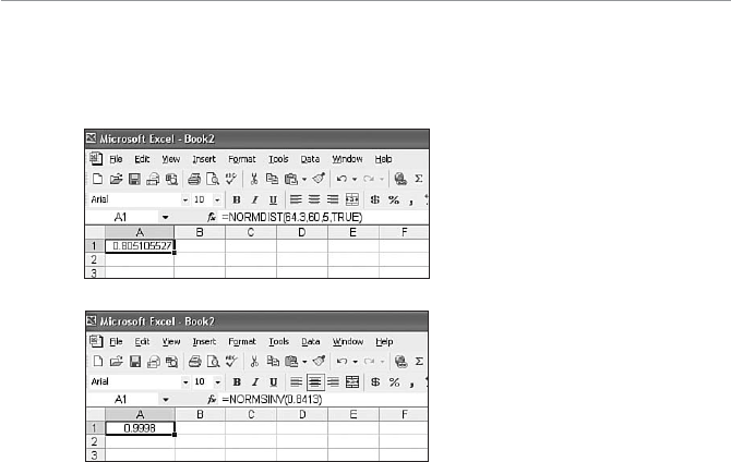
1VO^bS`( BVS<]`[OZ>`]POPWZWbg2Wab`WPcbW]\ #%
You provide this function a probability between 0 and 1, and it returns the corre-
sponding z-score. Figure 11.14 shows the NORMSINV function returning a z-score
for a probability of 0.8413, which is 1.0 standard deviation from the mean.
4WUc`S!
NORMDIST function in
Excel for less than 64.3
ounces.
Cell A1 contains the Excel formula =NORMSINV(0.8413) with the result being
0.9998 (close enough to 1.0). If you look back to Figure 11.12, notice that the area to
the left of 1.0 standard deviation from the mean totals to 0.8413. You can also find this
value in the standard normal table next to z = 1.0.
CaW\UbVS<]`[OZ2Wab`WPcbW]\OaO\/^^`]fW[ObW]\b]
bVS0W\][WOZ2Wab`WPcbW]\
Remember how nasty our friend the binomial distribution can get sometimes? Well,
the normal distribution may be able help us out during these difficult times under the
right conditions. Recall from Chapter 9 that the binomial equation will calculate the
probability of r successes in n trials with p = the probability of a success for each trial
and q = the probability of a failure. If np r5 and nq r5, we can use the normal distri-
bution to approximate the binomial.
4WUc`S"
NORMSINV function in
Excel for 1.0 standard
deviation.
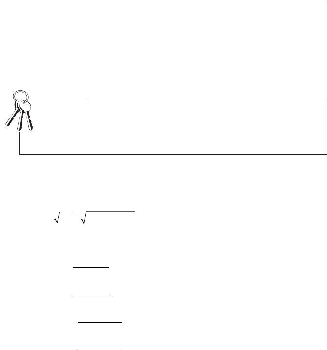
>O`b ( >`]POPWZWbgB]^WQa#&
As an example, suppose my statistics class is composed of 60 percent females. If I
select 15 students at random, what is the probability that this group will include 8,
9, 10, or 11 female students? For this example, n = 15; p = 0.6; q = 0.4; and r = 8, 9,
10, and 11. We can use the normal approximation because np = (15)(0.6) = 9 and
nq = (15)(0.4) = 6. (Sorry, guys. I didn’t mean to infer picking you would be classified
a failure!)
Even if you are not interested in learning how the normal distribution can be
used to approximate the binomial, I strongly encourage you to work through the
example in this section. It will be good practice for determining probabilities for a
normal distribution. And we all know that practice makes perfect!
Bob’s Basics
Also recall from Chapter 9 that the mean and standard deviation of this binomial dis-
tribution is this:
M
np 15 0 6 9.
S
npq 15 06 04 1897.. .
The probability that the group of 15 students will include 8, 9, 10, or 11 female
students can be calculated using the following equations:
P[8, ] !
()!!
..15 15
15 8 8 0 6 0 4 6435 0
8158
... .0168 0 0016 0 1730
P[9, ] !
()!!
..15 15
15 9 9 0 6 0 4 5005 0
9159
... .0101 0 0041 0 2073
P[10, ] !
()!!
..15 15
15 10 10 06 04 30
10 15 10
003 0 0060 0 0102 0 1838
.. .
P[11, ] !
()!!
..15 15
15 11 11 06 04 13
11 15 11
665 0 0036 0 0256 0 1258
.. .
P , 9, 10, or 11][...r8 0 1730 0 2073 0 1838 0...1258 0 6899
Now let’s solve this problem using the normal distribution and compare the results.
Figure 11.15 shows the normal distribution with R" and X".
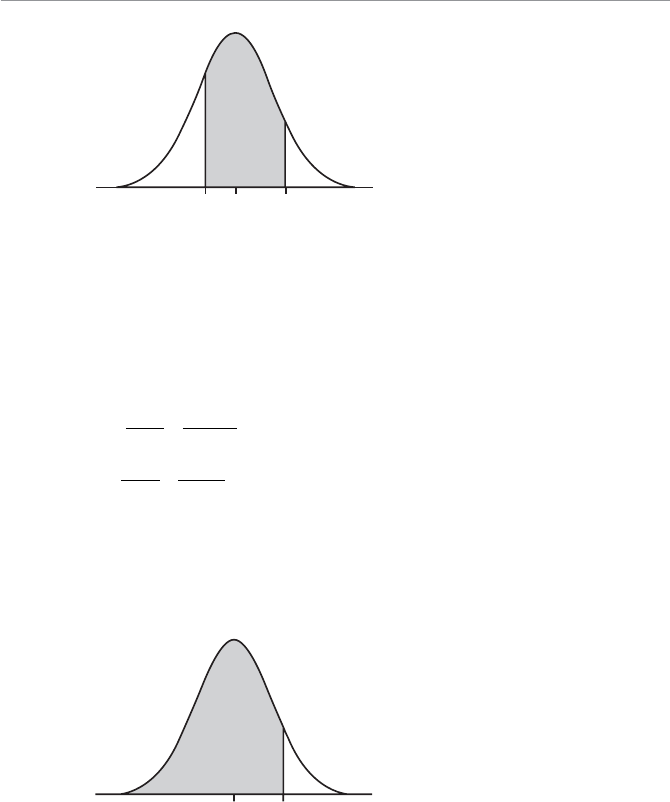
1VO^bS`( BVS<]`[OZ>`]POPWZWbg2Wab`WPcbW]\ #'
Notice that the shaded interval goes from 7.5 to 11.5 rather than 8 to 11. Don’t
worry; I didn’t make a mistake. I subtracted 0.5 from 8 and added 0.5 to 11 to com-
pensate for the fact that the normal distribution is continuous and the binomial is
discrete. Adding and subtracting 0.5 is known as the continuity correction factor. For
larger values of n, like 100 or more, you can ignore this correction factor.
Now we need to calculate the z-scores.
zx
11 5
11 5 9
1 897 132
.
.
..
M
S
zx
75
75 9
1 897 079
.
.
..
M
S
According to the normal table:
P[ . ] .zb 132 0 9066
This area is shown in the shaded region of Figure 11.16.
4WUc`S#
The normal approximation to
the binomial distribution.
Number of Female Students
11.57.5 9
= 9
= 1.897
Number of Standard Deviations
0.7852
+1.320
= 0
= 1 4WUc`S$
The probability that
zf +1.32 standard
deviations from the mean.
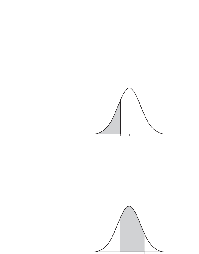
>O`b ( >`]POPWZWbgB]^WQa$
We also know because of symmetry with the normal curve that:
PP[.
] [.]zzb b079 1 079
According to the normal table:
P[ . ] .zb 079 0 7852
Therefore:
P[ . ] . .zb 0 79 1 0 7852 0 2148
This probability is shown in the shaded area in Figure 11.17.
4WUc`S%
The probability that
zf –0.79 standard
deviations from the mean.
Number of Standard Deviations
0-0.79
= 0
= 1
0.2148
The probability of interest for this example is the area between z-scores of –0.79 and
+1.32. We can use the following calculations to find this area:
PPP[. .
] [ .] [ .] b b b b079 132 132 079zzz
P[ . . ] . . .bb 0 79 1 32 0 9066 0 2148 0 6918z
This probability is shown in the shaded area in Figure 11.18.
Number of Standard Deviations
0 +1.32-0.79
= 0
= 1
0.6918
4WUc`S&
The probability that
–0.79 f z f +1.32 standard
deviations from the mean.

1VO^bS`( BVS<]`[OZ>`]POPWZWbg2Wab`WPcbW]\ $
Using the normal distribution, we have determined the probability that my group of
15 students will contain 8, 9, 10, or 11 females is 0.6916. As you can see, this prob-
ability is very close to the result we obtained using the binomial equations, which was
0.6899.
Well, this ends our chapter on the normal probability distribution. And I feel much
better prepared for next year’s return visit of my archenemy, the Japanese beetle. Wish
me luck.
G]c`Bc`\
1. The speed of cars passing through a checkpoint follows a normal distribution
with R = 62.6 miles per hour and X = 3.7 miles per hour. What is the probability
that the next car passing will …
a. Be exceeding 65.5 miles per hour?
b. Be exceeding 58.1 miles per hour?
c. Be between 61 and 70 miles per hour?
2. The selling price of various homes in a community follows the normal distribu-
tion with R = $176,000 and X = $22,300. What is the probability that the next
house will sell for …
a. Less than $190,000?
b. Less than $158,000?
c. Between $150,000 and $168,000?
3. The age of customers for a particular retail store follows a normal distribution
with R = 37.5 years and X = 7.6 years. What is the probability that the next cus-
tomer who enters the store will be …
a. More than 31 years old?
b. Less than 42 years old?
c. Between 40 and 45 years old?
4. A coin is flipped 14 times. Use the normal approximation to the binomial distri-
bution to calculate the probability of a total of 4, 5, or 6 heads. Compare this to
the binomial probability.

>O`b ( >`]POPWZWbgB]^WQa$
5. A certain statistics author’s golf scores follow the normal distribution with a
mean of 92 and a standard deviation of 4. What is the probability that, during his
next round of golf, his score will be …
a. More than 97?
b. More than 90?
6. The number of text messages that Debbie’s son Jeff sends and receives a month
follows the normal distribution with a mean of 4,580 (I am not making this up!)
and a standard deviation of 550. What is the probability that next month he will
send and receive …
a. Between 4,000 and 5,000 text messages?
b. Less than 4,200 text messages?
BVS:SOabG]c<SSRb]9\]e
UThe normal distribution is bell-shaped and symmetrical around the mean.
UThe total area under the normal distribution curve is equal to 1.0.
UThe normal distribution tables are based on the standard normal distribution
where R"1 and X"1.
UThe number of standard deviations between a normally distributed random vari-
able, x, and R is known as the standard z-score and can be found with zx
M
S
.
UExcel has two built-in functions that you can use to perform normal distribution
calculations: NORMDIST and NORMSINV.
UYou can use the normal distribution to approximate the binomial distribution
when
np r5
and nq r5.

3
>O`b
Now we can take all those wonderful concepts that we have stuffed into
our overloaded brains from Parts 1 and 2 and put them to work using
statistically sounding words, such as confidence interval and hypothesis test.
Inferential statistics enables us to make statements about a general popu-
lation using the results of a random sample from that population. For
instance, using inferential statistics, the winner of a political election can be
accurately predicted very early in the polling process based on the results of
a relatively small random sample that is properly chosen. Pretty cool stuff!
7\TS`S\bWOZAbObWabWQa


12
1VO^bS`
AO[^ZW\U
7\BVWa1VO^bS`
UThe reason for measuring a sample rather than the population
UThe various methods for collecting a random sample
UDefining sampling errors
UConsequences for poor sampling techniques
This first chapter dealing with the long-awaited topic of inferential statis-
tics focuses on the subject of sampling. Way back in Chapter 1, we defined
a population as representing all possible outcomes or measurements of
interest, and a sample as a subset of a population. Here we’ll talk about
why we use samples in statistics and what can go wrong if they are not used
properly.
Virtually all statistical results are based on the measurements of a sample
drawn from a population. Major decisions are often made based on infor-
mation from samples. For instance, the Nielson ratings gather information
from a small sample of homes and are used to infer the television-viewing
patterns of the entire country. The future of your favorite TV show rests
in the hands of these select few! So choosing the proper sample is a critical
step to ensure accurate statistical conclusions.
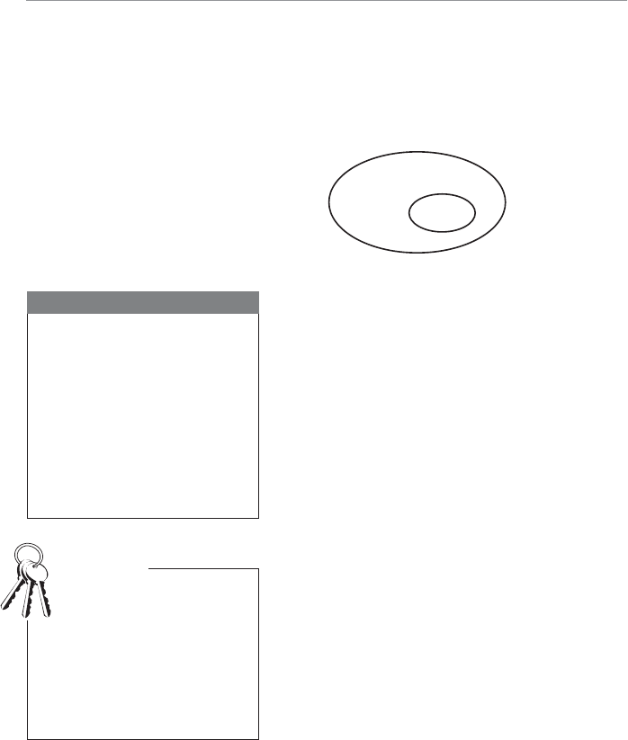
>O`b!( 7\TS`S\bWOZAbObWabWQa$$
EVgAO[^ZS-
Most statistical studies are based on a sample of the population at large. The relation-
ship between a population and sample is shown in Figure 12.1 (and also described in
Chapter 1).
4WUc`S
The relationship between a
population and sample.
Population
Sample
Why not just measure the whole population rather
than rely on only a sample? That’s a very good ques-
tion! Depending on the study, measuring an entire
population could be very expensive or just plain
impossible. If I want to measure the life span of a
certain breed of pesky mosquitoes (extremely short
if I had any say in the matter), I could not possibly
observe every single mosquito in the population.
Rather, I would need to rely on a sample of the mos-
quito population, measure their life span, and make
a statement about the life span of the entire popula-
tion. That’s the whole concept of inferential statis-
tics in one paragraph! Unfortunately, doing what I
just wrote is a whole lot harder than just writing it.
Doing it is what the rest of this book is all about!
Even if we could feasibly measure the entire popula-
tion, to do so would often be a wasteful decision.
If a sample is collected properly and the analysis
performed correctly, we can make a very accurate
assessment of the entire population. There is very
little added benefit to continue beyond the sample
and measure everything in sight. Measuring the
population often is a waste of both time and money,
resources that seem to be very scarce these days.
Nielsen Media Research
surveys 5,000 households
nationwide to infer the television
habits of millions of people.
Because the results of these sur-
veys are the basis for decisions
such as show cancellations and
advertising revenue, you better
believe they select this sample
very carefully.
Random Thoughts
Often it is just not feasible to
measure an entire popula-
tion. Even when it is feasible,
measuring an entire popula-
tion can be a waste of time
and money and provides little
added benefit beyond measur-
ing a sample.
Bob’s Basics
1VO^bS` ( AO[^ZW\U $%
One example where such a decision was recently made occurred at Goldey-Beacom
College, where I presently teach. I am also the Chair of the Academic Honor Code
Committee and was involved in a project whose goal was to gather information
regarding the attitude of our student body on the topic of academic integrity. It would
have been possible to ask every student at our college to respond to the survey, but
it was really unnecessary with the availability of inferential statistics. We eventually
made the intelligent decision and sampled only a portion of the students to infer the
attitudes of the population.
@O\R][AO[^ZW\U
The term random sampling refers to a sampling procedure where every member in the
population has a chance of being selected. The objective of the sampling procedure is
to ensure that the final sample to be measured is representative of the population from
which it was taken. If this is not the case, then we have a biased sample, which can lead
to misleading results. If you recall, we discussed an example of a biased sample back in
Chapter 1 with the golf course survey. The selection of a proper sample is critical to
the accuracy of the statistical analysis.
Since you can select a random sample in sev-
eral ways, I’ll use the following example to
demonstrate these techniques.
Most of the time, I consider Debbie to be
a person of sound mind and judgment (she
married me, after all). Lately, however, I
have had some concerns about her behav-
ior dealing with the fact that she is reach-
ing a major milestone in life before I am.
Although I am not permitted to mention
exactly what this milestone is (under penalty
of her not proofreading any more chapters and other certain activities), I will say it
involves dividing the number 100 by 2. (You do the math.)
Anyway, recently we were walking through the local mall when Debbie suddenly ran to
a sales counter where they were selling fake ponytails for your hair. I had never heard
of such a thing in my life and never would have conceived of the idea in a million
years. Debbie, on the other hand, thought it was absolutely brilliant. Within seconds,
a total stranger appeared from nowhere and before I could say, “That’s my wife,” had
rearranged Debbie’s hair and, in his final crowning moment, expertly arranged a fake
hairpiece that somewhat resembled a small, furry animal on the top of her head.
Random sampling refers to
a sampling procedure where
every member in the popula-
tion has a chance of being
selected. A biased sample is a
sample that does not represent
the intended population and
can lead to distorted findings.

>O`b!( 7\TS`S\bWOZAbObWabWQa$&
Debbie, beaming with her “new look,” turned to me to ask what I thought. Because
this also happened to be our wedding anniversary, I weakly said it looked great as I
handed this total stranger my credit card. (I might be a little slow in these matters, but
I’m not stupid.) Debbie spent the rest of the evening prancing through the mall with
her new cute furry animal hanging on for dear life. I have to admit, once I got used to
the idea, it did look pretty cute.
Now let’s say we wanted to conduct a survey to collect opinions of Debbie’s new look.
In fact, you, the reader, can render your opinion of Debbie after observing Figure 12.2
by sending me an e-mail from the book’s website at www.stat-guide.com.
4WUc`S
Debbie’s new look; what do
you think?
If I consider the current shoppers at the mall that night as my population, I need to
decide how to select the random sample from whose opinion I will ask. As we will see
in the following sections, there are four different ways to gather a random sample:
simple random, systematic, cluster, and stratified.
AW[^ZS@O\R][AO[^ZW\U
Asimple random sample is a sample in which every member of the population has an
equal chance of being chosen. Unfortunately, this is easier said than done. In our mall
example, I can randomly approach people to ask their opinion. However, I might have
1VO^bS` ( AO[^ZW\U $'
some biases in my selection. For instance,
if I observe that a certain menacing-looking
person has a tattoo that says, “Death to All
Statisticians,” I might choose not to ask him
what he thinks of Debbie’s new ponytail. But
in doing so, I might be biasing my sample.
Assuming I can rid myself of any biased
selection, Figure 12.3 would describe a
simple random sample at the mall.
Asimple random sample is a
sample in which every member
of the population has an equal
chance of being chosen.
4WUc`S !
Simple random sample.
X
X
X
X
X
X
X
X
X
X
X
X
X
X
X
X
X
Store 3
Store 2
Store 1
Store 7
Store 6
Store 5
Store 4
Each “X” represents a shopper, and each “X” that’s circled represents a shopper in my
sample.
There would be other options for choosing a simple random sample for the Academic
Integrity survey mentioned earlier in the chapter. I could randomly choose students
using a random number table, which is aptly named. (After all, it is simply a table of
numbers that are completely random.) An excerpt of such a table is shown here:
57245 39666 18545 50534 57654 25519 35477 71309 12212 98911
42726 58321 59267 72742 53968 63679 54095 56563 09820 86291
82768 32694 62828 19097 09877 32093 23518 08654 64815 19894
97742 58918 33317 34192 06286 39824 74264 01941 95810 26247
48332 38634 20510 09198 56256 04431 22753 20944 95319 29515
26700 40484 28341 25428 08806 98858 04816 16317 94928 05512
66156 16407 57395 86230 47495 13908 97015 58225 82255 01956
64062 10061 01923 29260 32771 71002 58132 58646 69089 63694
24713 95591 26970 37647 26282 89759 69034 55281 64853 50837
90417 18344 22436 77006 87841 94322 45526 38145 86554 42733
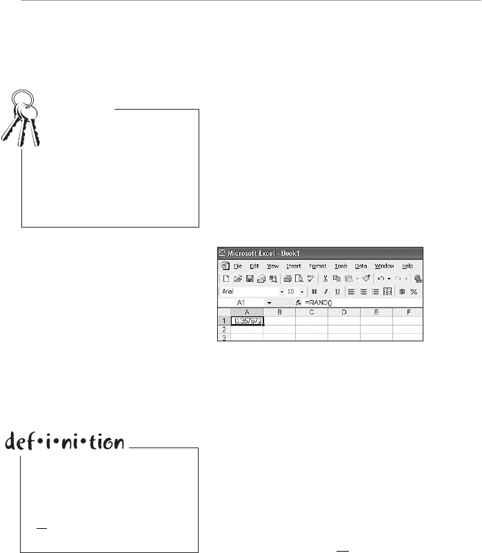
>O`b!( 7\TS`S\bWOZAbObWabWQa%
Suppose we had 1,000 students in the population from which we were drawing a
sample size of 100. (We’ll discuss sample size in Chapter 14.) I would list these stu-
dents with assigned numbers from 0 to 999. The random number table would tell me
to select student 572, followed by student 427, and so forth until I had selected 100
students. Using this technique, my sample of 100 stu-
dents would be chosen with complete randomness.
Random numbers can also be generated with Excel
using the RAND function. Figure 12.4 demonstrates
how this is done.
Cell A1 contains the formula =RAND(), which
provides a random number between 0 and 1. This
random number would result in student 357 being
chosen for the sample.
Each time a change is made
in the spreadsheet, Excel
automatically recalculates
all the functions and formulas,
resulting in the generation of a
new random number for each
RAND function being used.
Bob’s Basics
4WUc`S "
Excel’s random number
generator.
AgabS[ObWQAO[^ZW\U
One way to avoid a personal bias when selecting people at random is to use system-
atic sampling. This technique results in selecting every kth member of the population
to be in your sample. The value of k will depend on
the size of the sample and the size of the population.
Using my Academic Integrity survey, with a popula-
tion of 1,000 students and a sample of 100,
k = 10. From a listing of the entire population, I
would choose every tenth student to be included in
the sample. In general, if N = the size of the popula-
tion and n = the size of the sample, the value of k
would be approximately N
n.
In systematic sampling, every
kth member of the population is
chosen for the sample, with the
value of k being approximately
N
n.

1VO^bS` ( AO[^ZW\U %
We could also apply this sampling technique to the mall survey. Figure 12.5 shows
every third customer walking into the mall being asked his or her opinion of Debbie’s
ponytail, even if the customer does have a tattoo.
Again, each “X” represents a shopper, and each “X” that’s circled represents a shopper
in my sample.
4WUc`S #
Systematic sampling.
X
X
XX X X
X
X
X
X
XX
Store 3
Store 2
Store 1
Store 7
Store 6
Store 5
Store 4
The benefit of systematic sampling is that it’s easier to conduct than a simple random
sample, often resulting in less time and money. The downside is the danger of select-
ing a biased sample if there is a pattern in the population that is consistent with the
value of k. For instance, let’s say I’m conducting a survey on campus asking students
how many hours they are studying during the week, and I select every fourth week to
collect my data. Because we are on an 8-week semester schedule at Goldey-Beacom,
every fourth week could end up being mid-terms and finals week, which would result
in a higher number of study hours than normal (or at least I would hope so!).
1ZcabS`AO[^ZW\U
If we can divide the population into groups, or clusters, then we can select a simple
random sample from these clusters to form the final sample. Using the Academic
Integrity survey, the clusters could be defined as classes. We would randomly choose
different classes to participate in the survey. In each class chosen, every student would
be selected to be part of the sample.
>O`b!( 7\TS`S\bWOZAbObWabWQa%
We could also conduct the mall survey using cluster
sampling. Clusters could be defined as stores in the
mall population. We could randomly choose differ-
ent stores and ask each customer in these stores his
or her opinion about Debbie’s ponytail. Figure 12.6
shows cluster sampling graphically.
Acluster sample is a simple
random sample of groups, or
clusters, of the population. Each
member of the chosen clusters
would be part of the final
sample.
4WUc`S $
Cluster sampling.
According to this figure, stores one, three, and four have been chosen to participate in
the survey.
For cluster sampling to be effective, it is assumed that each cluster selected for the
sample is representative of the population at large. In effect, each cluster is a minia-
turized version of the overall population. If used properly, cluster sampling can be a
very cost-effective way of collecting a random sample from the population. In the mall
example, I would only have to visit three stores to conduct my survey, saving me valu-
able time on my wedding anniversary.
Ab`ObWTWSRAO[^ZW\U
In stratified sampling, we divide the population into mutually exclusive groups, or
strata, and randomly sample from each of these groups. Using our mall example, we
could define our strata as male and female shoppers. Using stratified sampling, I can
be sure that my final sample contains an equal number of male and female shoppers.
This can be shown graphically in Figure 12.7.
XXX
X
X
X
X
X
X
X
X
XX X
X
X
X
X
X
Store 3
Store 2
Store 1
Store 7
Store 6
Store 5
Store 4
1VO^bS` ( AO[^ZW\U %!
There are many different ways to estab-
lish strata from the population. Using the
Academic Integrity survey, we could define
our strata as undergraduate and graduate
students. If 20 percent of our college popu-
lation are graduate students, I could use
stratified sampling to ensure that 20 percent
of my final sample are also graduate stu-
dents. Other examples of criteria that we
can use to divide the population into strata
are age, income, or occupation.
Astratified sample is obtained
by dividing the population into
mutually exclusive groups, or
strata, and randomly sampling
from each of these groups.
4WUc`S %
Stratified sampling.
M
F
F
F
F
F
M
M
M
FF
F
M
M
M
F
M
Store 3
Store 2
Store 1
Store 7
Store 6
Store 5
Store 4
Stratified sampling is helpful when it is important that the final sample has certain
characteristics of the overall population. If we chose to use a simple random sample at
the mall, the final sample may not have the desired proportion of males and females.
This would lead to a biased sample if males feel differently about Debbie’s new look
than females.
AO[^ZW\U3``]`a
Up to this point, we have stressed the benefits of drawing a sample from a population
rather than measuring every member of the population. However, in statistics, as in
life, there’s no such thing as a free lunch. By relying on a sample, we expose ourselves
to errors that can lead to inaccurate conclusions about the population.
>O`b!( 7\TS`S\bWOZAbObWabWQa%"
The type of error that a statistician is most concerned about is called sampling error,
which occurs when the sample measurement is different from the population measure-
ment. Because the population is rarely measured in its entirety, the sampling error
cannot be directly calculated. However, with inferential statistics, we’ll be able to
assign probabilities to certain amounts of sampling error later in Chapter 15.
Sampling errors occur because we might have the
unfortunate luck of selecting a sample that is not a
perfect match to the entire population. If the majority
of mall shoppers really did like Debbie’s new look but
we just happened to choose a bunch of morons for
our sample who did not fully appreciate a good thing
when they saw it, Debbie might never wear her new
ponytail again.
Sampling errors are expected and usually are a small
price to pay to avoid measuring an entire population.
One way to reduce the sampling error of a statistical
study is to increase the size of the sample. In general, the larger the sample size, the
smaller the sampling error. If you increase the sample size until it reaches the size of
the population, then the sampling error will be reduced to zero. But in doing so, you
forfeit the benefits of sampling.
3fO[^ZSa]T>]]`AO[^ZW\UBSQV\W_cSa
The technique of sampling has been widely used, both properly and improperly, in
the area of politics. One of the most famous mishaps with sampling occurred during
the 1936 presidential race when the Literary Digest predicted Alf Landon to win the
election over Franklin D. Roosevelt. Even if history is not your best subject, you can
realize somebody had egg on his face after this election day. Literary Digest drew their
sample from phonebooks and automobile registrations. The problem was that people
with phones and cars in 1936 tended to be wealthier Republicans and were not repre-
sentative of the entire voting population.
Another sampling blunder occurred in the 1948 presidential race when the Gallup poll
predicted Thomas Dewey to be the winner over Harry Truman. The picture in Figure
12.8 shows a victorious Truman holding up the morning copy of the Chicago Tribune
with the headline “Dewey Defeats Truman.”
Sampling error occurs when
the sample measurement is
different from the population
measurement. It is the result of
selecting a sample that is not
a perfect match to the entire
population.
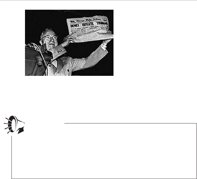
1VO^bS` ( AO[^ZW\U %#
The failure of the Gallup poll stemmed from the fact that there were a large number
of undecided voters in the sample. It was wrongly assumed that these voters were rep-
resentative of the decided voters who happened to favor Dewey. Truman easily won
the election with 303 electoral votes compared to Dewey’s 189.
4WUc`S &
Dewey Defeats Truman.
Have you ever participated in an online survey on a sports or news website that
allowed you to view the results? These surveys can be fun and interesting, but
you need to take the results with a grain of salt. That’s because the respondents are
self-selected, which means the sample is not randomly chosen. The results of these
surveys are most likely biased because the respondents would not be representative
of the population at large. For example, people without Internet access would not
be part of the sample and might respond differently than people with access to the
Internet.
Wrong Number
As you can see, choosing the proper sample is a critical step when using inferential
statistics. Even a large sample size cannot hide the errors of choosing a sample that
is not representative of the population at large. History has shown that large sample
sizes are not needed to ensure accuracy. For example, the Gallup poll predicted that
Richard Nixon would receive 43 percent of the votes for the 1968 presidential elec-
tion and in fact he won 42.9 percent. This Gallup poll was based on a sample size of
only 2,000; whereas the disastrous 1936 Literary Digest poll sampled 2,000,000 people
(source: www.personal.psu.edu/faculty/g/e/gec7/Sampling.html).

>O`b!( 7\TS`S\bWOZAbObWabWQa%$
G]c`Bc`\
1. You are to gather a systematic sample from a local phone book with 75,000
names. If every kth name in the phone book is to be selected, what value of k
would you choose to gather a sample size of 500?
2. Consider a population that is defined as every employee in a particular company.
How could you use cluster sampling to gather a sample to participate in a survey
involving employee satisfaction?
3. Consider a population that is defined as every employee in a particular company.
How could you use stratified sampling to gather a sample to participate in a sur-
vey involving employee satisfaction?
BVS:SOabG]c<SSRb]9\]e
UA simple random sample is a sample in which every member of the population
has an equal chance of being chosen.
UIn systematic sampling, every kth member of the population is chosen for the
sample, with the value of k being approximately N
n.
UA cluster sample is a simple random sample of groups, or clusters, of the popula-
tion. Each member of the chosen clusters would be part of the final sample.
UObtain a stratified sample by dividing the population into mutually exclusive
groups, or strata, and randomly sampling from each of these groups.
USampling error occurs when the sample measurement is different from the popu-
lation measurement. It is the result of selecting a sample that is not a perfect
match to the entire population.

13
1VO^bS`
AO[^ZW\U2Wab`WPcbW]\a
7\BVWa1VO^bS`
UUsing sampling distributions of the mean and proportion
UWorking with the central limit theorem
UUsing the standard error of the mean and proportion
In Chapter 12, we praised the wonders of using samples in our statistical
analysis because it was more efficient than measuring an entire population.
In this chapter, we’ll discover another benefit of using samples—sampling
distributions.
Sampling distributions describe how sample averages behave. You may be
surprised to hear they behave very well—even better than the populations
from which they are drawn. Good behavior means we can do a pretty good
job at predicting future values of sample means with a little bit of informa-
tion. This might sound a little puzzling now, but by the end of this chapter
you’ll be shaking your head in utter amazement.
EVOb7aOAO[^ZW\U2Wab`WPcbW]\-
Let’s say I want to perform a study to determine the number of miles the
average person drives a car in one day. Because it’s not possible to measure
the driving patterns of every person in the population, I randomly choose a

>O`b!( 7\TS`S\bWOZAbObWabWQa%&
sample size of 10 (n = 10) qualified individuals and record how many miles they drove
yesterday. I then choose another 10 drivers and record the same information. I do this
three more times, with the results in the following table.
Sample Number Average Number of Miles (Sample Mean)
1 40.4
2 76.0
3 58.9
4 43.6
5 62.6
As you can see, each sample has its own mean value, and each value is different. We
can continue this experiment by selecting many more samples and observe the pattern
of sample means. This pattern of sample means represents the sampling distribution
for the number of miles the average person drives in one day.
AO[^ZW\U2Wab`WPcbW]\]TbVS;SO\
The distribution from the previous example represents the sampling distribution of the
mean because the mean of each sample was the measurement of interest. This particu-
lar distribution has some interesting properties that I will discuss with the following
example.
On a recent beach vacation, the resort we had chosen advertised a ping-pong tour-
nament, which caught the eye of my 15-year-old son, John, who has enough skill to
embarrass his poor old father. (This is the thanks I get for teaching him how to play
the game when he had to stand on top of a cooler to see over the table.) As fate would
have it, we were paired against each other and, to my relief, I found myself losing
10–8. With John needing one more point to win, I fed him two serves that he usually
crams down my throat, but he somehow missed them both, and the score was tied at
10–10.
If we had been playing back home in our basement,
I’d have been dancing for joy and feeding him trash
talk. But standing at that resort surrounded by spec-
tators, all I could think about was a ruined vacation
over a silly ping-pong game. On John’s next serve, I
attacked the ball with a motion that somewhat resem-
bled a person having an epileptic seizure and hit the
ball into the net. I gave my best “I can’t believe I just
The sampling distribution of
the mean refers to the pattern
of sample means that will occur
as samples are drawn from the
population at large.

1VO^bS`!( AO[^ZW\U2Wab`WPcbW]\a %'
did that” expression and quickly sat down, breathing a hidden sigh of relief. But that
was a small price to pay since John’s pride was saved, as well as the rest of my vacation
week. The things we do for our children!
Anyway, using ping-pong balls to describe the way sample means behave, assume that
I have 100 ping-pong balls in a container in which 20 balls are marked with the num-
ber 1, 20 are marked with 2, 20 with 3, 20 with 4, and 20 with 5.
We can look at the probability distribution of this population in the following table.
Ball Number Frequency Relative Frequency Probability
1 20 20/100 0.20
2 20 20/100 0.20
3 20 20/100 0.20
4 20 20/100 0.20
5 20 20/100 0.20
This is known as a discrete uniform probability distribution because each event has the
same probability, as you can see in Figure 13.1.
4WUc`S!
Discrete uniform probability
distribution.
0
0.05
0.1
0.15
0.2
0.25
12345
Ball Number
Probability
>O`b!( 7\TS`S\bWOZAbObWabWQa&
We can calculate the mean and variance of a discrete
uniform distribution as follows:
M
1
2ab
S22
1
12 1
ba
where:
a = minimum value of the distribution
b = maximum value of the distribution
For the ping-pong ball population:
M
1
215 30.
S22
1
12 511 25
12 208
.
Keep these results in mind. We’ll be referring to them later in the chapter.
Now for my demonstration. With the balls evenly mixed, I select one ball, record the
number, place it back in the container, and then select a second ball, doing the same.
This is my first sample with a size of 2 (n = 2). After doing this 25 times, I calculate
the means of each sample and show the results in the following table.
AO[^ZW\U2Wab`WPcbW]\]TbVS;SO\[+
Sample First Ball Second Ball Sample Mean x
1 1 3 2.0
2 1 1 1.0
3 2 1 1.5
4 1 1 1.0
5 4 2 3.0
6 1 3 2.0
7 1 2 1.5
8 3 1 2.0
9 2 5 3.5
10 1 3 2.0
11 3 3 3.0
12 4 2 3.0
Adiscrete uniform probability
distribution is a distribution that
assigns the same probability to
each discrete event (and is dis-
crete if it is countable).
1VO^bS`!( AO[^ZW\U2Wab`WPcbW]\a &
13 5 2 3.5
14 3 1 2.0
15 1 4 2.5
16 4 4 4.0
17 2 2 2.0
18 2 2 2.0
19 1 1 1.0
20 2 5 3.5
21 1 2 1.5
22 5 5 5.0
23 3 2 2.5
24 5 5 5.0
25 2 1 1.5
I have a slight confession to make here. I
really didn’t buy 100 ping-pong balls and
mark each one. The numbers from the pre-
vious table came from Excel’s random num-
ber function that we discussed in Chapter
12.
We can convert this table into a relative fre-
quency distribution, which is shown in the
following table.
Sample Mean xFrequency Relative Frequency Probability
1.0 3 3/25 0.12
1.5 4 4/25 0.16
2.0 7 7/25 0.28
2.5 2 2/25 0.08
3.0 3 3/25 0.12
3.5 3 3/25 0.12
4.0 1 1/25 0.04
4.5 0 0/25 0.00
5.0 2 2/25 0.08
Students often confuse
sample size, n, and
number of samples. In the
previous example, the sample
size equals 2 (n = 2), and the
number of samples equals 25.
In other words, we have 25
samples, each of size 2.
Wrong Number
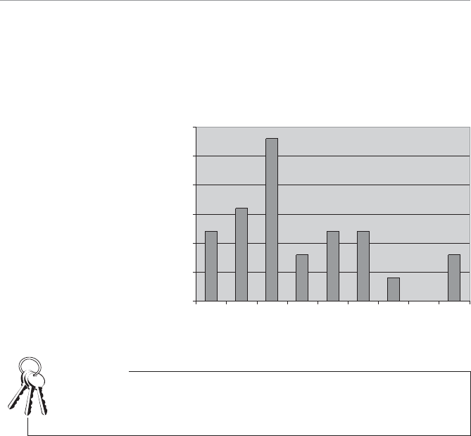
>O`b!( 7\TS`S\bWOZAbObWabWQa&
The previous table represents the sampling distribution of the mean for our ping-
pong experiment with n = 2. We can show this distribution graphically in Figure 13.2.
I’m sure by now your highly inquisitive mind is screaming, “What happens to the
sampling distribution if we increase the sample size?” That’s an excellent question that
I will address in the next section.
4WUc`S!
Sampling distribution of the
mean for n = 2.
0
0.05
0.1
0.15
0.2
0.25
0.3
1.0 1.5 2.0 2.5 3.0 3.5 4.0 4.5 5.0
Sample Means
Probability
The central limit theorem, in my humble opinion, is the most powerful concept for
inferential statistics. It forms the foundation for many statistical models that are used
today. It’s a good idea to cozy up to this theorem.
Bob’s Basics
BVS1S\b`OZ:W[WbBVS]`S[
As I mentioned earlier, sample means behave in a very special way. According to the
central limit theorem, as the sample size, n, gets larger, the sample means tend to follow
a normal probability distribution. This holds true regardless of the distribution of the
population from which the sample was drawn. Amazing, you say.
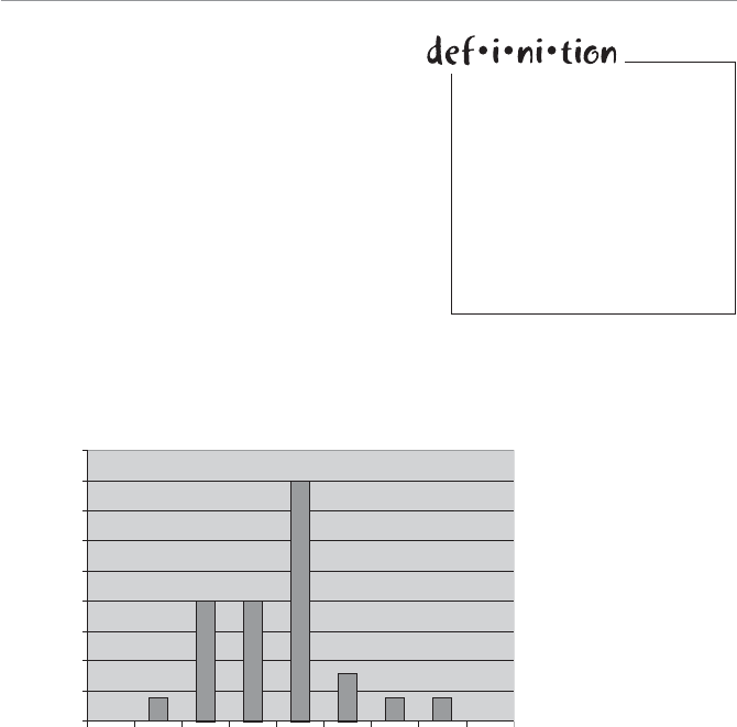
1VO^bS`!( AO[^ZW\U2Wab`WPcbW]\a &!
As you look at Figure 13.2, you’re probably
scratching your head and thinking, “That
distribution doesn’t look like a normal curve,
which I know is bell-shaped and symmetri-
cal.” You’re absolutely right because a sam-
ple size of two is generally not big enough
for the central limit theorem to kick in.
Let’s satisfy your curiosity and repeat my
experiment by gathering 25 samples each
consisting of 5 ping-pong balls (n = 5). I cal-
culate the average of each sample and plot
them in Figure 13.3.
Notice the impact that increasing the sample size has on the shape of the sample dis-
tribution. It’s starting to appear somewhat bell-shaped with a little more symmetry.
Let’s look at sample sizes of 10 and 20 in Figures 13.4 and 13.5.
According to the central limit
theorem, as the sample size, n,
gets larger, the sample means
tend to follow a normal prob-
ability distribution and tend to
cluster around the true popu-
lation mean. This holds true
regardless of the distribution of
the population from which the
sample was drawn.
0
0.05
0.1
0.15
0.2
0.25
0.3
0.35
0.4
0.45
1.0 1.5 2.0 2.5 3.0 3.5 4.0 4.5 5.0
Sam
p
le Means
Probability
4WUc`S!!
Sampling distribution of the
mean for n = 5.
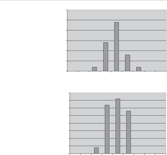
>O`b!( 7\TS`S\bWOZAbObWabWQa&"
Note that as the sample size increases, the sampling distribution tends to resemble a
normal probability distribution. I don’t know about you, but I find this pretty impres-
sive considering the fact that the population that these samples were drawn from was
not even close to being a normal distribution. If you recall, the ping-pong ball popula-
tion followed a uniform distribution as shown in Figure 13.1.
Also, notice that as the sample size increases, the sample means tend to cluster around
the true population mean, which if you recall we calculated as 3.0. This is another
important feature of the central limit theorem.
And believe it or not, the central limit theorem has even one more important feature.
0
0.1
0.2
0.3
0.4
0.5
0.6
1.0 1.5 2.0 2.5 3.0 3.5 4.0 4.5 5.0
Sample Means
Probability
0
0.05
0.1
0.15
0.2
0.25
0.3
0.35
0.4
1.0 1.5 2.0 2.5 3.0 3.5 4.0 4.5 5.0
Sample Means
Probability
4WUc`S!"
Sampling distribution of the
mean for n = 10.
4WUc`S!#
Sampling distribution of the
mean for n = 20.
1VO^bS`!( AO[^ZW\U2Wab`WPcbW]\a &#
AbO\RO`R3``]`]TbVS;SO\
Notice in the last four figures that as the sample size increased, the distribution of
sample means tended to converge closer together. In other words, as the sample size
increased, the standard deviation of the sample means became smaller. According to
the central limit theorem (here we go again!), the standard deviation of the sample
means can be calculated as follows:
SS
xn
where:
Sx = the standard deviation of the sample means
S = the standard deviation of the population
n = sample size
The standard deviation of the sample means
is formally known as the standard error of the
mean.
Recall that earlier in the chapter, in the sec-
tion “Sampling Distribution of the Mean,”
we determined that the variance of the ping-
pong ball population was 2.08. Therefore:
SS
2208 144..
We can now calculate the standard error of
the mean for n = 2 in our example:
SS
xn
144
2102
..
The standard error of the mean
is the standard deviation of
sample means. According to
the central limit theorem, the
standard error of the mean can
be determined by SS
xn
.
Students often confuse X and Sx. The symbol X, the standard deviation of the
population, measures the variation within the population and was discussed in
Chapter 5. The symbol Sx, the standard error, measures the variation of the sam-
ple means and will decrease as the sample size increases.
Bob’s Basics

>O`b!( 7\TS`S\bWOZAbObWabWQa&$
The following table summarizes how the standard error varies with sample size in our
ping-pong ball example.
AbO\RO`R3``]`DO`WSaeWbVAO[^ZSAWhS
Sample Size Standard Error
2 1.02
5 0.64
10 0.46
20 0.32
EVg2]SabVS1S\b`OZ:W[WbBVS]`S[E]`Y-
Let me explain why the central limit theorem behaves the way it does. If this concept
does not interest you, feel free to skip this section. I promise you won’t hurt my feel-
ings.
Going back to our original experiment with a sample size of two, the following table
shows all the two-ball combinations that are possible along with the sample mean.
This represents the theoretical sampling distribution of the mean because it represents all
the possible combinations of samples along with their respective probabilities.
Sample First Ball Second Ball Sample Mean x
1 1 1 1.0
2 1 2 1.5
3 1 3 2.0
4 1 4 2.5
5 1 5 3.0
6 2 1 1.5
7 2 2 2.0
8 2 3 2.5
9 2 4 3.0

1VO^bS`!( AO[^ZW\U2Wab`WPcbW]\a &%
10 2 5 3.5
11 3 1 2.0
12 3 2 2.5
13 3 3 3.0
14 3 4 3.5
15 3 5 4.0
16 4 1 2.5
17 4 2 3.0
18 4 3 3.5
19 4 4 4.0
20 4 5 4.5
21 5 1 3.0
22 5 2 3.5
23 5 3 4.0
24 5 4 4.5
25 5 5 5.0
We can convert this table into a relative frequency distribution, which is shown in the
following table.
Sample Mean xFrequency Relative Frequency Probability
1.0 1 1/25 0.04
1.5 2 2/25 0.08
2.0 3 3/25 0.12
2.5 4 4/25 0.16
3.0 5 5/25 0.20
3.5 4 4/25 0.16
4.0 3 3/25 0.12
4.5 2 2/25 0.08
5.0 1 1/25 0.04
This distribution is shown graphically in Figure 13.6.
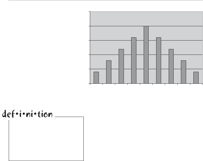
>O`b!( 7\TS`S\bWOZAbObWabWQa&&
You can see by this figure that the most common
sample average is 3.0, whereas sample averages of
1.0 and 5.0 occur the least number of times. This is
because there are more possible combinations of two-
ball samples that average to 3.0 (5 to be exact) than
two-ball samples that average to 1.0 or 5.0 (1 to be
exact). In other words, we have five times the likeli-
hood of drawing a two-ball sample that averages 3.0
when compared to sample averages of 1.0 or 5.0.
As we increase our sample size to 5, 10, and 20, the probability of drawing a sample
with an average of 1.0 or 5.0 decreases while the probability of drawing a sample with
an average of 3.0 increases. This explains why as sample size grows, more sample aver-
ages center around 3.0 and fewer around 1.0 and 5.0.
>cbbW\UbVS1S\b`OZ:W[WbBVS]`S[b]E]`Y
I can just sense your need right now to do something really neat with this wonderful
new tool. Look no further. If we know the sample means follow the normal probabil-
ity distribution and we also know the mean and standard deviation of that distribution,
we can predict the likelihood that the sample means will be greater or less than certain
values.
4WUc`S!$
Theoretical sampling
distribution of the mean.
0
0.05
0.1
0.15
0.2
0.25
1.0 1.5 2.0 2.5 3.0 3.5 4.0 4.5 5.0
Sample Means
Probability
The theoretical sampling dis-
tribution of the mean displays
all the possible sample means
along with their classical prob-
abilities. See Chapter 6 for a
review of classical probability.
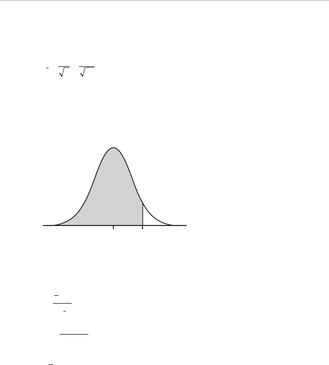
1VO^bS`!( AO[^ZW\U2Wab`WPcbW]\a &'
For example, let’s take our ping-pong ball experiment with n = 20. From the central
limit theorem, we know the sample means follow a normal distribution with:
M30.
SS
xn
144
20 032
..
What is the probability that our next sample of 20 ping-pong balls will have a sample
average of 3.5 or less? The sample mean distribution is shown in Figure 13.7, with the
shaded region indicating the probability of interest.
4WUc`S!%
Probability the next sample
mean will be less than or
equal to 3.5.
Sampling Distribution of the Mean
n = 20
3.0 3.5
Sample Means
= 3.0
= 0.32
x
As we did in Chapter 11, we need to calculate the z-score. The equation looks slightly
different because we are working with sample means, but in reality, it is identical to
what we saw in Chapter 11.
zx
x
M
S
z35
35 30
032 156
.
..
..
Using the standard z-table in Appendix B:
PP[.][.].xzbb 3 5 1 56 0 9406
This probability is shown in Figure 13.8.
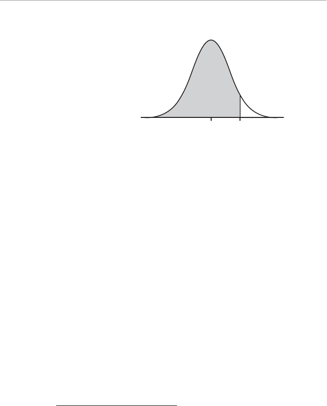
>O`b!( 7\TS`S\bWOZAbObWabWQa'
According to the shaded region, the probability that our next sample of 20 ping-pong
balls will have a sample mean of 3.5 or less is approximately 94 percent.
The power of the central limit theorem lies in the fact that you need little information
about the distribution of the population to apply it. The sample means will behave
very nicely as long as the sample size is large enough. It’s a very versatile theorem that
has countless applications in the real world. I knew you’d be impressed!
AO[^ZW\U2Wab`WPcbW]\]TbVS>`]^]`bW]\
The sample mean is not the only statistical measurement that is performed. What if
I want to measure the percentage of teenagers in this country who would agree with
the following statement: “My parents are an excellent resource when I’m looking for
advice on an important matter in my life.” Because each respondent has only two
choices (agree or disagree), this experiment follows the binomial probability distribu-
tion, which I discussed in Chapter 9.
1OZQcZObW\UbVSAO[^ZS>`]^]`bW]\
My measurement of interest is the proportion of teenagers in my sample of size n,
who will agree with the statement “My parents are an excellent resource when I’m
looking for advice on an important matter in my life.” The sample proportion, ps, is
calculated by:
pn
sNumber of Successes in the Sample
4WUc`S!&
Probability the next sample
mean will be less than or
equal to 1.56 standard devia-
tions from the population
mean.
Sampling Distribution of the Mean
n = 20
0 +1.56
Number of Standard Deviations
0.9406
= 3.0
= 0.32
x
1VO^bS`!( AO[^ZW\U2Wab`WPcbW]\a '
Because I don’t know the population pro-
portion, p, who would agree with the state-
ment, I need to collect data from samples
and approximate the population proportion.
With proportion data, I want the sample
size to be large enough so I can use the nor-
mal probability distribution to approximate
the binomial distribution. As you recall from
Chapter 11, if np r5 and nq r5, we can use
the normal distribution to approximate the
binomial (q = 1 – p, the probability of a fail-
ure). I’m hopeful that p will be at least 5 percent
(at least a few teenagers might listen to their
parents), so if I choose n = 150, then:
np = (150)(0.05) = 7.5
nq = (150)(0.95) = 142.5
Suppose I choose 10 samples, each of size 150, and record the number of agreements
(successes) in each sample in the table that follows.
Sample Number of Successes psSample Proportion
1 26 26/150 = 0.173
2 18 18/150 = 0.120
3 21 21/150 = 0.140
4 30 30/150 = 0.200
5 24 24/150 = 0.160
6 21 21/150 = 0.140
7 16 16/150 = 0.107
8 28 28/150 = 0.187
9 35 35/150 = 0.233
10 27 27/150 = 0.180
Next I average the sample proportions to approximate the population proportion, p:
pp
s
z
0 173 0 12 0 14 0 233 0 18
10 0 164
........
.
It’s important to remember
that a proportion, either p
or ps, cannot be less than 0 or
greater than 1. A common mis-
take that students make is when
told that the proportion equals
10 percent, they set p = 10
rather than p = 0.10.
Wrong Number
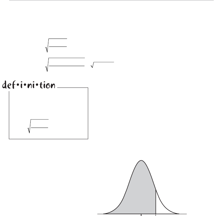
>O`b!( 7\TS`S\bWOZAbObWabWQa'
1OZQcZObW\UbVSAbO\RO`R3``]`]TbVS>`]^]`bW]\
I now need to calculate the standard deviation of this sampling distribution, which is
known as the standard error of the proportion, or Sp, with the following equation:
Sp
pp
n
1
Sp
0 164 1 0 164
150 0 000914 0 030
.. ..
Now I’m ready to answer the age-old question,
“What is the probability that from my next sample
of 150 teenagers, 20 percent or less will agree with
the statement: ‘My parents are an excellent resource
when I’m looking for advice on an important matter
in my life’?” The shaded area in Figure 13.9 repre-
sents this probability, which displays the sampling
distribution of the proportion for this example.
The standard error of the pro-
portion is the standard devia-
tion of the sample proportions
and can be calculated by
Sp
pp
n
1.
4WUc`S!'
Sampling distribution of the
proportion.
Sampling Distribution of the Proportion
0.164 0.20
Sample Proportions
p = 0.164
= 0.030
p
Because our sample size allows us to use the normal approximation to the binomial
distribution, we now calculate the z-score for the proportion using the following
equation:
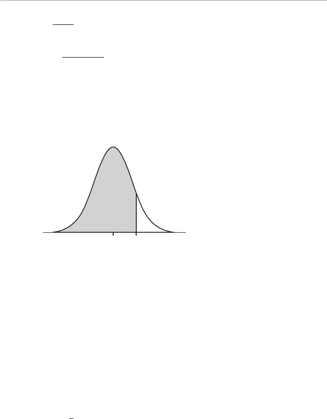
1VO^bS`!( AO[^ZW\U2Wab`WPcbW]\a '!
zpp
s
p
S
z020
0 20 0 164
0 030 120
.
..
..
Using the standard z-table in Appendix B:
PP[.
][.].pz
sbb0 20 1 20 0 8849
This probability is also shown graphically in the shaded region in Figure 13.10.
4WUc`S!
Probability that next sample
proportion will be less than or
equal to 1.2 standard devia-
tions from the population
proportion.
Sampling Distribution of the Proportion
0 +1.20
Number of Standard Deviations
0.8849
p = 0.164
= 0.030
p
According to our results, there is an 88.49 percent chance that 20 percent or fewer
teenagers will agree with our statement from the next sample of size 150. Oh well,
maybe when they get older, they’ll discover the real wisdom of their parents.
G]c`Bc`\
1. Calculate the standard error of the mean when …
a. S 10 15,n
b. S 47 1
2.,n
c. S 72
0,n
2. A population has a mean value of 16.0 and a standard deviation of 7.5. Calculate
the following with a sample size of 9.
a. Pxb
¨
ª·
¹
17

>O`b!( 7\TS`S\bWOZAbObWabWQa'"
b. Px
¨
ª·
¹
18
c. P145 165..bb
¨
ª·
¹
x
3. Calculate the standard error of the proportion when …
a. p = 0.25, n = 200
b. p = 0.42, n = 100
c. p = 0.06, n = 175
4. A population proportion has been estimated at 0.32. Calculate the following with
a sample size of 160.
a. Ppsb
¨
ª·
¹
030.
b. Pps
¨
ª·
¹
036.
c. P029 037..bb
¨
ª·
¹
ps
5. A hypothetical statistics author is obsessed with making 10-foot putts. Each day
that he practices, he putts 60 times and counts the number he makes. Over the
last 20 practice sessions, he has averaged 24 made putts. What is the probability
that he will make at least 30 putts during his next session?
BVS:SOabG]c<SSRb]9\]e
UThe sampling distribution of the mean refers to the pattern of sample means that
will occur as samples are drawn from the population at large.
UAccording to the central limit theorem, as the sample size, n, gets larger, the
sample means tend to follow a normal probability distribution.
UAccording to the central limit theorem, as the sample size, n, gets larger, the
sample means tend to cluster around the true population mean.
UThe standard error of the mean is the standard deviation of sample means.
According to the central limit theorem, the standard error of the mean can be
determined by
SS
xn
_.
UThe standard error of the proportion is the standard deviation of the sample
proportions and can be calculated by Sp
pp
n
1.

14
1VO^bS`
1]\TWRS\QS7\bS`dOZa
7\BVWa1VO^bS`
UInterpreting the meaning of a confidence interval
UCalculating the confidence interval for the mean with large and small
samples
UIntroducing the Student’s t-distribution
UCalculating the confidence interval for the proportion
UDetermining sample sizes to attain a specific margin of error
Now that we have learned how to collect a random sample and how sample
means and sample proportions behave under certain conditions, we are
ready to put those samples to work using confidence intervals.
One of the most important roles that statistics plays in today’s world is to
gather information from a sample and use that information to make a state-
ment about the population from which it was chosen. We are using the
sample as an estimate for the population. But just how good of an estimate
is the sample providing us? The concept of confidence intervals will pro-
vide us with that answer.
>O`b!( 7\TS`S\bWOZAbObWabWQa'$
1]\TWRS\QS7\bS`dOZaT]`bVS;SO\eWbV:O`USAO[^ZSa
So let’s learn how to construct a confidence interval for a population mean using a
large sample size. By a large sample size, we are generally referring to nv 30. The
first step in developing a confidence interval for a population involves the following
discussion on estimators.
3abW[Ob]`a
The simplest estimate of a population is the point estimate, the most common being
the sample mean. A point estimate is a single value that best describes the population
of interest. Let me explain this concept by using the following example.
I think my wife has been kidnapped and secretly
replaced by a Debbie look-alike who also happens to
be completely addicted to the QVC home shopping
channel. No one or nothing in our household has
escaped the products Debbie has found on her new
favorite TV show. She has purchased stuff for the car,
the kitchen floor, the dog, her skin, her hair, and my
back (an inversion table that she wants me to hang
upside down on!).
Suddenly “Diamonique Week” has become a
major holiday in our household. I’m not really sure
what Diamonique actually is, but I suspect it is “available for a limited time only.”
Whenever I turn on any TV in the house, the channel always seems to be set to a very
convincing home shopping channel-type person pleading with me to “Call now! Only
three left!”
Anyway, let’s say I want to estimate the average dollar value of an order for the home
shopping channel population. If my sample average was $78.25, I could use that as my
point estimate for the entire population of home shopping customers.
The advantage of a point estimate is that it is easy to calculate and easy to understand.
The disadvantage, however, is that I have no clue as to how accurate this estimate
really is.
To deal with this uncertainty, we can use an interval estimate, which provides a range of
values that best describes the population. To develop an interval estimate, we need to
learn about confidence levels.
Apoint estimate is a single
value that best describes the
population of interest, the
sample mean being the most
common. An interval estimate
provides a range of values that
best describes the population.

1VO^bS`"( 1]\TWRS\QS7\bS`dOZa '%
1]\TWRS\QS:SdSZa
Aconfidence level is the probability that the interval estimate will include the population
parameter. A parameter is defined as a numerical description of a population character-
istic, such as the mean.
Remember from Chapter 13 that sample
means will follow the normal probability dis-
tribution for large sample sizes. Let’s say we
want to construct an interval estimate with a
90 percent confidence level. This confidence
level corresponds to a z-score from the stan-
dard normal table equal to 1.64 as shown in
Figure 14.1.
Aconfidence level is the prob-
ability that the interval estimate
will include the population
parameter, such as the mean.
Aparameter is data that
describes a characteristic about
a population.
4WUc`S"
90 percent confidence inter-
val.
90% Confidence Interval
90%
5% 5%
0 +1.64-1.64
0.95
Notice that in Figure 14.1, 5 percent of the area under the curve lies to the right
of +1.64 and 95 percent of the area under the curve lies to the left. That’s why
you see 0.9495 (close enough to 0.95) corresponding to a z-score of 1.64 in
Table 3 of Appendix B. Remember, however, that z = 1.64 corresponds to a 90 per-
cent confidence interval, the shaded region in the figure.
Bob’s Basics
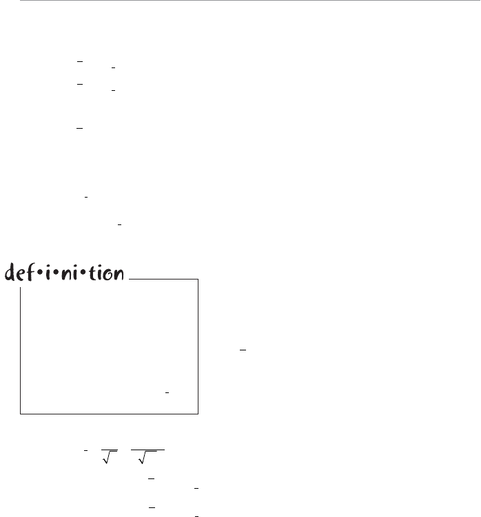
>O`b!( 7\TS`S\bWOZAbObWabWQa'&
In general, we can construct a confidence interval around our sample mean using the
following equations:
xz
cx
S
(upper limit of confidence interval)
xz
cx
S
(lower limit of confidence interval)
where:
x = the sample mean
zc = the critical z-score, which is the number of standard deviations based on
the confidence level
Sx = the standard error of the mean (remember our friend from Chapter 13?)
The term zcx
S is referred to as the margin of error, or E, a phrase often referred to in
polls and surveys.
Going back to our home shopping example, let’s say
from a sample of 32 customers the average order
is $78.25 and the population standard deviation is
$37.50. (This represents the variation among orders
within the population.) We can calculate our 90 per-
cent confidence interval as follows:
x$.78 25
n = 32
X = $37.50
zc = 1.64
SS
xn
$. $.
37 50
32 663
Upper limit = xx
164 7825 164 663 8912.$..$.$.S
Lower limit = xx
164 7825 164 663 6738.$..$.$.S
According to these results, our 90 percent confidence interval for this random sample
of home shoppers is between $67.38 and $89.12 or ($67.38, $89.12). This interval is
shown in Figure 14.2.
Aconfidence interval is a
range of values used to esti-
mate a population parameter
and is associated with a spe-
cific confidence level. The mar-
gin of error, E, determines the
width of the confidence interval
and is calculated using zcx
S.
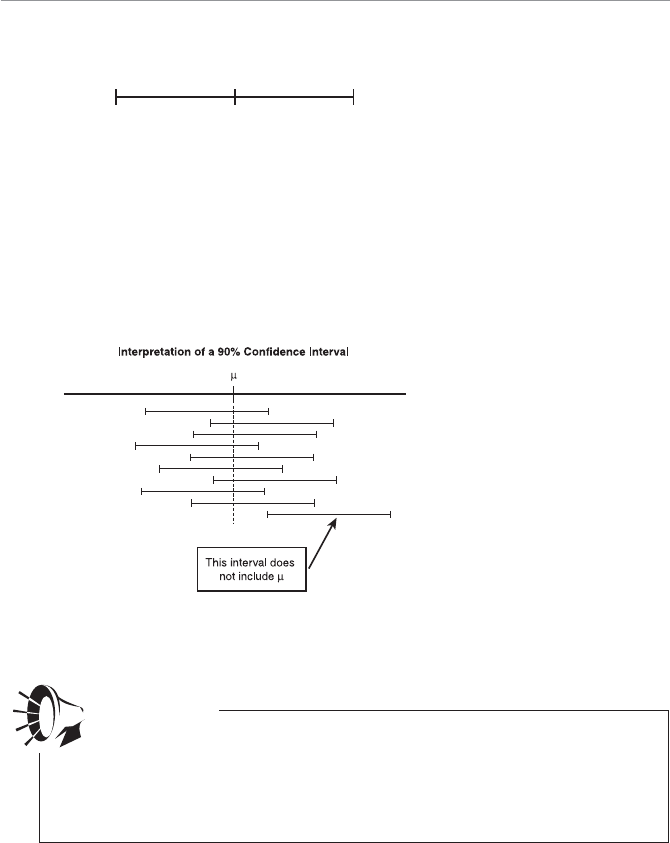
1VO^bS`"( 1]\TWRS\QS7\bS`dOZa ''
0SeO`S]TbVS7\bS`^`SbObW]\]T1]\TWRS\QS7\bS`dOZ
As described earlier, a confidence interval is a range of values used to estimate a
population parameter and is associated with a specific confidence level. A confidence
interval needs to be described in the context of several samples. If we select 10 samples
from our home shopping population and construct 90 percent confidence intervals
around each of the sample means, then theoretically 9 of the 10 intervals will contain
the true population mean, which remains unknown. Figure 14.3 shows this concept.
4WUc`S"
Interval estimate for the
average dollar value of a
home shopping order.
$67.38 $78.25 $89.12
Interval Estimate for the Average Order
Size of a Home Shopping Customer
4WUc`S"!
Interpreting the definition of
a confidence interval.
As you can see, Samples 1 through 9 have confidence intervals that include the true
population mean, whereas Sample 10 does not.
It is easy to misinterpret the definition of a confidence interval. For example, it is
not correct to state that “there is a 90 percent probability that the true population
mean is within the interval ($67.38, $89.12).” Rather, a correct statement would be
that “there is a 90 percent probability that any given confidence interval from a ran-
dom sample will contain the true population mean.”
Wrong Number
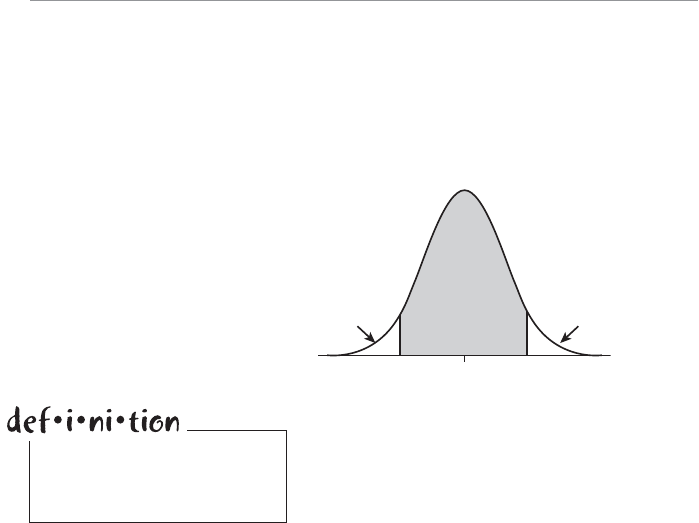
>O`b!( 7\TS`S\bWOZAbObWabWQa
Because there is a 90 percent probability that any given confidence interval will con-
tain the true population mean in the previous example, we have a 10 percent chance
that it won’t. This 10 percent value is known as the level of significance,F, which is rep-
resented by the total white area in both tails of Figure 14.4.
4WUc`S""
The level of significance.
Level of Significance
1–
2
/2
/
The probability for the confidence interval is a com-
plement to the significance level. For example, the
significance level for a 95 percent confidence interval
is 5 percent, the significance level for a 99 percent
confidence interval is 1 percent, and so on. In gen-
eral, a (1 – F) confidence interval has a significance
level equal to F.
We will revisit the level of significance in more detail
in later chapters.
BVS3TTSQb]T1VO\UW\U1]\TWRS\QS:SdSZa
So far, we have only referred to a 90 percent confidence interval. However, we can
choose other confidence levels to suit our needs. The following table shows our home
shopping example with confidence levels of 90, 95, and 99 percent.
The level of significance (F)
is the probability of making a
Type I error.
1VO^bS`"( 1]\TWRS\QS7\bS`dOZa
1]\TWRS\QS7\bS`dOZaeWbVDO`W]ca1]\TWRS\QS:SdSZa
Confidence Sample Lower Upper
Level zcSxMean Limit Limit
90 1.64 $6.63 $78.25 $67.38 $89.12
95 1.96 $6.63 $78.25 $65.26 $91.24
99 2.57 $6.63 $78.25 $61.21 $95.29
From the previous table, you can see that
there’s a price to pay for increasing the
confidence level—our interval estimate of
the true population mean becomes wider
and less precise. We have proven that once
again, there is no free lunch with statistics.
If we want more certainty that our confi-
dence interval will contain the true popu-
lation mean, that confidence interval will
become wider.
BVS3TTSQb]T1VO\UW\UAO[^ZSAWhS
There is one way, however, to reduce the width of our confidence interval while
maintaining the same confidence level. We can do this by increasing the sample size.
There is still no free lunch though because increasing the sample size has a cost asso-
ciated with it. Let’s say we increase our sample size to include 64 home shoppers. This
change will affect our standard error as follows:
SS
xn
$. $.
37 50
64 469
Our new 90 percent confidence interval for our original sample will be:
x$.78 25
n = 64
Sx$.469
Upper limit = xx
164 7825 164 469 8594.$..$.$.S
Lower limit = xx
164 7825 164 469 7056.$..$.$.S
I recommend that you confirm
the z-scores in this table for
yourself by checking with
Table 3 in Appendix B. Practice
makes perfect! Review Chapter
11 if you need to.
Bob’s Basics

>O`b!( 7\TS`S\bWOZAbObWabWQa
Increasing our sample size from 32 to 64 has reduced the 90 percent confidence inter-
val from ($67.38, $89.12) to ($70.56, $85.94), which is a more precise interval.
2SbS`[W\W\UAO[^ZSAWhST]`bVS;SO\
We can also calculate a minimum sample size that would be needed to provide a spe-
cific margin of error. What sample size would we need for a 95 percent confidence
interval that has a margin of error of $8.00 (E = $8.00) in our home shopping exam-
ple?
Ez
x
S
Ez
n
S
nz
E
S
nz
E
¥
§
¦´
¶
µ
S2
n
¥
§
¦´
¶
µz
196 3750
800 84 4 85
2
.$.
$. .
Therefore, to obtain a 95 percent confidence interval that ranges from
$78.25 – $8.00 = $70.25 to $78.25 + $8.00 = $86.25 would require a sample size
of 85 home shopping-addicted people.
1OZQcZObW\UO1]\TWRS\QS7\bS`dOZEVS\X7aC\Y\]e\
Here’s a simple section for you. (It’s about time!) So far, all of our examples have
assumed that we knew X,the population standard deviation. What happens if X is
unknown? Don’t panic, because as long as nr30, we can substitute s, the sample stan-
dard deviation, for X,the population standard deviation, and follow the same proce-
dure as before. T
o demonstrate this technique, consider the following table that shows
the order size in dollars of 30 home shoppers.
6][SAV]^^W\UAO[^ZS[+!
75 109 32 54 121 80 96 47 67 115
29 70 89 100 48 40 137 75 39 88
99 140 112 87 122 75 54 92 89 153

1VO^bS`"( 1]\TWRS\QS7\bS`dOZa !
Using Excel, we can confirm that:
x$.84 47 and s$.32 98
A 99 percent confidence interval around this sample mean would be:
x$.84 47
n = 30
s = $32.98
zc = 2.57
ˆ$. $.Sx
s
n
32 98
30 602
We use ˆ
Sx to indicate that we have approximated the standard error of the mean by
using s instead of X. We statisticians just love to put little hats on top of letters.
Upper limit = xx
257 8447 257 602 9994.ˆ$. . $. $.S
Lower limit = xx
257 8447 257 602 6900.ˆ$. . $. $.S
See! That wasn’t too bad.
CaW\U3fQSZÂa1=<4723<134c\QbW]\
Excel has a pretty cool built-in function that calculates confidence intervals for us.
The CONFIDENCE function has the following characteristics:
CONFIDENCE(alpha, standard_dev, size)
where:
alpha = the significance level of the confidence interval
standard_dev = the standard deviation of the population
size = sample size
For instance, Figure 14.5 shows the CONFIDENCE function being used to calculate
the confidence interval for our original home shopping example.

>O`b!( 7\TS`S\bWOZAbObWabWQa "
Cell A1 contains the Excel formula =CONFIDENCE(0.1,37.5,32) with the result
being 10.90394. This value represents the margin of error, or the amount to add and
subtract from the sample mean, as follows:
$78.25 + $10.90 = $89.15
$78.25 – $10.90 = $67.35
This confidence interval is slightly different from the one calculated earlier in the
chapter due to the rounding of numbers. This sure beats using tables and square root
functions on the calculator.
1]\TWRS\QS7\bS`dOZaT]`bVS;SO\eWbVA[OZZAO[^ZSa
So far, this entire chapter has dealt with the case where nr30. I’m sure you are now
wondering about how to construct a confidence interval when our sample size is less
than 30. Well, as with many things in life, it depends.
With a small sample size, we lose the use of our faithful friend, the central limit
theorem, and we need to assume that the population is normally (or approximately)
distributed for all cases. The first case that we’ll examine is when we know X,the
population standard deviation.
EVS\X7a9\]e\
When X is known, the procedure reverts back to the large sample size case. We can do
this because we are now assuming the population is normally distributed. Let’s con-
struct a 95 percent confidence interval from the following home shopping sample of
size 10.
4WUc`S"#
CONFIDENCE function in
Excel for the home shopping
sample.

1VO^bS`"( 1]\TWRS\QS7\bS`dOZa #
6][SAV]^^W\UAO[^ZS[+
75 109 32 54 121 80 96 47 67 115
We know the following information:
x$.79 60
n = 10
X= $37.50 (given from the original example)
zc = 1.96
SS
xn
$. $.
37 50
10 11 86
Upper Limit = xx
1 96 79 60 1 96 11 86 102 85.$..$.$.S
Lower Limit = xx
1 96 79 60 1 96 11 86 56 35. $. . $. $.S
Notice that the small sample size has resulted in a wide confidence interval. Again, we
are assuming here that the population from which the sample was drawn is normally
distributed, which is the first time we have made such an assumption in this chapter so
far.
EVS\X7aC\Y\]e\
More often, we don’t know the value of X. Here, we make a similar adjustment that
we made earlier and substitute s, the sample standard deviation, for X,the population
standard deviation. However, because of the small sample size, this substitution forces
us to use a new probability distribution known
as the Student’s t-distribution (named in honor
of you, the student).
The t-distribution is a continuous probability
distribution with the following properties:
UIt is bell-shaped and symmetrical around
the mean.
UThe shape of the curve depends on the
degrees of freedom (d.f.) which, when deal-
ing with the sample mean, would be equal
to n – 1.
The Student’s t-distribution was
developed by William Gosset
(1876–1937) while work-
ing for the Guinness Brewing
Company in Ireland. He
published his findings using
the pseudonym Student. Now
there’s a rare statistical event—
a bashful Irishman!
Random Thoughts
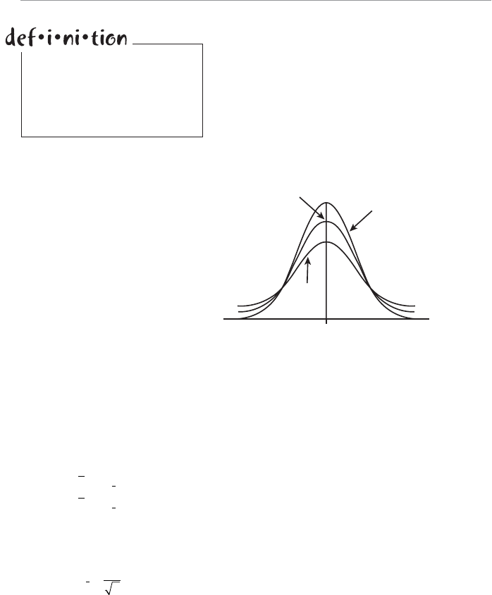
>O`b!( 7\TS`S\bWOZAbObWabWQa $
U The area under the curve is equal to 1.0.
U The t-distribution is flatter than the normal dis-
tribution. As the number of degrees of freedom
increase, the shape of the t-distribution becomes
similar to the normal distribution as seen in
Figure 14.6. With more than 30 degrees of free-
dom (a sample size of 30 or more), the two dis-
tributions are practically identical.
The degrees of freedom are the
number of values that are free
to be varied given information,
such as the sample mean, is
known.
4WUc`S"$
The Student’s t-distribution
compared to the normal dis-
tribution.
The t-Distribution Compared to the Normal Curve
d.f. = 15
d.f. = 2
Standard Normal Curve
0
Students often struggle with the concept of degrees of freedom, which represent the
number of remaining free choices you have after something has been decided, such
as the sample mean. For example, if I know that my sample of size 3 has a mean of
10, I can only vary two values (n – 1). After I set those two values, I have no control
over the third value because my sample average must be 10. For this sample, I have 2
degrees of freedom.
We can now set up our confidence intervals for the mean using a small sample:
xt
cx
ˆ
S (upper limit of confidence interval)
xt
cx
ˆ
S (lower limit of confidence interval)
where:
tc = critical t-value (can be found in Table 4 in Appendix B)
ˆ
Sx
s
n
, the estimated standard error of the mean

1VO^bS`"( 1]\TWRS\QS7\bS`dOZa %
To demonstrate this procedure, let’s assume the population of home shopping orders
follows a normal distribution and the following sample of size 10 was collected.
6][SAV]^^W\UAO[^ZST`][O<]`[OZ2Wab`WPcbW]\[+
29 70 89 100 48 40 137 75 39 88
With Xunknown, we will construct a 95 percent confidence interval around the sam-
ple mean.
To determine the value of tc for this example, I need to calculate the number
of degrees of freedom. Because n = 10, I have n – 1 = 9 d.f. This corresponds to
tc2 262., which is underlined in the following table taken from Table 4 in Appendix
B.
3fQS`^bT`][bVSAbcRS\bÂab2Wab`WPcbW]\
Selected right-tail areas with confidence levels underneath
Alpha 0.2000 0.1500 0.1000 0.0500 0.0250 0.0100 0.0050 0.0010 0.0005
Conf lev 0.6000 0.7000 0.8000 0.9000 0.9500 0.9800 0.9900 0.9980 0.9990
df
1 1.376 1.963 3.078 6.314 12.706 31.821 63.657 318.31 636.62
2 1.061 1.386 1.886 2.920 4.303 6.965 9.925 22.327 31.599
3 0.978 1.250 1.638 2.353 3.182 4.541 5.841 10.215 12.924
4 0.941 1.190 1.533 2.132 2.776 3.747 4.604 7.173 8.610
5 0.920 1.156 1.476 2.015 2.571 3.365 4.032 5.893 6.869
6 0.906 1.134 1.440 1.943 2.447 3.143 3.707 5.208 5.959
7 0.896 1.119 1.415 1.895 2.365 2.998 3.499 4.785 5.408
8 0.889 1.108 1.397 1.860 2.306 2.896 3.355 4.501 5.041
9 0.883 1.100 1.383 1.833 2.262 2.821 3.250 4.297 4.781
10 0.879 1.093 1.372 1.812 2.228 2.764 3.169 4.144 4.587
We next need to calculate the sample mean and sample standard deviation, which,
according to Excel, are as follows:
x$.71 50 and s = $33.50
>O`b!( 7\TS`S\bWOZAbObWabWQa &
We can now approximate the standard error of the mean:
ˆ$. $.Sx
s
n
33 50
10 10 59
and can construct our 95 percent confidence interval:
Upper limit = xt
cx
ˆ$. . $. $.S71 50 2 262 10 59 95 45
Lower limit = xt
cx
ˆ$. . $. $.S71 50 2 262 10 59 47 55
Now that wasn’t too bad!
We can use the t-distribution when all of the following conditions have been met:
UThe population follows the normal (or approximately normal) distribution.
UThe sample size is less than 30.
U The population standard deviation, X, is unknown and must be approximated
by s, the sample standard deviation.
Bob’s Basics
That ends our discussion on confidence intervals around the mean. Next on the menu
are proportions!
1]\TWRS\QS7\bS`dOZaT]`bVS>`]^]`bW]\eWbV:O`US
AO[^ZSa
We can also estimate the proportion of a population by constructing a confidence
interval from a sample. As you might recall from Chapter 13, proportion data follow
the binomial distribution that can be approximated by the normal distribution under
the following conditions:
np r5 and nq r5
where:
p = the probability of a success in the population
q= the probability of a failure in the population (q = 1 – p)

1VO^bS`"( 1]\TWRS\QS7\bS`dOZa '
Suppose I want to estimate the proportion of home shopping customers who are
female based on the results of a sample. In Chapter 13, we learned that we can calcu-
late the proportion of a sample using:
pn
sNumber of Successes in the Sample
1OZQcZObW\UbVS1]\TWRS\QS7\bS`dOZT]`bVS>`]^]`bW]\
The confidence interval around the sample proportion can be calculated by:
pz
scp
S
(upper limit of confidence interval)
pz
scp
S
(lower limit of confidence interval)
where Sp is the standard error of the proportion (which is the standard deviation of
the sample proportions) using:
Sp
pp
n
1
There’s extra credit for anyone who can see a problem arising here. Our challenge is
that we are trying to estimate p, the population proportion, but we need a value for p
to set up the confidence interval. Our solution—estimate the standard error by using
the sample proportion as an approximation for the population proportion as follows:
ˆ
Sp
ss
pp
n
1
We now can construct a confidence interval around the sample proportion by:
pz
scp
ˆ
S (upper limit of confidence interval)
pz
scp
ˆ
S (lower limit of confidence interval)
Let’s put these equations to work. In my efforts to estimate the proportion of female
home shopping customers, I sample 175 random customers, of which 110 are female.
I can now calculate ps, the sample proportion:
pn
s
Number of Successes in the Sample 110
1755 0 629.
The estimated standard error of the proportion would be:
ˆ.. .Sp
ss
pp
n
10 629 0 371
175 0 0365

>O`b!( 7\TS`S\bWOZAbObWabWQa
We are now ready to construct a 90 percent confidence interval around our sample
proportion (zc = 1.64):
Upper limit = psp
1 64 0 629 1 64 0 0365 0 689.... .S
Lower limit = psp
1 64 0 629 1 64 0 0365 0 569.... .S
Our 90 percent confidence interval for the proportion of female home shopping cus-
tomers is (0.569, 0.689). Debbie must be in there somewhere!
2SbS`[W\W\UAO[^ZSAWhST]`bVS>`]^]`bW]\
Almost done. Just as we did for the mean, we can determine a required sample size
that would be needed to provide a specific margin of error. What sample size would
we need for a 99 percent confidence interval that has a margin of error of 6 percent (E
= 0.06) in our home shopping example? The formula to calculate n, the sample size is:
npq
z
E
c
¥
§
¦´
¶
µ
2
Notice that we need a value for p and q. If we don’t have a preliminary estimate of the
values, set p = q = 0.50. Because half the population is female, that sounds like a good
strategy to me.
n
¥
§
¦´
¶
µ050 050 257
006 459
2
.. .
.
Therefore, to obtain a 99 percent confidence interval that provides a margin of error
no more than 6 percent would require a sample size of 459 home shoppers.
The reason we use p= q = 0.50 if we don’t have an estimate of the population pro-
portion is that these values provide the largest sample size when compared to other
combinations of p and q. It’s like being penalized for not having specific informa-
tion about your population. This way you are sure your sample size is large enough,
regardless of the population proportion.
Random Thoughts

1VO^bS`"( 1]\TWRS\QS7\bS`dOZa
G]c`Bc`\
1. Construct a 97 percent confidence interval around a sample mean of 31.3 taken
from a population that is not normally distributed with a standard deviation of
7.6 using a sample of size 40.
2. What sample size would be necessary to ensure a margin of error of 5 for a 98
percent confidence interval taken from a population that is not normal, which
has a population standard deviation of 15?
3. Construct a 90 percent confidence interval around a sample mean of 16.3 taken
from a population that is not normally distributed with a population standard
deviation of 1.8 using a sample of size 10.
4. The following sample of size 30 was taken from a population that is not nor-
mally distributed:
10 4 912 51720 9 415
11 12 16 22 10 25 21 14 9 8
14 16 20 18 8 10 28 19 16 15
Construct a 90 percent confidence interval around the mean.
5. The following sample of size 12 was taken from a population that is normally
distributed and that has a population standard deviation of 12.7:
37 48 30 55 50 46 40 62 50 43 36 66
Construct a 94 percent confidence interval around the mean.
6. The following sample of size 11 was taken from a population that is normally
distributed:
121 136 102 115 126 106 115 132 125 108 130
Construct a 98 percent confidence interval around the mean.
7. The following sample of size 11 was taken from a population that is not nor-
mally distributed:
87 59 77 65 98 90 84 56 75 96 66
Construct a 99 percent confidence interval around the mean.

>O`b!( 7\TS`S\bWOZAbObWabWQa
8. A sample of 200 light bulbs was tested, and it was found that 11 were defective.
Calculate a 95 percent confidence interval around this sample proportion.
9. What sample size would you need to construct a 96 percent confidence interval
around the proportion for voter turnout during the next election that would pro-
vide a margin of error of 4 percent? Assume the population proportion has been
estimated at 55 percent.
BVS:SOabG]c<SSRb]9\]e
UA confidence interval is a range of values used to estimate a population param-
eter and is associated with a specific confidence level.
UA confidence level is the probability that the interval estimate will include the
population parameter, such as the mean.
UIncreasing the confidence level results in the confidence interval becoming wider
and less precise.
UIncreasing the sample size reduces the width of the confidence interval, which
increases precision.
UUse the t-distribution to construct a confidence interval when the population
follows the normal (or approximately normal) distribution, the sample size is less
than 30, and the population standard deviation, X, is unknown.
UUse the normal distribution to construct a confidence interval around the sample
proportion when np r5 and nq r5.

15
1VO^bS`
7\b`]RcQbW]\b]6g^]bVSaWa
BSabW\U
7\BVWa1VO^bS`
UFormulating the null and alternative hypothesis
UDistinguishing between a one-tail and two-tail hypothesis test
UControlling the probability of a Type I and Type II error
UDetermining the boundaries for the rejection region for the
hypothesis test
UStating the conclusion of the hypothesis test
Now that we know how to make an estimate of a population parameter,
such as a mean, using a sample and a confidence interval, let’s move on to
the heart and soul of inferential statistics: hypothesis testing.
One thing statisticians like to do is to make a statement about a popula-
tion parameter, collect a sample from that population, measure the sample,
and declare, in a scholarly manner, whether or not the sample supports
the original statement. This, in a nutshell, is what hypothesis testing is
all about. Of course, I’ve included a few juicy details. Without them, this
would be one short chapter!
>O`b!( 7\TS`S\bWOZAbObWabWQa "
The purpose of this particular chapter is just to introduce the basic concept of hypoth-
esis testing. The following two chapters will then get into more specific examples of
how we put hypothesis testing to work. Stay tuned!
6g^]bVSaWaBSabW\U¾bVS0OaWQa
In the statistical world, a hypothesis is an assumption about a population parameter.
Examples of hypotheses (that’s plural for hypothesis) include the following:
UThe average adult drinks 1.7 cups of coffee per day.
UTwelve percent of undergraduate students will go directly to graduate school
after graduation.
UNo more than 2 percent of our products sold to customers are defective.
In each case, we have made a statement about the
population that may or may not be true. The purpose
of hypothesis testing is to make a statistical conclu-
sion about accepting or not accepting such state-
ments. To further explain this concept, I present the
following story.
I am man enough to admit that I am deathly afraid of snakes. That’s why I did not
hesitate to express my panic when Sam, Debbie’s oldest teenage son, brought home
a snake that he had caught and Debbie wholeheartedly agreed to let him keep in his
bedroom.
Well, my worst nightmare came true the following morning. The snake had pushed
off the top of the cage overnight and was loose somewhere in the house. I guess Sam
never heard the story of the mommy snake that once lifted a Volkswagen Beetle off
her baby snake to save it.
I won’t name names here, but somebody’s wife suggested that we put a mouse in Sam’s
room to attract the snake so we could catch it. I thought this was a very good joke
until a white mouse showed up in Sam’s room later that day posing as “snake bait.”
That night, I lay in bed under high alert (i.e., at least one eye always open and ears
finely tuned for a hissing noise) while Debbie lay calmly snoring next to me.
The next morning, I discovered that I had a new worst nightmare. The mouse had
chewed its way out of its container overnight, and it, too, was loose somewhere in the
house. I now had two wild animals roaming freely in the places where I eat, sleep, and
Ahypothesis is an assumption
about a population parameter.
1VO^bS`#( 7\b`]RcQbW]\b]6g^]bVSaWaBSabW\U #
watch TV. By this time I’m frantically looking through the phonebook for a motel
that specifically prohibits all snakes and mice. Debbie thought I was “overreacting.”
That night I lay in my bed in the fetal position to protect my vital organs and keep
my arms and legs away from the side of the bed while again Debbie lay calmly snoring
next to me.
Anyway, let’s try to tie this sci-fi tale to hypothesis testing. Let’s say that my hypothesis
is that it will take an average of six days to capture a loose snake in a house. In other
words, I would like to test my belief that the population mean, R, is equal to six days.
I do this by gathering a sample of people who have had a loose snake in their home
and calculate the average number of days required to capture it. Suppose the sample
average is 6.1 days. The hypothesis test will then tell me whether or not 6.1 days is
significantly different from 6.0 days or if the difference is merely due to chance. More
details to follow!
BVS<cZZO\R/ZbS`\ObWdS6g^]bVSaWa
Every hypothesis test has both a null hypothesis and an alternative hypothesis. The
null hypothesis, denoted by H0, represents the status quo and involves stating the belief
that the mean of the population is f, =, or v a specific value. The null hypothesis is
believed to be true unless there is overwhelming evidence to the contrary. In this
example, my null hypothesis would be stated as:
H060:.M days
The alternative hypothesis, denoted by H1,
represents the opposite of the null hypoth-
esis and holds true if the null hypothesis is
found to be false. The alternative hypothesis
always states the mean of the population is
<, |, or > a specific value. In this example,
my alternative hypothesis would be stated as:
H160:.Mx days
The following table shows the three valid
combinations of the null and alternative
hypothesis.
The null hypothesis, denoted by
H0, represents the status quo
and involves stating the belief
that the mean of the population
is f, =, or v a specific value.
The alternative hypothesis,
denoted by H1, represents the
opposite of the null hypothesis
and holds true if the null hypoth-
esis is found to be false.

>O`b!( 7\TS`S\bWOZAbObWabWQa $
Null Hypothesis Alternative Hypothesis
H060:.M H160:.Mx
H060:.Mr H160:.M
H060:.Mb H160:.M
Some textbooks will use the convention that the null hypothesis will always be stated
as = and will never use f or v. Choosing either method of stating your hypothesis will
not affect the statistical analysis. Just be consistent with the convention you decide to
use.
Random Thoughts
Note that the alternative hypothesis is never associated with f, =, or v. Selecting the
proper combination is the topic of the next section.
AbObW\UbVS<cZZO\R/ZbS`\ObWdS6g^]bVSaWa
You need to be careful how you state the null and alternative hypothesis. Your choice
will depend on the nature of the test and the motivation of the person conducting it.
If the purpose is to test that the population mean is equal to a specific value, such as
our snake example, assign this statement as the null hypothesis, which results in the
following:
H060:.M days
H160:.Mx days
Often hypothesis testing is performed by researchers who want to prove that their
discovery is an improvement over current products or procedures. For example, if I
invented a golf ball that I claimed would increase your distance off the tee by more
than 20 yards, I would set up my hypothesis as follows:
H020:Mb yards
H120:M yards
Note that I used the alternative hypothesis to represent the claim that I want to prove
statistically so that I can make a fortune selling these balls to desperate golfers such
as myself. Because of this, the alternative hypothesis is also known as the research
hypothesis because it represents the position that the researcher wants to establish.
1VO^bS`#( 7\b`]RcQbW]\b]6g^]bVSaWaBSabW\U %
Be]BOWZ6g^]bVSaWaBSab
Atwo-tail hypothesis test is used whenever the alternative hypothesis is expressed as |.
Our snake example would involve a two-tail test because the alternative hypothesis is
stated as H160:.Mx . This test is shown graphically in Figure 15.1 which, as you can
see, is considered a two-tail hypothesis test.
4WUc`S#
Two-tail hypothesis test.
Two-Ta
i
l Hypothes
i
sTest
6.0
Mean No. of Days to Catch a Snake
Reject H0Reject H0
Do Not Reject
H0
μ
H0
μ
The curve in the figure represents the
sampling distribution of the mean for the
number of days to catch a snake. The mean
of the population, assumed to be 6.0 days
according to the null hypothesis, is the mean
of the sampling distribution and is desig-
nated by MH0.
The procedure is as follows:
UCollect a sample of size n, and calculate the test statistic, which in this case is the
sample mean.
UPlot the sample mean on the x-axis of the sampling distribution curve.
UIf the sample mean falls within the white region, we do not reject H0. That
is, we do not have enough evidence to support H1, the alternative hypothesis,
which states that the population mean is not equal to 6.0 days.
UIf the sample mean falls in either shaded region, otherwise known as the rejec-
tion region, we reject H0. That is, we have enough evidence to support H1, which
results in our belief that the true population mean is not equal to 6.0 days.
The two-tail hypothesis test is
used whenever the alternative
hypothesis is expressed as |.

>O`b!( 7\TS`S\bWOZAbObWabWQa &
Because there are two rejection regions in this figure, we have a two-tail hypoth-
esis test. We will discuss how to determine the boundaries for the rejection regions
shortly.
The only two statements that we can make about the null hypothesis are that
we …
UReject the null hypothesis.
UDo not reject the null hypothesis.
Because our conclusions are based on a sample, we will never have enough evi-
dence to accept the null hypothesis. It’s a much safer statement to say that we do not
have enough evidence to reject H0. We can use the analogy of the legal system to
explain. If a jury finds a defendant “not guilty,” they are not saying the defendant is
innocent. Rather, they are saying that there is not enough evidence to prove guilt.
Wrong Number
=\SBOWZ6g^]bVSaWaBSab
Aone-tail hypothesis test involves the alternative hypothesis being stated as < or >. My
golf ball example results in a one-tail test because the alternative hypothesis is being
expressed as H120:M and is shown in Figure 15.2.
4WUc`S#
One-tail hypothesis test.
Mean Increase in Yards off the Tee
Reject H0
Do Not Reject H0
12
H0
Here, there is only one rejection region, which is the
shaded area on the right tail of the distribution. We
follow the same procedure outlined for the two-tail
test and plot the sample mean, which represents the
average increase in distance from the tee with my
new golf ball. Two possible scenarios exist.
The one-tail hypothesis test
is used when the alternative
hypothesis is being stated as <
or >.

1VO^bS`#( 7\b`]RcQbW]\b]6g^]bVSaWaBSabW\U '
UIf the sample mean falls within the
white region, we do not reject
H0. That is, we do not have enough
evidence to support H1, the alterna-
tive hypothesis, which states that my
golf ball increased distance off the tee
by more than 20 yards. There goes
my fortune down the drain!
UIf the sample mean falls in the rejection
region, we reject H0. That is, we have
enough evidence to support H1, which
confirms my claim that my new golf
ball will increase distance off the tee by
more than 20 yards. Early retirement,
here I come!
Now that we have covered the basics of hypothesis testing, we need to consider errors
that can occur due to sampling.
Bg^S7O\RBg^S773``]`a
Remember that the purpose of the hypothesis test is to verify the validity of a claim
about a population based on a single sample. Because we are relying on a sample, we
expose ourselves to the risk that our conclusions about the population will be wrong.
Using the golf ball example, suppose that my sample falls within the “Reject H0” region
of the last figure. That is, according to the sample, my golf ball increases distance off
the tee by more than 20 yards. But what if the true population mean is actually much
less than 20 yards? This can occur primarily because of sampling error, which I dis-
cussed in Chapter 12. This type of error, when we reject H0 when in reality it’s true,
is known as a Type I error. The probability of making a Type I error is known as F, the
level of significance, which I first introduced in Chapter 14.
We also can experience another type of error with hypothesis testing. Let’s say the
golf ball sample fell within the “Do Not Reject H0” region of the last figure. That
is, according to the sample, my golf ball does not increase the distance off the tee by
more than 20 yards. But what if the true population mean is actually much more than
20 yards? This type of error, when we do not reject
H0
when in reality it’s false, is
known as a Type II error. The probability of making a Type II error is known as G.
For a one-tail hypothesis
test, the rejection region will
always be consistent with the
direction of the inequality for
H1
. For
H120:M
, the rejec-
tion region will be in the right
tail of the sampling distribution.
For H120:M , the rejection
region will be in the left tail.
Bob’s Basics
>O`b!( 7\TS`S\bWOZAbObWabWQa
The following table summarizes the two types of hypothesis errors.
H0 Is True H0 Is False
Reject
H0
Type I Error Correct Outcome
P[Type I Error] = F
Do Not Reject H0Correct Outcome Type II Error
P[Type II Error] = G
Normally, with hypothesis testing, we decide on a
value for F that is somewhere between 0.01 and 0.10
before we collect the sample. The value of G can then
be calculated, but that topic goes beyond the scope of
this book. Be grateful for this because that concept is
very complicated!
Let’s put these concepts to work now and do some
real hypothesis testing!
AType I error occurs when the
null hypothesis is not accepted
when in reality it is true. A Type
II error occurs when we fail to
reject the null hypothesis when
in reality it is not true.
Ideally, we would like the values of F and G to be as small as possible. However,
for a given sample size, reducing the value of F will result in an increase in the value
of G. The opposite also holds true. The only way to reduce both F and G simultane-
ously is to increase the sample size. Once the sample size has been increased to the
size of the population, the values of F and G will be 0. However, as we discussed in
Chapter 12, this is not a recommended strategy.
Random Thoughts
3fO[^ZS]TOBe]BOWZ6g^]bVSaWaBSab
I stated the hypotheses for the snake example as:
H060:.M days
H160:.Mx days
Where R = the mean number of days to catch a loose snake in a home.
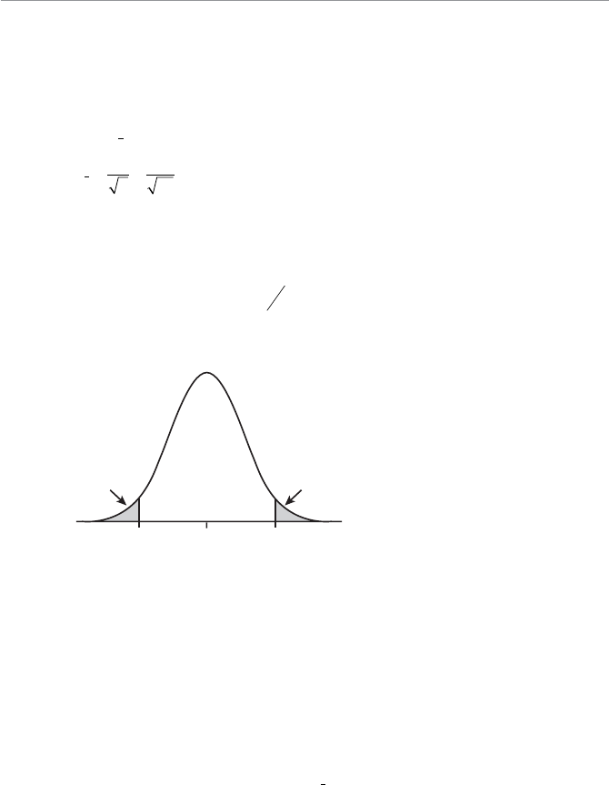
1VO^bS`#( 7\b`]RcQbW]\b]6g^]bVSaWaBSabW\U
Let’s say that I know that the standard deviation of the population, X, is 0.5 days, and
my sample size to test the hypothesis, n, is 30 homes. (Please don’t ask me how I’m
going to find 30 homes with loose snakes. I’m making this up as I go along, so just
humor me.) We’ll also set F = 0.05, which means I’m willing to accept a 5 percent
chance of committing a Type I error. Our first step is to calculate the standard error of
the mean, Sx. If you remember from Chapter 13, the equation is:
SS
xn
050
30 0 0913
..days
Let’s assume the sample mean from the 30 homes is 6.1 days. What is our conclusion
about our estimate of the population mean, R?
To answer this, we next have to determine the critical z-score, which corresponds to
F = 0.05. Because this is a two-tail test, this area needs to be evenly divided between
both tails, with each tail receiving A20 025.. According to Figure 15.3, we need to
find the critical z-score that corresponds to the area 0.950 + 0.025 = 0.975. As you can
see, the 0.950 area is derived from 1 – F.
4WUc`S#!
Critical z-score for F = 0.05.
0 +1.96-1.96
0.950
1–
2
/2
/
= 0.025 = 0.025
Using Table 3 in Appendix B, we look for the closest value to 0.9750 in the body of
the table. We can find this value by looking across column 1.9 and down row 0.06 to
arrive at the z-score of +1.96 for the right tail and –1.96 for the left tail.
CaW\UbVSAQOZS]TbVS=`WUW\OZDO`WOPZS
Now let’s determine the rejection region using the scale of the original variable, which
in this case is the number of days. To calculate the upper and lower limits of the rejec-
tion region, we use the following equations. Recall from Chapter 14 that we use the
z-scores from the standard normal distribution when nr30 and X is known.
Limits of rejection region = MS
Hc
x
z
0
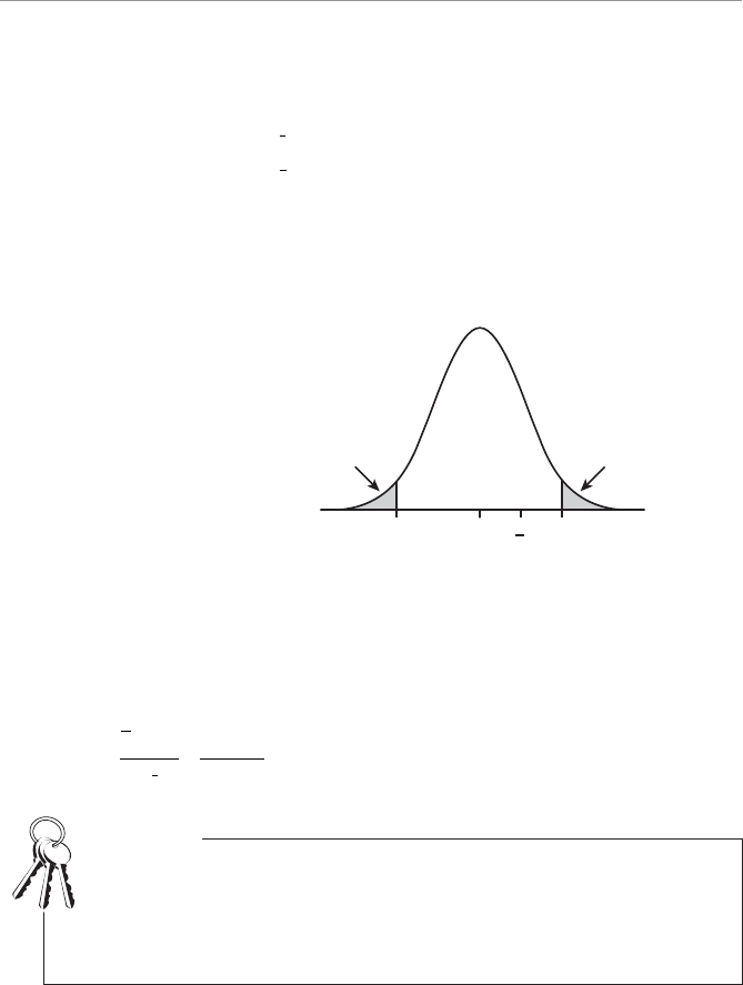
>O`b!( 7\TS`S\bWOZAbObWabWQa
where MH0 = the population mean assumed by the null hypothesis.
For our snake example:
Upper limit = MS
Hc
x
z
06 0 1 96 0 0913 6 18
... .
days
Lower limit = MS
Hc
x
z
06 0 1 96 0 0913 5 82
... .
days
Because our sample mean is 6.1 days, this falls within the “Do Not Reject H0” region
as shown in Figure 15.4. Our conclusion is that the difference between 6.1 days and
6.0 days is merely due to chance variation, and we have support that the population
mean is 6 days.
4WUc`S#"
Hypothesis test for the snake
example (original variable
scale).
6.0 6.15.82 6.18
Mean Number of Days to Catch a Snake
Reject H0Reject H0
Do Not Reject H0
x
H0
CaW\UbVSAbO\RO`RWhSR<]`[OZAQOZS
We can arrive at the same conclusion by setting up the boundaries for the rejection
region using the standardized normal scale. We do this by calculating the z-score that
corresponds to the sample mean as follows:
zxH
x
M
S
061 60
0 0913 109
..
..
Be sure to distinguish between the calculated z-score and the critical z-score. The
calculated z-score, z, represents the number of standard deviations between the
sample mean and MH0, the population mean according to the null hypothesis. The
critical z-score, zc, is based on the significance level, F, and determines the bound-
ary for the rejection region.
Bob’s Basics
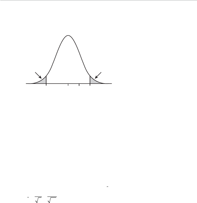
1VO^bS`#( 7\b`]RcQbW]\b]6g^]bVSaWaBSabW\U !
Figure 15.5 shows this result graphically. Because the calculated z-score of +1.09 is
within the “Do Not Reject H0” region, the conclusions of both techniques are consis-
tent.
4WUc`S##
Hypothesis test for the snake
example (standardized scale).
0 +1.09-1.96 +1.96
Number of Standard Deviations from the Mean
Reject H0Reject H0
Do Not Reject H0
z+z
c
–zc
3fO[^ZS]TO=\SBOWZ6g^]bVSaWaBSab
Because I formulated the alternative hypothesis for the golf ball example as > 20, this
becomes a one-tail test. The hypothesis for this example is stated as:
H020:Mb yards
H120:M yards
Where R = the mean increase in yards off the tee using my new golf ball.
Let’s say that I know that the standard deviation of the population, X, is 5.3 yards and
my sample size to test the hypothesis, n, is 40 golfers. For this example, we’ll set
F = 0.01. The standard error of the mean, Sx, will now be equal to:
SS
xn
53
40 0 838
.. yards
Let’s assume the sample mean from the 40 golfers is 22.5 yards. What is our conclu-
sion about our estimate of the population mean, R?
Once again, we next have to determine the critical z-score, which corresponds to F =
0.01. Because this is a one-tail test, this entire area needs to be in one rejection region
on the right side of the distribution. According to Figure 15.6, we need to find the z-
score that corresponds to the area 0.99 or 1 – F.
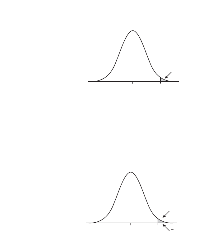
>O`b!( 7\TS`S\bWOZAbObWabWQa "
Using Table 3 in Appendix B, we look for the closest value to 0.9900 in the body of
the table, which results in a critical z-score of 2.33.
4WUc`S#$
Critical z-score for F = 0.01.
0 +2.33
Number of Standard Deviations from the Mean
= 0.01
0.99
+zc
To calculate the limit for this rejection region using the scale of the original variable,
we use:
Limit = MS
Hc
x
z
020 2 33 0 838 21 95
.. .
yards
Because our sample mean is 22.5 yards, this falls within the “Reject H0” region as
shown in Figure 15.7. Our conclusion is that we have enough evidence to support the
hypothesis that the mean increase in distance off the tee with my new balls exceeds 20
yards. I’m in business!
4WUc`S#%
Hypothesis test for the golf
ball example (original vari-
able scale).
20 21.95
Mean Increase in Distance off the Tee in Yards
Reject H0
Do Not Reject H0
x = 22.5
H0

1VO^bS`#( 7\b`]RcQbW]\b]6g^]bVSaWaBSabW\U #
As I mentioned earlier, the purpose of this chapter was to introduce the basic concepts
of hypothesis testing. The following two chapters will explore hypothesis testing in
even more loving detail. So hang in there—we’re just getting warmed up!
G]c`Bc`\
1. Formulate a hypothesis statement for the following claim: “The average adult
drinks 1.7 cups of coffee per day.” A sample of 35 adults drank an average of
1.95 cups per day. Assume the population standard deviation is 0.5 cups. Using
F = 0.10, test your hypothesis. What is your conclusion?
2. Formulate a hypothesis statement for the following claim: “The average age of
our customers is less than 40 years old.” A sample of 50 customers had an aver-
age age of 38.7 years. Assume the population standard deviation is 12.5 years.
Using F = 0.05, test your hypothesis. What is your conclusion?
3. Formulate a hypothesis statement for the following claim: “The average life of
our light bulbs is more than 1,000 hours.” A sample of 32 light bulbs had an
average life of 1,190 hours. Assume the population standard deviation is 325
hours. Using F = 0.02, test your hypothesis. What is your conclusion?
4. Formulate a hypothesis statement for the following claim: “The average delivery
time is less than 30 minutes.” A sample of 42 deliveries had an average time of
26.9 minutes. Assume the population standard deviation is 8 minutes. Using F =
0.01, test your hypothesis. What is your conclusion?
5. Formulate a hypothesis statement for the following claim: “Students graduating
from college have an average credit card debt of $2,700.” A sample of 40 college
graduates averaged $2,450 in credit card debt. Assume the population standard
deviation is $950. Using A00
5., test your hypothesis. What is your conclusion?
You might be asking yourself, “If the sample mean was 21.0 yards, shouldn’t that
provide conclusive evidence that the new ball increases distance by more than 20
yards?” According to the previous figure, the answer is no. Because we are bas-
ing our decision on a sample, an average of 21 is just too close to 20 to satisfy my
claim. The sample average would have to be 21.95 yards or more in order to reject
the null hypothesis.
Random Thoughts

>O`b!( 7\TS`S\bWOZAbObWabWQa $
BVS:SOabG]c<SSRb]9\]e
UThe null hypothesis, denoted by H0, represents the status quo and involves stat-
ing the belief that the mean of the population is f, =, or v a specific value.
UThe alternative hypothesis, denoted by H1, represents the opposite of the null
hypothesis and holds true if the null hypothesis is found to be false.
UUse a two-tail hypothesis test whenever the alternative hypothesis is expressed
as |; whereas a one-tail hypothesis test involves the alternative hypothesis being
stated as < or >.
UA Type I error occurs when the null hypothesis is rejected when, in reality, it is
true. The probability of this error occurring is known as F, the level of signifi-
cance.
UA Type II error occurs when the null hypothesis is accepted when, in reality, it is
not true. The probability of this error occurring is known as G.

16
1VO^bS`
6g^]bVSaWaBSabW\UeWbV=\S
AO[^ZS
7\BVWa1VO^bS`
UTesting the mean of a population using a large and small sample
UExamining the role of alpha (F) in hypothesis testing
UUsing the p-value to test a hypothesis
UTesting the proportion of a population using a large sample
In Chapter 15, I introduced the concept of hypothesis testing to whet your
appetite. I have devoted this chapter to hypothesis testing that involves only
one population, whereas in Chapter 17 I will discuss testing that compares
two different populations to each other.
Hypothesis testing involving one population focuses on confirming claims
such as the population average is equal to a specific value. We will con-
sider many different cases with this type of hypothesis testing in the fol-
lowing sections. This chapter relies on many of the concepts we explored
in Chapters 14 and 15, so be sure you are comfortable with that material
before you dive into this chapter.

>O`b!( 7\TS`S\bWOZAbObWabWQa &
6g^]bVSaWaBSabW\UT]`bVS;SO\eWbV:O`USAO[^ZSa
When the sample size we use to test our hypothesis is large (nv 30), we can rely on
our old friend the central limit theorem which we met in Chapter 13. However, we
still have two cases to consider—whether X, the population standard deviation, is
known or unknown.
EVS\AWU[O7a9\]e\
To demonstrate this type of hypothesis test, I’ll use the following story.
One of the most feared phrases a husband can hear from his wife is, “Honey, let’s go
on a diet together.” I should have been suspicious of Debbie’s motives when she sug-
gested we go on the low-carbohydrate diet, especially because she wears size 2 pants.
But I guess I could stand to lose a few pounds, so in a weak moment, I agreed. After
all, I figured we could turn this into a competition to make things more interesting.
After a few harrowing days without my beloved carbohydrates (who would have
guessed a grown man could dream about Cheez-its night after night), I began to won-
der how Debbie was doing so well with the diet. I found the answer to this mystery
hidden deep in the trunk of her car—a half-eaten box of cinnamon rolls. I guess that
makes me the winner. The thrill of victory!
Anyway, let’s say that this particular diet claims that the average age of the person
who participates in this self-inflicted torture is less than 40 years old. We set up our
hypothesis as follows:
H040:Mr years old
H140:M years old
We sample 60 people on the diet and find that their average age is 35.7 years. Given
that X, the population standard deviation, is 16 years, we’ll test the hypothesis at
A00
5..
Remember from Chapter 15 that F, the level of significance, represents the prob-
ability of making a Type I error. A Type I error occurs when we reject H0, when H0
is actually true. In this case, a Type I error would mean that we believe the claim
that the average person on the diet is less than 40 years old when, in reality, the
claim is not true. For this example there’s a 5 percent chance of this error happening.
Bob’s Basics
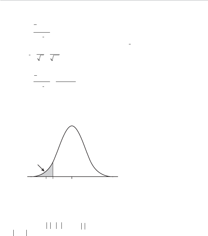
1VO^bS`$( 6g^]bVSaWaBSabW\UeWbV=\SAO[^ZS '
Because the sample size is greater than 30 and we know the value of X, we calculate
the z-score from the standardized normal distribution as we did in Chapter 15.
zxH
x
M
S
0
For our example, the standard error of the mean, Sx, would be:
SS
xn
16
60 207. years
This results in a calculated z-score of:
zxH
x
M
S
035 7 40
207 208
.
..
Also recall from Chapter 15, the critical z-score, which defines the boundary for the
rejection region, is –1.64 for a one-tail (left side) test with F = 0.05.Figure 16.1 shows
this test graphically.
4WUc`S$
One-tail hypothesis test for
the diet example (standard-
ized scale).
0-1.64
Number of Standard Deviations from the Mean
Do Not Reject H0
-2.08
zc
z
0.95
1–
= 0.05
Reject H0
As you can see in the figure, the calculated z-score of –2.08 falls within the “Reject
H0” region, which allows us to conclude that the claim that the average age of those
on this diet is less than 40 years old. I knew I was too old for this diet! In general,
we reject H0 if zz
c
, where z means the “absolute value of z.” For instance,
208 208...
EVS\AWU[O7aC\Y\]e\
Many times, we just don’t have enough information to know the value of X, the popu-
lation standard deviation. However, as long as our sample size is 30 or more, we can
substitute s, the sample standard deviation for X. To illustrate this technique, let’s use
the following example.

>O`b!( 7\TS`S\bWOZAbObWabWQa !
I don’t know about you, but it seems I spend too much time on the phone waiting
on hold for a live customer service representative. Let’s say a particular company has
claimed that the average time a customer waits on hold is less than five minutes. We’ll
assume we do not know the value of X. The following table represents the wait time in
minutes for a random sample of 30 customers.
Wait Time in Minutes
6.2 3.8 1.3 5.4 4.7 4.4 4.6 5.0 6.6 8.3
3.2 2.7 4.0 7.3 3.6 4.9 0.5 2.9 2.5 5.6
5.5 4.7 6.5 7.1 4.4 5.2 6.1 7.4 4.8 2.9
Using Excel, we can determine that x474. minutes and s = 1.82 minutes. At first
glance, it appears the company’s claim is valid. But let’s put it through a hypothesis
test with A00
2. to be sure.
State the hypothesis as:
H050:.Mr minutes
H150:.M minutes
From Chapter 15, we know that the critical z-score for a one-tail (left side) hypothesis
test with F = 0.02 is –2.05.
As we did earlier in Chapter 14, we can approximate the standard error of the mean
by:
ˆ..Sx
s
n
182
30 0 332 minutes
Our calculated z-score using this particular sample would be:
zxH
x
M
S
0474 50
0 332 078
ˆ
..
..
Figure 16.2 shows this test graphically.
According to our figure, we do not reject the null hypothesis. In other words, we do
not have enough evidence from this sample to support the company’s claim that the
average wait on hold is less than five minutes. Even though the sample average is
actually less than five minutes (4.74), it is too close to five minutes to say there is a
difference between the two values. Another way to state this is to say: “The difference
between 4.74 and 5.0 is not statistically significant in this case.”
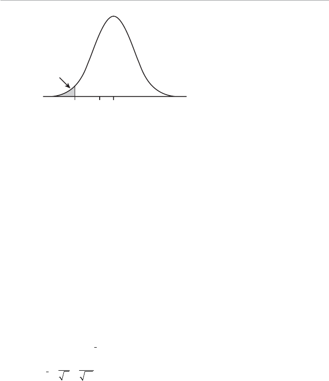
1VO^bS`$( 6g^]bVSaWaBSabW\UeWbV=\SAO[^ZS !
BVS@]ZS]T/Z^VOW\6g^]bVSaWaBSabW\U
For all the examples in these last two chapters, I have just stated a value for F, the
level of significance. I’m sure you’re wondering what impact changing the value of F
will have on the hypothesis test. Great question!
Suppose that I am making a claim that the average grade for a person using this book
will be more than an 87. (I’m not really making this claim, so don’t get too excited!) I
would state the hypothesis test as follows:
H087:Mb
H187:M
Now, it would be in my best interest if I could reject H0, which would validate my
claim. I can do so by choosing a fairly high value for F, say 0.10. This corresponds to
a critical z-score of +1.28, because we are using the right tail of a one-tail hypothesis
test.
Let’s say that X, the population standard deviation, is 12 and my sample mean is 90.6,
which was taken from a sample size of 32 students. For this example, the standard
error of the mean, Sx, would be:
SS
xn
12
32 212.
4WUc`S$
One-tail hypothesis test for
waiting on hold example
(standardized scale).
0-2.05 -0.78
Number of Standard Deviations from the Mean
Do Not Reject H0
zcz
0.98
1–
= 0.02
Reject H0
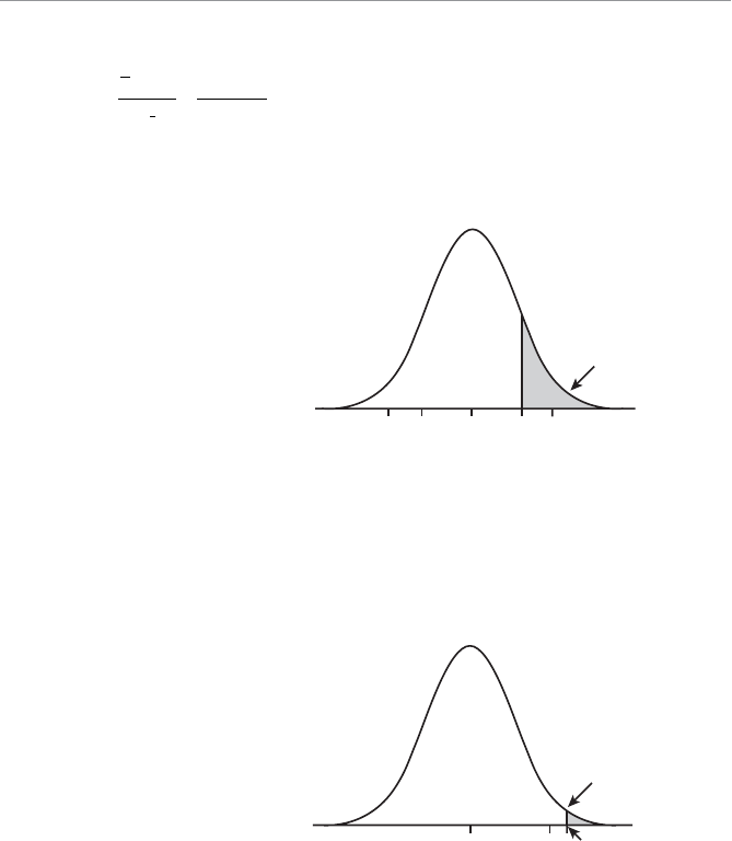
>O`b!( 7\TS`S\bWOZAbObWabWQa !
This results in a calculated z-score of:
zxH
x
M
S
090 6 87
212 170
.
..
According to Figure 16.3, I have achieved my goal of rejecting H0, because the calcu-
lated z-score is within the shaded region. My book appears to have done the trick!
4WUc`S$!
Hypothesis test for grade
example, F = 0.10.
1.71.280
Number of Standard Deviations from the Mean
Do Not Reject H0
zcz
0.90
1–
= 0.10
Reject H0
However, I must admit, I chose a pretty “wimpy” value of F = 0.10 in an effort to help
prove my claim. In this case, I am willing to accept a 10 percent chance of a Type I
error. A more impressive test would be to set alpha lower, say F = 0.01. Now that’s a
“real man’s alpha.” The level of significance corresponds to a critical z-score of +2.33.
Figure 16.4 shows the impact of this change.
4WUc`S$"
Hypothesis test for grade
example, F = 0.01.
2.33
1.70
Number of Standard Deviations from the Mean
Do Not Reject H0
zc
z
0.99
1–
= 0.01
Reject H0
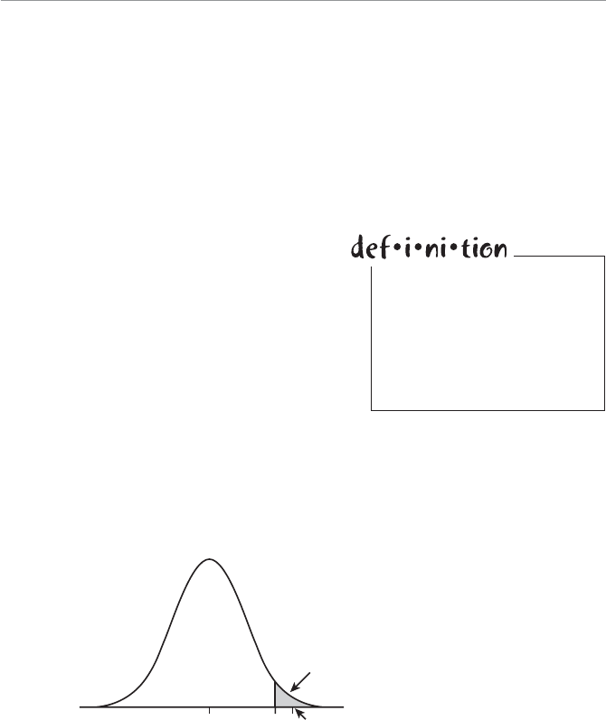
1VO^bS`$( 6g^]bVSaWaBSabW\UeWbV=\SAO[^ZS !!
As you can see, to my horror, the shaded region no longer includes my calculated
z-score of +1.7. Therefore, I do not reject H0 and cannot claim the average grade of
those using my book exceeds an 87. In general, a hypothesis test that rejects H0 is most
impressive with a low value of F.
7\b`]RcQW\UbVS]DOZcS
Just when you thought it was safe to get back in the water, along comes another shark!
This is the perfect opportunity to throw another concept at you. You might feel like
grumbling a little right now, but in the end
you’ll be thanking me.
The p-value is the smallest level of signifi-
cance at which the null hypothesis will be
rejected, assuming the null hypothesis is
true. The p-value is sometimes referred to
as the observed level of significance. I know this
may sound like a lot of mumbo-jumbo right
now, but an illustration will help make this
clear.
BVS]DOZcST]`O=\SBOWZBSab
Using the previous grade example (over 87 if using this book), the p-value is repre-
sented by the shaded area to the right of the calculated z-score of +1.7. This is shown
in Figure 16.5.
The observed level of sig-
nificance is the smallest level
of significance at which the
null hypothesis will be rejected,
assuming the null hypothesis is
true. It is also known as the p-
value.
4WUc`S$#
p-value for the grade
example.
2.33
1.70
Number of Standard Deviations from the Mean
Do Not Reject H0
zc
z
0.9554
p – value
0.0446
>O`b!( 7\TS`S\bWOZAbObWabWQa !"
Using our standardized normal z table (Table 3 in Appendix B), we can confirm that
the shaded area in the right tail is equal to P[ . ] .z 17 0 0446.
Because our p-value of 0.0446 is more than the value
of F (set at 0.01), we do not reject H0. Most statistical
software packages (including Excel) provide p-values
with the analysis.
Another way to describe this p-value is to say, in a
very scholarly voice, “Our results are significant at
the 0.0446 level.” This means that as long as the
value of F is 0.0446 or larger, we will reject H0, which
is normally good news for researchers trying to vali-
date their findings.
Calculating the p-value for a two-tail hypothesis test
is slightly different, and I’ll show you how in the next
section.
BVS]DOZcST]`OBe]BOWZBSab
Recall that you use a two-tail hypothesis test when the null hypothesis is stated as an
equality. For example, let’s test a claim that states the average number of miles driven
by a passenger vehicle in a year equals 11,500 miles. I have serious reservations about
this claim after spending half the day being a taxi driver to the kids. We would state
the hypotheses as follows:
H0:R" 11,500 miles
H1:R| 11,500 miles
Let’s assume X" 3000 miles, and we want to set F" 0.05. We sample 80 drivers and
determine the average number of miles driven is 11,900. What is our p-value, and
what do we conclude about the hypothesis?
Recall that PP[.
][.] . .zz b 1 7 1 1 7 1 0 9554 0 0446 . See Chapter 11
if you need a refresher on using the standardized normal z table.
Bob’s Basics
We can use the p-value to
determine whether or not to
reject the null hypothesis. In
general …
U If p-value fF, we reject
the null hypothesis.
U If p-value #F, we do not
reject the null hypothesis.
Bob’s Basics
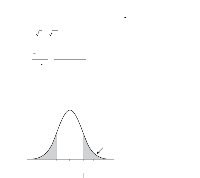
1VO^bS`$( 6g^]bVSaWaBSabW\UeWbV=\SAO[^ZS !#
For this example, the standard error of the mean, Sx, would be:
SS
xn
3000
80 335 41. miles
This results in a calculated z-score of:
zxH
x
M
S
011 900 11 500
335 41 119
,,
..
The critical z-score for a two-tail test with F" 0.05 is t 1.96. The shaded area in
Figure 16.6 shows the p-value for this test.
4WUc`S$$
p-value for the miles driven
per year example.
p-Value for a Two-Tail Hyphothesis Test
+1.190
zc
zc
-1.19-1.96 +1.96
z
0.766
0.8830
0.117 0.117
p-Value Equals the Sum
of the Shaded Regions
p-Value = 0.117 + 0.117
= 0.234
According to Table 3 in Appendix B, the P[ . ] .zb 1 19 0 8830. This means the shaded
region in the right tail of Figure 16.6 is
P[ . ] . .z 1 19 1 0 8830 0 117
. Because this
is a two-tail test, we need to double this area to arrive at our p-value. According to our
figure, the p-value is the total area of both shaded regions, which is 2 0 117 0 234s...
Because pA, we do not reject the null hypothesis. Our data supports the claim that
the average number of miles driven per year by a passenger vehicle is 11,500.
In general, the smaller the p-value, the more confident we are about rejecting the null
hypothesis. In most cases a researcher is attempting to find support for the alternative
hypothesis. A low p-value provides support that brings joy to his or her heart.

>O`b!( 7\TS`S\bWOZAbObWabWQa !$
6g^]bVSaWaBSabW\UT]`bVS;SO\eWbVA[OZZAO[^ZSa
Recall, from Chapter 14, that with a small sample size, we lose the use of the central
limit theorem, so, therefore, we need to assume that the population is normally dis-
tributed for all cases in this section. The first case that we’ll examine is when we know
X,the population standard deviation.
EVS\AWU[O7a9\]e\
When X is known, the hypothesis test reverts back to the large sample size case. We
can do this because we are now assuming the population is normally distributed. We
can demonstrate this method with the following example.
Opening up my monthly cell phone bill lately has become a nerve-wracking experi-
ence. As I warily open the envelope, I wonder what surprises await me. With several
users on our family “share plan,” I can often count on somebody having discovered a
new feature that has nothing to do with talking to another person on the phone and
having used this new-found discovery over and over and over again. Occasionally, after
digging through countless pages full of numbers and codes, I breathe a sigh of relief
and say a silent prayer of thanks. Most months, however, I end up clutching my chest
and screaming “AIEEEEEEEE!” It’s like playing a subtle form of Russian roulette
with the phone company.
Anyway, let’s say the phone company claims that the average monthly cell phone bill
for their customers is $92 (I wish). We can test this claim by stating our hypothesis as:
H0:R" $92
H1:R| $92
We’ll assume that X" $22.50 and that the popula-
tion is normally distributed. We select 18 phone bills
randomly and determine the sample average equals
$107. Using F" 0.02, what do we conclude?
For this example, the standard error of the mean,
Sx, would be:
SS
xn
$. $.
22 50
18 530
Recall from Chapter 14 that
because we know X and
we assumed the population
is normally distributed, we can
use the z-scores from the normal
probability distribution to test
this hypothesis.
Bob’s Basics
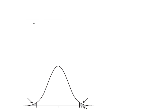
1VO^bS`$( 6g^]bVSaWaBSabW\UeWbV=\SAO[^ZS !%
This results in a calculated z-score of:
zxH
x
M
S
0107 92
530 283
$$
$. .
The critical z-score for a two-tail test with F" 0.02 is t 2.33. Figure 16.7 shows this
test graphically.
As you can see in Figure 16.7, the calculated z-score of +2.83 is with the “Reject H0”
region. We, therefore, conclude that the average cell phone bill is not equal to $92. I
didn’t think so!
4WUc`S$%
Hypothesis test for cell phone
bills.
Number of Standard Deviations from the Mean
0
zc
zc
-2.33 +2.83+2.33
z
0.98
1–
Do Not Reject H0
/2 = 0.01
Reject H0
/2 = 0.01
Reject H0
EVS\AWU[O7aC\Y\]e\
As we did in Chapter 14, when X is unknown for a small sample size taken from a
normally distributed population, we use the Student’s t-distribution. This particular
distribution allows us to substitute s, the sample standard deviation for X.
As an example, suppose my son John claims his average golf score is less than 88. Not
to be one to doubt him, I can test this claim with the following hypothesis:
H0:Rv 88
H1:R! 88
We will assume that we do not know X and that John’s scores follow a normal distri-
bution. The following represents a random sample of 10 golf scores from John.

>O`b!( 7\TS`S\bWOZAbObWabWQa !&
8]V\Âa5]ZTAQ]`Sa
86 87 85 90 86 84 84 91 87 83
Using Excel, we can determine that x86 3. and s = 2.58 for this sample. Recall from
Chapter 14, we can approximate the standard error of the mean using the following
equation:
ˆ..Sx
s
n
258
10 0 816
We can then determine the calculated t-score using the following equation:
txH
x
M
S
086 3 88
0 816 208
ˆ
.
..
We’ll test this hypothesis using F" 0.05. T
o find the corresponding critical t-score, we
use T
able 4 from Appendix B. Here is an excerpt of this table.
AbcRS\bÂab2Wab`WPcbW]\BOPZS
Selected right-tail areas with confidence levels underneath
Alpha 0.2000 0.1500 0.1000 0.0500 0.0250 0.0100 0.0050 0.0010 0.0005
Conf lev 0.6000 0.7000 0.8000 0.9000 0.9500 0.9800 0.9900 0.9980 0.9990
d.f.
1 1.376 1.963 3.078 6.314 12.706 31.821 63.657 318.31 636.62
2 1.061 1.386 1.886 2.920 4.303 6.965 9.925 22.327 31.599
3 0.978 1.250 1.638 2.353 3.182 4.541 5.841 10.215 12.924
4 0.941 1.190 1.533 2.132 2.776 3.747 4.604 7.173 8.610
5 0.920 1.156 1.476 2.015 2.571 3.365 4.032 5.893 6.869
6 0.906 1.134 1.440 1.943 2.447 3.143 3.707 5.208 5.959
7 0.896 1.119 1.415 1.895 2.365 2.998 3.499 4.785 5.408
8 0.889 1.108 1.397 1.860 2.306 2.896 3.355 4.501 5.041
9 0.883 1.100 1.383 1.833 2.262 2.821 3.250 4.297 4.781
10 0.879 1.093 1.372 1.812 2.228 2.764 3.169 4.144 4.587
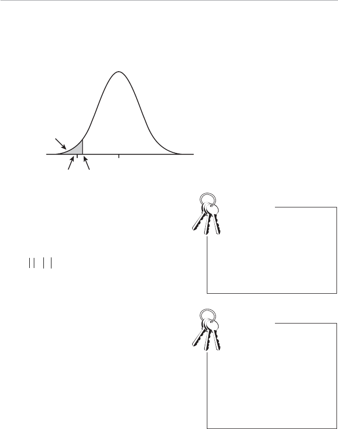
1VO^bS`$( 6g^]bVSaWaBSabW\UeWbV=\SAO[^ZS !'
You recall from Chapter 14, we need to determine the number of degrees of freedom,
which is equal to n 11
019 for this example. Because this is a one-tail (left side)
test, we look under the A00
5. column resulting in a critical t-score,
tc
, equal to
–1.833, which is underlined. Figure 16.8 shows this test graphically.
4WUc`S$&
Hypothesis test for John’s golf
scores.
0
tc= –1.833 t= –2.08
0.95
1–
Do Not Reject H0
= 0.05
Reject H0
As we can see in the figure, the calculated
t-score of –2.08 falls within the shaded
“Reject H0” region. Therefore, we can
conclude that John’s average golf score is
indeed lower than 88. So that explains why
he usually beats me! In general, we reject H0
if tt
c
.
Let’s take another example to demonstrate
a two-tail hypothesis test using the t-
distribution. I would like to test a claim
that the average speed of cars passing a
specific spot on the interstate is 65 miles
per hour. We can express the hypothesis
test as follows:
H0:R" 65 miles per hour
H1:R| 65 miles per hour
We will assume that we do not know X and
that speeds follow a normal distribution.
The following represents a random sample
of the speed of seven cars.
Because John’s golf score
example is a one-tail test on
the left side of the distribu-
tion, we use a negative critical
t-score. Had this been a one-tail
test on the right side, we would
use a positive critical t-score.
Bob’s Basics
It is not possible to determine
the p-value for a hypothesis
test when using the Student’s
t-distribution table in Appendix
B. However, most statistical soft-
ware will provide the p-value as
part of the standard analysis.
We’ll see this in later chapters
as we use Excel.
Bob’s Basics

>O`b!( 7\TS`S\bWOZAbObWabWQa "
1O`A^SSRa
62 74 65 68 71 64 68
Using Excel, we can determine that x66 9. mph and s = 4.16 mph for this sample.
We can approximate the standard error of the mean:
ˆ..Sx
s
n
416
7157mph
We can then determine the calculated t-score:
txH
x
M
S
066 9 65
157 121
ˆ
.
..
We’ll test this hypothesis using F" 0.05. T
o find the corresponding critical t-score, we
use T
able 4 from Appendix B. Here is an excerpt of this table.
AbcRS\bÂab2Wab`WPcbW]\BOPZS
Selected right-tail areas with confidence levels underneath
Alpha 0.2000 0.1500 0.1000 0.0500 0.0250 0.0100 0.0050 0.0010 0.0005
Conf lev 0.6000 0.7000 0.8000 0.9000 0.9500 0.9800 0.9900 0.9980 0.9990
d.f.
1 1.376 1.963 3.078 6.314 12.706 31.821 63.657 318.31 636.62
2 1.061 1.386 1.886 2.920 4.303 6.965 9.925 22.327 31.599
3 0.978 1.250 1.638 2.353 3.182 4.541 5.841 10.215 12.924
4 0.941 1.190 1.533 2.132 2.776 3.747 4.604 7.173 8.610
5 0.920 1.156 1.476 2.015 2.571 3.365 4.032 5.893 6.869
6 0.906 1.134 1.440 1.943 2.447 3.143 3.707 5.208 5.959
7 0.896 1.119 1.415 1.895 2.365 2.998 3.499 4.785 5.408
The number of degrees of freedom for this example equals n – 1 = 7 – 1 = 6. Because
this is a two-tail test, we need to divide F" 0.05 into two equal portions, one on
the right side of the distribution, the other on the left. We then look under the
A20 025. column resulting in a critical t-score, tc, equal to t 2.447, which is under-
lined. This test is shown graphically in Figure 16.9.
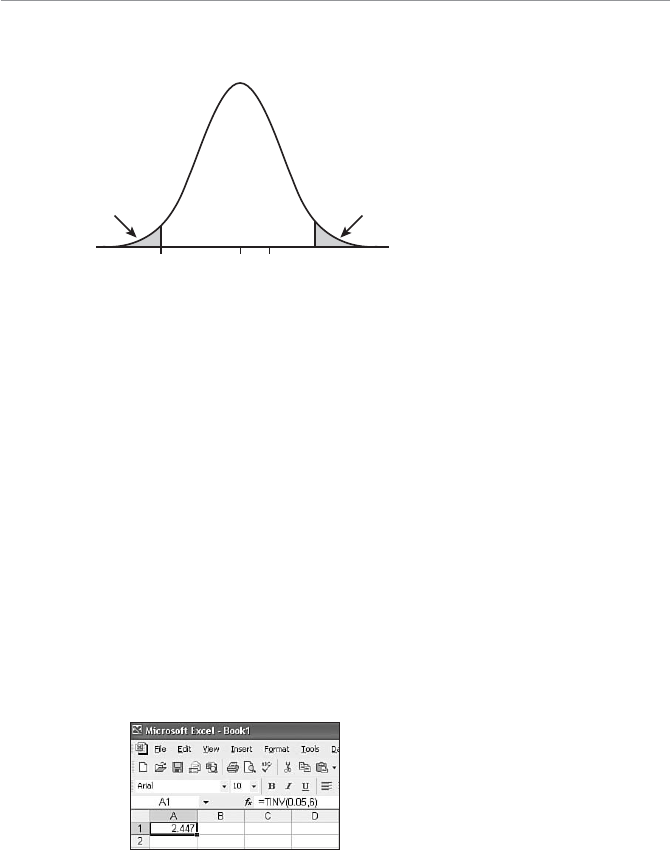
1VO^bS`$( 6g^]bVSaWaBSabW\UeWbV=\SAO[^ZS "
As we can see in the figure, the calculated t-score of +1.21 falls within the “Do Not
Reject H0” region. Therefore, we can conclude that the average speed past this spot on
the interstate averages 65 miles per hour.
CaW\U3fQSZÂaB7<D4c\QbW]\
We can generate critical t-scores using Excel’s TINV function, which has the follow-
ing characteristics:
TINV(probability, deg-freedom)
where:
probability = the level of significance, F, for a two-tail test
deg-freedom = the number of degrees of freedom
For instance, Figure 16.10 shows the TINV function being used to determine the
critical t-score for F" 0.05 and d.f. = 6 from our previous example, which was a two-
tail test.
4WUc`S$'
Hypothesis test for car speed.
Hypothesis Test for Car Speeds
(Two Tail t-Distribution)
0 +2.447-2.447 1.21
tctc
t
0.95
1–
Do Not Reject H0
= 0.025
Reject H0
/2= 0.025
Reject H0
/2
4WUc`S$
Excel’s TINV function for a
two-tail test.

>O`b!( 7\TS`S\bWOZAbObWabWQa "
Cell A1 contains the Excel formula =TINV(0.05, 6) with the result being 2.447. This
probability is underlined in the previous table.
A one-tail test requires a slight modification. We need to multiply the probability in
the TINV function by two because this parameter is based on a two-tail test. Figure
16.11 shows the TINV function being used to determine the critical t-score for F"
0.05 and d.f. = 9 from our earlier one-tail test example with John’s golf scores.
4WUc`S$
Excel’s TINV function for a
one-tail test.
Cell A1 contains the Excel formula =TINV(2*0.05, 9) with the result being 1.833.
This is consistent with the result from our previous example.
6g^]bVSaWaBSabW\UT]`bVS>`]^]`bW]\eWbV:O`US
AO[^ZSa
You can perform hypothesis testing for the proportion of a population as long as the
sample size is large enough. Recall from Chapter 13, that proportion data follows the
binomial distribution, which can be approximated by the normal distribution under
the following conditions:
np r5 and nq r5
where:
p = the probability of a success in the population
q= the probability of a failure in the population (q = 1 – p)
We will examine both one-tail and two-tail hypothesis testing for the proportion in
the following sections.
1VO^bS`$( 6g^]bVSaWaBSabW\UeWbV=\SAO[^ZS "!
=\SBOWZ6g^]bVSaWaBSabT]`bVS>`]^]`bW]\
Let’s say we would like to test the hypothesis that more than 30 percent of U.S.
households have Internet access. We would state the hypothesis as:
H0:pv 0.30
H1:p! 0.30
where p = the proportion of U.S. house-
holds with Internet access.
We collect a sample of 150 households and
find that 38 percent of these have Internet
access. What can we conclude at the
F" 0.05 level?
Our first step is to calculate Sp, the stan-
dard error of the proportion, which was
described in Chapter 13 using the following
equation:
Sp
HH
pp
n
00
1
where pH0 = the proportion assumed by the null hypothesis. For our example:
Sp
030 1 030
150 037
..
.
Next, we can determine the calculated z-score using:
zpp
H
p
0
S
where p = the sample proportion. For our example:
zpp
H
p
0038 030
0 037 216
S
..
..
The critical z-score for a one-tail test with F" 0.05 is +1.64. This hypothesis test is
shown graphically in Figure 16.12.
Be careful not to confuse
this definition of p with the
p-value that we talked about
earlier.
Wrong Number
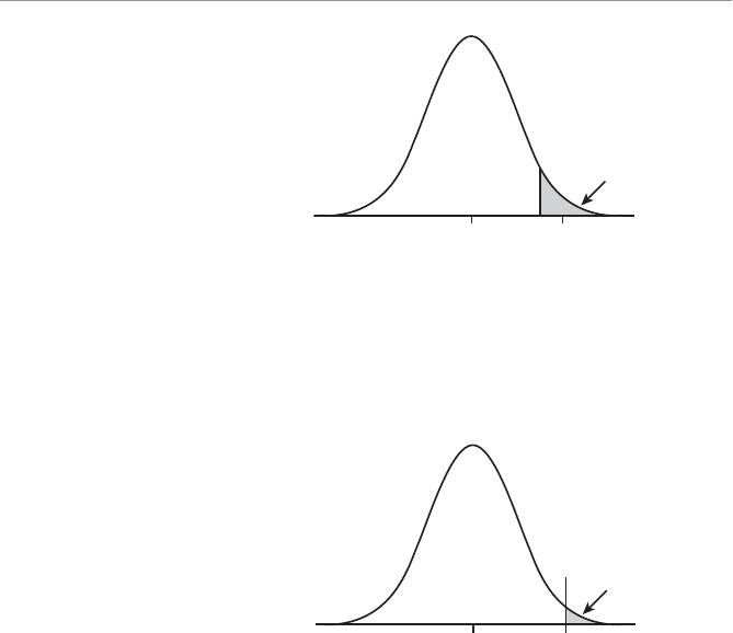
>O`b!( 7\TS`S\bWOZAbObWabWQa ""
As you can see in Figure 16.12, the calculated z-score of +2.16 is within the “Reject
H0” region. Therefore, we conclude that the proportion of U.S. households with
Internet access exceeds 30 percent.
We can show the p-value for this test graphically in Figure 16.13.
4WUc`S$
Hypothesis test for the
Internet access example.
Number of Standard Deviations from the Mean
0
zc
2.161.64
z
0.95
1– a
Do Not Reject H0
a= 0.05
Reject H0
4WUc`S$!
p-value for the Internet access
example.
Number of Standard Deviations from the Mean
0 2.16
z
0.9846
p-Value
0.0154
Using our standardized normal z table (Table 3 in Appendix B), we can confirm that
the shaded area in the right tail is equal to:
PP
P
[.
] [.]
[.
].
zz
z
b
216 1 216
2 16 1 0 9846 00 0154.
Therefore, our results are significant at the 0.0154 level. As long as Fv 0.0154, we
will be able to reject H0.
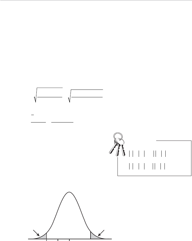
1VO^bS`$( 6g^]bVSaWaBSabW\UeWbV=\SAO[^ZS "#
Be]BOWZ6g^]bVSaWaBSabT]`bVS>`]^]`bW]\
We’ll wrap this chapter up with one final two-tail example. Here, we want to test a
hypothesis for a company that claims 50 percent of their customers are of the male
gender. We state our hypothesis as:
H0:p" 0.50
H1:p| 0.50
We randomly select 256 customers and find that 47 percent are male. What can we
conclude at the F" 0.05 level?
We need to determine Sp, the standard error of the proportion:
Sp
HH
pp
n
00
1050 1 050
256 0 0312
..
.
Next, we can determine the calculated z-score:
zpp
H
p
0047 050
0 0312 096
S
..
..
The critical z-score for a two-tail test with
F" 0.05 is t 1.96. This hypothesis test is
shown graphically in Figure 16.14.
As you can see in Figure 16.14, the calcu-
lated z-score of –0.86 is within the “Do Not
Reject H0” region. There, we conclude that
the proportion of male customers is equal to
50 percent for this company.
In general, we reject H0 if
zz
c
or tt
c
.
Also, we do not reject H0 if
zz
c
b or
tt
c
b
.
Bob’s Basics
Number of Standard Deviations from the Mean
0 +1.96-1.96
zczc
-0.86
z
0.95
1– a
Do Not Reject H0
= 0.025
Reject H0
/2= 0.025
Reject H0
/2
aa
4WUc`S$"
Hypothesis test for the per-
centage of males example.
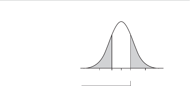
>O`b!( 7\TS`S\bWOZAbObWabWQa "$
Figure 16.15 graphically shows the p-value for this test.
4WUc`S$#
p-value for the percentage of
males example.
0-1.96 +1.96
zc
zc
-0.86 +0.86
z
0.663
0.1685
0.8315
0.1685
p-Value Equals the Sum
of the Shaded Regions
p-Value = 0.1685 + 0.1685
= 0.337
Using our standardized normal z table (Table 3 in Appendix B), we can confirm that
the shaded area in the left tail is equal to:
PP
P
[.
] [.]
[.
].
zz
z
b b
b
086 1 086
0 86 1 0 8315 00 1685.
Because this is a two-tail test, the p-value would be 2 0 1685 0 337s.., which repre-
sents the total area in both shaded regions.
G]c`Bc`\
1. Test the claim that the average SAT score for graduating high school students
is equal to 1100. A random sample of 70 students was selected, and the average
SAT score was 1035. Assume X" 310 and use F" 0.10.What is the p-value for
this sample?
2. A student organization at a small business college claims that the average class
size is greater than 35 students. Test this claim at F" 0.02, using the following
sample of class size:
42 28 36 47 35 41 33 30 39 48
Assume the population is normally distributed and that X is unknown.

1VO^bS`$( 6g^]bVSaWaBSabW\UeWbV=\SAO[^ZS "%
3. Test the claim that the average gasoline consumption per car in the United
States is more than 7 liters per day. (We’re going metric here!) Use the random
sample here, which represents daily gasoline usage for one car:
9 6 4 124 3 1810 4 5
3 8 4113 5 8 41210
9 5 15176 13 7 8 14 9
Assume the population is normally distributed, and that X is unknown. Use
F" 0.05 and determine the p-value for this sample.
4. Test the claim that the proportion of Republican voters in a particular city is less
than 40 percent. A random sample of 175 voters was selected and found to con-
sist of 30 percent Republicans. Use F" 0.01 and determine the p-value for this
sample.
5. Test the claim that the proportion of teenage cell phone users exceeding their
allotted monthly minutes equals 65 percent. A random sample of 225 teenagers
was selected and found to consist of 69 percent exceeding their minutes. Use
F" 0.05 and determine the p-value for this sample.
6. Test the claim that the mean number of hours that undergraduate students work
at a particular college is less than 15 hours per week. A random sample of 60 stu-
dents was selected, and the average number of working hours was 13.5 hours per
week. Assume X" 5 hours, and use F" 0.10. What is the p-value for this sample?
BVS:SOabG]c<SSRb]9\]e
UThe smaller the value of F, the level of significance; the more difficult it is to
reject the null hypothesis.
UWe reject H0 if zz
c
or tt
c
.
UThe p-value is the smallest level of significance at which the null hypothesis will
be rejected, assuming the null hypothesis is true.
UIf the p-value bA, we reject the null hypothesis. If p-value A, we do not reject
the null hypothesis.
UUse the Student’s t-distribution for the hypothesis test when n < 30, X is
unknown, and the population is normally distributed.

17
1VO^bS`
6g^]bVSaWaBSabW\UeWbVBe]
AO[^ZSa
7\BVWa1VO^bS`
UDeveloping the sampling distribution for the difference in means
UTesting the difference in means between populations using a large and
small sample
UDistinguishing between independent and dependent samples
UUsing Excel to perform a hypothesis test
UTesting the difference in proportions between populations
Now we’re really cooking. Because you have done so well with one sample
hypothesis testing, you are ready to graduate to the next level—two-sample
testing. Here we often test to see whether there is a difference between two
separate populations. For instance, I could test to see whether there was a
difference between Brian and John’s average golf score. But being an “expe-
rienced” parent, I know better than to go near that one.
Because many similarities exist between the concepts of this chapter and
those of Chapter 16, you should have a firm handle on the previous chap-
ter’s material before you jump into this one.
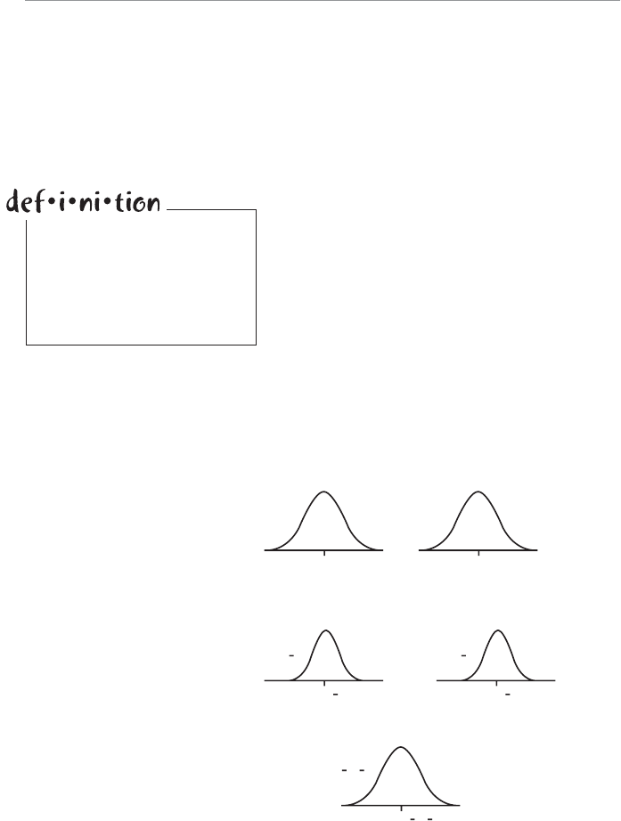
>O`b!( 7\TS`S\bWOZAbObWabWQa #
BVS1]\QS^b]TBSabW\UBe]>]^cZObW]\a
Many statistical studies involve comparing the same parameter, such as a mean,
between two different populations. For example:
UIs there a difference in average SAT scores between males and females?
UDo “long-life” light bulbs really outlast standard light bulbs?
U Does the average selling price of a house in
Newark differ from the average selling price for
a house in Wilmington?
To answer such questions, we need to explore a new
sampling distribution. (I promise this will be the last.)
This one has the fanciest name of them all—the sam-
pling distribution for the difference in means. (Dramatic
background music brings us to the edge of our seats.)
AO[^ZW\U2Wab`WPcbW]\T]`bVS2WTTS`S\QSW\;SO\a
The sampling distribution for the difference in means can best be described in Figure
17.1.
The sampling distribution
for the difference in means
describes the probability of
observing various intervals for
the difference between two
sample means.
4WUc`S%
The sampling distribution for
the difference in means. 1
Population 1
1
1
2
Population 2
2
2
3
Sampling Distribution for the Mean
(Population 1)
x1
x1 4
Sampling Distribution for the Mean
(Population 2)
x2
x2
5
Sampling Distribution for the Difference in Means
x1–x2
x1–x2
1VO^bS`%( 6g^]bVSaWaBSabW\UeWbVBe]AO[^ZSa #
As an example, let’s consider testing for a difference in SAT scores for male and female
students. We’ll assign female students as Population 1 and male students as Population
2. Graph 1 in Figure 17.1 represents the distribution of SAT scores for the female
students with mean R1 and standard deviation X1. Graph 2 represents the same for the
male population.
Graph 3 represents the sampling distribution for the mean for the female students.
This graph is the result of taking samples of size n1 and plotting the distribution of
sample means. Recall that we discussed this distribution of sample means back in
Chapter 13. The mean of this distribution would be:
MM
x11
This is according to the central limit theorem from Chapter 13. The same logic holds
true for Graph 4 for the male population.
Graph 5 in Figure 17.1 shows the distribution that represents the difference of sample
means from the female and male populations. This is the sampling distribution for the
difference in means, which has the following mean:
MMM
xx x x
12 1 2
In other words, the mean of this distribution, shown in Graph 5, is the difference
between the means of Graphs 3 and 4.
The standard deviation for the Graph 5 is known as the standard error of the difference
between two means and is calculated with:
SSS
xx nn
12
1
2
1
2
2
2
where:
S1
2,S2
2 = the variance for Populations
1 and 2
n1,n2 = the sample size from
Populations 1 and 2
Now before you pull the rest of your hair
out, let’s put these guys to work in the fol-
lowing section.
The standard error of the dif-
ference between two means
describes the variation in the
difference between two sample
means and is calculated using:
SSS
xx nn
12
1
2
1
2
2
2

>O`b!( 7\TS`S\bWOZAbObWabWQa #
BSabW\UT]`2WTTS`S\QSa0SbeSS\;SO\aeWbV:O`US
AO[^ZSAWhSa
When the sample sizes from both populations of interest are greater than 30, the
central limit theorem allows us to use the normal distribution to approximate the sam-
pling distribution for the difference in means. Let’s demonstrate this technique with
the following example.
Studies have been done to investigate the effects of stimulation on the brain develop-
ment of rats. I guess the logic being what’s good for rats can’t be all that bad for us
humans. Two samples were randomly selected from the same rat population.
The first sample, we’ll call these the “lucky rats” (Population 1), was surrounded with
every luxury a rat could imagine. I can envision a country club atmosphere, complete
with a golf course (and tiny golf carts), tennis courts, and a five-star restaurant where
our lucky rats could feast on imported cheese and French wine while they discussed
the state of the rat economy.
The second sample, we’ll call them the “less-fortunate rats” (Population 2), didn’t
have it quite so good. These guys were locked in a barren cage and were forced to eat
Cheez Whiz from a can and watch reruns of reality TV shows. Animal rights activists
protested against this experiment, claiming the involuntary use of Cheez Whiz was
“inhumane.”
After spending three months in each of these environments, the size of each rat brain
was measured by weight for development. I’ll spare you the details as to how this was
done, but I will tell you that Harvey the Rat mysteriously failed to show for his 8 A.M.
tee time. His group went off without him.
The following table summarizes these gruesome findings.
Ac[[O`WhSR2ObOT]`@Ob3f^S`W[S\b
Average Brain Sample Standard Sample
Population Weight in Grams Deviation Size
x
_sn
Lucky (1) 2.4 0.6 50
Less-Fortunate (2) 2.1 0.8 60
For this hypothesis test, we need to assume that the two samples are independent
of each other. In other words, there is no relationship between the rats in the lucky

1VO^bS`%( 6g^]bVSaWaBSabW\UeWbVBe]AO[^ZSa #!
sample and the rats in the less-fortunate sample. The hypothesis statement for this
two-sample test would be as follows:
H0:R1f R2
H1:R1# R2
where:
R1 = the mean brain weight of the lucky rat population
R2 = the mean brain weight of the less-fortunate rat population
The hypothesis can also be expressed as:
H0:R1R2f 0
H1:R1R2# 0
The alternative hypothesis supports the claim that the lucky rats will have heavier
brains. Seems to me this could lead to neck problems for these rats—but I’ll leave that
question for another study. We’ll test this hypothesis at the F" 0.05 level.
If X1 or X2 are not known, then we can use s1 or s2, the standard deviation from the
samples of populations 1 and 2 as an approximation, as long as nv 30 for both popula-
tions, as shown here:
ˆ
Ss
With this assumption, we can approximate the standard error of the difference
between two means using:
ˆˆˆ
SSS
xx nn
12
1
2
1
2
2
2
Because we do not know X1 or X2 in our rat example, we set:
ˆ
S11
s and ˆ
S22
s
ˆˆˆ ..
.
SSS
xx
nn
12
1
2
1
2
2
2
22
06
50
08
60 01
334 grams
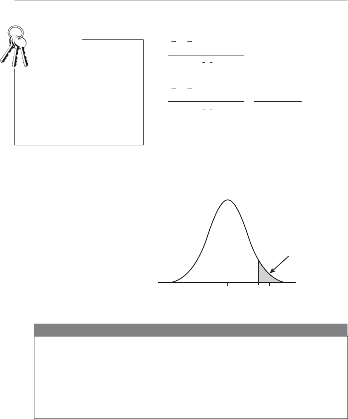
>O`b!( 7\TS`S\bWOZAbObWabWQa #"
We are now ready to determine the calculated z-
score using the following equation:
zxx H
xx
12 12
0
12
MM
S
ˆ
For the rat example, our calculated z-score becomes:
zxx H
xx
12 12
0
1
2
24 21 0
0 134
MM
S
ˆ
..
.224.
Figure 17.2 shows the results of this hypothesis test.
The critical z-score for a one-tail (right side) test
with F" 0.05 is +1.64. According to Figure 17.2, this
places the calculated z-score of +2.24 in the “Reject
H0” region, which leads to our conclusion that the lucky rats have heavier brains than
the less-fortunate rats.
The term MM
12
0
H refers
to the hypothesized dif-
ference between the two
population means. When the
null hypothesis is testing that
there is no difference between
population means, then the term
MM
12
0
H is set to 0.
Bob’s Basics
4WUc`S%
Hypothesis test for rat
example.
Number of Standard Deviations from the Mean
2.241.640
0.95
1–
Do Not Reject H0
= 0.05
Reject H
0
zcz
The conditions that are necessary for the hypothesis test for differences between means
with large sample sizes are as follows:
UThe samples are independent of each other.
UThe size of each sample must be greater than or equal to 30.
U If the population standard deviations are unknown, we can use the sample stan-
dard deviations to approximate them.
Random Thoughts
1VO^bS`%( 6g^]bVSaWaBSabW\UeWbVBe]AO[^ZSa ##
We can find the p-value for this sample by using the normal z-score table found in
Appendix B as follows:
PP
P
[.
] [.]
[.
].
zz
z
b
224 1 224
2 24 1 0 9875 00 0125.
We can also apply this technique to hypothesis tests that involve sample sizes less
than 30. However, to do so, the following conditions must be met:
UBoth populations must be normally distributed.
UBoth population standard deviations must be known.
Bob’s Basics
The results of our rat study can greatly improve the lives of many. When your spouse
catches you sneaking off to the golf course on Saturday morning, you can tell him or
her with a straight face that you are just trying to improve your mind. We now have
the statistics to support you. But be warned, you might develop a sore neck with all
that extra brain weight.
BSabW\UO2WTTS`S\QS=bVS`BVO\HS`]
In the previous example, we were just testing whether or not there was any difference
between the two populations. We can also test whether the difference exceeds a cer-
tain value. As an example, suppose we want to test the hypothesis that the average sal-
ary of a mathematician in New Jersey exceeds the average salary in Virginia by more
than $5,000. We would state the hypotheses as follows:
H0:R1R2f 5000
H1:R1R2# 5000
where:
R1 = the mean salary of a mathematician in New Jersey
R2 = the mean salary of a mathematician in Virginia
We’ll assume that X1 = $8100 and X2 = $7600, and we’ll test this hypothesis at the
F = 0.10 level.
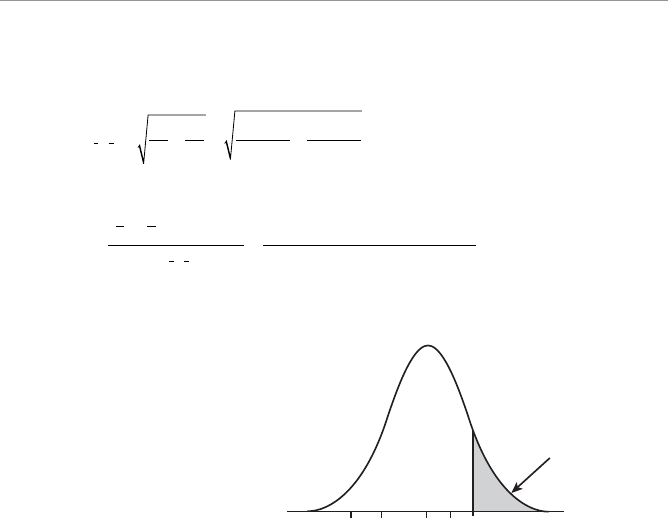
>O`b!( 7\TS`S\bWOZAbObWabWQa #$
A sample of 42 mathematicians from New Jersey had a mean salary of $51,500,
whereas a sample of 54 mathematicians from Virginia had a mean salary of $45,400.
The standard error of the difference between two means is:
SSS
xx nn
12
2
1
1
2
2
2
22
8100
42
7600
54 162
$223.
Our calculated z-score becomes:
zxx
xx
12 12
12
51 500 45 400
MM
S
$, $, $55000
1622 3 068
..
The results of this hypothesis test are shown in Figure 17.3.
4WUc`S%!
Hypothesis test for the salary
example.
Number of Standard Deviations from the Mean
0.680 1.28
0.90
1–
Do Not Reject H0
= 0.10
Reject H
0
zz
c
The critical z-score for a one-tail (right side) test with F = 0.10 is +1.28. According
to Figure 17.3, this places the calculated z-score of +0.68 in the “Do Not Reject H0”
region, which leads to our conclusion that the difference in salaries between the two
states does not exceed $5,000.
BSabW\UT]`2WTTS`S\QSa0SbeSS\;SO\aeWbVA[OZZ
AO[^ZSAWhSaO\RC\Y\]e\AWU[O
This section addresses the situation where the population standard deviation, X, is not
known and the sample sizes are small. If one or both of our sample sizes is less than
30, the population needs to be normally distributed to use any of the following tech-
niques. We made the same assumption for small sample sizes back in Chapters 14 and
16.

1VO^bS`%( 6g^]bVSaWaBSabW\UeWbVBe]AO[^ZSa #%
The sampling distribution for the difference between sample means for this scenario
follows the Student’s t-distribution. Also for small sample sizes, the equation for the
standard error of the difference between two means, Sxx
12
, depends on whether or
not the standard deviations (or the variances) of the two populations are equal. The
first example will deal with equal standard deviations.
3_cOZ>]^cZObW]\AbO\RO`R2SdWObW]\a
We have a very mysterious occurrence in our household—batteries seem to vanish
into thin air. So I started buying them in 24-packs at the warehouse store, naively
thinking that “these will last a long time.” Wrong again—the more I buy, the faster
they disappear. Maybe it has something to do with certain teenagers listening to music
on their portable CD players at a “brain-numbing” volume into the wee hours of the
morning. Just a thought. So if I ever hear about a new “longer-lasting battery,” I’m all
over it. Let’s say a company is promoting one of these batteries, claiming that its life is
significantly longer than regular batteries. The hypothesis statement would be:
H0:R1f R2
H1:R1# R2
where:
R1 = the mean life of the long-lasting batteries
R2 = the mean life of the regular batteries
We’ll test this hypothesis at the F = 0.01 level. The following data was collected mea-
suring the battery life in hours for both types of batteries:
@Oe2ObOT]`0ObbS`g3fO[^ZS
Long-Lasting Battery (Population 1):
51 44 58 36 48 53 57 40 49 44 60 50
Regular Battery (Population 2):
42 29 51 38 39 44 35 40 48 45
Using Excel, we can summarize this data in the following table.
>O`b!( 7\TS`S\bWOZAbObWabWQa #&
Ac[[O`WhSR0ObbS`g2ObO
Sample Sample Standard Sample
Population in Hours Mean Deviation Size
x
_sn
Long-lasting (1) 49.2 7.31 12
Regular (2) 41.1 6.40 10
In this example, we are assuming that X1 = X2, but that the values of X1 and X2 are
unknown. Under these conditions, we calculate a pooled estimate of the standard deviation
using the following equation:
snsns
nn
p
11
2
22
2
12
11
2
The pooled estimate of the standard deviation combines two sample variances into
one variance and is calculated using snsn s
nn
p
11
2
22
2
12
11
2.
Don’t panic just yet. This equation looks a whole lot better with numbers plugged in.
snsns
nn
p
11
2
22
2
12
2
11
2
12 1 7 31.
10 1 6 40
12 10 2
956 44
20 692
2
.
..sp
We can now approximate the standard error of the difference between two means
using:
ˆ
Sxx p
snn
12
11
12
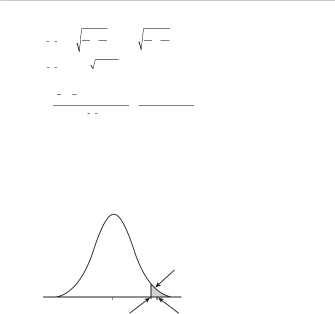
1VO^bS`%( 6g^]bVSaWaBSabW\UeWbVBe]AO[^ZSa #'
Let’s apply our example to this fellow.
ˆ.Sxx p
snn
12
11 692 1
12
1
10
12
ˆ.. .Sxx
12 6 92 0 1833 2 96
hours
We are now ready to determine our calculated t-score using the following equation:
txx H
xx
12 12
0
12
49 2 41 1 0
29
MM
S
ˆ
..
.66 273 .
The number of degrees of freedom for this test are:
df n n..
12
21210220
The critical t-score, taken from Table 4 in Appendix B, for a one-tail (right) test using
F = 0.01 with d.f. = 20 is +2.528. This hypothesis test is shown graphically in Figure
17.4.
4WUc`S%"
Hypothesis test for the battery
example.
0
0.99
1–
Do Not Reject H0
= 0.01
Reject H0
tc= 2.528 t= 2.73
According to Figure 17.4, our calculated t-score of +2.73 is found in the “Reject H0”
region, which leads to our conclusion that the long-lasting batteries do indeed have a
longer life than the regular batteries. Now that has my attention!
This procedure was based on the assumption that the standard deviations of the popu-
lations were equal. What if this assumption is not true? I’m glad you asked!

>O`b!( 7\TS`S\bWOZAbObWabWQa $
C\S_cOZ>]^cZObW]\AbO\RO`R2SdWObW]\a
We’ll investigate this scenario using the same battery example, but now we will
assume that X1|X
2. The procedure is identical to the previous method except for two
changes.
The first difference involves the standard error of the difference between two means.
The equation used for this scenario is as follows:
ˆ
Sxx
s
n
s
n
12
1
2
1
2
2
2
For the battery example, our result is:
ˆ.. ..Sxx
12
731
12
640
10 445 410 2
22
..92
We are now ready to determine our calculated t-score using the following equation:
txx H
xx
12 12
0
12
49 2 41 1 0
29
MM
S
ˆ
..
.22 277 .
The second difference (hold on to your hat) is the method for determining the num-
ber of degrees of freedom for the Student’s t-distribution.
df
s
n
s
n
s
n
n
s
..
¥
§
¦´
¶
µ
¥
§
¦´
¶
µ
1
2
1
2
2
2
2
1
2
1
2
1
2
2
1
nn
n
2
2
21
¥
§
¦´
¶
µ
The conditions that are necessary for the hypothesis test for differences between means
with small sample sizes are as follows:
UThe samples are independent of each other.
UThe population must be normally distributed.
U If X1 and X2 are known, use the normal distribution to determine the rejection
region.
U If X1 and X2 are unknown, approximate them with s1 and s2 and use the Student’s
t-distribution to determine the rejection region.
Random Thoughts

1VO^bS`%( 6g^]bVSaWaBSabW\UeWbVBe]AO[^ZSa $
Before you have a seizure, let me demonstrate that this animal’s bark is worse than its
bite. First, recognize that for our battery example:
s
n
s
n
1
2
1
2
2
2
2
2
731
12 445 640
10 410
....and
We can now plug these values into the above equation as follows:
df.. ..
..
¨
ª·
¹
445 410
445
11
410
9
7
2
22
3310
180 187 19 92
.
.. .
Because the number of degrees of freedom must be an integer, we round this result to
20. The critical t-score, taken from T
able 4 in Appendix B, for a one-tail (right) test
using F = 0.01 with d.f. = 20 is +2.528. Because tt
c
, we reject H0.
:SbbW\U3fQSZ2]bVS5`c\bE]`Y
Excel performs many of the hypothesis tests that we’ve discussed in this chapter. So let
me explain how to perform the previous battery example using this nifty tool. Follow
these steps:
1. Open a blank Excel sheet and enter the data from the battery example in
Columns A and B as shown in Figure 17.5.
2. From the Tools menu, choose Data Analysis and select t-Test: Two-Sample
Assuming Unequal Variances. (Refer to the section “Installing the Data Analysis
Add-in” from Chapter 2 if you don’t see the Data Analysis command on the
Tools menu.)
4WUc`S%#
Data entry for the battery
example.
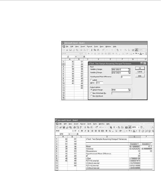
>O`b!( 7\TS`S\bWOZAbObWabWQa $
3. Click OK.
4. In the t-Test: Two-Sample Assuming Unequal Variances dialog box, choose cells
B1:B12 for Variable 1 Range and cells A1:A10 for Variable 2 Range. Set the
Hypothesized Mean Difference to 0, Alpha to 0.01, and Output Range to cell
D1, as shown in Figure 17.6.
4WUc`S%$
The t-test: Two-Sample
Assuming Unequal Variances
dialog box.
5. Click OK. The t-test output is shown in Figure 17.7.
4WUc`S%%
t-test output.
According to Figure 17.7, the calculated t-score of 2.758 is found in cell E9, which
differs slightly from what we calculated in the previous section (2.77) due to the
rounding of numbers. The p-value of 0.006 is found in cell E10. Because p-value bA,
we reject the null hypothesis.
1VO^bS`%( 6g^]bVSaWaBSabW\UeWbVBe]AO[^ZSa $!
BSabW\UT]`2WTTS`S\QSa0SbeSS\;SO\aeWbV2S^S\RS\b
AO[^ZSa
Up to this point, all the samples that we have used in the chapter have been indepen-
dent samples. Samples are independent if they are not related in any way with each
other. This is in contrast to dependent samples, where each observation of one sample is
related to an observation in another.
An example of a dependent sample would be
a weight-loss study. Each person is weighed
at the beginning (Population 1) and end
(Population 2) of the program. The change
in weight of each person is calculated by
subtracting the Population 2 weights from
the Population 1 weights. Each observation
from Population 1 is matched to an observa-
tion in Population 2. Dependent samples are
tested differently than independent samples.
To demonstrate testing dependent samples, let’s revisit my golf ball example from
Chapter 15. If you remember, I dreamed I had invented a golf ball that I claimed
would increase the distance off the tee by more than 20 yards. To test my claim,
suppose we had nine golfers hit my golf ball and the same golfers hit a regular golf
ball. The following table shows these results. The letter “d” refers to the difference
between my ball and the other ball.
2WabO\QSW\GO`RaT]`5]ZT0OZZ3fO[^ZS
Golfer 123456789
My ball 215 228 256 264 248 255 239 218 239
Other ball 201 213 230 233 218 226 212 195 208
d 14 15 26 31 30 29 27 23 31
d2196 225 676 961 900 841 729 529 961
For future calculations, we will need:
d
¤14 15 26 31 30 29 27 23 31 226
d2196 225 676 961 900 841 729 529 961 601
¤88
With independent samples,
there is no relationship in the
observations between the sam-
ples. With dependent samples,
the observation from one sam-
ple is related to an observation
from another sample.

>O`b!( 7\TS`S\bWOZAbObWabWQa $"
The distances using my golf ball will be considered Population 1, and the distances
with the other golf ball will be labeled Population 2. Because the same golfer hit both
balls in each instance in the preceding table, these two samples are considered depen-
dent.
My hypothesis statement for my claim would look like:
H0:R1R2f 20
H1:R1R2# 20
where:
R1 = the average distance off the tee with my new golf ball
R2 = the average distance off the tee with the other golf ball
However, because we are only interested in the difference between the two popula-
tions, we can rewrite this statement as a single sample hypothesis as follows:
H0:Rdf 20
H1:Rd# 20
where Rd is the mean of the difference between the two populations.
We will test this hypothesis using F = 0.05.
Our next step is to calculate the mean difference, d, and the standard deviation of the
difference, sd, between the two samples as follows:
dd
n
¤226
925 11. yards
s
dd
n
n
d
¤¤
2
2
1
sd
6018 226
9
8
342 89
8655
2
.. yards.
The equation for sd is the same standard deviation equation that you learned in
Chapter 5.
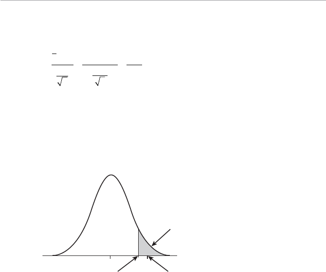
1VO^bS`%( 6g^]bVSaWaBSabW\UeWbVBe]AO[^ZSa $#
If both populations follow the normal distribution, we use the Student’s t-distribution
because both sample sizes are less than 30 and X1 and X2 are unknown. The calculated
t-score is found using:
td
s
n
d
d
M25 11 20
655
9
511
218 234
.
.
.
..
The number of degrees of freedom for this test is:
df n..
1918
The critical t-score, taken from Table 4 in Appendix B, for a one-tail (right) test using
F = 0.05 with d.f. = 8 is +1.86. This hypothesis test is shown graphically in Figure
17.8.
4WUc`S%&
Hypothesis test for the golf
ball example.
0
0.95
1–
Do Not Reject H0
= 0.05
Reject H
0
tc= 1.86 t= 2.34
According to Figure 17.8, our calculated t-score of +2.34 is found in the “Reject H0”
region, which leads to our conclusion that my golf ball increases the distance off the
tee by more than 20 yards. Too bad this was only a dream!
BSabW\UT]`2WTTS`S\QSa0SbeSS\>`]^]`bW]\aeWbV
7\RS^S\RS\bAO[^ZSa
We can perform hypothesis testing to examine the difference between proportions of
two populations as long as the sample size is large enough. Recall from Chapter 13,
proportion data follow the binomial distribution, which can be approximated by the
normal distribution under the following conditions.

>O`b!( 7\TS`S\bWOZAbObWabWQa $$
np v 5 and nq v 5
where:
p = the probability of a success in the population
q= the probability of a failure in the population (q = 1 – p)
Let’s say that I want to test the claim that the proportion of males and females
between the ages of 13 and 19 who use instant messages (IM) on the Internet every
week are the same. My hypothesis would be stated as:
H0:p1" p2
H1:p1| p2
where:
p1 = the proportion of 13- to 19-year-old males who use IMs every week
p2 = the proportion of 13- to 19-year-old females who use IMs every week
The following table summarizes the data from the IM samples:
Ac[[O`WhSR2ObOT]`7;AO[^ZSa
Population Number of Successes Sample Size
xn
Male 207 300
Female 266 350
What can we conclude at the F = 0.10 level?
Our sample proportion of male IM users, p1, and female users, p2, can be found by:
px
n
1
1
1
207
300 069 . and px
n
2
2
2
266
350 076 .
To determine the calculated z-score, we need to know the standard error of the differ-
ence between two proportions (that’s a mouthful),
Spp
12
, which is found using:
Spp
pp
n
pp
n
12
11
1
22
2
11

1VO^bS`%( 6g^]bVSaWaBSabW\UeWbVBe]AO[^ZSa $%
Our problem is that we don’t know the values of p1 and p2, the actual population pro-
portions of male and female IM users. The next best thing is to calculate the estimated
standard error of the difference between two proportions, ˆ
Spp
12
, using the following
equation:
ˆˆˆ
Spp pp
nn
12 111
12
¥
§
¦´
¶
µ
where ˆ
p, the estimated overall proportion of two populations, is found using the
following equation:
ˆ.pxx
nn
12
12
207 266
300 350 0 728
For our IM example, the estimated standard error of the difference between two pro-
portions is:
ˆ.. .Spp
12 0 728 1 0 728 1
300
1
350 00
¥
§
¦´
¶
µ335
The term pp
H
12
0
refers to the hypothesized difference between the two
population proportions. When the null hypothesis is testing that there is no differ-
ence between population proportions, then the term pp
H
12
0
is set to 0.
Bob’s Basics
Now we can finally determine the calculated z-score using:
zpp pp
H
pp
12 12
0
12
ˆ
S
For the IM example, our calculated z-score becomes:
zpp pp
H
pp
12 12
0
12
069 076 0
00
ˆ
..
.S335 200 .
The critical z-scores for a two-tail test with F = 0.10 are +1.64 and –1.64. This
hypothesis test is shown graphically in Figure 17.9.
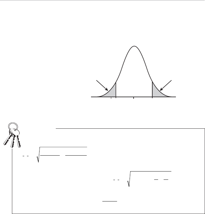
>O`b!( 7\TS`S\bWOZAbObWabWQa $&
As you can see in Figure 17.9, the calculated z-score of –2.00 is within the “Reject H0”
region. There, we conclude that the proportions of male and female IM users between
13 and 19 years old are not equal to each other.
4WUc`S%'
Hypothesis test for the IM
example.
Hypothesis Test for the Difference in Proportions
0
0.90
1–
Do Not Reject H0
= 0.05
Reject H0
Number of Standard Deviations from the Mean
-2.0 +1.64
z
-1.64
zczc
2
/
= 0.05
Reject H0
2
/
The standard error of the difference between two proportions describes the varia-
tion in the difference between two sample proportions and is calculated using
Spp
pp
n
pp
n
12
11
1
22
2
11
. The estimated standard error of the difference
between two proportions approximates the variation in the difference between two
sample proportions and is calculated using ˆˆˆ
Spp pp
nn
12
111
12
¥
§
¦´
¶
µ. The esti-
mated overall proportion of two populations is the weighted average of two sample
proportions and is calculated using ˆ
pxx
nn
12
12
.
Bob’s Basics
The p-value for these samples can be found using the normal z-score table found in
Appendix B as follows:
2(P[z# +2.00]) = 2(1–P[zf +2.00])
2(P[z# +2.00]) = 2(1–0.9772) = 0.0456
This also confirms that we reject H0 because the p-value bA
.

1VO^bS`%( 6g^]bVSaWaBSabW\UeWbVBe]AO[^ZSa $'
This completes our invigorating journey through the land of hypothesis testing. Don’t
be too sad, though. We’ll have the pleasure of revisiting this technique in Part 4 of
this book—Advanced Inferential Statistics. I just bet you can’t wait.
G]c`Bc`\
1. Test the hypothesis that the average SAT math scores from students in
Pennsylvania and Ohio are different. A sample of 45 students from Pennsylvania
had an average score of 552, whereas a sample of 38 Ohio students had an aver-
age score of 530. Assume the population standard deviations for Pennsylvania
and Ohio are 105 and 114 respectively. Test at the F = 0.05 level. What is the
p-value for these samples?
2. A company tracks satisfaction scores based on customer feedback from individual
stores on a scale of 0 to 100. The following data represents the customer scores
from Stores 1 and 2.
Store 1:
90 87 93 75 88 96 90 82 95 97 78
Store 2:
82 85 90 74 80 89 75 81 93 75
Assume population standard deviations are equal but unknown and that the
population is normally distributed. Test the hypothesis using F = 0.10.
3. A new diet program claims that participants will lose more than 15 pounds after
completion of the program. The following data represents the before and after
weights of nine individuals who completed the program. Test the claim at the
F = 0.05 level.
Before: 221 215 206 185 202 197 244 188 218
After: 200 192 195 166 187 177 227 165 201
4. Test the hypothesis that the proportion of home ownership in the state of
Florida exceeds the national proportion at the F = 0.01 level using the following
data.

>O`b!( 7\TS`S\bWOZAbObWabWQa %
Population Number of Successes Sample Size
Florida 272 400
Nation 390 600
What is the p-value for these samples?
5. Test the hypothesis that the average hourly wage for City A is more than $0.50 per
hour above the average hourly wage in City B using the following sample data:
City Average Wage Sample Standard Sample Size
Deviation
A $9.80 $2.25 60
B $9.10 $2.70 80
Test at the F = 0.05 level. What is the p-value for this test?
6. Test the hypothesis that the average number of days that a home is on the mar-
ket in City A is different from City B using the following sample data:
City A: 12 8 19 10 26 4 15 20 18 25 7 11
City B: 15 31 14 5 18 20 10 7 25 20 27
Assume population standard deviations are unequal and that the population is
normally distributed. Test the hypothesis using F = 0.10.
BVS:SOabG]c<SSRb]9\]e
UWe use the normal distribution for the hypothesis test for the difference between
means when nv 30 for both samples.
UWe use the normal distribution for the hypothesis test for the difference between
means when n < 30 for either sample, if X1 and X2 are known, and both popula-
tions are normally distributed.
UWe use the Student’s t-distribution for the hypothesis test for the difference
between means when n < 30 for either sample, X1 and X2 are unknown, and both
populations are normally distributed.
UWith dependent samples, the observation from one sample is related to an obser-
vation from another sample. With independent samples, there is no relationship
in the observations between the samples.

4
>O`b
We covered a lot of ground so far in the first three parts of this book. What
could possibly be left? Well, the last few topics focus on the more advanced
statistical methods (don’t worry, you can handle it) of chi-square tests,
analysis of variance, and simple regression. Armed with these techniques,
we can determine whether two categorical variables are related (chi-square),
compare three or more populations (analysis of variance), and describe the
strength and direction of the relationship between two variables (simple
regression). After you have mastered these concepts, the sky is the limit!
/RdO\QSR7\TS`S\bWOZ
AbObWabWQa


18
1VO^bS`
BVS1VWA_cO`S>`]POPWZWbg
2Wab`WPcbW]\
7\BVWa1VO^bS`
UPerforming a goodness-of-fit test with the chi-square distribution
UPerforming a test of independence with the chi-square distribution
UUsing contingency tables to display frequency distributions
In the last three chapters, we explored the wonderful world of hypothesis
testing as we compared means and proportions of one and two populations,
making an educated conclusion about our initial claims. With that tech-
nique under our belt, we are now ready for bigger and better things.
In this chapter, we will compare two or more proportions using a new
probability distribution: the chi-square. With this new test, we can confirm
whether a set of data follows a specific probability distribution, such as the
binomial or Poisson. (Remember those? They’re back!) We can also use
this distribution to determine whether two variables are statistically inde-
pendent. It’s actually a lot of fun—really it is!
>O`b"( /RdO\QSR7\TS`S\bWOZAbObWabWQa %"
@SdWSe]T2ObO;SOac`S[S\bAQOZSa
In Chapter 2, we discussed the different type of data measurement scales, which were
nominal, ordinal, interval, and ratio. Here is a brief refresher of each:
UNominal level of measurement deals strictly with qualitative data. Observations
are simply assigned to predetermined categories. One example is gender of the
respondent with the categories being male and female.
UOrdinal measurement is the next level up. It has all the properties of nominal
data with the added feature that we can rank order the values from highest to
lowest. An example would be ranking a movie as great, good, fair, or poor.
UInterval level of measurement involves strictly quantitative data. Here we can use
the mathematical operations of addition and subtraction when comparing values.
For this data, the difference between the different categories can be measured
with actual numbers and also provides meaningful information. Temperature
measurement in degrees Fahrenheit is a common example here.
URatio level is the highest measurement scale. Now we can perform all four math-
ematical operations to compare values. Examples of this type of data are age,
weight, height, and salary. Ratio data has all the features of interval data with the
added benefit of a “true zero point,” meaning that a zero data value indicates the
absence of the object being measured.
The hypothesis testing that we covered in the last
three chapters strictly used interval and ratio data.
However, the chi-square distribution in this chapter
will allow us to perform hypothesis testing on nomi-
nal and ordinal data.
The two major techniques that we will learn about
are using the chi-square distribution to perform a
goodness-of-fit test and to test for the independence
of two variables. So let’s get started!
BVS1VWA_cO`S5]]R\Saa]T4WbBSab
One of the many uses of the chi-square distribution is to perform a goodness-of-fit
test, which uses a sample to test whether a frequency distribution fits the predicted
The chi-square distribution
is used to perform hypothesis
testing on nominal and ordinal
data.

1VO^bS`&( BVS1VWA_cO`S>`]POPWZWbg2Wab`WPcbW]\ %#
distribution. As an example, let’s say that a new movie in the making has an expected
distribution of ratings summarized in the following table.
3f^SQbSR;]dWS@ObW\U2Wab`WPcbW]\
Number of Stars Percentage
5 40%
4 30%
3 20%
2 5%
1 5%
Total 100%
After its debut, a sample of 400 moviegoers were asked to rate the movie, with the
results shown in the following table.
=PaS`dSR;]dWS@ObW\U2Wab`WPcbW]\
Number of Stars Number of Observations
5 145
4 128
3 73
2 32
1 22
Total 400
Can we conclude that the expected movie
ratings are true based on the observed rat-
ings of 400 people? The goodness-of-fit test uses
a sample to test whether a
frequency distribution fits the
predicted distribution.
>O`b"( /RdO\QSR7\TS`S\bWOZAbObWabWQa %$
AbObW\UbVS<cZZO\R/ZbS`\ObWdS6g^]bVSaWa
The null hypothesis in a chi-square goodness-of-fit test states that the sample of
observed frequencies supports the claim about the expected frequencies. The alterna-
tive hypothesis states that there is no support for the claim pertaining to the expected
frequencies. For our movie example, the hypothesis
statement would look like the following:
H0: The actual rating distribution can be described
by the expected distribution.
H1: The actual rating distribution differs from the
expected distribution.
We will test this hypothesis at the F" 0.10 level.
=PaS`dSRDS`aca3f^SQbSR4`S_cS\QWSa
The chi-square test basically compares the observed (O) and expected (E) frequen-
cies to determine whether there is a statistically significant difference. For our movie
example, the observed frequencies are simply the number of observations collected for
each category of our sample. The expected frequencies are the expected number of
observations for each category and are calculated in the following table.
The total number of expected
(E) frequencies must be
equal to the total number of
observed (O) frequencies.
Bob’s Basics
Observed frequencies are the number of actual observations noted for each category
of a frequency distribution with chi-squared analysis. Expected frequencies are the
number of observations that would be expected for each category of a frequency dis-
tribution assuming the null hypothesis is true with chi-squared analysis.
3f^SQbSR4`S_cS\QgBOPZS
Movie Expected Sample Expected Observed
Rating Percentage Size Frequency (E) Frequency (O)
5 40% 400 0.40(400) = 160 145
4 30% 400 0.30(400) = 120 128
3 20% 400 0.20(400) = 80 73

1VO^bS`&( BVS1VWA_cO`S>`]POPWZWbg2Wab`WPcbW]\ %%
2 5% 400 0.05(400) = 20 32
1 5% 400 0.05(400) = 20 22
Total 100% 400 400
We are now ready to calculate the chi-square statistic.
1OZQcZObW\UbVS1VWA_cO`SAbObWabWQ
The chi-square statistic is found using the following equation:
C2
2
¤OE
E
where:
O = the number of observed frequencies for each category
E = the number of expected frequencies for each category
The calculation using this equation is shown in the following table.
BVS1OZQcZObSR1VWA_cO`SAQ]`ST]`bVS;]dWS3fO[^ZS
Movie
Rating OEOE
OE
2OE
E
2
Five 145 160 –15 225 1.41
Four 128 120 8 64 0.53
Three 73 80 –7 49 0.61
Two 32 20 12 144 7.20
One 22 20 2 4 0.20
Total C2
2
995
¤OE
E.
2SbS`[W\W\UbVS1`WbWQOZ1VWA_cO`SAQ]`S
The critical chi-square score, Cc
2, depends on the number of degrees of freedom,
which for this test would be:
d.f. = k – 1
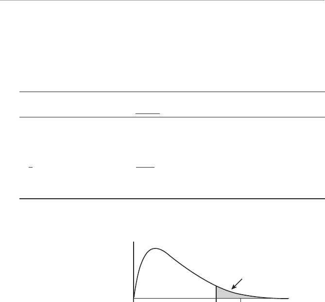
>O`b"( /RdO\QSR7\TS`S\bWOZAbObWabWQa %&
where k equals the number of categories in the frequency distribution. For the movie
example, there are 5 categories, so d.f. = k – 1 = 5 – 1 = 4.
The critical chi-square score is read from the chi-square table found on Table 5 in
Appendix B of this book. Here is an excerpt of this table.
1`WbWQOZ1VWA_cO`SDOZcSa
Selected right tail areas
d.f. 0.3000 0.2000 0.1500 0.1000 0.0500 0.0250 0.0100 0.0050 0.0010
1 1.074 1.642 2.072 2.706 3.841 5.024 6.635 7.879 10.828
2 2.408 3.219 3.794 4.605 5.991 7.378 9.210 10.597 13.816
3 3.665 4.642 5.317 6.251 7.815 9.348 11.345 12.838 16.266
4 4.878 5.989 6.745 7.779 9.488 11.143 13.277 14.860 18.467
5 6.064 7.289 8.115 9.236 11.070 12.833 15.086 16.750 20.515
6 7.231 8.558 9.446 10.645 12.592 14.449 16.812 18.548 22.458
For F" 0.10 and d.f. = 4, the critical chi-square score,
C
c
27 779., is indicated in the
underlined part of the table. Figure 18.1 shows the results of our hypothesis test.
xc
0.90
1–
Do Not Reject H0
= 0.10
Reject H0
0 7.779 9.95
d f =4 2x2
4WUc`S&
Chi-square test for the movie
example.
According to Figure 18.1, the calculated chi-square score of 9.95 is within the “Reject
H0” region, which leads us to the conclusion that the actual movie-rating frequency
distribution differs from the expected distribution. We will always reject H0 as long as
CC
c
22
b.
Also, because the calculated chi-square score for the goodness-of-fit test can only be
positive, the hypothesis test will always be a one-tail with the rejection region on the
right side.

1VO^bS`&( BVS1VWA_cO`S>`]POPWZWbg2Wab`WPcbW]\ %'
CaW\U3fQSZÂa1677<D4c\QbW]\
You don’t have a chi-square distribution table handy? No need to panic. We can gen-
erate critical chi-square scores using Excel’s CHIINV function, which has the follow-
ing characteristics:
CHIINV(probability, deg-freedom)
where:
probability = the level of significance, F
deg-freedom = the number of degrees of freedom
For instance, Figure 18.2 shows the CHIINV function being used to determine the
critical chi-square score for F" 0.10 and d.f. = 4 from our previous example.
4WUc`S&
Excel’s CHIINV function.
Cell A1 contains the Excel formula =CHIINV(0.10, 4) with the result being 7.779.
This probability is underlined in the previous table.
1VO`OQbS`WabWQa]TO1VWA_cO`S2Wab`WPcbW]\
We can see from Figure 18.2 that the chi-square distribution is not symmetrical but
rather has a positive skew. The shape of the distribution will change with the number
of degrees of freedom as shown in Figure 18.3.
As the number of degrees of freedom increases, the shape of the chi-square distribu-
tion becomes more symmetrical.
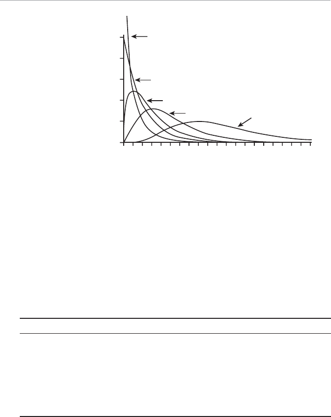
>O`b"( /RdO\QSR7\TS`S\bWOZAbObWabWQa &
/5]]R\Saa]T4WbBSabeWbVbVS0W\][WOZ2Wab`WPcbW]\
In past chapters, we have occasionally made assumptions that a population follows a
specific distribution such as the normal or binomial. In this section, we can demon-
strate how to verify this claim.
As an example, suppose that a certain major league baseball player claims the probabil-
ity that he will get a hit at any given time is 30 percent. The following table is a fre-
quency distribution of the number of hits per game over the last 100 games. Assume
he has come to bat four times in each of the games.
2ObOT]`bVS0OaSPOZZ>ZOgS`
Number of Hits Number of Games
026
134
230
37
43
Total 100
Chi-Square Values
01234567891011121314151617181920
0
.1
.2
.3
.4
.5 d f =1
d f =2
d f =3
d f =5 d f = 10
4WUc`S&!
Family of chi-square
distributions.

1VO^bS`&( BVS1VWA_cO`S>`]POPWZWbg2Wab`WPcbW]\ &
In other words, in 26 games he had 0 hits, in 34 games he had 1 hit, etc. Test the
claim that this distribution follows a binomial distribution with p = 0.30 using
F" 0.05.
The hypothesis statement would look like the following:
H0: The distribution of hits by the baseball player can be described with the
binomial probability distribution using p = 0.30.
H1: The distribution differs from the binomial probability distribution using
p = 0.30.
Our first step is to calculate the frequency distribution for the expected number of hits
per game. To do this, we need to look up the binomial probabilities in Table 1 from
Appendix B for n = 4 (the number of trials per game) and p = 0.30 (the probability of a
success). These probabilities, along with the calculations for the expected frequencies,
are shown in the following table.
3f^SQbSR4`S_cS\Qg1OZQcZObW]\aT]`0OaSPOZZ>ZOgS`
Number of Hits Binomial Number of Expected
per Game Probabilities Games Frequency
0 0.2401 w100 = 24.01
1 0.4116 w100 = 41.16
2 0.2646 w100 = 26.46
3 0.0756 w100 = 7.56
4 0.0081 w100 = 0.81
Total 1.0000 100.00
Before continuing, we need to make one
adjustment to the expected frequencies.
When using the chi-square test, we need
at least five observations in each of the
expected frequency categories. If there are
less than five, we need to combine catego-
ries. In the previous table, we will combine
3 and 4 hits per game into one category to
meet this requirement.
Expected frequencies do not
have to be integer numbers
because they only represent
theoretical values.
Bob’s Basics
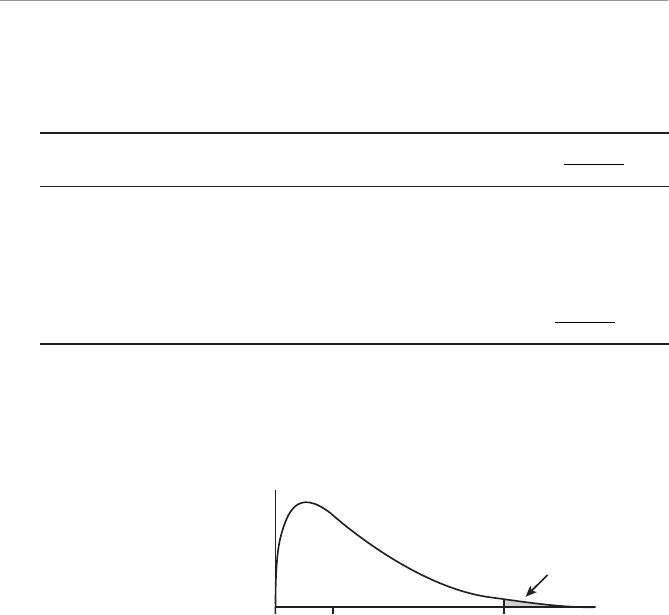
>O`b"( /RdO\QSR7\TS`S\bWOZAbObWabWQa &
Now we are ready to determine the calculated chi-square score using the following
table:
BVS1OZQcZObSR1VWA_cO`SAQ]`ST]`bVS0OaSPOZZ3fO[^ZS
Hits OEOE
OE
2OE
E
2
0 26 24.01 1.99 3.96 0.16
1 34 41.16 -7.16 51.27 1.25
2 30 26.46 3.54 12.53 0.47
3-4 10* 8.37** 1.63 2.66 0.32
Total
C
2
2
220
¤OE
E.
* 7 + 3 = 10
** 7.56 + 0.81 = 8.37
According to Table 5 in Appendix B, the critical chi-square score for F" 0.05 and
d.f. =k= 1 = 4 – 1 = 3 is 7.815. This test is shown in Figure 18.4.
4WUc`S&"
Chi-square test for the
baseball example.
xc
0.95
1–
Do Not Reject H0
= 0.05
Reject H0
0 7.815
d f =3 2
x2
2.20
According to Figure 18.4, the calculated chi-square score of 2.20 is within the “Do
Not Reject H0” region, which leads us to the conclusion that the baseball player’s hit-
ting distribution can be described with the binomial distribution using p = 0.30.
1VWA_cO`SBSabT]`7\RS^S\RS\QS
In addition to the goodness-of-fit test, the chi-square distribution can also test for
independence between variables. To demonstrate this technique, I’m going to revisit
the tennis example from Chapter 7.

1VO^bS`&( BVS1VWA_cO`S>`]POPWZWbg2Wab`WPcbW]\ &!
If you recall, Debbie felt that a short warm-up period before playing our match was
hurting her chances of beating me. After examining the conditional probabilities, I
had to admit there was some evidence supporting Debbie’s claim. However, I’m not
one to take this sitting down. I demand justice, I demand further evidence, I demand
a recount. (Oh, wait a minute, this isn’t Florida.) I demand … a hypothesis test using
the chi-square distribution!
Unbeknownst to Debbie, I have meticulously collected data from our 50 previous
matches. The following table represents the number of wins for each of us according
to the length of the warm-up period.
=PaS`dSR4`S_cS\QWSaT]`BS\\Wa3fO[^ZS
0–10 11–20 More than
Min Min 20 Min Total
Debbie wins 4 10 9 23
Bob wins 14 9 4 27
Total 18 19 13 50
This is known as a contingency table, which shows the observed frequencies of two
variables. In this case, the variables are warm-up time and tennis player. The table is
organized into r rows and c columns. For our table, r = 2 and c = 3. An intersection of
a row and column is known as a cell. A contingency table has rzccells, which in our
case, would be 6.
The chi-square test of independence will
determine whether the proportion of times
that Debbie wins is the same for all three
warm-up periods. If the outcome of the
hypothesis test is that the proportions are
not the same, we conclude that the length
of warm-up does impact the performance of
the players. But I have my doubts.
First we state the hypotheses as:
H0: Warm-up time is independent of
performance
H1: Warm-up time affects performance
Acontingency table shows the
observed frequencies of two
variables. An intersection of a
row and column in a contin-
gency table is known as a cell.
A contingency table has rzc
cells.

>O`b"( /RdO\QSR7\TS`S\bWOZAbObWabWQa &"
We will test this hypothesis at F" 0.10 level.
Our next step is to determine the expected frequency of each cell in the contingency
table under the assumption that the two variables are independent. We do this using
the following equation:
Erc
rc,Total of Row Total of Column
Total NNumber of Observations
where Erc, = the expected frequency of the cell that corresponds to the intersection of
Row r and Column c.
The following table applies this notation to our tennis example.
Row/Column Category Total Observations
r=1 Debbie Wins 23
r=2 Bob Wins 27
c=1 0-10 Minute Warm-up 18
c=2 11-20 Minute Warm-up 19
c=3 More than 20 Minute Warm-up 13
The total number of observations for this example is 50, which we can confirm by
adding 23 + 27 or 18 + 19 + 13. We can now determine the expected frequencies for
each cell:
E11
23 18
50 828
,.
E12
23 19
50 874
,.
E13
23 13
50 598
,.
E21
27 18
50 972
,.
E22
27 19
50 10 26
,.
E23
27 13
50 702
,.
The following table summarizes these findings.
3f^SQbSR4`S_cS\QWSaT]`BS\\Wa3fO[^ZS
0–10 11–20 More Than
Min Min 20 Min Total
Debbie wins 8.28 8.74 5.98 23
Bob wins 9.72 10.26 7.02 27
Total 18 19 13 50
1VO^bS`&( BVS1VWA_cO`S>`]POPWZWbg2Wab`WPcbW]\ &#
We now need to determine the calculated
chi-square score using:
C2
2
¤OE
E
This calculation is summarized in the fol-
lowing table.
1VWA_cO`S1OZQcZObW]\T]`bVSBS\\Wa3fO[^ZS
Row Column OEOE
OE
2OE
E
2
1 1 4 8.28 -4.28 18.32 2.21
1 2 10 8.74 1.26 1.59 0.18
1 3 9 5.98 3.02 9.12 1.53
2 1 14 9.72 4.28 18.32 1.88
2 2 9 10.26 -1.26 1.59 0.15
2 3 4 7.02 -3.02 9.12 1.30
C2
2
725
¤OE
E.
To determine the critical chi-square score, we need to know the number of degrees of
freedom, which for the independence test would be:
d.f. = (r – 1)(c – 1)
For this example, we have (r – 1)(c – 1) = (2 – 1)(3 – 1) = 2 degrees of freedom.
According to Table 5 in Appendix B, the critical chi-square score for F" 0.10 and
d.f. = 2 is 4.605. This test is shown in Figure 18.5.
According to Figure 18.5, the calculated chi-square score of 7.25 is within the “Reject
H0” region, which leads us to the conclusion that there is a relationship between
warm-up time and performance when Debbie and I play tennis. Darn it—once again,
Debbie is right. Boy, does that have a familiar ring to it.
Notice that the expected
frequencies for a contingency
table add up to the row and
column totals from the observed
frequencies.
Bob’s Basics
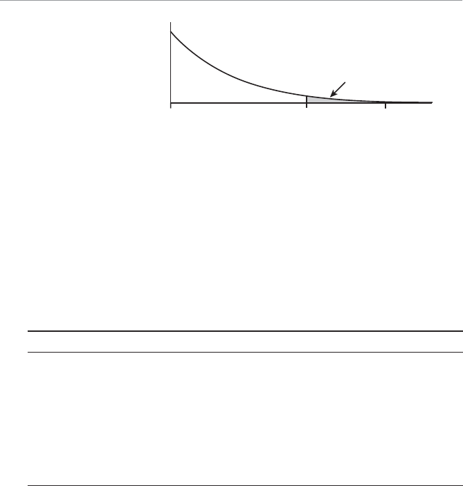
>O`b"( /RdO\QSR7\TS`S\bWOZAbObWabWQa &$
However, I do have one consolation. The chi-square test of independence only
investigates whether a relationship exists between two variables. It does not conclude
anything about the direction of the relationship. In other words, from a statistical per-
spective, Debbie cannot claim that she is disadvantaged by the short warm-up time.
She can only claim that warm-up time has some effect on her performance. We statis-
ticians always leave ourselves a way out!
G]c`Bc`\
1. A company believes that the distribution of customer arrivals during the week
are as follows:
Day Expected Percentage of Customers
Monday 10
Tuesday 10
Wednesday 15
Thursday 15
Friday 20
Saturday 30
Total 100
A week was randomly chosen and the number of customers each day was
counted. The results were: Monday—31, Tuesday—18, Wednesday—36,
Thursday—23, Friday—47, Saturday—60. Use this sample to test the expected
distribution using F" 0.05.
4WUc`S&#
Chi-square test for the tennis
example.
xc
0.90
1–
Do Not Reject H0
= 0.10
Reject H0
0 7.254.605
d f =2 2x2

1VO^bS`&( BVS1VWA_cO`S>`]POPWZWbg2Wab`WPcbW]\ &%
2. An e-commerce site would like to test the hypothesis that the number of hits per
minute on their site follows the Poisson distribution with Q = 3. The following
data was collected:
Number of Hits
Per Minute 01234567 or More
Frequency 22 51 72 92 60 44 25 14
Test the hypothesis using F" 0.01.
3. An English professor would like to test the relationship between an English
grade and the number of hours per week a student reads. A survey of 500 stu-
dents resulted in the following frequency distribution.
Numbers of Hours Grade
Reading per Week A B C D F Total
Less than 2 36 75 81 63 10 265
2–4 27 28 50 25 10 140
More than 4 32 25 24 6 8 95
Total 95 128 155 94 28 500
Test the hypothesis using F" 0.05.
4. John Armstrong, salesman for the Dillard Paper Company, has five accounts to
visit each day. It is suggested that the random variable, successful sales visits by
Mr. Armstrong, may be described by the binomial distribution, with the prob-
ability of a successful visit being 0.4. Given the following frequency distribution
of Mr. Armstrong’s number of successful sales visits per day, can we conclude
that the data actually follows the binomial distribution? Use F = 0.05.
Number of Successful
Visits per Day: 012345
Observed Frequency: 10 41 60 20 6 3

>O`b"( /RdO\QSR7\TS`S\bWOZAbObWabWQa &&
BVS:SOabG]c<SSRb]9\]e
UThe chi-square distribution is not symmetrical but rather has a positive skew.
As the number of degrees of freedom increases, the shape of the chi-square
distribution becomes more symmetrical.
UThe chi-square distribution allows us to perform hypothesis testing on nominal
and ordinal data.
UWe can use the chi-square distribution to perform a goodness-of-fit test,
which uses a sample to test whether a frequency distribution fits a predicted
distribution.
UThe chi-square test for independence investigates whether a relationship exists
between two variables. It does not, however, test the direction of that relation-
ship.
UA contingency table shows the observed frequencies of two variables. An inter-
section of a row and column in a contingency table is known as a cell.

19
1VO^bS`
/\OZgaWa]TDO`WO\QS
7\BVWa1VO^bS`
UComparing three or more population means using analysis of variance
(ANOVA)
UUsing the F-distribution to perform a hypothesis test for ANOVA
UUsing Excel to perform a one-way ANOVA test
UComparing pairs of sample means using the Scheffé test
In Chapter 17, you learned about a hypothesis test where you could com-
pare the means of two different populations to see whether they were
different. But what if you want to compare the means of three or more
populations? Well, you’ve come to the right place, because that’s what this
chapter is all about.
To perform this new hypothesis test, I need to introduce one last probabil-
ity distribution, known as the F-distribution. The test that we will perform
has a very impressive name associated with it—the analysis of variance.
This test is so special, it even has its own acronym: ANOVA. Sounds like
something from outer space … keep reading to find out.

>O`b"( /RdO\QSR7\TS`S\bWOZAbObWabWQa '
=\SEOg/\OZgaWa]TDO`WO\QS
If you want to compare the means for three or more populations, ANOVA is the test
for you. Let’s say I’m interested in determining whether there is a difference in con-
sumer satisfaction ratings between three fast-food chains. I would collect a sample of
satisfaction ratings from each chain and test to see whether there is a significant differ-
ence between the sample means. Suppose my data look like the following:
Population Fast-Food Chain Sample Mean Rating
1 McDoogles 7.8
2 Burger Queen 8.2
3 Windy’s 8.3
My hypothesis statement would look like the following:
H01 2 3
:MMM
H1: not all ’s are equalM
Essentially, I’m testing to see whether the variations in customer ratings from the
previous table are due to the fast-food chains or whether the variations are purely
random. In other words, do customers perceive any differences in satisfaction
between the three chains? If I reject the null hypothesis, however, my only conclu-
sion is that a difference does exist. Analysis of variance does not allow me to compare
population means to one another to determine which is greater. That task requires
further analysis.
To use one-way ANOVA, the following conditions must be present:
UThe populations of interest must be normally distributed.
UThe samples must be independent of each other.
UEach population must have the same variance.
Bob’s Basics
Afactor in ANOVA describes the cause of the variation in the data. In the previous
example, the factor would be the fast-food chain. This would be considered a one-way
ANOVA because we are considering only one factor. More complex types of ANOVA
can examine multiple factors, but that topic goes beyond the scope of this book.
1VO^bS`'( /\OZgaWa]TDO`WO\QS '
Alevel in ANOVA describes the number of categories within the factor of interest.
For our example, we have three levels based on the three different fast-food chains
being examined.
To demonstrate one-way ANOVA, I’ll use the following example. I admit, much to
Debbie’s chagrin, that I am clueless when it comes to lawn care. My motto is, “If it’s
green, it’s good.” Debbie, on the other hand, knows exactly what type of fertilizer
to get and when to apply it during the year. I hate spreading this stuff on the lawn
because it apparently makes the grass grow faster, which means I have to cut it more
often.
To make matters worse, we have a neighbor,
Bill, whose yard puts my yard to shame. Mr.
“Perfect Lawn” is out every weekend, metic-
ulously manicuring his domain until it looks
like the home field for the National Lawn
Bowling Association. This gives Debbie a
serious case of “lawn envy.” Bill even has one
of those cute little carts that he pulls on the
back of his tractor. I asked Debbie if I could
get one for my tractor, but she said based on
my “Lawn IQ” I would probably just injure
myself.
Anyway, there are several different types of analysis of variance, and covering them all
would take a book unto itself. So throughout the remainder of this chapter, we’ll use
my lawn-care topic to describe two basic ANOVA procedures.
1][^ZSbSZg@O\R][WhSR/<=D/
The simplest type of ANOVA is known as
completely randomized one-way ANOVA, which
involves an independent random selection
of observations for each level of one fac-
tor. Now that’s a mouthful! To help explain
this, let’s say I’m interested in comparing
the effectiveness of three lawn fertilizers.
Suppose I select 18 random patches of my
precious lawn and apply either Fertilizer 1,
2, or 3 to each of them. After a week, I mow
the patches and weigh the grass clippings.
Afactor in ANOVA describes
the cause of the variation in the
data. When only one factor
is being considered, the pro-
cedure is known as one-way
ANOVA. A level in ANOVA
describes the number of catego-
ries within the factor of interest.
The simplest type of ANOVA is
known as completely random-
ized one-way ANOVA, which
involves an independent ran-
dom selection of observations
for each level of one factor.

>O`b"( /RdO\QSR7\TS`S\bWOZAbObWabWQa '
The factor in this example is fertilizer. There are three levels, representing the three
types of fertilizer we are testing. The table that follows indicates the weight of the
clippings in pounds from each patch. The mean and variance of each level are also
shown.
2ObOT]`:Oe\1ZW^^W\Ua
Fertilizer 1 Fertilizer 2 Fertilizer 3
10.2 11.6 8.1
8.5 12.0 9.0
8.4 9.2 10.7
10.5 10.3 9.1
9.0 9.9 10.5
8.1 12.5 9.5
Mean 9.12 10.92 9.48
Variance 1.01 1.70 0.96
We’ll refer to the data for each type of fertilizer as a sample. From the previous table,
we have three samples, each consisting of six observations. The hypotheses statement
can be stated as:
H01 2 3
:MMM
H1: not all ’s are equalM
where R1,R2, and R3 are the true population means for the pounds of grass clippings
for each type of fertilizer.
>O`bWbW]\W\UbVSAc[]TA_cO`Sa
The hypothesis test for ANOVA compares two types of variations from the samples.
We first need to recognize that the total variation in the data from our samples can be
divided, or as statisticians like to say, “partitioned,” into two parts.
The first part is the variation within each sample, which is officially known as the sum
of squares within (SSW). This can be found using the following equation:
SSW n s
ii
i
k
¤12
1

1VO^bS`'( /\OZgaWa]TDO`WO\QS '!
where k = the number of samples (or levels). For the fertilizer example, k = 3 and:
s1
2101.s2
2170.s3
2096.
n1 = 6 n2 = 6 n3 = 6
The sum of squares within can now be calculated as:
SSW = (6 – 1)1.01 + (6 – 1)1.70 + (6 – 1)0.96 = 18.35
Some textbooks will also refer to this value as the error sum of squares (SSE).
The second partition is the variation among the
samples, which is known as the sum of squares
between (SSB). This can be found by:
SSB n x x
ii
i
k
¤2
1
where x is the grand mean or the average value
of all the observations. For the fertilizer example:
x1912.x210 92.x3948.
We find x, the grand mean, using:
xx
N
¤
where N = the total number of observations from all samples.
For the fertilizer example:
x
102 85 84 105 91 105 95
18 983
. . . . ... . . . .
We can now calculate the sum of squares between:
SSB n x x
ii
i
k
¤2
1
SSB
6 9 12 9 83 6 10 92 9 83 6 9 48 9 83
22
.. .. ..
210 86.
Some textbooks will also refer
to this SSB value as the treat-
ment sum of squares (SSTR).
Random Thoughts
ANOVA does not require that all the sample sizes are equal, as they are in the fertil-
izer example. See Problem 1 in the “Your Turn” section as an example of unequal
sample sizes.
Random Thoughts

>O`b"( /RdO\QSR7\TS`S\bWOZAbObWabWQa '"
Finally, the total variation of all the observations is known as the total sum of squares
(SST) and can be found by:
SST x x
ij
j
b
i
k
¤¤ 2
11
This equation may look nasty, but it is just the difference between each observation
and the grand mean squared and then totaled over all of the observations. This is
clarified more in the following table.
xij xxx
ij
xx
ij
2
10.2 9.83 0.37 0.14
8.5 9.83 -1.33 1.77
8.4 9.83 -1.43 2.04
10.5 9.83 0.67 0.45
9.0 9.83 -0.83 0.69
8.1 9.83 -1.73 2.99
11.6 9.83 1.77 3.13
12.0 9.83 2.17 4.71
9.2 9.83 -0.63 0.40
10.3 9.83 0.47 0.22
9.9 9.83 0.07 0.01
12.5 9.83 2.67 7.13
8.1 9.83 -1.73 2.99
9.0 9.83 -0.83 0.69
10.7 9.83 0.87 0.76
9.1 9.83 -0.73 0.53
10.5 9.83 0.67 0.45
9.5 9.83 -0.33 0.11
SST x x
ij
j
b
i
k
¤¤ 2
11
29 21.
This total sum of squares calculation can be confirmed recognizing that:
SST SSW SSB
SST = 18.35 + 10.86 = 29.21

1VO^bS`'( /\OZgaWa]TDO`WO\QS '#
Note that we can determine the variance of the original 18 observations, s2, by:
sSST
N
2
1
29 21
18 1 172
..
This result can be confirmed by using the variance equation that we discussed in
Chapter 5 or by using Excel.
2SbS`[W\W\UbVS1OZQcZObSR4AbObWabWQ
To test the hypothesis for ANOVA, we need to compare the calculated test statistic to
a critical test statistic using the F-distribution. The calculated F-statistic can be found
using the equation:
FMSB
MSW
where MSB is the mean square between, found by:
MSB SSB
k
1
and MSW is the mean square within, found by:
MSW SSW
Nk
Now, let’s put these guys to work with our fertilizer example.
MSB SSB
k
1
10 86
31 543
..
MSW SSW
Nk
18 35
18 3 122
..
FMSB
MSW
543
122 445
.
..
If the variation between the samples (MSB) is much greater than the variation within
the samples (MSW), we will tend to reject the null hypothesis and conclude that there
is a difference between population means. T
o complete our test for this hypothesis, we
need to introduce the F-distribution.

>O`b"( /RdO\QSR7\TS`S\bWOZAbObWabWQa '$
2SbS`[W\W\UbVS1`WbWQOZ4AbObWabWQ
We use the F-distribution to determine the critical F-statistic, which is compared
to the calculated F-statistic for the ANOVA hypothesis test. The critical F-statistic,
FkNkA,,1, depends on two different degrees of freedom, which are determined by:
v1 = k – 1 and v2 = N – k
For our fertilizer example:
v1 = 3 – 1 = 2 and v2 = 18 – 3 = 15
The critical F-statistic is read from the F-distribution table found in Table 6 in
Appendix B of this book. Here is an excerpt of this table.
BOPZS]T1`WbWQOZ4AbObWabWQa
F = 0.05
\ v112345678910
v2
1 161.448 199.500 215.707 224.583 230.162 233.986 236.768 238.882 240.543 241.882
2 18.513 19.000 19.164 19.247 19.296 19.330 19.353 19.371 19.385 19.396
3 10.128 9.552 9.277 9.117 9.013 8.941 8.887 8.845 8.812 8.786
4 7.709 6.944 6.591 6.388 6.256 6.163 6.094 6.041 5.999 5.964
5 6.608 5.786 5.409 5.192 5.050 4.950 4.876 4.818 4.772 4.735
6 5.987 5.143 4.757 4.534 4.387 4.284 4.207 4.147 4.099 4.060
7 5.591 4.737 4.347 4.120 3.972 3.866 3.787 3.726 3.677 3.637
8 5.318 4.459 4.066 3.838 3.687 3.581 3.500 3.438 3.388 3.347
The mean square between (MSB) is a measure of variation between the sample
means. The mean square within (MSW) is a measure of variation within each
sample. A large MSB variation, relative to the MSW variation, indicates that the
sample means are not very close to one another. This condition will result in a large
value of F, the calculated F-statistic. The larger the value of F, the more likely it will
exceed the critical F-statistic (to be determined shortly), leading us to conclude there is
a difference between population means.
Bob’s Basics
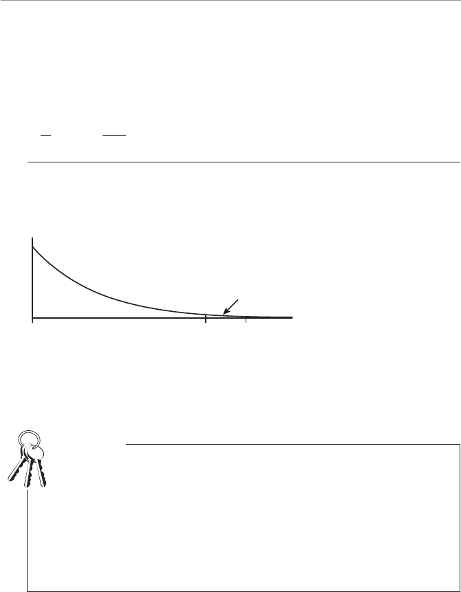
1VO^bS`'( /\OZgaWa]TDO`WO\QS '%
9 5.117 4.256 3.863 3.633 3.482 3.374 3.293 3.230 3.179 3.137
10 4.965 4.103 3.708 3.478 3.326 3.217 3.135 3.072 3.020 2.978
11 4.844 3.982 3.587 3.357 3.204 3.095 3.012 2.948 2.896 2.854
12 4.747 3.885 3.490 3.259 3.106 2.996 2.913 2.849 2.796 2.753
13 4.667 3.806 3.411 3.179 3.025 2.915 2.832 2.767 2.714 2.671
14 4.600 3.739 3.344 3.112 2.958 2.848 2.764 2.699 2.646 2.602
15 4.543 3.682 3.287 3.056 2.901 2.790 2.707 2.641 2.588 2.544
16 4.494 3.634 3.239 3.007 2.852 2.741 2.657 2.591 2.538 2.494
Note that this table is based only on F = 0.05. Other values of F will require a differ-
ent table. For v1 = 2 and v2 = 15, the critical F-statistic, F.05,2,15 = 3.682, as indicated in
the underlined part of the table. Figure 19.1 shows the results of our hypothesis test.
4WUc`S'
ANOVA test for the fertilizer
example.
Fc
0.95
1–
Do Not Reject H0
= 0.05
Reject H0
0 4.453.682
v1=2 v2= 15 F
According to Figure 19.1, the calculated F-statistic of 4.45 is within the “Reject H0”
region, which leads us to the conclusion that the population means are not equal. We
will always reject H0 as long as FF,k–1,N–kfF.
The F-distribution has the following characteristics:
UIt is not symmetrical but rather has a positive skew.
U The shape of the F-distribution will change with the degrees of freedom speci-
fied by the values of v1 and v2.
U As v1 and v2 increase in size, the shape of the F-distribution becomes more
symmetrical.
UThe total area under the curve is equal to 1.
UThe F-distribution mean is approximately equal to 1.
Bob’s Basics

>O`b"( /RdO\QSR7\TS`S\bWOZAbObWabWQa '&
Our final conclusion is that one or more of those darn fertilizers is making the grass
grow faster than the others. Sounds like trouble to me.
Even though we have rejected H0 and concluded that the population means are
not all equal, ANOVA does not allow us to make comparisons between means.
In other words, we do not have enough evidence to conclude that Fertilizer 2 pro-
duces more grass clippings than Fertilizer 1. This requires another test known as pair-
wise comparisons, which we’ll address later in this chapter.
Wrong Number
Now let’s explore how Excel can take some of the burden from all these nasty calcula-
tions.
CaW\U3fQSZb]>S`T]`[=\SEOg/<=D/
I’m sure you’ve come to the conclusion that calculating ANOVA manually is a lot of
work, and I think you’ll be amazed how easy this procedure is using Excel.
1. Start by placing the fertilizer data in Columns A, B, and C in a blank sheet.
2. Go to the Tools menu and select Data Analysis. (Refer to the section “Installing
the Data Analysis Add-in” from Chapter 2 if you don’t see the Data Analysis
command on the Tools menu.)
3. From the Data Analysis dialog box, select Anova: Single Factor as shown in
Figure 19.2 and click OK.
4WUc`S'
Setting up the one-way
ANOVA in Excel.
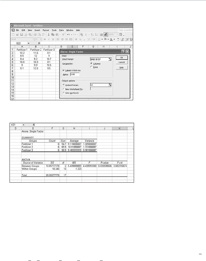
1VO^bS`'( /\OZgaWa]TDO`WO\QS ''
4. Set up the Anova: Single Factor dialog box according to Figure 19.3.
4WUc`S'!
The ANOVA: Single Factor
dialog box.
5. Click OK. Figure 19.4 shows the final ANOVA results.
4WUc`S'"
Final results of the one-way
ANOVA in Excel.
These results are consistent with what we found doing it the hard way in the previ-
ous sections. Notice that the p-value = 0.0305 for this test, meaning we can reject H0,
because this p-value fF. If you remember, we had set F = 0.05 when we stated the
hypothesis test.
>OW`eWaS1][^O`Wa]\a
Once we have rejected H0 using ANOVA, we can determine which of the sample
means are different using the Scheffé test. This test compares each pair of sample
means from the ANOVA procedure. For the fertilizer example, we would compare x1
versus x2,x1 versus x3, and x2 versus x3 to see whether any differences exist.
>O`b"( /RdO\QSR7\TS`S\bWOZAbObWabWQa!
First, the following test statistic for the Scheffé
test, FS, is calculated for each of the pairs of sample
means:
Fxx
SSW
nnn
S
ab
i
k
ab
¨
ª
©·
¹
¸
¤
2
1
11
where:
xa,xb = the sample means being compared
SSW = the sum of squares within from the ANOVA procedure
na,nb = the samples sizes
k = the number of samples (or levels)
Comparing x1 and x2, we have:
FS
¨
ª
©·
¹
¸
912 1092
18 35
555
1
6
1
6
324
1
2
..
.
.
... .
22 0 33 8 048
;=
Comparing x1 and x3, we have:
FS
¨
ª
©·
¹
¸
912 948
18 35
555
1
6
1
6
013
1
2
..
.
.
.222 0 33 0 323
..
;=
Comparing x2 and x3, we have:
FS
¨
ª
©·
¹
¸
10 92 9 48
18 35
555
1
6
1
6
207
1
2
..
.
.
... .
22 0 33 5 142
;=
Next the critical value for the Scheffé test, FSC , is determined by multiplying the criti-
cal F-statistic from the ANOVA test by k – 1 as follows:
FkF
SC k N k
11A,,
After rejecting H0 using
ANOVA, we can determine
which of the sample means
are different using the Scheffé
test.
Bob’s Basics

1VO^bS`'( /\OZgaWa]TDO`WO\QS !
For the fertilizer example:
F.05,2,15 = 3.682
FSC = (3 – 1)(3.682) = 7.364
If FSf FSC, we conclude there is no difference between the sample means; otherwise
there is a difference. The following table summarizes these results.
Ac[[O`g]TbVSAQVSTT{BSab
Sample Pair FS
FSC
Conclusion
x1 and x28.048 7.364 Difference
x1 and x30.323 7.364 No Difference
x2 and x35.142 7.364 No Difference
According to our results, the only statistically significant difference is between
Fertilizer 1 and Fertilizer 2. It appears that Fertilizer 2 is more effective in making
grass grow faster when compared to Fertilizer 1. I better keep Debbie away from this
brand.
1][^ZSbSZg@O\R][WhSR0Z]QY/<=D/
Now let’s modify the original fertilizer example: rather than select 18 random samples
from my lawn, we are going to collect 3 random samples from 6 different lawns.
Using the original data, the samples look as follows:
Lawn Fertilizer 1 Fertilizer 2 Fertilizer 3 Block
Mean
1 10.2 11.6 8.1 9.97
2 8.5 12.0 9.0 9.83
3 8.4 9.2 10.7 9.43
4 10.5 10.3 9.1 9.97
5 9.0 9.9 10.5 9.80
6 8.1 12.5 9.5 10.03
Fertilizer 9.12 10.92 9.48
Mean
>O`b"( /RdO\QSR7\TS`S\bWOZAbObWabWQa!
One concern in this scenario is that the variations in the lawns will account for some
of the variation in the three fertilizers, which may interfere with our hypothesis test.
We can control for this possibility by using a completely randomized block ANOVA,
which is used in the previous table. The type of fertilizer is still the factor, and the
lawns are called blocks.
There are two hypotheses for the completely ran-
domized block ANOVA. The first (primary) hypoth-
esis tests the equality of the population means, just
like we did earlier with one-way ANOVA:
H01 2 3
:MMM
H1: not all ’s are equalM
The secondary hypothesis tests the effectiveness of
the blocking variable as follows:
H
H
0
1
’:
’:
the block means are all equal
the bloock means are not all equ
a
The blocking variable would be an effective contributor to our ANOVA model if we
can reject H0’ and claim that the block means are not equal to each other.
>O`bWbW]\W\UbVSAc[]TA_cO`Sa
For the completely randomized block ANOVA, the sum of squares total is partitioned
into three parts according to the following equation:
SST = SSW + SSB + SSBL
where:
SSW = sum of squares within
SSB = sum of squares between
SSBL = sum of squares for the blocking variable (lawns)
Fortunately for us, the calculations for SST and SSW are identical to the one-way
ANOVA procedure that we’ve already discussed, so those values remain unchanged
(SST = 29.21 and SSB = 10.86). We can find the sum of squares block (SSBL) by using
the equation:
Completely randomized block
ANOVA controls for varia-
tions from other sources than
the factors of interest. This is
accomplished by grouping the
samples using a blocking vari-
able.

1VO^bS`'( /\OZgaWa]TDO`WO\QS !!
SSBL k x x
j
j
b
¤2
1
where:
xj the average observation of each blocking level
b = the number of blocking levels (b = 6 for our example)
Using the values from the previous table, we have:
SSBL
3 9 97 9 83 3 9 83 9 83 3 9 43 9 83
22
.. .. ..
2
22
3 997 983 3 980 983 310.. .. ...
.
03 9 83
072
2
SSBL
That leaves us with the sum of squares within (SSW ), which we can find using:
SSW = SST – SSB – SSBL
SSW = 29.21 – 10.86 – 0.72 = 17.63
Almost done!
2SbS`[W\W\UbVS1OZQcZObSR4AbObWabWQ
Since we have two hypothesis tests for the completely randomized block ANOVA, we
have two calculated F-statistics. The F-statistic to test the equality of the population
means (the original hypothesis) is found using:
FMSB
MSW
where MSB is the means square between, found by:
MSB SSB
k
1
and MSW is the mean square within, found by:
MSW SSW
kb
11

>O`b"( /RdO\QSR7\TS`S\bWOZAbObWabWQa!"
Inserting our fertilizer values into these equations looks like this:
MSB SSB
k
MSW SSW
kb
1
10 86
31 543
11
1
..
7763
3161 176
543
176 309
..
.
..
FMSB
MSW
The second F-statistic will test the significance of the blocking variable (the second
hypothesis) and will be denoted F’. We will determine this statistic using:
FMSBL
MSW
’
where MSBL is the (can you guess?) mean square blocking, found by:
MSBL SSBL
b
1
Plugging our numbers into these guys results in:
MSBL SSBL
b
1
072
61 014
..
FMSBL
MSW
’.
..
014
176 008
We now need to sit back, catch our breath, and figure out what all these numbers
mean.
B]0Z]QY]`<]bb]0Z]QYBVOb7abVS?cSabW]\
First, we will examine the primary hypothesis, H0, that all population means are equal
using F = 0.05. The degrees of freedom for this critical F-statistic would be:
vk
vk b
1
2
1312
11316110
The critical F-statistic from Appendix B is F0.05, 2, 10 = 4.103. Since the calculated
F-statistic equals 3.09 and is less than this critical F-statistic, we fail to reject H0 and
cannot conclude that the fertilizer means are different.

1VO^bS`'( /\OZgaWa]TDO`WO\QS !#
We next examine the secondary hypothesis, H0’, concerning the effectiveness of the
blocking variable, also using F = 0.05. The degrees of freedom for this critical F-sta-
tistic would be:
vb
vkb
1
2
1615
11316110
’
’
The critical F-statistic from Appendix B is F0.05, 5, 10 = 3.326. Since the calculated F-sta-
tistic, F’, equals 0.08 and is less than this critical F-statistic, we fail to reject H0’ and
cannot conclude that the block means are different.
What does all this mean? Since we failed to reject H0’, the hypothesis that states the
blocking means are equal, the blocking variable (lawns) proved not to be effective and
should not be included in the model. Including an ineffective blocking variable in the
ANOVA increases the chance of a T
ype II error in the primary hypothesis, H0. The
conclusion of the primary hypothesis in this example would be more precise without
the blocking variable. In fact, this is what essentially happened when we included the
blocking variable with the randomized block design. With the blocking variable pres-
ent in the model, we failed to discover a difference in the population means. Now go
back to the beginning of the chapter. When we tested the population means using
one-way ANOVA (without a blocking variable), we concluded that the population
means were indeed different.
In summary (It’s about time!), if you feel there is a variable present in your model that
could contribute undesirable variation, such as taking samples from different lawns,
use the randomized block ANOVA. First test H0’, the blocking hypothesis.
UIf you reject H0’, the blocking procedure was effective. Proceed to test H0, the
primary hypothesis concerning the population means, and draw your conclu-
sions.
UIf you fail to reject H0’, the blocking procedure was not effective. Redo the anal-
ysis using one-way ANOVA (without blocking) and draw your conclusions.
UIf all else fails, take two aspirin and call me in the morning.
G]c`Bc`\
1. A consumer group is testing the gas mileage of three different models of cars.
Several cars of each model were driven 500 miles and the mileage was recorded
as follows.

>O`b"( /RdO\QSR7\TS`S\bWOZAbObWabWQa!$
Car 1 Car 2 Car 3
22.5 18.7 17.2
20.8 19.8 18.0
22.0 20.4 21.1
23.6 18.0 19.8
21.3 21.4 18.6
22.5 19.7
Note that the size of each sample does not have to be equal for ANOVA.
Test for a difference between sample means using F = 0.05.
2. Perform a pairwise comparison test on the sample means from Problem 1.
3. A vice president would like to determine whether there is a difference between
the average number of customers per day between four different stores using the
following data.
Store 1 Store 2 Store 3 Store 4
36 35 26 26
48 20 20 52
32 31 38 37
28 22 32 36
31 19 37 18
55 42 15 30
29 21
Note that the size of each sample does not have to be equal for ANOVA.
Test for a difference between sample means using F = 0.05.
4. A certain unnamed statistics author and his two sons played golf at four different
courses with the following scores:

1VO^bS`'( /\OZgaWa]TDO`WO\QS !%
Dad Brian John
Course 1 93 85 80
Course 2 98 87 88
Course 3 89 82 84
Course 4 90 80 82
Using completely randomized block ANOVA, test for the difference of golf
score means using F = 0.05 and using the courses as the blocking variable.
BVS:SOabG]c<SSRb]9\]e
UAnalysis of variance, also known as ANOVA, compares the means of three or
more populations.
UA factor in ANOVA describes the cause of the variation in the data. When only
one factor is being considered, the procedure is known as one-way ANOVA.
UA level in ANOVA describes the number of categories within the factor of
interest.
UThe simplest type of ANOVA is known as completely randomized one-way
ANOVA, which involves an independent random selection of observations for
each level of one factor.
UCompletely randomized block ANOVA controls for variations from other
sources than the factors of interest. This is accomplished by grouping the sam-
ples using a blocking variable.
UAfter rejecting H0 using ANOVA, we can determine which of the sample means
are different using the Scheffé test.

20
1VO^bS`
1]``SZObW]\O\RAW[^ZS
@SU`SaaW]\
7\BVWa1VO^bS`
UDistinguishing between independent and dependent variables
UDetermining the correlation and regression line for a set of ordered-
pair data
UCalculating a confidence interval for a regression line
UPerforming a hypothesis test on the regression line
UUsing Excel to perform simple regression analysis
For the last several chapters, we have put inferential statistics to work draw-
ing conclusions about one, two, or more population means and propor-
tions. I know this has been a lot of fun for you, but it’s time to move to
another type of inferential statistics that’s even more exciting. (If you can
imagine that!)
This final chapter focuses on describing how two variables relate to one
another. Using correlation and simple regression, we will be able to first
determine whether a relationship does indeed exist between the variables
and second describe the nature of this relationship in mathematical terms.
And hopefully we’ll have some fun doing it!
>O`b"( /RdO\QSR7\TS`S\bWOZAbObWabWQa!
7\RS^S\RS\bDS`aca2S^S\RS\bDO`WOPZSa
Suppose I would like to investigate the relationship between the number of hours that
a student studies for a statistics exam and the grade for that exam (uh-oh). The follow-
ing table shows sample data from six students whom I randomly chose.
2ObOT]`AbObWabWQa3fO[
Hours Studied Exam Grade
386
595
492
483
278
382
Obviously, we would expect the number of hours
studying to affect the grade. The Hours Studied vari-
able is considered the independent variable (x) because
it causes the observed variation in the Exam Grade,
which is considered the dependent variable (y). The
data from the previous table is considered ordered
pairs of (x,y) values, such as (3,86) and (5,95).
This “causal relationship” between independent and
dependent variables only exists in one direction, as
shown here:
Independent variable (x)m Dependent
variable (y)
This relationship does not work in reverse. For
instance, we would not expect that the exam grade
variable would cause the student to study a certain
number of hours in our previous example.
Other examples of independent and dependent variables are shown in the following
table.
The independent variable (x)
causes variation in the depen-
dent variable (y).
Exercise caution when
deciding which variable
is independent and which is
dependent. Examine the rela-
tionship from both directions to
see which one makes the most
sense. The wrong choice will
lead to meaningless results.
Wrong Number
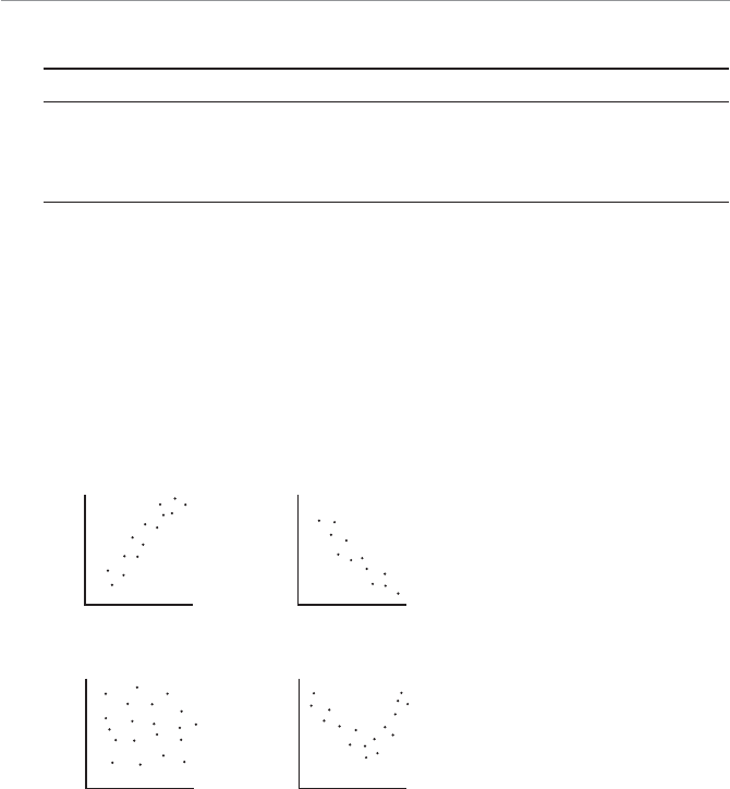
1VO^bS` ( 1]``SZObW]\O\RAW[^ZS@SU`SaaW]\ !
3fO[^ZSa]T7\RS^S\RS\bO\R2S^S\RS\bDO`WOPZSa
Independent Variable Dependent Variable
Size of TV Selling price of TV
Level of advertising Volume of sales
Size of sports team payroll Number of games won
Now, let’s focus on describing the relationship between the x and y variables using
inferential statistics.
1]``SZObW]\
Correlation measures both the strength and direction of the relationship between x
and y. Figure 20.1 illustrates the different types of correlation in a series of scatter
plots, which graphs each ordered pair of (x,y). The convention is to place the x vari-
able on the horizontal axis and the y variable on the vertical axis.
4WUc`S
Different types of correlation.
(A) Positive Linear Correlation
X
y
(B) Negative Linear Correlation
X
y
(C) No Correlation
X
y
(D) Nonlinear Correlation
X
y
Graph A in Figure 20.1 shows an example of positive linear correlation where, as x
increases, y also tends to increase in a linear (straight line) fashion. Graph B shows a
negative linear correlation where, as x increases, y tends to decrease linearly. Graph
C indicates no correlation between x and y. This set of variables appears to have no
impact on each other. And finally, Graph D is an example of a nonlinear relationship
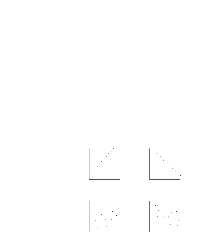
>O`b"( /RdO\QSR7\TS`S\bWOZAbObWabWQa!
between variables. As x increases, y decreases at first and then changes direction and
increases.
For the remainder of this chapter, we will focus on linear relationships between the
independent and dependent variables. Nonlinear relationships can be very disagree-
able and go beyond the scope of this book.
1]``SZObW]\1]STTWQWS\b
The correlation coefficient, r, provides us with both the strength and direction of
the relationship between the independent and dependent variables. Values of r range
between –1.0 and +1.0. When r is positive, the relationship between x and y is posi-
tive (Graph A from Figure 20.1), and when r is negative, the relationship is negative
(Graph B). A correlation coefficient close to 0 is evidence that there is no relationship
between x and y (Graph C).
The strength of the relationship between x and y is measured by how close the corre-
lation coefficient is to +1.0 or –1.0 and can be viewed in Figure 20.2.
4WUc`S
The strength of the
relationship.
The Strength of the Relationship
A
X
y
B
X
y
C
X
y
D
X
y
r = +1.0
r = +0.60 r = -0.60
r = -1.0
1VO^bS` ( 1]``SZObW]\O\RAW[^ZS@SU`SaaW]\ !!
Graph A illustrates a perfect positive corre-
lation between x and ywith r = +1.0. Graph
B shows a perfect negative correlation
between x and y with r= –1.0. Graphs C
and D are examples of weaker relationships
between the independent and dependent
variables.
We can calculate the actual correlation coef-
ficient using the following equation:
rnx
yx y
nx x ny y
¨
ª
©·
¹
¸
¨
ª
¤¤¤
¤¤ ¤¤
2222
©© ·
¹
¸
Wow! I know this looks overwhelming, but before we panic, let’s try out our exam
grade example on this. The following table will help break down the calculations and
make them more manageable.
Hours of Exam Grade
Study
x y xy x2y2
3 86 258 9 7396
5 95 475 25 8464
4 92 368 16 9025
4 83 332 16 6889
2 78 156 4 6084
3 82 246 9 6724
x
¤21 y
¤516 xy
¤1835 x279
¤
y244582
¤
The correlation coefficient, r,
indicates both the strength and
direction of the relationship
between the independent and
dependent variables. Values
of r range from –1.0, a strong
negative relationship, to +1.0,
a strong positive relationship.
When r = 0, there is no rela-
tionship between variables x
and y.
>O`b"( /RdO\QSR7\TS`S\bWOZAbObWabWQa!"
Using these values along with n = 6, the number of ordered pairs, we have:
rnx
yx y
nx x ny y
¨
ª
©·
¹
¸
¨
ª
¤¤¤
¤¤ ¤¤
2222
©© ·
¹
¸
r
¨
ª·
¹
6 1835 21 516
6 79 21 6 44582
25516
174
33 1236 0 862
2
¨
ª·
¹
r.
As you can see, we have a fairly strong positive correlation between hours of study and
the exam grade. That’s good news for us teachers.
Be careful to distinguish between x2
¤ and x
¤
2. With x2
¤, we first
square each value of x and then add each squared term. With x
¤
2, we first
add each value of x and then square this result. The answers between the two are
very different!
Wrong Number
What is the benefit of establishing a relationship between two variables such as these?
That’s an excellent question. When we discover that a relationship does exist, we can
predict exam scores based on a particular number of hours of study. Simply put, the
stronger the relationship, the more accurate our prediction will be. You will learn how
to make such predictions later in this chapter when we discuss simple regression.
BSabW\UbVSAWU\WTWQO\QS]TbVS1]``SZObW]\1]STTWQWS\b
We can perform a hypothesis test to determine whether the population correlation
coefficient, p, is significantly different from 0 based on the value of the calculated cor-
relation coefficient, r. We can state the hypotheses as:
H0:pf 0
H1:p# 0
1VO^bS` ( 1]``SZObW]\O\RAW[^ZS@SU`SaaW]\ !#
This statement tests whether a positive correlation exists between x and y. I could also
choose a two-tail test that would investigate whether any correlation exists (either
positive or negative) by setting H0 : p" 0 and H1 : p| 0.
The test statistic for the correlation coefficient uses the Student’s t-distribution as
follows:
tr
r
n
1
2
2
where:
r = the calculated correlation coefficient from the ordered pairs
n = the number of ordered pairs
For the exam grade example, the calculated t-statistic becomes:
tr
r
n
t
1
2
0 862
1 0 862
62
0 862
0 257
4
22
.
.
.
.33 401.
The critical t-statistic is based on d.f. = n – 2 if we choose F = 0.05, tc = 2.132 from
Table 4 in Appendix B for a one-tail test. Because t > tc, we reject H0 and conclude that
there is indeed a positive correlation coefficient between hours of study and the exam
grade. Once again, statistics has proven that all is right in the world!
CaW\U3fQSZb]1OZQcZObS1]``SZObW]\1]STTWQWS\ba
After looking at the nasty calculations involved for the correlation coefficient, I’m
sure you’ll be relieved to know that Excel will do the work for you with the CORREL
function that has the following characteristics:
CORREL(array1, array2)
where:
array1 = the range of data for the first variable
array2 = the range of data for the second variable
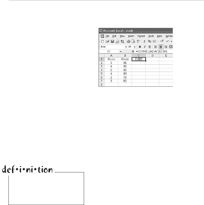
>O`b"( /RdO\QSR7\TS`S\bWOZAbObWabWQa!$
For instance, Figure 20.3 shows the CORREL function being used to calculate the
correlation coefficient for the exam grade example.
4WUc`S !
CORREL function in
Excel with the exam grade
example.
Cell C1 contains the Excel formula =CORREL(A2:A7,B2:B7) with the result being
0.862.
AW[^ZS@SU`SaaW]\
The technique of simple regression enables us to describe a straight line that best fits a
series of ordered pairs (x,y). The equation for a straight line, known as a linear equa-
tion, takes the form:
ˆ
yab
x
where:
ˆ
y= the predicted value of y, given a value of x
x = the independent variable
a = the y-intercept for the straight line
b = the slope of the straight line
Figure 20.4 illustrates this concept.
Figure 20.4 shows a line described by the equation ˆ.yx20
5
. The y-intercept is the
point where the line crosses the y-axis, which in this case is a = 2. The slope of the
line, b, is shown as the ratio of the rise of the line over the run of the line, shown as
b = 0.5. A positive slope indicates the line is rising from left to right. A negative slope,
you guessed it, moves lower from left to right. If b = 0, the line is horizontal, which
means there is no relationship between the independent and dependent variables. In
other words, a change in the value of x has no effect on the value of y.
The technique of simple regres-
sion enables us to describe a
straight line that best fits a series
of ordered pairs (x,y).
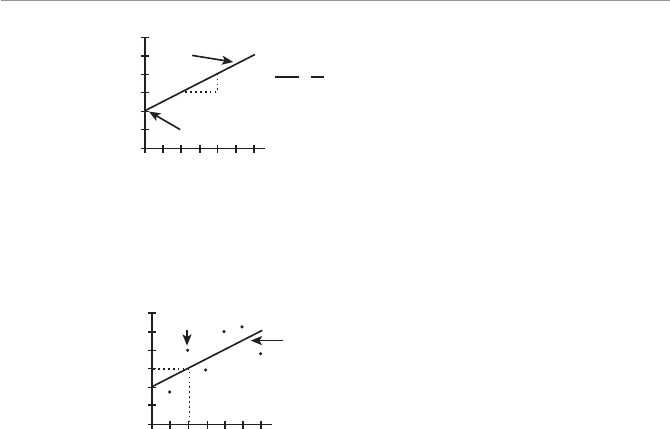
1VO^bS` ( 1]``SZObW]\O\RAW[^ZS@SU`SaaW]\ !%
Students sometimes struggle with the distinction between ˆ
yand y. Figure 20.5 shows
six ordered pairs and a line that appears to fit the data described by the equation
ˆ.yx20
5
.
4WUc`S "
Equation for a straight line.
y
x
1234560
0
1
2
3
4
5
6^
y = 2 + 0.5x
a = 2
2
1b = 0.5
Rise
Run
1
2
==
4WUc`S #
The difference between y
and ˆ
y.
y
x
1234560
0
1
2
3
4
5
6
^
y = 2 + 0.5x
(2,4)
^
x = 2
y = 4
y = 3
Figure 20.5 shows a data point that corresponds to the ordered pair x = 2 and y =
4. Notice that the predicted value of y according to the line at x = 2 is ˆ
y = 3. We can
verify this using the equation as follows:
ˆ..yx
205 2052 3
The value of y represents an actual data point, while the value of ˆ
y is the predicted
value of y using the linear equation, given a value for x.
Our next step is to find the linear equation that best fits a set of ordered pairs.
BVS:SOabA_cO`Sa;SbV]R
The least squares method is a mathematical procedure to identify the linear equation
that best fits a set of ordered pairs by finding values for a, the y-intercept; and b, the
slope. The goal of the least squares method is to minimize the total squared error
between the values of y and ˆ
y. If we define the error as yyˆfor each data point, the
least squares method will minimize:
yy
ii
i
n
¤ˆ2
1
where n is the number of ordered pairs around the line that best fits the data.
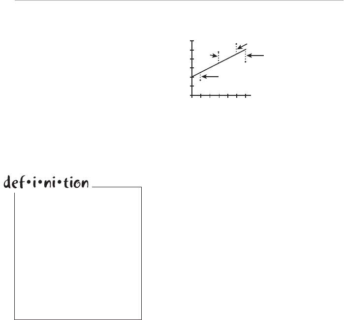
>O`b"( /RdO\QSR7\TS`S\bWOZAbObWabWQa!&
This concept is illustrated in Figure 20.6.
4WUc`S $
Minimizing the error.
y
x
1234560
0
1
2
3
4
5
6^
y – y
33
^
y – y
44
^
y – y
11
^
y – y
22
According to Figure 20.6, the line that best fits the data, the regression line, will mini-
mize the total squared error of the four data points. I’ll demonstrate how to deter-
mine this regression equation using the least squares method through the following
example.
Apparently, there has been a silent war raging in our
bathroom at home that has recently caught my atten-
tion. I’m of course referring to the space on our bath-
room countertop that, under an unwritten agreement,
Debbie and I are supposed to “share.” Over the past
few months, I have been keeping a wary eye on the
increasing number of “things” on her side that are
growing in number at a rate faster than the federal
deficit. I’m slowly being squeezed out of my end of
the bathroom by containers with words such as “volu-
mizing fixative” and “soyagen complex.” Debbie’s
little army has even taken both electrical outlets, cut-
ting me off from any source of power. I might as well
just raise the white towel in surrender and head off to
the teenagers’ bathroom in exile, a room I had vowed
never to step foot into because … well, I’ll just spare you the messy details. Just believe
me—you don’t ever want to go in there voluntarily.
Anyway, let’s say the following table shows the number of Debbie’s items on the bath-
room counter for the past several months.
The least squares method is
a mathematical procedure to
identify the linear equation that
best fits a set of ordered pairs
by finding values for a, the
y-intercept; and b, the slope.
The goal of the least squares
method is to minimize the total
squared error between the val-
ues of y and ˆ
y. The regression
line is the line that best fits the
data.

1VO^bS` ( 1]``SZObW]\O\RAW[^ZS@SU`SaaW]\ !'
0ObV`]][1]c\bS`2ObO
Month Number of Items Month Number of Items
1 8 6 13
2 6 7 9
310 8 11
4 6 9 15
510 10 17
Because my goal is to investigate whether the number of items is increasing over time,
Month will be the independent variable and Number of Items will be the dependent
variable.
The least squares method finds the linear equation that best fits the data by determin-
ing the value for a, the y-intercept; and b, the slope, using the following equations:
bnxy x y
nx x
¤¤¤
¤¤
22
aybx
where:
x = the average value of x, the independent variable
y = the average value of y, the dependent variable
The following table summarizes the calculations necessary for these equations.
1OZQcZObW]\aT]`bVSAZ]^SO\R7\bS`QS^b
Month Items
x y xy x2y2
1 8 8 1 84
2 612 4 36
3 10 30 9 100
4 6 24 16 36

>O`b"( /RdO\QSR7\TS`S\bWOZAbObWabWQa!
Month Items
x y xy x2y2
5 10 50 25 100
6 13 78 36 169
7 9 63 49 81
8 11 88 64 121
9 15 135 81 225
10 17 170 100 289
x
¤55 y
¤105 xy
¤658 x2385
¤y21221
¤
x
55
10 55.y
105
10 10 5.
bnxy x y
nx x
¤¤¤¤¤
22
10 658 55 105
110 385 55
805
825 0 976
2
b.
aybx
10 5 0 976 5 5 5 13.. ..
The regression line for the bathroom counter example would be:
ˆ..yx513 0 976
Because the slope of this equation is a positive 0.976, I have evidence that the number
of items on the counter is increasing over time at an average rate of nearly one per
month. Figure 20.7 shows the regression line with the ordered pairs.
My prediction for the number of items on the counter in another six months (Month
16 from my data) will be:
ˆ.. .. .yx
z5 13 0 976 5 13 0 976 16 20 7 21 items
Look out, kids. Make room for Dad.
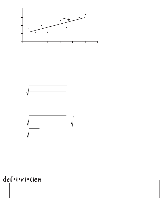
1VO^bS` ( 1]``SZObW]\O\RAW[^ZS@SU`SaaW]\ !
1]\TWRS\QS7\bS`dOZT]`bVS@SU`SaaW]\:W\S
Just how accurate is my estimate for the number of items on the counter for a particu-
lar month? To answer this, we need to determine the standard error of the estimate, se,
using the following formula:
syaybxy
n
e
¤¤¤
2
2
The standard error of the estimate measures the amount of dispersion of the observed
data around the regression line. If the data points are very close to the line, the stan-
dard error of the estimate is relatively low and vice versa. For our bathroom example:
syaybxy
n
e
¤¤¤
2
2
1221 5 13 105 0 976 65..
88
10 2
40 14
8224
se
..
We are now ready to calculate a confidence interval (remember those from Chapter
14?) for the mean of y around a particular value of x. For Month 8 (x = 8) in the data,
Debbie has 11 items (y = 11) on the counter. The regression line predicted she would
have:
ˆ.. .. .yx
5 13 0 976 5 13 0 976 8 12 9 items
4WUc`S %
Regression line for the bath-
room counter example.
0
5
10
15
20
0
Items
2 4 6 8 10 12
Month
y = 5.13 + 0.976x
^
The standard error of the estimate, se, measures the amount of dispersion of the
observed data around the regression line.
>O`b"( /RdO\QSR7\TS`S\bWOZAbObWabWQa!
In general, the confidence interval around the mean of ygiven a specific value of x can
be found by:
CI y t s n
xx
xx
n
ce
p
¤¤
ˆ1
2
2
2
where:
tc = the critical t-statistic from the Students’ t-distribution
se = the standard error of the mean
n = the number of ordered pairs
Hold on to your hat while we dive into this one with our example. Suppose we would
like a 95 percent confidence interval around the mean of y for Month 8. To find our
critical t-statistic, we look to Table 4 in Appendix B. This procedure has n – 2 = 10 – 2
= 8 degrees of freedom, resulting in tc = 2.306 from Table 4 in Appendix B. Our confi-
dence interval is then:
CI y t s n
xx
xx
n
ce
p
¤¤
ˆ1
2
2
2
CI p
12 9 2 306 2 24 1
10
855
385 55
2
.. . .
22
10
CI p
p12 9 2 306 2 24 0 419 12 9 2 16.. .. ..
CI 10 74 15 06..and
This interval is shown graphically on Figure 20.8.
Our 95 percent confidence interval for the number of items on the counter in Month
8 is between 10.74 and 15.06 items. Sounds like a very crowded countertop to me.
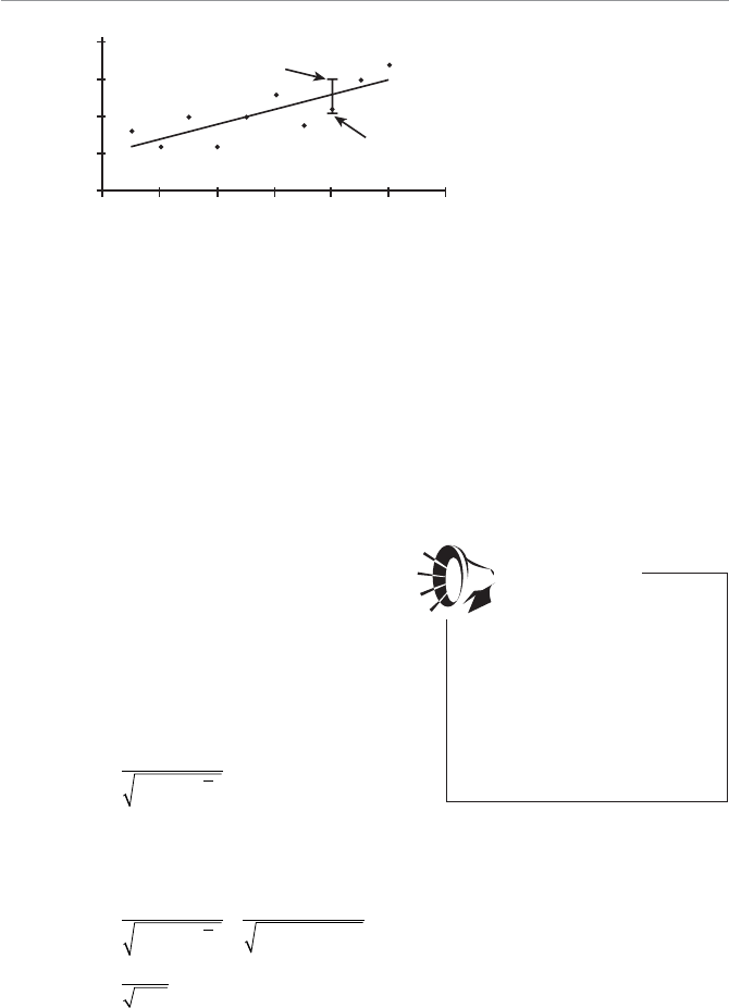
1VO^bS` ( 1]``SZObW]\O\RAW[^ZS@SU`SaaW]\ ! !
BSabW\UbVSAZ]^S]TbVS@SU`SaaW]\:W\S
Recall that if the slope of the regression line, b, is equal to 0, then there is no relation-
ship between x and y. In our bathroom counter example, we found the slope of the
regression line to be 0.976. However, because this result was based on a sample of
observations, we need to test to see whether 0.976 is far enough away from 0 to claim
a relationship really does exist between the variables. If G is the slope of the true popu-
lation, then our hypotheses statement would be:
H0:G" 0
H1:G| 0
If we reject the null hypothesis, we conclude
that a relationship does exist between the
independent and dependent variables based
on our sample. We’ll test this using
F = 0.01.
This hypothesis test requires the standard
error of the slope, sb, which is found with
the following equation:
ss
xnx
b
e
¤22
where se is the standard error of the estimate
that we calculated earlier.
For our bathroom example:
ss
xnx
s
b
e
b
¤222
224
385 10 5 5
224
82 5 0
.
.
.
..2247
4WUc`S &
95 percent confidence interval
for x = 8.
y = 15.06
y = 10.74
0
5
10
15
20
0
Items
2 4 6 8 10 12
Month
Just because a relationship
between two variables is
statistically significant doesn’t
necessarily mean that a causal
relationship truly exists. The
mathematical relationship could
be due to pure coincidence.
Always use your best judgment
when making these decisions.
Wrong Number
>O`b"( /RdO\QSR7\TS`S\bWOZAbObWabWQa! "
The test statistic for this hypothesis is:
tb
s
H
b
B
0
where
B
H0 is the value of the population slope according to the null hypothesis.
For this example, our calculated t-statistic is:
tb
s
H
b
B
00 976 0
0 247 3 951
.
..
The critical t-statistic is taken from the Student’s t-distribution with n – 2 = 10 – 2 =
8 degrees of freedom. With a two-tail test and F = 0.01, tc= 3.355 according to Table
4 in Appendix B. Because t > tc, we reject the null hypothesis and conclude there is a
relationship between the month and the number of items on the bathroom counter-
top. I thought so!
BVS1]STTWQWS\b]T2SbS`[W\ObW]\
Another way of measuring the strength of a relationship is with the coefficient of
determination, r2..This represents the percentage of the variation in y that is explained
by the regression line. We find this value by simply
squaring r, the correlation coefficient. For the bath-
room example, the correlation coefficient is:
rnxy x y
nx x ny y
¨
ª·
¹
¨
ª·
¹
¤¤¤
¤¤ ¤¤
2222
r
¨
ª·
¹
10 658 55 105
10 385 55 10 1221
2
¨
ª·
¹
105
805
825 1185 0 814
2
r.
The coefficient of determination becomes:
r22
0814 0 663
..
In other words, 66.3 percent of the variation in the number of items on the counter is
explained by the Month variable. If r2 = 1, all of the variation in y is explained by the
variable x. If r2 = 0, none of the variation in y is explained by the variable x.
The coefficient of determina-
tion, r2, represents the percent-
age of the variation in y that
is explained by the regression
line.
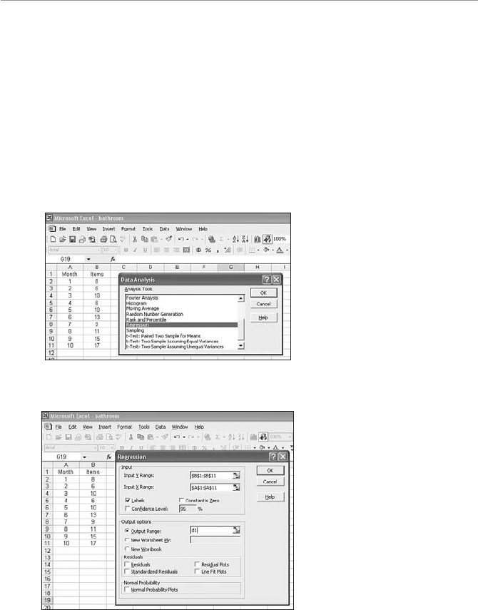
1VO^bS` ( 1]``SZObW]\O\RAW[^ZS@SU`SaaW]\ ! #
CaW\U3fQSZT]`AW[^ZS@SU`SaaW]\
Now that we have burned out our calculators with all these fancy equations, let me
show you how Excel does it all for us.
1. Start by placing the bathroom counter data in Columns A and B in a blank sheet.
2. Go to the Tools menu and select Data Analysis. (Refer to the section “Installing
the Data Analysis Add-in” from Chapter 2 if you don’t see the Data Analysis
command on the Tools menu.)
3. From the Data Analysis dialog box, select Regression as shown in Figure 20.9
and click OK.
4WUc`S '
Setting up simple regression
with Excel.
4. Set up the Regression dialog box according to Figure 20.10.
4WUc`S
The Regression dialog box.
5. Click OK. Figure 20.11 shows the final regression results.

>O`b"( /RdO\QSR7\TS`S\bWOZAbObWabWQa! $
4WUc`S
Final results of the regression
analysis in Excel.
These results are consistent with what we found after grinding it out in the previous
sections. Because the p-value for the independent variable Month is shown as 0.00414,
which is less than F = 0.01, we can reject the null hypothesis and conclude that a rela-
tionship between the variables does exist. Debbie has to believe me now!
/AW[^ZS@SU`SaaW]\3fO[^ZSeWbV<SUObWdS1]``SZObW]\
Both of these past examples have involved a positive relationship between x and y.
Now this example will summarize performing simple regression with a negative rela-
tionship.
Recently, I had the opportunity to “bond” with my son Brian as we shopped for his
first car when he turned 16. Brian had visions of Mercedes and BMWs dancing in his
head, whereas I was thinking more along the line of Hondas and Toyotas. After many
“discussions” on the matter, we compromised on looking for 1999 Volkswagen Jettas.
However, Brian had two requirements:
UIt had to be black.
UIt had to be the “new body” style.
Apparently, somebody at Volkswagen had the brilliant idea back in 1999 to sub-
tly change the design of the Jetta halfway through the production year. Personally,
I would never have noticed the difference. Brian, on the other hand, wouldn’t be
caught dead driving the original version, essentially eliminating half the used 1999
Volkswagen Jettas on the market. Undeterred, I searched the world over, asking each
seller, “Is it the new body style?” Ahh, the joys of parenthood! Anyway, what follows

1VO^bS` ( 1]``SZObW]\O\RAW[^ZS@SU`SaaW]\ ! %
is a table showing the mileage of eight cars with the new body style and their ask-
ing price. The remainder of this chapter demonstrates the correlation and regression
technique using this data.
2ObOT]`1O`3fO[^ZS
Mileage Price Mileage Price
21,800 $16,000 65,800 $10,500
34,000 $11,500 72,100 $12,300
41,700 $13,400 76,500 $8,200
53,500 $14,800 84,700 $9,500
The following table, which shows the data in thousands, will be used for the various
equations.
Mileage Price
x y xy x2y2
21.8 16.0 348.80 475.24 256.00
34.0 11.5 391.00 1156.00 132.25
41.7 13.4 558.78 1738.89 179.56
53.5 14.8 791.80 2862.25 219.04
65.8 10.5 690.90 4329.64 110.25
72.1 12.3 886.83 5198.41 151.29
76.5 8.2 627.30 5852.25 67.24
84.7 9.5 804.65 7174.09 90.25
x
¤450 1.y
¤96 2.xy
¤5100 1.
x228786 8
¤.
y21205 9
¤.
x
450
856 3.y
96 2
812 0
..
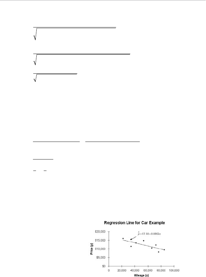
>O`b"( /RdO\QSR7\TS`S\bWOZAbObWabWQa! &
The correlation coefficient can be found using:
rnx
yx y
nx x ny y
¨
ª
©·
¹
¸
¨
ª
¤¤¤
¤¤ ¤¤
2222
©© ·
¹
¸
r
¨
8 5100 1 450 1 96 2
8 28786 8 450 2
...
.
ªª ·
¹
¨
ª·
¹
8 1205 9 96 2
2498 82
27794 4
2
..
.
.
r
392 76 0 756
..
The negative correlation indicates that as mileage (x)increases, the price (y) decreases
as we would expect. The coefficient of determination becomes:
r22
0 756 0 572
..
Approximately 57 percent of the variation in price is explained by the variation in
mileage. The regression line is determined using:
bnxy x y
nx x
¤¤¤
¤¤
22
8 5100 1 450 1..996 2
8 28786 8 450 1
2498 82
27704 3
2
.
..
.
.
b99 0 0902 .
aybx
12 025 0 0902 56 26 17 100....
We can describe the regression line by the equation:
ˆ..yx17 10 0902
This equation is shown graphically in Figure 20.12.
4WUc`S
Regression line for car
example.

1VO^bS` ( 1]``SZObW]\O\RAW[^ZS@SU`SaaW]\ ! '
What would the predicted price be for a car with 45,000 miles?
ˆ.. .$.y
17 1 0 0902 45 0 13 041
The regression line would predict that a car with 45,000 miles would be priced at
$13,041. What would be the 90 percent confidence interval at x = 45,000? The stan-
dard error of the estimate would be:
syaybxy
n
e
¤¤¤
2
2
se
1205 9 17 1 96 2 0 0902 5100 1
82
... . .
se
1205 9 1645 02 460 03
61 867
...
.
The critical t-statistic for n – 2 = 8 – 2 = 6 degrees of freedom and a 90 percent con-
fidence interval is tc = 1.943 from Table 4 in Appendix B. Our confidence interval is
then:
CI y t s n
xx
xx
n
ce
p
¤¤
ˆ1
2
2
2
CI p
13 041 1 934 1 867 1
8
45 56 26
28786
2
... .
.. .
8450 1
8
2
CI p
p13 041 1 934 1 867 0 402 13 041 1 45. ... ..22
CI 11 589 14 493..and
The 90 percent confidence interval for a car with 45,000 miles is between $11,589 and
$14,493.
Is the relationship between mileage and price statistically significant at the
F = 0.10 level? Our hypotheses’ statement is:
H0:G" 0
H1:G| 0
>O`b"( /RdO\QSR7\TS`S\bWOZAbObWabWQa!!
The standard error of the slope, sb,is found using:
ss
xnx
s
b
e
b
¤222
1 867
28786 8 8 56 26
1 867
.
..
.
33465 3 0 0317
..
The calculated test statistic for this hypothesis is:
tb
s
H
b
B
00 0902 0
0 0317 2 845
.
..
The critical t-statistic is taken from the Student’s t-distribution with n – 2 = 8 – 2 = 6
degrees of freedom. With a two-tail test and F = 0.10 level, tc = 1.943 according to
Table 4 in Appendix B. Because tt
c
, we reject the null hypothesis and conclude
there is a relationship between the mileage and price variable. We use the absolute
values because the calculated t-statistic is in the left tail of the t-distribution with a
two-tail hypothesis test.
/aac[^bW]\aT]`AW[^ZS@SU`SaaW]\
For all these results to be valid, we need to make sure that the underlying assumptions
of simple regression are not violated. These assumptions are as follows:
UIndividual differences between the data and the regression line,
yy
ii
ˆ
, are inde-
pendent of one another.
UThe observed values of y are normally distributed around the predicted value, ˆ
y.
UThe variation of y around the regression line is equal for all values of x.
Unfortunately (or fortunately), the techniques to test these assumptions go beyond the
level of this book.
AW[^ZSDS`aca;cZbW^ZS@SU`SaaW]\
Simple regression is limited to examining the relationship between a dependent variable
and only one independent variable. If more than one independent variable is involved in
the relationship, then we need to graduate to multiple regression. The regression equa-
tion for this method looks like this:
ˆ...ya
b
x bx bx
nn
11 22

1VO^bS` ( 1]``SZObW]\O\RAW[^ZS@SU`SaaW]\ !!
As you can imagine, this technique gets really messy and goes beyond the scope of this
book. I’ll have to save this topic for The Complete Idiot’s Guide to Statistics, Part 3. Uh-
oh, I think I just heard Debbie faint.
G]c`Bc`\
1. The following table shows the payroll for 10 major league baseball teams (in mil-
lions) for the 2002 season, along with the number of wins for that year.
Payroll Wins Payroll Wins
$171 103 $56 62
$108 75 $62 84
$119 92 $43 78
$43 55 $57 73
$58 56 $75 67
Calculate the correlation coefficient. Test to see whether the correlation coeffi-
cient is not equal to 0 at the 0.05 level.
2. Using the data from Problem 1, answer the following questions:
a) What is the regression line that best fits the data?
b) Is the relationship between payroll and wins statistically significant at the
0.05 level?
c) What is the predicted number of wins with a $70 million payroll?
d) What is the 99 percent confidence interval around the mean number of
wins for a $70 million payroll?
e) What percent of the variation in wins is explained by the payroll?
3. The following table shows the grade point average (GPA) for five students along
with their entrance exam scores for MBA programs (GMAT). Develop a model
that would predict the GPA of a student based on his GMAT score. What would
be the predicted GPA for a student with a GMAT score of 600?

>O`b"( /RdO\QSR7\TS`S\bWOZAbObWabWQa!!
Student GPA GMAT
1 3.7 660
2 3.0 580
3 3.2 450
4 4.0 710
5 3.5 550
BVS:SOabG]c<SSRb]9\]e
UThe independent variable (x) causes variation in the dependent variable ( y).
UThe correlation coefficient, r, indicates both the strength and direction of the
relationship between the independent and dependent variables.
UThe technique of simple regression enables us to describe a straight line that best
fits a series of ordered pairs (x,y).
UThe least squares method is a mathematical procedure to identify the linear
equation that best fits a set of ordered pairs by finding values for a, the
y-intercept; and b, the slope.
UThe standard error of the estimate, se, measures the amount of dispersion of the
observed data around the regression line.
UThe coefficient of determination, r2, represents the percentage of the variation
in y that is explained by the regression line.

A]ZcbW]\ab]¿G]c`Bc`\À
1VO^bS`
1. Inferential statistics, because it would not be feasible to survey every
Asian American household in the country. These results would be
based on a sample of the population and used to make an inference on
the entire population.
2. Inferential statistics, because it would not be feasible to survey every
household in the country. These results would be based on a sample
of the population and used to make an inference on the entire popula-
tion.
3. Descriptive statistics, because Hank Aaron’s home run total is based
on the entire population, which is every at-bat in his career.
4. Descriptive statistics, because the average SAT score would be based
on the entire population, which is the incoming freshman class.
5. Inferential statistics, because it would not be feasible to survey every
American in the country. These results would be based on a sample of
the population and used to make an inference on the entire popula-
tion.
A
/^^S\RWf

/^^S\RWf/
!!"
1VO^bS`
1. Interval data, because temperature in degrees Fahrenheit does not contain a true
zero point.
2. Ratio data, because monthly rainfall does have a true zero point.
3. Ordinal data, because a Master’s degree is a higher level of education than a
Bachelor’s or high school degree. However, we cannot claim that a Master’s
degree is two or three times higher than the others.
4. Nominal data, because we cannot place the categories in any type of order.
5. Ratio data, because age does have a true zero point.
6. Definitely nominal data, unless you want to get into an argument about which is
the lesser gender!
7. Interval data, because the difference between years is meaningful but a true zero
point does not exist.
8. Nominal data, because I am not prepared to name one political party superior to
another.
9. Nominal data, because these are simply unordered categories.
10. Ordinal data, because we can specify that “Above Expectation” is higher on the
performance scale than the other two but we cannot comment on the differences
between the categories.
11. Nominal data, because we cannot claim a person wearing the number “10” is any
better then a person wearing the number “4.”
12. Ordinal data, because we cannot comment on the difference in performance
between students. The top two students may be very far apart grade-wise,
whereas the second and third students could be very close.
13. Ratio data, because these exam scores have a true zero point.
14. Nominal data, because there is no order in the states’ categories.
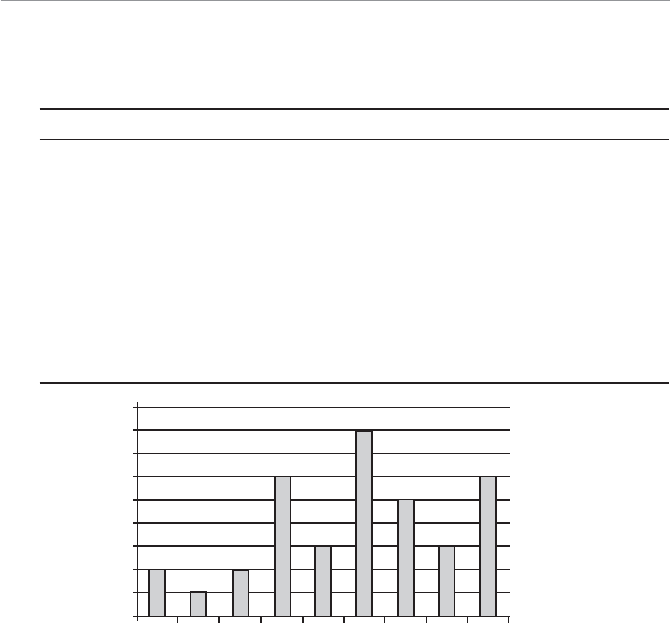
A]ZcbW]\ab]¿G]c`Bc`\À !!#
1VO^bS`!
1.
Exam Grade Number of Students
56–60 2
61–65 1
66–70 2
71–75 6
76–80 3
81–85 8
86–90 5
91–95 3
96–100 6
2.
Histogram for Exam Grades
56-60
0
1
2
3
4
5
6
7
8
9
61-65 66-70 71-75 76-80 81-85 86-90 91-95 96-100
Number of Students
Exam Scores
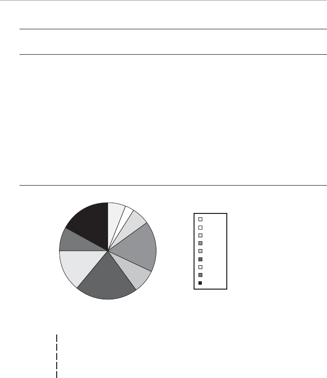
/^^S\RWf/
!!$
3.
Number of Cumulative
Exam Grade Students Percentage Percentage
56–60 2 2/36 = .06 .06
61–65 1 1/36 = .03 .09
66–70 2 2/36 = .06 .15
71–75 6 6/36 = .17 .32
76–80 3 3/36 = .08 .40
81–85 8 8/36 = .22 .62
86–90 5 5/36 = .14 .76
91–95 3 3/36 = .08 .84
96–100 6 6/36 = .16 1.00
Total = 36
4. 6% 3%
6%
17%
8%
21%
14%
8%
17%
56-60
61-65
66-70
71-75
76-80
81-85
86-90
91-95
96-100
Pie Chart for Exam Grades
5. 5
6
7
8
9
8
0268
222455899
1123455566689
125688999
Stem and Leaf for Problem 5

A]ZcbW]\ab]¿G]c`Bc`\À !!%
6. 5 (5)
6 (0)
6 (5)
7 (0)
7 (5)
8 (0)
8 (5)
9 (0)
9 (5)
8
02
68
2224
55899
11234
55566689
12
5688999
Stem and Leaf for Problem 6
1VO^bS`"
1. Mean = 15.9, Median = 17, Mode = 24
2. Mean = 81.7, Median = 82, Mode = 82
3. Mean = 32.7, Median = 32.5, Mode = 36 and 27
4. Mean = 7.2, Median = 6, Mode = 6
5. x
2282737322537484227
47 10
83725482710 34 5. years
6. x
3 118 2 125 1 107
321 118 5.
7. x
51 72 103 84 125 36
57108123 35. years
1VO^bS`#
1.
xix2
20 400
15 225
24 576
10 100
8 64
19 361
24 576
xi
i
n
¤
1
= 120 xi
i
n2
1
¤ = 2,302

/^^S\RWf/
!!&
xi
i
n
¤
¥
§
¦´
¶
µ
1
2
2
120 14 400() , ,s
x
x
n
n
i
i
ni
i
n
2
2
1
1
2
1
2 302 14 400
¥
§
¦´
¶
µ
¤¤
-
,,
77
640 8.,
s40 8 6 4.., Range = 24 – 8 = 16
2.
xix2
84 7,056
82 6,724
90 8,100
77 5,929
75 5,625
77 5,929
82 6,724
86 7,396
82 6,724
xi
i
n
¤
1
= 735 xi
i
n2
1
¤= 60,207
xi
i
n
¤
¥
§
¦´
¶
µ
1
2
2
735 540 225() ,,
S
2
2
1
1
2
60 207 540 225
¥
§
¦´
¶
µ
¤¤
x
x
N
N
i
i
Ni
i
N
,,
99
920 2.
S
20 2 4 5.., Range = 90 – 75 = 15
3. Range = 25, Variance = 75.4, Standard Deviation = 8.7
4.25666 8 10 11 11 15
Q
1 = 5.5 Q2 = 7 Q3 = 11
Note the median of the data set is underlined.

A]ZcbW]\ab]¿G]c`Bc`\À !!'
5.
x
fx
f
ii
i
m
i
i
m
¤
¤
1
1
822 3727 25
32 48 37 27 42 10 47
8372548
27 10 34 5.
xifix(
)
xx
i()xx
i2()xxf
ii
2
22 8 34.5 -12.5 156.25 1,250.00
27 37 34.5 -7.5 56.25 2,081.25
32 25 34.5 -2.5 6.25 156.25
37 48 34.5 2.5 6.25 300.00
42 27 34.5 7.5 56.25 1,518.75
47 10 34.5 12.5 156.25 1,562.50
nf
i
i
m
¤155
1
() ,.xxf
ii
i
m
¤2
1
6 868 75
s
xxf
n
ii
i
m
¤() ,. ..
2
1
1
6 868 75
155 1 44 60 6 688 years
6.
x
fx
f
ii
i
m
i
i
m
¤
¤
1
1
51 72 103
84 125 36
57108123 35.
xifix(
)
xx
i()xx
i2()xxf
ii
2
1 5 3.5 -2.5 6.25 31.25
2 7 3.5 -1.5 2.25 15.75
3 10 3.5 -0.5 0.25 2.50
4 8 3.5 0.5 0.25 2.00
5 12 3.5 1.5 2.25 27.00
6 3 3.5 2.5 6.25 18.75
nf
i
i
m
¤45
1
() .xxf
ii
i
m
¤2
1
97 25
/^^S\RWf/
!"
s
xxf
n
ii
i
m
¤() ...
2
1
1
97 25
45 1 221 14
9
years
7. Using the empirical rule, 95 percent of the values will fall within k = 2 standard
deviations from the mean.
R = kX = 75 + 2(10) = 95, R = kX = 75 – 2(10) = 55
Therefore, 95 percent of the data values should fall between 55 and 95.
8. The values 38 and 62 are two standard deviations from the mean of 50. This can
be shown with the following:
R + kX = 62, R + kX = 38
k
62 62 50
620
M
S
.,k
¥
§
¦´
¶
µ
¥
§
¦´
¶
µ
38 38 50
620
M
S
.
Using Chebyshev’s theorem, at least 11100
2
¥
§
¦´
¶
µs
k% = 11
2100
2
¥
§
¦´
¶
µs% = 75
percent of the data values will fall between 38 and 62.
1VO^bS`$
1a. Empirical, because we have historical data for Derek Jeter’s batting average.
1b. Classical, because we know the number of cards and the number of aces in the
deck.
1c. If I have data from my last several rounds of golf, this would be empirical, other-
wise subjective.
1d. Classical, because we can calculate the probability based on the lottery rules.
1e. Subjective, because I would not be collecting data for this experiment.
1f. Subjective, because I would not be collecting data for this experiment.
2a. Yes.

A]ZcbW]\ab]¿G]c`Bc`\À !"
2b. No, probability cannot be greater than 1.
2c. No, probability cannot be greater than 100 percent.
2d. No, probability cannot be less than 1.
2e. Yes.
2f. Yes.
3a. P[A]
52
125 042.
3b. P[B]
41
125 033.
3c. P[A and B] P[A B].
23
125 018
3d. The following table identifies the total number of families for the union of
Events A and B.
Race Internet Number of Families
Asian American Yes 23
Asian American No 18
Caucasian Yes 15
African American Yes 14
Total = 70
P[A or B] P[B A].
70
125 056
4a. P[A and B] P[A B].
10
50 020
4b. The following table identifies the total number of phone calls for the union of
Events A and B.
Child Type of Call Number of Calls
Christin Noncrisis 6
Brian Noncrisis 4
Brian Crisis 10
John Noncrisis 12
Total = 32
P[A or B] P[B A].
32
50 064

/^^S\RWf/
!"
1VO^bS`%
1. P[A]
177
260 068.
2. P[B]
152
260 058.
3. P[A’]
83
260 032.
4. P[B’]
108
260 042.
5. P[A/B]
98
152 064.
6. P[A /B]’.
54
152 036
7. P[A/B’]
79
108 073.
8. P[A and B] P[A/B]P[B]
064 058 037.. .
9. P[A and B’] P[A/B’]P[B’]
073 042 031.. .
10. P[A or B] P[A] P[B] P[A and B]068 058 0...337 0 89.
11. P[A or B’] P[A]+P[B’] P[A and B’]
068 042..031 079..
12. P[B/A] P[B]P[A/B]
(P[B]P[A/B]) (P[B’]P[A/B’]
))
P[B/A]
058 064
058 064 042 073
..
..)..
037
037 031 054
.
...
1VO^bS`&
1. 3 x 8 x 4 x 3 = 288 different meals
2. There are 4 x 4 x 4 x 4 x 4 x 4 x 4 x 4 x 4 x 4 = 1,048,576 different ways to
answer the exam. If only one of these sequences is correct, the probability
is 1/1048576 = 0.00000095 that the student will correctly guess the correct
sequence.
3. 13! = 6,227,020,800 different ordered arrangements

A]ZcbW]\ab]¿G]c`Bc`\À !"!
4. 83 8
83 8 7 6 336P
!
()!
5. 10 2 10
10 2 10 9 90P
!
()!
6. 40 3 40
40 3 40 39 38 59 280P
!
()! ,
7. 12 3 12
12 3 3
12 11 10
321 220C
!
()!!
8. 50 12 50
50 12 12
50 49 48 47 46 45 44 4
C!
()!!
3342414039
121110987654321 12
11 399 651 100,,,
9.
Number of Number of Probability
Cats Families xiP[xi]xi2xi2P[xi]
0 137 137/450 = 0.304 0 0
1 160 160/450 = 0.356 1 0.356
2 112 112/450 = 0.249 4 0.996
3 31 31/450 = 0.069 9 0.621
4 10 10/450 = 0.022 16 0.352
Total xx
i
i
n
i
2
1
¤P[ ] = 2.325
M
¤xx
i
i
n
i
P
1
0 0 304 1 0 356 2 0 2[] . . .449 3 0 069 4 0 022 1 149
...
SM
22
1
22
2 325 1 149 1¥
§
¦´
¶
µ
¤xx
i
i
n
i
P[ ] . ( . ) .0005
SS
21 005 1 002..
10. The number of three-of-a-kind combinations is (13)4C3 = 52. The number
of remaining pairs is (12)4C2 = 72. The total number of full house hands is
(52)(72) = 3,744. P[Full House]
3 744
2 598 960 0 00144
,
,, .

/^^S\RWf/
!""
1VO^bS`'
1. Because n = 10, r = 7, p= 0.5
P[ , ] !
()!!
..710 10
10 7 7 05 05 10 9 8
7107
77654
7654321 0 0078 0 125
¥
§
¦´
¶
µ
..00 117.
2. Because n = 6, r = 3, p= 0.75
P[ , ] !
()!!
..36 6
633075 025 654
32
363
11 0 4219 0 0156 0 1316
¥
§
¦´
¶
µ
.. .
3. The probability of making at least 6 of 8 is P[6,8] + P[7,8] + P[8,8]. Because
n = 8, p= 0.8
P[ , ] !
()!!
..68 8
86608 02 87
21
686
¥
§
¦´
¶
µµ
0 2621 0 04 0 2936...
P[ , ] !
()!!
.. .78 8
8770 8 0 2 8 0 2097
787
00 2 0 3355..
P[ , ] !
()!!
.. .88 8
8880 8 0 2 1 0 1678
888
11 0 1678
.
Therefore, the probability of making at least 6 out of 8 is 0.2936 + 0.3355 +
0.1678 = 0.7969.
4. Because n = 12, r = 6, p= 0.2
P[ , ] !
()!!
..612 12
12 6 6 02 08 12 11 1
6126
00987
654321 0 000064 0 2621
¥
§
¦´
¶
µ
.. 0 0155.
5. The probability of no more than 2 out of the next 7 is P[0,7] + P[1,7] + P[2,7].
Because n = 7, p = 0.05
P[ , ] !
()!!
.. .07 7
700005 095 1 1 00
070
44 0 6983
.
P[ , ] !
()!!
.. .17 7
7110 05 0 95 7 0 05
171
00 7351 0 2573..
P[ , ] !
()!!
..27 7
722
005 095 76
21
272
¥
§
¦
´´
¶
µ
0 0025 0 7738..
Therefore, the probability that no more than two of the next seven people will
purchase is 0.6983 + 0.2573 + 0.0406 = 0.9962.

A]ZcbW]\ab]¿G]c`Bc`\À !"#
6. Since n = 4, p = 0.335
P[ , ] !
()!!
..04 4
4000 335 0 665 1 1 0
040
...196 0 196
P[ , ] !
()!!
.. .14 4
4110 335 0 665 4 0 33
141
55 0 294 0 394
..
P[ , ] !
()!!
.. .24 4
422
0 335 0 665 6 0 11
242
22 0 442 0 297
..
P[ , ] !
()!!
.. .34 4
433
0 335 0 665 4 0 03
343
88 0 665 0 101
..
P[ , ] !
()!!
.. .44 4
4440 335 0 665 1 0 01
444
33 1 0 013
.
7. P[ , ] !
!! ..410 10
10 4 4 06 04 10 9 8
4104
77
4321 0 1296 0 004096 0 1115
¥
§
¦´
¶
µ
.. .
1VO^bS`
1. P[ ] .
!
..4 6 2 71838
4
1296 002479
24 0
46
11339
2. P[ ] ..
!
..
.
57 5 2 71838
5
23730 469 0 000
575
55531
120 0 1094
.
3. PP PPP[] [] [][][]xx xxx b
21 21 0 1 2
P[ ] ..
!
..
.
04 2 2 71838
0
1 0150
1015
042
00
P[ ] ..
!
.. .
.
14 2 2 71838
1
4 2 0150
10
142
6630
P[ ] ..
!
..
.
24 2 2 71838
2
17 64 0150
2
242
00 1323.
P[]... .x
2 1 0 0150 0 0630 0 1323 0 7897
4. PPPPP[][ ][][][]xxxxxb
3 0123
P[ ] ..
!
..
.
03 6 2 71838
0
1 027324
10
036
00273

/^^S\RWf/
!"$
P[ ] ..
!
..
.
13 6 2 71838
1
3 6 027324
1
136
00 0984.
P[ ] ..
!
..
.
23 6 2 71838
2
12 96 027324
236
22 0 1771.
P[ ] ..
!
..
.
33 6 2 71838
3
46 656 027324
336
60 2125.
P[ ] . . . . .xb
3 0 0273 0 0984 0 1771 0 2125 0 5152
5. P[ ] ..
!
..
.
12 5 2 71838
1
2 5 082085
1
125
00 2052.
6. P[ ] !
xnp e
x
xnp
,np np 25 0 05 1 25,., .
P[ ] .
!
..
.
2125
2
1 5625 0 286505
2
2125
e 0 2238.
7. P[ ] ..
!
..
.
02 5 2 71838
0
1 082085
10
025
00821
1VO^bS`
1a. z65 5
65 5 62 6
37 078
.
..
.. ,PP[.
] [.] . .zz b 0 78 1 0 78 1 0 7834 0 2166
1b. z58 1
58 1 62 6
37 122
.
..
.. ,PP[.
][.].zz b 1 22 1 22 0 8880
1c. z70
70 62 6
37 20
.
..,z61
61 62 6
37 043
.
..,
PPP[. .
] [ .] [ .] b b b b043 20 20 043zzz,
P[ . . ] . . .b
b 043 2 0 0 9772 0 3327 0 6445z
2a. z190
190 176
22 3 063
..,P[ . ] .zb 063 0 7349
2b. z158
158 176
22 3 081
..,PP[.
] [.].zzb b 0 81 1 0 81 0 2098

A]ZcbW]\ab]¿G]c`Bc`\À !"%
2c. z168
168 176
22 3 036
..,z150
150 176
22 3 117
..
PPP[. .] [ .] [ .] b b b b117 036 036 117zzz
PP[.
] [.].zzb b 0 36 1 0 36 0 3599 ,PP[.] [.].zzb b 1 17 1 1 17 0 1218
P[ . . ] . . .b
b 117 0 36 0 3599 0 1218 0 2381z
3a. z31
31 37 5
76 086
.
..,PP[.
][.].zz b 0 86 0 86 0 8038
3b. z42
42 37 5
76 059
.
..,P[ . ] .zb 059 0 7231
3c. z45
45 37 5
76 099
.
..,z40
40 37 5
76 033
.
..
PPP[. .] [ .] [ .] .b b b b 099 033 099 033 083zzz 881 0 6289 0 2092..
4. For this problem, n = 14, p = 0.5, and q = 0.5. We can use the normal approxi-
mation since np = nq = (14)(0.5) = 7. The binomial probabilities from the
binomial table are P[r = 4, 5, or 6] = 0.0611 + 0.1222 + 0.1833 = 0.3666. Also,
M
np 14 0 5 7. and
S
npq 14 05 05 1871.. .. The normal
approximation would be finding P[ . . ]35 65bbx.
z65
65 7
1 871 027
.
.
.. ,z35
35 7
1 871 187
.
.
..
PPP[. .] [ .] [ .]b b b b187 027 027 187zzz
PP[.
] [.].zzb b 0 27 1 0 27 0 3946 ,PP[.] [.].zzb b 1 87 1 1 87 0 0307
P[ . . ] . . .b
b 187 0 27 0 3946 0 0307 0 3639z
5a. z97
97 92
4125 .,PP[.
] [.]. .zz b 1 25 1 1 25 1 0 8944 0 1056
5b. z90
90 92
4050 .,PP[.
][.].zz b 0 50 0 50 0 6915
6a. z4000
4000 4580
550 105 .,z5000
5000 4580
550 076 .
PPP[. .] [ .] [ .] b b b b105 076 076 105zzz

/^^S\RWf/
!"&
P[ . ] .zb 0 76 0 7764 ,PP[.] [.] . .
zz
b b 1 05 1 1 05 1 0 8531 0 1469
P[ . . ] . . .bb 1 05 0 76 0 7764 0 1469 0 6295z
6b. z4200
4200 4580
550 069 .,PP[.
] [.].zzb b 0 69 1 0 69 0 2451
1VO^bS`
1. kN
n
75000
500 150
2. If every employee belonged to a particular department, certain departments
could be chosen for the survey, with every individual in those departments asked
to participate. Other answers are also possible.
3. If each employee can be classified as either a manager or a nonmanager, ensure
that the sample proportion for each type is similar to the proportion of managers
and nonmanagers in the company. Other answers are also possible.
1VO^bS`!
1a.
SS
xn
10
15 258.
1b.
SS
xn
47
12 136
..
1c.
SS
xn
7
20 157.
2a.
SS
xn
75
925
..,z17
17 16
25 040
..,P[ . ] .zb 040 0 6554
2b. z18
18 16
25 080
..,P[ . ] [ . ] . .zP
z b 0 80 1 0 80 1 0 7881 0 2119
2c. z14 5
14 5 16
25 060
.
.
.. ,z16 5
16 5 16
25 020
.
.
..
P[ . ] .zb 020 0 5793 ,PP[.] [.].zzb b 0 60 1 0 60 0 2743
PP14 5 16 5 0 60 0 20 0 5793 0 2.. ....bb
¨
ª·
¹ bb
;=
xz 7743 0 3050.

A]ZcbW]\ab]¿G]c`Bc`\À !"'
3a.
S
p
pp
n
1 0 25 1 0 25
200 0 0306
..
.
3b.
S
p
pp
n
1 0 42 1 0 42
100 0 0494
..
.
3c.
S
p
pp
n
1 0 06 1 0 06
175 0 0179
..
.
4a.
S
p
pp
n
1 0 32 1 0 32
160 0 0369
..
.,
z030
030 032
0 0369 054
.
..
..
PP[.] [.].zzb b 0 54 1 0 54 0 2946
4b. z036
036 032
0 0369 108
.
..
.. ,PP[.
] [.] . .zz b 1 08 1 1 08 1 0 8599 0 1401
4c. z029
029 032
0 0369 081
.
..
.. ,z037
037 032
0 0369 136
.
..
..
P[ . ] .zb 136 0 9131 ,PP[.] [.].zzb b 0 81 1 0 81 0 2090
PP..
.
..029 0 37 0 81 1 36 0 9131 0bb
¨
ª·
¹ bb
;=
pz
s...2090 0 7041
5.
S
p
pp
n
104104
60 0 063
..
.,z05
05 04
0 063 151
.
..
..
PP[.] [.].zz b 1 51 1 1 51 0 0655
1VO^bS`"
1.
SS
xn
76
40 120
..,zc217.
Upper Limit = xz
cx
S
31 3 2 17 1 20 33 90... .
Lower Limit = xz
cx
S
31 3 2 17 1 20 28 70... .
2. nz
E
¥
§
¦´
¶
µ
¥
§
¦´
¶
µz
S
22
233 15
548 9 49
..
3. This is a trick question! The sample size is too small to be used from a popula-
tion that is not normally distributed. This question goes beyond the scope of this
book. You would need to consult a statistician.
/^^S\RWf/
!#
4. Using Excel, we can calculate x13 9. and
s604.
.
ˆ..
S
x
s
n
604
30 110
Upper Limit = xz
cx
ˆ... .
S
13 9 1 64 1 10 15 70
Lower Limit = xz
cx
ˆ... .
S
13 9 1 64 1 10 12 10
5. Using Excel, we can calculate x46 92..
S
12 7.,zc188., and
SS
xn
12 7
12 367
..
Upper Limit = xz
cx
S
46 92 1 88 3 67 53 82... .
Lower Limit = xz
cx
S
46 92 1 88 3 67 40 02... .
6. Using Excel, we can calculate x119 64.,s11 29.,ˆ..
S
x
s
n
11 29
11 340.
For a 98 percent confidence interval with n 11
1110 degrees of freedom,
tc2 764..
Upper Limit = xt
cx
ˆ... .
S
119 64 2 764 3 40 129 04
Lower Limit = xt
cx
ˆ... .
S
119 64 2 764 3 40 110 24
7. This is another trick question! The sample size is too small to be used from a
population that is not normally distributed. This question goes beyond the scope
of this book. You would need to consult a statistician.
8. ps
11
200 0 055.. Since nps
200 0 055 11. and nqs
200 0 945 189.,
we can use the normal approximation.
ˆ.. .
S
p
ss
pp
n
10 055 0 945
200 0 0161 ,
zc196.
Upper Limit = pz
scp
S
0 055 1 96 0 0161 0 087... .
Lower Limit = pz
scp
S
0 055 1 96 0 0161 0 023... .
9. npq
z
E
c
¥
§
¦´
¶
µ
¥
§
¦´
¶
µ
22
055 045 205
004
.. .
.6650
A]ZcbW]\ab]¿G]c`Bc`\À !#
1VO^bS`#
1. H017:.
M
,H117:.
M
x
n = 35,
S
05. cups,
SS
xn
050
35 0 0845
.. cups, zcp164.
Upper limit =
MS
Hc
x
z
01 7 1 64 0 0845 1 84
.. . . cups
Lower limit =
MS
Hc
x
z
01 7 1 64 0 0845 1 56
.. . . cups
Since x195. cups, we reject H0 and conclude that the population mean is not
1.7 cups per day.
2. H040:
M
r,H140:
M
,n50 ,
S
12 5. years,
SS
xn
12 5
50 1 768
.. years,
zc164.
Lower limit =
MS
Hc
x
z
040 1 64 1 768 37 1
.. . years
Since x38 7. years, we do not reject H0 and conclude that we do not have
enough evidence to support the claim that the average age is less than 40 years
old.
3. H01000:
M
b,H11000:
M
,n32 ,
S
325
hours,
SS
xn
325
32 57 45. hours, zc205.
Upper limit =
MS
Hc
x
z
01000 2 05 57 45 1117 8
.. . hours
Since x1190 hours, we reject H0 and conclude the average light bulb life
exceeds 1000 hours.
4. H030:
M
r,H130:
M
,n42,
S
80. minutes,
SS
xn
80
42 123
..
minutes, zc233.
Lower limit =
MS
Hc
x
z
030 2 33 1 23 27 13
.. . minutes
Since x26 9. minutes, we reject
H0
and conclude that the average delivery
time is less than 30 minutes.
5. H02700:$
M
,H12700:$
M
x,n40 ,
S
$950
,
SS
xn
$$.
950
40 150 20 ,
zcp196.
Upper limit =
MS
Hc
x
z
02700 1 96 150 20 2994
..$
Lower limit =
MS
Hc
x
z
02700 1 96 150 20 2406
..$
Since x$2450 , we do not reject
H0
and conclude that we do not have enough
evidence to contradict the claim that the average college student has $2,700 in
credit card debt.

/^^S\RWf/
!#
1VO^bS`$
1. H01100:
M
,H11100:
M
x,n70 ,
S
310
,
SS
xn
310
70 37 05.
zcp164.,zxH
x
M
S
01035 1100
37 05 175
..,
p-value = 2 1 75 2 1 1 75 2 1 0 95
b
b
PP[.] [.] .zz 999 0 0802
.,
Since p-value b
A
, we reject H0 and conclude that the average SAT score does
not equal 1100.
2. H035:M ,H135:Mx ,x37 9.,s67
4.,n10,df n..19
,
ˆ..
S
x
s
n
674
10 213
,tcp2 821.,txH
x
M
S
037 9 35
213 136
ˆ
.
..
Since tt
c
b, we do not reject H0 and conclude that the average class size equals
35 students.
3. H07: Mb ,H17: M ,x82.,s429.,
n30
,
S
x
s
n
429
30 078
..,
zc164.,zxH
x
M
S
082 7
078 154
ˆ
.
..
p-value = PP[.
] [.] . .zz b 1 54 1 1 54 1 0 9382 0 0618
Since zz
c
b or p-value
A
, we do not reject H0 and conclude that average
gasoline consumption in the U.S. does not exceed seven liters per car per day.
4. Hp
0040:.r,Hp
1040:.,
S
p
HH
pp
n
00
1040 1 040
175 0 037
..
.,
zpp
H
p
0030 040
0 037 270
S
..
..
p-value = PP[.
] [.]. .zzb b 2 70 1 2 70 1 0 9965 0 0035,zc233.
Since p-value b
A
, we reject H0 and conclude that the proportion of
Republicans is less than 40 percent.

A]ZcbW]\ab]¿G]c`Bc`\À !#!
5. Hp
0065:.,Hp
1065:.x,
S
p
HH
pp
n
00
1065 1 065
225 0 032
..
.,
zpp
H
p
069
0069 065
0 032 125
.
..
..
S
.
p-value = 2 1 25 2 1 1 25 2 1 0 8944
b
PP[.] [.] .zz
0 2122.,
Since p-value r
A
, we fail to reject
H0
and conclude that the proportion of teen-
agers who exceed their minutes equals 65 percent.
6. H015:
M
r,H115:
M
,n60 ,
S
5,
SS
xn
5
60 0 645.
zxH
x
M
S
013 5 15
0 645 233
.
...
p-value = PP[.
] [.] . .zzb
b
233 1 233 1 099 0010,
Since p-value b
A
, we reject H0 and conclude that the average number of hours
worked is less than 15.
1VO^bS`%
1. H01 2
:
MM
,H11 2
:
MM
x, PA = 1, Ohio = 2
SSS
xx nn
12
1
2
1
2
2
2
22
105
45
114
38 24 22
.,
zcp196.
zxx H
xx
12 12
0
12
552 530 0
24 22
MM
S
.091.
Since zz
c
b, we do not reject H0 and conclude there is not enough evidence to
support a difference between the two states.
p-value = 2 0 91 2 1 0 91 2 1 0 8186
b
PP[.] [.] .zz 0 3628.
2. H01 2
:
MM
,H11 2
:
MM
x,x188 3.,s1730.,x282 4.,s2674.,
snsns
nn
p
11
2
22
2
12
2
11
2
10 7 30 9.
674
11 10 2 704
2
..

/^^S\RWf/
!#"
ˆ...
S
xx p
snn
12
11 704 1
11
1
10 7 04 0 190
12
99308.
txx H
xx
12 12
0
12
88 3 82 4 0
30
MM
S
ˆ
..
.88 192 .
df n n..
12
21110219,tcp1 729.
Since tt
c
, we reject H0 and conclude the satisfaction scores are not equal
between the two stores.
3. Hd015:
M
b,Hd115:
M
,d
¤21 23 11 19 15 20 17 23 17 166
d2441 529 121 361 225 400 289 529 289 318
¤44
dd
n
¤166
918 44.,
s
dd
n
n
d
¤¤
2
22
1
3184 166
9
8
122 22
83
..991
td
s
n
d
d
M
18 44 15
391
9
344
130 264
.
.
.
..,df n..1918
,tc1 860.
Since tt
c
, we reject H0 and conclude the weight loss program claim is valid.
4. Hp p
01 2
:b,Hp p
11 2
:, Pop 1 = Florida, Pop 2 = Nation
px
n
1
1
1
272
400 068 .,px
n
2
2
2
390
600 065 .,ˆ.pxx
nn
12
12
272 390
400 600 0 662
ˆˆˆ ..
S
pp pp
nn
12 111 0 662 1 0
12
¥
§
¦´
¶
µ
6662 1
400
1
600 0 0305
¥
§
¦´
¶
µ.
zpp pp
H
pp
12 12
0
12
068 065 0
00
ˆ
..
.
S
3305 098 .,
zc233.
Since zz
c
b, we do not reject H0 and conclude there is not enough evidence to
support the claim that the proportion of home ownership in Florida is greater
than the national proportion.
p-value = PP[.
] [.] . .zz b
0 98 1 0 98 1 0 8365 0 1635

A]ZcbW]\ab]¿G]c`Bc`\À !##
5.
H01 2
:
MM
b
,H11 2
:
MM
, Pop 1 = City A, Pop 2 = City B.
ˆˆˆ ..
SSS
xx nn
12
1
2
1
2
2
2
22
225
60
270
80 0
..419
zxx H
xx
12 12
0
12
980 910 0
04
MM
S
ˆ
..
.119 167 .
p-value = PP[.
] [.] . .zz b
1 67 1 1 67 1 0 9525 0 475
Since p-value b
A
, we reject H0 and conclude that the average wage in City A is
higher than City B.
6.
H01 2
:
MM
,H11 2
:
MM
x,x114 58.,s1709.,
x217 45.
,s2826.
ˆˆˆ ..
SSS
xx nn
12
1
2
1
2
2
2
22
709
12
826
11 3
..224 ,
s
n
1
2
1
2
709
12 419
..,s
n
2
2
2
2
826
11 620
..
df
s
n
s
n
s
n
n
s
..
¥
§
¦´
¶
µ
¥
§
¦´
¶
µ
1
2
1
2
2
2
2
1
2
1
2
1
2
2
1
nn
n
2
2
2
2
2
1
419 620
419
12 1
620
¥
§
¦´
¶
µ
..
..
z
2
11 1
107 98
5 447 20
.
.
txx H
xx
12 12
0
12
14 58 17 45 0
3
MM
S
ˆ
..
.. .
224 0 890 ,tc1 725.
Since tt
c
b, we fail to reject H0 and conclude that the number of days that a
home is on the market in City A does not differ from City B.

/^^S\RWf/
!#$
1VO^bS`&
1. H0: The arrival process can be described by the expected distribution
H1: The arrival process differs from the expected distribution
Day Expected Sample Expected Observed
Percentage Size Frequency (E) Frequency (O)
Mon 10% 215 0.10(215) = 21.5 31
Tues 10% 215 0.10(215) = 21.5 18
Wed 15% 215 0.15(215) = 32.25 36
Thurs 15% 215 0.15(215) = 32.25 23
Fri 20% 215 0.20(215) = 43 47
Sat 30% 215 0.30(215) = 64.5 60
Total 100% 215 215
OE
E
2
Day OE (O–E)(O–E)2
Mon 31 21.50 9.50 90.25 4.20
Tues 18 21.50 -3.50 12.25 0.57
Wed 36 32.25 3.75 14.06 0.44
Thurs 23 32.25 -9.25 85.56 2.65
Fri 47 43.00 4.00 16.00 0.37
Sat 60 64.50 -4.50 20.25 0.31
Total
C
2
2
854
¤OE
E.
For
A
005. and d.f. =k – 1 = 6 – 1 = 5,
C
c
211 070.. Since
CC
c
22
, we do
not reject H0 and conclude that the arrival distribution is consistent with the
expected distribution.
2. H0: The process can be described with the Poisson distribution using
L
3
.
H1: The process differs from the Poisson distribution using
L
3.

A]ZcbW]\ab]¿G]c`Bc`\À !#%
Number of Hits Poisson Number of Expected
Per Minute Probabilities Hits Frequency
0 0.0498 x380 = 18.92
1 0.1494 x380 = 56.77
2 0.2240 x380 = 85.12
3 0.2240 x380 = 85.12
4 0.1680 x380 = 63.84
5 0.1008 x380 = 38.30
6 0.0504 x380 = 19.15
7 or more 0.0336 x380 = 12.77
Total 1.0000 380.00
Hits OE
E
2
per Min OE(O–E)(O–E)2
0 22 18.92 3.08 9.46 0.50
1 51 56.77 -5.77 33.32 0.59
2 72 85.12 -13.12 172.13 2.02
3 92 85.12 6.88 47.33 0.56
4 60 63.84 -3.84 14.75 0.23
5 44 38.30 5.70 32.44 0.84
6 25 19.15 5.85 34.19 1.79
7 or more 14 12.77 1.23 1.52 0.12
Total
C
2
2
665
¤OE
E.
For
A
001. and d.f. = l – 1 = 8 – 1 = 7,
C
c
218 475.. Since
CC
c
22
, we do not
reject H0 and conclude that the process is consistent with the Poisson distribu-
tion using
L
3.
3. H0: Grades are independent of reading time
H1: Grades are dependent of reading time

/^^S\RWf/
!#&
Sample expected frequency calculations:
E11
265 95
500 50 35
,.
E12
265 128
500 67 84
,.
E13
265 155
500 82 15
,.
OE
E
2
Row Column OE (O–E)(O–E)2
1 1 36 50.35 -14.35 205.92 4.09
1 2 75 67.84 7.16 51.27 0.76
1 3 81 82.15 -1.15 1.32 0.02
1 4 63 49.82 13.18 173.71 3.49
1 5 10 14.84 -4.84 23.43 1.58
2 1 27 26.60 0.40 0.16 0.01
2 2 28 35.84 -7.84 61.47 1.72
2 3 50 43.40 6.60 43.56 1.00
2 4 25 26.32 -1.32 1.74 0.07
2 5 10 7.84 2.16 4.67 0.60
3 1 32 18.05 13.95 194.60 10.78
3 2 25 24.32 0.68 0.46 0.02
3 3 24 29.45 -5.45 29.70 1.01
3 4 6 17.86 -11.96 140.66 7.88
3 5 8 5.32 2.68 7.18 1.35
Total
C
2
2
34 38
¤OE
E.
For
A
005. and d.f. = (r – 1)(c – 1) = (3 – 1)(5 – 1) = 8,
C
c
215 507.. Since
CC
22
c, we reject H0 and conclude that there is a relationship between grades
and the number of hours reading.
4. H0: The process can be described with the Binomial distribution using p = 0.4.
H1: The process differs from the Binomial distribution using p = 0.4.

A]ZcbW]\ab]¿G]c`Bc`\À !#'
Number of Visits Binomial Sample Expected
Per Day Probabilities Size Frequency
0 0.0778 x140 = 10.9
1 0.2592 x140 = 36.3
2 0.3456 x140 = 48.4
3 0.2304 x140 = 32.3
4 0.0768 x140 = 10.8
5 0.0102 x140 = 1.4
Total 1.0000 140
Number OE
E
2
of Visits OE (O–E)(O–E)2
0 10 10.9 -0.9 0.8 0.07
1 41 36.3 4.7 22.2 0.61
2 60 48.4 11.6 134.9 2.79
3 20 32.3 -12.3 150.2 4.66
4 6 10.8 -4.8 22.6 2.10
5 3 1.4 1.6 2.5 1.73
Total
C
2
2
11 96
¤OE
E.
For
A
005. and d.f. = k – 1 = 6 – 1 = 5,
C
c
211 070.
. Since
CC
c
22
, we reject
H0 and conclude that the process differs from the Binomial distribution using
p = 0.4.
1VO^bS`'
1. H01 2 3
:
MMM
x122 12.x219 67.
x318 94.
H1: not all 's are equal
M
s1
2098.s2
2145.s3
2236.
N = 17 n16n26n35
SSW n s
ii
i
k
¤1610986114551
2
1
..
236 2159..
xx
N
¤22 5 20 8 22 0 23 6 18 0 21 1 19..........88186
17 20 32
..

/^^S\RWf/
!$
SSB n x x
ii
i
k
¤2
1
2
6 2212 2032 6 1967.. .22032 5 1894 2032 3150
22
....
MSB SSB
k
1
31 50
31 15 75
..,MSW SSW
Nk
21 59
17 3 154
..
FMSB
MSW
15 75
154 10 23
.
..,FF F
ckNk
A
,, .,, .
105214
3 739 ,
Since FF
c
, we reject H0 and conclude that there is a difference between the
sample means.
2. For x1 and x2,Fxx
SSW
nnn
S
ab
i
i
k
ab
¨
ª
©·
¹
¸
¤
2
1
1
11
22 1.221967
21 59
554
1
6
1
6
11 70
2
¨
ª
©·
¹
¸
.
..
For x1 and x3,Fxx
SSW
nnn
S
ab
i
i
k
ab
¨
ª
©·
¹
¸
¤
2
1
1
11
22 1.221894
21 59
554
1
6
1
5
17 88
2
¨
ª
©·
¹
¸
.
..
For x2 and x3,Fxx
SSW
nnn
S
ab
i
i
k
ab
¨
ª
©·
¹
¸
¤
2
1
1
11
19 6.771894
21 59
554
1
6
1
5
094
2
¨
ª
©·
¹
¸
.
..
FkF
SC k N k
1 3 1 3 739 7 478
1
A
,, ..
Sample Pair FSFSC Conclusion
x1 and x211.70 7.478 Difference
x1 and x317.88 7.478 Difference
x2 and x3 0.94 7.478 No Difference
We conclude that there is a difference between gas mileage of Cars 1 and 2 and
Cars 1 and 3.

A]ZcbW]\ab]¿G]c`Bc`\À !$
3. H01 2 3
:
MMM
x138 33.
x228 29.
x328 0.x431 43.
H1:’not all s are equal
M
s1
2115 47.
s2
272 57.
s3
286 8.s4
2132 62.
N26
n16n27n36n47
SSW
6 1 115 47 7 1 72 57 6 1 86 8 7 1 1...332 62 2242 49..
xx
N
¤36 48 32 28 36 18 30 21
26 31 38
... .
SSB
6 38 33 31 38 7 28 29 31 38 6 28 31
22
.. .. .....38 7 31 43 31 38 425 22
22
MSB SSB
k
1
425 22
41 141 74
..,MSW SSW
Nk
2242 49
26 4 101 93
..
FMSB
MSW
141 74
101 93 1 391
.
..,FF F
ckNk
A
,, .,, .
1 05322 3 049
Since FF
c
b, we do not reject H0 and conclude that there is no difference
between the sample means.
4. H01 2 3
:
MMM
Pop 1 = Dad,
x192 5.
,n14
H1:’not all s are equal
M
Pop 2 = Brian, x283 5.,n24
N12, k = 3, b = 4, Pop 3 = John,
x383 5.
,n34
H
H
0
1
'
'
:
:
the block means are all equal
the bloock means are not all equal
xx
N
¤93 98 89 90 80 88 84 82
12 86 5
... .
xij xxx
ij
xx
ij
2
93 86.5 6.5 42.25
98 86.5 11.5 132.25
89 86.5 2.5 6.25
90 86.5 3.5 12.25
85 86.5 -1.5 2.25
continues

/^^S\RWf/
!$
xij xxx
ij
xx
ij
2
87 86.5 0.5 0.25
82 86.5 -4.5 20.25
80 86.5 -6.5 42.25
80 86.5 -6.5 42.25
88 86.5 1.5 2.25
84 86.5 -2.5 6.25
82 86.5 -4.5 20.25
SST x x
ij
j
b
i
k
¤¤ 2
11
329
SSB n x x
ii
i
k
¤2
1
2
4 92 5 86 5 4 83 5 86.. ..55 4 83 5 86 5 216
22
..
SSBL k x x
j
j
b
¤2
1
where j = 1 for Course 1, etc.
Block (course) averages: x186,x291,x385,x484
SSBL
3 86 865 3 91 865 3 85 865
22
...
22
384 865 87.
SSW SST SSB SSBL
329 216 87 26
MSW SSW
kb
11
26
23 433.,MSBL SSBL
b
1
87
329 ,
FMSBL
MSW
'
..
29
433 670
vb
113
',vk b
211236
'
,FF
c
'
.,, .
05 3 6 4 757
Since
FF
c
''
, we reject H0
' and conclude that the blocking procedure was effec-
tive and proceed to test H0.
MSB SSB
k
1
216
2108 ,FMSB
MSW
108
433 24 92
..,
vk
112,vk b
211236
,FF
c
.,, .
05 2 6 5 143
Since FF
c
, we reject H0 and conclude that there is a difference between the
golfer means.
continued

A]ZcbW]\ab]¿G]c`Bc`\À !$!
1VO^bS`
1. Payroll Wins
x y xy x2y2
171 103 17613 29241 10609
108 75 8100 11664 5625
119 92 10948 14161 8464
43 55 2365 1849 3025
58 56 3248 3364 3136
56 62 3472 3136 3844
62 84 5208 3844 7056
43 78 3354 1849 6084
57 73 4161 3249 5329
75 67 5025 5625 4489
x
¤745 y
¤792 xy
¤63494 x277982
¤y257661
¤
x
792
10 79 2.,y
745
10 74 5.,
rnxy x y
nx x ny y
¨
ª
©·
¹
¸
¨
ª
¤¤¤
¤¤ ¤¤
2222
©© ·
¹
¸
r
¨
ª·
¹
10 63494 792 745
10 77982 792 1
200 57661 745
44900
152556 21585 0
2
¨
ª·
¹
..782
Hp
00: ,Hp
10: x
tr
r
n
1
2
0 782
1 0 782
10 2
3 549
22
.
.
.,d.f. = n – 2 = 10 – 2 = 8, tc2 306.
Since tt
c
, we reject H0 and conclude the correlation coefficient is not equal
to zero.

/^^S\RWf/
!$"
2a. bnxy x y
nx x
¤¤¤
¤¤
22
10 63494 792 7455
10 77982 792
44900
152556 0 294
2
.
aybx
74 5 0 294 79 2 51 21.. . .
,ˆ..yx51 21 0 294
2b. H00:
B
,H10:
B
x
syaybxy
n
e
¤¤¤
2
2
57661 51 21 745 0 294..
63494
10 2 10 26.
ss
xnx
b
e
¤222
10 26
77982 10 79 2
0 0831
.
.
.,
tb
s
H
b
B
00 294 0
0 0831 3 538
.
..
df n.. 21
028
,tc2 306.
Since tt
c
, we reject H0 and conclude there is a relationship between payroll
and wins.
2c. ˆ.. .. .yx
51 21 0 294 51 21 0 294 70 71 79
2d. CI y t s n
xx
xx
n
ce
p
¤¤
ˆ1
2
2
2,df n.. 21028,tc3 355.
CI p
71 79 3 355 10 26 1
10
70 79 2
77982
2
.. . .
792
10
2
CI p
p71 79 3 355 10 26 0 325 71 79 11 19.. .. ..
, (60.60, 82.98)
2e. r22
0 782 0 612
.. or 61.2 percent

A]ZcbW]\ab]¿G]c`Bc`\À !$#
3. GMAT GPA
xyxy x
2
660 3.7 2442 435600
580 3.0 1740 336400
450 3.2 1440 202500
710 4.0 2840 504100
550 3.5 1925 302500
x
¤2 950,y
¤17 4.xy
¤10 387,x21 781 100
¤,,
bnxy x y
nx x
¤¤¤
¤¤
22
5 10387 2950 17.. .
4
5 1781100 2950
605
203000 0 003
2
aybx
¥
§
¦´
¶
µ
17 4
50 003 2950
5171
...
,
ˆ.. .. .yx
1 71 0 003 1 71 0 003 600 3 51

B
/^^S\RWf
AbObWabWQOZBOPZSa
Source: Mr. Carl Schwarz, www.stat.sfu.ca/~cschwarz/. Used with permis-
sion.
0W\][WOZ>`]POPWZWbgBOPZSa
The following table provides the probability of exactly r successes in n trials
for various values of p.

/^^S\RWf0
!$&
BOPZS 0W\][WOZ>`]POPWZWbgBOPZSa
Values of p
nr 0.1 0.2 0.3 0.4 0.5 0.6 0.7 0.8 0.9
2 0 0.8100 0.6400 0.4900 0.3600 0.2500 0.1600 0.0900 0.0400 0.0100
1 0.1800 0.3200 0.4200 0.4800 0.5000 0.4800 0.4200 0.3200 0.1800
2 0.0100 0.0400 0.0900 0.1600 0.2500 0.3600 0.4900 0.6400 0.8100
3 0 0.7290 0.5120 0.3430 0.2160 0.1250 0.0640 0.0270 0.0080 0.0010
1 0.2430 0.3840 0.4410 0.4320 0.3750 0.2880 0.1890 0.0960 0.0270
2 0.0270 0.0960 0.1890 0.2880 0.3750 0.4320 0.4410 0.3840 0.2430
3 0.0010 0.0080 0.0270 0.0640 0.1250 0.2160 0.3430 0.5120 0.7290
4 0 0.6561 0.4096 0.2401 0.1296 0.0625 0.0256 0.0081 0.0016 0.0001
1 0.2916 0.4096 0.4116 0.3456 0.2500 0.1536 0.0756 0.0256 0.0036
2 0.0486 0.1536 0.2646 0.3456 0.3750 0.3456 0.2646 0.1536 0.0486
3 0.0036 0.0256 0.0756 0.1536 0.2500 0.3456 0.4116 0.4096 0.2916
4 0.0001 0.0016 0.0081 0.0256 0.0625 0.1296 0.2401 0.4096 0.6561
5 0 0.5905 0.3277 0.1681 0.0778 0.0313 0.0102 0.0024 0.0003 0.0000
1 0.3280 0.4096 0.3601 0.2592 0.1563 0.0768 0.0284 0.0064 0.0005
2 0.0729 0.2048 0.3087 0.3456 0.3125 0.2304 0.1323 0.0512 0.0081
3 0.0081 0.0512 0.1323 0.2304 0.3125 0.3456 0.3087 0.2048 0.0729
4 0.0005 0.0064 0.0283 0.0768 0.1563 0.2592 0.3601 0.4096 0.3281
5 0.0000 0.0003 0.0024 0.0102 0.0313 0.0778 0.1681 0.3277 0.5905
6 0 0.5314 0.2621 0.1176 0.0467 0.0156 0.0041 0.0007 0.0001 0.0000
1 0.3543 0.3932 0.3025 0.1866 0.0938 0.0369 0.0102 0.0015 0.0001
2 0.0984 0.2458 0.3241 0.3110 0.2344 0.1382 0.0595 0.0154 0.0012
3 0.0146 0.0819 0.1852 0.2765 0.3125 0.2765 0.1852 0.0819 0.0146
4 0.0012 0.0154 0.0595 0.1382 0.2344 0.3110 0.3241 0.2458 0.0984
5 0.0001 0.0015 0.0102 0.0369 0.0938 0.1866 0.3025 0.3932 0.3543
6 0.0000 0.0001 0.0007 0.0041 0.0156 0.0467 0.1176 0.2621 0.5314
7 0 0.4783 0.2097 0.0824 0.0280 0.0078 0.0016 0.0002 0.0000 0.0000
1 0.3720 0.3670 0.2471 0.1306 0.0547 0.0172 0.0036 0.0004 0.0000
2 0.1240 0.2753 0.3177 0.2613 0.1641 0.0774 0.0250 0.0043 0.0002

AbObWabWQOZBOPZSa !$'
3 0.0230 0.1147 0.2269 0.2903 0.2734 0.1935 0.0972 0.0287 0.0026
4 0.0026 0.0287 0.0972 0.1935 0.2734 0.2903 0.2269 0.1147 0.0230
5 0.0002 0.0043 0.0250 0.0774 0.1641 0.2613 0.3177 0.2753 0.1240
6 0.0000 0.0004 0.0036 0.0172 0.0547 0.1306 0.2471 0.3670 0.3720
7 0.0000 0.0000 0.0002 0.0016 0.0078 0.0280 0.0824 0.2097 0.4783
8 0 0.4305 0.1678 0.0576 0.0168 0.0039 0.0007 0.0001 0.0000 0.0000
1 0.3826 0.3355 0.1977 0.0896 0.0313 0.0079 0.0012 0.0001 0.0000
2 0.1488 0.2936 0.2965 0.2090 0.1094 0.0413 0.0100 0.0011 0.0000
3 0.0331 0.1468 0.2541 0.2787 0.2188 0.1239 0.0467 0.0092 0.0004
4 0.0046 0.0459 0.1361 0.2322 0.2734 0.2322 0.1361 0.0459 0.0046
5 0.0004 0.0092 0.0467 0.1239 0.2188 0.2787 0.2541 0.1468 0.0331
6 0.0000 0.0011 0.0100 0.0413 0.1094 0.2090 0.2965 0.2936 0.1488
7 0.0000 0.0001 0.0012 0.0079 0.0313 0.0896 0.1977 0.3355 0.3826
8 0.0000 0.0000 0.0001 0.0007 0.0039 0.0168 0.0576 0.1678 0.4305
>]Waa]\>`]POPWZWbgBOPZSa
This table provides the probability of exactly x number of occurrences for various val-
ues of R.
BOPZS >]Waa]\>`]POPWZWbgBOPZSa
Values of R
x0.1 0.2 0.3 0.4 0.5 0.6 0.7 0.8 0.9 1.0
0 0.9048 0.8187 0.7408 0.6703 0.6065 0.5488 0.4966 0.4493 0.4066 0.3679
1 0.0905 0.1637 0.2222 0.2681 0.3033 0.3293 0.3476 0.3595 0.3659 0.3679
2 0.0045 0.0164 0.0333 0.0536 0.0758 0.0988 0.1217 0.1438 0.1647 0.1839
3 0.0002 0.0011 0.0033 0.0072 0.0126 0.0198 0.0284 0.0383 0.0494 0.0613
4 0.0000 0.0001 0.0003 0.0007 0.0016 0.0030 0.0050 0.0077 0.0111 0.0153
5 0.0000 0.0000 0.0000 0.0001 0.0002 0.0004 0.0007 0.0012 0.0020 0.0031
6 0.0000 0.0000 0.0000 0.0000 0.0000 0.0000 0.0001 0.0002 0.0003 0.0005

/^^S\RWf0
!%
Values of R
x1.1 1.2 1.3 1.4 1.5 1.6 1.7 1.8 1.9 2.0
0 0.3329 0.3012 0.2725 0.2466 0.2231 0.2019 0.1827 0.1653 0.1496 0.1353
1 0.3662 0.3614 0.3543 0.3452 0.3347 0.3230 0.3106 0.2975 0.2842 0.2707
2 0.2014 0.2169 0.2303 0.2417 0.2510 0.2584 0.2640 0.2678 0.2700 0.2707
3 0.0738 0.0867 0.0998 0.1128 0.1255 0.1378 0.1496 0.1607 0.1710 0.1804
4 0.0203 0.0260 0.0324 0.0395 0.0471 0.0551 0.0636 0.0723 0.0812 0.0902
5 0.0045 0.0062 0.0084 0.0111 0.0141 0.0176 0.0216 0.0260 0.0309 0.0361
6 0.0008 0.0012 0.0018 0.0026 0.0035 0.0047 0.0061 0.0078 0.0098 0.0120
7 0.0001 0.0002 0.0003 0.0005 0.0008 0.0011 0.0015 0.0020 0.0027 0.0034
8 0.0000 0.0000 0.0001 0.0001 0.0001 0.0002 0.0003 0.0005 0.0006 0.0009
9 0.0000 0.0000 0.0000 0.0000 0.0000 0.0000 0.0001 0.0001 0.0001 0.0002
Values of R
x2.1 2.2 2.3 2.4 2.5 2.6 2.7 2.8 2.9 3.0
0 0.1225 0.1108 0.1003 0.0907 0.0821 0.0743 0.0672 0.0608 0.0550 0.0498
1 0.2572 0.2438 0.2306 0.2177 0.2052 0.1931 0.1815 0.1703 0.1596 0.1494
2 0.2700 0.2681 0.2652 0.2613 0.2565 0.2510 0.2450 0.2384 0.2314 0.2240
3 0.1890 0.1966 0.2033 0.2090 0.2138 0.2176 0.2205 0.2225 0.2237 0.2240
4 0.0992 0.1082 0.1169 0.1254 0.1336 0.1414 0.1488 0.1557 0.1622 0.1680
5 0.0417 0.0476 0.0538 0.0602 0.0668 0.0735 0.0804 0.0872 0.0940 0.1008
6 0.0146 0.0174 0.0206 0.0241 0.0278 0.0319 0.0362 0.0407 0.0455 0.0504
7 0.0044 0.0055 0.0068 0.0083 0.0099 0.0118 0.0139 0.0163 0.0188 0.0216
8 0.0011 0.0015 0.0019 0.0025 0.0031 0.0038 0.0047 0.0057 0.0068 0.0081
9 0.0003 0.0004 0.0005 0.0007 0.0009 0.0011 0.0014 0.0018 0.0022 0.0027
10 0.0001 0.0001 0.0001 0.0002 0.0002 0.0003 0.0004 0.0005 0.0006 0.0008
11 0.0000 0.0000 0.0000 0.0000 0.0000 0.0001 0.0001 0.0001 0.0002 0.0002

AbObWabWQOZBOPZSa !%
Values of R
x3.2 3.4 3.6 3.8 4.0 4.2 4.4 4.6 4.8 5.0
0 0.0408 0.0334 0.0273 0.0224 0.0183 0.0150 0.0123 0.0101 0.0082 0.0067
1 0.1304 0.1135 0.0984 0.0850 0.0733 0.0630 0.0540 0.0462 0.0395 0.0337
2 0.2087 0.1929 0.1771 0.1615 0.1465 0.1323 0.1188 0.1063 0.0948 0.0842
3 0.2226 0.2186 0.2125 0.2046 0.1954 0.1852 0.1743 0.1631 0.1517 0.1404
4 0.1781 0.1858 0.1912 0.1944 0.1954 0.1944 0.1917 0.1875 0.1820 0.1755
5 0.1140 0.1264 0.1377 0.1477 0.1563 0.1633 0.1687 0.1725 0.1747 0.1755
6 0.0608 0.0716 0.0826 0.0936 0.1042 0.1143 0.1237 0.1323 0.1398 0.1462
7 0.0278 0.0348 0.0425 0.0508 0.0595 0.0686 0.0778 0.0869 0.0959 0.1044
8 0.0111 0.0148 0.0191 0.0241 0.0298 0.0360 0.0428 0.0500 0.0575 0.0653
9 0.0040 0.0056 0.0076 0.0102 0.0132 0.0168 0.0209 0.0255 0.0307 0.0363
10 0.0013 0.0019 0.0028 0.0039 0.0053 0.0071 0.0092 0.0118 0.0147 0.0181
11 0.0004 0.0006 0.0009 0.0013 0.0019 0.0027 0.0037 0.0049 0.0064 0.0082
12 0.0001 0.0002 0.0003 0.0004 0.0006 0.0009 0.0013 0.0019 0.0026 0.0034
13 0.0000 0.0000 0.0001 0.0001 0.0002 0.0003 0.0005 0.0007 0.0009 0.0013
14 0.0000 0.0000 0.0000 0.0000 0.0001 0.0001 0.0001 0.0002 0.0003 0.0005
15 0.0000 0.0000 0.0000 0.0000 0.0000 0.0000 0.0000 0.0001 0.0001 0.0002
<]`[OZ>`]POPWZWbgBOPZSa
Table 3 provides the area to the left of the corresponding z-score for the standard nor-
mal distribution.
BOPZS! <]`[OZ>`]POPWZWbgBOPZSa
Second digit of z
z0.00 0.01 0.02 0.03 0.04 0.05 0.06 0.07 0.08 0.09
0.0 0.5000 0.5040 0.5080 0.5120 0.5160 0.5199 0.5239 0.5279 0.5319 0.5359
0.1 0.5398 0.5438 0.5478 0.5517 0.5557 0.5596 0.5636 0.5675 0.5714 0.5753
0.2 0.5793 0.5832 0.5871 0.5910 0.5948 0.5987 0.6026 0.6064 0.6103 0.6141
0.3 0.6179 0.6217 0.6255 0.6293 0.6331 0.6368 0.6406 0.6443 0.6480 0.6517
0.4 0.6554 0.6591 0.6628 0.6664 0.6700 0.6736 0.6772 0.6808 0.6844 0.6879

/^^S\RWf0
!%
z0.00 0.01 0.02 0.03 0.04 0.05 0.06 0.07 0.08 0.09
0.5 0.6915 0.6950 0.6985 0.7019 0.7054 0.7088 0.7123 0.7157 0.7190 0.7224
0.6 0.7257 0.7291 0.7324 0.7357 0.7389 0.7422 0.7454 0.7486 0.7517 0.7549
0.7 0.7580 0.7611 0.7642 0.7673 0.7704 0.7734 0.7764 0.7794 0.7823 0.7852
0.8 0.7881 0.7910 0.7939 0.7967 0.7995 0.8023 0.8051 0.8078 0.8106 0.8133
0.9 0.8159 0.8186 0.8212 0.8238 0.8264 0.8289 0.8315 0.8340 0.8365 0.8389
1.0 0.8413 0.8438 0.8461 0.8485 0.8508 0.8531 0.8554 0.8577 0.8599 0.8621
1.1 0.8643 0.8665 0.8686 0.8708 0.8729 0.8749 0.8770 0.8790 0.8810 0.8830
1.2 0.8849 0.8869 0.8888 0.8907 0.8925 0.8944 0.8962 0.8980 0.8997 0.9015
1.3 0.9032 0.9049 0.9066 0.9082 0.9099 0.9115 0.9131 0.9147 0.9162 0.9177
1.4 0.9192 0.9207 0.9222 0.9236 0.9251 0.9265 0.9279 0.9292 0.9306 0.9319
1.5 0.9332 0.9345 0.9357 0.9370 0.9382 0.9394 0.9406 0.9418 0.9429 0.9441
1.6 0.9452 0.9463 0.9474 0.9484 0.9495 0.9505 0.9515 0.9525 0.9535 0.9545
1.7 0.9554 0.9564 0.9573 0.9582 0.9591 0.9599 0.9608 0.9616 0.9625 0.9633
1.8 0.9641 0.9649 0.9656 0.9664 0.9671 0.9678 0.9686 0.9693 0.9699 0.9706
1.9 0.9713 0.9719 0.9726 0.9732 0.9738 0.9744 0.9750 0.9756 0.9761 0.9767
2.0 0.9772 0.9778 0.9783 0.9788 0.9793 0.9798 0.9803 0.9808 0.9812 0.9817
2.1 0.9821 0.9826 0.9830 0.9834 0.9838 0.9842 0.9846 0.9850 0.9854 0.9857
2.2 0.9861 0.9864 0.9868 0.9871 0.9875 0.9878 0.9881 0.9884 0.9887 0.9890
2.3 0.9893 0.9896 0.9898 0.9901 0.9904 0.9906 0.9909 0.9911 0.9913 0.9916
2.4 0.9918 0.9920 0.9922 0.9925 0.9927 0.9929 0.9931 0.9932 0.9934 0.9936
2.5 0.9938 0.9940 0.9941 0.9943 0.9945 0.9946 0.9948 0.9949 0.9951 0.9952
2.6 0.9953 0.9955 0.9956 0.9957 0.9959 0.9960 0.9961 0.9962 0.9963 0.9964
2.7 0.9965 0.9966 0.9967 0.9968 0.9969 0.9970 0.9971 0.9972 0.9973 0.9974
2.8 0.9974 0.9975 0.9976 0.9977 0.9977 0.9978 0.9979 0.9979 0.9980 0.9981
2.9 0.9981 0.9982 0.9982 0.9983 0.9984 0.9984 0.9985 0.9985 0.9986 0.9986
3.0 0.9987 0.9987 0.9987 0.9988 0.9988 0.9989 0.9989 0.9989 0.9990 0.9990
3.1 0.9990 0.9991 0.9991 0.9991 0.9992 0.9992 0.9992 0.9992 0.9993 0.9993
3.2 0.9993 0.9993 0.9994 0.9994 0.9994 0.9994 0.9994 0.9995 0.9995 0.9995
3.3 0.9995 0.9995 0.9995 0.9996 0.9996 0.9996 0.9996 0.9996 0.9996 0.9997
3.4 0.9997 0.9997 0.9997 0.9997 0.9997 0.9997 0.9997 0.9997 0.9997 0.9998
3.5 0.9998 0.9998 0.9998 0.9998 0.9998 0.9998 0.9998 0.9998 0.9998 0.9998

AbObWabWQOZBOPZSa !%!
AbcRS\bÂab2Wab`WPcbW]\
Table 4 provides the t-statistic for the corresponding value of alpha or confidence
interval and the number of degrees of freedom.
BOPZS" AbcRS\bÂab2Wab`WPcbW]\
Selected right-tail areas with confidence levels underneath
alpha 0.2000 0.1500 0.1000 0.0500 0.0250 0.0100 0.0050 0.0010 0.0005
conf
lev 0.6000 0.7000 0.8000 0.9000 0.9500 0.9800 0.9900 0.9980 0.9990
d.f.
1 1.376 1.963 3.078 6.314 12.706 31.821 63.657 318.31 636.62
2 1.061 1.386 1.886 2.920 4.303 6.965 9.925 22.327 31.599
3 0.978 1.250 1.638 2.353 3.182 4.541 5.841 10.215 12.924
4 0.941 1.190 1.533 2.132 2.776 3.747 4.604 7.173 8.610
5 0.920 1.156 1.476 2.015 2.571 3.365 4.032 5.893 6.869
6 0.906 1.134 1.440 1.943 2.447 3.143 3.707 5.208 5.959
7 0.896 1.119 1.415 1.895 2.365 2.998 3.499 4.785 5.408
8 0.889 1.108 1.397 1.860 2.306 2.896 3.355 4.501 5.041
9 0.883 1.100 1.383 1.833 2.262 2.821 3.250 4.297 4.781
10 0.879 1.093 1.372 1.812 2.228 2.764 3.169 4.144 4.587
11 0.876 1.088 1.363 1.796 2.201 2.718 3.106 4.025 4.437
12 0.873 1.083 1.356 1.782 2.179 2.681 3.055 3.930 4.318
13 0.870 1.079 1.350 1.771 2.160 2.650 3.012 3.852 4.221
14 0.868 1.076 1.345 1.761 2.145 2.624 2.977 3.787 4.140
15 0.866 1.074 1.341 1.753 2.131 2.602 2.947 3.733 4.073
16 0.865 1.071 1.337 1.746 2.120 2.583 2.921 3.686 4.015
17 0.863 1.069 1.333 1.740 2.110 2.567 2.898 3.646 3.965
18 0.862 1.067 1.330 1.734 2.101 2.552 2.878 3.610 3.922
19 0.861 1.066 1.328 1.729 2.093 2.539 2.861 3.579 3.883
20 0.860 1.064 1.325 1.725 2.086 2.528 2.845 3.552 3.850
21 0.859 1.063 1.323 1.721 2.080 2.518 2.831 3.527 3.819
22 0.858 1.061 1.321 1.717 2.074 2.508 2.819 3.505 3.792

/^^S\RWf0
!%"
alpha 0.2000 0.1500 0.1000 0.0500 0.0250 0.0100 0.0050 0.0010 0.0005
conf
lev 0.6000 0.7000 0.8000 0.9000 0.9500 0.9800 0.9900 0.9980 0.9990
d.f.
23 0.858 1.060 1.319 1.714 2.069 2.500 2.807 3.485 3.768
24 0.857 1.059 1.318 1.711 2.064 2.492 2.797 3.467 3.745
25 0.856 1.058 1.316 1.708 2.060 2.485 2.787 3.450 3.725
26 0.856 1.058 1.315 1.706 2.056 2.479 2.779 3.435 3.707
27 0.855 1.057 1.314 1.703 2.052 2.473 2.771 3.421 3.690
28 0.855 1.056 1.313 1.701 2.048 2.467 2.763 3.408 3.674
29 0.854 1.055 1.311 1.699 2.045 2.462 2.756 3.396 3.659
30 0.854 1.055 1.310 1.697 2.042 2.457 2.750 3.385 3.646
1VWA_cO`S>`]POPWZWbg2Wab`WPcbW]\
Table 5 provides the chi-square for the corresponding value of alpha and the number
of degrees of freedom.
BOPZS# 1VWA_cO`S>`]POPWZWbg2Wab`WPcbW]\
Selected right-tail areas
d.f. 0.3000 0.2000 0.1500 0.1000 0.0500 0.0250 0.0100 0.0050 0.0010
1 1.074 1.642 2.072 2.706 3.841 5.024 6.635 7.879 10.828
2 2.408 3.219 3.794 4.605 5.991 7.378 9.210 10.597 13.816
3 3.665 4.642 5.317 6.251 7.815 9.348 11.345 12.838 16.266
4 4.878 5.989 6.745 7.779 9.488 11.143 13.277 14.860 18.467
5 6.064 7.289 8.115 9.236 11.070 12.833 15.086 16.750 20.515
6 7.231 8.558 9.446 10.645 12.592 14.449 16.812 18.548 22.458
7 8.383 9.803 10.748 12.017 14.067 16.013 18.475 20.278 24.322
8 9.524 11.030 12.027 13.362 15.507 17.535 20.090 21.955 26.124
9 10.656 12.242 13.288 14.684 16.919 19.023 21.666 23.589 27.877
10 11.781 13.442 14.534 15.987 18.307 20.483 23.209 25.188 29.588
11 12.899 14.631 15.767 17.275 19.675 21.920 24.725 26.757 31.264
12 14.011 15.812 16.989 18.549 21.026 23.337 26.217 28.300 32.909

AbObWabWQOZBOPZSa !%#
42Wab`WPcbW]\
Table 6 provides the F-statistic for the corresponding degrees of freedom v1 and v2
using a value of alpha equal to 0.05.
BOPZS$ 42Wab`WPcbW]\
F = 0.05
\ v112345678910
v2
1 161.448 199.500 215.707 224.583 230.162 233.986 236.768 238.882 240.543 241.882
2 18.513 19.000 19.164 19.247 19.296 19.330 19.353 19.371 19.385 19.396
3 10.128 9.552 9.277 9.117 9.013 8.941 8.887 8.845 8.812 8.786
4 7.709 6.944 6.591 6.388 6.256 6.163 6.094 6.041 5.999 5.964
5 6.608 5.786 5.409 5.192 5.050 4.950 4.876 4.818 4.772 4.735
6 5.987 5.143 4.757 4.534 4.387 4.284 4.207 4.147 4.099 4.060
7 5.591 4.737 4.347 4.120 3.972 3.866 3.787 3.726 3.677 3.637
8 5.318 4.459 4.066 3.838 3.687 3.581 3.500 3.438 3.388 3.347
9 5.117 4.256 3.863 3.633 3.482 3.374 3.293 3.230 3.179 3.137
10 4.965 4.103 3.708 3.478 3.326 3.217 3.135 3.072 3.020 2.978
11 4.844 3.982 3.587 3.357 3.204 3.095 3.012 2.948 2.896 2.854
12 4.747 3.885 3.490 3.259 3.106 2.996 2.913 2.849 2.796 2.753
13 4.667 3.806 3.411 3.179 3.025 2.915 2.832 2.767 2.714 2.671
14 4.600 3.739 3.344 3.112 2.958 2.848 2.764 2.699 2.646 2.602
15 4.543 3.682 3.287 3.056 2.901 2.790 2.707 2.641 2.588 2.544
16 4.494 3.634 3.239 3.007 2.852 2.741 2.657 2.591 2.538 2.494
17 4.451 3.592 3.197 2.965 2.810 2.699 2.614 2.548 2.494 2.450
18 4.414 3.555 3.160 2.928 2.773 2.661 2.577 2.510 2.456 2.412
19 4.381 3.522 3.127 2.895 2.740 2.628 2.544 2.477 2.423 2.378
20 4.351 3.493 3.098 2.866 2.711 2.599 2.514 2.447 2.393 2.348

C
/^^S\RWf
5Z]aaO`g
Addition Rule of Probabilities Determines the probability of the union
of two or more events.
Alternative Hypothesis Denoted by H1, represents the opposite of the
null hypothesis and holds true if the null hypothesis is found to be false.
Analysis of Variance (ANOVA) A procedure to test the difference
between more than two population means.
Bar Chart A data display where the value of the observation is propor-
tional to the height of the bar on the graph.
Bayes’ Theorem A theorem used to calculate P[B/A] from information
about P[A/B]. The term P [A/B] refers to the probability of Event A, given
that Event B has occurred.
Biased Sample A sample that does not represent the intended population
and can lead to distorted findings.
Binomial Experiment An experiment that has only two possible out-
comes for each trial. The probability of success and failure is constant.
Each trial of the experiment is independent of any other trial.
Binomial Probability Distribution A method used to calculate the prob-
ability of a specific number of successes for a certain number of trials.
Central Limit Theorem A theorem that states as the sample size, n, gets
larger, the sample means tend to follow a normal probability distribution.

/^^S\RWf1
!%&
Class The interval in a frequency distribution.
Classical Probability Reference to situations when we know the number of possible
outcomes of the event of interest.
Cluster Sample A simple random sample of groups, or clusters, of the population.
Each member of the chosen clusters would be part of the final sample.
Coefficient of Determination, r2Term represents the percentage of the variation
in y that is explained by the regression line.
Combinations The number of different ways in which objects can be arranged
without regard to order.
Completely Randomized One-Way ANOVA An analysis of variance procedure
that involves the independent random selection of observations for each level of one
factor.
Conditional Probability The probability of Event A, knowing that Event B has
already occurred.
Confidence Interval A range of values used to estimate a population parameter and
associated with a specific confidence level.
Confidence Level The probability that the interval estimate will include the popu-
lation parameter.
Contingency Table A table which shows the actual or relative frequency of two
types of data at the same time in a table.
Continuous Random Variable A variable that can assume any numerical value
within an interval as a result of measuring the outcome of an experiment.
Correlation Coefficient Indicates the strength and direction of the linear relation-
ship between the independent and dependent variables.
Cumulative Frequency Distribution Indicates the percentage of observations that
are less than or equal to the current class.
Data The value assigned to an observation or a measurement and the building block
to statistical analysis.
Degrees of Freedom The number of values that are free to be varied given infor-
mation, such as the sample mean, is known.
Dependent Sample The observation from one sample is related to an observation
from another sample.

5Z]aaO`g !%'
Dependent Variable The variable denoted by y in the regression equation that is
suspected to be influenced by the independent variable.
Descriptive Statistics Used to summarize or display data so that we can quickly
obtain an overview.
Direct Observation Gathering data while the subjects of interest are in their natu-
ral environment.
Discrete Probability Distribution A listing of all the possible outcomes of an
experiment for a discrete random variable along with the relative frequency or prob-
ability.
Discrete Random Variable A variable that is limited to assuming only specific inte-
ger values as a result of counting the outcome of an experiment.
Empirical Probability Type of probability that observes the number of occurrences
of an event through an experiment and calculates the probability from a relative fre-
quency distribution.
Empirical Rule If a distribution follows a bell-shaped, symmetrical curve centered
around the mean, we would expect approximately 68, 95, and 99.7 percent of the
values to fall within one, two, and three standard deviations around the mean respec-
tively.
Expected Frequencies The number of observations that would be expected for
each category of a frequency distribution, assuming the null hypothesis is true with
chi-squared analysis.
Experiment The process of measuring or observing an activity for the purpose of
collecting data.
Event One or more outcomes that are of interest for the experiment and which is/
are a subset of the sample space.
Factor Describes the cause of the variation in the data for analysis of variance.
Frequency Distribution A table that shows the number of data observations that
fall into specific intervals.
Focus Group An observational technique where the subjects are aware that data is
being collected. Businesses use this type of group to gather information in a group
setting that is controlled by a moderator.
Fundamental Counting Principle A concept that states if one event can occur in
m ways and a second event can occur in n ways, the total number of ways both events
can occur together is m• n ways.

/^^S\RWf1
!&
Goodness-of-Fit Test Uses a sample to test whether a frequency distribution fits
the predicted distribution.
Histogram A bar graph showing the number of observations in each class as the
height of each bar.
Hypothesis An assumption about a population parameter.
Independent Event The occurrence of Event B has no effect on the probability of
Event A.
Independent Sample The observation from one sample is not related to any obser-
vations from another sample.
Independent Variable The variable denoted by x in the regression equation is sus-
pected to influence the dependent variable.
Inferential Statistics Used to make claims or conclusions about a population based
on a sample of data from that population.
Interquartile Range Measures the spread of the center half of the data set and is
used to identify outliers.
Intersection Two or more events occurring at the same time.
Interval Estimate Provides a range of values that best describe the population.
Interval Level of Measurement Level of data that allows the use of addition and
subtraction when comparing values, but the zero point is arbitrary.
Joint Probability The probability of the intersection of two events.
Law of Large Numbers This law states that when an experiment is conducted a
large number of times, the empirical probabilities of the process will converge to the
classical probabilities.
Least Squares Method A mathematical procedure to identify the linear equation
that best fits a set of ordered pairs by finding values for a, the y-intercept; and b, the
slope. The goal of the least squares method is to minimize the total squared error
between the values of y and ˆ
y.
Level The number of categories within the factor of interest in the analysis of vari-
ance procedure.
Level of Significance (F)Probability of making a T
ype I error.

5Z]aaO`g !&
Line Chart A display where ordered pair data points are connected together with a
line.
Margin of Error Concept determines the width of a confidence interval and is cal-
culated using zcx
S.
Mean Measure is calculated by adding all the values in the data set and then dividing
this result by the number of observations.
Mean Square Between (MSB)A measure of variation between the sample means.
Mean Square Within (MSW )A measure of variation within each sample.
Measure of Central Tendency Describes the center point of our data set with a
single value.
Measure of Relative Position Describes the percentage of the data below a certain
point.
Median The value in the data set for which half the observations are higher and half
the observations are lower.
Mode The observation in the data set that occurs most frequently.
Multiplication Rule of Probabilities This rule determines the probability of the
intersection of two or more events.
Mutually Exclusive Events When two events cannot occur at the same time during
an experiment.
Nominal Level of Measurement Lowest level of data where numbers are used to
identify a group or category.
Null Hypothesis Denoted by H0, this represents the status quo and involves stating
the belief that the mean of the population is f, =, or v a specific value.
Observed Frequencies The number of actual observations noted for each category
of a frequency distribution with chi-squared analysis.
Observed Level of Significance The smallest level of significance at which the null
hypothesis will be rejected, assuming the null hypothesis is true. It is also known as
the p-value.
One-Tail Hypothesis Test This test is used when the alternative hypothesis is
being stated as < or >.
One-Way ANOVA An analysis of variance procedure where only one factor is
being considered.

/^^S\RWf1
!&
Ordinal Level of Measurement This measurement has all the properties of nomi-
nal data with the added feature that we can rank the values from highest to lowest.
Outcome A particular result of an experiment.
Outliers Extreme values in a data set that should be discarded before analysis.
p-Value The smallest level of significance at which the null hypothesis will be
rejected, assuming the null hypothesis is true.
Parameter Data that describes a characteristic about a population.
Percentiles Measures of the relative position of the data values from dividing the
data set into 100 equal segments.
Permutations The number of different ways in which objects can be arranged in
order.
Pie Chart Chart used to describe data from relative frequency distributions with a
circle divided into portions whose area is equal to the relative frequency distribution.
Point Estimate A single value that best describes the population of interest, the
sample mean being the most common.
Poisson Probability Distribution A measurement that is used to calculate the
probability that a certain number of events will occur over a specific period of time.
Pooled Estimate of the Standard Deviation A weighted average of two sample
variances.
Population A number which represents all possible outcomes or measurements of
interest.
Primary Data Data that is collected by the person who eventually uses the data.
Probability The likelihood that a particular event will occur.
Probability Distribution A listing of all the possible outcomes of an experiment
along with the relative frequency or probability of each outcome.
Qualitative Data Information which uses descriptive terms to measure or classify
something of interest.
Quantitative Data Information which uses numerical values to describe something
of interest.
Quartiles Measures the relative position of the data values by dividing the data set
into four equal segments.

5Z]aaO`g !&!
Random Variable A variable that takes on a numerical value as a result of an experi-
ment.
Randomized Block ANOVA Analysis of variance procedure that controls for varia-
tions from other sources than the factors of interest.
Range Obtained by subtracting the smallest measurement from the largest measure-
ment of a sample.
Ratio Level of Measurement Level of data that allows the use of all four math-
ematical operations to compare values and has a true zero point.
Relative Frequency Distribution Displays the percentage of observations of each
class relative to the total number of observations.
Sample A subset of a population.
Sample Space All the possible outcomes of an experiment.
Sampling Distribution for the Difference in Means Describes the probability of
observing various intervals for the difference between two sample means.
Sampling Distribution of the Mean The pattern of the sample means that will
occur as samples are drawn from the population at large.
Sampling Error An error which occurs when the sample measurement is different
from the population measurement.
Standard Error of the Difference between Two Means The error describes the
variation in the difference between two sample means.
Standard Error of the Estimate (se)Measures the amount of dispersion of the
observed data around the regression line.
Scheffé Test This test is used to determine which of the sample means are different
after rejecting the null hypothesis using analysis of variance.
Secondary Data Data that somebody else has collected and made available for oth-
ers to use.
Simple Random Sample A sample where every element in the population has a
chance at being selected.
Simple Regression A procedure that describes a straight line that best fits a series
of ordered pairs (x,y).
Standard Deviation A measure of variation calculated by taking the square root of
the variance.

/^^S\RWf1
!&"
Standard Error of the Mean The standard deviation of sample means.
Standard Error of the Proportion The standard deviation of the sample propor-
tions.
Statistic Data that describes a characteristic about a sample.
Statistics The science that deals with the collection, tabulation, and systematic clas-
sification of quantitative data, especially as a basis for inference and induction.
Stem and Leaf Display This chart displays the frequency distribution by splitting
the data values into leaves (the last digit in the value) and stems (the remaining digits
in the value).
Stratified Sample A sample that is obtained by dividing the population into mutu-
ally exclusive groups, or strata, and randomly sampling from each of these groups.
Subjective Probability This probability is estimated based on experience and intu-
ition.
Sum of Squares Between (SSB)The variation among the samples in analysis of
variance.
Sum of Squares Block (SSBL) The variation among the blocks in analysis of vari-
ance.
Sum of Squares Within (SSW )The variation within the samples in analysis of
variance.
Surveys Data collection that involves directly asking the subject a series of ques-
tions.
Systematic Sample A sample where every kth member of the population is chosen
for the sample, with value of k being approximately N
n, where N equals the size of
the population and n equals the size of the sample.
Test Statistic A quantity from a sample used to decide whether or not to reject the
null hypothesis.
Total Sum of Squares The total variation in analysis of variance that is obtained by
adding the sum of squares between (SSB) and the sum of squares within (SSW).
Two-Tail Hypothesis Test This test is used whenever the alternative hypothesis is
expressed as |.
Type I Error Occurs when the null hypothesis is rejected when, in reality, it is true.

5Z]aaO`g !&#
Type II Error Occurs when the null hypothesis is accepted when, in reality, it is not
true.
Union At least one of a number of possible events occur.
Variance A measure of dispersion that describes the relative distance between the
data points in the set and the mean of the data set.
Weighted Mean Measure which allows the assignment of more weight to certain
values and less weight to others when calculating an average.

7\RSf
/
Add-Ins dialog box, 25
addition rule of probabilities,
99-101
alpha role (one sample
hypothesis testing), 231-233
alternative hypothesis, 215
chi-square goodness-of-fit
test, 276
stating, 216-217
analysis of variance. See
ANOVA (analysis of vari-
ance), 289
Analysis ToolPak, 25
ANOVA (analysis of variance),
289
completely randomized
block ANOVA, 301
calculated F-statistic,
303-304
critical F-statistic,
304-305
partitioning the sum of
squares, 302-303
one-way ANOVA, 290
completely randomized
one-way ANOVA,
291-298
Excel application,
298-299
pairwise comparisons,
299-301
practice, 305-307
assumptions, simple regres-
sion, 330
average, 48-50
0
bar charts, 41-42
bar graphs, 34
Bayes, Thomas, 5
Bayes theorem, 102-103
bell-shape distribution, empir-
ical rule, 69
Bernoulli, James, 5, 121
Bernoulli process.
See binomial probability
distribution
biased samples, 10, 167
BINOMDIST function
(Excel), 127
binomial distribution,
goodness-of-fit test, 280-282
binomial probability distri-
bution (Bernoulli process),
121-126
approximation
normal distribution, 157,
160-161
Poisson distribution,
140-142
characteristics of
experiments, 122-123
Excel calculation, 127-129
mean, 129
practice, 129-130
standard deviation, 129
tables, 126-127
blocking variables, 302
1
calculated F-statistic
completely randomized
block ANOVA, 303-304
completely randomized
one-way ANOVA,
295-296
cells, 283
census data, 17
center angle (pie charts), 40
central limit theorem, 182-190
central tendency, measures
of, 48
Excel application, 56-58
mean, 48-50
mean of grouped data from
frequency distribution,
51-54
median, 54-55
mode, 55-56
practice, 58-60
selecting measure, 56
weighted mean, 50-51
characteristics
binomial probability
distribution, 122-123
chi-square distribution,
279-280
normal probability distribu-
tion, 146-148
Poisson probability
distribution, 132-133
Chart Wizard (Excel), 39
charts, 39
bar charts, 41-42
line charts, 43-44
pie charts, 39-41
Chebyshev’s theorem, 71-73

!&& BVS1][^ZSbS7RW]ba5cWRSb]AbObWabWQaASQ]\R3RWbW]\
chi-square probability distri-
bution, 273
characteristics, 279-280
chi-square statistic, 277
CHIINV function (Excel),
279
critical chi-square score,
277-279
data measurement scales,
274
goodness-of-fit test,
274-275
binomial distribution,
280-282
null and alternative
hypothesis, 276
observed versus expected
frequencies, 276-277
practice, 286-288
test for independence,
282-286
class frequencies, 31
classical probability, 82
cluster samples, 171
coefficient of determination,
324-325
combinations (probability),
109-112
complements (probability), 86
completely randomized block
ANOVA, 301
calculated F-statistic,
303-304
critical F-statistic, 304-305
partitioning the sum of
squares, 302-303
completely randomized
one-way ANOVA, 291
calculated F-statistic,
295-296
critical F-statistic, 296-298
partitioning the sum of
squares, 292-295
computer programs
Excel. See Excel (Microsoft)
performance of statistical
techniques, 7, 23-26
conditional probability, 94-97
CONFIDENCE function
(Excel), 203-204
confidence intervals, 195
large samples, 196
calculating intervals,
202-203
changing confidence
levels, 200-201
changing sample size,
201-202
CONFIDENCE func-
tion (Excel), 203-204
determining sample size
for the mean, 202
interpretation, 199-200
interval estimate,
196-198
point estimate, 196
proportion, 208-211
practice, 211-212
regression line, 321-323
small samples, 204-208
confidence levels, 197-198
construction, frequency
distributions, 31-32
contingency tables, 87, 283
continuous random variables,
113
CORREL function (Excel),
316
correlation, 311
correlation coefficient,
312-314
calculating with Excel,
315-316
significance, 314-315
practice, 331
counting principles, probabil-
ity, 106
combinations, 109-111
Excel applications, 112
fundamental counting prin-
ciple, 106-107
permutations, 107-109
criteria, discrete probability
distributions, 115
critical chi-square score,
277-279
critical F-statistic
completely randomized
block ANOVA, 304-305
completely randomized
one-way ANOVA,
296-298
cumulative frequency distribu-
tion, 33-34
2
d.f. (degrees of freedom), 205
data
defined, 15
importance of, 16-17
measurement classification
identification of, 26-27
interval level, 22
nominal level, 21
ordinal level, 21
ratio level, 22-23
ordered pairs. See ordered
pair data
presentation, 29
charts, 39-44
frequency distributions,
30-37
practice, 44
stem and leaf display,
37-39
qualitative, 20
quantitative, 20
sources, 17-18
direct observation, 19
experiments, 19
surveys, 20

7\RSf !&'
summarization, 47
measures of central
tendency, 48-60
measures of dispersion,
61-78
Data Analysis add-in, 24-26
data measurement scales,
chi-square probability
distribution, 274
degrees of freedom (d.f.), 205
Deming, W. Edwards (14
points), 6
Department of Commerce,
census data, 17
Department of Labor, labor
statistics, 18
Department of the Interior,
U.S. resource data, 18
dependent events
conditional probability,
96-97
testing difference between
means, 263-265
dependent variables, 310-311
descriptive statistics, 6-8
data presentation, 29
charts, 39-44
frequency distributions,
30-37
practice, 44
stem and leaf display,
37-39
data summarization, 47
central tendency, 48-60
dispersion, 61-78
identification of, 12
dialog boxes
Add-Ins, 25
ANOVA: Single Factor,
298
Histogram, 36
direct observation, as source
of data, 19
discrete probability distribu-
tions, 113
mean, 115-116
rules, 115
standard deviation, 116-118
variance, 116-118
discrete random variables, 113
discrete uniform probability
distribution, 179-180
dispersion, measures of, 61
Chebyshev’s theorem,
71-73
Excel calculation, 75-76
measures of relative posi-
tion, 73-75
practice, 76-78
range, 62-63
standard deviation, 67-71
variance, 63-67
distributions
chi-square probability, 273
characteristics, 279-280
chi-square statistic, 277
CHIINV function
(Excel), 279
critical chi-square score,
277-279
data measurement scales,
274
goodness-of-fit test,
274-282
observed versus expected
frequencies, 276
practice, 286-288
test for independence,
282-286
probability. See probability
distributions
sampling, 177-178
central limit theorem,
182-190
mean, 178-180
practice, 193-194
proportion, 190-193
standard error of the
mean, 185-186
3
E (margin of error), 198
empirical probability, 83
empirical rule
normal probability distribu-
tion, 155-156
standard deviation, 69-71
equal population standard
deviations, 257-260
equations. See formulas
error sum of squares (SSE),
293
errors
hypothesis testing, 219-220
sampling, 173
estimators
interval estimate, 196-198
point estimate, 196
ethics, 10-12
events
mutually exclusive, 98-99
probability, 82
intersection of, 87-88
union of, 88-89
Excel (Microsoft)
calculations
binomial probabilities,
127-129
central tendency, 56-58
correlation coefficient,
315-316
frequency distributions,
34-37
measures of dispersion,
75-76
normal probabilities,
156-157
permutations and com-
binations, 112
Poisson probabilities,
139-140
Chart Wizard, 39
CHIINV function, 279

!' BVS1][^ZSbS7RW]ba5cWRSb]AbObWabWQaASQ]\R3RWbW]\
confidence intervals,
203-204
one-way ANOVA, 298-299
performance of statistical
techniques, 7, 23-24
frequency distributions,
34-37
installation of Data
Analysis add-in, 24-26
simple regression, 325-326
TINV function, 241-242
expected frequencies, chi-
square probability distribu-
tion, 276-277
experiments
as source of data, 19
binomial characteristics,
122-123
probability, 82
4
F-distribution (ANOVA), 289
completely randomized
block ANOVA, 301-305
completely randomized
one-way ANOVA,
291-298
Excel application, 298-299
one-way ANOVA, 290
pairwise comparisons,
299-301
practice, 305-307
factor (ANOVA), 290
focus groups, 19
formulas
classical probability, 82
mean of frequency distribu-
tion, 52-53
permutations, 108
population mean, 49
population variance, 65
range, 62
raw score method, 64
sample mean, 48
sample proportion, 191
standard deviation, 67-68
variance, 63
z-score for the proportion,
193
frequency distributions, 30
construction of, 31-32
cumulative frequency
distribution, 33-34
Excel application, 34-37
histograms, 34
relative frequency distribu-
tion, 32-33
fundamental counting prin-
ciple, probability, 106-107
5½6
goodness-of-fit test
chi-square probability
distribution, 274-275
binomial distribution,
280-282
null and alternative
hypothesis, 276
Poisson process, 134
Gossett, William, 6, 205
graphs
data presentation
frequency distributions,
30-37
stem and leaf display,
37-39
deceptive presentation,
11-12
Histogram dialog box, 36
histograms, 34
history of statistics, 5-6
hypothesis testing, 213
alternative hypothesis,
215-216
null hypothesis, 215
one sample. See one sample
hypothesis testing
one-tail hypothesis test,
218-219, 223-225
practice, 225-226
stating the null and alterna-
tive hypothesis, 216-217
two samples. See two sam-
ple hypothesis testing
two-tail hypothesis test,
217-218
sample, 220-223
scale of the original
variable, 221-222
standardized normal
scale, 222-223
Type I and II errors,
219-220
7½8½9
independence test, chi-square
distribution, 282-286
independent events, condi-
tional probability, 96-97
independent samples, 265-269
independent trials, 5
independent variables,
310-311
inference, 5
inferential statistics, 6-9
correlation, 311-316
hypothesis testing, 213
alternative hypothesis,
215-216
null hypothesis, 215
one sample, 227-247
one-tail hypothesis test,
218-219, 223-225
practice, 225-226
stating the null and
alternative hypothesis,
216-217
two samples, 250-270

7\RSf !'
two-tail hypothesis test,
217-223
Type I and II errors,
219-220
identification of, 12
independent versus depen-
dent variables, 310-311
samples, 165
cluster, 171
errors, 173
poor techniques, 174
population versus,
166-167
practice, 176
random, 167-170
sampling distributions,
177-194
stratified, 172
systematic, 170
simple regression, 316
assumptions, 330
coefficient of determina-
tion, 324-325
Excel application,
325-326
least squares method,
317-321
multiple regression
versus, 330-331
negative correlation
example, 326-330
regression line confi-
dence intervals,
321-323
regression line slope,
323-324
information, data versus, 17
Internet, misuse of statistics,
12
interquartile range (IQR),
74-75
intersection of events,
probability, 87-88
interval estimates, 196-198
interval level of measurement
(data), 22
intervals, frequency distribu-
tions, 31
IQR (interquartile range),
74-75
:
labor statistics, 18
least squares method (linear
equations), 317-321
level (ANOVA), 291
line charts, 43-44
linear relationships
correlation coefficient,
312-316
simple regression, 316
assumptions, 330
coefficient of determina-
tion, 324-325
Excel application,
325-326
least squares method,
317-321
multiple regression
versus, 330-331
negative correlation
example, 326-330
regression line
confidence intervals,
321-323
regression line slope,
323-324
;
margin of error (E), 198
mean, 48-50
binomial probability
distribution, 129
confidence intervals for
large samples, 196
calculating intervals,
202-203
changing confidence
levels, 200-201
changing sample size,
201-202
CONFIDENCE func-
tion (Excel), 203-204
determining sample size,
202
interpretation, 199-200
interval estimate,
196-198
point estimate, 196
confidence intervals for
small samples, 204-208
discrete probability distri-
butions, 115-116
sampling distributions,
178-180
two sample hypothesis
testing, 252-255
dependent samples,
263-265
equal population
standard deviations,
257-260
small sample size and
unknown sigma, 256
unequal population
standard deviations,
260-263
mean square between (MSB),
296
mean square within (MSW),
296
measurements
central tendency, 48
Excel application, 56-58
mean, 48-50
mean of grouped data
from frequency distri-
bution, 51-54
median, 54-55
mode, 55-56
practice, 58-60
selecting measure, 56
weighted mean, 50-51
data, 21

!' BVS1][^ZSbS7RW]ba5cWRSb]AbObWabWQaASQ]\R3RWbW]\
identification of, 26-27
interval level, 22
nominal level, 21
ordinal level, 21
ratio level, 22-23
dispersion, 61
Chebyshev’s theorem,
71-73
Excel calculation, 75-76
measures of relative
position, 73-75
practice, 76-78
range, 62-63
standard deviation,
67-71
variance, 63-67
relative position, 73-75
median, 54-55
Microsoft Excel. See Excel
(Microsoft)
mode, 55-56
MSB (mean square between),
296
MSW (mean square within),
296
multiple regression, 330-331
multiplication rule of prob-
abilities, 97-98
mutually exclusive classes (fre-
quency distributions), 32
mutually exclusive events,
98-99
<
negative correlation, 326-330
negative linear correlation,
311
Nielsen Media Research, 166
nominal level of measurement
(data), 21
normal probability distribu-
tion, 145
approximating binomial
distribution, 157, 160-161
calculating probabilities,
148
empirical rule, 155-156
Excel, 156-157
standard normal table,
150-155
standard z-score,
148-150
characteristics, 146-148
practice, 161-162
NORMDIST function
(Excel), 156
null hypothesis, 215
chi-square goodness-of-fit
test, 276
stating, 216-217
numerical summarization of
data, 47
central tendency, 48
Excel application, 56-58
mean, 48-50
mean of grouped data
from frequency distri-
bution, 51-54
median, 54-55
mode, 55-56
practice, 58-60
selecting measure, 56
weighted mean, 50-51
dispersion, 61
Chebyshev’s theorem,
71-73
Excel calculation, 75-76
measures of relative
position, 73-75
practice, 76-78
range, 62-63
standard deviation,
67-71
variance, 63-67
=
object order, permutations,
107-109
observation, direct, 19
observed frequencies, 276-277
observed level of significance,
233
one sample hypothesis testing,
227
large sample when sigma is
known, 228-229
large sample when sigma is
unknown, 229-231
one-tail hypothesis test for
proportion, 243-245
p-value, 233-236
practice, 246-247
proportion with large sam-
ples, 242
role of alpha, 231-233
small sample when sigma is
known, 236-237
small sample when sigma is
unknown, 237-241
TINV function (Excel),
241-242
two-tail hypothesis test for
proportion, 245-246
one-tail hypothesis test,
218-219
p-value, 233-234
sample, 223-225
one-way ANOVA, 290
completely randomized
one-way ANOVA, 291
calculated F-statistic,
295-296
critical F-statistic,
296-298
partitioning the sum of
squares, 292-295
Excel application, 298-299
ordered pair data, 310
correlation, 311-316
independent versus depen-
dent variables, 310-311
simple regression, 316
assumptions, 330

7\RSf !'!
coefficient of determina-
tion, 324-325
Excel application,
325-326
least squares method,
317-321
multiple regression
versus, 330-331
negative correlation
example, 326-330
regression line confi-
dence intervals,
321-323
regression line slope,
323-324
order of objects, permutations,
107-109
ordinal level of measurement
(data), 21
>
p-value, 233-236
pairwise comparisons, Scheffé
test, 299-301
parameters (population), 16,
197
partitioning the sum of
squares
completely randomized
block ANOVA, 302-303
completely randomized
one-way ANOVA,
292-295
permutations, probability,
107-109, 112
Petty, Sir William, 5
pie charts, 39-41
point estimate, 196
Poisson, Simeon, 131
POISSON function (Excel),
139
Poisson probability distribu-
tion, 131
approximating binomial
distribution, 140-142
calculating with Excel,
139-140
characteristics, 132-133
practice, 142-143
tables, 136-139
population
mean, 49
parameters, 16
sample versus, 8, 166-167
variance, 65-67
positive linear correlation, 311
posterior probabilities, 96
presentation of data, 29
charts, 39
bar charts, 41-42
line charts, 43-44
pie charts, 39-41
graphs
frequency distributions,
30-37
stem and leaf display,
37-39
practice, 44
primary sources of data, 17-20
prior probabilities, 95
probability, 101
addition rule, 99-101
Bayes theorem, 102-103
classical, 82
conditional, 94-97
counting principles, 106
combinations, 109-111
Excel applications, 112
fundamental counting
principle, 106-107
permutations, 107-109
defined, 82
distributions, 112
binomial experiments,
121-130
discrete, 113-118
normal distribution,
145-162
Poisson process, 131-143
practice, 118-119
random variables,
112-113
empirical, 83
intersection of events,
87-88
multiplication rule, 97-98
mutually exclusive events,
98-99
posterior probabilities, 96
practice, 89-91, 103-104
prior probabilities, 95
properties, 86-87
subjective, 85
union of events, 88-89
proportion
confidence intervals for
large samples, 208-211
one sample hypothesis
testing, 242
one-tail hypothesis test,
243-245
sampling distributions,
190-193
two sample hypothesis
testing, 265-269
two-tail hypothesis test,
245-246
purpose of statistics, 4
?½@
qualitative data, 20
quality control, 6
quantitative data, 20
quartiles, 73-74
r (correlation coefficient), 313
RAND function (Excel), 170
random number table, 169
random samples, 167-170
random variables
Poisson probability distri-
bution, 132

!'" BVS1][^ZSbS7RW]ba5cWRSb]AbObWabWQaASQ]\R3RWbW]\
probability distributions,
112-113
range (measure of dispersion),
62-63
ratio level of measurement
(data), 22-23
raw score method (variance
calculations), 64-65
relative position, 73-75
regression
lines
confidence intervals,
321-323
slope, 323-324
simple regression. See
simple regression
relative frequency distribution,
32-33
resources, data, 18
role of alpha, one sample
hypothesis testing, 231-233
A
samples
biased, 10
clustered, 171
confidence intervals for the
mean, 196
calculating intervals,
202-203
changing confidence
levels, 200-201
changing sample size,
201-202
CONFIDENCE func-
tion (Excel), 203-204
determining sample size,
202
interpretation, 199-200
interval estimate,
196-198
point estimate, 196
practice, 211-212
proportion, 208-211
small samples, 204-208
distributions, 177
central limit theorem,
182-190
mean, 178-180
practice, 193-194
proportion, 190-193
standard error of the
mean, 185-186
errors, 173
mean, 48
poor techniques, 174
population versus, 8,
166-167
practice, 176
random, 167-170
stratified, 172
systematic, 170
SAS, 7
scale of the original variable,
221-222
Scheffé test, 299-301
secondary sources of data,
17-18
significance, correlation coef-
ficient, 314-315
simple random sampling,
168-170
simple regression, 316
assumptions, 330
coefficient of determina-
tion, 324-325
Excel application, 325-326
least squares method,
317-321
multiple regression versus,
330-331
negative correlation
example, 326-330
practice, 331
regression line, 321-324
slope, regression line, 323-324
software
Excel. See Excel (Microsoft)
performance of statistical
techniques, 7, 23-26
sources of data, 17-20
SPSS, 7
SSB (sum of squares between),
293
SSBL (sum of squares block),
303
SSE (error sum of squares),
293
SST (total sum of squares),
294
SSW (sum of squares within),
303
standard deviation, 67
binomial probability distri-
bution, 129
discrete probability distri-
butions, 116-118
empirical rule, 69-71
grouped data calculation,
67-69
standard error of the mean,
185-186
standard error of the propor-
tion, 192-193
standard normal distribution,
149
standard normal table (normal
probability distribution),
150-155
standard z-score (normal
probability distribution),
148-150
standardized normal scale,
222-223
Statistics Canada, 18
stem and leaf display, 37-39
stratified samples, 172
subjective probability, 85
summarization of data. See
numerical summarization of
data
surveys, as source of data, 20
symmetrical curve distribu-
tion, 69
systematic samples, 170

7\RSf !'#
B
t-distribution, 205
t-test, 6
tables
binomial probability,
126-127
contingency, 87
Poisson probability distri-
bution, 136-139
random number, 169
standard normal distribu-
tion, 150-155
test for independence,
282-286
theoretical sampling distribu-
tion of the mean, 186-188
TINV function (Excel),
241-242
total sum of squares (SST),
294
trials, independent, 5
true zero point, 22
twice as much rule, 22
two sample hypothesis testing,
250
differences between means,
252
dependent samples,
263-265
equal population
standard deviations,
257-260
small sample size and
unknown sigma, 256
unequal population
standard deviations,
260-263
differences between pro-
portions, 265-269
differences other than zero,
255-256
practice, 269-270
sampling distribution for
the difference in means,
250-252
two-tail hypothesis test,
217-218
p-value, 234-236
sample, 220-223
scale of the original
variable, 221-222
standardized normal scale,
222-223
Type I errors, 219-220
Type II errors, 219-220
C½D½E
U.S. resource data, 18
unequal population standard
deviations, 260-263
union of events, probability,
88-89
variables, 310-311
variance (measure of disper-
sion), 63
discrete probability distri-
butions, 116-118
population variance, 65-67
raw score method, 64-65
weighted mean, 50-51
F½G½H
x-axis (line charts), 44
y-axis (line charts), 44

Dear Reader,
Welcome to my world of statistics! I want to commend you for seeking help
with this very challenging topic. Countless individuals out there like you are
struggling with statistics, and many of those don’t make the effort to seek
additional help. I, too, was nearly one of those statistics (sorry, I just love
to use that word!) back in my graduate school days. One of my required
courses was an advanced, theoretical statistics class with seven students that
was taught by a very nice professor who was a brilliant researcher with only
one minor flaw—the man couldn’t teach you how to lick a stamp. After two
classes, a feeling of panic started to set in as I saw my dreams of earning a
Ph.D. fading away. My predominant thought in class was, “What is this guy
talking about?”
Like you, I decided to seek help. Unfortunately for me, the Complete Idiot’s
Guide series hadn’t been invented yet. So I sought the help of a private tutor.
Eugene was an international graduate student with a limited ability to speak
English, but he had a phenomenal sense of explaining abstract concepts. I
quickly fell into the routine of leaving class in a complete fog, meeting with
Eugene, and then exclaiming, “Eureka, that’s what he was talking about!”
I went on to receive an “A” in this class, earned my degree, and the rest is
history. As a token of my appreciation to Eugene, I presented him with my
first-born male child. (I’m only kidding, Brian!)
Based on my own experiences, my advice to you is to either find a brilliant
international graduate student with a limited ability to speak English who
can explain abstract concepts with amazing clarity to personally tutor you, or
use this book.
Each statistical concept in the chapters that follow is explained in loving
detail with plenty of examples and, when appropriate, a little humor. In
writing this book, my goal has been to play the role of Eugene for you and
explain those messy concepts in a way that makes sense to you, so you can
say “Eureka!” Only I won’t cost as much as Eugene, and I hope my English
is a little better.
Bob Donnelly

/P]cbbVS/cbV]`
Robert A. Donnelly, Jr., Ph.D. (bob@stat-guide.com) is a professor at
Goldey-Beacom College in Wilmington, Delaware, with more than 20 years
of teaching experience. He teaches classes in statistics, operations manage-
ment, management information systems, and database management at both
the undergraduate and graduate level. Bob earned an undergraduate degree
in chemical engineering from the University of Delaware, after which he
worked for several years as an engineer in a local chemical plant. Despite
success in this field, Bob felt drawn to pursue a career in education. It was
his desire to teach (or maybe he just had a bad day) that took him back to
school to earn his MBA and Ph.D. in operations research, also from the
University of Delaware. Go Blue Hens!
Bob’s working experience prior to his teaching career provides him with
many opportunities to incorporate real-life examples into classroom learn-
ing. His students appreciate his knowledge of the business world as well as
his mastery of the course subject matter. Many former students seek Bob’s
assistance in work-related issues that deal with his expertise. Typical student
comments focus on his genuine concern for their welfare and his desire to
help them succeed in reaching their goals. They also love when he cancels
class because the roads in his backwoods neighborhood have flooded.
While keeping teaching as his main focus, Bob performs consulting activities
through his firm, Partners for Strategic Solutions, which provides services
for businesses seeking management techniques to improve performance. He
recently completed a test bank for a new textbook on mathematical model-
ing using Excel for Prentice-Hall Publishers. Bob has also remained current
with today’s technology with CIW certification as Master CIW Designer.
You can reach him at bob@stat-guide.com.
It is obvious to anyone that Bob’s first love is teaching. His children can
attest to that when his eyes light up at the end of the day and he asks “Well,
does anybody need help with their math homework?” Sometimes they say
yes just to make him happy.

tear here
BVS1][^ZSbS7RW]bÂa5cWRSb]AbObWabWQa
@STS`S\QS1O`R
AO[^ZSAWhST]`1]\TWRS\QS7\bS`dOZa
Type Sample Size
Mean nz
E
¥
§
¦´
¶
µ
S2
Proportion npq
z
E
c
¥
§
¦´
¶
µ
2
1]\TWRS\QS7\bS`dOZa
Type Sample Population SConfidence Interval
Mean nr Any Known xz n
c
pS
Mean nr Any Unknown xzs
n
c
p
Mean n Must Be Normal Known xz n
c
pS
Mean n Must Be Normal Unknown xts
n
c
p df n..1
Proportionnpr
nqr Any pzpp
n
sc
ss
p
1
1`WbWQOZhAQ]`Sa
Alpha Tail Critical z-Score
0.01 One ±2.33
0.01 Two ±2.57
0.02 One ±2.05
0.02 Two ±2.33
Alpha Tail Critical z-Score
0.05 One ±1.64
0.05 Two ±1.96
0.10 One ±1.28
0.10 Two ±1.64
tear here
=\SAO[^ZS6g^]bVSaWaBSab
Type Sample Population STest Statistic
Proportion npr
nqr Any
zpp
pp
n
H
HH
0
00
1
Mean nr Any Known
zx
n
H
M
S
0
/
Mean nr Any Unknown
zx
sn
H
M 0
/
Mean n Must Be Normal Known
zx
n
H
M
S
0
/
Mean n Must Be Normal Unknown
tx
sn
H
M 0
/
df n..1
Be]AO[^ZS6g^]bVSaWaBSab
Type Sample Population SSTest Statistic
Mean n1, n2r Any Known
Independent
Samples
Mean n1, n2r Any Unknown
Independent
Samples
Mean n1, n2 Must Be Known
Independent Normal
Samples
Mean n1, n2 Must Be Unknown
Independent Normal and
Samples Equal
Mean n1, n2 Must Be Unknown
Independent Normal and
Samples Unequal
Proportion npr Any
nqr
Independent
Samples
zxx
nn
H
12 12
1
2
1
2
2
2
0
MM
SS
zxx
s
n
s
n
H
12 12
1
2
1
2
2
2
0
MM
zxx
nn
H
12 12
1
2
1
2
2
2
0
MM
SS
txx
nsns
nn
H
12 12
11
2
22
2
12
0
11
MM
2
11
12
nn
df n n..
12
2
txx
s
n
s
n
H
12 12
1
2
1
2
2
2
0
MM df
s
n
s
n
s
n
n
s
..
¥
§
¦´
¶
µ
¥
§
¦´
¶
µ
1
2
1
2
2
2
2
1
2
1
2
1
2
2
1
nn
n
2
2
21
¥
§
¦´
¶
µ
zpp pp
pp
nn
H
¥
§
¦´
¶
µ
12 12
12
0
111
ˆˆ
ˆ
pxx
nn
12
12
