React Physics3D User Manual
ReactPhysics3D-UserManual
ReactPhysics3D-UserManual
User Manual: Pdf
Open the PDF directly: View PDF ![]() .
.
Page Count: 49
Contents
1 Introduction 5
2 Features 5
3 License 5
4 Building the library 6
4.1 CMake using the command line (Linux and Mac OS X) ......... 6
4.2 CMake using the graphical interface (Linux, Mac OS X and Windows) . 6
4.3 CMake Variables ............................. 7
5 Using ReactPhysics3D in your application 7
5.1 Memory allocation ............................. 8
6 The Collision World 9
6.1 Creating the Collision World ....................... 9
6.1.1 World settings ........................... 9
6.2 Destroying the Collision World ...................... 10
6.3 Queries on the Collision World ...................... 10
7 Collision Bodies 11
7.1 Creating a Collision Body ......................... 11
7.2 Moving a Collision Body .......................... 12
7.3 Destroying a Collision Body ........................ 12
8 The Dynamics World 12
8.1 Creating the Dynamics World ....................... 12
8.2 Customizing the Dynamics World .................... 13
8.2.1 Solver parameters ......................... 13
8.2.2 Sleeping .............................. 13
8.3 Updating the Dynamics World ...................... 14
8.4 Destroying the Dynamics World ..................... 15
9 Rigid Bodies 16
9.1 Creating a Rigid Body ........................... 16
9.2 Customizing a Rigid Body ......................... 16
9.2.1 Type of a Rigid Body (static, kinematic or dynamic) . . . . . . . 17
9.2.2 Gravity ............................... 17
9.2.3 Material of a Rigid Body ...................... 17
9.2.4 Velocity Damping ......................... 18
9.2.5 Sleeping .............................. 18
9.2.6 Applying Force or Torque to a Rigid Body ............ 18
9.3 Updating a Rigid Body .......................... 19
9.4 Destroying a Rigid Body ......................... 21
2
10 Collision Shapes 22
10.1 Box Shape ................................. 22
10.2 Sphere Shape ............................... 23
10.3 Capsule Shape .............................. 23
10.4 Convex Mesh Shape ........................... 24
10.5 Concave Mesh Shape ........................... 26
10.6 Heightfield Shape ............................. 28
10.7 Adding a Collision Shape to a body - The Proxy Shape concept . . . . 29
10.8 Collision filtering .............................. 30
11 Joints 31
11.1 Ball and Socket Joint ........................... 32
11.2 Hinge Joint ................................. 33
11.2.1 Limits ................................ 33
11.2.2 Motor ................................ 34
11.3 Slider Joint ................................. 35
11.3.1 Limits ................................ 36
11.3.2 Motor ................................ 37
11.4 Fixed Joint ................................. 37
11.5 Collision between the bodies of a Joint .................. 38
11.6 Destroying a Joint ............................. 39
12 Ray casting 39
12.1 Ray casting against multiple bodies ................... 40
12.1.1 The RaycastCallback class .................... 40
12.1.2 Raycast query in the world .................... 41
12.2 Ray casting against a single body .................... 41
12.3 Ray casting against the proxy shape of a body ............. 42
13 Testbed application 43
13.1 Cubes Scene ............................... 43
13.2 Cubes Stack Scene ............................ 43
13.3 Joints Scene ................................ 44
13.4 Collision Shapes Scene .......................... 44
13.5 Heightfield Scene ............................. 44
13.6 Raycast Scene .............................. 44
13.7 Collision Detection Scene ......................... 44
13.8 Concave Mesh Scene ........................... 44
14 Retrieving contacts 44
14.1 Contacts of a given rigid body ...................... 44
14.2 All the contacts of the world ........................ 45
15 Receiving Feedback 46
15.1 Contacts .................................. 47
16 Profiler 47
3
1 Introduction
ReactPhysics3D is an open source C++ physics engine library that can be used in 3D
simulations and games. The library is released under the ZLib license.
2 Features
The ReactPhysics3D library has the following features:
•Rigid body dynamics
•Discrete collision detection
•Collision shapes (Sphere, Box, Capsule, Convex Mesh, Static Concave Mesh,
Height Field)
•Multiple collision shapes per body
•Broadphase collision detection (Dynamic AABB tree)
•Narrowphase collision detection (SAT/GJK)
•Collision response and friction (Sequential Impulses Solver)
•Joints (Ball and Socket, Hinge, Slider, Fixed)
•Collision filtering with categories
•Ray casting
•Sleeping technique for inactive bodies
•Multi-platform (Windows, Linux, Mac OS X)
•No external libraries (do not use STL containers)
•Documentation (user manual and Doxygen API)
•Testbed application with demos
•Integrated Profiler
•Logs
•Unit tests
3 License
The ReactPhysics3D library is released under the open-source ZLib license. For more
information, read the "LICENSE" file.
5
4 Building the library
You should use the CMake software to generate the makefiles or the project files
for your IDE. CMake can be downloaded at http://www.cmake.org or using your
package-management program (apt, yum, . . . ) on Linux. Then, you will be able to
compile the library to create the static library file. In order to use ReactPhysics3D in
your application, you can link your program with this static library. If you have never
used cmake before, you should read the page http://www.cmake.org/cmake/help/
runningcmake.html as it contains a lot of useful information.
It is also possible to compile the testbed application using CMake. This application
contains different physics demo scenes.
4.1 CMake using the command line (Linux and Mac OS X)
Now, we will see how to build the ReactPhysics3D library using the CMake tool with
the command line. First, create a folder where you want to build the library. Then go
into that folder and run the ccmake command:
ccmake <path_to_library_source>
where <path_to_library_source> must be replaced by the path to the
reactphysics3d-0.7.0/ folder. It is the folder that contains the CMakeLists.txt
file. Running this command will launch the CMake command line interface. Hit the ’c’
key to configure the project. There, you can also change some predefined variables
(see section 4.3 for more details) and then, hit the ’c’ key again. Once you have set
all the values as you like, you can hit the ’g’ key to generate the makefiles in the build
directory that you have created before and exit.
Now that you have generated the makefiles, you can compile the code to build the
static library in the /lib folder with the following command in your build directory:
make
Finally, you can use the following command to install the static library and headers
on your system:
make install
4.2 CMake using the graphical interface (Linux, Mac OS X and
Windows)
You can also use the graphical user interface of CMake. To do this, run the cmake-gui
program. First, the program will ask you for the source folder. You need to select the
reactphysics3d-0.7.0/ folder. You will also have to select a folder where you want
to build the library and the testbed application. Select any empty folder that is on
your system. Then, you can click on Configure. CMake will ask you to choose an
6
IDE that is on your system. For instance, you can select Visual Studio, Qt Creator,
XCode, ... Then, you can change the compilation options. See section 4.3 to see
what are the possible options. Once this is done, click on Configure again and finally
on Generate.
Now, if you go into the folder you have chosen to build the library, you should be
able to open the project file that corresponds to your IDE and compile the library.
4.3 CMake Variables
You can find bellow the different CMake variables that you can set before generating
the makefiles:
CMAKE_BUILD_TYPE If this variable is set to Debug, the library will be compiled in
debugging mode. This mode should be used during development stage to know
where things might crash. In debugging mode, the library might run a bit slow
due to all the debugging information. However, if this variable is set to Release,
no debugging information is stored and therefore, it will run much faster. This
mode must be used when you compile the final release of your application.
RP3D_COMPILE_TESTBED If this variable is ON, the tesbed application of the li-
brary will be compiled. The testbed application uses OpenGL for rendering.
Take a look at the section 13 for more information about the testbed application.
RP3D_COMPILE_TESTS If this variable is ON, the unit tests of the library will be
compiled. You will then be able to launch the tests to make sure that they are
running fine on your system.
RP3D_PROFILING_ENABLED If this variable is ON, the integrated profiler will collect
data during the execution of the application. This might be useful to see which
part of the ReactPhysics3D library takes time during its execution. This variable
must be set to OFF when you compile the final release of your application. You
can find more information about the profiler in section 16.
RP3D_LOGS_ENABLED Set this variable to ON if you want to enable the internal
logger of ReactPhysics3D. Logs can be useful for debugging the application.
You can find more information about the logger in section 17.
RP3D_DOUBLE_PRECISION_ENABLED If this variable is ON, the library will be
compiled with double floating point precision. Otherwise, the library will be com-
piled with single precision.
5 Using ReactPhysics3D in your application
In order to use ReactPhysics3D in your own application, first build and install the static
library and headers as described above. Then, in your code, you have to include the
7

ReactPhysics3D header file with the line:
// Include the ReactPhy sics3D header file
# include " reactphy sics3d . h"
Note that the reactphysics3d.h header file can be found in the src/ folder of the
library. Do not forget to add the src/ folder in your include directories in order that the
reactphysics3d.h file is accessible in your code.
Do not forget to also link your application with the ReactPhysics3D static library.
Then, you should be able to compile your application using the ReactPhysics3D
library.
All the classes of the library are available in the reactphysics3d namespace or
its shorter alias rp3d. Therefore, you need to include this namespace into your code
with the following declaration:
// Use the ReactPhysics3D namespace
using namespac e reactphys ics3d ;
You can also take a look at the examples and the API documentation to get a
better idea of how to use the ReactPhysics3D library.
5.1 Memory allocation
When using the ReactPhysics3D library, you will probably have to allocate new ob-
jects but the library will also allocate some objects for you. ReactPhysics3D uses a
simple rule: all the memory that is allocated by yourself (using the C++ new operator
for instance) will have to be destroyed by you (with the corresponding delete opera-
tor). However, if you receive a pointer to an object from a call to a ReactPhysics3D
method, you have not allocated memory for this object by yourself and therefore, you
are not responsible to destroy it. ReactPhysics3D will have to destroy it.
For instance, if you create a sphere collision shape with the following code:
// Here memory is allocated by yourself
rp3d::SphereShape* sphereShape = new SphereShape ( radius );
In this example, you have allocated memory for the collision shape and therefore,
you have to destroy this object at the end as follows:
8

delete sphereShape;
However, when you create a RigidBody with the following code:
// Here memory is allocated by the R eac tPhysics3D library
RigidBody * body = dyn amicsWor ld . createRi gid Body ( transform );
Here, the ReactPhysics3D library has allocated the memory for the rigid body and
has returned a pointer so that you can use it. Because you have not allocated memory
by yourself here, you must not destroy the rigid body. The library is responsible to do it.
6 The Collision World
There are two main ways to use ReactPhysics3D. The first one is to create bodies
that you have to manually move so that you can test collision between them. To do
this, you need to create a collision world with several collision bodies in it. The second
way is to create bodies and let ReactPhysics3D simulate their motions automatically
using the physics. This is done by creating rigid bodies in a dynamics world instead.
In summary, a collision world is used to simply test collision between bodies that you
have to manually move and a dynamics world is used to create bodies that will be
automatically moved using collisions, joints and forces.
The CollisionWorld class represents a collision world in the ReactPhysics3D
library.
6.1 Creating the Collision World
If you only have to test collision between bodies, the first thing to do is to create an
instance of the CollisionWorld class.
Here is how to create a collision world:
// Create the collision world
rp3d :: Collisi onWorld world ;
6.1.1 World settings
When you create a world as in the previous example, it will have default settings. If
you want to customize some settings, you need to create a WorldSettings object
and give it in paramater when you create your world as in the following example:
9

// Create the world settings
rp3d :: WorldSettings settings ;
settings . nbVelo citySol verIter ations = 20;
settings . is Sle epi ngE nab led = false;
// Create the world with your settings
rp3d :: CollisionWor ld world ( settings );
The settings are copied into the world at its creation. Therefore, changing the
values of your WorldSettings instance after the world constructor call will not have
any effects. However, some methods are available to change settings after the world
creation. You can take a look at the API documentation to see what world settings
can be changed.
6.2 Destroying the Collision World
Do not forget to destroy the CollisionWorld instance at the end of your program in
order to release the allocated memory. If the object has been created statically, it will
be destroyed automatically at the end of the scope in which it has been created. If the
object has been created dynamically (using the new operator), you need to destroy it
with the delete operator.
When the CollisionWorld is destroyed, all the bodies that have been added
into it and that have not been destroyed already will be destroyed. Therefore, the
pointers to the bodies of the world will become invalid after the existence of their
CollisionWorld.
6.3 Queries on the Collision World
Once your collision world has been created, you can add collision bodies and move
them around manually. Now there are some queries that you can perform on the
collision world. Here are the main methods that you can use:
testOverlap() Those methods can be used to test whether the collision shapes of
two bodies overlap or not. You can use this if you just want to know if bodies are
colliding but your are not interested in the contact information. This method can
be called on a CollisionWorld.
testCollision() Those methods will give you the collision information (contact points,
normals, ...) for colliding bodies. This method can be called on a Collision
World.
testAABBOverlap() Those methods will test whether AABBs of bodies overlap. This
is faster than testOverlap() but less precise because it only use the AABBs
and not the actual collision shapes of the bodies. This method can be called on
aCollisionWorld.
10

testPointInside() This method will tell if you if a 3D point is inside a given Collision
Body or ProxyShape.
Take a look at the API documentation for more information about those methods.
7 Collision Bodies
Once the collision world has been created, you can create collision bodies into the
world. A collision body represents an object in the collision world. It has a position,
an orientation and one or more collision shapes. It has to be moved manually in the
collision world. You can then test collisions between the collision bodies of the world.
In ReactPhysics3D, the CollisionBody class is used to describe a collision body.
If you do not want to simply test collision between your bodies but want them to
move automatically according to the physics, you should use rigid bodies in a dynam-
ics world instead. See section 8for more information about the dynamics world and
section 9if you would like to know more about the rigid bodies.
7.1 Creating a Collision Body
In order to create a collision body, you need to specify its transform. The transform
describes the initial position and orientation of the body in the world. You need to
create an instance of the Transform class with a vector describing the initial position
and a quaternion for the initial orientation of the body.
In order to test collision between your body and other bodies in the world, you
need to add one or several collision shapes to your body. Take a look at section 10 to
learn about the different collision shapes and how to create them.
You need to call the CollisionWorld::createCollisionBody() method to cre-
ate a collision body in the world previously created. This method will return a pointer
to the instance of the CollisionBody class that has been created internally. You will
then be able to use that pointer to get or set values of the body.
You can see in the following code how to create a collision body in the world.
// Initial position and orientation of the c ollision body
rp3d :: V ector3 initPosi tion (0.0 , 3.0 , 0.0) ;
rp3d :: Quaternion initOrientatio n = rp3d :: Quaterni on ::
identity();
rp3d :: Transform transform ( initPosition , initOrienta tion ) ;
// Create a collision body in the world
rp3d :: Collisi onBo dy * body ;
body = world . cr eat eCollisionBody ( transform );
11

7.2 Moving a Collision Body
A collision body has to be moved manually in the world. To do that, you need to use
the CollisionBody::setTransform() method to set a new position and new orien-
tation to the body.
// New position and ori entat ion of the collision body
rp3d :: V ect or3 positi on (10.0 , 3.0 , 0.0) ;
rp3d :: Quaternion orientation = rp3d :: Quate rnion :: identity () ;
rp3d :: Transf orm ne wTra nsform ( position , o rienta tion ) ;
// Move the collision body
body -> setTransform ( n ewTransform );
7.3 Destroying a Collision Body
In order to destroy a collision body from the world, you need to use the
CollisionWorld::destroyCollisionBody() method. You need to use the
pointer to the body you want to destroy in argument. Note that after calling that
method, the pointer will not be valid anymore and therefore, you should not use it.
Here is how to destroy a collision body:
// Here , world is an instance of the CollisionWor ld class
// and body is a Co llisionBody * pointer
// Destroy the collision body and remove it from the world
world . des troyC ollision Body ( body ) ;
8 The Dynamics World
The collision world of the previous section is used to manually move the bodies and
check for collision between them. On the other side, a dynamics world is used to
automatically simulate the motion of your bodies using the physics. You do not have
to move the bodies manually (but you still can if needed). The dynamics world will
contain the bodies and joints that you create. You will then be able to run your sim-
ulation across time by updating the world at each frame. The DynamicsWorld class
(which inherits from the CollisionWorld class) represents a dynamics world in the
ReactPhysics3D library.
8.1 Creating the Dynamics World
The first thing you have to do when you want to simulate the dynamics of rigid bodies
in time is to create an instance of the DynamicsWorld. You need to specify the gravity
12

acceleration vector (in m/s2) in the world as parameter. Note that gravity is activated
by default when you create the world.
Here is how to create the dynamics world:
// Gravity vector
rp3d :: V ect or3 gravity (0.0 , -9.81 , 0.0) ;
// Create the dynamics world
rp3d :: D ynamicsW orld world ( gravity );
8.2 Customizing the Dynamics World
8.2.1 Solver parameters
ReactPhysics3D uses an iterative solver to simulate the contacts and joints. For con-
tacts, there is a unique velocity solver and for joints there is a velocity and a position
solver. By default, the number of iterations of the velocity solver is 10 and the number
of iterations for the position solver is 5. It is possible to change the number of itera-
tions for both solvers.
To do this, you need to use the following two methods:
// Change the number of iteratio ns of the velocity solver
world.setNbIterationsVelocitySolver(15);
// Change the number of iteratio ns of the position solver
world.setNbIterationsPositionSolver(8);
Increasing the number of iterations of the solvers will make the simulation more
precise but also more expensive to compute. Therefore, you need to change those
values only if needed.
8.2.2 Sleeping
The purpose of the sleeping technique is to deactivate resting bodies so that they
are not simulated anymore. This is used to save computation time because simulat-
ing many bodies is costly. A sleeping body (or group of sleeping bodies) is awaken
as soon as another body collides with it or a joint in which it is involed is enabled.
The sleeping technique is enabled by default. You can disable it using the following
method:
// Disable the sleeping technique
world . en able Slee ping ( false);
13
Note that it is not recommended to disable the sleeping technique because the
simulation might become slower. It is also possible to deactivate the sleeping tech-
nique on a per body basis. See section 9.2.5 for more information.
A body is put to sleep when its linear and angular velocity stay un-
der a given velocity threshold for a certain amount of time (one second by
default). It is possible to change the linear and angular velocity thresh-
olds using the two methods DynamicsWorld::setSleepLinearVelocity() and
DynamicsWorld::setSleepAngularVelocity(). Note that the velocities must be
specified in meters per second. You can also change the amount of time (in seconds)
the velocity of a body needs to stay under the threshold to be considered sleeping. To
do this, use the DynamicsWorld::setTimeBeforeSleep() method.
8.3 Updating the Dynamics World
The DynamicsWorld is used to simulate physics through time. It has to be updated
each time you want to simulate a step forward in time. Most of the time, you want to
update the world right before rendering a new frame in a real-time application.
To update the physics world, you need to use the DynamicsWorld::update()
method. This method will perform collision detection and update the position and ori-
entation of the bodies and joints. After updating the world, you will be able to get the
new position and orientation of your bodies for the next frame to render. This method
requires a timeStep parameter. This is the amount of time you want to advance the
physics simulation (in seconds).
The smaller the time step you pick, the more precise the simulation will be but it
can also be more expensive to compute. For a real-time application, you probably
want a time step of at most 1
60 seconds to have at least a 60 Hz framerate. Most of
the time, physics engines prefer to work with a constant time step. It means that you
should always call the DynamicsWorld::update() method with the same time step
parameter. You do not want to use the time between two frames as your time step
because it will not be constant.
You can use the following technique. First, you choose a constant time step for
the physics. Let say the time step is 1
60 seconds. Then, at each frame, you compute
the time difference between the current frame and the previous one and you accumu-
late this difference in a variable called accumulator. The accumulator is initialized to
zero at the beginning of your application and is updated at each frame. The idea is
to divide the time in the accumulator in several constant time steps. For instance, if
your accumulator contains 0.145 seconds, it means that we can take 8physics steps
of 1
60 seconds during the current frame. Note that 0.012 seconds will remain in the
accumulator and will probably be used in the next frame. As you can see, multiple
physics steps can be taken at each frame. It is important to understand that each call
to the DynamicsWorld::update() method is done using a constant time step that is
not varying with the framerate.
14

Here is what the code looks like at each frame:
// Constant physics time step
const float timeStep = 1.0 / 60.0;
// Get the current system time
long double c ur ren tF ra meT im e = g et Cu rre nt Sys te m Ti me () ;
// Compute the time diffe rence between the two frames
long double deltaTime = currentFrameTime -
previousFrameTime;
// Update the previous time
previousFrameTime = currentFrameTime ;
// Add the time difference in the acc umula tor
accumulator += mDeltaTime ;
// While there is enough accumulated time to take
// one or several physics steps
while ( accumulator >= timeStep ) {
// Update the Dynamics world with a constant time step
dynamicsWorld -> update ( timeStep );
// Decrease the accumulated time
accumulator -= timeStep ;
}
If you want to know more about physics simulation time interpolation, you can
read the nice article from Glenn Fiedler at https://gafferongames.com/post/fix_
your_timestep/.
8.4 Destroying the Dynamics World
Do not forget to destroy the DynamicsWorld instance at the end of your program in
order to release the allocated memory. If the object has been created statically, it will
automatically be destroyed at the end of the scope in which it has been created. If the
object has been created dynamically (using the new operator), you need to destroy it
with the delete operator.
When the DynamicsWorld is destroyed, all the bodies and joints that have been
added into it and that have not been destroyed already will be destroyed. Therefore,
the pointers to the bodies and joints of the world will become invalid after the existence
of their DynamicsWorld.
15

9 Rigid Bodies
Once the dynamics world has been created, you can create rigid bodies into the
world. A rigid body represents an object that you want to simulate in the world. It
has a mass, a position, an orientation and one or several collision shapes. The dy-
namics world will compute collisions between the bodies and will update its position
and orientation accordingly at each time step. You can also create joints between the
bodies in the world. In ReactPhysics3D, the RigidBody class (which inherits from the
CollisionBody class) is used to describe a rigid body.
9.1 Creating a Rigid Body
In order to create a rigid body, you need to specify its transform. The transform de-
scribes the initial position and orientation of the body in the world. You need to create
an instance of the Transform class with a vector describing the initial position and a
quaternion for the initial orientation of the body.
You have to call the DynamicsWorld::createRigidBody() method to create a
rigid body in the world previously created. This method will return a pointer to the
instance of the RigidBody object that has been created internally. You will then be
able to use that pointer to get or set values of the body.
You can see in the following code how to create a rigid body in your world:
// Initial position and orientation of the rigid body
rp3d :: V ector3 initPosi tion (0.0 , 3.0 , 0.0) ;
rp3d :: Quaternion initOrientatio n = rp3d :: Quaterni on ::
identity();
rp3d :: Transform transform ( initPosition , initOrienta tion ) ;
// Create a rigid body in the world
rp3d :: RigidB ody * body ;
body = d ynamicsW orld . cre ateRigidBody ( transform );
Once your rigid body has been created in the world, you need to add one or sev-
eral collision shapes to it. Take a look at section 10 to learn about the different collision
shapes and how to create them.
9.2 Customizing a Rigid Body
Once a rigid body has been created, you can change some of its properties.
16
9.2.1 Type of a Rigid Body (static, kinematic or dynamic)
There are three types of bodies: static,kinematic and dynamic. A static body has
infinite mass, zero velocity but its position can be changed manually. Moreover,
a static body does not collide with other static or kinematic bodies. On the other
side, a kinematic body has infinite mass, its velocity can be changed manually and
its position is computed by the physics engine. A kinematic body does not collide
with other static or kinematic bodies. Finally, A dynamic body has non-zero mass,
non-zero velocity determined by forces and its position is determined by the physics
engine. Moreover, a dynamic body can collide with other dynamic, static or kinematic
bodies.
When you create a new body in the world, it is of dynamic type by default. You
can change the type of the body using the CollisionBody::setType() method as
follows:
// Change the type of the body to Kinematic
body -> setType ( KINEMATIC ) ;
9.2.2 Gravity
By default, all the rigid bodies with react to the gravity force of the world. If you
do not want the gravity to be applied to a given body, you can disable it using the
RigidBody::enableGravity() method as in the following example:
// Disable gravity for this body
rigidBody - > ena bleGravity ( false);
9.2.3 Material of a Rigid Body
The material of a rigid body is used to describe the physical properties it is made of.
This is represented by the Material class. Each body that you create will have a
default material. You can get the material of the rigid body using the RigidBody::
getMaterial() method. Then, you will be able to change some properties.
For instance, you can change the bounciness of the rigid body. The bounciness
is a value between 0 and 1. The value 1 is used for a very bouncy object and the
value 0 means that the body will not be bouncy at all. To change the bounciness of
the material, you can use the Material::setBounciness() method.
You are also able to change the friction coefficient of the body. This value needs
to be between 0 and 1. If the value is 0, no friction will be applied when the body
is in contact with another body. However, if the value is 1, the friction force will be
high. You can change the friction coefficient of the material with the Material::
17

setFrictionCoefficient() method.
You can use the material to add rolling resistance to a rigid body. Rolling re-
sistance can be used to stop a rolling object on a flat surface for instance. You
should use this only with SphereShape or CapsuleShape collision shapes. By de-
fault, rolling resistance is zero but you can set a positive value using the Material::
setRollingResistance() method to increase resistance.
Here is how to get the material of a rigid body and how to modify some of its prop-
erties:
// Get the current material of the body
rp3d :: Material & material = rigidBody -> getMaterial () ;
// Change the bounciness of the body
material . setB ounciness ( rp3d :: decimal (0.4) );
// Change the friction coeff icien t of the body
material . setFrict ion Coefficien t ( rp3d :: decimal (0.2) ) ;
9.2.4 Velocity Damping
Damping is the effect of reducing the velocity of the rigid body during the sim-
ulation to simulate effects like air friction for instance. By default, no damping
is applied. However, you can choose to damp the linear or/and the angular ve-
locity of a rigid body. For instance, without angular damping a pendulum will
never come to rest. You need to use the RigidBody::setLinearDamping() and
RigidBody::setAngularDamping() methods to change the damping values. The
damping value has to be positive and a value of zero means no damping at all.
9.2.5 Sleeping
As described in section 8.2.2, the sleeping technique is used to disable the simula-
tion of resting bodies. By default, the bodies are allowed to sleep when they come to
rest. However, if you do not want a given body to be put to sleep, you can use the
Body::setIsAllowedToSleep() method as in the next example:
// This rigid body cannot sleep
rigidBody - > setIsAllowedT oSl eep ( false) ;
9.2.6 Applying Force or Torque to a Rigid Body
During the simulation, you can apply a force or a torque to a given rigid body. This
force can be applied to the center of mass of the rigid body by using the RigidBody::
applyForceToCenter() method. You need to specify the force vector (in Newton) as
18

a parameter. If the force is applied to the center of mass, no torque will be created
and only the linear motion of the body will be affected.
// F or ce ve ctor ( in N ewton )
rp3d :: V ector3 force (2.0 , 0.0 , 0.0) ;
// Apply a force to the center of the body
rigidBody - > applyForceToCenter ( force );
You can also apply a force to any given point (in world-space) using the
RigidBody::applyForce() method. You need to specify the force vector (in
Newton) and the point (in world-space) where to apply the given force. Note
that if the point is not the center of mass of the body, applying a force will gener-
ate some torque and therefore, the angular motion of the body will be affected as well.
// F or ce ve ctor ( in N ewton )
rp3d :: V ector3 force (2.0 , 0.0 , 0.0) ;
// Point where the force is applied
rp3d :: V ector3 point (4.0 , 5.0 , 6.0) ;
// Apply a force to the body
rigidBody - > applyForce ( force , point );
It is also possible to apply a torque to a given body using the
RigidBody::applyTorque() method. You simply need to specify the torque
vector (in Newton ·meter) as in the following example:
// Torque vector
rp3d :: V ect or3 torque (0.0 , 3.0 , 0.0) ;
// Apply a torque to the body
rigidBody - > applyTorque ( torque );
Note that when you call the previous methods, the specified force/torque will be
added to the total force/torque applied to the rigid body and that at the end of each call
to the DynamicsWorld::update(), the total force/torque of all the rigid bodies will be
reset to zero. Therefore, you need to call the previous methods during several frames
if you want the force/torque to be applied during a certain amount of time.
9.3 Updating a Rigid Body
When you call the DynamicsWorld::update() method, the collisions between the
bodies are computed and the joints are evaluated. Then, the bodies positions and
19

orientations are updated accordingly. After calling this method, you can retrieve the
updated position and orientation of each body to render it. To do that, you simply need
to use the RigidBody::getTransform() method to get the updated transform. This
transform represents the current local-to-world-space transformation of the body.
As described in section 8.3, at the end of a frame, there might still be some re-
maining time in the time accumulator. Therefore, you should not use the updated
transform directly for rendering but you need to perform some interpolation between
the updated transform and the one from the previous frame to get a smooth real-time
simulation. First, you need to compute the interpolation factor as folows:
// Compute the time interpol ation factor
decimal factor = accumulator / timeStep ;
Then, you can use the Transform::interpolateTransforms() method to com-
pute the linearly interpolated transform:
// Compute the interpolate d transform of the rigid body
rp3d :: Transform int erpolatedTran sform = Transform ::
interp olateTransfor ms ( prevTransform , currTransform ,
factor ) ;
The following code is the one from section 8.3 for the physics simulation loop but
with the update of a given rigid body.
// Constant physics time step
const float timeStep = 1.0 / 60.0;
// Get the current system time
long double c ur ren tF ra meT im e = g et Cu rre nt Sys te m Ti me () ;
// Compute the time diffe rence between the two frames
long double deltaTime = currentFrameTime -
previousFrameTime;
// Update the previous time
previousFrameTime = currentFrameTime ;
// Add the time difference in the acc umula tor
accumulator += mDeltaTime ;
// While there is enough accumulated time to take
// one or several physics steps
while ( accumulator >= timeStep ) {
20

// Update the Dynamics world with a constant time step
dynamicsWorld -> update ( timeStep );
// Decrease the accumulated time
accumulator -= timeStep ;
}
// Compute the time interpol ation factor
decimal factor = accumulator / timeStep ;
// Get the updated transform of the body
rp3d :: T rans form c ur rTr an sf or m = body - > ge tT ra nsf or m () ;
// Compute the interpolate d transform of the rigid body
rp3d :: Transform int erpolatedTran sform = Transform ::
interp olateTransfor ms ( prevTransform , currTransform ,
factor ) ;
// Now you can render your body using the interpolated
transform here
// Update the previous transform
prevTransform = currTranform;
If you need the array with the corresponding 4×4OpenGL transformation matrix
for rendering, you can use the Transform::getOpenGLMatrix() method as in the
following code:
// Get the OpenGL matrix array of the transform
float matrix [16];
transform . g etOp enGLMatrix ( matrix ) ;
A nice article to read about this time interpolation is the one from Glenn Fiedler at
https://gafferongames.com/post/fix_your_timestep/.
9.4 Destroying a Rigid Body
It is really simple to destroy a rigid body. You simply need to use the
DynamicsWorld::destroyRigidBody() method. You need to use the pointer
to the body you want to destroy as a parameter. Note that after calling that method,
the pointer will not be valid anymore and therefore, you should not use it. Note that
you must destroy all the rigid bodies at the end of the simulation before you destroy
the world. When you destroy a rigid body that was part of a joint, that joint will be
automatically destroyed as well.
21
Here is how to destroy a rigid body:
// Here , world is an instance of the DynamicsWorld class
// and body is a RigidBody * pointer
// Destroy the rigid body
world . des tro yRi gid Body ( body );
10 Collision Shapes
Once you have created a collision body or a rigid body in the world, you need to add
one or more collision shapes into it so that it is able to collide with other bodies. This
section describes all the collision shapes available in the ReactPhysics3D library and
how to use them.
The collision shapes are also the way to represent the mass of a Rigid Body.
Whenever you add a collision shape to a rigid body, you need to specify the mass of
the shape. Then the rigid body will recompute its total mass, its center of mass and its
inertia tensor taking into account all its collision shapes. Therefore, you do not have to
compute those things by yourself. However, if needed, you can also specify your own
center of mass or inertia tensor. Note that the inertia tensor is a 3×3matrix describ-
ing how the mass is distributed inside the rigid body which will be used to calculate its
rotation. The inertia tensor depends on the mass and the shape of the body.
10.1 Box Shape
The BoxShape class describes a box collision shape. The box is aligned with the
shape local X, Y and Z axis. In order to create a box shape, you only need to specify
the three half extents dimensions of the box in the three X, Y and Z directions.
For instance, if you want to create a box shape with dimensions of 4 meters, 6
meters and 10 meters along the X, Y and Z axis respectively, you need to use the
22
following code:
// Half extents of the box in the x , y and z directions
const rp3d :: V ector3 halfExtents (2.0 , 3.0 , 5.0) ;
// Create the box shape
const rp3d :: BoxShape boxShape ( halfExtents );
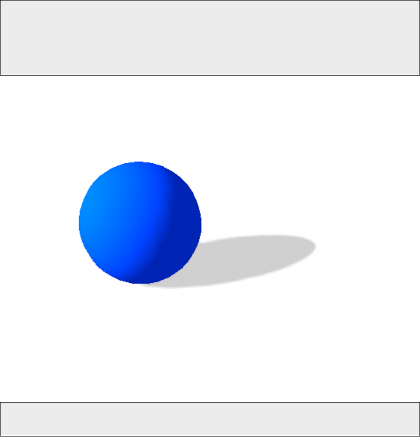
10.2 Sphere Shape
The SphereShape class describes a sphere collision shape centered at the origin
of the shape local space. You only need to specify the radius of the sphere to create it.
For instance, if you want to create a sphere shape with a radius of 2 meters, you
need to use the following code:
// Create the sphere shape with a radius of 2m
const rp3d :: SphereShape sphereShape (2.0) ;
10.3 Capsule Shape
The CapsuleShape class describes a capsule collision shape around the local Y axis
and centered at the origin of the shape local-space. It is the convex hull of two
spheres. It can also be seen as an elongated sphere. In order to create it, you only
need to specify the radius of the two spheres and the height of the capsule (distance
between the centers of the two spheres).
For instance, if you want to create a capsule shape with a radius of 1 meter and
the height of 2 meters, you need to use the following code:
23
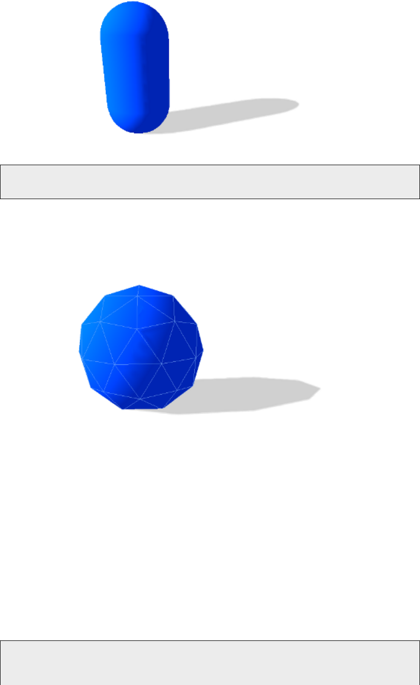
// Create the capsule shape
const rp3d :: Capsule Shape cap sule Shap e (1.0 , 2.0) ;
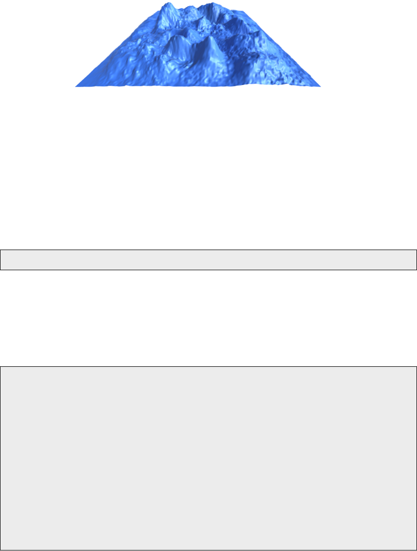
10.4 Convex Mesh Shape
The ConvexMeshShape class can be used to describe the shape of a convex
mesh. In order to create a convex mesh shape, you first need to create an array
of PolygonFace to describe each face of your mesh. You also need to have an ar-
ray with the vertices coordinates and an array with the vertex indices of each face
of you mesh. Then, you have to create a PolygonVertexArray with your vertices
coordinates and indices array. You also need to specify your array of PolygonFace.
Then, you have to create a PolyhedronMesh with your PolygonVertexArray. Once
this is done, you can create the ConvexMeshShape by passing your PolyhedronMesh
in paramater.
The following example shows how to create a convex mesh shape. In this exam-
ple, we create a cube as a convex mesh shape. Of course, this is only for the example.
If you really need a cube collision shape, you should use the BoxShape instead.
// Array with the vertices coordinates of the convex mesh
float vertices [24];
vertices [0] = -3; vertices [1] = -3; vertices [2] = 3;
24

vertices [3] = 3; vertices [4] = -3; vertices [5] = 3;
vertices [6] = 3; vertices [7] = -3; vertices [8] = -3;
vertices [9] = -3; vertices [10] = -3; vertices [11] = -3;
vertices [12] = -3; vertices [13] = 3; vertices [14] = 3;
vertices [15] = 3; vertices [16] = 3; vertices [17] = 3;
vertices [18] = 3; vertices [19] = 3; vertices [20] = -3;
vertices [21] = -3; vertices [22] = 3; vertices [23] = -3;
// Array with the vertices indices for each face of the mesh
int indices [24];
indices [0]=0; indices [1]=3; indices [2]=2; indices [3]=1;
indices [4]=4; indices [5]=5; indices [6]=6; indices [7]=7;
indices [8]=0; indices [9]=1; indices [10]=5; indices [11]=4;
indices [12]=1; indices [13]=2; indices [14]=6; indices [15]=5;
indices [16]=2; indices [17]=3; indices [18]=7; indices [19]=6;
indices [20]=0; indices [21]=4; indices [22]=7; indices [23]=3;
// Description of the six faces of the convex mesh
polygonFaces = new rp3d :: PolygonVer tex Arr ay :: Pol ygonF ace [6];
rp3d :: Poly gon Ver tex Arr ay :: PolygonFace * face = polygo nFaces ;
for (int f = 0; f < 6; f ++) {
// First vertex of the face in the indices array
face -> indexBase = f * 4;
// Number of vertices in the face
face -> nbVertices = 4;
face ++;
}
// Create the polygon vertex array
polygonVertexArray = new rp3d::PolygonVertexArray(8,
vertices , 3 x sizeof (float) ,
indices , sizeof (int ) , 6 , p oly go nFa ces ,
rp3d :: PolygonVertexArray :: VertexDat aType :: VERTEX_FLOAT_TYPE ,
rp3d::PolygonVertexArray::IndexDataType::INDEX_INTEGER_TYPE)
;
// Create the polyhedron mesh
polyhedr onMesh = new rp3d :: Po lyhedronMes h ( pol ygo nVe rtexArray
);
// Create the convex mesh collision shape
convexMeshShape = new rp3d::ConvexMeshShape(polyhedronMesh);
Note that the vertex coordinates and indices array are not copied and therefore,
you need to make sure that they exist until the collision shape exists. This is also true
25

for the all the PolygonFace, the PolygonVertexArray and the PolyhedronMesh.
You need to make sure that the mesh you provide is indeed convex. Secondly,
you should provide the simplest possible convex mesh. It means that you need to
avoid coplanar faces in your convex mesh shape. Coplanar faces have to be merged
together. Remember that convex meshes are not limited to triangular faces, you can
create faces with more than three vertices.
When you specify the vertices for each face of your convex mesh, be careful with
their order. The vertices of a face must be specified in counter clockwise order as
seen from the outside of your convex mesh.
You can also specify a scaling factor in the constructor when you create a Convex
MeshShape. All the vertices of your mesh will be scaled from the origin by this factor
when used in the collision shape.
Note that collision detection with a ConvexMeshShape is more expensive than with
aSphereShape or a CapsuleShape.
10.5 Concave Mesh Shape
The ConcaveMeshShape class can be used for a static concave triangular mesh.
It can be used to describe an environment for instance. Note that it cannot be
used with a dynamic body that is allowed to move. Moreover, make sure to use
aConcaveMeshShape only when you are not able to use a convex shape and also
try to limit the number of triangles of that mesh because collision detection with
ConcaveMeshShape is quite expensive compared to convex shapes.
In order to create a concave mesh shape, you need to supply a pointer to a
TriangleMesh. A TriangleMesh class describes a mesh made of triangles. It may
contain several parts (submeshes). Each part is a set of triangles represented by a
TriangleVertexArray object. A TriangleVertexArray represents a continuous ar-
ray of vertices and indexes for a triangular mesh. When you create a TriangleVertex
Array, no data is copied into the array. It only stores a pointer to the data. The idea is
to allow the user to share vertices data between the physics engine and the rendering
part. Therefore, make sure that the data pointed by a TriangleVertexArray remains
26

valid during the whole TriangleVertexArray life.
The following code shows how to create a TriangleVertexArray:
const int nbVertices = 8;
const int nbTriangles = 12;
float vertices [3 * nbVertices ] = ...;
int indices [3 * nbTriangles ] = ...;
rp3d :: TriangleVerte xAr ray * triangleA rray =
new rp3d :: Tr iangleVertexArray ( nbVertices , vertices , 3 *
sizeof (float) , nb Trian gle s ,
indices , 3 * sizeof (int ) ,
rp3d :: TriangleVertexAr ray :: VERTEX_FLOAT_TYPE ,
rp3d::TriangleVertexArray::INDEX_INTEGER_TYPE);
Now that we have a TriangleVertexArray, we need to create a TriangleMesh
and add the TriangleVertexArray into it as a subpart. Once this is done, we can
create the actual ConcaveMeshShape.
rp3d :: T riangleMesh t riangleMesh ;
// Add the triangle vertex array to the triangle mesh
triangleMesh . addSubpart ( tr iangleAr ray ) ;
// Create the concave mesh shape
ConcaveMeshShape * c oncav eMesh = new rp3d :: ConcaveMeshShape (&
triangleMesh );
Note that the TriangleMesh object also needs to exist during the whole life of the
collision shape because its data is not copied into the collision shape.
When you specify the vertices for each triangle face of your mesh, be careful with
the order of the vertices. They must be specified in counter clockwise order as seen
from the outside of your mesh.
You can also specify a scaling factor in the constructor when you create a Concave
MeshShape. All the vertices of your mesh will be scaled from the origin by this factor
when used in the collision shape.
In the previous example, the vertex normals that are needed for collision detection
are automatically computed. However, if you want to specify your own vertex normals,
you can do it by using another constructor for the TriangleVertexArray.
27
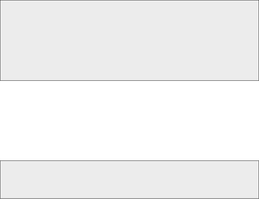
10.6 Heightfield Shape
The HeightFieldShape is a collision shape that can be used to represent a static
terrain for instance. You can define a heightfield with a two dimensional grid that has
a given height value at each point.
In order to create a HeightFieldShape, you need to have an array with all the
height values of your field. You can have height values of type int, float or double. You
need to give the number of rows and columns of your two dimensional grid. Note that
the height values in your array must be organized such that the value at row indexRow
and column indexColumn is located at the following position in the array:
heighFieldValues [ indexRow * nbColumns + indexColumn ]
Morevover, you need to provide the minimum and maximum height values of your
height field.
Here is an example that shows how to create a HeightFieldShape:
const int nbRows = 40;
const int nbColumns = 50;
float minHeight = 100;
float maxHeight = 500;
// Height values
float heigh tValues [ nbRows * nbColumns ] = ...;
// Create the hei ghtfi eld c ollision shape
rp3d :: HeightFieldShap e = new rp3d :: He igh tFieldShape (
nbColumns , nbRows , minHeight ,
maxHeight , heightValues , rp3d :: HeightFieldShape ::
HEIGHT_FLOAT_TYPE);
Note that the array of height values are not copied into the HeightFieldShape.
Therefore, you need to make sure they exist during the lifetime of the HeightField
Shape and you must not forget to release their memory when you destroy the collision
shape or at the end of your application.
28

You can also specify a scaling factor in the constructor when you create a Height
FieldShape. All the vertices of your mesh will be scaled from the origin by this factor
when used in the collision shape.
When creating a HeightFieldShape, the origin of the shape will be at the center
of its bounding volume. Therefore, if you create a HeightFieldShape with a minimum
height of 100 and a maximum height of 500, the maximum coordinates of the shape
on the Y axis will be 200 and the minimum coordinates will be -200.
10.7 Adding a Collision Shape to a body - The Proxy Shape con-
cept
Now that you know how to create a collision shape, we will see how to add it to a
given body.
First note that when you add a collision shape to a body, the shape will not be
copied internally. You only give a pointer to the shape in parameter. The shape must
exist during the whole lifetime of the body. This way, you can create a collision shape
and reuse it for multiple bodies. You are also responsible to destroy the shape at the
end when the bodies are not used anymore.
In order to add a collision shape to a body, you need to use the
CollisionBody::addCollisionShape() method for a collision body and the
RigidBody::addCollisionShape() method for a rigid body. You will have to provide
the collision shape transform in parameter. This is the transformation mapping the
local-space of the collision shape to the local-space of the body. For a rigid body,
you will also have to provide the mass of the shape you want to add. As explained
before, this is used to automatically compute the center of mass, total mass and
inertia tensor of the body.
The addCollisionShape() method returns a pointer to a proxy shape. A proxy
shape is what links a given collision shape to the body it has been added. You can
use the returned proxy shape to get or set parameters of the given collision shape in
that particular body. This concept is also called fixture in some other physics engines.
In ReactPhysics3D, a proxy shape is represented by the ProxyShape class.
The following example shows how to add a sphere collision shape with a given
mass to a rigid body and also how to remove it from the body using the Proxy Shape
pointer.
// Create the sphere collision shape
rp3d :: decimal radius = rp3d :: decimal (3.0)
const rp3d :: BoxShape shape ( radius ) ;
// Transform of the collision shape
// Place the shape at the origin of the body local - space
29

rp3d :: Transform transform = rp3 :: Transform :: identity () ;
// Mass of the collision shape ( in kilograms )
rp3d :: decimal mass = rp3d :: decimal (4.0) ;
// Add the collision shape to the rigid body
rp3d::ProxyShape* proxyShape;
proxyShape = body - > addCollisionShape (& shape , transform , mass
);
// If you want to remove the co llision shape from the body
// at some point , you need to use the proxy shape
body -> re moveCollision Sha pe ( pr oxyShape );
As you can see, you can use the removeCollisionShape() method to remove
a collision shape from a body by using the proxy shape. Note that after removing a
collision shape, the corresponding proxy shape pointer will not be valid anymore. It is
not necessary to manually remove all the collision shapes from a body at the end of
your application. They will automatically be removed when you destroy the body.
10.8 Collision filtering
By default all the collision shapes of all your bodies are able to collide with each other
in the world. However, sometimes we want a body to collide only with a given group of
bodies and not with other bodies. This is called collision filtering. The idea is to group
the collision shapes of bodies into categories. Then we can specify for each collision
shape against which categories it will be able to collide.
ReactPhysics3D uses bits mask to represent categories. The first thing to do is
to assign a category to the collision shapes of your body. To do this, you need to
call the ProxyShape::setCollisionCategoryBits() method on the corresponding
proxy shape as in the following example. Here we consider that we have four bodies
where each one has a single collision shape.
// Enumeration for categories
enum Category {
CATEG ORY1 = 0 x0001 ,
CATEG ORY2 = 0 x0002 ,
CATEGORY3 = 0 x0004
};
// Set the collision category for each proxy shape of
// each of the four bodies
proxyShapeBody1 - > setCo llision CategoryBi ts ( CATEGORY1 ) ;
proxyShapeBody2 - > setCo llision CategoryBi ts ( CATEGORY2 ) ;
30

proxyShapeBody3 - > setCo llision CategoryBi ts ( CATEGORY3 ) ;
proxyShapeBody4 - > setCo llision CategoryBi ts ( CATEGORY3 ) ;
As you can see, the collision shape of body 1 will be part of the category 1, the
collision shape of body 2 will be part of the category 2 and the collision shapes of
bodies 3 and 4 will be part of the category 3.
Now, for each collision shape, we need to specify with which categories
the shape is allowed to collide with. To do this, you need to use the
ProxyShape::setCollideWithMaskBits() method of the proxy shape. Note
that you can specify one or more categories using the bitwise OR operator. The
following example shows how to specify with which categories the shapes can collide.
// For each shape , we specify with which categories it
// is allowed to collide
proxyShapeBody1 - > setCo llideWithM ask Bits ( CATEGORY3 );
proxyShapeBody2 - > setC oll ideWithMas kBits ( CATEGORY1 |
CATEGORY3);
proxyShapeBody3 - > setCo llideWithM ask Bits ( CATEGORY2 );
proxyShapeBody4 - > setCo llideWithM ask Bits ( CATEGORY2 );
As you can see, we specify that the body 1 will be allowed to collide with bodies
from the categorie 3. We also indicate that the body 2 will be allowed to collide with
bodies from the category 1 and 3 (using the bitwise OR operator). Finally, we specify
that bodies 3 and 4 will be allowed to collide against bodies of the category 2.
A collision shape is able to collide with another only if you have specify that the
category mask of the first shape is part of the collide with mask of the second shape. It
is also important to understand that this condition must be satisfied in both directions.
For instance in the previous example, the body 1 (of category 1) says that it wants
to collide against bodies of the category 3 (for instance against body 3). However,
body 1 and body 3 will not be able to collide because the body 3 does not say that
it wants to collide with bodies from category 1. Therefore, in the previous example,
the body 2 is allowed to collide against bodies 3 and 4 but no other collision is allowed.
In the same way, you can perform this filtering for ray casting (described in section
12). For instance, you can perform a ray cast test against a given subset of categories
of collision shapes only.
11 Joints
Joints are used to constrain the motion of the rigid bodies between each other. A
single joint represents a constraint between two rigid bodies. When the motion of the
first body of the joint is known, the relative motion of the second body has at most six
31

degrees of freedom (three for the translation and three for the rotation). The different
joints can reduce the number of degrees of freedom between two rigid bodies.
Some joints have limits to control the range of motion and some joints have motors
to automatically move the bodies of the joint at a given speed.
11.1 Ball and Socket Joint
The BallAndSocketJoint class describes a ball and socket joint between two bod-
ies. In a ball and socket joint, the two bodies cannot translate with respect to each
other. However, they can rotate freely around a common anchor point. This joint has
three degrees of freedom and can be used to simulate a chain of bodies for instance.
In order to create a ball and socket joint, you first need to create an instance of the
BallAndSocketJointInfo class with the necessary information. You need to provide
the pointers to the two rigid bodies and also the coordinates of the anchor point (in
world-space). At the joint creation, the world-space anchor point will be converted
into the local-space of the two rigid bodies and then, the joint will make sure that the
two local-space anchor points match in world-space. Therefore, the two bodies need
to be in a correct position at the joint creation.
Here is the code to create the BallAndSocketJointInfo object:
// Anchor point in world - space
const rp3d :: V ector3 anchorPoint (2.0 , 4.0 , 0.0) ;
// Create the joint info object
rp3d :: B al lA ndS oc ke tJ oin tI nf o joi ntIn fo ( body1 , body2 ,
anchorPoint);
Now, it is time to create the actual joint in the dynamics world using the Dynamics
World::createJoint() method. Note that this method will also return a pointer to
the BallAndSocketJoint object that has been created internally. You will then be
able to use that pointer to change properties of the joint and also to destroy it at the
end.
Here is how to create the joint in the world:
// Create the joint in the dynamics world
rp3d::BallAndSocketJoint* joint;
joint = dynamic_cast < rp3 d :: B al lAn dS oc ke tJ oin t * >( worl d .
createJoint ( jointInfo )) ;
32
11.2 Hinge Joint
The HingeJoint class describes a hinge joint (or revolute joint) between two rigid
bodies. The hinge joint only allows rotation around an anchor point and around a
single axis (the hinge axis). This joint can be used to simulate doors or pendulums for
instance.
In order to create a hinge joint, you first need to create a HingeJointInfo object
with the necessary information. You need to provide the pointers to the two rigid bod-
ies, the coordinates of the anchor point (in world-space) and also the hinge rotation
axis (in world-space). The two bodies need to be in a correct position when the joint
is created.
Here is the code to create the HingeJointInfo object:
// Anchor point in world - space
const rp3d :: V ector3 anchorPoint (2.0 , 4.0 , 0.0) ;
// Hinge rotation axis in world - space
const rp3d :: Vector3 axis (0.0 , 0.0 , 1.0) ;
// Create the joint info object
rp3d :: H in ge Jo in tInf o joint Info ( body1 , body2 , a nch orP oin t ,
axis );
Now, it is time to create the actual joint in the dynamics world using the Dynamics
World::createJoint() method. Note that this method will also return a pointer to
the HingeJoint object that has been created internally. You will then be able to use
that pointer to change properties of the joint and also to destroy it at the end.
Here is how to create the joint in the world:
// Create the hinge joint in the dynamics world
rp3d :: H ingeJoint * joint ;
joint = dynamic_cast < rp3 d :: H in geJo in t * >( wo rl d . c re at eJ oint (
jointInfo));
11.2.1 Limits
With the hinge joint, you can constrain the motion range using limits. The limits of the
hinge joint are the minimum and maximum angle of rotation allowed with respect to
the initial angle between the bodies when the joint is created. The limits are disabled
by default. If you want to use the limits, you first need to enable them by setting the
isLimitEnabled variable of the HingeJointInfo object to true before you create the
joint. You also have to specify the minimum and maximum limit angles (in radians)
33

using the minAngleLimit and maxAngleLimit variables of the joint info object. Note
that the minimum limit angle must be in the range [−2π; 0] and the maximum limit
angle must be in the range [0; 2π].
For instance, here is the way to use the limits for a hinge joint when the joint is
created:
// Create the joint info object
rp3d :: H in ge Jo in tInf o joint Info ( body1 , body2 , a nch orP oin t ,
axis );
// Enable the limits of the joint
jointInfo . isLimitEn abled = true ;
// Minimum limit angle
jointInfo . minAngleLim it = - PI / 2.0;
// Maximum limit angle
jointInfo . maxAng leLimit = PI / 2.0;
// Create the hinge joint in the dynamics world
rp3d :: H ingeJoint * joint ;
joint = dynamic_cast < rp3 d :: H in geJo in t * >( wo rl d . c re at eJ oint (
jointInfo));
It is also possible to use the HingeJoint::enableLimit(),
HingeJoint::setMinAngleLimit() and HingeJoint::setMaxAngleLimit()
methods to specify the limits of the joint after its creation. See the API documentation
for more information.
11.2.2 Motor
A motor is also available for the hinge joint. It can be used to rotate the bodies around
the hinge axis at a given angular speed and such that the torque applied to rotate the
bodies does not exceed a maximum allowed torque. The motor is disabled by default.
If you want to use it, you first have to activate it using the isMotorEnabled boolean
variable of the HingeJointInfo object before you create the joint. Then, you need to
specify the angular motor speed (in radians/seconds) using the motorSpeed variable
and also the maximum allowed torque (in Newton ·meters) with the maxMotorTorque
variable.
For instance, here is how to enable the motor of the hinge joint when the joint is
created:
// Create the joint info object
34

rp3d :: H in ge Jo in tInf o joint Info ( body1 , body2 , a nch orP oin t ,
axis );
// Enable the motor of the joint
jointInfo . isMotorEn abled = true ;
// Motor angular speed
jointInfo . motorSpeed = PI / 4.0;
// Maximum allowed torque
jointInfo . maxMotorT orque = 10.0;
// Create the hinge joint in the dynamics world
rp3d :: H ingeJoint * joint ;
joint = dynamic_cast < rp3 d :: H in geJo in t * >( wo rl d . c re at eJ oint (
jointInfo));
It is also possible to use the HingeJoint::enableMotor(),
HingeJoint::setMotorSpeed() and HingeJoint::setMaxMotorTorque() meth-
ods to enable the motor of the joint after its creation. See the API documentation for
more information.
11.3 Slider Joint
The SliderJoint class describes a slider joint (or prismatic joint) that only allows
relative translation along a single direction. It has a single degree of freedom and
allows no relative rotation. In order to create a slider joint, you first need to specify
the anchor point (in world-space) and the slider axis direction (in world-space). The
constructor of the SliderJointInfo object needs two pointers to the bodies of the
joint, the anchor point and the axis direction. Note that the two bodies have to be in a
correct initial position when the joint is created.
You can see in the following code how to specify the information to create a slider
joint:
// Anchor point in world - space
const rp3d :: Vector3 anchorPoint = rp3d :: decimal (0.5) * (
body2Position + body1Position);
// Slider axis in world - space
const rp3d :: Vector3 axis = ( body2Position - body1 Position ) ;
// Create the joint info object
rp3d :: S li de rJ oint In fo jo in tInfo ( body1 , body2 , a nch orP oi nt ,
axis );
35

Now, it is possible to create the actual joint in the dynamics world using the
DynamicsWorld::createJoint() method. Note that this method will also return a
pointer to the SliderJoint object that has been created internally. You will then be
able to use that pointer to change properties of the joint and also to destroy it at the
end.
Here is how to create the joint in the world:
// Create the slider joint in the dynamics world
rp3d :: S liderJ oint * joint ;
joint = dynamic_cast < rp3d :: Sl ider Jo int * >( worl d . c re ateJ oi nt (
jointInfo));
11.3.1 Limits
It is also possible to control the range of the slider joint motion using limits. The limits
are disabled by default. In order to use the limits when the joint is created, you first
need to activate them using the isLimitEnabled variable of the SliderJointInfo
class. Then, you need to specify the minimum and maximum translation limits (in me-
ters) using the minTranslationLimit and maxTranslationLimit variables. Note
that the initial position of the two bodies when the joint is created corresponds to a
translation of zero. Therefore, the minimum limit must be smaller or equal to zero and
the maximum limit must be larger or equal to zero.
You can see in the following example how to set the limits when the slider joint is
created:
// Create the joint info object
rp3d :: S li de rJ oint In fo jo in tInfo ( body1 , body2 , a nch orP oi nt ,
axis );
// Enable the limits of the joint
jointInfo . isLimitEn abled = true ;
// Minimum translation limit
jointInfo . m inT ran slationLimit = -1.7;
// Maximum translation limit
jointInfo . m axT ran slationLimit = 1.7;
// Create the hinge joint in the dynamics world
rp3d :: S liderJ oint * joint ;
joint = dynamic_cast < rp3d :: Sl ider Jo int * >( worl d . c re ateJ oi nt (
jointInfo));
36

You can also use the SliderJoint::enableLimit(),SliderJoint::-
setMinTranslationLimit() and SliderJoint::setMaxTranslationLimit()
methods to enable the limits of the joint after its creation. See the API documentation
for more information.
11.3.2 Motor
The slider joint also has a motor. You can use it to translate the bodies along the slider
axis at a given linear speed and such that the force applied to move the bodies does
not exceed a maximum allowed force. The motor is disabled by default. If you want to
use it when the joint is created, you first have to activate it using the isMotorEnabled
boolean variable of the SliderJointInfo object before you create the joint. Then,
you need to specify the linear motor speed (in meters/seconds) using the motorSpeed
variable and also the maximum allowed force (in Newtons) with the maxMotorForce
variable.
For instance, here is how to enable the motor of the slider joint when the joint is
created:
// Create the joint info object
rp3d :: S li de rJ oint In fo jo in tInfo ( body1 , body2 , a nch orP oi nt ,
axis );
// Enable the motor of the joint
jointInfo . isMotorEn abled = true ;
// Motor linear speed
jointInfo . motorSpeed = 2.0;
// Maximum allowed force
jointInfo . maxMot orForce = 10.0;
// Create the slider joint in the dynamics world
rp3d :: S liderJ oint * joint ;
joint = dynamic_cast < rp3d :: Sl ider Jo int * >( worl d . c re ateJ oi nt (
jointInfo));
It is also possible to use the SliderJoint::enableMotor(),
SliderJoint::setMotorSpeed() and SliderJoint::setMaxMotorForce()
methods to enable the motor of the joint after its creation. See the API documentation
for more information.
11.4 Fixed Joint
The FixedJoint class describes a fixed joint between two bodies. In a fixed joint,
there is no degree of freedom, the bodies are not allowed to translate or rotate with
37

respect to each other. In order to create a fixed joint, you simply need to specify an
anchor point (in world-space) to create the FixedJointInfo object.
For instance, here is how to create the joint info object for a fixed joint:
// Anchor point in world - space
rp3d :: V ect or3 an chor Point (2.0 , 3.0 , 4.0) ;
// Create the joint info object
rp3d :: F ix edJo in tI nf o jo in tInf o1 ( body1 , body2 , anc horP oi nt );
Now, it is possible to create the actual joint in the dynamics world using the
DynamicsWorld::createJoint() method. Note that this method will also return a
pointer to the FixedJoint object that has been created internally. You will then be
able to use that pointer to change properties of the joint and also to destroy it at the
end.
Here is how to create the joint in the world:
// Create the fixed joint in the dynamics world
rp3d :: F ixedJoint * joint ;
joint = dynamic_cast < rp3 d :: F ix edJo in t * >( wo rl d . c re at eJ oint (
jointInfo));
11.5 Collision between the bodies of a Joint
By default, the two bodies involved in a joint are able to collide with each other. How-
ever, it is possible to disable the collision between the two bodies that are part of the
joint. To do it, you simply need to set the variable isCollisionEnabled of the joint
info object to false when you create the joint.
For instance, when you create a HingeJointInfo object in order to construct a
hinge joint, you can disable the collision between the two bodies of the joint as in the
following example:
// Create the joint info object
rp3d :: H in ge Jo in tInf o joint Info ( body1 , body2 , a nch orP oin t ,
axis );
// Disable the collision between the bodies
jointInfo.isCollisionEnabled = false;
// Create the joint in the dynamics world
rp3d :: H ingeJoint * joint ;
38

joint = dynamic_cast < rp3 d :: H in geJo in t * >( wo rl d . c re at eJ oint (
jointInfo));
11.6 Destroying a Joint
In order to destroy a joint, you simply need to call the
DynamicsWorld::destroyJoint() method using the pointer to a previously
created joint object as argument as shown in the following code:
// rp3d :: Ba llA ndSocketJoint * joint is a previously created
joint
// Destroy the joint
world . destroy Joint ( joint );
It is important that you destroy all the joints that you have created at the end of the
simulation. Also note that destroying a rigid body involved in a joint will automatically
destroy that joint.
12 Ray casting
You can use ReactPhysics3D to test intersection between a ray and the bodies of the
world you have created. Ray casting can be performed against multiple bodies, a
single body or any proxy shape of a given body.
The first thing you need to do is to create a ray using the Ray class of React-
Physics3D. As you can see in the following example, this is very easy. You simply
need to specify the point where the ray starts and the point where the ray ends (in
world-space coordinates).
// Start and end points of the ray
rp3d :: V ector3 start Point (0.0 , 5.0 , 1.0) ;
rp3d :: Vector3 endP oint (0.0 , 5.0 , 30) ;
// Create the ray
rp3d :: Ray ray ( startPoint , endPoint ) ;
Any ray casting test that will be described in the following sections returns a
RaycastInfo object in case of intersection with the ray. This structure contains the
following attributes:
worldPoint Hit point in world-space coordinates
39

worldNormal Surface normal of the proxy shape at the hit point in world-space co-
ordinates
hitFraction Fraction distance of the hit point between startPoint and endPoint of the
ray. The hit point pis such that p=startP oint +hitF raction ·(endP oint −
startP oint)
body Pointer to the collision body or rigid body that has been hit by the ray
proxyShape Pointer to the proxy shape that has been hit by the ray
Note that you can also use collision filtering with ray casting in order to only test
ray intersection with specific proxy shapes. Collision filtering is described in section
10.8.
12.1 Ray casting against multiple bodies
This section describes how to get all the proxy shapes of all bodies in the world that
are intersected by a given ray.
12.1.1 The RaycastCallback class
First, you have to implement your own class that inherits from the RaycastCallback
class. Then, you need to override the RaycastCallback::notifyRaycastHit()
method in your own class. An instance of your class have to be provided as a pa-
rameter of the raycast method and the notifyRaycastHit() method will be called
for each proxy shape that is hit by the ray. You will receive, as a parameter of this
method, a RaycastInfo object that will contain the information about the raycast hit
(hit point, hit surface normal, hit body, hit proxy shape, . . . ).
In your notifyRaycastHit() method, you need to return a fraction value that
will specify the continuation of the ray cast after a hit. The return value is the next
maxFraction value to use. If you return a fraction of 0.0, it means that the raycast
should terminate. If you return a fraction of 1.0, it indicates that the ray is not clipped
and the ray cast should continue as if no hit occurred. If you return the fraction in
the parameter (hitFraction value in the RaycastInfo object), the current ray will be
clipped to this fraction in the next queries. If you return -1.0, it will ignore this Prox-
yShape and continue the ray cast. Note that no assumption can be done about the
order of the calls of the notifyRaycastHit() method.
Here is an example about creating your own raycast callback class that inher-
its from the RaycastCallback class and how to override the notifyRaycastHit()
method:
// Class WorldRa yca stC allback
class MyCallbackClass : public rp3d::RaycastCallback {
40

public :
virtual decimal not ifyRaycast Hit ( const RaycastInfo & info )
{
// Display the world hit point coordinates
std :: cout << " Hit po in t : " <<
info . world Point .x <<
info . world Point .y <<
info . world Point .z <<
std :: endl ;
// Return a fraction of 1.0 to gather all hits
return decimal (1.0) ;
}
};
12.1.2 Raycast query in the world
Now that you have your own raycast callback class, you can use the raycast()
method to perform a ray casting test on a collision world or a dynamics world.
The first parameter of this method is a reference to the Ray object representing the
ray you need to test intersection with. The second parameter is a pointer to the object
of your raycast callback object. You can specify an optional third parameter which
is the bit mask for collision filtering. It can be used to raycast only against selected
categories of proxy shapes as described in section 10.8.
// Create the ray
rp3d :: Vector3 st artP oint (1 , 2 , 10) ;
rp3d :: Vector3 e ndPo int (1 , 2 , -20) ;
Ray ray ( startPoint , endPoint ) ;
// Create an instance of your callback class
MyCallbackClass callbackObject;
// Raycast test
world -> raycast (ray , & callb ack Object ) ;
12.2 Ray casting against a single body
You can also perform ray casting against a single specific collision body or rigid body
of the world. To do this, you need to use the CollisionBody::raycast() method.
This method takes two parameters. The first one is a reference to the Ray object
and the second one is a reference to the RaycastInfo object that will contain hit
41

information if the ray hits the body. This method returns true if the ray hits the body.
The RaycastInfo object will only be valid if the returned value is true (a hit occured).
The following example shows how test ray intersection with a body:
// Create the ray
rp3d :: Vector3 st artP oint (1 , 2 , 10) ;
rp3d :: Vector3 e ndPo int (1 , 2 , -20) ;
Ray ray ( startPoint , endPoint ) ;
// Create the raycast info object for the
// raycast result
RaycastInfo raycastInfo;
// Raycast test
bool isHit = body -> raycast (ray , raycastInfo ) ;
12.3 Ray casting against the proxy shape of a body
You can also perform ray casting against a single specific proxy shape of a collision
body or rigid body of the world. To do this, you need to use the ProxyShape::raycast()
method of the given proxy shape. This method takes two parameters. The first one is
a reference to the Ray object and the second one is a reference to the RaycastInfo
object that will contain hit information if the ray hits the body. This method returns true
if the ray hits the body. The RaycastInfo object will only be valid if the returned value
is true (a hit occured).
The following example shows how to test ray intersection with a given proxy shape:
// Create the ray
rp3d :: Vector3 st artP oint (1 , 2 , 10) ;
rp3d :: Vector3 e ndPo int (1 , 2 , -20) ;
Ray ray ( startPoint , endPoint ) ;
// Create the raycast info object for the
// raycast result
RaycastInfo raycastInfo;
// Test raycasting against a proxy shape
bool isHit = proxyShape -> raycast (ray , raycastInfo ) ;
42
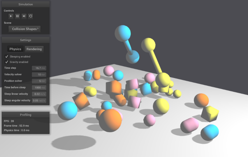
13 Testbed application
The testbed application is a graphical interface where you can select and see
some demo scenes using the ReactPhysics3D library.
Follow the instructions described in section 4to compile the testbed application.
Note that OpenGL is required to compile it.
The testbed application can be found in the testbed/ folder of the ReactPhysics3D
library. Do not hesitate to take a look at the code of the demo scenes to better under-
stand how to use the library in your application.
The following subsections describe the demo scenes that can be found in the
testbed application.
13.1 Cubes Scene
In this scene, you will see how to create a floor and some cubes using the Box Shape
for collision detection. Because of gravity, the cubes will fall down on the floor. After
falling down, the cubes will come to rest and start sleeping (become inactive). In this
scene, the cubes will become red as they get inactive (sleeping).
13.2 Cubes Stack Scene
This scene has a dynamics world and a pyramid of cubes.
43
13.3 Joints Scene
In this scene, you will learn how to create different joints (ball and socket, hinge, slider,
fixed) into the dynamics world. You can also see how to set the motor or limits of the
joints.
13.4 Collision Shapes Scene
In this scene, you will see how to create a floor (using the Box Shape) and some other
bodies using the different collision shapes available in the ReactPhysics3D library like
capsules, spheres, boxes and convex meshes. Those bodies will fall down to the floor.
13.5 Heightfield Scene
In this scene, you will see how to use the Height field collision shape of the library.
Several bodies will fall down to the height field.
13.6 Raycast Scene
In this scene, you will see how to use the ray casting methods of the library. Several
rays are thrown against the different collision shapes. It is possible to switch from a
collision shape to another using the spacebar key.
13.7 Collision Detection Scene
This scene has a collision world and several collision bodies that can be move around
with keyboard keys. This scene shows how to manually compute collision detection
in a collision world.
13.8 Concave Mesh Scene
In this scene, you will see how to use the static concave mesh collision shape of the
library.
14 Retrieving contacts
There are several ways to get the contacts information (contact point, normal, pene-
tration depth, . . . ) from the DynamicsWorld.
14.1 Contacts of a given rigid body
If you are interested to retrieve all the contacts of a single rigid body, you can use the
RigidBody::getContactManifoldsList() method. This method will return a linked
list with all the current contact manifolds of the body. A contact manifold can contains
44

several contact points.
Here is an example showing how to get the contact points of a given rigid body:
// Get the head of the linked list of contact manifolds of
the body
const Con tactMan ifoldLi stEleme nt * listElem ;
listEle m = r igi dbody - > g et Con ta c tM an ifo ld sLi st () ;
// For each contact manifold of the body
for (; listElem != nullptr ; listElem = listElem - > next ) {
ContactManifold* manifold = listElem->contactManifold;
// For each contact point of the manifold
for (int i =0; i < manifold - > get Nb Co nt ac tP oi nts () ; i ++) {
// Get the contact point
ContactPoint * point = manifold -> getContactP oin t (i);
// Get the world - space contact point on body 1
Ve ct or3 pos = point - > g et Wo rld Po int On Bod y1 () ;
// Get the world - space contact normal
Ve ct or3 n or mal = point -> g etNo rm al () ;
}
}
Note that this technique to retrieve the contacts, if you use it between the Dynamics
World::update() calls, will only give you the contacts at the end of each frame. You
will probably miss several contacts that have occured in the physics internal sub-steps.
In section 15, you will see how to get all the contact occuring in the physis sub-steps
of the engine.
14.2 All the contacts of the world
If you want to retrieve all the contacts of any rigid body in the world, you can use the
DynamicsWorld::getContactsList() method. This method will a List with the all
the current contact manifolds of the world. A contact manifold may contain several
contact points.
The following example shows how to get all the contacts of the world using this
method:
rp3d :: List < const rp3d :: ContactManifo ld *> manifolds ;
45

// Get all the contacts of the world
manif ol ds = dynami cs Wor ld - > get Co nt ac tsL is t () ;
rp3d :: List < const rp3d :: ContactManifold * >:: iterator it ;
// For each contact manifold
for ( it = manifolds . begin () ; it != mani folds . end () ; ++ it ) {
const rp3d :: C on ta ct Man if ol d * ma nifo ld = * it ;
// For each contact point of the manifold
rp3d :: C ontactPoint * contactPoin t = manifold ->
getContactPoints();
while ( contactPoint != nullptr ) {
// Retrieve the world contact point and normal
rp3d :: Vector3 worldPoint = manifold -> getShape1 ()
-> getL ocalToWo rldTrans for m () * contactPoint - >
getLocalPointOnShape1();
rp3d :: Vector3 worldNormal = contactPoint - >
getNormal();
// Move to the next contact point
con ta ct Po in t = c ont actPoin t - > ge tN ext () ;
}
}
Note that this technique to retrieve the contacts, if you use it between the Dynamics
World::update() calls, will only give you the contacts are the end of each frame. You
will probably miss several contacts that have occured in the physics internal sub-steps.
In section 15, you will see how to get all the contact occuring in the physis sub-steps
of the engine.
15 Receiving Feedback
Sometimes, you want to receive notifications from the physics engine when a given
event occurs. The EventListener class can be used for that purpose. In order to
use it, you need to create a new class that inherits from the EventListener class
and overrides some methods that will be called by the ReactPhysics3D library when
some events occur. You also need to register your class in the physics world using
the DynamicsWorld::setEventListener() as in the following code:
// Here , You rEv ent Lis ten er is a class that inherits
// from the EventListener class of reactp hysics3d
YourEventListener listener ;
// Register your event listener class
world . se tEventL istener (& listener ) ;
46

15.1 Contacts
If you want to be notified when two bodies that were separated before become in
contact, you need to override the EventListener::beginContact() method in your
event listener class. Then, this method will be called when the two separated bodies
becomes in contact.
If you receive a notification when a new contact between two bodies is found, you
need to override the EventListener::newContact() method in your event listener
class. Then, this method will be called when a new contact is found.
16 Profiler
If you build the library with the RP3D_PROFILING_ENABLED variable enabled (see sec-
tion 4.3), a real-time profiler will collect information while the application is running.
Then, at the end of your application, when the destructor of the DynamicsWorld class
is called, information about the running time of the library will be displayed in the stan-
dard output. This can be useful to know where time is spent in the different parts of
the ReactPhysics3D library in case your application is too slow.
Each collision or dynamics world has its own profiler. By default, the profiling re-
port wil be written in a text file next to the executable. If you have multiple worlds
in your application, there will be one profile file for each world. The profile files will
be named after the name of the worlds. By defaults worlds will have names: world,
world1, world2, world3, . . . You can change the name of the world by setting it into the
WorldSettings object when you create the world (see section 6).
It is also possible to output the profiling report to another destination. To do this,
you have to create your own profiler object before the creation of the physics world.
You will then be able to add one or more profile destinations to the profiler. A destina-
tion can be either a file or an output stream (std::ostream) of your choice. For each
destination, you also have to select the output format of the profiling report. When
this is done, you have to give the pointer to your profiler object in paramater when you
create the world.
The following example shows how to create your own profiler object and add a file
destination (custom_profile.txt) and a stream destination (std::cout):
// Create the profiler
rp3d::Profiler* profiler = new rp3d :: Profiler () ;
// Add a log destination file
profiler ->addFileDestination(" cus to m_ prof il e . txt " , Profiler
:: Format :: Text ) ;
// Add an output stream destination
47

profiler - > addStreamDest ina tio n ( std :: cout , Profiler :: Format ::
Text );
// Create the physics world with your profiler
rp3d :: Col lis ionWorld world (rp3d :: Wor ldSettin gs () , nullptr ,
profiler);
17 Logger
ReactPhysics3D has an internal logger that can be used to output logs while running
the application. This can be useful for debugging for instance. To enable the logger,
you need to build the library with the RP3D_LOGS_ENABLED variable enabled (see sec-
tion 4.3).
Each collision or dynamics world has its own logger. By default, logs wil be written
in an HTML file next to the executable. If you have multiple worlds in your application,
there will be one log file for each world. The logs files will be named after the name of
the worlds. By defaults worlds will have names: world, world1, world2, world3, . . . You
can change the name of the world by setting it into the WorldSettings object when
you create the world (see section 6).
It is also possible to output the logs to another destination. To do this, you have to
create your own logger object before the creation of the physics world. You will then
be able to add one or more logs destinations to the logger. A destination can be either
a file or an output stream (std::ostream) of your choice. For each destination, you
also have to select the output format of the logs (text or HTML). When this is done,
you have to give the pointer to your logger object in paramater when you create the
world.
The following example shows how to create your own logger object and add a file
destination (custom_log.html) and a stream destination (std::cout):
// Create the logger
rp3d :: Logger * logger = new rp3d :: Logger () ;
// Log level ( infor , w arning and error
uint logLevel = static_cast < uint >( Logger :: Level :: Info ) |
static_cast < uint >( Logger :: Level :: Warning ) |
static_cast < uint >( Logger :: Level :: Error );
// Add a log destination file
logger->addFileDestination("custom_log.html", logLevel ,
Logger :: Format :: HTML ) ;
// Add an output stream destination
48
logger -> ad dSt rea mDestination ( std :: cout , logLevel , Logger ::
Format :: Text ) ;
// Create the physics world with your logger
rp3d :: Col lis ionWorld world (rp3d :: Wor ldSettin gs () , logger ) ;
18 API Documentation
Some documentation about the API of the code has been generated using Doxy-
gen. You will be able to find this documentation in the library archive in the folder
/documentation/API/html/. You just need to open the index.html file with your
favorite web browser.
The API documentation is also available online here: http://www.reactphysics3d.
com/documentation/api/html/
19 Issues
If you find some bugs, do not hesitate to report them on our issue tracker here:
https://github.com/DanielChappuis/reactphysics3d/issues
Thanks a lot for reporting the issues that you find. It will help us to correct and
improve the library.
49
