SAS/STAT 9.2 User's Guide: The CLUSTER Procedure (Book Excerpt) SAS Users Guide
User Manual: Pdf
Open the PDF directly: View PDF ![]() .
.
Page Count: 104 [warning: Documents this large are best viewed by clicking the View PDF Link!]

SAS/STAT®9.2 User’s Guide
The CLUSTER Procedure
(Book Excerpt)
SAS®Documentation
This document is an individual chapter from SAS/STAT®9.2 User’s Guide.
The correct bibliographic citation for the complete manual is as follows: SAS Institute Inc. 2008. SAS/STAT®9.2
User’s Guide. Cary, NC: SAS Institute Inc.
Copyright © 2008, SAS Institute Inc., Cary, NC, USA
All rights reserved. Produced in the United States of America.
For a Web download or e-book: Your use of this publication shall be governed by the terms established by the vendor
at the time you acquire this publication.
U.S. Government Restricted Rights Notice: Use, duplication, or disclosure of this software and related documentation
by the U.S. government is subject to the Agreement with SAS Institute and the restrictions set forth in FAR 52.227-19,
Commercial Computer Software-Restricted Rights (June 1987).
SAS Institute Inc., SAS Campus Drive, Cary, North Carolina 27513.
1st electronic book, March 2008
2nd electronic book, February 2009
SAS®Publishing provides a complete selection of books and electronic products to help customers use SAS software to
its fullest potential. For more information about our e-books, e-learning products, CDs, and hard-copy books, visit the
SAS Publishing Web site at support.sas.com/publishing or call 1-800-727-3228.
SAS®and all other SAS Institute Inc. product or service names are registered trademarks or trademarks of SAS Institute
Inc. in the USA and other countries. ® indicates USA registration.
Other brand and product names are registered trademarks or trademarks of their respective companies.

Chapter 29
The CLUSTER Procedure
Contents
Overview: CLUSTER Procedure ........................... 1230
Getting Started: CLUSTER Procedure ........................ 1231
Syntax: CLUSTER Procedure ............................ 1239
PROC CLUSTER Statement .......................... 1239
BY Statement ................................. 1247
COPY Statement ................................ 1247
FREQ Statement ................................ 1248
ID Statement .................................. 1248
RMSSTD Statement .............................. 1249
VAR Statement ................................. 1249
Details: CLUSTER Procedure ............................ 1250
Clustering Methods .............................. 1250
Miscellaneous Formulas ............................ 1258
Ultrametrics .................................. 1259
Algorithms ................................... 1259
Computational Resources ........................... 1260
Missing Values ................................. 1261
Ties ....................................... 1261
Size, Shape, and Correlation .......................... 1262
Output Data Set ................................ 1263
Displayed Output ................................ 1265
ODS Table Names ............................... 1268
ODS Graphics ................................. 1269
Examples: CLUSTER Procedure ........................... 1270
Example 29.1: Cluster Analysis of Flying Mileages between 10 American
Cities ................................. 1270
Example 29.2: Crude Birth and Death Rates ................. 1277
Example 29.3: Cluster Analysis of Fisher’s Iris Data ............. 1289
Example 29.4: Evaluating the Effects of Ties ................. 1304
References ...................................... 1316

1230 FChapter 29: The CLUSTER Procedure
Overview: CLUSTER Procedure
The CLUSTER procedure hierarchically clusters the observations in a SAS data set by using one of
11 methods. The data can be coordinates or distances. If the data are coordinates, PROC CLUSTER
computes (possibly squared) Euclidean distances. If you want non-Euclidean distances, use the
DISTANCE procedure (see Chapter 32) to compute an appropriate distance data set that can then
be used as input to PROC CLUSTER.
The clustering methods are: average linkage, the centroid method, complete linkage, density linkage
(including Wong’s hybrid and kth-nearest-neighbor methods), maximum likelihood for mixtures of
spherical multivariate normal distributions with equal variances but possibly unequal mixing pro-
portions, the flexible-beta method, McQuitty’s similarity analysis, the median method, single link-
age, two-stage density linkage, and Ward’s minimum-variance method. Each method is described
in the section “Clustering Methods” on page 1250.
All methods are based on the usual agglomerative hierarchical clustering procedure. Each obser-
vation begins in a cluster by itself. The two closest clusters are merged to form a new cluster that
replaces the two old clusters. Merging of the two closest clusters is repeated until only one cluster
is left. The various clustering methods differ in how the distance between two clusters is computed.
The CLUSTER procedure is not practical for very large data sets because the CPU time is roughly
proportional to the square or cube of the number of observations. The FASTCLUS procedure
(see Chapter 34) requires time proportional to the number of observations and thus can be used
with much larger data sets than PROC CLUSTER. If you want to cluster a very large data set
hierarchically, use PROC FASTCLUS for a preliminary cluster analysis to produce a large number
of clusters. Then use PROC CLUSTER to cluster the preliminary clusters hierarchically. This
method is illustrated in Example 29.3.
PROC CLUSTER displays a history of the clustering process, showing statistics useful for estimat-
ing the number of clusters in the population from which the data are sampled. PROC CLUSTER
also creates an output data set that can be used by the TREE procedure to draw a tree diagram of the
cluster hierarchy or to output the cluster membership at any desired level. For example, to obtain
the six-cluster solution, you could first use PROC CLUSTER with the OUTTREE= option, and then
use this output data set as the input data set to the TREE procedure. With PROC TREE, specify
NCLUSTERS=6 and the OUT= options to obtain the six-cluster solution and draw a tree diagram.
For an example, see Example 91.1 in Chapter 91, “The TREE Procedure.”
For coordinate data, Euclidean distances are computed from differences between coordinate values.
The use of differences has several important consequences:
For differences to be valid, the variables must have an interval or stronger scale of measure-
ment. Ordinal or ranked data are generally not appropriate for cluster analysis.
For Euclidean distances to be comparable, equal differences should have equal practical im-
portance. You might need to transform the variables linearly or nonlinearly to satisfy this
condition. For example, if one variable is measured in dollars and one in euros, you might
need to convert to the same currency. Or, if ratios are more meaningful than differences, take
logarithms.

Getting Started: CLUSTER Procedure F1231
Variables with large variances tend to have more effect on the resulting clusters than variables
with small variances. If you consider all variables to be equally important, you can use
the STD option in PROC CLUSTER to standardize the variables to mean 0 and standard
deviation 1. However, standardization is not always appropriate. See Milligan and Cooper
(1987) for a Monte Carlo study on various methods of variable standardization. You should
remove outliers before using PROC CLUSTER with the STD option unless you specify the
TRIM= option. The STDIZE procedure (see Chapter 81) provides additional methods for
standardizing variables and imputing missing values.
The ACECLUS procedure (see Chapter 22) is useful for linear transformations of the variables if
any of the following conditions hold:
You have no idea how the variables should be scaled.
You want to detect natural clusters regardless of whether some variables have more influence
than others.
You want to use a clustering method designed for finding compact clusters, but you want to
be able to detect elongated clusters.
Agglomerative hierarchical clustering is discussed in all standard references on cluster analysis,
such as Anderberg (1973), Sneath and Sokal (1973), Hartigan (1975), Everitt (1980), and Spath
(1980). An especially good introduction is given by Massart and Kaufman (1983). Anyone consid-
ering doing a hierarchical cluster analysis should study the Monte Carlo results of Milligan (1980),
Milligan and Cooper (1985), and Cooper and Milligan (1988). Other essential, though more ad-
vanced, references on hierarchical clustering include Hartigan (1977, pp. 60–68; 1981), Wong
(1982), Wong and Schaack (1982), and Wong and Lane (1983). See Blashfield and Aldenderfer
(1978) for a discussion of the confusing terminology in hierarchical cluster analysis.
Getting Started: CLUSTER Procedure
The following example shows how you can use the CLUSTER procedure to compute hierarchical
clusters of observations in a SAS data set.
Suppose you want to determine whether national figures for birth rates, death rates, and infant death
rates can be used to categorize countries. Previous studies indicate that the clusters computed from
this type of data can be elongated and elliptical. Thus, you need to perform a linear transformation
on the raw data before the cluster analysis.
The following data1from Rouncefield (1995) are birth rates, death rates, and infant death rates for
97 countries. The DATA step creates the SAS data set Poverty:
1These data have been compiled from the United Nations Demographic Yearbook 1990 (United Nations publications,
Sales No. E/F.91.XII.1, copyright 1991, United Nations, New York) and are reproduced with the permission of the United
Nations.
1232 FChapter 29: The CLUSTER Procedure
data Poverty;
input Birth Death InfantDeath Country $20. @@;
datalines;
24.7 5.7 30.8 Albania 12.5 11.9 14.4 Bulgaria
13.4 11.7 11.3 Czechoslovakia 12 12.4 7.6 Former_E._Germany
11.6 13.4 14.8 Hungary 14.3 10.2 16 Poland
13.6 10.7 26.9 Romania 14 9 20.2 Yugoslavia
17.7 10 23 USSR 15.2 9.5 13.1 Byelorussia_SSR
13.4 11.6 13 Ukrainian_SSR 20.7 8.4 25.7 Argentina
46.6 18 111 Bolivia 28.6 7.9 63 Brazil
23.4 5.8 17.1 Chile 27.4 6.1 40 Columbia
32.9 7.4 63 Ecuador 28.3 7.3 56 Guyana
34.8 6.6 42 Paraguay 32.9 8.3 109.9 Peru
18 9.6 21.9 Uruguay 27.5 4.4 23.3 Venezuela
29 23.2 43 Mexico 12 10.6 7.9 Belgium
13.2 10.1 5.8 Finland 12.4 11.9 7.5 Denmark
13.6 9.4 7.4 France 11.4 11.2 7.4 Germany
10.1 9.2 11 Greece 15.1 9.1 7.5 Ireland
9.7 9.1 8.8 Italy 13.2 8.6 7.1 Netherlands
14.3 10.7 7.8 Norway 11.9 9.5 13.1 Portugal
10.7 8.2 8.1 Spain 14.5 11.1 5.6 Sweden
12.5 9.5 7.1 Switzerland 13.6 11.5 8.4 U.K.
14.9 7.4 8 Austria 9.9 6.7 4.5 Japan
14.5 7.3 7.2 Canada 16.7 8.1 9.1 U.S.A.
40.4 18.7 181.6 Afghanistan 28.4 3.8 16 Bahrain
42.5 11.5 108.1 Iran 42.6 7.8 69 Iraq
22.3 6.3 9.7 Israel 38.9 6.4 44 Jordan
26.8 2.2 15.6 Kuwait 31.7 8.7 48 Lebanon
45.6 7.8 40 Oman 42.1 7.6 71 Saudi_Arabia
29.2 8.4 76 Turkey 22.8 3.8 26 United_Arab_Emirates
42.2 15.5 119 Bangladesh 41.4 16.6 130 Cambodia
21.2 6.7 32 China 11.7 4.9 6.1 Hong_Kong
30.5 10.2 91 India 28.6 9.4 75 Indonesia
23.5 18.1 25 Korea 31.6 5.6 24 Malaysia
36.1 8.8 68 Mongolia 39.6 14.8 128 Nepal
30.3 8.1 107.7 Pakistan 33.2 7.7 45 Philippines
17.8 5.2 7.5 Singapore 21.3 6.2 19.4 Sri_Lanka
22.3 7.7 28 Thailand 31.8 9.5 64 Vietnam
35.5 8.3 74 Algeria 47.2 20.2 137 Angola
48.5 11.6 67 Botswana 46.1 14.6 73 Congo
38.8 9.5 49.4 Egypt 48.6 20.7 137 Ethiopia
39.4 16.8 103 Gabon 47.4 21.4 143 Gambia
44.4 13.1 90 Ghana 47 11.3 72 Kenya
44 9.4 82 Libya 48.3 25 130 Malawi
35.5 9.8 82 Morocco 45 18.5 141 Mozambique
44 12.1 135 Namibia 48.5 15.6 105 Nigeria
48.2 23.4 154 Sierra_Leone 50.1 20.2 132 Somalia
32.1 9.9 72 South_Africa 44.6 15.8 108 Sudan
46.8 12.5 118 Swaziland 31.1 7.3 52 Tunisia
52.2 15.6 103 Uganda 50.5 14 106 Tanzania
45.6 14.2 83 Zaire 51.1 13.7 80 Zambia
41.7 10.3 66 Zimbabwe
;
Getting Started: CLUSTER Procedure F1233
The data set Poverty contains the character variable Country and the numeric variables Birth,Death,
and InfantDeath, which represent the birth rate per thousand, death rate per thousand, and infant
death rate per thousand. The $20. in the INPUT statement specifies that the variable Country is a
character variable with a length of 20. The double trailing at sign (@@) in the INPUT statement
holds the input line for further iterations of the DATA step, specifying that observations are input
from each line until all values are read.
Because the variables in the data set do not have equal variance, you must perform some form
of scaling or transformation. One method is to standardize the variables to mean zero and variance
one. However, when you suspect that the data contain elliptical clusters, you can use the ACECLUS
procedure to transform the data such that the resulting within-cluster covariance matrix is spherical.
The procedure obtains approximate estimates of the pooled within-cluster covariance matrix and
then computes canonical variables to be used in subsequent analyses.
The following statements perform the ACECLUS transformation by using the SAS data set Poverty.
The OUT= option creates an output SAS data set called Ace to contain the canonical variable scores:
proc aceclus data=Poverty out=Ace p=.03 noprint;
var Birth Death InfantDeath;
run;
The P= option specifies that approximately 3% of the pairs are included in the estimation of the
within-cluster covariance matrix. The NOPRINT option suppresses the display of the output. The
VAR statement specifies that the variables Birth,Death, and InfantDeath are used in computing the
canonical variables.
The following statements invoke the CLUSTER procedure, using the SAS data set ACE created in
the previous PROC ACECLUS run:
ods graphics on;
proc cluster data=Ace method=ward ccc pseudo print=15 outtree=Tree;
var can1 can2 can3 ;
id country;
format country $12.;
run;
ods graphics off;
The ods graphics on statement asks procedures to produce ODS graphics where possible.
Ward’s minimum-variance clustering method is specified by the METHOD= option. The CCC
option displays the cubic clustering criterion, and the PSEUDO option displays pseudo Fand t2
statistics. The PRINT=15 option displays only the last 15 generations of the cluster history. The
OUTTREE= option creates an output SAS data set called Tree that can be used by the TREE proce-
dure to draw a tree diagram.
The VAR statement specifies that the canonical variables computed in the ACECLUS procedure are
used in the cluster analysis. The ID statement specifies that the variable Country should be added to
the Tree output data set.
The results of this analysis are displayed in the following figures.

1234 FChapter 29: The CLUSTER Procedure
PROC CLUSTER first displays the table of eigenvalues of the covariance matrix (Figure 29.1).
These eigenvalues are used in the computation of the cubic clustering criterion. The first two
columns list each eigenvalue and the difference between the eigenvalue and its successor. The
last two columns display the individual and cumulative proportion of variation associated with each
eigenvalue.
Figure 29.1 Table of Eigenvalues of the Covariance Matrix
The CLUSTER Procedure
Ward’s Minimum Variance Cluster Analysis
Eigenvalues of the Covariance Matrix
Eigenvalue Difference Proportion Cumulative
1 64.5500051 54.7313223 0.8091 0.8091
2 9.8186828 4.4038309 0.1231 0.9321
3 5.4148519 0.0679 1.0000
Root-Mean-Square Total-Sample Standard Deviation 5.156987
Root-Mean-Square Distance Between Observations 12.63199
Figure 29.2 displays the last 15 generations of the cluster history. First listed are the number of
clusters and the names of the clusters joined. The observations are identified either by the ID value
or by CLn, where nis the number of the cluster. Next, PROC CLUSTER displays the number of
observations in the new cluster and the semipartial R square. The latter value represents the decrease
in the proportion of variance accounted for by joining the two clusters.
Figure 29.2 Cluster History
Cluster History
T
i
NCL ------Clusters Joined------ FREQ SPRSQ RSQ ERSQ CCC PSF PST2 e
15 Oman CL37 5 0.0039 .957 .933 6.03 132 12.1
14 CL31 CL22 13 0.0040 .953 .928 5.81 131 9.7
13 CL41 CL17 32 0.0041 .949 .922 5.70 131 13.1
12 CL19 CL21 10 0.0045 .945 .916 5.65 132 6.4
11 CL39 CL15 9 0.0052 .940 .909 5.60 134 6.3
10 CL76 CL27 6 0.0075 .932 .900 5.25 133 18.1
9 CL23 CL11 15 0.0130 .919 .890 4.20 125 12.4
8 CL10 Afghanistan 7 0.0134 .906 .879 3.55 122 7.3
7 CL9 CL25 17 0.0217 .884 .864 2.26 114 11.6
6 CL8 CL20 14 0.0239 .860 .846 1.42 112 10.5
5 CL14 CL13 45 0.0307 .829 .822 0.65 112 59.2
4 CL16 CL7 28 0.0323 .797 .788 0.57 122 14.8
3 CL12 CL6 24 0.0323 .765 .732 1.84 153 11.6
2 CL3 CL4 52 0.1782 .587 .613 -.82 135 48.9
1 CL5 CL2 97 0.5866 .000 .000 0.00 . 135
Getting Started: CLUSTER Procedure F1235
Next listed is the squared multiple correlation, R square, which is the proportion of variance ac-
counted for by the clusters. Figure 29.2 shows that, when the data are grouped into three clusters,
the proportion of variance accounted for by the clusters (R square) is just under 77%. The approx-
imate expected value of R square is given in the ERSQ column. This expectation is approximated
under the null hypothesis that the data have a uniform distribution instead of forming distinct clus-
ters.
The next three columns display the values of the cubic clustering criterion (CCC), pseudo F(PSF),
and t2(PST2) statistics. These statistics are useful for estimating the number of clusters in the data.
The final column in Figure 29.2 lists ties for minimum distance; a blank value indicates the ab-
sence of a tie. A tie means that the clusters are indeterminate and that changing the order of the
observations may change the clusters. See Example 29.4 for ways to investigate the effects of ties.
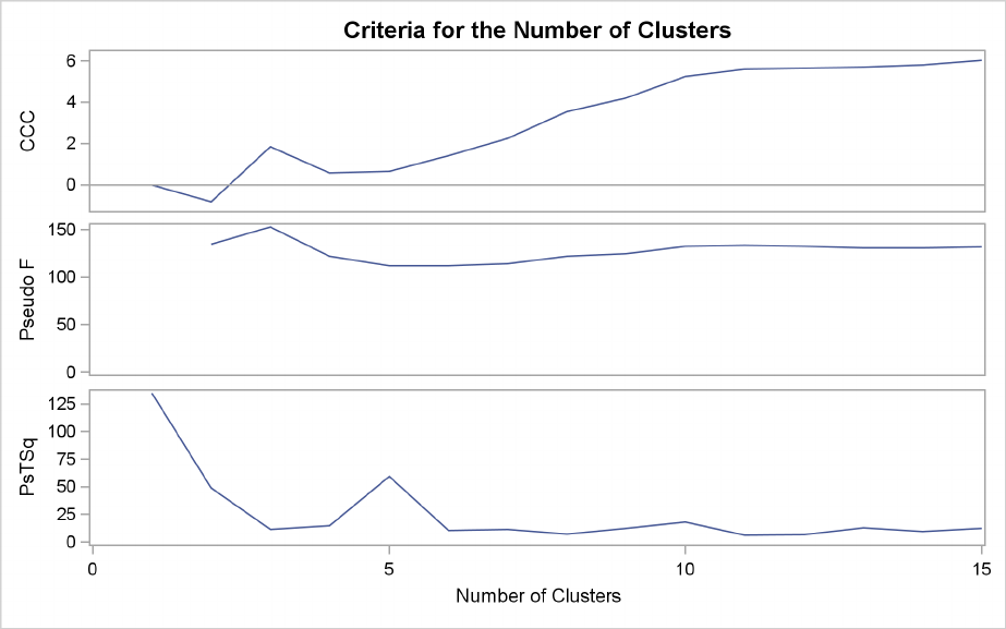
Figure 29.3 plots the three statistics for estimating the number of clusters. Peaks in the plot of the
cubic clustering criterion with values greater than 2 or 3 indicate good clusters; peaks with values
between 0 and 2 indicate possible clusters. Large negative values of the CCC can indicate outliers.
In Figure 29.3, there is a local peak of the CCC when the number of clusters is 3. The CCC drops
at 4 clusters and then steadily increases, leveling off at 11 clusters.
Another method of judging the number of clusters in a data set is to look at the pseudo Fstatistic
(PSF). Relatively large values indicate good numbers of clusters. In Figure 29.3, the pseudo F
statistic suggests 3 clusters or 11 clusters.
Figure 29.3 Plot of Statistics for Estimating the Number of Clusters
1236 FChapter 29: The CLUSTER Procedure
To interpret the values of the pseudo t2statistic, look down the column or look at the plot from
right to left until you find the first value markedly larger than the previous value, then move back
up the column or to the right in the plot by one step in the cluster history. In Figure 29.3, you can
see possibly good clustering levels at 11 clusters, 6 clusters, 3 clusters, and 2 clusters.
Considered together, these statistics suggest that the data can be clustered into 11 clusters or 3
clusters. The following statements examine the results of clustering the data into 3 clusters.
A graphical view of the clustering process can often be helpful in interpreting the clusters. The
following statements use the TREE procedure to produce a tree diagram of the clusters:
goptions vsize=9in hsize=6.4in htext=.9pct htitle=3pct;
axis1 order=(0 to 1 by 0.2);
proc tree data=Tree out=New nclusters=3
haxis=axis1 horizontal;
height _rsq_;
copy can1 can2 ;
id country;
run;
The AXIS1 statement defines axis parameters that are used in the TREE procedure. The ORDER=
option specifies the data values in the order in which they should appear on the axis.
The preceding statements use the SAS data set Tree as input. The OUT= option creates an output
SAS data set named New to contain information about cluster membership. The NCLUSTERS=
option specifies the number of clusters desired in the data set New.
The TREE procedure produces high-resolution graphics by default. The HAXIS= option specifies
AXIS1 to customize the appearance of the horizontal axis. The HORIZONTAL option orients the
tree diagram horizontally. The HEIGHT statement specifies the variable _RSQ_ (R square) as the
height variable.
The COPY statement copies the canonical variables can1 and can2 (computed in the ACECLUS
procedure) into the output SAS data set New. Thus, the SAS output data set New contains informa-
tion for three clusters and the first two of the original canonical variables.
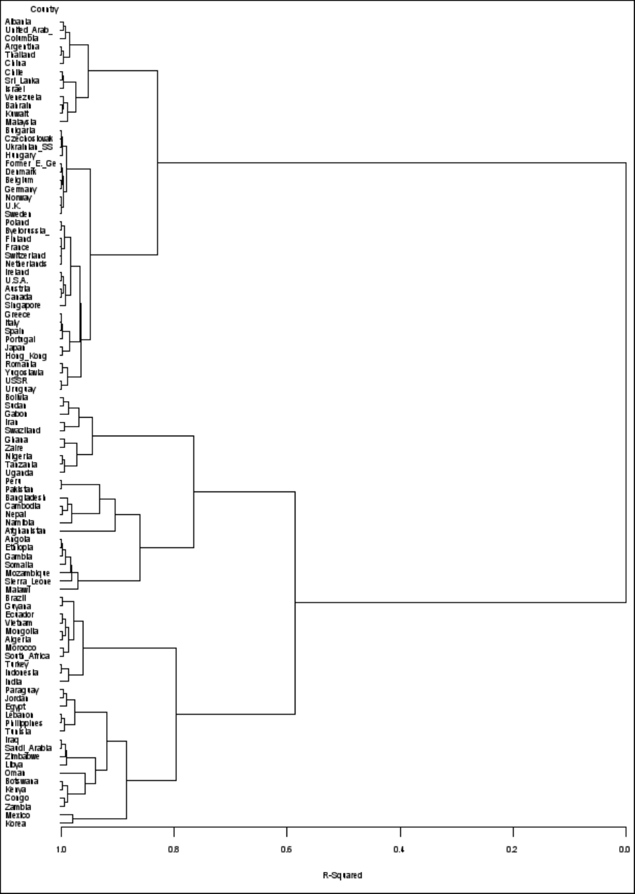
Figure 29.4 displays the tree diagram. The figure provides a graphical view of the information in
Figure 29.2. As the number of branches grows to the left from the root, the R square approaches 1;
the first three clusters (branches of the tree) account for over half of the variation (about 77%, from
Figure 29.4). In other words, only three clusters are necessary to explain over three-fourths of the
variation.
Getting Started: CLUSTER Procedure F1237
Figure 29.4 Tree Diagram of Clusters versus R-Square Values
1238 FChapter 29: The CLUSTER Procedure
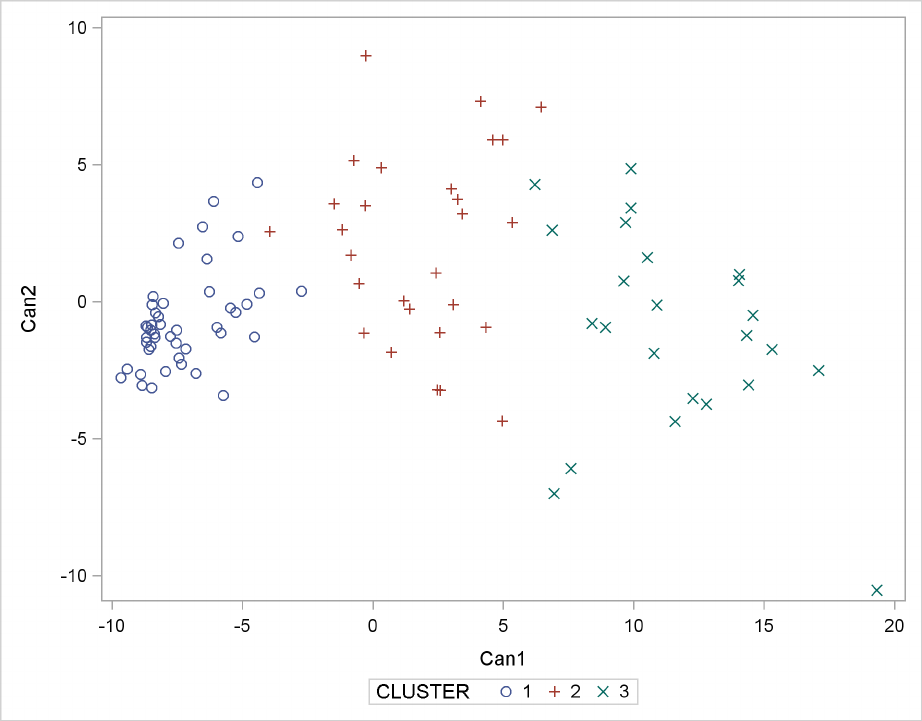
The following statements invoke the SGPLOT procedure on the SAS data set New:
proc sgplot data=New ;
scatter y=can2 x=can1 / group=cluster ;
run;
The PLOT statement requests a plot of the two canonical variables, using the value of the variable
cluster as the identification variable, as shown in Figure 29.5.
Figure 29.5 Plot of Canonical Variables and Cluster for Three Clusters
The statistics in Figure 29.2 and Figure 29.3, the tree diagram in Figure 29.4, and the plot of the
canonical variables in Figure 29.5 assist in the estimation of clusters in the data. There seems
to be reasonable separation in the clusters. However, you must use this information, along with
experience and knowledge of the field, to help in deciding the correct number of clusters.

Syntax: CLUSTER Procedure F1239
Syntax: CLUSTER Procedure
The following statements are available in the CLUSTER procedure:
PROC CLUSTER METHOD = name <options >;
BY variables ;
COPY variables ;
FREQ variable ;
ID variable ;
RMSSTD variable ;
VAR variables ;
Only the PROC CLUSTER statement is required, except that the FREQ statement is required when
the RMSSTD statement is used; otherwise the FREQ statement is optional. Usually only the VAR
statement and possibly the ID and COPY statements are needed in addition to the PROC CLUSTER
statement. The rest of this section provides detailed syntax information for each of the preceding
statements, beginning with the PROC CLUSTER statement. The remaining statements are covered
in alphabetical order.
PROC CLUSTER Statement
PROC CLUSTER METHOD=name <options >;
The PROC CLUSTER statement starts the CLUSTER procedure, specifies a clustering method, and
optionally specifies details for clustering methods, data sets, data processing, and displayed output.
The METHOD= specification determines the clustering method used by the procedure. Any one of
the following 11 methods can be specified for name:
AVERAGE | AVE requests average linkage (group average, unweighted pair-group method
using arithmetic averages, UPGMA). Distance data are squared unless
you specify the NOSQUARE option.
CENTROID | CEN requests the centroid method (unweighted pair-group method using cen-
troids, UPGMC, centroid sorting, weighted-group method). Distance
data are squared unless you specify the NOSQUARE option.
COMPLETE | COM requests complete linkage (furthest neighbor, maximum method, diam-
eter method, rank order typal analysis). To reduce distortion of clusters
by outliers, the TRIM= option is recommended.
DENSITY | DEN requests density linkage, which is a class of clustering methods using
nonparametric probability density estimation. You must also specify
either the K=, R=, or HYBRID option to indicate the type of density
estimation to be used. See also the MODE= and DIM= options in this
section.

1240 FChapter 29: The CLUSTER Procedure
EML requests maximum-likelihood hierarchical clustering for mixtures of
spherical multivariate normal distributions with equal variances but pos-
sibly unequal mixing proportions. Use METHOD=EML only with co-
ordinate data. See the PENALTY= option for details. The NONORM
option does not affect the reported likelihood values but does affect other
unrelated criteria. The EML method is much slower than the other meth-
ods in the CLUSTER procedure.
FLEXIBLE | FLE requests the Lance-Williams flexible-beta method. See the BETA= op-
tion in this section.
MCQUITTY | MCQ requests McQuitty’s similarity analysis (weighted average linkage,
weighted pair-group method using arithmetic averages, WPGMA).
MEDIAN | MED requests Gower’s median method (weighted pair-group method using
centroids, WPGMC). Distance data are squared unless you specify the
NOSQUARE option.
SINGLE | SIN requests single linkage (nearest neighbor, minimum method, con-
nectedness method, elementary linkage analysis, or dendritic
method). To reduce chaining, you can use the TRIM= option with
METHOD=SINGLE.
TWOSTAGE | TWO requests two-stage density linkage. You must also specify the K=, R=,
or HYBRID option to indicate the type of density estimation to be used.
See also the MODE= and DIM= options in this section.
WARD | WAR requests Ward’s minimum-variance method (error sum of squares, trace
W). Distance data are squared unless you specify the NOSQUARE op-
tion. To reduce distortion by outliers, the TRIM= option is recom-
mended. See the NONORM option.
Table 29.1 summarizes the options in the PROC CLUSTER statement.
Table 29.1 PROC CLUSTER Statement Options
Option Description
Specify input and output data sets
DATA= specifies input data set
OUTTREE= creates output data set
Specify clustering methods
METHOD= specifies clustering method
BETA= specifies beta value for flexible beta method
MODE= specifies the minimum number of members for modal
clusters
PENALTY= specifies the penalty coefficient for maximum likelihood
HYBRID specifies Wong’s hybrid clustering method
Control data processing prior to clustering
NOEIGEN suppresses computation of eigenvalues
NONORM suppresses normalizing of distances
NOSQUARE suppresses squaring of distances

PROC CLUSTER Statement F1241
Table 29.1 continued
Option Description
STANDARD standardizes variables
TRIM= omits points with low probability densities
Control density estimation
K= specifies number of neighbors for kth-nearest-neighbor
density estimation
R= specifies radius of sphere of support for uniform-kernel
density estimation
Ties
NOTIE suppresses checking for ties
Control display of the cluster history
CCC displays cubic clustering criterion
NOID suppresses display of ID values
PRINT= specifies number of generations to display
PSEUDO displays pseudo Fand t2statistics
RMSSTD displays root mean square standard deviation
RSQUARE displays R square and semipartial R square
Control other aspects of output
NOPRINT suppresses display of all output
SIMPLE displays simple summary statistics
PLOTS= specifies ODS graphics details
The following list provides details on these options.
BETA=n
specifies the beta parameter for METHOD=FLEXIBLE. The value of nshould be less than 1,
usually between 0 and 1. By default, BETA=0:25. Milligan (1987) suggests a somewhat
smaller value, perhaps 0:5, for data with many outliers.
CCC
displays the cubic clustering criterion and approximate expected R square under the uniform
null hypothesis (Sarle 1983). The statistics associated with the RSQUARE option, R square
and semipartial R square, are also displayed. The CCC option applies only to coordinate
data. The CCC option is not appropriate with METHOD=SINGLE because of the method’s
tendency to chop off tails of distributions. Computation of the CCC requires the eigenvalues
of the covariance matrix. If the number of variables is large, computing the eigenvalues
requires much computer time and memory.
DATA=SAS-data-set
names the input data set containing observations to be clustered. By default, the procedure
uses the most recently created SAS data set. If the data set is TYPE=DISTANCE, the data
are interpreted as a distance matrix; the number of variables must equal the number of ob-
servations in the data set or in each BY group. The distances are assumed to be Euclidean,
but the procedure accepts other types of distances or dissimilarities. If the data set is not
1242 FChapter 29: The CLUSTER Procedure
TYPE=DISTANCE, the data are interpreted as coordinates in a Euclidean space, and Eu-
clidean distances are computed. For more about TYPE=DISTANCE data sets, see Chapter A,
“Special SAS Data Sets.”
You cannot use a TYPE=CORR data set as input to PROC CLUSTER, since the procedure
uses dissimilarity measures. Instead, you can use a DATA step or the IML procedure to extract
the correlation matrix from a TYPE=CORR data set and transform the values to dissimilarities
such as 1ror 1r2, where ris the correlation.
All methods produce the same results when used with coordinate data as when used with
Euclidean distances computed from the coordinates. However, the DIM= option must be
used with distance data if you specify METHOD=TWOSTAGE or METHOD=DENSITY or
if you specify the TRIM= option.
Certain methods that are most naturally defined in terms of coordinates require
squared Euclidean distances to be used in the combinatorial distance formulas (Lance
and Williams 1967). For this reason, distance data are automatically squared when
used with METHOD=AVERAGE, METHOD=CENTROID, METHOD=MEDIAN, or
METHOD=WARD. If you want the combinatorial formulas to be applied to the (unsquared)
distances with these methods, use the NOSQUARE option.
DIM=n
specifies the dimensionality used when computing density estimates with the TRIM= option,
METHOD=DENSITY, or METHOD=TWOSTAGE. The values of nmust be greater than or
equal to 1. The default is the number of variables if the data are coordinates; the default is 1
if the data are distances.
HYBRID
requests Wong’s (1982) hybrid clustering method in which density estimates are computed
from a preliminary cluster analysis using the k-means method. The DATA= data set must
contain means, frequencies, and root mean square standard deviations of the preliminary
clusters (see the FREQ and RMSSTD statements). To use HYBRID, you must use either a
FREQ statement or a DATA= data set that contains a _FREQ_ variable, and you must also use
either an RMSSTD statement or a DATA= data set that contains an _RMSSTD_ variable.
The MEAN= data set produced by the FASTCLUS procedure is suitable for input to
the CLUSTER procedure for hybrid clustering. Since this data set contains _FREQ_ and
_RMSSTD_ variables, you can use it as input and then omit the FREQ and RMSSTD state-
ments.
You must specify either METHOD=DENSITY or METHOD=TWOSTAGE with the HY-
BRID option. You cannot use this option in combination with the TRIM=, K=, or R= option.
K=n
specifies the number of neighbors to use for kth-nearest-neighbor density estimation (Silver-
man 1986, pp. 19–21 and 96–99). The number of neighbors (n) must be at least two but less
than the number of observations. See the MODE= option, which follows.
Density estimation is used with the TRIM=, METHOD=DENSITY, and METHOD=TWOSTAGE
options.
PROC CLUSTER Statement F1243
MODE=n
specifies that, when two clusters are joined, each must have at least nmembers in order for
either cluster to be designated a modal cluster. If you specify MODE=1, each cluster must
also have a maximum density greater than the fusion density in order for either cluster to be
designated a modal cluster.
Use the MODE= option only with METHOD=DENSITY or METHOD=TWOSTAGE. With
METHOD=TWOSTAGE, the MODE= option affects the number of modal clusters formed.
With METHOD=DENSITY, the MODE= option does not affect the clustering process but
does determine the number of modal clusters reported on the output and identified by the
_MODE_ variable in the output data set.
If you specify the K= option, the default value of MODE= is the same as the value of K=
because the use of kth-nearest-neighbor density estimation limits the resolution that can be
obtained for clusters with fewer than kmembers. If you do not specify the K= option, the
default is MODE=2.
If you specify MODE=0, the default value is used instead of 0.
If you specify a FREQ statement or if a _FREQ_ variable appears in the input data set, the
MODE= value is compared with the number of actual observations in the clusters being
joined, not with the sum of the frequencies in the clusters.
NOEIGEN
suppresses computation of the eigenvalues of the covariance matrix and substitutes the vari-
ances of the variables for the eigenvalues when computing the cubic clustering criterion. The
NOEIGEN option saves time if the number of variables is large, but it should be used only if
the variables are nearly uncorrelated. If you specify the NOEIGEN option and the variables
are highly correlated, the cubic clustering criterion might be very liberal. The NOEIGEN
option applies only to coordinate data.
NOID
suppresses the display of ID values for the clusters joined at each generation of the cluster
history.
NONORM
prevents the distances from being normalized to unit mean or unit root mean square with
most methods. With METHOD=WARD, the NONORM option prevents the between-cluster
sum of squares from being normalized by the total sum of squares to yield a squared semi-
partial correlation. The NONORM option does not affect the reported likelihood values with
METHOD=EML, but it does affect other unrelated criteria, such as the _DIST_ variable.
NOPRINT
suppresses the display of all output. Note that this option temporarily disables the Output
Delivery System (ODS). For more information, see Chapter 20, “Using the Output Delivery
System.”
1244 FChapter 29: The CLUSTER Procedure
NOSQUARE
prevents input distances from being squared with METHOD=AVERAGE,
METHOD=CENTROID, METHOD=MEDIAN, or METHOD=WARD.
If you specify the NOSQUARE option with distance data, the data are assumed to be squared
Euclidean distances for computing R-square and related statistics defined in a Euclidean co-
ordinate system.
If you specify the NOSQUARE option with coordinate data with METHOD=CENTROID,
METHOD=MEDIAN, or METHOD=WARD, then the combinatorial formula is applied to
unsquared Euclidean distances. The resulting cluster distances do not have their usual Eu-
clidean interpretation and are therefore labeled “False” in the output.
NOTIE
prevents PROC CLUSTER from checking for ties for minimum distance between clusters at
each generation of the cluster history. If your data are measured with such precision that ties
are unlikely, then you can specify the NOTIE option to reduce slightly the time and space
required by the procedure. See the section “Ties” on page 1261 for more information.
OUTTREE=SAS-data-set
creates an output data set that can be used by the TREE procedure to draw a tree diagram. You
must give the data set a two-level name to save it. See SAS Language Reference: Concepts
for a discussion of permanent data sets. If you omit the OUTTREE= option, the data set is
named by using the DATAnconvention and is not permanently saved. If you do not want to
create an output data set, use OUTTREE=_NULL_.
PENALTY=p
specifies the penalty coefficient used with METHOD=EML. See the section “Clustering
Methods” on page 1250 for more information. Values for pmust be greater than zero. By
default, PENALTY=2.
PLOTS < (global-plot-options) > < = plot-request >
PLOTS < (global-plot-options) > < = (plot-request < ... plot-request >) >
controls the plots produced through ODS Graphics.
PROC CLUSTER can produce line plots of the cubic clustering criterion, the pseudo Fstatis-
tic, and the pseudo t2statistic from the cluster history table. These statistics are useful for
estimating the number of clusters. Each statistic is plotted against the number of clusters.
To obtain ODS Graphics plots from PROC CLUSTER, you must do two things. First, enable
ODS Graphics before running PROC CLUSTER. For example:
ods graphics on;
proc cluster plots=all;
run;
ods graphics off;
Second, request that PROC CLUSTER compute the desired statistics by specifying the CCC
or PSEUDO options, or by specifying the statistics in a plot-request in the PLOT option.
PROC CLUSTER Statement F1245
PROC CLUSTER might be unable to compute the statistics in some cases; for details, see the
CCC and PSEUDO options. If a statistic cannot be computed, it cannot be plotted. PROC
CLUSTER plots all of these statistics that are computed unless you tell it specifically what to
plot using PLOTS=.
The maximum number of clusters shown in all the plots is the minimum of the following
quantities:
the number of observations
the value of the PRINT= option, if that option is specified
the maximum number of clusters for which CCC is computed, if CCC is plotted
The global-plot-options apply to all plots generated by the CLUSTER procedure. The global
plot options are as follows:
UNPACKPANELS breaks a plot that is otherwise paneled into plots separate plots for each
statistic. This option can be abbreviated as UNPACK.
ONLY has no effect, but is accepted for consistency with other procedures.
The following plot-requests can be specified:
ALL implicitly specifies the CCC and PSEUDO options and, if possible, pro-
duces all three plots.
NONE suppresses all plots.
CCC implicitly specifies the CCC option and, if possible, plots the cubic clus-
tering criterion against the number of clusters.
PSEUDO implicitly specifies the PSEUDO option and, if possible, plots the pseudo
Fstatistic and the pseudo t2statistic against the number of clusters.
PSF implicitly specifies the PSEUDO option and, if possible, plots the pseudo
Fstatistic against the number of clusters.
PST2 implicitly specifies the PSEUDO option and, if possible, plots the pseudo
t2statistic against the number of clusters.
When you specify only one plot-request, you can omit the parentheses around the plot-
request. You can specify one or more of the CCC, PSEUDO, PSF, or PST2 plot requests
in the same PLOT option. For example, all of the following are valid:
PROC CLUSTER PLOTS=(CCC PST2);
PROC CLUSTER PLOTS=(PSF);
PROC CLUSTER PLOTS=PSF;
The first statement plots both the cubic clustering criterion and the pseudo t2statistic, while
the second and third statements plot the pseudo Fstatistic only.
The names of the graphs that PROC CLUSTER generates are listed in Table 29.5, along with
the required statements and options.
1246 FChapter 29: The CLUSTER Procedure
PRINT=n| P=n
specifies the number of generations of the cluster history to display. The P= option displays
the latest ngenerations; for example, P=5 displays the cluster history from 1 cluster through
5 clusters. The value of P= must be a nonnegative integer. The default is to display all
generations. Specify PRINT=0 to suppress the cluster history.
PSEUDO
displays pseudo Fand t2statistics. This option is effective only when the data are coor-
dinates or when METHOD=AVERAGE, METHOD=CENTROID, or METHOD=WARD is
specified. See the section “Miscellaneous Formulas” on page 1258 for more information.
The PSEUDO option is not appropriate with METHOD=SINGLE because of the method’s
tendency to chop off tails of distributions.
R=n
specifies the radius of the sphere of support for uniform-kernel density estimation (Silverman
1986, pp. 11–13 and 75–94). The value of R= must be greater than zero.
Density estimation is used with the TRIM=, METHOD=DENSITY, and METHOD=TWOSTAGE
options.
RMSSTD
displays the root mean square standard deviation of each cluster. This option is effective only
when the data are coordinates or when METHOD=AVERAGE, METHOD=CENTROID, or
METHOD=WARD is specified.
See the section “Miscellaneous Formulas” on page 1258 for more information.
RSQUARE | RSQ
displays the R square and semipartial R square. This option is effective only when the data
are coordinates or when METHOD=AVERAGE or METHOD=CENTROID is specified. The
R square and semipartial R square statistics are always displayed with METHOD=WARD.
See the section “Miscellaneous Formulas” on page 1258 for more information..
SIMPLE | S
displays means, standard deviations, skewness, kurtosis, and a coefficient of bimodality. The
SIMPLE option applies only to coordinate data. See the section “Miscellaneous Formulas”
on page 1258 for more information.
STANDARD | STD
standardizes the variables to mean 0 and standard deviation 1. The STANDARD option ap-
plies only to coordinate data.
TRIM=p
omits points with low estimated probability densities from the analysis. Valid values for the
TRIM= option are 0p < 100. If p < 1, then pis the proportion of observations omitted.
If p1, then pis interpreted as a percentage. A specification of TRIM=10, which trims
10% of the points, is a reasonable value for many data sets. Densities are estimated by the
kth-nearest-neighbor or uniform-kernel method. Trimmed points are indicated by a negative
value of the _FREQ_ variable in the OUTTREE= data set.

BY Statement F1247
You must use either the K= or R= option when you use TRIM=. You cannot use the HYBRID
option in combination with TRIM=, so you might want to use the DIM= option instead. If you
specify the STANDARD option in combination with TRIM=, the variables are standardized
both before and after trimming.
The TRIM= option is useful for removing outliers and reducing chaining. Trimming is
highly recommended with METHOD=WARD or METHOD=COMPLETE because clus-
ters from these methods can be severely distorted by outliers. Trimming is also valuable
with METHOD=SINGLE since single linkage is the method most susceptible to chaining.
Most other methods also benefit from trimming. However, trimming is unnecessary with
METHOD=TWOSTAGE or METHOD=DENSITY when kth-nearest-neighbor density esti-
mation is used.
Use of the TRIM= option can spuriously inflate the cubic clustering criterion and the pseudo
Fand t2statistics. Trimming only outliers improves the accuracy of the statistics, but trim-
ming saddle regions between clusters yields excessively large values.
BY Statement
BY variables ;
You can specify a BY statement with PROC CLUSTER to obtain separate analyses on observations
in groups defined by the BY variables. When a BY statement appears, the procedure expects the
input data set to be sorted in order of the BY variables.
If your input data set is not sorted in ascending order, use one of the following alternatives:
Sort the data by using the SORT procedure with a similar BY statement.
Specify the BY statement option NOTSORTED or DESCENDING in the BY statement for
the CLUSTER procedure. The NOTSORTED option does not mean that the data are unsorted
but rather that the data are arranged in groups (according to values of the BY variables) and
that these groups are not necessarily in alphabetical or increasing numeric order.
Create an index on the BY variables by using the DATASETS procedure.
For more information about the BY statement, see SAS Language Reference: Concepts.
For more information about the DATASETS procedure, see the Base SAS Procedures Guide.
COPY Statement
COPY variables ;
The variables in the COPY statement are copied from the input data set to the OUTTREE= data set.
Observations in the OUTTREE= data set that represent clusters of more than one observation from
the input data set have missing values for the COPY variables.

1248 FChapter 29: The CLUSTER Procedure
FREQ Statement
FREQ variable ;
If one variable in the input data set represents the frequency of occurrence for other values in the
observation, specify the variable’s name in a FREQ statement. PROC CLUSTER then treats the
data set as if each observation appeared ntimes, where nis the value of the FREQ variable for the
observation. Noninteger values of the FREQ variable are truncated to the largest integer less than
the FREQ value.
If you omit the FREQ statement but the DATA= data set contains a variable called _FREQ_, then
frequencies are obtained from the _FREQ_ variable. If neither a FREQ statement nor an _FREQ_
variable is present, each observation is assumed to have a frequency of one.
If each observation in the DATA= data set represents a cluster (for example, clusters formed by
PROC FASTCLUS), the variable specified in the FREQ statement should give the number of origi-
nal observations in each cluster.
If you specify the RMSSTD statement, a FREQ statement is required. A FREQ statement or
_FREQ_ variable is required when you specify the HYBRID option.
With most clustering methods, the same clusters are obtained from a data set with a FREQ variable
as from a similar data set without a FREQ variable, if each observation is repeated as many times
as the value of the FREQ variable in the first data set. The FLEXIBLE method can yield different
results due to the nature of the combinatorial formula. The DENSITY and TWOSTAGE methods
are also exceptions because two identical observations can be absorbed one at a time by a cluster
with a higher density. If you are using a FREQ statement with either the DENSITY or TWOSTAGE
method, see the MODE=option for details.
ID Statement
ID variable ;
The values of the ID variable identify observations in the displayed cluster history and in the OUT-
TREE= data set. If the ID statement is omitted, each observation is denoted by OBn, where nis the
observation number.

RMSSTD Statement F1249
RMSSTD Statement
RMSSTD variable ;
If the coordinates in the DATA= data set represent cluster means (for example, formed by
the FASTCLUS procedure), you can obtain accurate statistics in the cluster histories for
METHOD=AVERAGE, METHOD=CENTROID, or METHOD=WARD if the data set contains
both of the following:
a variable giving the number of original observations in each cluster (see the discussion of
the FREQ statement earlier in this chapter)
a variable giving the root mean squared standard deviation of each cluster
Specify the name of the variable containing root mean squared standard deviations in the RMSSTD
statement. If you specify the RMSSTD statement, you must also specify a FREQ statement.
If you omit the RMSSTD statement but the DATA= data set contains a variable called _RMSSTD_,
then the root mean squared standard deviations are obtained from the _RMSSTD_ variable.
An RMSSTD statement or _RMSSTD_ variable is required when you specify the HYBRID option.
A data set created by PROC FASTCLUS, using the MEAN= option, contains _FREQ_ and
_RMSSTD_ variables, so you do not have to use FREQ and RMSSTD statements when using such
a data set as input to the CLUSTER procedure.
VAR Statement
VAR variables ;
The VAR statement lists numeric variables to be used in the cluster analysis. If you omit the VAR
statement, all numeric variables not listed in other statements are used.

1250 FChapter 29: The CLUSTER Procedure
Details: CLUSTER Procedure
Clustering Methods
The following notation is used, with lowercase symbols generally pertaining to observations and
uppercase symbols pertaining to clusters:
nnumber of observations
vnumber of variables if data are coordinates
Gnumber of clusters at any given level of the hierarchy
xior xiith observation (row vector if coordinate data)
CKKth cluster, subset of f1; 2; : : : ; ng
NKnumber of observations in CK
N
xsample mean vector
N
xKmean vector for cluster CK
kxkEuclidean length of the vector x—that is, the square root of the sum of the squares
of the elements of x
TPn
iD1kxiN
xk2
WKPi2CkkxiN
xKk2
PGPWJ, where summation is over the Gclusters at the Gth level of the hierarchy
BKL WMWKWLif CMDCK[CL
d.x;y/any distance or dissimilarity measure between observations or vectors xand y
DKL any distance or dissimilarity measure between clusters CKand CL
The distance between two clusters can be defined either directly or combinatorially (Lance and
Williams 1967)—that is, by an equation for updating a distance matrix when two clusters are joined.
In all of the following combinatorial formulas, it is assumed that clusters CKand CLare merged
to form CM, and the formula gives the distance between the new cluster CMand any other cluster
CJ.
For an introduction to most of the methods used in the CLUSTER procedure, see Massart and
Kaufman (1983).
Average Linkage
The following method is obtained by specifying METHOD=AVERAGE. The distance between two
clusters is defined by
DKL D1
NKNLX
i2CKX
j2CL
d.xi; xj/

Clustering Methods F1251
If d.x;y/D kxyk2, then
DKL D kN
xKN
xLk2CWK
NKCWL
NL
The combinatorial formula is
DJM DNKDJK CNLDJL
NM
In average linkage the distance between two clusters is the average distance between pairs of ob-
servations, one in each cluster. Average linkage tends to join clusters with small variances, and it is
slightly biased toward producing clusters with the same variance.
Average linkage was originated by Sokal and Michener (1958).
Centroid Method
The following method is obtained by specifying METHOD=CENTROID. The distance between
two clusters is defined by
DKL D kN
xKN
xLk2
If d.x;y/D kxyk2, then the combinatorial formula is
DJM DNKDJK CNLDJL
NMNKNLDKL
N2
M
In the centroid method, the distance between two clusters is defined as the (squared) Euclidean
distance between their centroids or means. The centroid method is more robust to outliers than
most other hierarchical methods but in other respects might not perform as well as Ward’s method
or average linkage (Milligan 1980).
The centroid method was originated by Sokal and Michener (1958).
Complete Linkage
The following method is obtained by specifying METHOD=COMPLETE. The distance between
two clusters is defined by
DKL Dmax
i2CK
max
j2CL
d.xi; xj/
The combinatorial formula is
DJM Dmax.DJK ; DJL/
In complete linkage, the distance between two clusters is the maximum distance between an obser-
vation in one cluster and an observation in the other cluster. Complete linkage is strongly biased
toward producing clusters with roughly equal diameters, and it can be severely distorted by moder-
ate outliers (Milligan 1980).
Complete linkage was originated by Sorensen (1948).

1252 FChapter 29: The CLUSTER Procedure
Density Linkage
The phrase density linkage is used here to refer to a class of clustering methods that use nonpara-
metric probability density estimates (for example, Hartigan 1975, pp. 205–212; Wong 1982; Wong
and Lane 1983). Density linkage consists of two steps:
1. A new dissimilarity measure, d, based on density estimates and adjacencies is computed.
If xiand xjare adjacent (the definition of adjacency depends on the method of density
estimation), then d.xi; xj/is the reciprocal of an estimate of the density midway between
xiand xj; otherwise, d.xi; xj/is infinite.
2. A single linkage cluster analysis is performed using d.
The CLUSTER procedure supports three types of density linkage: the kth-nearest-neighbor
method, the uniform-kernel method, and Wong’s hybrid method. These are obtained by using
METHOD=DENSITY and the K=, R=, and HYBRID options, respectively.
kth-Nearest-Neighbor Method
The kth-nearest-neighbor method (Wong and Lane 1983) uses kth-nearest-neighbor density esti-
mates. Let rk.x/ be the distance from point xto the kth-nearest observation, where kis the value
specified for the K= option. Consider a closed sphere centered at xwith radius rk.x/. The estimated
density at x,f .x/, is the proportion of observations within the sphere divided by the volume of the
sphere. The new dissimilarity measure is computed as
d.xi; xj/D8
<
:
1
21
f .xi/C1
f .xj/if d.xi; xj/max.rk.xi/; rk.xj//
1otherwise
Wong and Lane (1983) show that kth-nearest-neighbor density linkage is strongly set consistent
for high-density (density-contour) clusters if kis chosen such that k=n !0and k= ln.n/ ! 1
as n! 1. Wong and Schaack (1982) discuss methods for estimating the number of population
clusters by using kth-nearest-neighbor clustering.
Uniform-Kernel Method
The uniform-kernel method uses uniform-kernel density estimates. Let rbe the value specified for
the R= option. Consider a closed sphere centered at point xwith radius r. The estimated density
at x,f .x/, is the proportion of observations within the sphere divided by the volume of the sphere.
The new dissimilarity measure is computed as
d.xi; xj/D8
<
:
1
21
f .xi/C1
f .xj/if d.xi; xj/r
1otherwise
Wong’s Hybrid Method
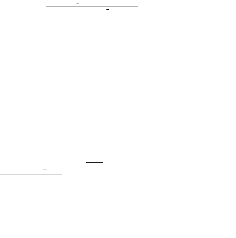
Wong’s (1982) hybrid clustering method uses density estimates based on a preliminary cluster anal-
ysis by the k-means method. The preliminary clustering can be done by the FASTCLUS procedure,
Clustering Methods F1253
by using the MEAN= option to create a data set containing cluster means, frequencies, and root
mean squared standard deviations. This data set is used as input to the CLUSTER procedure, and
the HYBRID option is specified with METHOD=DENSITY to request the hybrid analysis. The
hybrid method is appropriate for very large data sets but should not be used with small data sets—
say, than those with fewer than 100 observations in the original data. The term preliminary cluster
refers to an observation in the DATA= data set.
For preliminary cluster CK,NKand WKare obtained from the input data set, as are the cluster
means or the distances between the cluster means. Preliminary clusters CKand CLare considered
adjacent if the midpoint between NxKand N
xLis closer to either N
xKor N
xLthan to any other pre-
liminary cluster mean or, equivalently, if d2.N
xK;N
xL/<d2.N
xK;N
xM/Cd2.N
xL;N
xM/for all other
preliminary clusters CM,M¤Kor L. The new dissimilarity measure is computed as
d.N
xK;N
xL/D8
<
:
.WKCWLC1
4.NKCNL/d 2.NxK;NxL//v
2
.NKCNL/1Cv
2if CKand CLare adjacent
1otherwise
Using the K= and R= Options
The values of the K= and R= options are called smoothing parameters. Small values of K= or
R= produce jagged density estimates and, as a consequence, many modes. Large values of K= or
R= produce smoother density estimates and fewer modes. In the hybrid method, the smoothing
parameter is the number of clusters in the preliminary cluster analysis. The number of modes in
the final analysis tends to increase as the number of clusters in the preliminary analysis increases.
Wong (1982) suggests using n0:3 preliminary clusters, where nis the number of observations in the
original data set. There is no rule of thumb for selecting K= values. For all types of density linkage,
you should repeat the analysis with several different values of the smoothing parameter (Wong and
Schaack 1982).
There is no simple answer to the question of which smoothing parameter to use (Silverman 1986,
pp. 43–61, 84–88, and 98–99). It is usually necessary to try several different smoothing parameters.
A reasonable first guess for the R= option in many coordinate data sets is given by
"2vC2.v C2/. v
2C1/
nv2#1
vC4v
u
u
t
v
X
lD1
s2
l
where s2
lis the standard deviation of the lth variable. The estimate for R= can be computed in a
DATA step by using the GAMMA function for . This formula is derived under the assumption that
the data are sampled from a multivariate normal distribution and tends, therefore, to be too large
(oversmooth) if the true distribution is multimodal. Robust estimates of the standard deviations can
be preferable if there are outliers. If the data are distances, the factor Ps2
lcan be replaced by an
average (mean, trimmed mean, median, root mean square, and so on) distance divided by p2. To
prevent outliers from appearing as separate clusters, you can also specify K=2, or more generally
K=m,m2, which in most cases forces clusters to have at least mmembers.
If the variables all have unit variance (for example, if the STANDARD option is used), Table 29.2
can be used to obtain an initial guess for the R= option.

1254 FChapter 29: The CLUSTER Procedure
Since infinite dvalues occur in density linkage, the final number of clusters can exceed one when
there are wide gaps between the clusters or when the smoothing parameter results in little smooth-
ing.
Density linkage applies no constraints to the shapes of the clusters and, unlike most other hier-
archical clustering methods, is capable of recovering clusters with elongated or irregular shapes.
Since density linkage uses less prior knowledge about the shape of the clusters than do methods
restricted to compact clusters, density linkage is less effective at recovering compact clusters from
small samples than are methods that always recover compact clusters, regardless of the data.
Table 29.2 Reasonable First Guess for the R= Option for Standardized Data
Number of Number of Variables
Observations 12345678910
20 1.01 1.36 1.77 2.23 2.73 3.25 3.81 4.38 4.98 5.60
35 0.91 1.24 1.64 2.08 2.56 3.08 3.62 4.18 4.77 5.38
50 0.84 1.17 1.56 1.99 2.46 2.97 3.50 4.06 4.64 5.24
75 0.78 1.09 1.47 1.89 2.35 2.85 3.38 3.93 4.50 5.09
100 0.73 1.04 1.41 1.82 2.28 2.77 3.29 3.83 4.40 4.99
150 0.68 0.97 1.33 1.73 2.18 2.66 3.17 3.71 4.27 4.85
200 0.64 0.93 1.28 1.67 2.11 2.58 3.09 3.62 4.17 4.75
350 0.57 0.85 1.18 1.56 1.98 2.44 2.93 3.45 4.00 4.56
500 0.53 0.80 1.12 1.49 1.91 2.36 2.84 3.35 3.89 4.45
750 0.49 0.74 1.06 1.42 1.82 2.26 2.74 3.24 3.77 4.32
1000 0.46 0.71 1.01 1.37 1.77 2.20 2.67 3.16 3.69 4.23
1500 0.43 0.66 0.96 1.30 1.69 2.11 2.57 3.06 3.57 4.11
2000 0.40 0.63 0.92 1.25 1.63 2.05 2.50 2.99 3.49 4.03
EML
The following method is obtained by specifying METHOD=EML. The distance between two clus-
ters is given by
DKL Dnv ln 1CBKL
PG2.NMln.NM/NKln.NK/NLln.NL//
The EML method joins clusters to maximize the likelihood at each level of the hierarchy under the
following assumptions:
multivariate normal mixture
equal spherical covariance matrices
unequal sampling probabilities

Clustering Methods F1255
The EML method is similar to Ward’s minimum-variance method but removes the bias toward
equal-sized clusters. Practical experience has indicated that EML is somewhat biased toward
unequal-sized clusters. You can specify the PENALTY= option to adjust the degree of bias. If
you specify PENALTY=p, the formula is modified to
DKL Dnv ln 1CBKL
PGp.NMln.NM/NKln.NK/NLln.NL//
The EML method was derived by W. S. Sarle of SAS Institute from the maximum likelihood for-
mula obtained by Symons (1981, p. 37, Equation 8) for disjoint clustering. There are currently no
other published references on the EML method.
Flexible-Beta Method
The following method is obtained by specifying METHOD=FLEXIBLE. The combinatorial for-
mula is
DJM D.DJK CDJL/1b
2CDKLb
where bis the value of the BETA= option, or 0:25 by default.
The flexible-beta method was developed by Lance and Williams (1967); see also Milligan (1987).
McQuitty’s Similarity Analysis
The following method is obtained by specifying METHOD=MCQUITTY. The combinatorial for-
mula is
DJM DDJK CDJL
2
The method was independently developed by Sokal and Michener (1958) and McQuitty (1966).
Median Method
The following method is obtained by specifying METHOD=MEDIAN. If d.x;y/D kxyk2, then
the combinatorial formula is
DJM DDJK CDJL
2DKL
4
The median method was developed by Gower (1967).
Single Linkage
The following method is obtained by specifying METHOD=SINGLE. The distance between two
clusters is defined by
DKL Dmin
i2CK
min
j2CL
d.xi; xj/
1256 FChapter 29: The CLUSTER Procedure
The combinatorial formula is
DJM Dmin.DJK ; DJL/
In single linkage, the distance between two clusters is the minimum distance between an observation
in one cluster and an observation in the other cluster. Single linkage has many desirable theoretical
properties (Jardine and Sibson 1971; Fisher and Van Ness 1971; Hartigan 1981) but has fared poorly
in Monte Carlo studies (for example, Milligan 1980). By imposing no constraints on the shape of
clusters, single linkage sacrifices performance in the recovery of compact clusters in return for
the ability to detect elongated and irregular clusters. You must also recognize that single linkage
tends to chop off the tails of distributions before separating the main clusters (Hartigan 1981). The
notorious chaining tendency of single linkage can be alleviated by specifying the TRIM= option
(Wishart 1969, pp. 296–298).
Density linkage and two-stage density linkage retain most of the virtues of single linkage while
performing better with compact clusters and possessing better asymptotic properties (Wong and
Lane 1983).
Single linkage was originated by Florek et al. (1951a, 1951b) and later reinvented by McQuitty
(1957) and Sneath (1957).
Two-Stage Density Linkage
If you specify METHOD=DENSITY, the modal clusters often merge before all the points in the
tails have clustered. The option METHOD=TWOSTAGE is a modification of density linkage that
ensures that all points are assigned to modal clusters before the modal clusters are permitted to
join. The CLUSTER procedure supports the same three varieties of two-stage density linkage as of
ordinary density linkage: kth-nearest neighbor, uniform kernel, and hybrid.
In the first stage, disjoint modal clusters are formed. The algorithm is the same as the single linkage
algorithm ordinarily used with density linkage, with one exception: two clusters are joined only if at
least one of the two clusters has fewer members than the number specified by the MODE= option.
At the end of the first stage, each point belongs to one modal cluster.
In the second stage, the modal clusters are hierarchically joined by single linkage. The final number
of clusters can exceed one when there are wide gaps between the clusters or when the smoothing
parameter is small.
Each stage forms a tree that can be plotted by the TREE procedure. By default, the TREE pro-
cedure plots the tree from the first stage. To obtain the tree for the second stage, use the option
HEIGHT=MODE in the PROC TREE statement. You can also produce a single tree diagram con-
taining both stages, with the number of clusters as the height axis, by using the option HEIGHT=N
in the PROC TREE statement. To produce an output data set from PROC TREE containing the
modal clusters, use _HEIGHT_ for the HEIGHT variable (the default) and specify LEVEL=0.
Two-stage density linkage was developed by W. S. Sarle of SAS Institute. There are currently no
other published references on two-stage density linkage.

Clustering Methods F1257
Ward’s Minimum-Variance Method
The following method is obtained by specifying METHOD=WARD. The distance between two
clusters is defined by
DKL DBKL DkN
xKN
xLk2
1
NKC1
NL
If d.x;y/D1
2kxyk2, then the combinatorial formula is
DJM D.NJCNK/DJK C.NJCNL/DJL NJDKL
NJCNM
In Ward’s minimum-variance method, the distance between two clusters is the ANOVA sum of
squares between the two clusters added up over all the variables. At each generation, the within-
cluster sum of squares is minimized over all partitions obtainable by merging two clusters from the
previous generation. The sums of squares are easier to interpret when they are divided by the total
sum of squares to give proportions of variance (squared semipartial correlations).
Ward’s method joins clusters to maximize the likelihood at each level of the hierarchy under the
following assumptions:
multivariate normal mixture
equal spherical covariance matrices
equal sampling probabilities
Ward’s method tends to join clusters with a small number of observations, and it is strongly biased
toward producing clusters with roughly the same number of observations. It is also very sensitive
to outliers (Milligan 1980).
Ward (1963) describes a class of hierarchical clustering methods including the minimum variance
method.

1258 FChapter 29: The CLUSTER Procedure
Miscellaneous Formulas
The root mean squared standard deviation of a cluster CKis
RMSSTD DsWK
v.NK1/
The R-square statistic for a given level of the hierarchy is
R2D1PG
T
The squared semipartial correlation for joining clusters CKand CLis
semipartial R2DBKL
T
The bimodality coefficient is
bDm2
3C1
m4C3.n1/2
.n2/.n3/
where m3is skewness and m4is kurtosis. Values of bgreater than 0.555 (the value for a uniform
population) can indicate bimodal or multimodal marginal distributions. The maximum of 1.0 (ob-
tained for the Bernoulli distribution) is obtained for a population with only two distinct values. Very
heavy-tailed distributions have small values of bregardless of the number of modes.
Formulas for the cubic-clustering criterion and approximate expected R square are given in Sarle
(1983).
The pseudo Fstatistic for a given level is
pseudo FD
TPG
G1
PG
nG
The pseudo t2statistic for joining CKand CLis
pseudo t2DBKL
WKCWL
NKCNL2
The pseudo Fand t2statistics can be useful indicators of the number of clusters, but they are not
distributed as Fand t2random variables. If the data are independently sampled from a multi-
variate normal distribution with a scalar covariance matrix and if the clustering method allocates
observations to clusters randomly (which no clustering method actually does), then the pseudo F
statistic is distributed as an Frandom variable with v.G 1/ and v.n G/ degrees of freedom.
Under the same assumptions, the pseudo t2statistic is distributed as an Frandom variable with v
and v.NKCNL2/ degrees of freedom. The pseudo t2statistic differs computationally from
Hotelling’s T2in that the latter uses a general symmetric covariance matrix instead of a scalar
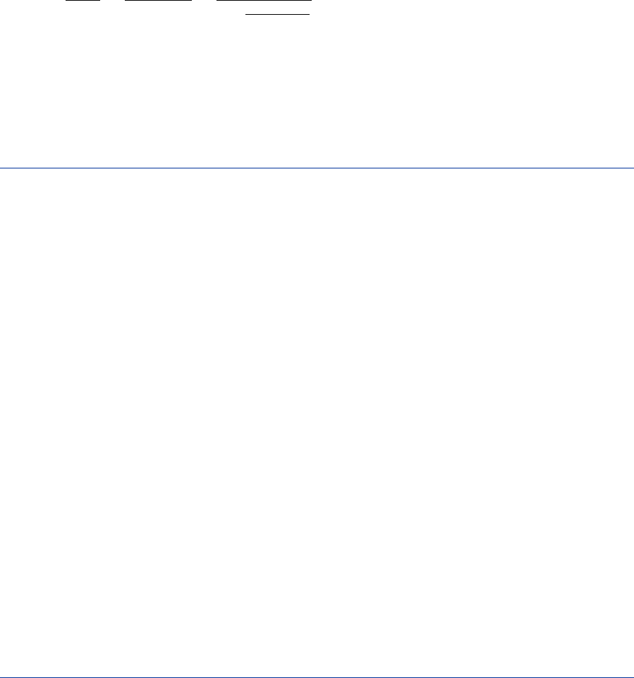
Ultrametrics F1259
covariance matrix. The pseudo Fstatistic was suggested by Calinski and Harabasz (1974). The
pseudo t2statistic is related to the Je.2/=Je.1/ statistic of Duda and Hart (1973) by
Je.2/
Je.1/ DWKCWL
WMD1
1Ct2
NKCNL2
See Milligan and Cooper (1985) and Cooper and Milligan (1988) regarding the performance of
these statistics in estimating the number of population clusters. Conservative tests for the number of
clusters using the pseudo Fand t2statistics can be obtained by the Bonferroni approach (Hawkins,
Muller, and ten Krooden 1982, pp. 337–340).
Ultrametrics
A dissimilarity measure d.x; y/ is called an ultrametric if it satisfies the following conditions:
d.x; x/ D0for all x
d.x; y/ 0for all x,y
d.x; y/ Dd.y; x/ for all x,y
d.x; y/ max .d.x; z/; d.y; z//for all x,y, and z
Any hierarchical clustering method induces a dissimilarity measure on the observations—say,
h.xi; xj/. Let CMbe the cluster with the fewest members that contains both xiand xj. Assume
CMwas formed by joining CKand CL. Then define h.xi; xj/DDKL.
If the fusion of CKand CLreduces the number of clusters from gto g1, then define D.g/ DDKL.
Johnson (1967) shows that if
0D.n/ D.n1/ D.2/
then h.;/is an ultrametric. A method that always satisfies this condition is said to be a monotonic
or ultrametric clustering method. All methods implemented in PROC CLUSTER except CEN-
TROID, EML, and MEDIAN are ultrametric (Milligan 1979; Batagelj 1981).
Algorithms
Anderberg (1973) describes three algorithms for implementing agglomerative hierarchical cluster-
ing: stored data, stored distance, and sorted distance. The algorithms used by PROC CLUSTER for
each method are indicated in Table 29.3. For METHOD=AVERAGE, METHOD=CENTROID, or
METHOD=WARD, either the stored data or the stored distance algorithm can be used. For these
methods, if the data are distances or if you specify the NOSQUARE option, the stored distance
algorithm is used; otherwise, the stored data algorithm is used.
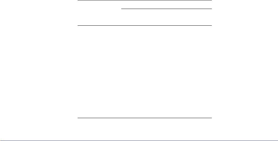
1260 FChapter 29: The CLUSTER Procedure
Table 29.3 Three Algorithms for Implementing Agglomerative Hierarchical Clustering
Algorithm
Stored Stored Stored Sorted
Method Data Distance Distance
AVERAGE x x
CENTROID x x
COMPLETE x
DENSITY x
EML x
FLEXIBLE x
MCQUITTY x
MEDIAN x
SINGLE x
TWOSTAGE x
WARD x x
Computational Resources
The CLUSTER procedure stores the data (including the COPY and ID variables) in memory or,
if necessary, on disk. If eigenvalues are computed, the covariance matrix is stored in memory. If
the stored distance or sorted distance algorithm is used, the distances are stored in memory or, if
necessary, on disk.
With coordinate data, the increase in CPU time is roughly proportional to the number of variables.
The VAR statement should list the variables in order of decreasing variance for greatest efficiency.
For both coordinate and distance data, the dominant factor determining CPU time is the number
of observations. For density methods with coordinate data, the asymptotic time requirements are
somewhere between nln.n/ and n2, depending on how the smoothing parameter increases. For
other methods except EML, time is roughly proportional to n2. For the EML method, time is
roughly proportional to n3.
PROC CLUSTER runs much faster if the data can be stored in memory and, when the stored dis-
tance algorithm is used, if the distance matrix can be stored in memory as well. To estimate the bytes
of memory needed for the data, use the following formula and round up to the nearest multiple of
d.

Missing Values F1261
n.vd C8d Ci
Ciif density estimation or the
sorted distance algorithm is used
C3d if stored data algorithm is used
C3d if density estimation is used
Cmax(8, length of ID variable) if ID variable is used
Clength of ID variable if ID variable is used
Csum of lengths of COPY variables) if COPY variables is used
where
nis the number of observations
vis the number of variables
dis the size of a C variable of type double. For most computers, dD8.
iis the size of a C variable of type int. For most computers, iD4.
The number of bytes needed for the distance matrix is d n.n C1/=2.
Missing Values
If the data are coordinates, observations with missing values are excluded from the analysis. If the
data are distances, missing values are not permitted in the lower triangle of the distance matrix. The
upper triangle is ignored. For more about TYPE=DISTANCE data sets, see Chapter A, “Special
SAS Data Sets.”
Ties
At each level of the clustering algorithm, PROC CLUSTER must identify the pair of clusters with
the minimum distance. Sometimes, usually when the data are discrete, there can be two or more
pairs with the same minimum distance. In such cases the tie must be broken in some arbitrary way.
If there are ties, then the results of the cluster analysis depend on the order of the observations in
the data set. The presence of ties is reported in the SAS log and in the column of the cluster history
labeled “Tie” unless the NOTIE option is specified.
PROC CLUSTER breaks ties as follows. Each cluster is identified by the smallest observation
number among its members. For each pair of clusters, there is a smaller identification number and a
larger identification number. If two or more pairs of clusters are tied for minimum distance between
clusters, the pair that has the minimum larger identification number is merged. If there is a tie for
minimum larger identification number, the pair that has the minimum smaller identification number
is merged.

1262 FChapter 29: The CLUSTER Procedure
A tie means that the level in the cluster history at which the tie occurred and possibly some of the
subsequent levels are not uniquely determined. Ties that occur early in the cluster history usually
have little effect on the later stages. Ties that occur in the middle part of the cluster history are cause
for further investigation. Ties that occur late in the cluster history indicate important indetermina-
cies.
The importance of ties can be assessed by repeating the cluster analysis for several different random
permutations of the observations. The discrepancies at a given level can be examined by crosstabu-
lating the clusters obtained at that level for all of the permutations. See Example 29.4 for details.
Size, Shape, and Correlation
In some biological applications, the organisms that are being clustered can be at different stages of
growth. Unless it is the growth process itself that is being studied, differences in size among such
organisms are not of interest. Therefore, distances among organisms should be computed in such a
way as to control for differences in size while retaining information about differences in shape.
If coordinate data are measured on an interval scale, you can control for size by subtracting a
measure of the overall size of each observation from each data item. For example, if no other direct
measure of size is available, you could subtract the mean of each row of the data matrix, producing
a row-centered coordinate matrix. An easy way to subtract the mean of each row is to use PROC
STANDARD on the transposed coordinate matrix:
proc transpose data= coordinate-datatype ;
proc standard m=0;
proc transpose out=row-centered-coordinate-data;
Another way to remove size effects from interval-scale coordinate data is to do a principal compo-
nent analysis and discard the first component (Blackith and Reyment 1971).
If the data are measured on a ratio scale, you can control for size by dividing each observation by
a measure of overall size; in this case, the geometric mean is a more natural measure of size than
the arithmetic mean. However, it is often more meaningful to analyze the logarithms of ratio-scaled
data, in which case you can subtract the arithmetic mean after taking logarithms. You must also
consider the dimensions of measurement. For example, if you have measures of both length and
weight, you might need to cube the measures of length or take the cube root of the weights. Various
other complications can also arise in real applications, such as different growth rates for different
parts of the body (Sneath and Sokal 1973).
Issues of size and shape are pertinent to many areas besides biology (for example, Hamer and Cun-
ningham 1981). Suppose you have data consisting of subjective ratings made by several different
raters. Some raters tend to give higher overall ratings than other raters. Some raters also tend to
spread out their ratings over more of the scale than other raters. If it is impossible for you to adjust
directly for rater differences, then distances should be computed in such a way as to control for
differences both in size and variability. For example, if the data are considered to be measured on
an interval scale, you can subtract the mean of each observation and divide by the standard devi-
ation, producing a row-standardized coordinate matrix. With some clustering methods, analyzing
squared Euclidean distances from a row-standardized coordinate matrix is equivalent to analyzing

Output Data Set F1263
the matrix of correlations among rows, since squared Euclidean distance is an affine transformation
of the correlation (Hartigan 1975, p. 64).
If you do an analysis of row-centered or row-standardized data, you need to consider whether the
columns (variables) should be standardized before centering or standardizing the rows, after cen-
tering or standardizing the rows, or both before and after. If you standardize the columns after
standardizing the rows, then strictly speaking you are not analyzing shape because the profiles are
distorted by standardizing the columns; however, this type of double standardization might be nec-
essary in practice to get reasonable results. It is not clear whether iterating the standardization of
rows and columns can be of any benefit.
The choice of distance or correlation measure should depend on the meaning of the data and the
purpose of the analysis. Simulation studies that compare distance and correlation measures are
useless unless the data are generated to mimic data from your field of application. Conclusions
drawn from artificial data cannot be generalized, because it is possible to generate data such that
distances that include size effects work better or such that correlations work better.
You can standardize the rows of a data set by using a DATA step or by using the TRANSPOSE and
STANDARD procedures. You can also use PROC TRANSPOSE and then have PROC CORR create
a TYPE=CORR data set containing a correlation matrix. If you want to analyze a TYPE=CORR
data set with PROC CLUSTER, you must use a DATA step to perform the following steps:
1. Set the data set TYPE= to DISTANCE.
2. Convert the correlations to dissimilarities by computing 1r,p1r,1r2, or some other
decreasing function.
3. Delete observations for which the variable _TYPE_ does not have the value ’CORR’.
Output Data Set
The OUTTREE= data set contains one observation for each observation in the input data set, plus
one observation for each cluster of two or more observations (that is, one observation for each node
of the cluster tree). The total number of output observations is usually 2n 1, where nis the
number of input observations. The density methods can produce fewer output observations when
the number of clusters cannot be reduced to one.
The label of the OUTTREE= data set identifies the type of cluster analysis performed and is auto-
matically displayed when the TREE procedure is invoked.
The variables in the OUTTREE= data set are as follows:
the BY variables, if you use a BY statement
the ID variable, if you use an ID statement
the COPY variables, if you use a COPY statement

1264 FChapter 29: The CLUSTER Procedure
_NAME_, a character variable giving the name of the node. If the node is a cluster, the name
is CLn, where nis the number of the cluster. If the node is an observation, the name is OBn,
where nis the observation number. If the node is an observation and the ID statement is used,
the name is the formatted value of the ID variable.
_PARENT_, a character variable giving the value of _NAME_ of the parent of the node
_NCL_, the number of clusters
_FREQ_, the number of observations in the current cluster
_HEIGHT_, the distance or similarity between the last clusters joined, as defined in the section
“Clustering Methods” on page 1250. The variable _HEIGHT_ is used by the TREE proce-
dure as the default height axis. The label of the _HEIGHT_ variable identifies the between-
cluster distance measure. For METHOD=TWOSTAGE, the _HEIGHT_ variable contains the
densities at which clusters joined in the first stage; for clusters formed in the second stage,
_HEIGHT_ is a very small negative number.
If the input data set contains coordinates, the following variables appear in the output data set:
the variables containing the coordinates used in the cluster analysis. For output observa-
tions that correspond to input observations, the values of the coordinates are the same in
both data sets except for some slight numeric error possibly introduced by standardizing and
unstandardizing if the STANDARD option is used. For output observations that correspond
to clusters of more than one input observation, the values of the coordinates are the cluster
means.
_ERSQ_, the approximate expected value of R square under the uniform null hypothesis
_RATIO_, equal to 1_ERSQ_
1_RSQ_
_LOGR_, natural logarithm of _RATIO_
_CCC_, the cubic clustering criterion
The variables _ERSQ_,_RATIO_,_LOGR_, and _CCC_ have missing values when the number of
clusters is greater than one-fifth the number of observations.
If the input data set contains coordinates and METHOD=AVERAGE, METHOD=CENTROID, or
METHOD=WARD, then the following variables appear in the output data set:
_DIST_, the Euclidean distance between the means of the last clusters joined
_AVLINK_, the average distance between the last clusters joined
If the input data set contains coordinates or METHOD=AVERAGE, METHOD=CENTROID, or
METHOD=WARD, then the following variables appear in the output data set:
_RMSSTD_, the root mean squared standard deviation of the current cluster

Displayed Output F1265
_SPRSQ_, the semipartial squared multiple correlation or the decrease in the proportion of
variance accounted for due to joining two clusters to form the current cluster
_RSQ_, the squared multiple correlation
_PSF_, the pseudo Fstatistic
_PST2_, the pseudo t2statistic
If METHOD=EML, then the following variable appears in the output data set:
_LNLR_, the log-likelihood ratio
If METHOD=TWOSTAGE or METHOD=DENSITY, the following variable appears in the output
data set:
_MODE_, pertaining to the modal clusters. With METHOD=DENSITY, the _MODE_
variable indicates the number of modal clusters contained by the current cluster. With
METHOD=TWOSTAGE, the _MODE_ variable gives the maximum density in each modal
cluster and the fusion density, d, for clusters containing two or more modal clusters; for
clusters containing no modal clusters, _MODE_ is missing.
If nonparametric density estimates are requested (when METHOD=DENSITY or METHOD=TWOSTAGE
and the HYBRID option is not used; or when the TRIM= option is used), the output data set contains
the following:
_DENS_, the maximum density in the current cluster
Displayed Output
If you specify the SIMPLE option and the data are coordinates, PROC CLUSTER produces simple
descriptive statistics for each variable:
the Mean
the standard deviation, Std Dev
the Skewness
the Kurtosis
a coefficient of Bimodality
If the data are coordinates and you do not specify the NOEIGEN option, PROC CLUSTER displays
the following:
1266 FChapter 29: The CLUSTER Procedure
the Eigenvalues of the Correlation or Covariance Matrix
the Difference between successive eigenvalues
the Proportion of variance explained by each eigenvalue
the Cumulative proportion of variance explained
If the data are coordinates, PROC CLUSTER displays the Root Mean Squared Total-Sample Stan-
dard Deviation of the variables
If the distances are normalized, PROC CLUSTER displays one of the following, depending on
whether squared or unsquared distances are used:
the Root Mean Squared Distance Between Observations
the Mean Distance Between Observations
For the generations in the clustering process specified by the PRINT= option, PROC CLUSTER
displays the following:
the Number of Clusters or NCL
the names of the Clusters Joined. The observations are identified by the formatted value of
the ID variable, if any; otherwise, the observations are identified by OBn, where nis the
observation number. The CLUSTER procedure displays the entire value of the ID variable
in the cluster history instead of truncating at 16 characters. Long ID values might be split
onto several lines. Clusters of two or more observations are identified as CLn, where nis the
number of clusters existing after the cluster in question is formed.
the number of observations in the new cluster, Frequency of New Cluster or FREQ
If you specify the RMSSTD option and the data are coordinates, or if you specify
METHOD=AVERAGE, METHOD=CENTROID, or METHOD=WARD, then PROC CLUSTER
displays the root mean squared standard deviation of the new cluster, RMS Std of New Cluster or
RMS Std.
PROC CLUSTER displays the following items if you specify METHOD=WARD. It also displays
them if you specify the RSQUARE option and either the data are coordinates or you specify
METHOD=AVERAGE or METHOD=CENTROID.
the decrease in the proportion of variance accounted for resulting from joining the two clus-
ters, Semipartial R-Squared or SPRSQ. This equals the between-cluster sum of squares di-
vided by the corrected total sum of squares.
the squared multiple correlation, R-Squared or RSQ. R square is the proportion of variance
accounted for by the clusters.
Displayed Output F1267
If you specify the CCC option and the data are coordinates, PROC CLUSTER displays the follow-
ing:
Approximate Expected R-Squared or ERSQ, the approximate expected value of R square
under the uniform null hypothesis
the Cubic Clustering Criterion or CCC. The cubic clustering criterion and approximate ex-
pected R square are given missing values when the number of clusters is greater than one-fifth
the number of observations.
If you specify the PSEUDO option and the data are coordinates, or if you specify
METHOD=AVERAGE, METHOD=CENTROID, or METHOD=WARD, then PROC CLUSTER
displays the following:
Pseudo For PSF, the pseudo Fstatistic measuring the separation among all the clusters at
the current level
Pseudo t2or PST2, the pseudo t2statistic measuring the separation between the two clusters
most recently joined
If you specify the NOSQUARE option and METHOD=AVERAGE, PROC CLUSTER displays the
(Normalized) Average Distance or (Norm) Aver Dist, the average distance between pairs of objects
in the two clusters joined with one object from each cluster.
If you do not specify the NOSQUARE option and METHOD=AVERAGE, PROC CLUSTER dis-
plays the (Normalized) RMS Distance or (Norm) RMS Dist, the root mean squared distance be-
tween pairs of objects in the two clusters joined with one object from each cluster.
If METHOD=CENTROID, PROC CLUSTER displays the (Normalized) Centroid Distance or
(Norm) Cent Dist, the distance between the two cluster centroids.
If METHOD=COMPLETE, PROC CLUSTER displays the (Normalized) Maximum Distance or
(Norm) Max Dist, the maximum distance between the two clusters.
If METHOD=DENSITY or METHOD=TWOSTAGE, PROC CLUSTER displays the following:
Normalized Fusion Density or Normalized Fusion Dens, the value of das defined in the
section “Clustering Methods” on page 1250
the Normalized Maximum Density in Each Cluster joined, including the Lesser or Min, and
the Greater or Max, of the two maximum density values
If METHOD=EML, PROC CLUSTER displays the following:
Log Likelihood Ratio or LNLR
Log Likelihood or LNLIKE
1268 FChapter 29: The CLUSTER Procedure
If METHOD=FLEXIBLE, PROC CLUSTER displays the (Normalized) Flexible Distance or
(Norm) Flex Dist, the distance between the two clusters based on the Lance-Williams flexible for-
mula.
If METHOD=MEDIAN, PROC CLUSTER displays the (Normalized) Median Distance or (Norm)
Med Dist, the distance between the two clusters based on the median method.
If METHOD=MCQUITTY, PROC CLUSTER displays the (Normalized) McQuitty’s Similarity or
(Norm) MCQ, the distance between the two clusters based on McQuitty’s similarity method.
If METHOD=SINGLE, PROC CLUSTER displays the (Normalized) Minimum Distance or (Norm)
Min Dist, the minimum distance between the two clusters.
If you specify the NONORM option and METHOD=WARD, PROC CLUSTER displays the
Between-Cluster Sum of Squares or BSS, the ANOVA sum of squares between the two clusters
joined.
If you specify neither the NOTIE option nor METHOD=TWOSTAGE or METHOD=DENSITY,
PROC CLUSTER displays Tie, where a T in the column indicates a tie for minimum distance and a
blank indicates the absence of a tie.
After the cluster history, if METHOD=TWOSTAGE or METHOD=DENSITY, PROC CLUSTER
displays the number of modal clusters.
ODS Table Names
PROC CLUSTER assigns a name to each table it creates. You can use these names to reference
the table when using the Output Delivery System (ODS) to select tables and create output data sets.
These names are listed in Table 29.4. For more information about ODS, see Chapter 20, “Using the
Output Delivery System.”
Table 29.4 ODS Tables Produced by PROC CLUSTER
ODS Table Name Description Statement Option
ClusterHistory Observation or clusters joined,
frequencies and other cluster
statistics
PROC default
SimpleStatistics Simple statistics, before or after
trimming
PROC SIMPLE
EigenvalueTable Eigenvalues of the CORR or
COV matrix
PROC default
rmsstd Root mean square total sample
standard deviation
PROC default
avdist Root mean square distance be-
tween observations
PROC default
ODS Graphics F1269
ODS Graphics
To produce graphics from PROC CLUSTER, you must enable ODS Graphics by specifying the ods
graphics on statement before running PROC CLUSTER. See Chapter 21, “Statistical Graphics
Using ODS,” for more information.
PROC CLUSTER can produce line plots of the cubic clustering criterion, pseudo F, and pseudo
t2statistics. To plot a statistic, you must ask for it to be computed via one or more of the CCC,
PSEUDO, or PLOT options.
You can reference every graph produced through ODS Graphics with a name. The names of the
graphs that PROC CLUSTER generates are listed in Table 29.5, along with the required statements
and options.
Table 29.5 ODS Graphics Produced by PROC CLUSTER
ODS Graph Name Plot Description Statement & Option
CubicClusCritPlot Cubic clustering crite-
rion for the number of
clusters
PROC CLUSTER PLOTS=CCC
PseudoFPlot Pseudo Fcriterion for
the number of clusters
PROC CLUSTER PLOTS=PSF
PseudoTSqPlot Pseudo t2criterion for
the number of clusters
PROC CLUSTER PLOTS=PST2
CccAndPsTSqPlot Cubic clustering crite-
rion and pseudo t2
PROC CLUSTER PLOTS=(CCC PST2)
CccAndPsfPlot Cubic clustering crite-
rion and pseudo F
PROC CLUSTER PLOTS=(CCC PSF)
CccPsfAndPsTSqPlot Cubic clustering crite-
rion, pseudo F, and
pseudo t2
PROC CLUSTER PLOTS=ALL

1270 FChapter 29: The CLUSTER Procedure
Examples: CLUSTER Procedure
Example 29.1: Cluster Analysis of Flying Mileages between 10
American Cities
This example clusters 10 American cities based on the flying mileages between them. Six clustering
methods are shown with corresponding tree diagrams produced by the TREE procedure. The EML
method cannot be used because it requires coordinate data. The other omitted methods produce
the same clusters, although not the same distances between clusters, as one of the illustrated meth-
ods: complete linkage and the flexible-beta method yield the same clusters as Ward’s method, Mc-
Quitty’s similarity analysis produces the same clusters as average linkage, and the median method
corresponds to the centroid method.
All of the methods suggest a division of the cities into two clusters along the east-west dimension.
There is disagreement, however, about which cluster Denver should belong to. Some of the methods
indicate a possible third cluster containing Denver and Houston.
title ’Cluster Analysis of Flying Mileages Between 10 American Cities’;
data mileages(type=distance);
input (Atlanta Chicago Denver Houston LosAngeles
Miami NewYork SanFran Seattle WashDC) (5.)
@55 City $15.;
datalines;
0 Atlanta
587 0 Chicago
1212 920 0 Denver
701 940 879 0 Houston
1936 1745 831 1374 0 Los Angeles
604 1188 1726 968 2339 0 Miami
748 713 1631 1420 2451 1092 0 New York
2139 1858 949 1645 347 2594 2571 0 San Francisco
2182 1737 1021 1891 959 2734 2408 678 0 Seattle
543 597 1494 1220 2300 923 205 2442 2329 0 Washington D.C.
;
goptions htext=0.15in htitle=0.15in;
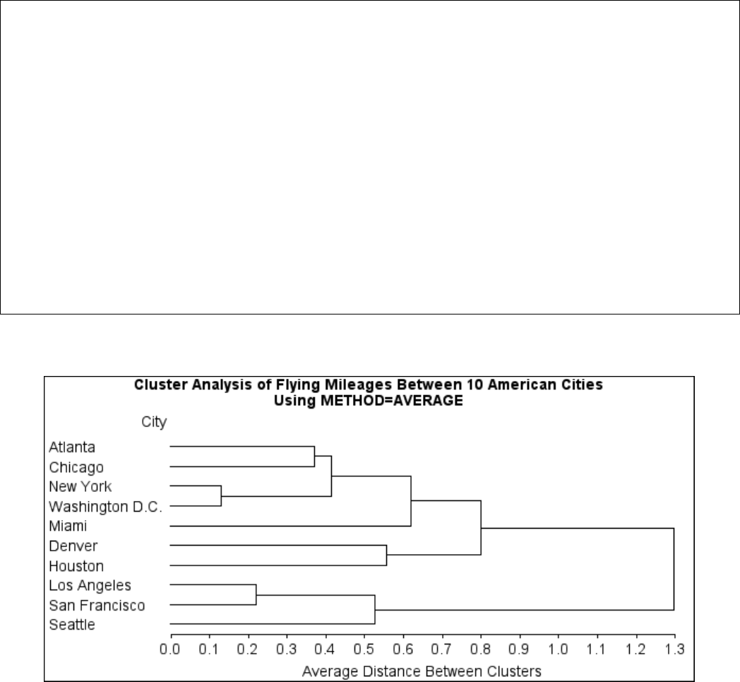
Example 29.1: Cluster Analysis of Flying Mileages between 10 American Cities F1271
The following statements produce Output 29.1.1 and Output 29.1.2:
/*---------------------- Average linkage --------------------*/
proc cluster data=mileages outtree=tree method=average pseudo;
id City;
run;
title2 ’Using METHOD=AVERAGE’ ;
proc tree horizontal; id City; run;
title2;
Output 29.1.1 Cluster History Using METHOD=AVERAGE
Cluster Analysis of Flying Mileages Between 10 American Cities
The CLUSTER Procedure
Average Linkage Cluster Analysis
Cluster History
Norm T
RMS i
NCL ---------Clusters Joined---------- FREQ PSF PST2 Dist e
9 New York Washington D.C. 2 66.7 . 0.1297
8 Los Angeles San Francisco 2 39.2 . 0.2196
7 Atlanta Chicago 2 21.7 . 0.3715
6 CL7 CL9 4 14.5 3.4 0.4149
5 CL8 Seattle 3 12.4 7.3 0.5255
4 Denver Houston 2 13.9 . 0.5562
3 CL6 Miami 5 15.5 3.8 0.6185
2 CL3 CL4 7 16.0 5.3 0.8005
1 CL2 CL5 10 . 16.0 1.2967
Output 29.1.2 Tree Diagram Using METHOD=AVERAGE
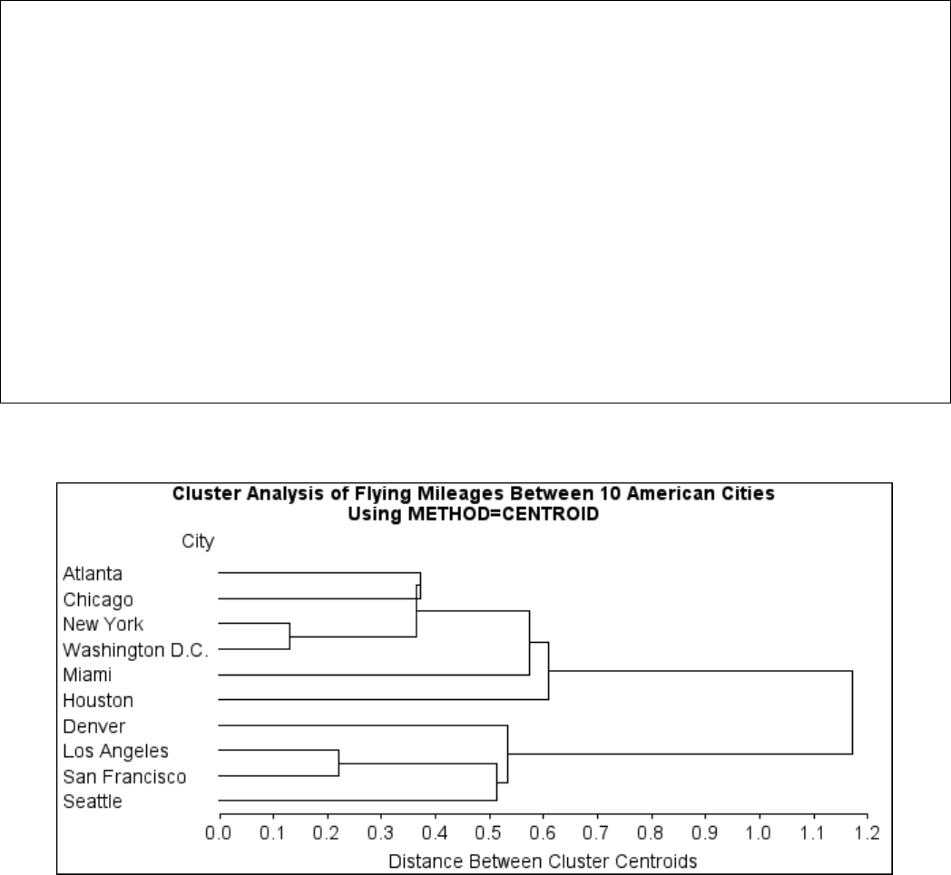
1272 FChapter 29: The CLUSTER Procedure
The following statements produce Output 29.1.3 and Output 29.1.4:
/*---------------------- Centroid method --------------------*/
proc cluster data=mileages method=centroid pseudo;
id City;
run;
title2 ’Using METHOD=CENTROID’ ;
proc tree horizontal; id City; run;
title2;
Output 29.1.3 Cluster History Using METHOD=CENTROID
Cluster Analysis of Flying Mileages Between 10 American Cities
The CLUSTER Procedure
Centroid Hierarchical Cluster Analysis
Cluster History
Norm T
Cent i
NCL ---------Clusters Joined---------- FREQ PSF PST2 Dist e
9 New York Washington D.C. 2 66.7 . 0.1297
8 Los Angeles San Francisco 2 39.2 . 0.2196
7 Atlanta Chicago 2 21.7 . 0.3715
6 CL7 CL9 4 14.5 3.4 0.3652
5 CL8 Seattle 3 12.4 7.3 0.5139
4 Denver CL5 4 12.4 2.1 0.5337
3 CL6 Miami 5 14.2 3.8 0.5743
2 CL3 Houston 6 22.1 2.6 0.6091
1 CL2 CL4 10 . 22.1 1.173
Output 29.1.4 Tree Diagram Using METHOD=CENTROID
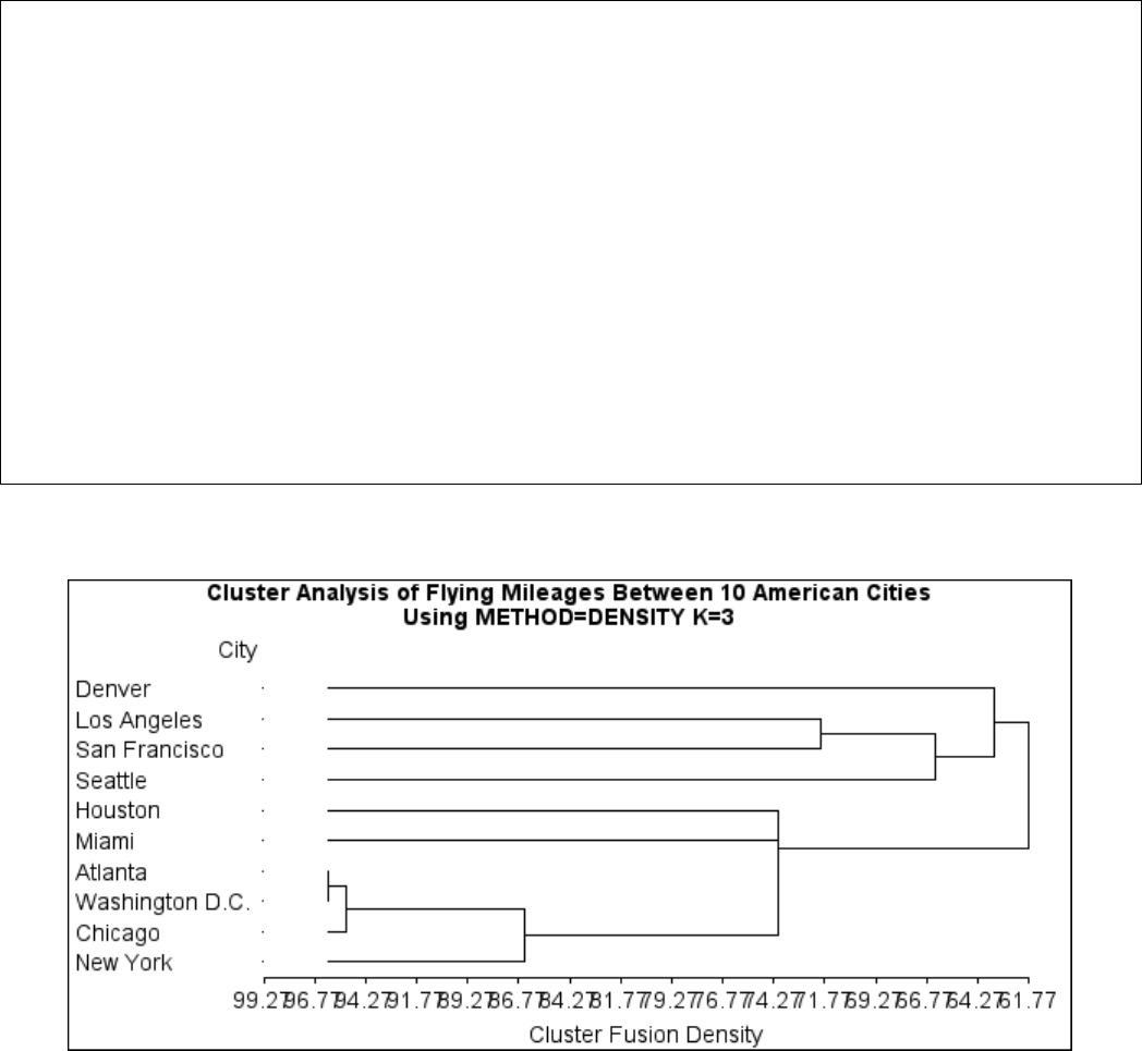
Example 29.1: Cluster Analysis of Flying Mileages between 10 American Cities F1273
The following statements produce Output 29.1.5 and Output 29.1.6:
/*-------- Density linkage with 3rd-nearest-neighbor --------*/
proc cluster data=mileages method=density k=3;
id City;
run;
title2 ’Using METHOD=DENSITY K=3’ ;
proc tree horizontal; id City; run;
title2;
Output 29.1.5 Cluster History Using METHOD=DENSITY K=3
Cluster Analysis of Flying Mileages Between 10 American Cities
The CLUSTER Procedure
Density Linkage Cluster Analysis
Cluster History
Normalized Maximum Density T
Fusion in Each Cluster i
NCL ---------Clusters Joined--------- FREQ Density Lesser Greater e
9 Atlanta Washington D.C. 2 96.106 92.5043 100.0
8 CL9 Chicago 3 95.263 90.9548 100.0
7 CL8 New York 4 86.465 76.1571 100.0
6 CL7 Miami 5 74.079 58.8299 100.0 T
5 CL6 Houston 6 74.079 61.7747 100.0
4 Los Angeles San Francisco 2 71.968 65.3430 80.0885
3 CL4 Seattle 3 66.341 56.6215 80.0885
2 CL3 Denver 4 63.509 61.7747 80.0885
1 CL5 CL2 10 61.775 *80.0885 100.0
Output 29.1.6 Tree Diagram Using METHOD=DENSITY K=3
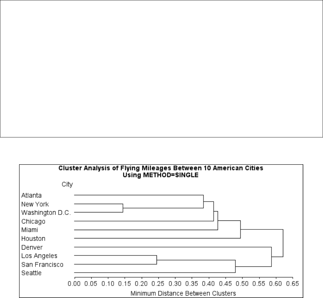
1274 FChapter 29: The CLUSTER Procedure
The following statements produce Output 29.1.7 and Output 29.1.8:
/*--------------------- Single linkage ----------------------*/
proc cluster data=mileages method=single;
id City;
run;
title2 ’Using METHOD=SINGLE’ ;
proc tree horizontal; id City; run;
title2;
Output 29.1.7 Cluster History Using METHOD=SINGLE
Cluster Analysis of Flying Mileages Between 10 American Cities
The CLUSTER Procedure
Single Linkage Cluster Analysis
Cluster History
Norm T
Min i
NCL ---------Clusters Joined---------- FREQ Dist e
9 New York Washington D.C. 2 0.1447
8 Los Angeles San Francisco 2 0.2449
7 Atlanta CL9 3 0.3832
6 CL7 Chicago 4 0.4142
5 CL6 Miami 5 0.4262
4 CL8 Seattle 3 0.4784
3 CL5 Houston 6 0.4947
2 Denver CL4 4 0.5864
1 CL3 CL2 10 0.6203
Output 29.1.8 Tree Diagram Using METHOD=SINGLE
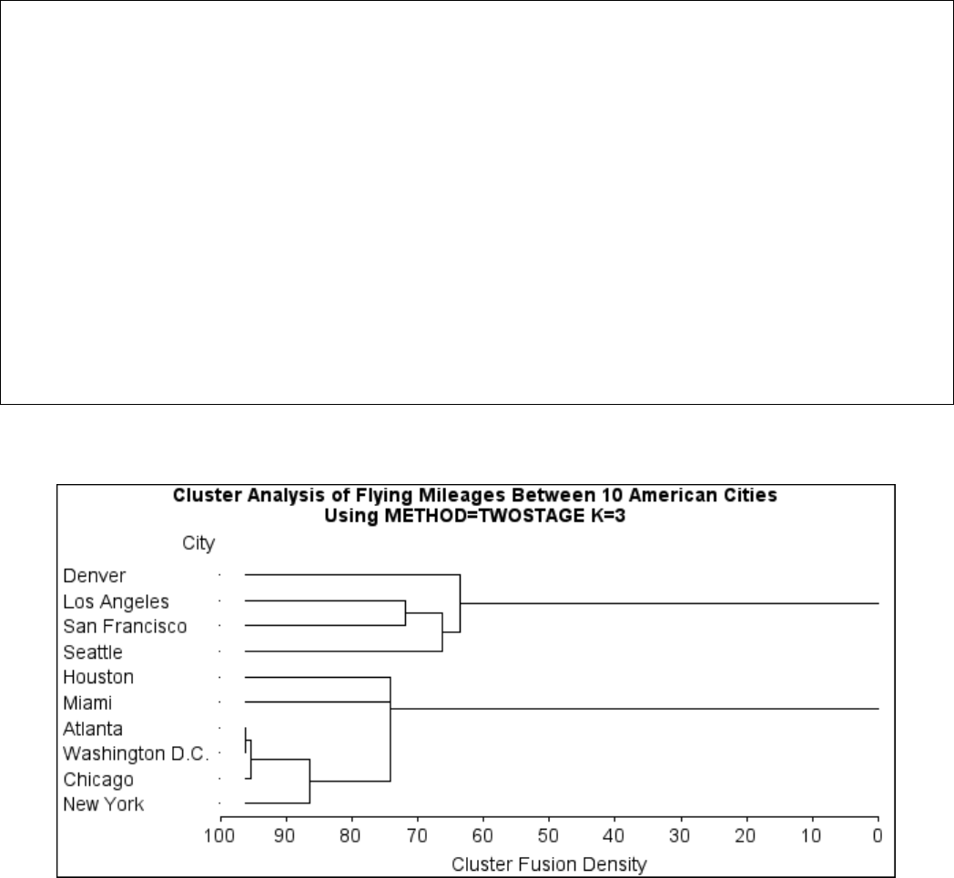
Example 29.1: Cluster Analysis of Flying Mileages between 10 American Cities F1275
The following statements produce Output 29.1.9 and Output 29.1.10:
/*--- Two-stage density linkage with 3rd-nearest-neighbor ---*/
proc cluster data=mileages method=twostage k=3;
id City;
run;
title2 ’Using METHOD=TWOSTAGE K=3’ ;
proc tree horizontal; id City; run;
title2;
Output 29.1.9 Cluster History Using METHOD=TWOSTAGE K=3
Cluster Analysis of Flying Mileages Between 10 American Cities
The CLUSTER Procedure
Two-Stage Density Linkage Clustering
Cluster History
Normalized Maximum Density T
Fusion in Each Cluster i
NCL ---------Clusters Joined--------- FREQ Density Lesser Greater e
9 Atlanta Washington D.C. 2 96.106 92.5043 100.0
8 CL9 Chicago 3 95.263 90.9548 100.0
7 CL8 New York 4 86.465 76.1571 100.0
6 CL7 Miami 5 74.079 58.8299 100.0 T
5 CL6 Houston 6 74.079 61.7747 100.0
4 Los Angeles San Francisco 2 71.968 65.3430 80.0885
3 CL4 Seattle 3 66.341 56.6215 80.0885
2 CL3 Denver 4 63.509 61.7747 80.0885
1 CL5 CL2 10 61.775 80.0885 100.0
Output 29.1.10 Tree Diagram Using METHOD=TWOSTAGE K=3
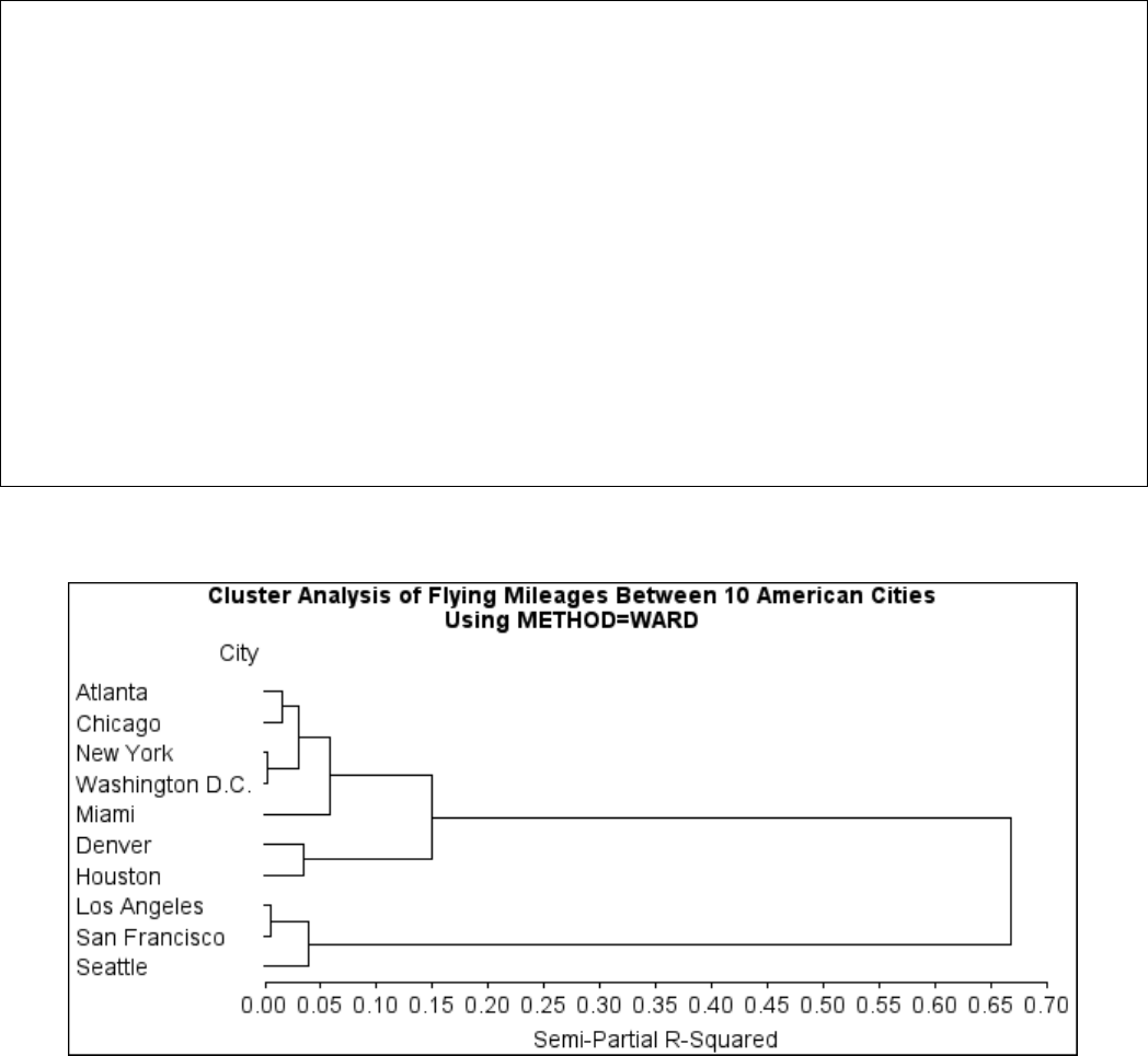
1276 FChapter 29: The CLUSTER Procedure
The following statements produce Output 29.1.11 and Output 29.1.12:
/*------------- Ward’s minimum variance method --------------*/
proc cluster data=mileages method=ward pseudo;
id City;
run;
title2 ’Using METHOD=WARD’ ;
proc tree horizontal; id City; run;
title2;
Output 29.1.11 Cluster History Using METHOD=WARD
Cluster Analysis of Flying Mileages Between 10 American Cities
The CLUSTER Procedure
Ward’s Minimum Variance Cluster Analysis
Cluster History
T
i
NCL ---------Clusters Joined---------- FREQ SPRSQ RSQ PSF PST2 e
9 New York Washington D.C. 2 0.0019 .998 66.7 .
8 Los Angeles San Francisco 2 0.0054 .993 39.2 .
7 Atlanta Chicago 2 0.0153 .977 21.7 .
6 CL7 CL9 4 0.0296 .948 14.5 3.4
5 Denver Houston 2 0.0344 .913 13.2 .
4 CL8 Seattle 3 0.0391 .874 13.9 7.3
3 CL6 Miami 5 0.0586 .816 15.5 3.8
2 CL3 CL5 7 0.1488 .667 16.0 5.3
1 CL2 CL4 10 0.6669 .000 . 16.0
Output 29.1.12 Tree Diagram Using METHOD=WARD

Example 29.2: Crude Birth and Death Rates F1277
Example 29.2: Crude Birth and Death Rates
This example uses the SAS data set Poverty created in the section “Getting Started: CLUSTER
Procedure” on page 1231. The data, from Rouncefield (1995), are birth rates, death rates, and infant
death rates for 97 countries. Six cluster analyses are performed with eight methods. Scatter plots
showing cluster membership at selected levels are produced instead of tree diagrams.
Each cluster analysis is performed by a macro called ANALYZE. The macro takes two arguments.
The first, &METHOD, specifies the value of the METHOD= option to be used in the PROC CLUS-
TER statement. The second, &NCL, must be specified as a list of integers, separated by blanks,
indicating the number of clusters desired in each scatter plot. For example, the first invocation of
ANALYZE specifies the AVERAGE method and requests plots of 3 and 8 clusters. When two-stage
density linkage is used, the K= and R= options are specified as part of the first argument.
The ANALYZE macro first invokes the CLUSTER procedure with METHOD=&METHOD, where
&METHOD represents the value of the first argument to ANALYZE. This part of the macro pro-
duces the PROC CLUSTER output shown.
The %DO loop processes &NCL, the list of numbers of clusters to plot. The macro variable &K
is a counter that indexes the numbers within &NCL. The %SCAN function picks out the &Kth
number in &NCL, which is then assigned to the macro variable &N. When &K exceeds the number
of numbers in &NCL, %SCAN returns a null string. Thus, the %DO loop executes while &N is not
equal to a null string. In the %WHILE condition, a null string is indicated by the absence of any
nonblank characters between the comparison operator (NE) and the right parenthesis that terminates
the condition.
Within the %DO loop, the TREE procedure creates an output data set containing &N clusters.
The SGPLOT procedure then produces a scatter plot in which each observation is identified by the
number of the cluster to which it belongs. The TITLE2 statement uses double quotes so that &N
and &METHOD can be used within the title. At the end of the loop, &K is incremented by 1, and
the next number is extracted from &NCL by %SCAN.

1278 FChapter 29: The CLUSTER Procedure
title ’Cluster Analysis of Birth and Death Rates’;
ods graphics on;
%macro analyze(method,ncl);
proc cluster data=poverty outtree=tree method=&method print=15 ccc pseudo;
var birth death;
title2;
run;
%let k=1;
%let n=%scan(&ncl,&k);
%do %while(&n NE);
proc tree data=tree noprint out=out ncl=&n;
copy birth death;
run;
proc sgplot;
scatter y=death x=birth / group=cluster ;
title2 "Plot of &n Clusters from METHOD=&METHOD";
run;
%let k=%eval(&k+1);
%let n=%scan(&ncl,&k);
%end;
%mend;
The following statement produces Output 29.2.1,Output 29.2.3, and Output 29.2.4:
%analyze(average, 3 8)
For average linkage, the CCC has peaks at 3, 8, 10, and 12 clusters, but the 3-cluster peak is lower
than the 8-cluster peak. The pseudo Fstatistic has peaks at 3, 8, and 12 clusters. The pseudo t2
statistic drops sharply at 3 clusters, continues to fall at 4 clusters, and has a particularly low value at
12 clusters. However, there are not enough data to seriously consider as many as 12 clusters. Scatter
plots are given for 3 and 8 clusters. The results are shown in Output 29.2.1 through Output 29.2.4.
In Output 29.2.4, the eighth cluster consists of the two outlying observations, Mexico and Korea.
Output 29.2.1 Cluster Analysis for Birth and Death Rates: METHOD=AVERAGE
Cluster Analysis of Birth and Death Rates
The CLUSTER Procedure
Average Linkage Cluster Analysis
Eigenvalues of the Covariance Matrix
Eigenvalue Difference Proportion Cumulative
1 189.106588 173.101020 0.9220 0.9220
2 16.005568 0.0780 1.0000
Root-Mean-Square Total-Sample Standard Deviation 10.127
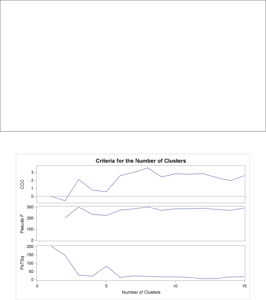
Example 29.2: Crude Birth and Death Rates F1279
Output 29.2.1 continued
Root-Mean-Square Distance Between Observations 20.25399
Cluster History
Norm T
RMS i
NCL --Clusters Joined-- FREQ SPRSQ RSQ ERSQ CCC PSF PST2 Dist e
15 CL27 CL20 18 0.0035 .980 .975 2.61 292 18.6 0.2325
14 CL23 CL17 28 0.0034 .977 .972 1.97 271 17.7 0.2358
13 CL18 CL54 8 0.0015 .975 .969 2.35 279 7.1 0.2432
12 CL21 CL26 8 0.0015 .974 .966 2.85 290 6.1 0.2493
11 CL19 CL24 12 0.0033 .971 .962 2.78 285 14.8 0.2767
10 CL22 CL16 12 0.0036 .967 .957 2.84 284 17.4 0.2858
9 CL15 CL28 22 0.0061 .961 .951 2.45 271 17.5 0.3353
8 OB23 OB61 2 0.0014 .960 .943 3.59 302 . 0.3703
7 CL25 CL11 17 0.0098 .950 .933 3.01 284 23.3 0.4033
6 CL7 CL12 25 0.0122 .938 .920 2.63 273 14.8 0.4132
5 CL10 CL14 40 0.0303 .907 .902 0.59 225 82.7 0.4584
4 CL13 CL6 33 0.0244 .883 .875 0.77 234 22.2 0.5194
3 CL9 CL8 24 0.0182 .865 .827 2.13 300 27.7 0.735
2 CL5 CL3 64 0.1836 .681 .697 -.55 203 148 0.8402
1 CL2 CL4 97 0.6810 .000 .000 0.00 . 203 1.3348
Output 29.2.2 Criteria for the Number of Clusters: METHOD=AVERAGE
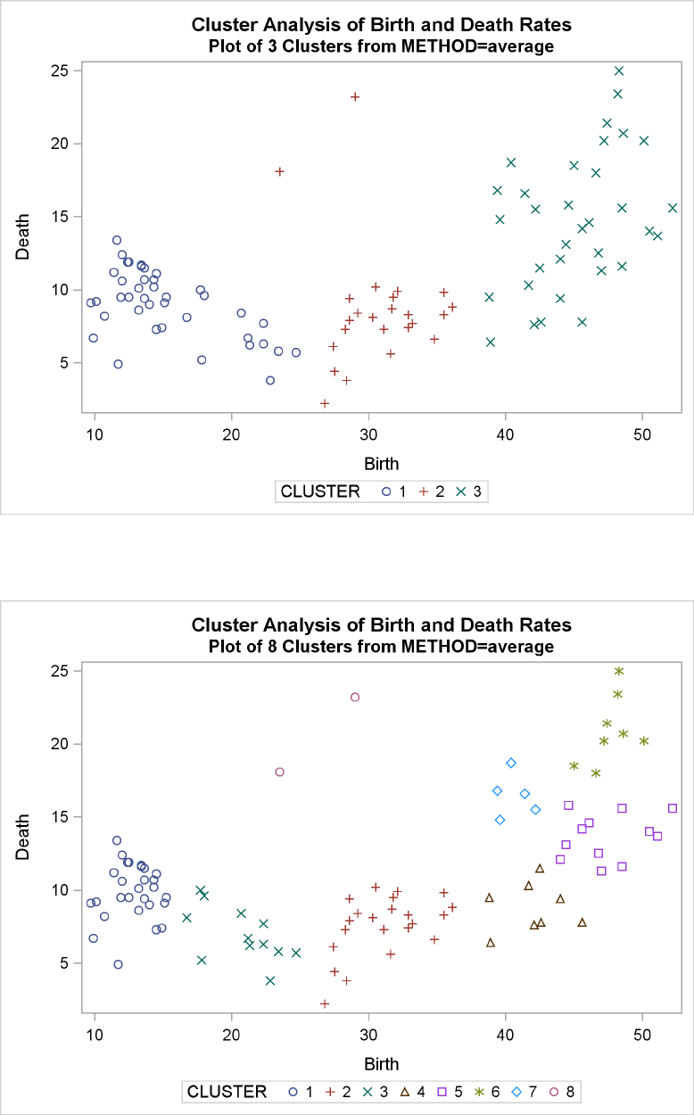
1280 FChapter 29: The CLUSTER Procedure
Output 29.2.3 Plot of Three Clusters: METHOD=AVERAGE
Output 29.2.4 Plot of Eight Clusters: METHOD=AVERAGE

Example 29.2: Crude Birth and Death Rates F1281
The following statement produces Output 29.2.5 and Output 29.2.7:
%analyze(complete, 3)
Complete linkage shows CCC peaks at 3, 8 and 12 clusters. The pseudo Fstatistic peaks at 3 and
12 clusters. The pseudo t2statistic indicates 3 clusters.
The scatter plot for 3 clusters is shown.
Output 29.2.5 Cluster History for Birth and Death Rates: METHOD=COMPLETE
Cluster Analysis of Birth and Death Rates
The CLUSTER Procedure
Complete Linkage Cluster Analysis
Eigenvalues of the Covariance Matrix
Eigenvalue Difference Proportion Cumulative
1 189.106588 173.101020 0.9220 0.9220
2 16.005568 0.0780 1.0000
Root-Mean-Square Total-Sample Standard Deviation 10.127
Mean Distance Between Observations 17.13099
Cluster History
Norm T
Max i
NCL --Clusters Joined-- FREQ SPRSQ RSQ ERSQ CCC PSF PST2 Dist e
15 CL22 CL33 8 0.0015 .983 .975 3.80 329 6.1 0.4092
14 CL56 CL18 8 0.0014 .981 .972 3.97 331 6.6 0.4255
13 CL30 CL44 8 0.0019 .979 .969 4.04 330 19.0 0.4332
12 OB23 OB61 2 0.0014 .978 .966 4.45 340 . 0.4378
11 CL19 CL24 24 0.0034 .974 .962 4.17 327 24.1 0.4962
10 CL17 CL28 12 0.0033 .971 .957 4.18 325 14.8 0.5204
9 CL20 CL13 16 0.0067 .964 .951 3.38 297 25.2 0.5236
8 CL11 CL21 32 0.0054 .959 .943 3.44 297 19.7 0.6001
7 CL26 CL15 13 0.0096 .949 .933 2.93 282 28.9 0.7233
6 CL14 CL10 20 0.0128 .937 .920 2.46 269 27.7 0.8033
5 CL9 CL16 30 0.0237 .913 .902 1.29 241 47.1 0.8993
4 CL6 CL7 33 0.0240 .889 .875 1.38 248 21.7 1.2165
3 CL5 CL12 32 0.0178 .871 .827 2.56 317 13.6 1.2326
2 CL3 CL8 64 0.1900 .681 .697 -.55 203 167 1.5412
1 CL2 CL4 97 0.6810 .000 .000 0.00 . 203 2.5233
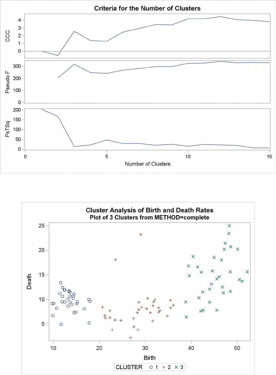
1282 FChapter 29: The CLUSTER Procedure
Output 29.2.6 Criteria for the Number of Clusters: METHOD=COMPLETE
Output 29.2.7 Plot of Clusters for METHOD=COMPLETE

Example 29.2: Crude Birth and Death Rates F1283
The following statement produces Output 29.2.8 and Output 29.2.10:
%analyze(single, 7 10)
The CCC and pseudo Fstatistics are not appropriate for use with single linkage because of the
method’s tendency to chop off tails of distributions. The pseudo t2statistic can be used by looking
for large values and taking the number of clusters to be one greater than the level at which the large
pseudo t2value is displayed. For these data, there are large values at levels 6 and 9, suggesting 7 or
10 clusters.
The scatter plots for 7 and 10 clusters are shown.
Output 29.2.8 Cluster History for Birth and Death Rates: METHOD=SINGLE
Cluster Analysis of Birth and Death Rates
The CLUSTER Procedure
Single Linkage Cluster Analysis
Eigenvalues of the Covariance Matrix
Eigenvalue Difference Proportion Cumulative
1 189.106588 173.101020 0.9220 0.9220
2 16.005568 0.0780 1.0000
Root-Mean-Square Total-Sample Standard Deviation 10.127
Mean Distance Between Observations 17.13099
Cluster History
Norm T
Min i
NCL --Clusters Joined-- FREQ SPRSQ RSQ ERSQ CCC PSF PST2 Dist e
15 CL37 CL19 8 0.0014 .968 .975 -2.3 178 6.6 0.1331
14 CL20 CL23 15 0.0059 .962 .972 -3.1 162 18.7 0.1412
13 CL14 CL16 19 0.0054 .957 .969 -3.4 155 8.8 0.1442
12 CL26 OB58 31 0.0014 .955 .966 -2.7 165 4.0 0.1486
11 OB86 CL18 4 0.0003 .955 .962 -1.6 183 3.8 0.1495
10 CL13 CL11 23 0.0088 .946 .957 -2.3 170 11.3 0.1518
9 CL22 CL17 30 0.0235 .923 .951 -4.7 131 45.7 0.1593 T
8 CL15 CL10 31 0.0210 .902 .943 -5.8 117 21.8 0.1593
7 CL9 OB75 31 0.0052 .897 .933 -4.7 130 4.0 0.1628
6 CL7 CL12 62 0.2023 .694 .920 -15 41.3 223 0.1725
5 CL6 CL8 93 0.6681 .026 .902 -26 0.6 199 0.1756
4 CL5 OB48 94 0.0056 .021 .875 -24 0.7 0.5 0.1811 T
3 CL4 OB67 95 0.0083 .012 .827 -15 0.6 0.8 0.1811
2 OB23 OB61 2 0.0014 .011 .697 -13 1.0 . 0.4378
1 CL3 CL2 97 0.0109 .000 .000 0.00 . 1.0 0.5815
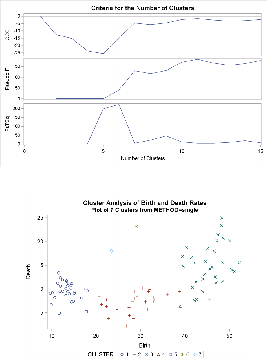
1284 FChapter 29: The CLUSTER Procedure
Output 29.2.9 Criteria for the Number of Clusters: METHOD=SINGLE
Output 29.2.10 Plot of Clusters for METHOD=SINGLE
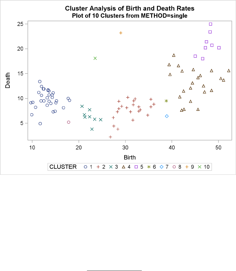
Example 29.2: Crude Birth and Death Rates F1285
Output 29.2.10 continued
The following statements produce Output 29.2.11 through Output 29.2.14, :
%analyze(two k=10, 3)
%analyze(two k=18, 2)
For kth-nearest-neighbor density linkage, the number of modes as a function of kis as follows (not
all of these analyses are shown):
kmodes
3 13
4 6
5-7 4
8-15 3
16-21 2
22+ 1
Thus, there is strong evidence of 3 modes and an indication of the possibility of 2 modes. Uniform-
kernel density linkage gives similar results. For K=10 (10th-nearest-neighbor density linkage), the
scatter plot for 3 clusters is shown; and for K=18, the scatter plot for 2 clusters is shown.

1286 FChapter 29: The CLUSTER Procedure
Output 29.2.11 Cluster History for Birth and Death Rates: METHOD=TWOSTAGE K=10
Cluster Analysis of Birth and Death Rates
The CLUSTER Procedure
Two-Stage Density Linkage Clustering
Eigenvalues of the Covariance Matrix
Eigenvalue Difference Proportion Cumulative
1 189.106588 173.101020 0.9220 0.9220
2 16.005568 0.0780 1.0000
K = 10
Root-Mean-Square Total-Sample Standard Deviation 10.127
Cluster History
Normalized Maximum Density T
Fusion in Each Cluster i
NCL --Clusters Joined-- FREQ SPRSQ RSQ ERSQ CCC PSF PST2 Density Lesser Greater e
15 CL16 OB94 22 0.0015 .921 .975 -11 68.4 1.4 9.2234 6.7927 15.3069
14 CL19 OB49 28 0.0021 .919 .972 -11 72.4 1.8 8.7369 5.9334 33.4385
13 CL15 OB52 23 0.0024 .917 .969 -10 76.9 2.3 8.5847 5.9651 15.3069
12 CL13 OB96 24 0.0018 .915 .966 -9.3 83.0 1.6 7.9252 5.4724 15.3069
11 CL12 OB93 25 0.0025 .912 .962 -8.5 89.5 2.2 7.8913 5.4401 15.3069
10 CL11 OB78 26 0.0031 .909 .957 -7.7 96.9 2.5 7.787 5.4082 15.3069
9 CL10 OB76 27 0.0026 .907 .951 -6.7 107 2.1 7.7133 5.4401 15.3069
8 CL9 OB77 28 0.0023 .904 .943 -5.5 120 1.7 7.4256 4.9017 15.3069
7 CL8 OB43 29 0.0022 .902 .933 -4.1 138 1.6 6.927 4.4764 15.3069
6 CL7 OB87 30 0.0043 .898 .920 -2.7 160 3.1 4.932 2.9977 15.3069
5 CL6 OB82 31 0.0055 .892 .902 -1.1 191 3.7 3.7331 2.1560 15.3069
4 CL22 OB61 37 0.0079 .884 .875 0.93 237 10.6 3.1713 1.6308 100.0
3 CL14 OB23 29 0.0126 .872 .827 2.60 320 10.4 2.0654 1.0744 33.4385
2 CL4 CL3 66 0.2129 .659 .697 -1.3 183 172 12.409 33.4385 100.0
1 CL2 CL5 97 0.6588 .000 .000 0.00 . 183 10.071 15.3069 100.0
3 modal clusters have been formed.

Example 29.2: Crude Birth and Death Rates F1287
Output 29.2.12 Cluster History for Birth and Death Rates: METHOD=TWOSTAGE K=18
Cluster Analysis of Birth and Death Rates
The CLUSTER Procedure
Two-Stage Density Linkage Clustering
Eigenvalues of the Covariance Matrix
Eigenvalue Difference Proportion Cumulative
1 189.106588 173.101020 0.9220 0.9220
2 16.005568 0.0780 1.0000
K = 18
Root-Mean-Square Total-Sample Standard Deviation 10.127
Cluster History
Normalized Maximum Density T
Fusion in Each Cluster i
NCL --Clusters Joined-- FREQ SPRSQ RSQ ERSQ CCC PSF PST2 Density Lesser Greater e
15 CL16 OB72 46 0.0107 .799 .975 -21 23.3 3.0 10.118 7.7445 23.4457
14 CL15 OB94 47 0.0098 .789 .972 -21 23.9 2.7 9.676 7.1257 23.4457
13 CL14 OB51 48 0.0037 .786 .969 -20 25.6 1.0 9.409 6.8398 23.4457 T
12 CL13 OB96 49 0.0099 .776 .966 -19 26.7 2.6 9.409 6.8398 23.4457
11 CL12 OB76 50 0.0114 .764 .962 -19 27.9 2.9 8.8136 6.3138 23.4457
10 CL11 OB77 51 0.0021 .762 .957 -18 31.0 0.5 8.6593 6.0751 23.4457
9 CL10 OB78 52 0.0103 .752 .951 -17 33.3 2.5 8.6007 6.0976 23.4457
8 CL9 OB43 53 0.0034 .748 .943 -16 37.8 0.8 8.4964 5.9160 23.4457
7 CL8 OB93 54 0.0109 .737 .933 -15 42.1 2.6 8.367 5.7913 23.4457
6 CL7 OB88 55 0.0110 .726 .920 -13 48.3 2.6 7.916 5.3679 23.4457
5 CL6 OB87 56 0.0120 .714 .902 -12 57.5 2.7 6.6917 4.3415 23.4457
4 CL20 OB61 39 0.0077 .707 .875 -9.8 74.7 8.3 6.2578 3.2882 100.0
3 CL5 OB82 57 0.0138 .693 .827 -5.0 106 3.0 5.3605 3.2834 23.4457
2 CL3 OB23 58 0.0117 .681 .697 -.54 203 2.5 3.2687 1.7568 23.4457
1 CL2 CL4 97 0.6812 .000 .000 0.00 . 203 13.764 23.4457 100.0
2 modal clusters have been formed.
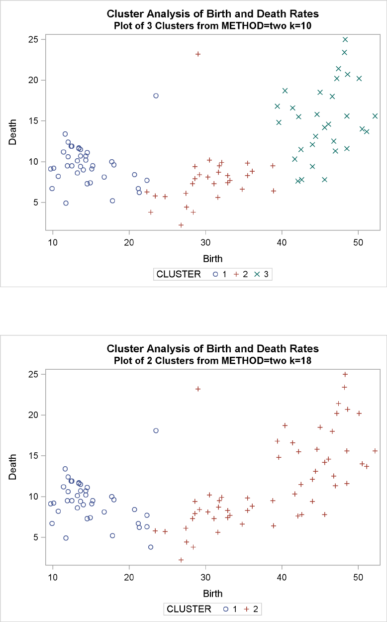
1288 FChapter 29: The CLUSTER Procedure
Output 29.2.13 Plot of Clusters for METHOD=TWOSTAGE K=10
Output 29.2.14 Plot of Clusters for METHOD=TWOSTAGE K=18

Example 29.3: Cluster Analysis of Fisher’s Iris Data F1289
In summary, most of the clustering methods indicate 3 or 8 clusters. Most methods agree at the
3-cluster level, but at the other levels, there is considerable disagreement about the composition of
the clusters. The presence of numerous ties also complicates the analysis; see Example 29.4.
Example 29.3: Cluster Analysis of Fisher’s Iris Data
The iris data published by Fisher (1936) have been widely used for examples in discriminant anal-
ysis and cluster analysis. The sepal length, sepal width, petal length, and petal width are measured
in millimeters on 50 iris specimens from each of three species, Iris setosa, I. versicolor, and I.
virginica. Mezzich and Solomon (1980) discuss a variety of cluster analyses of the iris data.
The following code analyzes the iris data by using Ward’s method and two-stage density linkage and
then illustrates how the FASTCLUS procedure can be used in combination with PROC CLUSTER
to analyze large data sets.
title ’Cluster Analysis of Fisher (1936) Iris Data’;
proc format;
value specname
1=’Setosa ’
2=’Versicolor’
3=’Virginica ’;
run;
data iris;
input SepalLength SepalWidth PetalLength PetalWidth Species @@;
format Species specname.;
label SepalLength=’Sepal Length in mm.’
SepalWidth =’Sepal Width in mm.’
PetalLength=’Petal Length in mm.’
PetalWidth =’Petal Width in mm.’;
symbol = put(species, specname10.);
datalines;
503314021642856223652846152673156243
632851153463414031693151233622245152
593248182463610021613046142602751162
653052203562539112653055183582751193
683259233513317051572845132623454233
773867223633347162673357253763066213
492545173553513021673052233703247142
643245152612840132483116021593051183
552438112632550193643253233523414021
493614011543045152793864203443213021
673357213503516061582640122443013021
772867203632749183473216021552644122
502333102723260183483014031513816021
613049183483419021503016021503212021
612656143642856213433011011584012021
513819041673144142622848183493014021
513514021563045152582741102503416041
463214021602945152572635102574415041
503614021773061233633456243582751193
1290 FChapter 29: The CLUSTER Procedure
57 29 42 13 2 72 30 58 16 3 54 34 15 04 1 52 41 15 01 1
71 30 59 21 3 64 31 55 18 3 60 30 48 18 3 63 29 56 18 3
49 24 33 10 2 56 27 42 13 2 57 30 42 12 2 55 42 14 02 1
49 31 15 02 1 77 26 69 23 3 60 22 50 15 3 54 39 17 04 1
66 29 46 13 2 52 27 39 14 2 60 34 45 16 2 50 34 15 02 1
44 29 14 02 1 50 20 35 10 2 55 24 37 10 2 58 27 39 12 2
47 32 13 02 1 46 31 15 02 1 69 32 57 23 3 62 29 43 13 2
74 28 61 19 3 59 30 42 15 2 51 34 15 02 1 50 35 13 03 1
56 28 49 20 3 60 22 40 10 2 73 29 63 18 3 67 25 58 18 3
49 31 15 01 1 67 31 47 15 2 63 23 44 13 2 54 37 15 02 1
56 30 41 13 2 63 25 49 15 2 61 28 47 12 2 64 29 43 13 2
51 25 30 11 2 57 28 41 13 2 65 30 58 22 3 69 31 54 21 3
54 39 13 04 1 51 35 14 03 1 72 36 61 25 3 65 32 51 20 3
61 29 47 14 2 56 29 36 13 2 69 31 49 15 2 64 27 53 19 3
68 30 55 21 3 55 25 40 13 2 48 34 16 02 1 48 30 14 01 1
45 23 13 03 1 57 25 50 20 3 57 38 17 03 1 51 38 15 03 1
55 23 40 13 2 66 30 44 14 2 68 28 48 14 2 54 34 17 02 1
51 37 15 04 1 52 35 15 02 1 58 28 51 24 3 67 30 50 17 2
63 33 60 25 3 53 37 15 02 1
;
The following macro, SHOW, is used in the subsequent analyses to display cluster results. It invokes
the FREQ procedure to crosstabulate clusters and species. The CANDISC procedure computes
canonical variables for discriminating among the clusters, and the first two canonical variables are
plotted to show cluster membership. See Chapter 27, “The CANDISC Procedure,” for a canonical
discriminant analysis of the iris species.
/*--- Define macro show ---*/
%macro show;
proc freq;
tables cluster*species / nopercent norow nocol plot=none;
run;
proc candisc noprint out=can;
class cluster;
var petal: sepal:;
run;
proc sgplot data=can ;
scatter y=can2 x=can1 / group=cluster ;
run;
%mend;
The first analysis clusters the iris data by using Ward’s method (see Output 29.3.1) and plots the
CCC and pseudo Fand t2statistics (see Output 29.3.2). The CCC has a local peak at 3 clusters but
a higher peak at 5 clusters. The pseudo Fstatistic indicates 3 clusters, while the pseudo t2statistic
suggests 3 or 6 clusters.
The TREE procedure creates an output data set containing the 3-cluster partition for use by the
SHOW macro. The FREQ procedure reveals 16 misclassifications. The results are shown in
Output 29.3.3.

Example 29.3: Cluster Analysis of Fisher’s Iris Data F1291
title2 ’By Ward’’s Method’;
ods graphics on ;
proc cluster data=iris method=ward print=15 ccc pseudo;
var petal: sepal:;
copy species;
run;
proc tree noprint ncl=3 out=out;
copy petal: sepal: species;
run;
%show;
Output 29.3.1 Cluster Analysis of Fisher’s Iris Data: PROC CLUSTER with METHOD=WARD
Cluster Analysis of Fisher (1936) Iris Data
By Ward’s Method
The CLUSTER Procedure
Ward’s Minimum Variance Cluster Analysis
Eigenvalues of the Covariance Matrix
Eigenvalue Difference Proportion Cumulative
1 422.824171 398.557096 0.9246 0.9246
2 24.267075 16.446125 0.0531 0.9777
3 7.820950 5.437441 0.0171 0.9948
4 2.383509 0.0052 1.0000
Root-Mean-Square Total-Sample Standard Deviation 10.69224
Root-Mean-Square Distance Between Observations 30.24221
Cluster History
T
i
NCL --Clusters Joined--- FREQ SPRSQ RSQ ERSQ CCC PSF PST2 e
15 CL24 CL28 15 0.0016 .971 .958 5.93 324 9.8
14 CL21 CL53 7 0.0019 .969 .955 5.85 329 5.1
13 CL18 CL48 15 0.0023 .967 .953 5.69 334 8.9
12 CL16 CL23 24 0.0023 .965 .950 4.63 342 9.6
11 CL14 CL43 12 0.0025 .962 .946 4.67 353 5.8
10 CL26 CL20 22 0.0027 .959 .942 4.81 368 12.9
9 CL27 CL17 31 0.0031 .956 .936 5.02 387 17.8
8 CL35 CL15 23 0.0031 .953 .930 5.44 414 13.8
7 CL10 CL47 26 0.0058 .947 .921 5.43 430 19.1
6 CL8 CL13 38 0.0060 .941 .911 5.81 463 16.3
5 CL9 CL19 50 0.0105 .931 .895 5.82 488 43.2
4 CL12 CL11 36 0.0172 .914 .872 3.99 515 41.0
3 CL6 CL7 64 0.0301 .884 .827 4.33 558 57.2
2 CL4 CL3 100 0.1110 .773 .697 3.83 503 116
1 CL5 CL2 150 0.7726 .000 .000 0.00 . 503
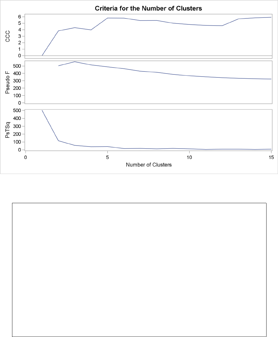
1292 FChapter 29: The CLUSTER Procedure
Output 29.3.2 Criteria for the Number of Clusters with METHOD=WARD
Output 29.3.3 Crosstabulation of Clusters for METHOD=WARD
Cluster Analysis of Fisher (1936) Iris Data
By Ward’s Method
The FREQ Procedure
Table of CLUSTER by Species
CLUSTER Species
Frequency|Setosa |Versicol|Virginic| Total
| |or |a |
---------+--------+--------+--------+
1 | 0 | 49 | 15 | 64
---------+--------+--------+--------+
2 | 0 | 1 | 35 | 36
---------+--------+--------+--------+
3 | 50 | 0 | 0 | 50
---------+--------+--------+--------+
Total 50 50 50 150
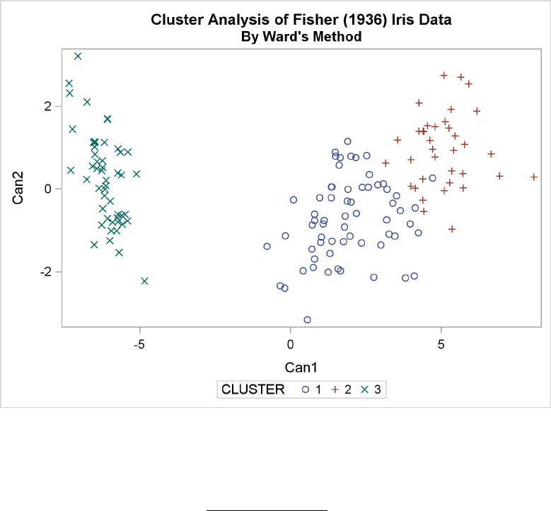
Example 29.3: Cluster Analysis of Fisher’s Iris Data F1293
Output 29.3.4 Scatter Plot of Clusters for METHOD=WARD
The second analysis uses two-stage density linkage. The raw data suggest 2 or 6 modes instead of
3:
kmodes
3 12
4-6 6
7 4
8 3
9-50 2
51+ 1
The following analysis uses K=8 to produce 3 clusters for comparison with other analyses. There
are only 6 misclassifications. The results are shown in Output 29.3.5 and Output 29.3.6.
title2 ’By Two-Stage Density Linkage’;
ods graphics on ;
proc cluster data=iris method=twostage k=8 print=15 ccc pseudo;
var petal: sepal:;
copy species;
run;
proc tree noprint ncl=3 out=out;
copy petal: sepal: species;
run;
%show;

1294 FChapter 29: The CLUSTER Procedure
Output 29.3.5 Cluster Analysis of Fisher’s Iris Data: PROC CLUSTER with
METHOD=TWOSTAGE
Cluster Analysis of Fisher (1936) Iris Data
By Two-Stage Density Linkage
The CLUSTER Procedure
Two-Stage Density Linkage Clustering
Eigenvalues of the Covariance Matrix
Eigenvalue Difference Proportion Cumulative
1 422.824171 398.557096 0.9246 0.9246
2 24.267075 16.446125 0.0531 0.9777
3 7.820950 5.437441 0.0171 0.9948
4 2.383509 0.0052 1.0000
K=8
Root-Mean-Square Total-Sample Standard Deviation 10.69224
Cluster History
Normalized Maximum Density T
Fusion in Each Cluster i
NCL --Clusters Joined-- FREQ SPRSQ RSQ ERSQ CCC PSF PST2 Density Lesser Greater e
15 CL17 OB127 43 0.0024 .917 .958 -11 107 3.4 0.3903 0.2066 3.5156
14 CL16 OB137 50 0.0023 .915 .955 -10 113 5.6 0.3637 0.1837 100.0
13 CL15 OB74 44 0.0029 .912 .953 -9.8 119 3.8 0.3553 0.2130 3.5156
12 CL22 OB49 47 0.0036 .909 .950 -7.7 125 5.2 0.3223 0.1736 8.3678 T
11 CL12 OB85 48 0.0036 .905 .946 -7.4 132 4.8 0.3223 0.1736 8.3678
10 CL11 OB98 49 0.0033 .902 .942 -6.8 143 4.1 0.2879 0.1479 8.3678
9 CL13 OB24 45 0.0036 .898 .936 -6.2 155 4.5 0.2802 0.2005 3.5156
8 CL10 OB25 50 0.0019 .896 .930 -5.2 175 2.2 0.2699 0.1372 8.3678
7 CL8 OB121 51 0.0035 .893 .921 -4.2 198 4.0 0.2586 0.1372 8.3678
6 CL9 OB45 46 0.0041 .888 .911 -3.0 229 4.7 0.1412 0.0832 3.5156
5 CL6 OB39 47 0.0048 .884 .895 -1.5 276 5.1 0.107 0.0605 3.5156
4 CL5 OB21 48 0.0048 .879 .872 0.54 353 4.7 0.0969 0.0541 3.5156
3 CL4 OB90 49 0.0046 .874 .827 3.49 511 4.2 0.0715 0.0370 3.5156
2 CL7 CL3 100 0.1017 .773 .697 3.83 503 96.3 2.6277 3.5156 8.3678
3 modal clusters have been formed.
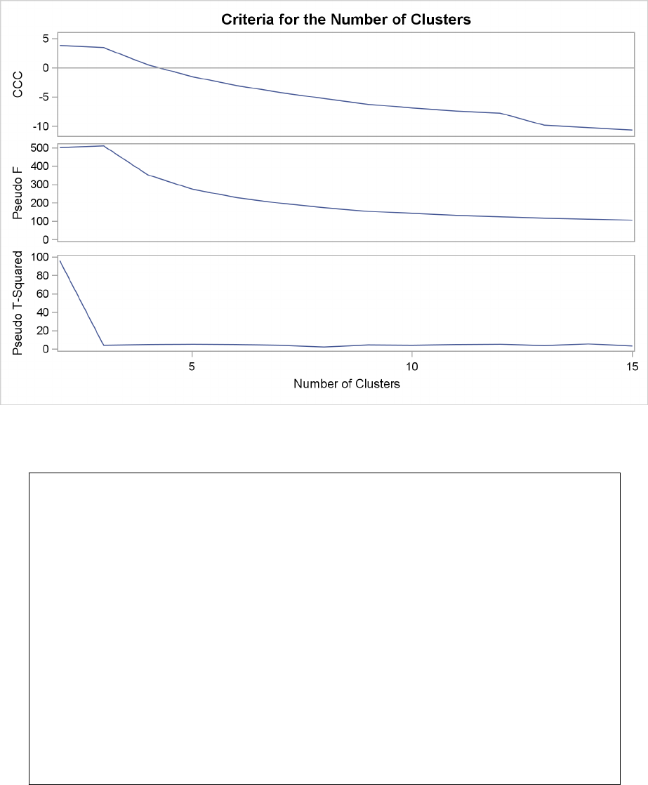
Example 29.3: Cluster Analysis of Fisher’s Iris Data F1295
Output 29.3.6 Criteria for the Number of Clusters with METHOD=TWOSTAGE
Output 29.3.7 Crosstabulation of Clusters for METHOD=TWOSTAGE
Cluster Analysis of Fisher (1936) Iris Data
By Two-Stage Density Linkage
The FREQ Procedure
Table of CLUSTER by Species
CLUSTER Species
Frequency|Setosa |Versicol|Virginic| Total
| |or |a |
---------+--------+--------+--------+
1 | 50 | 0 | 0 | 50
---------+--------+--------+--------+
2 | 0 | 48 | 3 | 51
---------+--------+--------+--------+
3 | 0 | 2 | 47 | 49
---------+--------+--------+--------+
Total 50 50 50 150
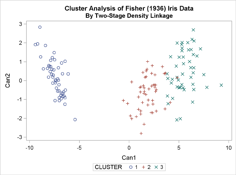
1296 FChapter 29: The CLUSTER Procedure
Output 29.3.8 Scatter Plot of Clusters for METHOD=TWOSTAGE
The CLUSTER procedure is not practical for very large data sets because, with most methods,
the CPU time is roughly proportional to the square or cube of the number of observations. The
FASTCLUS procedure requires time proportional to the number of observations and can therefore
be used with much larger data sets than PROC CLUSTER. If you want to hierarchically cluster a
very large data set, you can use PROC FASTCLUS for a preliminary cluster analysis to produce
a large number of clusters and then use PROC CLUSTER to hierarchically cluster the preliminary
clusters.
FASTCLUS automatically creates the variables _FREQ_ and _RMSSTD_ in the MEAN= output data
set. These variables are then automatically used by PROC CLUSTER in the computation of various
statistics.
The following SAS code uses the iris data to illustrate the process of clustering clusters. In the
preliminary analysis, PROC FASTCLUS produces 10 clusters, which are then crosstabulated with
species. The data set containing the preliminary clusters is sorted in preparation for later merges.
The results are shown in Output 29.3.9 and Output 29.3.10.
title2 ’Preliminary Analysis by FASTCLUS’;
proc fastclus data=iris summary maxc=10 maxiter=99 converge=0
mean=mean out=prelim cluster=preclus;
var petal: sepal:;
run;
proc freq;
tables preclus*species / nopercent norow nocol plot=none;
run;
proc sort data=prelim;

Example 29.3: Cluster Analysis of Fisher’s Iris Data F1297
by preclus;
run;
Output 29.3.9 Preliminary Analysis of Fisher’s Iris Data: Fastclus Procedure
Cluster Analysis of Fisher (1936) Iris Data
Preliminary Analysis by FASTCLUS
The FASTCLUS Procedure
Replace=FULL Radius=0 Maxclusters=10 Maxiter=99 Converge=0
Convergence criterion is satisfied.
Criterion Based on Final Seeds = 2.1389
Cluster Summary
Maximum Distance
RMS Std from Seed Radius Nearest
Cluster Frequency Deviation to Observation Exceeded Cluster
-----------------------------------------------------------------------------
1 9 2.7067 8.2027 5
2 19 2.2001 7.7340 4
3 18 2.1496 6.2173 8
4 4 2.5249 5.3268 2
5 3 2.7234 5.8214 1
6 7 2.2939 5.1508 2
7 17 2.0274 6.9576 10
8 18 2.2628 7.1135 3
9 22 2.2666 7.5029 8
10 33 2.0594 10.0033 7
Cluster Summary
Distance Between
Cluster Cluster Centroids
-----------------------------
1 8.7362
2 6.2243
3 7.5049
4 6.2243
5 8.7362
6 9.3318
7 7.9503
8 7.5049
9 9.0090
10 7.9503
Pseudo F Statistic = 370.58
Observed Over-All R-Squared = 0.95971
Approximate Expected Over-All R-Squared = 0.82928
Cubic Clustering Criterion = 27.077
WARNING: The two values above are invalid for correlated variables.

1298 FChapter 29: The CLUSTER Procedure
Output 29.3.10 Crosstabulation of Species and Cluster From the Fastclus Procedure
Cluster Analysis of Fisher (1936) Iris Data
Preliminary Analysis by FASTCLUS
The FREQ Procedure
Table of preclus by Species
preclus(Cluster) Species
Frequency|Setosa |Versicol|Virginic| Total
| |or |a |
---------+--------+--------+--------+
1 | 0 | 0 | 9 | 9
---------+--------+--------+--------+
2 | 0 | 19 | 0 | 19
---------+--------+--------+--------+
3 | 0 | 18 | 0 | 18
---------+--------+--------+--------+
4 | 0 | 3 | 1 | 4
---------+--------+--------+--------+
5 | 0 | 0 | 3 | 3
---------+--------+--------+--------+
6 | 0 | 7 | 0 | 7
---------+--------+--------+--------+
7 | 17 | 0 | 0 | 17
---------+--------+--------+--------+
8 | 0 | 3 | 15 | 18
---------+--------+--------+--------+
9 | 0 | 0 | 22 | 22
---------+--------+--------+--------+
10 | 33 | 0 | 0 | 33
---------+--------+--------+--------+
Total 50 50 50 150
The following macro, CLUS, clusters the preliminary clusters. There is one argument to choose the
METHOD= specification to be used by PROC CLUSTER. The TREE procedure creates an output
data set containing the 3-cluster partition, which is sorted and merged with the OUT= data set from
PROC FASTCLUS to determine which cluster each of the original 150 observations belongs to. The
SHOW macro is then used to display the results. In this example, the CLUS macro is invoked using
Ward’s method, which produces 16 misclassifications, and Wong’s hybrid method, which produces
22 misclassifications.

Example 29.3: Cluster Analysis of Fisher’s Iris Data F1299
/*--- Define macro clus ---*/
%macro clus(method);
proc cluster data=mean method=&method ccc pseudo;
var petal: sepal:;
copy preclus;
run;
proc tree noprint ncl=3 out=out;
copy petal: sepal: preclus;
run;
proc sort data=out;
by preclus;
run;
data clus;
merge out prelim;
by preclus;
run;
%show;
%mend;
The following statements produce Output 29.3.11 through Output 29.3.14.
title2 ’Clustering Clusters by Ward’’s Method’;
%clus(ward);
Output 29.3.11 Clustering Clusters by Ward’s Method
Cluster Analysis of Fisher (1936) Iris Data
Clustering Clusters by Ward’s Method
The CLUSTER Procedure
Ward’s Minimum Variance Cluster Analysis
Eigenvalues of the Covariance Matrix
Eigenvalue Difference Proportion Cumulative
1 416.976349 398.666421 0.9501 0.9501
2 18.309928 14.952922 0.0417 0.9918
3 3.357006 3.126943 0.0076 0.9995
4 0.230063 0.0005 1.0000
Root-Mean-Square Total-Sample Standard Deviation 10.69224
Root-Mean-Square Distance Between Observations 30.24221
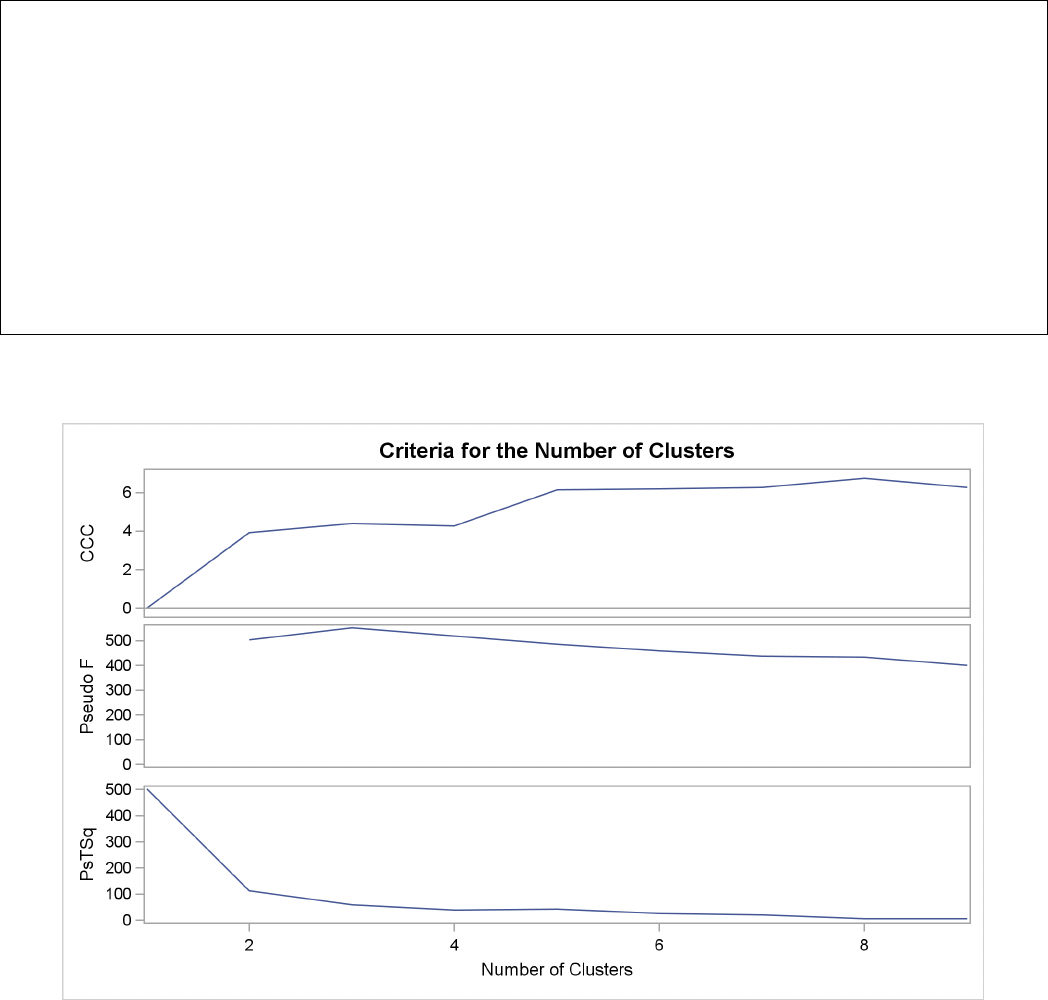
1300 FChapter 29: The CLUSTER Procedure
Output 29.3.11 continued
Cluster History
T
i
NCL --Clusters Joined--- FREQ SPRSQ RSQ ERSQ CCC PSF PST2 e
9 OB2 OB4 23 0.0019 .958 .932 6.26 400 6.3
8 OB1 OB5 12 0.0025 .955 .926 6.75 434 5.8
7 CL9 OB6 30 0.0069 .948 .918 6.28 438 19.5
6 OB3 OB8 36 0.0074 .941 .907 6.21 459 26.0
5 OB7 OB10 50 0.0104 .931 .892 6.15 485 42.2
4 CL8 OB9 34 0.0162 .914 .870 4.28 519 39.3
3 CL7 CL6 66 0.0318 .883 .824 4.39 552 59.7
2 CL4 CL3 100 0.1099 .773 .695 3.94 503 113
1 CL2 CL5 150 0.7726 .000 .000 0.00 . 503
Output 29.3.12 Criteria for the Number of Clusters for Clustering Clusters from Ward’s Method
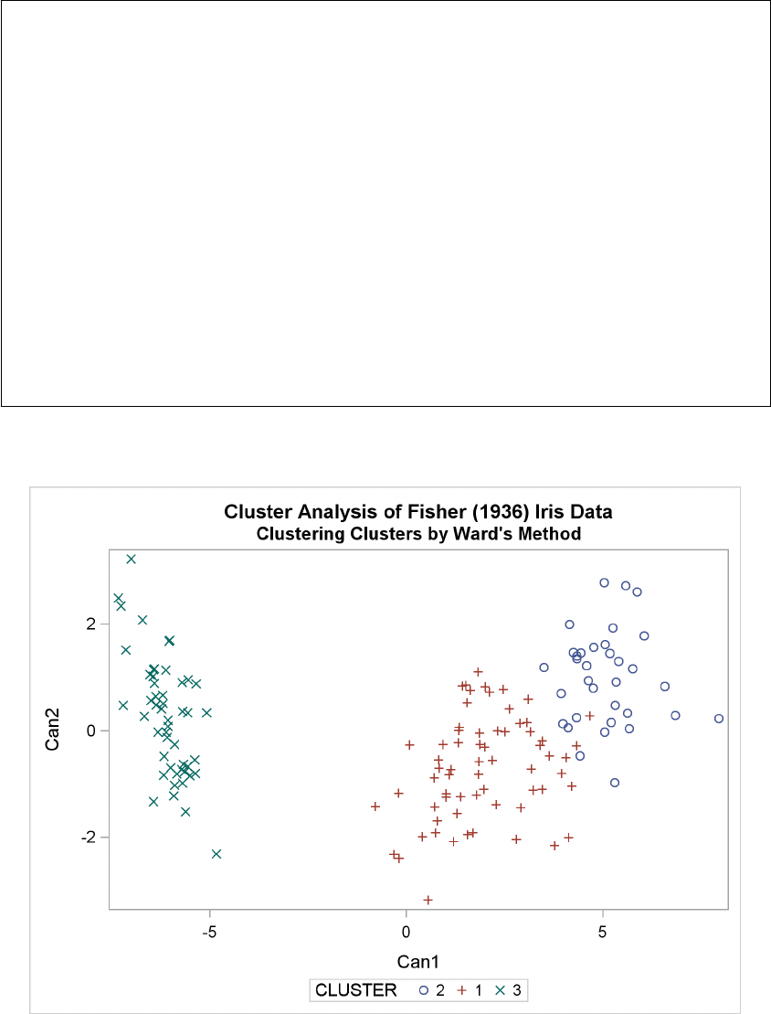
Example 29.3: Cluster Analysis of Fisher’s Iris Data F1301
Output 29.3.13 Crosstabulation for Clustering Clusters from Ward’s Method
Cluster Analysis of Fisher (1936) Iris Data
Clustering Clusters by Ward’s Method
The FREQ Procedure
Table of CLUSTER by Species
CLUSTER Species
Frequency|Setosa |Versicol|Virginic| Total
| |or |a |
---------+--------+--------+--------+
1 | 0 | 50 | 16 | 66
---------+--------+--------+--------+
2 | 0 | 0 | 34 | 34
---------+--------+--------+--------+
3 | 50 | 0 | 0 | 50
---------+--------+--------+--------+
Total 50 50 50 150
Output 29.3.14 Scatter Plot for Clustering Clusters using Ward’s Method

1302 FChapter 29: The CLUSTER Procedure
The following statements produce Output 29.3.15 through Output 29.3.17.
title2 "Clustering Clusters by Wong’s Hybrid Method";
%clus(twostage hybrid);
Output 29.3.15 Clustering Clusters by Wong’s Hybrid Method
Cluster Analysis of Fisher (1936) Iris Data
Clustering Clusters by Wong’s Hybrid Method
The CLUSTER Procedure
Two-Stage Density Linkage Clustering
Eigenvalues of the Covariance Matrix
Eigenvalue Difference Proportion Cumulative
1 416.976349 398.666421 0.9501 0.9501
2 18.309928 14.952922 0.0417 0.9918
3 3.357006 3.126943 0.0076 0.9995
4 0.230063 0.0005 1.0000
Root-Mean-Square Total-Sample Standard Deviation 10.69224
Cluster History
Normalized Maximum Density T
Fusion in Each Cluster i
NCL --Clusters Joined-- FREQ SPRSQ RSQ ERSQ CCC PSF PST2 Density Lesser Greater e
9 OB10 OB7 50 0.0104 .949 .932 3.81 330 42.2 40.24 58.2179 100.0
8 OB3 OB8 36 0.0074 .942 .926 3.22 329 26.0 27.981 39.4511 48.4350
7 OB2 OB4 23 0.0019 .940 .918 4.24 373 6.3 23.775 8.9675 46.3026
6 CL8 OB9 58 0.0194 .921 .907 2.13 334 46.3 20.724 46.8846 48.4350
5 CL7 OB6 30 0.0069 .914 .892 3.09 383 19.5 13.303 17.6360 46.3026
4 CL6 OB1 67 0.0292 .884 .870 1.21 372 41.0 8.4137 10.8758 48.4350
3 CL4 OB5 70 0.0138 .871 .824 3.33 494 12.3 5.1855 6.2890 48.4350
2 CL3 CL5 100 0.0979 .773 .695 3.94 503 89.5 19.513 46.3026 48.4350
1 CL2 CL9 150 0.7726 .000 .000 0.00 . 503 1.3337 48.4350 100.0
3 modal clusters have been formed.
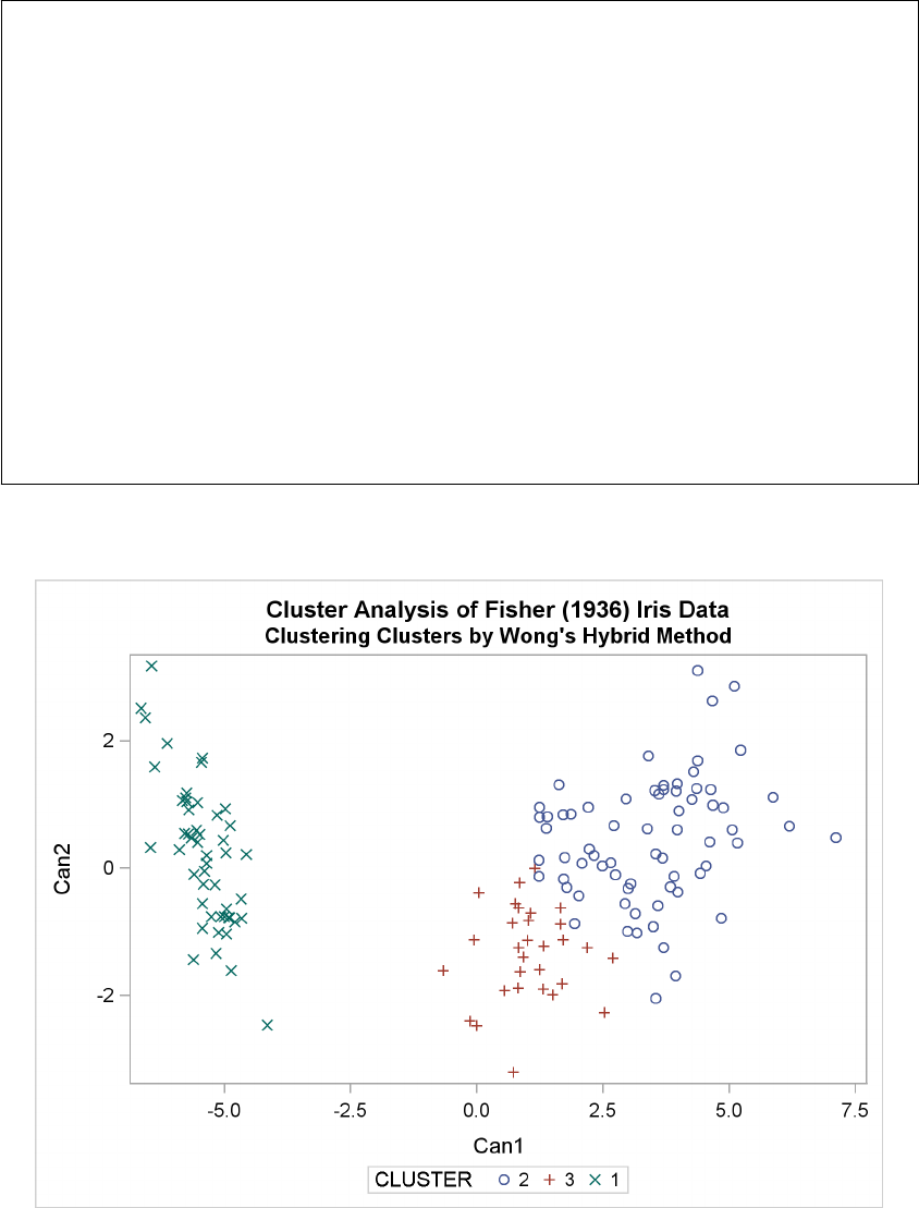
Example 29.3: Cluster Analysis of Fisher’s Iris Data F1303
Output 29.3.16 Crosstabulation for Clustering Clusters from Wong’s Hybrid Method
Cluster Analysis of Fisher (1936) Iris Data
Clustering Clusters by Wong’s Hybrid Method
The FREQ Procedure
Table of CLUSTER by Species
CLUSTER Species
Frequency|Setosa |Versicol|Virginic| Total
| |or |a |
---------+--------+--------+--------+
1 | 50 | 0 | 0 | 50
---------+--------+--------+--------+
2 | 0 | 21 | 49 | 70
---------+--------+--------+--------+
3 | 0 | 29 | 1 | 30
---------+--------+--------+--------+
Total 50 50 50 150
Output 29.3.17 Scatter Plot for Clustering Clusters using Wong’s Hybrid Method

1304 FChapter 29: The CLUSTER Procedure
Example 29.4: Evaluating the Effects of Ties
If, at some level of the cluster history, there is a tie for minimum distance between clusters, then
one or more levels of the sample cluster tree are not uniquely determined. This example shows how
the degree of indeterminacy can be assessed.
Mammals have four kinds of teeth: incisors, canines, premolars, and molars. The following data set
gives the number of teeth of each kind on one side of the top and bottom jaws for 32 mammals.
Since all eight variables are measured in the same units, it is not strictly necessary to rescale the
data. However, the canines have much less variance than the other kinds of teeth and, therefore,
have little effect on the analysis if the variables are not standardized. An average linkage cluster
analysis is run with and without standardization to enable comparison of the results.
Example 29.4: Evaluating the Effects of Ties F1305
title ’Hierarchical Cluster Analysis of Mammals’’ Teeth Data’;
title2 ’Evaluating the Effects of Ties’;
data teeth;
input mammal $ 1-16
@21 (v1-v8) (1.);
label v1=’Top incisors’
v2=’Bottom incisors’
v3=’Top canines’
v4=’Bottom canines’
v5=’Top premolars’
v6=’Bottom premolars’
v7=’Top molars’
v8=’Bottom molars’;
datalines;
BROWN BAT 23113333
MOLE 32103333
SILVER HAIR BAT 23112333
PIGMY BAT 23112233
HOUSE BAT 23111233
RED BAT 13112233
PIKA 21002233
RABBIT 21003233
BEAVER 11002133
GROUNDHOG 11002133
GRAY SQUIRREL 11001133
HOUSE MOUSE 11000033
PORCUPINE 11001133
WOLF 33114423
BEAR 33114423
RACCOON 33114432
MARTEN 33114412
WEASEL 33113312
WOLVERINE 33114412
BADGER 33113312
RIVER OTTER 33114312
SEA OTTER 32113312
JAGUAR 33113211
COUGAR 33113211
FUR SEAL 32114411
SEA LION 32114411
GREY SEAL 32113322
ELEPHANT SEAL 21114411
REINDEER 04103333
ELK 04103333
DEER 04003333
MOOSE 04003333
;

1306 FChapter 29: The CLUSTER Procedure
The following statements produce Output 29.4.1:
title3 ’Raw Data’;
proc cluster data=teeth method=average nonorm noeigen;
var v1-v8;
id mammal;
run;
Output 29.4.1 Average Linkage Analysis of Mammals’ Teeth Data: Raw Data
Hierarchical Cluster Analysis of Mammals’ Teeth Data
Evaluating the Effects of Ties
Raw Data
The CLUSTER Procedure
Average Linkage Cluster Analysis
Root-Mean-Square Total-Sample Standard Deviation 0.898027
Cluster History
T
RMS i
NCL ----------Clusters Joined----------- FREQ Dist e
31 BEAVER GROUNDHOG 2 0 T
30 GRAY SQUIRREL PORCUPINE 2 0 T
29 WOLF BEAR 2 0 T
28 MARTEN WOLVERINE 2 0 T
27 WEASEL BADGER 2 0 T
26 JAGUAR COUGAR 2 0 T
25 FUR SEAL SEA LION 2 0 T
24 REINDEER ELK 2 0 T
23 DEER MOOSE 2 0
22 BROWN BAT SILVER HAIR BAT 2 1 T
21 PIGMY BAT HOUSE BAT 2 1 T
20 PIKA RABBIT 2 1 T
19 CL31 CL30 4 1 T
18 CL28 RIVER OTTER 3 1 T
17 CL27 SEA OTTER 3 1 T
16 CL24 CL23 4 1
15 CL21 RED BAT 3 1.2247
14 CL17 GREY SEAL 4 1.291
13 CL29 RACCOON 3 1.4142 T
12 CL25 ELEPHANT SEAL 3 1.4142
11 CL18 CL14 7 1.5546
10 CL22 CL15 5 1.5811
9 CL20 CL19 6 1.8708 T
8 CL11 CL26 9 1.9272
7 CL8 CL12 12 2.2278
6 MOLE CL13 4 2.2361
5 CL9 HOUSE MOUSE 7 2.4833
4 CL6 CL7 16 2.5658
3 CL10 CL16 9 2.8107
2 CL3 CL5 16 3.7054
1 CL2 CL4 32 4.2939

Example 29.4: Evaluating the Effects of Ties F1307
The following statements produce Output 29.4.2:
title3 ’Standardized Data’;
proc cluster data=teeth std method=average nonorm noeigen;
var v1-v8;
id mammal;
run;
Output 29.4.2 Average Linkage Analysis of Mammals’ Teeth Data: Standardized Data
Hierarchical Cluster Analysis of Mammals’ Teeth Data
Evaluating the Effects of Ties
Standardized Data
The CLUSTER Procedure
Average Linkage Cluster Analysis
The data have been standardized to mean 0 and variance 1
Root-Mean-Square Total-Sample Standard Deviation 1
Cluster History
T
RMS i
NCL ----------Clusters Joined----------- FREQ Dist e
31 BEAVER GROUNDHOG 2 0 T
30 GRAY SQUIRREL PORCUPINE 2 0 T
29 WOLF BEAR 2 0 T
28 MARTEN WOLVERINE 2 0 T
27 WEASEL BADGER 2 0 T
26 JAGUAR COUGAR 2 0 T
25 FUR SEAL SEA LION 2 0 T
24 REINDEER ELK 2 0 T
23 DEER MOOSE 2 0
22 PIGMY BAT RED BAT 2 0.9157
21 CL28 RIVER OTTER 3 0.9169
20 CL31 CL30 4 0.9428 T
19 BROWN BAT SILVER HAIR BAT 2 0.9428 T
18 PIKA RABBIT 2 0.9428
17 CL27 SEA OTTER 3 0.9847
16 CL22 HOUSE BAT 3 1.1437
15 CL21 CL17 6 1.3314
14 CL25 ELEPHANT SEAL 3 1.3447
13 CL19 CL16 5 1.4688
12 CL15 GREY SEAL 7 1.6314
11 CL29 RACCOON 3 1.692
10 CL18 CL20 6 1.7357
9 CL12 CL26 9 2.0285
8 CL24 CL23 4 2.1891
7 CL9 CL14 12 2.2674
6 CL10 HOUSE MOUSE 7 2.317
5 CL11 CL7 15 2.6484
4 CL13 MOLE 6 2.8624
3 CL4 CL8 10 3.5194
2 CL3 CL6 17 4.1265
1 CL2 CL5 32 4.7753
1308 FChapter 29: The CLUSTER Procedure
There are ties at 16 levels for the raw data but at only 10 levels for the standardized data. There are
more ties for the raw data because the increments between successive values are the same for all of
the raw variables but different for the standardized variables.
One way to assess the importance of the ties in the analysis is to repeat the analysis on several
random permutations of the observations and then to see to what extent the results are consistent at
the interesting levels of the cluster history. Three macros are presented to facilitate this process, as
follows.
/*--------------------------------------------------------- */
/* */
/*The macro CLUSPERM randomly permutes observations and */
/*does a cluster analysis for each permutation. */
/*The arguments are as follows: */
/* */
/*data data set name */
/*var list of variables to cluster */
/*id id variable for proc cluster */
/*method clustering method (and possibly other options) */
/*nperm number of random permutations. */
/* */
/*--------------------------------------------------------- */
%macro CLUSPERM(data,var,id,method,nperm);
/*------CREATE TEMPORARY DATA SET WITH RANDOM NUMBERS------ */
data _temp_;
set &data;
array _random_ _ran_1-_ran_&nperm;
do over _random_;
_random_=ranuni(835297461);
end;
run;
/*------PERMUTE AND CLUSTER THE DATA----------------------- */
%do n=1 %to &nperm;
proc sort data=_temp_(keep=_ran_&n &var &id) out=_perm_;
by _ran_&n;
run;
proc cluster method=&method noprint outtree=_tree_&n;
var &var;
id &id;
run;
%end;
%mend;
Example 29.4: Evaluating the Effects of Ties F1309
/*--------------------------------------------------------- */
/* */
/*The macro PLOTPERM plots various cluster statistics */
/*against the number of clusters for each permutation. */
/*The arguments are as follows: */
/* */
/*nclus maximum number of clusters to be plotted */
/*nperm number of random permutations. */
/* */
/*--------------------------------------------------------- */
%macro PLOTPERM(nclus,nperm);
/*---CONCATENATE TREE DATA SETS FOR 20 OR FEWER CLUSTERS--- */
data _plot_;
set %do n=1 %to &nperm; _tree_&n(in=_in_&n) %end; ;
if _ncl_<=&nclus;
%do n=1 %to &nperm;
if _in_&n then _perm_=&n;
%end;
label _perm_=’permutation number’;
keep _ncl_ _psf_ _pst2_ _ccc_ _perm_;
run;
/*---PLOT THE REQUESTED STATISTICS BY NUMBER OF CLUSTERS--- */
proc sgscatter ;
compare y=(_ccc_ _psf_ _pst2_) x=_ncl_ /group=_perm_ ;
run;
%mend;
/*--------------------------------------------------------- */
/* */
/*The macro TABPERM generates cluster-membership variables */
/*for a specified number of clusters for each permutation. */
/*PROC TABULATE gives the frequencies and means. */
/*The arguments are as follows: */
/* */
/*var list of variables to cluster */
/*(no "-" or ":" allowed) */
/*id id variable for proc cluster */
/*meanfmt format for printing means in PROC TABULATE */
/*nclus number of clusters desired */
/*nperm number of random permutations. */
/* */
/*--------------------------------------------------------- */
%macro TABPERM(var,id,meanfmt,nclus,nperm);
/*------CREATE DATA SETS GIVING CLUSTER MEMBERSHIP--------- */
%do n=1 %to &nperm;
proc tree data=_tree_&n noprint n=&nclus
out=_out_&n(drop=clusname
rename=(cluster=_clus_&n));
copy &var;
id &id;
1310 FChapter 29: The CLUSTER Procedure
run;
proc sort;
by &id &var;
run;
%end;
/*------MERGE THE CLUSTER VARIABLES------------------------ */
data _merge_;
merge
%do n=1 %to &nperm;
_out_&n
%end; ;
by &id &var;
length all_clus $ %eval(3*&nperm);
%do n=1 %to &nperm;
substr( all_clus, %eval(1+(&n-1)*3), 3) =
put( _clus_&n, 3.);
%end;
run;
/*------ TABULATE CLUSTER COMBINATIONS------------ */
proc sort;
by _clus_:;
run;
proc tabulate order=data formchar=’ ’;
class all_clus;
var &var;
table all_clus, n=’FREQ’*f=5. mean*f=&meanfmt*(&var) /
rts=%eval(&nperm*3+1);
run;
%mend;
To use these macros, it is first convenient to define a macro, VLIST, listing the teeth variables, since
the forms V1-V8 or V: cannot be used with the TABULATE procedure in the TABPERM macro:
/*-TABULATE does not accept hyphens or colons in VAR lists- */
%let vlist=v1 v2 v3 v4 v5 v6 v7 v8;
The CLUSPERM macro is then called to analyze 10 random permutations. The PLOTPERM macro
plots the pseudo Fand t2statistics and the cubic clustering criterion. Since the data are discrete,
the pseudo Fstatistic and the cubic clustering criterion can be expected to increase as the number
of clusters increases, so local maxima or large jumps in these statistics are more relevant than the
global maximum in determining the number of clusters. For the raw data, only the pseudo t2
statistic indicates the possible presence of clusters, with the 4-cluster level being suggested. Hence,
the macros are used as follows to analyze the results at the 4-cluster level:
title3 ’Raw Data’;
/*------CLUSTER RAW DATA WITH AVERAGE LINKAGE-------------- */
%clusperm( teeth, &vlist, mammal, average, 10);
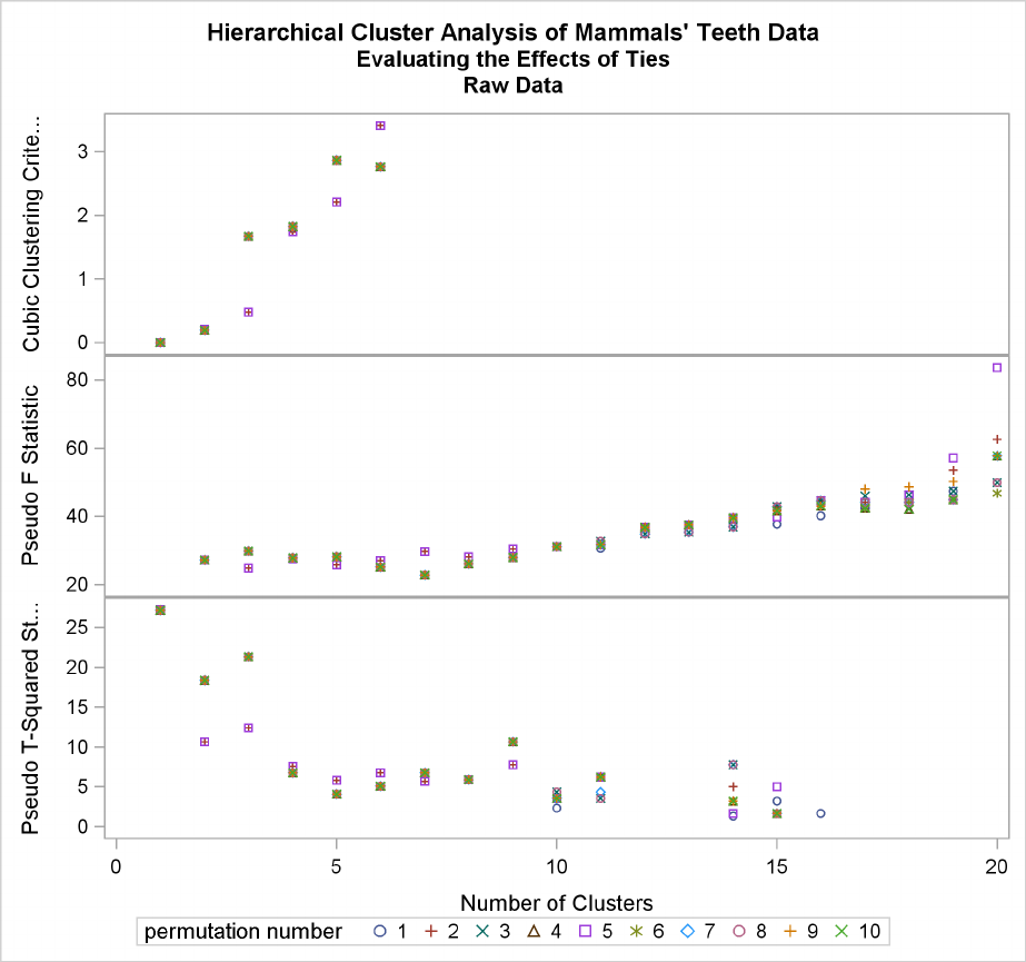
Example 29.4: Evaluating the Effects of Ties F1311
The following statements produce Output 29.4.3.
/*-----PLOT STATISTICS FOR THE LAST 20 LEVELS-------------- */
%plotperm(20, 10);
Output 29.4.3 Analysis of 10 Random Permutations of Raw Mammals’ Teeth Data
The following statements produce Output 29.4.4.
/*------ANALYZE THE 4-CLUSTER LEVEL------------------------ */
%tabperm( &vlist, mammal, 9.1, 4, 10);

1312 FChapter 29: The CLUSTER Procedure
Output 29.4.4 Raw Mammals’ Teeth Data: Indeterminacy at the 4-Cluster Level
Hierarchical Cluster Analysis of Mammals’ Teeth Data
Evaluating the Effects of Ties
Raw Data
-----------------------------------------------------------------------------
| | | Mean |
| | |---------------------------------------|
| | | Top | Bottom | Top | Bottom |
| |FREQ |incisors |incisors | canines | canines |
|-----------------------------+-----+---------+---------+---------+---------|
|all_clus | | | | | |
|-----------------------------| | | | | |
|1 3 1 1 1 3 3 3 2 3 | 4| 0.0| 4.0| 0.5| 0.0|
|-----------------------------+-----+---------+---------+---------+---------|
|2 2 2 2 2 2 1 2 1 1 | 15| 2.9| 2.6| 1.0| 1.0|
|-----------------------------+-----+---------+---------+---------+---------|
|2 4 2 2 4 2 1 2 1 1 | 1| 3.0| 2.0| 1.0| 0.0|
|-----------------------------+-----+---------+---------+---------+---------|
|3 1 3 3 3 1 2 1 3 2 | 5| 1.0| 1.0| 0.0| 0.0|
|-----------------------------+-----+---------+---------+---------+---------|
|3 4 3 3 4 1 2 1 3 2 | 2| 2.0| 1.0| 0.0| 0.0|
|-----------------------------+-----+---------+---------+---------+---------|
|4 4 4 4 4 4 4 4 4 4 | 5| 1.8| 3.0| 1.0| 1.0|
-----------------------------------------------------------------------------
(Continued)
Hierarchical Cluster Analysis of Mammals’ Teeth Data
Evaluating the Effects of Ties
Raw Data
-----------------------------------------------------------------------
| | Mean |
| |---------------------------------------|
| | Top | Bottom | Top | Bottom |
| |premolars|premolars| molars | molars |
|-----------------------------+---------+---------+---------+---------|
|all_clus | | | | |
|-----------------------------| | | | |
|1 3 1 1 1 3 3 3 2 3 | 3.0| 3.0| 3.0| 3.0|
|-----------------------------+---------+---------+---------+---------|
|2 2 2 2 2 2 1 2 1 1 | 3.6| 3.4| 1.3| 1.8|
|-----------------------------+---------+---------+---------+---------|
|2 4 2 2 4 2 1 2 1 1 | 3.0| 3.0| 3.0| 3.0|
|-----------------------------+---------+---------+---------+---------|
|3 1 3 3 3 1 2 1 3 2 | 1.2| 0.8| 3.0| 3.0|
|-----------------------------+---------+---------+---------+---------|
|3 4 3 3 4 1 2 1 3 2 | 2.5| 2.0| 3.0| 3.0|
|-----------------------------+---------+---------+---------+---------|
|4 4 4 4 4 4 4 4 4 4 | 2.0| 2.4| 3.0| 3.0|
-----------------------------------------------------------------------
Example 29.4: Evaluating the Effects of Ties F1313
From the TABULATE output, you can see that two types of clustering are obtained. In one case,
the mole is grouped with the carnivores, while the pika and rabbit are grouped with the rodents. In
the other case, both the mole and the lagomorphs are grouped with the bats.
Next, the analysis is repeated with the standardized data as shown in the following statements. The
pseudo Fand t2statistics indicate 3 or 4 clusters, while the cubic clustering criterion shows a sharp
rise up to 4 clusters and then levels off up to 6 clusters. So the TABPERM macro is used again at the
4-cluster level. In this case, there is no indeterminacy, because the same four clusters are obtained
with every permutation, although in different orders. It must be emphasized, however, that lack of
indeterminacy in no way indicates validity.
title3 ’Standardized Data’;
/*------CLUSTER STANDARDIZED DATA WITH AVERAGE LINKAGE------*/
%clusperm( teeth, &vlist, mammal, average std, 10);
The following statements produce Output 29.4.5.
/*-----PLOT STATISTICS FOR THE LAST 20 LEVELS-------------- */
%plotperm(20, 10);
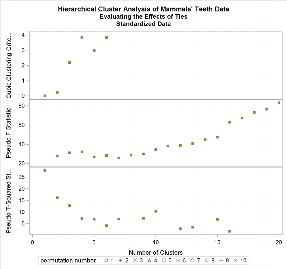
1314 FChapter 29: The CLUSTER Procedure
Output 29.4.5 Analysis of 10 Random Permutations of Standardized Mammals’ Teeth Data

Example 29.4: Evaluating the Effects of Ties F1315
The following statements produce Output 29.4.6.
/*------ANALYZE THE 4-CLUSTER LEVEL------------------------ */
%tabperm( &vlist, mammal, 9.1, 4, 10);
Output 29.4.6 Standardized Mammals’ Teeth Data: No Indeterminacy at the 4-Cluster Level
Hierarchical Cluster Analysis of Mammals’ Teeth Data
Evaluating the Effects of Ties
Standardized Data
-----------------------------------------------------------------------------
| | | Mean |
| | |---------------------------------------|
| | | Top | Bottom | Top | Bottom |
| |FREQ |incisors |incisors | canines | canines |
|-----------------------------+-----+---------+---------+---------+---------|
|all_clus | | | | | |
|-----------------------------| | | | | |
|1 3 1 1 1 3 3 3 2 3 | 4| 0.0| 4.0| 0.5| 0.0|
|-----------------------------+-----+---------+---------+---------+---------|
|2 2 2 2 2 2 1 2 1 1 | 15| 2.9| 2.6| 1.0| 1.0|
|-----------------------------+-----+---------+---------+---------+---------|
|3 1 3 3 3 1 2 1 3 2 | 7| 1.3| 1.0| 0.0| 0.0|
|-----------------------------+-----+---------+---------+---------+---------|
|4 4 4 4 4 4 4 4 4 4 | 6| 2.0| 2.8| 1.0| 0.8|
-----------------------------------------------------------------------------
(Continued)
Hierarchical Cluster Analysis of Mammals’ Teeth Data
Evaluating the Effects of Ties
Standardized Data
-----------------------------------------------------------------------
| | Mean |
| |---------------------------------------|
| | Top | Bottom | Top | Bottom |
| |premolars|premolars| molars | molars |
|-----------------------------+---------+---------+---------+---------|
|all_clus | | | | |
|-----------------------------| | | | |
|1 3 1 1 1 3 3 3 2 3 | 3.0| 3.0| 3.0| 3.0|
|-----------------------------+---------+---------+---------+---------|
|2 2 2 2 2 2 1 2 1 1 | 3.6| 3.4| 1.3| 1.8|
|-----------------------------+---------+---------+---------+---------|
|3 1 3 3 3 1 2 1 3 2 | 1.6| 1.1| 3.0| 3.0|
|-----------------------------+---------+---------+---------+---------|
|4 4 4 4 4 4 4 4 4 4 | 2.2| 2.5| 3.0| 3.0|
-----------------------------------------------------------------------

1316 FChapter 29: The CLUSTER Procedure
References
Anderberg, M. R. (1973), Cluster Analysis for Applications, New York: Academic Press.
Batagelj, V. (1981), “Note on Ultrametric Hierarchical Clustering Algorithms,” Psychometrika, 46,
351–352.
Blackith, R. E. and Reyment, R. A. (1971), Multivariate Morphometrics, London: Academic Press.
Blashfield, R. K. and Aldenderfer, M. S. (1978), “The Literature on Cluster Analysis,” Multivariate
Behavioral Research, 13, 271–295.
Calinski, T. and Harabasz, J. (1974), “A Dendrite Method for Cluster Analysis,” Communications
in Statistics, 3, 1–27.
Cooper, M. C. and Milligan, G. W. (1988), “The Effect of Error on Determining the Number of
Clusters,” in Data, Expert Knowledge, and Decisions, 319–328, ed. W. Gaul and M. Schrader,
London: Springer-Verlag.
Duda, R. O. and Hart, P. E. (1973), Pattern Classification and Scene Analysis, New York: John
Wiley & Sons.
Everitt, B. S. (1980), Cluster Analysis, Second Edition, London: Heineman Educational Books.
Fisher, L. and Van Ness, J. W. (1971), “Admissible Clustering Procedures,” Biometrika, 58, 91–104.
Fisher, R. A. (1936), “The Use of Multiple Measurements in Taxonomic Problems,” Annals of
Eugenics, 7, 179–188.
Florek, K., Lukaszewicz, J., Perkal, J., and Zubrzycki, S. (1951a), “Sur la Liaison et la Division des
Points d’un Ensemble Fini,” Colloquium Mathematicae, 2, 282–285.
Florek, K., Lukaszewicz, J., Perkal, J., and Zubrzycki, S. (1951b), “Taksonomia Wroclawska,”
Przeglad Antropol., 17, 193–211.
Gower, J. C. (1967), “A Comparison of Some Methods of Cluster Analysis,” Biometrics, 23, 623–
637.
Hamer, R. M. and Cunningham, J. W. (1981), “Cluster Analyzing Profile Data with Interrater Dif-
ferences: A Comparison of Profile Association Measures,” Applied Psychological Measurement, 5,
63–72.
Hartigan, J. A. (1975), Clustering Algorithms, New York: John Wiley & Sons.
Hartigan, J. A. (1977), “Distribution Problems in Clustering,” in Classification and Clustering, ed.
J. Van Ryzin, New York: Academic Press.
Hartigan, J. A. (1981), “Consistency of Single Linkage for High-Density Clusters,” Journal of the
American Statistical Association, 76, 388–394.
References F1317
Hawkins, D. M., Muller, M. W., and ten Krooden, J. A. (1982), “Cluster Analysis,” in Topics in
Applied Multivariate Analysis, ed. D. M. Hawkins, Cambridge: Cambridge University Press.
Jardine, N. and Sibson, R. (1971), Mathematical Taxonomy, New York: John Wiley & Sons.
Johnson, S. C. (1967), “Hierarchical Clustering Schemes,” Psychometrika, 32, 241–254.
Lance, G. N. and Williams, W. T. (1967), “A General Theory of Classificatory Sorting Strategies. I.
Hierarchical Systems,” Computer Journal, 9, 373–380.
Massart, D. L. and Kaufman, L. (1983), The Interpretation of Analytical Chemical Data by the Use
of Cluster Analysis, New York: John Wiley & Sons.
McQuitty, L. L. (1957), “Elementary Linkage Analysis for Isolating Orthogonal and Oblique Types
and Typal Relevancies,” Educational and Psychological Measurement, 17, 207–229.
McQuitty, L. L. (1966), “Similarity Analysis by Reciprocal Pairs for Discrete and Continuous Data,”
Educational and Psychological Measurement, 26, 825–831.
Mezzich, J. E. and Solomon, H. (1980), Taxonomy and Behavioral Science, New York: Academic
Press.
Milligan, G. W. (1979), “Ultrametric Hierarchical Clustering Algorithms,” Psychometrika, 44, 343–
346.
Milligan, G. W. (1980), “An Examination of the Effect of Six Types of Error Perturbation on Fifteen
Clustering Algorithms,” Psychometrika, 45, 325–342.
Milligan, G. W. (1987), “A Study of the Beta-Flexible Clustering Method,” College of Administra-
tive Science Working Paper Series, 87–61 Columbus: Ohio State University.
Milligan, G. W. and Cooper, M. C. (1985), “An Examination of Procedures for Determining the
Number of Clusters in a Data Set,” Psychometrika, 50,159–179.
Milligan, G. W. and Cooper, M. C. (1987), “A Study of Variable Standardization,” College of Ad-
ministrative Science Working Paper Series, 87–63, Columbus: Ohio State University.
Rouncefield, M. (1995), “The Statistics of Poverty and Inequality,” Journal of Statistics Education,
3(2). [Online]: [http://www.stat.ncsu.edu/info/jse], accessed Dec. 19, 1997.
Sarle, W. S. (1983), Cubic Clustering Criterion, SAS Technical Report A-108, Cary, NC: SAS
Institute Inc.
Silverman, B. W. (1986), Density Estimation, New York: Chapman & Hall.
Sneath, P. H. A. (1957), “The Application of Computers to Taxonomy,” Journal of General Micro-
biology, 17, 201–226.
Sneath, P. H. A. and Sokal, R. R. (1973), Numerical Taxonomy, San Francisco: Freeman.
Sokal, R. R. and Michener, C. D. (1958), “A Statistical Method for Evaluating Systematic Relation-
ships,” University of Kansas Science Bulletin, 38, 1409–1438.
1318 FChapter 29: The CLUSTER Procedure
Sorensen, T. (1948), “A Method of Establishing Groups of Equal Amplitude in Plant Sociology
Based on Similarity of Species Content and Its Application to Analyses of the Vegetation on Danish
Commons,” Biologiske Skrifter, 5, 1–34.
Spath, H. (1980), Cluster Analysis Algorithms, Chichester, Eng.: Ellis Horwood.
Symons, M. J. (1981), “Clustering Criteria and Multivariate Normal Mixtures,” Biometrics, 37,
35–43.
Ward, J. H. (1963), “Hierarchical Grouping to Optimize an Objective Function,” Journal of the
American Statistical Association, 58, 236–244.
Wishart, D. (1969), “Mode Analysis: A Generalisation of Nearest Neighbour Which Reduces
Chaining Effects,” in Numerical Taxonomy, ed. A. J. Cole, London: Academic Press.
Wong, M. A. (1982), “A Hybrid Clustering Method for Identifying High-Density Clusters,” Journal
of the American Statistical Association, 77, 841–847.
Wong, M. A. and Lane, T. (1983), “A kth Nearest Neighbor Clustering Procedure,” Journal of the
Royal Statistical Society, Series B, 45, 362–368.
Wong, M. A. and Schaack, C. (1982), “Using the kth Nearest Neighbor Clustering Procedure to
Determine the Number of Subpopulations,” American Statistical Association 1982 Proceedings of
the Statistical Computing Section, 40–48.
Subject Index
agglomerative hierarchical clustering analysis,
1230
average linkage
CLUSTER procedure, 1239,1250
bimodality coefficient
CLUSTER procedure, 1246,1258
centroid method
CLUSTER procedure, 1239,1251
chaining, reducing when clustering, 1247
CLUSTER procedure
algorithms, 1259
average linkage, 1230
centroid method, 1230
clustering methods, 1230,1250
complete linkage, 1230
computational resources, 1260
density linkage, 1230,1239
Euclidean distances, 1230
Fstatistics, 1246,1258
FASTCLUS procedure, compared, 1230
flexible-beta method, 1230,1240,1241,
1255
hierarchical clusters, 1230
input data sets, 1241
interval scale, 1262
kth-nearest-neighbor method, 1230
maximum likelihood, 1230,1239
McQuitty’s similarity analysis , 1230
median method, 1230
memory requirements, 1260
missing values, 1261
non-Euclidean distances, 1230
ODS Graph names, 1269
output data sets, 1244,1263
output table names, 1268
pseudo Fand tstatistics, 1246
ratio scale, 1262
single linkage, 1230
size, shape, and correlation, 1262
test statistics, 1241,1246,1247
ties, 1261
time requirements, 1260
TREE procedure, compared, 1230
two-stage density linkage, 1230
types of data sets, 1230
using macros for many analyses, 1290
Ward’s minimum-variance method, 1230
Wong’s hybrid method, 1230
clustering, 1229,see also CLUSTER procedure
average linkage, 1239,1250
centroid method, 1239,1251
complete linkage method, 1239,1251
density linkage methods, 1239,1240,1242,
1243,1246,1252,1254,1256
Gower’s method, 1240,1255
maximum-likelihood method, 1244,1254,
1255
McQuitty’s similarity analysis, 1240,1255
median method, 1240,1255
methods affected by frequencies, 1248
outliers in, 1230,1247
penalty coefficient, 1244
single linkage, 1240,1255,1256
smoothing parameters, 1253
standardizing variables, 1246
transforming variables, 1230
two-stage density linkage, 1240
Ward’s method, 1240,1257
weighted average linkage, 1240,1255
complete linkage
CLUSTER procedure, 1239,1251
computational resources
CLUSTER procedure, 1260
connectedness method, see single linkage
cubic clustering criterion, 1243,1247
CLUSTER procedure, 1241
dendritic method, see single linkage
density linkage
CLUSTER procedure, 1239,1240,1242,
1243,1246,1252,1254,1256
diameter method, see complete linkage
DISTANCE data sets
CLUSTER procedure, 1241
elementary linkage analysis, see single linkage
error sum of squares clustering method, see
Ward’s method
Euclidean distances, 1242,1244
clustering, 1230
Fstatistics
CLUSTER procedure, 1246,1258
flexible-beta method
CLUSTER procedure, 1230,1240,1241,
1255
FREQ statement
and RMSSTD statement (CLUSTER), 1248,
1249
furthest neighbor clustering, see complete linkage
Gower’s method, see also median method
CLUSTER procedure, 1240,1255
group average clustering, see average linkage
hierarchical clustering, 1239,1254
HYBRID option
and FREQ statement (CLUSTER), 1248
and other options (CLUSTER), 1246
PROC CLUSTER statement, 1252
k-th-nearest neighbor, see also density linkage,
see also single linkage
k-th-nearest neighbor
estimation (CLUSTER), 1242,1246
k-th-nearest-neighbor
estimation (CLUSTER), 1252
K= option
and other options (CLUSTER), 1242,1246
kurtosis
displayed in CLUSTER procedure, 1246
Lance-Williams flexible-beta method, see
flexible-beta method
maximum likelihood
hierarchical clustering (CLUSTER), 1239,
1244,1254,1255
maximum method, see complete linkage
McQuitty’s similarity analysis
CLUSTER procedure, 1240
means
displayed in CLUSTER procedure, 1246
median
method (CLUSTER), 1240,1255
memory requirements
CLUSTER procedure, 1260
METHOD= specification
PROC CLUSTER statement, 1239
missing values
CLUSTER procedure, 1261
modal clusters
density estimation (CLUSTER), 1243
nearest neighbor method, see also single linkage
NOSQUARE option
algorithms used (CLUSTER), 1259
ODS Graph names
CLUSTER procedure, 1269
output data sets
CLUSTER procedure, 1244
output table names
CLUSTER procedure, 1268
preliminary clusters
definition (CLUSTER), 1252
using in CLUSTER procedure, 1242
pseudo Fand tstatistics
CLUSTER procedure, 1246
R-square statistic
CLUSTER procedure, 1246
R= option
and other options (CLUSTER), 1242,1246
radius of sphere of support, 1246
rank order typal analysis, see complete linkage
RMSSTD statement
and FREQ statement (CLUSTER), 1248,
1249
semipartial correlation
formula (CLUSTER), 1258
single linkage
CLUSTER procedure, 1240,1255
skewness
displayed in CLUSTER procedure, 1246
smoothing parameter
cluster analysis, 1253
squared semipartial correlation
formula (CLUSTER), 1258
standard deviation
CLUSTER procedure, 1246
standardizing
CLUSTER procedure, 1246
stored data algorithm, 1259
stored distance algorithms, 1259
t-square statistic
CLUSTER procedure, 1246,1258
ties
checking for in CLUSTER procedure, 1244
time requirements
CLUSTER procedure, 1260
trace W method, see Ward’s method
transformations
cluster analysis, 1230
TRIM= option
and other options (CLUSTER), 1242,1246
two-stage density linkage
CLUSTER procedure, 1240,1256
ultrametric, definition, 1259
uniform-kernel estimation
CLUSTER procedure, 1246,1252
unsquared Euclidean distances, 1242,1244
unweighted pair-group clustering, see average
linkage, see centroid method
UPGMA, see average linkage
UPGMC, see centroid method
Ward’s minimum-variance method
CLUSTER procedure, 1240,1257
weighted average linkage
CLUSTER procedure, 1240,1255
weighted pair-group methods, see McQuitty’s
similarity analysis, see median method
weighted-group method, see centroid method
Wong’s hybrid method
CLUSTER procedure, 1242,1252
WPGMA, see McQuitty’s similarity analysis
WPGMC, see median method
Syntax Index
BETA= option
PROC CLUSTER statement, 1241
CCC option
PROC CLUSTER statement, 1241
CLUSTER procedure
syntax, 1239
CLUSTER procedure, BY statement, 1247
CLUSTER procedure, COPY statement, 1247
CLUSTER procedure, FREQ statement, 1248
CLUSTER procedure, ID statement, 1248
CLUSTER procedure, PROC CLUSTER
statement, 1239
BETA= option, 1241
CCC option, 1241
DATA= option, 1241
DIM= option, 1242
HYBRID option, 1242
K= option, 1242
MODE= option, 1243
NOEIGEN option, 1243
NOID option, 1243
NONORM option, 1243
NOPRINT option, 1243
NOSQUARE option, 1244
NOTIE option, 1244
OUTTREE= option, 1244
PENALTY= option, 1244
PLOTS option, 1244
PRINT= option, 1246
PSEUDO= option, 1246
R= option, 1246
RMSSTD option, 1246
RSQUARE option, 1246
SIMPLE option, 1246
STANDARD option, 1246
TRIM= option, 1246
CLUSTER procedure, RMSSTD statement, 1249
CLUSTER procedure, VAR statement, 1249
DATA= option
PROC CLUSTER statement, 1241
DIM= option
PROC CLUSTER statement, 1242
HYBRID option
PROC CLUSTER statement, 1242
K= option
PROC CLUSTER statement, 1242
MODE= option
PROC CLUSTER statement, 1243
NOEIGEN option
PROC CLUSTER statement, 1243
NOID option
PROC CLUSTER statement, 1243
NONORM option
PROC CLUSTER statement, 1243
NOPRINT option
PROC CLUSTER statement, 1243
NOSQUARE option
PROC CLUSTER statement, 1242,1244
NOTIE option
PROC CLUSTER statement, 1244
OUTTREE= option
PROC CLUSTER statement, 1244
PENALTY= option
PROC CLUSTER statement, 1244
PLOTS option
PROC CLUSTER statement, 1244
PRINT= option
PROC CLUSTER statement, 1246
PROC CLUSTER statement, see CLUSTER
procedure
PSEUDO= option
PROC CLUSTER statement, 1246
R= option
PROC CLUSTER statement, 1246
RMSSTD option
PROC CLUSTER statement, 1246
RSQUARE option
PROC CLUSTER statement, 1246
SIMPLE option
PROC CLUSTER statement, 1246
STANDARD option
PROC CLUSTER statement, 1246
TRIM= option
and other options, 1242
PROC CLUSTER statement, 1242,1246

Your Turn
We welcome your feedback.
If you have comments about this book, please send them to
yourturn@sas.com. Include the full title and page numbers (if
applicable).
If you have comments about the software, please send them to
suggest@sas.com.

SAS® Publishing Delivers!
Whether you are new to the work force or an experienced professional, you need to distinguish yourself in this rapidly
changing and competitive job market. SAS® Publishing provides you with a wide range of resources to help you set
yourself apart. Visit us online at support.sas.com/bookstore.
SAS® Press
Need to learn the basics? Struggling with a programming problem? You’ll find the expert answers that you
need in example-rich books from SAS Press. Written by experienced SAS professionals from around the
world, SAS Press books deliver real-world insights on a broad range of topics for all skill levels.
support.sas.com/saspress
SAS® Documentation
To successfully implement applications using SAS software, companies in every industry and on every
continent all turn to the one source for accurate, timely, and reliable information: SAS documentation.
We currently produce the following types of reference documentation to improve your work experience:
• Onlinehelpthatisbuiltintothesoftware.
• Tutorialsthatareintegratedintotheproduct.
• ReferencedocumentationdeliveredinHTMLandPDF– free on the Web.
• Hard-copybooks. support.sas.com/publishing
SAS® Publishing News
Subscribe to SAS Publishing News to receive up-to-date information about all new SAS titles, author
podcasts, and new Web site features via e-mail. Complete instructions on how to subscribe, as well as
access to past issues, are available at our Web site. support.sas.com/spn
SAS and all other SAS Institute Inc. product or service names are registered trademarks or trademarks of SAS Institute Inc. in the USA and other countries. ® indicates USA registration.
Otherbrandandproductnamesaretrademarksoftheirrespectivecompanies.©2009SASInstituteInc.Allrightsreserved.518177_1US.0109