VLP 16 User Manual
63-9243%20REV%20D%20MANUAL%2CUSERS%2CVLP-16
63-9243%20REV%20D%20MANUAL%2CUSERS%2CVLP-16
VLP-16_User_Manual
63-9243%20REV%20D%20MANUAL%2CUSERS%2CVLP-16
VLP16_User_Manual
User Manual: Pdf
Open the PDF directly: View PDF ![]() .
.
Page Count: 138 [warning: Documents this large are best viewed by clicking the View PDF Link!]
- Chapter 1 • About This Manual
- Chapter 2 • VLP-16 Overview
- Chapter 3 • Safety Precautions
- Chapter 4 • Unboxing & Verification
- Chapter 5 • Installation & Integration
- Chapter 6 • Key Features
- Chapter 7 • Sensor Inputs
- 7.1 Power Requirements
- 7.2 Interface Box Signals
- 7.3 Ethernet Interface
- 7.4 GPS, Pulse Per Second (PPS) and NMEA GPRMC Message
- Chapter 8 • Sensor Operation
- Chapter 9 • Sensor Data
- Chapter 10 • Sensor Communication
- 10.1 Web Interface
- 10.2 Sensor Control with curl
- 10.2.1 Using curl with Velodyne LiDAR Sensors
- 10.2.2 curl Command Parameters
- 10.2.3 Command Line curl Examples
- 10.2.3.1 Get Diagnostic Data
- 10.2.3.2 Conversion Formulas
- 10.2.3.3 Interpret Diagnostic Data
- 10.2.3.3.1 top:hv
- 10.2.3.3.2 top:lm20_temp
- 10.2.3.3.3 top:pwr_5v
- 10.2.3.3.4 top:pwr_2_5v
- 10.2.3.3.5 top:pwr_3_3v
- 10.2.3.3.6 top:pwr_5v_raw
- 10.2.3.3.7 top:pwr_vccint
- 10.2.3.3.8 bot:i_out
- 10.2.3.3.9 bot:lm20_temp
- 10.2.3.3.10 bot:pwr_1_2v
- 10.2.3.3.11 bot:pwr_1_25v
- 10.2.3.3.12 bot:pwr_2_5v
- 10.2.3.3.13 bot:pwr_3_3v
- 10.2.3.3.14 bot:pwr_5v
- 10.2.3.3.15 bot:pwr_v_in
- 10.2.3.4 Get Snapshot
- 10.2.3.5 Get Sensor Status
- 10.2.3.6 Set Motor RPM
- 10.2.3.7 Set Field of View
- 10.2.3.8 Set Return Type (Strongest, Last, Dual)
- 10.2.3.9 Save Configuration
- 10.2.3.10 Reset System
- 10.2.3.11 Network Configuration
- 10.2.3.12 Set Host (Destination) IP Address
- 10.2.3.13 Set Data Port
- 10.2.3.14 Set Telemetry Port
- 10.2.3.15 Set Network (Sensor) IP Address
- 10.2.3.16 Set Netmask
- 10.2.3.17 Set Gateway
- 10.2.3.18 Set DHCP
- 10.2.4 curl Example using Python
- Chapter 11 • Troubleshooting
- Appendix A • Sensor Specifications
- Appendix B • Firmware Update
- Appendix C • Mechanical Diagrams
- Appendix D • Wiring Diagrams
- Appendix E • VeloView
- Appendix F • Laser Pulse
- Appendix G • Time Synchronization
- Appendix H • Phase Lock
- Appendix I • Sensor Care
- Appendix J • Network Configuration
VLP-16 User Manual
63-9243 Rev. D

Copyright 2018 Velodyne LiDAR, Inc. All rights reserved.
Trademarks
Velodyne™, HDL-32E™, HDL-64E™, VLP-16™, VLP-32™, Puck™, Puck LITE™, Puck Hi-Res™, and Ultra Puck™ are trade-
marks of Velodyne LiDAR, Inc. All other trademarks, service marks, and company names in this document or website are
properties of their respective owners.
Disclaimer of Liability
The information contained in this document is subject to change without notice. Velodyne LiDAR, Inc. shall not be liable for
errors contained herein or for incidental or consequential damage in connection with the furnishing, performance, or use
of this document or equipment supplied with it.
The materials and information contained herein are being provided by Velodyne LiDAR, Inc. to its Customer solely for Cus-
tomer’s use for its internal business purposes. Velodyne LiDAR, Inc. retains all right, title, interest in and copyrights to the
materials and information herein. The materials and information contained herein constitute confidential information of
Velodyne LiDAR, Inc. and Customer shall not disclose or transfer any of these materials or information to any third party.
No part of this publication may be reproduced or transmitted in any form or by any means, electronic or mechanical, includ-
ing photocopying and recording, or stored in a database or retrieval system for any purpose without the express written
permission of Velodyne LiDAR, Inc., which reserves the right to make changes to this document at any time without notice
and assumes no responsibility for its use. This document contains the most current information available at the time of pub-
lication. When new or revised information becomes available, this entire document will be updated and distributed to all
registered users.
Limited Warranty
Except as specified below, products sold hereunder shall be free from defects in materials and workmanship and shall con-
form to Velodyne's published specifications or other specifications accepted in writing by Velodyne for a period of one (1)
year from the date of shipment of the products. The foregoing warranty does not apply to any Garmin products, other
products not manufactured by Velodyne or products that have been subject to misuse, neglect, or accident, or have been
opened, dissembled, or altered in any way. Velodyne shall make the final determination as to whether its products are
defective. Velodyne 's sole obligation for products failing to comply with this warranty shall be, at its option, to either repair,
replace or issue credit for the nonconforming product where, within fourteen (14) days of the expiration of the warranty
period, (i) Velodyne has received written notice of any nonconformity; (ii) after Velodyne's written authorization, Buyer has
returned the nonconforming product to Velodyne at Buyer's expense; and (iii) Velodyne has determined that the product is
nonconforming and that such nonconformity is not the result of improper installation, repair or other misuse. Velodyne will
pay for return shipping for all equipment repaired or replaced under warranty and Buyer will pay all duties or taxes, if any,
on all equipment repaired or replaced under warranty. THE FOREGOING WARRANTY AND REMEDIES ARE
EXCLUSIVE AND MADE EXPRESSLY IN LIEU OF ALL OTHER WARRANTIES, EXPRESSED, IMPLIED OR
OTHERWISE, INCLUDING WARRANTIES OF 65-0003 Rev E Velodyne LiDAR Terms & Conditions Page 3 of 5 2016-
03-31 MERCHANTABILITY AND FITNESS FOR A PARTICULAR PURPOSE. VELODYNE DOES NOT ASSUME OR
AUTHORIZE ANY OTHER PERSON TO ASSUME FOR IT ANY OTHER LIABILITY IN CONNECTION WITH ITS
PRODUCTS. This warranty is non-transferable.
Velodyne LiDAR, Inc.
5521 Hellyer Ave
San Jose, CA 95138
Phone +1 408-465-2800
Revision History
Sensor Firmware Release
Date Release Notes
VLP-16 3.0.37.0 2017-12-12
• CHANGED: Phase Lock Offset setting now expects
integer degrees instead of hundredths of degrees.
• IMPROVED: Removed 'Update Calibration' from System
tab.
• IMPROVED: Sun Noise Filter.
• ADDED: Ability to change sensor's Ethernet MAC
Address from Web Interface.
• IMPROVED: Low signal cross-talk filtering performance.
• IMPROVED: Firmware update messages during update.
• IMPROVED: Phase Lock rotations error < ±5 degrees.
• FIXED: Intermittent ghost returns at 40, 80 and greater
than 124 meters.
• IMPROVED: Several JSON data additions and changes.
• ADDED: Reverse rotation capability. Specify negative
RPM values to use this capability.
For details, see the full Release Notes at http://www.ve-
lodynelidar.com/downloads.html#firmware.
3

Table of Contents
Chapter 1 • About This Manual
1.1 Manual Scope
16
1.2 Prerequisite Knowledge
16
1.3 Audience
16
1.4 Document Conventions
16
Chapter 2 • VLP-16 Overview
2.1 Overview
18
2.2 Product Models
19
2.3 Time of Flight
19
2.4 Data Interpretation Requirements
19
Chapter 3 • Safety Precautions
3.1 Warning and Caution Definitions
20
3.1.1 Caution Hazard Alerts
20
3.2 Safety Overview
20
3.2.1 Electrical Safety
20
3.2.2 Mechanical Safety
20
3.2.3 Laser Safety
21
Chapter 4 • Unboxing & Verification
4.1 What’s in the Box?
22
4.1.1 Variants
22
4.2 Verification Procedure
22
4.2.1 Network Setup in Isolation
23
4.2.2 Access Sensor’s Web Interface
24
4.2.3 Visualize Live Sensor Data with VeloView
26
4.2.3.1 VeloView Operation
27
Chapter 5 • Installation & Integration
5.1 Overview
29
5.2 Mounting
29
5.3 Encapsulation, Solar Hats, and Ventilation
30
4 VLP-16 User Manual

5.4 Connections
30
5.4.1 Integrated Cable and Interface Box
31
5.4.2 Operation Without an Interface Box
31
5.4.3 Power
31
Chapter 6 • Key Features
6.1 Calibrated Reflectivity
32
6.2 Laser Return Modes
32
6.2.1 Single Return Modes: Strongest, Last
32
6.2.2 Multiple Returns
33
6.2.3 Dual Return Mode
33
6.3 Phase Locking Multiple Sensors
37
Chapter 7 • Sensor Inputs
7.1 Power Requirements
39
7.2 Interface Box Signals
40
7.3 Ethernet Interface
41
7.4 GPS, Pulse Per Second (PPS) and NMEA GPRMC Message
41
7.4.1 GPS Input Signals
41
7.4.2 Electrical Requirements
41
7.4.3 Timing and Polarity Requirements
41
7.4.4 GPS Connection Scenarios
44
7.4.4.1 Connecting a Garmin 18x LVC GPS Receiver
44
7.4.4.2 Connecting to a computer's serial port
44
7.4.4.3 Connecting to a microcomputer’s UART
45
7.4.5 NMEA Message Formats
46
7.4.5.1 Pre-NMEA Version 2.3 Message Format
46
7.4.5.2 NMEA Version 2.3 Message Format
47
7.4.6 Accepting NMEA Messages Via Ethernet
48
Chapter 8 • Sensor Operation
8.1 Firing Sequence
49
8.2 Throughput Calculations
49
5

8.2.1 Data Packet Rate
49
8.2.2 Position Packet Rate
50
8.2.3 Total Packet Rate
50
8.2.4 Laser Measurements Per Second
50
8.2.4.1 Single Return Mode (Strongest, Last)
50
8.2.4.2 Dual Return Mode
50
8.3 Rotation Speed (RPM)
50
8.3.1 Horizontal Angular (Azimuth) Resolution
50
8.3.2 Rotation Speed Fluctuation and Point Density
51
Chapter 9 • Sensor Data
9.1 Sensor Origin and Frame of Reference
52
9.2 Calculating X,Y,Z Coordinates from Collected Spherical Data
52
9.3 Packet Types and Definitions
54
9.3.1 Definitions
54
9.3.1.1 Firing Sequence
55
9.3.1.2 Laser Channel
55
9.3.1.3 Data Point
55
9.3.1.4 Azimuth
55
9.3.1.5 Data Block
55
9.3.1.6 Time Stamp
55
9.3.1.7 Factory Bytes
56
9.3.2 Data Packet Structure
56
9.3.3 Position Packet Structure
60
9.4 Discreet Point Timing Calculation
61
9.5 Precision Azimuth Calculation
65
9.6 Converting PCAP Files to Point Cloud Formats
66
Chapter 10 • Sensor Communication
10.1 Web Interface
68
10.1.1 Configuration Screen
69
10.1.1.1 MAC Address
71
10.1.1.2 Correctly reset MAC Address to Factory MAC Address
71
6 VLP-16 User Manual

10.1.2 System Screen
72
10.1.3 Info Screen
73
10.1.4 Diagnostics Screen
75
10.2 Sensor Control with curl
76
10.2.1 Using curl with Velodyne LiDAR Sensors
76
10.2.2 curl Command Parameters
76
10.2.3 Command Line curl Examples
77
10.2.3.1 Get Diagnostic Data
77
10.2.3.2 Conversion Formulas
78
10.2.3.3 Interpret Diagnostic Data
78
10.2.3.3.1 top:hv
78
10.2.3.3.2 top:lm20_temp
79
10.2.3.3.3 top:pwr_5v
79
10.2.3.3.4 top:pwr_2_5v
79
10.2.3.3.5 top:pwr_3_3v
79
10.2.3.3.6 top:pwr_5v_raw
79
10.2.3.3.7 top:pwr_vccint
80
10.2.3.3.8 bot:i_out
80
10.2.3.3.9 bot:lm20_temp
80
10.2.3.3.10 bot:pwr_1_2v
80
10.2.3.3.11 bot:pwr_1_25v
81
10.2.3.3.12 bot:pwr_2_5v
81
10.2.3.3.13 bot:pwr_3_3v
81
10.2.3.3.14 bot:pwr_5v
81
10.2.3.3.15 bot:pwr_v_in
81
10.2.3.4 Get Snapshot
82
10.2.3.5 Get Sensor Status
82
10.2.3.6 Set Motor RPM
82
10.2.3.7 Set Field of View
83
10.2.3.8 Set Return Type (Strongest, Last, Dual)
83
10.2.3.9 Save Configuration
83
7

10.2.3.10 Reset System
83
10.2.3.11 Network Configuration
83
10.2.3.12 Set Host (Destination) IP Address
83
10.2.3.13 Set Data Port
84
10.2.3.14 Set Telemetry Port
84
10.2.3.15 Set Network (Sensor) IP Address
84
10.2.3.16 Set Netmask
84
10.2.3.17 Set Gateway
84
10.2.3.18 Set DHCP
84
10.2.4 curl Example using Python
84
Chapter 11 • Troubleshooting
11.1 Troubleshooting Process
87
11.1.1 Turned DHCP On, Lost Contact With Sensor
88
11.2 Service and Maintenance
89
11.2.1 Fuse Replacement
89
11.3 Technical Support
90
11.3.1 Purchased through a Distributor
90
11.3.2 Factory Support
90
11.3.3 Support Desk
90
11.4 Return Merchandise Authorization (RMA)
90
Appendix A • Sensor Specifications
Appendix B • Firmware Update
B.1 Firmware Update Procedure
92
B.1.1 Special Procedure to Update Firmware
98
B.1.2 If An Error Occurs
99
Appendix C • Mechanical Diagrams
C.1 Interface Box Mechanical Drawing
101
C.2 VLP-16 and Puck LITE Mechanical Drawing
102
C.3 VLP-16 and Puck LITE Optical Drawing
103
C.4 VLP-16 and Puck LITE Optical Keep Out Zone
104
8 VLP-16 User Manual

C.5 Puck Hi-Res Mechanical Drawing
105
C.6 Puck Hi-Res Optical Drawing
106
C.7 Puck Hi-Res Optical Keep Out Zone
107
Appendix D • Wiring Diagrams
D.1 Interface Box Wiring Diagram
109
D.2 Interface Box Schematic
110
Appendix E • VeloView
E.1 Features
111
E.2 Install VeloView
112
E.3 Visualize Streaming Sensor Data
112
E.4 Capture Streaming Sensor Data to PCAP File
114
E.5 Replay Captured Sensor Data from PCAP File
114
Appendix F • Laser Pulse
F.1 The Semiconductor Laser Diode
119
F.2 Laser Patterns
120
F.2.1 Laser Spot Pattern
120
F.2.2 Laser Scan Pattern
120
F.2.3 Beam Divergence
121
Appendix G • Time Synchronization
G.1 Introduction
123
G.2 Background
123
G.3 PPS Qualifier
124
G.3.1 Require GPS Receiver Valid
124
G.3.2 Require PPS Lock
124
G.3.3 Delay
125
G.4 GPS Qualifier
125
G.5 Application
125
G.6 Logic Tables
125
Appendix H • Phase Lock
H.1 Phase Lock
127
9

H.1.1 Setting the Phase Lock
127
H.1.2 Application Scenarios
128
H.2 Field of View
130
Appendix I • Sensor Care
I.1 Cleaning the Sensor
131
I.1.1 Required Materials
131
I.1.2 Determine Method of Cleaning
132
I.1.3 Method One
132
I.1.4 Method Two
132
I.1.5 Method Three
132
I.1.6 Method Four
133
Appendix J • Network Configuration
J.1 Ethernet and Network Setup
134
J.1.1 Defaults
134
J.1.2 Establishing Communication via Ethernet
134
J.2 Network Considerations
135
J.2.1 Throughput Requirements
135
J.2.2 Single Sensor Transmitting to a Broadcast Address
136
J.2.3 Multiple Sensors in the Same Network
136
J.2.3.1 Multiple Sensors Transmitting to a Broadcast Address
136
J.2.3.2 Multiple Sensors Transmitting to a Specific Address
137
10 VLP-16 User Manual

List of Tables
Table 1-1 Document Conventions
16
Table 2-1 3D Sensing System Components
19
Table 7-1 Interface Box Signals
40
Table 7-2 Pre-NMEA Version 2.3 Message Format
47
Table 7-3 Post-NMEA Version 2.3 Message Format
47
Table 8-1 Rotation Speed vs Resolution
51
Table 9-1 Vertical Angles (ω) by Laser ID and Model
53
Table 9-2 Factory Byte Values
56
Table 9-3 Position Packet Structure Field Offsets
60
Table 9-4 PPS Status Byte Values
60
Table 10-1 Configuration Screen Functionality and Features
69
Table 10-2 System Screen Functionality and Features
72
Table 10-3 Info Screen Functionality and Features
73
Table 10-4 System Screen Functionality and Features
75
Table 11-1 Common Problems and Resolutions
87
Table F-1 VLP-16 Beam Divergence
122
Table F-2 Dimensions of VLP-16 Laser Spots at Distance
122
11

List of Figures
Figure 2-1 Example 3D Sensing System
18
Figure 3-1 Class 1 Laser
21
Figure 4-1 Sensor Network Settings
24
Figure 4-2 Interface Box (power and data connections)
25
Figure 4-3 Sample Web Interface Main Configuration Screen
26
Figure 4-4 VeloView Open Sensor Stream
27
Figure 4-5 VeloView Select Sensor Calibration
27
Figure 4-6 VeloView Sensor Stream Display
28
Figure 5-1 Mounting Details
30
Figure 6-1 A Single Return
33
Figure 6-2 Dual Return with Last and Strongest Returns
34
Figure 6-3 Dual Return with Second Strongest Return
35
Figure 6-4 Dual Return with Far Retro-Reflector
36
Figure 6-5 Forestry Application Multiple Returns
37
Figure 6-6 Phase Locking Example
38
Figure 7-1 Interface Box (sensor power and data connections)
40
Figure 7-2 Synchronizing PPS with NMEA GPRMC Message
42
Figure 7-3 PPS Signal Closely Followed by NMEA GPRMC Message
42
Figure 7-4 PPS Signal Followed 600 ms later by NMEA GPRMC Message
43
Figure 7-5 RS-232 Example Transmission
44
Figure 7-6 Garmin GPRMC Message
44
Figure 7-7 DB9 Pin-outs (DTE) and USB-to-Serial Adapter
45
Figure 7-8 Signal Directly from UART (incorrect polarity)
46
Figure 7-9 Inverted Signal from UART (correct polarity)
46
Figure 8-1 Firing Sequence Timing
49
Figure 8-2 Point Density Example
51
Figure 9-1 VLP-16 Sensor Coordinate System
53
Figure 9-2 VLP-16 Single Return Mode Data Structure
57
Figure 9-3 VLP-16 Dual Return Mode Data Structure
58
Figure 9-4 Single Return Mode Packet Data Trace (packet start)
59
Figure 9-5 Single Return Mode Packet Data Trace (ending)
59
Figure 9-6 Wireshark Position Packet Trace
61
Figure 9-7 Firing Sequence Timing
62
Figure 9-8 Example Data Point Timing Calculation
63
12 VLP-16 User Manual

Figure 9-9 Single Return Mode Timing Offsets (in µs)
64
Figure 9-10 Dual Return Mode Timing Offsets (in µs)
65
Figure 10-1 VLP-16 Configuration Screen
69
Figure 10-2 VLP-16 System Screen
72
Figure 10-3 VLP-16 Info Screen
73
Figure 10-4 VLP-16 Diagnostics Screen
75
Figure B-1 Velodyne Downloads Page
92
Figure B-2 Compare Firmware Versions
93
Figure B-3 Select New Firmware Image
94
Figure B-4 Upload New Firmware Image
95
Figure B-5 Firmware Update Complete Page
96
Figure B-6 Finalize Firmware Update
97
Figure B-7 Verify Firmware Versions
98
Figure C-1 Interface Box Mechanical Drawing 50-6001 Rev A
101
Figure C-2 VLP-16 and Puck LITE Mechanical Drawing 86-0101 Rev B1
102
Figure C-3 VLP-16 and Puck LITE Optical Drawing 86-0101 Rev B1
103
Figure C-4 VLP-16 and Puck LITE Optical Keep Out Zone 86-0101 Rev B1
104
Figure C-5 Puck Hi-Res Mechanical Drawing 86-0129 Rev A
105
Figure C-6 Puck Hi-Res Optical Drawing 86-0129 Rev A
106
Figure C-7 Puck Hi-Res Optical Keep Out Zone 86-0129 Rev A
107
Figure D-1 Interface Box Wiring Diagram 86-0107A
109
Figure D-2 Interface Box Schematic 69-8230A
110
Figure E-1 VeloView Open Sensor Stream
112
Figure E-2 VeloView Select Sensor Calibration
113
Figure E-3 VeloView Sensor Stream Display
113
Figure E-4 VeloView Record Button
114
Figure E-5 VeloView Open Capture File
115
Figure E-6 VeloView Play Button
115
Figure E-7 VeloView Spreadsheet Tool
116
Figure E-8 VeloView Data Point Table
116
Figure E-9 VeloView Show Only Selected Elements
117
Figure E-10 VeloView Select All Points
117
Figure E-11 VeloView List Selected Points
118
Figure F-1 Laser Diode Concept
119
Figure F-2 Laser Spot Shape
120
Figure F-3 Laser Spots on a Wall
121
13

Figure G-1 Web Interface PPS and GPS Qualifier Option Selections
123
Figure G-2 Top of Hour Counters
124
Figure G-3 Sub-Second Counter Behavior
125
Figure G-4 Minutes and Seconds Counter Behavior
126
Figure H-1 Direction of Laser Firing
127
Figure H-2 Configuration Screen - Phase Lock
128
Figure H-3 Right and Left Sensor Phase Offset
129
Figure H-4 Fore and Aft Sensor Phase Offset
129
Figure H-5 Sensor Data Shadows
130
Figure J-1 Sensor Network Settings
135
Figure J-2 Single Sensor Broadcasting on a Simple Network
136
Figure J-3 Multiple Sensors - Improper Network Setup
137
Figure J-4 Multiple Sensors - Proper Network Setup
137
14 VLP-16 User Manual


Chapter 1 • About This Manual
1.1 Manual Scope
This manual provides descriptions and procedures supporting the installation, verification, operation, and diagnostic eval-
uation of the VLP-16, Puck LITE and Puck Hi-Res sensors.
For readability, all products in the VLP-16 LiDAR sensor family are referred to as “VLP-16” in this manual, except
where noted.
1.2 Prerequisite Knowledge
This manual is written with the premise that the user has some basic engineering experience and general understanding
of LiDAR technology. In addition, some familiarity with the configuration and operation of networking applications and
equipment is recommended.
It is recommended that prior to installation or other procedures covered in this manual, the user fully reads and com-
prehends all information within this manual.
1.3 Audience
The user mentioned occasionally in this document is typically an engineer tasked with sensor integration for a project, a
tech tasked with sensor upkeep, or data scientist looking to understand sensor output data.
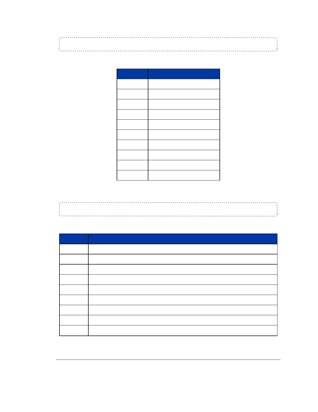
1.4 Document Conventions
This document uses the following typographic conventions:
Convention Description
Bold Indicates text on a window, other than the window title, including menus, menu options, buttons,
fields, and labels. Example: Click OK.
Italic
Indicates a variable, which is a placeholder for actual text provided by the user or system. Example:
copy
source-file
target-file
Note: Angled brackets (< >) are also used to indicate variables.
screen/code Indicates text that is displayed on screen or entered by the user. Example:
# pairdisplay -g oradb
[ ] square
brackets Indicates optional values. Example: [ a | b ] indicates that you can choose a, b, or nothing.
{ } braces Indicates required or expected values. Example: { a | b } indicates that you must choose either a or
b.
| vertical bar Indicates that you have a choice between two or more options or arguments. Examples: [ a | b ]
indicates that you can choose a, b, or nothing. { a | b } indicates that you must choose either a or b.
Table 1-1 Document Conventions
16 VLP-16 User Manual

Note: Notes such as this indicate important information. They call attention to an operating procedure or practice which
may enhance user interaction with the product. Notes may also be used to prevent information loss or product damage.
Chapter 1 • About This Manual 17
Chapter 2 • VLP-16 Overview
This chapter provides basic information on the sensor's hardware and software components.
2.1 Overview
18
2.2 Product Models
19
2.3 Time of Flight
19
2.4 Data Interpretation Requirements
19
2.1 Overview
The VLP-16 sensor uses an array of 16 infra-red (IR) lasers paired with IR detectors to measure distances to objects. The
device is mounted securely within a compact, weather-resistant housing. The array of laser/detector pairs spins rapidly
within its fixed housing to scan the surrounding environment, firing each laser approximately 18,000 times per second,
providing, in real-time, a rich set of 3D point data.
Advanced digital signal processing and waveform analysis provide highly accurate long-range sensing, as well as cal-
ibrated reflectivity data, enabling easy detection of retro-reflectors like street-signs, license plates, and lane markings.
Combining 16 laser/detector pairs into one VLP-16 sensor and pulsing each at 18.08 kHz enables measurements of up to
300,000 data points per second -- or double that in dual return mode.
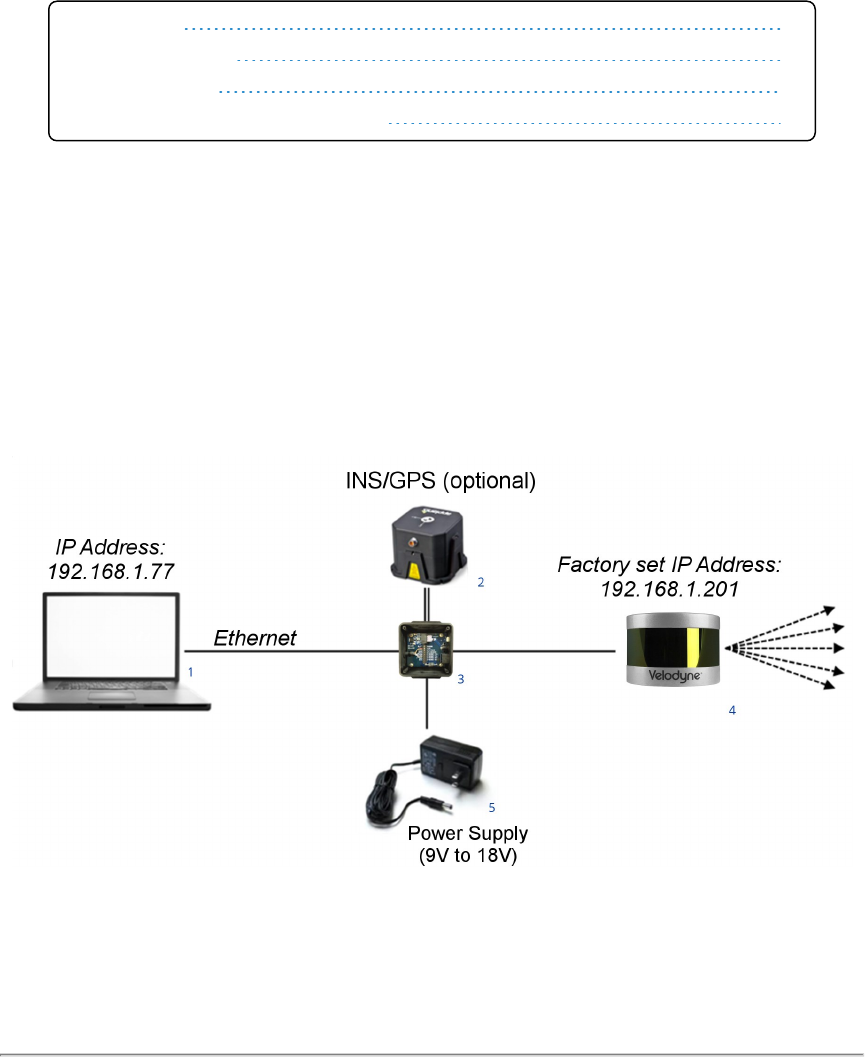
Figure 2-1 Example 3D Sensing System
18 VLP-16 User Manual
Item Description
1 Desktop/Laptop Computer
2 INS/GPS Antenna/Interface (optional)
3 Velodyne Interface Box
4 Velodyne LiDAR Sensor
5 DC Power Supply
Table 2-1 3D Sensing System Components
Note: Optional - not included unless ordered: Garmin GPS receiver (P/N: 80-GPS18LVC).
2.2 Product Models
For ordering information, contact Sales at http://www.velodynelidar.com/contacts.php.
2.3 Time of Flight
Velodyne LiDAR sensors use time-of-flight (ToF) methodology.
When each IR laser emits a laser pulse, its time-of-shooting and direction are registered. The laser pulse travels through
air until it hits an obstacle which reflects some of the energy. A portion of that energy is received by the paired IR detector,
which registers the time-of-acquisition and power received.
2.4 Data Interpretation Requirements
Desktop or Laptop computer
Advanced geo-referencing software application
GPS-Based
SLAM-Based
User Built
Purchased from System Integrator
For more software details, see
Converting PCAP Files to Point Cloud Formats on page 66
.
Note: Click the following link to view a list of Velodyne system integrators who can sell you imaging software or a complete
system: http://velodyneLiDAR.com/integrators.php.
Chapter 2 • VLP-16 Overview 19
Chapter 3 • Safety Precautions
This chapter provides information necessary for the safe operation of Velodyne LiDAR sensors.
Observe the following general safety precautions during all LiDAR sensor phases of operation. Failure to comply with
these precautions or with specific warnings elsewhere in this manual violates safety standards of intended sensor usage
and may impair the protection provided by the equipment. Velodyne LiDAR, Inc. assumes no liability for failure to comply
with these requirements.
3.1 Warning and Caution Definitions
3.1.1 Caution Hazard Alerts
CAUTION
CAUTION indicates a potentially hazardous situation which may res-
ult in minor or moderate injury. It may also be used to alert against
unsafe practices. The icon shown in the left column displays the spe-
cific concern; in this case, a hot surface.
3.2 Safety Overview
3.2.1 Electrical Safety
Your sensor is powered by a 12 VDC (1.5 A-rated) power supply.
IMPORTANT: Read all installations instructions before powering up the sensor.
Note: The VLP-16 sensor is not field serviceable. For servicing and repair, the equipment must be completely shut off,
removed, packaged carefully, and shipped back to the manufacturer's facility with a completed RMA Form. See
Service
and Maintenance on page 89
for details.
3.2.2 Mechanical Safety
CAUTION
The VLP-16 sensor contains a rapidly spinning assembly. Do not
operate the VLP-16 sensor without its cover firmly installed. The
sensor does not contain user serviceable parts. It should not be
opened in the field.
20 VLP-16 User Manual

3.2.3 Laser Safety
This device complies with FDA performance standards for laser products except for deviations pursuant to Laser Notice
No. 50, dated June 24, 2007.
Figure 3-1 Class 1 Laser
Note: The VLP-16 sensor is a CLASS 1 LASER PRODUCT. The product fulfills the requirements of IEC 60825-1:2014
(Safety of Laser Products).
There are no controls or adjustments on the sensor itself that are user accessible.
Never look directly at the transmitting laser through a magnifying device.
Chapter 3 • Safety Precautions 21
Chapter 4 • Unboxing & Verification
This chapter provides the procedure to test and verify that your sensor is operating properly. Do this to check out a new
sensor before permanently mounting it somewhere.
4.1 What’s in the Box?
22
4.1.1 Variants
22
4.2 Verification Procedure
22
4.2.1 Network Setup in Isolation
23
4.2.2 Access Sensor’s Web Interface
24
4.2.3 Visualize Live Sensor Data with VeloView
26
4.1 What’s in the Box?
A standard Velodyne VLP-16 sensor comes packaged in its own cardboard box.
Ensure all the components are present:
VLP-16 sensor with a fixed 3.0 m data/power cable terminated inside its Interface Box
AC/DC power adapter and 1.8 m AC power cord (once assembled, this is the power cord)
1.0 m Ethernet cable
Velodyne USB memory stick, containing:
User Manual
VeloView application installers for PC, Mac, and linux
Sensor sample data (i.e. pcap files)
Miscellaneous documents
4.1.1 Variants
Variants of the sensor exist, particularly with other connector types and/or cable lengths, and even without an Interface
Box. Your sensor (or the type you are interested in) may vary from the standard configuration above. Contact Velodyne
Sales for details.
4.2 Verification Procedure
The purpose of this procedure is to verify the sensor’s basic functionality and get you started on your way to processing
sensor data in (or from) the field. It involves one computer and one sensor in isolation at a workbench or desk. You’ll need
AC power. You won’t need a GPS receiver.
A video of the VLP-16 installation process is on YouTube at the following location: https://www.y-
outube.com/watch?v=Pa-q5elS_nE.
22 VLP-16 User Manual

Note: Due to the large volume of data produced by the sensor when scanning, users are cautioned against connecting it
to a corporate network.
1. Unpack the sensor and its accessories, and place them on a workbench or desk. Ensure the sensor is upright with
clear space around it.
2. Create a simple network setup with a test computer and the sensor in isolation. Follow the procedure in
Network
Setup in Isolation below
.
3. Use the sensor’s Web Interface to perform basic sensor configuration. Follow the procedure in
Access Sensor’s
Web Interface on the next page
.
4. Use VeloView (or other visualization software of your choice) to view data streaming from your sensor. Follow the
procedure in
Visualize Live Sensor Data with VeloView on page 26
.
When finished, the sensor should be ready for more complicated usage scenarios.
4.2.1 Network Setup in Isolation
Your sensor’s IP address comes from the factory set to its default value, 192.168.1.201. This procedure prepares a com-
puter to communicate directly with the sensor at that address.
Note: If using the computer’s main Ethernet port, disconnect it from whatever network it’s on. If using a secondary Eth-
ernet interface, the primary network cannot be a 192.168.1 network. If it is, use the primary Ethernet interface instead.
1. Open the computer’s Network Connections page.
2. Open the applicable Ethernet adapter and make sure the interface is enabled.
3. Open Properties > Internet Protocol Version 4 (TCP/IPv4) (
Figure 4-1 on the next page
).
4. Select the Use the following IP address: function.
5. Make up an IP address for the Ethernet port and enter it: 192.168.1.XXX.
“XXX” may be any integer from 2 to 254 except 201.
6. Enter the subnet mask: 255.255.255.0.
When using a Windows-based computer, you can press the TAB key and the subnet mask field will automatically
populate with the default mask for the network class indicated by the IP address entered; which is 255.255.255.0 in
this case.
Chapter 4 • Unboxing & Verification 23
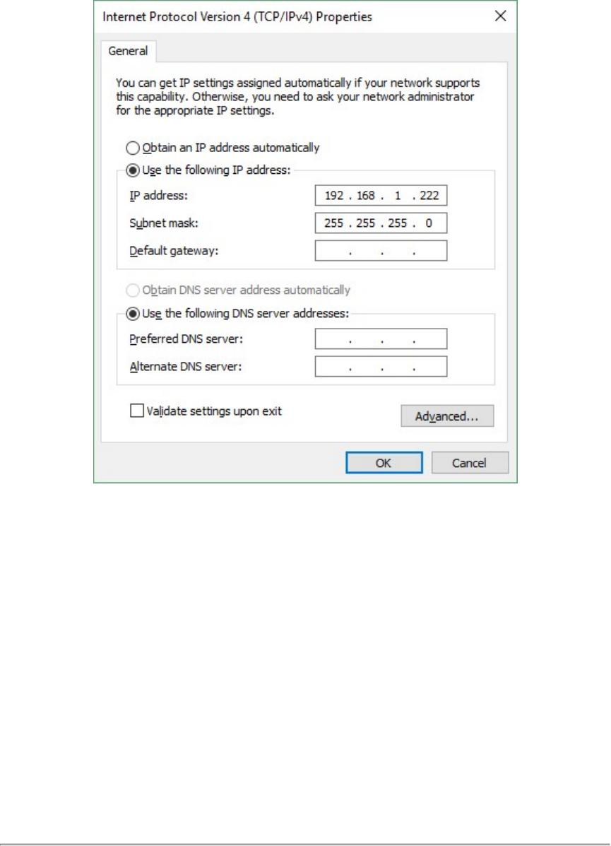
Figure 4-1 Sensor Network Settings
7. Click OK. Gateway and DNS are not necessary when testing in isolation.
In some cases it may be necessary to disable the computer’s firewall or configure it to allow UDP I/O on that Ethernet inter-
face. How to do this is not covered here as the process varies widely.
4.2.2 Access Sensor’s Web Interface
Now the computer is ready to connect to the sensor.
1. Plug the Ethernet cable into the computer and then plug its other end into the Ethernet port on the sensor’s Inter-
face Box.
Figure 4-2 on the facing page
shows the Interface Box, its external ports, internal sensor terminal, and
fuse.
24 VLP-16 User Manual
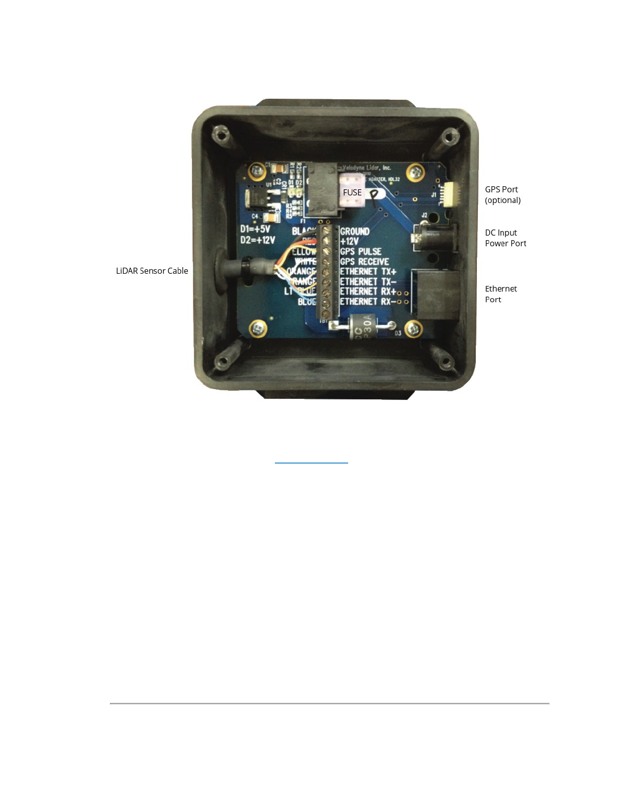
Figure 4-2 Interface Box (power and data connections)
2. Connect power to the sensor’s Interface Box.
When power is applied, two green LEDs in the Interface Box light up. The sensor begins scanning its environment
and transmitting data approximately 30 seconds after power up.
3. On the computer, point a browser to http://192.168.1.201.
4. The sensor’s Web Interface should appear (
Figure 4-3 on the next page
).
The Web Interface provides access to many of the sensor’s control settings. See
Web Interface on page 68
for
details.
Chapter 4 • Unboxing & Verification 25
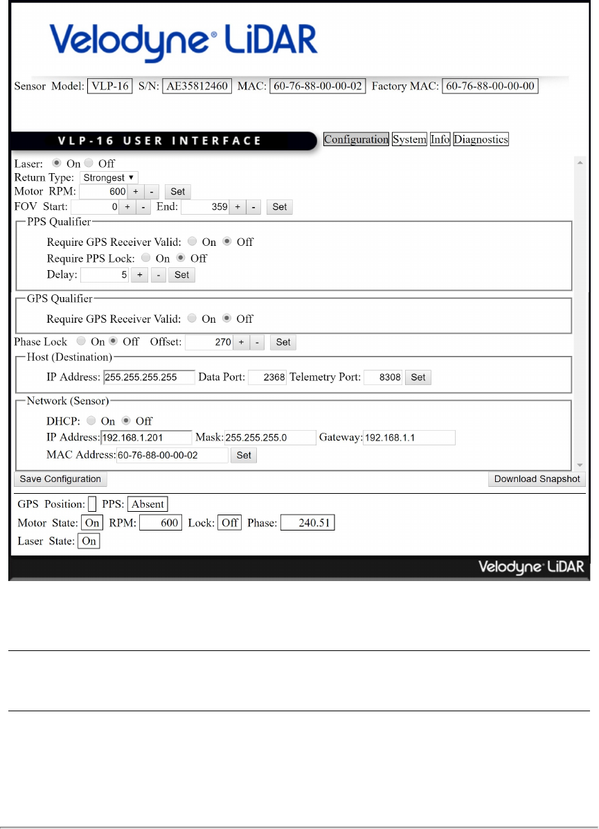
Figure 4-3 Sample Web Interface Main Configuration Screen
4.2.3 Visualize Live Sensor Data with VeloView
Now that the computer can access the sensor’s Web Interface, it’s time to get a first look at the sensor’s data.
Note: VeloView is an open source visualization and recording application tailored for Velodyne LiDAR sensors. Other
visualization software (e.g. ROS, DSR and PCL) can perform similar functions and may be used instead.
VeloView is documented in more detail in
VeloView on page 111
. If the application isn’t already on the computer, perform
the procedure detailed in
Install VeloView on page 112
. Older versions should be updated to at least the version installed
by following the procedure.
26 VLP-16 User Manual
4.2.3.1 VeloView Operation
1. Power-up the sensor.
2. Start the VeloView application.
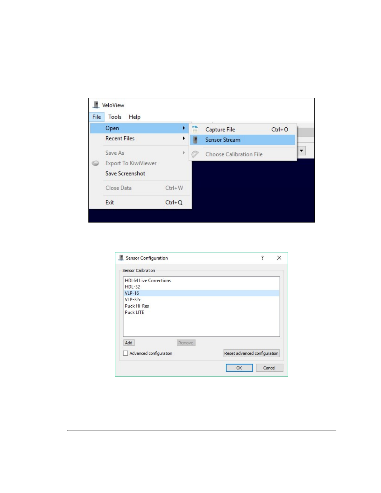
3. Click on File->Open and select Sensor Stream (
Figure 4-4 below
).
Figure 4-4 VeloView Open Sensor Stream
4. The Sensor Configuration dialog will appear (
Figure 4-5 below
). Select the correct sensor type then click OK.
Figure 4-5 VeloView Select Sensor Calibration
5. VeloView begins displaying the sensor data stream. See
VeloView Sensor Stream Display on the next page
.
Chapter 4 • Unboxing & Verification 27
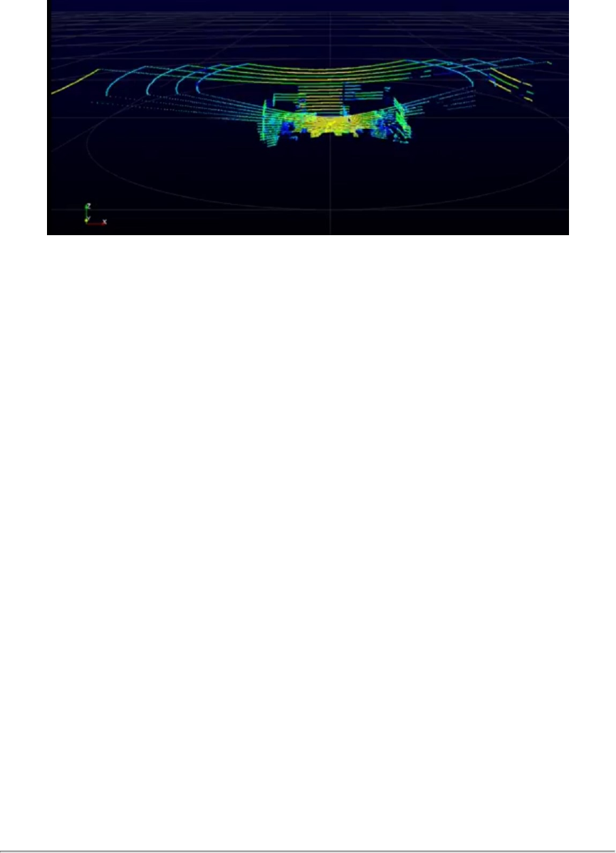
Figure 4-6 VeloView Sensor Stream Display
Above is an example of a VeloView screen in an office, workbench or lab scenario.
28 VLP-16 User Manual

Chapter 5 • Installation & Integration
This chapter provides important information for integrating the VLP-16 sensor into your application environment.
5.1 Overview
29
5.2 Mounting
29
5.3 Encapsulation, Solar Hats, and Ventilation
30
5.4 Connections
30
5.4.1 Integrated Cable and Interface Box
31
5.4.2 Operation Without an Interface Box
31
5.4.3 Power
31
5.1 Overview
Ensure the sensor is functional first before beginning sensor integration. See
Verification Procedure on page 22
.
Common steps in installation and integration involve:
Securely mounting the sensor to a vehicle, drone, robot, or other scanning platform
Allowing for proper ventilation, providing thermal protection, and sensor encapsulation
Connecting power to the sensor
Connecting the sensor's Ethernet data output to a computer, switch, or network – see
Network Configuration on
page 134
Optionally, connecting a GPS receiver or INS (Inertial Navigation System) – see
GPS, Pulse Per Second (PPS)
and NMEA GPRMC Message on page 41
The typical sensor setup uses a standard computer or laptop connected to the sensor. However, it is recommended to use
at least a 100 Mbps Ethernet adapter to accommodate the sensor data rate.
5.2 Mounting
The sensor base provides one ¼”-20-threaded, 9/32"-deep mounting hole, and two precision locating holes for locator
pins (
Figure 5-1 on the next page
). The sensor may be mounted at any angle or orientation, though reliability should be
best at 0° inclination (i.e. level to ground) as reductions to bearing life may occur at other orientations.
Ensure the sensor is mounted securely to withstand vibration and shock without risk of detachment. The unit does not
need shock proofing. The unit is designed to withstand automotive G-forces (i.e. 500 m/s2 amplitude, 11 ms duration
shock and 3 GRMS 5 Hz to 2,000 Hz vibration).
Chapter 5 • Installation & Integration 29
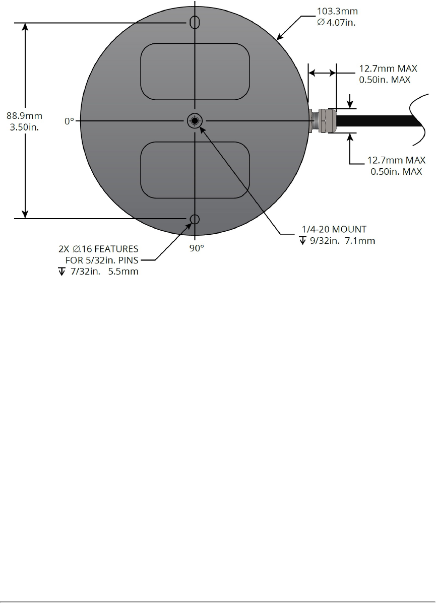
Figure 5-1 Mounting Details
5.3 Encapsulation, Solar Hats, and Ventilation
For various reasons, you may wish to encapsulate the sensor, either wholly or partially. The working field of view, if
covered with transparent material, should be highly transmissive of near-IR light at and near the 903 nm wavelength. Any
moisture that enters should have a way to drain passively.
The VLP-16 generates a moderate amount of heat during normal operation. Strategies for managing heat in hot weather
include employing a "thermal hat," exposing the sensor to moving air, and drawing heat from the sensor with a heat sink
(e.g. aluminum plate(s)).
The sensor reports internal temperatures passively on its web interface. The same readings may be obtained pro-
grammatically via curl commands (i.e. http GET requests). See
Sensor Communication on page 68
for details. The
sensor's operating temperature range can be found on its data sheet.
Do not operate the sensor without sufficient ambient air flow or cooling.
5.4 Connections
This section covers the sensor’s physical connections.
See
Network Considerations on page 135
before connecting one or more Velodyne LiDAR sensors physically to your net-
work. See
Ethernet and Network Setup on page 134
for instructions on how to configure the sensor's Ethernet con-
nection.
30 VLP-16 User Manual

Note: Do not twist or otherwise adjust the strain relief gland nut where the interface cable enters the sensor. Adjusting
the position of the gland nut may damage the VLP-16 sensor internally.
5.4.1 Integrated Cable and Interface Box
The standard VLP-16 sensor comes with an integrated cable that is terminated inside the Interface Box. The cable is
approximately 3.0 m in length and is permanently attached to the sensor.
Note: If you need to cut the integrated cable for any reason, please contact Velodyne Sales to get a waiver. Cutting this
cable could have warranty and RMA cost implications. Also, there is a minimum length requirement.
The Interface Box provides convenient connections for power, Ethernet, and GPS inputs. It protects the sensor from
power irregularities by incorporating a replaceable fuse and a reverse-current protection diode. When connected cor-
rectly to power, the diode allows current through to the sensor. If, however, the power and ground are switched, the diode
blocks current flow.
Opening the Interface Box and making modifications inside, such as replacing the fuse or reverse-current protection
diode, or repairing wires, is permitted.
For more information on the Interface Box, see
Interface Box Signals on page 40
.
5.4.2 Operation Without an Interface Box
The VLP-16's Interface Box is a convenience, but it also adds bulk. The sensor may be ordered and used without the Inter-
face Box to accommodate the needs of the user. Contact Velodyne Sales for details (i.e. SKUs).
If used without the Interface Box, the user must provide sufficient reverse- and over-voltage protection circuitry to protect
the sensor. The schematic for the circuitry in the Interface Box can be found in
Wiring Diagrams on page 108
.
5.4.3 Power
The VLP-16 sensor does not have a physical power switch. The power source must be capable of providing as much as
3.0 A to accommodate the current surge that occurs during rotor spin-up when power is supplied to the sensor.
In normal operation the sensor draws approximately 8 W of power.
The sensor's data sheet specifies the input voltage that should be supplied to the unit. The sensor will not operate outside
that voltage range.
The power input jack on the Interface Box accommodates a 5.5 mm (O.D.) x 2.5 mm (I.D.) barrel connector. The center
pin has positive (+) polarity.
Note: Before operating the sensor, ensure it is securely mounted and that power will be applied in the correct polarity.
If the sensor doesn't spin up when power is applied, check the fuse, check the sensor's web interface if Laser is On and
Motor RPM is a valid value, check the input voltage, and make sure that the power source (battery, power inverter, or
power rail) is providing sufficient current. If they check out and yet the problem persists, get
Technical Support on page 90
.
Chapter 5 • Installation & Integration 31

Chapter 6 • Key Features
6.1 Calibrated Reflectivity
32
6.2 Laser Return Modes
32
6.2.1 Single Return Modes: Strongest, Last
32
6.2.2 Multiple Returns
33
6.2.3 Dual Return Mode
33
6.3 Phase Locking Multiple Sensors
37
6.1 Calibrated Reflectivity
The VLP-16 measures reflectivity of an object independent of laser power and distances involved. Reflectivity values
returned are based on laser calibration against NIST-calibrated reflectivity reference targets at the factory.
For each laser measurement, a reflectivity byte is returned in addition to distance. Reflectivity byte values are segmented
into two ranges, allowing software to distinguish diffuse reflectors (e.g. tree trunks, clothing) in the low range from retrore-
flectors (e.g. road signs, license plates) in the high range.
A retroreflector reflects light back to its source with a minimum of scattering. The VLP-16 provides its own light, with neg-
ligible separation between transmitting laser and receiving detector, so retroreflecting surfaces
pop
with reflected IR light
compared to diffuse reflectors that tend to scatter reflected energy.
Diffuse reflectors report values from 0 to 100 for reflectivities from 0% to 100%.
Retroreflectors report values from 101 to 255, where 255 represents an ideal reflection.
Note: When a laser pulse doesn't result in a measurement, such as when a laser is shot skyward, both distance and
reflectivity values will be 0. The key is a distance of 0, because 0 is a valid reflectivity value (i.e. one step above noise).
6.2 Laser Return Modes
The VLP-16 supports three laser return modes: Strongest, Last, and Dual. A sensor can be configured to handle laser
returns in one of these ways interactively via the sensor's web interface (where the setting is called Return Type) or pro-
grammatically via curl command. (See
Configuration Screen on page 69
or
Sensor Control with curl on page 76
for addi-
tional information related to setting laser return modes.)
A laser return is a detection of a reflection. Up to two returns per laser shot are supported by the VLP-16.
6.2.1 Single Return Modes: Strongest, Last
As shown in
Figure 6-1 on the facing page
, when a laser pulse hits a solid wall a single return or measurement is obtained.
In this situation, the reading is considered both the strongest and the last return. (More on the nature of laser pulses emit-
ted by your sensor, including the rectangular shape of the pulse, is covered in
Laser Pulse on page 119
.)
32 VLP-16 User Manual
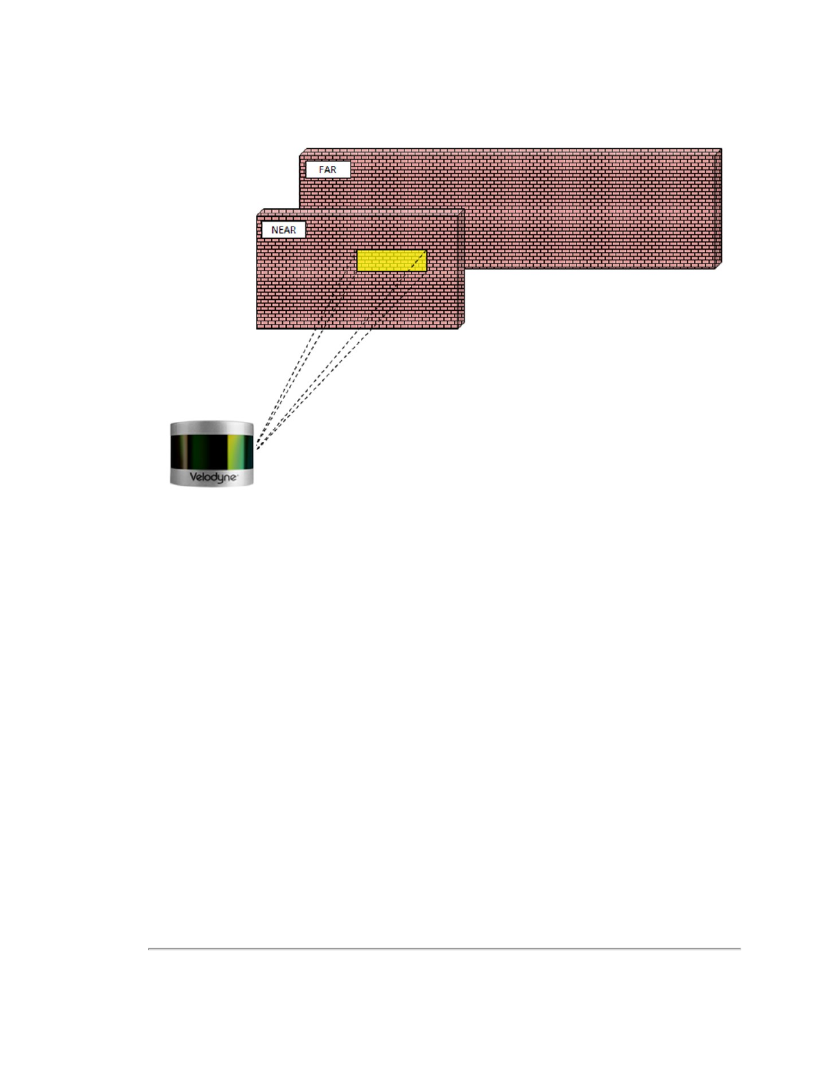
Figure 6-1 A Single Return
6.2.2 Multiple Returns
Multiple laser returns are possible from any single laser shot because of beam divergence. When a laser pulse leaves the
sensor it slowly, gradually grows larger. A pulse can be big enough to hit multiple objects producing multiple reflections.
Usually, the farther away a reflection starts, the weaker it is at the detector. Bright or retroreflective surfaces may flip that,
however.
The VLP-16 analyzes multiple returns and reports either the strongest return, the last return, or both returns, depending
on the laser return mode setting. If the setting is Strongest and a pulse produces multiple returns, only the strongest reflec-
tion results in a measurement. Likewise, if the setting is Last, only the last (time-wise) reflection results in a measurement.
This could be used to measure distances to the ground from the air.
6.2.3 Dual Return Mode
Figure 6-2 on the next page
shows the majority of a laser pulse striking the near wall while the remainder hits the far wall.
The Dual return mode setting allows you obtain both measurements.
Note that the sensor records both returns only when the separation between the two objects is one meter or more.
Chapter 6 • Key Features 33
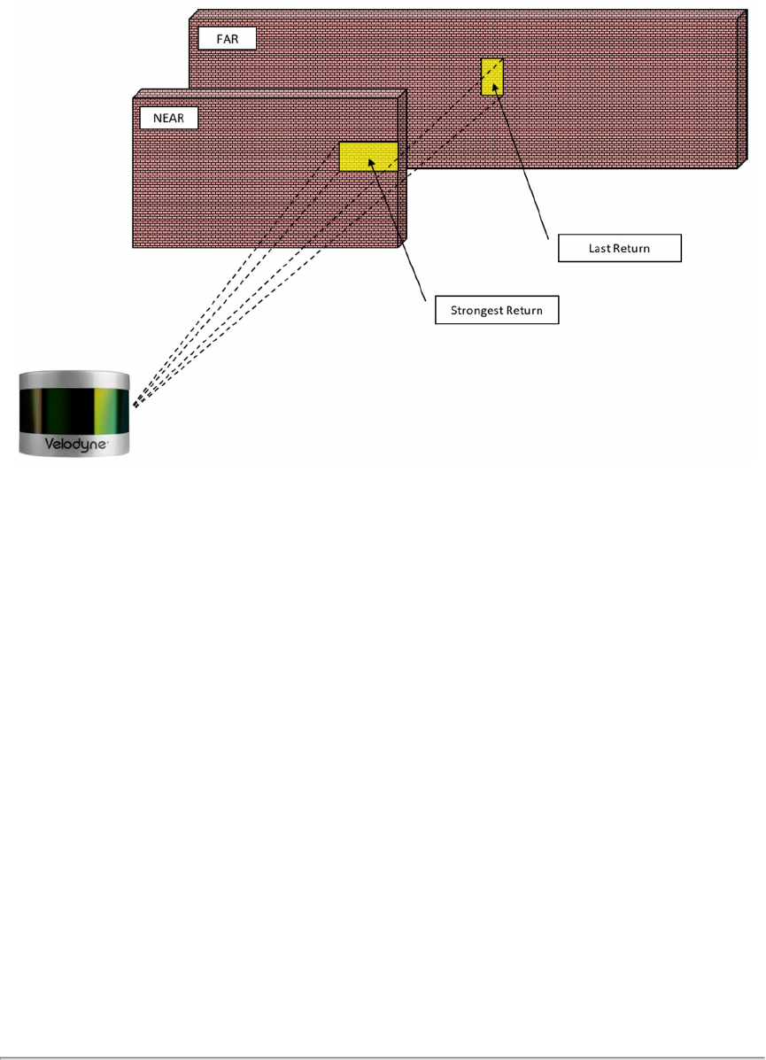
Figure 6-2 Dual Return with Last and Strongest Returns
As shown in
Figure 6-3 on the facing page
, in the event the strongest return is the last return, the second-strongest return
is reported. The majority of the beam hits the far wall and is (in this case) the strongest return.
It's entirely possible, however, that the far wall might be far enough away that despite reflecting the majority of the beam,
the return from the near wall would be the strongest return.
34 VLP-16 User Manual
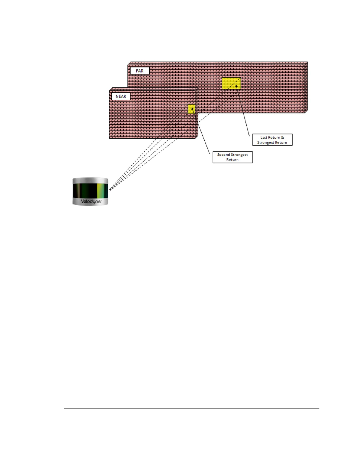
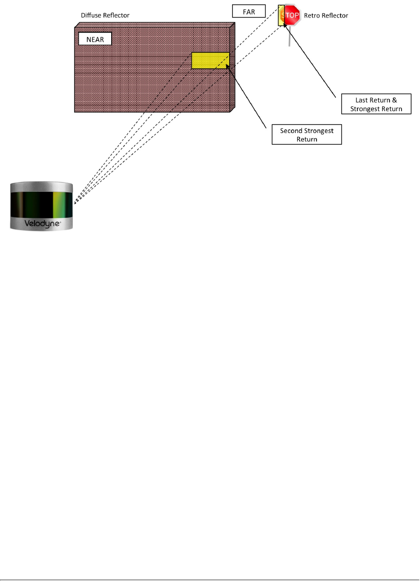
Figure 6-4 Dual Return with Far Retro-Reflector
The dual return function is often used in forestry applications where measurement of the height of trees is desired.
Figure
6-5 on the facing page
indicates a sample response when the laser pulse initially hits the upper canopy, penetrates it, and
eventually hits the ground, producing multiple returns. Which laser return mode would be best in this situation?
36 VLP-16 User Manual
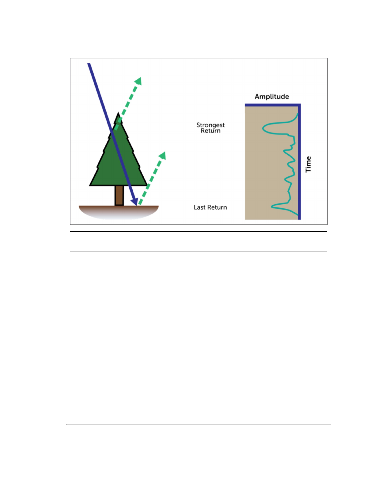
Figure 6-5 Forestry Application Multiple Returns
Note: In dual return mode, the data rate of the sensor doubles.
6.3 Phase Locking Multiple Sensors
When using multiple Velodyne LiDAR sensors in proximity to one another, users may observe interference between them
due to one sensor picking up a reflection intended for another. To minimize this interference, the sensor provides a phase-
locking feature that enables the user to control where the laser firings overlap.
The Phase Lock feature can be used to synchronize the relative rotational position of multiple sensors based on the PPS
signal and relative sensor orientation. To operate correctly, the PPS signal must be present and locked. Phase locking
works by offsetting the firing position based on the rising edge of the PPS signal.
Note: For phase lock to work correctly, the sensor’s RPM setting must be set to a multiple of 60 RPM between 300 RPM
and 1200 RPM (inclusive).
Chapter 6 • Key Features 37
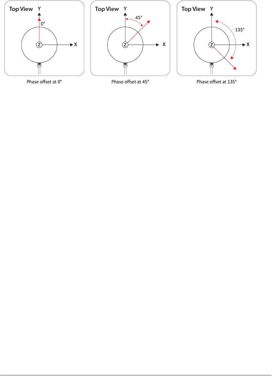
Figure 6-6 Phase Locking Example
The red arrows shown in
Figure 6-6 above
indicate the firing direction of the sensor's laser at the moment it receives the
rising edge of the PPS signal.
Additional information for phase locking multiple sensors is located in
Phase Lock on page 127
.
38 VLP-16 User Manual

Chapter 7 • Sensor Inputs
This chapter covers sensor input requirements and functionality, including power, PPS, and Ethernet. It also covers scen-
arios for obtaining GPS input.
7.1 Power Requirements
39
7.2 Interface Box Signals
40
7.3 Ethernet Interface
41
7.4 GPS, Pulse Per Second (PPS) and NMEA GPRMC Message
41
7.4.1 GPS Input Signals
41
7.4.2 Electrical Requirements
41
7.4.3 Timing and Polarity Requirements
41
7.4.4 GPS Connection Scenarios
44
7.4.5 NMEA Message Formats
46
7.4.6 Accepting NMEA Messages Via Ethernet
48
7.1 Power Requirements
Power requirements are detailed in Chapter 5:
Power on page 31
.
Chapter 7 • Sensor Inputs 39
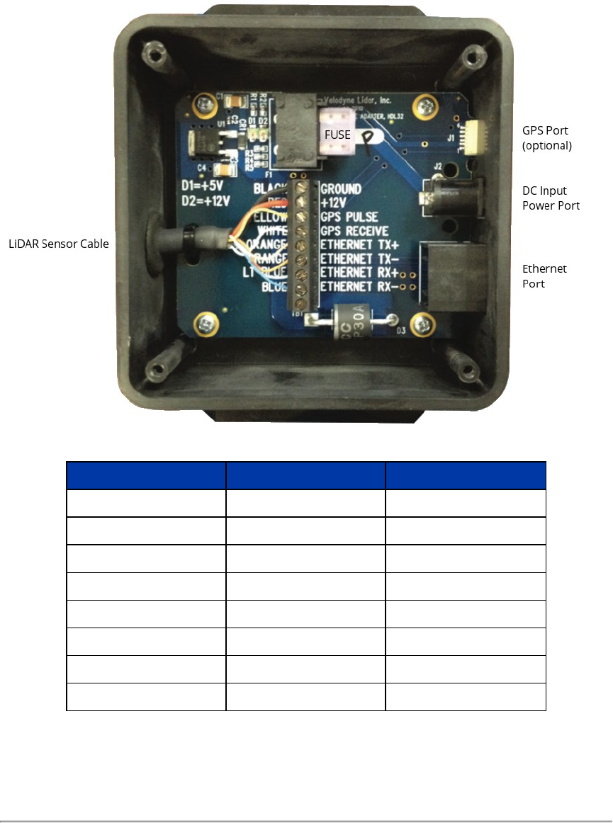
7.2 Interface Box Signals
Figure 7-1 Interface Box (sensor power and data connections)
Signal Specifications Signal Input/Output
Black Ground Input
Red Power Input
Yellow GPS Sync Pulse Input
White GPS Serial Receive Input
Light Orange Ethernet TX+ Output
Orange Ethernet TX- Output
Light Blue Ethernet RX+ Input
Blue Ethernet RX- Input
Table 7-1 Interface Box Signals
40 VLP-16 User Manual

7.3 Ethernet Interface
Your sensor's primary interface is its Ethernet interface. All command and control occurs over it, and all sensor data is
transmitted over it.
The RJ45 Ethernet connector on the Interface Box connects to any standard 100 Mbps Ethernet NIC or switch with MDI
or AUTO MDIX capability.
See
Ethernet and Network Setup on page 134
for more.
7.4 GPS, Pulse Per Second (PPS) and NMEA GPRMC Message
Your sensor can synchronize data with precise GPS-supplied time. Synchronizing to a GPS-supplied Pulse-Per-Second
(PPS) signal provides the ability to compute the exact firing moment of each data point as required by some geo-ref-
erencing applications. See
Time Synchronization on page 123
for details on GPS time synchronization and how important
it is for associating sensor data with the sensor’s environment.
To utilize these features, configure your GPS/INS device to issue a PPS signal in conjunction with a once-per-second
NMEA GPRMC sentence. No other NMEA message is accepted by the sensor.
Note: The GPRMC record may be configured for HHMMSS, HHMMSS.s, HHMMSS.ss, and HHMMSS.sss formats.
7.4.1 GPS Input Signals
The serial data output from the GPS/INS is connected to the sensor’s Interface Box via the screw terminal labeled: “GPS
RECEIVE.”
The PPS output from the GPS/INS is connected to the sensor’s Interface Box via the screw terminal labeled: “GPS
PULSE.”
The ground signal from the GPS/INS is connected to the sensor’s Interface Box via the screw terminal labeled:
“GROUND.”
Note: You can use the provided GPS port on the Interface Box if using the Velodyne GPS Receiver (P/N 80-
GPS18LVC).
7.4.2 Electrical Requirements
“High” voltage must be greater than 3.0 V and less than 15.0 V.
“Low” voltage must be less than 1.2 V, and greater than -15.0 V.
The GPS/INS unit must be able to supply at least 2 mA of current in the “High” state.
7.4.3 Timing and Polarity Requirements
The PPS synchronization pulse and GPRMC message (or GPGGA) may be issued concurrently or sequentially. The PPS
synchronization pulse width is not critical (typical lengths are between 10 μs and 200 ms).
Note: Reception of the GPRMC sentence must conclude no more than 300 ms before the rising edge of the subsequent
synchronization pulse as shown in
Figure 7-2 on the next page
,
Figure 7-3 on the next page
and
Figure 7-4 on page 43
.
Chapter 7 • Sensor Inputs 41
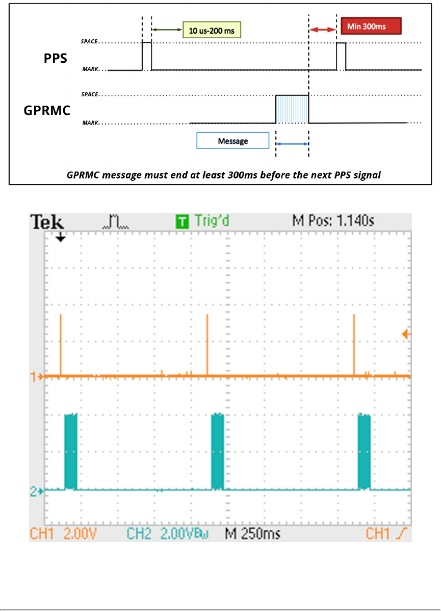
Figure 7-2 Synchronizing PPS with NMEA GPRMC Message
Figure 7-3 PPS Signal Closely Followed by NMEA GPRMC Message
42 VLP-16 User Manual
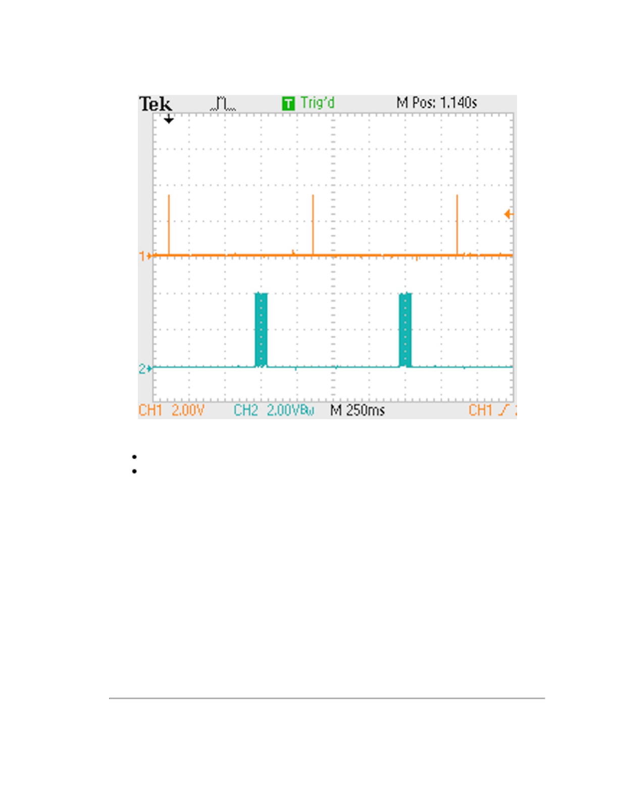
Figure 7-4 PPS Signal Followed 600 ms later by NMEA GPRMC Message
The serial connection for the NMEA message follows the RS232 standard. The interface is capable of handling voltages
between ±15 VDC.
Low voltages are marks and represent a logical 1.
High voltages are spaces and represent a logical 0.
The serial line idle state (MARK) is a low voltage indicating a logical 1. When the start bit is asserted, the positive voltage will
be asserted representing a logical 0. As an example, the transmission of an ASCII "$" character is shown in
Figure 7-5 on
the next page
.
Chapter 7 • Sensor Inputs 43
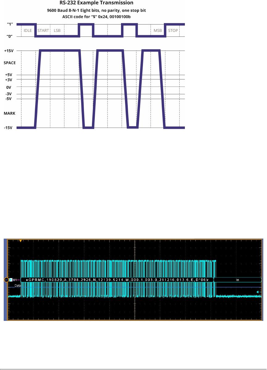
Figure 7-5 RS-232 Example Transmission
7.4.4 GPS Connection Scenarios
Depending on the user’s application, the source of the NMEA message (and PPS) can be a GPS/INS receiver or a sub-
stitute device such as a laptop or microcomputer.
There are three common connection scenarios: connecting to a sensor from a Velodyne-supplied Garmin 18x LVC GPS
receiver, connecting to it from a computer's serial port, and connecting directly from a microcomputer’s UART.
7.4.4.1 Connecting a Garmin 18x LVC GPS Receiver
As an option, Velodyne LiDAR offers a Garmin 18x LVC GPS Receiver (P/N 80-GPS18LVC) pre-configured for optimized
operation with your sensor. The receiver plugs directly into the Interface Box’s GPS port and is used to synchronize your
sensor's timestamp with precision GPS time. The signals from the Garmin receiver will be similar to those shown in
Figure
7-6 below
where the signal is normally low and zeros are represented by the high voltage.
Figure 7-6 Garmin GPRMC Message
7.4.4.2 Connecting to a computer's serial port
In some situations, you may wish to source NMEA messages from a computer instead of a GPS receiver.
44 VLP-16 User Manual
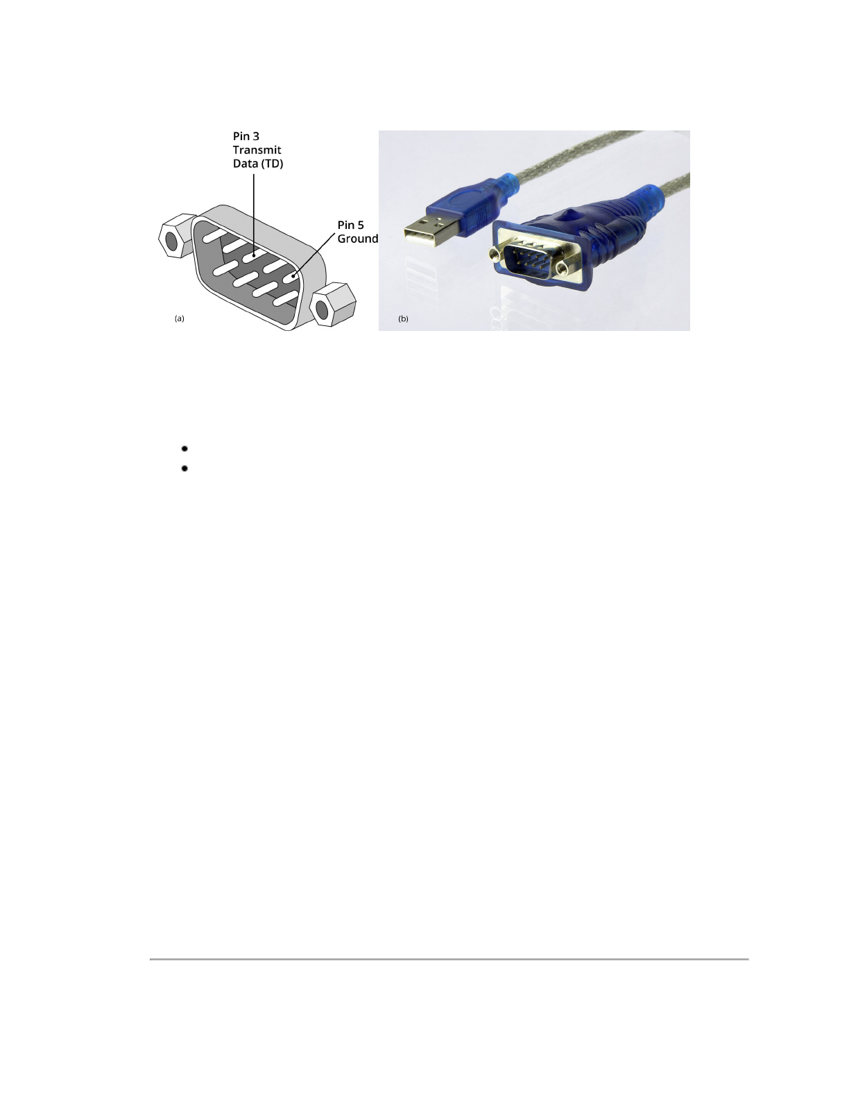
Figure 7-7 DB9 Pin-outs (DTE) and USB-to-Serial Adapter
An example of a standard DB9 serial port is shown in
Figure 7-7 above
(a). Because modern computers use USB ports, a
USB to Serial Adapter, as shown in
Figure 7-7 above
(b), will be required. The DB9 connector on the adapter provides a
signal with the proper polarity and voltage levels to connect directly to the sensor’s Interface Box.
After connecting the USB to Serial Adapter to your computer and wiring up a mating DB9 connector (not pictured), you
can complete the connection to your sensor. Remove the cover from the Interface Box and make the following con-
nections to the terminal screw strip in the Interface Box.
DB9 pin 3 to GPS RECEIVE
DB9 pin 5 connects to GROUND
7.4.4.3 Connecting to a microcomputer’s UART
In other situations, you may wish to source NMEA messages from a microcomputer such as a Raspberry Pi or Arduino,
instead. The native signal coming from the microcomputer’s UART will have incorrect polarity. In this instance, invert the
signal using a 7404 hex inverter chip or equivalent circuitry. To connect to the sensor, remove the cover from the Interface
Box and connect the appropriate leads to the GPS RECEIVE and GROUND connections on the terminal strip.
Figure 7-8 on the next page
shows a signal directly from a Raspberry Pi UART output and
Figure 7-9 on the next page
shows the same output inverted into a signal compatible with your Velodyne sensor.
Chapter 7 • Sensor Inputs 45
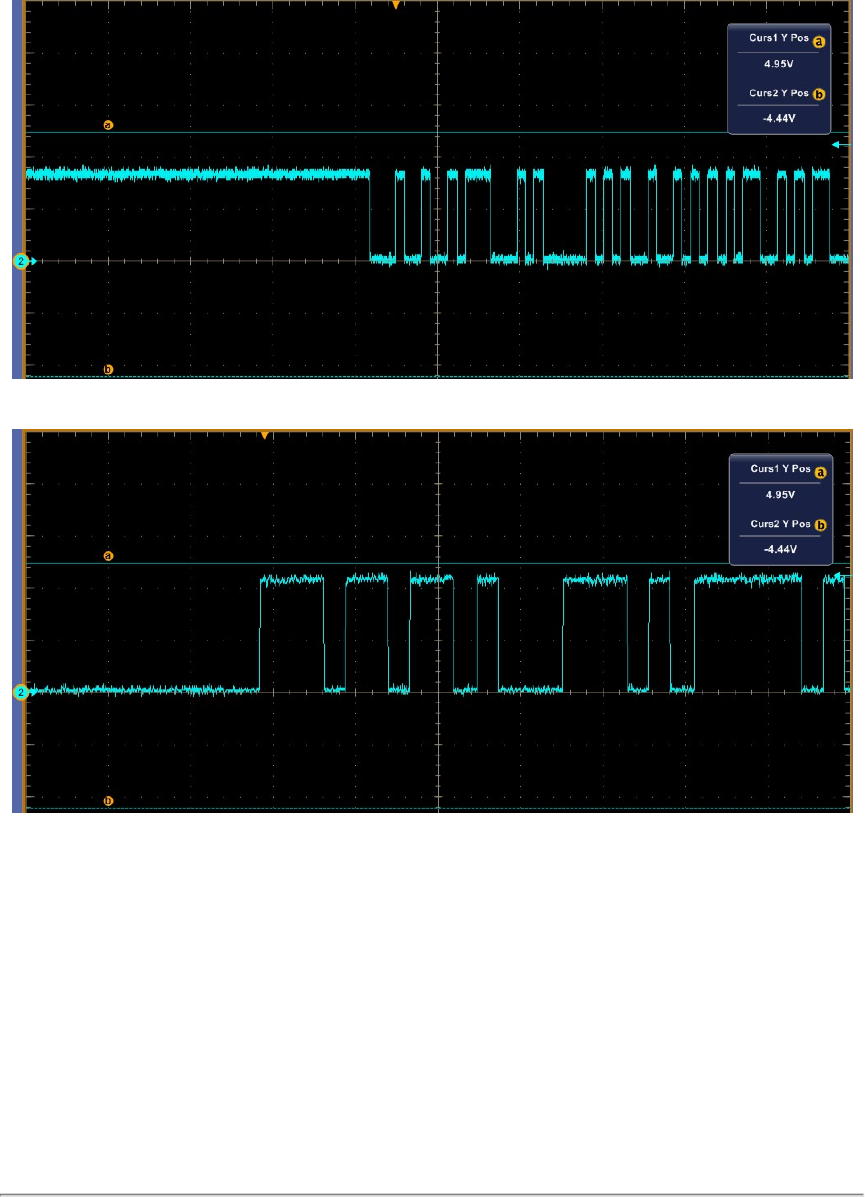
Figure 7-8 Signal Directly from UART (incorrect polarity)
Figure 7-9 Inverted Signal from UART (correct polarity)
7.4.5 NMEA Message Formats
GPGGA may be substituted in place of GPRMC.
The sensor accepts both pre- and post-NMEA version 2.3 sentence structures. The difference is that in version 2.3 a Fix
Mode Indicator field was added after Magnetic Variation and before the Checksum.
NMEA messages are terminated with sentence delimiter <CR><LF> (HEX 0D0A).
7.4.5.1 Pre-NMEA Version 2.3 Message Format
Table 7-2 on the facing page
provides a description of the pre-NMEA 2.3 message format contents shown below.
46 VLP-16 User Manual
$GPRMC,123519,A,4807.038,N,01131.000,E,022.4,084.4,230394,003.1,W*6A
Value Description
$GPRMC Recommended Minimum sentence
123519 Fix taken at 12:35:19 UTC
A Receiver status: A = Active, V = Void
4807.038,N Latitude 48 deg 07.038' N
01131.000,E Longitude 11 deg 31.000' E
022.4 Speed over the ground (knots)
084.4 Track made good (degrees True)
230394 23rd of March 1994
003.1,W Magnetic Variation
*6A * followed by 2-byte Checksum
Table 7-2 Pre-NMEA Version 2.3 Message Format
7.4.5.2 NMEA Version 2.3 Message Format
Table 7-3 below
provides a description of the post-NMEA 2.3 message format contents shown below.
$GPRMC,123519,A,4807.038,N,01131.000,E,022.4,084.4,230394,003.1,W,A*02
Value Description
$GPRMC Recommended Minimum sentence
123519 Fix taken at 12:35:19 UTC
A Receiver status: A = Active, V = Void
4807.038,N Latitude 48 deg 07.038' N
01131.000,E Longitude 11 deg 31.000' E
022.4 Speed over the ground (knots)
084.4 Track made good (degrees True)
230394 23rd of March 1994
003.1,W Magnetic Variation
Table 7-3 Post-NMEA Version 2.3 Message Format
Chapter 7 • Sensor Inputs 47

Value Description
A
Fix Mode Indicator:
A = Autonomous, D = Differential, E = Estimated, N = Not valid, S = Simulator. Sometimes there can be
a null value as well.
*6A * followed by 2-byte Checksum
Note: The Receiver Status (aka Validity) field in the GPRMC message ('A' or 'V') should be checked to ensure the GPS
receiver is actively positioning and is providing trustworthy UTC (Coordinated Universal Time) and position updates. If
status is Void, which usually occurs when the GPS receiver is searching for satellites, GPS position should be ignored. In
many instances, the GPS receiver, if its status is Void, will continue to provide a PPS signal based on the GPS receiver's
internal clock. More on this can be found in
Time Synchronization on page 123
.
7.4.6 Accepting NMEA Messages Via Ethernet
Your sensor can accept NMEA sentences over Ethernet. Three methods are supported:
1. A host opens a TCP connection to the sensor’s port 10110 and transmits NMEA sentences on the socket.
2. A host transmits NMEA sentences in UDP packets to the sensor’s UDP port 10110.
3. A host transmits NMEA sentences in UDP packets to a broadcast address on port 10110 with an NMEA sen-
tence.
1 and 2 require knowledge of the sensor’s IP address. 3 does not, but it may load devices on the network that don’t want
the packets.
Note: The supported NMEA sentence and syntax are exactly the same as on the wired (serial) GPS interface. Supported
sentence delimiter sequences include <CR><LF> (HEX 0D0A, the standard), <CR> by itself, and <LF> by itself.
The support follows the ad-hoc but widely supported NMEA over Ethernet approach utilized by the OpenCPN project.
Additional information can be found at the following web sites:
http://stripydog.blogspot.com/2015/03/nmea-0183-over-ip-unwritten-rules-for.html
https://opencpn.org/wiki/dokuwiki/doku.php?id=opencpn:supplementary_software:nmea_instruments
http://arundale.com/docs/ais/nmearouter.html
48 VLP-16 User Manual
Chapter 8 • Sensor Operation
This chapter provides details on the laser firing sequence, point density, and how to determine throughput rate and angu-
lar resolution.
8.1 Firing Sequence
49
8.2 Throughput Calculations
49
8.2.1 Data Packet Rate
49
8.2.2 Position Packet Rate
50
8.2.3 Total Packet Rate
50
8.2.4 Laser Measurements Per Second
50
8.3 Rotation Speed (RPM)
50
8.3.1 Horizontal Angular (Azimuth) Resolution
50
8.3.2 Rotation Speed Fluctuation and Point Density
51
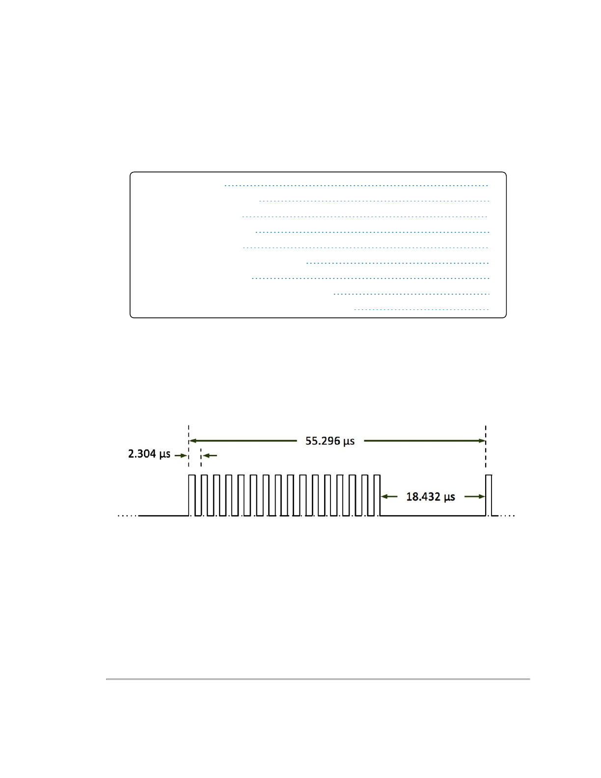
8.1 Firing Sequence
All 16 lasers are fired and recharged every 55.296 μs. The time between firings is 2.304 μs. There are 16 firings (16 ×
2.304 μs) followed by an idle period of 18.43 μs. Therefore, the timing cycle to fire and recharge all 16 lasers is given by (16
× 2.304 μs) + 18.432 μs = 55.296 μs.
Figure 8-1 Firing Sequence Timing
8.2 Throughput Calculations
Some terms used here are defined in
Packet Types and Definitions on page 54
.
8.2.1 Data Packet Rate
There are 24 firing cycles in a data packet. 24 x 55.296 μs = 1.327 ms is the accumulation delay per packet.
1 packet/1.327 ms = 753.5 packets/second
1248 bytes/packet * 753.5 packets/second = 940368 bytes/second
Chapter 8 • Sensor Operation 49

8.2.2 Position Packet Rate
Position packets arrive at approximately 1/14th the rate of data packets.
554 bytes/packet * 753.5 packets/second / 14 = 29817 bytes/second
8.2.3 Total Packet Rate
Summing yields 970185 bytes/second for single return mode.
Dual return mode doubles the data rate but not the position packet rate: (2 * 970185 bytes/second) + 29817 bytes/second
= 1970187 bytes/second
8.2.4 Laser Measurements Per Second
A laser firing results in a single data point, which is a measurement of distance to target and its reflectivity.
16 laser firings/data block * 24 data blocks/packet = 384 laser firings/packet
8.2.4.1 Single Return Mode (Strongest, Last)
384 laser firings/packet * 753.5 packets/second = 289344 laser measurements per second
8.2.4.2 Dual Return Mode
384 laser firings/packet * 1507 packets/second = 578688 laser measurements per second
8.3 Rotation Speed (RPM)
The sensor’s motor can be set to rotate between 300 RPM and 1200 RPM, inclusive, in increments of 60 RPM (e.g. 300,
360, 420, 480, … 1140, 1200).
Note: If the RPM setting is not evenly divisible by 60, neither motor speed control nor phase lock functions will
function properly.
The user can set this parameter using the sensor’s Web Interface or curl commands. See
Configuration Screen on
page 69
or
Sensor Control with curl on page 76
for more on setting rotation speed.
Note: In VeloView, one rotation can be referred to as a single “frame” of data, beginning and ending at approximately 0°
azimuth. The number of frames per second of data generated depends entirely on the RPM setting, e.g. 600 RPM / 60
s/min = 10 frames per second.
Choice of RPM is up to the user and depends on the application. For example, an autonomous vehicle may wish to
increase rotation speed so it could more quickly identify frame-to-frame variations in the environment, such as a child run-
ning across a street. Conversely, a cart-based mapping solution might use a lower RPM to increase the detail in each
frame.
8.3.1 Horizontal Angular (Azimuth) Resolution
Because the firing timing of the sensor is fixed at 55.296 μs per firing cycle, the speed of rotation changes the angular res-
olution of the sensor.
An example calculation for 600 RPM is given in
Equation 8-1 below
.
Equation 8-1 Azimuth Resolution at 600 RPM
50 VLP-16 User Manual
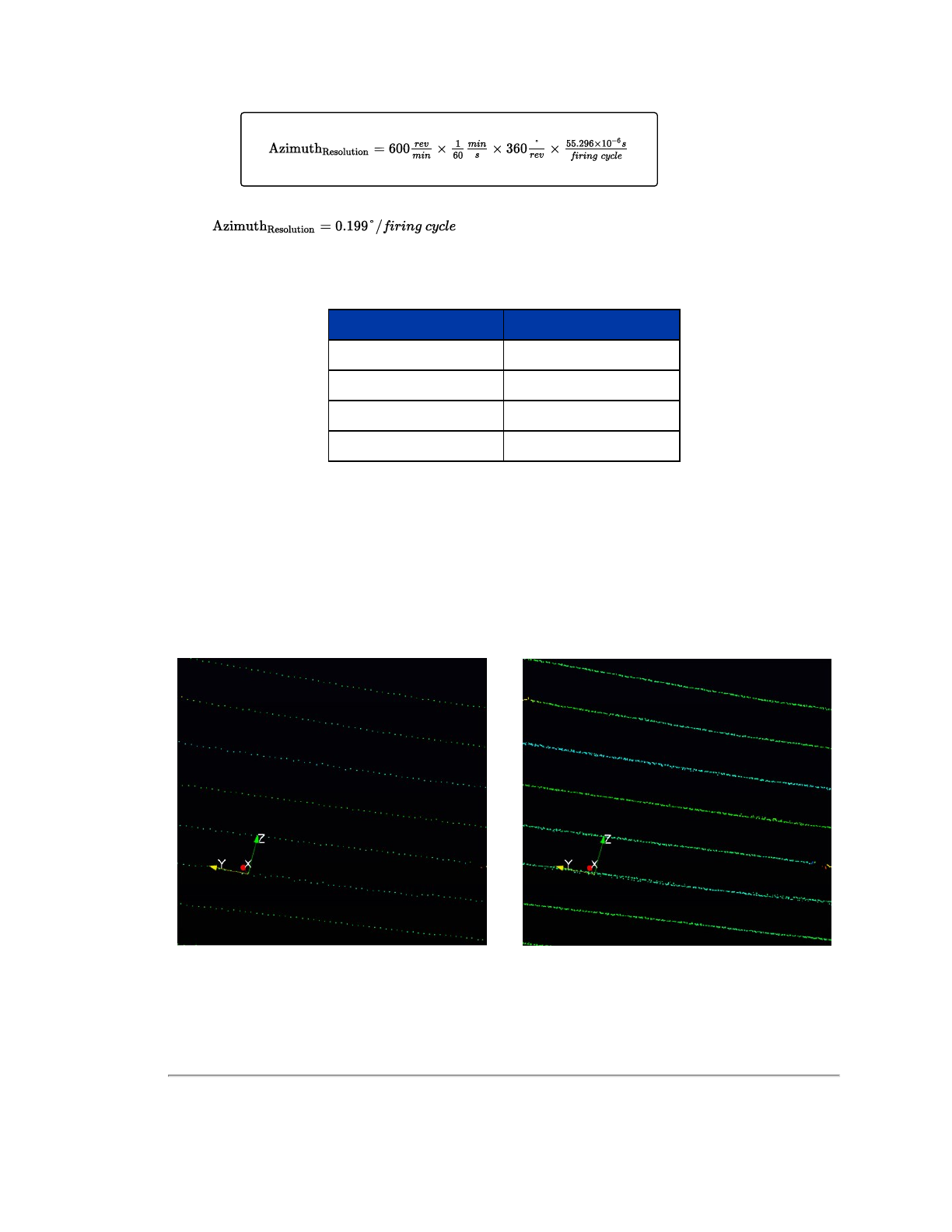
By changing the RPM in the equation above you can calculate the azimuthal resolution for any rotation speed.
RPM Resolution
300 0.1°
600 0.2°
900 0.3°
1200 0.4°
Table 8-1 Rotation Speed vs Resolution
8.3.2 Rotation Speed Fluctuation and Point Density
Your sensor uses a feedback control function to maintain its rotational speed within ±3 RPM of its configured setting. This
small variation in speed produces a small change in the azimuthal gaps with every revolution. Consequently, over time, the
sensor automatically “fills in the gaps” between successive laser firings.
A data set from a stationary sensor provides an example of the how the sensor “fills in the gaps,” and the effect is demon-
strated in
Figure 8-2 below
. On the left is a single frame of data. On the right is the same frame and the nine preceding
frames overlaid on each other. You can see how the azimuth gaps are filled.
Figure 8-2 Point Density Example
Chapter 8 • Sensor Operation 51

Chapter 9 • Sensor Data
This chapter provides detailed information about sensor data characteristics.
9.1 Sensor Origin and Frame of Reference
52
9.2 Calculating X,Y,Z Coordinates from Collected Spherical Data
52
9.3 Packet Types and Definitions
54
9.3.1 Definitions
54
9.3.2 Data Packet Structure
56
9.3.3 Position Packet Structure
60
9.4 Discreet Point Timing Calculation
61
9.5 Precision Azimuth Calculation
65
9.6 Converting PCAP Files to Point Cloud Formats
66
9.1 Sensor Origin and Frame of Reference
The sensor reports distances relative to itself in spherical coordinates (radius r, elevation ω, azimuth α). Sensor data origin
(0,0,0) is 37.7 mm above the sensor base, on the center axis, as shown in
Figure 9-1 on the facing page
(see the side and
top views), which also shows the sensor’s frame of reference. See also the mechanical/optical drawings in
VLP-16 and
Puck LITE Mechanical Drawing on page 102
.
9.2 Calculating X,Y,Z Coordinates from Collected Spherical Data
A computation is necessary to convert the spherical data (radius r, elevation ω, azimuth α) from the sensor to Cartesian
coordinates.
Figure 9-1 on the facing page
lists the formulas for converting spherical coordinates (R, ω, α) to Cartesian
coordinates (X, Y, Z).
52 VLP-16 User Manual
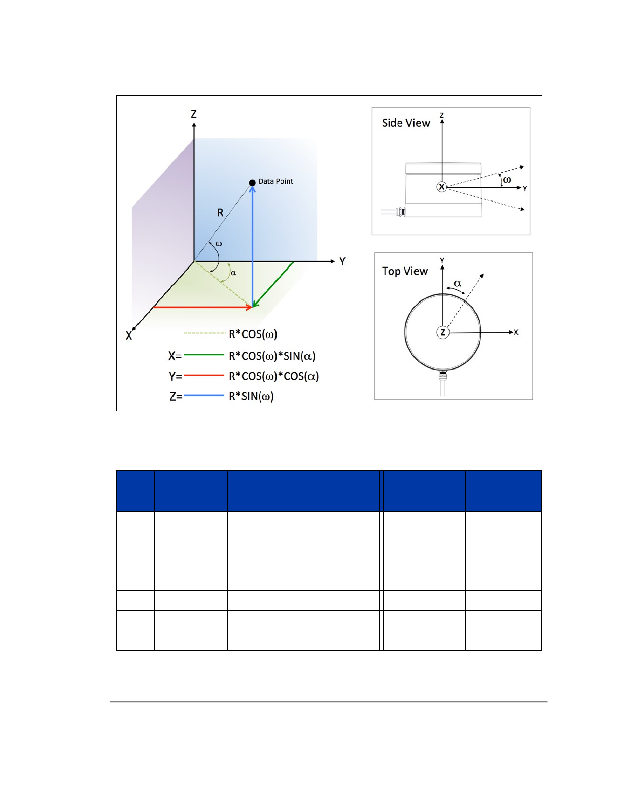
Figure 9-1 VLP-16 Sensor Coordinate System
Table 9-1 below
lists the fixed vertical/elevation angles for each laser in the sensor, along with vertical corrections. The set
of angles vary by sensor model (see
Factory Bytes on page 56
for more).
Laser
ID
Vertical
Angle VLP-
16
Vertical Angle
Puck LITE
Vertical Cor-
rection (mm) Vertical Angle
Puck Hi-Res
Vertical Cor-
rection (mm)
0 -15° -15° 11.2 -10.00° 7.4
1 1° 1° -0.7 0.67° -0.9
2 -13° -13° 9.7 -8.67° 6.5
3 3° 3° -2.2 2.00° -1.8
4 -11° -11° 8.1 -7.33° 5.5
5 5° 5° -3.7 3.33° -2.7
6 -9° -9° 6.6 -6.00 4.6
Table 9-1 Vertical Angles (ω) by Laser ID and Model
Chapter 9 • Sensor Data 53

Laser
ID
Vertical
Angle VLP-
16
Vertical Angle
Puck LITE
Vertical Cor-
rection (mm) Vertical Angle
Puck Hi-Res
Vertical Cor-
rection (mm)
7 7° 7° -5.1 4.67° -3.7
8 -7° -7° 5.1 -4.67° 3.7
9 9° 9° -6.6 6.00° -4.6
10 -5° -5° 3.7 -3.33° 2.7
11 11° 11° -8.1 7.33° -5.5
12 -3° -3° 2.2 -2.00° 1.8
13 13° 13° -9.7 8.67° -6.5
14 -1° -1° 0.7 -0.67° 0.9
15 15° 15° -11.2 10.00° -7.4
Note:
Table 9-1 on the previous page
lists lasers in the order they are fired. Though the VLP-16's lasers are organized in
a single, vertical column, they are not fired from one end to the other. Instead, the firing sequence "hops around." This is to
avoid "cross-talk" or interference.
After computing X,Y,Z, apply the vertical correction in
Table 9-1 on the previous page
for greatest accuracy. This rep-
resents the vertical offset of the laser with respect to sensor origin. These vertical offset corrections are also found in the
VLP-16 and Puck LITE Optical Drawing on page 103
and the Hi-Res version below it.
9.3 Packet Types and Definitions
There are two types of packets generated by the sensor: data packets and position packets. Position packets are some-
times referred to as telemetry packets, or GPS packets.
Data packets contain the 3D data measured by the sensor as well as the calibrated reflectivity of the surface from which
the light pulse was returned. Also contained in the data packet is a set of azimuths and a 4-byte timestamp, as well as two
factory bytes identifying the model of sensor and the return mode. Knowing the model and return mode provides your soft-
ware the information to automatically adjust to the different data formats.
Position packets provide a copy of the last GPRMC NMEA message received if you've configured your sensor to syn-
chronize with a GPS time source. See
GPS, Pulse Per Second (PPS) and NMEA GPRMC Message on page 41
for addi-
tional information. Position packets also provide a byte identifying the state of the PPS signal for synchronizing with a time
source.
Note: In both types of packets, multi-byte values (e.g. azimuth, distance, and timestamp) are transmitted with the least
significant byte first (i.e. little-endian).
9.3.1 Definitions
The following sections provide explanations of sensor data packet constructs.
54 VLP-16 User Manual

9.3.1.1 Firing Sequence
A firing sequence occurs when all the lasers in a sensor are fired. They are fired in a sequence specific to a given product
line. Laser recharge time is included. A firing sequence is sometimes referred to as a firing group.
It takes 55.296 μs to fire all 16 lasers in a VLP-16 and recharge.
9.3.1.2 Laser Channel
A laser channel is a single 903 nm laser emitter and detector pair. Each laser channel is fixed at a particular elevation angle
relative to the horizontal plane of the sensor. Each laser channel is given its own Laser ID number as shown in
Table 9-1
on page 53
. The elevation angle of a particular laser channel is inferred by its data packet location.
9.3.1.3 Data Point
A data point is a measurement by one laser channel of a reflection of a laser pulse.
A data point is represented in the packet by three bytes - two bytes of distance and one byte of calibrated reflectivity. The
distance is an unsigned integer. It has 2 mm granularity. Hence, a reported value of 51,154 represents 102,308 mm or
102.308 m. Calibrated reflectivity is reported on a scale of 0 to 255 as described in
Key Features on page 32
. The elevation
angle (ω) is inferred based on the position of the data point within a data block.
9.3.1.4 Azimuth
A two-byte azimuth value (α) appears after the flag bytes at the beginning of each data block. The azimuth is an unsigned
integer. It represents an angle in hundredths of a degree. Therefore, a raw value of 27742 should be interpreted as
277.42°.
Valid values for azimuth range from 0 to 35999. Only one azimuth value is reported per data block.
9.3.1.5 Data Block
The information from two firing sequences of 16 lasers is contained in each data block. Each packet contains the data from
24 firing sequences in 12 data blocks.
Only one Azimuth is returned per data block.
A data block consists of 100 bytes of binary data:
A two-byte flag (0xFFEE)
A two-byte Azimuth
32 Data Points
[2 + 2 + (32 × 3)] = 100 bytes
For calculating time offsets it is recommended that the data blocks in a packet be numbered 0 to 11.
9.3.1.6 Time Stamp
The four-byte time stamp is a 32-bit unsigned integer marking the moment of the first data point in the first firing sequence
of the first data block. The time stamp’s value is the number of microseconds elapsed since the top of the hour. The num-
ber ranges from 0 to 3,599,999,999, the number of microseconds in one hour.
The time stamp is critical because it's used by geo-referencing software to match each laser firing with corresponding data
from an inertial navigation system. The inertial navigation system provides a series of time stamped values for pitch, roll,
yaw, latitude, longitude, and elevation. By matching the time of the data point to the time-stamped data from the INS, the
user's software can mathematically transform the data from the sensor's coordinate frame to an earth-based reference
frame. The time stamps are matched to Universal Coordinated Time (UTC) provided by the GPS/INS.
When the sensor powers up it begins counting microseconds using an internal time reference. However, the sensor can
synchronize its data with UTC time so you can ascertain the exact firing time of each laser in any particular packet.
Chapter 9 • Sensor Data 55
UTC synchronization requires a user-supplied GPS/INS receiver generating a synchronizing Pulse Per Second (PPS) sig-
nal and an NMEA GPRMC message. The GPRMC message provides minutes and seconds in UTC. Upon syn-
chronization, the sensor reads the minutes and seconds from the GPRMC message and uses the information to set the
sensor’s time stamp to the number of microseconds past the hour, per UTC.
Note: A full description of electrical and timing requirements can be found in
GPS, Pulse Per Second (PPS) and NMEA
GPRMC Message on page 41
. A full description of timing options can be found in
Time Synchronization on page 123
.
9.3.1.7 Factory Bytes
Beginning with firmware release 3.0.29.0, every data packet includes a pair of bytes called the Factory Bytes. Their values
indicate how azimuths and data points are organized in the packet. Their packet locations, values, and meanings are spe-
cified in
Table 9-2 below
.
The Return Mode byte indicates how the packet’s azimuth and data points are organized. See
Data Packet Structure
below
for details.
Every sensor model line has its lasers arrayed vertically at slightly different angles. Use the Product ID byte to identify the
correct set of vertical (or elevation) angles. Product IDs are not unique and may be shared by different sensors. For
example, per
Table 9-2 below
, the VLP-16 and Puck LITE share the same elevation angles. Hence, the two products
share the same Product ID. Conversely, the Puck Hi-Res has a different Product ID since it has a different set of elevation
angles.
Return Mode Product ID
Offset in packet: 0x04DE Offset in packet: 0x04DF
Mode Value Product Model Value
Strongest 0x37 (55) HDL-32E 0x21 (33)
Last Return 0x38 (56) VLP-16 0x22 (34)
Dual Return 0x39 (57) Puck LITE 0x22 (34)
-- -- Puck Hi-Res 0x24 (36)
-- -- VLP-32C 0x28 (40)
-- -- Velarray 0x31 (49)
-- -- VLS-128 0x63 (99)
Table 9-2 Factory Byte Values
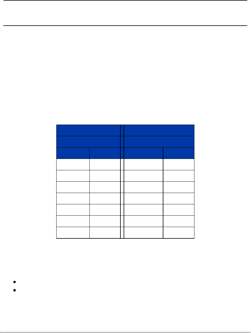
9.3.2 Data Packet Structure
A data packet is 1248 bytes long and sent via a UDP packet on port 2368. The data packet is comprised of 42 bytes of pro-
tocol header, twelve Data Blocks, a four-byte timestamp, and two factory bytes.
There are two formats for the data packet:
Single Return Mode (either Strongest or Last)
Dual Return Mode
See
Laser Return Modes on page 32
for an illustration of what Strongest, Last, and Dual mean in this context.
56 VLP-16 User Manual
The packet data structure for Single Return Mode is shown in
Figure 9-2 below
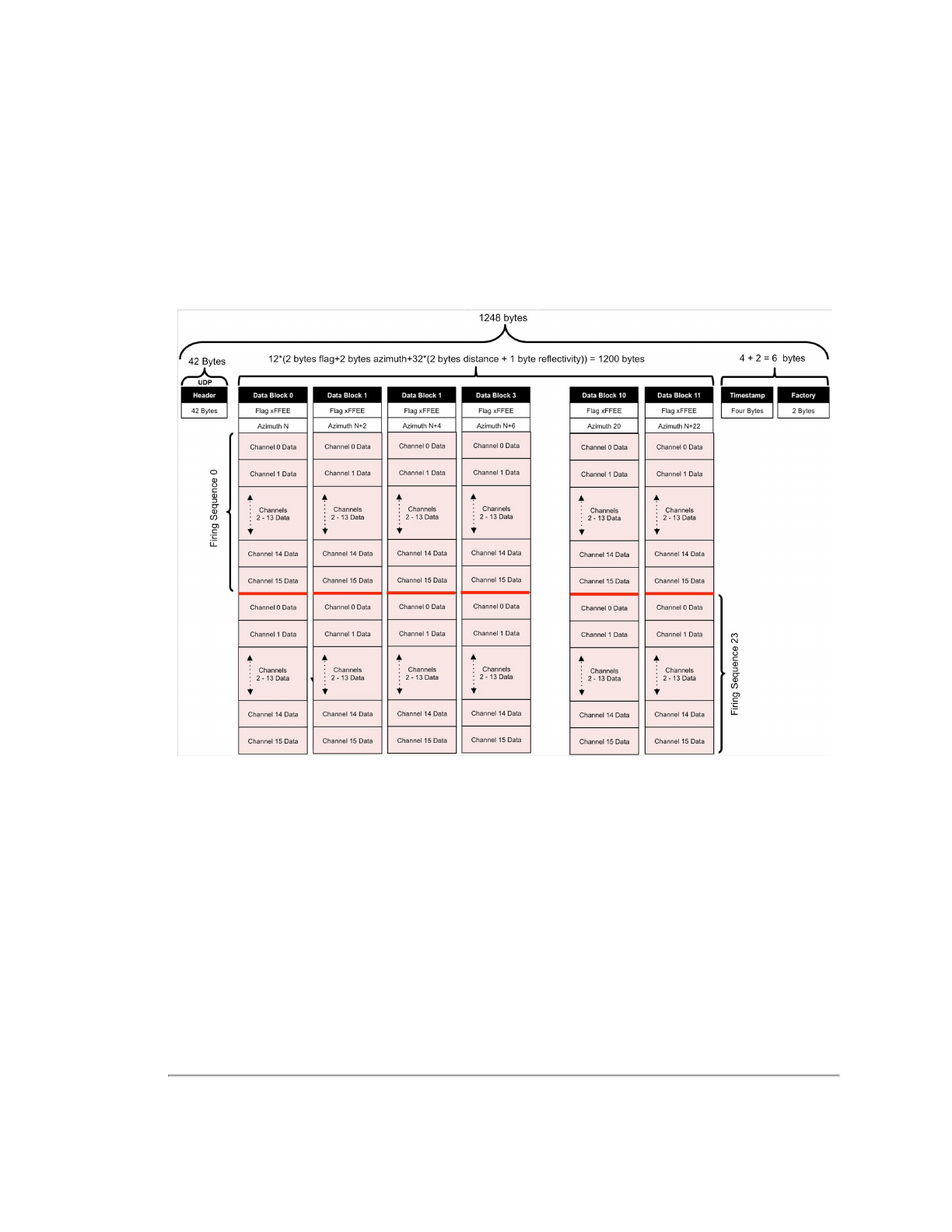
. The packet data structure for Dual Return
Mode is shown in
Figure 9-3 on the next page
.
There are several key differences between the packet structures.
First, in Dual Return Mode the sensor sends a pair of data blocks for each azimuth angle firing. The odd numbered blocks
(1, 3, ..., 9, 11) contain either the strongest or second-strongest return and the even numbered blocks (0, 2, ..., 8, 10) con-
tain the last return.
If the strongest return is also the last return, then the second-strongest return is provided. If only one return was detected,
the data will be identical in the even|odd block pairs (0|1, 2|3, 4|5, 6|7, 8|9, 10|11).
Figure 9-2 VLP-16 Single Return Mode Data Structure
Chapter 9 • Sensor Data 57
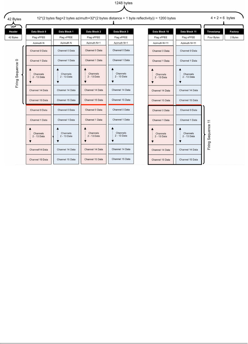
Figure 9-3 VLP-16 Dual Return Mode Data Structure
The figures below show a Wireshark trace of a single packet in Single Return Mode.
Figure 9-4 on the facing page
shows
the beginning of the packet and
Figure 9-5 on the facing page
shows packet end. The location/offset of the data relative to
the initial byte in the packet is shown in parentheses.
58 VLP-16 User Manual
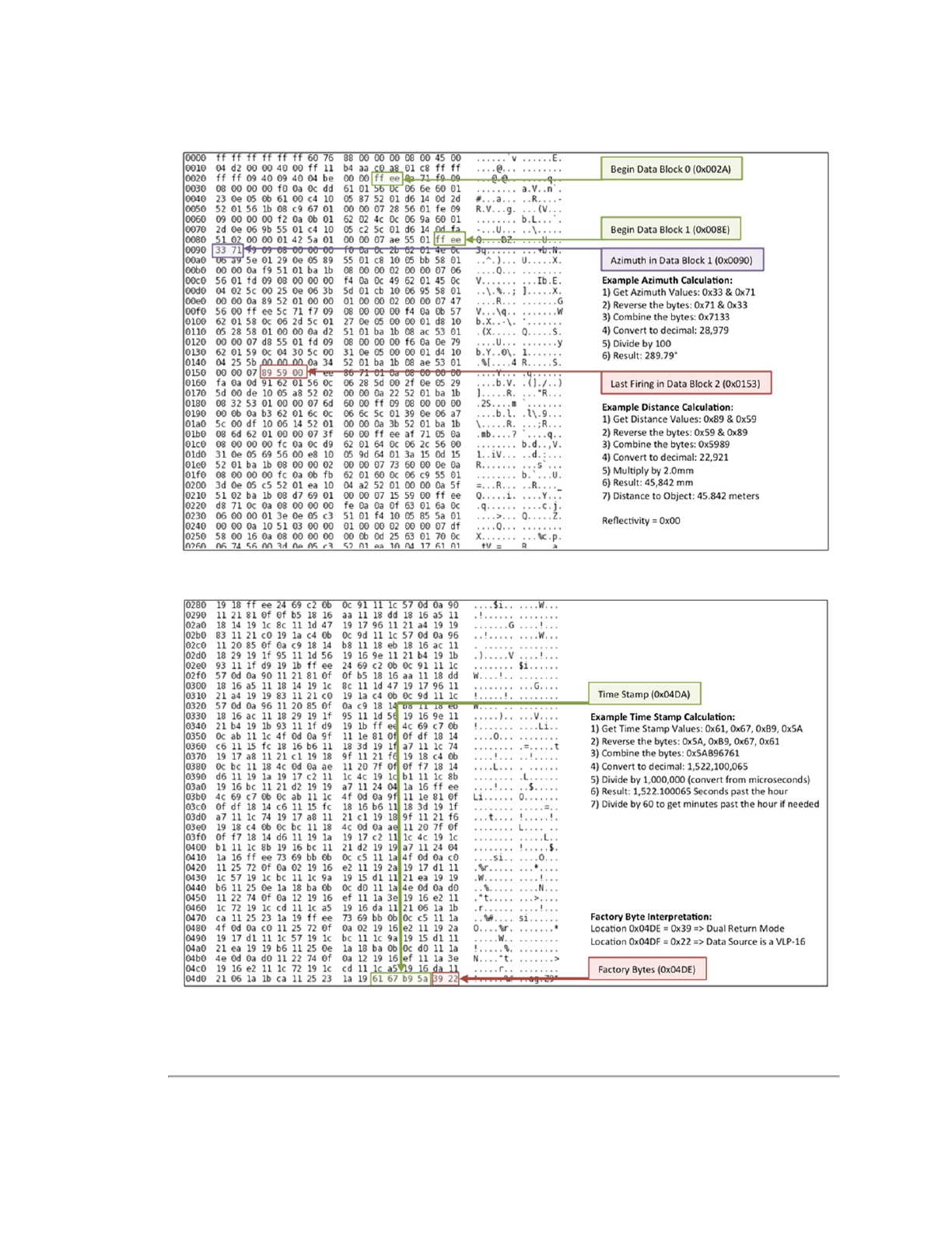
Figure 9-4 Single Return Mode Packet Data Trace (packet start)
Figure 9-5 Single Return Mode Packet Data Trace (ending)
Chapter 9 • Sensor Data 59
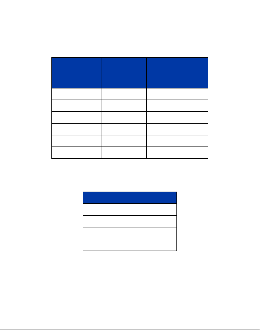
9.3.3 Position Packet Structure
The position packet provides an echo of the NMEA sentence received from an external time source as well as the Pulse
Per Second status and a time stamp representing when the position packet was assembled.
The position packet is a 554 byte UDP packet received on port 8308. The structure of the position packet is given in
Table
9-3 below
.
Note: You may notice the timestamps in the position packets are occasionally out of order with respect to the data pack-
ets. This is normal as the delivery of data packets is the sensor's highest priority, and a position packet may get deferred
momentarily in favor of transmitting a data packet. The ratio of data packets to position packets is about 14 to 1. See
NMEA
Message Formats on page 46
for details on the GPRMC message.
Number of Bytes
Byte Offset from
beginning of
packet (hex)
Description
42 0x0000 UDP header
198 0x002A unused (null bytes)
4 0x00F0 Timestamp (µs)
1 0x00F4 Pulse Per Second status
3 0x00F5 unused
variable length 0x00F8 NMEA GPRMC sentence
Table 9-3 Position Packet Structure Field Offsets
Payload length is 512 bytes. The GPRMC sentence is terminated with CR/LF and padded to end of payload with null
bytes.
Value Description
0 No PPS detected
1 Synchronizing to PPS
2 PPS Locked
3 Error
Table 9-4 PPS Status Byte Values
A position packet is shown in the figure below. Packet offsets are on the left, raw data bytes in hex are in the center, and the
ASCII interpretation is on the right.
60 VLP-16 User Manual
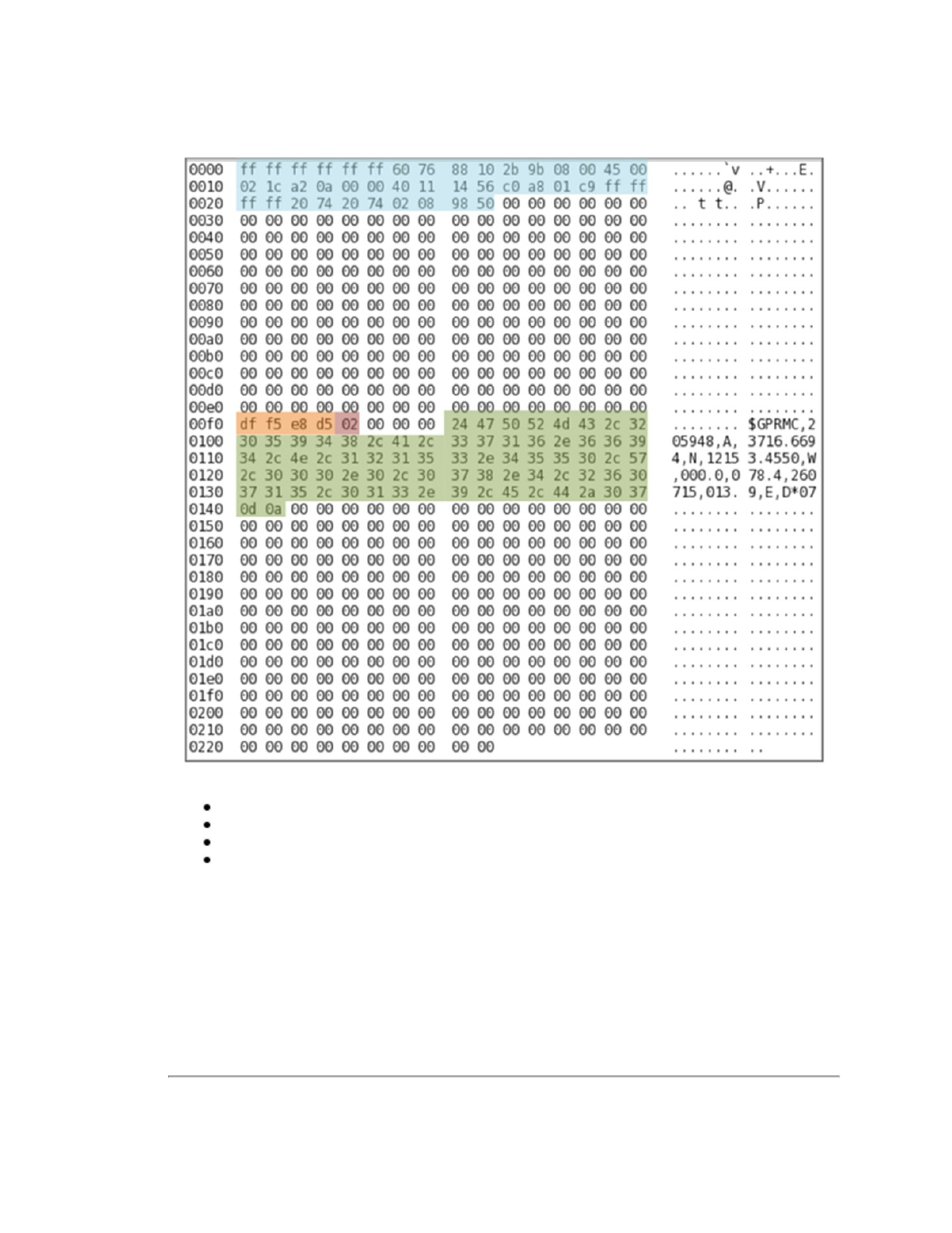
Figure 9-6 Wireshark Position Packet Trace
Legend:
light blue: Ethernet+IP+UDP packet header (42 bytes)
orange: Timestamp (4 bytes)
red: PPS status (1 byte)
green: NMEA GPRMC sentence (length varies)
9.4 Discreet Point Timing Calculation
For the purpose of geo-referencing LiDAR data, it is helpful to calculate the exact moment of a particular laser firing in
order to more closely associate it with time stamped data from an INS. By using the firing timing information given in
Figure
9-7 on the next page
you are able to compute the exact firing time for each data point.
Chapter 9 • Sensor Data 61
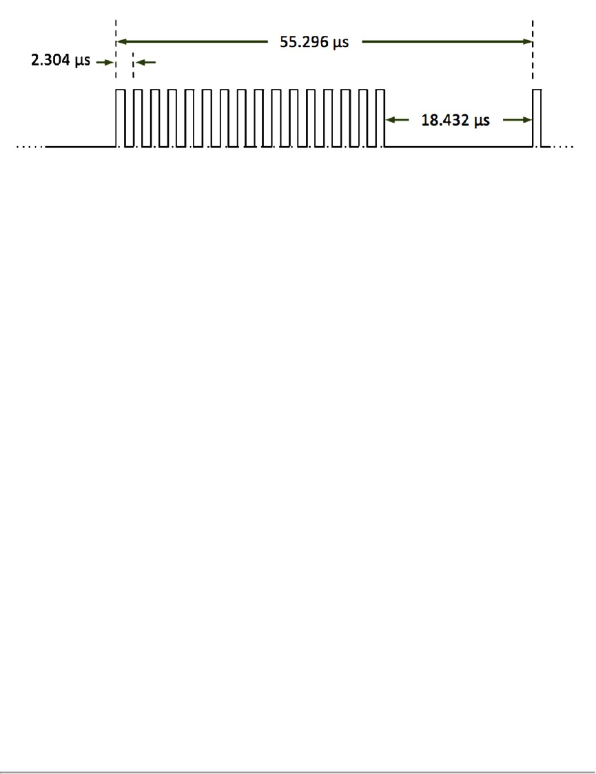
All sixteen lasers are fired and recharged every 55.296 μs. The cycle time between firings is 2.304 μs. There are 16 firings
(16 × 2.304 μs) followed by a recharge period of 18.43 μs. Therefore, the timing cycle to fire and recharge all 16 lasers is
given by (16 × 2.304 μs) + 18.43 μs = 55.296 μs.
Figure 9-7 Firing Sequence Timing
To calculate the exact time, in microseconds, of each data point, first number the points in the firing sequence as 0 to 15.
This becomes the data point index (aka Laser ID) for your calculations. Next, number the firing sequences 0 to 23. This
becomes your sequence index.
The timestamp in the packet indicates the time of the first data point in the packet. You’ll need to calculate a time offset for
each data point and then add that offset to the timestamp. See
Figure 9-9 on page 64
for specific Data Point Timing Off-
sets (Single Return Mode) and
Figure 9-10 on page 65
for specific Data Point Timing Offsets (Dual Return Mode).
The offset equation is given by:
TimeOffset = (55.296 µs * SequenceIndex)+(2.304 µs * DataPointIndex)
To calculate the exact point time, add the TimeOffset to the timestamp.
ExactPointTime = Timestamp + TimeOffset
Example: Calculate the timing offsets of every point in a packet, in single or dual return mode. The following is working
Python code:
def make_table(dual_mode):
timing_offsets = [[0.0 for x in range(12)] for y in range(32)] # Init matrix
# constants
full_firing_cycle = 55.296 # µs
single_firing = 2.304 # µs
# compute timing offsets
for x in range(12):
for y in range(32):
if dual_mode:
dataBlockIndex = (x - (x % 2)) + (y / 16)
else:
dataBlockIndex = (x * 2) + (y / 16)
dataPointIndex = y % 16
timing_offsets[y][x] = \
(full_firing_cycle * dataBlockIndex) + (single_firing * dataPointIndex)
return timing_offsets
To verify the values are correct, you can print them out and compare them with values in
Figure 9-9 on page 64
and
Figure
9-10 on page 65
.
62 VLP-16 User Manual
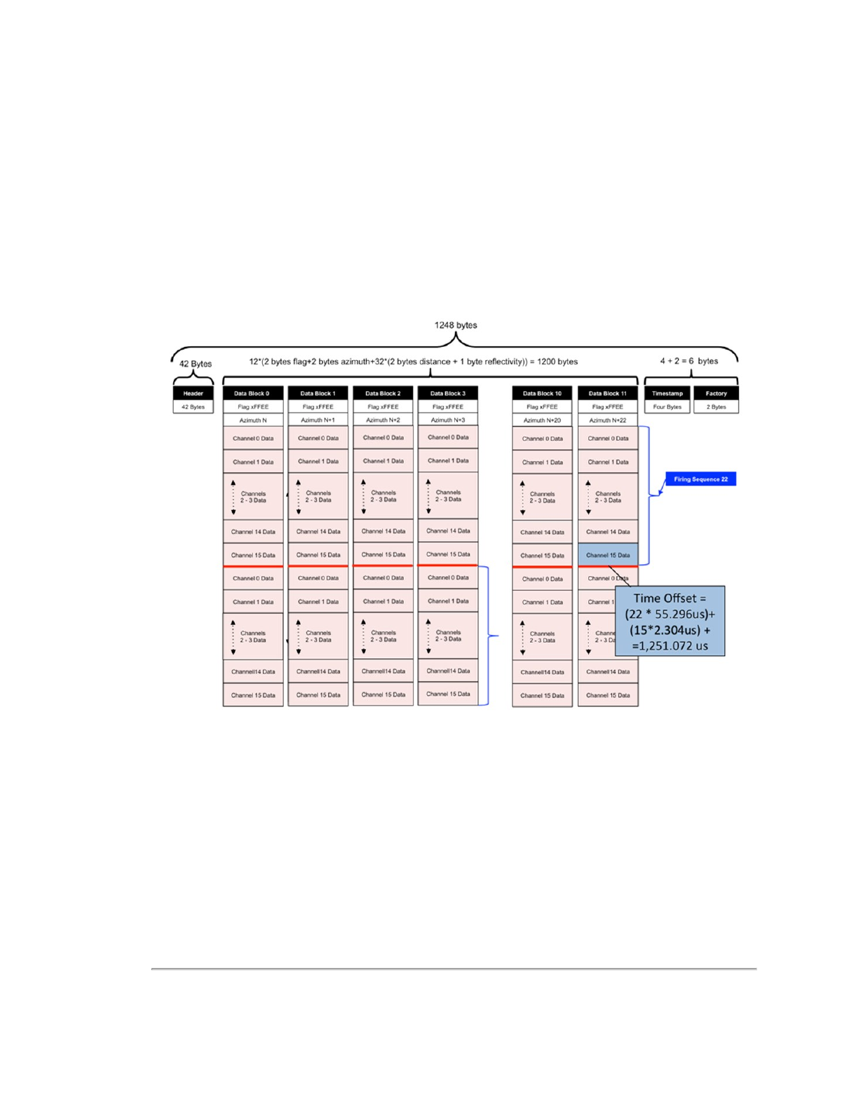
timing_offsets = make_table(False) # False : single return mode
print('\n'.join([', '.join(['{:8.3f}'.format(value) for value in row])
for row in timing_offsets]))
Example: Calculate the exact firing time of the last firing in a packet if the timestamp value is 45,231,878 µs.
Timestamp = 45,231,878 µs
TimeOffset = timing_offsets[15][23]
ExactPointTime = Timestamp + TimeOffset
ExactPointTime = 45,231,878 + 1,306.368 µs
ExactPointTime = 45,233,184.368 µs
Figure 9-8 below
shows the timing calculation for a specific data point.
Figure 9-8 Example Data Point Timing Calculation
Chapter 9 • Sensor Data 63
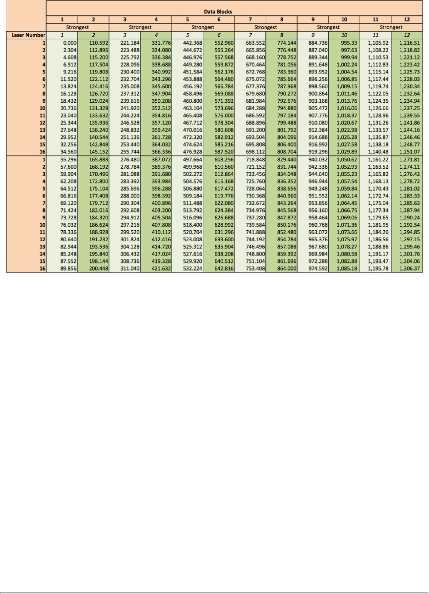
Figure 9-9 Single Return Mode Timing Offsets (in µs)
64 VLP-16 User Manual
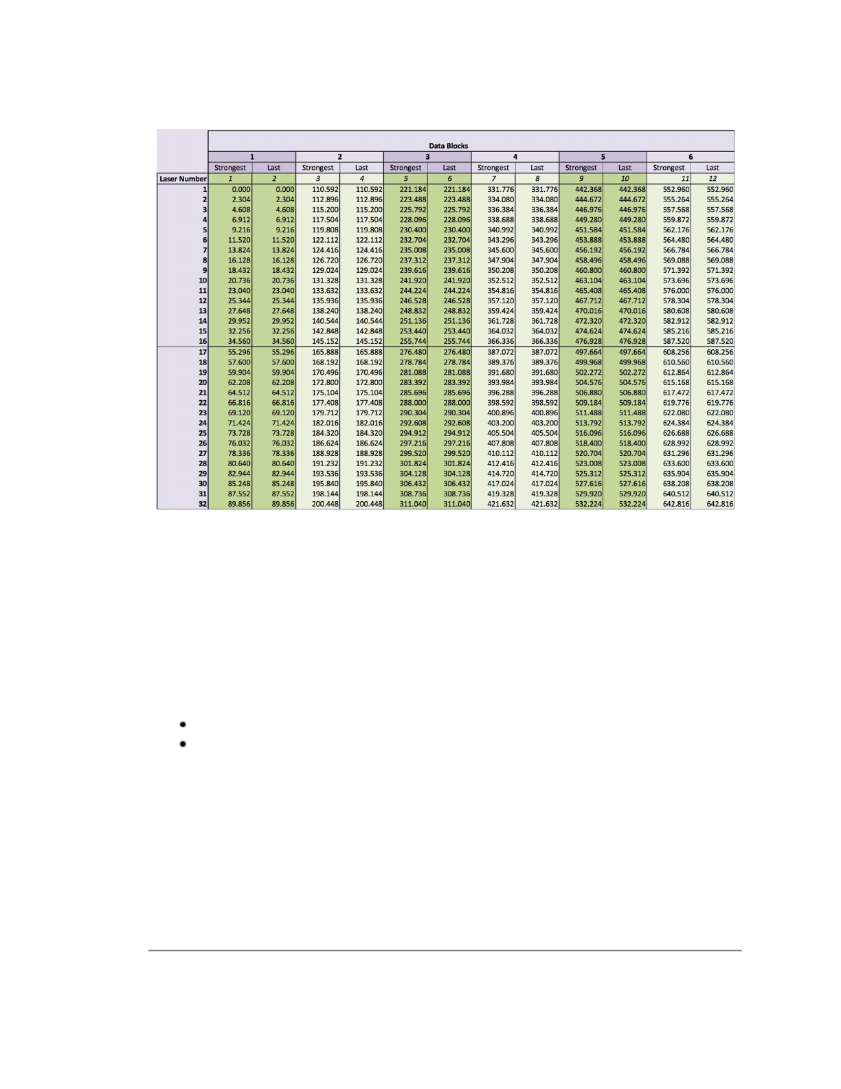
Figure 9-10 Dual Return Mode Timing Offsets (in µs)
9.5 Precision Azimuth Calculation
The azimuth (α) reported by the sensor in each data block is the azimuth at the moment the first laser in a firing sequence
fires.
To get better precision when geo-referencing, it’s useful to precisely calculate the unique azimuth for each point by
accounting for the firing timing. These precision azimuths may be calculated/interpolated using the timing offsets shown in
Figure 9-9 on the previous page
and
Figure 9-10 above
.
Consider a single data packet with 12 data blocks. If you assume the rotational speed is constant over the two 55.296 µs fir-
ing sequences in each data block, you can use the algorithm below to estimate a more precise azimuth angle for each
point.
The pseudo code below illustrates the concept.
K represents an index to a data point in the Nth data block, where its valid range is 0 to 31.
Do this for each data block.
// First, adjust for an Azimuth rollover from 359.99° to 0°
If (Azimuth[datablock_n+1] < Azimuth[datablock_n])
Then
Azimuth[datablock_n+1] := Azimuth[datablock_n+1] + 360;
Endif;
// Determine the Azimuth Gap between data blocks
AzimuthGap = Azimuth[datablock_n+1] - Azimuth[datablock_n];
Chapter 9 • Sensor Data 65

// Perform the interpolation using the timing firing
K = 0;
While (K < 31)
// Determine if you’re in the first or second firing sequence of the data block
if (K < 16)
Then
// Interpolate
Precision_Azimuth[K] := Azimuth[datablock_n] + (AzimuthGap * 2.304 μs * K) /
55.296 μs);
Else
// Interpolate
Precision_Azimuth[K] := Azimuth[datablock_n] + (AzimuthGap * 2.304 μs * ((K-16) +
55.296 μs)) / (2 * 55.296 μs);
Endif
// Adjust for any rollover
If Precision_Azimuth[K] >= 360
Then
Precision_Azimuth[K] := Precision_Azimuth[K] – 360;
Endif
K++;
End While
Note:
If you examine the VeloView code in GITHUB, you’ll notice that VeloView uses a slightly different method to cal-
culate XYZ coordinates. VeloView operates on the azimuth as if it were read as positive in the counter-clockwise
direction with the origin along the X axis.
9.6 Converting PCAP Files to Point Cloud Formats
Converting a packet capture (pcap) file of Velodyne LiDAR data to a LAS, LAZ, XYZ, PLY, or other point cloud file format
can be a non-trivial process.
The data provided by the sensor in the pcap file is measured relative to the sensor’s reference frame - the sensor’s internal
three dimensional coordinate system which moves with the sensor. That’s markedly different from a point cloud file where
the data points are referenced to a single coordinate system. That coordinate system might be an earth-frame (latitude,
longitude, elevation) or another convenient reference frame.
Processing the raw LiDAR data into a point cloud is called geo-referencing. In geo-referencing, the user takes into account
the sensor’s position (X/Y/Z) and orientation (pitch/roll/yaw) for each measurement. Knowing these six values enables a
user to perform the proper mathematical rotations and translations to reference the LiDAR data into a single coordinate
system.
Two popular techniques Velodyne LiDAR customers use for geo-referencing are inertial referencing and Simultaneous
Localization and Mapping (SLAM).
With inertial referencing, the location and orientation of the sensor at every moment is recorded with an Inertial Navigation
System (INS). An INS combines a Global Positioning System (GPS) receiver with an Inertial Measurement Unit (IMU).
Data from the both the INS and LiDAR sensor are time-synchronized to the GPS satellite’s reference clock, enabling the
user to match each LiDAR data point with its corresponding position and orientation from the INS. Having matched the
LiDAR data with the INS data, each measurement is mathematically translated into a single coordinate system.
66 VLP-16 User Manual

SLAM is a technique used by robots to analyze and navigate their environment. SLAM software automatically identifies sta-
tionary objects in the LiDAR data. The algorithm then uses the location of the stationary objects to mathematically back-out
the movement of the LiDAR and translate the data into a single coordinate system.
Most Velodyne LiDAR customers develop their own geo-referencing systems. However, inertial referencing and SLAM
solutions are available through third parties, and many can be found on the system integrators page at: http://velo-
dyneLiDAR.com/integrators.php.
Chapter 9 • Sensor Data 67

Chapter 10 • Sensor Communication
This section provides detailed information about sensor communication methods.
10.1 Web Interface
68
10.1.1 Configuration Screen
69
10.1.2 System Screen
72
10.1.3 Info Screen
73
10.1.4 Diagnostics Screen
75
10.2 Sensor Control with curl
76
10.2.1 Using curl with Velodyne LiDAR Sensors
76
10.2.2 curl Command Parameters
76
10.2.3 Command Line curl Examples
77
10.2.4 curl Example using Python
84
10.1 Web Interface
The easiest way to control a sensor’s operation is through its Web Interface. It has four screens. This section provides an
explanation of the feature sets and functionality on each screen.
68 VLP-16 User Manual
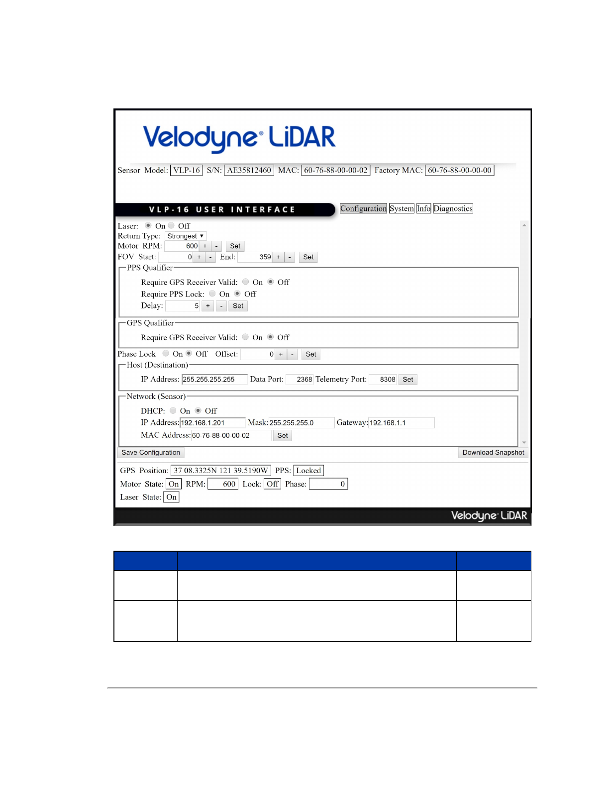
10.1.1 Configuration Screen
Figure 10-1 VLP-16 Configuration Screen
Function Description Default
Laser
ON/OFF Turns the sensor's laser ON or OFF. ON
Return Type
Strongest — Sensor provides only the strongest detected return.
Last — Sensor provides only the last (temporally) detected return.
Dual — Sensor provides both the strongest and last returns. If the last is also
Strongest
Table 10-1 Configuration Screen Functionality and Features
Chapter 10 • Sensor Communication 69

Function Description Default
the strongest, the sensor provides the second-strongest return. If only one
return is detected, the two values will be identical.
Motor RPM
Sets the sensor’s internal spin rate. Valid values include the range from 300 to
1200 RPM, and 0. Setting it to 0 during active scanning will auto-disable the
sensor’s lasers, which re-enable automatically the next time RPM is set in the
valid non-zero range.
Set - Activates the changes.
600
FOV Start
Sets the start azimuth for a user-defined Field of View. Units: integer
degrees.
Set - Activates the changes.
0
FOV End Sets the end azimuth for a user-defined Field of View. Units: integer degrees.
Set - Activates the changes. 359
PPS Qual-
ifier
Adjusts parameters that affect how PPS is used when synchronizing time
stamps to UTC.
Require GPS Receiver Valid: ON/OFF.
Require PPS Lock: ON/OFF.
Delay: Sets the qualification period (in seconds) for PPS.
Set - Activates the changes.
OFF
ON
5
GPS Qual-
ifier
Controls whether GPS Receiver Valid is required when synchronizing time
stamps to UTC.
Require GPS Receiver Valid: ON/OFF.
Set - Activates the changes.
OFF
Phase Lock
Used to synchronize the firing of two or more sensors. The offset is used to
set the azimuth at which the laser fires in conjunction with the PPS signal’s
rising edge. Requires a valid PPS signal.
Offset: Enter the offset as the desired degrees multiplied by 100. For
example, if the desired offset is 270º, enter 27000.
Set - Activates the changes.
OFF
0
Host (Destin-
ation)
IP Address (IPv4) to which the sensor transmits its data. By default it is set to
the broadcast address. If using one or more sensors in a network it must be
set to a non-broadcast IP address to avoid cross-loading.
Data Port — Port number for laser data packets.
Telemetry Port — Port number for position (telemetry) packets.
Set — Activates changes.
255.255.255.255
2368
8308
Network
(Sensor)
DHCP — When ON, the sensor obtains its IP address from a DHCP server on
its local network. When set to OFF, it uses the IP Address, Mask, and Gate-
way the user configures.
IPv4 Address — Sensor IP address as specified by the user.
Mask — Sensor subnet mask as specified by the user.
Gateway — Sensor gateway as specified by the user.
MAC Address - Sensor MAC address override.
Set — Activates changes.
OFF
192.168.1.201
255.255.255.0
192.168.1.1
70 VLP-16 User Manual

Function Description Default
Note: Take care when turning DHCP ON. Before doing so, ensure a DHCP
server on the network is available to provide the sensor with an IP address. If
you turn DHCP ON and lose contact with the sensor, follow the
Turned
DHCP On, Lost Contact With Sensor on page 88
procedure to get it back.
Save Con-
figuration
Saves all current settings to flash memory. Whenever the sensor powers up
or is reset, it is restored to these saved settings. Only the most recent save is
kept.
Download
Snapshot
Clicking this button generates an ASCII text file (name format: <Seri-
alNumber>.hdl) for downloading. It contains a JSON object capturing the
sensor’s state at that moment. The file can be sent to Velodyne
Technical Sup-
port on page 90
for analysis and to obtain troubleshooting advice.
GPS Position Displays the last received GPS latitude and longitude.
PPS Displays the current state of the PPS signal if provided from a GPS. Absent,
Synchronizing, Locked, and Error are the valid states.
Motor State
Indicates if the sensor’s internal motor is spinning: ON/OFF.
RPM — The sensor’s current RPM.
Lock — Indicates the phase lock feature state: ON/OFF.
Phase — Indicates the current phase offset. Only relevant when the phase
lock feature is active. This value is presented in hundredths of a degree.
Laser State Indicates the current laser array firing status: ON/DISABLED.
See
Time Synchronization on page 123
for additional information on the PPS and GPS Qualifier functions.
10.1.1.1 MAC Address
The ability to change the sensor's MAC Address was introduced with VLP-16 firmware release 3.0.34.0.
It may be advantageous to do this for asset management in multi-sensor situations where the MAC address is the closest
thing to a hard sensor ID, or as an anti-tracking measure. Bear in mind, however, that multiple sensors with the same MAC
address running on the same network will likely produce undesirable results.
Note: When changing the sensor's MAC Address, the first octet must not be set to an odd value. 00 is ok. 60 is ok. ff is
not ok.
As defined by IEEE 802 Standards, the least significant bit of the first octet of a MAC address identifies it as a multicast
address. A sensor bearing a multicast MAC address may cause undesirable network issues.
By extension, never set a MAC Address to the broadcast address (aka. all bits on) or any other group address.
10.1.1.2 Correctly reset MAC Address to Factory MAC Address
If you have changed the sensor's MAC Address to something other than the Factory MAC Address and wish to reset it
back, follow the procedure below.
Chapter 10 • Sensor Communication 71
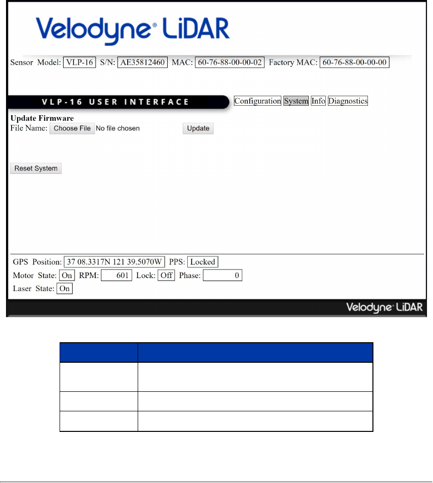
1. On the sensor's Configuration Screen, enter 00-00-00-00-00-00 in the MAC Address field. The '-' characters
must be present and the six octet values must be expressed as two hexadecimal digits each, all zeroes.
2. Click the Save Configuration button.
3. Click System to view the System Screen.
4. Click the Reset System button.
Once the sensor is done resetting, you may refresh the page and go back to the Configuration Screen. The MAC Address
should match the Factory MAC Address.
10.1.2 System Screen
Figure 10-2 VLP-16 System Screen
Function Description
Update Firmware Choose File — Enables user to select a new firmware image file.
Update — Initiates the firmware update process.
Reset System Used to reset the system after a firmware update.
GPS Position See description in
Table 10-1 on page 69
.
Table 10-2 System Screen Functionality and Features
72 VLP-16 User Manual
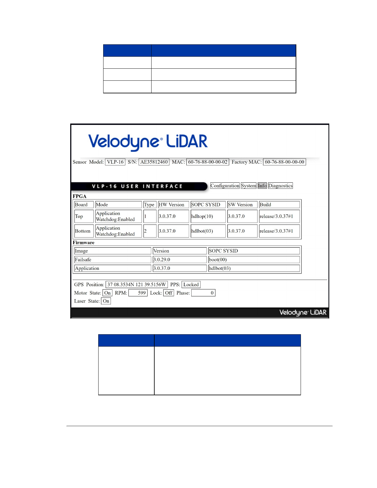
Function Description
PPS See description in
Table 10-1 on page 69
.
Motor State See description in
Table 10-1 on page 69
.
Laser State See description in
Table 10-1 on page 69
.
10.1.3 Info Screen
Figure 10-3 VLP-16 Info Screen
Function Description
FPGA (top board)
Board — Top or Bottom board information.
Mode — State of the Application Watchdog – Velodyne use only.
Type — Velodyne Use Only.
HW Version — Velodyne Use Only.
SOPC SYSID — Velodyne Use Only.
SW Version — Current operating firmware version.
Build — Velodyne Use Only.
Table 10-3 Info Screen Functionality and Features
Chapter 10 • Sensor Communication 73

Function Description
FPGA (bottom board)
Board — Top or Bottom board information.
Mode – Velodyne use only.
Type — Velodyne Use Only.
HW Version — Velodyne Use Only.
SOPC SYSID — Velodyne Use Only.
SW Version — Current operating firmware version.
Firmware Image Image — Firmware type (Failsafe and Application).
Firmware Version Version — Number of the stored Failsafe and Application images.
SOPC SYSID Failsafe boot(00) — Velodyne Use Only.
Application hdlbot(03) — Velodyne Use Only.
GPS Position See description in
Table 10-1 on page 69
.
PPS See description in
Table 10-1 on page 69
.
Motor State See description in
Table 10-1 on page 69
.
Laser State See description in
Table 10-1 on page 69
.
74 VLP-16 User Manual
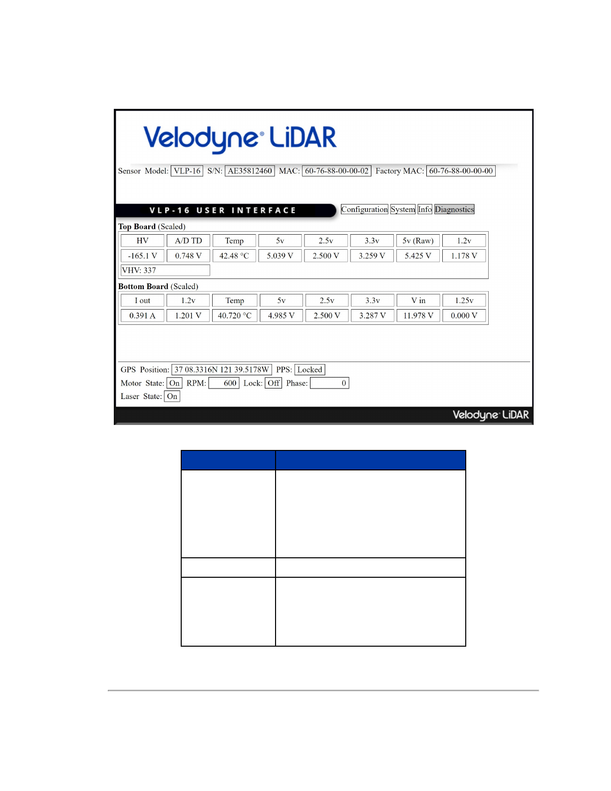
10.1.4 Diagnostics Screen
Figure 10-4 VLP-16 Diagnostics Screen
Function Description
Top Board (Scaled)
HV — Velodyne Use Only.
A/D TD — Velodyne Use Only.
Temp — Circuit board temperature.
5v — Internal voltage status.
2.5v — Internal voltage status.
3.3v — Internal voltage status.
5v (Raw) — Internal voltage status.
1.2v — Internal voltage status.
VHV Velodyne Use Only.
Bottom Board (Scaled)
I out — The sensor's electrical current consumption.
1.2v — N/A.
Temp — Circuit board temperature.
5v — Internal voltage status.
2.5v — Internal voltage status.
3.3v — Internal voltage status.
Table 10-4 System Screen Functionality and Features
Chapter 10 • Sensor Communication 75
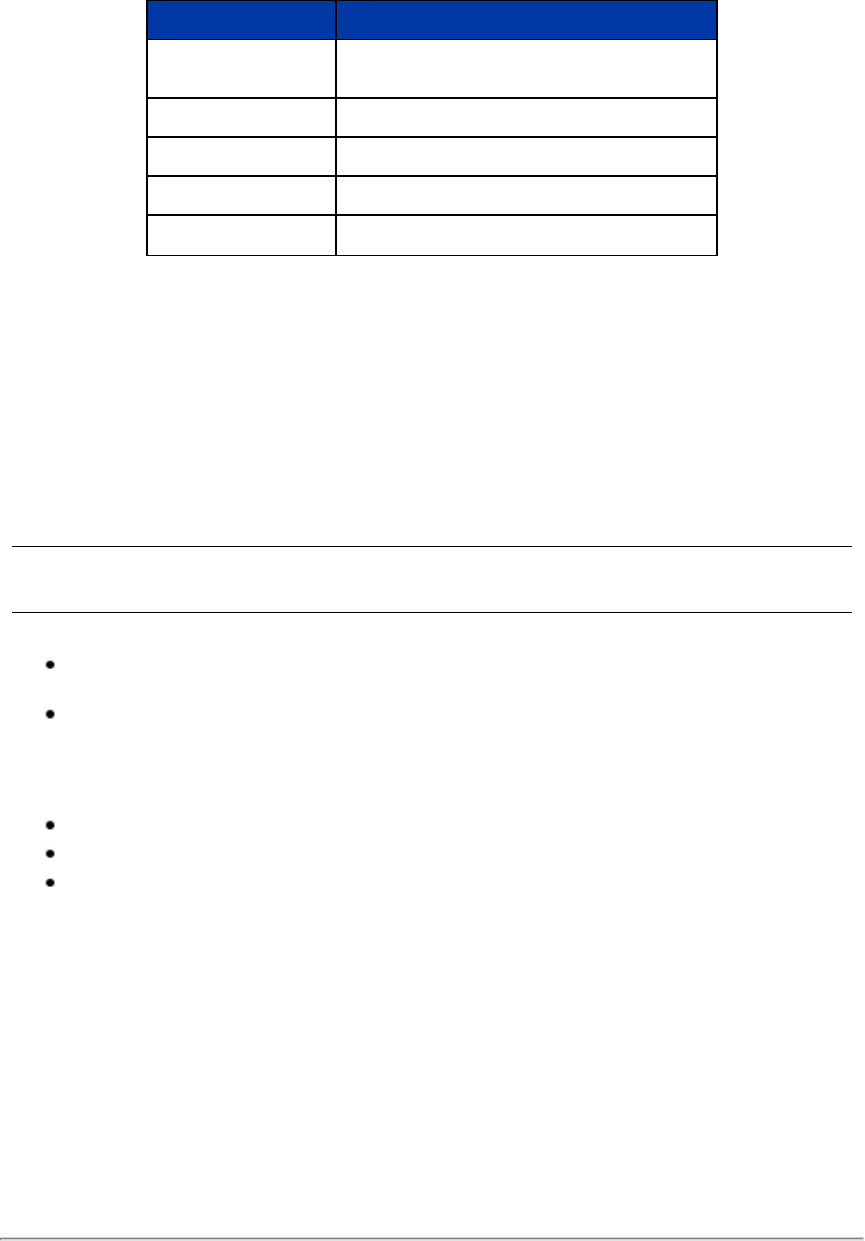
Function Description
V in — Internal voltage status.
1.25v — N/A.
GPS Position See description in
Table 10-1 on page 69
.
PPS See description in
Table 10-1 on page 69
.
Motor State See description in
Table 10-1 on page 69
.
Laser State See description in
Table 10-1 on page 69
.
10.2 Sensor Control with curl
In addition to the Web Interface, Velodyne LiDAR sensors provide an HTTP interface for programmatic configuration and
control. One of the easiest tools to use for this purpose is curl. curl is a command line program freely available on a wide
variety of operating systems. curl specializes in transferring data between devices using Internet protocols. You can learn
more about curl and libcurl, the library (written in C) it uses to do all the heavy lifting, at this page: https://ec.haxx.se/curl-
does.html. libcurl has bindings for many environments and programming languages.
The sections below show how to command and control a sensor from the command line using curl, and from a Python pro-
gram using pycurl, a Python binding for libcurl.
10.2.1 Using curl with Velodyne LiDAR Sensors
Note: It is recommended to issue at most one curl command per second to the sensor.
curl takes care of the following items for you. But you should follow them when using libcurl in your software.
Always check the response from the sensor, even if the function used does not return one. (curl can and will
respond with status/error messages.)
Always close the socket connection to the sensor when finished.
10.2.2 curl Command Parameters
To obtain JSON-formatted sensor status, invoke curl with the following URLs:
http://192.168.1.201/cgi/status.json - Returns the current operational state and parameters of the sensor.
http://192.168.1.201/cgi/diag.json - Returns diagnostic information from the sensor.
http://192.168.1.201/cgi/snapshot.hdl - Returns current sensor configuration and status data.
The following sensor parameters can be changed by sending a urlencoded tagged key and data pair to
http://192.168.1.201/cgi/setting:
1. rpm=[integer]
2. returns=[Strongest]|[Last]|[Dual]
Set Field of View by sending a urlencoded key and data pair to http://192.168.1.201/cgi/setting/fov:
1. [start]|[end]=[integer]
Set Sensor Address, Destination Port, or Telemetry Port by sending a urlencoded key and data pair to
http://192.168.1.201/cgi/setting/host:
76 VLP-16 User Manual

1. addr=255.255.255.255
2. dport=2368
3. tport=8309
Network Settings can be set by providing the urlencoded key and data pair to http://192.168.1.201/cgi/setting/net:
1. addr=192.168.1.200
2. mask=255.255.255.0
3. gateway=192.168.1.2
4. dhcp=[on|off]
Special Commands to Save settings to NVRAM and Reset the sensor:
1. http://192.168.1.201/cgi/save
a. submit
2. http://192.168.1.201/cgi/reset
a. reset_system
10.2.3 Command Line curl Examples
10.2.3.1 Get Diagnostic Data
Returns a JSON-formatted string containing values as seen on the Diagnostics page of the sensor’s Web Interface.
Command:
curl http://192.168.1.201/cgi/diag.json
Example Response:
{
"volt_temp":{
"top":{
"hv":2917,
"lm20_temp":1105,
"pwr_5v":2075,
"pwr_2_5v":2047,
"pwr_3_3v":2693,
"pwr_5v_raw":2263,
"pwr_vccint":977
},
"bot":{
"i_out":2086,
"pwr_1_2v":992,
"lm20_temp":1231,
"pwr_5v":2046,
"pwr_2_5v":2046,
"pwr_3_3v":2692,
"pwr_v_in":910,
"pwr_1_25v":1
}
},
}
Chapter 10 • Sensor Communication 77
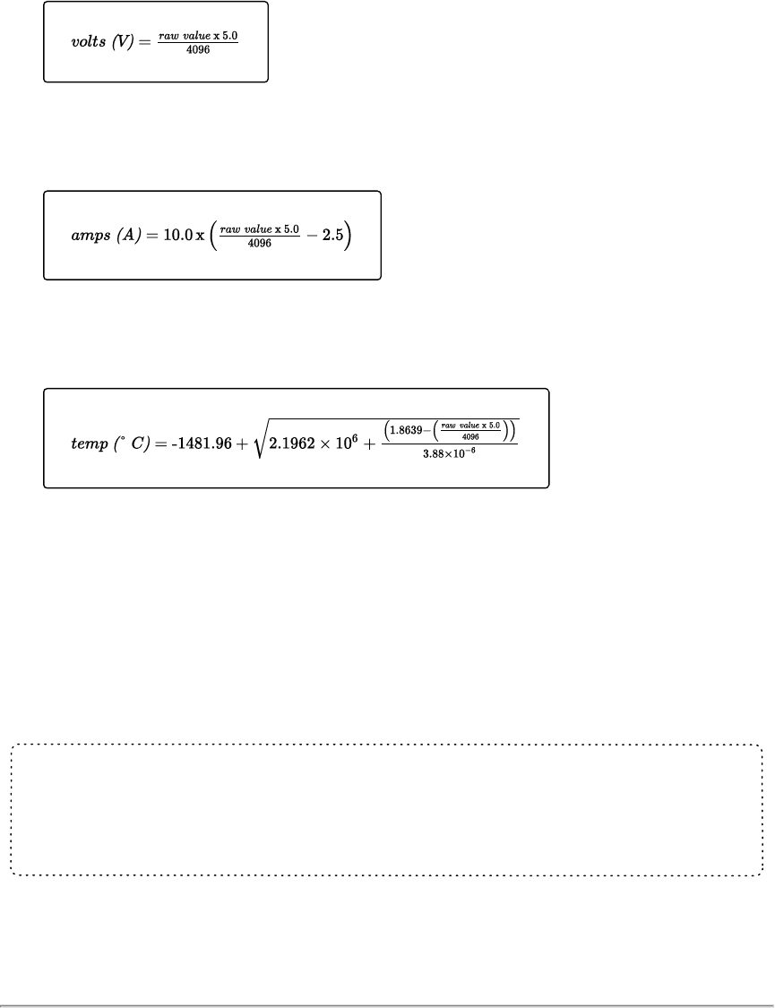
10.2.3.2 Conversion Formulas
Equation 10-1 Standard Voltage Conversion
Equation 10-2 Standard Current Conversion
Equation 10-3 Standard Temperature Conversion
10.2.3.3 Interpret Diagnostic Data
Use the formulas above to convert raw diagnostic data fields below to usable values. Some fields are scaled by additional
factors.
10.2.3.3.1 top:hv
The HV field comes from the sensor's top board. It represents the high voltage bias to the APD (Avalanche photodiode).
Its operating range is -150.0 V to -132.0 V.
To convert the raw value, use
Equation 10-1 above
then scale the result by subtracting 5.0 and multiplying the result by
101.0.
Example:
hv = 2917
(raw value)
(2917 * 5.0) / 4096 = 3.561
101.0 * (3.561 - 5.0) = -145.34 V
78 VLP-16 User Manual

10.2.3.3.2 top:lm20_temp
This field indicates the temperature of the top board. Its operating range is -25.0° C to 94.0° C.
To convert the raw value, use
Equation 10-3 on the previous page
.
Example:
lm20_temp = 1105
(raw value)
(1105 * 5.0) / 4096 = 1.3489
-1481.96 + SQRT(2.1962E6 + ((1.8639 – 1.3489) / 3.88E-6)) = 44.126° C
10.2.3.3.3 top:pwr_5v
This is the top board's 5.0 V rail. Its operating range is 4.8 V to 5.2 V.
To convert the raw value, use
Equation 10-1 on the previous page
then scale the result by multiplying it by 2.0.
Example:
pwr_5v = 2075
(raw value)
(2075 * 5.0) / 4096 = 2.533
2.533 * 2.0 = 5.066 V
10.2.3.3.4 top:pwr_2_5v
This is the top board's 2.5 V rail. Its operating range is 2.3 V to 2.7 V.
To convert the raw value, use
Equation 10-1 on the previous page
.
Example:
pwr_2_5v = 2047
(raw value)
(2047 * 5.0) / 4096 = 2.499 V
10.2.3.3.5 top:pwr_3_3v
This is the top board's 3.3 V rail. Its operating range is 3.1 V to 3.5 V.
To convert the raw value, use
Equation 10-1 on the previous page
.
Example:
pwr_3_3v = 2693
(raw value)
(2693 * 5.0) / 4096 = 3.287 V
10.2.3.3.6 top:pwr_5v_raw
This is the top board's unregulated 5.0 V rail. Its operating range is 2.3 V to 2.7 V.
To convert the raw value, use
Equation 10-1 on the previous page
then scale the result by multiplying it by 2.0.
Chapter 10 • Sensor Communication 79

Example:
pwr_5v_raw = 2263
(raw value)
(2263 * 5.0) / 4096 = 2.762
2.762 * 2.0 = 5.525 V
10.2.3.3.7 top:pwr_vccint
This is the top board's 1.2 V rail. Its operating range is 1.0 V to 1.4 V.
To convert the raw value, use
Equation 10-1 on page 78
.
Example:
pwr_vccint = 977
(raw value)
(977 * 5.0) / 4096 = 1.193 V
10.2.3.3.8 bot:i_out
This is the sensor's input power line. Its operating range is 0.3 A to 1.0 A. (It spikes whenever the motor spins up.)
To convert the raw value, use
Equation 10-2 on page 78
.
Example:
i_out = 2086
(raw value)
(2086 * 5.0) / 4096 = 2.546
10.0 * (2.546 - 2.5) = 0.464 A
10.2.3.3.9 bot:lm20_temp
This field indicates the temperature of the bottom board. Its operating range is -25.0° C to 94.0° C.
To convert the raw value, use
Equation 10-3 on page 78
.
Example:
lm20_temp = 1231
(raw value)
(1105 * 5.0) / 4096 = 1.503
-1481.96 + SQRT(2.1962E6 + ((1.8639 – 1.503) / 3.88E-6)) = 31.082° C
10.2.3.3.10 bot:pwr_1_2v
This is the bottom board's 1.2 V rail. Its operating range is 1.0 V to 1.4 V.
To convert the raw value, use
Equation 10-1 on page 78
.
Example:
80 VLP-16 User Manual

pwr_1_2v = 992
(raw value)
(992 * 5.0) / 4096 = 1.211 V
10.2.3.3.11 bot:pwr_1_25v
This is the bottom board's 1.25 V rail. Its operating range is 1.0 V to 1.4 V.
To convert the raw value, use
Equation 10-1 on page 78
.
Example:
pwr_1_25v = 1
(raw value)
(1 * 5.0) / 4096 = 0.001 V
10.2.3.3.12 bot:pwr_2_5v
This is the bottom board's 2.5 V rail. Its operating range is 2.3 V to 2.7 V.
To convert the raw value, use
Equation 10-1 on page 78
.
Example:
pwr_2_5v = 2046
(raw value)
(2046 * 5.0) / 4096 = 2.498 V
10.2.3.3.13 bot:pwr_3_3v
This is the bottom board's 3.3 V rail. Its operating range is 3.1 V to 3.5 V.
To convert the raw value, use
Equation 10-1 on page 78
.
Example:
pwr_3_3v = 2692
(raw value)
(2692 * 5.0) / 4096 = 3.286 V
10.2.3.3.14 bot:pwr_5v
This is the bottom board's 5.0 V rail. Its operating range is 4.8 V to 5.2 V.
To convert the raw value, use
Equation 10-1 on page 78
then scale the result by multiplying it by 2.0.
Example:
pwr_5v = 2046
(raw value)
(2046 * 5.0) / 4096 = 2.498
2.498 * 2.0 = 4.995 V
10.2.3.3.15 bot:pwr_v_in
This is the voltage of the input power. Its operating range is 8.0 V to 19.0 V.
Chapter 10 • Sensor Communication 81

To convert the raw value, use
Equation 10-1 on page 78
then scale the result by multiplying it by 11.0.
Example:
pwr_v_in = 910
(raw value)
(910 * 5.0) / 4096 = 1.111
1.111 * 11.0 = 12.219 V
10.2.3.4 Get Snapshot
Downloads sensor snapshot data to an HDL file. This has the same effect as clicking on the Download Snapshot button
under the Configuration tab.
Command:
curl http://192.168.1.201/cgi/snapshot.hdl > snapshot.hdl
10.2.3.5 Get Sensor Status
Returns sensor state data, such as: GPS PPS is present, GPS position, motor status, phase, and laser states.
Command:
curl http://192.168.1.201/cgi/status.json
Example Response:
{
"gps":{
"pps_state":"Absent",
"position":""
},
"motor":{
"state":"On",
"rpm":600,
"lock":"Off",
"phase":0
},
"laser":{
"state":"On"
}
}
10.2.3.6 Set Motor RPM
Sets the RPM of the motor. Valid integer values range from 300 to 1200, in increments of 60. (If the RPM setting is not
evenly divisible by 60, neither motor speed control nor phase lock functions will function properly.) For values 1
through 299, the sensor defaults back to 300 RPM. If a value of 0 or less is entered, the sensor motor powers down and
the lasers are turned off, as leaving them on with the motor stopped would be an unsafe eye state. This has the same
effect as setting the value for the Motor RPM in the Web Interface.
Command:
curl --data “rpm=[integer]” http://192.168.1.201/cgi/setting
Example:
curl --data “rpm=600” http://192.168.1.201/cgi/setting
82 VLP-16 User Manual

10.2.3.7 Set Field of View
Sets the field of view (0° to 359°). Numbers outside this range are quietly ignored. This has the same effect as setting the
FOV Start and FOV End values on the Web Interface.
Command:
curl --data “[start]|[end]=[integer]” http://192.168.1.201/cgi/setting/fov
Examples:
curl --data "start=10" http://192.168.1.201/cgi/setting/fov
curl --data "end=270" http://192.168.1.201/cgi/setting/fov
10.2.3.8 Set Return Type (Strongest, Last, Dual)
This command sets the return type (or mode) of the sensor. Choose one: Strongest, Last, and Dual. This has the same
effect as selecting the Web Interface Return Type.
Command:
curl --data “returns=[Strongest]|[Last]|[Dual]” http://192.168.1.201/cgi/setting
Examples:
curl --data “returns=Strongest” http://192.168.1.201/cgi/setting
curl --data “returns=Last” http://192.168.1.201/cgi/setting
curl --data "returns=Dual" http://192.168.1.201/cgi/setting
10.2.3.9 Save Configuration
Saves the configuration so that the settings are persistent across power cycles. This is equivalent to clicking on the Save
Configuration button under the Configuration tab in the Web Interface.
Command:
curl --data “submit” http://192.168.1.201/cgi/save
10.2.3.10 Reset System
Resets the sensor. This command performs the same operation as pressing the Reset System button under the System
tab in the Web Interface, or if you cycled power to the sensor.
Command:
curl --data "reset_system" http://192.168.1.201/cgi/reset
Example Response:
The system resets.
10.2.3.11 Network Configuration
Use the curl commands below to alter the network configuration of the sensor.
Once changed, the settings must be saved and the sensor reset for the new configuration to take effect.
10.2.3.12 Set Host (Destination) IP Address
This command sets the destination IP address where firing data and Position/Telemetry packets are sent. This has the
same effect as entering a Host IP address on the sensor’s Web Interface.
Command:
curl --data "addr=255.255.255.255" http://192.168.1.201/cgi/setting/host
Chapter 10 • Sensor Communication 83

10.2.3.13 Set Data Port
This command sets the sensor’s data port (default: 2368). It has the same effect as setting the Web Interface’s Data Port
field to the given number.
Command:
curl --data "dport=2368" http://192.168.1.201/cgi/setting/host
10.2.3.14 Set Telemetry Port
This command sets the sensor’s telemetry port (default: 8308). It has the same effect as setting the port number in the
Web Interface’s Telemetry Port field.
Command:
curl --data "tport=8309" http://192.168.1.201/cgi/setting/host
10.2.3.15 Set Network (Sensor) IP Address
This sets the IP address of the device. The default is 192.168.1.201. This has the same effect as entering an IP address in
the Web Interface Network IP field.
Command:
curl --data "addr=192.168.1.200" http://192.168.1.201/cgi/setting/net
10.2.3.16 Set Netmask
This sets the network mask of the sensor. The default is 255.255.255.0. This has the same effect as entering a net mask in
the Web Interface Mask field.
Command:
curl --data "mask=255.255.0.0" http://192.168.1.201/cgi/setting/net
10.2.3.17 Set Gateway
This sets the gateway address of the sensor. The default is 192.168.1.1. This has the same effect as entering a gateway
address in the Web Interface Gateway field.
Command:
curl --data "gateway=192.168.1.2" http://192.168.1.201/cgi/setting/net
10.2.3.18 Set DHCP
This determines if the sensor is to rely on a DHCP server for its IP address.
This has the same effect as selecting the corresponding radio button for DHCP in the Web Interface.
Take care when turning DHCP ON. Before doing so, ensure a DHCP server on the network is available to provide the
sensor with an IP address. If you turn DHCP ON and lose contact with the sensor, follow the
Turned DHCP On, Lost
Contact With Sensor on page 88
procedure to get it back.
Command:
curl --data "dhcp=[on|off]" http://192.168.1.201/cgi/setting/net
10.2.4 curl Example using Python
The script below demonstrates how to do basic operations with a sensor using PycURL, a Python package built on libcurl.
It works in Python 2 and 3. For more information on PycURL go to: http://pycurl.io/docs/.
The script expects the sensor to have its default IP address. If it’s different, change Base_URL accordingly.
84 VLP-16 User Manual

The sensor object contains the interface to the actual sensor. A buffer is required because PycURL does not provide stor-
age for the network response. After each sensor request, the HTTP response code is checked for success.
The first operation is to reset the sensor. After a delay, the script changes a couple of sensor parameters. Waiting another
10 seconds (for the motor to spin up), sensor status is obtained and printed to standard out.
import pycurl
try:
from io import BytesIO
except ImportError:
from StringIO import StringIO as BytesIO
try:
from urllib.parse import urlencode
except ImportError:
from urllib import urlencode
import urllib2
import json
import time
def sensor_do(s, url, pf, buf):
s.setopt(s.URL, url)
s.setopt(s.POSTFIELDS, pf)
s.setopt(s.WRITEDATA, buf)
s.perform()
rcode = s.getinfo(s.RESPONSE_CODE)
success = rcode in range(200, 207)
print('%s %s: %d (%s)' % (url, pf, rcode, 'OK' if success else 'ERROR'))
return success
Base_URL = 'http://192.168.1.201/cgi/'
sensor = pycurl.Curl()
buffer = BytesIO()
rc = sensor_do(sensor, Base_URL+'reset', urlencode({'data':'reset_system'}), buffer)
if rc:
time.sleep(10)
rc = sensor_do(sensor, Base_URL+'setting', urlencode({'rpm':'300'}), buffer)
if rc:
time.sleep(1)
rc = sensor_do(sensor, Base_URL+'setting', urlencode({'laser':'on'}), buffer)
if rc:
time.sleep(10)
response = urllib2.urlopen(Base_URL+'status.json')
if response:
status = json.loads(response.read())
print 'Sensor laser is %s, motor rpm is %s' % \
(status['laser']['state'], status['motor']['rpm'])
sensor.close()
Typical output looks like the following:
http://192.168.1.201/cgi/reset data=reset_system: 204 (OK)
http://192.168.1.201/cgi/setting rpm=300: 204 (OK)
Chapter 10 • Sensor Communication 85

http://192.168.1.201/cgi/setting laser=on: 204 (OK)
Sensor laser is On, motor rpm is 301
86 VLP-16 User Manual
Chapter 11 • Troubleshooting
This section provides detail on how to troubleshoot your sensor, how to request technical assistance, how to have the
sensor repaired, and how to replace the fuse in the Interface Box.
11.1 Troubleshooting Process
87
11.1.1 Turned DHCP On, Lost Contact With Sensor
88
11.2 Service and Maintenance
89
11.2.1 Fuse Replacement
89
11.3 Technical Support
90
11.3.1 Purchased through a Distributor
90
11.3.2 Factory Support
90
11.3.3 Support Desk
90
11.4 Return Merchandise Authorization (RMA)
90
11.1 Troubleshooting Process
Problem Resolution
Interface Box LEDs
do not light
Verify:
Power connection and polarity.
Proper voltage should be between 9 V and 18 V, drawing a maximum of 0.9 A dur-
ing normal operation.
Fuse in the Interface Box is okay. See
Fuse Replacement on page 89
if it’s blown.
Rotor doesn’t spin
Verify:
Power connection and polarity.
Proper voltage should be between 9 V and 18 V, drawing a maximum of 0.9 A dur-
ing normal operation.
Fuse in the Interface Box is okay. See
Fuse Replacement on page 89
if it’s blown.
Unit spins but no data
Verify:
Ethernet wiring is functional.
Packet output using another application (e.g. VeloView/Wireshark).
Receiving computer's network settings.
Correct static IP address in your computer's network settings.
No security software is installed which may block Ethernet broadcasts.
Laser ON radio button is selected in Web Interface
Configuration Screen on
page 69
.
Input voltage and current draw are in proper ranges.
Table 11-1 Common Problems and Resolutions
Chapter 11 • Troubleshooting 87
Problem Resolution
Can see data in Wire-
shark but not
VeloView
Wireshark sniffs packets promiscuously but VeloView does not. VeloView needs permission
to receive packets from the system firewall, if active.
Check:
No firewall is active on receiving computer.
Sensor's destination address.
Port numbers are set to 2368 (data) and 8308 (position/telemetry).
Cannot see sensor’s
Web Interface
Verify:
Ethernet wiring is functional.
Packet output using another application (e.g. VeloView/Wireshark).
Receiving computer's network settings.
Correct static IP address in your computer's network settings.
No security software is installed which may block Ethernet broadcasts.
Action:
Reboot computer - sometimes network settings do not take effect until the com-
puter is rebooted.
Data dropouts
This is nearly always an issue with the network and/or user computer.
Check the following:
Is the sensor’s horizontal field of view set to less than 360°?
Is there excessive traffic and/or collisions on network?
Is a network device throttling back traffic? Devices such as wireless access points
often throttle broadcast data.
Are excessive broadcast packets from another service being seen by the sensor?
This can slow the sensor down.
Is the computer fast enough to keep up with the packet flow coming from the
sensor?
Remove all network devices and test with a computer directly connected to the
sensor.
GPS Not Syn-
chronizing
Check the following:
Baud rate set to 9600 and serial port set to 8N1 (8 bits, no parity, 1 stop bit).
Electrical continuity of PPS and serial wiring.
Incorrect construction of NMEA sentence.
Incorrect signal levels:
“High” voltage must be greater than 3.0 V and less than 15.0 V.
“Low” voltage must be less than 1.2 V.
Serial line not sourcing enough current:
The GPS/INS unit must be able to source at least 2 mA in the “high” voltage
state.
The polarity of the serial and PPS signals.
The GPS signal may be obscured by being indoors, near buildings, tree cover, etc.
Bring the receiver outside, exposed to as much open sky as possible for best signal
reception.
11.1.1 Turned DHCP On, Lost Contact With Sensor
When the sensor's DHCP is set to ON, the configuration saved, and the sensor is reset or power cycled, the sensor will no
longer have an IP address as it expects a DHCP server to assign it one.
88 VLP-16 User Manual

Because no DHCP server is present, the sensor performs Automatic Private IP Addressing (APIPA) and self-assigns a
Class B IP address that looks like 169.254.x.x. Your computer's IP address will likely be very different (not on the same
logical network) resulting in a failure to communicate with the sensor.
Perform the following procedure to regain communication with the sensor.
1. Isolate the sensor and your computer on the same network segment.
2. Use any of the following techniques to discover the sensor’s current IP address.
a. Launch Wireshark with the sensor powered on and connected. Capture UDP packets on the Ethernet inter-
face. You should see packets coming from the sensor with an IP address that looks like 169.254.x.x.
b. Find the IP address of the sensor using the arp command on your operating system.
On Windows, if Cygwin is installed, use the ‘arp -a’ command. Cygwin can be obtained from
https://www.cygwin.com/.
On Mac OS and various linuxes, use the ‘arp -a’ command.
Velodyne LiDAR sensors respond to ARP. The arp command displays the current IP-to-physical address
translation table. If desired, you can narrow it to a specific interface with the ‘-N if_addr’ argument. Look
for an address that matches the pattern 169.254.x.x. This will be your sensor's self-assigned address.
c. Many third-party software tools capable of performing IP scans and ARP sweeps for various operating sys-
tems exist. Any of them should be able to discover the sensor’s IP address. However, this may be the least
efficient, most time-consuming approach as 169.254.x.x is a large list to scan.
3. Once you have the address of the sensor, change the IP address of the corresponding Ethernet interface on your
computer to something on the same logical network segment. For example, if the sensor is found at
169.254.134.79, you can change the computer’s IP address to 169.254.134.222.
4. Now point your browser at the sensor's IP address and you should see its Web Interface. Set DHCP to OFF and
check that the sensor's network settings (specifically, IP Address, Mask, and Gateway) are configured properly.
5. Press the Save Configuration button.
6. Either power cycle the sensor or reset it (press the Reset System button on the System page).
7. Set your computer's IP address and subnet mask to something compatible with the sensor’s address (step 4) and
communication will be restored.
11.2 Service and Maintenance
Apart from a small, replaceable 3.0 A Mini automotive fuse in the Interface Box and keeping the sensor clean (see
Clean-
ing the Sensor on page 131
), there are no field-serviceable components, maintenance requirements or procedures for
the sensor.
For service or maintenance, see
Technical Support on the next page
.
Note: Opening the sensor or compromising the integrity of the sensor housing by modifying it (e.g. drilling holes) will void
the warranty.
11.2.1 Fuse Replacement
If the LEDs in the sensor’s Interface Box do not light up when power is provided, check the horizontally-mounted fuse
inside. It is designed to blow if a power surge of 3.0 A or greater occurs.
Fuse Specification: 3.0 A Mini ATM Blade Fuse (32 V Max, Color: violet)
To replace the fuse:
Chapter 11 • Troubleshooting 89

1. Unplug/disconnect power from the Interface Box.
2. Remove the Interface Box cover with a small Phillips screwdriver, retaining all four screws.
3. Carefully remove the fuse.
4. Replace it with an identical, fresh fuse.
5. Replace the Interface Box’s cover and restore power.
11.3 Technical Support
11.3.1 Purchased through a Distributor
IMPORTANT: If you purchased the sensor through a distributor, you should pursue technical assistance through the dis-
tributor first.
11.3.2 Factory Support
Follow the steps below to obtain technical assistance from the factory.
1. On your browser go to the Contact Us page at http://www.velodynelidar.com/contacts.php.
2. Click CONTACT TECHNICAL SUPPORT.
3. Select 'for Technical Support' if it isn't already selected.
4. Fill out the rest of the form. Required fields are marked with a red asterisk. Optional fields may be left empty.
5. IMPORTANT: In the Description field, please describe the problem concisely, including any non-default sensor
configuration and setup details as necessary.
6. Attachments are limited to a maximum individual file size of 20 MB. No limit is placed on the number of attach-
ments, nor on the total size of all attachments. For very large files, please host them somewhere suitable and
include a link in the Description field. Bundling files in zip files is fine.
7. Click the Submit button.
11.3.3 Support Desk
You may also contact our Support Desk directly at +1 (669) 275-2230. Toll charges may apply.
11.4 Return Merchandise Authorization (RMA)
If your product was damaged during initial shipping or has failed during or beyond its warranty period, a Return Mer-
chandise Authorization (RMA) must be issued prior to shipping the product to Velodyne LiDAR for service.
The Return Merchandise Authorization (RMA) form can be downloaded from the Velodyne LiDAR Downloads page at:
http://velodyneLiDAR.com/downloads.html. Follow its instructions to complete the RMA process. Once filed, you may
request status on the repair by contacting lidarservice@velodyne.com.
90 VLP-16 User Manual

Appendix A • Sensor Specifications
Sensor specifications (including environmental and regulatory specifications) have been moved to product data sheets
found on the Velodyne LiDAR web site at this address: http://www.velodynelidar.com/downloads.html#datasheets.
For additional information, contact Velodyne LiDAR Sales: http://www.velodynelidar.com/contacts.php.
Appendix A • Sensor Specifications 91
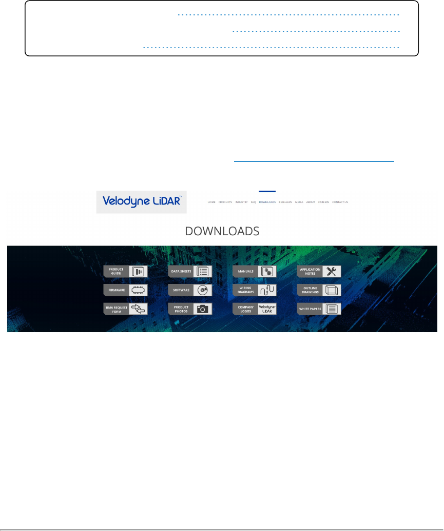
Appendix B • Firmware Update
To update your sensor’s firmware, follow the procedure below. If a problem occurs, follow the steps in
If An Error Occurs
on page 99
.
B.1 Firmware Update Procedure
92
B.1.1 Special Procedure to Update Firmware
98
B.1.2 If An Error Occurs
99
B.1 Firmware Update Procedure
Before starting the procedure, make sure your computer can communicate with the sensor over Ethernet.
The first part of the procedure checks if the sensor needs an update. The second part (beginning with step 6) performs the
update in two stages.
This procedure works best with the Chrome browser.
1. Point your browser to the Velodyne Downloads page at http://velodyneLiDAR.com/downloads.html.
Figure B-1 Velodyne Downloads Page
2. Click the FIRMWARE icon (on the left) to advance to the Firmware section. Note the latest version available.
3. Open the sensor’s Web Interface in your browser and click the Info button.
4. Check the Firmware Application Version on the Info page (red box in the figure below). This is the active firmware
on the sensor.
5. Compare the versions. If they differ, download the newer firmware version to your computer from the Downloads
page, and continue the procedure. If not, stop here.
92 VLP-16 User Manual
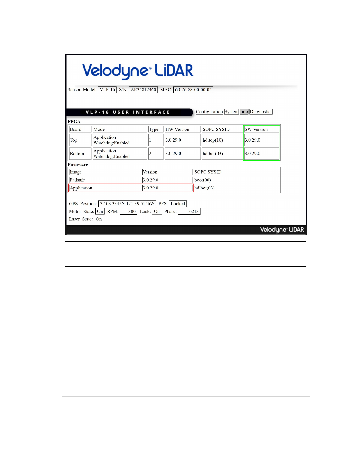
Figure B-2 Compare Firmware Versions
Note: The firmware image labeled “Failsafe” is the original image programmed into the sensor when it was man-
ufactured. It cannot be updated.
6. When updating VLP-16 firmware specifically from 3.0.29.x to 3.0.37.x, or downgrading it from 3.0.37.x to
3.0.29.x, a special procedure must be performed instead. Stop the regular procedure here and proceed to
Spe-
cial Procedure to Update Firmware on page 98
.
7. If your VLP-16's firmware version predates 3.0.24.x, it cannot be updated in the field. Stop the regular procedure
here and, instead, follow the
Return Merchandise Authorization (RMA) on page 90
process to return the unit to
the factory for firmware update.
Appendix B • Firmware Update 93
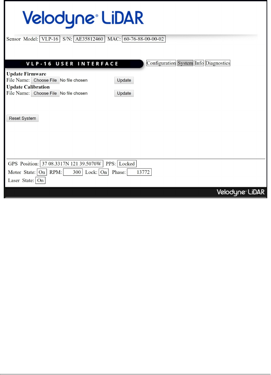
Figure B-3 Select New Firmware Image
8. Click the System button.
9. Click the Choose File button under Update Firmware.
10. Using the dialog, locate the new firmware file on your computer and select it.
11. Verify that the correct file for your sensor model has been selected. It must have the ‘.flash’ file extension.
12. Click Update Firmware's Update button to initiate the update process.
94 VLP-16 User Manual
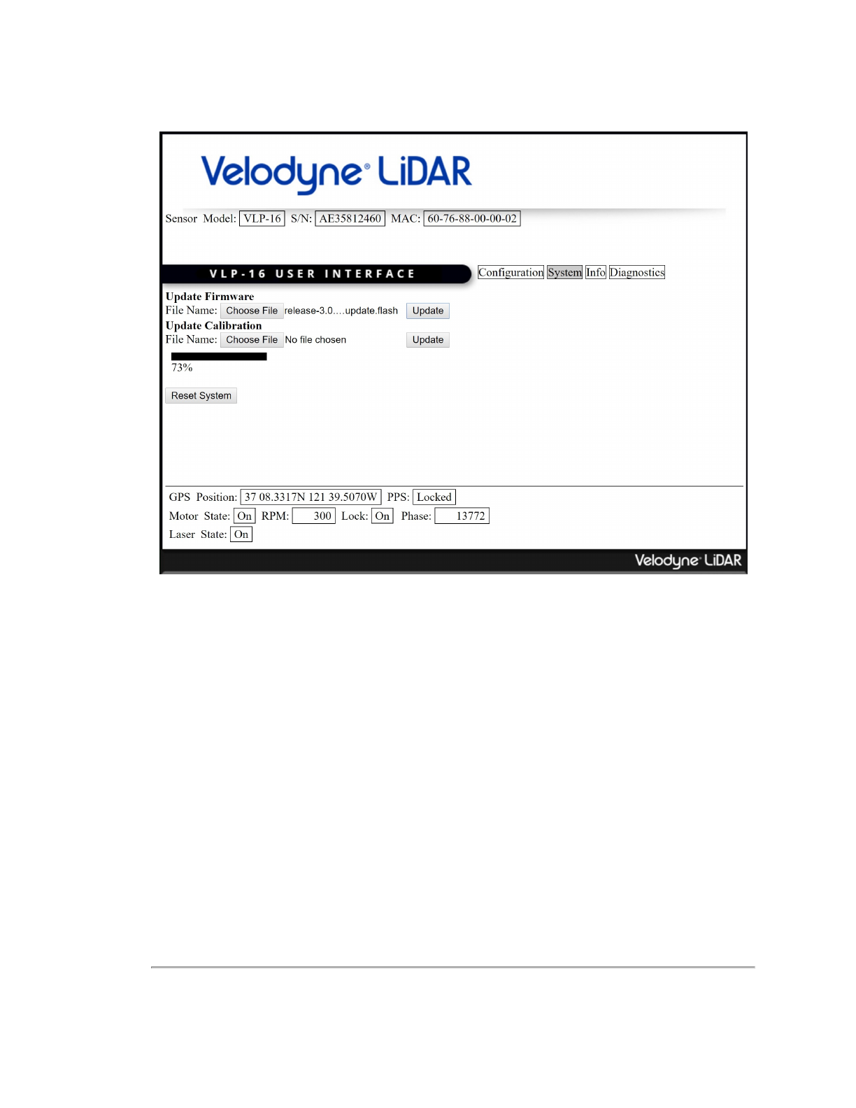
Figure B-4 Upload New Firmware Image
13. As shown in the figure above, a progress bar indicating the percentage of update completion is displayed.
14. When this first stage of the update is complete, the Firmware Update Complete screen (below) is displayed.
But
wait, there's more.
Internally, you've updated the bottom board but not the top, yet.
Appendix B • Firmware Update 95
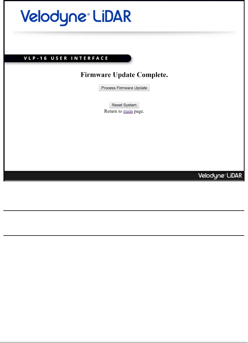
Figure B-5 Firmware Update Complete Page
15. Now click the Process Firmware Update button to initiate the second stage of the procedure. The firmware
image that you just uploaded is being prepared for use by the sensor.
16. A second progress bar is shown.
Note: This step should take approximately 70 seconds. If it completes in less than 10 seconds an error occurred. Instead
of continuing, perform the
If An Error Occurs on page 99
procedure.
96 VLP-16 User Manual
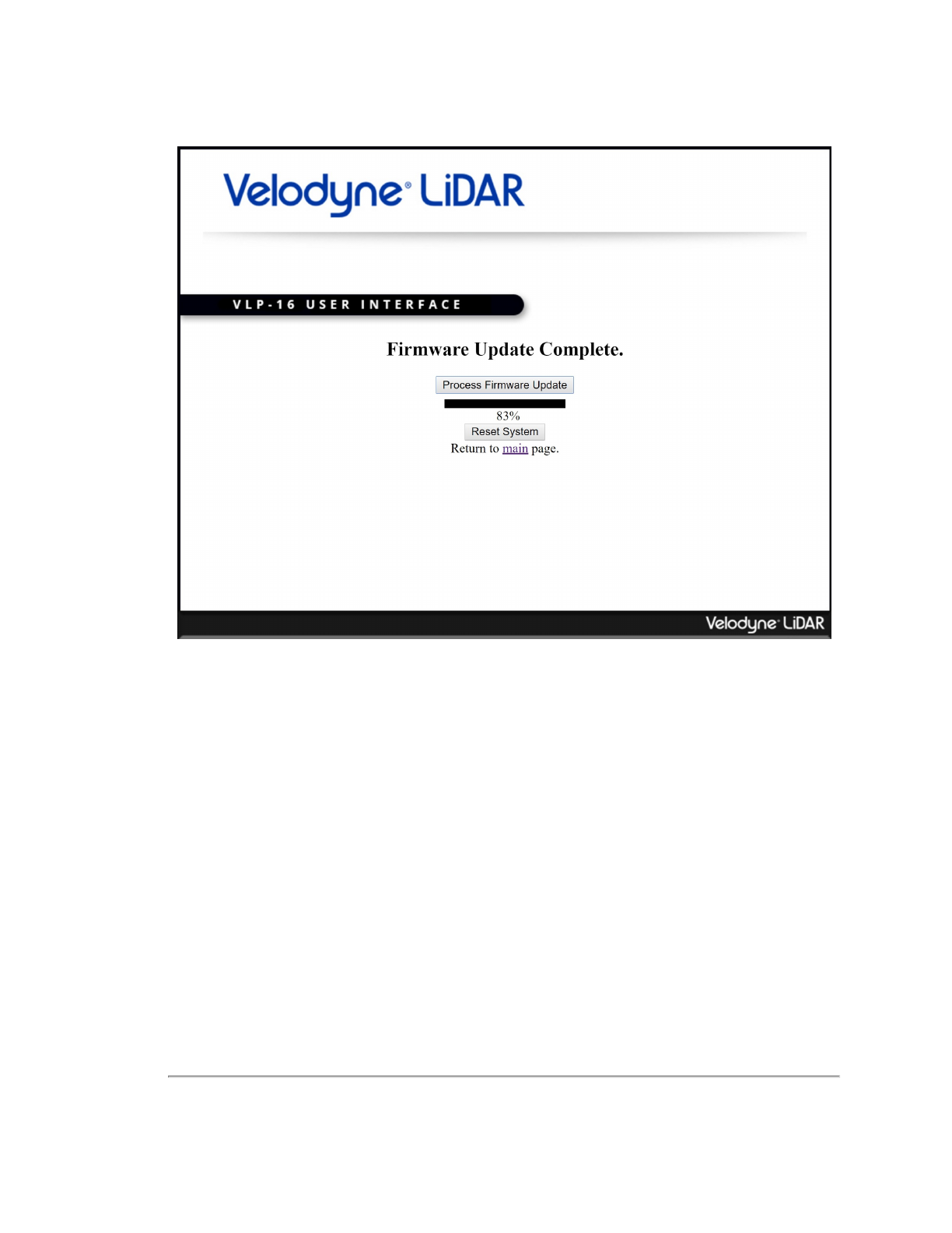
Figure B-6 Finalize Firmware Update
17. When processing completes, press the Reset System button to finalize the update. The sensor will perform a
warm boot.
18. The Configuration screen will be shown when the sensor finishes rebooting.
19. Return to the Info page.
Appendix B • Firmware Update 97
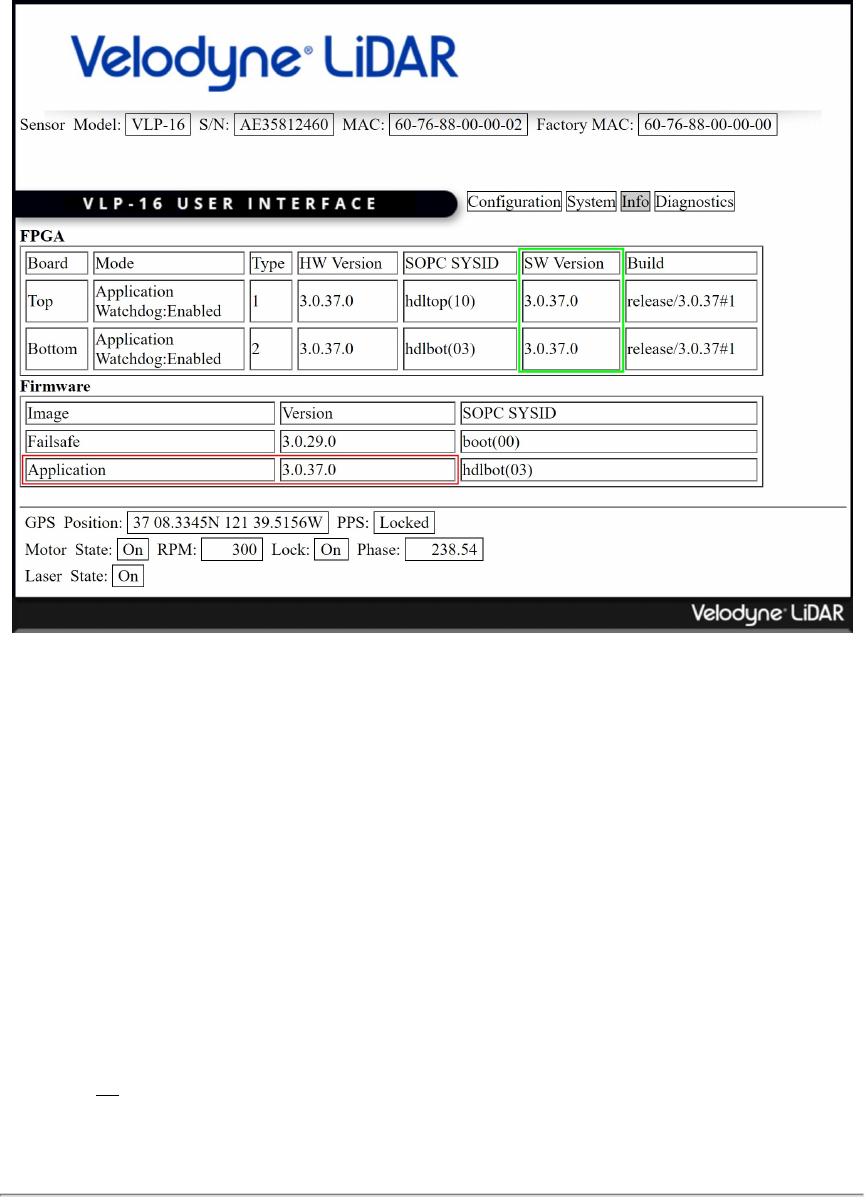
Figure B-7 Verify Firmware Versions
20. Verify that the Firmware Application Version (red box) matches the version of the firmware downloaded and
installed. Also verify that the same version appears in the SW Version column for both the Top and Bottom
boards (green box). If everything matches, the procedure completed successfully.
Any mismatches indicate an error occurred in the last stage of the update. (Occasionally, the screen may indicate
that “Firmware Update Processing is not available in Failsafe mode.” In Failsafe mode, the lasers and motor are dis-
abled.) Perform the If An Error Occurs on the facing page procedure below to resolve the issue.
B.1.1 Special Procedure to Update Firmware
The firmware update process requires both the top and bottom boards be flashed. A minor tweak is made to the steps nor-
mally used to update both boards. When this tweak is made, the normal procedure becomes the “Special Procedure to
Update Firmware.”
1. First, go to the System tab.
2. Click on Choose File and specify the flash file name.
3. Press Update to update the bottom board.
4. Wait a bit.
5. You will eventually see another screen entitled, “Firmware Upload Complete.”
6. Do not press the Process Firmware Update button to flash the top board.
*This is where the process deviates
98 VLP-16 User Manual

from the normal procedure.*
7. Instead, reset the sensor, either by pressing the Reset System button or cycling power to the sensor.
8. The sensor boots up. At this point, you do not have to run the update process for the bottom board again. Go to
the System tab and click on the Update button associated with 'Update Firmware'. Do not specify a flash file
name.
9. After several seconds, a page for updating the top board’s firmware appears.
10. Press the Process Firmware Update button to update the top board’s firmware.
Note: Sometimes the update process for the top board times out and eventually fails. When this happens, reset the
sensor or cycle power to it. You will see explicit instructions to cycle power to the sensor if the case warrants it.
11. Wait a bit.
12. Reset sensor for the new firmware version to take effect.
13. Return to the Info page and verify that the Firmware Application Version and SW Versions are as expected
(
Figure B-7 on the previous page
).
Why the change?
The starting address of the NIOS code was changed in 3.0.34 (VLP-16) and 2.2.23 (HDL-32E). For example, when
3.0.34 is flashed onto the sensor, it is not loaded until the sensor is reset. As a result, the older firmware is grabbing the
NIOS code at the wrong starting address of the new firmware image to push onto the top board.
B.1.2 If An Error Occurs
If an error occurs during the Firmware Update Procedure, it did not finish. Perform the steps below to complete the pro-
cess.
1. Reset the sensor. Either power cycle it (remove power, wait at least 10 seconds, apply power, wait 30 seconds),
or click the Reset System button if you’re on the sensor’s Firmware Update Complete screen or can get to the
sensor’s System page. The Configuration screen will be shown when the sensor finishes rebooting.
2. Go back to the sensor’s System page (
Figure B-3 on page 94
).
3. In the Update Firmware section, just click the Update button (
Figure B-4 on page 95
). A progress bar is briefly dis-
played.
4. When complete, the Firmware Update Complete screen is displayed (
Figure B-5 on page 96
).
5. Click the Process Firmware Update button. A second progress bar is displayed. This step should take approx-
imately 70 seconds (
Figure B-6 on page 97
).
6. When processing completes, press the Reset System button to finalize the update. The sensor will perform a
warm boot. The Configuration screen will be shown when the sensor finishes rebooting.
7. Return to the sensor's Info page.
8. Verify that the Firmware Application Version (red box in
Figure B-2 on page 93
) matches the version of the firm-
ware downloaded and installed. Also verify that the same version appears in the SW Version column for both the
Top and Bottom boards (green box in
Figure B-2 on page 93
). At this point they should all match.
Appendix B • Firmware Update 99

Appendix C • Mechanical Diagrams
This appendix provides technical drawings and diagrams of mechanical assemblies. High resolution versions may be
accessed on the Velodyne LiDAR web site.
C.1 Interface Box Mechanical Drawing
101
C.2 VLP-16 and Puck LITE Mechanical Drawing
102
C.3 VLP-16 and Puck LITE Optical Drawing
103
C.4 VLP-16 and Puck LITE Optical Keep Out Zone
104
C.5 Puck Hi-Res Mechanical Drawing
105
C.6 Puck Hi-Res Optical Drawing
106
C.7 Puck Hi-Res Optical Keep Out Zone
107
100 VLP-16 User Manual
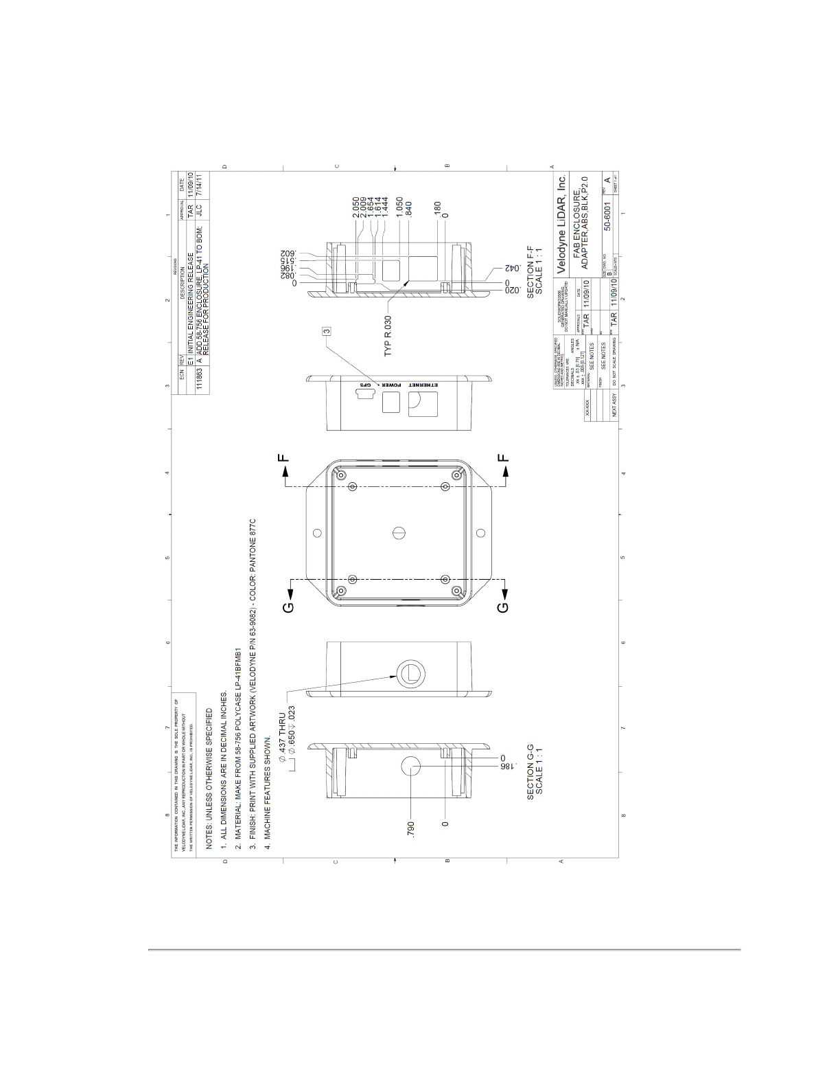
C.1 Interface Box Mechanical Drawing
Figure C-1 Interface Box Mechanical Drawing 50-6001 Rev A
Appendix C • Mechanical Diagrams 101
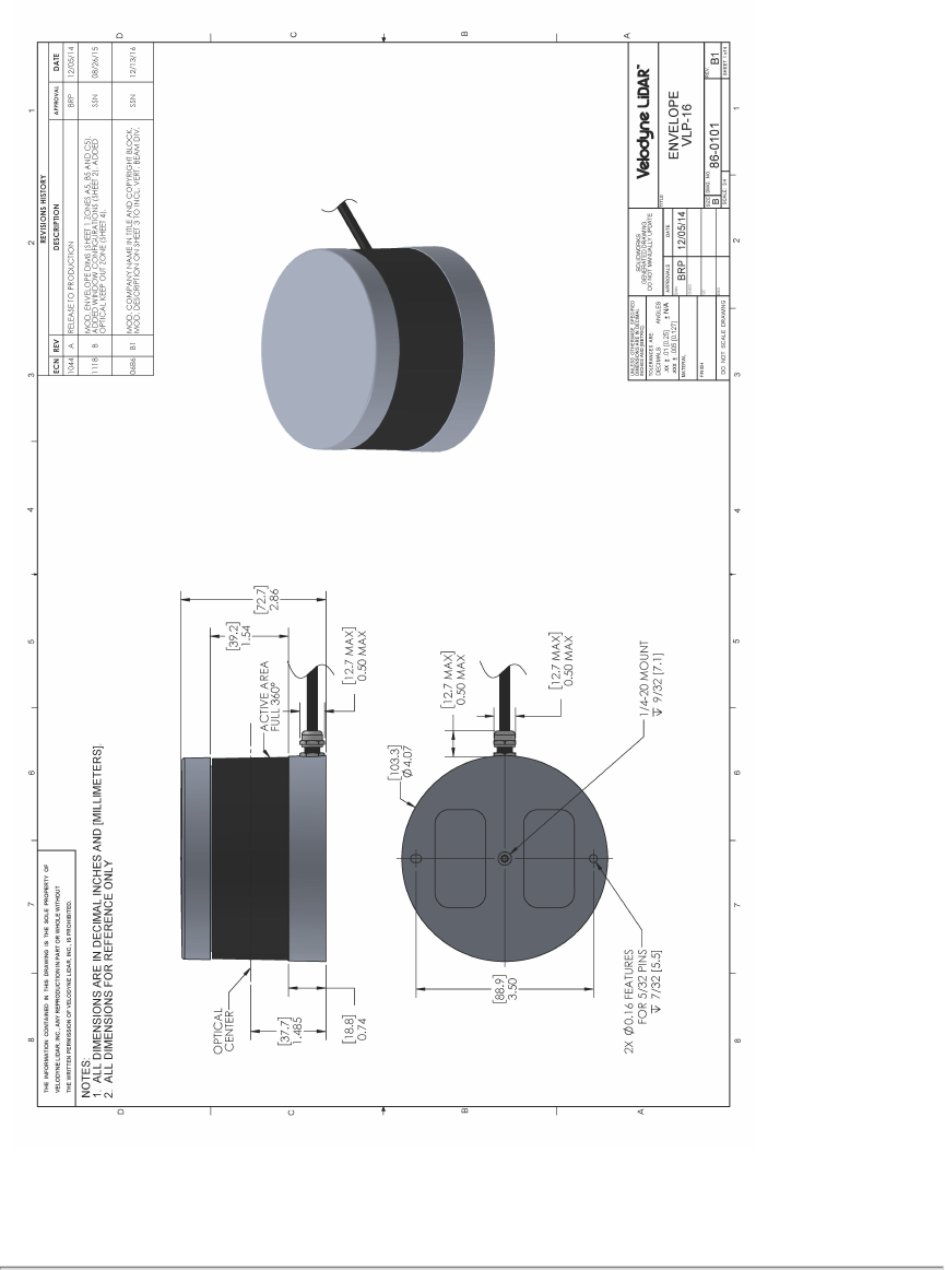
C.2 VLP-16 and Puck LITE Mechanical Drawing
Figure C-2 VLP-16 and Puck LITE Mechanical Drawing 86-0101 Rev B1
102 VLP-16 User Manual
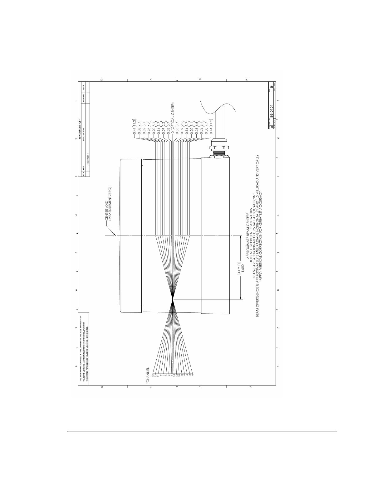
C.3 VLP-16 and Puck LITE Optical Drawing
Figure C-3 VLP-16 and Puck LITE Optical Drawing 86-0101 Rev B1
Appendix C • Mechanical Diagrams 103
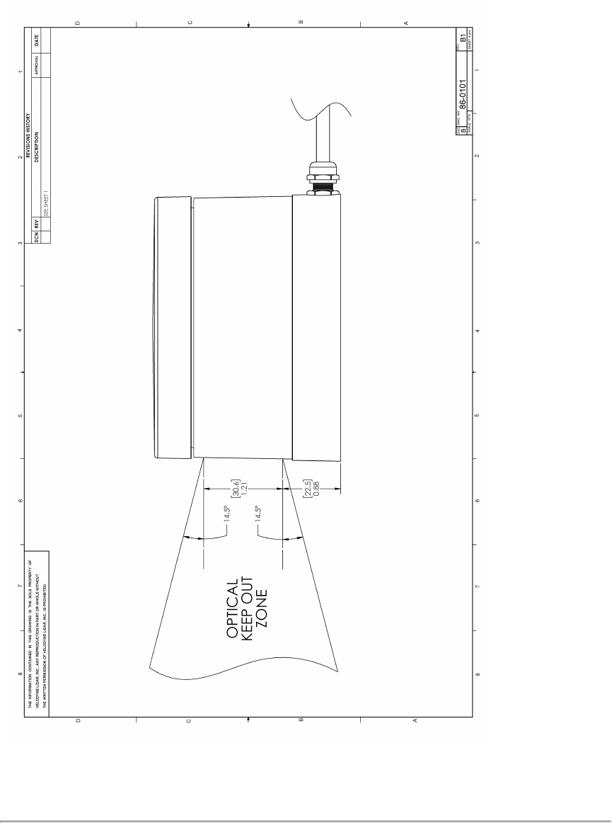
C.4 VLP-16 and Puck LITE Optical Keep Out Zone
Figure C-4 VLP-16 and Puck LITE Optical Keep Out Zone 86-0101 Rev B1
104 VLP-16 User Manual
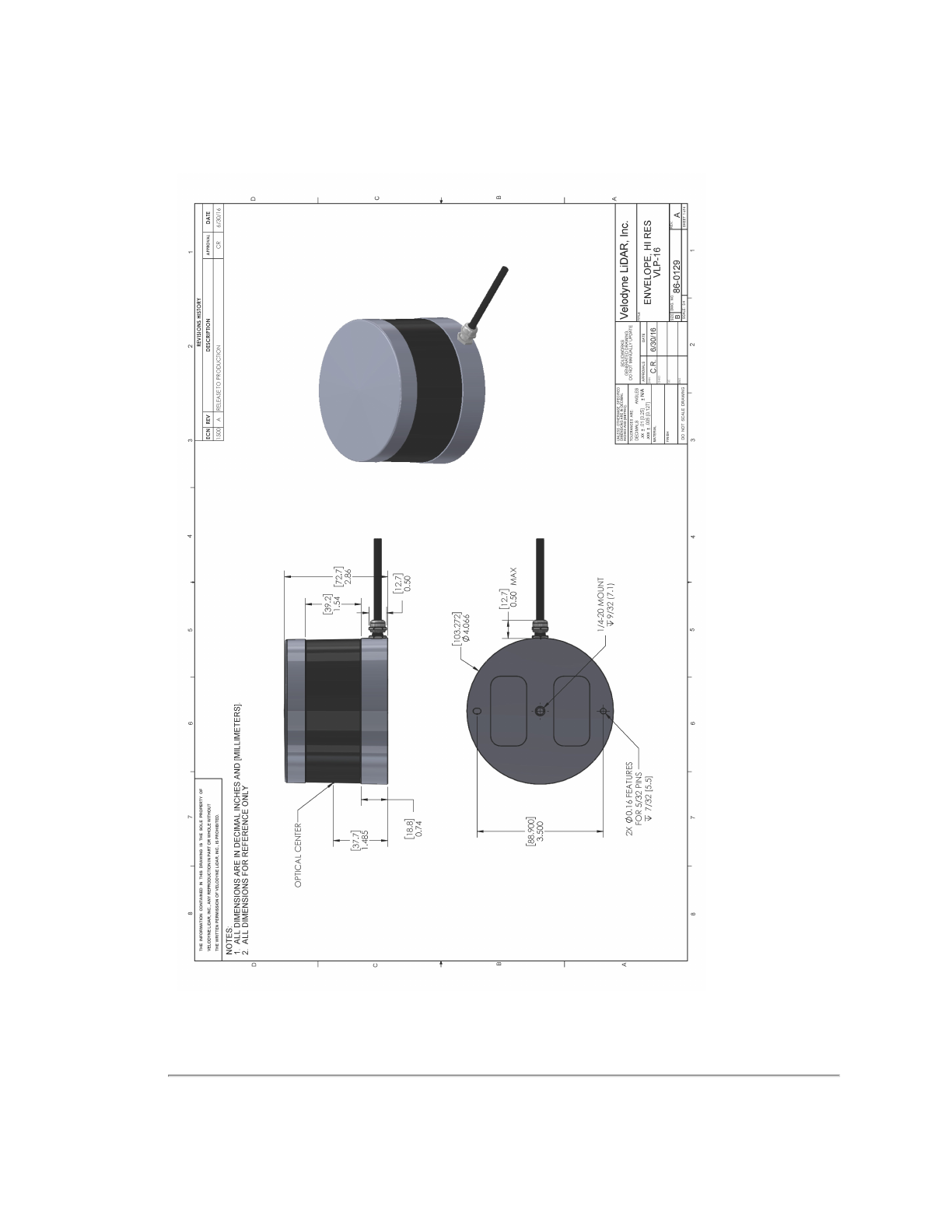
C.5 Puck Hi-Res Mechanical Drawing
Figure C-5 Puck Hi-Res Mechanical Drawing 86-0129 Rev A
Appendix C • Mechanical Diagrams 105
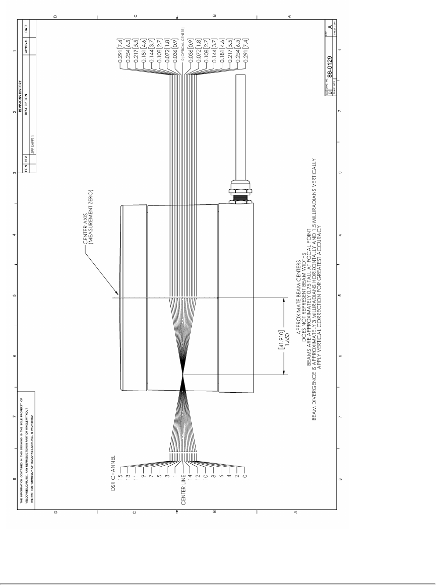
C.6 Puck Hi-Res Optical Drawing
Figure C-6 Puck Hi-Res Optical Drawing 86-0129 Rev A
106 VLP-16 User Manual
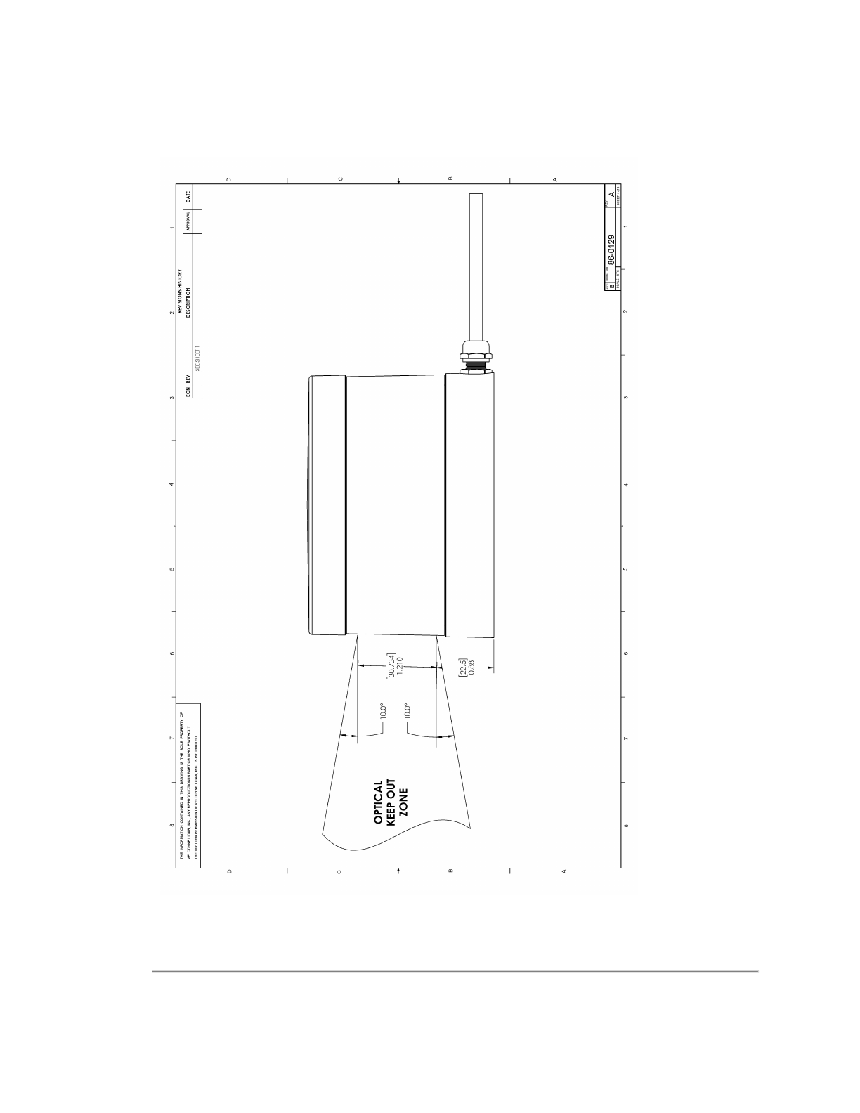
C.7 Puck Hi-Res Optical Keep Out Zone
Figure C-7 Puck Hi-Res Optical Keep Out Zone 86-0129 Rev A
Appendix C • Mechanical Diagrams 107

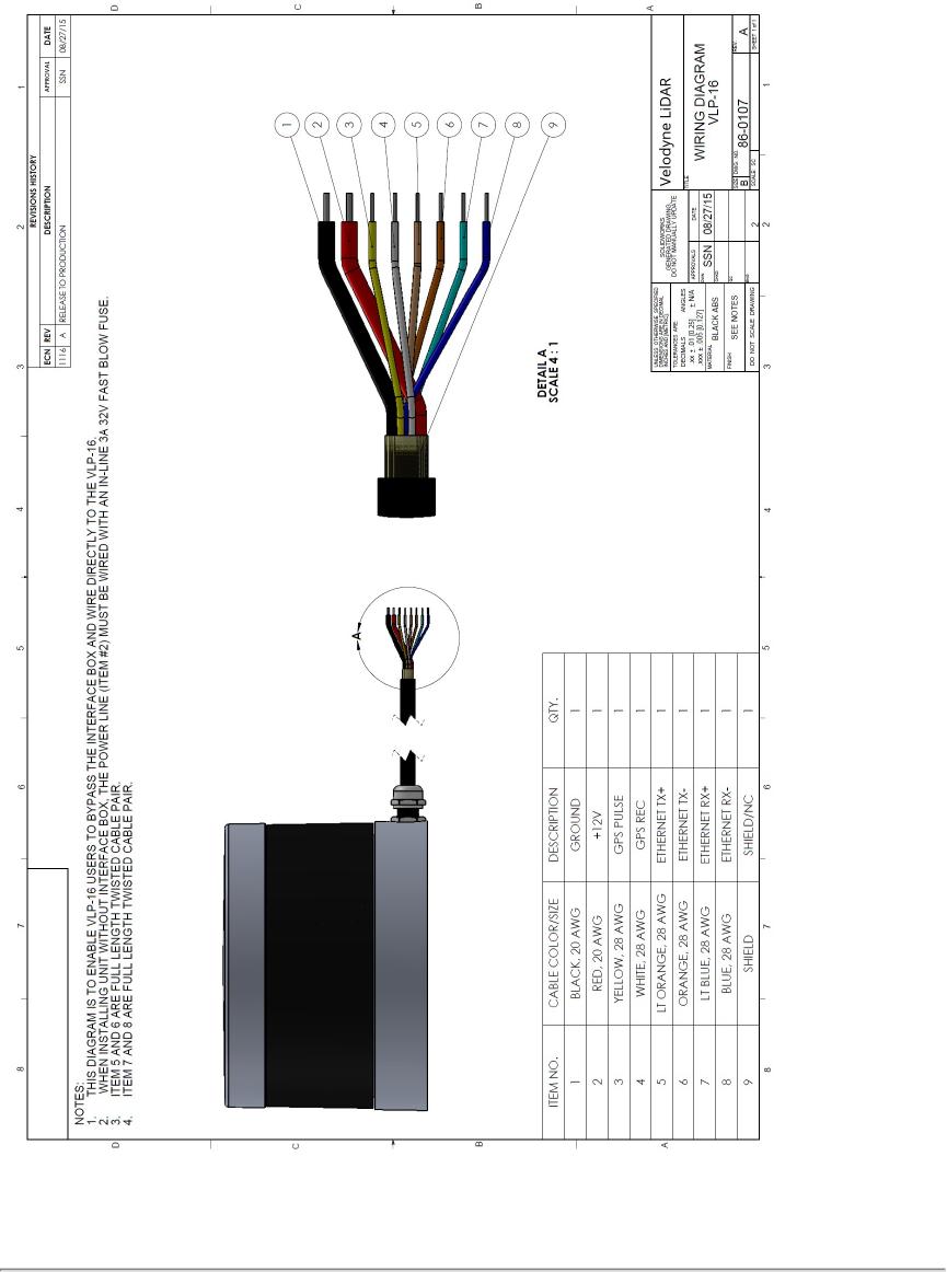
D.1 Interface Box Wiring Diagram
Figure D-1 Interface Box Wiring Diagram 86-0107A
Appendix D • Wiring Diagrams 109
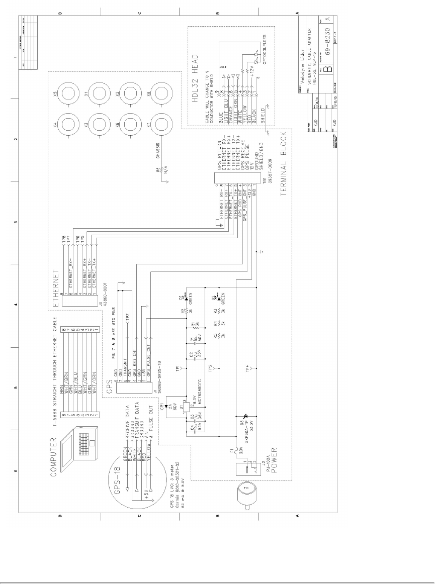
D.2 Interface Box Schematic
Figure D-2 Interface Box Schematic 69-8230A
110 VLP-16 User Manual
Appendix E • VeloView
This appendix gets you started with VeloView. It shows you how to use the application to acquire, visualize, save, and
replay sensor data.
You can examine sensor data with other free tools, such as Wireshark (available from wireshark.org) or tcpdump. But to
visualize the 3D data, use VeloView. It’s free and relatively easy to use.
E.1 Features
111
E.2 Install VeloView
112
E.3 Visualize Streaming Sensor Data
112
E.4 Capture Streaming Sensor Data to PCAP File
114
E.5 Replay Captured Sensor Data from PCAP File
114
E.1 Features
VeloView provides real-time visualization of 3D LiDAR data from Velodyne LiDAR sensors. VeloView can also playback
pre-recorded data stored in “pcap” (Packet Capture) files.
Note: VeloView does not support .pcapng files.
VeloView displays distance measurements from a Velodyne LiDAR sensor as point data. It supports custom-colored dis-
play of variables such as intensity-of-return (i.e. calibrated reflectivity), time, distance, azimuth, and laser ID. The data can
be exported as XYZ data in CSV format.
Functionality and features include:
Visualize live streaming sensor data over Ethernet
Record live sensor data in pcap files
Visualize sensor data from a recording (pcap file)
Interprets point data such as distance timestamp, azimuth, laser ID, etc.
Tabular point data inspector
Export to CSV format
Record and export GPS data
Ruler tool
Display multiple frames of data simultaneously (Trailing Frames)
Display or hide subsets of lasers
Crop views
Appendix E • VeloView 111
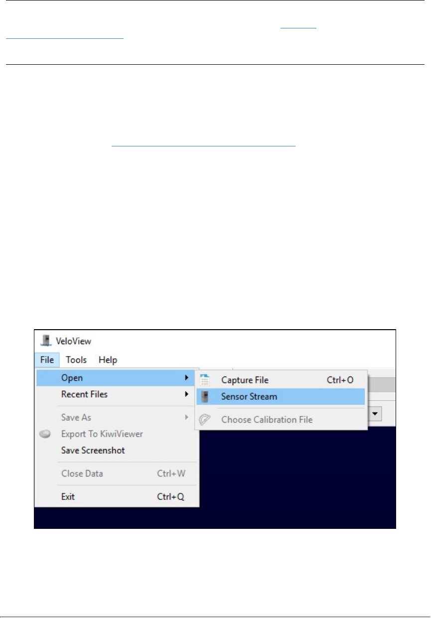
Note: VeloView is not intended to generate point cloud files in LAS, XYZ, or PLY formats (see
Converting PCAP Files to
Point Cloud Formats on page 66
). See the list of Velodyne system integrators at http://velo-
dyneLiDAR.com/integrators.php for vendors who can sell you more advanced imaging software or a complete mapping
system.
E.2 Install VeloView
Installers for VeloView for Windows (32-bit and 64-bit) and Macintosh computers can be found on the USB stick included
with your sensor. Links to the latest installers can be found on the Velodyne web site. You can install VeloView from the
USB stick or follow the steps below to install from the web site.
1. Point your browser to http://velodynelidar.com/downloads.html#software.
2. Click the VeloView Download button to go the official VeloView download page.
3. Scroll down to the How to Obtain section.
4. Choose the correct binary installer for your operating system; click the link.
5. Save the executable installer to disk.
6. Launch the installer and follow the on-screen instructions.
E.3 Visualize Streaming Sensor Data
1. Setup access to your sensor over Ethernet as described in
Unboxing & Verification on page 22
or
Installation &
Integration on page 29
and power it up.
2. Start the VeloView application.
3. Click on File > Open and select Sensor Stream.
Figure E-1 VeloView Open Sensor Stream
4. The Sensor Configuration dialog will appear. Select your sensor type then click OK.
112 VLP-16 User Manual
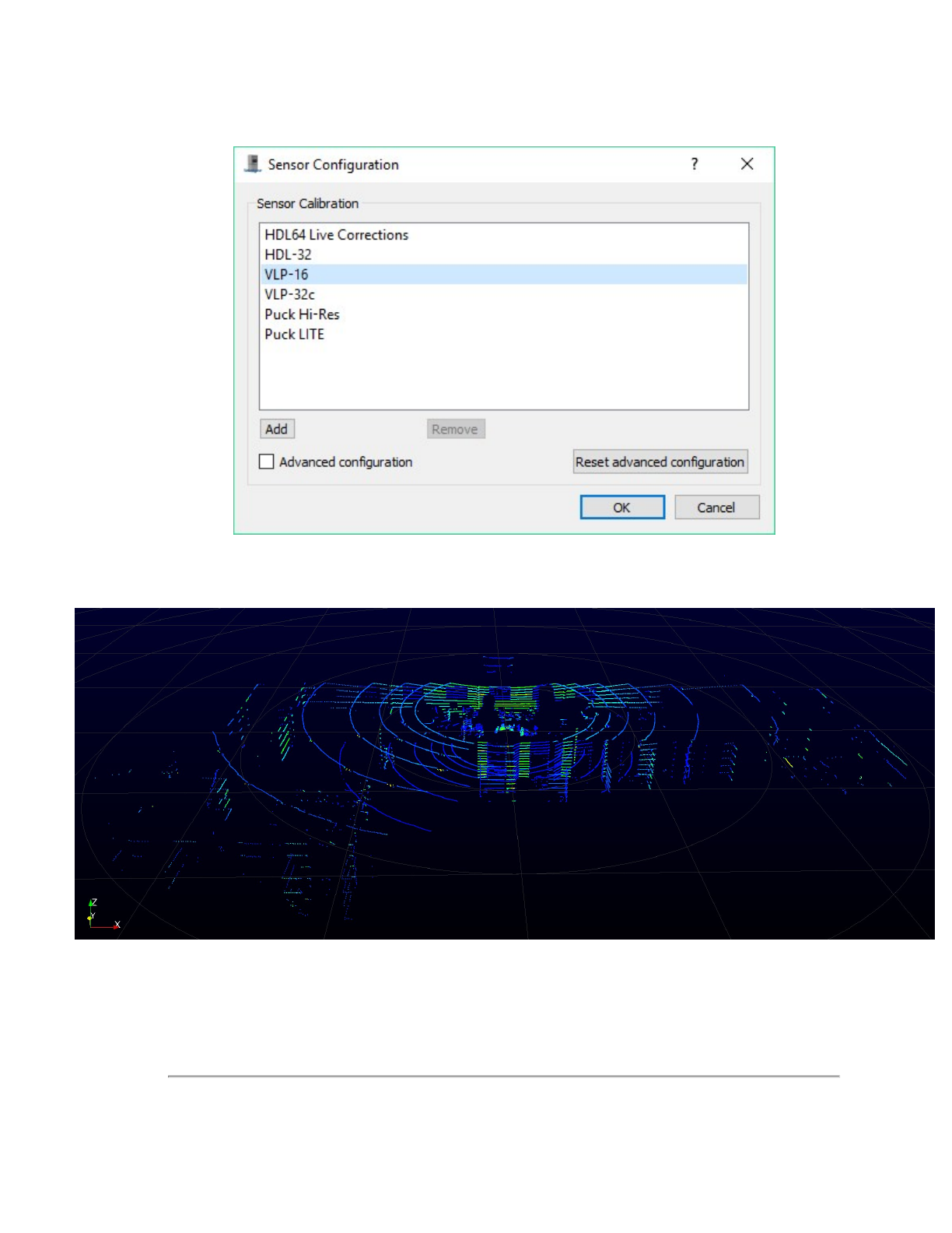
Figure E-2 VeloView Select Sensor Calibration
5. VeloView begins displaying the sensor data stream.
Figure E-3 VeloView Sensor Stream Display
The stream can be paused by pressing the Play button. Press it again to resume streaming.
Appendix E • VeloView 113
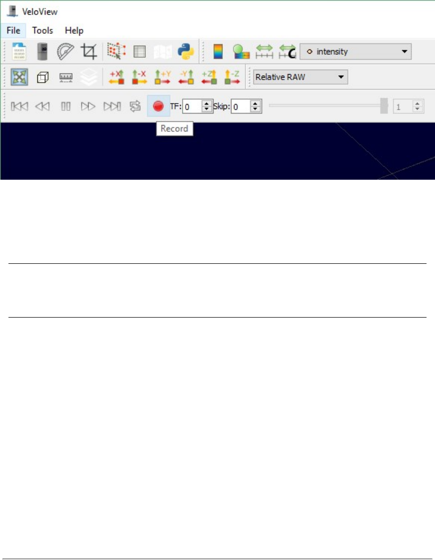
E.4 Capture Streaming Sensor Data to PCAP File
1. Click the Record button.
Figure E-4 VeloView Record Button
A Choose Output File dialog will pop up with the file name field pre-loaded with something like 2016-12-22-16-25-50_
Velodyne-VLP-16-Data.pcap. You may alter it if you like.
2. Navigate to where you want the file to be saved and click the Saved button.
VeloView begins writing packets to your pcap file.
3. Recording will continue until the Record button is clicked again, which stops the recording and closes the pcap file.
Note: Velodyne LiDAR sensors generate a lot of data. (See
Sensor Specifications on page 91
for data rates.) The pcap
file can become quite large if the recording duration is lengthy. Also, it is best to record to a fast, local HDD or SSD, not to a
slow subsystem such as a USB storage device or network drive.
E.5 Replay Captured Sensor Data from PCAP File
To replay (or examine) a pcap file, open it with VeloView. You can press Play to let it run, or scrub through the data frames
with the Scrub slider. Select a set of 3D rendered data points with your mouse and examine the numbers with a Spread-
sheet sidebar.
1. Click on File > Open and select Capture File.
114 VLP-16 User Manual
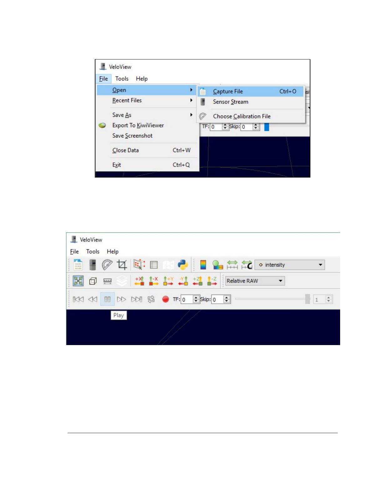
Figure E-5 VeloView Open Capture File
2. An Open File dialog will pop up. Navigate to a pcap file, select it, and click the Open button. The Sensor Con-
figuration dialog will pop-up.
3. Select your sensor type and click OK.
VeloView should display frame 0.
Figure E-6 VeloView Play Button
4. Press Play to replay/pause the data stream. Use the Scrub slider tool (it looks like an old-fashioned volume slider)
to move back and forth through the data frames. Both controls are in the same toolbar as the Record button.
5. To take a closer look at some data, scrub to an interesting frame and click the Spreadsheet button.
Appendix E • VeloView 115
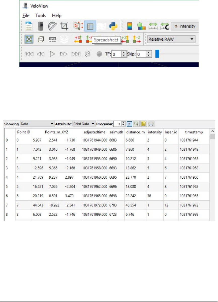
Figure E-7 VeloView Spreadsheet Tool
A sidebar of tabular data is displayed to the right of the rendered frame, containing all data points in the frame.
6. Adjust the columns to get a better view of the numbers. If you’ve adjusted columns in Excel, some of this will be
familiar. You can change column widths by dragging the column header divider left or right, and by double-clicking
them. Drag column headers left or right to reorder them. Sort the table by clicking column headers. And you can
make the table itself wider by dragging the table’s sides left or right. Make Points_m_XYZ wider to expose the
XYZ points themselves.
Figure E-8 VeloView Data Point Table
7. Click Show only selected elements.
116 VLP-16 User Manual
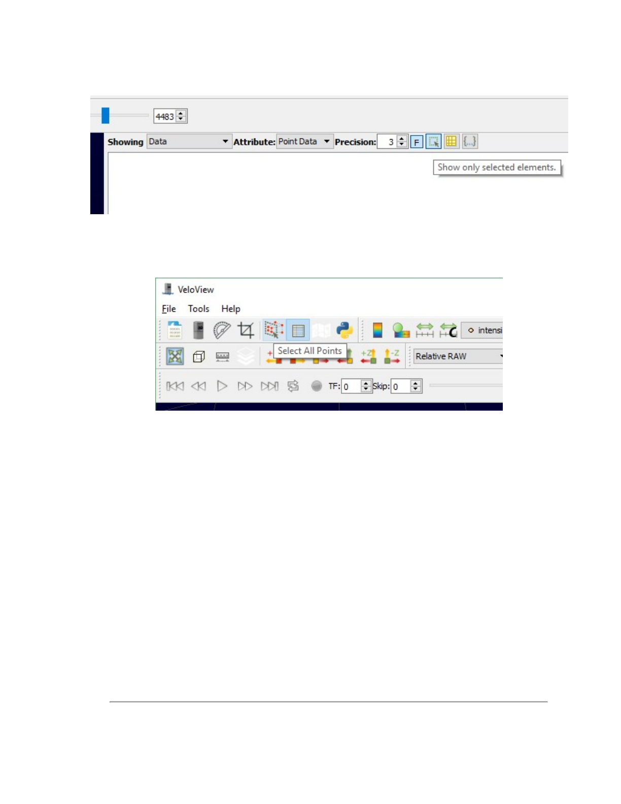
Figure E-9 VeloView Show Only Selected Elements
Since no points are selected yet, the table will be empty.
8. Click the Select All Points tool. This turns your mouse into a point selection tool.
Figure E-10 VeloView Select All Points
9. In the 3D rendered data pane use your mouse to draw a rectangle around a small number of points. They will
immediately populate the data table.
Appendix E • VeloView 117
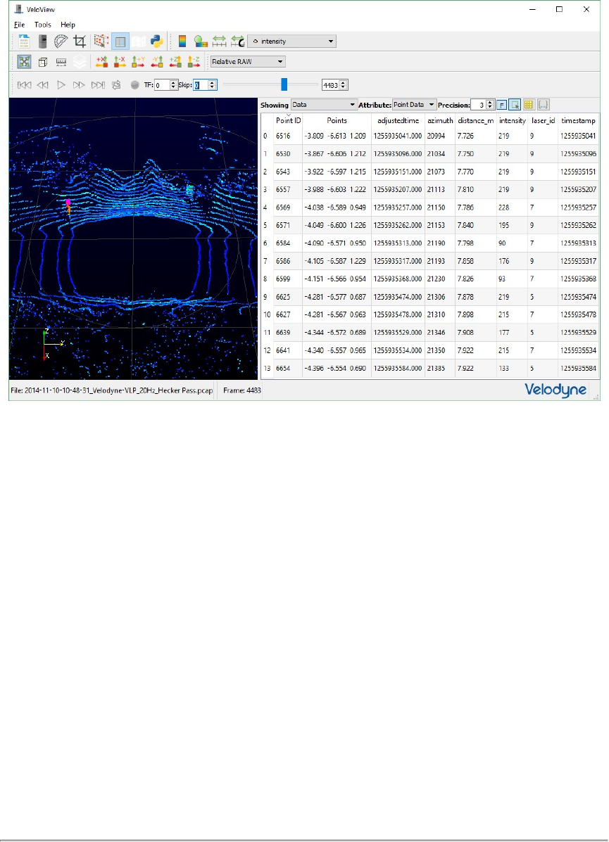
Figure E-11 VeloView List Selected Points
In
Figure E-11 above
, 14 data points were selected with a small selection rectangle. The points appear in pink. Their attrib-
utes are listed on the right. In this example, most of their intensity values exceed 100, indicating something retro-reflective
is there (see
Key Features on page 32
for details). Azimuth is in hundredths of a degree. Distances are with respect to the
sensor’s origin.
At any point you can save a subset of data frames by doing File > Save As > Select Frames.
118 VLP-16 User Manual
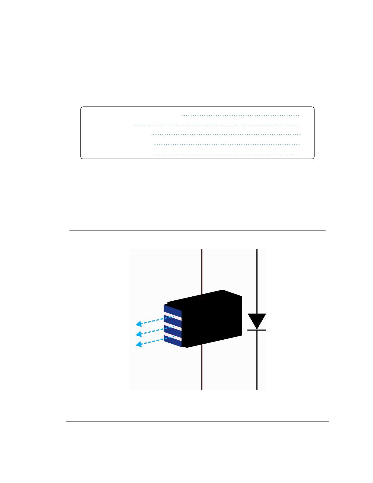
Appendix F • Laser Pulse
This section provides details on your sensor’s laser diodes, the laser pulse and scan patterns, and certain beam char-
acteristics of the laser pulses.
F.1 The Semiconductor Laser Diode
119
F.2 Laser Patterns
120
F.2.1 Laser Spot Pattern
120
F.2.2 Laser Scan Pattern
120
F.2.3 Beam Divergence
121
F.1 The Semiconductor Laser Diode
The source of each laser pulse in the sensor is a semiconductor laser diode. The laser diode is a series of stacked p-n junc-
tions similar, at least in concept, to that shown in
Figure F-1 below
. When a current is applied across the junction, photons
are produced and routed out one end to form a tightly focused laser beam.
Note: The physics of laser diodes can be found elsewhere on the Internet. Start by searching for
p-n junction
,
laser
diode
, and
principles of semiconductor laser diodes
.
Figure F-1 Laser Diode Concept
Appendix F • Laser Pulse 119

F.2 Laser Patterns
Laser firings produced by the sensor can be viewed with an infrared viewer or camera. Photos in this section were taken
with an infrared camera.
F.2.1 Laser Spot Pattern
While the terms laser “spot” and “dot” are often used when describing a laser pulse hitting a target, in reality the sensor’s
laser “spot” is a small rectangular area comprised of three smaller bars or bands of light as shown in
Figure F-2 below
.
The long axis of the rectangle coincides with the direction of the laser scan.
The dimensions of this laser spot at the sensor’s ring lens is 9.5 mm tall by 12.7 mm wide - but it doesn’t remain that size as
it speeds away. Read more about that in
Beam Divergence on the facing page
.
Figure F-2 Laser Spot Shape
F.2.2 Laser Scan Pattern
Inside each VLP-16 sensor is a vertical array of lasers.
Figure F-3 on the facing page
shows three adjacent, concurrent,
laser scans on the corner of a wall about 3 meters from the sensor. Each laser scan is composed of multiple laser spots or
pulses. Each spot is composed of three short closely-spaced horizontal bars or bands of light.
The gap between scan lines can be calculated with the following equation:
120 VLP-16 User Manual
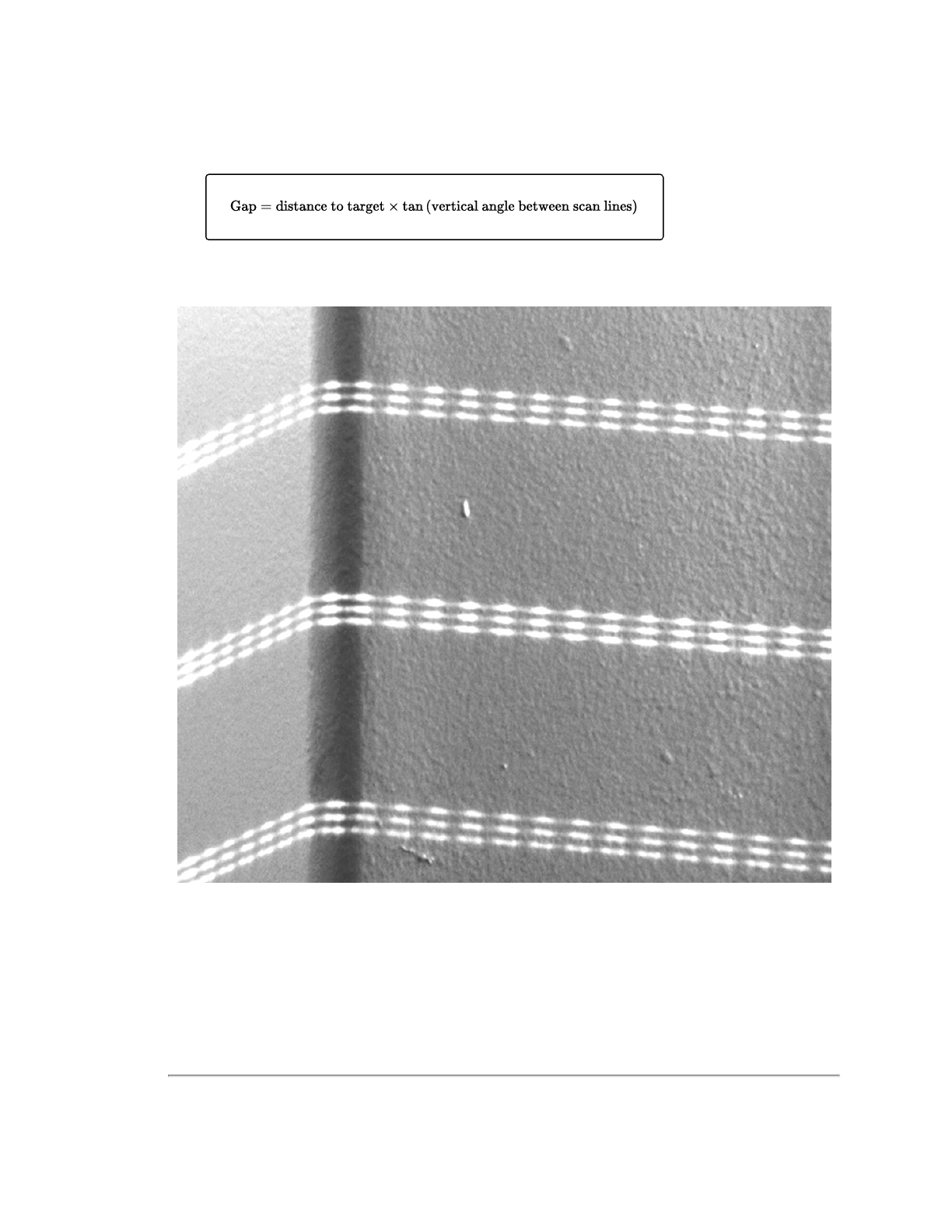
Equation F-1 Gap Between Scan Lines
Figure F-3 Laser Spots on a Wall
Photo of sensor laser pattern reflecting off of a flat target a short distance away.
F.2.3 Beam Divergence
As a laser pulse propagates outward from the sensor the cross-section of the laser beam describing the path of the pulse
gradually, steadily grows larger. The angular measure of this increase in beam path diameter is called Beam Divergence.
Appendix F • Laser Pulse 121

VLP-16 beam divergence on the horizontal axis (i.e. along the direction of the laser scan) differs from beam divergence on
the vertical axis (transverse to the scan) by roughly a factor of two.
Horizontal Beam Divergence Vertical Beam Divergence
3.0 mrad (0.18 deg) 1.5 mrad (0.09 deg)
Table F-1 VLP-16 Beam Divergence
Table F-2 below
lists laser spot horizontal and vertical dimensions at various distances from the sensor.
Distance (mm) Horizontal (mm)
(Scan Direction) Vertical (mm)
1000 15.4 11.0
2000 18.2 12.5
5000 26.4 17.0
10000 40.1 24.5
15000 53.8 32.0
25000 81.2 47.0
50000 149.7 84.6
100000 286.8 159.6
Table F-2 Dimensions of VLP-16 Laser Spots at Distance
122 VLP-16 User Manual
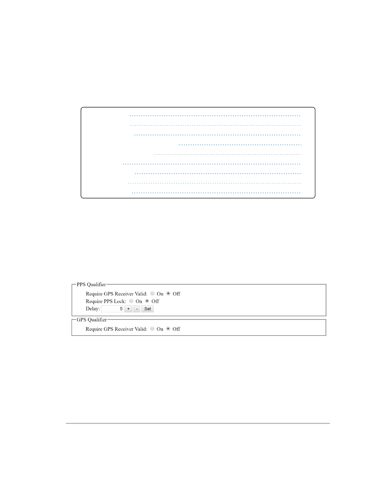
Appendix G • Time Synchronization
This section provides a detailed discussion of the GPS Qualifier and PPS Qualifier functions. These features were intro-
duced with firmware release 3.0.34.0 (VLP-16).
G.1 Introduction
123
G.2 Background
123
G.3 PPS Qualifier
124
G.3.1 Require GPS Receiver Valid
124
G.3.2 Require PPS Lock
124
G.3.3 Delay
125
G.4 GPS Qualifier
125
G.5 Application
125
G.6 Logic Tables
125
G.1 Introduction
The following describes the new interface options found in sensor firmware version 3.0.34.0 (VLP-16).
These two new options control how the sensor utilizes the GPS information supplied to the sensor. The first control option
determines how the sensor utilizes the PPS signal (PPS Qualifier). The second control option determines how the sensor
utilizes the timestamp provided in a National Marine Electronics Association (NMEA) sentence (GPS Qualifier).
The new options, shown below in their default positions, can be found on the Configuration tab in the sensor’s Web Inter-
face.
Figure G-1 Web Interface PPS and GPS Qualifier Option Selections
G.2 Background
Your sensor maintains a counter representing the number of microseconds since the Top Of Hour (TOH). The TOH count
is incremented based on an internal oscillator. When the sensor is presented with a valid PPS signal the TOH count is adjus-
ted on the rising edge of each PPS to align the TOH with UTC Time. The TOH is sent as a four-byte time stamp in both the
data and position/telemetry packets.
The TOH is comprised of two separate counters. One counter maintains the number of minutes and seconds since the top
of the hour, and the other counter maintains the sub-second count (
Figure G-2 on the next page
).
Appendix G • Time Synchronization 123
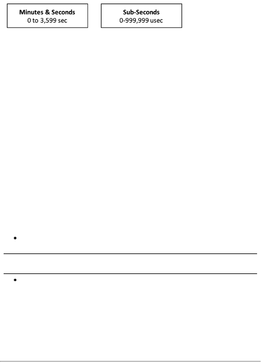
Figure G-2 Top of Hour Counters
The combined value represents the number of microseconds since the top of the hour. It ranges from 0 to 3,599,999,999
μs -- there are 3.6 × 10⁹ μs in one hour. The sub-second counter range alone spans 0 to 999,999 μs.
The sensor continuously monitors the PPS input assessing the timing characteristics of any pulses presented. This pro-
cess is indicated both on the Web Interface (see
Configuration Screen on page 69
) and in the position packet. When the
sensor detects a valid, stable PPS signal, the Web Interface indicates “PPS: Locked” and the PPS status field in the pos-
ition packet at offset 0xF4 is set to 0x02.
As noted, the sensor counts microseconds using an internal oscillator. This internal oscillator always drives the sub-second
counter; however, the sensor may be configured to use a valid PPS signal to adjust the value of the sub-second counter
every second, thereby reflecting the "top of second" moment indicated by the rising edge of the PPS.
The minutes and seconds counter may be adjusted to the time values provided in the NMEA sentence. If no NMEA sen-
tence is provided, the minutes and seconds counter is incremented every second.
Using the PPS signal to adjust the sub-second counter allows the sensor to remain synchronized to a PPS source even if
that source is drifting slightly. This might occur when a GPS receiver indicates an invalid fix and begins using its own internal
time to drive the PPS reference.
New control options (PPS Qualifier and GPS Qualifier, described below) have been added to allow the user to finely adjust
the manner in which the sensor reacts when a valid PPS is confirmed and locked onto.
G.3 PPS Qualifier
The three settings described below (and in
Logic Tables on the facing page
) control how the sensor adjusts the TOH
counter based on GPS and PPS signal status.
Depending on the GPS receiver's valid/invalid status, the three settings determine if the sensor's Top-Of-The-Hour (TOH)
counter should enter free-running mode or synchronize the sub-second counter with the rising edge of the PPS signal.
G.3.1 Require GPS Receiver Valid
This setting determines the manner in which the sensor utilizes the current status of the GPS receiver provided in the
NMEA sentence.
If the Require GPS Receiver Valid is set to On, the sensor requires the GPS receiver to indicate a valid satellite
condition before using the rising edge of a PPS signal to adjust the internal sub-second counter.
Note: The sensor must also receive a valid NMEA message indicating the GPS receiver is providing a valid time stamp.
If Require GPS Receiver Valid is set to Off, the sensor synchronizes its sub-second counter to the rising edge of
the PPS signal regardless of GPS receiver satellite status.
G.3.2 Require PPS Lock
This setting determines the manner in which the sensor validates the PPS signal prior to adjusting the internal sub-second
counter to the rising edge of that PPS signal.
124 VLP-16 User Manual

If Require PPS Lock is set to On the sensor utilizes the value in the Delay field to determine the validity of a PPS
signal prior to synchronizing its internal sub-second counter to the rising edge of a PPS signal.
If Require PPS Lock is set to Off the sensor ignores the value in the Delay field and the sensor uses a rolling win-
dow of 2 cycles before the PPS signal may be considered valid and then used as a time reference by the sensor.
Turning this option off effectively sets the Delay value to 2.
G.3.3 Delay
This parameter allows the user to extend the time the sensor requires to validate the PPS. The units are in integer
seconds. Acceptable values range from 0 to 65535. The default is 5 seconds.
The sensor constantly qualifies the PPS signal over a rolling N-second window defined by the Delay parameter. At the first
instance the PPS signal is deemed unstable, the sensor enters free-running mode where the sub-second counter is driven
by the internal oscillator. In free-running mode the sub-second counter is no longer adjusted with the rising edge of the
PPS signal. Additionally, the minutes and seconds component of the TOH begins incrementing based on the rollover of the
free-running sub-second counter.
G.4 GPS Qualifier
This setting determines if the minutes and seconds component of the TOH counter are adjusted to the timestamp provided
by the GPS receiver or driven by the rollover of the sub-second counter.
If the Require GPS Receiver Valid is On, the minutes and seconds field in the NMEA sentence timestamp is used to
adjust the minutes and seconds component of the TOH counter only when GPS receiver indicates a valid status.
If the Require GPS Receiver Valid is Off, then the sensor ignores the GPS receiver status and always adjusts the
minutes and seconds component of the TOH counter with the timestamp provided in the NMEA message.
G.5 Application
Most GPS receivers have low-drift internal clocks and may be configured to use this clock to maintain the PPS signal in the
event the GPS fix becomes invalid. Alternatively, the GPS might be configured to discontinue the PPS in the event the fix
becomes invalid.
In the default settings (and previous versions of firmware), the sensor uses PPS to synchronize to the time contained in the
GPRMC message regardless of the state of valid flag in the GPRMC message. In this configuration, all the elements in a
larger system (LiDAR, IMU, RGB cameras, etc.) will be clocked off the same time source (the internal clock in the GPS
receiver) in the event the GPS fix becomes invalid. This allows for proper reconciliation of the data during post- or real-time
processing.
G.6 Logic Tables
Figure G-3 Sub-Second Counter Behavior
Appendix G • Time Synchronization 125
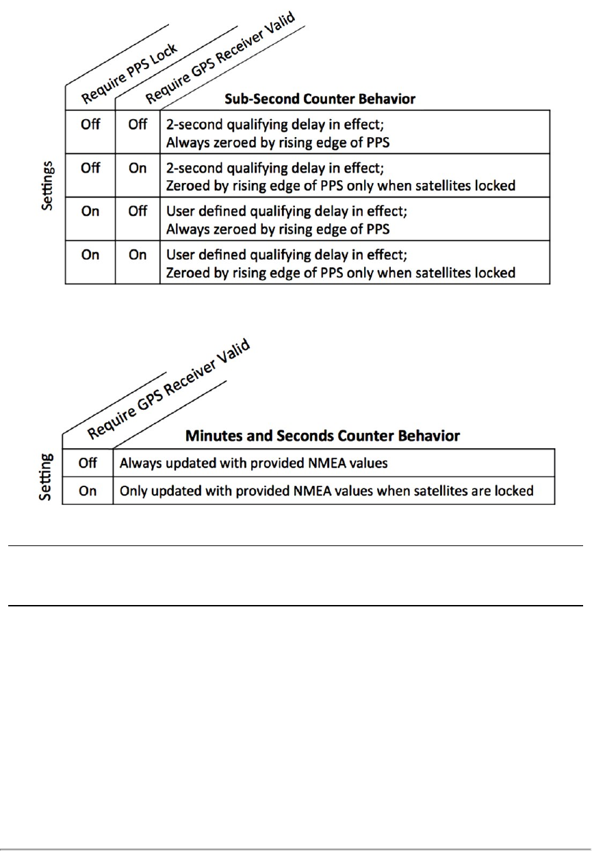
Figure G-4 Minutes and Seconds Counter Behavior
Note: If no NMEA sentence is provided, the Minutes and Seconds counter is driven by the rollover of the sub-seconds
counter.
126 VLP-16 User Manual
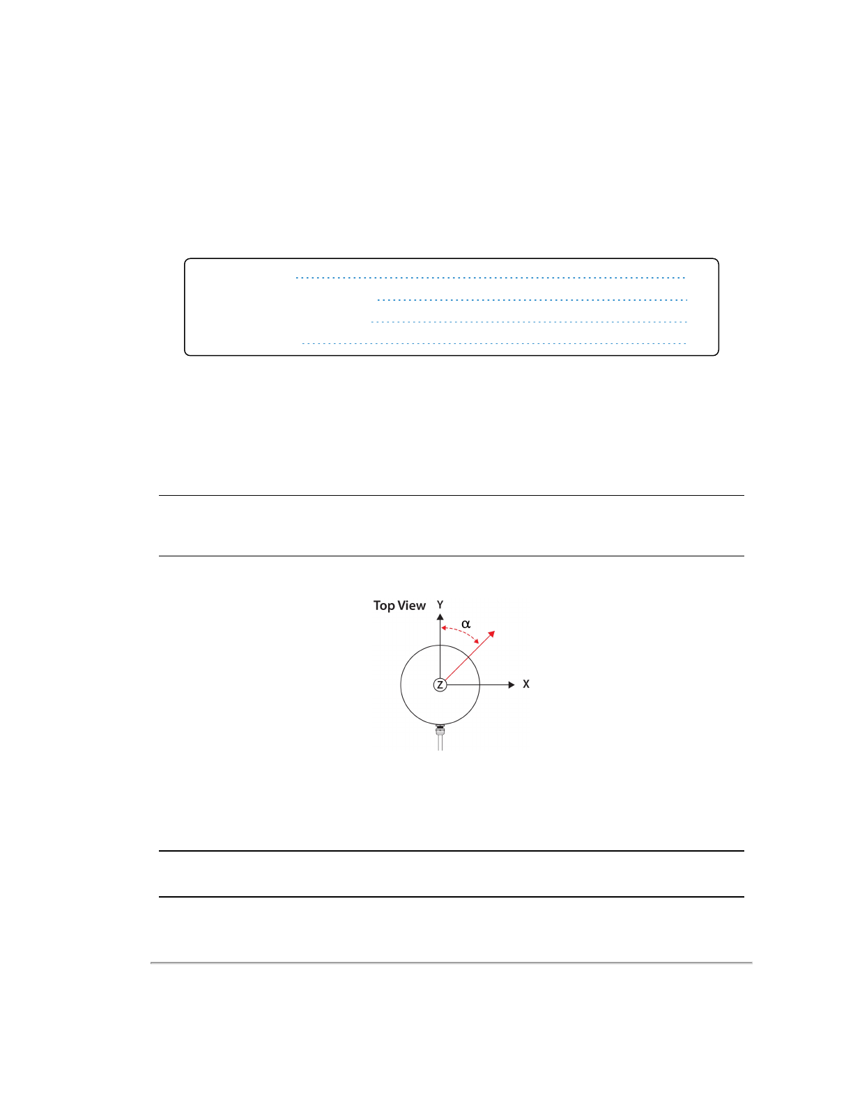
Appendix H • Phase Lock
When using multiple sensors close to one another (e.g. mounted on top of a vehicle), occasional interference patterns may
appear in the sensor data. Velodyne provides firing controls to minimize this interference by controlling where data is
gathered. The sensors can then be configured to ignore the data containing the interference.
H.1 Phase Lock
127
H.1.1 Setting the Phase Lock
127
H.1.2 Application Scenarios
128
H.2 Field of View
130
H.1 Phase Lock
The Phase Lock feature requires that a PPS signal be present and locked. The sensor uses the rising edge of the PPS as
the zero-degree reference moment for all its firing references. The sensor then adjusts its timing such that it initiates a fir-
ing sequence at the phase lock offset specified by the user.
For example, assume the user enters an angle of 35° (α) as the phase offset. The red arrow in
Figure H-1 below
indicates
the laser firing direction precisely as the sensor receives the rising edge of the PPS signal.
Note: For Phase Lock to work correctly, the sensor’s RPM must be set to a multiple of 60 RPM between 300 RPM and
1200 RPM (inclusive).
Figure H-1 Direction of Laser Firing
H.1.1 Setting the Phase Lock
To enable Phase Lock, enter the desired phase offset in the Phase Lock Offset field shown in
Figure H-2 on the next page
.
Enter the offset in degrees. For example, if the desired offset is 270°, enter 270 in the Offset field. Click the Phase Lock On
radio button (as needed) and then the Set button to the right.
Note: To retain these settings over the next power cycle or reset, click the Save Configuration button.
Appendix H • Phase Lock 127
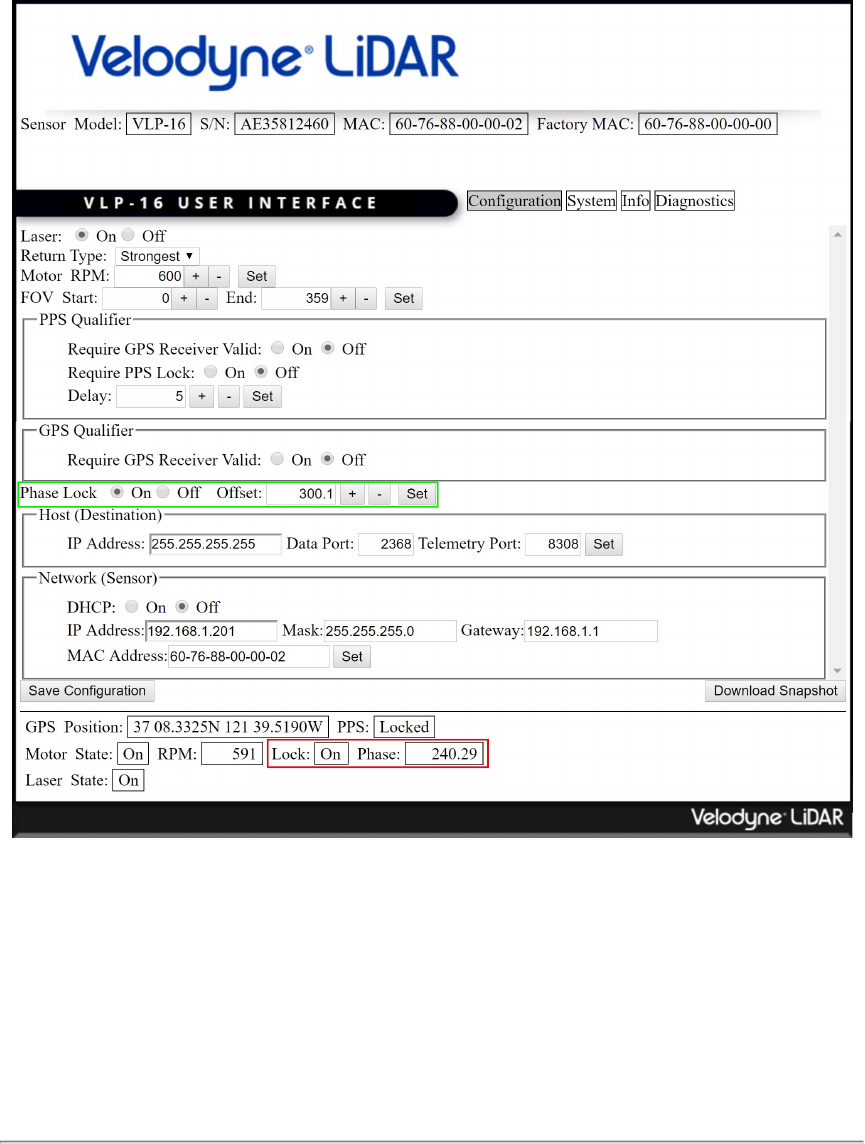
The current phase lock status (On/Off) and phase lock offset can be viewed on the Web Interface (red box). The current
phase lock offset is presented in degrees. The accuracy of the offset is ±5° (subject to change).
Figure H-2 Configuration Screen - Phase Lock
H.1.2 Application Scenarios
When setting the phase lock offset for two or more sensors, Velodyne recommends the sensors be configured to fire at
each other. This is the optimal configuration for minimizing interference because the location of the interference is under
user control.
Figure H-3 on the facing page
shows two sensors mounted on a vehicle. The sensor mounted on the car’s left side has its
phase lock offset set to 90°, and the phase lock offset of the sensor mounted on the right side of the vehicle is set to 270°, as
shown by the red arrows.
128 VLP-16 User Manual
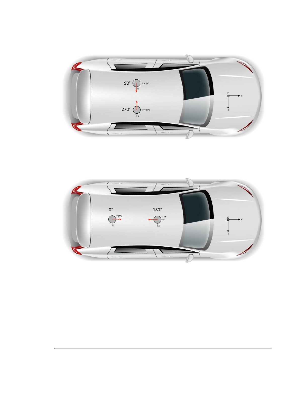
Figure H-3 Right and Left Sensor Phase Offset
When sensors are placed on the roof in the fore and aft positions, the phase offsets are set to 180° and 0° as shown in
Fig-
ure H-4 below
.
Figure H-4 Fore and Aft Sensor Phase Offset
In both scenarios the two sensors create data shadows behind each other.
To avoid any spurious data due to blockage or reflections from the opposing sensor, the user should ignore any data in the
shadowed azimuth ranges as shown in
Figure H-5 on the next page
. To do that, you need to know the diameter of the
sensors (see
Sensor Specifications on page 91
) and distance between the sensor centers.
Appendix H • Phase Lock 129
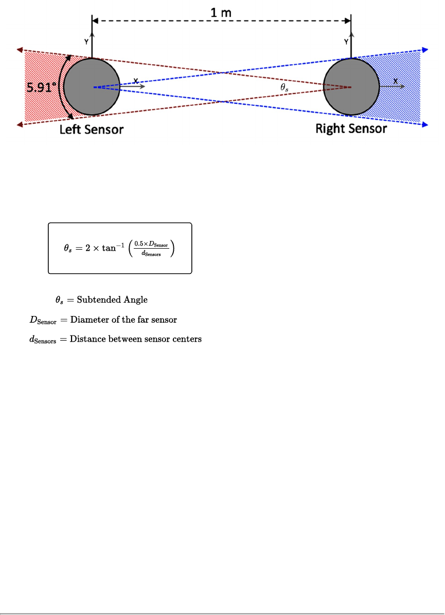
Figure H-5 Sensor Data Shadows
The angle subtended by the shadow of a sensor in range but at some distance from another sensor is given by the fol-
lowing formula:
Equation H-1 Arc of Shadow
Data reported at the azimuths included within the subtended angle should be ignored.
H.2 Field of View
Alternatively, each sensor's Field of View control may be used to remove the subtended azimuths from the data stream.
Use
Figure H-5 above
and
Equation H-1 above
to determine for each sensor the azimuthal angles at which the shadows
begin and end.
Then, using each sensor's Web Interface or curl commands (or equivalent programmatic commands), configure the
sensor's horizontal FOV start and end angles. See
Configuration Screen on page 69
and
Set Field of View on page 83
for
more.
130 VLP-16 User Manual
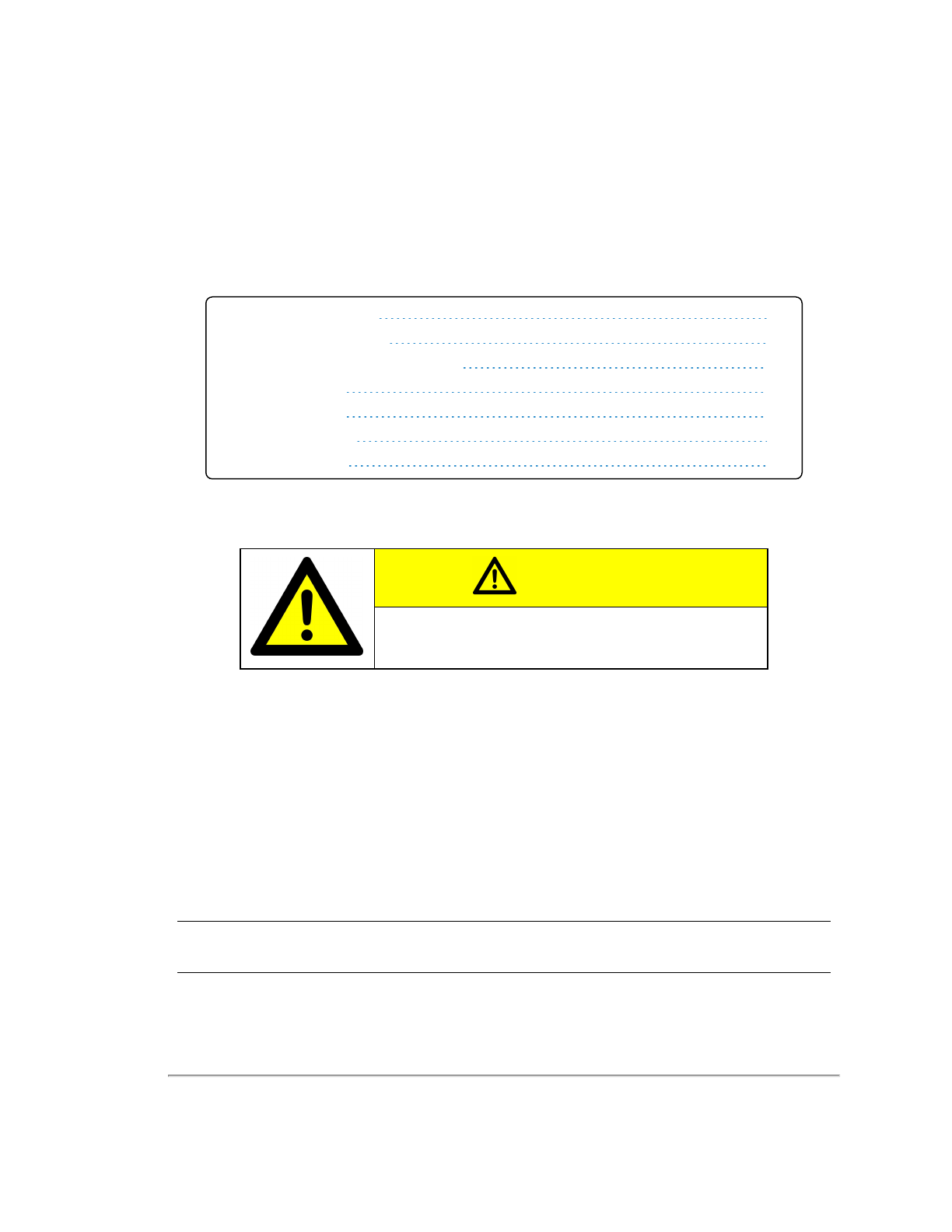
Appendix I • Sensor Care
To accurately sense its environment, the VLP-16 sensor should be kept clean, especially its ring lens.
This section lists various approved cleaning methods, but it is important to use the correct method. Start with
Determine
Method of Cleaning on the next page
.
I.1 Cleaning the Sensor
131
I.1.1 Required Materials
131
I.1.2 Determine Method of Cleaning
132
I.1.3 Method One
132
I.1.4 Method Two
132
I.1.5 Method Three
132
I.1.6 Method Four
133
I.1 Cleaning the Sensor
CAUTION
READ THROUGH THIS ENTIRE SECTION BEFORE CLEANING
YOUR VLP-16 SENSOR
Improper handling can permanently damage it.
I.1.1 Required Materials
1. Clean microfiber cloths
2. Mild, liquid dish-washing soap
3. Spray bottle with warm, clean water
4. Spray bottle with warm, mildly soapy water
5. 70% isopropyl alcohol (Method 2 ONLY)
6. NACL Precision Optics Cleaner (Method 3 ONLY, Optional)
7. Simple Green (Method 4 ONLY)
8. Distilled water (Method 4 ONLY)
9. 99% isopropyl alcohol (Method 4 ONLY)
Note: Avoid using hard water when cleaning the VLP-16 sensor.
Appendix I • Sensor Care 131

I.1.2 Determine Method of Cleaning
The first five characters of the sensor’s serial number represent the year (AE = 2015) and day of manufacture (031 = Janu-
ary 31st) of the device. If the first five characters of the serial number are between AE001 and AE229, clean the sensor
using Method 1 below.
Note: The easiest way to get a sensor's serial number is from the label on the device's underside. Sometimes, however,
it's mounted somewhere inaccessible and that's not possible. The next easiest way is to view the sensor's
Web Interface
on page 68
. Look for S/N at the top. Other ways include getting a snapshot from the command line (see
Get Snapshot on
page 82
) or requesting the snapshot programmatically (see
curl Example using Python on page 84
). In both cases, you
can find the serial number in the snapshot['info']['serial'] field.
If the first five characters of the sensor’s serial number are AE230 or greater, or if the sensor was serviced by Velodyne
LiDAR after August 17th, 2015, use either Method 2 or 3 below.
I.1.3 Method One
This sensor's ring lens is made of acrylic. If the sensor is caked with mud and bugs, use a spray bottle with clean, warm
water to loosen any debris from it. Do not wipe dirt directly off the sensor. Doing so may abrade the surface. Try to spray it
off with warm water first. Next, use warm, mildly soapy water and a clean microfiber cloth to gently wipe the sensor, again
taking care not to abrade the surface. When cleaning the ring lens, wipe gently along the curve of the sensor, not top-to-
bottom. To finish, spray the sensor with clean water to rinse off any remaining soap, then dry with another clean microfiber
cloth.
I.1.4 Method Two
This sensor’s ring lens is made of polycarbonate and may be cleaned with isopropyl alcohol.
But first, if the sensor is caked with mud or bugs, use a spray bottle with clean, warm water to loosen any debris from it. Do
not wipe dirt directly off the sensor. Doing so may abrade the surface. Try to spray it off with warm water first.
Then, if necessary, use isopropyl alcohol and a clean microfiber cloth to clean any remaining dirt from the sensor. Next,
use warm, mildly-soapy water and gently wipe the sensor with a clean microfiber cloth. Wipe the ring lens gently along the
curve of the sensor, not top-to-bottom. To finish, spray the sensor with clean water to rinse off any remaining soap, then
dry with another clean microfiber cloth.
I.1.5 Method Three
North American Coating Laboratories has formulated a cleaning solution for Velodyne optical devices. It can be ordered
directly from them.
NACL part number: 98-0020
NACL description: NACL Precision Optics Cleaner 6 oz
North American Coating Laboratories
9450 Pineneedle Drive, Mentor, OH 44060
Toll-Free: +1 (866) 216-6225
Tel: +1 (440) 357-7000
Fax: +1 (440) 357-7001
Email: info@nacl.com
URL: http://www.nacl.com/
132 VLP-16 User Manual

1. Spray NACL Precision Optics Cleaner solution onto a clean, dry microfiber cloth.
2. Gently wipe the VLP-16’s ring lens along the curve of the sensor, not top-to-bottom.
I.1.6 Method Four
Use a diluted mixture (50/50) of Simple Green and distilled water to remove particulates on the lens with a rinsing action.
After heavy particulates are removed, additional Simple Green solution and a soft microfiber cloth can be used gently to
clean the lens. This should then be followed up with a 99% IPA (Isopropyl Alcohol) wipe using a microfiber cloth to remove
any residual Simple Green. Never use an ammonia-based cleaner.
Appendix I • Sensor Care 133

Appendix J • Network Configuration
Your sensor generates lots of data which it transmits via Ethernet. This section covers various aspects of this interface and
how to connect and configure it. It also touches on the situation where you have more than one sensor on the same net-
work.
J.1 Ethernet and Network Setup
134
J.1.1 Defaults
134
J.1.2 Establishing Communication via Ethernet
134
J.2 Network Considerations
135
J.2.1 Throughput Requirements
135
J.2.2 Single Sensor Transmitting to a Broadcast Address
136
J.2.3 Multiple Sensors in the Same Network
136
J.1 Ethernet and Network Setup
The RJ45 Ethernet connector on the Interface Box connects to any standard 100 Mbps Ethernet NIC or switch with MDI
or AUTO MDIX capability.
J.1.1 Defaults
Each sensor’s IP address is set at the factory to 192.168.1.201.
By default, the sensor sends UDP data packets to broadcast address 255.255.255.255.
Note: Each sensor has a unique MAC Address and Serial Number set at the factory by Velodyne LiDAR that cannot be
changed.
J.1.2 Establishing Communication via Ethernet
The instructions below are for Windows computers. For linux or Macintosh computers, perform equivalent steps (not spe-
cified here).
1. Connect the computer to the Interface Box with an Ethernet cable.
Velodyne recommends disabling WiFi on your computer to avoid possible network conflicts.
2. Provide power to the sensor.
3. Open your computer’s Network/Ethernet settings page.
4. Select Internet Protocol Version 4 (TCP/IPv4).
5. Select the Use the following IP address: function.
The sensor requires a static IP address.
6. Enter the following IP address: 192.168.1.XXX. See
Figure J-1 on the facing page
.
“XXX” can be any number from 2 to 254 except 201.
134 VLP-16 User Manual

7. Enter the subnet mask: 255.255.255.0
When using a Windows OS based computer, you can press the TAB key and the subnet mask automatically pop-
ulates with the 255.255.255.0 value.
8. Click OK.
9. We recommend disabling any firewall software the computer may have running.
10. Point your browser to 192.168.1.201 to access the sensor’s Web Interface to confirm communication.
Figure J-1 Sensor Network Settings
J.2 Network Considerations
Your application network topology may be simple, with a single sensor transmitting data on a basic network. Or, it could be
complicated, with multiple sensors. This section presents certain topics to consider.
J.2.1 Throughput Requirements
When actively sensing its environment, your sensor produces a lot of data which it transmits via Ethernet. The volume of
data depends partly on which Return Type (or mode) it’s in. Details on return modes can be found in
Laser Return Modes
on page 32
. See
Chapter 6 • on page 32
for return mode data rates.
Appendix J • Network Configuration 135
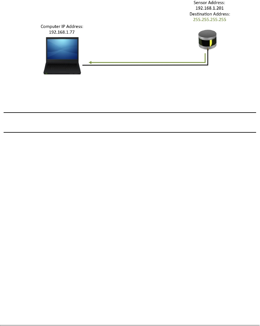
You should assess network loading to see if your network’s topology can accommodate the sensor data rate you select.
J.2.2 Single Sensor Transmitting to a Broadcast Address
Below is a single sensor on a network transmitting to a broadcast address works without any contention.
Figure J-2 Single Sensor Broadcasting on a Simple Network
This is the simplest network, with sensor data flow free from competition or interference. Here it is acceptable for the
sensor to broadcast its data on the network.
J.2.3 Multiple Sensors in the Same Network
Note: Each sensor must have its own, unique IP address in a given network.
When using multiple Velodyne LiDAR sensors in a network it is imperative that you set each sensor's destination IP
address to a specific, non-broadcast IP address. However, two or more sensors may share the same destination address.
The scenarios below illustrate the wrong way and then a better way to configure them. (An alternative would be to direct-
connect sensors to separate NICs.)
J.2.3.1 Multiple Sensors Transmitting to a Broadcast Address
If multiple sensors on a network transmit data to a broadcast address, each sensor will see the broadcast data of the other
sensors. The additional overhead steals cycles from the sensor (and possibly other networked devices) and may lead to a
degradation in performance. (See
Phase Lock on page 127
and
Phase Locking Multiple Sensors on page 37
for additional
information on using multiple sensors within sensing range of each other.)
An improper setup is shown in
Figure J-3 on the facing page
. Note that each sensor’s destination address is set to
255.255.255.255.
136 VLP-16 User Manual
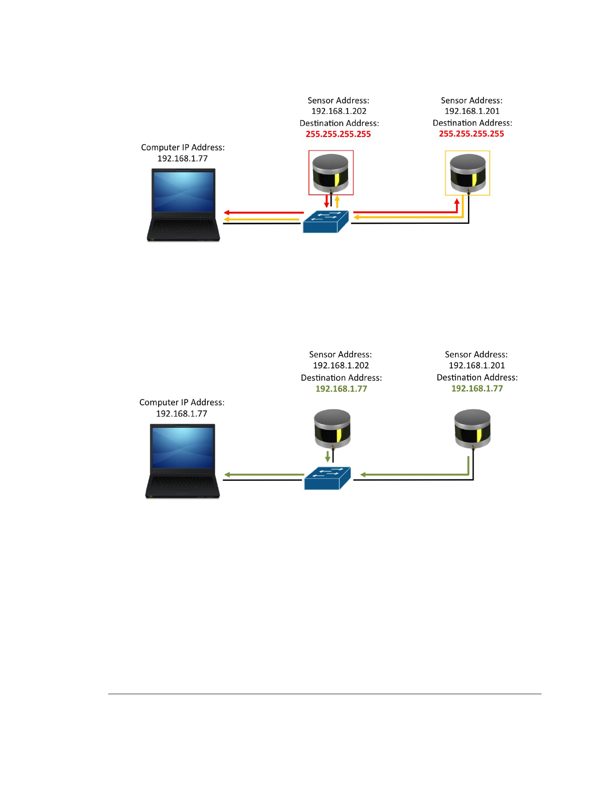
Figure J-3 Multiple Sensors - Improper Network Setup
J.2.3.2 Multiple Sensors Transmitting to a Specific Address
The solution is to configure each sensor on such a network to transmit their data to a non-broadcast address.
If every sensor in the same network transmits packets to a specific, non-broadcast, destination address (doesn’t have to
be the same one), as illustrated in
Figure J-4 below
, the other sensors will not suffer unnecessary network overhead.
Figure J-4 Multiple Sensors - Proper Network Setup
Appendix J • Network Configuration 137

Corporate Headquarters:
Velodyne LiDAR, Inc.
5521 Hellyer Ave
San Jose, CA 95138
U.S.A.
www.VelodyneLiDAR.com
Phone +1 408-465-2800
Fax +1 408-779-9227
Email lidar@velodyne.com
VLP-16 User Manual
63-9243 Rev. D
