ProteinSimple MAURICE Protein Detection Instrument User Manual Maurice manual
ProteinSimple Protein Detection Instrument Maurice manual
Contents
- 1. Users Manual Part 1
- 2. Users Manual Part 2
- 3. Users Manual Part 3
Users Manual Part 2
page 151
User Guide for Maurice, Maurice C. and Maurice S.
Chapter 9:
Run Status
Chapter Overview
• Run Summary Screen Overview
• Opening Run Files
• Batch Injection Information
• Run Status Information
• Viewing the Focus Series (cIEF Only)
• Viewing the Separation (CE-SDS Only)
• Current and Voltage Plots
•Run History
• Viewing Run Errors
•Injection Reports
• Switching Between Open Run Files
• Closing Run Files
page 152 Chapter 9: Run Status
User Guide for Maurice, Maurice C. and Maurice S.
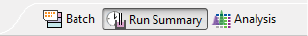
Run Summary Screen Overview
You can use the Run Summary screen to monitor the stats of a batch in progress, see the CE-SDS separation
or cIEF Focus series for your injections or the current and voltage plots for each injection. To get to this
screen, click the Run Summary screen tab:
Run Summary Screen Panes
The Run Summary screen has five panes:
•Injections - Lists the sample IDs, sample locations and methods used for each injection in the run. It
also shows the status of the current injection if a run is in progress.
• Status - Displays run file information and the current status of a run if one’s in progress.
•History - Running history of all run file events from when the run was first started to the most current
analysis update.
•Separation Plot (CE-SDS only)- Lets you view the raw protein separation in the capillary for each
injection.
•Focus Series (cIEF only) - Lets you view the recorded focusing of proteins along the pH gradient in
the capillary for each injection.
•IV Plot - Lets you view plots of the total current and voltage measured during the separation for each
injection.
Run Summary Screen Overview page 153
User Guide for Maurice, Maurice C. and Maurice S.
page 154 Chapter 9: Run Status
User Guide for Maurice, Maurice C. and Maurice S.
Software Menus Active in the Run Summary Screen
These main menu items are active in the Run Summary screen:
•File
•Edit
• Instrument (when the software is connected to an instrument)
•Window
•Help
Run Summary Screen Overview page 155
User Guide for Maurice, Maurice C. and Maurice S.
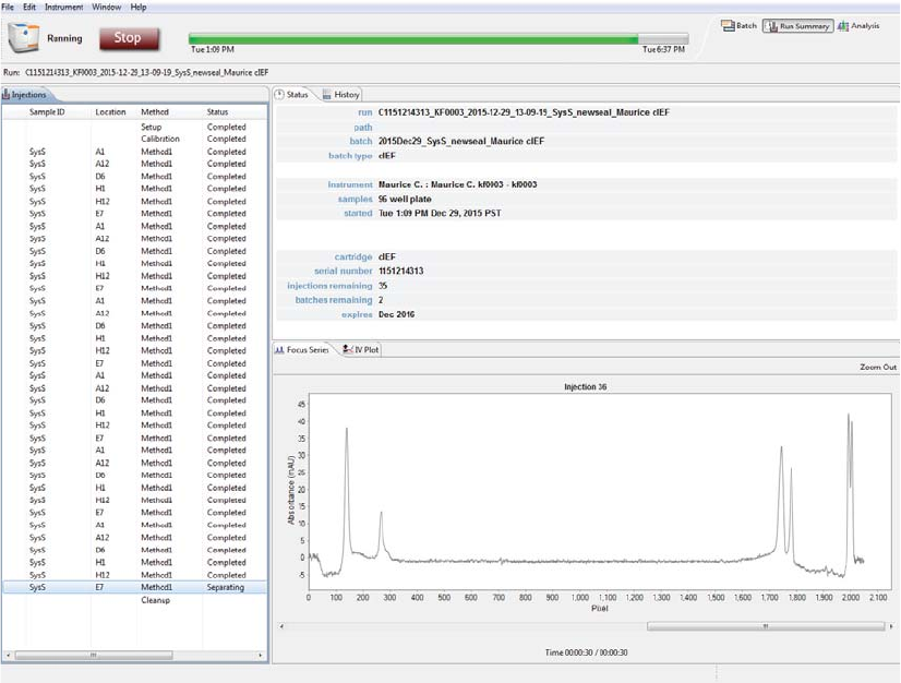
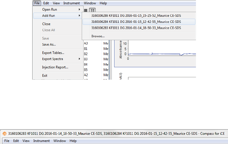
File Menu
These File menu options are active:
•Open Run - Opens a run file.
•Add Run - Lets you open and view other run files besides the one that’s already open.
•Close - Closes the run file currently being viewed.
•Close All - Closes all open run files.
•Save/Save As - If you made changes in the Analysis screen before you went to the Run Summary
screen, this saves your changes to the run file.
•Injection Report - Exports the raw and analyzed data, IV plot, peaks table, sample and system info for
individual injections as PDF files. You can also export the run history with all analysis events.
•Exit - Closes Compass for iCE.
Edit Menu
These Edit menu options are active:
•Copy - Copies the information in the History pane so you can paste it into other documents.
•Preferences - Lets you set and save your preferences for data export, graph colors, grouped data and
Twitter settings. See Chapter 13, “Setting Your Preferences“ for more information.
page 156 Chapter 9: Run Status
User Guide for Maurice, Maurice C. and Maurice S.
Opening Run Files
You can open one run file or multiple files at the same time to compare information between runs.
Opening One Run File
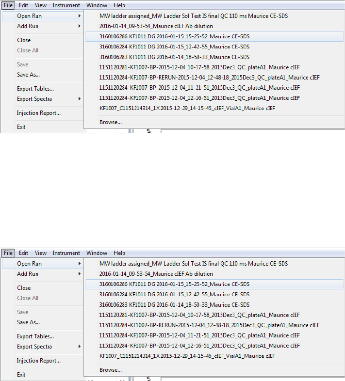
1. Select File in the main menu and click Open Run.
2. A list of the last 10 runs opened will display. Select one of these runs or click Browse to open the Runs
folder and select a different file.
Opening Multiple Run Files
1. To open the first run file, select File in the main menu and click Open Run.
2. A list of the last 10 runs opened will display. Select one of these runs or click Browse to open the Runs
folder and select a different file.
Batch Injection Information page 157
User Guide for Maurice, Maurice C. and Maurice S.
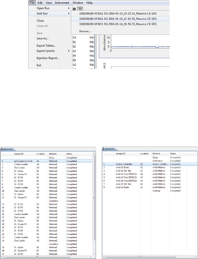
3. To open another run file, select File in the main menu and click Add Run.
4. A list of runs will display. You can only open a run that uses the same application as the run that’s already
open (cIEF or CE-SDS), so the run files displayed are only for that application. Select one of these runs or
click Browse to open the Runs folder and select a different file.
5. Repeat the last two steps to open additional runs.
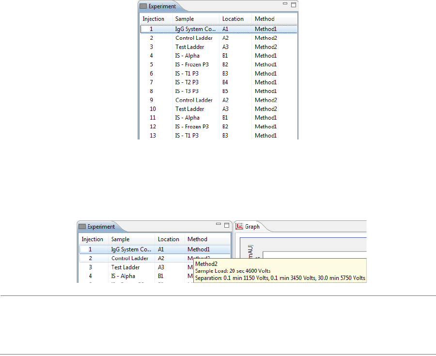
Batch Injection Information
The Injections pane lists the system protocols (Setup and Cleanup) and injections performed during the run.
page 158 Chapter 9: Run Status
User Guide for Maurice, Maurice C. and Maurice S.
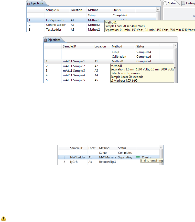
• Clicking on an injection displays its data in the Focus Series (cIEF) or Separation (CE-SDS) and IV Plot
panes.
• Hovering over a method name displays the method parameters:
For runs in progress, the Status column displays:
•Running for Setup, Conditioning (CE-SDS only) and Cleanup protocols that are in progress
•Loading or Separating for injections in progress. Once the separation starts, a status bar displays
next to the injection so you know when the separation will be done. Hovering your mouse over the
progress bar tells you the time left for the injection.
•Completed for Setup, Conditioning and Cleanup protocols and injections that are done.
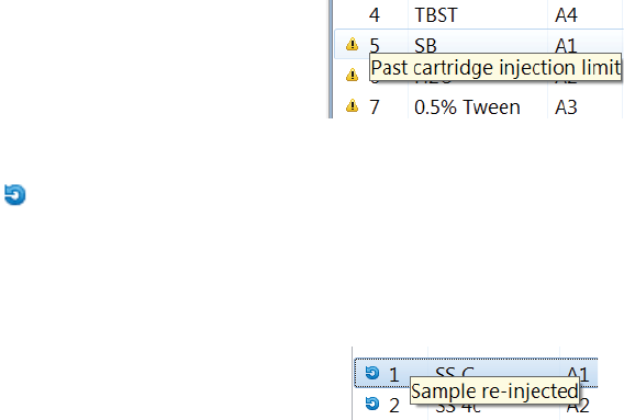
Injection Flags
If Compass for iCE detects a potential injection issue, a flag icon will display next to the injection row in the
Injections pane.
Past cartridge injection limit notification - This means the injection is over the guaranteed
number of injections for the cartridge. Roll your mouse over the icon to display details.
Run Status Information page 159
User Guide for Maurice, Maurice C. and Maurice S.
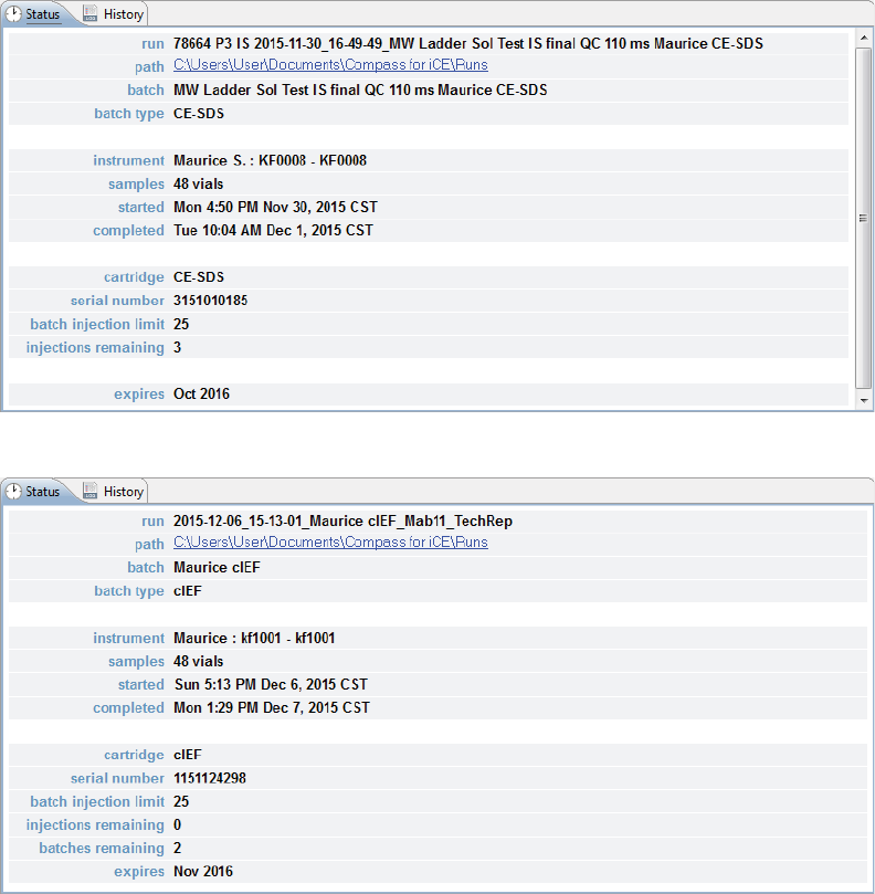
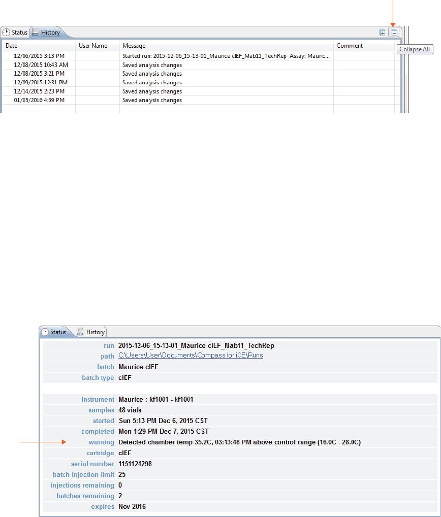
Run Status Information
The Status pane shows info specific to each run file:
• Run file name and path (directory location)
• Batch name and type
• Instrument and serial number
• Type of sample tray used
• Run start/complete date and time
• Type of cartridge
• Cartridge serial number
Reinjection notification (CE-SDS only) - This means the current during the separation
dropped below the minimum value, so the separation was stopped and the sample was rein-
jected. The second injection always runs to completion even if the current drops again. Roll
your mouse over the icon to display details.
page 160 Chapter 9: Run Status
User Guide for Maurice, Maurice C. and Maurice S.
• Cartridge batch injection limit, injections/batches remaining and expiration date
•To go to the run file directory location - Double click the path hyperlink, or right-click and select
Open Directory.
•To copy the path - Right-click on the path hyperlink and click Copy. The path can then be copied
into documents. The path can also be copied into the Windows Explorer address bar to launch Com-
pass for iCE and open the run file automatically.
Viewing the Focus Series (cIEF Only) page 161
User Guide for Maurice, Maurice C. and Maurice S.
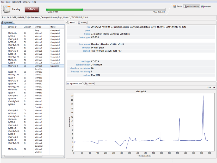
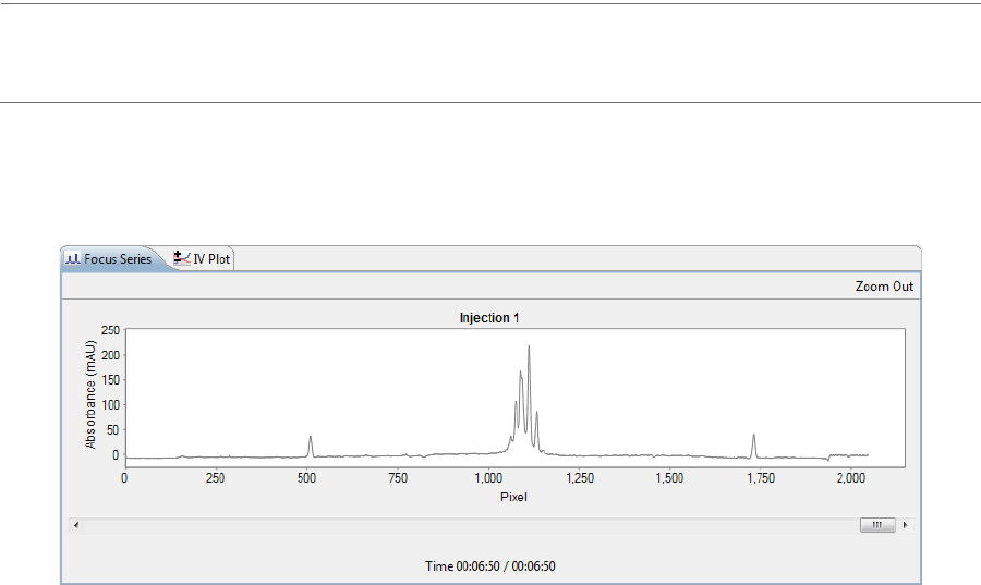
Viewing the Focus Series (cIEF Only)
You can view your proteins focusing along the pH gradient in the capillary for each injection in the Focus
Series pane.
NOTE: The Focus Series plot displays in absorbance only, even if the fluorescence detection mode is
selected in the Analysis settings.
1. Select an injection in the Injections pane.
2. Click the Focus Series pane. It’ll display the final focusing plot:
page 162 Chapter 9: Run Status
User Guide for Maurice, Maurice C. and Maurice S.
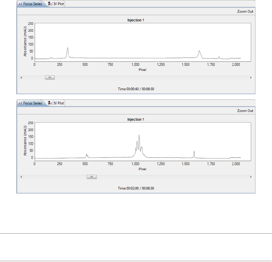
3. To view the focusing as it happened, drag the slider bar under the plot to the left or right. To view it
frame by frame, click the left/right arrows.
•To zoom in on an area of the plot - Hold the mouse button down and draw a box around the area
with the mouse.
•To zoom out - Click Zoom Out in the upper right corner of the pane.
NOTE: Focus Series data for a run in progress won’t be available until the injection is executing. Once it
starts, the plot displays data up to the current point in time.
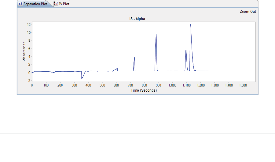
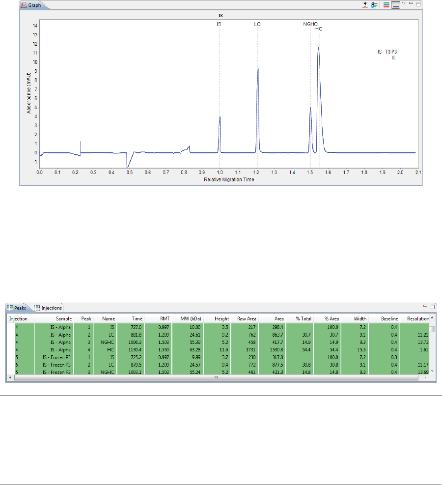
Viewing the Separation (CE-SDS Only)
You can view your protein separation in the capillary for each injection in the Separation pane.
Current and Voltage Plots page 163
User Guide for Maurice, Maurice C. and Maurice S.
1. Select an injection in the Injections pane.
2. Click the Separation pane. It’ll display a plot of the raw separation data.
•To zoom in on an area of the plot - Hold the mouse button down and draw a box around the area
with the mouse.
•To zoom out - Click Zoom Out in the upper right corner of the pane.
NOTE: Separation data for a run in progress won’t be available until the injection is executing. Once it
starts, the plot displays data up to the current point in time.
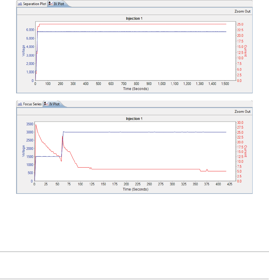
Current and Voltage Plots
To view plots of the total current and voltage measured during an injection:
1. Select an injection in the Injections pane.
page 164 Chapter 9: Run Status
User Guide for Maurice, Maurice C. and Maurice S.
2. Click the IV Plot pane.
The blue Y-axis and plot shows the run voltage in volts (V), and the red Y-axis and plot shows the run current
in microamps (μA). The X-axis displays time in seconds.
•To zoom in on an area of the plot - Hold the mouse button down and draw a box around the area
with the mouse.
•To zoom out - Click Zoom Out in the upper right corner of the pane.
NOTE: IV Plots for a run in progress won’t be available until the injection is executing. Once it starts, the plot
displays in real time.
Run History page 165
User Guide for Maurice, Maurice C. and Maurice S.
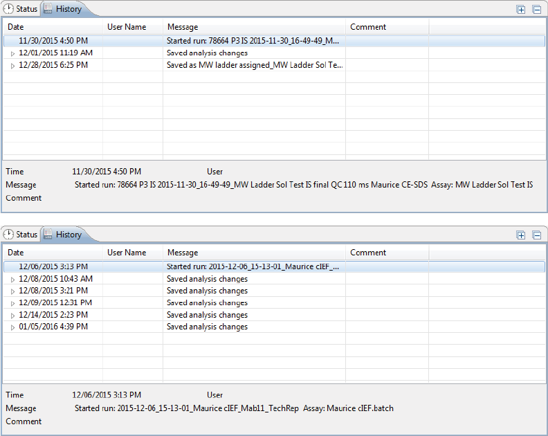
Run History
The History pane shows the run file event history, starting with the date and time the run was started
through the most current analysis event. Clicking on a row in the table displays the full event details in the
box under the table.
•Date: Date and time of the run event.
•User Name: User that initiated the event. User names only display if you’re using the Access Con-
trol feature to help satisfy the 21CFR Part 11 data security requirements.
•Message: Description of the event that took place.
•Comment: Comments entered by the user when the batch was saved.
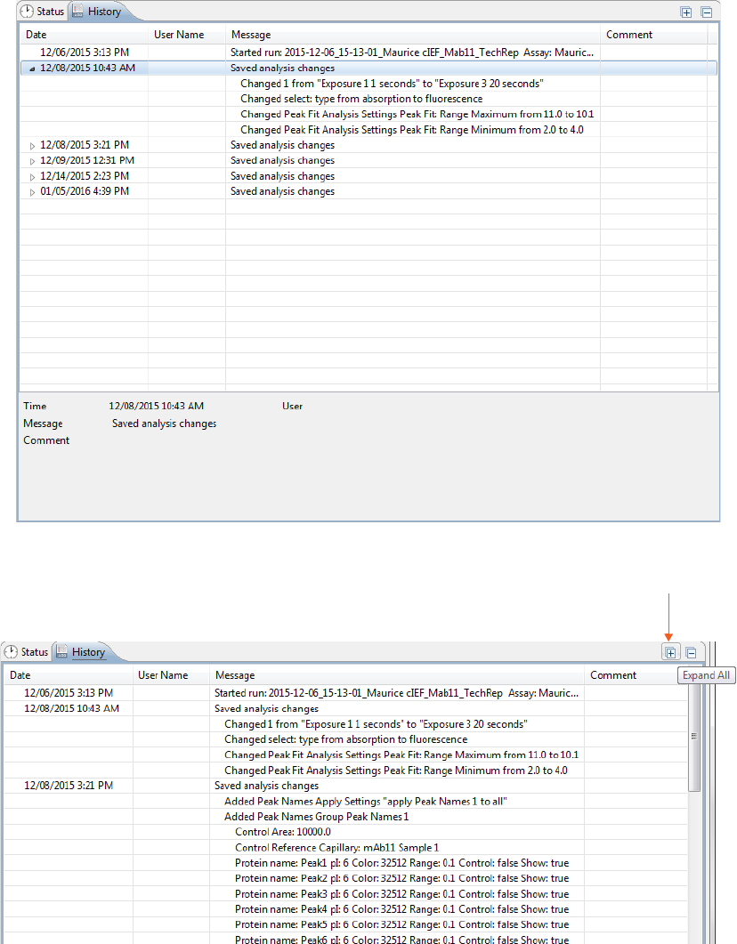
Viewing Multiple Events
Items in the table with multiple analysis events have an arrow next to the date and time. You can view or
hide these details by toggling the arrow:
page 166 Chapter 9: Run Status
User Guide for Maurice, Maurice C. and Maurice S.
• To view details for all items with multiple analysis events in the run, click the Expand All button.
Viewing Run Errors page 167
User Guide for Maurice, Maurice C. and Maurice S.
• To hide all items with multiple analysis events, click the Collapse All button.
Copying History Info
You can copy the information in the History pane to use in other documents:
1. Click the History pane to make sure it’s active.
2. Click Edit in the main menu and select Copy.
3. Open a document and click Paste.
Viewing Run Errors
If an error is detected during the run it will display in the Status pane:
page 168 Chapter 9: Run Status
User Guide for Maurice, Maurice C. and Maurice S.
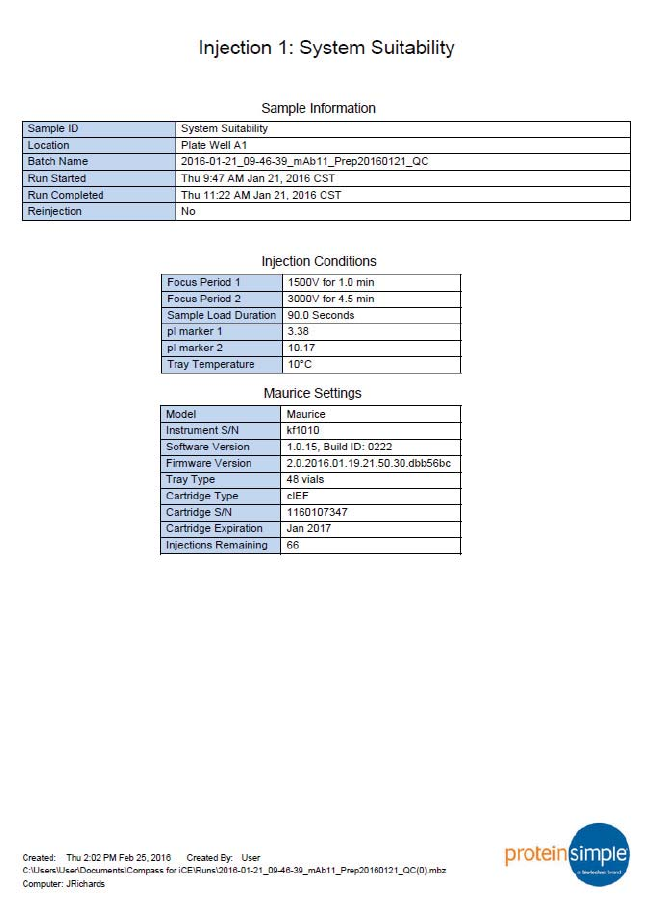
Injection Reports
You can export PDF files of the raw and analyzed data, IV plot, peaks table, sample and system info for indi-
vidual or all injections in a run file. You can also export the run history with all analysis events.
1. Click File > Open Run and select a run file.
2. If you want reports for all injections, skip to the next step. Otherwise, select the injection in the Injection
pane that you want a report for.
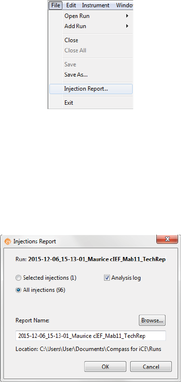
3. Select File from the main menu in either screen and click Injection Report.
4. In the Injection Reports window:
a. Choose either Selected injections or All injections.
b. Select the Analysis log checkbox if you want a run history report with all analysis events.
c. The report name defaults to the run file name. If you want to change it, type in the Report Name
box to make updates.
d. Click OK.
Injection Reports page 169
User Guide for Maurice, Maurice C. and Maurice S.
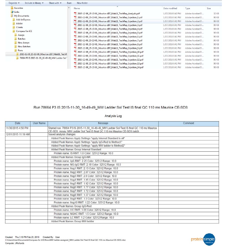
5. The Injection Report PDF(s) are exported to the Runs folder in the Compass for iCE directory. They’ll be
in a folder with the report name used in the prior step. When the reports are done, the folder opens for
you automatically.
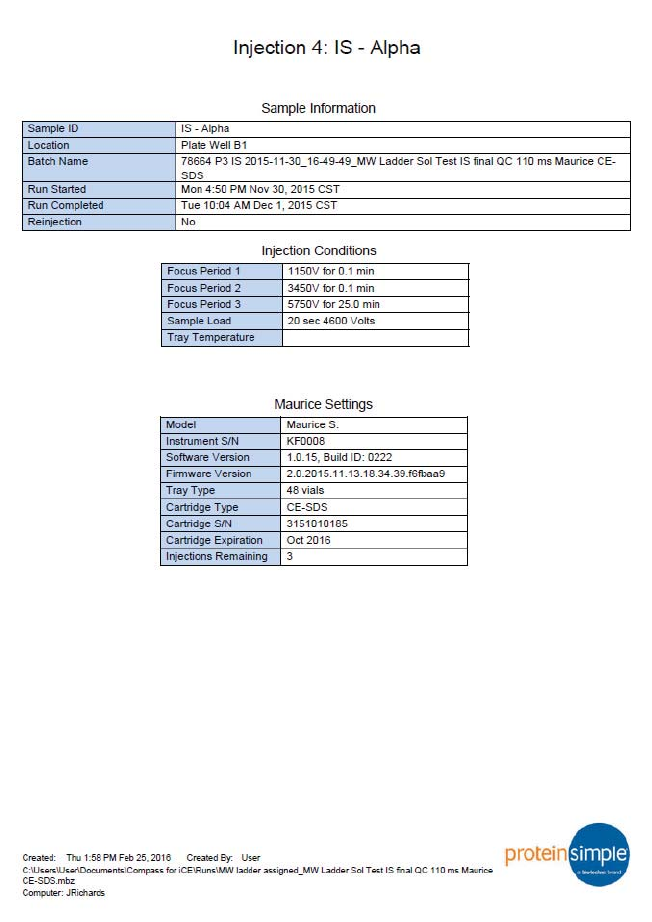
Example Analysis and Injection Report: CE-SDS

page 170 Chapter 9: Run Status
User Guide for Maurice, Maurice C. and Maurice S.
Injection Reports page 171
User Guide for Maurice, Maurice C. and Maurice S.
page 172 Chapter 9: Run Status
User Guide for Maurice, Maurice C. and Maurice S.
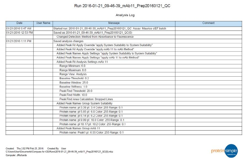
Example Analysis and Injection Report: cIEF
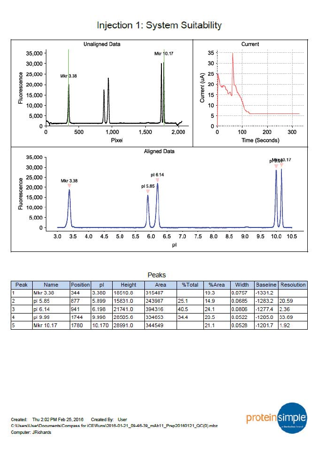
Injection Reports page 173
User Guide for Maurice, Maurice C. and Maurice S.
page 174 Chapter 9: Run Status
User Guide for Maurice, Maurice C. and Maurice S.
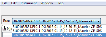
Switching Between Open Run Files
If you’ve got more than one run file open, you can switch between viewing the run information in each.
Closing Run Files page 175
User Guide for Maurice, Maurice C. and Maurice S.
1. Click the down arrow in the Run box.
2. Select the run you want to view from the drop down list.
Closing Run Files
If you’ve got more than one run file open, you can close just one file or all the open files at the same time.
•To close the run file being viewed - Select File from the main menu and click Close.
•To close all open run files - Select File from the main menu and click Close All.
page 176 Chapter 9: Run Status
User Guide for Maurice, Maurice C. and Maurice S.
page 177
User Guide for Maurice, Maurice C. and Maurice S.
Chapter 10:
Controlling Maurice, Maurice C. and
Maurice S.
Chapter Overview
• Instrument Control
• Stopping a Run
•Status Modes
• Instrument Software (Embedded) Updates
•Self Test
• Viewing and Changing System Properties
• Checking Cartridge Status
•Viewing Log Files

page 178 Chapter 10: Controlling Maurice, Maurice C. and Maurice S.
User Guide for Maurice, Maurice C. and Maurice S.
Instrument Control
The Instrument menu lets you to control Maurice, Maurice C. and Maurice S.
NOTE: Instrument menu options are only active when you’ve got a computer with Compass for iCE soft-
ware connected directly to your Maurice system.
Starting a Run
To start your run, click the Start button in the Batch screen. You can also start a run by selecting Instrument
in the main menu and clicking Start. For more info on creating and starting batches check out Chapter 7,
“Running cIEF Applications on Maurice and Maurice C.“ or Chapter 8, “Running CE-SDS Applications on Maurice
and Maurice S.“
Cleaning
Cartridge Cleanup (CE-SDS Cartridges Only)
If you've still got injections left after your last run and you won’t use the cartridge again within 2 hours, you’ll
need to run a clean up and store it. Check out page 137 for the details on how to do that.
Cartridge Purge
You’ll want to run the Cartridge Purge any time you have to stop a run manually or if the run stops because
of an error. This runs the Cleanup step that normally happens at the end of a batch. It flushes the cartridge of
any reagents and samples so it’s ready to go for the next run.
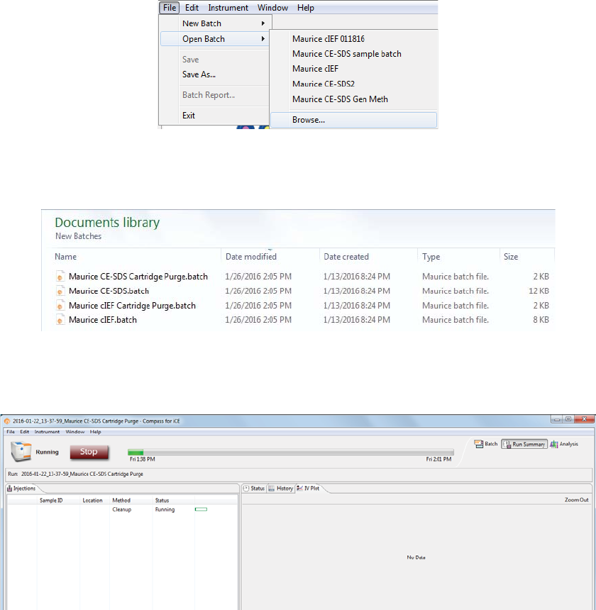
1. In the Batch screen, select File > Open Batch and click Browse.
Instrument Control page 179
User Guide for Maurice, Maurice C. and Maurice S.
2. Go to the New Batches folder and select either Maurice cIEF Cartridge Purge or Maurice CE-SDS Car-
tridge Purge, depending on what cartridge you’re using.
3. After the purge batch loads, just click Start. The CE-SDS Cartridge purge takes about 25 minutes, and
the cIEF one takes a little over 10 minutes.
page 180 Chapter 10: Controlling Maurice, Maurice C. and Maurice S.
User Guide for Maurice, Maurice C. and Maurice S.
4. Once the purge is done, if you’ll be starting a new run:
•cIEF Cartridges: If you've still got injections left and the cartridge will be used again within 24
hours, you don't need to do anything. Just leave the cartridge in Maurice.
•CE-SDS Cartridges: If you've still got injections left and the cartridge will be used again within 2
hours, you'll just need to put in a new Top Running Buffer vial in the cartridge insert.
If you won’t be starting a new run:
•cIEF Cartridges: Follow the steps in “Post-batch Procedures” on page 102.
•CE-SDS Cartridges: Follow the steps in “Post-batch Procedures” on page 135.
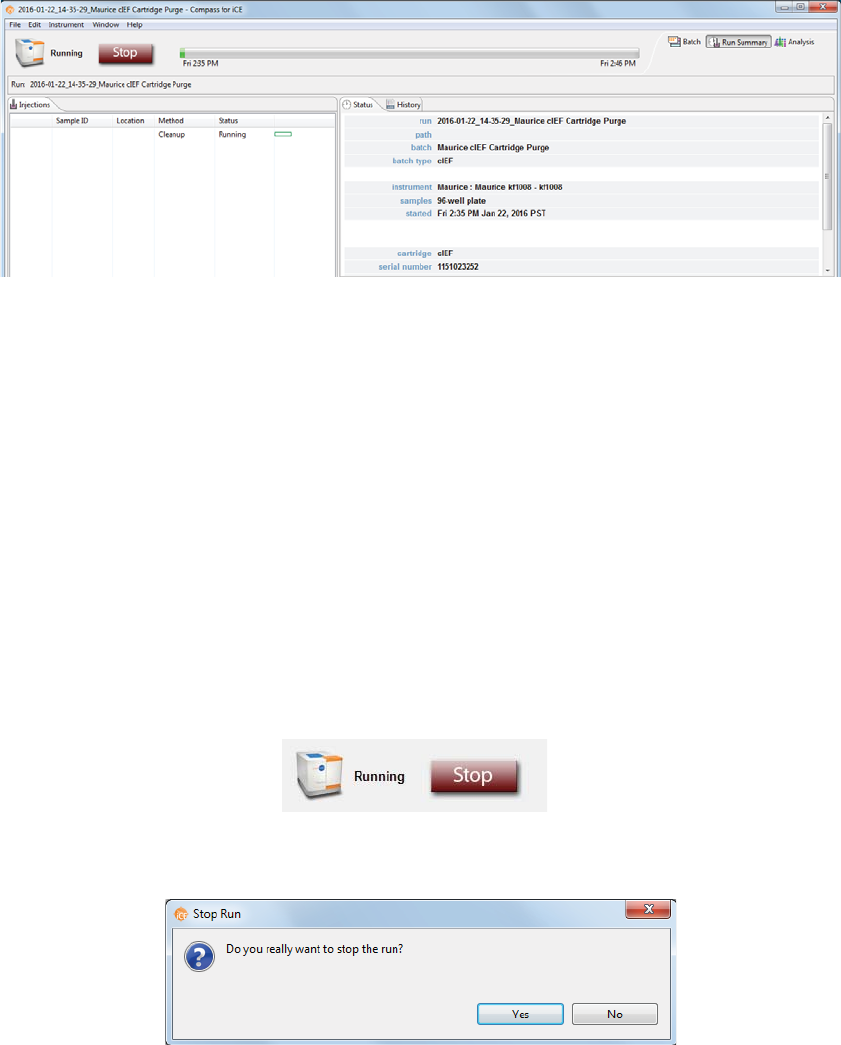
Stopping a Run
1. Click Stop.
2. Click Yes in the pop-up window.
Status Modes page 181
User Guide for Maurice, Maurice C. and Maurice S.
3. When the run stops, run the “Cartridge Purge” on page 178.
4. Once the purge is done:
If you’ll be starting a new run:
•cIEF Cartridges: If you've still got injections left and the cartridge will be used again within 24
hours, you don't need to do anything. Just leave the cartridge in Maurice.
•CE-SDS Cartridges: If you've still got injections left and the cartridge will be used again within 2
hours, you don't need to do anything other than prepare the cartridge for the next batch as
described “Step 2: Prep the Cartridge” on page 120.
If you won’t be starting a new run:
•cIEF Cartridges: Follow the steps in “Post-batch Procedures” on page 102.
•CE-SDS Cartridges: Follow the steps in “Post-batch Procedures” on page 135.
Status Modes
The instrument status bar displays status, buttons and progress bars depending on what Maurice, Maurice C.
or Maurice S. are doing.
•Ready/Start button - The instrument is ready and a batch is loaded. Click Start to begin a run.
•Not Ready/Reset button - The instrument isn’t ready and needs to reinitialize. Click Reset to start
the initialization protocol.
•Running/Stop button - The instrument is running. The run name, time it started and when it will be
done show in the run progress bar. Click Stop to stop the run.
•Cleaning/Stop button - The instrument is running a cleaning protocol. The time the cleaning proto-
col started and when it will be done show in the run progress bar.
•Error/Reset button - There’s an error. Go to the Status pane in the Run Summary screen to view
details. When you’ve fixed the source of the error, click Reset.
Shutdown
Close Compass for iCE software. Maurice can stay on unless he won’t be used for an extended period.
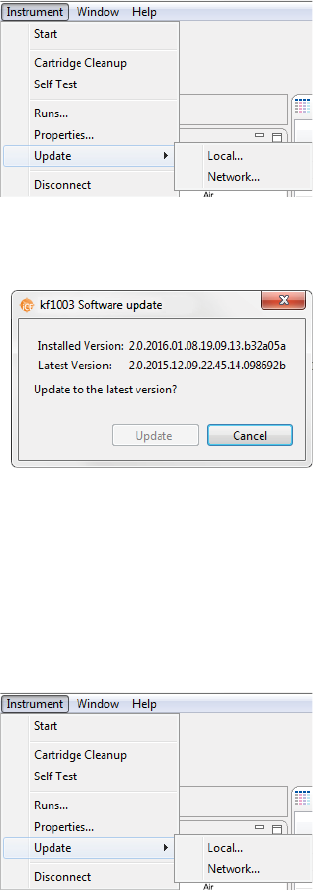
Instrument Software (Embedded) Updates
To check for embedded software updates:
page 182 Chapter 10: Controlling Maurice, Maurice C. and Maurice S.
User Guide for Maurice, Maurice C. and Maurice S.
If you’re on the network:
1. Select Instrument > Update, then select Network.
2. The following screen displays. Click Update.
If you’re not on the network:
1. Call ProteinSimple Technical Support or your FAS for assistance on getting the latest update.
2. Copy the new embedded software file onto Maurice’s computer.
3. Select Instrument > Update, then select Local.
4. Browse to the location of the embedded software file, select it and click OK.
5. The following screen displays. Click Update.
Self Test page 183
User Guide for Maurice, Maurice C. and Maurice S.
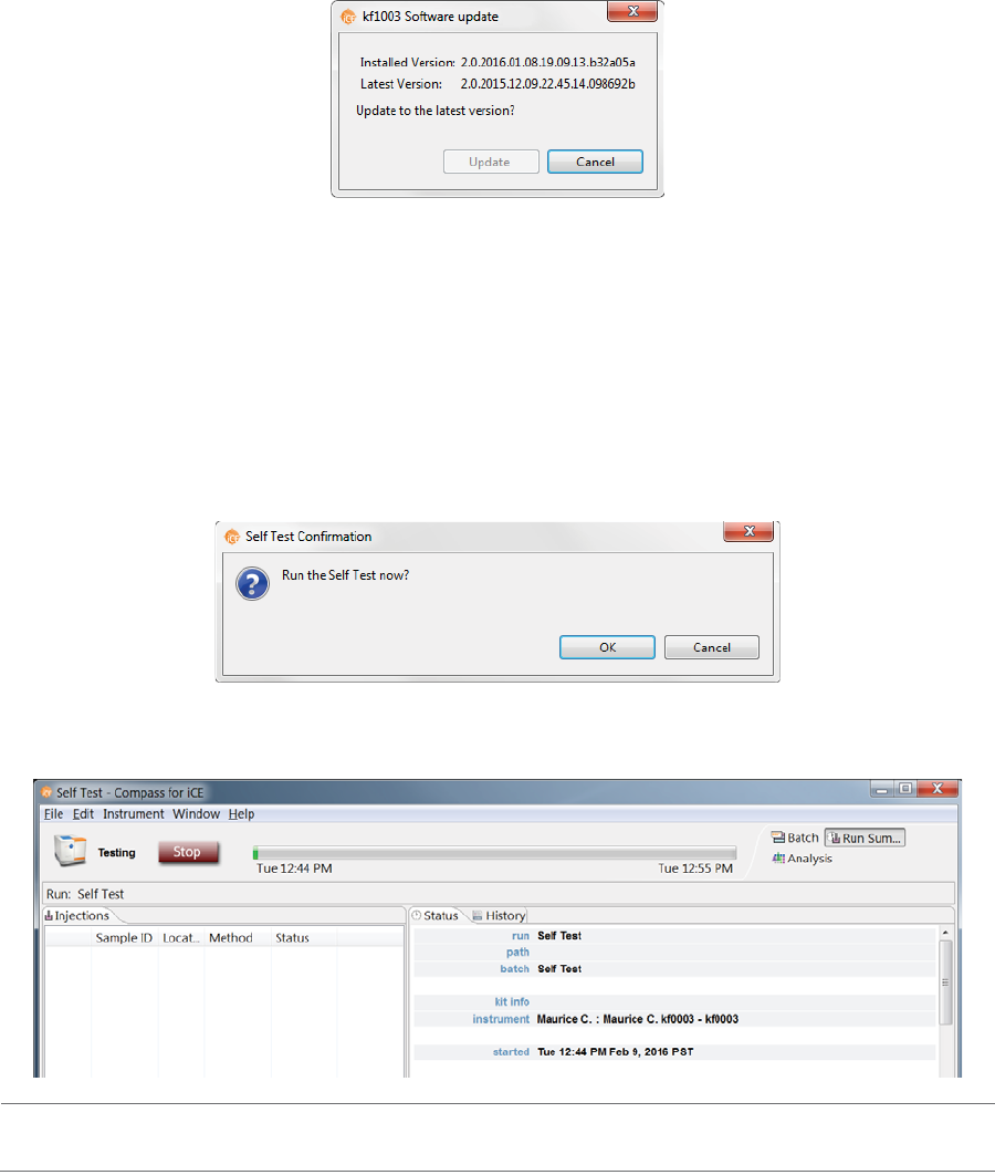
Self Test
Maurice, Maurice C. and Maurice S. can run a series of self tests for you to make sure they’re operating prop-
erly.
1. To start the test, select Instrument > Self Test.
2. The following screen displays. Click OK.
The test takes approximately 11 minutes.
NOTE: We recommend running the self test before you start a run.
page 184 Chapter 10: Controlling Maurice, Maurice C. and Maurice S.
User Guide for Maurice, Maurice C. and Maurice S.
To view the results when the test’s done, select Instrument > Properties and click Test Log. See “Self Test
Logs” on page 192 for more info.
Viewing and Changing System Properties
Selecting Instrument > Properties displays your system properties. They include:
•System Name
•System Location
• Instrument Type
•Serial number
• Instrument software version (firmware)
• Network name and address
• Date and time of the instrument clock
• Adapter block currently in use
• Number of hours on the Deuterium (UV) lamp
• Current sample chiller temperature
Checking Cartridge Status page 185
User Guide for Maurice, Maurice C. and Maurice S.
•To change the system name or location: Click in the name or location boxes and enter your new
info, then click OK.
•To sync the instrument clock with the computer: Click Set to PC time.
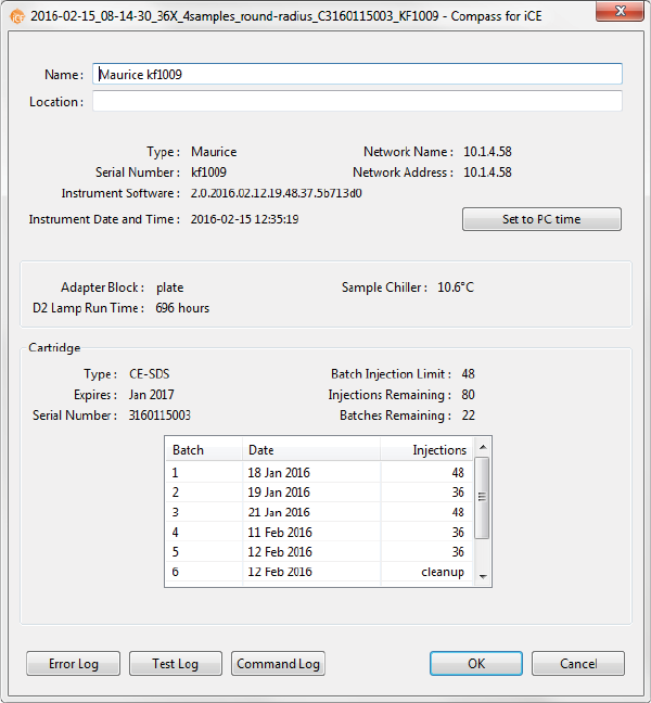
Checking Cartridge Status
If you’ve got a cartridge installed in the system, you can see its serial number, the injections and batches it
still has available, and a history of batches and injections its run to date. To view this info, select Instrument
> Properties.
Insert image here.

page 186 Chapter 10: Controlling Maurice, Maurice C. and Maurice S.
User Guide for Maurice, Maurice C. and Maurice S.
Viewing Log Files
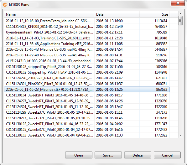
Runs Log
To see a history of all runs your system has performed, select Instrument > Runs:
Insert image here.
Viewing Log Files page 187
User Guide for Maurice, Maurice C. and Maurice S.
•To open a run file: Select a run file from the list and click Open.
•To save a run file: Select a run file from the list and click Save. This lets you save a copy of a com-
pleted run or one in progress to either a USB drive or the local computer.
•To delete a run file: Select a run file from the list and click Delete. The run file will be deleted from
the history and from the Run file in the Compass for iCE directory.
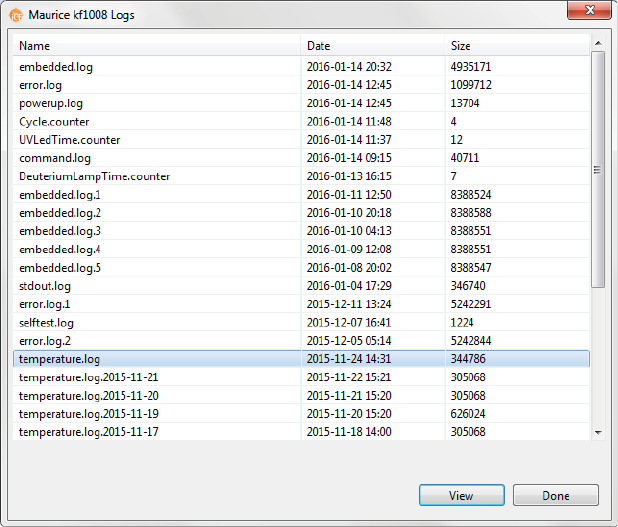
System Logs
1. Select Instrument > Properties to display your system’s properties.
2. Click Error Log. A list of system logs displays:
page 188 Chapter 10: Controlling Maurice, Maurice C. and Maurice S.
User Guide for Maurice, Maurice C. and Maurice S.
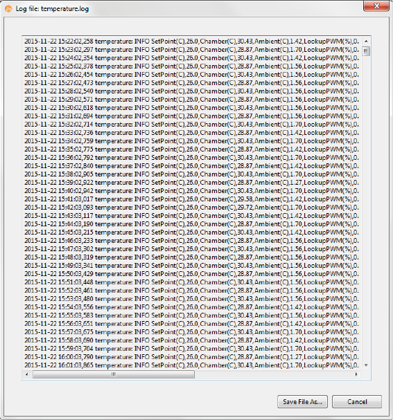
3. To view a log, select it in the list and click View.
Viewing Log Files page 189
User Guide for Maurice, Maurice C. and Maurice S.
4. Click Save File As to save a copy of the log file.
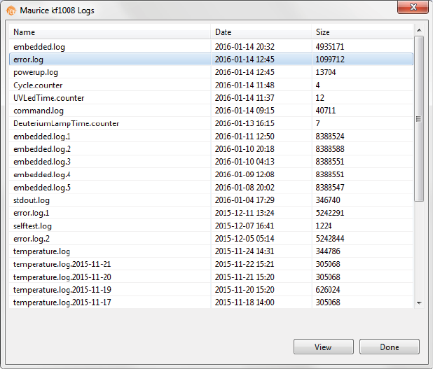
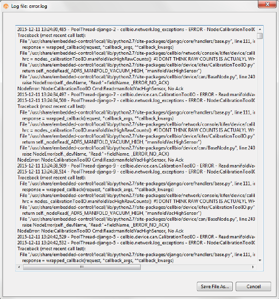
Error Log
1. Select Instrument > Properties to display your system’s properties.
2. Click Error Log. A list of system logs displays:
page 190 Chapter 10: Controlling Maurice, Maurice C. and Maurice S.
User Guide for Maurice, Maurice C. and Maurice S.
3. Select the error.log you’re interested in from the list and click View.
Viewing Log Files page 191
User Guide for Maurice, Maurice C. and Maurice S.
4. Click Save File As to save a copy of the log file.
page 192 Chapter 10: Controlling Maurice, Maurice C. and Maurice S.
User Guide for Maurice, Maurice C. and Maurice S.
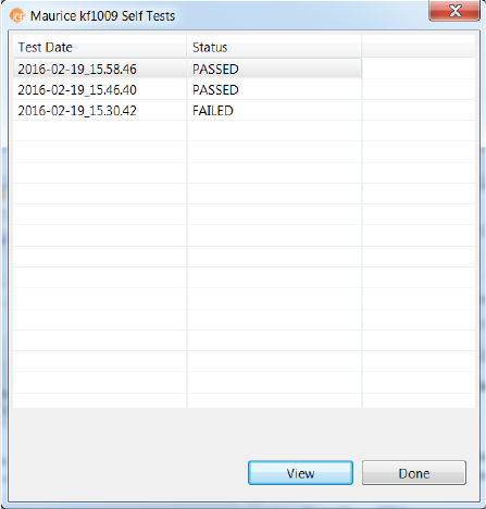
Self Test Logs
1. Select Instrument > Properties.
2. Click Test Log. A list of dates each self test was run displays:
Viewing Log Files page 193
User Guide for Maurice, Maurice C. and Maurice S.
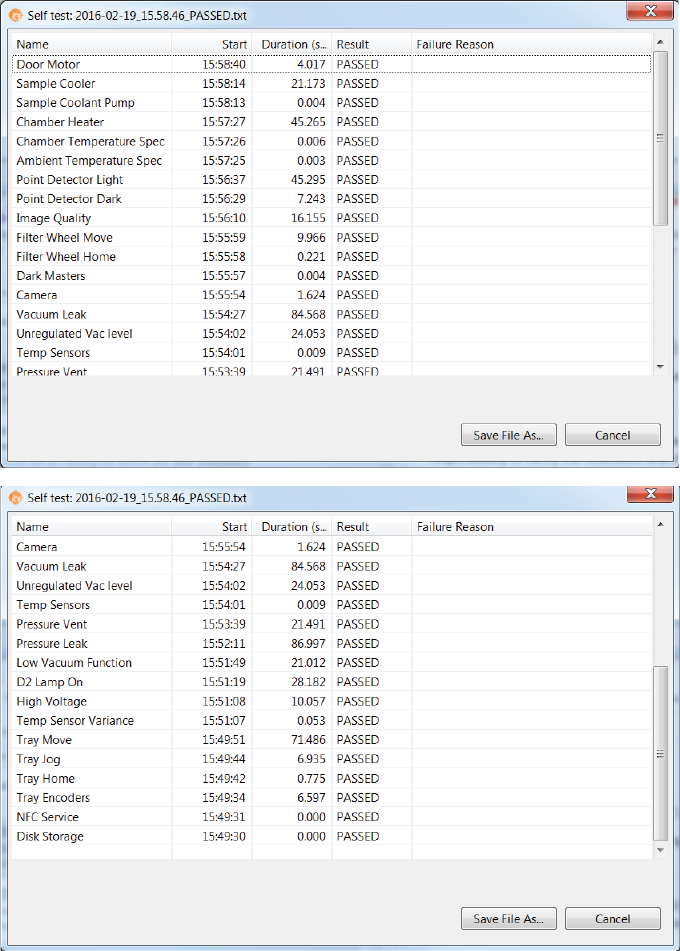
3. Select a test date in the list and click View to see the individual test results:
4. Click Save File As to save a copy of the test log file.
page 194 Chapter 10: Controlling Maurice, Maurice C. and Maurice S.
User Guide for Maurice, Maurice C. and Maurice S.
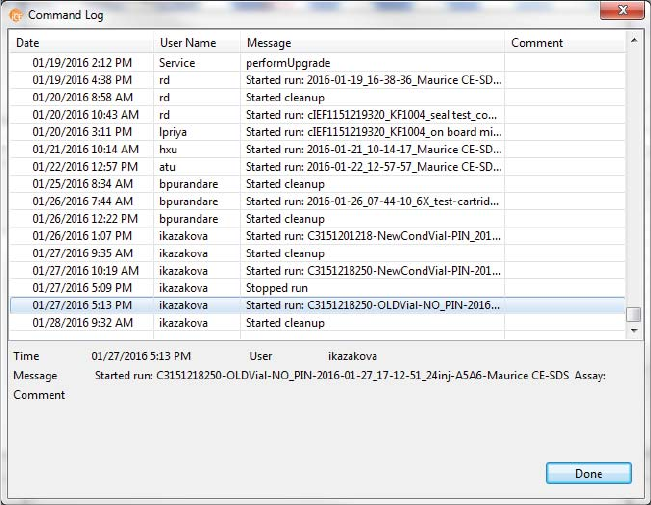
Command Log
1. Select Instrument > Properties to display your system’s properties.
2. Click Command Log. A list of system commands displays:
page 195
User Guide for Maurice, Maurice C. and Maurice S.
Chapter 11:
CE-SDS Data Analysis
Chapter Overview
• Analysis Screen Overview
• Opening Run Files
• How Run Data is Displayed
• Viewing Run Data
• Data Notifications and Warnings
•Checking Your Results
•Group Statistics
• Copying Results Tables and Graphs
• Exporting Run Files
• Changing Sample Protein Identification
• Changing the Electropherogram View
• Closing Run Files
• Analysis Settings Overview
• Advanced Analysis Settings
• Markers Analysis Settings
• Peak Fit Analysis Settings
• Peak Names Settings
•Injection Reports
• Importing and Exporting Analysis Settings
page 196 Chapter 11: CE-SDS Data Analysis
User Guide for Maurice, Maurice C. and Maurice S.
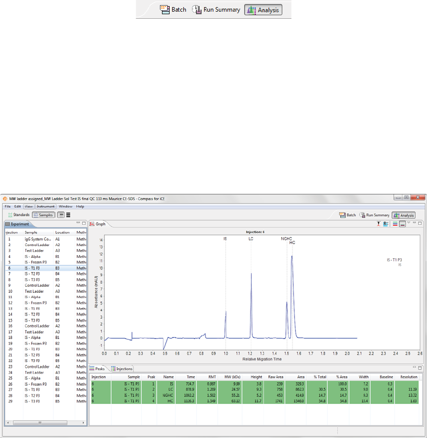
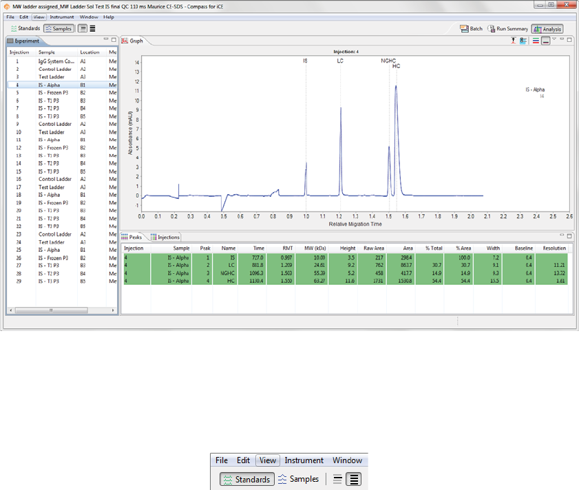
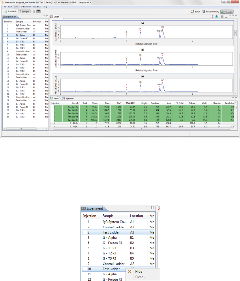
Analysis Screen Overview
You can use the Analysis screen to view electropherograms and tabulated results for your injections. If any
post-run analysis is needed, you can do it here too. To get to this screen, click the Analysis screen tab:
Analysis Screen Panes
The Analysis screen has four panes:
•Experiment - Lists the injection number, sample IDs, sample locations and methods for each injec-
tion in the run and lets you get a quick view of method parameters.
•Graph - Displays the electropherograms for sample proteins or standards.
•Peaks - Shows the tabulated results for sample proteins, internal standards and CE-SDS MW Markers.
•Injections - Displays a list of the sample proteins Compass for iCE names automatically using the
user-defined peak name analysis parameters.
Analysis Screen Overview page 197
User Guide for Maurice, Maurice C. and Maurice S.
Software Menus Active in the Analysis Screen
These main menu items are active in the Analysis Screen:
•File
•Edit
•View
• Instrument (when Compass for iCE is connected to Maurice, Maurice C. or Maurice S.)
•Window
•Help
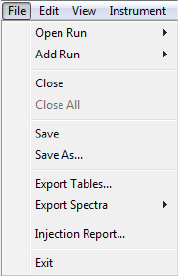
File Menu
These File menu options are active:
•Open Run - Opens a run file.
•Add Run - Lets you open and view other run files besides the one that’s already open.
•Close - Closes the run file currently being viewed.
•Close All - Closes all open run files.
•Save/Save As - If you made changes in the Analysis screen before you went to the Run Summary
screen, this saves your changes to the run file.
•Export Tables - Exports the results for all injections in the run in .txt format.
•Export Spectra - Exports the raw and analyzed data traces and background for each injection in the
run in .txt or .cdf format.
•Injection Report - Exports the raw and analyzed data, IV plot, peaks table, sample and system info for
individual injections as PDF files. You can also export the run history with all analysis events.
page 198 Chapter 11: CE-SDS Data Analysis
User Guide for Maurice, Maurice C. and Maurice S.
•Exit - Closes Compass for iCE.
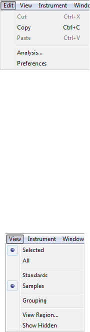
Edit Menu
These Edit menu options are active:
•Copy - Copies the information in the History pane so you can paste it into other documents.
•Analysis - Displays the analysis settings used to analyze the run data and lets you change them as
needed. See “Analysis Settings Overview” on page 244 for more information.
•Preferences - Lets you set and save your preferences for data export, graph colors, grouped data and
Twitter settings. See Chapter 13, “Setting Your Preferences“ for more information.
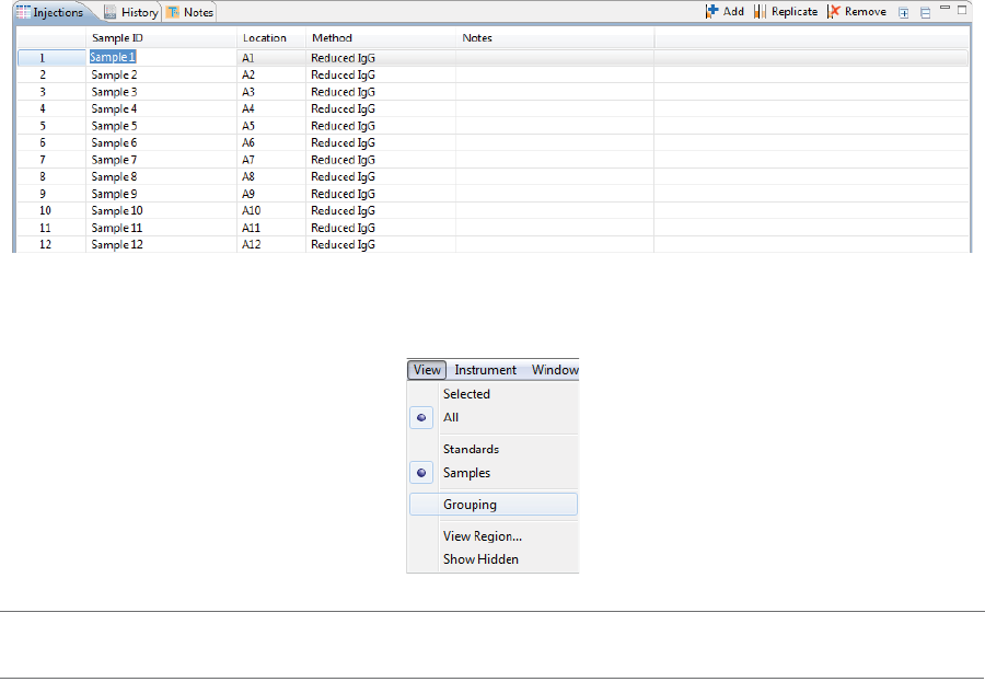
View Menu
These View menu options are active:
•Single View - Displays the data for only the injections selected.
•Multiple View - Displays data for all injections so you can scroll through them.
•Standards - Lets you view data just for the internal standards in your injections.
•Samples - Lets you view data just for sample proteins in your injections.
•Grouping - Displays data for injection groups.
•View Region - Lets you change the x-axis range of the data displayed.
•Show Hidden- Shows injections that are hidden from the data view.
Opening Run Files page 199
User Guide for Maurice, Maurice C. and Maurice S.
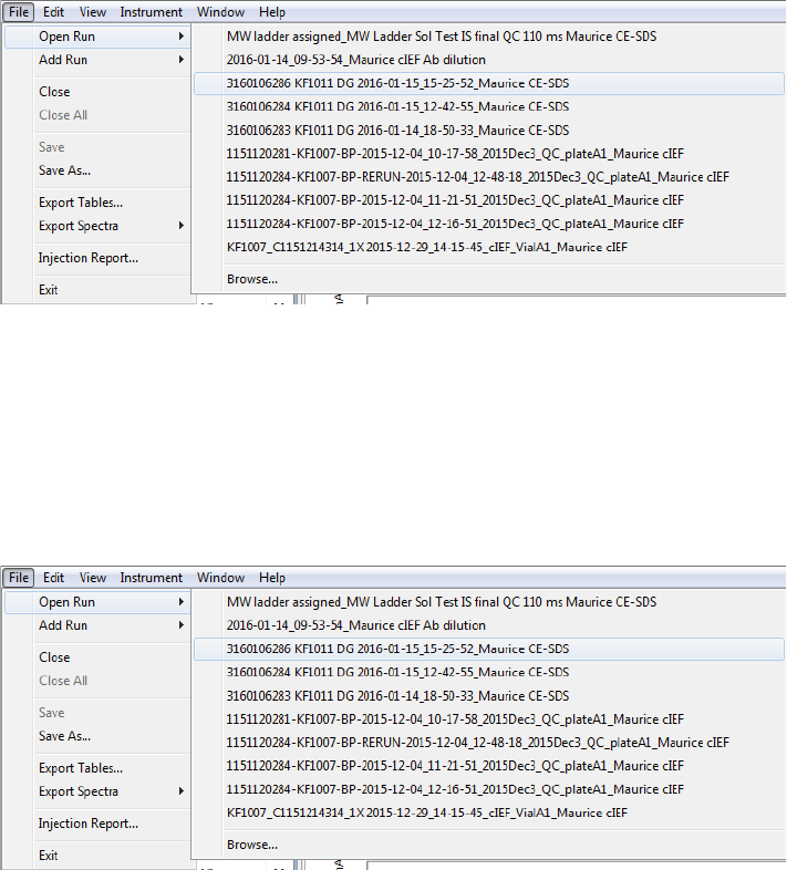
Opening Run Files
You can open one run file or multiple files at the same time to compare information between runs.
Opening One Run File
1. Select File in the main menu and click Open Run.
2. A list of the last 10 runs opened will display. Select one of these runs or click Browse to open the Runs
folder and select a different file.
Opening Multiple Run Files
1. To open the first run file, select File in the main menu and click Open Run.
2. A list of the last 10 runs opened will display. Select one of these runs or click Browse to open the Runs
folder and select a different file.
page 200 Chapter 11: CE-SDS Data Analysis
User Guide for Maurice, Maurice C. and Maurice S.
3. To open another run file, select File in the main menu and click Add Run.
4. A list of CE-SDS runs will display. Select one of these runs or click Browse to open the Runs folder and
select a different file.
When a run is added, its data appends to the open run file and displays as a second set of injections in all
screen panes. The second run file name also appears in the title bar:
5. Repeat the last two steps to add additional runs.
How Run Data is Displayed page 201
User Guide for Maurice, Maurice C. and Maurice S.
How Run Data is Displayed
Data in the run file is organized for easy review.
Experiment Pane: Batch Injection Information
The Experiment pane lists all the injections performed in the run, which samples were used for each, the
sample location in the 96-well plate or 48-vial tray and the method used.
•To view all columns - Use the scroll bar or click Maximize in the upper right corner.
•To resize columns - Roll the mouse over a column border until the sizing arrow appears, then click
and drag to resize.
•To view method parameters - Hover the mouse over a method name.
NOTE: Data notification icons will display in the Injection column if Compass for iCE detects a potential
analysis issue or data was manually modified by the user. For more information see “Data Notifications
and Warnings” on page 214.
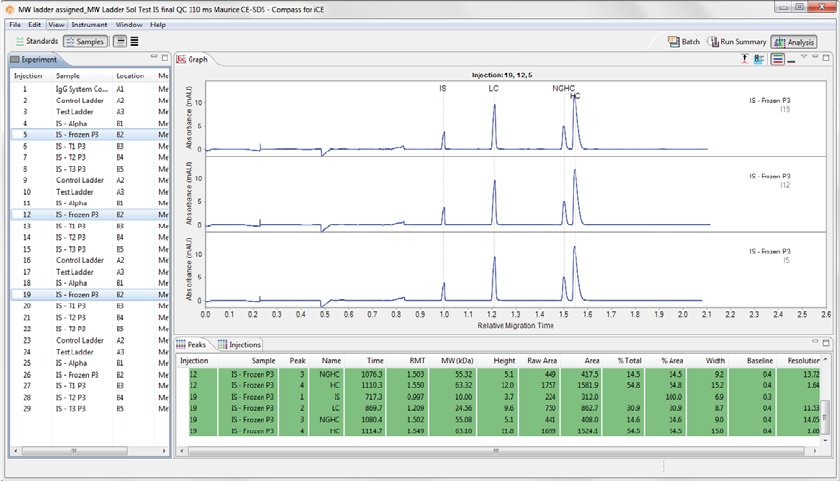
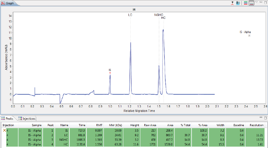
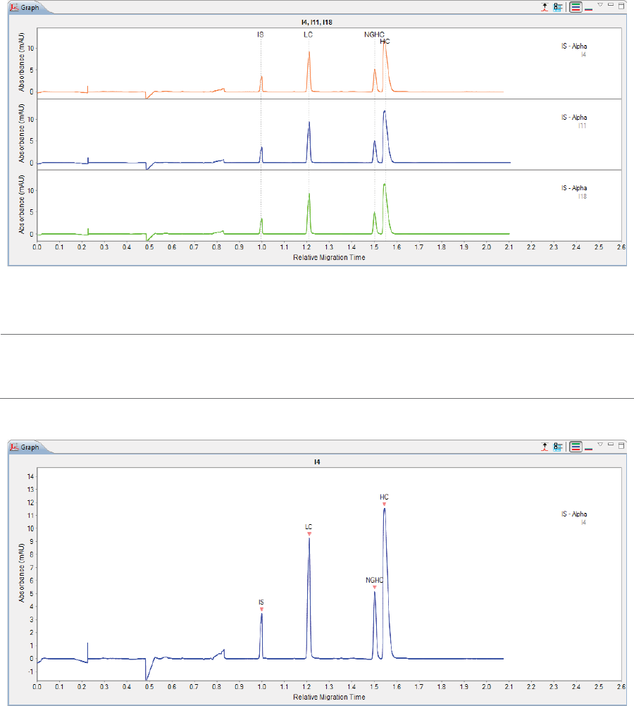
Graph Pane: Electropherogram Data
The Graph pane displays the electropherogram(s) for sample proteins or internal standards depending on
the view options you’ve selected.
page 202 Chapter 11: CE-SDS Data Analysis
User Guide for Maurice, Maurice C. and Maurice S.
You can get more info on graph view options in “Changing the Electropherogram View” on page 226.
Peaks Pane: Calculated Results
The Peaks pane shows the tabulated results for your sample proteins or internal standards. Each row in the
table has the individual results for each peak detected in an injection. Results shown will either be for one
injection or multiple injections, samples or standards depending on the view options you’re using. Check
out “Viewing Run Data” on page 205 for more info.
NOTES:
Peaks that Compass for iCE names automatically with user-defined peak name settings are color-coded.
When the Standards view is selected, the information in the Peaks table includes only injection, sample,
peak, time and height. Internal standards the software has identified are marked with an S.
•To view all rows - Use the scroll bar or click Maximize in the upper right corner.
How Run Data is Displayed page 203
User Guide for Maurice, Maurice C. and Maurice S.
•To resize columns - Roll the mouse over a column border until the sizing arrow appears, then click
and drag to resize.
The following results and info are listed in the Peaks table:
•Injection - Injection number.
•Sample - If sample names were entered in the batch, those names will display here. Otherwise, Sample
(default name) will display.
•Peak - Peaks are numbered in order of detection.
•Name - Displays peaks Compass for iCE named automatically using the user-defined peak name anal-
ysis parameters. These cells are blank if the software wasn’t able to name the peak or if you didn’t
enter naming parameters.
•Time - Peak detection time (seconds). This is the elapsed time between the start of the separation
and when the peak is detected.
•RMT - Relative migration time of the peak to the Internal Standard which has an RMT of 1.0.
•MW (kDa) - Displays the relative molecular weight in kDa for sample peaks. MW only displays if you’ve
run the CE-SDS MW Markers as one of the injections in the run and identified that injection in your
analysis parameters.
•Height - The calculated peak height.
•Raw Area - Displays the uncorrected peak area.
•Area - Displays the time-corrected peak area. This includes corrections for big and/or slow moving
peaks which can be artificially large when uncorrected.
•% Total - Displays the peak area ratio compared to the sum of all peak areas (excluding the Internal
Standard peak). This value results from dividing the individual peak area by the sum of all peak areas
for the injection and multiplying by 100.
•% Area - Displays the calculated percent area for the named peak compared to all named peaks. This
value results from dividing the individual peak area by the sum of all named peak areas for the injec-
tion and multiplying by 100 (shown for named peak sample data only).
•Width - Displays the calculated peak width (sample data only).
•Baseline - Displays the raw baseline signal of each peak.
•Resolution - Displays resolution of the peak compared to neighboring peaks. Two peaks that are
baseline resolved will have a resolution value of 1.5. Smaller values means the peaks are not com-
pletely resolved, larger values mean the peaks are fully resolved.
page 204 Chapter 11: CE-SDS Data Analysis
User Guide for Maurice, Maurice C. and Maurice S.
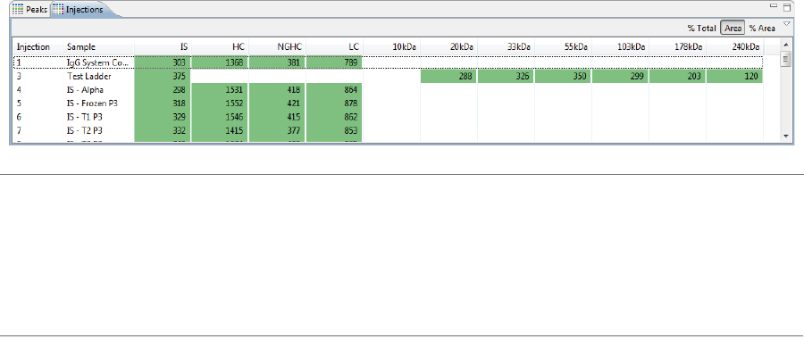
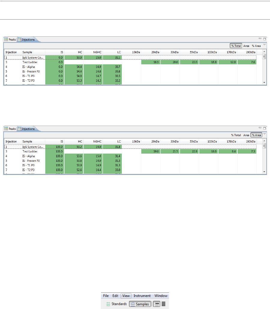
Injections Pane: User-Specified Peak Names
The Injections pane shows tabulated results for sample proteins Compass for iCE labels automatically using
user-defined peak name settings. Each row in the table shows the individual results for the named peaks
detected in each injection.
NOTES:
Peaks that Compass for iCE names automatically with user-defined peak name settings are color-coded.
When the Standards view is selected, the information in the Injections table includes only injection, sam-
ple and std 1 (the migration time of the standard peak).
•To view all rows - Use the scroll bar or click Maximize in the upper right corner.
•To resize columns - Roll the mouse over a column border until the sizing arrow appears, then click
and drag to resize.
The following results and info are listed in the Injections table:
•Injection - Injection number.
•Sample - If sample names were entered in the batch, those names will display here. Otherwise, Sample
(default name) will display.
•Peak Name Columns - An individual column per peak name will display for every peak identified by
name or as a MW Marker peak in the run data. Cells for injections in these columns will be blank if
Compass for iCE didn’t find peaks automatically using the user-defined peak name analysis and maker
parameters (or none were entered).
•To view peak area in the peak name columns (default) - Select Area in the upper right corner
of the pane. This displays calculated peak area for the individual peak only.
•To view % total in the peak name columns - This displays the calculated percent area for the
named peak compared to all named peaks. This value results from dividing the individual peak
area by the sum of all named peak areas for the injection and multiplying by 100.
Viewing Run Data page 205
User Guide for Maurice, Maurice C. and Maurice S.
NOTE: The sum of the named peak percentages can be less than 100% if some peaks aren’t named.
•To view % area in the peak name columns - This displays the peak area ratio compared to the
sum of all named peak areas. This value results from dividing the individual peak area by the sum
of all peak areas for the injection and multiplying by 100.
Viewing Run Data
The Analysis screen lets you view data for just one injection, specific injections or all injections in the run.
Each run file has data for the sample proteins and the Internal Standard detected in each injection.
Switching Between Samples and Standards Data Views
Here’s how you switch between viewing data for your samples and standards:
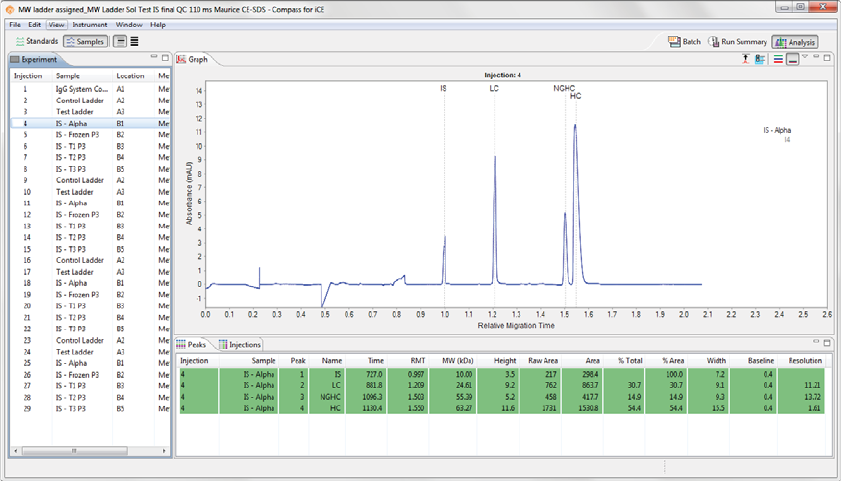
•To view sample data - Click Samples in the View bar or select View in the main menu and click
Samples.
• Data in this view is for sample proteins only.
page 206 Chapter 11: CE-SDS Data Analysis
User Guide for Maurice, Maurice C. and Maurice S.
• The graph displays electropherograms with a y-axis of Absorbance units (mAU) and an x-axis of
RMT (relative migration time).
• Results for each protein are shown in the Peaks and Injections panes.
For information on checking and identifying sample peaks, see “Checking Your Data” on page 139.
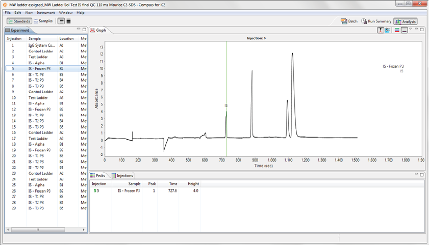
•To view Internal Standard data - Click Standards in the View bar or select View in the main menu
and click Standards.
• Data in this view is for analyzing standards only. This is the Internal Standard you add to your sam-
ples during prep.
• The graph displays electropherograms with a y-axis of Absorbance units (mAU) and an x-axis of
time in seconds.
Viewing Run Data page 207
User Guide for Maurice, Maurice C. and Maurice S.
• The Internal Standard is identified in the Peaks pane with an S and as Std1 in the Injections pane.
For information on checking and identifying the Internal Standard peak, see “Checking Your Data” on
page 139.
page 208 Chapter 11: CE-SDS Data Analysis
User Guide for Maurice, Maurice C. and Maurice S.
Selecting and Displaying Injection Data
You can view data from one, multiple, or all injections at once.
•To look at data for one injection - Click an injection row in the Experiment pane. Data for just that
injection displays in the graph and tables.
Viewing Run Data page 209
User Guide for Maurice, Maurice C. and Maurice S.
•To look at data for specific injections - Hold the Ctrl key and select just the injection rows you want
to view in the Experiment pane. Data for only the injections selected display in the graph and tables.
page 210 Chapter 11: CE-SDS Data Analysis
User Guide for Maurice, Maurice C. and Maurice S.
•To look at data for sequential injections - Select the first injection row in the Experiment pane that
you want to view, then hold the Shift key and select the last. This selects all rows between the two
injections. Data for only the injections selected display in the graph and tables.
Viewing Run Data page 211
User Guide for Maurice, Maurice C. and Maurice S.
•To look at data for all injections - Just click View All in the View bar. Data for all injections displays in
the graph and tables.
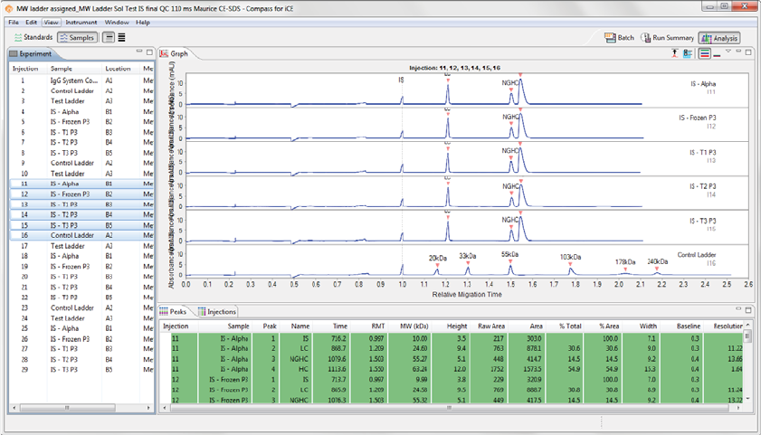
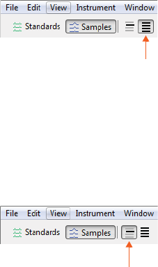
Switching Between Single and Multiple Views of Injections
You can switch between displaying run data in a single, per-injection format or a multi-injection format.
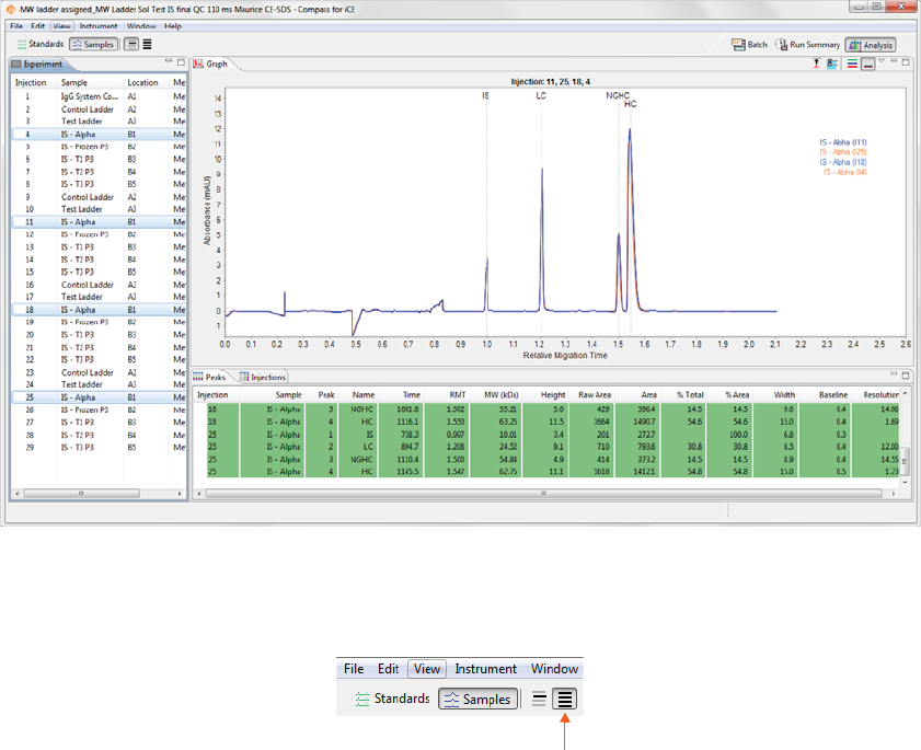
•To view data per in a per-injection format - Click Single View in the View bar or select View in the
main menu and click Single View.
Data for the injection row(s) selected in the Experiment pane:
• Displays with electropherograms either overlaid or stacked in the Graph pane depending on the
option you’ve got chosen.
page 212 Chapter 11: CE-SDS Data Analysis
User Guide for Maurice, Maurice C. and Maurice S.
• Shows only results for the selected row(s) in the Peaks and Injections panes.
•To view data in a multi-injection format - Click View All in the View bar or select View in the main
menu and click Multiple View:
Data for the injection row(s) selected in the Experiment pane:
• Displays with the electropherograms of the selected injections highlighted in the Graph pane.
• Shows the results for the selected injections highlighted in the Peaks and Injections panes.
Viewing Run Data page 213
User Guide for Maurice, Maurice C. and Maurice S.
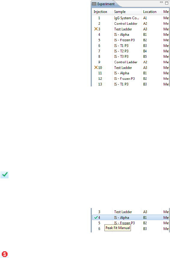
Hiding Injection Data
You can hide injection data from the view if needed.
•To hide injections - Select the injection rows you want to hide in the Experiment pane, then right
click one and select Hide.
Data for the injections will be hidden in all data views and results tables.
page 214 Chapter 11: CE-SDS Data Analysis
User Guide for Maurice, Maurice C. and Maurice S.
•To view hidden injections - Select View in the main menu and click Show Hidden. Hidden rows
will become visible again in all panes, and are marked with an X in the Experiment pane.
•To unhide injections - Select the hidden row(s). Right click on one and click Unhide.
Data Notifications and Warnings
If Compass for iCE detects a potential data issue, a notification or warning icon will display next to the injec-
tion row in the Experiment pane.
Manual correction of sample data notification - This means the sample data was manually
changed by a user, for example to add or remove a sample peak. Roll your mouse over the icon
to display the type of modification that was made.
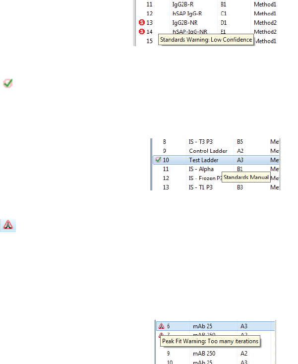
Standards warning - This means the Internal Standard may not be identified properly. You
can fix this by manually identifying the standard using the steps in “Step 1: Check Your Internal
Standard” on page 139. Roll your mouse over the icon to display warning details.
Checking Your Results page 215
User Guide for Maurice, Maurice C. and Maurice S.
Checking Your Results
Compass for iCE detects your sample protein, CE-SDS MW Markers and Internal Standard peaks and reports
results automatically. But, we always recommend you review and check your data as a good general practice
to make sure your results are accurate. Please see the step by step procedure in “Checking Your Data” on
page 139 to do this. If you see a data warning in the Experiment pane, these steps will also help you identify
and correct any issues.
Manual correction of standards data notification - This means a user changed the stan-
dards data manually. Roll your mouse over the icon to display the type of modification that was
made.
Peak fit warning - Means that a peak can’t be fit properly. This can sometimes be caused
when a broad peak is fitted as multiple narrow peaks. Changing the peak width can help in this
case. The warning is also caused by very small peaks around main peaks, or small peaks that are
close to the end of the separation range. You can often fix this by removing the peak(s) using
the steps in “Step 3: Checking Sample Peaks” on page 147. Roll your mouse over the icon to
display warning details.
page 216 Chapter 11: CE-SDS Data Analysis
User Guide for Maurice, Maurice C. and Maurice S.
Group Statistics
You can use the Grouping view to have Compass for iCE do a statistical analysis of named proteins in your
injections (see “Peak Names Settings” on page 271 for more info on setting named peaks up). Statistics for
each protein are also plotted for easy comparison.
Using Groups
1. Groups are automatically created for injections that use the same sample name and method, so to use
this feature, you need to make sure you’ve got sample names entered.
a. Go to the Batch screen.
b. Click the Sample ID cells in the Injection pane and type a name for any samples you want to calcu-
late statistics for.
2. Go back to the Analysis screen. Click View in the main menu and select Grouping.
NOTE: To turn Grouping off, select View in the main menu and deselect Grouping.
Group Statistics page 217
User Guide for Maurice, Maurice C. and Maurice S.
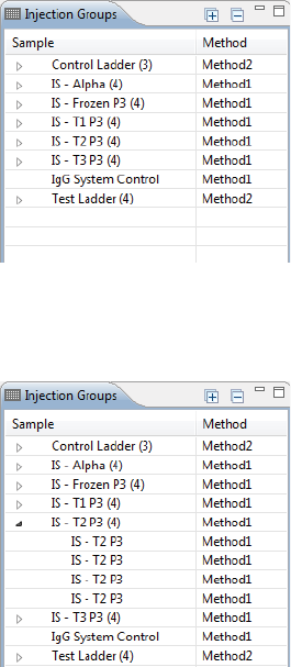
Viewing Sample Injection Groups
Compass for iCE automatically groups all injections using the same sample name together in the Injection
Groups pane.
•To expand a group - Click the arrow next to a group to see the individual injections in the group and
reported data for each
•To expand all groups - Click Expand All (+) in the upper right corner of the pane.
•To collapse all groups - Click Collapse All (-) in the upper right corner of the pane.
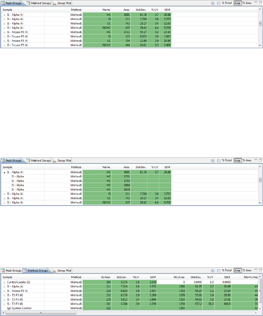
Viewing Statistics
Peak and Method Groups
The Peak Groups pane reports statistics for each named protein in every group. Each group shows the statis-
tics for named proteins which includes average area, standard deviation, %CV and SEM (standard error mea-
surement). The number in parenthesis after the sample name is the number of injections in the group.
page 218 Chapter 11: CE-SDS Data Analysis
User Guide for Maurice, Maurice C. and Maurice S.
•To display results using area - Click Area in the upper right corner of the pane.
•To display results using % total - Click % Total in the upper right corner of the pane to display the
calculated percent area for the named peak compared to the total area measured in the injection.
This value results from dividing the individual peak area by the sum of all peak areas for the injection
and multiplying by 100.
•To display results using % area - Click % Area in the upper right corner of the pane to display the
calculated percent area for the named peak compared to all named peaks. This value results from
dividing the individual peak area by the sum of all named peak areas for the injection and multiplying
by 100 (shown for named peak sample data only).
•To expand a group - Click the arrow next to a group to see the individual injections in the group and
reported data for each
•To expand all groups - Click Expand All (+) in the upper right corner of the pane.
•To collapse all groups - Click Collapse All (-) in the upper right corner of the pane.
The Method Groups pane pivots the Peak Groups pane results to show statistics for named protein peaks in
individual columns.
Group Statistics page 219
User Guide for Maurice, Maurice C. and Maurice S.
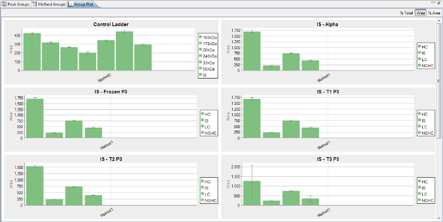
Group Plots
The mean values for named peaks using the same method in each injection group are plotted in bar graphs
with error bars showing the standard deviation in the Group Plots pane. You’ll also get plots that compare
samples using the same method in the run.
Hiding or Removing Injections in Group Analysis
Hidden injections are not included in injection groups. But, hiding injections gives you an easy way to reject
individual injections from the statistical analysis. See “Hiding Injection Data” on page 213 for details on how
to do this.
page 220 Chapter 11: CE-SDS Data Analysis
User Guide for Maurice, Maurice C. and Maurice S.
Copying Results Tables and Graphs
You can copy and paste data and results tables into other documents, or save the electropherogram as a
graphic file.
Copying Results Tables
1. Click in the Peaks or Injections pane.
2. Select one or multiple rows.
3. Select Edit in the main menu and click Copy, or right click on row(s) you selected and click Copy.
4. Open a document (Microsoft® Word®, Excel®, PowerPoint®, etc.). Right click in the document and select
Paste. Data for the rows selected will be pasted into the document.
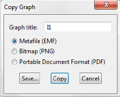
Copying the Graph
1. Select the Graph pane.
2. Select Edit in the main menu and click Copy, or right click in the Graph pane and select Copy.
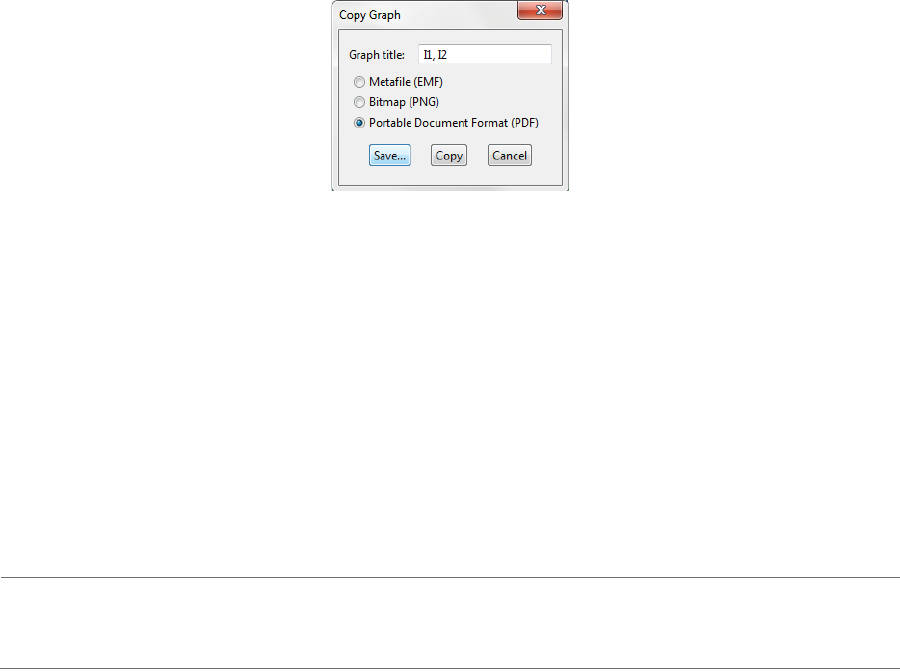
3. Select an image option (EMF, PNG or PDF) in the pop-up window, then click Copy.
4. Open a document (Microsoft® Word®, Excel®, PowerPoint®, etc.). Right click in the document and select
Paste. A graphic of the copied electropherogram will be pasted into the document.
Saving the Graph as an Image File
1. Select the Graph pane.
2. Select Edit in the main menu and click Copy, or right click in the Graph pane and select Copy.
3. Select an image option (EMF, PNG or PDF) in the pop-up window, then click Save.
Exporting Run Files page 221
User Guide for Maurice, Maurice C. and Maurice S.
4. Select a directory to save the file to, enter a file name, then click OK.
Exporting Run Files
Results tables and raw plot data can be exported for use in other applications.
Exporting Results Tables
To export the information in the Peaks and Injections tables:
1. Click File in the main menu and click Export Tables.
2. Select a directory to save the files to and click OK. Data will be exported in .txt format.
NOTE: To exclude export of standards data or export results table data in .csv format, see “Setting Data
Export Options” on page 379.
Exporting Raw Sample Electropherogram Data
To export raw sample plot and background data:
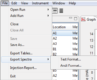
1. Click File in the main menu and click Export Spectra.
page 222 Chapter 11: CE-SDS Data Analysis
User Guide for Maurice, Maurice C. and Maurice S.
•To export data in .txt format - Select Text Format. Data will be exported in one file for all injec-
tions.
•To export data in .cdf format - Select Andi Format. Data will be exported in one file per injec-
tion.
2. Select a directory to save the files to and click OK. Data will be exported in the selected format.
Changing Sample Protein Identification
Compass for iCE lets you customize what sample proteins are reported in the results tables by making man-
ual adjustments in the electropherogram or Peaks table.
Adding or Removing Sample Data
1. Click Show Samples in the View bar.
2. Click Single View in the View bar.
3. Click on the row in the experiment pane that has the injection you want to correct, then click the Graph
tab.
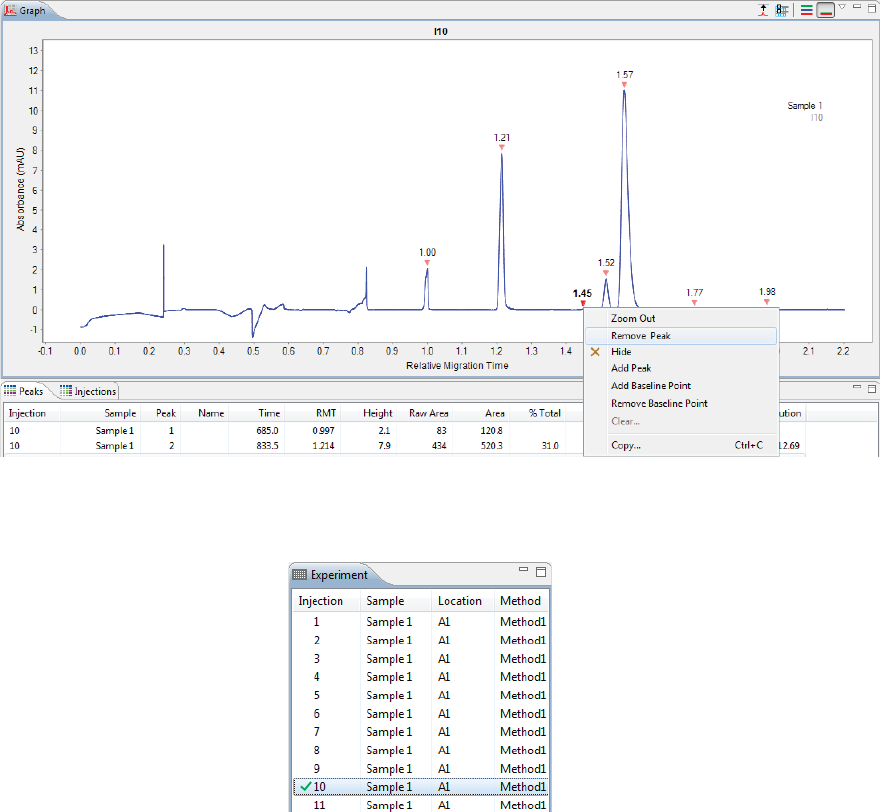
•To remove a peak from the data - Right click the peak in the electropherogram or Peaks table
and select Remove peak. The software will no longer identify it as a sample peak in the elec-
tropherogram, and the peak data will be removed in the results tables.
Changing Sample Protein Identification page 223
User Guide for Maurice, Maurice C. and Maurice S.
A check mark will appear next to the injection in the Experiment pane to indicate a manual correc-
tion was made.
•To add an unidentified peak to the data - Right click the peak in the electropherogram or
peaks table and select Add Peak. The software will calculate and display the results for the
peak in the results tables and identify the peak in the electropherogram.
A check mark will appear next to the injection in the Experiment pane to indicate a manual cor-
rection was made.
page 224 Chapter 11: CE-SDS Data Analysis
User Guide for Maurice, Maurice C. and Maurice S.
NOTE: To remove sample peak assignments that were made manually and go back to the original peak
data, right-click the peak in the electropherogram and select Clear for the current injection or Clear All
for all injections in the batch.
Hiding Sample Data
You can hide the results for a sample protein in the results tables without completely removing it from the
reported results.
1. Click Show Samples in the View bar.
2. Click Single View in the View bar.
3. Click on the row in the experiment pane that contains the injection you want to correct, then click the
Graph tab.
4. Right click the peak in the electropherogram or Peaks table and select Hide. Compass for iCE will hide
the peak data in the results tables.
Changing Sample Protein Identification page 225
User Guide for Maurice, Maurice C. and Maurice S.
5. To view hidden peak data, click View in the main menu and click Show Hidden. Hidden peak data will
display in the results table and be marked with an X.
6. To unhide a peak, right click on the peak in the electropherogram or peaks table and select Unhide.
Changing Peak Names for Sample Data
If Compass for iCE did not automatically name a sample protein peak, you can do it manually.
1. Click Show Samples in the View bar.
2. Click Single View in the View bar.
3. Click on the row in the experiment pane that has the sample you want to correct, then click the Graph
pane.
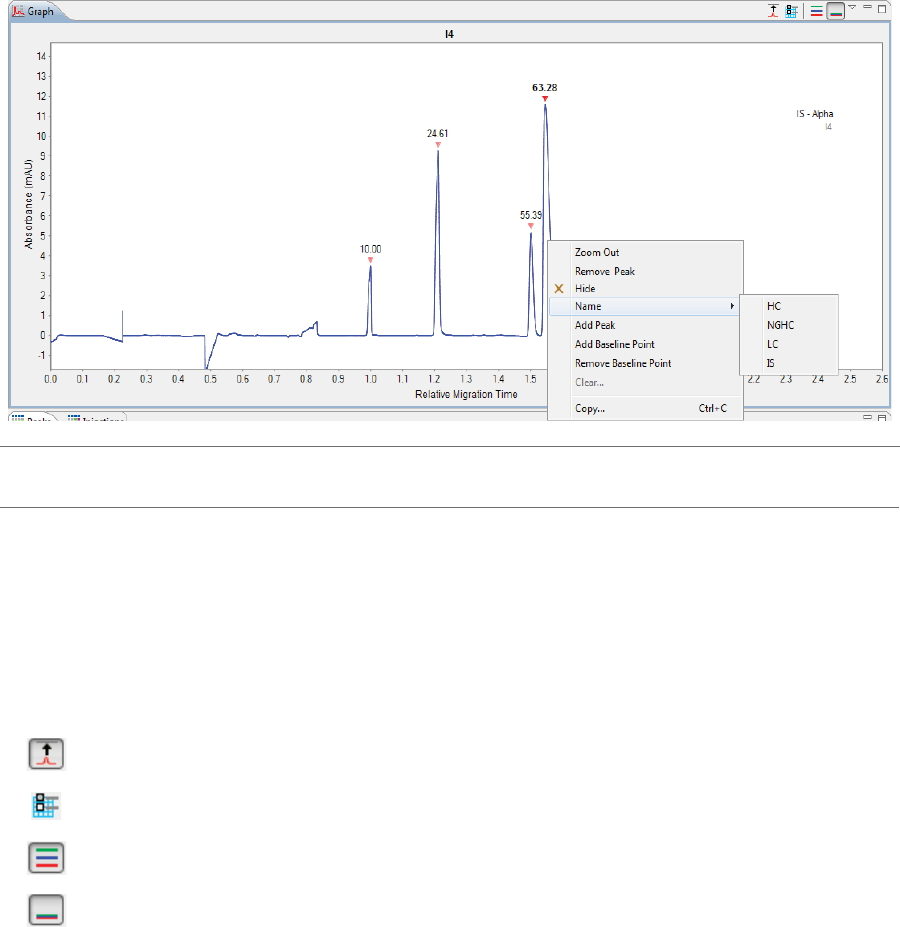
page 226 Chapter 11: CE-SDS Data Analysis
User Guide for Maurice, Maurice C. and Maurice S.
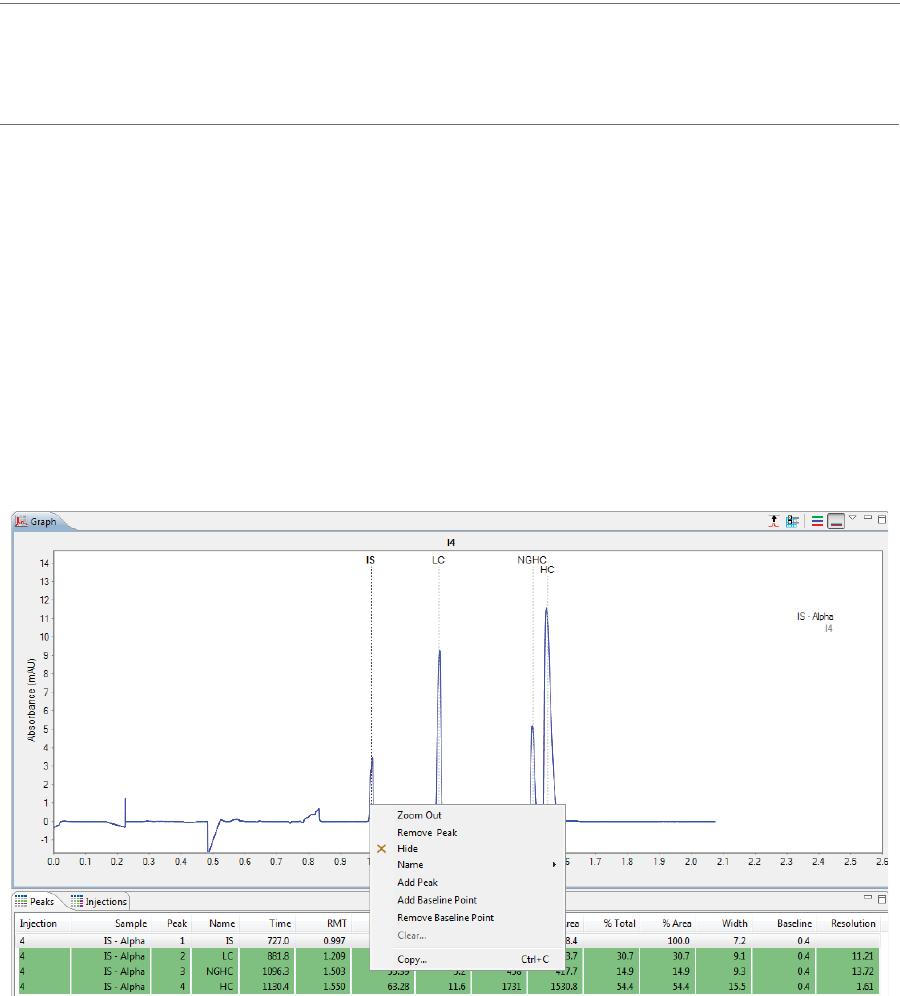
4. Right click the peak in the electropherogram or Peaks table and click Name, then select a name from
the list. Compass for iCE will change the peak name in the electropherogram and results tables, and
adjust peak names for other sample proteins accordingly.
NOTE: For details on how to specify peak name settings, see “Peak Names Settings” on page 271.
Changing the Electropherogram View
Options in the Graph pane let you zoom and rescale electropherograms, overlay or stack plots and change
the peak and plot info displayed.
The Graph pane toolbar has these options:
Auto Scale
Graph Options
Stack the Plots
Overlay the Plots
Changing the Electropherogram View page 227
User Guide for Maurice, Maurice C. and Maurice S.
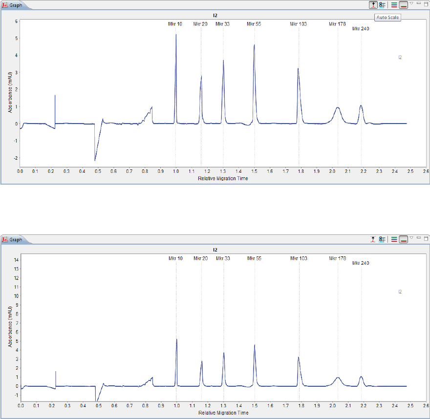
Autoscaling the Electropherogram
Click the Auto Scale button to scale the y-axis to the largest peak in the electropherogram.
Click the Auto Scale button again to return to default scaling.
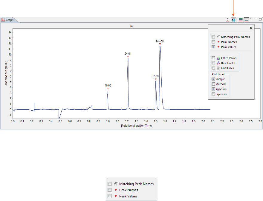
Customizing the Data Display
You can customize electropherogram peak labels, plot labels and display options. To do this, just select the
Graph Options button.
page 228 Chapter 11: CE-SDS Data Analysis
User Guide for Maurice, Maurice C. and Maurice S.
Peak Labels
You can customize the labels used to identify peaks in the electropherogram with these options:
•Matching Peak Names - Checking this box will draw vertical lines through each named peak. Using
this option with Stack the Plots or Overlay the Plots features is helpful for visually comparing your
named peaks across multiple injections.
Changing the Electropherogram View page 229
User Guide for Maurice, Maurice C. and Maurice S.
•Peak Names - Checking this box displays peak name labels on all named peaks in the electrophero-
gram.
NOTE: If more than one peak label option is selected, peak name labels will always be used for named
peaks.
•Peak Values - Checking this box will display the molecular weight labels on all peaks in the electro-
pherogram.
page 230 Chapter 11: CE-SDS Data Analysis
User Guide for Maurice, Maurice C. and Maurice S.
NOTE: If more than one peak label option is selected, peak name labels will always be used for named
peaks.
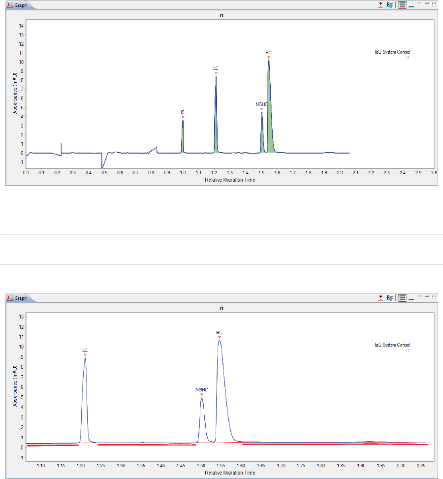
Baseline and Grid Options
You can view the calculated baseline fit, peak integration and show grid lines with these options.
•Fitted peaks - Checking this box displays how the peaks were fit by the software. For CE-SDS runs,
the software uses Gaussian fit by default.
NOTE: This option is only available for sample data.
Changing the Electropherogram View page 231
User Guide for Maurice, Maurice C. and Maurice S.
•Baseline Fit - Checking this box displays the calculated baseline for the peaks. Baseline points will
also display for regions of the electropherogram considered to be at baseline.
NOTE: This option is only available for sample data.
page 232 Chapter 11: CE-SDS Data Analysis
User Guide for Maurice, Maurice C. and Maurice S.
•Grid Lines - Checking this box adds grid lines in the graph.
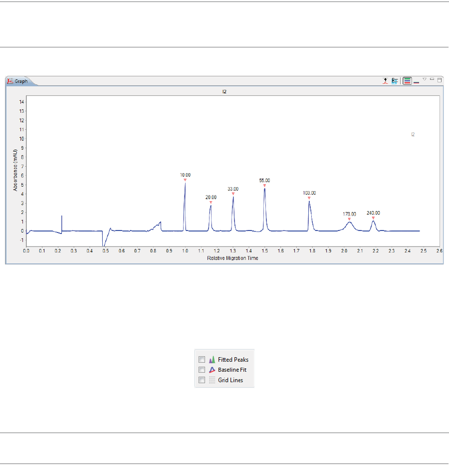
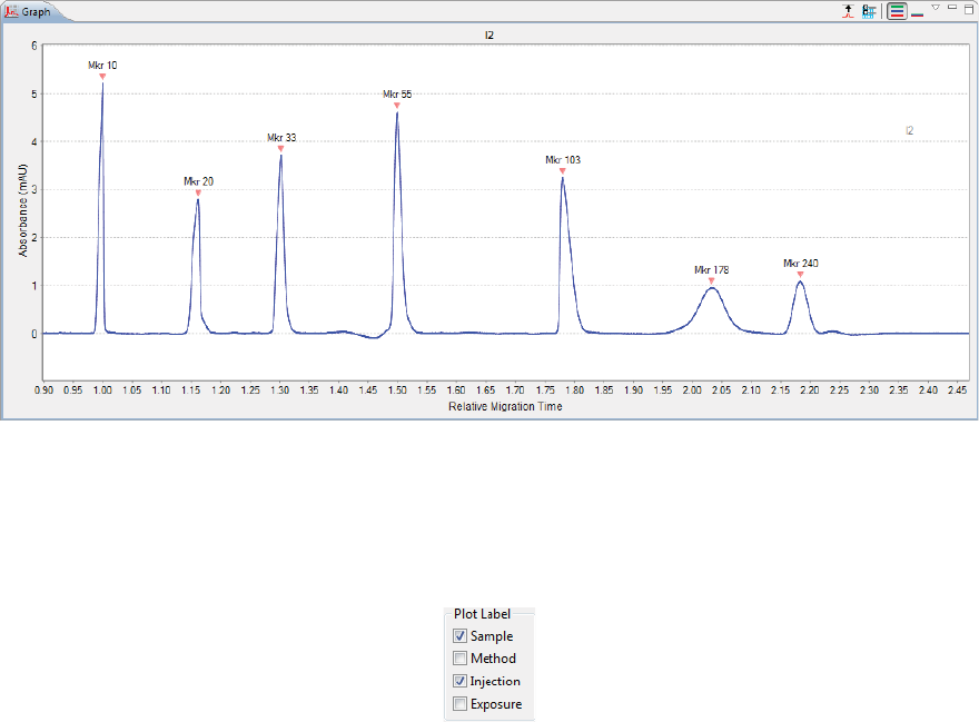
Plot Labels
You can customize the plot labels displayed on the electropherogram with these options.
Plot labels are shown in the upper right side of the graph.
•Sample - Checking this box displays the sample name used for the injection. If sample names were
entered with the batch, those names will display here. If not, Sample (default name) displays.
•Method - Checking this box displays the method used for the injection.
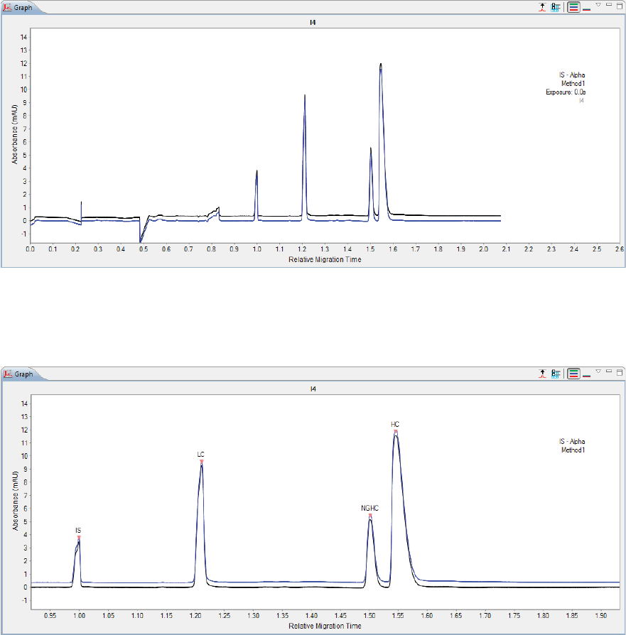
•Exposure - Checking this box display the exposure time(s) used for the data. For CE-SDS data this
value will be 0.0 seconds.
•Injection - Checking this box displays the injection number. For example, I4 for injection 4 in the run.
Here’s an example of an electropherogram with all plot labels selected:
Changing the Electropherogram View page 233
User Guide for Maurice, Maurice C. and Maurice S.
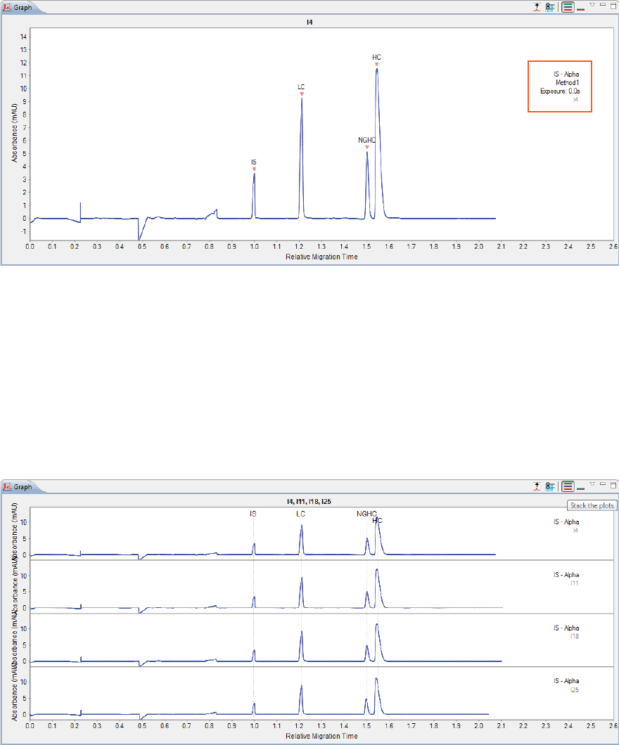
Stacking Multiple Electropherograms
You can stack electropherograms for multiple injections vertically in the Graph pane for comparison.
1. Click Single View.
2. Select multiple injection rows in the Experiment pane.
3. Click the Stack the Plots button. The individual electropherograms for each injection you selected will
stack in the Graph pane.
page 234 Chapter 11: CE-SDS Data Analysis
User Guide for Maurice, Maurice C. and Maurice S.
You can also customize the colors used for the stacked plot display. To do that go to “Selecting Custom Plot
Colors for Graph Overlay” on page 380.
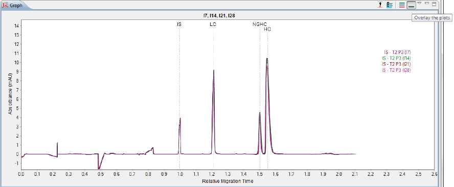
Overlaying Multiple Electropherograms
You can overlay electropherograms for multiple injections on top of each other for comparison in the Graph
pane.
1. Click Single View.
2. Select multiple injection rows in the Experiment pane.
3. Click the Overlay the Plots button. The individual electropherograms for each injection you selected
will overlay in the Graph pane.
You can also customize the colors used for the overlay plot display. To do that go to “Selecting Custom Plot
Colors for Graph Overlay” on page 380.
Changing the Electropherogram View page 235
User Guide for Maurice, Maurice C. and Maurice S.
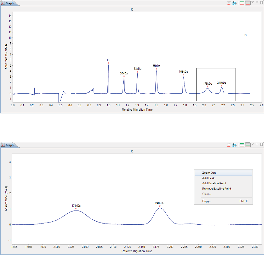
Zooming
To zoom in on a specific area of the electropherogram, hold the mouse button down and draw a box around
the area with your mouse:
To return to default scaling, right click in the electropherogram and click Zoom Out.
page 236 Chapter 11: CE-SDS Data Analysis
User Guide for Maurice, Maurice C. and Maurice S.
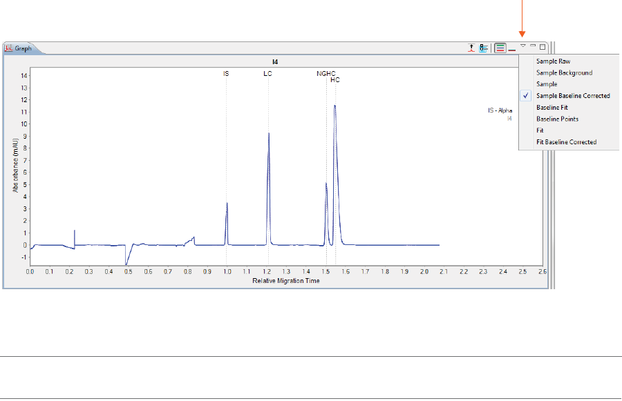
Selecting Data Viewing Options
The graph view menu gives you multiple options for changing what type of electropherogram data is dis-
played. Just click the down arrow next to the graph pane toolbar to view the menu:
A check mark next to the menu option indicates it’s currently selected, and you can select multiple options
at once.
NOTE: Unless noted otherwise, graph view menu options are available for sample data only.
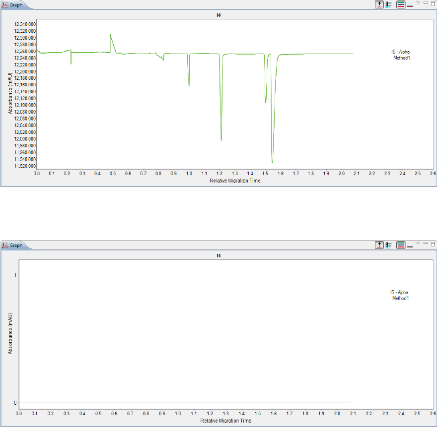
•Sample Raw - Clicking this option displays the basic detector values used to calculate peak absor-
bance. To view this you’ll need to select Auto Scale in the Graph pane tool bar.
Changing the Electropherogram View page 237
User Guide for Maurice, Maurice C. and Maurice S.
•Sample Background - Clicking this option displays the basic detector values used to calculate base-
line absorbance. To view this you’ll need to select Auto Scale in the Graph pane tool bar.
page 238 Chapter 11: CE-SDS Data Analysis
User Guide for Maurice, Maurice C. and Maurice S.
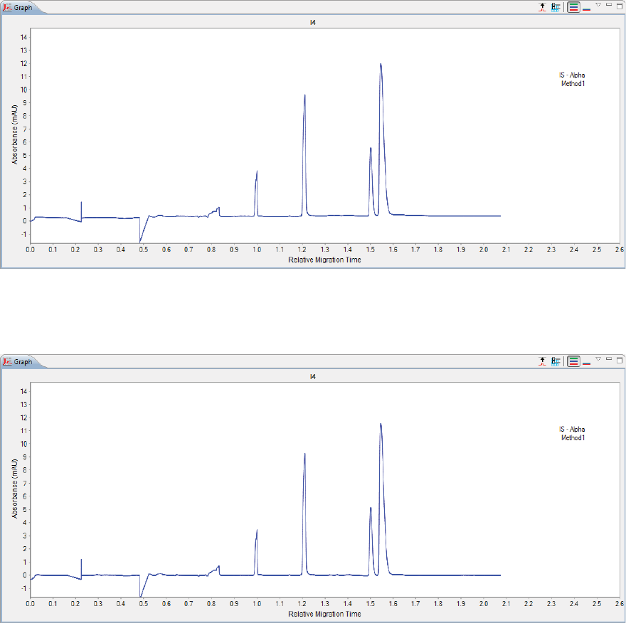
•Sample - Clicking this option displays raw, uncorrected sample data.
•Sample Baseline Corrected - Clicking this option displays sample data with the baseline subtracted
(zeroed). This is the default view.
•Baseline Fit - Clicking this option displays the calculated baseline for the raw sample data. In this
next example, both Baseline Fit and Sample are selected.
Changing the Electropherogram View page 239
User Guide for Maurice, Maurice C. and Maurice S.
NOTE: This option is selected automatically when Baseline Fit is selected in graph options.
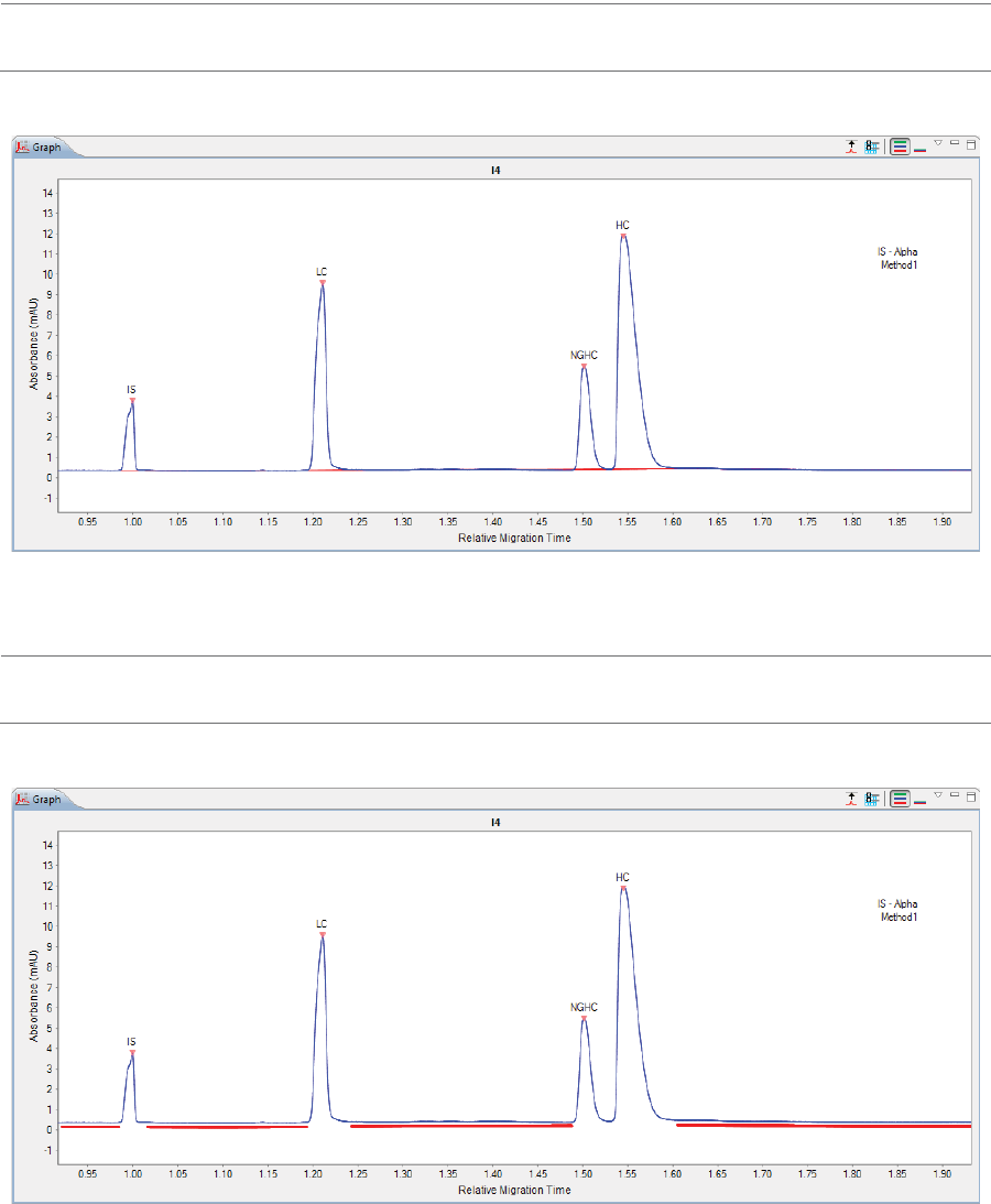
•Baseline Points - Clicking this option displays regions of the electropherogram considered to be at
baseline. In this example, both Baseline Points and Sample are selected.
NOTE: This option is selected automatically when Baseline Fit is selected in graph options.
page 240 Chapter 11: CE-SDS Data Analysis
User Guide for Maurice, Maurice C. and Maurice S.
•Fit - Clicking this option displays the bounding envelope of the fitted peaks as calculated by the soft-
ware for the raw sample data. In this example, both Fit and Sample Baseline Corrected are selected.
•Fit Baseline Corrected - Clicking this option displays the fitted peaks as calculated by the software
for the sample baseline corrected data. In this example, both Fit Baseline Corrected and Sample are
selected, the fit plot is on the bottom.
Adding and Removing Baseline Points
Points in the baseline can be added or removed as needed.
Changing the Electropherogram View page 241
User Guide for Maurice, Maurice C. and Maurice S.
1. Click the Graph Options button in the graph pane toolbar and check Baseline Points. This will display
baseline points for the raw sample data.
2. Use the mouse to draw a box around the area you want to correct. This will zoom in on the area.
3. Right click a baseline point and select Add Baseline Point or Remove Baseline Point.
NOTE: To clear the manual addition or removal of baseline points and go back to the original view of the
data, right click in the electropherogram and click Clear All.
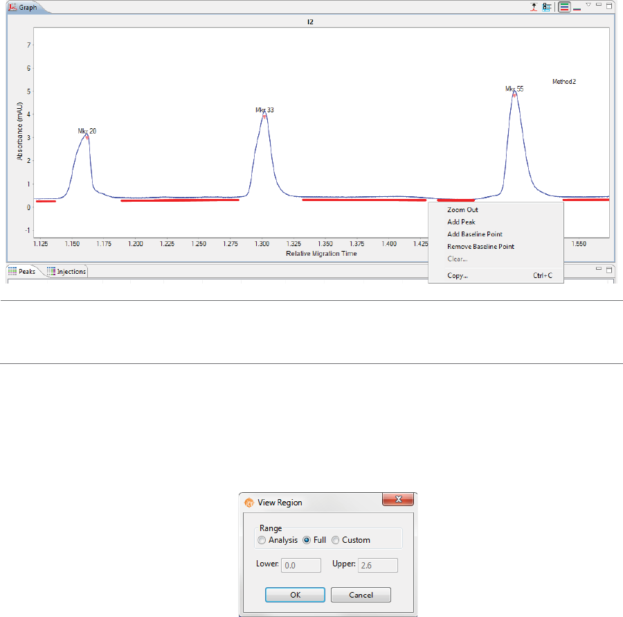
Selecting the Graph X-axis Range
The RMT (relative migration time) range used for the x-axis can be changed. Just select View in the main
menu and click View Region.
page 242 Chapter 11: CE-SDS Data Analysis
User Guide for Maurice, Maurice C. and Maurice S.
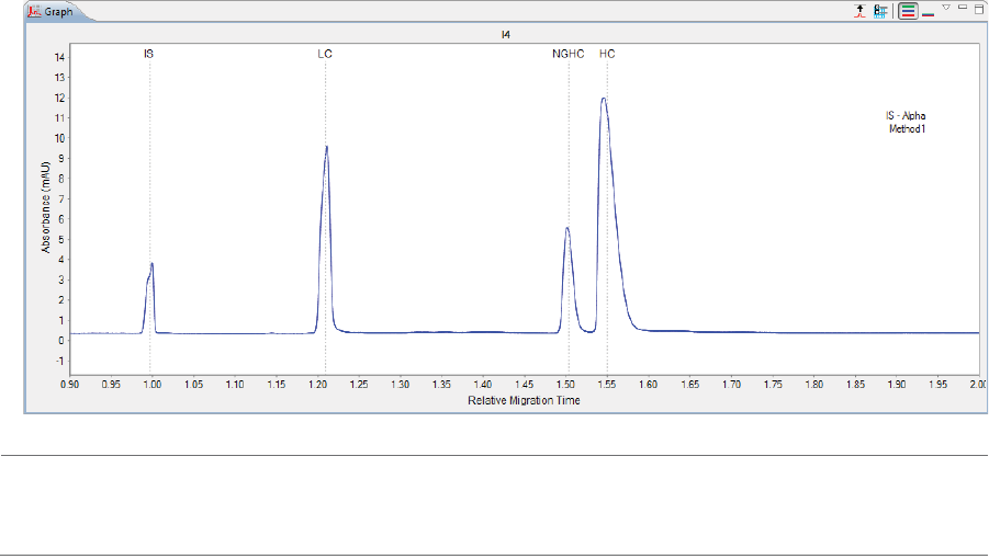
•Analysis sets the x-axis range of the electropherogram to what is selected in the Peak Fit range set-
tings. To view or change these analysis settings, go to Edit > Analysis and click Peak Fit in the left
sidebar. In this example, the lower and upper range settings are 0.9 and 2.5.
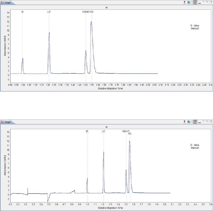
•Full displays the entire separation in the electropherogram. This is the default setting. In this example
the lower and upper range settings are 0 and 2.6.
•Custom lets you manually enter the lower and upper range settings to display in the electrophero-
gram. In this example the lower and upper range settings are 0.9 and 2.0.
Closing Run Files page 243
User Guide for Maurice, Maurice C. and Maurice S.
NOTE: You can change the default x-axis range that Compass for iCE uses. Go to “Advanced Analysis Set-
tings” on page 246 for more info.
Closing Run Files
If more than one run file is open, you can close just one file or all the open files at the same time.
•To close one run file - In the Experiment pane, click on one of the sample rows in the file. Then click
File from the main menu and click Close.
•To close all open run files - Select File from the main menu and click Close All.
page 244 Chapter 11: CE-SDS Data Analysis
User Guide for Maurice, Maurice C. and Maurice S.
Analysis Settings Overview
Compass for iCE has many analysis features and settings that you can change to enhance your run data.
Select Edit in the main menu and click Analysis. If more than one run file is open, select the run file you
want to view settings for from the list:
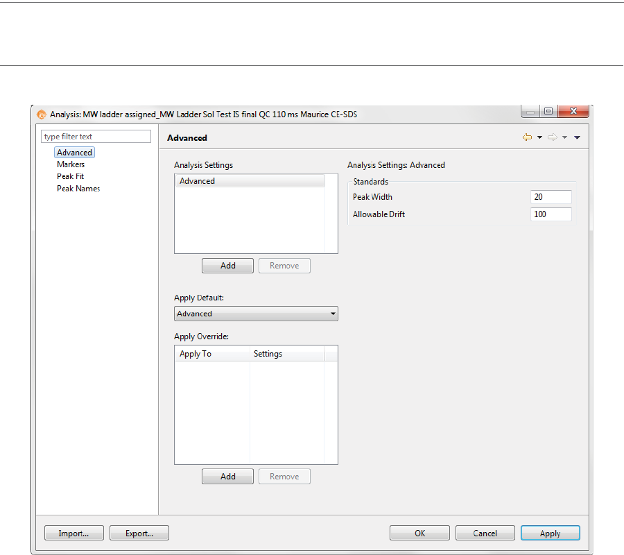
This opens the Analysis window:
Analysis Settings Overview page 245
User Guide for Maurice, Maurice C. and Maurice S.
To move between pages in the window, click on an option in the left sidebar.
•Advanced - Lets you customize analysis settings for the Internal Standard.
•Markers - Lets you customize the Internal Standard migration time, and the molecular weight and
RMT Compass for iCE uses to identify your CE-SDS MW Markers.
•Peak Fit - Lets you customize peak fit settings for sample data.
•Peak Names - Lets you enter custom naming settings for sample proteins and have Compass for iCE
automatically label the peaks in the run data.
On all pages in the Analysis window:
•Click Import to import an analysis settings file. Go to “Importing Analysis Settings” on page 283 to
learn how to do this.
•Click Export to export the current analysis settings file. Go to “Exporting Analysis Settings” on
page 283 to learn how to do this.
•Click Apply to apply changes to the run file and update results in real time.
•Click OK to save changes to the run file and exit.
•Click Cancel to exit without saving changes.
page 246 Chapter 11: CE-SDS Data Analysis
User Guide for Maurice, Maurice C. and Maurice S.
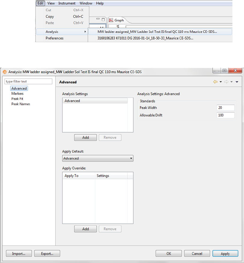
Advanced Analysis Settings
This page lets you view and change analysis settings for the Internal Standard data. Select Edit in the main
menu and click Analysis, then click Advanced in the left sidebar:
NOTE: Settings can be changed in batches before you start the run, or in run files once they’re completed. If
you make analysis settings changes to an executing run, they won’t be saved to the final run file.
Internal Standard Settings
•Peak Width - The approximate width (at full width half max) used to filter out absorbance artifacts
which improves recognition of standards.
•Allowable Drift - The distance the Internal Standard is expected to move compared to the entered
number of seconds on the Markers page. This setting helps with recognition of the Internal Standard.
Advanced Analysis Settings page 247
User Guide for Maurice, Maurice C. and Maurice S.
Advanced Analysis Settings Groups
Advanced analysis settings are saved as a group, and you can create multiple settings groups. Specific group
settings can be applied to methods, injections, sample names or other attributes in the run data.
NOTES:
We recommend using the Compass for iCE default values for advanced analysis settings. These settings
are included in the default Advanced group.
Analysis settings are run-file specific. But, settings can be imported or exported for use with other run files.
See “Importing and Exporting Analysis Settings” on page 283 for more info.
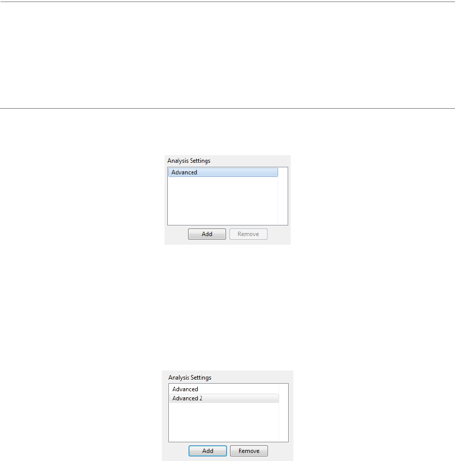
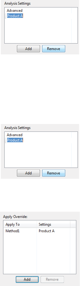
Analysis groups are displayed in the analysis settings box:
The Advanced group shown contains the Compass for iCE default analysis settings. You can make changes
to this group and create new groups. To view settings for a group, click on the group name.
Creating a New Analysis Group
1. Select Edit > Analysis, and select Advanced in the left sidebar.
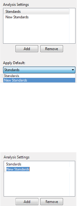
2. Click Add under the analysis settings box. A new group will be created:
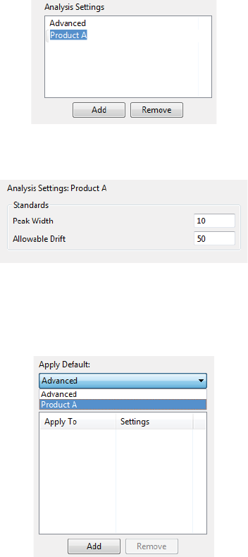
3. Click on the new group and enter a new name.
page 248 Chapter 11: CE-SDS Data Analysis
User Guide for Maurice, Maurice C. and Maurice S.
4. Change the settings in the Standards box as needed.
5. To use the new group as the default analysis settings for the run data, click the arrow in the drop down
list next to Apply Default, then click the new group from the list. Analysis settings in the new group will
then be applied to the run data.
6. Click OK to save changes.
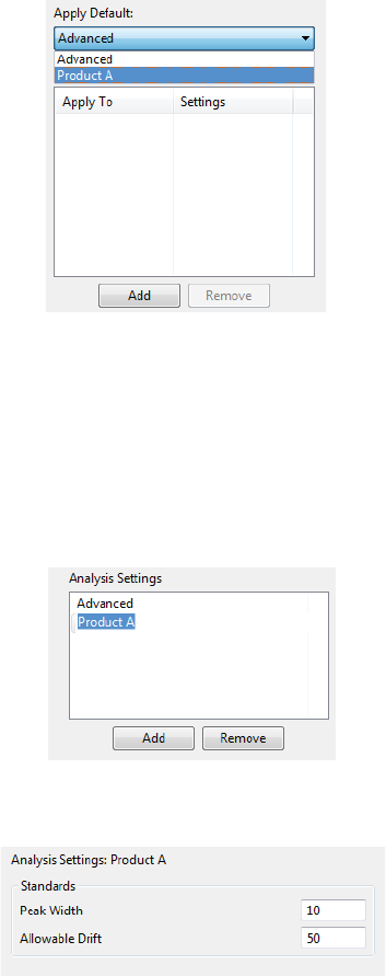
Changing the Default Analysis Group
1. Select Edit > Analysis, and select Advanced in the left sidebar.
2. Click the arrow in the drop down list next to Apply Default, then click a new default group from the list.
Advanced Analysis Settings page 249
User Guide for Maurice, Maurice C. and Maurice S.
3. Click OK to save changes. Analysis settings in the group selected will be applied to the run data.
Modifying an Analysis Group
1. Select Edit > Analysis, and select Advanced in the left sidebar.
2. Click on the group in the analysis settings box you want to modify.
3. Change the settings in the Standards box as needed.
4. Click OK to save changes. The new analysis settings will be applied to the run data.
Deleting an Analysis Group
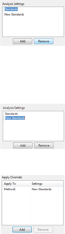
1. Select Edit > Analysis, and select Advanced in the left sidebar.
2. Click on the group in the analysis settings box you want to delete and click Remove.
page 250 Chapter 11: CE-SDS Data Analysis
User Guide for Maurice, Maurice C. and Maurice S.
3. Click OK to save changes.
Applying Analysis Groups to Specific Run Data
1. Select Edit > Analysis, and select Advanced in the left sidebar.
2. Click on the group in the analysis settings box you want to apply to specific run data.
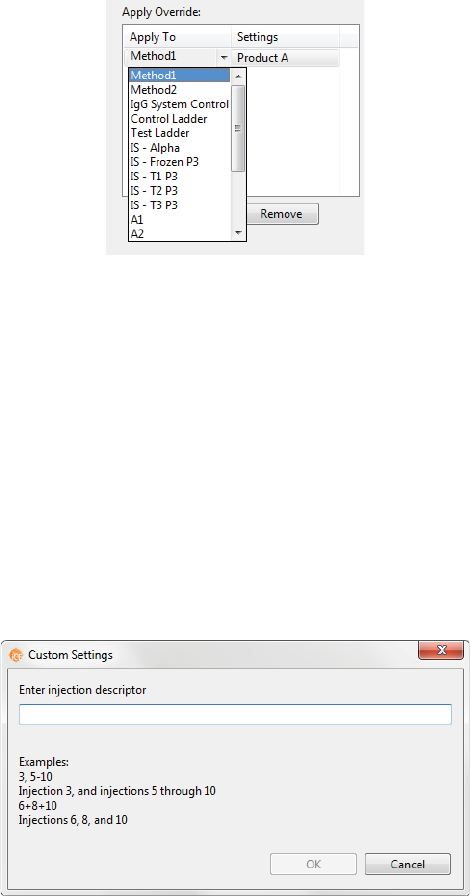
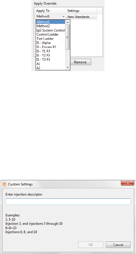
3. Application of analysis groups to specific run data is done in the override box. Click Add under the over-
ride box. A default override data set will be created from sample information found in the run file.
4. Click the cell in the Apply To column, then click the down arrow.
Advanced Analysis Settings page 251
User Guide for Maurice, Maurice C. and Maurice S.
5. Select an option from the drop down list. This applies the settings group selected to specific run data as
follows:
•Methods - All methods in the run file display in the list. Selecting a method applies the group
settings to all injections that used that method.
•Sample names - All sample names in the run file display in the list, otherwise the default name
of Sample shows. Selecting a sample name applies the group settings to all injections that used
that sample name.
•Wells or vials - All well or vial numbers used in the run display in the list. Selecting a well/vial
number applies the group settings to all injections that used that well/vial.
•Custom settings - Lets you choose specific injections to apply the group settings to. When you
select this in the list, a pop-up box displays to let you enter a specific injection number or range
of injections:
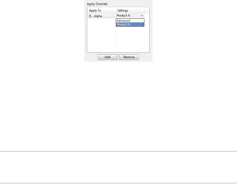
6. If you need to change the analysis group used for a data set, click the cell in the Settings column and
click the down arrow. Select a group from the drop down list.
page 252 Chapter 11: CE-SDS Data Analysis
User Guide for Maurice, Maurice C. and Maurice S.
7. Repeat the previous steps to apply other groups to specific run data.
8. To remove a data set, click on its cell in the Apply To column, then click Remove.
9. Click OK to save changes.
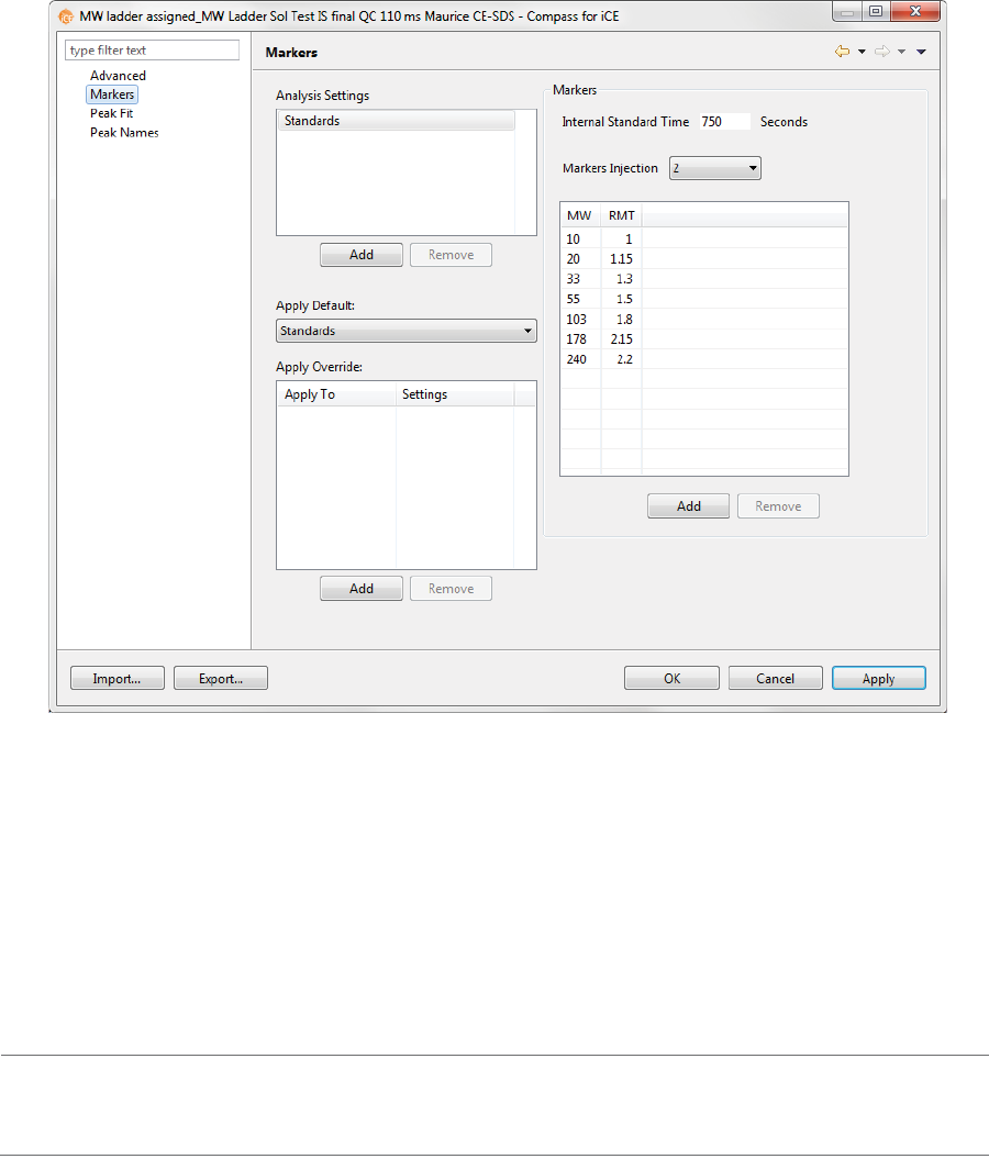
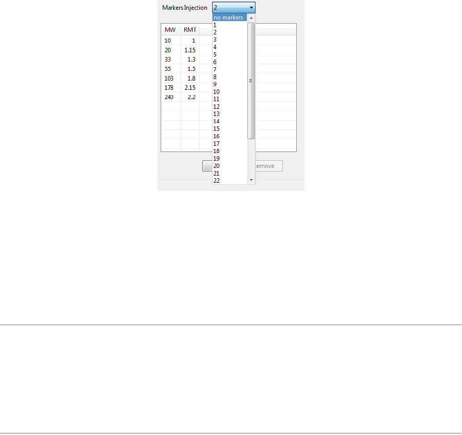
Markers Analysis Settings
This page lets you select the injection for your CE-SDS MW Markers, enter a list of molecular weights and
RMTs for each marker peak, and set the expected migration time of the Internal Standard for all injections.
Select Edit in the main menu and click Analysis, then click Markers in the left sidebar.
NOTE: Settings can be changed in the batch default analysis before you start the run, or in run files once
they’re completed. If you make analysis settings changes to an executing run, they won’t be saved to the
final run file.
Markers Analysis Settings page 253
User Guide for Maurice, Maurice C. and Maurice S.
Markers Settings
•Internal Standard Time - The approximate migration time (in seconds) of the Internal Standard. This
is applied to all injections.
Changing the Injection Used for the CE-SDS MW Markers
You can use known markers to calculate molecular weights of your unknown sample proteins. You can
select the injection you ran your CE-SDS MW Markers in, or opt to not use one.
NOTE: When the markers injection is set to no markers, the molecular weight for sample proteins in the
run isn’t displayed.
page 254 Chapter 11: CE-SDS Data Analysis
User Guide for Maurice, Maurice C. and Maurice S.
To change the markers injection:
1. Select Edit > Analysis, and select Markers in the left sidebar.
2. Click the arrow in the drop down list next to Markers Injection, then select an injection number or no
markers from the list.
Compass for iCE will use the data in the selected injection to calculate molecular weights for sample
proteins in the run data using the information in the table. If no markers is selected, Compass for iCE
doesn’t display molecular weight for sample proteins.
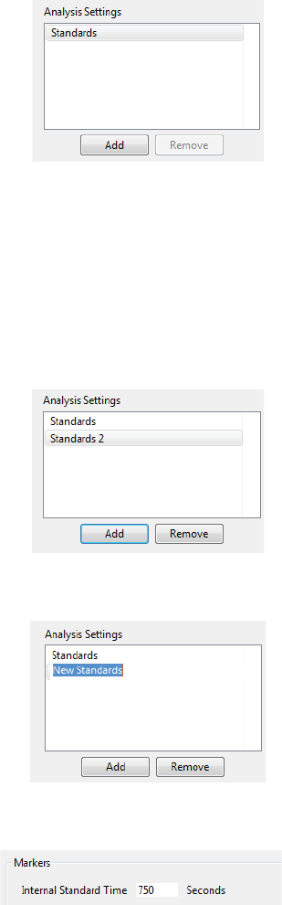
Standards Analysis Settings Groups
Standards settings are saved as a group, and you can create multiple settings groups. Specific group settings
can be applied to methods, injections, sample names or other attributes in the run data.
NOTES:
We recommend using the Compass for iCE default values. These settings are included in the default Stan-
dards group.
Analysis settings are run-file specific. But, settings can be imported or exported for use with other run files.
For more information see “Importing and Exporting Analysis Settings” on page 283.
Standards groups are displayed in the analysis settings box:
Markers Analysis Settings page 255
User Guide for Maurice, Maurice C. and Maurice S.
The Standards group shown uses the Compass for iCE default settings. You can make changes to this group
and create new groups. To view settings for a group, click on the group name.
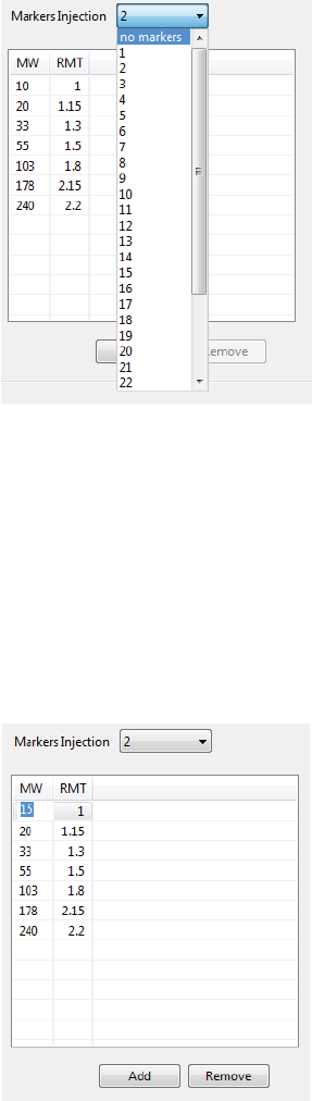
Creating a New Standards Group
1. Select Edit > Analysis, and select Markers in the left sidebar.
2. Click Add under the analysis settings box. A new group will be created:
3. Click on the new group and enter a new name.
4. Change the Internal Standard time as needed.
5. Click the arrow in the drop down list next to Markers Injection, then click an injection number or no
markers from the list.
page 256 Chapter 11: CE-SDS Data Analysis
User Guide for Maurice, Maurice C. and Maurice S.
Compass for iCE will use the data in the selected injection to recalculate molecular weights for sample
proteins in the run data using the information in the table. If no markers is selected, Compass for iCE
doesn’t display molecular weight for sample proteins.
6. If a markers injection was selected, the default Maurice CE-SDS MW Markers molecular weights and rela-
tive migration time (RMT) values are already populated in the table. If you’d like to use these values, skip
to the next step. If you’re using different markers, here’s how to change the values:
a. Click in the first cell in the MW column in the table and enter the molecular weight (in kDa) for the
marker.
b. Click in the first cell in the RMT column and enter a value for the marker.
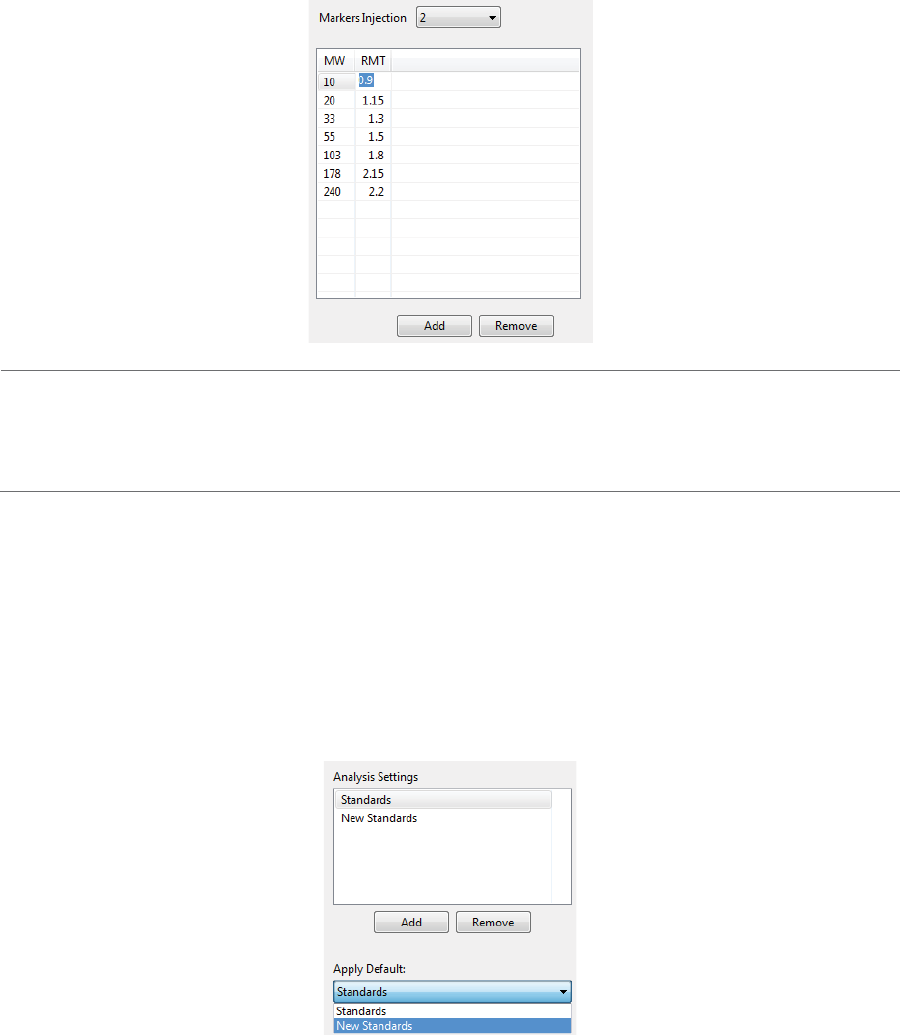
Markers Analysis Settings page 257
User Guide for Maurice, Maurice C. and Maurice S.
NOTE: Marker peak positions are relative to each other. Only the difference in RMT is used to help identify
them. When entering marker peak information for the first time, review the marker data in the Analysis
screen to find the correct peak RMT.
c. Repeat the steps above for the remaining markers in the table.
•To add another marker - Click Add under the table, then change the information in the new
row.
•To remove a marker - Select its row and click Remove.
7. To use the new group as the default settings for the run, click the arrow in the drop down list next to
Apply Default, then click the new group in the list. The settings in the new group will then be applied to
the run data.
8. Click OK to save changes.
page 258 Chapter 11: CE-SDS Data Analysis
User Guide for Maurice, Maurice C. and Maurice S.
Changing the Default Standards Group
1. Select Edit > Analysis, and click Markers in the left sidebar.
2. Click the arrow in the drop down list next to Apply Default, then select a new default group from the list.
3. Click OK to save changes. Analysis settings in the group selected will be applied to the run data.
Modifying a Standards Group
1. Select Edit > Analysis, and click Markers in the left sidebar.
2. Click on the group in the analysis settings box you want to modify.
3. Change the marker info as needed as in “Creating a New Standards Group” on page 255.
4. Click OK to save changes. The new analysis settings will be applied to the run data.
Deleting a Standards Group
1. Select Edit > Analysis, and click Markers in the left sidebar.
2. Click on the group in the analysis settings box you want to delete and click Remove.
Markers Analysis Settings page 259
User Guide for Maurice, Maurice C. and Maurice S.
3. Click OK to save changes.
Applying Standards Groups to Specific Run Data
1. Select Edit > Analysis, and select Markers in the left sidebar.
2. Click on the group in the analysis settings box you want to apply to specific run data.
3. Application of standards groups to specific run data is done in the override box. Click Add under the
override box. A default override data set will be created from sample information found in the run file.
4. Click the cell in the Apply To column, then click the down arrow.
page 260 Chapter 11: CE-SDS Data Analysis
User Guide for Maurice, Maurice C. and Maurice S.
5. Select an option from the drop down list. This applies the settings group selected to specific run data as
follows:
•Methods - All methods in the run file display in the list. Selecting a method applies the group
settings to all injections that used that method.
•Sample names - All sample names in the run file display in the list, otherwise the default name
of Sample shows. Selecting a sample name applies the group settings to all injections that used
that sample name.
•Wells or vials - All well or vial numbers used in the run display in the list. Selecting a well/vial
number applies the group settings to all injections that used that well/vial.
•Custom settings - Lets you choose specific injections to apply the group settings to. When you
select this in the list, a pop-up box displays to let you enter a specific injection number or range
of injections:
6. If you need to change the analysis group used for a data set, click the cell in the Settings column and
click the down arrow. Select a group from the drop down list.
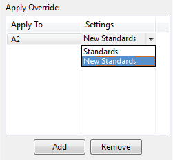
Peak Fit Analysis Settings page 261
User Guide for Maurice, Maurice C. and Maurice S.
7. Repeat the previous steps to apply other groups to specific run data.
8. To remove a data set, click on its cell in the Apply To column, then click Remove.
9. Click OK to save changes.
Peak Fit Analysis Settings
This page lets you view and change peak fit settings for sample data. Select Edit in the main menu and click
Analysis, then click Peak Fit in the left sidebar:
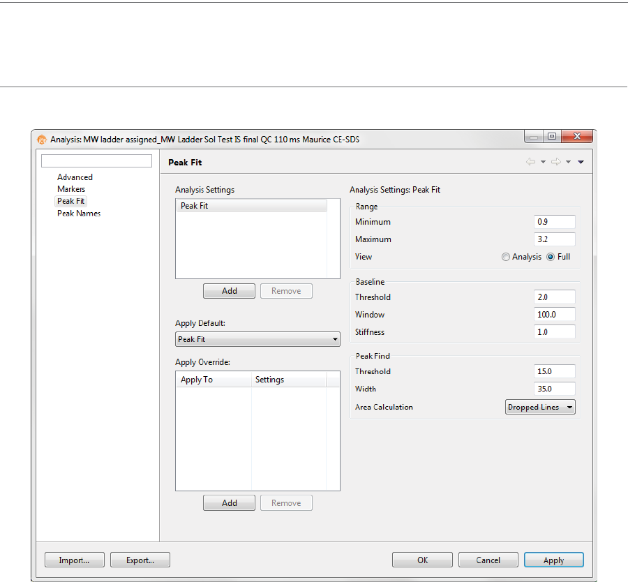
page 262 Chapter 11: CE-SDS Data Analysis
User Guide for Maurice, Maurice C. and Maurice S.
NOTE: Settings can be changed in the batch default analysis before you start the run, or in run files once
they’re completed. If you make analysis settings changes to an executing run, they won’t be saved to the
final run file.
Range Settings
•Minimum - The RMT value below which peaks won’t be identified. This value is also used as the
default lower RMT range for data displayed in the electropherogram.
•Maximum - The RMT value above which peaks won’t be identified. This value is also used as the
default upper RMT range for data displayed in the electropherogram.
•View - Sets the default range to either Full or Analysis for the electropherogram x-axis range in the
View Region window (select View in the main menu and click View Region).
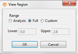
Peak Fit Analysis Settings page 263
User Guide for Maurice, Maurice C. and Maurice S.
•Analysis sets the x-axis range of the electropherogram to the Peak Fit range minimum and max-
imum settings in the electropherogram.
•Full displays the entire separation range of the run data in the electropherogram. This is the
default setting.
Baseline Settings
•Threshold - The variance, or roughness, in a baseline data segment below which a point is called part
of the baseline.
•Window - How long baseline data segments are expected to be in pixels. Shorter segments let the
baseline follow plateau sections of the signal.
•Stiffness - The amount the baseline is allowed to vary from a straight line. Settings between 0.1 and
1.0 make the baseline fit closer to a straight line. Settings from 1.0 to 10.0 will make the baseline fit fol-
low the data more closely.
Peak Find Settings
•Threshold - The minimum signal to noise ratio required for a peak to be identified. A setting of 1.0 will
detect many peaks, a setting of 10.0 will detect fewer peaks.
•Width - The approximate peak width (at full width half max) in pixels used to detect peaks. The mini-
mum value for this setting is 3.0. Larger widths help eliminate the detection of shoulder and noise
peaks.
•Area Calculation - Two fits are used, either Gaussian Fit or Dropped Lines. These settings can be
changed before or after the run is finished.
• For CE-SDS applications, peak area is calculated using Dropped Lines by default. This type of area
calculation is also often called the perpendicular drop method. This is the preferred method
when peaks overlap or are close to each other. It draws two vertical lines from the left and right
bounds of the peak down to the x-axis and then measures the total area bounded by the signal
curve, the x-axis (y=0 line), and the two vertical lines.
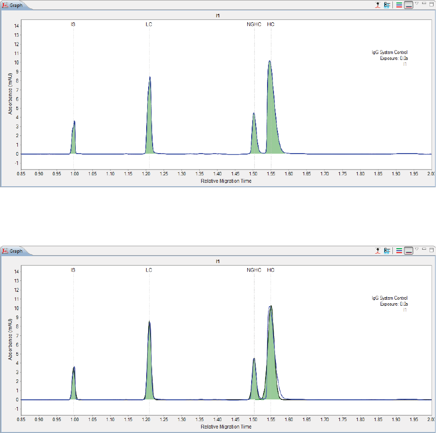
page 264 Chapter 11: CE-SDS Data Analysis
User Guide for Maurice, Maurice C. and Maurice S.
• This next view is of the same data using Gaussian fit instead:
Peak Fit Analysis Settings Groups
Peak fit settings are saved as a group, and you can create multiple settings groups. Specific group settings
can then be applied to methods, injections, sample names or other attributes in the run data.
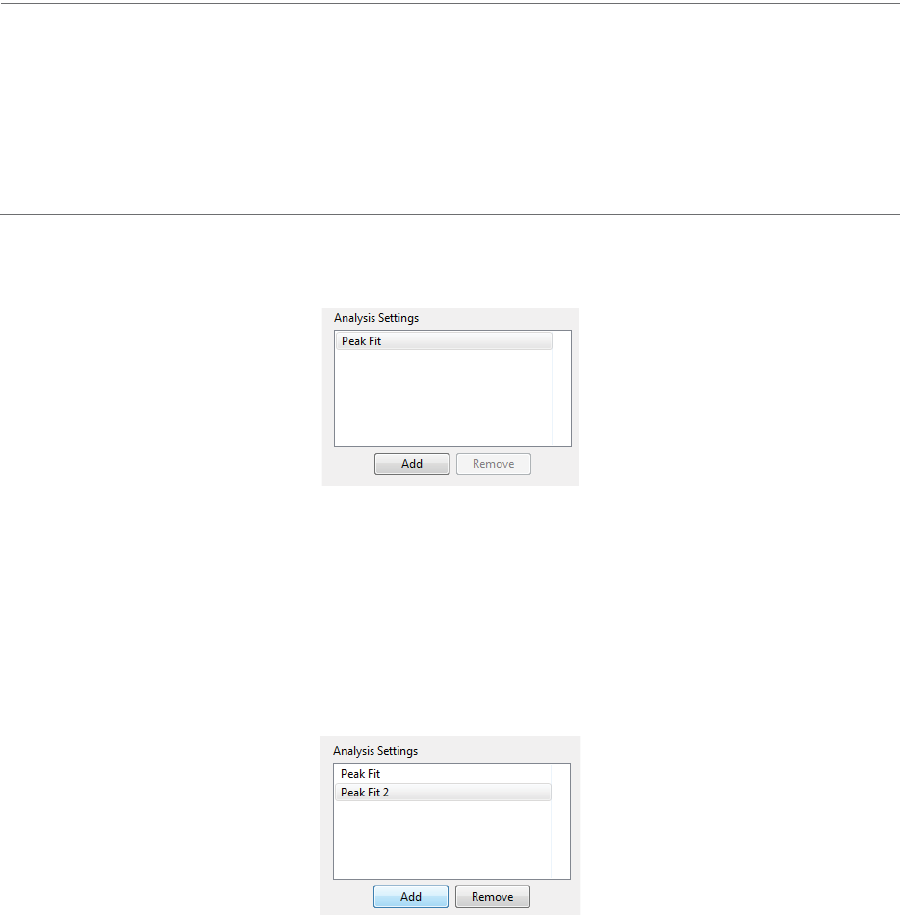
Peak Fit Analysis Settings page 265
User Guide for Maurice, Maurice C. and Maurice S.
NOTES:
We recommend using the Compass for iCE default values for peak fit analysis settings. These settings are
included in the default Peak Fit group.
Analysis settings are run-file specific. But, settings can be imported or exported for use with other run files.
For more information see “Importing and Exporting Analysis Settings” on page 283.
Peak fit groups are displayed in the analysis settings box:
The Peak Fit group shown contains the Compass for iCE default analysis settings. You can make changes to
this group and create new groups. To view settings for a group, click on the group name.
Creating a New Peak Fit Group
1. Select Edit > Analysis, and select Peak Fit in the left sidebar.
2. Click Add under the analysis settings box. A new group will be created:
3. Click on the new group and enter a new name.
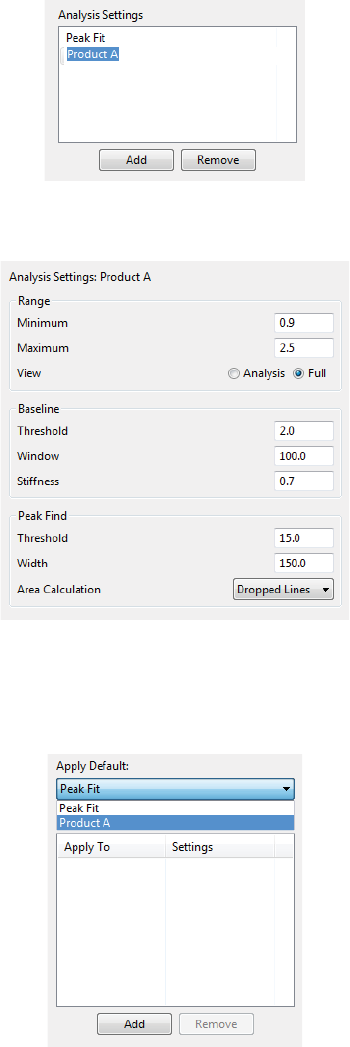
page 266 Chapter 11: CE-SDS Data Analysis
User Guide for Maurice, Maurice C. and Maurice S.
4. Change the settings in the range, baseline or peak find boxes as needed.
5. To use the new group as the default peak fit settings for the run file data, click the arrow in the drop
down list next to Apply Default, then click the new group from the list. Peak fit settings in the new group
will then be applied to the run data.
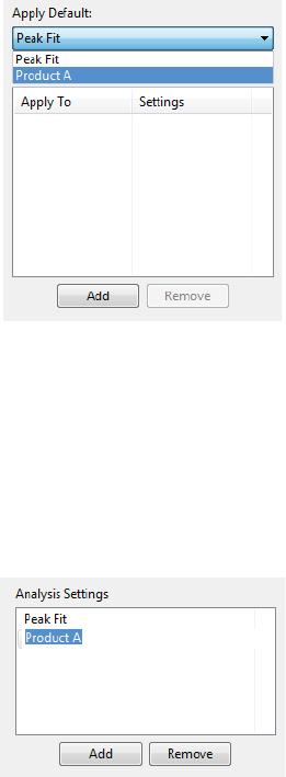
Peak Fit Analysis Settings page 267
User Guide for Maurice, Maurice C. and Maurice S.
6. Click OK to save changes.
Changing the Default Peak Fit Group
1. Select Edit > Analysis, and select Peak Fit in the left sidebar.
2. Click the arrow in the drop down list next to Apply Default, then click a new default group from the list.
3. Click OK to save changes. Peak fit settings in the group selected will be applied to the run data.
Modifying a Peak Fit Group
1. Select Edit > Analysis, and click Peak Fit in the left sidebar.
2. Click on the group in the analysis settings box you want to modify.
3. Change the settings in the range, baseline or peak find boxes as needed.
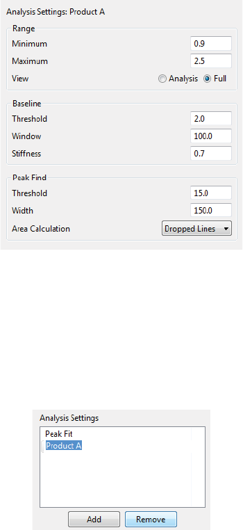
page 268 Chapter 11: CE-SDS Data Analysis
User Guide for Maurice, Maurice C. and Maurice S.
4. Click OK to save changes. The new peak fit settings will be applied to the run data.
Deleting a Peak Fit Group
1. Select Edit > Analysis, and select Peak Fit in the left sidebar.
2. Click on the group in the analysis settings box you want to delete and click Remove.
3. Click OK to save changes.
Applying Peak Fit Groups to Specific Run Data
1. Select Edit > Analysis, and select Peak Fit in the left sidebar.
2. Click on the group in the analysis settings box you want to apply to specific run data.
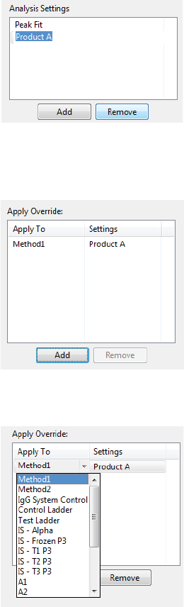
Peak Fit Analysis Settings page 269
User Guide for Maurice, Maurice C. and Maurice S.
3. Application of analysis groups to specific run data is done in the override box. Click Add under the over-
ride box. A default override data set will be created from sample information found in the run file.
4. Click the cell in the Apply To column, then click the down arrow.
5. Select an option from the drop down list. This applies the settings group selected to specific run data as
follows:
•Methods - All methods in the run file display in the list. Selecting a method applies the group
settings to all injections that used that method.
•Sample names - All sample names in the run file display in the list, otherwise the default name
of Sample shows. Selecting a sample name applies the group settings to all injections that used
that sample name.
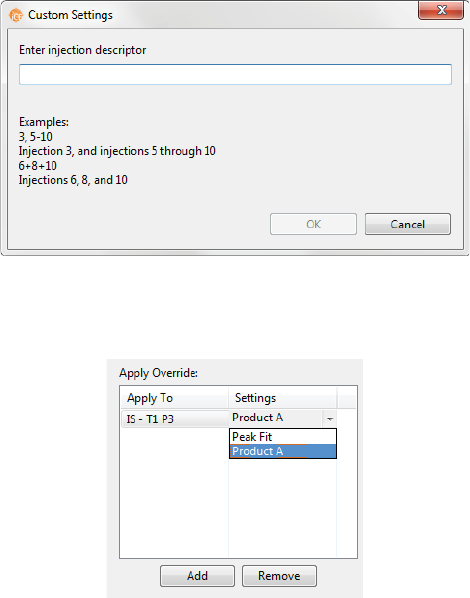
page 270 Chapter 11: CE-SDS Data Analysis
User Guide for Maurice, Maurice C. and Maurice S.
•Wells or vials - All well or vial numbers used in the run display in the list. Selecting a well/vial
number applies the group settings to all injections that used that well/vial.
•Custom settings - Lets you choose specific injections to apply the group settings to. When you
select this in the list, a pop-up box displays to let you enter a specific injection number or range
of injections:
6. If you need to change the analysis group used for a data set, click the cell in the Settings column and
click the down arrow. Select a group from the drop down list.
7. Repeat the previous steps to apply other groups to specific run data.
8. To remove a data set, click on its cell in the Apply To column, then click Remove.
9. Click OK to save changes.
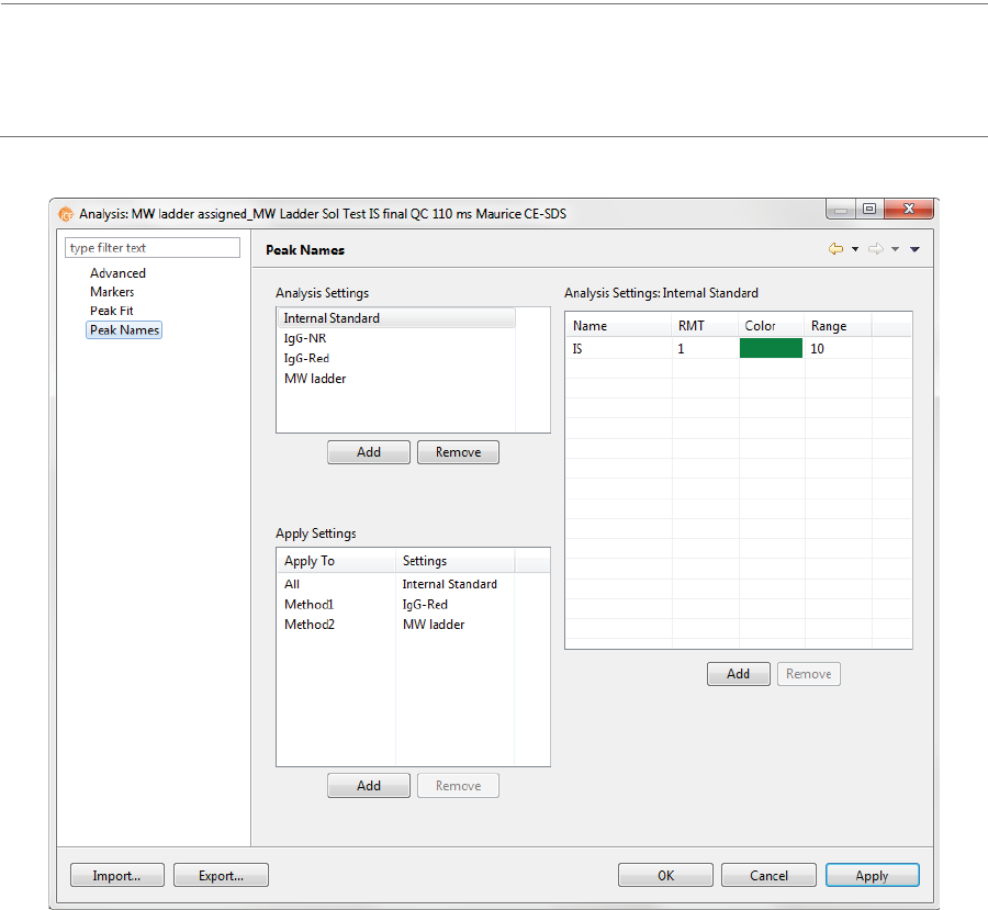
Peak Names Settings page 271
User Guide for Maurice, Maurice C. and Maurice S.
Peak Names Settings
This page lets you view and change custom naming settings for sample proteins. Select Edit in the main
menu and click Analysis, then click Peak Names in the left sidebar.
NOTE: Settings can be changed in the batch default analysis before you start the run, or in run files once
they’re completed. If you make analysis settings changes to an executing run, they won’t be saved to the
final run file.
Peak Names Analysis Settings Groups
Peak name settings are saved as a group, and you can create multiple settings groups. Specific group set-
tings can be applied to methods, injections, sample names or other attributes in the run data.
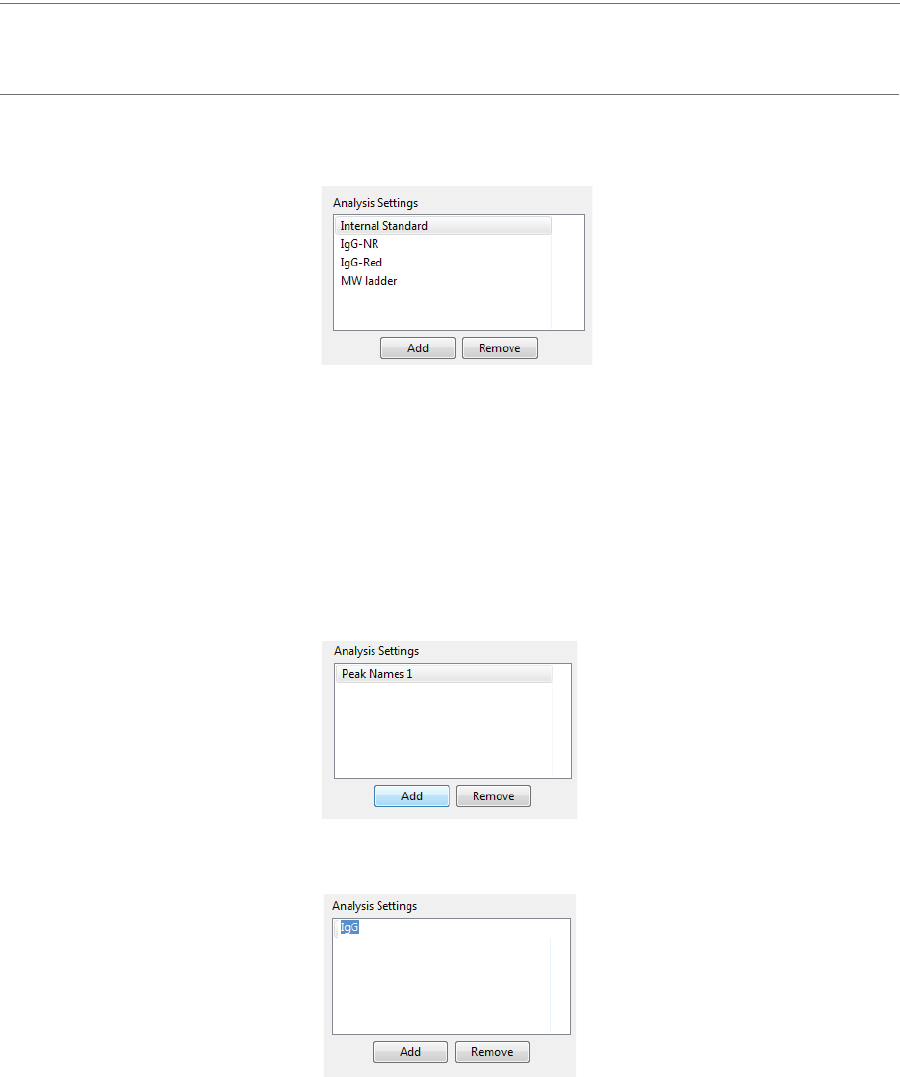
page 272 Chapter 11: CE-SDS Data Analysis
User Guide for Maurice, Maurice C. and Maurice S.
NOTE: Analysis settings are run-file specific. But, settings can be imported or exported for use with other
run files. For more information see “Importing and Exporting Analysis Settings” on page 283.
Peak name groups are displayed in the analysis settings box:
There aren’t any Compass for iCE default settings groups, but you can make changes to groups you’ve cre-
ated and create new groups. To view settings for a group, click on the group name in the analysis settings
box.
Creating a Peak Names Group
1. Select Edit > Analysis, and select Peak Names in the left sidebar.
2. Click Add under the analysis settings box.
3. Enter a new name for the group.
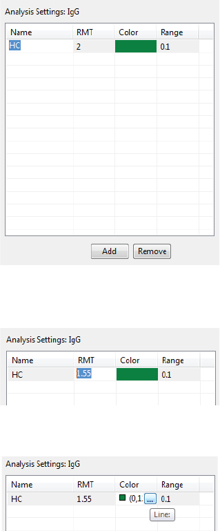
Peak Names Settings page 273
User Guide for Maurice, Maurice C. and Maurice S.
4. Click in the first cell in the Name column in the analysis settings peak table and enter a sample protein
name.
5. Click in the first cell in the RMT column and enter the relative migration time for the sample protein.
6. Click in the first cell in the Color column, then click the button.
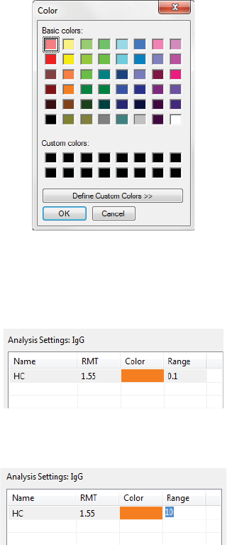
page 274 Chapter 11: CE-SDS Data Analysis
User Guide for Maurice, Maurice C. and Maurice S.
The color selection box displays:
7. The color you pick is used to identify the sample protein peak in the Peaks and Injections panes in the
Analysis screen. Click a color or define a custom color and click OK. The color selection will update in the
table:
8. Click in the first cell in the Range column.
9. Enter a % range for the RMT entered. Compass for iCE will automatically name peaks found within this
percent of the RMT. For example, if the RMT entered is 2 and a 10% range is used, all peaks with RMTs
between 1.8 and 2.2 will be identified with this peak name and color.
10. To add another sample protein, click Add under the peak table. Repeat the previous steps for other sam-
ple proteins. In this example, three proteins were entered:
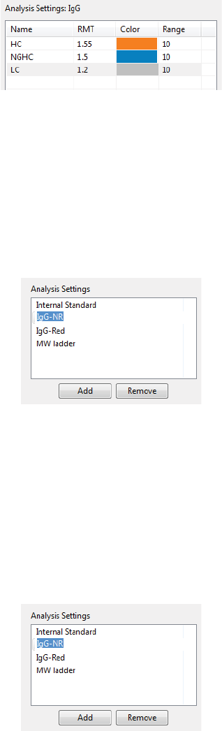
Peak Names Settings page 275
User Guide for Maurice, Maurice C. and Maurice S.
To remove a sample protein, select its row and click Remove.
11. Click OK to save changes.
Modifying a Peak Names Group
1. Select Edit > Analysis, then click Peak Names in the left sidebar.
2. Click on the group in the analysis settings box you want to modify.
3. Change the information in the analysis settings peak table as described in “Creating a Peak Names
Group” on page 272.
4. Click OK to save changes.
Deleting a Peak Names Group
1. Select Edit > Analysis, then click Peak Names in the left sidebar.
2. Click on the group in the analysis settings box you want to delete and click Remove.
3. Click OK to save changes.
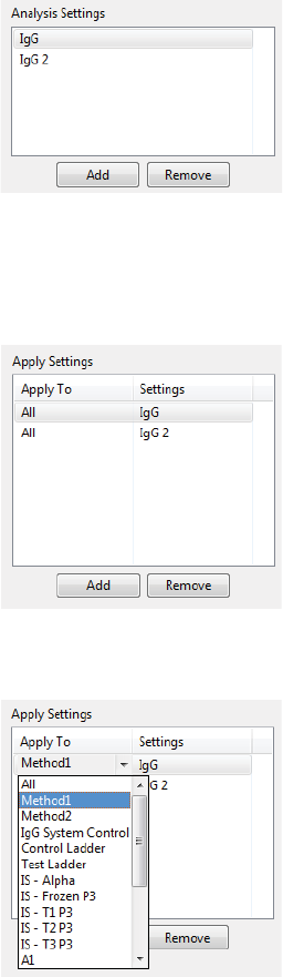
page 276 Chapter 11: CE-SDS Data Analysis
User Guide for Maurice, Maurice C. and Maurice S.
Applying Peak Names Groups to Run Data
1. Select Edit > Analysis, then click Peak Names in the options list.
2. Click on the group in the analysis settings box you want to apply to specific run data.
3. Application of peak names groups to specific run data is done in the apply settings box. A default data
set automatically gets created whenever you create a new group and it’s applied to all injections in the
run. You can either modify the default group or click Add under the box to create a new one.
4. Click the cell in the Apply To column, then click the down arrow.
5. Select an option from the drop down list. This applies the peak names group selected to specific run
data as follows:

Peak Names Settings page 277
User Guide for Maurice, Maurice C. and Maurice S.
•All - Selecting this applies peak names group settings to all injections.
•Methods - All methods in the run file display in the list. Selecting a method applies the group
settings to all injections that used that method.
•Sample names - All sample names in the run file display in the list, otherwise the default name
of Sample shows. Selecting a sample name applies the group settings to all injections that used
that sample name.
•Wells or vials - All well or vial numbers used in the run display in the list. Selecting a well/vial
number applies the group settings to all injections that used that well/vial.
•Custom settings - Lets you choose specific injections to apply the group settings to. When you
select this in the list, a pop-up box displays to let you enter a specific injection number or range
of injections:
6. If you need to change the peak names group used for a data set, click the cell in the Settings column
and click the down arrow. Select a group from the drop down list.
7. Repeat the previous steps to apply other groups to specific run data.
8. To remove a data set, click on its cell in the Apply To column, then click Remove.
9. Click OK to save changes. Named peaks will be identified with a peak name label in the electrophero-
gram and color-coded in the Peaks and Injections panes:
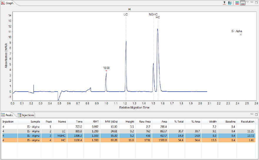
page 278 Chapter 11: CE-SDS Data Analysis
User Guide for Maurice, Maurice C. and Maurice S.
Injection Reports
You can export PDF files of the raw and analyzed data, IV plot, peaks table, sample and system info for indi-
vidual or all injections in a run file. You can also export the run history with all analysis events.
1. Click File > Open Run and select a run file.
2. If you want reports for all injections, skip to the next step. If you only want reports for certain injections,
in the Experiment pane:
•To select sequential injections: Select the first injection, then hold the Shift key and select the
last injection you want a report for. This selects all rows between the two injections.
•To select specific injections: Hold the Ctrl key and select just the injections you want reports
for.
3. Select File from the main menu in either screen and click Injection Report.
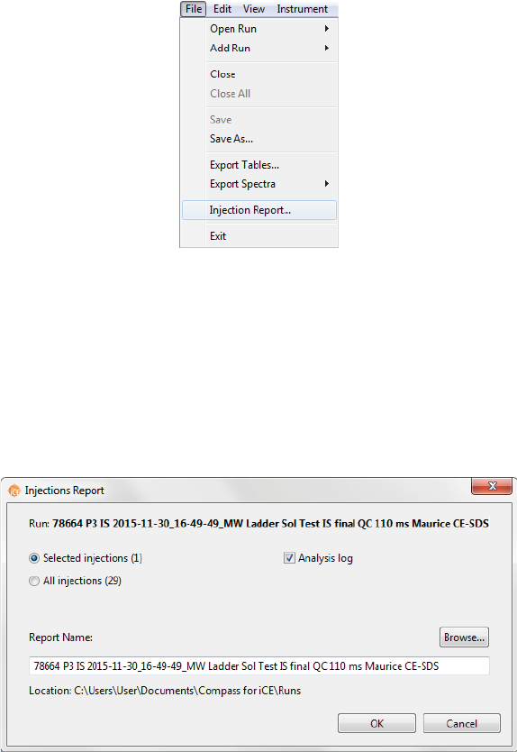
Injection Reports page 279
User Guide for Maurice, Maurice C. and Maurice S.
4. In the Injection Reports window:
d. Choose either Selected injections or All injections.
e. Select the Analysis log checkbox if you want a run history report with all analysis events.
f. The report name defaults to the run file name. If you want to change it, type in the Report Name
box to make updates.
g. Click OK.
5. The Injection Report PDF(s) are exported to the Runs folder in the Compass for iCE directory. They’ll be
in a folder with the report name used in the prior step. When the reports are done, the folder opens for
you automatically.
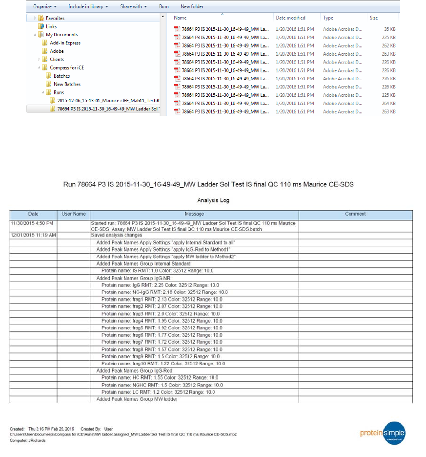
page 280 Chapter 11: CE-SDS Data Analysis
User Guide for Maurice, Maurice C. and Maurice S.
Example Analysis and Injection Report
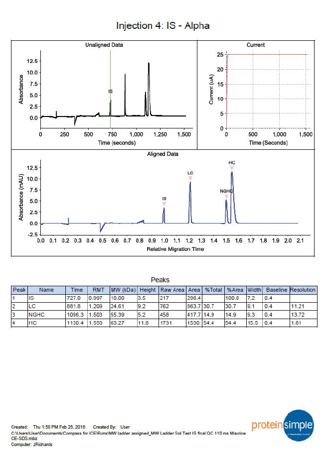
Injection Reports page 281
User Guide for Maurice, Maurice C. and Maurice S.

page 282 Chapter 11: CE-SDS Data Analysis
User Guide for Maurice, Maurice C. and Maurice S.
Importing and Exporting Analysis Settings page 283
User Guide for Maurice, Maurice C. and Maurice S.
Importing and Exporting Analysis Settings
The analysis settings in a run file can be exported as a separate file. This allows the same analysis settings to
be imported into other batches or run files at a later time, rather than you having to re-enter them manually.
Importing Analysis Settings
NOTE: Importing an analysis settings file populates the settings in all analysis pages.
1. Open the run file or batch you want to import analysis settings to.
2. Select Edit in the main menu and click Default Analysis (Batch screen) or Analysis (Analysis screen).
3. Click Import on any page.
4. Select a settings file (*.settings) and click OK. The imported settings will display in all analysis pages.
Exporting Analysis Settings
NOTE: Exporting an analysis settings file exports the settings in all analysis pages.
1. Open the run file or batch you want to export analysis settings from.
2. Select Edit in the main menu and click Default Analysis (Batch screen) or Analysis (Analysis screen).
3. Click Export on any page. The following window displays:
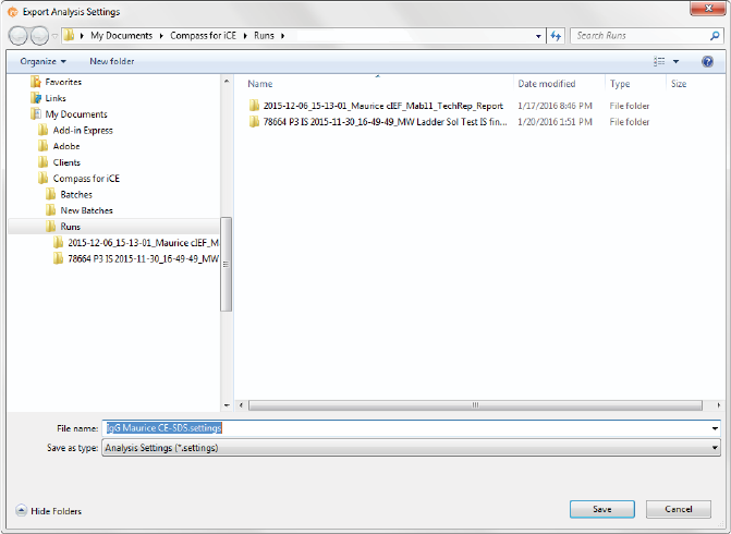
page 284 Chapter 11: CE-SDS Data Analysis
User Guide for Maurice, Maurice C. and Maurice S.
4. The default directory is Compass for iCE/Runs. Change the directory if needed.
5. Enter a file name and click Save. The settings will be saved as a *.settings file.