Sensors and Software NG500 Noggin Gold 500 User Manual NogginGold Manual
Sensors & Software Inc. Noggin Gold 500 NogginGold Manual
UserManual.wiki
>
Sensors and Software
>
NG500 User Manual
>
User Manual 2
Contents
1.
User Manual 1
2.
User Manual 2
User Manual 2
Navigation menu
Upload a User Manual
Namespaces
Wiki Guide
HTML
PDF
Info
Views
User Manual
Discussion / Help
Navigation
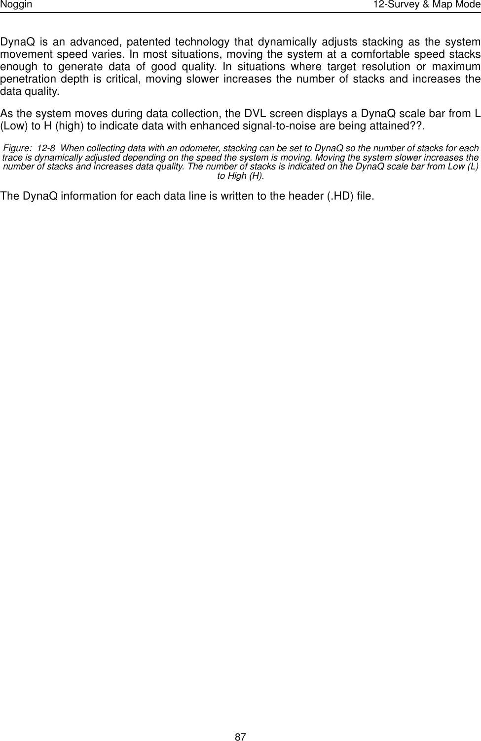
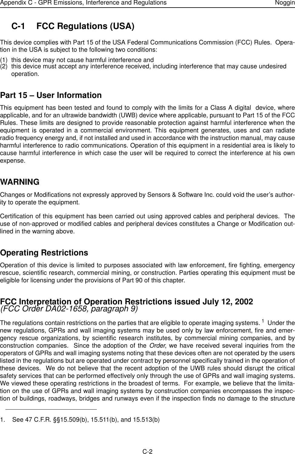
![Appendix C - GPR Emissions, Interference and Regulations NogginC-4ferent locations upon coordination of change of ownership or location to the FCC and coordination withexisting authorized operations. (e) The FCC/NTIA coordination report shall identify those geographical areas within which the operationof an imaging system requires additional coordination or within which the operation of an imaging systemis prohibited. If additional coordination is required for operation within specific geographical areas, a localcoordination contact will be provided. Except for operation within these designated areas, once the infor-mation requested on the UWB imaging system is submitted to the FCC no additional coordination with theFCC is required provided the reported areas of operation do not change. If the area of operation changes,updated information shall be submitted to the FCC following the procedure in paragraph (b) of this section. (f) The coordination of routine UWB operations shall not take longer than 15 business days from thereceipt of the coordination request by NTIA. Special temporary operations may be handled with an expe-dited turn-around time when circumstances warrant. The operation of UWB systems in emergency situa-tions involving the safety of life or property may occur without coordination provided a notificationprocedure, similar to that contained in Sec. 2.405(a) through (e) of this chapter, is followed by the UWBequipment user.[67 FR 34856, May 16, 2002, as amended at 68 FR 19751, Apr. 22, 2003] Effective Date Note: At 68 FR 19751, Apr. 22, 2003, Sec. 15.525 was amended by revising[[Page925]]paragraphs (b) and (e). This amendment contains information collection and recordkeeping require-ments and will not become effective until approval has been given by the Office of Management and Bud-get.](https://usermanual.wiki/Sensors-and-Software/NG500.User-Manual-2/User-Guide-1440912-Page-66.png)
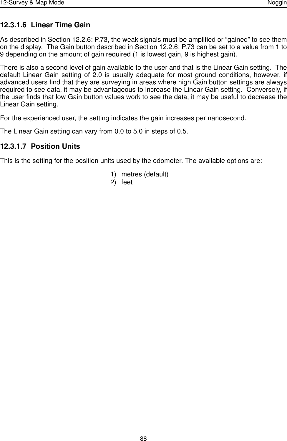
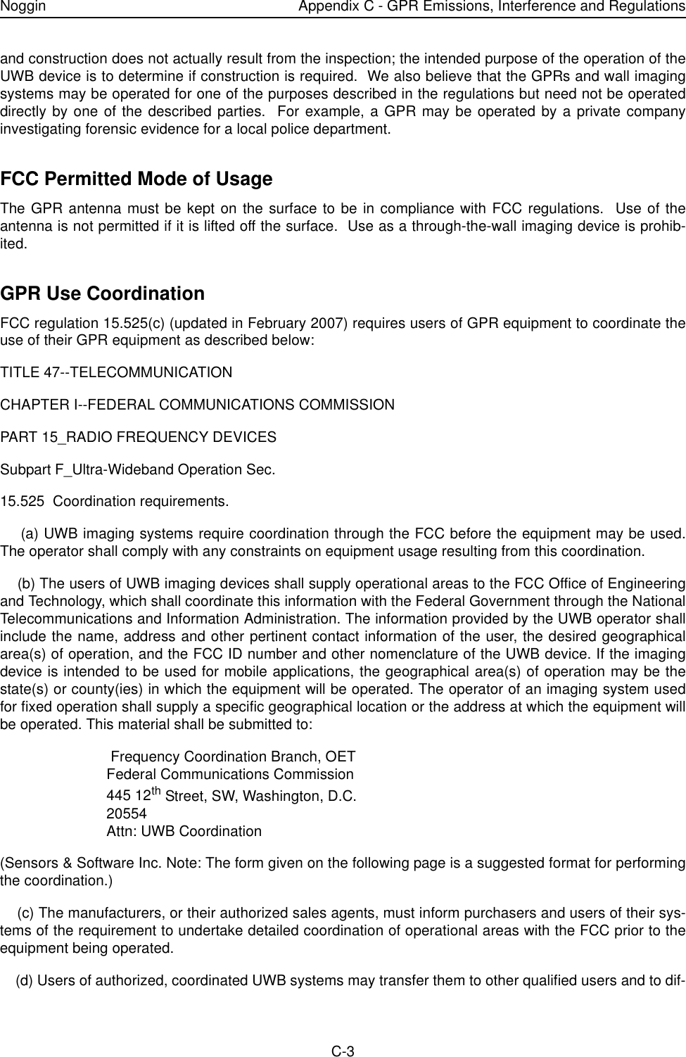
![Noggin Appendix C - GPR Emissions, Interference and RegulationsC-5FCC GROUND PENETRATING RADAR COORDINATION NOTICE NAME:ADDRESS:CONTACT INFORMATION [CONTACT NAME AND PHONE NUMBER]:AREA OF OPERATION [COUNTIES, STATES OR LARGER AREAS]:FCC ID: [E.G. QJQ-NOGGIN100 FOR NOGGIN 100 SYSTEM, QJQ-NOGGIN250 FOR NOGGIN 250SYSTEM, QJQ-NOGGIN500 FOR NOGGIN 500 SYSTEM, QJQ-NOGGIN1000 FOR NOGGIN 1000 SYS-TEM]EQUIPMENT NOMENCLATURE: [E.G. NOGGIN 250] Send the information to:Frequency Coordination Branch., OETFederal Communications Commission445 12th Street, SWWashington, D.C. 20554ATTN: UWB CoordinationFax: 202-418-1944INFORMATION PROVIDED IS DEEMED CONFIDENTIAL](https://usermanual.wiki/Sensors-and-Software/NG500.User-Manual-2/User-Guide-1440912-Page-67.png)