Sensors and Software NG500 Noggin Gold 500 User Manual NogginGold Manual
Sensors & Software Inc. Noggin Gold 500 NogginGold Manual
Contents
- 1. User Manual 1
- 2. User Manual 2
User Manual 2
Noggin 11-Locate & Mark Mode
61
11.4.2 Clear Image
Deletes the current data image on the display.
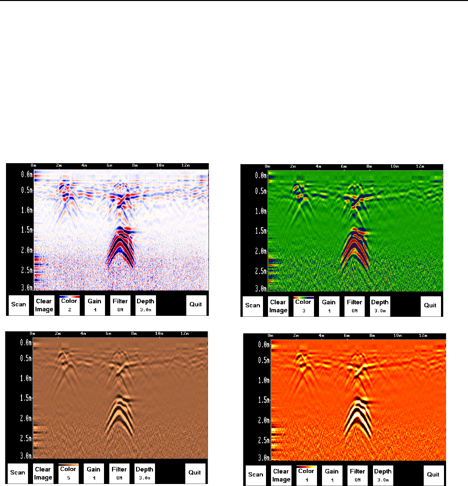
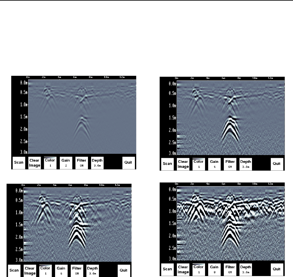
11.4.3 Color
GPR images are displayed in colors corresponding to a color palette. In general, stronger GPR
signals appear in stronger colors. A number of different color palettes are available to display the
image. Some color palettes may show the target better than others.
11-Locate & Mark Mode Noggin
62
11.4.4 Gain
Since GPR signals are absorbed by the material being scanned, deeper targets have weaker
signals. Gain acts like an audio volume control, amplifying the signals and making deeper
targets appear stronger in the image. The Gain varies from 1 to 9 with 1 being no gain and 9
being the maximum gain.
As the Gain changes, the current image on the display updates so it is not necessary to re-collect
an image with a different gain setting. Use the lowest gain setting that shows the targets. Try to
avoid over-gaining as understanding the image may become more difficult.
Noggin 11-Locate & Mark Mode
63
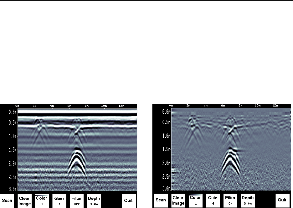
11.4.5 Filter
The filter has the effect of removing flat-lying reflections in the image and enhancing the dipping
reflections and arches usually caused by targets. It can also assist in identifying very shallow
targets that might be masked by the strong signals at the top of the image.
The Filter defaults to ON, so if you are looking for a layer or other flat-lying target, turn the Filter
OFF.
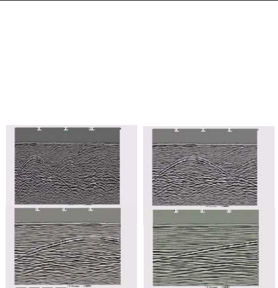
The image below shows the same scan with the Filter OFF and ON.
11-Locate & Mark Mode Noggin
64
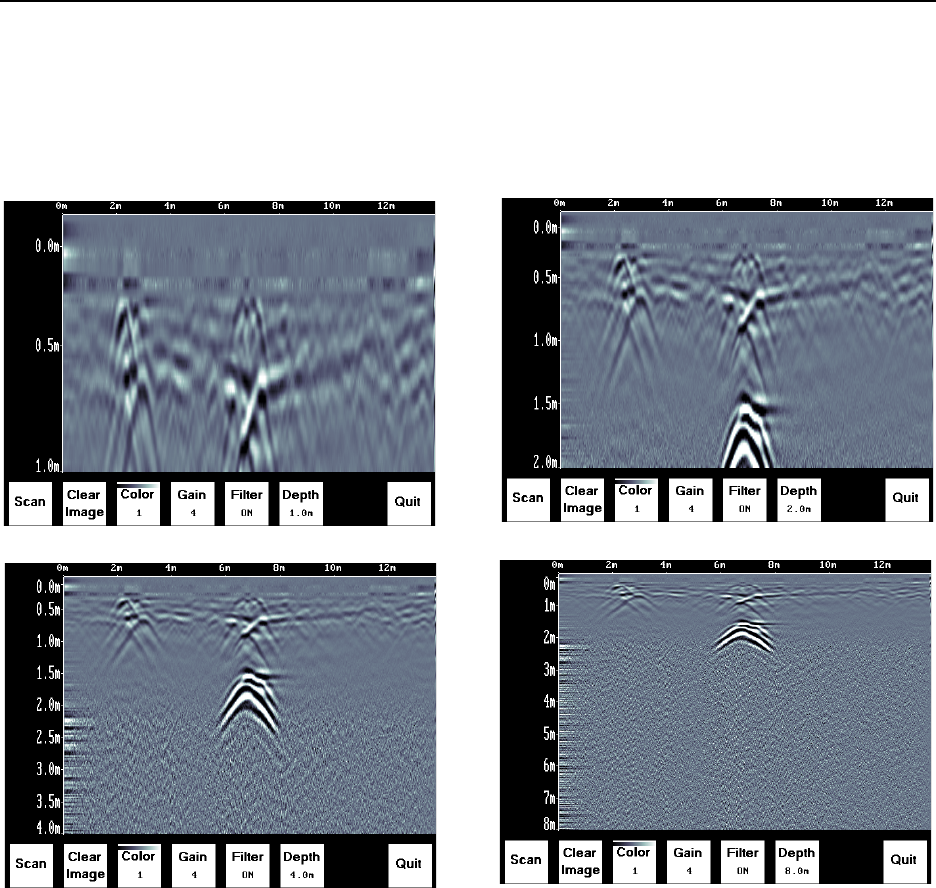
11.4.6 Depth
The depth setting is an estimate of the total depth displayed on the Scanning Screen based on
the current Soil Type setting. The depth setting ranges from 1 to 8 meters.
The system always collects data to a depth of approximately 8 meters but the Depth setting on
this menu determines how much of the data is displayed on the screen. It is possible to scan with
a Depth setting of, say 2 meters, pause scanning and then increase the depth setting to re-
display the image to look for deeper targets.
11.4.7 Quit
Exits the Scanning and Image Settings Screens and returns to the Systems Settings Screen.
Noggin 11-Locate & Mark Mode
65
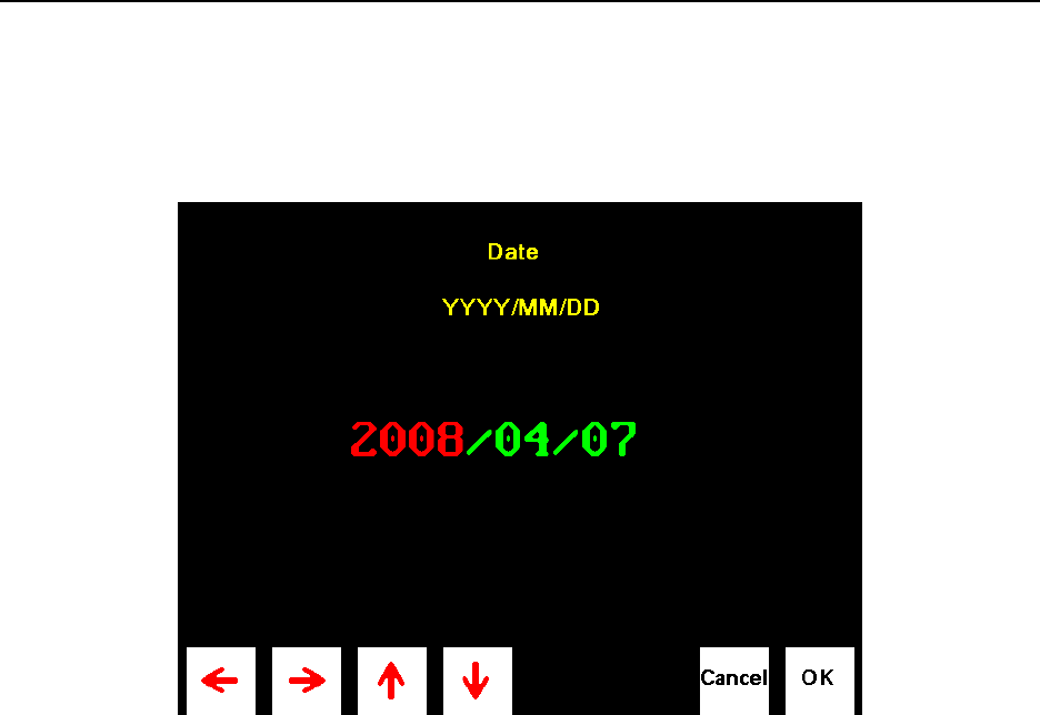
11.5 Changing the Date and Time
From the System Settings Screen, select the Date option. The Time option is similar.
Use the Left and Right Arrow buttons to highlight the number to change in red.
Increase the number using the Up Arrow and decrease the number using the Down Arrow.
Pressing OK saves the new date or time and exits the screen.
Pressing Cancel exits the screen without saving the date or time.

11-Locate & Mark Mode Noggin
66
11.6 English and Equivalent Icons
11.6.1 System Settings Screen Menu
11.6.2 Locating Screen Menu
11.6.3 Image Settings Screen Menu
11.6.4 Date and Time Menus
Noggin 12-Survey & Map Mode
67
12 Survey & Map Mode
The Survey & Map main menu has the following choices:
12.1 Survey & Map Menu
12.1.1 Line
Survey lines collected with the Noggin are saved as digital data files that can be viewed on the
DVL or exported to an external computer for processing and plotting. Sensors & Software
programs like EKKO_View, EKKO_Mapper and EKKO_3D are available to process and display
the data.
Pressing the A button from the main Noggin menu takes the user to Line data collection. This
menu allows the user to select a project number and line number to save each data file to.
Data files from the same area can be organized and saved under a project number selected by
the user. As each individual line is collected, it is given a line number. These line numbers are
usually in sequential order but this is up to the user.
12.1.2 Grid
Survey lines collected with the Noggin are saved as digital data files that can be viewed on the
DVL or exported to an external computer for processing and plotting.
Pressing the B button from the main Noggin menu takes the user to Grid data collection.

12-Survey & Map Mode Noggin
68
Grid collection involves collecting data in an organized pattern over an area. This type of data
acquisition allows the GPR data to be presented as plan maps with the EKKO_Mapper software
or 3D volumes with the EKKO_Mapper 3D software.
For inexperienced surveyors, laying out a grid with straight lines and all the corners at 90
degree angles can be difficult. Sensors & Software provides a product called EasyGrid to
make laying out an accurate grid simple. Contact Sensors & Software for more details.
The Grid menu allows the user to select a grid number and line number to save each data file to.
Before the data acquisition on a grid begins, the user must define the size of the area to be
surveyed, the direction of the survey lines and line spacing. The details of the grid survey are
specified in the Grid Setup menu option (Section 12.3.4: P.97).
12.1.3 Setup
There are many background setup parameters related to the Noggin Smart Systems operation
for line and grid surveys that can be edited. This menu allows the user to display and change
various settings for different aspects of the Smart system (see Section 12.3: P.84). The user can
also reset all the parameters to the factory default settings.
12.1.4 File Management
The File Management menu allows the user to delete data from the DVL and copy data from the
internal compact flash drive to the removable compact flash drive.
The Export options in this menu require the use of the optional PXFER cable and WinPXFER
software so this menu is not required for users transferring Noggin data using the removable
compact flash drive. This type of data transfer is described in Appendix F.
12.1.5 Run without Saving Data
This option allows the user to go straight into data acquisition. This feature is to allow a “quick
look” at the data in the area. The data collected when in this mode are NOT saved and cannot be
reviewed later or exported. Data that scrolls off the edge of the screen is gone and cannot be
reviewed.
If a GPS receiver is attached to the DVL, GPS information can be logged to a file even when the
Noggin data are not being saved (see Section 12.3.5: P.103).
12.1.6 Utilities
This menu has utility programs to:
a) Change the Date and Time on the DVL (see Section 12.5.1: P.110)
b) Calibrate the odometer (see Section 12.5.2: P.110),
c) Use the optional PXFER cable and the WinPXFER software installed on a PC
to transfer upgraded firmware to the DVL (see Section 12.5.3: P.111),
d) List or print or transfer system information to assist Sensors & Software in
troubleshooting problems with your system (see Section 12.5.4: P.111) and

Noggin 12-Survey & Map Mode
69
e) Determine how much space is left on the DVL (see Section 12.5.5: P.111).
f) For the optional PXFER cable used to transfer data from the DVL to a PC, set
the PXFER Transfer Mode to Normal or Turbo (see Section 12.5.6: p.111)
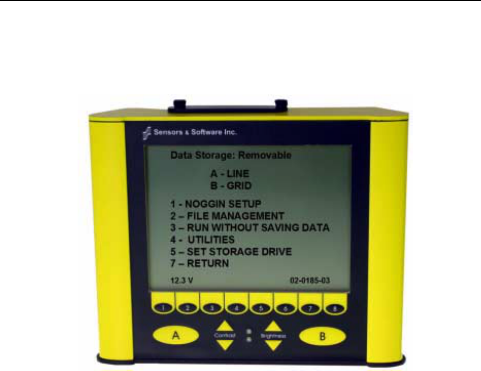
12.1.7 Set Storage Drive
This setting controls how data are saved on the DVL. The available options are:
1) Internal: If this setting is selected, the data are saved to the internal compact flash
drive in the DVL.
2) Removable: If this setting is selected, the data are saved to the removable compact
flash drive accessible by opening the door at the top of the DVL (see Figure 9-1).
12.1.8 Return
This button will return the user to main menu.

12-Survey & Map Mode Noggin
70
12.2 Data Acquisition
Selecting the Line, Grid or Run without Saving Data options from the main Noggin menu will start
data acquisition. The Run without Saving Option goes straight to data acquisition while the Line
and Grid options require the user to select a project number, file number and press Run before
data acquisition begins.
If the Auto Start option is set to ON (see Section 12.3.2.3: p.90 for details) the system will
automatically boot up and be ready for data acquisition. If Auto Start is set to OFF the user must
press the Start button to boot up the system.
After acquisition has started, the Start button disappears and a Stop button (used to halt
acquisition) appears on the right. A Gain button is also visible as well as the current Depth
setting and equivalent Time Window length in nanoseconds (see Figure 12-1).
Data acquisition begins by pressing the Start button on the DVL.
When the Start button is pressed for the first time after the unit is turned on, the Noggin will boot
up (this can take up to 30 seconds depending on the software version of the Noggin). During this
time the system is self-calibrating and measuring such factors as temperature and battery
voltage.
Once this boot up has been completed, data acquisition can begin. For subsequent lines there is
only a short delay before data acquisition can begin.
Data acquisition is done by moving the Smart System along the survey line. During data
acquisition, the Gain button is dynamic and the screen display of the signal sensitivity can be
changed on the go (see Section 12.2.6: P.73).
When the survey line is completed, press the Stop button to stop data acquisition. At this point
no more data can be collected without starting a new line.
12.2.1 Replaying or Overwriting Data
Immediately after a data file has been collected and the Stop button pressed, the data file can be
replayed by pressing the left and right arrow buttons to the scroll the data to the left and right. As
well, during data replay, the data can be enlarged or “zoomed” by pressing the Zoom button and
changing the zoom factor. For example, zooming 2 times on data with a depth setting of 5.0
metres will show the first 2.5 metres of data on the screen.
Any data file that has been collected can be replayed at any time by selecting the file number and
selecting Run. The user then has the option to View, Overwrite or Delete the data file.
Noggin 12-Survey & Map Mode
71
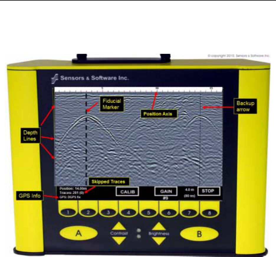
12.2.2 Screen Overview
The data acquisition screen is shown in Figure 12-1. It is divided into 3 sections.
Figure: 12-1 Noggin Data Acquisition Screen
The Noggin screen is shown in Figure 12-1. It is divided into 3 sections. The top section provides
positioning information. The center section contains the actual data and the bottom section
contains the menu.
12.2.3 Position Information
The top section contains horizontal spatial positioning information in feet or metres depending on
the position units setting (see Position Units on page 88)

12-Survey & Map Mode Noggin
72
12.2.4 Data Display
This section contains the actual data collected or replayed. The section also contains the Depth
Lines and any Fiducial Markers the user enters. See the sections below for more details.
12.2.4.1 Depth Lines
Depth lines are horizontal lines indicating the estimated depth. They are very useful for getting
depth estimates to features of interest in the data.
The Depth Lines are controlled by the current velocity value as well as the depth selected. See
Depth on page 84 on changing the depth setting and for more details on how depths are
determined.
To display the correct depth, it is the responsibility of the user to calibrate the system to
the correct velocity of the material (see Section 12.2.11: P.79 on how to calibrate the
system). Once a velocity value has been determined see Velocity on page 85 on how to
change the velocity setting.
Note that it is possible to change the depth units between metres and feet (see Position Units on
page 88).
12.2.4.2 Fiducial Markers
A fiducial marker is a dotted vertical line placed on the data section at a specific position during
data acquisition. Adding these markers during data acquisition is useful for recording significant
positions or the positions of surface objects encountered during the survey.
A fiducial marker is activated by pressing the A button on the keypad during data acquisition. As
well, when using the backup arrow (Section 12.2.7: P.74) fiducial markers can be added at the
current arrow location by pressing the A button.
The position and name of the object encountered at each marker can be recorded in a field
notebook. The fiducial marker is written to the trace header of the next trace to be collected.
Fiducial markers are numbered sequentially (F1, F2 etc.). When the data are transferred to a PC
and reviewed, these markers can assist with data interpretation.
If a GPS receiver is attached to the DVL, a file containing GPS information can be saved. In
Fuducial Tagging mode, whenever a fiducial marker is added to the data, a line of GPS
information will be added to the GPS file (see Section 12.3.5: P.103)
12.2.5 Section C - Menu
The bottom section (Section C) contains the user menu selection and current program settings.
This includes:
1) The total depth (and time window) to the bottom of the data image in Section B (see
Section 12.3.1: P.84),
2) The Gain button and current Gain setting (see Section 12.2.6: P.73),
3) GPS information (if GPS receiver attached, see below and Section 12.3.5: P.103),
4) The current position based on the current triggering device (see Trigger Method on
page 89) and Station Interval (see Section 12.3.3.3: p.93),

Noggin 12-Survey & Map Mode
73
5) The Repeat Trace Number which indicates when the system is being moved too fast
(see Section 12.2.7: P.74) and
6) The Calib button for calibrating the velocity setting (see Section 12.2.11: P.79).
If a GPS receiver is attached to the DVL (see Section 12.3.5: P.103) a message will appear in the
bottom left corner of the menu indicating whether the GPS data is successfully being logged.
The possible messages are:
1) GPS: DGPS fix means differential GPS data are currently being logged.
2) GPS: GPS fix means standard GPS data are currently being logged.
3) GPS: fix not valid means GPS data are NOT currently being logged. This is usually
because GPS satellites are not available.
4) GPS: No Input means the GPS receiver is not operating properly. Check the settings
and test the system (see Section 12.3.5: P.103).
5) GPS: No GGA means the GPS receiver is not outputting a GGA NMEA string that
the DVL requires (see Section 12.3.5: P.103).
12.2.6 Gain
During data acquisition, the Gain setting can be changed by pressing the Gain button until the
desired setting appears. This can be done while the instrument is collecting data; there is no
need to stop first.
The signals that the Noggin system collects from the ground can be very weak, especially from
deeper objects. To see these weak signals it is necessary to amplify or apply “gain” to them.
The Gain setting controls how much the signal is amplified. It varies from 1 to 9 with 1 the lowest
and 9 the highest. In general, if the target is relatively shallow (1-2 metres) a low gain value can
be used. If the target is deeper or if the screen seems to be blank or speckled in the lower part of
the data section, increase the gain setting. Remember, however, that if the Noggin signal is not
penetrating to the maximum depth setting, even the maximum gain setting will not show any
data.
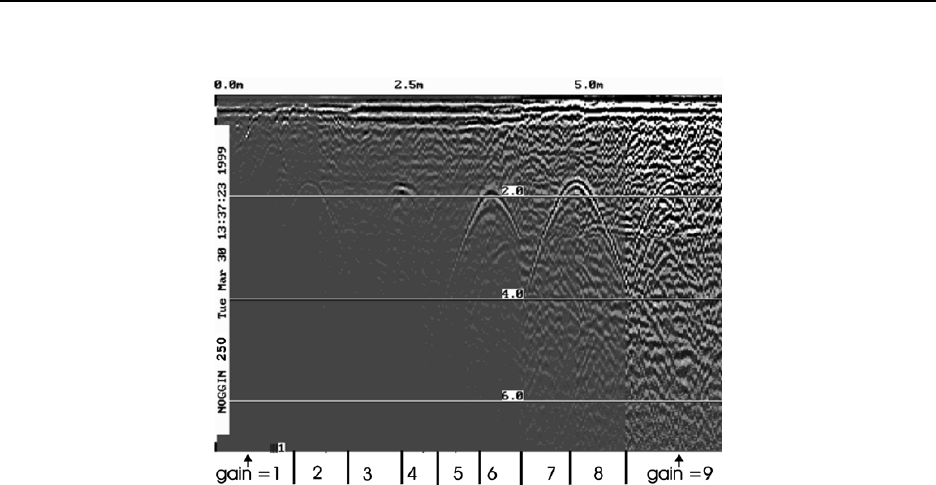
Figure 12-2 shows the effect of the gain setting. The data on the left has a gain of 1 incrementing
to the right up to a gain of 9.
12-Survey & Map Mode Noggin
74
Figure: 12-2 Effects of the Gain setting
Note that the gain setting is only for data display. The data are always saved without any
gain applied. It is not possible to collect Noggin data with an “incorrect” gain setting.
If the user finds that they are always using very high or very low gain settings to see the data
adequately, the user may want to adjust the Linear Gain setting under Setup (see Linear Time
Gain on page 88).
12.2.7 Collecting Data using the Odometer
As the Smart System moves, the odometer triggers the system to collect a data trace at fixed
distance intervals. This interval is called the “station interval”. For the Noggin 250, the normal
station interval is 5 centimeters (about 2 inches). For the Noggin 500, the normal station interval
is 2.5 centimeters (about 1 inch). For the Noggin 1000, the normal station interval is 1.0
centimeter (about 0.48 inch). The station interval can be changed to a longer or short distance in
the Setup (see Station Interval on page 93).
Each data trace is plotted as a vertical strip on the screen (see Figure 12-1). The width of this
strip can be changed to 1, 2, 4, or 8 pixels (see Plot Interval on page 96). The normal trace width
for Noggin 250 traces is 2 pixels while the normal width for Noggin 500 and Noggin 1000 systems
is 1 pixel.
The odometer units that appear across the top of the screen can be set to either metres or feet
(see Depth Units on page 85).
Smart Systems can normally collect data at a very fast walking pace. However, if the system is
moved too quickly, data quality is reduced (see below).
During data acquisition, the current odometer position value (in the current units, either metres or
feet) is written to the lower left corner of the screen (see Figure 12-1).
Note that Smart systems can be configured to collect data either by pushing the system (forward)
or pulling the system (reverse). See Cart Direction on page 89 about changing the direction of
data acquisition.

Noggin 12-Survey & Map Mode
75
The odometer should be periodically re-calibrated to ensure accuracy. The procedure for re-
calibrating the odometer is described in Section 12.5.2: P.110.
12.2.7.1 Reducing Data Quality by Moving too Fast
On the lower part of the data acquisition screen, beside the current total number of traces
collected is the total number of traces skipped.
If the Smart System is being used with the odometer and is moved too quickly for the Noggin
system to keep up, traces are skipped and the quality of the survey is reduced. The skipped
traces do not actually create gaps in the data but rather, the last trace that was collected properly
is repeated. The Skipped Traces number displays the total number of skipped traces. If this
number exceeds 0 this is due to moving the system too quickly. To eliminate this either slow
down the system speed, decrease the number of Stacks or reduce the Depth setting (see Section
12.3.1: P.84).
If the system is moved too fast, after the data survey line is complete, the DVL will indicate the
total number of traces that were “skipped”. The user then has the option to Autofix the data. The
Autofix process replaces any repeated traces in the data with interpolated traces. While this
process does not solve the problem of skipping traces, it will make the data traces look less
“blocky”.
If the number of traces skipped is a significant percentage of the total number of traces collected,
i.e. 10% or more, the operator should slow down, decrease the number of Stacks or reduce the
Depth setting (see Section 12.3.1: P.84).
12.2.7.2 Backing up the Smart System to Pinpoint Target Positions
The odometer also allows the user to stop the Smart System in the middle of a survey line and
back up. When this is done, an arrow and vertical line appear on the data image and move back
along the image as the system moves backwards (see Figure 12-1). This makes it possible to
correlate a target in the data image to an exact location on the ground. Once the arrow lines up
with the target, mark the ground at the centre point of the Noggin.
When the system is moved forward again to continue with the survey, the Smart system does not
start collecting data again until you reach the position where you stopped at. This feature is
useful for producing a continuous data image even if the system is backed up during the survey
line.
Note that it is not possible to back up and have the arrow indicator move more than one screen.
The physical position corresponding to the Back-up arrow is the centre of the Noggin. This
position can be changed from the centre of the Noggin to any other position. See Arrow Offset on
page 90 on changing the Arrow Offset value.
12.2.8 Collecting Data in Free Run Mode
It is possible to change the triggering method from the odometer and have the Noggin system run
in Free Run (or continuous mode) (see Trigger Method on page 89). This means that the system
collects data even if it is not moving. This option is useful for collecting data when using the
odometer wheel is not practical.

12-Survey & Map Mode Noggin
76
When the Smart System is used in Free Run mode, it is up to the user to keep track of
positioning by some other method, for example, a measuring tape, using fiducial markers (see
Fiducial Markers on page 72) or GPS (see Section 12.3.5: P.103).
In this mode, data collection is dependent on two factors,
1) the speed that the Noggin system is collecting data and
2) the speed the Noggin system is moving.
12.2.8.1 Controlling Data Collection Speed in Free Run Mode
In Free Run mode the user can control the speed the Noggin collects data by increasing or
decreasing the number of stacks (for more details on Stacking, see Stacks on page 86).
Increasing the number of Stacks has the effect of slowing down the data collection speed of the
Noggin system. Decreasing the number of Stacks has the effect of speeding up the data
collection speed Noggin system. The user can also control the speed of the Noggin data
collection by adjusting a time delay between data collection points. Note that any time delay
more than 0.0 seconds causes the system to emit a beeping sound as the data trace is collected.
12.2.8.2 Noggin Speed in Free Run Mode
In Free Run mode, the speed the Noggin moves determines the distance between sample points
on the ground (station interval). This type of data collection requires experimenting with the
number of stacks and time delay (see Trigger Method on page 89) and practicing to find a
satisfactory speed for the Noggin. Moving too quickly may result in under-sampling the data
making it more difficult to interpret. Moving too slowly may result in over-sampling the data. This
stretches the data image making it more difficult to interpret. As well, maintaining a uniform
speed is important for minimizing image distortion.
12.2.8.3 Positions in Free Run Mode
Each data trace is plotted as a vertical strip on the screen (see Plot Interval on page 96). In Free
Run mode the station interval is not fixed so each screen of data can represent any ground
distance. This means that the position values displayed in Section A at the top of the data image
(see Section 12.2.3: P.71) are not correct.
When running the system in Free Run mode it is best to set the units (see Position Units on page
88) to metres and the Station Interval (see Section 12.3.3.3: p.93) to a value of 1.0 metre. Then
the position values appearing on the top of the data image can be interpreted as trace numbers
and not an absolute position.
12.2.9 Collecting Data using the Trigger (or B) Button
It is possible to change the triggering method from the odometer and have the Noggin system
only collect data when the Trigger button (or B button on the DVL) is pressed (see Section
12.2.9: P.76). This option is useful for collecting data when using the odometer wheel is not
practical.
After the user selects this option (see Trigger Method on page 89), a menu appears to select the
number of stacks for each trace. Generally, the more stacks the better the data quality (for more
details on Stacking, see Stacks on page 86).

Noggin 12-Survey & Map Mode
77
In Trigger Button mode, the system “beeps” as each trace is collected. The length of the beep
will depend on the number of stacks (the more stacks, the longer it takes to collect a trace and
therefore the longer the beep).
When the Smart System is used in Trigger Button Mode, it is up to the user to keep track of
positioning by some other method, for example, using a measuring tape, fiducial markers (see
Fiducial Markers on page 72) or GPS (see Section 12.3.5: P.103).
Since data collection only occurs by the user pressing the trigger button, usually a fewer number
of traces are collected in this mode compared to odometer triggering mode or Free Run mode
(see above). Therefore, it is often useful to increase the trace width to 4 or 8 pixels so that the
data are more easily seen on the DVL screen (see Plot Interval on page 96).
12.2.10 Noggin Data Screens
Total Distance Per Screen
The total distance that can be displayed on one screen varies depending on the Noggin system,
Station Interval and Plot Interval (see Section 12.3.3.4: p.96). As the Station Interval increases,
the distance between data traces increases and the total distance per screen increases. As the
Plot Interval increases, the total distance per screen decreases.
Noggin 100
For the Noggin 100, each trace is normally 2 pixels wide. Since the screen is 640 pixels wide,
each screen has 320 traces. When the station interval is set to Normal (10 centimetres or 4
inches), each screen displays 32 metres or 105 feet of data.??
Noggin 250
For the Noggin 250, each trace is normally 2 pixels wide. Since the screen is 640 pixels wide,
each screen has 320 traces. When the station interval is set to Normal (5 centimetres or 1.92
inches), each screen displays 16.0 metres or 52.5 feet of data.
Noggin 500
For the Noggin 500, each trace is normally 1 pixel wide. Since the screen is 640 pixels wide,
each screen has 640 traces. When the station interval is set to Normal (2.5 centimetres or 0.96
inches), each screen displays 16.0 metres or 52.5 feet of data.
Noggin 1000
For the Noggin 1000, each trace is normally 1 pixel wide. Since the screen is 640 pixels wide,
each screen has 640 traces. When the station interval is set to Normal (1.0 centimetres or 0.48
inches), each screen displays 6.4 metres or 25.7 feet of data.
Total Data Distance on the DVL
For more details on total distances and Station Intervals see Section 12.3.3.3: p.93.

12-Survey & Map Mode Noggin
78
To see how much data can be collected before the DVL memory is full and data must be deleted
or downloaded, see DVL Recording Space in Section 12.5.5: P.111.
Noggin 12-Survey & Map Mode
79
12.2.11 Calib. (Calibration) Menu
Noggin systems can be used to scan into many different materials including soil, rock, concrete,
snow, ice and wood. The radio wave emitted by a Noggin system will travel at different velocities
depending on the material being scanned. The depth value (see Section 12.3.1: P.84) and on
Depth Lines (see Section 12.2.4: P.72) are only accurate if the system has been properly
calibrated to determine the velocity of the material being scanned. See Depth on page 84 for
more details about how depth is calculated.
The Calibration function is a tool for determining the velocity of the material being scanned. A
velocity value can be input directly (see Section 12.3.1.2: p.85) or determined in one of two
different ways depending on the situation:
1) Hyperbola matching
2) Target of known depth
Note that unlike the Calibration with Noggin systems (see Section 12.2.11: P.79), the
Noggin Calibration does NOT automatically update the velocity value in the software. In
the Noggin calibration, once a velocity is determined, the user must enter it into the
System Parameters (see Velocity on page 85).
12.2.11.1Hyperbola Matching
The most accurate way of determining the velocity of the material being scanned is to use the
hyperbola-fitting method because it extracts the velocity using data collected in the area. This
method may not work in all situations because it depends on having a good quality hyperbola (or
inverted U) in the data.
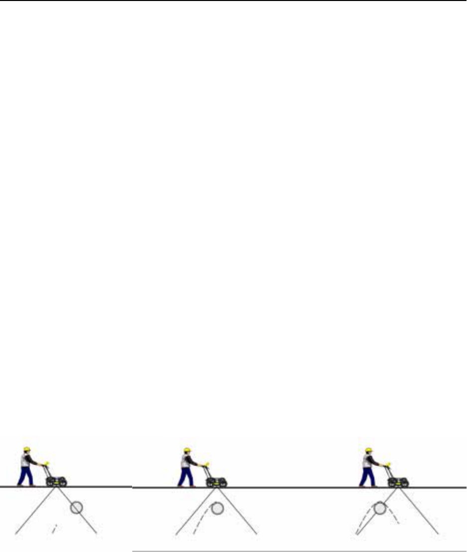
A hyperbola is the characteristic GPR response from a small point target like a pipe, rock or even
a tree root. This phenomenon occurs because radar energy does not radiate as a pencil-thin
beam but more like a 3D cone. Reflections can appear on the record even though the object is
not directly below the radar system. Thus, the radar system “sees” the pipe before and after
going over top of it and forms a hyperbolic reflection.
Figure: 12-3 Hyperbolas in the data result from the conical shape of the GPR energy as it goes into the ground. Tar-
gets, like pipes, are detected as the GPR approaches them (left), passes over them (middle) and after it has passed by
them (right) because the GPR energy propagates both in front and behind the instrument.
If the hyperbola has long tails on it, we can match the shape of the hyperbola and determine the
velocity of the material in the area.
12-Survey & Map Mode Noggin
80
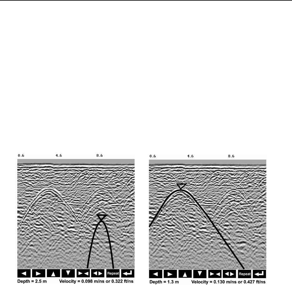
With the hyperbola visible on the DVL screen, select the hyperbola (
∩
) button. This will
superimpose a hyperbola on the data. This hyperbola can be moved up (!), down ("), left (#)
and right ($) using the appropriate arrow buttons. The goal is move the hyperbola until it lies on
top of the hyperbola in the data (see Figure 12-4). Then, the user can adjust the width of the
hyperbola to make it wider (#$) or narrower ($#) until the shape of the hyperbola matches the
shape of the hyperbola in the data. After matching the hyperbola, the velocity value is displayed
and now can be entered under the System Parameters (see Velocity on page 85).
Pressing the up, down left, right, wider and narrow buttons once makes a very small change in
the position or width of the hyperbola. These buttons must sometimes be pressed many times to
move the hyperbola to the correct position or width. To speed up the movement of the hyperbola,
use the REPEAT button. For example, to move the hyperbola up a long distance, press the up
button (!) followed by the REPEAT button. The hyperbola will then start moving upward without
having to press any more buttons. When it gets close to the desired location press any button to
stop it and then use the up, down, left and right buttons to fine-tune the position. The REPEAT
button can also be used after pressing the wider (#$) or narrower ($#) button.
(a) (b)
Figure: 12-4 Hyperbola matching to extract velocity. After pressing the CALIB button a hyperbola
appears on the screen (a). This hyperbola should be moved overtop of a hyperbola in the data using
the arrow keys. It can then be widened or narrowed to match the shape of the hyperbola in the data (b).
When the hyperbola shapes match, the velocity is extracted and displayed. The user can then use this
velocity value for surveys done in the area.
In Noggin mode, hyperbola Matching calibration can be done during data acquisition and also
while viewing previously collected data.
If units are metres then depths will appear in metres and velocities in metres per nanosecond (m/
ns). If units are feet then depths will appear in feet and velocities in feet per nanosecond (ft/ns).
To change units see Depth Units on page 85.
Noggin 12-Survey & Map Mode
81
12.2.11.2Identifying Air Reflections
Some hyperbolic reflections can also be caused by objects not in the subsurface such as fences,
overhead wires and, in some conditions, even large trees.
An important part of data interpretation is learning to recognize these unwanted “air” events and
differentiate them from the desired subsurface events. Good field notes are indispensable for
helping identify unwanted events on the data.
One way of identifying air reflections is to use the hyperbola fitting method. If the object is in air,
the radar velocity will be 0.3 m/ns or 0.984 ft/ns and will be much faster than if it is in the ground
(v ~ 0.1 m/ns or 0.328 ft/ns).
Figure: 12-5 Hyperbola matching can be used to identify reflections from objects that are not in the subsurface but
are from objects above ground. If the hyperbola matching velocity is near the speed of light (0.3 m/ns or 0.984 ft/ns)
then the hyperbola was caused by surface object like a overhead wire, tree, etc. After matching the hyperbola (right),
the “depth” value displayed on the bottom of the screen is really a measure of how far from the survey line the object is.
12-Survey & Map Mode Noggin
82
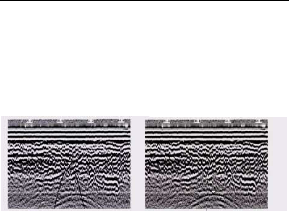
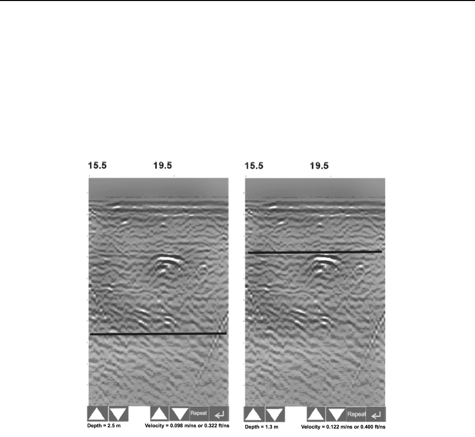
12.2.11.3Target of Known Depth
If there are no suitable hyperbolas visible in the data to perform the Hyperbola Matching
described above, it may be the situation that there is a target of known depth in the area being
scanned. If this is the case, selecting the button with the circle with a horizontal line through it will
superimpose a horizontal line on the data. This line can then be moved up or down until it lies on
top of the Noggin response to the known target. Then, the user can adjust the velocity value up
or down until the known target depth is correct. Once the depth is matched, the current velocity
value is the one used for all subsequent data acquisition.
(a) (b)
Figure: 12-6 Using a target of known depth to extract velocity. After selecting CALIB, choosing the
known depth button (a circle with a horizontal line through it) will superimpose a horizontal line on the
data (a). Using the depth buttons, this line can then be moved up or down until it lies on top of the
Noggin response to the known target (b). Then, the user can use the velocity buttons to adjust the
velocity value up or down until the known target depth is correct. Once the depth is matched, the
velocity value should be used for all subsequent data acquisition.
If units are metres then depths will appear in metres and velocities in metres per nanosecond (m/
ns). If units are feet then depths will appear in feet and velocities in feet per nanosecond (ft/ns).
To change units see Depth Units on page 85.

Noggin 12-Survey & Map Mode
83
12.2.12 Error Messages
If an error occurs during data acquisition, an error message will appear in the bottom left section
of the data acquisition screen. Note the message number, exit the program and turn off the
Digital Video Logger.
Make sure the cables are not damaged and that all cable connections are tightly secured.
Sometimes vibrations cause the cable connections to loosen just a bit and break contact and this
can cause errors. Disconnecting cables and reconnecting them may provide a better contact
and solve the problem. Also check and make sure the battery is adequately charged. Turn the
Digital Video Logger back on and try running the system again.
For more information on Troubleshooting the system, see Section 13: P.112.

12-Survey & Map Mode Noggin
84
12.3 Noggin Setup
Pressing the number 1 on the main menu selects the Setup item. Setup lists the various
parameters that can be edited. These parameters are organized under the following headings:
1 - System Parameters
2 - Cart Parameters
3 - Line Parameters
4 - Grid Parameters
5 – GPS Parameters
6 – Set Defaults
To select a setting to edit, press the corresponding number button. Then use the numbered
buttons to select the new setting. It is also possible to change all the settings back to the factory
default settings by pressing the 6 button (labelled Set Defaults).
The SETUP options are outlined below.
12.3.1 System Parameters
The System Parameters settings allow the user to view and modify settings specific to the data
collection of the Noggin system. This includes the type of Noggin system, the desired depth of
investigation, the velocity of the material being surveyed, the units of depth and position, the
number of stacks and the amount of linear gain.
12.3.1.1 Depth
The depth setting is how deep the radar will try to probe in to the subsurface. It is important to
realize that the depth setting is an estimated value that is dependent on the velocity of the
material being probed.
Ground penetrating radar systems record the time for a radio wave to travel to a target and back.
They do not measure the depth to that target directly. The depth to a target is calculated based
on the velocity at which the wave travels to the target and back. It is calculated as:
D = V x T/2
Where D is Depth (m)
V is Velocity (m/ns)
T is Two-way travel time (ns)
The Depth units can be changed to metres, feet or time in nanoseconds. For details, see Depth
Units below in this section.
It is important to remember that just because the Depth setting is set to a certain value, it
does not necessarily mean that the Noggin is able to penetrate to that depth and collect
data. For example, if the Depth setting is 5 metres but the material penetration is only 3
metres the last 2 metres of the image will not contain subsurface information. Some
materials will absorb the Noggin signal and limit penetration to less than the selected
depth.
If the depth setting is deeper than the Noggin signals penetrate, the data in the lower part of the
data screen will look blank or speckled rather than signal with continuity.
Noggin 12-Survey & Map Mode
85
12.3.1.2 Velocity
The wave velocity depends on the properties of the material. The Noggin software allows the
user to input a velocity, which changes the total time window collected by the system.
See Section 12.2.11: P.79 for a discussion about determining velocity.
A table of typical radar velocities in various materials is given below. If in doubt, use a value of
0.10 m/ns. This is a good average velocity that will provide a good estimate of depth in most
situations.
If units are metres then velocities will appear in metres per nanosecond (m/ns). If units are feet
then velocities will appear in feet per nanosecond (ft/ns). To change units see Depth Units on
page 85.
The Noggin will accept units in metres/nanosecond or feet/nanosecond depending on the Depth
Units setting.
12.3.1.3 Depth Units
This is the setting for the units of the horizontal depth lines that appear on the screen. The
available settings are metres, feet or nanoseconds (ns). If nanoseconds are selected the “depth”
lines (see Section 12.2.2: P.71) are actually time lines.
1) metres
2) feet
3) nanoseconds
12.3.1.4 Noggin System
The Noggin System should be set to the type of Noggin currently in use on the Smart System.
The Noggins available are: 1) Noggin 100
2) Noggin 250
Material Velocity (m/ns) (ft/ns)
Air 0.300 1.000
Ice 0.170 0.558
Dry Soil 0.130 0.427
Dry Rock 0.120 0.394
Soil 0.100 0.328
Wet Rock 0.100 0.328
Concrete 0.100 0.328
Pavement 0.100 0.328
Wet Soil 0.065 0.213
Water 0.033 0.108
12-Survey & Map Mode Noggin
86
3) Noggin 500
4) Noggin 1000
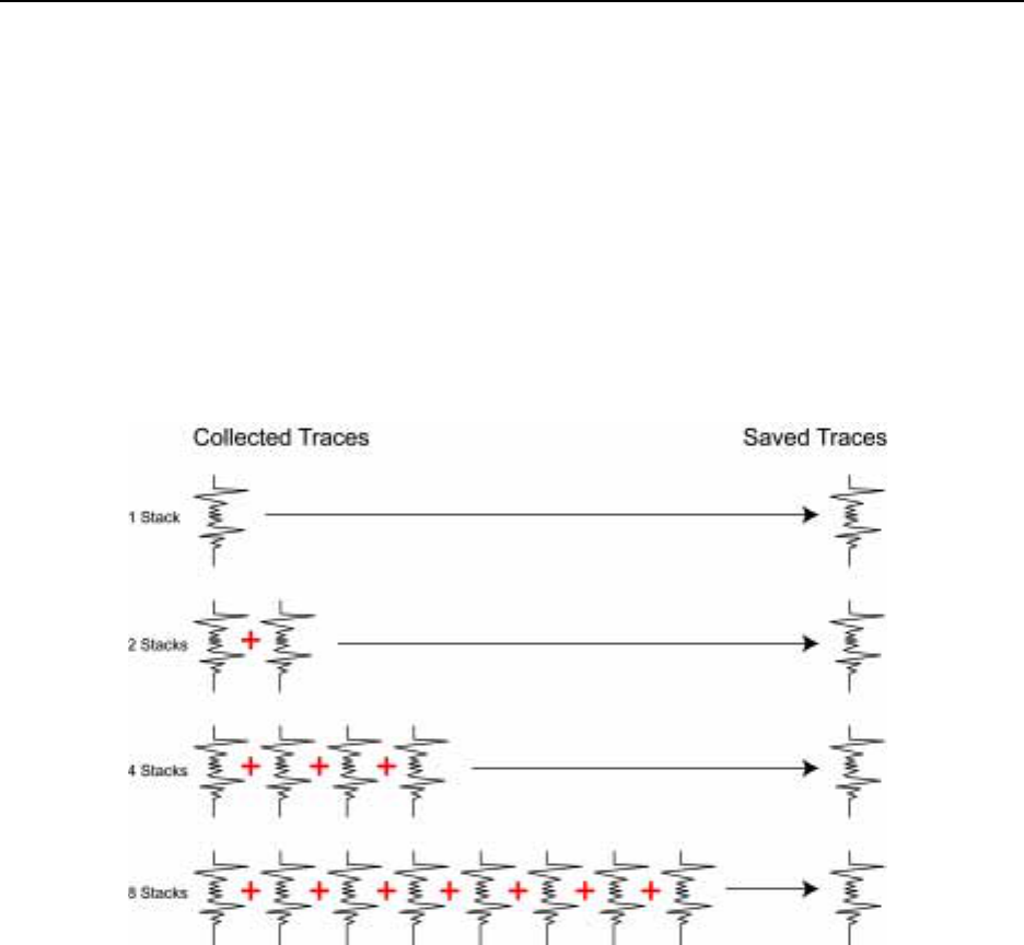
12.3.1.5 Stacks
Some materials tend to absorb radar signals and limit penetration. These materials are said to
be lossy. When collecting data in lossy areas or areas with a lot of radio frequency noise, one
way of increasing data quality is to collect more than one trace at each survey position, average
them and save the averaged trace. This is known as “stacking”. Data quality improves because
the noise, which is usually random (like white noise on a TV screen with no station in the area),
tends to zero when averaged. Consequently, the usable signal is easier to see. This is known as
increasing the “signal-to-noise ratio”.
Figure: 12-7 The concept of stacking data. At each data location point, the trace is collected multiple times. These
traces are averaged together to calculate the trace that is actually saved. Stacking improves the data quality by
increasing the signal to noise ratio.
The amount of Stacking can vary from 1 to 2048 by factors of 2.
While stacking improves data quality, it also forces the user to slow down survey production. The
more stacks the longer it takes to collect data at each survey position. Therefore, it is important to
find the lowest number of stacks that still reveal the target adequately. For most surveys, stacking
4 times is suitable.
See the warning in Section 12.2.7 Collecting Data using the Odometer about losing data if the
Smart System is moving too quickly for the odometer to keep up.
Increasing Data Quality with DynaQ
If the Trigger Method (Section 12.3.2.2 Trigger Method) is set to odometer, one of the options
for Stacking is DynaQ.

Noggin 12-Survey & Map Mode
87
DynaQ is an advanced, patented technology that dynamically adjusts stacking as the system
movement speed varies. In most situations, moving the system at a comfortable speed stacks
enough to generate data of good quality. In situations where target resolution or maximum
penetration depth is critical, moving slower increases the number of stacks and increases the
data quality.
As the system moves during data collection, the DVL screen displays a DynaQ scale bar from L
(Low) to H (high) to indicate data with enhanced signal-to-noise are being attained??.
Figure: 12-8 When collecting data with an odometer, stacking can be set to DynaQ so the number of stacks for each
trace is dynamically adjusted depending on the speed the system is moving. Moving the system slower increases the
number of stacks and increases data quality. The number of stacks is indicated on the DynaQ scale bar from Low (L)
to High (H).
The DynaQ information for each data line is written to the header (.HD) file.

12-Survey & Map Mode Noggin
88
12.3.1.6 Linear Time Gain
As described in Section 12.2.6: P.73, the weak signals must be amplified or “gained” to see them
on the display. The Gain button described in Section 12.2.6: P.73 can be set to a value from 1 to
9 depending on the amount of gain required (1 is lowest gain, 9 is highest gain).
There is also a second level of gain available to the user and that is the Linear Gain setting. The
default Linear Gain setting of 2.0 is usually adequate for most ground conditions, however, if
advanced users find that they are surveying in areas where high Gain button settings are always
required to see data, it may be advantageous to increase the Linear Gain setting. Conversely, if
the user finds that low Gain button values work to see the data, it may be useful to decrease the
Linear Gain setting.
For the experienced user, the setting indicates the gain increases per nanosecond.
The Linear Gain setting can vary from 0.0 to 5.0 in steps of 0.5.
12.3.1.7 Position Units
This is the setting for the position units used by the odometer. The available options are:
1) metres (default)
2) feet

Noggin 12-Survey & Map Mode
89
12.3.2 Cart Parameters
The Cart Parameters settings allow the user to view and modify settings specific to the Smart
System. This includes the direction the Noggin will move to collect data, whether or not the
odometer is active and whether Auto Start is on or off.
12.3.2.1 Cart Direction
This setting determines whether data are collected as the Noggin is pushed forward or pulled in
reverse. The back up arrow (see Section 12.2.7: P.74) will work in the direction opposite to this
setting. The available options are:
1) Push (default)
2) Pull
12.3.2.2 Trigger Method
This setting determines the method used to trigger the Smart System to collect data at each data
collection point. The available options are:
1) Odometer
2) Free Run
3) Button
Trigger with Odometer: Selecting this option means that the Smart System will be triggered to
collect data using the input from the currently selected odometer (see Odometer Number below).
See Section 12.2.7: P.74 for more details about data acquisition with an odometer.
When collecting data with an odometer, data quality can be increased using the DynaQ stacking
option (Section 12.3.1.5 Stacks).
Free Run Operation: Selecting this option means that the Smart System runs continuously in
time, independent of any other triggering device (see Section 12.2.8: P.75). When continuous
operation is selected, two other menus appear to select the number of stacks and time delay
between data traces. These options allow the user to control the speed of the data acquisition.
The user can control the speed the Noggin collects data by increasing or decreasing the number
of stacks (for more details on Stacking, see Stacks on page 86). Increasing the number of Stacks
has the effect of slowing down the data collection speed of the Noggin system. Decreasing the
number of Stacks has the effect of speeding up the data collection speed of the Noggin system.
The second menu to appear prompts the user to input the time delay, in seconds, between each
data collection point. To run the system as quickly as possible, set this value to 0.0 seconds. For
a longer time delay, use the buttons to set the value. Note that any time delay longer than zero
(0.0) seconds causes the Smart System to emit a beeping sound to indicate data collection is
taking place.
The number of stacks and time delay should be set to values that, when combined with speed
the Noggin is moving at, provide an appropriate station interval. This may take a little
experimenting to determine the optimal values for stacks, time delay and the actual speed the
Noggin is moving at.
Trigger with Button: Selecting this means that the Smart System will be triggered to collect data
by pressing the trigger button (if the Smart System has a trigger button) or the B button on the
DVL (see Section 12.2.9: P.76).

12-Survey & Map Mode Noggin
90
After the user selects this option, a menu appears to select the number of stacks for each trace
(for more details on Stacking, see Stacks on page 86).
Note that when data are collected in Trigger Button mode, the Smart System will emit a beeping
sound after the button is pressed to indicate data collection is taking place.
12.3.2.3 Auto Start
If the Auto Start option is set to ON, after the user presses Run to collect a data line, the system
will automatically boot up and be ready for data acquisition, rather than having the Start button
appear. This prevents the user from having to press the Start button at the start of every new
line. This setting is especially useful when collecting numerous lines as occurs when
collecting grid data. If Auto Start is set to OFF the user must press the Start button to begin
data acquisition for each line.
12.3.2.4 Arrow Offset
Section 12.2.7: P.74 describes the Back-up Arrow that appears when the Smart System is
backed up. The Back-up Arrow allows the user to pinpoint the exact ground position
corresponding to a target response on the data image. The Arrow Offset value is used to change
the physical position that corresponds to the Back-up Arrow. If the Arrow Reference value is set
to the default value of zero (0.0) metres, the Back-up arrow position corresponds with the centre
point of the Noggin.
However, the Arrow Offset value can be changed so that the Back-up Arrow corresponds to a
position at any offset from the centre of the Noggin. For example, setting the Arrow Offset value
to +0.25 metres moves the Back-up Arrow to line up with a position 25 centimetres in front of the
Noggin centre point (on the Noggin 500 SmartCart this roughly corresponds to the front axle).
Setting the Arrow Reference value to -0.25 metres moves the Back-up Arrow to line up with a
position 25 centimetres in behind the Noggin centre point (on the Noggin 500 SmartCart this
roughly corresponds to the back axle). In this way, the Arrow Offset value can be changed to
correspond with any position desired by the user.
One reason the user may want to change the Arrow Offset value is to ensure that the Noggin
does not cover the actual target location. This makes it easier to spray paint a mark or put a flag
on the ground where the target occurs.
Positive values correspond to positions in front of the Noggin and negative values are positions
behind the Noggin. Note that the Arrow Offset value is always expressed in metres regardless of
the settings of the other units.
12.3.2.5 Trip Menu
The software records the total distance the system has travelled. This value is displayed but
cannot be changed.
The software also records a distance that can be reset by the user. To reset the distance counter,
move to the Reset Counter option and press the Zero button.
12.3.2.6 Transfer Rate
Transfer Rate is a variable from 1 to 8 that corresponds to the speed of the data transfer from the
Noggin to the DVL. A value of 8 provides the fastest transfer speed while a value of 1 is the
slowest.

Noggin 12-Survey & Map Mode
91
For standard Smart Systems the Transfer Rate value must be set to 8.
The Transfer Rate value will only be decreased for systems with data cables longer than
standard lengths. Please contact Sensors & Software before changing the Transfer Rate on your
system.
12.3.2.7 Odometer Number
Noggin Smart Systems can take input from several different odometers.
It is very important that the user selects and calibrates the odometer appropriate for their
Smart System.
When Odometer Number is selected, the user is prompted to select the odometer that is being
used with the Smart System.
If a SmartCart System is being used, select one of the two SmartCart odometers (usually #1).
If a SmartHandle system is being used, select one of the two SmartHandle odometers (usually
#1).
If the system is being towed behind a vehicle and using the transmission odometer to trigger the
system, select one of the two Vehicle odometers (usually #1).
The odometers labelled Other are to be used in future configurations.
The number after the odometer is the current Odometer Calibration value for that odometer. To
calibrate the odometer, see Section 12.5.2: P.110.

12-Survey & Map Mode Noggin
92
12.3.3 Line Parameters
The Line Parameters settings allow the user to view and modify settings specific to collecting
data as individual lines, namely, the starting position of the line and line direction.
12.3.3.1 Start Position
The Start Position is the position value at the very beginning of a line. This will usually be set to
zero (0.0). However, if the user wants a data file to start at a position other than zero, this value
can be edited.
12.3.3.2 Line Direction
The Line Direction setting specifies which direction that line will be collected, either Forward or
Reverse. Data are usually collected in a forward direction.
If data are collected in the Forward direction the position stepsize is positive, that is, the position
value of each data collection point increments positively. For example, for a Noggin 250 system,
if the Start Position is 10.0 and the Line Direction is Forward, the positions on the line will
increment 10.00, 10.05, 10.10, 10.15 ….
If data are collected in the Reverse direction the position stepsize is negative, that is, the position
value of each data collection point increments negatively. For example, for a Noggin 250 system,
if the Start Position is 10.0 and the Line Direction is Reverse, the positions on the line will
decrement 10.00, 9.95, 9.90, 9.85 ….
Noggin 12-Survey & Map Mode
93
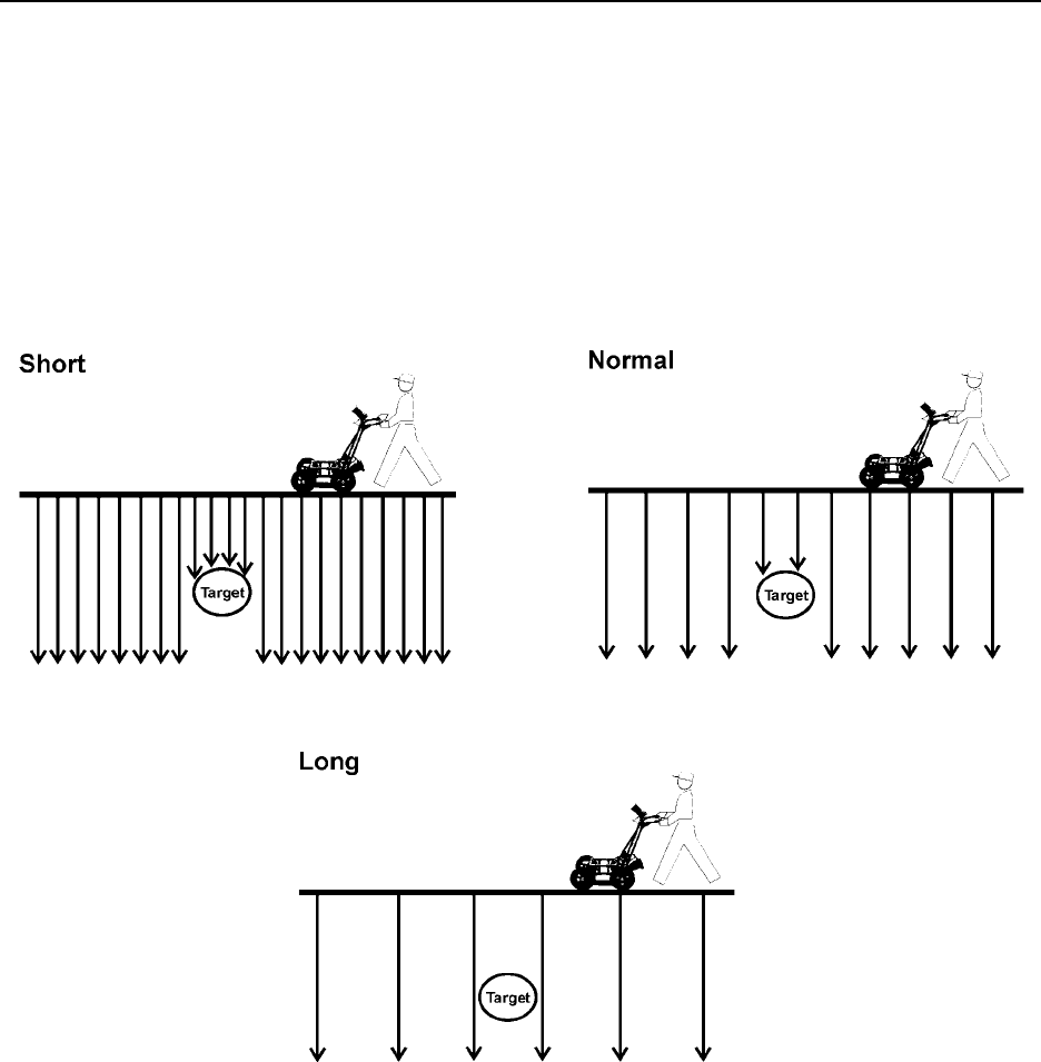
12.3.3.3 Station Interval
As Smart Systems moves, the odometer triggers the system to collect a data trace at fixed
distance intervals. This interval is called the “station interval”.
The station interval can be changed to allow a longer or shorter distance between traces. For a
successful survey, it is important that several traces be collected over a target. If the target is
small, the user may want to shorten the station interval to ensure that data traces are collected
over the target. Conversely, if the target is very large or is a flat-lying feature it is probably not
necessary to collect a lot of traces over the target, in fact, sometimes this can make the target
more difficult to see in the data. In this case it may be beneficial to increase the station interval.
Figure: 12-9 The Station Interval is the distance between sample points on the ground. Be careful not
to choose a Station Interval that is larger than the smallest target to be detected.
Note that decreasing the station interval increases the data volume and increasing the station
interval reduces the data volume.
12-Survey & Map Mode Noggin
94
The choices available are:
1) Short
2) Normal
3) Long
4) X-Long
5) 10x Normal
6) 20x Normal
7) 40x Normal
8) 50x Normal
9) 100x Normal
Each choice listed will be followed by an actual value in metres or inches depending on which
units are selected and which Noggin system is being used. Here is a chart showing the station
interval for each system and setting. Note the calculations for Data per Screen assumes that the
Plot Interval is set to Normal for the particular Noggin system (Noggin 250 = 2 pixels per trace
and Noggin 500 and 1000 = 1 pixel per screen). If this assumption is not true, see the formula
after the charts for calculating this value.
N
OGGIN
250 S
YSTEM
N
OGGIN
500 S
YSTEM
Setting Station Interval Data per Screen
Short 2.5 cm or 0.96 in 8 m or 25.6 ft
Normal 5.0 cm or 1.92 in 16 m or 51.2 ft
Long 10.0 cm or 3.84 in 32 m or 102.4 ft
X-Long 25.0 cm or 9.6 in 80 m or 256 ft
Norm x10 50.0 cm or 19.20 in 160 m or 512 ft
Norm x20 100.0 cm or 38.4 in 320 m or 1024 ft
Norm x40 200.0 cm or 76.8 in 640 m or 2048 ft
Norm x50 250.0 cm or 96.0 in 800 m or 2560 ft
Norm x100 500.0 cm or 192.0 in 1600 m or 5120 ft
Setting Station Interval Data per Screen
Short 1.0 cm or 0.48 in 6.4 m or 25.6 ft
Normal 2.5 cm or 0.96 in 16 m or 51.2 ft
Long 5.0 cm or 1.92 in 32 m or 102.4 ft
X-Long 12.5 cm or 4.8 in 80 m or 256 ft
Norm x10 25 cm or 9.6 in 160 m or 512 ft
Norm x20 50 cm or 19.2 in 320 m or 1024 ft
Norm x40 100 cm or 38.4 in 640 m or 2048 ft
Norm x50 125 cm or 48.0 in 800 m or 2560 ft
Norm x100 250 cm or 96.0 in 1600 m or 5120 ft

Noggin 12-Survey & Map Mode
95
N
OGGIN
1000 S
YSTEM
If the Plot Interval is not set to Normal, use the following formula to calculate the total distance
per screen:
Total Distance Per Screen = Station Interval * (640 / Plot Interval)
where: Station Interval is in metres or feet, and
Plot Interval is in Pixels.
For example, if the Station Interval is 10 centimetres (0.1 metres) and the Plot Interval is 4 pixels,
the total distance per screen is calculated as follows:
0.10 * (640 / 4) = 16.0 metres per screen
To see how much data can be collected before the DVL memory is full and data must be deleted
or downloaded, see DVL Recording Space in Section 12.5.5: P.111.
To delete Noggin data see Section 12.4.5: P.109.
Setting Station Interval Data per Screen
Short 0.5 cm or 0.24 in 3.2 m or 12.8 ft
Normal 1.0 cm or 0.48 in 6.4 m or 25.6 ft
Long 2.0 cm or 0.96 in 12.8 m or 51.2 ft
X-Long 5.0 cm or 2.4 in 32.0 m or 128 ft
Norm x10 10 cm or 4.8 in 64.0 m or 256 ft
Norm x20 20 cm or 9.6 in 128 m or 512 ft
Norm x40 40 cm or 19.2 in 256 m or 1024 ft
Norm x50 50 cm or 24.0 in 320 m or 1280 ft
Norm x100 100 cm or 48.0 in 640 m or 2560 ft
12-Survey & Map Mode Noggin
96
12.3.3.4 Plot Interval
The plot interval setting determines the width of data traces plotted to the screen. Traces can be
1, 2, 4 or 8 pixels wide.
The Normal setting for Noggin 250 systems is 2 pixels per trace and the Normal setting the
Noggin 500 and 1000 is 1 pixel per trace.
It can be useful to plot traces narrower than normal to allow more data to fit onto one screen. It
can also be useful to plot traces wider on the screen so that they are easier to see. For example,
when collecting data using the button to trigger the system (see Section 12.2.9: P.76) it is often
preferable to make each trace 4 or 8 pixels wide.
Figure: 12-10 Data traces can be plotted to the screen with a width of 1 pixel (top left), 2 pixels (top right), 4 pixels
(bottom left) or 8 pixels (bottom right). The narrower the trace width, the more data that can be plotted on one screen.
In this example, plotting the data 1 pixel wide results in 16 metres of data displayed on one screen while 2 pixels
results in 8 metres of data, 4 pixels results in 4 metres of data and 8 pixels results in 2 metres of data
Note that the Plot Interval in Noggin is strictly for display purposes on the DVL screen in real time.
The Plot Interval setting has no effect on the actual data collected and, in fact, data can be
viewed later on the DVL screen with any Plot Interval value. Similarly, data downloaded to a PC
can be plotted using any trace width.
Noggin 12-Survey & Map Mode
97
12.3.4 Grid Parameters
The Grid Parameters settings allow the user to view and modify settings specific to collecting
data in organized grids. This includes the grid dimensions, line spacing, grid type and survey
format.
Data are normally collected on a grid if the user is interested in displaying the data as a 3D
volume (using the EKKO_3D software) or as a plan map (using the EKKO_Mapper and/or
EKKO_Pointer software). Producing accurate 3D volumes or plan maps is easier if the field
survey is properly designed and data are collected correctly.
Positional accuracy of each line is vital if the user wants to be able to relocate targets of interest
after the data have been processed.
For linear targets like pipes and utilities, the best GPR response occurs when the GPR survey
line crosses the target at right angles. If possible, it is always best to run GPR survey lines
perpendicular to the direction of linear targets.
For inexperienced surveyors, laying out a grid with straight lines and all corners at 90
degree angles can be difficult. Sensors & Software provides a product called EasyGrid to
make laying out an accurate grid simple. Contact Sensors & Software for more details.
12.3.4.1 Grid Type
The Grid Type asks specifically the way that the area of the grid is to be covered by the survey
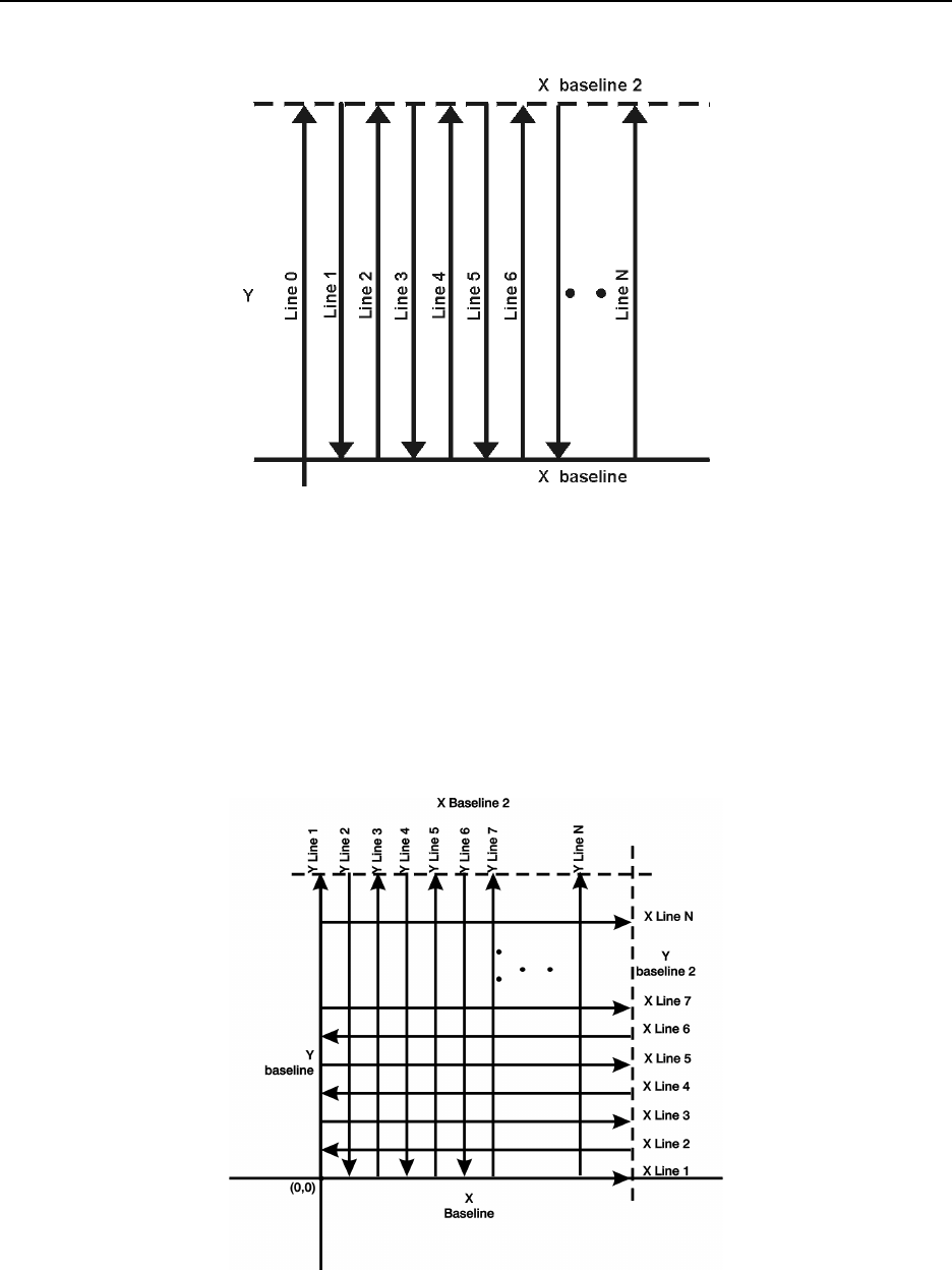
lines. Survey lines can be either a set of parallel lines in the X axis direction (Figure 12-11), a set
of parallel lines in the Y axis direction (Figure 12-12), or, for complete coverage, parallel lines in
both the X and Y direction (Figure 12-13).
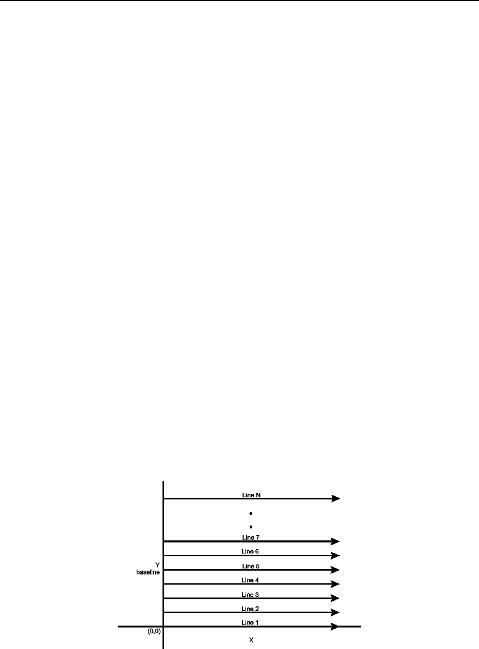
X Lines Only - Forward
Set up a first-quadrant XY grid. Data lines run in the X direction, distance increasing from the Y
axis baseline. Line numbers increase in the positive Y direction (see Figure 12-11). Lines must
be equally spaced. It is not critical that all the lines are the same length. However, it does make
processing easier if all the lines start at the same baseline position (usually defined as zero
(0.0)).
Figure: 12-11 Proper X Line surveying pattern. Following this pattern and starting each line from the
same baseline minimizes the data editing required to produce a spatially accurate map of GPR data.
12-Survey & Map Mode Noggin
98
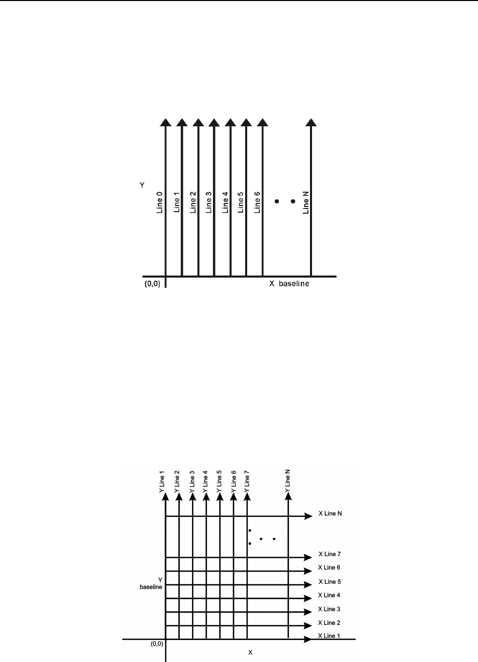
Y Lines Only - Forward
Set up a first-quadrant XY grid. Data lines run in the Y direction, distance increasing from the X
axis baseline. Line numbers increase in the positive X direction (see Figure 12-12). Lines must
be equally spaced. It is not critical that all the lines are the same length. However, it does make
processing easier if all the lines start at the same baseline position (usually defined as zero
(0.0)).
Figure: 12-12 Proper Y Line surveying pattern. Following this pattern and starting each line from the
same baseline minimizes the data editing required to produce a spatially accurate map of GPR data.
XY Lines - Forward
Set up a first-quadrant XY grid. X data lines run in the X direction, distance increasing from the Y
axis baseline. Line numbers increase in the positive Y direction (see Figure 12-13). Lines must
be equally spaced. Y data lines run in the Y direction, distance increasing from the X axis
baseline. Line numbers increase in the positive X direction. Lines should be equally spaced.
The line spacing of the X lines and Y lines can be different.
It is not critical that all the lines are the same lengths. However, it does make processing easier
if all the lines start at the same baseline position (usually defined as zero (0.0)).
Figure: 12-13 Proper XY grid surveying pattern. Following this pattern and starting each line from the
same baseline minimizes the data editing required to produce a spatially accurate map of GPR data.
Noggin 12-Survey & Map Mode
99
12.3.4.2 Survey Format
The Survey Format specifies how the lines will be collected. The lines shown in Figure 12-11,
Figure 12-12, and Figure 12-13 are all collected in the Forward direction only. This means that
each line starts at the X or Y baseline.
When the length of the survey lines are more than about 20 metres, data acquisition speed may
be increased by collecting every second line in the reverse direction (Figure 12-14, Figure 12-15,
and Figure 12-16). This is called a Forward and Reverse survey format.
Using forward and reverse format can speed acquisition but can lead to mapping artifacts called
“herringbone” if there are positional errors. It is important that the odometer is calibrated (Section
12.5.2: P.110), the Grid Dimensions are correct (see Grid Dimensions on page 101) and that
lines are always collected starting on a baseline.
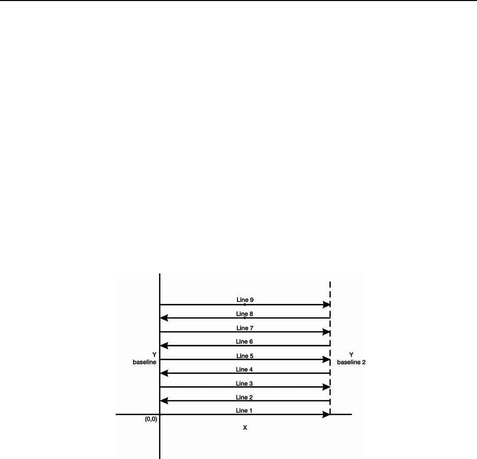
X Lines Only – Forward and Reverse
Using the Forward and Reverse survey format, X line data are collected in the pattern shown in
Figure 12-14.
Figure: 12-14 For collecting GPR data consisting of long data lines it makes more sense to follow a
forward and reverse surveying pattern. For the final data to be spatially correct with a minimum of
editing, data collected in this pattern should be on lines that extend completely from one baseline to the
other.
Y Lines Only – Forward and Reverse
Using the Forward and Reverse survey format, Y line data are collected in the pattern shown in
Figure 12-15.
When data are collected like this, it is important that lines start and end on established baselines,
otherwise, when lines are reversed to the correct orientation for the display, they may be offset
from one another.
12-Survey & Map Mode Noggin
100
Figure: 12-15 For collecting GPR data consisting of long data lines it makes more sense to follow a
forward and reverse surveying pattern. For the final data to be spatially correct with a minimum of
editing, data collected in this pattern should be on lines that extend completely from one baseline to the
other.
XY Lines – Forward and Reverse
Using the Forward and Reverse survey format, XY line data are collected in the pattern shown in
Figure 12-16.
When data are collected like this, it is important that lines start and end on established baselines,
otherwise, when lines are reversed to the correct orientation for the display, they may be offset
from one another.
Figure: 12-16 For collecting GPR data on a grid consisting of long data lines, it makes more sense to
follow a forward and reverse surveying pattern. For the final data to be spatially correct with a minimum
of editing, data collected in this pattern should be on lines that extend completely from one baseline to
the other.

Noggin 12-Survey & Map Mode
101
12.3.4.3 Grid Dimensions
For grid data acquisition, the grid size needs to be specified. The user needs to input the length
of the X dimension and the length of the Y dimension. The dimensions entered are assumed to
be in the same units as the Position Units (see Section 12.3.1.7: P.88), i.e. metres or feet.
On this screen the user needs to highlight the dimension to be changed. The user can toggle
between the X and Y fields by pressing the X/Y button.
The dimension value is incremented or decremented by pressing the +Line or –Line buttons.
The dimension value will change by a value equal to the current Line Spacing in that dimension.
For example, if the Line Spacing in the X direction is 0.5 metres, the grid dimension in the X
direction will increment or decrement in 0.5 metre intervals.
Note that the maximum number of lines that can be collected in each direction is 100.
Therefore, the X and Y grid dimensions cannot be set to a value that will result in more
than 100 lines being collected.
For example, if the Line Spacing between Y lines (defined as lines parallel to the Y axis) is set to
0.25 metres, the maximum X dimension is (100-1) X 0.25 = 24.75 metres. (One is subtracted
because the first line is at position 0.0 metres.)
To increase the X dimension value, the Y line spacing must be increased. Using the example
above, if the Y Line Spacing is increased to 0.30 metres then the maximum X dimension is (100-
1) X 0.30 = 29.70 metres.
If the Grid Type is set to X Lines only or Y Lines only (see Section 12.3.4: P.97), the length of
those lines are not restricted by the Line Spacing parameter of the opposite dimension. That is
why if an X Lines only grid is selected, the X dimension can be input as a value rather than an
increment of the Y Line Spacing. Similarly, if a Y Lines only grid is selected, the Y dimension can
be input as a value rather than an increment of the X Line Spacing.
12.3.4.4 Line Spacing
For grid data acquisition, the distance between survey lines needs to be specified.
If the grid type is X Lines only (see Section 12.3.4: P.97) then the spacing between the X lines
needs to be input.
If the grid type is Y Lines only (see Section 12.3.4: P.97) then the spacing between the Y lines
needs to be input.
If the grid type is XY Lines (see Section 12.3.4: P.97) then the spacing between the X lines and Y
lines need to be input. The line spacing can be different. The user can toggle between the X line
spacing and Y line spacing fields by pressing the X/Y button.
Note that the maximum number of lines that can be collected in each direction is 100.
The calculation for determining an appropriate line spacing is complex. One has to consider
system frequency, target size and practical considerations. In general, the Noggin 250 should
have a line spacing of 0.5 metres or less, the Noggin 500 should have a line spacing of 0.25
metres or less and the Noggin 1000 should have a line spacing of 0.10 metres or less.

12-Survey & Map Mode Noggin
102
However, line spacing should really be determined by target size. In most cases the system
must pass over a target to detect it. Therefore, the line spacing needs to be on the order of the
size of the target or smaller, if practical. This can be adjusted to a larger spacing for larger targets
or targets with a linear extent. As well, these rules may have to be bent for practical purposes
like survey production rates. The fact is that a tighter line spacing takes longer to collect and this
may not be economically possible in all circumstances.

Noggin 12-Survey & Map Mode
103
12.3.5 GPS Parameters
The Global Positioning System (GPS) uses special satellites around the Earth to determine the
position of a GPS receiver located at any position on the surface of the Earth. GPS receivers can
be purchased from a number of manufacturers.
The DVL has a serial port on the back for attaching a GPS receiver. This port will accommodate
any GPS receiver that has a standard serial port output.
The GPS receiver can be set up to send one or more types of data strings to the DVL. These
strings are called NMEA-0183 strings and each contains positional or other information in
specific formats. Each type of string is specified by a 5-character prefix. There are numerous
NMEA strings but to integrate the GPS data into the Noggin data, the GPS must be sending at
least one of the following NMEA strings: GPGGA, GPGLL and GPRMC.
This feature allows GPS information to be logged while collecting Noggin data. The GPS
information may be useful for mapping where GPR surveys have been performed (see Reading
per Trace mode below) or determining where a specific target of interest is located in GPS co-
ordinates (see Fiducial Tagging mode below).
The DVL can be set up to read and log GPS information collected during data acquisition with the
Noggin system. GPS information can be logged in two different ways:
1) For every trace collected by the Noggin system, or
2) Every time the user adds a fiducial to the data by pressing the A button (see Fiducial
Markers on page 72).
This feature provides a means of logging GPS information to an independent file. Note that the
GPS information is NOT automatically integrated with the Noggin data. After data
acquisition is complete, the data can be downloaded to a PC and the EKKO_View Deluxe
software can be used to integrate the GPS data with the Noggin data.
In order for the DVL to read the GPS data string, the GPS settings for the specific GPS receiver
being used must be input into this menu. There are 4 important items that must be specified
correctly for the DVL to display the GPS strings. These items are Baud Rate, Stop Bits, Data Bits
and Parity. These are discussed in more detail below. The default values listed below are the
values that are typically used. Read the GPS Receiver User’s Guide or experiment with the
settings to find the correct ones.
Once these 4 items are set correctly you should be able to run System Test #1 and have GPS
information written to the screen.
When the logging of GPS information is enabled, during data acquisition a message will appear
in the bottom left-hand corner of the DVL screen indicating whether GPS data is successfully
being received (see Section 12.2.4: P.72).

12-Survey & Map Mode Noggin
104
Mode
There are three GPS modes available:
1) Off mode means that a GPS receiver is not connected to the DVL so no GPS
information is being logged. This should be the setting if you do not have a GPS
receiver.
2) Reading every x traces mode means that every time the Noggin collects a user-
defined number of traces of GPR data, a data string of GPS information will be added
to a file. This file has the same name as the data file i.e. LINE6, but with a GPS
extension. This file can be accessed after transferring the GPR data files to an
external PC (see Section 12.4.1: p.108).
For example, if the number of traces is set to 1, the LINE6.GPS may look like this:
Trace #1 at position 0.00
$GPGGA,134713.00,4338.221086,N,07938.421365,W,2,06,2.1,152.51,M,-35.09,M,5.0,0118*79
$GPVTG,34.0,T,,,001.4,N,002.5,K,D*70
$GPGSA,A,3,30,26,10,13,24,06,,,,,,,4.2,2.1,3.6*36
Trace #2 at position 0.05
$GPGGA,134713.00,4338.221086,N,07938.421365,W,2,06,2.1,152.51,M,-35.09,M,5.0,0118*79
$GPVTG,34.0,T,,,001.4,N,002.5,K,D*70
$GPGSA,A,3,30,26,10,13,24,06,,,,,,,4.2,2.1,3.6*36
Trace #3 at position 0.10
$GPGGA,134713.00,4338.221086,N,07938.421365,W,2,06,2.1,152.51,M,-35.09,M,5.0,0118*79
$GPVTG,34.0,T,,,001.4,N,002.5,K,D*70
$GPGSA,A,3,30,26,10,13,24,06,,,,,,,4.2,2.1,3.6*36
Trace #4 at position 0.15
$GPGGA,134713.00,4338.221086,N,07938.421365,W,2,06,2.1,152.51,M,-35.09,M,5.0,0118*79
$GPVTG,34.0,T,,,001.4,N,002.5,K,D*70
$GPGSA,A,3,30,26,10,13,24,06,,,,,,,4.2,2.1,3.6*36
Note that when the Reading per Trace option is on, it is still possible to add fiducial markers to
the GPS file. These will appear as F1, F2 etc. between the trace numbers. For example, a
portion of LINE6.GPS may look like this:
Trace #85 at position 4.20
$GPGGA,134850.00,4338.204868,N,07938.429003,W,2,06,2.1,152.60,M,-35.09,M,4.2,0118*74
$GPVTG,152.6,T,,,002.3,N,004.3,K,D*43
$GPGSA,A,3,30,26,10,13,24,06,,,,,,,4.2,2.1,3.7*37
F1
$GPGGA,134850.00,4338.204868,N,07938.429003,W,2,06,2.1,152.60,M,-35.09,M,4.2,0118*74
$GPVTG,152.6,T,,,002.3,N,004.3,K,D*43
$GPGSA,A,3,30,26,10,13,24,06,,,,,,,4.2,2.1,3.7*37
Trace #86 at position 4.25
$GPGGA,134851.00,4338.204362,N,07938.428362,W,2,06,2.1,152.40,M,-35.09,M,5.2,0118*72
$GPVTG,136.9,T,,,002.8,N,005.2,K,D*45
$GPGSA,A,3,30,26,10,13,24,06,,,,,,,4.2,2.1,3.7*37

Noggin 12-Survey & Map Mode
105
3) Fuducial Tagging mode means that whenever a fiducial marker (F1, F2 etc.) is
added to the data (see Section 12.2.4: P.72), a data string of GPS information will be
added to a file. This file has the same name as the data file i.e. LINE6, but with a
GPS extension. This file can be accessed after transferring the GPR data files to an
external PC (see Section 12.4.1: p.108).
For example, LINE6.GPS may look like this:
F1
$GPGGA,134218.00,4338.190204,N,07938.438411,W,2,05,2.6,154.60,M,-35.09,M,4.0,0118*7B
$GPVTG,356.8,T,,,000.2,N,000.4,K,D*4B
$GPGSA,A,3,30,10,13,24,06,,,,,,,,4.3,2.6,3.4*36
F2
$GPGGA,134219.00,4338.190294,N,07938.438409,W,2,05,2.6,154.45,M,-35.09,M,5.0,0118*7C
$GPVTG,1.3,T,,,000.4,N,000.7,K,D*44
$GPGSA,A,3,30,10,13,24,06,,,,,,,,4.3,2.6,3.4*36
F3
$GPGGA,134221.00,4338.190261,N,07938.438285,W,2,05,2.6,154.05,M,-35.09,M,5.2,0118*79
$GPVTG,10.0,T,,,000.2,N,000.4,K,D*72
$GPGSA,A,3,30,10,13,24,06,,,,,,,,4.3,2.6,3.4*36
F4
$GPGGA,134222.00,4338.190397,N,07938.438255,W,2,05,2.6,153.95,M,-35.09,M,5.0,0118*73
$GPVTG,9.8,T,,,000.3,N,000.5,K,D*42
$GPGSA,A,3,30,10,13,24,06,,,,,,,,4.3,2.6,3.4*36
If the GPS mode is set to Reading per Trace or Fiducial Tagging AND the Noggin is Run Without
Saving Data (see Section 12.1.5: P.68), it is still possible to log GPS data strings. Every time a
fiducial marker is added to the data (see Section 12.2.4: P.72), a data string of GPS information is
added to a file. This file is called TAGGED.GPS and can be exported and/or deleted using the
Noggin File Management (see Section 12.4: P.108).
An example of a TAGGED.GPS file is shown below.
New File 09-18-2000 13:53:38
F1
$GPGGA,134227.00,4338.190520,N,07938.438280,W,2,05,2.6,153.98,M,-35.09,M,4.6,0118*7E
$GPVTG,347.7,T,,,000.3,N,000.5,K,D*44
$GPGSA,A,3,30,10,13,24,06,,,,,,,,4.3,2.6,3.4*36
F2
$GPGGA,134228.00,4338.190238,N,07938.438286,W,2,05,2.6,153.87,M,-35.09,M,4.4,0118*75
$GPVTG,5.4,T,,,000.2,N,000.4,K,D*42
$GPGSA,A,3,30,10,13,24,06,,,,,,,,4.3,2.6,3.4*36
F3
$GPGGA,134229.00,4338.190277,N,07938.438273,W,2,05,2.6,153.76,M,-35.09,M,5.4,0118*7A
$GPVTG,23.4,T,,,000.1,N,000.2,K,D*73
$GPGSA,A,3,30,10,13,24,06,,,,,,,,4.3,2.6,3.4*36
F4
$GPGGA,134231.00,4338.190127,N,07938.438362,W,2,05,2.6,154.59,M,-35.09,M,5.0,0118*7A
$GPVTG,20.2,T,,,000.2,N,000.3,K,D*74
$GPGSA,A,3,30,10,13,24,06,,,,,,,,4.3,2.6,3.4*36
********************************************************************************
New File 09-18-2000 13:55:36
F1
$GPGGA,134259.00,4338.192453,N,07938.449096,W,2,06,2.4,153.14,M,-35.09,M,5.4,0118*75
$GPVTG,310.9,T,,,000.5,N,001.0,K,D*4A
$GPGSA,A,3,04,30,10,13,24,06,,,,,,,3.2,2.4,2.1*32
F2
$GPGGA,134301.00,4338.192559,N,07938.449176,W,2,06,2.4,153.17,M,-35.09,M,5.0,0118*7A
$GPVTG,314.4,T,,,000.6,N,001.1,K,D*41
$GPGSA,A,3,04,30,10,13,24,06,,,,,,,3.2,2.4,2.1*32
F3

12-Survey & Map Mode Noggin
106
4) GPR data out port mode means that the GPR data stream will be output to the serial
port of the DVL. This is for users who wish to read the GPR data into their own PC or
other device. Contact Sensors & Software Inc. for more details if you want to use this
option.
Note that this option slows down data acquisition speeds.
Baud Rate
The baud rate is the speed that data is sent from the GPS receiver to the serial port of the DVL.
The available options are: 2400, 4800, 9600 (default) or 19200.
Stop Bits
The available settings for Stop Bits are: 1 (default) or 2.
Data Bits
The available settings for Data Bits are: 7 or 8 (default).
Parity
The available settings for Parity are: none (default), odd or even.
End String
The GPS receiver can be set up to send one or more types of data strings to the DVL. These
strings are called NMEA-0183 strings and each contains positional or other information in
specific formats. Each type of string is specified by a 5-character prefix. There are numerous
NMEA strings but examples of three different NMEA strings (GPGGA, GPVTG and GPGSA) are
shown below.
$GPGGA,134713.00,4338.221086,N,07938.421365,W,2,06,2.1,152.51,M,-35.09,M,5.0,0118*79
$GPVTG,34.0,T,,,001.4,N,002.5,K,D*70
$GPGSA,A,3,30,26,10,13,24,06,,,,,,,4.2,2.1,3.6*36
$GPGGA,134713.00,4338.221086,N,07938.421365,W,2,06,2.1,152.51,M,-35.09,M,5.0,0118*79
$GPVTG,34.0,T,,,001.4,N,002.5,K,D*70
$GPGSA,A,3,30,26,10,13,24,06,,,,,,,4.2,2.1,3.6*36
$GPGGA,134713.00,4338.221086,N,07938.421365,W,2,06,2.1,152.51,M,-35.09,M,5.0,0118*79
$GPVTG,34.0,T,,,001.4,N,002.5,K,D*70
$GPGSA,A,3,30,26,10,13,24,06,,,,,,,4.2,2.1,3.6*36
$GPGGA,134713.00,4338.221086,N,07938.421365,W,2,06,2.1,152.51,M,-35.09,M,5.0,0118*79
$GPVTG,34.0,T,,,001.4,N,002.5,K,D*70
$GPGSA,A,3,30,26,10,13,24,06,,,,,,,4.2,2.1,3.6*36
Before using the GPS with the Noggin, the DVL software needs to know the prefix of the LAST
string being sent in each group. In the example above, three strings are being sent each time
(GPGGA, GPVTG and GPGSA). Since GPGSA is the last one being sent in each group, the End
String needs to be specified as GPGSA.
To see what the End String is for your particular GPS, run System Test #1 and note the first 5
characters on the last line after each series of strings is written to the screen. These are the 5
characters that need to be filled in under End String.

Noggin 12-Survey & Map Mode
107
The End String option allows the user to fill in the 5 character GPS prefix. Use the Left and Right
buttons to move left or right to different characters in the string. The currently selected character
will have an “^” under it. To change the letter of the current character, use the Next button to
change it to the next letter in the alphabet and the Previous button to change it to the previous
letter in the alphabet. Using these keys all 5 characters can be filled in with the necessary GPS
End String.
See the GPS Receiver User’s Guide for details on how to set up the receiver to output specific
NMEA strings or groups of NMEA strings.
System Test #1
After all the settings above have been input and the GPS receiver is attached to the serial port on
the DVL, the user can test that the DVL is receiving the GPS output by using the Test option.
If the NMEA strings are successfully being read by the DVL they will appear on the DVL screen.
This is a good time to note the prefix of the last NMEA string in the list and input it in the End
String setting above.
If the NMEA strings do not appear, check that the port settings are correct. It is also possible that
a crossover cable is required between the output cable of the GPS receiver and the serial port on
the DVL.
System Test #2
Once the GPS system is running successfully, System Test #2 can be used to graphically display
the GPS data. This screen displays the GPS Time, Latitude, Longitude and Altitude as well as
other values indicating the accuracy of the GPS reading. The GPS position is also displayed in a
square that can be Zoomed from 2 metres square to 16384 metres square.
12.3.6 Set Defaults
To reset all the parameter settings back to the factory default settings press the 6 button (labelled
Set Defaults).
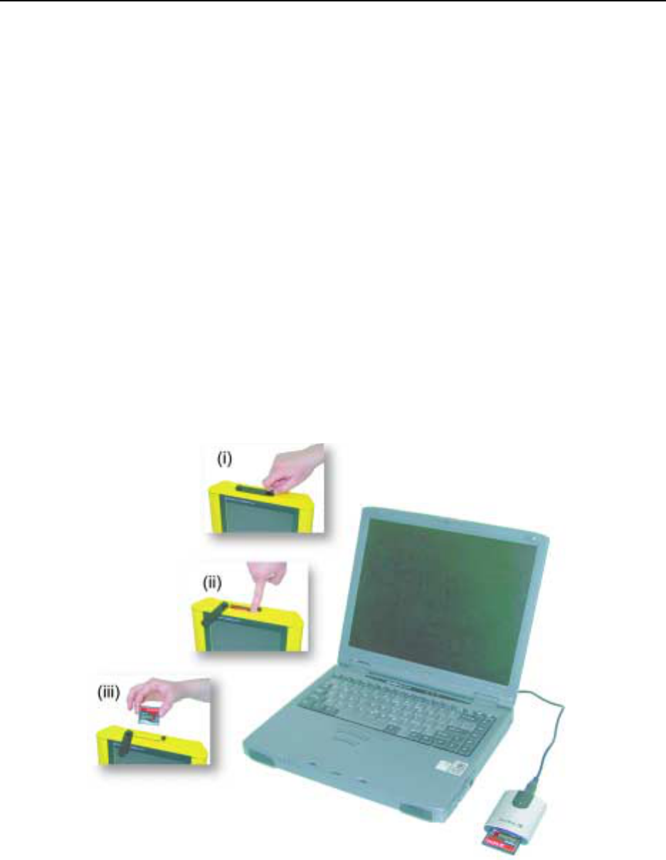
12-Survey & Map Mode Noggin
108
12.4 Noggin File Management
The File Management option is available by pressing 2 from the main Noggin menu.
The File Management menu allows the user to delete data from the DVL and copy data from the
internal compact flash drive to the removable compact flash drive.
The Export options in this menu require the use of the optional PXFER cable and WinPXFER
software so this menu is not required for users transferring Noggin data using the removable
compact flash drive. These options allow the user to export Noggin data or the TAGGED.GPS file
(see Section 12.3.5: P.103) to a PC using the optional PXFER cable. This is described in
Appendix F.
12.4.1 Transferring Noggin Data to a PC using the Removable Drive
Files collected with the Noggin system are saved either to the Internal or the Removable drive on
the DVL. To transfer data collected on the removable drive to a PC, eject the compact flash drive
from the DVL and insert it into a user-supplied card reader connected to a PC. Use the Windows
Explorer program to make a new folder on the PC, read the removable drive and copy the
Noggin data files to the new folder.
If data were collected to the internal drive of the DVL (Section 12.1.7: p.69), the data can be
copied to the removable drive so it can be transferred to a PC (see Section 12.4.2: p.109).
Figure: 12-17 Noggin data files saved to the removable drive are easily transferred to a PC. First, power down the
DVL, then (i) loosen both of the finger-screws on the top of the DVL so the drive door can swing open freely. (ii) Press
the button to partially eject the compact flash drive. (iii) Remove the drive and insert it into a PC card reader (user sup-
plied). Copy the Noggin data files from the drive into a folder on the PC using the Windows Explorer program. The Win-
PXFER program can then be used to view the Noggin data.

Noggin 12-Survey & Map Mode
109
12.4.2 Copying Noggin Data from the Internal Drive to the Removable
Drive
If data were collected to the internal drive of the DVL (Section 12.1.7: p.69), the data can be
copied to the removable drive so the data transfer method described above can be used. To copy
Noggin data from the internal drive to the removable drive, from the Noggin menu select 2 - File
Management and then select 7 - Copy Internal to Removable.
12.4.3 Transferring Noggin Data to a PC using the PXFER Cable
Files collected with the Noggin system are saved to the Internal or the Removable drive on the
DVL. While the method described above, of transferring data by ejecting the removable drive, is
the usual method of data transfer, data can also be transferred to a PC using the optional PXFER
cable and the WinPXFER program. This process is described in Appendix F.
12.4.4 Viewing Data Files on the External Computer
After transferring data files to the external computer the Noggin data files can be viewed,
processed and plotted using the EKKO_View, EKKO_3D and EKKO_Mapper software.
Appendix A contains details about the file format of Noggin data.
12.4.5 Deleting Data on the DVL
After data has been successfully transferred to an external computer or if the data is longer
required, the whole Line or Grid project can be deleted from the DVL. From the File
Management main menu, select Delete Line Project or Delete Grid Project. The next screen lists
all the current projects.
To delete a project, use the up and down arrows to highlight it and then press the DEL button.
It is also possible to use the TAG button to select several projects and delete them all at once.
Use the up and down arrows to highlight the projects, the TAG button to tag each project and
then press the DEL button to delete the data from the DVL.
Before the project is deleted, the user is asked to confirm the deletion by pressing Yes or No. If
the answer to the question is No, the project is not deleted.
This menu also allows the user to delete the TAGGED.GPS file.

12-Survey & Map Mode Noggin
110
12.5 Noggin Utilities
Pressing the number 4 on the main menu selects Utilities. This menu has utility programs to
change the date and time on the DVL and also calibrate the odometer.
12.5.1 Time and Date
The date and time are saved with the data files. The DVL date and time setting can be changed
by moving to one or more of the appropriate fields and editing the current setting. The LEFT and
RIGHT arrows are used to move between fields. To change any of the numbers or months, use
the UP and DOWN arrows to increase or decrease the value. When the desired date and time
are set, press ENTER to save the changes.
12.5.2 Odometer Calibration
The odometer should be calibrated periodically to ensure accuracy.
Noggin Smart Systems can take input from several different odometers.
It is very important that the user selects and calibrates the odometer appropriate for their
Smart System.
When Odometer Calibration is selected, the user is prompted to select the odometer that is being
used with the Smart System.
If a SmartCart System is being used, select one of the two SmartCart odometers (usually #1).
If a SmartHandle system is being used, select one of the two SmartHandle odometers (usually
#1).
If the system is being towed behind a vehicle and using the transmission odometer to trigger the
system, select one of the two Vehicle odometers (usually #1).
The odometers labelled Other are to be used in future configurations.
Once an odometer is selected, the user is prompted to either 1) manually enter the odometer
calibration factor or 2) to actually calibrate the odometer over a known distance. To achieve the
highest accuracy, it is recommended that the user choose option number 2 - Odometer
Calibration.
When Odometer Calibration is selected, the user is prompted to select the length of the line to
calibrate on. There are 8 different choices in metres and 8 choices in feet. To toggle the units
between metres and feet, press the B button. Pressing the A button on this screen gives the
additional option to select a user-defined value. The user-defined value can range from 0.01 to
5000 metres or 0.01 to 26400 feet.
When the calibration distance has been selected follow the directions on the screen:
1) Set the cart at zero and press A
2) Move the cart the selected distance and press B
3) Press A to exit.
Odometer calibration values for the SmartCart odometer should be around 1080.

Noggin 12-Survey & Map Mode
111
Odometer calibration values for the SmartHandle odometer should be around 1530.
Odometer calibration values for the Vehicle odometer vary but may be around 50.
12.5.3 Upgrade
Upgrade requires the use of the optional PXFER cable so this menu is not required for users
who upgrade their DVL firmware using a removable compact flash drive.
The menu allows the user to enter Upgrade mode to update the firmware on the DVL. Selecting
Upgrade puts the DVL into listen mode to allow a software upgrade to be transferred from an
external PC to the DVL using the PXFER and WinPXFER cable. Avoid pressing this button until
the instructions in a software upgrade tell you to. Once pressed, the DVL must have the power
disconnected to exit from this menu item.
12.5.4 System Information
This option can be used to list system information that may be useful to troubleshoot a problem
with the Noggin. The information is intended for the use of Sensors & Software staff to assist in
solving a problem with the Noggin system.
System information can be listed to the screen, printed directly to an attached printer or
transferred to a PC.
To print the information to a printer, attach the printer to the parallel port of the DVL and then
press the B button.
To transfer the information file to a PC, attach the parallel XFER cable from the parallel port of the
PC to the parallel port of the DVL. Then run the WinPXFER program on the PC (see Section
12.4.1: p.108) and press the 1 button.
Sensors & Software technical staff may request that this information be sent to them. A printed
copy of the information can be faxed to Sensors & Software Inc. If the data is transferred to a
PC, the data file can be e-mailed to Sensors & Software Inc.
12.5.5 DVL Recording Space
This option shows, based on the current data collection settings, the total number of traces that
can be collected before the DVL memory is full. It also lists, based on the current Station Interval,
the total distance of data that can be collected before the DVL memory is full.
12.5.6 Transfer Mode
Transfer Mode requires the use of the optional PXFER cable so this menu is not required for
users transferring Noggin data using the removable compact flash drive. This menu allows the
user to set the transfer mode to Normal or Turbo depending on what type of PXFER cable they
have (see Appendix F).

13-Troubleshooting Noggin
112
13 Troubleshooting
Noggin Smart Systems are designed to minimize user problems; however, all electronic devices
are subject to possible failure. The following are troubleshooting hints in the likelihood of
occurrence if your Smart System fails to operate.
13.1 Power Supply
The most common problem that can occur while trying to run a system is insufficient power. The
battery may be dead or have a low voltage. If the system is being run from AC, there may be a
problem with the AC power supply or adapter.
If there is enough power to run the DVL, the upper red LED on the front of the DVL will light up
when the battery is plugged into the system. If this light is on and the DVL boots up, runs and
displays the main menu, next check that the red light on the connector to the Noggin is on. If this
light is off then there is a problem with the connection from the DVL to the Noggin. Check the
connection and this part of the cable.
If the DVL is running but the Noggin system will not run, go to the main menu and check that
battery voltage in the lower left corner is above 10.2 volts. If not, the battery needs to be
recharged or replaced for the Noggin to run (see below).
If the battery voltage is less than about 10.2 volts, the DVL may not turn on and the upper red
LED will flash or not illuminate.
Check the battery voltage with a voltmeter. Try to do this while the system is still attached to the
Smart System to get a true measure of the voltage while under load (it will be necessary to open
the SmartCart battery case or belt battery case and connect the voltmeter to the positive and
negative battery terminals). If the battery has a low voltage or seems dead, try the system with
another battery (if available), or give the battery a good 12-14 hour charge and try running the
system again.
If the battery does not charge up to 12 Volts or more, it should be replaced.
Smart System batteries are fused to protect the system. For the SmartCart system, open the
battery case and check that the 10 Amp fuse is OK. If necessary, replace it with one of the spare
fuses available inside the battery case. The smaller belt batteries available for the SmartHandle
systems are also fused. Remove the battery from padded casing and check the 5 Amp fuse.
Replace the fuse if necessary.
13.2 System Communications
If the system power supply is OK but the Noggin does not respond there may be a
communication failure between the DVL and the Noggin. This type of failure is often indicated by
a 10000 series error number like 10012.
If an error occurs, an error message will appear in the bottom left section of the Noggin screen.
EXIT the program and turn off the Digital Video Logger. Disconnect the power source to
completely shut down the system.

Noggin 13-Troubleshooting
113
Make sure the cables are not damaged and that all cable connections are tightly secured. Use a
slotted screwdriver to snug up the connections. Sometimes vibrations cause the cable
connections to loosen just a bit and break contact and this can cause errors. Disconnecting
cables and reconnecting them may provide a better contact and solve the problem. Turn the
Digital Video Logger back on and try running the system again.
If the power supply and cable are OK, the problem is likely a failure of the DVL. The DVL has no
user-serviceable parts so it will have to be returned to Sensors & Software Inc for inspection and
possible repair (see Section 13.6: P.114).
13.3 System Overheating
The Noggin systems are designed to operate to a maximum internal temperature of 70 C or 158
F. In situations of high ambient temperatures or long exposure to direct sun, this maximum
internal temperature may be exceeded and cause the system to fail. While the temperature
displayed on the DVL in the lower left corner of the main menu indicates the internal temperature
of the DVL and not the Noggin, this temperature should give an idea of whether the Noggin is
overheating.
If you suspect that the Noggin system is overheating, shut it off and give it a chance to cool down
in a shady location before trying to run it again. Placing a wet cloth on top of the Noggin may
help in cooling it down.
If the situation is such that the high temperatures or direct sun cannot be avoided, it may be a
good idea to put some sort of shade over the Noggin.
Contact Sensors & Software Inc. if the problem persists as there may be defective electronic
components that need to be replaced (see Section 13.6: P.114).
13.4 DVL Problem
While the DVL has been ruggedized as much as possible, it should be handled in much the same
way a notebook computer is. If the DVL does not power up and boot up, there may be a problem
with the CPU or the storage media. If this occurs, contact Sensors & Software Inc. (see Section
13.6: P.114).
13.5 Noggin Problem
When the Smart System is powered up and the user selects data acquisition in Noggin or Noggin
mode, the Noggin system goes through a self-calibration sequence. While the self-calibration is
occurring the user sees the words “Booting Noggin” in the lower left corner of the DVL screen.
These words are followed by a number that counts up from 1. Normally, once the count reaches
6 the text disappears and the Noggin is ready to collect data. Sometimes, however, this count
goes beyond 6 and keeps going without stopping. This indicates an internal problem with the
Noggin. No error message will be displayed on the screen and the only way to exit from the
screen is to pull out the power connection.

13-Troubleshooting Noggin
114
If this error occurs, power the system down, power it up again and retry data acquisition. If the
error persists, contact Sensors & Software Inc. (see Section 13.7: P.114).
13.6 Creating a Test Line for Data Quality
One of the best ways of detecting problems with the GPR system is, shortly after receiving the
system and getting comfortable with its operation, to collect a line of data at a convenient, easily
accessible location. The line does not have to be too long but 100 - 200 traces is a good guide.
This data line should be saved electronically and perhaps plotted out on paper and dated. The
test line could be collected say, every 6 months and, by reviewing the previous data, system
problems can be detected early. As well, if there is a suspected problem with the system, this test
line could be collected and compared with earlier tests.
13.7 Contacting Sensors & Software Inc.
If you develop problems with your Noggin system, contact your agent or Sensors & Software Inc.
Sensors & Software Inc.’s hours of operation are 9:00 AM to 5:00 PM Eastern Standard Time,
Monday to Friday. You can contact Sensors & Software Inc. at:
Sensors & Software Inc.
1040 Stacey Court
Mississauga, Ontario
Canada L4W 2X8
Tel: (905) 624-8909
Fax: (905) 624-9365
E-mail: sales@sensoft.ca
When contacting Sensors & Software Inc., please have the following information
available:
1) Noggin and/or DVL Serial Number.
2) Version number of the data acquisition software.
3) The error number or message appearing.
4) A brief description of when the error is happening and the operating conditions
(temperature, humidity, sunshine, system and survey setup, etc.).
5) Sensors & Software Inc. technical staff may request a copy of the System Information
file be sent to them by fax or e-mail. See Section 12.5.4: P.111 on how to view, print
and download this file.

Noggin 14-Care and Maintenance
115
14 Care and Maintenance
14.1 Battery Care
Smart Systems use 12-volt sealed lead acid batteries. They are fused with a 10 Amp fuse to
protect them from short circuit damage.
The SmartCart battery unit uses contains a 9 Amp-hour battery. The battery unit should run the
Cart Noggin for 4-5 hours before recharging is necessary. If long days of data surveying are
typical, a second battery unit may be a useful item.
If batteries are maintained in a charged condition they will give long life and reliable service.
Improper use and lack of maintenance will greatly reduce their life.
Sealed lead acid batteries should NEVER be left in a discharged condition for any period of time.
Charge the batteries as soon as possible after use.
Charge batteries at room temperature whenever possible.
The Noggin and DVL contain a voltage monitoring circuit that will turn off the unit when the input
voltage drops below 10.2 volts.
If a battery has been deeply discharged or left in a discharged condition for some period of time it
may not accept charge immediately when it is connected to the charger (The fast charge LED will
not light). If the fast charge light does not come on within 6 hours the battery should be
considered damaged and should be discarded.
Do not assume that a battery that is still charging after 8 hours is nearing the end of its charge
cycle. Typical charging time for an empty battery is 12-14 hours from start of fast charge.
Ensure that the batteries are fully charged before storing. If practical, store the batteries in a cool
place, 10
o
c (a refrigerator is ideal), but make sure the temperature is not likely to drop below -
30
o
C or the electrolyte may freeze and possibly split the case.
14.2 DVL Internal Battery
If the Smart System has not been powered up for an extended period of time, the internal battery
will discharge. The dead battery causes the DVL time and date to reset to January 1, 1988 at
12:00 PM. To correct the time and date see Section 12.5.1: P.110.
To recharge the internal battery the Smart System must be powered up and left running for at
least one hour and preferably longer.
14.3 Cable Care
1) The cable connectors as well as the connectors on the Noggin and DVL need to stay
clean and free of dust and moisture. Use a brush or air spray to clean dust, lint and
other foreign particles from these connectors.
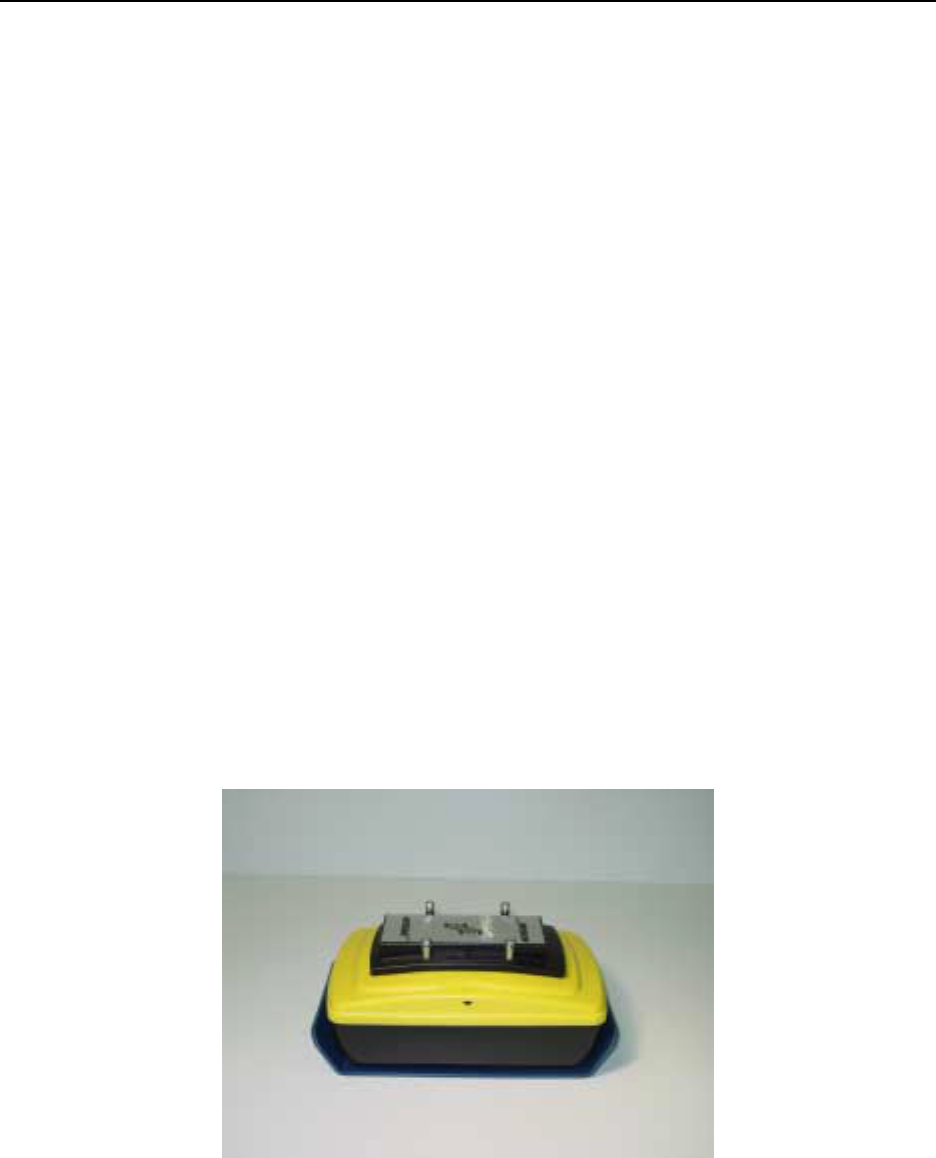
14-Care and Maintenance Noggin
116
2) When the system is not being used, make sure the connections are done up to
prevent dust and moisture from collecting inside. If the connectors are exposed,
cover them with some sort of dust cap.
3) Cables are designed to be as tough as practical.
4) Careless use of cables making them carry loads that they are not designed for can
cause internal damage.
5) Connectors are weak points in any system. With the use of this product in rough,
dusty and outdoor environments, users can minimize potential down time if they care
for cables and treat connectors with respect.
6) Cables and connectors are not designed to suspend or tow or otherwise carry the
weight of systems. They are part of the electronic circuit and should be treated
accordingly. When not in use they should be placed in their storage box.
14.4 Skid Pads
The bottom of the Noggin unit is covered with one large wear-resistant skid pad. The skid pad is
designed to protrude from the bottom of the Noggin and take the majority of the abrasive wear. If
the pad wears down enough, the less-resistant plastic housing may start to wear. If this occurs, it
is best to replace the skid pad. It is easily removed with a Phillips screwdriver and a new one can
be purchased from Sensors & Software Inc.
Note that there are two types of skid pads available. The standard type is flat and covers the
bottom of the Noggin. There is also an optional skid pad that covers the bottom of the Noggin but
also has curved edges that covers the front and back portions of the Noggin. Contact Sensors &
Software for details.
Figure: 14-1 Noggin with optional curved skid pad.

Noggin 14-Care and Maintenance
117
14.5 Storage Cases
Equipment that is transported and stored loosely is more susceptible to damage. All equipment
should be stored in its shipping case or a storage box. Sensors & Software has shipping cases
available as options for all Noggins and DVL’s.
14.6 Spare Parts
For customers working in remote areas or if downtime in the field is unacceptable, consider
buying our optional extended spares kit. This kit includes extra cables, batteries and chargers.

14-Care and Maintenance Noggin
118

Noggin Appendix A - Noggin Data file Format
A-1
Appendix A Noggin Data file Format
Noggin data consists of two files, a Header file and a Data file. The files have the same name but
different extensions. The format details of these files are given below.
Header (.HD) File:
The header file, identified by the file extension .HD, is an ASCII file. An example is shown below.
The heading identifies what each piece of information represents.
1234
Data Collected with Noggin Plus
12/10/2000
NUMBER OF TRACES = 220
NUMBER OF PTS/TRC = 156
TIMEZERO AT POINT = 31
TOTAL TIME WINDOW = 62
STARTING POSITION = 0.0000
FINAL POSITION = 10.9500
STEP SIZE USED = 0.0500
POSITION UNITS = m
NOMINAL FREQUENCY = 250.00
ANTENNA SEPARATION = 0.3048
PULSER VOLTAGE (V) = 100
NUMBER OF STACKS = 4
SURVEY MODE = Reflection
This file can be read and/or printed using any Word Processor.
Data (.DT1) File:
The data file contains as many records as there are traces. Each record in turn consists of a
header section and a data section. The header section consists of an array of 25 real*4 numbers
and a string of 28 characters which is used for annotation. The 25 element real array contains the
following information:
Item # Description
1 Trace number
2Position
3 Number of points per trace
4 Topographic data, if available
5 (not used)
6 # bytes/point (always 2 for Rev 3 firmware)
7 Time Window
8 # of stacks
9-10 reserved for GPS X position (double*8 number)
11-12 reserved for GPS Y position (double*8 number)
13-14 reserved for GPS Z position (double*8 number)
15 reserved for receiver x position

Appendix A - Noggin Data file Format Noggin
A-2
16 reserved for receiver y position
17 reserved for receiver z position
18 reserved for transmitter x position
19 reserved for transmitter y position
20 reserved for transmitter z position
21 timezero adjustment
where:point(x)= point(x+adjustment)
22 Zero flag: 0 = data okay, 1=zero data
23 (not used)
24 Time of day data collected in seconds past midnight.
25 Comment flag: 1 = comment attached.
26 - 32 Comment
The data section consists of an array of two-byte integers, one value for every data point.
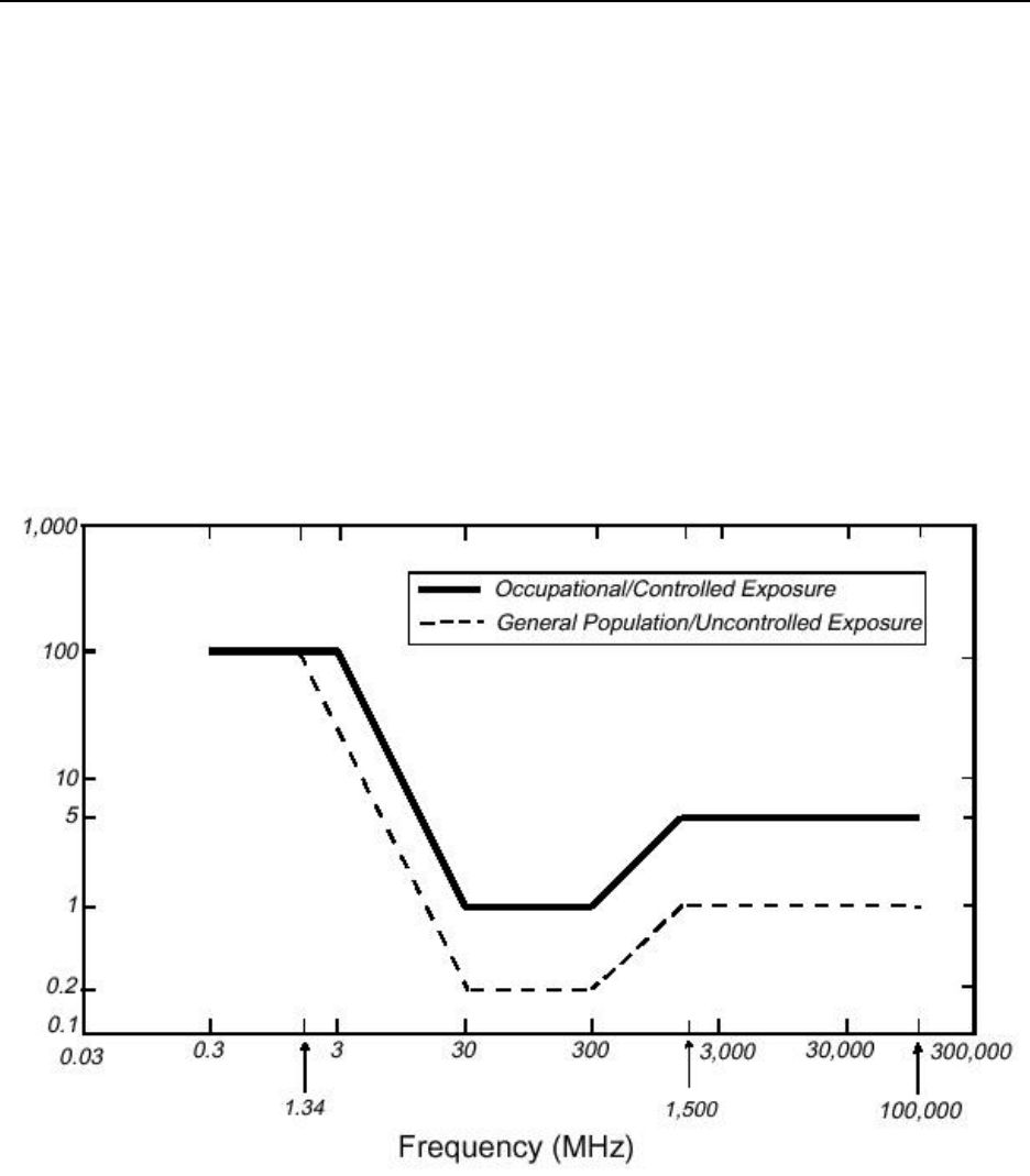
Noggin Appendix B - Health & Safety Certification
B-1
Appendix B Health & Safety Certification
Radio frequency electromagnetic fields may pose a health hazard when the fields are intense.
Normal fields have been studied extensively over the past 30 years with no conclusive epidemiol-
ogy relating electromagnetic fields to health problems. Detailed discussions on the subject are
contained in the references and the web sites listed below.
The USA Federal Communication Commission (FCC) and Occupational Safety and Health
Administration (OSHA) both specify acceptable levels for electromagnetic fields. Similar power
levels are mandated by corresponding agencies in other countries. Maximum permissible expo-
sures and time duration specified by the FCC and OSHA vary with excitation frequency. The low-
est threshold plane wave equivalent power cited is 0.2 mW/cm2 for general population over the
30 to 300 MHz frequency band. All other applications and frequencies have higher tolerances as
shown in graphically in Figure B-1.
Figure B-1: FCC limits for maximum permissible exposure (MPE) plane-wave equivalent power density mW/cm
2
.
All Sensors & Software Inc. pulseEKKO, Noggin and Conquest products are normally operated
at least 1 m from the user and as such are classified as “mobile” devices according to the FCC.
Typical power density levels at a distance of 1 m or greater from any Sensors & Software Inc.
product are less than 10
-3 mW/cm2 which are 200 to 10,000 times lower than mandated limits.
As such, Sensors & Software Inc. products pose no health and safety risk when operated in the
normal manner of intended use.

Appendix B - Health & Safety Certification Noggin
B-2
References
1. Questions and answers about biological effects and potential hazards of radio-frequency
electromagnetic field
USA Federal Communications Commission, Office of Engineering & Technology
OET Bulletin 56
(Contains many references and web sites)
2. Evaluation Compliance with FCC Guidelines for Human Exposure to Radio Frequency Elec-
tromagnetic Fields.
USA Federal Communications Commission, Office of Engineering & Technology
OET Bulletin 56
(Contains many references and web sites)
3. USA Occupational Safety and Health Administration regulations paragraph 1910.67 and
1910.263.
Web Sites
www.fcc.gov/Bureau/EngineeringTechnlogy/Documents/bulletin
www.osha-slc.gov/SLTC (see radio frequency)

Noggin Appendix C - GPR Emissions, Interference and Regulations
C-1
Appendix C GPR Emissions, Interference and Regulations
All governments have regulations on the level of electromagnetic emissions that an electronic apparatus
can emit. The objective is to assure that one apparatus or device does not interfere with any other appara-
tus or device in such a way as to make the other apparatus non-functional.
Sensors & Software Inc. extensively test their pulseEKKO, Noggin and Conquest subsurface imaging
products using independent professional testing houses and comply with latest regulations of the USA,
Canada, European Community, and other major jurisdictions on the matter of emissions.
GPR instruments are considered to be UWB (ultra-wideband) devices. The regulatory regimes worldwide
are devising new rules for UWB devices. Sensors & Software Inc. maintains close contact with the regula-
tors to help guide standard development and assure that all products conform. You should continually
monitor the "News" link on our website (www.sensoft.ca) for updates on standards.
Electronic devices have not always been designed for proper immunity. If a GPR instrument is placed in
close proximity to an electronic device, interference may occur. While there have been no substantiated
reports of interference to date, if any unusual behavior is observed on nearby devices, test if the distur-
bance starts and stops when the GPR instrument is turned on and off. If interference is confirmed, stop
using the GPR.
Where specific jurisdictions have specific GPR guidelines, these are described below.

Appendix C - GPR Emissions, Interference and Regulations Noggin
C-2
C-1 FCC Regulations (USA)
This device complies with Part 15 of the USA Federal Communications Commission (FCC) Rules. Opera-
tion in the USA is subject to the following two conditions:
(1) this device may not cause harmful interference and
(2) this device must accept any interference received, including interference that may cause undesired
operation.
Part 15 – User Information
This equipment has been tested and found to comply with the limits for a Class A digital device, where
applicable, and for an ultrawide bandwidth (UWB) device where applicable, pursuant to Part 15 of the FCC
Rules. These limits are designed to provide reasonable protection against harmful interference when the
equipment is operated in a commercial environment. This equipment generates, uses and can radiate
radio frequency energy and, if not installed and used in accordance with the instruction manual, may cause
harmful interference to radio communications. Operation of this equipment in a residential area is likely to
cause harmful interference in which case the user will be required to correct the interference at his own
expense.
WARNING
Changes or Modifications not expressly approved by Sensors & Software Inc. could void the user’s author-
ity to operate the equipment.
Certification of this equipment has been carried out using approved cables and peripheral devices. The
use of non-approved or modified cables and peripheral devices constitutes a Change or Modification out-
lined in the warning above.
Operating Restrictions
Operation of this device is limited to purposes associated with law enforcement, fire fighting, emergency
rescue, scientific research, commercial mining, or construction. Parties operating this equipment must be
eligible for licensing under the provisions of Part 90 of this chapter.
FCC Interpretation of Operation Restrictions issued July 12, 2002
(FCC Order DA02-1658, paragraph 9)
The regulations contain restrictions on the parties that are eligible to operate imaging systems.
1
Under the
new regulations, GPRs and wall imaging systems may be used only by law enforcement, fire and emer-
gency rescue organizations, by scientific research institutes, by commercial mining companies, and by
construction companies. Since the adoption of the Order, we have received several inquiries from the
operators of GPRs and wall imaging systems noting that these devices often are not operated by the users
listed in the regulations but are operated under contract by personnel specifically trained in the operation of
these devices. We do not believe that the recent adoption of the UWB rules should disrupt the critical
safety services that can be performed effectively only through the use of GPRs and wall imaging systems.
We viewed these operating restrictions in the broadest of terms. For example, we believe that the limita-
tion on the use of GPRs and wall imaging systems by construction companies encompasses the inspec-
tion of buildings, roadways, bridges and runways even if the inspection finds no damage to the structure
1. See 47 C.F.R. §§15.509(b), 15.511(b), and 15.513(b)

Noggin Appendix C - GPR Emissions, Interference and Regulations
C-3
and construction does not actually result from the inspection; the intended purpose of the operation of the
UWB device is to determine if construction is required. We also believe that the GPRs and wall imaging
systems may be operated for one of the purposes described in the regulations but need not be operated
directly by one of the described parties. For example, a GPR may be operated by a private company
investigating forensic evidence for a local police department.
FCC Permitted Mode of Usage
The GPR antenna must be kept on the surface to be in compliance with FCC regulations. Use of the
antenna is not permitted if it is lifted off the surface. Use as a through-the-wall imaging device is prohib-
ited.
GPR Use Coordination
FCC regulation 15.525(c) (updated in February 2007) requires users of GPR equipment to coordinate the
use of their GPR equipment as described below:
TITLE 47--TELECOMMUNICATION
CHAPTER I--FEDERAL COMMUNICATIONS COMMISSION
PART 15_RADIO FREQUENCY DEVICES
Subpart F_Ultra-Wideband Operation Sec.
15.525 Coordination requirements.
(a) UWB imaging systems require coordination through the FCC before the equipment may be used.
The operator shall comply with any constraints on equipment usage resulting from this coordination.
(b) The users of UWB imaging devices shall supply operational areas to the FCC Office of Engineering
and Technology, which shall coordinate this information with the Federal Government through the National
Telecommunications and Information Administration. The information provided by the UWB operator shall
include the name, address and other pertinent contact information of the user, the desired geographical
area(s) of operation, and the FCC ID number and other nomenclature of the UWB device. If the imaging
device is intended to be used for mobile applications, the geographical area(s) of operation may be the
state(s) or county(ies) in which the equipment will be operated. The operator of an imaging system used
for fixed operation shall supply a specific geographical location or the address at which the equipment will
be operated. This material shall be submitted to:
Frequency Coordination Branch, OET
Federal Communications Commission
445 12
th
Street, SW, Washington, D.C.
20554
Attn: UWB Coordination
(Sensors & Software Inc. Note: The form given on the following page is a suggested format for performing
the coordination.)
(c) The manufacturers, or their authorized sales agents, must inform purchasers and users of their sys-
tems of the requirement to undertake detailed coordination of operational areas with the FCC prior to the
equipment being operated.
(d) Users of authorized, coordinated UWB systems may transfer them to other qualified users and to dif-

Appendix C - GPR Emissions, Interference and Regulations Noggin
C-4
ferent locations upon coordination of change of ownership or location to the FCC and coordination with
existing authorized operations.
(e) The FCC/NTIA coordination report shall identify those geographical areas within which the operation
of an imaging system requires additional coordination or within which the operation of an imaging system
is prohibited. If additional coordination is required for operation within specific geographical areas, a local
coordination contact will be provided. Except for operation within these designated areas, once the infor-
mation requested on the UWB imaging system is submitted to the FCC no additional coordination with the
FCC is required provided the reported areas of operation do not change. If the area of operation changes,
updated information shall be submitted to the FCC following the procedure in paragraph (b) of this section.
(f) The coordination of routine UWB operations shall not take longer than 15 business days from the
receipt of the coordination request by NTIA. Special temporary operations may be handled with an expe-
dited turn-around time when circumstances warrant. The operation of UWB systems in emergency situa-
tions involving the safety of life or property may occur without coordination provided a notification
procedure, similar to that contained in Sec. 2.405(a) through (e) of this chapter, is followed by the UWB
equipment user.[67 FR 34856, May 16, 2002, as amended at 68 FR 19751, Apr. 22, 2003]
Effective Date Note: At 68 FR 19751, Apr. 22, 2003, Sec. 15.525 was amended by revising[[Page
925]]paragraphs (b) and (e). This amendment contains information collection and recordkeeping require-
ments and will not become effective until approval has been given by the Office of Management and Bud-
get.

Noggin Appendix C - GPR Emissions, Interference and Regulations
C-5
FCC GROUND PENETRATING RADAR COORDINATION NOTICE
NAME:
ADDRESS:
CONTACT INFORMATION [CONTACT NAME AND PHONE NUMBER]:
AREA OF OPERATION [COUNTIES, STATES OR LARGER AREAS]:
FCC ID: [E.G. QJQ-NOGGIN100 FOR NOGGIN 100 SYSTEM, QJQ-NOGGIN250 FOR NOGGIN 250
SYSTEM, QJQ-NOGGIN500 FOR NOGGIN 500 SYSTEM, QJQ-NOGGIN1000 FOR NOGGIN 1000 SYS-
TEM]
EQUIPMENT NOMENCLATURE: [E.G. NOGGIN 250]
Send the information to:
Frequency Coordination Branch., OET
Federal Communications Commission
445 12
th
Street, SW
Washington, D.C. 20554
ATTN: UWB Coordination
Fax: 202-418-1944
INFORMATION PROVIDED IS DEEMED CONFIDENTIAL

Noggin Appendix C - GPR Emissions, Interference and Regulations
C-6
C-2 ETSI Regulations for the EC (European Community)
In the European Community (EC), GPR instruments must conform to ETSI (European Technical Standards
Institute) standard EN 302 066-1 v1.2.1. Details on individual country requirements for licensing are coor-
dinated with this standard. For more information, contact Sensors & Software’s technical staff.
All Sensors & Software ground penetrating radar (GPR) products offered for sale in European Community
countries or countries adhering to ETSI standards are tested to comply with EN 302 066 v1.2.1.
For those who wish to get more detailed information, they should acquire copies of the following docu-
ments available from ETSI.
ETSI EN 302 066-1 V1.2.1 (February 2008) Electromagnetic compatibility and Radio spectrum Matters
(ERM); Ground and Wall- Probing Radar applications (GPR/WPR) imaging systems; Part 1: Technical
characteristics and test methods
ETSI EN 302 066-2 V1.2.1 (February 2008) Electromagnetic compatibility and Radio spectrum Matters
(ERM); Ground and Wall- Probing Radar applications (GPR/WPR) imaging systems; Part 2: Harmonized
EN covering essential requirements of article 3.2 of the R&TTE Directive
ETSI TR 101 994-2 V1.1.2 (March 2008) Electromagnetic compatibility and Radio spectrum Matters
(ERM); Short Range Devices (SRD); Technical characteristics for SRD equipment using Ultra Wide Band
technology (UWB); Part 2: Ground- and Wall- Probing Radar applications; System Reference Document

Noggin Appendix C - GPR Emissions, Interference and Regulations
C-7
C-3 Industry Canada Regulations
Industry Canada published it regulations for ground penetrating radar (GPR) on Mar 29 2009 as part of the
RSS-220 titled 'Devices Using Ultra-Wideband (UWB) Technology'.
Industry Canada has made a unique exception for GPR by not requiring user licensing. The user does
have to comply with the following directives:
(1) This Ground Penetrating Radar Device shall be operated only when in contact with or within
1 m of the ground.
(2) This Ground Penetrating Radar Device shall be operated only by law enforcement agencies,
scientific research institutes, commercial mining companies, construction companies, and
emergency rescue or firefighting organizations.
Should the ground penetrating radar be used in a wall-penetrating mode then the following restriction
should be noted by the user:
(1) This In-wall Radar Imaging Device shall be operated where the device is directed at the wall
and in contact with or within 20 cm of the wall surface.
(2) This In-wall Radar Imaging Device shall be operated only by law enforcement agencies, sci-
entific research institutes, commercial mining companies, construction companies, and emer-
gency rescue or firefighting organizations.
Since operation of GPR is on a licence-exempt basis, the user must accept the following:
Operation is subject to the following two conditions: (1) this device may not cause interference, and (2) this
device must accept any interference, including interference that may cause undesired operation of the
device.

Noggin Appendix D - Instrument Interference
D-1
Appendix D Instrument Interference
Immunity regulations place the onus on instrument/apparatus/device manufacturers to assure
that extraneous interference will not unduly cause an instrument/apparatus/device to stop func-
tioning or to function in a faulty manner.
Based on independent testing house measurements, Sensors & Software Inc. systems comply
with such regulations in Canada, USA, European Community and most other jurisdictions. GPR
devices can sense electromagnetic fields. External sources of electromagnetic fields such as TV
stations, radio stations and cell phones, can cause signals detectable by a GPR which may
degrade the quality of the data that a GPR device records and displays.
Such interference is unavoidable but sensible survey practice and operation by an experienced
GPR practitioner can minimize such problems. In some geographic areas emissions from exter-
nal sources may be so large as to preclude useful measurements. Such conditions are readily
recognized and accepted by the professional geophysical community as a fundamental limitation
of geophysical survey practice. Such interference being present in the GPR recordings is not
considered as an equipment fault or as a failure to comply with immunity regulations.

Appendix D - Instrument Interference Noggin
D-2

Noggin Appendix E - Safety Around Explosive Devices
E-1
Appendix E Safety Around Explosive Devices
Concerns are expressed from time to time on the hazard of GPR products being used near blast-
ing caps and unexploded ordnance (UXO). Experience with blasting caps indicates that the
power of Sensors & Software Inc.’s GPR products are not sufficient to trigger blasting caps.
Based on a conservative independent testing house analysis, we recommend keeping the GPR
transmitters at least 5 feet (2m) from blasting cap leads as a precaution. Some customers do
experimental trials with their particular blasting devices to confirm with safety. We strongly rec-
ommend that GPR users routinely working with explosive devices develop a systematic safety
methodology in their work areas.
The UXO issue is more complex and standards on fuses do not exist for obvious reasons. To
date, no problems have been reported with any geophysical instrument used for UXO. Since
proximity and vibration are also critical for UXO, the best advice is to be cautious and understand
the risks.

Appendix E - Safety Around Explosive Devices Noggin
E-2
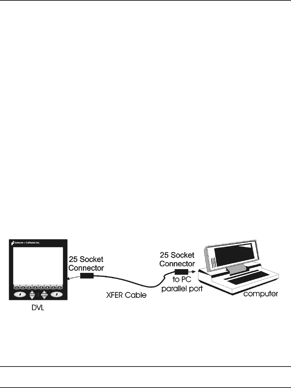
Noggin Appendix F - Using the PXFER Cable and WinPXFER Software
F-1
Appendix F Using the PXFER Cable and WinPXFER Software
F1 Transferring Data to a PC using the PXFER Cable
There are two methods available to transfer data files from the DVL to a PC. The usual method is
to save the data to the removable compact flash drive that is accessible using the door on the top
of the DVL. After powering down the DVL, this drive can be removed and inserted into a card
reader attached to a PC.
The other method of transferring data files to a PC, described in detail in this section, requires the
use of the optional PXFER cable and WinPXFER software.
There are two ways of transferring data to PC using the PXFER cable and WinPXFER. This
section describes transferring all data files to a PC. The other method is to transfer one or more
screens of data as a single PCX graphics file (see F2: p.F-6). This other type of transfer is
appropriate when the user wants to transfer a small amount of data to an external computer for
use with third-party graphics software packages like Microsoft Paint and Word.
To transfer all the data buffers from the DVL to an external computer, the computer must be
connected to the DVL using the special parallel XFER cable that is supplied with the system
(Section F1.1: p.1). Note that this is a special cable and standard 25 pin to 25 pin or Laplink
cables will not work. As well, the computer must have the WinPXFER program running on it
(Section F1.3: p.3).
F1.1 Connecting the Digital Video Logger to a PC
The Smart System comes with a separate cable called the parallel XFER cable. This cable is
designed to connect the DVL to an external computer.
Figure F-1: Parallel XFER cable (CABL0023) connections
The 2 connections that must be made before attempting to transfer data are:
1) Attach the 25 socket parallel connector to the 25 socket parallel port on back of the
Digital Video Logger, and
2) Attach the 25 socket parallel connector the parallel port of the external computer.
WARNING: To avoid damaging any of the components, turn off the DVL and computer
before making any of these connections.
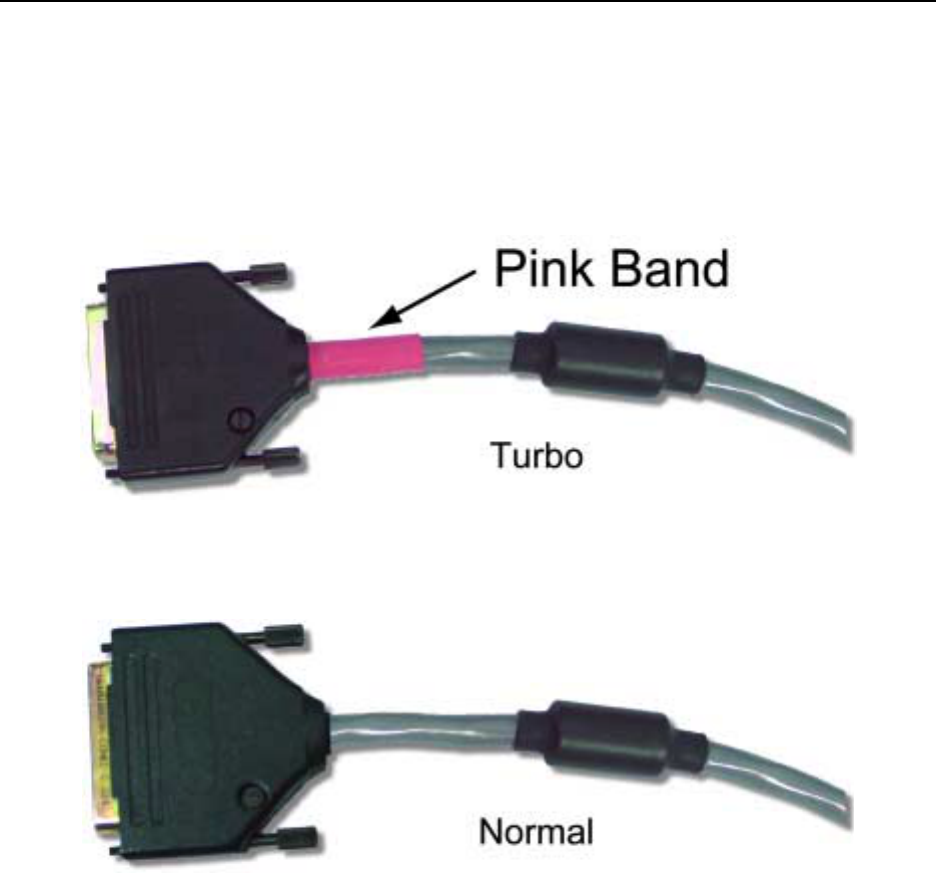
Appendix F - Using the PXFER Cable and WinPXFER Software Noggin
F-2
F1.2 PXFER Cable Types
There are two types of PXFER cable, Normal and Turbo. The Turbo PXFER cable can be identi-
fied by the pink band visible near the connector at either end. The Normal PXFER cable does
not have this pink band.
Figure F-2: Turbo PXFER cable.
Figure F-3: Normal PXFER cable.
Data transfer can only occur if the DVL is set to the correct type of cable (see F1.4: p.F-4). As
well, the WinPXFER software must be set to the correct type of cable (see F1.2: p.F-2).
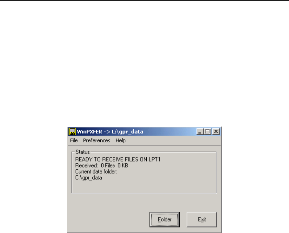
Noggin Appendix F - Using the PXFER Cable and WinPXFER Software
F-3
F1.3 Installing and Running the WinPXFER Program
The Smart system comes with a CD-ROM containing the WinPXFER program.
To install the WinPXFER program, follow the directions in the “Software Installation” document
that accompanies the CD. Briefly, running the SETUP.EXE program from the WinPXFER folder
on the CD will install WinPXFER on the computer.
Once the WinPXFER program has been installed on the computer and the user is ready to
transfer data to the computer, the WinPXFER program needs to be run. This can be done using
the WinPXFER shortcut on the Desktop, double-clicking the WinPXFER.EXE program in
Windows Explorer or pressing Start – Programs – Sensors & Software GPR and finally
WinPXFER.
Figure F-4: WinPXFER main screen
When the WinPXFER program has been run, it will display a screen as shown in Figure F-4.
This means that it is ready to receive data transferred from the DVL to the LPT port number 1.
This command assumes that the data buffers are being transferred across Parallel Port 1 (LPT1).
If using Parallel Port 2 (LPT2) or higher (LPT3, LPT4 etc.), specify the parallel port number under
the Port menu item from WinPXFER.
The name of the folder that the Noggin data will be transferred into is listed under the “Current
data folder”. In the example in Figure F-4, the data will be transferred to the C:\gpr_data folder.
The data folder can be changed by pressing the Folder button and choosing another folder.
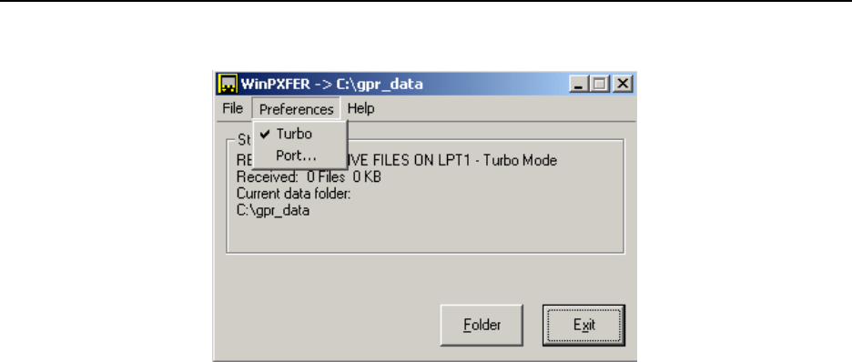
Noggin Appendix F - Using the PXFER Cable and WinPXFER Software
F-4
Figure F-5: Turbo mode under Preferences should only be checked if a Turbo PXFER cable is being
used.
It is vital that WinPXFER be configured properly for the type of PXFER cable (see F1.2: p.F-2). If
the PXFER cable is a Normal cable, the Turbo option under Preferences should NOT be checked
when attempting to transfer data. If the PXFER cable is a Turbo cable, the Turbo option under
Preferences should be checked when attempting to transfer data.
F1.4 Setting the DVL to the PXFER Cable Type
Noggin Mode: The DVL needs to be configured for the type of PXFER cable being used (see
F1.2: p.F-2). In Noggin mode, select 4 - Transfer Setup from the Noggin main menu. The
choices are Normal and Turbo.
Nogginplus Mode: The DVL needs to be configured for the type of PXFER cable being used
(see F1.2: p.F-2). In Nogginplus mode, select 4 - Utilities from the Nogginplus main menu and
then Transfer Mode. The choices are Normal and Turbo.
F1.5 Transferring Noggin Data Buffer Files
Once the parallel XFER cable is connected and the WinPXFER software is installed and running
(see above), it is now possible to transfer all data buffer files to the external computer.
On the DVL, from the main menu, select number 2 – TRANSFER ALL BUFFERS.
The data will be transferred from the DVL to the computer and saved in the current working
directory. The progress of the data transfer will be displayed on the DVL screen and the external
computer.
When the data transfer is complete, on the external computer, exit from the WinPXFER program.
Press any button on the DVL to return to the main menu.

Noggin Appendix F - Using the PXFER Cable and WinPXFER Software
F-5
F1.6 Exporting Noggin
plus
Data
Once the parallel XFER cable is connected (see above) and the WinPXFER software is installed
and running, it is now possible to export data to the external computer.
All the data in one or more Line or Grid Projects or the TAGGED.GPS file can be transferred to
an external computer. From the main File Management menu, the user selects whether to export
Line data, Grid data or the TAGGED.GPS file. If Line or Grid data is selected, the next screen
lists the current projects.
One project can be highlighted and selected for export. Use the up and down arrows to highlight
the project and then press the XFER button to transfer to the PC.
It is also possible to use the TAG button to select several projects and export them all at once.
Use the up and down arrows to highlight the projects, the TAG button to tag each project and
then press the XFER button to transfer all the projects to the PC.
The data will be transferred from the DVL to the computer and saved in a sub-folder from the
current data directory indicated on the WinPXFER program, for example, \DATA\PROJECT2.
The progress of the data transfer will be displayed on the DVL screen and the external computer.
When the data transfer is complete, exit from the WinPXFER program. Press any button on the
DVL to return to the main menu.

Noggin Appendix F - Using the PXFER Cable and WinPXFER Software
F-6
F2 Transferring One or More Noggin PCX Files to an External PC
using WinPXFER
There are two ways of using the PXFER cable and the WinPXFER software to transfer Noggin
data to an external computer. The first is to transfer one or more screens (or buffers) of data as a
single PCX graphics file. This method is described in this section. The second way of transferring
data files to an external computer is to copy all the individual SPI (PCX) files from the DVL (see
Section F1: p.1). This method is useful when the user wants to view the data on an external
computer using the Win_SpiView software.
The data transfer function can only be used after the parallel XFER cable has been
connected from the DVL to the external computer and after the WinPXFER program has
been installed on the external computer and run. Section F1: p.1 describes how to attach
the parallel XFER cable and also how to install and run the WinPXFER program.
Once WinPXFER has been run on the external computer, it is ready to receive data image files
from the Digital Video Logger.
On the Digital Video Logger, after the Print option is selected, the user must define the section to
be printed. The left edge of the page must be established first. This is done by lining up the left
edge of the Digital Video Logger screen with the edge of the plot desired. Use the arrow buttons
on the screen to move the section back and forth. A single arrow moves the image 8 pixels either
right ($), or left (#). A double arrow will move the image 640 pixels or 1 full page to the right (%)
or left (&). A single arrow with a vertical line will move the section either to the start (y#), or end
($y) of the section. If the start or end of section button is pressed, the image will page through
one screen at a time. Data scrolling can be stopped by pressing any button. Once the left edge is
in place, pressing the OK button will lock the left edge of the plot.
The right edge of the plot must now be defined the same as the left, however now using the right
edge of the Digital Video Logger screen. Note that the right edge cannot exceed the left edge.
Next, select a name for the image file from the options CART-1 to CART-4. As long as the
WinPXFER program is running on the external PC, the file will be transferred to the current
directory indicated by WinPXFER. When the data image file transfer is complete, the user will
find a data image (CART-n.PCX) file on the external computer in the current directory.
When the data transfer is complete, on the external computer, exit from the WinPXFER program.
Press any button on the DVL to return to the Noggin screen.

Noggin
G-1
Appendix G GPR Glossaries
G-1 Basic GPR Terms
alpha exponential attenuation coefficient - normal units dB/m (see attenuation)
K relative permittivity or dielectric constant
sigma electrical conductivity - normal units mS/m
v propagation velocity - normal units m/ns
dB/m decibels/metre, common unit for attenuation,
m/ns metre/nanosecond, common unit of GPR velocity, v (see nanosecond)
mS/m milli-Siemens/metre, common unit for conductivity,
ns nanosecond, normal unit of GPR time (see nanosecond)
ps picosecond = 0.001 ns =10
-12
s, occasion unit of GPR time
us microsecond = 1000ns =10
-6
s, occasion unit of GPR time
COR common offset reflection (survey type where a constant antenna separation is main-
tained).
CMP common mid-point (survey type where a transmitter and receiver antenna separation
are changed but the mid point remains constant)
GPR ground penetrating radar
EM electromagnetic (common abbreviation)
antenna Device used to couple electromagnetic energy into the ground. Sometimes called a
transducer.
antenna separation Spacing between transmitting and receiving antennas.
attenuation A reduction in signal amplitude caused by energy dissipation in the transmitting media
(see alpha).
bandwidth The range of frequencies over which a given device transmits or detects signals above
a specified amplitude or power
centre frequency Middle of the frequency band defined by a device's bandwidth
conductivity The ability of a material to conduct electrical current. In isotropic materials the recipro-
cal of resistivity. Sometimes called specific conductance. Units are siemen/m or S/m.
(Or occasionally, mhos/m). For GPR, usually expressed as mS/m. Common symbol
nanosecond 10
-9
s (One Billionth of a second)
radio wave Electromagnetic fields that travel through a material as waves and typically have oscil-
lating frequencies in the 1 GHz to 10 GHz range

Noggin
G-2
receiver (Rx) General term for electronics devices used to detect fields and translate signals into
records or displays
resolution The minimum separation of two objects before their individual responses merge into a
single response
signal amplitude A measure of the strength of the radio wave signal
station interval Spatial distance between observation points along a survey traverse line or mesh
points on a grid
step size See station interval
transmitter (Tx) General term used for electronics devices used to create propagating electromagnetic
fields
transducer Name used where GPR antenna, electronics, and shield are combined into one physi-
cal unit
sample point Signal amplitude measured at specific point in time
trace Sequence of sample points from a single GPR channel that indicate time variation of
signal amplitude
cross section Image that results from side-by-side display of a number of traces which are from adja-
cent spatial measurement position
gain Process of amplifying signals to match recording device or display dynamic range
G-2 Common GPR Terms
zone of influence The size of an area on a reflecting feature that can be uniquely resolved. (See lat-
eral resolution length).
fresnel zone See zone of influence.
range resolution length The radial distance separation between two objects that is needed so that a GPR
clearly detects two responses.
lateral resolution length The lateral separation between two objects that is needed so that a GPR clearly
detects two responses.
ringing Impulsive GPR signals can give rise to reverberating responses that oscillate for a
much longer time than the GPR pulse or wavelet. Such a response is referred to
as a "ringing" response or "ringing" for short.
hyperbola Characteristic inverted "U" GPR response from a point target. (Mathematical form
of the position-travel time response from a point target)
signal to noise ratio The ratio of GPR signal amplitude to the average noise amplitude. A large ratio
results in a larger penetration depth or detection of weaker signals.
system performance Measure of system exploration depth indicated by the ratio of transmitter output
power or voltage to receiver noise power or voltage.

Noggin
G-3
wavelet or EM pulse Impulsive GPR's emit an oscillatory electromagnetic pulse which is short in time
and space and is often referred to as a wavelet.
penetration depth The depth of a GPR wavelet can penetrate to before it is attenuated to an unde-
tectable amplitude.
air waves GPR systems can create and detect energy which travels through air above the
ground. Undesired responses from above ground targets are often called 'air
waves'.
G-3 Advanced GPR Terms
GPS global positioning system (satellite based positioning).
DMI distance measuring indicator.
stacks number of repeated measurements averaged to get resulting measurements.
reflectivity measure of amplitude returned by a target.
reflection coefficient normally named fresnel reflection coefficient and quantifies GPR signal reflection
amplitude from a flat interface between two materials.
3 dB bandwidth Range of spectrum over which the GPR signal amplitude remains above a value
equal to the (peak amplitude).
6 dB bandwidth Range of spectrum over which the GPR signal amplitude remains above a value
equal to the (peak amplitude).

Noggin
G-4