Toshiba 62373831 Density Meter User Manual 6F8A0521 LQ500 030910
Toshiba Corporation Density Meter 6F8A0521 LQ500 030910
Toshiba >
User Manual

6 F 8 A 0 5 2 1
OPERATION MANUAL
DENSITY METER
TYPE LQ500

1
6 F 8 A 0 5 2 1
INTRODUCTION
Thank you very much for your purchase of the LQ500 Density Meter (Hereafter, LQ500).
This manual is prepared for people in charge of installation, operation or maintenance. The manual
describes the precautions in using the meter, and explains about installing, adjusting, calibrating and
maintaining the LQ500 meter.
Carefully read this manual before using the meter for efficient and safe operation. Always keep the
manual in a place where you can easily access.
◆ About Safety Precautions
Carefully read the Safety Precautions that appear in the following pages before using the Meter.
The safety signs used in the Safety Precautions will appear again in the following sections for your
safety.
■ Notice
1. Do not copy or transcribe this manual in part or entirety without written permission from Toshiba.
2. The manual is subject to change without notice.
3. Although we tried hard to make this manual error free, if you find any errors or unclear passages,
kindly let us know.
2
6 F 8 A 0 5 2 1
Important information is shown on the product itself and in the operation manual to protect users
from bodily injuries and property damages, and to enable them to use the product safely and
correctly.
Please be sure to thoroughly understand the meanings of the following signs and symbols
before reading the sections that follow, and observe the instructions given herein. Keep the
manual in a place you can easily access to whenever you need it.
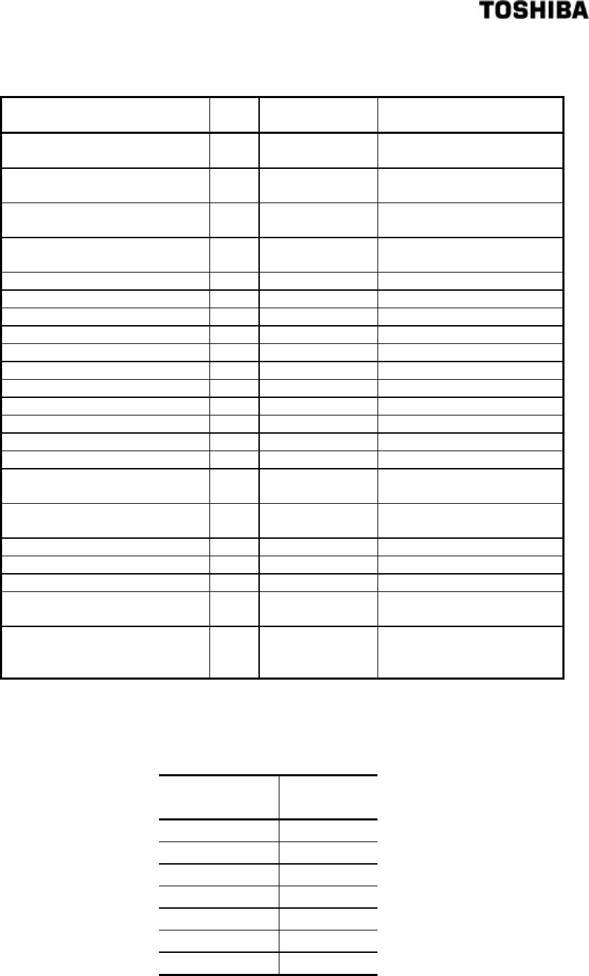
[Explanation of Signs]
Sign Description
WARNING
Indicates a potentially hazardous situation which could result in
death or serious injury, if you do not follow the instructions in this
manual.
CAUTION Indicates a potentially hazardous situation which may result in
minor or moderate injury*1, and/or equipment-only-damage*2, if
you do not follow the instruction in this manual.
Note 1: Serious injury refers to cases of loss of eyesight, wounds, burns (high or low temperature),
electric shock, broken bones, poisoning, etc., which leave after-effects or which require
hospitalization or a long period of outpatient treatment of cure.
Note 2: Minor or moderate injury refers to cases of burns, electric shock, etc., which do not require
hospitalization or a long period of outpatient treatment for cure; equipment damage refers
to cases of extensive damage involving damage to property or equipment.
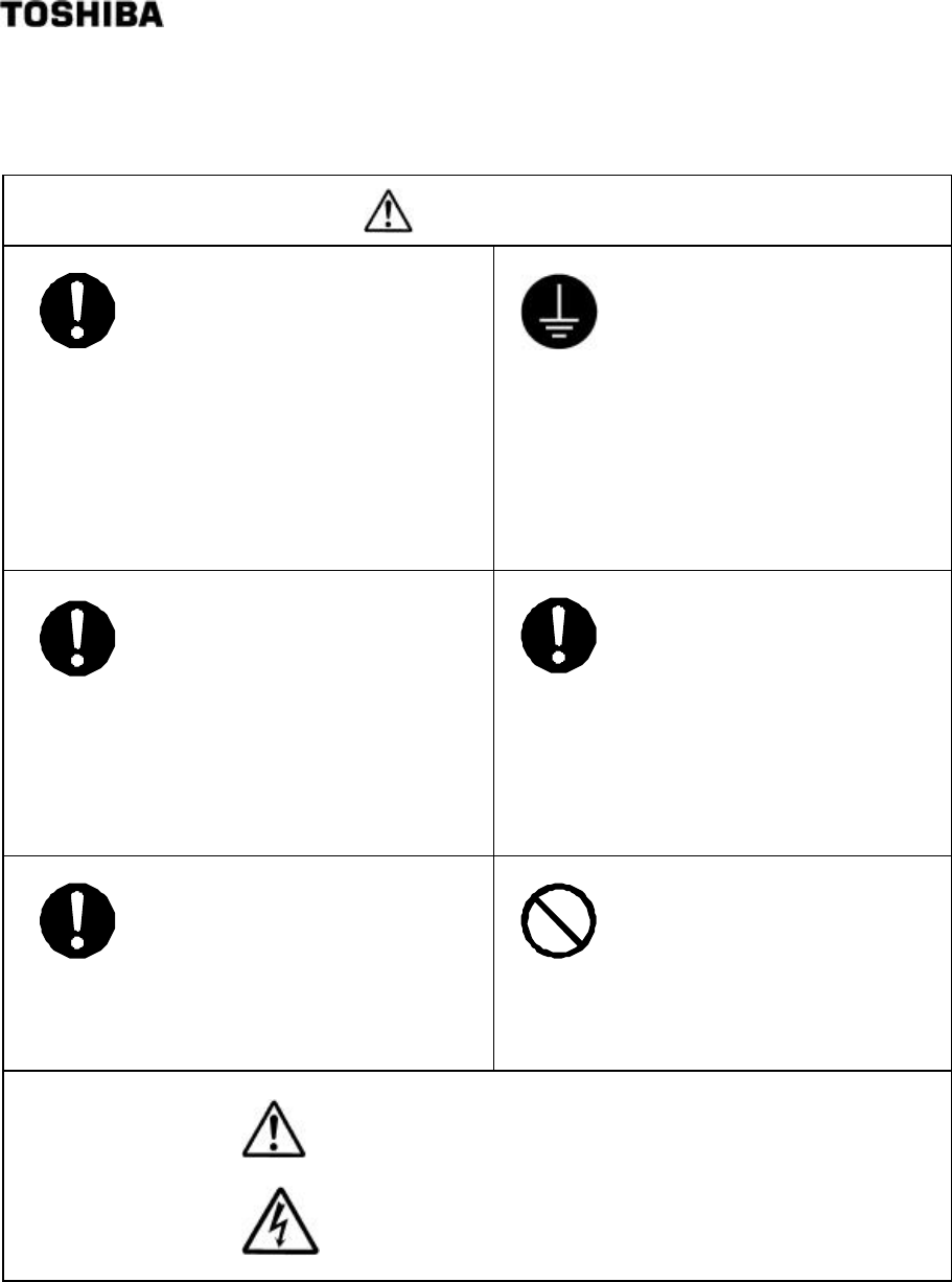
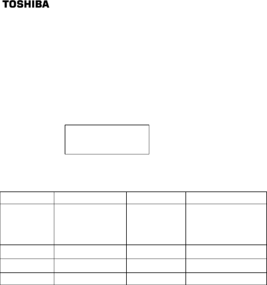
[Explanation of the Symbols]
Symbol Description
This sign indicates PROHIBITION (Do not).
The content of prohibition is shown by a picture or words beside the
symbol.
This sign indicates MANDATORY ACTION (You are required to do).
The content of action is shown by a picture or words beside the symbol.
This shape or symbol indicates WARNING.
The content of WARNING is shown by a picture or words beside the
symbol.
◆Color back : red, flame, picture and words : black
This shape or symbol indicates CAUTION.
The content of CAUTION is shown by a picture or words beside the
symbol.
◆Color back : yellow, flame, picture and words : black
SAFETY PRECAUTIONS
Yellow
Red
3
6 F 8 A 0 5 2 1
Contents
For a safe use of the LQ500 Density Meter, take precautions described in this manual and
observe ordinances in making the installation and operation. Toshiba is not responsible for any
accident arising from the use that does not conform to above.
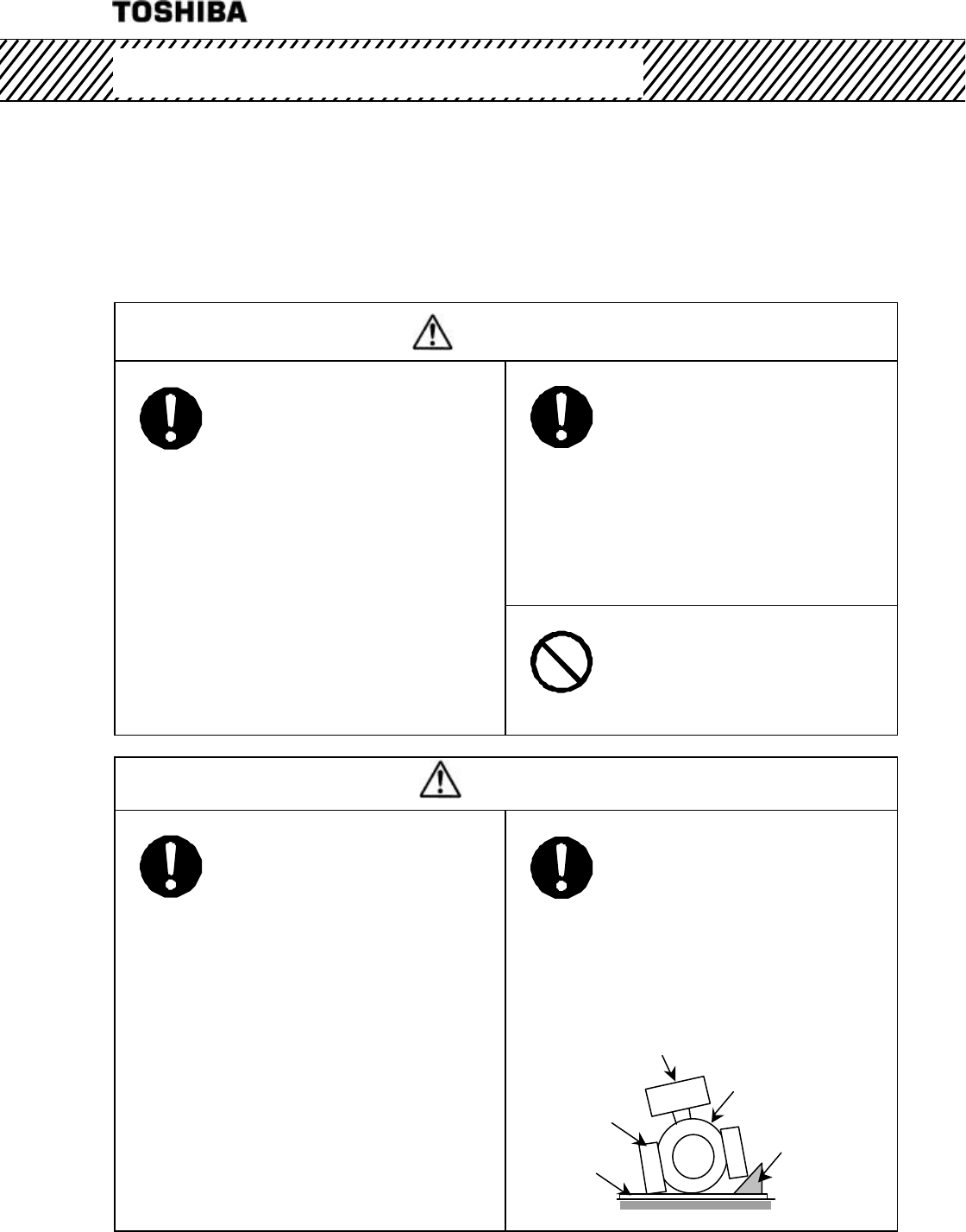
INSTALLATION PRECAUTIONS
WARNING
DO
■Electrical work, installation
work are needed for the meter.
Please consult with the sales
agent you purchased the meter,
some of the companies
specialized in this field or your
Toshiba representative.
If any of these work items is
performed incorrectly, this can
cause fire or explosion.
DO
■The meter is heavy. To move
the meter for relocation or
installation, a qualified operator
must handle it by using
equipment such as a truck, a
crane or a sling.
In addition, when you lift the
meter with its lifting bolts, make
sure the bolts have been
securely tightened to the end.
Overturning or dropping can cause
injuries or equipment failure.
DON’T
■Do not operate where there is
a possibility of leakage of
flammable or explosive gas.
A fire or explosion can occur.
CAUTION
DO
■Avoid installing the meter in
any of the following places:
Otherwise, a fire or equipment
breakdown or failure can occur.
l Dusty place
l Place where corrosive gases
(SO2, H2S) or flammable gases
may be generated.
l Place exposed to strong vibration
or shock.
l Place exposed to condensation
due to abrupt change in
temperature.
l Place too cold or hot for
installation
l Near an apparatus that generates
strong radio waves or strong
magnetic field.
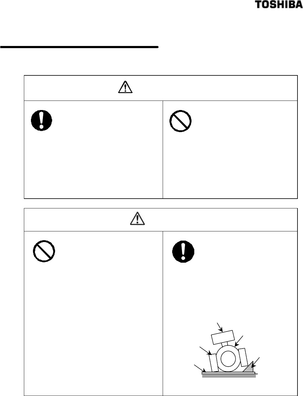
DO
■Install the meter in a place
easier for operation,
maintenance and inspection.
In addition, when you place the
meter temporarily in a stocking
area, make sure to execute fall
prevention measures.
Stumbling over the meter or a fall of
the meter can cause injury.
Red
Yellow
RF section
Detector
Applicator
Cure sheet
Roll-over
prevention
stopper
SAFETY PRECAUTIONS (Continued)
4
6 F 8 A 0 5 2 1
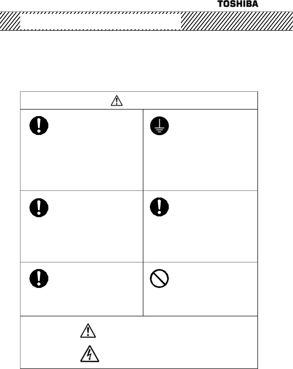
WIRING PRECAUTIONS
WARNING
DO
■Be sure to install a fuse and a
switch to disconnect the
equipment from the power
source.
Failure to observe this can cause
electric shock or equipment failure.
DO
■Be sure to ground the
equipment using a grounding
wire separate from those used
for power tools.
(Grounding resistance: 100 Ω or
less)
Without grounding, electric shock,
malfunction, or equipment failure
can be caused by electric
leakage.
DO
■Make sure that the main
power line is off before wiring or
cabling.
Wiring or cabling without switching
off the main power line can cause
electric shock.
DO
■Use crimp terminals with
insulation sleeves for power
line and grounding wire
terminals.
A disconnected cable or wire from
the terminal or a loose terminal
can cause electric shock or
generate heat and cause a fire or
equipment failure.
DO
■Wiring and cabling should be
done as shown in the wiring and
connection diagrams.
Wrong wiring or cabling can cause
malfunctions, overheating, sparking,
or electric shock.
DON’T
■Do not wire or cable with wet
hands.
A wet hand can cause electric
shock.
The label shown left appears near a terminal block on
the equipment to which power is supplied. Take
precautions to avoid electric shock.
Yellow
Yellow
SAFETY PRECAUTIONS (Continued)
Yellow
5
6 F 8 A 0 5 2 1
Contents
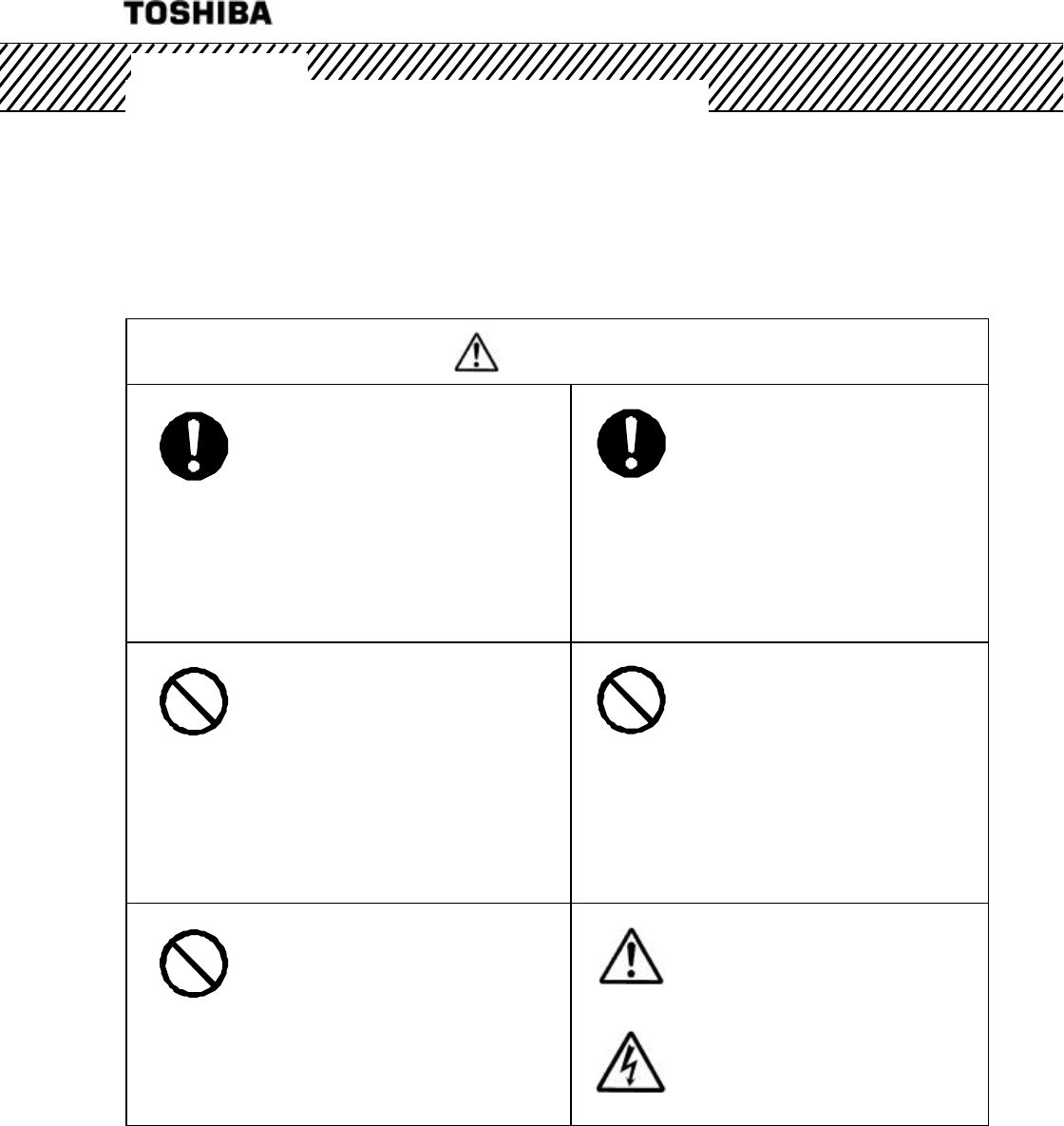
PRECAUTIONS REGARDING MAINTENANCE, INSPECTION,
AND PARTS REPLACEMENT
WARNING
DO
■Be sure to set the power
switch on the equipment to the
OFF position before doing
maintenance or inspection
inside the equipment or
replacing its parts.
Failure to observe this can cause
electric shock or equipment failure.
DO
■Be sure to set the power
switch on the equipment to the
OFF position before replacing
the fuse.
Failure to observe this can cause
electric shock.
DON’T
■Do not touch the terminal
block during maintenance or
inspection. If it is necessary to
touch the terminal block, set the
power switch on the equipment
to the OFF position in advance.
Failure to observe this can cause
electric shock.
DON’T
■Do not attempt disassemble
or modify the equipment.
Failure to observe this can cause
electric shock or equipment
failure.
DON’T
■Do not touch the detector
pipe when high temperature
liquid is flowing in the detector
pipe. The detector pipe also
gets hot from the flowing liquid.
Otherwise, a burn can result.
Yellow
Yellow
The label shown at left is
placed near each
terminal block on the
equipment to which
power is supplied. Be
careful of electric shock.
SAFETY PRECAUTIONS (Continued)
Yellow
6
6 F 8 A 0 5 2 1
Limited Applications of the product
• This product is designed and manufactured for use in systems such as general industrial equipment
(food manufacturing line control, various process control, manufacturing line control water treatment
facility and so on). This product is not designed or manufactured for the purpose of applying to the
systems, such as shown below, which require the level of safety that directly concerns with human
life. When your use includes potential applications in those systems, contact Toshiba for consultation.
(Example)
• Main control system for atomic power generating plant/Safety protection system for
nuclear facilities/Other critical safety systems
• Medical control system for sustaining life
• This product is manufactured under strict quality control but components might fail and if this product
is likely to be applied to a system that concerns with human life or it is likely to be applied to a facility
that may cause serious effects, please give special consideration to make the system safe regarding
the operation, maintenance and management of the system.
• This product is not approved as an explosion-proof device. Do not use this product in an area of
explosive atmosphere (explosion protected area).
Liability Exemptions
• Toshiba assumes liability exemptions from the following examples.
• Damages caused by fire, earthquake, actions by third party, other accidents, abuse or
faulty use whether accidental or intentional by the user, or by other uses of abnormal
conditions.
• Damages or losses that are incidental to the use of or disuse of the product (loss of
business profit, interruption of business operation, etc.)
SAFETY PRECAUTIONS (Continued)

7
6 F 8 A 0 5 2 1
Contents
When an explanation is made in the text regarding the Safety Precautions, the [NOTE] sign
shown below appears in the left margin of a page. The [NOTE] gives you directions to follow in
the following instances.
• To use product correctly and effectively.
• To prevent abnormal or degrading performance of the product.
• To prevent faulty actions.
• To store the product when you do not use the product for a long time.
[NOTE] Sign
8
6 F 8 A 0 5 2 1
Be sure to observe following instructions in order to maintain the original performance of the
LQ500 Density Meter and safely use it over a long period of time.
• Toshiba is not held responsible for any fault or result caused by not observing the precautions
described in this manual or by not observing the laws or regulations in installing or using the product.
[NOTE] Do not install or store the product in the following places.
Otherwise, meter performance can deteriorate and malfunction, fault, or breakage can
occur. Place exposed to direct sunlight
Hot, humid place
Place exposed to severe vibration and shock
Place that can be under water
Place of corrosive atmosphere
[NOTE] Use a separate wire for grounding the meter. Do not share the same
grounding wire with other devices.
Otherwise, malfunction, fault, or breakage can occur.
[NOTE] Lay the output signal cable through their own conduit away from the AC power
cable and other sources of noise.
Noise can interrupt correct measurement.
[NOTE] Perform periodic maintenance and inspection.
A long period of reliable measurement requires periodic span calibration
[NOTE] Be careful not to let water or moisture into the applicator mount of the detector,
converter, or cable ends.
Water or moisture can adversely affect performance and shorten parts service life.
Close the covers and doors securely, and make the cable outlets airtight.
[NOTE] Turn on power when the meter is installed on metal pipe.
When you install or remove the meter, make sure to turn off power beforehand.
This can affect other equipment due to leakage of radio waves.
[NOTE] Do not remove the cover of the applicator mount of the detector as well as the
cover of the detector RF section while the meter is in operation after power is
applied.
This can affect other equipment due to leakage of radio waves.
Important Notes of Use of LQ500 Density Meter
[NOTE] Do not step on any part of the density meter (applicator mount, converter for
example) when you do piping work. Do not place any heavy object on it.
Otherwise, deformation or fault can occur.
Important Notes of Use of LQ500 Density Meter
9
6 F 8 A 0 5 2 1
Contents
[NOTE] Do not use a transceiver, handy telephone, or other wireless device nearby.
Such a device can adversely affect correct measurement. In the event one must be
used, observe the following precautions.
(1) When using a transceiver, make sure that its output power is 5W or less.
(2) When using a transceiver or a handy telephone, keep the converter and signal
cable at least 30cm away from the antenna.
(3) Do not use a transceiver or a portable telephone nearby while the density meter
is in online operation. This is important to protect if from being affected by a
sudden output power change.
(4) Do not install the fixed antenna of a wireless device in the area around the
converter and signal cable.
[NOTE] Use a fuse of the specified rating.
A fuse other than that specified can cause density meter malfunction or breakage.
[NOTE] Do not modify or disassemble the density meter unnecessarily. Do not use
parts other than specified.
Failure can cause malfunction and density meter fault.
[NOTE] When moving the meter elsewhere for installation, be careful not to drop, hit,
or subject to strong shock.
Otherwise, the density meter may be broken, resulting in malfunction or fault.
[NOTE] Before returning your meter to Toshiba for repair, etc., make sure to inform us
about the measured matter remaining in the density meter pipe, including
whether it is dangerous or not to touch the material and then clean the meter
so that no measured matter remains in its pipe.
About disposal
[NOTE] When you dispose of this density meter, follow the ordinance or regulations of
your state.
[FCC notice] This equipment has been tested and found to comply with the limits for a field disturbance
sensor, pursuant to Part 15 of the FCC rules. These limits are designed to provide reasonable
protection against harmful interference in a residential installation. This equipment generates,
uses and can radiate radio frequency energy and, if not installed and used in accordance with the
instructions, it may cause harmful interference to radio communications. However, there is no
guarantee that interference will not occur in a particular installation. If this equipment does cause
harmful interference to radio or television reception, which can be determined by turning the
equipment off and on, the user is encouraged to try to correct the interference by one or more of
the following measures.
• Reorient the receiving antenna.
• Increase the separation between the equipment and receiver.
• Connect the equipment into an outlet on a circuit different fr6m' that to which the receiver
is connected.
• Consult the dealer or an experienced radio,'1'V technician for help.
WARNING: This equipment has been certified to comply with the limits for a field disturbance
sensor, pursuant to Subpart C of part 15 FCC rules. Except AC power cable, shielded cables must be
used between the external devices and the terminals of the converter of the equipment.
Changes or modifications made to this equipment, not expressly approved by Toshiba or parties
authorized by Toshiba could void the user's authority to operate the equipment.
10
6 F 8 A 0 5 2 1
Contents
SAFETY PRECAUTIONS..........................................................................................................2
[NOTE] SIGN.............................................................................................................................7
IMPORTANT NOTES OF USE OF LQ500 DENSITY METER ..............................................8
1 OVERVIEW........................................................................................................................13
1.1 Principle of Measurement.................................................................................................13
1.2 Features.........................................................................................................................14
2. UNPACKING .....................................................................................................................15
2.1 Standard Components.....................................................................................................15
2.2 Standard Accessories .....................................................................................................15
3. INSTALLATION.................................................................................................................16
3.1 Precautions for Installation...............................................................................................16
3.2 Installation Location.........................................................................................................17
3.3 Installation and Piping......................................................................................................18
3.4 Precautions for wiring ......................................................................................................21
3.5 Wiring............................................................................................................................22
4. PART NAMES AND FUNCTIONS....................................................................................25
4.1 Detector.........................................................................................................................25
4.2 Converter........................................................................................................................27
5. OPERATION PROCEDURE ............................................................................................29
5.1 Parameter and Set Values ...............................................................................................29
5.2 Menus and operations .....................................................................................................31
5.2.1. Main menu................................................................................................................31
5.2.2 Setting keys .............................................................................................................32
5.2.3 Menu display.............................................................................................................33
5.2.4 Monitoring menu display and operating procedures .......................................................36
5.2.5. Setting menu display and operating procedures............................................................37
5.2.6 Measuring mode display and operating procedures .......................................................38
5.2.7 Reading of parameters display and operating procedures ..............................................38
5.2.8 Measured values display and operating procedures.......................................................41
5.2.9 Self-diagnosis data display operating procedures..........................................................41
5.2.10 Parameter setting display and operating procedures .....................................................43
5.2.11 Zero calibration display and operating procedures.........................................................46
5.2.12 Span calibration display and operating procedures........................................................46
5.2.13 Phase angle rotation correction display and operating procedures ..................................47
5.2.14 Linearize/conductity correction display and operating procedures ...................................48

11
6 F 8 A 0 5 2 1
Contents
5.2.15 Additives correction display and operating procedures .................................................. 51
5.2.16 Other menus display and operating procedures ............................................................ 54
6. OPERATIONS...................................................................................................................56
6.1 Procedures for Preparing and Running .............................................................................. 56
6.2 Preparations before Turning on Power............................................................................... 57
6.3 Power on and Preparations for Measuring.......................................................................... 57
6.3.1 Turning power on....................................................................................................... 57
6.3.2 Verifying and setting measurement conditions ............................................................. 58
6.4 Zero Calibration............................................................................................................... 60
6.5 Span Calibration ............................................................................................................. 62
6.6 Operation....................................................................................................................... 64
6.7 External Synchronized Operation ..................................................................................... 65
6.7.1 Movement of the external synchronized operation......................................................... 65
6.7.2 Setting the external synchronized operation................................................................. 66
6.8 Functions Related to Operation........................................................................................ 67
7. MAINTENANCE ................................................................................................................68
7.1 Precautions for Maintenance, Inspection and Parts Replacement ........................................ 68
7.2 Maintenance and Inspection Items.................................................................................... 69
8. TROUBLESHOOTING.....................................................................................................71
8.1 Troubleshooting .............................................................................................................. 71
8.2 Error Indications and Recovery Operations ........................................................................ 73
9. CORRECTIONS IN DENSITY CALCULATION.............................................................75
9.1 Density Calculation......................................................................................................... 75
9.2 Various Kinds of Corrections............................................................................................ 76
9.2.1 Phase angle rotation correction .................................................................................. 76
9.2.2 Fluid temperature correction....................................................................................... 76
9.2.3 RF correction............................................................................................................ 77
9.2.4 Ambient temperature correction.................................................................................. 77
9.3 Phase Angle Rotation Correction (Details)......................................................................... 78
9.3.1 Care point concerning phase angle rotation.................................................................. 78
9.3.2 Phase angle rotation in external synchronized operation................................................ 78
9.3.3 Outline of automatic adjustment function of phase angle rotations................................. 78
9.3.4 Judgment conditions and adjustments for automatic adjustment of phase angle rotations 78
9.3.5 Restrictions and invalidation in applying the automatic adjustment of phase angle rotations
............................................................................................................................... 79
9.3.6 Invalidation by setting the automatic adjustment of phase angle rotations ...................... 79
9.3.7 Actions after invalidating the automatic adjustment of phase angle rotations .................. 80
9.3.8 Return to the normal through manual input of the phase angle rotations ......................... 81

12
6 F 8 A 0 5 2 1
Contents
10. VARIOUS FUNCTIONS....................................................................................................82
10.1 Various Functions and their Outlines.................................................................................82
10.2 Moving Average...............................................................................................................83
10.2.1 Function of moving average........................................................................................83
10.2.2 Setting of the moving average times............................................................................83
10.2.3 Cautions in using the moving average function.............................................................83
10.3 Change-rate limit.............................................................................................................84
10.3.1 Outline of change-rate limit function............................................................................84
10.3.2 Examples of operating the change-rate limit function ....................................................84
10.3.3 Cautions in using the change-rate limit factor...............................................................85
10.3.4 Setting the change-rate limit.......................................................................................86
10.4 Electric Conductivity Correction........................................................................................87
10.4.1 Standard conductivity correction factors ......................................................................87
10.4.2 How to obtain and set a correction factor.....................................................................88
10.5 Additives Correction Factor ..............................................................................................92
10.5.1 Additive Correction Function.......................................................................................92
10.5.2 Density calculation ....................................................................................................93
10.5.3 Procedures for using the additives correction function...................................................94
10.5.4 How to set the additives correction function .................................................................95
10.5.5 Simplified Correction on Additives...............................................................................96
10.6 LINEARIZER SETTING ....................................................................................................97
10.6.1 Linearizer function.....................................................................................................97
10.6.2 Linearizer setting.......................................................................................................98
10.7 Density Multiplier Switching by External Signals.............................................................. 100
10.7.1 Density multiplier switching function by external signals.............................................. 100
10.7.2 Setting the density multiplier switching by external signals .......................................... 100
11. SPECIFICATIONS...........................................................................................................102
11.1 General Specifications................................................................................................... 102
11.2 Detector Specifications.................................................................................................. 103
11.3 Conveter Specifications.................................................................................................. 104
11.4 Model Number Table...................................................................................................... 106
APPENDIX..............................................................................................................................107
Attached Figure1. Detector outline dimensions .......................................................................... 107
Attached Figure2. Converter dimensions.................................................................................... 109
13
6 F 8 A 0 5 2 1
1 OVERVIEW
The LQ500 Density Meter measures the density of a substance that flows through a pipe by means
of a phase difference method using microwaves.
This method is little affected by the presence of contamination. It uses no moving mechanical parts
or mechanism that is often used in other measuring methods for cleaning, sampling, or defoaming.
It permits continuous measurement.
The density meter, which outputs measured density in electric current, is suitable for an application
in a process for monitoring and controlling.
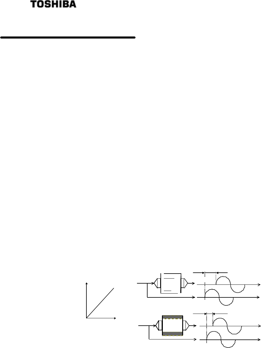
1.1 Principle of Measurement
This density meter has adopted a new measuring method called “Phase difference method by
microwaves.” When microwaves go through a substance and comes out of it, by measuring the
phase lag of the waves, we get a certain physical property of the substance that is proportional to
the density.
The theory of density measurement based on the phase difference method is shown in Figure 1.1
The difference between the phase lagθ1 of the microwave received through water (density 0%)
and the phase lagθ2 of the microwave received through the object substance, that is,
Δθ = θ2 − θ1
is determined, and since the differenceΔθis in direct proportion to the density, the density of the
object substance is measured.
Microwave
transmission
Density
Phase difference
Δθ
Phase difference Δθ=θ
W−θ
S
Density =K・Δθ (K: Coefficient)
t
t
t
t
Phase lagθ
W
Drinking
water
Phase lagθ
s
Reception
Substance to
be measured
Fig. 1.1 Principle of phase angle difference

14
6 F 8 A 0 5 2 1
1.2 Features
Compared with the conventional method, this phase difference measurement method using micro
waves, in principle, has the following features.
(1) Not easily affected by contamination.
This method is measuring the variation of the transmission time but not for measuring the
attenuation of the wave motion strength that has been transmitted into the measured matter.
Therefore, it is unnecessary for the window part for sending/receiving microwaves to be
transparent as the optical type.
(2) This meter is not affected as much as an ultrasonic type is by air bubbles
In an ultrasonic system, measurement is affected by attenuation of wave motion by foreign
matters such as air bubbles but the feature of the microwave method is that measurement is
not easily affected by foreign matters such as air bubbles because the method is not using the
attenuation of wave motion strength.
(3) High liability and simple maintenance.
Having no movable part of the rotating pulp density meter nor the protruding portion into the
pipe as with the blade-type pulp density meter, the new method is free from fiber tangling, thus
realizing a high level of reliability. Requiring no consumable parts such as bearings and pulleys,
the maintenance is also easy and simple.
(4) Not easily affected by the speed of flow.
Taking density measurements captivating the dielectric change following the density change in
the measured matter, this method is not affected by the speed of flow.
(5) Not easily affected by the pulp material type or freeness.
Taking density measurements captivating the dielectric change following the density change in
the measured matter, the new method has the feature of not easily affected by the pulp
material type or freeness, etc.
(6) Being of the flow-through type, the new method is capable of continuous measurement.
As others, the new density meter model LQ500 boasts of the following features.
(7) Can easily change the measurement range.
(8) The operation is simple because complex processings such as density calculation and
correction, etc. are performed automatically by micro computers.
(9) Remote control is made possible by using the hand-held terminal AF100LQ3 type (optional),
which is a specialized terminal for communication.
<Supplementary Explanation>
Density meter LQ500 is equipped with the display/operation consoles as standard.
Therefore, if the meter is installed on a location easy for maintenance, the hand-held
terminal is not always needed.
(10) Measurable up to 50% TS density
(11) Conforming to low-level radio wave equipment
The microwave output of this meter is low with about 10mW and this meter conforms to
“Low-level radio wave equipment” specified by Radio Law. Therefore, the customer is free
to use this meter without applying for permission, notification or licensing of this meter.
15
6 F 8 A 0 5 2 1
2. UNPACKING
Check items by the following list and table at unpacking.
2.1 Standard Components
(1) Density Meter : 1 unit (One unit each of Detector and Converter,)
(2) Standard accessories : 1 unit (One set of cables,Fuse,Operation manual)
<Supplementary Explanation>
In the event of performing remote control through communications, you are required to have the
hand-held terminal AF100 type (type code: AF100LQ4BAA3, Instruction Manual: 6F8A0763),
which is a specialized terminal for communications. Therefore, please purchase one separately.
2.2 Standard Accessories
Table.2.1 Standard accessories
Accessory Specifications Qty
Power supply
cable
Used to supply DC power from the converter to the RF section
(detector)
Overall diameter: 11.0 to 13.0 mm
JCS 258 C 2-core CVV-S
10m
(32.8ft)
Communication
cable
Used between the converter and the RF section (detector) to
communicate with each other.
Overall diameter: 11.0 to 13.0 mm
JCS 258 C 4-core CVV-S
10m
(32.8ft)
Fuse
2A(T),250V cartridge, glass tubular fuse,
5.2mm outer dia. x 20mm long
Shape/characteristics: 5NM or equivalent (based on JIS C
6575)
2
Operation manual
(The document you are reading.) 1
16
6 F 8 A 0 5 2 1
3. INSTALLATION
3.1 Precautions for Installation
WARNING
DO
■The meter is heavy. To move
the meter for relocation or
installation, a qualified operator
must handle it by using
equipment such as a truck, a
crane or a sling.
In addition, when you lift the meter
with its lifting bolts, make sure the
bolts have been securely
tightened to the end.
Overturning or dropping can cause
injuries or equipment failure.
DON’T
■Do not operate where there is
a possibility of leakage of
flammable or explosive gas.
A fire or explosion can occur.
CAUTION
DON’T
■Avoid installing the meter in
any of the following places:
Otherwise, a fire or equipment
breakdown or failure can occur.
l Dusty place
l Place where corrosive gases
(SO2, H2S) or flammable gases
may be generated.
l Place exposed to vibration or
shock that exceeds permissible
level.
l Place exposed to condensation
due to abrupt change in
temperature.
l Place too cold or hot for
installation
l Place too humid for installation
l Near an apparatus that generates
strong radio waves or strong
magnetic field.
DO
Install the meter in a place
easier for operation,
maintenance and inspection.
In addition, when you place the
meter temporarily in a stocking
area, make sure to execute fall
prevention measures.
Stumbling over the meter or a fall
of the meter can cause injury.
RF section
Detector
Applicator
Cure sheet
Roll-over
prevention
stopper
17
6 F 8 A 0 5 2 1
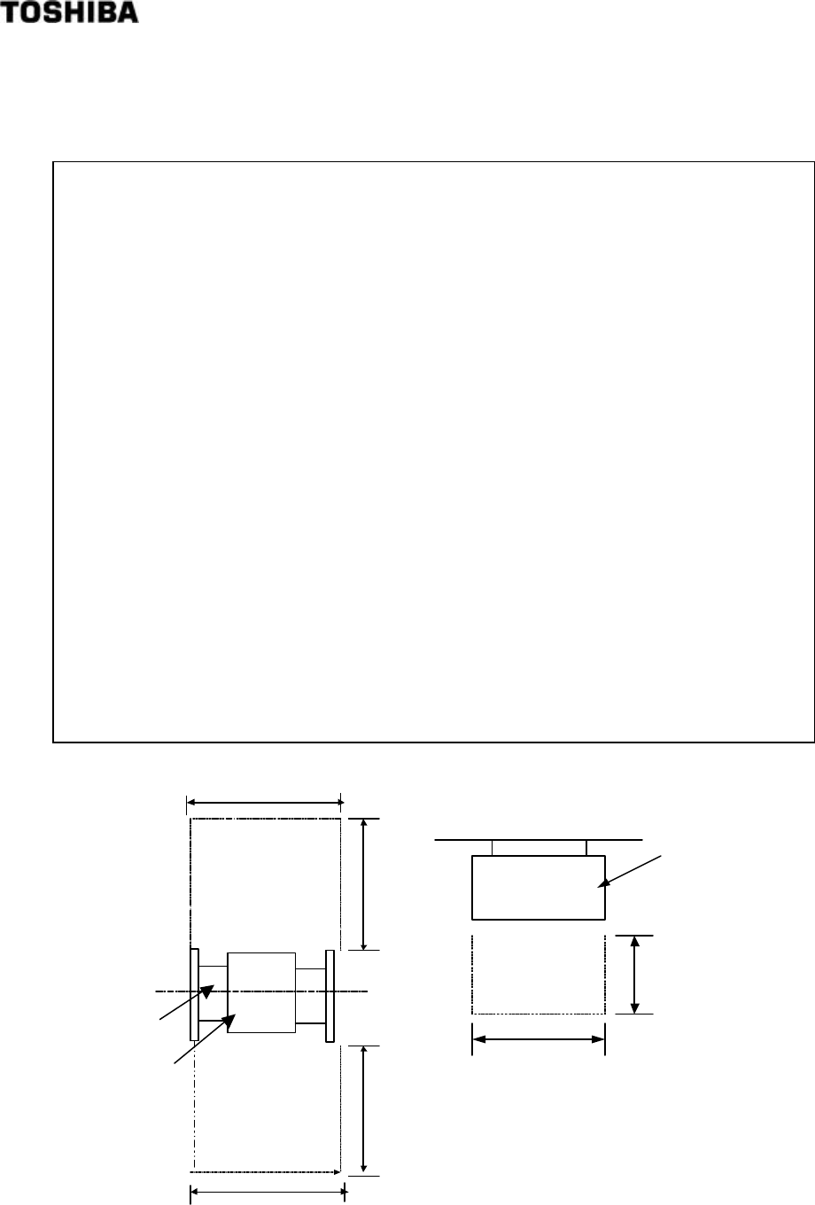
3.2 Installation Location
[NOTE]
◆ Determine an indoor installation place in accordance with the following instructions.
(1) Choose a place that is free of vibrations and corrosive gasses, and has ample space for
maintenance.
(2) Secure maintenance space in front, rear and above the density meter. (Refer to fig. 3.2.11)
(3) In the case of outdoor installation, provide covering against sun .
(4) Do not install the meter in a place where there is a possibility of leakage of flammable or
explosive gas.
(5) Do not install the meter in any of the following places:
• A place where condensation due to a sudden temperature change occurs.
• A place where extreme low or high temperatures occur outside the specification range.
• A place near the equipment generating strong radio waves or electric fields.
(6) Make sure the upstream and downstream pipes have enough strength to hold the density
meter. If it is not possible, provide a supporting base to hold the density meter.
(7) Install the meter in a place where density distribution is uniform. If the distribution inside the
pipe is uneven, manual analysis data and the indicated value of the density meter may not
show the same value.
(8) Install the meter in a place where air bubbles are not generated, inside the pipe is always
filled, and sedimentation and accumulation of solid matters do not occur.
(9) The liquid contacting materials of this meter are stainless steel SCS14A(equivalent to
316SS) and polysulfone. Install the meter in a place where measuring liquid or environment
does not corrode these materials.
(10) If the cover of the density meter is removed or the density meter is disassembled while the
meter is powered, radio waves will leak out. (However, the amount is about equal toPHS
and one tenth of mobile phones.)
In addition, provide maintenance
space of 500mm in height above
the RF section and the Converter.
Back
Front
Maintenance
space
600
500
600
500
Convertor
500
600
Maintenance
space
Fig. 3.2.1 Space for Maintenance
Detector
RF section
Converter

18
6 F 8 A 0 5 2 1
3.3 Installation and Piping
Figures 3.3.1 through 3.3.4 are examples of density meter installation.
[NOTE]
(1) Install the meter in a place where density distribution is uniform.
(2) Avoid such a location where the measured matter will settle and build up on the bottom of
the density meter.
(3) Avoid such a location which will allow bubbles to move into the pipe line.
(4) We recommend that this density meter should be installed to a vertical piping system.
Horizontal installation can also be used with the same performance but under the following
conditions, vertical installation must be chosen:
(5) Especially in the following situations, make sure that the piping is vertical.
a) Bubbles may stay in the pipe.
b) Slow flow speed or other factors may cause the measured matter to sink or float
substantially making the distribution of the measured-matter density uneven in the pipe.
c) The main pipe has been enlarged thus using the density meter of a diameter greater than
that of the main pipe.
(6) When installing on the horizontal piping, make sure that the meter is installed directly on top
of the converter section for purposes of maintenance and performance assurance (in other
words, so that the paired applicator sections are placed directly side by side).
(7) This density meter does not distinguish between the upstream side and the downstream side.
Neither does it require a straight tube length. Install it in a direction that will make
maintenance easy.
(8) The front side of the density meter's converter section is equipped with an LCD density
display section. When installing the meter, choose a location and direction in which this
density display section will be easily visible. (See Fig. 3.3.3)
(9) When you anticipate a marginal error between the side-to-side dimensions of this density
meter and the installation space of the piping line, prepare a loose mechanism in advance.
(10) To minimize the impact of the bubbles mingled, it is recommended that the meter be installed
on a location as far as possible from the pipe outlet for air release but still within the distance
where a reasonable degree of hydraulic pressure is applied.
(11) In the event that the density meter may no longer be full of the fluid while the pump is shut
down or the density distribution in the density meter may become uneven, make sure to take
measurements only while the pump is operating by using the external interlock function.
(12) Take necessary measures to prevent vibration from a pump or other equipment applied to
the density meter transmitted through the piping.
(13) On both the upstream and downstream sides of the density meter, install shutoff valves.
Furthermore, between these valves and the density meter, install the sampling port, the zero
water supply port, the air release port, the drain port with a shutoff valve attached
respectively. In the event that the flow of the pipe line cannot be stopped, provide a bypass
pipe halfway with a shutoff valve attached. When performing zero point calibration, these
are needed to discharge the measured matter out of the density meter through its drain port
and fill up the meter with fresh water of zero density. (See Fig.3.3.1 and Fig.3.3.2)
(14) As for gaskets to be used in piping, select the one with the dimension conforming to the
flange standard and of the material appropriate for the substance to be measured.
(15) If the cover of the density meter is removed or the density meter is disassembled while the
meter is powered, radio waves will leak out. (However, the amount is about equal to PHS
and one tenth of mobile phones.)
19
6 F 8 A 0 5 2 1
[NOTE]
◆Sampling valve: Used to extract fluids for manual analysis. Install this valve to the side
of the pipe in the case of horizontal installation. It is recommended that
a 1-inch ball valve be installed to the side of the pipe.
◆Zero point water valve: Used to supply drinking water (density or consistency 0%) to the
detector pipe for zero point adjustment. Install this valve at the top of
the pipe in the case of horizontal installation. It is recommended that a
1-inch ball valve be installed in the top of the pipe and zero point water
is supplied through this inlet using a vinyl hose etc.
If valve water pipe is connected to this valve, air cannot be extracted.
Therefore, another valve (vent valve) is needed to extract air.
◆Vent valve: Used to vent process fluids to open air when performing zero
adjustment. This helps the drinking water (density or consistency 0%)
enter the detector pipe easily. Install this valve in the top of the pipe in
the case of horizontal installation.
◆Drain valve: Used to drain the fluids before supplying drinking water (density or
consistency 0%) to the detector pipe for zero adjustment. Install this
valve at the lowest point of the pipe. It is recommended that a 1-inch
ball valve be installed at the lowest point of the pipe.
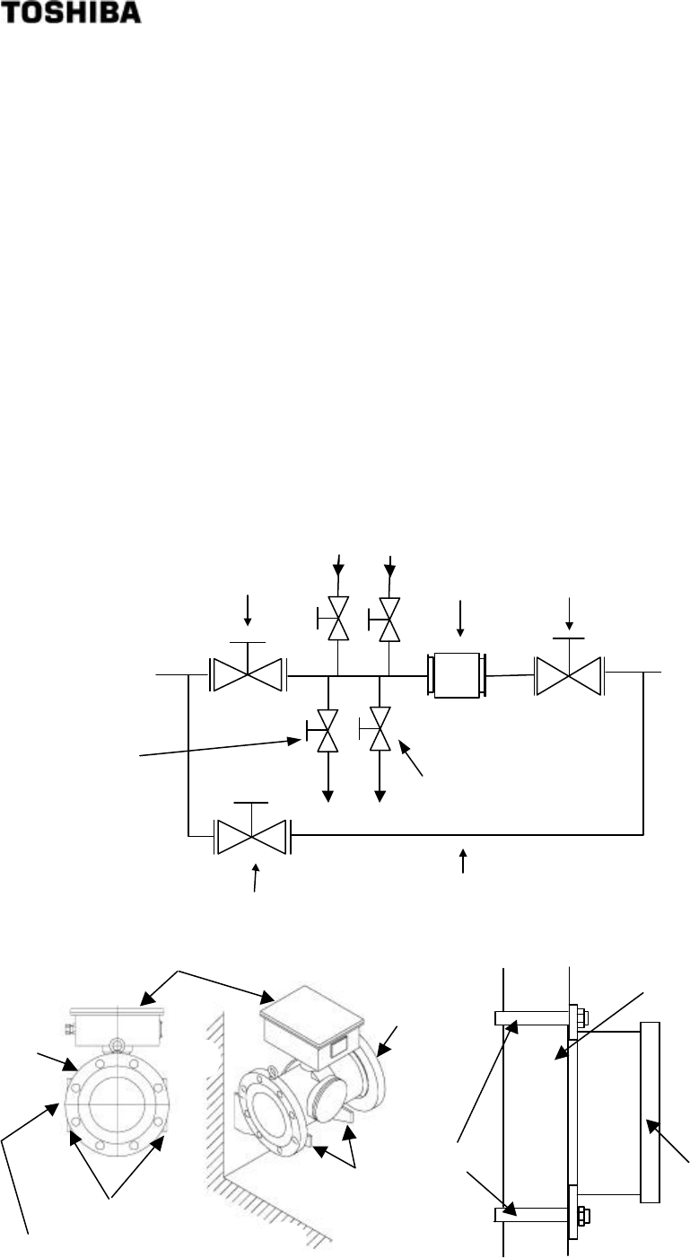
Fig.3.3.1 Meter mounted horizontally
Vent valve
Zero point water valve
Stop valve
Stop valve
Drain valve
Bypass piping
Density meter
Stop valve
Sampling valve
Fig 3.3.2 Setting example (Horizontally)
RF section (RF section must stay at the top.)
Detector
Applicator (one pair)
This section must be level.
Wall
Floor
Detector
Base frame
U-bolt
s
Wall mounting or
pipe mounting
Converter
Fig 3.3.2 Setting example (from converter side)
20
6 F 8 A 0 5 2 1
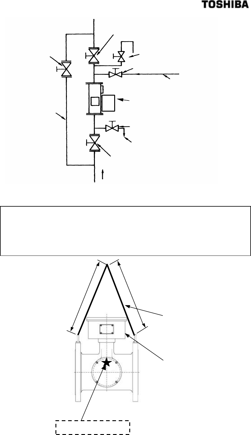
Fig.3.3.4 Meter mounted vertically
[NOTE]
When you lift the meter using a lifting wire for relocation, installation or for other purposes, use
the wire so that the wire does not touch the RF section of the density meter. We recommend
you use a lifting wire of 2m or more in length (A/2 + A/2 shown below). In case the lifting wire
rubs against the RF section, the RF section may be damaged. Care should be taken not to
damage the RF section by applying cure such as cushioning materials between the lifting wire
and the RF section.
A/2
A/2
Lifting wire
RF section
The center of gravity
Stop valve
Bypass piping
Density meter
Zero point water valve
Zero water piping
Stop valve
Drain
Direction of flow Upward
Drain valve
Stop valve
Air release valve
Figure 3.3.5 Lifting the Density Meter with a Lifting Wire
21
6 F 8 A 0 5 2 1
3.4 Precautions for wiring
WARNING
DO
■Be sure to install a fuse and a
switch to disconnect the
equipment from the power
source.
Failure to observe this can cause
electric shock or equipment failure.
DO
■Be sure to ground the
equipment using a grounding
wire separate from those used
for power tools.
(Grounding resistance: 100 Ω or
less)
Without grounding, electric shock,
malfunction, or equipment failure
can be caused by electric
leakage.
DO
■Make sure that the main
power line is off before wiring or
cabling.
Wiring or cabling without switching
off the main power line can cause
electric shock.
DO
■Use crimp terminals with
insulation sleeves for power
line and grounding wire
terminals.
A disconnected cable or wire from
the terminal or a loose terminal
can cause electric shock or
generate heat and cause a fire or
equipment failure.
DO
■Wiring and cabling should be
done as shown in the wiring and
connection diagrams.
Wrong wiring or cabling can cause
malfunctions, overheating, sparking,
or electric shock.
DON’T
■Do not wire or cable with wet
hands.
A wet hand can cause electric
shock.
The label shown left appears near a terminal block on
the equipment to which power is supplied. Take
precautions to avoid electric shock.
Yellow
Yellow
Yellow

22
6 F 8 A 0 5 2 1
3.5 Wiring
Figure 3.5.1 on the next page shows connections to the density meter and the external units. Figure
3.5.2 shows wiring assignment to a converter terminal. Refer to these figures for correct wiring.
[IMPORTANT]
(1) A density meter has to be separated from the power supply line when performing the
maintenance and inspection operation. A fuse must be installed on the power supply side to
protect a switch and the power. A power requirement for this unit is approximately 50 VA.
Power consumption of this meter is 24VA (at 100VAC).
(2) Grounding resistance should be 100 Ω or less and the grounding should be made independently
from the one used for power equipment.
(3) To connect between the detector and the converter, use the attached power cable (to supply
DC power supply) and communication cable. Connect these cables by matching the terminal
symbols of the detector RF section’s terminal block (can be seen when the RF section cover
is removed) and the converter’s terminal block with those shown on each cable.
(4) Use power cables of 2 mm2 or more in sectional area and its voltage drop should be 2V
maximum. In addition, use an M4 size crimped terminal for each terminal connections.
(5) Consider wiring when installed so that vibration or sway will not be applied to cables.
(6) Output signal wires should be installed in thick walled steel conduit and separated from AC
power supply, control signal, alarm signal and other wires that may become a source of noise.
(7) Signal wires of the density meter measured value (4-20 mA output) should be a 2-conductor
shielded cable (CVVS 2 mm2) and the grounding of the shield should be made on the receiving
instrument side. When conductivity correction is employed, use the same type of 2-conductor
shielded cable (CVVS 2 mm2) for conductivity signal wires and the grounding of the shield
should be made on the receiving instrument side.
(8) Cable wiring port is airtight with gland and packing; therefore, tighten the cable gland securely
when wiring is completed. Applicable cable sizes are 11 to 13 mm in diameter. If the cable
diameter is smaller than the inside diameter of the gasket, wind tape or something around the
cable until the cable diameter becomes about the size of the inside diameter of the gasket.
(9) Tighten terminal screws securely. Appropriate tightening torque for terminal block screws is
1.2 N•m (1.4 N•m MAX).
(10)Do not apply power when the density meter is not installed properly in the piping system.
Leakage of radio waves may cause interference with other equipment.
23
6 F 8 A 0 5 2 1
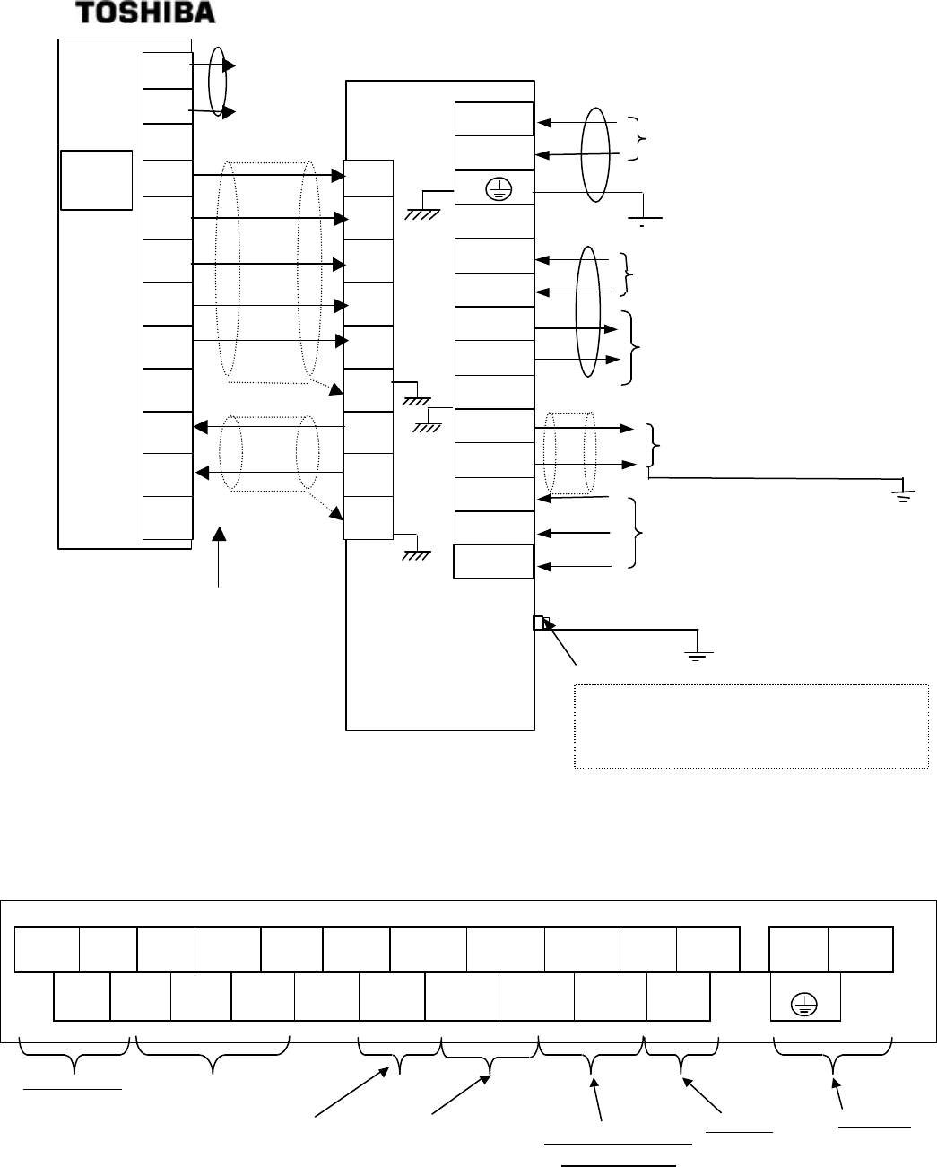
Fig. 3.5.1 External connection
Fig. 3.6 Terminals inside the converter
Ground (PE)
(Ground resistance: 100Ω or less)
Density meter error or
maintenance-in-progress contact
output
Grounding terminal
Note: The ground should be connected to either the PE
terminal of the terminal bock inside converter or to the
grounding terminal of the case.
Density correction multiplier switching
voltage input signal
(H: 20-30VDC, L: 2VDC or less, input
resistance about 3kΩ)
External sync contact input
(Contact capacity: 24VDC, 1A or more)
Measured density output
(4-20mADC, 750Ω or less, isolated
CVV
CVVS
Converter
Power 100 to 240VAC, 50/60Hz
CVV
DI
COM
COM1
DO1
FG
AO+
AO-
COM2
DI2
L1
L2
DI3
Tx+
Tx-
Rx+
Rx-
SG
FG
+24
V
0V
FG
Tx+
Tx-
Rx+
Rx-
SG
FG
+24
V
0V
Power
cable
Communication
cable
RF
section
FG
Ec-
Ec+
Conductivity
signal input
(4 ~ 20mADC)
Note: The FG wires of the dedicated
cables A and B should not be
connected to the FG terminal on the
detector (measuring section) side.
FG
CVVS
CVVS
Ground
(Ground resistance: 100Ω or less)
Power supply
Terminal block
+24V
0V Tx+
Rx+ NC (FG) DI D01 DI2 DI3
AO+
L1 L2
FG Tx−
Rx−
SG (FG) COM COM1 (FG) COM2
AO−
Communication
External sync in
put DI,
COM
Density meter error or
maintenance-in-progress
signal: DO1, COM1
Multiplier switching:
DI2, DI3, COM2
AO (+, −)
4-20mA
Density output
(HART)
AC Power
24
6 F 8 A 0 5 2 1
Figure3.5.3 Terminals arrangement inside the RF section
[NOTE] For connection between the converter and the RF section, connect cables according to
the band marks attached to the power cable (1) and the communication cable (2).
Erroneous connection can cause a failure or an erroneous operation.
[NOTE] For connection between the converter and the RF section, make sure to use the attached
power cable (1) and communication cable (2). Using other cables can cause an erroneous
operation.
Power supply
Terminal block
+24V
0V Tx+
Rx+ FG EC+
NC
FG Tx−
Rx−
SG EC−
FG
Communication
Conductivity signal input
(4 ~ 20 mADC)
25
6 F 8 A 0 5 2 1
4. PART NAMES AND FUNCTIONS
The detector is integrated with the converter in LQ500 Density meter.
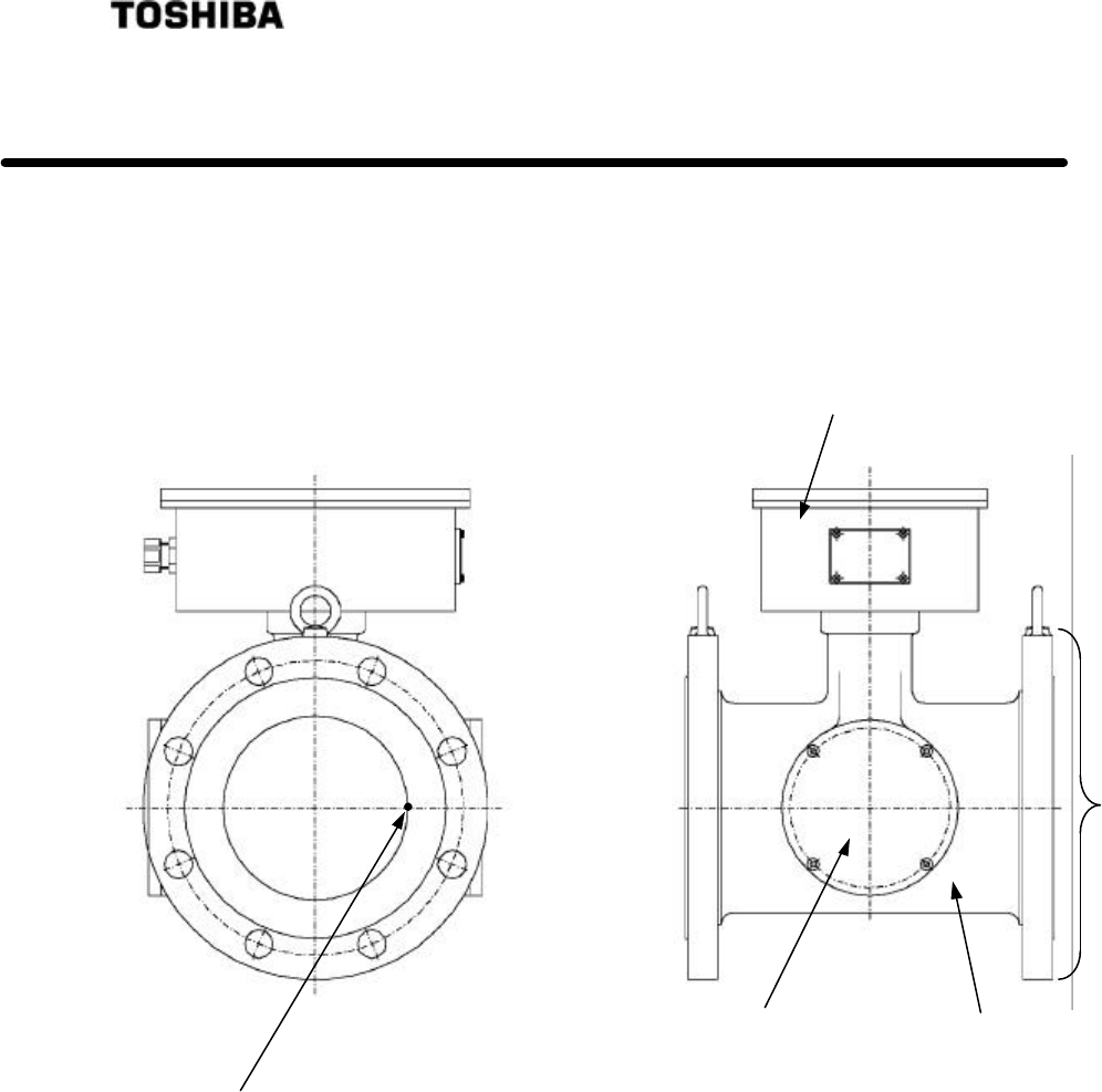
4.1 Detector
Fig.4.1.1 Detector
(3) Temperature detector
RF section
(2) Applicator section (1) Main pipe
Detector

26
6 F 8 A 0 5 2 1
(1) Main pipe
Refers to the part connected to the pipe line of a measured object. FLANGE is JIS 10K or
equivalent. Contact Toshiba for connections other than this method (shown left).
(2) Applicator mount
The applicators (antenna) for transmitting and receiving microwaves are built inside. The
applicator on the front in Fig.4.1 is for transmitting and the rear is for receiving. Always keep
the lids closed and the screws of the lids secured.
(3) Temperature detector
The temperature detector (RTD) is for temperature correction. It measures temperature of the
fluid flowing through the main pipe.
(4) RF section
This is the section that generates and detects microwaves and also performs signal processing.
Do not open the case cover or loosen the bolts of the cover.
27
6 F 8 A 0 5 2 1
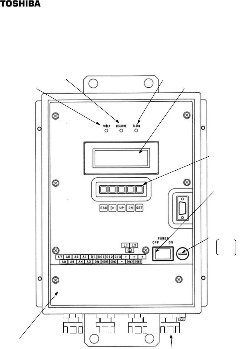
4.2 Converter
Figure 4.2 shows the converter with its door open.
(3) [POWER]
indicator
FUSE
2A(T)
250V
(4) [MEASURE]
indicator (5) [ALARM]
indicator
(6) LCD indicator
(7) Setting keys
(1) Power switch
(2) Fuse
(8) Terminal block
(9) Cable gland
FUSE
2A(T)
250V

28
6 F 8 A 0 5 2 1
[NOTE] Install the converter cover when operating the density meter. In addition, tighten securely
the screws of the converter cover. If screws are not tightened enough, moisture, dust or
other particles enters the converter and can cause a converter failure.
(1) [POWER] switch
The power switch for the density meter.
(2) [Fuse]
2A(T), 250V glass tube fuse is inside.
(3) [POWER] Indicator (Green LED)
Green LED lights when AC power turns on by the power switch.
(4) [MEASURE] Indicator (Green LED)
The indicator lights when measuring, and turns off when setting and when measuring stops at
externally synchronized operation.
(5) [ALARM] Indicator (Red LED)
Lights on error signal from the meter.
(6) LCD indicator
Displays measured values, set values and self-diagnosis data, etc. Being an indicator of 20
characters by 4 lines, it displays numerical values, alphanumeric characters and symbols in
accordance with needs.
(7) Setting keys
These keys are used for switching between display contents of the LCD indicator or setting
various set values. They include the [ESC] key, the [→] key, the [UP] key, [DN] key and the
[SET] key.
(8) Terminal block
Refers to the terminal block connecting cables for external connection.
(9) Cable glands
Six cable glands are available for introducing cables for external connection, such as power
supplies and output signals.
29
6 F 8 A 0 5 2 1
5. OPERATION PROCEDURE
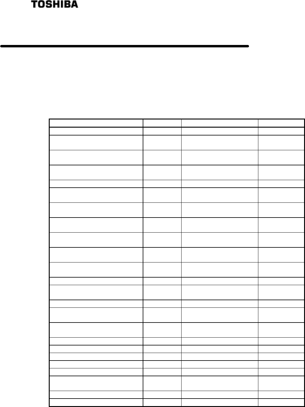
5.1 Parameter and Set Values
The set values and setting ranges by parameter at the time of factory shipment are listed in Table
5.1.1 below.
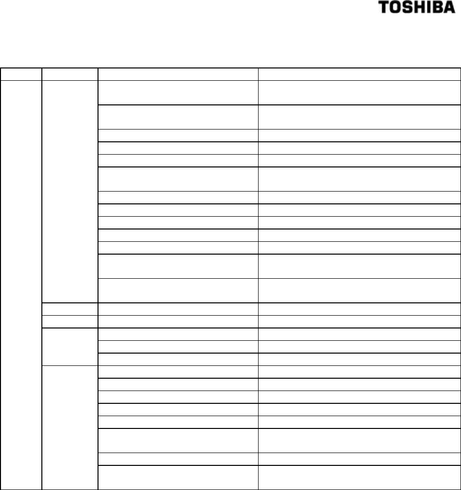
Table 5.1.1 Parameters and Set Values (No.1)
Measurement Condition Parameter
Unit Ex-factory Set Value Setting Range
Density multiplier (C) ― 1.000 (Standard value) 0.00 ∼ 9.99
Upper density
measurement range (UR) %TS Value specified in your order 1.0 ∼ 99.9
Lower density
measurement range (LR) %TS Value specified in your order 0.0 ∼ 99.5
Density line slope (a) %TS per degree
Value in Table 5.1.2 for each
aperture - 0.2000 ∼ 0.2000
Density intercept (b) %TS 0.00 (Standard value) - 99.99 ∼ 99.99
Density test output
during setting mode (ot) %TS 50% density of FS (Provisional
value) 0.0 ∼ 99.9
Delayed time in external synchronized
operation (dt) Minute 0.5 (Provisional value) 0.1 ∼ 99.9
Zero-point phase θ1 (zp) Degree Value at the time
of factory adjustment 0.00 ∼ 359.99
Zero-point fluid temperature T0 (zT) ℃ Value at the time
of factory adjustment 0.00 ∼ 100.00
RF correction factor (cG) − Value at the time
of factory adjustment -9.99 ∼ 9.99
Zero-point RF data (zG) − Value at the time
of factory adjustment 0.00 ∼ 100.00
Moving average times (ma) Time 1 (Without moving averaging) 1 ∼ 99
Permissible width of change-rate limit
(dx) %TS 0.00 (NONE) 0.00∼9.99
Limit times of change-rate limit (HL) − 0 (Without change-rate limit ) 0∼99
Upper angle of angle
rotation correction (UH) Degree 260 240∼360
Upper angle of angle
rotation correction (SH) Degree 100 0∼120
Linearizer density A (LA) %TS 0.60 (Provisional value) 0.00∼99.99
Linearizer density B (LB) %TS 1.00 (Provisional value) 0.00∼99.99
Linearizer inclination (K1) − 1.00 (Without linearization) 0.00∼9.99
Linearizer inclination (K2) − 1.00 (Without linearization) 0.00∼9.99
Linearizer inclination (K3) − 1.00 (Without linearization) 0.00∼9.99
Electric conductivity correction factor
γ(r)
Degree
(per mS/cm)
00 (Without electric conductivity
correction) 0.00 ∼ 99.99
Zero-point electric conductivity Eo (zE)
mS / cm 0.00 0.00 ∼10.00
Measured object electric conductivity (EC)
mS / cm 0.00 0.00 ∼10.00
30
6 F 8 A 0 5 2 1
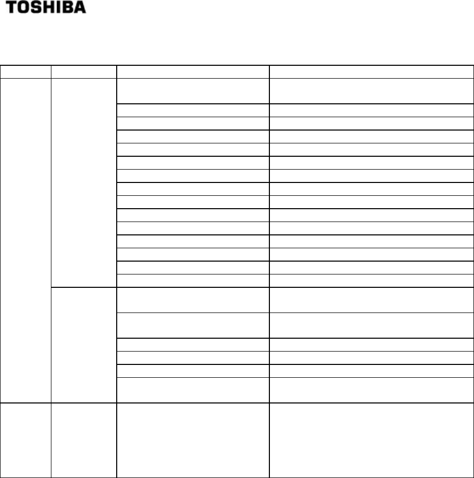
Table 5.1.1 Parameters and Set Values (No.2)
Measurement Condition Parameter Unit Ex -factory Set
Values Setting Range
Availability of additives correction
(AF) − No (Without loading
material correction) OFF / ON
Display density type of
additives correction (Ad) − Total TOTAL / MAIN
Output density type of
additives correction (Ac) − Total TOTAL / MAIN
Parameter set No. of
additives correction (Ap) − 1 1∼10
Main-object sensitivity (sO) − 1.00 −9.99∼9.99
Additives sensitivity (s1) − 0.00 −9.99∼9.99
Additives sensitivity (s2) − 0.00 −9.99∼9.99
Additives sensitivity (s3) − 0.00 −9.99∼9.99
Additives sensitivity (s4) − 0.00 −9.99∼9.99
Additives sensitivity (s5) − 0.00 −9.99∼9.99
Loading additive ratio (R1) − 0.000 0.000∼1.999
Loading additive ratio (R2) − 0.000 0.000∼1.999
Loading additive ratio (R3) − 0.000 0.000∼1.999
Loading additive ratio (R4) − 0.000 0.000∼1.999
Loading additive ratio (R5) − 0.000 0.000∼1.999
Output at contact OFF in external
synchronized operation (ho) − 4mA Value immediately before 4mA ;
simulated output in setting mode
Availability of density multiplier
switching (D1) − OFF(NONE) ON / OFF
Density multiplier at DI (C2) − 1.000 0.000∼9.999
Density multiplier at DI (C3) − 1.000 0.000∼9.999
Density multiplier at DI (C4) − 1.000 0.000∼9.999
Availability of automatic
adjustment of angle rotation (NA)
− ON ON / OFF
Switching between continuous
operation and external
synchronized operation (OP)
− CONT CONT (Continuous) /
EXT(External)
Note : The expression "without ..." has been used in several places in Table 5.1.1 to mean that the
respective numeric values in the table above are set to invalidate their functions.
Table 5.1.2 Density line slope (a)
meter size
(mm) a
50 0.168
80 0.105
100 0.084
150 0.056
200 0.042
250 0.034
300 0.028
31
6 F 8 A 0 5 2 1
5.2 Menus and operations
Operations should be done with five keys for setting, in combination with the LCD display.
This section shows menus and operations.
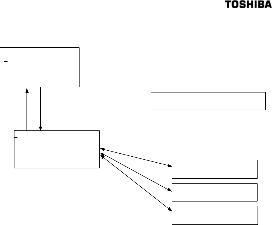
5.2.1. Main menu
Main menu is composed of three basic menus shown below. Table 5.2.1 shows the functions of
each menu and performances when selected.
<main menu>
Table 5.2.1 Functions and performances of main menu
1 : MONITORING MENU 2 : SETTING MENU 3 : MEASURING MODE
Functions
Reading of each
measuring conditions
(parameters), measured
values, and self-diagnosis
data
Changing of each
measuring conditions
(parameters), zero
calibration and span
calibration
Mode selection from among
two measuring modes
(operation modes) of the
normal continuous operation
and the externally
synchronized operation
Measured density
Output (4 ~ 20mA)
Measured density
continuous output Density Test output Measured density continuous
output
LCD Density
display Measured density value Density Test output Measured density valve
[Measure] indicator
On Off On
Note: “Measured density value”is output instead of “Density Test output” as the LCD density display
on the panel when “Zero calibration” or “Span calibration” is selected in the setting menu. This
arrangement is intended to compare the measured density values before and after the
calibration for both Zero and Span calibrations. As to the measured density output (4−20 mA),
“Density Test output” is used for all menu items including Zero calibration and Span calibration.
1 : MONITORING MENU
2 : SETTING MENU
3 : MEASURING MODE
32
6 F 8 A 0 5 2 1
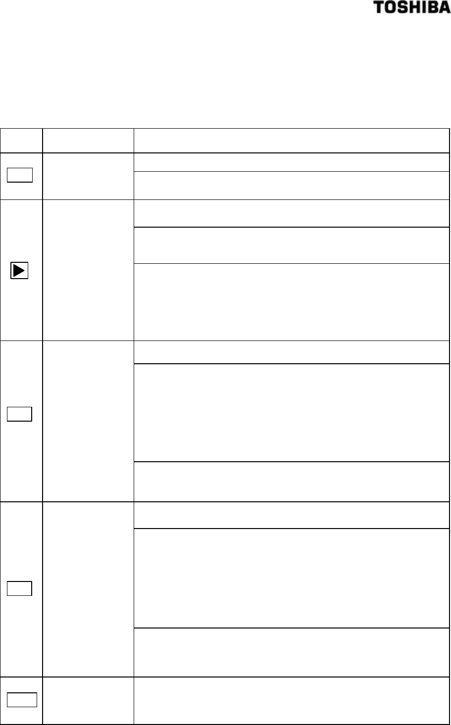
5.2.2 Setting keys
Five setting keys are available. The basic methods for using them are described in Table 5.2.2. For
specification information, please refer to their respective operating procedures.
Table 5.2.2 Basic Methods for Using Operation Keys
Setting
Key Notation in
Operation Manual Basic Use
Returns to the menu screen that is one level higher.
ESC
[ESC] On the set value change screen, use this key to clear the setup change
before returning to the previous screen.
On the menu list screen, use this key to move the cursor under the menu
number to the location of the next number.
In the state of setting numerical values, press this key each time the
cursor has to be shifted rightwards by a digit's worth. If the cursor is
located rightmost, the cursor is shifted to the leftmost digit.
[→] In the event of entering the setting menu, press the [SET] key to display
the message saying that the output will be switched to the simulated
value. After making sure that no problem is present, press the [→] key to
enter the setting menu. This procedure is taken for the purpose of
preventing the output from being switched to the simulated value as a
result of mistakenly pressing the [SET] key twice in a row.
On the menu screen, use this key to switch to the next menu screen.
In the state of setting numerical values, use this key to move up the
numeric value of the digit where the cursor is located. Each time the key
is pressed, the numeric value changes incrementally, as following; "0",
"1", "2", ・・・・, "9", "-"(minus symbol), "."(decimal point), "0", "1",
"2", ・・・・.
Note: If the numerical value does not belong to the leftmost digit, "-"
(minus symbol) will not appear after 9.
UP
[UP]
In the event of selecting an item from multiple items (such as ON/OFF),
the cursor (of the selected item) is switched each time this key is
pressed.
On the menu screen, use this key to switch to the previous menu screen.
In the state of setting numerical values, use this key to move down the
numerical value of the digit where the cursor is located. Each time the
key is pressed, the numerical value changes detrimentally , as following;
"0", "."(decimal point), "-"(minus symbol), "9", "8", ・・・・ "1", "0".
Note: If the numerical value does not belong to the leftmost digit, "-"
(minus symbol) will not appear after "."(decimal point).
DN [DN]
In the event of selecting an item from multiple items (such as ON/OFF),
the cursor (of the selected item) is switched each time this key is
pressed.
SET
[SET] Use this key to select the menu number where the cursor is located or
confirm the set value.
33
6 F 8 A 0 5 2 1
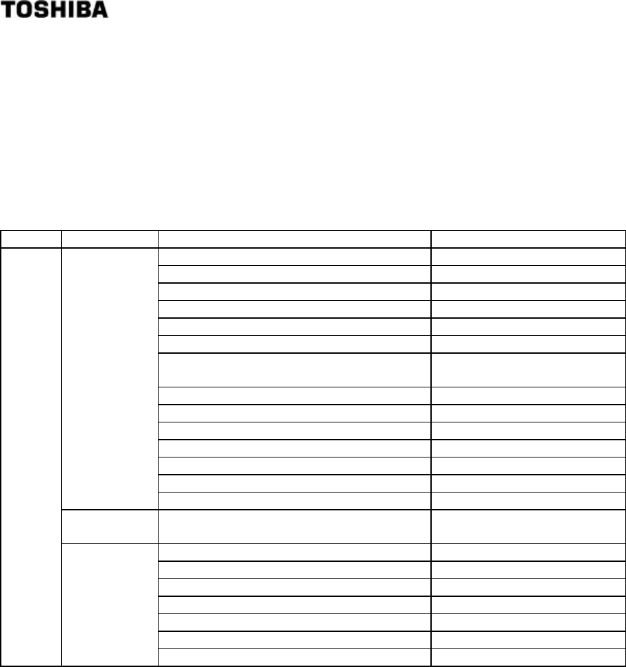
5.2.3 Menu display
The menu display of the converter LCD display section has a hierarchical structure as shown in
Table 5.2.3.
Note: Occasionally using some abbreviated terms as well, actual LCD displays differ from Table
5.2.3. For details, refer to Section 5.2.4. The symbols in parentheses in Table 5.2.3
correspond to those displayed on the upper left corner of their respective LCD screens.
Table 5.2.3 Menu Display (1)
Menu 1 Menu 2 Menu 3 Menu 4
Density multiplier (C)
Upper density measurement range (UR)
Lower density measurement range (LR)
Density line slope (a)
Density intercept (b)
Density test output(ot)
Delayed time in external synchronized operation
(dt)
Zero-point phase θ1 (zp)
Zero-point fluid temperature T0 (zT)
RF correction factor (cG)
Zero-point RF data (zG)
Moving average times (ma)
Permissible width of change-rate limit (dx)
Read
parameters
Limit times of change-rate limit (HL)
Measured value
Phase θ2(p), fluid temperature (T),
ambient temperature (A), density (X)
Operation status (ST)
Microwave signal level (SL)
Micro wave factor (F)
RF data(G)
+5V power supply voltage(J)
Reference phase error (pd)
Monitorin
g
menu
Self-diagnosis
data
Memory check (Mc)
34
6 F 8 A 0 5 2 1
Table 5.2.3 Menu Display (2)
Menu 1 Menu 2 Menu 3 Menu 4
Upper density measurement range
(UR)
Setting the upper density measurement range
(UR)
Lower density measurement range
(LR) Setting the lower d ensity measurement range (LR)
Density line slope (a) Setting the density line slope (a)
Density intercept (b) Setting the density intercept (b)
Density test output (ot) Setting the density test output (ot)
Delayed time in external synchronized
operation (dt)
Setting the delayed time in external synchronized
operation (dt)
Zero-point phase θ1 (zp) Setting the zero-point phase θ1 (zp)
Zero-point fluid temperature T0 (zT) Setting the zero-point fluid temperature T0 (zT)
RF correction factor (cG) Setting the RF correction factor (cG)
Zero-point RF data (zG) Setting the zero-point RF data(zG)
Moving average times (ma) Setting the Moving average times (ma)
Permissible width of change-rate limit
(dX)
Setting the permissible width of change-rate limit
(dX)
Parameter
setting
Limit times of change-rate limit (HL) Setting the permissible times of change-
rate limit
(HL)
Zero calib.
Zero calibration Zero calibration implementation verification
Span calib.
Density multiplier (C1) Setting the density multiplier (C1)
Upper angle (UH) Setting the upper angle (UH)
Lower angle (SH) Setting the lower angle (SH)
Angle
rotation
correction Angle rotation (N) Setting the angle rotation (N)
Linearizer density A (LA) Setting the linearizer density A (LA)
Linearizer density B (LB) Setting the linearizer density B (LB)
Linearizer line slope (K1) Setting the linearizer line slope (K1)
Linearizer line slope (K2) Setting the linearizer line slope (K2)
Linearizer line slope (K3) Setting the linearizer line slope (K3)
Electric conductivity correction factor
γ(r)
Setting the electric conductivity correction factor
γ(r)
Zero-point electric conductivity E0 (zE)
Setting the zero-point electric conductivity E0 (zE)
Setting
menu
Linearizer /
electric
conductivity
correction
Measured object electric conductivity
(EC)
Setting the measured object electric conductivity
(EC)
35
6 F 8 A 0 5 2 1
Table 5.2.3 Menu Display (3)
Menu 1 Menu 2 Menu 3 Menu 4
Availability of additives correction
(AF)
Selecting the availability of additives correction
(AF)
Display density type (Ad) Selecting the display density type (Ad)
Output density type (Ac) Displaying the output density type (Ac)
Parameter set No. (Ap) Setting parameter set No. (Ap)
Main-object sensitivity (s0) Setting the main-object sensitivity (s0)
Additives sensitivity (s1) Setting the additives sensitivity (s1)
Additives sensitivity (s2) Setting the additives sensitivity (s2)
Additives sensitivity (s3) Setting the additives sensitivity (s3)
Additives sensitivity (s4) Setting the additives sensitivity (s4)
Additives sensitivity (s5) Setting the additives sensitivity (s5)
Loading additive ratio (R1) Setting the loading additive ratio (R1)
Loading additive ratio (R2) Setting the loading additive ratio (R2)
Loading additive ratio (R3) Setting the loading additive ratio (R3)
Loading additive ratio (R4) Setting the loading additive ratio (R4)
Additives
correction
Loading additive ratio (R5) Setting the loading additive ratio (R5)
Output at contact OFF in external
synchronized operation(ho)
Selecting the output at contact OFF in external
synchronized operation (ho)
Availability of density multiplier
switching (D1)
Selecting the availability of density multiplier
switching (D1)
Density multiplier at DI (C2) Setting the density multiplier at DI (C2)
Density multiplier at DI (C3) Setting the density multiplier at DI (C3)
Density multiplier at DI (C4) Setting the density multiplier at DI (C4)
Setting
menu
Others
Availability of automatic
adjustment of angle rotation (NA)
Selecting the availability of automatic
adjustment of angle rotation (NA)
Measurin
g mode
Continuous
operation
and external
synchronized
operation
(OP)
Switching between continuous
operation and external
synchronized operation (OP)
36
6 F 8 A 0 5 2 1
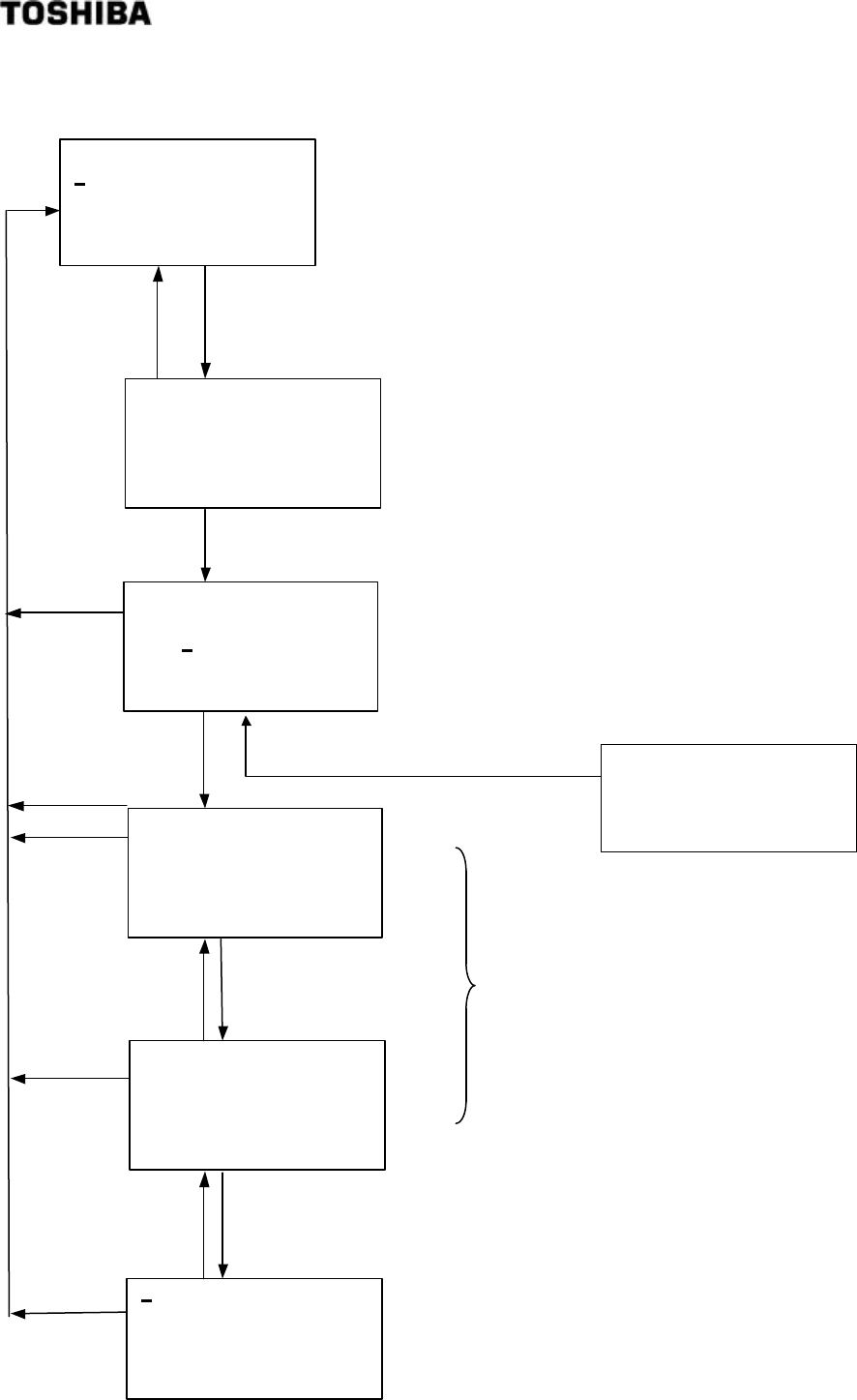
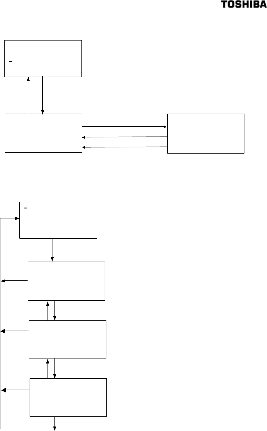
5.2.4 Monitoring menu display and operating procedures
1 :READ PARAMETERS
2 :MEASURED VALUES
3 :SELF-DIAGNOSIS
1 :MONITORING MENU
2 :SETTING MENU
3 :MEASURING MODE
Menus of
「1 :READ PARAMETERS」
Data display of
「2:MEASURED VALUES」
Data display of
「3:SELF-DIAGNOSIS」
Move the cursor to the menu
number with [→] key, and
press [SET] key.
Move the cursor to "1" with [→] key, and
press [SET] key.
[ESC]
(Previous
Menu)
[ESC]
(Previous
Menu)
Note: In actual display, the cursor is
blinking.
37
6 F 8 A 0 5 2 1
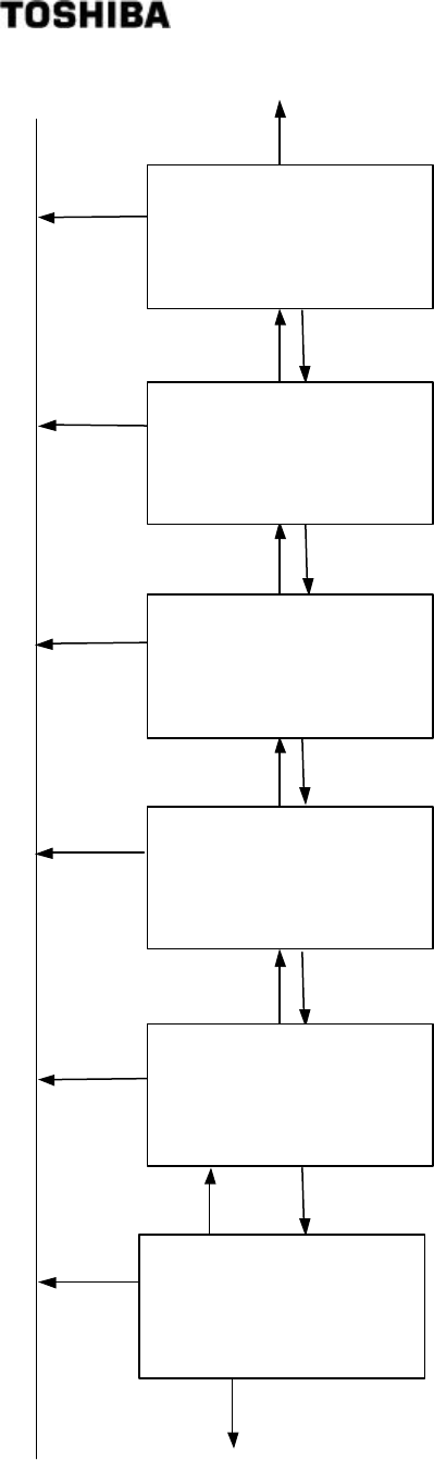
5.2.5. Setting menu display and operating procedures
When [2: SETTING MENU] is selected, the density ou
tput
signal and the density display are hold in the simulated
values that have been set. This warning screen will
appear once before getting into [2: SETTING MENU].
After making sure that there is no problem, press the [→
]
key to get into [2: SETTING MENU].
1 :MONITORING MENU
2 :SETTING MENU
3 :MEASURING MODE
9:LINEARIZ/CNDUCTVTY
10:ADDITIVES CORRECT
11:OTHERS
Move the cursor to the menu number with
[→] key, and press [SET] key.
Press the [→] key to get into [2: SETTING MENU].
1 :READ PARAMETERS
2 :MEASURED VALUES
3 :SELF-DIAGNOSIS
Move the cursor to "2" with [→] key, and press [SET] key.
Test output will be
valid.
[→] : CONTINUE
[ESC]: CANCEL
5:SET PARAMETERS
6:ZERO CALIBRATION
7:SPAN CALIBRATION
8:ANGLE ROTATION
[ESC]
(Previous
Menu)
[ESC]
(Previous
Menu)
[ESC]
(Previous
Menu)
[ESC]
(Previous
Menu)
[DN]
(Pre. menu)
[UP]
(Next menu)
[DN]
(Pre. menu)
[UP]
(Next menu)
To get into [2: SETTING MENU], it is necessary to further
enter the password "8000". In the initial condition, th
e cursor
is on the forth digit. Therefore, press [DN] key 4 times to set to
"8" and press the [SET] key to get into [2: SETTING MENU]. An
incorrect password will cause the following message to
appear. Return to the screen a
t left by pressing any key and
then enter the correct password once again.
Input password
PASSWORD
:0000
[SET]SET,[ESC]CANCEL
PASSWORD ERROR
PUSH ANY KEY.
[ESC]
(Previous
Menu)
38
6 F 8 A 0 5 2 1
5.2.6 Measuring mode display and operating procedures
5.2.7 Reading of parameters display and operating procedures
OP:MEASURING MODE
DATA:CONT
[SET] CHANGE
[ESC] RETURN
OP:MEASURING MODE
RANGE :CONT/EXT
DATA :CONT
[SET] SET,[ESC]CANCEL
1 :MONITORING MENU
2 :SETTING MENU
3 :MEASURING MODE
Move the cursor to "3" with [→] key, and press [SET] key.
Press the SET key to set.
Press the SET key to confirm.
Press the ESC key to cancel.
E
ach time the
゚
[UP] or [DN] key is pressed, CONT/EXT are
mutually alternated thus making it possible to select an operation
mode. Select "CONT" for normal continuous operations; select
"EXT" for external synchronized operations. For details on the
external synchronized operation, refer to Section 6.7.
[ESC]
(Previous
Menu)
Move the cursor to "1" with [→] key, and press [SET] key,
and select [1 : READ PARAMETERS]
UR:UPPER RANGE
DATA:3.0
[ESC] RETURN
LR:LOWER RANGE
DATA:0.0
[ESC] RETURN
1 :READ PARAMETERS
2 :MEASURED VALUES
3 :SELF-DIAGNOSIS
C:DENSITY MULTIPLIER
DATA:1.000(C1)
[ESC] RETURN
The set value of the density multiplier C, which is used for
density calculation, can be verified. If C2, C3 or C4 is
displayed in the parentheses, it indicates that the density
multiplier switched to by the external voltage signal (DI) is
selected.
The set value of the upper density measurement range
(the density whose current output is 20mA) can be verified.
The set value of the lower density measurement range
(the density whose current output is 4mA) can be verified.
[ESC]
(Previous
Menu)
[ESC]
(Previous
Menu)
[ESC]
(Previous
Menu)
[DN]
(Pre. menu)
[UP]
(Next menu)
[DN]
(Pre. menu)
[UP]
(Next menu)
[UP]
(Next menu)
39
6 F 8 A 0 5 2 1
The set value of "density line slope" of
the
arithmetic expression for calculating the density
from the phase measurement data, etc. can be
verified.
The set value of "density intercept" of the arithmetic
expression for calculating the density from the
phase measurement data, etc. can be verified.
Normally, this is set to zero.
Upon getting into [2: SETTING MENU], the current
output and the LED density display are switched to
simulated values. In this screen, the set value of the
simulated value (unit: %TS) can be verified.
In external synchronized operations, the set value
of the delayed time (unit: minute) from when the
external contact input is turned ON until the
measurement starts can be verified. For details,
refer to Section 6.7.
The phase at the time of zero calibration can be
verified.
[ESC]
(Previous
Menu)
[ESC]
(Previous
Menu)
[ESC]
(Previous
Menu)
[ESC]
(Previous
Menu)
[ESC]
(Previous
Menu)
a:DENSITY LINE SLOPE
DATA:0.0840
[ESC] RETURN
b:DENSITY INTERCEPT
DATA:0.0
[ESC] RETURN
ot:DENSTY TEST OUT
DATA:1.5
[ESC] RETURN
dt:DELAYED SYNC.TIME
DATA:0.5
[ESC] RETURN
zp:ZERO POINT PHASE
DATA:80.00
[ESC] RETURN
[DN]
(Pre. menu)
[UP]
(Next menu)
[DN]
(Pre. menu)
[DN]
(Pre. menu)
[UP]
(Next menu)
[DN]
(Pre. menu)
[UP]
(Next menu)
[DN]
(Pre. menu)
[UP]
(Next menu)
[UP]
(Next menu)
The fluid temperature at the time of zero calibration can
be verified.
[ESC]
(Previous
Menu)
[DN]
(Pre. menu)
[UP]
(Next menu)
zT:ZERO WATER TEMP.
DATA:25.00
[ESC] RETURN
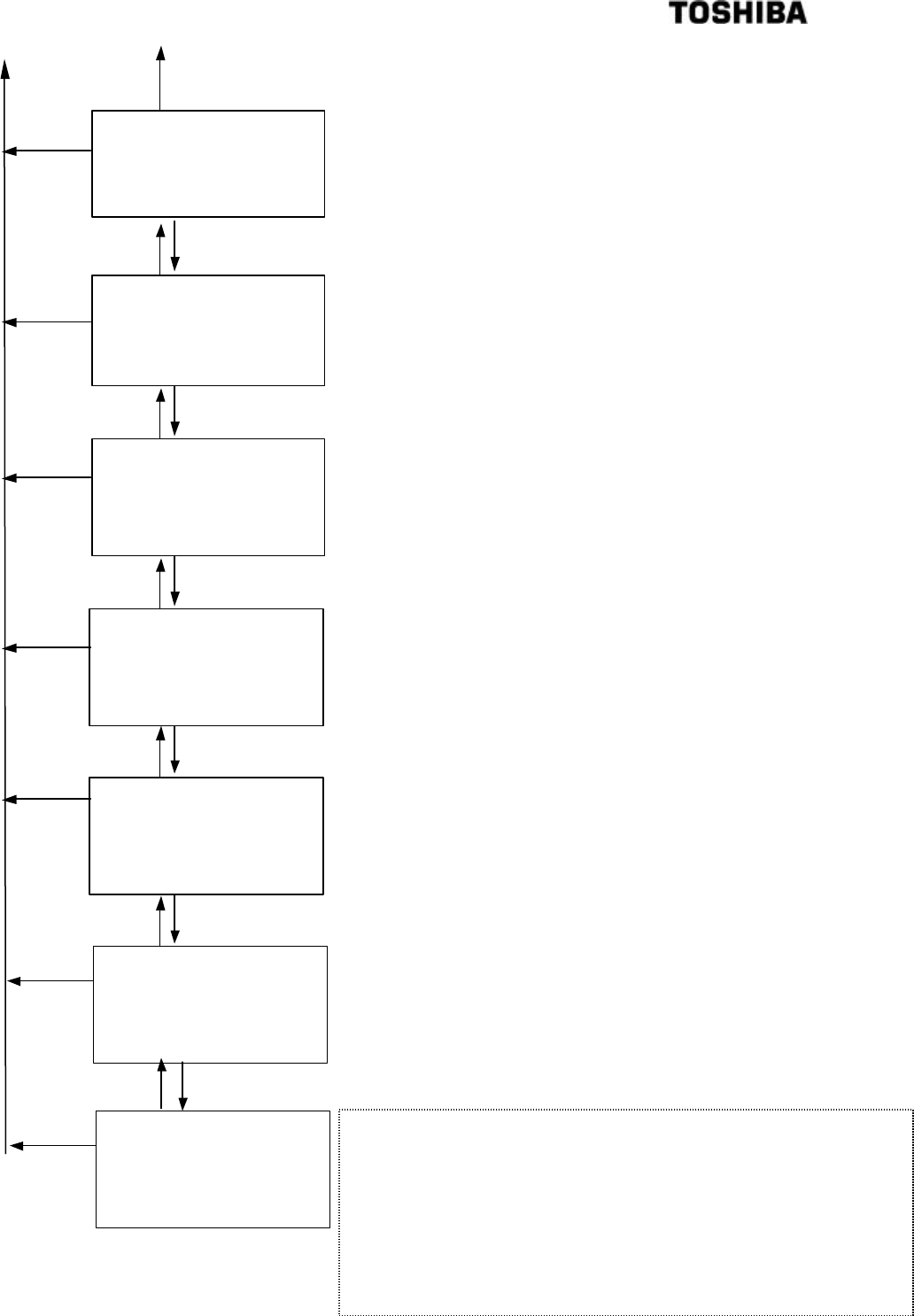
40
6 F 8 A 0 5 2 1
The set value of the RF correction factor used for density
calculation can be verified. Before shipment, this value is
already set in accordance with the product's characteristics in
the shipping test. If you change this value, it will affect the
performance; therefore, normally, do not change it.
The RF data at the time of zero calibration can be verifie
d.
The set value of the moving average times can be verified.
The variation width (%TS) permitted in the change
-
rate limit
function can be verified.
[ESC]
(Previous
Menu)
[ESC]
(Previous
Menu)
[ESC]
(Previous
Menu)
[ESC]
(Previous
Menu)
[ESC]
(Previous
Menu)
[ESC]
(Previous
Menu)
The times permitted in the chan
ge
-
rate limit function can be
verified.
cG:RF COEF.
DATA:0.00
[ESC] RETURN
zG:ZERO RF DATA
DATA:50.00
[ESC] RETURN
ma:AVERAGING TIMES
DATA:1
[ESC] RETURN
dx: CHANGE-RATE LIMIT
DATA:0.00
[ESC] RETURN
HL:LIMIT TIMES
DATA:0
[ESC] RETURN
C:DENSITY MULTIPLIER
DATA:1.000
[ESC] RETURN
[DN]
(Pre. menu)
[UP]
(Next menu)
[DN]
(Pre. menu)
[DN]
(Pre. menu)
[UP]
(Next menu)
[DN]
(Pre. menu)
[UP]
(Next menu)
[DN]
(Pre. menu)
[UP]
(Next menu)
[DN]
(Pre. menu)
[UP]
(Next menu)
[ESC]
(Previous
Menu)
OI:OUTPUT INTERVAL
DATA:HART 0s
[ESC] RETURN
[DN]
(Pre. menu)
[UP]
(Next menu)
W
hich type of communication method is selected, HART
communication*1 or RS232C communication*2, can be checked
and also the output interval can be checked.
Note *1: HART protocol
is set when the density meter is shipped from
the factory. In addition, 0 second appears as its output interval.
This is because the output for HART communication is
requested by the nature of this protocol from a super-
ordinate
device such as the hand-held terminal AF100 and the output
interval has no meaning.
Note *2: RS232C can be used by adding the data save function.
For how to switch the communication method and how to set
the output interval, refer to the LQ600 Data Save Function
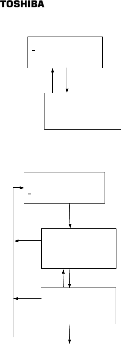
41
6 F 8 A 0 5 2 1
5.2.8 Measured values display and operating procedures
5.2.9 Self-diagnosis data display operating procedures
MEASURED VALUES *
p PHASE: 123.56 N=0
T TEMP: 30.00 °C
X DENSITY: 2.34 %TS
Move the cursor to "2" with [→
] key, and press [SET] key to
select [ 2:MEASURED VALUES]
1 :READ PARAMETERS
2 :MEASURED VALUES
3 :SELF-DIAGNOSIS
It is possible to verify the measured phase value (and
the angle rotation N), the measured fluid temperature
value, as well as the density calculated based on them.
[*] in the upper right corner will blink synchronously with
the data updating thus making it possible to verify that
the data updating is definitely taking place.
[ESC]
(Previous
Menu)
[ESC]
(Previous
Menu)
[ESC]
(Previous
Menu)
SL:MICROWAVE SIG.LVL
DATA :−53 dBm
[ESC] RETURN
Move the cursor to "3" with [→] key,
and press [SET] key to select [3:SELF-DIAGNOSIS]
ST:STATUS :GOOD
[ESC] RETURN
Whether the phase m
easurement operation is
normally functioning or not can be verified.
The micro wave receive signal level can be
verified. Normally, the level is -45 to -75. (dBm)
1 :READ PARAMETERS
2 :MEASURED VALUES
3 :SELF-DIAGNOSIS
[DN]
(Pre. menu)
[UP]
(Next menu)
[UP]
(Next menu)
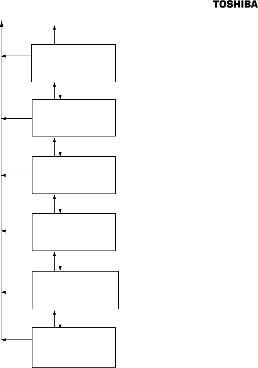
42
6 F 8 A 0 5 2 1
[ESC]
(Previous
Menu)
The micro wave signal constant can be verified.
Normally, the value is 1825 to 1975.
[ESC]
(Previous
Menu)
[ESC]
(Previous
Menu)
[ESC]
(Previous
Menu)
[ESC]
(Previous
Menu)
[ESC]
(Previous
Menu)
The soundness of the phase measurement unit
can be verified.
The soundness of various memory units can be
verified.
The converter's RF data (concerning the micro
wave phase measurement) can be verified.
Normally, the value is 10 to 70.
The voltage of the 5
-
volt power supply can be
checked.
G:RF DATA.
DATA : 50.00
[ESC] RETURN
J:+5V POWER SUPPLY
DATA :5.00
[ESC] RETURN
Mc:MEMORY CHECK:GOOD
EPROM :GOOD
RAM :GOOD
EEPROM
:GOOD
ST:STATUS :GOOD
[ESC] : RETURN
pd:REF PHASE
DATA:0.0
[ESC] RETURN
F:MICROWAVE COEF.
DATA : 1910
[ESC] RETURN
[DN]
(Pre. menu)
[UP]
(Next menu)
[DN]
(Pre. menu)
[UP]
(Next menu)
[DN]
(Pre. menu)
[UP]
(Next menu)
[DN]
(Pre. menu)
[UP]
(Next menu)
[DN]
(Pre. menu)
[UP]
(Next menu)
[DN]
(Pre. menu)

43
6 F 8 A 0 5 2 1
5.2.10 Parameter setting display and operating procedures
Move the cursor to "5" with [→] key, and press [SET] key to select[ 5:SET PARAMETERS]
5:SET PARAMETERS
6:ZERO CALIBRATION
7:SPAN CALIBRATION
8:ANGLE ROTATION
UR:UPPER RANGE
DATA:3.0
[SET] CHANGE
[ESC] RETURN.
LR:LOWER RANGE
DATA:0.0
[SET] CHANGE
[ESC] RETURN
UR:UPPER RANGE
RANGE :1.0-99.9 %TS
DATA : 0.30
[SET] SET,[ESC] CANCEL
[SET](Set)
[SET](Fix)
[ESC](Cancel)
LR:LOWER RANGE
RANGE :0.0-99.5 %TS
DATA :00.0
[SET] SET,[ESC] CANCEL
[SET](Set)
[SET](Fix)
[ESC](Cancel)
a:DENSITY LINE SLOPE
DATA:0.0840
[SET] CHANGE
[ESC] RETURN
a:DENSITY LINE SLOPE
RANGE :−0.2000−0.2000
DATA : 0.0840
[SET] SET,[ESC] CANCEL
[SET](Set)
[SET](Fix)
[ESC](Cancel)
b:DENSITY INTERCEPT
DATA:0.00
[SET] CHANGE
[ESC] RETURN
b:DENSITY INTERCEPT
RANGE :−99.99−99.99
DATA : 00.00
[SET] SET,[ESC] CANCEL
[SET](Set)
[SET](Fix)
[ESC](Cancel)
ot:DENSTY TEST OUT.
DATA:1.5
[SET] CHANGE
[ESC] RETURN
ot:DENSTY TEST OUT.
RANGE :0.0-99.9 %TS
DATA : 01.5
[SET] SET,[ESC] CANCEL
[SET](Set)
[ESC]
(Previous
Menu)
[ESC]
(Previous
Menu)
[ESC]
(Previous
Menu)
[SET](Fix)
[ESC](Cancel)
The upper density measurement range
(whose current output is 20mA) is set.
The lower density measurement range
(whose current output is 4mA) is set.
The "density line slope" of the arithmetic expression for
calculating the density from the phase measurement data, etc. is
set. Before shipping, this is s
et in accordance with the aperture,
based on Table 5.1.2. Normally, do not change the setting.
The "density intercept" of the arithmetic expression for calculating
the density from
the phase measurement data, etc. is set. In the
event that the zero point is out of position, it is corrected through
zero calibration; it is also possible to shift the zero point by
changing this coefficient. Normally, set the value to zero.
When [2: SETTING MENU] is selected, the density output
signal and the density display are hold in the simulated values
that have been set.
In this screen, the simulated values are
set in terms of "%TS".
[ESC]
(Previous
Menu)
[ESC]
(Previous
Menu)
[DN]
(Pre. menu)
[UP]
(Next menu)
[DN]
(Pre. menu)
[UP]
(Next menu)
[DN]
(Pre. menu)
[UP]
(Next menu)
[DN]
(Pre. menu)
[UP]
(Next menu)
[UP]
(Next menu)
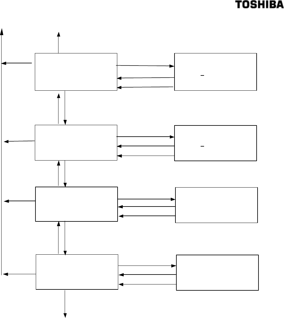
44
6 F 8 A 0 5 2 1
zp:ZERO POINT PHASE
DATA:80.00
[SET] CHANGE
[ESC] RETURN
zp:ZERO POINT PHASE
RANGE :0.00-359.99
DATA : 080.00
[SET] SET,[ESC] CANCEL
[SET](Set)
[SET](Fix)
[ESC](Cancel)
zT:ZERO WATER TEMP
DATA:25.00
[SET] CHANGE
[ESC] RETURN
zT:WATER TEMP./ZERO
RANGE :0.00-100.00 (C
DATA : 025.00
[SET] SET,[ESC] CANCEL
[SET](Set)
[SET](Fix)
[ESC](Cancel)
The zero-point phase can be set in this menu through
manual input. Normally, the zero-point phase is
automatically set when implementing the zero calibration.
The zero
-
point fluid temperature can be set in this menu
through manual input. Normally, the zero-point fluid
temperature is automatically set when implementing the zero
calibration.
The RF correction factor used for density calculation is set.
Before shipment, this value is already set in accordance with
the product's characteristics in the shipping test. If you
change this value, it will affect the performance; therefore,
normally, do not change it.
cG:RF COEF.
DATA: 0.00
[SET] CHANGE
[ESC] RETURN
cG:RF COEF.
RANGE : -9.99-9.99
DATA: 0.00
[SET] SET,[ESC] CANCEL
[SET](Set)
[SET](Fix)
[ESC](Cancel)
[ESC]
(Previous
Menu)
[ESC]
(Previous
Menu)
[ESC]
(Previous
Menu)
dt:DELAYED SYNC.TIME
DATA:0.5
[SET] CHANGE
[ESC] RETURN
dt:DELAYED SYNC.TIME
RANGE :0.1-99.9 min
DATA : 00.5
[SET] SET,[ESC] CANCEL
[SET](Set)
[SET](Fix)
[ESC](Cancel)
In external sync
hronized operations, the delayed time from when the
external contact input is turned ON until the measurement starts is set.
For details, refer to Section 6.7.
[ESC]
(Previous
Menu)
[DN]
(Pre. menu)
[UP]
(Next menu)
[DN]
(Pre. menu) [UP]
(Next menu)
[DN]
(Pre. menu)
[UP]
(Next menu)
[UP]
(Next menu)
[DN]
(Pre. menu)
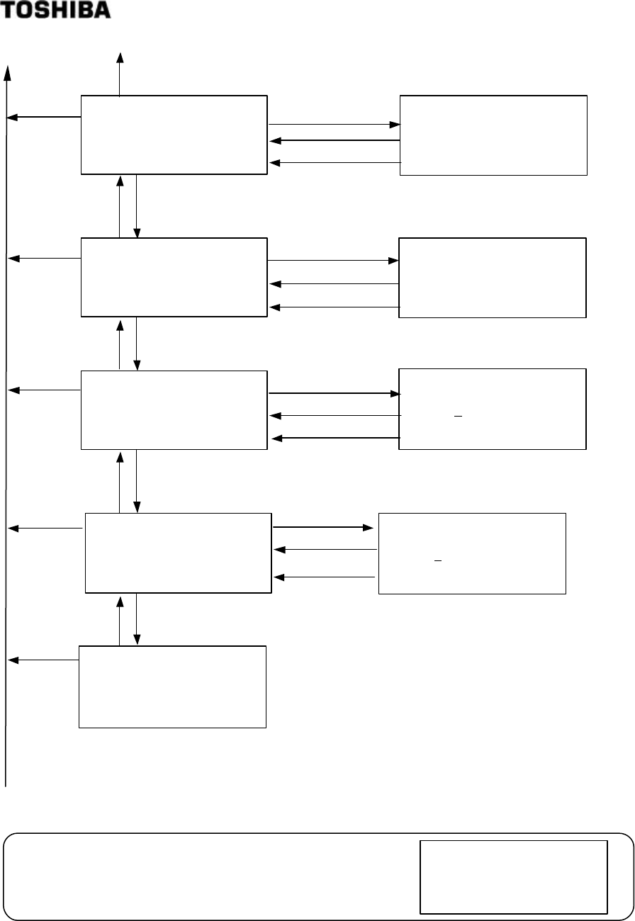
45
6 F 8 A 0 5 2 1
VALUE OUT OF RANGE
UR:UPPER RANGE
PRESS ANY KEY TO
RETURN
For all menus, when data outside the allowed range is
input, the error message is displayed, and the wrong data is
refused. Press any key to return, and input adequate data.
[NOTE]:
[DN]
The limit times in the change-rate limit function are set. If the
variation width exceeds dx(%TS) that was set in the previous
menu, the signal is exc
luded for up to the HL times that are set in
this menu. At HL=0, the change
-rate limit function does not work.
[ESC]
(Previous
Menu)
ma:AVERAGING TIMES
RANGE : 1-99
DATA : 01
[SET] SET,[ESC] CANCEL
[SET](Set)
[SET](Fix)
[ESC](Cancel)
dx:CHANGE RATE LIMIT
RANGE :0.00-9.99 °
DATA: 0.00
[SET] SET,[ESC] CANCEL
[SET](Set)
[SET](Fix)
[ESC](Cancel)
zG:ZERO RF DATA
RANGE :0.00-100.00 (C
DATA: 050.00
[SET] SET,[ESC] CANCEL
[SET](Set)
[SET](Fix)
[ESC](Cancel)
HL:LIMIT TIMES
RANGE :0-99
DATA: 00
[SET] SET,[ESC] CANCEL
[SET](Set)
[SET](Fix)
[ESC](Cancel)
[ESC]
(Previous
Menu)
The zero
-
point RF data can be set in this menu through
manual input. Normally, the zero-point RF constant is
automatically set when implementing the zero calibration.
The moving average times are set. If the output averaged for
density control, etc. is needed, the value from 5 to about 10 is
set.
If there is a signal of sharp variation, the change-rate limit fu
nction
excludes this signal to restrict a sudden output variation. In this
menu, the permissible variation width is set in terms of "%TS".
[ESC]
(Previous
Menu)
[ESC]
(Previous
Menu)
[ESC]
(Previous
Menu)
UR:UPPER RANGE
DATA:3.0
[SET] CHANGE
[ESC] RETURN
ma:AVERAGING TIMES
DATA:1
[SET] CHANGE
[ESC] RETURN
dx:CHANGE RATE LIMIT
DATA:0.00
[SET] CHANGE
[ESC] RETURN
zG:ZERO RF DATA
DATA: 50.00
[SET] CHANGE
[ESC] RETURN
HL:LIMIT TIMES
DATA: 0
[SET] CHANGE
[ESC] RETURN
[SET](Set)
[DN]
(Pre. menu)
[UP]
(Next menu)
[DN]
(Pre. menu)
[UP]
(Next menu)
[DN]
(Pre. menu)
[UP]
(Next menu)
[DN]
(Pre. menu)
[UP]
(Next menu)
[DN]
(Pre. menu)
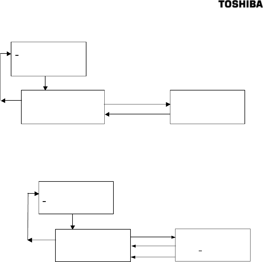
46
6 F 8 A 0 5 2 1
5.2.11 Zero calibration display and operating procedures
5.2.12 Span calibration display and operating procedures
Move the cursor to "7" with [→] key, and press [SET] key
to select [7:SPAN CALIBRATION]
5:SET PARAMETERS
6:ZERO CALIBRATION
7:SPAN CALIBRATION
8:ANGLE ROTATION
C1:DensityMultiplier
DATA:1.000
[SET] CHANGE
[ESC] RETURN
[ESC]
(Previous
Menu)
C1:DensityMultiplier
RANGE :0.000-9.999
DATA : 1.000
[SET] SET,[ESC]CANCEL
[SET](Set)
[SET](Fix)
[ESC](Cancel)
The density multiplier C1 should be set to the suitable
value so that the measured density value is
corresponding to the manual analysis value. For
details, refer to Section 6.5.
Move the cursor to "6" with [→] key, and press [SET] key to select [6:ZERO CALIBRATION]
5:SET PARAMETERS
6:ZERO CALIBRATION
7:SPAN CALIBRATION
8:ANGLE ROTATION
ZERO CAL *
p PHASE: 87.93 ° N=0
T TEMP.: 26.55 °C
X DENSITY: 0.02 %TS
ZERO POINT
CALIBRATION
HAS BEEN COMPLETED
[SET](Set)
New data displayed
[ESC]
(Previous
Menu)
Press the [SET] key for zero calibration. In zero calibration, the
phase and the fluid temperature of zero point will be replaced
with the present measured values. And also, angle rotation "N"
will be set to zero.
Note: The display will return to the left display automatically
after approximately one second.
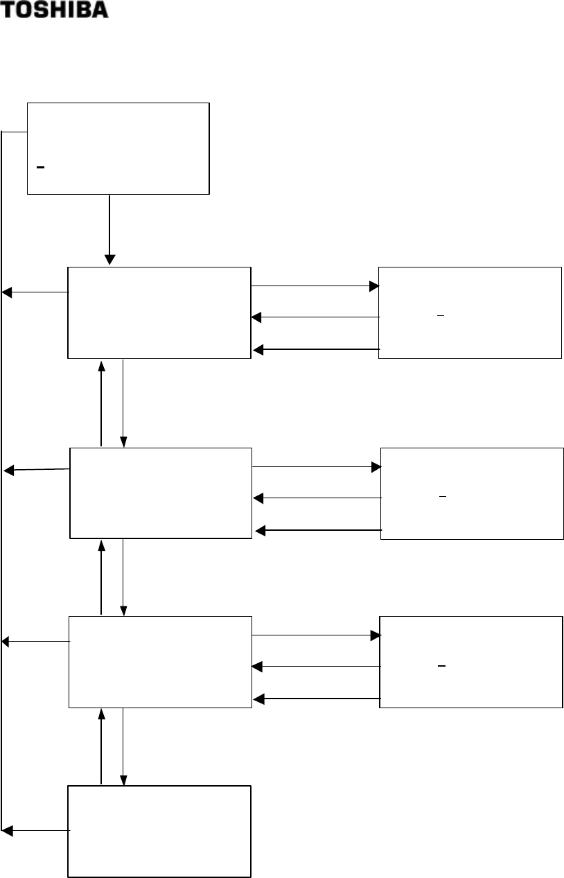
47
6 F 8 A 0 5 2 1
5.2.13 Phase angle rotation correction display and operating procedures
Move the cursor to "8" with [→
] key, and press [SET] key
to select [8:ANGLE ROTATION]
5:SET PARAMETERS
6:ZERO CALIBRATION
7:SPAN CALIBRATION
8:ANGLE ROTATION
UH:UPPER ANGLE
DATA : 260
[SET] CHANGE
[ESC] RETURN
SH:LOWER ANGLE
DATA :100
[SET] CHANGE
[ESC] RETURN
UH:UPPER ANGLE
RANGE :240-360 °
DATA : 260
[SET] SET,[ESC] CANCEL
[SET](Set)
[SET](Fix)
[ESC](Cancel)
SH:LOWER ANGLE
RANGE :0-120
DATA : 100
[SET] SET,[ESC] CANCEL
[SET](Set)
[SET](Fix)
[ESC](Cancel)
N:ROTATION
DATA:0
[SET] CHANGE
[ESC] RETURN
N:ROTATION
RANGE :−10 - 10
DATA : 00
[SET] SET,[ESC] CANCEL
[SET](Set)
[SET](Fix)
[ESC](Cancel)
UH:UPPER ANGLE
DATA :260
[SET] CHANGE
[ESC] RETURN
Before shipping, this value is set to 260 degrees. Changing
the setting may result in damaging the otherwise normal
operation. Therefore, normally, do not change the setting.
Before shipping, this value is set to 100 degrees. Changing
the setting may result in damaging the otherwise normal
operation. Therefore, normally, do not change the setting.
Normally, the angle rotation N is automatically computed;
therefore, it is unnecessary to change the setting through
manual input. However, there are some cases of high density
measurements which require settings through manual input.
[ESC]
(Previous
Menu)
[ESC]
(Previous
Menu)
[ESC]
(Previous
Menu)
[ESC]
(Previous
Menu)
[DN]
(Pre. menu)
[UP]
(Next menu)
[DN]
(Pre. menu)
[UP]
(Next menu)
[DN]
(Pre. menu)
[UP]
(Next menu)
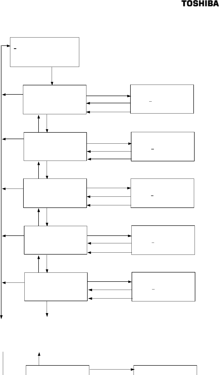
48
6 F 8 A 0 5 2 1
5.2.14 Linearize/conductity correction display and operating procedures
Move the cursor to "9" with [→] key, and press [SET] key to
select [ 9:LINEARIZ/CNDUCTVTY]
LA:DENSITY A
RANGE :0.00-99.99
DATA :00.60
[SET] SET,[ESC] CANCEL
[SET](Set)
[SET](Fix)
[ESC](Cancel)
LB:DENSITY B
RANGE :0.00-99.99
DATA : 01.00
[SET] SET,[ESC] CANCEL
[SET](Set)
[SET](Fix)
[ESC](Cancel)
K1:COEF.
RANGE:0.00-9.99
DATA : 1.00
[SET] SET,[ESC] CANCEL
[SET](Set)
[SET](Fix)
[ESC](Cancel)
K2:COEF.
RANGE:0.00-9.99
DATA : 1.00
[SET] SET,[ESC] CANCEL
[SET](Set)
[SET](Fix)
[ESC](Cancel)
K3:COEF.
RANGE :0.00-9.99
DATA : 1.00
[SET] SET,[ESC] CANCEL
[SET](Set)
[SET](Fix)
[ESC](Cancel)
9:LINEARIZ/CNDUCTVTY
10:ADDITIVES CORRECT
11:OTHERS
[ESC]
(Previous
Menu)
[ESC]
(Previous
Menu)
[ESC]
(Previous
Menu)
[ESC]
(Previous
Menu)
[ESC]
(Previous
Menu)
In the event of three straight lines which closely analogous
each other, the density of the crossover point A of the 2nd
and 3rd lines is set.
In the event of three straight lines which closely analogous
each other, the density of the crossover point B of the 2nd
and 3rd lines is set.
In the event of three straight lines which closely analogous
each other, the inclination K1 of the 1st line is set.
In the event of three straight lines which closely analogous
each other, the inclination K2 of the 2nd line is set.
In the event of three straight lines which closely analogous
each other, the inclination K2 of the 3rd line is set.
LA:DENSITY A
DATA :0.60
[SET] CHANGE
[ESC] RETURN
LB:DENSITY B
DATA:1.00
[SET] CHANGE
[ESC] RETURN
K1:COEF.
DATA:1.00
[SET] CHANGE
[ESC] RETURN
K2:COEF.
DATA:1.00
[SET] CHANGE
[ESC] RETURN
K3:COEF.
DATA:1.00
[SET] CHANGE
[ESC] RETURN
[DN]
(Pre. menu)
[UP]
(Next menu)
[UP]
(Next menu)
[DN]
(Pre. menu)
[UP]
(Next menu)
[DN]
(Pre. menu)
[UP]
(Next menu)
[DN]
(Pre. menu)
[UP]
(Next menu)
r:CNDUCTVTY. COEF.
RANGE : 0.00
r:CNDUCTVTY. COEF.
RANGE :0.00
-
99.99
[SET](Set)
[SET](Fix)
[DN]
(Pre. menu)

49
6 F 8 A 0 5 2 1
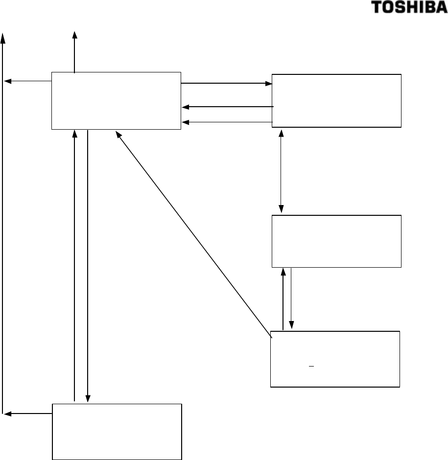
50
6 F 8 A 0 5 2 1
EC:CONDUCTIVITY
DATA:1.23(LINE)
[SET] CHANGE
[ESC] RETURN
EC:CONDUCTIVITY
RANGE :0.00-10.00
DATA: 00.00
[SET] SET,[ESC] CANCEL
LA:DENSITY A
DATA :0.60
[SET] CHANGE
[ESC] RETURN
MANU/LINE SELECTION
RANGE :MANU/LINE
DATA:(LINE)
[SET] SET,[ESC] CANCEL
MANU/LINE SELECTION
RANGE :MANU/LINE
DATA:(MANU)
[SET] SET,[ESC] CANCEL
[SET](Set)
[SET](Fix in
"LINE mode")
[ESC](Cancel)
[ESC]
(Previous
Menu)
[ESC]
(Previous
Menu)
By selecting "MANU" (see the screen
above) and then pressing [SET], the
electric conductivity of the measured
object is made settable as the fixed value
through manual input.
After the electric
conductivity is
entered, [SET] is used
to confirm the setting
in MANU mode.
[ESC]
(Cancel)
[UP]
(First menu)
[DN]
(Pre. menu)
[UP] and [DN] is used to switch between
MANU/LINE to select the method for setting
the electric conducti
vity.
By selecting "LINE" and pressing [SET] (see
the screen above), the electric conductivity
is continually corrected with the electric
conductivity of the measured object.
[DN]
(Pre. menu)
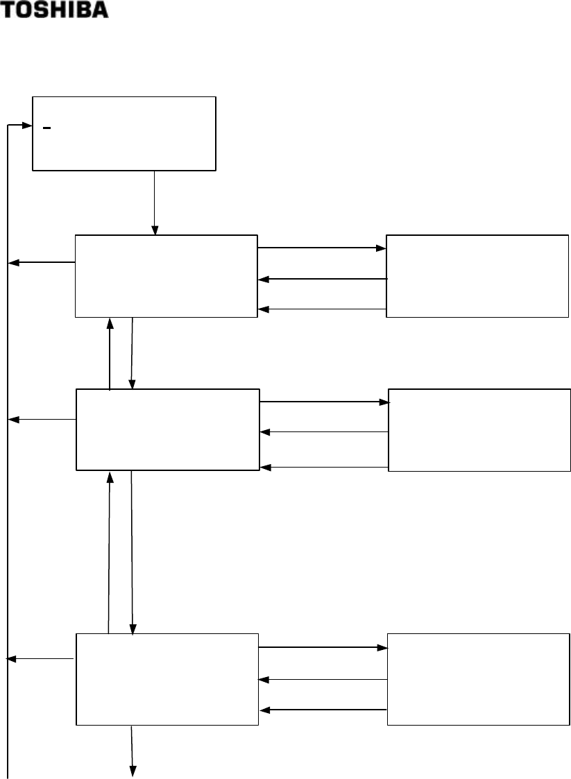
51
6 F 8 A 0 5 2 1
5.2.15 Additives correction display and operating procedures
Move the cursor to "10" with [
→
] key, and press [SET]
key to select [10:ADDITIVES CORRECT ]
AF:ADDITIVES COMP.
DATA :ON
[SET] CHANGE
[ESC] RETURN
Ad:DISPLAY DENSITY
DATA:TOTAL
[SET] CHANGE
[ESC] RETURN
AF:ADDITIVES COMP.
RANGE :OFF/ON
DATA:ON
[SET] SET,[ESC] CANCEL
[SET](Set)
[SET](Fix)
[ESC](Cancel)
Ad:DISPLAY DENSITY
RANGE :TOTAL/MAIN
DATA:TOTAL
[SET] SET,[ESC] CANCEL
[SET](Set)
[SET](Fix)
[ESC](Cancel)
Ac:OUTPUT DENSITY
DATA:TOTAL
[SET] CHANGE
[ESC] RETURN
Ac:OUTPUT DENSITY
RANGE :TOTAL/MAIN
DATA:TOTAL
[SET] SET,[ESC] CANCEL
[SET](Set)
[SET](Fix)
[ESC](Cancel)
9:LINEARIZ/CNDUCTVTY
10:ADDITIVES CORRECT
11:OTHERS
Each time the [UP] or [DN] key is pressed, OFF/ON are
mutually alternated thus making it possible to select the
availability of the additives correction function. If OFF is
selected, the following screen will not appear.
Each time the [UP] or [DN] key is pressed, TOTAL/MAIN are
mutually alternated thus making it possible to switch between
density calculations to be displayed. If TOTAL is selected, the
density of the entirety in which the pulp and the additives are
combined will be displayed. If MAIN is selected, the density of
only the pulp, which is the main object, will be displayed.
Each time the [UP] or [DN] key is pressed, TOTAL/MAIN are
mutually alternated thus making it possible to switch between
density calculations to be output. If TOTAL is selected, the
density of the entirety in which the pulp and the additives are
combined will be output. If MAIN i
s selected, the density of only
the pulp, which is the main object, will be output.
[ESC]
(Previous
Menu)
[ESC]
(Previous
Menu)
[ESC]
(Previous
Menu)
[DN]
(Pre. menu)
[UP]
(Next menu)
[UP]
(Next menu)
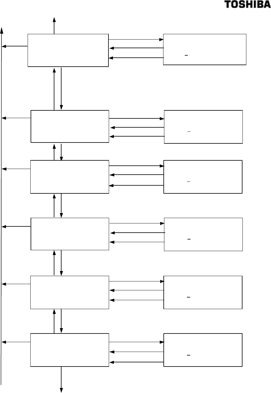
52
6 F 8 A 0 5 2 1
Ap:PARAMETER SET NO.
RANGE:1 - 10
DATA:01
[SET] SET,[ESC] CANCEL
[SET](Set)
[SET](Fix)
[ESC](Cancel)
s0:MAIN OBJ. SENS.
RANGE :−9.99 - 9.99
DATA: 1.00
[SET] SET,[ESC] CANCEL
[SET](Set)
[SET](Fix)
[ESC](Cancel)
s1:ADDITIVE SENS.
RANGE :−9.99 - 9.99
DATA: 0.00
[SET] SET,[ESC] CANCEL
[SET](Set)
[SET](Fix)
[ESC](Cancel)
s2:ADDITIVE SENS.
RANGE :−9.99 - 9.99
DATA: 0.00
[SET] SET,[ESC] CANCEL
[SET](Set)
[SET](Fix)
[ESC](Cancel)
s3:ADDITIVE SENS.
RANGE :−9.99 - 9.99
DATA: 0.00
[SET] SET,[ESC] CANCEL
[SET](Set)
[SET](Fix)
[ESC](Cancel)
s4:ADDITIVE SENS.
RANGE :−9.99 - 9.99
DATA: 0.00
[SET] SET,[ESC] CANCEL
[SET](Set)
[SET](Fix)
[ESC](Cancel)
[ESC]
(Previous
Menu)
[ESC]
(Previous
Menu)
[ESC]
(Previous
Menu)
[ESC]
(Previous
Menu)
[ESC]
(Previous
Menu)
[ESC]
(Previous
Menu)
Ten parameter sets ( tables for each brands) can be
registered for additives correction. This is used for selecting
the parameter set number appropriate to the brand in the
event of mak
ing measurements with additives correction, or
for selecting the parameter set number in the event of newly
registering or changing an individual parameter.
The sensitivity of component 0 (pulp) is set.
The sensitivity of additive 1 is set. In the same manner, the
sensitivities of the following additives 2 to 5 are set.
Ap:PARAMETER SET NO.
DATA:01
[SET] CHANGE
[ESC] RETURN
s0:MAIN OBJ. SENS.
DATA:1.00
[SET] CHANGE
[ESC] RETURN
s1:ADDITIVE SENS.
DATA:0.00
[SET] CHANGE
[ESC] RETURN
s2:ADDITIVE SENS.
DATA:0.00
[SET] CHANGE
[ESC] RETURN
s3:ADDITIVE SENS.
DATA:0.00
[SET] CHANGE
[ESC] RETURN
s4:ADDITIVE SENS.
DATA:0.00
[SET] CHANGE
[ESC] RETURN
[DN]
(Pre. menu)
[UP]
(Next menu)
[DN]
(Pre. menu)
[UP]
(Next menu)
[DN]
(Pre. menu)
[UP]
(Next menu)
[DN]
(Pre. menu)
[UP]
(Next menu)
[DN]
(Pre. menu)
[UP]
(Next menu)
[UP]
(Next menu)
[DN]
(Pre. menu)
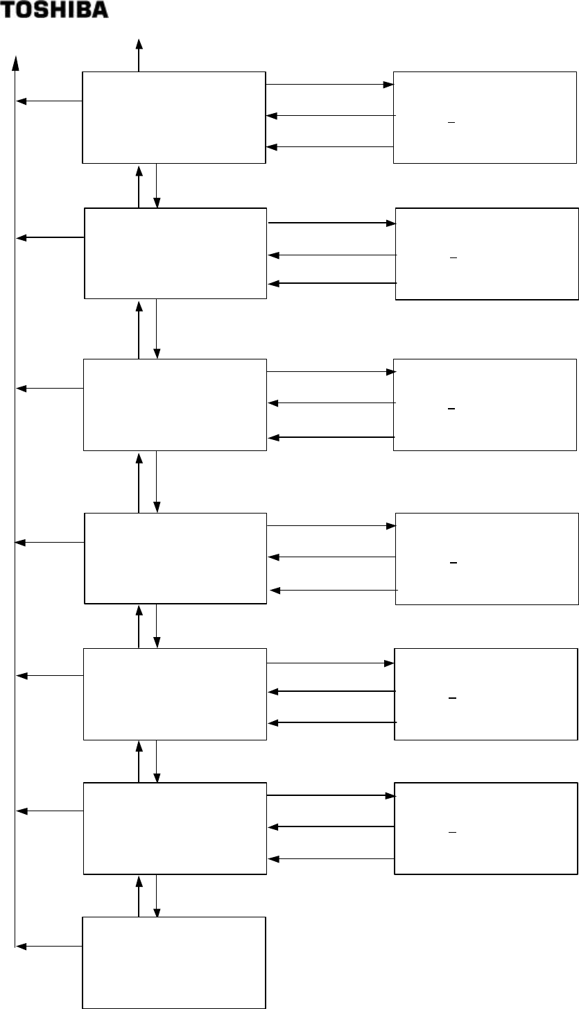
53
6 F 8 A 0 5 2 1
[ESC]
(Previous
Menu)
[ESC]
(Previous
Menu)
[ESC]
(Previous
Menu)
[ESC]
(Previous
Menu)
[ESC]
(Previous
Menu)
[ESC]
(Previous
Menu)
[ESC]
(Previous
Menu)
s5:ADDITIVE SENS.
RANGE :−9.99 - 9.99
DATA: 0.00
[SET] SET,[ESC] CANCEL
[SET](Set)
[SET](Fix)
[ESC](Cancel)
R1:ADDITIVE RATIO
RANGE :0.000 - 1.999
DATA: 0.000
[SET] SET,[ESC] CANCEL
[SET](Set)
[SET]Fix)
[ESC](Cancel)
R2:ADDITIVE RATIO
RANGE :0.000 - 1.999
DATA: 0.000
[SET] SET,[ESC] CANCEL
[SET](Set)
[SET](Fix)
[ESC](Cancel)
R3:ADDITIVE RATIO
RANGE :0.000 - 1.999
DATA: 0.000
[SET] SET,[ESC] CANCEL
[SET](Set)
[SET](Fix)
[ESC](Cancel)
R4:ADDITIVE RATIO
RANGE :0.000 - 1.999
DATA: 0.000
[SET] SET,[ESC] CANCEL
[SET](Set)
[SET](Fix)
[ESC](Cancel)
R5:ADDITIVE RATIO
RANGE :0.000 - 1.999
DATA: 0.000
[SET] SET,[ESC] CANCEL
[SET](Set)
[SET](Fix)
[ESC](Cancel)
The additive ratio of additive 1 (the mass ratio with regard to
component 0) is set. In the same manner, the sensitivities of
the following additives 2 to 5 are set.
s5:ADDITIVE SENS.
DATA: 0.00
[SET] CHANGE
[ESC] RETURN
R1:ADDITIVE RATIO
DATA:0.000
[SET] CHANGE
[ESC] RETURN
R2:ADDITIVE RATIO
DATA:0.000
[SET] CHANGE
[ESC] RETURN
R3:ADDITIVE RATIO
DATA:0.000
[SET] CHANGE
[ESC] RETURN
R4:ADDITIVE RATIO
DATA:0.000
[SET] CHANGE
[ESC] RETURN
R5:ADDITIVE RATIO
DATA:0.000
[SET] CHANGE
[ESC] RETURN
AF:ADDITIVES COMP.
DATA :ON
[SET] CHANGE
[ESC] RETURN
[DN]
(Pre. menu)
[UP]
(Next menu)
[DN]
(Pre. menu)
[DN]
(Pre. menu)
[UP]
(Next menu)
[DN]
(Pre. menu)
[UP]
(Next menu)
[DN]
(Pre. menu)
[UP]
(Next menu)
[DN]
(Pre. menu)
[UP]
(Next menu)
[DN]
(Pre. menu)
[UP]
(Next menu)
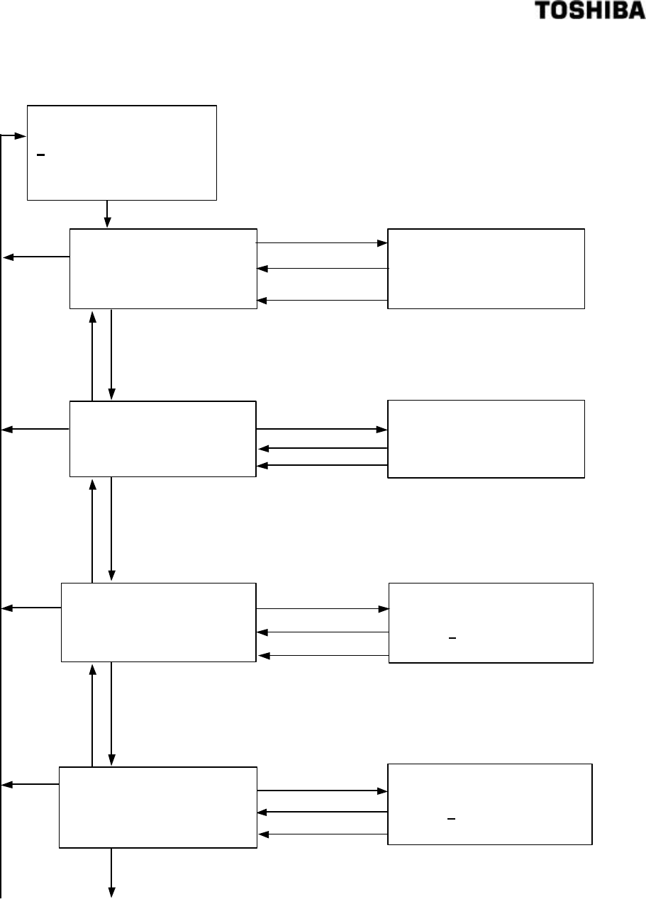
54
6 F 8 A 0 5 2 1
5.2.16 Other menus display and operating procedures
[ESC]
(Previous
Menu)
[ESC]
(Previous
Menu)
[ESC]
(Previous
Menu)
Move the cursor to "11" with [→] key, and press [SET] key to select
[ 11:OTHERS]
ho:4-20mA IN [EXT]
DATA :4mA
[SET] CHANGE
[ESC] RETURN
ho:4-20mA IN [EXT]
RANGE :LAST/4mA/TEST
DATA: 4mA
[SET] SET,[ESC] CANCEL
[SET](Set)
[SET](Fix)
[ESC](Cancel)
DI:C CHANGE. ON/OFF
RANGE :ON/OFF
DATA: OFF
[SET] SET,[ESC] CANCEL
[SET](Set)
[SET](Fix)
[ESC](Cancel)
9:LINEARIZ/CNDUCTVTY
10:ADDITIVES CORRECT
11:OTHERS
C2:DensityMultiplier
RANGE :0.000-9.999
DATA: 1.000
[SET] SET,[ESC] CANCEL
[SET](Set)
[SET](Fix)
[ESC](Cancel)
C3:DensityMultiplier
RANGE :0.000-9.999
DATA: 1.000
[SET] SET,[ESC] CANCEL
[SET](Set)
[SET](Fix)
[ESC](Cancel)
The simulated output at contact OFF in the event of external
synchronized
operation can be selected. Each time the[UP] or [DN] key is pressed, the mode
display is switched around among LAST VALUE (immediately preceding value),
4mA and TEST OUTPUT (simulated output 0.0 to 99.9%TS when in setting mode).
[SET] is pressed with the mode display to select.
Up to four den
sity multipliers can be switched around by the external voltage
signal (DI) of two points. This is used for switching the brand, etc. On this
menu, whether to perform the density multipliers switching (ON) or not (OFF)
is selected. Each time the [UP] or [DN] key is pressed, ON/OFF are mutually
alternated.
In the event of performing the density multiplier switching by means of the
external voltage signal (DI) of two points, the second density multiplier is set. In
the same manner, the following 3rd and 4th density multipliers are set. The first
density multiplier is performed with the menu for span calibration.
DI:C CHANGE. ON/OFF
DATA :OFF
[SET] CHANGE
[ESC] RETURN
C2:DensityMultiplier
DATA:1.000
[SET] CHANGE
[ESC] RETURN
C3:DensityMultiplier
DATA:1.000
[SET] CHANGE
[ESC] RETURN
[ESC]
(Previous
Menu)
[DN]
(Pre. menu)
[UP]
(Next menu)
[DN]
(Pre. menu)
[UP]
(Next menu)
[DN]
(Pre. menu)
[UP]
(Next menu)
[UP]
(Next menu)
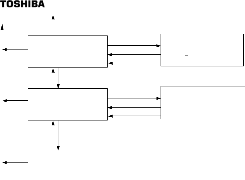
55
6 F 8 A 0 5 2 1
[ESC]
(Previous
Menu)
[ESC]
(Previous
Menu)
[ESC]
(Previous
Menu)
C4:DensityMultiplier
RANGE :0.000-9.999
DATA: 1.000
[SET] SET,[ESC] CANCEL
[SET](Set)
[SET](Fix)
[ESC](Cancel)
Although, in the event of high density measurement, the software is
installed in such a manner t
hat the automatic adjustment function of
the phase angle rotation is automatically canceled (OFF) by the
setting full-scale (the upper density measurement range), the
function can also be canceled by force through manual input.
However, normally, set it to "ON".
Each time the [UP] or [DN] key is pressed, ON/OFF are mutually
alternated.
NA:N AUTO ADJUSTMENT
RANGE :ON/OFF
DATA: ON
[SET] SET,[ESC]CANCEL
[SET](Set)
[SET](Fix)
[ESC](Cancel)
ho:4-20mA IN [EXT]
DATA :4mA
[SET] CHANGE
[ESC] RETURN
C4:DensityMultiplier
DATA:1.000
[SET] CHANGE
[ESC] RETURN
NA:N AUTO ADJUSTMENT
DATA:ON
[SET] : CHANGE
[ESC] : RETURN
[ESC] RET
URN
[DN]
(Pre. menu)
[UP]
(Next menu)
[DN]
(Pre. menu)
[UP]
(Next menu)
[DN]
(Pre. menu)
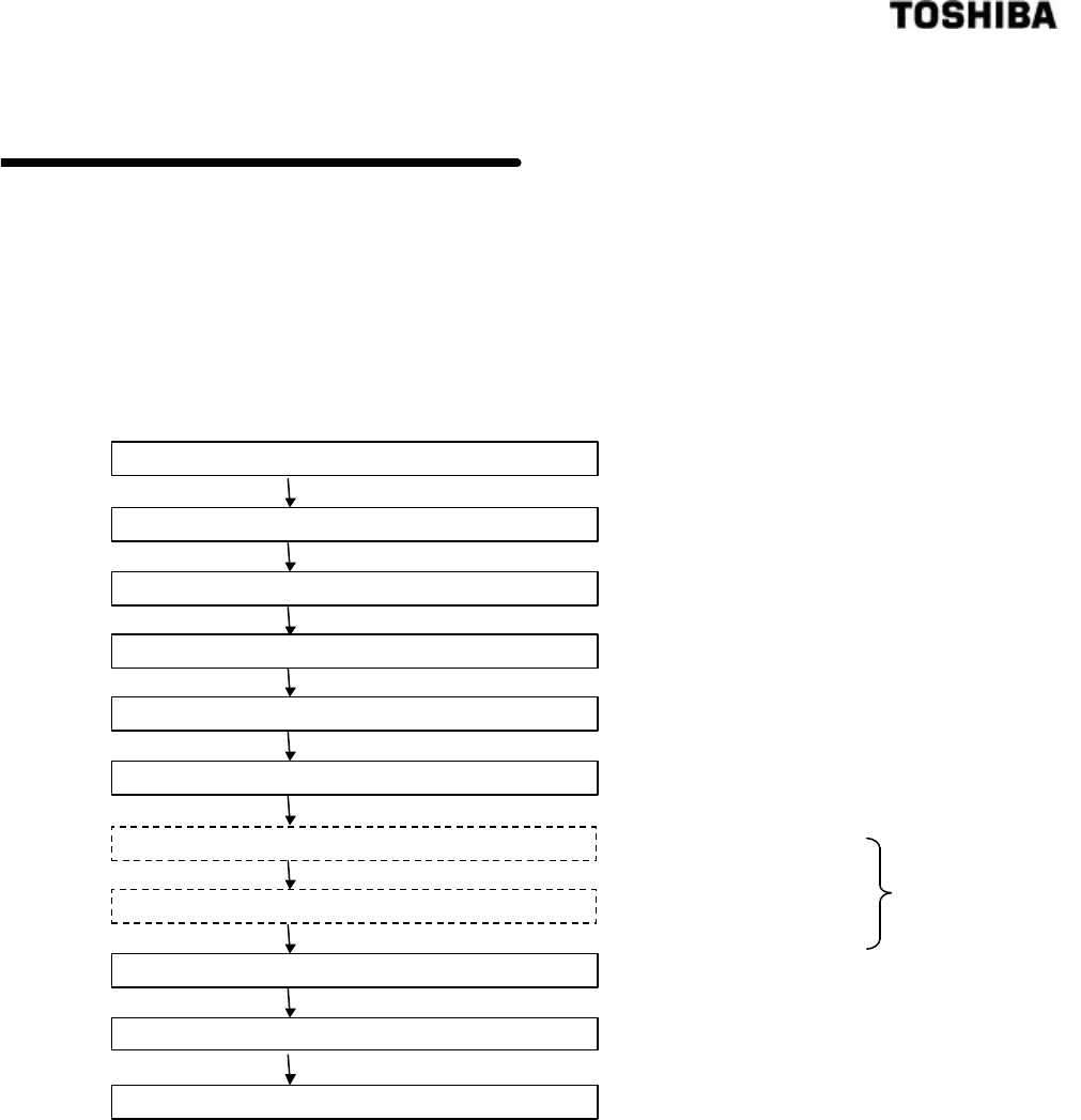
56
6 F 8 A 0 5 2 1
6. OPERATIONS
6.1 Procedures for Preparing and Running
Make preparations and perform operations, that is, density measurements, in accordance with the
following procedure.
Verifying the piping
Verifying the valve closure
Verifying the cable connection
Verifying the converter power-ON & display
Warm-up
Verifying and setting measurement
conditions
Filling up the density meter pipe with drinking
water
(density 0%)
Zero calibration
Pour the fluid to be measured
Span calibration
Startup
See 6.2(1)
See 6.2(2)
See 6.2(3)
See 6.3.1(1)
See 6.3.1(2)
See 6.3.2(1) and (2)
See 6.4(2) to (10)
See 6.4(11) to (15)
See 6.5
Refer to 6.6, 6.7
See 6.6
Normally omitted.

57
6 F 8 A 0 5 2 1
6.2 Preparations before Turning on Power
(1) Check piping
Check piping and ensure that there are no loose nuts and bolts, or missing gaskets. Make sure that
the density meter is properly connected in the pipeline.
See the section 3.3, Installation and Piping.
(2) Close the valves
Make sure that the drain valve, sampling valve, and zero water valve, which are installed in the
pipeline, are all closed.
(3) Verifying the cable connection
It is verified that cables are correctly connected to their respective terminal blocks. It is verified
that the ground (grounding resister: less than 100 Ω) is reliably connected to this density meter. In
the event of performing an external synchronized operation, the external contact input signal
connected with ON/OFF of the pump is required; therefore, make sure that the external contact
input signal cable is reliably connected.
6.3 Power on and Preparations for Measuring
6.3.1 Turning power on
(1) Turn the power switch on
Turn on the power switch of the converter and see that the power indicator([POWER]), the
density indicator, and the LCD indicator are lit.
(2) Warming-up
Please warm up for 30 minutes or more to achieve a steady measurement after turning power on.

58
6 F 8 A 0 5 2 1
6.3.2 Verifying and setting measurement conditions
(1) Verifications and settings for initial powering-ON
In the event of starting the operation after turning on the power for the first time since installing this
density meter, it is necessary to first set the measurement conditions of the converter. Various
measurement conditions (parameters) are verified and set by means of the setting key while
viewing each menu screen of the LCD indicator. Major measurement conditions are as follows.
① Verifying and setting the measurement range.
Unless otherwise specified in your order, the value here is set to 0 to 3%TS, which is the
provisional set value at the time of factory shipment. Reset the value in accordance with the
operation condition of your plant. If the measurement range is specified in your order, verify
that the value is set as specified. If the value is different, reset it.
② Verifying and setting the operation mode
At the time of factory shipment, this is set to "CONT" (the normal continuous operation
mode). In the event of the density meter being made empty due to pump shutdown or valve
closure, etc. or of using such a method that stops the flow for some time, it is recommended
that "EXT" (the external synchronized operation of switching between ON/OFF of
measurement by means of ON/OFF of the external contact input signal connected with the
pump ON/OFF) be selected.
In the event that the external synchronized operation is selected, the values of“delayed time
(dt)” and “output at contact OFF(ho)”are the provisional set values at the factory shipment.
If the those values are meet to the operation conditions of the plant rest it to an appropriate
value in accordance with the operation conditions of the plant.
③ Verifying and setting the simulated output in setting mode.
Normal measurements are suspended while this density meter is in the setting mode (see "2
SETTING MENU"); thus, both the density display and the density output are given the
simulated values ( density test output (ot)) that are set beforehand. Although, at the time of
factory shipment, the value is provisionally set to "1.5%TS" (50% of the specified full-scale
density if the measurement range is specified), reset it to an appropriate value in accordance
with the operation conditions of the plant.
④ Verifying and setting the moving average times
At the time of factory shipment, the "moving average times" is set to 1 (without the moving
average). If the averaged output is required to be used for density control, etc., set it to about
10. The more the moving average times, the worse the responsiveness becomes with regard
to density variation. Therefore, set it to an appropriate value in accordance with the plant
conditions, including the right balance with the responsiveness.
⑤ For other measurement conditions, the standard values are set. Therefore, it is normally
unnecessary to change these settings.
[NOTE] “10 VARIOUS FUNCTION” describes various functions of the Density Meter LQ500.
If necessary, make additional settings for using these functions appropriately.
(2) Verifications at the time of normal power-ON
In the event that measurement conditions of the converter are already set with the operation not
being the first one since installation, verify the set value while referring to (1).

59
6 F 8 A 0 5 2 1

60
6 F 8 A 0 5 2 1
6.4 Zero Calibration
All the density meters are calibrated for zero point [zero point phase ( θ1 ) and zero point water
temperature (T0) ] at the time of shipment and parameters are set correctly. You do not need to
calibrate the meter for zero point before using it at site.
In the case of the density readings are found to be way off from the result by manual analysis, or
when you need to read just the zero point for a particular reason, follow the procedures below in
calibrating the zero.
For information on the converter operation and the LCD display regarding zero-point calibration,
please refer to Subsection 5.2.11.
(1) Switching to the setting mode (see Subsection 5.2.5)
First of all, press the [ESC] key of the converter several times (normally once although this varies
with the operation status) to return to the initial menu display. Next, use the [→] key to move the
LCD indicator cursor to the menu number "2" of "2 SETTING MENU" and then press the [SET]
key to display the warning message saying "Test output will be valid." Make sure that there is no
problem and then press [→] to get into the setting mode. And return to [2: SETTING MENU].
Then, the output will be switched to the simulated output that is set beforehand.
(2) Stopping the flow in the pipeline
If it is allowed to stop the flow in the pipeline where the detector is installed, do so by, for example,
turning off the pump.
● If it is not allowed to stop the fluid flow through the pipeline:
When it is not permitted to stop the flow of the line, bypass the flow by opening the valve on the
bypass pipe.
◆ It is recommended that the bypass piping be installed for adjustment/maintenance purposes
such as zero calibration in the event that the flow in the pipe line cannot be stopped.
(3) Close the upstream valve and downstream valve
Close the shutoff valves on both sides of the detector tightly.
Note: Be sure to close the upstream valve first.
◆ In the event that the density meter is installed on the discharge side of the pump, make sure to
shut the valves starting from the upstream one to prevent the fluid pressure in the density meter
from rising.
(4) Drain the detector pipe
Open the drain valve of the pipeline where the detector is installed to discharge the fluid.
(5) Open the zero water feed port
Open the valve or remove the cap to feed zero water.
◆ When you open the zero water feed port, make sure that the pressure of the fluid in the pipeline
where density meter is installed becomes zero before opening the port. Any remaining pressure
will cause the measured matter to be spurted out. Be careful about this.
(6) Close the drain valve
(7) Supplying zero water
Put zero water (such as tap water) in the pipeline where the density meter is installed through the
zero water supply port by using a vinyl hose.

61
6 F 8 A 0 5 2 1
(8) Clean inside of the detector main pipe
When the pipeline where the detector is installed is filled with zero water, open the drain valve to let
out the water from the pipeline.
Clean inside of the pipeline where the density meter is installed by repeating Steps (7) and (8) until
the water density can be said to be zero against the density of the object fluid. (It is not necessary
to make the water clean and transparent.)
(9) Fill up the detector pipe with zero water
After cleaning the pipeline where the density meter is installed, close the drain valve, and fill it with
zero water. Keep adding water while releasing air until water overflows the feed port.
(10) Wait
Leave the detector and water in this state for about 15 minutes.
◆ In the event that the flow of the measured matter can be switched to that of the zero water by
switching over to another valve, etc., it is all right to replace the work activities (2) to (10) with
the relevant method and implement the following zero calibration while allowing the zero water
to keep flowing. Even when switching the flow to that of zero water, wait for about 15 minutes
before implementing the zero calibration.
(11) Selecting the zero calibration menu (see Subsection 5.2.5)
After verifying that the converter is in the setting mode ("2 SETTING MENU") through the
operation of (1), use the [→] key to move the cursor of the LCD indicator to the menu number "6"
of [6 ZERO CALIBRATION] and then press the [SET] key.
(12) Check zero water density reading (see Subsection 5.2.11)
The measured density of zero water is displayed on the density indicator. If the indicator shows [−
0.00], it means that the zero point is off toward the negative.
(13) Zero calibration (see Subsection 5.2.11)
If the zero point is found to be off, press the [SET] key. The data (θ1, T0, zG) of the zero point is
replaced by the current data, thus rendering the angle rotation to N=0 and automatically the density
display to zero. The data (θ1, T0, zG) of the zero point is stored in the memory of the density meter
until the zero calibration is implemented once again, thus making it possible to verify it on the
constant monitoring menu. However, for the purpose of history management, keep a note of the
data.
◆ Unless the zero point is out of place, the zero calibration is suspended by pressing the [ESC]
key.
(14) End zero calibration
This completes the zero calibration. Close the zero water valve, ensure that the sampling valve and
drain valve are closed, then open the shutoff valves on both ends of the detector pipe, downstream
first and upstream next. Lastly, close the shutoff valve on the bypass pipe to restore the flow of the
fluid as before the calibration.
(15) Restoring to the measuring mode
Press the [ESC] key of the converter twice to return the menu of the LCD indicator to the initial
menu display to return to the usual measuring mode from the setting mode. Thus, the measurement
starts.
◆ In the event that the external synchronized operation is selected, the external contact input
signal is changed to ON, thus starting the density measurement after the specified delayed time
has elapsed.

62
6 F 8 A 0 5 2 1
6.5 Span Calibration
Span calibration is for adjusting the readings of the density meter to the values determined by
manual (off-line) analysis.
For information on the converter operation and the LCD display regarding span calibration, please
refer to Subsection 5.2.12.
(1) Preparations for manual analysis
Prepare following items for manual analysis; a moisture meter (for example, an infrared moisture
meter, with the accuracy or percentage reading down to 0. 1 %), plastic bottles of about l liter with
a wide opening, and plastic beakers of about l00 ml for manual analysis.
(2) Sample fluid for manual analysis
Slightly open the sampling valve on the pipeline and let out the fluid a while before filling a 1-liter
bottle to half. Read and record the density value of the current fluid.
[NOTE] ◆ Make sure to carry out the sampling when the density of the measured matter is in a
stable state with the measured matter flowing.
(3) Manual analysis
Put a part of the sample fluid into a 100-ml plastic beaker, and measure the density of it using drying
and weighing method of analysis.
(4) Calculation of density multiplier
Use the result of analysis to calculate a density multiplier using the following equation after the
manual analysis conducted:
Density multiplier C = A/(M/C’)
where M is the density by the density meter (as read and recorded);
A is the result of the manual analysis
C’ is the density multiplier before span calibration
(Initially, C’ is equal to 1.000 which is the value set in the factory before shipping)
For example, if M = 4.0 %TS, A = 4.8 %TS and C’=1.000
C = 4.8 / (4.0/1) = 4.8/4.0 = 1.2
◆ In the case that span calibration has been done already, and density multiplier C is not 1.000, the
new density multiplier C can be calculated in the following way.
For example, if M = 4.8 %TS, A = 4.2 %TS and C0=1.2
C = 4.2 / (4.8/1.2) = 4.2/4 = 1.050

63
6 F 8 A 0 5 2 1
(5) Setting the density multiplier
(5-1) Switching to the setting mode (see Subsection 5.2.5)
First of all, press the [ESC] key of the converter several times (normally once
although this varies with the operation status). Next, use the [→] key to move the
LCD indicator cursor to the menu number "2" of "2 SETTING MENU" and then
press the [SET] key to display the warning message saying "Tset output will be vaild."
Make sure that there is no problem and then press [→] to get into the setting mode.
And return to [2: SETTING MENU]. Then, the output will be switched to the
simulated output that is set beforehand.
(5-2) Selecting the converter constant setting menu (see Subsection 5.25)
The menu list of menu numbers 5 to 8 is displayed. Use the [→] key to move the LCD
indicator cursor to the menu number "7" of "7: SPAN CALIBRATION" and then
press the [SET] key to select the menu of "7: SPAN CALIBRATION."
(5-3) Verifying and recording the density multiplier before span calibration
For example, the set value of the current density multiplier as is displayed as in
"DATA: 1.000" is displayed. Record this value.
(5-4) Setting the density multiplier
Press the [SET] key to switch over to the setting menu of the density multiplier and
enter the density multiplier found in (4). Use the [→] key to move from one digit to
another. Use the [UP] and [DN] keys to switch around the number of the relevant
digit. When the input is completed, press the [SET] key to confirm it. Then, the display
will be returned to the immediately preceding menu screen. Verify that the resetting
has been done correctly.
(5-5) Restoring to the measuring mode
Press the [ESC] key twice to return to the initial menu screen and return to the
measuring mode from the setting mode, thus restarting the usual measurement. Verify
that the density display has been changed appropriately in accordance with the setting
of the density multiplier.
◆ In the event that the external synchronized operation is selected, the external
contact input signal is changed to ON, thus starting the density measurement after
the specified delayed time has elapsed.
(6) Completing the span calibration
Thus, the span calibration is completed.
[NOTE] The above describes the method for finding the density multiplier as an example in the
comparison with one-time manual analysis. However, to exclude errors caused by sampling,
it is recommended that as many comparative data as possible be collected to find the density
multiplier from their mean value.

64
6 F 8 A 0 5 2 1
6.6 Operation
(1) Startup (see Subsection 5.2.5)
When the power is turned ON, the menu setup is automatically changed to the measuring mode
(the state of "1: MONITORING MENU"), thus starting the density measurement. If the meter is in
setting mode (the state of "2:SETTING MENU"), the density measurement operation is started by
pressing the [ESC] key several times (varying between one to three times depending on the
operation status) and thus pulling the menu setup out of the setting mode.
◆ In the event that the external synchronized operation is selected, the menu setup is changed to
the measuring mode and the external contact input signal is turned ON, thus starting the density
measurement after the specified delayed time has elapsed.
(2) Executing the measurement
Executes the density measurement while updating the output values (density current output value;
LED density display; LCD density display on the monitor menu) approximately every second.
(3) Suspending the measurement (see Subsection 5.2.5)
When stopping the measurement, select "2: SETTING MENU" from the initial menu list to get into
the setting mode. Once in the setting mode, the density measurement will be suspended and the
output will be switched to the simulated value that was set beforehand.
◆ In the event that the external synchronized operation is selected, the density measurement is
suspended if the external contact input signal is turned OFF even in the measuring mode. For
details including the output when the density measurement is suspended, refer to Section 6.7.
[NOTE] ◆ In the event the fluid does not flow continuously in the pipeline where the density meter
is installed or the pipeline is temporarily left empty due to the intermittent operation of the
shifting pump, perform the external synchronized operation described in Section 6.7.
◆ When the flow in the pipeline is stopped, solid matters may settle down or float causing
the density in the pipe to lose its uniformity, which in turn may cause the density measured
value to gradually rise or fall. In addition, if the fluid drains out from the pipeline, the
pipeline where the density meter is installed is not completely filled with the fluid, the
density measured value turns out to be erroneous (such as exceeding the full-scale range;
shifting to the minus side; major marginal error). However, this does not mean that the
density meter has failed. Even to avoid such a phenomenon, it is necessary to perform the
external synchronized operation.
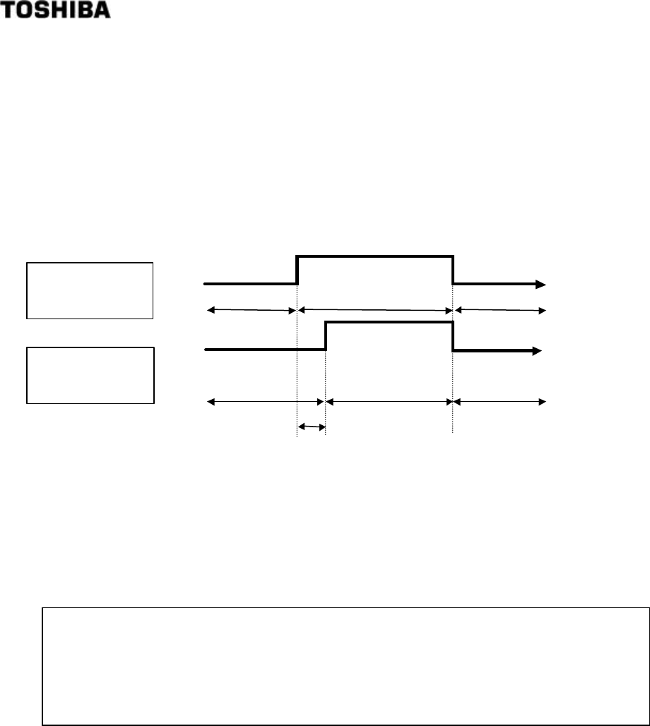
65
6 F 8 A 0 5 2 1
6.7 External Synchronized Operation
This operation mode is used in the event that the measured matter does not flow continuously or the
interior of the detector is temporarily left empty due to the intermittent operation of the shifting
pump to the pipe line on which the density meter is installed. This mode is used to take
measurements only when operating the shifting pump.
To use this operation mode, it is necessary to connect the shifting pump operation and the contact
signal (no-voltage) to the external synchronized input signal pins beforehand.
6.7.1 Movement of the external synchronized operation
Fig.6.7.1 External synchronized Operation
The external synchronized operation, as shown in Fig. 6.7.1, is so designed that the density
measurement is executed only while the pump is being operated; and the density measurement is
suspended while the pump is shut down and the simulated output is issued during this time. The
external synchronized operation is effective in preventing the following inadequate phenomena.
① The pump shutdown causes solid matters to subside or float thus making it impossible to take
density measurements correctly.
② The pump shutdown may cause the fluid to escape from the density meter thus either leaving
it completely empty or insufficiently filled with fluid. In such a situation, the measured value of
the density meter falls into error such as full-scale excess, shift to the minus side, or
occurrence of fluctuation within major marginal error.
It takes time for the pipeline where the density meter is installed to be filled sufficiently with the
fluid after the pump is operated. Here, it is so arranged that the measurement start after the
"delayed time" that is set beforehand has elapsed since receiving the contact signal linked with the
pump operation. Make sure that the delayed time that is set is sufficient for the whole process of
the pipe length and flow, etc. from the pump to the density meter.
As the simulated value when the density measurement is suspended, it is possible to select from
among three options: "4mA", "density measured value immediately preceding the pump shutdown"
and "simulated output in setting mode". The default value is 4mA. However, make sure to select a
simulated output suitable to your system.
Pump operating status
(External contact)
Density measuring
status(Output)
Time
Time
delayed time
Pump operation (ON) Pump shutdown (OFF) Pump shutdown (OFF)
Suspension of density
measurement (Simulated output)
Suspension of density
measurement
(Simulated output)
Execu
tion of density
measurement
(Measured value output)

66
6 F 8 A 0 5 2 1
6.7.2 Setting the external synchronized operation
(1) Setting the delayed time (see Subsection 5.2.10)
(1-1) Switching to the setting mode (see Subsection 5.2.5)
First of all, press the [ESC] key of the converter several times (normally once
although this varies with the operation status) to return to the initial menu display.
Next, use the [→] key to move the LCD indicator cursor to the menu number "2" of "2
SETTING MENU" and then press the [SET] key to display the warning message
saying "Test output will be valid." Make sure that there is no problem and then press
[→] to get into the setting mode. And return to [2: SETTING MENU]. Then, the
output will be switched to the simulated output that is set beforehand.
(1-2) Selecting the parameter setting menu (see Subsection 5.25)
The menu list of menu numbers 5 to 8 is displayed. Use the [→] key to move the LCD
indicator cursor to the menu number "5" of "5: SET PARAMETERS" and then press
the [SET] key to select the menu of "5: SET PARAMETERS."
(1-3) Setting the delayed time at the time of external synchronized(see Subsection 5.2.10)
Press the [UP] key five times to select the setting menu of the delayed time at the
time of external synchronized(dt: DELAYED SYNC. TIME). Press the [SET] key to
get into the set value input screen and then enter an appropriate value (the time
sufficient for the measured matter to flow up to the density meter and fill up the pipe
after the shifting pump operation is started). Use the [→] key to move from one digit
to another. Use the [UP] and [DN] keys to switch around the number of the relevant
digit. When the input is completed, press the [SET] key to confirm it. Then, the display
will be returned to the immediately preceding menu screen. Verify that the resetting
has been done correctly.
(2) Setting the simulated output at measurement suspension (at external contact OFF)
(see Subsection 5.2.16)
As the simulated output when the measurement is suspended (at external contact OFF), it is
possible to select from among three options as shown in Table 6.7.1. Make sure to select a
simulated output suitable to your system.
Table 6.7.1 Density Display and Output at Measurement Suspension
in External Synchronized Operation
Mode Density Indicator Display Output (4 - 20mA)
"4mA" (Standard) Held in 0%TS Output held in 4mA
"TEST"
same as the simulated output
value in setting mode
Same as the simulated output value
correspondence output in setting
mode
"LAST"
Holds the density measured value
immediately before OFF
Holds the density measured value
correspondence output immediately
before OFF
(2-1) Selecting the "OTHERS" setting menu (see Subsection 5.2.5)
Continuing on from (1), press the [ESC] key to return to the display of menus 5 to 8 in
setting mode. Press the [UP] key to switch to the display of the next menus 9 to 11.
Use the [→] key to move the cursor of the LCD indicator to the menu number "11" of
"11: OTHERS" and press the [SET] key to select the "11: OTHERS" menu.

67
6 F 8 A 0 5 2 1
(2-2) Setting the output mode at contact OFF in external synchronized operation (see
5.2.16)
The current output mode at contact OFF in external synchronized operation is
displayed in the initial menu "ho: 4-20mA IN [EXT]" of "11: OTHERS". To make
changes, it is necessary to press the [SET] key and place the software in the setup
state. Each time the [UP] or [DN] key is pressed, the mode display is switched
around from "LAST" (immediately preceding value), through "4mA" to "TEST" (the
simulated output value in setting mode). Press the [SET] key on the display in the
selected mode to confirm. The screen is returned to that of the immediately preceding
menu screen. Make sure that the resetting is done correctly.
(2-3) Returning to the measuring mode
Press the [ESC] key twice to return to the initial menu and return from the setting
mode to the measuring mode to resume the normal measurement.
(3) Setting the operation mode
(3-1) Selecting the operation mode change menu (see Subsection 5.2.6)
In the initial menu, use the [→] key to move the cursor of the LCD indicator to the
menu number "3" of "3: MEASURING MODE" and then press the [SET] key to get
into the operation mode menu.
(3-2) Verifying and setting the operation mode
The current operation mode is displayed at "DATA" of the LCD indicator . "CONT"
refers to the mode of taking measures continuously without relying on the status of the
external contact signal, whereas "EXT" refers to the external synchronized operation
mode. If the current setting is "CONT," press the [SET] key to get into the setup
screen of operation mode; press the [UP] or [DN] key to switch the set value of the
operation mode to "EXT"; and press the [SET] key to confirm. The screen is returned
to the immediately preceding menu screen. Make sure that the resetting has been
done correctly.
(4) Starting the external synchronized operation
With the settings above, measurement ON/OFF are proceeded with as shown in Fig.6.7.1 in
accordance with external synchronized contact signal ON/OFF.
6.8 Functions Related to Operation
To enable you to use the Density Meter Type LQ500 more appropriately in various processes and
situations, the device is equipped with various functions including the moving average, the
change-rate limit, the electric conductivity correction, the additive correction, the linearizer and the
density multiplier switching by external signals. Make settings necessary for using these functions
appropriately where necessary. For details, please refer to Chapter 10.
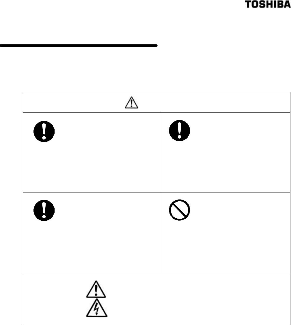
68
6 F 8 A 0 5 2 1
7. MAINTENANCE
7.1 Precautions for Maintenance, Inspection and Parts
Replacement
WARNING
DO
■Be sure to set the power
switch on the equipment to the
OFF position before doing
maintenance or inspection
inside the equipment or
replacing its parts.
Failure to observe this can cause
electric shock or equipment failure.
DO
■Be sure to set the power
switch on the equipment to the
OFF position before replacing
the fuse.
Failure to observe this can cause
electric shock.
DO
■Do not touch the terminal
block during maintenance or
inspection. If it is necessary to
touch the terminal block, set the
power switch on the equipment
to the OFF position in advance.
Failure to observe this can cause
electric shock.
DON’T
■Do not attempt disassemble
or modify the equipment.
Failure to observe this can cause
electric shock or equipment
failure.
The label shown at left is placed near
each terminal block on the equipment
to which power is supplied. Be careful
of electric shock.
Yellow
Yellow
Yellow
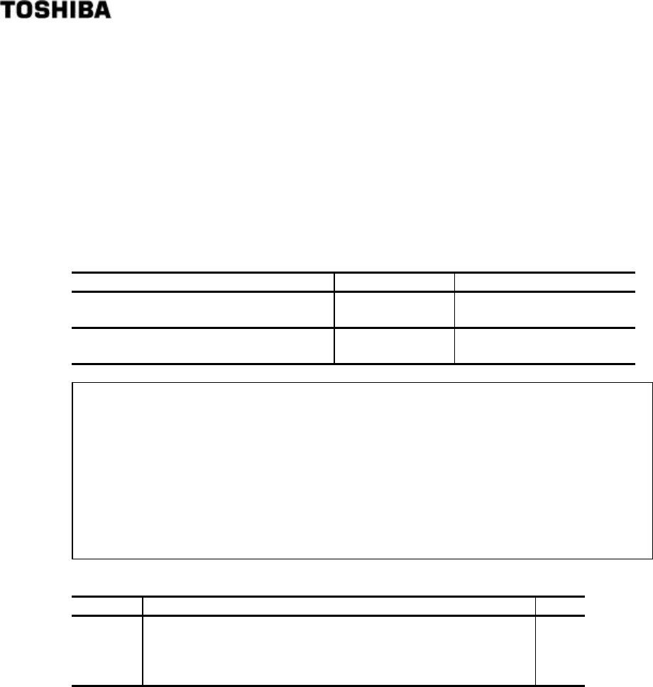
69
6 F 8 A 0 5 2 1
7.2 Maintenance and Inspection Items
Periodic maintenance and inspection is necessary for reliable measurement over a long period of
time. Since the density meter has no mechanically moving parts, however, it does not require
replacement of mechanism elements in a normal operating environment.
Compare the density measured value and the manually analyzed value in the cycle shown in Table
7.1. If necessary, implement the span calibration after implementing the zero calibration. Clean up
the detector when it is necessary.
The spare parts that must be kept on hand are the fuses in Table 7.2.
Table 7.1 Maintenance and Inspection Items
Item Cycle Remarks
Comparison of density meter measured
value with manually analyzed value Any time At least three samples are
desirable.
Check the appearance of detector
(accumulation of dirts, scratches, etc) Any time
[NOTE] ◆ If the density meter measured value deviates from the manually analyzed value to the
extent of causing obstacles, implement the span calibration (changing the density
multiplier C) while referring to Section 6.5.
◆ If the density meter measured value greatly deviates from the manually analyzed value by
less than half or more than twice, implement the span calibration after implementing the
zero calibration while referring to Section 6.4 and 6.5.
◆ If the density meter is used to measure process flow which contains plenty of wool or
fabric substances, these substances may accumulate on the detector, thus perform
maintenance and inspection, and cleaning periodically (every 3 months).
Table 7.2 Spare Parts
Name Specifications Qty
Fuse
2A(T),250V cartridge, glass tubular fuse,
5.2mm outer dia. x 20mm long
Shape/characteristics: 5NM or equivalent (based on JIS C
6575)
2

70
6 F 8 A 0 5 2 1
[NOTE] ◆ Fuses are parts with expected life span. Therefore, replace them periodically.
(Recommended replacement cycle: about 3 years)
◆ In general, the service life of an electronic part becomes shorter at higher ambient
temperature. There is a DC switching power supply in the converter that contains
electrolytic capacitors. The service life is about 10 years at the ambient temperature of
20°C or about 3 years at 50°C. For stable use of the meter for many years, it is desirable
to replace these parts in time. When replacing the capacitors, please contact Toshiba's
Service Dept.
◆ In the event that the characters on the LCD display becomes weak in contrast or edge,
it is considered that the LCD display unit has reached the end of its life. Although such
unsatisfactory visibility may not affect the performance of the density measurement, the
display unit should be replaced if it interferes with the operation. When replacing the
display unit, contact Toshiba's Service Dept.
◆ Regarding the arrester (converter), part replacement differs depending on how often
lightning occurs.
Suppose lightning (induction lightning) occurs twice a year, service life expires in 5 years
and replacement is necessary.
For arrester replacement, an entire arrester unit (board: converter) should be replaced.
To replace the unit, please contact our service personnel.
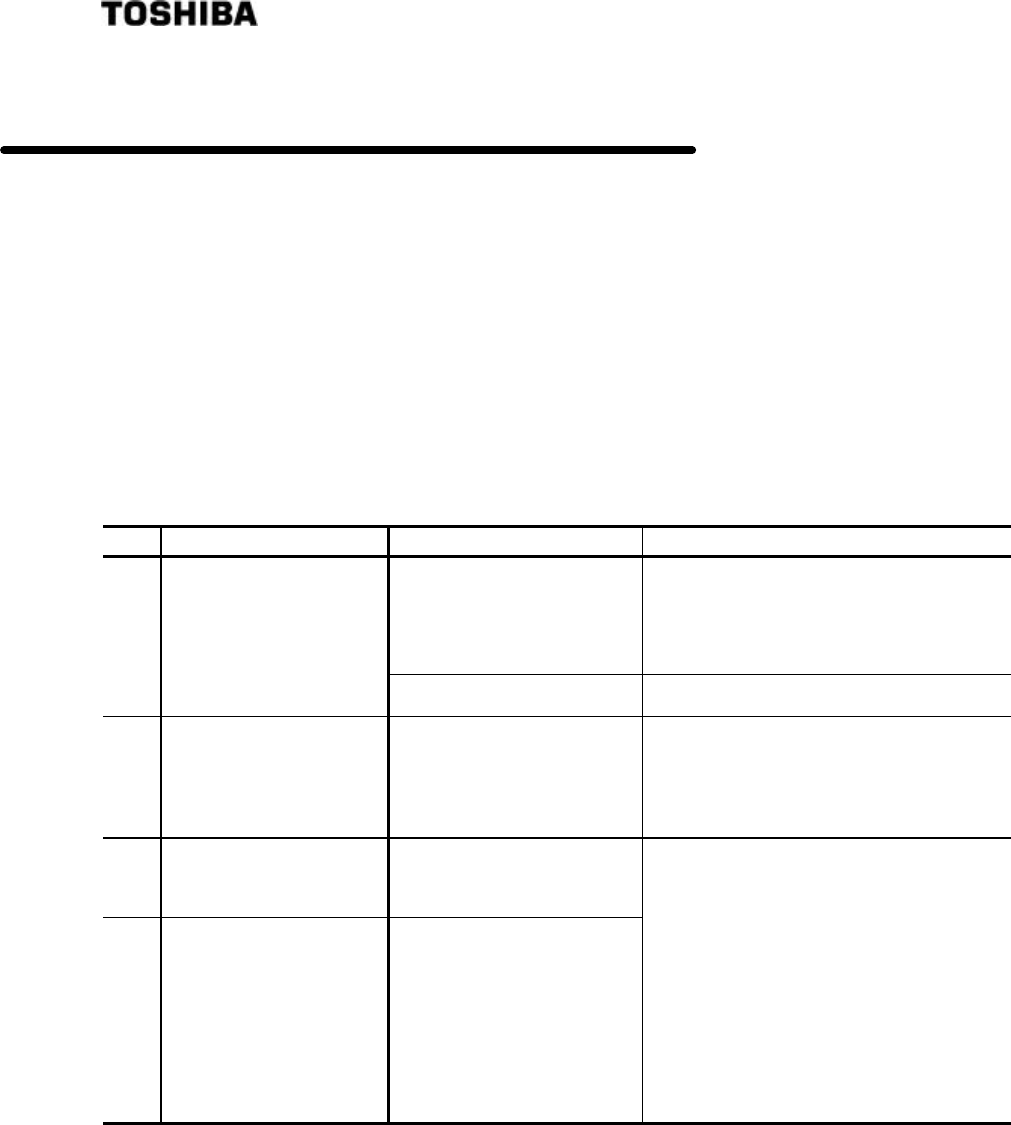
71
6 F 8 A 0 5 2 1
8. TROUBLESHOOTING
8.1 Troubleshooting
If any trouble has developed, make a careful check and take appropriate steps. Table 8.1 shows
possible troubles, their causes, and remedies. If anything wrong occurs, refer to the table below and
take the necessary steps. If that does not remedy the trouble, send information on the trouble, in as
much detail as possible, and self-diagnosis data to our Service Department.
Table 8.1 Troubleshooting (1)
No.
Trouble Cause Remedy
AC power is not supplied.
Check terminals [L1] and [L2] on terminal
block with voltage tester. If AC voltage is
not supplied, supply AC power in
accordance with specifications.
1 Converter power cannot
be switched on.
Fuse (2A) is blown. Replace fuse.
2 ALARM indicator lights;
density meter error
contact output.. Fault in the density meter
In accordance with Section 8.2, perform
self-diagnosis data check and restoration
operations. If ALARM indicator lights
again, send self-diagnosis data to our
Service Department.
3 While the flow is
stagnant, the indicator
is in error.
The fluid in the pipeline
where the detector is
installed drained out.
4
While the flow is
stagnant, the measured
density value slowly
increases or decreases.
Density becomes uneven
because the measurement
object fluid in the fluid in the
pipe starts to sinks or
floats, thus causing the
density in the center portion
of measured fluid to
increase or decrease.
Use the externally synchronized
operation.
See Section 6.7.
(Density meter is not faulty.)

72
6 F 8 A 0 5 2 1
Table 8.1 Troubleshooting (2)
No.
Trouble Cause Remedy
Inappropriate density
correction factor setting. Calibrate span as described in
section 6.5.
Air accumulates and keep
staying inside the detector.
Or substance being
measured is sediment.
Very slow flow can be the cause.
Make the flow faster by using
smaller bore detector to prevent air
or substance from remaining in the
detector. If this does not solve the
problem, resort to vertical piping.
Large quantity of bubbles are
contained in the fluid.
Find out where the air is brought
in, and make necessary
adjustments. Keep mixer vanes
under water. Position the pump
inlet low enough. Keep fluid
pressure high (0.1MPa or more is
recommended).
Large quantity of bubbles are
contained in the fluid.
Remedy the locations containing
air bubbles. An example is to
position the blade of the agitator in
the tank below the fluid level.
Another example is to position the
inlet port of the pump sufficiently
below the fluid level.
Take necessary steps to make
the fluid pressure high (0.1MPa or
more is recommended).
It is desirable to install the meter
on the discharge port of the pump.
At the same time, make sure that
the meter is placed as far as
possible (closer to the pump) from
the pipe outlet for air release.
5
Too much difference
between measured
density and manual
analysis value
6
Measured density
varies widely and does
not agree with manual
analysis value.
The pipeline where the
detector is installed is not
filled with the substance to
be measured that flows.
Or air remains in the pipeline
where the detector is
installed.
Keep the tube always filled up with
fluid by closing the downstream
valve slightly or add a relief valve.
Installing the density meter on the
outlet side of the pump can help
eliminate the cause of those
troubles. Vertical piping is
recommended for filling the pipe.
7 Suitable location
varies depending on
density. Zero point is off. Calibrate zero point as described
in Section 6. 4, then calibrate
span described in Section 6.5
The electric conductivity of
the measured matter is too
high.
Check if the electric conductivity
is within the specified range.
If the electric conductivity is
beyond the range, send its
measurement results and
self-diagnosis data to our Service
Department.
8 Output is either
unstable or unsuitable.
Converter failure Send self-diagnosis data to our
Service Department.

73
6 F 8 A 0 5 2 1
8.2 Error Indications and Recovery Operations
If an error occurs to the density meter, the error indicator [ALARM] will light up and a contact
signal (OFF) will be output.
Check the self-diagnosis data for any faulty values in accordance with the following steps.
(1) Monitor menu display (see Subsection 5.2.4)
First of all, press the [ESC] key of the converter several times (normally once although this
varies with the operation status) to return to the initial menu display. Next, use the [→] key to
move the LCD indicator cursor to the menu number "1" of "1: MONITORING MENU" and
then press the [SET] key. (The cursor of the initial state is located on "1".)
(2) Switching to the self-diagnosis menu (see Subsection 5.2.7)
In the monitoring menu, use the [→] key to move the cursor of the LCD indicator to the menu
number "3" of "3: SELF-DIAGNOSIS" and then press the [SET] key.
(3) Checking the self-diagnosis data (see Subsection 5.2.9)
Press the [UP] key to move from one self-diagnosis data to another to check for any error.
◆ To detect which numerical range is an error value, please refer to Table 8.2.
(4) Terminating the self-diagnosis
After checking, press the [ESC] key twice to return to the initial menu display.
If an error value is found, turn off all the power switches of the converter and then turn them back
on. The self-diagnosis is executed all over again by the powering-ON. If an error is displayed again
as a result of the self-diagnosis, send the relevant item to our Service Department.
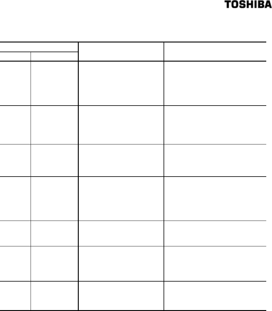
74
6 F 8 A 0 5 2 1
Table. 8.2 Self-diagnosis data
Data Item
Symbol
Item name Data Status Data (Numeric value range;
normal data range, status)
ST Status
[STATUS]
• Normal [GOOD]
• Warning [WARNING.]
Whether the phase
measurement operation is
normally functioning or not can
be verified.
SL
Microwave
recieved signal
level
[MICROWAVE
SIG. LVL]
Without error judgment based
on data numeric • Usual range: -90 to -40 (dBm)
F
Microwave coef.
[MICROWAV
E COEF.]
Without error judgment based
on data numeric • Normal range: 1825 ∼ 1975
G
Data
concerning
microwave
phase
measurement
[RF DATA]
Without error judgment based
on data numeric • Normal range + 10.0 ∼ + 80.0 (°C)
J +5 V voltage
[+5V POWER
SUPPLY]
Without error judgment based
on data numeric • Normal range 4.5 ∼ 5.5(V)
pd
Reference
phase error
[REF
PHASE]
Without error judgment based
on data numeric • Normal range - 9.9 ∼ + 9.9 (°C)
P
Memory check
[MEMORY
CHECK]
Normal [GOOD]
Abnormal [N.G.]
EPROM, RAM, EEPROM are
checked

75
6 F 8 A 0 5 2 1
9. CORRECTIONS IN
DENSITY CALCULATION
This density meter, which operates on the basis of phase difference measurement by microwaves
makes automatic corrections to the measured phase angel for the fluid temperature and phase
angel rotation before making the density calculations for the measured substance.
This chapter describes the methods for corrections and the density calculations.
9.1 Density Calculation
This density meter measures the phase lag θ1 in the density zero water (zero water), which is the
basis, and the phase lag θ2 in the measured matter, the difference △θ(= θ2 - θ1) of which
being proportional to the density is used to obtain the density. The density (X) of the measured
matter is calculated in accordance with the following equation.
X= C ×( a × △θ )+ b
where
X : Measured density value (%TS)
△θ : Phase difference. △θ = θ2−θ1 (degrees)
a : Density line slope;
b : Density intercept;
c : Density multiplier (Density correction factor.)

76
6 F 8 A 0 5 2 1
9.2 Various Kinds of Corrections
9.2.1 Phase angle rotation correction
The phase is available only from 0 degree to 360 degrees. If the phase incrementally reaches 360
degrees, it returns to 0 degree, from which it keeps incrementing again. If the phase decreasingly
reaches 0 degrees, it returns to 360 degrees, from which it keeps decreasing again. Accordingly,
the concept of phase angle rotation is incorporated into this density meter and some corrections
have been made so to allow the phase to change to an unlimited extent. In such a manner, this
density meter has overcome the limit that the phase is available only from 0 to 360 degrees, thus
realizing high density measurement.
Phase angle rotation correction refers to obtaining the real phase angle θ2 by judging the number
of rotations the dummy angle θ2' belongs to based on the measured values coming before and
after.
θ2 = θ2' + N x 360 (degrees)
N: Number of rotations
Set N=0 at the time of zero calibration, making the number of rotations to zero for the phase
angle
θ1 at zero point.
If the θ2' exceeds 360 degrees to enter into the next rotation, set N=1. If it again exceeds
360 degrees to enter into the rotation after the next rotation, set N=2.
(N will move up to 2 only if the meter is of large diameter and the density is high.)
On the other hand, if θ2' goes below zero (0) degree to enter into the previous rotation,
decrease N by one (1). In other words, when it goes into the -1st rotation from the 0th one,
set N=−1; and when into the 0th rotation from the 1st one, set N=0.
Note: The description above is the basics regarding the phase angle rotation correction. Normally,
it is all right to use the density meter without being aware of this correction. However, in the
event of measuring high density, etc., special setups and actions may be needed. For details,
refer to Section 9.3.
9.2.2 Fluid temperature correction
The phase tends to change in a straight line with regard to the fluid temperature. In this connection,
fluid temperature correction is performed on θ2 as follows to obtain the phase difference △θ
△θ={θ2−α(Τ−Τ0
)}− θ1
△θ : △θ: Phase difference [degrees]
θ2 : Actual phase angle of measurement object fluid [degrees]
θ1 : Phase during zero water measurement (degrees)
(Measured during zero calibration, and set in advance as a constant)
α : Fluid temperature correction factor (degrees/℃)
T : Temperature of measurement object fluid (℃)
T 0 : Water temperature during zero calibration (℃)
(Measured during zero calibration, and set in advance as a constant)

77
6 F 8 A 0 5 2 1
9.2.3 RF correction
In addition to the fluid temperature correction, the density meter is equipped with the RF correction
function in accordance with the features of the converter. The correction is performed on θ2 as
follows to obtain the phase difference △θ.
△θ={θ2−α(Τ−Τ0)−δ(G−G0)}−θ1
△θ : Phase difference [degrees]
θ2 : Actual phase angle of measurement object fluid [degrees]
θ1
: Phase during zero water measurement (degrees)
(Measured during zero point calibration, and set in advance as a constant)
α : Fluid correction factor (degrees/℃)
Τ : Temperature of measurement object fluid (℃)
Τ0
: Water temperature during zero adjustment (℃)
(Measured during zero point calibration, and set in advance as a constant)
δ : RF correction factor
G : RF data during measurement
G0
: Zero point RF data
(Measured during zero point calibration, and set in advance as a constant)
9.2.4 Ambient temperature correction
In addition to the fluid temperature correction and RF correction, the density meter is equipped with
the ambient temperature correction function. The correction is performed on θ2 as follows to
obtain the phase difference △θ.
<Note> Since ambient temperature correction function is an option, ambient temperature
correction factor ß must be set “0.00”.
△θ={θ2−α(Τ−Τ0)−δ(G−G0)ß(A‐A 0
)}−θ1
△θ : Phase difference (degrees)
θ2 : Actual phase angle of measurement object fluid (degrees)
θ1
: Phase during zero water measurement (degrees)
(Measured during zero point calibration, and set in advance as a constant)
α : Fluid correction factor (degrees/℃)
Τ : Temperature of measurement object fluid (℃)
Τ0
: Water temperature during zero adjustment (℃)
(Measured during zero point calibration, and set in advance as a constant)
δ : RF correction factor
G : RF data during measurement
G0
: Zero point RF data
(Measured during zero point calibration, and set in advance as a constant)
ß : Ambient temperature correction factor (degrees/℃)
A : Ambient temperature (℃)
A0
: Ambient temperature during zero adjustment
(Measured during zero point calibration, and set in advance as a constant)

78
6 F 8 A 0 5 2 1
9.3 Phase Angle Rotation Correction (Details)
This section describes the special setups and actions required for cases of measuring high density.
In normal measurement, it is unnecessary to be aware of the phase angle rotation correction, which
is performed automatically.
9.3.1 Care point concerning phase angle rotation
As described in 9.2.1, the number of phase angle rotations N is incremented or decreased judging
from the values before and after the measured value. Such a processing requires the condition that
the measured phase value varies continuously in accordance with the density of the measured
matter. If the density meter detector is empty, however, the continuity of measured phase values is
damaged thus making a normal phase angle rotation correction impossible, which in turn may cause
the number of phase angle rotations to jump to a faulty value. If the number of phase angle rotations
N is inappropriate, the density calculation result will also turn out to be erroneous. Once such a
trouble occurs, it is necessary to reset the number of phase angle rotations N to an appropriate
value through manual input.
9.3.2 Phase angle rotation in external synchronized operation
The trouble previously described will be solved by performing the "external synchronized
operation" incorporated into this density meter. In the external synchronized operation, if the
contact signal is switched OFF synchronized with the pump shutdown, not only the output is
switched to the simulated one but also the immediately preceding value is kept as the number of
phase angle rotations N.
9.3.3 Outline of automatic adjustment function of phase angle rotations
Furthermore, this density meter is equipped with the function of "automatic adjustment of phase
angle rotations." This function judges whether the measured density calculated with the number of
phase angle rotations N is proper or not in terms of the set density measurement range, etc. and
then adjusts the number of phase angle rotations either incrementally or decreasingly if necessary.
Even when the density meter detector is temporarily made empty thus causing the number of phase
angle rotations N to jump to an inappropriate value, this function is also used to fill up the density
meter detector once again with the matter to be measured and automatically adjust the number of
phase angle rotations N to an appropriate value, which in turn will render an appropriate value for
the measured density. While the density meter detector is left empty, the measured phase value
itself comes to have an indefinite value, which in turn will render the measured density indefinite.
Therefore, if the density meter detector could be made empty, it is desirable to perform the external
synchronized operation.
9.3.4 Judgment conditions and adjustments for automatic adjustment of phase angle
rotations
The judgment conditions and adjustments regarding the automatic adjustment of phase angle
rotations and the measured density are listed in Table 9.3.1.
Table 9.3.1 Judgment Conditions and Adjustments
for Automatic Adjustment of Phase Angle Rotations
Measured Density Automatic Adjustment of Phase Angle Rotations N
Xmin = Less than −4(%TS) Incremented (N = N+1)
−4∼C×a×360(%TS) Unadjusted
Xmax = More than C x a x 360 (%TS) Decreased (N = N-1)
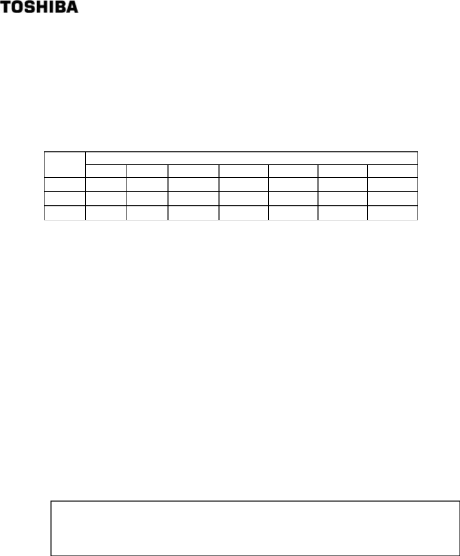
79
6 F 8 A 0 5 2 1
In Table 9.3.1 above,
C: Density multiplier (Varies with the character of the measured matter.)
a: Density slope (A constant determined by the meter size)
The values of the respective meter size in C = 1, 0.7 and 1.8 as examples of the value Xmax in which
N is judged to be too large are listed in Table 9.3.2. Each of the values is the result of the value
when C=1 in Table 9.3.2 multiplied by C.
Table 9.3.2 Value of XMAX (%TS)
Aperture
C 50mm
80mm
100mm 150mm
200mm
250mm
300mm
0.7 42.34
26.46
21.17 14.11 10.57 8.57 7.06
1.0 60.48
37.80
30.24 20.16 15.12 12.24 10.08
1.8 108.86
68.04
54.43 32.29 27.22 22.03 18.14
9.3.5 Restrictions and invalidation in applying the automatic adjustment of phase angle
rotations
This function of automatic adjustment of phase angle rotations involves some application
restrictions. For example, it cannot be applied to the case of measuring high density as follows.
<Example> In the case of meter size: 150 mm; upper density measurement range: 20%TS; and
density multiplier: 0.7
As shown in Table 9.3.2, Xmax=14.11(%TS). Therefore, when the measured density
exceeds 14.11(%TS), the adjustment of decreasing the number of phase angle
rotations applies as shown in Table 9.3.1, thus making it impossible to measure the
density in excess of 14.1(%TS).
To solve the problems as shown in the example above, measurement is taken so that the function of
automatic adjustment of phase angle rotations is automatically invalidated if the upper measured
density range exceeds Xmax.
Check the operating conditions to see if the function of automatic adjustment of phase angle
rotations is applicable or not.
[NOTE] In the cases where the automatic adjustment of phase angle rotations is not applicable, after
the density meter detector is temporarily made empty, it is necessary to reset the phase angle
rotation to an appropriate value through manual input. In the cases, it is more desirable to
perform the external synchronized operation.
9.3.6 Invalidation by setting the automatic adjustment of phase angle rotations
As mentioned in the previous subsection, the density meter is equipped with the function of
automatically invalidating the function of automatic adjustment of phase angle rotations, based on
the conditions for setting the upper density measurement range and the density multiplier.
However, in the state of starting the operation, the upper density measurement range is determined
but the density multiplier is not determined yet (determined in the span calibration described in
Section 6.5), thus the operation is started with a provisional value (initial value: 1). Therefore, the
function of automatic adjustment of phase angle rotations, which is supposed to be invalidated, may
not be invalidated, making it impossible to take an appropriate measurement (including the span
calibration). This applies to the case in which the original density multiplier is smaller than the
current set value (the initial value 1 in the initial operation).

80
6 F 8 A 0 5 2 1
There are two ways of dealing with such a case.
One is to automatically invalidate the function of automatic adjustment of phase angle rotations by
provisionally setting a sufficiently small value such as about 0.5 for the density multiplier C so that
Xmax is smaller than the upper density measurement range.
Another is to forcibly invalidate the function of automatic adjustment of phase angle rotations. The
latter's setting method is described below.
(1) Switching to the setting mode (see Subsection 5.2.5)
First of all, press the [ESC] key of the converter several times (normally once although this
varies with the operation status) to return to the initial menu display. Next, use the [→] key to
move the LCD indicator cursor to the menu number "2" of "2 SETTING MENU" and then
press the [SET] key to display the warning message saying "Test output will be valid." Make
sure that there is no problem and then press [→] to get into the setting mode. And return to [2:
SETTING MENU]. Then, the output will be switched to the simulated output that is set
beforehand.
(2) Selecting the "OTHERS" setting menu (see Subsection 5.2.5)
Initially, the menu list of menu numbers 5 to 8 is displayed. However, by pressing the [UP] key
once, this display can be switched to the menu list of the next menu numbers 9 to 11. Use the
[→] key to move the LCD indicator cursor to the menu number "11" of "11: OTHERS" and
then press the [SET] key to select the menu of "11: OTHERS."
(3) Verifying or changing ON/OFF of automatic adjustment of phase angle rotations
(see Subsection 5.2.16)
Press the [DN] key once (or the [UP] key five times) to display "NA: N AUTO
ADJUSTMENT". On this screen, it is possible to verify whether the automatic adjustment of
phase angle rotations is valid (ON) or invalid (OFF). Here, if it is necessary to alter the setting,
press the [SET] key to switch to the setup display of the automatic adjustment of phase angle
rotations. Each time the [UP] or [DN] key is pressed, the set value is alternated between ON
and OFF. Set the value to OFF and then press the [SET] key to confirm it. The screen will be
returned to the immediately preceding one; make sure that the value is correctly reset.
(4) Returning to the measuring mode
Press the [ESC] key twice to return to the initial menu screen and return to the measuring
mode from the setting mode to resume the normal measurement.
9.3.7 Actions after invalidating the automatic adjustment of phase angle rotations
After invalidating the automatic adjustment of phase angle rotations to make it possible to take
measurements appropriately even at high density in excess of Xmax, implement the span
calibration in accordance with Section 6.5 and set the density multiplier to an appropriate value.
While referring to Table 9.3.2, use this reset density multiplier to calculate the maximum density
Xmax, which can be applied to the function of automatic adjustment of phase angle rotations and
judge whether this Xmax is greater than the value of the upper density measurement range that is
set.
If Xmax is greater than the upper density measurement range, the function of automatic adjustment
of phase angle rotations is applicable. Therefore, return the function of automatic adjustment of
phase angle rotations which is set to "OFF" in Subsection 9.3.6 to“ON”.
If Xmax is smaller than the upper density measurement range, the function of automatic adjustment
of phase angle rotations is invalid. Therefore, it is unnecessary to return the function of automatic
adjustment of phase angle rotations which is set to "OFF" in Subsection 9.3.6 to “ON”.

81
6 F 8 A 0 5 2 1
9.3.8 Return to the normal through manual input of the phase angle rotations
If the function of automatic adjustment of phase angle rotations is not applicable whereas the
density meter detector is temporarily made empty thus causing the number of phase angle rotations
to jump to a faulty number, the number of phase angle rotations fails to return to an appropriate
value even when the density meter detector is refilled with the matter to be measured, thus allowing
the measured density to remain in error. In this connection, it is necessary to reset the phase angle
rotation to an appropriate value through manual input. The setting method is described below.
(1) Switching to the setting mode (see Subsection 5.2.5)
First of all, press the [ESC] key of the converter several times (normally once although this
varies with the operation status) to return to the initial menu display. Next, use the [→] key to
move the LCD indicator cursor to the menu number "2" of "2 SETTING MENU" and then
press the [SET] key to display the warning message saying "Test output will be valid." Make
sure that there is no problem and then press [→] to get into the setting mode. And return to [2:
SETTING MENU]. Then, the output will be switched to the simulated output that is set
beforehand.
(2) Selecting the "ANGLE ROTATION" setting menu (see Subsection 5.2.5)
In the state that the menu list of menu numbers 5 to 8 is displayed, use the [→] key to move the
LCD indicator cursor to the menu number "8" of "8: ANGLE ROTATION" and then press the
[SET] key to select the menu of "8: ANGLE ROTATION".
(3) Verifying or changing the number of phase angle rotations (see Subsection 5.2.13)
Press the [DN] key once (or the [UP] key twice) to display "N: ROTATION". On this screen,
it is possible to verify the number of phase angle rotations. Here, press the [SET] key to switch
to the setup display of the number of phase angle rotations and enter an appropriate value
(note). At the initial digit, use the [UP] or [DN] key to select whether to attach the "-" symbol
or not. Use the [→] key to move to the digit, and use the [UP] or [DN] key to alter the
numeric value of the relevant digit. When entering input is completed, press the [SET] key to
confirm it. The screen will be returned to the immediately preceding one; make sure that the
value is correctly reset.
Note: In many cases, an appropriate value for the number of phase angle rotations N is
0. In the event that the density or the fluid temperature is high, this value may be 1.
In the event that the density or the fluid temperature is low, it may be -1. Set either
of 0, 1 and -1 and then verify that the measured density at this time has returned to
an appropriate value.
(4) Returning to the measuring mode
Press the [ESC] key twice to return to the initial menu screen and return to the measuring
mode from the setting mode to resume the normal measurement.
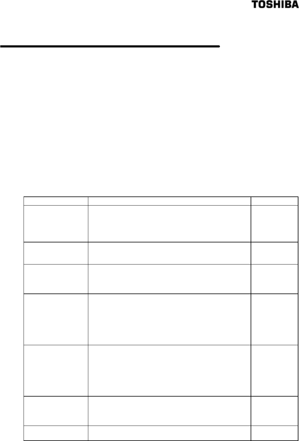
82
6 F 8 A 0 5 2 1
10. VARIOUS FUNCTIONS
10.1 Various Functions and their Outlines
The density meter LQ500 is equipped with various functions to be used more appropriately in
various processes and in various situations. Depending on the process being applied or the method
of using the meter, some functions may not be necessary. Based on the descriptions below, choose
the functions you need. Table 10.1.1 describes the functions equipped in this meter and outlines.
Table 10.1.1 Various Functions
Function Name Application and Outline Remarks
1) External
synchronized
operation
Perform this external synchronized operation in the event that the
pump to the pipe line on which the density meter is installed is
operated intermittently and the object of measurement does not
flow continuously or in the event that the detector is temporarily
made empty.
See Section 6.7.
2) Moving
average
Use this function in the event of requiring the averaged output to
be used for density control, etc. The function is useful for
suppressing the deflection width of the output.
See Section
10.2.
3) Change-rate
limit
In the event of a sudden change in the density or a sudden
variation in the output due to intrusion by bubbles, etc., this
function is used to exclude these signals to restrain the sudden
output change.
See Section 10.3
4) Electric
conductivity
correction
This function is used in the event that the electric conductivity of
the matter to be measured has changed substantially. Since this
does not usually become a real problem, it does not need this
function usually. When using this function, however, it is
necessary to separately prepare a electric conductivity meter,
install it on a proper location and input the electric conductivity
signal into the density meter.
See Section
10.4.
5) Additives
correction
In the event that the brand (with varying components and
compound ratio) of the matter to be measured is switched from
one to another, this function is used to omit the span calibration
in terms of each brand by registering beforehand the list in which
the sensitivity and compound ratio of the respective components
are input (up to ten lists can be registered) and then selecting the
list number.
See Section
10.5.
6) Linearizer Since the density meter has a satisfactory linear relationship
between its actual density and instrument output, a linearization
correction is normally unnecessary. Therefore, this function is
provided as a measure to deal with special cases.
See Section
10.6.
7) Density
multiplier switching
This function is to switch around up to four density multipliers by
means of ON/OFF of two external voltage signals(DI). The
See Section
10.7.

83
6 F 8 A 0 5 2 1
by external signal function can be used to facilitate the density measurement of up
to four different types of matters (brand) which differ in
measurement sensitivity.
10.2 Moving Average
10.2.1 Function of moving average
Assuming that the moving average times is "n", this function is to calculate and output the mean
value of n preceding measured values each time. The function is used when an averaged output is
required such as for density control. This function is also useful for suppressing the deflection width
of output.
The value that can be set as the moving average times "n" is 1 to 99. Setting 1 for "n" means that no
moving average takes place.
10.2.2 Setting of the moving average times
(1) Switching to the setting mode (see Subsection 5.2.5)
First of all, press the [ESC] key of the converter several times (normally once although this
varies with the operation status) to return to the initial menu display. Next, use the [→] key to
move the LCD indicator cursor to the menu number "2" of "2 SETTING MENU" and then
press the [SET] key to display the warning message saying "Test output will be valid." Make
sure that there is no problem and then press [→] to get into the setting mode. And return to [2:
SETTING MENU]. Then, the output will be switched to the simulated output that is set
beforehand.
(2) Selecting the parameter setting menu (see Subsection 5.2.10)
In the state that the menu list of menu numbers 5 to 8 is displayed, use the [→] key to move the
LCD indicator cursor to the menu number "5" of "5: SET PARAMETERS" and then press the
[SET] key to select the menu of "5: SET PARAMETERS."
(3) Verifying or setting the moving average times (see Subsection 5.2.10)
Press the [DN] key three times (or the [UP] key eleven times) to display "ma: AVERAGING
TIMES". On this screen, it is possible to verify the set value of the moving average times. If it
is necessary to change the setting, press the [SET] key here to switch to the setup display of
the moving average times and enter an appropriate value. Use the [→] key to move to the digit,
and use the [UP] or [DN] key to alter the numeric value of the relevant digit. When entering
input is completed, press the [SET] key to confirm it. The screen will be returned to the
immediately preceding one; make sure that the value is correctly reset.
(4) Returning to the measuring mode
Press the [ESC] key twice to return to the initial menu screen and return to the measuring
mode from the setting mode to resume the normal measurement.
10.2.3 Cautions in using the moving average function
Setting an excessively large value for the moving average times will result in deteriorated
responsiveness. Therefore, make sure to set a value appropriate to the process situation and the
required responsiveness.
84
6 F 8 A 0 5 2 1
10.3 Change-rate limit
10.3.1 Outline of change-rate limit function
In the event of a sudden change in the density or a sudden variation in the output due to intrusion by
bubbles, etc., this function is used to exclude these signals to restrain the sudden output change. By
setting two measurement conditions of permissible variation width and limit times, the conditions for
change-rate limit are set.
It is possible to set 0.00 to 9.99(%TS) as the permissible variation width and 0 to 99 times as the
limit times. Setting the limit times to zero means that no change-rate limit is imposed.
10.3.2 Examples of operating the change-rate limit function
The change-rate limit function is described with examples below.
<Setting conditions>
The setting conditions shall be as follows.
* Width of change-rate limit function: 0.5%TS
* Times of change-rate limit function: Twice
The conditions that are set as above mean the following.
① All the variations within 0.5%TS are permitted and output without modification.
② Variations exceeding 0.5%TS are limited up to twice, outputting the immediately preceding
signal in place of the relevant signals.
③ Variations in excess of 0.5%TS which continue three times are judged to be signal variations
resulting from actual density variations, thus outputting the 3rd signal without modification.
Example 1: Operation for temporary and sudden signal variation
Fig.10.3.1 Original Signal
0.0
0.5
1.0
1.5
2.0
2.5
3.0
1 2 3 4 5 6 7 8 9 10
Signal No..
Density signal (%TS)
Fig.10.3.2 Output Signal After Variation Factor
Restriction
0.0
0.5
1.0
1.5
2.0
2.5
3.0
12345678910
Signal No..
Density signal
(%TS)
Fig.10.3.1 shows the original signal before the change-rate limit is processed. No.1 to No.4 are
varying within a small width; however, only signals No.5 and No.6 are varying in excess of 0.5%TS
deviation from the immediately preceding signal No.4. No.7 to No.10 are back to a small width of
variation.
In the event that the above-set change-rate limit is applied to such signals, the output signals are as
shown in Fig.10.3.2. Since signals No.5 and No.6 are varying in excess of 0.5%TS with regard to
signal No.4, signal No.4 is output instead with regard to No.5 and No.6. Signal No.7 is output
without modification. Signals No.8 to No.10, which are also within the variation width of 0.5%TS
with regard to the respective immediately preceding signals, are output without modification.
85
6 F 8 A 0 5 2 1
Example 2: Signal change in the shape of steps
Fig.10.3.3 Original Signal
0.0
0.5
1.0
1.5
2.0
2.5
3.0
12345678910
Signal No.
Density signal (%TS)
Fig.10.3.4 Output Signal After change-rate limit
0.0
0.5
1.0
1.5
2.0
2.5
3.0
12345678910
Signal No.
Density signal (%TS)
Fig.10.3.3 shows the original signal before the change-rate limit is processed. The numeric values
along the horizontal axis refer to the signal numbers. No.1 to No.4 are varying within a small width;
however, signal No.5 is varying in excess of 0.5%TS with No.6 to No.10 remaining in a state not
very different from No.5.
In the event that the above-set change-rate limit is applied to such signals, the output signals are as
shown in Fig.10.3.4. Since signals No.5 and No.6 are varying in excess of 0.5%TS with regard to
signal No.4, signal No.4 is output instead with regard to No.5 and No.6.
Signals No.7 to No.10, which are within the variation width of 0.5%TS with regard to the
respective immediately preceding signals, are output without modification.
10.3.3 Cautions in using the change-rate limit factor
(1) Setting the change-rate limit width
The value can be set within the range of 0.00%TS to 9.99%TS. If the width is set to as little a
value as the normally indicated deflection width, restricted signals will increase and indications
will vary in the shape of steps. Therefore, set a sufficiently large value so that the variation
width is reliably judged to be in error.
(2) Setting the times of change-rate limit
Signals that are made faulty due to intrusion of large bubbles, etc. may affect two neighboring
signals in relation to measurement timing. Therefore, although the change-rate limit has an
effect even when it is applied only once, it is desirable to set the times of change-rate limit at
least to two times in order to reliably exclude error signals. In the event of density variations in
the shape of steps as shown in Example 2, a delay increases in accordance with the set times.
Set an appropriate value for the times in accordance with the responsiveness required of the
plant.

86
6 F 8 A 0 5 2 1
10.3.4 Setting the change-rate limit
(1) Switching to the setting mode (see Subsection 5.2.5)
First of all, press the [ESC] key of the converter several times (normally once although this
varies with the operation status) to return to the initial menu display. Next, use the [→] key to
move the LCD indicator cursor to the menu number "2" of "2 SETTING MENU" and then
press the [SET] key to display the warning message saying "Test output will be valid". Make
sure that there is no problem and then press [→] to get into the setting mode. And return to [2:
SETTING MENU]. Then, the output will be switched to the simulated output that is set
beforehand.
(2) Selecting the parameter setting menu (see Subsection 5.2.5)
In the state that the menu list of menu numbers 5 to 8 is displayed, use the [→] key to move the
LCD indicator cursor to the menu number "5" of "5: SET PARAMETERS" and then press the
[SET] key to select the menu of "5: SET PARAMETERS".
(3) Verifying or changing the change-rate limit width (see Subsection 5.2.16)
Press the [DN] key two times (or the [UP] key twelve times) to display "dx: CHANGE
RATE LIMIT". On this screen, it is possible to verify the set value of the change-rate limit
width. If it is necessary to change the setting, press the [SET] key here to switch to the setup
display of the change-rate limit width and enter an appropriate value for the width. Use the
[→] key to move to the digit, and use the [UP] or [DN] key to alter the numeric value of the
relevant digit. When entering input is completed, press the [SET] key to confirm it. The screen
will be returned to the immediately preceding one; make sure that the value is correctly reset.
(4) Verifying or changing the times of change-rate limit (see Subsection 5.2.16)
Continuing on from the operation in (3) above, press the [UP] key once to display "HL: LIMIT
TIMES". On this screen, it is possible to verify the set value of the change-rate limit times. If
it is necessary to change the setting, press the [SET] key here to switch to the setup display of
the change-rate limit times and enter an appropriate value for the times. Use the [→] key to
move to the digit, and use the [UP] or [DN] key to alter the numeric value of the relevant digit.
When entering input is completed, press the [SET] key to confirm it. The screen will be
returned to the immediately preceding one; make sure that the value is correctly reset.
Note: If the times of change-rate limit is set to zero, the change-rate limit function is
made inactive.
(5) Returning to the measuring mode
Press the [ESC] key twice to return to the initial menu screen and return to the measuring
mode from the setting mode to resume the normal measurement.

87
6 F 8 A 0 5 2 1
10.4 Electric Conductivity Correction
10.4.1 Standard conductivity correction factors
The indication of the density meter varies with the conductivity of the measured object fluid;
however, the variance is as small as approx. 0.15%TS to 1mS/cm change in conductivity and
usually practically negligible, thus making it unnecessary to input the conductivity meter signal to
perform electric conductivity correction. In the event that the conductivity change is large and thus
its impact is not ignoble, make sure to use the electric conductivity correction function. The formula
for this correction including the other corrections described in Chapter 9 is as follows.
△θ={θ2 -α(Τ-Τ0)-δ(G-G0)-ß (A-A0) -γ(E-E0)} -θ1
△θ : Phase difference (degrees)
θ2 : Actual phase angle of measured object fluid (degrees)
θ1 : Phase during zero water measurement (degrees)
(Measured during zero calibration, and set in advance as a constant)
α : Fluid temperature correction factor (degrees/℃)
Τ : Fluid temperature of measured object fluid (℃)
Τ0
: Water temperature during zero calibration
(Measured during zero calibration, and set in advance as a constant)
δ : RF correction factor
G : RF data during measurement
G0
: Zero point RF data
(Measured during zero calibration, and set in advance as a constant)
γ : Electric conductivity correction factor (degrees/(mS/cm))
E : Electric conductivity of measured object fluid (mS/cm)
E0
: Zero water conductivity (mS/cm)
ß : Ambient temperature correction factor (degrees/℃)
A : Ambient temperature (℃)
A0
: Ambient temperature during zero adjustment
(Measured during zero point calibration, and set in advance as a constant)
At the time of factory shipment, the [electric conductivity correction factor γ] is set to zero for all
the products. If the conductivity change of the measured object fluid is large, input the electric
conductivity signal in accordance with "Fig.3.5 External Connection Diagram" and then reset the
[electric conductivity correction factor γ].
Table 10.4.1 shows the "standard values" of electric conductivity correction factors as well as the
"density line slope (a)" required in the event of obtaining electric conductivity correction factors
through calculation from measured values. The "standard values" shall be applicable when the
range of the electric conductivity meter used for conductivity correction is
0 to 10 mS/cm.
88
6 F 8 A 0 5 2 1
Table 10.4.1 Standard Values of Electric Conductivity Correction Factor (γ)
(Based on Electric Conductivity Meter with a Range of 0 to 10 mS/cm)
and Slope of the Line (a)
Meter size
(mm) a γ (Standard value)
50 0.168 0.9
80 0.105 1.4
100 0.084 1.8
150 0.056 2.7
200 0.042 3.6
250 0.034 4.5
300 0.028 5.4
In the event of performing a electric conductivity correction on this density meter, it is a basic
principle to externally connect and use a conductivity meter with a range of 0 to 10 mS/cm. In the
event of using a conductivity meter of another range (0 - R mS/cm), obtain the conductivity
correction factor in accordance with the following formula.
γ=(R/10)×γ0
γ0 : Standard value of electric conductivity correction factor (see Table 9.1)
R: Upper range of conductivity meter used
For example, if the meter size is 150 mm, the standard value of the electric conductivity correction
factor of the density meter is 2.7 and a conductivity meter with a range of 0 to 5 mS/cm is
connected to this,
γ = (R/10)×γ0
= (5×10)×2.7
= 1.35
is used as the correction factor.
[NOTE] ◆ In the event of implementing a electric conductivity correction, separately prepare a
electric conductivity meter and install it on a location where the conductivity can be
measured correctly (where the measurement object process is appropriate).
◆ The "standard values" of electric conductivity correction factors shown in Table 10.4.1
are criteria. It is necessary to use the linear relationship that exists between the
conductivity and the output to survey and determine the electric conductivity correction
factor in terms of each actual measured object fluid. See Subsection 10.4.2.
◆ In the event of not executing any electric conductivity correction, set the "electric
conductivity correction factor (γ)" to zero.
10.4.2 How to obtain and set a correction factor
Obtain and set a electric conductivity correction factor as appropriate to the applicable process in
accordance with the following procedure.
(1) To set the density multiplier to 1.000
(1-1) Switching to the setting mode (see Subsection 5.2.5)
First of all, press the [ESC] key of the converter several times (normally once
although this varies with the operation status) to return to the initial menu display.
Next, use the [→] key to move the LCD indicator cursor to the menu number "2" of
"2: SETTING MENU" and then press the [SET] key to display the warning message

89
6 F 8 A 0 5 2 1
saying "Test output will be valid." Make sure that there is no problem and then press
[→] to get into the setting mode. And return to [2: SETTING MENU]. Then, the
output will be switched to the simulated output that is set beforehand.
(1-2) Selecting the span calibration menu (see Subsection 5.2.5)
The menu list of menu numbers 5 to 8 is displayed. Use the [→] key to move the LCD
indicator cursor to the menu number "7" of "7: SPAN CALIBRATION" and then
press the [SET] key to select the menu of "7: SPAN CALIBRATION."
(1-3) Verifying or recording the density multiplier (see Subsection 5.2.12)
For example, the set value of the current density multiplier C' is displayed as in
"DATA: 1.265". Record this value.
(1-4) Setting the density multiplier to "1.000" (see Subsection 5.2.12)
Press the [SET] key to switch to the setup display of the density multiplier and reset
the density multiplier to 1.000. Use the [→] key to move to the digit, and use the [DN]
key to alter the numeric value of the relevant digit. When entering input is completed,
press the [SET] key to confirm it. The screen will be returned to the immediately
preceding one; make sure that the value is correctly reset.
(2) To suspend the electric conductivity correction function
(with the conductivity correction factor set to 0.00)
(2-1) Returning to the initial screen of the setting mode
Continuing on from (1-4) above, press the [ESC] key once to return to the menu list
display of the menu numbers 5 to 8 of the setting mode.
(2-2) Selecting the linearizer /conductivity menu (see Subsection 5.2.5)
Press the [UP] key once to switch to the menu list display of the next menu numbers
9 to 11. Use the [→] key to move the cursor of the LCD indicator to the menu number
"9" of "9: LINEARIZ/CNDUCTVTY" and then press the [SET] key to select the
menu of "9: LINEARIZ/CNDUCTVTY".
(2-3) Setting the electric conductivity correction factor to 0.00 (see Subsection 5.2.14)
Press the [UP] key five times (or the [DN] key three times) to display "r:
CNDUCTVTY COEF". Press the [SET] key here to switch to the setup display of
the electric conductivity correction factor and then input 0.00 for the electric
conductivity correction factor. Use the [→] key to move to the digit, and use the [DN]
key to alter the numeric value of the relevant digit. When entering input is completed,
press the [SET] key to confirm it. The screen will be returned to the immediately
preceding one; make sure that the value is correctly reset.
(3) To measure the electric conductivity of the measured object fluid
(3-1) Selecting the monitoring menu (see Subsection 5.2.4)
Press the [ESC] key twice to return to the initial menu screen and return to the
measuring mode from the setting mode to resume the normal measurement. Use the
[→] key to move the cursor to the menu number "1" of the LCD indicator's "1:
MONITORING MENU" and then press the [SET] key to select "1: MONITORING
MENU".
(3-2) Selecting the measured value data display menu (see Subsection 5.2.4)
In the monitoring menu list of the menu numbers 1 to 3, use the [→] key to move the
cursor to the menu number "2" of the LCD indicator's "2: MEASURED VALUES"
and then press the [SET] key to select "2: MEASURED VALUES".

90
6 F 8 A 0 5 2 1
(3-3) Reading and recording measured conductivity and density values
The externally installed conductivity meter is used to measure the conductivity (E1) of
the measured object fluid while, at the same time, reading the measured density (M1)
from the LCD indicator or from the LED display outside the converter. Take notes of
each measured value.
Next, while varying the conductivity of the measured object fluid, measure as well as
take notes of the conductivity (E2) and the measured density (M2). At this time, take
care to prevent the actual density of the measured object fluid from changing.
E1, E2 : Conductivity (mS/cm)
M1, M2: Measured density value (%TS)
(4) To calculate the electric conductivity correction factor
Obtain the electric conductivity correction factor (γ) in accordance with the following
arithmetic expression.
γ= ΔM/(a×ΔE)
a : Density line slope (see Table 9.1: varies with the aperture)
ΔM : Measured density value difference (M2 – M1)
ΔE : Measured conductivity value difference (E2 – E1)
For example, if the meter size is 150 mm, it follows that a = 0.056. At this time, let's assume
that the conductivity and the measured density (specified value) are as follows respectively.
1st measurement: E1=1 mS/cm M1=4.0%TS
2nd measurement: E2=2 mS/cm M2=4.2%TS
From here, it follows that
DE =1 mS/cm
DM=0.2 %TS
and the conductivity correction factor is
γ = 0.2/(0.056×1)
= 3.57
(5) To correct the electric conductivity correction factor by means of the conductivity meter's
range.
In the event that the range of the conductivity meter being used is other than "0 to 10 mS/cm",
correct the conductivity correction factor in accordance with the conductivity meter range
while referring to the method of calculating the correction factor in the event that the
conductivity meter range is other than the standard described in Subsection 10.4.1.
(6) To set the electric conductivity correction factor
In the same manner as the operation described in (2), set the electric conductivity correction
factor to the value calculated in (4) and (5).
(7) To return the density multiplier to its original value
In the same manner as the operation described in (1), return the density multiplier to its original
value which has been previously recorded.
(8) To return to the measuring mode
Press the [ESC] key twice to return to the initial menu screen and return to the measuring

91
6 F 8 A 0 5 2 1
mode from the setting mode to resume the normal measurement
92
6 F 8 A 0 5 2 1
10.5 Additives Correction Factor
10.5.1 Additive Correction Function
This function refers to handling the different brands made from main material with various
additives. If the physical property of the measured object fluid varies, it is necessary to set the
density multiplier for a value appropriate to this difference. Even with multiple types of measured
objects mixed together (mixed fluid), if their compound ratio is regarded to be consistent, it is
possible to measure the density of the entirety or the density of a particular type among them. In
measuring the density of such mixed fluid, each time the physical property and compound ratio of
the objects included in the fluid differ (that is, the brand is different), it is necessary to set the
density multiplier in accordance with the brand of the relevant mixed fluid.
By selecting an applicable brand number from about ten brands registered in advance, this additive
correction function calculates the density in accordance with the brand, thus making it possible to
omit the span calibration in terms of each brand.
Using this function in a simplified manner, by selecting the span calibration factor(density
multiplier) in terms of each brand from the brand list registered in advance, it is possible to simplify
the span calibration. For information on the simplified way of this function, refer to "10.5.5
Simplified way of using the additive correction function".
The contents to be registered into the brand list are as follows.
Table 10.5.1 Brand List
Sensitivity (Note 2) Ratio of mixture (Note 3)
Component
Note 1 Sign
Setting range Set at
shipping
Sign
Setting range Set at
shipping
Comp. 0 s0 -9.99 to +9.99
1.00 -- -- ---
Comp.1 s1 -9.99 to +9.99
0.00 R1 0.000 to 1.999 0.000
Comp.2 s2 -9.99 to +9.99
0.00 R2 0.000 to 1.999 0.000
Comp.3 s3 -9.99 to +9.99
0.00 R3 0.000 to 1.999 0.000
Comp.4 s4 -9.99 to +9.99
0.00 R4 0.000 to 1.999 0.000
Comp.5 s5 -9.99 to +9.99
0.00 R5 0.000 to 1.999 0.000
(Note 1) Component 0 is the main component. Components 1 to 5 are the additives #1 to #5.
(Note 2) Sensitivity values for components #0 to #5 are to be registered for each of 10 brands.
Usually, the sensitivity value for main component s, 0 is set to “1.000.” The sensitivity
values of typical additives are shown in Table 10.5.2. Register s1 to s5 referring to this
table. For the sensitivity values of additives other than the ones shown in Table 10.5.2,
please contact Toshiba. Whenever you send us a sample of additives, we can measure
their sensitivity values. Sensitivity values are measured in the same way as used for span
calibration for each of additives (measured density reading / density by manual analysis).
Table 10.5.2
Additives name Sensitivity
Calcium carbonate
0.45
Titanium oxide 0.13
Zinc oxide 0.12
Talc 0.61
(Note 3) For each formula in the list of 10 brand, the ratio of mixture for the components #1 to 5 is
to be entered. A ratio of mixture is a ratio of a component against the component 0 (main
component) in weight.

93
6 F 8 A 0 5 2 1
10.5.2 Density calculation
Following calculation modes can be selected.
(1) Additives correction ON (To be made) / OFF (Not to be made)
(a) Set value at shipping the density meter: OFF
(2) When additives correction is "ON"(to be made), you can select two calculation modes.
(b) Total density of mixture including the additives (TOTAL)
(c) Density of the main component only (MAIN)
In the mode (2) above, each of the density outputs (LED display of the converter, and the
current output in 4 to 20mA dc) can be either (b) or (c) separately.
* Set value at shipping: Both the density display and the density current output are in
"TOTAL" of (b) above.
(a) Density without additives correction
Following calculation is made (same density calculation as in section 9.1.3)
Xa = C × (a × Δθ) +b
where, Xa : Measured density value
Δθ : Phase difference that varies in proportion to the actual density
a : Density line slope
b : Density intercept (normally zero).
C : Density multiplier
(b) Additives correction to be made for getting Total Density of whole mixture including the
additives (TOTAL)
b)(aC
R5
s5
R4
s4
R3
s3
R2
s2
R1
s1
s0
R5R4R3R2R11
Xb +×××
⋅
+
⋅
+
⋅
+
⋅
+
⋅
+
+
+
+
+
+
=Δθ
where, Xb : Density of the whole mixture
s0 : Sensitivity of the main component only
s1 : Sensitivity of additive #1, R1 : Mixture ratio of additive #1
s2 : Sensitivity of additive #2, R2 : Mixture ratio of additive #2
s3 : Sensitivity of additive #3, R3 : Mixture ratio of additive #3
s4 : Sensitivity of additive #4, R4 : Mixture ratio of additive #4
s5 : Sensitivity of additive #5, R5 : Mixture ratio of additive #5
Δθ : Phase difference that varies in proportion to the diameter
a : Density line slope determined by diameter
b : Intercept of the line (normally zero).
C : Density multiplier
(c) Additives correction to be made for getting density of main component only (MAIN)
Xc s s RsRsRsRsRCab=+⋅+⋅+⋅+⋅+⋅× × × +
1
0 1 1 2 2 3 3 4 4 5 5 ( )∆θ
where, Xc : Density of main component
Others are same as in (b)
(Note) When using the additives correction functions of (b) or (c), set the density multiplier C to
1.000. Following procedure is recommended for making span adjustment. At the
beginning of the use of correction, for a whole mixture of a formula, compare the
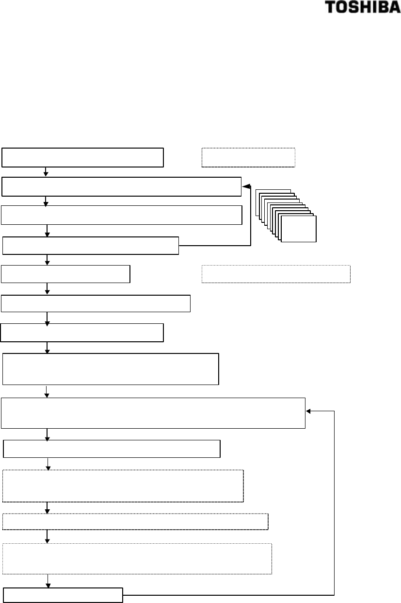
94
6 F 8 A 0 5 2 1
measured density readings you get in dry method (dry weight) and in manual analysis,
and when required, make span adjustment by adjusting the density multiplier C of the
whole mixture.
10.5.3 Procedures for using the additives correction function
The procedure for the additives correction function is described as following steps.
Obtain sensitivities of the components ....... Refer to table 10.5.2.
Select the formula list number for registering (parameters)
Set sensitivities of main component and additives (s0 to s5)
Set mixture ratios of additives (R1 to R5)
Perform zero point calibration .................. Refer to [6.4 Zero Point Calibration]
Set the density multiplier to 1.000
Select ON for additives correction
Select calculation mode for additives correction
(TOTAL or MAIN)
Select the brand list number that corresponds with the formula
(Parameter set)
Let the liquid mixture of selected brand flow.
Read the density indication(M), and simultaneously
sample the substance to measure.
Measure the density (A) of the sample by manual analysis
Calculate C as below, then fine adjust C (density multiplier)
C=(A/M)x1 (Default value of C is 1)
Start measuring Density When brand is changed
You can set for up to
ten formulas. Each
of which can have
up to five additives,
to which
sensitivities and
ratios can be
entered individually.
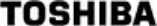
95
6 F 8 A 0 5 2 1
10.5.4 How to set the additives correction function
(1) Switching to the setting mode (see Subsection 5.2.5)
First of all, press the [ESC] key of the converter several times (normally once although this
varies with the operation status) to return to the initial menu display. Next, use the [→] key to
move the LCD indicator cursor to the menu number "2" of "2 SETTING MENU" and then
press the [SET] key to display the warning message saying "Test output will be valid.". Make
sure that there is no problem and then press [→] to get into the setting mode. And return to [2:
SETTING MENU]. Then, the output will be switched to the simulated output that is set
beforehand.
(2) Selecting the additives correction menu (see Subsection 5.2.5)
Initially, the menu list of the menu numbers 5 to 8 is displayed. Press the [UP] key once to
switch to the menu list display of the next menu numbers 9 to 11. Use the [→] key to move the
cursor of the LCD indicator to the menu number "10" of "10: ADDITIVES CORRECT" and
then press the [SET] key to select the menu of "10: ADDITIVES CORRECT".
(3) Verifying and changing the various settings for additives correction (see Subsection 5.2.15)
(3-1) Selecting the OFF/ON of the additives correction function
Verify the set value of the initial menu "AF: ADDITIVES COMP." of the additives
correction. "OFF" means that the additives correction function is unavailable, thus not
displaying the detailed menu concerning the additives correction. When using the
additives correction function, press the [SET] key to switch to the OFF/ON selection
display of the additives correction. Each time the [UP] or [DN] key is pressed, the set
value alternates between "OFF" and "ON". With the value set to "ON", press the
[SET] key to verify it. The screen will be returned to the immediately preceding one;
make sure that the value is correctly reset.
(3-2) Selecting a density display (see subsection 10.5.2)
Continuing on from (3-1), press the [UP] key to switch to the display of "Ad:
DISPLAY DENSITY". In this menu, decide whether the density display should be
the density of the entire mixed fluid including the additives "TOTAL" or the density of
the pulp only "MAIN". When changing the setting, press the [SET] key to switch to
the selected display, use the [UP] or [DN] key to switch between "TOTAL" and
"MAIN" and then press the [SET] key at the status to be set.
(3-3) Selecting a density display (see Subsection 10.5.2)
Continuing on from (3-2), press the [UP] key to switch to the display of "Ac:
OUTPUT DENSITY". In this menu, decide whether the density current output of 4 to
20mA should be the density of the entire mixed fluid including the additives (TOTAL)
or the density of the pulp only (MAIN). When changing the setting, press the [SET]
key to switch to the selected display, use the [UP] or [DN] key to switch between
"TOTAL" and "MAIN" and then press the [SET] key at the status to be set.
(3-4) Selecting a parameter set number (a brand list number)
Continuing on from (3-3), press the [UP] key to switch to the display of "Ap:
PARAMETER SET NO.". In this menu, select a parameter set number. Press the
[SET] key to switch to the setup display and then input the parameter set number. Use
the [→] key to move to the digit, and use the [UP] or [DN] key to alter the numeric
value of the relevant digit. When entering input is completed, press the [SET] key to
confirm it. The screen will be returned to the immediately preceding one; make sure
that the value is correctly reset.

96
6 F 8 A 0 5 2 1
(3-5) Setting the sensitivity and the compound ratio
Continuing on from (3-4), press the [UP] key to switch to the menu of "s0: MAIN
OBJ SENS." and then, after switching to the setup display by pressing the [SET] key,
input the sensitivity of the main object (component 0). Use the [→] key to move to the
digit, and use the [UP] or [DN] key to alter the numeric value of the relevant digit.
When entering input is completed, press the [SET] key to confirm it. The screen will
be returned to the immediately preceding one; make sure that the value is correctly
reset. Continue on to switch to the next setup menu display with the [UP] key. And, in
accordance with the same procedure, set the sensitivities s0 to s5 of components
(additives) 1 to 5 as well as compound ratios R1 to R5 of components (additives) 1 to
5.
(4) Returning to the measuring mode
Press the [ESC] key twice to return to the initial menu screen and return to the measuring
mode from the setting mode to resume the normal measurement.
10.5.5 Simplified Correction on Additives
Previous section describes complete correction on additives in which sensitivities and ratios of
mixture per additive were taken into account in calculation. By using only a sensitivity for the whole
mixture (a mixture of pulp and additives), the additives correction can be simplified as described
below. In this simplified correction, a density multiplier (sensitivity) is obtained separately for each
formula and entered into the list of formula. When a formula is changed, you need to select a new
formula number to change the density mulyiplier to continue measuring density. Up to ten formulas
can be entered into the list.
Procedures for a simplified correction is as follows. See the section 10.5.1 to 10.5.3 for basic
information, and refer to section 10.5.4 Operations for correction.
● Procedures for simplified correction of additives.
Set the density multiplier C to 1.000
Select Calculation Mode for additives correction...No (correction)
Perform zero calibration ....................... See “6.4 Zero calibration”
Carry out span calibration for each brand, and obtain sensitivity as below.
Sensitivity = (Measured density reading)/(Density obtained by manual analysis)
Enter the sensitivity of a formula into the sensitivity s0
of the component 0 in the formula list.
Select (TOTAL) [total density of a mixture,
with additives correction] for the calculation mode
Select a brand list number
that corresponds with the mixture to be measured.
Run the fluid to measure and measure density
When the brand is changed.
See Note 1.
97
6 F 8 A 0 5 2 1
(Note1) Set all sensitivities and ratios to 0.00 and 0.000 respectively for all of the components 1 to
5. (Or to the default values set at shipping.)
10.6 LINEARIZER SETTING
10.6.1 Linearizer function
Depending on the kind of substance to be measured, there may not be a linear relationship between
the values measured by the meter and those obtained by manual analysis. Particularly, in the
measurement of low density substance of about 1%, the meter tends to show readings in higher
value at or less than 0.5% or show lower for the density about 1.5% or higher. In such a case, the
1inealization is necessary because it is difficult to match meter-measured values with manual
analysis values with a single density multiplier over a wide range of densities from low to high.
Suppose there is a curve relationship such as that shown in figure 10.6. 1 between meter-measured
values (using a density multiplier of 1.000) and manual analysis values when a certain substance is
measured at varying degrees of density. To make linealization, the curve is approximated by three
straight lines of A, B, and C.
•
•
•
••
••••
•
••
••
••
••
A
B
C
0.6 1.0 1.5
B
A
a c
計器測定値 X O (濃度補正係数 1.00 )
0
0.8
1.2
1.5
f
手
分
析
値
濃
度
%
d
e
b
Figure 1 0.6.1 Linearizer setting Diagram
Let the meter-measured value (XO) at the bend of the lines A and B (crosspoint) as density A, and
the value at lines B and C to be density B. Also let the slopes of lines A, B, and C as K1, K2, and K3
respectively.
Instrument reading X0 (density multiplier 1.00)
Manual ly analyzed density %

98
6 F 8 A 0 5 2 1
Meter-measured value XO (density multiplier 1.000) before linearization and meter-measured
value X after linearization have the following relationship.
For X 0 ≤ A X = C ( K 1 X 0 )
For A < X 0 ≤ B X = C { K 1 A + K 2 ( X 0 − A)}
For B < X 0 X = C { K 1 A + K 2 ( B − A ) + K 3 ( X 0 − B )}
where
C: Density multiplier.
The procedures for making 1inearizer lines and setting them into the meter are as follows:
(1) Create a graph
Plot the relationships between the meter-measured value (X0) at a density multiplier of 1.000
and manual analysis value to make into a graph as shown in figure 10.6.1.
(2) Draw approximate straight lines
Draw in three straight lines that approximate the relationships.
(3) Read densities at crosspoints
Read the meter-measured values (XO) at the cross-points of these lines and get cross-point
densities A and B.
(4) Get the slopes of the lines.
Calculate the slopes of the straight lines as follows to determine K1, K2, and K3.
K 1 = d / a
K 2 = e / b
K 3 = f / c
● Defaults are set as : A = 0.60, B = 1.00, K1 = 1.00, K2 = 1.00, K3 = 1.00
Example of set values (Fig. 10.6.l)
A = 0.6 (%), B = 1.0 (%)
K 1 = 0.8 / 0.6 = 1.33、K 2 = 0.4 / 0.4 = 1.00、K 3 = 0.3 / 0.5 = 0.6
10.6.2 Linearizer setting
(1) Switching to the setting mode (see Subsection 5.2.5)
First of all, press the [ESC] key of the converter several times (normally once although this
varies with the operation status) to return to the initial menu display. Next, use the [→] key to
move the LCD indicator cursor to the menu number "2" of "2 SETTING MENU" and then
press the [SET] key to display the warning message saying "Test output will be valid.". Make
sure that there is no problem and then press [→] to get into the setting mode. And return to [2:
SETTING MENU]. Then, the output will be switched to the simulated output that is set
beforehand.
(2) Selecting the linearizer menu (see Subsection 5.2.5)
Initially, the menu list of the menu numbers 5 to 8 is displayed. Press the [UP] key to switch to
the menu list display of the menu numbers 9 to 11. Use the [→] key to move the cursor of the
LCD indicator to the menu number "9" of "9: LINEARIZ/CNDUCTVTY" and then press the
[SET] key to select the menu of "9: LINEARIZ/CNDUCTVTY".

99
6 F 8 A 0 5 2 1
(3) Setting the density and the factor (see Subsection 5.2.14)
The setup menus of density and factor are called one after another from the start of the menu
development of "9: LINEARIZ/CNDUCTVTY". First of all, press the [SET] key at "LA:
DENSITY A" and then, after the setup display of density A is displayed, input the value for
density A. Use the [→] key to move to the digit, and use the [UP] or [DN] key to alter the
numeric value of the relevant digit. When entering input is completed, press the [SET] key to
confirm it. The screen will be returned to the immediately preceding one; make sure that the
value is correctly reset. Continue on to switch to the next setup menu display with the [UP]
key. And, in accordance with the same procedure, set density B and factors K1, K2 and K3.
(4) Returning to the measuring mode
Press the [ESC] key twice to return to the initial menu screen and return to the measuring
mode from the setting mode to resume the normal measurement.
(5) Determining and setting the density multiplier
Perform the density measurement after setting the linearizer and, in accordance with the span
calibration in Section 6.5, determine and set the density multiplier C.
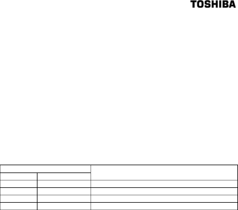
100
6 F 8 A 0 5 2 1
10.7 Density Multiplier Switching by External Signals
10.7.1 Density multiplier switching function by external signals
When switching around multiple measurement objects fulid of differing measurement sensitivities
to measure their respective sensitivities, it is possible to take appropriate density measurements by
resetting the density multiplier to a value in accordance with the relevant measured object fluid
each time the measured object fluid is changed. In the event that the measurement objects fluid are
limited to no more than four types, this function can be used to save the trouble of resetting the
density multiplier each time through manual input. Implement the span calibration in terms of each
measured object fluid in advance, obtain and set the respective density multipliers C1 to C4 and
then switch around the density multipliers to be used for density calculation by means of the
external voltage signals of two points in accordance with the measurement objects fluid being
switched around.
Table 10.7.1 shows the relationship between the statuses of external voltage signals and selected
density correction factors.
Table 10.7.1
Status of External Voltage Signal
DI2 DI3 Selected Density Multiplier
L L C1(Same as the normally used density multiplier C)
H L C2
L H C3
H H C4
H: Voltage signals of 20 to 30VDC
L: Signals of no more than 2VDC
10.7.2 Setting the density multiplier switching by external signals
(1) Switching to the setting mode (see Subsection 5.2.5)
First of all, press the [ESC] key of the converter several times (normally once although this
varies with the operation status) to return to the initial menu display. Next, use the [→] key to
move the LCD indicator cursor to the menu number "2" of "2 SETTING MENU" and then
press the [SET] key to display the warning message saying "Test output will be valid.". Make
sure that there is no problem and then press [→] to get into the setting mode. And return to [2:
SETTING MENU]. Then, the output will be switched to the simulated output that is set
beforehand.
(2) Selecting the "OTHERS" setting menus (see Subsection 5.2.5)
Initially, the menu list of menu numbers 5 to 8 is displayed. However, by pressing the [UP] key,
this display is switched to the menu list of the next menu numbers 9 to 11. Use the [→] key to
move the LCD indicator cursor to the menu number "11" of "11: OTHERS" and then press the
[SET] key to select the menu of "11: OTHERS."
(3) Selecting of density multiplier switching ON/OFF(see Subsection 5.2.16)
Press the [UP] key once to display "DI: C CHANGE ON/OFF". Press the [SET] key here to
switch to the setup display. Each time the [UP] or [DN] key is pressed, the set value
alternates between "ON" and "OFF". Therefore, when using the function of density multiplier
switching by external signals, set the value to "ON" and then press the [SET] key to verify it.
The screen will be returned to the immediately preceding one; make sure that the value is

101
6 F 8 A 0 5 2 1
correctly reset.
(4) Setting density multipliers C2, C3 and C4
Continuing on from (3), press the [UP] key once to switch to the display of "C2:
DensityMultiplier". Switch to the setup display by pressing the [SET] key here and then input
the density multiplier C2. Use the [→] key to move to the digit, and use the [UP] or [DN] key
to alter the numeric value of the relevant digit. When entering input is completed, press the
[SET] key to confirm it. The screen will be returned to the immediately preceding one; make
sure that the value is correctly reset. Continue on to switch to the next setup menu display with
the [UP] key and set C3 and C4 in accordance with the same procedure. When setting the
density multiplier C1, refer to "6.5 Span Calibration".
(5) Returning to the measuring mode
Press the [ESC] key twice to return to the initial menu screen and return to the measuring
mode from the setting mode to resume the normal measurement.

102
6 F 8 A 0 5 2 1
11. SPECIFICATIONS
11.1 General Specifications
Measurement method: Microwave phase difference method
Measurement range: Density measurement range can be set by defining the lower point
(density corresponding to 4mA) and the upper point (density
corresponding to 20mA) within the following setting ranges. The object
to be measured should be free from cavities inside and should have
sufficient fluidity. For the ranges other than the ones described below,
please contact Toshiba.
Density measurement range lower side: 0 to 49%TS
Density measurement range upper side: 1 to 50%TS
Span range: 0 to 50%TS
Setting step: 0.1%TS
Note 1: TS (Total Solids) = Soluble materials + Non-soluble materials, Span = Density
measurement range upper side − Density measurement range lower side
Note 2: In the case of 50mm in meter size,
Density measurement range lower side: 0 to 48%TS
Density measurement range upper side: 2 to 50%TS
Span range: 2 to 50%TS
Note 3: The object to be measured is required to be free from cavities and have fluidity. Contact
Toshiba for measurement ranges other than those described above.
Note 4: For the range larger than 50%TS, please contact Toshiba.
Repeatability: In the case of 2%TS or more in full-scale, ±2%FS
In the case of less than 2%TS in full-scale, ±4%TS
Note: The values are taken at measuring points above 5% of full-scale using simulated
reagent.
Note: The full scale value is the maximum value on the upper side of the density measurement
range.
Note: In the case of 50mm in meter size, the full-scale shall be 2%TS or more
Linearity: In the case of 2%TS or more in full-scale, ±2%FS
In the case of less than 2%TS in full-scale, ±4%TS
Note: The values are taken at measuring points above 5% of full-scale using simulated
reagent.
Note: In the case of 50mm in meter size, the full-scale shall be 2%TS or more
Electrical resolution: 0.001%TS
Note: Verifiable resolution using the simulated reagent: 0.05%TS
The verifiable resolution value refers to the value which is verified through a test of the
density difference which can be resolved as a density meter output. Marginal errors in
testing such as uneven density distribution, testing errors, environmental variations and
so on are also included in this value.
Note: In the case of 50mm in meter size, electrical resolution: 0.002%TS
Verifiable resolution using the simulated reagent: 0.1%TS
103
6 F 8 A 0 5 2 1
Ambient environment condition: Temperature: 0 to 50°C (Option: Detector −20 to 50°C)
Humidity: 5 to 90%RH (No condensation)
Structure: Detector Immersion-proof type (IP67: Immersion-proof type or equivalent)
Converter Waterproof type (IP65: Waterproof type or equivalent)
Note: Outdoor installation is possible. If there is a possibility of direct sunlight, however,
provide a sunshade to the converter to avoid direct sunlight.
Vibration: (1) Applying vibration of a resonant frequency in 5 to 150 Hz range in x, y and z
directions for 30 minutes each totaling 90 minutes, and no deterioration of
performance nor damage shall be found.
However, acceleration is as follows:
• Detector: 25m/s2
• Converter: 4.9m/s2
(2) Applying vibration of 5 to 150 to 5 Hz with the acceleration shown in (1) above for
3 minutes and this is repeated 10 times for each direction of vibration totaling 90
minutes, and no deterioration of performance nor damage shall be found.
Altitude : Up to 2000m
Mass: Refer to the Attached Figure 1, “Dimensions” in “Appendix.”
Microwave transmission power: Approx. 10W
11.2 Detector Specifications
Meter size: 50mm, 80mm, 100mm, 150mm, 200mm, 250mm, 300mm
Flange standard and maximum operating pressure
Flange standard Maximum operating pressure
JIS 10K(JIS B 2238 10K) or equivalent
1MPa
ANSI150 1MPa
DIN10 & BS 10 1MPa
DIN 16 1.6MPa
Fluid temperature: 0 to 100°C (Not freezing)
Fluid conductivity:
Meter size Fluid conductivity
50 mm 20 mS/cm or less
80 mm 16 mS/cm or less
100 mm 15 mS/cm or less
150 mm 10 mS/cm or less
200 mm 8 mS/cm or less
250 mm 8 mS/cm or less
300 mm 6 mS/cm or less
Note: Precautions about measuring fluids
When measuring density in liquids containing conductive particles such as the carbon
particles of activated carbon or metal powder, density measurement may be affected by

104
6 F 8 A 0 5 2 1
conductive particles. Avoid using the density meter for the fluids like these. For details,
please contact Toshiba.
Material contacting liquid:
Main pipe: Stainless steel SCS14A (equivalent to 316SS)
Temperature detector holder: Stainless steel (SUS 316)
Applicator window : Polysulfone
Applicator window sealing material: Fluororubber (Viton)
Note: Do not apply this density meter to fluids that may corrode, deteriorate or degenerate
the above liquid contacting materials. Fore details, please contact Toshiba.
Applicators: A pair of applicators provided for microwave reception/transmission
Temperature detector: RTD (resistance temperature detector) (Pt100)
Mounting style: Vertical piping installation is recommended (Horizontal piping installation
is also possible. Refer to the Installation section.)
11.3 Conveter Specifications
Output signals:
Density measurement output: 4 to 20mADC (load resistance 750 Ω or less; insulated output)
Density meter fault or maintenance signal:
Semiconductor contact output capacitance 125VAC, 0.1A (resistive load)
The contact opens when in fault and closes otherwise.
* When the density meter converter is in error or in maintenance (setting change) mode,
the contact will be open.
Communication signals:
Digital signals are sent superimposed on the 4 to 20mADC signal line (based on the
HART*1 protocol).
*1 HART: Abbreviated from Highway Addressable Remote Transducer as the name of
an industrial sensor communications protocol recommended by HCF (HART
Communication Foundation).
Note: Various operations can be made from remote places by connecting the cable
terminals of a communication hand-held terminal (option) to the output
terminals of 4-20mADC signal. For the specification regarding the
communication hand-held terminal, refer to the AF100 specification.
Input signals
Externally synchronized input signal: No-voltage "a" contact
Use a contact with the capacitance of at least 24VDC and 1A.
This signal is used to take external synchronized operation with the flow of measured
substances including the pump operation.
Contact close: measurement implemented
Density correction factor switching signal: Voltage signal 2 points
Input voltage H level: 20 to 30VDC
L level: 2VDC or less
Input resistance: Approx. 3kΩ
Using this signal, the density correction factor can be changed into 4 types of values from
remote places and measurements corresponding to 4 different objects to be measured or

105
6 F 8 A 0 5 2 1
4 kinds of mixed fluids (brands) of different component substances or compounding
ratios can be made.
Conductivity correction signal:
4-20mADC (corresponding to conductivity level of 0 to 10mS/cm)
To perform conductivity correction, prepare a conductivity meter and install it in a place
where conductivity can be measured correctly and steadily and enter the obtained
conductivity correction signal here.
Update cycle of density measurement output and display: Approx. 1 second
Moving average: Density measured values are output as moving averages of 1 to 99
measurements made approximately every 1 second.
This output is used when the averaged output is required for density control
or other purpose.
Rate-of-change limit: Rate-of-change width: 0.00 to 9.99%TS, Count: 0 to 99
This is a function to limit a sudden output change by eliminating signals that
cause sudden output changes in such cases as when a sudden density
change occurs or air bubbles are mixed in the liquid to be measured. You
can set the condition of the rate-of-change limit using the rate-of-change
width and how many times the change occurs (count).
Additives correction function:
Capable of handling up to ten brands, this function performs the sensitivity
correction appropriate to the additives type and compound ratio in
accordance with the parameters that are registered in advance.
Arresters: Mounted as standard on the current output and AC power supply lines.
Operation console (inside the converter):
Used for verifying, changing and manipulating various data.
Five control switches
Display: LCD of 4 lines by 20 characters (dot matrix)
Power supply: 100 to 240 VAC; 50/60 Hz
(Allowable power supply voltage: 85 to 264 VAC)
Power consumption: Approximately 25 VA(100VAC) ,
Approximately 35 VA(240VAC)
Case material: Steel sheet
Finish: Plyurethane finish
106
6 F 8 A 0 5 2 1
11.4 Model Number Table
Table 11.1 Model number table
Model number
Specification code Description
1 2 3 4 5 6
7 8
9
10
11
12
L Q 5 0 0
A
Density meter
0 5
0 8
1 0
1 5
2 0
2 5
3 0
Detector meter size
50 mm
80 mm
100 mm
150 mm
200 mm
250 mm
300 mm
B
C
E
F
G
Detector flange standard
JIS10K (JIS B 2238 10K) or equivalent
Equipment for ANSI 150
Equipment for DIN 10
Equipment for DIN 16
Equipment for BS 10
A
B
Use
Standard
For PED(for EU)(Note 1)
A
B
C
D
Liquid contacting specification
SCS14A cast(Equivalent to 316SS)pipe
(standard)
SCS14A cast(Equivalent to 316SS)pipe with
Teflon PFA coating for sticky application
SCS14A cast(Equivalent to 316SS)pipe for
abrasive application
Piping material: HasteloyC (Note 1)
A
B
C
D
E
Cable length
(dedicated cable between converter and
detector)
Standard (10m)
20 m
30 m
40 m
50 m
Note 1: The specification of PED(Pressure Equipment Directive)is required from 150 to 300 mm
When the installation location is in the Europe.
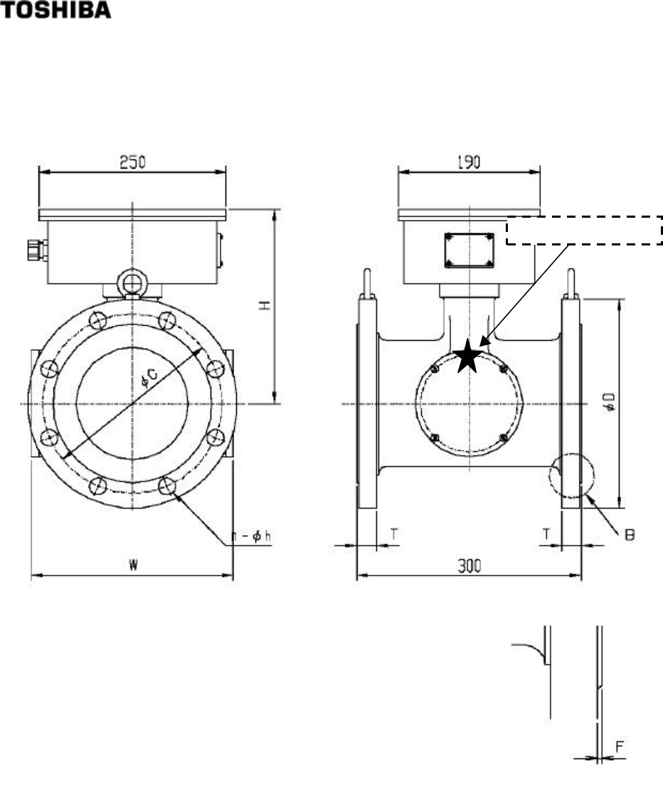
107
6 F 8 A 0 5 2 1
APPENDIX 1
Attached Figure1. Detector outline dimensions
●
The center of gravity
C: Bolt pitch circle
n: Number of bole holes
h: Bolt diameter
[Unit: mm]
Enlarged view of B
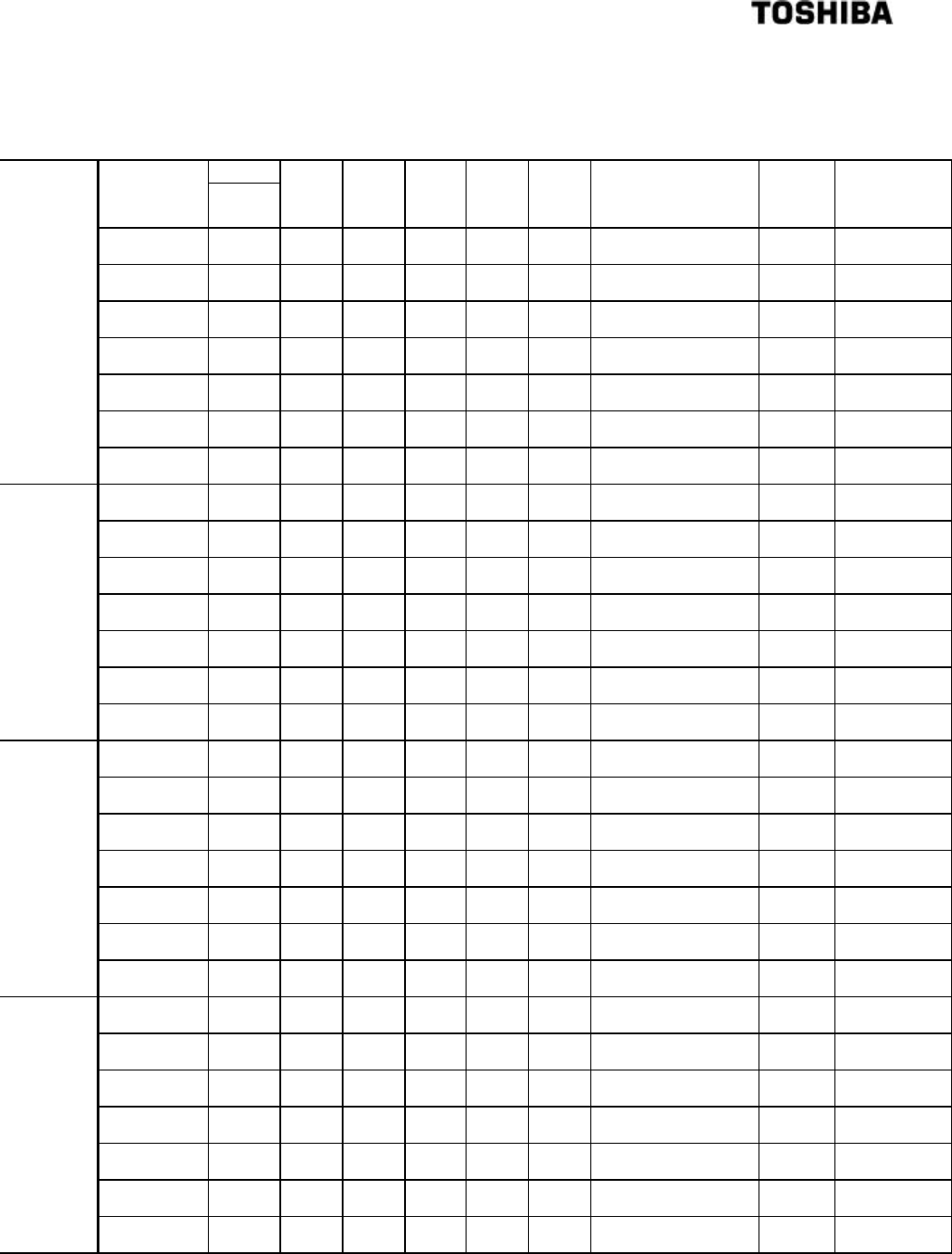
108
6 F 8 A 0 5 2 1
External dimensions (Flange)
H
Meter size
(mm) Std.
spec.
W D T F C Appropriate bolt
size
(Diameter × length)
n-Φh Mass (kg)
50 225 170
155 16 2 120
M16×60 4-19 Approx. 21
80 225 200
185 18 2 150
M16×65 8-19 Approx. 26
100 240 220
210 18 2 175
M16×65 8-19 Approx. 29
150 260 270
280 22 2 240
M20×75 8-23 Approx. 42
200 290 320
330 22 2 290
M20×75 12-23 Approx. 48
250 315 300
400 24 2 355
M22×80 12-25 Approx. 64
JIS10K
300 340 360
445 24 3 400
M22×85 16-25 Approx. 76
50 225 170
152.4
19.1
1.5 120.7
M16×60 4-19.1
Approx. 21
80 225 200
190.5
23.9
1.5 152.4
M16×70 4-19.1
Approx. 31
100 240 220
228.6
23.9
1.5 190.5
M16×70 8-19.1
Approx. 34
150 260 270
279.4
25.4
1.5 241.3
M20×80 8-22.4
Approx. 44
200 290 320
342.9
28.4
1.5 298.5
M20×80 8-22.4
Approx. 54
250 315 300
406.4
30.2
1.5 362.0
M22×90 12-25.5
Approx. 68
ANSI150
300 340 360
482.6
31.8
1.5 431.8
M22×90 12-25.4
Approx. 99
50 225 170
165 18 3 125
M16×60 4-18 Approx. 22
80 225 200
200 20 3 160
M16×70 8-18 Approx. 30
100 240 220
220 20 3 180
M16×70 8-18 Approx. 31
150 260 270
285 22 3 240
M20×80 8-22 Approx. 43
200 290 320
340 24 3 295
M20×80 8-22 Approx. 54
250 315 300
395 26 3 350
M22×90 12-22 Approx. 65
DIN10
&
BS10
300 340 360
445 26 4 400
M22×90 12-22 Approx. 78
50 225 170
165 18 3 125
M16×60 4-18 Approx. 22
80 225 200
200 20 3 160
M16×70 8-18 Approx. 30
100 240 220
220 20 3 180
M16×70 8-18 Approx. 31
150 260 270
285 22 3 240
M20×80 8-22 Approx. 43
200 290 320
340 24 3 295
M20×80 12-22 Approx. 52
250 315 300
405 26 3 355
M22×90 12-26 Approx. 68
DIN16
300 340 360
460 28 4 410
M22×90 12-26 Approx. 85
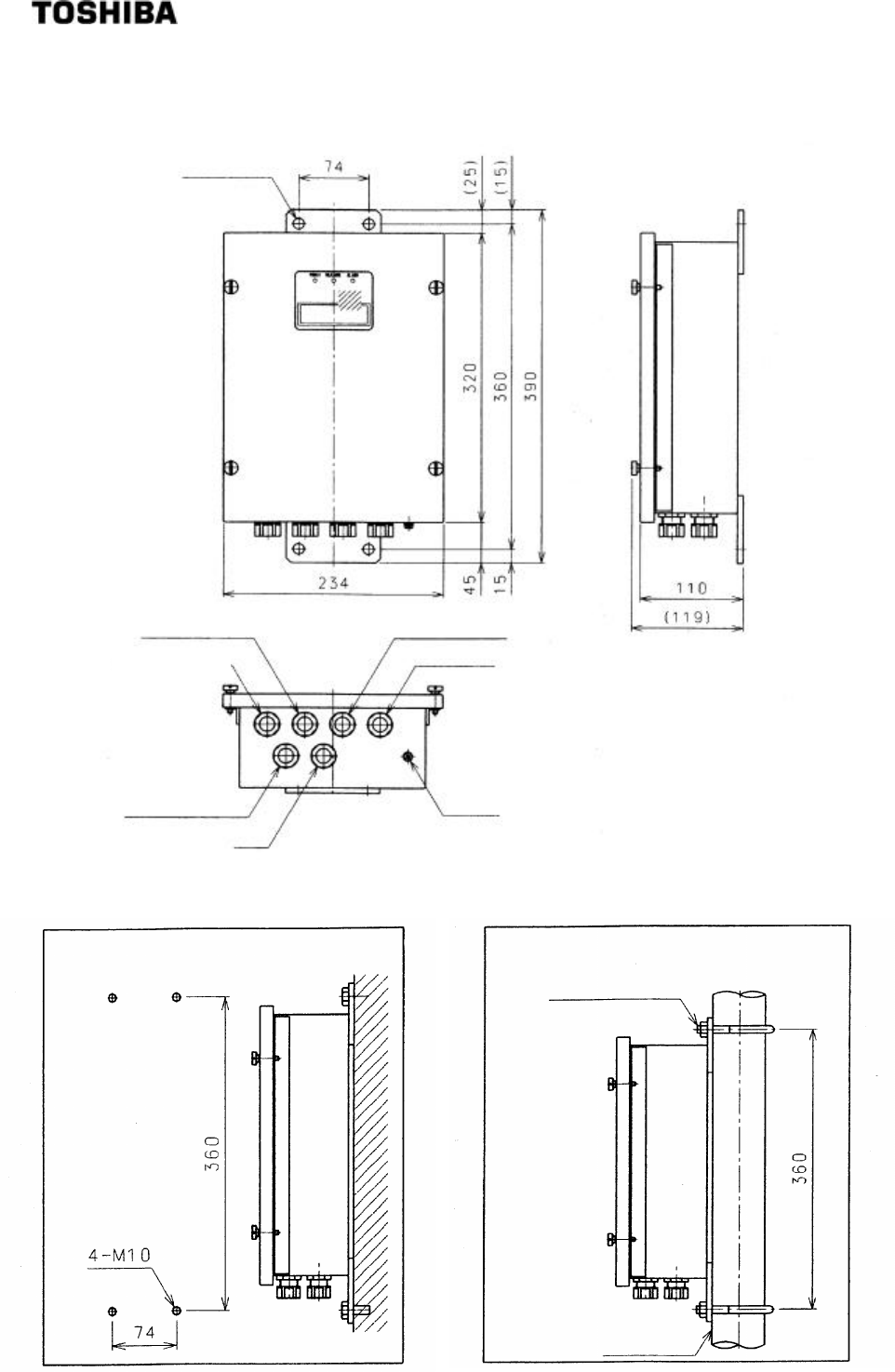
109
6 F 8 A 0 5 2 1
Attached Figure2. Converter dimensions
●
[Unit: mm]
4-φ12 mounting holes
Converter communication port
Converter power
supply cable port
Contact signal I/O (1) port
Density signal output port
Contact signal
I/O (2) port
Rerserved
Grounding terminal
In the case of wall mounting
In the case of 50A mounting
Marine-use steel
pipe mounting U bolt
Steel pipe (50A)
APPENDIX 3
Microwave Density Meter LQ500 has been confirmed to comply with the requirements of the EMC
directive 89/336/EEC and the low voltage directive 93/68/EEC. And Microwave Density Meter of model
number LQ500******D** has been confirmed to comply with the requirements of the Pressure Equipment
directive 97/23/EC.
EMC directive
This device has been tested in a typical configuration in accordance with the following standards in an
industrial environment.
・Generic emission standard EN50081-2 : 1994
Radiated RF Emission EN55011 Class A
Conducted RF Emission EN55011 Class A
Limits for harmonic current emissions EN61000-3-2
・Generic immunity standard EN50082-2 : 1995
Radiated RF Immunity ENV50140
Conducted RF Immunity ENV50141
Radiated RF Immunity ENV50204
Electrostatic Discharge Immunity EN61000-4-2
Electrical Fast Transient Immunity EN61000-4-4
Low voltage directive
Low voltage standards EN61010-1, /A2
Safety requirements for electrical equipment for measurement control and laboratory use (amended)
Over voltage category Ⅱ
Altitude Up to 2000m
Pressure equipment directive
Conformity assessment procedure : module H
