Understanding Digital Audio Sampling
This document delves into the foundational principles of digital audio, tracing its roots back to Claude Shannon's information theory and the advent of technologies like the Compact Disc. It highlights how sampling theory, while fundamental, remains a subject of misunderstanding even among audio professionals.
Rob Watts' Filter Philosophy
Chord Electronics' Digital Design Consultant, Rob Watts, has challenged conventional industry practices by developing increasingly longer digital filters for their DACs. This approach, driven by the pursuit of enhanced sound quality, contrasts with the shorter filters typically employed in high oversampled DACs.
The Chord Electronics M Scaler
A significant advancement in this field is the Chord Electronics M Scaler, featuring an interpolation filter with over one million taps. This technology significantly surpasses the filter lengths found in other Chord products, such as the 'Dave' DAC, which uses 164,000 taps.
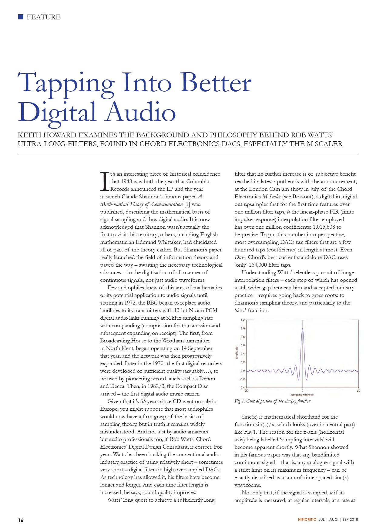
The document explains the theoretical basis for these long filters, referencing the 'sinc' function and Shannon's sampling theorem. It details how the ideal reconstruction of an analogue signal from digital samples requires a filter with a sinc function impulse response. However, practical limitations necessitate compromises in real-world DACs.
Filter Design and Implementation
The article discusses the challenges in approximating the ideal low-pass filter and the compromises made in DAC design, such as the 'sample and hold' process and the use of filters with slower roll-off rates. It contrasts typical filter designs with the theoretical ideal, illustrating the differences in frequency and impulse responses.
Rob Watts' approach utilizes a 'windowed-sinc' technique, employing his proprietary WTA (Watts Time Alignment) windowing algorithm to shape the filter excerpt for optimal transient timing. This method aims to achieve a more accurate reconstruction of the original waveform.
The Impact on Sound Quality
According to Watts, the extended filter lengths lead to improved transient accuracy, resulting in clearer instrumental timbre, tighter bass, and a more expansive soundstage. The M Scaler, in particular, is noted for its significant sonic improvements over previous Chord Electronics models.
Exploring the Technology
For those interested in experiencing this technology, the document suggests offline software interpolation as a method to understand the benefits of full sinc interpolation. It also touches upon the hardware implementation, mentioning the use of Xilinx FPGAs in products like the M Scaler.
The M Scaler is positioned as a high-end audio device, with details on its connectivity and pricing. The ongoing development suggests a continued exploration into even longer filter lengths for future audio processing advancements.
For more information on Chord Electronics products, visit Chord Electronics.
