Baron Services XDD-1000C C-BAND DOPPLER WEATHER RADAR User Manual
Baron Services Inc C-BAND DOPPLER WEATHER RADAR
Contents
- 1. Modulator Manual
- 2. Users Manual Part 1
- 3. Users Manual Part 2
- 4. Users Manual Part 3
- 5. S10 OPERATION AND MAINTENANCE MANUAL
- 6. S10 FAST TRAC MILLENIUM USERS GUIDE
- 7. S10 TECHNICAL MANUAL
- 8. S10 RECEIVER AND PROCESSOR USERS MANUAL PART 1
- 9. S10 RECEIVER AND PROCESSOR USERS MANUAL PART 2
- 10. S10 RECEIVER AND PROCESSOR USERS MANUAL PART 3
S10 RECEIVER AND PROCESSOR USERS MANUAL PART 2
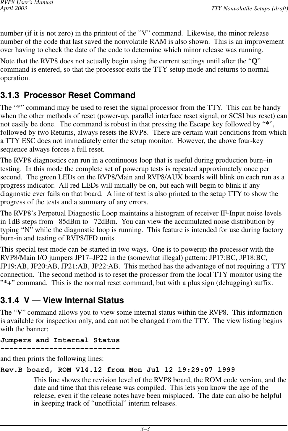
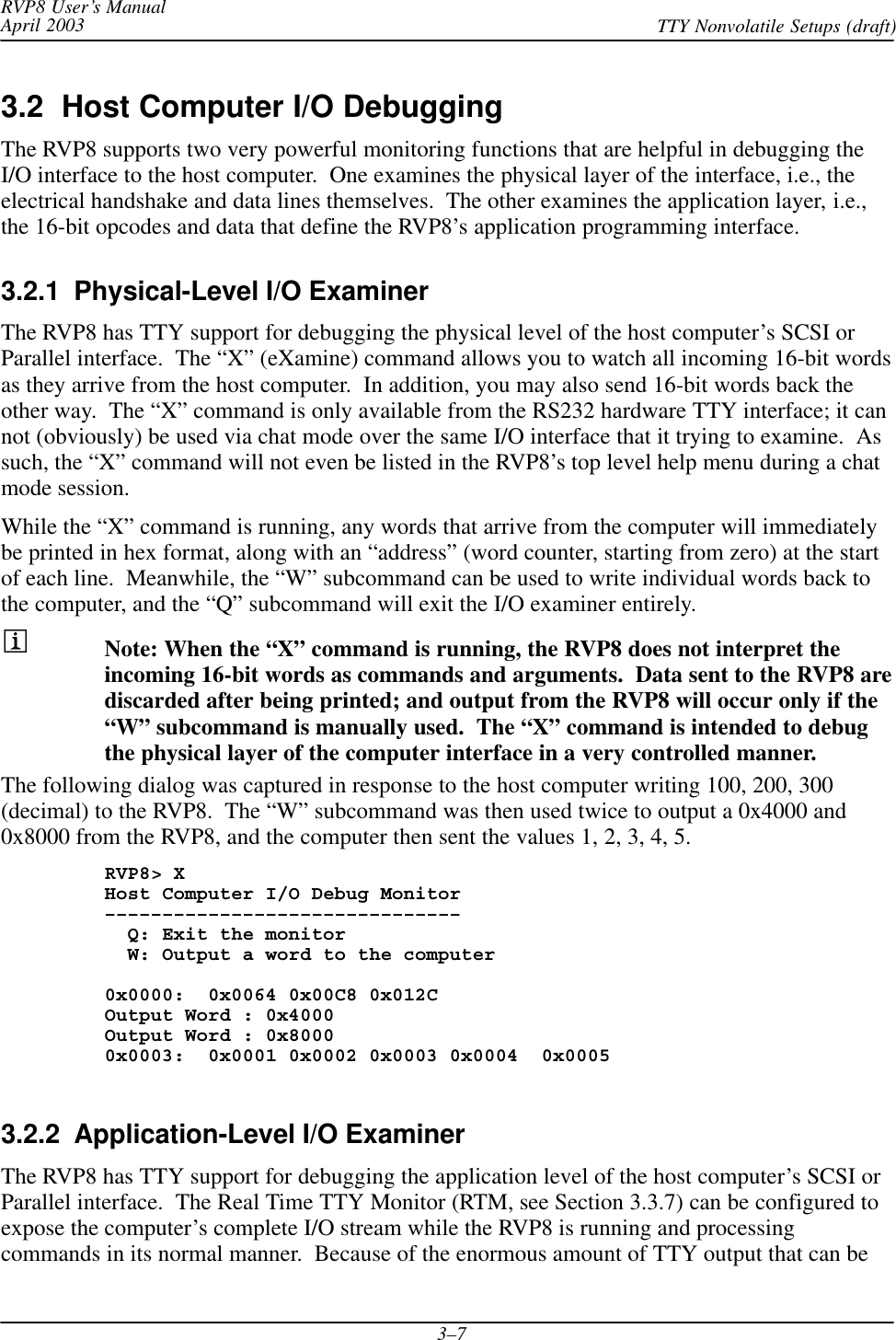
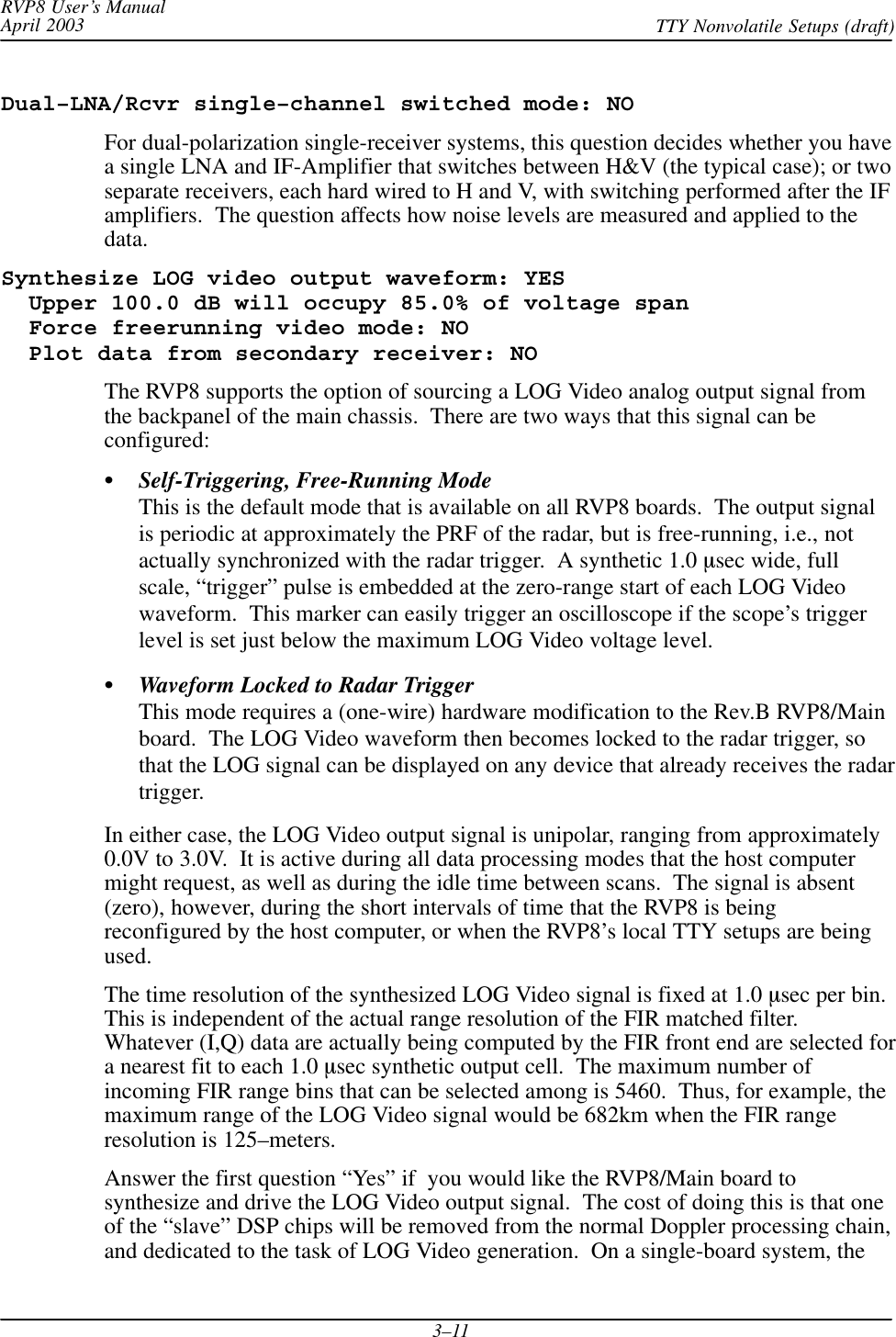
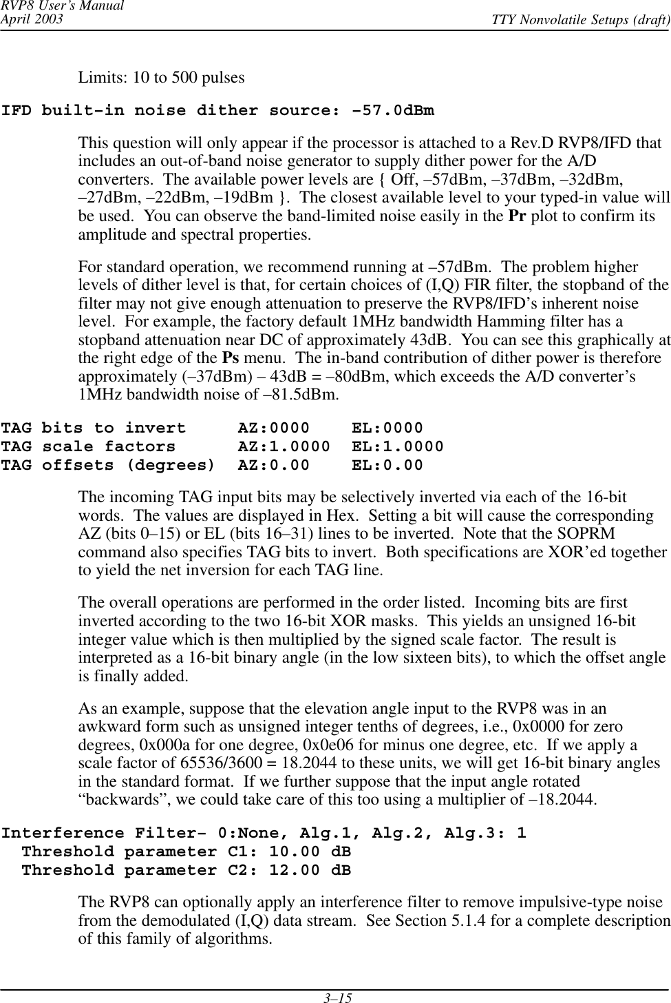
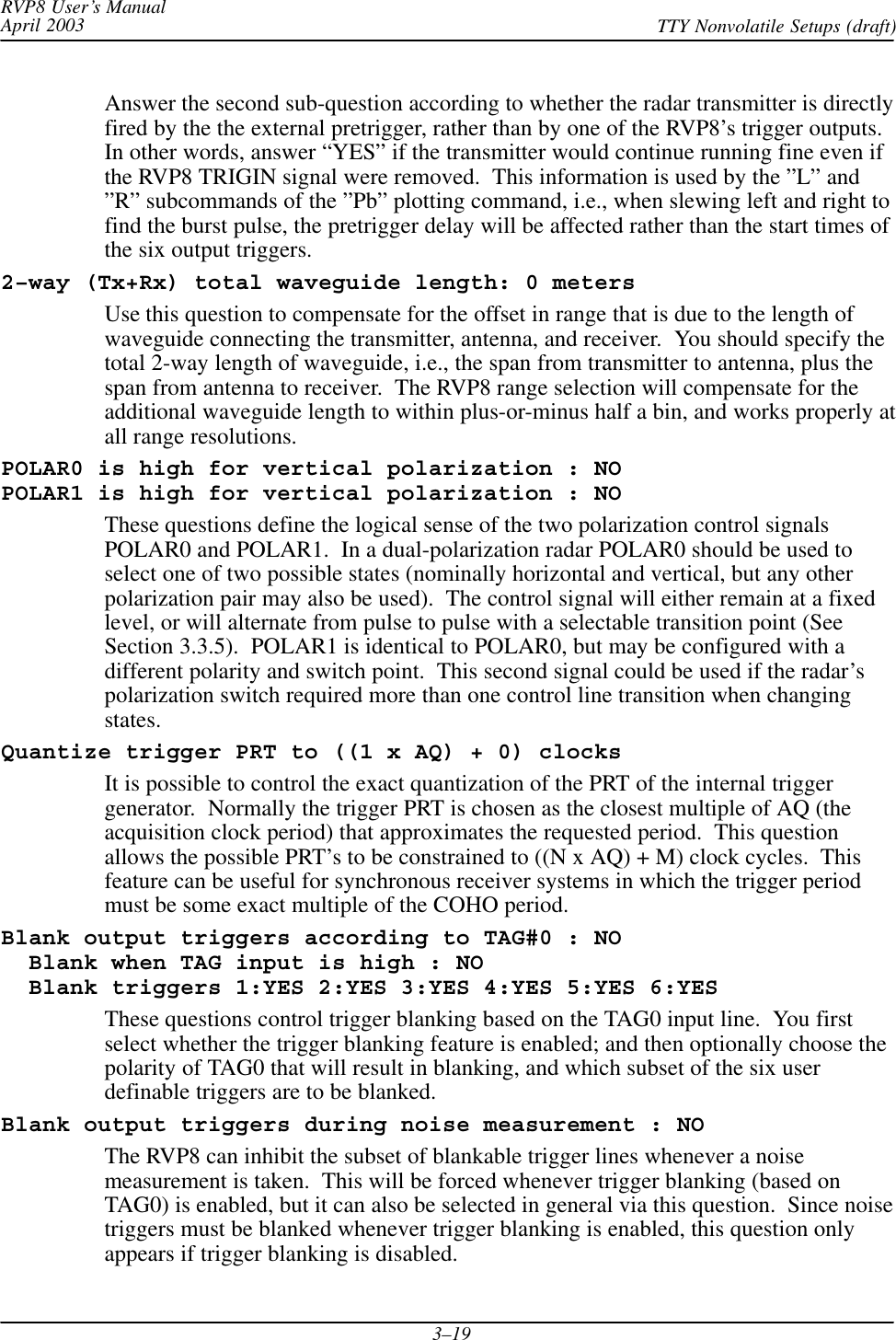
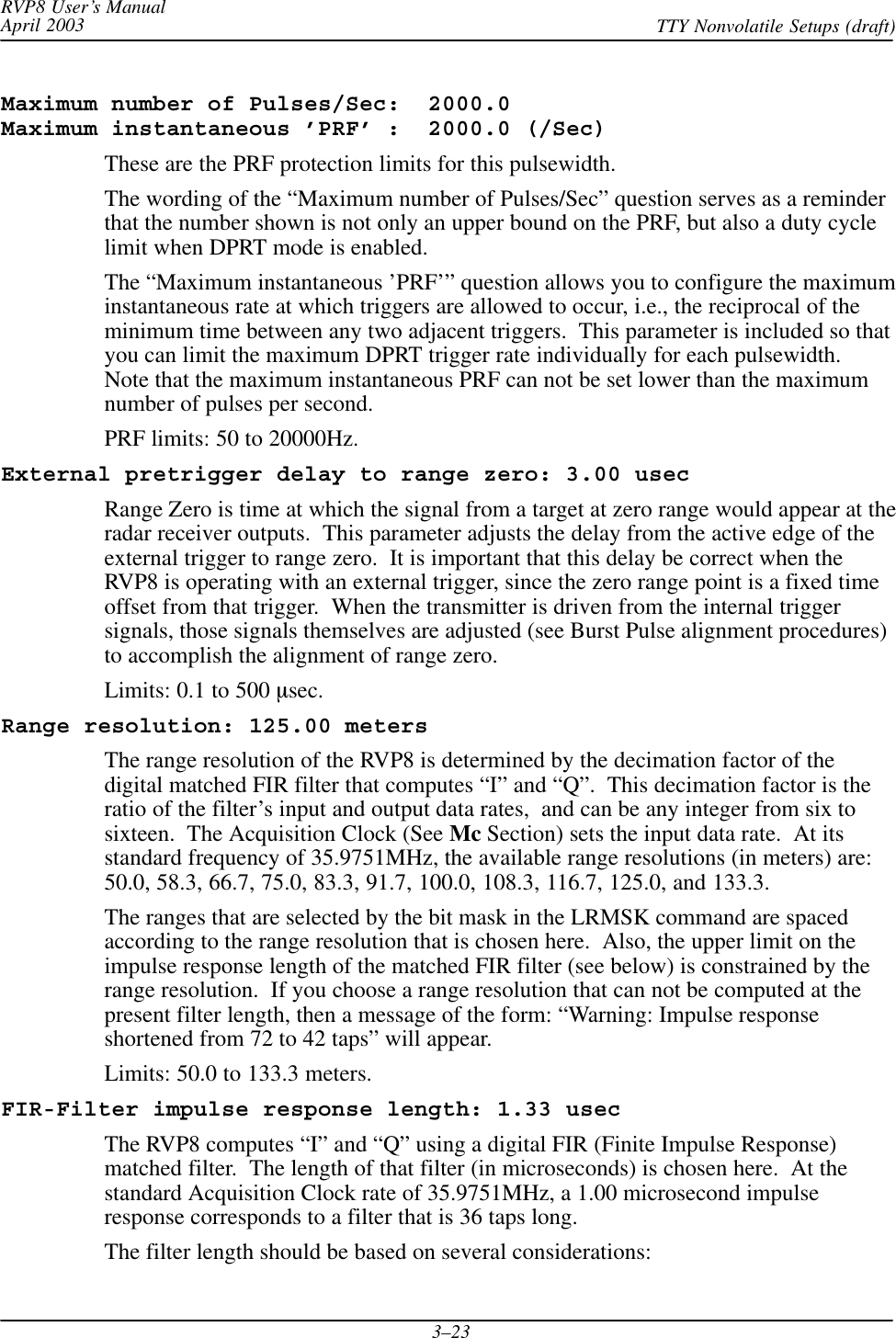
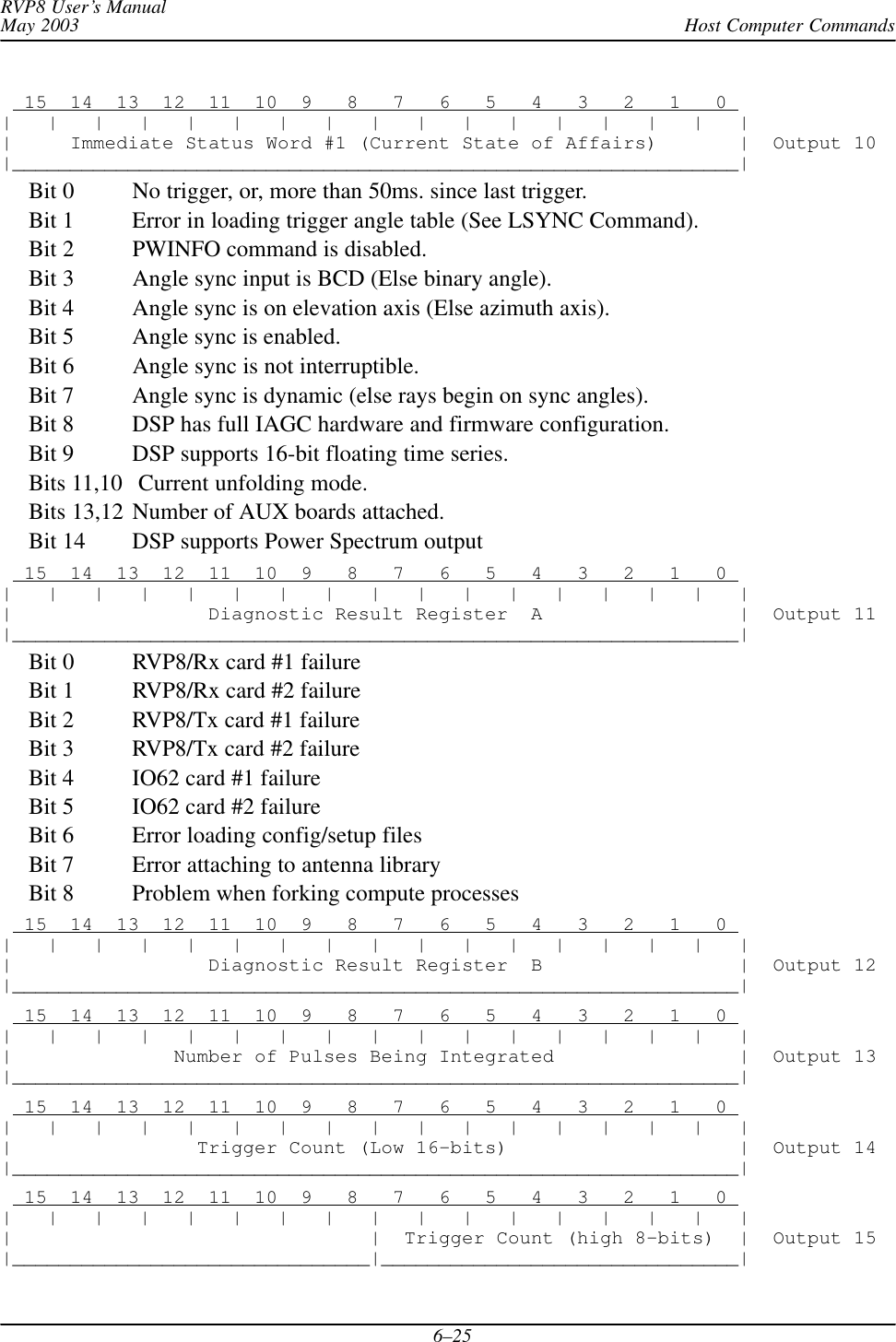
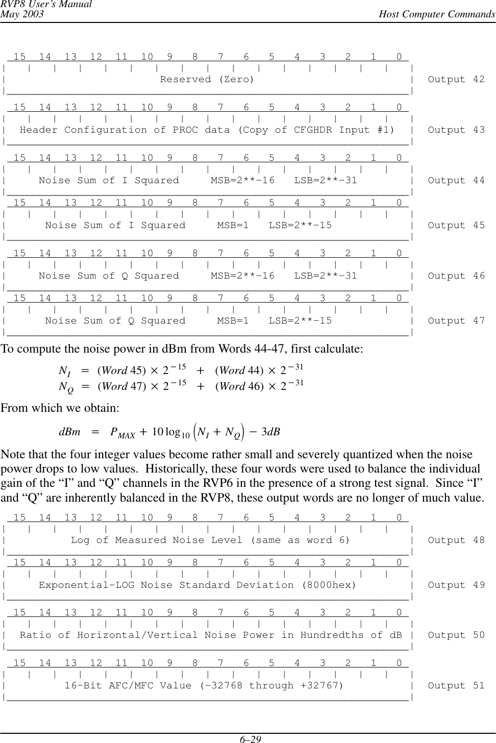
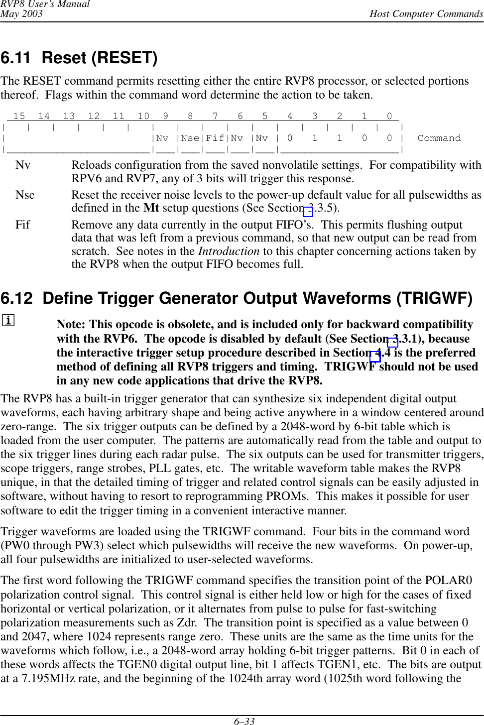
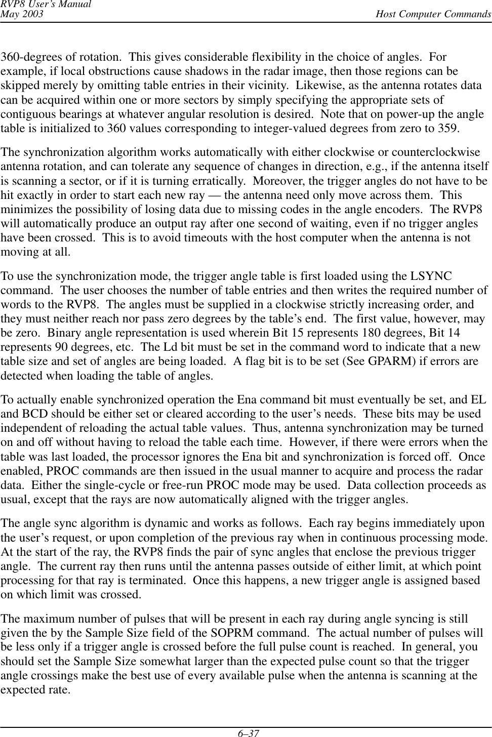
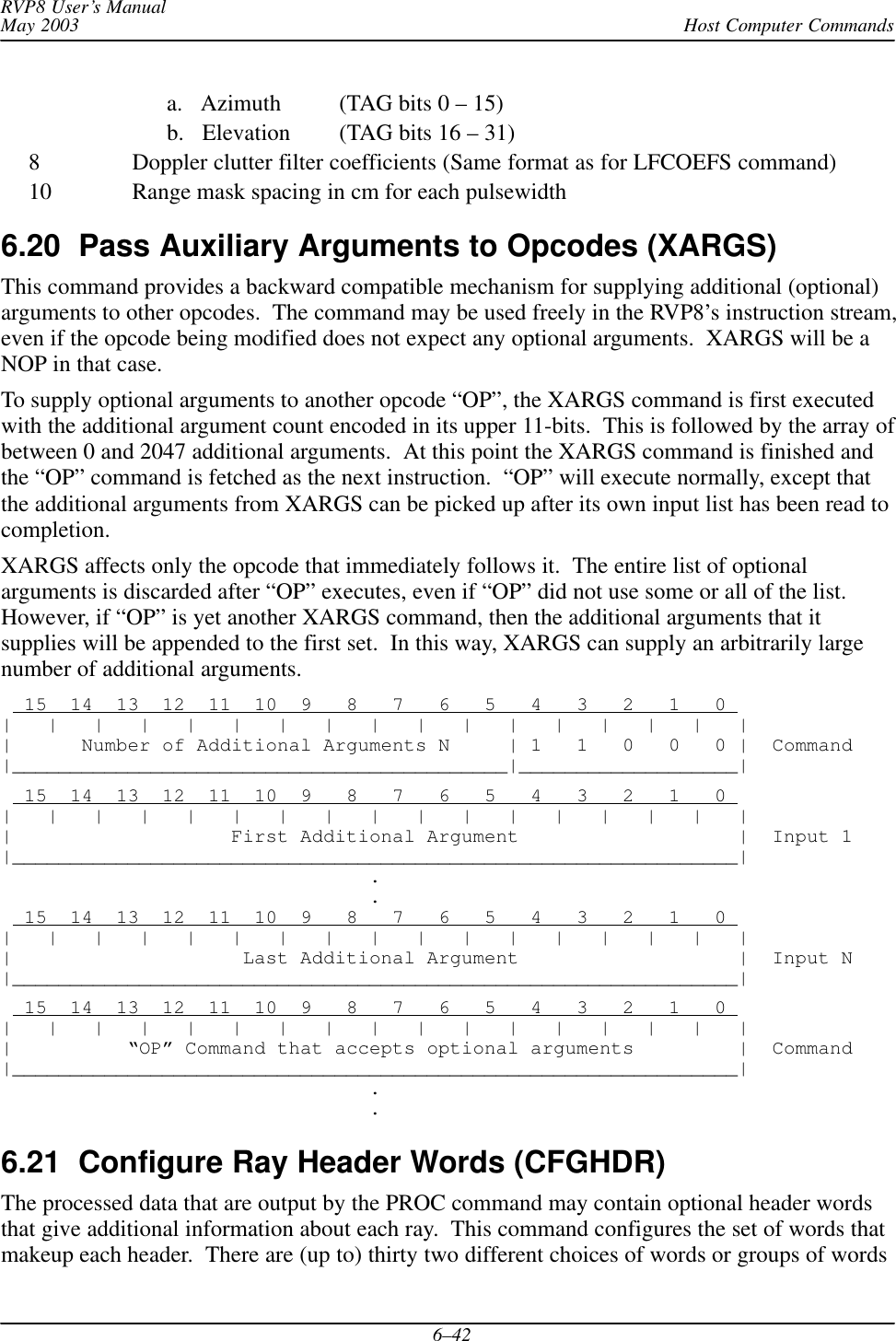
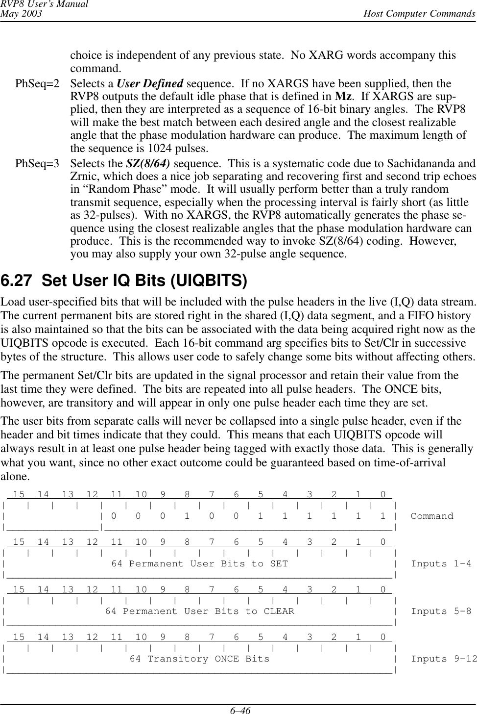
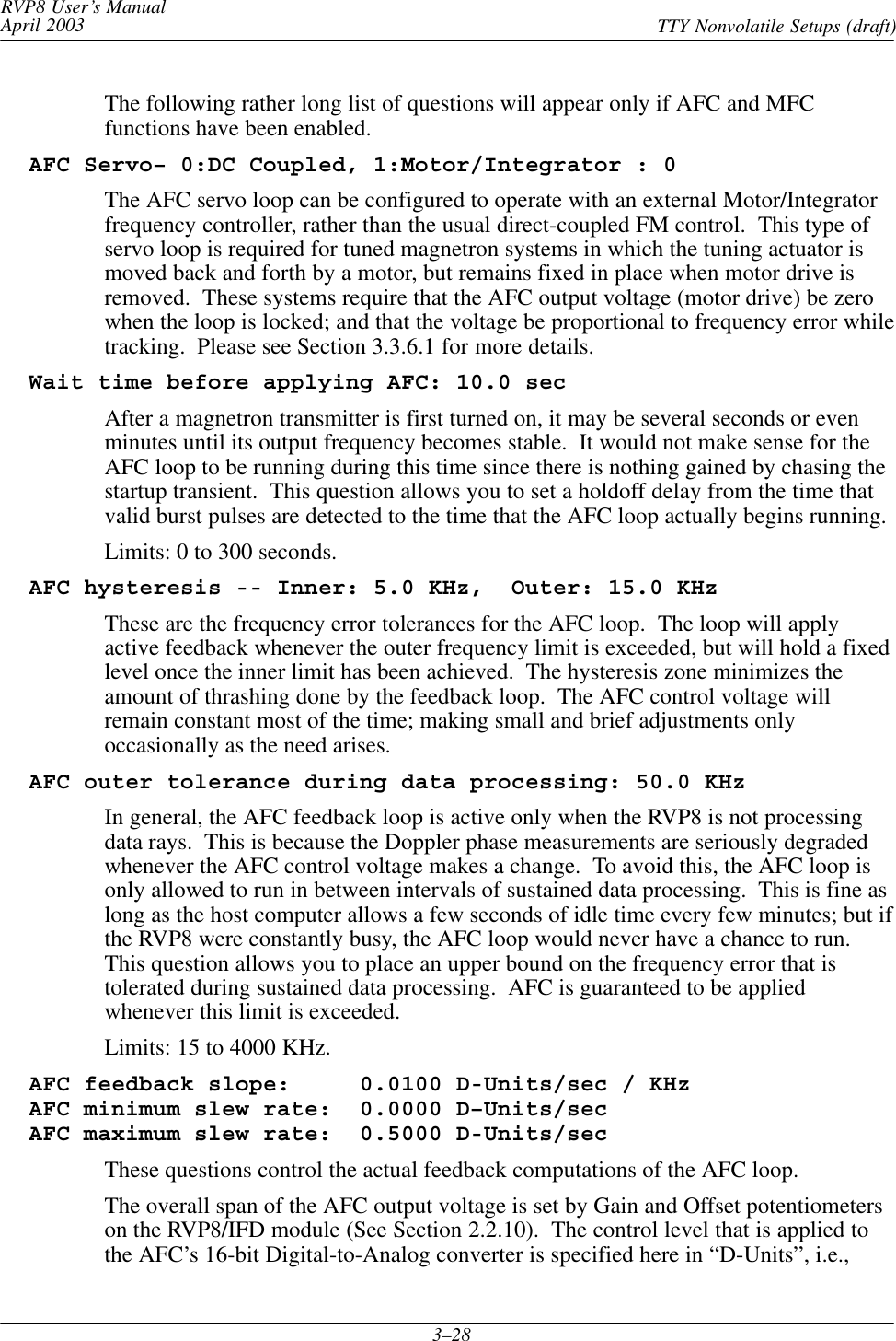
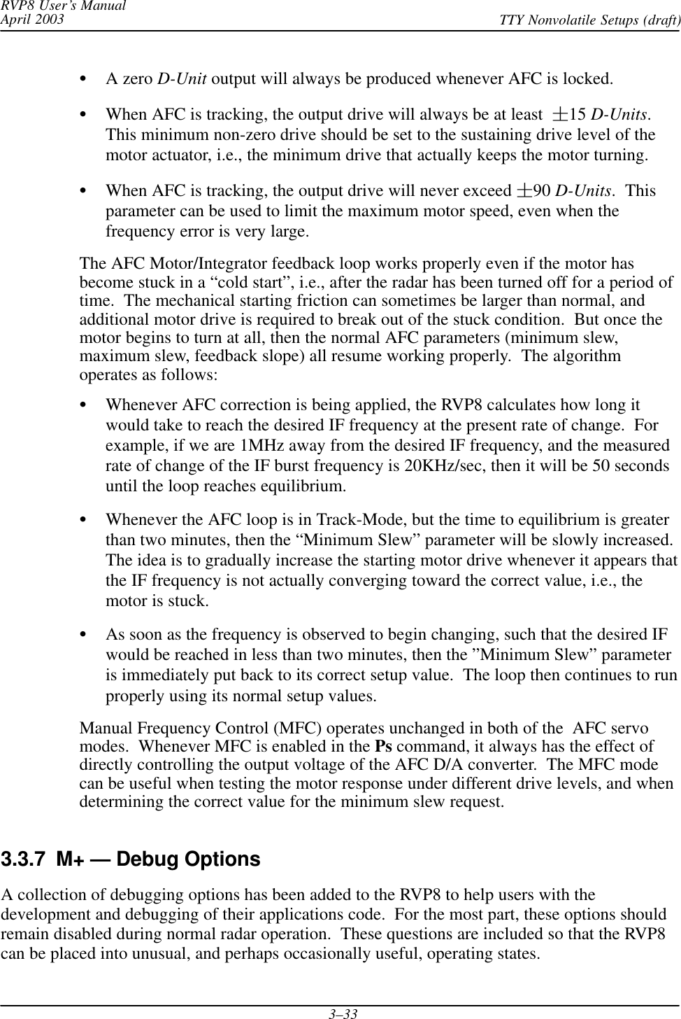
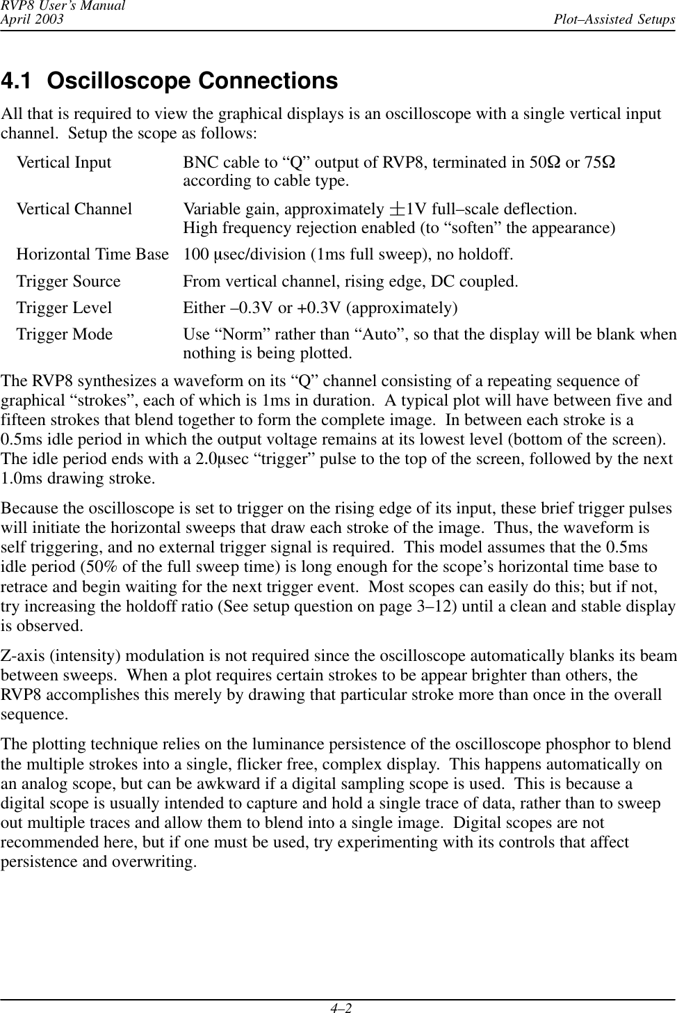
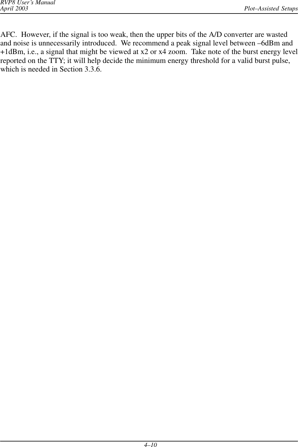
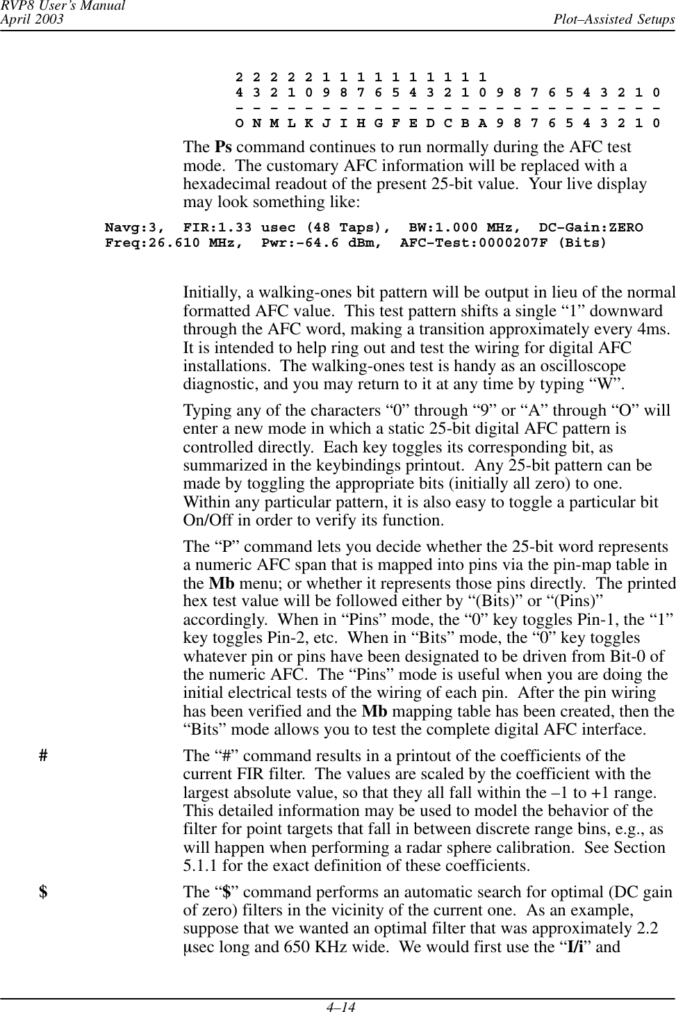
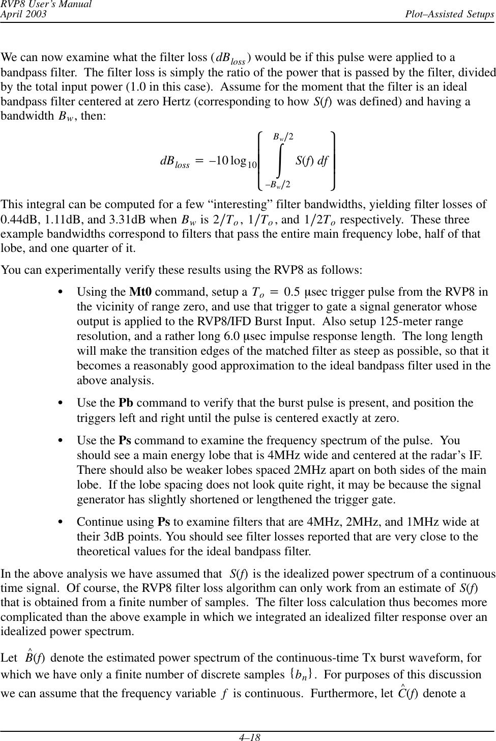
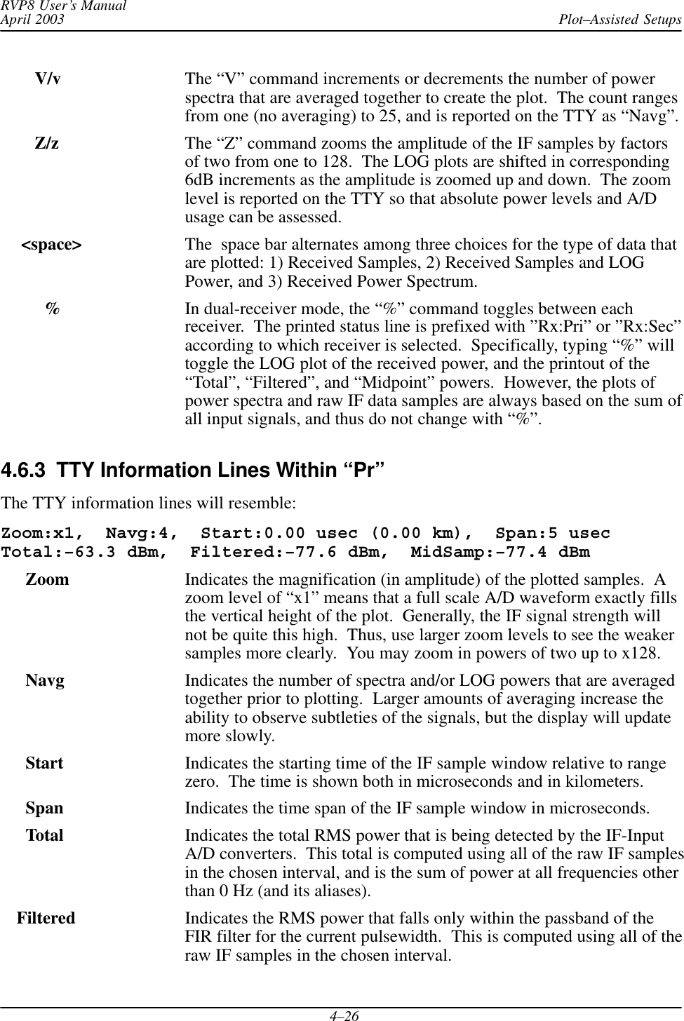
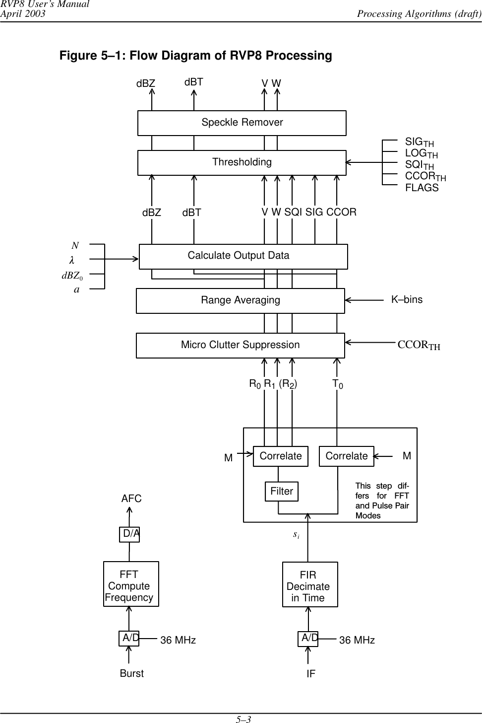
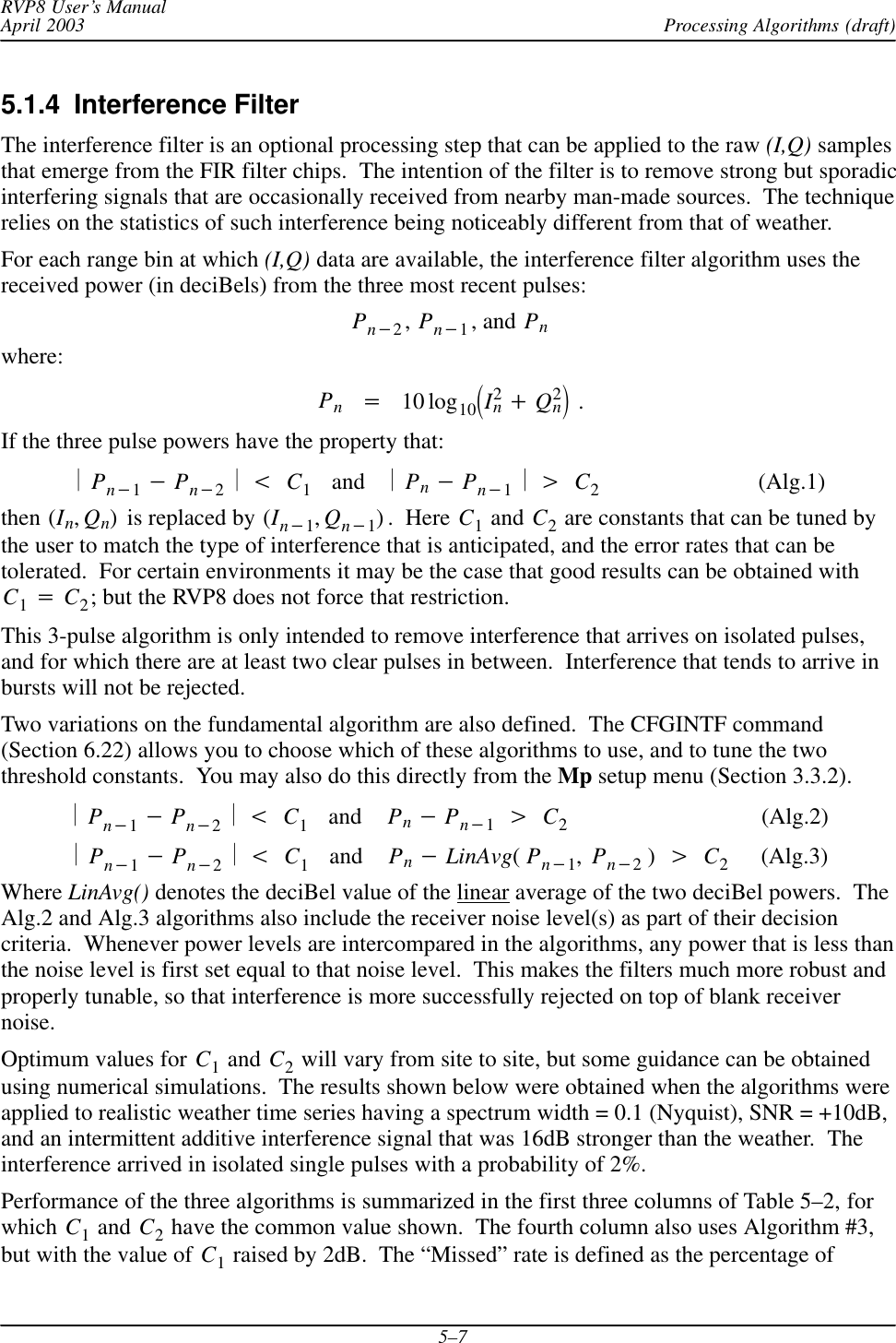
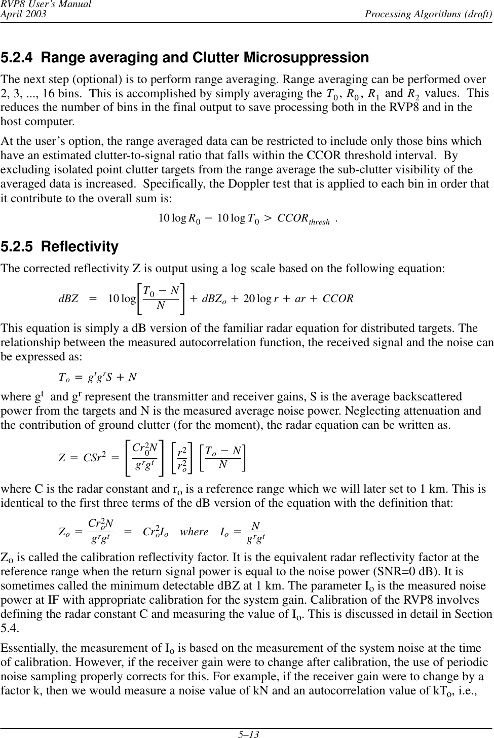
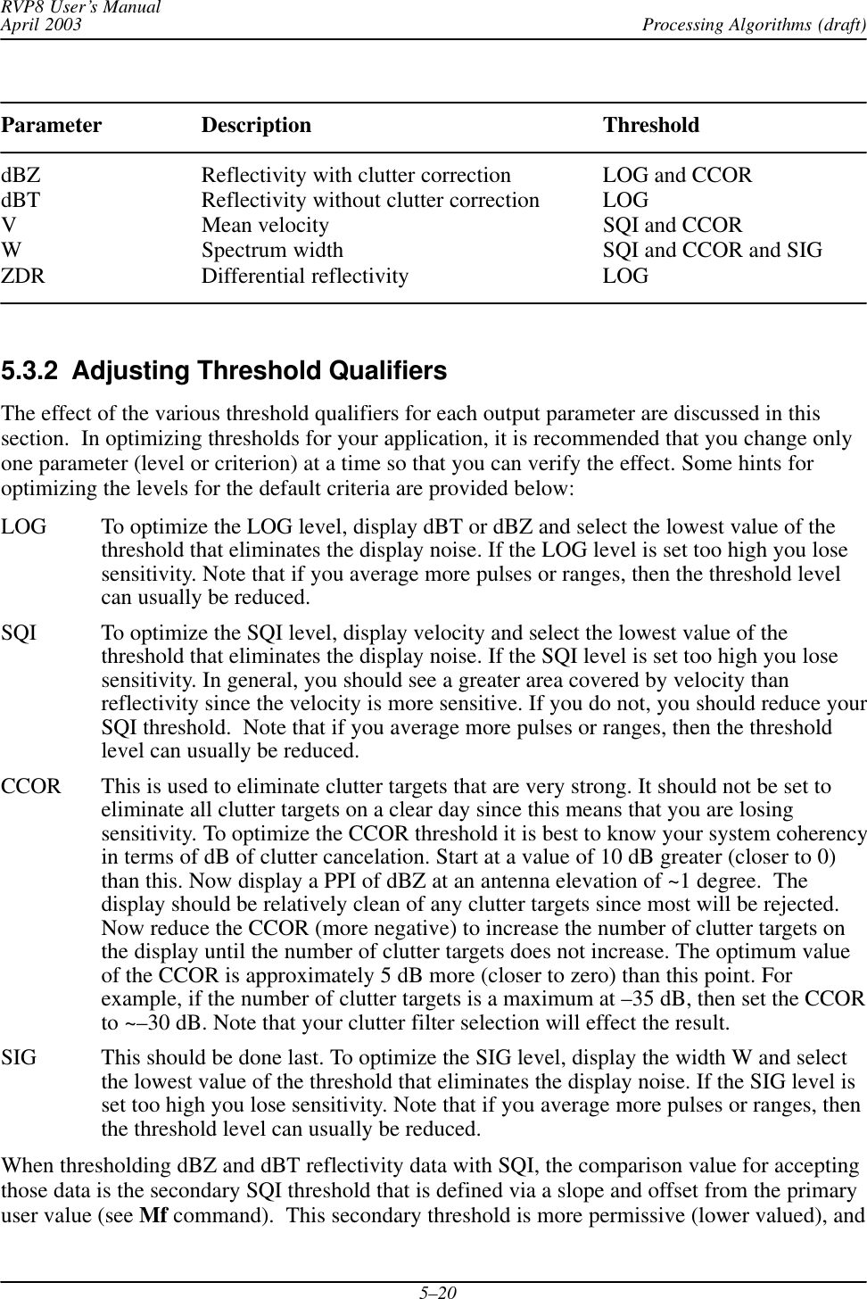
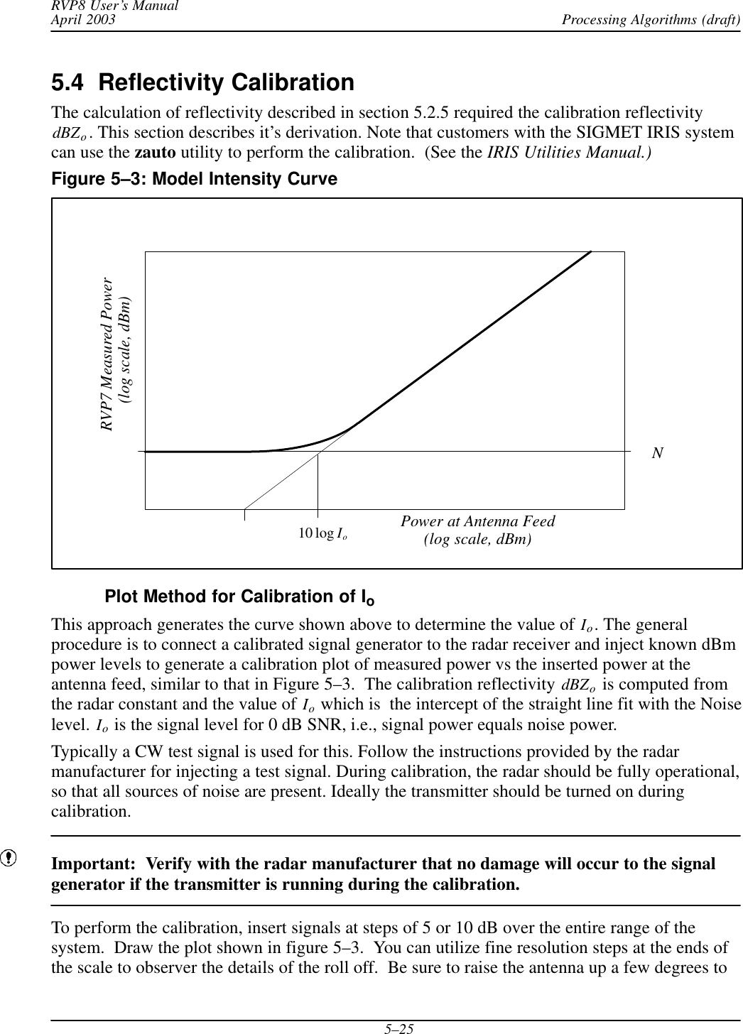
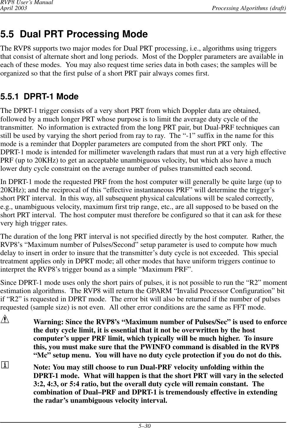
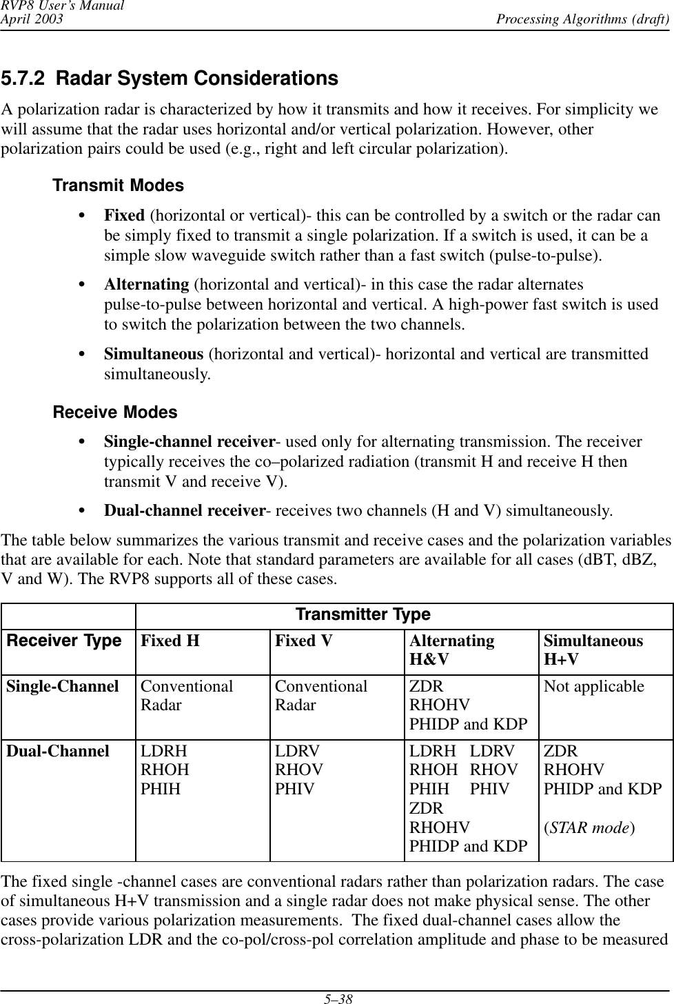
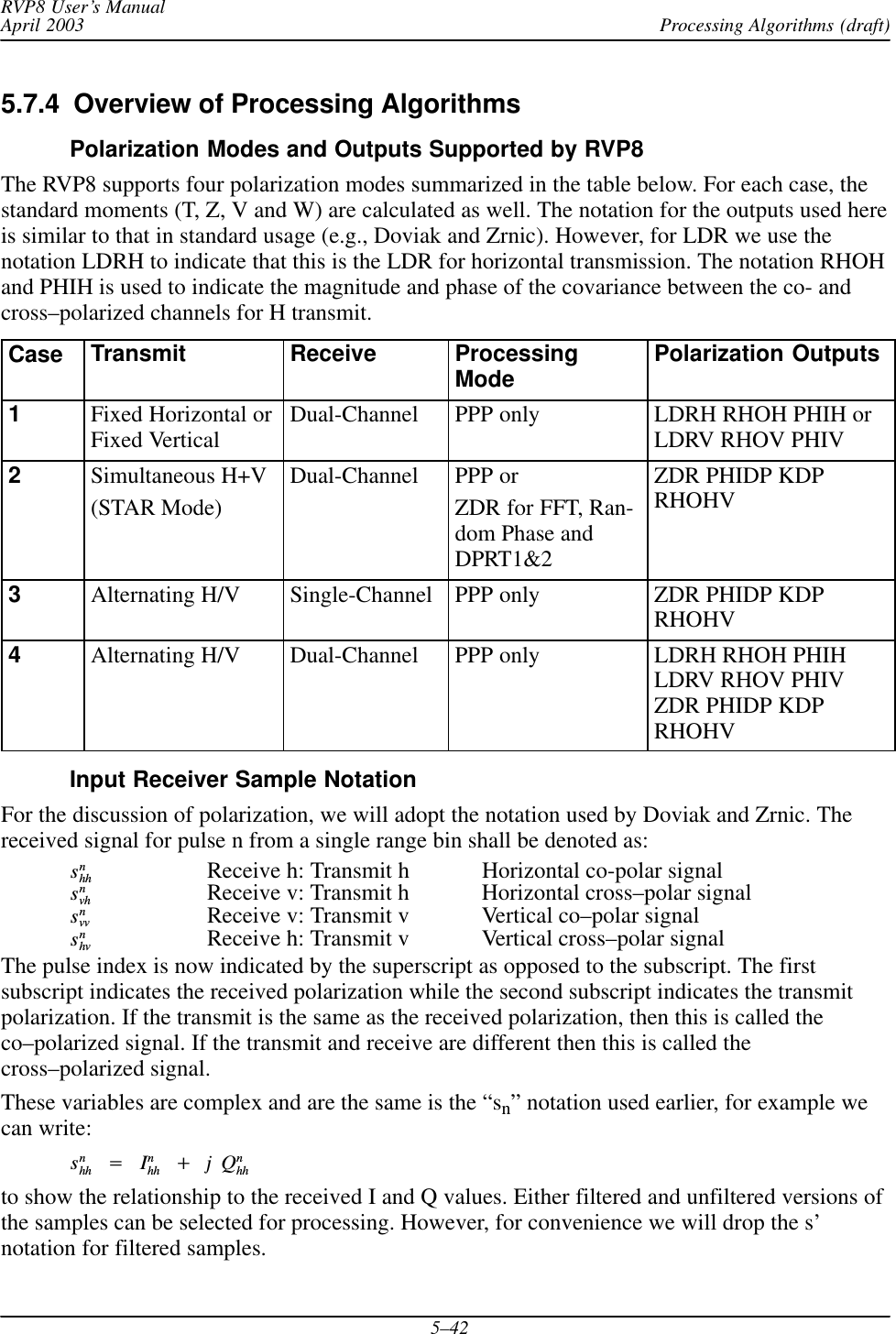
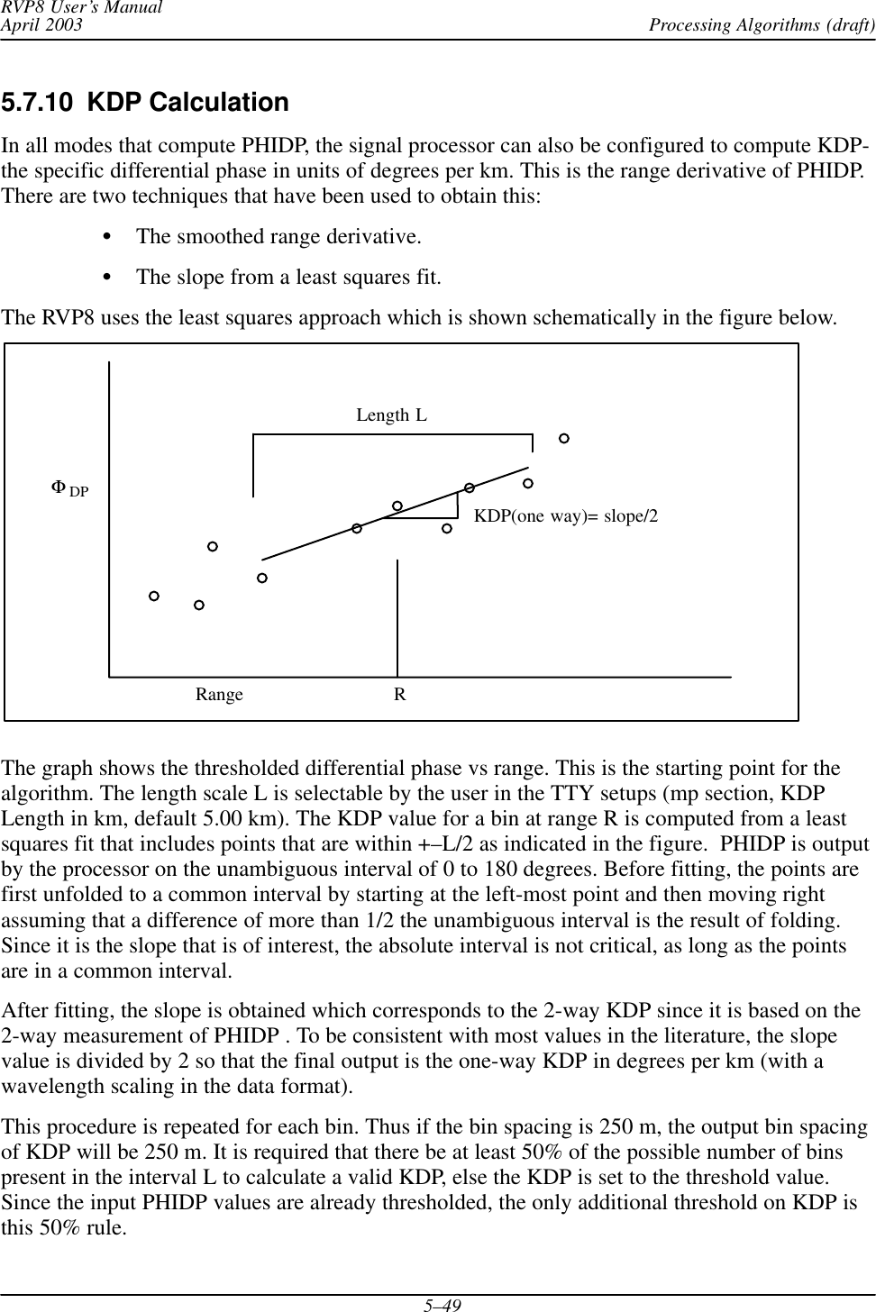
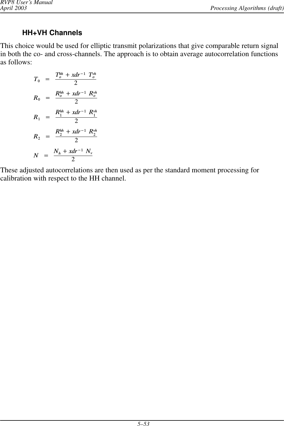
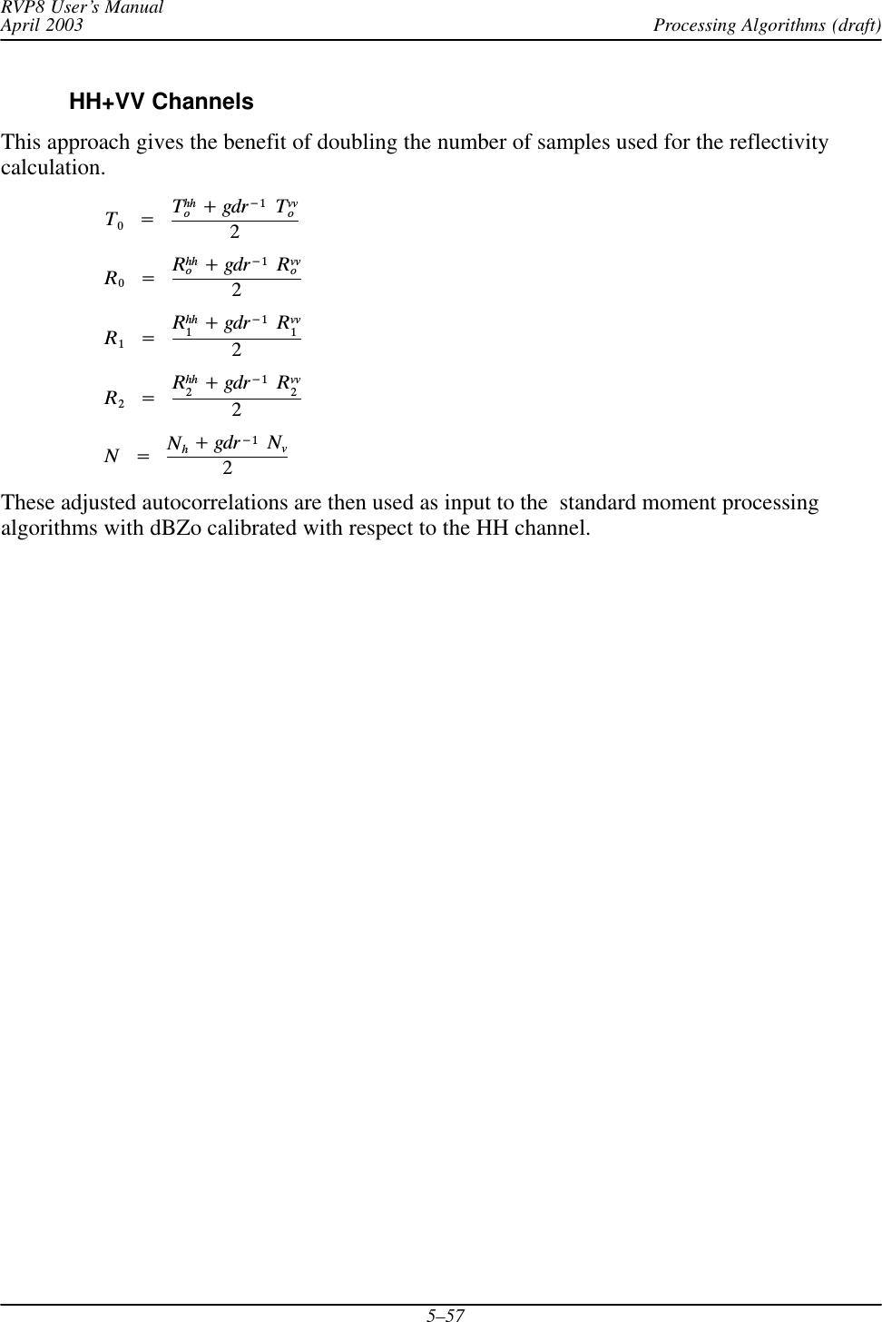
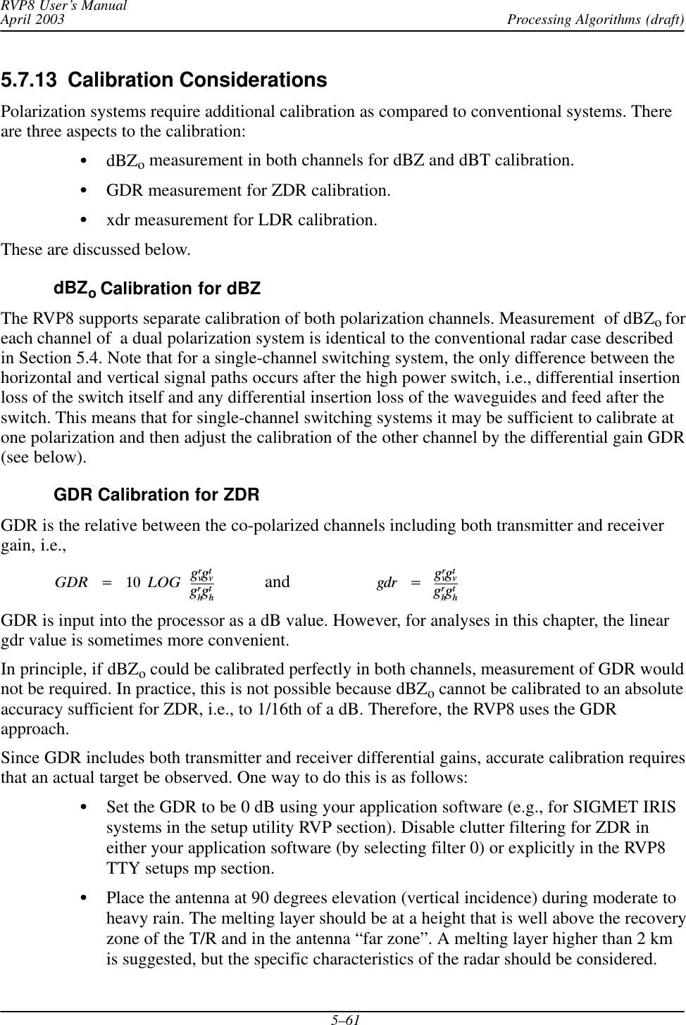
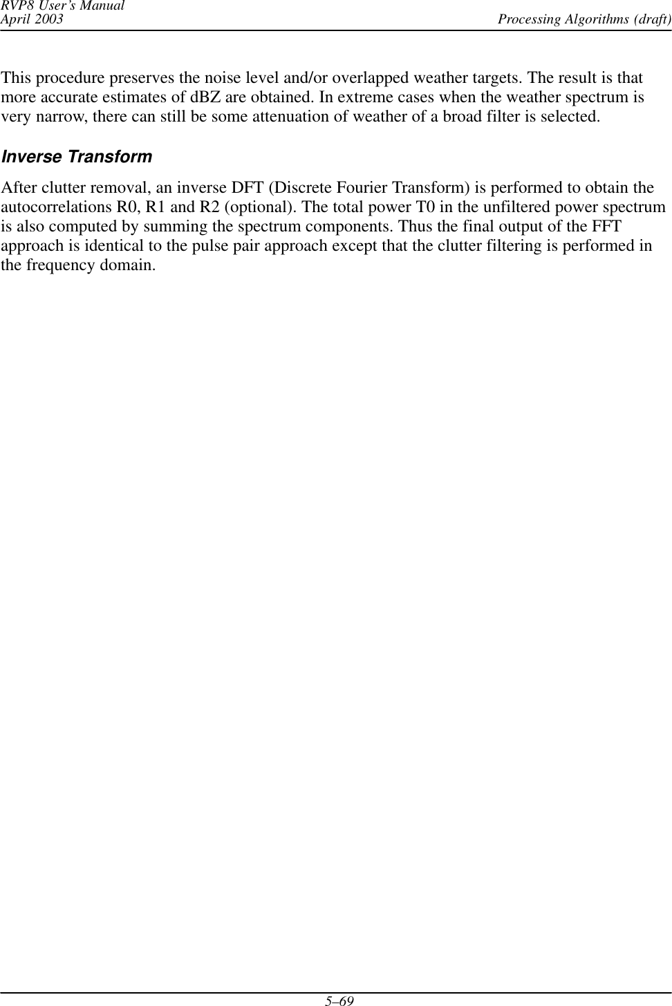
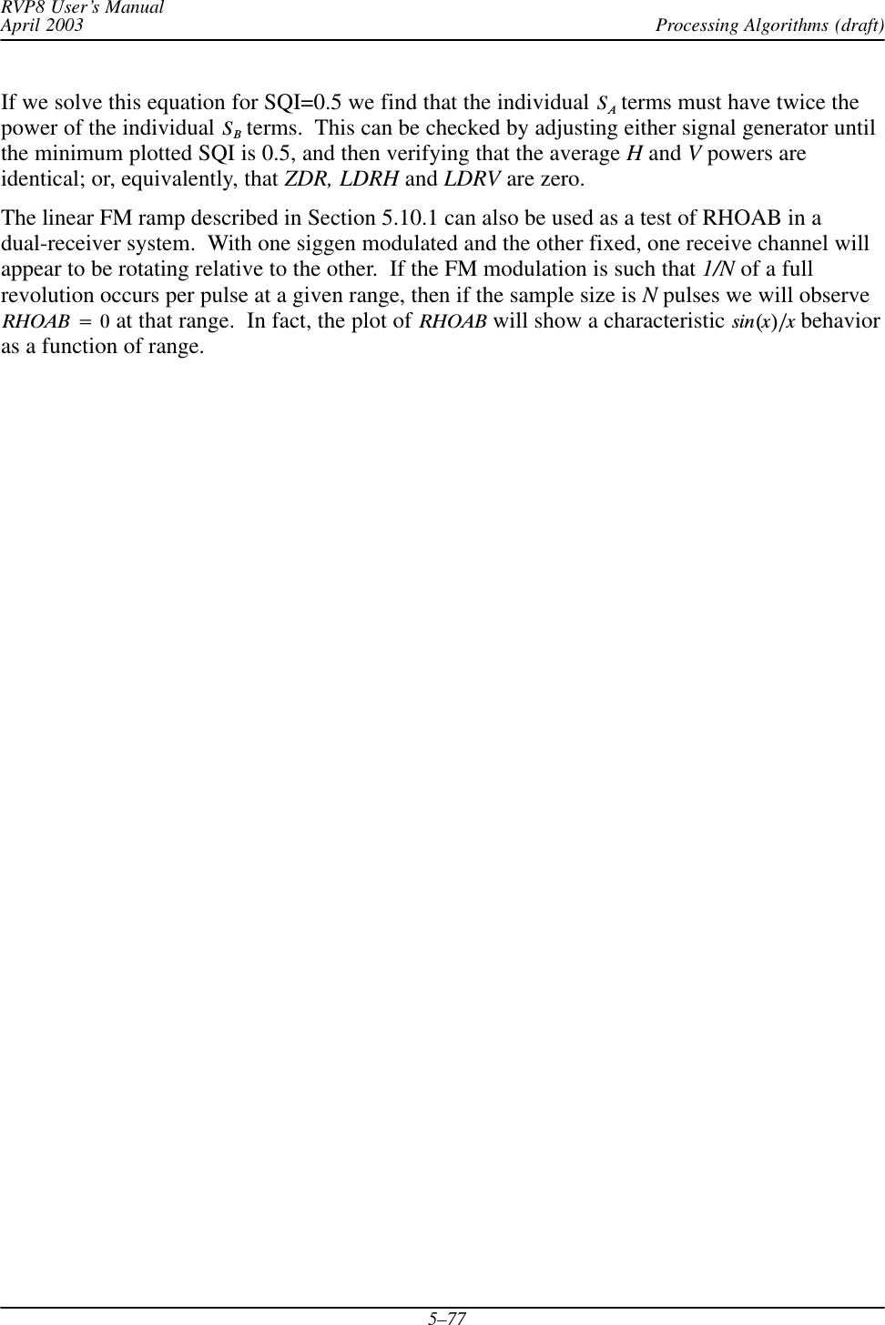
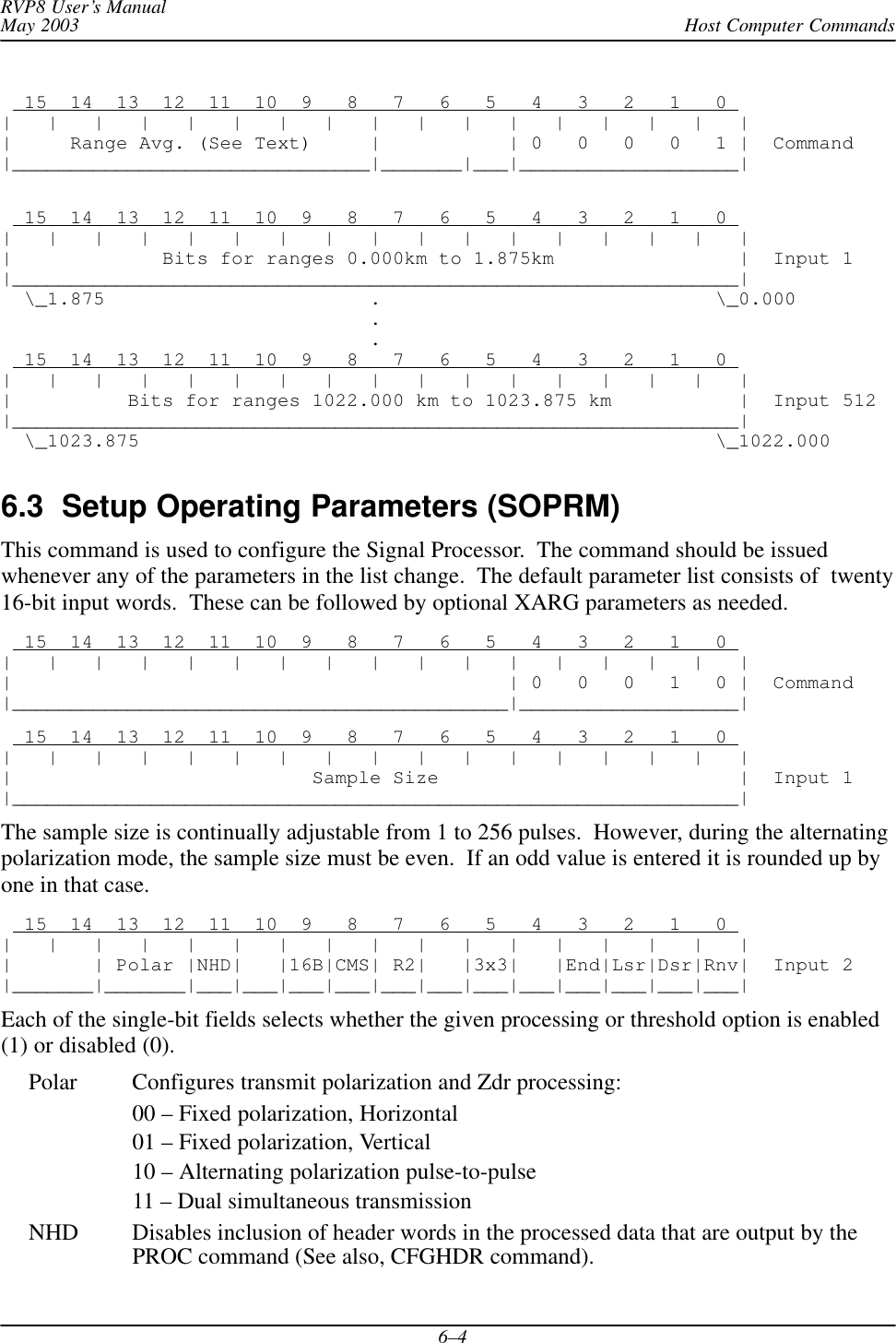
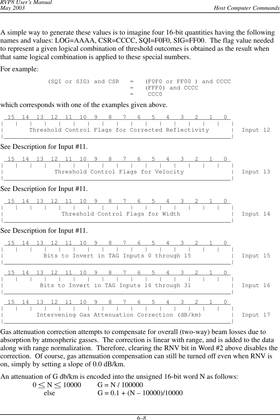
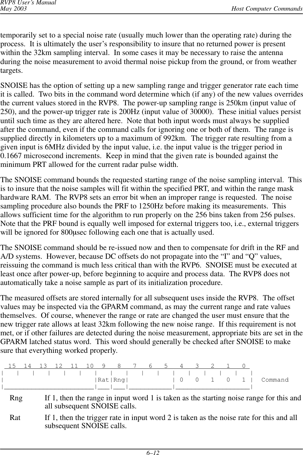
![RVP8 User’s ManualApril 2003 TTY Nonvolatile Setups (draft)3–25Output control 4–bit pattern: 0001These are the hardware control bits for this pulsewidth. The bits are the 4-bit binarypattern that is output on PWBW0:3Bit Limits: 0 to 15 (input must be typed in decimal)Current noise level: –75.00 dBmPowerup noise level: –75.00 dBm–or–Current noise levels – PriRx: –75.00 dBm, SecRx: –75.00 dBmPowerup noise levels – PriRx: –75.00 dBm, SecRx: –75.00 dBmThese questions allow you to set the current value and the power-up value of thereceiver noise level for either a single or dual receiver system. The noise level(s) areshown in dBm, and you may alter either one from the TTY. The power-up level(s)are assigned by default when the RVP8 first starts up, and whenever the RESETopcode is issued with Bit #8 set. Likewise, the current noise level is revisedwhenever the SNOISE opcode is issued. These setup questions are intended forapplications in which the RVP8 must operate with a reasonable default value, up untilthe time that an SNOISE command is actually received. They may also be used tocompare the receiver noise levels during normal operation, which serves as a checkthat each FIR filter is behaving as expected when presented with thermal noise.Transmitter phase switch point: –1.00 usecThis is the transition time of the RVP8’s phase control output lines during randomphase processing modes. The switch point should be selected so that there isadequate settling time prior to the burst/COHO phase measurement on each pulse.This question only appears if the PHOUT[0:7] lines are actually configured for phasecontrol (See Section 3.3.1).Limits: –500 to 500 msec.Polarization switch point for POLAR0: –1.00 usecPolarization switch point for POLAR1: 1.00 usecThe RVP8’s POLAR0 and POLAR1 digital output lines control the polarizationswitch in a dual-polarization radar. During data processing modes in which thepolarization alternates from pulse to pulse, the transition points of these controlsignals are set by these two questions. The values are in microseconds relative torange zero; the same units used to define the start times of the six user triggers. Thelogical sense of POLAR0 and POLAR1 is set by questions described in Section 3.3.4.Limits: –500 to 500 msec.3.3.6 Mb — Burst Pulse and AFCThese questions are accessed by typing “Mb”. They set the parameters that influence the phaseand frequency analysis of the burst pulse, and the operation of the AFC feedback loop.Receiver Intermediate Frequency: 30.0000 MHzThis is the center frequency of the IF receiver and burst pulse waveform. The RVP8can operate at an intermediate frequency from any of the three alias bands22–32MHz, 40–50MHz, and 58–68MHz. These bands are delineated by 4MHz](https://usermanual.wiki/Baron-Services/XDD-1000C.S10-RECEIVER-AND-PROCESSOR-USERS-MANUAL-PART-2/User-Guide-374023-Page-25.png)
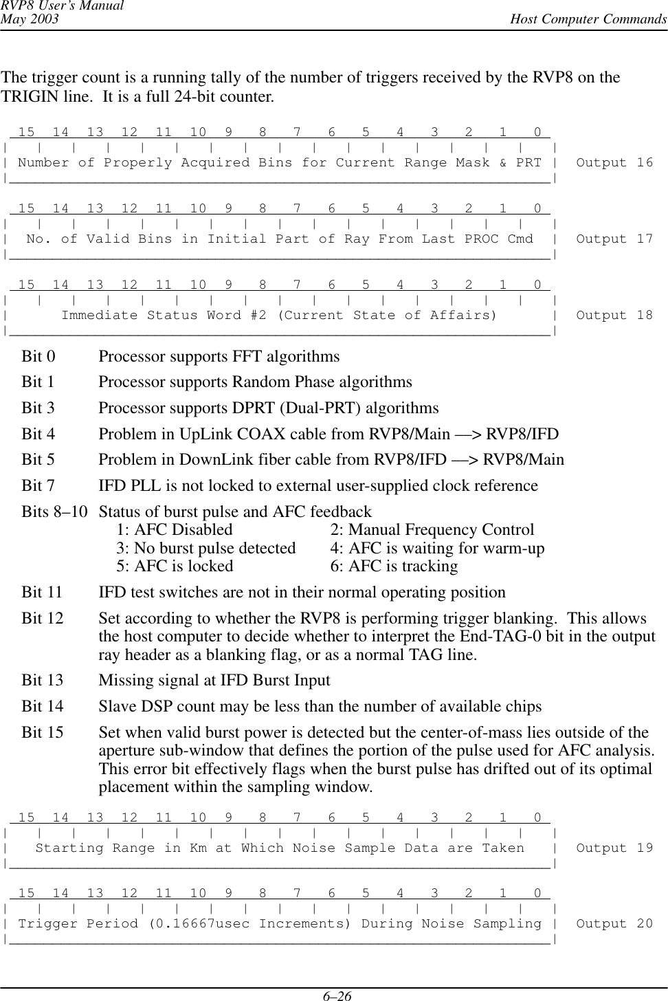
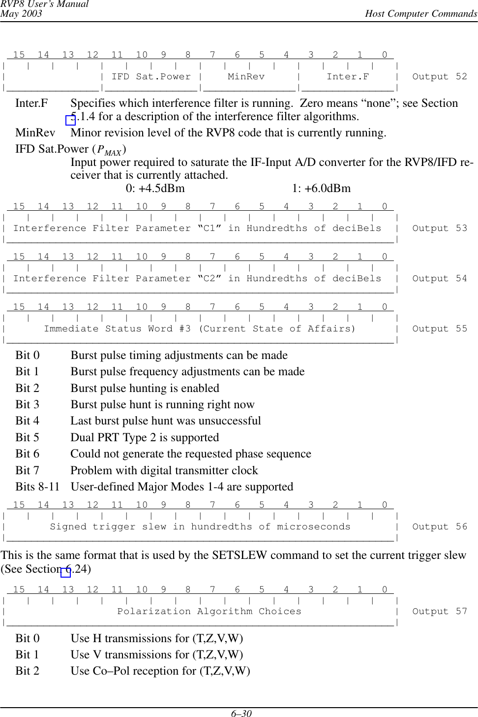
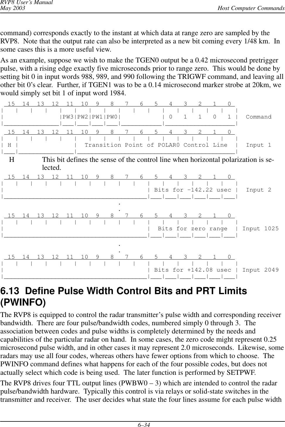
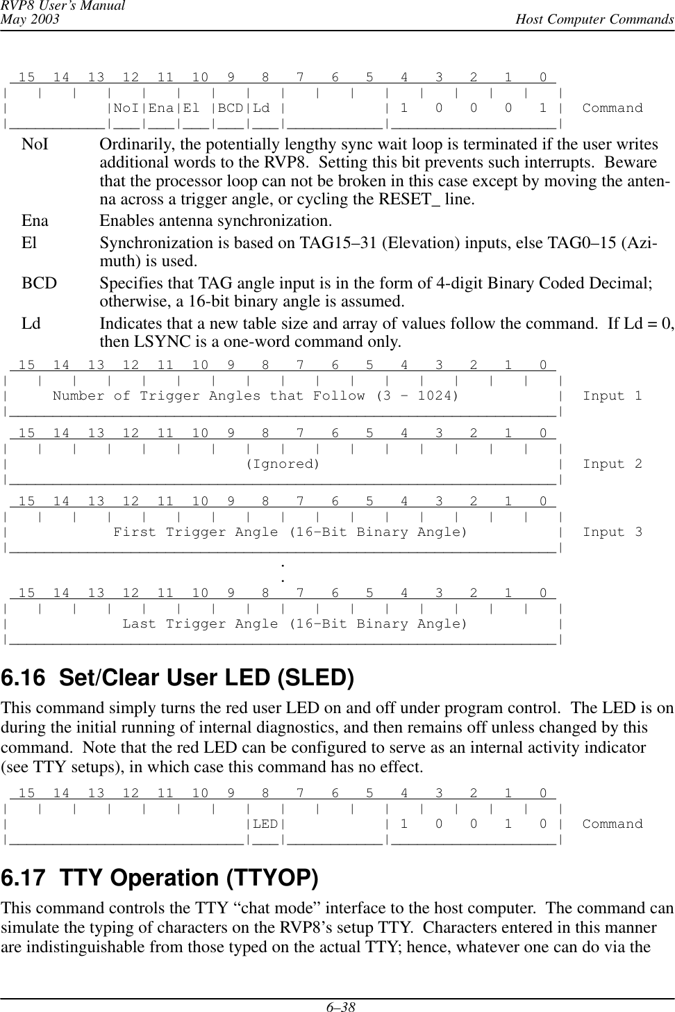
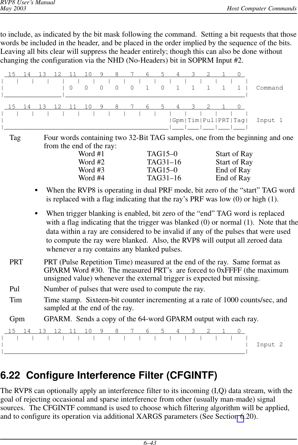
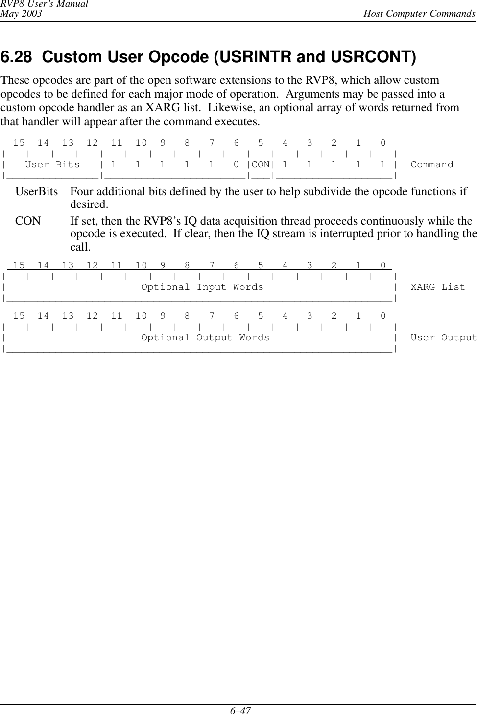
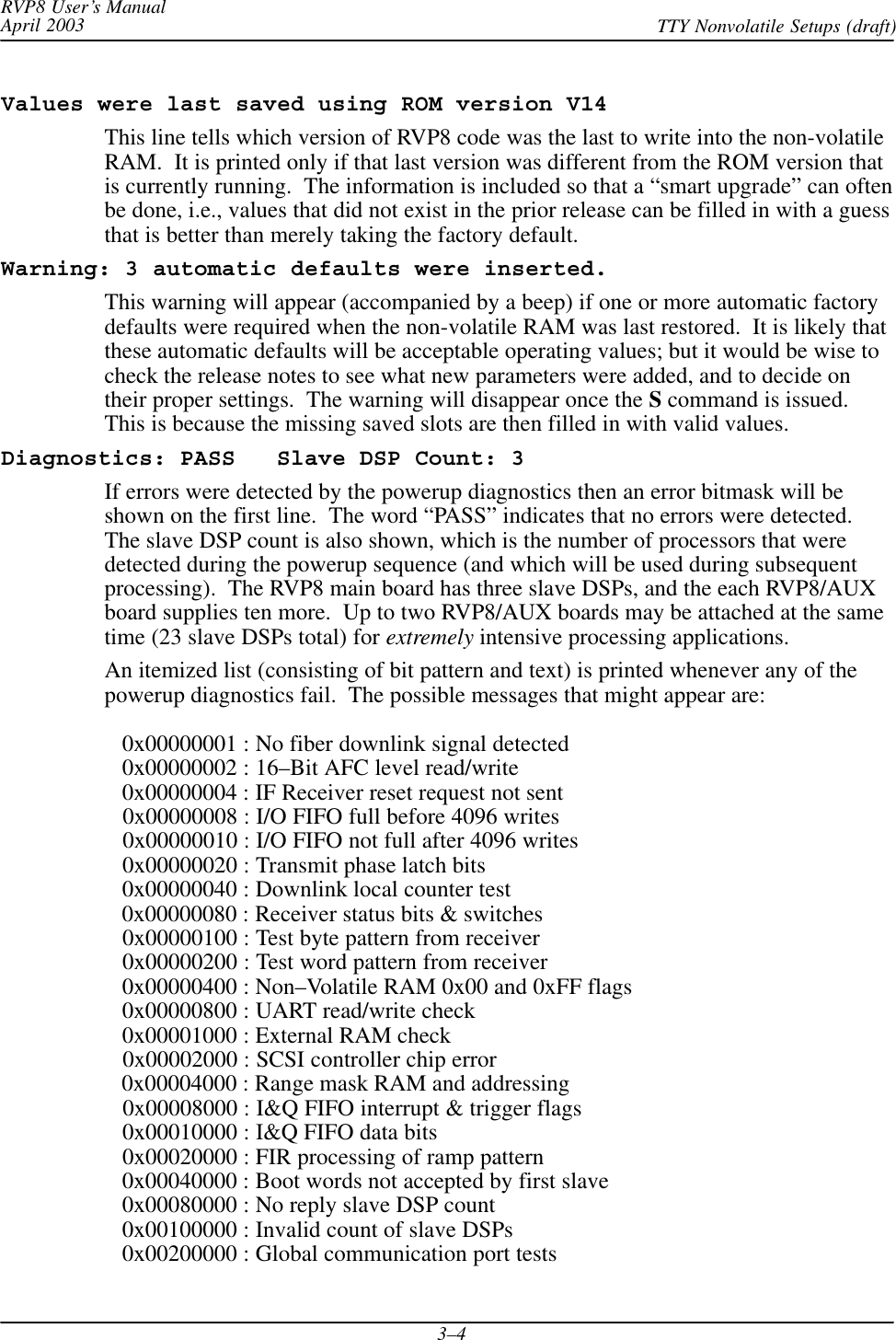
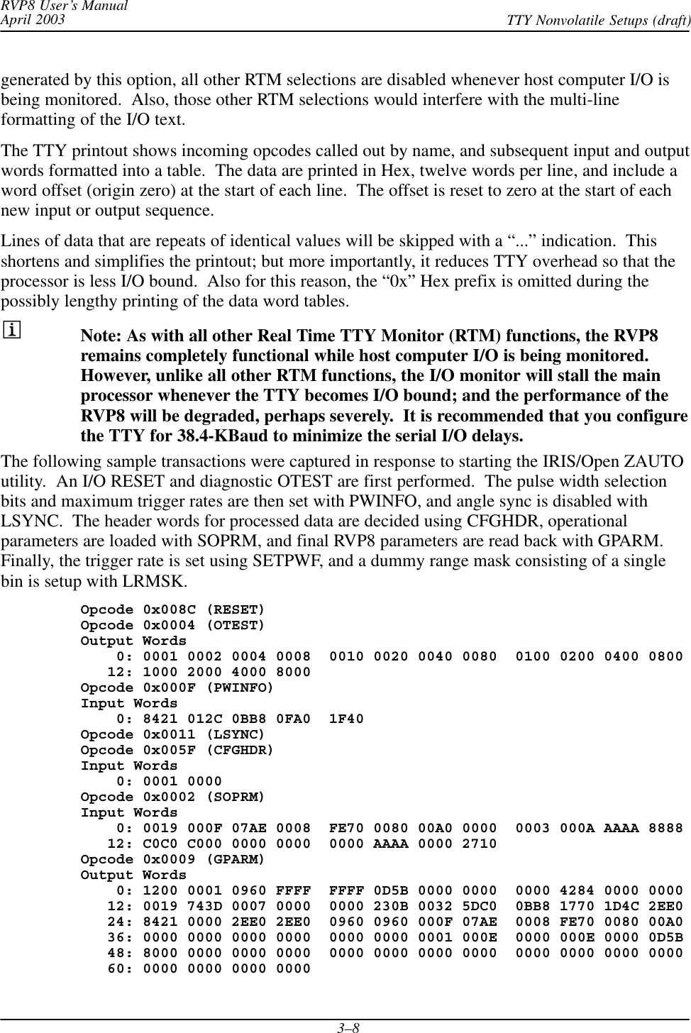
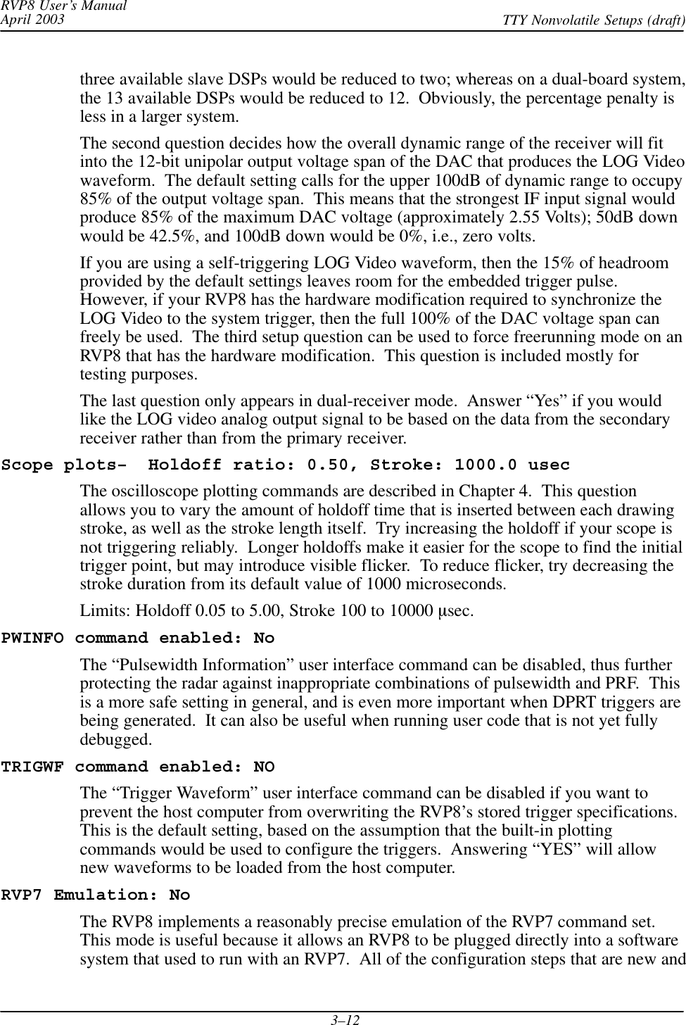
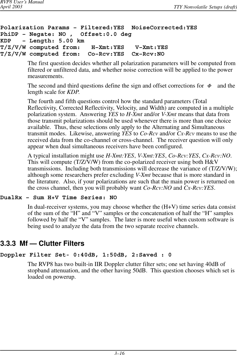
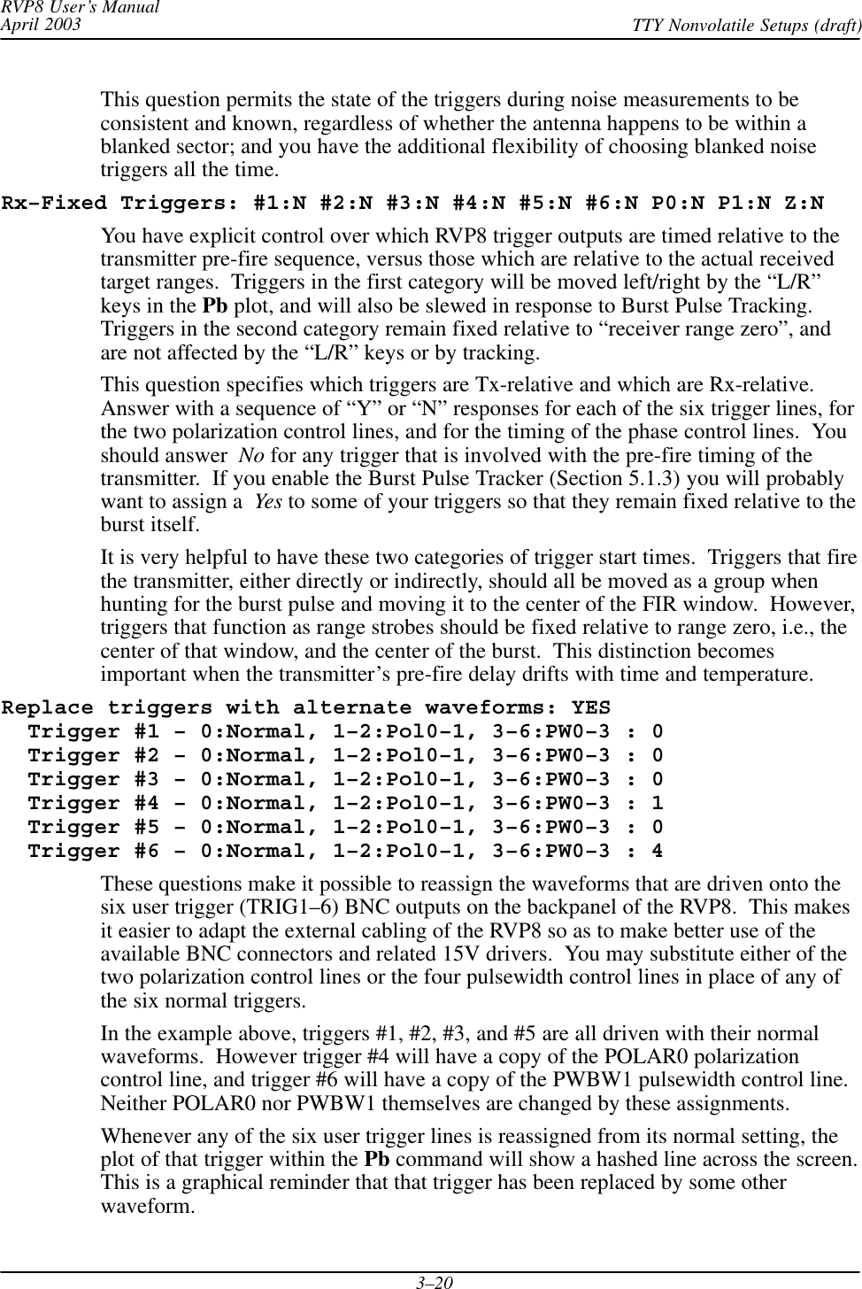
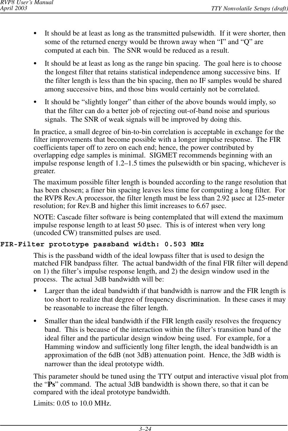
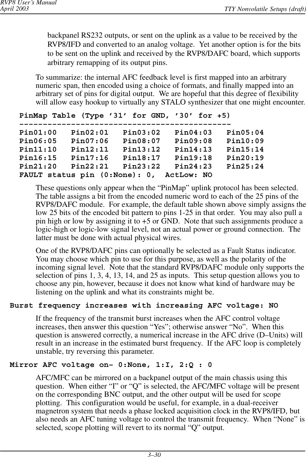
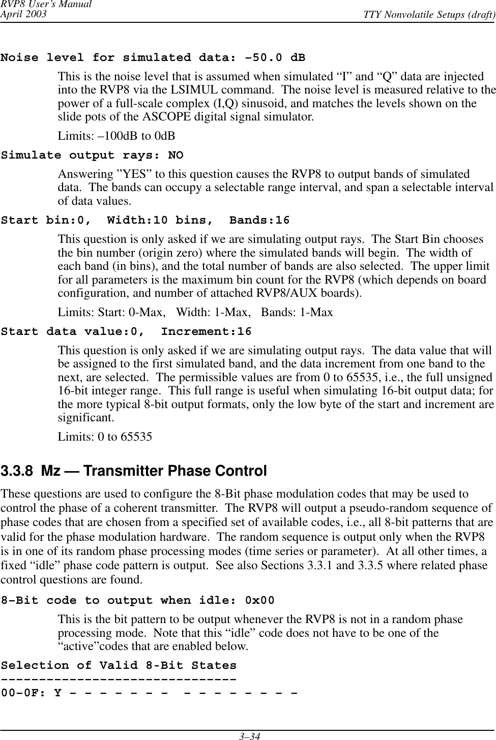
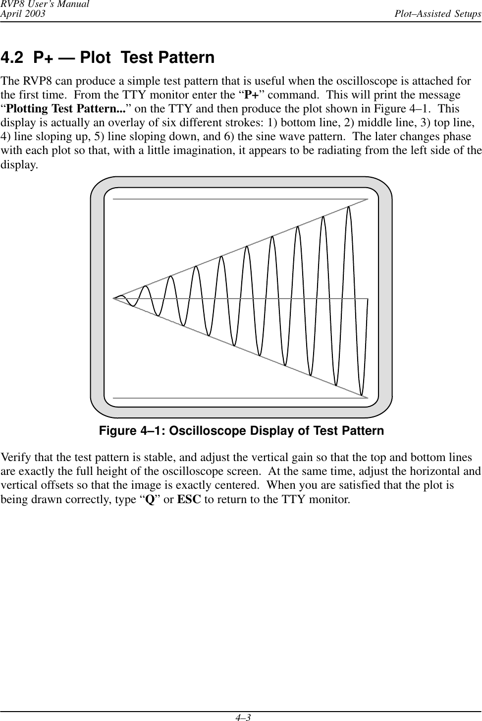
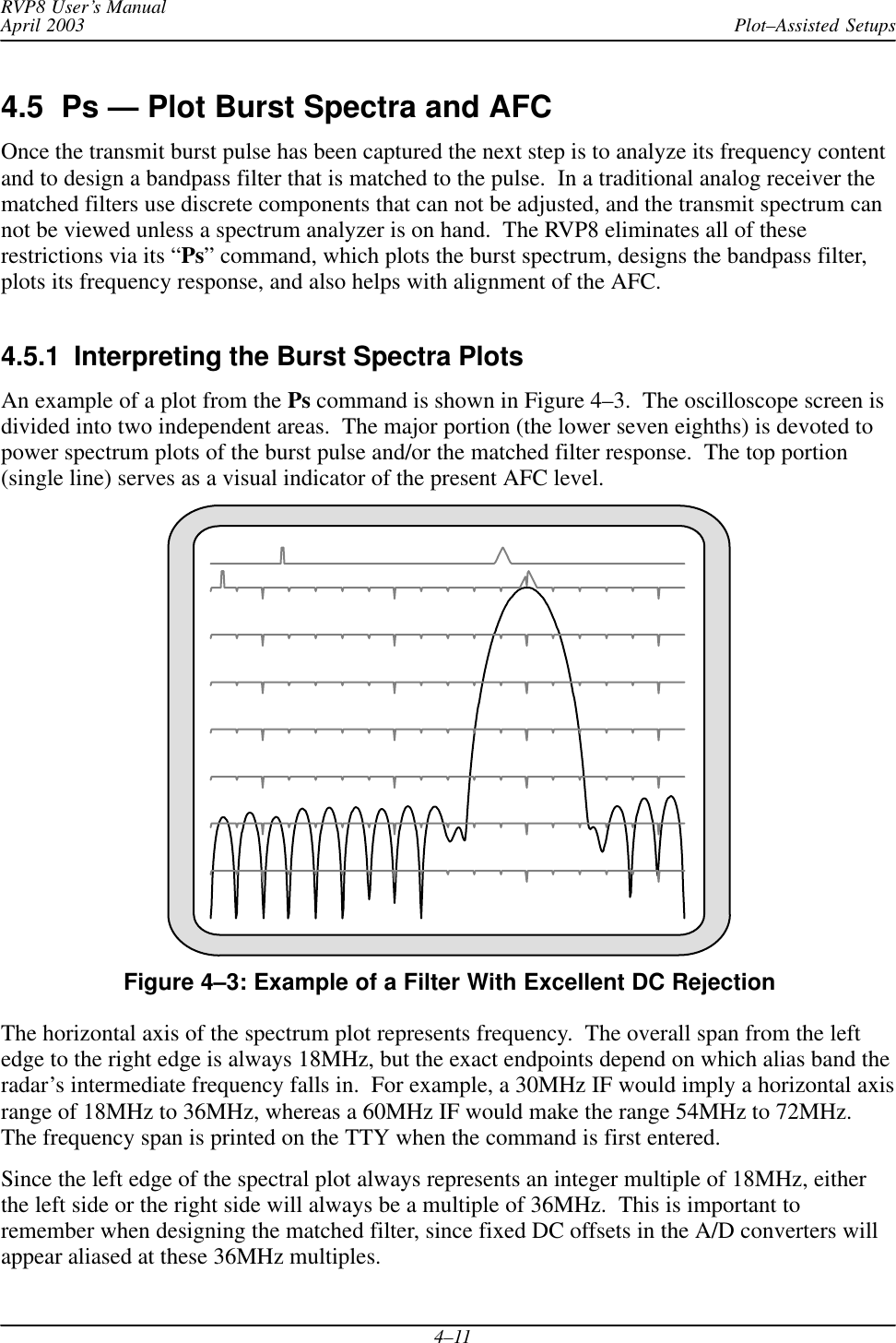
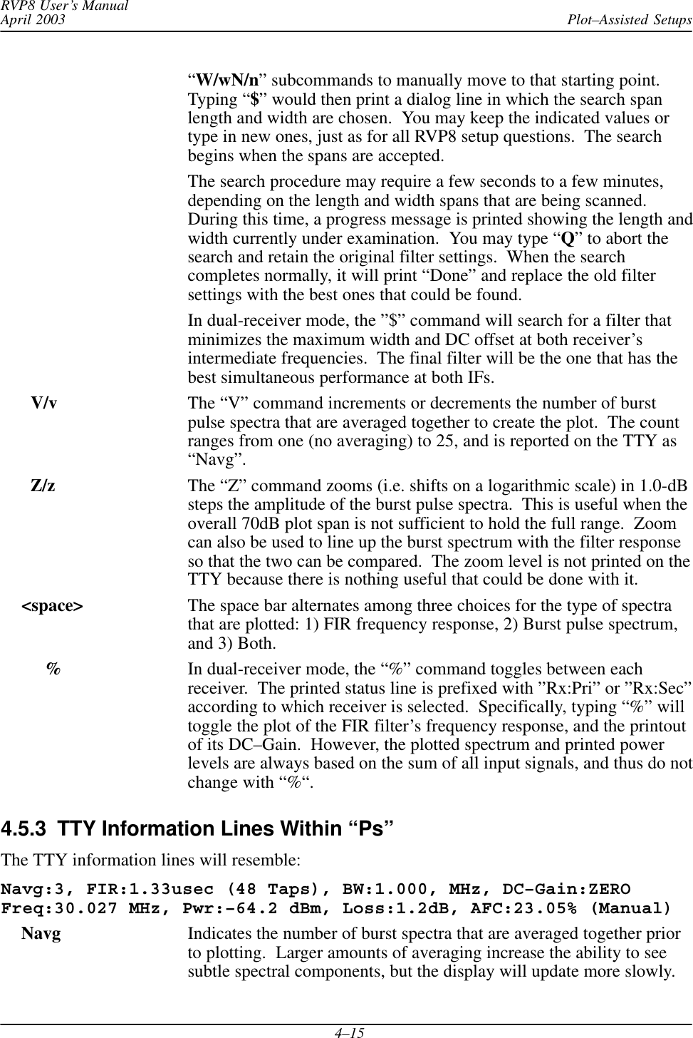
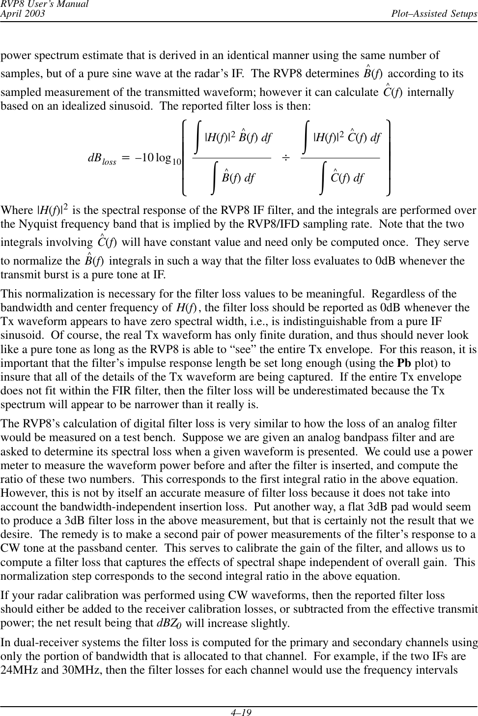
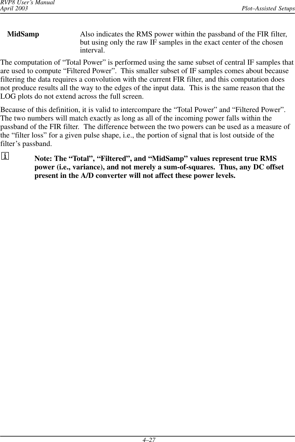
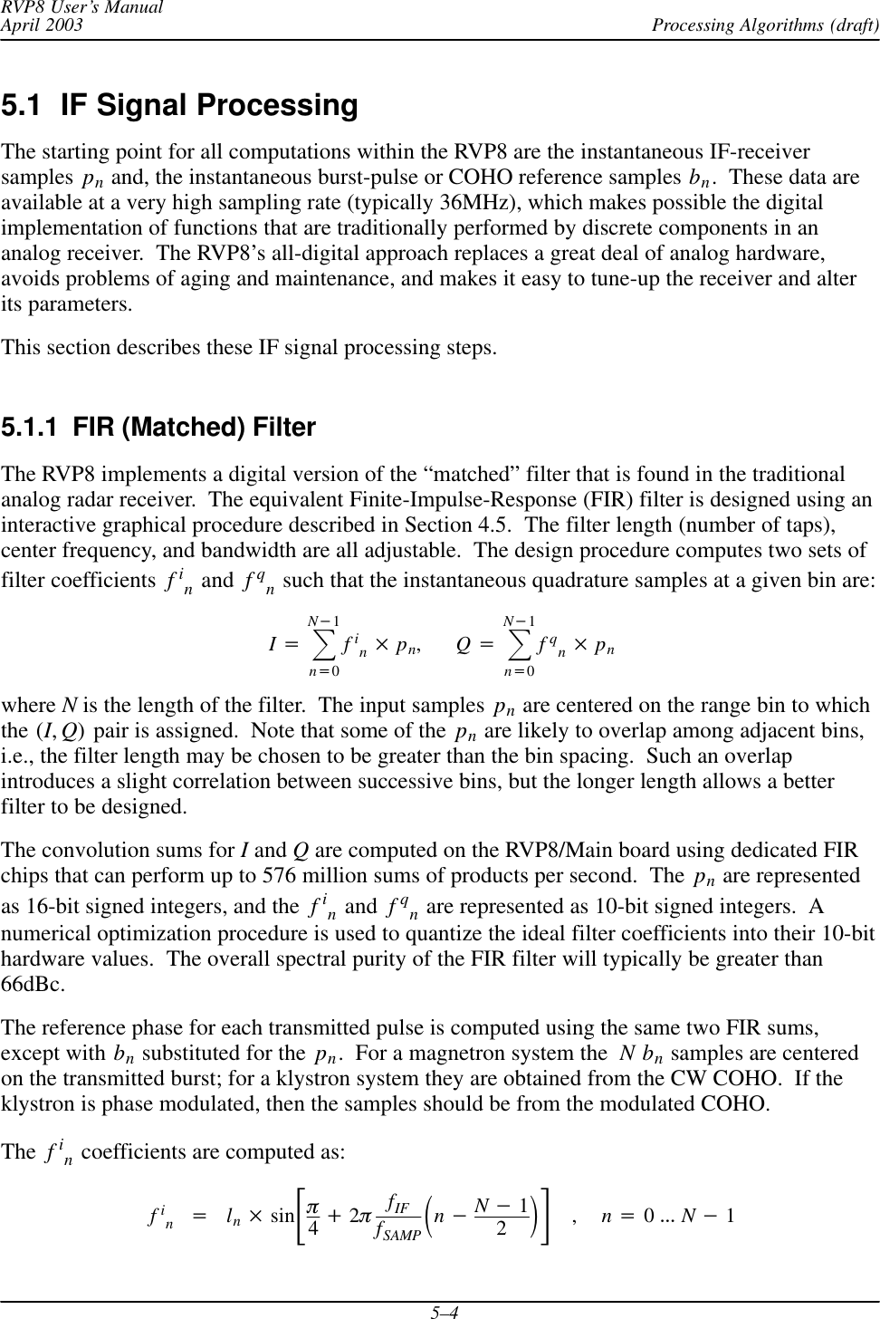
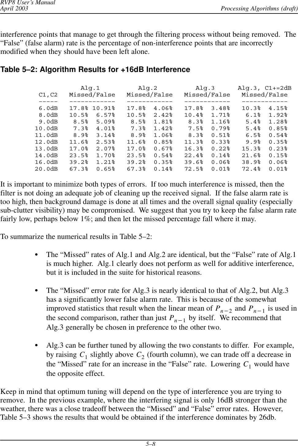
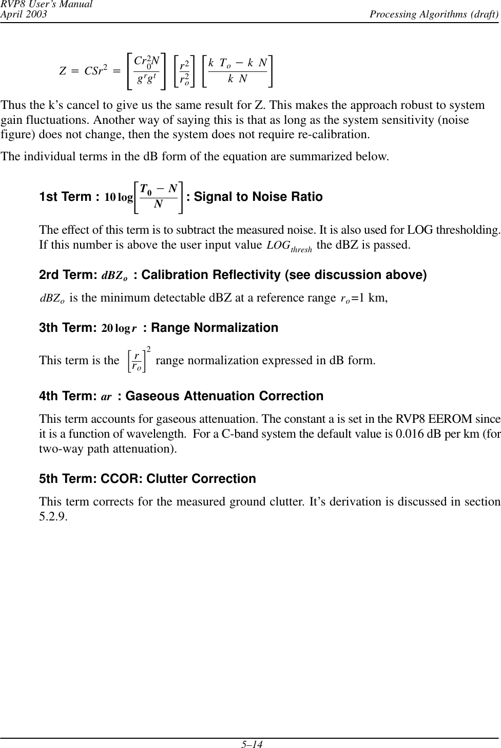
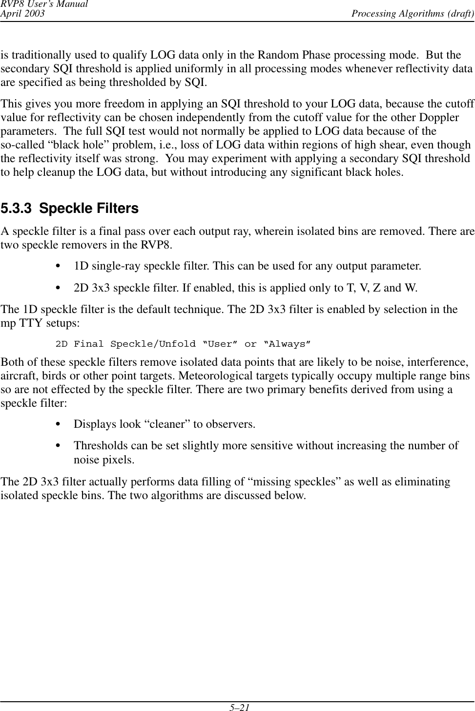
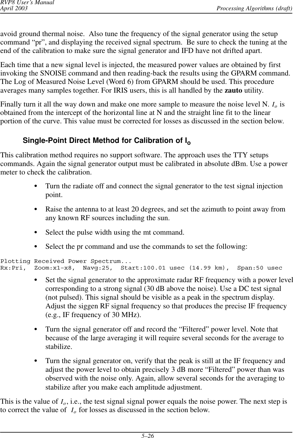
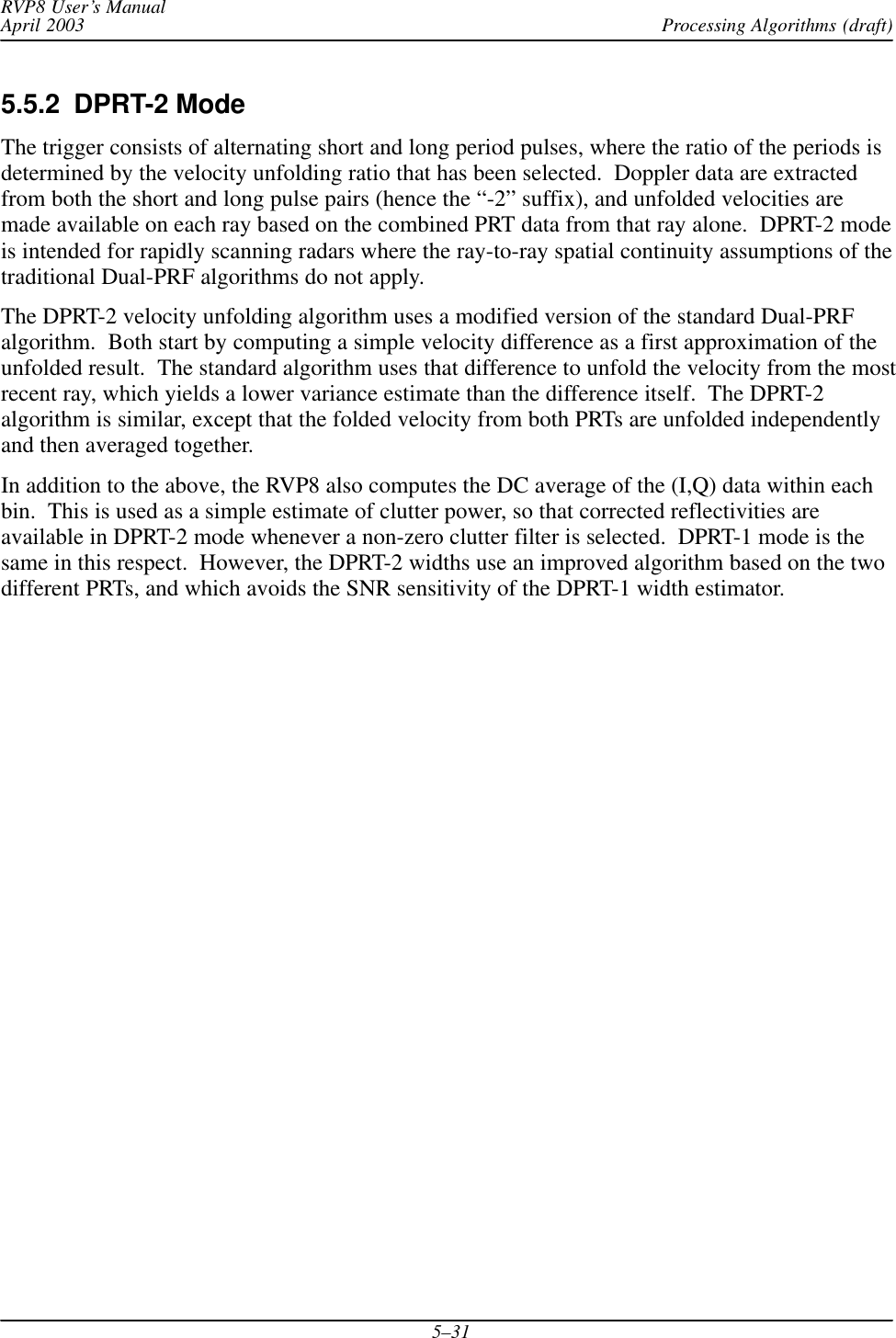
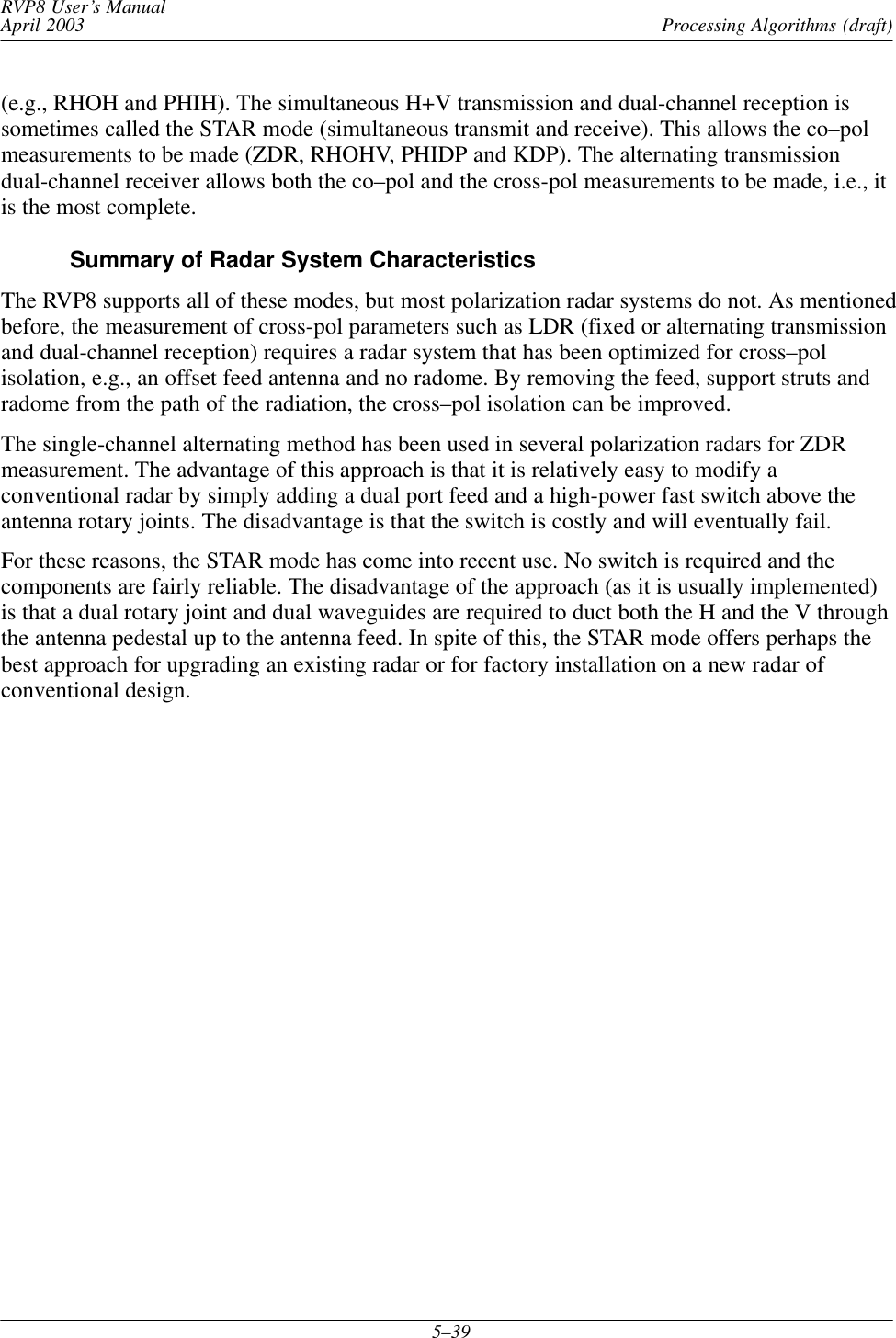
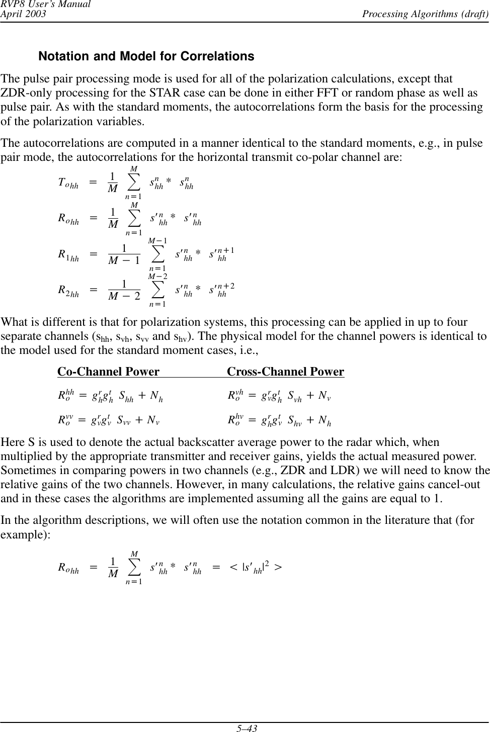
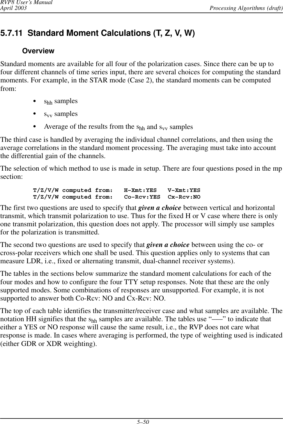
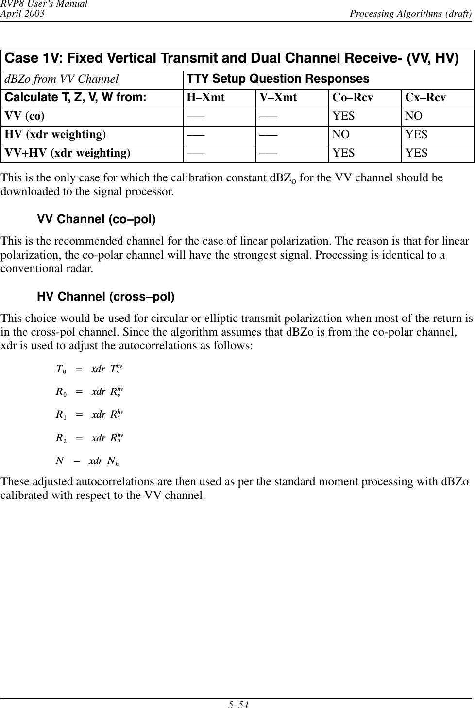
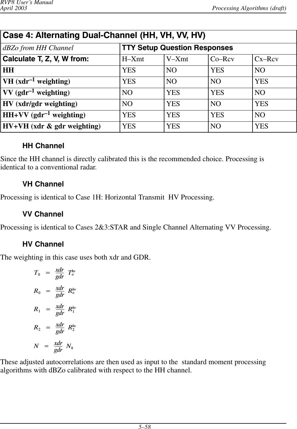
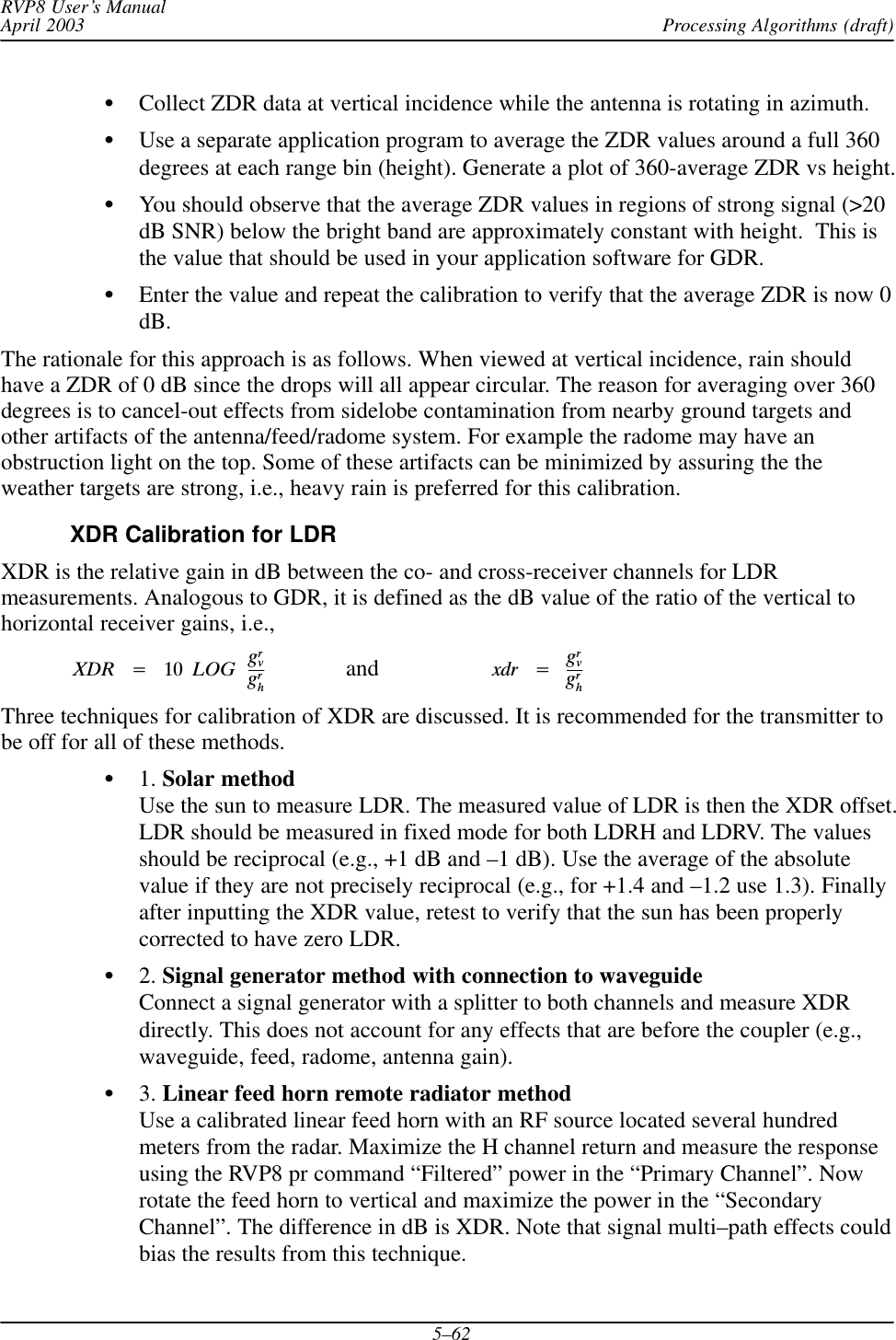
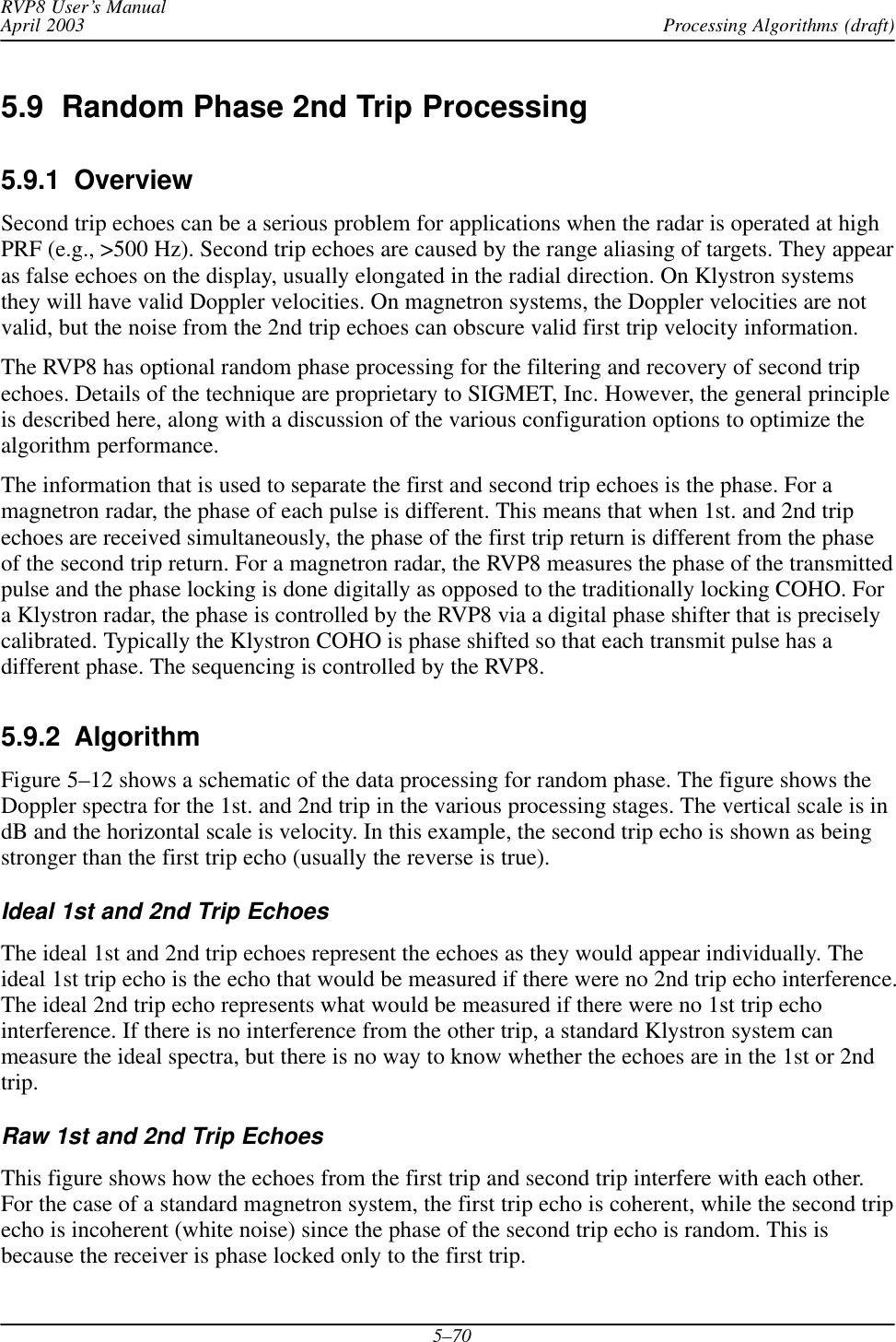
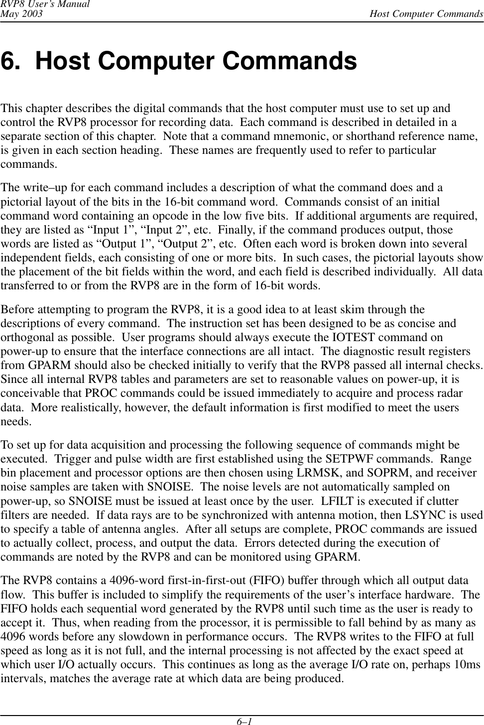
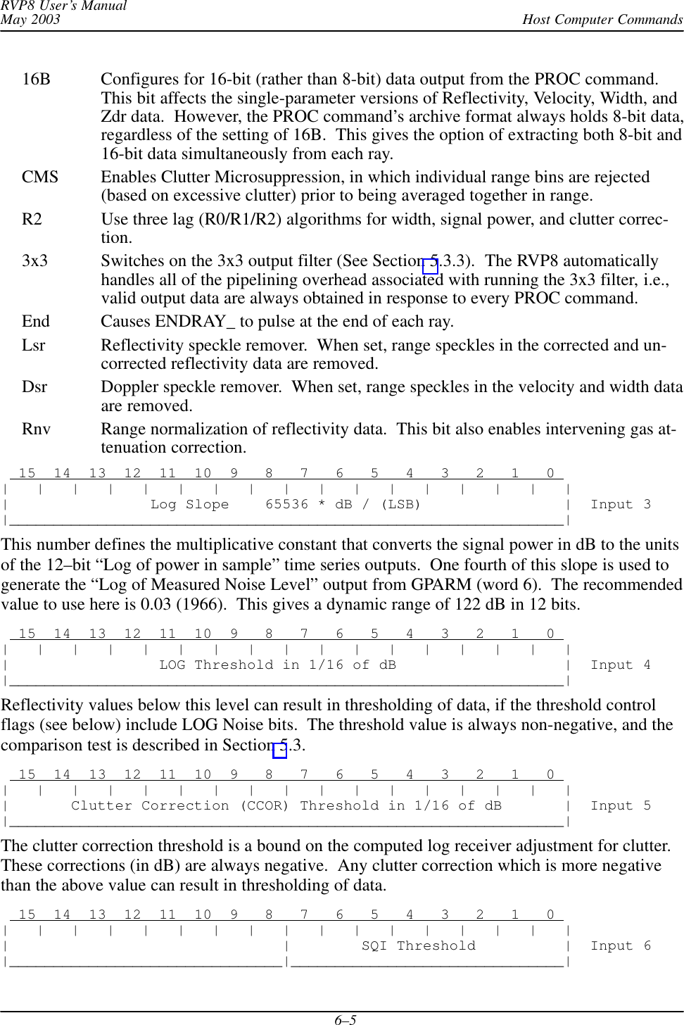
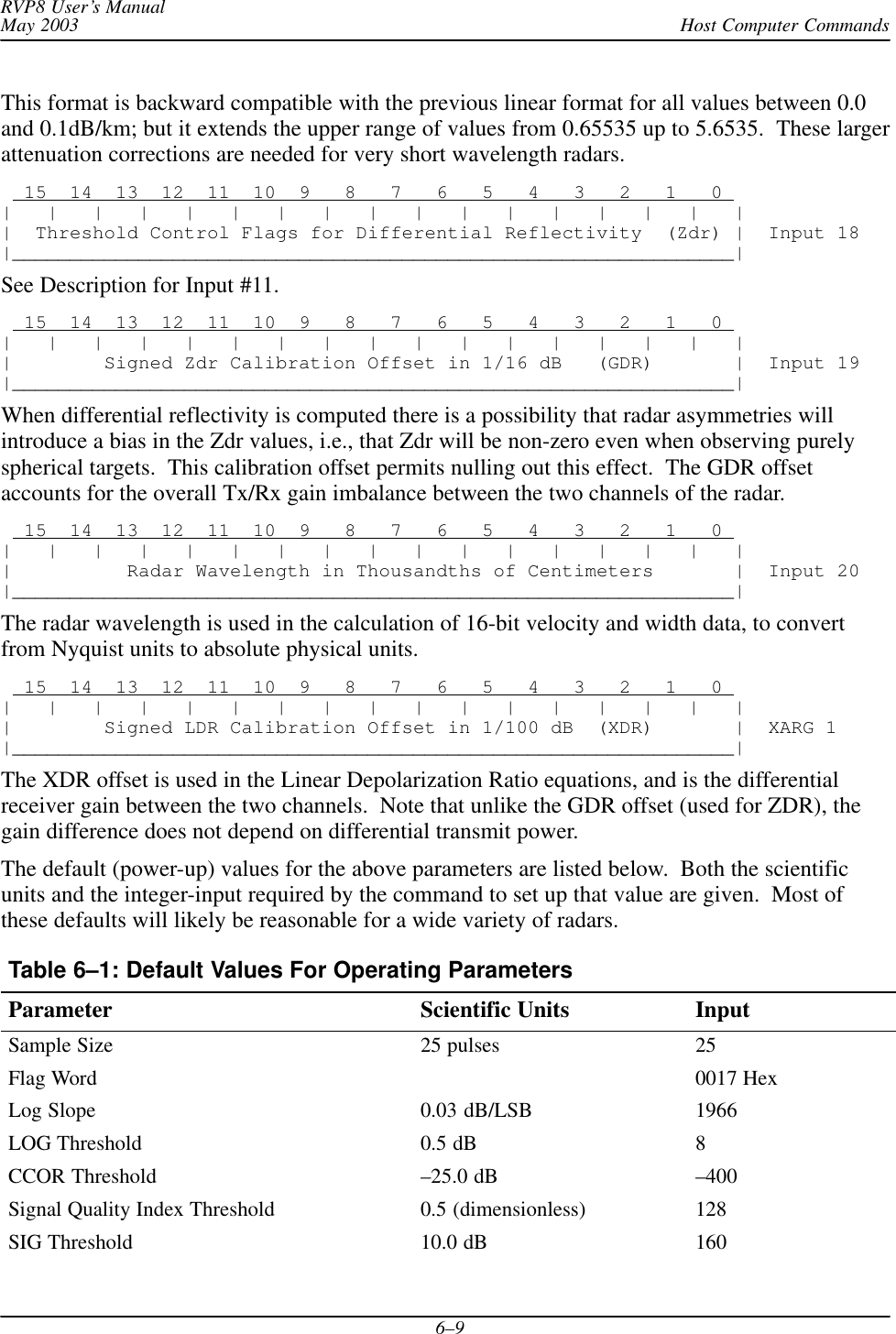
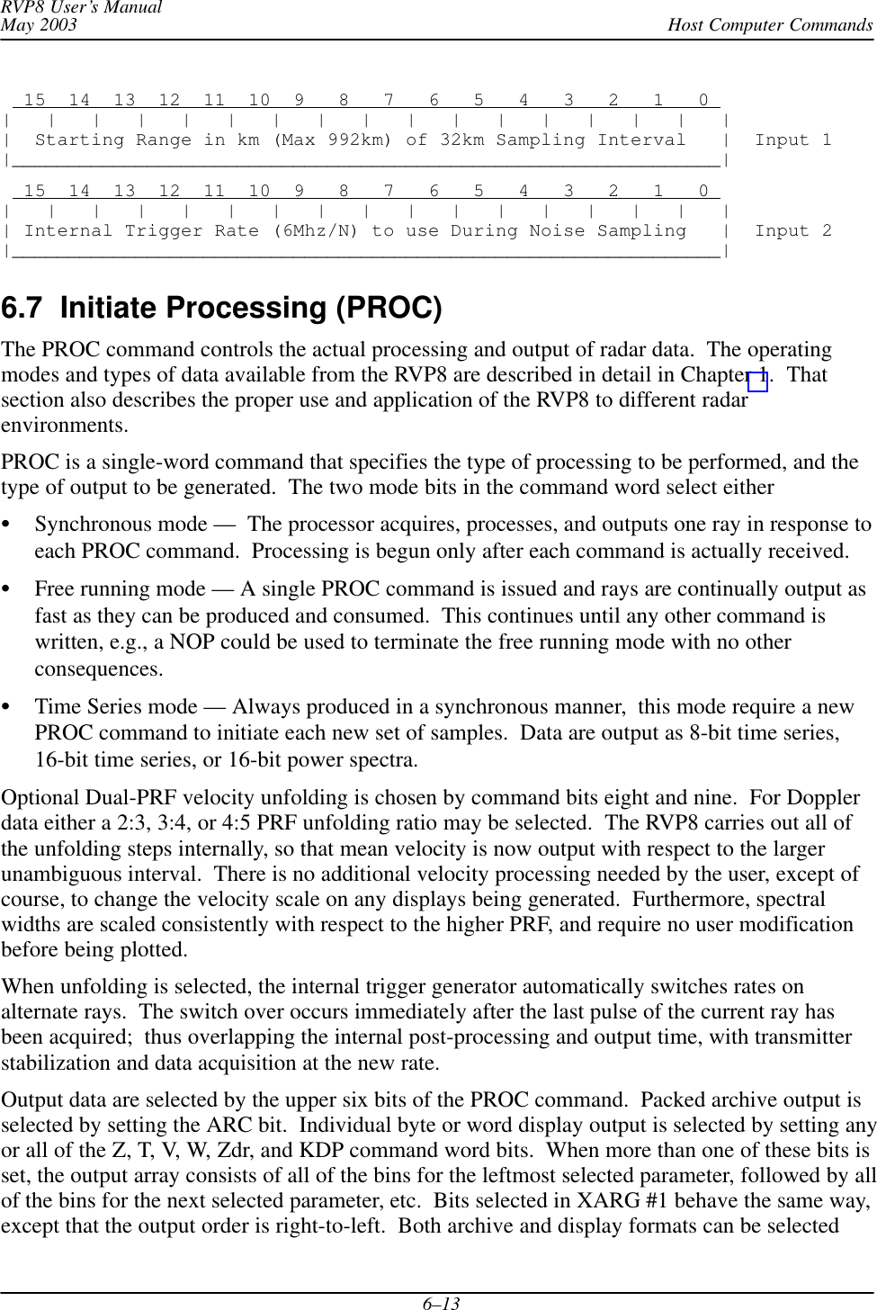
![RVP8 User’s ManualApril 2003 TTY Nonvolatile Setups (draft)3–29arbitrary units ranging from –100 to +100 corresponding to the complete span of theD/A converter. Since the D–Unit corresponds in a natural way to a percentage scale,the shorter “%” symbol is sometimes used.AFC feedback will be applied in proportion to the frequency error that the algorithmis attempting to correct. The feedback slope determines the sensitivity and timeconstant of the loop by establishing the AFC’s rate of change in (D-Units / sec) perthousand Hertz of frequency error. For example, a slope of 0.01 and a frequencyerror of 30KHz would result in a control voltage slew of 0.3 D-Units per second. Atthat rate it would take approximately 67 seconds for the output voltage to slew onetenth of its total span (20 D-Units / (0.3 D-Units / sec) = 67 sec). AFC is intended totrack very slow drifts in the radar system, so response times of this magnitude arereasonable.Keep in mind that the feedback slew is based on a frequency error which itself isderived from a time averaging process (see Burst Frequency Estimator Settling Timedescribed above) . The AFC loop will become unstable if a large feedback slope isused together with a long settling time constant, due to the phase lag introduced bythe averaging process. Keep the loop stable by choosing a small enough slope thatthe loop easily comes to a stop within the inner hysteresis zone.See Section 3.3.6.1 for more information about these slope and slew rate parameters. AFC span– [–100%,+100%] maps into [ –32768 , 32767 ] AFC format– 0:Bin, 1:BCD, 2:8B4D: 0, ActLow: NO AFC uplink protocol– 0:Off, 1:Normal, 2:PinMap : 1The RVP8’s implementation of AFC has been generalized so that there is nodifference between configuring an analog loop and a digital loop. The AFC feedbackloop parameters are setup the same way in each case; the only difference being themodel for how the AFC information is made available to the outside world. Manytypes of interfaces and protocols thus become possible according to how these threequestions are answered. AFC output follows these three steps:SThe internal feedback loop uses a conceptual [–100%,+100%] range of values.However, this range may be mapped into an arbitrary numeric span for eventualoutput. For example, choosing the span from –32768 to +32767 would result in16-bit AFC, and 0 to 999 might be appropriate for 3-digit BCD; but any otherspan could also be selected from the full 32-bit integer range.SNext, an encoding format is chosen for the specified numeric span. The result ofthe encoding step is another 32-bit pattern which represents the above numericvalue. SIGMET will make an effort to include in the list of supported formats allcustom encodings that our customers encounter from their vendors.Available formats include straight binary, BCD, and mixed-radix formats thatmight be required by a specialized piece of equipment. The “8B4D” formatencodes the low four decimal digits as four BCD digits, and the remaining upperbits in binary. For example, 659999 base-10 would encode into 0x00419999Hex.SFinally, an output protocol is selected for the bit pattern that was produced byencoding the numeric value. The bits may be written to the eight RVP8/Main](https://usermanual.wiki/Baron-Services/XDD-1000C.S10-RECEIVER-AND-PROCESSOR-USERS-MANUAL-PART-2/User-Guide-374023-Page-29.png)
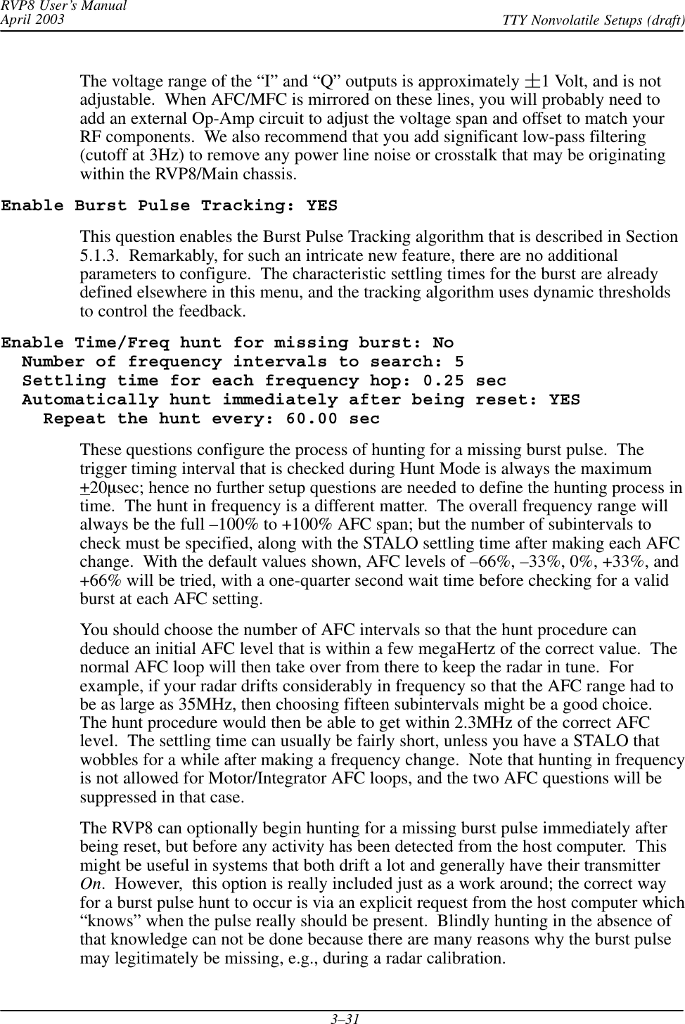
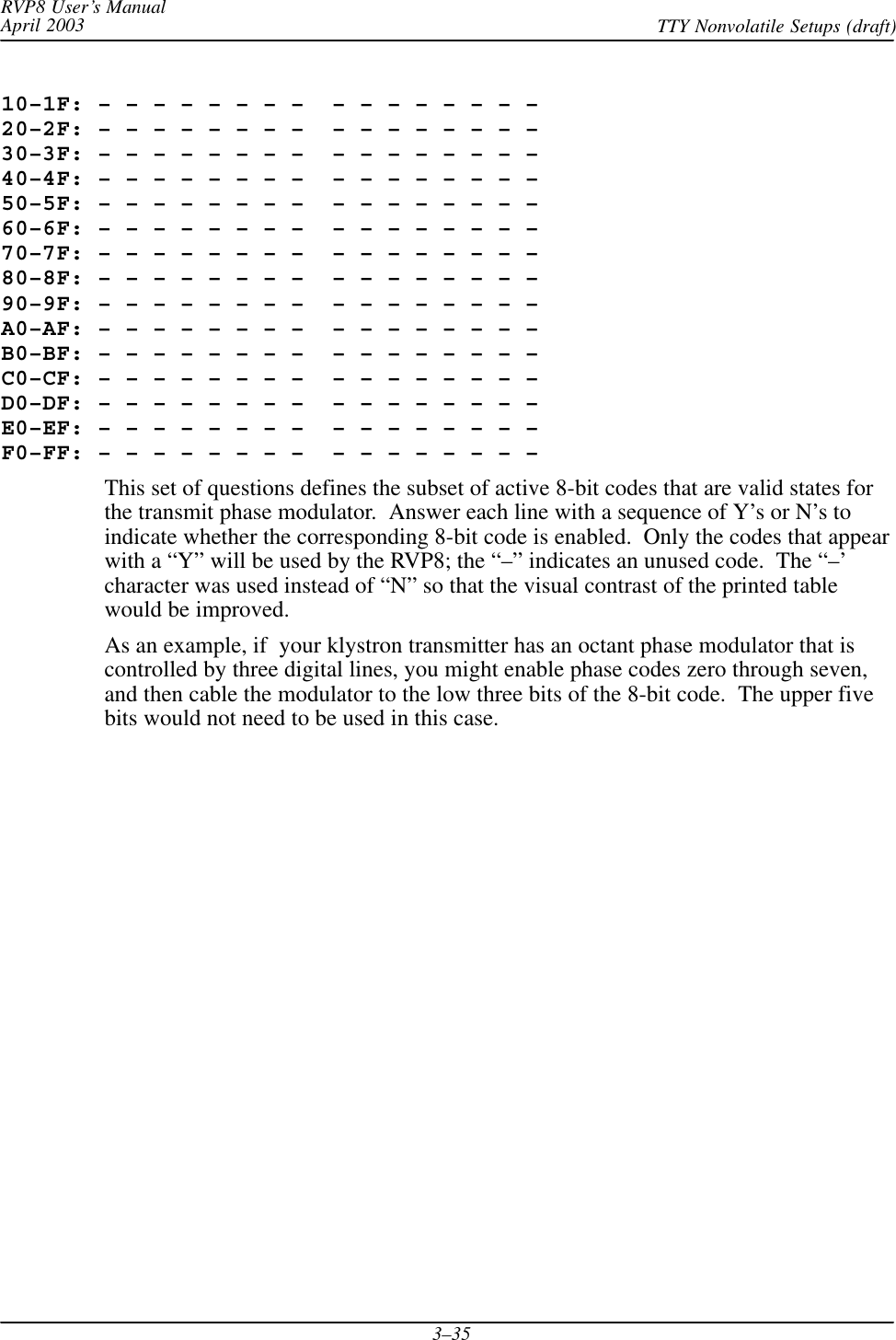
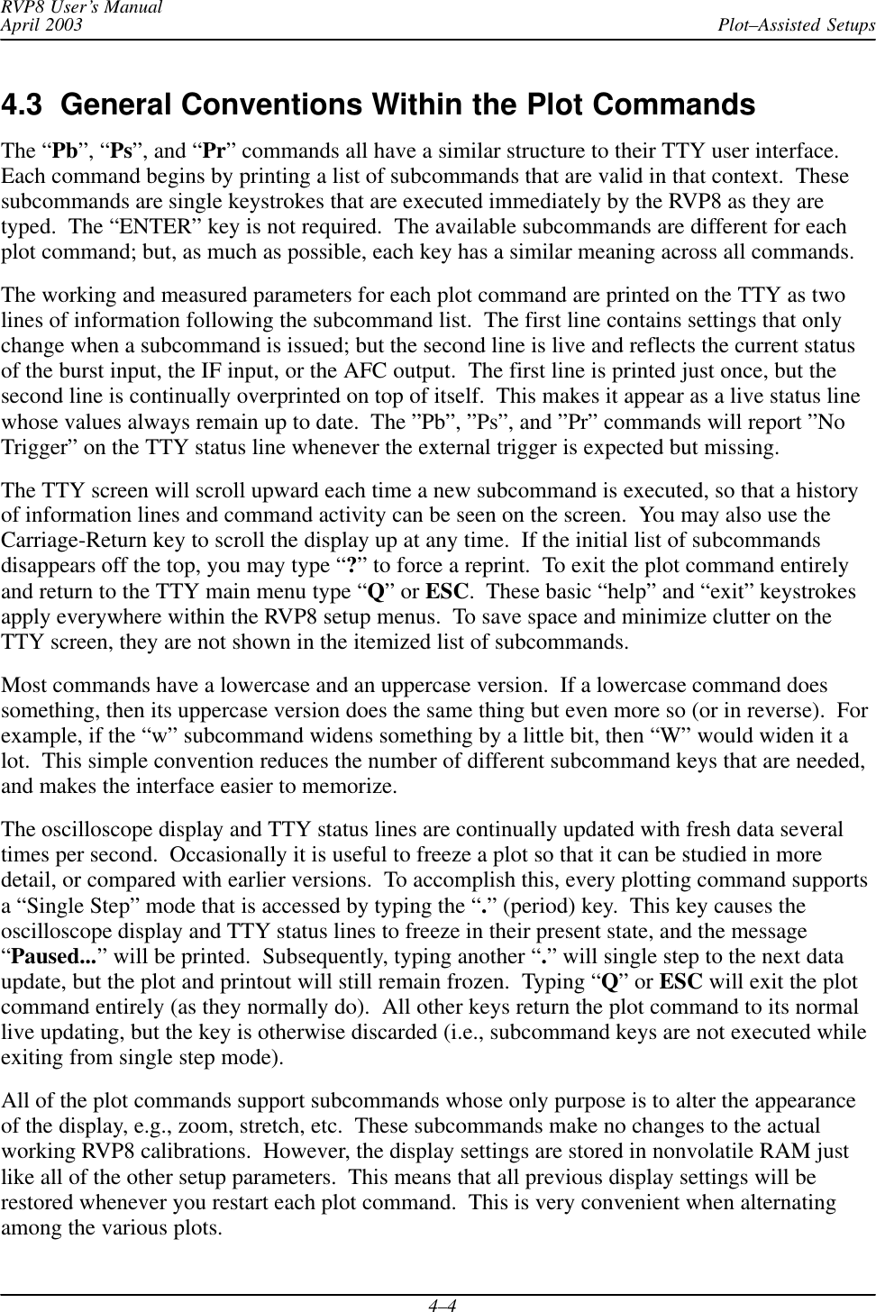
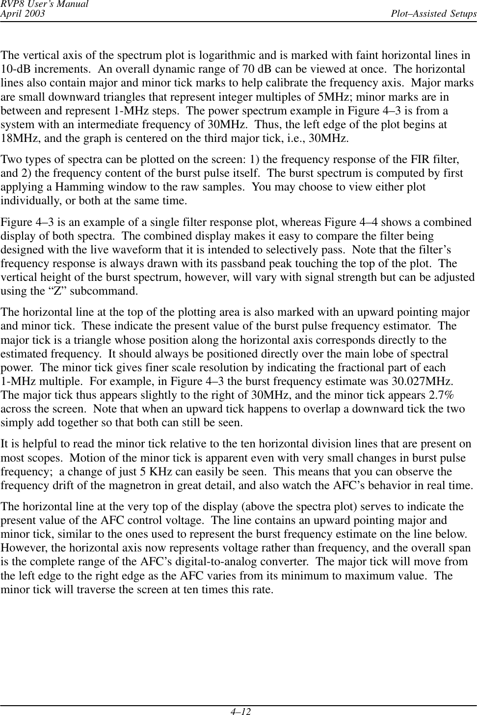
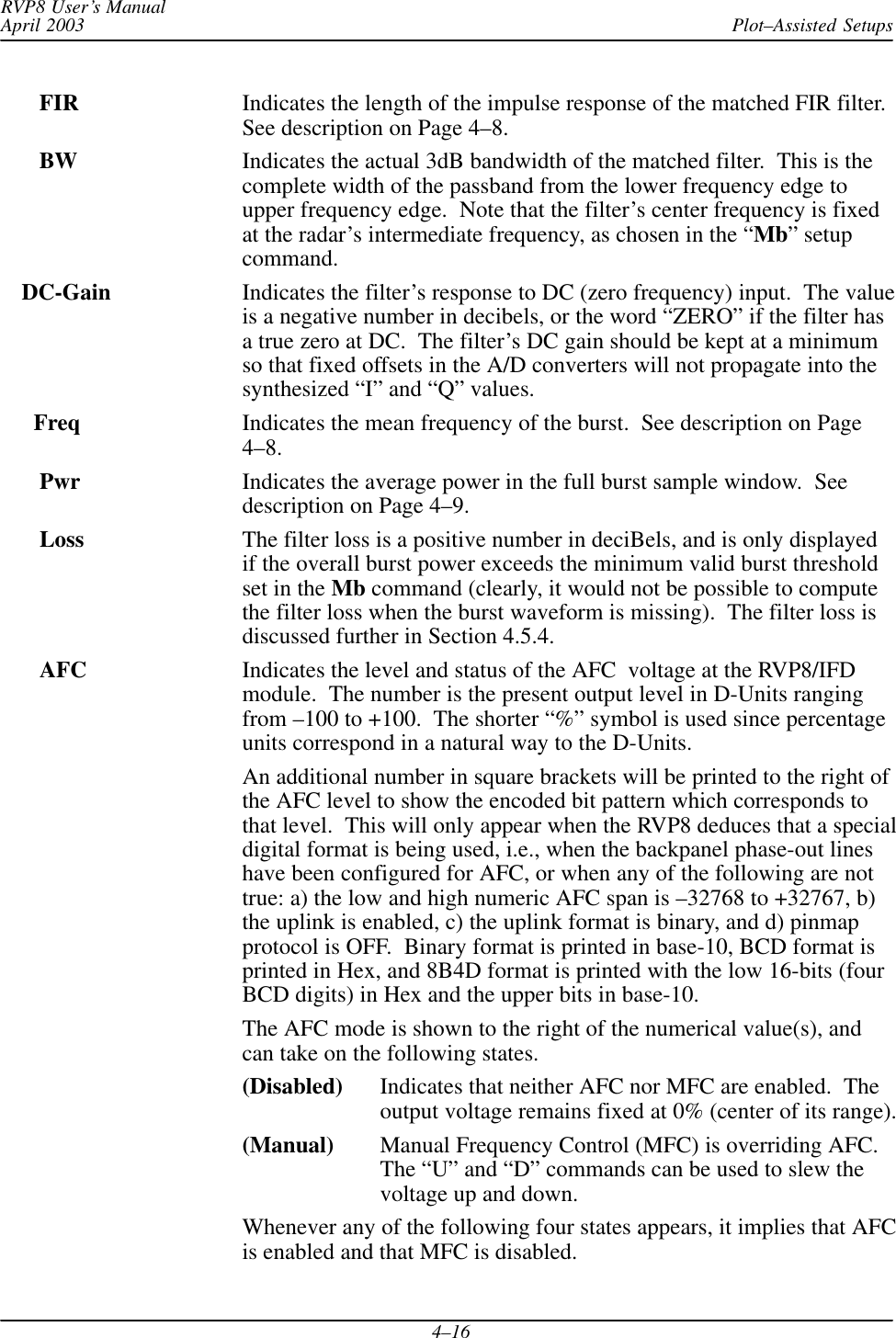
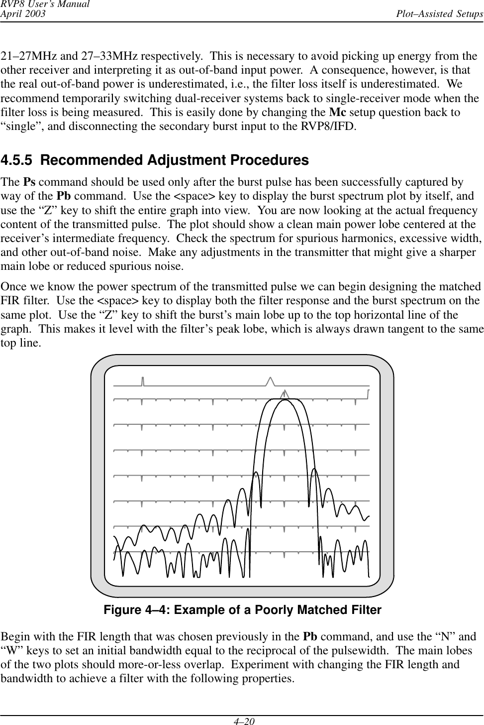
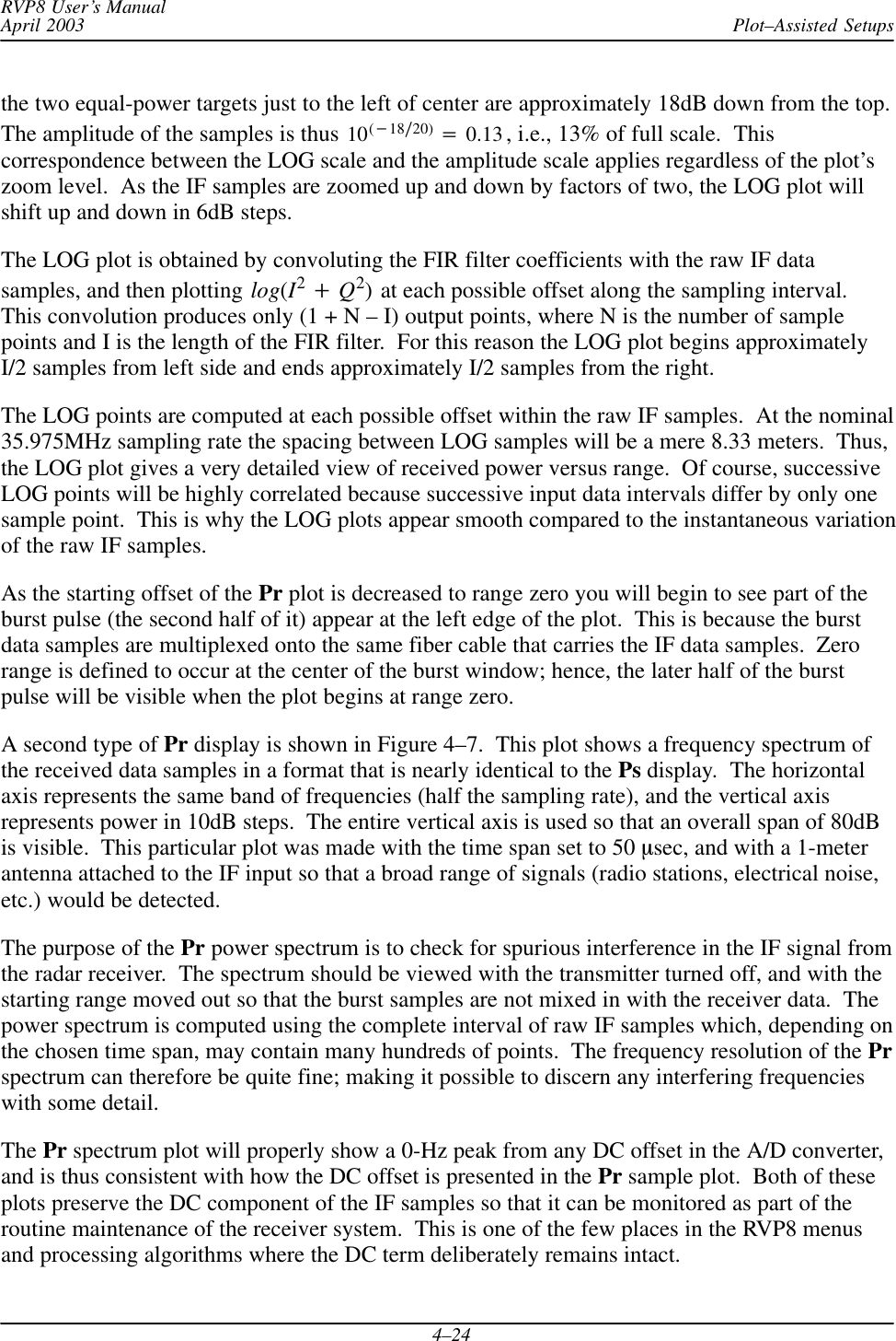
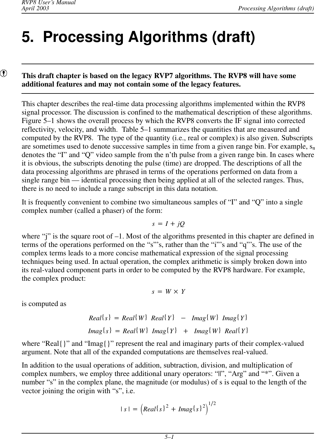
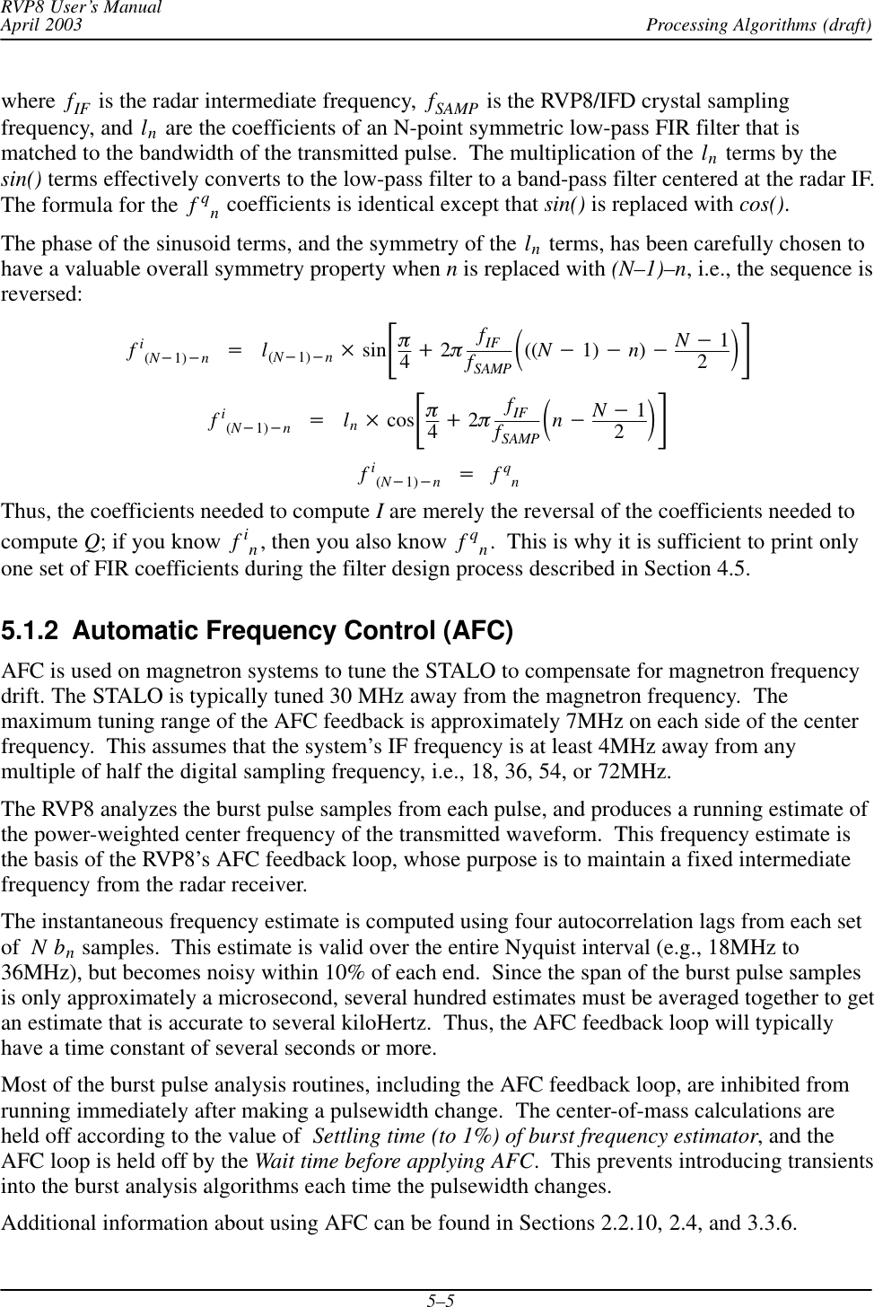
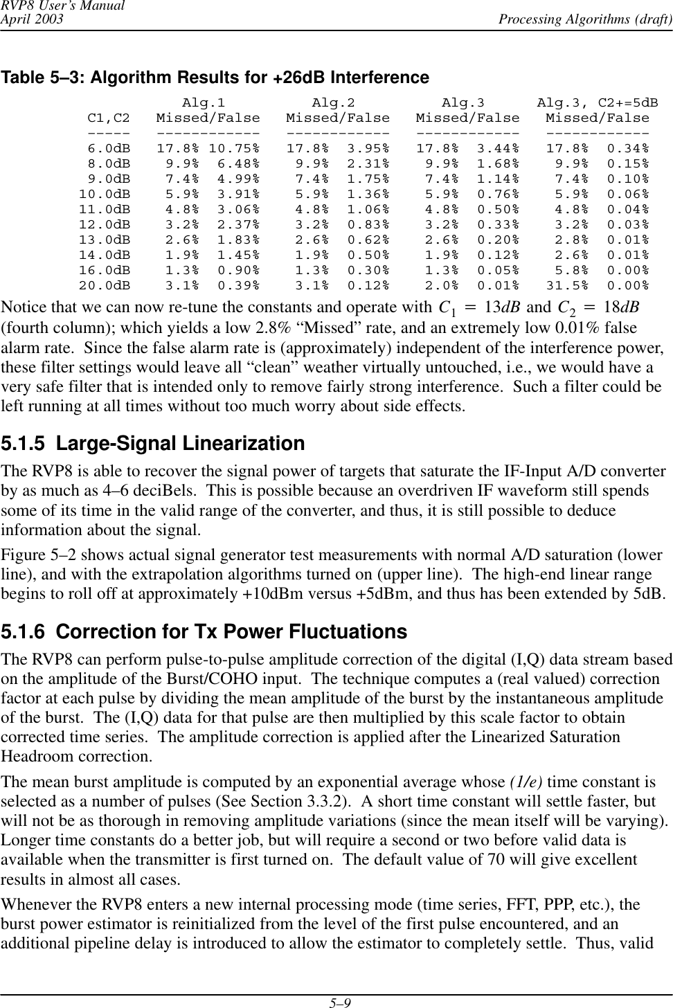
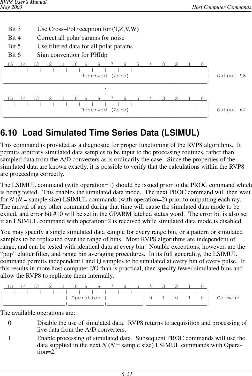
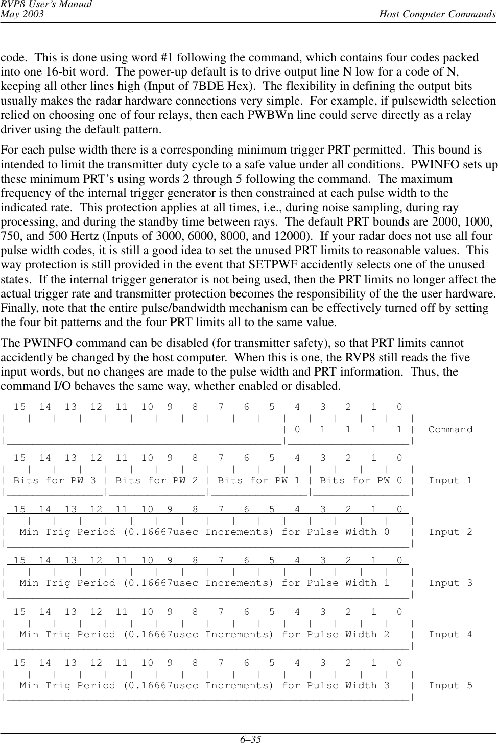
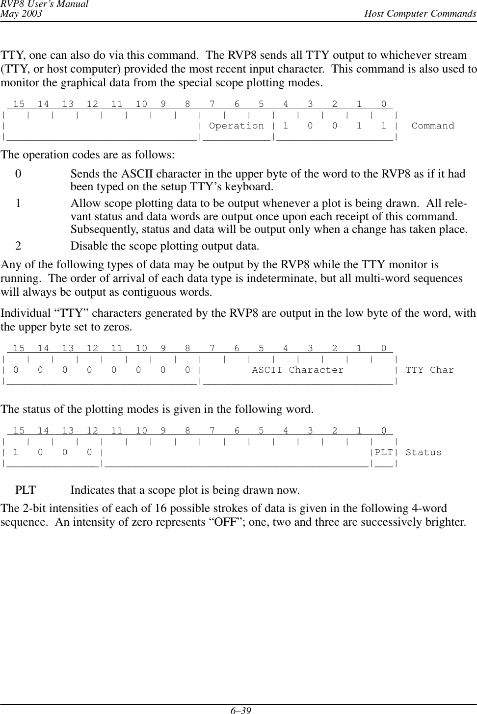
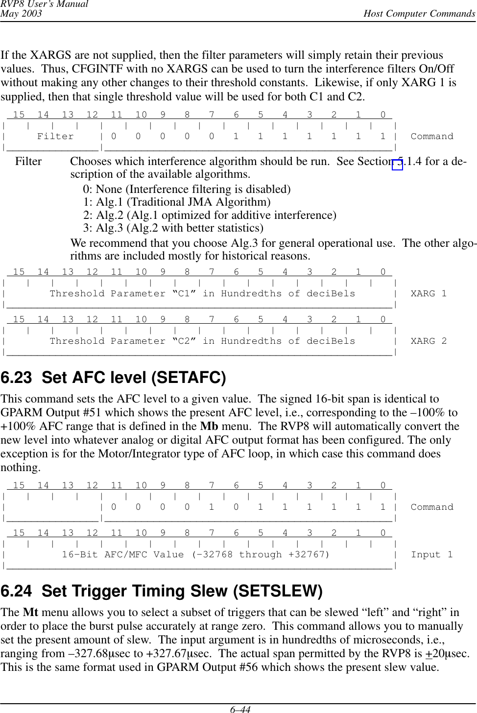
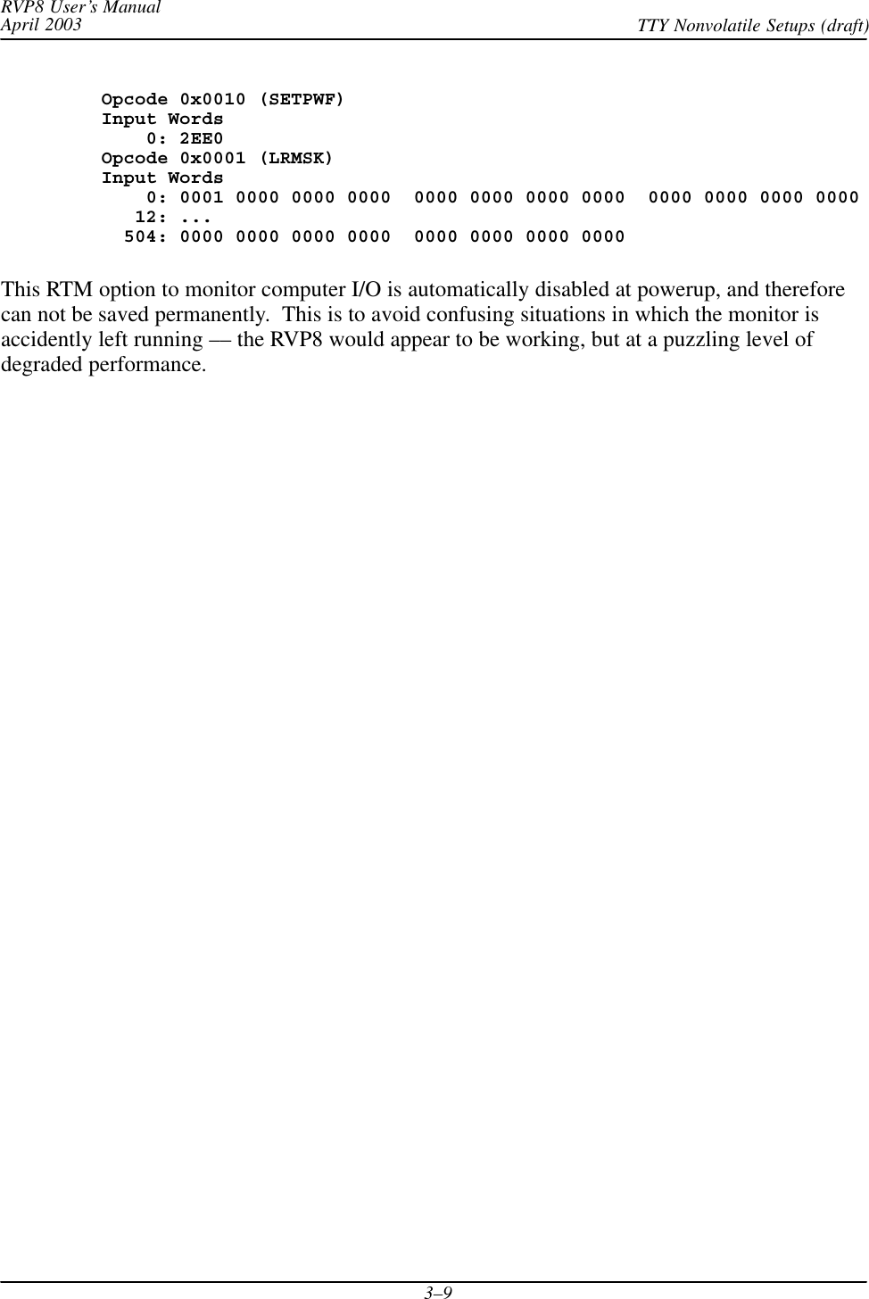
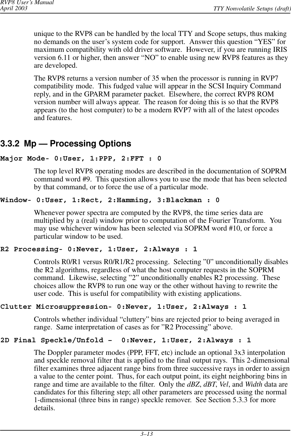
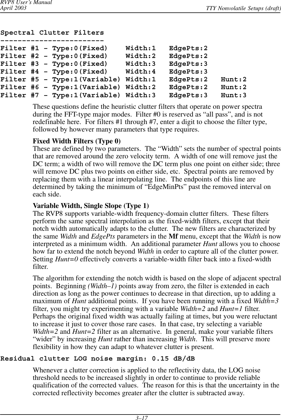
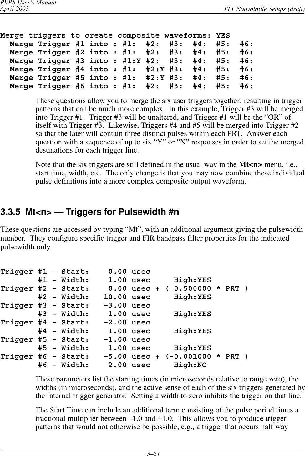
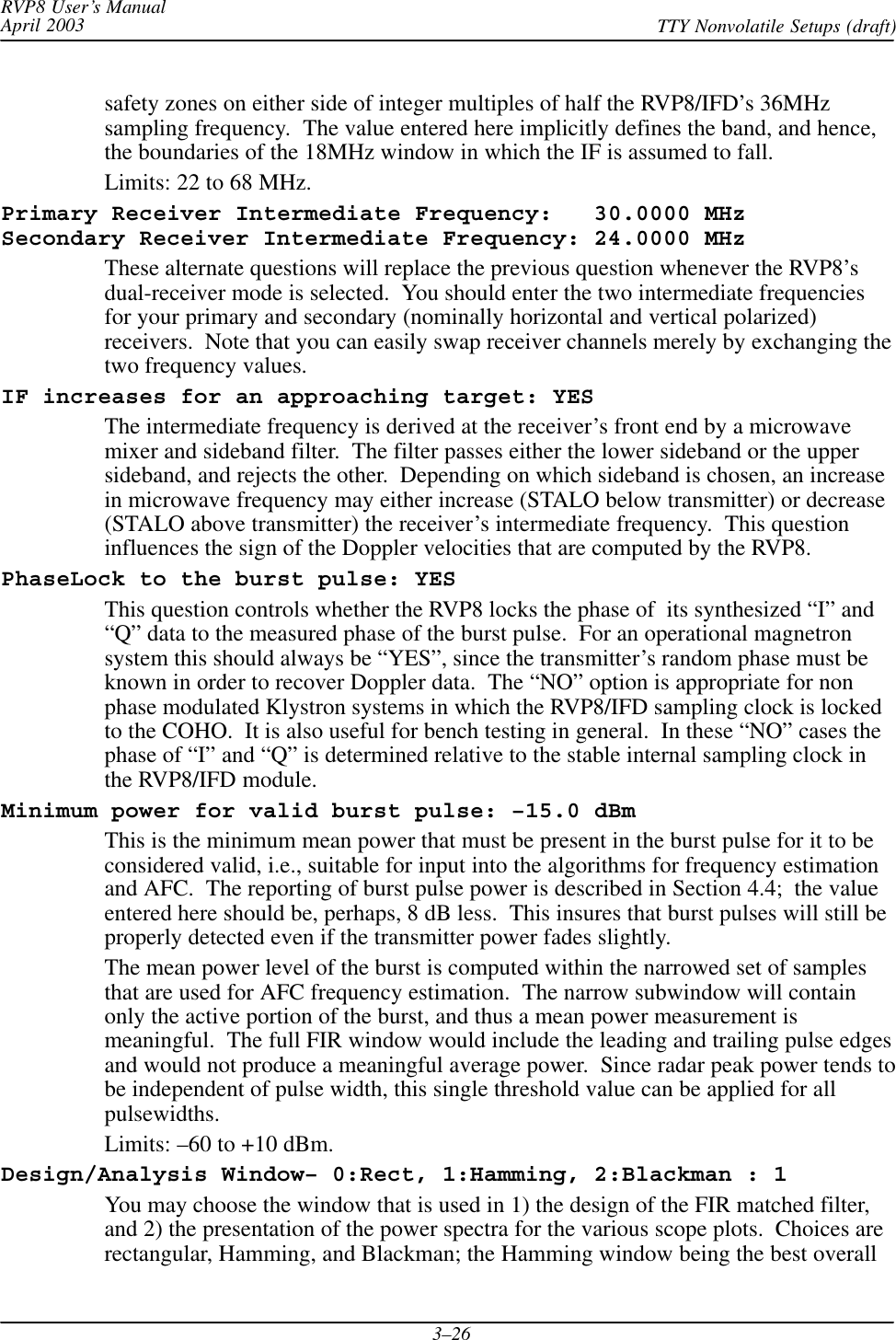
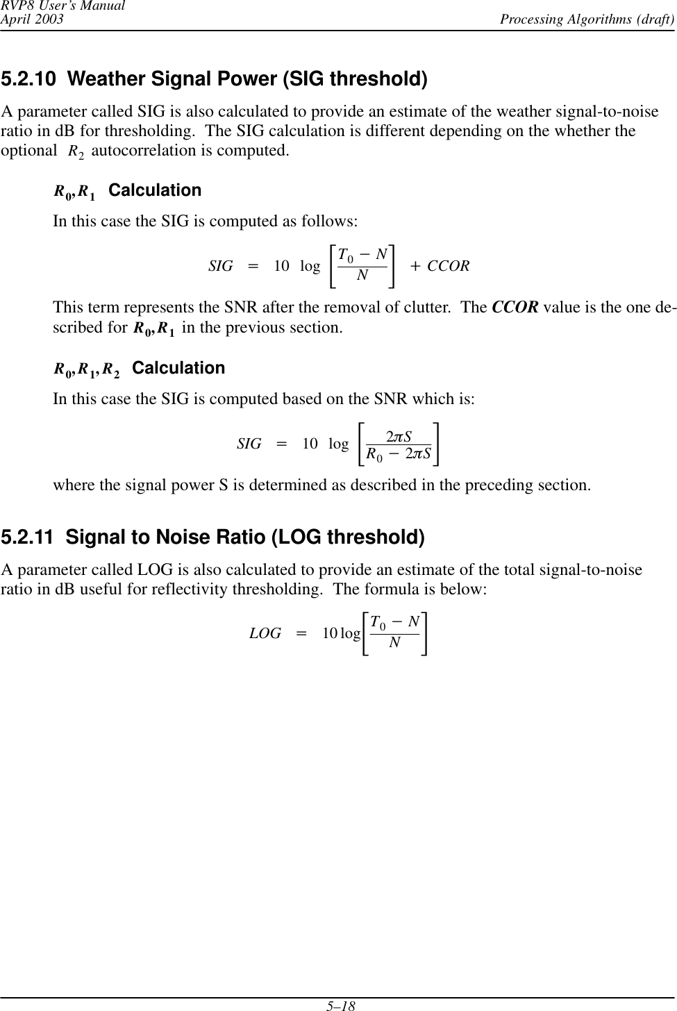
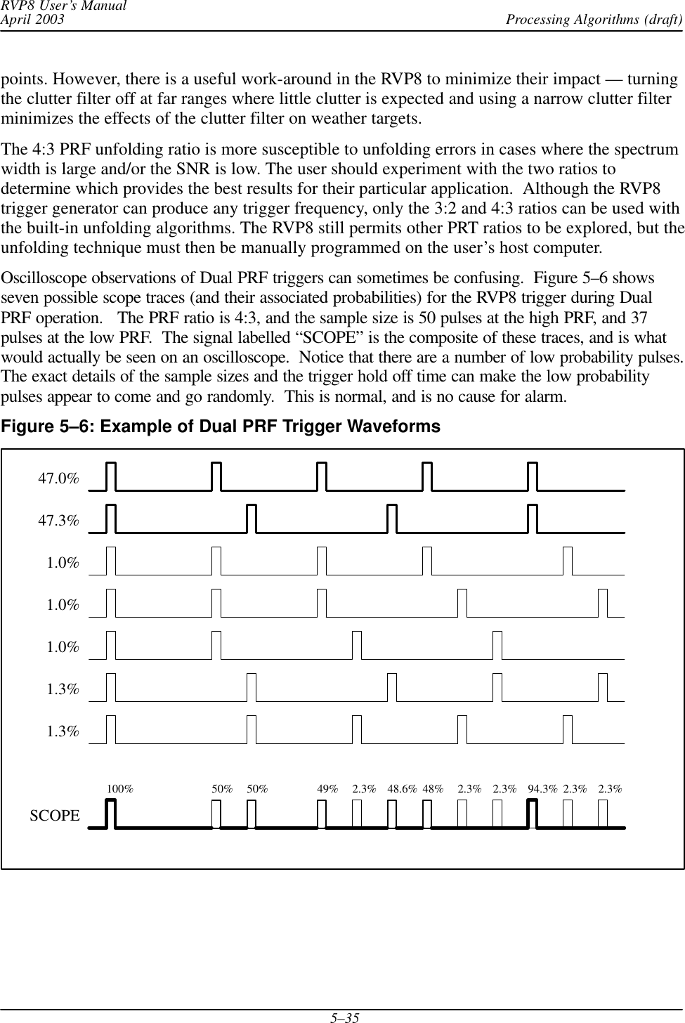
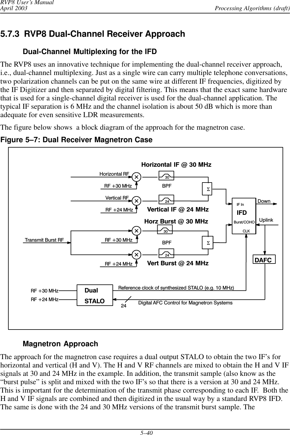
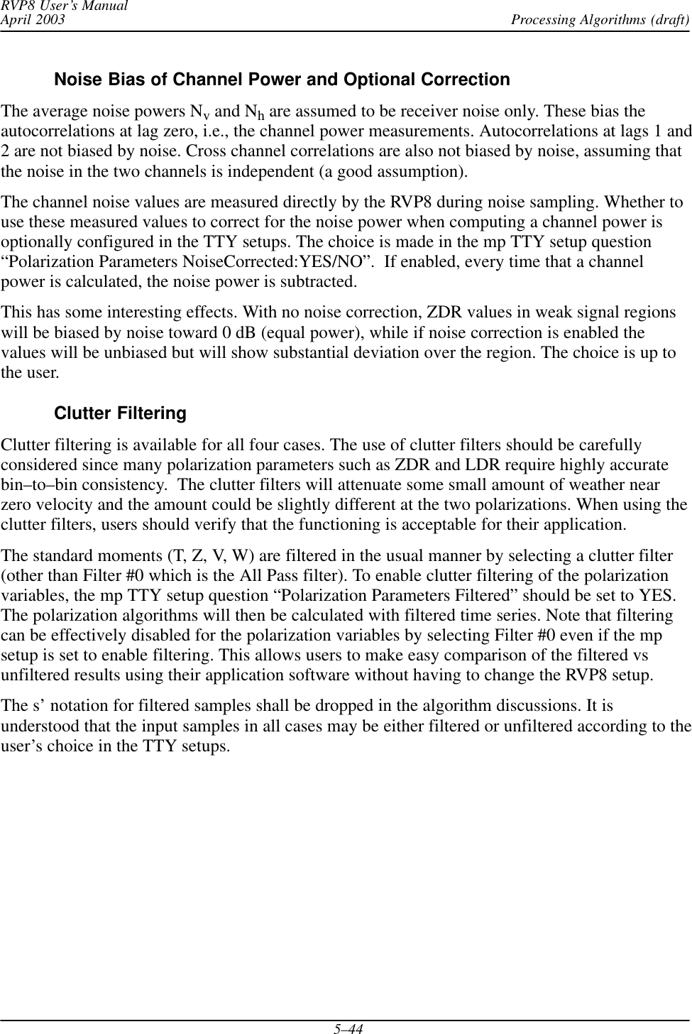
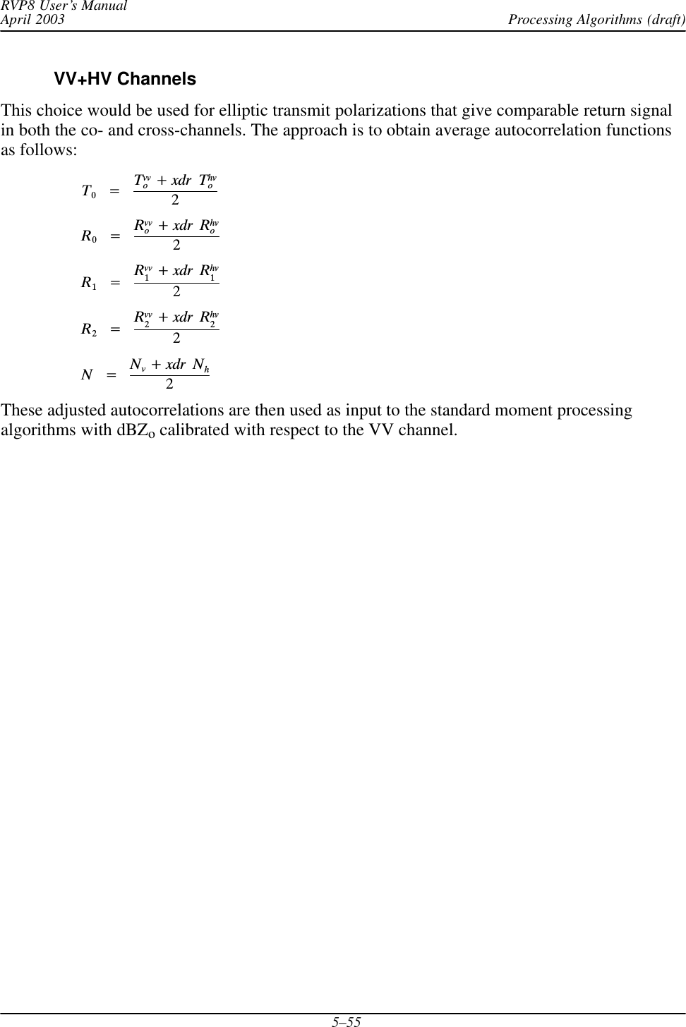
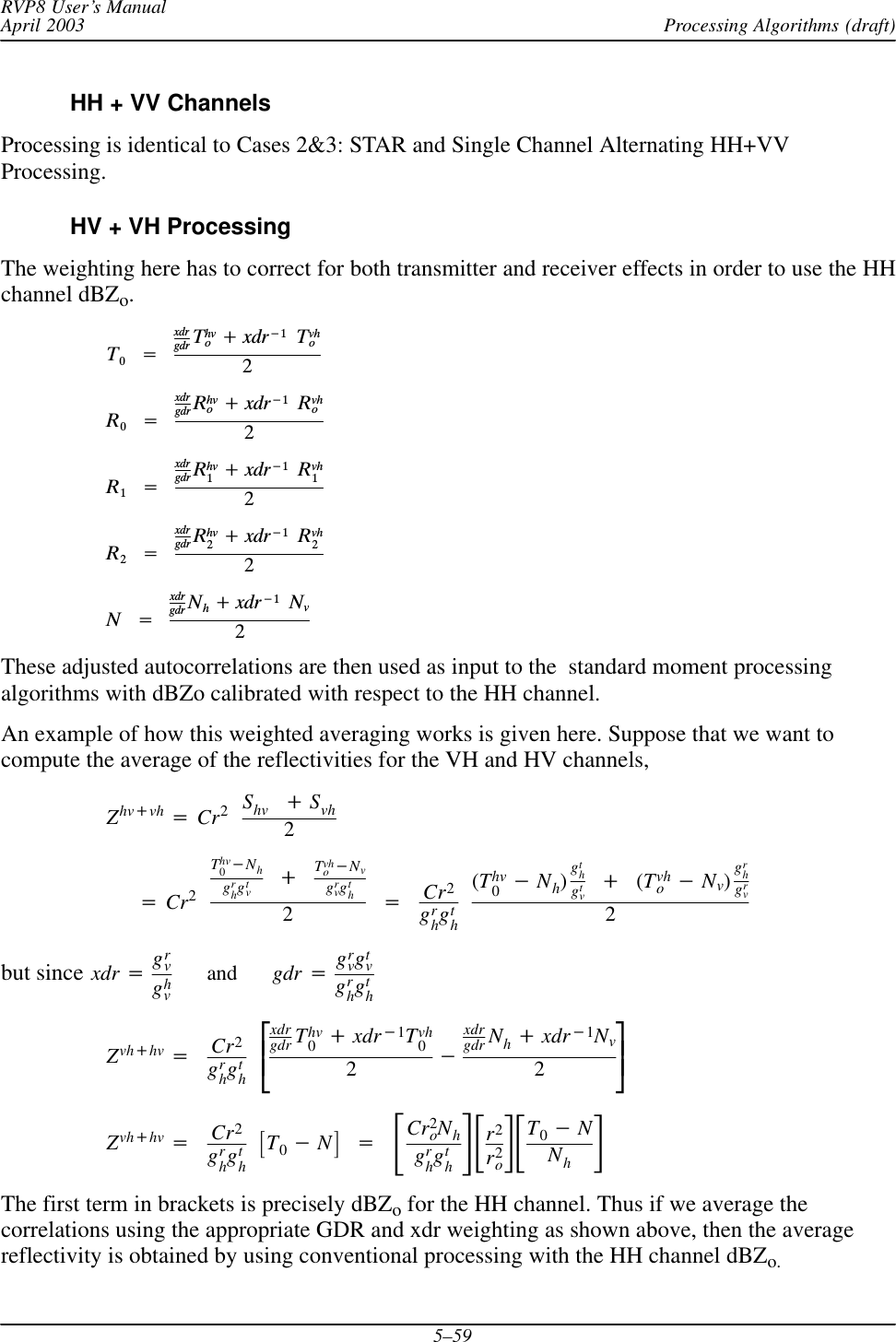
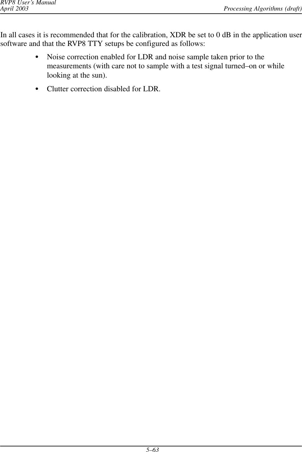
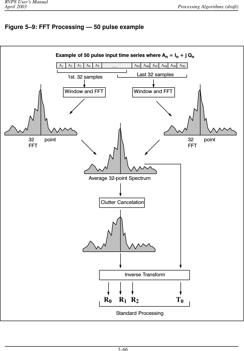
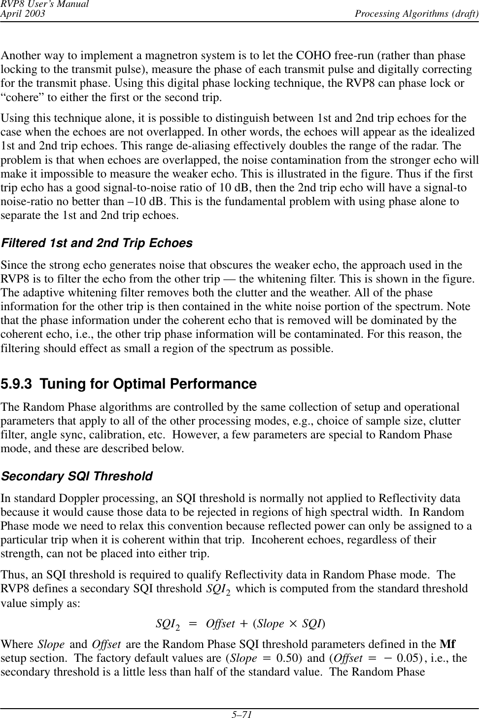
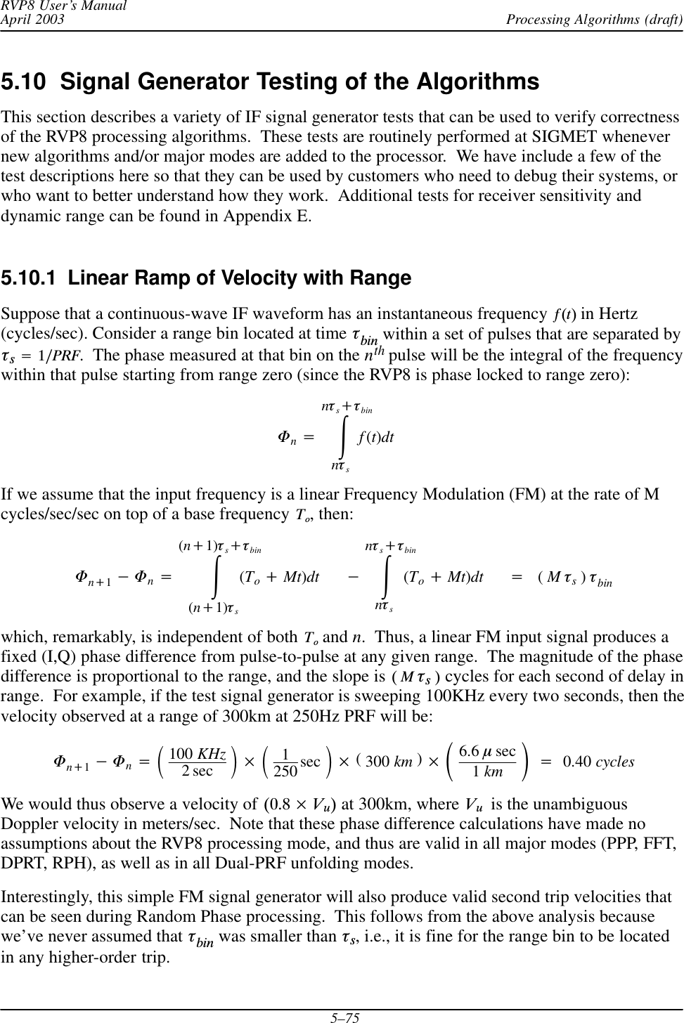
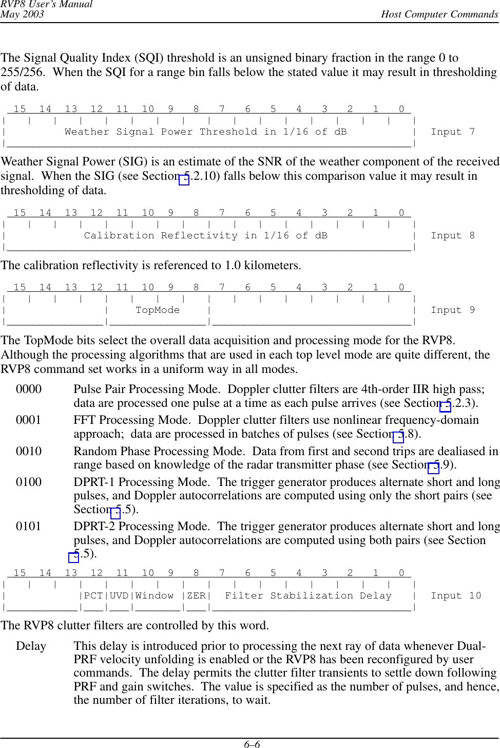
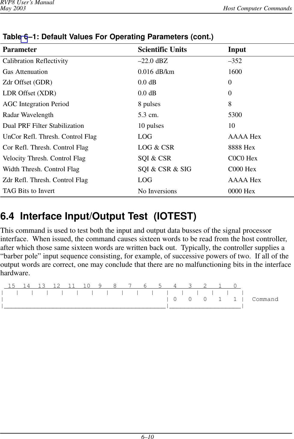
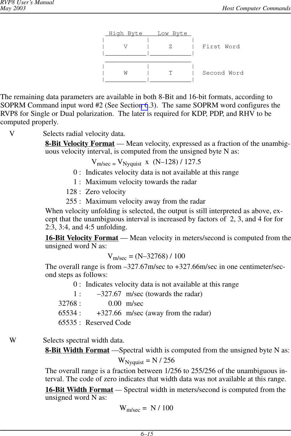
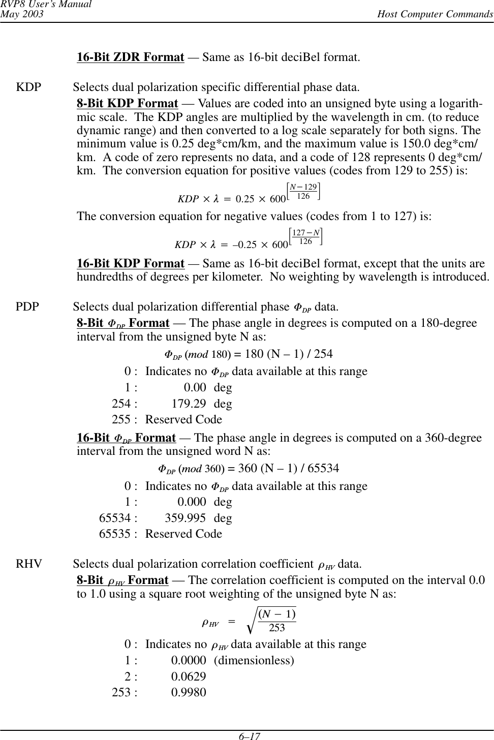
![Processing Algorithms (draft)RVP8 User’s ManualApril 20035–115.2 Video (“I” and “Q”) Signal ProcessingThis section describes the processing of the video (“I” and “Q”) data to obtain the reducedparameters: reflectivity, total power, velocity, width, signal quality index, clutter powercorrection, and sometimes ZDR. The RVP8 employs two methods (selectable) for processingthe I and Q signals: pulse-pair and FFT. The methods are similar except in regard to theprocedures for clutter filtering. The pulse pair methods are described below; the FFT clutterfiltering algorithms are described in Section 5.8.5.2.1 Time SeriesRecall that the time series synthesized by the FIR filter consist of an array of complex numbers:sn+[In)jQn]for n+1, 2, 3, AAA,Mwhere “j” is *11ń2. These data samples are analogous to the “I” and “Q” samples in atraditional analog receiver. They are sampled at a selectable resolution in the range 50–133meters. The time series are the starting point for all calculations performed within the RVP8.5.2.2 IIR Clutter Filter for PPP-ModeThe RVP8’s pulse-pair-processing mode employs a 4th order Infinite Impulse Response (IIR)digital high pass filter to remove low frequency signals due to ground clutter from the timeseries. Since the width of the clutter can change with the antenna rotation rate, eight differentfilters (seven high-pass, plus one all-pass) are provided. The filter stop-bandwidths vary fromapproximately 2% to 14% of the Nyquist interval, and stop band attenuation is at least 40 dB. Asetup question allows selection of either 40 dB or 50 dB filters. The 50 dB filters are intendedfor Klystron systems. Any of the eight filters can be selected independently at each individualrange bin. This permits range-dependent clutter removal. The filter algorithm is outlined below.The input time series sn is processed to form a filtered output time series sȀn as follows:sȀn+B0sn)B1sn*1)B2sn*2)B3sn*3)B4sn*4*C1sȀn*1*C2sȀn*2*C3sȀn*3*C4sȀn*4where the B’s and C’s are the filter coefficients. Appendix C gives the magnitude responseplots for the set of filters supplied with the RVP8.](https://usermanual.wiki/Baron-Services/XDD-1000C.S10-RECEIVER-AND-PROCESSOR-USERS-MANUAL-PART-2/User-Guide-374023-Page-73.png)
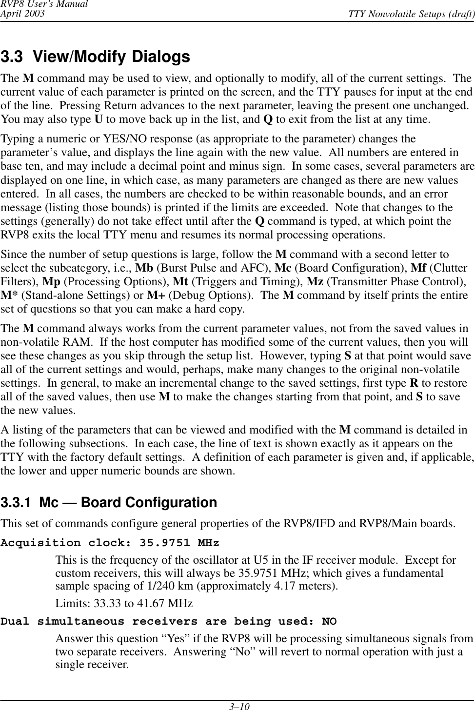
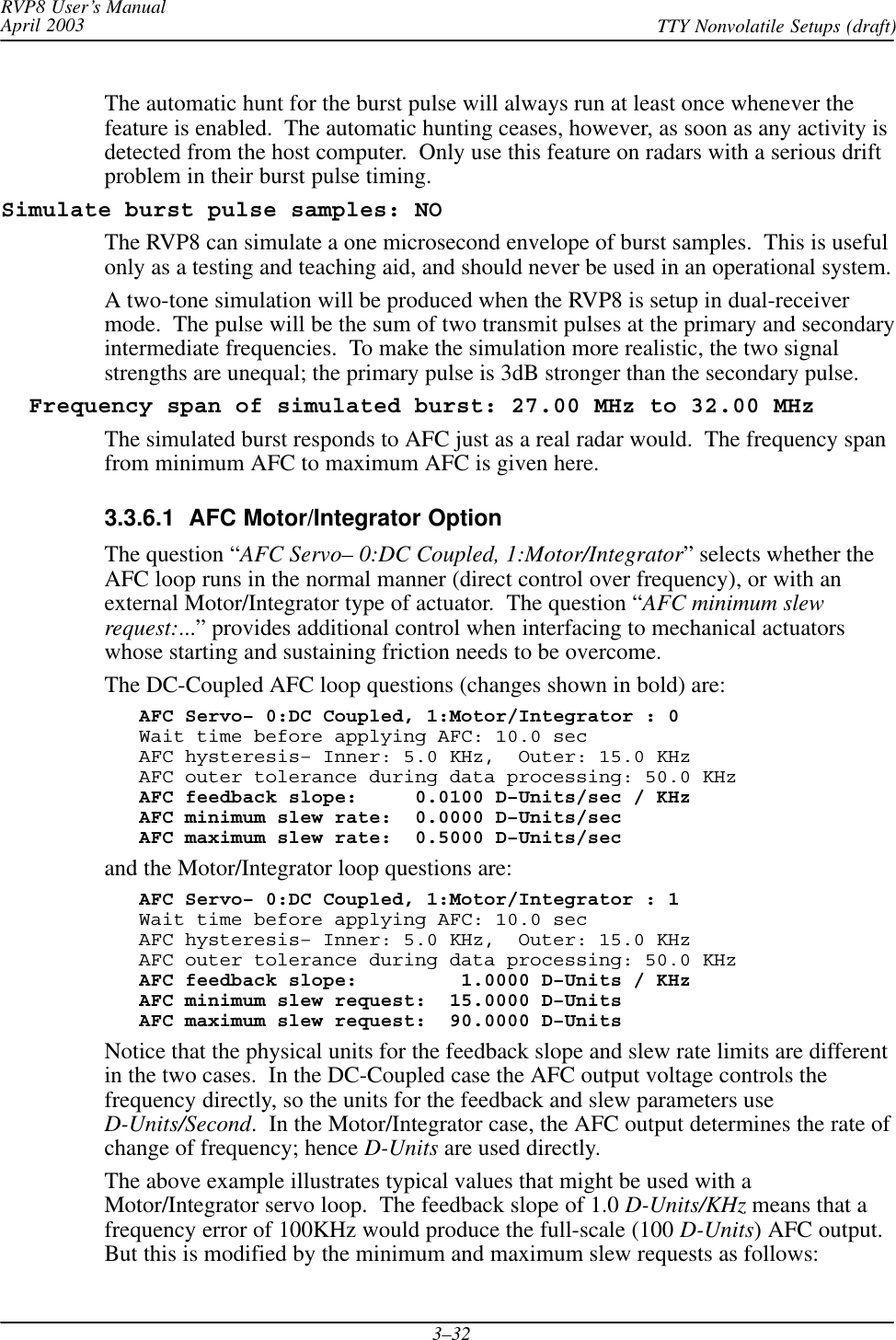
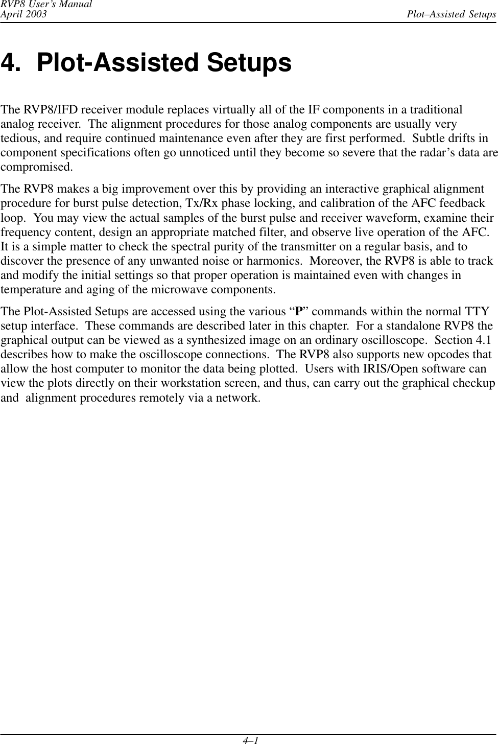
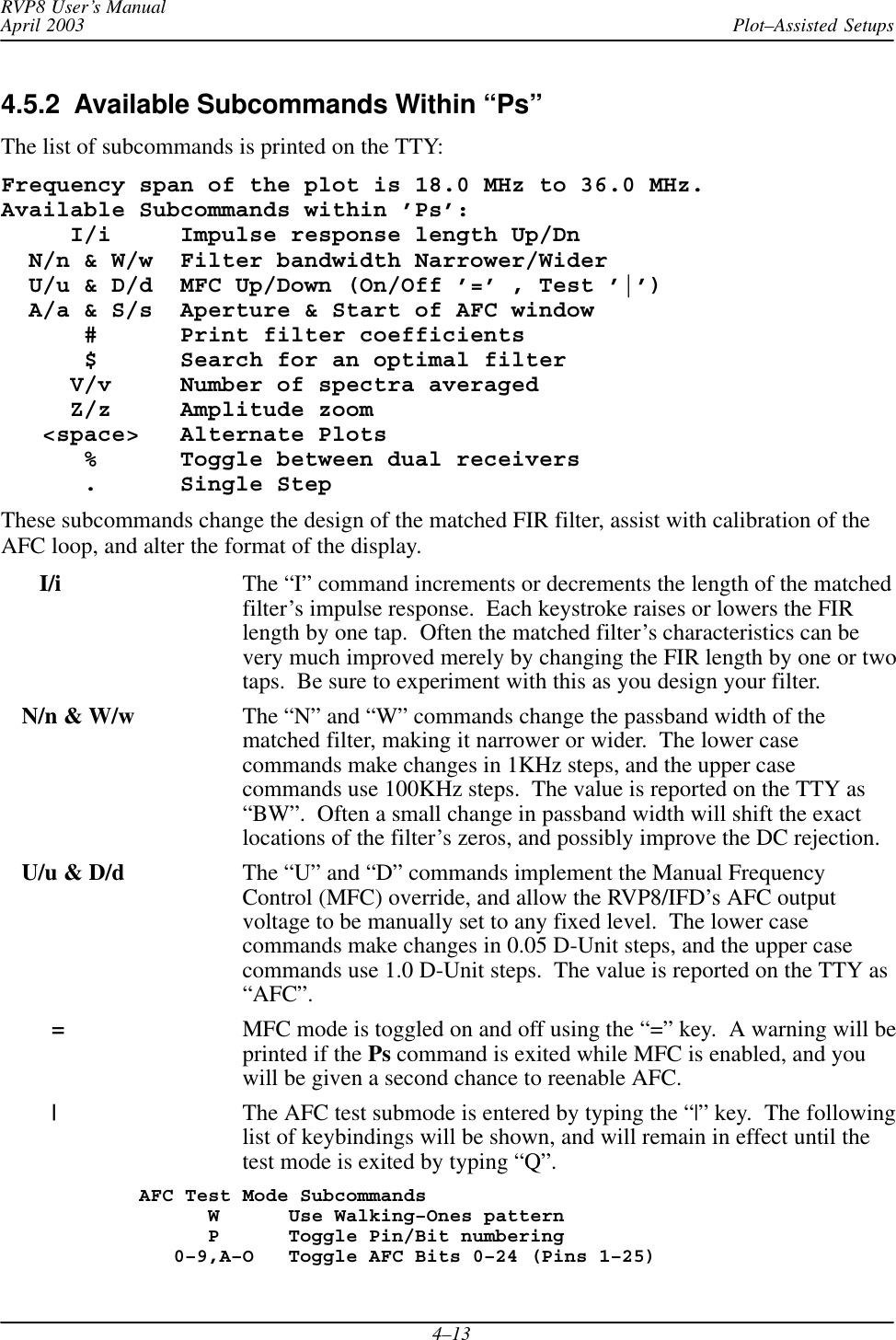
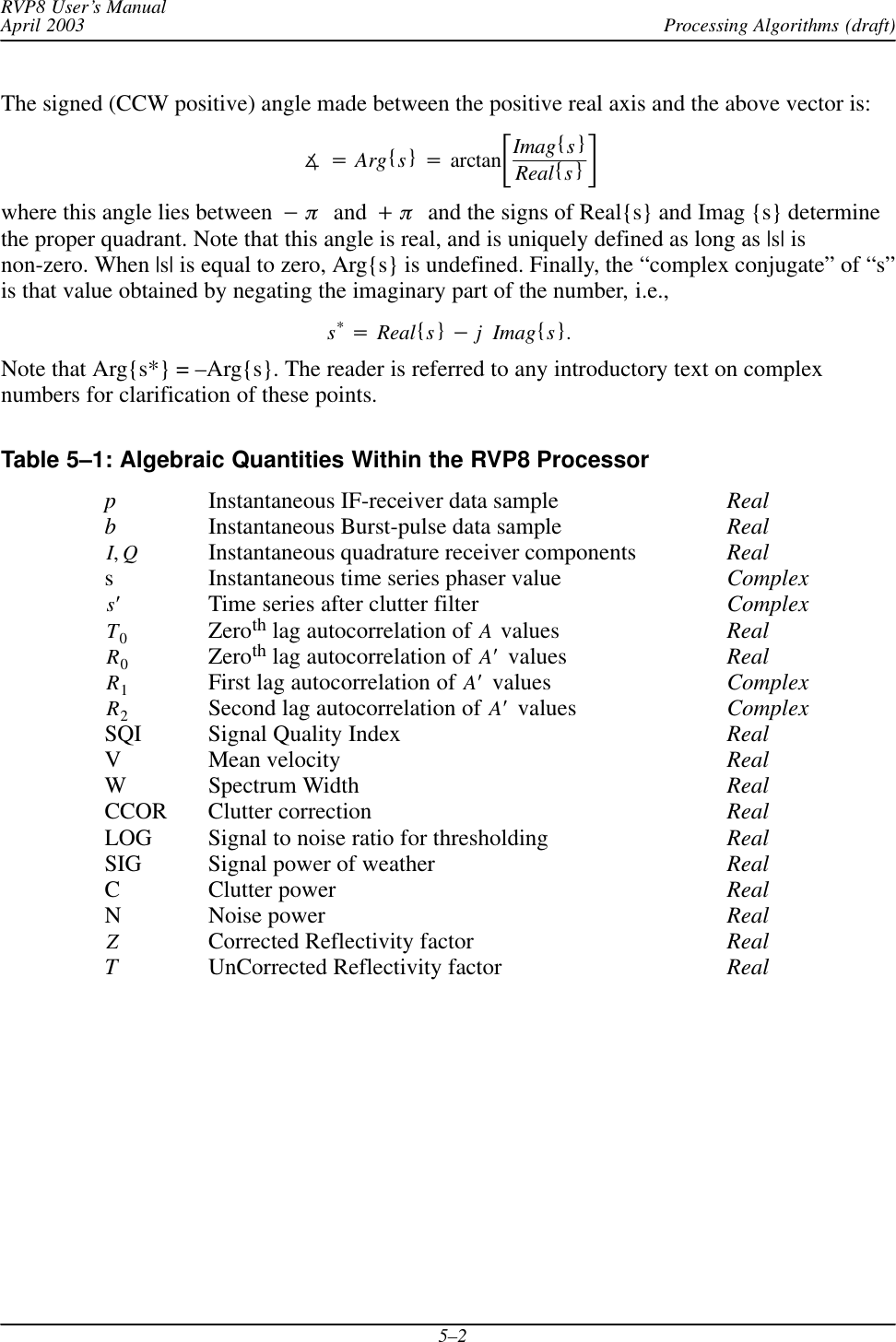
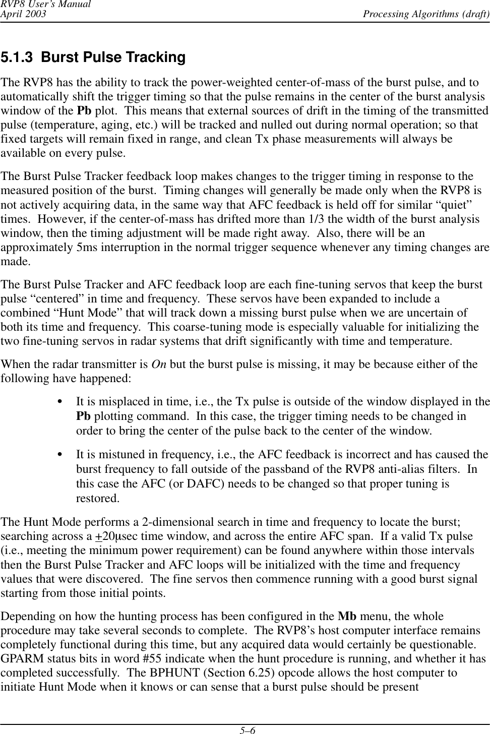
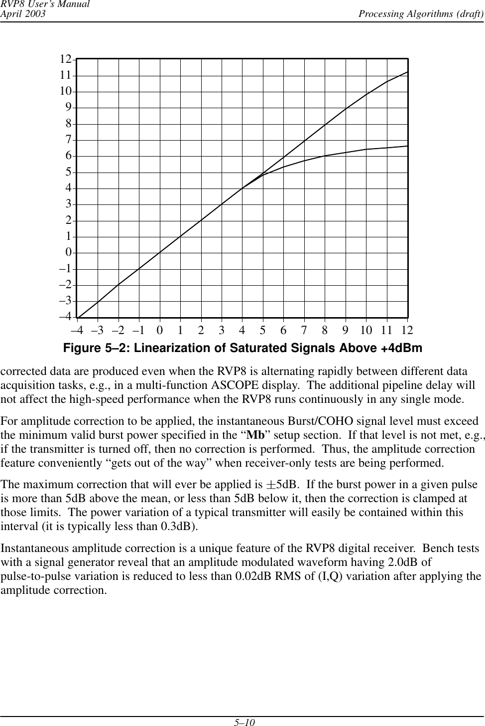
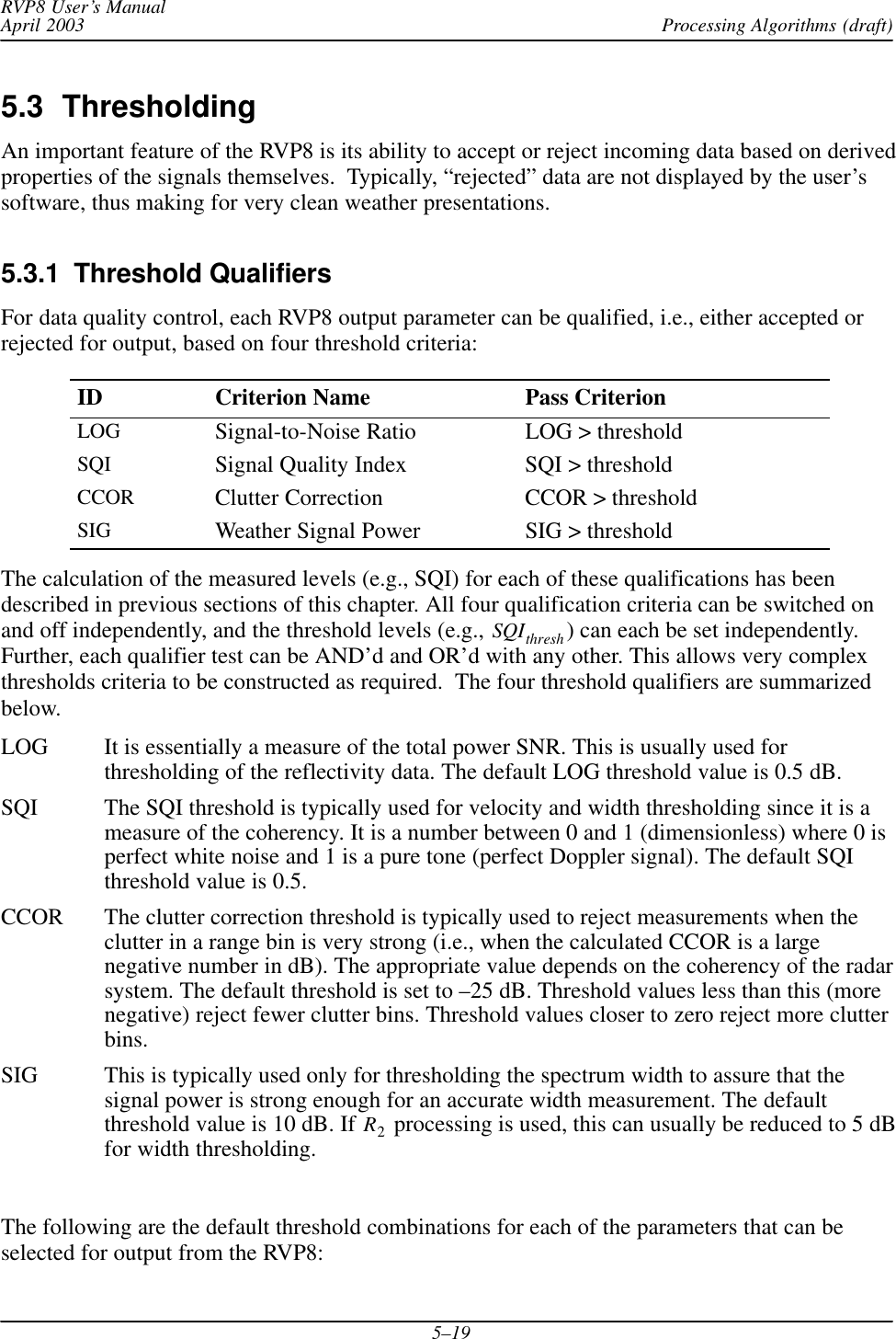
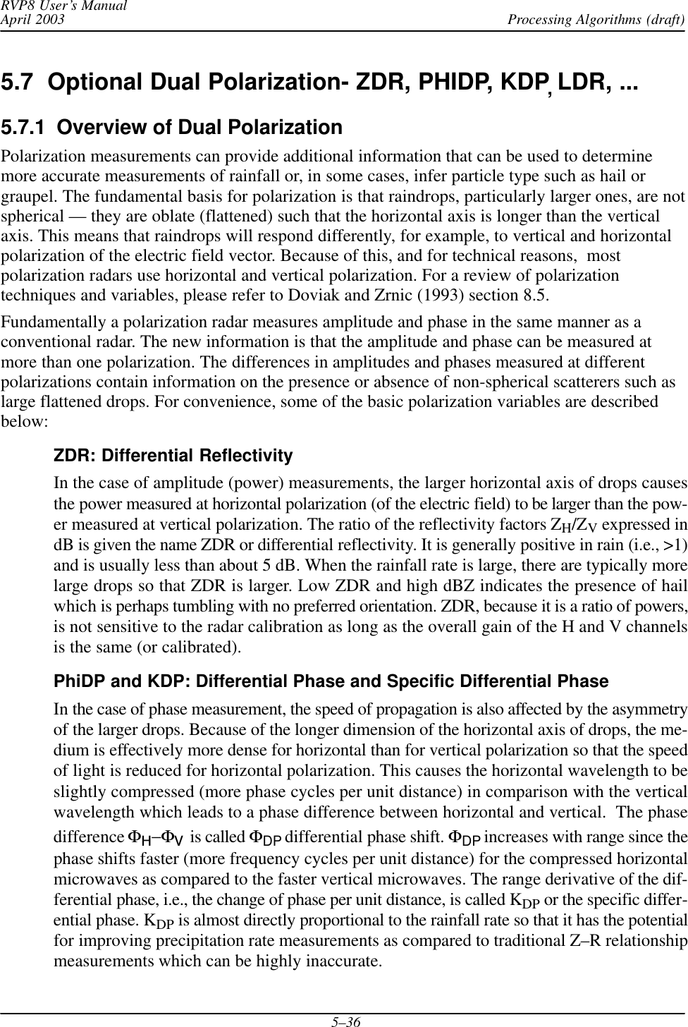
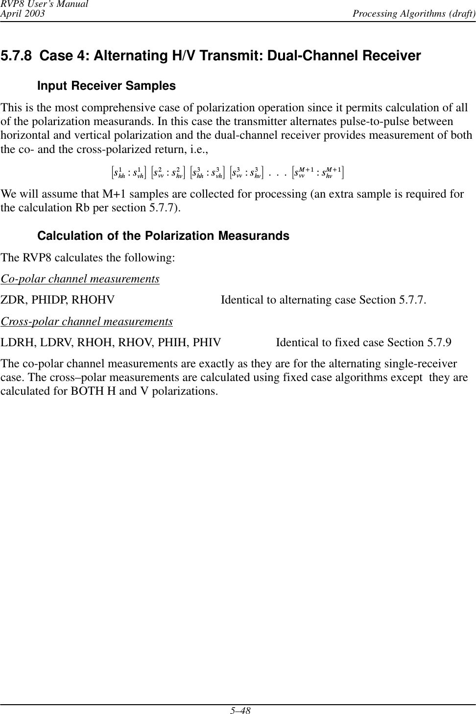
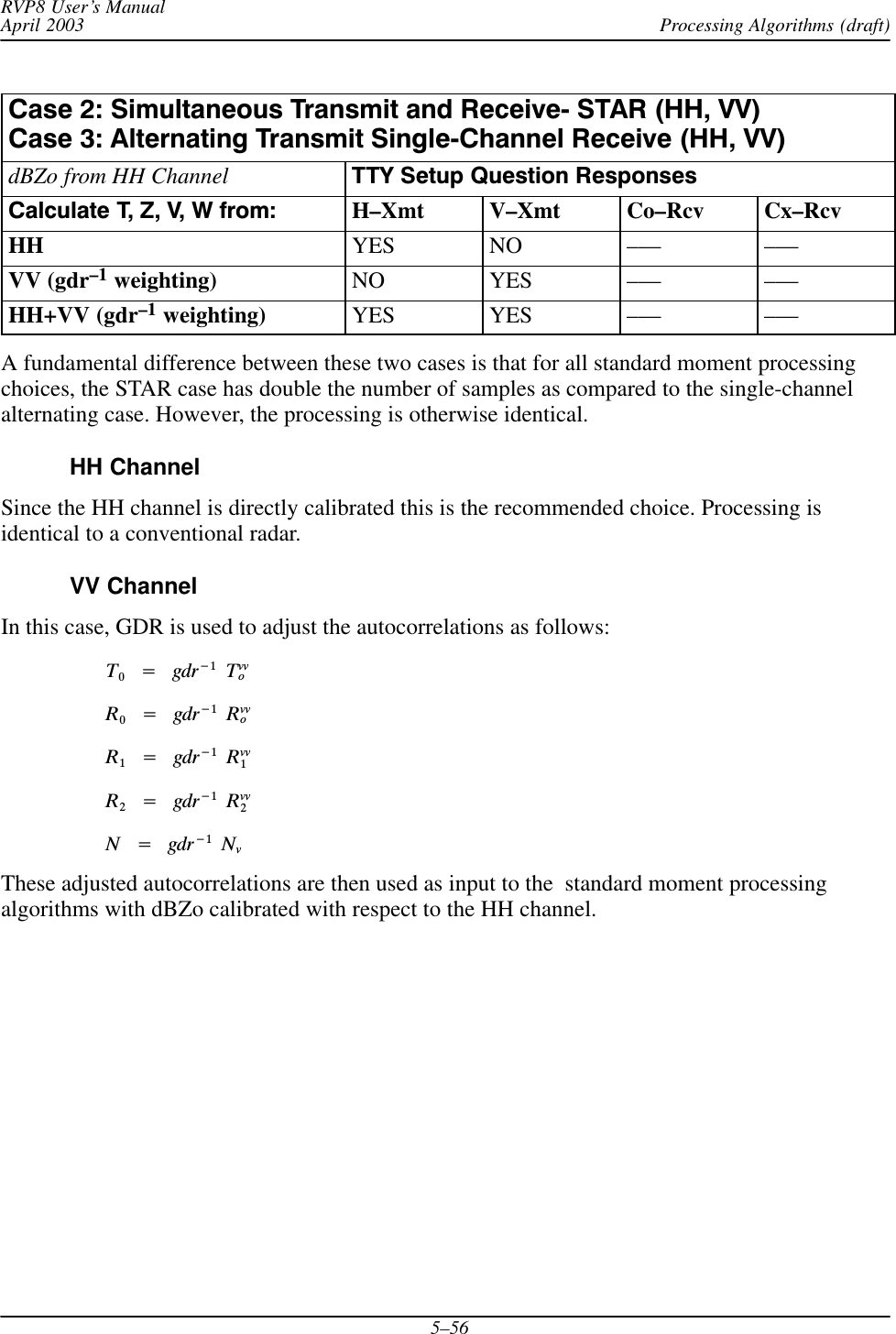
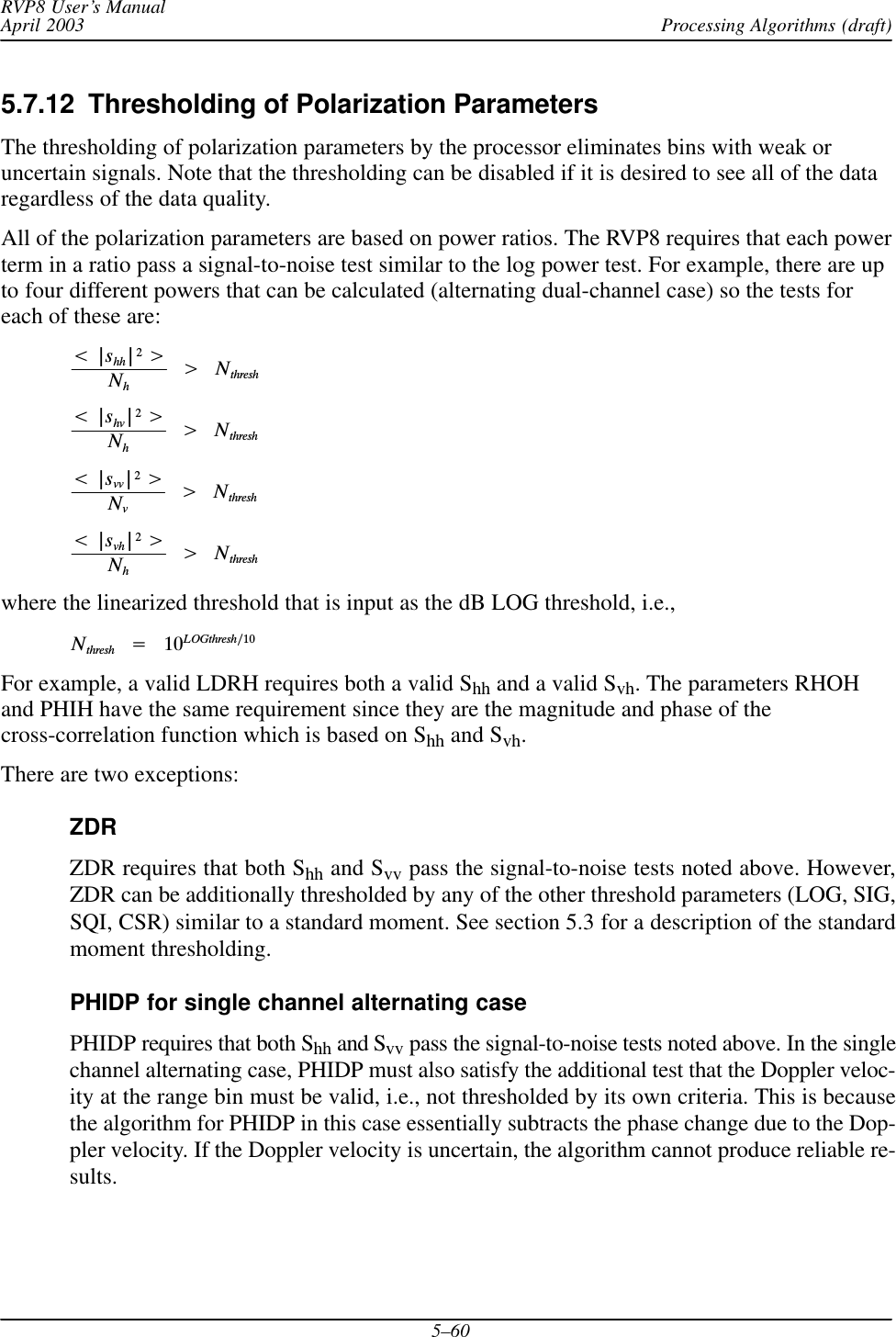
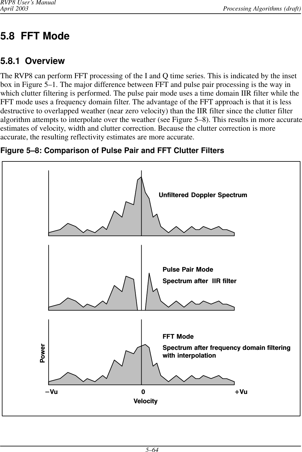
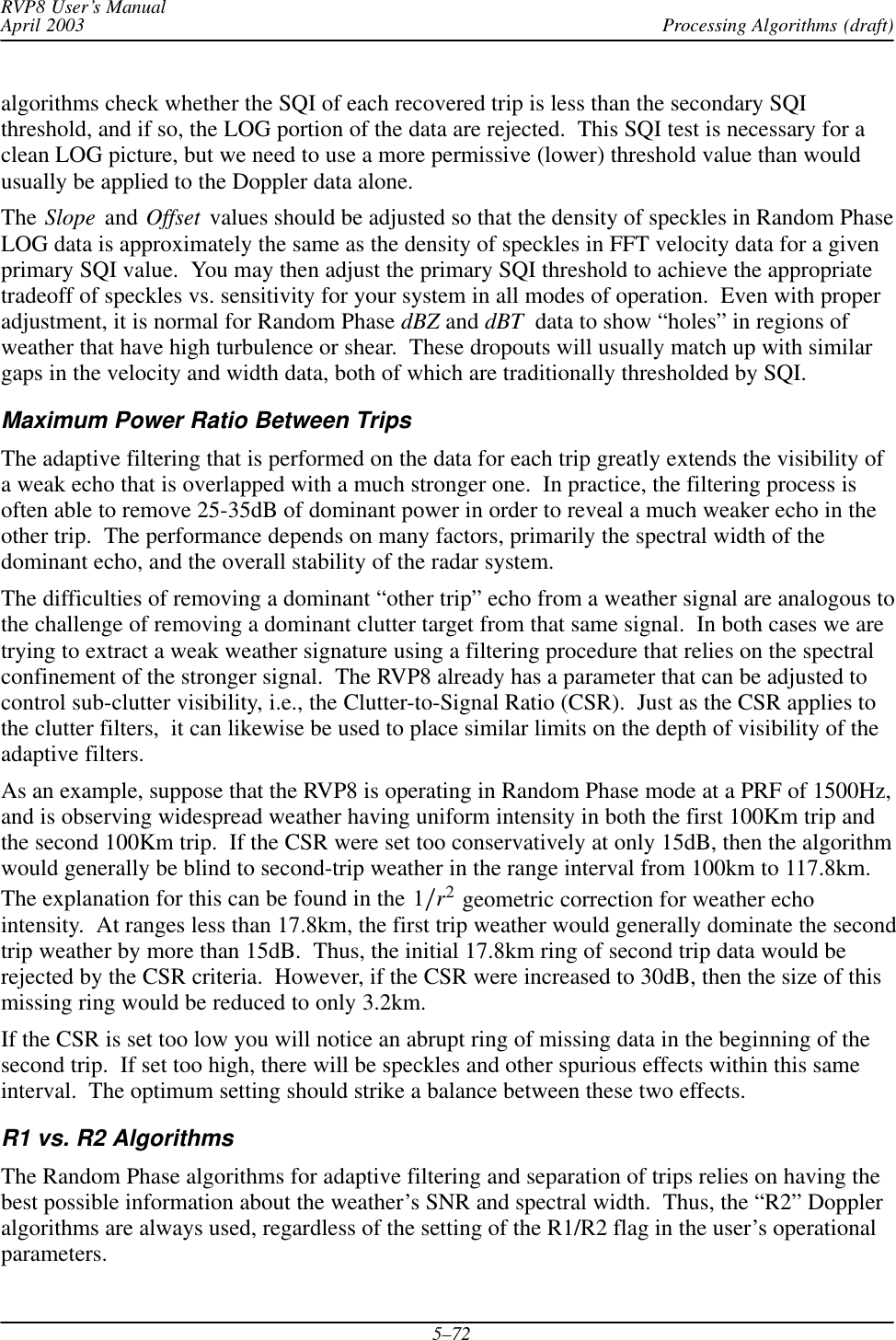
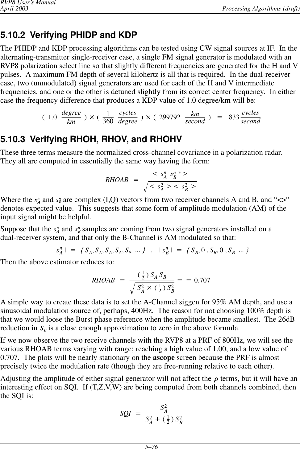
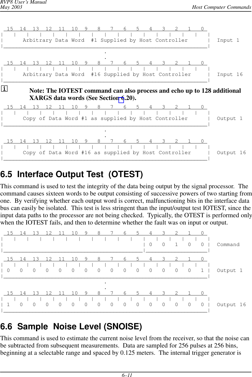
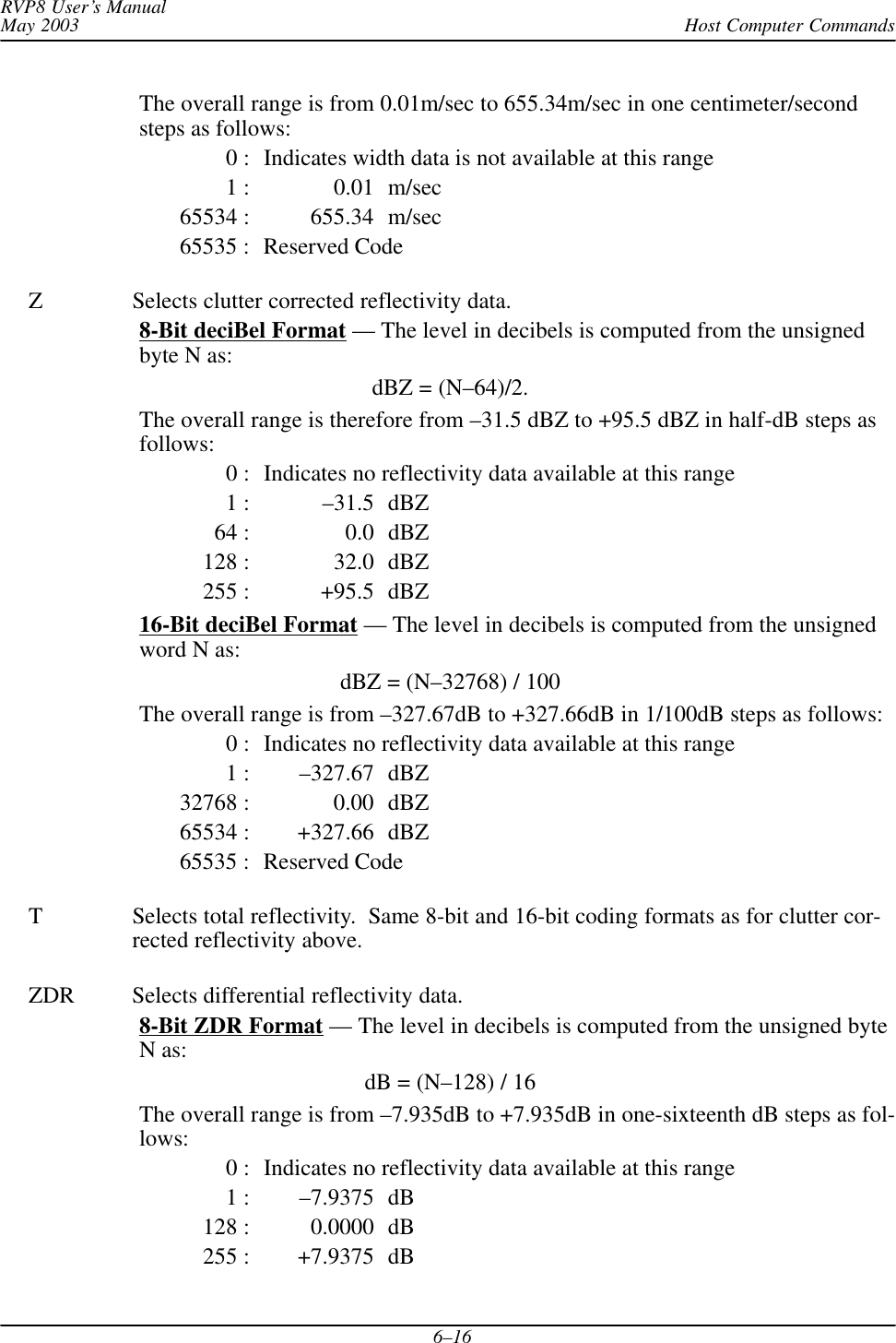
![Processing Algorithms (draft)RVP8 User’s ManualApril 20035–125.2.3 Autocorrelations for PPP-ModeThe autocorrelations are computed during pulse-pair-processing mode according to thefollowing algorithms (corresponding physical models are also given):Parameter and Definition Physical ModelTo+1MȍMn+1sn*sngrgt(S)C))NRo+1MȍMn+1sȀ*nsȀngrgtS)NR1+1M*1ȍM*1n+1sȀ*nsȀn)1grgtSejpVȀ*p2W2ń2R2+1M*2ȍM*2n+1sȀ*nsȀn)2grgtSej2pVȀ*2p2W2where M is the number of pulses in the time average. Here, sȀ denotes the filtered time series, sdenotes the original unfiltered time series and the * denotes a complex conjugate. gr and gtrepresent the transmitter and receiver gains, i.e., their product represents the total system gain.Since the RVP8 is a linear receiver, there is a single gain number that relates the measuredautocorrelation magnitude to the absolute received power. However, since many of thealgorithms do not require absolute calibration of the power, the gain terms will be ignored in thediscussion of these. To for the unfiltered time series is proportional to the sum of themeteorological signal S, the clutter power C and the noise power N. R0 is equal to the sum ofthe meteorological signal S and noise power N which is measured directly on the RVP8 byperiodic noise sampling. To and R0 are used for calculating the dBZ values- the equivalent radarreflectivity factor which is a calibrated measurement. The physical models for R0,R1 and R2correspond to a Gaussian weather signal and white noise. W is the spectrum width and V’ themean velocity, both for the normalized Nyquist interval [–1 to 1].The exact value of M that is used for each time average will generally be the “Sample Size” thatis selected by the SOPRM command (See Section 6.3). However, when the RVP8 is in PPPmode and antenna angle synchronization is enabled, the actual number of pulses used may belimited by the number that fit within each ray’s angular limits at the current antenna scan rate.The value of M will never be greater than the SOPRM Sample Size, but it may sometimes beless. For example, at 1KHz PRF, 20_/sec scan rate, 1_ ray synchronization, and a Sample Sizeof 80, there will be 50 pulses used for each ray (not 80). Note, however, that the number ofpulses used in the “batched” (non-PPP) modes will always be exactly equal to the Sample Size,since those modes are allowed to use overlapping pulses.](https://usermanual.wiki/Baron-Services/XDD-1000C.S10-RECEIVER-AND-PROCESSOR-USERS-MANUAL-PART-2/User-Guide-374023-Page-74.png)
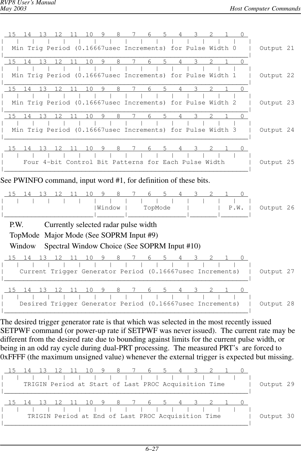
![Processing Algorithms (draft)RVP8 User’s ManualApril 20035–155.2.6 VelocityFor a Doppler power spectrum that is symmetric about its mean velocity, the velocity is obtaineddirectly from the argument of the autocorrelation at the first lag, i.e.,V+l4ptsq1 where q1+arg NJR1Nj.l is the radar wavelength, ts is the sampling time (1/PRF). q1 is constrained to be on theinterval [*p,p]. When q1+" p , then V+" Vu where the unambiguous velocity is ,Vu+l4ts .If the absolute value of the true velocity of the scatterers is greater than Vu , then the velocitycalculated by the RVP8 is folded into the interval ƪ*Vu,Vuƫ , which is called the Nyquistinterval. Folding is usually easily recognized on a color display by a discontinuous jump invelocities. For example, if the true velocity is Vu)DV, then the velocity calculated by theRVP8 is *Vu)DV, which is 2Vu away from the true mean velocity.For 8-bit outputs, rather than calculating the absolute velocity in scientific units, the RVP8calculates the mean velocity for the normalized Nyquist interval [–1,1], i.e., the output valuesare,VȀ+q1p.For example, an output value of –0.5 corresponds to a mean velocity of *Vuń2. Thenormalized velocity VȀ is more efficient use of the limited number of bits.5.2.7 Spectrum Width AlgorithmsThe spectrum width is a measure of the combined effects of shear and turbulence. To a lesserextent, the antenna rotation rate can also effect the spectrum width. At high elevation angles, thefall speed dispersion of the scatterers also effects spectrum width.There are two choices for the spectrum width algorithm used in the RVP8, depending on thespeed and accuracy that are required for the application:R0,R1 “fast” algorithm valid when SNR >> 10 dBR0,R1,R2 “accurate” algorithm for SNR >> 0 to 5 dBThe approach used is selected in the SOPRM command. The two approaches are described below:R0,R1Width AlgorithmGiven samples of the Doppler autocorrelation function, numerous estimates of spectral vari-ance can be computed (Passarelli & Siggia, 1983). The particular estimator used by theRVP8 employs the magnitudes of R0 and R1 and assumes that the Doppler spectrum isGaussian (usually an acceptable assumption) and that the signal-to-noise ratio is large. Spe-cifically we have (similar to Srivastava, et al 1979):Variance +2lnƪRo|R1|ƫ+*2ln[SQI]](https://usermanual.wiki/Baron-Services/XDD-1000C.S10-RECEIVER-AND-PROCESSOR-USERS-MANUAL-PART-2/User-Guide-374023-Page-77.png)
![Processing Algorithms (draft)RVP8 User’s ManualApril 20035–16where “ln” represents the natural logarithm. This can be compared to the expression in thepreceding section for SQI to illustrate that this expression for the variance is only valid when:SNRSNR )1[1which occurs when the SNR is large.This variance estimator is normalized to the Nyquist interval in units of [*p,p]. Thus, forexample, a variance of p2ń25 would be obtained from a Gaussian spectrum having a stan-dard deviation equal to one fifth of the total width of the plotted spectral distribution. Forscientific purposes, the spectrum width (standard deviation) is more physically meaningfulthan the variance, since it scales linearly with the severity of wind shear and turbulence. Forthese reasons, the width W is output by the RVP8:W+VarianceǸpAgain, for efficient packing in 8-bits, width is normalized to the Nyquist interval [–1, 1 ].For the example given above, the output width W would be (1/5). To obtain the width in me-ters per second, one multiplies the output width by Vu .R0,R1,R2 Width AlgorithmThe width algorithm in this case is similar except that the addition of R2 extends the validityof the width estimates to weak signals. In this case the variance is:Variance +23lnƪ|R1||R2|ƫThe output width W is then defined as in the previous section.5.2.8 Signal Quality Index (SQI threshold) An important feature of the RVP8 is its ability to eliminate signals which are either too weak tobe useful, or which have widths too large to justify further analysis. This is done via the signalquality index (SQI) which is defined as:SQI +|R1|R0The SQI is the normalized magnitude of the autocorrelation at lag 1 and varies between 0 for anuncorrelated signal (white noise) to 1 for a noise-free zero-width signal (pure tone). Meanvelocity estimates are degraded when the spectrum, width is large or when the signal-to-noiseratio is weak. The SQI is a good measure of the uncertainty in the velocity estimates and is aconvenient screening parameter to compute. In terms of the Gaussian model, the SQI is :SQI +SNRSNR )1e*p2W22where the SNR is the signal-to-noise ratio. For very large SNR’s the SQI is a function of thespectrum width only. For a zero-width pure tone (W=0), the SQI is a function of the SNR only(e.g., for W=0, an SNR of 1 corresponds to SQI=0.5). The SQI threshold is typically set to avalue of 0.4 to 0.5.](https://usermanual.wiki/Baron-Services/XDD-1000C.S10-RECEIVER-AND-PROCESSOR-USERS-MANUAL-PART-2/User-Guide-374023-Page-78.png)
![Processing Algorithms (draft)RVP8 User’s ManualApril 20035–175.2.9 Clutter Correction (CCOR threshold) In addition to calculating the R0,R1 and optional R2 autocorrelation terms, which are based onfiltered time series data, the RVP8 also computes T0 which is the total unfiltered power. Bycomparing the total filtered and unfiltered powers at each range bin, a clutter power, and hence aclutter correction, for that bin can be derived. The clutter correction is defined as,CCOR +10 log SC)S+10 log 1CSR )1where S is the weather signal power, C is the clutter power and CSR is the clutter-to-signalratio. The algorithm for calculating CCOR depends on whether the optional R2 autocorrelationlag is computed as described below.R0,R1 Clutter CorrectionIn this case CCOR is estimated from,CCORest +10 logƪR0T0ƫ+10 logƪS)NC)S)Nƫ+10 logƪ1)1SNRCSR )1)1SNRƫHere, the expression is strictly valid only when the signal-to-noise ratio(SNR=S/N) is large. Thus when the 2-lag approach is used, the clutter corrections are notas accurate for weak weather signals. However, the error is typically less than 3 dB.R0,R1,R2 Clutter CorrectionIn this case there is enough information to compute the clutter signal and noise power inde-pendently. The algorithm for CCOR is:CCORest +10 log SC)S+10 log 1CSR )1The clutter power is computed from:C+To*Ro+[C)S)N]*[S)N]The signal power S is then computed from:S+|R1| exp p2W22W is the width that has been previously calculated. This approach yields more accurate re-sults for the clutter correction in the case of a low SNR.](https://usermanual.wiki/Baron-Services/XDD-1000C.S10-RECEIVER-AND-PROCESSOR-USERS-MANUAL-PART-2/User-Guide-374023-Page-79.png)
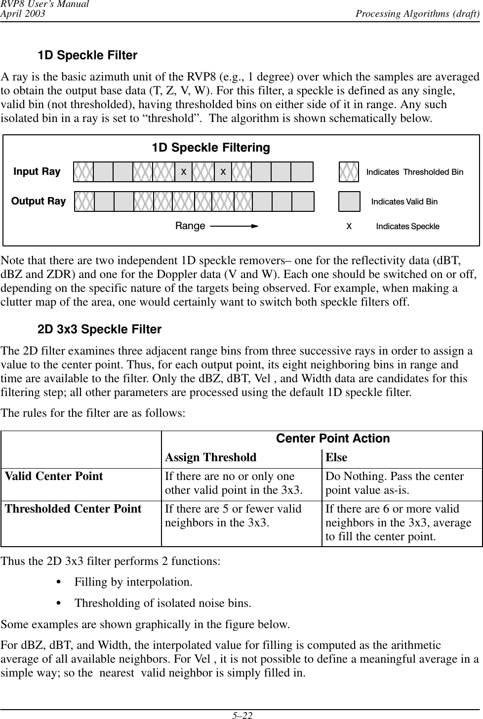
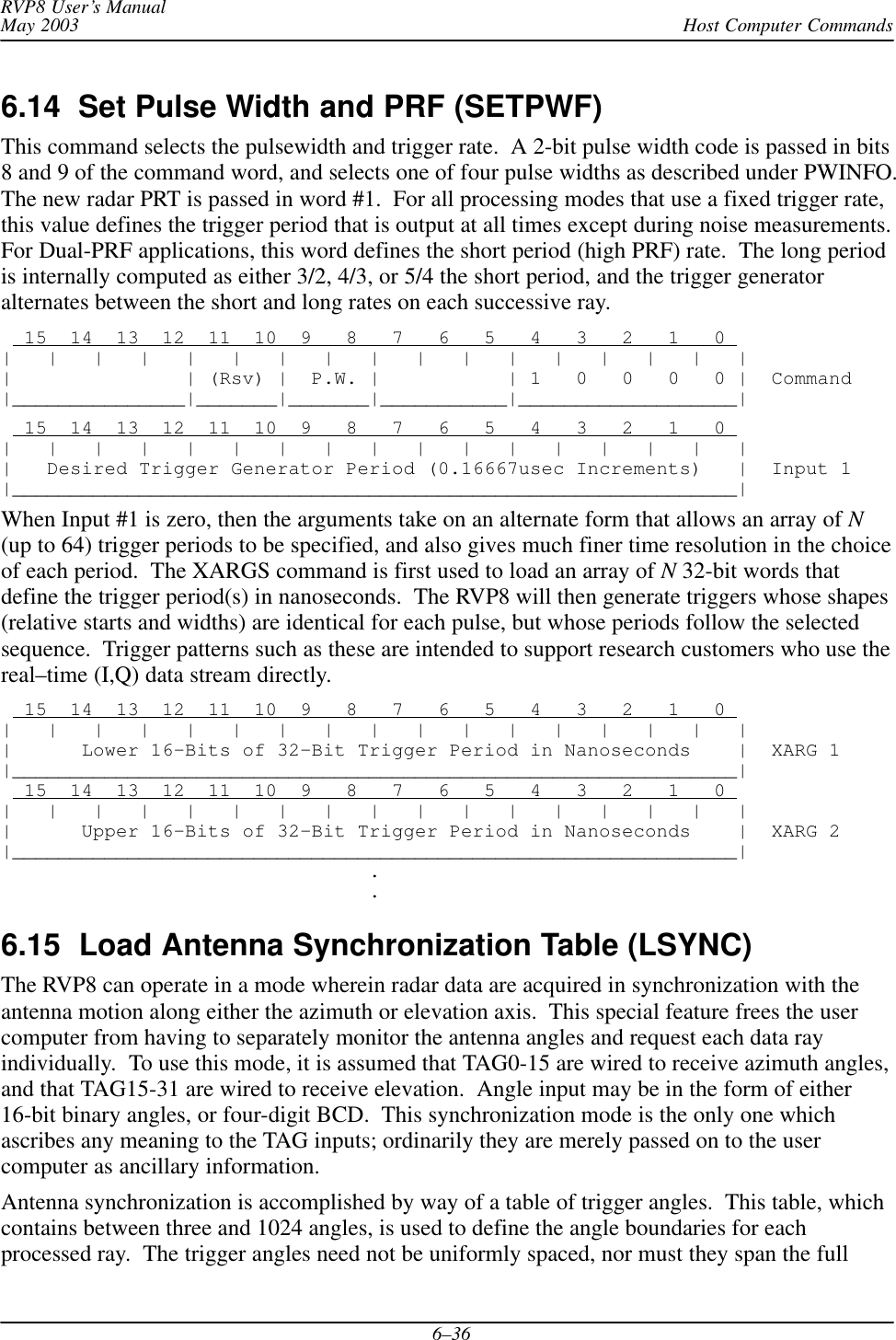
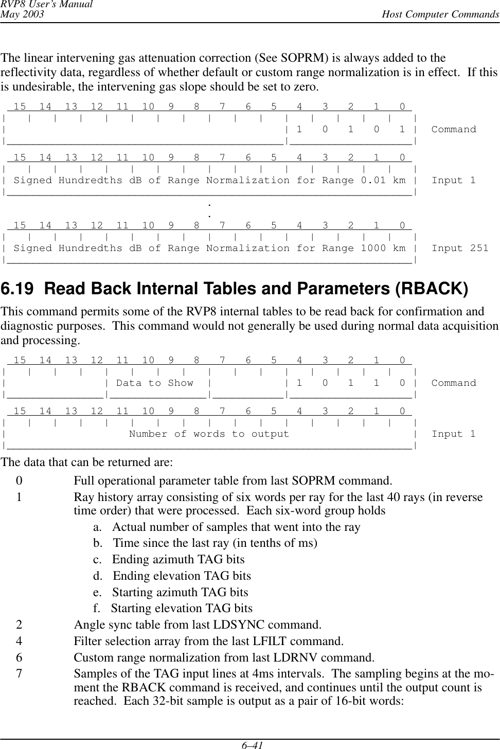
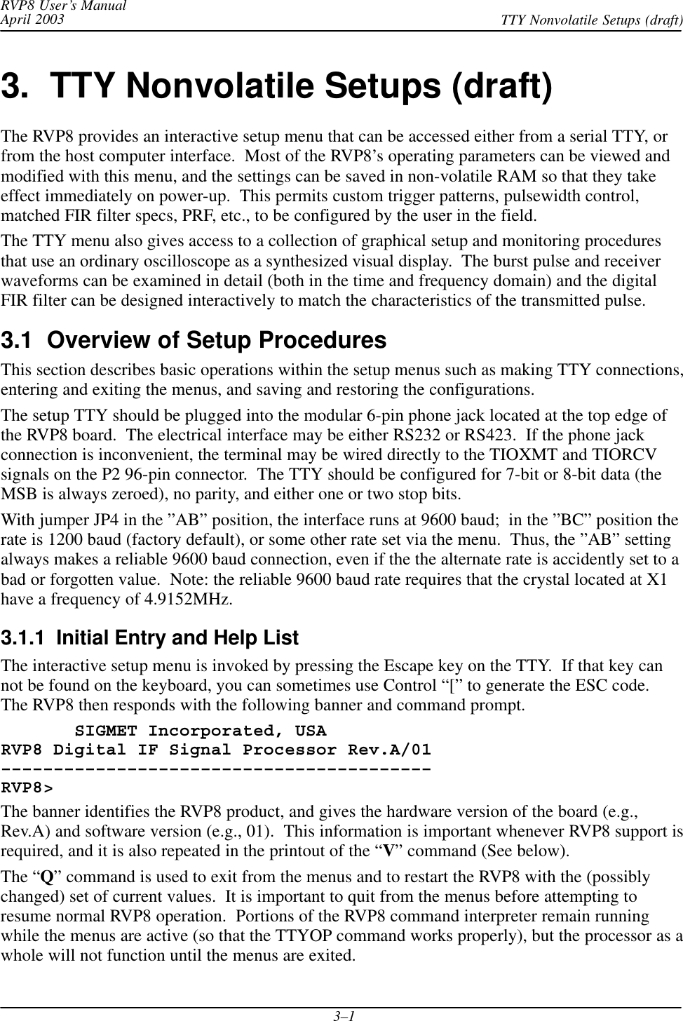
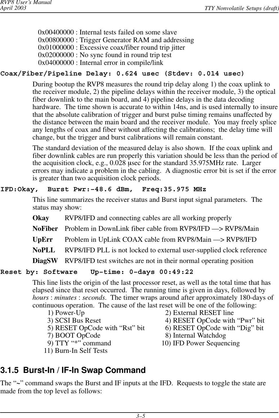
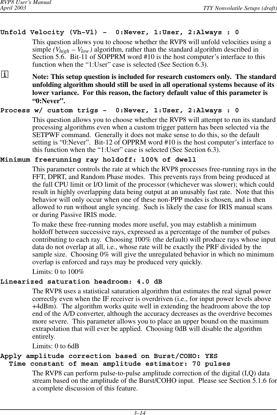
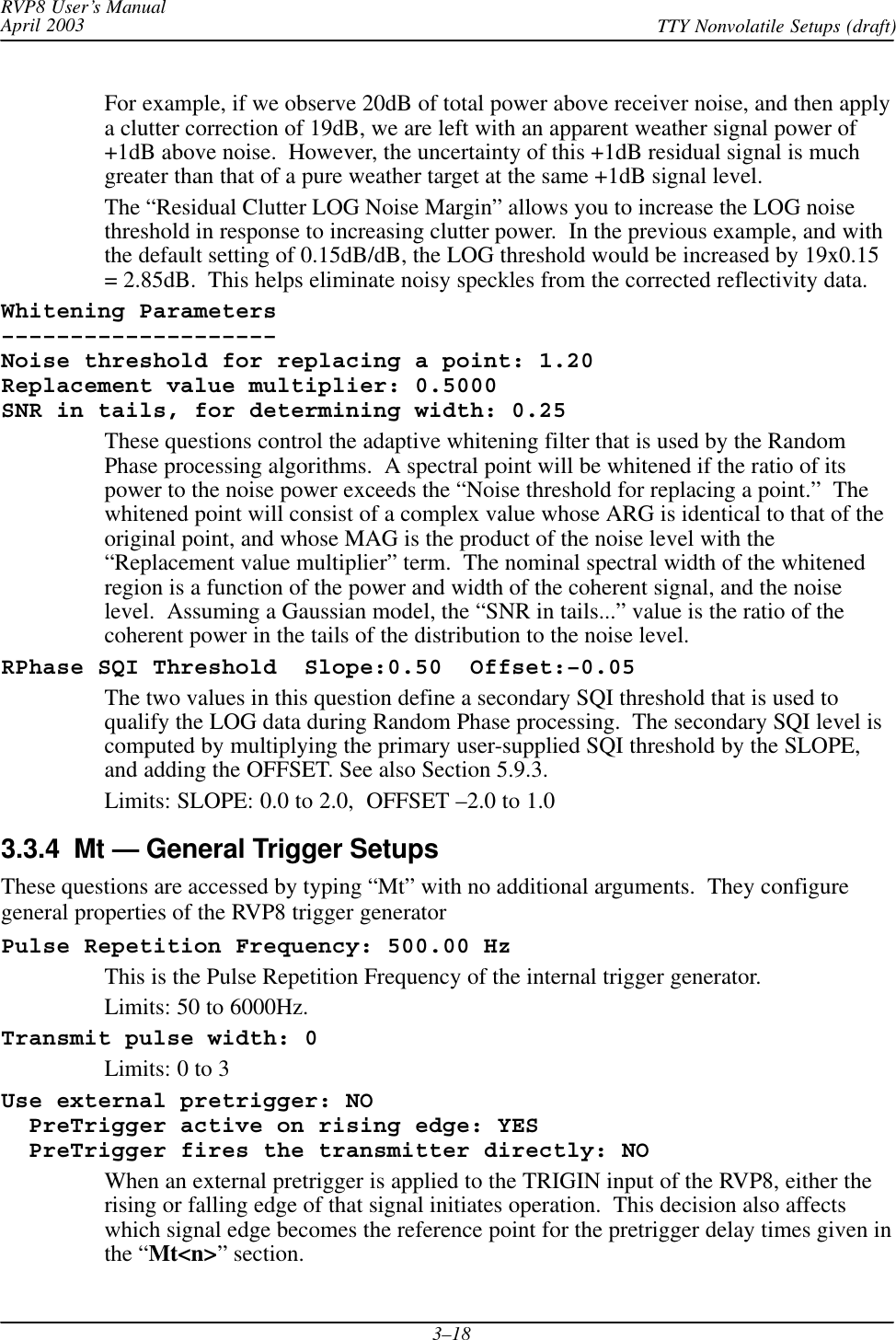
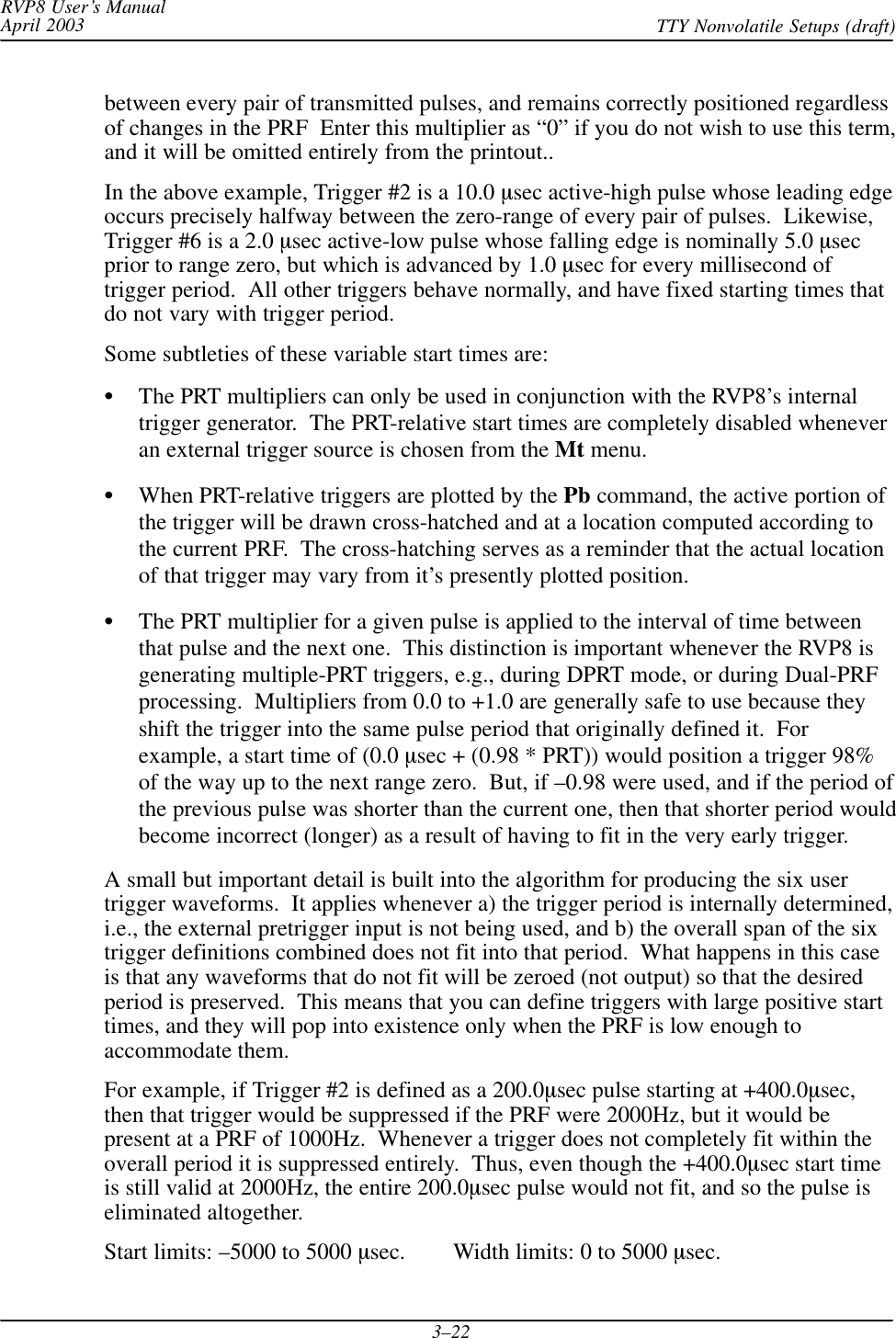
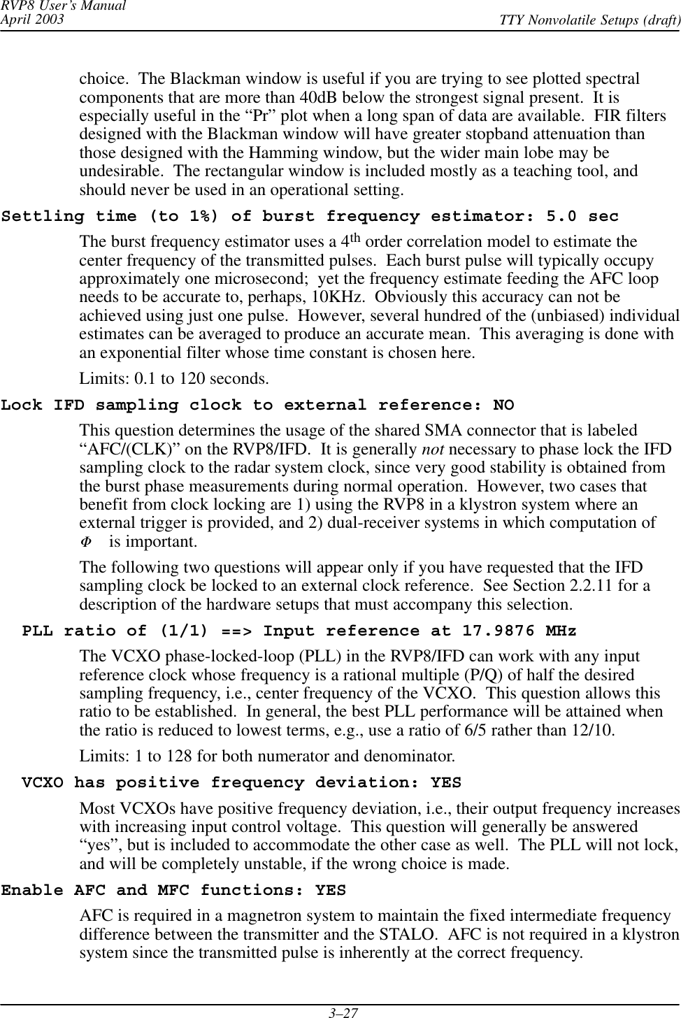
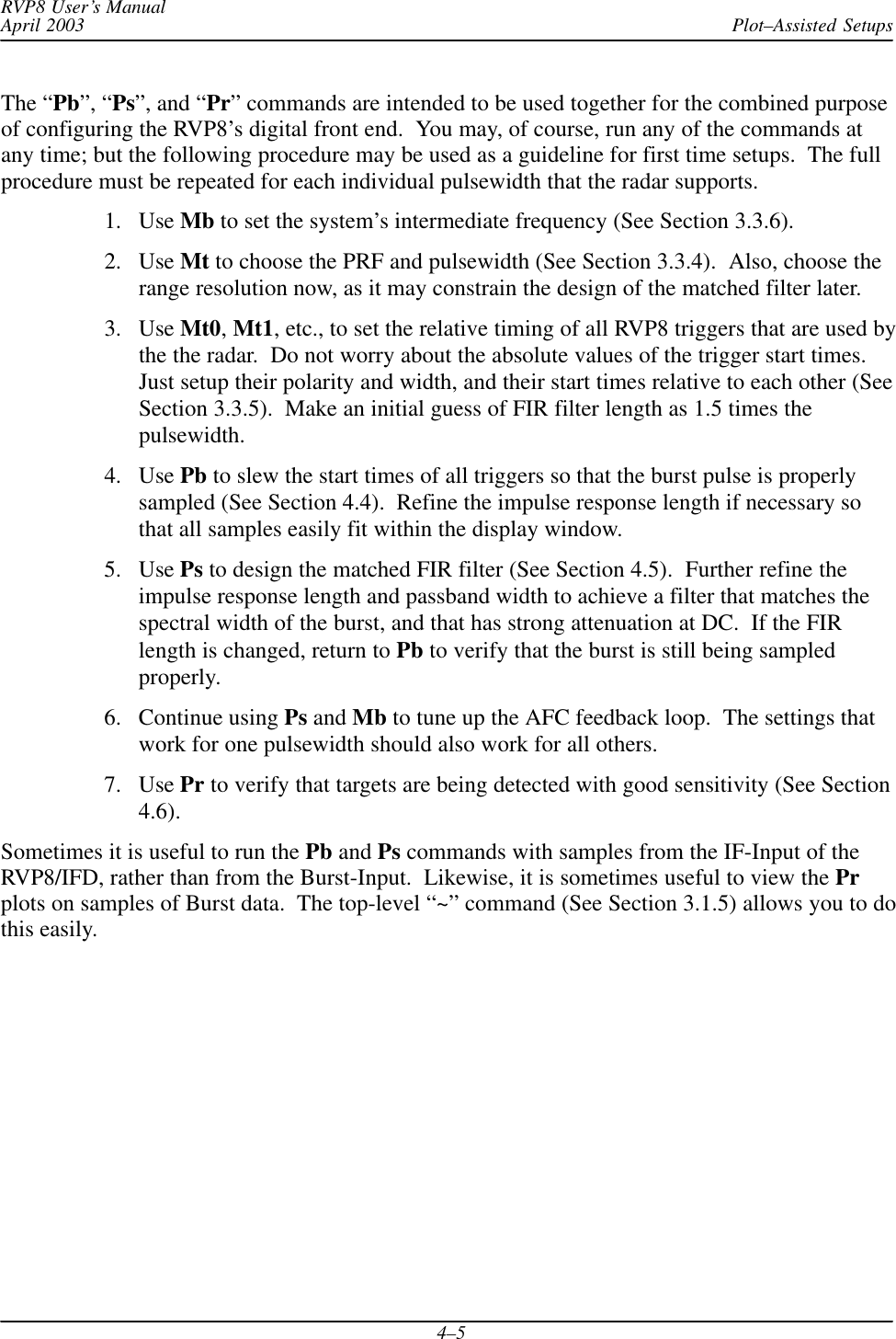
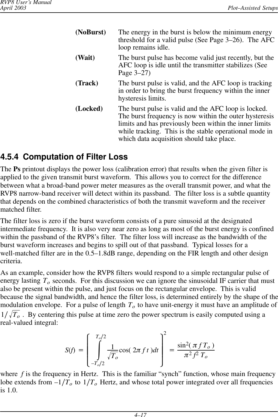
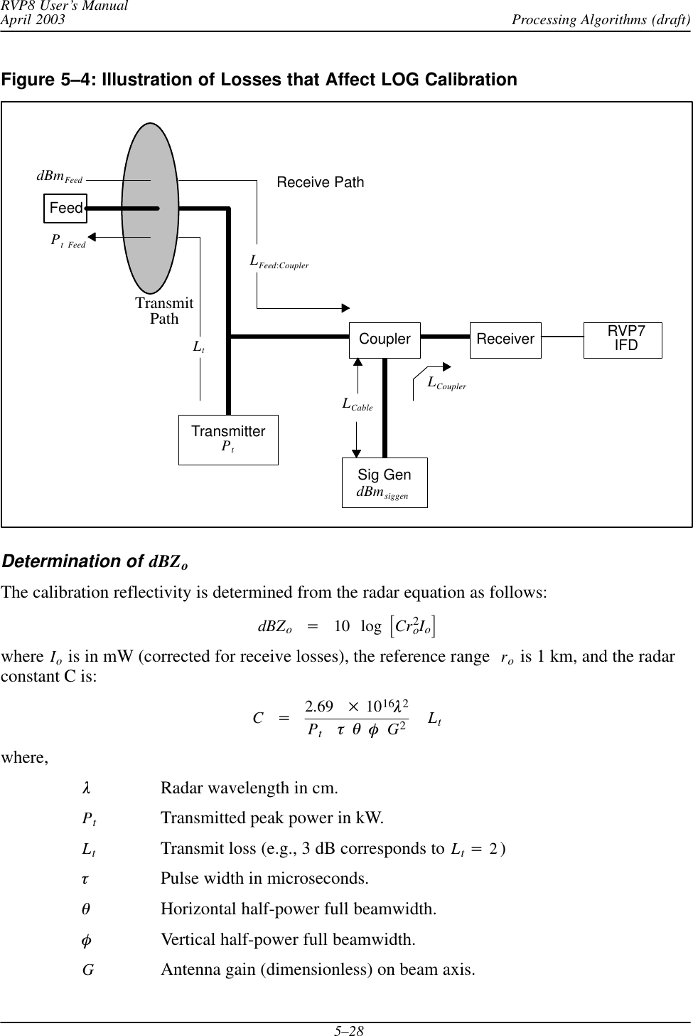
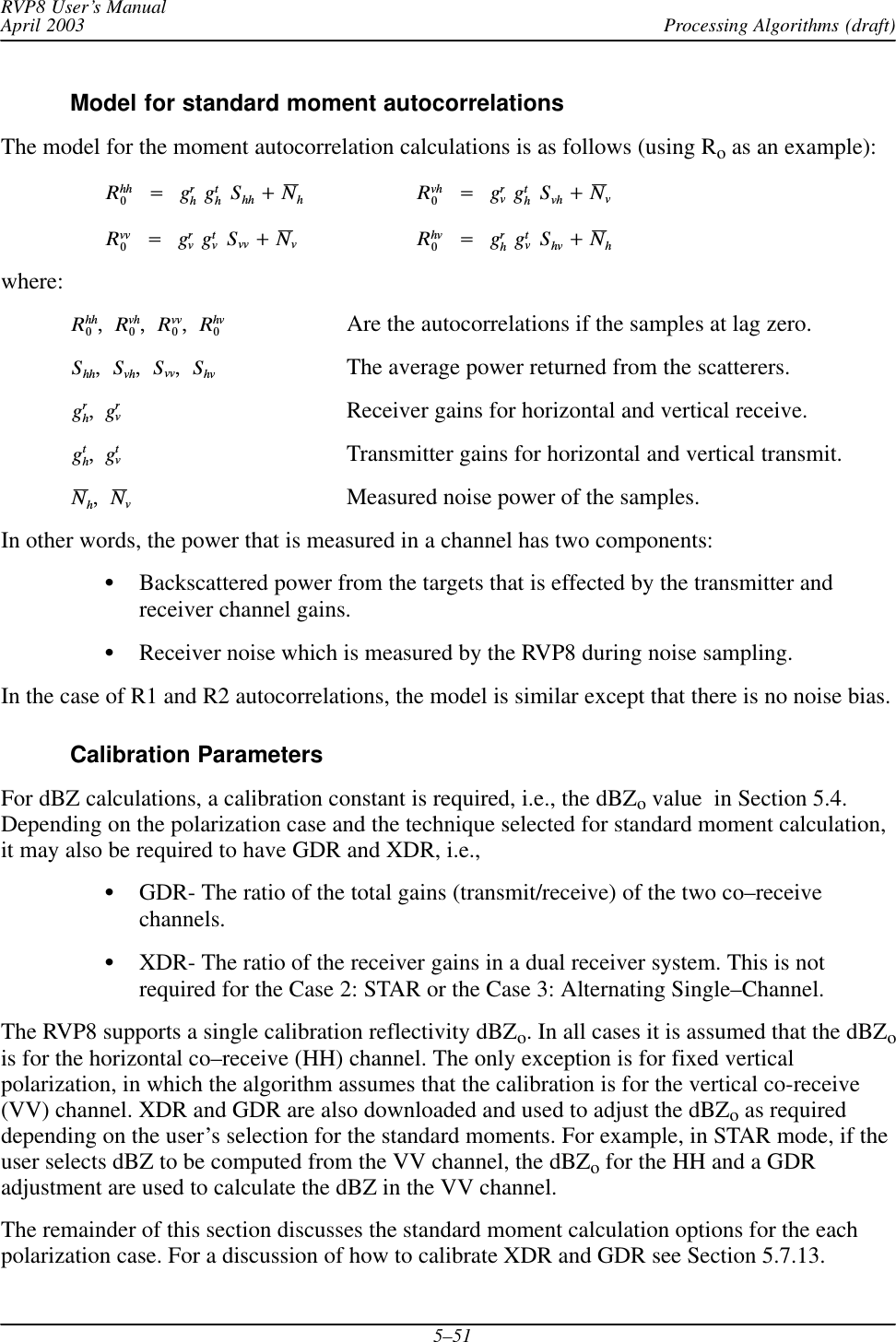
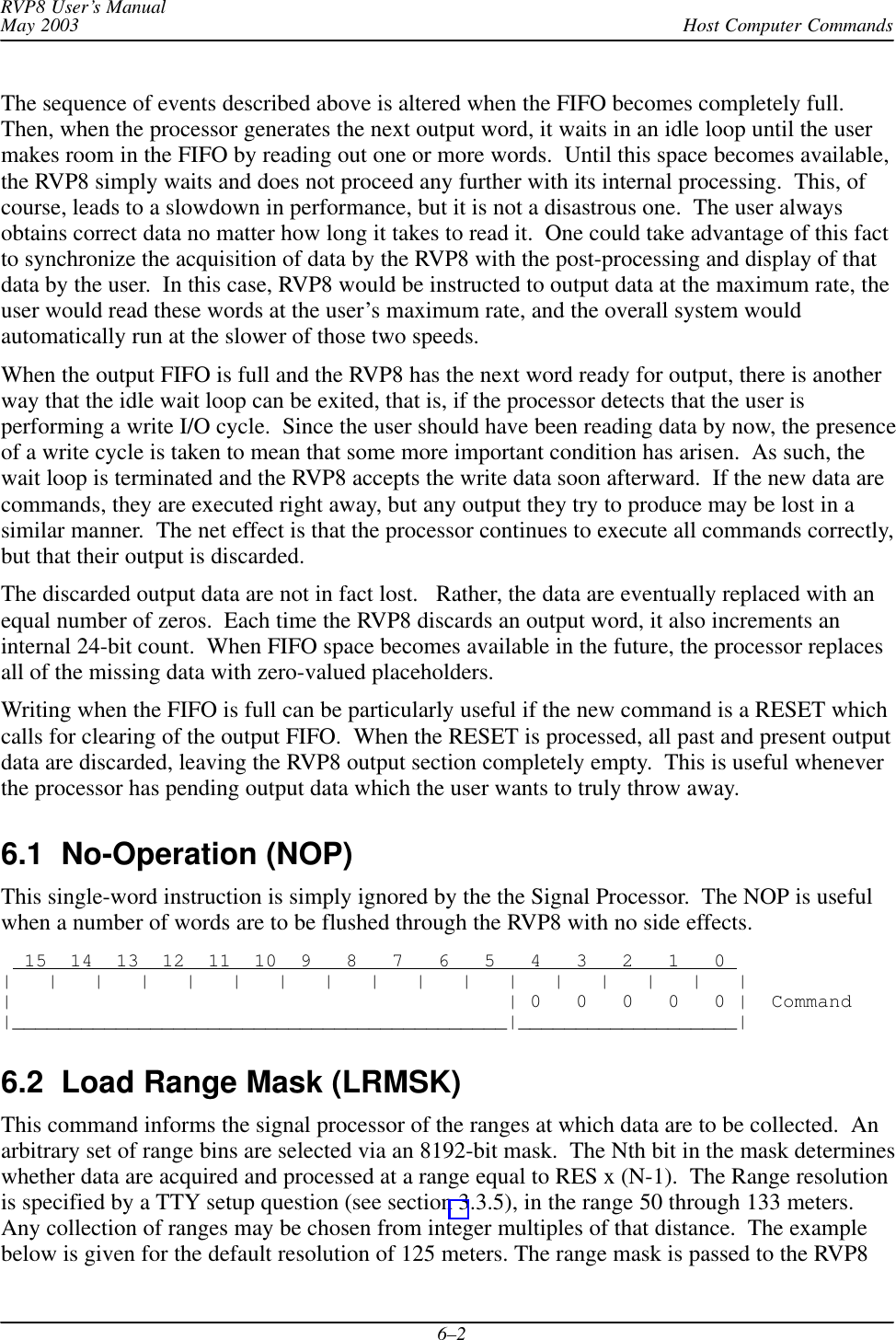
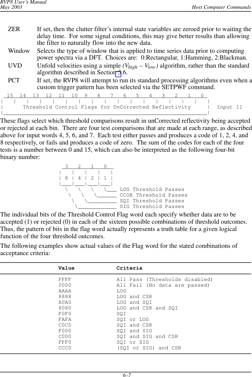
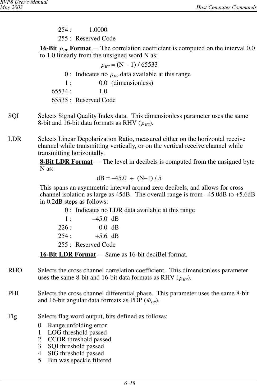
![Processing Algorithms (draft)RVP8 User’s ManualApril 20035–23RangeAzimuth0-1101-1Zoutput00 +ThresholdThreshold if center point is valid but there are no or only one valid neighbor.Z00Z0*1RangeAzimuth0-1101-1Fill thresholded center point with average if there 6 or more valid neighbors.Z0*1Z*11 Z01Zoutput00 +[Z*11 )Z01 )Z11 )Z10 )Z*1*1)Z0*1]6RangeAzimuth00-11-12D Velocity Unfolding Step 1: Search pattern for valid second velocityPRF2PRF1V200231V11*1Z11Z10Z*1*1Indicates Thresholded Bin2D 3x3 Filtering ConceptsThe filter has some interesting properties when combined with other algorithms.Dual PRF UnfoldingDual–PRF velocity unfolding is computed within the 3x3 filter whenever both are enabled.There are two steps to the process:SStep 1: The most recent and the previous ray are used. For every valid point inthe most recent ray, the algorithm performs a search among the three nearestneighbors in the previous ray to find a valid velocity. The search pattern is shownat the bottom of the previous figure. This larger selection of alternate–PRF bins](https://usermanual.wiki/Baron-Services/XDD-1000C.S10-RECEIVER-AND-PROCESSOR-USERS-MANUAL-PART-2/User-Guide-374023-Page-85.png)
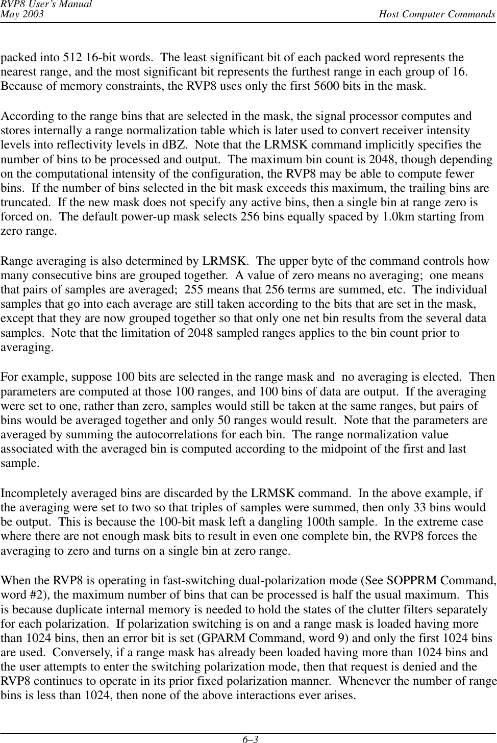
![Processing Algorithms (draft)RVP8 User’s ManualApril 20035–27Treatment of Losses in the CalibrationIn the calibration of the dBm level of the test signal, be sure to account for any losses that mayoccur between the antenna feed and the injection point, and in the cable and coupler that is usedto connect the signal generator to the injection point. Figure 5–4 illustrates the nomenclature ofthe various losses that are involved in the calibration. The relationship between the injected testsignal and the value of the received power relative to the feed is:dBmFeed +dBmInjected )dBLFeed:CouplerdBmFeed +dBmSiggen *dBLCoupler *dBLCable )dBLFeed:CouplerFor example, assume the following:Loss between the feed and the coupler dBLFeed:Coupler 3 dBLoss caused by the coupler dBLCoupler 30 dBLoss in the cable from siggen to coupler dBLCable 2 dBThen if the test signal generator output is –50 dBm, the injected power isdBmInjected = –50–[30+2]= –82 dBm.The equivalent power at the feed is then 3 dB more than thisdBmFeed = –82+3 = –79 dBm.During the calibration, there are several ways to handle the losses using these equations. Twoexamples are:SEach signal generator value can be corrected for losses so that the calibration plot shows IFDmeasured power vs received power at the feed. This is recommended for manual calibration.SThe signal generator values can be plotted directly and the intercept power Io can becorrected for losses so that it is properly referenced to power at the feed. This is the approachused by the IRIS zauto utility.](https://usermanual.wiki/Baron-Services/XDD-1000C.S10-RECEIVER-AND-PROCESSOR-USERS-MANUAL-PART-2/User-Guide-374023-Page-89.png)
![Processing Algorithms (draft)RVP8 User’s ManualApril 20035–325.6 Dual PRF Velocity UnfoldingFor a radar of wavelength l operating at a fixed sampling period ts+1ńPRF , the unambiguousvelocity and range intervals are given by:Vu+l4ts and Ru+cts2where “c” is the speed of light. Often these intervals do not fully cover the span of velocity andrange that one would like to measure. The problem is generally worse for short wavelengthradars, since that unambiguous velocity span is directly proportional to l for a given ts. If theunambiguous range interval is made sufficiently large by increasing ts , then the resultingvelocity span may be unacceptably small.The RVP8 provides a built-in mechanism for extending the unambiguous velocity span by afactor of two, three, or four beyond that given above. The technique, called Dual PRF velocityunfolding, uses two pulse periods rather than one, and relies on the extra information thusobtained to correct (i.e. unfold) the mean velocity measurement from each individual period.The Dual PRF trigger pattern consists of alternating (N+k)-pulse intervals where the period ineach interval is either tl (for the low-PRF) or th (for the high-PRF). Here “N” is the samplesize, and “k” represents a delay that permits the clutter filter to equilibrate to the new PRF aftereach change. The clutter filter impulse response lengths vary according to which filter isselected.The two trigger periods tl and th must be chosen in either a 3:2, 4:3, or 5:4 ratio. These ratiosgive factors of two, three, and four times velocity expansion over the th period alone. Theunfolding algorithm makes use of the following results. Suppose that the radar observes a targetwith mean velocity V at each of the two trigger periods. The measured phase angles for the R1autocorrelations at the two PRFs are:ql+4pVtll and qh+4pVthlwhere angles outside the basic [*p,p] interval are returned to that interval by appropriateadditions of "2p. These angles correspond to the ordinary single-PRF Doppler velocitymeasurements, and the "2p uncertainties reflects the fact that each measurement is foldedinto its own unambiguous interval:Vul +l4tl and Vuh +l4thIf we define f to be the difference between the two measured phases then:f+ql*qh+4plƪtl*thƫwhich can be interpreted as a phase angle within the unfolded interval:Vu unfold +l4(tl*th)](https://usermanual.wiki/Baron-Services/XDD-1000C.S10-RECEIVER-AND-PROCESSOR-USERS-MANUAL-PART-2/User-Guide-374023-Page-94.png)
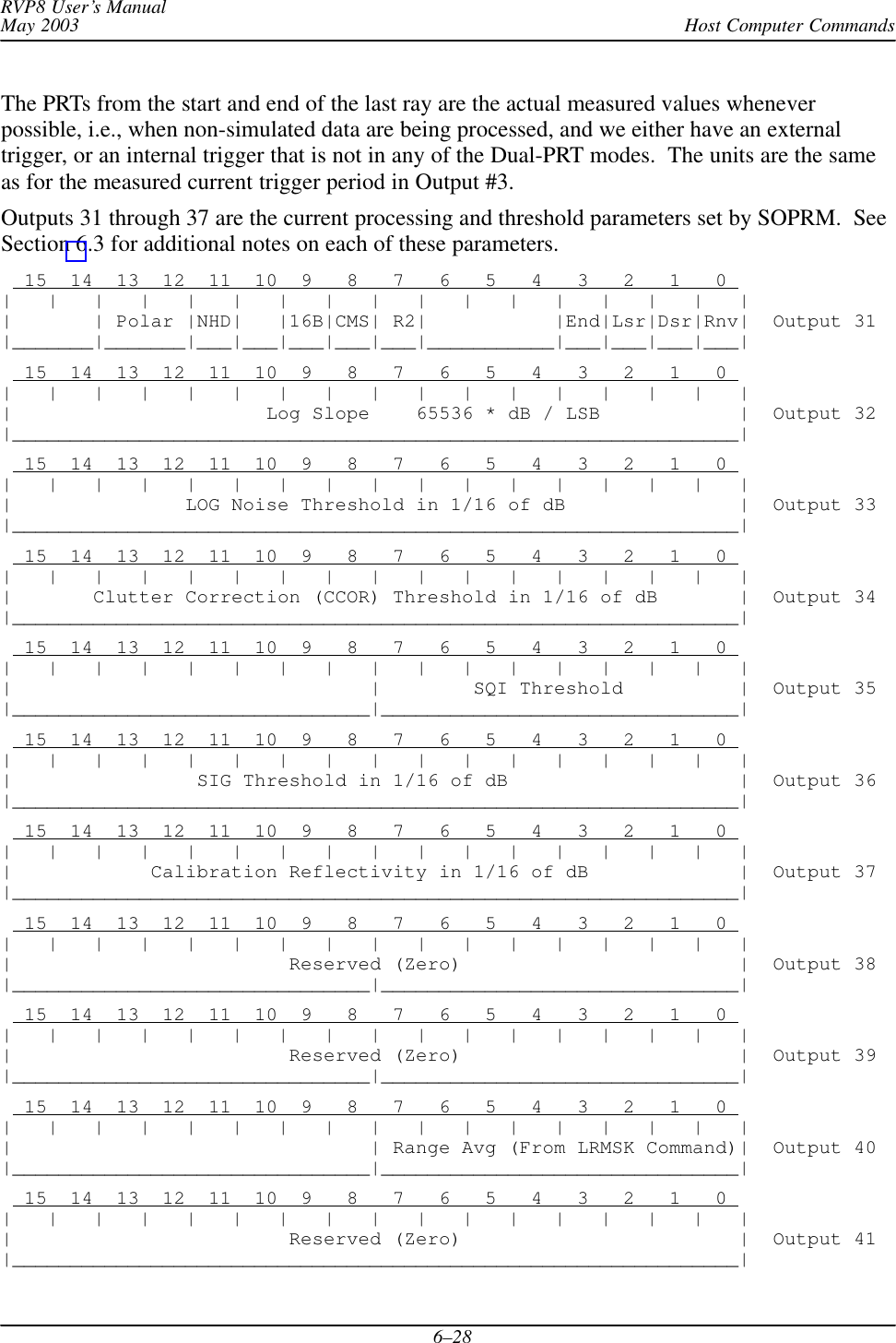
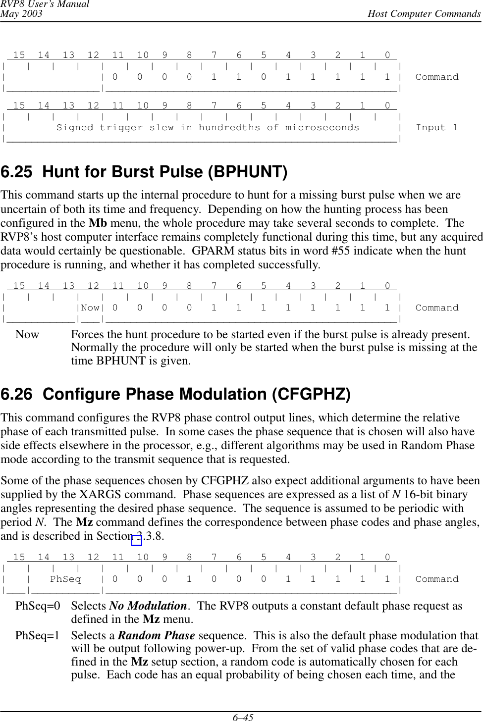
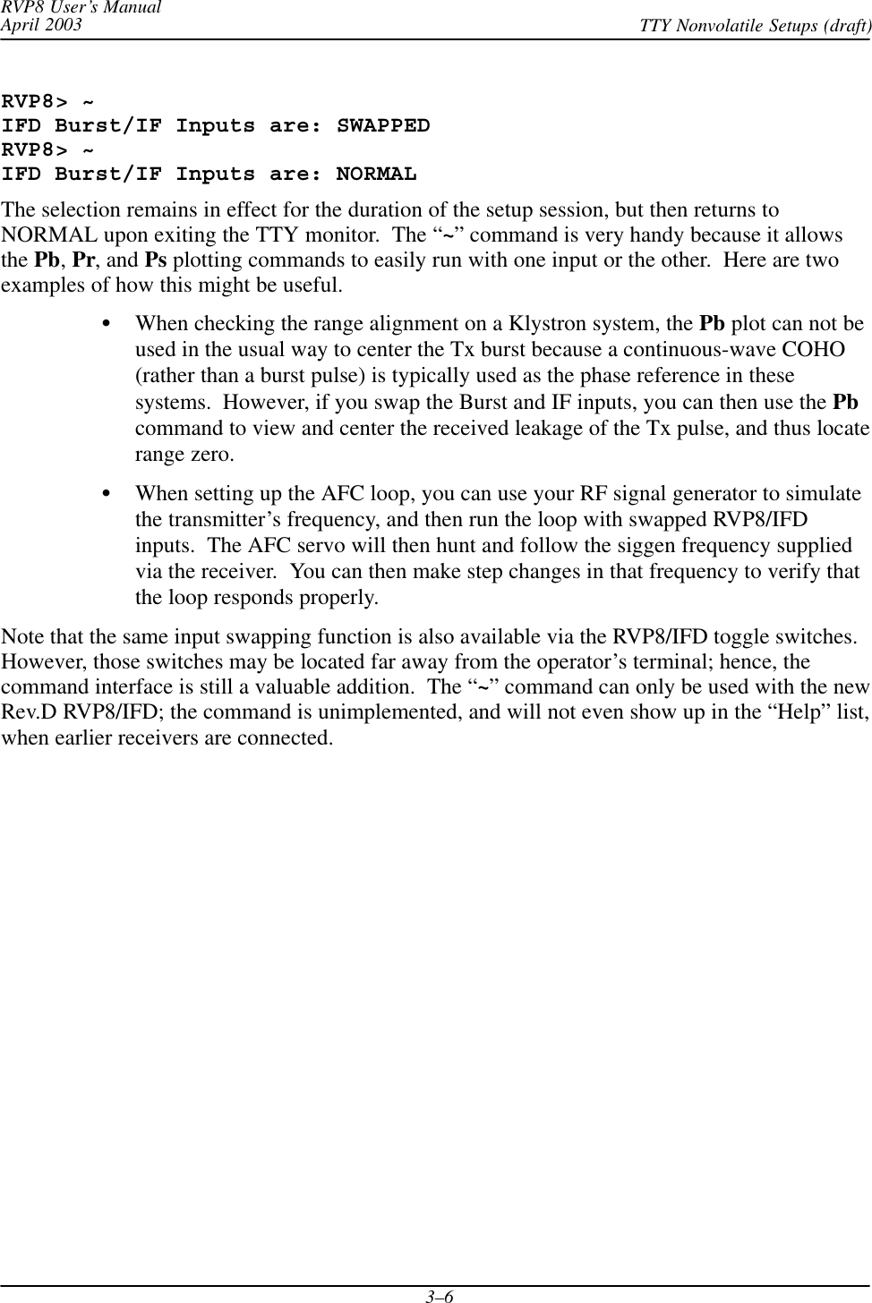
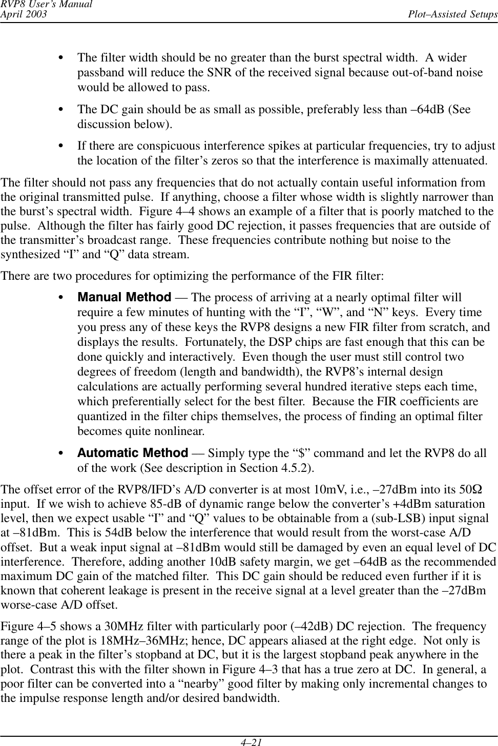
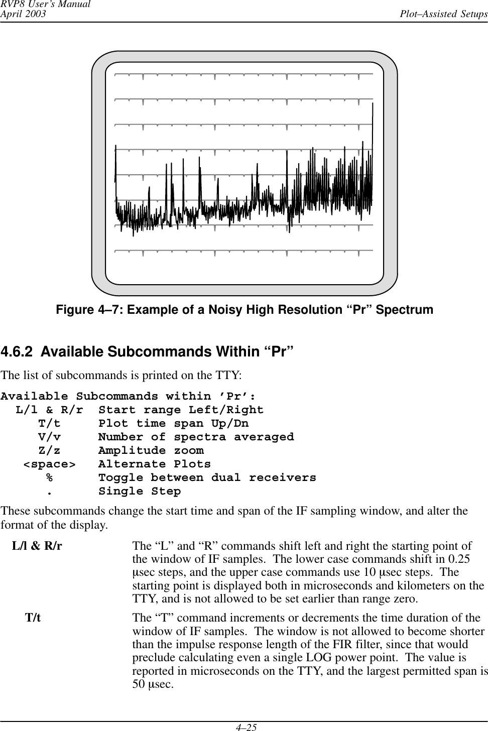
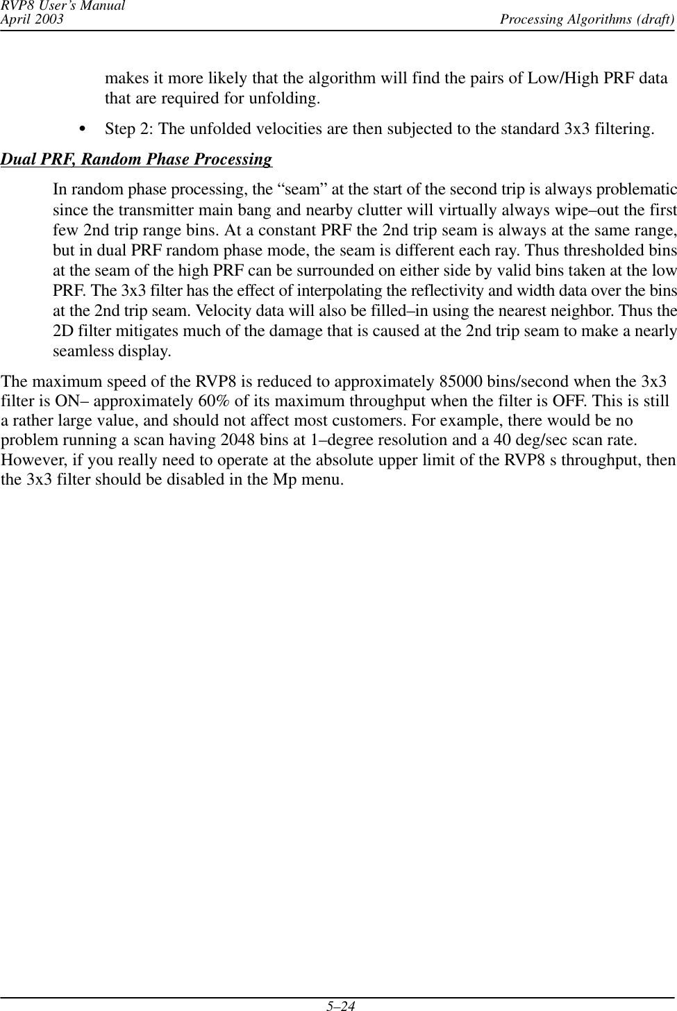
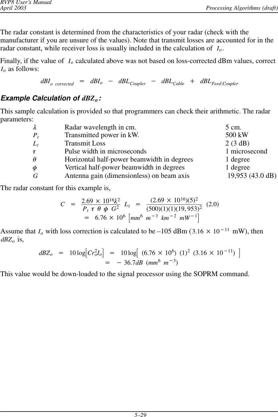
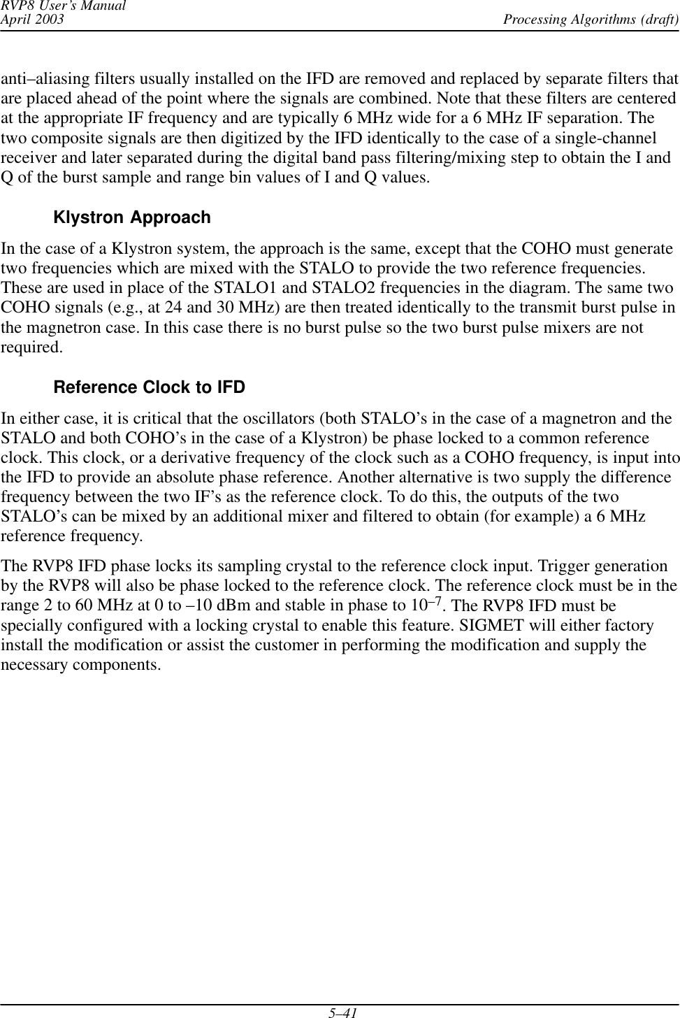
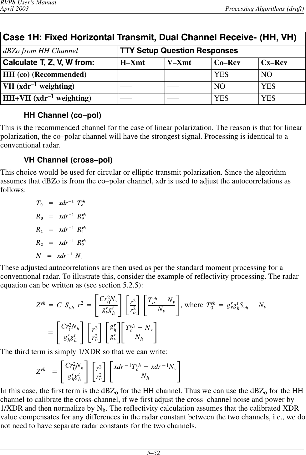
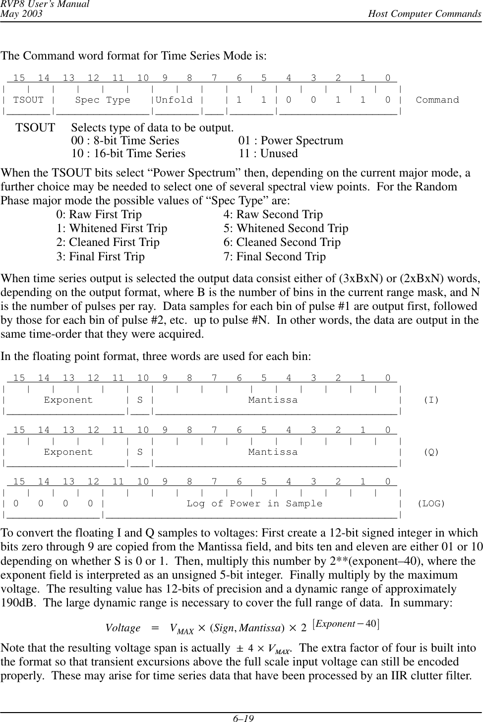
![Processing Algorithms (draft)RVP8 User’s ManualApril 20035–33Now if tl and th are in a 3:2 ratio, then:tl*th+tl3+th2and thus Vu unfold +3Vul +2VuhThe angle f represents a velocity phase angle in [*p,p] , but with respect to an enlargedunambiguous interval. Thus, by simply differencing the folded angles from the high and lowPRFs, we obtain an angle that is unfolded to a larger velocity span. Similar reasoning shows thatthe 4:3 ratio gives a factor of three improvement over Vuh .In practice, the unfolded angle f is not in itself a suitable velocity estimator. The reason is thatthe variance of f is equal to the sum of the variances of each of its components, i.e., twice thatof the individual measurements alone. If the target is at all noisy, then this increase in variancecan be severe. Rather than use f directly, the RVP8 uses it only as a rough estimate indetermining how to unfold the individual velocity measured from each PRF.Figure 5–5: Dual PRF Conceptsql*qhResultqlń3Region IIIRegion IIRegion ILow PRF Case High PRF CaseRegion IRegion IIql*qhResultqhń2This technique is illustrated in Figure 5–5. The figure shows how the low-PRF and high-PRFangles are unfolded based on the difference angle. The diagrams show phase planes representingthe large unfolded velocity interval, and the locations of various vectors on those planes.Referring first to the right figure, the difference angle is plotted, and the plane is divided intotwo equal size regions, one of which is centered on the difference vector. The high-PRF angle isthen divided by two and plotted. The resultant unfolded velocity angle must either be this vector,or this vector plus p. Since adding p places the vector into acceptance Region 1 where it is](https://usermanual.wiki/Baron-Services/XDD-1000C.S10-RECEIVER-AND-PROCESSOR-USERS-MANUAL-PART-2/User-Guide-374023-Page-95.png)
![Processing Algorithms (draft)RVP8 User’s ManualApril 20035–34nearest the difference angle, we conclude that this is the correct unfolding. Likewise, on the leftdiagram we unfold the low-PRF angle by dividing the plane into thirds centered on thedifference angle. The result angle is eitherql3,ql3)2p3or ql3)4p3depending on which one falls into the acceptance Region 1. Note that the resultant angle is thesame in each case.The RVP8 makes efficient use of the incoming data by unfolding velocities from both the lowand the high-PRF data, making use each time of information in the previous ray. When low-PRFdata are taken the derived velocities are unfolded by combining information from the previoushigh-PRF interval. Likewise, when high-PRF data are acquired the velocities are unfolded basedon the previous low-PRF interval. Thus, when operating in the Dual PRF mode, the RVP8outputs one data ray for each (N+k)-pulse interval. However, the velocity data in the Dual PRFrays are unfolded, so that the [–1,+1] interval now represents either two or three times the priorvelocity range. Put another way, the data are still interpreted as described in the section on meanvelocity estimation, except that Vu is now larger.The width data are also modified somewhat during Dual PRF unfolding. Although valid widthsare obtained independently on all rays, those measured at low-PRF are larger than those athigh-PRF. This is simply because the dimensionless width units are with respect to a largervelocity interval in the latter case. To compensate for this, low-PRF widths are multiplied byeither 2/3 or 3/4 before being output. This puts them in the same scale as the high-PRF values,and thus, the widths do not vary on alternate pulses. A useful consequence of this is that widthdata can be sent directly to a color display generator without having to plot every other ray in adifferent scale.There are a few words of caution that should be kept in mind when using the RVP8 in the DualPRF processing modes. The unfolding algorithms make the assumption that targets aremore-or-less continuous from ray to ray. Otherwise, it would not make sense to use data from aprevious ray to unfold velocities in the current ray. Users must therefore assure that their antennascan rate and beamwidth are such that each target is illuminated, at least partially, over each full2(N+k)-pulse interval. In practice, a certain amount of decorrelation from ray to ray isacceptable, since the previous rays are used only to decide into which unfolded interval thecurrent ray should be placed. Small errors in the previous ray data, therefore, cause no error inthe output. However, large previous-ray errors would lead to incorrect unfolding.A more subtle side effect of Dual PRF processing arises from clutter filtering because clutternotches now appear at several locations in the unfolded velocity span, rather than just at zerovelocity. These additional rejection points come about because the original velocity intervals aremapped some integer number of times to create the unfolded interval. Since each originalinterval has a clutter notch at DC, it follows that the final expanded velocity interval will haveseveral such notches. For example, in the 3:2 case, in addition to removing DC the clutter filterremoves velocities at *2Vuń3,)2Vuń3, and Vu.Unfortunately, these clutter filter “images” are a fundamental consequence of the Dual PRFprocessing technique and are not easily removed. They can cause trouble not only for thevelocity unfolding itself, but because the computed clutter corrections to be wrong at the image](https://usermanual.wiki/Baron-Services/XDD-1000C.S10-RECEIVER-AND-PROCESSOR-USERS-MANUAL-PART-2/User-Guide-374023-Page-96.png)
![Processing Algorithms (draft)RVP8 User’s ManualApril 20035–37LDR: Linear Depolarization RatioSome advanced polarization radars can transmit at one polarization and receive simulta-neously in two channels, usually the co–polarized and cross–polarized components. For ex-ample, when transmitting horizontal, both horizontal (co–polarized) and vertical (cross–po-larized) are received by two separate channels. In the case of vertical or horizontal, the ratioof the power Zcross / Zco is called the linear depolarization ratio or LDR. The amount of inci-dent radiation that is depolarized by a particle depends on the particle shape and orientation(e.g., canting angle with respect to horizontal). Perfectly spherical particles do not depolarizeeither horizontal or vertical polarization so that LDR is zero. Particles that are wet, tumblingand irregularly shaped will give larger LDR values. Therefore, LDR values in rain tend tobe small, e.g., less than –25dB. Larger values of LDR can occur in the bright band or in thepresence of hail.A radar and antenna system must be optimized to measure LDR by assuring that the antenna,feed and supporting struts and radome are not themselves depolarizing the transmitted andreceived radiation. This is called “cross–pol isolation”. The integrated cross–pol isolationof the antenna pattern must be better than about 30 dB for LDR measurement since –20 dBis a large LDR.[RHOHV, PHIDP] [RHOH, PHIH] [RHOV, PHIV]: Correlation VariablesThere are several correlation functions that can be calculated depending on the capabilitiesof the radar. These are generally complex having both an amplitude and phase. These are allnormalized so that a perfect correlation magnitude is 1 and perfectly decorrelated is 0.RHOHV and PHIDP are the magnitude and phase of the correlation between the horizontaland vertical co-polarized channels. These are available on H/V switching systems or on sys-tems that transmit simultaneous H and V. As discussed in a preceding paragraph, PHIDPcan be used to infer precipitation rate. RHOHV in rain is typically very close to 1 (0.98).RHOHV values can be reduced in the case of irregularly shaped, randomly oriented, wettumbling particles. Thus RHOHV has information on the particle type.RHOH and PHIH are the magnitude and phase of the correlation between the co-polarizedand cross-polar channels for H transmission and simultaneous H and V reception. RHOVand PHIV denote the cross–channel correlation magnitude and phase for vertical transmis-sion. These are available on dual-channel receiver with transmit either fixed or alternating.The information content of the cross-pol correlations is the topic of current research.](https://usermanual.wiki/Baron-Services/XDD-1000C.S10-RECEIVER-AND-PROCESSOR-USERS-MANUAL-PART-2/User-Guide-374023-Page-99.png)
![Processing Algorithms (draft)RVP8 User’s ManualApril 20035–455.7.5 Case 1: Fixed Transmit: Dual-Channel ReceiverInput Receiver SamplesIn fixed mode the radar is configured (either permanently or by means of a switch) to transmiteither vertical or horizontal polarization with dual-channel reception of both the co- andcross–channel polarizations, e.g., transmit horizontal and receive both horizontal (co) andvertical (cross) polarizations.The received samples in the two transmit cases are:Transmit Horizontal or Transmit Verticalƪs1hh :s1vhƫĄƪs2hh :s2vhƫĄƪs3hh :s3vhƫĄ.Ą.Ą.ĄƪsMhh :sMvhƫƪs1vv :s1hvƫĄƪs2vv :s2hvƫĄƪs3vv :s3hvƫĄ.Ą.Ą.ĄƪsMvv :sMhvƫCalculation of the Polarization MeasurandsThe processing in this mode is done by pulse pair algorithm. The user may select a clutter filter,but in general this is not recommended for polarization studies since the clutter filter mightinterfere with the accuracy of sensitive parameters such as LDR.The polarization measurands for the two transmit cases are as follows:Transmit Horizontal or Transmit VerticalLDRH +10ĄLOGĄƪSvhShhƫ or LDRV +10ĄLOGĄƪShvSvvƫ+10ĄLOGĄƪt|svh|2u*Nvt|shh|2u*NhƫĄ*XDR or +10ĄLOGĄƪt|shv|2u*Nht|svv|2u*NvƫĄ)XDRRHOH +|òh|or RHOV +|òv|PHIH +arg[òh]or PHIV +arg[òv]Here, the H and V average channel powers are computed as follows with optional noisecorrection, i.e.,Co- grhgthĄShh +t |shh|2u*Nhor grvgtvĄSvv +t |svv|2u*NvCross- grvgthĄSvh +t |svh|2u*Nvor grhgtvĄShv +t |shv|2u*NhThe complex covariance ρ (used above) is:for H transmit òh+tsvhĄs*hh uSvhShhǸor for V transmit òv+tshvĄs*vv uShvSvvǸFortunately, the algorithms do not require us to know all of the individual gain terms. Theycancel in the calculation of ρ so are taken as =1 in the implementation. However, the differentialreceiver gain XDR must be known from calibration to calculate LDR:dBĄValueĄisĄĄXDR +10ĄLOGĄxdrĄĄĄwhereĄtheĄlinearĄvalueĄisĄĄĄxdrĄ+Ągrvgrh](https://usermanual.wiki/Baron-Services/XDD-1000C.S10-RECEIVER-AND-PROCESSOR-USERS-MANUAL-PART-2/User-Guide-374023-Page-107.png)
![Processing Algorithms (draft)RVP8 User’s ManualApril 20035–465.7.6 Case 2: Simultaneous Dual Transmit and Receive (STAR mode)Input Receiver SamplesIn this mode there is simultaneous transmit and receive of both vertical and horizontalpolarization. For each pulse there is a measurement of the complex amplitude in each channel,i.e.,ƪs1hh :s1vvƫĄƪs2hh :s2vvƫĄƪs3hh :s3vvƫĄ.Ą.Ą.ĄƪsMhh :sMvvƫWe will assume that M samples are collected for processing, i.e., Note that even though there iscross–polarized radiation received in each channel, this cross–polar contribution can beneglected since the co-polarized received signal is much stronger.Calculation of the Polarization MeasurandsThe processing in this case is done by pulse pair mode. However both FFT and random phaseprocessing can be performed if only ZDR and standard moments are requested for ouput. In anymode, the user may select a clutter filter, but in general this is not recommended for polarizationmeasurements since the clutter filter might interfere with the accuracy of sensitive parameterssuch as ZDR.The RVP8 calculates the following polarization parameters:ZDR +10ĄLOGĄƪShhSvvƫZDR +10ĄLOGĄƪt|shh|2u*Nht|svv|2u*NvƫĄ)GDRRHOHV +|òhv(0)|PHIDP +arg[òhv(0)]KDP based on least squares fit to PHIDP (see Section 5.7.10).where the following definitions are used:grhgthĄShh +t |shh|2u*NhgrvgtvĄSvv +t |svv|2u*NvThe noise powers the two channels are denoted as Nh and Nv . The noise corrections to Shh andSvv are optionally configured in the TTY setups. GDR is the total (transmit and receive)differential channel gain. It must be calibrated for the system.dBĄValueĄisĄĄGDR +10ĄLOGĄxdrĄĄĄwhereĄtheĄlinearĄvalueĄisĄĄĄgdrĄ+ĄgrvgtvgrhgthThe correlation function is computed from:òhv(0) +tsvvĄs*hh uShhSvvǸThe gain terms cancel in the calculation of ρ so in the implementation they are simply assumedto be =1.](https://usermanual.wiki/Baron-Services/XDD-1000C.S10-RECEIVER-AND-PROCESSOR-USERS-MANUAL-PART-2/User-Guide-374023-Page-108.png)
![Processing Algorithms (draft)RVP8 User’s ManualApril 20035–475.7.7 Case 3: Alternating H/V Transmit: Single-Channel ReceiverInput Receiver SamplesThis is the traditional ZDR radar with a high-power fast switch that alternates betweenhorizontal and vertical on each pulse. The switch is made just prior to the transmit pulse so thatthe transmitter radiates and then receives at a single polarization for each pulse. Thus thesamples are:s1hh s2vv s3hh . . . sM)1vvFor the discussion below we will assume that there are M+1 total samples with M/2 horizontalpulses indexed by (1, 2, 3...M–1) and M/2+1 vertical pulses indexed at (2, 4, 6, ...M). Note thatthe processor does not assume that the first pulse in a sequence is horizontal.Calculation of the Polarization MeasurandsThe processing is done in pulse pair with optional clutter filter. Again, for accurate ZDRmeasurements, the clutter filter may interfere.The RVP8 calculates the following:ZDR +10ĄLOGĄƪShhSvvƫZDR +10ĄLOGĄƪt|shh|2u*Nht|svv|2u*NvƫĄ)GDRPHIDP +12Ą argĄƪRaĄR*bƫRHOHV +|òhv(Ts)|Ąƪòhv(2Ts)ƫ0.25KDP based on least squares fit to PHIDP (see Section 5.7.10).where the following definitions are used:|òhv(Ts)| +|Ra|)|Rb|2ShhSvvǸò(2Ts)+ŤȍMń2*1n+1(s*hh[2n*1]Ąshh[2n)1]Ą )Ąs*vv[2n]Ąsvv[2n)2])Ť(Mń2*1)(Shh )Svv)Ra+1Mń2ȍMń2n+1s2n*1hh *s2nvv and Rb+1Mń2ȍMń2n+1s2nvv *s2n)1hhThe calculation of the channel powers (t|shh|2u and t|svv|2u) is done using alternatingpulses in this case. Note that in the calculation of Rb, the RVP8 uses the extra M+1 sample. Thegain terms cancel in the calculation of ρ so in the implementation they are simply assumed to be=1.](https://usermanual.wiki/Baron-Services/XDD-1000C.S10-RECEIVER-AND-PROCESSOR-USERS-MANUAL-PART-2/User-Guide-374023-Page-109.png)
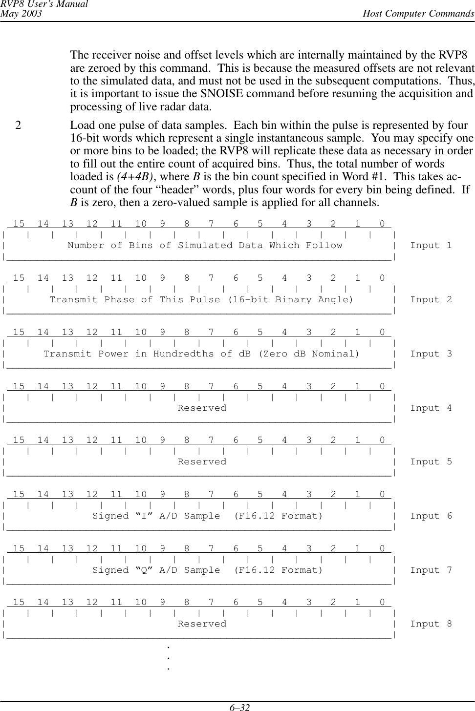
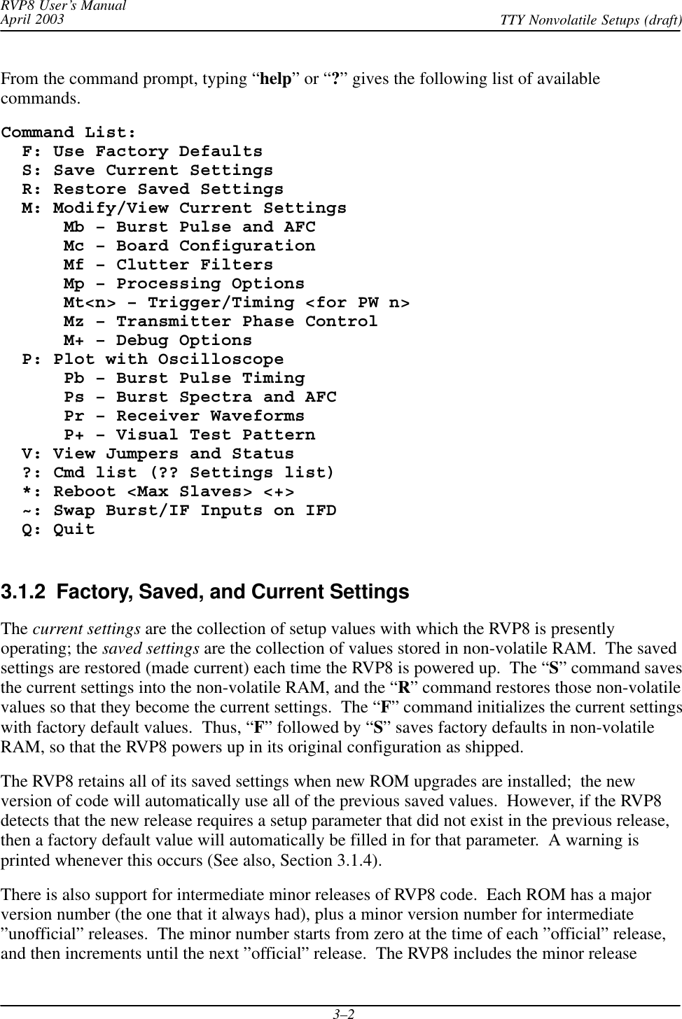
![Host Computer CommandsRVP8 User’s ManualMay 20036–14simultaneously, in which case the archive format is output first, followed by whicheverindividual display format values were also selected. The archive format is not recommended foruse with new drivers because it can only handle four of the many possible output parametertypes.When time series mode is selected there are three output data formats available. For backwardscompatibility, there is an 8-bit integer format in which the eight most significant bits from the I,Q, and LOG signals are represented in a byte. This format is not recommended because it willgenerally miss weak signals. We recommend the floating-point format that uses 16-bits per A/Dsample. There is also a 16-bit power spectrum output that is accurate to 0.01dB. (See alsoGPARM output word #10).In addition to the above output data, the first words of each ray optionally contain additionalinformation about the ray itself. These header words are configured by the CFGHDR opcode,and are included only if the NHD (No-Headers) bit in SOPRM Input #2 is clear. For example, ifTAG angle headers are requested, if the ARC, Z and V bits are all set, and if there are 100 binsselected in the current range mask, then each RVP8 output ray consists of the following:1] TAG15 – TAG0 \ From Start of Acquisition2] TAG31 – TAG16 / Interval3] TAG15 – TAG0 \ From End of Acquisition4] TAG31 – TAG16 / Interval* 200 words of packed archive data,* 100 words of Corrected Reflectivity data in low byte only.* 100 words of Velocity data in low byte only,The Command word format for Synchronous Doppler Mode is: 15 14 13 12 11 10 9 8 7 6 5 4 3 2 1 0 | | | | | | | | | | | | | | | | ||ARC| Z | T | V | W |ZDR|Unfold |KDP| 0 1 | 0 0 1 1 0 | Command|___|___|___|___|___|___|_______|___|_______|___________________|The Command word format for Free Running Doppler Mode is: 15 14 13 12 11 10 9 8 7 6 5 4 3 2 1 0 | | | | | | | | | | | | | | | | ||ARC| Z | T | V | W |ZDR|Unfold |KDP| 1 0 | 0 0 1 1 0 | Command|___|___|___|___|___|___|_______|___|_______|___________________|Either of these may be augmented by an optional XARG word (See Section 6.20) 15 14 13 12 11 10 9 8 7 6 5 4 3 2 1 0 | | | | | | | | (Tx Vert) | (Tx Horz) | | | || |Flg|Phi Rho Ldr|Phi Rho Ldr|SQI|RHV|PDP| XARG 1|_______________________|___|___|___|___|___|___|___|___|___|___|Unfold Selects Dual–PRF unfolding scheme:00 : No Unfolding 01 : Ratio of 2:310 : Ratio of 3:4 11 : Ratio of 4:5ARC Selects archive output format in which four data bytes (see 8-Bit descriptions be-low) are packed into two output words per bin as follows:](https://usermanual.wiki/Baron-Services/XDD-1000C.S10-RECEIVER-AND-PROCESSOR-USERS-MANUAL-PART-2/User-Guide-374023-Page-153.png)
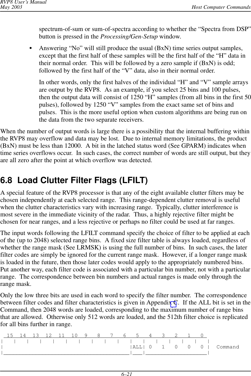
![Host Computer CommandsRVP8 User’s ManualMay 20036–20The “Log of Power in Sample” is provided mainly for backwards compatibility. It can becalculated from the I and Q numbers. To convert to dBm it requires a slope and offset asfollows:dBm PMAX Slope [Value 3584]Where:PMAX = +4.5dBm for 12-bit IFD, +6.0dBm for 14-bit IFDVMAX = 0.5309 Volts for 12-bit IFD, 0.6310 Volts for 14-bit IFDSlope = “Log Power Slope” word 3 of SOPRM command. 0.03 recommended.For backwards compatibility the RVP8 produces a 8-bit fixed point time series format. Becauseof the limited dynamic range available, this will only show strong signals, and is notrecommended for use. The I, Q, and Log power triplets are packed into two 16-bit output wordsas follows: High Byte Low Byte | | || Q Sample | I Sample | First Word|___________|___________| | | | | Zero | Log Power | Second Word|___________|___________|The “Log Power” value is the upper 8 bits of the long format. The other numbers are producedby the equation:Voltage VMAX Sample128 When Power Spectrum output is selected, the spectrum size is chosen as the largest power of two(N2) that is less than or equal to the current sample size (N). When the sample size is not apower of two, a smaller spectrum is computed that by averaging the spectra from the first N2and the last N2 points. The data format is one word/bin/pulse, in the same order as for timeseries output. Each word gives the spectral power in hundredths of dB, with zero representingthe level that would result from the strongest possible input signal. Thus, the spectral outputterms are almost always negative.The time series that are output by the RVP8 are the filtered versions of the raw data, whenavailable. If a non-zero time-domain clutter filter is selected at a bin, then the I and Q data forthat bin show the effects of the filter. Whenever you need to observe the raw samples, make surethat no clutter filters are being applied.In pulse pair time series mode with dual receivers, selecting (H+V) will produce data in one oftwo formats according to the “Sum H+V Time Series” question in the Mp setup section:Answering “Yes” will result in summed time series from both channels, butspectra from the DSP will be the averaged spectra from each channelindividually. This allows the IRIS ascope utility to display either the](https://usermanual.wiki/Baron-Services/XDD-1000C.S10-RECEIVER-AND-PROCESSOR-USERS-MANUAL-PART-2/User-Guide-374023-Page-159.png)