CyberOptics 003 WML-C40 User Manual 20171102 v1 11 11616692 AMS 8023533 REV E 2
CyberOptics Corporation WML-C40 20171102 v1 11 11616692 AMS 8023533 REV E 2
Contents
- 1. User Manual
- 2. Users Manual
- 3. User Manual_20171102_v1 - 11_11616692 AMS-8023533-REV_E (2)
- 4. User Manual_20200121_v1 - 11_APS3-8025869-User-Guide-REV_A resize
User Manual_20171102_v1 - 11_11616692 AMS-8023533-REV_E (2)
8023533 Rev E
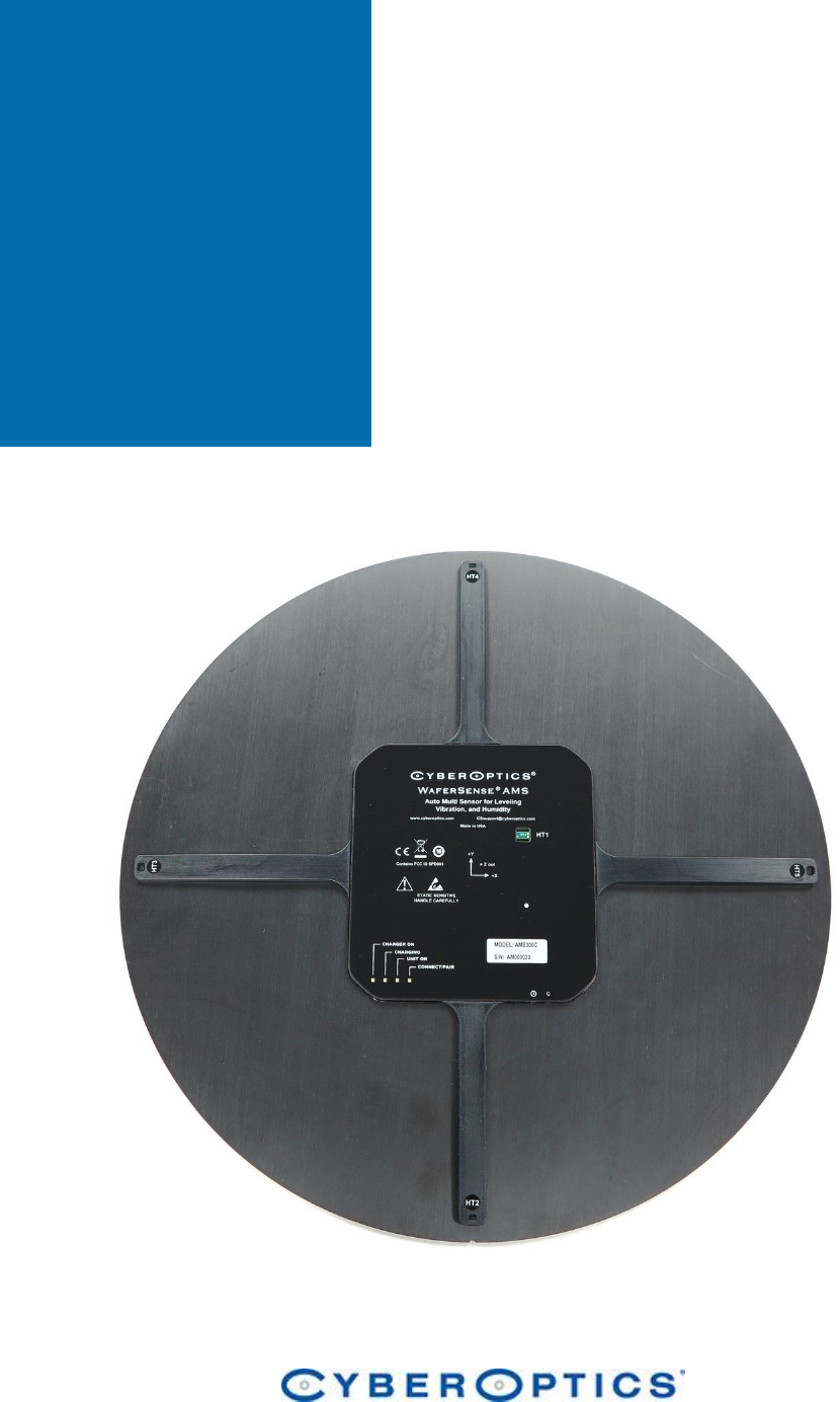
CyberOptics
WaferSense® and
ReticleSense®
AMS
User’s Guide
For AMS-300C, AMS-200C, AMS-150C,
and AMSR wireless Auto Multi-Sensors

2
General information ........................................................................................... 6
Introduction ........................................................................................................ 9
Installing the AMS Software ......................................................................... 12
Installing the Wireless Link .......................................................................... 14
Checking the Communications Between the Link and the AMS ................... 15
Registering Your AMS for Calibration Service ............................................... 16
Running the MultiView Application ............................................................. 17
Technical Support ........................................................................................ 19
Using Your AMS ................................................................................................ 21
Opening and Closing the Charging Case ....................................................... 22
Using the AMS Controls ............................................................................... 23
Using the AMS Indicators ............................................................................. 23
Using the Vibration, Humidity, and Leveling Tabs ........................................ 24
Changing Colors in the Trace Screen ............................................................ 24
Printing the MultiView Window ................................................................... 26
Monitoring the Operating Temperature of the AMS .................................... 27
Using the Rechargeable Battery ................................................................... 28
Table of
Contents
3
Monitoring the Battery Level.................................................................................................... 28
Charging the Battery ................................................................................................................. 28
Monitoring the Wireless Connection to the AMS Device ............................. 30
Changing the Pairing between the AMS and Link ......................................... 31
Overview of Main AMS Sub-Functions .............................................................. 32
Setting Go/No-Go Tolerances ...................................................................... 33
Setting Triggers ............................................................................................ 35
Setting Station Information .......................................................................... 38
Saving Your MultiView Settings ................................................................... 40
Loading Previously Saved Settings from a File .............................................. 40
Using the Vibration Function ............................................................................ 41
Reading the Vibration Trace Display ............................................................ 42
Freezing the Trace Display ........................................................................... 45
Monitoring Traces for Excessive Vibration Levels ........................................ 46
Setting the Go/No-Go Tolerances ............................................................................................ 47
Setting Options for the No-Go Indicators ................................................................................. 48
Recording the Traces ................................................................................... 49
Changing the Pre-Recording Length ............................................................. 54
Placing Marks in a Log File ........................................................................... 55
Including User-Specified Information in the Log File .................................... 58
Understanding Log File Names..................................................................... 58
Importing Log Files into Other Applications ................................................. 60
Configuring the Trace Display ...................................................................... 62
Minimizing the Trace Bars ........................................................................................................ 62
Filtering the Data ...................................................................................................................... 63
Changing the Time-Domain Format ......................................................................................... 64
Changing the Horizontal Time and Scale .................................................................................. 66
Changing Colors ........................................................................................................................ 68
4
Displaying the Frequency Spectrum ......................................................................................... 69
Showing and Hiding Trigger Settings ........................................................................................ 71
Viewing Log Files............................................................................................... 72
Running MultiReview ................................................................................... 73
Using the Playback Controls ......................................................................... 75
Working with Marks..................................................................................... 78
Monitoring Traces for Excessive Vibration Levels ........................................ 80
Comparing Log Files ..................................................................................... 81
Changing MultiView Settings from MultiReview .......................................... 83
Changing Log Files ........................................................................................ 85
Analyzing Narrow Peaks ............................................................................... 85
Saving a Sub-Set of a Log File ....................................................................... 87
Compiling Summary Statistical Reports ....................................................... 88
Compiling a Peak-Acceleration Summary Report ..................................................................... 88
Compiling a Peak-Excursion Summary Report ......................................................................... 90
Compiling a Time-Domain Statistics Summary Report ............................................................. 92
Printing the MultiReview Window ............................................................... 93
Using the Humidity Function ............................................................................. 94
How the Humidity/Temperature Sensors Work ........................................... 95
Factors to Consider When Making Humidity Measurements ....................... 98
Setting Go/No-Go Tolerances ...................................................................... 99
Setting Triggers .......................................................................................... 100
Using Other Humidity Menus and Functions.............................................. 100
Using the Leveling Function ............................................................................ 101
Performing Horizontal Inclination Measurements ..................................... 103
Choosing Display Units and Conventions ............................................................................... 106
Setting the Stabilization Criteria ............................................................................................. 109
Setting the Go/No-Go Tolerance ............................................................................................ 110
5
Specifying a Reference Plane .................................................................................................. 112
Calibration for zero point drift (Field Calibration) ...................................... 113
Viewing Leveling Log Files .......................................................................... 118
Running MultiReview .............................................................................................................. 119
Choosing Display Units and Conventions ............................................................................... 120
Temporarily Changing the Go/No-Go Tolerance .................................................................... 121
Temporarily Changing the Vertical Tolerance and Target ...................................................... 122
Maintaining Your AMS .................................................................................... 124
Annual Factory Calibration and Battery Replacement ................................ 125
Battery Use and Disposal ........................................................................... 126
Specifications .................................................................................................. 127
Glossary .......................................................................................................... 133
Appendices ..................................................................................................... 135
Appendix A—Moisture Conversion Table .................................................. 136
Appendix B—Psychrometric Chart ............................................................. 137
Appendix C—Acoustic Resonances and other factors Affecting Acceleration
Measurements ........................................................................................... 138
AHS Addendum .......................................................................................... 141
Wafersense AHS ........................................................................................ 141

6
General information
Note: This manual is for the AMS family of products including the AMS-300C, AMS-200C, AMS-150C and AMRS
WaferSense and ReticleSense Device and Link
Changes or modifications not expressly approved by CyberOptics Corporation, may void your authority to operate
the AMS device.
The radio contained in the AMS meets all the applicable FCC requirements for RF Safety. While in operation, the
FCC requires users and nearby persons to maintain a minimum separation distance of 20 cm (8 inches) or farther
from the AMS.
The AMS and Link have been tested and found to comply with the limits for a Class B digital device, pursuant to
Part 15 of the FCC Rules. These limits are designed to provide reasonable protection against harmful interference
in a residential installation. This equipment generates, uses and can radiate radio frequency energy and, if not
installed and used in accordance with the instructions, may cause harmful interference to radio communications.
However, there is no guarantee that interference will not occur in a particular installation. If this equipment does
cause harmful interference to radio or television reception, which can be determined by turning the equipment off
and on, the user is encouraged to try to correct the interference by one or more of the following measures:
• Reorient or relocate the receiving antenna.
• Increase the separation between the equipment and receiver.
• Connect the equipment into an outlet on a circuit different from that to which the receiver is connected.
• Consult the dealer or an experienced radio/TV technician for help.
FCC COMPLIANCE STATEMENT
CAUTION: Changes or modifications not expressly approved could void your authority to use this equipment. This
device complies with part 15 of the FCC Rules. Operation is subject to the following two conditions: (1) This device
may not cause harmful interference, and (2) this device must accept any interference received, including
interference that may cause undesired operation.
General
Information
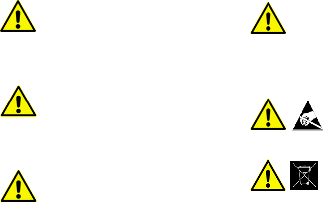
The exclamation point within an equilateral triangle
is intended to alert the user to the presence of
important operating and maintenance instructions in
the literature accompanying the device.
Service:
Do not remove cover. No user serviceable parts
inside. Return to CyberOptics for service and
calibration.
Power Supply and Charging:
Use only the power supply provided with this
equipment for charging.
Input: 100-240 VAC, 50-60 Hz, 0.6A
Output: 5 VDC, 3.0A
Lithium Rechargeable Batteries:
Internal lithium batteries, if handled incorrectly,
could cause injury or death. Refer to local
regulations for handling and disposal of batteries.
Battery should only be serviced by CyberOptics.
Static Sensitive Components:
Observe precautions for static sensitive components.
Disposal:
The product must not be disposed of with normal
waste. Instead, it is your responsibility to dispose of
your waste equipment by arranging to return it to
CyberOptics for recycling. By separating and
recycling your waste equipment at the time of
disposal you will help to conserve natural resources
and ensure that the equipment is recycled in a
manner that protects human health and the
environment. For more information about how to
recycle your CyberOptics supplied waste equipment
please contact our customer services department at
1-763-542-5000.
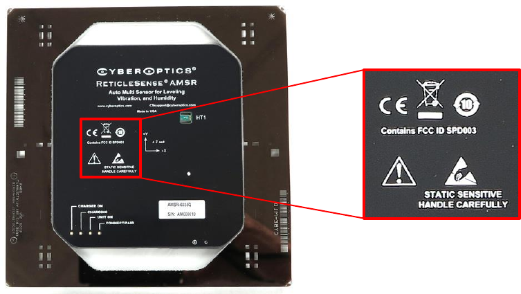
Labels on Devices
Hazard labels as they appear on the AMS devices.
WaferSense and ReticleSense Technical Support
Technical support is available from CyberOptics Corporation.
E-mail: CSsupport@cyberoptics.com
Phone: 763-542-5000
800-366-9131 (US and Canada only)
WaferSense and ReticleSense are registered trademarks, and ParticleView, and ParticleReview are trademarks, of
CyberOptics Corporation.
Third-party brands and names are the property of their respective owners.
Copyright © 2017 CyberOptics Corporation. All rights reserved.
5900 Golden Hills Drive, Minneapolis, Minnesota, 55416

9
Introduction
The CyberOptics WaferSense® and ReticleSense® Auto Multi-Sensors measure leveling, vibration and humidity
inside semiconductor process equipment. The family of products includes versions for 300mm (AMS-300C),
200mm (AM-200C), 150mm (AMS-150C) and 6 inch reticles (AMSR).
The MultiView™ software application makes it easy to see results in real- time. The large display and wireless link
let you place the computer at a convenient distance from the AMS device.
The AMS consists of the following components:
• AMS hardware. The AMS is designed with a wafer-like or reticle-like form factor, so it can fit in most
handling equipment or tools. The device is also vacuum compatible.
• MultiView and MultiReview™ software. The MultiView software application monitors the vibration,
humidity, and leveling measurements and other status information in real time. MultiReview lets you play
back log files recorded in MultiView. Both applications run on most personal computers that use the
Microsoft Windows operating system. See “Specifications” on page 127 for platform requirements.
• Wireless link. The software communicates with the AMS by using a Bluetooth wireless link that attaches
to a USB port on a personal computer.
• Charging case. The AMS is powered by an internal rechargeable battery, which you recharge by placing
the AMS into the charging case.
• Carrying case. The carrying case makes it easy to take your complete AMS system with you in the plant or
on the road.
The following section provides you with instructions for installing your AMS system.
Introduction
10
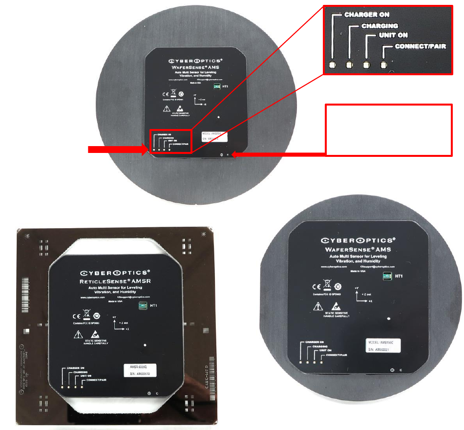
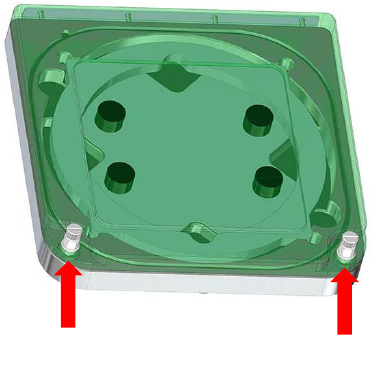
The AMS controls and LED indicators are visible on the outside of the device as shown below.
Figure 1. Controls and LED Indicators
LED indicators
Reset switches are
located on the edge of
the unit

11
Installing Your AMS
This section describes the procedures you need to perform to install your AMS system and get it ready for use. For
best results, perform the procedures in the order they are presented in this chapter:
• Installing the AMS software
• Installing the wireless link on the USB port
• Checking communications between the link and the AMS
• Registering your AMS
• Running the MultiView application
Installing
your AMS
Caution
Dropping the AMS or hitting it against a hard object can bend, break, or chip the housing; damage the internal
components; or knock the AMS out of calibration. While it is not as fragile as an actual silicon wafer, handle the
AMS with care, as you would any precision instrument. If the AMS is damaged or in need of calibration, see the
“Maintaining Your AMS” section.
Caution
The AMS is thicker than a standard silicon wafer so use extreme care to assure that the wafer has proper
clearances when being transported through the tool. For example, when you use the device in a tool for the
first time, move the AMS through the tool in manual mode, visually verifying all clearances. Even when
clearances are sufficient for safe AMS pass-through, if the robot end-effector is taught too high, you risk
crashing and damaging the AMS.
Do not direct compressed air or gas into the humidity sensors on the AMS. Damage to the unit may result.
12
Installing the AMS Software
To install and run the AMS software MultiView and MultiReview, your computer must have the following:
• Windows XP, or Windows Vista and Windows 7 (32-bit or 64-bit), Windows 8, Windows 10 operating
systems
• One free high-power USB 1.1 or USB 2.0 port
To install the AMS software, do not plug in the link before you start. The software must be installed first using the
following steps:
1) Log on using an account with Administrator privileges.
2) Insert the AMS Installation Disk into the CD drive.
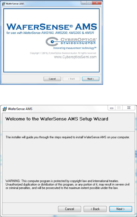
The Setup Wizard starts automatically, as shown in the figure below. If the wizard doesn’t start automatically,
use Windows Explorer to view the contents of the CD and double-click the setup.exe program.
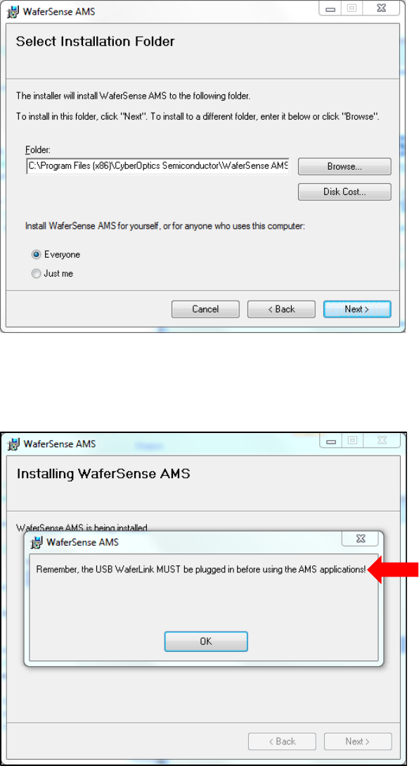
3) Click Next and the Welcome screen of the Setup Wizard appears.
13
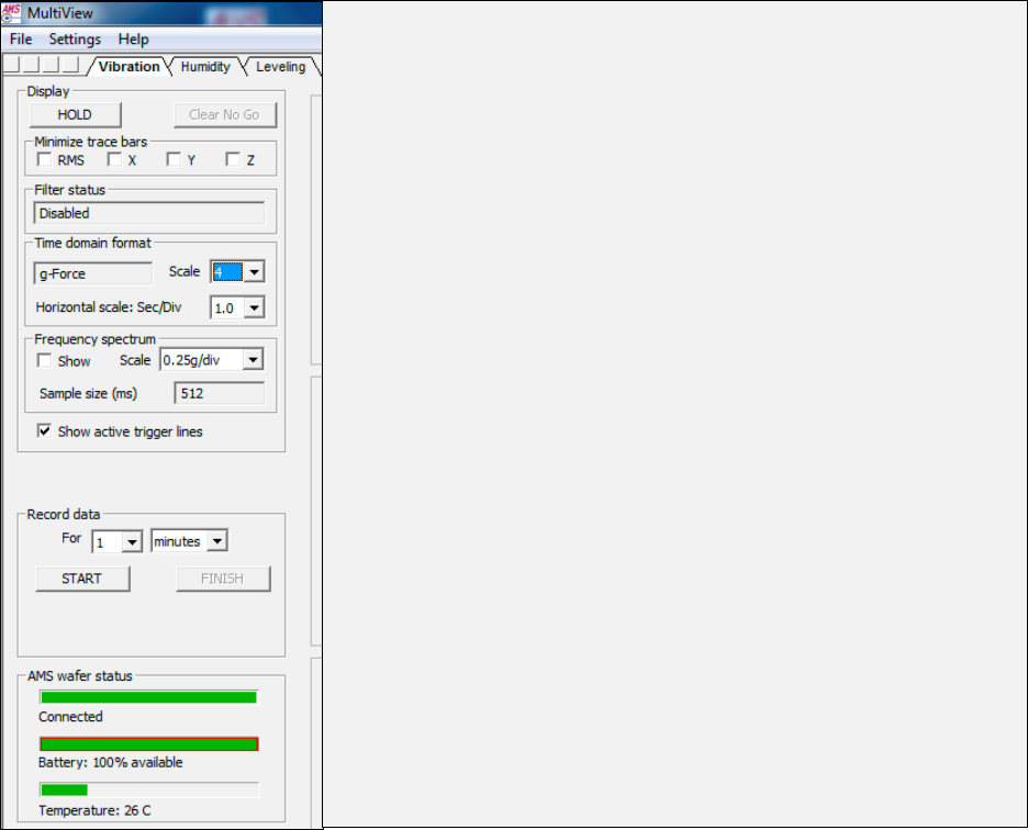
4) Click Next and License Agreement screen appears. Click the I agree button. Click the Next button and the
Select Installation Folder screen appears. Either accept the default settings, or enter a different path and
access settings.
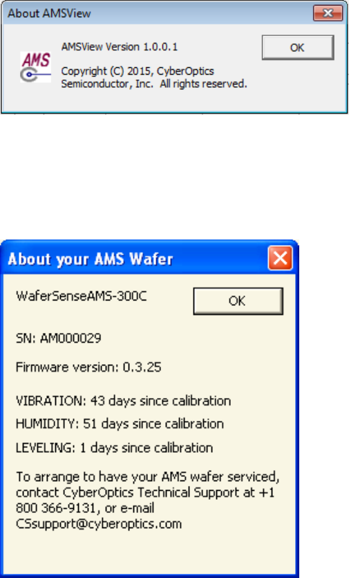
5) Click the Next button and Confirm Installation screen appears. Click the Next button, and the Setup Wizard
starts installing the WaferSense AMS operating software on your computer. A blue progress bar appears and,
when the installation is complete, the following screen appears.
6) Click OK. The WaferSense AMS software is now installed. This is important! Do not run the AMS software at
this time. If you do, you will compromise the overall AMS installation procedure, and get an error message
saying ftd2xx.dll not found.
7) The next step is to install the wireless link (as described in the next section).
14
Installing the Wireless Link
Before starting the wireless link installation, complete “Installing the AMS Software” on page 12. To install the
wireless link:
1) Turn on your computer.
2) Locate an unused, high-power USB port on your computer. The AMS wireless link module requires a high-
power USB port, such as the built-in ports on your computer and ports on USB hubs that have power cords.
Unpowered USB hubs won’t work.
3) The USB cable provided with your AMS system has a different plug on each end. Locate the end with the plug
that matches the USB port on your computer and plug the cable into the port.
4) Plug the other end of the cable into the link module.
5) Windows automatically finds the drivers installed during the Link Device Installer—see the figures on the
previous page.
6) The Power light on the module turns on indicating that the module is getting power from the USB port. Ignore
the Pair Status and Connection Status lights for now.
15
Checking the Communications Between the Link
and the AMS
To complete the installation, verify that the AMS and link can communicate:
1) The AMS operates from an internal rechargeable battery. Before using the AMS for the first time, charge it for
two hours. For information on checking the charge on the battery and the procedure for recharging, see
“Using the Rechargeable Battery” on page 28.
2) On the AMS, there are reset switches as described in the “Introduction” section on page 9. These switches are
recessed and are rarely used, and require the use of a paper clip, or small device to activate. Placing the unit in
the charging case and connecting the charger power supply will start the AMS, see “Opening and Closing the
Charging Case” on page 22.
3) Verify that the Pair Status lights on both the AMS and link module are on. The AMS and link module in your kit
were paired at the factory and will operate with only that particular link module. If either light is not on, your
AMS and link might not be paired with each other. To reset the pairing, see “Changing the Pairing between the
AMS and Link” on page 31.
4) Immediately after turning on the AMS, the Connection Status lights on the AMS and link will blink slowly.
After a few seconds the AMS and link will connect and both lights will be on and no longer blinking. If the
lights continue to blink, see “Monitoring the Wireless Connection to the AMS Device” on page 30.
5) After starting the MultiView application (see “Running the MultiView Application” on page 17), you can verify
the connection to the AMS by comparing the serial number printed on the AMS to the serial number shown in
the About dialog, which is available in the MultiView application by choosing the Help > About menu item. If
the MultiView application is not running, the AMS turns off automatically after 30 minutes.
That completes the installation of your AMS system.

16
Registering Your AMS for Calibration Service
To maintain optimum performance, every twelve months you should have your AMS calibrated and the battery
replaced. These services can be performed only at the factory.
To help you keep track of the next service date so you can schedule this service when it is convenient, register your
AMS with the factory. When you start the MultiView application (see “Running the MultiView Application” on
page 17), it prompts you to register your AMS for calibration. You can also register your AMS in any of the
following ways:
• On the Internet: http://cyberoptics.com/semiconductor_categories/wsregistration.html
• By sending an e-mail message containing the model, serial number, and contact information to
wsregister@cyberoptics.com
17
Running the MultiView Application
To start the MultiView application:
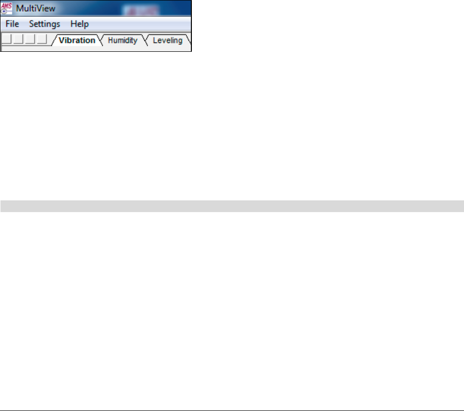
1) From the Windows Start > Programs menu, choose WaferSense AMS > MultiView.exe. The MultiView
application starts, as shown in the figure below. Initializing communications usually takes less than a second. If
the AMS has not been registered, MultiView will display the Calibration Registration dialog. To complete the
registration, proceed to the next step.
Graphing section of the screen

18
2) If MultiView displays the AMS Calibration Registration dialog, as shown in the figure below, you haven’t
registered your AMS. Follow the instructions in the dialog to complete the registration.
19
Technical Support
CyberOptics offers free technical support to customers. If the AMS hardware or software appear to be
malfunctioning, please contact us, and we’ll be happy to assist you.
When you contact us, please make sure that you have the following information available:
• A detailed description of the problem you are having, including the exact text of any error messages and a
list of steps to reproduce the problem.
• Information about your computer, including manufacturer, CPU type, version of Windows, and memory
size.
• The version of the MultiView application. The software version is available in the MultiView application by
choosing the Help > About AMSView menu item.
• If you are using MultiReview, a similar dialog is available from the Help > About MultiReview menu item.
• The serial number of your AMS. The serial number of the AMS is printed on a label on the top of the AMS.
In addition, the serial number is also available in the MultiView application by choosing the Help > About
menu item.

20
Technical support:
• Toll free: 800-366-9131 (US and Canada only)
• E-mail: CSsupport@cyberoptics.com
• Internet: www.Cyberoptics.com

21
Using Your AMS
This section gives you instructions for performing the following tasks with the AMS device:
• Open and closing the charging case
• Use the AMS controls
• Use the AMS indicators
• Use the Vibration, Humidity, and Leveling tabs
• Change colors in the trace screen
• Print the MultiView window
• Monitor the operating temperature of the AMS
• Use the rechargeable battery
• Monitor the wireless connection to the AMS device
• Change the pairing between the AMS device and link
Using
Your AMS
22
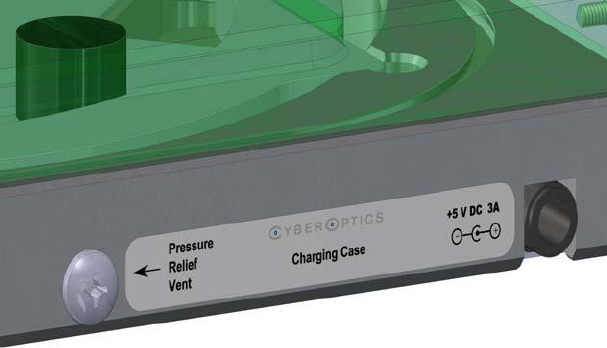
Opening and Closing the Charging Case
The AMS device comes in a plastic charging case that is used for storing it when not in use and for charging the
rechargeable battery in the AMS (see “Using the Rechargeable Battery” on page 28). The AMS device should be
stored in the sealed charging case when not in use.
The charging case is air-tight. After air transport it may be necessary to relieve the pressure differential in order to
open the case. To do so, loosen the pressure relief vent screen until air enters the case. Then re-tighten the screw.
Opening the Charging Case
To open the charging case:
1) Loosen the captive screws on the top of the case.
2) Lift the lid of the charging case using the captive screws.
Closing the Charging Case
To close the charging case:
1) Lower the lid.
2) Tighten the captive screws until the top of the case is secured.
Loosen the captive screws
23
Using the AMS Controls
AMS devices are designed to operate “hands free” in normal use.
• The unit is turned on by inserting the unit in the charging case and applying power to the charging case.
• The unit is completely turned off by activating the “shutdown” button in the MultiView software.
• A “shutdown” turns off all internal electronics in the AMS. After a shutdown the unit must be restarted in
the charging case. Therefore, if the intent is to put the unit into standby mode where the electronics are
still active, the “stop” button in MultiView should be used instead of the “shutdown” button.
• In abnormal situations, the reset switches on the front panel can be used to activate a shutdown or to
turn the unit on from a shutdown. See “Controls and LED Indicators” on page 10 for a view of the reset
switches. The switch indicated by a combined “1” and “0” symbol turns the unit both on and off.
Using the AMS Indicators
The AMS has the following status LEDs (see “Controls and LED Indicators” on page 10).
• Charger On. Glows green, when power is applied to the charging case.
• Charging. Glows red, when the unit is being charged. Goes dark when the battery has reached 100%
charge. Glows red, if the charger is connected and the battery discharges below 95%. Goes dark when the
inductive charger is no longer powered.
• Unit On. Indicates when the device is on.
• Connect/Pair. Note: Glows green, when the unit is successfully paired with a link box. Blinks red/green
slowly, when it is searching for a link. This usually occurs just after turn on or before the link box is
powered by the host computer. Blinks red/ green rapidly, when the pairing function is activated by the
“C” reset switch. This rapid blinking indicates it is receptive to a new pairing.
• When the AMS is on and has been removed from its charger and is ready for in-tool use, the “Unit on”
and the “Connect/Pair” LEDs should both be glowing steady green. The AMS does not necessarily need to
be removed from its charger to be used, nor does it need to be used in-tool.
24
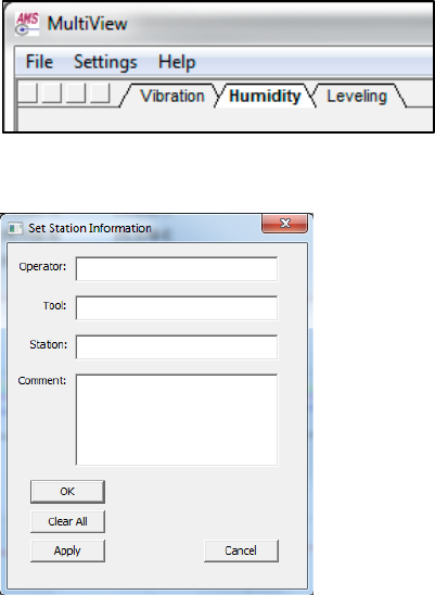
Using the Vibration, Humidity, and Leveling Tabs
The MultiView opening screen contains three tabs, which allow you to access the following AMS functions.
• Vibration
• Humidity
• Leveling
Click on the appropriate tab, and the opening screen for that particular function is displayed.
Changing Colors in the Trace Screen
You can change the colors used to display traces and other elements of the display. The table below shows the
display elements that you can change.
Display Element
Description
RMS
RMS trace
X
X trace
Y
Y trace
Z
Z trace
Indicator
Vertical line at the right edge of the trace display, where new data is first displayed
Go/No-Go lines
Horizontal lines showing current active Go/No-Go tolerances
Trigger lines
Horizontal lines showing current active trigger settings
Grid lines
Horizontal and vertical section lines
Text
Labels on axes and for annotation
Background
Background color of the trace
25
To change colors of the display elements, do the following.
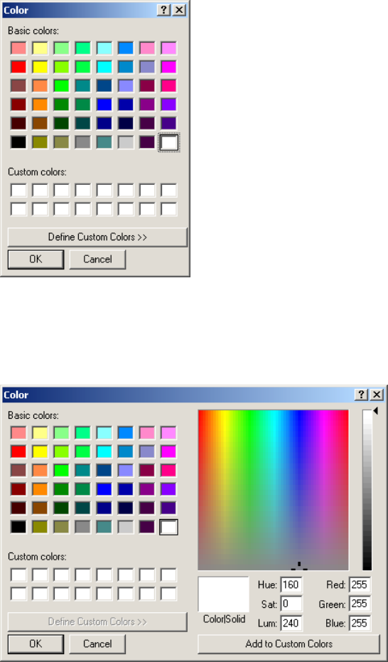
1) From the Settings > Select Colors menu item, choose the display element you want to change. The color
palette is displayed.
2) If you want to use one of the existing color definitions, skip to the next step. If you want to define a custom
color, click Define Custom Colors. The color palette expands, as shown below. Specify the color as a
combination of hue, saturation, and luminosity, or as a combination of red, green, and blue, and click Add to
Custom Colors.
3) Click on the color you want to use for the display element and click OK.
4) To reset all colors to the default values, go to the Settings > Select Colors menu and choose Restore Defaults
to All.
5) To reset only the background color to the default value, go to the Settings > Select Colors menu, and choose
Restore Default Background.
26
Printing the MultiView Window
You can print an image of the MultiView window to have a graphical record of the session. To print an image of the
MultiView window, do the following.
1) Choose File > Print.
2) In the Print dialog, click OK.
3) You can also select a printer other than the default and change the printer setup, or see a preview of what
MultiView will print.
• To select a different printer, change the paper selection or print orientation, or set printer properties,
choose the File > Print Setup menu item.
• To see a preview of what MultiView will print, choose the File > Print Preview menu item.
27
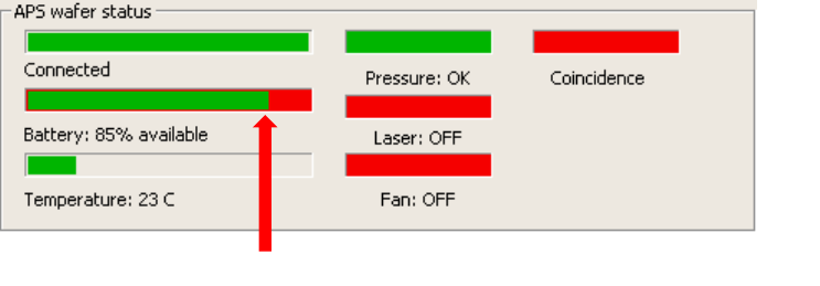
Monitoring the Operating Temperature of the AMS
The operating range for the AMS is 20–70 °C. The AMS can withstand exposure to higher temperatures for very
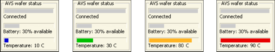
brief periods, if not in direct contact with a heating element. The Temperature monitor in the AMS wafer status of
the MultiView window shows the current operating temperature of the AMS using a numeric readout and a bar
graphic (as shown below).
Low Optimum Warning Danger
<20 °C 20–70 °C 71–80 °C > 80 °C
The temperature bar changes color to indicate where the current temperature is relative to the accurate operating
range, using the following color-coded bars.
• Blue
Less than 20 °C. The AMS is operating below the range, where it produces accurate readings.
• Green
20–70 °C. The AMS is operating in its optimum temperature range, where it produces readings meeting the
specified accuracy.
• Orange
71–80 °C. The AMS is operating above the range, where it produces the most accurate readings, but not so hot
that the AMS will be damaged.
• Red
Greater than 80 °C. The AMS is operating at a temperature so high that it might be damaged.
28
Using the Rechargeable Battery
The AMS operates from an internal rechargeable battery. From a full charge, the battery provides about four hours
of continuous use. Before using your AMS device for the first time, charge it for two hours.
The battery can be recharged about 400 times before the charge life starts to degrade significantly. The battery is
not user replaceable. For information on replacing the battery, see “Annual Factory Calibration and Battery
Replacement” on page 125.
Battery performance degrades at temperatures outside the temperature range: 15–45 °C.
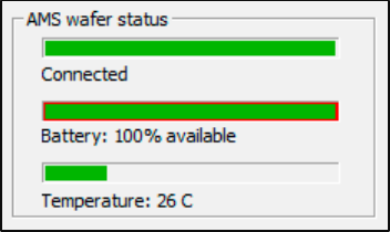
Monitoring the Battery Level
MultiView receives frequent updates from the AMS on the status of the AMS’s battery. The Battery indicator in
the AMS status area of the MultiView window shows the approximate percentage of operating time remaining
before you must charge the battery.
Charging the Battery
To charge the AMS device’s battery:
1) Use only the battery charger supplied with your AMS device. Using a different battery charger might damage
your AMS or create a safety hazard.
2) Do not charge the AMS, if the temperature is higher than 45°C. Charging the AMS device at a temperature
higher than 45 °C might damage the AMS housing or create a safety hazard.
Battery status—connected and at 85% of full charge
29
3) Place the AMS device in the charging case (see “Opening and Closing the Charging Case” on page 22). Close
the lid.
4) Plug the charger line adapter into a 100 VAC to 240 VAC mains, and plug the other end into the charging case
connection on the right side of the charging case.
The charging case is air-tight. After air transport it may be necessary to relieve the pressure differential in
order to open the case. To do so, loosen the Pressure Relief Vent screw until air enters the case. Then re-
tighten the screw.
5) When power is applied to the charging case, the Charger on LED will light and the Charging LED will also light,
unless the unit is already fully charged. In addition, the Unit on LED will light. If the unit is still paired to a
powered link box, the Connect/ Pair LED will light.
6) Charge the unit until the Charging LED goes dark. The unit is now fully charged and ready for data collection.
However, the unit can be used if not fully charged.
7) The AMS can remain in the charging case with power applied to the case even when fully charged. The battery
will not be damaged. The AMS should be stored in the sealed charging case when not in use.
30
Monitoring the Wireless Connection to the AMS
Device
The MultiView application communicates with the AMS device by using a Bluetooth wireless link. The wireless link
has a range of up to 30 ft (10 m).
The Connection indicator in the AMS wafer status area of the MultiView window shows the quality of the wireless
connection between the AMS and the link module. The connection quality is indicated by the color of the bar and
the wording below the bar.
• Green—Connected. The connection between the link and AMS is good. With a good connection, the AMS
device is sending the maximum number of readings per second to the link module (at least 200 readings per
second).
• Yellow—Poor connection. There is some interference or other problem with the signal that is preventing the
link and AMS device from communicating at their maximum rate. When the indicator is yellow, the readings
are still accurate but aren’t being updated as frequently.
• Red—No connection. Indicates that there is no connection between the AMS device and link module. The
values in the display do not update when the indicator is red.
The Bluetooth wireless link technology used in the AMS is a low-power technology that operates in the 2.4 GHz
radio frequency band. This unlicensed band is also used by many other types of devices, such as cordless phones
and microwave ovens. Another 2.4 GHz device operating in close proximity could interfere with the AMS system.
When this happens, separating the devices by at least 6 ft (2 m) usually solves the problem.
Other factors can also affect the wireless link, such as the distance between the AMS device and link, and obstacles
between the device and link that block the signal. If MultiView indicates that the connection isn’t good, try moving
the wireless link module a few feet closer to the AMS device.
After turning off the AMS, the Connection indicator might not change to red for a few seconds.
31
Changing the Pairing between the AMS and Link
The AMS and link module in your kit were paired at the factory and will operate with only that particular link
module. You can change this pairing, so that you can use your AMS with a different AMS link module, or vice versa.
Link modules for different CyberOptics WaferSense or ReticleSense products, such as Auto Gapping Sensors (AGS),
are not interchangeable.
To pair an AMS and link module:
1) If you are changing the pairing of an AMS that is already paired with a link module, first unplug the currently
paired link module. You can’t pair an AMS with a new link module, while the currently paired link module is
powered on.
2) Make sure the Power LED is illuminated on the link module you want to pair, and make sure the Unit on LED is
illuminated on the AMS.
3) On the AMS, press and hold the “C” reset switch until the Connect/Pair LED starts to blink rapidly (about four
times per second).
4) On the link module, press and hold the New Pair button until the Pair Status and Connection Status LED lights
start to blink rapidly (about four times per second).
The LEDs on the link module and the AMS will continue to blink for a few seconds, until the link and the AMS
have established a new pairing, after which the LEDs will be on and no longer blinking.

32
Overview of Main AMS Sub-Functions
As described above, the AMS collects vibration, humidity, and leveling data from your wafer-manufacturing
process in real time. The vibration, humidity, and leveling functions share many of the same sub-functions, and all
of these sub-functions operate in exactly the same way. The sub-functions, of course, vary slightly in their details
(because the vibration, humidity, and leveling functions use different parameters), but operate along the same
lines and use the same basic, underlying principles. As a result, once you understand a sub-function in “Vibration,”
you understand it in “Humidity” and “Leveling” as well.
The purpose of the following sections therefore is to introduce you to some commonly used MultiView sub-
functions, so you can quickly get up to speed on the way the MultiView software operates. The idea here is to
introduce you to the underlying concepts behind each sub-function, so do not worry about the details. The sub-
functions that are discussed are as follows.
• Setting Go/No-Go Tolerances
This allows you get an on-screen warning, when a measured parameter strays from its defined limits.
• Setting Triggers
This tells the AMS download current real-time data to a log file, whenever a measured parameter strays
beyond its defined Go/No-Go tolerances. The log file can be reviewed during the run, or at a later date.
• Setting Station Information
This allows you to keep track of each AMS run for record-keeping and quality-control purposes.
• Saving Your MultiView Settings
This allows you to save your current function and sub-function settings, so they can be used again.
• Loading Previously Saved Settings from a File
This saves you a lot of time and effort, because you can load settings from previously saved files.
Overview of
Main AMS
Sub-Functions
33
Setting Go/No-Go Tolerances
Setting the Go/No-Go tolerances gives you an on-screen warning, when a measured parameter strays from its
defined limits. This is useful, because it alerts you to the fact that something undesirable may be about to happen,
so you can keep a very close eye on what is going on as the AMS moves through your manufacturing process.
Example
In this example we are worried that one of the robots that feeds wafers into one of our tools is reaching the end of
its service life. Specifically, the robot has logged over 10,000 hours of use, and the bearings in its end-effect that is
responsible for horizontal back-and-forth movements (the y axis), is about to fail.
Setting Go/No-Go Tolerances
To set Go/No-Go tolerances, do the following.
1) Open MultiView and click the Vibration tab.
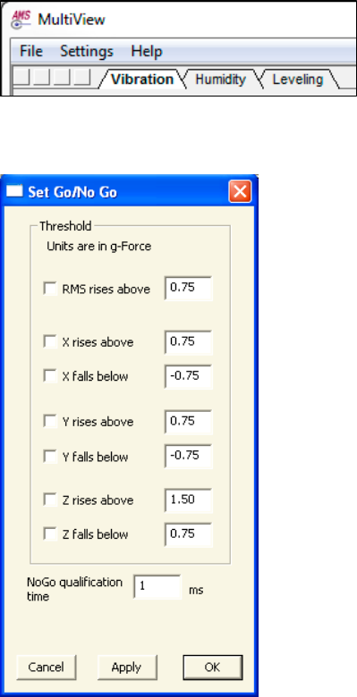
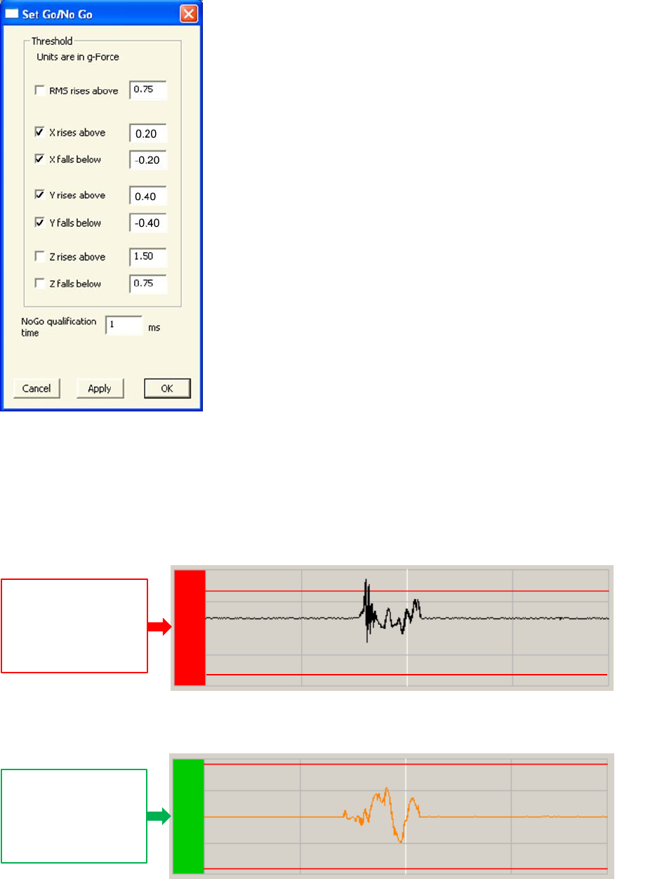
2) Choose the Settings > Set Go/No-Go menu item.
The dialog shows the default settings for vibration in the x, y, and z axes.
34
5) Check the appropriate box and enter the Go/no-Go tolerances (in g force) for the x, y, and z axes. Check the
root mean square box, if you want MultiView to graph an average vibration trace for all three axes.
In our example, our previous experience with this particular brand of robot tells us that the bearings are about to
fail, if the vibration exceeds ± 0.4g, and that ± 0.20 is normal. Hence we set ± 0.40 g for horizontal back-and-forth
movements (the y axis—the key point here), as these are the bearings we believe are about to fail in the end-
effector.
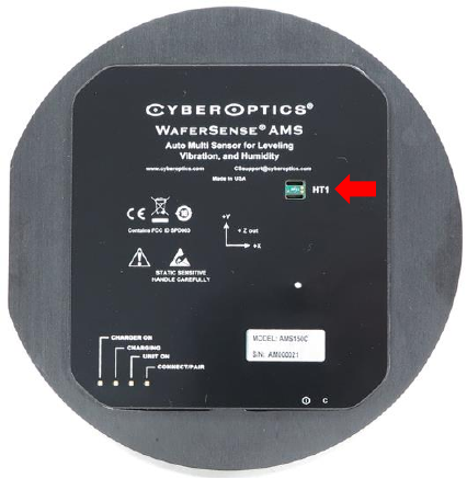
6) In our example, we ran the AMS through our system, and observed the following traces in the Vibration
screen. (The bearings are clearly about to fail.)
y axis
x axis
Red color
indicates trace is
beyond Go/No
tolerances
0.4
–0.4
Green color
indicates trace is
within Go/No
tolerances
–0.2
0.2
35
Setting Triggers
Triggers are used to tell the AMS to start capturing real-time data to a log file, as soon as the measured parameter
strays beyond its defined upper or lower limits. MultiView continues downloading data for as long as the
parameter stays out of bounds, and stops when the parameter is back in bounds.
Clearly, you can set your Trigger values to exactly the same values as those you set for your Go/No-Go tolerances.
In this instance, when the measured parameter strays out of bounds, MultiView immediately downloads data to a
log file and issues an on-screen warning. You can, however, set your Go/No-Go tolerances, so you get an on-screen
warning when the parameter is about to move close to the upper and lower limits you have set in the Trigger
menu. This is useful, because it alerts you to the fact that something undesirable may be about to happen, so you
can keep a very close eye on what is going on as the AMS moves through your manufacturing process. And, if the
parameter in question actually strays beyond its Trigger settings, MultiView will download a log file of the event
for future reference.
Example
In this example, we have just installed a fancy new—and very expensive—dehumidifying system in our clean room,
because we need to minimize gallium arsenide oxidation on our wafers. The new dehumidifying system is
supposed to keep the relative humidity (RH) in our clean room in the range 6% ± 2%. We are now going to use the
AMS to tell us whether the new dehumidifying system is, in fact, keeping the RH inside our tools—the key point
here—within this critical range.
By setting the appropriate Trigger parameters, the AMS will download humidity data to a log file, every time the
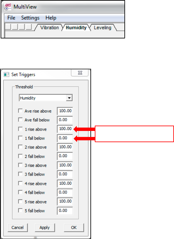
RH strays outside the desired range of 4–8% RH. Please note that in this example we are using the 150mm
WaferSense AMS, which has only one humidity/temperature (HT) sensor, located near the center of the disk
(designated “HT1”), as shown below. (Some AMS models have five HT sensors.)
We normally store the AMS in our office, which frequently has an RH in excess of 70%. As a result, we left the AMS
overnight in our clean room to equilibrate, and to prevent problems with hysteresis (a lag in reading-response
times produced when the AMS is moved from one humidity environment to another) before running our
experiment.
36
Setting the Triggers for Humidity
To set the appropriate triggers for monitoring humidity, do the following.
1) Open MultiView and click the Humidity tab.
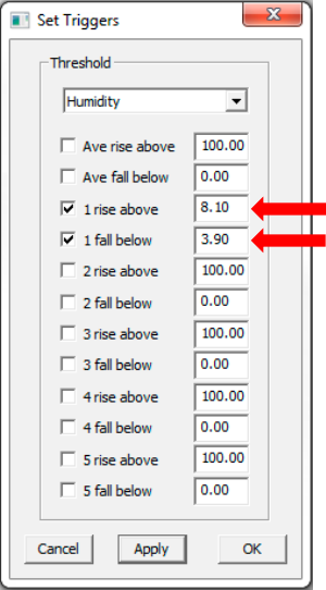
2) Choose the Settings > Set Triggers menu item.
MultiView populates the Set Triggers dialog with the default values (0% and 100% RH) for the maximum possible
number (5) of HT sensors on an AMS unit. As our particular unit has only one HT sensor, we are going to enter the
upper (“rises above”) values and lower (“falls below”) values only for HT1, and ignore the default values for HT2
through HT5.
Default values for HT1
37
3) Check the HT1 box, and enter the upper and lower trigger values for humidity. (Do the same for the other
sensors HT2–HT5, if your AMS is equipped with them.)
In our example, to give ourselves a little leeway and to make sure the RH values actually fall outside the range
4–8% before data is downloaded to a log file. As a result, we have chosen 1 rises above and 1 falls below values of
3.90 and 8.10, respectively. (We ignored the other settings, because they do not apply to our particular model of
AMS.)
7) Click Apply to save the settings you entered.
8) Click OK to close the dialog.
38
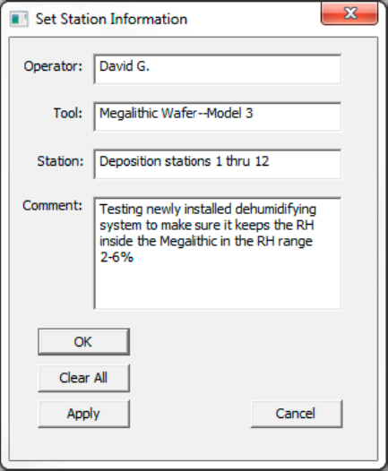
Setting Station Information
The Station Information screen allows you keep track of each AMS run by entering operator name, tool and
station ID, and other relevant information about your AMS run. It is a good idea to 1) always fill in the Set Station
Information dialog every time you run the AMS through your wafer-manufacturing process, and 2) make filling in
this dialog part of your everyday record-keeping and quality-control procedures. If you need to refer to your log
files in the future, having this detailed information on file will make life much simpler.
Example
See the humidity example on page 35.
Setting Station Information
To include user-specified information in your log files, do the following.
1) Open MultiView and click the appropriate tab.
2) Choose the Settings > Set Station Information menu item.
39
3) Type your text into the Operator, Tool, Station, and Comment text fields. (We entered data for our humidity
experiment.)
4) Click Apply to accept the changes without closing the dialog. To accept the changes and close the dialog, click
OK instead.
You can leave the Set Station Information dialog open while using MultiView (drag it off to the side, so it
doesn’t cover the MultiView window). Doing so makes it easy to change the Comment or other fields each
time you start recording, or as needed. Be sure to click Apply after you finish making changes, though, or
MultiView won’t use the latest changes for the next log file.
You can change or delete this information at any time for future log files. To quickly clear all of the fields, click
Clear All.
40
Saving Your MultiView Settings
Each time you exit MultiView , it saves all your current function and sub-function settings in a log file in the
Windows registry. The next time you start MultiView, it restores those saved settings. You can also tell MultiView
to save your settings to a file you specify, and you can have MultiView read those settings back at any time. This
lets you have several different configurations for MultiView, and be able to switch between them easily, without
having to reenter the settings.
To save your settings in a file you specify:
1) Choose the File > Save Settings As menu item.
2) In the AMS Settings File dialog, specify the directory and file name and click Save. MultiView saves your
settings, and the file you specified becomes the current settings file.
To save your settings in the current settings file:
1) Choose the File > Save Settings menu item.
2) Each time you start MultiView, the application automatically reads in the most recent settings from the
Windows registry, including the last settings file you specified, if any.
Loading Previously Saved Settings from a File
To load previously saved function and sub-function settings from a file:
1) Choose the File > Open Settings menu item.
2) In the AMS Settings File dialog, specify the directory and file name and click Open. MultiView reads the
settings from the specified file and applies the settings. These settings are also written to the Windows
registry, and will be loaded the next time you start the MultiView application.

41
Using the Vibration Function
The section tells you how to use the AMS to monitor vibration in the X, Y, and Z axes using the MultiView operating
software. More specifically, this section tells you how to do the following.
• Read the vibration trace display
• Freeze the trace display
• Monitor traces for excessive vibration levels
• Record the traces
• Chang the pre-recording length
• Place marks in a log file
• Include user-specified information in a log file
• Understand log file names
• Import log files into other applications
• Configure the trace display
Using the
Vibration
Function
42
Reading the Vibration Trace Display
The AMS is like a seismograph, but instead of charting movements in the earth’s plates, you’ll probably be using
the AMS to look for unwanted vibrations in wafer handling and processing equipment. The AMS continuously
detects vibrations and transmits the readings to the MultiView application. MultiView displays the readings as
traces, similar to the traces on a seismograph drum. You can place the AMS in a tool, run the manufacturing
equipment through its paces, and watch the MultiView display for levels of vibration that might indicate a
problems with the equipment, such as places where the AMS is making unwanted contact with a tool. Appendix C
describes acoustic resonances and other factors that affect vibration measurements.
To use the AMS Vibration system:
1) Make sure the computer running the MultiView software is within the range of the link module, up to 30 ft
(10 m).
2) Normally, you would place the AMS on the equipment you want to check, and then start the equipment in
motion, monitoring the MultiView display. To get a feeling for how the AMS works, for now just set the AMS
on a desk or table.
3) Start the MultiView application.
43
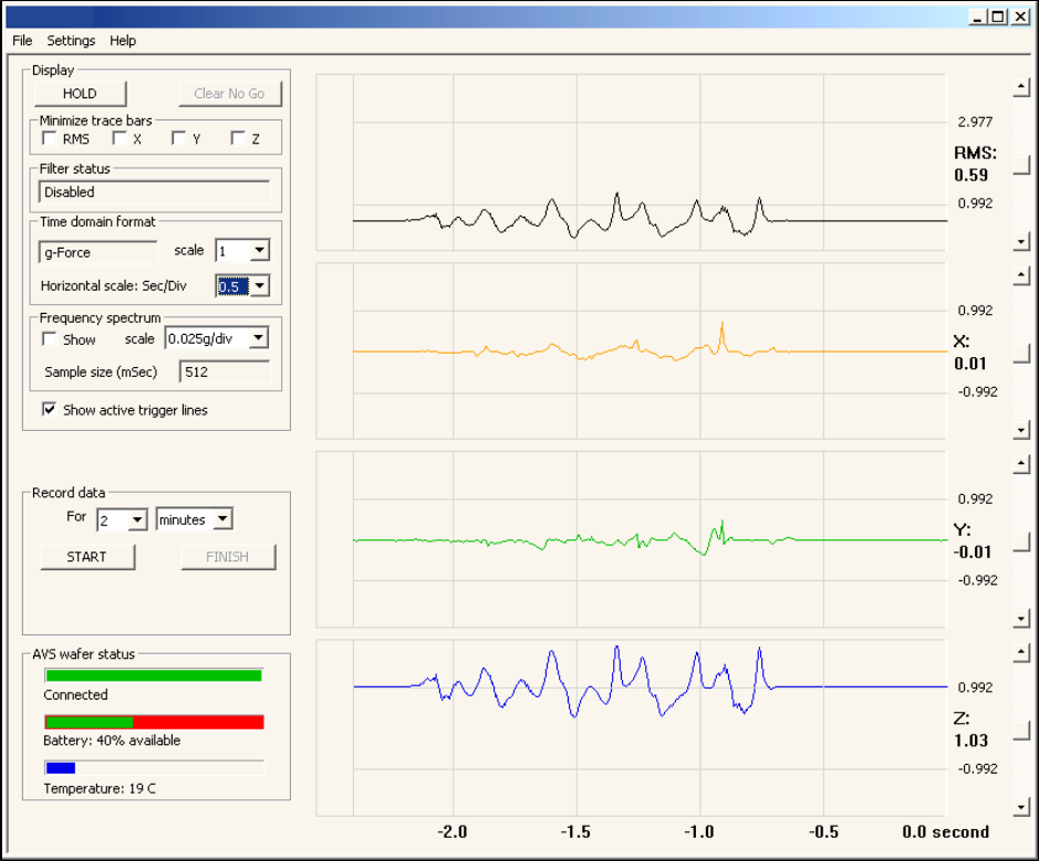
4) Click the Vibration tab and the Vibration Trace screen is displayed.
The gridded area of the display on the right shows the traces. When the AMS is turned on and has a
connection to the computer running MultiView, the AMS transmits vibration data in nearly real time.
5) Give the AMS a light tap. A spike in the traces will appear at the far right of the MultiView screen. New
readings always appear at the far right edge of the display. As more readings are displayed, the spike scrolls to
the left and eventually disappears. The trace area of the display is described below.
• X, Y, and Z Axes
These traces show the vibration measured in each of three directions. Looking down on the AMS with the logo
at the top, the X trace shows horizontal movement to left and right, the Y trace shows horizontal movement to
top and bottom, and the Z trace shows vertical movement.
The AMS measures vibration in units of g-force, which is actually a measure of acceleration. One g is the
acceleration of gravity (approximately 32 ft/s2 9.81 m/s2), with a range from -2 g to +2 g. The number
displayed below the label (X, Y, or Z) at the far right of the screen is the current value: the value displayed at
that instant at the far right of edge of the trace. The default vertical scale shows units of g-force, but you can
change the units to galileos (1 Gal = 0.01 m/s2). You can also change from displaying acceleration to displaying
the signal energy (g2-s). To change the displayed readings and scales, see “Changing the Time-Domain Format”
on page 64.

44
You can minimize the display of one or more traces, to focus on the trace or traces of most interest (see
“Minimizing the Trace Bars” on page 62).
• RMS (Root mean square)
The RMS trace displays the calculated root mean square of the X, Y, and Z values, using the following formula.
√ ⅓ x (x2 + y2 + z2)
The default vertical scale shows units of g-force, but you can change the units to galileos (1 Gal = 0.01 m/s2).
You can also change from displaying acceleration to displaying the signal energy (g2-s). For more information
on displayed readings and scales, see “Changing the Time-Domain Format” on page 64.
• Grid Lines
The vertical grid lines represent time intervals. The default interval between grid lines is 0.5 seconds, with 100
data points plotted in each interval. To change the horizontal scale for the traces, see “Changing the
Horizontal Time and Scale” on page 66.
• Scroll Bars
Scroll bars let you move the traces by ±2g. As you increase the vertical scale factor, you might need to scroll to
view the full range of a trace.
45
Freezing the Trace Display
When the AMS is powered up and connected to the MultiView software, the AMS sends blocks of 100 readings to
MultiView every 100 milliseconds. MultiView displays the data continuously in nearly real time. That means that
the display is constantly moving. If you notice a spike in one of the traces, it could scroll off the left side of the
display and disappear in as little as half a second, depending on the display settings. MultiView includes a Hold
feature that lets you freeze the display (though not the data stream).
1) To freeze the trace display, click Hold (shown below). The Hold button changes to Release and the traces stop
moving, but the AMS continues to send data to MultiView.
2) To resume the trace display, click Release. The traces jump ahead to display the most-current data and start
moving again. If the hold is long enough, some of the data received might not be displayed, when the trace
resumes.
46
Monitoring Traces for Excessive Vibration Levels
You can use the Go/No-Go feature in MultiView to monitor the traces for excessive levels of vibration and indicate
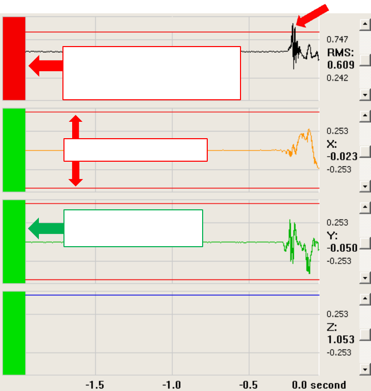
when your specified levels are exceeded. The figure below shows the trace display with the Go/No-Go feature
active.
Parallel red lines in each trace indicate the Go/No-Go tolerances, which you can set separately for each trace. A
vertical green bar appears at the far left of each trace to indicate that the trace is within your specified tolerances.
When the trace continuously exceeds your tolerance settings for more than one millisecond (the qualification
time), the vertical bar changes to red. You can specify a qualification time from 1 to 10 milliseconds. If the trace
exceeds your settings, but remains so for less than the qualification time, the No-Go tolerances are not affected,
and the bar remains green.
You can set the amount of time the red bar remains on from 1 to 10 seconds, or it can stay on until you clear it
with the Clear No-Go button. Extending the length of time the red bar remains on makes it easier to catch narrow
spikes. However, if another Go/No-Go event occurs while the bar is already red, it restarts the timer for displaying
the red bar. So in practice, a red bar might remain on for many seconds, when multiple events occur in close
succession. In addition, MultiView can issue an audible beep to indicate when a trace exceeds a Go/No-Go
tolerance.
Red bar shows RMS trace has
exceeded one of the Go/No-Go
limits
No/No-Go limits for X trace
Green bar shows Y trace is
within Go/No-Go limits

47
Setting the Go/No-Go Tolerances
To set the Go/No-Go tolerances:
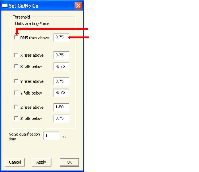
1) Choose the menu item Settings > Set Go/No-Go. The Set Go/No-Go dialog is displayed.
2) Check the boxes to activate Go/No-Go for one or more traces.
3) For each trace you activated, specify the Go/No-Go tolerances. You can specify separate upper and lower
settings for X, Y, and Z. The units for Go/No-Go tolerances depend on the time domain format you have
specified (see “Changing the Time-Domain Format” on page 64).
4) For the No-Go qualification time, specify the length of time any trace must exceed any Go/No-Go tolerance,
before the No-Go condition is triggered. A trace that exceeds a tolerance for less than the qualification time
will not trigger a No-Go condition.
5) Click Apply and the Go/No-Go tolerances take effect immediately. When the next active No-Go event lasting
longer than the qualification time occurs, MultiView changes the green Go/No-Go bar to red and beeps, if you
enabled this option.
Click box to activate named Go/No-Go setting
Enter appropriate number for setting

48
6) You can leave the “Set Go/No-Go” menu open, while using MultiView. Doing so makes it easy to change the
Go/No-Go tolerances. To close the menu, click OK.
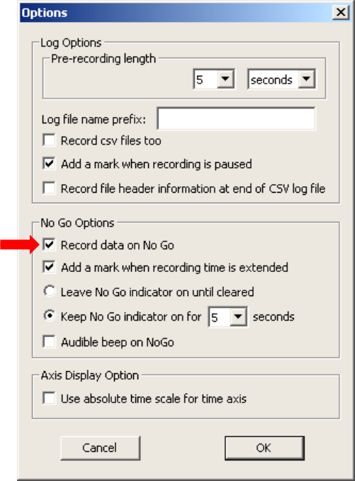
Setting Options for the No-Go Indicators
To set options for the No-Go indicators:
1) Choose the menu item Settings > Options. The options dialog is displayed.
2) If you want the indicator to remain red for a certain length of time following the event, choose Keep No-Go
indicator on for, and choose the number of seconds.
3) If you want MultiView to alert you with an audible beep when a Go/No-Go condition is exceeded, check Audio
Beep on No-Go.
4) Click OK and the No-Go options take effect immediately.
No-Go options, which are described
in more detail below
49
Recording the Traces
You can record the vibration data to a log file and then play it back later. For information on playing back log files,
see “Viewing Log Files” on page 72. You can start a recording session manually or automatically (described below).
Once MultiView starts recording, it records for the length of time you specify. The log file includes data for five
seconds prior to the event that initiates the recording (see “Changing the Pre-Recording Length” on page 54). Log
files include the vibration data, user-specified data, and trigger information. All data received by MultiView (1,000
points per second) is recorded regardless of the display settings. Detailed information on recording log files is
described in the following sections.
Manually Recording Traces
With manual recording, you start the recording by clicking a button and the recording runs for the length of time
you specify, unless you stop the recording. You can also pause recording and later resume recording in the same
log file. The manual recording controls for pausing and stopping recording are active even when recording is
started by using triggers or No-Go events (see sections below).
To record vibration data manually:
1) In the Record Data menu, use the For lists to set the length of time for the recording. You can choose
recording times of up to four hours. Note that four hours of recording at 1,000 data points per second will fill
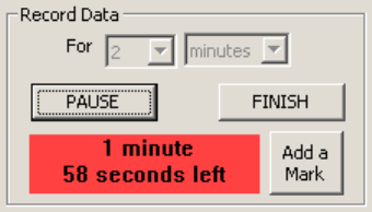
about 150 MB of disk space.
2) To start recording, click Start. The Start button changes to Pause. MultiView will record for the specified
length of time. The remaining time is shown below the Pause button, with a red background to indicate that
recording is in progress.
While a recording is in progress, holding your cursor over the Pause/Continue button displays a ToolTip with
the name of the current log file and the event that initiated recording.
3) To stop the recording before the specified recording time has expired, click Finish. Clicking Finish closes the
current log file.
4) To temporarily stop recording but keep the current log file open, click Pause. When you want to continue
recording, click Continue. While recording is paused, MultiView continues to display data in real time. During a
pause, the background color for the countdown timer changes to yellow, and the countdown pauses. While a
recording is in progress or paused, holding the cursor over the Pause/Continue button displays a ToolTip that
shows the name of the log file and the trigger event.
50
Automatically Recording Traces
Instead of starting a recording manually, by clicking Start, you can have MultiView start the recording
automatically, when one of the MultiView traces rises above, or falls below, a specified value. Once the recording
starts, MultiView records for the length of time you specify, or until you click Finish.
You have two options for starting to automatically record traces, as follows.
• Triggers
The triggers feature is primarily for recording data. Triggers don’t give you any visual indication in the display,
when the traces exceed your specified limits. You can’t set a qualification time for triggers, because a trigger starts
recording immediately when the trigger level is exceeded—see section below.
• Go/No-Go
The Go/No-Go feature is primarily for helping you view events in the data on the display (see page 46). During a
recording initiated by a Go/No-Go event, subsequent events extend the recording time, which is not true for
triggers—see section below.
Recording with Triggers
Once recording has started, any subsequent trigger events are ignored. When recording stops, any active trigger
event can start a new recording.
To record vibration data using triggers:
1) In the Record Data menu, use the For lists to set the length of time for the recording. You can choose
recording times of up to four hours. Note that four hours of recording at 1,000 data points per second will fill
about 150 MB of disk space. Once triggered, MultiView records data for the specified length of time (or until
you manually stop or pause recording), regardless of any subsequent trigger events.
51
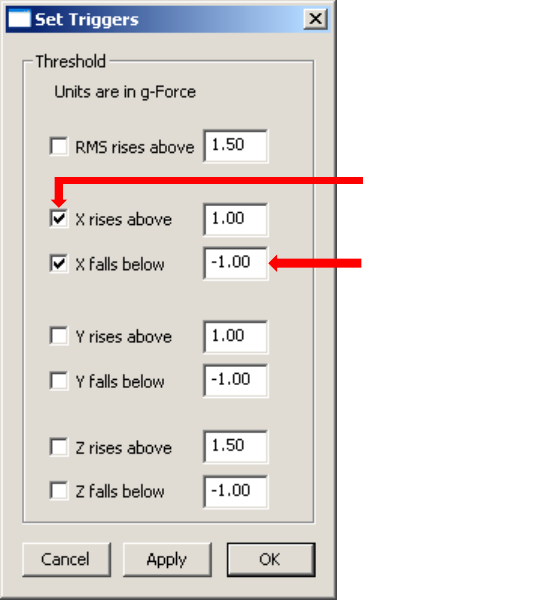
2) Choose the menu item Settings > Set Triggers. The Set Triggers dialog is displayed.
3) Check the boxes to activate triggers for any events that you want to trigger the start of recording.
4) For each of the triggers you activated, specify the value that you want to trigger the start of recording. You can
have MultiView start recording when a trace rises above a specified value, or when a trace falls below a
specified value. The units for trigger settings are the same as the units for the time domain format you have
specified—see above.
5) Click Apply and the trigger settings take effect immediately.
6) When the next active trigger event occurs, MultiView starts recording data. MultiView records for the
specified length of time, unless you click Finish or Pause—see above. The remaining time is shown below the
Finish and Pause buttons.
7) You can leave the Set Triggers menu open while using MultiView. Doing so makes it easy to change the
triggers. If you want to close the dialog, click OK.
Active triggers
Trigger setting
52
Recording with Go/No-Go
Once recording has started, any subsequent No-Go events cause the recording time to be extended. Recording
continues for the specified time from the moment of the most-recent event. When recording stops, any active No-
Go event can start a new recording.
To record vibration data using Go/No-Go tolerances:
1) In the Record Data menu, use the For lists to set the length of time for the recording. You can choose
recording times of up to four hours. Note that four hours of recording at 1,000 data points per second will fill
about 150 MB of disk space. The recording time is restarted every time a No-Go event occurs. So, if you set the
time for 30 seconds, but a second No-Go event occurs after recording has been in process for 20 seconds, the
total recording time will be 50 seconds.
2) Choose the menu item Settings > Set Go/No-Go. The Set Go/No-Go dialog is displayed.
3) Check the boxes to activate Go/No-Go for one or more traces.
4) For each trace you activated, specify the Go/No-Go tolerances. You can specify separate upper and lower
settings. The units for Go/No-Go tolerances are the same as the units for the time domain format you have
specified—see above.
Click box to activate named Go/No-Go setting
Enter appropriate number for setting
53
5) For No-Go qualification time, specify the length of time any trace must exceed any Go/No-Go tolerance before
the No-Go condition will start recording. A trace that exceeds a setting for less than the qualification time will
not start recording.
6) Click Apply.
7) You can leave the Set Go/No-Go menu open, while using MultiView. Doing so makes it easy to change the
Go/No-Go tolerances. If you want to close the menu, click OK.
8) Choose the menu item Settings > Options. The options dialog is displayed.
9) Check the Record data on No-Go box.
10) Click OK.
11) When the next active No-Go event lasting longer than the qualification time occurs, MultiView starts
recording data. MultiView records for the specified length of time, unless you click Finish or Pause, or the
time is extended by the occurrence of another No-Go event. The remaining time is shown below the Finish
and Pause buttons.
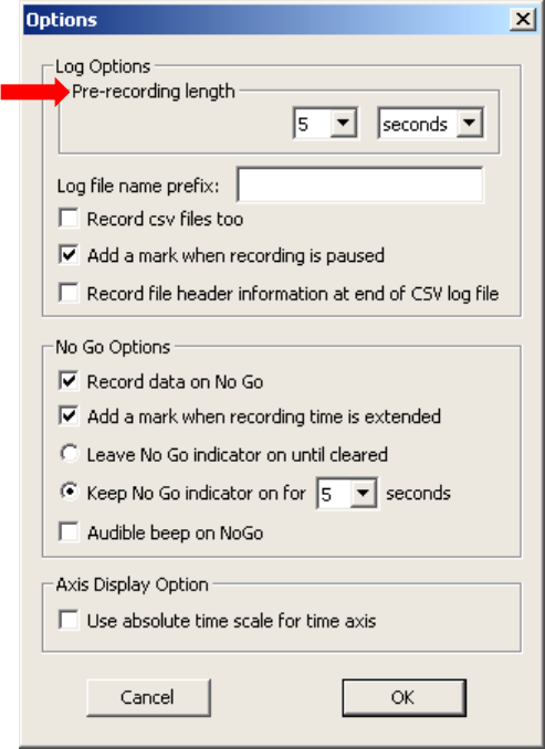
54
Changing the Pre-Recording Length
When recording data, MultiView includes data in the log file beginning five seconds prior to the event that initiates
the recording, whether that event is the Start button, a trigger, or a No-Go event. When you play back a log file in
MultiReview, this length of pre-recording data allows you to see a few seconds of data just prior to the event that
started the recording. You can adjust the length of this pre-recording data from zero to five minutes.
To set the length of time for pre-recording data:
1) Choose the menu item Settings > Options. The options dialog is displayed.
2) Under Pre-recording length, choose the interval of time and the units for pre-recording data.
3) Click OK.
55
Placing Marks in a Log File
At the start of recording, at trigger events, at No-Go events, and when MultiView loses communication with the
AMS, MultiView automatically places marks in the log file. You can also have MultiView automatically mark
locations in the log file for other events. In addition to marks created automatically by MultiView, you can
manually create your own marks in a file while you are recording, and you can add annotations to the marks.
When you use MultiReview to play back the log file (see “Viewing Log Files” on page 72), you can quickly jump to
the location of any mark in the file.
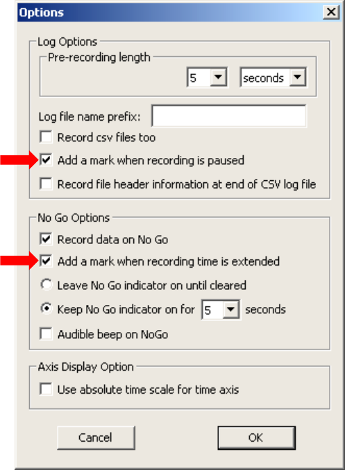
Adding Marks Automatically for Pauses and for Recording
Time Extensions
In addition to the marks that MultiView places in the log file for the start of recording, trigger events, No-Go
events, and when MultiView loses communication with the wafer, you can have MultiView mark locations in the
file where you pause recording and where the recording time is extended by additional No-Go events.
To have MultiView add marks for pauses and for recording time extensions:
1) Choose the menu item Settings > Options. The options menu is displayed.
2) To have MultiView add a mark to the log file each time you pause recording, check the Add a mark when
recording is paused box.
56
3) To have MultiView add a mark to the log file each time recording is extended by an additional No-Go event,
check the Add a mark when recording is extended box.
4) Click OK.
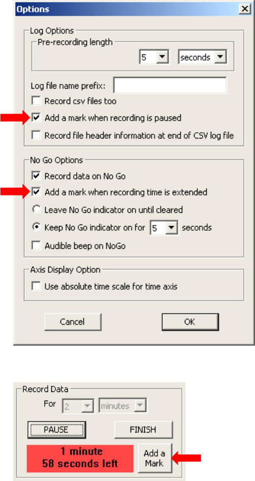
Adding Marks Manually
To manually add a mark to a log file:
1) Choose the menu Settings > Show Annotation Dialog. This menu toggles the display of the Annotate Mark
dialog on and off. The setting is off by default.
2) While you are recording data, click Add a Mark.
57
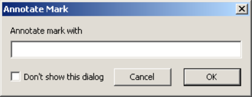
3) The Annotate Mark dialog is displayed.
4) In the Annotate Mark dialog, type the text you want to record with the mark location in the file and click OK.
The mark is placed in the log file at the instant you click Add a Mark, even though it might be some time
before you click OK in the Annotate Mark dialog. You can’t add another mark until you click OK.
If you don’t want to be prompted with the Annotate Mark dialog when you click Add a Mark, the next time
the dialog appears, check Don’t show this dialog and click OK. If you have previously checked this box, and
you now want to have the dialog displayed again, choose the menu Settings > Show Annotation Dialog to
toggle the display of the Annotate Mark dialog on again.
58
Including User-Specified Information in the Log File
See “Setting Station Information” on page 38.
Understanding Log File Names
By default, log file names are automatically assigned by MultiView, and consist of the serial number for the AMS
wafer followed by the date and time. A sample file name is shown below.
HV123456 2016-05-21 15-47-39.amvdata
Key
yyyy = year
mm = month
dd = day
Key
hh = hour (in 24-hour notation)
mm = minutes
ss = seconds
When you add marks to the log file (see “Placing Marks in a Log File” on page 55), MultiView creates a second file
with the same name as that of the log file, but with the file extension amvmarks.
You can specify a different log file name prefix to replace the wafer serial number, in which case, MultiView still
adds the date, time, and the appropriate extension.
AMS serial
number
Date in format
yyyy-mm- dd
Time in format
hh-mm-ss
59
Specifying a Different Log-File Prefix
When you add marks to the log file (see above), MultiView creates a second file with the same name as that of the
log file, but with the file extension .amvmarks. You can specify a different log-file-name prefix to replace the AMS
serial number, in which case, MultiView still adds the date, time, and the appropriate extension.
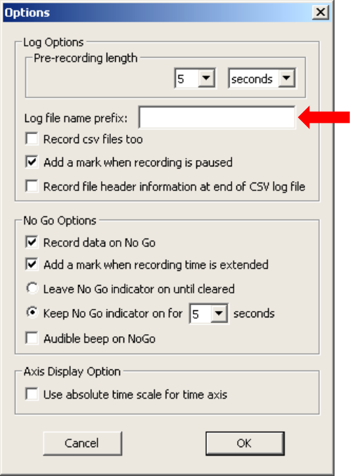
To specify a different log-file prefix:
1) Choose the menu item Settings > Options. The options dialog is displayed.
2) In the Log file name prefix box, enter the file name prefix you want to use for log files.
3) Click OK.
60
Importing Log Files into Other Applications
If you want to be able to import AMS log files into other programs, such as MATLAB or Microsoft Excel, you need
to have the AMS write log files in comma-delimited format (also called comma-separated-values, or CSV, files), as
well as the standard binary .amvdata file format. Note that only relatively short files (65,000 readings, or about
one-minute’s worth) can be imported into Excel.
When you set MultiView to record CSV files, MultiView records both the .amvdata file and a .csv file. Data written
to the .amvdata file is in g-force units with no filtering. Data written to the .csv file has been filtered (if filtering is
active), and is converted to the units for the currently set time-domain format (see “Filtering the Data” on page 63
and “Changing the Time-Domain Format” on page 64).
At the top of the file, MultiView writes a file header including the AMS serial number, and the current settings for
the filter and time-domain format. Each line of data consists of six entries: RMS, X, Y, Z, Time, and Marks with
annotations, if any. You can choose to have the header information recorded at the end of the file, instead of at
the beginning (see “Importing Log Files into Other Applications” on page 60), which can be useful for importing the
data into some applications.
The comma-delimited files are named as described in “Understanding Log File Names” on page 58, but with two
differences, as follows.
• The file extension is .csv, rather than .amvdata.
• The filter settings are appended to the log file name, as shown below.
HW123456 2016-05-21 15-47-39 BandPass 1Hz~5Hz.csv
The AMS includes a sample Script M-file that you can use to import files into MATLAB to generate a Fast Fourier
Transform frequency analysis. The file is AvsFft.m and is located in the \Program Files\ CyberOptics
Semiconductor\WaferSense AMS\Matlab folder.
61
Telling the AMS to Record Comma-Delimited Files
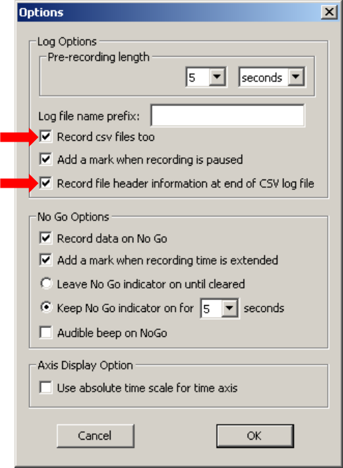
To have MultiView record comma-delimited files:
1) Choose the menu item Settings > Options. The options dialog is displayed.
2) Check the Record csv files too box.
3) To have MultiView record the header information (AMS serial number and the current settings for the filter
and time-domain format) at the end of the file, instead of at the beginning, check the Record file header
information at end of CSV log file box.
4) Click OK.
62
Changing the Log File Directory
By default, MultiView writes log entries to the directory My Documents\AMS Files\. If you prefer, you can specify a
different directory.
To change the log file directory:
1) Choose the File > Select Log Directory menu item.
2) In the Browse For Folder dialog, specify the folder name for the log files, and click Save.
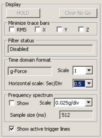
Configuring the Trace Display
You can change the way the vibration traces are displayed by minimizing or maximizing the bars for displaying the
traces, by applying a filter to the data, by changing the vertical and horizontal scales, by changing the colors of
traces and other elements in the display, and by showing or hiding the trigger settings and frequency spectrum.
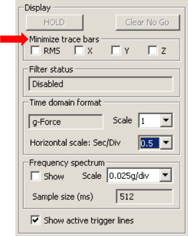
Minimizing the Trace Bars
You can minimize the bars for displaying the traces. Minimizing the bar for a trace collapses the height of the bar
for that trace. The heights of the bars for the remaining traces expand to fill the area. You can minimize the bars
for up to three traces at any time—but at least one trace is always maximized.
1) To minimize the bar for displaying a trace, in the Minimize trace bars section of the screen, check the boxes
for the traces you want to minimize.
2) To restore the bar for a trace to its normal height, uncheck the box for that trace under the Minimize trace
bars section of the screen.
63
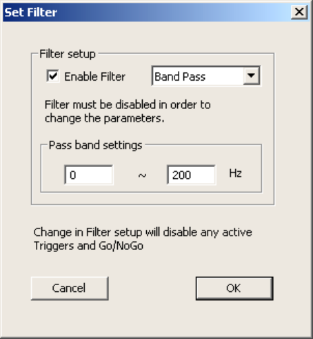
Filtering the Data
MultiView can filter the data to remove unwanted parts of the signal spectrum before displaying it. You can choose
a low-pass filter, a high-pass filter, or a band-pass filter. Changing the filter can dramatically affect the range of
values in the data, which affects the trigger and Go/No-Go values, so when you change filter settings, MultiView
automatically disables all trigger and Go/No-Go tolerances. If you make any changes to the filter (enabling,
disabling, changing filter type, or band pass settings), you’ll need to adjust and re-enable any triggers or Go/No-Go
tolerances.
Filters can be useful for a variety of situations, such as the following.
• Removing constant g-force
• Removing very low frequency acceleration resulting from slow moves
• Removing high frequency noise
The filter affects the display of the data, but does not affect the data written to the .amvdata log file. However, the
filter does affect the data written to the optional .csv file (see “Importing Log Files into Other Applications” on
page 60).
To set up the filter:
1) Choose the menu item Settings > Set Filter. The Set Filter dialog is displayed.
2) If Enable Filter is checked, clear the box. You can’t make any changes to the filter settings when the filter is
enabled.
3) From the list, choose the type of filter you want to apply to the data: Low Pass, High Pass, or Band Pass.
4) Specify the Pass band settings for the filter.
5) Check Enable Filter and click OK. The new filter settings take effect immediately. Any trigger or Go/No-Go
tolerances are disabled. If you want to use triggers or Go/No-Go, you must re-enable them.

64
Changing the Time-Domain Format
MultiView gives you three options for setting the time-domain format for traces, as shown below.
• g-Force
Displays acceleration values from -2 g to +2 g. One g is the acceleration of gravity (approximately 32 ft/s2 or 9.81
m/s2). With this vertical scale setting, when the AMS is sitting motionless and horizontal, the Z trace will show 1 g,
the X and Y traces will show 0 g, and the RMS trace will show 0.58 g. This is because the AMS senses the
acceleration of the earth’s gravitational field, which is 1 g in the vertical (Z) direction. You can also choose to
display the absolute value of acceleration in g-Force. Using the absolute value can be helpful when comparing
traces. When displaying absolute value, you will usually want to also use the high-pass filter (see “Filtering the
Data” on page 63).
• Gal
Displays values in galileo units, where 1 g = 981 Gal. With this vertical scale setting, when the AMS is sitting
motionless and horizontal, the Z trace will show 981 Gal, the X and Y traces will show 0 Gal, and the RMS trace will
show 566 Gal. This is because the wafer senses the acceleration of the earth’s gravitational field, which is 981 Gal
in the vertical (Z) direction. You can also choose to display the absolute value of acceleration in Gals. Using the
absolute value can be helpful when comparing traces. When displaying absolute value, you will usually want to
also use the high-pass filter (see “Filtering the Data” on page 63).
• Energy
Displays the signal energy for the last specified number (n) of acceleration values. Signal energy is calculated using
the following formula.
1
N
n
∑
x2 (k)
k =1
Where:
N is the sample rate (1 KHz for the AMS).
n is the number of samples, which is the sample size you have set for the frequency spectrum (see
“Displaying the Frequency Spectrum” on page 69).
x(k) is the kth sample of the acceleration in g-force. Using the energy format with appropriate
Go/No-Go tolerances can identify vibrations that don’t have large amplitudes (and might not trip the
Go/No-Go tolerances for g-force or Gals), but extend for longer periods of time.
Values that are too large to display are truncated.
Changing the time domain format can dramatically affect the range of values in the data, which affects the trigger
and Go/No-Go values, so when you change time domain format settings, MultiView automatically disables all
trigger and Go/No-Go tolerances. If you change the time-domain format, you’ll need to adjust and re-enable any
triggers or Go/No-Go tolerances. For more information, see “Recording with Triggers” on page 50 and “Monitoring
Traces for Excessive Vibration Levels” on page 46.
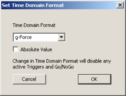
65
Changing the Time-Domain Format
When you change the time-domain format, the triggers and Go/No-Go tolerances are disabled. You might need to
re-enable these settings.
To change the time-domain format:
1) Choose the menu item Settings > Set Time Domain Format. The Set Time Domain Format dialog is displayed.
2) Click the down-arrow and, from the list, choose the appropriate time-domain format.
3) If you want MultiView to display the absolute value of the acceleration values, check the box for Absolute
Value.
4) Click OK.
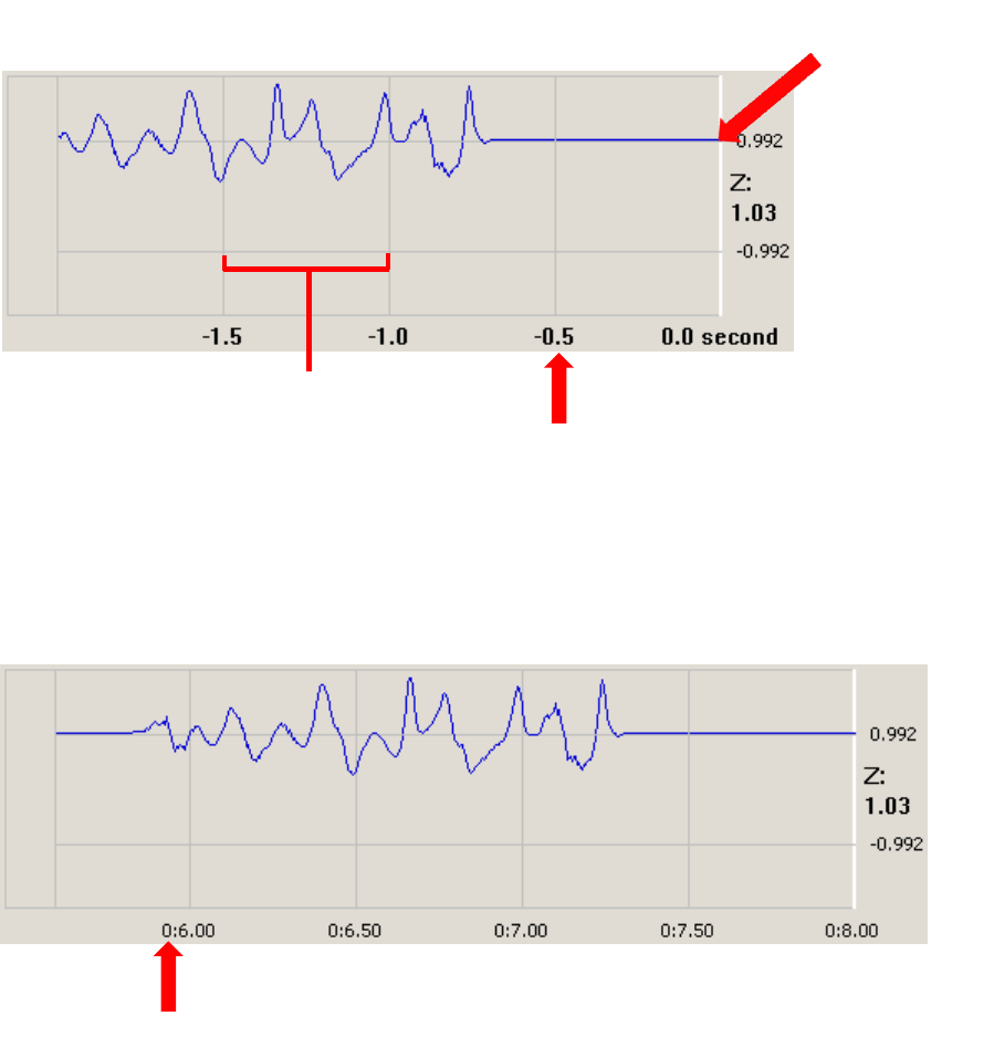
66
Changing the Horizontal Time and Scale
The default horizontal-axis labels show time relative to the right-edge of the trace, where the newest data points
appear.
With this relative time scale, the time labels on the horizontal axis indicate the time that has elapsed since the data
was first displayed at the right edge. The numbers increase negatively as you move from right to left indicating that
the older data is to the left. You can change the horizontal scale to show absolute time (as shown in the figure
below) since the start of recording, rather than relative time (as shown in the figure above) . When you aren’t
recording, the scale always shows time relative to the right edge.
The default horizontal scale shows 0.5 seconds between vertical grid lines and plots one point for every five
readings received from the AMS. You can change the horizontal scale to show from 0.1 seconds to 100 seconds
between the grid lines. At the 0.1 second setting, MultiView displays every reading received from the AMVS (that
is, one data-point per millisecond). When displaying at the higher scales, MultiView can’t display every reading
received from the AMS, so it displays a vertical bar indicating the range of values for the time span represented by
any given point on the horizontal axis. For example, at the default scale of 0.5 seconds/division, each vertical bar
plotted represents five readings and shows the range of those five readings. The horizontal-scale setting doesn’t
affect the data recorded, only the data displayed.
0.5 seconds—the default setting
Relative time—increases to the left
New data
appears here
Absolute time—increases to the right
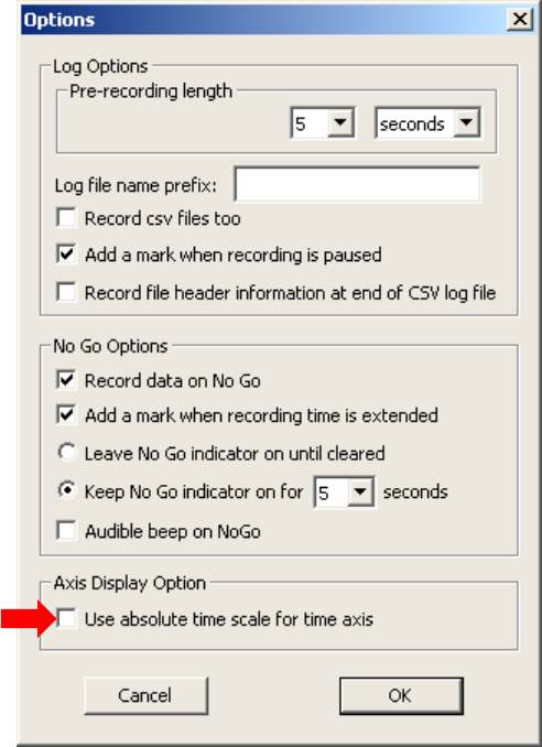
67
Changing the Horizontal Axis Time
To change the horizontal axis time:
1) Choose the menu item Settings > Options. The options dialog is displayed.
2) For absolute time, check the Use absolute time scale for time axis box.
3) Click OK.
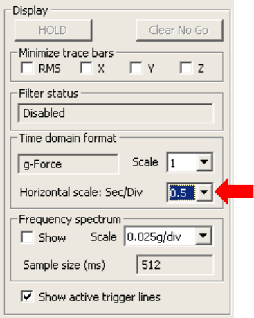
68
Changing the Horizontal Scale
To change the horizontal scale:
• Using the Horizontal scale list, choose the time interval you want between vertical grid lines and the new scale
setting takes effect immediately.
Changing Colors
For more information, see “Changing Colors in the Trace Screen” on page 24.
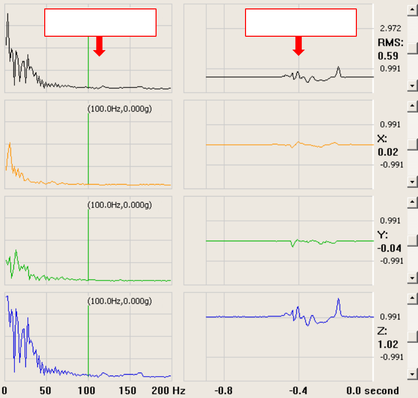
69
Displaying the Frequency Spectrum
By default, MultiView displays time-domain data: vibration readings over time. You can also have MultiView
display frequency-domain data: the frequency spectrum determined by a Fast Fourier Transform (FFT) of the time-
domain data. As shown in the figure below, when displaying a frequency spectrum, MultiView divides the trace
area, showing the vibration traces on the right, and the frequency spectrum on the left.
In the frequency-spectrum display, the horizontal axis is the vibration frequency, and the vertical axis displays the
amplitude for that frequency. Both scales are linear. Frequencies are limited to 200 Hz and below, by the AMS.
Each frequency display has a vertical green line. The line is positioned at a particular frequency (100 Hz, by
default), and the text at the top of the line identifies the frequency and the current amplitude for that frequency.
You can move the lines to monitor the amplitude at different frequencies.
By default, MultiView performs the frequency analysis using a sample of 512 data points (512 milliseconds of
data). MultiView receives data from the AMS in packets of 100 data points. The FFT is computed every 100
milliseconds, using the latest packet of 100 points, plus the previous 412 data points. You can specify a different
sample size. Increasing the sample size increases the resolution of the frequency spectrum, but the additional data
points cause the FFT results to respond more slowly to changes, similar to the way a rolling average tends to
smooth out changes. When you change the FFT sample size, MultiView automatically disables all trigger and
Go/No-Go tolerances. After changing the sample size, you’ll need to adjust and re-enable any triggers or Go/No-Go
tolerances.
Frequency spectra
Vibration traces
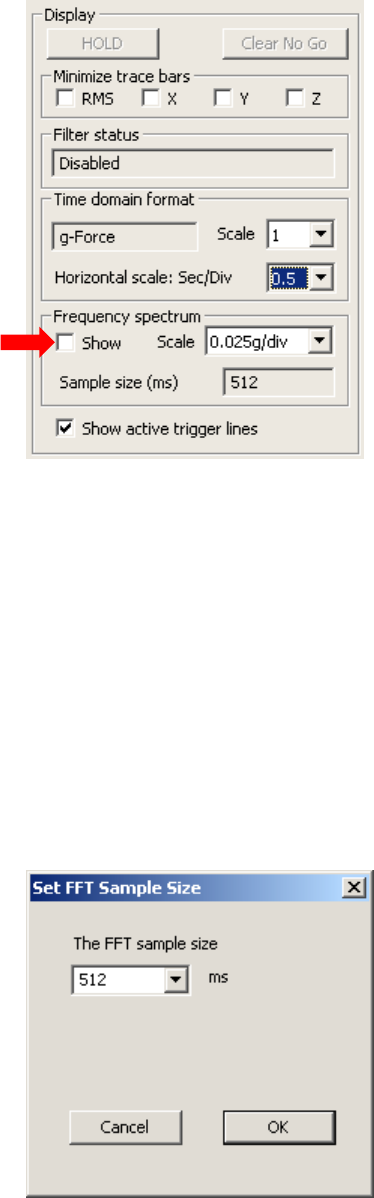
70
To display a frequency spectrum in MultiView:
1) Under Frequency spectrum, check the Show box.
2) To adjust the vertical scale of the frequency spectrum, choose a value from the Scale list. The new setting
takes effect immediately.
3) To display the amplitude for any specific frequency component, move the green lines.
• To move one of the vertical green lines, right-click in the frequency-spectrum display.
• To adjust the position of a line after using right-click, press the left- or right-arrow keys.
• To line up all of the green lines, double-right-click.
When you move the green line, it moves between the frequency values determined by the FFT, which in
general are not integer values.
4) To change the FFT sample size, choose the menu item Settings > Set FFT Sample Size and the Set FFT Sample
Size dialog is displayed.
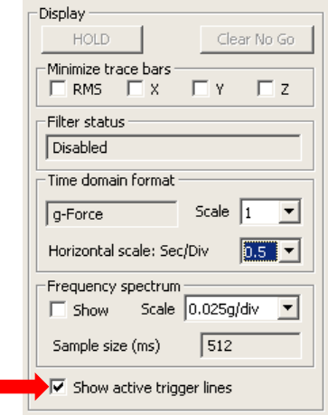
71
5) From the list, choose a sample size, click OK and the new setting takes effect immediately.
When you change the FFT sample size, triggers and Go/No-Go tolerances are disabled. You might need to re-
enable these tolerances.
Showing and Hiding Trigger Settings
You can add lines to the trace displays to show the active trigger settings, see “Recording with Triggers” on
page 50.
• To show active trigger lines on the display, check the box for Show active trigger lines (see figure below).
• To hide all trigger lines on the display, clear the box for Show active trigger lines.

72
Viewing Log Files
MultiReview allows you to play back the log files you recorded, while running the AMS through your wafer-
manufacturing process. More specifically, MultiReview allows you to do the following.
• Run MultiReview
• Use the playback controls
• Work with marks
• Monitor traces for excessive vibration levels
• Compare log files
• Change MultiView settings from MultiReview
• Change log files
• Analyze narrow peaks
• Save a subset of a log file
• Compile summary statistical reports
• Print the MultiReview window
Viewing
Log Files
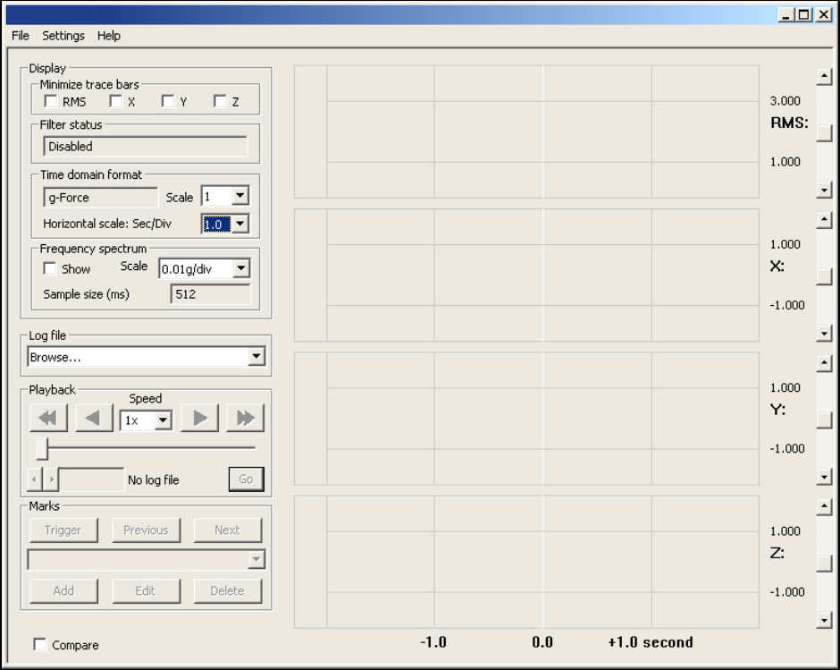
73
Running MultiReview
To view a log file, do the following.
1) In Windows, press Start > All Programs > AMS > MultiReview and the MultiReview screen is displayed.
2) From the File menu, choose Open Log File and the AMS Log Files dialog is displayed.
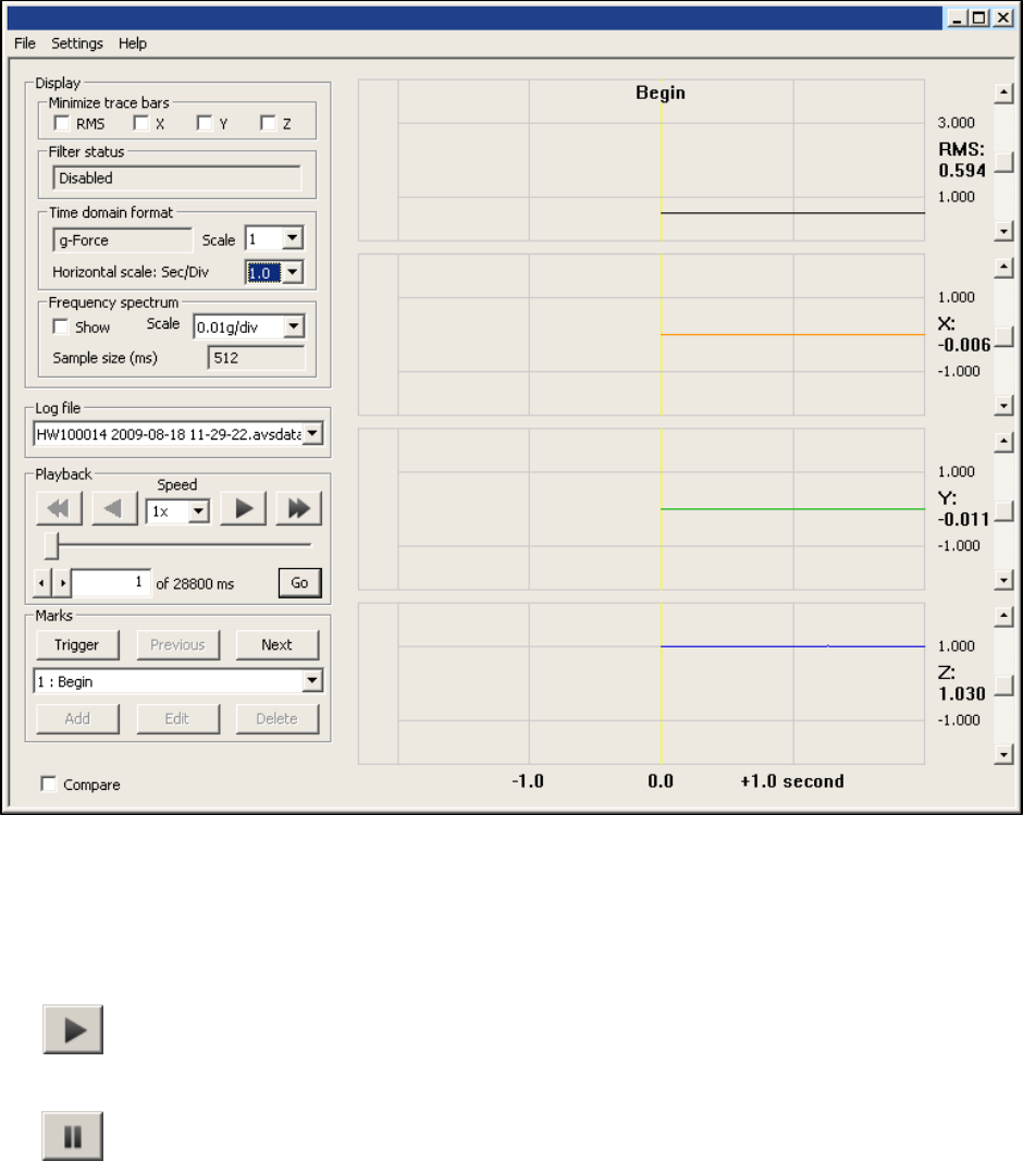
74
3) Choose a log file and click Open. MultiReview opens the log file, and displays the traces at the beginning of the
file.
Settings stored in the log file for the filter, FFT sample size, Go/No-Go, and time-domain format are all applied
when you open a log file.
4) To start the log file playing, click the Play button.
The traces start scrolling from right to left, and the Play button changes to Pause.
You can use the other Playback controls to jump ahead or back or to a particular place in the file, play the file
in reverse, and adjust the playback speed. These are described on the next page.
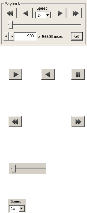
75
Using the Playback Controls
You can play a log file forward or in reverse, pause during playback, and jump ahead or back by using the playback
controls. You can also move around in log files by jumping to marks or triggers, see “Working with Marks” on
page 78.
The buttons are described in more detail below.
• Forward Reverse Pause
These buttons start the file playing from the current position forward in the file, and changes the Play forward
button to a Pause button. Clicking Pause halts the playback at the current position, and changes the button
back to Play forward. Play Reverse works similarly, but plays backward toward the beginning of the file.
• Back One Division Forward One Division
Jumps forward or back one division. One division refers to the time between the vertical grid lines, which can
be from 100–100,000 milliseconds, depending on the horizontal scale setting, see “Configuring the Trace
Display” on page 62.
• Slider
Dragging the slider lets you quickly move to any position in the file.
• Speed
The speed control lets choose a playback speed from 1x to 10x. Playing a file containing 60,000 milliseconds of
data at 1x takes about 60 seconds; at 10x, the same file plays in about 6 seconds. This playback speed is not
affected by the horizontal scale setting.
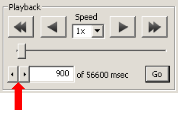
76
• Counter
The counter shows the current position within the file at any given time. The indicator, the white vertical line
in the middle of the trace display, marks the point in the trace that corresponds to the counter value—see
figure on the next page. The count is the number of milliseconds (equivalent to the number of data points),
regardless of the control horizontal scale setting.
The value to the right of the counter is the total length of the file in milliseconds (or data points). To change
the position in the file, you can type a number into the counter text field and click Go. Compared to the slider,
the counter gives you more precise control over positioning within the file.
You can also change the position in the file by using the arrows in the spin control. A single click increments
(right arrow) or decrements (left arrow) the counter by one. Clicking and holding causes the counter to
increment or decrement repeatedly, changing faster the longer you hold down the arrow button.
Spin controls
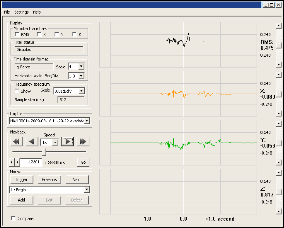
77
Figure 2. MultiReview Screen Showing the “Begin” Indicator Line
Clicking and Dragging Traces
When the trace display is paused, you can use the counter in the playback controls to move the trace display to a
different location in the log file. However, for small changes, you might find it easier to move the traces by clicking
and dragging. When you click and drag the traces, the counter changes accordingly.
To click and drag the traces:
1) Move the cursor into the trace area, and the cursor changes to a pointing hand.
2) Click and hold the left mouse button.
3) Drag the mouse to the left or right and release the mouse button. When you release the button, the trace
display jumps forward or back the distance you moved the mouse.
Indicator line
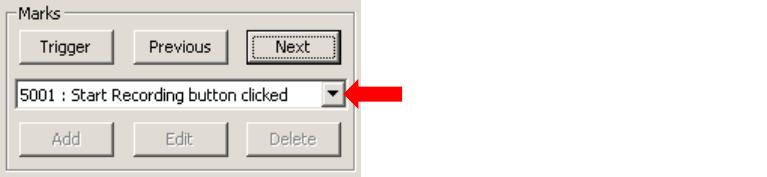
78
Working with Marks
Marks indicate points of interest within log files. Every log file has one trigger mark that tells you where recording
started and what caused the recording to start. Clicking the Start button, the occurrence of the first trigger event
in one of the traces, or the first Go/No-Go event, will cause MultiView to place a trigger mark in the file. You can
also create your own marks in a file while you are recording in MultiView, and you can add annotations to the
marks. For more information on triggers and marks, see “Recording with Triggers” on page 50 and “Placing Marks
in a Log File” on page 55.
Finding Marks in a File
In MultiReview, you can quickly go to the position in the file that corresponds to the trigger or to another mark.
• Going to a Trigger event
To go to the trigger event in a log file, click the Trigger button. Note that the “trigger event” can be clicking the
Start button, an actual trigger, or a No-Go event.
• Going to specific mark
To go to a specific mark in a log file, use the drop-down list to choose a mark. As soon as you click on a mark in
the list, MultiReview jumps to that position in the file.
• Next and Previous buttons
The Next and Previous buttons let you jump to the next or previous marks in the file. At the last mark, clicking
Next takes you to the end of the file. At the first mark, clicking Previous takes you to the beginning of the file.
When you go to a trigger mark or to a user-defined mark in the file, the counter shows the file position of the
mark. For example, if you go to a mark at 45,000 in a data file, the playback counter will show 45,000, and the
list of marks will show 45,000 with the mark annotation, if any. When you use the playback controls to move
from that mark, the counter shows the new location, but the list of marks does not change. The counter
always shows the current location in the file, but the list of marks shows the last mark that you selected, even
if the position in the file has moved from that mark.
Click here to access named marks
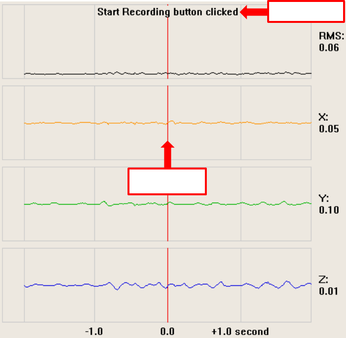
79
When the trigger event is visible in the trace display, the trigger event is marked by a vertical red line with an
annotation. Other marks appear as vertical yellow lines with annotations.
Adding Marks to a File
You can add marks to a file whenever playback is paused. MultiView automatically creates marks at the beginning
and end of the file and for the trigger event. You can’t add user-created marks where MultiView has created the
Begin, End, and Trigger marks. The Add button in MultiReview works just as the Add a Mark button does in
MultiView. For more information, see “Placing Marks in a Log File” on page 55.
Annotation
Trigger line
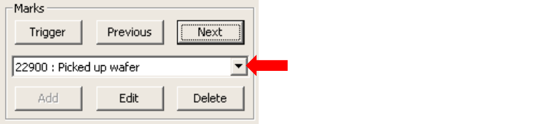
80
Editing Existing Marks
You can edit the annotation text that is associated with a user-created mark. You can also delete a user-created
mark from a file. You can’t edit or delete the Begin, End, or Trigger marks.
To delete or edit a mark:
1) Choose the mark you want to edit from the drop-down list under Marks (playback must be paused). You can
also go to the mark using Next and Previous. When you are at a mark, the Edit and Delete buttons are active
(except for the Trigger, Begin, and End marks).
2) To delete the mark, click Delete. To edit the annotation associated with the mark, click Edit. When you click
Edit, the Annotate Mark dialog appears.
3) If you clicked Edit, edit the text in the Annotate Mark dialog and click OK to save the change.
Monitoring Traces for Excessive Vibration Levels
Monitoring your traces for excessive vibration levels has already been discussed in detail above—see page 46. Use
the Playback and Marks features of the MultiReview screen (see page 77) to go to the marks you want to review.
Click here to access named marks
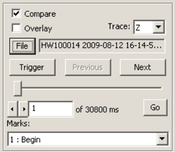
81
Comparing Log Files
You can compare two log files, using the playback controls to move through the traces from both files in unison.
When comparing files, by default MultiReview displays all individual traces from the first file, but only one trace
from the second file. You can select which trace (X, Y, Z, or RMS) to display from the second file. In addition to
having MultiReview display one of the traces from the second file, you can have it overlay all traces from the
second file in the traces for the first file. Overlaid traces appear in gray along with the colored traces from the first
file.
To compare two log files:
1) From the File menu, choose Open Log File and the AMS Log Files dialog is displayed.
2) Choose the first log file you want to compare, and click Open. MultiReview opens the log file and displays the
traces at the beginning of the file.
3) In the lower-left corner of the MultiReview window, check the Compare box and a second set of log file
controls appears.
4) In the Compare controls, click File and the AMS Log Files dialog is displayed.
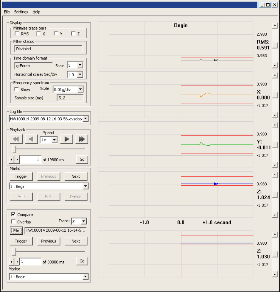
82
5) Choose the second log file you want to compare, and click Open. MultiReview opens the log file and displays
one of the traces at the bottom of the window, below the traces for the first file. By default, MultiReview
displays all traces from the first file but only one trace at a time from the second file.
6) To change which trace from the second file is displayed at the bottom of the window, select a different trace
from the Trace drop-down menu (see figure on the previous page).
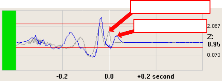
83
7) To have MultiReview overlay all traces from the second file on the corresponding traces from the first file, in
the Compare controls, check Overlay. The traces from the second file appear as gray lines over the traces
from the first file.
8) To synchronize the two files to a common event, use Trigger, Next, and Previous or Marks to find
corresponding events for the two files. To synchronize based on times, use the counters for each file. You can
also make adjustments by clicking and dragging the traces, see “Clicking and Dragging Traces” on page 77.
Separate slider, counter, and marks controls for each file let you manipulate them independently.
9) When you have the traces synchronized, use the playback controls to play the log files. The playback controls
play both log files in unison, see “Using the Playback Controls” on page 75.
Changing MultiView Settings from MultiReview
Based on what you see in reviewing a log file in MultiReview, you might want to change some of the settings that
you will use for a subsequent run in MultiView. For example, you might notice a specific event in the log file that
you want to take a closer look at with another MultiView run. MultiReview makes this easy to do by allowing you
to open a MultiView settings file, make changes, and save the file without leaving MultiReview. In MultiReview,
you can change MultiView settings for Go/No-Go events, for filters, for time-domain formats, for FFT sample sizes,
and for the user-specified information.
To change MultiView settings from MultiReview:
1) In MultiReview, make your selections for the parameters listed below.
• Go/No-Go tolerances —see “Monitoring Traces for Excessive Vibration Levels” on page 80.
• Filter —see “Filtering the Data” on page 63.
• Time-domain format —see “Changing the Time-Domain Format” on page 64.
• FFT sample size —see “Displaying the Frequency Spectrum” on page 69.
Trace from second file
Trace from first file
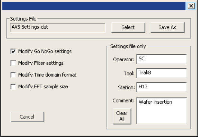
84
2) Choose the menu item Settings > Modify MultiView Settings. The Modify MultiView Settings dialog is
displayed.
3) To open a MultiView settings file, click Select, choose a settings file from the AMS Settings File dialog, and click
Open.
4) In the Modify MultiView Settings dialog, check the Modify boxes for any settings you want to save in the
settings file.
5) Modify any of the user-defined information for Operator, Tool, Station, and Comment. Clear All lets you clear
all of these fields.
6) To save the settings for a future MultiView run, click Save As. In the AMS Settings File dialog, edit the file as
needed, and click Save. Note the file name, so you can open it in MultiView.
7) To close the Modify MultiView Settings dialog, click Cancel.
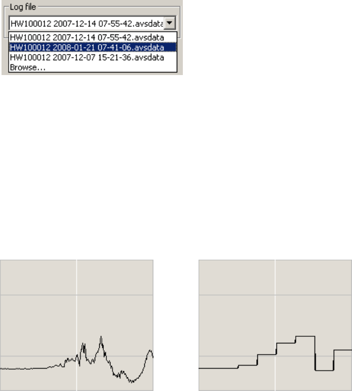
85
Changing Log Files
You can open a log file using the Open Log File command on the File menu, see “Running MultiReview” on
page 73. If you have previously opened files in MultiReview, the last few files you opened are listed in the Log file
pull-down menu. That gives you a quick way to select a recently opened log file. If you don’t see the file you want
in the list, choose Browse at the end of the list to open the log file. Note that any settings stored in the log file for
the filter, FFT sample size, Go/No-Go, and time-domain format are all applied, when you open a new log file.
Analyzing Narrow Peaks
This function allows you to more easily analyze narrow peaks in your traces. As such, please see “Configuring the
Trace Display” on page 62 for more information about configuring the trace display in MultiView. MultiReview,
however, offers one additional feature, the ability to analyze narrow peaks in greater detail that is not available in
MultiView.
Narrow peaks in the traces can be difficult to analyze, because of the need to pause and position the peak right on
the indicator to check the amplitude. To make it easier to analyze peaks, you can tell MultiReview to hold a peak
for a specified period of time. When the hold-peak feature is active, each time a signal peak is detected,
MultiReview holds the trace level at that peak value for the time period you specify.
Standard trace Trace with Hold Peak active
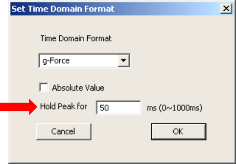
86
To activate the Hold Peak function:
1) Choose the menu item Settings > Set Time Domain Format. The Set Time Domain Format dialog is displayed.
2) From the Time Domain Format list, choose your time domain format from the drop-down menu.
3) If you want MultiReview to display the absolute value of the acceleration values, check the box for Absolute
Value.
4) If you want MultiReview to hold and display peak values, specify the hold time in the Hold Peak for box.
5) Click OK.
6) When you change the time domain format, you might need to adjust Go/No-Go tolerances.
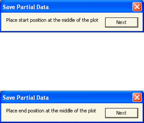
87
Saving a Sub-Set of a Log File
The AMS takes readings at the rate of 1,000/second, so log files can become quite large. You can save a subset of a
log file by specifying the beginning position and the ending position, so that the partial log file contains only your
selected data. You can also modify the associated filter setting, time domain format, FFT size, and Go/No-Go
tolerances when saving a partial log file.
To save a subset of a log file:
1) From the File menu, choose Save Partial Log File. The Save Partial Data dialog is displayed prompting you to
specify the start position of the subset of the log file that you want to save.
2) Using the playback controls, locate the starting point of the data subset you want to save, aligning that point
on the indicator line in the center of the trace display.
3) In the Save Partial Data dialog, click Next. The Save Partial Data dialog now prompts you to specify the end
position of the subset of the log file that you want to save.
4) Using the playback controls again, locate the end position of the subset of the log file that you want to save.
5) In the Save Partial Data dialog, click Next. The AMS Data Log File dialog is displayed.
6) Specify a filename for the partial log file that you want to save, and click Save. MultiReview saves the partial
log file.
88
Compiling Summary Statistical Reports
This section tells you how to use MultiReview to compile summary statistical reports on the following data
collected from your traces.
• Peak-acceleration data
• Peak-excursion data
• Time-domain data
Compiling a Peak-Acceleration Summary Report
A peak acceleration summary report shows, for each mark in each file, the frequency at which the maximum
acceleration was recorded and the amplitude of that acceleration for each of the X, Y, and Z traces. The report can
summarize data from up to 50 log files.
Different log files can have different settings for time-domain format, filter, and FFT sample size, so when
compiling a report, MultiReview uses the same settings for all files. The settings are determined by the following.
• The settings for the most-recent log file opened (other than a comparison file).
• The settings you make using the Settings menu items.
The default report format uses a vertical layout for each of the X, Y, and Z traces: the table of amplitude data is
listed first, and the table of frequency data follows below the amplitude data. You have the option of choosing a
horizontal layout: the table of frequency data is listed to the right of the table of amplitude data.
Different log files can have different annotations for the marks in the file, so by default, the report identifies the
marks as Mark1, Mark2, Mark n…, and so on. You have the option of having the report identify the marks by using
the annotations for the marks from the first file you open.
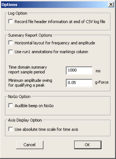
89
To compile a peak-acceleration summary report:
1) Choose the menu item Settings > Options. The options dialog is displayed.
Figure 3. MultiView Options Dialog
2) If you want the frequency and amplitude data shown horizontally in the report, check the box Horizontal
layout for frequency and amplitude. If you want the frequency data shown below the amplitude data in the
report, clear the check box.
3) If you want the marks identified with the annotations for the marks in the first file you open, check the box
Use run1 annotations for markings column. If you want the marks identified generically (Mark 1, Mark 2,
Mark n…, and so on), clear the check box.
4) Click OK.
5) Choose the menu item File > Create CSV File > Compile Summary Report > Peak Acceleration and Frequency.
The AMS log files dialog is displayed.
6) Select the files that you want to include in the report. To select a range of files, click the first filename, and
then shift-click the last filename. To select multiple files individually, select each using control-click. When you
have selected all files you want, click Open. The CSV file dialog is displayed.

90
7) Enter a name for the peak-acceleration summary report file, and click Save. MultiReview compiles and saves
the summary report. You can open the report in applications, such as Microsoft Excel, that can read CSV files.
Compiling a Peak-Excursion Summary Report
A peak-excursion summary report shows, for each mark in each file, the frequency at which the maximum
displacement (peak excursion) of the AMS was recorded, and the amplitude of that displacement for each of the X,
Y, and Z traces. The amplitude is shown in units of millimeters. The peak excursion at each mark is found from the
frequency-domain data by calculating the displacement (d) for each frequency, using the following formula.
d =
A
ω2
Where the frequency is ω/2π Hz, and A is the amplitude at that frequency. The maximum excursion for a
given mark is the largest value of d for the frequency spectrum at that mark, with the following restrictions.
• Only frequencies above 5 Hz are evaluated because of limits in the AMS electronics.
• Only sustained signals are evaluated, that is signals that last longer than the FFT sample size.
The report can summarize data from up to 50 log files. Different log files can have different settings for filter and
FFT sample size, so when compiling a report, MultiReview uses the same settings for all file. The settings are
determined by the following.
• The settings for the most recent log file opened (other than a comparison file).
• The settings you make using the Settings menu items.
The default report format uses a vertical layout for each of the X, Y, and Z traces: the table of amplitude data is
listed first, and the table of frequency data follows below the amplitude data. You have the option of choosing a
horizontal layout: the table of frequency data is listed to the right of the table of amplitude data.
Different log files can have different annotations for the marks in the file, so by default, the report identifies the
marks as Mark 1, Mark 2, Mark n...,and so on. You have the option of having the report identify the marks by using
the annotations for the marks from the first file you open.
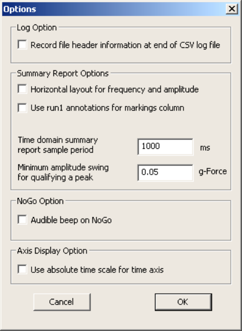

92
Compiling a Time-Domain Statistics Summary Report
A time-domain statistics summary report shows the slippage factor for each mark in each file. For each mark in
each file, for the X, Y, and Z traces, the report also shows the following statistics: number of peaks, mean,
maximum, minimum, standard deviation, and integral. The slippage factor is defined using the following formula.
√ x2 + y2
z
For counting the number of peaks, you can have the report ignore small peaks by specifying the minimum
amplitude swing that qualifies a peak to be counted. The statistics are computed at each mark in the file over a
user-specified sample period beginning at the mark. Different log files can have different annotations for the marks
in the file, so by default, the report identifies the marks as Mark 1, Mark 2, Mark n…, and so on. You have the
option of having the report identify the marks by using the annotations for the marks from the first file you open.
To compile a time domain statistics summary report:
1) Choose the menu item Settings > Options. The options dialog is displayed—see page 89.
2) If you want the marks identified with the annotations for the marks in the first file you open, check the box
Use run1 annotations for markings column. If you want the marks identified generically (Mark 1, Mark 2,
Mark n…, and so on), clear the check box.
3) In the Time domain summary report sample period box, specify the sample period you want MultiReview to
use in calculating statistics for each mark.
4) In the Minimum amplitude swing for qualifying a peak box, specify the minimum amplitude you want
MultiReview to use for counting an amplitude change as a peak.
5) Click OK.
6) Choose the menu item File > Create CSV File > Compile Summary Report > Time Domain Statistics. The AMS
log files dialog is displayed.
7) Select the files that you want to include in the report. To select a range of files, click the first filename and
then shift-click the last filename. To select multiple files individually, use control-click. When you have selected
all files, click Open and the CSV file dialog is displayed.
8) Enter a name for the time domain statistics summary report file and click Save. MultiReview compiles and
saves the summary report. You can open the report in applications, such as Microsoft Excel, that can read CSV
files.
93
Printing the MultiReview Window
You can print an image of the MultiReview window to have a graphical record of the session. To print an image of
the MultiReview window:
1) Choose File > Print.
2) In the Print dialog, click OK. You can also select a printer other than the default and change the printer setup,
or see a preview of what MultiReview will print.
• To select a different printer, change the paper selection or print orientation, or set printer properties,
choose the File > Print Setup menu item.
• To see a preview of what MultiReview will print, choose the File > Print Preview menu item.
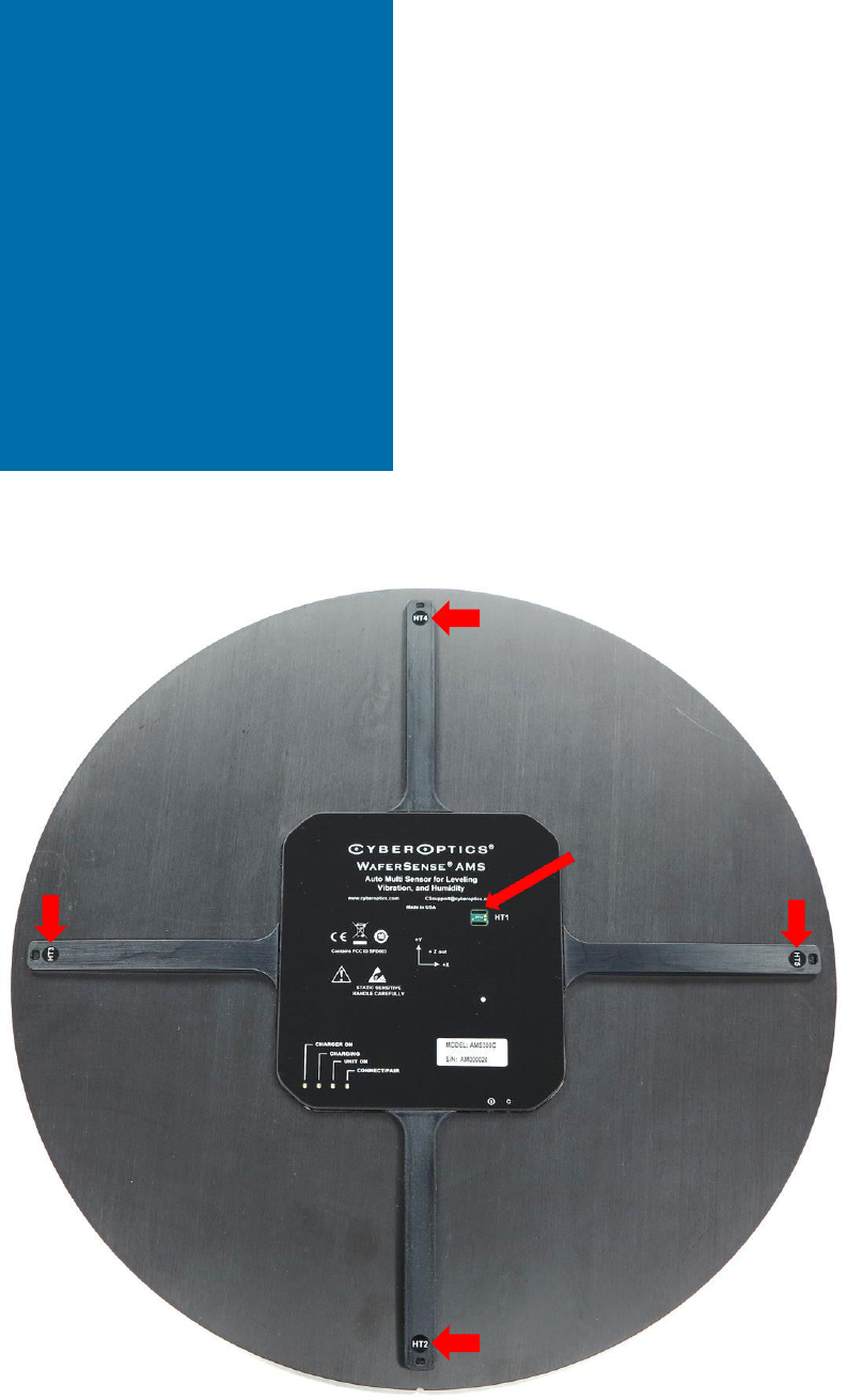
94
Using the Humidity Function
The humidity function allows you to measure both humidity and temperature at up to five locations (depends
which model you bought) on the upper surface of the AMS, as shown below.
Using the
Humidity
Function
1
2
3
5
4
95
How the Humidity/Temperature Sensors Work
The following sections provide a detailed overview of how the humidity sensors in the AMS operate, and outlines
some of the cautions you should be aware of, when recording and interpreting the RH readings generated by the
AMS. In particular, please note that varying temperatures, high air-flow environments, and hysteresis can have
significant effects on the RH readings.
General Principles
The AMS uses solid state MEMS humidity/temperature sensors. Each sensor contains a capacitive-type humidity
sensor, a band-gap temperature sensor, and specialized analog and digital circuitry, all inside the IC package. The
capacitor inside the sensor contains a polymer between the electrodes, which absorbs and desorbs water
molecules as the relative humidity changes. The change in capacitance is translated into a relative humidity output
by the internal circuitry. Each sensor is internally calibrated at the time of manufacture to be within 2% relative
humidity over most of the 0–100% RH range. However, in order to increase accuracy, the AMS undergoes an
additional calibration that corrects the factory calibration and extends it to lower RH values. Thus the internal
sensor calibration is corrected via look-up tables in the AMS firmware. Then these values are displayed in
MultiView.
Relative Humidity versus Absolute Humidity
Relative humidity (RH) measures the amount of moisture in the air relative to the maximum amount of moisture
that can be held in the air at that temperature. Zero % (0%) RH means there is a negligible amount of moisture in
the air. One hundred % (100%) RH means that the air cannot contain any more moisture before the moisture
begins to condense. Relative humidity is extremely temperature sensitive. Hence the reason for including a very
precise (± 0.3 °C accuracy) air-temperature sensor.
Absolute humidity measures the total amount of moisture in the air and is independent of the temperature.
Absolute humidity can be specified in a number of ways: dew point, ppm on a volume basis, and ppm on a weight
basis (kg/kg of dry air). Appendix A (see “Appendix A—Moisture Conversion Table” on page 136) contains a table
that gives corresponding values for these units at room temperature. Appendix A also contains a psychrometric
chart that allows you to convert humidity to dew point, vapor pressure, and the parts-per-million concentration of
water on a volume or weight basis.
Effect of Temperature
As noted above, relative humidity can be extremely sensitive to the local air temperature. Assuming the air in a
chamber all contains the same amount of absolute humidity, the relative humidity will vary greatly, if there is local
heating of the air.
For instance, at 85% RH and 20°C, the dew point will be 17.4° C. If the air near the sensor is heated by only 1°C, the
RH will change to 80% RH—a 5% RH change for just a 1°C change in temperature. At low RH the situation is
somewhat better; a 1°C change in temperature at 10% RH only causes a 0.6 % RH change.
In order to record relative humidity accurately, the air temperature must be extremely uniform. The
humidity/temperature sensors in the AMS should be shielded from any external heat source—such as a strong
convective-flow of heated or cooled air, radiant heat, and any heat conduction into the AMS housing.
The AMS humidity/temperature sensors are designed so that there is very little self-heating from the internal
circuitry. In addition, the central AMS humidity/temperature sensor (labelled “HT1”) that resides in the central
housing, has constricted heat paths to the sensor in order to minimize heat conduction to the HT1 sensor from the
other AMS internal electronics. Please note that the air-temperature sensor on the HT sensors will display a
different temperature from the internal electronics temperature sensor.

96
Differences between Various AMS Models
There are at least 10 different AMS models that utilize the same basic electronics. Most of these models contain a
single central humidity/temperature sensor designated as HT1. However, there is one model, the AMS-300C that
contains four additional sensors near the edge of the AMS. The five humidity/ temperature sensors in the AMS-
300C allow you to characterize a large wafer area for variations in humidity and temperature.
Storage and Handling of the AMS
Because of the polymer sensing element in the humidity/temperature (HT) sensors, the AMS requires special care
in handling. Prior to calibration at CyberOptics, all the HT sensors are reconditioned to bring them back to their
original, uniform response. This reconditioning consists of a mild bake out to 82 °C in order to evaporate any
contamination hydrocarbons, followed by a re-hydration step at greater than 74% RH in order to return the
polymer to its original hydrated state. Under normal operating conditions this reconditioning is not required again.
CAUTION. Do not place the AMS in close proximity to volatile chemicals such as solvents or other
organic compounds. Also avoid exposure to ozone, acids and bases, and cleaning agents. Do not wipe
the top surface of the AMS with IPA. In general, if a material emits a strong odor, it should not be used
in close proximity to the HT sensors.
CAUTION. Do not direct strong air blasts into the HT sensors.
CAUTION. Store the AMS unit at a temperature of 10–50 °C and in the range of 20–60% RH. Short
times (up to four hours) at RH levels outside of this range are acceptable. If the AMS is stored at RH
levels outside of this range for longer than four hours, the AMS should be returned to an environment
of 20–60% RH for 12 or more hours to return the AMS to its normal sensitivity and accuracy.
CAUTION. Do not store the AMS unit in polyethylene antistatic bags (light blue, pink, or rose color). If it
is necessary to use tape in the vicinity of the HT sensors, use only Kapton Electrical Tape 92
manufactured by 3M.
Hysteresis and Long-Term Stability of the RH Readings
Almost all humidity sensors exhibit hysteresis. That is, the RH reading will vary depending on the recent exposure.
Sensors with a dry history carry some negative offset, while sensors with a humid history carry some positive
offset—that is, the reading will be slightly higher than the actual RH. The amount of hysteresis is roughly 1 %RH in
the range of 40–80% RH, and smaller at RH levels above and below this range. The HT sensors are calibrated by
starting at low RH values and moving upwards. So maximum accuracy is obtained by following the same procedure
during measurement. Try to acclimate the AMS at RH levels lower than those expected during measurement. The
long-term stability of the HT sensors is better than 0.25% RH per year, and for temperature is better than 0.03°C
per year.
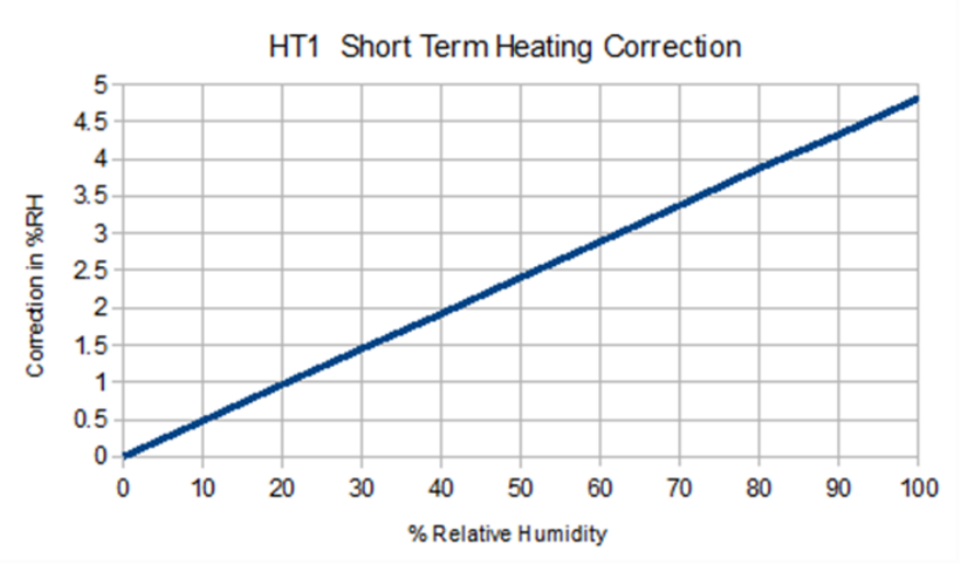
97
Relative Humidity Measurement Range
The AMS RH sensors are calibrated in the range of 2–85% RH. In the 0–2% RH range the sensors will output the
same “zero” reading, indicating that the actual RH is in this range. Above 85% RH the sensor will output readings
that may not be as accurate as those below 85% RH.
Response Time
The AMS RH sensors have an inherent response time of eight seconds. That is, with a sudden step change in RH
level, the sensor will respond with a reading of 63% of the step within eight seconds. However, this sudden change
of RH level is difficult to achieve, except in special test setups. It is very difficult in most “real world” situations to
totally change the air in a chamber in this short amount of time. So, the AMS HT sensors will almost always be
faster than the change in the air environment.
The HT1 Sensor and Its Thermal Environment
Because RH sensors are so dependent on the thermal environment, it is often necessary to correct the RH reading
to account for heating around the sensor. One such case occurs in the AMS, because the central (HT1)
humidity/temperature sensor is in close proximity to the AMS electronics. CyberOptics has taken great precautions
to isolate the HT1 sensor as much as possible from its surroundings. The heat path to HT1 has been constricted via
slots in the PCB. The air around HT1 is totally isolated from the air inside the AMS electronics cavity. However,
there is still a 0.8°C temperature difference between the air near HT1 and the outside surrounding air. The AMS
unit was calibrated with this 0.8°C offset, since this offset is the normal long-term environment for the sensor.
Shown below is a correction graph for HT1. The other satellite HT sensors on the AMS-300C do not need to be
corrected, since they are far away from internal heat sources. In the following circumstances, you should correct
the MultiView reading on the HT1 sensor by adding the correction to the indicated RH reading.
The following circumstances require correction.
• When the AMS has been on for only a short period of time (less than 20 minutes).
• When the AMS is in rapidly circulating air.
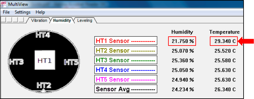
98
Factors to Consider When Making Humidity
Measurements
If you are using the 300 mm WaferSense AMS (see page 94), which has five humidity/temperature (HT) sensors,
please note that the HT1 sensor is near the center of the wafer (close to the warm electronics), but the other four
sensors (HT2 through HT5) are on the cooler periphery of the wafer. As a result, the HT1 sensor usually returns a
higher temperature reading than HT2–HT5, and—the key point here—also returns a lower RH reading than the
other sensors, as shown in the figure below.
The sections below, tell you how to do the following.
• Set Go/No-Go Tolerances for humidity
• Set Triggers for humidity
• Access other humidity menus and functions
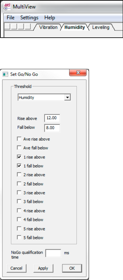
99
Setting Go/No-Go Tolerances
To set Go/No-Go tolerances, do the following.
1) Open MultiView and click the Humidity tab.
2) Choose the Settings > Set Go/No-Go menu item.
MultiView populates the Set Go/No-Go dialog with the default values (12.00 and 8.00).
3) Enter the appropriate values in the Rise above and Fall below data-entry box. (If your AMS has additional HT
sensors, check the HT2–HT5 boxes, if you want to set tolerances for these sensors.)
4) Click Apply to save your entries.
5) Click OK to close the dialog.
100
Setting Triggers
See page 35.
Using Other Humidity Menus and Functions
Here’s how to get information about other Humidity menus and functions
File Menu
• Select Log Directory —see page 60
• Open Settings —see page 60
• Save Settings —see page 40
• Print —see page 26
• Print Preview —see page 26
• Print Set-Up —see page 26
• Exit —select Exit to close the MultiView software
Settings Menu
• Show Annotation Dialog —see page 55
• Set Go/No-Go tolerances —see page 99
• Set Triggers —see page 35
• Set Station Information —see page 38
• Select Colors —see page 68
• Options —see page 48
Help Menu
• Display On-Line Manual —select to display the AMS manual
• Register WaferSense AMS —see page 16
• About Your AMS Wafer —see page 19
• About AMS View —see page 19
MultiReview
• Using MultiReview —see page 73

101
Using the Leveling Function
The AMS uses electronic inclinometer technology to give you more precise and efficient inclination measurements
than is possible using the human eye or traditional bubble levels. The large leveling screen shown in the MultiView
allows you to quickly and precisely adjust the robots and other components in your manufacturing process.
The leveling function allows you to make inclination measurements in the horizontal plane.
Using Your AMS
This section tells you how to do the following.
• Open the leveling function
• Use the AMS leveling wafer buttons and indicators
• Perform horizontal inclination measurements
• Perform vertical inclination measurements
• Log your readings
Using the
Leveling
Function
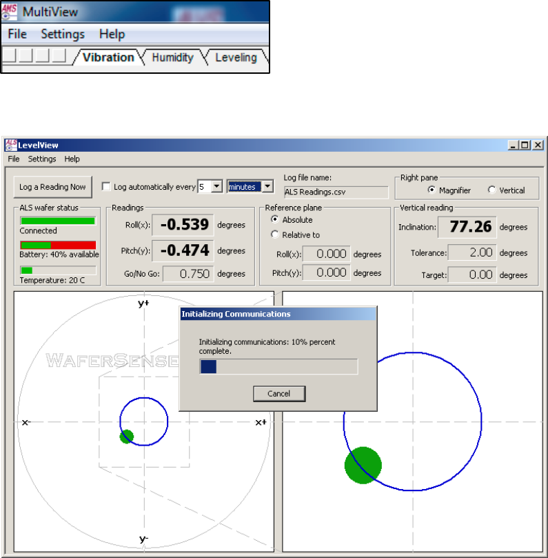
102
Opening the Leveling Function
1) Locate the Leveling tab in the top-left corner of the MultiView opening screen.
2) Click the Leveling tab and the following screen appears. Wait while the system initializes.
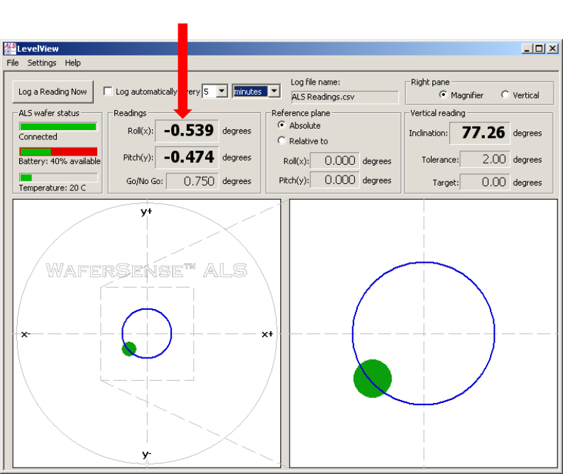
103
Performing Horizontal Inclination Measurements
MultiView shows the angle of inclination for horizontal measurements using two types of readouts (see figure
below).
• Graphical readouts that mimic bubble levels.
• Numeric readouts that show inclination in two dimensions. MultiView updates the readings several times per
second, so you see any changes in real time.
The left bubble-display (see figure below) shows a representation the whole AMS wafer, and the right shows a
magnified view that allows you to make very precise leveling adjustments.
Figure 4. Whole Disk Bubble and Magnified Bubble Display
Whole Disk Bubble Display Magnified Bubble Display
Numeric readouts
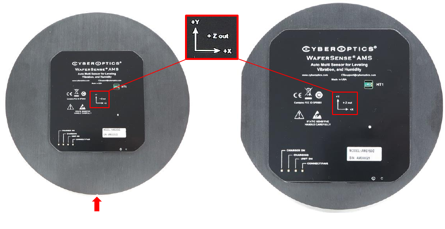
104
To perform a basic inclination measurement:
1) Make sure the computer running the MultiView application is within the range of the link module, about 30 ft
(10 m).
2) In the MultiView window, for Right pane, choose Magnifier.
3) Place the leveling wafer on the equipment you want to check. Align the leveling wafer so it matches the
MultiView display by doing the following.
• Rotating the AMS until logo is right-side up.
• Depending the model you are using, rotating the AMS so the notch is pointing toward you as you view the
AMS, or the flat side of the AMS is to the left as you view the AMS, as shown in the figure below.
Figure 5. Orienting the AMS
When you move the leveling wafer, the readings typically need some time to stabilize. The bubble displays and
numerical readouts are shaded during this stabilization period. For ALS1 systems, a message in the left bubble
display counts down the seconds (see the figure on the next page). Whenever the leveling wafer detects
movement, MultiView restarts the stabilization countdown. For ALS1 systems, you can set the length of the
stabilization period and the sensitivity that triggers the countdown (see “Setting the Stabilization Criteria” on
page 109). For ALS2 and ALS2 Vertical wafers, MultiView determines the necessary stabilization time
automatically. You can’t set the stabilization criteria for ALS2 or ALS2 Vertical wafers.
Notch
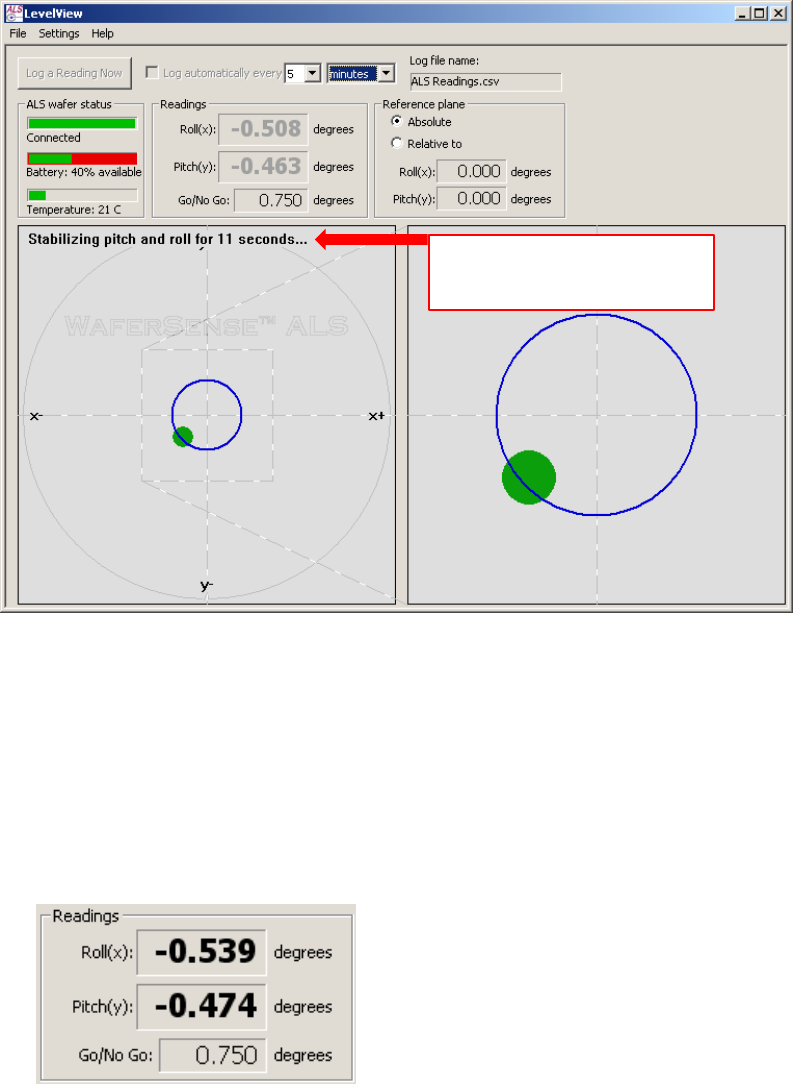
105
4) The numeric readouts and bubble displays indicate the inclination of the leveling wafer.
• The Horizontal readings (see figure below) can be displayed using different units and different conventions for
measuring the inclination. For more information, see “Choosing Display Units and Conventions” on page 106.
Readings outside the working range of the leveling wafer are displayed as ####. Readings within the working
range, but beyond the range where readings meet the specified accuracy, are shown in gray. MultiView always
displays a fixed number of decimal places for readings, which might not reflect the actual accuracy of the
measurement. For information on the accuracy of the readings, see “Specifications” on page 127.
• The bubble level displays (see the figure on the next page) show the inclination graphically in real time. In
both displays, the solid green circle represents inclination as a bubble in a bubble level would. The blue circle
indicates the Go/No-Go tolerance, which you can adjust (see “Setting the Go/No-Go Tolerance” on page 110).
In the left display, the perimeter represents the maximum inclination reading in the specified accuracy range
of the wafer, which depends on the wafer model (see “Specifications” on page 127). The display on the right is
a magnified view showing just the area within the dashed magnifier square of the display on the left. The size
of the magnifier square adjusts to keep the bubble in the right display visible.
Countdown for stabilizing
the readings
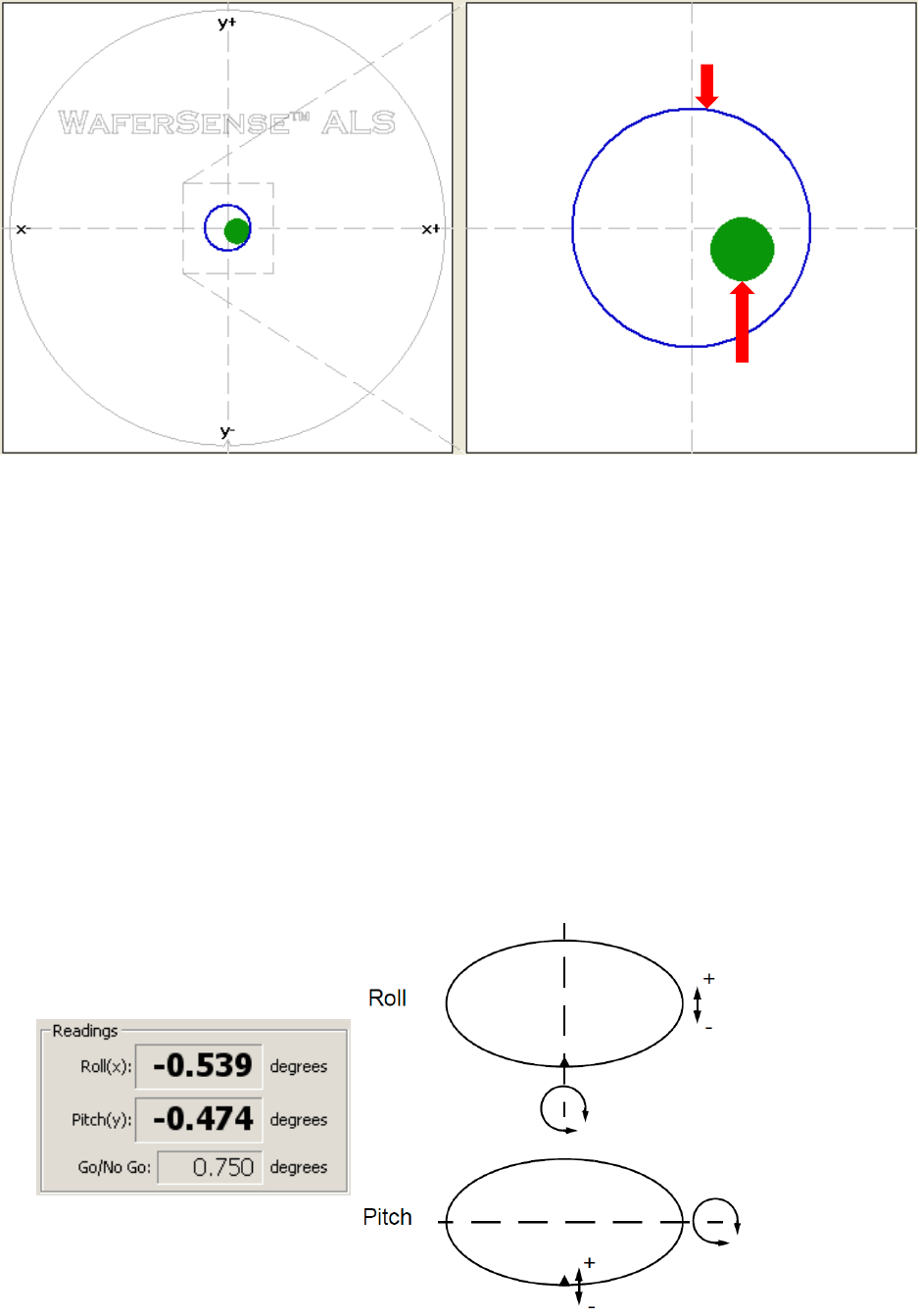
106
Choosing Display Units and Conventions
By default, MultiView displays horizontal readings in degrees using the roll and pitch convention. You can choose
different conventions and also different units.
Conventions for Horizontal Inclination
For displaying horizontal inclination, you can choose between the Cartesian roll and pitch convention and the polar
magnitude and direction convention.
• Cartesian Roll and Pitch (see figure below) indicate the inclination angle in two dimensions. Assuming you
aligned the WaferSense™ AMS logo as described above (see page 104), Roll indicates side-to-side tilt, and
Pitch indicates front-to-back tilt. If the front edge is higher than the back, or the right edge is higher than the
left, the readings are positive.
Bubble
Go/No-Go circle
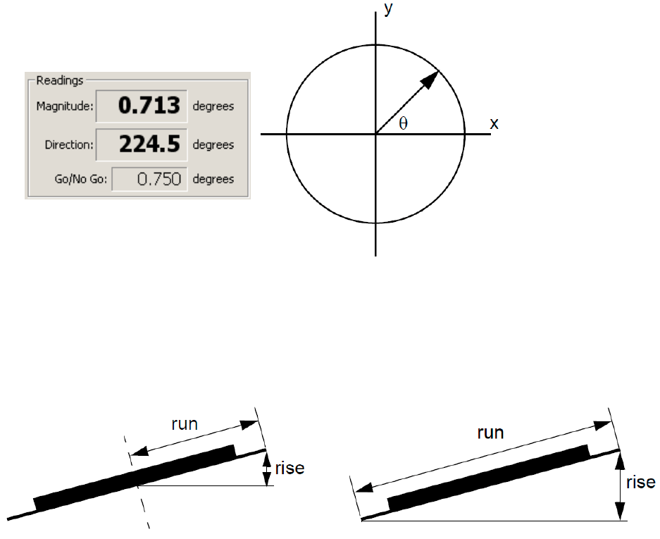
107
The precision of displayed readings depends on the units you choose. For example, readings in degrees are
displayed to three decimal places. However, that doesn’t mean that the readings are accurate to 1/1000ths of a
degree. In general, you can’t assume that readings are accurate to all displayed decimal places. For information on
the accuracy of the readings, see “Specifications” on page 127.
• Polar Magnitude and Direction indicate the angle of inclination in the direction of maximum inclination. In the
figure below, the highest point on the edge of the wafer is indicated by the arrow, Direction is the angle the
arrow makes with the x-axis, and Magnitude is the angle between the wafer and the horizontal (or reference)
plane. Direction is measured counter-clockwise from the x-axis and is always positive. Magnitude is also
always positive.
Display Units for Horizontal Inclination
Horizontal inclination angles can be displayed in degrees or milliradians (mradians), or as rise over run. Rise over
run is the vertical height of a point on the edge of the wafer relative to the center of the wafer (rise over radius) or
relative to a point on the opposite edge (rise over diameter), as shown below.
Rise over Radius Rise over Diameter
In addition to choosing whether to display the measured rise over the radius or diameter of the wafer, you can also
choose to display the value in either inches or millimeters:
• mm/r Millimeters of rise over the radius.
• in/r Thousandths of an inch of rise over the radius.
• mm/d Millimeters of rise over the diameter.
• in/d Thousandths of an inch of rise over the diameter.

108
Setting Display Units and Conventions
To set the units and conventions used to display horizontal inclination:
1) Choose the menu item Settings > Set Display Units (on the ALS2 Vertical, choose Set Horizontal Units). The
Set Display Units (or Set Horizontal Units) dialog is displayed, as shown in the figure below.
2) For Display type, if you want pitch and roll angles displayed, choose Cartesian; if you want the direction and
magnitude of maximum inclination displayed, choose Polar.
3) For Inclination units, choose either Angle or Rise over run and then select the units. If the Rise over run
choice isn’t available, MultiView isn’t connected to a leveling wafer. After you turn on the wafer and establish
a connection, you can make that selection.
4) To save your settings, click OK.
Note: You can also set the display units and conventions in the dialog used to set the Go/No-Go tolerance. The
result is the same using either dialog. For more information, see “Setting the Go/No-Go Tolerance” on page 110.
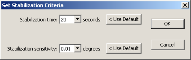
109
Setting the Stabilization Criteria
When you move the leveling wafer, the readings typically need some time to stabilize. The bubble displays and
numerical readouts are shaded during this stabilization period. The length of time that the readings need to
stabilize depends on the type of leveling wafer, the operating conditions, and your required tolerance for stability.
For ALS2 and ALS2 Vertical wafers, MultiView determines the necessary stabilization time automatically. You can’t
set the stabilization criteria for ALS2 or ALS2 Vertical wafers, so this section applies only to ALS1 systems.
The default stabilization time (20 seconds) and stabilization sensitivity (0.01 degrees) provide for the maximum
stability. These default settings yield the most accurate measurements for all types of situations. However, when
the position of the leveling wafer changes only a small amount between successive measurements, you can adjust
these settings so that you can work more quickly, without sacrificing accuracy.
To specify the stabilization criteria:
1) Choose the menu item Settings > Set Stabilization Criteria. The Set Stabilization Criteria dialog is displayed, as
shown below.
2) In the Stabilization time list, choose the number of seconds you want MultiView to pause to allow readings to
stabilize, or click Use Default to reset the time to the default 20 seconds.
3) In the Stabilization sensitivity list, choose the fraction of a degree in pitch or roll movement that you want to
trigger MultiView to restart the stabilization counter. To reset the value to the default, click Use Default to
reset the sensitivity to 0.01 degree.
4) Click OK.
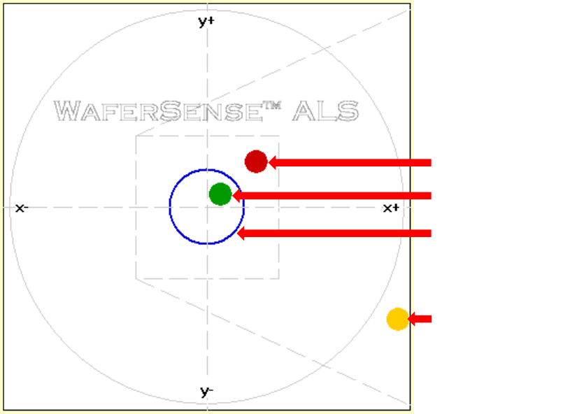
110
Setting the Go/No-Go Tolerance
The Go/No-Go tolerance sets the diameter of the blue circle in the center of the bubble displays. This circle makes
it easy to see when you have leveled a piece of equipment to within an acceptable tolerance. When the center of
the bubble is within the Go/No-Go circle, the bubble is green, indicating that the reading is within your specified
tolerance. When the center of the bubble reaches or passes the edge of the Go/No-Go circle, the bubble changes
to red to indicate the reading exceeds your specified tolerance. When the readings are beyond the specified
accuracy range of the sensor, the bubble is pinned against the edge of the display area, and the color of the bubble
changes to amber.
Out of tolerance
In tolerance
Go/No-Go circle
Out of range
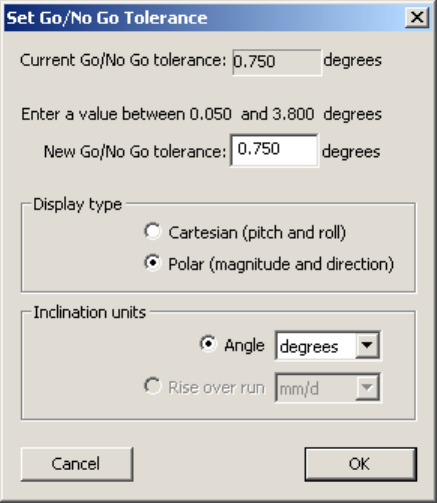
111
To change the Go/No-Go value:
1) Choose the menu item Settings > Set Go/No-Go Tolerance. The Set Go/No-Go Tolerance dialog is displayed.
2) Specify the New Go/No-Go tolerance and click OK.
You can set the tolerance to any value in the range 0.05 to 3.8 degrees. However, if you are using a reference
plane (see the next page), the maximum value is less than 3.8 degrees. You can’t set a tolerance that would
extend the Go/No-Go circle beyond the edge of the left bubble display area. If you try to set a value that is too
large or too small, MultiView prompts you to enter a value that is within the correct range.
You can also set the Horizontal display type and inclination units in this dialog. For more information on these
settings, see “Choosing Display Units and Conventions” on page 106.
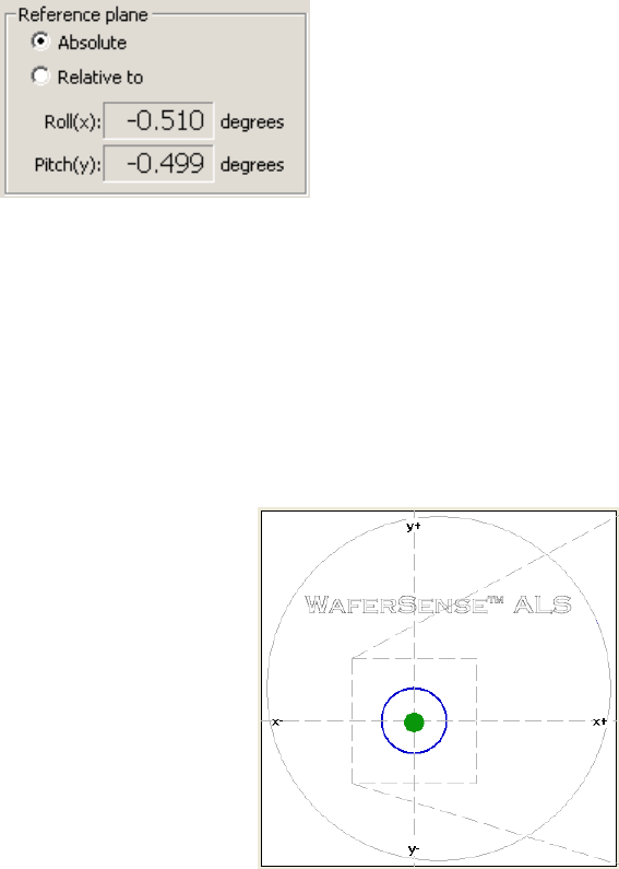
112
Specifying a Reference Plane
By default, the leveling wafer indicates absolute degrees of inclination, which is relative to a plane perpendicular to
the direction of the earth’s gravitational force. You can specify a different reference plane, and the leveling wafer
will indicate degrees of inclination relative to that plane.
To specify a reference plane:
1) Place the leveling wafer on the surface that you want to use as your reference plane.
2) Choose the menu item Settings > Set Reference Plane. The leveling wafer takes the current absolute
inclination readings as offsets to the new relative plane. The offsets are displayed in the Horizontal reference
plane readouts.
3) Select the Relative to option above the Horizontal reference plane readouts.
You can switch the leveling wafer between indicating absolute and relative inclination by clicking the
corresponding option button (see the figure above). Switching between Absolute and Relative to does not affect
the current offsets for the reference plane inclination angles; MultiView retains the last offsets until you change
them.
When you specify a reference plane and set MultiView to display Relative to that plane, the coordinate axes of the
left bubble-display shift within the display area, as shown below.
This shift in the axes reflects the fixed range of the leveling wafer relative to absolute level. For a leveling wafer
that has a range of -4 degrees to +4 degrees from absolute level, if you set a reference plane at -2 degrees absolute
pitch, the range of the leveling wafer relative to that reference plane is -2 degrees to +6 degrees pitch. Shifting the
center of the bubble display to the left accurately represents the new range of the leveling wafer relative to the
reference plane. For more information on the working range of different models, see “Specifications” on page 127.
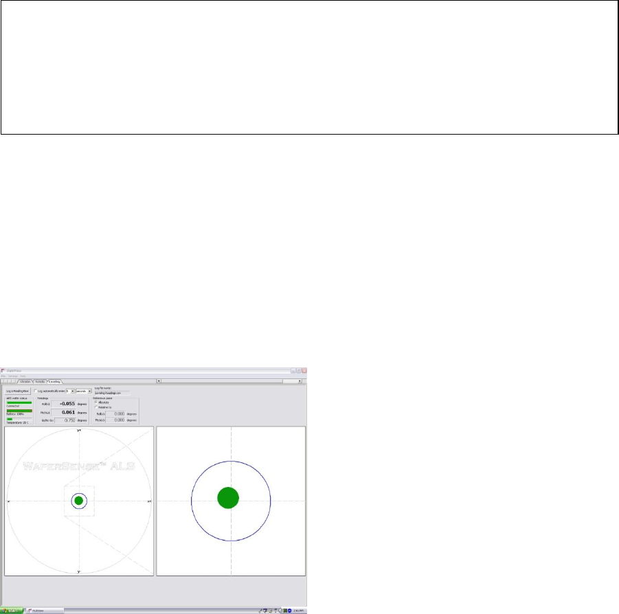
113
Calibration for zero point drift (Field Calibration)
The zero point of the electronic inclinometers used in the AMS can drift slightly over time. If you use absolute level
as your reference plane, you might want to calibrate for zero-point drift occasionally. You can perform this
calibration in your own facility by using the calibration routine built into the MultiView application. If you work
relative to a reference plane other than absolute level, zero point drift won’t affect your measurements, and you
don’t need to perform this calibration procedure. In the following procedure for calibrating the zero point of the
AMS, the software instructs you to place the leveling wafer on a flat, level surface. The software takes an
inclination reading, instructs you to rotate the leveling wafer in place 180 degrees, and then takes a second
reading. The two readings are used to set the new zero point. It is important that the center of the leveling wafer is
in the same position on the surface before and after you rotate the leveling wafer. Most surfaces are not perfectly
flat, so moving the leveling wafer while rotating it can affect the accuracy of the calibration. The procedure,
therefore, instructs you to place marks on the surface at four points around the outside edge of the leveling wafer.
You can use these marks to rotate the leveling wafer without moving it off center relative to the first calibration
reading.
To calibrate your AMS using MultiView:
Locate a surface large enough to hold the AMS and having the following
characteristics:
• Level to within about 1 degree.
• Stable enough to ensure that the inclination of the surface does not change during the
procedure.
• Sufficiently smooth and flat that the inclination readings of the AMS don’t
change if you move the AMS slightly in any direction.
If the surface doesn’t meet these requirements, it might introduce an error in the
calibration results.
Caution
Performing a zero-point calibration improperly can actually cause the AMS to produce absolute level
readings that are less accurate than readings from the AMS prior to the zero-point calibration. This is likely
to be true if the surface used for the calibration is not sufficiently stable and flat. To remove a zero-point
field calibration, run the zero-point calibration procedure again and click Reset to Factory Default in the
first step of the procedure.
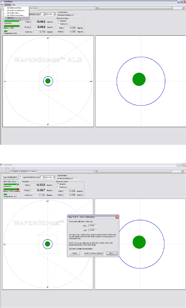
114
1. Choose the menu item Settings > Calibrate.
The Field Cal Wizard will pop up and show any existing field Cal values.
This dialog displays the current calibration values. If you haven’t calibrated the AMS since the last factory
calibration, both values are zero. Clicking Reset to Factory Default changes the calibration values to the
values set when the leveling wafer was last calibrated at the factory.
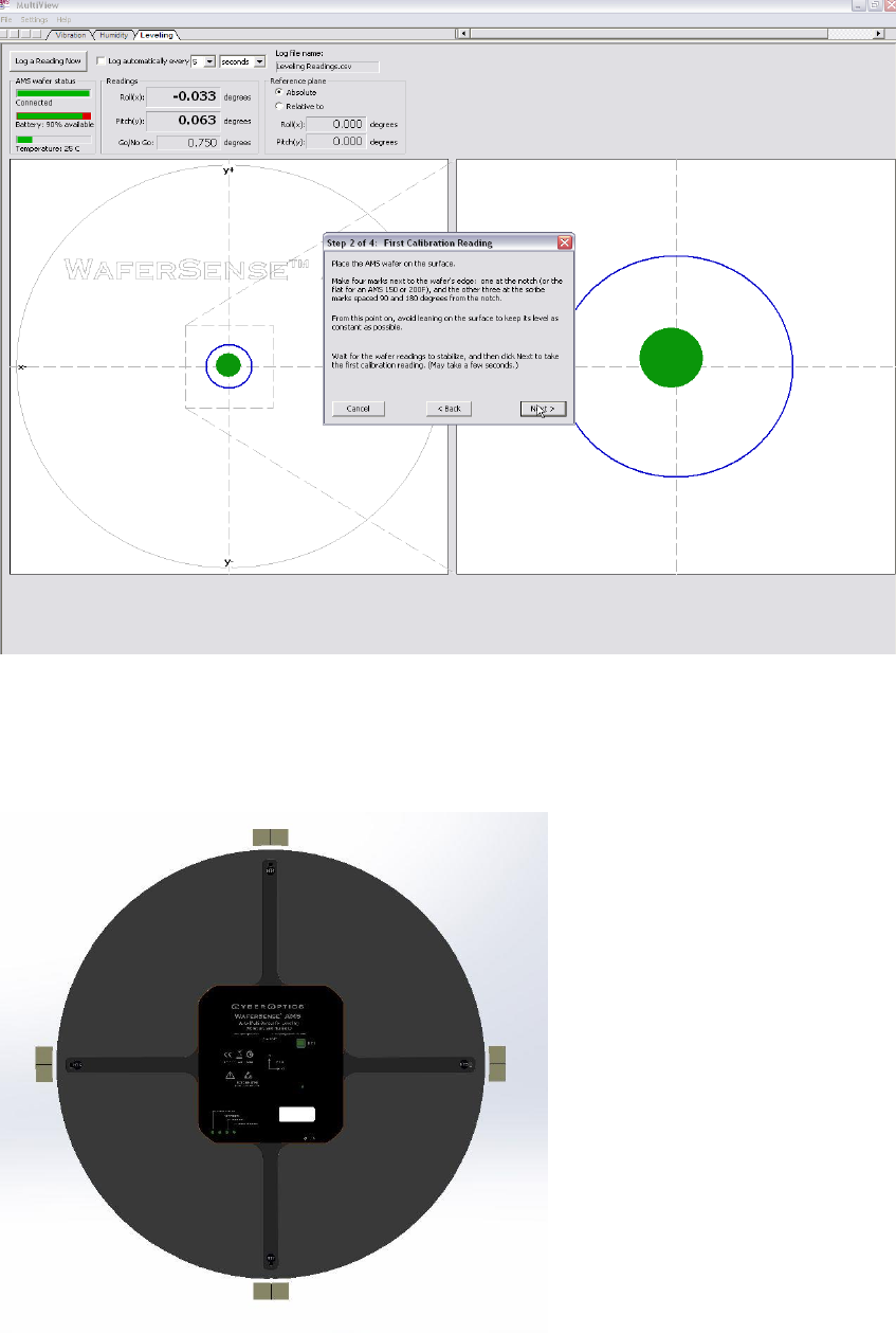
115
2. Allow the Pitch and Roll values to stabilize (around 30 seconds) and then hit Next.
This step calls for marking the position of the AMS on the reference surface. For 300mm or 200mm wafers
with notch, place a mark on the surface (or on tape on the surface) next to the edge of the AMS at the
notch. Place three additional marks on the surface next to the edge of the AMS at the scribe marks that
are 90 degrees, 180 degrees, and 270 degrees from the notch or flat side. Always mark all four positions.
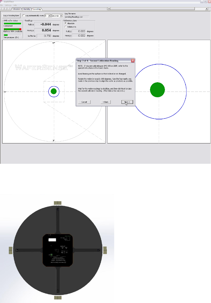
116
3. Wait for the AMS readings to stabilize and then click Next to take the first calibration reading.
After a few seconds, the wizard displays the Step 3 of 4 Second Calibration Reading
Dialog.
WAFERSEN
Rotate the AMS 180 degrees and align the AMS with the four marks you made in the earlier steps, as
shown below. Be sure to line up all four marks, so that the rotated AMS is as close as possible to the same
position it was in when you took the first calibration reading.
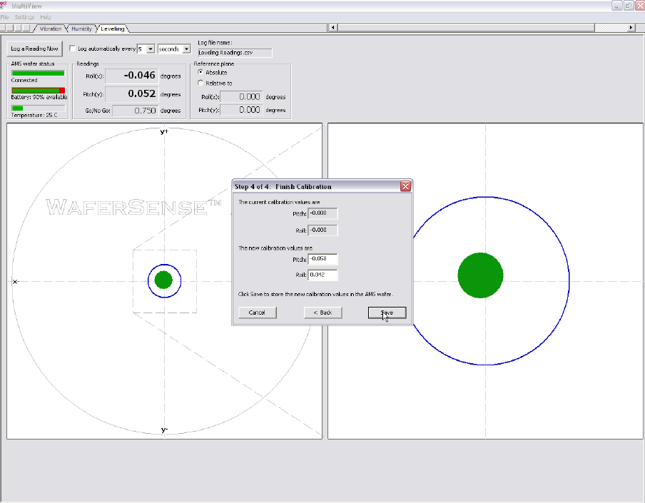
117
4. Click Next to take the second calibration reading.
If the new calibration offsets are too large (> 0.5 degrees) for your AMS to operate reliably, a dialog
displays telling you to contact customer support at CyberOptics.
If the new calibration offsets are within the allowed limits, the wizard displays the
Step 4 of 4 Finish Calibration dialog, as shown above.
Click Save to save the new calibration values. That completes the zero-point calibration.
118
Viewing Leveling Log Files
The MultiReview application lets you view log files that you previously recorded using MultiView. This section gives
you instructions for performing the following tasks with MultiReview:
• Running MultiReview
• Choosing display units and conventions
• Temporarily changing the Go/No-Go tolerance
• Temporarily changing the vertical tolerance and target
• Changing log files
• Displaying station and wafer information
• Printing the MultiReview window
This section assumes that you are familiar with the information in “Using Your AMS” starting on page 21.
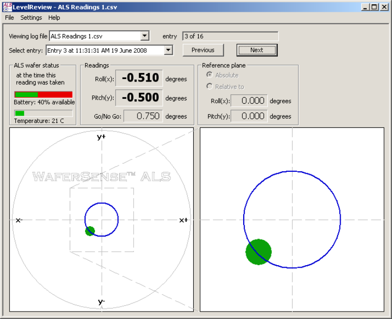
119
Running MultiReview
To view a log file:
1) From the Windows Start > All Programs menu, choose WaferSense AMS > MultiReview.
2) The MultiReview application starts. Click the Leveling tab.
3) From the File menu, choose Open Log File. The AMS Log File dialog is displayed.
4) Choose a log file and click Open. MultiReview opens the log file and displays the data for the first entry in the
file (see figure below).
5) To view the data for a different entry in the log file, use the Next and Previous buttons, or choose an entry
from the Select entry list.
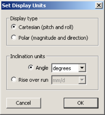
120
Choosing Display Units and Conventions
By default, MultiReview displays horizontal readings in degrees using the roll and pitch convention. You can choose
different conventions and also different units.
Conventions for Horizontal Inclination
For displaying horizontal inclination, you can choose between the Cartesian roll and pitch convention and the polar
magnitude and direction convention. For more information, see “Choosing Display Units and Conventions” on
page 106.
Display Units for Horizontal Inclination
Horizontal inclination angles can be displayed in degrees or milliradians (mradians), or as rise over run. For more
information, see “Choosing Display Units and Conventions” on page 106.
Setting Display Units and Conventions
To set the units and convention used to display horizontal inclination:
1) Choose the menu item Settings > Set Display Units (on the ALS2 Vertical, choose Set Horizontal Units). The
Set Display Units (or Set Horizontal Units) dialog is displayed, as shown below.
2) For Display type, if you want pitch and roll angles displayed, choose Cartesian; if you want the direction and
magnitude of maximum inclination displayed, choose Polar.
3) For Inclination units, choose either Angle or Rise over run and then select the units.
4) To save your settings, click OK.
You can also set the display units and conventions on in the dialog used to set the Go/No-Go tolerance. The result
is the same using either dialog. For more information, see the next page.
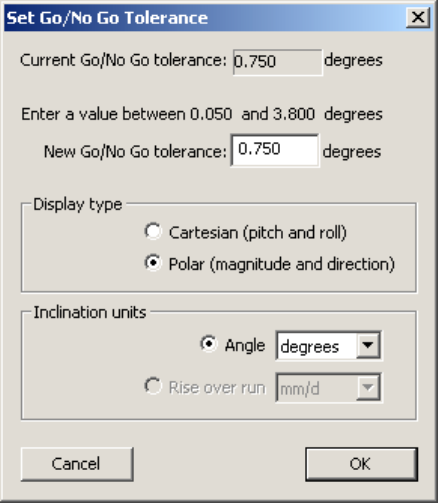
121
Temporarily Changing the Go/No-Go Tolerance
The Go/No-Go tolerance in effect at the time a log file entry is made is recorded in the log file as part of the log
entry. That value is used when you first display an entry from the log file. You can temporarily change the Go/No-
Go tolerance for the entry you are currently viewing. However, as soon as you select a new entry from the log file,
the Go/No-Go tolerance displayed reverts to that of the log file entry.
To temporarily change the Go/No-Go tolerance:
1) Choose the menu item Settings > Set Go/No-Go Tolerance. The Set Go/No-Go Tolerance dialog is displayed,
as shown below.
2) Specify the New Go/No-Go tolerance and click OK.
You can set the tolerance to any value in the range 0.05 to 3.8 degrees. However, if you are using a reference plane
(see “Specifying a Reference Plane” on page 112), the maximum value is less than 3.8 degrees. You can’t set a
tolerance that would extend the Go/No-Go circle beyond the edge of the left bubble display area. If you try to set a
value that is too large, MultiReview prompts you to enter a value that is within the correct range.
You can also set the Horizontal display type and inclination units in this dialog. For more information on these
settings, see “Choosing Display Units and Conventions” on page 106.
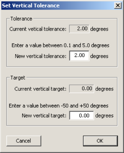
122
Temporarily Changing the Vertical Tolerance and Target
The vertical tolerance and target in effect at the time a log file entry is made are recorded in the log file as part of
the log entry. Those values are used when you first display an entry from the log file. You can temporarily change
vertical tolerance and target for the entry you are currently viewing. However, as soon as you select a new entry
from the log file, the vertical tolerance and target displayed revert to that of the log file entry.
To change the target and tolerance settings:
1) Choose the menu item Settings > Set Vertical Tolerance.
2) The Set Vertical Tolerance dialog is displayed, as shown below. The currently set values for both Tolerance and
Target are shown.
3) Enter the New vertical tolerance and New vertical target values, and click OK.
4) If you want to return to measuring relative to absolute vertical, change the Target setting back to zero.

124
Maintaining Your AMS
This section provides details about the following.
• Annual factory calibration and battery replacement
• Battery use and disposal
WARNING. The edges of the AMS are thin. It may be possible to sustain injury from these edges, if the
AMS device is not handled with proper care. Protection afforded by compliance EN61010-1 (2010) may
be impaired, if the equipment is not used as specified.
CAUTION. Use extreme care to assure that the AMS has proper clearances, when being transported
through the tool. For example, when you use the AMS in the tool for the first time, move the device
through the tool in manual mode, visually verifying all clearances. Even when clearances are sufficient
for safe AMS pass-through, if the robot end-effector is taught too high, you risk crashing and damaging
the AMS.
Maintaining
Your AMS
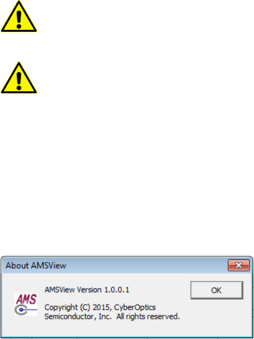
125
Periodic calibration and battery replacement is the only regular maintenance your AMS requires:
Annual Calibration and Battery Replacement
Once a year, you should have your AMS calibrated, and the internal rechargeable battery replaced by returning the
AMS to the CyberOptics factory.
Cleaning the AMS
If cleaning is required, wipe the outside of the AMS with IPA (isopropyl alcohol). However, do not apply IPA near
any of the humidity sensors. If the AMS is used in a clean environment, follow proper procedures for this
environment.
WARNING. Do not immerse the AMS or the link module in liquid. Do not spill liquid on the AMS or on
the link module. Do not apply IPA near any of the humidity (HT) sensors.
WARNING. The use of controls, adjustments, or procedures other than those specified in this manual
may result in exposure to hazardous optical radiation.
Annual Factory Calibration and Battery
Replacement
Every 12 months, you should return your AMS to the CyberOptics factory, where we will calibrate the AMS and
replace the internal rechargeable battery. You can find the date when the AMS was last calibrated at the factory by
choosing the Help> About AMS View menu item in the MultiView application.
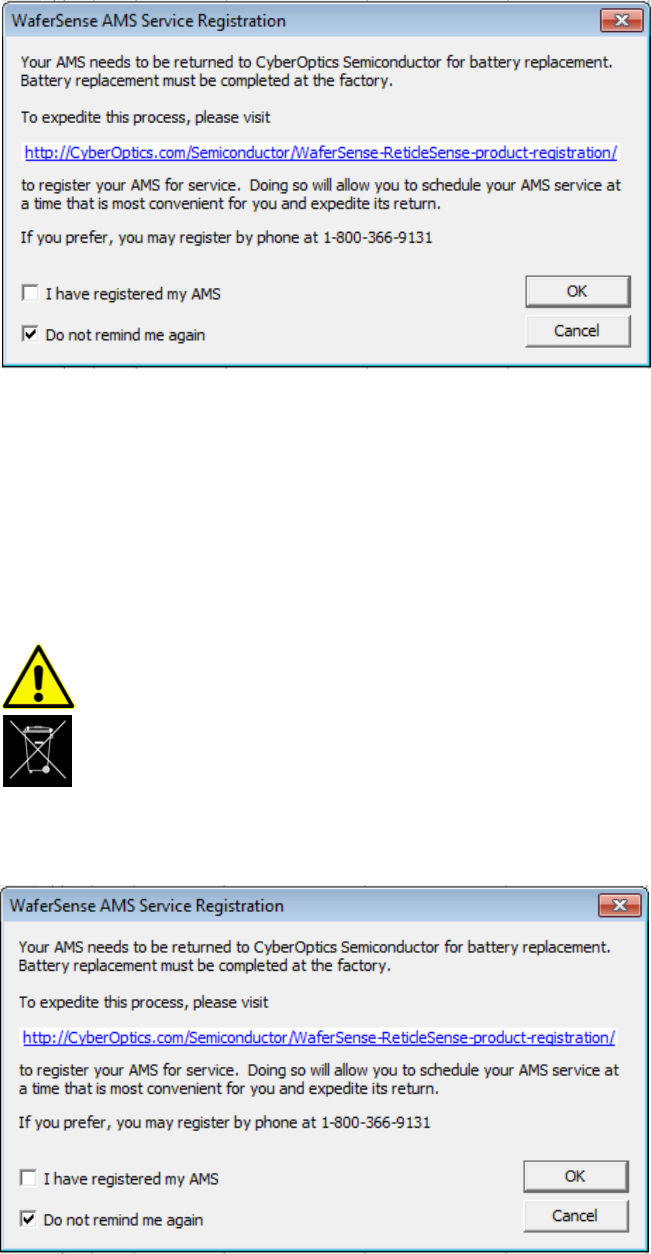
126
When the date for calibration approaches, MultiView will occasionally notify you by displaying the AMS calibration
status dialog.
If you drop the AMS or suspect that it is no longer in calibration, contact CyberOptics technical support (see
page 19.
Battery Use and Disposal
Please dispose of AMS and the lithium-ion battery it contains in a responsible manner.
WARNING. Your AMS contains a lithium-polymer battery. To avoid damage to the AMS, only use the
supplied charger. Do not charge the AMS at temperatures outside the specified range (0–45° C). Do not
incinerate or dispose of the AMS into fire. Do not immerse the AMS when cleaning, or spill liquids on
the AMS.
For proper battery disposal, please return the AMS to CyberOptics. Contact customer support (see page 19).

127
Specifications
Here are the AMS specifications.
Specification
AMS-300C, AMS-200C, AMS-
150C
AMSR-6025Q
Wireless, reticle-shaped, and battery
powered
Easy to use software: MultiView and
MultReview
Inductive wireless charging and
hands-free operation
Durable housing - see outline
drawing for dimensions
4.1mm nominal – 4.3mm max
housing center thickness –--
Carbon fiber composite over-
coated with Parylene C
6.35mm housing thickness.
Quartz outer frame. Rear
surface of quartz is an
uninterrupted quartz surface.
Dimensions, chamfers, and
squareness conform to SEMI
standards for 6 inch square
reticles. Bar-codes and
alignment marks allow
placement in most scanners
and steppers
Weight
340 grams +/-15g
Operating Pressure
0-1.6 atmosphere
0-1.6 atmosphere
Operating internal temperature
15-60ºC non-condensing, up to
82ºC for short periods
15-60ºC non-condensing, up
to 82ºC for short periods
Storage temperature
-15-+60ºC, non-condensing
-15-+60ºC, non-condensing
Charging temperature range
0-45ºC
0-45ºC
Link Box
Blue-tooth, Class 1, 2.4GHz
connected via USB
Blue-tooth, Class 1, 2.4GHz
connected via USB
Systems Requirements
Operating systems: Windows
7,8,10, XP, Vista ---------One free
high-powered USB 1.1 or 2.0
port
Operating systems: Windows
7,8,10, XP, Vista ---------One
free high-powered USB 1.1 or
2.0 port
Product components
AMS unit, charging case,
carrying suitcase, link module,
USB cable, charging supply,
application software CD,
AMS unit, charging case,
carrying suitcase, link module,
USB cable, charging supply,
application software CD,
Specifications

128
calibration certificate, and start
guide
calibration certificate, and
start guide
Calibration
Factory calibration
recommended annually
Factory calibration
recommended annually
Horizontal leveling range
+/- 14 degrees from absolute
horizontal
+/- 14 degrees from absolute
horizontal
Horizontal leveling accuracy
+/- 0.03 deg within +/-7 deg
from absolute horizontal. Field
calibrate before use for
maximum accuracy (see page
113)
+/- 0.03 deg within +/-7 deg
from absolute horizontal.
Field calibrate before use for
maximum accuracy (see page
113)
Leveling resolution
0.002 degrees
0.002 degrees
Vibration range
Range: +/- 2 G
Range: +/- 2 G
Vibration resolution
0.01G
0.01G
Vibration frequency response
0-200Hz (3dB point)
0-200Hz (3dB point)
Humidity and temperature range and
accuracy
RH Range: 2.5-85%RH
RH Accuracy:+/-2%RH at 20ºC
T Range 15-60ºC
T Accuracy +/-0.3ºC
RH Range: 2.5-85%RH
RH Accuracy:+/-2%RH at 20ºC
T Range 15-60ºC
T Accuracy +/-0.3ºC
Humidity and temperature resolution
0.02%RH, 0.01ºC
0.02%RH, 0.01ºC
Humidity response time
8 seconds to 63% of step change
8 seconds to 63% of step
change
Number of humidity and temperature
sensors
5-AMS-300C
1-AMS-200C
1-AMS-150C
1
Battery Life
2 hours minimum
2 hours minimum
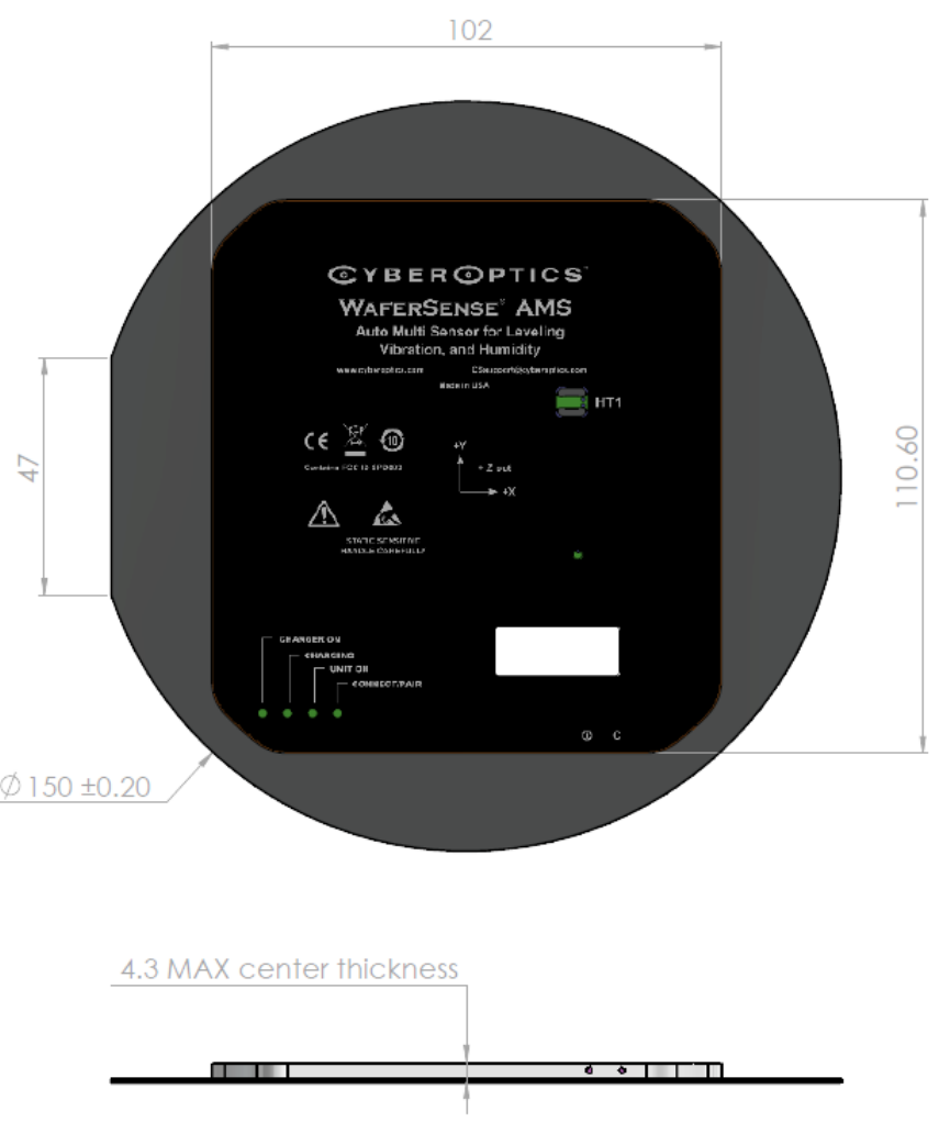
129
Dimensional Drawings
Here are the dimensional drawings for the AMS.
AMS 150C
Dimensions = millimeters
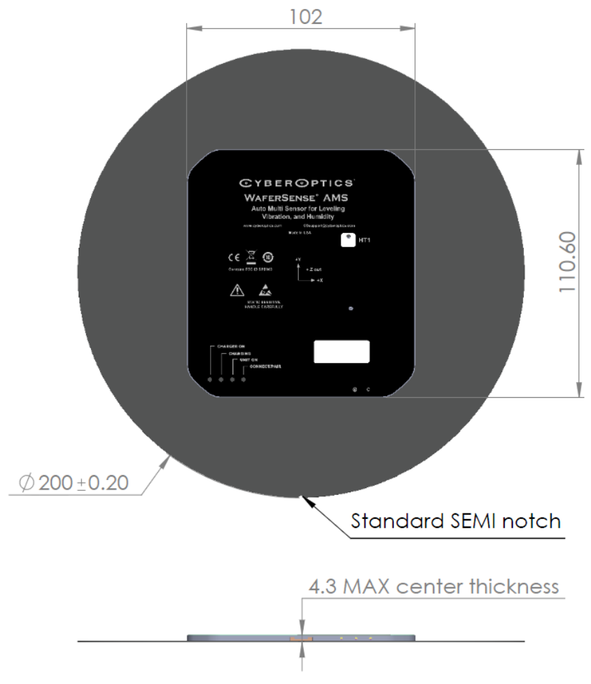
130
AMS 200mm
Dimensions = millimeters
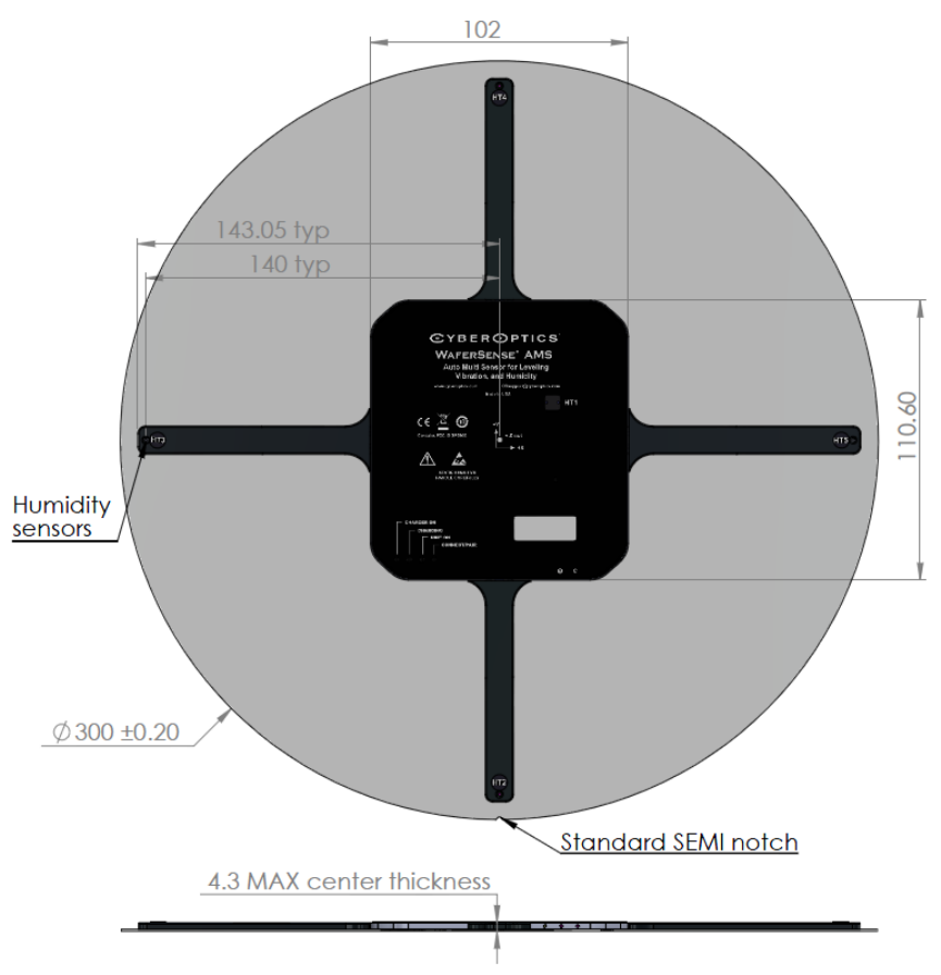
131
AMS 300C
Dimensions = millimeters
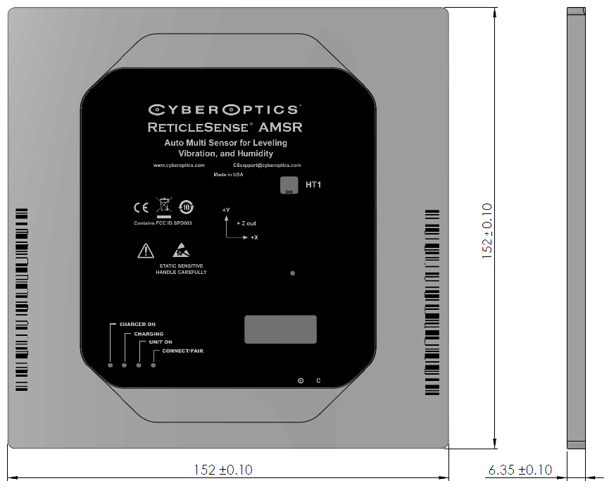
132
AMSR
Dimensions = millimeters

133
Glossary
Acronym
Description
AGS
Auto-gapping sensor
AMS
Auto multi-sensor
APS2
Air-borne particle sensor—Model 2
APSR
Air-borne particle sensor reticle
APSRQ
Air-borne particle sensor reticle quartz
ATM
Atmospheres
CD
Compact disk
CPU
Central processing unit
CSV
Comma-separated values
FCC
Federal Communications Commission
FFT
Fast Fourier transform
HT
Humidity/temperature sensor (on the upper surface of the AMS)
IC
Integrated circuit
ID
Identity
IPA
Isopropyl alcohol
ISM
Institute for Supply Management
LED
Light-emitting diode
MB
Megabytes
Glossary

134
Acronym
Description
MEMS
Micro-electro-mechanical system
PCB
Printed-circuit board
PPM
Parts per million
RF
Radio frequency
RMS
Root mean square
RH
Relative humidity
USB
Universal serial bus

135
Appendices
The appendices contain additional information about humidity measurements, as follows.
• Appendix A—Moisture Conversion Table
• Appendix B—Psychrometric Chart
• Appendix C—Acoustic Resonances and other factors Affecting Acceleration Measurements
Appendices

136
Appendix A—Moisture Conversion Table
Relative
Humidity at
20ºC & 1 atm
Dew Point in
ºC at 1 atm
PPM on
volume basis
at 1 atm
PPM on weight
basis in air
Partial water
vapor pressure
in mbar
95 19.2 22390 13897 22.19
90 18.3 21187 13150 21.02
85 17.4 19987 12405 19.85
80 16.5 18788 11662 18.67
75 15.4 17594 10920 17.52
70 14.4 16402 10180 16.35
65 13.2 15212 9442 15.18
60 12 14026 8705 14.02
55 10.7 12842 7971 12.85
50 9.3 11661 7238 11.68
45 7.7 10483 6506 10.51
40 69307 5777 9.34
35 4.1 8134 5049 8.17
30 1.9 6964 4322 7.01
25 -0.5 5797 3598 5.84
20 -3.2 4632 2875 4.67
15 -6.6 3470 2154 3.5
10 -11.2 2311 1434 2.34
9 -12.4 2079 1290 2.1
8 -13.6 1848 1147 1.87
7 -15.1 1616 1003 1.63
6 -16.8 1385 860 1.4
5 -18.7 1154 716 1.17
4 -21 923 573 0.934
3 -24 692 430 0.701
2 -28 461 286 0.467
1 -32.6 285 177 0.288
Moisture Conversion Table
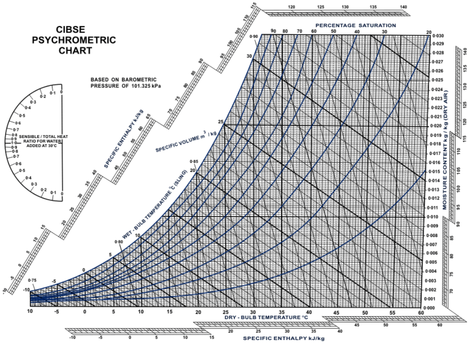
137
Appendix B—Psychrometric Chart
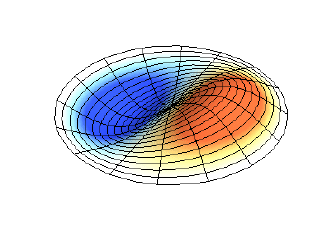
138
Appendix C—Acoustic Resonances and other
factors Affecting Acceleration Measurements
Any mechanical system has acoustic resonances that can be excited by either sinusoidal acceleration or repeated
impulses. Traditional accelerometers are usually mounted into metal blocks that have thicknesses comparable to
their lateral dimensions. This is done so that the resonance frequency of the mechanical system is driven to high
frequencies and therefore does not interfere with the acceleration measurement. However, in trying to measure
accelerations in systems that handle semiconductor wafers, the thin flat shape of the wafer and the relatively low
resonant frequencies makes comparative acceleration measurements difficult.
Semiconductor wafers can have “drumhead” resonances at relatively low frequencies. As the name suggests,
these resonances occur in the direction normal to the flat surface of the wafer. Because of the large diameter to
thickness ratio, the resonant frequencies can be quite low. A typical illustration of one of the lower order
drumhead mode patterns (0,1) is shown below. Depending on the excitation frequency, multiple modes, such as
(0,0), (0,1), (2,1), etc. can be excited.
In the same way, Wafersense units that measure vibration, such as AVS and AMS, also have these modes, as well
as other smaller resonances caused by the housing structures. The resonance frequency is primarily determined
by the thickness, area and material density. So, an AMS unit will have different resonances from an AVS unit which
will have different resonances from a silicon wafer.
The method of clamping, whether uniformly clamped at the edge, clamped in a few places at the edge, or
supported in the middle, will also change the resonant frequencies in both Wafersense units as well as silicon
wafers.
The amplitude of the driving force, i.e. the acceleration, will not affect the resonant frequencies, but will
determine which resonances show up in the measurement.
One common question is whether two AVS units or two AMS units will show the same waveform if vibrated or
translated in the same manner. The answer is that two units of the same type will show the same acceleration if a
resonance is not excited. Even an AVS and an AMS unit will show almost the same waveform off resonance.
Below in figure 1 is a comparison of an AVS unit (top) and an AMS unit (bottom) that were clamped together and
simultaneously shaken in the z direction. As you can see, their waveforms are very similar but not identical. One
would not expect them to be identical since the housing construction of the two are different. The AMS housing is
much thinner and the electronics enclosure is smaller in diameter than the AVS housing.
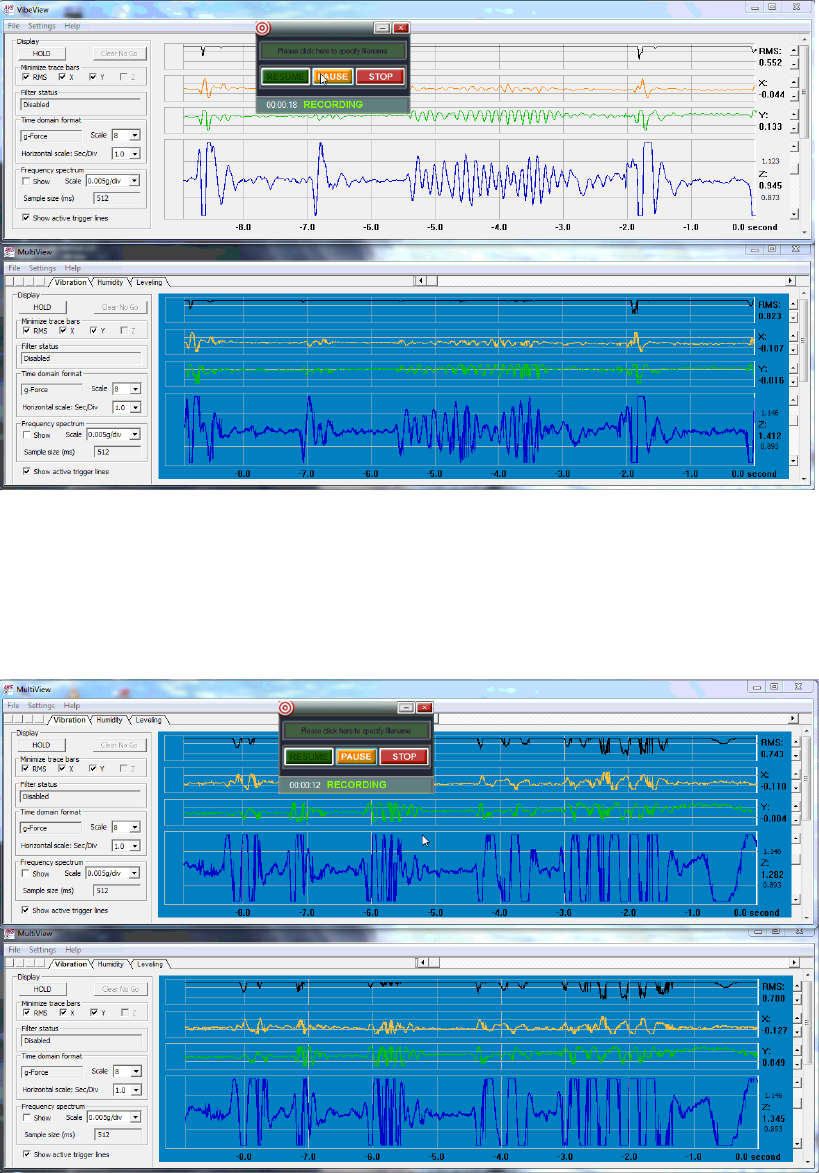
139
Figure 1: Response of AVS unit (top) and AMS unit (bottom) clamped together
and simultaneously shaken in the z direction.
An AMS unit compared to another AMS unit will have traces almost identical to each other. Figure 2 below shows a
200mm AMS unit (top) compared to a 300mm AMS unit (bottom).
Figure 2: Response of 200mm AMS unit (top) and 300mm AMS unit (bottom)
clamped together and simultaneously shaken in the z direction.
140
An AVS unit and another AVS unit will also have identical traces if they are not on resonance. As shown in figure 1
above, the z axis correspondence of an AMS and AVS unit are good but not perfect. The correspondence in the x
and y directions is also very good. So, the z direction correspondence shown above is close to the worst-case
condition.
But, AVS units will not show the same waveform as AMS units if, in one of the cases, a resonance is excited by the
movement.
One potential way to lessen the resonance problem is with acoustic damping. Adding a plate that consists of a
resilient and low density material (foam or rubber) sandwiched between the AVS or AMS housing and another stiff,
high density material will attenuate resonances. The alternating layers of high and low density materials damp the
resonances.
Therefore, when AMS and AVS units are compared against each other there will be some unavoidable differences
caused by the resonances and different housing construction. Resonances cause the largest differences. But even
off resonance there will be some differences between AMS and AVS units.
Both the AMS and AVS units cover the same frequency bandwidth with the same sensitivity. Both are calibrated at
0 Hz and in both units any cross-axis sensitivities are corrected out. Because of the simpler internal structure, the
AVS may have slightly less noise and a cleaner response to a single excitation frequency.

141
Wafersense AHS
This addendum is for the humidity only WaferSense AHS sensor.
MultiView
AMS/AHS automatic detection
When MultiView attaches to a wafer it automatically checks to determine whether it is an AMS or AHS
WaferSense. The application then configures the main screen to display the appropriate view. When the
device is an AHS wafer the main screen will hide the tab control and display the humidity view (see Figure
A.1). The tab control is used to switch between the vibration, humidity and leveling views. Since vibration
and leveling are not available on AHS wafers the tab control is unnecessary.
Main Screen
The MultiView main screen, in AHS mode, looks and functions like the humidity view tab in AMS mode.
This view is described in the AMS manual. The only distinction in AHS mode is that recording now
generates humidity log files only.
AHS
Addendum
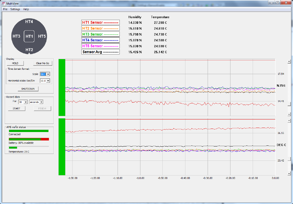
142
Figure A.1: AHS Mode MultiView Main Screen
MultiReview
Main Screen
When log files are recorded in MultiView using a WaferSense AHS device are opened in MultiReview, the
application will configure the main screen similarly to MultiView with the tab control hidden and the
humidity tab as the main view (see Figure A.2). The MultiReview main screen, in AHS mode, looks and
functions like the MultiReview humidity view tab in AMS mode. This view is described in the AMS
manual.
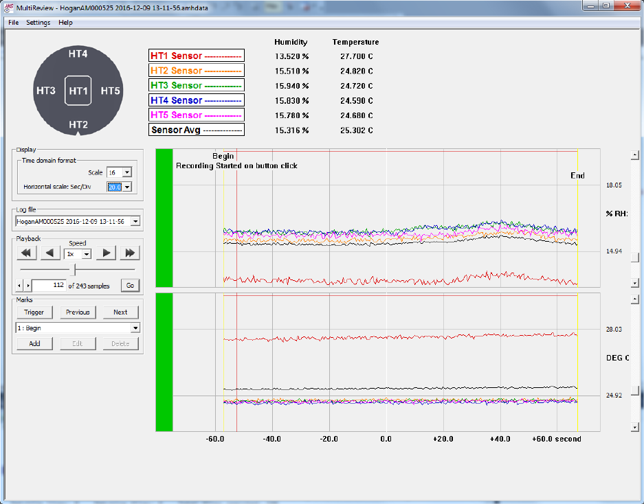
143
Figure A.2: AHS Mode MultiReview Main Screen