Sensors and Software NOGGIN500 NOGGIN 500 User Manual SmartSystemsV11
Sensors & Software Inc. NOGGIN 500 SmartSystemsV11
Contents
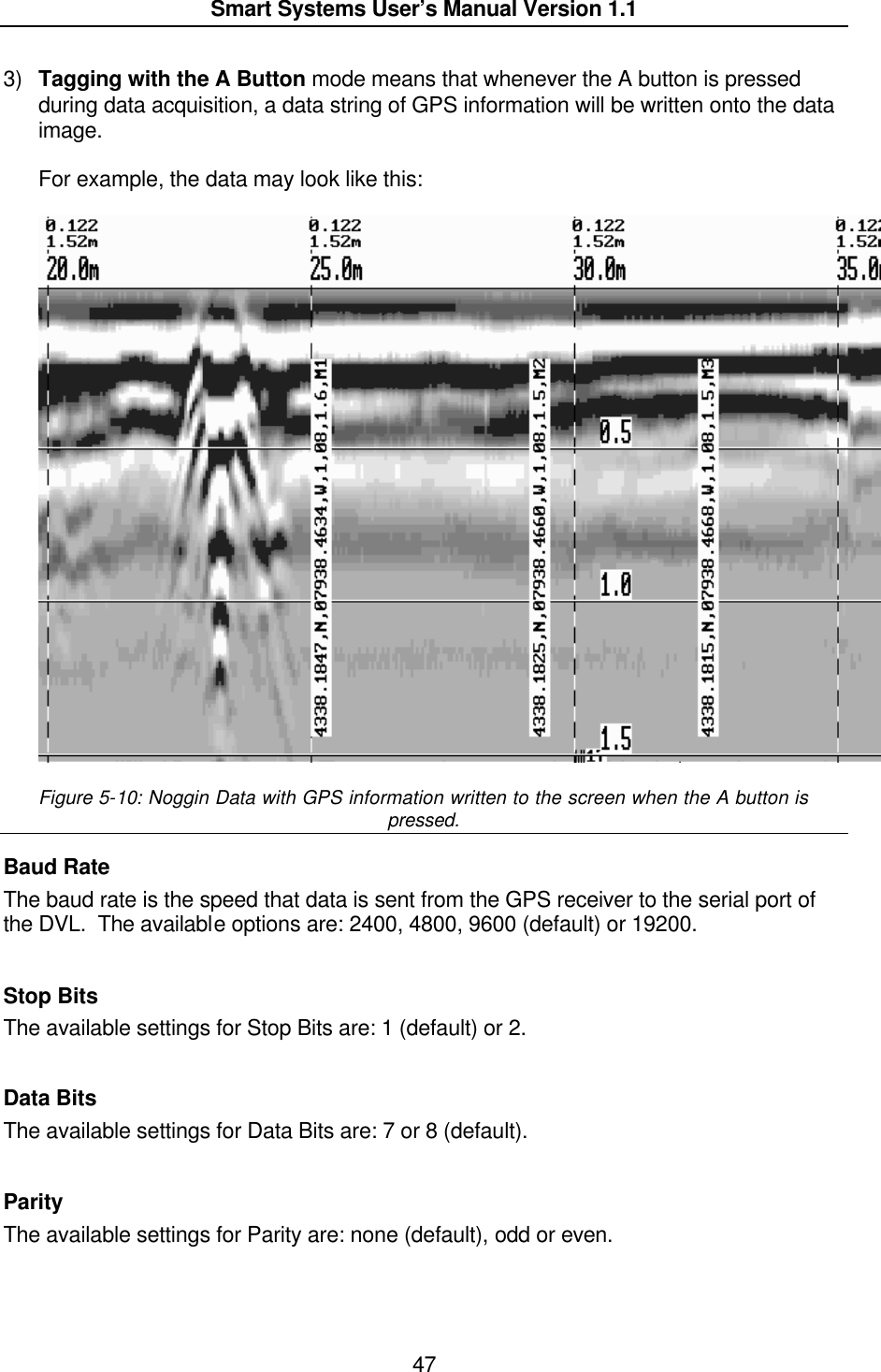
- 1. Users Manual Pages 1 to 40
- 2. Users Manual Pages 41 to 80
- 3. Users Manual Pages 801 to end
- 4. Revsied Users Manual
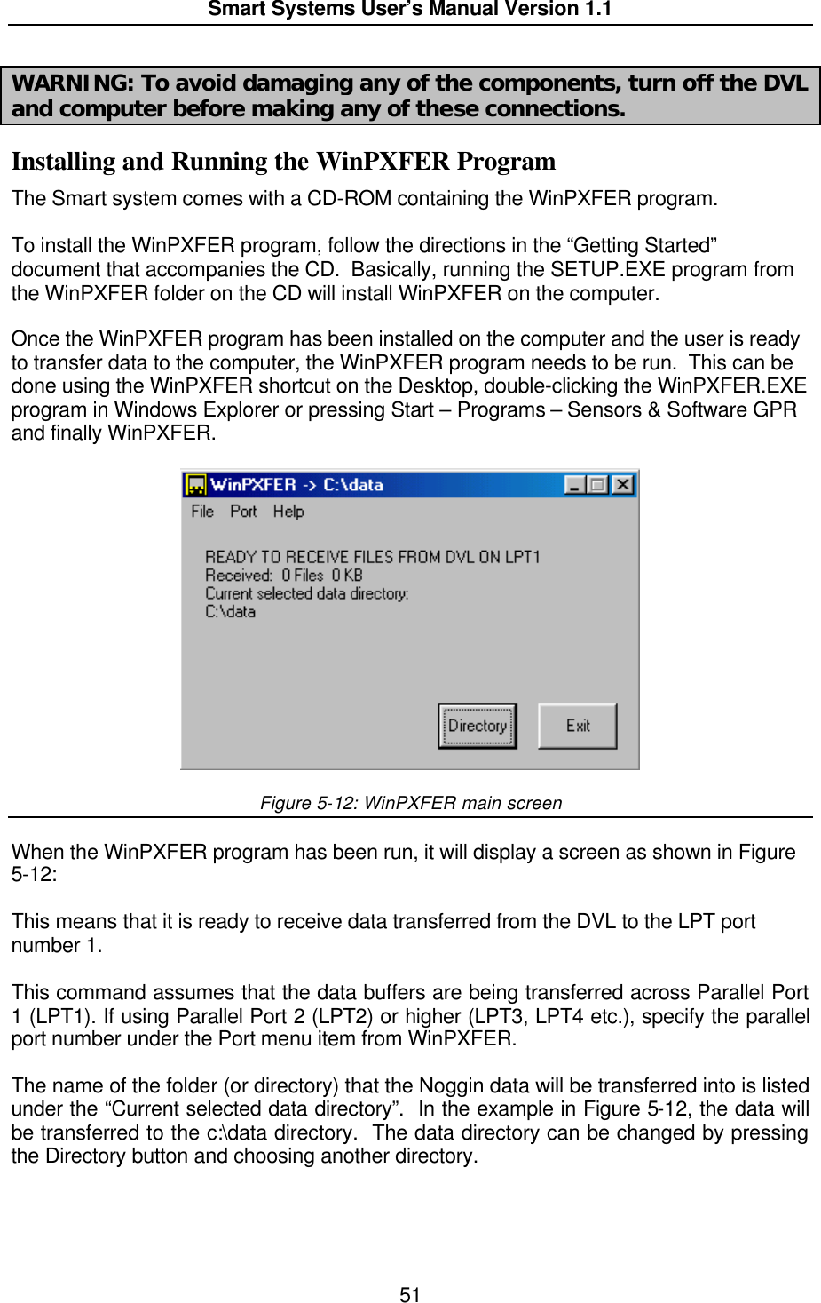
Users Manual Pages 41 to 80