Baron Services DSSR-250C Pulsar Digital Solid-State Radar System User Manual
Baron Services Inc Pulsar Digital Solid-State Radar System
Contents
Plot Assisted Setups

Plot–Assisted Setups
RVP8 User’s Manual
October 2004
4–1
4. Plot-Assisted Setups
The IFD receiver module replaces virtually all of the IF components in a traditional analog
receiver. The alignment procedures for those analog components are usually very tedious, and
require continued maintenance even after they are first performed. Subtle drifts in component
specifications often go unnoticed until they become so severe that the radar’s data are
compromised.
The RVP8 makes a big improvement over this by providing an interactive graphical alignment
procedure for burst pulse detection, Tx/Rx phase locking, and calibration of the AFC feedback
loop. You may view the actual samples of the burst pulse and receiver waveform, examine their
frequency content, design an appropriate matched filter, and observe live operation of the AFC.
It is a simple matter to check the spectral purity of the transmitter on a regular basis, and to
discover the presence of any unwanted noise or harmonics. Moreover, the RVP8 is able to track
and modify the initial settings so that proper operation is maintained even with changes in
temperature and aging of the microwave components.
The Plot-Assisted Setups are accessed using the various “P” commands within the normal TTY
setup interface. These commands are described later in this chapter. The RVP8 supports
opcodes that allow the host computer to monitor the data being plotted. The dspx utility can
display these plots directly on the workstation screen, and thus, can carry out the graphical
checkup and alignment procedures remotely via a network.
Plot–Assisted Setups
RVP8 User’s Manual
October 2004
4–2
4.1 P+ — Plot Test Pattern
The RVP8 can produce a simple test pattern to verify that the display software is working
properly. From the TTY monitor enter the “P+” command. This will print the message
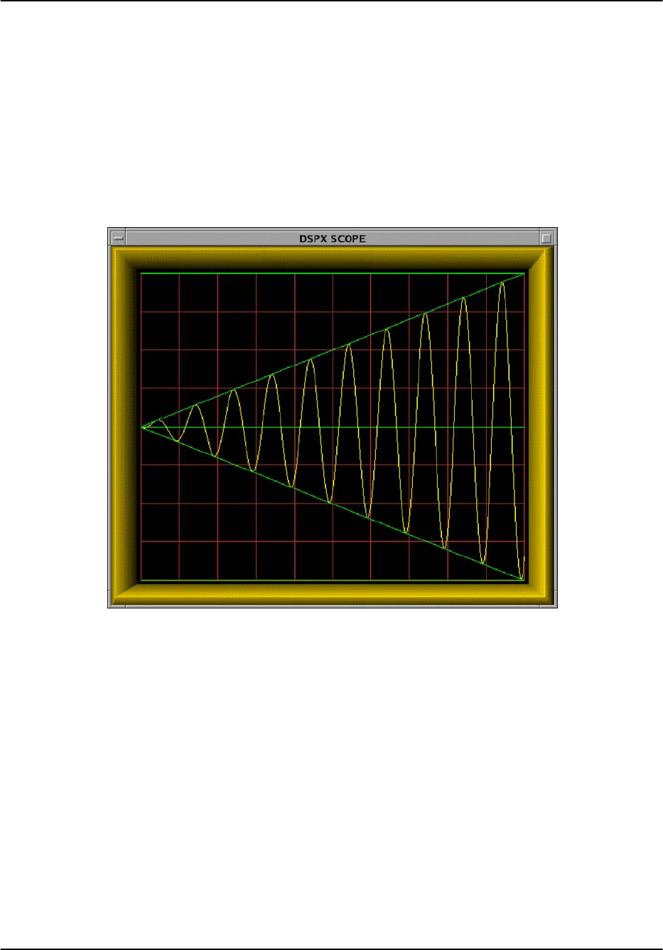
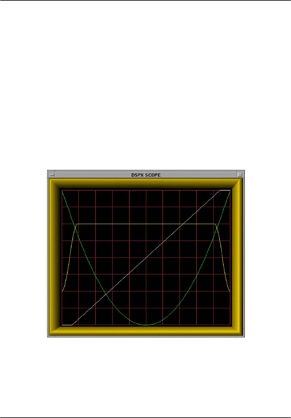
“Plotting Test Pattern...” on the TTY and then produce the plot shown in Figure 4–1.
This display is actually an overlay of six different strokes: 1) bottom line, 2) middle line, 3) top
line, 4) line sloping up, 5) line sloping down, and 6) the sine wave pattern. The later changes
phase with each plot so that, with a little imagination, it appears to be radiating from the left side
of the display.
Figure 4–1: The Test Pattern Display
When you are satisfied that the plot is being drawn correctly, type “Q” or hit ESC to return to
the TTY monitor.

Plot–Assisted Setups
RVP8 User’s Manual
October 2004
4–3
4.2 General Conventions Within the Plot Commands
The “Pb”, “Ps”, and “Pr” commands all have a similar structure to their TTY user interface.
Each command begins by printing a list of subcommands that are valid in that context. These
subcommands are single keystrokes that are executed immediately by the RVP8 as they are
typed. The “ENTER” key is not required. The available subcommands are different for each
plot command; but, as much as possible, each key has a similar meaning across all commands.
The working and measured parameters for each plot command are printed on the TTY as two
lines of information following the subcommand list. The first line contains settings that only
change when a subcommand is issued; but the second line is live and reflects the current status
of the burst input, the IF input, or the AFC output. The first line is printed just once, but the
second line is continually overprinted on top of itself. This makes it appear as a live status line
whose values always remain up to date. The ”Pb”, ”Ps”, and ”Pr” commands will report ”No
Trigger” on the TTY status line whenever the external trigger is expected but missing.
The TTY screen will scroll upward each time a new subcommand is executed, so that a history
of information lines and command activity can be seen on the screen. You may also use the
Carriage-Return key to scroll the display up at any time. If the initial list of subcommands
disappears off the top, you may type “?” to force a reprint. To exit the plot command entirely
and return to the TTY main menu type “Q” or ESC. These basic “help” and “exit” keystrokes
apply everywhere within the RVP8 setup menus. To save space and minimize clutter on the
TTY screen, they are not shown in the itemized list of subcommands.
Most commands have a lowercase and an uppercase version. If a lowercase command does
something, then its uppercase version does the same thing but even more so (or in reverse). For
example, if the “w” subcommand widens something by a little bit, then “W” would widen it a
lot. This simple convention reduces the number of different subcommand keys that are needed,
and makes the interface easier to memorize.
The graphical display and TTY status lines are continually updated with fresh data several times
per second. Occasionally it is useful to freeze a plot so that it can be studied in more detail, or
compared with earlier versions. To accomplish this, every plotting command supports a “Single
Step” mode that is accessed by typing the “.” (period) key. This key causes the display and TTY
status lines to freeze in their present state, and the message “Paused...” will be printed.
Subsequently, typing another “.” will single step to the next data update, but the plot and printout
will still remain frozen. Typing “Q” or ESC will exit the plot command entirely (as they
normally do). All other keys return the plot command to its normal live updating, but the key is
otherwise discarded (i.e., subcommand keys are not executed while exiting from single step
mode).
All of the plot commands support subcommands whose only purpose is to alter the appearance
of the display, e.g., zoom, stretch, etc. These subcommands make no changes to the actual
working RVP8 calibrations. However, the display settings are stored in nonvolatile RAM just
like all of the other setup parameters. This means that all previous display settings will be
restored whenever you restart each plot command. This is very convenient when alternating
among the various plots.

Plot–Assisted Setups
RVP8 User’s Manual
October 2004
4–4
The “Pb”, “Ps”, and “Pr” commands are intended to be used together for the combined purpose
of configuring the RVP8’s digital front end. You may, of course, run any of the commands at
any time; but the following procedure may be used as a guideline for first time setups. The full
procedure must be repeated for each individual pulsewidth that the radar supports.
1. Use Mb to set the system’s intermediate frequency (See Section 3.2.6).
2. Use Mt to choose the PRF and pulsewidth (See Section 3.2.4). Also, choose the
range resolution now, as it may constrain the design of the matched filter later.
3. Use Mt0,Mt1, etc., to set the relative timing of all RVP8 triggers that are used by
the the radar. Do not worry about the absolute values of the trigger start times.
Just setup their polarity and width, and their start times relative to each other (See
Section 3.2.5). Make an initial guess of FIR filter length as 1.5 times the
pulsewidth.
4. Use Pb to slew the start times of all triggers so that the burst pulse is properly
sampled (See Section 4.3). Refine the impulse response length if necessary so
that all samples easily fit within the display window.
5. Use Ps to design the matched FIR filter (See Section 4.4). Further refine the
impulse response length and passband width to achieve a filter that matches the
spectral width of the burst, and that has strong attenuation at DC. If the FIR
length is changed, return to Pb to verify that the burst is still being sampled
properly.
6. Continue using Ps and Mb to tune up the AFC feedback loop. The settings that
work for one pulsewidth should also work for all others.
7. Use Pr to verify that targets are being detected with good sensitivity (See Section
4.5).
Sometimes it is useful to run the Pb and Ps commands with samples from the IF-Input of the
IFD, rather than from the Burst-Input. Likewise, it is sometimes useful to view the Pr plots on
samples of Burst data. The top-level “~” command (See Section 3.3.3) allows you to do this
easily.
Plot–Assisted Setups
RVP8 User’s Manual
October 2004
4–5
4.3 Pb — Plot Burst Pulse Timing
For magnetron radars the RVP8 relies on samples of the transmit pulse to lock the phase of its
synthesized “I” and “Q” data, and to run the AFC feedback loop. The “Pb” command is used to
adjust the trigger timing and A/D sampling window so that the burst pulse is correctly measured.
4.3.1 Interpreting the Burst Timing Plot
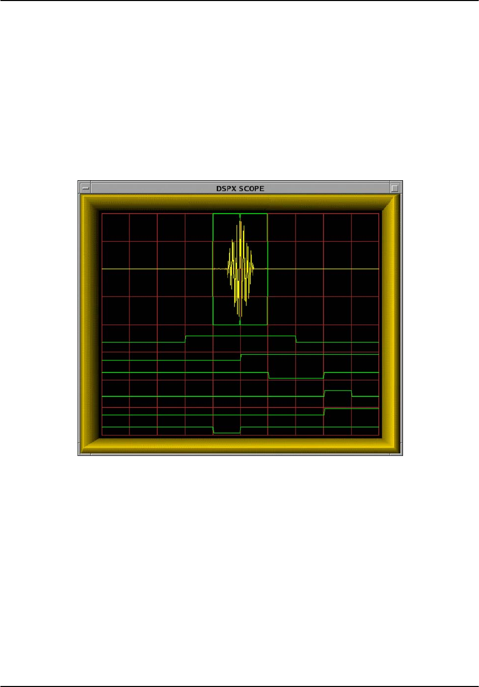
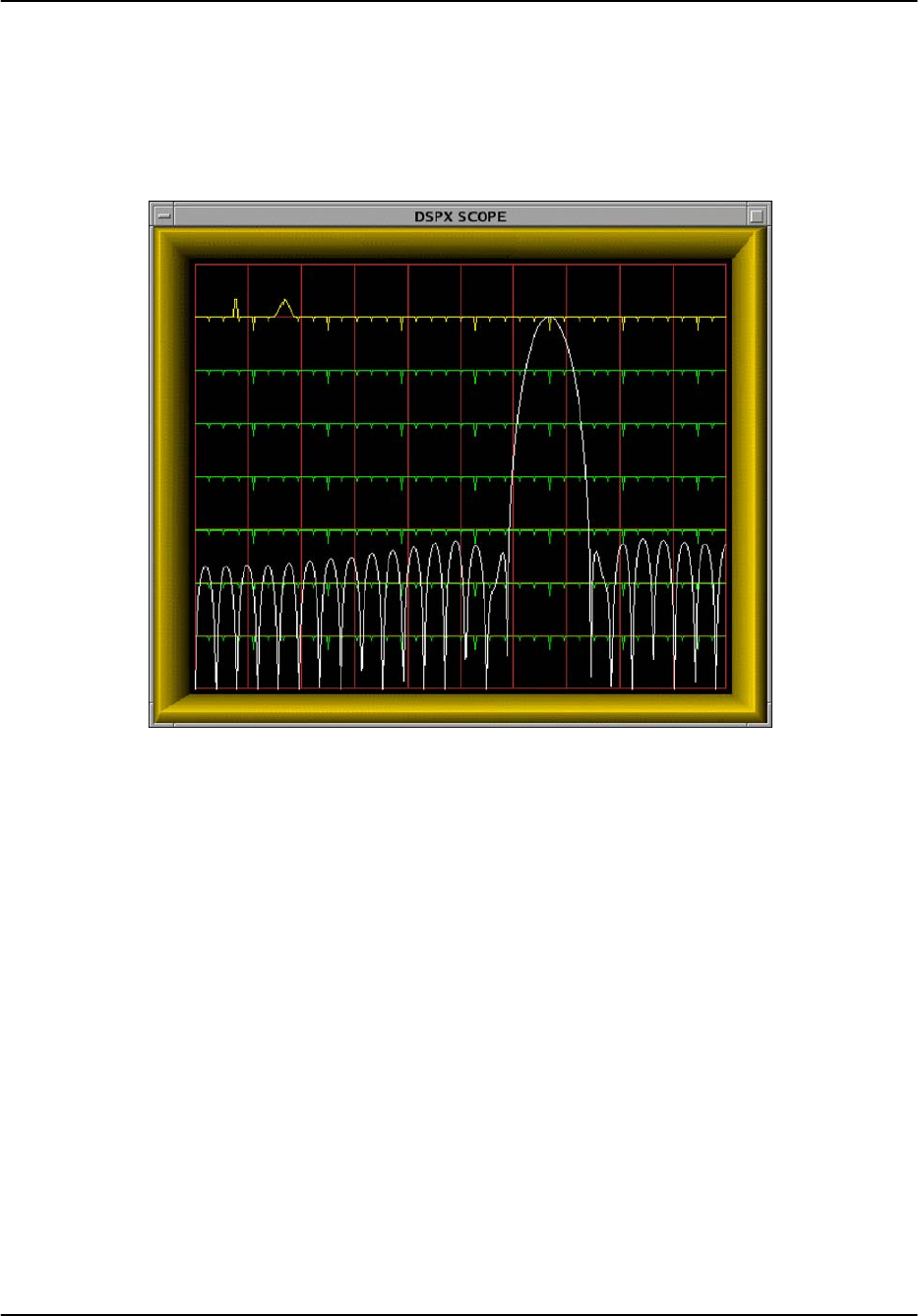
The display plot will ultimately resemble Figure 4–2, which shows a successful capture of the
transmitter’s burst pulse. The horizontal axis of the display represents time, and the overall time
span from the left edge to the right edge is listed as “PlotSpan” on the TTY.
Figure 4–2: Successful Capture of the Transmit Burst
The upper portion of the plot shows the sampling window wherein the burst pulse is measured.
The duration of this window is determined by the impulse response length of the matched FIR
filter. This is because the same FIR coefficients that compute “I” and “Q” are also used to
compute the reference phase vectors for the burst pulses. The A/D samples of the RVP8/IFD’s
burst input are plotted (somewhat brighter) within the sample window.
The RVP8 computes the power-weighted center-of-mass (COM) of the burst pulse envelope.
This allows the processor to determine the location of the “middle” of the transmitted pulse
within the burst analysis window. The Pb plot displays small tick marks on the top and bottom
of the burst sample window to indicate the location of the COM. These markers are only
displayed when valid burst power is detected. A second “error bar” is drawn surrounding the
tick mark to indicate the uncertainty of the mark itself. This error interval is used by the burst
pulse tracking algorithm to decide when a timing change can be made with confidence.

Plot–Assisted Setups
RVP8 User’s Manual
October 2004
4–6
It is possible to independently choose a subinterval of burst pulse samples that are used by the
AFC frequency estimator. Thus, the AFC feedback loop is not constrained to use the same set of
samples that are chosen for the FIR filter window. The FIR window typically is longer than the
actual transmitted pulse, and thus, the samples contributing to the frequency estimate will
include the leading and trailing edges of the pulse. These edges tend to have severe chirps and
sidebands, compared to the more pure center portion of the pulse. The AFC frequency estimate
(which is power weighted) could be mislead by these edges and might not tune to the optimum
center frequency if they were included.
The lower portion of the plot shows the six triggers that are output by the RVP8. Trigger #0 is at
the top, and Trigger #5 is on the bottom. They are drawn in their correct polarity and timing
relative to each other, and relative to the burst sample window. Note that the sample window is
always drawn in the center of the overall time span. Thus, depending on the PlotSpan and
location of the six trigger’s edges, triggers that do not vary within the plotted time span will
appear simply as flat lines.
The RVP8 defines “Range Zero” to occur at the center of the burst sample window. This also
defines the zero reference point for the starting times of the six programmable triggers. For
example, a trigger whose starting time is zero will be plotted with its leading edge in the exact
horizontal center of the display. Knowing this convention makes the absolute value of the
trigger start times more meaningful.
4.3.2 Available Subcommands Within “Pb”
The list of subcommands is printed on the TTY:
Available Subcommands within ’Pb’:
I/i Impulse response length Up/Dn
A/a & S/s Aperture & Start of AFC window
L/l & R/r Shift triggers & RVP8/Tx waveform left/right,
T/t Plot time span Up/Dn
Z/z Amplitude zoom
B/b BP Tracking On/Off (temporary)
+ Hunt for missing burst
. Single Step
These subcommands change the matched filter’s impulse response length, shift the radar
triggers, and alter the format of the display.
I/i The “I” command increments or decrements the length of the matched
filter’s impulse response. Each keystroke raises or lowers the FIR
length by one tap.
A/a & S/s These commands raise/lower the aperture/start of the subwindow of
burst pulse samples for AFC. If you never use these commands, then
the full FIR window will be used; however, shortening the AFC
interval will result in two sample windows being drawn on the plot.
The smaller AFC window should be positioned into the center portion
of the transmitted pulse, where the burst amplitude and frequency are
fairly stable.

Plot–Assisted Setups
RVP8 User’s Manual
October 2004
4–7
L/l & R/r These two commands shift the entire group of six RVP8 triggers left
or right (earlier or later in time). The lowercase commands shift in
0.025 msec steps, and the uppercase commands shift in 1.000 msec
steps (approximately). The reason for shifting all six triggers at once
is that the relative timing among the triggers remains preserved.
However, the absolute timing (relative to range zero) will vary, and
this will cause the burst pulse A/D samples to move within the sample
window.
T/t The “T” command increments or decrements the overall time span of
the plot. The available spans are 2, 5, 10, 20, 50, 100, 200, 500, 1000,
2000 and 5000 microseconds. The value is reported on the TTY as
“PlotSpan”.
Z/z The “Z” command zooms the amplitude of the burst pulse samples so
that they can be seen more easily. The value is reported on the TTY as
“Zoom”.
B/b These keys temporarily disable or re-enable the Burst Pulse Tracker.
The tracker must be disabled in order for the L/R keys to be used to
shift the nominal trigger timing. The “b” key disables tracking and
sets the trigger slew to zero; the “B” key re-enables tracking starting
from that zero value.
+The “+” subcommand initiates a hunt for the burst pulse. Progress
messages are printed as successive AFC values are tried, and the
trigger slew and AFC level are set according to where the pulse was
found. If no burst pulse can be found, then the previous trigger slew
and AFC are not changed.
4.3.3 TTY Information Lines Within “Pb”
The TTY information lines will resemble:
Zoom:x2, PlotSpan:5 usec, FIR:1.36 usec (49 Taps)
Freq:27.817 MHz, Pwr:–53.9 dBm, DC:0.14%, Trig#1:–5.00, BPT:0.00
Zoom Indicates the magnification (in amplitude) of the plotted samples. A
zoom level of “x1” means that a full scale A/D waveform exactly fills
the height of the sample window. Generally, the signal strength of the
burst pulse will not be quite this high. Thus, use larger zoom levels to
see the weaker samples more clearly. You may zoom in powers of two
up to x128.
PlotSpan Indicates the overall time span in microseconds of the complete scope
display, from left edge to right edge.
FIR Indicates the length of the impulse response of the matched FIR filter,
and hence, the duration of the burst pulse sample window. The length
is reported both as a number of taps, and as a time duration in
microseconds.

Plot–Assisted Setups
RVP8 User’s Manual
October 2004
4–8
Freq Indicates the mean frequency of the burst, derived from a 4th order
correlation model. The control parameters for this model are set using
the “Mb” command (Section 3.2.6).
Pwr Indicates the mean power within the full window of burst samples.
DC offsets in the A/D converter do not affect the computation of the
power, i.e., the value shown truly represents the waveform’s
(Signal+Noise) energy.
DC Indicates the nominal DC offset of the burst pulse A/D converter. This
is of interest only as a check on the integrity of the front end analog
components. The value should be in the range 2.0%.
Trig#1 Indicates the starting time of the first (of six) RVP8 trigger outputs.
This number will vary as the “L” and “R” subcommands cause the
triggers to slew left and right. Note that if the radar transmitter is
directly fired by an external pretrigger, then the pretrigger delay (in
the form “PreDly:6.87”) will be printed instead.
BPT This shows the present value of timing slew (measured in
microseconds) being applied to track the burst. The slew will be zero
initially when the RVP8 is first powered up, meaning that the normal
trigger start times are all being used.
4.3.4 Recommended Adjustment Procedures
The burst pulse timing must be calibrated separately for each individual pulsewidth. Repeat the
following procedure for each pulsewidth that you plan to use. Each iteration is independent.
It is first necessary to setup the proper relative timing for all RVP8 triggers that are being used.
The six trigger output lines are completely interchangeable, and each may be assigned to any
function within the radar system. For example, Trigger #0 might be the transmitter pretrigger,
Triggers #2 and #3 might synchronize external displays, and Triggers #1, #4, and #5 might be
unused.
Choose an initial impulse response length of 1.5 times the transmit pulsewidth. This length will
be refined later when the matched filter is designed (See Section 4.4). Adjust the plot time span
to view a small region around the sample window, and set the initial amplitude zoom to x16.
This assures that the plotted waveform will still be noticeable even if the burst signal strength is
very weak.
Verify that the transmitter is radiating, and observe the burst pulse samples on the display. Use
the “L” and “R” commands to shift the timing of all six triggers relative to range zero. This has
the effect of moving the burst sampling window relative to the transmitted pulse. Depending on
whether the triggers are set properly, you may at first see nothing more than a flat line of
misplaced A/D samples. However, after a few moments of hunting, the burst pulse should
appear on the display screen. Fine tune the triggers so that the burst envelope is centered in the
window, and adjust the amplitude zoom for a comfortable size display.
The clean center portion of the burst pulse should then be isolated to a narrower subwindow of
the overall FIR interval. Use the”A” and “S” commands to change the aperture and start of the
narrowed region from which the AFC frequency estimator’s data will be derived.

Plot–Assisted Setups
RVP8 User’s Manual
October 2004
4–9
Check that the burst pulse signal strength is reasonably matched to the input span of the
RVP8/IFD’s A/D converter. The maximum analog signal level is +4dBm. Exceeding this level
produces distorted samples that would seriously degrade the algorithms for phase locking and
AFC. However, if the signal is too weak, then the upper bits of the A/D converter are wasted
and noise is unnecessarily introduced. We recommend a peak signal level between –6dBm and
+1dBm, i.e., a signal that might be viewed at x2 or x4 zoom. Take note of the burst energy level
reported on the TTY; it will help decide the minimum energy threshold for a valid burst pulse,
which is needed in Section 3.2.6.
Plot–Assisted Setups
RVP8 User’s Manual
October 2004
4–10
4.4 Ps — Plot Burst Spectra and AFC
Once the transmit burst pulse has been captured the next step is to analyze its frequency content
and to design a bandpass filter that is matched to the pulse. In a traditional analog receiver the
matched filters use discrete components that can not be adjusted, and the transmit spectrum can
not be viewed unless a spectrum analyzer is on hand. The RVP8 eliminates all of these
restrictions via its “Ps” command, which plots the burst spectrum, designs the bandpass filter,
plots its frequency response, and also helps with alignment of the AFC.
4.4.1 Interpreting the Burst Spectra Plots
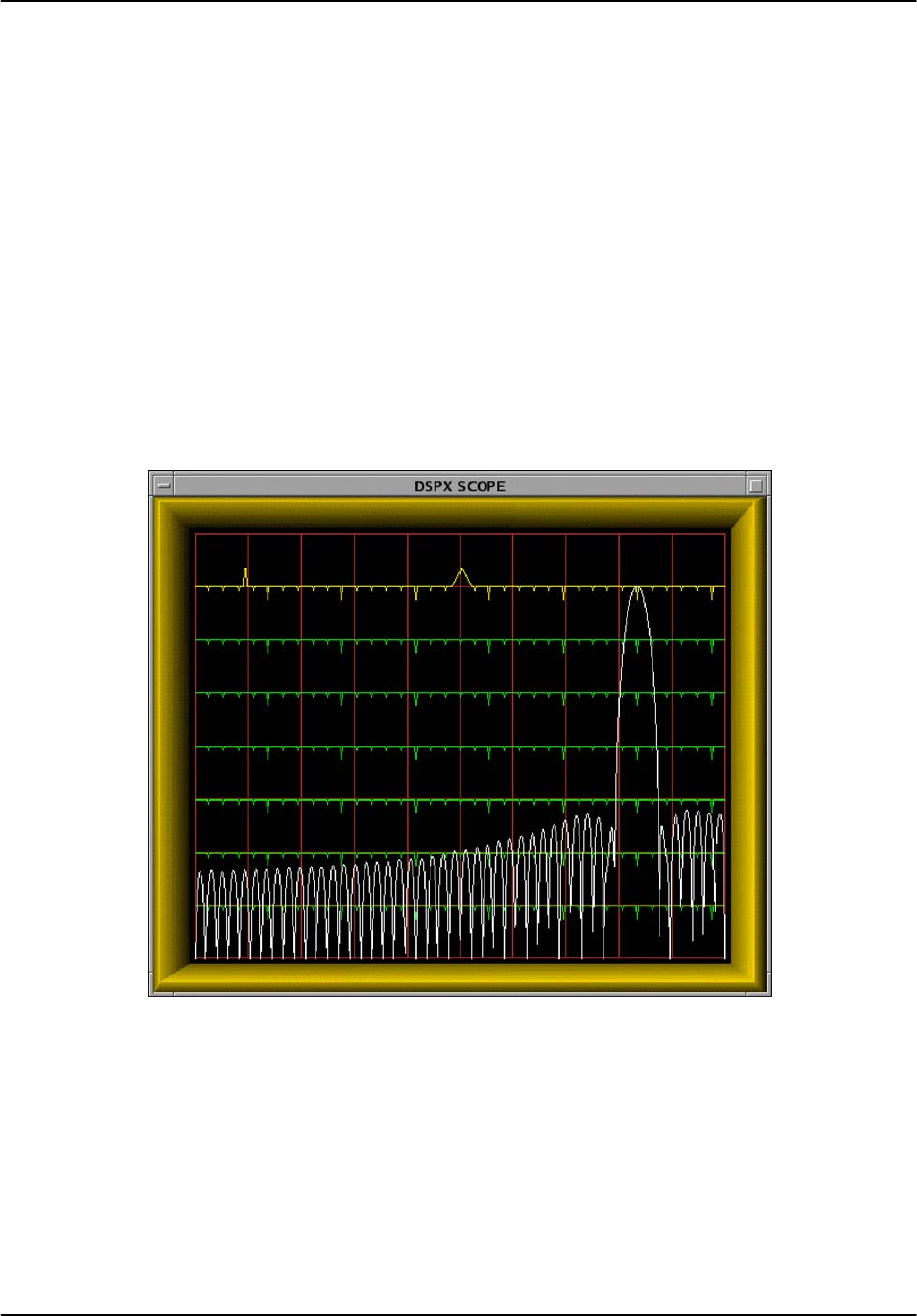
An example of a plot from the Ps command is shown in Figure 4–3. The display screen is
divided into two independent areas. The major portion (the lower seven eighths) is devoted to
power spectrum plots of the burst pulse and/or the matched filter response. The top portion
(single line) serves as a visual indicator of the present AFC level.
Figure 4–3: Example of a Filter With Excellent DC Rejection
The horizontal axis of the spectrum plot represents frequency. The overall span from the left
edge to the right edge is 36MHz for the RVP8 CAT-5E IFD, and 18MHz when the legacy RVP7
FibreOptic IFD is used. The remainder of this chapter will refer only to the newer RVP8 unit.
The exact endpoints of the plot depend on which alias band the radar’s intermediate frequency
falls in. For example, a 30MHz IF would imply a horizontal axis range of DC to 36MHz,
whereas a 60MHz IF would make the range 36MHz to 72MHz. The frequency span is printed
on the TTY when the command is first entered. Since the left edge of the spectral plot always

Plot–Assisted Setups
RVP8 User’s Manual
October 2004
4–11
represents an integer multiple of 36MHz, either the left side or the right side will always be a
multiple of 36MHz. This is important to remember when designing the matched filter, since
fixed DC offsets in the A/D converters will appear aliased at these 72MHz multiples.
The vertical axis of the spectrum plot is logarithmic and is marked with faint horizontal lines in
10-dB increments. An overall dynamic range of 70 dB can be viewed at once. The horizontal
lines also contain major and minor tick marks to help calibrate the frequency axis. Major marks
are small downward triangles that represent integer multiples of 5MHz; minor marks are in
between and represent 1-MHz steps. The power spectrum example in Figure 4–3 is from a
system with an intermediate frequency of 30MHz. Thus, the left edge of the plot begins at DC,
and the graph is centered on the sixth major tick, i.e., 30MHz.
Two types of spectra can be plotted on the screen: 1) the frequency response of the FIR filter,
and 2) the frequency content of the burst pulse itself. The burst spectrum is computed by first
applying a Hamming window to the raw samples. You may choose to view either plot
individually, or both at the same time.
Figure 4–3 is an example of a single filter response plot, whereas Figure 4–4 shows a combined
display of both spectra. The combined display makes it easy to compare the filter being
designed with the live waveform that it is intended to selectively pass. Note that the filter’s
frequency response is always drawn with its passband peak touching the top of the plot. The
vertical height of the burst spectrum, however, will vary with signal strength but can be adjusted
using the “Z” subcommand.
The horizontal line at the top of the plotting area is also marked with an upward pointing major
and minor tick. These indicate the present value of the burst pulse frequency estimator. The
major tick is a triangle whose position along the horizontal axis corresponds directly to the
estimated frequency. It should always be positioned directly over the main lobe of spectral
power. The minor tick gives finer scale resolution by indicating the fractional part of each
1-MHz multiple.
It is helpful to read the minor tick relative to the ten horizontal division lines that are present on
most scopes. Motion of the minor tick is apparent even with very small changes in burst pulse
frequency; a change of just 5 KHz can easily be seen. This means that you can observe the
frequency drift of the magnetron in great detail, and also watch the AFC’s behavior in real time.
The horizontal line at the very top of the display (above the spectra plot) serves to indicate the
present value of the AFC control voltage. The line contains an upward pointing major and
minor tick, similar to the ones used to represent the burst frequency estimate on the line below.
However, the horizontal axis now represents voltage rather than frequency, and the overall span
is the complete range of the AFC’s digital-to-analog converter. The major tick will move from
the left edge to the right edge as the AFC varies from its minimum to maximum value. The
minor tick will traverse the screen at ten times this rate.

Plot–Assisted Setups
RVP8 User’s Manual
October 2004
4–12
4.4.2 Available Subcommands Within “Ps”
The list of subcommands is printed on the TTY:
Frequency span of the plot is 36.0 MHz to 72.0 MHz.
Available Subcommands within ’Ps’:
I/i Impulse response length Up/Dn
N/n & W/w Filter bandwidth Narrower/Wider
U/u & D/d MFC Up/Down (On/Off ’=’ , Test ’|’)
A/a & S/s Aperture & Start of AFC window
# Print filter coefficients
$ Search for an optimal filter
V/v Number of spectra averaged
Z/z Amplitude zoom
<space> Alternate Plots
% Toggle between dual receivers
. Single Step
These subcommands change the design of the matched FIR filter, assist with calibration of the
AFC loop, and alter the format of the display.
I/i The “I” command increments or decrements the length of the matched
filter’s impulse response. Each keystroke raises or lowers the FIR
length by one tap. Often the matched filter’s characteristics can be
very much improved merely by changing the FIR length by one or two
taps. Be sure to experiment with this as you design your filter.
N/n & W/w The “N” and “W” commands change the passband width of the
matched filter, making it narrower or wider. The lower case
commands make changes in 1KHz steps, and the upper case
commands use 100KHz steps. The value is reported on the TTY as
“BW”. Often a small change in passband width will shift the exact
locations of the filter’s zeros, and possibly improve the DC rejection.
U/u & D/d The “U” and “D” commands implement the Manual Frequency
Control (MFC) override, and allow the RVP8/IFD’s AFC output
voltage to be manually set to any fixed level. The lower case
commands make changes in 0.05 D-Unit steps, and the upper case
commands use 1.0 D-Unit steps. The value is reported on the TTY as
“AFC”.
=MFC mode is toggled on and off using the “=” key. A warning will be
printed if the Ps command is exited while MFC is enabled, and you
will be given a second chance to reenable AFC.
|The AFC test submode is entered by typing the “|” key. The following
list of keybindings will be shown, and will remain in effect until the
test mode is exited by typing “Q”.
AFC Test Mode Subcommands
W Use Walking–Ones pattern
P Toggle Pin/Bit numbering
0–9,A–O Toggle AFC Bits 0–24 (Pins 1–25)

Plot–Assisted Setups
RVP8 User’s Manual
October 2004
4–13
2 2 2 2 2 1 1 1 1 1 1 1 1 1 1
4 3 2 1 0 9 8 7 6 5 4 3 2 1 0 9 8 7 6 5 4 3 2 1 0
– – – – – – – – – – – – – – – – – – – – – – – – –
O N M L K J I H G F E D C B A 9 8 7 6 5 4 3 2 1 0
The Ps command continues to run normally during the AFC test
mode. The customary AFC information will be replaced with a
hexadecimal readout of the present 25-bit value. Your live display
may look something like:
Navg:3, FIR:1.33 usec (48 Taps), BW:1.000 MHz, DC–Gain:ZERO
Freq:26.610 MHz, Pwr:–64.6 dBm, AFC–Test:0000207F (Bits)
Initially, a walking-ones bit pattern will be output in lieu of the normal
formatted AFC value. This test pattern shifts a single “1” downward
through the AFC word, making a transition approximately every 4ms.
It is intended to help ring out and test the wiring for digital AFC
installations. The walking-ones test is handy as an oscilloscope
diagnostic, and you may return to it at any time by typing “W”.
Typing any of the characters “0” through “9” or “A” through “O” will
enter a new mode in which a static 25-bit digital AFC pattern is
controlled directly. Each key toggles its corresponding bit, as
summarized in the keybindings printout. Any 25-bit pattern can be
made by toggling the appropriate bits (initially all zero) to one.
Within any particular pattern, it is also easy to toggle a particular bit
On/Off in order to verify its function.
The “P” command lets you decide whether the 25-bit word represents
a numeric AFC span that is mapped into pins via the pin-map table in
the Mb menu; or whether it represents those pins directly. The printed
hex test value will be followed either by “(Bits)” or “(Pins)”
accordingly. When in “Pins” mode, the “0” key toggles Pin-1, the “1”
key toggles Pin-2, etc. When in “Bits” mode, the “0” key toggles
whatever pin or pins have been designated to be driven from Bit-0 of
the numeric AFC. The “Pins” mode is useful when you are doing the
initial electrical tests of the wiring of each pin. After the pin wiring
has been verified and the Mb mapping table has been created, then the
“Bits” mode allows you to test the complete digital AFC interface.
#The “#” command results in a printout of the coefficients of the
current FIR filter. The values are scaled by the coefficient with the
largest absolute value, so that they all fall within the –1 to +1 range.
This detailed information may be used to model the behavior of the
filter for point targets that fall in between discrete range bins, e.g., as
will happen when performing a radar sphere calibration. See Section
5.1.1 for the exact definition of these coefficients.
$The “$” command performs an automatic search for optimal (DC gain
of zero) filters in the vicinity of the current one. As an example,
suppose that we wanted an optimal filter that was approximately 2.2
msec long and 650 KHz wide. We would first use the “I/i” and

Plot–Assisted Setups
RVP8 User’s Manual
October 2004
4–14
“W/wN/n” subcommands to manually move to that starting point.
Typing “$” would then print a dialog line in which the search span
length and width are chosen. You may keep the indicated values or
type in new ones, just as for all RVP8 setup questions. The search
begins when the spans are accepted.
The search procedure may require a few seconds to a few minutes,
depending on the length and width spans that are being scanned.
During this time, a progress message is printed showing the length and
width currently under examination. You may type “Q” to abort the
search and retain the original filter settings. When the search
completes normally, it will print “Done” and replace the old filter
settings with the best ones that could be found.
In dual-receiver mode, the ”$” command will search for a filter that
minimizes the maximum width and DC offset at both receiver’s
intermediate frequencies. The final filter will be the one that has the
best simultaneous performance at both IFs.
V/v The “V” command increments or decrements the number of burst
pulse spectra that are averaged together to create the plot. The count
ranges from one (no averaging) to 25, and is reported on the TTY as
“Navg”.
Z/z The “Z” command zooms (i.e. shifts on a logarithmic scale) in 1.0-dB
steps the amplitude of the burst pulse spectra. This is useful when the
overall 70dB plot span is not sufficient to hold the full range. Zoom
can also be used to line up the burst spectrum with the filter response
so that the two can be compared. The zoom level is not printed on the
TTY because there is nothing useful that could be done with it.
<space> The space bar alternates among three choices for the type of spectra
that are plotted: 1) FIR frequency response, 2) Burst pulse spectrum,
and 3) Both.
%In dual-receiver mode, the “%” command toggles between each
receiver. The printed status line is prefixed with ”Rx:Pri” or ”Rx:Sec”
according to which receiver is selected. Specifically, typing “%” will
toggle the plot of the FIR filter’s frequency response, and the printout
of its DC–Gain. However, the plotted spectrum and printed power
levels are always based on the sum of all input signals, and thus do not
change with “%“.
4.4.3 TTY Information Lines Within “Ps”
The TTY information lines will resemble:
Navg:3, FIR:1.33usec (48 Taps), BW:1.000, MHz, DC–Gain:ZERO
Freq:30.027 MHz, Pwr:–64.2 dBm, Loss:1.2dB, AFC:23.05% (Manual)
Navg Indicates the number of burst spectra that are averaged together prior
to plotting. Larger amounts of averaging increase the ability to see
subtle spectral components, but the display will update more slowly.

Plot–Assisted Setups
RVP8 User’s Manual
October 2004
4–15
FIR Indicates the length of the impulse response of the matched FIR filter.
See description on Page 4–7.
BW Indicates the actual 3dB bandwidth of the matched filter. This is the
complete width of the passband from the lower frequency edge to
upper frequency edge. Note that the filter’s center frequency is fixed
at the radar’s intermediate frequency, as chosen in the “Mb” setup
command.
DC-Gain Indicates the filter’s response to DC (zero frequency) input. The value
is a negative number in decibels, or the word “ZERO” if the filter has
a true zero at DC. The filter’s DC gain should be kept at a minimum
so that fixed offsets in the A/D converters will not propagate into the
synthesized “I” and “Q” values.
Freq Indicates the mean frequency of the burst. See description on Page
4–8.
Pwr Indicates the average power in the full burst sample window. See
description on Page 4–8.
Loss The filter loss is a positive number in deciBels, and is only displayed
if the overall burst power exceeds the minimum valid burst threshold
set in the Mb command (clearly, it would not be possible to compute
the filter loss when the burst waveform is missing). The filter loss is
discussed further in Section 4.4.4.
AFC Indicates the level and status of the AFC voltage at the RVP8/IFD
module. The number is the present output level in D-Units ranging
from –100 to +100. The shorter “%” symbol is used since percentage
units correspond in a natural way to the D-Units.
An additional number in square brackets will be printed to the right of
the AFC level to show the encoded bit pattern which corresponds to
that level. This will only appear when the RVP8 deduces that a special
digital format is being used, i.e., when the backpanel phase-out lines
have been configured for AFC, or when any of the following are not
true: a) the low and high numeric AFC span is –32768 to +32767, b)
the uplink is enabled, c) the uplink format is binary, and d) pinmap
protocol is OFF. Binary format is printed in base-10, BCD format is
printed in Hex, and 8B4D format is printed with the low 16-bits (four
BCD digits) in Hex and the upper bits in base-10.
The AFC mode is shown to the right of the numerical value(s), and
can take on the following states.
(Disabled) Indicates that neither AFC nor MFC are enabled. The
output voltage remains fixed at 0% (center of its range).
(Manual) Manual Frequency Control (MFC) is overriding AFC.
The “U” and “D” commands can be used to slew the
voltage up and down.
Whenever any of the following four states appears, it implies that AFC
is enabled and that MFC is disabled.

Plot–Assisted Setups
RVP8 User’s Manual
October 2004
4–16
(NoBurst) The energy in the burst is below the minimum energy
threshold for a valid pulse (See Page 3–25). The AFC
loop remains idle.
(Wait) The burst pulse has become valid just recently, but the
AFC loop is idle until the transmitter stabilizes (See
Page 3–26)
(Track) The burst pulse is valid, and the AFC loop is tracking
in order to bring the burst frequency within the inner
hysteresis limits.
(Locked) The burst pulse is valid and the AFC loop is locked.
The burst frequency is now within the outer hysteresis
limits and has previously been within the inner limits
while tracking. This is the stable operational mode in
which data acquisition should take place.
4.4.4 Computation of Filter Loss
The Ps printout displays the power loss (calibration error) that results when the given filter is
applied to the given transmit burst waveform. This allows you to correct for the difference
between what a broad-band power meter measures as the overall transmit power, and what the
RVP8 narrow-band receiver will detect within its passband. The filter loss is a subtle quantity
that depends on the combined characteristics of both the transmit waveform and the receiver
matched filter.
The filter loss is zero if the burst waveform consists of a pure sinusoid at the designated
intermediate frequency. It is also very near zero as long as most of the burst energy is confined
within the passband of the RVP8’s filter. The filter loss will increase as the bandwidth of the
burst waveform increases and begins to spill out of that passband. Typical losses for a
well-matched filter are in the 0.5–1.8dB range, depending on the FIR length and other design
criteria.
As an example, consider how the RVP8 filters would respond to a simple rectangular pulse of
energy lasting To seconds. For this discussion we can ignore the sinusoidal IF carrier that must
also be present within the pulse, and just focus on the rectangular envelope. This is valid
because the signal bandwidth, and hence the filter loss, is determined entirely by the shape of the
modulation envelope. For a pulse of length To to have unit-energy it must have an amplitude of
1ńTo
Ǹ . By centering this pulse at time zero the power spectrum is easily computed using a
real-valued integral:
S(f)+ȧ
ȧ
ȡ
Ȣŕ
Toń2
–Toń2
1
To
Ǹcos( 2pft)dt ȧ
ȧ
ȣ
Ȥ
2
+sin2(pfT
o)
p2f2To
where f is the frequency in Hertz. This is the familiar “synch” function, whose main frequency
lobe extends from –1ńTo to 1ńTo Hertz, and whose total power integrated over all frequencies
is 1.0.

Plot–Assisted Setups
RVP8 User’s Manual
October 2004
4–17
We can now examine what the filter loss (dBloss ) would be if this pulse were applied to a
bandpass filter. The filter loss is simply the ratio of the power that is passed by the filter, divided
by the total input power (1.0 in this case). Assume for the moment that the filter is an ideal
bandpass filter centered at zero Hertz (corresponding to how S(f) was defined) and having a
bandwidth Bw, then:
dBloss +–10 log10
ȧ
ȧ
ȡ
Ȣŕ
Bwń2
–Bwń2
S(f)df ȧ
ȧ
ȣ
Ȥ
This integral can be computed for a few “interesting” filter bandwidths, yielding filter losses of
0.44dB, 1.11dB, and 3.31dB when Bw is 2ńTo, 1ńTo, and 1ń2To respectively. These three
example bandwidths correspond to filters that pass the entire main frequency lobe, half of that
lobe, and one quarter of it.
You can experimentally verify these results using the RVP8 as follows:
SUsing the Mt0 command, setup a To+0.5 msec trigger pulse from the RVP8 in the
vicinity of range zero, and use that trigger to gate a signal generator whose output is
applied to the RVP8/IFD Burst Input. Also setup 125-meter range resolution, and a
rather long 6.0 msec impulse response length. The long length will make the transition
edges of the matched filter as steep as possible, so that it becomes a reasonably good
approximation to the ideal bandpass filter used in the above analysis.
SUse the Pb command to verify that the burst pulse is present, and position the triggers
left and right until the pulse is centered exactly at zero.
SUse the Ps command to examine the frequency spectrum of the pulse. You should see a
main energy lobe that is 4MHz wide and centered at the radar’s IF. There should also be
weaker lobes spaced 2MHz apart on both sides of the main lobe. If the lobe spacing does
not look quite right, it may be because the signal generator has slightly shortened or
lengthened the trigger gate.
SContinue using Ps to examine filters that are 4MHz, 2MHz, and 1MHz wide at their 3dB
points. You should see filter losses reported that are very close to the theoretical values
for the ideal bandpass filter.
In the above analysis we have assumed that S(f) is the idealized power spectrum of a continuous
time signal. Of course, the RVP8 filter loss algorithm can only work from an estimate of S(f)
that is obtained from a finite number of samples. The filter loss calculation thus becomes more
complicated than the above example in which we integrated an idealized filter response over an
idealized power spectrum.
Let B
^(f) denote the estimated power spectrum of the continuous-time Tx burst waveform, for
which we have only a finite number of discrete samples {bn}. For purposes of this discussion
we can assume that the frequency variable f is continuous. Furthermore, let C
^(f) denote a
power spectrum estimate that is derived in an identical manner using the same number of

Plot–Assisted Setups
RVP8 User’s Manual
October 2004
4–18
samples, but of a pure sine wave at the radar’s IF. The RVP8 determines B
^(f) according to its
sampled measurement of the transmitted waveform; however it can calculate C
^(f) internally
based on an idealized sinusoid. The reported filter loss is then:
dBloss +–10 log10
ȧ
ȧ
ȧ
ȧ
ȡ
Ȣ
ŕ|H(f)|2B
^(f)df
ŕB
^(f)df
Bŕ|H(f)|2C
^(f)df
ŕC
^(f)df
ȧ
ȧ
ȧ
ȧ
ȣ
Ȥ
Where |H(f)|2 is the spectral response of the RVP8 IF filter, and the integrals are performed over
the Nyquist frequency band that is implied by the RVP8/IFD sampling rate. Note that the two
integrals involving C
^(f) will have constant value and need only be computed once. They serve
to normalize the B
^(f) integrals in such a way that the filter loss evaluates to 0dB whenever the
transmit burst is a pure tone at IF.
This normalization is necessary for the filter loss values to be meaningful. Regardless of the
bandwidth and center frequency of H(f), the filter loss should be reported as 0dB whenever the
Tx waveform appears to have zero spectral width, i.e., is indistinguishable from a pure IF
sinusoid. Of course, the real Tx waveform has only finite duration, and thus should never look
like a pure tone as long as the RVP8 is able to “see” the entire Tx envelope. For this reason, it is
important that the filter’s impulse response length be set long enough (using the Pb plot) to
insure that all of the details of the Tx waveform are being captured. If the entire Tx envelope
does not fit within the FIR filter, then the filter loss will be underestimated because the Tx
spectrum will appear to be narrower than it really is.
The RVP8’s calculation of digital filter loss is very similar to how the loss of an analog filter
would be measured on a test bench. Suppose we are given an analog bandpass filter and are
asked to determine its spectral loss when a given waveform is presented. We could use a power
meter to measure the waveform power before and after the filter is inserted, and compute the
ratio of these two numbers. This corresponds to the first integral ratio in the above equation.
However, this is not by itself an accurate measure of filter loss because it does not take into
account the bandwidth-independent insertion loss. Put another way, a flat 3dB pad would seem
to produce a 3dB filter loss in the above measurement, but that is certainly not the result that we
desire. The remedy is to make a second pair of power measurements of the filter’s response to a
CW tone at the passband center. This serves to calibrate the gain of the filter, and allows us to
compute a filter loss that captures the effects of spectral shape independent of overall gain. This
normalization step corresponds to the second integral ratio in the above equation.
If your radar calibration was performed using CW waveforms, then the reported filter loss
should either be added to the receiver calibration losses, or subtracted from the effective transmit
power; the net result being that dBZ0 will increase slightly.
In dual-receiver systems the filter loss is computed for the primary and secondary channels using
only the portion of bandwidth that is allocated to that channel. For example, if the two IFs are
24MHz and 30MHz, then the filter losses for each channel would use the frequency intervals
21–27MHz and 27–33MHz respectively. This is necessary to avoid picking up energy from the
Plot–Assisted Setups
RVP8 User’s Manual
October 2004
4–19
other receiver and interpreting it as out-of-band input power. A consequence, however, is that
the real out-of-band power is underestimated, i.e., the filter loss itself is underestimated. We
recommend temporarily switching dual-receiver systems back to single-receiver mode when the
filter loss is being measured. This is easily done by changing the Mc setup question back to
“single”, and disconnecting the secondary burst input to the RVP8/IFD.
4.4.5 Recommended Adjustment Procedures
The Ps command should be used only after the burst pulse has been successfully captured by
way of the Pb command. Use the <space> key to display the burst spectrum plot by itself, and
use the “Z” key to shift the entire graph into view. You are now looking at the actual frequency
content of the transmitted pulse. The plot should show a clean main power lobe centered at the
receiver’s intermediate frequency. Check the spectrum for spurious harmonics, excessive width,
and other out-of-band noise. Make any adjustments in the transmitter that might give a sharper
main lobe or reduced spurious noise.
Once we know the power spectrum of the transmitted pulse we can begin designing the matched
FIR filter. Use the <space> key to display both the filter response and the burst spectrum on the
same plot. Use the “Z” key to shift the burst’s main lobe up to the top horizontal line of the
graph. This makes it level with the filter’s peak lobe, which is always drawn tangent to the same
top line.
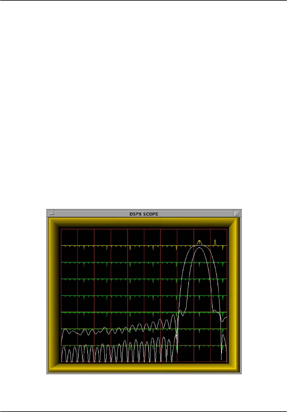
Figure 4–4: Example of a Poorly Matched Filter

Plot–Assisted Setups
RVP8 User’s Manual
October 2004
4–20
Begin with the FIR length that was chosen previously in the Pb command, and use the “N” and
“W” keys to set an initial bandwidth equal to the reciprocal of the pulsewidth. The main lobes
of the two plots should more-or-less overlap. Experiment with changing the FIR length and
bandwidth to achieve a filter with the following properties.
SThe filter width should be no greater than the burst spectral width. A wider passband
will reduce the SNR of the received signal because out-of-band noise would be allowed
to pass.
SThe DC gain should be as small as possible, preferably less than –64dB (See discussion
below).
SIf there are conspicuous interference spikes at particular frequencies, try to adjust the
location of the filter’s zeros so that the interference is maximally attenuated.
The filter should not pass any frequencies that do not actually contain useful information from
the original transmitted pulse. If anything, choose a filter whose width is slightly narrower than
the burst’s spectral width. Figure 4–4 shows an example of a filter that is poorly matched to the
pulse. Although the filter has fairly good DC rejection, it passes frequencies that are outside of
the transmitter’s broadcast range. These frequencies contribute nothing but noise to the
synthesized “I” and “Q” data stream.
There are two procedures for optimizing the performance of the FIR filter:
SManual Method –– The process of arriving at a nearly optimal filter will require a few
minutes of hunting with the “I”, “W”, and “N” keys. Every time you press any of these
keys the RVP8 designs a new FIR filter from scratch, and displays the results.
Fortunately, the DSP chips are fast enough that this can be done quickly and
interactively. Even though the user must still control two degrees of freedom (length and
bandwidth), the RVP8’s internal design calculations are actually performing several
hundred iterative steps each time, which preferentially select for the best filter. Because
the FIR coefficients are quantized in the filter chips themselves, the process of finding an
optimal filter becomes quite nonlinear.
SAutomatic Method –– Simply type the “$” command and let the RVP8 do all of the
work (See description in Section 4.4.2).
The offset error of the RVP8/IFD’s A/D converter is at most 10mV, i.e., –27dBm into its 50W
input. If we wish to achieve 85-dB of dynamic range below the converter’s +4dBm saturation
level, then we expect usable “I” and “Q” values to be obtainable from a (sub-LSB) input signal
at –81dBm. This is 54dB below the interference that would result from the worst-case A/D
offset. But a weak input signal at –81dBm would still be damaged by even an equal level of DC
interference. Therefore, adding another 10dB safety margin, we get –64dB as the recommended
maximum DC gain of the matched filter. This DC gain should be reduced even further if it is
known that coherent leakage is present in the receive signal at a level greater than the –27dBm
worse-case A/D offset.
Plot–Assisted Setups
RVP8 User’s Manual
October 2004
4–21
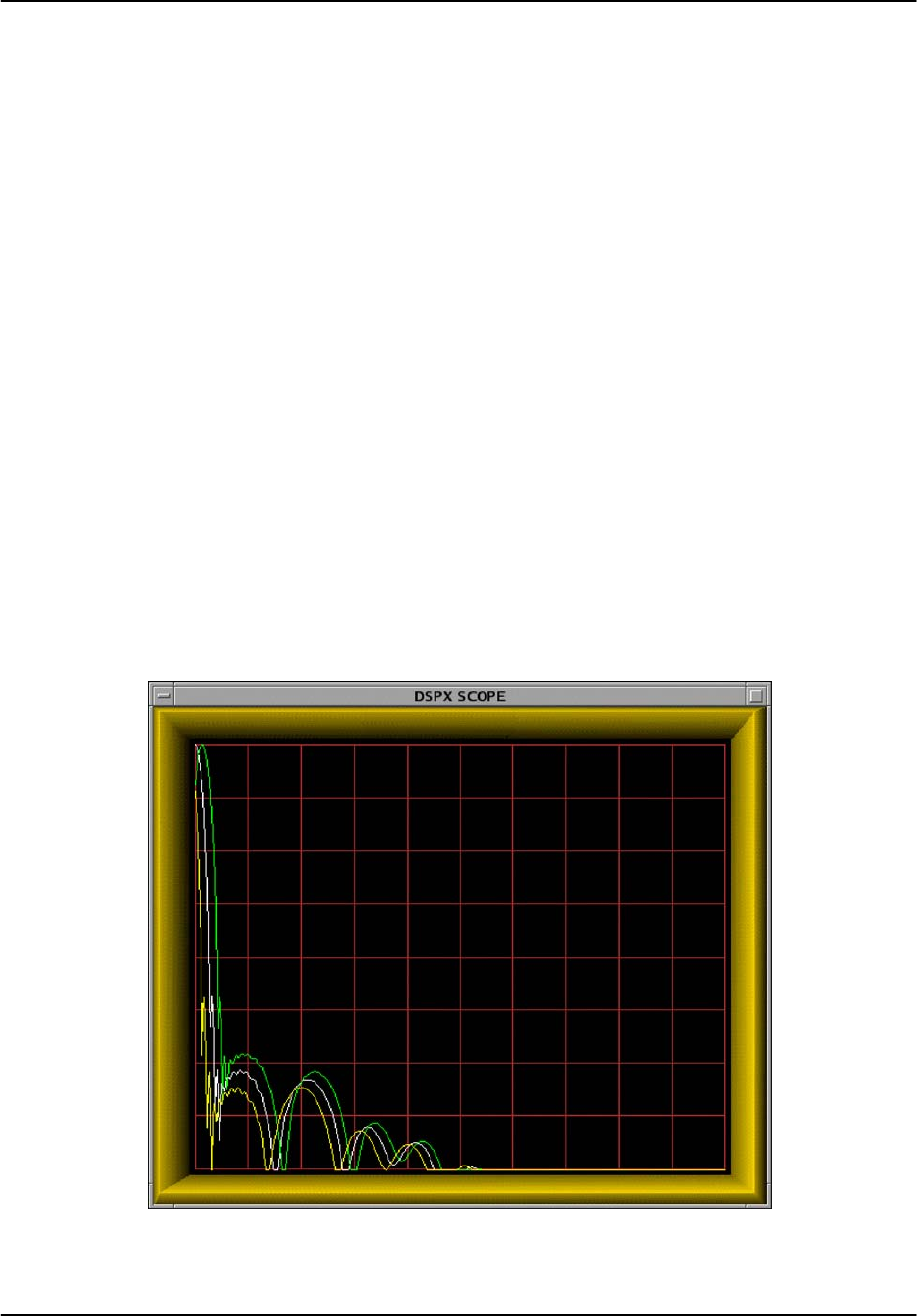
Figure 4–5 shows a 60MHz filter with particularly poor (–42dB) DC rejection. The frequency
range of the plot is 36–72MHz; hence, DC appears aliased at the right edge and we can see a
peak in the filter’s stopband at DC. Contrast this with the filter shown in Figure 4–3 that has a
true zero at DC. In general, a poor filter can be converted into a “nearby” good filter by making
only incremental changes to the impulse response length and/or desired bandwidth.
Figure 4–5: Example of a Filter With Poor DC Rejection
Plot–Assisted Setups
RVP8 User’s Manual
October 2004
4–22
4.5 Pr — Plot Receiver Waveforms
The “Pb” and “Ps” commands described in the previous sections have been used to analyze the
signal that is applied to the “Burst-In” connector of the RVP8/IFD receiver module. The task
that remains is to checkout the actual received signal that is connected to “IF-In”. The goal is to
verify that the received signal is clean and appropriately scaled, and that nearby targets can be
seen clearly. The “Pr” command is used to make these measurements.
4.5.1 Interpreting the Receiver Waveform Plots
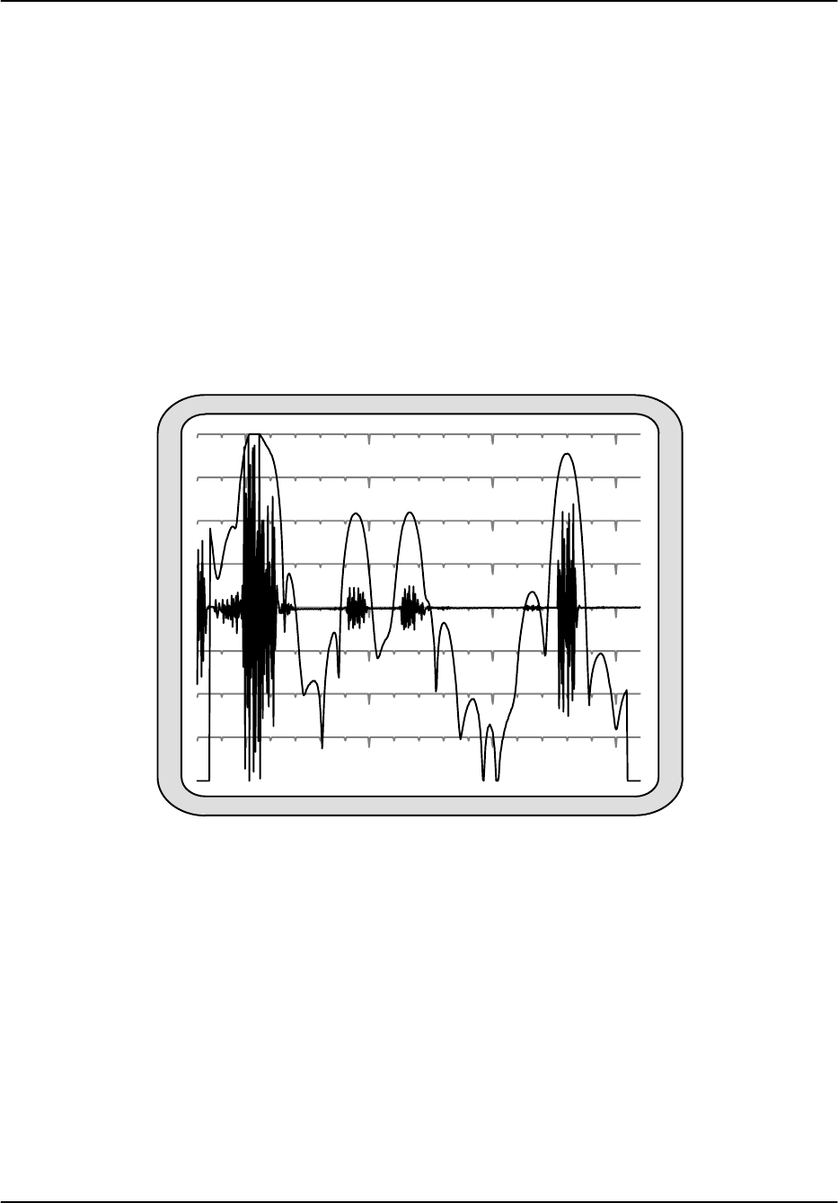
An example of a plot from the Pr command is shown in Figure 4–6. The horizontal axis
represents time (range) starting from a selectable offset and spanning a selectable interval. The
data are acquired from a single transmitted pulse, are are plotted both as raw IF samples and as
the LOG of the detected power using the FIR filter for the current pulsewidth.
Figure 4–6: Example of Combined IF Sample and LOG Plot
The IF samples are plotted on a linear scale as signed quantities, with zero appearing at the
center line of the scope. Any DC offset that may be present in the A/D converter is not
removed, and will be seen as a shift in the baseline at higher zoom levels. For example, the
converter’s worst case DC offset of 10mv would appear as a 91-count offset in the 12-bit range
spanning –2048 to +2047. At the x32 or higher zoom scales, this offset would peg the sample
plot off scale. Typically the DC offset will be much less than this worst case value; but the
RVP8 preserves the DC term in the Pr sample plot so that its presence is not forgotten.
The “AC” amplitude of the IF samples will increase wherever targets are present. On top of
these samples is drawn the detected power on a logarithmic scale. Each horizontal line
represents a 10dB change in power. The graph is scaled so that the LOG power reaches the top
display line when the samples occupy the full amplitude span. Using Figure 4–6 as an example,

Plot–Assisted Setups
RVP8 User’s Manual
October 2004
4–23
the two equal-power targets just to the left of center are approximately 18dB down from the top.
The amplitude of the samples is thus 10(*18ń20) +0.13, i.e., 13% of full scale. This
correspondence between the LOG scale and the amplitude scale applies regardless of the plot’s
zoom level. As the IF samples are zoomed up and down by factors of two, the LOG plot will
shift up and down in 6dB steps.
The LOG plot is obtained by convoluting the FIR filter coefficients with the raw IF data
samples, and then plotting log(I2)Q2) at each possible offset along the sampling interval.
This convolution produces only (1 + N – I) output points, where N is the number of sample
points and I is the length of the FIR filter. For this reason the LOG plot begins approximately
I/2 samples from left side and ends approximately I/2 samples from the right.
The LOG points are computed at each possible offset within the raw IF samples. At the nominal
72MHz sampling rate the spacing between LOG samples will be a mere 4.17 meters. Thus, the
LOG plot gives a very detailed view of received power versus range. Of course, successive
LOG points will be highly correlated because successive input data intervals differ by only one
sample point. This is why the LOG plots appear smooth compared to the instantaneous variation
of the raw IF samples.
As the starting offset of the Pr plot is decreased to range zero you will begin to see part of the
burst pulse (the second half of it) appear at the left edge of the plot. This is because the burst
data samples are multiplexed onto the same fiber cable that carries the IF data samples. Zero
range is defined to occur at the center of the burst window; hence, the later half of the burst
pulse will be visible when the plot begins at range zero.
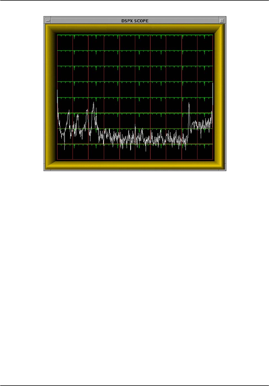
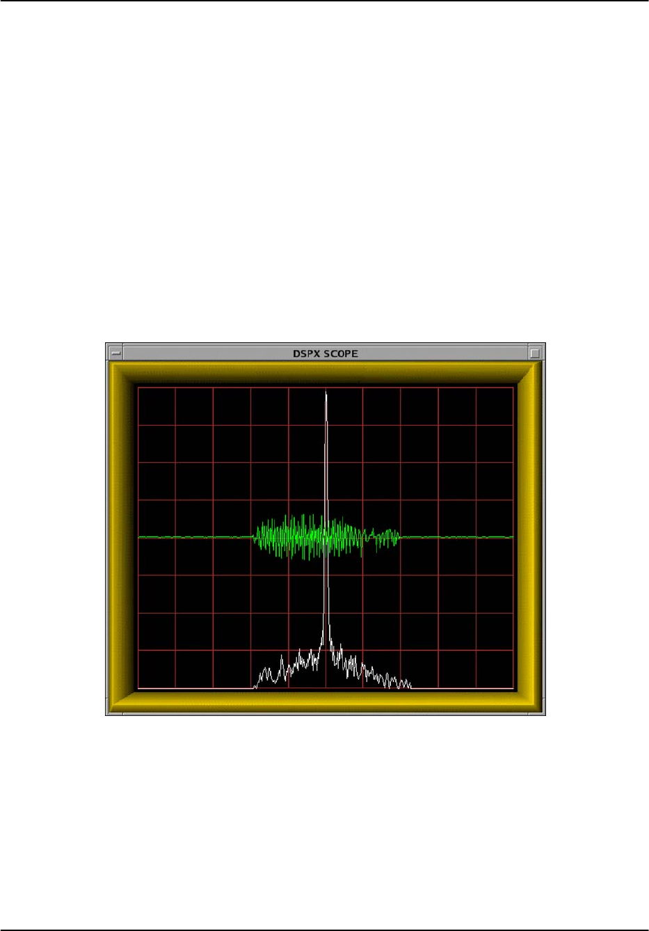
A second type of Pr display is shown in Figure 4–7. This plot shows a frequency spectrum of
the received data samples in a format that is nearly identical to the Ps display. The horizontal
axis represents the same band of frequencies (half the sampling rate), and the vertical axis
represents power in 10dB steps. The entire vertical axis is used so that an overall span of 80dB
is visible. This particular plot was made with the time span set to 50 msec, and with a 1-meter
antenna attached to the IF input so that a broad range of signals (radio stations, electrical noise,
etc.) would be detected.
The purpose of the Pr power spectrum is to check for spurious interference in the IF signal from
the radar receiver. The spectrum should be viewed with the transmitter turned off, and with the
starting range moved out so that the burst samples are not mixed in with the receiver data. The
power spectrum is computed using the complete interval of raw IF samples which, depending on
the chosen time span, may contain many hundreds of points. The frequency resolution of the Pr
spectrum can therefore be quite fine; making it possible to discern any interfering frequencies
with some detail.
Plot–Assisted Setups
RVP8 User’s Manual
October 2004
4–24
Figure 4–7: Example of a Noisy High Resolution “Pr” Spectrum
The Pr spectrum plot will properly show a 0-Hz peak from any DC offset in the A/D converter,
and is thus consistent with how the DC offset is presented in the Pr sample plot. Both of these
plots preserve the DC component of the IF samples so that it can be monitored as part of the
routine maintenance of the receiver system. This is one of the few places in the RVP8 menus
and processing algorithms where the DC term deliberately remains intact.
4.5.2 Available Subcommands Within “Pr”
The list of subcommands is printed on the TTY:
Available Subcommands within ’Pr’:
L/l & R/r Start range Left/Right
T/t Plot time span Up/Dn
V/v Number of spectra averaged
Z/z Amplitude zoom
<space> Alternate Plots
% Toggle between dual receivers
. Single Step
These subcommands change the start time and span of the IF sampling window, and alter the
format of the display.
L/l & R/r The “L” and “R” commands shift left and right the starting point of
the window of IF samples. The lower case commands shift in 0.25
msec steps, and the upper case commands use 10 msec steps. The

Plot–Assisted Setups
RVP8 User’s Manual
October 2004
4–25
starting point is displayed both in microseconds and kilometers on the
TTY, and is not allowed to be set earlier than range zero.
T/t The “T” command increments or decrements the time duration of the
window of IF samples. The window is not allowed to become shorter
than the impulse response length of the FIR filter, since that would
preclude calculating even a single LOG power point. The value is
reported in microseconds on the TTY, and the largest permitted span is
50 msec.
V/v The “V” command increments or decrements the number of power
spectra that are averaged together to create the plot. The count ranges
from one (no averaging) to 25, and is reported on the TTY as “Navg”.
Z/z The “Z” command zooms the amplitude of the IF samples by factors
of two from one to 128. The LOG plots are shifted in corresponding
6dB increments as the amplitude is zoomed up and down. The zoom
level is reported on the TTY so that absolute power levels and A/D
usage can be assessed.
<space> The space bar alternates among three choices for the type of data that
are plotted: 1) Received Samples, 2) Received Samples and LOG
Power, and 3) Received Power Spectrum.
%In dual-receiver mode, the “%” command toggles between each
receiver. The printed status line is prefixed with ”Rx:Pri” or ”Rx:Sec”
according to which receiver is selected. Specifically, typing “%” will
toggle the LOG plot of the received power, and the printout of the
“Total”, “Filtered”, and “Midpoint” powers. However, the plots of
power spectra and raw IF data samples are always based on the sum of
all input signals, and thus do not change with “%”.
4.5.3 TTY Information Lines Within “Pr”
The TTY information lines will resemble:
Zoom:x1, Navg:4, Start:0.00 usec (0.00 km), Span:5 usec
Total:–63.3 dBm, Filtered:–77.6 dBm, MidSamp:–77.4 dBm
Zoom Indicates the magnification (in amplitude) of the plotted samples. A
zoom level of “x1” means that a full scale A/D waveform exactly fills
the vertical height of the plot. Generally, the IF signal strength will
not be quite this high. Thus, use larger zoom levels to see the weaker
samples more clearly. You may zoom in powers of two up to x128.
Navg Indicates the number of spectra and/or LOG powers that are averaged
together prior to plotting. Larger amounts of averaging increase the
ability to observe subtleties of the signals, but the display will update
more slowly.
Start Indicates the starting time of the IF sample window relative to range
zero. The time is shown both in microseconds and in kilometers.
Span Indicates the time span of the IF sample window in microseconds.

Plot–Assisted Setups
RVP8 User’s Manual
October 2004
4–26
Total Indicates the total RMS power that is being detected by the IF-Input
A/D converters. This total is computed using all of the raw IF samples
in the chosen interval, and is the sum of power at all frequencies other
than 0 Hz (and its aliases).
Filtered Indicates the RMS power that falls only within the passband of the
FIR filter for the current pulsewidth. This is computed using all of the
raw IF samples in the chosen interval.
MidSamp Also indicates the RMS power within the passband of the FIR filter,
but using only the raw IF samples in the exact center of the chosen
interval.
The computation of “Total Power” is performed using the same subset of central IF samples that
are used to compute “Filtered Power”. This smaller subset of IF samples comes about because
filtering the data requires a convolution with the current FIR filter, and this computation does
not produce results all the way to the edges of the input data. This is the same reason that the
LOG plots do not extend across the full screen.
Because of this definition, it is valid to intercompare the “Total Power” and “Filtered Power”.
The two numbers will match exactly as long as all of the incoming power falls within the
passband of the FIR filter. The difference between the two powers can be used as a measure of
the “filter loss” for a given pulse shape, i.e., the portion of signal that is lost outside of the
filter’s passband.
Note: The “Total”, “Filtered”, and “MidSamp” values represent true RMS
power (i.e., variance), and not merely a sum-of-squares. Thus, any DC offset
present in the A/D converter will not affect these power levels.
Plot–Assisted Setups
RVP8 User’s Manual
October 2004
4–27
4.6 Pa — Plot Tx Waveform Ambiguity
With the introduction of the RVP8/Tx Digital Transmitter PCI Card it is now possible for the
RVP8 to make radar observations using compressed pulse waveforms. This opens up many new
opportunities within the weather radar community for using low-power solid-state transmitters
that employ very long pulse lengths (20–80μsec) . Transmitters of this kind are less expensive,
both to build and to maintain, compared with traditional Magnetron or Klystron systems.
However, the signal processing and waveform design that are required to make good use of these
long transmit pulses is also much more complex. To help with this, the RVP8 provides the Pa
(Plot Ambiguity) command in which compressed transmit waveforms can be designed, studied,
and optimized. Within the Pa plots you can experiment with different waveform designs, try out
various bandwidth and pulsewidth options, and examine and optimize the range/time sidelobes
of your waveform.
4.6.1 Interpreting the Ambiguity Plots
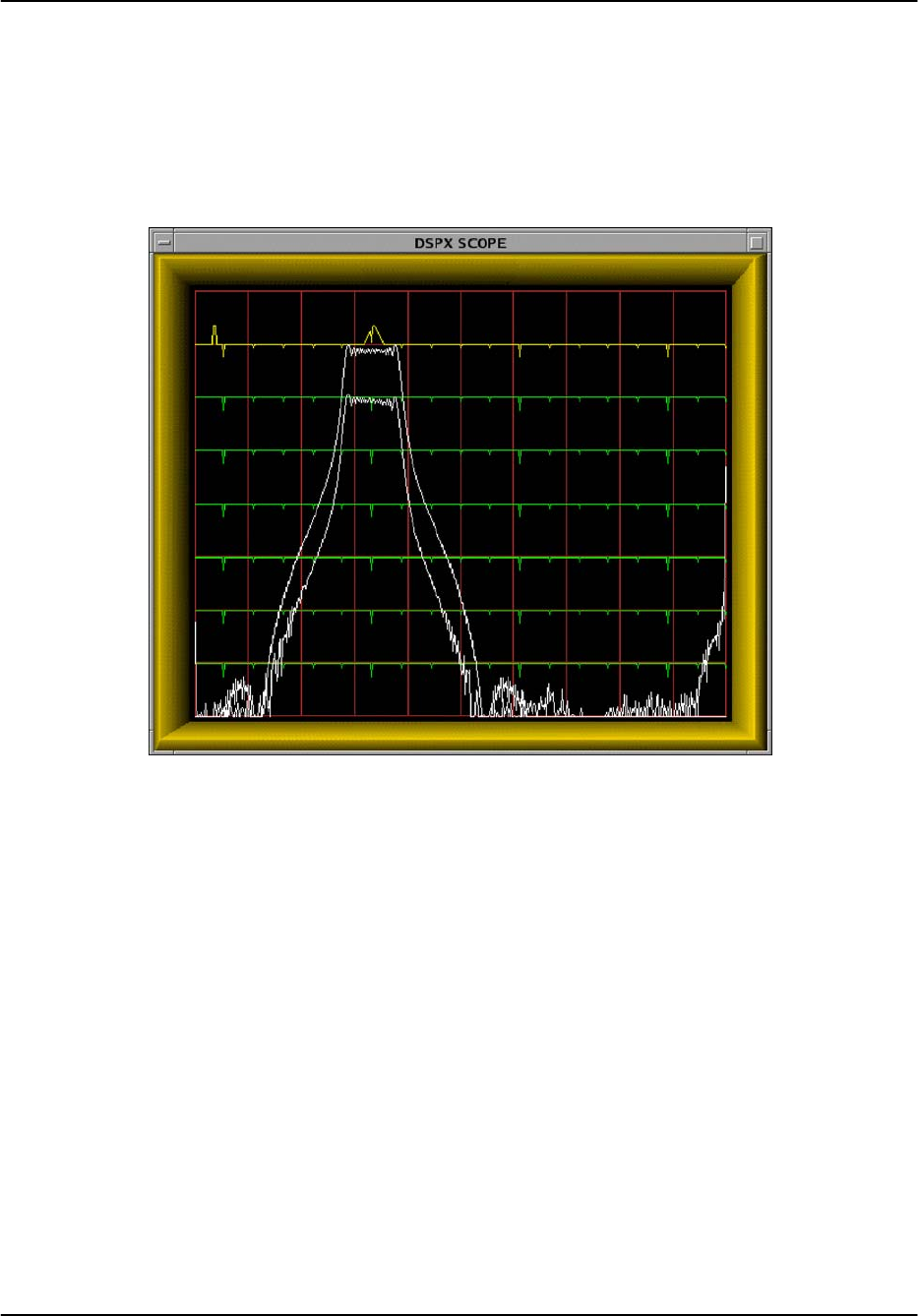
Figure 4–8 shows one form of Pa plot in which the magnitude of the Tx/Rx range sidelobes are
drawn on a log scale having 10dB vertical ticks. The horizontal span of the plot is equal to the
length of the pulse, and consequently, only half of the complete ambiguity diagram is shown.
This was done to make the plots more viewable; and no information lost since the zero-Doppler
response (white plot) can safely be assumed to be symmetric. In this example the pulsewidth is
30μsec, bandwidth is 3MHz, PSL is –61.2dB and ISL is –50.8dB, Doppler shift +/– 50 KHz.
Figure 4–8: Ambiguity Diagram of a Compressed Tx Pulse
Plot–Assisted Setups
RVP8 User’s Manual
October 2004
4–28
Also shown in yellow and green are the Tx/Rx responses when the overall waveform is modified
by a 50KHz target Doppler shift. Real weather targets would never have such a large Doppler
component, but the Pa menu allows you to study its effect anyway.
An alternate form of Pa plot of the same Tx waveform is shown in Figure 4–9. The horizontal
axis again represents time, but now spans the entire duration of the pulse. Three different plots
are drawn, hence the vertical axis is interpreted differently in each case:
SThe instantaneous frequency across the full length of the pulse is shown in white. The
vertical scale is normalized to hold the overall frequency span, which is also shown
numerically in the Pa TTY output.
SThe waveform baseband phase is shown in green, and is normalized so that the vertical
axis holds the full span of values. Note that the phase, which generally spans a few
thousand degrees, is “unwound” in this plot so that you can see its behavior nicely.
SThe amplitude of the Tx waveform envelope is shown in yellow. It is drawn using a
linear vertical scale which occupies only the middle half of the plot. This is to avoid
creating too much “plotting clutter” in the corners.
Figure 4–9: Frequency, Phase and Amplitude of a Compressed Tx Pulse
From Figure 4–9 we can see that the waveform consists of a linear FM chirp that occupies about
87% of the central pulse duration. The frequency remains nearly constant in the leading and
trailing edges, hence the overall label “Non-Linear FM”. The central chirp is contained within a
somewhat larger amplitude modulation envelope that applies full scale power within the middle
82% of the pulse, and also provides bandlimited shaping of the leading and trailing edges.

Plot–Assisted Setups
RVP8 User’s Manual
October 2004
4–29
This waveform was designed using the “$” automatic search-and-optimize command in the Pa
menu. For a given pulse length and bandwidth of the Tx waveform, this command allows you to
try thousands of combinations of FM shape and amplitude shape, searching for the combination
that minimizes the sum of PSL and ISL (in dB). This gives the best overall waveform for
weather radar observations in which both the PSL and ISL are important.
4.6.2 Available Subcommands Within “Pa”
The list of subcommands is printed on the TTY:
Available Subcommands within ’Pa’:
S/s & L/l Pulse Length Shorter/Longer
N/n & W/w Bandwidth Narrower/Wider
1/2/3 Select Tuning Parameter to Change
D/d & U/u Selected Tuning parameter Down/Up
V/v Doppler Frequency Shift Up/Down
Z/z Amplitude Zoom
$ Search for Optimal Waveform
These subcommands change the bandwidth, pulsewidth, and shaping parameters of the transmit
waveform, and alter the format of the display.
S/s & L/l The “Shorter” and “Longer” commands decrease or increase the time
duration (i.e., pulsewidth) of the transmitted pulse. The lower case
commands shift in 0.05 msec steps, while the upper case commands
use 1 msec steps.
N/n & W/w The “Narrower” and “Wider” commands decrease or increase the
bandwidth of the transmitted pulse. The lower case commands shift in
10KHz steps, while the upper case commands use 200KHz steps.
1 & 2 & 3 Typing one of these numbers chooses which of the three waveform
tuning parameters will be altered by the “D” and “U” keys.
D/d & U/u The “Down” and “Up” commands decrease or increase the waveform
tuning parameter that has been chosen by the most recent “1”, “2” or
“3” key. The lower case commands shift in 0.001 (dimensionless)
steps, while the upper case commands use 0.05 steps. Present values
of all three parameters will be printed each time a Down/Up key is
pressed, e.g.,:
Tuning parameters: 0.9000 1.0000 0.1770
Please see Section 3.2.5.1 for a description of how each of the tuning
parameters are used.
V/v The “Velocity” command allows you to investigate how the overall
compressed pulse Tx/Rx system will respond to the the effects of
target Doppler shift. Frequency shifts as large as 100KHz can be
introduced in order to see their effect on the Range/Time sidelobes.
The Pa plot will show the effects of +V and –V shifts as green and
yellow plots in addition to the standard white (zero Doppler) plot.

Plot–Assisted Setups
RVP8 User’s Manual
October 2004
4–30
Z/z The dynamic range of the Pa sidelobe plot is 80dB. Usually this will
give plenty of room to examine the properties of the waveform. But
for very wide dynamic range pulses, you can shift the plot up/down in
10dB steps using these “Zoom” keys.
$Designs an optimal compressed waveform. For a given pulsewidth
and bandwidth of the Tx waveform, this command allows you to try
many thousands of combinations of FM shape and amplitude shape,
searching for the one that minimizes the sum of PSL and ISL (in dB).
This gives the best overall waveform for weather radar observations in
which both the PSL and ISL are important.
The following dialog appears in response to the “$” command:
TuningParam #1 (0.9000) –– 1 Grid Point from 0.9000 to 0.9000
TuningParam #2 (1.0000) –– 1 Grid Point from 1.0000 to 1.0000
TuningParam #3 (0.1774) –– 1 Grid Point from 0.1774 to 0.1774
As the line is printed for each parameter, you may either accept the
default single grid point (no search), or enter a desired number of grid
search points followed by a span of values within which to search.
For example, typing:
200 .9 .95
will request that the parameter be searched using 200 evenly spaced
grid points lying between 0.9000 and 0.9500 inclusive. After all three
parameter spans have been entered, the RVP8 will begin searching for
the optimum waveform. Progress messages are printed on the TTY,
and the plot will update every time a better waveform is discovered.
In this way it is easy to tell whether the search is converging.
The process normally runs to completion on its own; but if the search
is taking too long, or you’ve changed your mind about which intervals
to search, typing “Q” will exit right away. In either case, the prompt:
Keep this waveform ? [Y]
will appear. Typing “Y” (or Enter) will keep the optimized tuning
parameters that were just discovered, overwriting whatever starting
values were originally there. Typing “N” will discard the search
results and return to the original settings, as if “$” had never been
typed.
4.6.3 TTY Information Lines Within “Pa”
The TTY information lines will resemble:
BW:3.40MHz PW:29.99usec PSL:–61.2dB ISL:–51.3dB
TxLoss:0.5dB RxLoss:2.4dB
BW Bandwidth of the Tx waveform in MegaHertz.
PW Pulsewidth (pulse length) of the Tx waveform in microseconds.

Plot–Assisted Setups
RVP8 User’s Manual
October 2004
4–31
PSL Peak Sidelobe Level of the ambiguity diagram, expressed in deciBels
relative to the main lobe level. This is the peak height of the strongest
range/time sidelobe, and measures the ability of the compressed pulse
to distinguish a given target from a small number of individual point
targets that also lie within the pulse volume. The waveform’s ability
to “see” between clutter targets is largely determined by the PSL level.
ISL Integrated Sidelobe Level of the ambiguity diagram, expressed in dB
relative to the main lobe. This is the total power in all range/time
sidelobes divided by the total power in the main lobe. ISL measures
the ability of the compressed pulse to distinguish a given target from
other distributed targets (such as rain) that also lie within the pulse
volume.
TxLoss The TxLoss is calculated as the total power in the transmit waveform
divided by the power that would be contained in an equal length ideal
rectangular pulse. It is a measure of how much power does not get
transmitted due to the amplitude shaping of the synthesized waveform.
TxLoss should be included in the computation of the radar constant,
since the latter is based on a nominal pulsewidth equal to the overall
length of the entire Tx waveform (including the amplitude tapering).
RxLoss The RxLoss is a measure of how much information is “thrown away”
by the receiving filter in order to achieve the desired level of sidelobe
suppression. These two quantities often trade off against each other in
receiver systems, so that optimum range/time sidelobes can only be
achieved at the expense of a few deciBels of loss of sensitivity. The
receiver filter loss is calculated as:
dBloss +–10 log10
ȧ
ȧ
ȧ
ȧ
ȡ
Ȣ
ŤŕT(t)R(t)dt Ť2
ŕ|T(t)|2dt ŕ|R(t)|2dt
ȧ
ȧ
ȧ
ȧ
ȣ
Ȥ
Where T(t) is the complex-valued transmit waveform, and R(t) is the
complex-valued filter being used to receive it. When R(t) is designed
to be the complex conjugate of T(t), we have the ideal matched filter
case whose receive loss is 0dB. However, this matched filter has
rather poor sidelobe behavior that makes it unsuitable for use directly
in the receiver. Instead, a windowed version (Hamming, Blackman,
etc.) of the ideal matched filter is used to achieve the desired sidelobe
levels. Of course, that windowing operation also has the effect of
discarding some valid information in the leading and trailing portions
of the pulse. Hence, there is a loss in receive sensitivity whenever a
window is applied.
Note: Given a compressed transmit waveform, the RVP8 designs the
appropriate “mismatch” Rx filter automatically, using an optimized
Blackman window in all cases. Code developers can also access the
Plot–Assisted Setups
RVP8 User’s Manual
October 2004
4–32
internal APIs directly to design any desired transmit waveform along
with the associated FIR filter to receive it.
4.6.4 Bench Testing of Compressed Waveforms
Working with compressed pulse waveforms can be tricky, so it is reassuring to run some simple
bench tests to verify that things are working properly. Once the Tx waveform has been designed
it can be injected into the IFD for testing with the Pr command. This not only verifies that the
analog waveform is generated properly, but also that the matched filtering on the RVP8/Rx card
is able to deconvolve the compressed information.
To setup the test, simply connect the Channel #1 or Channel #2 output of the RVP8/Tx card to
the IF-Input of the IFD. Use whichever RVP8/Tx channel has been configured for waveform
synthesis in the Mz menu, and set the Zero Offset of the Transmitter Pulse in the Mt<n> menu
to, perhaps, 50μsec. The latter step will shift the waveform out in range so that the Pr plot is
able to see it.
Figure 4–10: IFD Sampling of Optimized Compressed Tx Waveform
Figure 4–10 shows an actual Pr plot of a 40μsec, 5MHz optimized waveform generated by the
RVP8/Tx card and fed into the IFD. In this example, the ideal Tx waveform has a Peak Sidelobe
Level (PSL) of –76.7dB and an Integrated Sidelobe Level (ISL) of –62.3dB. The measured
testbench performance is several dB short of this, probably because of the uncompensated analog
bandpass filters on the RVP8/Tx and IFD. These filters have several tenths of a dB of amplitude
ripple as well as minor deviations from linear phase within the 5MHz signal bandwidth. The
effect is that the sampled analog waveform is not quite identical to the ideal waveform.
Plot–Assisted Setups
RVP8 User’s Manual
October 2004
4–33
The Ps plotting command can also be used to examine the ideal transmit spectrum and actual
received spectrum of compressed pulses. An example is shown in Figure 4–11 below for a
60MHz, 40μsec linear FM pulse having a bandwidth of 2MHz. The energy in the pulse is both
sharply contained within and uniformly distributed over the 2MHz frequency interval centered
on the IF carrier. This demonstrates the ability of synthesized transmit waveforms to remain
cleanly within their allocated bounds.
Figure 4–11: Ideal and Actual Linear-FM Spectrum Displayed in Ps Plot